&_____________ AECL EACL - International Nuclear ...
522
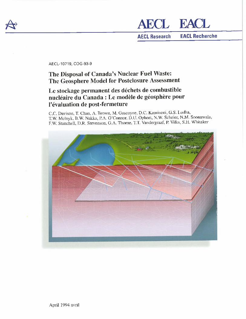
& _____________ AECL EACL AECL Research EACL Recherche AECL-10719, COG-93-9 The Disposal of Canada’s Nuclear Fuel Waste: The Geosphere Model for Postclosure Assessment Le stockage permanent des déchets de combustible nucléaire du Canada : Le modèle de géosphère pour l'évaluation de post-fermeture C.C. Davison, T. Chan, A. Brown, M. Gascoyne, D.C. Kamineni, G.S. Lodha, T.W. Melnyk, B.W. Nakka, P.A. O’Connor, D.U. Ophori, N.W. Scheier, N.M. Soonawala, F.W. Stanchell, D.R. Stevenson, G.A. Thorne, T.T. Vandergraaf, P. Vilks, S.H. Whitaker April 1994 avril
-
Upload
khangminh22 -
Category
Documents
-
view
1 -
download
0
Transcript of &_____________ AECL EACL - International Nuclear ...
& _____________ AECL EACLAECL Research EACL Recherche
AECL-10719, COG-93-9
The Disposal of Canada’s Nuclear Fuel Waste:The Geosphere Model for Postclosure AssessmentLe stockage permanent des déchets de combustible nucléaire du Canada : Le modèle de géosphère pour l'évaluation de post-fermetureC.C. Davison, T. Chan, A. Brown, M. Gascoyne, D.C. Kamineni, G.S. Lodha,T.W. Melnyk, B.W. Nakka, P.A. O’Connor, D.U. Ophori, N.W. Scheier, N.M. Soonawala, F.W. Stanchell, D.R. Stevenson, G.A. Thorne, T.T. Vandergraaf, P. Vilks, S.H. Whitaker
April 1994 avril
AECL' RESEARCH
THE DISPOSAL OF CANADA'S NUCLEAR FUEL WASTE:
THE GEOSPHERE MODEL FOR POSTCLOSURE ASSESSMENT
C.C. Davison, T. Chan, A. Brown, M. Gascoyne, D.C. Kamineni, G.S. Lodha, T.W. Melnyk, B.W. Nakka, P.A. OpConnor, D.U. Ophori,
N.W. Scheier, N.M. Soonawala, F.W. Stanchell, D.R.Stevenson, G.A. Thorne, T.T. Vandergraaf,
P. Vilks and S.H. Whitaker
The Canadian Nuclear Fuel Waste Management Program is funded jointly by AECL and Ontario Hydro under the auspices of the CANDU Owners Group
Whiteshell Laboratories Pinawa, Manitoba ROE 1LO
1994
LE STOCKAGE PERMANENT DES DÉCHETS DE COMBUSTIBLE NUCLÉAIRE DU CANADA : LE MODÈLE DE GÉOSPHÈRE POUR L'ÉVALUATION DE POST-FERMETURE
par
C.C. Davison, T. Chan, A. Brown, M. Gascoyne, D.C. Karaineni, G.S. Lohda, T.W. Melnyk, B.W. Nakka, P.A. O'Connor, D.U. Ophori, N.W. Scheier,
N.M. Soonawala, F.W. Stanchell, D.R. Stevenson, G.A. Thorne,T.T. Vandergraaf, P. Vilks et S.H. Whitaker
RÉSUMÉ
EACL prépare l'Étude d'impact sur l'environnement (EIE) d'un concept de stockage permanent des déchets de combustible nucléaire du Canada. Le concept porte sur une installation souterraine scellée de façon étanche, construite à une profondeur de 500 à 1000 m dans la roche plutonique du Bouclier canadien. Ce rapport est l'un des neuf documents de référence principaux de l'EIE. Un programme d'analyse probabiliste de variabilité des systèmes sert à évaluer les impacts à long terme, sur la sûreté et l'environnement, du concept de stockage permanent des déchets nucléaires. Dans ce rapport, on décrit la méthode de conception du modèle de géosphère SYVAC3-CC3 (GEONET) qui simule le transport des contaminants de l'installation souterraine à la biosphère par l'intermédiaire de la géosphère. En outre, on y décrit les résultats ayant servi à construire le modèle ainsi que les hypothèses émises et les justifications présentées quant aux résultats et à ce modèle.
La géosphère comprend le massif rocheux entourant l'installation souterraine, les eaux souterraines renfermées dans les pores et les fissures de la roche, les matériaux de scellement d'étanchéité des puits et des trous de forage d'exploration du site ainsi qu'un puits d'alimentation en eau domestique qui est censé couper la voie de transport la plus rapide de l'installation souterraine à la biosphère. GEONET simule l'écoulement des eaux souterraines à partir de l'installation souterraine, à travers la géosphère et vers des points de déversement de la biosphère; l'advection des contaminants dans les eaux souterraines, dispersion hydrodynamique et diffusion moléculaire; la sorption chimique des contaminants sur les minéraux de la roche au cours du transport; la désintégration radioactive; et la vitesse de décharge des contaminants de l'installation souterraine dans la biosphère.
La conception du modèle de géosphère comporte plusieurs opérations. On commence par la construction d'un modèle conceptuel de la structure géologique souterraine et du régime d'écoulement d'eaux souterraines à l'aide de résultats d'études sur le terrain et en laboratoire. Après la construction du modèle conceptuel, on résout les équations couplées décrivant l'écoulement d'eaux souterraines et le transport de chaleur tridimensionnels à
l'aide du programme à méthode des éléments finis pour calculer la distribution de pression hydraulique (hauteur piézométrique) et de vitesse des eaux souterraines. Ensuite, on détermine les trajectoires d'écoulement, des eaux souterraines de l'installation souterraine aux points de déversement de la biosphère, au moyen du programme de calcul du suivi du déplacement des particules, TRACK3D. On se sert des trajectoires d'écoulement et de diffusion pour construire un réseau tridimensionnel simplifié de voies d'écoulement composé de segments de transport unidimensionnels. On exécute les analyses de sensibilité à l'aide de MOTIF pour déterminer la forme appropriée des voies d'écoulement incorporées dans l'approximation par GEONET. GEONET modifie la distribution de pression hydraulique prédite par MOTIF pour tenir compte des effets du pompage à partir d'un puits d'alimentation en eau domestique et calcule la vitesse moyenne des eaux souterraines du réseau par la loi de Darcy. Ensuite, il résout les équations d'advection - de dispersion - de ralentissement unidimensionnelles, pour une chaîne de désintégration radioactive de radionucléides, en se servant des fonctions de réaction analytiques pour déterminer la vitesse de déplacement des contaminants de l'installation souterraine à travers le réseau de voies d'écoulement de la géosphère.
EACL a procédé à une évaluation de post-fermeture d'étude de cas dans laquelle on a appliqué la méthode d'évaluation à un système de stockage permanent hypothétique de référence. On a supposé les caractéristiques géosphériques de ce système semblables aux conditions existant dans l'Aire de recherches de Whiteshell dans le sud-est du Manitoba, une des aires de recherches géologiques d'EACL. L'installation souterraine hypothétique de stockage permanent aurait une superficie d'à peu près 2 km x 2 km, serait située à une profondeur de 500 m, près d'une grande zone de fractures de faible inclinaison. La zone de fractures servirait de voie d'écoulement d'eaux souterraines relativement rapide vers la surface. Bien que la méthode de modélisation de la géosphère soit générique et puisse s'appliquer à tout site de stockage permanent de la région du Bouclier canadien, nous avons employé un modèle de géosphère propre à un site pour l'évaluation. On l'a fait pour montrer comment les conditions hydrogéologiques et géochimiques particulières d'un site influent sur le transport des contaminants d'une installation souterraine à travers la géosphère et pour expliquer comment la conception et la disposition de l'installation souterraine interagissent avec ces conditions.
Le Programme canadien de gestion des déchets de combustible nucléaire est financé en commun par EACL et Ontario Hydro sous les auspices du Groupe des propriétaires de réacteurs CANDU.
EACL Recherche Laboratoires de Vhiteshell Pinawa (Manitoba) ROE 1L0
AECL-10719COG-93-9
THE DISPOSAL OF CANADA'S NUCLEAR FUEL WASTE:
THE GEOSPHERE MODEL FOR POSTCLOSURE ASSESSMENT
C.C. Davison, T. Chan, A. Brown, M. Gascoyne, D.C. Kamineni, G.S. Lodha, T.W. Melnyk, B.W. Nakka, P.A. O'Connor, D.U. Ophori, N.W. Scheier,
N.M. Soonawala, F.W. Stanchell, D.R. Stevenson, G.A. Thorne, T.T. Vandergraaf, P. Vilks and S.H. Whitaker
ABSTRACT
AECL is preparing an Environmental Impact Statement (EIS) of a concept for disposing of Canada's nuclear fuel waste. The disposal concept is that of a sealed vault constructed at a depth of 500 to 1 000 m in plutonic rock of the Canadian Shield. This report is one of nine primary references for the EIS. A probabilistic system variability analysis code (SYVAC3) has been used to perform a case study assessment of the long-term safety and environmental impacts for the EIS. This report describes the methodology for developing the SYVAC3-CC3 Geosphere Model (GEONET) which simulates the transport of contaminants from the vault through the geosphere to the biosphere. It also discusses the data used to construct the model, as well as assumptions and justifications for the data and model. -~
The geosphere consists of the rock mass surrounding the vault, including the groundwater in the pores and cracks in the rock, the materials used to seal the shafts and exploratory boreholes at the site, and a domestic water well that is assumed to intersect the pathway of most rapid transport from the vault to the biosphere. GEONET simulates the movement of groundwater from the vault through the geosphere to discharge locations at the biosphere; the movement of contaminants in the groundwater by advection, hydrodynamic dispersion, and molecular diffusion; chemical sorption of contaminants onto minerals in the rock during transport; radioactive decay; and the rate of discharge of vault contaminants to the biosphere.
Development of the Geosphere Model involves several steps. The initial step is to construct a conceptual model of the subsurface geological structure and ground water flow conditions using data from site investigations and laboratory tests. Once a conceptual model has been constructed, the coupled equations describing 3-D groundwater flow and heat transport are solved using the MOTIF finite-element code to calculate hydraulic head and groundwater velocity distributions. Next, the groundwater flow paths from the vault to discharge areas in the biosphere are determined by means of a particle-tracking code, TRACK3D. The flow paths and diffusion paths are used to construct a simplified 3-D pathways network composed of 1-D transport segments for GEONET. Sensitivity analyses are performed with MOTIF to determine the appropriate form of the pathways used in the GEONET approximation. GEONET modifies the head
distribution predicted by MOTIF to account for the effects of pumping from a domestic well and calculates the mean groundwater velocities in the network by Darcyrs law. It then solves the 1-D advection-dispersion- retardation equations for a radionuclide decay chain by using analytical response functions and numerical convolutions to determine the rate of movement of vault contaminants through the network of geosphere pathways.
AECL has done a postclosure assessment case study, in which the assessment methodology was applied to a hypothetical reference disposal system. The geosphere characteristics of this system were assumed to be similar to conditions at the Whiteshell Research Area in southeastern Manitoba, one of AECL's geologic research areas. The hypothetical disposal vault, approximately 2 km x 2 km in area, was located at 500-m depth, near an assumed large low-dipping fracture zone. The fracture zone provides a relatively rapid groundwater pathway to the surface. Although the geosphere modelling approach is generic and can be applied to any disposal site in the Canadian Shield, we have used a site specific geosphere model for the assessment. This was done to show how the particular hydrogeologic and geochemical conditions of a site affect the transport of vault contaminants through the geosphere, to illustrate how the design and layout of the vault interact with these conditions.
The Canadian Nuclear Fuel Waste Management Program is funded jointly by AECL and Ontario Hydro under the auspices of the CANDU Owners Group.
AECL Research Whiteshell Laboratories Pinawa, Manitoba ROE 1LO
1994
In 1992, 15% of the electricity generated in Canada was produced using CANDU nuclear reactors. A by-product of the nuclear power is used CANDU fuel, which consists of ceramic uranium dioxide pellets and metal structural components. Used fuel is highly radioactive. The used fuel from Canada's power reactors is currently stored in water-filled pools or dry storage concrete containers. Humans and other living organisms are protected by isolating the used fuel from the natural environment and by surrounding it with shielding material. Current storage practices have an excellent safety record.
At present, used CANDU fuel is not reprocessed. It could, however, be reprocessed to extract useful material for recycling, and the highly radioactive material that remained could be incorporated into a solid. The term "nuclear fuel waste,!! as used by AECL, refers to either
- the used fuel, if it is not reprocessed, or
- a solid incorporating the highly radioactive waste from reprocessing.
Current storage practices, while safe, require continuing institutional controls such as security measures, monitoring, and maintenance. Thus storage is an effective interim measure for protection of human health and the natural environment but not a permanent solution. A permanent solution is disposal, a method "in which there is no intention of retrieval and which, ideally, uses techniques and designs that do not rely for their success on long-term institutional control beyond a reasonable period of time" (AECB 1987a).
In 1978, the governments of Canada and Ontario established the Nuclear Fuel Waste Management Program I f . . . to assure the safe and permanent disposal" of nuclear fuel waste. AECL was made responsible for research and development on "... disposal in a deep underground repository in intrusive igneous rocku (Joint Statement 1978). Ontario Hydro was made responsible for studies on interim storage and transportation of used fuel and has contributed to the research and development on disposal. Over the years a number of other organizations have also contributed to the Program, including Energy, Mines and Resources Canada; Environment Canada; universities; and companies in the private sector.
The disposal concept is to place the waste in long-lived containers; emplace the containers, enveloped by sealing materials, in a disposal vault excavated at a nominal depth of 500 to 1 000 m in intrusive igneous (plutonic) rock of the Canadian Shield; and (eventually) seal all excavated openings and exploration boreholes to form a passively safe system. Thus there would be multiple barriers to protect humans and the natural environment from contaminants in the waste: the container, the very low- solubility waste form, the vault seals, and the geosphere. The disposal technology includes options for the design of the engineered components,
including the disposal container, disposal vault, and vault seals, so that I
it is adaptable to a wide range of regulatory standards, physical conditions, and social requirements. Potentially suitable bodies of plutonic rock occur in a large number of locations across the Canadian Shield.
In developing and assessing this disposal concept, AECL has consulted broadly with members of Canadian society to help ensure that the concept and the way in which it would be implemented are technically sound and represent a generally acceptable disposal strategy. Many groups in Canada have had opportunities to comment on the disposal concept and on the waste management program. These include government departments and agencies, scientists, engineers, sociologists, ethicists, and other members of the public. The Technical Advisory Committee to AECL on the Nuclear Fuel Waste Management Program, whose members are nominated by Canadian scientific and engineering societies, has been a major source of technical advice.
In 1981, the governments of Canada and Ontario announced that "... no disposal site selection will be undertaken until after the concept has been accepted. This decision also means that the responsibility for disposal site selection and subsequent operation need not be allocated until after concept acceptance" (Joint Statement 1981).
The acceptability of the disposal concept is now being reviewed by a federal Environmental Assessment Panel, which is also responsible for examining a broad range of issues related to nuclear fuel waste management (Minister of the Environment, Canada 1989). After consulting the public, the Panel issued guidelines to identify the information that should be provided by AECL, the proponent of the disposal concept (Federal Environmental Assessment Review Panel 1992).
AECL is preparing an Environmental Impact Statement to provide information requested by the Panel and to present AECLrs case for the acceptability of the disposal concept. A Summary will be issued separately. This report is one of nine primary references that summarize major aspects of the disposal concept and supplement the information in the Environmental Impact Statement. A guide to the contents of the EIS, the Summary, and the primary references follows this Preface.
In accordance with the 1981 Joint Statement of the governments of Canada and Ontario, no site for disposal of nuclear fuel waste is proposed at this time. Thus in developing and assessing the disposal concept, AECL could not design a facility for a proposed site and assess the environmental effects to determine the suitability of the design and the site, as would normally be done for an Environmental Impact Statement. Instead, AECL and Ontario Hydro have specified illustrative "referencen disposal systems and assessed those.
A "reference" disposal system illustrates what a disposal system, including the geosphere and biosphere, might be like. Although it is hypothetical, it is based on information derived from extensive laboratory and field research. Many of the assumptions made are conservative, that is, they
would tend to overestimate adverse effects. The technology specified is either available or judged to be readily achievable. A reference disposal system includes one possible choice among the options for such things as the waste form, the disposal container, the vault layout, the vault seals, and the system for transporting nuclear fuel waste to a disposal facility. The components and designs chosen are not presented as ones that are being recommended but rather as ones that illustrate a technically feasible way of implementing the disposal concept.
Af ter the Panel has received the requested information, it will hold public hearings. It will also consider the findings of the Scientific Review Group, which it established to provide a scientific evaluation of the disposal concept. According to the Panel's terms of reference "As a result of this review the Panel will make recommendations to assist the governments of Canada and Ontario in reaching decisions on the acceptability of the disposal concept and on the steps that must be taken to ensure the safe long-term management of nuclear fuel wastes in Canada" (Minister of the Environment, Canada 1989).
Acceptance of the disposal concept at this time would not imply approval of any particular site or facility. If the disposal concept is accepted and implemented, a disposal site would be sought, a disposal facility would be designed specifically for the site that was proposed, and the potential environmental effects of the facility at the proposed site would be assessed. Approvals would be sought in incremental stages, so concept implementation would entail a series of decisions to proceed. Decision- making would be shared by a variety of participants, including the public. In all such decisions, however, safety would be the paramount consideration.
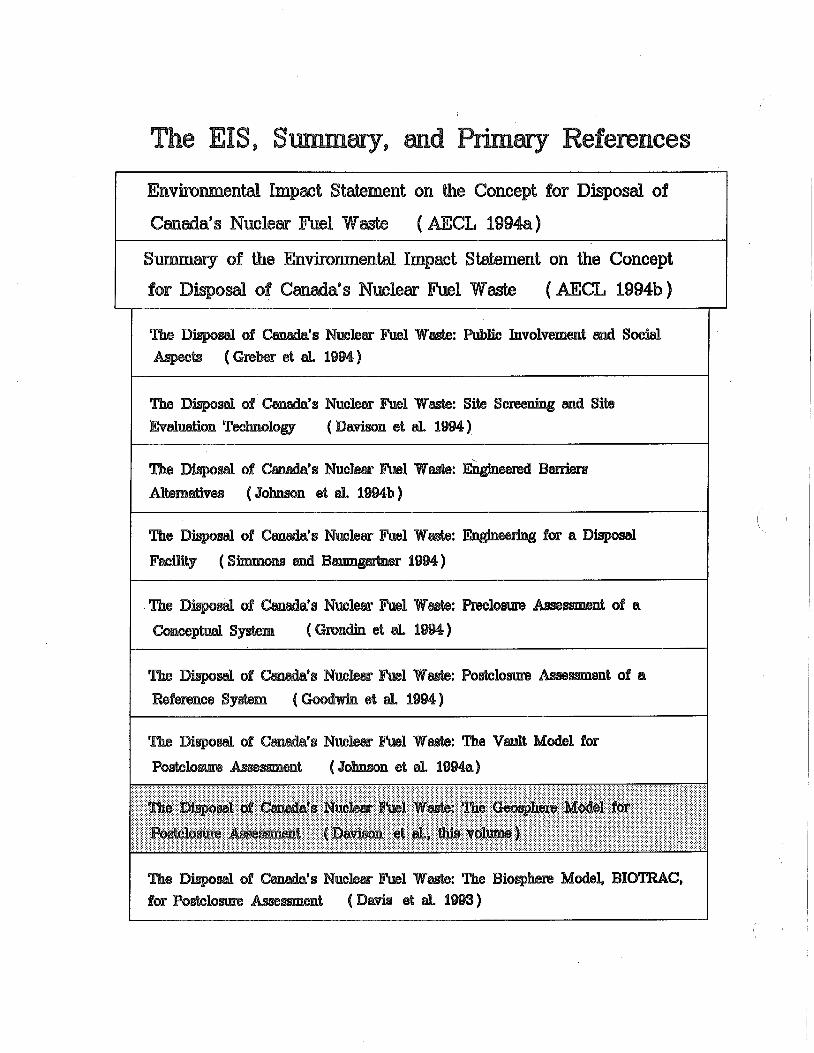
The EIS, S ary References
a's Nwhm h l W& ering for a Disposal
G m n h et al, la
s Nuleer pl'uel W&: The vault Model for
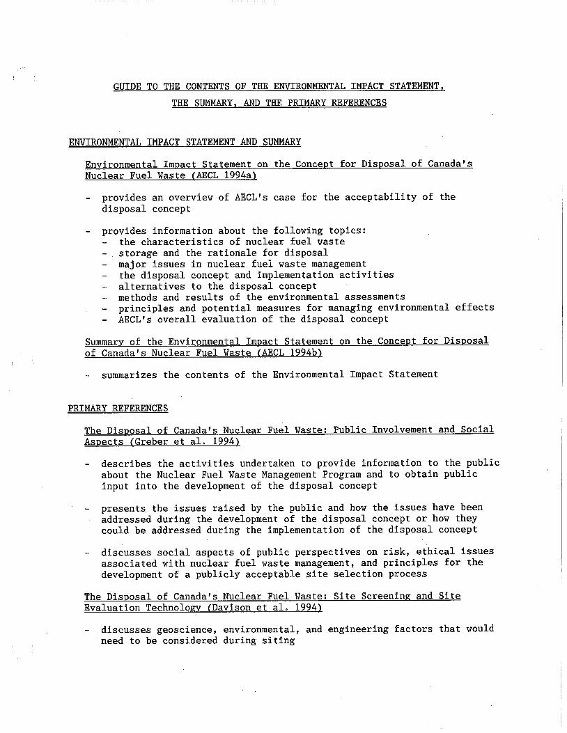
GUIDE TO THE CONTENTS OF THE ENVIRONMENTAL IMPACT STATEMENT,
THE SUMMARY, AND THE PRIMARY REFERENCES
ENVIRONMENTAL IMPACT STATEMENT AND SUMMARY
Environmental Impact Statement on the Concept for Disposal of Canada's Nuclear Fuel Waste (AECL 1994a)
- provides an overview of AECLps case for the acceptability of the disposal concept
- provides information about the following topics: - the characteristics of nuclear fuel waste - storage and the rationale for disposal - major issues in nuclear fuel waste management - the disposal concept and implementation activities - alternatives to the disposal concept - methods and results of the environmental assessments - principles and potential measures for managing environmental effects - AECL's overall evaluation of the disposal concept
Summary of the Environmental Impact Statement on the Concept for Disposal of Canada's Nuclear Puel Waste (AECL 1994b)
- summarizes the contents of the Environmental Impact Statement
PRIMARY REFERENCES
The Disposal of Canada's Nuclear Fuel Waste: Public Involvement and Social Aspects (Greber et al. 1994)
- describes the activities undertaken to provide information to the public about the Nuclear Puel Waste Management Program and to obtain public input into the development of the disposal concept
- presents the issues raised by the public and how the issues have been addressed during the development of the disposal concept or how they could be addressed during the implementation of the disposal concept
- discusses social aspects of public perspectives on risk, ethical issues associated with nuclear fuel waste management, and principles for the development of a publicly acceptable site selection process
The Disposal of Canada's Nuclear Fuel Waste: Site Screening and Site Evaluation Technolo~y (Davison et al. 1994)
- discusses geoscience, environmental, and engineering factors that would need to be considered during siting
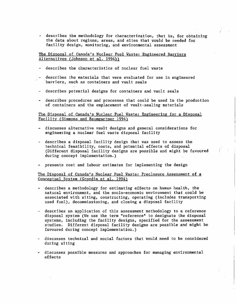
- describes the methodology for characterization, that is, for obtaining the data about regions, areas, and sites that would be needed for facility design, monitoring, and environmental assessment
The Disposal of Canada's Nuclear Fuel Waste: Engineered Barriers Alternatives (Johnson et al. 1994b)
- describes the characteristics of nuclear fuel waste
- describes the materials that were evaluated for use in engineered barriers, such as containers and vault seals
- describes potential designs for containers and vault seals
- describes procedures and processes that could be used in the production of containers and the emplacement of vault-sealing materials
The Disposal of Canada's Nuclear Fuel Waste: Enpineering for a Disposal Facility (Simmons and Baumgartner 19941
- discusses alternative vault designs and general considerations for engineering a nuclear fuel waste disposal facility
- describes a disposal facility design that was used to assess the technical feasibility, costs, and potential effects of disposal (Different disposal facility designs are possible and might be favoured I
during concept implementation.)
- presents cost and labour estimates for implementing the design
The Disposal of Canada's Nuclear Fuel Waste: Preclosure Assessment of a Conceptual Svstem (Grondin et al. 1994)
- describes a methodology for estimating effects on human health, the natural environment, and the socio-economic environment that could be associated with siting, constructing, operating (includes transporting used fuel), decommissioning, and closing a disposal facility
- describes an ap-plication of this assessment methodology to a reference disposal system (We use the term "reference" to designate the disposal systems, including the facility designs, specified for the assessment studies. Different disposal facility designs are possible and might be favoured during concept implementation.)
- discusses technical and social factors that would need to be considered during siting
- discusses possible measures and approaches for managing environmental effects
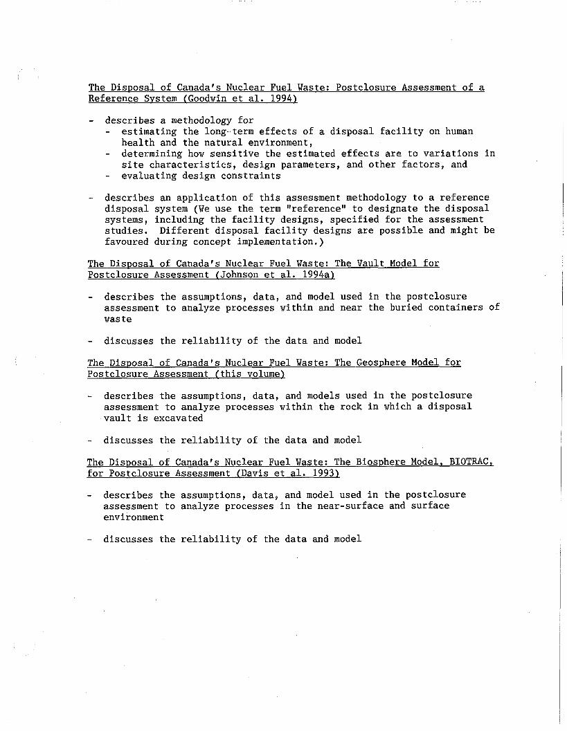
The Disposal of Canada's Nuclear Fuel Waste: Postclosure Assessment of a Reference System (Goodwin et al. 1994)
- describes a methodology for - estimating the long-term effects of a disposal facility on human
health and the natural environment, - determining how sensitive the estimated effects are to variations in
site characteristics, design parameters, and other factors, and - evaluating design constraints
- describes an application of this assessment methodology to a reference disposal system (We use the term "reference" to designate the disposal systems, including the facility designs, specified for the assessment studies. Different disposal facility designs are possible and might be favoured during concept implementation.)
The Disposal of Canada's Nuclear Fuel Waste: The Vault Model for Postclosure Assessment (Johnson et al. 1994a)
- describes the assumptions, data, and model used in the postclosure assessment to analyze processes within and near the buried containers of waste
- discusses the reliability of the data and model
The Disposal of Canada's Nuclear Fuel Waste: The Geosphere Model for Postclosure Assessment (this volume)
- describes the assumptions, data, and models used in the postclosure assessment to analyze processes within the rock in which a disposal vault is excavated
- discusses the reliability of the data and model
The Disposal of Canada's Nuclear Fuel Waste: The Biosphere Model, BIOTRAC, for Postclosure Assessment (Davis et al. 1993)
- describes the assumptions, data, and model used in the postclosure assessment to analyze processes in the near-surface and surface environment
- discusses the reliability of the data and model
TABLE OF CONTENTS
LIST OF TABLES
LIST OF FIGURES
EXECUTIVE SUMMARY
1. INTRODUCTION
BACKGROUND THE DISPOSAL CONCEPT POSTCLOSURE ASSESSMENT
Assessment Methodology The Postclosure Assessment Case Study Reference Disposal System The Postclosure Assessment Case Study System- Model Using the System-Model
MODELLING THE GEOSPHERE Introduction Conceptual Hydrogeological Model of the Site Groundwater Flow Model of the Site Geosphere Model for the Postclosure Assessment Study Developing a Geosphere Model During Implementation of Disposal
SCOPE OF THE GEOSPHERE MODEL REPORT
2 . EVOLUTION OF THE GEOSPHERE 25
INTRODUCTION VAULT SITING AND CONSTRUCTION
Hydrogeological Effects Geochemical Effects Stress Effects Thermal Effects Microbial Effects Implications for Geosphere Modelling
CLIMATE AND METEOROLOGICAL FLUCTUATIONS Climate Meteorological Input and Water Table Fluctuations Implications for Geosphere Modelling
TOPOGRAPHIC FLUCTUATIONS Uplift and Depression
25 2 7 2 7 28 2 8 29 29 3 0 32 3 2
3 3 34 35 36
continued...
TABLE OF CONTENTS (continued)
Erosion and Deposition Implications for Geosphere Modelling
GLACIATION Frequency of Glaciation Erosion by Ice Sheets Effect of Glaciation on Stress and Groundwater Flow Implications for Geosphere Modelling
SEISMICITY Geological Considerations Historical Seismicity Considerations Preclosure Seismic Effects Implications for Geosphere Modelling
METEORITE IMPACT VOLCANISM HUMAN INTRUSION
METHODOLOGY FOR MODELLING THREE-DIMENSIONAL GROUNDWATER FLOW, HEAT TRANSPORT AND SOLUTE TRANSPORT IN FRACTURED/POROUS MEDIA 5 3
INTRODUCTION 53 1 THE MOTIF FINITE-ELEMENT CODE 53
Conceptual Model, Processes Simulated, Assumptions and Input/Output Data 5 3
Conceptual Model Incorporated in the MOTIF Code 53 Geometry and Processes 55 Assumptions 56 Model Input Data 5 7 Model Output 5 9
Mathematical Formulation 5 9 Governing Flow Equations 5 9 Governing Solute Transport Equation 6 1 Heat Transport Equation 62 Supplementary Equations 63 MOTIF Flow Model Boundary Conditions 6 4
Numerical Solution Techniques 66 The Galerkin Finite-element Formulation 6 6 Temporal Discretization 7 0 Treatment of Nonlinearity 7 0 Solution of Algebraic Equations 7 1 Calculation of Linear Fluid Velocity 7 1
Limitations 73 PARTICLE TRACKING 75 APPLICATION OF THE METHODOLOGY TO DEVELOP THE GEOSPHERE MODEL FOR POSTCLOSURE ASSESSMENT 79
continued...

TABLE OF CONTENTS (continued)
VERIFICATION AND EVALUATION OF DETAILED NUMERICAL MODELS 8 0
INTRODUCTION 8 0 MOTIF VERIFICATION 8 0 THE URL DRAWDOWN EXPERIMENT AND HYDROGEOEBGPC MODEL VALIDATION 8 3 TRACER TEST PROGRAM 94 VERIFICATION OF THE PARTICLE-TRACKING PROGRAM (TRACK3D) 9 8
DETAILED GROUNDWATER FLOW MODELLING OF THE WHITESHELL RESEARCH AREA 100
INTRODUCTION 100 DEVELOPMENT OF THE WRA MODELS 100 THE CONCEPTUAL HYDROGEOLOGICAL MODEL OF THE WRA 104
Hydrogeological Structure 104 Permeability and Porosity 11 1 Other Properties 113
TWO DIMENSIONAL THERMOHYDROGEOLOGICAL SENSITIVITY ANALYSIS 113
Base Case 114 Layer Properties 130 Fracture Zone Configuration 130 Boundary Conditions 140 Extent of the Region Requiring Detailed Three- Dimensional Modelling 140 Summary of Two-Dimensional Sensitivity Analysis 143
THREE-DIMENSIONAL THERMOHYDROGEOLOGICAL SENSITIVITY ANALYSIS 147
Preliminary Modelling 147 Backfill Properties, Waste Exclusion Distance and Excavation Damage 156 Vault Heat 167 Perturbed Near Surface Region 176 Summary of Three-Dimensional Sensitivity Analysis 178
SIMULATIONS TO FINALIZE THE GEOMETRY OF, AND INPUTS TO, THE GEOSPHERE MODEL, GEONET, USED IN SYVAC3-CC3 180
Natural Conditions (No water supply well) 181 Water Supply Well Pumping Conditions 184
THREE-DIMENSIONAL MODELS OF THE EFFECTS OF AN OPEN BOREHOLE 188
Vault-scale Modelling 188 Room-Scale Advection-Dispersive Transport Modelling 189
continued...
TABLE OF CONTENTS (continued)
6 . GEONET - THE GEOSPHERE MODEL OF SYVAC3-CC3 192
INTRODUCTION GEONET MODEL OVERVIEW THE TRANSPORT MODEL
The Transport Equation The Transport Calculation Using Response Functions Boundary Conditions
PARAMETERS IN THE TRANSPORT EQUATION Groundwater Velocity Dispersion Coefficient Retardation Factors
WELL MODEL Maximum Well Capacity Drawdowns in the Fracture Zone Surface Water Captured Plume Capture Fractions Site-Specific Effects of the Well
INTERFACE WITH VAULT MODEL INTERFACE WITH BIOSPHERE MODEL GEONET MODEL VERIFICATION AND QUALITY ASSURANCE
Introduction Testing of GEONET Modules Simple Test Cases Comparison with similar codes
INTRACOIN Comparisons Comparisons with Literature Comparisons with PSAC
Comparison with Detailed Transport Calculations Sensitivity Analysis with GEONET Main Conclusion
7 . DEVELOPMENT OF POSTCLOSURE ASSESSMENT MODEL OF THE GEOSPHERE 244
7 .1 INTRODUCTION 244 7.2 THE INTERFACING OF MOTIF AND GEONET 245 7 . 3 THE MOTIF FLOW MODEL 25 1 7 .4 THE MOTIF-GEONET CONNECTION 252 7.4.1 The Network Geometry 252 7.4.2 Empirical Effects of The Well 255 7.4.2.1 Scaling Factor Applied to the Well Model 257 7.4.2.2 Drawdowns in Vault 258 7.4.2.3 Effects on Discharge Area 261 7.4.2.4 Effects Outside Fracture Zone 265
continued...
TABLE OF CONTENTS (continued)
CAPTURE FRACTIONS IN PATHWAYS THROUGH THE FRACTURE ZONE GROUNDWATER VELOCITY SCALING FACTOR MATRIX DIFFUSION EFFECTS ON CONTAMINANT RETARDATION AND DISPERSION SUMMARY OF DATA TRANSFERRED TO GEONET
Network Geometry Hydrogeologic Properties Data From MOTIF Results Transport Properties Mineralogy and Groundwater Chemistry Miscellaneous Properties
CONCLUSION
8. CONCLUSIONS
ACKNOWLEDGEMENTS
REFERENCES
LIST OF SYMBOLS
GLOSSARY
APPENDIX A
APPENDIX B
APPENDIX C
APPENDIX D
APPENDIX E
APPENDIX P
APPENDIX G
LIST OF TABLES
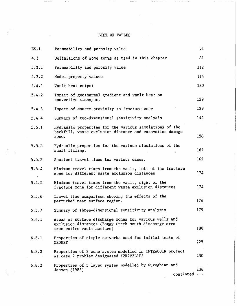
ES. 1
4.1
5.3.1
5.3.2
5.4.1
5.4.2
Permeability and porosity value
Definitions of some terms as used in this chapter
Permeability and porosity value
Model property values
Vault heat output
Impact of geothermal gradient and vault heat on convective transport
Impact of source proximity to fracture zone
Summary of two-dimensional sensitivity analysis
Hydraulic properties for the various simulations of the backfill, waste exclusion distance and excavation damage zone.
Hydraulic properties for the various simulations of the shaft filling.
Shortest travel times for various cases.
Minimum travel times from the vault, left of the fracture zone for different waste exclusion distances
Minimum travel times from the vault, right of the fracture zone for different waste exclusion distances
Travel time comparison showing the effects of the perturbed near surface region.
Summary of three-dimensional sensitivity analysis
Areas of surface discharge zones for various wells and exclusion distances (Boggy Creek south discharge area from entire vault surface) 186
Properties of simple networks used for initial tests of GEONET 225
Properties of 3 zone system modelled in INTRACOIN project as case 2 problem designated 12R2T2LlP2 230
Properties of 3 layer system modelled by Gureghian and Jansen (1985) 236
continued . . .
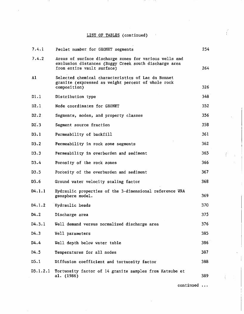
LIST OF TABLES (continued) .
7.4.1 Peclet number for GEONET segments
7.4.2 Areas of surface discharge zones for various wells and exclusion distances (Boggy Creek south discharge area from entire vault surface)
A 1 Selected chemical characteristics of Lac du Bonnet granite (expressed as weight percent of whole rock composition)
D1.l Distribution type
D2.1 Node coordinates for GEONET
D2.2 Segments, nodes, and property classes
D2'. 3 Segment source fraction
D3.1 Permeability of backfill
D3.2 Permeability in rock zone segments
D3.3 Permeability in overburden and sediment
D3.4 Porosity of the rock zones
D3.5 Porosity of the overburden and sediment
D3.6 Ground water velocity scaling factor
Hydraulic properties of the 3-dimensional reference WRA geosphere model.
Hydraulic heads
Discharge area
Well demand versus normalized discharge area
Well parameters
Well depth below water table
Temperatures for all nodes
Diffusion coefficient and tortuosity factor
Tortuosity factor of 14 granite samples from Katsube et al. (1986)
continued ...
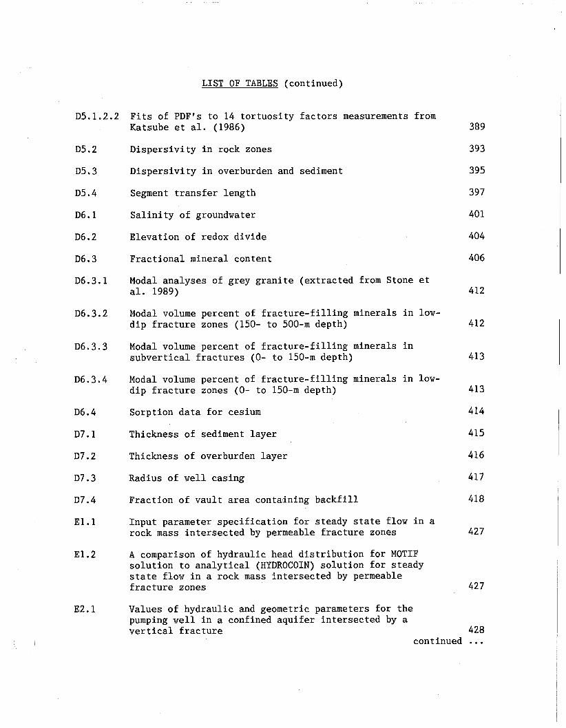
LIST OF TABLES (continued)
D5.1.2.2 Fits of PDF1s to 14 tortuosity factors measurements from Katsube et al. (1986)
D5.2 Dispersivity in rock zones
D5.3 Dispersivity in overburden and sediment
D5.4 Segment transfer length
D6.1 Salinity of groundwater
D6.2 Elevation of redox divide
D6.3 Fractional mineral content
D6.3.1 Modal analyses of grey granite (extracted from Stone et al. 1989)
D6.3.2 Modal volume percent of fracture-filling minerals in low- dip fracture zones (150- to 500-m depth)
D6.3.3 Modal volume percent of fracture-filling minerals in subvertical fractures (0- to 150-m depth)
D6.3.4 Modal volume percent of fracture-filling minerals in low- dip fracture zones (0- to 150-m depth)
D6.4 Sorption data for cesium 414
D7.1 Thickness of sediment layer 415
D7.2 Thickness of overburden layer 416
D7.3 Radius of well casing 417
D7.4 Fraction of vault area containing backfill 418
El.l Input parameter specification for steady state flow in a rock mass intersected by permeable fracture zones 427
E1.2 A comparison of hydraulic head distribution for MOTIF solution to analytical (HYDROCOIN) solution for steady state flow in a rock mass intersected by permeable fracture zones 427
E2.1 Values of hydraulic and geometric parameters for the pumping well in a confined aquifer intersected by a vertical fracture 428
continued ...
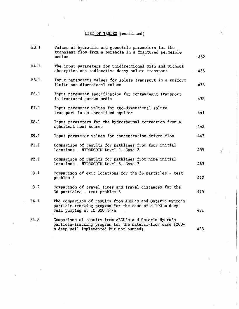
LIST OF TABLES (continued)
Values of hydraulic and geometric parameters for the transient flow from a borehole in a fractured permeable medium
The input parameters for unidirectional with and without absorption and radioactive decay solute transport
Input parameters values for solute transport in a uniform finite one-dimensional column
Input parameter specification for contaminant transport in fractured porous media
Input parameter values for two-dimensional solute transport in an unconfined aquifer
Input parameters for the hydrothermal convection from a spherical heat source
Input parameter values for concentration-driven flow
Comparison of results for pathlines from four initial locations - HYDROCOIN Level 1, Case 2 Comparison of results for pathlines from nine initial locations - HYDROCOIN Level 3 , Case 7
Comparison of exit locations for the 36 particles - test problem 3
Comparison of travel times and travel distances for the 36 particles - test problem 3
The comparison of results from AECL1s and Ontario Hydro's particle-tracking program for the case of a 100-m-deep well pumping at 10 000 m3/a
Comparison of results from AECLPs and Ontario Hydro's particle-tracking program for the natural-flow case (200- m deep well implemented but not pumped)

LIST OF FIGURES
Schematic of Vault, Geosphere and Biosphere 2
Reference Disposal Vault in the Nuclear Fuel Disposal Concept (UFDC) 6
The Whiteshell Research Area (WRA) 7
Location of the hypothetical disposal vault 10
A Schematic illustrating the linked models for the postclosure assessment
A schematic illustrating the SYVAC system-model 12
Pathways for the movement of contaminants from the vault to the Biosphere 13
Steps in developing the Geosphere model (GEONET) 18
The three main fracture domains at the WRA; a). fracture zones (faults), b). moderately fractured rock, and c). sparsely fractured rock. 2 0
Major geological and hydrogeologic features of the Underground Research Laboratory 2 6
The location of the disposal rooms relative to fracture zone LD1 3 1
Major geographic regions and drainage basins on the Canadian Shield in Ontario 3 7
The ACLIN "states" as defined by Findlay et al. (1984). Figure (a) is the deep-sea chronostratigraphy data from Martinson et al. (1967). Figure (b) is the relative volume of ice sheets at maximum 80% of land covered. 42
Seismicity on the Canadian Shield in Ontario 4 7
Conceptual model used in MOTIF 54
Element types available in MOTIF (clockwise from upper left); three-dimensional eight-noded hexahedral isoparametric, two-dimensional four-noded quadrilateral isoparametric, and one-dimensional two-noded lineal. Xi is the Cartesian coordinate axes and ti are the elements local coordinate system. 6 7
continued...
LIST OF FIGURES (continued)
3.2.3 Example of typical finite element discretization, found in a MOTIF model, of a flow domain traversed by fracture zones: a). flow domain, b). finite element discretization, and c). an exploded view of a typical assemblage of planar and hexahedral elements. 6 9
3.2.4 Time stepping and Picard iteration loop in the MOTIF code 72
3.3.1 Schematic diagram illustrating a typical particle track calculated by a numerical particle-tracking program (TRACK3D) from the groundwater velocity distribution predicted in a MOTIF transient flow simulation. Individual points along the particle track are represented by the sequence of dots. The portion of a particle track within the same finite element can be curved because the velocity within the element can change with time (but not position) as the particle traverses the element. 7 6
3.3.2 Schematic diagram illustrating a typical particle track calculated by a numerical particle-tracking program (TRACK3D) from a groundwater velocity distribution predicted in a MOTIF steady-state flow simulation. I
Individual points along the particle track are represented by the sequence of dots. The portion of a particle track within the same finite element is linear because the velocity within the element is uniform throughout the element (though it can vary from element to element). The overall particle track is piecewise linear because the particle can change direction as it enters a new element. 77
4.3.1 The distribution of the boreholes that were used to characterize the hydrogeology at the URL. Two geological sections AAf and BBp are also shown. FZ1 to 3 are fracture zones. 84
4.3.2 A cross-section of the piezometric pressure distribution that was measured in the rock mass prior to any construction at the URL site. Groundwater moved generally updip, along fracture zone 2 to discharge where the zone intersected ground surface; groundwater recharge entered fracture zone 2 at various locations where vertical fracture zones penetrated down from ground surf ace. 8 6
4.3.3 A plan view of the three-dimensional finite element mesh for the URL regional MOTIF model 8 8
continued... I
LIST OF FIGURES (continued)
A plan view of the three-dimensional finite element mesh for the URL local groundwater flow model. This model extended only to Boggy Creek and the Lee River. Also illustrated is how the hydrogeologic features of the URL site were represented by the MOTIF hydrogeologic model. 89
The vertical discretization along a typical cross-section of INTERAps finite difference model of the local hydrogeologic conditions
A comparison between the predicted and observed spatial drawdown distribution in fracture zone 3. Also presented are some examples of the comparisons between the piezometric responses that were predicted by the MOTIF model and the actual responses that were observed. 9 2
Changes in hydraulic head during the 41 day pumping test, WL borehole site 9 5
Changes in hydraulic head during the conservative Iodide tracer test, WL borehole site 9 6
Bormide-82 Tracer Test - Tracer breakthrough times at the withdrawal well, WL borehole site 97
Iodide 131 Tracer Test - Tracer breakthrough times at the withdrawal well, WL borehole site 97
The Whiteshell Research Area (WRA) in southeastern Manitoba. Included within the area are the sites of the Whiteshell Laboratories and the Underground Research Laboratory (URL) both of which are located on the Lac du Bonnet Batholith, a large granitic pluton. 101
This figure shows the occurrence of lineaments (magnetic anomalies associated with increased fracture frequency or long fractures in outcrop, mapped faults, and linear features associated with major topographic lows or stream channels) based on McCrank (1985) and an analysis of potential structural discontinuities by Brown and Brown (in prep). The lineaments are highlighted in blue. 105
This figure illustrates in cross-section how the structural inferences from the region were combined with the conceptual model of the URL and how the geometry of the features in the conceptual model were regularized 109
continued ...
LIST OF FIGURES (continued)
This figure illustrates, for the immediate vicinity of the hypothetical vault, how we modified the features in the conceptual model in order to model the groundwater flow using a finite element approach 110
The base case, two-dimensional numerical model. The top figure illustrates an exaggerated cross-section of the surface topography (vertical = 50x horizontal). 115
The Whiteshell Research Area showing the location of the two-dimensional numerical model, label AA'. This line is approximately along a regional groundwater flow line, i.e., there is little flow perpendicular to the plane. 117
The coarse finite element mesh for the vault region 121
Predicted temperature and velocities near the vault. Refer to Figure 5.4.3. for locations L, M and V. 123
The predicted steady-state velocity pattern near the vault 125
The predicted velocity pattern near the vault at 9 800 I
years 127
The predicted steady-state velocity vector pattern for the entire model 131
The predicted steady-state groundwater flow lines for the entire model 133
The predicted convective transport for selected particles released from the hypothetical vault into the transient flow field 135
The impact of the extension of fracture zone V1 on convective transport from the vault
The two-dimensional local model 141
A top view of the three-dimensional regional model. It is bounded by the Winnipeg River system, except in the east where it is bounded by major faults. 145
A top view of the three-dimensional local finite element model 148
continued...
LIST OF FIGURES (continued)
Surface topography for the 3-D local finite element model. The elevation is in metres. 149
A side view of the three-dimensional local finite element model 151
Head contours (m) for vault region of prescribed heads boundary along the sides of the 3-dimensional Whiteshell local geosphere model. The contours are plotted along the centreline of the Whiteshell 3-D local model extending from vertical fracture zone V-1 on the right to vertical fracture zone V3 on the left. 153
Head contours (m) for vault region of noflow head boundary along the sides of the 3-dimensional Whiteshell local model. The contours are plotted along the centreline of the Whiteshell 3-D local model extending from vertical fracture zone V-1 on the right to vertical fracture zone V3 on the left. 153
Typical paths for water coincident particles started in the vault for the prescribed head boundary along the sides of the 3-dimensional Whiteshell local model 155
Typical paths for water coincident particles started in the vault for the noflow head boundary along the sides of the 3-dimensional Whiteshell local model 155
Flow field as traced out by water coincident particles started at the vault/fracture zone intersection for the prescribed head boundary along the sides of the 3- dimensional Whiteshell local model. The plot is in the plane of fracture zone LD1. 155
The hypothetical vault layout showing the location of the up and downcast shafts, access and panel drifts, and the disposal rooms (Simmons and Baumgartner 1994) 159
Plan view of the finite element discretization of the vault area for the 3-dimensional Whiteshell local geosphere model. The slashed areas represent panels of backfilled waste disposal rooms while the white areas represent rock pillars. Note the waste-exclusion zones (cross-hatched) on either side of fracture zone LD1 (black). 160
A section view of the central portion of the three- dimensional local finite-element mesh 160
continued...
LIST OF FIGURES (continued)
5.5.13 Groundwater travel time histograms illustrating the effects of backfill properties and the presence of a waste exclusion distance. In Case 1 all the underground openings have the same hydraulic properties as those of the undisturbed rock layer 3 of the geosphere. Case 2 incorporates a waste-exclusion zone on either side of the fracture zone, the minimum perpendicular distance is 10 m to the nearest disposal panel. The only excavations in the exclusion zone are the access tunnels. Case 3 corresponds to Case 1, except that the shafts, tunnels and disposal panels are backfilled with fine crushed granite. Case 4 differs from Case 3 only by having a 10 m waste exclusion distance.
5.5.14 Groundwater travel time histograms illustrating the effects of backfill properties and the presence of a waste exclusion distance. In Case 5, the backfill permeability and porosity are assigned the values specified in the conceptual reference vault design. Cases 6 to 8 study the influence of excavation damage to the rock immediately adjacent to the underground openings. This was simulated by incorporating a 3 m thick layer surrounding all excavations with increased permeability and porosity. The same damaged rock properties were assigned to the entire waste exclusion distance. The damaged rock is assumed to be 10, lo2 or lo5 times more permeable than rock layer 3 in Cases 6, 7 and 8, respectively. 164
5.5.15 Typical flow paths for water coincident particles released from the vault in the 3-dimensional Whiteshell local geosphere model. The shorter travel times correspond to convective transport of contaminants from the upstream (right) portion of the vault towards the fracture zone LD1 and then up LD1, while the long travel times correspond to convection from the downstream (left) portion of the vault to the surface, with at least part of the path through the low-permeability rock layer 3. 165
5.5.16 The heat generated in the waste disposal vault plotted in watts per square meter of vault area. This comes from the heat of radioactive decay for the various radioactive elements in the used fuel. The heat generated by different elements decrease over time at different rates, giving this curve when all elements are combined. 168
continued...
LIST OF FIGURES (continued)
5.5.17a Temperature distribution ("C) in a vertical slice centered on the vault through the entire model, for 70, 4 400, and 8 800 years 169
5.5.17b Temperature distribution ("C) in a vertical slice centered on the vault through the entire model, for 17 700, 35 000 and 100 000 years 17 1
5.5.18 Temperature of the hottest point in the waste disposal vault, plotted versus log time. When this point reaches the normal geologic temperature of 12°C at 100 000 years, all points have returned to their normal temperatures. 173
5.5.19 Travel time for water particles to travel from the waste disposal vault to the surface. The bottom histograms are for the case with no heat, and the top includes the effect of vault heat. The histograms on the left side of the page are for water particles release in the vault to the left and below the well aquifer fracture zone. The histograms on the right side of the page include water particles release in both sides of the vault. The water particles released in the vault to the right and above the well aquifer fracture zone all arrive at the surface earlier than the particles released on the left side. 175
5.5.20 Schematic vertical section of the central portion of the 3-dimensional Whiteshell local geosphere model. The mesh extends 3.9 km to the left of fracture zone VO. The location of the shafts and vault are shown. 177
5.6.1 Location and tracks of a representative set of particles from entire vault surface. The thick lines are tracks of a series of particles that were evenly distributed across the surface of the vault and tracked to the surface; a) plan view, b) vertical section view. 181
5.6.2 Surface discharge areas of particles under natural steady-state flow conditions. Discharge areas are outlined by tracing zones on the surface where particles exit. Short-term and long-term discharge mean areas where particles arrive in less or more than lo5 years. 182
5.6.3 The surface discharge of groundwater and helium gas anomaly in the Boggy Creek area. The predicted discharge area in Boggy Creek South overlaps with the area of high He gas anomaly in bottom water in winter. 183
continued...
LIST OF FIGURES (continued)
5.6.4 The histogram of residence times as determined from the groundwater velocities obtained from MOTIF for water- coincident particles which were tracked from recharge to the intersection of the vault horizon and fracture zone LD1. The mean residence time is 3 x lo6 years. 183
5.6.5 The groundwater residence time at the URL site as inferred from isotope abundance. The residence time at 500 m depth in the lowest fracture zone LD1 is in excess of lo6 years. 184
5.6.6 Particle tracks describing flow from vault in system with 200m-deep well pumping at 60 000 m3/a. Note that most of the particles are captured by the well W; i.e., flow pattern is significantly altered by pumping; a) plan view, b) vertical section view. 185
5.6.7 Surface discharge areas due to pumping: a, b, c: well depth = 30 m, 100 m, 200 m; 1, 2, 3, 4: pumping rate = 120, 1 500, 4 000, 10 000 m3/a; 4" pumping rate = 8 750 m3/a (Maximum well pumping capacity) 187
5.7.1 Schematic vertical section of near-field model. The details of a typical waste disposal room are shown. A 3 m region surrounding the room, which represents an area of possible rock bolting and the possible extent of an excavation damage zone, is highlighted.
5.7.2 Schematic horizontal section of near-field model. The extent of the room has been truncated for illustrative purposes. The circles are emplacement boreholes.
6.1.1 A schematic example of a conceptual model geosphere (surface relief exaggerated) for use with GEONET. In this example a detailed two-dimensional model is approximated by a network of 13 nodes (N1 to N13) connected by 10 one-dimensional transport segments (S1 to S10). A set of 5 nodes (Nl, N2, N4, N9, and N11) are source nodes connected to the vault which is divided into 5 sectors (MI to M5). A set of 4 nodes (N3, N6, N8, and N13) are discharges to the biosphere. The node N7 is the location where a well intersects the low-dipping fracture zone and the well discharges through node N8. 193
continued...
LIST OF FIGURES (continued)
6.2.1 Schematic example of a transport network. Each line connecting two nodes and ending with an arrowhead is a transport segment. The segments connect together in series to form transport pathways leading from the contaminant sources to the discharges, for example, N1 to N4 to N6 to N9. In this example, three sources (Nl,N2 and N3)and two discharges (N8 and N9) are shown. The pathways may converge and diverge as at N4 and N6. Each segment may have a unique set of properties, different from those of the other segments. The geosphere is depicted to have three layers of different material properties to illustrate how the segments conform to the layers and do not cross the layer boundaries. 196
6.2.2 Illustration of the principal properties of a transport segment. Hydraulic heads are defined at the inlet and outlet nodes of the segment. The path length or segment length is the distance between the inlet and outlet node positions. The principal physical properties of the segment are: porosity, tortuosity, dispersivity, and permeability. The hydraulic heads, the path length, the permeability and the porosity are used to determine the average linear groundwater velocity. The dispersivity, the groundwater velocity, and the tortuosity are used to determine the hydrodynamic dispersion coefficient. Chemical properties of the segment are the groundwater salinity, the E,, and the mineralogy. These chemical properties are used to determine a retardation factor for each chemical element. 197
6.2.3 Illustration of the insertion of sediment and overburden layers. Figure A shows a transport segment passing through a layer of bedrock leading to a discharge as modelled by MOTIF. Figure B shows the introduction of sediment and overburden nodes to define sediment and overburden layers in the contaminant transport network for use in GEONET. The thickness of these two layers are defined by sampled parameters in the model. 198
continued...

LIST OF FIGURES (continued)
6.2.4 Schematic illustration of a vertical cross-section through the well reference nodes. These two reference nodes define the central groundwater flow line passing through the well. The well itself is defined by four nodes. Three of these nodes, the well node in the fracture zone and the two drawdown nodes, are constrained to lie in the fracture zone on the line passing through the reference nodes. The well node in the fracture zone is vertically below the well node at the ground surface. The distance between these two nodes is the well depth. The positions of these four nodes are adjusted to give the required well depth to the dipping fracture zone. Transport up the well segment is assumed to be instantaneous.
6.3.1 Illustration of the boundary conditions for which response functions have been developed for use in transport of contaminants across segments of a transport network in GEONET. In all cases the response function gives the mass flow rate of a contaminant at position c=L in response to an impulse source of contaminant at f=0. The impulse source is denoted by the symbol 6 in the diagram. The response function for the fourth case "Source within medium" can be shown to be mathematically equivalent to the first case "semi-infinite mediuml1. 203
6.5.1 Schematic illustration in cross-section of piezometric surfaces in the well aquifer with no well present and with a well supplying groundwater present. The indicated drawdown in hydraulic head Ahd is applied to the hydraulic head at the network node in the fracture zone before groundwater velocities in transport segments in the fracture zone are determined. L, is the distance of the well from the constant head boundary at the ground surface. d, is the depth of the well. 212
continued...
LIST OF FIGURES (continued)
6.5.2 Plan view of groundwater streamlines in the fracture zone supplying groundwater to the well with moderate well demand (upper figure) and higher well demand (lower figure). Only the upper half plane is shown in each case, since there is a line of symmetry along the well centre line. Hence, the well itself is shown by "0" on the lower axis at v=O. The <-coordinate depicted is measured along the aquifer from the constant head boundary (at the ground surface). The q-coordinate is measured orthogonal to the central flow line of the well. The vertical dotted line shows the width of the contaminant plume at this location and is the line at which plume capture fraction is determined. The stagnation points are shown by the square. The upper figure shows one stagnation point on the well centre line with about 75% plume capture. The lower figure shows two stagnation points (one depicted and a matching one by symmetry). In this case, the well captures 100% of the contaminant plume, together with diluting water from outside the plume and surface water infiltrated from the constant head boundary. 214
6.5.3 Schematic plan view showing capture line, capture nodes, and dividing streamline in the fracture zone. This figure illustrates the capture fraction calculation. As in Figure 6.5.2, there is a line of symmetry at the bottom of the figure. The plume width associated with the central capture node lies completely inside the dividing streamline and this portion of the plume is 100% captured by the well. The plume width associated with the other capture node shown in the figure lies partially within the dividing streamline. Hence, 30% of this portion of the plume is captured by the well and the other 70% of this portion of the plume bypasses the well and discharges elsewhere at the ground surface.
6.6.1 Schematic illustration of the geometry on which the calculation Darcy velocity in the backfilled drifts, q,, is determined from the Darcy velocity in the surrounding rock, q,, based on groundwater mass balance. Total groundwater flow through the pillars and backfilled drifts across the plane M is equal to the total ground water flow through the rock across the plane R. 2 19
continued...
LIST OF FIGURES (continued)
6.7.1 Illustration of the locations of interpolated hydraulic heads associated with the insertion of sediment and overburden layers. Compare with Figure 6.2.3. Figure A shows a transport segment passing through a layer of bedrock leading to a discharge as modelled by MOTIF. The head at the discharge, hds, and the head in the bedrock at the inlet of this segment, hrk, are fixed at the values determined by MOTIF. Figure B shows the locations of the interpolated heads at the introduced nodes: h,, at the sediment node and h,, at the overburden node.
6.8.1 Schematic diagram of simple networks used in testing of GEONET. Each of the networks has a total length of 20 m and has a groundwater velocity of 0.02 m/a. Other properties of the networks are given in Table 6.8.1. Network 1 is a single segment, which is given various values for retardation and dispersion in different tests. Network 2 has 8 successive segments, each of length 2.5 m. Network 3 has a branch point after 10 m. This network starts with twice the size source as the other networks, which divides into two equal parts at the branch point. Network 4 has a point of convergence. The two segments leading to the convergence point are assigned different properties so that the individual contributions can be distinguished in the resulting summation of contaminant flows.
6.8.2 Contaminant flow rates from test cases 2, 3 and 4. Retardation factor varied from 2 to 11 to 101.
6.8.3 Contaminant flow rates from test cases 1, 5 and 6. Dispersivity varied from 0.07 to 0.35 to 2.0 m. Increasing dispersivity lowers and broadens the peak and shifts it to slightly earlier times. 227
6.8.4 Contaminant flow rates from test cases 1, 7, and 8. Examination of segmentation of the transport path and of branching the network. The branched network test began with a source twice as large as the other tests which was then fractionated into two equal parts after 10 m. The curve plotted shows the final contaminant flow rate for one of these two branches. 228
6.8.5 Contaminant flow rates from test cases 1, 2 and 9. Examination of convergence of the transport network. Summation of the contaminant flow rates from the two converging paths in test case 9 produces a result that reproduces the two individual results obtained in test cases 1 and 2. 229
continued...
LIST OF FIGURES (continued)
6.8.6 Activities at the outflow of the third zone in INTRACOIN case 12R2T2LlP2 calculated with GEONET. The results agree with the corresponding results from the INTRACOIN report, which are shown in the next figure for comparison.
6.8.7 Activities at the outflow of the third zone in INTRACOIN case 12R2T2LlP2. Nuclide 1 is Cm-245; nuclide 2 is Np- 237; nuclide 3 is U-233. The figures are from INTRACOIN, 1984.
6.8.8 Activities of the three nuclides in the U-234, Th-230, Ra-226 radionuclide decay chain, calculated with GEONET, for a case defined by Gureghian and Jansen 1985. The upper figure plots activities at 250 m, at the boundary between the second and third layers. The lower figure plots activities at 600 m, at the outlet from the third layer. A very small dispersion coefficient was used for these calculations. The results agree with those published in Gureghian and Jansen 1985. The corresponding figures from their paper are shown in Figure 6.8.10 for comparison.
Activities of the three nuclides in the U-234, Th-230, Ra-226 radionuclide decay chain, calculated with GEONET, for a case defined by Gureghian and Jansen 1985. The upper figure plots activities at 250 m, at the boundary between the second and third layers. The lower figure plots activities at 600 m, at the outlet from the third layer. A dispersion was applied for these calculations. The results agree with those published in Gureghian and Jansen 1985, although they seem to have had difficulties in obtaining smooth curves for this case and report a result at only 250 m. The corresponding figure from their paper is shown in Figure 6.8.10 for comparison.
Activities of the three nuclides in the U-234, Th-230, Ra-226 radionuclide decay chain from Gureghian and Jansen 1985. The upper figures plot activities at 250 m, at the boundary between the second and third layers and at 600 m, at the outlet from the third layer calculated without dispersion. The lower figure plots activities at 250 m with dispersion applied. The figures are from Gureghian and Jansen 1985. 235
continued...
LIST OF FIGURES (continued)
6.8.11 Peak mean dose rates from probabilistic runs in the PSAC Level lb case reported by 11 different submissions. The SYVAC3-GEONET results are the ones on the far right hand side and agree well with the results of the other participants. The figure is from PSAC (1990).
6.8.12 Cross-section, with hypothetical vault adjacent to a fracture zone, used in the two-dimensional MOTIF-GEONET transport comparisons. The MOTIF code used a very fine mesh, with more than 10 000 nodes and elements. The GEONET code used the coarse network shown in this figure. The "vault" shown is treated as a line source of solute. The comparison and the case used is fully described in Chan et al. (1991a). 239
6.8.13 Contaminant mass fluxes at 100 000 years into a fracture zone, as a function of distance along the fracture zone, calculated by the MOTIF code and the GEONET code for a 2- dimensional case. The agreement between the two calculations is best for the curves labelled R.H.S., where the GEONET discretization is finer, than for the curves labelled L.H.S., where the network is coarser. The figure is from Chan et al. (1991a).
6.8.14 Total contaminant mass flow rate into a fracture zone, as a function of time, from the section labelled R.H.S. on the previous figure, calculated by the MOTIF code and by the GEONET code for a 2-dimensional case. Three choices of positions for the GEONET network segments were made giving shortest GEONET transport distances to the fracture zone of 10 m, 12 m, and 15 m, respectively. The minimum transport distance in the MOTIF calculations is 10 m. The figure is from Chan et al. (1991a). 24 1
6.8.15 Total contaminant mass flow rate into a fracture zone, as a function of time, calculated by the MOTIF code and by the GEONET code for a 2-dimensional case with a 46 m exclusion distance. The GEONET network has shortest GEONET transport.
7.1.1 The development of the SYVAC3-CC3 geosphere model (Chan 1989) involves the following steps: a) selecting the most likely scenario, b) constructing a conceptual model, c) performing detailed MOTIF finite-element modelling of groundwater flow, d) determining the major groundwater flow paths, e) developing a 3-D network for use in GEONET, and f) compiling the input parameter distributions for the GEONET model. 245
continued...
LIST OF FIGURES (continued)
This diagram shows only the external connections of this couple. The top four connections are to field data like chemical and hydrological and stratigraphic data. The external supply of an analytical well model, based on the field setting, is also explicitly shown. The bottom two connections are within the SYVAC3-CC3 assessment code to the vault and biosphere models. The ultimate aim of the MOTIF/GEONET set of two models is to use all this external information in order to accept TRANSPORT-FROM- VAULT and to pass on the appropriate TRANSPORT-TO- BIOSPHERE. The next diagram will show the expansion of the central process bubble, that is what is involved within the "MOTIF GEONET CONNECTION". 246
This diagram shows what is involved in using the MOTIF GEONET CONNECTION to determine contaminant flows. The MOTIF/GEONET calculations consist of three distinct parts: the MOTIF groundwater flow modelling, process 1; an interface between the two models, process 2 ; and the GEONET contaminant transport modelling. It requires all three of these process to achieve the ultimate end of accepting TRANSPORT-FROM-VAULT and passing on the appropriate TRANSPORT-TO-BIOSPHERE. The MOTIF only process is not further expanded here since we are focussing on the connections between the two models.
This diagram shows what processes make up the "MANUAL INTERFACEIf. While this interface is labelled "MANUAL", it uses a variety of computer codes. These codes are not seamlessly integrated however and significant manual intervention, judgement and interpretation are required, especially in the first process: deriving the one- dimensional transport network from the geochemical data, the stratigraphic data on geological structures, and the groundwater velocity field, mapped using particle tracks, from the MOTIF modelling. Once the network is derived, the other processes of determining discharge areas, heads at the network nodes and permeabilities for the network segments are more straightforward and mechanical. 248
This diagram illustrates the fact that the GEONET transport calculation consists of two distinct parts: determining the groundwater velocities, as affected by the well model, and transporting the contaminants. The next figure shows what is involved in the water velocity calculations. 249
continued...
LIST OF FIGURES (continued)
7.2.4 In order to calculate groundwater velocities, first a series of calculations using the analytical well model are made to determine drawdowns. Plume capture fractions and modifications to the discharge areas are also determined from these calculations. The drawdowns are then used to modify the hydraulic heads that were obtained directly from MOTIF before the groundwater velocities in each segment of the network are determined by Darcy's law. 250
7.4.1 Location and tracks of a representative set of particles from entire vault surface. The thick lines are tracks of 121 particles that were evenly distributed across the surface of the vault and tracked to the surface; a) plan view, b) vertical section view. 253
7.4.2 Selected representative particle tracks and equivalent GEONET network and nodes (for SYVAC3-CC3 simulation). Dotted lines are particle tracks and solid lines are GEONET network. The GEONET network is selected by aligning segments to particle tracks where convective transport dominates. In areas with dominant diffusion transport, segment are in direction of maximum concentration gradient. 256 I
7.4.3 A 3-dimensional view of the GEONET network. Each source node originates from a distinct vault sector. 257
7.4.4 Regions where the 3 EVHE equations apply are shown. The first equation applies to region 1, where the vault is above the fracture zone. The second equation applies to region 2, where the vault is near to, but below the fracture zone. The third equation applies to region 3, which is further from the fracture zone. Parameter e, determines the boundary between regions 2 and 3. x, is the x coordinate of the well. x, is the x coordinate of the EVHE reference node in the fracture zone. 259
7.4.5 Surface discharge areas of vault particles under natural steady-state flow conditions. Discharge areas outline emergence zones on the surface for particles released from the vault horizon. Short-term and long-term discharge mean areas where particles arrive in less or greater than lo5 years respectively. 262
7.4.6 The changes in surface discharge areas due to pumping: a, b, c: well depth = 30 m, 100 m, 200 m; 1, 2, 3, 4: pumping rate = 120, 1 500, 4 000, 10 000 m3/a ; 4" pumping rate = 8 750 m3/a (capacity) 263
continued...

LIST OF FIGURES (continued)
7.4.7 The change in the main discharge area as a function of well demand for wells greater than 100m in depth
7.4.8 Portion of the geosphere transport network for the WRA model used in SYVAC3-CC3 in cross-sectional view. This figure shows branching pathways leading contaminant from outside the fracture zone, originating in vault sectors 1, 2, and 3, either to the well along segments 64, 63, and 62 or to discharge areas at the surface along segments 49, 50, and 51. The amounts of contaminants that reach the well from outside the fracture zone by these pathways are determined by empirical equations (7.10) to (7.13). 268
7.5.1 Plan view of the streamlines originating from particles placed along the intersection of fracture zone LD1 with the vault horizon for the natural flow (i.e., Zero well demand) case. The line used by GEONET to calculate capture fraction in LD1 is indicated. 270
Al.l Generalized evolution of groundwater chemistry with flow through crystalline rock showing typical ranges of salinity (TDS) encountered at depth 321
A1.2 Schematic cross-section through the URL area showing locations of inclined fracture zones (numbered) and groundwater compositions and salinities (TDS) in the fracture zones (bases on pumping and sampling from numerous boreholes in the area). Flow directions are determined from pre- and post-excavation head distributions.
A1.3 Variation of TDS (salinity) with depth for groundwater from permeable fractures in the Whiteshell Research Area (Gascoyne and Kamineni 1992). The rock layers, upper, intermediate and lower, are numbered 1, 2, and 3 respectively. The location of the WRA -500m reference groundwater (WN1-M) is shown (Gascoyne et al. 1988). The solid circles indicate samples known to be contaminated by surface water. The solid lines are drawn in by eye and represent likely boundaries of composition. 323
continued...
LIST OF FIGURES (continued)
A1.4 Variation of redox potential (measured as Eh using electrochemical sensors) of groundwaters in the WRA with depth. The rock layers, upper, intermediate and lower, are numbered 1, 2, and 3 respectively. The location of the WRA -500m reference groundwater (WN1-M) is shown (Gascoyne et al. 1988). The solid inclined line is an envelope curve indicating the general trend of Eh with depth. 324
B3.1 The effect of colloid concentration and distribution coefficient (kd) on the retardation factor. The conservative assumption was made that the kd values for radionuclide sorption on colloids is 100 times higher than sorption on rock surfaces (F=100). The different curves in the figure correspond to different colloid concentrations. 338
D2.1.1 Selected representative particle tracks and equivalent GEONET network and nodes for the SYVAC3-CC3 simulations 349
D2.1.2 The convergent flow field within fracture zone LD1. The location and size of the segment transfer length in calculation of the mass transfer coefficient is shown. I
The well collection nodes are represent by blacked-out circles. 350
D2.2.1 Variation of TDS (salinity) with depth for groundwater from permeable fractures in the Whiteshell Research Area (Gascoyne and Kamineni 1992). The rock layers, upper, intermediate and lower, are numbered 1, 2, and 3 respectively. The location of the WRA -500m reference groundwater (WN1-M) is shown (Gascoyne 1988). The solid circles indicate samples known to be contaminated by surface water. The solid lines are drawn in by eye and represent likely boundaries of composition. 355
D4.2.1 Particle exit locations for starting locations in the vault. Dotted lines represents the closed curves used to calculate discharge areas. 373
D4.3.2.1 Plot of hydraulic head versus distance along dip of fracture zone LD1 and passing through the 200-m-deep well having a well demand of 30 000 m3/a. Analytical calculations are shown with the position of the well node, the well collection node and the two drawdown nodes. 377
continued...
LIST OF FIGURES (continued)
D4.3.3.1 Regions where the 3 EVHE equations apply are shown. The first equation applies to region 1, where the vault is above the fracture zone. The second equation applies to region 2, where the vault is near to, but below the fracture zone. The third equation applies to region 3, which is further from the fracture zone. Parameter e, determines the boundary between regions 2 and 3. x, is the x coordinate of the well. x, is the x coordinate of the EVHE reference node in the fracture zone. 380
D4.3.3.2 "DRAWDOWN" or reduction in water pressure heads due to pumping on the well, with a demand of 10 000 m3/a. This is plotted along a line that is 1 000 m from the well in the Y direction.
D4.3.3.3 Head differences are shown for several GEONET 1-D segments that run from the vault to the well aquifer fracture zone. These plots show the difference in the water pressure head between the aquifer end and the vault end, of these segments. Data for one curve comes from the MOTIF model, and the other uses the AWME in the aquifer, and the EVHE in the vault. Plots 'a-nd 'b' are for a well demand of 10 000 cubic meters per year. Plot 'ar is for a line that is 1 000 meters from the well in the Y direction. Plot 'bV is a line that is 300 meters from the well in the Y direction. Plot 'c' shows the head differences for nodes that are 300 m from the well centreline in the y direction with a well demand of 60 000 m3 per year. All plots show good agreement between the MOTIF model and the GEONET model base on the Empirical Vault Head Equation (EVHE) and the Analytical Well Model Equation (AWME). 382
D4.3.5.1 The capture-fraction ratio for well depths ranging from 30 to 200m and well demands ranging from 120 m3/a to 10 000 m3/a. The dashed line represents a ratio of unity .
D5.1.2.1 Four PDFvs fitted to the histogram of 14 tortuosity values on granite samples summarized in Katsube et al. (1986)
D5.1.2.2 Four PDFrs fitted to the histogram of 14 tortuosity values on granite samples summarized in Katsube et al. (1986) 391
continued. ..
LIST OF FIGURES (continued)
D5.4.1.1 The convergent flow field within fracture zone LD1. The location and size of the segment transfer length in calculation of the mass transfer coefficient is shown. The well collection nodes are represented by blacked-out circles. 399
D6.1.1 Variation of TDS (salinity) with depth for groundwater from permeable fractures in the Whiteshell Research Area (Gascoyne and Kamineni 1992). The rock layers, upper, intermediate and lower, are numbered 1, 2, and 3 respectively. The location of the WRA -500 m reference groundwater (WN1-M) is shown (Gascoyne 1988). The solid circles indicate samples known to be contaminated by surface water. The solid lines are drawn in by eye and represent likely boundaries of composition. 402
D6.1.2 Variation of redox potential (measured as Eh using electrochemical sensors) of groundwaters in the WRA with depth. The rock layers, upper, intermediate and lower, are numbered 1, 2, and 3 respectively. The location of the WRA -500 m reference groundwater (WN1-M) is shown (Gascoyne 1988). The solid inclined line is an envelope curve indicating the general trend of Eh with depth. 403
El.l The model geometry used to study a topographically driven, steady-state flow in a two-dimensional cut of a fractured rock. The cut intersects two inclined fracture zones with a relatively high permeability, 2 orders of magnitude, than the surrounding rock. The fracture zones intersect each other at a depth of 577 m. This is the HYDROCOIN Level 1 Case 2 problem. 426
E2.1 The geometry of the problem with a production well within a confined aquifer intersected by a vertical fracture (X,/X, = 1.0) 429
E2.2 Plot of dimensionless drawdown in a pumping well a confined aquifer intersected by a vertical fracture plane (X,/X, = 1.0), versus dimensionless time 429
E3.1 Schematic diagram of the test problem used to verify the transient flow from a borehole in a fractured permeable medium. The HYDROCOIN Level 1 Case 1 problem as defined by Hodgkinson and Barker. 43 1
E3.2 This plot compares the MOTIF computed relative hydraulic head values to analytical values obtained from Hodgkinson and Barker (1985) for transient flow from a borehole in a fractured permeable medium case 43 1
continued...
LIST OF FIGURES (continued)
Concentration profiles for the one-dimensional solute transport case with dispersion and without absorption and radioactive decay. The analytical solution is that of Marino (1974).
Concentration profiles for the one-dimensional solute transport case with dispersion and linear absorption and without radioactive decay. The analytical solution is that of Marino (1974).
Concentration profiles for the one-dimensional solute transport case with dispersion and radioactive decay but without absorption. The analytical solution is that of Marino (1974). 435
A graphical comparison of the MOTIF computed relative concentration as compared to the analytical values of Bastian and Lapidus (1956) for the solute transport in a uniform finite one-dimensional column case 436
The geometry of the model used to verify radionuclide transport along a discrete, water-filled fracture in a saturated rock matrix 438
A comparison of relative concentration versus distance along the fracture for the analytical solution of Tang et a1 (1981) with the MOTIP finite element solution for contaminant transport in fractured porous media case for times of 100, 1 000 and 10 000 days 439
The physical system and flow and concentration boundary conditions for the contaminant transport in an unconfined aquifer comprised of silty fine-grained sand in which a discontinuous medium-grain sand layer is located. (Sudicky 1989)
The contaminant plume contours for a conservative solute in a 250-m long unconfined aquifer comprised of a fine silty sand, within which a discontinuous 2-m thick medium-grained sand layer is located. The MOTIP solutions with and without diffusion are compared to that of Sudicky for times t = 8, 12 and 20 years. (a) MOTIF without diffusion. (b) MOTIF with diffusion. (c) Sudickyrs results. 443
The geometry used to model heat transport and thermally driven groundwater flow caused by an exponentially decaying, spherical heat source in an infinite saturated porous medium. Hodgkinson (1980) 445
continued...
LIST OF FIGURES (continued)
E8.2 A plot of the temperature rise above the centre of a spherical heat source comparing the MOTIF results with those obtained by Hodgkinson for times = 50, 100, 500 and 1 000 years for groundwater flow in an infinite saturated porous medium which is thermally driven by an exponentially decaying, spherical heat source. 445
E8.3 A plot of the dynamic pressure rise above the centre of a spherical heat source comparing the MOTIF results with those obtained by Hodgkinson for times = 50, 100, 500 and 1 000 years for groundwater flow in an infinite saturated porous medium which is thermally driven by an exponentially decaying, spherical heat source. 446
E9.1 The model consists of a square vertically oriented saturated flow domain, consisting of several rectangular porous layers with negligible mechanical dispersion. There is a solute source at the top left half of the domain. Tests runs were made using this model to simulate steady and transient free cellular thermal convective motions. 448
E9.2 Isochlors due to concentration-driven flow in a square domain. Plots of the MOTIF results and those obtained from Diersch's solution are compared for dimensionless times = .00625 and 0.01. It should be noted that the plots are mirror imaged.
F1.l Comparison of Pathlines 1-4 Calculated by TRACK3D, PARTICLE and the METROPOL Tracking System (Coarse Mesh Discretizations) - HYDROCOIN Level 1, Case 2. The TRACK3D pathlines agree very well with PARTICLE and METROPOL pathlines, even though different discretization strategies and different flow solvers were used by each team. This is Test Case 1 in the verification of the numerical particle-tracking program, TRACK3D9 by comparison with other numerical codes. 454
F1.2 Comparison of TRACK3D results with those from 11 other project teams - the International HYDROCOIN Project (1988). a. Pathline 2 calculated with the fine meshes. b. Accumulated travel distance as a function of travel time for pathline 2 with fine meshes. 457
continued...
LIST OF FIGURES (continued)
F2.1 Two-dimensional flow field near a pumped well with uniform background velocity v, = -q,, illustrating the flow streamlines and equipotential lines (modified from Bear (1972)). The resulting groundwater divide defines two flow regions: one that converges on the well and one that bypasses the well - HYDROCOIN Level 3, Case 7. This is Test Case 2 in the verification of the numerical particle-tracking program TRACK3D, by comparison with (a) analytical streamlines derived from an expression for the stream function, and (b) numerical pathlines obtained by Runge-Kutta integration of expressions defining the particle's linear velocity.
P2.2 Finite-Element Mesh (Coarse Discretization) Showing the Locations of the Well and Stagnation Point, Initial Locations of the Nine Particles and the Groundwater Divide - HYDROCOIN Level 3, Case 7. Particle 9 is located directly on the groundwater divide.
F2.3 Comparison Between TRACK3D Pathlines (Solid Lines) and Analytical Streamlines (Dashed Lines) Superimposed onto Contours of the Analytical Hydraulic Head at 1 m H,O Spacing (Fine Mesh Discretization) - HYDROCOIN Level 3, Case 7 462
F3.1 Plan, Front- and Side-Elevation Views of the Mesh Showing the Simulated Horizontal and Vertical Fracture Zones. The fracture zones form a "T" intersection about halfway vertically upwards from the base of the mesh. Arrows in the fracture zones indicate the direction of the velocities. This AECL-formulated test case is concerned with particle tracking in the transient flow field of a 3-D region of rock containing two intersecting highly- permeable fracture zones. This is Test Case 3 in the verification of the numerical particle-tracking program, TRACK3D, by comparison with an analytical solution. 47 1
F3.2 Plan, Front- and Side-Elevation Views of a Comparison Between TRACK3D Pathlines (Solid Lines) and Analytical Pathlines (Dotted Lines) for a Typical One of 36 Particles Tested. Boundaries of the mesh (dash-dotted lines) and of the intersecting horizontal and vertical fracture zones (dashed lines) are shown. 474
continued...
LIST OF FIGURES (continued)
Schematic illustration of an impulse source of contaminant shown as a large concentration with zero extent at t = 0 and r = c p , commonly referred to as a 6- function and denoted in this Appendix by 6(r-r,,.
Schematic illustration of the three domains over which solutions to the partial differential equations governing mass transport are obtained in this Appendix. The locations of impulse sources of contaminants are shown by the 6-function notation. The response functions for flux of contaminant at 5 = L are shown to be equivalent for the latter two domains.
Normalized concentration of contaminant plotted against normalized transport distance for three different normalized times, as obtained from Equation (6.3)
Normalized flux of contaminant plotted against normalized transport distance for three different normalized times, as obtained from Equation (G.6)
Normalized concentration of contaminant plotted against normalized transport distance for three different normalized times, as obtained from Equation (G.13)
EXECUTIVE SUMMARY
AECL (Atomic Energy of Canada Limited) is preparing an Environmental Impact Statement (EIS) to provide information required by the Federal Environmental Assessment Review Panel which has been formed to review AECL's case for the acceptability of the proposed concept for disposal of Canada's nuclear fuel waste. The proposed disposal concept is to place nuclear fuel waste in long-lived containers and emplace the containers with sealing materials in a vault at a depth of 500 to 1 000 m in plutonic rock of the Canadian Shield. The EIS (AECL, 1994a) will be accompanied by a summary report (AECL, 1994b) and nine primary references. This report is one of the nine primary references that supplement the information in the EIS. The other primary references are identified in the preface.
A probabilistic system variability analysis code (SYVAC3) has been used to perform the postclosure assessment done to evaluate the long-term safety and environmental impacts of a nuclear fuel waste disposal system (Goodwin et al., 1994). In the assessment the disposal system is divided into three subsystems: the vault, the geosphere and biosphere. Each subsystem is represented by a computationally simplified model within SYVAC3. This report describes the approach for developing the Geosphere Model used in , the postclosure assessment to analyze important processes within the geosphere (the rock in which a disposal vault is excavated). The report discusses the model itself, including the assumptions and data, that were used to construct the model. The report also discusses verification steps and validation cases for the model.
This report is organized into eight chapters and several appendices. In Chapter 1 we present the background and scope for this work and outline our methodology for developing a geosphere model. It is important to note that we did not undertake to develop a generic geosphere model. Although many aspects of our approach are expected to be similar from site to site, we believe that a meaningful and realistic geosphere model can only be developed using a consistent set of data from a particular site. We illustrate our approach by applying it to a hypothetical reference disposal system, using information derived from our investigations of the Whiteshell Research Area (WRA), located on a granitic batholith in southeastern Manitoba . The SYVAC3 geosphere model, GEONET, simulates the flow of groundwater and the advective, dispersive and diffusive transport of radioactive and chemically toxic nuclide from the vault through the rock to the biosphere. It also determines the discharge areas to the biosphere. GEONET is also used to provide to the SYVAC vault model, the properties of the rock surrounding the vault, and to provide the SYVAC3 biosphere model, the capacity of the well included in the geosphere. The development of the SYVAC3 geosphere model involves the following steps:
1. determining the scenario(s) - the combination(s) of features, events and processes - that must be treated by the geosphere,

2. constructing a conceptual model of the subsurface geological structure and hydrogeology consistent with airborne, surface and subsurface geological, geophysical, geochemical and hydrogeological data from field investigations in a research area, as well as material properties determined in laboratory testing,
3. performing detailed two- and three-dimensional MOTIF (Bodel pf Transport in Practured/Porous Media) finite-element modelling of - groundwater flow through the geosphere under the driving forces of gravity and thermal buoyancy, based on the conceptual model constructed in step (2),
4. determining the major groundwater flow paths by means of a particle-tracking technique applied to the velocity field calculated in step (3),
5 . developing a 3-D network composed of 1-D transport segments for use in GEONET, the SYVAC3 geosphere model, compatible with the results of the detailed model in steps (3) and (4) above and,
6. compiling the input parameter distributions for the GEONET model, including coordinates and hydraulic heads for the nodes of the transport network, and permeabilities and dispersivities for the transport segments, together with other properties of each distinctive zone of the conceptual model.
Prior to proceeding to the final step, (6) above, the transport predictions of a 2-D section of the GEONET model are compared with those from a corresponding 2-D MOTIF finite-element transport model to ensure that the GEONET transport model is a good approximation in spite of a number of simplifying assumptions.
In Chapter 2 we examine the potential changes in the geosphere that might occur due to vault siting, construction, waste emplacement, operation and closure, as well as possible natural and human induced events and processes in the future. The main conclusions are as follows.
1. Transient hydraulic responses to perturbations associated with siting and construction can be monitored and utilized for model validation. Likewise, changes in hydrogeochemistry can be monitored and included in the model if necessary.
2. It is unlikely that micro-organisms would accelerate the rate of contaminant transport in the geosphere.
3. Good engineering design and control would be sufficient to prevent detrimental effects on the long-term integrity of the vault and the surrounding rock from the excavation itself and the presence of the waste as a heat source.
4. Over the 10 000-year period of quantitative assessment, climate and meteorological changes in'the Canadian Shield are not
expected to cause large changes in the hydraulic gradient. In general, it would be conservative to assume the water table to correspond to the present topography.
5 . Tilting due to postglacial uplift and erosion in the next 10 000 years would be very small, compared the local topographic gradient.
6. Glaciation is not expected before at least 20 000 years from present. No sudden and dramatic changes in contaminant transport rate is expected from glaciation. However, confidence in this conclusion can be enhanced by developing mathematical models for quantitative analysis of effects of glaciation on hydrogeology.
7. Seismic damage to underground openings in competent rock are usually far less severe than to surface facilities. Site specific seismic hazard assessments and techniques used for siting nuclear power plants can be adopted for siting the disposal vault to mitigate seismic hazards.
8. The probability of meteorite impact or volcanism disrupting the vault in the Canadian Shield is judged to be less than 8 x 10-ll/a, too small to deserve further quantitative analysis.
9. Human intrusions that breach the containment of the vault cannot be analyzed with a geosphere transport model and are treated in a separate report. Inadvertent use of groundwater from a well drilled into a major fracture zone, thermal convection and the effects of an excavation damaged zone have to be analyzed in detail.
In Chapter 3 we present the mathematical and numerical methodology in the MOTIF finite-element code developed by AECL for detailed 3-D modelling of groundwater flow, heat transport and solute transport in subsurface environment with complex geological structure, along with its post- processor, TRACK3D, for calculating groundwater flow paths and travel times using the velocity field predicted by a MOTIF flow model. The methodology used in the modelling is discussed in Chapter 3.
MOTIF solves the steady-state and transient problems of groundwater flow, contaminant (including one-species radionuclide) transport, and heat transport in saturated or partially saturated fractured or porous media. The MOTIF code solves the three partial differential equations governing these physical phenomena, i.e., the fluid mass balance equation, the contaminant mass balance equation and the heat energy balance equation. The fluid flow is assumed to be laminar and sufficiently slow that momentum conservation can be approximated by Darcyvs law. In the generalized fluid mass balance equation, the fluid density and viscosity can vary with temperature, pressure and solute or contaminant concentration. In the energy balance equation, conductive, dispersive and convective heat transfer mechanisms are included. Similarly, the solute mass balance equation accounts for diffusive, dispersive and convective transport
mechanisms as well as linear equilibrium sorption. Therefore, the flow and transport processes are generally coupled.
Three types of isoparametric elements are available in MOTIF: a hexahedron, a 2-D quadrilateral and a 1-D line element. These elements are all defined in a 3-D space, thus the hexahedron element can be used to represent porous media in a 3-D model while the quadrilateral element can be used either to represent porous media in a 2-D model or planar fractures or fracture zones in a 3-D model. Similarly the line element can be used to represent porous media in a 1-D model, or planar fractures or fracture zones in a 2-D model, or narrow channels and pipes in a 3-D model. A combination of these can be employed in a single model. The finite-element approach in MOTIF is inherently quite general so that a hydrogeological system composed of fracture zones, discrete fractures and unfractured, low-permeability rock with arbitrary geometry and boundary conditions can be simulated.
Major limitations are heavy demand on computational resources, and difficulty in characterizing the detailed geometry and hydraulic properties of all relevant fractures. Consequently, in applying MOTIF to a hydrogeological model of a site, an equivalent porous medium (EPM) model is often necessary. With currently available computer hardware, even a 3-D MOTIF EPM transport model would not be computationally feasible for probabilistic assessment. Therefore, further geometric approximation is made to arrive at GEONET, the geometrically simplified SYVAC3 geosphere model for postclosure assessment.
In Chapter 4 we report on the numerous verification tests and comparison of model predictions with field test data, that enabled us to build confidence in the reliability of the numerical modelling methodology described in Chapter 3. MOTIF model results for a number of test cases, including several cases from the international HYDROCOIN (Hydrology Code Intercomparison) project, have been compared with known analytical or - numerical solutions. These cases test a wide variety of modelling capabilities, including steady-state and transient flow in porous media and fractures, advective, convective, dispersive and diffusive transport, linear equilibrium sorption, simple exponential decay, matrix diffusion, conductive and convective heat transport, and thermally driven and salinity driven flow. This thorough verification study has established the ability of MOTIF to accurately model the groundwater flow and solute transport phenomena for which it is intended. A similar set of verification tests established our confidence in the accuracy and correctness of the TRACK3D particle tracking code which is used to numerically calculate groundwater flow paths and travel times from the velocity distribution predicted by a MOTIF flow model.
As a major validation exercise, the MOTIF code was employed to predict in advance the hydraulic perturbations caused by the excavation for a large underground experimental facility for Canada's Underground Research Laboratory (URL) located within the WRA. The predicted drawdown histories agree very well with observations. The MOTIF code was also used to model solute transport in the groundwater tracer tests in a major fracture zone at the Whiteshell Laboratories Borehole Site in the WRA. With calibration
1 the MOTIF transport models predicted tracer breakthrough curves that agreed well with field test data.
In Chapter 5 we describe the construction of the conceptual hydrogeological model based on information from the WRA. We also describe the two- dimensional and three-dimensional MOTIF thermohydrogeological sensitivity analyses that were performed to determine the extent, boundary conditions, features and processes that should be included in the final MOTIF flow model. The final flow model was then used to calculate the flow field and estimate the discharge areas and to develop empirical factors and equations for the Geosphere Model for the reference postclosure assessment.
The WRA covers an area of about 750 km2 including a large portion of the Lac du Bonnet Batholith, a large granitic pluton. There is a moderate topographic slope from an elevation of 300 m in the southeast to 250 m in the northwest. The general features of the groundwater flow system in the WRA are similar to those found in AECLps investigation of other plutonic rock masses in the Canadian Shield. There is a background rock mass in which the degree of systematic fracturing decreases with depth. Embedded in the background rock are several low-dip or vertical fracture zones of relatively intense fracturing.
The conceptual hydrogeological model of the WRA for the reference postclosure assessment covers a 27 km x 40 km area, almost bounded by the Winnipeg River system, and extends to a depth of 4 km. The background rock was divided into five layers with permeability and porosity decreasing with depth. The top two layers (from ground surface to 300-m depth) were assigned anisotropic permeabilities, with vertical permeability equal to five times the horizontal permeability to represent the average effect of systematic subvertical fractures. The major fracture zones were assumed to have a uniform thickness of 20 m and were modelled as porous media with 10% porosity and 10-l3 m2 longitudinal permeability. Table ES-1 lists the permeability and porosity distributions.
For the reference postclosure assessment we assumed a hypothetical disposal vault, with an approximate area of 2 km x 2 km, to be located at a depth of 500 m beneath the location of the URL. To assess the effect of proximity to a fracture zone, we locate the vault close to a major low dipping fracture zone LD1. We assumed LD1 was extensive and was interconnected to other vertical and low dip fracture zones. This causes LD1 to act as a relatively rapid groundwater flowpath from the depth of the vault to ground surf ace.
We have performed sensitivity analyses using three types of MOTIF flow models: (1) 2-D vertical section models, covering a 27-km x 4- km section in the direction of the general gradient, (2) a 3-D regional model covering the entire volume of the conceptual model described above and (3) 3-D local models covering the central 10-km x 9-km x 1.5-km portion of the regional model with refined finite-element meshes. In the 2-D model the top boundary of the model has prescribed head values equal to estimated water table elevations. These closely follow the topography but in a subdued manner. In the 3-D models the watertable was assumed to correspond to the surface topography. Bottom and side boundaries of the 2-D model and 3-D
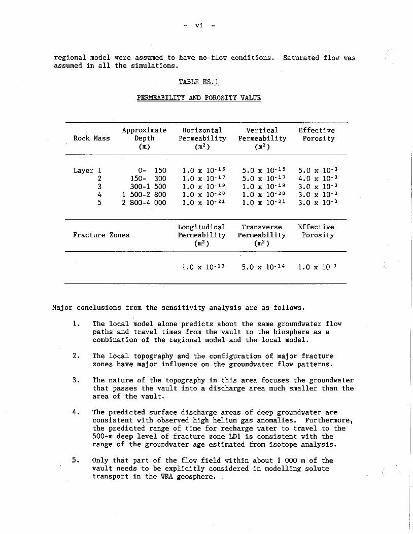
regional model were assumed to have no-flow conditions. Saturated flow was I assumed in all the simulations.
TABLE ES. 1
PERMEABILITY AND POROSITY VALUE
Approximate Horizontal Vertical Effective Rock Mass Depth Permeability Permeability Porosity
(m) (m2 (m2 )
Layer 1 0- 150 1.0 10-15 5.0 x 10-l5 5.0 x lo-3 2 150- 300 1.0 x 10⁻¹⁷ 5.0 x 10-l7 4.0 x 3 300-1 500 1.0 x 10-l9 1.0 x 10-l9 3.0 x lo-3 4 1 500-2 800 1.0 x 1.0 lo-2o 3.0 x lo-3 5 2 800-4 000 1.0 x lo-" 1 . 0 ~ 10-21 3 . 0 ~ lo-3
Fracture Zones Longitudinal Transverse Effective Permeability Permeability Porosity
(m2 > (m2 1
Major conclusions from the sensitivity analysis are as follows.
1. The local model alone predicts about the same groundwater flow paths and travel times from the vault to the biosphere as a combination of the regional model and the local model.
2. The local topography and the configuration of major fracture zones have major influence on the groundwater flow patterns.
3. The nature of the topography in this area focuses the groundwater that passes the vault into a discharge area much smaller than the area of the vault.
4. The predicted surface discharge areas of deep groundwater are consistent with observed high helium gas anomalies. Furthermore, the predicted range of time for recharge water to travel to the 500-m deep level of fracture zone LD1 is consistent with the range of the groundwater age estimated from isotope analysis.
5. Only that part of the flow field within about 1 000 m of the vault needs to be explicitly considered in modelling solute transport in the WRA geosphere.
- vii -
6. Both the groundwater travel time, and the area in the biosphere to which contaminated groundwater from the vault is predicted to discharge, can be substantially reduced by pumping at the well, especially at higher pumping rates.
7. The waste exclusion distance, the shortest distance between the vault and fracture zone LD1, affects the contaminant transport times significantly.
8. Thermal convection due to heat generation by the fuel waste in the vault may or may not be important depending on the waste exclusion distance. For a 46-m waste exclusion distance; thermal convection due to waste heat does not significantly affect groundwater travel times.
9. The presence of shafts and tunnels, variations in hydraulic properties of backfill materials, the existence of an excavation damaged zone, or the presence of a perturbed fissure zone near ground surface do not significantly affect convective transport from the vault to the biosphere.
The simulations used to finalize the geometry of, and inputs to, GEONET for the reference postclosure assessment have been formulated considering the characteristics of the assessment case study, the nature of the GEONET code and the above conclusions of the sensitivity analyses. The simulations were performed using the MOTIF 3-D local model. A domestic water-supply well was assumed to intersect fracture zone LD1. A waste exclusion distance of 46 m was chosen after sensitivity analyses using MOTIF and GEONET. No excavation damaged zone was simulated. All shafts, tunnels and disposal rooms were assumed to be filled with reference backfill. Steady- state isothermal flow was simulated.
In Chapter 6 we provide the transport equations and their solution in GEONET using analytical response functions. GEONET solves a set of 1-D transport equations for a radionuclide decay chain including advection, dispersion and sorption. The model assumptions, geometric simplifications, approximations and the resulting limitations are discussed, as are quality assurance and verification, including a comparison between MOTIF and GEONET transport predictions.
GEONET approximates the three-dimensional transport paths by a network of one-dimensional transport paths connected in three-dimensional space. Where advection is estimated to be the predominant mode of transport, the GEONET pathways are constructed to match as closely as possible the three- dimensional flow paths predicted by the MOTIF flow model and particle tracking. When groundwater velocity is so low that contaminant transport is dominated by molecular diffusion, the GEONET pathways are constructed to give the shortest diffusion paths to zones with significantly higher groundwater velocity. This corresponds to diffusion down the concentration gradient. Each GEONET transport path is composed of a number of linear segments. Within each segment, GEONET modifies the head distribution predicted by the MOTIF flow model according to an analytical well model and then calculates the mean groundwater velocity by finite difference. Next
- viii -
it solves the one-dimensional advection-dispersion-retardation equations for a radionuclide decay chain by a standard, computationally efficient analytical method of mathematical physics known as the response function method, a type of Green's function method. The response function is the solution for a delta function impulse contaminant source at the inlet boundary. In SYVAC3 the solution to the transport equation for a time dependent source function is obtained by numerical convolution of the response function with the source function. These calculations are done sequentially, segment by segment, using the output of one segment as input boundary condition for the following segment in the same pathway. Segments can also converge or diverge. For converging segments, the contaminant mass flow rates are summed whereas for diverging segments the contaminant mass flow rate is divided according to the branching ratio of groundwater flux estimated from the particle tracking.
The geosphere model implemented in GEONET includes the following major features: several layers of rock, overburden, lake sediment, a major fracture zone with asymmetric and nonuniform flow, a waste exclusion distance and a domestic water-supply well. The model allows switching of flow from some transport.segments to others as the well affects the flow field. Sorption coefficients are nuclide/mineral specific and are dependent on the redox condition and groundwater salinity.
An analytical well model is used to calculate four quantities:
1. the maximum well capacity,
2. the drawdowns in the fracture zone from which the well draws water,
3. the quantity of surface water captured by the well, and
4. the contaminant capture fractions in the fracture which determine the quantity of radionuclides entering the well.
In addition, there are several empirical site specific equations which have to be determined by detailed 3-D flow modelling and particle tracking. These are described in Chapter 7.
Apart.from the geometric simplification, the major assumption in GEONET is that the uncertainty and spatial variability in the permeability of the hydrogeological system can be simulated in a probabilistic assessment by randomly sampling a distribution of a single velocity factor. This means that the groundwater flow field is deterministic except for this randomly sampled scaling factor, along with the well depth and pumping rate.
Chemical retardation is modelled using an equilibrium linear sorption (kd) approach. Retardation factors are calculated, using empirical equations, from a set of basic chemical and mineralogical properties. For each nuclide/mineral combination, and for either oxidizing or reducing conditions, the distribution coefficient k, is given by an empirical quadratic expression in log(TDS) where TDS denotes the concentration of
total dissolved solids. Dependence of k, on radionuclide concentration is - treated approximately as an additional uncertainty.
To build confidence in the correct implementation of GEONET, the following quality assurance and verification measures were undertaken:
- Testing of the modules of the code;
- Comparison of calculations with known results obtained from analytical solutions for some simple cases;
- Comparison with calculations done by similar codes including those published in the open literature;
- Participation in INTRACOIN (International Transport Code Intercomparison) and PSAC (Probabilistic Systems Assessment Code User's Group);
- Comparison with calculations done by a 2-D MOTIF advection- dispersion transport model; and
- Examination of results of sensitivity analysis.
The geometry of the GEONET network was subsequently adjusted slightly to ensure conservative transport predictions, i.e., a peak contaminant flow rate in GEONET is slightly higher than that given by the MOTIF transport model.
In Chapter 7 we illustrate the methodology presented in the preceding chapters by showing how we use the predictions of the 3-D MOTIF flow model, based on the conceptual hydrogeological model of the WRA, to determine the geometry, the hydraulic heads, the discharge areas, and the empirical factors and equations for the Geosphere Model for the reference postclosure assessment case. This chapter also outlines other input data for the Geosphere Model. These include hydraulic, transport and sorption properties, as well as groundwater chemistry and mineralogy.
Three-dimensional MOTIF WRA flow models, in conjunction with particle tracking, have been used to determine :
1. the hydraulic heads under natural steady-state flow,
2. the GEONET network geometry with and without the well,
3. calibration factors for adjusting the drawdown and contaminant capture fraction predicted by the analytical well model,
4. an empirical equation for estimating the drawdown at the vault due to pumping at the well,
5 . several empirical equations for estimating the fraction of contaminant that is captured by the well from the groundwater in rock outside of fracture zone LD1, and
6. empirical equations relating the contaminated groundwater discharge area at surface to the well depth and pumping rate.
In addition, the following data derived from field and laboratory work or literature review are transferred to GEONET:
1. hydraulic properties - porosities and permeabilities; 2. transport properties - dispersivities, free-water diffusion
coefficients and tortuosity factors;
3. mineralogy and groundwater chemistry - groundwater salinity (total dissolved solids), redox divide (the position along a flow path at which the redox potential changes sign, from oxidizing to reducing), fractional mineral content, and sorption data; and
4. miscellaneous properties such as the thickness of sediment and overburden, the radius of well casing, and the fraction of the backfill in the vault.
In addition to the main text, this report contains several Appendices which treat special topics or provide detailed input data for the reference postclosure assessment. Appendix A discusses the groundwater geochemistry and colloid contents, the rock mineralogy and fracture fillings for the WRA. Appendix B outlines the sorption model and possible impacts for colloids and microorganism on chemical retardation. Appendix C gives the I mathematical equations for projecting the 3-D permeability tensor onto the direction of the piecewise linear transport paths in GEONET. Appendix D contains extensive tabulation of input data and their justification for the GEONET/SYVAC3 Geosphere Model for the reference postclosure assessment. Appendices E and F are collections of verification test cases for the MOTIF and TRACK3D codes, respectively. Appendix G presents a mathematical argument that the principal response function used for mass transport in GEONET can be applied to two different physical situations.

INTRODUCTION
1.1 BACKGROUND
In 1978, AECL was given the responsibility to conduct research and develop- ment on disposal of Canadian nuclear fuel waste It... in a deep underground repository [vault] in intrusive igneous rock..." (Joint Statement 1978). A summary of the results of the research and development and our conclusions are given in an Environmental Impact Statement (EIS) on the Concept for Disposal of Canada's Nuclear Fuel Waste (AECL 1994). The EIS is being reviewed under the federal Environmental Assessment and Review Process and will be submitted to an Environmental Assessment Panel.
An important aspect of the R&D has been the development and demonstration of a suitable methodology for mathematical modelling of the expected long- term performance of a disposal system so that the acceptability of the potential environmental effects can be evaluated in terms of quantitative regulatory standards. The methodology AECL has developed (Goodwin et al. 1994) assesses the performance of the disposal system following closure using models representing the disposal vault (the Vault Model, Johnson et al. 1994a), the rock and its groundwater flow systems (the Geosphere Model, this report), and the surface and near-surface environment (the Biosphere Model, Davis et al. 1993).
The surface environment as used here is made up of the soil, water, air and living things (including humans) at the surface of the earth. We use "sur- face and near-surface environment" synonymously with "biosphere" while recognizing that micro-organisms can also occur to great depths in the geosphere. How we apply the terms vault, geosphere and biosphere in developing the models is illustrated in Figure 1.1.1. Environmental assessment is used to include both safety evaluation (potential health effects on humans and other organisms) and socio-economic evaluation (potential social and economic effects). The environmental assessment case studies of reference disposal systems presented in the EIS (AECL 1994) include a preclosure assessment case study for the period when a disposal facility is being sited, constructed, operated, decommissioned and closed (i.e. placed in a passively safe state); and a postclosure assessment case study for the period after a disposal facility has been closed. The post- closure assessment is an assessment of the long-term performance of a reference disposal system after closure, when the facility has been placed in a state of passive safety such that there is no longer need to rely on institutional controls to ensure safety. It is primarily an evaluation of long-term safety.
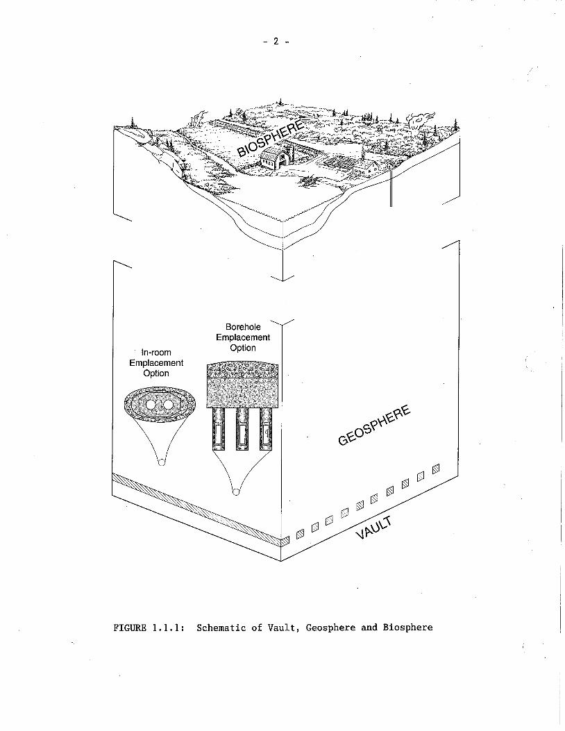
Borehole Emplacement
In-room Option
FIGURE 1.1.1: Schematic of Vault, Geosphere and Biosphere
1.2 THE DISPOSAL CONCEPT
The disposal concept is a proposed method for geological disposal of nuclear fuel waste in which
- the waste form (either used CANDU fuel or solidified highly radioactive reprocessing waste) would be sealed in long-lived containers designed to last at least 500 years and possibly much longer,
- the containers would be emplaced in rooms in a disposal vault or in boreholes drilled from the rooms,
- the rooms would be excavated deep (nominally 500 to 1 000 m) in plutonic rock of the Canadian Shield,
- each waste container would be surrounded by a buffer,
- each room would be sealed with backfill and other vault seals, and
- all tunnels, shafts, and exploration boreholes would ultimately be sealed in such a way that the disposal vault would be passive- ly safe.
The disposal vault would be located and designed to inhibit future human intrusions, to withstand the expected range of natural disruptions, to inhibit movement of contaminants into the groundwater present within the surrounding rock and to promote the release of contaminants into pathways where the movement of groundwater would be slow and the transit time for contaminants from the vault to the biosphere would be long.
The combination of the characteristics of all the components of the dis- posal system would protect the environment from adverse effects of the nuclear fuel waste (the multiple barrier approach). In the postclosure phase the disposal system would comprise the engineered components of the disposal vault (the waste form; the containers; and the buffer, backfill and other vault seals), the geosphere (the rock mass and associated ground- water regime that surrounds the vault), and the biosphere (the potentially affected near-surface and surface environment). Each component of the disposal system would play some role in delaying and reducing the movement of radioactive material such that their combined effect would ensure that there were no unacceptable adverse effects when contaminants from the waste eventually reach the biosphere.
It is important to make the distinction between this general disposal con- cept and a site-specific design of a disposal facility or its components. The disposal concept permits a choice of disposal site locations and a choice of methods, materials, and designs for many of the components of the disposal system. To implement the concept using a site-specific design, these choices would be made based on an evaluation of performance, avail- ability, cost and practicality in the context of the particular character- istics of the selected site.
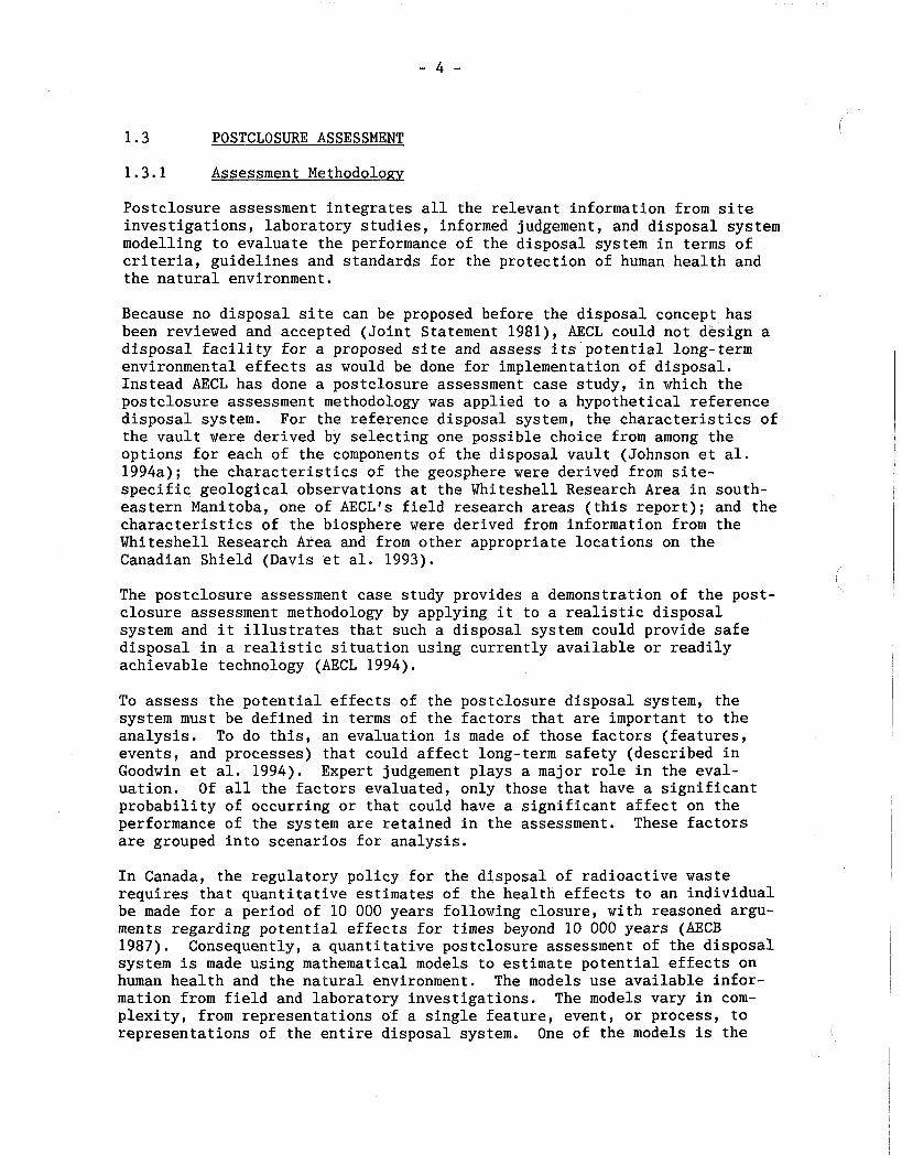
1.3 POSTCLOSURE ASSESSMENT
1.3.1 Assessment Methodolonv
Postclosure assessment integrates all the relevant information from site investigations, laboratory studies, informed judgement, and disposal system modelling to evaluate the performance of the disposal system in terms of criteria, guidelines and standards for the protection of human health and the natural environment.
Because no disposal site can be proposed before the disposal concept has been reviewed and accepted (Joint Statement 1981), AECL could not design a disposal facility for a proposed site and assess its potential long-term environmental effects as would be done for implementation of disposal. Instead AECL has done a postclosure assessment case study, in which the postclosure assessment methodology was applied to a hypothetical reference disposal system. For the reference disposal system, the characteristics of the vault were derived by selecting one possible choice from among the options for each of the components of the disposal vault (Johnson et al. 1994a); the characteristics of the geosphere were derived from site- specific geological observations at the Whiteshell Research Area in south- eastern Manitoba, one of AECL's field research areas (this report); and the characteristics of the biosphere were derived from information from the Whiteshell Research Area and from other appropriate locations on the Canadian Shield (Davis et al. 1993).
The postclosure assessment case study provides a demonstration of the post- closure assessment methodology by applying it to a realistic disposal system and it illustrates that such a disposal system could provide safe disposal in a realistic situation using currently available or readily achievable technology (AECL 1994).
To assess the potential effects of the postclosure disposal system, the system must be defined in terms of the factors that are important to the analysis. To do this, an evaluation is made of those factors (features, events, and processes) that could affect long-term safety (described in Goodwin et al. 1994). Expert judgement plays a major role in the eval- uation. Of all the factors evaluated, only those that have a significant probability of occurring or that could have a significant affect on the performance of the system are retained in the assessment. These factors are grouped into scenarios for analysis.
In Canada, the regulatory policy for the disposal of radioactive waste requires that quantitative estimates of the health effects to an individual be made for a period of 10 000 years following closure, with reasoned argu- ments regarding potential effects for times beyond 10 000 years (AECB 1987). Consequently, a quantitative postclosure assessment of the disposal system is made using mathematical models to estimate potential effects on human health and the natural environment. The models use available infor- mation from field and laboratory investigations. The models vary in com- plexity, from representations of a single feature, event, or process, to representations of the entire disposal system. One of the models is the

postclosure assessment system-model, which incorporates as many of the scenarios (combinations of significant features, events, and processes) as is judged to be practical and appropriate. Significant features, events, and processes that are not incorporated in the system-model are incor- porated in scenarios that are analysed using other quantitative models or using qualitative expert judgement.
The models and expert judgement are used to estimate the effects of dis- posal on human health and the natural environment. The estimates produced in the postclosure assessment are not intended to be precise predictions of actual future effects of disposal. They are intended to be pessimistic estimates (higher than any expected) of the magnitude of potential adverse effects of disposal to assist in judging the capability of the disposal system to protect human health and the natural environment.
For the evaluation of the long-term safety of a disposal system, the measure of adverse effect from disposal used by the AECB (1987) is the radiological risk, "defined as the probability that a fatal cancer or serious genetic effect will occur to an individual or his or her descend- ant~.~! The risk is calculated by adding the results from all significant scenarios, where the result of each scenario is a product of the prob- ability that the scenario occurs, the magnitude of the estimated radio- logical dose from the scenario, and the probability of a fatal cancer or serious genetic effect per unit dose (AECB 1987).
The criterion specified by the AECB for judging acceptability of a disposal facility in the long-term is a calculated radiological risk of less than
per year to individuals in the critical group (a hypothetical group of people assumed to live at a time and place and in such a way that it is exposed to maximum risk from the disposal system. The definition of the critical group is expected to lead to estimates of the effects of disposal on an individual in this group being higher than estimates that would be made for an individual in any actual group of people.
1.3.2 The Postclosure Assessment Case Study Reference Disposal System
To illustrate the use of the postclosure assessment methodology, AECL applied it to a hypothetical reference disposal system (Goodwin et al. 1994). The reference disposal system is based on a conceptual design for a disposal facility described by Simmons and Baumgartner (1994). In this facility corrosion-resistant titanium containers, each containing 72 used- fuel bundles, are placed in boreholes in the floor of a square array of disposal rooms excavated in a granitic pluton and accessed by shafts and tunnels. Each container is surrounded by a buffer and the rooms, tunnels, and shafts are backfilled and sealed (Figure 1.3.1).
For the postclosure assessment case study, the characteristics of the geo- sphere in the reference disposal system are derived from site-specific information from AECLvs Whiteshell Research Area, near Lac du Bonnet, Manitoba (Figure 1.3.2). Most of the information about the rock, such as the orientation and properties of fracture zones, is based on the infor- mation available when the conceptual design was developed in 1985,
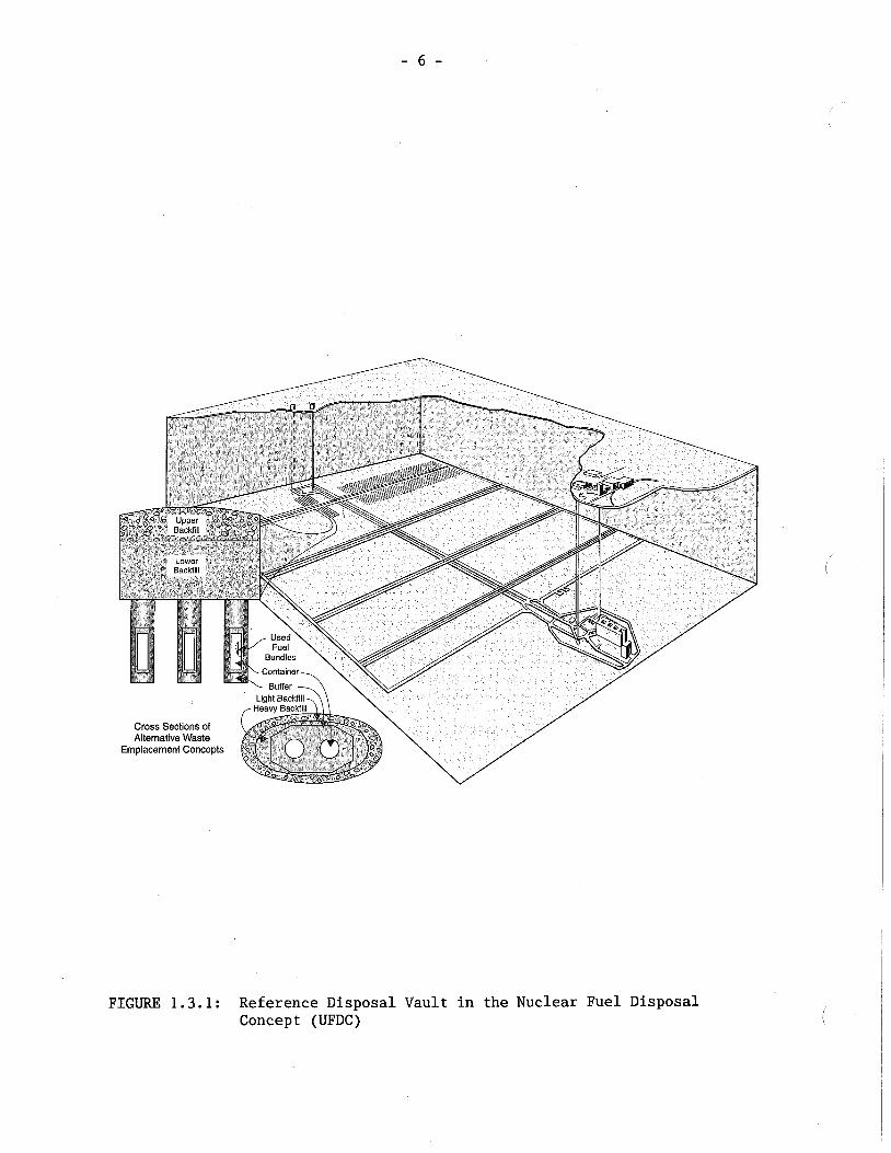
FIGURE 1.3.1: Reference Disposal Vault in the Nuclear Fuel Disposal Concept (UFDC)
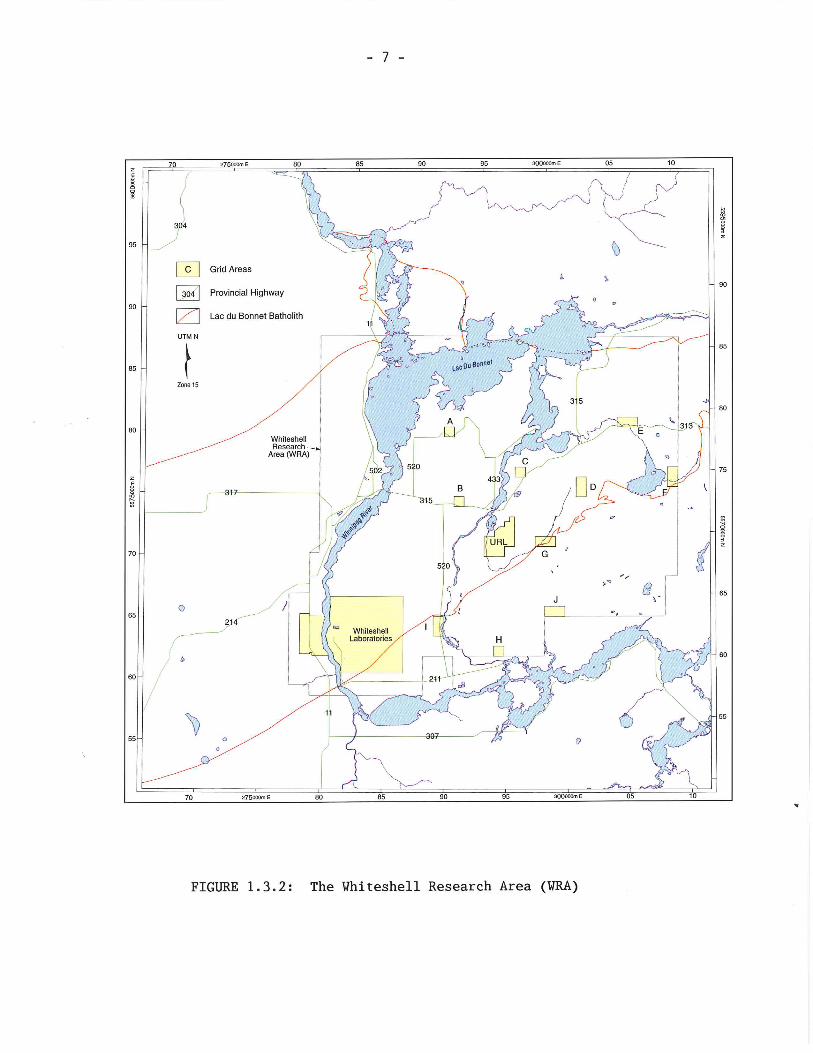
primarily from the detailed site investigations undertaken to locate and construct AECL's Underground Research Laboratory. For features away from locations where detailed borehole information was available, assumptions about characteristics at depth were made on the basis of information obtained from geological mapping, remote sensing and geophysical surveys from surface.
Figure 1.3.3 shows the location of the hypothetical disposal vault in relation to the major geologic features included in the geosphere for the postclosure assessment case study. The hypothetical disposal vault is at a depth of 500 m, nominally the shallowest considered in the disposal con- cept. This depth was chosen because it would tend to provide the shortest path for movement of contaminants from the vault to the biosphere.
The characteristics of the biosphere used in the postclosure assessment case study are derived from information from both the Whiteshell Research Area and elsewhere on the Canadian Shield. The general characteristics are typical of the Shield, but specific locations of water bodies and discharge points of groundwater that could have passed through or near the hypo- thetical disposal vault are derived using the information from the Whiteshell Research Area.
1.3.3 The Postclosure Assessment Case Study System-Model
The system-model for the postclosure assessment case study describes the behaviour of the components of the postclosure reference disposal system. It is used to analyze the performance of the entire system and to provide an understanding of the relationship between the behaviour of the system components and the potential effects of disposal.
The system-model contains linked mathematical models of the vault, geo- sphere, and biosphere (Figure 1.3.4). In general, these models are simpl- ified representations of the processes affecting the release and movement of contaminants from the waste. More detailed models of some of the pro- cesses, such as groundwater flow, are also used in the development of the system-model and to complement, calibrate, or verify portions of the analy- sis done using the system-model. The system-model is discussed in detail by Goodwin et al. (1994).
The vault consists of the engineered barriers, which include the waste form, the container, the buffer material, and the materials used to back- fill and seal the underground disposal vault. It is represented by the Vault Model, a computer code used to estimate the time-dependent release of contaminants from the disposal vault into the surrounding geosphere. The vault would contain both elements that were radioactive as well as elements that were chemically toxic. Johnson et al. (1994a) provide a list of the elements present in used fuel. In this report, we refer to any element released from the vault as a contaminant. The Vault Model simulates the processes causing failure of the waste containers, dissolution of the waste form and release of contaminants, and the transport of contaminants within the disposal vault to the excavated surface of the rock. The Vault Model is discussed in detail by Johnson et al. (1994a).
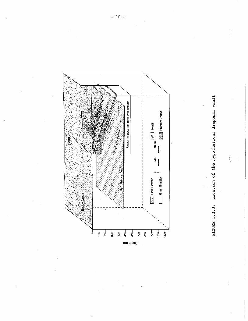
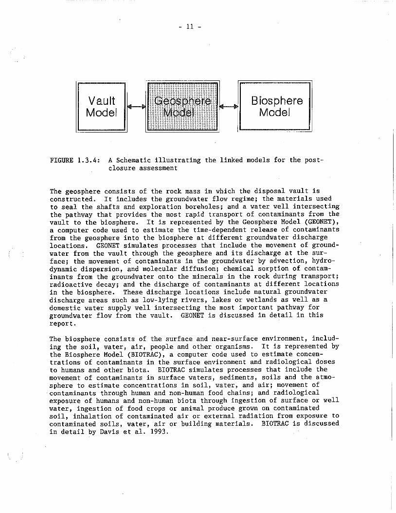
FIGURE 1.3.4: A Schematic illustrating the linked models for the post- closure assessment
The geosphere consists of the rock mass in which the disposal vault is constructed. It includes the groundwater flow regime; the materials used to seal the shafts and exploration boreholes; and a water well intersecting the pathway that provides the most rapid transport of contaminants from the vault to the biosphere. It is represented by the Geosphere Model (GEONET), a computer code used to estimate the time-dependent release of contaminants from the geosphere into the biosphere at different groundwater discharge locations. GEONET simulates processes that include the movement of ground- water from the vault through the geosphere and its discharge at the sur- face; the movement of contaminants in the groundwater by advection, hydro- dynamic dispersion, and molecular diffusion; chemical sorption of contam- inants from the groundwater onto the minerals in the rock during transport; radioactive decay; and the discharge of contaminants at different locations in the biosphere. These discharge locations include natural groundwater discharge areas such as low-lying rivers, lakes or wetlands as well as a domestic water supply well intersecting the most important pathway for groundwater flow from the vault. GEONET is discussed in detail in this report.
The biosphere consists of the surface and near-surface environment, includ- ing the soil, water, air, people and other organisms. It is represented by the Biosphere Model (BIOTRAC), a computer code used to estimate concen- trations of contaminants in the surface environment and radiological doses to humans and other biota. BIOTRAC simulates processes that include the movement of contaminants in surface waters, sediments, soils and the atmo- sphere to estimate concentrations in soil, water, and air; movement of contaminants through human and non-human food chains; and radiological exposure of humans and non-human biota through ingestion of surface or well water, ingestion of food crops or animal produce grown on contaminated soil, inhalation of contaminated air or external radiation from exposure to contaminated soils, water, air or building materials. BIOTRAC is discussed in detail by Davis et al. 1993.
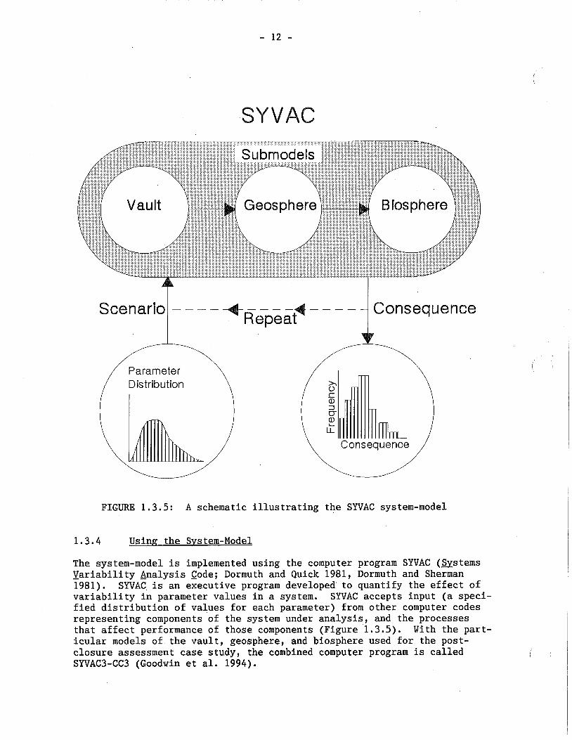
SYVAC
Scenario - - - - + - - - -4 - - A
' 1 Repeat Consequence
/ Distribution \
\ Consequence
FIGURE 1.3.5: A schematic illustrating the SYVAC system-model
1.3.4 Using the System-Model
The system-model is implemented using the computer program SYVAC (&stems Variability Analysis Code; Dormuth and Quick 1981, Dormuth and Sherman - 1981). SYVAC is an executive program developed to quantify the effect of variability in parameter values in a system. SYVAC accepts input (a speci- fied distribution of values for each parameter) from other computer codes representing components of the system under analysis, and the processes that affect performance of those components (Figure 1.3.5). With the part- icular models of the vault, geosphere, and biosphere used for the post- closure assessment case study, the combined computer program is called SYVAC3-CC3 (Goodwin et al. 1994).
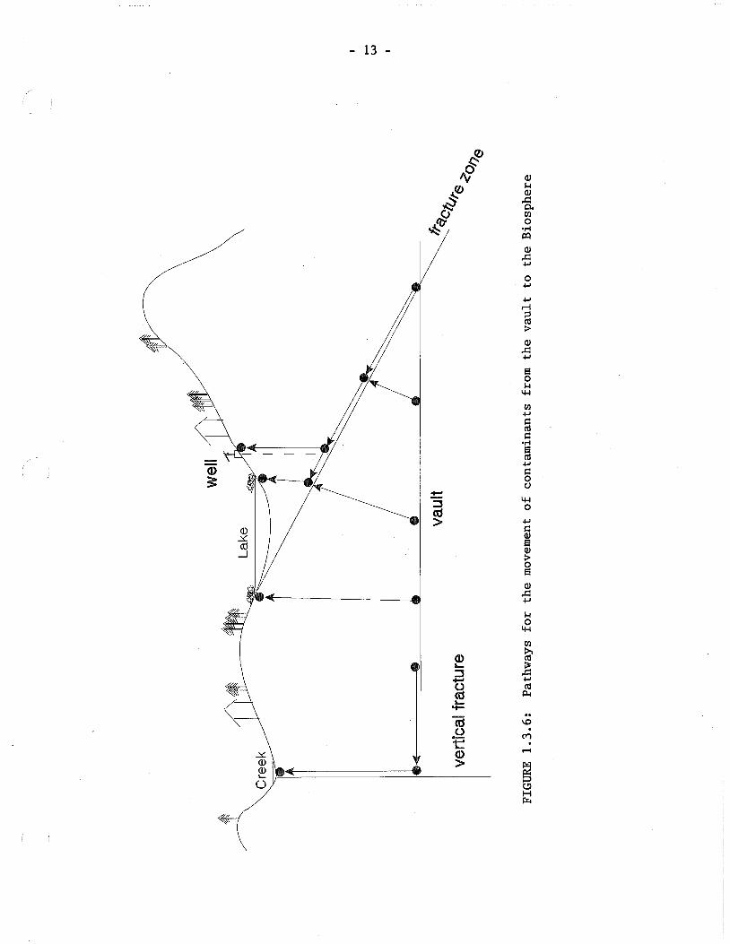
For each simulation, SYVAC3-CC3 selects a value for each parameter in the system by sampling from the specified distribution and uses these values in the vault, geosphere, and biosphere models. Contaminants entering the geosphere from different portions of the vault used in the postclosure assessment case study, follow pathways through the geosphere that have different characteristics. To account for this, the vault is divided into 12 sectors and the Vault Model estimates the release of contaminants from each sector independently. Each vault sector is associated with an adjoin- ing segment of the geosphere, which receives contaminants only from that sector. Linkages between the Vault Model and the Geosphere Model ensure that the groundwater flow inside the vault, and contaminant movement from the vault to the geosphere, are consistent with hydrogeological conditions in the geosphere adjacent to each vault sector. Geosphere segments are linked together to form pathways for the movement of contaminants from each vault sector to locations of discharge in the biosphere, which are either surface water bodies or a domestic water supply well (Figure 1.3.6). Linkages between the Geosphere Model and the Biosphere Model ensure that usage of the water supply well and movement of contaminants from the geosphere to the biosphere are consistent with hydrogeological conditions adjacent to the well and the other discharge points.
Much of this report is about how information from the Whiteshell Research Area was incorporated in a variety of conceptual models, how these concept- ual models were used in developing hydrogeological models, and how the hydrogeological models were used in developing GEONET, the Geosphere Model used in the postclosure assessment case study.
The output of a simulation is an estimate of annual radiological dose to an individual of the critical group as a function of time, or of dose to non- human biota, or concentration of a contaminant. To quantify the effects of variability represented by the parameter value distributions, SYVAC3-CC3 repeats the simulation many times (typically thousands of times), selecting new parameter values each time. The distribution of all the estimates reflects the variability associated with modelling the system. For this kind of probabilistic modelling, the AECB (1987) requires that the arith- metic average of the estimates of dose to an individual of the critical group be used in the calculation of the radiological risk that is compared with the risk criterion. Use of the arithmetic average ensures that simu- lations producing high estimates of dose dominate in the calculated risk that is used for comparison with the regulatory criterion.
The system-model simulates processes taking place within a complex natural environment that has been modified by the construction and operation of the disposal facility. The mathematical description of such a disposal system entails considerable uncertainty resulting from unknown processes; changes with time; use of assumptions and approximations; errors in programming, data, and measurement; and natural unsystematic variation in the system (Dormuth 1992). Although measures can be taken to reduce and quantify this uncertainity, it cannot be eliminated. The AECB (1987) took this into account specifically when establishing the risk criterion to be "suffic- iently low so as to allow for uncertainties in exposure scenarios and their consequences."
Much of the uncertainty derives from the natural variability in the real world and from the fact that we will always have a less than perfect under- standing of the detailed behaviour of the natural and engineered components of the disposal system when such long time periods are involved. Known systematic variations (such as radioactive decay) can often be modelled explicitly; if so, they do not contribute to uncertainty.
Non-systematic variations generally cannot be known in sufficient detail to model the distribution of their values explicitly. This sort of uncertain- ty is addressed by incorporating known ranges in variation of parameters in the models, primarily by specifying distributions for the parameters rather than giving them fixed values. If parameters are known to be correlated and the correlation can be modelled, it can also be incorporated in the assessment. To the extent that random error in field and laboratory mea- surements can be quantified, it can also be included in the variation in parameter values. Running thousands of simulations using SYVAC3-CC3 pro- duces a distribution of results that quantifies the effect of the parameter variablility on the estimates.
Systematic errors in field and laboratory measurements are minimized by quality control of procedures and peer review. Errors in developing com- puter programs and entering data into the programs are minimized by formal programming and data-handling procedures, scrutiny of results to detect inconsistencies, intercomparison with results from independently developed programs, and use of the program to analyze cases for which the results are
I known.
The possible existence of unknown processes that could have a significant effect on the disposal system introduces an uncertainty that cannot be quantified. It is likely minimized, however, by the extensive investi- gations by scientists in many countries to identify processes important to waste disposal, including detailed investigations in relevant natural sys- tems that have existed for periods very much longer than the period for which the disposal system must be modelled.
The assumptions and approximations made in order to represent the important processes as mathematical equations in the models introduce uncertainty by causing the models to be inaccurate to some extent. The degree to which it is desirable to reduce this uncertainty depends on the purpose for which the models are used. When the models are being used to gain an understand- ing of the processes, the assumptions and approximations used should be chosen to be as accurate as possible, and the uncertainty should be reduced by comparing model results with actual observations from field or labora- tory experiments. When the models are being used to establish an upper limit on radiological risk, as is the case for the system-model for the postclosure assessment case study, the assumptions and approximations should be chosen to be conservative so that they tend to result in the calculated radiological risk being higher than the expected risk (pessi- mistic); the uncertainty is then not in the accuracy of the calculated risk, but rather in how much the expected risk has been over-estimated. When the models are being used to optimize designs, assumptions and approximations that lead to pessimistic results may be inappropriate be-
cause their use might lead to designs that would not provide the lowest expected risk.
MODELLING THE GEOSPHERE
1.4.1 Introduction
An understanding of the characteristics of the geosphere at a potential disposal site is essential for selecting a potential vault location, de- signing a disposal vault, and assessing the potential effects of the dis- posal system on human health and the natural environment.
Models of the geosphere are visual or mathematical representations of the understanding of the geological and hydrogeological site characteristics (structure, lithology, stress, temperature, hydraulic head, and rock and fluid properties). The models are used for:
- planning the site investigations;
- locating and designing the vault;
- assessing the performance of the disposal system and estimating the effects of disposal (using the site-specific design) on human health and the natural environment; and
- communicating the understanding of the site, the disposal system, and the results of the assessment to regulatory agencies, repre- sentatives of potential host communities, and members of the public.
In AECLfs postclosure assessment methodology, the Geosphere Model is a mathematical representation of those physical and chemical characteristics of a particular site, and those processes acting at the site and its sur- roundings, that are believed to control movement of contaminants from the disposal vault to the biosphere during the time of the quantitative esti- mation of risk (10 000 a). Identifying the important pathways for contam- inant movement through the rock to the biosphere, and the factors that would be important in controlling contaminant movement along those pathways requires a thorough knowledge of the geologic, hydrogeologic, geomechanical and geochemical conditions at a site.
The knowledge of the conditions at an actual disposal site would be obtain- ed by characterization and monitoring of the site using a wide variety of methods (Davison et al. 1994). The groundwater flow characteristics of a large region encompassing potential disposal sites would need to be under- stood, so that favorable locations within the groundwater flow regime could be identified and taken into account in selecting a suitable location for the site. We would need to know how these characteristics varied spatially at the site before the disposal vault was constructed and how they might vary in the future due to potential changes caused by the disposal vault, natural geological processes, or accidental human intrusion.
The location, orientation, physical and chemical characteristics of the main geologic and hydrogeologic features of the site and its surroundings would be determined by site characterization so that a three-dimensional picture of the geosphere around the vault could be created. Because solute transport by advection and diffusion in groundwater within the geosphere would be such an important aspect in the postclosure assessment, we would focus on the data relevant for determining the hydrogeological and solute transport properties of the geosphere. Detailed measurements would be made to determine the permeability, porosity, dispersivity and chemical proper- ties of the pathways for groundwater movement through the geosphere so that these could be appropriately represented in the models.
A large amount of information and data would be produced in any site eval- uation. In order to determine what characteristics should be incorporated in the Geosphere Model for postclosure assessment, we would use two kinds of models to evaluate the available information:
- models representing individual site characteristics, processes, or events; and
- models representing an integration of the site characteristics, processes, and events that would affect the movement of contam- inants from a disposal vault to the biosphere.
These models could be'either
- qualitative (a conceptual or schematic representation such as a map, cross-section, or block diagram), or
- quantitative (a mathematical representation such as an analytical or numerical model of a process implemented by equations in a computer program).
Figure 1.4.1 illustrates the following steps followed in developing the Geosphere Model (GEONET) for the postclosure assessment case study:
A . constructing a conceptual model of the hydrogeological units using data from field investigations at the Whiteshell Research Area and the results of laboratory testing of rock properties (Chapter 5),
B. constructing 2-D and 3-D finite-element models based on the con- ceptual model for analyzing groundwater flow through the geo- sphere under the driving forces of gravity and thermal bouyancy using the MOTIF code (Chapter 51,
C. identifying the groundwater flow paths from the hypothetical vault to groundwater discharge areas in the biosphere for the groundwater velocity field calculated by MOTIF using the TRACK3D code (Chapter 5), and
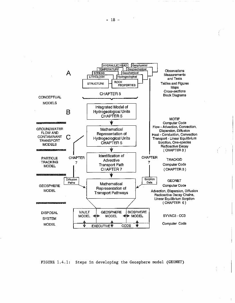
ITHOLOGY I 1 Hydrogeological I Observations
Measurements and Tests I Tables and Figures
Maps
CHAPTER 5 CONCEPTUAL
MODELS
B
GROUNDWATER FLOW AND
CONTAMINANT C TRANSPORT
MODELS f
Hydrogeological Units
PSr Mathematical
Representation of Hydrogeological Units
CHAPTER 5
Cross-sections Block Diagrams
MOTIF Computer Code
Flow - ~dve'ction, Convection, Dispersion, Diffusion
Heat - Conduction, Convection Transport - Linear Equilibrium
Sorption, One-species Radioactive Decay
I \I I ( CHAPTER 3 ) -
GEONET GEOSPHERE Mathematical Computer Code
MODEL Representation of
Transport Pathways Advection, Dispersion, Diffusion Radioactive Decav Chains,
I
PARTICLE CHAPTER TRACKING 7
MODEL I
Linear ~~u i l ib r ium sorption ( CHAPTER 6 )
DISPOSAL VAULT MODEL
SYSTEM
Identification of Advect ive
Transport Path CHAPTER 7
MODEL
I
CHAPTER TRACK3D 7
I Computer Code ( CHAPTER 3 )
SYVAC3 - CC3
Computer Code
FIGURE 1.4.1: Steps in developing the Geosphere model (GEONET)
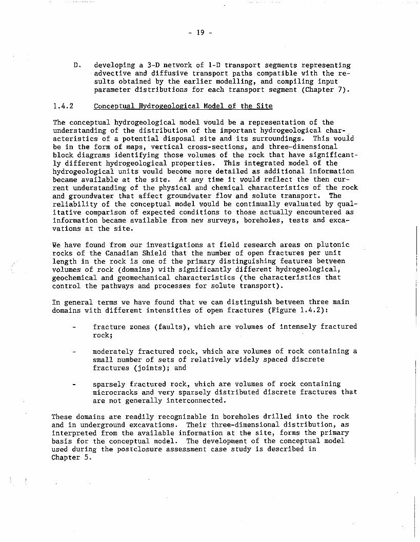
D. developing a 3-D network of 1-D transport segments representing advective and diffusive transport paths compatible with the re- sults obtained by the earlier modelling, and compiling input parameter distributions for each transport segment (Chapter 7).
1.4.2 Conceptual Hvdro~eolonical Model of the Site
The conceptual hydrogeological model would be a representation of the understanding of the distribution of the important hydrogeological char- acteristics of a potential disposal site and its surroundings. This would be in the form of maps, vertical cross-sections, and three-dimensional block diagrams identifying those volumes of the rock that have significant- ly different hydrogeological properties. This integrated model of the hydrogeological units would become more detailed as additional information became available at the site. At any time it would reflect the then cur- rent understanding of the physical and chemical characteristics of the rock and groundwater that affect groundwater flow and solute transport. The reliability of the conceptual model would be continually evaluated by qual- itative comparison of expected conditions to those actually encountered as information became available from new surveys, boreholes, tests and exca- vations at the site.
We have found from our investigations at field research areas on plutonic rocks of the Canadian Shield that the number of open fractures per unit length in the rock is one of the primary distinguishing features between
I volumes of rock (domains) with significantly different hydrogeological, geochemical and geomechanical characteristics (the characteristics that control the pathways and processes for solute transport).
In general terms we have found that we can distinguish between three main domains with different intensities of open fractures (Figure 1.4.2):
- fracture zones (faults), which are volumes of intensely fractured rock;
- moderately fractured rock, which are volumes of rock containing a small number of sets of relatively widely spaced discrete fractures (joints); and
- sparsely fractured rock, which are volumes of rock containing microcracks and very sparsely distributed discrete fractures that are not generally interconnected.
These domains are readily recognizable in boreholes drilled into the rock and in underground excavations. Their three-dimensional distribution, as interpreted from the available information at the site, forms the primary basis for the conceptual model. The development of the conceptual model used during the postclosure assessment case study is described in Chapter 5.
1.4.3 Groundwater Flow Model of the Site
The groundwater flow model would be a three-dimensional mathematical repre- sentation of the conceptual model of the groundwater flow and solute trans- port conditions for the area surrounding the potential disposal site. The reliability of the groundwater flow model is evaluated by performing a variety of tests, including comparisons with problems that have solutions that are known exactly and comparisons with observations from laboratory and field experiments (Chapter 4.).
The initial model (representing the spatial distribution of hydrogeological properties) would be calibrated using the existing hydrogeological and chemical data from the site investigations (such as straddle-packer perme- ability tests, large-scale groundwater pumping tests, measurements of groundwater pressure at isolated monitoring locations in the rock, measure- ments of groundwater recharge and discharge, groundwater tracer tests and groundwater chemistry information). As with the conceptual model, there would be continual evaluation of the groundwater flow model as new infor- mation became available during the site investigations. In this case the model would be used to make quantitative predictions of responses to changes in conditions induced by ongoing activities at the site. The reliability of the model would be continually evaluated by comparing the predicted responses to the observed responses during site evaluation, ex- ploratory excavation, facility construction and operation. The results of each comparison would be used to recalibrate the model prior to the next set of predictions. For a reliable model, we would expect the modifi- cations made during successive recalibrations to become less and less significant as more complete information became available at the site.
The characteristics of the disposal vault design (geometry of the vault, hydrological properties of buffer and backfill, excavation effects) would be incorporated into the model in order to analyse groundwater flow and contaminant transport under a variety of assumed postclosure conditions. This groundwater flow model of the disposal system in the postclosure period could not be evaluated by comparing postclosure predictions to observations prior to closure. Confidence in this model would be esta- blished by using it to predict conditions and responses to new activities at the site and comparing the observed conditions and responses to those predicted. Since there would be a wide variety of possible ways of repre- senting the conceptual model of a site mathematically, the rationale for that chosen would be documented and justified.
We have developed a finite-element code called MOTIF (Model Qf Transport In Fractured/Porous Media) (Guvanasen 1984a, Chan et al. 1987) to simulate the - hydrogeologic processes controlling contaminant transport from a nuclear fuel waste disposal vault through the geosphere to the biosphere. The MOTIF code is described in Chapter 3. The use of the MOTIF code in the postclosure assessment case study to model groundwater flow using infor- mation from AECLvs Whiteshell Research Area is described in Chapter 7.
1.4.4 Geosphere Model for the Postclosure Assessment Study
There are a variety of possible ways of incorporating the pathways and their important characteristics into a Geosphere Model. We have developed a network code called GEONET to represent the important pathways for con- taminant movement from the hypothetical vault to the biosphere in the post- closure assessment case study. GEONET represents a network of one-dimen- sional segments connected together in three-dimensional space. In the postclosure assessment case study, the geometry of the network was selected to match the geometrical structure of the transport pathways from the vault to the biosphere, the groundwater velocity distribution along these tran- sport paths predicted using MOTIF, and the physical and chemical character- istics of the transport pathways. Where modelling indicated advective transport in groundwater was significant, the network geometry was con- structed to reflect the averaged flowlines identified by the groundwater flow model MOTIF. Where modelling indicated diffusive transport dominated, the network geometry was constructed to represent the expected diffusion paths.
Within a single SYVAC3-CC3 simulation in the postclosure assessment case study, GEONET uses the flow rate of radioactive or toxic contaminants from the Vault Model as input, calculates the movement of the contaminants through the geosphere transport network, and provides the calculated con- taminant flow rate to the Biosphere Model as output. It does this by solving a system of one-dimensional advection-dispersion-retardat ion equations for a radionuclide decay chain. These calculations are done sequentially, segment by segment, using an analytical response function and numerical convolution. The development of the GEONET code is described in Chapter 6 and its use for the postclosure assessment case study is discussed in Chapter 7.
1.4.5 Developing a Geosphere Model During Implementation of Disposal
Several sequential system assessments would be done for any implementation of the disposal concept at an actual site. For each assessment a new or modified Geosphere Model would be developed incorporating the then current understanding of conditions at the site and any modifications in the vault design. We would expect that a prudent proponent would undertake assess- ments at the following times, regardless of regulatory requirements: prior to excavating exploratory shafts and tunnels, prior to beginning construct- ion of the disposal vault and surface facilities, prior to beginning dis- posal operations, periodically during disposal operations, prior to decom- missioning the disposal facilities, and prior to closing the disposal site.
The Geosphere Model used in the postclosure assessment case study was based on a conceptual model and a groundwater flow model developed from infor- mation obtained at the URL location of the Whiteshell Research Area between 1980, when investigations first began, and early 1984 when excavation of the URL shaft began.

In general, the models used for postclosure assessment would be applicable only for a specific disposal facility design for conditions at a specific site. Although we believe GEONET was a good representation of transport pathways for contaminant movement from the hypothetical vault to the bio- sphere in the postclosure assessment case study, it would not represent transport pathways through the geosphere in a disposal system-model used for postclosure assessment at another site. The representation of the geosphere pathways used in postclosure assessment would need to be develop- ed for each potential site to reflect the conditions at the site.
SCOPE OF THE GEOSPHERE MODEL REPORT
In this report, we describe our approach to the development of a Geosphere Model for a specific site, for use in the performance assessment case study done to illustrate the methodology for evaluating the long-term environ- mental effects of a nuclear fuel waste disposal system. Because the process of selecting an actual site cannot begin before the proposed dis- posal concept has been accepted, a specific site and facility are not available for evaluation. Therefore, we have illustrated our approach by applying it to a reference disposal system using information derived from our investigations of the Whiteshell Research Area (WRA), located on a granitic batholith in southeastern Manitoba.
In this chapter (Chapter 1) we described briefly:
- the proposed disposal concept;
- AECL's methodology for postclosure assessment and the postclosure assessment case study used to illustrate the methodology (includ- ing the identification of scenarios for evaluation, the reference disposal system, and the system-model); and
- AECLfs methodology for developing a site-specific Geosphere Model for use in postclosure assessment and the development of GEONET, the Geosphere Model used in the postclosure assessment case study.
In Chapter 2 we discuss potential changes in the geosphere with time and the implications of those changes for postclosure assessment models in general and for the case study model, GEONET, in particular.
In Chapter 3 we describe MOTIF, the finite-element code developed by AECL for detailed 3-D modelling of groundwater flow, heat transport and solute transport in subsurface environments with complex geological structure. We also describe TRACKSD, a particle-tracking code that uses the velocity field determined by MOTIF to calculate groundwater flow paths and travel times . In Chapter 4 we describe the verification tests and comparisons of model predictions with field test data used to evaluate the reliability of MOTIF and TRACK3D.
In Chapter 5 we describe the following initial steps in developing the Geosphere Model for the postclosure assessment case study:
- how information from the Whiteshell Research Area was used to develop a conceptual hydrogeological model;
- how the conceptual model was represented using MOTIF for 2-D and 3-D thermohydrogeologica1 sensitivity analyses to determine the extent, boundary conditions, features and processes that should be included in the analysis; and
- how MOTIF was used to calculate the flow field and establish the geometry, the discharge areas, and empirical factors and equations to be used in GEONET.
In Chapter 6 we describe GEONET, the Geosphere Model in the system-model (SYVAC3-CC3) used in the postclosure assessment case study. GEONET solves a set of 1-D transport equations including advection, dispersion, sorption and a radioactive decay chain. The model assumptions, geometric simplifi- cations, approximations, and resulting limitations are discussed, as are quality assurance and verification.
In Chapter 7 we describe the use of the information from the Whiteshell " Research Area in developing the GEONET model for the postclosure assessment case study. We describe how the flow field predicted using MOTIF is used to establish the geometry, the hydraulic heads, the discharge areas, and the empirical factors and equations used in GEONET and how other infor- mation from the field and laboratory investigations (hydraulic, transport and sorption properties, as well as groundwater chemistry and mineralogy) are incorporated in GEONET.
In addition to the main text, there are several Appendices that treat special topics or provide detailed input data for the postclosure assess- ment case study. Appendix A discusses the geochemistry of the groundwater (including colloid content) and the mineralogy and chemistry of the rock matrix and fracture fillings at the Whiteshell Research Area. Appendix B outlines the sorption model and possible effects of colloids and micro- organisms on chemical retardation of radionuclides. Appendix C gives the mathematical equations for projecting the 3-D permeability tensor onto the direction of the piecewise linear transport paths used in GEONET. Appendix D contains a tabulation and justification for the input data used in GEONET for the postclosure assessment case study. Appendices E and F provide details for the verification tests for MOTIF and TRACK3D, respectively. Appendix G establishes the equivalence of two response functions used in GEONET for a pulse source of contaminant.
2. EVOLUTION OF THE GEOSPHERE
INTRODUCTION
The conditions that currently exist at a candidate site for nuclear fuel waste disposal would be changed by site characterization activities and by the construction, operation and closure of the disposal vault. Important effects of these changes on the transport of vault contaminants through the geosphere, are incorporated in the Geosphere Model.
Natural disruptive events such as seismic activity, meteorite impacts, or volcanism and slowly changing processes such as glacial cycles or climate fluctuations could also affect the future transport properties of the geo- sphere in the future. We need to consider the likelihood of occurrence of these events within the next 10 000 years to judge if it is necessary to include them in the quantitative postclosure analysis. We also need to consider the potential for these events and processes to cause a sudden or dramatic increase in the rate of release of vault contaminants to the environment after 10 000 years.
Early in the research and development program for the nuclear fuel waste disposal, Merrett and Gillespie (1983) evaluated the processes that could affect the long-term integrity of a disposal vault. For those processes affecting the geosphere, they concluded that accidental human intrusion through drilling or mining, volcanism, and meteorite impact were suffic- iently unlikely to warrant further consideration. They considered good engineering design and control to be sufficient to prevent detrimental effects on the long-term integrity of the vault from the excavation itself and the presence of the waste as a heat source. They identified earth- quakes, glaciation, and erosion as the events and processes that might require further evaluation. Subsequent studies have refined the method- ology for evaluating the probabilities of some of these events (e.g. Hunter and Mann 1989) or have evaluated the potential impacts (as discussed below), but the results have generally remained consistent with the con- clusions of Merrett and Gillespie (1983).
The probability of some events (such as meteorite impact) is unrelated to location or to site conditions, whereas the probability of others (such as glaciation and earthquakes) is related to the location of a specific candi- date site. In this chapter we discuss the events and processes that could affect the long-term integrity of the geosphere at a disposal vault site, specifically in the context of the study we have used as a reference case for the postclosure assessment (i.e. the URL location at the Whiteshell Research Area). Although the conclusions drawn here (namely that none of these events and processes need be specifically included in the reference postclssure assessment) are likely to be the same for many candidate sites on the Shield, a site specific evaluation would always need to be done.
The important geologic and hydrogeologic features of the URL site at the WRA have been represented in the Geosphere Model and are shown in Figure 2.1.1.
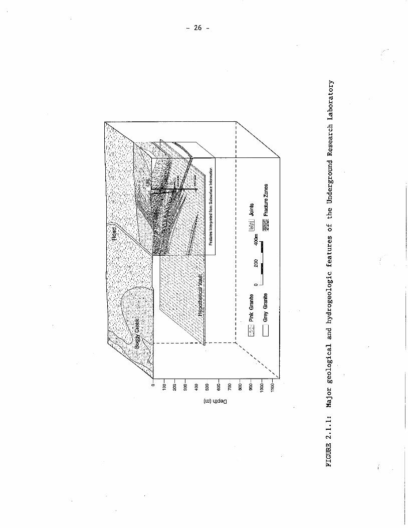
I I U)
I 0 C
I I
N" I 3 I .E 5 i! l 4 u I 111 I
I 0 E I I
8 I I I 0 I :: I I I I 0 I
1 s 8 I .- 1 5 z I a a I % $ 1 i i a
I
+ \
\ \ \ \ \ \ \ \
We assumed that the water table approximates the surface topography and will remain constant throughout the time frame of the postclosure assess- ment (10 000 a). We also assumed that the geometry of the major hydogeo- logical features in the rock (such as fractures and fracture zones) remains constant. Changes that might significantly alter the conditions controlling contaminant transport represented by the Geosphere Model are not expected before the next continental glacier overruns the disposal site. Continental glaciation is not expected within the next 10 000 years for the geosphere region used as the basis for the postclosure assessment study (Section 2.5.1). Sensitivity analyses with the MOTIF groundwater flow model showed that significant changes in the hydrogeological proper- ties of the rock immediately adjacent to the excavations (the excavation damage zone) had only minor effects on the time it takes groundwater to move from the depth of the vault to surface (Chan and Stanchell 1991). In addition, neither changes in the hydrogeological properties of the differ- ent lithostructural domains, or the addition of major lithostructural features at distances greater than about 2 km from the disposal vault or deeper than about 2 km had any significant effect on the transport pathways from the vault to the surface (Scheier et al. 1992). Consequently the major concern for the postclosure performance assessment is evaluating the likelihood that the water table relief or the geometry of the features controlling groundwater flow in the immediate vicinity of the disposal vault would change significantly in the time beyond 10 000 a. If signifi- cant changes seem likely, then the concern is whether the changes might lead to a sudden or dramatic increase in releases of vault contaminants to the environment.
2.2 VAULT SITING AND CONSTRUCTION
2.2.1 Hydroneolonical Effects
During the early stages of site screening and site evaluation, the investi- gations involve airborne or surface methods that do not disturb the char- acteristics of the site that affect the natural groundwater flow conditions or solute transport properties. However, as borehole drilling and other subsurface activities take place during site evaluation, these properties will be disturbed to varying degrees (Davison et al. 1994). Open boreholes allow groundwater to flow between different intervals of the boreholes. This can disturb both the groundwater pressure and the groundwater chem- istry at the site. Although our approach is to seal boreholes with hydro- geological monitoring equipment as soon as possible after they have been drilled, disturbances can be created during the short time the boreholes must remain open for other surveys and tests. Hydraulic tests in borehole intervals also cause disturbances during site evaluation.
The construction of exploratory shafts and tunnels at the site will create a large disturbance in the groundwater flow conditions around the exca- vations. Groundwater will be continuously drawn from the surrounding rock as the excavations are kept pumped dry during construction and operation. As additional underground excavation is carried out during construction, further changes in the natural groundwater conditions will also occur. The distance to which these effects extended from the excavations could be controlled to some degree by grouting in the vicinity of the excavations,
particularly where shafts or tunnels penetrated fracture zones or other more permeable fractured domains of the rock.
The geosphere surrounding the vault would be expected to remain saturated during the construction and operation of the vault except for a small volume of rock near the excavated openings. Assuming that the clay-based materials described in the postclosure assessment study are used, the buffer would be 75-85X saturated and the backfill 60-80X saturated when initially placed in the disposal vault (Johnson et al. 1994b). Hence there would be a hydraulic gradient toward the room and a thermal gradient away from the room due to the heat generated by the waste. The rate of resatur- ation of the vault rooms would depend on variations in the permeability of the rock adjacent to the room and the properties of the excavation damage zone. If the permeability was relatively high, resaturation of the vault rooms could take place within a few years. If the permeability of the rock were similar to that of the buffer, resaturation could take thousands of years (Johnson et al. 1994b).
In the postclosure assessment study the vault is assumed to be saturated when closure takes place. Further study of resaturation of the vault and the geosphere is in progress.
2.2.2 Geochemical Effects
Chemical changes could take place during characterization of the site due to a variety of causes such as: simple movement of groundwater in response to pumping; mixing of groundwaters of different chemistries; chemical reactions (dissolution or precipitation of minerals, release of dissolved gases) in response to changes in pressure, temperature, acidity (pH), or reducing/oxidizing conditions (redox or Eh). These changes could affect the properties of the geosphere pathways that control groundwater flow and contaminant transport from the vault.
The possible chemical changes would be evaluated by knowing the natural chemical evolution of the groundwater along the flow paths at the site and by knowing the chemistry of the different lithostructural domains at the site. These aspects are described in Appendix A for the Whiteshell Research Area . Monitoring at the site during site characterization could be used to deter- mine whether the disturbances in pressure and chemistry were temporary, or if there were permanent changes whose inclusion in the geosphere model would be required.
2.2.3 Stress Effects
The underground construction would also create a region of altered stress in the near-field, immediately adjacent to the excavated openings. Micro- cracks and small fractures will develop within this region and these could form additional new pathways for groundwater flow or contaminant transport from the vault. Depending on the type of excavation method used, some mechanical or thermal damage of the excavation walls might also occur.
We refer to that portion of the rock damaged by stress changes due to exca- vation, and by the excavation method, as the excavation damage zone. The excavation damage zone would need to be simulated in the groundwater flow model to determine whether it was significant for the performance of the disposal system and needed to be included explicitly in the Geosphere Model. Changes in stress, the development of the excavation damage zone, and the changes in hydrogeological properties of fractures and fracture zones related to these mechanical responses in the rock would be monitored during underground site characterization and used in calibrating models of mechanical rock response (Everitt et al. 1994, Davison et al. 1994).
For the reference disposal system, sensitivity analyses using the MOTIF groundwater flow model have shown that significant alterations in the hydrogeological properties of the rock immediately surrounding the exca- vations (the excavation damage zone) had only a minor effect on the overall groundwater transit time from the vault to the surface (Chan and Stanchell 1991).
Thermal Effects
Heat would be generated by the nuclear fuel waste after it was packaged in containers and placed in the disposal vault. For used fuel that has been out of a CANDU reactor for about 10 years, a container with 72 bundles of used fuel would emit about 300 watts of heat. The rate of heat production would decrease with increasing time and after about 10 000 years the rate of heat production would be less than 10 watts (Simmons and Baumgartner 1994). The heat produced by the containers in the disposal vault would slowly dissipate by heat conduction through the surrounding rock. The rate of heat transfer would depend on the thermal conductivity of the rock and the depth of the vault.
When the rock was heated it would expand (thermal expansion) and some new micro-cracks might form within it. Heating of the rock would lower the viscosity of the groundwater in the pores and cracks allowing it to flow more easily. The thermal field could also induce thermal gradients that would change the rate and direction of groundwater flow in the geosphere. We incorporate the thermal properties of the disposal vault and surrounding geosphere into our groundwater flow model to evaluate the effects caused by the transient production of heat in the vault. During site characteri- zation of an actual operating vault, temperatures in the disposal vault would be monitored and used in calibrating thermal and thermo-mechanical models and in evaluating their reliability for predicting both short-term and long-term responses.
2.2.5 Microbial Effects
Microbes have been detected in deep groundwater on the Fennoscandian Shield (Pederson et al. 1991) and at the Underground Research Laboratory (Brown and Hamon 1993, Stroes-Gascoyne et al. 1993). We would expect them to be found in groundwater at any potential disposal site in plutonic rocks of the Canadian Shield. Excavation and construction of a disposal vault would inevitably introduce micro-organisms from the surface as well as nutrient and energy sources necessary for their survival and growth.
Microbes introduced to the vault would be predominantly aerobic. Condit- ions would favour them over the indigenous microbes present in the ground- water within the vault environment, and perhaps to some small distance into the surrounding rock, where oxygen was present due to desaturation or dif- fusion of oxygen into the groundwater. Following vault closure, ground- water would resaturate the rock and preconstruction conditions (low nutri- ents, high salinity, low or no oxygen) would be expected to return even- tually in the geosphere. Johnson et al. (1994b) estimate this process would take up to 300 years. Any surviving microbes (whether indigenous or introduced) would have to be adapted to these conditions. The effects of indigenous microbes (which are adapted to low nutrient conditions) on transport would be included in the observations made during in situ tracer migration experiments.
Stroes-Gascoyne and West (1994) have evaluated the potential effects of micro-organisms in the context of our disposal concept. Expansion of either introduced or indigenous microbiological communities within the open excavations could be controlled by good housekeeping. The most likely effect of microbiological activity on the geosphere would be the develop- ment of biofilms on available aerated surfaces (e.g. open fractures and microcracks in the excavation damage zone) immediately behind the surface of the excavations. If this did occur, it would tend to reduce the trans- port porosity and permeability of the region and could be potentially bene- f icial.
Stroes-Gascoyne and West (1994) consider it unlikely that microbiological activity would cause any significant geochemical changes in the geosphere because of the very large buffering capacity in the geosphere and the low nutrient availability (indigenous microbial populations are presumably in equilibrium with the geochemical conditions at the site). If biofilms are developed by introduced microbes or by expanding populations of indigenous microbes (the likely situation if microbes are present, because biofilms improve the chance for survival in nutrient poor conditions) they would tend to retard the transport of vault contaminants by fixing contaminants by sorption. Biofilms may also compete with colloids for sorption of vault contaminants thus tending to reduce the already negligible effect that colloids have on radionuclide transport if radiocolloid formation is rever- sible (Vilks et al. 1991).
2.2.6 Implications for Geosphere Modelling
The potential impacts of changes in the geosphere caused by site character- ization and constructing the vault would be evaluated both in the pre- closure and postclosure assessments. The changes that take place during siting, construction, and operation would be monitored and used in cali- brating and evaluating the reliability of the models used for design, licensing, and the preparation of the Geosphere Model for postclosure assessment.
For the reference postclosure assessment, we have assumed that recovery to preconstruction hydrogeological conditions occurs instantaneously when the vault is sealed. This should be a pessimistic assumption, because it takes 1
no credit for a time period following closure when groundwater flow could
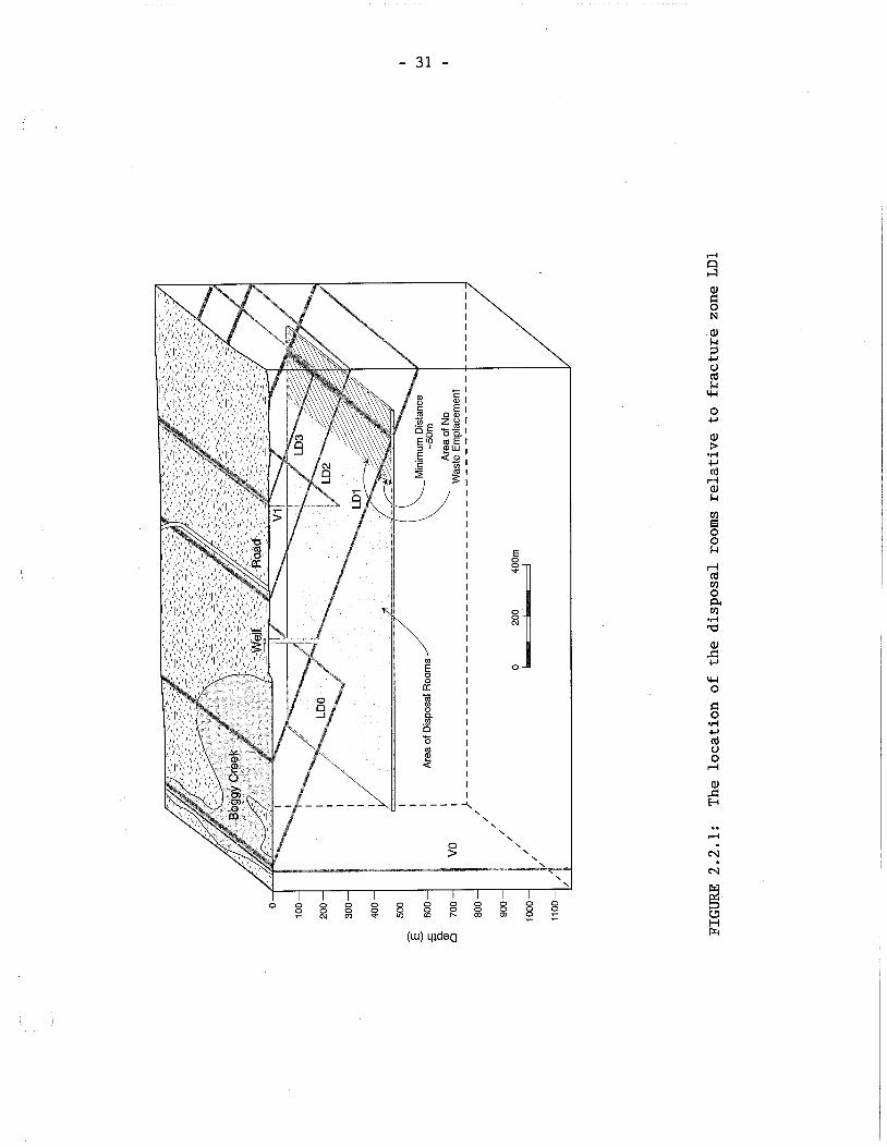
only be toward the vault to resaturate the backfilled underground openings. I
A possible exception might be a case where sufficient gas could be generat- ed in the vault to exceed the gas solubility limit of the groundwater prior to resaturation. We have not included this situation in our postclosure assessment, because preliminary calculations of gas generation (based on the organic content of engineered barrier materials and the potential for radiolysis near the waste containers) suggest that there is insufficient gas for this to occur (Johnson et al. 1994b).
The only features of the disposal vault explicitly included in the Geo- sphere Model are representations of the disposal rooms. Sensitivity analy- ses conducted using the MOTIF groundwater flow model (Chan and Stanchell 1991) showed that including the properties of the shafts and tunnels, the excavation damage zone, variations in the properties of the backfill in the disposal rooms, or the effects due to the heat from the waste, made little difference in groundwater travel times through the geosphere, so long as no waste was emplaced in the groundwater flow system above a nearby fracture zone and no waste was emplaced within about 50 m of the fracture zone (Figure 2.2.1).
Based on the evaluation of potential microbiological effects by Stroes- Gascoyne and West (1994), we conclude that it is unnecessary to include microbiological processes explicitly in the Geosphere Model and that their potential effects in the geosphere would not be sufficient to lead to a sudden or dramatic increase in contaminant releases to the environment beyond 10 000 years.
1
Both the radiation and thermal fields caused by the disposal vault would be continually decreasing for the period beyond 10 000 years. Because neither was shown to have a significant effect on the transport of contaminants through the geosphere during the 10 000 a period of the quantitative cal- culation, there is no potential for either to cause a change in conditions in the geosphere beyond 10 000 a that could lead to a sudden or dramatic increase in releases of contaminants to the environment. Likewise, the existence of the disposal vault itself could only cause a change in the geosphere that could affect the rate of release of contaminants to the environment if the buffer and backfill either disappeared or were so altered that they no longer provided physical support for the excavations. Johnson et al. (1994a) conclude that no significant degradation of the buffer and backfill is likely within 100 000 a.
2.3 CLIMATE AND METEOROLOGICAL FLUCTUATIONS
2.3.1 Climate
We can evaluate past and present climatic conditions to make assumptions or predictions about the expected future climate conditions on the Canadian Shield. The consequences of past warming or cooling trends are evident in geologic history. The last major glaciation was a result of such changes and had a major influence on global climate conditions. We have evaluated the possible effects of climatic change to the geosphere and biosphere of the Canadian Shield through workshops and scoping studies (e.g. Heinrich , 1984, Elson and Webber 1991).
The period of systematic collection, analysis, and publication of climato- logic data for most regions of the Canadian Shield is relatively brief. Few weather observation stations have more than 100 years of record and most stations have less than 50 years of reliable and continuous record. Assumptions regarding the present and future climate of the Canadian Shield are based on analysis of this brief data and other indirect evidence from studying geologic and environmental climate records (e.g., sediments, soil maturity, flora and fauna succession) since the last glaciation. Based on this historical evidence the present climatic conditions of the Canadian Shield are believed to have been relatively constant for the past 3 500- 4 500 years (Findlay et al. 1984, Last and Teller 1983).
The final ice retreat of the latest Pleistocene glaciation that affected the Shield (the Wisconsinan glaciation) occurred about 9 000 years ago (Zoltai 1965, Teller and Thorleifson 1983) and the climate since then has evolved in response to the moderating effects of large glacial and post- glacial lakes and to increased annual mean temperatures. Last and Teller (1983) determined that a dryer and warmer climate existed in the Manitoba and Ontario regions between 9 000 and 4 500 years before present. Sediment core evidence indicates that the present day Lake Manitoba dried up several times during this warm, dry period. They also determined that the upper 3 m of sediment, representing deposition that occurred during the past 4 500 years, do not have characteristics different from present day sedi- ments. This indicates that during the past 4 500 years climatic conditions were probably very similar to present day climate, and were wetter and cooler than immediately after the glacial retreat. Elson and Webber (1991) discuss the evidence available for estimating climate for northwestern Ontario during the past 130 000 a.
Future climate predictions are made more uncertain because of the increas- ing effect of human activities on the atmosphere and environment. The build up of CO, in the atmosphere is receiving considerable attention as a potential cause of global warming, although Elson and Webber (1991) con- clude that atmospheric dust content has a greater effect on temperature. Increased global temperatures could potentially cause melting of existing ice sheets and cause shifts in air mass circulation, precipitation distri- bution and sea level.
2.3.2 Meteorolonical Input and Water Table Fluctuations
As part of our research, we have conducted meteorological and hydrological studies at the Whiteshell, Chalk River and Atikokan Research areas. The objective has been to develop the methods for characterizing the hydrologic conditions of Canadian Shield environments and to use this data to assist in constructing local and regional groundwater flow models (Davison et al. 1994).
Generally the groundwater table within the Canadian Shield is very close to ground surface and is a subdued replica of the topography. Areas of higher topographic elevation have a correspondingly higher water table than adja- cent low lying areas. In low lying areas the water table is generally less than 1 metre below ground surface. These low lying areas are often dis- charge areas for local, intermediate, or regional groundwater flow systems.
The groundwater level is generally from 1 to 10 metres below ground surface in upland areas (Thorne 1990). These topographic highs often occur as either bedrock outcrops or bedrock uplands covered with a thin veneer of overburden. Infiltration and percolation of rain aad snowmelt recharges the groundwater flow systems in the rock from these topographic highs.
The water table most often reaches annual maximum levels subsequent to the spring snowmelt, especially if spring rains supplement the moisture avail- able from snowmelt. Annual minimum water table elevations occur in late winter, just prior to snowmelt. Water levels also decline during the summer period in response to moisture loss to evapotranspiration. Most precipitation during the summer period is used to meet vegetation demands and reduce the soil moisture deficit of the unsaturated zone. During the warm periods of the summer little if any moisture is available for ground- water recharge except following intense rainfall events (Thorne 1990 and Thorne et al. 1992).
Regardless of the amount of precipitation that occurs during the spring or autumn the water table in rocks of the Canadian Shield generally rises to about the same level every year. This indicates that the rock mass is always very near its limit of groundwater saturation and only requires a small amount of infiltration each year to reach this limit. After full saturation is attained, any additional water that is added as precipitation does not infiltrate to the groundwater flow systems in the rock but runs off as surface stream flow. Only about 1-2% of the total annual preci- pitation is required to replenish the water that discharges to surface from /
groundwater flow systems in the rocks of the Shield areas (Thorne and Gascoyne 1993).
In most regions of the Canadian Shield the annual range of natural water table fluctuation is small in comparison to either local or regional relief. Therefore, it is reasonable to use the mean water table elevation, based on several years of observation, in groundwater flow models. Most surface water bodies such as lakes and rivers have mean annual water levels which are relatively stable and these provide stable hydrogeological bound- aries for regional groundwater flow models.
2.3.3 Implications for Geosphere Modelling
There will undoubtedly be climatic changes during the time period of the quantitative assessment (10 000 a). It is reasonable to assume that a full glaciation will not take place during that time (Section 2.5) and that the effects of climatic change on the geosphere will be limited to changes in the water table configuration. The water table configuration is important because the differences in elevation between high points and low points on the water table are a primary control on the gradients that induce ground- water flow.
On the basis given in our earlier discussion we assume that the elevation of the water table corresponds to the elevation of the topography. Conseq- uently the magnitude of the hydraulic gradients for groundwater flow through the rock tends to be maximized in the models. A wetter climate I
cannot increase the gradient significantly because the high points on the

water table cannot rise above the topographic surface. A drier climate could potentially decrease the hydraulic gradient for groundwater flow by allowing the high points on the water table to fall if recharge decreased. However, infiltration into the rocks of the Canadian Shield is currently such a small portion of the annual precipitation (less than 2%) that a much drier climate would be required. It would only be the development of cli- matic conditions equivalent to a tundra region as a continental glacier ice advanced on the site that might lower precipitation sufficiently to have a significant effect in the low relief Shield environment (Elson and Webber 1991).
If a decrease in hydraulic gradient occurred due to lower relief on the water table, it would tend to reduce the groundwater flow in the geosphere. Sensitivity analyses using the Geosphere Model (GEONET) for the reference disposal system show that increases in the rate of groundwater flow from the vault to the geosphere increase the rate of transport of vault contam- inants. However, there are certain conditions associated with the proport- ion of the total contaminant discharge captured by a groundwater supply well for which a decrease in overall groundwater flow rates increases the estimated risk (Goodwin et al. 1994). We include a range of groundwater flow conditions in the Geosphere Model that extends below the range that exhibited this effect in the sensitivity analysis, so we expect that further decreases in the groundwater flow along geosphere pathways caused by long-term climatic changes, would be beneficial if they occurred.
We do not incorporate the effects of future changes in climate in the Geo- sphere Model directly. The range we have used for groundwater flow variations (a factor of 100) would indirectly account for any probable changes in infiltration. Effects of changes of climate in the biosphere are addressed by Davis et al. (1993).
We expect that glaciation would take place between about 10 000 to 20 000 years. The implications for the geosphere during glaciation are addressed in Section 2.5. We could assume that the current increase in global temp- eratures attributed to human activity would eventually be sufficient to break the glacial cycle. If so, there would be a significant rise in sea level due to continued melting of existing ice sheets. This would have the effect of decreasing the regional hydrologic gradients available to drive erosion and groundwater flow, although it would not significantly affect the hydraulic gradients driven by the local topographic relief, which appear to be most important in controlling groundwater flow to disposal vault depths in the rocks of the Shield. Lack of onset of glaciation would (in principle) extend the time period over which the Geosphere Model (GEONET) would be expected to remain a reasonable representation of condit- ions for purposes of an assessment.
TOPOGRAPHIC FLUCTUATIONS
Because the water table which controls the gradients for groundwater flow in the Geosphere Model reflects the current topographic surface, future changes in the landscape could affect groundwater flow and contaminant transport. There are two kinds of change of particular concern: one is the change that could take place due to regional uplift or depression, the
other is the change that could take place due to erosion or deposition. The two are related to some degree because uplift can change the slope on the land surface, either increasing or decreasing the tendency for erosion (or deposition) to occur.
2.4.1 Uplift and Depression
The land surface of the Canadian Shield in Ontario is currently rising slowly as a result of the melting and retreat of the last continental glacier (called the Laurentide Ice Sheet). During a glaciation the surface is depressed due to the mass of the overlying ice. The thickness of the Laurentide Ice Sheet has been inferred from interpretation of the distri- bution of glacial deposits, evidence for glacial rebound, and by modelling the deformation behaviour of the ice sheet and the underlying rocks. Andrews (1987) and Hughes (1987) discuss the issues involved and the different approaches that have been taken in reconstructing the Laurentide Ice Sheet . Estimates for the ice sheet thickness vary from about 1 800 m to about 5 000 m, implying depression of the surface beneath the ice ranging from about 450 m to about 1 700 m. There is evidence of more than 220 m of relative sea level change over the past 7 000 years in the vicinity of James Bay, the assumed center of the Laurentide Ice Sheet that covered the Shield in Ontario (Andrews 1989). This is substantially less than the estimated depression, however, it is not known how much rebound took place at the center of the ice sheet during the period between about 18 000 years I
(the glacial maximum) and about 8 000 years when Hudson Bay first became ice free. The rate of rebound decreases with time, but it is still over 6 m/l 000 years around Hudson Bay. This rate of rebound declines with distance away from Hudson Bay and approaches zero at the southern edge of the Shield.
2.4.2 Erosion and Deposition
The landscape of the Canhdian Shield in Ontario is generally low and roll- ing with relatively gentle regional slopes (1 m/km). Figure 2.4.1 shows the major geographic regions and drainage basins of the Canadian Shield in Ontario. Local relief seldom exceeds 90 m except in a few regions near the Great Lakes (Nipigon Plain, Port Arthur Hills, Penokean Hills). In these locations higher regional slopes (5-10 m/km) and high contrast in the resistance to erosion of adjacent igneous and metamorphic rocks has produc- ed local relief up to 300 m (Dredge and Cowan 1989).
The topography of the Shield generally reflects the local structure and lithology of the rock. High areas have rocks more resistant to erosion than those in low areas. The topography of the Shield where it emerges from overlying younger sedimentary rocks at the Shield margin is similar to that in the central Shield. This suggests that the present Shield topo- graphy is dominated by the effects of erosion that took place during the Precambrian more than 570 million years ago (Stearn, et al. 1979).
Superimposed on the local erosional relief of the rock surface of the Shield is a blanket of glacial deposits of highly variable thickness.
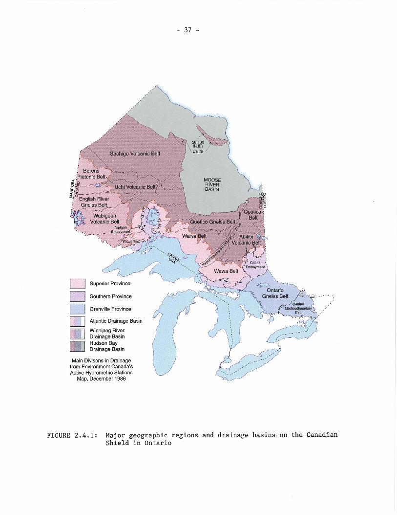
The result is a very poorly drained landscape with many wetland areas and small lakes, often in small closed drainage basins. Most of the erosion that is taking place is transferring glacial sediment from the slopes of these drainage basins to the lake bottoms, so that the large Shield lakes are in the process of being filled, while many small lakes have been filled since deglaciation.
Susceptibility to erosion is primarily related to the strength and cohesion of the material at the land surface. Therefore we would expect that sedi- ments, soft rocks, and rocks that are highly fractured or chemically alter- ed should be more readily eroded than rocks that are strong, cohesive, unfractured, and unaltered.
Exposed rock on the Shield in topographically high locations is commonly both strong and cohesive. It may show scratches due to glacial erosion by abrasion (striae) but there is little evidence of erosion by running water. Exposures in topographically low locations tend to be at river rapids, where the rock is acting as a barrier to rapid erosion. Where the rock was intensely fractured or altered, it has generally been preferential.1~ remov- ed by repeated glaciation so that depressions have been formed between areas of strong rock. The potential for additional amplification of the relief by erosion is limited because most of the erodible bedrock material has already been removed (Elson and Webber 1991).
Because of the low relief and poorly integrated drainage, we expect that the erosion in the next 10 000 years will be no more than what took place in the comparable period since deglaciation and will be confined primarily to areas covered by sediments. Erosion due to glaciation is discussed in Section 2.5.2.
2.4.3 Implications for Geosphere Modelling
Based on declining current rates of isostatic rebound from the last contin- ental glaciation, the maximum rebound at Hudson Bay in the next 10 000 years would be expected to be less than 100 m. At the divide between drainage to Hudson Bay and to t'he Great Lakes the maximum rebound would be expected to be less than 50 m during the next 10 000 years. At the south- ern margin of the Shield it might vary from 0 to perhaps 20 m. This repre- sents a maximum tilt of the northeast-southwest regional topographic slope across the Shield in Ontario of only 1 m in 10 km It would repre- sent a decrease in stream gradients and regional groundwater flow gradients from the continental watershed divide northwards to Hudson Bay and an in- crease in gradients from the divide southwards to the Great Lakes. In either case this change in regional hydraulic gradient is so small that its implications can only be assessed in the context of a specific site.
For example at the Whiteshell Research Area the regional topographic grad- ient controlling groundwater flow and drainage is actually southeast to northwcst pcrpcndicular to thc tilt causcd by rcbound. This gradient is about 20 m in 10 km (2 x so that the change represented by ongoing rebound would not be significant regionally nor in comparison to the local topographic gradients (which can reach 1 0 - l , 40 m in 400 m) for this parti- cular site.
The potential for erosion to decrease the thickness of the rock overlying a disposal vault in plutonic rock of the Shield in the next 10 000 years is not significant. The potential for erosion of sediments, either increasing the gradient for groundwater flow along a transport pathway from the dis- posal vault to the biosphere or creating a new transport pathway, can only be assessed in the context of a specific site.
For example, at the Whiteshell Research Area the existing pattern of streams was established following the retreat of the Laurentide Ice Sheet and the drainage of Lake Agassiz about 8 000 years ago. The maximum grad- ient for the drainage of the Winnipeg River system to Hudson Bay would have occurred soon after Hudson Bay became ice free. Erosion during this time has cut down through the glacial sediments only on the order of 10 m within the area included in the Geosphere Model. Exposures of rock created natural dams along the rivers that controlled the rate of erosion prior to the recent addition of dams constructed by humans. Since deglaciation, rebound will have been slowly decreasing the gradient as the southern shoreline of Hudson Bay moved northward, so that even in the absence of human control structures on the rivers, the rate of erosion in the next 10 000 years would be less than it was in the time since deglaciation.
In view of the above discussion, the effects of continued glacial rebound and erosion have not been included in the Geosphere Model used for the postclosure assessment study.
GLACIATION
During the Quaternary Period the Canadian Shield has been subjected to numerous glaciations as the climate has fluctuated from being significantly warmer than today to significantly colder. Evidence for these climatic changes is contained in sediments on land and on the ocean floor as well as in the ice of the remaining continental glaciers on Greenland and Antarctica.
Frequency of Glaciation
Since a glacier tends to destroy much of the evidence of earlier glaci- ations, the physical evidence prior to the last ice sheet is fragmentary. However, there is evidence of at least four major glacial episodes during the Quaternary in several parts of Canada. Fulton (1989) summarizes the evidence from the Quaternary deposits of Canada.
Due to the fragmentary nature of direct evidence, the glacial chronology is based primarily on the climatic chronology derived from oxygen-isotope records for the calcium carbonate shells of marine protozoa (foraminifera) found in deep-sea sediments. Both increases in global ice volume and de- creases in deep-water temperatures lead to an increase in the ratio of 180 to 160 (called delta oxygen-18, S180) in the oceans. Since most of the variation is due to the change in ice volume, the oxygen-isotope ratios preserved in sea sediments are used as a proxy for the chronology of ice volume in glaciers (Mix 1987).
Core from the North Atlantic Ocean (Shackleton et al. 1984) showed that variations in 6180 reflecting glaciation began 2.4 Ma ago and have con- tinued to the present. The glacial chronology implied by the climatic evidence is cyclic with frequencies roughly at 23 000, 41 000, and 100 000 years. The periodicity is believed to be related primarily to changes in the orbit of the earth (the tilt, obliquity, and precession of the axis of rotation relative to the sun) affecting the amount of radiation received from the sun, although there is still debate about the role of other factors in triggering the abrupt climatic changes seen in the record and in initiating and terminating the most prominant cycle at 100 000 years (Ruddiman and Wright 1987, Peltier 1987, Broecker and Denton 1989).
The basic shape of the record implies that glaciers have repeatedly built up slowly over a period of about 100 000 years and then rapidly disappear- ed. Based on climate record models (Imbrie and Imbrie 1980 and Kukla et al. 1981) glacial climatic conditions are expected to reoccur on the Shield within the next 20 000 years.
Elson and Webber (1991) evaluated the evidence for conditions in Ontario during the last glacial cycle from about 130 000 years ago to the present. They discussed the conditions in terms of the relationship between Astrono- mical aimate Zdex (ACLIN) "states" defined by Findlay et al. (1984) and global ice cover percentages derived from 180 data in Martinson et al. (1987) shown in Figure 2.5.1. For each ACLIN state Elson and Webber (1991) estimated ranges for mean annual temperature and July temperatures for a site near Sioux Lookout in northwestern Ontario. They also discussed the evidence for where ice cover on the Canadian Shield might have been.
Based on the past climatic record and the continued existence of the con- ditions that are believed to have led to previous glaciations (the locations of the continental plates and earth's orbital elements), we believe it is appropriate to assume that another continental glaciation of the Shield will begin sometime between the next 10 000 to 20 000 years. Since the range of temperature associated with the climatic variation in- creases as the time period considered increases from about 0.5"C over the last 1UO years to about 10°C over the last 10 000 years (Bartlein et al. 1989), it does not seem possible to determine whether the current increases in temperature attributed to human activities are sufficient to disrupt the glacial climatic cycles that have dominated the last 2.5 million years. If the glacial cycle were broken, it would imply that there would be continued melting of existing ice caps and a significant increase in sea level.
2.5.2 Erosion by Ice Sheets
Erosion of the surface by an ice sheet depends on a variety of factors including the nature of the underlying rock (hardness, permeability, rough- ness of the surface), hydrology at the base of the glacier, glacier dynamics, thermal regime in the glacier, and topographic relief on the rock surface. There have been widely divergent estimates made of the glacial erosion that has taken place on the Canadian Shield, from as little as a few tens of metres (Flint 1971) to as much as hundreds of metres (White 1972).
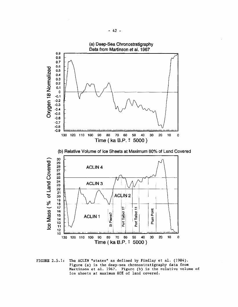
(a) Deep-Sea Chronostratigraphy Data from Martinson et al. 1967
0.9 0.8 -
0.7 -
0.6 - a, 0.5 - N - . - 0.4 -
a 0.3 - E 0.2 j 0 0.1 = 0 - 00 -0.1 --
-0.2 - a> -0.3 -
$ 1::; 1 O -0.6 -
-0.7 -
-0.8 - -0.9 9
Time ( ka B.P. 2 5000 ) 130 120 110 100 90 80 70 60 50 40 30 20 10 0
(b) Relative Volume of Ice Sheets at Maximum 80% of Land Covered
130 120 110 100 90 80 70 60 50 40 30 20 10 0
Time ( ka B.P. 2 5000 )
FIGURE 2.5.1: The ACLIN I1states" as defined by Findlay et al. (1984). Figure (a) is the deep-sea chronostratigraphy data from Martinson et al. 1967. Figure (b) is the relative volume of ice sheets at maximum 80% of land covered.
Kaszycki and Shilts (1980) investigated glacial erosion of the Shield by studying the dispersal of a distinctive rock type on the northwest coast of Hudson Bay. Using this method they concluded that between 6 m and 20 m of erosion took place in the region during the last glaciation. Shilts (1984) used a similar method in southeastern Quebec and obtained a value of 4.3 m for average erosion during the last glaciation there. He also reported estimates of 2 m for erosion of plutons elsewhere in the Appalachians and a revision of the estimate for the northwest coast of Hudson Bay to a range of 6 m to 11 m. Assuming as many as seven cycles of erosion, he concluded that this implied between 14 m and 77 m of Shield erosion during the last 250 000 years.
Based on these estimates, he calculated that future glacial erosion over the next million years might range from a minimum of 20 m to a maximum of 385 m. However, he also expressed the opinion that average glacial erosion on the southern Canadian Shield had been even less than the calculated minimum of 20 m based on the similarity of relief on well exposed Precam- brian rocks and those just exposed from beneath Paleozoic rocks and the preservation of both low-relief drainage patterns and extensive soft weathered zones on preglacial surfaces. Elson and Webber (1991) considered the potential for additional erosion to be limited because the more erod- ible bedrock material has already been removed.
2.5.3 Effect of Glaciation on Stress and Groundwater Flow
The most significant potential effects of glaciation are the changes that might be caused in the in situ stress field and in the groundwater flow regime. The principal cause is the load placed on the region by the glacier. Depending on whether the base of the ice sheet is melting, there may also be Iree water under high pressure at the rock surface.
During glaciation the ice load would depress the region. This would in- crease confinement by adding a surcharge to all the principal stresses, but mostly to the vertical component. The net effect would be reductions in the vertical to horizontal stress ratio, normal stresses, and stress dis- continuities near faults, reducing the potential for movement on existing faults. This may account for the suppression of seismicity observed in regions currently covered by continental glaciers (Section 2.6).
On deglaciation the glacial load would be removed and a readjustment of stresses would be expected, possibly accompanied with movement along exist- ing faults. At the Whiteshell Research Area this process would have occur- red several times in the past 2.5 million years, yet there is no evidence that there has been any significant effect on the characteristics of the major permeable fracture zones in the rock, which were formed during the cooling of the batholith over 2 billion years ago (Stone et al. 1989).
If a uniform layer of glacial ice lies above the vault site, it would tend to eliminate local hydrologic gradients. At any time when the glacial ice margin is in the immediate vicinity of the vaulL, iL could affect gradients in ways that could change the flow of groundwater in the major permeable pathways and that could change the location of the local discharge (Elson and Webber 1991). During a glacial advance these effects would be a relat-
ively short-lived transient between present day conditions and glacial cover. During retreat there would be increased gradients at the ice margin with increased groundwater flow, particularly in the shallow groundwater flow system. Modelling has suggested that transient increases in flow rates of up to a factor of ten might occur.
2.5.4 Implications for Geosphere Modelling
No potential effects on the disposal vault due to glaciation are expected during the next 10 000 years. Consequently, the effects of glaciation have not been included in the modelling done for the postclosure assessment study.
Glaciation would be expected at some time after 10 000 years. During the advance of the glacier over the disposal site, there could be an increase in groundwater flow in the rock due to the increased head from the thick- ness of the ice. However, the concentration of any vault contaminants in the discharging groundwater would likely be reduced due to dilution from a larger volume of recharge to the shallow groundwater flow system from basal melting of the glacier. There would also be much more surface water for dilution in the form of proglacial lakes in regions where the glacier was advancing uphill regionally, or where the glacier had cut off the pre- existing drainage.
During glaciation there could be a build-up of vault contaminants in the more permeable groundwater flow pathways in the rock because they would not be flushed to surface while the glacier covered the discharge locations. If the discharge locations remained the same following deglaciation, these contaminants could be rapidly released when groundwater flow to the surface was re-established. The potential effect of this pulse of water containing a higher concentration of contaminants would likely be offset by the large volumes of glacial meltwater and proglacial lake water available at the surface for dilution during the first few hundred years after glacial re- treat. In addition, until the proglacial lakes drained, it would be un- likely that humans could resettle in the vicinity of the locations of dis- charge from the disposal vault.
We would expect the landscape following a future glaciation to be similar to the present landscape, although the detailed distribution of exposed rock, sediments, and water bodies would change. This could change the number and specific locations of discharges from the disposal vault. These changes would tend to decrease releases of contaminants from the vault in the short term until the transport pathways readjusted, and contaminants newly released from the vault, reached the surface following the fastest new transport pathway.
2.6 SEISMICITY
Seismicity (earth movements) is one of the natural processes that has the potential to disrupt the integrity of the disposal vault or the surrounding rock mass, either causing the release of contaminants from the emplaced waste or enhancing the rate of migration of contaminants that had already been released.
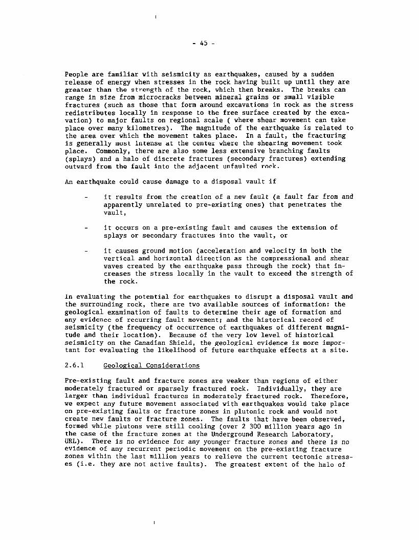
People are familiar with seismicity as earthquakes, caused by a sudden release of energy when stresses in the rock having built up until they are greater than the strength of the rock, which then breaks. The breaks can range in size from microcracks between mineral grains or small visible fractures (such as those that form around excavations in rock as the stress redistributes locally in response to the free surface created by the exca- vation) to major faults on regional scale ( where shear movement can take place over many kilometres). The magnitude of the earthquake is related to the area over which the movement takes place. In a fault, the fracturing is generally most intense at the center where the shearing movement took place. Commonly, there are also some less extensive branching faults (splays) and a halo of discrete fractures (secondary fractures) extending outward from the fault into the adjacent unfaulted rock.
An earthquake could cause damage to a disposal vault if
- it results from the creation of a new fault (a fault far from and apparently unrelated to pre-existing ones) that penetrates the vault ,
- it occurs on a pre-existing fault and causes the extension of splays or secondary fractures into the vault, or
- it causes ground motion (acceleration and velocity in both the vertical and horizontal direction as the compressional and shear waves created by the earthquake pass through the rock) that in- creases the stress locally in the vault to exceed the strength of the rock.
In evaluating the potential for earthquakes to disrupt a disposal vault and the surrounding rock, there are two available sources of information: the geological examination of faults to determine their age of formation and any evidence of recurring fault movement; and the historical record of seismicity (the frequency of occurrence of earthquakes of different magni- tude and their location). Because of the very low level of historical seismicity on the Canadian Shield, the geological evidence is more impor- tant for evaluating the likelihood of future earthquake effects at a site.
Geological Considerations
Pre-existing fault and fracture zones are weaker than regions of either moderately fractured or sparsely fractured rock. Individually, they are larger than individual fractures in moderately fractured rock. Therefore, we expect any future movement associated with earthquakes would take place on pre-existing faults or fracture zones in plutonic rock and would not create new faults or fracture zones. The faults that have been observed, formed while plutons were still cooling (over 2 300 million years ago in the case of the fracture zones at the Underground Research Laboratory, URL). There is no evidence for any younger fracture zones and there is no evidence of any recurrent periodic movement on the pre-existing fracture zones within the last million years to relieve the current tectonic stress- es (i.e. they are not active faults). The greatest extent of the halo of
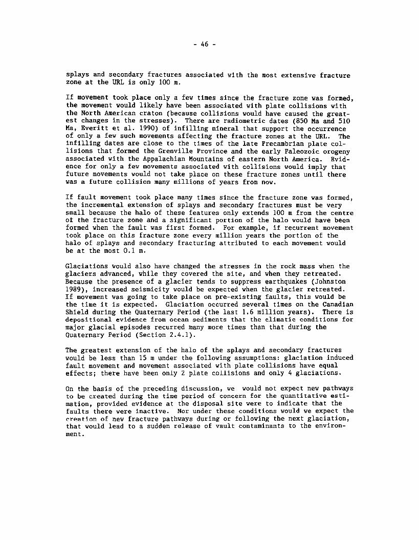
splays and secondary fractures associated with the most extensive fracture zone at the URL is only 100 m.
If movement took place only a few times since the fracture zone was formed, the movement would likely have been associated with plate collisions with the North American craton (because collisions would have caused the great- est changes in the stresses). There are radiometric dates (850 Ma and 510 Ma, Everitt et al. 1990) of infilling mineral that support the occurrence of only a few such movements affecting the fracture zones at the URL. The infilling dates are close to the times of the late Precambrian plate col- lisions that formed the Grenville Province and the early Paleozoic orogeny associated with the Appalachian Mountains of eastern North America. Evid- ence for only a few movements associated with collisions would imply that future movements would not take place on these fracture zones until there was a future collision many millions of years from now.
If fault movement took place many times since the fracture zone was formed, the incremental extension of splays and secondary fractures must be very small because the halo of these features only extends 100 m from the centre of the fracture zone and a significant portion of the halo would have been formed when the fault was first formed. For example, if recurrent movement took place on this fracture zone every million years the portion of the halo of splays and secondary fracturing attributed to each movement would be at the most 0.1 m.
Glaciations would also have changed the stresses in the rock mass when the glaciers advanced, while they covered the site, and when they retreated. Because the presence of a glacier tends to suppress earthquakes (Johnston 1989), increased seismicity would be expected when the glacier retreated. If movement was going to take place on pre-existing faults, this would be the time it is expected. Glaciation occurred several times on the Canadian Shield during the Quaternary Period (the last 1.6 million years). There is depositional evidence from ocean sediments that the climatic conditions for major glacial episodes recurred many more times than that during the Quaternary Period (Section 2.4.1).
The greatest extension of the halo of the splays and secondary fractures would be less than 15 rn under the following assumptions: glaciation induced fault movement and movement associated with plate collisions have equal effects; there have been only 2 plate collisions and only 4 glaciations.
On the basis of the preceding discussion, we would not expect new pathways to be created during the time period of concern for the quantitative esti- mation, provided evidence at the disposal site were to indicate that the faults there were inactive. Nor under these conditions would we expect the creation of new fracture pathways during or following the next glaciation, that would lead to a sudden release of vault contaminants to the environ- ment.
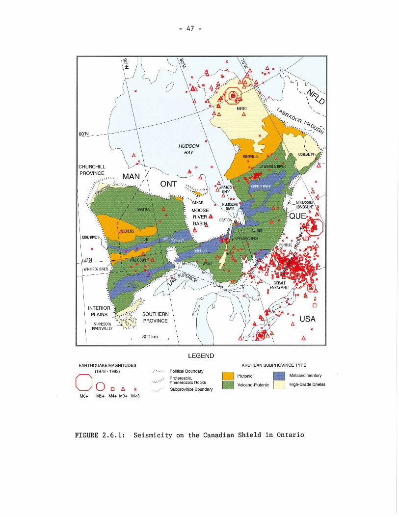
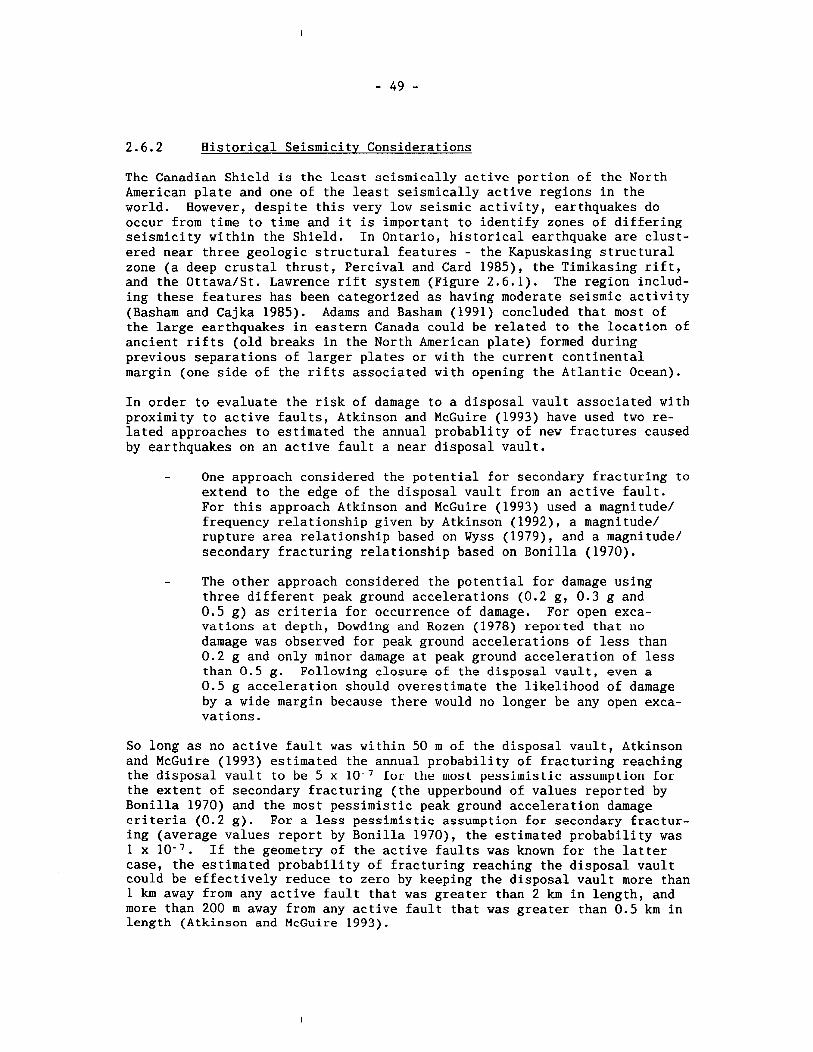
2.6.2 Historical Seismicity Considerations
Thc Canadian Shield is the least seismically active portion of the North American plate and one of the least seismically active regions in the world. However, despite this very low seismic activity, earthquakes do occur from time to time and it is important to identify zones of differing seismicity within the Shield. In Ontario, historical earthquake are clust- ered near three geologic structural features - the Kapuskasing structural zone (a deep crustal thrust, Percival and Card 1985), the Timikasing rift, and the Ottawa/St. Lawrence rift system (Figure 2.6.1). The region includ- ing these features has been categorized as having moderate seismic activity (Basham and Cajka 1985). Adams and Basham (1991) concluded that most of the large earthquakes in eastern Canada could be related to the location of ancient rifts (old breaks in the North American plate) formed during previous separations of larger plates or with the current continental margin (one side of the rifts associated with opening the Atlantic Ocean).
In order to evaluate the risk of damage to a disposal vault associated with proximity to active faults, Atkinson and McGuire (1993) have used two re- lated approaches to estimated the annual probablity of new fractures caused by earthquakes on an active fault a near disposal vault.
- One approach considered the potential for secondary fracturing to extend to the edge of the disposal vault from an active fault. For this approach Atkinson and McGuire (1993) used a magnitude/ frequency relationship given by Atkinson (1992), a magnitude/ rupture area relationship based on Wyss (1979), and a magnitude/ secondary fracturing relationship based on Bonilla (1970).
- The other approach considered the potential for damage using three different peak ground accelerations (0.2 g, 0.3 g and 0.5 g) as criteria for occurrence of damage. For open exca- vations at depth, Dowding and Rozen (1978) reported that no damage was observed for peak ground accelerations of less than 0.2 g and only minor damage at peak ground acceleration of less than 0.5 g. Following closure of the disposal vault, even a 0.5 g acceleration should overestimate the likelihood of damage by a wide margin because there would no longer be any open exca- vations.
So long as no active fault was within 50 m of the disposal vault, Atkinson and McGuire (1993) estimated the annual probability of fracturing reaching the disposal vault to be 5 x lo-' for the most pessimistic assumption for the extent of secondary fracturing (the upperbound of values reported by Bonilla 1970) and the most pessimistic peak ground acceleration damage criteria (0.2 g). For a less pessimistic assumption for secondary fractur- ing (average values report by Bonilla 1970), the estimated probability was 1 x lo-'. If the geometry of the active faults was known for the latter case, the estimated probability of fracturing reaching the disposal vault could be effectively reduce to zero by keeping the disposal vault more than 1 km away from any active fault that was greater than 2 km in length, and more than 200 m away from any active fault that was greater than 0.5 km in length (Atkinson and McGuire 1993).
We conclude that the likelihood of new faults or fractures forming at dis- posal depth would be sufficiently low to be negligible, if the disposal vault were located in seismic zones 0 or 1; far from ancient rifts, far from clusters of historic earthquake activity; far from regional-scale faults, and where there was no evidence of post glacial faulting. These conditions would all be considered favourable during siting (Davison et al. 1994).
A site specific seismic hazard analysis would provide the basis for deriv- ing constraints on the location of a disposal vault at a candidate site, with respect to any potentially active faults that might exist nearby. Such constraints could minimize the potential for earthquakes to contribute to the estimated risk to the disposal vault for the 10 000 year period following closure and also minimize the probability of any sudden and dra- matic increases in the rate of release of contaminants to the environment after 10 000 years.
2.6.3 Preclosure Seismic Effects
Application of existing standards of design and construction for earthquake resistant nuclear-safety-related structures would provide adequate safety for the period of construction, operation, decommissioning and closure of a disposal facility. A survey of the effects of ground shaking at surface due to earthquakes on underground openings (Dowding and Rozen 1978) showed that ground motion accelerations below 20% of the acceleration due to gravity (0.2 g or about 1.9 m ~ - ~ for the Canadian Shield) produced no de- tectable damage and accelerations up to 0.5 g (about 4.9 ms-2) produced only minor damage to the excavation surfaces. So long as seismically active faults are not in the immediate vicinity of the excavated openings, the risk to satety from earthquake damage underground during construction and operation would not be significant (Ates et a1 1994).
The seismic stability of the underground vault would be increased by closure due to the support supplied by the buffer, backfill and seal materials (Ates et al. 1994).
2.6.4 Implications for Geosphere Modelling
The potential impacts on the disposal facility of earthquakes during the preclosure period would be evaluated through a standard seismic hazard analysis for the site. A long-term hazard analysis combining evaluation of the geological evidence from faults and fracture zones at the site, with analyses such as those demonstrated in Atkinson (1992) and Atkinson and McGuire (1993), would be done for the postclosure period. So long as the faults and fracture zones in the immediate vicinity of the disposal vault were not active and the disposal vault was located sufficiently far from active faults in the area or region (based on an analysis such as that of Atkinson and McGuire), no disruptive effects on the disposal vault due to earthquakes would be expected during the next 10 000 years. On the basis of the lack of evidence for active movement along faults a1 the URL during the last million years, the effects of earthquakes have not been included directly in the Geopshere Model used for the postclosure assessment case study.
Changes in the properties of pre-existing pathways for contaminant movement could result from future movement on the pre-existing faults. If a pre- existing fault was a significant potential pathway for contaminant move- ment, it would likely be because of its high permeability relative to the adjacent moderately fractured or sparsely fracture rock. Our investi- gations at field research areas have shown that the permeability of such features can be variable (Davison et al. 1994). This variability would be reflected in the models used to assess the postclosure effects on the dis- posal vault. New movement could either cause an increase, or a decrease, or no change in the permeability at any specific location. However, be- cause the permeability already has a large variability, the net change along the length of the pathway would be unlikely to be significant and very unlikely to be outside the pre-existing range. We are of the opinion that the conservative assumptions we have made in the Geosphere Model about the extent and interconnectivity of the fracture zones, and the sensitivity analysis we have preformed with the hydrogeological model (Chapter 5), cover the range of effects that could results from such changes. Faults contain a variety of minerals with high sorption capacity for contaminants found in nuclear fuel waste. New movement is unlikely to create different minerals, however, it would tend to increase the porosity and the area of mineral surfaces available for sorption by crushing rock fragments into smaller sizes. As with the permeability, the variability of sorption properties included in the models for the pathways in faults is large and it is unlikely that new movement would cause a net change in the retard- ation along the pathway and create retardation conditions outside the range already included in the models.
Beyond 10 000 years, the effects of glaciation on seismicity need to be considered. The presence of glaciers tends to suppress seismic activity (Johnston 1989), so it is likely that during each period of glacial cover there would be even less seismic activity than at present, and that with each deglaciation there would be a period of increased seismic activity as the stored stresses are released. This process is probably accentuated by the process of postglacial rebound. Because glaciation has occurred sever- al times on the Canadian Shield in the last million years, if there was no evidence of postglacial movement on faults at the disposal site, it would be reasonable to conclude that faults at the site would not undergo move- ment following future glaciations.
METEORITE IMPACT
A meteorite impact is one of the few events that has the potential to cause a sudden and dramatic increase in the release of contaminants from a dis- posal vault. There is a considerable literature available concerning both frequencies of impacts producing craters of different size and the depths to which various kinds of damage occur for craters of different size.
Grieve and Robertson (1984) evaluated the probabilities of impacts of meteorites that would lead to damage at the depths of a disposal vault. They looked at complete excavation of the overlying rock to the top of the vault, crushing and redistribution of the rock to the top of the vault, some displacement of rock to 'the top of the vault, and creation of fractur- ing in the rock to the top of the vault.
For a 4 km2 vault at a depth of 500 m, probabilities range from 2.3 x 10⁻¹²/a for an impact causing complete excavation of the overlying rock to 7.8 x 10-ll/a for an impact causing fracturing to extend to the top of the vault through the overlying rock. These probabilities are too low to contribute to risk in the regulatory time frame of 10 000 years.
Even if these probabilities were higher, there are two characteristics of the risk associated with a meteorite impact that make it of less relevance to the safety case than other risks. First, the risk is the same every- where, so no location is safer than any other. Second, the impact of a meteorite large enough to damage the integrity of the disposal vault would be so severe for humans and the environment, not just locally, but through- out North America if not globally, that the potential impacts associated with any releases of contaminants from the vault would be inconsequential in comparison.
VOLCANISM
There has been no volcanic activity on the Canadian Shield for the past 500 million years. Volcanism has, however, occurred in the Appalachian region more recently in association with the collisions of tectonic plates, bet- ween about 400 million years ago and 200 million years ago. Volcanism is occurring now on the west coast of North America in association with col- lisions of tectonic plates. Volcanism would not be expected on the Shield before there were either new plate collisions on the eastern or Arctic margins of North America or renewed rifting on the continent. Neither of these events are likely within tens of millions of years.
HUMAN INTRUSION
Another potential future disruption to the geosphere that we must consider is the effect of some form of inadvertent human intrusion. Wuschke (1992) has analysed human intrusion scenarios and concluded that although it is extremely unlikely, an exploratory borehole could be accidentally drilled into the disposal vault at some future time and the drill crew or staff who examine the core could become exposed to contamination. This type of human intrusion breaches the geosphere barrier completely and requires no analy- sis with a geosphere model.
However, other more subtle geosphere intrusions may result from certain future human activities and these can be examined. For instance a water supply well may exist (or be drilled) near the disposal site and it may draw contaminated groundwater toward it from the vault. Similarly, a fail- ure could occur in the seals of one of the many boreholes drilled from either ground surface or underground during the various phases of site characterization. This would result in a short circuiting of part of the geosphere barrier. The possibilities of these sorts of geosphere intrus- ions occurring at a disposal site must be examined along with their result- ing consequences to judge their overall relative importance. The detailed groundwater transport model of the vault/geosphere system can be used ro perform sensitivity analyses which examine the consequences of these scenarios (Section 5.5 and Section 5.7).
3. METHODOLOGY FOR MODELLING THREE-DIMENSIONAL GROUNDWATER FLOW, HEAT TRANSPORT AND SOLUTE TRANSPORT IN FRACTURED/POROUS MEDIA
INTRODUCTION
As part of the Canadian Nuclear Fuel Waste Management Program (CNFWMP) AECL has developed a three-dimensional finite-element code, MOTIF (Model Qf Transport In Fractured/porous media), for detailed modelling of groundwater - flow, heat transport and solute transport in a fractured rock mass. In addition, a numerical particle-tracking code (TRACK3D) has been developed to model purely convective (or advective) transport by postprocessing the groundwater velocity field calculated by MOTIF. This chapter describes
1. the methodology embodied in the MOTIF code,
2. the particle-tracking algorithm, and
3. the application of this methodology to develop the geosphere model used in the postclosure assessment case study of the Canadian Nuclear Fuel Waste Disposal concept.
3.2 THE MOTIF FINITE-ELEMENT CODE
The MOTIF finite-element code solves the transient and steady-state equations of groundwater flow, solute (including one-species radionuclide) transport, and heat transport in variably-saturated fractured/porous media. The initial development was completed in 1985 (Guvanasen 1985). The code has since undergone extensive testing and upgrading (Chan et al. 1987, Guvanasen and Chan 1991), primarily to improve its capabilities, computat- ional efficiency, accuracy and flexibility. Version 3.0 is used for the work described in this report. Its development was completed in 1986. For detailed documentation of the code please refer to Guvanasen and Chan ( 1994).
The model incorporated into the MOTIF code can simulate partially saturated flow and solute transport. It assumes that the air phase is immobile and water moves in the liquid phase only, not in the vapour phase. As discuss- ed earlier in Section 2.2.6, in developing the geosphere model for the postclosure assessment case study, we have made the conservative assumption that the hypothetical vault and geosphere are immediately resaturated after closure, and the groundwater flow regime at the site returns to the precon- struction condition. Hence, in the following sections we discuss only those aspects that pertain to groundwater flow and solute transport in saturated fractured/porous media.
3.2.1 Conceptual Model, Processes Simulated, Assumptions and Input/Output Data
3.2.1.1 Conceptual Model Incorporated in the MOTIF Code
As illustrated in Figure 3.2.1, the rock mass is conceptualized in MOTIF as comprising three types of components:
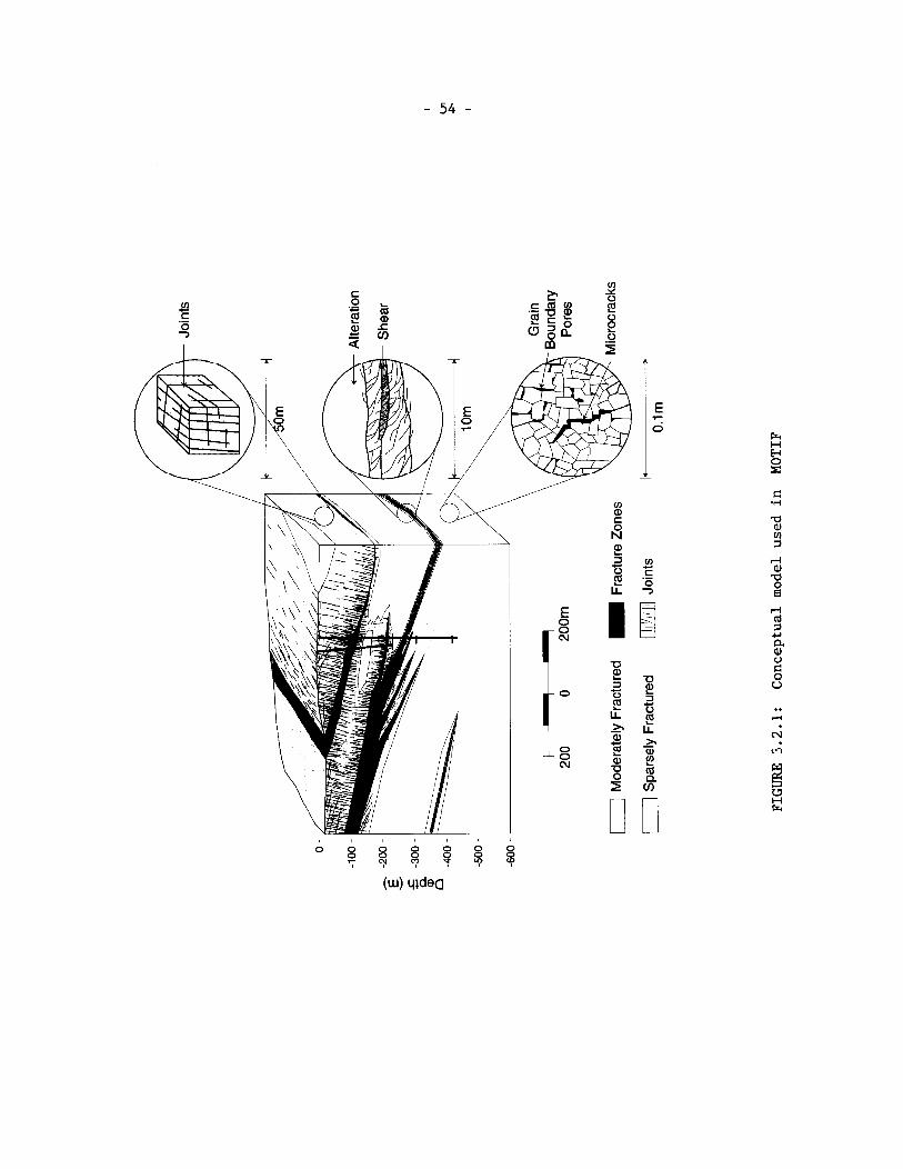
1. Blocks of sparsely fractured rock, which may contain numerous microscopic cracks and pores but no macroscopic hydraulic conduits ;
2. Moderately fractured rock, which are volumes of rock containing macroscopic, distinctly more permeable and interconnected planar fractures or narrow fracture zones; and
3. Fracture zones (faults), which are volumes of intensely fractured rock. These are distinctly more permeable and can contain tubular flow conduits or channels within them.
A deterministic approach is adopted so that groundwater transport through the distinct fractures, fracture zones with channels within them, can be simulated when their geometry, hydraulic and transport properties are known. In practice, for real-world groundwater transport problems on a regional scale (100 km2 or larger) it is not possible, or even desirable, to perform site characterization investigations to determine all the relevant transport data for all the distinct hydrogeological features that might exist in the rock. Instead, we generally represent the rock mass and its systematic fractures by an equivalent porous medium. However important distinct features can be accommodated as required. This equivalent porous medium (Bear 1972,1979) is a fictitious, fluid-transmitting medium with material properties selected so that, under specific hydrogeological and geometrical conditions, the hydraulic behaviour of the medium is essential- ly the same as that of the real system. For application to fractured/ porous media the model implicitly assumes that the rock mass being simulat- ed either contains a sufficiently large enough number of fractures, to be represented, on average, as a heterogeneous medium, or contains such a small number of fractures that they can either be neglected or be modelled explicitly. The dominant fracture zones (faults) are also represented explicitly as distinct features embedded in the background rock mass. The applicability of this equivalent porous media approach may be site specific and groundwater flow path specific; however, it appears to be reasonable for the site conditions we have determined at our various geologic research areas on the Canadian Shield.
3.2.1.2 Geometry and Processes
The groundwater flow and solute transport models employed in MOTIF follow closely the conventional continuum models discussed in the classic ground- water flow texts of Bear (1972,1979) with special mathematical formulation for planar and linear features to represent particular fractures and fracture zones at the site. The mathematical formulation is described in Section 3.2.2 below.
With the three-dimensional finite-element formulation in MOTIF, any flow domain with arbitrary geometry can be simulated.
Hydrogeological processes that can be simulated in a MOTIF model include
1. steady-state or transient Darcian flow of groundwater due to the hydraulic head gradient. For example, the hydraulic head grad- ient may be induced by gravity, external forces, and internal buoyancy forces due to spatial variations in temperature or solute concentration;
2. heat energy transport including thermal conduction, forced or natural convection and hydrodynamic thermal dispersion;
3 . solute transport including hydrodynamic dispersion, forced con- vection (advection), natural (thermal or concentration-driven) convection, equilibrium linear sorption and one-species, one-step exponential radioactive decay chain.
The hydrodynamic dispersion includes both mechanical dispersion, which refers to the spreading of the solute caused by pore fluid velocity vari- ation at the microscopic level, and molecular diffusion. Molecular dif- fusion is caused by Brownian motion of the solute molecules and results in transport in the direction opposite to the concentration gradient. It should be noted that when the transport through discrete hydrogeological features, such as fracture zones, is explicitly represented in the MOTIF model, diffusion of solutes into the pore water is simulated both in dis- crete features and in the adjacent rock mass. We make no prior assumption whether this diffusion acts as a retardation mechanism (through solute diffusing from the more rapidly flowing water in the fractures or one- dimensional conduits into the stagnant or slow moving water in the adjacent rock mass) or acts as a transport mechanism when the other transport mech- anisms are comparatively ineffective.
3 . 2 . 1 . 3 Assumptions
Tn addition to the general conceptual model discussed above, the MOTIF model is based on the following general assumptions.
1. The background rock mass, the planar fractures or fractures zones and the tubular conduits within the fractures (channels) can be represented, respectively, by three-, two-, and one-dimensional anisotropic, heterogeneous porous media.
2 . Fluid flow through the porous media is slow and laminar, obeying Darcy's law.
3 . When dealing with fluids within solids, it is sometimes necessary to distinguish between the energy transport in the two phases. Since we are dealing with very slow saturated flow in the appli- cations in this report, we assume that the temperature in the confined fluid is the same as that in the solid, so that we can define an average temperature as required in Fourier's law of heat conduction. (Bear 1972 and Domenico and Schwartz 1990).
4 . Temperature and solute concentration affect fluid flow only through their effects on fluid density and viscosity, i.e., through buoyancy forces. Other effects of concentration or ther-
ma1 gradients, such as osmotic and thermo-osmotic effects are neglected.
5 . Solute transport obeys the conventional convection-dispersion equation. The hydrodynamic dispersion coefficient is defined as the sum of the coefficients of mechanical dispersion and mole- cular diffusion. The medium dispersivity is assumed to corres- pond to that of an isotropic porous medium and is related to the longitudinal and transverse dispersivities as discussed by Scheidegger (1961).
6. The only physico-chemical interaction between the solute and the solid skeleton is equilibrium linear sorption and is represented by a distribution coefficient.
7. There is complete fluid mixing at fracture intersections or across the thickness of a planar fracture zone (when it is repre- sented as a two-dimensional feature).
8. For the version of MOTIF used in the postclosure assessment case study the solid skeleton is assumed to be undeformable except with regard to the effect of compressibility on groundwater stor- ativity.
9. For radionuclide transport only one radionuclide undergoing simple exponential decay can be simulated in a single run of the model. Radionuclide chains cannot be simulated.
10. For the version of MOTIF used for the analyses in this report fluid viscosity is assumed to vary only with temperature, but fluid density can vary with pressure, temperature and solute concentration.
11. For the version of MOTIF used in the postclosure assessment case study the total porosity and the effective transport porosity are assumed to be equal to the connected porosity.
3.2.1.4 Model Input Data
Input data for a MOTIF fluid flow model include the following.
1. System geometry including the locations of major fracture zones and domains of different hydrogeologic or lithologic properties.
2. Porous medium properties, including spatial distribution of permeability tensor, spatial distribution of porosity, and com- pressibility of the dry rock mass.
3. Fluid properties, including nominal groundwater temperature, density, viscosity and compressibility of groundwater, and coef- ficients for equations of state for water viscosity and density for coupled flow, heat transport and solute transport simulations.
4. Initial and boundary conditions including, initial spatial dis- tribution of reference hydraulic head (equivalent fresh water head, related to groundwater pressure as described in Section 3.2.2.1 below), prescribed boundary values of reference hydraulic head, and prescribed boundary values of fluid flux.
Input data for a MOTIF solute transport model include the following.
1. System geometry identical to that used for the flow model.
2. Porous medium properties including, longitudinal and traverse dispersivity, tortuosity of the diffusion pathways, porosity, density of the solid phase of the rock.
3. Properties of solute species including, molecular diffusion coef- ficient in free water, distribution coefficient, and radioactive decay constant for radionuclide transport simulations.
4. An initial spatial distribution of water and the initial linear velocity of the groundwater fluids, if necessary.
5. Initial conditions and boundary conditions including, spatial distribution of initial solute concentration, prescribed boundary values of solute concentration, prescribed boundary values of dispersive solute flux, and prescribed forced advective boundary conditions.
Input data for a MOTIF heat transport model include the following.
1. System geometry as above.
2. Porous medium properties including, effective bulk thermal con- ductivity of the equivalent porous medium, specific heat of the solid phase of the rock, density of the solid phase of the rock, longitudinal and traverse dispersivity, tortuosity of the dif- fusion pathways, and porosity.
3 . Fluid properties including, specific heat of fluid and density of fluid.
4 . An initial spatial distribution of water and the initial linear velocity of the groundwater fluids, if necessary.
5. Initial conditions and boundary conditions including, spatial distribution of initial temperature, prescribed boundary values of temperature, prescribed boundary values of thermal dispersive flux, and prescribed forced convective thermal boundary conditions.
Internal sources and sinks are represented in MOTIF by flux boundary conditions.
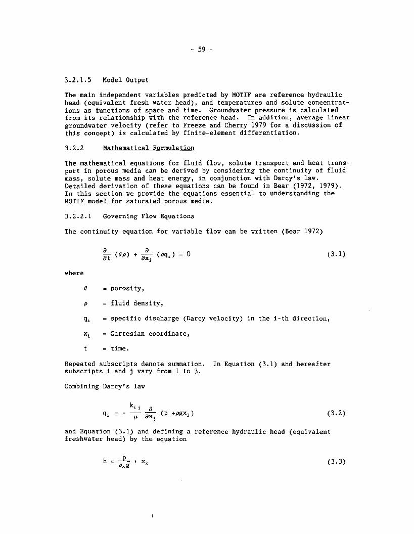
3.2.1.5 Model Output
The main independent variables predicted by MOTIF are reference hydraulic head (equivalent fresh water head), and temperatures and solute concentrat- ions as functions of space and time. Groundwater pressure is calculated from its relationship with the reference head. In addition, average linear groundwater velocity (refer to Freeze and Cherry 1979 for a discussion of this concept) is calculated by finite-element differentiation.
3.2.2 Mathematical Formulation
The mathematical equations for fluid flow, solute transport and heat trans- port in porous media can be derived by considering the continuity of fluid mass, solute mass and heat energy, in conjunction with Darcy's law. Detailed derivation of these equations can be found in Bear (1972, 1979). In this section we provide the equations essential to understanding the MOTIF model for saturated porous media.
3.2.2.1 Governing Flow Equations
The continuity equation for variable flow can be written (Bear 1972)
where
6 = porosity,
p = fluid density,
q, = specific discharge (Darcy velocity) in the i-th direction,
xi = Cartesian coordinate,
t = time.
Repeated subscripts denote summation. In Equation (3.1) and hereafter subscripts f and j vary from 1 to 3.
Combining Darcy's law
and Equation (3.1) and defining a reference hydraulic head (equivalent freshwater head) by the equation
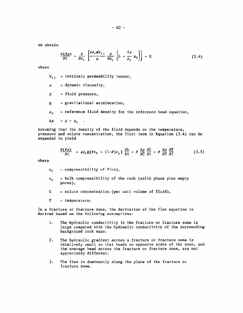
we obtain
where
kij = intrinsic permeability tensor,
p = dynamic viscosity,
p = fluid pressure,
g = gravitational acceleration,
p , = reference fluid density for the reference head equation,
Assuming that the density of the fluid depends on the temperature, pressure and solute concentration, the first term in Equation (3.4) can be expanded to yield
where
c, = compressibility of fluid,
CS = bulk compressibility of the rock (solid phase plus empty pores),
C = solute concentration (per unit volume of fluid),
T = temperature.
In a fracture or fracture zone, the derivation of the flow equation is derived based on the following assumptions:
1. The hydraulic conductivity in the fracture or fracture zone is large compared with the hydraulic conductivity of the surrounding background rock mass.
2. The hydraulic gradient across a fracture or fracture zone is relatively small so that heads on opposite sides of the zone, and the average head across the fracture or fracture zone, are not appreciably different.
3. The flow is dominantly along the plane of the fracture or fracture zone.
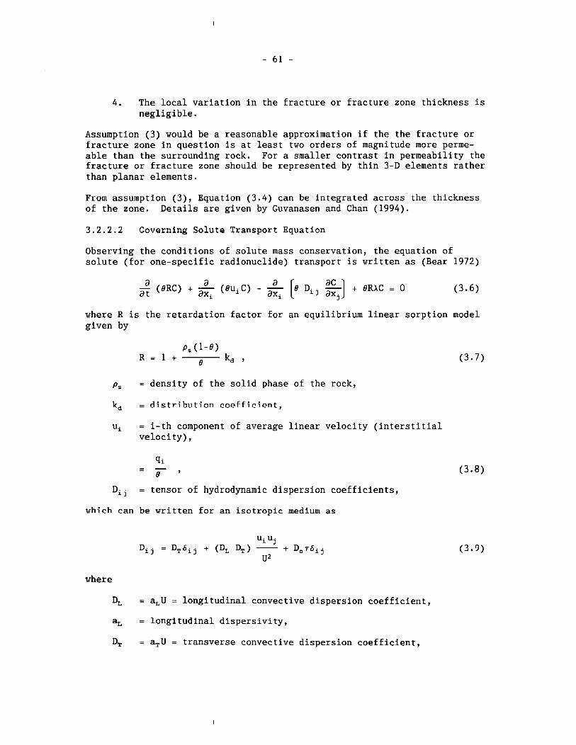
4. The local variation in the fracture or fracture zone thickness is negligible.
Assumption (3) would be a reasonable approximation if the the fracture or fracture zone in question is at least two orders of magnitude more perme- able than the surrounding rock. For a smaller contrast in permeability the fracture or fracture zone should be represented by thin 3-D elements rather than planar elements.
From assumption (3), Equation (3.4) can be integrated across the thickness of the zone. Details are given by Guvanasen and Chan (1994).
3.2.2.2 Governing Solute Transport Equation
Observing the conditions of solute mass conservation, the equation of solute (for one-specific radionuclide) transport is written as (Bear 1972)
where R is the retardation factor for an equilibrium linear sorption model given by
p, = density of the solid phase of the rock,
k, = distribution coefficient,
ui = i-th component of average linear velocity (interstitial velocity),
Dij = tensor of hydrodynamic dispersion coefficients,
which can be written for an isotropic medium as
where
DL = aLU = longitudinal convective dispersion coefficient,
a, = longitudinal dispersivity,
D, = a,U = transverse convective dispersion coefficient,
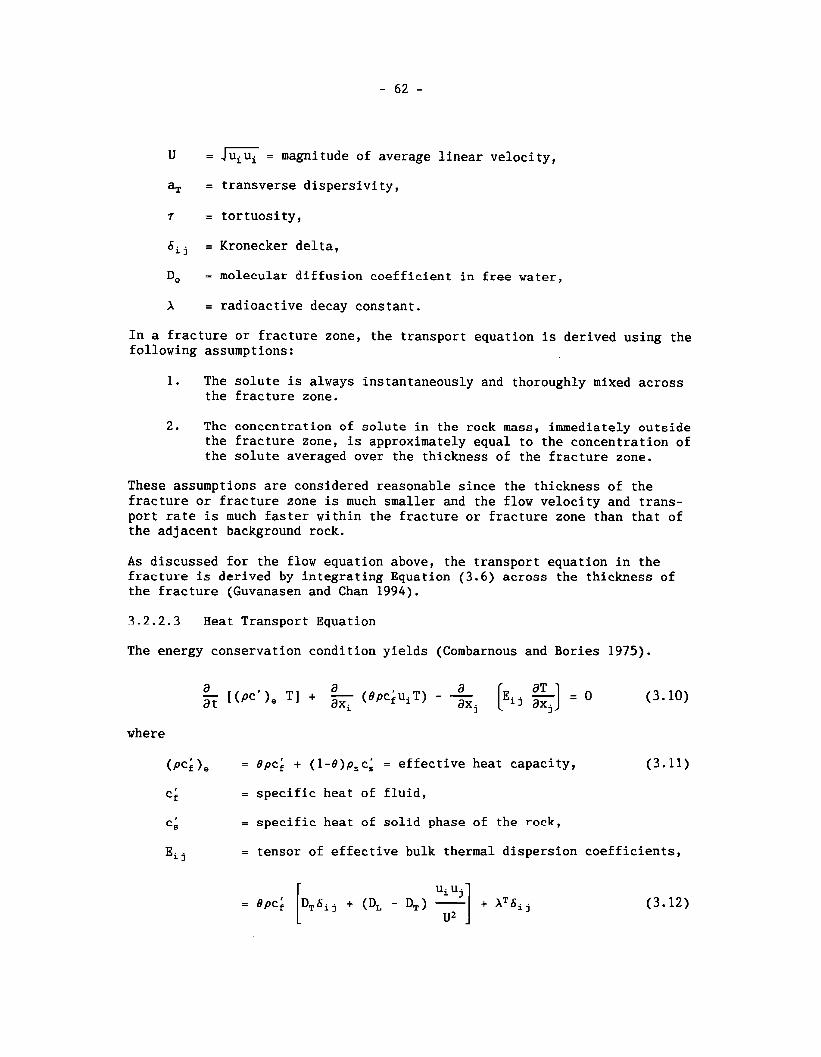
U = = magnitude of average linear velocity,
a, = transverse dispersivity,
7 = tortuosity,
6ij = Kronecker delta,
D, = molecular diffusion coefficient in free water,
X = radioactive decay constant.
In a fracture or fracture zone, the transport equation is derived using the following assumptions:
1. The solute is always instantaneously and thoroughly mixed across the fracture zone.
2. The concentration of solute in the rock mass, immediately outside the fracture zone, is approximately equal to the concentration of the solute averaged over the thickness of the fracture zone.
These assumptions are considered reasonable since the thickness of the fracture or fracture zone is much smaller and the flow velocity and trans- port rate is much faster within the fracture or fracture zone than that of the adjacent background rock.
As discussed for the flow equation above, the transport equation in the fracture is derived by integrating Equation (3.6) across the thickness of the fracture (Guvanasen and Chan 1994).
3.2.2.3 Heat Transport Equation
The energy conservation condition yields (Combarnous and Bories 1975).
where
(PC; ), = Bpc; + (1-B)p,ci = effective heat capacity, (3.11)
c ; = specific heat of fluid,
c6 = specific heat of solid phase of the rock,
Ei = tensor of effective bulk thermal dispersion coefficients,
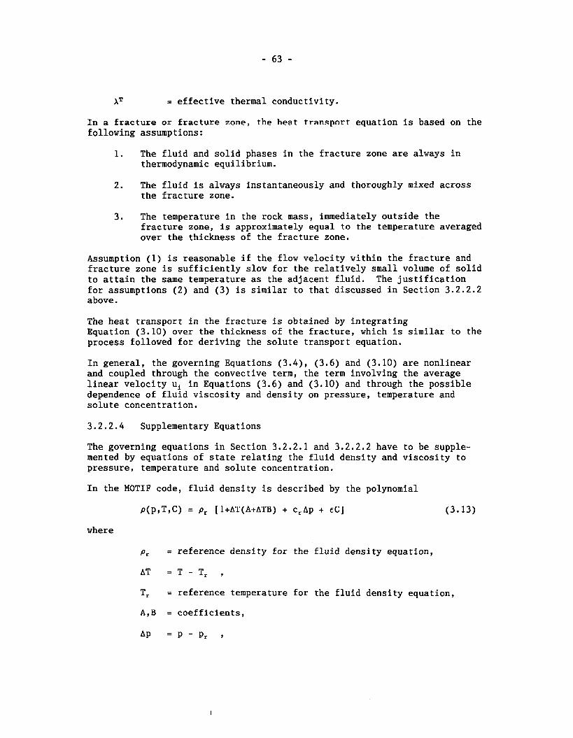
AT = effective thermal conductivity.
In a fracture or fracture zone, the heat transport equation is based on the following assumptions:
1. The fluid and solid phases in the fracture zone are always in thermodynamic equilibrium.
2. The fluid is always instantaneously and thoroughly mixed across the fracture zone.
3. The temperature in the rock mass, immediately outside the fracture zone, is approximately equal to the temperature averaged over the thickness of the fracture zone.
Assumption (1) is reasonable if the flow velocity within the fracture and fracture zone is sufficiently slow for the relatively small volume of solid to attain the same temperature as the adjacent fluid. The justification for assumptions (2) and (3) is similar to that discussed in Section 3.2.2.2 above.
The heat transport in the fracture is obtained by integrating Equation (3.10) over the thickness of the fracture, which is similar to the process followed for deriving the solute transport equation.
In general, the governing Equations (3.4), (3.6) and (3.10) are nonlinear and coupled through the convective term, the term involving the average linear velocity ui in Equations (3.6) and (3.10) and through the possible dependence of fluid viscosity and density on pressure, temperature and solute concentration.
3.2.2.4 Supplementary Equations
The governing equations in Section 3.2.2.1 and 3.2.2.2 have to be supple- mented by equations of state relating the fluid density and viscosity to pressure, temperature and solute concentration.
In the MOTIF code, fluid density is described by the polynomial
p(p,T,C) = p, [l+AT(A+ATB) + c,Ap + E C ] (3.13)
where
p, = reference density for the fluid density equation,
AT = T - T , ,
T, = reference temperature for the fluid density equation,
A,B = coefficients,
AP = P - P r 9
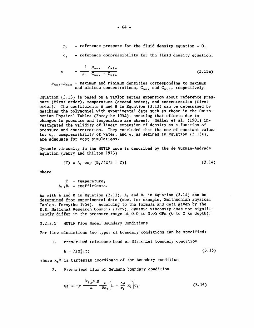
p, = reference pressure for the fluid density equation = 0,
c, - reference compressibility for the fluid density equation,
pmax,pmin = maximum and minimum densities corresponding to maximum and minimum concentrations, C,,, and Cmi,, respectively.
Equation (3.13) is based on a Taylor series expansion about reference pres- sure (first order), temperature (second order), and concentration (first order). The coefficients A and B in Equation (3.13) can be determined by matching the polynomial with experimental data such as those in the Smith- sonian Physical Tables (Forsythe 1954), assuming that effects due to changes in pressure and temperature are absent. Muller et al. (1981) in- vestigated the validity of linear expansion of density as a function of pressure and concentration. They concluded that the use of constant values for c,, compressibility of water, and c , as defined in Equation (3.13a), are adequate for most simulations.
Dynamic viscosity in the MOTIF code is described by the de Guzman-Andrade equation (Perry and Chilton 1973)
(T) = A, exp [B,/(273 + T)] (3.14)
where
T = temperature, Al,Bl = coefficients.
As with A and B in Equation (3.13), Al and B1 in Equation (3.14) can be determined from experimental data (see, for example, Smithsonian Physical Tables, Forsythe 1954). According to the formula and data given by the U.S. National Research Council (1929), dynamic viscosity does not signifi- cantly differ in the pressure range of 0.0 to 0.05 GPa (0 to 2 km depth).
3.2.2.5 MOTIF Flow Model Boundary Conditions
For flow simulations two types of boundary conditions can be specified:
1. Prescribed reference head or Dirichlet boundary condition
where xiB is Cartesian coordinate of the boundary condition
2. Prescribed flux or Neumann boundary condition
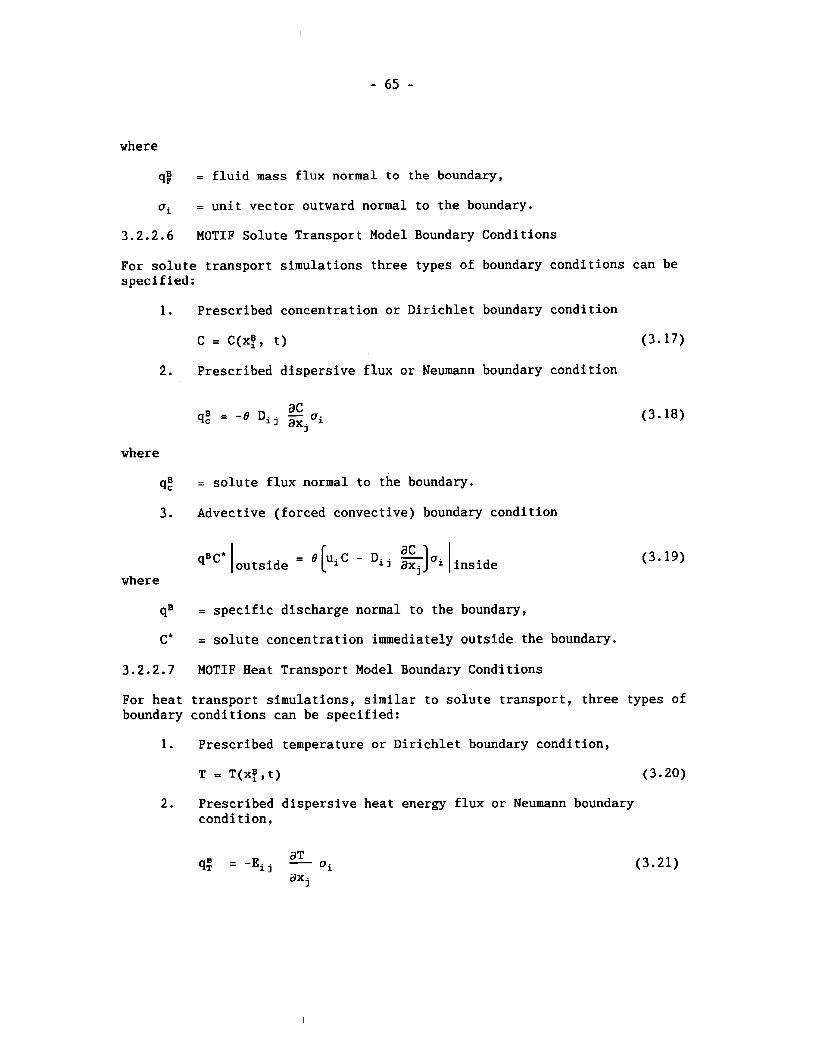
where
q: = fluid mass flux normal to the boundary,
ai = unit vector outward normal to the boundary.
3.2.2.6 MOTIF Solute Transport Model Boundary Conditions
For solute transport simulations three types of boundary conditions can be specified:
1. Prescribed concentration or Dirichlet boundary condition
c = c(x~, t) (3.17)
2. Prescribed dispersive flux or Neumann boundary condition
where
q: = solute flux normal to the boundary.
3. Advective (forced convective) boundary condition
- e U,C - ac qBC* lout side - [ Di~~]"ilinside j
where
qB = specific discharge normal to the boundary,
C* = solute concentrat ion immediately outside the boundary.
3.2.2.7 MOTIF Heat Transport Model Boundary Conditions
For heat transport simulations, similar to solute transport, three types of boundary conditions can be specified:
1. Prescribed temperature or Dirichlet boundary condition,
T = T(x!,t) (3.20)
2. Prescribed dispersive heat energy flux or Neumann boundary condition,
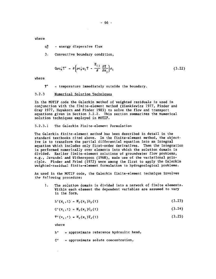
where
q! = energy dispersive flux
3. Convective boundary condition,
where
T* = temperature immediately outside the boundary.
3.2.3 Numerical Solution Techniques
In the MOTIF code the Galerkin method of weighted residuals is used in conjunction with the finite-element method (Zienkiewicz 1977, Pinder and Gray 1977, Huyakorn and Pinder 1983) to solve the flow and transport equations given in Section 3.2.2. This section summarizes the numerical solution techniques employed in MOTIF.
3.2.3.1 The Galerkin Finite-element Formulation
The Galerkin finite-element method has been described in detail in the standard textbooks cited above. In the finite-element method, the object- ive is to transform the partial differential equation into an integral equation which includes only first-order derivatives. Then the integration is performed numerically over elements into which the solution domain is divided. Earlier finite-element solutions of groundwater flow problems, e.g., Javandel and Witherspoon (1968), made use of the variational prin- ciple. Pinder and Frind (1972) were among the first to apply the Galerkin weighted-residual finite-element formulation to hydrogeological problems.
As used in the MOTIF code, the Galerkin finite-element technique involves the following procedure:
1. The solution domain is divided into a network of finite elements. Within each element the dependent variables are assumed to vary in the form,
where
h' = approximate reference hydraulic head,
C' = approximate solute concentration,
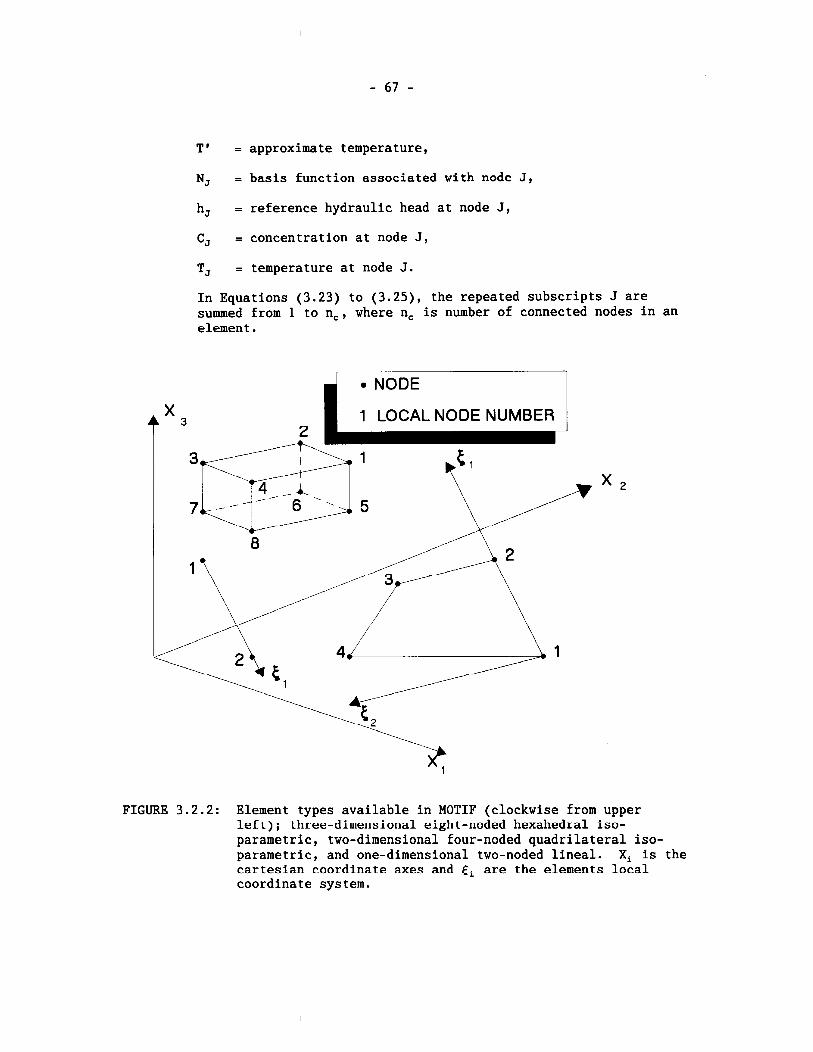
Tp = approximate temperature,
N, = basis function associated with node J,
h, = reference hydraulic head at node J,
C, = concentration at node J,
T, = temperature at node J.
In Equations (3.23) to (3.25), the repeated subscripts J are summed from 1 to n,, where n, is number of connected nodes in an element .
FIGURE 3.2.2: Element types available in MOTIF' (clockwise from upper left); three-dimensional eight-noded hexahedral iso- parametric, two-dimensional four-noded quadrilateral iso- parametric, and one-dimensional two-noded lineal. Xi is the cartesian coordinate axes and Ei are the elements local coordinate system.
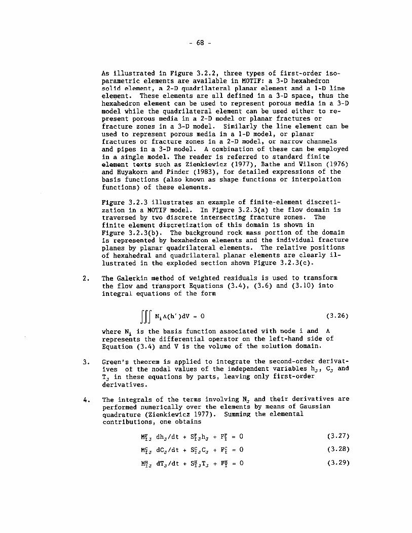
As illustrated in Figure 3.2.2, three types of first-order iso- parametric elements are available in MOTIF: a 3-D hexahedron solid element, a 2-D quadrilateral planar element and a 1-D line element. These elements are all defined in a 3-D space, thus the hexahedron element can be used to represent porous media in a 3-D model while the quadrilateral element can be used either to re- present porous media in a 2-D model or planar fractures or fracture zones in a 3-D model. Similarly the line element can be used to represent porous media in a 1-D model, or planar fractures or fracture zones in a 2-D model, or narrow channels and pipes in-a 3-D model. A combination of these can be employed in a single model. The reader is referred to standard finite element texts such as Zienkiewicz (1977), Bathe and Wilson (1976) and Huyakorn and Pinder (1983), for detailed expressions of the basis functions (also known as shape functions or interpolation functions) of these elements.
Figure 3.2.3 illustrates an example of finite-element discreti- zation in a MOTIF model. In Figure 3.2.3(a) the flow domain is traversed by two discrete intersecting fracture zones. The finite element discretization of this domain is shown in Figure 3.2.3(b). The background rock mass portion of the domain is represented by hexahedron elements and the individual fracture planes by planar quadrilateral elements. The relative positions of hexahedral and quadrilateral planar elements are clearly il- lustrated in the exploded section shown Figure 3.2.3(c).
2. The Galerkin method of weighted residuals is used to transform the flow and transport Equations (3.4), (3.6) and (3.10) into integral equations of the form
where Ni is the basis function associated with node i and A represents the differential operator on the left-hand side of Equation (3.4) and V is the volume of the solution domain.
3. Green's theorem is applied to integrate the second-order derivat- ives of the nodal values of the independent variables h,, C, and T, in these equations by parts, leaving only first-order derivatives.
4. The integrals of the terms involving N, and their derivatives are performed numerically over the elements by means of Gaussian quadrature (Zienkiewicz 1977). Summing the elemental contributions, one obtains

where
M = "mass matrix",
F = "load vector",
n, = total number of nodes in the system.
Repeated capital subscripts denote summation from 1 to n,. The superscripts F, C, and H refer to flow, solute transport and heat transport, respectively. The above equations are coupled through the convective terms, and the variation of fluid density and dynamic viscosity.
FRACTURE ZONE 1 l
TURE ZONE 2
HEXAHEDRAL ELEMENTS - - - - _ _
--.
FIGURE 3.2.3: Example of typical finite element discretization, found in a MOTIF model, of a flow domain traversed by fracture zones: a). flow domain, b). finite element discretization, and c). an exploded view of a typical assemblage of planar and hexahedral elements.
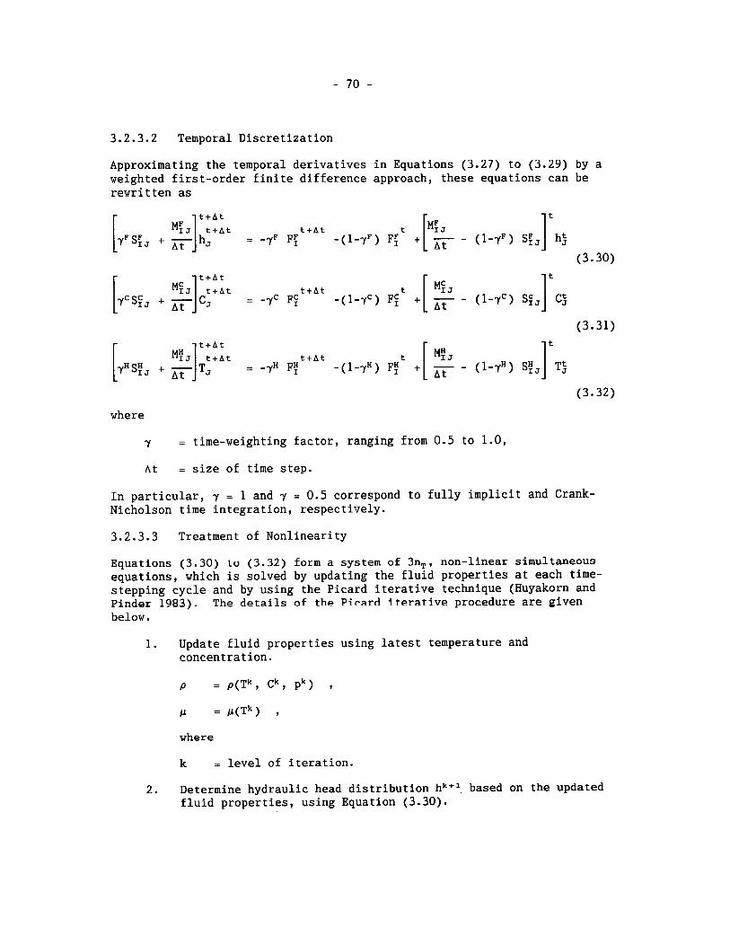
3.2.3.2 Temporal Discretization
Approximating the temporal derivatives in Equations (3.27) to (3.29) by a weighted first-order finite difference approach, these equations can be rewritten as
where
y = time-weighting factor, ranging from 0.5 to 1.0,
At = size of time step.
In particular, 7 = 1 and y = 0.5 correspond to fully implicit and Crank- Nicholson time integration, respectively.
3.2.3.3 Treatment of Nonlinearity
Equations (3.30) Lo (3.32) form a system of 3n,, non-linear simultaneous equations, which is solved by updating the fluid properties at each time- stepping cycle and by using the Picard iterative technique (Huyakorn and Pinder 1983). The details of the Picard iterative procedure are given below.
1. Update fluid properties using latest temperature and concentration.
where
k = level of iteration.
2. Determine hydraulic head distribution hk+l based on the updated fluid properties, using Equation (3.30).
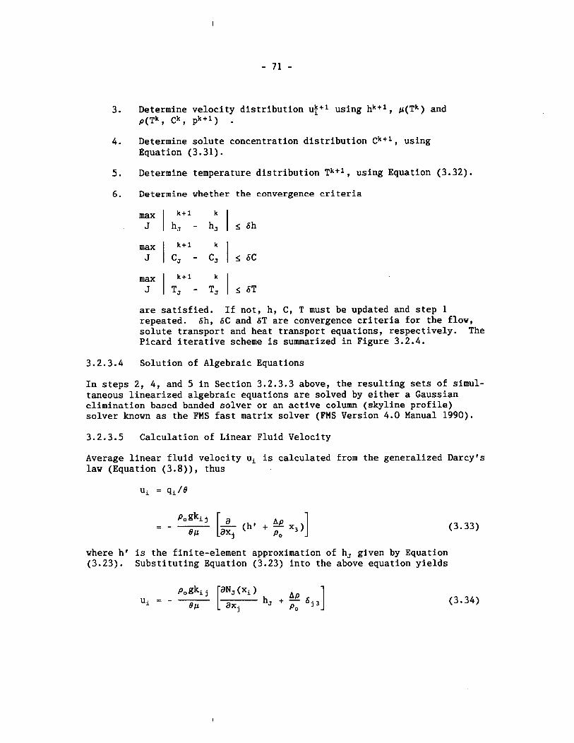
3. Determine velocity distribution u:+l using hk+l , p(Tk) and p(Tk, Ck, pk+l) .
4. Determine solute concentration distribution Ck+l, using Equation (3.31).
5. Determine temperature distribution Tk+l, using Equation (3.32).
6. Determine whether the convergence criteria
max k+l
J Ih, - h: 1 < 6 h
max k+l
J I C, - C: I s 6 C max k+l
J I Tj - T: ) < 6 T
are satisfied. If not, h, C, T must be updated and step 1 repeated. 6h, 6C and 6T are convergence criteria for the flow, solute transport and heat transport equations, respectively. The Picard iterative scheme is summarized in Figure 3.2.4.
3.2.3.4 Solution of Algebraic Equations
In steps 2, 4, and 5 in Section 3.2.3.3 above, the resulting sets of simul- taneous linearized algebraic equations are solved by either a Gaussian elimination based banded solver or an active column (skyline profile) solver known as the FMS fast matrix solver (FMS Version 4.0 Manual 1990).
3.2.3.5 Calculation of Linear Fluid Velocity
Average linear fluid velocity ui is calculated from the generalized Darcy's law (Equation (3.8)), thus
where h' is the finite-element approximation of h, given by Equation (3.23). Substituting Equation (3.23) into the above equation yields
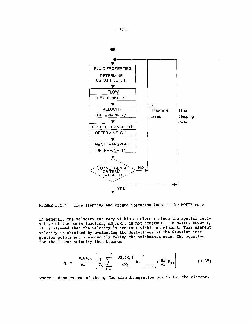
FLUID PROPERTIES
DETERMINE / USINGTk,Ck . tf 1 t
FLOW
DETERMINE hh
VELOCIn
DETERMINE uik
/ DETERMINE C /
HEAT TRANSPORT & DETERMINE T k
1
k+ 1
ITERATION
LEVEL
Time
Stepping
cycle
FIGURE 3.2.4: Time stepping and Picard iteration loop in the MOTIF code
In general, the velocity can vary within an element since the spatial deri- vative of the basis function, aNJ/axj, is not constant. In MOTIF, however, it is assumed that the velocity is constant within an element. This element velocity is obtained by evaluating the derivatives at the Gaussian inte- gration points and subsequently taking the arithmetic mean. The equation for the linear velocity thus becomes
where G denotes one of the n, Gaussian integration points for the element.
3.2.4 Limitations
MOTIF has a number of application limitations as summarized below.
1. Unconfined free surface
Because the code has no provision for adjusting the finite- element mesh to conform to the free surface (water table), uncon- fined flow problems have to be solved by iterative execution and adjustment of the top elevation of a saturated flow domain. Alternatively, the free surface can be determined by the variably saturated flow option.
2. Phase changes
No fluid phase changes, such as water to steam or to ice, are allowed.
3. Reactive solute/radionuclide transport
Only one solute interacting with the solid by linear equilibrium sorption and/or undergoing one-step radioactive decay chain, can be simulated. Longer decay chains are not allowed.
4. Velocity discontinuity
Since first-order elements are employed in MOTIF, only the primary independent variables, i.e., reference head, solute con- centration and temperature, are continuous across element bound- aries. The linear velocity, being a derivative quantity, is discontinuous across an element boundary. In practice, this may not be a severe limitation. Frind (1982) has investigated this question numerically, and concluded that it is computationally more effective to use first-order elements with a fine mesh to obtain a sufficiently accurate velocity distribution than to employ a finite-element formulation in which the velocity compon- ents, as well as the head, are treated as independent variables.
5. Double porosity, double permeability, and matrix diffusion simulations
Double porosity, double permeability and matrix diffusion (dif- fusion into stagnant water) can be simulated only if the discrete features such as fracture zones, fracture planes, conductive channels or low-permeability pore channels are explicitly repre- sented by a grid of special finite elements. No special formu- lation has been incorporated in MOTIF to allow these features to be represented in a single element.
6. Practical computational considerations
As with any numerical code, the number of nodes (grid points) that can be used in a MOTIF flow or transport model is limited by
considerations of computer storage and computer speed. Current- ly, large production runs of MOTIF models are executed on either a FPS 364/MAX or DEC ALPHA minisupercomputer located at AECLfs Whiteshell Laboratories (WL). The FPS 364/MAX is a Single In- struction Multiple Data (SIMD) parallel processing machine. The CPU (Central Processing Unit) together with two Matrix Accel- erators (MAX) boards provides a theoretical speed of 55 MFLOPS (Million Floating Point Operations Per Second). The DEC ALPHA is a RISC (Reduced Instruction Set Computing) machine, which is rated at 150 MFLOPS. Approximately half to two-thirds of these speeds are achievable during actual benchmark testing with large MOTIF models. The largest three-dimensional MOTIF model that can be run on these computers contains about 100 000 nodes. Although this is adequate for most groundwater flow simulations on a local (10 km) scale, it may not be adequate for some three-dimensional local-scale solute transport simulations. In transport simu- lations, fine discretization is necessary to avoid numerical dispersion (see, for example, Bear and Verujit 1987). Numerical testing with MOTIF transport models has indicated that in order to avoid numerical dispersion, the grid Peclet number should not exceed 5. With the current computer hardware and software at AECL/WL, accurate MOTIF solute transport modelling can be per- formed on a local (10 km) scale in two dimensions or on a vault room (hundreds of meters) scale in three dimensions.
More powerful supercomputers are available at other institutions, some of which can be accessed remotely to run larger MOTIF models than are currently possible at WL. For example, the CRAY C-90 supercomputer in Eagan, Minnesota, with a speed of over 10 GFLOPS (Billion Floating Point Operations Per Second), is 100 times faster than either computer at WL. It has been projected (IEEE, 1992) that supercomputers with speeds in the range of TeraFLOPS (lo1* Floating Point Operations Per Second) might become avail- able in about five years, which is much sooner than the time currently scheduled for application for a license to construct a nuclear waste disposal facility in Canada, should the concept be accepted.
Significant progress is being made in developing highly efficient computational techniques for solute transport modelling (see Sudicky and Huyakorn 1991, for a review). Some of the more pro- mising techniques being investigated for use within geosphere transport modelling are: the Laplace Transform Galerkin method of Sudicky (1989), Lanczos and Arnoldi methods for reducing the size of the system matrix (Nour-Omid et al. 1991, Li and Chan 1993) , an efficient iterative equation solver package using precon- ditioned conjugate gradient and ORTHOMIN methods (Mendoza et al. 1992) and the multigrid finite-element method (Fuhrmann and Gartner 1991, McKeon and Chu 1987).
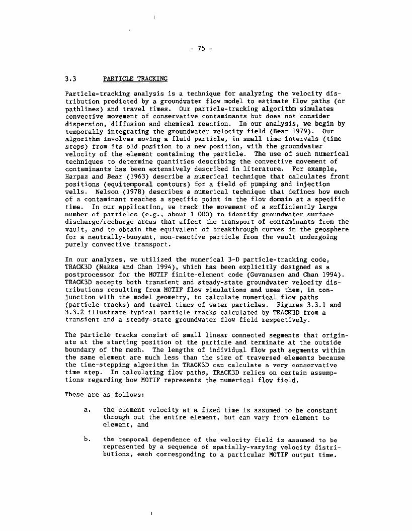
3.3 PARTICLE TRACKING
Particle-tracking analysis is a technique for analyzing the velocity dis- tribution predicted by a groundwater flow model to estimate flow paths (or pathlines) and travel times. Our particle-tracking algorithm simulates convective movement of conservative contaminants but does not consider dispersion, diffusion and chemical reaction. In our analysis, we begin by temporally integrating the groundwater velocity field (Bear 1979). Our algorithm involves moving a fluid particle, in small time intervals (time steps) from its old position to a new position, with the groundwater velocity of the element containing the particle. The use of such numerical techniques to determine quantities describing the convective movement of contaminants has been extensively described in literature. For example, Harpaz and Bear (1963) describe a numerical technique that calculates front positions (equitemporal contours) for a field of pumping and injection wells. Nelson (1978) describes a numerical technique that defines how much of a contaminant reaches a specific point in the flow domain at a specific time. In our application, we track the movement of a sufficiently large number of particles (e.g., about 1 000) to identify groundwater surface discharge/recharge areas that affect the transport of contaminants from the vault, and to obtain the equivalent of breakthrough curves in the geosphere for a neutrally-buoyant, non-reactive particle from the vault undergoing purely convective transport.
In our analyses, we utilized the numerical 3-D particle-tracking code, TRACK3D (Nakka and Chan 1994), which has been explicitly designed as a postprocessor for the MOTIF finite-element code (Guvanasen and Chan 1994). TRACK3D accepts both transient and steady-state groundwater velocity dis- tributions resulting from MOTIF' flow simulations and uses them, in con- junction with the model geometry, to calculate numerical flow paths (particle tracks) and travel times of water particles. Figures 3.3.1 and 3.3.2 illustrate typical particle tracks calculated by TRACK3D from a transient and a steady-state groundwater flow field respectively.
The particle tracks consist of small linear connected segments that origin- ate at the starting position of the particle and terminate at the outside boundary of the mesh. The lengths of individual flow path segments within the same element are much less than the size of traversed elements because the time-stepping algorithm in TRACK3D can calculate a very conservative time step. In calculating flow paths, TRACK3D relies on certain assump- tions regarding how MOTIF represents the numerical flow field.
These are as follows:
a. the element velocity at a fixed time is assumed to be constant through out the entire element, but can vary from element to element, and
b. the temporal dependence of the velocity field is assumed to be represented by a sequence of spatially-varying velocity distri- butions, each corresponding to a particular MOTIF output time.
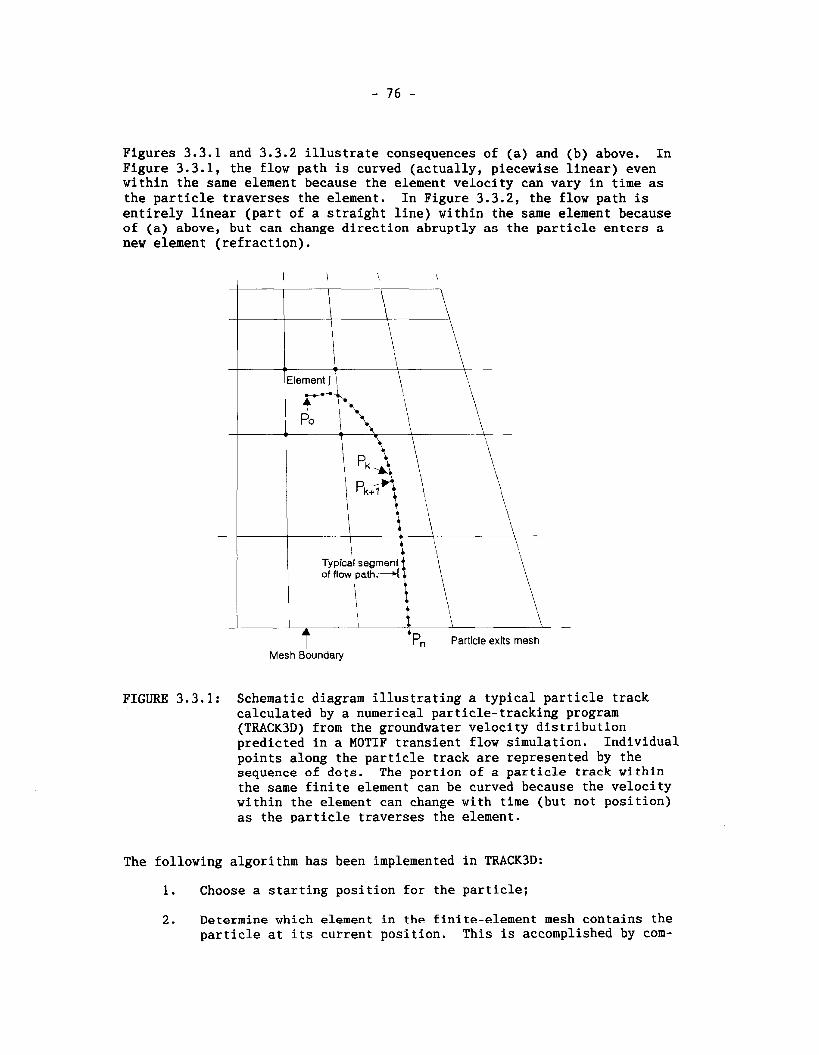
Figures 3.3.1 and 3.3.2 illustrate consequences of (a) and (b) above. In Figure 3.3.1, the flow path is curved (actually, piecewise linear) even within the same element because the element velocity can vary in time as the particle traverses the element. In Figure 3.3.2, the flow path is entirely linear (part of a straight line) within the same element because of (a) above, but can change direction abruptly as the particle enters a new element (refraction).
Mesh Boundary
FIGURE 3.3.1: Schematic diagram illustrating a typical particle track calculated by a numerical particle-tracking program (TRACKSD) from the groundwater velocity distribution predicted in a MOTIF transient flow simulation. Individual points along the particle track are represented by the sequence of dots. The portion of a particle track within the same finite element can be curved because the velocity within the element can change with time (but not position) as the particle traverses the element.
The following algorithm has been implemented in TRACK3D:
1. Choose a starting position for the particle;
2. Determine which element in the finite-element mesh contains the particle at its current position. This is accomplished by com-
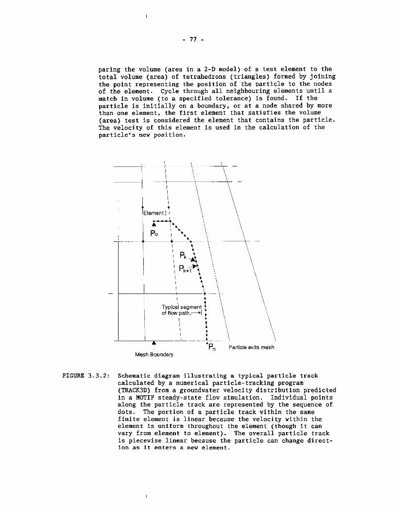
paring the volume (area in a 2-D model) of a test element to the total volume (area) of tetrahedrons (triangles) formed by joining the point representing the position of the particle to the nodes of the element. Cycle through all neighbouring elements until a match in volume (to a specified tolerance) is found. If the particle is initially on a boundary, or at a node shared by more than one element, the first element that satisfies the volume (area) test is considered the element that contains the particle. The velocity of this element is used in the calculation of the particle's new position.
Mesh ~ o u n d a r ~
IGURE 3 . 3 . 2 : Schematic diagram illustrating a typical particle track calculated by a numerical particle-tracking program (TRACK3D) from a groundwater velocity distribution predicted in a MOTIF steady-state flow simulation. Individual points along the particle track are represented by the sequence of dots. The portion of a particle track within the same finite element is linear because the velocity within the element is uniform throughout the element (though it can vary from element to element). The overall particle track is piecewise linear because the particle can change direct- ion as it enters a new element.
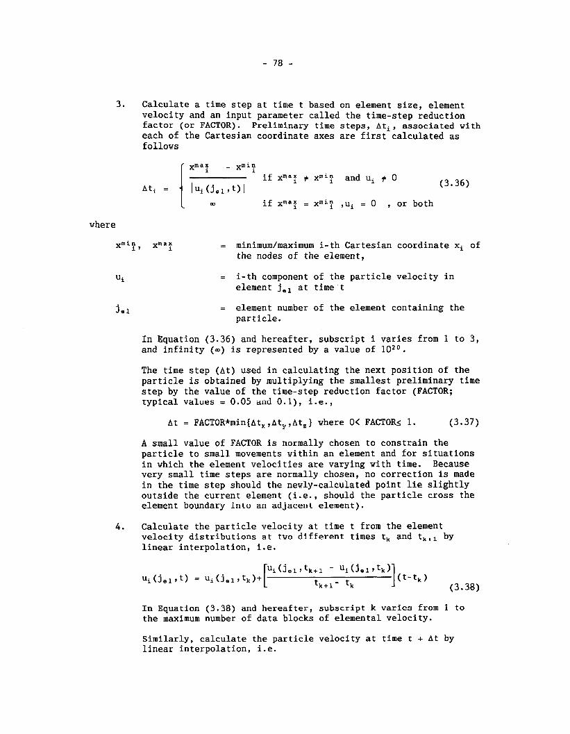
3. Calculate a time step at time t based on element size, element velocity and an input parameter called the time-step reduction factor (or FACTOR). Preliminary time steps, Ati, associated with each of the Cartesian coordinate axes are first calculated as follows
I if ~ m a x = ~ m i n 1
,ui = 0 , or both
where
xmip, xmaq = minimum/maximum i-th Cartesian coordinate xi of the nodes of the element,
= i-th component of the particle velocity in element jel at time t
= element number of the element containing the particle.
In Equation (3.36) and hereafter, subscript i varies from 1 to 3, and infinity (Q) is represented by a value of 1020.
The time step (At) used in calculating the next position of the particle is obtained by multiplying the smallest preliminary time step by the value of the time-step reduction factor (FACTOR; typical values = 0.05 and 0.1), i.e.,
At = FACTOR*min(At,,At,,Atz} where O< FACTORS 1. (3.37)
A small value of FACTOR is normally chosen to constrain the particle to small movements within an element and for situations in which the element velocities are varying with time. Because very small time steps are normally chosen, no correction is made in the time step should the newly-calculated point lie slightly outside the current element (i.e., should the particle cross the element boundary into an adjacent element).
4 . Calculate the particle velocity at time t from the element velocity distributions at two different times t, and t,,, by linear interpolation, i.e.
In Equation (3.38) and hereafter, subscript k varies from 1 to the maximum number of data blocks of elemental velocity.
Similarly, calculate the particle velocity at time t + At by linear interpolation, i.e.

5. Calculate the new position of the particle, i.e., xi(t + At), from the previous position, xi(t), the time step and the average particle velocity over the time step as follows
[ui(jel ,t) + ui(j.1 ,t + At) xi(t + At) - xi(t) + 2
This is the same as the Euler integration method described in Anderson et al. (1992), except that we use the average velocity over the time step instead of the velocity at the beginning of the time step.
6. Calculate the cumulative path length and travel time.
7. Repeat steps 2 to 6 for the next time step. This step is repeated until the particle leaves the finite-element mesh or enters certain preselected locations such as a well.
3 . 4 APPLICATION OF THE METHODOLOGY TO DEVELOP THE GEOSPHERE MODEL FOR POSTCLOSURE ASSESSMENT
Only some aspects of the groundwater flow and transport methodology des- cribed in Sections 3.2 and 3.3 above have been utilized to develop the geosphere model for the postclosure assessment case study presented. These include :
1. three-dimensional MOTIF steady-state groundwater flow simulations under natural topographic gradients. Also considered are the the influences of a pumping groundwater supply well (Section 5.6) and various changes to hydraulic properties or boundary conditions associated with the construction, operation and closure of a hypothetical nuclear fuel waste disposal vault (Section 5.5),
2. two and three-dimensional MOTIF transient coupled thermohydro- geological simulations (Sections 5.4 and 5.5.3),
3 . the numerical particle-tracking technique calculations as done in Section 3.3 to integrate temporally the groundwater velocity fields predicted by the MOTIF flow models in (1) and (2) above in order to delineate representative groundwater flowpaths, travel times and surface discharge areas for contaminants from the vault .
4. two and three-dimensional MOTIF advection-dispersion solute transport simulations (SecLion 6.8).
4. VERIFICATION AND EVALUATION OF DETAILED NUMERICAL MODELS
4.1 INTRODUCTION
In Chapter 3 we presented the methodology for the detailed groundwater flow and transport model as embodied in the MOTIF finite-element code and its postprocessor, the particle tracking code, TRACK3D. In this chapter we describe the procedure we have used to verify (Section 4.2) and validate the MOTIF code (Section 4.3 and 4.4) and to verify TRACK3D (Section 4.5). In addition, a separate evaluation of the suitability of the geosphere model we have adopted for our Performance Assessment case study is provided in Section 5.6, where we compare the surface groundwater discharge areas and groundwater residence times predicted by the MOTIF WRA flow model and TRACK3D with hydrogeochemical data from the research area. Quality assur- ance and verification of GEONET, the SYVAC3 geosphere model used for the Postclosure Assessment case study, are discussed in Section 6.8.
Technical terms like verification, validation, and calibration may have slightly different meanings depending on the context in which they appear. In this report, these terms are used in the sense in which they have been generally understood in connection with performance assessment of radio- active waste repositories. These terms are defined in Table 4.1. The definitions are not intended to be exhaustive nor are they intended to convey an undue sense of correctness of the models to the general public. There is currently significant debate amongst hydrogeologists regarding the degree to which groundwater models can be validated. Some hydrogeologists are adamantly opposed to the use of the term "validate" in the context of models used to estimate long term hydrogeologic conditions (Bredehoeft and Konikow 1993). We agree with the concern that the use of the term "vali- date" can imply a correctness of the models that does not necessarily exist especially in so far as very long term predictions of behaviour are con- cerned. We believe that our usage of the term "model validation1' embodies the basic principals of ensuring and demonstrating that the model is a reasonable and realistic representation of the features, processes and events that could affect the transport of contaminants from the vault to the discharge areas in the biosphere. We recognize the need to be very clear in our meaning and usage of the term "model validation".
4.2 MOTIF VERIFICATION
A series of nine verification cases have been used to test the numerical solution techniques and coding in MOTIF, as well as to demonstrate some of the MOTIF analysis capabilities. The MOTIF solution for each verification case has been compared with corresponding analytical or numerical solution(s). Three of the verification cases (1, 2 and 8 outlined below) are cases that were developed for Level 1 of the International Hydrologic Code Intercomparison project (HYDROCOIN). The MOTIF solutions for these three verification cases, as well as verification cases (6) and (9), were compared with independent analytical or numerical solutions in Chan et al. (1987). The MOTIF results for the HYDROCOIN Level 1 verification cases are also included in the HYDROCOIN Secretariat's compilation and comparison of
results submitted by various participating project teams (The International HYDROCOIN Project 1988).
TABLE 4.1
DEFINITIONS OF SOME TERMS AS USED IN THIS CHAPTER
TERM DEFINITION
Calibration A process in which the conceptual model assumptions and model parameters are varied to fit the model predictions to observations. The model calibration, described in Section 4.3 below, follows the traditional trial-and-error procedure.
Verification A mathematical model, or the corresponding computer code, is verified when it is shown that the code behaves as intended, i.e., that it is a proper mathematical representation of the conceptual model and that the equations are correctly encoded and solved (IAEA 1988)
Validation The process of obtaining assurance that a model as embodied in a computer program is a proper representation of the process or system for which it is intended. Ideally, validation is a comparison between empirical observation and predictions derived from the model. However, as this is frequently impractical or impossible due to the large length and time scales involved in nuclear fuel waste disposal, history matching, short term testing and post audits of predicted behaviour supported by other avenues or inquiry such as peer review are used to obtain such assurance (Randall et al. 1990).
The above definitions are from the Level 3 project report (HYDROCOIN Project Coordinating Group 1992) of the international cooperative project HYDROCOIN (Hydrologic Code Intercomparison).
Appendix E of this report contains the verification case descriptions and the comparison of MOTIF model results with independent solutions for the verification cases outlined below:
1. Topographically driven, steady-state groundwater flow in a two- dimensional porous medium intersected by two highly permeable fracture zones. This is the HYDROCOIN Level 1 (The International HYDROCOIN Project 1988) Case 2 problem. The MOTIF solution was compared with independent numerical solutions.
2. A groundwater pumping well in a confined horizontal, homogeneous, and isotropic aquifer which is intersected by a planar vertical fracture. The aquifer is initially at constant groundwater pressure. The MOTIF results were compared to the analytical solution reported by Gringarten et al. (1974) for such a case.
3. The transient flow of water from a single vertical borehole in a homogeneous, isotropic and saturated permeable layer of rock which is underlain by a horizontal fracture and confined between impermeable horizontal boundaries. This is HYDROCOIN Level 1 Case 1. Hodgkinson and Barker (1985) have provided the analytical solution for this case.
4. One-dimensional simultaneous advection, dispersion, sorption and radioactive decay of a solute in a homogeneous and isotropic porous media. The following cases are investigated; a) transport without adsorption and radioactive decay, b) transport with ad- sorption, and c) transport with radioactive decay. Analytical solutions for these cases have been obtained by Marino (1974).
5. One-dimensional solute transport in a finite-length, one- dimensional ion-exchange or chromatographic column with mixed (Cauchy) boundary condition. The MOTIF solution was compared with the analytical solution of Bastian and Lapidus (1956) for this case.
6. One-dimensional radionuclide transport along a discrete, water- filled fracture in a saturated rock matrix. Tang et al. (1981) obtained an analytical solution assuming the following a) the width of the fracture is much smaller than its length, b) there is complete mixing across the fracture, c) there is only mole- cular diffusion within the rock matrix, d) transport within the fracture is much faster than within the matrix, and e) the fracture is considered to be thin and rigid.
7. Two-dimensional transport of a conservative solute in a long unconfined aquifer comprised of a fine silty sand within which a thin, discontinuous, medium-grained sand layer is located. The MOTIF solution for this case was compared to the Laplace trans- form Galerkin finite element solution of Sudicky (1989).
8. Three-dimensional heat transport and buoyancy driven groundwater convection caused by an exponentially decaying, spherical heat source in an infinite saturated permeable medium. An analytical solution for this situation has been given by Hodgkinson (1980).
9. Steady-state and transient free cellular convective motion of water in a saturated permeable layer caused by spatial variation of salinity, assuming that mechanical dispersion is negligible. The MOTIF solution was compared to the finite-element solution published by Diersch (1981).
It is evident from the graphical and tabulated comparisons given in Appendix E that the MOTIF solutions for verification cases (1) to (8) are in excellent agreement with known analytical or numerical solutions obtain- ed from independent sources. In verification case (9) the graphical com- parison shows reasonable agreement. The discrepancies between the MOTIF and Diersch solutions are probably comparable to the errors associated with transferring the isoconcentration contours from Diersch's paper.
We believe this extensive series of verification studies has established the ability of the MOTIF finite-element code to accurately model the groundwater flow and transport phenomena for which it is intended.
4.3 THE URL DRAWDOWN EXPERIMENT AND HYDROGEOLOGIC MODEL VALIDATION
The siting and construction of the Underground Research Laboratory (URL) at a previously undisturbed location in the granitic Lac du Bonnet Batholith provided us with a unique opportunity to test the groundwater flow aspects of the MOTIF code for plutonic rock conditions. After the URL site was thoroughly characterized using surface-based methods, but before any exca- vation of the shafts or tunnels had begun, the site characterization data were used to construct three-dimensional groundwater flow models of the URL site as part of a major groundwater model validation experiment.
The objective of the experiment was to see if various hydrogeologic models could successfully predict the hydrogeologic disturbance that would be caused by the excavation of the URL facility to a depth of 255 m, approxi- mately 250 m below the groundwater table (Betcher and Pearson 1982). Predictions were made of the expected groundwater inflow to the shaft and the associated groundwater pressure drawdowns that would develop in the surrounding rock mass during a period of about two years after construction time. In particular, time-variant groundwater pressure responses were predicted at 171 groundwater pressure monitoring locations in the rock mass surrounding the URL shaft to allow a comparison or post audit with actual observations of the drawdown.
Although several independent modelling teams initially participated in the study, only two of the teams, INTERA and AECL, produced predictions of the hydrogeologic disturbance that would be created by the excavation of the URL shaft (Guvanasen et al. 1985). The modelling team from INTERA used a finite difference code (SWIFT) to simulate the hydrogeological conditions (Lafleur and Lanz 1984, INTERA 1985), whereas the modelling team from AECL used the finite element code MOTIF.
Prior to any excavation at the URL site, a thorough site evaluation program was carried out to determine the geologic and hydrogeologic conditions of the 3.8 km2 area of the site to a depth of approximately 500 m. The initial information from this program was used to select the location for the URL shaft and underground facility and to design a hydrogeological monitoring system to record the groundwater pressure conditions in the rock mass surrounding the location chosen for the shaft and underground facilities (Davison 1982, Davison et al. 1982, Davison 1984a).
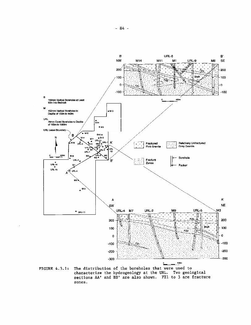
152mm Vertical Boreholes at Least 50m Into Bedrock
M
URL
URL Lease Boundaly
\
URL-13
0 400m - - ,
FIGURE 4.3.1: The distribution of the boreholes that were used to characterize the hydrogeology at the URL. Two geological sections AA' and BB' are also shown. FZ1 to 3 are fracture zones.
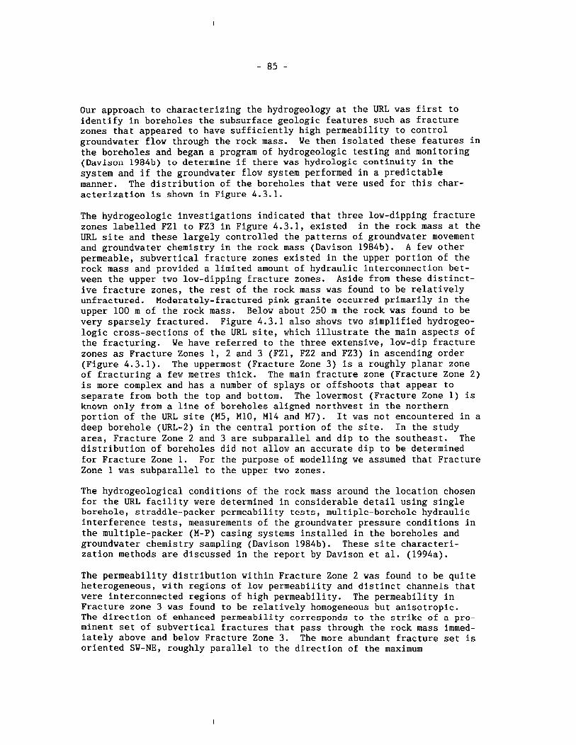
Our approach to characterizing the hydrogeology at the URL was first to identify in boreholes the subsurface geologic features such as fracture zones that appeared to have sufficiently high permeability to control groundwater flow through the rock mass. We then isolated these features in the boreholes and began a program of hydrogeologic testing and monitoring (Davison 1984b) to determine if there was hydrologic continuity in the system and if the groundwater flow system performed in a predictable manner. The distribution of the boreholes that were used for this char- acterization is shown in Figure 4.3.1.
The hydrogeologic investigations indicated that three low-dipping fracture zones labelled FZ1 to FZ3 in Figure 4.3.1, existed in the rock mass at the URL site and these largely controlled the patterns of groundwater movement and groundwater chemistry in the rock mass (Davison 1984b). A few other permeable, subvertical fracture zones existed in the upper portion of the rock mass and provided a limited amount of hydraulic interconnection bet- ween the upper two low-dipping fracture zones. Aside from these distinct- ive fracture zones, the rest of the rock mass was found to be relatively unfractured. Moderately-fractured pink granite occurred primarily in the upper 100 m of the rock mass. Below about 250 m the rock was found to be very sparsely fractured. Figure 4.3.1 also shows two simplified hydrogeo- logic cross-sections of the URL site, which illustrate the main aspects of the fracturing. We have referred to the three extensive, low-dip fracture zones as Fracture Zones 1, 2 and 3 (FZ1, FZ2 and FZ3) in ascending order (Figure 4.3.1). The uppermost (Fracture Zone 3) is a roughly planar zone of fracturing a few metres thick. The main fracture zone (Fracture Zone 2) is more complex and has a number of splays or offshoots that appear to separate from both the top and bottom. The lowermost (Fracture Zone 1) is known only from a line of boreholes aligned northwest in the northern portion of the URL site (M5, M10, M14 and M7). It was not encountered in a deep borehole (URL-2) in the central portion of the site. In the study area, Fracture Zone 2 and 3 are subparallel and dip to the southeast. The distribution of boreholes did not allow an accurate dip to be determined for Fracture Zone 1. For the purpose of modelling we assumed that Fracture Zone 1 was subparallel to the upper two zones.
The hydrogeological conditions of the rock mass around the location chosen for the URL facility were determined in considerable detail using single borehole, straddle-packer permeability tests, multiple-borehole hydraulic interference tests, measurements of the groundwater pressure conditions in the multiple-packer (M-P) casing systems installed in the boreholes and groundwater chemistry sampling (Davison 1984b). These site characteri- zation methods are discussed in the report by Davison et al. (1994a).
The permeability distribution within Fracture Zone 2 was found to be quite heterogeneous, with regions of low permeability and distinct channels that were interconnected regions of high permeability. The permeability in Fracture zone 3 was found to be relatively homogeneous but anisotropic. The direction of enhanced permeability corresponds to the strikc of a pro- minent set of subvertical fractures that pass through the rock mass immed- iately above and below Fracture Zone 3. The more abundant fracture set is oriented SW-NE, roughly parallel to the direction of the maximum
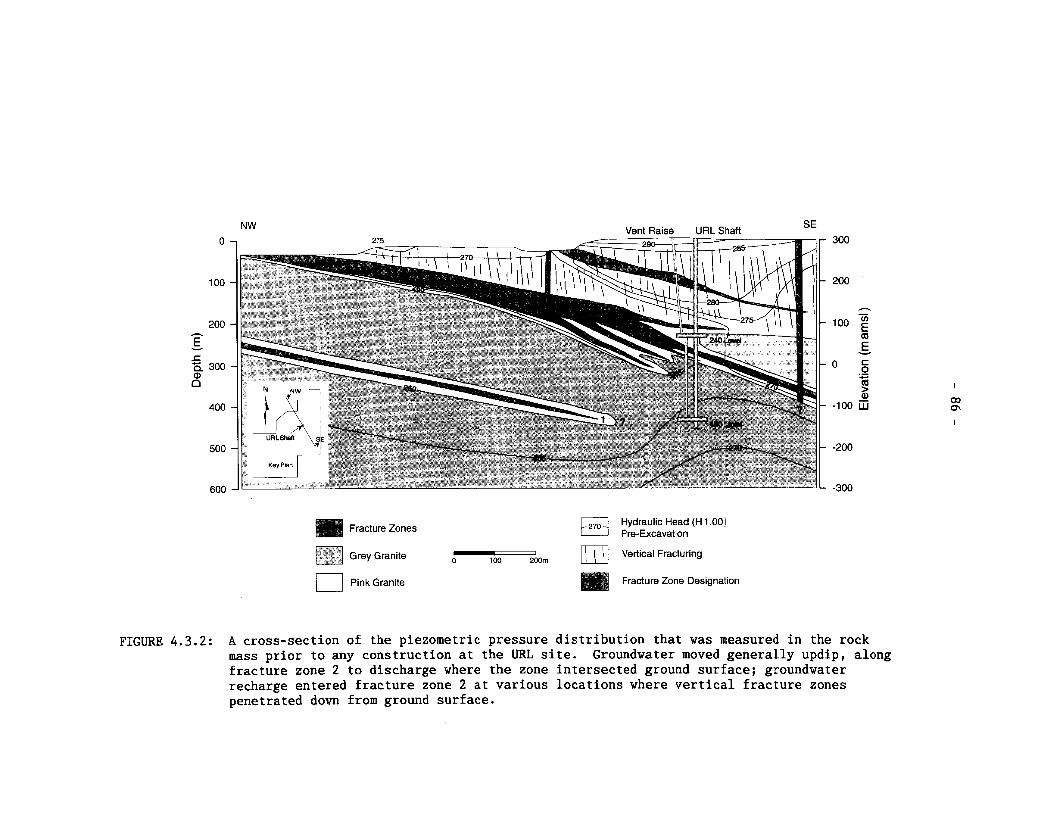
NW Vent Raise URL Shaft SE
Fracture Zones Hydraulic Head (H 1.00:1 Pre-Excavatton
Grey Granite 7 100 200117 Vedical Fracturing
0 Pink Granite Fracture Zone Designation
FIGURE 4.3.2: A cross-section of the piezometric pressure distribution that was measured in the rock mass prior to any construction at the URL site. Groundwater moved generally updip, along fracture zone 2 to discharge where the zone intersected ground surface; groundwater recharge entered fracture zone 2 at various locations where vertical fracture zones penetrated down from ground surface.

principal stress at the site (Everitt and Brown 1986); the less well- de- veloped fracture set is oriented NW-SE, roughly perpendicular to the maxi- mum principal stress.
Within the major fracture zones clear patterns of groundwater flow and groundwater chemistry were found to exist. These were related to the per- meability distributions within the zones and to their intersections with recharge or discharge areas. Figure 4.3.2 shows a generalized cross- section of the piezometric pressure distribution that was measured in the rock mass prior to any construction at the URL site. In Fracture Zone 2, for example, the figure illustrates that groundwater recharge entered the zone at various locations where vertical fracture zones penetrate down from ground surface (Figure 4.3.2). Groundwater moved updip along Fracture Zone 2 and discharged where the zone intersected the ground surface.
The information from these surface-based hydrogeological investigations of the URL site and limited regional investigations was used to develop and calibrate three-dimensional regional groundwater flow models of the region- al area surrounding the URL and local groundwater flow models of the URL site itself. The data from the multiple-borehole hydraulic interference tests and the piezometric pressure records from the M-P casing systems at the URL site were considered particularly useful in calibrating the local models (Guvanasen 1984a, Guvanasen et al. 1985, INTERA 1985). This approach in model development is often referred to as history matching and is usually the final step used to ensure the reliability of groundwater flow models. In our case we used the calibrated models to predict ahead of time the hydrogeologic responses that would occur in the rock due to the construction of the URL shaft. These predictions were later compared with observations of the actual responses and spanned several orders of magni- tude in time beyond the time period used for the history matching. Such a comparison or post audit, seldom done in the development of groundwater flow models is considered an important step in evaluating groundwater flow models that are intended to be used for long term predictions (Konikow and Bredehoeft 1992).
From a numerical point of view the MOTIF finite element code used by AECL's modelling team has proven to be very appropriate for the hydrogeology of the URL site. It represented much of the rock mass as an equivalent aniso- tropic porous medium with three-dimensional permeability and porosity char- acteristics that accounted for the effects of fracturing. The availability of a planar element that can have arbitrary orientation in three-dimension- al space makes it very convenient to represent fracture zones as discrete features. This feature of MOTIF was utilized in modelling the hydrogeo- logic disturbance expected from excavation of the URL facility to a depth of 255 m. The fracture zones were treated as discrete features that were represented by planar elements superimposed upon the mesh of solid elements representing the rock mass (Guvanasen 1985, Guvanasen and Davison 1984). The location, orientation and spatial distribution of permeability and porosity characteristics of the main fracture zones known to exist at the URL site and Whiteshell Laboratories site were represented in the larger scale (regional) model of the WRA surrounding the URL model using these planar elements. The regional model (Figure 4.3.3) was a three-dimensional finite element mesh extending to a depth of about 1.6 km that incorporated
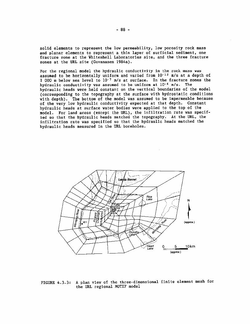
solid elements to represent the low permeability, low porosity rock mass and planar elements to represent a thin layer of surficial sediment, one fracture zone at the Whiteshell Laboratories site, and the three fracture zones at the URL site (Guvanasen 1984a).
For the regional model the hydraulic conductivity in the rock mass was assumed to be horizontally uniform and varied from 10-l2 m/s at a depth of 1 000 m below sea level to lo- ' m/s at surface. In the fracture zones the hydraulic conductivity was assumed to be uniform at 10-6 m / s . The hydraulic heads were held constant on the vertical boundaries of the model (corresponding to the topography at the surface with hydrostatic conditions with depth). The bottom of the model was assumed to be impermeable because of the very low hydraulic conductivity expected at that depth. Constant hydraulic heads at surface water bodies were applied to the top of the model. For land areas (except the URL), the infiltration rate was specif- ied so that the hydraulic heads matched the topography. At the URL, the infiltration rate was specified so that the hydraulic heads matched the hydraulic heads measured in the URL boreholes.
FIGURE 4.3.3: A plan view of the three-dimensional finite element mesh for the URL regional MOTIF model
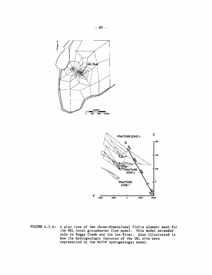
FRACTURE ZONE 3 z
FRACTURE ZONE 1
FIGURE 4.3.4: A plan view of the three-dimensional finite element mesh for the URL local groundwater flow model. This model extended only to Boggy Creek and the Lee River. Also illustrated is how the hydrogeologic features of the URL site were represented by the MOTIF hydrogeologic model.
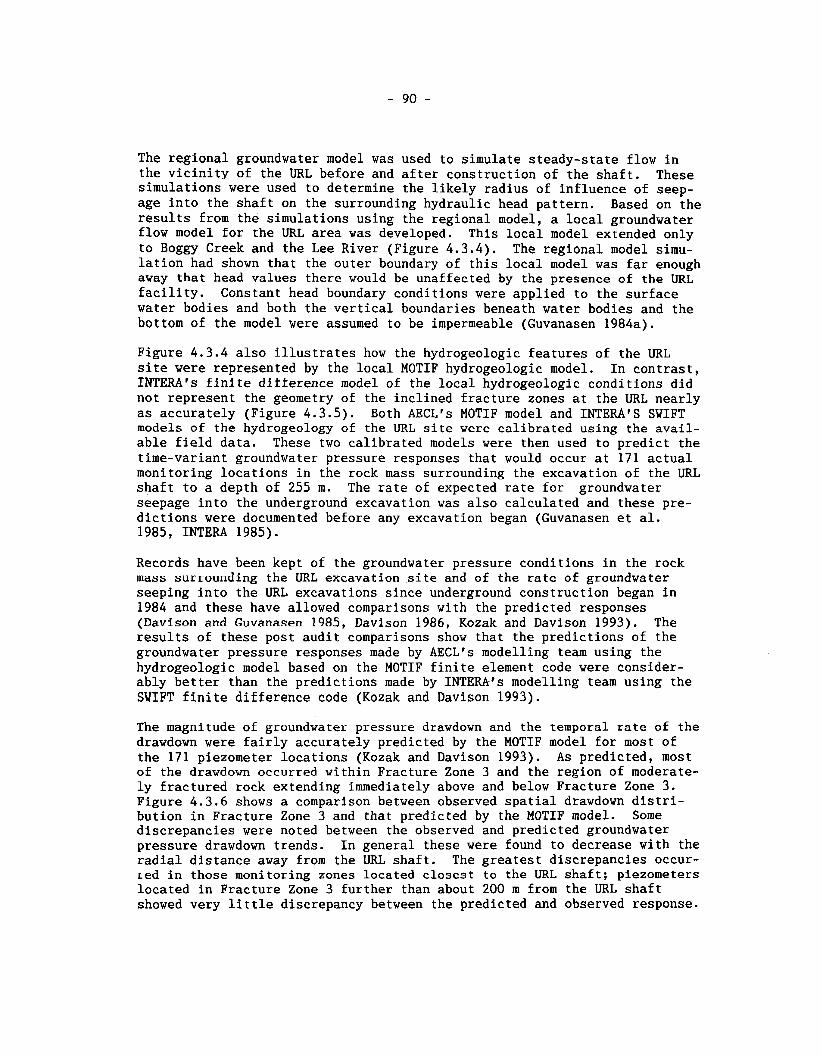
The regional groundwater model was used to simulate steady-state flow in the vicinity of the URL before and after construction of the shaft. These simulations were used to determine the likely radius of influence of seep- age into the shaft on the surrounding hydraulic head pattern. Based on the results from the simulations using the regional model, a local groundwater flow model for the URL area was developed. This local model extended only to Boggy Creek and the Lee River (Figure 4.3.4). The regional model simu- lation had shown that the outer boundary of this local model was far enough away that head values there would be unaffected by the presence of the URL facility. Constant head boundary conditions were applied to the surface water bodies and both the vertical boundaries beneath water bodies and the bottom of the model were assumed to be impermeable (Guvanasen 1984a).
Figure 4.3.4 also illustrates how the hydrogeologic features of the URL site were represented by the local MOTIF hydrogeologic model. In contrast, INTERAts finite difference model of the local hydrogeologic conditions did not represent the geometry of the inclined fracture zones at the URL nearly as accurately (Figure 4.3.5). Both AECLrs MOTIF model and INTERA'S SWIFT models of the hydrogeology of the URL site wcrc calibrated using the avail- able field data. These two calibrated models were then used to predict the time-variant groundwater pressure responses that would occur at 171 actual monitoring locations in the rock mass surrounding the excavation of the URL shaft to a depth of 255 m. The rate of expected rate for groundwater seepage into the underground excavation was also calculated and these pre- dictions were documented before any excavation began (Guvanasen et al. 1985, INTERA 1985).
Records have been kept of the groundwater pressure conditions in the rock Inass surrounding the URL excavation site and of the rate of groundwater seeping into the URL excavations since underground construction began in 1984 and these have allowed comparisons with the predicted responses (Davison and Guvanasen 1985, Davison 1986, Kozak and Davison 1993). The results of these post audit comparisons show that the predictions of the groundwater pressure responses made by AECLrs modelling team using the hydrogeologic model based on the MOTIF finite element code were consider- ably better than the predictions made by INTERA's modelling team using the SWIFT finite difference code (Kozak and Davison 1993).
The magnitude of groundwater pressure drawdown and the temporal rate of the drawdown were fairly accurately predicted by the MOTIF model for most of the 171 piezometer locations (Kozak and Davison 1993). As predicted, most of the drawdown occurred within Fracture Zone 3 and the region of moderate- ly fractured rock extending immediately above and below Fracture Zone 3. Figure 4.3.6 shows a comparison between observed spatial drawdown distri- bution in Fracture Zone 3 and that predicted by the MOTIF model. Some discrepancies were noted between the observed and predicted groundwater pressure drawdown trends. In general these were found to decrease with the radial distance away from the URL shaft. The greatest discrepancies occur- red in those monitoring zones located closest to the URL shaft; piezometers located in Fracture Zone 3 further than about 200 m from the URL shaft showed very little discrepancy between the predicted and observed response.
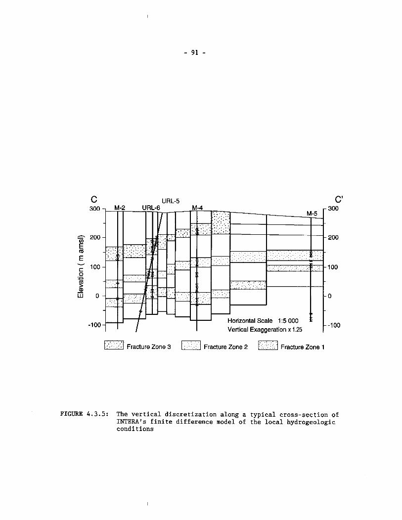
w] Fracture Zone 3 . . . . Fracture Zone 2 1-1 .. - . . .. Fracture Zone 1
FIGURE 4.3.5: The vertical discretization along a typical cross-section of INTERA1s finite difference model of the local hydrogeologic conditions
Piezometric Drawdown In Fracture Zone 3 at URL-1 ( 93.4 to 131 .Om Interval )
= 284- predicted by MOTIF Model 5 -
I
0
>
-
284
E - 5 268- 268
3 - 5 252- -s
- - - - - - _ 5 - $ 236- Shaft 236 I
Excavation
Groundwater Level Drawdown within Fracture Zone 3 - 1985 March
12.8 Observed Drawdown (m)
(18.0) Predicted Drawdown (m)
,\a' Contour of Drawdown in Metres
Observation Borehole
!
Piezomet~ic Drawdown in Fracture Zone 2 at MIA ( 240 to 324m Interval )
Predicted by MOTIF Model
- - - - _ _ _ 264
0
Excavatlon by Drlllino Actlvltles
248
1984 1985 1986 t IF1 1 A 1 I J I 1A1 101 I D 1 IF1 I A I IJ1 1 A 1 1 0 1 ID1 I F 1 I A l I J I 1 A 1 101 IDI
240
FIGURE 4 . 3 . 6 : A comparison between the predicted and observed spatial drawdown distribution in fracture zone 3. Also presented are some examples of the comparisons between the piezometric responses that were predicted by the MOTIF model and the actual responses that were observed.
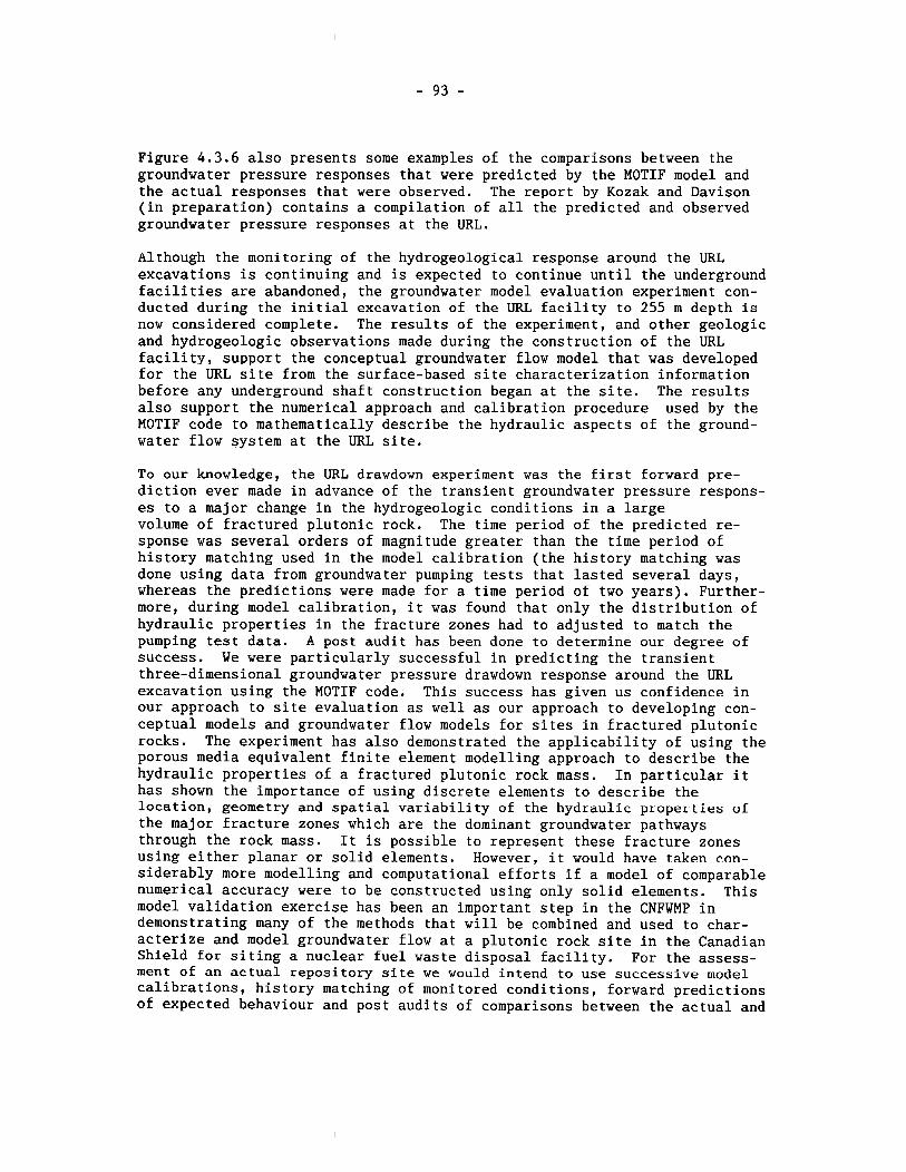
Figure 4.3.6 also presents some examples of the comparisons between the groundwater pressure responses that were predicted by the MOTIF model and the actual responses that were observed. The report by Kozak and Davison (in preparation) contains a compilation of all the predicted and observed groundwater pressure responses at the URL.
Although the monitoring of the hydrogeological response around the URL excavations is continuing and is expected to continue until the underground facilities are abandoned, the groundwater model evaluation experiment con- ducted during the initial excavation of the URL facility to 255 m depth is now considered complete. The results of the experiment, and other geologic and hydrogeologic observations made during the construction of the URL facility, support the conceptual groundwater flow model that was developed for the URL site from the surface-based site characterization information before any underground shaft construction began at the site. The results also support the numerical approach and calibration procedure used by the MOTIF code to mathematically describe the hydraulic aspects of the ground- water flow system at the URL site.
To our knowledge, the URL drawdown experiment was the first forward pre- diction ever made in advance of the transient groundwater pressure respons- es to a major change in the hydrogeologic conditions in a large volume of fractured plutonic rock. The time period of the predicted re- sponse was several orders of magnitude greater than the time period of history matching used in the model calibration (the history matching was done using data from groundwater pumping tests that lasted several days, whereas the predictions were made for a time period of two years). Further- more, during model calibration, it was found that only the distribution of hydraulic properties in the fracture zones had to adjusted to match the pumping test data. A post audit has been done to determine our degree of success. We were particularly successful in predicting the transient three-dimensional groundwater pressure drawdown response around the URL excavation using the MOTIF code. This success has given us confidence in our approach to site evaluation as well as our approach to developing con- ceptual models and groundwater flow models for sites in fractured plutonic rocks. The experiment has also demonstrated the applicability of using the porous media equivalent finite element modelling approach to describe the hydraulic properties of a fractured plutonic rock mass. In particular it has shown the importance of using discrete elements to describe the location, geometry and spatial variability of the hydraulic properties of the major fracture zones which are the dominant groundwater pathways through the rock mass. It is possible to represent these fracture zones using either planar or solid elements. However, it would have taken con- siderably more modelling and computational efforts if a model of comparable numerical accuracy were to be constructed using only solid elements. This model validation exercise has been an important step in the CNFWMP in demonstrating many of the methods that will be combined and used to char- acterize and model groundwater flow at a plutonic rock site in the Canadian Shield for siting a nuclear fuel waste disposal facility. For the assess- ment of an actual repository site we would intend to use successive model calibrations, history matching of monitored conditions, forward predictions of expected behaviour and post audits of comparisons between the actual and
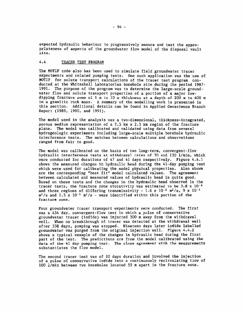
expected hydraulic behaviour to progressively ensure and test the appro- priateness of aspects of the groundwater flow model of the disposal vault site.
TRACER TEST PROGRAM
The MOTIF code also has been used to simulate field groundwater tracer experiments and related pumping tests. One such application was the use of MOTIF for solute transport calculations of the tracer test program con- ducted at the Whiteshell Laboratories borehole site during the period 1987- 1991. The purpose of the program was to determine the large-scale ground- water flow and solute transport properties of a portion of a major low- dipping fracture zone o1 1 ni to 10 m thickness at a depth of 200 m to 400 m in a granitic rock mass. A summary of the modelling work is presented in this section. Additional details can be found in Applied Geoscience Branch Report (1989, 1990, and 1991).
The model used in the analysis was a two-dimensional, thickness-integrated, porous medium representation of a 2.5 km x 2.3 km region of the fracture plane. The model was calibrated and validated using data from several hydrogeologic experiments including large-scale multiple borehole hydraulic interference tests. The matches between calculations and observations ranged from fair to good.
The model was calibrated on the basis of two long-term, convergent-flow hydraulic interference tests at withdrawal rates of 30 and 130 l/min, which were conducted for durations of 47 and 41 days respectively. Figure 4.4.1 shows the measured changes in hydraulic head during the 41-day pumping test which were used for calibrating the model physical properties. Also shown are the corresponding "best fit" model calculated values. The agreement between calculated and measured values of hydraulic head is quite good. Based on these tests and the changes in the hydraulic head observed in the tracer tests, the fracture zone storativity was estimated to be 3.8 x lo -" and three regions of differing transmissivity - 1.6 x 10- * m2/s, 9 x 10- m2/s and 1.3 x m2/s - were identified within this portion of the fracture zone.
Four groundwater tracer transport experiments were conducted. The first was a 434 day, convergent-flow test in which a pulse of conservative groundwater tracer (iodide) was injected 300 m away from the withdrawal well. When no breakthrough of tracer was detected at the withdrawal well after 338 days, pumping was stopped. Nineteen days later iodide labelled groundwater was purged from the original injection well. Figure 4.4.2 shows a typical example of the changes in hydraulic head during the first part of the test. The predictions are from the model calibrated using the data of the 41 day pumping test. The close agreement with the measurements substantiates the flow model.
The second tracer test was of 10 days duration and involved the injection of a pulse of conservative iodide into a continuously recirculating flow of 100 l/min between two boreholes located 55 m apart in the fracture zone.
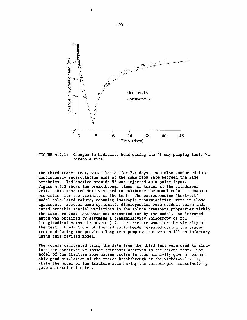
Measured
0 1 - I I I I I I I
' 0 8 16 24 32 40 48 Time (days)
FIGURE 4.4.1: Changes in hydraulic head during the 41 day pumping test, WL borehole site
The third tracer test, which lasted for 7.6 days, was also conducted in a continuously recirculating mode at the same flow rate between the same boreholes. Radioactive bromide-82 was injected as a pulse input. Figure 4.4.3 shows the breakthrough times of tracer at the withdrawal well. This measured data was used to calibrate the model solute transport properties for the vicinity of the test. The corresponding "best-fit" model calculated values, assuming isotropic transmissivity, were in close agreement. However some systematic discrepancies were evident which indi- cated probable spatial variations in the solute transport properties within the fracture zone that were not accounted for by the model. An improved match was obtained by assuming a transmissivity anisotropy of 5:l (longitudinal versus transverse) in the fracture zone for the vicinity of the test. Predictions of the hydraulic heads measured during the tracer test and during the previous long-term pumping test were still satisfactory using this revised model.
The models calibrated using the data from the third test were used to simu- late the conservative iodide transport observed in the second test. The model of the fracture zone having isotropic transmissivity gave a reason- ably good simulation of the tracer breakthrough at the withdrawal well, while the model.of the fracture zone having the anisotropic transmissivity gave an excellent match.
Measured u
Predicted +
5) 0 9 60 120 180 240 300 360 Time (days)
FIGURE 4.4.2: Changes in hydraulic head during the conservative Iodide tracer test, WL borehole site
The fourth tracer test was performed in the fracture zone between the same boreholes used in the previous two tests and lasted 176 days. A pulse of radioactive iodine-131 and sorbing, radioactive strontium-85 and cesium-134 was injected into a recirculating flow of 50 l/min. Figure 4.4.4 shows the breakthrough times of iodine-131 at the withdrawal well. The predictions are from the models calibrated using the data of the bromide-82 test. The agreement with the measurements is quite good but not as exact as for the calibration case. This slight difference is probably due to unmodelled variations in flow and transport properties. A good simulation for the strontium-85 breakthrough could not be obtained. The MOTIF code can only simulate uniform, linear, equilibrium sorption, but the actual sorption in the experiment was likely non-uniform and non-equilibrium (Applied Geo- science Branch Report 1991). It should be mentioned that the possible occurrence of non-equilibrium sorption in this experiment, which lasted for about half a year, does not necessarily imply that a non-equilibrium sorpt- ion model must be used for postclosure assessment on a time scale of many thousand years. However, this question deserves further study. No break- through of cesium-134 was measured, in accordance with expectations that the cesium-134 would sorb strongly onto fracture filling minerals.
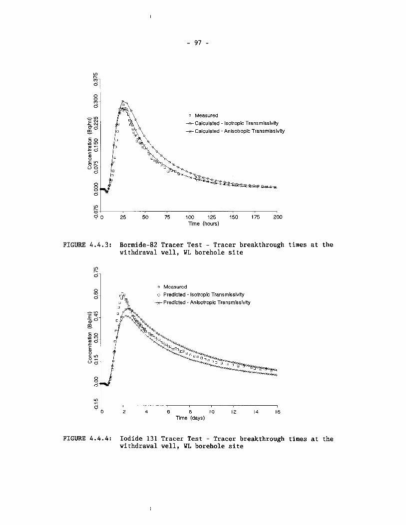
0 Measured
++Calculated - Isotropic Transmissivtty
x Calculated - Anisotropic Transrnissivity
Time (hours)
FIGURE 4.4.3: Bormide-82 Tracer Test - Tracer breakthrough times at the withdrawal well, WL borehole site
0 Measured 0
2 ++ Predlcted - Isotropic Transmissivity
x Predicted - Anisotropic Transmlssivity
A'D E -f. b0 m - g 53 a 0 b c P) 0
s 00
8 d
' 0 2 4 6 8 10 12 14 16 Time (days)
FIGURE 4.4.4: Iodide 131 Tracer Test - Tracer breakthrough times at the withdrawal well, WL borehole site
To summarize, with suitable calibration MOTIF transport models can accur- ately simulate groundwater tracer test results in fracture zones in pluton- ic rocks (at least for nonsorbing groundwater tracers). For sorbing tracers, MOTIF has some limitations particularly if non-uniform or non- equilibrium sorption occurs. Code enhancement is planned to improve the capability of MOTIF for modelling transport with nonuniform and non- equil- ibrium sorption. The following solute transport properties were estimated from these groundwater tracer tests in the 55 m portion of the major fracture zone at the WL site: effective thickness (product of porosity and fracture zone thickness) = 0.07-0.10 m ; longitudinal dispersivity =
5-9 m ; there was a slight non-equilibrium sorption of strontium-85; and, there was a considerable sorption of cesium-134.
4.5 VERIFICATION OF THE PARTICLE-TRACKING PROGRAM (TRACK3D)
Three test cases and an independent confirmation exercise were used to verify the accuracy and coding of the numerical particle-tracking code, TRACK3D. These are described briefly below. A more detailed account of the verification exercise and some of the results are given in Appendix P. A complete description, including our verification strategy and con- clusions, is also presented in Nakka and Chan (1994). The three verification cases are as follows:
1. Topographically driven, steady-state flow in a two-dimensional porous medium intersected by two highly permeable fracture zones. This is the same as the HYDROCOIN Level 1 (The International HYDROCOIN Project 1988) Case 2 problem, described in Section 4.2 on the MOTIF verification cases. Using the groundwater velocity distribution predicted by the MOTIF model for this test case, particle tracking was performed on four water particles in the flow field using TRACK3D. The results were compared with inde- pendent numerical results of Gureghian et al. (1987), Sauter and Hassanizadeh (1989) and Herbert (1985). The particle-tracking results obtained by the MOTIF-TRACK3D combination for this case are also included in the HYDROCOIN Secretariat's compilation and comparison of results submitted by various project teams (The International HYDROCOIN Project 1988).
2. HYDROCOIN Level 3, Case 7 Problem: Comparison of calculated flow paths to an analytical solution (Davis and Beyeler 1985). This problem dealt with steady-state flow in a homogeneous 2-D domain in the presence of a point sink and a flow stagnation point. A single well discharging at a constant rate was located in a uniform flow field to represent this situation. Particle tracking was performed on nine water particles in the flow field using TRACK3D and the particle tracking results were compared with streamlines derived from analytical solutions for the velocity potential and stream function, as provided by Bear (1972).
3. Three-dimensional transient flow in a rock mass containing simulated intersecting horizontal and vertical fracture zones: Comparison to an analytical solution (Nakka and Chan 1994). This case dealt with particle tracking in a hypothetical transient flow field of a 3-D region of a fractured rock containing inter- secting horizontal and vertical fracture zones. The form of the transient flow field in the rock region and in the fracture zones was reasonably general, yet simple enough to permit the analytical solution to be obtained by direct integration. Particle tracking was performed on 36 water particles in the flow field and the results were compared with those derived from an analytical solution.
In order to provide an independent confirmation of our results, Ontario Hydro (OH) Research developed a particle tracking program with similar capabilities to the TRACK3D program (Chan and Punhani 1991). This program used an algorithm entirely different from that used in TRACK3D. The OH program and TRACK3D were compared by modelling particle tracking in the 3-D steady-state flow field from MOTIF flow simulations for the natural and pumped condition of groundwater flow in the MOTIF WRA Local Flow Model. Both programs gave very similar results for these flow fields. The results of this comparison are also summarized in Appendix F.
As indicated by the graphical and tabulated comparisons in Appendix F, the TRACK3D results generally compare favourably with known analytical or numerical solutions. In verification test case ( I ) , TRACK3D pathlines are qualitatively similar to those present in the HYDROCOIN team reports. TRACK3D travel times are somewhat longer, possibly because of some numer- ical oscillation out of the fracture zone into the rock. The compilation in the International HYDROCOIN Project (1988) also indicates that the MOTIF-TRACK3D results lie within the range of results submitted by the various HYDROCOIN teams. In verification test case (2 ) , TRACK3D results are in close agreement with analytical predictions and numerical results obtained by the Runge-Kutta integration of an analytical expression for the particle velocity. The only exception is for a particle placed directly on the groundwater divide. There, TRACK3D results are accurate when the particle is distant from the stagnation point but become increasingly less accurate as the particle nears the stagnation point. The discrepancy results from omitting the stagnation point in the design of the finite- element mesh and is not caused by any inherent problem in TRACK3D. The effect can be mitigated by designing stagnation points into the mesh. In verification test case (3), errors between TRACK3D results and analytical predictions of mesh exit locations, travel distances and travel times each average about 1X for most particles, and the largest error in travel time is 5.3%. In the independent confirmation exercise, the particle tracking results obtained from TRACK3D compare favourably with the results obtained by a different particle tracking code developed by Ontario Hydro using an alternative tracking algorithm.
5. DETAILED GROUNDWATER FLOW MODELLING OF THE WHITESHELL RESEARCH AREA
5.1 INTRODUCTION
This chapter describes the detailed groundwater flow modelling done using the MOTIF and TRACK3D computer codes described in Chapter 3 in order to develop the GEONET geosphere model for the reference postclosure assessment case study.
First the development of the various models representing conditions at the Whiteshell Research Area (WRA) is discussed in general terms. This is followed by a detailed description of the conceptual hydrogeological model we developed for the WRA, and then by a summary of the two-dimensional thermohydrogeological sensitivity analysis performed with the MOTIF model. A summary of the three-dimensional thermohydrogeologica1 sensitivity analy- sis using the MOTIF model is given next, followed by a description of the model simulations used to finalize the GEONET geosphere model. Finally there is a brief discussion of the MOTIF modelling of the effects of an open borehole passing through a rock pillar near a waste emplacement room.
5.2 DEVELOPMENT OF THE WRA MODELS
In Section 1.5 we outlined the following process for developing a geosphere model :
- develop a conceptual hydrogeological model of the site and its surroundings,
- represent the conceptual model by a mathematical groundwater flow model,
- calibrate and evaluate the groundwater flow model,
- use the groundwater flow model to identify potential solute transport pathways from the disposal vault to groundwater dis- charge locations in the biosphere. These could be either the surface locations of discharge areas or the locations of domestic water supply wells in the vicinity of the disposal vault site, and
- represent the transport pathways from the vault to the discharge locations and their particular solute transport characteristics in a geosphere model.
To illustrate the process of developing a geosphere model for evaluating aspects of post closure vault performance we have used a case study. This case study considers a hypothetical disposal vault located at a depth of 500 m beneath the location of the Underground Research Laboratory (URL) at the Whiteshell Research Area (WRA). The conceptual hydrogeological model represents known and inferred conditions at the URL site and its surround- ings. The conceptual model is considered to be realistic in that it is
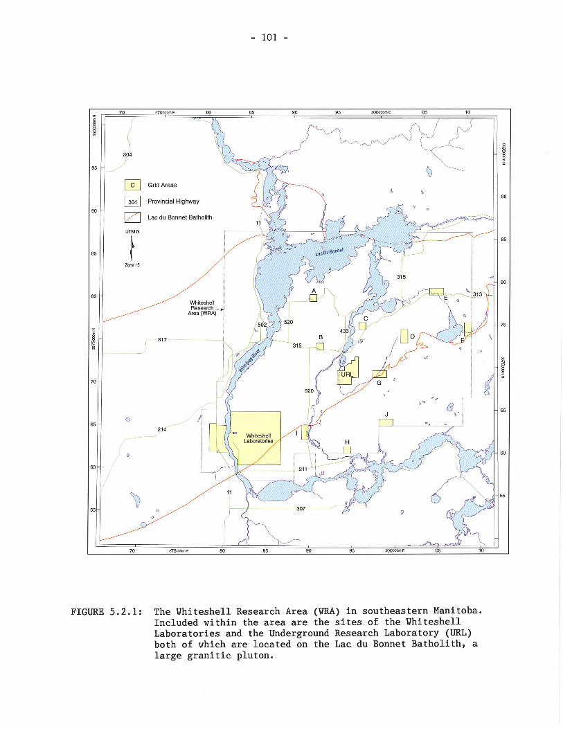
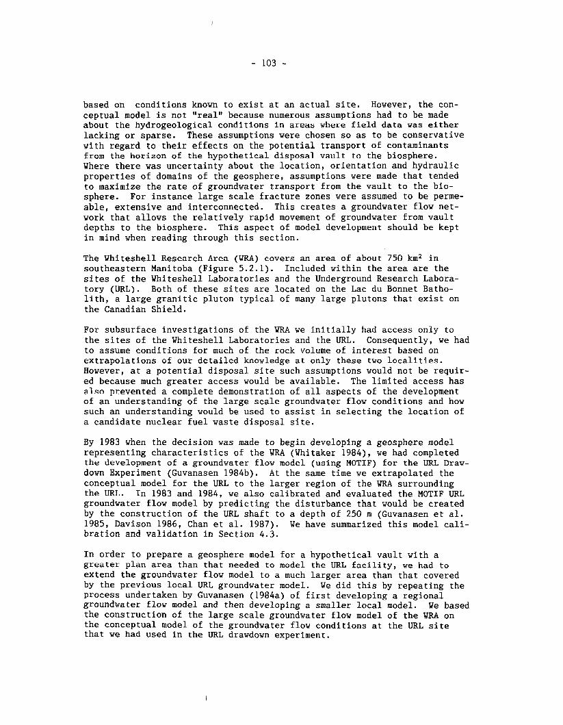
based on conditions known to exist at an actual site. However, the con- ceptual model is not "real" because numerous assumptions had to be made about the hydrogeological condltlons in areas where field data was either lacking or sparse. These assumptions were chosen so as to be conservative with regard to their effects on the potential transport of contaminants from the horizon of the hypothetical disposal vault to the biosphere. Where there was uncertainty about the location, orientation and hydraulic properties of domains of the geosphere, assumptions were made that tended to maximize the rate of groundwater transport from the vault to the bio- sphere. For instance large scale fracture zones were assumed to be perme- able, extensive and interconnected. This creates a groundwater flow net- work that allows the relatively rapid movement of groundwater from vault depths to the biosphere. This aspect of model development should be kept in mind when reading through this section.
The Whiteshell Research Area (WRA) covers an area of about 750 km2 in southeastern Manitoba (Figure 5.2.1). Included within the area are the sites of the Whiteshell Laboratories and the Underground Research Labora- tory (URL). Both of these sites are located on the Lac du Bonnet Batho- lith, a large granitic pluton typical of many large plutons that exist on the Canadian Shield.
For subsurface investigations of the WRA we initially had access only to the sites of the Whiteshell Laboratories and the URL. Consequently, we had to assume conditions for much of the rock volume of interest based on extrapolations of our detailed knowledge at only these two localities. However, at a potential disposal site such assumptions would not be requir- ed because much greater access would be available. The limited access has also prevented a complete demonstration of all aspects of the development of an understanding of the large scale groundwater flow conditions and how such an understanding would be used to assist in selecting the location of a candidate nuclear fuel waste disposal site.
By 1983 when the decision was made to begin developing a geosphere model representing characteristics of the WRA (Whitaker 1984), we had completed the development of a groundwater flow modcl (using MOTIF) for the URL Draw- down Experiment (Guvanasen 1984b). At the same time we extrapolated the conceptual model for the URL to the larger region of the WRA surrounding the URL. In 1983 and 1984, we also calibrated and evaluated the MOTIF URL groundwater flow model by predicting the disturbance that would be created by the construction of the URL shaft to a depth of 250 m (Guvanasen et al. 1985, Davison 1986, Chan et al. 1987). We have summarized this model cali- bration and validation in Section 4.3.
In order to prepare a geosphere model for a hypothetical vault with a greater plan area than that needed to model the URL facility, we had to extend the groundwater flow model to a much larger area than that covered by the previous local URL groundwater model. We did this by repeating the process undertaken by Guvanasen (1984a) of first developing a regional groundwater flow model and then developing a smaller local model. We based the construction of the large scale groundwater flow model of the WRA on the conceptual model of the groundwater flow conditions at the URL site that we had used in the URL drawdown experiment.
When we began the development of the geosphere model of the WRA, our avail- able computational resources also limited the number of nodes and elements we could include in a MOTIF finite-element mesh. As we developed a new large scale groundwater flow model for the WRA, this limitation meant that we could not retain the same degree of complexity used in the previous local model of the URL. We compromised by using the properties that had been used in the URL Drawdown Experiment for the features in the WRA model, but we gave the mesh a more regular geometry and abandoned detailed meshes around the locations of existing site characterization boreholes. Conse- quently, the groundwater flow model of the WRA we have used as the basis for the case study has not been directly calibrated using hydrogeological data from boreholes. By the time that we obtained access in 1986 to addit- ional areas in the regional area of the WRA for subsurface investigations (shown as permit areas in Figure 5.2.1), we were also developing the com- putational capability to incorporate the information needed to calibrate a regional groundwater flow model of the WRA. We also knew that we would have additional locations away from the URL and the Whiteshell Laboratories with borehole control at which calibrations of a large scale groundwater flow model could be done. However, the field data from the regional-scale groundwater flow investigations of the WRA would not be available soon enough to be able to develop a new calibrated groundwater flow model using MOTIF and incorporated into the postclosure assessment case study for the EIS.
An improved MOTIF groundwater flow model of the WRA, to be used for the geosphere model in the reference postclosure assessment case study, would have caused a delay, which in our view, could not have been justified. However, we are developing a revised groundwater flow model of the WRA using MOTIF, based on all the information obtained from our field investi- gations at the WRA between 1977 and 1993. The revised flow model will be calibrated against the records of historical data and used to select a new location for a hypothetical vault. Alternative locations will be evaluated with the view of selecting a location within the groundwater flow regime that maximizes the retention of contaminants in the geosphere. It will then be used to develop a geosphere model for that hypothetical disposal system.
Our current model of the WRA does not allow us to perform this type of analysis because there is a large degree of uncertainty in regions of the model away from the location of the URL site. Therefore, we have consider- ed only one location for the hypothetical disposal vault in the case study. We chose to locate the hypothetical disposal vault at a depth of 500 m in the WRA groundwater flow model near the location of the URL where there was the least uncertainty in the hydrogeological characteristics of the model.
5.3 THE CONCEPTUAL HYDROGEOLOGICAL MODEL OF THE WRA
5.3.1 Hvdroneolonical Structure
We based the initial conceptual model of hydrogeological conditions of the Whiteshell Research Area on the information we collected at the WL and URL sites up to 1985. We also studied linear geologic features mapped at the reconnaissance scale and linear geophysical anomalies identified from
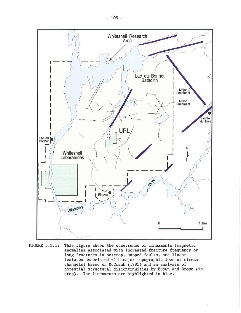
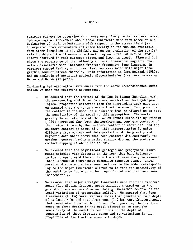
regional surveys to determine which ones were likely to be fracture zones. Hydrogeological inferences about these lineaments were then based on our evaluation of their orientations with respect to the stress field (as interpreted from information collected locally in the WRA and available from other locations on the Shield), and on our evaluation of the spatial relationship of the lineaments to fracturing and other structural indi- cators observed in rock outcrops (Brown and Brown in prep). Figure 5.3.1 shows the occurrence of the following surface lineaments: magnetic ano- malies associated with increased fracture frequency; long fractures in outcrop; mapped faults; and linear features associated with major topo- graphic lows or stream channels. This information is from McCrank (1985), and an analysis of potential geologic discontinuities (fracture zones) by Brown and Brown (in prep).
In drawing hydrogeological inferences from the above reconnaissance infor- mation we made the following assumptions.
- We assumed that the contact of the Lac du Bonnet Batholith with the surrounding rock formations was vertical and had hydrogeo- logical properties different from the surrounding rock mass i.e. we assumed that the contact was a fracture zone. Incorporating the contact in the model as a discrete feature allowed us to test the sensitivity of the model to this assumption. The early gravity interpretations of the Lac du Bonnet Batholith by Brisbin (1979) suggested that both the northern and southern contacts of the pluton dip north, the northern contact at about 55", and the southern contact at about 65". This interpretation is quite different from our current interpretation of the gravity and magnetic data which shows that both contacts dip southward, the northern contact having a rather shallow dip and the southern contact dipping at about 65" to 70".
- We assumed that the significant geologic and geophysical linea- ments coincide with features in the rock that have hydrogeo- logical properties different from the rock mass i.e., we assumed these lineaments represented permeable fraclure zones. Incor-- porating discrete fracture zone features in the model correspond- ing to the major lineaments allowed us to test the sensitivity of the model to variations in the properties of each fracture zone independently.
- We assumed that major straight lineaments were vertical fracture zones (low dipping fracture zones manifest themselves on the ground surface as curved or undulating lineaments because of the local variations of topographic relief). We assumed that long lineaments 0 5 km) were fracture zones that penetrated to a depth of at least 4 km and that short ones (1-5 km) were fracture zones that penetrated to a depth of 1 km. Incorporating the fracture zones to these depths in the model allowed us to test the sensitivity of the model to reductions in the depth of penetration of these fracture zones and to variations in the properties of the fracture zones with depth.
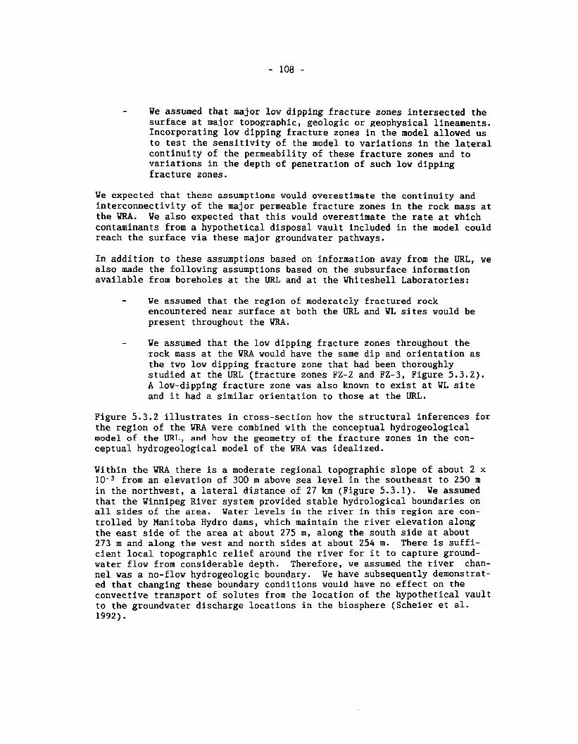
- We assumed that major low dipping fracture zones intersected the surface at major topographic, geologic or geophysical lineaments. Incorporating low dipping fracture zones in the model allowed us to test the sensitivity of the model to variations in the lateral continuity of the permeability of these fracture zones and to variations in the depth of penetration of such low dipping fracture zones.
We expected that these assumptions would overestimate the continuity and interconnectivity of the major permeable fracture zones in the rock mass at the WRA. We also expected that this would overestimate the rate at which contaminants from a hypothetical disposal vault included in the model could reach the surface via these major groundwater pathways.
In addition to these assumptions based on information away from the URL, we also made the following assumptions based on the subsurface information available from boreholes at the URL and at the Whiteshell Laboratories:
- We assumed that the region of moderately fractured rock encountered near surface at both the URL and WL sites would be present throughout the WRA.
- We assumed that the low dipping fracture zones throughout the rock mass at the WRA would have the same dip and orientation as the two low dipping fracture zone that had been thoroughly studied at the URL (fracture zones FZ-2 and FZ-3, Figure 5.3.2). A low-dipping fracture zone was also known to exist at WL site and it had a similar orientation to those at the URL.
Figure 5.3.2 illustrates in cross-section how the structural inferences for the region of the WRA were combined with the conceptual hydrogeological model of the URL, and how the geometry of the fracture zones in the con- ceptual hydrogeological model of the WRA was idealized.
Within the WRA there is a moderate regional topographic slope of about 2 x from an elevation of 300 m above sea level in the southeast to 250 m
in the northwest, a lateral distance of 27 km (Figure 5.3.1). We assumed that the Winnipeg River system provided stable hydrological boundaries on all sides of the area. Water levels in the river in this region are con- trolled by Manitoba Hydro dams, which maintain the river elevation along the east side of the area at about 275 m, along the south side at about 273 m and along the west and north sides at about 254 m. There is suffi- cient local topographic relief around the river for it to capture ground- water flow from considerable depth. Therefore, we assumed the river chan- nel was a no-flow hydrogeologic boundary. We have subsequently demonstrat- ed that changing these boundary conditions would have no effect on the convective transport of solutes from the location of the hypothetical vault to the groundwater discharge locations in the biosphere (Scheier et al. 1992).
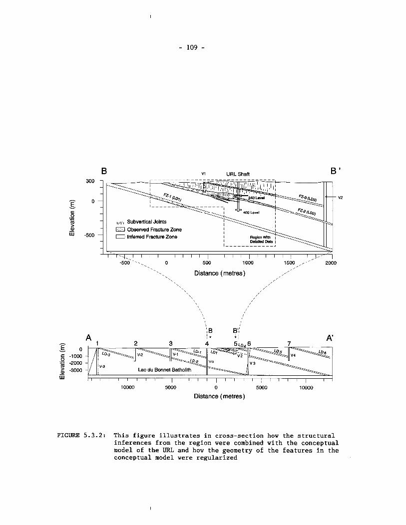
VI URL Shaft -
- -
- - -
- ,I+, Subvertical Joints
- 0 Observed Fracture Zone - 0 Inferred Fracture Zone
-
-
r - ~ I I I I I I I I I I I I I I I I I I I I I I I , ' I I . ,
,.
-. Distance (metres) ,
'>
\
\ \
, \
, \
, I
\ /
\ /
\ /
\ I
\ I
i I
I i I
: B B':
Distance ( metres)
FIGURE 5.3.2: This figure illustrates in cross-section how the structural inferences from the region were combined with the conceptual model of the URL and how the geometry of the features in the conceptual model were regularized
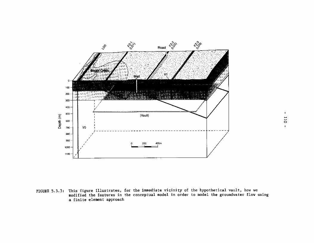
FIGURE 5 . 3 . 3 : This figure illustrates, for the immediate vicinity of the hypothetical vault, how we modified the features in the conceptual model in order to model the groundwater flow using a finite element approach
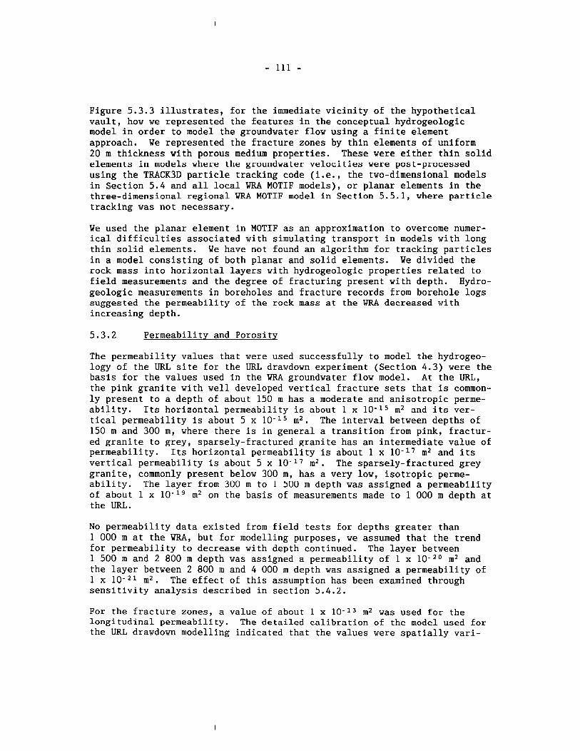
Figure 5.3.3 illustrates, for the immediate vicinity of the hypothetical vault, how we represented the features in the conceptual hydrogeologic model in order to model the groundwater flow using a finite element approach. We represented the fracture zones by thin elements of uniform 20 m thickness with porous medium properties. These were either thin solid elements in models where the groundwater velocities were post-processed using the TRACK3D particle tracking code (i.e., the two-dimensional models in Section 5.4 and all local WRA MOTIF models), or planar elements in the three-dimensional regional WRA MOTIF model in Section 5.5.1, where particle tracking was not necessary.
We used the planar element in MOTIF as an approximation to overcome numer- ical difficulties associated with simulating transport in models with long thin solid elements. We have not found an algorithm for tracking particles in a model consisting of both planar and solid elements. We divided the rock mass into horizontal layers with hydrogeologic properties related to field measurements and the degree of fracturing present with depth. Hydro- geologic measurements in boreholes and fracture records from borehole logs suggested the permeability of the rock mass at the WRA decreased with increasing depth.
5.3.2 Permeability and Porosity
The permeability values that were used successfully to model the hydrogeo- logy of the URL site for the URL drawdown experiment (Section 4.3) were the basis for the values used in the WRA groundwater flow model. At the URL, the pink granite with well developed vertical fracture sets that is common- ly present to a depth of about 150 m has a moderate and anisotropic perme- ability. Its horizontal permeability is about 1 x 10-15 m2 and its ver- tical permeability is about 5 x 10-l5 m2. The interval between depths of 150 m and 300 m, where there is in general a transition from pink, fractur- ed granite to grey, sparsely-fractured granite has an intermediate value of permeability. Its horizontal permeability is about 1 x 10-I' m2 and its vertical permeability is about 5 x 10-l7 m2. The sparsely-fractured grey granite, commonly present below 300 m, has a very low, isotropic perme- ability. The layer from 300 m to 1 500 m depth was assigned a permeability of about 1 x 10-l9 m2 on the basis of measurements made to 1 000 m depth at the URL.
No permeability data existed from field tests for depths greater than 1 000 m at the WRA, but for modelling purposes, we assumed that the trend for permeability to decrease with depth continued. The layer between 1 500 m and 2 800 m depth was assigned a permeability of 1 x 10- 20 m2 and the layer between 2 800 m and 4 000 m depth was assigned a permeability of 1 x m2. The effect of this assumption has been examined through sensitivity analysis described in section 5.4 .2 .
For the fracture zones, a value of about 1 x 10-l3 m2 was used for the longitudinal permeability. The detailed calibration of the modcl used for the URL drawdown modelling indicated that the values were spatially vari-
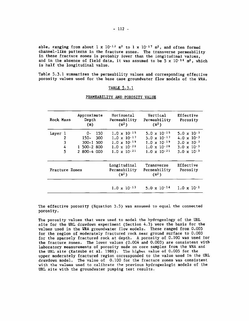
able, ranging from about 1 x 1 0 - l 2 m2 to 1 x 10 - l7 m2, and often formed channel-like patterns in the fracture zones. The transverse permeability in these fracture zones is probably lower than the longitudinal values, and in the absence of field data, it was assumed to be 5 x 10 - l4 m2, which is half the longitudinal value.
Table 5.3.1 summarizes the permeability values and corresponding effective porosity values used for the base case groundwater flow models of the WRA.
TABLE 5.3.1
PERMEABILITY AND POROSITY VALUE
Approximate Horizontal Vertical Effective Rock Mass Depth Permeability Permeability Porosity
(m) (m2 ) (m2 > Layer 1 0- 150 1 . 0 x 1 0 - ~ ~ 5 . 0 x 1 0 - ~ ~ 5 . 0 x 1 0 - ~
2 150- 300 1.0 x 10 - l7 5.0 x 10 - l7 4.0 x l o m 3 3 300-1500 ~ . O X ~ O - ~ ~ ~ . O X ~ O - ~ ~ 3 . 0 ~ 1 0 - ~ 4 1 5 0 0 - 2 8 0 0 1 . 0 ~ 1 0 - ~ ~ 1 . 0 ~ 10-*0 3 . 0 ~ l o - 3 5 2800-4000 1 . 0 ~ 1 0 - ~ ~ 1 . 0 ~ 1 0 - ~ ~ 3 . 0 ~ 1 0 - ~
Longitudinal Transverse Effective Fracture Zones Permeability Permeability Porosity
(m2 1 (m2 )
The effective porosity (Equation 3.5) was assumed to equal the connected porosity . The porosity values that were used to model the hydrogeology of the URL site for the URL drawdown experiment (Section 4.3) were the basis for the values used in the WRA groundwater flow models. These ranged from 0.005 for the region of moderately fractured rock near ground surface to 0.003 for the sparsely fractured rock at depth. A porosity of 0.100 was used for the fracture zones. The lower values (0.004 and 0.003) are consistent with laboratory measurements of porosity made on core samples from the WRA and the URL site (Katsube et al. 1986). The higher value of 0.005 for the upper moderately fractured region corresponded to the value used in the URL drawdown model. The value of 0.100 for the fracture zones was consistent with the values used to calibrate the previous hydrogeologic models of the URL site with the groundwater pumping test results.
Other recent work at the Whiteshell Laboratories borehole site and the URL site has shown that the porosity within the major fracture zones in the Lac du Bonnet Batholith can be quite variable and can range from less than .O1 to greater than .15.
5.3.3 Other Properties
In addition to the permeability and porosity distributions described in the previous section, values for other properties required to calculate solute transport were selected for the numerical model. These values are summarized in Table 5.3.2.
The dry bulk compressibilities of the background rock mass and the fracture zones were assumed to be 1.0 x 10- Pa- l and 1.0 x Pa- l respectively, based on literature values reported by Freeze and Cherry (1979). The fluid compressibility was assigned a value of 4.5 x 10-lo Pa-l (Weast 1971). This is the value corresponding to the spatially averaged geothermal temp- erature of 29"C, estimated from measurements at the URL by Drury (1982).
The selec~ed values of parameters controlling heat transport are as follows: effective thermal conductivity 3.34 W/(m."C) (Drury 1980); specific heat of rock 8.0 x lo2 J/(kgO0C) (Acres 1978); specific heat of fluid 4.2 x lo3 J/(kg.OC) (Weast 1971); solid phase of the rock density 2.640 x lo3 kg/m3 (Percival et al. 1983); longitudinal dispersivity 6.0 m; and transverse dispersivity 6.0 x 10-I m. The dispersivity values are considered to be approximate but they are not very important for the heat transport results. Conduction is by far the dominant heat transport mechanism (Scheier et al. 1992) due to the low porosity of the rock.
For the fluid density equation (3.13), Lhe reference temperature is 25"C, the reference density is 9.971 x lo2 kg/m3 (Weast 1971), and the reference compressibility of water is 4.57 x 10-lo Pa-l (Weast 1971). The coeffi- cients A and B have been determined to have values of -3.17 x 10⁻⁴ "C-1 and -2.56 x o C - ~ by curve fitting to experimental data (Forsythe 1964).
For the fluid viscosity equation (3.14) the coefficients A, and B, have been determined to have values of 1.98404 x Pa-s and 1.82585 x lo3 "C respectively, by curve fitting to experimental data (Forsythe 1964).
For the reference head equation (3.3) the reference fluid density is assigned a value of 1.0 x lo3 kg/m3. This density is the value for fresh water at atmospheric pressure and a temperature of 6°C. This temperature is the estimated mean value just below the surface of the geosphere, based on measurements at the URL by Drury (1982).
TWO DIMENSIONAL THERMOHYDROGEOLOGICAL SENSITIVITY ANALYSIS
This section describes two-dimensional simulations to: help in the initial definition of an adequate three-dimensional representation, select a suit- able form for the SYVAC3-CC3 geosphere model, and perform some sensitiviLy analyses.
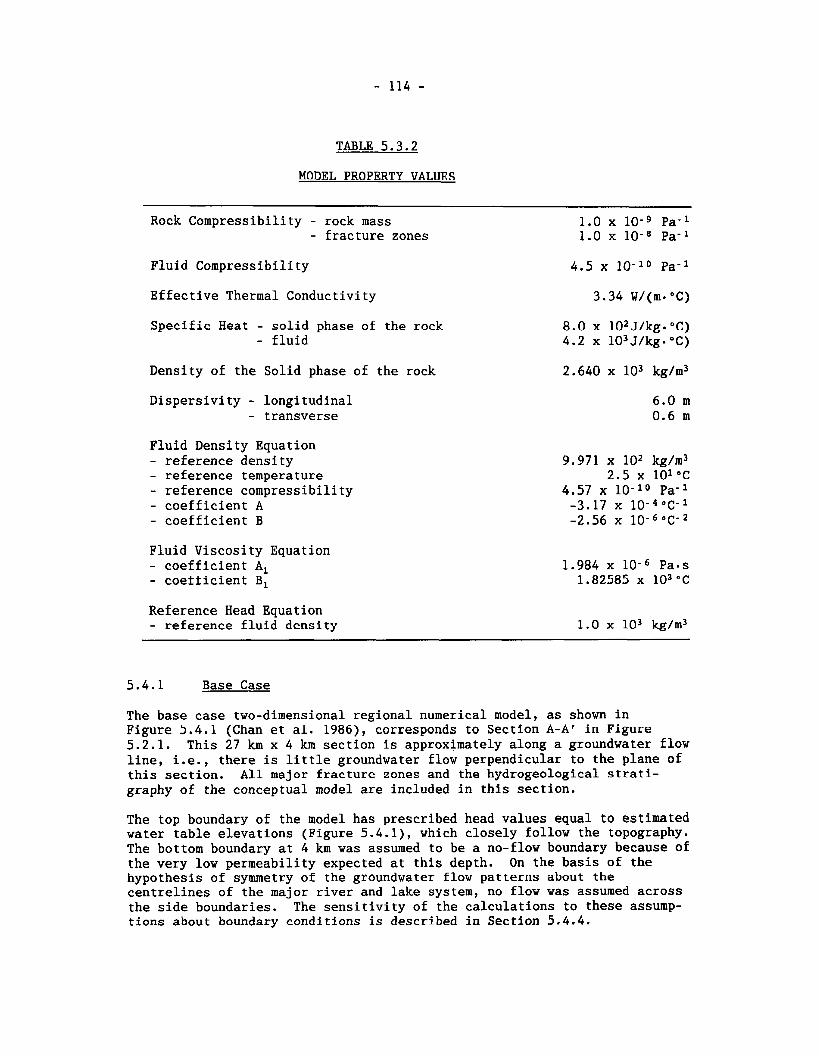
TABLE 5.3.2
MODEL PROPERTY VALUES
Rock Compressibility - rock mass - fracture zones
Pluid Compressibility
Effective Thermal Conductivity
Specific Heat - solid phase of the rock - fluid
Density of the Solid phase of the rock
Dispersivity - longitudinal - transverse
Fluid Density Equation - reference density - reference temperature - reference compressibility - coefficient A - coefficient B
Pluid Viscosity Equation - coefficient Al - coefficient B,
Reference Head Equation - reference fluid density
5.4.1 Base Case
The base case two-dimensional regional numerical model, as shown in Figure 5.4.1 (Chan et al. 1986), corresponds to Section A-A' in Figure 5.2.1. This 27 km x 4 km section is approximately along a groundwater flow line, i.e., there is little groundwater flow perpendicular to the plane of this section. All major fracture zones and the hydrogeological strati- graphy of the conceptual model are included in this section.
The top boundary of the model has prescribed head values equal to estimated water table elevations (Figure 5.4.1), which closely follow the topography. The bottom boundary at 4 km was assumed to be a no-flow boundary because of the very low permeability expected at this depth. On the basis of the hypothesis of symmetry of the groundwater flow patterns about the centrelines of the major river and lake system, no flow was assumed across the side boundaries. The sensitivity of the calculations to these assump- tions about boundary conditions is described in Section 5.4.4.

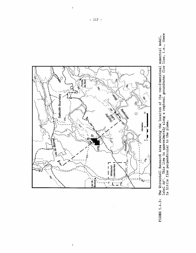
FIGURE 5.4.2:
The Whiteshell
Res
earc
h Area sh
owin
g the lo
cati
on of
the
two-
dime
nsio
nal nu
meri
cal model,
label
AA
'.
This
line is ap
prox
imat
ely al
ong a reg
iona
l gr
ound
wate
r flow lin
e, i.e., th
ere
is little flow per
pend
icul
ar to the
plane.

All boundary temperatures were based on the geothermal measurements at the URL (Drury 1982). The top boundary temperature was held at 6°C and the other boundary values were based on an average geothermal gradient of 11.5 OC/km.
Prior to analyzing the impact of the hypothetical vault, the steady-state condition under the combined influence of topography and the natural geothermal gradient was determined.
The hypothetical vault was located at a depth of 500 in at the URL site (Figures 5.4.1 and 5.4.3). It was intentionally located to intersect the plane of a hypothesized major low-dipping fracture zone (fracture zone LDl), in order to assess how sensitive the transport of contaminants from the vault to groundwater discharge locations was to the proximity of the fracture zone. It is now known from field investigations that fracture zone LD1 does not extend to this depth but rather it pinches out at a depth of about 450m. Therefore, the rate of movement of groundwater up the fracture zone from the depth of the vault to surface discharge locations has been over-estimated by the model used in the case study. Recent model- ling shows that this has the effect of increasing the time it takes for groundwater to move within the fracture zone from 450 m depth to ground surface from about 1 000 years for the non-truncated case to about 45 000 years for the truncated case (Stanchell 1992). The vault was assumed to have the same physical properties as the surrounding rock (Layer 3), and was modelled solely as a planar heat source. The heat output of the vault was initially 11.59 W/m2, which decayed to 0 in 100 000 a, as shown in Table 5.4.1 (Scheier et al. 1992).
To check numerical convergence of results, two meshes and three time-step- ping sequences of differing refinement were used in this analysis. Figure 5.4.3 illustrates the coarse-mesh option for the vault region. Small elements were used near the vault and fracture zones, with a progres- sive increase in size further away. This was done to ensure accurate cal- culation of heat transport and groundwater velocities along likely radio- nuclide pathways. Transient simulations were conducted for a period of one million years using geometrically increasing time steps. The numerical convergence study showed that the coarse mesh and medium time-stepping sequence were suitable for most cases considered in this analysis . A check was also made to ensure that the simulation conserves fluid mass over the entire model.
Examples of calculated temperature and groundwater flow velocities near the vault are shown in Figure 5.4.4. Locations M and L are about 100 m above the vault, in the rock mass and in the low-dipping fracture zone that intersects the vault, respectively (see Figure 5.4.3). Location V is about 200 m above the vault in a vertical fracture zone 325 m from the edge of the vault. In this simulation the groundwater flow velocity in fracture zones near the vault is of the order of 1 m/a. In the rock mass outside the fracture zones, velocities are typically four orders of magnitude lower. In general, the perturbation in both temperature and groundwater velocity lasts about 100 000 years.
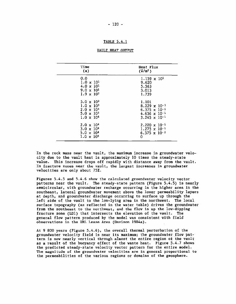
TABLE 5.4.1
VAULT HEAT OUTPUT
Time (a)
Heat Flux (W/m2 )
In the rock mass near the vault, the maximum increase in groundwater velo- city due to the vault heat is approximately 10 times the steady-state value. This increase drops off rapidly with distance away from the vault. In fracture zones near the vault, the largest increases in groundwater velocities are only about 75%.
Figures 5.4.5 and 5.4.6 show the calculated groundwater velocity vector patterns near the vault. The steady-state pattern (Figure 5.4.5) is nearly semicircular, with groundwater recharge occurring in the higher area in the southeast, lateral groundwater movement above the lower permeability layers at depth, and groundwater discharge occurring to surface up through the left side of the vault to the low-lying area in the northwest. The local surface topography (as reflected in the water table) drives the groundwater from the southeast to the northwest, and the flow is up the low-dipping fracture zone (LD1) that intersects the elevation of the vault. The general flow pattern produced by the model was consistent with field observations in the URL Lease Area (Davison 1984a).
At 9 800 years (Figure 5.4.6), the overall thermal perturbation of the groundwater velocity field is near its maximum; the groundwater flow pat- tern is now nearly vertical through almost the entire region of the vault as a result of the buoyancy effect of the waste heat. Figure 5.4.7 shows the predicted steady-state velocity vector pattern for the entire model. The magnitude of the groundwater velocities are in general proportional to the permeabilities of the various regions or domains of the geosphere.

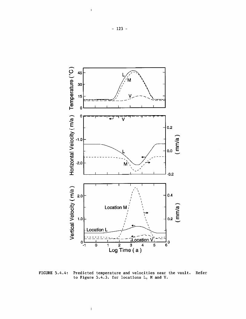
Log Time ( a )
FIGURE 5.4.4: Predicted temperature and velocities near the vault. Refer to Figure 5.4.3. for locations L, M and V.
0.4
h
a \
E 0.2 E
w
o
h
m \
E 2.0 w
> C, . - 0 0 - a, > 1.0- - a 0 .- e f
0 -1 0 1 2 3 4 5 6
I I I I I I
,/' I \
- I \\ - ; \
I 1
- Location M ,' \ - \
I I
I ?
I \ - \
I \
r l + \
- Location L- / - - - - - - - - - I + / -L \ ' - - - - - - ---- L -, " --; =
I I I ';Location V I

The configuration of the major fracture zones, particularly the low-dipping zones, has a strong influence on the directions and velocities of groundwater flow. Some numerical fl~ictuations were found to exist at a distance from the vault because of the relatively coarse finite element discretization in these areas. Subsequent particle track analyses showed that these numerical fluctuations do not affect the predicted flow paths, from the vault to groundwater discharge areas at surface, so no further refinement of the discretization was carried out.
As an initial step in transport modelling, the particle tracking code TRACK3D described in Section 3.3 was used to calculate advective pathlines and travel times based on the groundwater velocity distributions generated by the MOTIF model. Figure 5.4.8 shows the predicted steady-state path- lines for the entire model. The influence of the fracture zones on the pattern and rate of groundwater flow in the area is obvious. Figure 5.4 .9 illustrates estimated travel times for selected particles released from the hypothetical vault location into the groundwater flow field surrounding the vault. The path lengths from the vault horizon to the surface do not vary a great deal, and are about two to three times the depth of the vault. However, the travel times along the different grourldwater pathways in this simulation vary from 890 years to 26 million years. The fastest path, 890 years along path D, occurs up the low-dipping fracture zone that intersects the the vault horizon.
The effect of geothermal and vault heat on convective transport is summar- ized in Table 5.4.2 for particles released from the hypothetical vault location into the groundwater flow field, for paths illustrated in Figure 5.4.9. The geothermal gradient has minimal influence on the length of the flow path, but it reduces the groundwater travel times by about 20 to 25% from the isothermal values. The vault heat also has minimal effecl on the path length, but it reduces the travel time along the major low- dipping fracture zone, LD1, by about 30% from the values in the situation which considers only geothermal heat. There is negligible effect on groundwater travel times if a significant percentage of the groundwater flow path is through the sparsely-fractured rock mass. The small effect of the vault heat on convective transport in the sparsely fractured rock mass, despite a significant peak perturbation to velocities, is due to the fact that the transport is extremely slow through the sparsely fractured region of the rock. The result is that most of the transport through the sparse- ly-fractured region occurs during times when there is minimal thermal per- turbation to the flow field. The total convective transport time is two orders of magnitude longer than the duration of the velocity perturbation caused by vault heating in this sparsely-fractured region of the rock.
These results indicate that a wide range of radionuclide transport regimes should be considered in the geosphere model for performance assessment calculations. One extreme involves rapid groundwater convection in a major low-dipping fracture zones that might transect the rock mass near the dis- posal vault. In the other extreme, convective transport by groundwater flow through sparsely fractured regions of the rock mass can be negligible compared to diffusion, dispersion and retardation mechanisms.
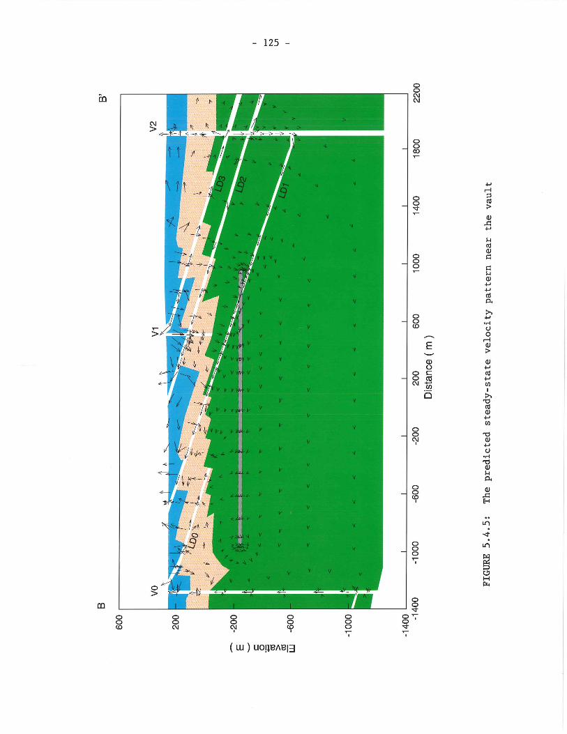
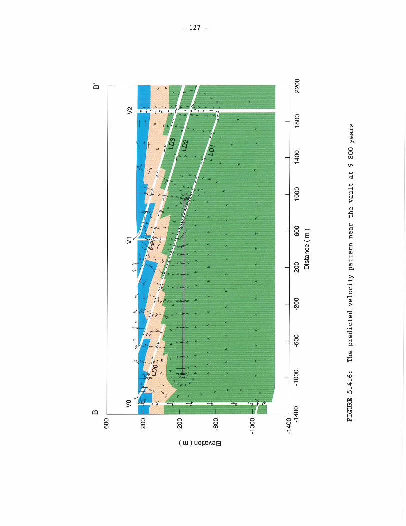
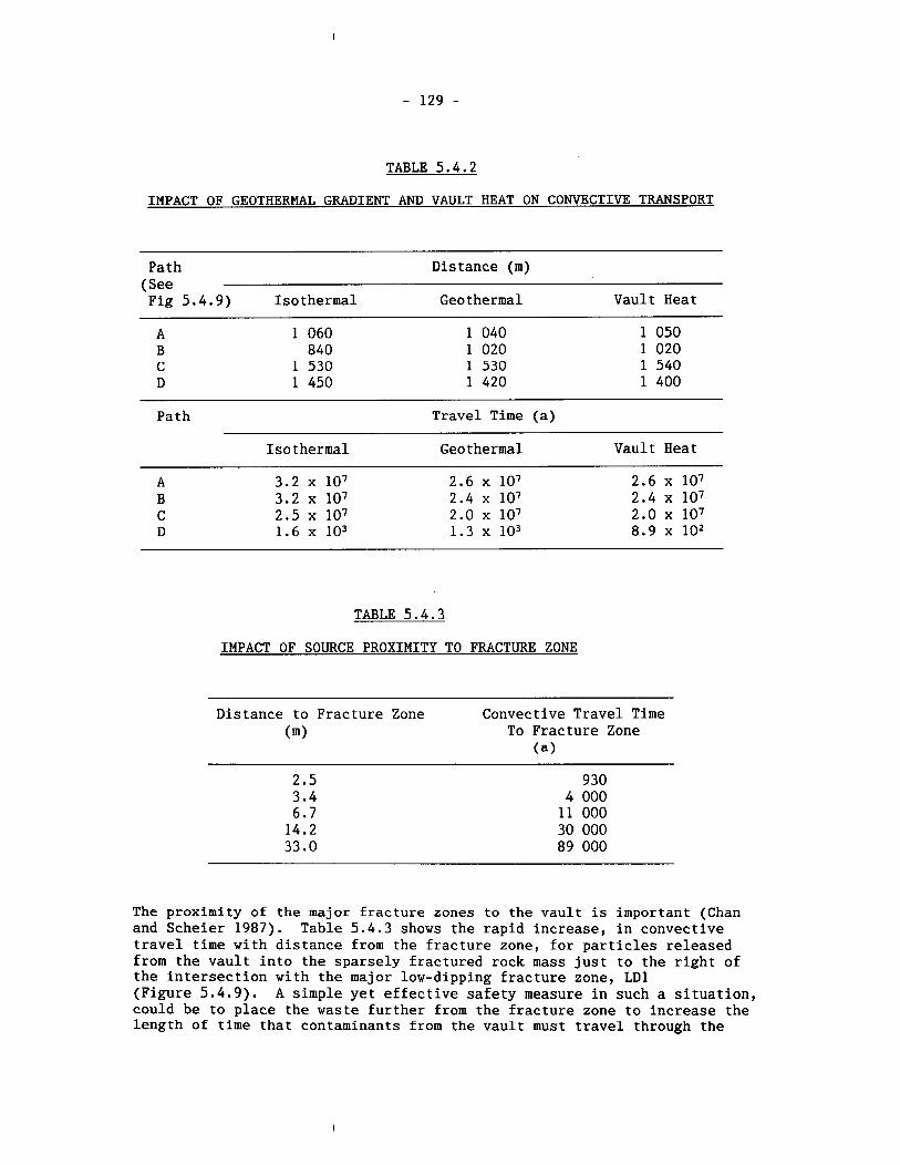
TABLE 5.4.2
IMPACT OF GEOTHERMAL GRADIENT AND VAULT HEAT ON CONVECTIVE TRANSPORT
Path Distance (m) ( See Fig 5.4.9) Isothermal Geothermal Vault Heat
Path Travel Time (a)
Isothermal Geothermal Vault Heat
TABLE 5.4.3
IMPACT OF SOURCE PROXIMITY TO FRACTURE ZONE
Distance to Fracture Zone Convective Travel Time (m> To Fracture Zone
(a>
The proximity of the major fracture zones to the vault is important (Chan and Scheier 1987). Table 5.4.3 shows the rapid increase, in convective travel time with distance from the fracture zone, for particles released from the vault into the sparsely fractured rock mass just to the right of the intersection with the major low-dipping fracture zone, LD1 (Figure 5.4.9). A simple yet effective safety measure in such a situation, could be to place the waste further from the fracture zone to increase the length of time that contaminants from the vault must travel through the

sparsely-fractured region of the rock mass, before entering the rapidly moving groundwater flow field within the fracture zone.
To ensure adequate representation of diffusion and dispersion in construct- ing the SYVAC3-CC3 geosphere model, detailed multi-dimensional, convective- dispersive transport modelling is also required. This is presented in Section 6.8.
5.4.2 Layer Properties
To assess the adequacy of using a 1.5 km deep model rather than a 4 km deep model, a case was simulated in which the lower two depth layers of the hydrogeologic model were considered to be practically impermeable. In this case the permeability of the lower two layers (see Figure 5.4.1) was reduced to 1 x m2 from the previously used values of 1 x m2 and 1 x m2, respectively. The bottom 2.5 km lengths of the fully-pene- trating vertical fracture zones V-3, VO, V3 and V5 were also deleted for this analysis. The predicted heads and groundwater flow velocities in the upper three layers of the model (down to 1.5 km) are almost identical to those for the base case where the model extended to 4 km depth. This is not surprising, since in the base case there is relatively little ground- water flow occurring in the lower two layers. There are no significant changes in the groundwater travel paths or times for particles convected from the hypothetical vault to the groundwater discharge locations.
A case considering the lower two layers having hydrogeologic properties equal to the properties of the middle layer of the model was also simulated because no field data are actually available for the lower two layers. In this case the permeability of the lower three layers was assumed to be constant at 1 x 10-l9 m2. Modelling of this case indicated there were no changes in the groundwater flow pattern in the upper three layers but, as expected, there was slightly more regional continuity of groundwater flow through the deeper layers of the model and somewhat higher groundwater flow velocities at depth than in the base case simulation.
The impact of possible permeability anisotropy in the middle layer of the model was investigated by increasing its vertical permeability to 5 x 10-l9 m2 from 1 x 10-l9 m2, giving the same degree of anisotropy as for the top two layers of the model. This resulted in a slight increase in vertical velocity components in the middle layer. The effect on convective transport from the vault to the discharge areas was minimal however and the maximum decrease in travel time was only 4%.
5.4.3 Fracture Zone Configuration
A simulation was preformed in which the vertically-oriented fracture zones VO and V3 (Figure 5.4.11) were truncated at shallower depths. In the con- ceptual hydrogeological model, vertical fracture zone VO (see Figure 5.4.1) was postulated to exist beneath the Lee River (Figure 5.2.1), although no subsurface investigations had been carried out to prove its existence at the time the conceptual model was constructed.
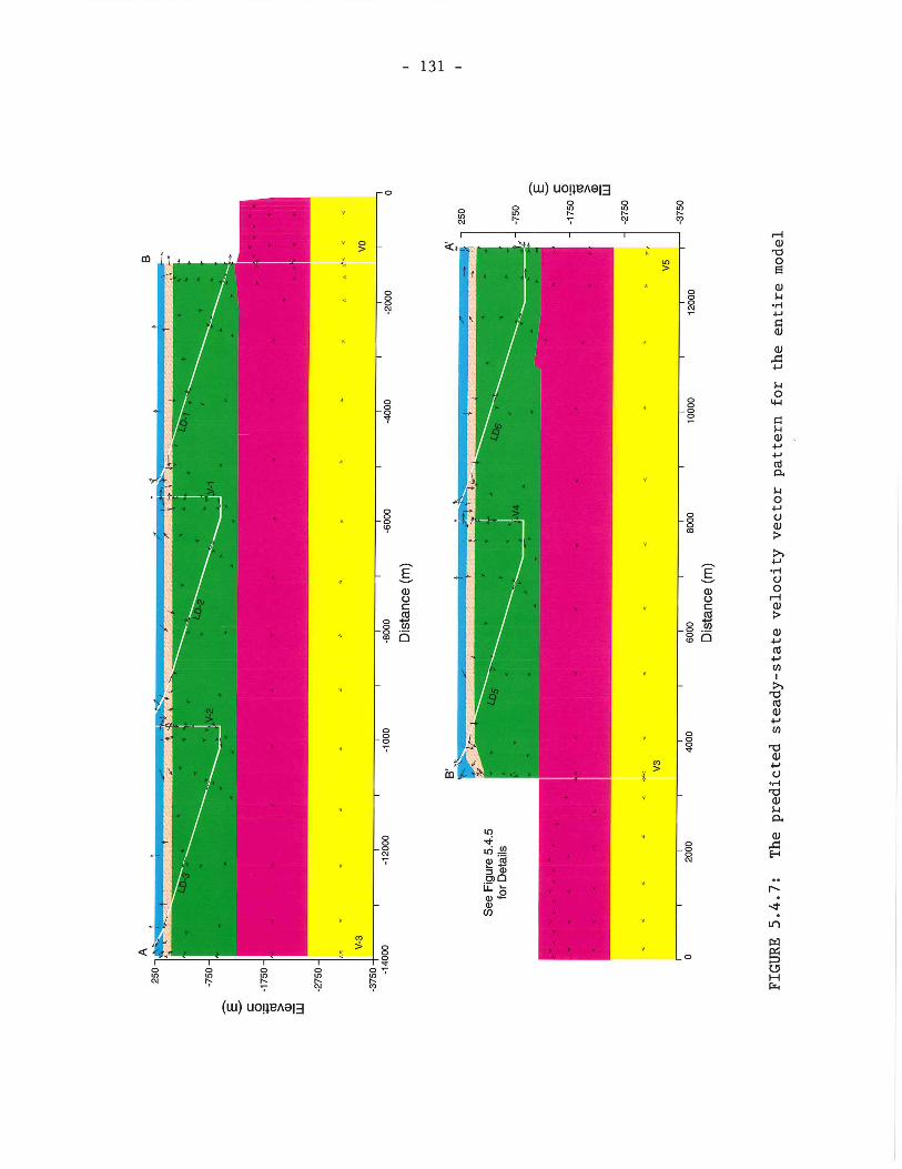
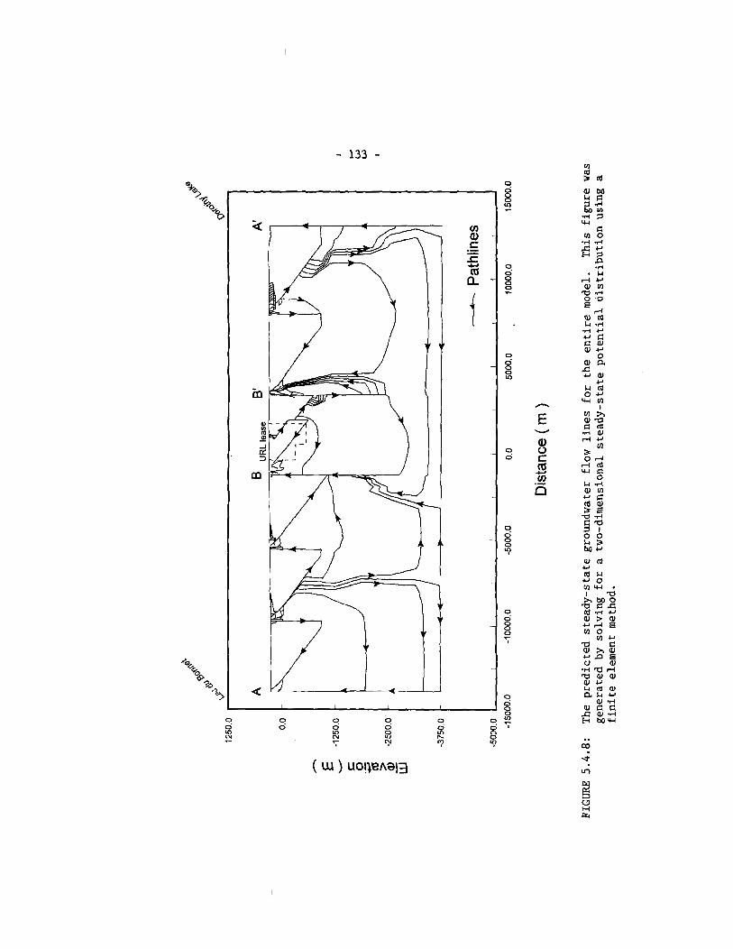
Dis
tanc
e (
m )
FIGU
RE 5
.4.8
: The
predicted
steady-state groundwater flow lines for the entir
e model.
This figure was
generated
by solving
for
a two-dimensional steady-state poten
tial
distribution using
a
finite element method.
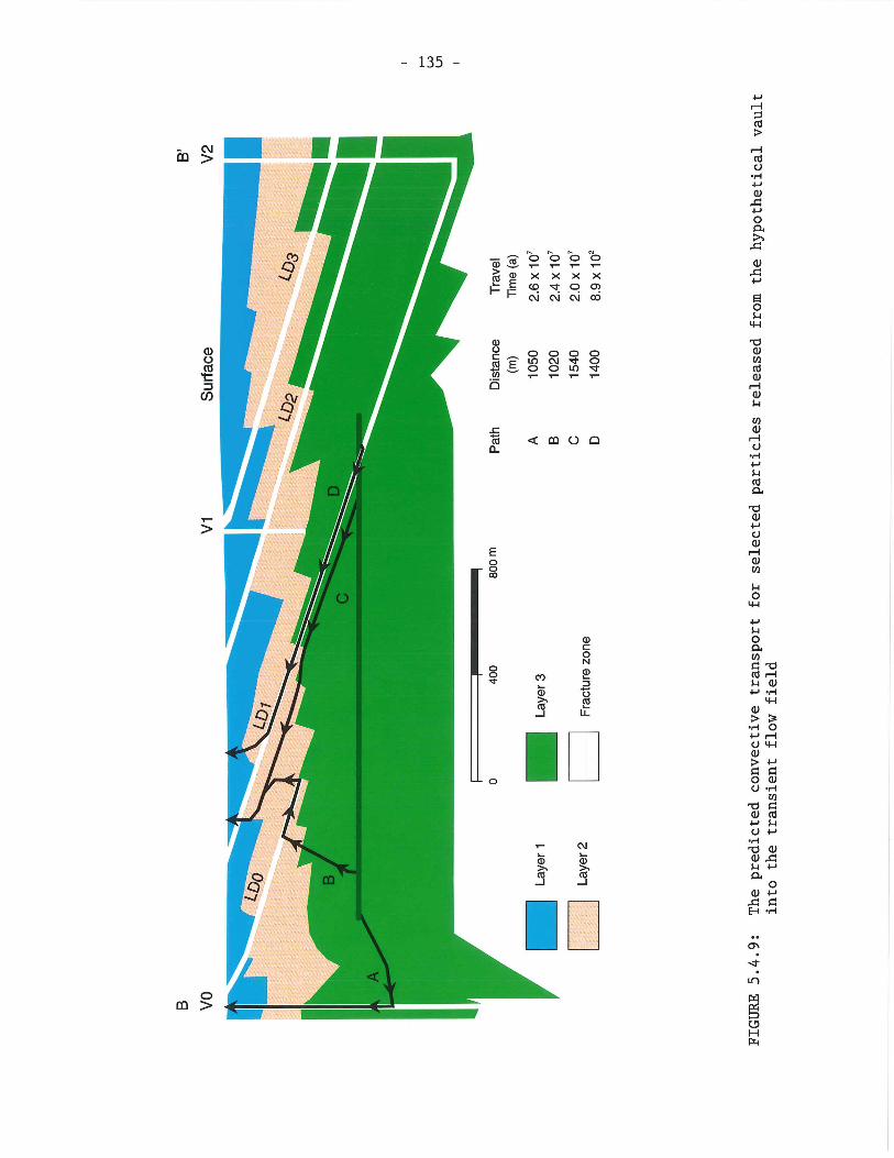
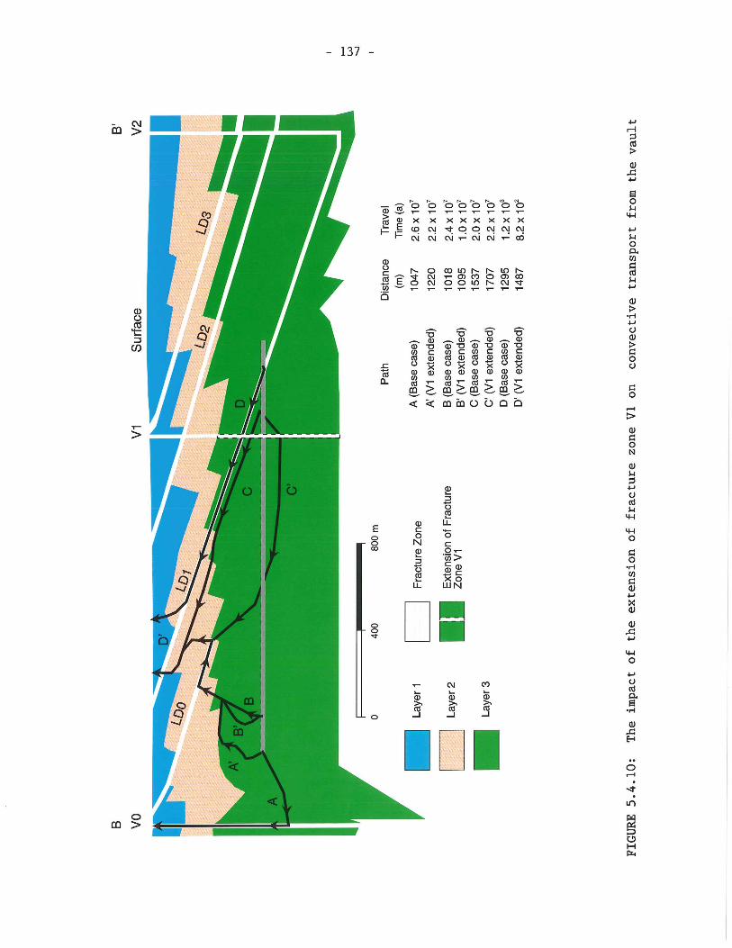

In the base case it was assumed to fully penetrate the 4 km depth of the model. In this alternate case the zone was assumed to extend down only to the depth of its intersection with the low-dipping fracture zone LD-1.
In the original conceptual model, the vertical fracture zone V3 (see Figure 5.4.7) was also postulated to exist at the southern boundary of the pluton, although no subsurface investigations had been carried out in the area at that time. In the base case it was assumed to fully penetrate the model. In this alternative case it was assumed to extend down only to the depth of its intersection with low-dipping fracture zone LD2.
These changes were found to have negligible effect on convective ground- water transport from the vault to the groundwater discharge locations.
Recent field investigations at the southern boundary of the pluton have shown that the pluton boundary actually dips at a southerly angle and there is no evidence of a major vertical fracture zone coinciding with the bound- ary. Therefore a simulation was performed without including the vertical fracture zone V3 in the model. This deletion results in no significant changes in the overall groundwater flow pattern and has no effect on the convective transport pathways leading from the vault to the groundwater discharge areas.
The existence of the vertical fracture zone V2 (see Figure 5.4.3) joining low-dipping fracture zone LD1 and LD2 has been inferred from interpreting groundwater pumping tests performed at the URL site, but it has not actual- ly been detected by any borehole drilling on the site. Therefore, a simu- lation has been performed without including fracture zone V2 in the model. The calculated groundwater velocities near the vault region are much lower in this case. This is a clear indication that the calculated groundwater travel time, from the vault to ground surface, would be much longer than in the base case model, if LD1 were not connected to the surface by a major vertical fracture zone. The predicted groundwater flow in fracture zone LD2 is also reversed compared to the base case. This is contrary to the field observations of groundwater flow up this fracture zone (Davison 1984a). This sensitivity analysis helps to confirm the existence of a hydrogeologic feature such as fracture zone V2, or an equivalent set of vertical fractures connecting the surface with at least fracture zone LD2 in this location of the WRA.
A case considering the possibility of fracture zone V1 extending down, to intersect low-dipping fracture zone LD1 as well as the depth horizon of the hypothetical vault, has also been simulated. Figure 5.4.10 illustrates the impact of this assumption on calculated convective groundwater transport from the vault. The groundwater travel paths from this analysis are slightly longer while the groundwater travel time can be either somewhat longer or shorter. The fastest convective groundwater flow path, Path D, is still up the low-dipping fracture zone LD1 in this case, but the travel time up the zone is reduced by 30X due to the effect of the interconnecting vertical fracture zone.
5.4.4 Boundary Conditions
The following simulations were performed to assess the significance of the assumption of a no-flow condition across the side boundaries of the model.
Since the land to the southeast of Dorothy Lake continues to rise gradually for several kilometres, it was considered possible that there was actually some component of groundwater flow occurring below Dorothy Lake, from the upland area to the southeast into the modelled region (Figures 5.4.1 and 5.4 .2) . In order to test this possibility a simulation was performed in which it was assumed that the southeast-side boundary of the model has a vertically varying groundwater inflow along it. This inflow was calculated using: Darcy's law, the average regional topographic gradient of 0.002, and the permeability of the layer the flow is entering.
To the northwest of Lac du Bonnet the topography also continues to gradual- ly decline for several kilometres (Figure 5.4.2) . Therefore it was con- sidered possible that some groundwater flow to the northwest could be occurring out of the modelling region below Lac du Bonnet(Figure 5.4.1). To investigate this possibility a simulation was conducted with the north- west boundary of the model having a specified head equal to the lake sur- face elevation. The boundary condition at the southeast side of the model was assumed to have the same inflow condition as used in the previous case.
Another case we considered was the effect of a major change in regional groundwater flow patterns, i.e., a reversal in the regional topographic slope. In this study we examined the effects of groundwater outflow occur- ring below Dorothy Lake, at the southeast-side boundary of the model. The case actually simulates a total reversal in the direction of regional groundwater flow through the area, an extremely unlikely situation even for the next tens of thousands of years.
The only effects that were observed in simulating all of the above cases, occurred only very close to the side boundaries of the model. The ground- water flow patterns throughout the rest of the groundwater flow model were almost unchanged from those of the base case. This clearly illustrates that the dominant controls on the large scale groundwater flow patterns are the local topographic variations, and local distributions of low-dipping and vertical permeable fracture zones.
5.4.5 Extent of the Region Reauiring Detailed Three-Dimensional Modelling
The simulations previously described, indicate that for the model of the case study, only relatively local hydrogeologic conditions have a signif- icant effect on the pattern of convective groundwater transport pathways from the vault to the groundwater discharge areas. Due to computational cost considerations, a three-dimensional finite-element mesh covering the entire WRA, to a depth of 4 km, would have to be rather coarse. An analy- sis based on such a coarse mesh could not be expected to produce reliable groundwater pathways predictions for the local vicinity of the vault. Therefore, in order to further assess the extent of the region
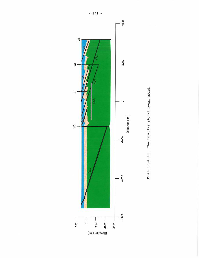
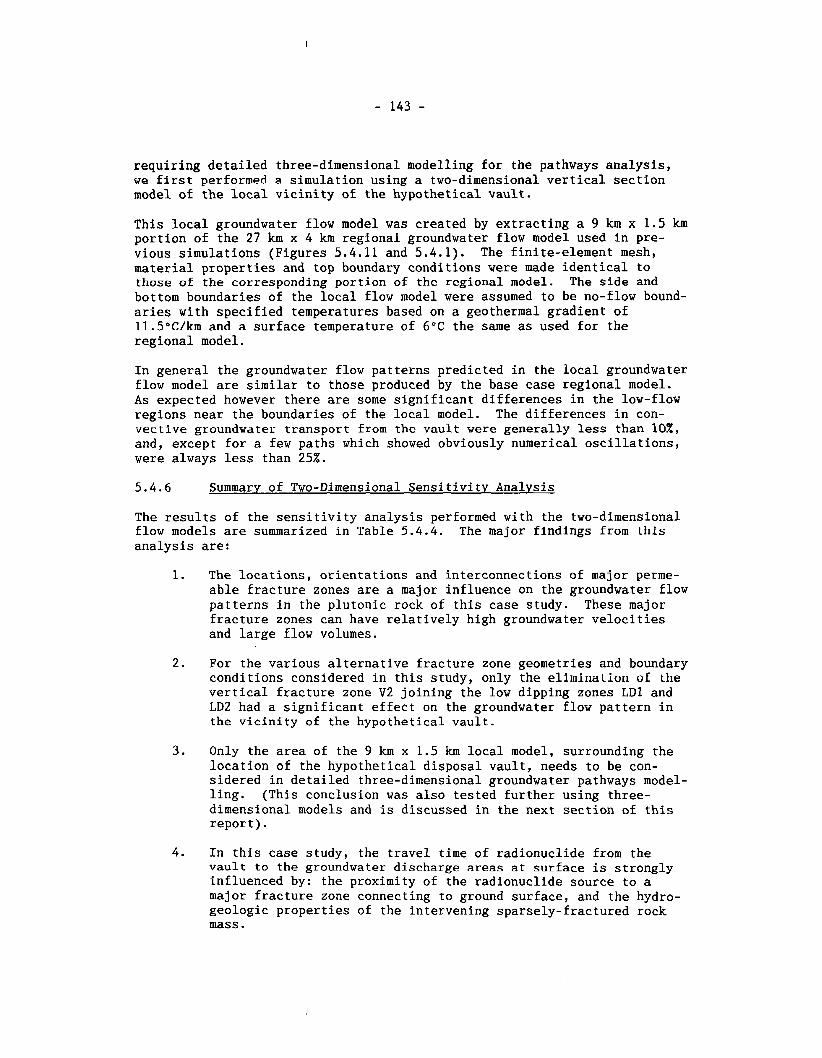
requiring detailed three-dimensional modelling for the pathways analysis, we first performed a simulation using a two-dimensional vertical section model of the local vicinity of the hypothetical vault.
This local groundwater flow model was created by extracting a 9 km x 1.5 km portion of the 27 km x 4 km regional groundwater flow model used In pre- vious simulations (Figures 5.4.11 and 5.4.1). The finite-element mesh, material properties and top boundary conditions were made identical to those of the corresponding portion of the regional model. The side and bottom boundaries of the local flow model were assumed to be no-flow bound- aries with specified temperatures based on a geothermal gradient of ll.S°C/km and a surface temperature of 6°C the same as used for the regional model.
In general the groundwater flow patterns predicted in the local groundwater flow model are similar to those produced by the base case regional model. As expected however there are some significant differences in the low-flow regions near the boundaries of the local model. The differences in con- vective groundwater transport from thc vault were generally less than 101, and, except for a few paths which showed obviously numerical oscillations, were always less than 25%.
5.4.6 Summary of Two-Dimensional Sensitivity Analysis
The results of the sensitivity analysis performed with the two-dimensional flow models are summarized in Table 5.4.4. The major findings from this analysis are:
1. The locations, orientations and interconnections of major perme- able fracture zones are a major influence on the groundwater flow patterns in the plutonic rock of this case study. These major fracture zones can have relatively high groundwater velocities and large flow volumes.
2. For the various alternative fracture zone geometries and boundary conditions considered in this study, only the elimination of the vertical fracture zone V2 joining the low dipping zones LD1 and LD2 had a significant effect on the groundwater flow pattern in the vicinity of the hypothetical vault.
3. Only the area of the 9 km x 1.5 km local model, surrounding the location of the hypothetical disposal vault, needs to be con- sidered in detailed three-dimensional groundwater pathways model- ling. (This conclusion was also tested further using three- dimensional models and is discussed in the next section of this report ) .
4. In this case study, the travel time of radionuclide from the vault to the groundwater discharge areas at surface is strongly influenced by: the proximity of the radionuclide source to a major fracture zone connecting to ground surface, and the hydro- geologic properties of the intervening sparsely-fractured rock mass.
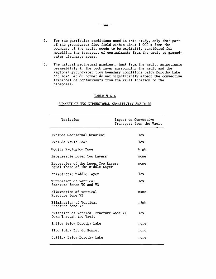
5. For the particular conditions used in this study, only that part of the groundwater flow field within about 1 000 m from the boundary of the vault, needs to be explicitly considered for modelling the transport of contaminants from the vault to ground- water discharge areas.
6. The natural geothermal gradient, heat from the vault, anisotropic permeability in the rock layer surrounding the vault and the regional groundwater flow boundary conditions below Dorothy Lake and Lake Lac du Bonnet do not significantly affect the convective transport of contaminants from the vault location to the biosphere.
TABLE 5.4.4
SUMMARY OF TWO-DIMENSIONAL SENSITIVITY ANALYSIS
Variation Impact on Convective Transport from the Vault
Exclude Geothermal Gradient
Exclude Vault Heat
Modify Exclusion Zone
Impermeable Lower Two Layers
Properties of the Lower Two Layers Equal Those of the Middle Layer
Anisotropic Middle Layer
Truncation of Vertical Fracture Zones VO and V3
Elimination of Vertical Fracture Zone V3
Elimination of Vertical Fracture Zone VZ
Extension of Vertical Fracture Zone V1 Down Through the Vault
Inflow Below Dorothy Lake
Flow Below Lac du Bonnet
low
low
high
none
none
low
low
none
high
low
none
none
none Outflow Below Dorothy Lake
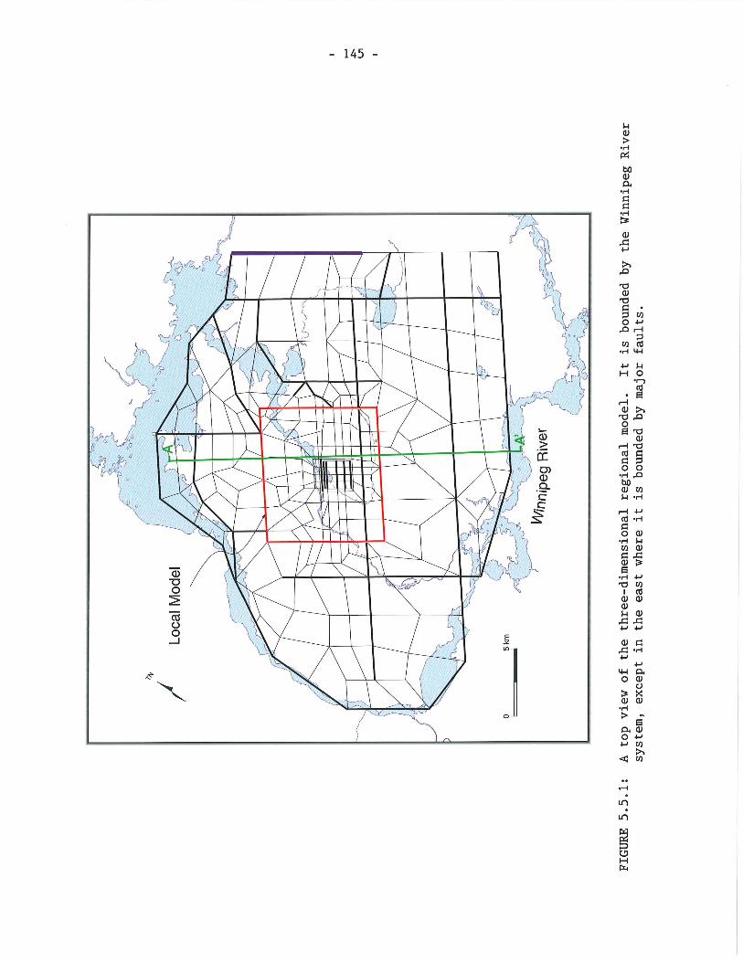
Additional details of the two-dimensional groundwater flow modelling and sensitivity analysis are given in Scheier et al. (1992).
THREE-DIMENSIONAL THERMOHYDROGEOLOGICAL SENSITIVITY ANALYSIS
5.5.1 Preliminary Modelling
This section describes the three-dimensional simulations we have performed: to investigate the effects of the spatial extent of the model; to examine the influence of pumping groundwater from a domestic groundwater water- supply well; and to identify the specific areas, at which groundwater passing through the hypothetical vault, would discharge to the biosphere.
In order to confirm the previous conclusions we had reached from two- dimensional sensitivity analysis, regarding the limited extent of the WRA requiring detailed three-dimensional groundwater flow modelling, the fol- lowing approach was adopted. A three-dimensional regional model with a coarse mesh was first used to simulate groundwater flow for the entire WRA Subsequently, a three-dimensional local groundwater flow model with a refined mesh was used for detailed simulations near the vault.
The three-dimensional regional groundwater flow model (Chan et al. 1986) represents the area bounded by the Winnipeg River system, except in the east where it is bounded by a series of major vertical fault zones (Figures 5.5.1 and 5.3.1). It extends to a depth of 4 km. All major fracture zones and the hydrogeologic stratigraphy of the conceptual model are included in the three-dimensional model. Figure 5.5.1 shows the top view of the finite-element mesh of the three-dimensional model. The fracture zones are represented by two-dimensional planar elements while the moderately fractured and sparsely fractured regions of the rock mass are represented by the three-dimensional volume elements.
No-flow boundary conditions are used for the bottom and sides of the regional groundwater flow model. The suitability of these approximations was previously shown by two-dimensional sensitivity analysis (Section 5.4). The top boundary has prescribed head values equal to the surface topo- graphy. This assumption is judged to be somewhat conservative, as it is expected to slightly exaggerate the hydraulic gradient, and hence lead to higher groundwater velocities than actually exist. Field observations reveal that the water table at the WRA is a subdued replica of the topo- graphy, being somewhat lower beneath upland groundwater recharge areas.
The three-dimensional local groundwater flow model (Chan et al. 1986) covers a 10 km x 9 km area centred on the URL site (Figure 5.5.1) and extends to a depth of 1.5 km. All the major hydrogeologic features of the conceptual model are included. Figures 5.5.2 and 5.5.4 show the top view and a section view of the finite-element mesh used in this analysis. Only three-dimensional finite elements were used in constructing the local model. This was necessary in order to use the TRACK3D particle tracking code to calculate advective groundwater transport paths based on ground- water velocity distributions calculated using MOTIF. The TRACK3D code was not used with the three-dimensional regional groundwater flow model.
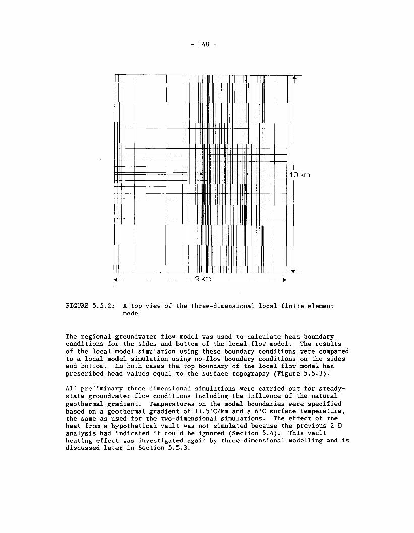
FIGURE 5.5.2: A top view of the three-dimensional local finite element model
The regional groundwater flow model was used to calculate head boundary conditions for the sides and bottom of the local flow model. The results of the local model simulation using these boundary conditions were compared to a local model simulation using no-flow boundary conditions on the sides and bottom. In both cases the top boundary of the local flow model has prescribed head values equal to the surface topography (Figure 5.5 .3) .
All preliminary three-dimensional simulations were carried out for steady- state groundwater flow conditions including the influence of the natural geothermal gradient. Temperatures on the model boundaries were specified based on a geothermal gradient of ll.S°C/km and a 6°C surface temperature, the same as used for the two-dimensional simulations. The effect of the heat from a hypothetical vault was not simulated because the previous 2-D analysis had indicated it could be ignored (Section 5 . 4 ) . This vault heating effect was investigated again by three-dimensional modelling and is discussed later in Section 5.5.3.
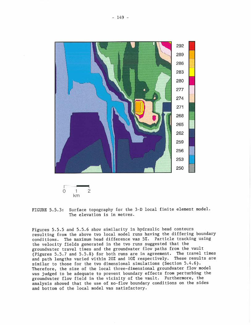
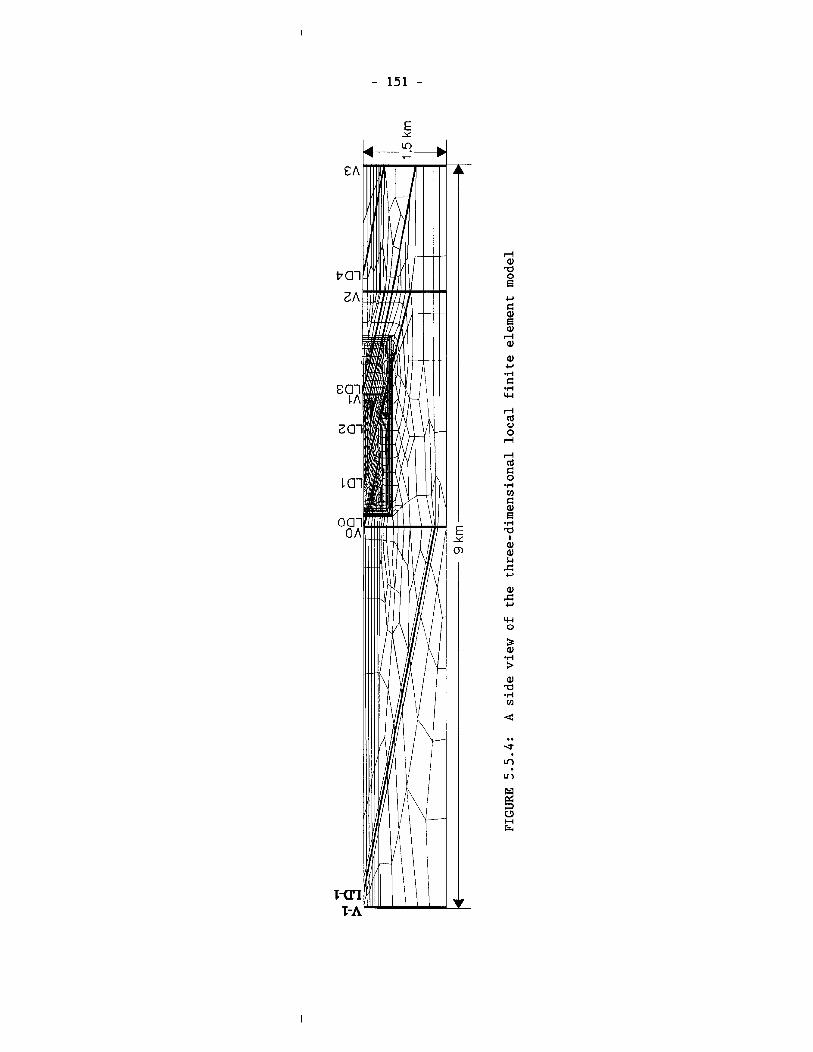
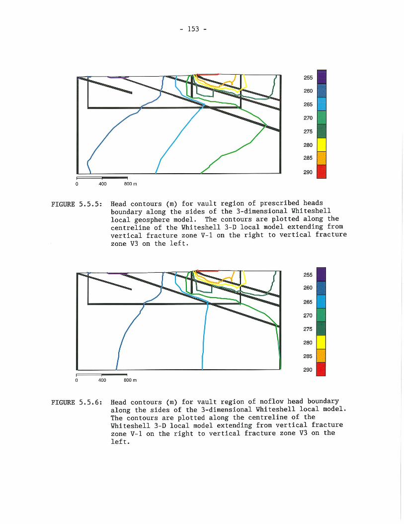
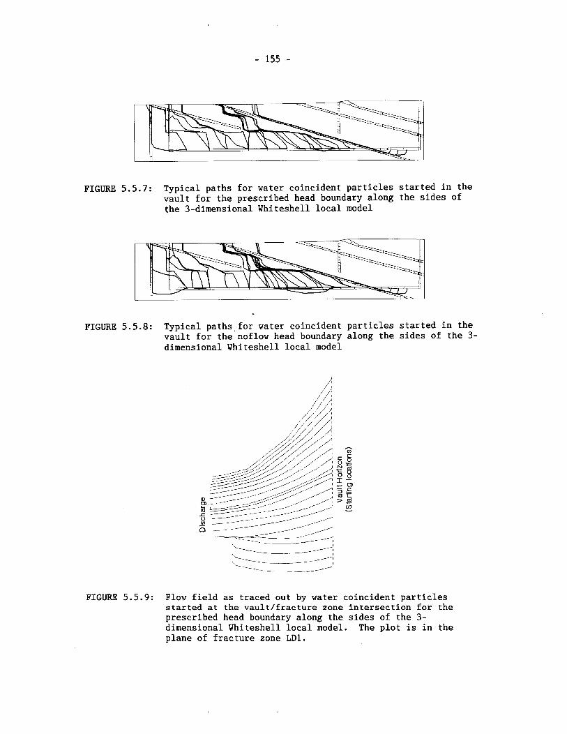
FIGURE 5.5.7: Typical paths for water coincident particles started in the vault for the prescribed head boundary along the sides of the 3-dimensional Whiteshell local model
FIGURE 5.5.8: Typical paths,for water coincident particles started in the vault for the noflow head boundary along the sides of the 3- dimensional Whiteshell local model
FIGURE 5.5.9: Flow field as traced out by water coincident particles started at the vault/fracture zone intersection for the prescribed head boundary along the sides of the 3- dimensional Whiteshell local model. The plot is in the plane of fracture zone LD1.

A major conclusion from preliminary three-dimensional modelling (Reid and Chan 1987) was that the shape of the local topography in this area focussed the groundwater flow paths, that passed through the vault, into a surface discharge area much smaller than the plan area of the vault (Figure 5.5.9).
Particle tracking in the three-dimensional flow field also showed that the minimum groundwater travel time from the vault to the surface was about half of that calculated using the previous two-dimensional analysis. This was caused by the focussing of the three dimensional groundwater flow paths up the low-dipping fracture zone in the direction perpendicular to the two- dimensional model section.
Next the effect of a domestic groundwater supply well drawing water contin- uously from the major, low-dipping fracture zone LD1 was added to the local three-dimensional groundwater flow model (Reid and Chan 1989). The well was assumed to intersect the major, low dipping fracture zone, LD1, at a depth of 200 m. This was the greatest depth at which a well at the WRA could intersect this particular fracture zone without first intersecting the shallower but permeable fracture zone LD2. This was considered to be the deepest well that would conceivably be drilled in such a setting for domestic water supply purposes. Any deeper well into LD1 would encounter the shallower LD2 zone and would be terminated before reaching LD1. The well pumping rate was assumed to be constant in each simulation and to range from 0 to 10 000 m3/a. The model predicted that:
1. the surface area in the biosphere, to which contaminated ground- water from the vault was discharged, could be significantly re- duced by pumping groundwater from the well intersecting the low- dipping fracture zone, especially at higher pumping rates. The well captured flow from a large portion of the groundwater path- ways leading up the fracture zone from the vault to the surface; and
2. the minimum groundwater travel time from the vault to surface was reduced by 30% to 50Z depending on the position of the pathway from the vault.
5.5.2 Backfill Properties, Waste Exclusion Distance and Excavation Damage
A series of simulations were performed to study the sensitivity of convect- ive groundwater transport between the vault and biosphere to the hydrogeo- logical properties of the near-field region within and surrounding the disposal vault (Chan and Stanchell 1991). These simulations considered were
(a) the existence of the underground shafts and tunnels of a disposal vault and how well they are sealed (Figure 5.5.10),
(b) different hydraulic properties used Lor the backfill material in the vault,

(c) varations on the thickness of the region of sparsely fractured rock isolating the waste emplacement areas of the vault from the nearby fracture zone LD1 (we refer to this thickness as the waste exclusion distance), and
(d) the existence of an excavation damaged zone of rock of increasing permeability, immediately around the underground openings.
These simulations were done using a modified version of the local ground- water flow model we had used for the preliminary three-dimensional model- ling (Section 5.5.1). Only one underground access tunnel of the disposal centre design was simulated explicitly, and the two clusters of vault shafts of the disposal centre design were represented by two shafts of equivalent area. Individual waste containers or emplacement rooms were not explicitly simulated, but backfill properties were assigned to panels of rooms of 20 m thickness. Figure 5.5.11 shows a plan and section view of the finite-element discretization we used to represent the vault in this manner. The slashed areas represent panels of backfilled waste emplacement rooms, and the white areas represent intervening rock pillars. Note the locations of the waste exclusion distances (cross-hatched areas)of sparsely fractured rock on either side of fracture zone LD1 (black). Figure 5.5.12 shows a section view of the central portion of this finite-element mesh. All simulations in this series were for steady-state groundwater flow con- ditions under the influence of the natural geothermal gradient. The bound- ary conditions used were the same as those used for the previous prelimin- ary local groundwater flow modelling (Section 5.5.1), with no-flow of groundwater across the model sides or bottom, as with the previous three- dimensional analysis. The effect of the thermal transient caused by decay heat from the vault was not considered in these simulations, because the two-dimensional sensitivity analysis (Section 5.4.1) indicated that the effect of decay heat on transport from the vault is relatively insignifi- cant. Three-dimensional sensitivity analysis of the influence of this thermal transient has since been performed and is discussed in Section 5.5.3.
Table 5.5.1 lists some important cases simulated. The cases differ in the hydrogeologic properties (permeabilities and porosities) used for the buffer and backfill components of the vault and for the damage zone sur- rounding the excavations. Case 1 is the base case in which all the back- filled underground openings have the same hydraulic properties as those of the undisturbed rock in layer 3 of the conceptual hydrogeological model. In this case the vault is assumed to have been constructed without con- sideration for the intersection with the major fracture zone LD1 and the waste has been emplaced uniformly throughout the vault horizon including the fracture zone.
To investigate the effectiveness of avoiding emplacing wastes too close to such fracture zones, Case 2 incorporates a waste-exclusion distance of sparsely-fractured rock on either side of the low-dipping fracture zone.
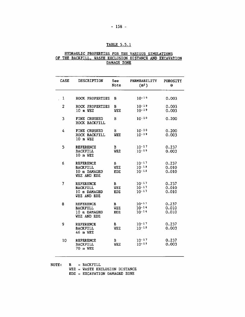
TABLE 5.5.1
HYDRAULIC PROPERTIES FOR THE VARIOUS SIMULATIONS OF THE BACKFILL, WASTE EXCLUSION DISTANCE AND EXCAVATION
DAMAGE ZONE
CASE DESCRIPTION See PERMEABILITY POROSITY Note (m2 ) 8
ROCK PROPERTIES
ROCK PROPERTIES 10 m WEZ
B WEZ
FINE CRUSHED ROCK BACKFILL
FINE CRUSHED ROCK BACKFILL 10 m WEZ
REFERENCE BACKFILL 10 m WEZ
B WEZ
REFERENCE BACKFILL 10 m DAMAGED WEZ AND EDZ
B WEZ EDZ
REFERENCE BACKFILL 10 m DAMAGED WEZ AND EDZ
B WEZ EDZ
REFERENCE BACKFILL 10 m DAMAGED WEZ AND EDZ
B WEZ EDZ
REFERENCE BACKFILL 46 m WEZ
REFERENCE BACKFILL 70 m WE2
B WEZ
NOTE: B = BACKFILL WE2 = WASTE EXCLUSION DISTANCE EDZ = EXCAVATION DAMAGED ZONE
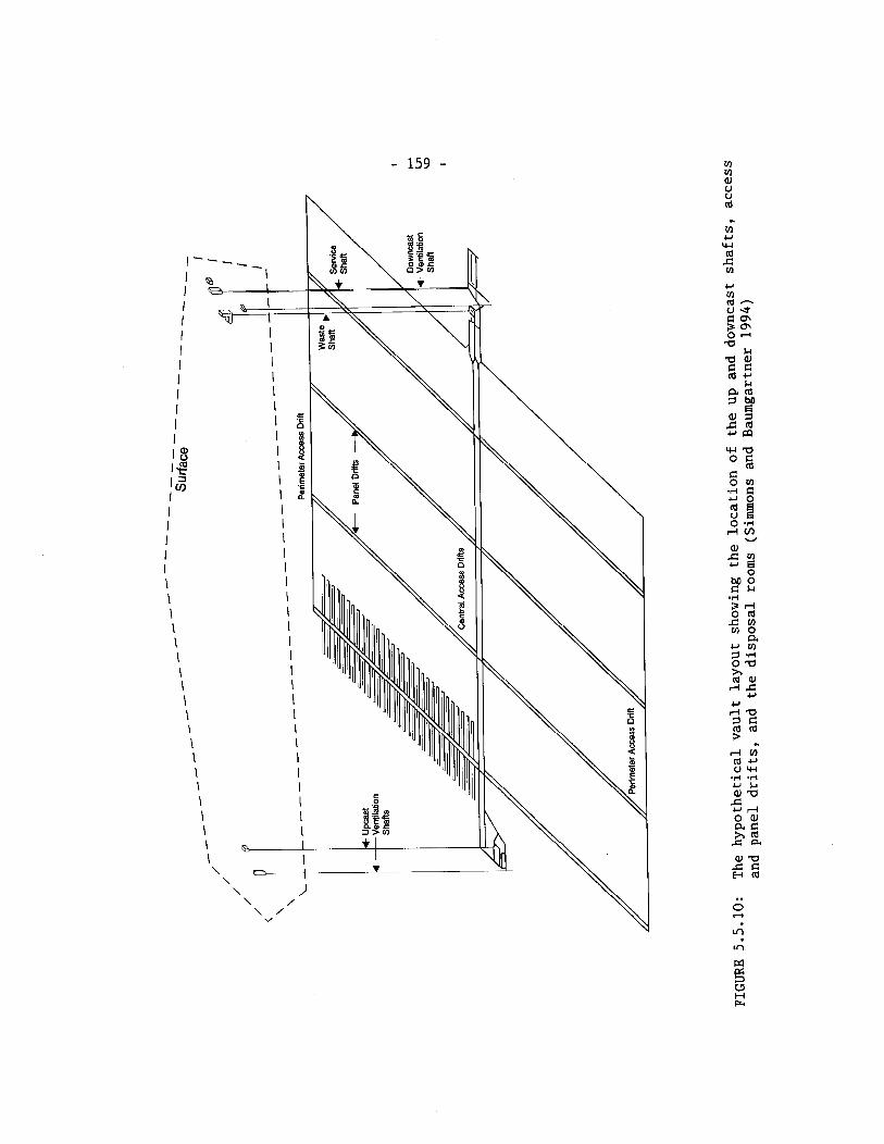
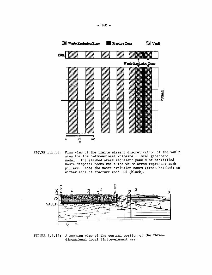
FIGURE 5.5.11: Plan view of the finite element discretization of the vault area for the 3-dimensional Whiteshell local geosphere model. The slashed areas represent panels of backfilled waste disposal rooms while the white areas represent rock pillars. Note the waste-exclusion zones (cross-hatched) on either side of fracture zone LD1 (black).
FIGURE 5.5.12: A section view of the central portion of the three- dimensional local finite-element mesh
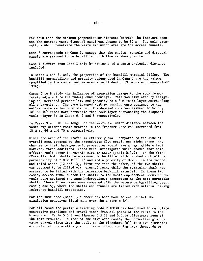
For this case the minimum perpendicular distance between the fracture zone and the nearest waste disposal panel was chosen to be 10 m. The only exca- vations which penetrate the waste exclusion area are the access tunnels.
Case 3 corresponds to Case l,,except that the shafts, tunnels and disposal panels are assumed to be backfilled with fine crushed granite.
Case 4 differs from Case 3 only by having a 10 m waste exclusion distance included.
In Cases 4 and 5, only the properties of the backfill material differ. The backfill permeability and porosity values used in Case 5 are the values specified in the conceptual reference vault design (Simmons and Baumgartner 1994).
Cases 6 to 8 study the influence of excavation damage to the rock immed- iately adjacent to the underground openings. This was simulated by assign- ing an increased permeability and porosity to a 3 m thick layer surrounding all excavations. The same damaged rock properties were assigned to the entire waste exclusion distance. The damaged rock was assumed to be 10, 102 or lo5 times more permeable than rock layer surrounding the disposal vault (layer 3) in Cases 6, 7 and 8 respectively.
In Cases 9 and 10 the length of the waste exclusion distance between the waste emplacement rooms nearest to the fracture zone was increased from 10 m to 46 m and 70 m respectively.
Since the area of the shafts is extremely small compared to the size of overall area covered by the groundwater flow model, one might expect any changes to their hydrogeologic properties would have a negligible effect. However, three additional cases were investigated which showed that some effects could occur in certain circumstances (Table 5.5.2). In the first (Case ll), both shafts were assumed to be filled with crushed rock with a permeability of 2.0 x 10-lo m2 and and a porosity of 0.20. In the second and third Cases (12 and 13), first one then the other, of the two shafts was assumed to be filled with crushed rock, while the remaining shaft was assumed to be filled with the reference backfill material. In these two cases, access tunnels from the shafts to the waste emplacement rooms in the vault were assigned the same hydrogeologic properties as the more permeable shaft. These three cases were compared with the reference backfilled vault case (Case 5), where the shafts and tunnels are filled with material having reference backfill properties.
For the base case (Case 1) a check has been made to ensure that the simulation conserves fluid mass over the entire model.
For all cases the particle tracking code TRACK3D has been used to calculate convective pathlines and travel times from all parts of the vault to the biosphere. Table 5.5.3 and Figures 5.5.13 and 5.5.14 illustrate some of the main results. In most of the simulated cases, the convective ground- water travel times from the vault to the biosphere fall into two clusters: a cluster of comparatively short travel times ranging from thousands or
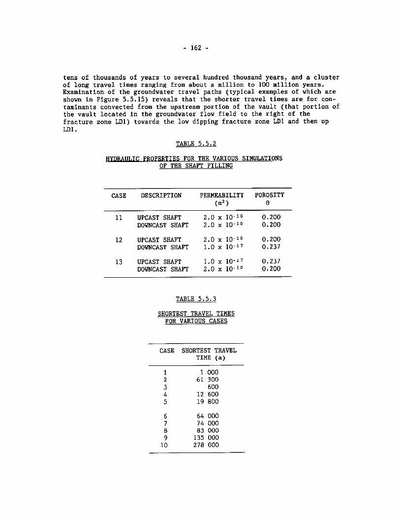
tens of thousands of years to several hundred thousand years, and a cluster of long travel times ranging from about a million to 100 million years. Examination of the groundwater travel paths (typical examples of which are shown in Figure 5.5.15) reveals that the shorter travel times are for con- taminants convected from the upstream portion of the vault (that portion of the vault located in the groundwater flow field to the right of the fracture zone LD1) towards the low dipping fracture zone LD1 and then up LD1.
TABLE 5.5.2
BYDRAULIC PROPERTIES FOR THE VARIOUS SIMULATIONS OF THE SHAFT FILLING
CASE DESCRIPTION PERMEABILITY POROSITY (m2 0
11 UPCAST SHAFT 2.0 x 10 - lo 0.200 DOWNCASTSHAFT 2 . 0 ~ 10- lo 0.200
12 UPCAST SHAFT 2.0 x 10 - lo 0.200 DOWNCAST SHAFT 1.0 x 10 - l7 0.237
13 UPCAST SHAFT 1.0 x 10 - l7 0.237 DOWNCAST SHAFT 2 . 0 ~ 10- lo 0.200
TABLE 5.5.3
SHORTEST TRAVEL TIMES FOR VARIOUS CASES
CASE SHORTEST TRAVEL TIME (a)
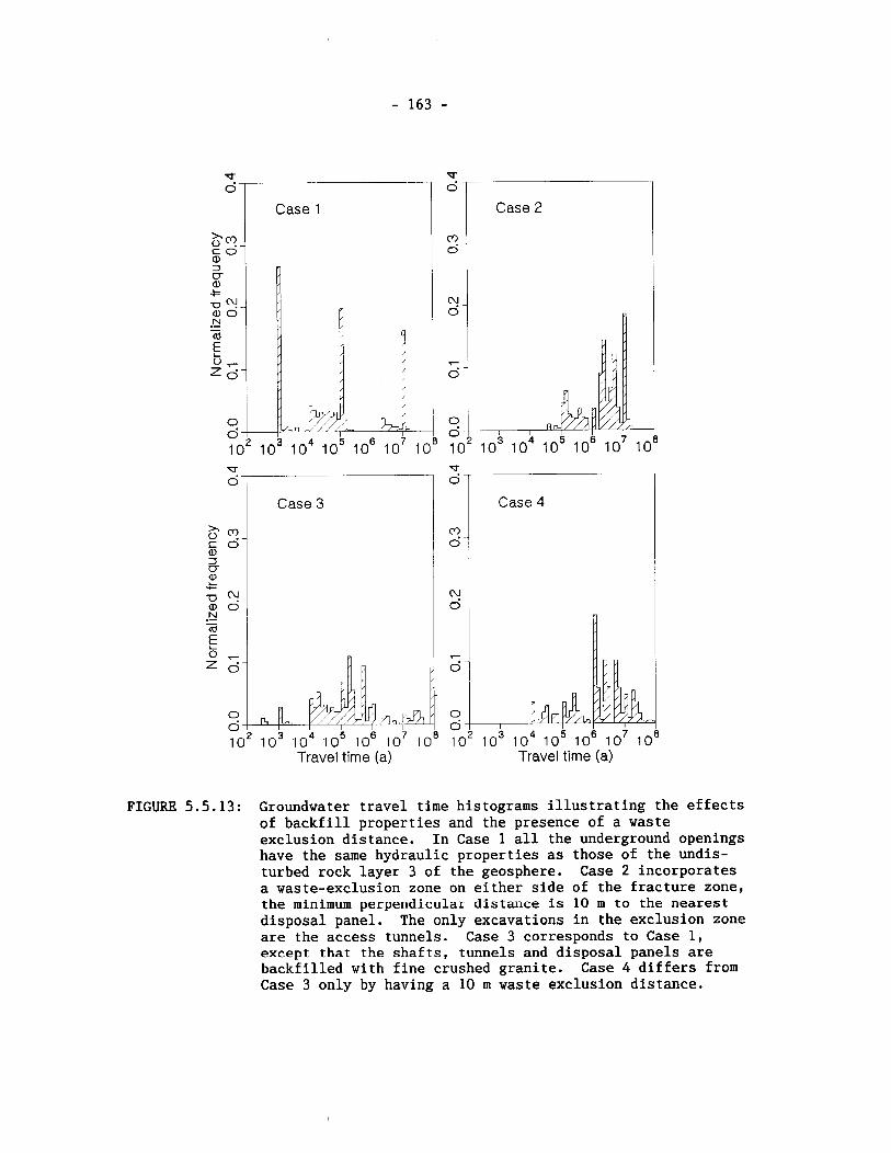
Case 1
Case 3 gr
Case 2
z
Case 4
Travel time (a) Travel time (a)
FIGURE 5.5.13: Groundwater travel time histograms illustrating the effects of backfill properties and the presence of a waste exclusion distance. In Case 1 all the underground openings have the same hydraulic properties as those of the undis- turbed rock layer 3 of the geosphere. Case 2 incorporates a waste-exclusion zone on either side of the fracture zone, the minimum perpendicular distance is 10 m to the nearest disposal panel. The only excavations in the exclusion zone are the access tunnels. Case 3 corresponds to Case 1, except that the shafts, tunnels and disposal panels are backfilled with fine crushed granite. Case 4 differs from Case 3 only by having a 10 m waste exclusion distance.
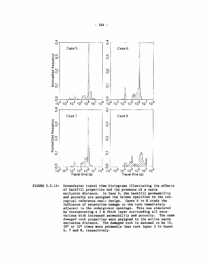
Travel time (a)
Case 8 ;I
Travel time (a)
FIGURE 5.5.14: Groundwater travel time histograms illustrating the effects of backfill properties and the presence of a waste exclusion distance. In Case 5, the backfill permeability and porosity are assigned the values specified in the con- ceptual reference vault design. Cases 6 to 8 study the influence of excavation damage to the rock immediately adjacent to the underground openings. This was simulated by incorporating a 3 m thick layer surrounding all exca- vations with increased permeability and porosity. The same damaged rock properties were assigned to the entire waste exclusion distance. The damaged rock is assumed to be 10, lo2 or lo5 times more permeable than rock layer 3 in Cases 6, 7 and 8, respectively.
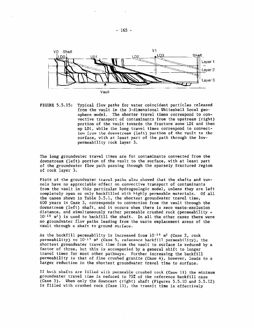
I I
Vault
FIGURE 5.5.15: Typical flow paths for water coincident particles released from the vault in the 3-dimensional Whiteshell local geo- sphere model. The shorter travel times correspond to con- vective transport of contaminants from the upstream (right) portion of the vault towards the fracture zone LD1 and then up LD1, while the long travel times correspond to convect- ion from the downstream (left) portion of the vault to the surface, with at least part of the path through the low- permeability rock layer 3.
The long groundwater travel times are for contaminants convected from the downstream (left) portion of the vault to the surface, with at least part of the groundwater flow path passing through the sparsely fractured region of rock layer 3.
Plots of the groundwater travel paths also showed that the shafts and tun- nels have no appreciable effect on convective transport of contaminants from the vault in this particular hydrogeologic model, unless they are left completely open or only backfilled with highly permeable materials. Of all the cases shown in Table 5.5.1, the shortest groundwater travel time, 600 years in Case 3, corresponds to convection from the vault through the downstream (left) shaft, and it occurs when there is zero waste-exclusion distance, and simultaneously rather permeable crushed rock (permeability = 10-lo m2) is used to backfill the shaft. In all the other cases there were no groundwater flow paths leading from the waste emplacement areas of the vault through a shaft to ground surface.
As the backfill permeability is increased from 10-l9 m2 (Case 2, rock permeability) to 10-l7 m2 (Case 5, reference backfill permeability), the shortest groundwater travel time from the vault to surface is reduced by a factor of three, but this is accompanied by a general shift to longer travel times for most other pathways. Further increasing the backfill permeability to that of fine crushed granite (Case 4 ) , however, leads to a larger reduction in the shortest groundwater travel time to surface.
If both shafts are filled with permeable crushed rock (Case 11) the minimum groundwater travel time is reduced to 75Z of the reference backfill case (Case 5). When only the downcast (right) shaft (Figures 5.5.10 and 5.5.12) is filled with crushed rock (Case 1 3 ) , the transit time is effectively
unchanged from the case where both shafts are filled with crushed rock. However, when only the upcast (left) shaft has crushed rock properties (Case 12) the travel time becomes identical to that of the reference back- fill vault case. The starting position for the minimum travel time particles, and their exit locations, are both identical to those for the reference backfill vault case.
Comparison of the predicted travel times for Cases 1 and 3 with Cases 2 and 4 shows that the presence of a 10 m waste-exclusion distance, between the nearest waste emplacement room and the low-dipping fracture zone LD1, in- creases the groundwater travel time for contaminants from the vault to surface discharge areas by orders of magnitude. It is also observed in Cases 5, 9 and 10, that increasing the waste exclusion distance to 46 m and 70 m further increases the time taken by contaminants to move from the vault to the biosphere.
Results from Cases 5 to 7 show that the existence of a 3 m thick exca- vation-damaged zone, with permeability up to 100 times that of the un- damaged rock around all the underground openings, has no significant effect on convective contaminant transport from the vault. In fact, the modelling showed there was an increase in groundwater travel time from the vault to the surface, as the permeability of the excavation-damaged zone was in- creased. This is an example of the "hydraulic cage" effect. The faster flow of groundwater through the more permeable excavation damaged zone is balanced by slower groundwater flow through the undamaged, less permeable rock, as expected from basic hydraulic principles. Even particles directly released into the damaged zone soon exit this relatively thin damaged zone (compared to the dimensions of the other components of the modelled system) and travel through the undamaged rock. The undamaged rock has slower groundwater velocities in this case than in the case where there is no excavation damage (Case 5). In Case 8 , the damaged zone is assumed to be 5 orders of magnitude more permeable than the undamaged rock. The shortest groundwater travel time to surface is also increased in this extreme case.
Under the particular conditions of the hydrogeological model of the area of the WRA considered for our case study, and the hydrogeologic conditions in the immediate vicinity of the location of the hypothetical disposal vault, our parameter sensitivity study shows that using an exclusion distance of sparsely fractured rock between the waste emplacement rooms nearest to a major permeable fracture zone, can be very effective in retarding the con- vective transport of contaminants from the vault to the surface. Shafts and tunnels sealed with the reference backfill material do not necessarily provide preferential paths for fast convective transport of contaminants from the vault to the surface.
Excavation-induced damage of the rock surrounding the underground openings in the vault in this model, does not appear to increase the rate at which contaminants from the vault would be transported by groundwater to the surface environment. The last two conclusions are due to particular aspects of the groundwater flow conditions at vault depth in our model. The hydraulic gradient for groundwater movement near the vault is neither parallel to the shafts and tunnels, nor parallel to the relatively thin
excavation damaged zone. Therefore a' particle originating from, or having entered the groundwater flow paths in these more permeable zones, will not remain there for a long time before exiting to the groundwater flow paths in the surrounding, less permeable rock.
The analysis in this section has been based on an equivalent porous medium flow model. It does not address questions such as :
- What would happen if there was one or a few very small fractures within the region of sparsely fractured zone connecting the vault to a major fracture zone such as LDl?
- What would be the effects of a damaged zone around the excavation on diffusive and dispersive transport?
Convective-dispersive transport modelling using MOTIF is currently underway to address these questions.
5.5.3 Vault Heat
In Section 5.4.1 it was found, by two-dimensional MOTIF simulations, that the heat generated from the waste in the vault would have only minor effects on groundwater flow paths and travel times from the vault to the biosphere. This, however, does not preclude the possibility of significant thermal convection effects in the three-dimensional system. Accordingly, a series of three-dimensional MOTIF simulations were performed to investi- gate the effects of the thermal transient in greater detail. The version of the three-dimensional local groundwater flow model described in the previous Section (5.5.2) was used for these simulations. Specific cases considered included Cases 5 and 9 of the previous section, which had 10 m and 46 m waste exclusion distances respectively, and a case having no waste exclusion distance. In all cases it was assumed that reference backfill material was used to fill all underground excavations.
Figure 5.5.16 shows the heat output of the vault versus time used for the transient simulations (Chan et al. 1994). This heat source function is the same as that used for the two-dimensional simulations (Table 5.4.1), except that for the two-dimensional simulations the heat output was assumed to have dropped to zero after lo5 years. This function assumes that heat is generated uniformly over the entire area of the vault, including the rock pillars between the waste emplacement rooms, but excluding the exclusion distance and the low-dipping fracture zone LD1. In the model the nodes representing the bottom plane of the vault were assumed to be the heat sources, because in the borehole emplacement concept, the waste will be located close to the bottom of the vault.
The transient simulations were conducted for periods of at least one million years, using geometrically increasing time steps. Figures 5.5.17a and 5.5.17b show predicted temperature distributions on a section through the centre of the vault, for the case with a 46 m exclusion distance and vault heat. Significant changes in the temperature of the surrounding rock are limited to within about 1 500 m laterally from the edge of the vault.
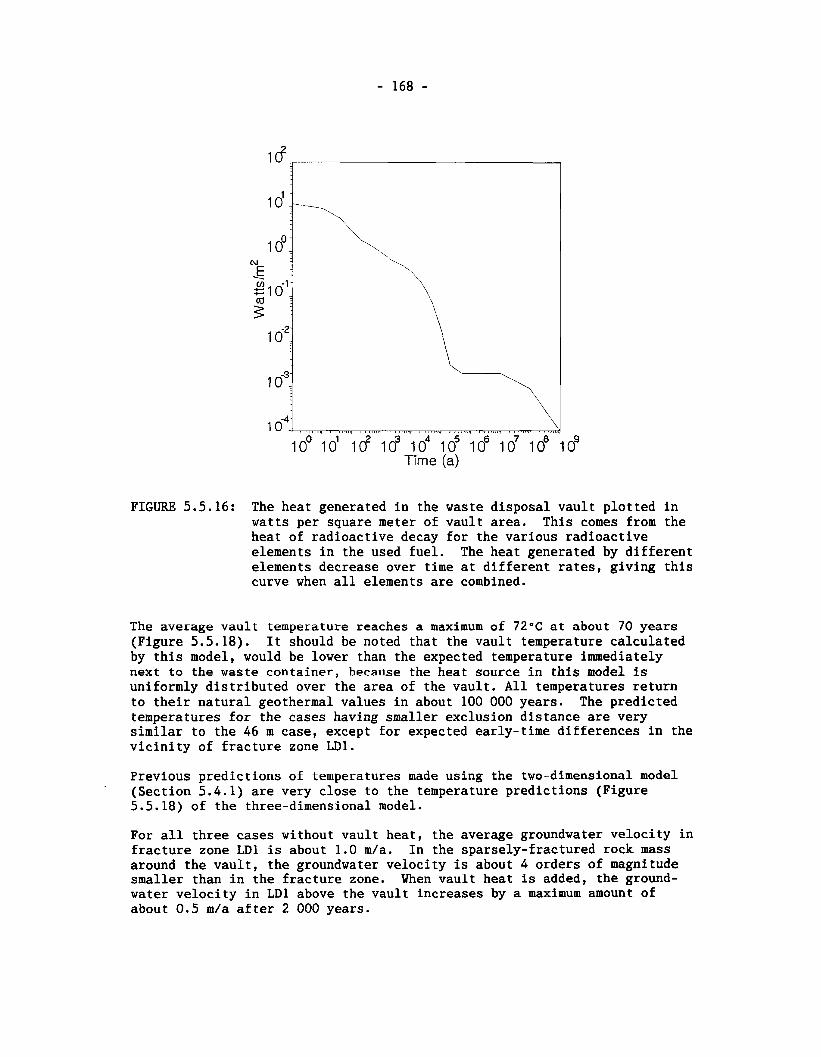
1 041 . . , . .. . . . . . . m m..... 8 , 8 , , 3 # . , , ,.,... . . .,,, . . , . . . . I . . ...... . . .\J 10' 110' 10' lo3 lo4 10' lo6 10' 10Vog
Time (a)
FIGURE 5.5.16: The heat generated in the waste disposal vault plotted in watts per square meter of vault area. This comes from the heat of radioactive decay for the various radioactive elements in the used fuel. The heat generated by different elements decrease over time at different rates, giving this curve when all elements are combined.
The average vault temperature reaches a maximum of 7Z°C at about 70 years (Figure 5.5.18). It should be noted that the vault temperature calculated by this model, would be lower than the expected temperature immediately next to the waste container, because the heat source in this model is uniformly distributed over the area of the vault. All temperatures return to their natural geothermal values in about 100 000 years. The predicted temperatures for the cases having smaller exclusion distance are very similar to the 46 m case, except for expected early-time differences in the vicinity of fracture zone LD1.
Previous predictions of temperatures made using the two-dimensional model (Section 5.4.1) are very close to the temperature predictions (Figure 5.5.18) of the three-dimensional model.
For all three cases without vault heat, the average groundwater velocity in fracture zone LD1 is about 1.0 m/a. In the sparsely-fractured rock mass around the vault, the groundwater velocity is about 4 orders of magnitude smaller than in the fracture zone. When vault heat is added, the ground- water velocity in LD1 above the vault increases by a maximum amount of about 0.5 m/a after 2 000 years.
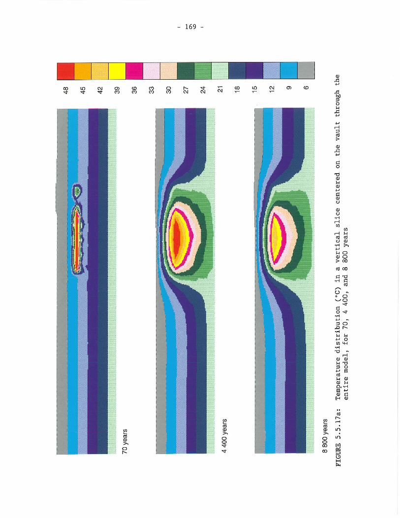
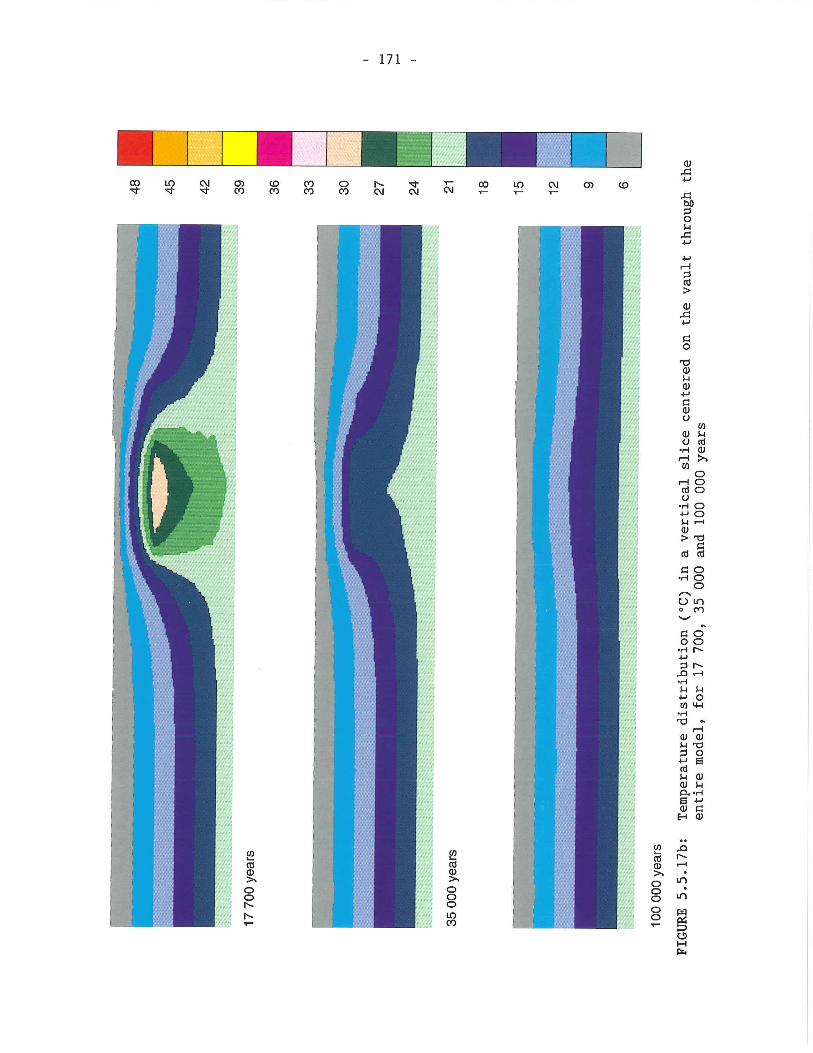

0 1 7
10.' lon 10' lo2 lo3 lo4 lo5 lo6 Time (a)
FIGURE 5.5.18: Temperature of the hottest point in the waste disposal vault, plotted versus log time. When this point reaches the normal geologic temperature of 12 degrees C. at 100 000 years, all points have returned to their normal temperatures.
The groundwater velocity in the sparsely fractured rock region increases by up to an order of magnitude. These effects are also very similar to those predicted by the earlier two-dimensional simulations.
For all cases particle tracking was used to determine the effect of vault heat on the convective transport of contaminants from the vault to the surface. As was observed in the two-dimensional simulations, the particles released from the vault into the groundwater flow paths on the left side of fracture zone LDl (Figure 5.5.15) are not significantly affected by vault heat. This is because their convective transport times through the sparse- ly-fractured rock are orders of magnitude longer than the duration of the velocity perturbation caused by the vault heat. For the cases with a 46 m waste exclusion distance, contaminants from the vault travelling in the fastest groundwater flow paths reach the surface 0.6 percent sooner if the effects of vault heat are considered (Table 5 .5 .4 ) .
All the particles released from the vault on the right side of LD1 reach the discharge locations in the biosphere by first travelling a short dis- tance through the sparsely fractured rock and then along rapid groundwater pathways in the low-dipping fracture zone. As a result, their travel times are much shorter than those for particles originating from the left side of the vault. For particles released from the right side of the vault, their travel is completed within the time duration of the groundwater velocity perturbation caused by vault heating. Therefore, the travel times for these pathways are significantly reduced when vault heat is included in the model (Table 5 .5 .5 ) .
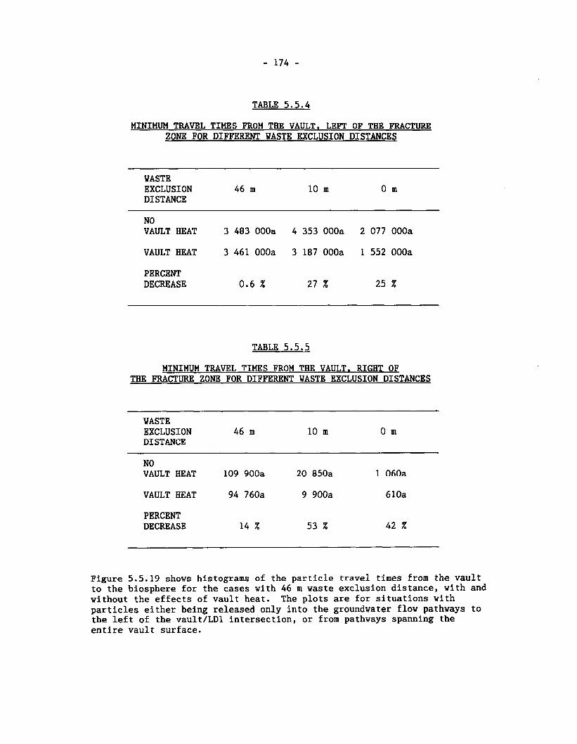
TABLE 5.5.4
MINIMUM TRAVEL TIMES PROM THE VAULT, LEFT OF THE FRACTURE ZONE FOR DIFFERENT WASTE EXCLUSION DISTANCES
WASTE EXCLUSION 46 m 10 m 0 m DISTANCE
NO VAULT HEAT 3 483 OOOa 4 353 OOOa 2 077 OOOa
VAULT HEAT 3 461 OOOa 3 187 OOOa 1 552 OOOa
PERCENT DECREASE 0.6 X 27 X 25 X
TABLE 5.5.5
MINIMUM TRAVEL TIMES FROM THE VAULT. RIGHT OF THE FRACTURE ZONE FOR DIFFERENT WASTE EXCLUSION DISTANCES
WASTE EXCLUSION 46 m 10 m 0 m DISTANCE
NO VAULT HEAT 109 900a 20 850a 1 060a
VAULT HEAT 94 760a 9 900a 610a
PERCENT DECREASE 14 X 53 X
Figure 5.5.19 shows histograms of the particle travel times from the vault to the biosphere for the cases with 46 m waste exclusion distance, with and without the effects of vault heat. The plots are for situations with particles either being released only into the groundwater flow pathways to the left of the vault/LDl intersection, or from pathways spanning the entire vault surface.
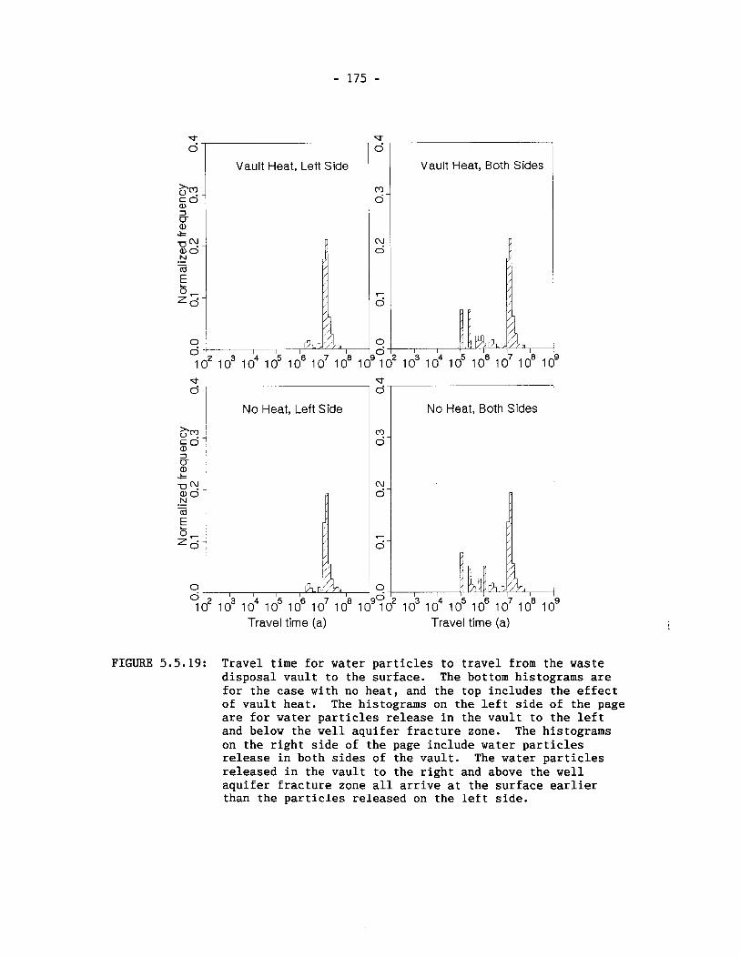
Travel time (a) Travel time (a)
FIGURE 5.5.19: Travel time for water particles to travel from the waste disposal vault to the surface. The bottom histograms are for the case with no heat, and the top includes the effect of vault heat. The histograms on the left side of the page are for water particles release in the vault to the left and below the well aquifer fracture zone. The histograms on the right side of the page include water particles release in both sides of the vault. The water particles released in the vault to the right and above the well aquifer fracture zone all arrive at the surface earlier than the particles released on the left side.
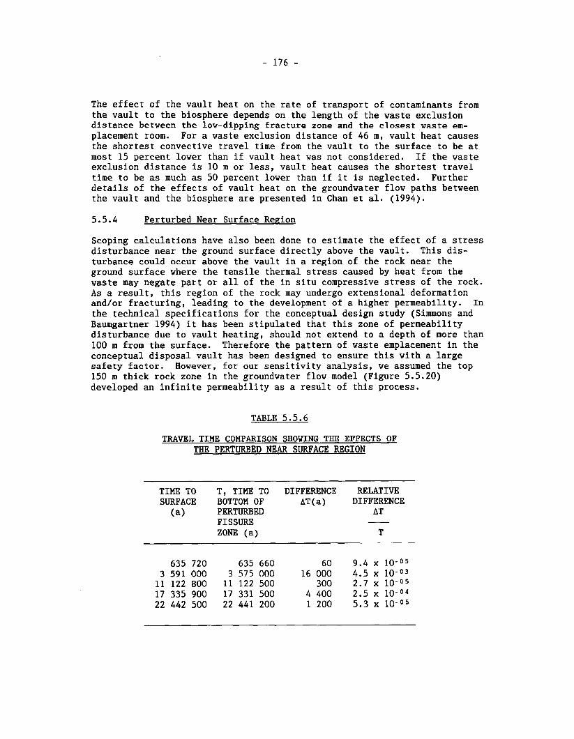
The effect of the vault heat on the rate of transport of contaminants from the vault to the biosphere depends on the length of the waste exclusion distance between the low-dipping fracture zone and the closest waste em- placement room. For a waste exclusion distance of 46 m, vault heat causes the shortest convective travel time from the vault to the surface to be at most 15 percent lower than if vault heat was not considered. If the waste exclusion distance is 10 m or less, vault heat causes the shortest travel time to be as much as 50 percent lower than if it is neglected. Further details of the effects of vault heat on the groundwater flow paths between the vault and the biosphere are presented in Chan et al. (1994).
5.5.4 Perturbed Near Surface Region
Scoping calculations have also been done to estimate the effect of a stress disturbance near the ground surface directly above the vault. This dis- turbance could occur above the vault in a region of the rock near the ground surface where the tensile thermal stress caused by heat from the waste may negate part or all of the in situ compressive stress of the rock. As a result, this region of the rock may undergo extensional deformation and/or fracturing, leading to the development of a higher permeability. I n the technical specifications for the conceptual design study (Simmons and Baumgartner 1994) it has been stipulated that this zone of permeability disturbance due to vault heating, should not extend to a depth of more than 100 m from the surface. Therefore the pattern of waste emplacement in the conceptual disposal vault has been designed to ensure this with a large safety factor. However, for our sensitivity analysis, we assumed the top 150 m thick rock zone in the groundwater flow model (Figure 5.5.20) developed an infinite permeability as a result of this process.
TABLE 5.5.6
TRAVEL TIME COMPARISON SHOWING THE EFFECTS OF THE PERTURBED NEAR SURFACE REGION
TIME TO T, TIME TO DIFPERENCE REL&l"I'VE SURFACE BOTTOM OF AT(a) DIFFERENCE (a) PERTURBED AT
FISSURE ZONE (a) T
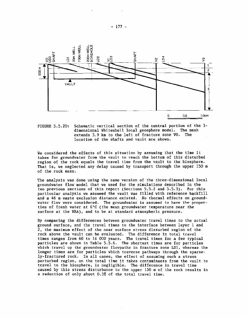
FIGURE 5.5.20: Schematic vertical section of the central portion of the 3- dimensional Whiteshell local geosphere model. The mesh extends 3.9 km to the left of fracture zone VO. The location of the shafts and vault are shown.
We considered the effects of this situation by assuming that the time it takes for groundwater from the vault to reach the bottom of this disturbed region of the rock equals the travel time from the vault to the biosphere. That is, we neglected any delay caused by transport through the upper 150 m of the rock mass.
The analysis was done using the same version of the three-dimensional local groundwater flow model that we used for the simulations described in the two previous sections of this report (Sections 5.5.2 and 5.5.3). For this particular analysis we assumed the vault was filled with reference backfill and a 46 m waste exclusion distance existed. No thermal effects on ground- water flow were considered. The groundwater is assumed to have the proper- ties of fresh water at 6°C (the mean groundwater temperature near the surface at the WRA), and to be at standard atmospheric pressure.
By comparing the differences between groundwater travel times to the actual ground surface, and the travel times to the interface between layer 1 and 2, the maximum effect of the near surface stress disturbed region of the rock above the vault can be evaluated. The difference in total travel times ranges from 60 to 16 000 years. The travel times for a few typical particles are shown in Table 5.5.6. The shortest times are for particles which travel up the groundwater flowpaths in fracture zone LD1, whereas the longer times are for particles which traverse pathways through the sparse- ly-fractured rock. In all cases, the effect of assuming such a stress perturbed region, on the total time it takes contaminants from the vault to travel to the biosphere, is negligible. The difference in travel time caused by this stress disturbance to the upper 150 m of the rock results in a reduction of only about 0.3% of the total travel time.
In the above sensitivity analysis the groundwater flow field was calculated using the hydraulic properties for the reference case as given in Table 5.3.1. The influence of the perturbed near surface region on groundwater travel was estimated approximately by tracking particles to the bottom of the top layer of moderately fractured rock. It is conceivable that a very permeable top layer of rock would modify the near surface groundwater flow field significantly from the one used in this analysis. This would likely produce a dispersing and diluting effect which would tend to increase, rather than decrease, the groundwater travel time from the vault to the biosphere. Modelling work is in progress to investigate this.
5.5.5 Summary of Three-Dimensional Sensitivity Analysis
The results of the sensitivity analysis performed with the three-dimension- al groundwater flow model of the WRA are summarized in Table 5.5.7. Major findings from this analysis are:
1. A local three-dimensional groundwater flow model covering the central 10 km x 9 km portion of the Whiteshell Research Area and extending to a depth of 1.5 km, (i.e., Including only the upper three rock layers), predicts about the same groundwater flow paths and travel times from the vault to the biosphere, as a combination of a regional groundwater flow model and a local flow model.
2. For these model conditions, only that part of the groundwater flow field within about 1 000 q of the hypothetical vault location needs to be explicitly considered in modelling solute transport from the vault to the groundwater discharge locations in the biosphere.
3 . The nature of the local topography in this area focuses the groundwater flow paths that pass through the vault into a surface discharge area that is much smaller than the plan area of the vault. This is caused by the focussing (convergence) up the low- dipping fracture zone of the flow paths, from the depth of the vault to the discharge area.
4. Both the groundwater travel times, and the area in the biosphere, to which groundwater flow paths from the vault are predicted to discharge, are substantially reduced when the effects of pumping from a groundwater supply well located in the low-dipping fracture zone LD1 are considered. This is especially the case at higher pumping rates.
5. The size of the waste exclusion distance of low permeability, sparsely fractured rock, between the nearest waste emplacement room in the vault and the nearby fracture zone LD1, significantly affects the length of time it takes for contaminants from the vault to move along groundwater flow paths from the vault to the groundwater discharge locations in the biosphere.
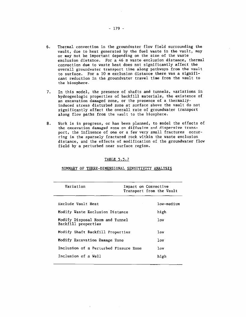
6. Thermal convection in the groundwater flow field surrounding the vault, due to heat generated by the fuel waste in the vault, may or may not be important depending on the size of the waste exclusion distance. For a 46 m waste exclusion distance, thermal convection due to waste heat does not significantly affect the overall groundwater transport time along pathways from the vault to surface. For a 10 m exclusion distance there was a signifi- cant reduction in the groundwater travel time from the vault to the biosphere.
. In this model, the presence of shafts and tunnels, variations in hydrogeologic properties of backfill materials, the existence of an excavation damaged zone, or the presence of a thermally- induced stress disturbed zone at surface above the vault do not significantly affect the overall rate of groundwater transport along flow paths from the vault to the biosphere.
8. Work is in progress, or has been planned, to model the effects of the excavation damaged zone on diffusive and dispersive trans- port, the influence of one or a few very small fractures occur- ring in the sparsely fractured rock within the waste exclusion distance, and the effects of modification of the groundwater flow field by a perturbed near surface region.
TABLE 5.5.7
SUMMARY OF THREE-DIMENSIONAL SENSITIVITY ANALYSIS
Variation Impact on Convective Transport from the Vault
Exclude Vault Heat low-medium
Modify Waste Exclusion Distance high
Modify Disposal Room and Tunnel Backfill properties
low
Modify Shaft Backfill Properties low
Modify Excavation Damage Zone low
Inclusion of a Perturbed Fissure Zorle low
Inclusion of a Well high
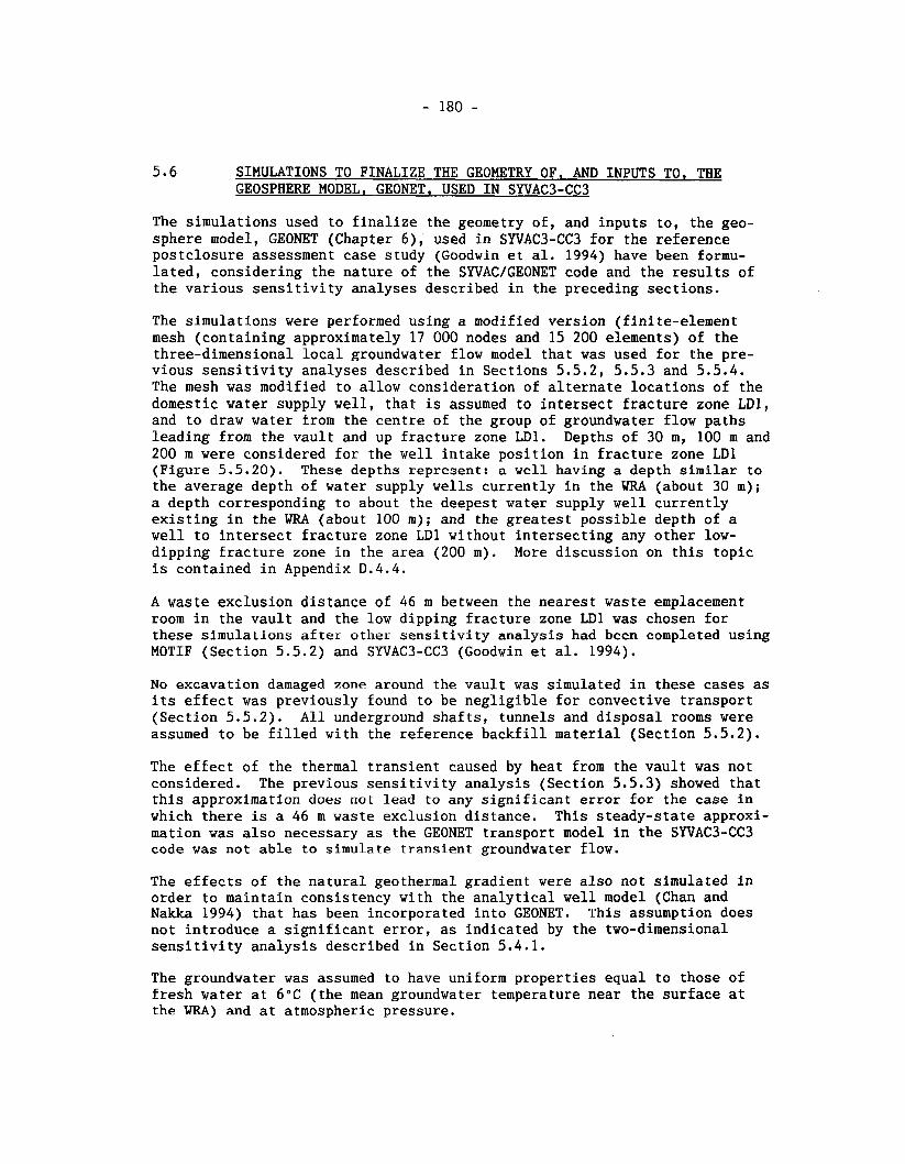
5.6 SIMULATIONS TO FINALIZE THE GEOMETRY OF, AND INPUTS TO, THE GEOSPHERE MODEL, GEONET, USED IN SYVAC3-CC3
The simulations used to finalize the geometry of, and inputs to, the geo- sphere model, GEONET (Chapter 6), used in SYVAC3-CC3 for the reference postclosure assessment case study (Goodwin et al. 1994) have been formu- lated, considering the nature of the SYVAC/GEONET code and the results of the various sensitivity analyses described in the preceding sections.
The simulations were performed using a modified version (finite-element mesh (containing approximately 17 000 nodes and 15 200 elements) of the three-dimensional local groundwater flow model that was used for the pre- vious sensitivity analyses described in Sections 5.5.2, 5.5.3 and 5.5.4. The mesh was modified to allow consideration of alternate locations of the domestic water supply well, that is assumed to intersect fracture zone LDl, and to draw water from the centre of the group of groundwater flow paths leading from the vault and up fracture zone LD1. Depths of 30 m, 100 m and 200 m were considered for the well intake position in fracture zone LD1 (Figure 5.5.20). These depths represent: a well having a depth similar to the average depth of water supply wells currently in the WRA (about 30 m); a depth corresponding to about the deepest water supply well currently existing in the WRA (about 100 m); and the greatest possible depth of a well to intersect fracture zone LD1 without intersecting any other low- dipping fracture zone in the area (200 m). More discussion on this topic is contained in Appendix D.4.4.
A waste exclusion distance of 46 m between the nearest waste emplacement room in the vault and the low dipping fracture zone LD1 was chosen for these simulations after other sensitivity analysis had been completed using MOTIF (Section 5.5.2) and SWAC3-CC3 (Goodwin et al. 1994).
No excavation damaged zone around the vault was simulated in these cases as its effect was previously found to be negligible for convective transport (Section 5.5.2). All underground shafts, tunnels and disposal rooms were assumed to be filled with the reference backfill material (Section 5.5.2).
The effect of the thermal transient caused by heat from the vault was not considered. The previous sensitivity analysis (Section 5.5.3) showed that this approximation does not lead to any significant error for the case in which there is a 46 m waste exclusion distance. This steady-state approxi- mation was also necessary as the GEONET transport model in the SYVAC3-CC3 code was not able to simulate transient groundwater flow.
The effects of the natural geothermal gradient were also not simulated in order to maintain consistency with the analytical well model (Chan and Nakka 1994) that has been incorporated into GEONET. This assumption does not introduce a significant error, as indicated by the two-dimensional sensitivity analysis described in Section 5.4.1.
The groundwater was assumed to have uniform properties equal to those of fresh water at 6°C (the mean groundwater temperature near the surface at the WRA) and at atmospheric pressure.
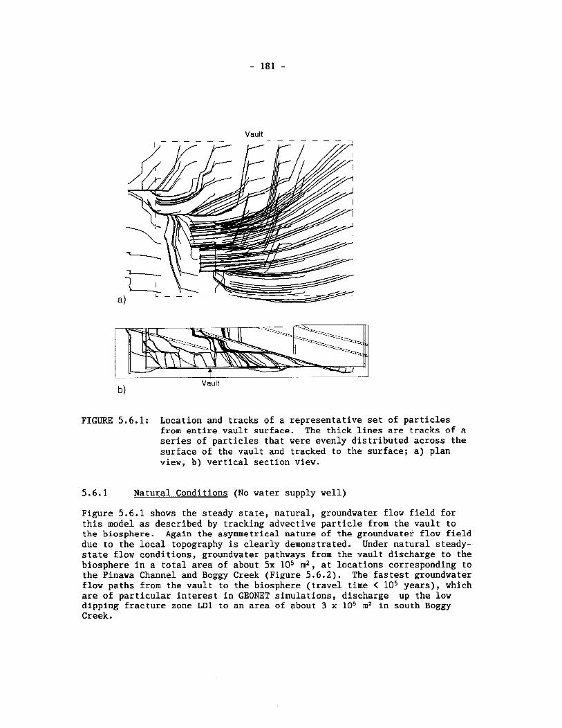
FIGURE 5.6.1: Location and tracks of a representative set of particles from entire vault surface. The thick lines are tracks of a series of particles that were evenly distributed across the surface of the vault and tracked to the surface; a) plan view, b) vertical section view.
5.6.1 Natural Conditions (No water supply well)
Figure 5.6.1 shows the steady state, natural, groundwater flow field for this model as described by tracking advective particle from the vault to the biosphere. Again the asymmetrical nature of the groundwater flow field due to the local topography is clearly demonstrated. Under natural steady- state flow conditions, groundwater pathways from the vault discharge to the biosphere in a total area of about 5x lo5 m2, at locations corresponding to the Pinawa Channel and Boggy Creek (Figure 5.6.2). The fastest groundwater flow paths from the vault to the biosphere (travel time < lo5 years), which are of particular interest in GEONET simulations, discharge up the low dipping fracture zone LD1 to an area of about 3 x lo5 m2 in south Boggy Creek.

r,
\
Boggy Creek North Discharge \
\
', \
\
\ Boggy Creek South Wcharge
\
/ /
/
/
0 0.5 1 km - I Short-term discharge: <1 o5 years
Long-term dlscharge: > 1 o5 years
FIGURE 5.6.2: Surface discharge areas of particles under natural steady- state flow conditions. Discharge areas are outlined by tracing zones on the surface where particles exit. Short- term and long-term discharge mean areas where particles arrive in less or more than lo5 years.
The results of this simulation have recently been compared to hydrogeo- chemical field data collected from this portion of the WRA. It was found that the areas where groundwater was predicted by the groundwater flow model to discharge from LD1 at ground surface coincided with areas where unusually high concentrations of helium gas occurred in overburden, sedi- ments and surface waters (Stephenson et al. 1992) (Figure 5.6.3).
These high helium concentrations in the soil and surface water are assoc- iated with the local discharge of deep groundwater from underlying fracture zones in the rock. In addition, the predicted range of times for water recharging the surface to travel to the 500 m deep level of fracture zone LD1 has recently been compared with the range of ages determined for groundwater samples collected from this location, as determined by isotopic analysis (Gascoyne and Chan 1992). The mean groundwater residence time for the recharging groundwater to reach this location in the flow system as determined by simulation was about 3x10⁶ years (Figure 5.6.4). The resid- ence time as estimated by isotopic analysis of the groundwaters collected from this location was in excess of lo6 years (Figure 5.6.5). Although our groundwater flow model of the WRA has not been rigorously calibrated again- st field observations of hydraulic heads or the responses of groundwater pumping tests, these agreements between the simulated conditions and field observations help establish the reliability of the three-dimensional groundwater flow simulation results.
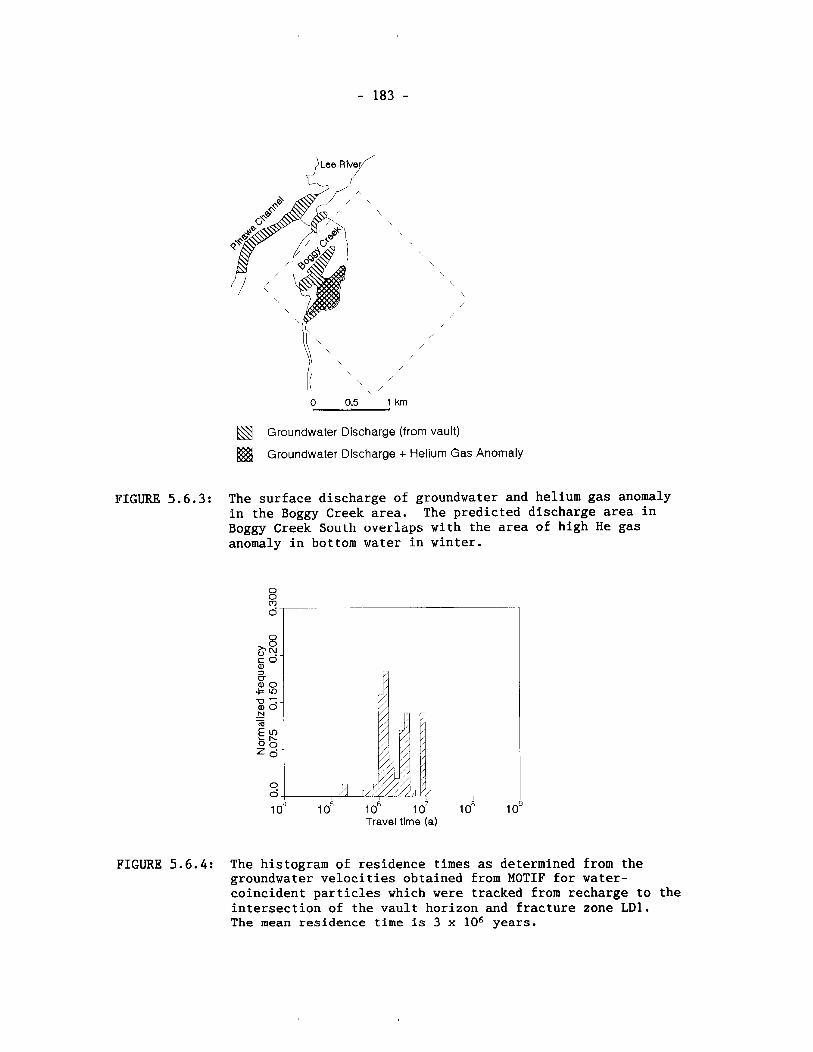
Groundwater Discharge (from vault)
Groundwater Discharge + Helium Gas Anomaly
FIGURE 5.6.3: The surface discharge of groundwater and helium gas anomaly in the Boggy Creek area. The predicted discharge area in Boggy Creek South overlaps with the area of high He gas anomaly in bottom water in winter.
Travel time (a)
FIGURE 5.6.4: The histogram of residence times as determined from the groundwater velocities obtained from MOTIF for water- coincident particles which were tracked from recharge to the intersection of the vault horizon and fracture zone LD1. The mean residence time is 3 x lo6 years.
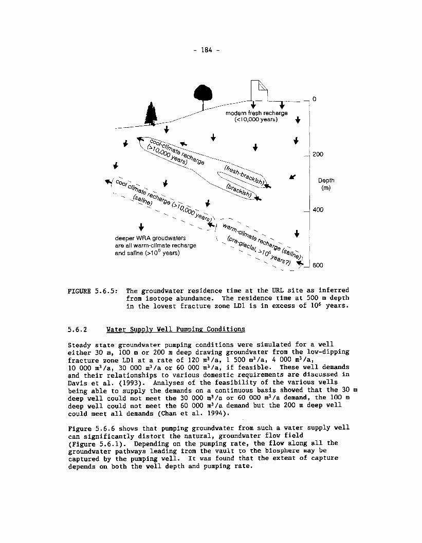
/ modern fresh recharge (~10,000 years)
\ -vu \ , I \ *@era,\ 1 + \
deeper WRA groudwaters \
+ are all warm-climate recharge and sallne (>1 o6 years) \
\ \
Depth (m)
FIGURE 5.6.5: The groundwater residence time at the URL site as inferred from isotope abundance. The residence time at 500 m depth in the lowest fracture zone LD1 is in excess of lo6 years.
5.6.2 Water SUDD~V Well Pum~inn Conditions
Steady state groundwater pumping conditions were simulated for a well either 30 m, 100 m or 200 m deep drawing groundwater from the low-dipping fracture zone LD1 at a rate of 120 m3/a, 1 500 m3/a, 4 000 m3/a, 10 000 m3/a, 30 000 m3/a or 60 000 m3/a, if feasible. These well demands and their relationships to various domestic requirements are discussed in Davis et al. (1993). Analyses of the feasibility of the various wells being able to supply the demands on a continuous basis showed that the 30 m deep well could not meet the 30 000 m 3 / a or 60 000 m3/a demand, the 100 m deep well could not meet the 60 000 m3/a demand but the 200 m deep well could meet all demands (Chan et al. 1994).
Figure 5.6.6 shows that pumping groundwater from such a water supply well can significantly distort the natural, groundwater flow field (Figure 5.6.1). Depending on the pumping rate, the flow along all the groundwater pathways leading from the vault to the biosphere may be captured by the pumping well. It was found that the extent of capture depends on both the well depth and pumping rate.
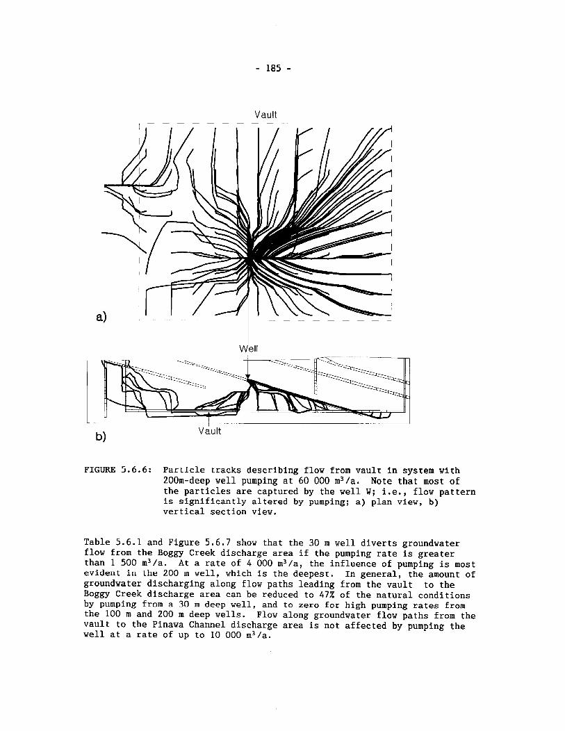
Vault I - - - - - - - - - - p p p p p p p
FIGURE 5.6.6: Parlicle tracks describing flow from vault in system with 200m-deep well pumping at 60 000 m3/a. Note that most of the particles are captured by the well W; i.e., flow pattern is significantly altered by pumping; a) plan view, b) vertical section view.
Table 5.6.1 and Figure 5.6.7 show that the 30 m well diverts groundwater flow from the Boggy Creek discharge area if the pumping rate is greater than 1 500 m3/a. At a rate of 4 000 m3/a, the influence of pumping is most evident in the 200 m well, which is the deepest. In general, the amount of groundwater discharging along flow paths leading from the vault to the Boggy Creek discharge area can be reduced to 47X of the natural conditions by pumping from a 30 m deep well, and to zero for high pumping rates from the 100 m and 200 m deep wells. Flow along groundwater flow paths from the vault to the Pinawa Channel discharge area is not affected by pumping the well at a rate of up to 10 000 m3/a.
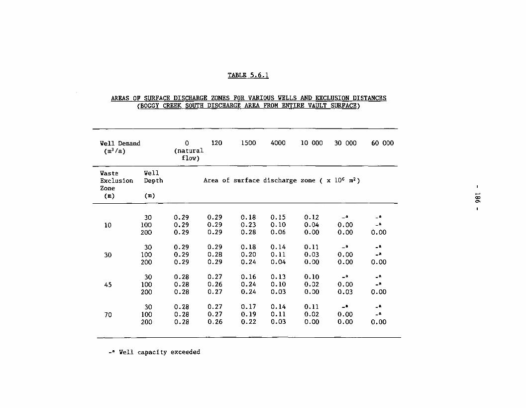
TABLE 5.6.1
AREAS OF SURFACE DISCHARGE ZONES FOR VARIOUS WELLS AND EXCLUSION DISTANCES (BOGGY CREEK SOUTH DISCHARGE AREA FROM ENTIRE VAULT SURFACE)
Well Demand 0 120 1500 4000 10 000 30 000 60 000 (m3 / a ) ( n a t u r a l
flow)
Waste Well Exclusion Depth Area of s u r f a c e discharge zone ( x lo6 m2) Zone
(m) ('"1
- a Well capaci ty exceeded
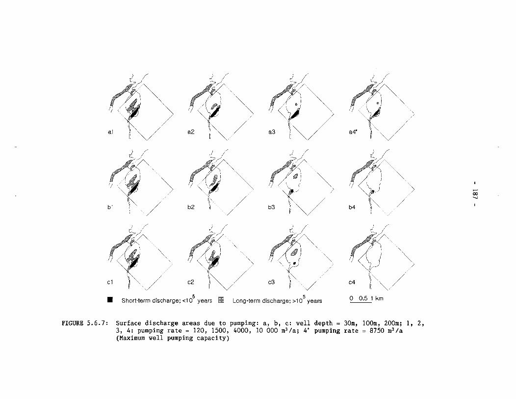
5 5 Short-term discharge; el 0 years Long-term discharge; >10 years 0 0.5 1 krn
FIGURE 5.6.7: Surface discharge areas due to pumping: a, b, c: well depth = 30m, loom, 200m; 1, 2, 3, 4: pumping rate = 120, 1500, 4000, 10 000 m3/a; 4* pumping rate = 8750 m3/a (Maximum well pumping capacity)
Additional discussion of the effects of pumping a groundwater supply well on the groundwater flow field of the WRA model may be found in the papers by Char1 eL al. (1991b) and Chan et al. (1994).
The use of the results of these simulations for both natural and pumping conditions to construct the GEONET model will be discussed further in Chapters 6 and 7.
5.7 THREE-DIMENSIONAL MODELS OF THE EFFECTS OF AN OPEN BOREHOLE
Another situation we considered involves the hydrogeological effects of an open site evaluation borehole located near a waste emplacement area of the vault. Such a borehole could be open either because it had been missed during the sealing operation or because the seals fail some time after borehole closure. In our analyses we assumed that the borehole was drilled from ground surface, that it passed through the low dipping fracture zone LD1, and that it intersected the vault horizon within a rock pillar between two waste emplacement rooms. We performed a series of simulations with the model of the Whiteshell Research Area, to evaluate the sensitivity of the transport along groundwater flow paths from the vault to the biosphere, to such an open borehole. We also considered how the groundwater flow within such an open borehole, could be influenced by an active water supply well that penetrates the fracture zone some distance downgradient of the point at which the open borehole penetrates the fracture. Two- and three- dimensional finite-element simulations were performed to study the advective, dispersive and diffusive transport from an emplacement room in the vault to the open borehole (Chan and Stanchell 1992).
This open borehole modelling was preliminary and exploratory in nature. The results of the finite-element modelling have not yet been condensed into a SYVAC/GEONET model for postclosure assessment and will not be reported in detail here. A brief summary is given below to indicate how detailed flow and transport modelling can be utilized to help develop suit- able derived criteria (e.g., the minimum distance to maintain between a borehole drilled for site evaluation purposes and a waste container) for conceptual vault design at a candidate site.
5.7.1 Vault-scale Modelling
A 3-D MOTIF finite element model, henceforth called the vault-scale model, was created by modifying the local three-dimensional groundwater flow model (Section 5.6 above) used to finalize GEONET to include a borehole which extends from the ground surface to a depth of 550 m. This borehole was located to intersect both the low-dipping fracture zone LD1 and the vault horizon (see Figure 5.5.20). The open borehole was positioned so that it would intersect the plume of any contaminants from the vault moving up groundwater flow paths along the low-dipping fracture zone LD1. The bore- hole was represented by line elements whose properties corresponded to an open pipe of either 76 mm or 165 mm diameter, the sizes of most boreholes that have been drilled for site characterization purposes in the Canadian Nuclear Fuel Waste Management program. Groundwater flow through the bore-
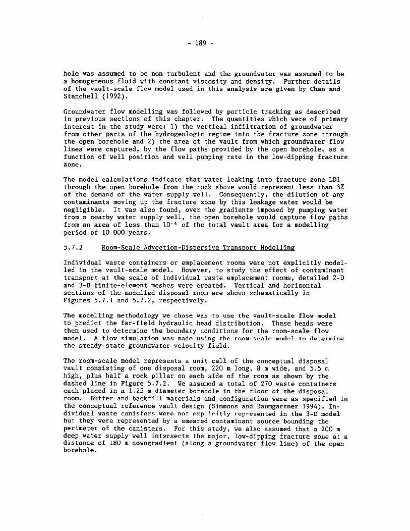
hole was assumed to be non-turbulent and the groundwater was assumed to be a homogeneous fluid with constant viscosity and density. Further details of the vault-scale flow model used in this analysis are given by Chan and Stanchell (1992).
Groundwater flow modelling was followed by particle tracking as described in previous sections of this chapter. The quantities which were of primary interest in the study were: 1) the vertical infiltration of groundwater from other parts of the hydrogeologic regime into the fracture zone through the open borehole and 2) the area of the vault from which groundwater flow lines were captured, by the flow paths provided by the open borehole, as a function of well position and well pumping rate in the low-dipping fracture zone.
The model calculations indicate that water leaking into fracture zone LD1 through the open borehole from the rock above would represent less than 3% of the demand of the water supply well. Consequently, the dilution of any contaminants moving up the fracture zone by this leakage water would be negligible. It was also found, over the gradients imposed by pumping water from a nearby water supply well, the open borehole would capture flow paths from an area of less than 10- of the total vault area for a modelling period of 10 000 years.
5.7.2 Room-Scale Advection-Dispersive Trans~ort Modellinq
Individual waste containers or emplacement rooms were not explicitly model- led in the vault-scale model. However, to study the effect of contaminant transport at the scale of individual waste emplacement rooms, detailed 2-D and 3-D finite-element meshes were created. Vertical and horizontal sections of the modelled disposal room are shown schematically in Figures 5.7.1 and 5.7.2, respectively.
The modelling methodology we chose was to use the vault-scale flow model to predict the far-field hydraulic head distribution. These heads were then used to determine the boundary conditions for the room-scale flow model. A flow simulation was made using the room-scale model to determine the steady-state groundwater velocity field.
The room-scale model represents a unit cell of the conceptual disposal vault consisting of one disposal room, 220 m long, 8 m wide, and 5.5 m high, plus half a rock pillar on each side of the room as shown by the dashed line in Figure 5.7.2. We assumed a total of 270 waste containers each placed in a 1.25 m diameter borehole in the floor of the disposal room. Buffer and backfill materials and configuration were as specified in the conceptual reference vault design (Simmons and Baumgartner 1994). In- dividual waste canisters were not explicitly represented in the 3-D model but they were represented by a smeared contaminant source bounding the perimeter of the canisters. For this study, we also assumed that a 200 m deep water supply well intersects the major, low-dipping fracture zone at a distance of 18U m downgradient (along a groundwater flow line) of the open borehole.
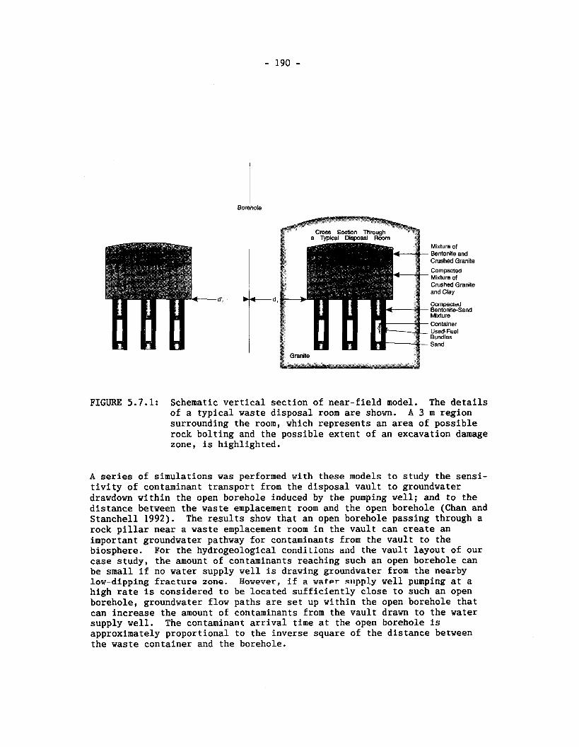
Borehole I
Mixture of Bentonite and Crushed Granite
Compacted Mixture of Crushed Granite and Clay
d', d, Compacted Bentonite-Sand Mixture Container Used-Fuel Bundles Sand
FIGURE 5.7.1: Schematic vertical section of near-field model. The details of a typical waste disposal room are shown. A 3 m region surrounding the room, which represents an area of possible rock bolting and the possible extent of an excavation damage zone, is highlighted.
A series of simulations was performed with these models to study the sensi- tivity of contaminant transport from the disposal vault to groundwater drawdown within the open borehole induced by the pumping well; and to the distance between the waste emplacement room and the open borehole (Chan and Stanchell 1992). The results show that an open borehole passing through a rock pillar near a waste emplacement room in the vault can create an important groundwater pathway for contaminants from the vault to the biosphere. For the hydrogeological conditions and the vault layout of our case study, the amount of contaminants reaching such an open borehole can be small if no water supply well is drawing groundwater from the nearby low-dipping fracture zone. However, if a water supply well pumping at a high rate is considered to be located sufficiently close to such an open borehole, groundwater flow paths are set up within the open borehole that can increase the amount of contaminants from the vault drawn to the water supply well. The contaminant arrival time at the open borehole is approximately proportional to the inverse square of the distance between the waste container and the borehole.
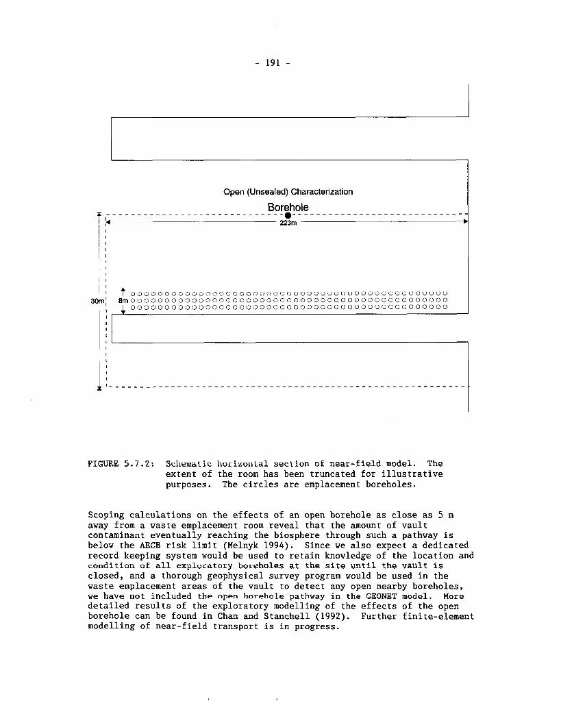
Open (Unsealed) Characterization
FIGURE 5.7.2: Schematic horizon~al section of near-f ield model. The extent of the room has been truncated for illustrative purposes. The circles are emplacement boreholes.
Scoping calculations on the effects of an open borehole as close as 5 m away from a waste emplacement room reveal that the amount of vault contaminant eventually reaching the biosphere through such a pathway is below the AECB risk limit (Melnyk 1994). Since we also expect a dedicated record keeping system would be used to retain knowledge of the location and condition of all explo~atory boreholes at the site until the vaulr is closed, and a thorough geophysical survey program would be used in the waste emplacement areas of the vault to detect any open nearby boreholes, we have not included the open borehole pathway in the GEONET model. More detailed results of the exploratory modelling of the effects of the open borehole can be found in Chan and Stanchell (1992). Further finite-element modelling of near-field transport is in progress.
6. GEONET - THE GEOSPHERE MODEL OF SYVAC3-CC3
INTRODUCTION
The geosphere model GEONET is a model for contaminant transport along a simplified set of pathways leading from the vault to groundwater discharge locations at ground surface. It calculates the transport rate of contam- inants along these pathways but it does not determine the groundwater flow field which is the basis for these pathways. Instead, GEONET depends on the groundwater flow field being provided from an external calculation, in the form of either a set of reference hydraulic heads or a set of ground- water velocities. For our analysis, we have used the groundwater flow field as determined by our detailed finite-element groundwater flow model MOTIF to provide the flow field and pathways input to GEONET.
GEONET uses a simplified geometry to represent the pathways through the groundwater flow field, from the vault to discharge locations in the bio- sphere. This flow field is approximated by a set of one-dimensional (1-D) transport elements or flow tubes called segments that are connected to- gether in three-dimensional (3-D) space to form a transport network. The transport network represents the pathways through the rock surrounding a disposal vault, that contaminants from the vault would follow to reach the biosphere. An example is shown in Figure 6.1.1. The transport network may converge and diverge. Convergence occurs, for example, at the location of a well pumping groundwater from the rock.
One-dimensional transport segments are used for computational efficiency so that analytical solutions to the transport equations for radionuclide decay chains can be used. The output from one segment of the network is cal- culated and used as the input to the next segment of the network. In im- plementing such a transport network for a specific disposal site with its particular solute transport characteristics, we closely represent the de- tailed field information on the transport characteristics and the geometry of the groundwater transport pathways as determined by detailed hydrogeo- logical modelling of the site. The network incorporates the hydrogeologic stratigraphy and geologic structures, the geochemistry of the rock and the groundwater, and the groundwater flow field from the vault to the biosphere.
Other network models have been developed by a number of other groups for use in contaminant transport calculations (Berman et al. 1978; Ross and Koplik 1979; Ross et al. 1979; Laurens et al. 1987; Longsine et al. 1987) and some of these network models also have been used to determine the groundwater flow field. While the GEONET network model has not been de- veloped to determine the groundwater flow field, it incorporates other features of particular interest to our application, such as a model that describes the transport of contaminants to a groundwater well.
This chapter describes the GEONET model. The model is formulated generally and can be applied to many different sites. These sites can have flow pathways or solute transport characteristics that are different than the conditions we have used in our case study. Most of the site-specific
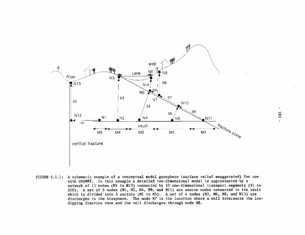
vertical fracture
FIGURE 6.1.1: A schematic example of a conceptual model geosphere (surface relief exaggerated) for use with GEONET. In this example a detailed two-dimensional model is approximated by a network of 13 nodes (N1 to N13) connected by 10 one-dimensional transport segments (S1 to S10). A set of 5 nodes (Nl, N2, N4, N9, and N11) are source nodes connected to the vault which is divided into 5 sectors (MI to M5). A set of 4 nodes (N3, N6, N8, and N13) are discharges to the biosphere. The node N7 is the location where a well intersects the low- dipping fracture zone and the well discharges through node N8.
information is incorporated into the GEONET model using input data files. Section 6.2 describes general features of the transport network. Section 6.3 describes the transport equations and their application, and Section 6.4 describes the parameters in the transport equation. Section 6.5 describes the approach that we have taken to model contaminant transport to a groundwater supply well that penetrates the geosphere. Sections 6.6 and 6.7 describe the interfaces between GEONET and the Vault and Biosphere models. Section 6.8 presents the quality assurance and veri- fication steps that have been taken to give confidence in the implement- ation of the GEONET model. Chapter 7 describes how we have applied GEONET to represent the geosphere of our WRA site for the postclosure assessment calculations.
GEONET MODEL OVERVIEW
In GEONET the three-dimensional description of the pathways of contaminants from the vault to the biosphere through the geosphere (as modified by the presence of a nuclear fuel waste disposal vault) is approximated by a 3-D network of nodes connected in pairs by one-dimensional transport segments. A schematic example of such a transport network is shown in Figure 6.2.1. Transport segments can either converge or diverge at nodes, and they con- nect together to represent the transport pathways leading from a source of contaminants to discharge locations in the biosphere. If segments con- verge, their output is summed before being used as input to the succeeding segment. If segments diverge, the output of a segment is fractionated, and a portion is used as input to each succeeding segment. In our approach, the network used for postclosure assessment calculations is derived from the detailed 3-D groundwater modelling of the geosphere at the disposal site. The detailed groundwater modelling is done using the finite-element groundwater flow code MOTIF (see Sections 3.2, 7.2 and 7.3). The ground- water flow field from the vault to the biosphere is mapped using TRACK3D a numerical, advective particle-tracking technique described in Section 3.3.
The transport segments of the GEONET network are placed to coincide with the pathways that contaminants would follow as they move from the vault to the biosphere, as determined by the MOTIF groundwater flow simulations. However, there are regions of the geosphere where the groundwater flow velocities are extremely low. In these regions contaminant transport is dominated by diffusion rather than by groundwater advection. We ignore the groundwater flow field in these regions and place the GEONET transport network segments along the lines of maximum concentration gradient, repre- senting the shortest diffusion pathways to regions where the permeability and groundwater flow are significantly higher.
The transport network is defined by a set of Cartesian nodal coordinates and tables of connectivities defining which transport segments connect which pair of nodes. Each segment of the network has location-specific chemical and physical properties that reflect the actual conditions deter- mined by site evaluation studies. The principal segment properties used in the model are depicted in Figure 6.2.2. Each segment of the transport network is assigned constant physical and chemical properties, so that analytical solutions can be used to simulate the transport of contaminants along the transport segment. However, transport properties can vary from
segment to segment along the transport pathway. The spatial variation in these properties depends on the details of the conceptual model of the site.
The physical properties of the segments include the porosity, the tortuo- sity factor that is used to modify diffusion characteristics, the longitud- inal dispersivity, the permeability for the transport path in the direction of the axis of the segment or flow tube, and a number of parameters used to simulate diffusion in the rock matrix in a direction orthogonal to the axis of the flow tube. The matrix diffusion parameters are used only if matrix diffusion is invoked as a transport process. These parameters include the matrix tortuosity factor, the effective fracture aperture, the effective fracture spacing, and a scaling factor that relates the contaminant retard- ation factors in the rock matrix to those in the fracture system. In this implementation, a value for the effective fracture aperture that is > 1 um is used as a switch that determines whether matrix diffusion is invoked as a transport process.
One set of nodes represents the sources of contaminants entering the geo- sphere from the various sectors of the disposal vault. Figure 6.2.1 de- picts an example of this where three source nodes (Nl, N2 and N3) originate at three different regions of the vault referred to as vault sectors. Each source node is associated with a unique vault sector. The total flow rate of each contaminant out of each vault sector is calculated by the vault model (Johnson et al. 1994) and is transferred to the source nodes in the GEONET model of the geosphere.
Another set of nodes represents the locations where pathways from the vault emerge at groundwater discharge arcas in the biosphere. Figure 6.2.1 shows two discharge areas, N8 and N9, where the transport pathways from the vault reach the biosphere. These discharge areas may discharge to an aquatic body such as a stream or a lake, discharge to a groundwater supply well, discharge to the base of the unsaturated zone of a terrestrial area, or discharge to a wetland area such as a swamp or fen. In the postclosure assessment calculations, the flow rates of contaminants from the vault calculated to reach these different discharge areas are transferred to the biosphere model (Davis et al. 1993).
In the GEONET model each of the nodes representing pathways emerging at aqueous, terrestrial and wetland discharge areas has two extra nodes assoc- iated with it, as shown in Figure 6.2.3. These extra nodes define the positions of the lowest extents of the compacted sediment layer and the overburden layer that might exist at these discharge areas and they are placed directly under the discharge nodes. The two extra layers have specified thicknesses and replace a portion of the last transport segment leading to the discharge area. These layers of surface deposits have not been included in the detailed groundwater model, since they are relatively thin and do not affect the overall flow of groundwater from the vault to the discharge arca. However, they have been added to the network model of the geosphere transport since they have chemical and sorption properties very different from the rest of the geosphere pathways through the rock and they do affect the transfer of contaminants to the biosphere.
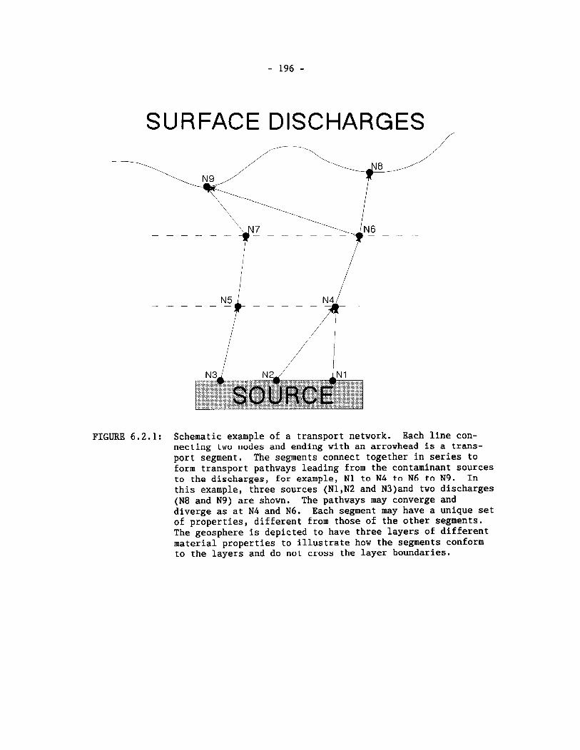
SURFACE DISCHARGES
N8 / /
- - - - - -
FIGURE 6.2.1: Schematic example of a transport network. Each line con- necting two nodes and ending with an arrowhead is a trans- port segment. The segments connect together in series to form transport pathways leading from the contaminant sources to the discharges, for example, N1 to NL to N6 to N9. In this example, three sources (Nl,N2 and N3)and two discharges (N8 and N9) are shown. The pathways may converge and diverge as at N4 and N6. Each segment may have a unique set of properties, different from those of the other segments. The geosphere is depicted to have three layers of different material properties to illustrate how the segments conform to the layers and do not cross the layer boundaries.
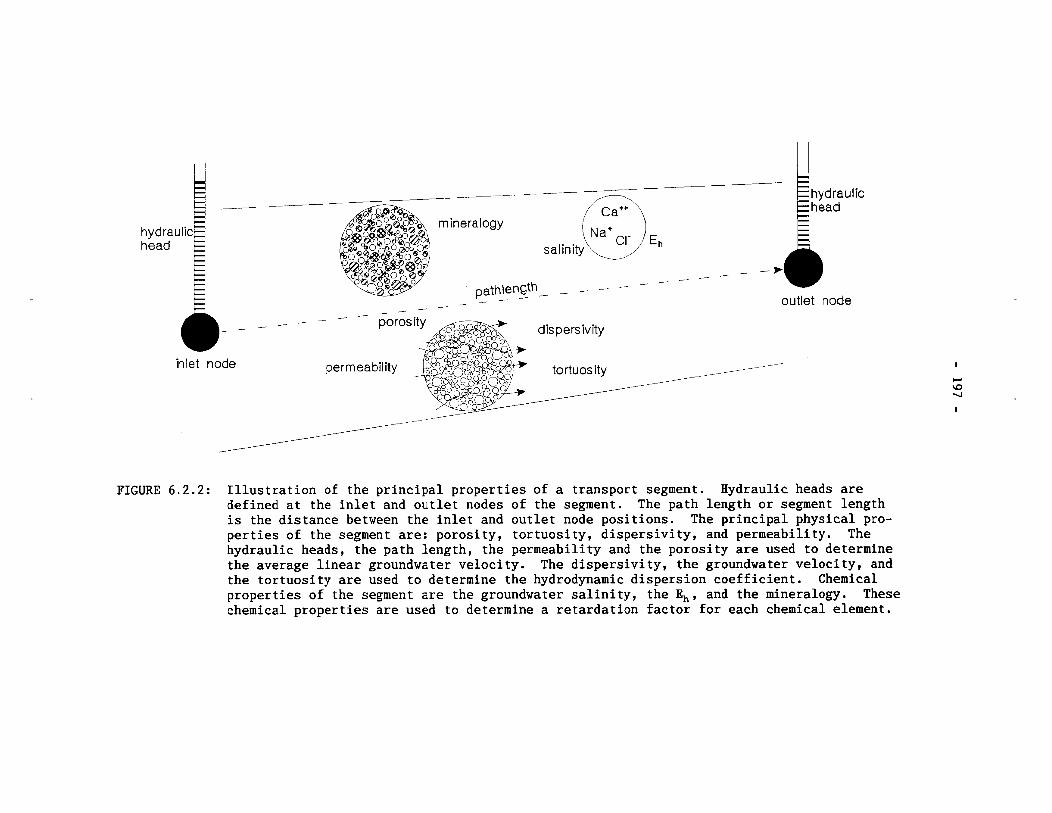
head
inlet node
salinity
/ /
/ -P /
/ /
,,thlenath - - / /
/ YU'';-. " - outlet node
FIGURE 6.2.2: Illustration of the principal properties of a transport segment. Hydraulic heads are defined at the inlet and outlet nodes of the segment. The path length or segment length is the distance between the inlet and outlet node positions. The principal physical pro- perties of the segment are: porosity, tortuosity, dispersivity, and permeability. The hydraulic heads, the path length, the permeability and the porosity are used to determine the average linear groundwater velocity. The dispersivity, the groundwater velocity, and the tortuosity are used to determine the hydrodynamic dispersion coefficient. Chemical properties of the segment are the groundwater salinity, the E,, and the mineralogy. These chemical properties are used to determine a retardation factor for each chemical element.
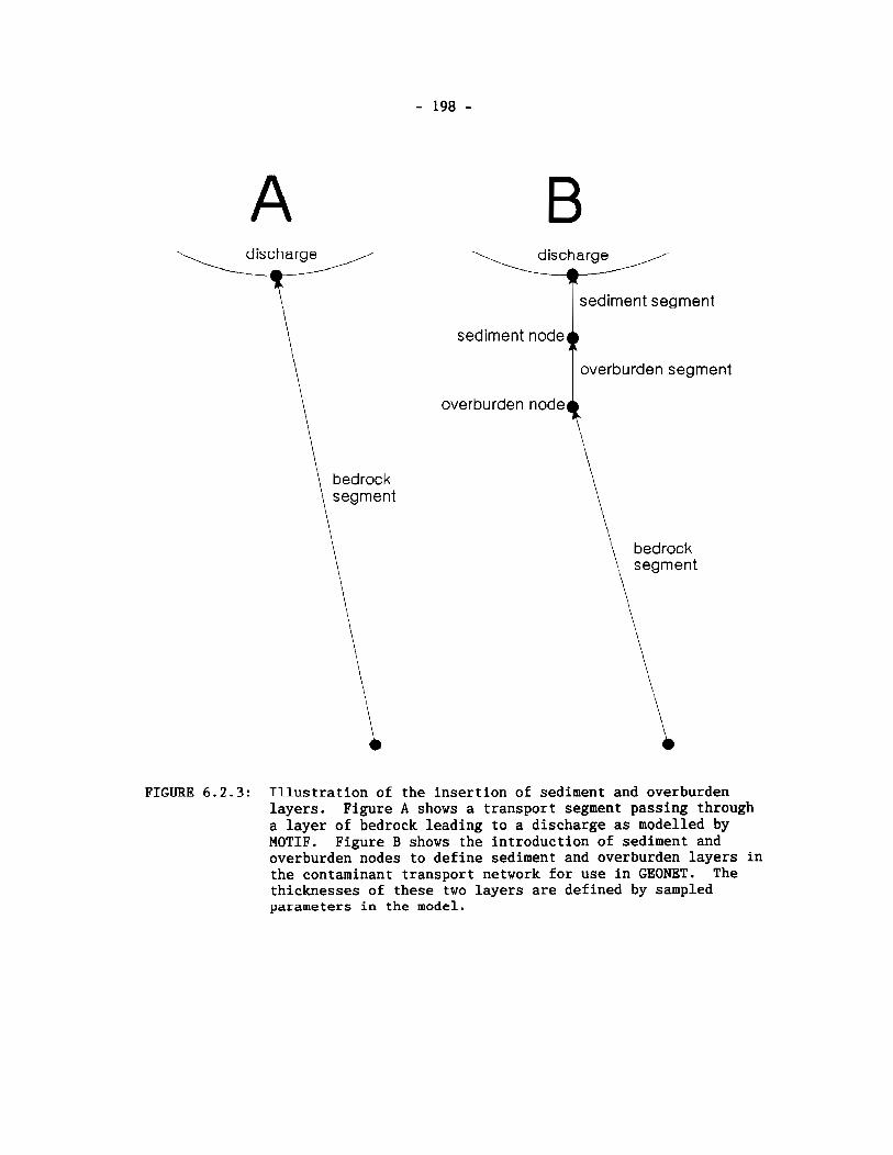
discharge discharge
sediment segment
sediment node
bedrock segment
\ overburden node t
overburden segment
bedrock segment
FIGURE 6.2.3: Illustration of the insertion of sediment and overburden layers. Figure A shows a transport segment passing through a layer of bedrock leading to a discharge as modelled by MOTIF. Figure B shows the introduction of sediment and overburden nodes to define sediment and overburden layers in the contaminant transport network for use in GEONET. The thicknesses of these two layers are defined by sampled parameters in the model.
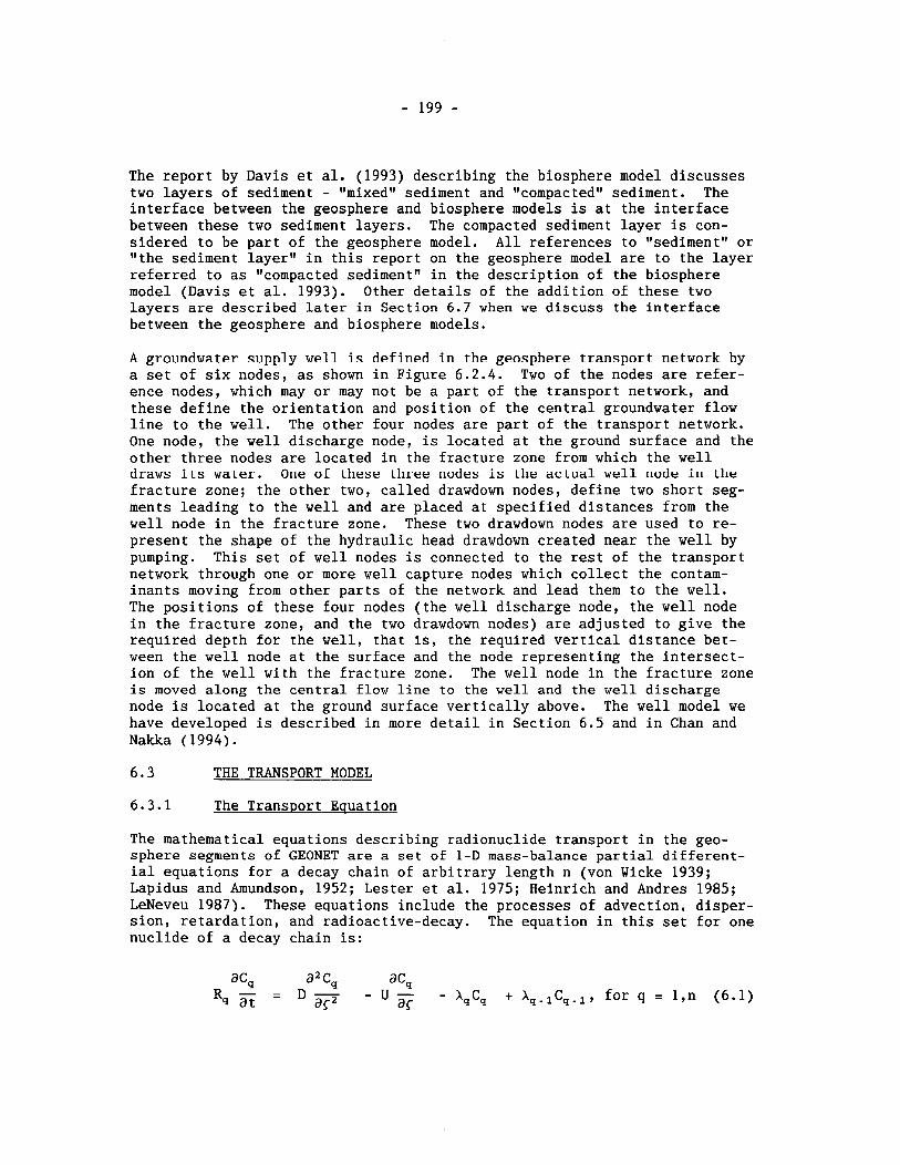
The report by Davis et al. (1993) describing the biosphere model discusses two layers of sediment - "mixed" sediment and "compacted" sediment. The interface between the geosphere and biosphere models is at the interface between these two sediment layers. The compacted sediment layer is con- sidered to be part of the geosphere model. All references to "sediment" or "the sediment layer" in this report on the geosphere model are to the layer referred to as llcompacted sediment" in the description of the biosphere model (Davis et al. 1993). Other details of the addition of these two layers are described later in Section 6.7 when we discuss the interface between the geosphere and biosphere models.
A groundwater supply well is defined in the geosphere transport network by a set of six nodes, as shown in Figure 6.2.4. Two of the nodes are refer- ence nodes, which may or may not be a part of the transport network, and these define the orientation and position of the central groundwater flow line to the well. The other four nodes are part of the transport network. One node, the well discharge node, is located at the ground surface and the other three nodes are located in the fracture zone from which the well draws its water. One of these three nodes is the actual well node in the fracture zone; the other two, called drawdown nodes, define two short seg- ments leading to the well and are placed at specified distances from the well node in the fracture zone. These two drawdown nodes are used to re- present the shape of the hydraulic head drawdown created near the well by pumping. This set of well nodes is connected to the rest of the transport network through one or more well capture nodes which collect the contam- inants moving from other parts of the network and lead them to the well. The positions of these four nodes (the well discharge node, the well node in the fracture zone, and the two drawdown nodes) are adjusted to give the required depth for the well, that is, the required vertical distance bet- ween the well node at the surface and the node representing the intersect- ion of the well with the fracture zone. The well node in the fracture zone is moved along the central flow line to the well and the well discharge node is located at the ground surface vertically above. The well model we have developed is described in more detail in Section 6.5 and in Chan and Nakka (1994).
6.3 THE TRANSPORT MODEL
6.3.1 The Transport Equation
The mathematical equations describing radionuclide transport in the geo- sphere segments of GEONET are a set of 1-D mass-balance partial different- ial equations for a decay chain of arbitrary length n (von Wicke 1939; Lapidus and Amundson, 1952; Lester et al. 1975; Heinrich and Andres 1985; LeNeveu 1987). These equations include the processes of advection, disper- sion, retardation, and radioactive-decay. The equation in this set for one nuclide of a decay chain is:
a% a* c, R q z = D c - U -
a i - XqCq + A,-,C,-,, for q = l,n (6.1)
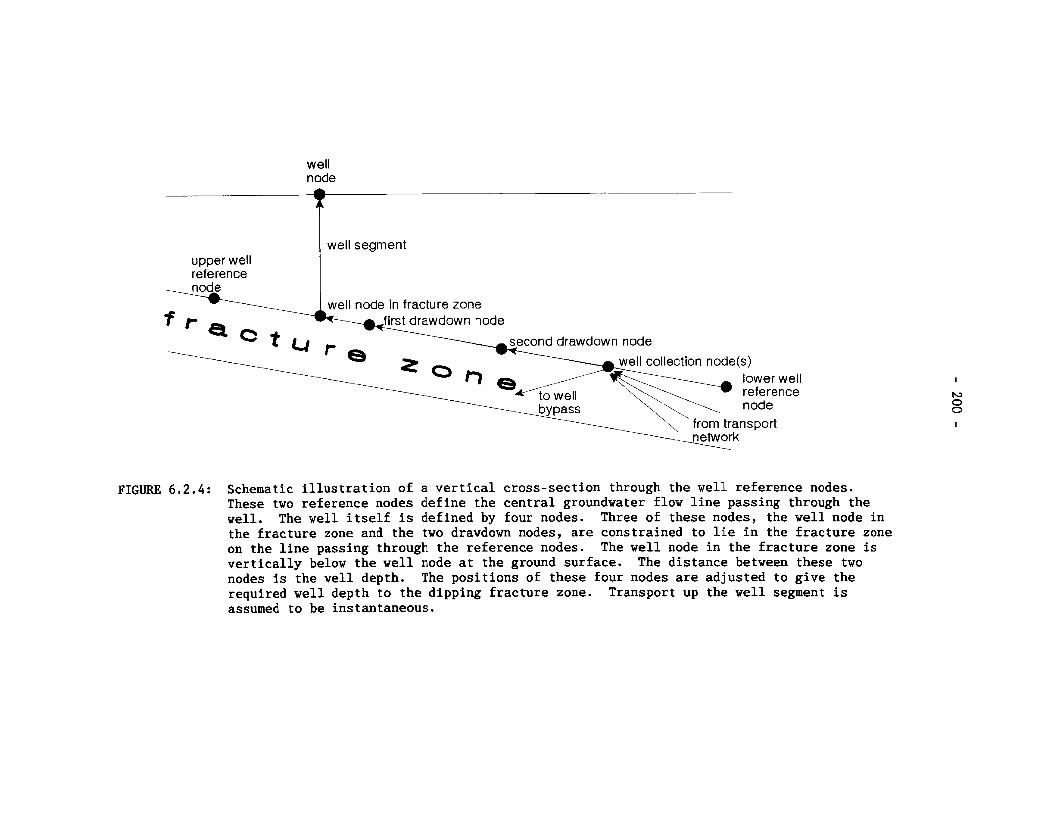
well node
upper well reference
well segment
FIGURE 6 .2 .4 : Schematic illustration of a vertical cross-section through the well reference nodes. These two reference nodes define the central groundwater flow line passing through the well. The well itself is defined by four nodes. Three of these nodes, the well node in the fracture zone and the two drawdown nodes, are constrained to lie in the fracture zone on the line passing through the reference nodes. The well node in the fracture zone is vertically below the well node at the ground surface. The distance between these two nodes is the well depth. The positions of these four nodes are adjusted to give the required well depth to the dipping fracture zone. Transport up the well segment is assumed to be instantaneous.
where the parameters characterizing the transport equations are:
U = the linear groundwater flow velocity, [m/a] , D = the dispersion coefficient, >O , [m2/a] , R, = a set of retardation factors, one for each nuclide, 21 , A, = a set of radioactive decay constants, one for each nuclide, >O
,[a-lI 9
C, = the concentration in groundwater of nuclide q.
The independent variables are time, t > 0, and a single linear spatial coordinate, c, measured along the axis of the transport segment. The term on the left hand side is an accumulation term, in which the retardation factor R, accounts for equilibrium linear sorption of the nuclide with the adjacent solid rock matrix. The successive terms on the right hand side of Equation (6.1) are the dispersive transport term, the advective transport term, the radioactive decay of nuclide q, and the radioactive production of nuclide q from decay of chain precursor nuclide.
In order to obtain an analytical solution to the transport equation, Equation (6.1), within each segment, all these parameters are considered to be constant (i.e. independent of time t and spatial coordinate I) through- out each transport segment of GEONET. However, the parameters may take on different values in different segments to represent the actual spatial variation in site specific conditions. A variety of different boundary conditions can used with Equation (6.1); the ones used in our case study are presented in the following sections.
6.3.2 The Transport Calculation Using Response Functions
The analytical expression for the contaminant flow rate out of each trans- port segment, in response to an impulse of contaminant flow into the seg- ment, is called a response function. The response function, G ,(t), is the mass flow rate of a nuclide q, J,, that corresponds to an impulse source of a chain precursor nuclide p at the inlet of the segment. The nuclide p is not necessarily the immediate parent of nuclide q; it can be any of the chain precursors or even the nuclide q itself. This mass flow response function can be obtained by applying the flux operator to a solution to Equation (6.1), and evaluating the result at the outlet of the segment at g = L . For semi-infinite domains with impulse sources, Equation (6.1) and its boundary conditions can be transformed so that it uses flux or mass flow rate of contaminant, J q l instead of concentration of contaminant, C,, as a dependent variable. Thls transformation between the use of concen- tration and of flux as dependent variables is further described in Appendix G and in Heinrich and Andres (1985). Expressions for the concen- tration of the nuclides in groundwater are not used explicitly; the res- ponse function gives the nuclide mass flow rate only, and in SYVAC3-CC3 we generally use flux or mass flow rate of nuclide as the dependent variable.
To calculate the total time-dependent mass flow rate of nuclide q exiting from each segment of the geosphere network, the response function for the segment is convoluted with a previously calculated set of time-varying input mass flow rates, I,(t). The contributions from all decay chain
precursors are summed to give the total mass flow rate out of the segment of nuclide q, Oq(t), where
t' is the time of integration and p takes values from 1 to q.
The form of the response function solution to Equation (6.1) depends on the boundary and initial conditions. Three different response functions have been developed for use in the GEONET model to determine the mass flow rate at the outlets of the transport segments. These response functions can be chosen independently for each transport segment of the network. These response functions are:
1. Semi-infinite medium response function (Heinrich and Andres 1985).
2. Mass transfer coefficient response function (LeNeveu 1987).
3. Zero concentration boundary condition response function obtained using the mass transfer coefficient response function with a large value for the mass transfer coefficient (Garisto and LeNeveu 1991, Johnson et al. 1994).
The differences in the boundary conditions for these three cases are schematically illustrated in Figure 6.3.1.
In some places in the geosphere network, contaminant flow is passed un- changed from the inlet to the outlet of a segment. This transfer is for- mally counted as a fourth response function:
4. Dirac delta function response function; contaminant flow is passed unchanged from inlet to outlet; that is, O,(t) = I,(t) .
The choice of which response function to use for any particular transport segment of the network depends on the assumed boundary conditions for the particular segment. These choices are described in the next section of this report.
6.3.3 Boundary Conditions
The response functions differ, depending on the boundary condition assumed at the segment outlet. They all have the same unit impulse boundary con- dition at the segment inlet, r = 0, expressed here with flux of contaminant as the dependent variable:
for all t, < = 0, + 1
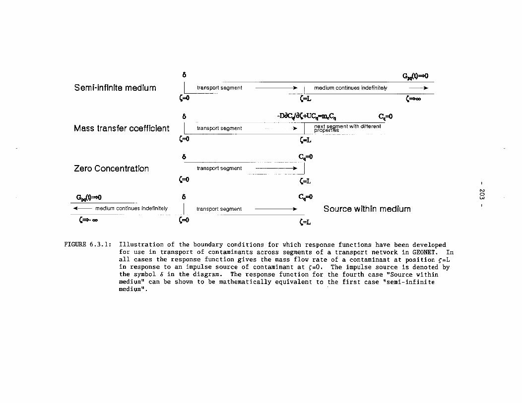
Semi-infinite medium transport segment
Zero Concentration 1 transport segment --- - 1
medium continues indefinitely 4
Mass transfer coefficient
c=o {=L C-
transport segment . $ ~ g $ ; ~ ~ ~ e n t with different I
FIGURE 6.3.1: Illustration of the boundary conditions for which response functions have been developed for use in transport of contaminants across segments of a transpart network in GEONET. In all cases the response function gives the mass flow rate of a contaminant at position r = L in response to an impulse source of contaminant at r=0. The impulse source is denoted by the symbol 6 in the diagram. The response function for the fourth case "Source within medium" can be shovn to be mathematically equivalent to the first case "semi-infinite medium".
Gpq(t)=$O 6 cq=o - medium continues indefinitely transport segment - Source within medium
where S(t-to) is the Dirac delta function and to is the time of the impulse of a parent nuclide p (not necessarily the immediate precursor of nuclide q), usually taken to be to = 0.
For those segments of the network where advective transport dominates, we use the semi-infinite medium response function. This response function is based on the assumption that the transport segment extends infinitely far from the inlet boundary, with the condition:
J,(t) = 0 , for all t, + Q ( 6 - 4 )
The response function is evaluated at c = L, giving the mass flow rate of nuclide q passing a plane within this semi-infinite transport segment at distance L from the inlet boundary.
Response functions based on mass transfer coefficients are appropriate choices for those transport segments in which the transport is not ad- vection dominated, and which do not originate at the contaminant source location at the vault.
The mass transfer coefficient response functions apply to a finite trans- port segment with outlet boundary at distance L from the inlet boundary. At the outlet boundary, the condition
ac, - D -
ac + UC, = m,C, , where c = L
applies where m, is the mass transfer coefficient. In this case, Equation (6.1) is solved with concentration of contaminant as the dependent variable and the mass flow rate of contaminant at the outlet boundary is obtained from J = m,C,. The mass transfer coefficient m, used in Equation (6.5) %epends on the properties of the media on both sides of this boundary and is determined from a formula based on one developed and des- cribed in the vault model report (Johnson et al. 1994). If m, approaches zero, the medium on the other side of the outlet boundary becomes very resistant to the passage of nuclides, and the contaminant flow rate out of the transport segment approaches zero. If m, becomes large, the contam- inant flow rate out of the transport segment approaches an asymptotic maxi- mum where mass flow across the outlet boundary is limited only by the transport properties of the segment itself and is not affected by the pro- perties of the medium on the other side of the boundary. This condition is equivalent to having a zero concentration (i.e., a large sink for nuclides) on the other side of the boundary, and is used for the third response function.
For the transport segments originating at the vault, a third physical sit- uation must be considered. This situation has an impulse source term at < = 0, not at a boundary of the transport medium, but within the transport medium itself. The transport medium is assumed to extend to infinity on one side of the source and to a finite distance L on the other side. At the outlet boundary of the transport segment, at distance L from the source, a zero concentration boundary condition applies. The complete
solution to the transport equation for this case is different than the solution for the other cases. However, the analytical expression for the response function for nuclide mass flow rate crossing the outlet boundary at r = L, is the same as that for the response function for nuclide mass flow rate crossing a plane at r = L in the semi-infinite transport segment case described above. This equivalence is established in Appendix G. Hence, for this physical situation, the semi-infinite medium response function can also be used. This case applies to all transport segments originating at the vault and having an outlet at a location where there is increased permeability and groundwater flow, such as at a fracture zone.
PARAMETERS IN THE TRANSPORT EQUATION
6.4.1 Groundwater Velocity
The groundwater flow field is not determined in GEONET itself. The trans- port network used in GEONET covers only the region of the geosphere through which contaminants move from the disposal vault to the biosphere. The groundwater flow information is obtained from results calculated by the MOTIF code, which uses a finite element mesh to describe groundwater flow for a large region surrounding the vault. By adopting the MOTIF results, and the parameters such as porosity and permeability on which these results are based, we also adopt the groundwater flow continuity and mass balance conditions that correspond to the MOTIF results.
Linear groundwater velocities, U, one for each segment, are determined by one of three possible methods:
1. Linear velocities, U, supplied directly for each segment from the MOTIF groundwater flow model.
2. Reference hydraulic heads, h, supplied for each node and hydraulic conductivities, K, supplied for each segment from the MOTIF groundwater flow model; groundwater velocities for each segment are then calculated in the network model from Darcy's law,
where
where Ah is the difference in hydraulic head between the inlet and outlet nodes of the segment, L is the geometric length of the segment, determined from the cartesian coordinates of the inlet and outlet nodes, K is the hydraulic conductivity (assumed to be constant within the segment), B is the porosity of the segment, and q is the specific discharge through the segment.
3. Reference hydraulic heads, h, and temperatures, T, supplied for each node and intrinsic permeabilities, kc, supplied for each segment from the MOTIF groundwater flow model; groundwater
velocities for each segment are calculated from Darcy's law, Equation (6.6), where hydraulic conductivities for each segment are calculated using the viscosity, p , and density, p , of the groundwater in the segment,
where g is the acceleration due to gravity. The density and viscosity of the groundwater in the segment may be calculated from the equations of state for water using the temperatures, T, and pressures, p calculated from the elevation of the midpoint of each segment. The resulting hydraulic conductivity calculated for the midpoint of the segment is assumed to be constant for the whole segment. In a case where constant groundwater properties are assumed for the entire transport network, a fixed density and viscosity for the water, corresponding to fixed reference values for the temperature and pressure, are used. For example, at a reference temperature of T0=60C, the reference density of water is po=l 000 Kg/m3, and the reference viscosity of water is p,=0.001472 Kg/(m- s) or Pa. s.
In cases 2 and 3, the heads are modified by the groundwater pressure draw- downs caused by the presence of the well before the velocities are calculated (see Section 6.5).
The hydrogeological data and the resulting calculated hydraulic heads are obtained from the detailed groundwater flow modelling with MOTIF and they cannot be varied randomly in the network model. They must have exactly the same values as those used in the MOTIF simulations. If they had different values, the connection with these detailed groundwater flow calculations, from which the heads and velocities were obtained, would be lost, and mass balance of the groundwater flow within the entire groundwater flow system would not necessarily be maintained. In order to account for uncertainty in the groundwater flow calculations within GEONET, a single overall seal- ing factor, S,, can be applied simultaneously to all groundwater velocities in the transport network. In this situation all velocities, U, are re- placed by US,. This approach ensures that groundwater mass balance is retained while the effects of some uncertainty in the groundwater flow velocities are evaluated in GEONET.
6.4.2 Dis~ersion Coefficient
A longitudinal dispersion coefficient, D, for each nuclide in each trans- port segment of the network is determined from
where a, is the longitudinal dispersivity for the segment, 7c is the tortuosity factor of the diffusive transport path along the axis of the segment, and Do is the molecular diffusion coefficient in free water for the nuclide. The effective tortuosity factor of the diffusion path 7c is related to the tortuosity 7 in Equation (3.8) by the relationship, r = 1/rc2. When the groundwater velocity is small, Equation (6.1) reduces

to a pure diffusion transport equation. When the groundwater velocity is large, the mechanical dispersion term, a,U, dominates the dispersion and the effects of diffusion become negligible. In any case, the full express- ions of Equations (6.1) and (6.9) are used for all segments.
The analytical solution to the coupled equations for nuclides in decay chains requires a single dispersion coefficient for each segment that ap- plies to all nuclides in the chain; the value determined for the first member of the chain is used for all chain members. When the mechanical dispersion term, a,U, dominates the dispersion, the dispersion coefficient has the same value for all chain members anyway. When the diffusion term dominates the dispersion, the diffusion coefficients for the actinide ele- ments in decay chains, Am, Np, Pa, Pu, Ra, Th, U, with similar atomic mass- es, have about the same value. (The range of values for diffusion coeffi- cients for all elements is not very large, see Appendix D). Hence, using a single value for dispersion coefficient for all members of a decay chain is a good approximation, and ensures a correlation between dispersion coeffi- cients for the similar mass elements in the chain.
6.4.3 Retardation Factors
Retardation factors are calculated using empirical equations depending on a set of location-specific chemical and mineralogical properties which are defined for each transport segment. A set of element/mineral-specific distribution coefficients has been developed to relate these specific pro- perties of the transport paths to the amount of retardation that can occur. More details of this sorption model are given in Appendix B and in Vandergraaf et al. (1992, 1993). Only the final equations of the model are summarized here. Retardation effects are determined for each element in each transport segment. These effects can also include an approximate consideration of the retardation effects of diffusion of the nuclides into the adjacent rock matrix (in a direction orthogonal to the direction of the advective LransporL), if matrix diffusion is invoked as a transport process for the segment.
For each nuclide/mineral combination, and for either oxidizing or reducing conditions existing in the transport segment, the distribution coefficient kd is given by the same mathematical model or equational form. For each combination of these conditions there are different values for the set of coefficients describing the retardation process. The distribution coefficient kd is calculated from:
Variable X1 is the logarithm, base 10, of the salinity of the groundwater in the transport segment. The salinity is expressed as total dissolved solids, TDS, in units of g/L or Kg/m3,
Variable X2 is the logarithm, base 10, of the radionuclide concentration, C,, in the groundwater of the transport segment solution in units of mole/L,
The function Q(rl,b,) is a function involving a random number, r,, that applies a variation to the calculated value of k, to account for any uncer- tainty there might be for the fitted equation. This function is
where r, is a lognormally distributed random number with geometric mean 1.0 which lies in the range [0.1, 10.01. With this choice of r,, the coeffi- cient b, is the number of orders of magnitude over which kd is allowed to vary, with the bracketed expression in Equation (6.10) giving the geometric mean value for k,.
The scientific literature contains a considerable body of sorption data that has been determined as a function of radionuclide concentration. This data is usually represented in the form of isotherms. We decided to incor- porate what is currently known about the dependence of sorption on radio- nuclide concentration into the parametric model. However, because the transport calculations across each segment in GEONET require retardation factors, or distribution coefficients, that are constant (independent of radionuclide concentration), the dependence of sorption on radionuclide concentration is treated as an additional source of uncertainty in the GEONET model.
The radionuclide concentration, C,, itself is also expressed in terms of another random number, r2, and coefficients b4 and b, in a similar manner to Equations (6.10) and (6.13).
where r, is a random number, similar to r,, from a logarithmic distribution with geometric mean 1.0 which lies in the range [0.1,10.0]. Coefficient b, gives the geometric mean nuclide concentration about which the nuclide concentration is varied and coefficient b,, similar to b,, is the number of orders of magnitude over which the nuclide concentration is varied about this mean. Thus, the presence of radionuclide concentration-dependent terms in the sorption Equation (6.10) is translated into an additional uncertainty in a concentration-independent distribution coefficient in GEONET through use of Equation (6.14).
Once a value for kd is obtained from Equation (6.10), the normalized quantity vk, is obtained by multiplying k, by another coefficient b,. The value used for this coefficient is based on the density and porosity of the rock sample under the conditions used in the laboratory to derive the k, relationship. The normalized quantities vk, are then considered to be approximately independent of density and porosity and can be applied to the
conditions of transport segment without change. More discussion of this topic is contained in Vandergraaf et al. (1993). The normalization is expressed as :
A value for (vk,), is obtained in this manner for each nuclide q with each mineral, m, present in the transport segment. These values are then com- bined, weighted by the fractional abundance, f,, of each mineral, m, to give an overall retardation factor, R,, for the nuclide q in the segment,
Hence each sorption equation has a full complement of ten coefficients: the six coefficients in the fitted sorption equation, the order of magni- tude for variation of k,, the geometric mean and order of magnitude for variation of nuclide concentration, and the normalization factor v used to give a retardation factor that is appropriate for the in-situ conditions of the transport segment.
There are some nuclide/mineral combinations for which a detailed sorption equation is unavailable and only a single constant k, is supplied. In these situations a minimum set of three coefficients is used: the geo- metric mean value for kd (coefficient bo), the order of magnitude for variation of this value (coefficient b3), and the normalization factor (coefficient b,). Equations (6.10) through (6.15) then reduce to
WELL MODEL
Because of the possibility of stratigraphic or topographic restrictions on the location of a groundwater supply well in the geosphere and since, in general, deeper wells tend to capture more contaminants from the vault, we have specified a minimum well depth for our model of the geosphere. If there are no restrictions on well location, then the minimum well depth can be set to zero. The well depth used in the simulation is the greater of the desired well depth and this minimum well depth. After the nodes defin- ing the groundwater supply well in the transport network are repositioned to give the required well depth, (described in Section 6.2) and the well demand is determined, (described in Section 6.7 below), a set of analytical equations is used to determine the effects of pumping the well on the transport of contaminants in the GEONET network.
Wells whose depth is less than the depth to the bottom of the overburden layer are classed as overburden wells. Overburden is only specified in the model at areas where transport pathways from the vault discharge to the biosphere. Therefore, we assign the maximum depth for an overburden well equal to the depth to the bottom of the overburden layer at the nearest discharge location. We assume the overburden wells do not intersect the
pathways of contaminants in the fracture zone that normally acts as the aquifer for the well. The overburden wells obtain their groundwater en- tirely from the overburden layers (described in Section 6.7) but we assume the capacity of these relatively shallow wells is still given approximately by Equation (6.18) below. We further assume that these wells draw no water from the fracture zone, do not affect the groundwater flow field in the rock, and do not capture or discharge any contaminants coming from the vault. These wells are dealt with as a special case in the biosphere model. The rest of this section discusses the effects of wells that are not classed as overburden wells.
The analytical equations describing the groundwater supply well model were derived using complex potential theory and the method of images (Chan and Nakka 1994). The well model assumes that pumping is from a fracture zone that behaves as a confined aquifer with constant and uniform hydraulic properties. The well is also assumed to be near a constant hydraulic head boundary (for example, a lake) located where the fracture zone comes to surface. Initially (i.e., with no well pumping) we assume there is a uni- form and symmetric groundwater flow field in the fracture zone in the vicinity of the well. In order to simulate pumping from the low-dipping fracture zone of our postclosure assessment case study, the aquifer for the well is assumed to dip from the constant head boundary. This analytical well model is used to calculate the following four quantities:
1. the maximum well capacity,
2. the drawdowns at nodes in the fracture zone, from which new hydraulic heads in the fracture zone are determined,
3 . the quantity of lake water captured by induced infiltration, and
4. the contaminant capture fractions by the well in the fracture zone, which determine the quantities of contaminants entering the well.
The groundwater flow field in the fracture zone is assumed to be represent- ed by an idealized, symmetrical flow field for application of the analyti- cal well model equations (AWME). The well is located in the network in a region where the groundwater flow field is fairly uniform and symmetrical so that this idealized flow field is a reasonable approximation in regions close to the well. Here the effect of drawdown on the flow field is great- est and this determines the extent of plume capture in the fracture zone by the pumping well. In regions far from the pumping well, the drawdowns are small and the errors in drawdown due to this approximation are small.
In the GEONET model, the location of the constant head boundary is deter- mined approximately from the extrapolation of the central groundwater flow line passing through the well, defined by the upper and lower well refer- ence nodes, to the elevation of the well discharge node located at the ground surface. Figure 6.2.4 shows a schematic illustration of the location of these nodes.
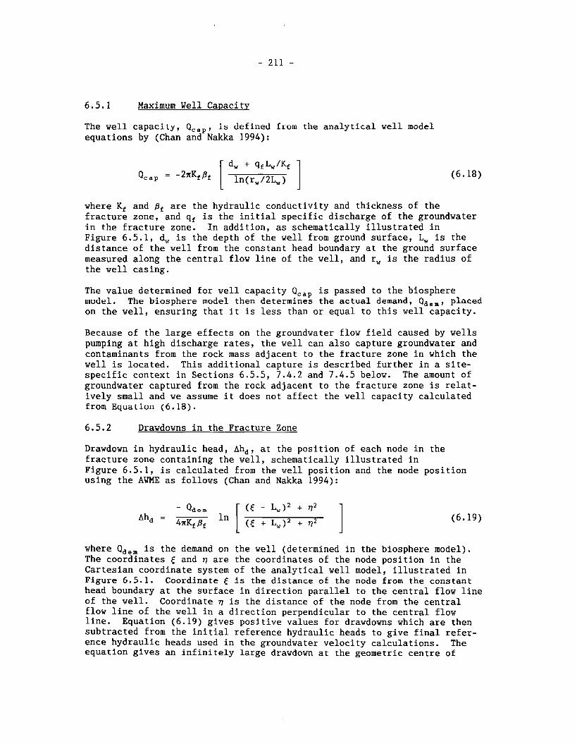
6.5.1 Maximum Well Capacity
The well capacily, Qcap, is defined from the analytical well model equations by (Chan and Nakka 1994):
where Kf and pf are the hydraulic conductivity and thickness of the fracture zone, and q, is the initial specific discharge of the groundwater in the fracture zone. In addition, as schematically illustrated in Figure 6.5.1, d, is the depth of the well from ground surface, L, is the distance of the well from the constant head boundary at the ground surface measured along the central flow line of the well, and r, is the radius of the well casing.
The value determined for well capacity Q,,, is passed to the biosphere model. The biosphere model then determines the actual demand, Qdem, placed on the well, ensuring that it is less than or equal to this well capacity.
Because of the large effects on the groundwater flow field caused by wells pumping at high discharge rates, the well can also capture groundwater and contaminants from the rock mass adjacent to the fracture zone in which the well is located. This additional capture is described further in a site- specific context in Sections 6.5.5, 7.4.2 and 7.4.5 below. The amount of groundwater captured from the rock adjacent to the fracture zone is relat- ively small and we assume it does not affect the well capacity calculated from Equatiori (6.18).
6.5.2 Drawdowns in the Fracture Zone
Drawdown in hydraulic head, Ah,, at the position of each node in the fracture zone containing the well, schematically illustrated in Figure 6.5.1, is calculated from the well position and the node position using the AWME as follows (Chan and Nakka 1994):
( E - L,)2 + q* Ah, = -
47% B, ( f + Lw)2 + v2 1 (6.19)
where Q,,, is the demand on the well (determined in the biosphere model). The coordinates f and Q are the coordinates of the node position in the Cartesian coordinate system of the analytical well model, illustrated in Figure 6.5.1. Coordinate is the distance of the node from the constant head boundary at the surface in direction parallel to the central flow line of the well. Coordinate q is the distance of the node from the central flow line of the well in a direction perpendicular to the central flow line. Equation (6.19) gives positive values for drawdowns which are then subtracted from the initial reference hydraulic heads to give final refer- ence hydraulic heads used in the groundwater velocity calculations. The equation gives an infinitely large drawdown at the geometric centre of

drawdown in hydraulic head
ground surface
- - - - - - - - - - piezometric surface in well aquifer
FIGURE 6.5.1: Schematic illustration in cross-section of piezometric surfaces in the well aquifer with no well present and with a well supplying groundwater present. The indicated drawdown in hydraulic head Ah, is applied to the hydraulic head at the network node in the fracture zone before groundwater velocities in transport segments in the fracture zone are determined. L, is the distance of the well from the constant head boundary at the ground surface. d, is the depth of the well.
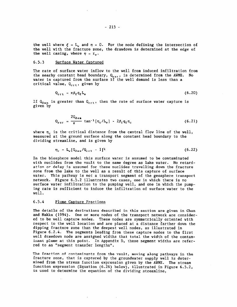
the well where E = L, and v = 0. For the node defining the intersection of the well with the fracture zone, the drawdown is determined at the edge of the well casing, where v = r,.
6.5.3 Surface Water Captured
The rate of surface water inflow to the well from induced infiltration from the nearby constant head boundary, (Isur, is determined from the AWME. No water is captured from the surface if the well demand is less than a critical value, Q,, , , given by
Qcrt = @fqfLw (6.20)
If Qdem is greater than Q,,,, then the rate of surface water capture is given by
where v, is the critical distance from the central flow line of the well, measured at the ground surface along the constant head boundary to the dividing streamline, and is given by
In the biosphere model this surface water is assumed to be contaminated with nuclides from the vault to the same degree as lake water. No retard- ation or delay is assumed for these nuclides travelling down the fracture zone from the lake to the well as a result of this capture of surface water. This pathway is not a transport segment of the geosphere transport network. Figure 6.5.2 illustrates two cases, one in which there is no surface water infiltration to the pumping well, and one in which the pump- ing rate is sufficient to induce the infiltration of surface water to the well.
6.5.4 Plume Capture Fractions
The details of the derivations described in this section are given in Chan and Nakka (1994). One or more nodes of the transport network are consider- ed to be well capture nodes. These nodes are symmetrically oriented with respect to the well location and are placed at a distance farther down the dipping fracture zone than the deepest well nodes, as illustrated in Figure 6.2.4. The segments leading from these capture nodes to the first well drawdown node are assigned widths that total the width of the contam- inant plume at this point. In Appendix D, these segment widths are refer- red to as "segment transfer lengths".
The fraction of contaminants from the vault, moving along pathways in the fracture zone, that is captured by the groundwater supply well is deter- mined from the stream function expression given by the AWME. The stream function expression (Equation (6.26) below), illustrated in Figure 6.5.2, is used to determine the equation of the dividing streamline,

€-coordinate in aquifer (m)
FIGURE 6.5.2: Plan view of groundwater streamlines in the fracture zone supplying groundwater to the well with moderate well demand (upper figure) and higher well demand (lower figure). Only the upper half plane is shown in each case, since there is a line of symmetry along the well centre line. Hence, the well itself is shown by "Ol1 on the lower axis at v=O. The <-coordinate depicted is measured along the aquifer from the constant head boundary (at the ground surface). The Q-coordinate is measured orthogonal to the central flow line of the well. The vertical dotted line shows the width of the contaminant plume at this location and is the line at which plume capture fraction is determined. The stagnation points are shown by the square. The upper figure shows one stagnation point on the well centre line with about 75X plume capture. The lower figure shows two stagnation points (one depicted and a matching one by symmetry). In this case, the well captures 100% of the contaminant plume, together with diluting water from outside the plume and surface water infiltrated from the constant head boundary.
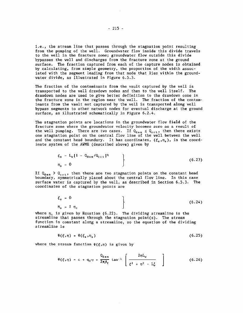
i.e., the stream line that passes through the stagnation point resulting from the pumping of the well. Groundwater flow inside this divide travels to the well in the fracture zone; groundwater flow outside this divide bypasses the well and discharges from the fracture zone at the ground surface. The fraction captured from each of the capture nodes is obtained by calculating, from simple geometry, the proportion of the width assoc- iated with the segment leading from that node that lies within the ground- water divide, as illustrated in Figure 6.5.3.
The fraction of the contaminants from the vault captured by the well is transported to the well drawdown nodes and then to the well itself. The drawdown nodes are used to give better definition to the drawdown cone in the fracture zone in the region near the well. The fraction of the contam- inants from the vault not captured by the well is transported along well bypass segments to other network nodes for eventual discharge at the ground surface, as illustrated schematically in Figure 6.2.4.
The stagnation points are locations in the groundwater flow field of the fracture zone where the groundwater velocity becomes zero as a result of the well pumping. There are two cases. If Qd,, s Q,,,, then there exists one stagnation point on the central flow line of the well between the well and the constant head boundary. It has coordinates, (f,,~,), in the coord- inate system of the AWME (described above) given by
If Qdem > Qcrt, then there are two stagnation points on the constant head boundary, symmetrically placed about the central flow line. In this case surface water is captured by the well, as described in Section 6.5.3. The coordinates of the stagnation points are
77, = f '1, I where v, is given by Equation (6.22). The dividing streamline is the streamline that passes through the stagnation point(s). The stream function is constant along a streamline, so the equation of the dividing streamline is
where the stream function Q(.$,v) is given by
Qd e m 2 vLw *(E,v) = c + qfv + - tan-
2x8, ~2 + ~2 - L2 W I
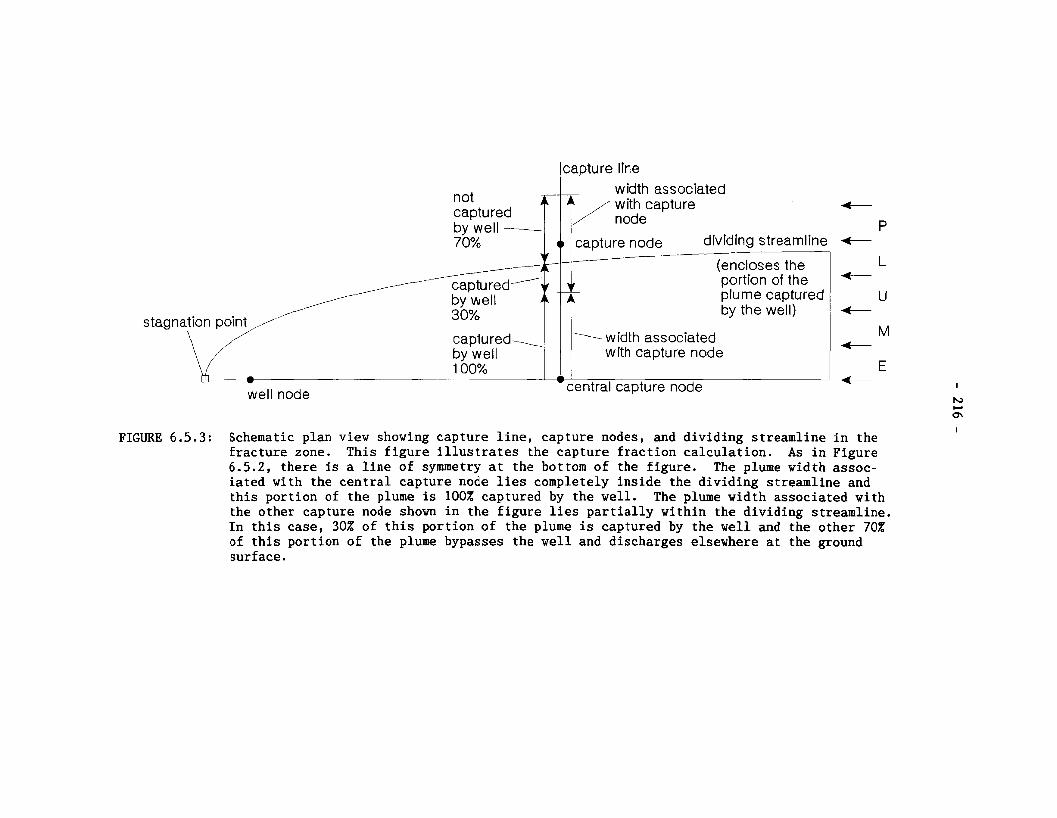
]capture line
not width associated
captured fi/ ;~it;apture f- by we l I----- P 70% capture node dividing streamline +-
(encloses the portion of the plume captured by the well)
captured\ 1 width associated by well with capture node 1 00%
well node 'central capture node
FIGURE 6.5.3: Schematic plan view showing capture line, capture nodes, and dividing streamline in the fracture zone. This figure illustrates the capture fraction calculation. As in Figure 6.5.2, there is a line of symmetry at the bottom of the figure. The plume width assoc- iated with the central capture node lies completely inside the dividing streamline and this portion of the plume is 100% captured by the well. The plume width associated with the other capture node shown in the figure lies partially within the dividing streamline. In this case, 30% of this portion of the plume is captured by the well and the other 70% of this portion of the plume bypasses the well and discharges elsewhere at the ground surf ace.
and where c is an arbitrary constant that determines a particular stream- line. The width of the groundwater divide at the well capture nodes is obtained by first finding the value of < = E , , the distance of the line of well capture nodes from the constant head boundary in the coordinate system of the AWME, and then finding q = q,, to give the point on the groundwater divide streamline with this value of c = c,. Hence, the transcendental equation
must be solved for q,. Having found q,, the total width of the groundwater divide at E=Er is 277, and this value is compared with the total plume width at this elevation to give the overall capture fraction.
However, the contaminant capture is determined separately for each segment leading to the well. For each segment leading from a capture node towards the well, a width (referred to as a "segment transfer length" in Appendix D) is assigned. The sum of these widths gives the total width of the contaminant pathways from the vault at the capture line at c - c,. The capture fraction for each segment is obtained by a geometrical calculation, illustrated in Figure 6.5.3, of how much of the width assigned to the segment lies inside the 2q, width of the groundwater divide streamlines at [ = e,. Each individual capture fraction and the overall capture fraction cannot exceed unity.
Figure 6.5.2 shows streamlines calculated from the AWME, in plan view, for two situations:
- one with a well demand only slightly smaller than Qcrt, in which case there is a single stagnation point and an overall capture of about 75W of the contaminant flowpaths within the fracture zone, and
- one with a well demand greater than Q,,,, in which case there are two stagnation points located on the constant head boundary. The entire width of the contaminant flowpaths is captured together with diluting water from outside of these flowpaths and surface water infiltrated from the constant head boundary.
In some cases, there may be capture of contaminants from the vault moving in flowpaths outside of the fracture zone. The AWME do not apply to these cases and, if required, capture fractions must be calculated from site- specific empirical equations. This capture is further discussed in a site- specific context in Sections 6.5.5 and 7.4.5
6.5.5 Site-Specific Effects of the Well
The well may affect three additional quantities, in which case relation- ships may be required to determine:
1. the drawdowns at nodes in the vault, from which new heads in the vault are determined,
2. reduced discharges for the discharges affected by the operation of the well, and
3. capture fraction for segments leading to the well from outside the fracture zone from which the well draws water.
The effect of the well on these three quantities is specific to the hydro- geologic conditions of the site being modelled and it may not be possible to determine them from fundamental principles. The derivation of empirical equations applicable to these quantities for use in the geosphere model of the Whiteshell Research Area is described in Chapter 7.4.
INTERFACE WITH VAULT MODEL
The principal interface between the geosphere model and the vault model is the passing of the time-dependent contaminant flow rates from each of the sectors of the vault to the geosphere transport network. These time-de- pendent flow rates are determined in the vault model and are used as con- taminant flow rates, Ip , at the source nodes of the network, which are the inlet nodes of each segment originating at the vault. These inlet flow rates are used in the solution of the transport equations for nuclide decay chains in each segment of the geosphere transport network as expressed in Equation (6.2), culminating in the determination of the contaminant flow rates at the discharges to the biosphere. In addition, there are other important connections between the vault and geosphere models which are described in this section.
The geosphere model determines and passes to the vault model the specific groundwater discharges through the buffer and backfill for each vault sector. These specific discharges are determined in the geosphere model so that consistency with specific discharges in the geosphere segments and groundwater mass balance can be maintained. The buffer is considered impermeable to groundwater movement and specific discharges in the buffer are all set to zero.
Specific discharges in the backfilled drifts of each vault sector, q,, are related to the specific discharges in the rock of the adjacent geosphere segment, q,. The geometry for this calculation is shown in Figure 6.6.1. The calculation is based upon the principle of groundwater mass balance, where the total groundwater flow across plane R must be equal to the sum of the groundwater flows through the backfilled drift region and through the intervening pillar region across plane M shown in Figure 6.6.1. The following two approximations are made:
1. The specific discharge q,, in the rock in the geosphere is not aftected by variations in the properties of the backfill, thus maintaining the connection with the hydraulic heads and/or groundwater velocities calculated for the geosphere transport network.
2. The pillars and the drifts of the vault layout can be considered to be parallel with one another and have essentially vertical groundwater flow through them. We assume the vertical hydraulic
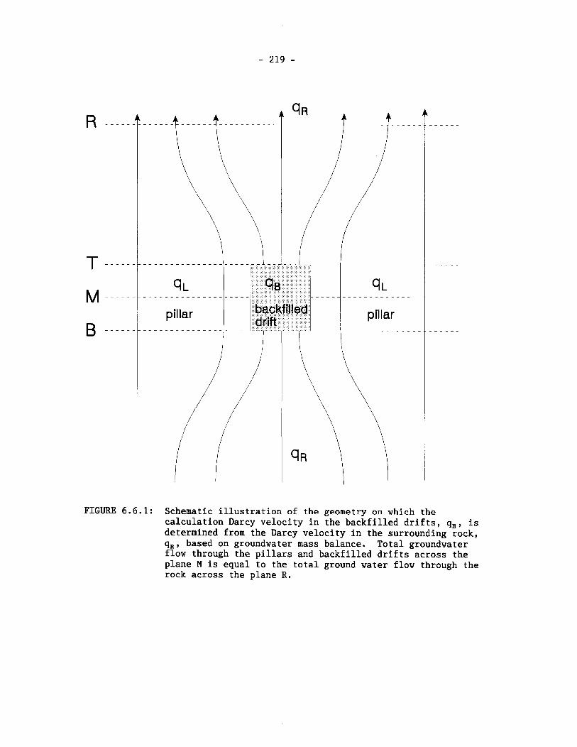
FIGURE 6.6.1: Schematic illustration of the geometry on which the calculation Darcy velocity in the backfilled drifts, q,, is determined from the Darcy velocity in the surrounding rock, q,, based on groundwater mass balance. Total groundwater flow through the pillars and backfilled drifts across the plane M is equal to the total ground water flow through the rock across the plane R.
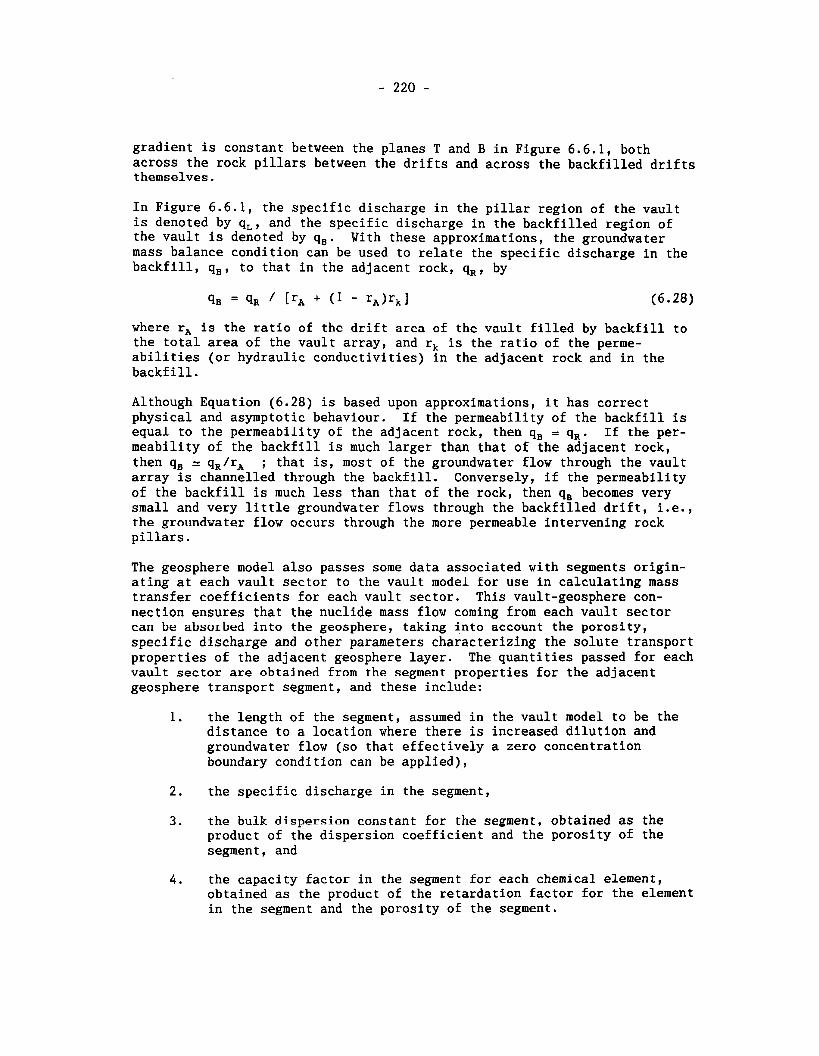
gradient is constant between the planes T and B in Figure 6.6.1, both across the rock pillars between the drifts and across the backfilled drifts themselves.
In Figure 6.6.1, the specific discharge in the pillar region of the vault is denoted by q,, and the specific discharge in the backfilled region of the vault is denoted by q,. With these approximations, the groundwater mass balance condition can be used to relate the specific discharge in the backfill, q,, to that in the adjacent rock, q,, by
where r, is the ratio of the drift area of the vault filled by backfill to the total area of the vault array, and rk is the ratio of the perme- abilities (or hydraulic conductivities) in the adjacent rock and in the backfill.
Although Equation (6.28) is based upon approximations, it has correct physical and asymptotic behaviour. If the permeability of the backfill is equal to the permeability of the adjacent rock, then q, = q,. If the per- meability of the backfill is much larger than that of the adjacent rock, then q, = q,/r, ; that is, most of the groundwater flow through the vault array is channelled through the backfill. Conversely, if the permeability of the backfill is much less than that of the rock, then q, becomes very small and very little groundwater flows through the backfilled drift, i.e., the groundwater flow occurs through the more permeable intervening rock pillars.
The geosphere model also passes some data associated with segments origin- ating at each vault sector to the vault model for use in calculating mass transfer coefficients for each vault sector. This vault-geosphere con- nection ensures that the nuclide mass flow coming from each vault sector can be absorbed into the geosphere, taking into account the porosity, specific discharge and other parameters characterizing the solute transport properties of the adjacent geosphere layer. The quantities passed for each vault sector are obtained from the segment properties for the adjacent geosphere transport segment, and these include:
1. the length of the segment, assumed in the vault model to be the distance to a location where there is increased dilution and groundwater flow (so that effectively a zero concentration boundary condition can be applied),
2. the specific discharge in the segment,
3 . the bulk dispersion constant for the segment, obtained as the product of the dispersion coefficient and the porosity of the segment, and
4. the capacity factor in the segment for each chemical element, obtained as the product of the retardation factor for the element in the segment and the porosity of the segment.

6.7 INTERFACE WITH BIOSPHERE MODEL
The principal interface between the geosphere and biosphere models is the passing of the time-dependent flow rates, O,, of contaminants, q, from the vault at each of the discharges to the biosphere. These time-dependent flow rates are determined in the geosphere model from the solution of the transport equations for nuclide decay chains in each segment of the network as expressed in Equation (6.2). In addition, there are other important connections between the two models which are also described in this sect ion.
Groundwater discharge from the geosphere to the biosphere can occur at a surface water body such as a stream or a lake, to the unsaturated zone of a low-lying terrestrial area, or to a wetland area such as a swamp or fen. These discharge areas are assigned layers of compacted sediment and over- burden associated with them. These thin surface layers are not included in the detailed MOTIF groundwater flow model since they do not affect the overall flow of groundwater from the vault to the biosphere. However, we have added these layers to the GEONET network model describing geosphere transport processes because they have chemical and sorption properties very different from the rest of the geosphere bedrock layers, and they affect the transfer of contaminants from the geosphere to the biosphere.
Each of the surface water, terrestrial and wetland discharge nodes has two extra nodes associated with it, a sediment node and an overburden node, as shown schematically in Figure 6.2.3. These two nodes define the positions of the bottom of two unconsolidated layers at these discharge locations. The positions of these extra nodes are adjusted such that they are placed directly under the discharge node giving layers of the specified thick- nesses (which may be zero if the layer is absent). These additional layers replace a small portion of the last bedrock segment leading to the ground- water discharge areas.
Reference hydraulic heads for the sediment node, h,,, and for the over- burden node, h,,, are determined by interpolation between the fixed head at the groundwater discharge location, h,,, and the fixed head at the bottom of the last bedrock segment, h,,. The locations at which these hydraulic heads are interpolated are shown schematically in Figure 6.7.1. This interpolation is based on both the thicknesses and permeabilities of the sediment, overburden and bedrock layers. In the interpolation, it is assumed that the three layers are in series and that no additional ground- water enters the flow system (so that groundwater mass balance is maintain- ed between all three layers). A constant common specific discharge is maintained in the last bedrock segment, the overburden segment and the sediment segment. However, these interpolated heads define a new common specific discharge that is slightly different from the original specific discharge calculated in the bedrock by the detailed groundwater flow model- ling with MOTIF in the absence of these layers. The interpolation yields the following:
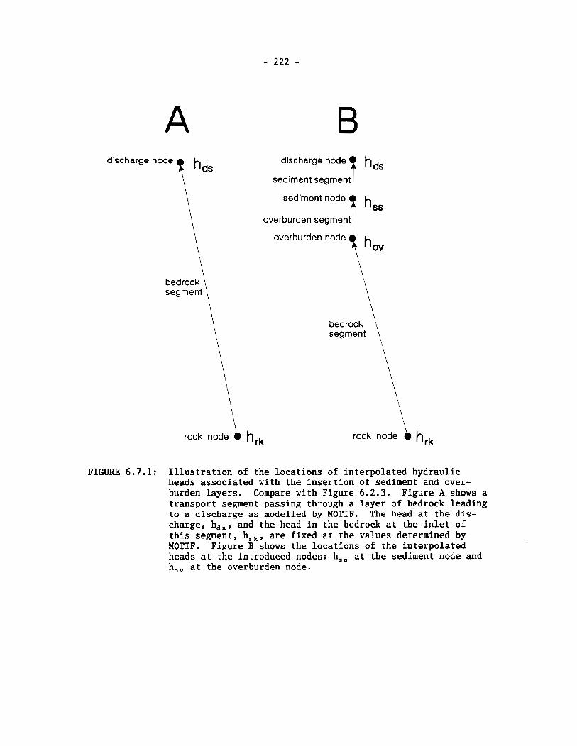
discharge node
t, hds
discharge node h sediment segment r ds
bedrock segment \
sediment node
overburden
overburden node \ h,
\ bedrock \
FIGURE 6.7.1: Illustration of the locations of interpolated hydraulic heads associated with the insertion of sediment and over- burden layers. Compare with Figure 6.2.3. Figure A shows a transport segment passing through a layer of bedrock leading to a discharge as modelled by MOTIF. The head at the dis- charge, h,,, and the head in the bedrock at the inlet of this segment, h,,, are fixed at the values determined by MOTIF. Figure B shows the locations of the interpolated heads at the introduced nodes: h,, at the sediment node and h,, at the overburden node.

where L, , , L, , , and L, are the lengths , and k, , , k, , , and k, , are the permeabilities of the sediment, overburden and last bedrock segments res- pectively. Alternatively, if hydraulic conductivities instead of perme- abilities are supplied, they can be used in place of the permeabilities in Equation (6.29).
Overburden wells, as described in Section 6.5, obtain their water entirely from the surface layers and we assume the capacity of these relatively shallow wells is still given approximately by Equation (6.18). The maximum well depth for wells to be classed as overburden wells is passed from the geosphere model to the biosphere model.
The geosphere model passes porosities, 8 , and distribution coefficients, k,, for the sediment layers, and the nuclide mass flow rates, 0 , out of the overburden layers to the biosphere model. It also passes t8e retard- ation factors, R,, for the last segment of the pathway leading to each groundwater discharge area. For most aquatic discharge locations this segment will be the sediment segment; for the situation describing dis- charge from a groundwater supply well this segment is the last segment in the fracture zone from which the well water is drawn. These retardation factors are used for calculations of nuclide mass flow rates of daughters in secular equilibrium with their parent nuclides. The details of these calculations are described in Davis et al. (1993).
The maximum well capacity obtained from the analytical well model (Section 6.5.1) is passed to the biosphere model for use in determining the possible well uses. Subsequently, the actual pumping demand placed on the well is determined by the biosphere model and the well demand is passed back to the geosphere model for use in the AWME, as described in Section 6.5. The principal biosphere parameters used in determining the well demand are: (a) the size of the critical group, and (b) whether or not the irrigation of their garden is done using well water. The determination of the well demand is fully described in Davis et al. (1994).
Empirical equations associated with the well model (Sections 6.5.5 and 7.4.5) may also be used to reduce the areas where the transport path- ways emerge at the ground surface, depending upon the effects of ground- water capture by the pumping well. These reduced discharge areas are also passed to the biosphere model.
GEONET MODEL VERIFICATION AND QUALITY ASSURANCE
6 . 8 . 1 Introduction
Our quantitative postclosure assessment of disposal vault performance relies on mathematical models of radionuclide transport, such as the geo- sphere model GEONET, that are implemented in the computer code, SYVAC3-CC3. These models are used to simulate a sequence of events that could lead to the transport of contaminants from the disposal vault to ground surface, and to estimate the potential impacts on human health and the environment for thousands of years into the future. Because the simulations are pro- jections of contaminant transport that could occur very far into the future, a direct comparison of impacts estimated using GEONET with actual observations is not possible.
The geosphere model used in SYVAC3-CC3 is a simplified representation of the transport of contaminants from the vault through the geosphere to dis- charge locations in the biosphere. Detailed site characterization infor- mation is first used to create a conceptual hydrogeologic model of the geosphere. This model, in turn, is used to develop a groundwater flow and solute transport model using the finite-element code, MOTIF. The GEONET model used in the postclosure assessment simulations incorporates the principal features of these models to describe contaminant transport from the location of the vault to the discharge locations in the biosphere. A full description of GEONET and its relationship to MOTIF is given earlier in this chapter and also in Chapter 7.
The discussion here focuses on measures taken to give credibility to the geosphere model GEONET in realistically simulating radionuclide transport in the SYVAC3-CC3 code. Five types of activities have proven useful:
- testing of the various modules of the GEONET code;
- GEONET calculations for simple test cases;
- comparisons of GEONET calculations with those made by similar codes ;
- comparisons of GEONET calculations with those made by more detailed 2-D or 3-D transport codes; and
- examination of results of a sensitivity analysis carried out with the GEONET model.
These activities are described in the following sections.
6.8.2 Testing of GEONET Modules
Each module of the GEONET code was tested as it was developed. Although it is not practicable to document all the tests and inspections that were performed during the code development, many tests were performed and the test results documented as part of each module's formal change and
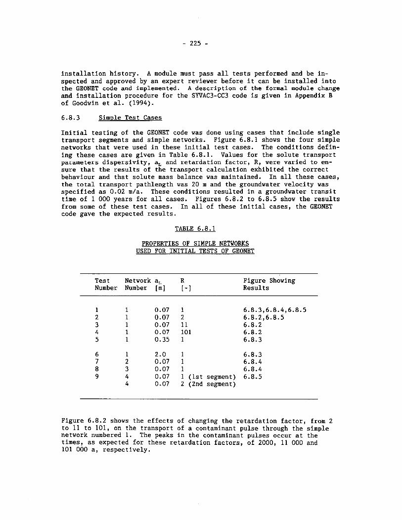
installation history. A module must pass all tests performed and be in- spected and approved by an expert reviewer before it can be installed into the GEONET code and implemented. A description of the formal module change and installation procedure for the SYVAC3-CC3 code is given in Appendix B of Goodwin et al. (1994).
6.8.3 Simple Test Cases
Initial testing of the GEONET code was done using cases that include single transport segments and simple networks. Figure 6.8.1 shows the four simple networks that were used in these initial test cases. The conditions defin- ing these cases are given in Table 6.8.1. Values for the solute transport parameters dispersivity, a, and retardation factor, R, were varied to en- sure that the results of the transport calculation exhibited the correct behaviour and that solute mass balance was maintained. In all these cases, the total transport pathlength was 20 m and the groundwater velocity was specified as 0.02 m/a. These conditions resulted in a groundwater transit time of 1 000 years for all cases. Figures 6.8.2 to 6.8.5 show the results from some of these test cases. In all of these initial cases, the GEONET code gave the expected results.
TABLE 6.8.1
PROPERTIES OF SIMPLE NETWORKS USED FOR INITIAL TESTS OF GEONET
Test Network a, R Number Number [m] [-I
Figure Showing Results
1 1 1 1 (1st segment) 2 (2nd segment)
Figure 6.8.2 shows the effects of changing the retardation factor, from 2 to 11 to 101, on the transport of a contaminant pulse through the simple network numbered 1. The peaks in the contaminant pulses occur at the times, as expected for these retardation factors, of 2000, 11 000 and 101 000 a, respectively.
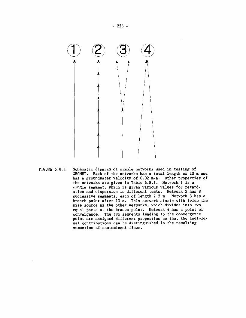
FIGURE 6.8.1: Schematic diagram of simple networks used in testing of GEONET. Each of the networks has a total length of 20 m and has a groundwater velocity of 0.02 m/a. Other properties of the networks are given in Table 6.8.1. Network 1 is a single segment, which is given various values for retard- ation and dispersion in different tests. Network 2 has 8 successive segments, each of length 2.5 m. Network 3 has a branch point after 10 m. This network starts with twice the size source as the other networks, which divides into two equal parts at the branch point. Network 4 has a point of convergence. The two segments leading to the convergence point are assigned different properties so that the individ- ual contributions can be distinguished in the resulting summation of contaminant flows.

---- Retardation factor 2 - - - - Retardation factor 1 1
Retardation factor 101
FIGURE 6.8.2: Contaminant flow rates from test cases 2, 3 and 4. Retardation factor varied from 2 to 11 to 101.
0
---- Flow rate base case, Retardation = 1, Dlspersivity = 0.07111
FIGURE 6.8.3: Contaminant flow rates from test cases 1, 5 and 6. Dispersivity varied from 0.07 to 0.35 to 2.0 m. Increasing dispersivity lowers and broadens the peak and shifts it to slightly earlier times.
Q
- 2- e b E 0 $ 2 - $
5 0 a 2- 9 - 0 3
= 0 - d -
8 0 '
Dispersivity increased to 0.35 m Dlsperslvlty increased to 2.0 rn
/ / '
/ '
/ . -.-. -1
I
0 200 400 600 800 1000 1200 1400 1600 1800 2000 Time (a)
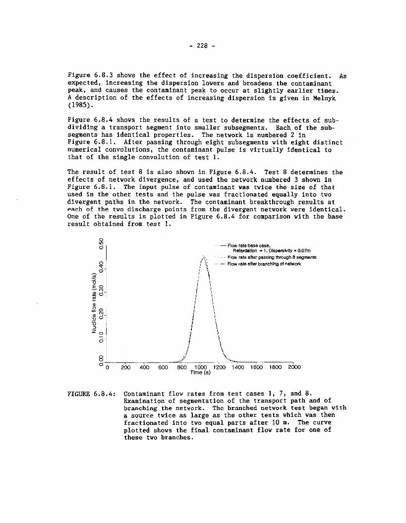
Figure 6.8.3 shows the effect of increasing the dispersion coefficient. As expected, increasing the dispersion lowers and broadens the contaminant peak, and causes the contaminant peak to occur at slightly earlier times.
- .
A description of the effects of increasing dispersion is given in Melnyk ( 1985).
Pigure 6.8.4 shows the results of a test to determine the effects of sub- dividing a transport segment into smaller subsegments. Each of the sub- segments has identical properties. The network is numbered 2 in Pigure 6.8.1. After passing through eight subsegments with eight distinct numerical convolutions, the contaminant pulse is virtually identical to that of the single convolution of test 1.
The result of test 8 is also shown in Figure 6.8.4. Test 8 determines the effects of network divergence, and used the network numbered 3 shown in Figure 6.8.1. The input pulse of contaminant was twice the size of that used in the other tests and the pulse was fractionated equally into two divergent paths in the network. The contaminant breakthrough results at each of the two discharge points from the divergent network were identical. One of the results is plotted in Figure 6.8.4 for comparison with the base result obtained from test 1.
--- Flow rate base case, Retardation = 1 , Dlspenhrlty = 0.07m
-... Flow rate after passlng through 8 segments - Flow rate after branching of network
I 0 I I I
I I I I I I I
0 200 400 600 800 1000 1200 1400 16M) 1800 2000 Time (a)
FIGURE 6.8.4: Contaminant flow rates from test cases 1, 7, and 8. Examination of segmentation of the transport path and of branching the network. The branched network test began with a source twice as large as the other tests which was then fractionated into two equal parts after 10 m. The curve plotted shows the final contaminant flow rate for one of these two branches.

-Flow rate base case, Retardation = 1,
A Dlsperslvtty = 0.07m
-.-- Retardatbn factor 2
Flow rate after convergence of two segments wnh R - 1 and R -2
o3 i o4 i o5 Time (a)
FIGURE 6.8.5: Contaminant flow rates from test cases 1, 2 and 9. Examination of convergence of the transport network. Summation of the contaminant flow rates from the two converging paths in test case 9 produces a result that reproduces the two individual results obtained in test cases 1 and 2.
Test 9, which examined the effects of network convergence, used network 4 shown in Figure 6.8.1. For this case the contaminant pulse was unretarded along one path and had a retardation factor of 2 along the other path. The two paths converged to a single discharge location. The result of this test is plotted in Figure 6.8.5, together with the results from tests 1 and 2. The two sets of curves are practically indistinguishable.
6.8.4 Comparison with similar codes
We have also acquired confidence in the GEONET code by comparing its results to those obtained from other computer codes that have been inde- pendently developed to solve the same problem. Similarity in the predict- ions from the different models/codes give confidence that the simulations have been properly performed. Several groups throughout the world are currently engaged in performance assessment work for high-level radioactive waste management. There are thus a variety of computer codes being de- veloped for use in simulating the performance of nuclear waste disposal systems. There has been valuable cooperation and interaction between these groups as discussed below.
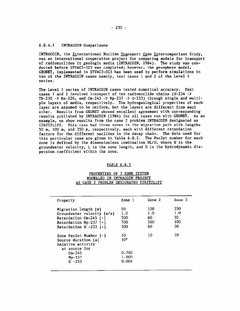
6.8.4.1 INTRACOIN Comparisons
INTRACOIN, the International Nuclide ansport Code Intercomparison Study, was an international cooperation project for comparing models for transport of radionuclides in geologic media (INTRACOIN, 1984). The study was con- ducted before SYVAC3-CC3 was completed; however, the geosphere model, GEONET, implemented in SYVAC3-CC3 has been used to perform simulations in two of the INTRACOIN cases namely, test cases 1 and 2 of the Level 1 series.
The Level 1 series of INTRACOIN cases tested numerical accuracy. Test cases 1 and 2 involved transport of two radionuclide chains (U-234 -> Th-230 -> Ra-226, and Cm-245 -> Np-237 -> U-233) through single and multi- ple layers of media, respectively. The hydrogeological properties of each layer are assumed to be uniform, but the layers are different from each other. Results from GEONET showed excellent agreement with corresponding results published by INTRACOIN (1984) for all cases run with GEONET. As an example, we show results from the case 2 problem INTRACOIN designated as 12R2T2LlP2. This case had three zones i n the migration path with lengths 50 m, 100 m, and 350 m, respectively, each with different retardation factors for the different nuclides in the decay chain. The data used for this particular case are given in Table 6.8.2. The Peclet number for each zone is defined by the dimensionless combination UL/D, where U is the groundwater velocity, L is the zone length, and D is the hydrodynamic dis- persion coefficient within the zone.
TABLE 6.8.2
PROPERTIES OF 3 ZONE SYSTEM MODELLED IN INTRACOIN PROJECT
AS CASE 2 PROBLEM DESIGNATED 12R2T2LlP2
Property
Migration length [m] Groundwater velocity [m/a] Retardation Cm-245 [ - I Retardation Np-237 [ - I Retardation U -233 [ - I
Zone Peclet Number [ - I Source duration [a] Relative activity at source for
Cm-245 Np-237 U -233
Zone 1 Zone 2 Zone 3
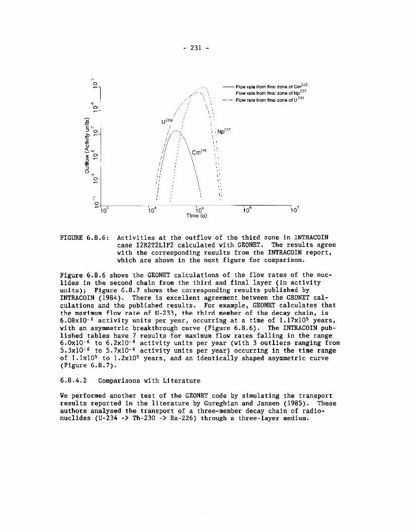
- - , , - Flow rate from flnal zone of ~m~~~ ' _... '/\ , Flow rate from flnal zone of ~p~~~
2' \ I , - - Flow rate from final zone of U 233 ' ,' \ '1 ' 0 / , \ ', / ,
i o4 i o5 i 0" i 0' 71r1e (ti)
FIGURE 6.8.6: Activities at the outflow of the third zone in INTRACOIN case 12R2T2LlP2 calculated with GEONET. The results agree with the corresponding results from the INTRACOIN report, which are shown in the next figure for comparison.
Figure 6.8.6 shows the GEONET calculations of the flow rates of the nuc- lides in the second chain from the third and final layer (in activity units); Figure 6.8.7 shows the corresponding results published by INTRACOIN (1984). There is excellent agreement between the GEONET cal- culations and the published results. For example, GEONET calculates that the maximum flow r a t e of U-933, t h e t h i r d member of t h e decay chain, is 6.08~10-~ activity units per year, occurring at a time of 1.17x10⁵ years, with an asymmetric breakthrough curve (Figure 6.8.6). The INTRACOIN pub- lished tables have 7 results for maximum flow rates falling in the range 6 . 0 ~ 1 0 - ~ to 6.2~10-~ activity units per year (with 3 outliers ranging from 5.3~10-~ to 5.7~10-~ activity units per year) occurring in the time range of l.lx105 to l.2x105 years, and an identically shaped asymmetric curve (Figure 6.8.7).
6.8.4.2 Comparisons with Literature
We performed another test of the GEONET code by simulating the transport results reported in the literature by Gureghian and Jansen (1985). These authors analysed the transport of a three-member decay chain of radio- nuclides (U-234 -> Th-230 -> Ra-226) through a three-layer medium.
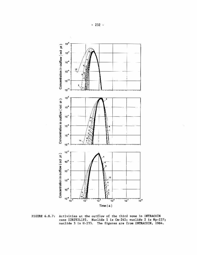
Time ( a )
FIGURE 6.8.7: Activities at the outflow of the third zone in INTRACOIN case 12R2T2LlP2. Nuclide 1 is Cm-245; nuclide 2 is Np-237; nuclide 3 is U-233. The figures are from INTRACOIN, 1984.
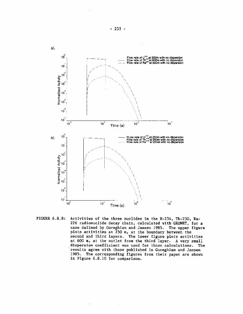
a).
--- FLOW rate of u ' ~ at 250m wtih no dispersion Flow rate of ~ h ~ a t 250m wlth no dispersion Flow rate of l3aZz6 at 250m with no dlsperslon
10"- - Flow rate of u~~~ at 600m with no dispersion
10' 1 ' i ; o4
lo' Time (a) ; 06 1 0'
10'-
FIGURE 6.8.8: Activities of the three nuclides in the U-234, Th-230, Ra- 226 radionuclide decay chain, calculated with GEONET, for a case defined by Gureghian and Jansen 1985. The upper figure plots activities at 250 m, at the boundary between the second and third layers. The lower figure plots activities at 600 m, at the outlet from the third layer. A very small dispersion coefficient was used for these calculations. The 'results agree with those published in Gureghian and Jansen 1985. The corresponding figures from their paper are shown in Figure 6.8.10 for comparison.
A. ' /.
5
2 lo3- -u Q) -4 g 10 - (d
s -5 2 10 - -6
10 -
Flow rate of ~ h ~ a t 60311 wlth no dispersion - .- Flow rate of I3dz6 at 600m with no dispersion
\ ._ /
? 1 ,- < .
1 ,,' I ,I Ill
'.
-. '.
\. '%,, '.
' \ , \,
, ',
-7 10
I \ \ ' \ \,
'\ \, '\ \, '! \,
'\ ', ', \
\ i
lo4 'o' Time (a) i o 6 'I o7
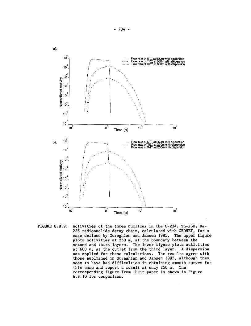
lo"
bl.
- Flow rate of LJ2~~,at 600m with dispersion Flow rate of at 600m with dkpenlon /-? - - - Flow rate of 2'' at 600m wlth dispersion
105 Time (a) lr o6 'l 0'
FIGURE 6 .8 .9 : Activities of the three nuclides in the U-234, Th-230, Ra- 226 radionuclide decay chain, calculated with GEONET, for a case defined by Gureghian and Jansen 1985. The upper figure plots activities at 250 m, at the boundary between the second and third layers. The lower figure plots activities at 600 m, at the outlet from the third layer. A dispersion was applied for these calculations. The results agree with those published in Gureghian and Jansen 1985, although they seem to have had difficulties in obtaining smooth curves for this case and report a result at only 250 m. The corresponding figure from their paper is shown in Figure 6.8.10 for comparison.
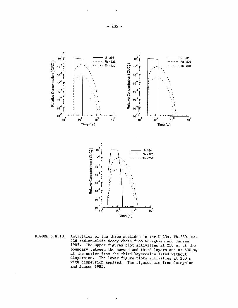
U - 234 - - - - Ra - 226 . . . . . Th - 230
C a -3
I . . \
2 l o r . \ 1: 6 , i 1.
- \
1. . I g 10 . I
I . .- . I 3 -5 ;: . I
10 1. a . I
I L' . I
lod I . I . I -
' I l l l l n l l 1 1 1 1 1 1 ,I I I , # A
I 04 I O~ 7
I 0
Time (a )
1 o0 A
g lo-' i3 - lo3 C 0 .- C
E C C a
FIGURE 6.8.10: Activities of the three nuclides in the U-234, Th-230, Ra- 226 radionuclide decay chain from Gureghian and Jansen 1985. The upper figures plot activities at 250 m, at the boundary between the second and third layers and at 600 m, at the outlet from the third layercalcu lated without dispersion. The lower figure plots activities at 250 m with dispersion applied. The figures are from Gureghian and Jansen 1985.
- U-234 - - - - Ra - 226 . . . . .
.*' Th - 230 / '
/ I \
\ . \ I : I - .. \ . \
!. - \ ! - \
I E lo4 0 a -5 > 10 .- C m - 2 l o6 :
I 04 I 0' lo lo 6
Time (a )
I I I I
I
1
. I . I . I . I . I . I
I I . I
l H a l l l E 1 t t l a l l - l t 1 1 u 1 u 7
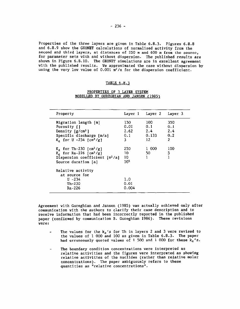
Properties of the three layers are given in Table 6.8.3. Figures 6.8.8 and 6.8.9 show the GEONET calculations of normalized activity from the second and third layers, at distances of 250 m and 600 m from the source, for parameter sets with and without dispersion. The published results are shown in Figure 6.8.10. The GEONET simulations are in excellent agreement with the published results. We approximated the case without dispersion by using the very low value of 0.001 m2/a for the dispersion coefficient.
TABLE 6.8.3
PROPERTIES OF 3 LAYER SYSTEM MODELLED BY GUREGHIAN AND JANSEN (1985)
Property Layer 1 Layer 2 Layer 3
Migration length [m] Porosity [I Density [g/cm3 ] Specific discharge [m/a] Kd for U -234 [cm3/g]
Kd for Th-230 [cm3/g] K, for Ra-226 [cm3/g] Dispersion coefficient [m2/a] Source duration [a]
Relative activity at source for
U -234 Th-230 Ra-226
Agreement with Gureghian and Jansen (1985) was actually achieved only after communication with the authors to clarify their case description and to receive information that had been incorrectly reported in the published paper (confirmed by communication B. Gureghian 1986). These revisions were :
- The values for the kdrs for Th in layers 2 and 3 were revised to the values of 1 000 and 100 as given in Table 6.8.3. The paper had erroneously quoted values of 1 500 and 1 000 for these k,'s.
- The boundary condition concentrations were interpreted as relative activities and the figures were interpreted as showing relative activities of the nuclides (rather than relative molar concentrations). The paper ambiguously refers to these quantities as "relative concentrations".
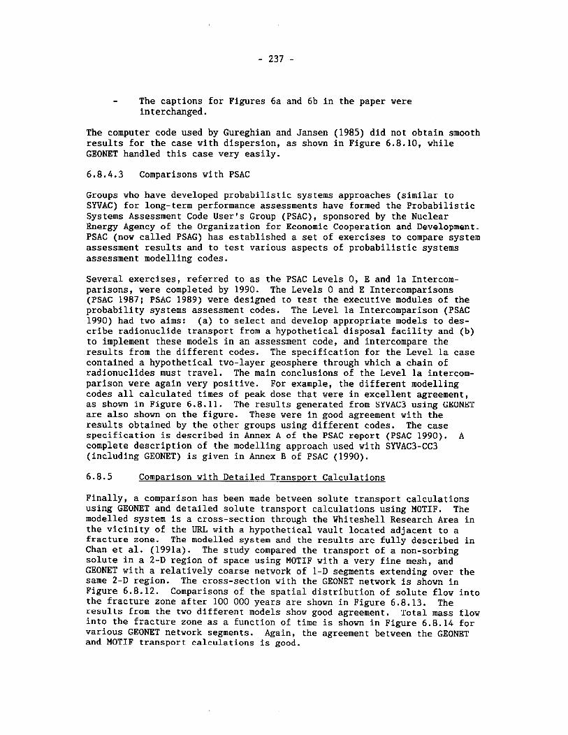
- The captions for Figures 6a and 6b in the paper were interchanged.
The computer code used by Gureghian and Jansen (1985) did not obtain smooth results for the case with dispersion, as shown in Figure 6.8.10, while GEONET handled this case very easily.
6.8.4.3 Comparisons with PSAC
Groups who have developed probabilistic systems approaches (similar to SYVAC) for long-term performance assessments have formed the Probabilistic Systems Assessment Code User's Group (PSAC), sponsored by the Nuclear Energy Agency of the Organization for Economic Cooperation and Development. PSAC (now called PSAG) has established a set of exercises to compare system assessment results and to test various aspects of probabilistic systems assessment modelling codes.
Several exercises, referred to as the PSAC Levels 0, E and la Intercom- parisons, were completed by 1990. The Levels 0 and E Intercomparisons (PSAC 1987; PSAC 1989) were designed to test the executive modules of the probability systems assessment codes. The Level la Intercomparison (PSAC 1990) had two aims: (a) to select and develop appropriate models to des- cribe radionuclide transport from a hypothetical disposal facility and (b) to implement these models in an assessment code, and intercompare the results from the different codes. The specification for the Level la case contained a hypothetical two-layer geosphere through which a chain of radionuclides must travel. The main conclusions of the Level la intercom- parison were again very positive. For example, the different modelling codes all calculated times of peak dose that were in excellent agreement, as shown in Figure 6.8.11. The results generated from SYVAC3 using GEONET are also shown on the figure. These were in good agreement with the results obtained by the other groups using different codes. The case specification is described in Annex A of the PSAC report (PSAC 1990). A complete description of the modelling approach used with SYVAC3-CC3 (including GEONET) is given in Annex B of PSAC (1990).
6.8.5 Comparison with Detailed Transport Calculations
Finally, a comparison has been made between solute transport calculations using GEONET and detailed solute transport calculations using MOTIF. The modelled system is a cross-section through the Whiteshell Research Area in the vicinity of the URL with a hypothetical vault located adjacent to a fracture zone. The modelled system and the results are fully described in Chan et al. (1991a). The study compared the transport of a non-sorbing solute in a 2-D region of space using MOTIF with a very fine mesh, and GEONET with a relatively coarse network of 1-D segments extending over the same 2-D region. The cross-section with the GEONET network is shown in Figure 6.8.12. Comparisons of the spatial distribution of solute flow into the fracture zone after 100 000 years are shown in Figure 6.8.13. The results from the two different models show good agreement. Total mass flow into the fracture zone as a function of time is shown in Figure 6.8.14 for various GEONET network segments. Again, the agreement between the GEONET and MOTIF transport calculations is good.
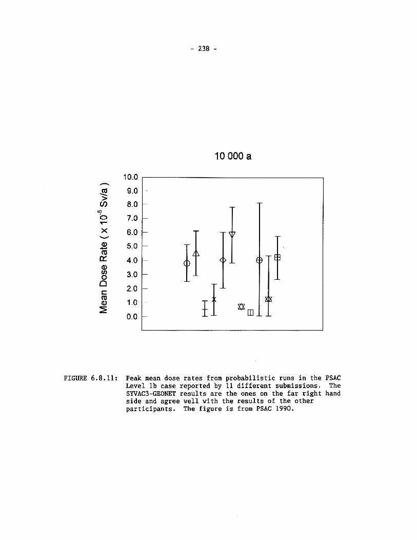
FIGURE 6.8.11: Peak mean dose rates from probabilistic runs in the PSAC Level lb case reported by 11 different submissions. The SYVAC3-GEONET results are the ones on the far right hand side and agree well with the results of the other participants. The figure is from PSAC 1990.
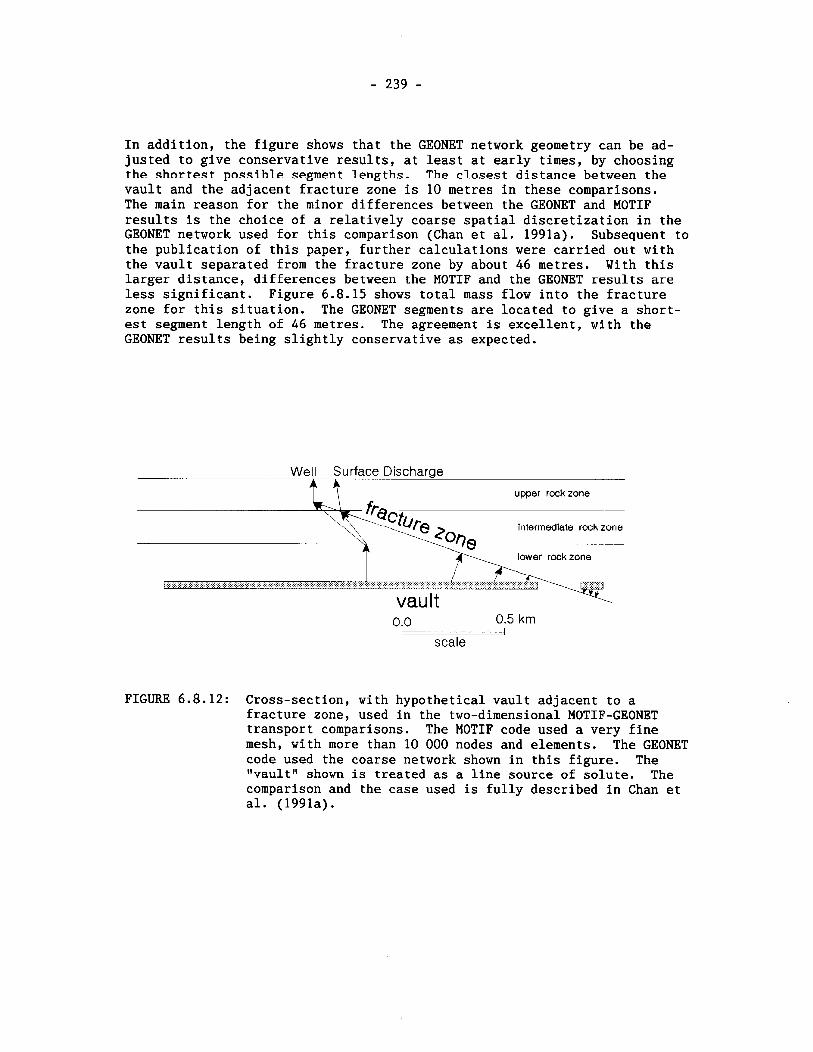
In addition, the figure shows that the GEONET network geometry can be ad- justed to give conservative results, at least at early times, by choosing the shortest possible segment lengths. The closest distance between the vault and the adjacent fracture zone is 10 metres in these comparisons. The main reason for the minor differences between the GEONET and MOTIF results is the choice of a relatively coarse spatial discretization in the GEONET network used for this comparison (Chan et al. 1991a). Subsequent to the publication of this paper, further calculations were carried out with the vault separated from the fracture zone by about 46 metres. With this larger distance, differences between the MOTIF and the GEONET results are less significant. Figure 6.8.15 shows total mass flow into the fracture zone for this situation. The GEONET segments are located to give a short- est segment length of 46 metres. The agreement is excellent, with the GEONET results being slightly conservative as expected.
Well Surface Discharge
upper rock zone
lnterrnediate rock zone
lower rock zone
0.0 0.5 km - scale
FIGURE 6.8.12: Cross-section, with hypothetical vault adjacent to a fracture zone, used in the two-dimensional MOTIF-GEONET transport comparisons. The MOTIF code used a very fine mesh, with more than 10 000 nodes and elements. The GEONET code used the coarse network shown in this figure. The 'Ivault" shown is treated as a line source of solute. The comparison and the case used is fully described in Chan et al. (1991a).
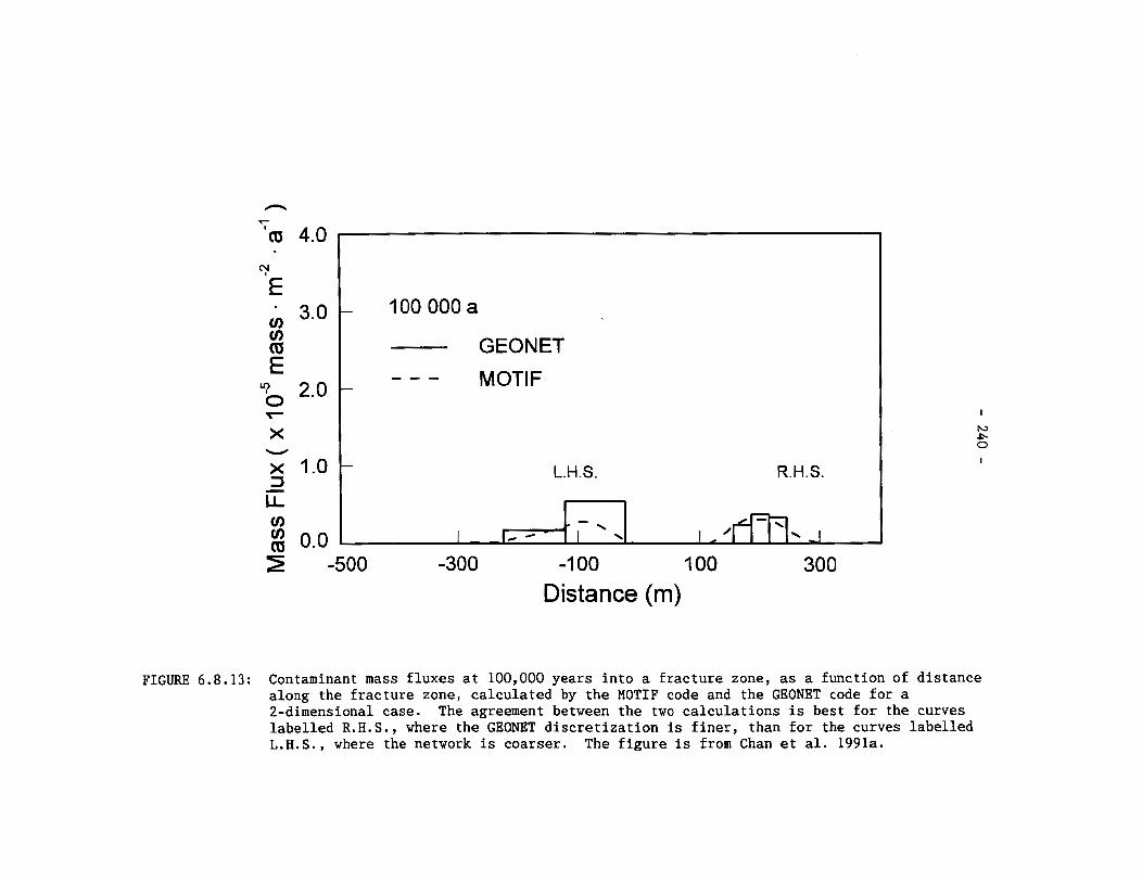
Distance (m)
- 100 000 a
GEONET - - - MOTIF -
- L.H.S. R.H.S.
FIGURE 6.8.13: Contaminant mass fluxes at 100,000 years into a fracture zone, as a function of distance along the fracture zone, calculated by the MOTIF code and the GEONBT code for a 2-dimensional case. The agreement between the two calculations is best for the curves labelled R.H.S., where the GEONBT discretization is finer, than for the curves labelled L.H.S., where the network is coarser. The figure is from Chan et al. 1991a.
I / \ I 4 i I lc - -
\ \
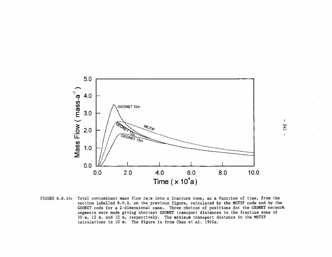
GEONET I Om
Time ( x 104a)
FIGURE 6.8.14: Total contaminant mass flow rate into a fracture zone, as a function of time, from the section labelled R.H.S. on the previous figure, calculated by the MOTIF code and by the GEONET code for a 2-dimensional case. Three choices of positions for the GEONET network segments were made giving shortest GEONET transport distances to the fracture zone of 10 m, 12 m, and 15 m, respectively. The minimum transport distance in the MOTIF calculations is 10 m. The figure is from Chan et al. 1991a.
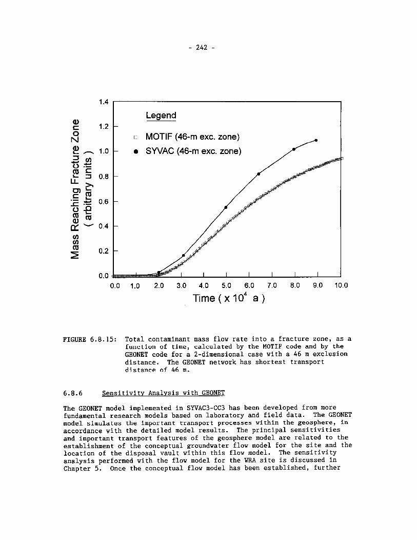
MOTIF (46-m exc. zone)
SWAC (46-m exc. zone)
0.0 1.0 2.0 3.0 4.0 5.0 6.0 7.0 8.0 9.0 10.0
Time ( x l o 4 a )
FIGURE 6.8.15: Total contaminant mass flow rate into a fracture zone, as a function of time, calculated by the MOTIF code and by the GEONET code for a 2-dimensional case with a 46 m exclusion distance. The GEONET network has shortest transport distance of 46 m.
6.8.6 Sensitivity Analysis with GEONET
The GEONET model implemented in SYVAC3-CC3 has been developed from more fundamental research models based on laboratory and field data. The GEONET mudel simulates the important transport processes within the geosphere, in accordance with the detailed model results. The principal sensitivities and important transport features of the geosphere model are related to the establishment of the conceptual groundwater flow model for the site and the location of the disposal vault within this flow model. The sensitivity analysis performed with the flow model for the WRA site is discussed in Chapter 5. Once the conceptual flow model has been established, further
sensitivity analyses can be performed with the GEONET model within SYVAC3- CC3 to reveal which parameters used in the GEONET model for the WRA site have the greatest effect on the long-term assessment ot the disposal system. The results of these SYVAC3-CC3 sensitivity analyses are described in detail in Goodwin et al. (1994).
The geosphere model parameters which were identified as being the most important in this analysis, in order of importance, were:
- tortuosity factor characterizing diffusion through the sparsely fractured rock zone separating the disposal vault from the nearby fracture zone,
- groundwater velocity scaling factor,
- retardation factor of Iodine in organic lake sediment,
- free-water diffusion coefficient for Iodine,
- thickness of compacted lake sediment at Boggy Creek South,
- depth of the well.
The parameters governing diffusive transport through the region of sparsely fractured rock separating the vault from fracture zone LD1 were identified as being most important in this case study. The properties of the sediment layer were identified as important because Iodine, the nuclide giving the largest dose, is sorbed only in this organic material. The groundwater velocity scaling factor and the depth of the well were important because they affect the capture of contaminants by the well. A complete des- cription of these parameters, and all other parameters used in GEONET, is given in Appendix D.
The sensitivity analysis performed on GEONET was presented for review to the research staff whose responsibilities were to develop the geosphere model and incorporate relevant data. Specifically, the reviewers were asked to confirm that the results from the sensitivity analysis of GEONET were consistent with their understanding of, and experience with, the more fundamental research models and data on the geosphere. The conclusion of this internal review verified the results of the GEONET sensitivity analy- ses. This review supported the geosphere model and the GEONET code as correctly representing the important features of the detailed groundwater flow and solute transport models from which they were derived.
6.8.7 Main Conclusion
The quality assurance of the code used to describe radionuclide transport through the geosphere from the vault to discharge locations in the bio- sphere has involved many approaches. These include code testing, code verification, code intercomparison and the investigation of model behaviour through sensitivity analysis. In the judgement of the developers, the GEONET code is a reliable implementation of the geosphere model for use in the postclosure assessment.
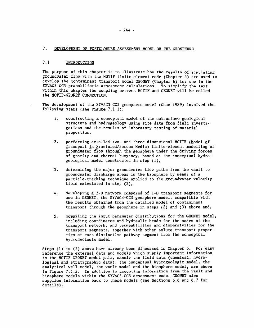
7. DEVELOPMENT OF POSTCLOSURE ASSESSMENT MODEL OF THE GEOSPHERE
INTRODUCTION
The purpose of this chapter is to illustrate how the results of simulating groundwater flow with the MOTIF finite element code (Chapter 5) are used to develop the contaminant transport model GEONET (Chapter 6) for use in the SYVAC3-CC3 probabilistic assessment calculations. To simplify the text within this chapter the coupling between MOTIF and GEONET will be called the MOTIF-GEONET CONNECTION.
The development of the SYVAC3-CC3 geosphere model (Chan 1989) involved the following steps (see Figure 7.1.1):
I. constructing a conceptual model of the subsurface geological structure and hydrogeology using site data from field investi- gations and the results of laboratory testing of material properties,
2. performing detailed two- and three-dimensional MOTIF (Model of Transport in Fractured/Porous Media) finite-element modelling of groundwater flow through the geosphere under the driving forces of gravity and thermal buoyancy, based on the conceptual hydro- geological model constructed in step (I),
3. determining the major groundwater flow paths from the vault to groundwater discharge areas in the biosphere by means of a particle-tracking technique applied to the groundwater velocity field calculated in step (2),
4. developing a 3-D network composed of 1-D transport segments for use in GEONET, the SYVAC3-CC3 geosphere model, compatible with the results obtained from the detailed model of contaminant transport through the geosphere in steps (2) and (3) above and,
5. compiling the input parameter distributions for the GEONET model, including coordinates and hydraulic heads for the nodes of the transport network, and permeabilities and dispersivities for the transport segments, together with other solute transport proper- ties of each distinctive pathway segment from the conceptual hydrogeologic model.
Steps (1) to (3) above have already been discussed in Chapter 5. For easy reference the external data and models which supply important information to the MOTIF-GEONET model pair, namely the field data (chemical, hydro- logical and stratigraphic data), the conceptual hydrogeologic model, the analytical well model, the vault model and the biosphere model, are shown in Figure 7.1.2. In addition to accepting information from the vault and biosphere models within the SYVAC3-CC3 assessment code, GEONET also supplies information back to these models (see Sections 6.6 and 6.7 for details).
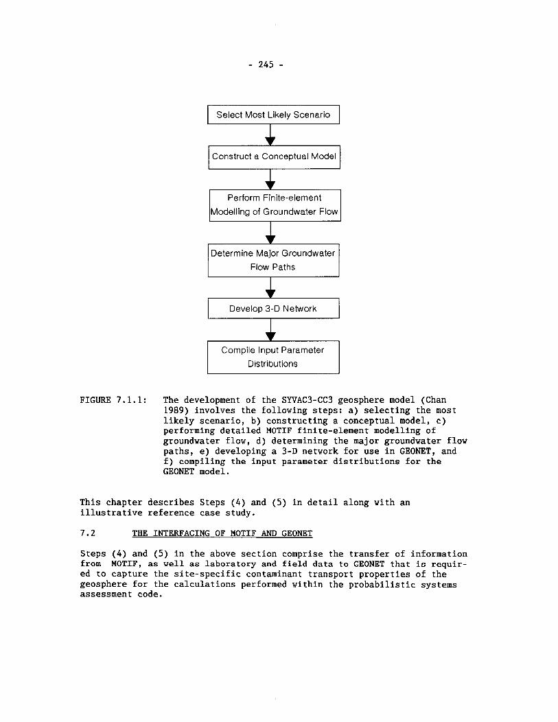
Select Most Likely Scenario s Construct a Conceptual Model c Modelling of Groundwater Flow
Determine Major Groundwater
Flow Paths
Develop 3-D Network P Compile Input Parameter
Distributions
FIGURE 7.1.1: The development of the SYVAC3-CC3 geosphere model (Chan 1989) involves the following steps: a) selecting the most likely scenario, b) constructing a conceptual model, c) performing detailed MOTIF finite-element modelling of groundwater flow, d) determining the major groundwater flow paths, e) developing a 3-D network for use in GEONET, and f) compiling the input parameter distributions for the GEONET model.
This chapter describes Steps (4) and (5) in detail along with an illustrative reference case study.
THE INTERFACING OF MOTIF AND GEONET
Steps (4) and (5) in the above section comprise the transfer of information from MOTIF, as well as laboratory and field data to GEONET that is requir- ed to capture the site-specific contaminant transport properties of the geosphere for the calculations performed within the probabilistic systems assessment code.
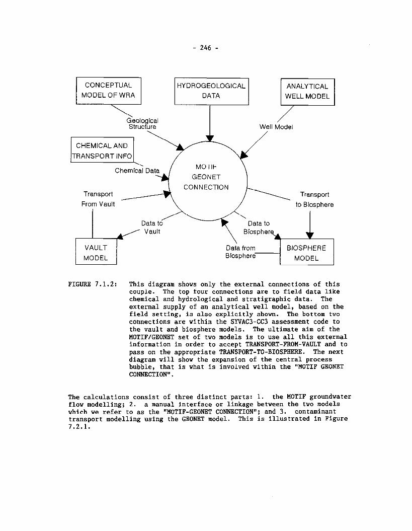
CONCEPTUAL
MODEL OF WRA
~ e o l o g ical Structure
CHEMICAL AND
TRANSPORT INFO
HY DROGEOLOGICAL 1 DATA
Chemical Data MOTIF
GEONET
WELL MODEL
/ Well Model
CONNECTION Transport Transport
From Vault to Biosphere
Data to Vault B i osphe rk
VAULT Data from BIOSPHERE MODEL Biosphere MODEL
FIGURE 7.1.2: This diagram shows only the external connections of this couple. The top four connections are to field data like chemical and hydrological and stratigraphic data. The external supply of an analytical well model, based on the field setting, is also explicitly shown. The bottom two connections are within the SYVAC3-CC3 assessment code to the vault and biosphere models. The ultimate aim of the MOTIF/GEONET set of two models is to use all this external information in order to accept TRANSPORT-FROM-VAULT and to pass on the appropriate TRANSPORT-TO-BIOSPHERE. The next diagram will show the expansion of the central process bubble, that is what is involved within the "MOTIF GEONET CONNECTION".
The calculations consist of three distinct parts: 1. the MOTIF groundwater flow modelling; 2. a manual interface or linkage between the two models which we refer to as the "MOTIF-GEONET CONNECTION"; and 3. contaminant transport modelling using the GEONET model. This is illustrated in Figure 7.2.1.
PERMEABILITY?' TENSOR
GEOLOGICAL CALCULATION
STRUCTURE
/ / w j PARTICLE 1 TRACKS
HYDRAULIC HEADS
GEONET k( MANUAL ___HEADS AT INTERFACE NODES
DISCHARGE /
TRANSPORT WELL MODEL CALCULATION
TRANSPORT FROM VAULT
TRANSPORT
FIGURE 7.2.1: This diagram shows what is involved in using the MOTIF GEONET CONNECTION to determine contaminant flows. The MOTIF/GEONET calculations consist of three distinct parts: the MOTIF groundwater flow modelling, process 1; an inter- face between the two models, process 2; and the GEONET contaminant transport modelling. It requires all three of these process to achieve the ultimate end of accepting TRANSPORT-FROM-VAULT and passing on the appropriate TRANSPORT-TO-BIOSPHERE. The MOTIF only process is not further expanded here since we are focussing on the connections between the two models.
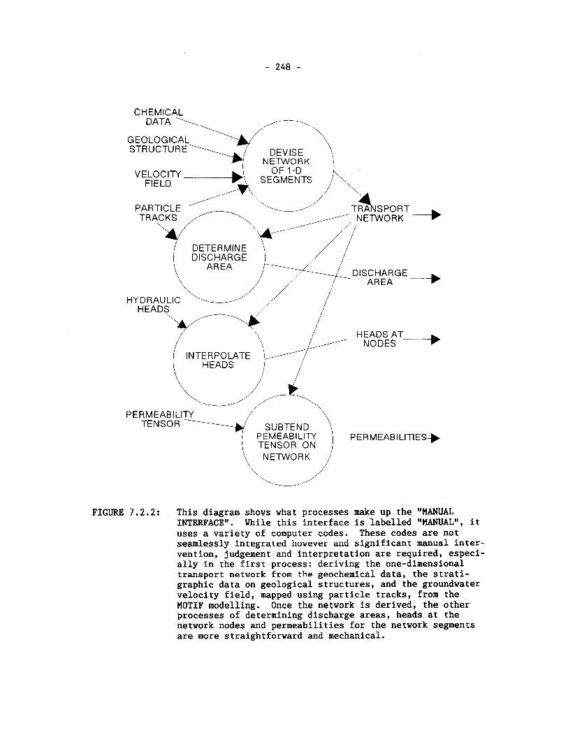
CHEMICAL DATA \
GEOLOGICAL STRUCTURE
I I L L C u I r l m l v a r w i ~ I
. . ..4CKS /, NETWORK --b \tc--
DETERMINE \ / /
HYDRAULIC \- ' /' /
HEADS
PERMEABILITY SUBTEND )
PEMEABlLlTY PERMEABILITIES) TENSOR ON
NETWORK
u FIGURE 7.2.2: This diagram shows what processes make up the "MANUAL
INTERFACEw. While this interface is labelled "MANUALI1, it uses a variety of computer codes. These codes are not seamlessly integrated however and significant manual inter- vention, judgement and interpretation are required, especi- ally in the first process: deriving the one-dimensional transport network from the geochemical data, the strati- graphic data on geological structures, and the groundwater velocity field, mapped using particle tracks, from the MOTIF modelling. Once the network is derived, the other processes of determining discharge areas, heads at the network nodes and permeabilities for the network segments are more straightforward and mechanical.
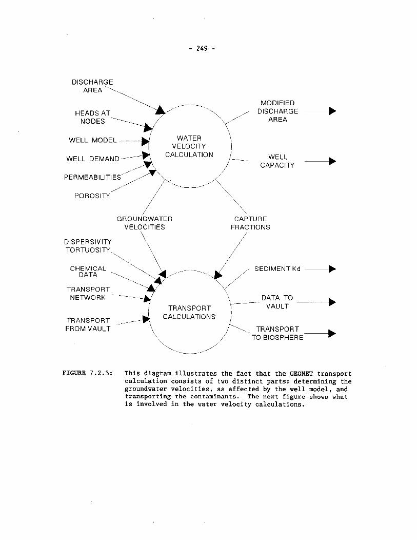
DISCHARGE AREA \
\ MODIFIED
HEADS AT DISCHARGE -b NODES ' AREA
WELL MODEL WATER ----)/ VELOCITY
PERMEABILITIES /A
/ GROUNDWATER
VELOCITIES
\ CAPTURE
FRACTIONS
DISPERSIVITY TORTUOSITY,
\
CHEMICAL DATA A/ - SEDlMENTKd -b
TRANSPORT NETWORK - 7 TRANSPORT
DATA TO VAULT 4
TRANSPORT / CALCULATIONS
FROM VAULT TRANSPORT TO BIOSPHERE +
u FIGURE 7.2.3: This diagram illustrates the fact that the GEONET transport
calculation consists of two distinct parts: determining the groundwater velocities, as affected by the well model, and transporting the contaminants. The next figure shows what is involved in the water velocity calculations.
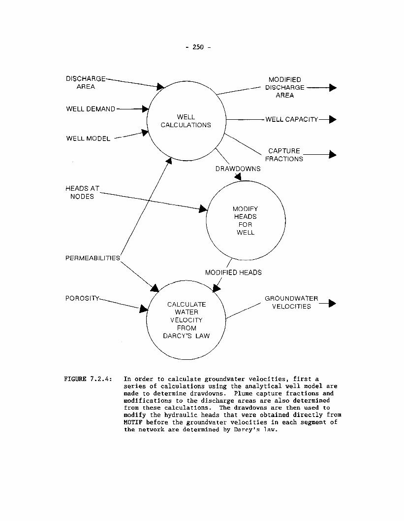
DISCHARGE AREA A DYziF:E -, WELL DEMAND
WELL CAPACITY+ CALCU LATlONS
WELL MODEL
CAPTURE FRACTIONS +
/ DRAWDOWNS
\ MODIFIED HEADS
-4 GROUNDW, CALCULATE / VELOCITI,,
WATER
FROM [ DARCY'S LAW
FIGURE 7.2.4: In order to calculate groundwater velocities, first a series of calculations using the analytical well model are made to determine drawdowns. Plume capture fractions and modifications to the discharge areas are also determined from these calculatlons. The drawdowns are then used to modify the hydraulic heads that were obtained directly from MOTIF before the groundwater velocities in each segment of the network are determined by Darcy's law.
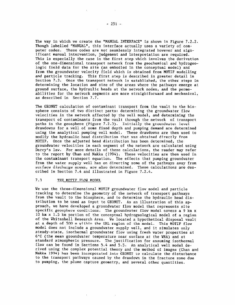
The way in which we create the "MANUAL INTERFACE" is shown in Figure 7.2.2. Though labelled "MANUAL", this interface actually uses a variety of com- puter codes. These codes are not seamlessly integrated however and sign- ificant manual intervention, judgement and interpretation are required. This is especially the case in the first step which involves the derivation of the one-dimensional transport network from the geochemical and hydrogeo- logic field data for the site (as embodied in the conceptual model) and from the groundwater velocity field which is obtained from MOTIF modelling and particle tracking. This first step is described in greater detail in Section 7.3. Once the transport network is established, the other steps in determining the location and size of the areas where the pathways emerge at ground surface, the hydraulic heads at the network nodes, and the perme- abilities for the network segments are more straightforward and mechanical, as described in Section 7.7.
The GEONET calculation of contaminant transport from the vault to the bio- sphere consists of two distinct parts: determining the groundwater flow velocities in the network affected by the well model, and determining the transport of contaminants from the vault through the network of transport paths in the geosphere (Figure 7.2.3). Initially the groundwater level drawdowns for a well of some fixed depth and pumping demand are determined using the analytical pumping well model. These drawdowns are then used to modify the hydraulic head distribution that was obtained directly from MOTIF. Once the adjusted head distribution has been determined, the groundwater velocities in each segment of the network are calculated using Darcy's law. For more details of these calculations, the reader may refer to the report by Chan and Nakka (1994). These velocities are then used in the contaminant transport equation. The effects that pumping groundwater from the water supply well has on diverting some of the pathways away from surface discharge areas, are also detern~ined. These calculations are des- cribed in Section 7.4 and illustrated in Figure 7.2.4.
7 . 3 THE MOTIF FLOW MODEL
We use the three-dimensional MOTIF groundwater flow model and particle tracking to determine the geometry of the network of transport pathways from the vault to the biosphere, and to determine the hydraulic head dis- tribution to be used as input to GEONET. As an illustration of this ap- proach, we have developed a groundwater flow model that represents site specific geosphere conditions. The groundwater flow model covers a 9 km x 10 km x 1.5 km portion of the conceptual hydrogeological model of a region of the Whiteshell Research Area. We located a hypothetical disposal vault at a depth of 500 m within the URL region of the model. This MOTIF flow model does not include a groundwater supply well, and it simulates only steady-state, isothermal groundwater flow using fresh water properties at 6°C (the mean groundwater temperature near surface at the WRA) and at standard atmospheric pressure. The justification for assuming isothermal flow can be found in Sections 5.4 and 5.5. An analytical well model de- rived using the complex potential theory and the method of images (Chan and Nakka 1994) has been incorporated i n t o GEONET to calculate the disturbance to the transport pathways caused by the drawdown in the fracture zone due to pumping, the plume capture geometry, and several other quantities.
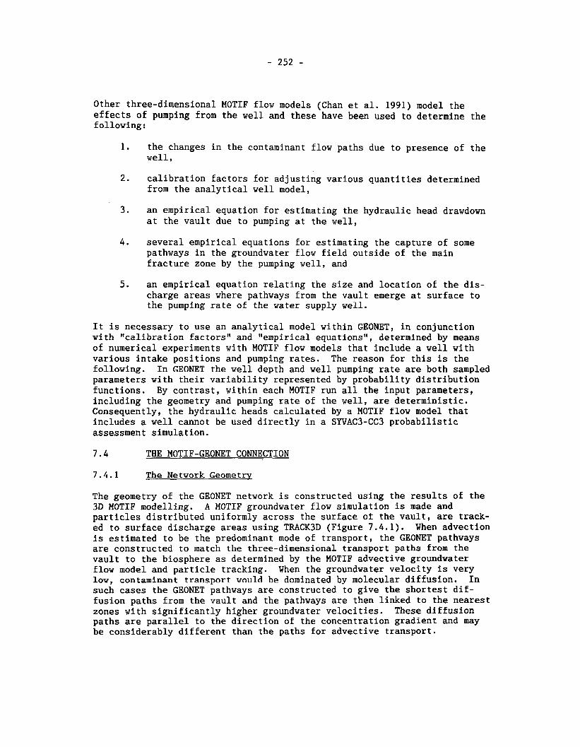
Other three-dimensional MOTIF flow models (Chan et al. 1991) model the effects of pumping from the well and these have been used to determine the following:
1. the changes in the contaminant flow paths due to presence of the well,
2. calibration factors for adjusting various quantities determined from the analytical well model,
3. an empirical equation for estimating the hydraulic head drawdown at the vault due to pumping at the well,
4 . several empirical equations for estimating the capture of some pathways in the groundwater flow field outside of the main fracture zone by the pumping well, and
5. an empirical equation relating the size and location of the dis- charge areas where pathways from the vault emerge at surface to the pumping rate of the water supply well.
It is necessary to use an analytical model within GEONET, in conjunction with "calibration factors'' and "empirical equations", determined by means of numerical experiments with MOTIF flow models that include a well with various intake positions and pumping rates. The reason for this is the following. In GEONET the well depth and well pumping rate are both sampled parameters with their variability represented by probability distribution functions. By contrast, within each MOTIF run all the input parameters, including the geometry and pumping rate of the well, are deterministic. Consequently, the hydraulic heads calculated by a MOTIF flow model that includes a well cannot be used directly in a SYVAC3-CC3 probabilistic assessment simulation.
THE MOTIF-GEONET CONNECTION
The Network Geometry
The geometry of the GEONET network is constructed using the results of the 3D MOTIF modelling. A MOTIF groundwater flow simulation is made and particles distributed uniformly across the surface of the vault, are track- ed to surface discharge areas using TRACK3D (Figure 7.4.1). When advection is estimated to be the predominant mode of transport, the GEONET pathways are constructed to match the three-dimensional transport paths from the vault to the biosphere as determined by the MOTIF advective groundwater flow model and particle tracking. When the groundwater velocity is very low, contaminant transport would be dominated by molecular diffusion. In such cases the GEONET pathways are constructed to give the shortest dif- fusion paths from the vault and the pathways are then linked to the nearest zones with significantly higher groundwater velocities. These diffusion paths are parallel to the direction of the concentration gradient and may be considerably different than the paths for advective transport.
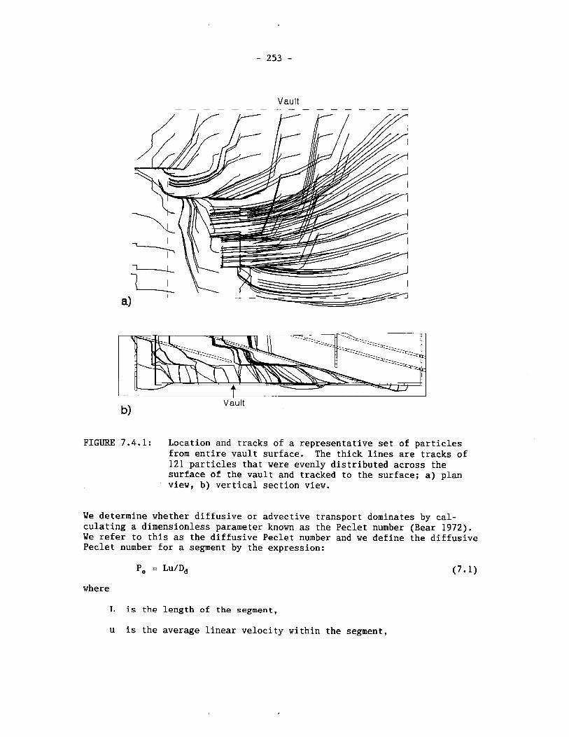
Vault - - - - - - - - - - - - - - - - -
FIGURE 7.4.1: Location and tracks of a representative set of particles from entire vault surface. The thick lines are tracks of 121 particles that were evenly distributed across the surface of the vault and tracked to the surface; a) plan view, b) vertical section view.
We determine whether diffusive or advective transport dominates by cal- culating a dimensionless parameter known as the Peclet number (Bear 1972). We refer to this as the diffusive Peclet number and we define the diffusive Peclet number for a segment by the expression:
where
1. is the length of the segment,
u is the average linear velocity within the segment,
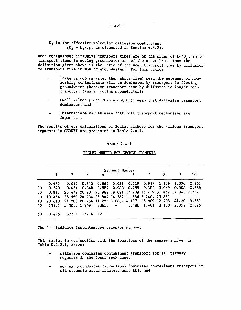
Dd is the effective molecular diffusion coefficient (D, = D,/T:, as discussed in Section 6.4.2).
Mean contaminant diffusive transport times are of the order of L2/Dd, while transport times in moving groundwater are of the order L/u. Thus the definition given above is the ratio of the mean transport time by diffusion to transport time in moving groundwater. Por this ratio:
- Large values (greater than about five) mean the movement of non- sorbing contaminants will be dominated by transport in flowing groundwater (because transport time by diffusion is longer than transport time in moving groundwater);
- Small values (less than about 0.5) mean that diffusive transport dominates; and
- Intermediate values mean that both transport mechanisms are important.
The results of our calculations of Peclet numbers for the various transport segments in GEONET are presented in Table 7.4.1.
TABLE 7.4.1
PECLET NUMBER FOR GEONET SEGMENTS
Segment Number 1 2 3 4 5 6 7 8 9 10
The '- ' indicate instantaneous transfer segment.
This table, in conjunction with the locations of the segments given in Table D.2.2.1, shows:
- diffusion dominates contaminant transport for all pathway segments in the lower rock zone,
- moving groundwater (advection) dominates contaminant transport in all segments along fracture zone LD1, and
- both diffusion and moving groundwater affect contaminant transport in the overburden and sediment segments.
Each GEONET transport pathway is composed of a number of linear segments. The end points of a segment are referred to as nodes. In locating the segments care is taken to ensure that the entire segment lies within a single material property zone and that the groundwater velocity does not vary excessively over the volume of rock represented by the segment.
Each segment is assigned to a chemical property class and a physical pro- perty class. Each chemical property class is characterized by a particular mineralogy and groundwater salinity. Each physical property class is char- acterized by a porosity, a tortuosity factor which relates to the diffusive part of transport in the direction of the segment or flow tube, and a number of parameters used in matrix diffusion calculations.
Figure 7.4.2a is a plan view projection of the network. Figure 7.4.2b shows the vertical section view of the network that was developed from the MOTIF results for the WRA, superimposed on the vertical section of particle tracks. It should be noted that the lines in these figures repre- sent the projection of the three-dimensional GEONET network or the particle tracks onto the appropriate horizontal or vertical plane. Most of the network segments and particle tracks shown, map the transport paths in the assymetrical groundwater flow field moving up the fracture zone located near the disposal vault. Each source node for the network begins in a unique vault sector (Figure 7.4.3).
The network has also been constructed to account for the influences on the flow paths by a well of variable depth and water supply demand. This was done by comparing the particle tracks vbbairled Irvm a series of separate MOTIF models in which the effects of wells of varying depth and pumping demand were determined. The pumping well changes the groundwater flow field as well as the location and size of the discharge areas where contam- inants from the vault would be expected to emerge at surface as described in Section 5.6. Additional segments were introduced to GEONET to allow for the increase in the capture of pathways in the groundwater flow field out- side the fracture zone by the pumping well.
The well depth is variable. To achieve the required well depth, the locations of the nodes defining the well are allowed to move along the central flow line of the well as discussed in Section 6.2.
7.4.2 Empirical Effects of The Well
An analytical well model (Chan and Nakka 1994), described in Section 6.5, is applied in GEONET to calculate the principal well quantities. As ex- plained in the last paragraph of Section 7.3, empirical site-specific re- lationships are required for four additional quantities:
1. a well scaling factor,
2. the hydraulic-head drawdowns at nodes in the vault, which are used to determine hydraulic heads in the vault,
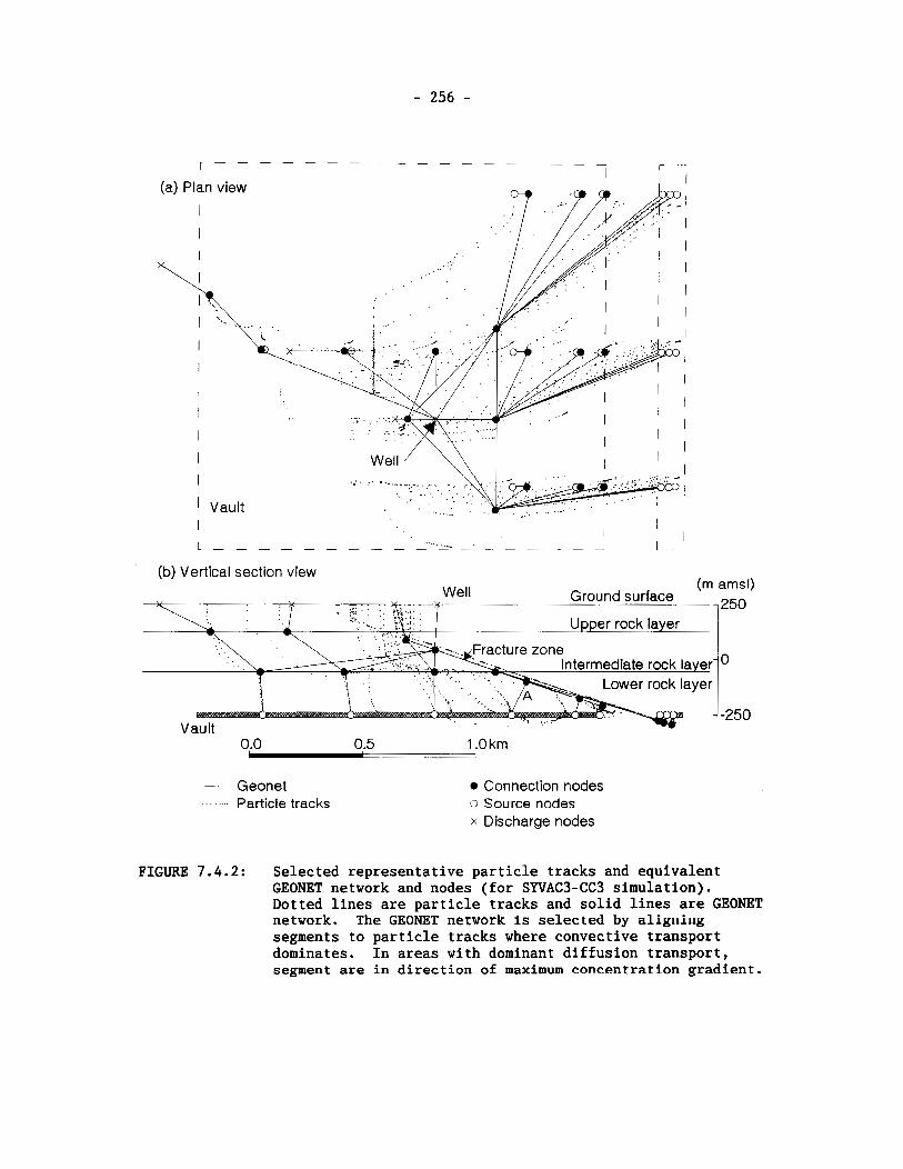
(a) Plan view
I I
I
(b) Vertical section view
- Geonet , . . . ..... Particle tracks
Connection nodes o Source nodes x Discharge nodes
FIGURE 7.4.2: Selected representative particle tracks and equivalent GEONET network and nodes (for SYVAC3-CC3 simulation). Dotted lines are particle tracks and solid lines are GEONET network. The GEONET network is selected by aligning segments to particle tracks where convective transport dominates. In areas with dominant diffusion transport, segment are in direction of maximum concentration gradient.
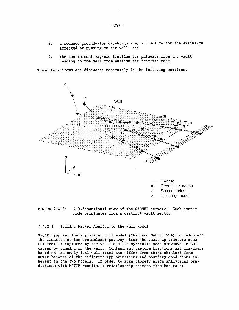
3 . a reduced groundwater discharge area and volume for the discharge affected by pumping on the well, and
4 . the contaminant capture fraction for pathways from the vault leading to the well from outside the fracture zone.
These four items are discussed separately in the following sections.
\ I Well
- Geonet a Connection nodes o Source nodes x Discharge nodes
FIGURE 7.4.3: A 3-dimensional view of the GEONET network. Each source node originates from a distinct vault sector.
7.4.2.1 Scaling Factor Applied to the Well Model
GEONET applies the analytical well model (Chan and Nakka 1994) to calculate the fraction of the contaminant pathways from the vault up fracture zone LD1 that is captured by the well, and the hydraulic-head drawdown in LDl caused by pumping on the well. Contaminant capture fractions and drawdowns based on the analytical well model can differ from those obtained from MOTIF because of the different approximations and boundary conditions in- herent in the two models. In order to more closely align analytical pre- dictions with MOTIF results, a relationship between them had to be
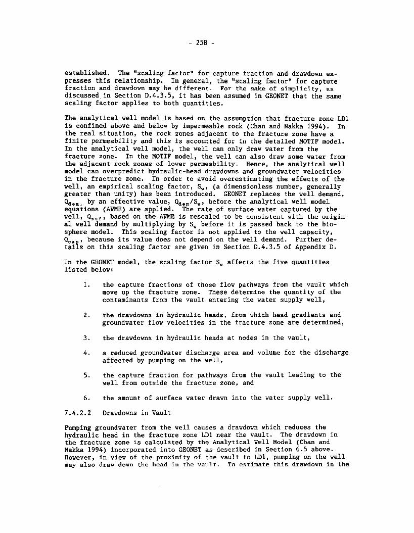
established. The "scaling factor" for capture fraction and drawdown ex- presses this relationship. In general, the "scaling factorw for capture fraction and drawdown may be different. For the sake of simplicity, as discussed in Section D.4.3.5, it has been assumed in GEONET that the same scaling factor applies to both quantities.
The analytical well model is based on the assumption that fracture zone LD1 is confined above and below by impermeable rock (Chan and Nakka 1994). In the real situation, the rock zones adjacent to the fracture zone have a finite permeability and this is accounted for in the detailed MOTIF model. In the analytical well model, the well can only draw water from the fracture zone. In the MOTIF model, the well can also draw some water from the adjacent rock zones of lower permeability. Hence, the analytical well model can overpredict hydraulic-head drawdowns and groundwater velocities in the fracture zone. In order to avoid overestimating the effects of the well, an empirical scaling factor, S,, (a dimensionless number, generally greater than unity) has been introduced. GEONET replaces the well demand, (Idern, by an effective value, Qdem/Sw, before the analytical well model equations (AWME) are applied. The rate of surface water captured by the well, Q,,,, based on the AWME is rescaled to be consist en^ with the origin- al well demand by multiplying by S, before it is passed back to the bio- sphere model. This scaling factor is not applied to the well capacity, Q,, , because its value does not depend on the well demand. Further de- tails on this scaling factor are given in Section D.4.3.5 of Appendix D.
In the GEONET model, the scaling factor S, affects the five quantities listed below:
1. the capture fractions of those flow pathways from the vault which move up the fracture zone. These determine the quantity of the contaminants from.the vault entering the water supply well,
2. the drawdowns in hydraulic heads, from which head gradients and groundwater flow velocities in the fracture zone are determined,
3. the drawdowns in hydraulic heads at nodes in the vault,
4. a reduced groundwater discharge area and volume for the discharge affected by pumping on the well,
5. the capture fraction for pathways from the vault leading to the well from outside the fracture zone, and
6 . the amount of surface water drawn into the water supply well.
7.4.2.2 Drawdowns in Vault
Pumping groundwater from the well causes a drawdown which reduces the hydraulic head in the fracture zone LD1 near the vault. The drawdown in the fracture zone is calculated by the Analytical Well Model (Chan and Nakka 1994) incorporated into GEONET as described in Section 6.5 above. However, in view of the proximity of the vault to LD1, pumping on the well may also draw down the head in the vault. To estimate this drawdown in the
vault we have devised a series of Empirical Vault Head Equations (EVHE) by combining specific results of the Analytical Well Model (AWM) with a corresponding MOTIF finite-element model. Heads in other regions ot the network (outside of the fracture zone and the vault) are not adjusted be- cause adjusting them does not have a significant effect on the contaminant transport results of the GEONET Model.
I -\--. I .
I \... I I '-. I
I I
level I Rsglon 3 Rsglon 2 :-egloni I I 1, 5 I
I I
I
'< 4- -. -
( x w - x,)
FIGURE 7.4.4: Regions where the 3 EVHE equations apply are shown. The first equation applies to region 1, where the vault is above the fracture zone. The second equation applies to region 2, where the vault is near to, but below the fracture zone. The third equation applies to region 3, which is further from the fracture zone. Parameter e4 determines the boundary between regions 2 and 3. x, is the x coordinate of the well. x, is the x coordinate of the EVHE reference node in the fracture zone.
Drawdowns in hydraulic head, Ah,, (Ah, is the difference in head between the no well case and a case with a pumped well) at nodes in the vault are calculated from the drawdown, Ah,, and slope of the drawdown, aAh,/a[, at a reference node at the intersection of the fracture zone and the vault hori- zon. Here, as depicted in Figure 6.5.2, < is the coordinate along the line of symmetry of the flow field of the well in the AWM. The reference node may be a node of the transport network or may be an extra unconnected node.
There may be more than one reference node. Each is located so that a line joining the vault node for which drawdown calculations are done and the corresponding reference node, is parallel to x-axis in Figure 7.4.3, which represents a vertical section normal to the line formed by the intersection of the LD1 plane with the vault plane. It should be noted that the axis is parallel to the vertical projection of the f-axis from the LD1 plane onto the vault plane. Since rows of source nodes in the GEONET WRA model are
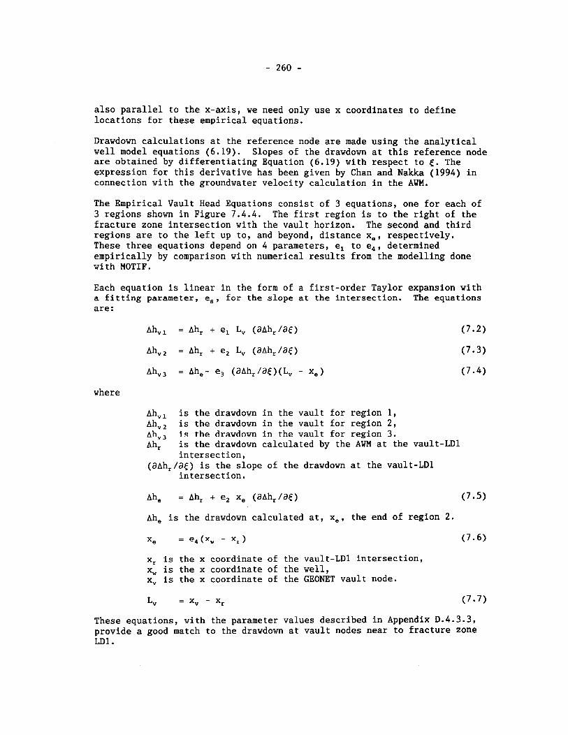
also parallel to the x-axis, we need only use x coordinates to define locations for these empirical equations.
Drawdown calculations at the reference node are made using the analytical well model equations (6.19). Slopes of the drawdown at this reference node are obtained by differentiating Equation (6.19) with respect to c . The expression for this derivative has been given by Chan and Nakka (1994) in connection with the groundwater velocity calculation in the AWM.
The Empirical Vault Head Equations consist of 3 equations, one for each of 3 regions shown in Figure 7.4.4. The first region is to the right of the fracture zone intersection with the vault horizon. The second and third regions are to the left up to, and beyond, distance x,, respectively. These three equations depend on 4 parameters, el to e,, determined empirically by comparison with numerical results from the modelling done with MOTIF.
Each equation is linear in the form of a first-order Taylor expansion with a fitting parameter, e,, for the slope at the intersection. The equations are :
A h = Ah, + el Lv (aAh,/aE)
A h = Ah, - e, (aAh, /ac)(Lv - x, )
where
A h is the drawdown in the vault for region 1, A h is the drawdown in the vault for region 2, A is the drawdown in the vault for region 3. Ah, is the drawdown calculated by the AWM at the vault-LD1
intersection, (aAh,/a() is the slope of the drawdown at the vault-LD1
intersection.
Ah, is the drawdown calculated at, x,, the end of region 2.
x, is the x coordinate of the vault-LD1 intersection, xw is the x coordinate of the well, xv is the x coordinate of the GEONET vault node.
These equations, with the parameter values described in Appendix D.4.3.3, provide a good match to the drawdown at vault nodes near to fracture zone LD1.
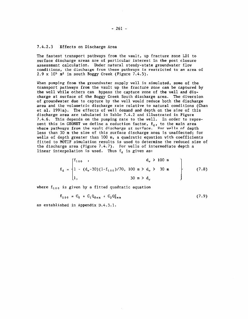
7.4.2.3 Effects on Discharge Area
The fastest transport pathways from the vault, up fracture zone LD1 to surface discharge areas are of particular interest in the post closure assessment calculation. Under natural steady-state groundwater flow conditions, the discharge from these pathways is restricted to an area of 2.9 x lo5 m2 in south Boggy Creek (Figure 7.4.5).
When pumping from the groundwater supply well is simulated, some of the transport pathways from the vault up the fracture zone can be captured by the well while others can bypass the capture zone of the well and dis- charge at surface of the Boggy Creek South discharge area. The diversion of groundwater due to capture by the well would reduce both the discharge area and the volumetric discharge rate relative to natural conditions (Chan et al. 1991a). The effects of well demand and depth on the size of this discharge area are tabulated in Table 7.4.2 and illustrated in Figure 7.4.6. This depends on the pumping rate to the well. In order to repre- sent this in GEONET we define a reduction factor, f,, to the main area where pathways from the vault discharge at surface. For wells of depth less than 30 m the size of this surface discharge area is unaffected; for wells of depth greater than 100 m, a quadratic equation with coefficients fitted to MOTIF simulation results is used to determine the reduced size of the discharge area (Figure 7.4.7). For wells of intermediate depth a linear interpolation is used. Thus f, is given as:
where f,,, is given by a fitted quadratic equation
as established in Appendix D.4.3.1.
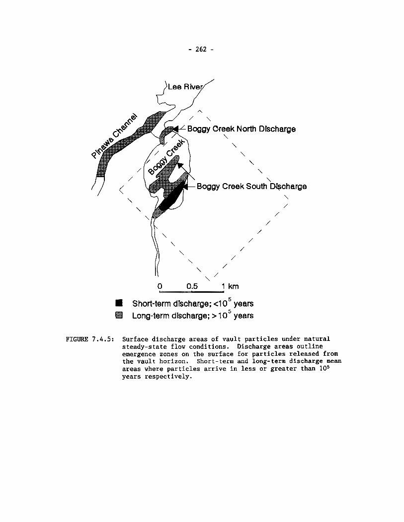
A
\
Boggy Week North Discharge \ \ \
\
\ \
Boggy Creek South Wcharge \ /
/
/
/ /
/ /
\ /
\ /
Short-term discharge: <10 years Long-term discharge; > 1 o5 years
FIGURE 7.4.5: Surface discharge areas of vault particles under natural steady-state flow conditions. Discharge areas outline emergence zones on the surface for particles released from the vault horizon. Short-term and long-term discharge mean areas where particles arrive in less or greater than lo5 years respectively.
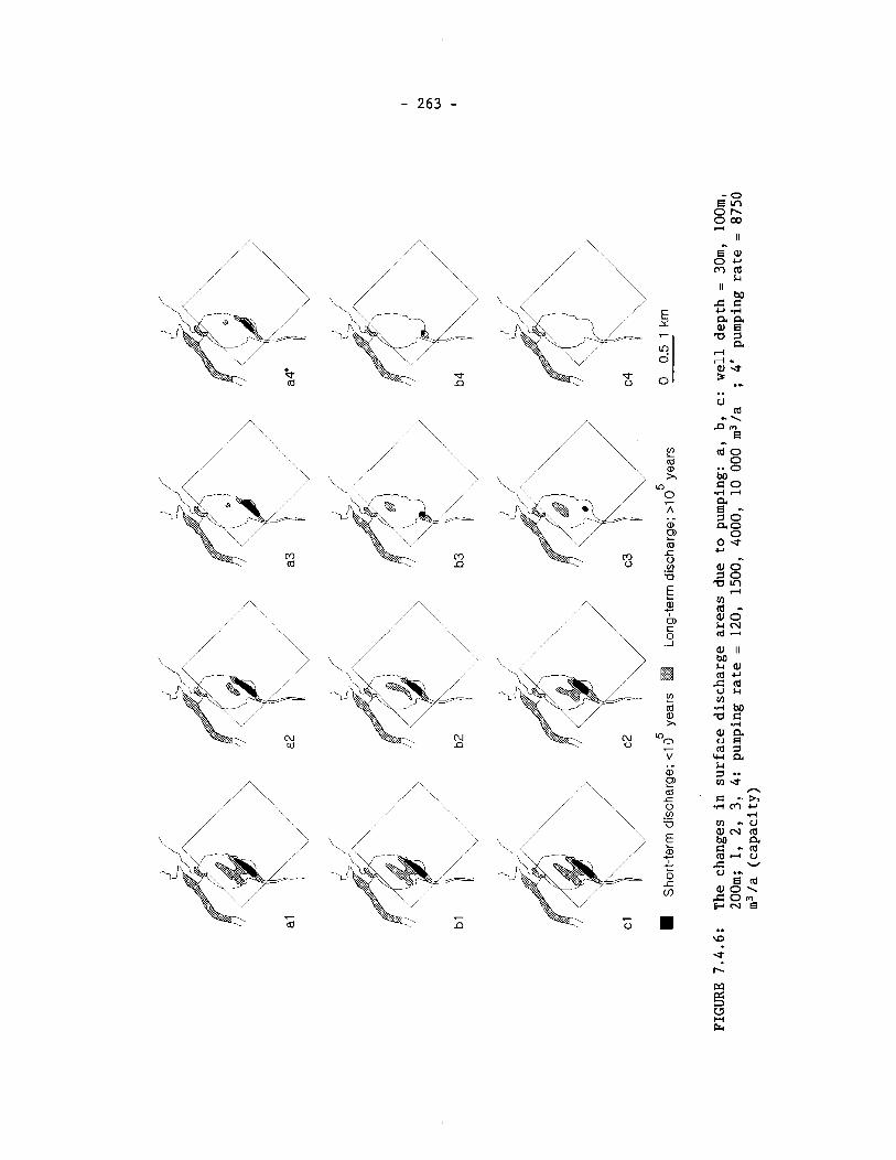
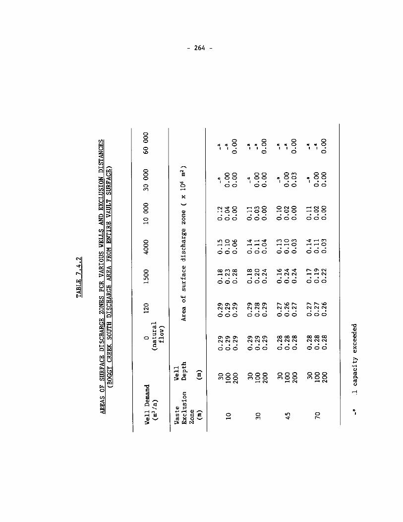
a
4 aJ 0
8 h C, .r( u
cd u
r!
m I
0 0 0 0 l a m 0 a m 0 a m ? m a 0
1 1 . 1 1 . I 1 1 1 ' 0 0 0 0
0 0 0 0 0 m 0 0 m O O n o 0 m O O 4 0 0 ~ . . ~ . . ~ . . I . . 0 0 0 0 0 0 0 0
N * O d m 0 O N 0 + N O ? ? ? t?? ? ? ? ? ? ? 0 0 0 0 0 0 0 0 0 0 0 0
m o w 4-4- m o m e , + m ,+,+a d d 0 d , + O y y q . , . . . . . . 0 0 0 0 0 0 0 0 0 0 0 0
m m m m o e w e * - m ~ " N ? " N ? ? y q ? ? ? . . . . 0 0 0 0 0 0 0 0 0 0 0 0
m m m m a m ha- - h a ? ? ? ??"! ? ? ? ? ? ? 0 0 0 0 0 0 0 0 0 0 0 0
m m m m o m m m w m c ~ m N N N N N N N N N N N N . . . . . . . . . . . . 0 0 0 0 0 0 0 0 0 0 0 0
0 0 0 0 0 0 0 0 0 s g g * 2 % * z S * z Z ,-I-
0 LA 0 2 m *
0 0 0
0 w
0 0 0
0 m
0 0 0
2
0 0 0 *
o 0
2
z ,+
d
2 7 9 0
o r r l z w
a d (d
8 2
2 % aJ - 3
n N a
w 0 d
X
w
2 0 N
aJ 2 a ."o 7n .rl a aJ 0 cd w L4 s 7n w 0
(d a,
2
C r+ r r l a n ~ J Q , a 3 0 -
.r( 7n
01 9 W r l - o n r n " G 5 a x 0 3 W N

X 2 10
Well Demand (x10 m3 la)
FIGURE 7.4.7: The change in the main discharge area as a function of well demand for wells greater than lOOm in depth
7.4.2.4 Effects Outside Fracture Zone
The effects of well depth and demand, on the amount of contaminants from the vault captured from pathways in the rock mass outside the main fracture zone pathway, is presented in this section. The effects on the discharge areas are also presented. A set of empirical relationships was determined by comparing the groundwater flow fields arid particle tracks calculated by MOTIF for various well demands and depths to the no well case. If these calculations showed the well captured particles moving along pathways other than the main fracture zone, new GEONET segments were introduced to reroute these pathways to the well and away from the discharge area where they would otherwise emerge.
The flow path from vault sector 3 to Boggy Creek South has such a segment, segment 62 in Figure 7.4.8, that can divert a fraction of the contaminant mass flow from this vault sector to the well. At the outlet node of segment 9 the contaminant mass flow branches into two fractions. One fraction, 1 - W,,, migrates through segment 62 to the well while the other fraction, W,,, migrates through segment 51 and, subsequently, segment 52 to the Boggy Creek South discharge area. In calculating the branching fractions it has been assumed, in accordance with Table 7.4.1, that advective transport dominates so that the fractional contaminant mass flow rate is proportional to the groundwater flow rate. The fraction, W,,, of the contaminant mass flow that bypasses the well and continues on, through segments 51 and 52, to the Boggy Creek South discharge area is given by:
Wb3 = 1, any depth of well and well demands less than 1 500 m3/a ;
Wb3 = 0.25, any depth of well and well demand of 4 000 m3/a with linear interpolation between 1.0 and 0.25 for well demands between 1 500 and 4 000 m3/a ;
wb3 = 0, any depth of well and well demand of 6 000 m3/a or more, with linear interpolation between 0.25 and 0.0 for well demands between 4 000 and 6 000 m3/a .
The discharge volume and the discharge area of contaminated groundwater at Boggy Creek South are modified by the factor f, as determined by Equation (7.8) already described in Section 7.4.2.3. Further discussion of this modified discharge area is presented later in this section.
Similarly, the flow path from vault sector 2 to the Boggy Creek North dis- charge area also has a segment ( 6 3 ) that can divert a fraction of the contaminant flow from this pathway to the water supply well. The fraction, W,,, of the flow in this pathway bypassing the well and continuing on to the Boggy Creek North discharge area is given by:
wb2 = 1, depth of well less than or equal to 100 m and all well demands;
wb2 = I9 depth of well greater than 100 m and well demand less than 10 000 m3/a .
Wb2 = 0.9, depth of well greater than 100 m and well demand of 30 000 m3/a with linear interpolation between 1.0 and 0.9 for well demands between 10 000 and 30 000 m3/a .
W,, = 0, depth of well greater than 100 m and well demand of 60 000 m3/a or more, with linear interpolation between 0.9 and 0.0 for well demands between 30 000 and 60 000 m3 /a .
The fraction of the flow in this pathway that is captured by the well is given by the complement, 1 - W,,. To account for this, the amount of con- taminants discharging from this pathway at the Boggy Creek North discharge area and the size of the discharge area are also modified by the reduction factor, W,, as discussed later in this section.
The pathway leading from vault sector 1 to the Pinawa Channel discharge area also has a segment (64) that can divert a fraction of the flow to the water supply well. The fraction, W,,, of the flow in this pathway that can bypass this segment and continue on to the Pinawa Channel discharge area is given by:
Wbl = 1, depth of well less than or equal to 150 m and all well demands;
Wb, = 1, depth of well greater than 150 m and well demand less than 30 000 m3/a .
W,, = 0, depth of well greater than 150 m and well demand of 80 000 m3/a or more, with linear interpolation between 1.0 and 0.0 for well demands between 30 000 and 80 000 m3/a .
The fraction of the flow in this pathway that is captured by the well is given by the complement, 1 - W,,. As in the other cases the amount of groundwater discharging through this pathway and the area of the discharge at the Pinawa Channel discharge area are also modified by the reduction factor, W,, . In summary, when the groundwater supply well is simulated, some of the groundwater flowpaths leading from the vault to groundwater discharge areas at surface will be captured by the well. This will reduce both the area and volumetric flow to these surface discharge areas. The adjusted area of the transport pathways emerging at these surface discharge areas, A',,, can be calculated using the following set of equations.
A',,, = f, A,,, for pathways leading to the Boggy Creek South discharge area. 1
A',,, = Wb2 A,,, for pathways leading to the Boggy Creek North discharge area. I
A',,, =Wb, A,,, for pathways leading to the Pinawa Channel discharge area. J
where A,,, is the area over which pathways from the vault would emerge in the absence of a well. For the Boggy Creek South discharge this area is 2.9 X lo5 m2 ; 7.5 X lo4 m2 for The Boggy Creek North discharge area and 1.9 X lo5 m2 for the Pinawa Channel discharge area (Chan et al. 1991).
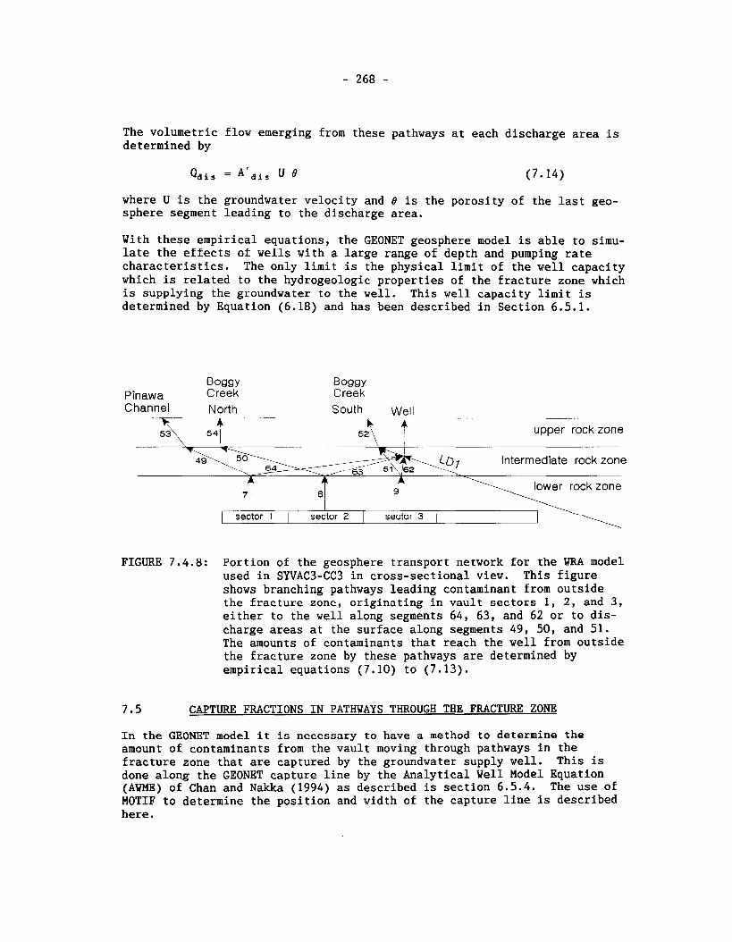
The volumetric flow emerging from these pathways at each discharge area is determined by
where U is the groundwater velocity and 8 is the porosity of the last geo- sphere segment leading to the discharge area.
With these empirical equations, the GEONET geosphere model is able to simu- late the effects of wells with a large range of depth and pumping rate characteristics. The only limit is the physical limit of the well capacity which is related to the hydrogeologic properties of the fracture zone which is supplying the groundwater to the well. This well capacity limit is determined by Equation (6.18) and has been described in Section 6.5.1.
Boggy W 3 g y Pinawa Creek Creek Channel North South Well
upper rock zone
intermediate rock zone
lower rock zone
I I I / sector 1 I sector 2 1 sector 3 1 \
FIGURE 7.4.8: Portion of the geosphere transport network for the WRA model used in SYVAC3-CC3 in cross-sectional view. This figure shows branching pathways leading contaminant from outside the fracture zonc, originating in vault sectors 1, 2, and 3, either to the well along segments 64, 63, and 62 or to dis- charge areas at the surface along segments 49, 50, and 51. The amounts of contaminants that reach the well from outside the fracture zone by these pathways are determined by empirical equations (7.10) to (7.13).
CAPTURE FRACTIONS IN PATHWAYS THROUGH THE FRACTURE ZONE
In the GEONET model it is necessary to have a method to determine the amount of contaminants from the vault moving through pathways in the fracture zone that are captured by the groundwater supply well. This is done along the GEONET capture line by the Analytical Well Model Equation (AWME) of Chan and Nakka (1994) as described is section 6.5.4. The use of MOTIF to determine the position and width of the capture line is described here.
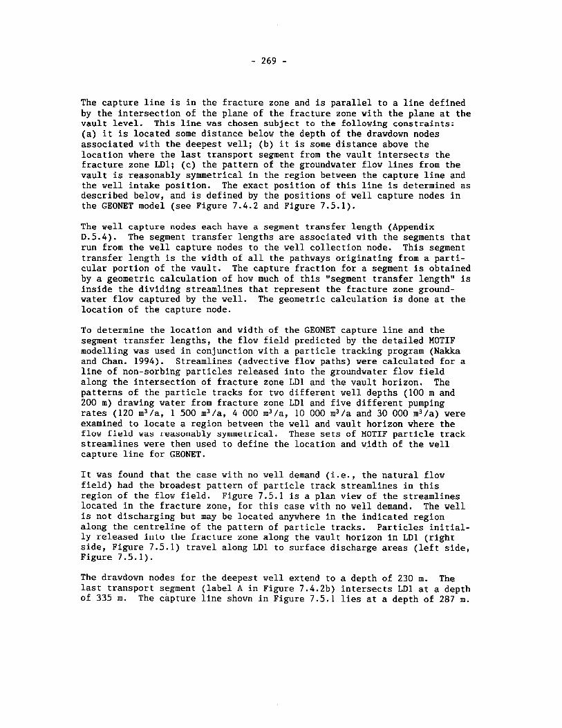
The capture line is in the fracture zone and is parallel to a line defined by the intersection of the plane of the fracture zone with the plane at the vault level. This line was chosen subject to the following constraints; (a) it is located some distance below the depth of the drawdown nodes associated with the deepest well; (b) it is some distance above the location where the last transport segment from the vault intersects the fracture zone LD1; (c) the pattern of the groundwater flow lines from the vault is reasonably symmetrical in the region between the capture line and the well intake position. The exact position of this line is determined as described below, and is defined by the positions of well capture nodes in the GEONET model (see Figure 7.4.2 and Figure 7.5.1).
The well capture nodes each have a segment transfer length (Appendix D.5.4). The segment transfer lengths are associated with the segments that run from the well capture nodes to the well collection node. This segment transfer length is the width of all the pathways originating from a parti- cular portion of the vault. The capture fraction for a segment is obtained by a geometric calculation of how much of this "segment transfer length" is inside the dividing streamlines that represent the fracture zone ground- water flow captured by the well. The geometric calculation is done at the location of the capture node.
To determine the location and width of the GEONET capture line and the segment transfer lengths, the flow field predicted by the detailed MOTIF modelling was used in conjunction with a particle tracking program (Nakka and Chan. 1994). Streamlines (advective flow paths) were calculated for a line of non-sorbing particles released into the groundwater flow field along the intersection of fracture zone LD1 and the vault horizon. The patterns of the particle tracks for two different well depths (100 m and 200 m) drawing water from fracture zone LD1 and five different pumping rates (120 m3/a, 1 500 m3/a, 4 000 m3/a, 10 000 m3/a and 30 000 m3/a) were examined to locate a region between the well and vault horizon where the flvw Iield was reasonably symmetrical. These sets of MOTIF particle track streamlines were then used to define the location and width of the well capture line for GEONET.
It was found that the case with no well demand (i.e., the natural flow field) had the broadest pattern of particle track streamlines in this region of the flow field. Figure 7.5.1 is a plan view of the streamlines located in the fracture zone, for this case with no well demand. The well is not discharging but may be located anywhere in the indicated region along the centreline of the pattern of particle tracks. Particles initial- ly released into the fracture zone along the vault horizon in LD1 (right side, Figure 7.5.1) travel along LD1 to surface discharge areas (left side, Figure 7.5.1).
The drawdown nodes for the deepest well extend to a depth of 230 m. The last transport segment (label A in Figure 7.4.2b) intersects LD1 at a depth of 335 m. The capture line shown in Figure 7.5.1 lies at a depth of 287 m.
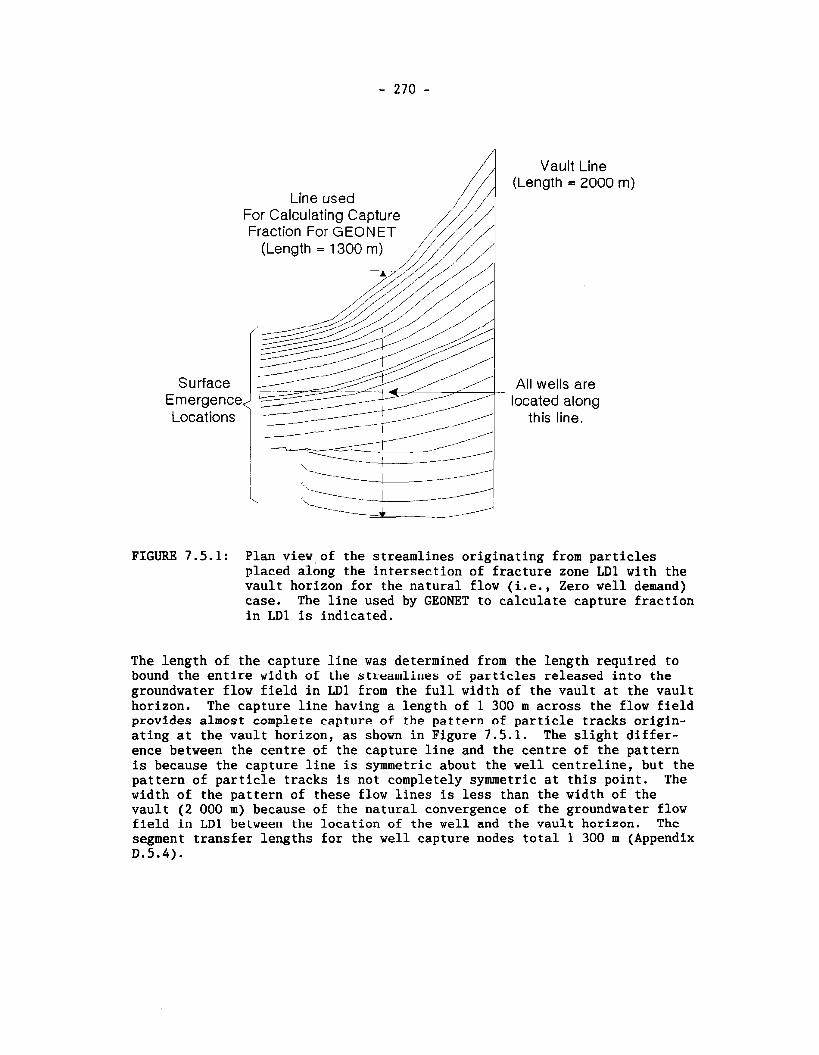
Line used
Vault Line (Length = 2000
All wells are located along
this line.
FIGURE 7 .5 .1 : Plan view,of the streamlines originating from particles placed along the intersection of fracture zone LD1 with the vault horizon for the natural flow (i.e., Zero well demand) case. The line used by GEONET to calculate capture fraction in LD1 is indicated.
The length of the capture line was determined from the length required to bound the entire width of the streamlines of particles released into the groundwater flow field in LD1 from the full width of the vault at the vault horizon. The capture line having a length of 1 300 m across the flow field provides almost complete capture of the pattern of particle tracks origin- ating at the vault horizon, as shown in Figure 7.5.1. The slight differ- ence between the centre of the capture line and the centre of the pattern is because the capture line is symmetric about the well centreline, but the pattern of particle tracks is not completely symmetric at this point. The width of the pattern of these flow lines is less than the width of the vault (2 000 m) because of the natural convergence of the groundwater flow field in LD1 between the location of the well and the vault horizon. The segment transfer lengths for the well capture nodes total 1 300 m (Appendix D.5.4) .
The capture fractions predicted by AWME and MOTIF were compared to deter- mine the value for the well scaling factor (Section 7.4.2.1). The MOTIF capture fractions were calculated from the streamlines from the particle tracking program. The particles were started at the capture line and were run for the same well depths and well demands as described above in this section. This was used to determine the well scaling factor as described in Appendix D.4.3.5.1.
Other information on the capture fraction for the fracture zone can be found in Chapter 6.5.4 and Appendix D.2.1, D.4.3.5.1, and D.5.4.
GROUNDWATER VELOCITY SCALING FACTOR
In order to account for the uncertainty in hydrogeological parameters used in the GEONET model and uncertainty due to model approximations, all groundwater velocities in the network of pathways are multiplied uniformly by a scaling factor S,, as described in Section 6.4.1. The analytical well model equations (AWME) use both the hydraulic conductivity of the fracture zone, K,, and the related quantity q,, the initial specific discharge in the fracture zone. For consistency with the scaling of all groundwater velocities by S,, these two quantities must also be scaled by S, before use in the AWME. In GEONET, the effect on well quantities due to multiplying K, and q, by S, is accounted for indirectly by invoking a set of "scaling laws" established by Chan and Nakka (1994). A scaling law is a mathe- matical identity that relates the change in a well quantity due to multi- plying K, and qf by S,, to the change in the well quantity caused by chang- ing (scaling) the well demand. For most quantities, the scaling law in- dicates that the well demand, Qdem, can be replaced by an effective value, Q,,,/S,, before the AWME are applied. The surface water captured by the well, Q,,,, and the well capacity, Q,, , however, are calculated by using the scaled well demand, Q d e m V , and tRen multiplying the result by S, . Further details on the scaling laws are provided in Appendix E of the analytical well model report (Chan and Nakka 1994).
7.7 MATRIX DIFFUSION EFFECTS ON CONTAMINANT RETARDATION AND DISPERSION
Matrix diffusion is the process whereby solutes that are being transported in moving groundwater diffuse into adjacent stagnant water in the rock matrix. Hence these effects can be applied when the groundwater is con- ceptually divided into a portion that moves within channels in fracture zones or fractures in the rock mass and a stagnant portion in an adjacent portion of the fracture zone or rock mass. The equations we use in GEONET to approximate the effects of diffusion into the rock matrix are based upon modelling the groundwater flow as occurring within a set of plane parallel fractures with constant effective aperture and constant average spacing (Lever et al. 1982).
In the conceptual model of the WRA and the groundwater flow modelling done with MOTIF, each region of the geosphere is treated as a porous rock block, through which all the groundwater is moving and in which there are
no stagnant water zones. Within the framework of this conceptual model, no matrix diffusion effects are explicitly applied.
The values we have chosen for dispersion coefficients used in the transport equation are designed to include the empirically derived effects of dis- persion. These include the effects of permeability channelling within the fracture zones and/or diffusion into nearby stagnant water zones.
SUMMARY OF DATA TRANSFERRED TO GEONET
Site specific geosphere data derived from field and laboratory work and the results of detailed groundwater flow and transport path modelling using MOTIF are transferred to GEONET. These data consist of the network geo- metry of the transport paths from the vault to the biosphere, the hydrogeo- logic properties of the transport network, other data from the MOTIF model- ling, the transport properties of the segments, the mineralogy and ground- water chemistry of the segments and a few other miscellaneous properties. These are summarized in the following:
Network Geometry
This includes the geometry of the network of pathways from the disposal vault to the biosphere, the coordinates of the nodes, describing this net- work, and a table of connectivities indicating which nodes are joined in pairs to form 1-D segments. The network segments are arranged such that no segment crosses a material property boundary so that constant properties can be assumed within each segment. Most of the segments follow flow paths where advection dominates transport. In some regions of the geosphere the groundwater flow model reveals that diffusion dominates the transport. Here, the pathways are chosen to be parallel to the diffusion gradient rather than follow the advective pathway. This network data set also in- cludes the segment source fractions, which quantify the volumetric rate of flow into the segment at the inlet node of each segment.
7.8.2 Hydroneologic Properties
The porosity and permeabilities for each segment of the GEONET model are chosen to be the same as those used in the MOTIF groundwater flow model. The permeabilities are calculated from the tensorial quantity used in MOTIF and are projected onto the 1-D direction of each segment, as described in Appendix C.
Data From MOTIF Results
The MOTIF model supplies the hydraulic heads to be used for each node in the GEONET model. GEONET uses these values to calculate groundwater veloc- ities in each segment from Darcy's law. The size and location of the areas where the pathways from the vault emerge in surface discharge areas are also supplied by the MOTIF model. Parameters related to a water supply well in the geosphere such as the minimum well depth and thickness of the fracture zone being pumped, are transferred directly from the MOTIF model.
The temperature at each node is also supplied. In the WRA model presented as a reference case study in this report, uniform and constant temperature was assumed throughout the entire GEONET model.
7.8.4 Transport Properties
Dispersivities are used in GEONET together with diffusion coefficients, tortuosity factors, and the calculated groundwater velocities in the net- work to determine the dispersion coefficients used in the transport equation for each segment. These properties are estimated from field and laboratory measurements, supplemented with literature review.
7.8.5 Mineralogy and Groundwater Chemistry
These are the chemical and mineralogical compositions of each chemical property zone in the GEONET model. These include: salinity or total dis- solved solids of the groundwater, redox conditions, mineral content and proportions, and the sorption coefficient of each element to be considered in the transport calculations. The tables in Appendix D give the sorption data for the element Cesium as an example. The complete set of sorption data used in the geosphere model of the WRA is given in Vandergraaf and Ticknor 1993.
7.8.6 Miscellaneous Properties
Miscellaneous properties that are also needed for the GEONET model include parameters such as the thickness of sediment and overburden, and the radius of the groundwater supply well. These are derived from field observations. The fraction of the backfill in the vault is also estimated from the infor- mation provided by the disposal vault engineering study (Simmons and Baumgartner 1994).
A detailed description and justification of the values chosen for these data for the geosphere model used in this case study are presented in Appendix D.
CONCLUSION
This chapter illustrated the methodology for condensing site-specific data on geological, hydrogeological and geochemical properties of the geosphere surrounding a disposal vault into a simplified model of the contaminant transport pathways from the vault to the biosphere. The geosphere pathways model, GEONET, is used in the SYVAC-CC3 code for conducting a probabilistic postclosure assessment of the long term performance of the entire disposal sys tem.
Site characterization data from the WRA was used to develop a 3-D MOTIF model of the groundwater flow conditions at the WRA and a hypothetical disposal vault was imbedded in the model at 500 m depth. The hydrogeo- logical model and particle tracking techniques were used to determine the pathways of vault contaminants from the vault to discharge locations in the biosphere.
The methodology was used to determine the geometry of the geosphere path- ways network with and without a groundwater supply well, hydraulic heads within the network, and calibration factors and emperical equations for estimating the effects of the well on the groundwater flow field. In addition, other field and laboratory data relating to the transport of vault contaminants through the geosphere pathways was also transferred to GEONET. This data includes the transport properties of the regions of sparsely fractured rock, the mineralogy and chemical composition of the groundwater along the transport pathways, and aspects of the linkages of the geosphere model to the vault and biosphere models.
Although this case study is hypothetical, it illustrates how site specific geological, hydrogeological and geochemical information from site char- acterization and laboratory measurements would be combined to produce a model of the transport of vault contaminants through the geosphere sur- rounding a nuclear fuel waste disposal vault. It also illustrates how aspects of the site characteristics, vault layout, and vault design and engineering interact to affect the transport of vault contaminants through the geosphere to the biosphere.
CONCLUSIONS
This report describes the approach for developing the geosphere model used in the postclosure assessment to analyse the transport of vault contam- inants through the rock surrounding a nuclear fuel waste disposal vault. The report presents the geosphere model in detail, including the assump- tions and data that were used in constructing and assuring the quality of the model. It is important to note that we did not undertake to develop a generic geosphere model representing the range of geosphere conditions that might exist anywhere on the Canadian Shield. Some aspects of plutonic rocks of the Canadian Shield may be similar from site to site, however, we believe that a meaningful and realistic model of the transport of contam- inants from a disposal vault in plutonic rock in the Canadian Shield can only be developed using a consistent set of geological, hydrogeological and geochemical data from a particular site. We have illustrated our geosphere model development approach by applying it to a hypothetical disposal system using geosphere information derived from our field investigations of the Whiteshell Research Area (WRA), located on a granitic batholith in the Canadian Shield of southeastern Manitoba. We refer to this hypothetical situation as a case study because the geosphere is a realistic represent- ation of the conditions found to exist at the WRA, and the hypothetical disposal vault has been specifically located within the geosphere.
One of the first steps in the development of the geosphere model involved determining the potential changes in the geosphere that might occur due to site characterization, the construction of the underground excavations for the vault, waste emplacement, vault operation and closure, as well as possible natural and human induced events and processes in the future. From these analyses the following conclusions were reached:
- Perturbations associated with site characterization and under- ground construction can be monitored and utilized for validating aspecLs of the hydrogeologic alodel.
- Micro-organisms in the groundwater would not likely accelerate the rate of transport of contaminants from the vault though the geosphere.
- The long-term integrity of the vault and the surrounding rock could be evaluated and controlled by engineering analyses and design.
- Postglacial uplift, erosion, and climatic and meteorological changes in the Canadian Shield are not expected to cause large changes to the transport of vault contaminants through the geo- sphere during the time frame of the quantitative risk analysis (10 000 a).
- Glaciation of the Canadian Shield is not expected to commence until at least 20 000 years from present. Also the onset of glaciation is not expected to cause dramatic changes in the rate of contaminant transport from the vault.
- The probability of meteorite impact or volcanism disrupting the transport of contaminants from a vault in the Canadian Shield is too small to deserve further quantitative analysis. Similarly, potential disruptions caused by seismic disturbances can be ignored provided no seismically active faults more than 500 m long are located within 200 m of the vault.
- Human intrusions into the geosphere surrounding a vault, such as inadvertent use of groundwater from a well drilled into a major fracture zone in the rock near the disposal vault, have to be analyzed in detail.
A conceptual model of the subsurface geological structure and hydrogeology was constructed for the Whiteshell Research Area. This model used data consistent with airborne, surface and subsurface geological, geophysical, geochemical and hydrogeological data from field investigations in the WRA, and used data on physical and chemical material properties determined from laboratory testing. From this conceptual model, a series of finite element models were created to describe the transport of groundwater, heat and vault contaminants in the geosphere surrounding the vault. The coupled equations describing 3-D groundwater flow and heat transport were solved using the MOTIF code to predict the hydraulic head and groundwater velocity distributions in thc model. Next, the groundwater flow paths from the vault to discharge areas in the biosphere were determined by means of a particle-tracking technique.
Sensitivity analyses were performed with the groundwater flow and heat transport models to assess the effects of varying different features and properties within the model. The conclusions from the sensitivity analyses were: (1) the local topography and the configuration of major fracture zones in the rock have major influence on the groundwater flow patterns from the vault to discharge locations in the biosphere; (2) the nature of the topography in this case study funnels the groundwater passing through the region of the vault into a surface discharge area much smaller than the area of the vault; (3) only that part of the groundwater flow field within about 1 000 m of the vault boundary needed to be explicitly considered in modelling transport of the vault contaminants through the geosphere in this case study; ( 4 ) both the groundwater travel time and the area in the bio- sphere at which contaminated groundwater pathways from the vault would emerge could be substantially altered by pumping groundwater from a nearby water-supply well in the rock near the vault; (5) the size of the region of low-permeability sparsely fractured rock, between the vault and the nearest low-dip fracture zone that is an important transport pathway from the vault affects the contaminant transport times and rates significantly; (6) ther- mal convection due to heat generation by the fuel waste in the vault might or might not be important depending on the size ot the region of sparsely- fractured rock between the vault and the nearest fracture zone; for a case having 46 m of sparsely fractured rock separating the vault from the near- est fracture zone, thermal convection due to waste heat does not significantly affect the travel time for vault contaminants to move through the geosphere; and (7) the presence of shafts and tunnels, variations in hydraulic properties of backfill materials, the existence of an excavation damaged zone, or the presence of a thermomechanically disturbed rock zone near ground surface above the vault would not significantly affect the rate or amount of contaminants transported from the vault to the biosphere.
GEONET accepts as input the time-dependent flow rates of radioactive and toxic nuclides determined from the vault model. It then calculates time- dependent radioactive and Loxic nuclide flow rates along transport pathways in the rock mass surrounding the vault and at locations of discharges to the biosphere model. It also determines other appropriate information for interfacing the geosphere model with the vault and biosphere models, such as the size of the areas where pathways from the vault emerge at discharge locations in the biosphere and the volumetric discharge rates at these locations.
From the MOTIF modelling and particle tracking for the conditions of the case study, the transport paths from the vault to the discharge locations in the biosphere were determined. These were used to construct a 3-D transport network composed of 1-D transport segments for the GEONET model. In some locations of the geosphere, the groundwater flow rate was suf- ficiently slow that diffusion was the dominant transport process. In these situations, the contaminant transport pathways were constructed to give the shortest diffusion paths to nearby zones with significantly higher rate of groundwater flow. These pathways correspond to diffusion down the steepest concentration gradient. The diffusion pathways were then combined with the groundwater flow pathways to construct the overall transport network from the vault to the biosphere for the GEONET model.
As input, the GEONET model uses hydraulic head values, as determined by the MOTIF flow model, for each node of the transport network. The permeability tensOK used in the MOTIF model is projected onto each segment of the net- work. The well model, based on a specific location and pumping rate for the groundwater supply well is then used to calculate: 1) the maximum well capacity, 2) the drawdowns in the hydraulic head in the geosphere caused by the pumping well, 3) the quantity of surface water captured by the well, and 4) the fraction of vault contaminants moving along pathways through the geosphere that is captured by the well. The well model is further augment- ed by empirical site specific equations to account for three additional effects: 1) the drawdowns in hydraulic head in the vault, 2) reduction in the size and rate of discharge to the surface caused by the pumping well, and 3) the degree to which other pathways from the vault are captured by the pumping well. These equations were derived from MOTIF simulations which examined the effects of different pumping rates and different well locations on the transport pathways.
GEONET calculates the transport rate of radioactive or chemically toxic vault contaminants, through the network of pathways from the vault to dis- charges located in the biosphere. This is done by solving a system of one-dimensional advection-dispersion transport equations for a radionuclide decay chain, including the effects of retardation due to chemical sorption and/or diffusion into regions of the rock where groundwater movement is virtually stagnant. These calculations are done sequentially, segment by segment along the pathways, using the output of one segment as the input boundary condition for the following segment in the same pathway. Segments can also converge or diverge to represent the geometry of the pathways. For converging segments, the contaminant mass flow rates are summed whereas for diverging segments the contaminant mass flow rate is divided according to the branching ratio of groundwater flux estimated from the particle tracking. Chemical retardation is modelled using an equilibrium linear sorption (k,) approach. Retardation factors for the segments of the path- ways are calculated using empirical equations that relate the chemical and mineralogical properties of each transport segment to a set of contaminant/ mineral-specific retardation coefficients. The redox condition in the groundwater can be either oxidizing or reducing depending on site specific conditions.
This report shows that a methodology has been developed for condensing site characterization data and the results of detailed 3-D hydrogeological modelling into a geosphere model for probabilistic postclosure assessment of the performance of a nuclear fuel waste disposal vault at a site in plutonic rock of the Canadian Shield. The methodology has been illustrated with a case study based on site characterization studies preformed at the Whiteshell Research Area on the Canadian Shield in southeastern Manitoba. Various model quality assurance measures have been used to provide con- fidence that the GEONET model represents a reasonably accurate approxi- mation of the site-specific geometrical structure and physical and chemical phenomena important to the transport of radioactive and toxic contaminants from the hypothetical vault location, through the groundwater in the pores and fractures in the rock surrounding the vault to discharge locations in the biosphere.
ACKNOWLEDGEMENTS
We would like to thank Dua Guvanasen, members of the Geoscience Subcom- mittee of the Technical Advisory Committee and the Ontario Hydro members of the Siting Geoscience working party of the CANDU Owners Group (COG) Nuclear Fuel Waste Management Program for their constructive comments and helping to improve this report. J. Halley and D. Good provided assistance in pre- paring the final diagrams for the document. K. Arsenault, P. Lucas, C. Meads and H. Worona helped with the word processing.
The Canadian Nuclear Fuel Waste Management Program is funded jointly by AECL and Ontario Hydro under the auspices of the CANDU Owners Group.

REFERENCES
Acres Consulting Services Ltd. 1978. Radioactive waste repository study. Atomic Energy of Canada Limited Report, AECL-6188.
Adams, J. and P. Basham. 1991. The seismicity and seismotectonincs of eastern Canada. & Neotectonics of North America, D.B. Slemmons, E.R. Engdahl, M.D. Zoback and D.D. Blackwell (Editors). The Geology of North America, Decade Map Volume 1. Geological Society of America, Boulder, Colorado, 261-276.
AECB (Atomic Energy Control Board). 1987. Regulatory policy statement. Regulatory objectives, requirements and guidelines for the disposal of radioactive wastes - long-term aspects. Atomic Energy Control Board Regulatory Document R-104, Ottawa, 1987 June 5.
AECL. 1994a. Environmental impact statement on the concept for disposal of Canada's nuclear fuel waste. Atomic Energy of Canada Limited Report, AECL-10711, COG-93-1. Available in French and English.
AECL. 1994b. Summary of the environmental impact statement on the concept for disposal of Canada's nuclear fuel waste. Atomic Energy of Canada Limited Report, AECL-10721, COG-93-11. Available in French and English.
Anderson, M.P. and W.W. Woessner. 1992. Applied groundwater modeling: simulation of flow and advective transport, Academic Press, Inc.
Andrews, J.T. 1987. The late wisconsin glaciation and deglaciation of the laurentide ice sheet. JXJ North America and Adjacent Oceans During the Last Deglaciation, W.F. Ruddiman and H.E. Wright Jr. (Editors). The Geology of North America, Geological Association of America, Boulder, Colorado, Volume K-3, 13-37.
Andrews, J.T. 1989. Postglacial emergence and submergence. Chapter 8 of Quaternary Geology of Canada and Greenland, R.J. Fulton (Editor). Geology of Canada, Volume 1, Geological Survey of Canada, Ottawa, 546- 562.
Applied Geoscience Branch Report. 1989. Final report of summary of the appendix A groundwater tracer test program at the WNRE borehole site, Report of Activities for the Period 1987 April to 1989 March. Atomic Energy of Canada Limited. Prepared for: The Power Reactor and Nuclear Fuel Development Corporation in Japan.
Applied Geoscience Branch Report. 1990. Report of summary of the appendix B groundwater tracer test program at the WNRE borehole site, report of activities for the period 1989 April to 1990 March. Atomic Energy of Canada Limited. Prepared for: The Power Reactor and Nuclear Fuel Development Corporation in Japan.

Applied Geoscience Branch Report. 1991. Report of summary of the appendix B groundwater tracer test program at the WL borehole site, report of activities for the period 1990 April to 1991 March. AECL research. Prepared for: The Power Reactor and Nuclear Fuel Development Corporation in Japan.
Ates, Y., D. Bruneau and W.R. Ridgway. 1994. An evaluation of potential effects of seismic events on a used-fuel disposal vault. Atomic Energy of Canada Limited Technical Record, TR-623.
Atkinson, G.M. 1992. Seismic hazard in northwestern Ontario. Atomic Energy of Canada Limited Technical Record, TR-M-22.
Atkinson, G.M. and R.K. McGuire. 1993. Probability of damaging earth- quakes in northwestern Ontario. Atomic Energy of Canada Limited Technical Record, TR-M-23.
Bartlein, P.J., T. Webb I11 and S. Hostetler. 1989. Chapter 3, Climato- logy. Techniques for Determining Probabilities of Events and Processes Affecting the Performance of Geologic Repositories: Volume l--Literature Review, R.L. Hunter and C.J. Mann (Editors). U.S. Nuclear Regulatory Commission Contractor Report, NUREG/CR-3964, 53-88.
Basham, P.W. and M.G Cajka. 1985. Contemporary seismicity on Northwestern Ontario. Atomic Energy of Canada Limited Technical Record, TR-299.
Bastian, W.C. and L. Lapidus. 1956. Longitudinal diffusion in ion exchange and chromatographic columns: Finite Column. J. Phys. Chem., 60, 816-817. -
Bathe, K. and E.L. Wilson. 1976. Numerical methods in finite element analysis, Prentice-Hall, Englewood Cliffs, N.J.
Bear, J. 1972. Dynamics of fluids in porous media, American Elsevier, New York.
Bear, J. 1979. Hydraulics of groundwater. McGraw-Hill, New York, 299.
Bear, J. and A. Verujit. 1987. Modeling groundwater flow and pollution, D. Reidel Publishing Co., 408
Berman, L.E., D.A. Ensminger, M.S. Guiffre, C.M. Koplik, S.G. Oston, G.D. Pollak and B.J. Ross. 1978. Analysis of Some Nuclear Waste Manage- ment Options, Volume I1 Appendices, Report UCRL-13917, University of California, Lawrence Livermore laboratory, Livermore, California.
Betcher, R.N. and R. Pearson. 1982. Hydrogeological research for the Canadian Nuclear Fuel Waste Program, Atomic Energy of Canada Limited Technical Record, TR-151.
Bonilla, M. 1970. Surface faulting and related effects. & Earthquake Engineering. R. Wiegel (Editor). Prentice-Hall Inc., Englewood Cliffs, N.J.
Bredehoeft, J.D. and L.F. Konikow. 1993. Groundwater models: validate or invalidate (Editorial). Ground Water, 3l, No. 2, 178-179.
Brisbin, W.C. 1979. A gravity profile across the Lac du Bonnet Batholith in Southeastern Manitoba. Atomic Energy of Canada Limited Technical Record, TR-17.
Broecker, W.S. and G.H. Denton. 1989. The role of ocean-atmosphere re- organizations in glacial cycles. Geochimica et Cosmochimica Acta, 53, 2465-2501.
Brown, D.A. and C.J. Hamon. 1993. Initial investigation of groundwater microbiology at AECL undergound laboratory. Atomic Energy of Canada Limited Technical Record, TR-608, COG-93-171.
Brown, P.A. and A. Brown. In preparation. Potential pathways within the Lac du Bonnet Batholith. Atomic Energy of Canada Limited Technical Record.
Chan, A.H.C. and A.L. Punhani. 1991. 3-D Particle Tracking Algorithm To Model Radionuclide Transport, Ontario Hydro Research Division Report NO. 91-161-K.
Chan, T. 1989. An Overview of Groundwater Flow and Radionuclide Transport Modelling in the Canadian Nuclear Fuel Waste Management Program, In Proceedings of conference on geostatistical, sensitivity, and uncer- tainty methods for groundwater flow and radionuclide transport model- ling, 1987 Sept. 15-17, San Francisco, Batelle Press, Columbus, Ohio, 1989, 39-61.
Chan, T. and B.W. Nakka. 1994. A two-dimensional analytical well model with applications to groundwater flow and convective transport model- ling in the geosphere. Atomic Energy of Canada Limited Report, AECL- 10880, COG-93-215.
Chan, T. and N.W. Scheier. 1987. Finite-element simulation of groundwater flow and heat and radionuclide transport in a plutonic rock mass. & Sixth International Congress on Rock Mechanics, Montreal, Balkema Press, Rotterdam, 41-46.
Chan, T. and F.W. Stanchell. 1991. A numerical study of some effects of nuclear fuel waste vault construction, closure and evolution on con- vective transport in the geosphere, American Nuclear Society, First annual internation high level radioactive waste management conference, Las Vegas, 525-534.
Chan, T. and F.W. Stanchell. 1992. Three-dimensional finite element modelling of near-field contaminant transport in a nuclear fuel waste disposal vault, American Nuclear Society, Second Annual International High Level Radioactive Waste Management Conference, Las Vegas, 297- 303.

Chan, T., N.W. Scheier and J.A.K. Reid. 1986. Finite-element thermohydro- geological modelling for Canadian nuclear fuel waste management. Presented at second international conference on radioactive waste management, Winnipeg, Manitoba, 1986 September 7-12, Canadian Nuclear Society, Toronto. 653-660.
Chan, T., J.A.K. Reid and V. Guvanasen. 1987. Numerical modelling of coupled fluid, heat, and solute transport in deformable fractured rock. &I Coupled Processes Associated with Nuclear Waste Repositories, Chin-Fu Tsang (Editor), Academic Press, Inc., Orlando, Florida, 605-625.
Chan, T., Y.C. Jin, C. Kitson, T. Melnyk and P.A. OrConnor. 1991a. Comparison of a 2-D finite element solute transport model with a 1-D network solute transport model. &I Joint International Waste Manage- ment Conference, 1991 Oct. 21-26, Seoul, ASME/KNS Volume 2, 283-290.
Chan, T., D. Ophori and F. Stanchell. 1991b. Sensitivity of advective contaminant movement to possible pumping near a hypothetical nuclear fuel waste disposal vault. In World Environment, An IASTED Inter- national Symposium, April 8-10, 1991, Calgary, ACTA Press, Calgary. 125-129
Chan, T., B.W. Nakka, P.A. Orconnor, D.U. Ophori, N.W. Scheier and F.W. Stanchell. 1994. Thermohydrogeologica1 modelling of the Whiteshell Research Area. Atomic Energy of Canada Limited Report, AECL-10947, COG-93-368.
Combarnous, M.A. and S.A. Bories. 1975. Hydrothermal convection in saturated porous media. Advances in Hydroscience, Volume 10, V.T. Chow (Editor), Academic Press, New York, NY, 231-307.
Davis, P. and W. Beyeler. 1985. Comparison of Calculated Flow Paths To An Analytical Solution, Proposal for a Test Problem for HYDROCOIN Level 3, Sandia National Laboratories, Albuquerque, New Mexico.
Davis, P.A., R. Zach, M.E. Stephens, B.D. Amiro, G.A. Bird, J.A.K. Reid, M.I. Sheppard, S.C. Sheppard and M. Stephenson. 1993. The disposal of Canada's nuclear fuel waste: the biosphere model, BIOTRAC, for postclosure assessment. Atomic Energy of Canada Limited Report, AECL- 10720, COG-93-10.
Davison, C.C. 1982. Hydrogeological studies at the URL Site. Twelfth Information Meeting of the Nuclear Fuel Waste Management Program, Waterloo, Ontario, 27-28 Jan., Atomic Energy of Canada Limited Technical Record, TR-200, Volume 2, 332-353.
Davison, C.C. 1984a. Monitoring hydrogeological conditions in fractured rock at the site of Canada's Underground Research Laboratory. The Ground Water Monitoring Review, 4, 95-102.
Davison, C.C. 1984b. Hydrogeological characterization of the site of Canada's Underground Research Laboratory. International Symposium on Grouridwater Resource Utilization and Contaminant Hydrogeology, Montreal, Canada, May 21-23, R. Pearson (Editor), Volume 2, 310-335.
Davison, C.C. 1986. URL Drawdown Experiment and comparison with model predictions. Twentieth Information Meeting of the Canadian Nuclear Fuel Waste Management Program, Atomic Energy of Canada Limited Technical Record, TR-375, 103-124.
Davison, C.C. and V. Guvanasen. 1985. Hydrogeological characterization, modelling and monitoring of the site of Canada's Underground Research Laboratory: Presented at IAH 17th international congress on hydro- geology of rocks of low permeability, Tucson, Arizona, January 7-11. Atomic Energy of Canada Limited Report, AECL-8676.
Davison, C.C., A. Brown and N.M. Soonawala. 1982. Preconstruction site evaluation program at the Canadian Underground Research Laboratory. In Fourteenth Information Meeting of the Canadian Nuclear Fuel Waste - Management Program, Winnipeg, Manitoba, September 15-16, Atomic Energy of Canada Limited Technical Record, TR-207, 162-187.
Davison, C.C., A. Brown, R.A. Everitt, M. Gascoyne, E.T. Kozak, G.S. Lodha, C.D. Martin, N.M. Soonawala, D.R. Stevenson, G.A. Thorne and S.H. Whitaker. 1994a. The disposal of Canada's nuclear fuel waste: site screening and site evaluation technology. Atomic Energy of Canada Limited Report, AECL-10713, COG-93-3.
Davison, C.C., T. Chan, A. Brown, M. Gascoyne, D.C. Kamineni, G.S. Lodha, T.W. Melnyk, B.W. Nakka, P.A. O'Connor, D.U. Ophori, N.W. Scheier, N.M. Soonawala, F.W. Stanchell, D.R.Stevenson, G.A. Thorne, T.T. Vandergraaf, P. Vilks and S.H. Whitaker. 1994b. The disposal of Canada's nuclear fuel waste: the geosphere model for postclosure assessment. Atomic Energy of Canada Limited Report, AECL-10719, COG- 93-9.
Diersch, H.J. 1981. Primitive variable finite element solutions of free convection flows in porous media. Zeitschrift Fuer Angewandte Mathematik Und Mechanik, 6l(7), 325-337.
Domenico, P.A. and F.W. Schwartz. 1990. Physical and Chemical Hydro- geology. John Wiley and Sons Inc. 1990 Toronto.
Dormuth, K.W. 1992. Mathematical modelling of a radioactive waste disposal system. Journal of Systems Integration, 2, 227.
Dormuth, K.W. and R.D. Quick. 1981. Accounting for parameter variability in risk assessment for a Canadian nuclear fuel waste disposal vault. International Journal of Energy Systems, 1, 125-127.
Dormuth, K.W. and G.R. Sherman. 1981. SYVAC - A computer program for assessment of nuclear fuel waste management systems, incorporating parameter variability. Atomic Energy of Canada Limited Report, AECL- 6814.
Dowding, C.H. and A. Rozen. 1978. Damage to rock tunnels from earthquake shaking. Journal Geotechnical Engineering Division, ASCE, 104, 229- 247.
Dredge, L.A. and W.R. Cowan. 1989. Quaternary geology of the southwestern Canadian Shield. In Chapter 3 of Quaternary Geology of Canada and Greenland, R. J. ~ u E o n (Editor). Geology of Canada, Voulme 1, (also The Geology of North America, Volume K-1). Geological Survey of Canada, Ottawa, 214-235.
Drury, M.J. 1980. Estimation of the thermal conductivity of some crystal- line rocks from their mineral composition. Earth Physics Branch, Department of Energy, Mines and Resources Internal Report, 80-9.
Drury, M.J. 1982. Geothermal Logging of URL Boreholes, 1981. Earth Physics Branch, Energy, Mines and Resources Canada Internal Report, 82-2.
Elson, J.A. and G.R. Webber. 1991. Data to model the migration of radio- nuclides through the biosphere during a glacial cycle. Atomic Energy of Canada Limited Technical Record, TR-527, COG-91-73.
Everitt, R., A. Brown. 1986. Subsurface geology of the underground research laboratory. An overview of recent developments. Twentieth Information Meeting of the Canadian Nuclear Fuel Waste Management Program (1985 general meeting), Winnipeg, Manitoba, 1-2 Oct 1985, Atomic Energy of Canada Limited Technical Record, TR-375, Volume 1, 146-181.
Everitt, R.A., A. Brown, C.C. Davison, M. Gascoyne and C.D. Martin. 1990. Regional and local setting of the Underground Research Laboratory. &I International Symposium on Unique Underground Structures, Denver, Col, 12-15 June 1990, 64, 1-23
Everitt, R.A., C.D. Martin and P.M. Thompson. 1994. An approach to under- ground characterization of a disposal vault in granite. Atomic Energy of Canada Limited Report, AECL-10560.
Federal Environmental Assessment Review Panel. 1992. Final guidelines for the preparation of an environmental impact statement on the nuclear fuel waste managemcnt and disposal concept. Federal Environmental Assessment Review Office, 13th floor, Fontaine Building, 200 Sacre- Coeur Blvd., Hull, Quebec, KIA OH3.
Findlay, R.F., G.A. McKay and B.E. Goodison. 1984. Climatic variability of of Northwestern Ontario for the next million years. In: Workshop of Transitional Processes, Proceedings, W.F. Heinrich (Editor). Atomic Energy of Canada Limited Report, AECL-7822, 14-39.
Flint, R.P. 1971. Glacial and Quaternary Geology. John Wiley & Sons, New York.
FMS (Fast Matrix Solver) Version 4.0 Manual 1990, Multipath Corporation, Santa Barbara CA 93103-3231.
Forsythe, W.E. 1954. Smithsonian physical tables, ninth revised edition, Smithsonian Institute, Washington, DC.
Forsythe, W.E. 1964. Smithsonian physical tables, ninth edition, Smith- sonian Institute, Washington, DC.
Freeze, R.A. and J.A. Cherry. 1979. Groundwater. Prentice-Hall Inc., Englewood Cliffs, N.J., 604
Prind, E.O. 1982. Simulation of long-term transient density-dependent transport in ground water. Advances in Water Resource, 5 , 73-88.
Fuhrmann, J. and K. Gartner. 1991. A multigrid method for the solution of a convection-diffusion equation with rapidly varying coefficients. Multigrid methods 111, international series of numerical mathematics, 98, Birkhauser Verlag Basel, 179-190. -
Fulton, R.J. (Editor). 1989. Quaternary geology of Canada and Greenland. Geology of Canada, Volume 1 (also The Geology of North America, Volume K-1). Geological Survey of Canada, Ottawa, 839
Garisto, N.C. and D.M. Leneveu. 1991. A radionuclide mass-transport model for the performance assessment of engineered barriers in a used nuclear fuel disposal vault. Atomic Energy of Canada Limited Report, AECL-10277.
Gascoyne, M. and T. Chan. 1992. Comparison of numerically modelled groundwater residence time with isotopic age data. OECD Workshop on paleohydrogeological methods and their applications for radioactive waste disposal, Paris, France, 1992 Nov.9-10.
Goodwin, B.W., D.B. McConnell, T.H. Andres, W.C. Hajas, D.M. LeNeveu, T.W. Melnyk, G.R. Sherman, M.E. Stephens, J.G. Szekely, P.C. Bera, C.M. Cosgrove, K.D. Dougan, S.B. Keeling, C.I. Kitson, B.C. Kummen, S.E. Oliver, K. Witzke, L. Wojciechowski and A.G. Wikjord. 1994. The disposal of Canada's nuclear fuel waste: postclosure assessment of a reference system. Atomic Energy of Canada Limited Report, AECL-10717, COG-93-7.
Greber, M.A., E.R. Frech and J.A.R. Hillier. 1994. The disposal of Canada's nuclear fuel waste: public involvement and social aspects. Atomic Energy of Canada Limited Report, AECL-10712, COG-93-2.
Grieve, R.A. and P.B. Robertson. 1984. The potential for the disturbance of a buried nuclear waste vault by large-scale meteorite impact. Workshop on Transitional Processes Proceedings, W.F. Heinrich (Editor). Atomic Energy of Canada Limited Report, AECL-7822, 231-269.
Gringarten, A.C., H.J. Ramey and R. Raghaven. 1974. Unsteady-state pressure distributions created by a well with a single infinite- conductivity vertical fracture. Society of Petroleum Engineers Journal, l4(4), 347-360.
Grondin, L., K. Johansen, W.C. Cheng, M. Fearn-Duffy, C.R. Frost, T.F. Kempe, J. Lockhart-Grace, M. Paez-Victor, H.E. Reid, S.B. Russell, C.H. Ulster, J.E. Villagran and M. Zeya. 1993. The disposal of Canada's nuclear fuel waste: Preclosure assessment of a conceptual system. Ontario Hydro Report N-03784-940010 (UFMED), COG-93-6. Available from Ontario Hydro, 700 University Avenue, Toronto, Ontario, M5G 1x6.
Gureghian, A.B. 1986. Private communication.
Gureghian, A.B. and G. Jansen. 1985. One-dimensional analytical solutions for the migration of a three-member radionuclide decay chain in a multilayered geologic medium, Water Res. Research, 2 l , 733.
Gureghian, A.B., A. Andrews, S.B. Steidl and A. Brandstetter. 1987. Solutions to HYDROCOIN level 1 problems (cases 1,2,4,7) using STOKES and PARTICLE, Technical Report, Office of Crystalline Repository Developmemt, Battelle Memorial Institute, Columbus, OH.
Guvanasen, V. 1984a. Flow simulation in a fractured rock mass. Inter- national Groundwater Symposium on Groundwater Resources, Utilization and Contaminant Hydrogeology, R. Pearson (Editor). Sponsored by the International Association of Hydrogeologists, Canadian National Chapter. Atomic Energy of Canada Limited, Pinawa, Manitoba, Volume 2, 403-412.
Guvanasen, V. 1984b. Hydrogeological modelling at the underground research laboratory. In Sixteenth Information Meeting of the Nuclear Fuel Waste Management Program. Atomic Energy of Canada Limited Technical Record, TR-218, 98-114.
Guvanasen, V. 1985. Development of a finite-element code and its application to geoscience research. JJ Seventeenth Information Meeting of the Nuclear Fuel Waste Management Program. Atomic Energy of Canada Limited Technical Record, TR-299.
Guvanasen, V. and T. Chan. 1991. Three-Dimensional Finite-element Solution for Heat and Fluid Transport in Deformable Rock Masses with Discrete Fractures. In International Conference of the International Association for Computer Methods and Advances in Geomechanics, May 6- 10, 1991, Cairns, Australia, Balkema Press, Rotherdam.
Guvanasen, V. and T. Chan. 1994. A finite element three-dimensional model of flow and transport in fractured/porous media (MOTIF): Mathematical Formulation and User's Manual. Atomic Energy of Canada Limited Report, Pinawa, Manitoba, Canada.
Guvanasen, V., J.A.K. Reid and B.W Nakka. 1985. Predictions of hydrogeo- logical perturbations due to the construction of the Underground Research Laboratory. Atomic Energy of Canada Limited Technical Record, TR-344.
Harpaz, Y. and J. Bear. 1963. Investigations on Mixing of Waters in Underground Storage Operations, International Association of Scientific Hydrology, 64, 132-153.
Herbert, A.W. 1985. Verification of NAMMU using HYDROCOIN level 1 case 2: steady-state flow in a rock mass intersected by permeable fracture zones, AERE-R.11636, Theoretical Physics Division, Harwell Laboratory, Oxfordshire.
Heinrich, W.F. 1984. Workshop on transitional processes. Atomic Energy of Canada Limited Report, AECL-7822.
Heinrich, W.F. and T.H Andres, 1985. Response functions of the convection- dispersion equations describing radionuclide migration in a semi- infinite medium, Annals of Nuclear Energy, =, 685-691.
Hodgkinson. D. 1980. A mathematical model for hydrothermal convection around a radioactive waste depository in hard rock. Annals of Nuclear Energy, 2 , 313-334.
Hodgkinson, D. and J. Barker. 1985. Specification of a test problem for HYDROCOIN level 1, case 1: transient flow from a borehole in a fractured permeable medium , AERE-R11574, Harwell, Oxfordshier, U.K.
Hughes, T. 1987. Ice dynamics and deglaciation models when ice sheets collapsed. In North America and Adjacent Oceans During the Last ~e~laciation,~.~. Ruddiman and H.E. Wright Jr. (Editors). The Geology of North America, Volume K-3. Geological Association of America, Boulder, Colorado, 183-220.
Hunter, R.L. and C.J. Mann (Editors). 1989. Techniques for determining probabilities of events and processes affecting the performance of geologic repositories: Volume 1, Literature review, U.S. Nuclear Regulatory Commission Contractor Report, NUREG/CR-3964, 170.
Huyakorn, P.S. and G.P. Pinder. 1983. Computational methods in subsurface flow. Academic Press, New York, NY, 473.
HYDROCOIN Project Coordinating Group. 1992. The international HYDROCOIN project, hroundwater hydrology modelling strategies for preformance assessment of nuclear waste disposal, level 3, uncertainty and sensitivity analysis, SKI/OECD, NEA, Paris, France.
IAEA Radioactive Waste Management Glossary. 1988. IAEA TECDOC-447, 2nd Edition, IAEA, Vienna, Austria.
IEEE Spectrum. 1992. Special Issue: Supercomputers, 29(9).
Imbrie, J. and J.Z. Imbrie. 1980. Modeling the climatic response to orbital variations. Science, 207, 943-953.
INTERA Technologies Ltd. 1985. Hydrogeological modelling of the under- ground research laboratory site: characterization and prediction, Atomic Energy of Canada Limited Technical Record, TR-345.
INTRACOIN. 1984. International nuclide transport code intercomparison study (INTRACOIN). Final report level 1: code verification, Swedish Nuclear Power Inspectorate, Stockholm, Sweden, Report No. SKI-84:3.
Javandel, I. and P.A. Witherspoon. 1968. Application of the finite element method to transient flow in porous media, Soc. Pet. Eng. J. 8(3), 241-252. -
Johnson, L.H., D.M. LeNeveu, D.W. Shoesmith, D.W. Oscarson, M.N. Gray, R.J. Lemire and N. Garisto. 1994a. The disposal of Canada's nuclear fuel waste: the vault model for postclosure assessment. Atomic Energy of Canada Limited Report, AECL-10714, COG-93-4.
Johnson, L.H., J.C. Tait, D.W. Shoesmith, J.L. Crosthwaite and M.N. Gray. 1994b. The disposal of Canada's nuclear fuel waste: engineered barriers alternatives. Atomic Energy of Canada Limited Report, AECL- 10718, COG-93-8.
Johnston, A.C. 1989. The seismicity of 'stable continental interiors'. in earthquakes at north-atlantic passive margins: neotectonics and postglacial rebound, S. Gregorsen and P.W. Basham (Editors). Kluwer Academic Publishers, Dordrecht, Netherlands, 299-327.
Joint Statement. 1978. Joint statement by the minister of energy, mines and resources canada and the ontario energy minister, 1978 June 05. Printing and Publishing, Supply and Services Canada, Ottawa, Canada KIA OS9.
Joint Statement. 1981. Joint statement by the minister of energy, mines and resources canada and the ontario energy minister, 1981 August 04. Printing and Publishing, Supply and Services Canada, Ottawa, Canada KIA OS9.
Kaszycki, C.A. and W.W. Shilts. 1980. Glacial erosion of the Canadian Shield - calculation of average depths. Atomic Energy of Canada Limited Technical Record, TR-106.
Katsube, T.J., T.W. Melnyk and J.P. Hume. 1986. Pore structure from diffusion in granitic rocks. Atomic Energy of Canada Limited Technical Record, TR-381.
Konikow, L.F.and J.D. Bredehoeff. 1992. Groundwater models cannot be validated. Advances in Water Resources, l5, 75-83.
Kozak, E.T. and C.C. Davison. In preparation. Comparison between model predictions and measured piezometric drawdown to construction of the URL Facility to 255 m depth. Atomic Energy of Canada Limited Technical Record.
Kukla, G., A. Berger, R. Lotti and J. Brown. 1981. Orbital signatures of interglacials. Nature, 290, 295-300.
Lafleur, D.W. and R.B. Lang. 1984. Numerical modelling of the Underground Research Laboratory: Calibration of field hydraulic tests and prediction of hydrogeological impact. In International Groundwater Symposium on Groundwater Resources ~t ilzat ion and Contaminant Hydro- geology, Montreal, Canada. May 21-23, 445-454.
Lapidus, L. and N.R. Amundson, 1952, J. Phys. Chem.,56, 984.
Last, W.M. and J.T. Teller. 1983. Holocene climate and hydrology of the Lake Manitoba basin. In Glacial Lake Agassiz, J.T. Teller and L. Clayton (Editors). ~ e z o ~ i c a l Association of Canada Special Paper 26, 333-353.
Laurens, J.M., L. Stoodley and I. Tesdale. 1987. WOLFNET users manual. Electrowatt Engineeing Services (UK) Ltd. U.K. Department of the Environment, DOE/RW/8.
T.eNeveu, D.M. 1987. Response function of the convection-dispersion equations describing radionuclide migration in a finite medium, Ann. Nucl. Energy, l4, 77.
Lester, D.H., G. Jansen and H.C. Burkholder. 1975. Migration of radio- nuclide chains through an adsorbing medium, AICHE Symposium Series No. 152 - Adsorption and Ion Exchange, 71, 202.
Lever, D.A., M.H. Bradbury and S.J. Hemingway. 1982. Modelling the effects of diffusion into the rock matrix on radionuclide migration. U.K. Atomic Energy Authority, Harwell, U . K . , Report AERE-R-10614.
Li, H. and T. Chan. 1993. Unsymmetric lanczos reduction method with eigenvalue translation technique for solving time-dependent advection- dispersion equation. Cornelius Lanczos International Centenary Conference, Raleigh, North Carolina, U.S.A., Dec. 12-17, 1993.
Longsirle, D.E., E.J. Bonano and C.P. Harlan. 1987. User's manual for the NEFTRAN computer code, Report SAND86-2405, Sandia National Laboratories, Albuquerque, New Mexico.
Marino, M.A. 1974. Distribution of contaminants in porous media flow. Water Res. Research, lO(5) , 1013-1018.

Martinson, D.G., N.G. Pisias, J.D. Hays, John Imbrie, T.C. Moore, Jr. and N.J. Shackleton. 1987. Age dating and the orbital theory of the ice ages; development of a high-resolution 0 to 3000 000-year chrono- stratigraphy. Quaternary Research 27, 1-29.
McCrank, G.F.D. 1985. A geological survey of the Lac du Bonnet batholith, Manitoba. Atomic Energy of Canada Limited Report, AECL-7816.
McKeon, T.J. and W.S. Chu. 1987. A multigrid model for steady flow in par tially saturated porous media. water Res. Research, 23(4), 542- 550.
Melnyk, T.W. 1985. Effects of sorption behaviour on contaminant migration, Atomic Energy of Canada Limited Report, AECL-8390.
Melnyk, T.W. 1994. Scoping calculation for open borehole scenario. unpublished Environmental and Safety Assessment Branch memo.
Mendoza. C.A., R. Therrien and E.A. Sudicky. 1992. ORTHOFEM user's guide, version 1.03, Waterloo Centre for Groundwater Research, University of Waterloo, Waterloo, Ontario.
Merrett, G.J. and P.A. Gillespie. 1983. Nuclear fuel waste disposal: Long-term stability analysis. Atomic Energy of Canada Limited Report, AECL-6820.
Minister of the Environment, Canada. 1989. Terms of reference for the nuclear fuel waste management and disposal concept environmental assessment panel.
Mix, A.C. 1987. The oxygen-isotope record of glaciation. North America and Adjacent Oceans During the Last Deglaciation, W.P. Ruddiman and H.E. Wright Jr. (Editors). The Geology of North America, Volume K-3. Geological Association of America, Boulder, Colorado, 111-135.
Muller, A.B., N.C. Finley and F.J. Pearson. 1981. Geochemical parameters used in the bedded salt reference repository risk assessment method- ology. Sandia National Laboratories Report, SAND81-0557, Albuquerque, NM .
Nakka, B.W. and T. Chan. 1994. A particle-tracking code (TRACK3D) for convective solute transport modelling in the geosphere: description and user's manual. Atomic Energy of Canada Limited Report, AECL- 10881, COG-93-216.
Nelson, R.W. 1978. Evaluating the environmental consequences of ground- water contamination, parts 1-4. Water Res. Research, 14 (3), 409-450.
Nour-Omid, B., W.S. Dunbar and A.D. Woodbury. 1991. Lanczos and Arnoldi methods for the solution of convection-diffusion equations. Computer Methods in Applied Mechanics and Engineering, North-Holland, 88, 75- 95.
PSAC (Probabilistic System Assessment Code User Group). 1987. PSACOIN Level 0 Intercomparison - An international code intercomparison exercise on a hypothetical safety assessment case study for radio- active waste disposal systems. Edited by A. Saltelli, E. Sartori, T.H. Andres, B.W. Goodwin and S.G. Carlyle. Published by the Nuclear Energy Agency of the Organisation for Economic Co-Operation and Development (available from Head of Publications Service, OECD, 2, rue Andre-Pascal, 75775 PARIS CEDEX 16, France).
PSAC (Probabilistic System Assessment Code User Group). 1989. PSACOIN Level E Intercomparison - An international code intercomparison exercise on a hypothetical safety assessment case study for radio- active waste disposal systems. Edited by D.W. Goodwin, J.-M. Laurens, J.E. Sinclair, D.A. Galson and E. Sartori. Published by the Nuclear Energy Agency of the Organisation for Economic Co-Operation and Development (available from Head of Publications Service, OECD, 2, rue Andre-Pascal, 75775 PARIS CEDEX 16, France).
PSAC (Probabilistic System Assessment Code User Group). 1990. PSACOIN Level la Intercomparison - An international code intercomparison exercise on a hypothetical safety assessment case study for radio- active waste disposal systems. Edited by A. Nies, J.-M. Laurens, A. Saltelli, D.A. Galson and S. Webster. Published by the Nuclear Energy Agency of the Organisation for Economic Co-Operation and Development (available from Head of Publications Service, OECD, 2, rue Andre- Pascal, 75775 PARIS CEDEX 16, France).
Pederson, K., S. Ekendahl and J. Arlinger. 1991. Microbes in crystalline bedrock. Assimilation of CO, and introduced organic compounds by bacterial populations in groundwater from deep crystalline bedrock at Laxemar and Stripa. SKB Technical Report, 91-56.
Peltier, W.R. 1987. Glacial isostasy, mantle viscosity, and Pleistocene climatic change. North America and Adjacent Oceans During the Last Deglaciation, W.F. Ruddiman and H.E. Wright Jr. (Editors). The Geology of North America, Volume K-3. Geological Association of America, Boulder, Colorado, 155-182.
Percival, J.A. and K.D. Card. 1985. Structure and evolution of Archean crust in central Superior province, Canada , Ayres, L.D., P.C. Thurston, K.D. Card and W. Weber, eds., Evolution of Archaen Supra- crustal Sequences, Geological Association of Canada Special Paper 28, 179-192.
Percival, J.B., J.P. Hume and T.J. Katsube. 1983. Lithological and density data on URL-1 standard core samples from thc underground research laboratory site near Lac du Bonnet, Manitoba. Atomic Energy of Canada Limited Technical Record, TR-230.
Perry, R.H. and C.H. Chilton. (editors). 1973. Chemical Engineers1 Handbook. Fifth Edition, McGraw-Hill, New York.
Pinder, G.F. and E.O. Frind. 1972. Application of Galerkin's procedure to aquifer analysis, Water Res Research, 8(1), 108-120.
Pinder, G.F. and W.G. Gray. 1977. Finite element simulation in surface and subsurface hydrology, Academic Press, 295.
Randall, J.D, E.J. Bonano, F.A. Kulacki, F.A. Constanzi, P.Davis, editors. 1990. Validation of mathematical models for waste repository perform- ance assessment - confidence building through synthesis if experiments and calculatlons, NUREG Report, U.S. Nuclear Regulatory Commission, Washington D.C.
Reid, J.A.K. and T. Chan. 1987. Sensitivity of Whiteshell geosphere modelling results to dimensionality (2-D/3-D) of the computer simulations employed. In DOE/AECL 1987 Conference on Geostatistical, Sensitivity, and Uncertainty Methods for Ground-Water Plow and Radio- nuclide Transport Modelling, San Francisco, CA, Conf-870971, 173-188.
Reid, J.A.K. and T. Chan. 1989. Simulation of convective contaminant movement from a nuclear waste vault through a domestic well to the surface. Fourth CanadiadAmerican Conference on Hydrogeology, Fluid Flow, Heat Transfer and Mass Transport in Fractured Rocks, Banff, Alberta, Canada, 1988 June 21 to 24, National Water Well Association, Dublin, Ohio, 1989, 267-277.
Ross, B. and C.M. Koplik. 1979. A New Numerical Method for solving the Solute Transport Equation, Water Res Research, l5, 949-955.
Ross, B., C.M. Koplik, M.S. Guiffre, S.P. Hodgin, J.J. Duffy. 1979. NUTRAN: A computer model of long-term hazards from waste repositories, Report UCRL-15150, University of California, Lawrence Livermore laboratory, Livermore, California.
Ruddiman, W.F. and H.E. Wright Jr. 1987. Introduction. & North America and adjacent oceans during the last deglaciation, W.F. Ruddiman and H.E. Wright Jr. (Editors). The Geology of North America, Volume K-3. Geological Association of America, Boulder, Colorado, 1-12.
Sauter, F.J. and S.M. Hassanizadeh. 1989. Verification of the METRPOL code for groundwater flow in inhomogeneous porous media. HYDROCOIN Project, Level 1, Cases 1 and 2. Report No. 728528001. National Institute of Public Health and Environmental Protection, Bilthoven.
Shackleton, N.J., J. Backman, H. Zimmerman, D.V. Kent, M.A. Hall, D.G. Roberts, D. Schnitker, J.G. Baldauf, A. Desprairies, R. Homrighausen, P. Huddlestun, J.B. Keene, A.J. Kaltenback, K.A.O. Krumsiek, A.C. Morton, J.W. Murray and J. Westburg-Smith. 1984. Oxygen isotope calibration of the onset of ice-rafting and history of glaciation in the North Atlantic region. Nature, 307, 620-623.
Scheidegger, A.E. 1961. General theory of dispersion in porous media. J. Geophys. Res., 66, 3273-3278.
Scheier, N.W., T. Chan and F.W. Stanchell. 1992. Sensitivity analysis using two-dimensional models of the Whiteshell geosphere. Atomic Energy of Canada Limited Technical Record, TR-572.
Shilts, W.W. 1984. Applications of techniques of glacial geology to radioactive waste disposal modelling. In Workshop on Transitional Processes Proceedings, W. F. Heinrich (~ditor) . Atomic Energy of Canada Limited Report, AECL-7822, 174-190.
Simmons, G.R. and P. Baumgartner. 1994. The disposal of Canada's nuclear fuel waste: engineering for a disposal facility. Atomic Energy of Canada Limited Report, AECL-10715, COG-93-5.
Stanchell, F.W. 1992. The effects of truncating fracture zone LD1 using the 3-D whiteshell geosphere model - Flow within the fracture zone, unpublished Applied Geoscience Branch memo, AGB-92-163 in AECL TR-567.
Stearn, C.W., R.L. Carroll and T.H. Clark. 1979. Geological Evolution of North America, 3rd ed., John Wiley & Sons, New York, 566.
Stephenson, M., W.J. Schwartz, L.D. Evenden and G.A. Bird. 1992. Identification of deep groundwater discharge areas in the Boggy Creek catchment, southeastern Manitoba, using excess aqueous helium, Can. J. Earth Sci., in press.
Stone, D., D.C. Kamineni, A. Brown and R .Everitt. 1989. A comparison of fracture styles in two granit bodies of the Superior Province, Can. J. Earth Sci., 26, 387-403.
Str-oes-Gascuyne, S. and J.M. West. 1994. Microbial issues pertaining to the Canadian High-Level Nuclear Fuel Waste Disposal Concept. Atomic Energy of Canada Limited Report, AECL-10808, COG-93-54.
Stroes-Gascoyne, S., M. Gascoyne, C.J. Hamon, D. Jain and P. Vilks. 1993. The influence of borehole flushing on the concentration of microbes in granitic groundwater. Scientific Basis for Nuclear Waste Management, MRS, Boston.
Sudicky, E.A. 1989. The Laplace transform Galerkin technique: A time- continuous finite element theory and application to mass transport in groundwater. Water Res. Research, 25(8), 1833-1846.
Sudicky, E. A. and P.S. Huyakorn. 1991. Contaminant migration in imper- fectly known heterogeneous groundwater systems. Review of Geophysics, Supplement, 240-253.
Tang, D.G., E.O. Frind and E.A. Sudicky. 1981. Contaminant transport in fractured porous media: Analytical solution for a single fracture, Water Res. Research, l7, 555.
Teller, J.T. and L.H. Thorleifson. 1983. The Lake Agassiz-Lake Superior connection. Glacial Lake Agassiz, J.T. Teller and L. Clayton (Editors). Geological Association of Canada Special Paper 26, 261- 289.
The International HYDROCOIN Project. 1988. Level 1: code verification. Organization for Economic Cooperation and Development/Nuclear Energy Agency (OECD/NEA) and Swedish Nuclear Power Inspectorate (SKI).
Thorne, G.A. 1990. Hydrogeology of surficial materials of Permit Areas D and F and the Lee River study area in the Whiteshell Research Area. Atomic Energy of Canada Limited Technical Record, TR-498, COG-90-315.
Thorne, G.A. and M. Gascoyne. 1993. Groundwater recharge and discharge characteristics in granitic terranes of the Canadian Shield. Presented at IAH 24th Congress on 'Hydrogeolory of Hard Rock', Oslo, Norway, June 28 - July 2, 1993.
Thorne, G.A., J.M. Laporte and D. Clarke. 1992. Hydrology and hydro- chemistry for the Rice Creek Watershed of the Whiteshell Research Area 1986-90. Atomic Energy of Canada Limited Technical Record, TR-570, COG-92-131.
U.S. National Research Council. 1929. International critical tables of numerical data, physics, chemistry and technology. Volume 5. McGraw- Hill, New York, NY.
Vandergraaf, T.T., K.V. Ticknor and T.W. Melnyk. 1993. Generation of a sorption database for the Canadian Nuclear Fuel Waste Management Program. Migration 91, to be published. Accepted for publication in the Journal of Contaminant Hydrology.
Vilks, P., D.B. Bachinski and T.T. Vandergraaf. 1991. The role uf parti- culates in radionuclide transport. Proceedings of the Third Inter- national Symposium on Advanced Nuclear Energy Research - Global Environment and Nuclear Encrgy. Mito City, Japan 1991. March 13-15. 394-401.
von Wicke, E.. 1939. Kolloid Z., 86, 289.
Weast, R.C. (editor). 1971. CRC handbook of chemistry and physics. 52nd edition, Chemical Rubber Company, Cleveland.
Whitaker, S.H. 1984. Geosphere models. Sixteenth Information Meeting of the Nuclear Fuel Waste Management Program, Atomic Energy of Canada Limited Technical Record, TR-218, 138-140.
White, W.A. 1972. Deep erosion by continental ice sheets. Geological Society of America Bulletin, 83, 1037-1056.
Wuschke, D.M. 1992. Assessment of the long-term risks of inadvertent human intrusion into a proposed Canadian nuclear fuel waste disposal vault in deep plutonic rock. Atomic Energy of Canada Limited Report, AECL-10279, COG-92-151.
Wyss, M. 1979. Estimating maximum expectable mahnitude of earthquakes from fault dimensions. Geology, 1, 336-340.
Zienkiewicz, O.C. 1977. The finite element method. Third edition, McGraw-Hill, London.
Zoltai, S.C. 1965. Glacial features of the Quetico-Nipigon area, Ontario. Canadian Journal of Earth Sciences, 2, 247-269.
(TR- indicates unrestricted, unpublished reports available from SDDO, AECL Research, Chalk River Laboratories, Chalk River, Ontario KOJ 1LO.)
- 296 -
LIST OF SYMBOLS
SUBSCRIPTS
I Node index
i Cartesian component index
J Node index
j Cartesian component index
k Time index
m Mineral index
Precursor nuclide index
Nuclide index
Component in the direction of the x cartesian coordinate axis
Component in the direction of the y cartesian coordinate axis
Component in the direction of the z cartesian coordinate axis
SUPERSCRIPTS
Solute transport solution quantity
Fluid flow solution quantity
Heat transport solution quantity
k Level of iteration
t Value at time t
t+At Value at time t+At
LIST OF SYMBOLS
Symbol Definition Units
A Coefficient in fluid density equation o ~ - 1
Adis Areas of surface discharge of contaminants in the absence of a well
A:= s Areas of surface discharge of contaminants in the presence of a well
4 Coefficient in the fluid viscosity equation Pa-s
a Borehole radius
a, Longitudinal dispersivity m
a~ Transverse dispersivity m
B Coefficient in fluid density equation OC- 2
B 1 Coefficient in fluid viscosity equation C
b Radial distance to boundary
b,,b,,b,, Coefficientsinequationforcalculating bll,b12,b22 distribution coefficient
b3 Number of orders of magnitude of variation of distribution coefficient
b4 Geometric mean nuclide concentration
b5 Number of orders of magnitude of variation of nuclide concentration
b, Sorption normalization coefficient
Solute concentration
Solute concentration in the rock matrix
CC Colloid concentration per m3 of water
CL Concentration at lower boundary
Cm,,,Cmin Maximum and minimum concentrations in the fluid density equation
continued. ..
Svmbol Definition Units
Radionuclide concentration in equation for calculating distribution coefficients mg/L
Concentration at upper boundary
Coefficients in equation for calculating None, a/m3 , a2 /m6 discharge area reduction factor floo
Approximate solute concentration mg/ L
Solute concentration immediately outside the mg/L boundary
Streamline constant
Compressibility of fluid Pa- l
Reference compressibility in fluid density equation
Bulk compressibility of rock (solid phase Pa- l plus empty pores
Specific heat of fluid J/(kg. "C)
Specific heat of solid phase of the rock J/(kg. "C)
Geometric capture fraction from MOTIF solution
Geometric capture fraction from analytical well model solution
Dispersion coefficient m2 /a
Effective molecular diffusion coefficient m2 /s
Tensor of hydrodynamic dispersion coefficient m2/s
Longitudinal convective dispersion coefficient m2 /s
Transverse convective dispersion coefficient m2/s
Molecular diffusion coefficient in free m2 /s water
Thickness of background rock mass m
continued ...
Symbol Definition Units
Distance between borehole and wall of disposal room m
Well depth m
Tensor of effective bulk thermal dispersion coefficients
Scaling parameter in empirical vault drawdown equation
Scaling parameters in empirical vault drawdown equation
Load vector
Factor to account for higher radionuclide sorption per unit mass of colloids, compared mineral surfaces
Discharge area reduction factor
Fractional abundance of mineral m,,,
Discharge area reduction factor for wells of depth greater than 100 m
Response function for nuclide q arising from nuclide p
None
Gravitational acceleration m/s2
Parameters in the particle tracking analytical solution
Reference hydraulic head m
Reference hydraulic head in borehole m
Reference hydraulic head in background m rock mass
Reference hydraulic head at discharge m
Reference hydraulic head in fracture m
Reference head at fracture zone intersection m with ground surface
continued...
Definition Units
Reference hydraulic head at overburden node m
Reference hydraulic head at bottom of last m bedrock segment
Reference head at ground surface m
Reference hydraulic head at sediment node m
Approximate reference hydraulic head m
Mass flow rate of nuclide p into segment m3/a or m3/s
Region of the background rock mass
Element number of the finite element containing the particle
Hydraulic conductivity m/ s
Hydraulic conductivity of background rock mass
Hydraulic conductivity of fracture zone
Hydraulic conductivity for fine sand
Hydraulic conductivity for medium sand
Intrinsic permeability
Distribution coefficient
Fracture permeability
Permeability in the direction of the m2 hydraulic gradient
Horizontal permeability for rock layers m2
Intrinsic permeability tensor m2
Longitudinal permeability for fracture zones mZ
Permeability of overburden segment m2
Permeability of last bedrock segment m2
Permeability of sediment segment m2
continued...
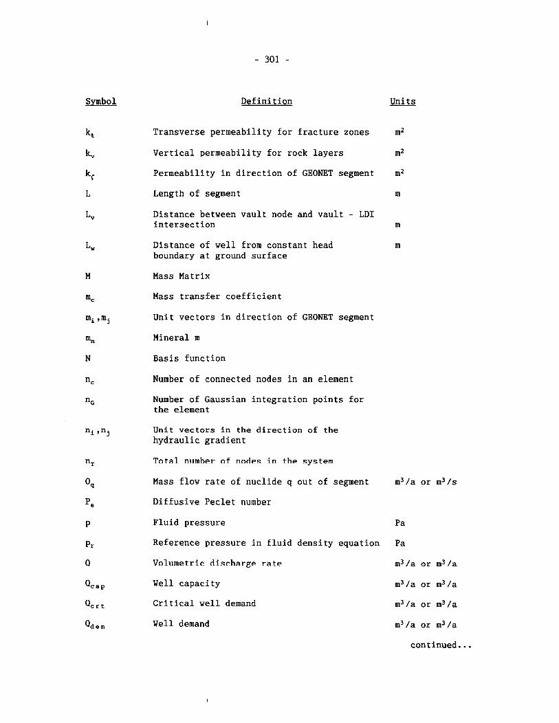
Symbol Definition Units
Qcap
Q c r t
Transverse permeability for fracture zones
Vertical permeability for rock layers
Permeability in direction of GEONET segment
Length of segment
Distance between vault node and vault - LDI intersection
Distance of well from constant head boundary at ground surface
Mass Matrix
Mass transfer coefficient
Unit vectors in direction of GEONET segment
Mineral m
Basis function
Number of connected nodes in an element
Number of Gaussian integration points for the element
Unit vectors in the direction of the hydraulic gradient
Total number of nodes in the system
Mass flow rate of nuclide q out of segment
Diffusive Peclet number
Fluid pressure
Reference pressure in fluid density equation
Volumetric discharge rate
Well capacity
Critical well demand
Well demand
Pa
Pa
m3/a or m3/a
m3/a or m3 /a
m3/a or m3 /a
m3/a or m3/a
continued...
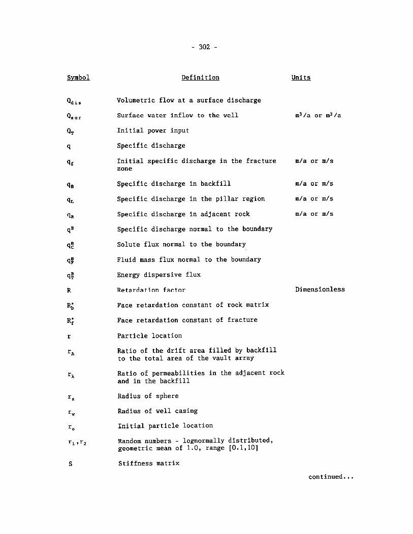
Definition
Volumetric flow at a surface discharge
Surface water inflow to the well
Initial power input
Specific discharge
Units
m3 /a or m3 /a
Initial specific discharge in the fracture m/a or m/s zone
Specific discharge in backfill m/a or m/s
Specific discharge in the pillar region m/a or m/s
Specific discharge in adjacent rock m/a or m/s
Specific discharge normal to the boundary
Solute flux normal to the boundary
Fluid mass flux normal to the boundary
Energy dispersive flux
Retardation factor
Face retardation constant of rock matrix
Face retardation constant of fracture
Particle location
Ratio of the drift area filled by backfill to the total area of the vault array
Ratio of permeabilities in the adjacent rock and in the backfill
Radius of sphere
Radius of well casing
Initial particle location
Random numbers - lognormally distributed, geometric mean of 1.0, range [0.1,10]
Dimensionless
Stiffness matrix
continued. ..
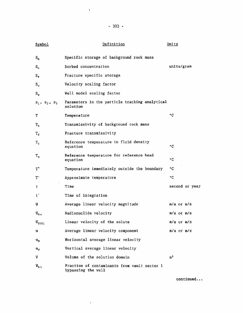
Symbol Definition Units
Specific storage of background rock mass
Sorbed concentration units/gram
Fracture specific storage
Velocity scaling factor
Well model scaling factor
Parameters in the particle tracking analytical solution
Temperature " C
Transmissivity of background rock mass
Fracture transmissivity
Reference temperature in fluid density equation " C
Reference temperature for reference head equation " C
Temperature immediately outside the boundary "C
Approximate temperature " C
Time second or year
Time of integration
Average linear velocity magnitude m/a or m/s
Radionuclide velocity m/a or m/s
Linear velocity of the solute m/a or m/s
Average linear velocity component m/a or m/s
Horizontal average linear velocity
Vertical average linear velocity
Volume of the solution domain
Fraction of contaminants from vault sector 1 bypassing the well
continued...
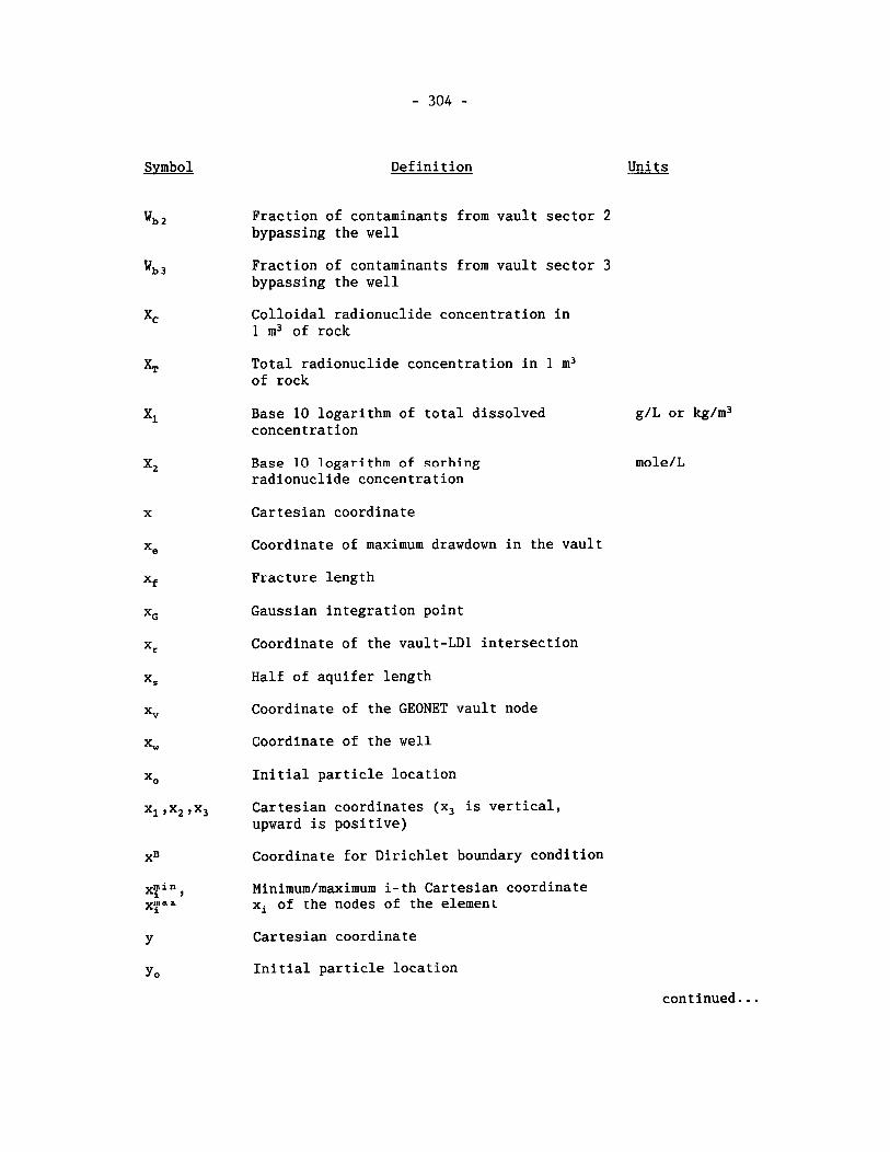
Definition Units
Fraction of contaminants from vault sector 2 bypassing the well
Fraction of contaminants from vault sector 3 bypassing the well
Colloidal radionuclide concentration in 1 m3 of rock
Total radionuclide concentration in 1 m3 of rock
Base 10 logarithm of total dissolved concentration
Base 10 logarithm of sorbing radionuclide concentration
Cartesian coordinate
Coordinate of maximum drawdown in the vault
Fracture length
Gaussian integration point
Coordinate of the vault-LD1 intersection
Half of aquifer length
Coordinate of the GEONET vault node
Coordinate of the well
Initial particle location
Cartesian coordinates (x3 is vertical, upward is positive)
Coordinate for Dirichlet boundary condition
Minimum/maximum i-th Cartesian coordinate xi of the nodes of the elemen1
Cartesian coordinate
Initial particle location
continued ...
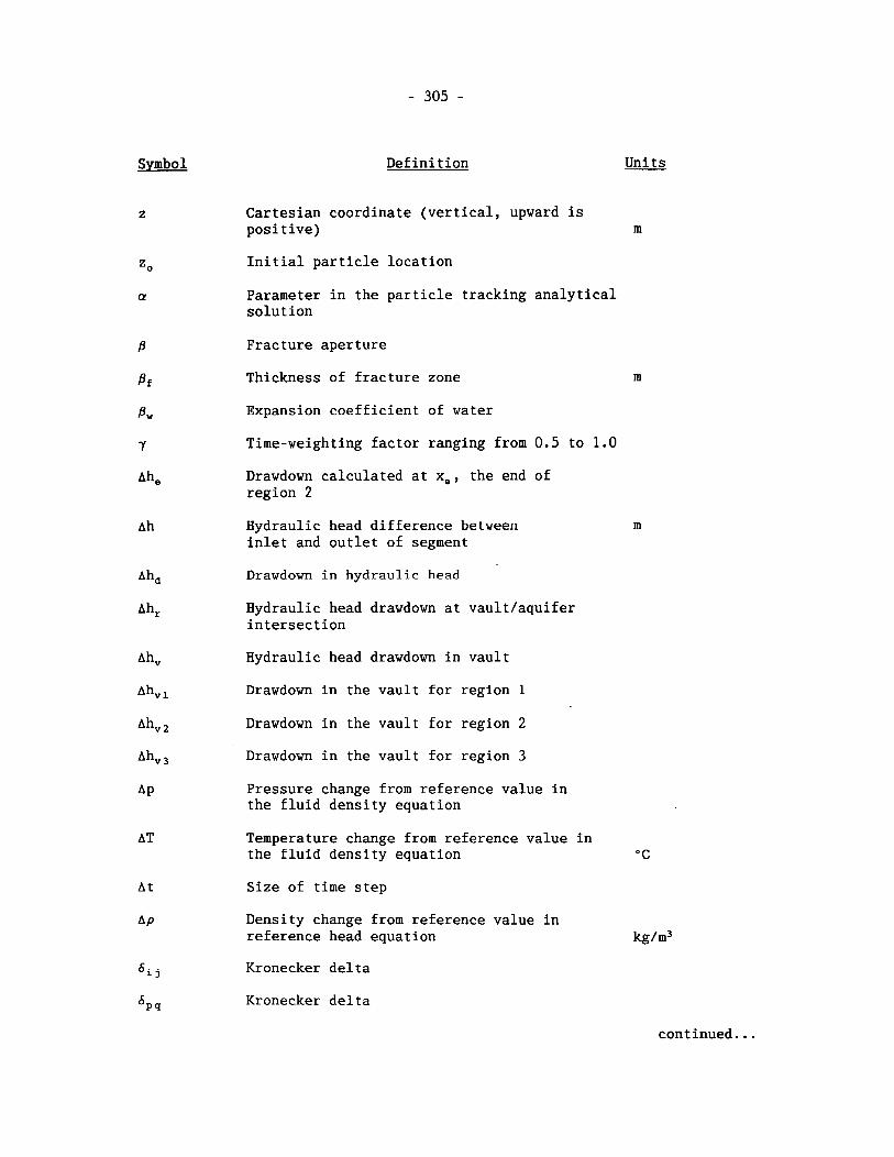
Symbol Definition Units.
Cartesian coordinate (vertical, upward is positive) q
Initial particle location
Parameter in the particle tracking analytical solution
Fracture aperture
Thickness of fracture zone q
Expansion coefficient of water
Time-weighting factor ranging from 0.5 to 1.0
Drawdown calculated at x,, the end of region 2
Hydraulic head difference between inlet and outlet of segment
Drawdown in hydraulic head
Hydraulic head drawdown at vault/aquifer intersection
Hydraulic head drawdown in vault
Drawdown In the vault for region 1
Drawdown in the vault for region 2
Drawdown in the vault for region 3
Pressure change from reference value in the fluid density equation
Temperature change from reference value in the fluid density equation " C
Size of time step
Density change from reference value in reference head equation kg/m3
Kronecker delta
Kronecker delta
eont inued . . .
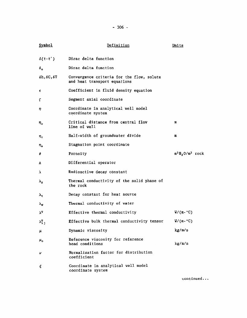
Symbol Definition Units
Dirac delta function
Dirac delta function
Convergence criteria for the flow, solute and heat transport equations
Coefficient in fluid density equation
Segment axial coordinate
Coordinate in analytical well model coordinate system
Critical distance from central flow line of well
Half-width of groundwater divide
Stagnation point coordinate
Porosity
Differential operator
Radioactive decay constant
Thermal conductivity of the solid phase of the rock
m3 H, O/m3 rock
Decay constant for heat source
Thermal conductivity of water
Effective thermal conductivity W/(m. "C)
Effective bulk thermal conductivity tensor W/(m- "C)
Dynamic viscosity kg/m/s
Reference viscosity for reference head conditions
Normalization factor for distribution coefficient
Coordinate in analytical well model coordinate system
continued...
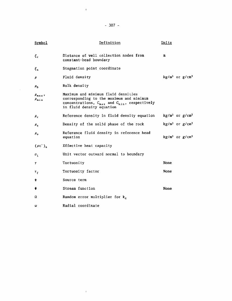
Symbol Definition Units
Distance of well collection nodes from constant-head boundary
Stagnation point coordinate
Fluid density
Bulk density
Maximum and minimum fluid densi~ies corresponding to the maximum and minimum concentrations, C,,, and C,,,, respectively in fluid density equation
Reference density in fluid density equation
Density of the solid phase of the rock
Reference fluid density in reference head equation
Effective heat capacity
Unit vector outward normal to boundary
Tortuosity
Tortuosity factor
Source term
Stream function
Random error multiplier for k,
None
None
None
Radial coordinate
GLOSSARY
advective: The process by.which a solute is transported by the bulk motion of groundwater flow caused by a hydraulic gradient. Sometimes called convection or forced convection.
alternative scenario: As used in the CNFWMP, some feasible combination of factors (features, events and processes) that describes a possible, but not the most probable, behaviour of the disposal system in time. This combination of factors also describes a possible mechanism for the release of contaminants from their engineered containment, followed by transport to the biosphere. Contrast with central scenario.
backfill: In a disposal vault, the material used to refill excavated portions in disposal rooms, shafts and tunnels after the waste packages and buffer have been emplaced.
background rock mass: The portion of the rock mass other than explicitly represented fracture zones or discrete fractures.
barrier: A feature of a disposal system which delays or prevents radio- nuclides from escaping from the disposal vault and migrating into the biosphere. A natural barrier is a feature of the geosphere in which the disposal vault is located. An engineered barrier is a feature made by or altered by humans and includes the wasteform and its container, casks for transportation and disposal of the waste, and any sealing materials used.
biosphere: Usually defined as the portion of the earth inhabited by living organisms. In the CNFWP, it has more specific meaning. In aqua- tic areas, the biosphere/geosphere interface occurs between the deep compacted and the shallow mixed sediments. In terrestrial areas the interface is formed by the watertable. Thus, the bio- sphere includes mixed sediments, surface water, soils, and the lower parts of the atmosphere. Even though the overburden and the geosphere may contain microorganisms, these regions are cons- idered parts of the geosphere.
biosphere model: The biosphere model describes the transport of contam- inants within the local surface water, soil, atmosphere and the food chain to humans, including the resultant health impact of contaminants on members of the critical group. In the SYVAC3-CC3 computer model, the disposal system is modelled using a system model that cvritairls models for the vault, geosphere and bio- sphere. These models were introduced to simplify the development of mathematical models of complex processes.
buffer: In the CNFWMP, a highly impermeable material placed around the waste containers in a disposal vault. The primary purpose of this material is to serve as an additional barrier by retarding the movement of water. It would also affect the rates of
container corrosion, fuel dissolution, and radionuclide migrat- ion. In the CNFWMP, the reference buffer material is a compacted sand-bentonite mixture.
Canadian Nuclear Fuel Waste Management Program (CNFWMP): A program of research and development on radioactive waste management estab- lished in a 1978 Joint Statement by the Federal Government and the Government of Ontario. The aim is to develop and assess the concept of disposing of nuclear fuel waste in the plutonic rock of the Canadian Shield. AECL is responsible for verifying the safety of this disposal method. Ontario Hydro is responsible for developing and demonstrating nuclear fuel waste storage techn- ology, and for trarisportation of these wastes from reactor sites. A second Joint statement in 1981 imposed the restriction that the concept must be assessed, reviewed and accepted before a site could be accepted.
central scenario: As used in the CNFWMP, the most probable combillation of factors (features, events and processes) that describe the expected behaviour of the disposal system in time. This combin- ation of factors also describes the most probable mechanism (if any) for the release of contaminants from their engineered con- tainment, followed by transport to the biosphere. In contrast, an alternative scenario consists of a feasible (but not most probable) combination of factors, and describes one possible (but not expected) behaviour of the disposal system.
closure: In the CNFWMP, a stage in the evolution of a disposal facility that follows decommissioning. Closure includes the shutdown and removal of monitoring systems whose continued existence could affect the long-term safety of the disposal vault, and the seal- ing of boreholes. Completion of this stage forms the event that defines the end of the preclosure phase and the start of the postclosure phase.
connected porosity: The fraction of connected pore space in the rock mass.
container: See disposal container.
convection: The process by which heat or a solute is transported by the bulk motion of groundwater flow caused by a hydraulic, thermal or concentration gradient. If the flow is due to a hydraulic grad- ient is is called forced convection. If the flow is due to thermal or concentration gradients it is called natural convect- ion.
deterministic analysis: A technique for studying system behavior mathe- matically using the laws of science and engineering, and assuming that all system parameters, events, and features are precisely defined. Compare to probalistic analysis.
disposal: A permanent method of long-term management of radioactive wastes in which there is no intention of retrieval and which, ideally,
uses techniques and designs that do not rely for their success on long-term institutional control beyond a reasonable period of time.
disposal container: A durable receptacle for enclosing, isolating and hand- ling nuclear fuel waste for disposal. In a disposal vault, the containers would serve as one barrier between the wasteform and the human population. Sometimes called waste container or just container.
isposal facility: A disposal vault and the supporting buildings and equip- ment to receive the waste and package it in durable containers; shafts and equipment to transfer the containers from the surface to the vault; equipment to handle the containers in the vault; and the materials and equipment to excavate the vault, emplace the disposal containers and to fill and seal the vault, tunnels and shafts.
disposal system: 1 - All structures, materials, processes, procedures or other aspects which, when taken together, constitute the means by which the safe disposal of waste is achieved. 2. In preclosure assessment, this includes a disposal facility and associated transportation facilities. 3. In postclosure assessment, it is a sealed disposal vault and its surrounding local geosphere and biosphere.
disposal vault: An underground structure excavated in rock for disposal of nuclear fuel waste. In the preclosure phase, the disposal vault would include the underground excavations in plutonic rock, the access shafts, access tunnels, underground service areas and installations, and disposal rooms. In the postclosure phase, it would include the disposal rooms and associated access tunnels, the nuclear fuel waste and the engineered barrier systems used to contain the waste and seal all openings. Also referred to as nuclear fuel waste disposal vault, nuclear waste disposal vault, used-fuel disposal vault, waste disposal vault and vault.
effective transport porosity: The fraction of pore space in the rock mass through which convective transport occurs.
environmental and safety assessment: Evaluation of the behaviour and potential impacts of a disposal system, and comparison of the results with appropriate standards or acceptability criteria. It includes evaluation of health impacts to humans and other biota. In the CNFWMP, the system under consideration is the entire dis- posal system, and one accep~ability criterion is a limit on radiological risk to an individual of the critical group. Also referred to as the preclosure assessment and the postclosure assessment. The preclosure assessment considers impacts over the period of time covering the construction, operation and decommis- sioning of a disposal facility, up to and including the final shaft sealing and surface facility decommissioning. The
postclosure assessment considers impacts starting after decommis- sioning, and extending far into the future.
fracture zones: The volumes of intensely fractured rock. They are dis- tinctly more permeable than the surrounding background rock mass and can contain tubular flow conduits or channels within them.
GEONET: An AECL Whiteshell computer code that implements a GEOsphere model as a NETwork of segments through which contaminants move. It was written to serve as the geosphere model in SYVAC3-CC3, and is used in the postclosure assessment of the CNFWMP.
geosphere: The solid outer portion of the earth's crust. In the CNFWMP concept for the geological disposal of nuclear fuel waste, the geosphere, consisting of rock, overburden, compacted sediment and associated groundwater flow systems, is one of the major barriers surrounding the disposal vault. See also biosphere.
geosphere model: A model that describes transport of contaminants through fractured and porous rock that is saturated with groundwater. In SWAC3-CC3, a waste disposal system is modelled using a system model that contains models for the vault, geosphere and bio- sphere. These models were introduced to simplify the development of mathematical models of complex processes. See also GEONET.
medium: In waste disposal, the type of rock in which a disposal facility is located, and through which released waste must move to reach the surface environment.
moderately fractured rock: The volumes of rock containing macroscopic, distinctly more permeable and interconnected planar fractures or narrow fracture zones.
MOTIF: Model Of Transport In Fractured/porous media, an AECL Whiteshell computer program for predicting mechanical behaviour, fluid flow, heat transport, and solute transport in fractured/porous rock formations.
performance assessment: Critical appraisal or evaluation in terms of one or more performance standards. For a disposal system this would mean evaluation of the behaviour of the system or subsystem, and comparison of the results with appropriate standards or criteria. It would be equivalent to a safety assessment if the system under consideration was the entire disposal system, and the performance measure was radiological impact or some other global measure of impact. For example, in the CNFWMP the systen~ under consider- ation is the entire disposal system and one measure of perform- ance is radiological risk to members of the critical group.
postclosure assessment: Safety analysis of the waste disposal system, starting after the disposal vault has been closed. The object- ives are to determine the long-term impacts of the disposal
facility, and to provide estimates of risk that can be compared with regulatory criteria. See also performance assessment.
postclosure phase: In the CNFWMP, the project phase following the closure stage for a disposal facility, after the underground facilities have been decommissioned and sealed, the monitoring systems whose continued operation could affect long-term disposal vault safety have been removed, and the surface facilities have been decontam- inated and decommissioned.
preclosure phase: In the CNFWMP, the project phase which includes the siting, construction, operation, decommissioning and closure of a disposal facility including the disposal vault, surface facll- ities and surrounding site. It also includes the final shaft and monitoring borehole sealing. The transportation of used nuclear fuel from nuclear generating stations to the disposal facility is also part of the preclosure phase.
preclosure assessment: Safety analysis of the waste disposal system that deals with potential impacts during construction, operation, decommissioning and closure of a disposal facility. It includes an assessment of the transportation of used nuclear reactor fuel from nuclear generating stations to the disposal facility.
probabilistic analysis: A statistical method for studying the behaviour of a system defined in terms of parameters whose values are given as probability distributions, events whose occurrences are random and/or features which may or may not be present. The analysis gives a corresponding probability distribution of results. When the method of analysis used involves random sampling, it is often called Monte Carlo analysis, stochastic analysis, systems varia- bility analysis or probabilistic systems assessment. Compare to deterministic analysis.
reference disposal system (or reference system): The hypothetical disposal system that has been evaluated in the postclosure assessment. The reference system is a specific (but hypothetical) implement- ation of the concept for disposal of Canada's nuclear fuel waste. It includes a number of assumptions that are needed to facilitate the postclosure assessment. For example, the geological and hydrological characteristics of the reference disposal system are taken from information available on the Whiteshell Research Area, and the containers are assumed to be made of a titanium alloy. Models representing the reference system take into account all factors that were identified as important by scenario analysis.
release: In waste management, the discharge of contaminants to an environ- ment where their effect may be detrimental.
risk: The term risk is commonly used in different ways and is under- stood in different ways by various segments of society. In technical terms, as used by AECL Research, risk is the proba- bility that a serious health effect will be suffered by an
individual. In the postclosure assessment, a measure of the expected harm that may result from the activities associated with nuclear fuel waste disposal. For radiological impacts, risk is defined by the AECB to be the "probability that a fatal cancer or serious genetic effect will occur to an individual or his or her descendants. Risk, when defined in this way, is the sum over all significant scenarios of the products of the probability of the scenario, the magnitude of the resultant dose and the probability of the serious health effect per unit dose". In mathematical terms,
Risk = C pi x di x k
where pi is the probability of occurrence of scenario i (dimensionless),
di is the estimated dose per year in scenario i (Sv/a), and k is the risk factor, giving the probability of serious
health effect per unit dose (probability of health effects/Sv). The AECB recommends a value of k equal to 2 x health effects per sievert (AECB 1987a).
The summation extends over all scenarios i, and the unit of risk is the probability of a serious health effect per year of exposure (l/a).
rock layers: Horizontally extensive units of background rock mass which have relatively uniform properties.
rock mass: The entire geosphere.
rock matrix: The portion of the rock mass through which transport occurs by diffusion only.
rock zones: See rock layers.
safety assessment: Critical appraisal or evaluation in terms of one or more safety standards. In the CNFWMP, the system under consider- ation is the entire disposal system, and one acceptability criterion is a limit on radiological risk to individuals of the critical group. See also environmental and safety assessment and performance assessment.
scenario: In the postclosure assessment, a set of factors (features, events and processes) that could affect the performance of the disposal facility in immobilizing and isolating nuclear fuel waste. The central scenario is the most probable set of factors. Alter- native scenarios define less probablc, but potentially signif- icant scenarios. Other possible scenarios that might be defined include a worst case scenario, which is intended to represent the most severe situation conceivable on the basis of pessimistic assumptions. Agreement on what constitutes a credible and meaningful worst case may be difficult.

seal : Such things as buffer material, backfill, bulkheads, grout and plugs which, in the CNFWMP, act as barriers in a disposal vault by helping to isolate the waste material and to retard the move- ment of water. Seals such as buffer materials would also affect the rates of container corrosion, fuel dissolution, and radio- nuclide migration.
segment: A portion of the transport network of the geosphere model with uniform chemical and physical properties. A segment is treated as a one-dimensional transport pathway between its inlet and outlet. The location of a segment is defined by the location of its inlet and outlet nodes.
sensitivity analysis: A quantitative examination of how the behaviour of a system varies with change, usually in the values of the governing parameters. Two common ways of varying input parameters are: 1. deterministic sensitivity analysis in which the parameters are varied only slightly about reference values (usually the median). The intent is to determine the partial derivative of some output variable with regard to a single parameter. 2. probabilistic sensitivity analysis in which all parameters vary across their distributions or even change distributions. The goal of proba- listic sensitivity analysis is to determine the average impact of a parameter change in circumstances where other parameters are free to vary across their ranges also.
siting: In the CNPWMP, the project stage of selecting a suitable location for a facility, including appropriate assessment and definition of the related design bases, and numerous other factors.
sparsely fractured rock: The volumes of rock which may contain numerous microscopic cracks and pores but no macroscopic hydraulic condui ts .
SYVAC: Systems Variability Analysis Code, a family of computer programs written at AECL Whiteshell to perform probabilistic calculations on the long-term performance of disposal systems. Several gener- ations and versions of SYVAC have been produced to assess, for example, disposal of high-level waste in an underground vault or under seabed sediment, and low-level tailings from uranium mining and milling operations. Different generations are substantially different from one another. Three generations of SYVAC now exist; they are referred to as SYVAC1, SYVAC2 and SWAC3. Different versions of code are only slightly different from one another; each SYVAC generation has several versions.
tortuosity: A measure of the effective increased pathlength for diffusion that results from the sinuous (or tortuous) nature of the pore space in a porous medium.
tortuosity factor: A measure of the effective increased pathlength for diffusion that results from the sinuous (or tortuous) nature of the pore space in a porous medium. The tortuosity factor rr used
in GEONET is related to the tortuosity 7 used in MOTIF by the relationship:
total porosity: The fraction of pore space in the rock mass.
validation: The process by which one provides evidence or increased confidence that the predictions of a model correspond to the real system it is asserted to represent. It is carried out by compar- ing calculated results with field observations and experimental measurements. A conceptual model and the computer program derived from it are considered to be validated when tlne compar- ison with measurements on a real system shows that they provide a sufficiently good representation of the actual processes occur- ring in the real system, in keeping with the intended use of the model. Compare with verification.
vault: See disposal vault.
vault model: A computer model describing processes in the vau1.t such as corrosion of metallic disposal containers and the transport of contaminants through the buffer. In SYVAC3-CC3, the disposal system is modelled using a system model that contains models for the vault, geosphere and biosphere. These models simplify the development of mathematical models of complex and unrelated processes.
verification: The process by which one provides evidence or increased confidence that a computer code correctly executes the cal- culations it is asserted to perform. A verified computer code is one that has correctly translated a specified algorithm into computer code. verification can be carried out, for example, by comparing the results of a computer code with results produced by other computer codes or by analytical solutions. Compare with validation.
waste disposal system: The engineered systems (e.g., containers, buffer and backfilled tunnels and rooms, sealed shafts and boreholes) and natural surroundings (e.g., rock and rubble-filled fractures) and local surface biosphere involved in forestalling, retarding and minimizing the effects of any release of waste substances from permanent isolation.
waste exclusion distance: The minimum distance specified as a vault design derived constraint between any disposal room and any potential pathway in the surrounding rock for rapid transport of contam- inants to the biosphere. This distance is dependent on the contaminant transport properties of the intervening rock mass.
waste form: One of the forms of nuclear fuel waste.
APPENDIX A
GEOCHEMISTRY
CONTENTS
A. 1 GROUNDWATER GEOCHEMISTRY
A. 2 CHEMISTRY OF ROCK MATRIX
A. 3 MINERALOGY AND CHEMISTRY OF FRACTURE FILLINGS AND SORPTION ASPECTS
A. 4 COLLOIDS
REFERENCES
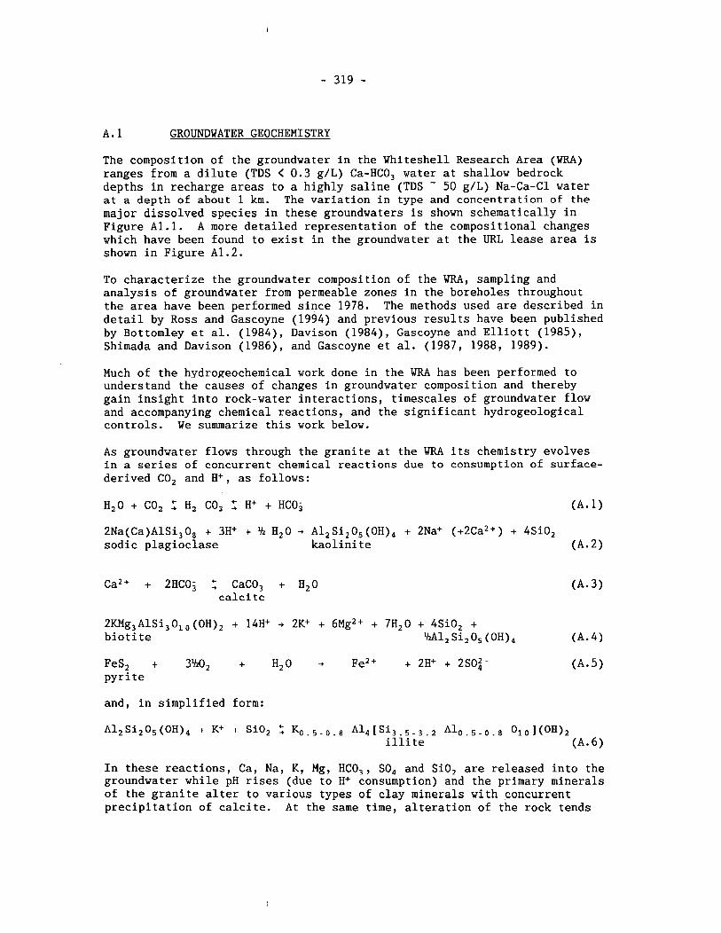
A. 1 GROUNDWATER GEOCHEMISTRY
The composition of the groundwater in the Whiteshell Research Area (WRA) ranges from a dilute (TDS < 0.3 g/L) Ca-HCO, water at shallow bedrock depths in recharge areas to a highly saline (TDS - 50 g/L) Na-Ca-C1 water at a depth of about 1 km. The variation in type and concentration of the major dissolved species in these groundwaters is shown schematically in Figure Al.l. A more detailed representation of the compositional changes which have been found to exist in the groundwater at the URL lease area is shown in Figure A1.2.
To characterize the groundwater composition of the WRA, sampling and analysis of groundwater from permeable zones in the boreholes throughout the area have been performed since 1978. The methods used are described in detail by Ross and Gascoyne (1994) and previous results have been published by Bottomley et al. (1984), Davison (1984), Gascoyne and Elliott (1985), Shimada and Davison (1986), and Gascoyne et al. (1987, 1988, 1989).
Much of the hydrogeochemical work done in the WRA has been performed to understand the causes of changes in groundwater composition and thereby gain insight into rock-water interactions, timescales of groundwa.ter flow and accompanying chemical reactions, and the significant hydrogeological controls. We summarize this work below.
As groundwater flows through the granite at the WRA its chemistry evolves in a series of concurrent chemical reactions due to consumption of surface- derived CO, and H+ , as follows:
H,O + CO, Z H, CO, Z H+ + HCO; ( A . 1)
2Na(Ca)A1Si308 + 3H+ + lh H,O + A1, Si205 (OH), + 2Na+ (+2Ca2+) + 4Si0, sodic plagioclase kaolini te (A.2)
Ca2+ + 2HC03 Z CaC03 + H20 calcite
2KMg3A1Si3Ol0 (OH), + 14H+ + 2K+ + 6~g,+ + 7H20 + 4Si0, + biotite 'Ml, Si,O, (OH), (A.4)
FeS, + 3lhO2 + H,O + Fe2+ + 2H+ + 2SOi- (A. 5 pyrite
and, in simplified form:
A12Si205(0H)4 I K+ I Si02 = K,. 5 - 0. 8 A14 [Si3. 5 - 3. 2 Aloe 5 - 0. 8 010 1 (OH), illite (A.6)
In these reactions, Ca, Na, K, Mg, HCO,, SO, and SiO, are released into the groundwater while pH rises (due to H+ consumption) and the primary minerals of the granite alter to various types of clay minerals with concurrent precipitation of calcite. At the same time, alteration of the rock tends
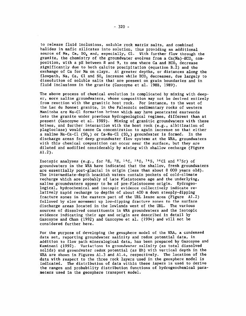
to release fluid inclusions, soluble rock matrix salts, and combined halides in mafic silicates into solution, thus providing an additional source of Na, Ca, SO, and, especially, C1. With further flow through the granite, the chemistry of the groundwater evolves from a Ca(Na)-HCO, com- position, with a pH between 8 and 9, to one where Ca and HCO, decrease significantly due to both calcite precipitation (equation B.2) and the exchange of Ca for Na on clays. At greater depths, or distances along the flowpath, Na, Ca, C1 and SO, increase while HCO, decreases, due largely to dissolution of soluble salts that are present on grain boundaries and in fluid inclusions in the granite (Gascoyne et al. 1988, 1989).
The above process of chemical evolution is complicated by mixing with deep- er, more saline groundwaters, whose composition may not be derived entirely from reaction with the granitic host rock. For instance, to the west of the Lac du Bonnet granite, in the Paleozoic sedimentary rocks of western Manitoba are Na-C1 formation brines which may have penetrated eastwards into the granite under previous hydrogeological regimes, different than at present (Gascoyne et al. 1989). Mixing of granitic groundwaters with these brines, and further interaction with the host rock (e.g., albitization of plagioclase) would cause Ca concentration to again increase so that either a saline Na-Ca-C1 (SO,) or Ca-Na-C1 (SO,) groundwater is formed. In the discharge areas for deep groundwater flow systems at the WRA, groundwaters with this chemical composition can occur near the surface, but they are diluted and modified considerably by mixing with shallow recharge (Figure A1.2).
Isotopic analyses (e.g., for 2H, 3H, 14C, 180, ,,S, 36Cl and 87Sr) of groundwaters in the WRA have indicated that the shallow, fresh groundwaters are essentially post-glacial in origin (less than about 8 000 years old). The intermediate-depth brackish waters contain pockets of cold-climate recharge which are probably of Late Pleistocene age and the underlying, saline groundwaters appear to be of pre-Pleistocene origin. Hydrogeo- logical, hydrochemical and isoLvpic evidence collectively indicate re- latively rapid recharge to depths of about 400 m down steeply-dipping fracture zones in the eastern part of the URL lease area (Figure A1.2) followed by slow movement up low-dipping fracture zones to the surface discharge areas located in the lowlands west of the URL. The various sources of dissolved constituents in WRA groundwaters and the isotopic evidence indicating their age and origin are described in detail by Gascoyne and Chan (1992) and Gascoyne et al. (1994) and will not be considered further here.
For the purpose of developing the geosphere model of the WRA, a condensed data set, reporting groundwater salinity and redox potential data, in addition to flow path mineralogical data, has been prepared by Gascoyne and Kamineni (1992). Variations in groundwater salinity (as total dissolved solids) and groundwater redox potential (as Eh) with vertical depth in the WRA are shown in Figures A1.3 and A1.4, respectively. The location of the data with respect to the three rock layers used in the geosphere model is indicated. The distribution of data within these layers is used to derive the ranges and probability distribution functions of hydrogeochemical para- meters used in the geosphere transport model.
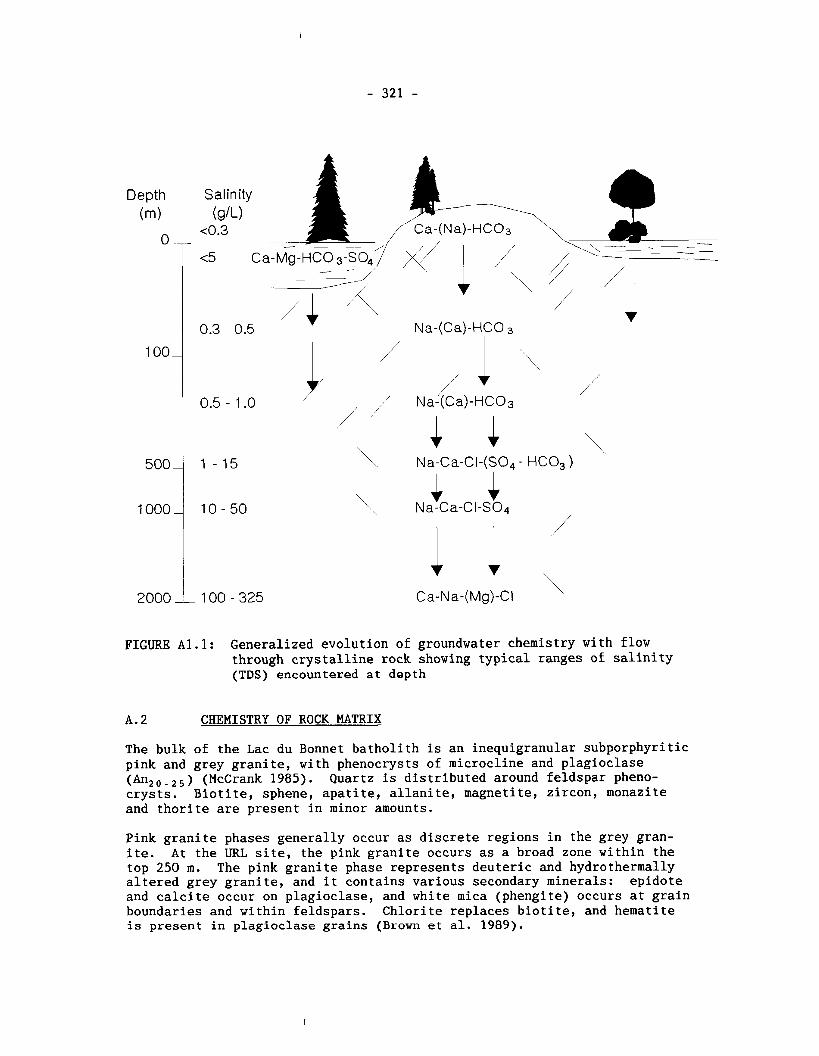
Depth (m>
Salinity (g/L)
<0.3 + - -
<5 Ca-Mg-HCO / -
0.3 - 0.5
0.5 - 1 .O /'
1 - 1 5 \ Na-Ca-CI-(SO, - HCO, )
FIGURE Al.l: Generalized evolution of groundwater chemistry with flow through crystalline rock showing typical ranges of salinity (TDS) encountered at depth
A. 2 CHEMISTRY OF ROCK MATRIX
The bulk of the Lac du Bonnet batholith is an inequigranular subporphyritic pink and grey granite, with phenocrysts of microcline and plagioclase (An, , - , , ) (McCrank 1985). Quartz is distributed around feldspar pheno- crysts. Biotite, sphene, apatite, allanite, magnetite, zircon, monazite and thorite are present in minor amounts.
Pink granite phases generally occur as discrete regions in the grey gran- ite. At the URL site, the pink granite occurs as a broad zone within the top 250 m. The pink granite phase represents deuteric and hydrothermally altered grey granite, and it contains various secondary minerals: epidote and calcite occur on plagioclase, and white mica (phengite) occurs at grain boundaries and within feldspars. Chlorite replaces biotite, and hematite is present in plagioclase grains (Brown et al. 1989).
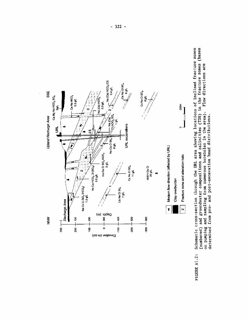
s o w s.4 ld & d bl -8-4
u w a
- U) -r(
8-2. . r i rn ldm r a aJ E l d b &I 0 u u (d -4 0 r , + m a 3
a z a M .,I r ..-I c - &
.r( -4 E r g .z .: zrl m a U) ld aJ
rnrla ld Old w a ~ & d aJA ld ld u
0 C J inn 0
S ~ W Z .rc :, ld
a J r O S
5': k 2 o a x
C a 3 aJ M e C L 7 0 0 u a Cn Ll 0 0 & & & a r aJw
r a C ld M C 0 3 c a
.r( a .r( + f ir l l u :, a 0 a J 0 B h v l h a a I Mm
U) a m a a o 0 C C U & ld ldw 0 - M a 0 a . i aJ .,-I aJ C u u a.r( l d a J a a a n 3 & a~ a a: 4 z c a J m ~ o a
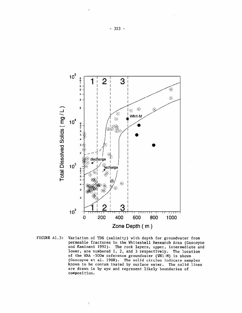
0 200 400 600 800 1000
Zone Depth ( m )
FIGURE A 1 . 3 : Variation of TDS (salinity) with depth for groundwater from permeable fractures in the Whiteshell Research Area (Gascoyne and Kamineni 1992). The rock layers, upper, intermediate and lower, are numbered 1, 2, and 3 respectively. The location of the WRA -500m reference groundwater (WN1-M) is shown (Gascoyne et al. 1988). The solid circles indicate samples known to be contam inated by surface water. The solid lines are drawn in by eye and represent likely boundaries of composition.
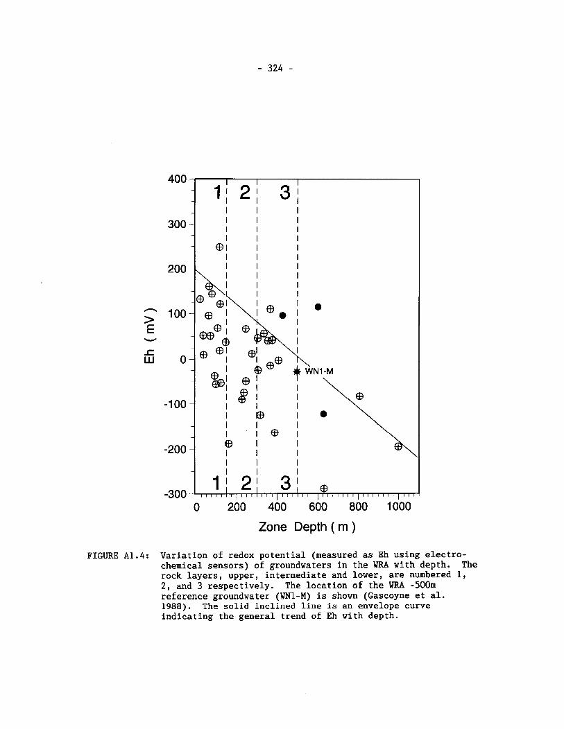
Zone Depth ( m )
FIGURE A1.4: Variation of redox potential (measured as Eh using electro- chemical sensors) of groundwaters in the WRA with depth. The rock layers, upper, intermediate and lower, are numbered 1, 2, and 3 respectively. The location of the WRA -500m reference groundwater (WN1-M) is shown (Gascoyne et al. 1988). The solid iricliried line is an envelope curve indicating the general trend of Eh with depth.
In the vicinity of the major fracture zones, both the grey and plink granite phases of the batholith are highly oxidized to a deep red granite. The alteration zone is characterized by numerous microfractures and an abund- ance of secondary minerals. Biotite is altered to chlorite and vermicul- ite, and plagioclase is highly altered to phengite. Hematite is concen- trated on plagioclase grains and microfractures that transect th~e rock and it imparts a reddish colour to the rock samples.
Near some specific fractures the dark red granite attains an ora.nge shade that grades into a creamy bleached material in the fracture zone itself (Kamineni et al. 1986a). This material comprises clays mixed with rock matrix. Illite is the dominant clay mineral occurring in microfractures in these bleached areas and it replaces feldspars and biotite (Kamineni et al. 1986b).
The textural characteristics strongly indicate that these four groups of granitic rocks of the Lac du Bonnet Batholith are co-magmatic and define an evolutionary sequence. Grey granite represents the least-altered pristine rock formed during magmatic crystallization of the Batholith. The pink granite is hydrothermally-altered grey granite. The deep red and clay-rich alteration zones formed later by low temperature diagenesis caused by groundwater movement in the highly fractured zones. Studies of the stable isotope characteristics of various groups of samples from the ba.tholith also support this interpretation (Kerrich and Kamineni 1988).
Samples of the grey granite phase have whole-rock oxygen isotope composit- ions of 6180 7.8 to 8.3"/,,, which are within the range of isotopically 'normalr granitic rocks defined by Taylor (1978) to be 6 to 10°/,, . 6180 is defined as
0/l 0 (sample) 1 ] x 1 000
l W / l 60 (standard)
and is expressed in units of per mille ("/,,). The standard used in this context is SMOW (Standard Mean Ocean Water).
These compositions are also similar to those of most fresh Archean grani- toids that have been analysed in NW Ontario (Longstaffe 1979). The pink granite phase has higher 6180 values (8.2 to 11.5°/00), but overlaps with the upper limit of the grey granite. This is in conformity with hydrother- mally altered granites (Taylor 1978). The 6180 values of the deep red and clay-rich granite phases range from 12.2 to 20.9°/00 the lower values being invariably associated with deep red granite (Kamineni et al. 1984). The 6D of clay-rich granite varies between -80 to -95"/,,. According to Kerrich and Kamineni (1988), these 6D-6180 values of the clay-rich granite phase provide strong evidence that the clays either formed, or re-equilibrated, in the presence of geologically recent groundwater, not water that was present in the batholith at the time of its crystallization.
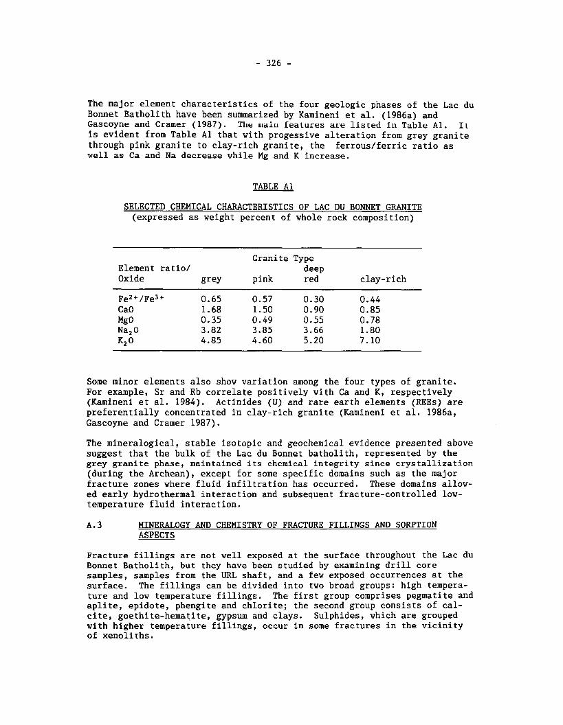
The major element characteristics of the four geologic phases of the Lac du Bonnet Batholith have been summarized by Kamineni et al. (1986a) and Gascoyne and Cramer (1987). The n ~ a i r l Keatures are listed in Table Al. It is evident from Table A1 that with progessive alteration from grey granite through pink granite to clay-rich granite, the ferrous/ferric ratio as well as Ca and Na decrease while Mg and K increase.
TABLE A1
SELECTED CHEMICAL CHARACTERISTICS OF LAC DU BONNET GRANITE (expressed as weight percent of whole rock composition)
Granite Type Element ratio/ deep Oxide grey pink red clay-rich
Fez + /Fe3 + 0.65 0.57 0.30 0.44 CaO 1.68 1.50 0.90 0.85 Mgo 0.35 0.49 0.55 0.78 Na2 0 3.82 3.85 3.66 1.80 K2° 4.85 4.60 5.20 7.10
Some minor elements also show variation among the four types of granite. For example, Sr and Rb correlate positively with Ca and K, respectively (Kamineni et al. 1984). Actinides (U) and rare earth elements (REEs) are preferentially concentrated in clay-rich granite (Kamineni et al. 1986a, Gascoyne and Cramer 1987).
The mineralogical, stable isotopic and geochemical evidence presented above suggest that the bulk of the Lac du Bonnet batholith, represented by the grey granite phase, maintained its chemical integrity since crystallization (during the Archean), except for some specific domains such as the major fracture zones where fluid infiltration has occurred. These domains allow- ed early hydrothermal interaction and subsequent fracture-controlled low- temperature fluid interaction.
A. 3 MINERALOGY AND CHEMISTRY OF FRACTURE FILLINGS AND SORPTION ASPECTS
Fracture fillings are not well exposed at the surface throughout the Lac du Bonnet Batholith, but they have been studied by examining drill core samples, samples from the URL shaft, and a few exposed occurrences at the surface. The fillings can be divided into two broad groups: high tempera- ture and low temperature fillings. The first group comprises pegmatite and aplite, epidote, phengite and chlorite; the second group consists of cal- cite, goethite-hematite, gypsum and clays. Sulphides, which are grouped with higher temperature fillings, occur in some fractures in the vicinity of xenoliths.
Pegmatite and aplite dykes, which are filled with late magmatic material, are abundant in the URL lease area and in various parts of the Batholith. Uykes are generally affected by hydrothermal alteration, consequently the feldspars are altered to phengite and sericite. Some pegmatites contain magnetite up to 5%.
Epidote is generally present in steeply-dipping fractures and steeply-dip- ping fault zones. Compositionally, the epidotes contain significant amounts of Fe+, with the pistacite component ranging from 35 to 42% (Kamineni et al. 1984).
Chlorite is the dominant filling in fractures associated with the low-dip- ping fracture zones and it also occurs in minor amounts in the steep epi- dote-filled fractures. The chlorite fillings show compositional variation in terms of Si, Al, Fe and Mg, and overlap epidolite-pychnochlorite-dibant- ite fields in the chlorite classification scheme of Hey (1954). The Mg/Fe ratio among the analyzed chlorites varies from 0.76-0.91.
Muscovite and/or sericite are commonly associated with epidote and chlor- ite-filled fractures. The muscovites generally contain significant amounts of (Fe+Mg), ranging from 6 to 7%, and can be categorized as phengite as defined by Velde (1965). The sericites,compared to phengites, are re- latively more aluminous and contain smaller (Fe+Mg) ranging from 2.5 to 3.5% (Kamineni et al. 1986b).
Illite is the predominant clay mineral in the low to intermediate-dipping fracture zones. It occurs in narrow fractures (< 1 mm width). Scanning electron microscope investigations indicate that the size of illite ranges from 0.0003 to 0.0018 mm. The illites show distinct compositional char- acteristics that can be related to their paragenesis. For example, illites formed on biotite are generally rich in Fe, Mg and K, compared to illites formed in macro- and microfractures (Kamineni et al. 1986b).
Iron oxide is one of the common fracture fillings. It occurs as hematite in epidote-filled fractures and as goethite and/or iron oxyhydroxides in fractures affected by low-temperature water-rock interaction. In the lat- ter it represents a residual product of chlorite alteration. Composition- ally, the iron oxides are homogeneous with minor amounts of Ti and Mn. The grain size is highly variable ranging from 0.02 to 0.0008 mm.
Calcite is present in almost all fractures but it is dominant in the high- angle fractures (50" to 75") that are concentrated at shallow depths of the Lac du Bonnet Batholith. The grain size of the calcite ranges from 0.50 to 0.005 mm. Other carbonates, such as siderite (FeCO,) occur sparsely in a few fractures . A number of other fracture-filling minerals such as laumontite, prehnite, smectite, mixed layer clays and gypsum occur in some geologic domains, but their abundances are not sufficient enough to include them in our conceptual model.
On the basis of our mineralogical examination of drill core samples from the WRA, a suite of 13 alteration minerals was selected to characterize the minerals coating the fracture surfaces. The rock type and the 13 infilling or alteration minerals are given in Table D.6.3.1 through D.6.3.4. The chemical sorption properties of these minerals were determined experiment- ally and from available literature sources (e.g. in the NEA data base).
Because fracture infilling minerals commonly are at least partially uncon- solidated, they tend to be easily lost during drilling. Consequently, there is very little reliable information on the in situ physical state of these infilling minerals from friable fracture zones. We have assumed that the alteration minerals exist as a continuous or nearly continuous coating on the fracture surfaces and that in many places the fractures are filled, at least in part, with unconsolidated secondary minerals with variable particle size.
A. 4 COLLOIDS
Studies carried out at the WRA have shown that natural colloid concentrat- ions in the groundwater seldom exceed a concentration of 1 mg/L, and they have an average concentration of 0.34 + 0.34 mg/L (Vilks et al. 1991). Colloid concentrations in samples of shallow dilute groundwaters from the WRA are not significantly different from those in the deeper saline waters. Concentrations of suspended particles larger than 450 nm range from 0.04 to 14 mg/L. Although these larger suspended particles can be mobilized by the rapid flow rates induced by groundwater pumping and sampling, they will not migrate with the slow natural groundwater flows that exist.
Colloidal particles consist mainly of alteration minerals, such as calcite, clays, Fe-Si oxides, quartz, K-feldspar and albite. In addition, some colloidal gypsum was observed in deep groundwater samples, organic particles and bacteria were observed in groundwater samples from all depths. The influence of microorganisms on contaminant transport is dis- cussed in Appendix B.4. Organic colloids in the 1 to 10 nm size range were found in shallow dilute groundwater, but not in the deeper saline waters (Vilks et al. 1991).
Less than 20 percent of the natural U and Ra in WRA groundwaters is assoc- iated with colloids, but as much as 68 percent of the Th may be attached to particles. The 4U/2 isotope ratios associated with particles suggest that colloids have obtained most of their U by sorption from groundwater.
Sorption of radionuclides on colloidal particles occurs with the same mechanisms as sorption on fixed minerals on fracture surfaces. However, the low colloid concentrations that have been observed in the WRA, coupled with a slow rate of groundwater flow even in the fractures, suggest that we can neglect colloid transport of radionuclides in our geosphere model of the WRA. Scoping calculations, summarized in Appendix B.3, show that col- loid transport in the geosphere can be ignored provided the integrity of the buffer is maintained (Vilks et al. 1991). Moreover, because of their size, colloids cannot be transported through the interconnected pore space of the sparsely-fractured rock.
REFERENCES:
Bottomley, D.J., J.D. Ross and W.B. Clarke. 1984. Helium and neon isotope geochemistry of some ground waters from the Canadian Precambrian Shield. Geochiom. Cosmochim. Acta, 48 1973-1985.
Brown, A,, N.M. Soonawala, R.A. Everitt and D.C. Kamineni. 1989. Geology and geophysics of the Underground Research Laboratory Site, Lac du Bonnet Batholith, Manitoba. Canadian Journal of Earth Sciences, Volume 26, 404-425.
Davison, C.C. 1984. Hydrogeological characterization at the site of Canada's Underground Research Laboratory: Proc. Int. Groundwater Symp. on Groundwater Resources Utilization and Contaminant Hydrogeo- logy, Volume 2, Montreal, Quebec, 1984 May, 310-335.
Gascoyne, M. and L.C.M. Elliott. 1985. A simple well-water dilution model. Atomic Energy of Canada Limited Technical Record, T'R-391.
Gascoyne, M. and J.J. Cramer. 1987. History of actinide and minor element mobility in an Archean granitic batholith in Manitoba, Cana.da. Applied Geochemistry, Volume 2, 1, 37-54.
Gascoyne, M. and T. Chan. 1992. Comparison of numerically modelled groundwater residence time with isotopic age data. OECD Workshop on Paleohydrogeological Methods and their Applications for Rad.ioactive Waste Disposal, Paris, France, 1992 Nov.9-10.
Gascoyne, M. and D.C. Kamineni. 1992. Groundwater chemistry and fracture mineralogy in the Whiteshell Research Area, Atomic Energy of Canada Limited Technical Record, TR-516.
Gascoyne, M., C.C. Davison, J.D. Ross and R. Pearson. 1987. Saline groundwater and brines in plutons in the Canadian Shield in Saline Water and Gases in Crystalline Rocks. Geol. Assoc. Can. Spec. Paper 33, 53-68.
Gascoyne, M., J.D. Ross and R.L. Watson. 1988. Geochemical and isotopic characterization of flow in fractured plutonic rocks: Examples from the Canadian Shield, Proc. 4th Can./Amer. Conf. on Hydrogeology, Banff, Alberta, 1988 June 21-24, 20-31.
Gascoyne, M., A. Purdy, P. Fritz, J.D. Ross, S.K. Frape, R.J. Drimmie and R.N. Betcher. 1989. Evidence for penetration of sedimentary basin brines into an Archean granite of the Canadian Shield, Proc:. 6th Int. Symp. on Water-Rock Interaction, 1989 Aug. 3-12, Malvern, CI.K., 243- 245.
Gascoyne, M., P. Sharma and P.W. Kubik. 1994. Origin of gro~indlwater salinity in the Lac du Bonnet granite, southeastern Manitoba, from 36Cl measurements. Nucl. Instr. Meth. Phys. Res., g , in press.
Hey, M.H. 1954. A new review of chlorites. Mineralogical Magazine, 30, 277-292.
Kamineni, D.C., J.J.B. Dugal and R.B. Ejeckam. 1984. Geochemical investi- gations of granitic core samples from boreholes at the Underground Research Laboratory site near Lac du Bonnet, Manitoba. Atomic Energy of Canada Limited Technical Record, TR-221.
Kamineni, D.C., C.P. Chung, J.J.B. Dugal and R.B. Ejeckam. 1986a. Distri- bution of uranium and thorium in core samples from the Underground Research Laboratory Lease area, southeastern Manitoba, Canada. Chemical Geology, Volume 54, 97-111.
Kamineni, D.C., K.V. Ticknor and T.T. Vandergraaf. 1986b. Occurrence, composition and radionuclide sorption characteristics of illite from a fractured granite pluton, southeastern Manitoba, Canada. Clay Minerals, Volume 21, 909-924.
Kerrich, R. and D.C. Kamineni. 1988. Characteristics and chronology of fracture-fluid infiltration in the Archean, Eye Dashwa Lakes pluton, Superior province: evidence from H, C, 0-isotopes and fluid inclusions. Contributions to Mineralogy and Petrology, 99, 430-445.
Longstaffe, F.J. 1979. The oxygen isotope geochemistry of Archean grani- toids. In Trondjemites, Dacites, and Related Rock (Developments in Petrology 6), Barker, P., (editor) Elsevier, Amsterdam, 363-399.
McCrank, G.P.D. 1985. A geological survey of the Lac du Bonnet batholith, Manitoba, Atomic Energy of Canada Limited Report, AECL-7816.
Ross, J.D. and M. Gasconye. 1994. Methods for sampling and analysis of groundwater in the CNFWMP. Atomic Energy of Canada Limited Technical Record, TR-588, COG-93-36.
Shimada, J., C.C. Davison. 1986. Environmental isotopes in groundwater at the URL site. Atomic Energy of Canada Limited Technical Record, TR- 388.
Taylor, H.P., Jr. 1978. Oxygen and hydrogen isotope studies of plutonic granitic rocks, Earth and Planetary Sc. Letters, Volume 38, 177-210.
Velde, B. 1965. Phengite micas: synthesis, stability and natural occur- rence. Amer. Jnl. of Sci., =, 886-913.
Vilks, P., D.B. Bachinski and T.T. Vandergraaf. 1991. The role of parti- culates in radionuclide transport. Proceedings of the Third Inter- national Symposium on Advanced Nuclear Energy Research - Global Environment and Nuclear Energy. Mito City, Japan. Mar 13-15. 394-401.
(TR- indicates unrestricted, unpublished reports available from SDDO, AECL Research, Chalk River Laboratories, Chalk River, Ontario KOJ 1LO.)
APPENDIX B
CHEMICAL RETARDATION
CONTENTS
B. 1 SORPTION MECHANISMS
B.2 DISTRIBUTION COEFFICIENTS AND SORPTION EQUATIONS
B.3 IMPACT OF COLLOIDS ON RADIONUCLIDE TRANSPORT
B.4 IMPACT OF MICROORGANISMS ON RADIONUCLIDE TRANSPORT
REFERENCES
SORPTION MECHANISMS
The transport of trace contaminants in the geosphere by groundwater can be retarded significantly by their chemical interaction with alteration minerals lining the fractures and with the mineral surfaces of the inter- connected pore spaces of the rock mass surrounding the fractures. These interactions are often very complex and can be in the form of physical sorption, chemisorption e.g., iodate on iron oxides (Couture and Seitz 1983, Ticknor and Cho 1990), ion exchange or ion substitution e.g., cadmium in calcite, Davis et al. 1987, and sorption or precipitation induced by changes in groundwater composition or redox potential e.g., technetium on hematite (Vandergraaf et al. 1984, Haines et al. 1987). These geochemical interactions can be described by chemical equations and can in principle be quantified on the basis of thermodynamic data. However, the present under- standing of the reactions that govern these interactions is in many cases inadequate to describe them in thermodynamic terms. In most cases, methods to describe a sorbing surface in chemical terms are not sufficiently well developed. The kinetics of the reactions that lead to surface are often very slow and many geochemical reactions do not reach an equilibrium over laboratory time scales.
B. 2 DISTRIBUTION COEFFICIENTS AND SORPTION EQUATIONS
Because of their complexity and the limited thermodynamic data presently available to describe the chemical reactions, the interaction of dissolved radionuclides with geological materials is usually expressed quantitatively by the ratio of sorbed vs. dissolved concentrations. This ratio is normal- ly called the bulk sorption or distribution coefficient, Kd, and is expressed in units of mL/g:
where
S, = sorbed concentration of material and C = dissolved concentration of solution.
The relationship between sorption and retardation is then given (e.g. Sherwood et al. 1975) by the equation:
where
R = retardation factor (dimensionless), Us,, = average linear velocity of the solute, 4 w = average linear velocity of the groundwater, P s = density of rock skeleton, 6 = porosity, p(1-6) = bulk density of sorbing substrate.
and where the assumption is made that sorption is reversible and is main- tained at equilibrium at all times. This is an important but conservative assumption, because it implies that the period of time that a solute is sorbed on a geological surface is finite and that all radionuclides will eventually migrate in the direction of the groundwater flow.
Sorption processes and the distribution coefficients themselves are affect- ed by a large number of variables, such as the mineralogical and chemical composition of the sorbing material and its specific surface area, the ionic strength of the concentrations of the various dissolved ionic species in the groundwater, pH, redox potential (Eh), and the concentration of the species to be sorbed. For example, for solutes that sorb by an ion ex- change mechanism, sorptiorl is suppressed in the presence of large concen- trations of ionic species that compete for the available sorption sites, while species that are removed from solution by redox-induced precipitation are much less affected by the ionic strength of the solution. The depend- ence of a distribution coefficient on the concentration of the sorbing species invariably results in a decrease in kd with increased concentration of that sorbing species. This is usually expressed as an isotherm that takes on the form of a Freundlich, Langmuir, or Dubinin-Radushkevich equation (Vandergraaf and Ticknor 1993).
In most environmental and safety assessment calculations for nuclear fuel waste disposal, such as in Sweden (SKBF 1983), Switzerland (McKinley and Hadermann 1985) and the Netherlands (Glasbergen et al. 1989), the contam- inant flow paths through the geosphere have been considered to be uniform in terms of both the groundwater composition and the composition of the minerals along these flow paths. Consequently, single values for kd have been used in these calculations. Even the dependence of sorption on con- centration of the trace contaminant has been ignored. However, our per- formance assessment case study has been based on data from a site within the Lac du Bonnet Batholith. The information we have obtained for the WRA suggests that the differences in mineralogy of the fracture inrilling minerals and groundwater compositions along the flow paths are sufficiently large to require the use of distribution coefficients that are specific to the various flow path segments through the geosphere. In principle, it would be possible to generate distribution coefficients for each radio- nuclide under the geochemical conditions that are expected to occur in each segment of the flow path through the geosphere. However, the amount of manpower that would be required to generate this volume of sorption data would be well in excess of the available resources. Therefore, a different approach has been used for our model of the sorption processes of the WRA. Distribution coefficients for the WRA are expressed for each radionuclide/ mineral/redox combination by a complete binomial expression:
where
XI = log (TDS), and TDS is the total dissolved solids content of the groundwater expressed in mg/L,
X2 = log ([RN]), where [RN] is the concentration of the sorbing radionuclide in the groundwater in mole/L, and
b, , b, , b, , b,, , b12 and b2, are coefficients obtained by fitting the existing laboratory sorption data to this quadratic equation.
Thus, for 39 radionuclides, 20 minerals and rock types and two redox con- ditions (Eh>O, Eh<O), there exist a total of 1560 radionuclide/mineral/ redox combinations and a possible 1560 equations, each with a maximum of six coefficients. However, in most of these cases, data is lacking to define the concentration dependence parameters, and all but the b, terms revert to zero, giving in effect a constant value for the distribution coefficient for that radionuclide/mineral/redox condition combination. The data that is used in these equations is obtained from laboratory studies, the literature, and from the Sorption Data Base (SDB) of the Nuclear Energy Agency (NEA) of the Organization for Economic Cooperation and Development (OECD) (Ruegger and Ticknor 1992). In cases where no data exists, best estimates have been obtained from sorption data for chemically siinilar elements (Vandergraaf et al. 1992).
Any uncertainty in the experimental sorption data is handled by multiplying the sorption equation (B.2.3) by an error factor,
where r, is a lognormally-distributed random number with a geomet:ric mean of 1.0, in the range [0.1,10] and b3 is the number of orders of magnitude over which k, is allowed to vary.
The static distribution coefficients that have been reported in the litera- ture and in the Sorption Data Base of the NEA/OECD have been determined on unconsolidated or crushed samples of geologic material, and should only be applied to cases where the specific surface area of the geological material in the flow path is comparable to that used in the sorption studies, i.e., at porosities greater than 30%. When the porosity is decreased much below 30%, the surfaces of the individual mineral grains may become partially covered by other grains, decreasing the specific surface area of the grains and, hence, the effective sorptive capacity. The specific surface area of the interconnected pore space in intact rock is estimated to be in the order of lo3 m2/m3 (Bradbury 1983) or 0.4 m2/kg. Crushed or unconsolidated material used in laboratory sorption determinations, on the other hand, has a specific surface area two to four orders of magnitude higher, on the order of lo2 to lo4 m2/kg. Because sorption is a surface phenomenon, the sorptive capacity of intact rock should be much lower than that of uncon- solidated material, and the distribution coefficient, kd, cannot be assumed to be constant over the range of porosities encountered in the geosphere. Therefore, it is inappropriate to apply sorption data, obtained on crushed or unconsolidated material, to describe the sorption that occurs when flow is through the interconnected fractures or pore spaces in intact rock, which have a much lower surface area per unit weight of rock. This can be seen from equation (B.2.2). Calculating the retardation factor for solute
flow through the sample of crushed or unconsolidated material with a poros- ity, 8, of 0.5 and using a rock density of 2.65 and a typical k, of 100 mL/g, an R value of 266 is obtained. Applying the same values to transport through the interconnected pore space of intact rock, with a typical poros- ity, 8, of 0.3 % gives a retardation value of 8.8 x lo4. This is an un- realistically high retardation value.
There is a limited amount of data (Vandergraaf et al. 1986) that. supports this argument: migration experiments with 13'Cs, performed in intact gran- ite cores with porosities on the order of 0.2 to 0.4X, produced much lower retardation factors than expected from distribution coefficients for uncon- solidated material, but consistent with retardation calculated on the basis of a 50% porosity. Thus, it would seem reasonable, as a first approxi- mation, to tie the distribution coefficient to a representative porosity and to use that k,-8 pair for all calculations, regardless of the actual porosity of the medium under consideration (Vandergraaf and Ticknor 1993). This is done by assuming these types of laboratory sorption experiments were carried out using crushed material with a porosity of 0.5 and cal- culating all retardation values using this porosity. Thus, the retardation equation then becomes:
where
Assuming a porosity of 0.5 has the effect of setting v equal to the density of the mineral. A refinement of this approach is to use the actual poros- ities and to express distribution coefficients as a function of porosity. Experimental studies to validate this approach are in progress.
B.3 IMPACT OF COLLOIDS ON RADIONUCLIDE TRANSPORT
Colloids are defined as any particulate with a diameter between 1 and 450 nm. They are considered important in contaminant transport calculations because they may be transported by groundwater through fractures without interacting with the minerals lining the fractures. Radionuclides attached to colloids (radiocolloids) therefore may not be subject to sorption on the alteration minerals lining the flow paths and hence would not be retarded in transit. Although radiocolloids may form in the vault by precipitation reactions and by erosion of the waste form, these colloids will not be able to escape to the geosphere through an intact clay buffer (Vilks 1993). The most likely mechanism of radiocolloid formation in the geosphere is by the sorption of radionuclides onto natural particles in groundwater. The amount of radiocolloid formation can be calculated from the groundwater colloid concentrations and the radionuclide sorption properties of the colloids. The mechanisms of sorption of radionuclides on colloidal particles are similar to those that control sorption on the minerals lining the flow paths. However, since colloids, by nature of their small size, tend to have much higher surface areas than alteration minerals that line the fractures, radionuclide sorption on colloids, expressed as k,'s, may be one or two orders of magnitude higher than on fracture surfaces.
Colloid migration can occur mainly through the larger fractures or fracture zones since colloid diffusion through the very small interconnected pore spaces of the sparsely-fractured rock at the WRA is limited (Vilks et al. 1991a). Contaminant transport by colloids is not included in the geosphere model of the WRA because the formation of radiocolloids will be limited by the low colloid concentrations (< 2 mg/L) observed in groundwater in the WRA (Vilks 1993). Assuming reversible radionuclide sorption, the effect of colloids on radionuclide retardation is given by the following equation.
where
Ugw = average groundwater velocity, URn = radionuclide velocity, C, = colloid concentration in 1 m3 of water, k, = distribution coefficient, e = porosity, p, = density of the solid phase of the rock, F, = factor to account for higher radionuclide sorption per
unit mass of colloids, compared to mineral surfaces. A factor of 100 is used; this value is based on sorption experiments (Vilks and Degueldre 1991).
Equation B.3.1 shows that increases in colloid concentration, k,,, and the factor I?, will reduce the retardation factor, causing an increase in the relative radionuclide velocity. To illustrate this effect the retardation factor has been plotted in Figure B.3.1 as a function of kd and colloid concentration. From Figure B.3.1 it is apparent that if radioco:lloid form- ation is reversible, the average colloid concentration of 0.34 mg/L observ- ed in the Whiteshell Research Area (Vilks et al. 1991b) will not affect the retardation factor until the k, increases to about lo4 mL/g. Contaminants with these high kd values can be considered to be virtually immobile.
If radionuclide sorption on colloids is not reversible, the above approach is not valid and it becomes necessary to estimate the fraction of a given radionuclide which will form colloids after leaving the vault. This fraction can be estimated by the following equation (Vilks et al. 1991a).
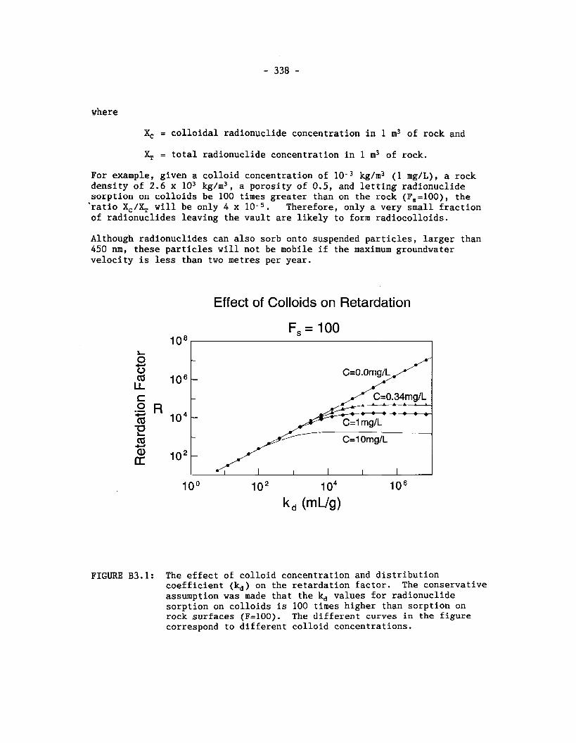
where
X, = colloidal radionuclide concentration in 1 m3 of rock and
X, = total radionuclide concentration in 1 m3 of rock.
For example, given a colloid concentration of 10- kg/m3 (1 mg/L), a rock density of 2.6 x lo3 kg/m3, a porosity of 0.5, and letting radionuclide sorption on colloids be 100 times greater than on the rock (F,=100), the 'ratio X,/& will be only 4 x Therefore, only a very small fraction of radionuclides leaving the vault are likely to form radiocolloids.
Although radionuclides can also sorb onto suspended particles, larger than 450 nm, these particles will not be mobile if the maximum groundwater velocity is less than two metres per year.
Effect of Colloids on Retardation
FIGURE B3.1: The effect of colloid concentration and distribution coefficient (k,) on the retardation factor. The conservative assumption was made that the k, values for radionuclide sorption on colloids is 100 times higher than sorption on rock surfaces (F=100). The different curves in the figure correspond to different colloid concentrations.
IMPACT OF MICROORGANISMS ON RADIONUCLIDE TRANSPORT
Microbes will be introduced into the vault during construction, emplacement of the wastes, and backfilling of the vault. Both native (autochthonous) microbes and microbes introduced as contaminants from the surface (allo- chthonous) microbes will be present during the construction and operation phases of the vault (West et al. 1985). After the vault has been backfill- ed and sealed, the microbes will evolve to fit the changing environment in the vault. Microbial activity has been shown to tolerate extrem~e con- ditions of temperature, pH, salinity, and radiation (West et al. 1985) and it must therefore be assumed that some microbial activity will continue in and around the vault for a considerable period of time (Stroes-Glascoyne 1989). Microbial activity can have a number of effects on contaminant migration. Some of these effects are the incorporation of radialnuclides into the structure of microbes (Champ and Merritt 1979), the pra~duction of organic compounds that can form complexes with radionuclides (Birch and Bachofen 1990) and the alteration of the redox conditions of the geological environment (Champ et a1 1973). The results from microbial activity can lead to enhanced retardation, if the microbes that have incorporated the radionuclides form biofilms that adhere to the fracture walls, or to re- duced retardation, if microbes form non-sorbing particulates or if non- sorbing organic complexes with radionuclides are created. In th,e absence of specific data, the uncertainty in the effects of microbes on radio- nuclide sorption is modelled by the uncertainty in the sorption data themselves.
REFERENCES :
Birch, L. and R. Bachofen. 1990. Complexing agents for microorganisms. Experientia 6, 827-834.
Bradbury, M.H. 1983. Permeability measurements in crystalline rocks and sands tone. United Ki~lgdol~~ A~OIII~C Er~ergy Author-i ty Har-well Report AERE-R 10836.
Champ, D.R., J. Gulens and R.E. Jackson. 1973. Oxidation-reduction sequences in groundwater flow systems. Canadian Journal of Earth Sciences. 16, 12-23.
Champ, D.R. and W.F. Merritt. 1979. Particulate transport of cesium in groundwater. In Proceedings of the Second Annual Conference of the Canadian Nuclear Society, F.N. McDonnell (Editor), 66-69.
Couture, R.A. and M.G. Seitz. 1983. Sorption of anions of iodine by iron oxides and kaolinite. Nuclear and Chemical Waste Management 4, 301- 306.
Davis, J.A., C.C. Fuller and A.D. Cook. 1987. A model for trace metal sorption at the calcite surface: adsorption of Cd2+ and subsequent solid solution formation. Geochimica and Cosmochimica Acta 51, 1477- 1490.
Glasbergen, P., G. Englund-Borowiec, I. Nijhof-Pan and A.F.M. Slot. 1989. Transport van radionucliden door de onderground. Rijksinstituut voor volksgezondheid en milieuhygiene. Bilthoven, The Netherlands. Final Report, Part 9. Report 728513010.
Haines, R.I., D.G. Owen and T.T. Vandergraaf. 1987. Technetium-iron oxide reactions under anaerobic conditions: a Fourier transform infrared, FTIR study. Nuclear Journal of Canada 10, 32-37.
McKinley, 1.G.and J. Hadermann. 1985. Radionuclide sorption database for Swiss safety assessment. Swiss Federal Institute for Reactor Research Technical Report 84-40.
Ruegger, B. and K.V. Ticknor. 1992. The NEA sorption data base (SDB) Radionuclide sorption from the safety evaluation prespective. Proceedings of an NEA Workshop on Sorption. Interlaken, Switzerland, 1991 October. 57-78.
Sherwood, T.K., R.L. Pigford and C.R. Wilke. 1975. Mass Transfer. McGraw-Hill, Inc. New York, NY.
SKBF. 1983. Final storage of spent nuclear fuel. KBS-3.
Stroes-Gascoyne, S. 1989. The potential for microbial life in a Canadian high-level nuclear fuel watse disposal vault: A nutrient and energy source analysis. Atomic Energy of Canada Limited Report, AECL-9574.
Ticknor, K.V. and Y.-H. Cho. 1990 Interaction of iodide and iodate with granitic fracture-filling minerals. Journal of Radioanalytical and Nuclear Chemistry 140(1), 75-90.
Vandergraaf, T.T., K.V. Ticknor and I.M. George. 1984. Reactions between technetium and iron-containing minerals under oxic and anoxic conditions. 2 Geochemical behaviour of disposed radioactive wastes (G.S. Barney, J.D. Navratil and W.W. Schultz, editors). ACS Symposium Series 246. American Chemical Society, Washington, DC, 1981. 26-43.
Vandergraaf, T.T., D.M. Grondin, P. Vilks and D.J. Drew. 1986. Radio- nuclide migration studies in the laboratory. In Conference proceedings 2nd International Conference on ~adionuclide Waste Manage- ment. Winnipeg, MB., 142-150.
Vandergraaf, T.T., K.V. Ticknor and T.W. Melnyk. 1992. The selection and use of a sorption database for the geosphere model in the Canadian Nuclear Fuel waste Management Program. Radionuclide sorption from the safety evaluation prespective. Proceedings of an NEA Workshop on Sorption. Interlaken, Switzerland, 1991 October. 81-120.
Vandergraaf, T.T. and K.V. Ticknor. 1993. A compilation and evaluation of sorption coefficients used in the geosphere model ot SWAC for the 1990 assessment of the Whiteshell Research Area. Atomic Energy of Canada Limited Report, AECL-10546 COG-92-59.
Vilks, P., D.B. Bachinski and T.T. Vandergraaf. 1991a. The ro1.e of parti- culates in radionuclide transport. Proceedings of the Third Inter- riatiollal Symposium on Advanced Nuclear Energy Research - GI-obal Environment and Nuclear Energy. Mito City, Japan 1991. March 13-15. 394-401.
Vilks, P., H.G. Miller and D.C. Doern. 1991b. Natural colloids and suspended particles in the Whiteshell research area and their potential effects on radiocolloid formation. Applied Geochemistry, 6(5), 565-574.
Vilks, P. and C. Degueldre. 1991. Sorption behaviour of Sr, I and Cs on colloids and suspended particles from the Grimsel Test Site, Switzerland. Applied Geochemistry, 60, 553-563.
Vilks, P. 1993. The Role of Colloids and Suspended Particles in Radio- nuclide Transport in the Vault and Geosphere. Atomic Energy of Canada Limited Report, AECL-10280, COG 92-26.
West, J.M., N. Christofi and I.M. McKinley. 1985. An overview of recent microbiological research relevant to the geological disposal of nuclear waste. Radioactive Wsate Management and the Nuclear Fuel Cycle, 60, 79-95.
(TR- indicates unrestricted, unpublished reports available from SDDO, AECL Research, Chalk River Laboratories, Chalk River, Ontario KOJ lLC).)
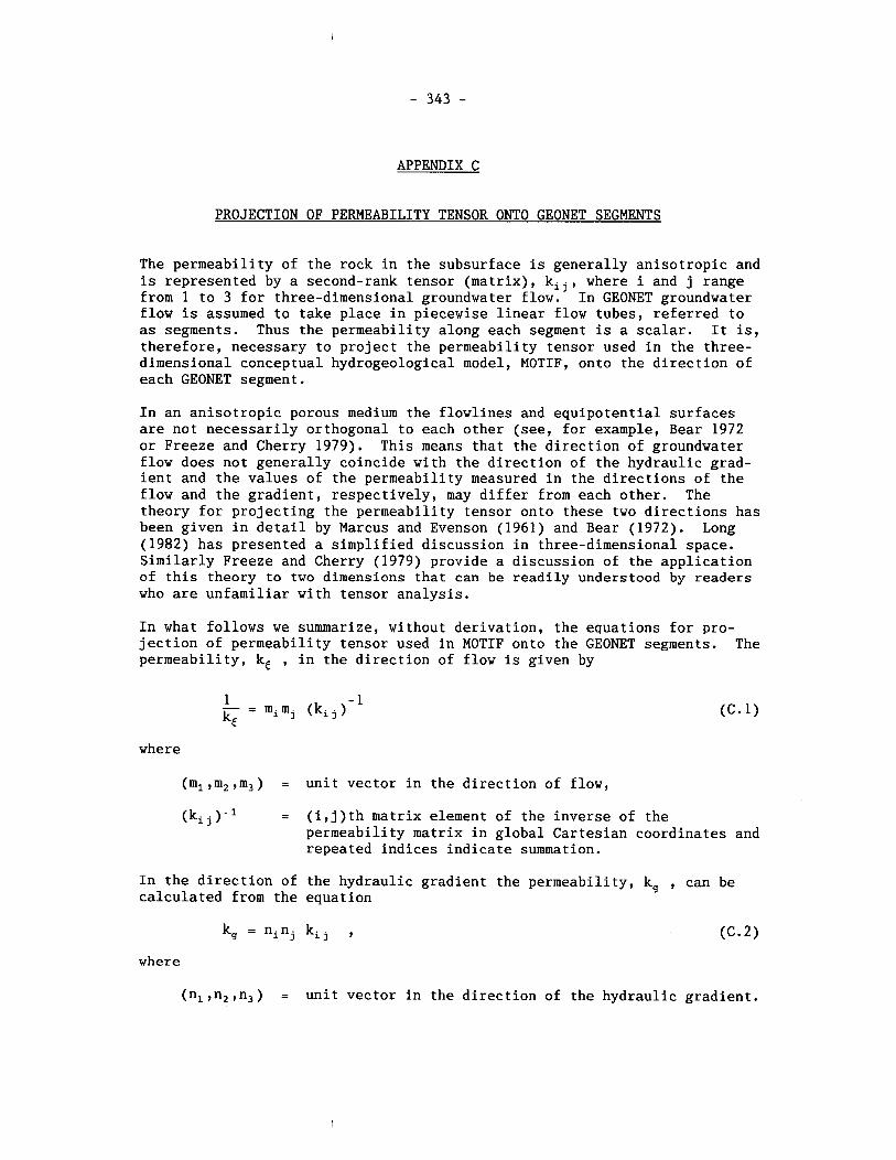
APPENDIX C
PROJECTION OF PERMEABILITY TENSOR ONTO GEONET SEGMENTS
The permeability of the rock in the subsurface is generally anisotropic and is represented by a second-rank tensor (matrix), kij, where i arid j range from 1 to 3 for three-dimensional groundwater flow. In GEONET groundwater flow is assumed to take place in piecewise linear flow tubes, referred to as segments. Thus the permeability along each segment is a scalar. It is, therefore, necessary to project the permeability tensor used in the three- dimensional conceptual hydrogeological model, MOTIF, onto the direction of each GEONET segment.
In an anisotropic porous medium the flowlines and equipotential surfaces are not necessarily orthogonal to each other (see, for example, Bear 1972 or Freeze and Cherry 1979). This means that the direction of groundwater flow does not generally coincide with the direction of the hydraulic grad- ient and the values of the permeability measured in the directions of the flow and the gradient, respectively, may differ from each other. The theory for projecting the permeability tensor onto these two directions has been given in detail by Marcus and Evenson (1961) and Bear (1972). Long (1982) has presented a simplified discussion in three-dimensional space. Similarly Freeze and Cherry (1979) provide a discussion of the application of this theory to two dimensions that can be readily understood by readers who are unfamiliar with tensor analysis.
In what follows we summarize, without derivation, the equations for pro- jection of permeability tensor used in MOTIF onto the GEONET segments. The permeability, kc , in the direction of flow is given by
where
(ml,m2,m,) = unit vector in the direction of flow,
(kij)" = (i,j)th matrix element of the inverse of the permeability matrix in global Cartesian coordinates and repeated indices indicate summation.
In the direction of the hydraulic gradient the permeability, kg , can be calculated from the equation
where
(nl,n2,n,) = unit vector in the direction of the hydraulic gradient.
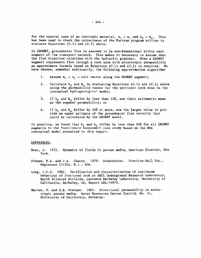
For the special case of an isotropic material, mi = ni and kt = !g. This has been used to check the correctness of the Fortran program wrltten to evaluate Equations (C.l) and (C.2) above.
In GEONET, groundwater flow is assumed to be one-dimensional within each segment of the transport network. This makes it necessary to assume that the flow direction coincides with the hydraulic gradient. When. a GEONET segment represents flow through a rock zone with anisotropic permeability an approximate formula based on Equations (C.l) and (C.2) is required. We have chosen, somewhat arbitrarily, the following approximation algorithm:
1. Assume mi = ni = unit vector along the GEONET segment;
2. Calculate kt and k by evaluating Equations (C.l) and (C.2) above using the permeability tensor for the pertinent rock zone in the conceptual hydrogeological model;
3. If k and kg differ by less than lo%, use their arithmetic mean as t f~ e segment permeability; or
4. If kt and k, differ by 10% or more, use the larger value to pro- vide an upper estimate of the groundwater flow velocity that could be calculated by the GEONET model.
In practice, we found that kt and kg differ by less than 10% for all GEONET segments in the Postclosure Assessment case study based on the WRA conceptual model presented in this report.
REFERENCES:
Bear, J. 1972. Dynamics of fluids in porous media, American Elsevier, New York.
Freeze, R.A. and J.A. Cherry. 1979. Groundwater. Prentice-Hall Inc., Englewood Cliffs, N.J., 604.
Long, J.C.S. 1982. Verification and characterization of continuum behaviour of fractured rock at AECL Underground Research Laboratory, Earth Sciences Division, Lawrence Berkeley Laboratory, University of California, Berkeley, CA, Report LBL-14975.
Marcus, H. and D.E. Evenson. 1961. Directional permeability in aniso- tropic porous media. Water Resources Center Contrib. No. 31, University of California, Berkeley.

APPENDIX D
GEONET INPUT DATA FOR POSTCLOSURE ASSESSMENT
CONTENTS
D. 1 INTRODUCTION 347 D.l.l PARAMETER ATTRIBUTES AND VALUES 347 D.1.2 JUSTIFICATION AND TABLES FOR GEONET INPUT DATA 347
D. 2 NETWORK GEOMETRY DATA 348 D.2.1 NODE COORDINATES 348 D.2.2 SEGMENT AND ZONES, PHYSICAL & CHEMICAL PROPERTI!
CLASSES 354 D.2.3 SEGMENT SOURCE FRACTION 358
D. 3 HYDRAULIC PROPERTIES 360 D.3.1 PERMEABILITY OF THE BACKFILL 360 D.3.2 PERMEABILITY OF THE ROCK ZONES 361 D.3.3 PERMEABILITY OF THE OVERBURDEN AND COMPACTED
SEDIMENT 363 D.3.4 POROSITY OF THE ROCK ZONES 365 D.3.5 POROSITY OF THE OVERBURDEN AND COMPACTED
SEDIMENT 366 D.3.6 GROUNDWATER VELOCITY SCALING FACTOR 367
D.4 DATA FROM MOTIF RESULTS 368 D.4.1 HYDRAULIC HEADS 368 D.4.2 DISCHARGE AREAS 37 1 D.4.3 WELL PARAMETERS 375
D.4.3.1 Well Bypass Discharge Reduction Relationship 375
D.4.3.2 Distance to Drawdown Nodes 376 D.4.3.3 Empirical Vault Head Equation (EVHE) 378 D.4.3.4 Minimum Well Depth 383 D.4.3.5 Scaling Factor for Well Demand 383
D.4.3.5.1 Comparison of Contaminant Capture Fractions in the Fracture Zone 383
D.4.3.5.2 Comparison of Head Drawdowns in the Fracture Zone 384
n.4.3.6 Thickness of We11 Aquifer 385 D.4.4 GEOSPHERE WELL DEPTH 386 D.4.5 NODAL TEMPERATURES 386
ctont inued . . .
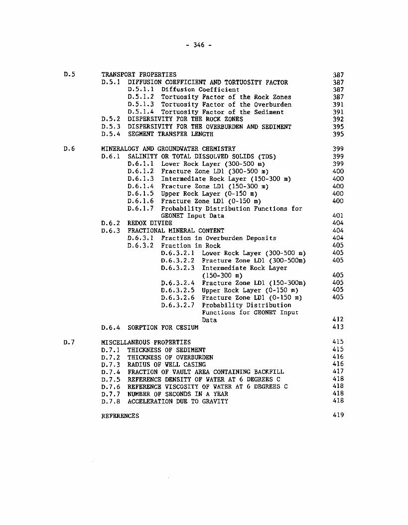
TRANSPORT PROPERTIES D.5.1 DIFFUSION COEFFICIENT AND TORTUOSITY FACTOR
D.5.1.1 Diffusion Coefficient D.5.1.2 Tortuosity Factor of the Rock Zones D.5.1.3 Tortuosity Factor of the Overburden D.5.1.4 Tortuosity Factor of the Sediment
D.5.2 DISPERSIVITY FOR THE ROCK ZONES D.5.3 DISPERSIVITY FOR THE OVERBURDEN AND SEDIMENT D.5.4 SEGMENT TRANSFER LENGTH
MINERALOGY AND GROUNDWATER CHEMISTRY D.6.1 SALINITY OR TOTAL DISSOLVED SOLIDS (TDS)
D.6.1.1 Lower Rock Layer (300-500 m) D.6.1.2 Fracture Zone LD1 (300-500 m) D.6.1.3 Intermediate Rock Layer (150-300 m) D.6.1.4 Fracture Zone LD1 (150-300 m) D.6.1.5 Upper Rock Layer (0-150 m) D.6.1.6 Fracture Zone LD1 (0-150 m) D.6.1.7 Probability Distribution Functions for
GEONET Input Data D.6.2 REDOX DIVIDE D.6.3 FRACTIONAL MINERAL CONTENT
D.6.3.1 Fraction in Overburden Deposits D.6.3.2 Fraction in Rock
D.6.3.2.1 Lower Rock Layer (300-500 m) D.6.3.2.2 Fracture Zone LD1 (300-500m) D.6.3.2.3 Intermediate Rock Layer
(150-300 m) D.6.3.2.4 Fracture Zone LD1 (150-300m) D.6.3.2.5 Upper Rock Layer (0-150 m) D.6.3.2.6 Fracture Zone LD1 (0-150 m) D.6.3.2.7 Probability Distribution
Funct ions for GEONET Input Data
D.6.4 SORPTION FOR CESIUM
MISCELLANEOUS PROPERTIES D.7.1 THICKNESS OF SEDIMENT D.7.2 THICKNESS OF OVERBURDEN D.7.3 RADIUS OF WELL CASING D.7.4 FRACTION OF VAULT AREA CONTAINING BACKFILL D.7.5 REFERENCE DENSITY OF WATER AT 6 DEGREES C D.7.6 REFERENCE VISCOSITY OF WATER AT 6 DEGREES C D.7.7 NUMBER OF SECONDS IN A YEAR D.7.8 ACCELERATION DUE TO GRAVITY
REFERENCES
D.l INTRODUCTION
This appendix contains the input data used by GEONET to describe contam- inant transport through the geosphere representing conditions encountered at the Whiteshell Research Area. It contains tables of data, and explanations justifying the data set used.
The data used in SYVAC3-CC3 are stored in a Master Database as described in Goodwin et al. (1994). The GEONET data in this appendix were printed using automated procedures to retrieve data from the Master Database, which eliminates the chance of errors being introduced by manually transcribing the data.
D.l.l PARAMETER ATTRIBUTES AND VALUES
The SYVAC3-CC3 program is designed so that any parameter can be represented as a statistical distribution of values. The tables in this appendix des- cribe the distributions for the parameters of the GEONET model used for the postclosure assessment case study.
The following table (D.l.l) shows the distribution types and explains their attributes. More information can be found in Table 3-1 of Stephens et al. (1989) and Goodwin et al. (1994)
The symbols for these attributes are not shown in the list of symbols and they may also be used to represent other quantities elsewhere in the text. The symbols used in this table only apply to this appendix.
D.1.2 JUSTIFICATION AND TABLES FOR GEONET INPUT DATA
The justification and tables that appear in this appendix are listed in the table of contents for this appendix.
The justification and tables have been arranged in 6 groups.
D.2 Network Geometry Data, D.3 Hydraulic Properties, D.4 Data from MOTIF Results, D.5 Transport Properties, D.6 Mineralogy and Groundwater Chemistry, D.7 Miscellaneous Properties.
Within each group the tables are ordered from the vault to the geosphere, where possible.
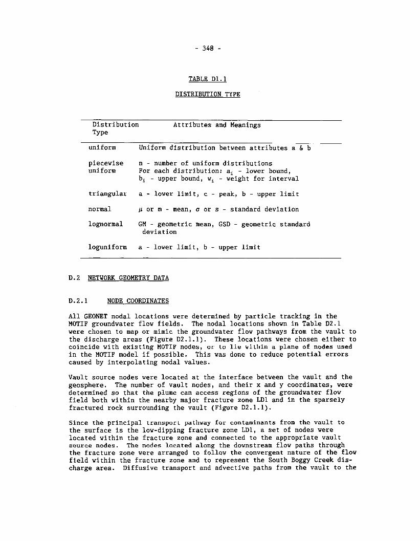
TABLE D1.l
DISTRIBUTION TYPE
Distribution Attributes and Meanings TY pe
uniform Uniform distribution between attributes a & b
piecewise n - number of uniform distributions uniform For each distribution: ai - lower bound,
bi - upper bound, wi - weight for interval
triangular a - lower limit, c - peak, b - upper limit normal p or m - mean, o or s - standard deviation
lognormal GM - geometric mean, GSD - geometric standard deviation
loguniform a - lower limit, b - upper limit
D.2 NETWORK GEOMETRY DATA
D.2.1 NODE COORDINATES
All GEONET nodal locations were determined by particle tracking in the MOTIF groundwater flow fields. The nodal locations shown in Table DZ.l were chosen to map or mimic the groundwater flow pathways from the vault to the discharge areas (Figure D2.1.1). These locations were chosen either to coincide with existing MOTIF nodes, or to lie within a plane of nodes used in the MOTIF model if possible. This was done to reduce potential errors caused by interpolating nodal values.
Vault source nodes were located at the interface between the vault and the geosphere. The number of vault nodes, and their x and y coordinates, were determined so that the plume can access regions of the groundwater flow field both within the nearby major fracture zone LD1 and in the sparsely fractured rock surrounding the vault (Figure D2.1.1).
Since the principal transport pathway for contaminants from the vault to the surface is the low-dipping fracture zone LD1, a set of nodes were located within the fracture zone and connected to the appropriate vault source nodes. The nodes located along the downstream flow paths through the fracture zone were arranged to follow the convergent nature of the flow field within the fracture zone and to represent the South Boggy Creek dis- charge area. Diffusive transport and advective paths from the vault to the
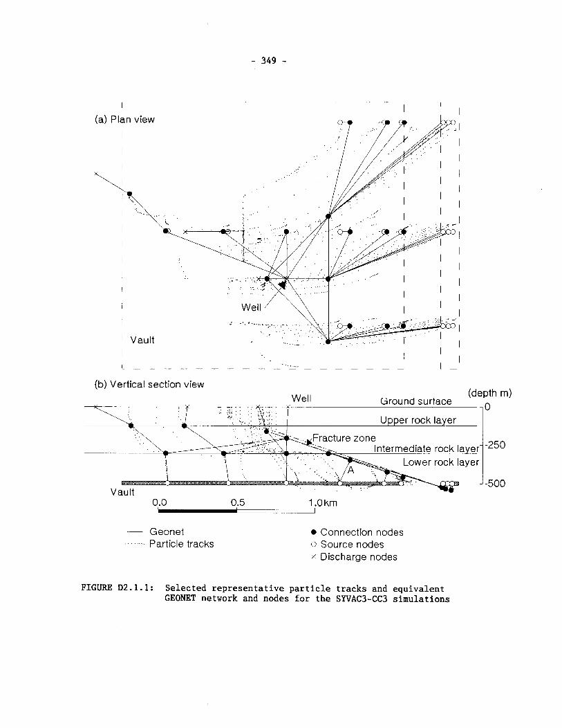
0.0 0.5 1 .O krn
(b) Vertical section view Well (depth m)
Ground surface 0
- Geonet . . . . . . . . . Particle tracks
~ c k layer
ate rock layer- ver rock layer
a Connection nodes 0 Source nodes x Discharge nodes
'250
FIGURE D2.1.1: Selected representative particle tracks and equivalent GEONET network and nodes for the SYVAC3-CC3 simulations
.... - 5 0 0 Vault
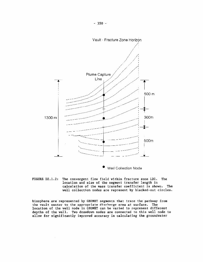
Vault - Fracture Zone ~ o r i z o n
Well Collection Node
FIGURE D2.1.2: The convergent flow field within fracture zone LD1. The location and size of the segment transfer length in calculation of the mass transfer coefficient is shown. The well collection nodes are represent by blacked-out circles.
biosphere are represented by GEONET segments that trace the pathway from the vault sector to the appropriate discharge area at surface. The location of the well node in GEONET can be varied to represent different depths of the well. Two drawdown nodes are connected to this well node to allow for significantly improved accuracy in calculating the groundwater
velocity near the well. The locations for these drawdown nodes are some- what arbitrary but have been chosen so that the steepness of the drawdown cone in the vicinity of the well is reasoriably well appLoximated. The actual locations for these nodes were established by applying the analytical well model (Chan and Nakka 1994) to calculate the hydraulic head near the well as a function of distance along the dip of the fracture zone.
In GEONET, the capture nodes are located in the fracture zone to define the location of the GEONET capture line. Along this capture line, the amount of the contaminants flowing in the fracture zone that is captured by the well is calculated. The location for the GEONET capture line was deter- mined by Chan and Nakka (1994) from the results of the detailed MOTIF modelling. In the MOTIF groundwater flow fields, particles with origins located evenly along the line of intersection of Cracture zone LD1 and the vault horizon were tracked to the surface or the well, using a particle tracking code, TRACK3D (Nakka and Chan 1994). This particle trackking simu- lates only advective movement of conservative contaminants because disper- sion, diffusion and chemical reaction are not considered in this tracking code.
The advective plumes were obtained for two different well depths (100 m and 200 m) for the intake position in fracture zone LD1, and for six different pumping rates (0 m3/a, 120 m3/a, 1 500 m3/a, 4 000 m3/a, 10 000 n13/a and 30 000 m3/a). The plumes were examined to identify a region between the well and the vault horizon where the flow field was reasonably symmetrical with respect to the well centreline. The widths of the advective plumes in the symmetrical region were also compared to find the minimum wiclth of a capture line necessary to secure complete capture. It was found that the natural-flow field corresponding to the no-pumping case had the ,-east convergence (broadest plume) in the symmetrical region. This case was used to define the location and width of the GEONET capture line.
The GEONET capture line must also be located between the deepest well draw- down node and the highest transport segment that leads contaminants into the fracture zone. For the deepest well, the drawdown nodes extend to a depth of 230 m. The last transport segment (labelled A in Figure D2.1.1) intersects LD1 at a depth of 335 m. The capture line shown in Figure D2.1.2 lies between the drawdown nodes and last transport segment: at a depth of 287 m.
Nodal locations in GEONET are constrained by the requirement that the material properties of the region between a connected pair of nodes, i.e., a transport segment, should be constant. Hence, as required, some GEONET network nodes are located at the transition between regions of different material properties.
Discharge nodes in GEONET are assigned the z coordinate corresporiding to the hydraulic-head boundary condition, i.e., the elevation of the topo- graphic surface at the discharge area.
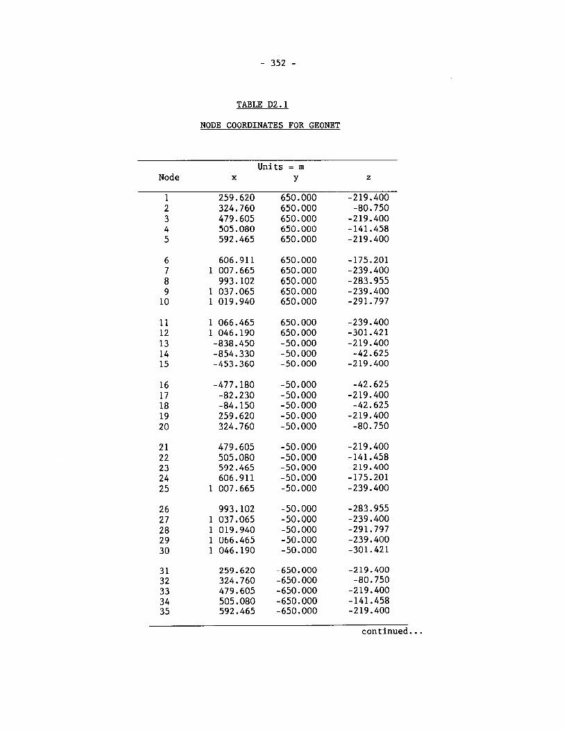
TABLE D2.1
NODE COORDINATES FOR GEONET
Units = m Node x Y z
continued...
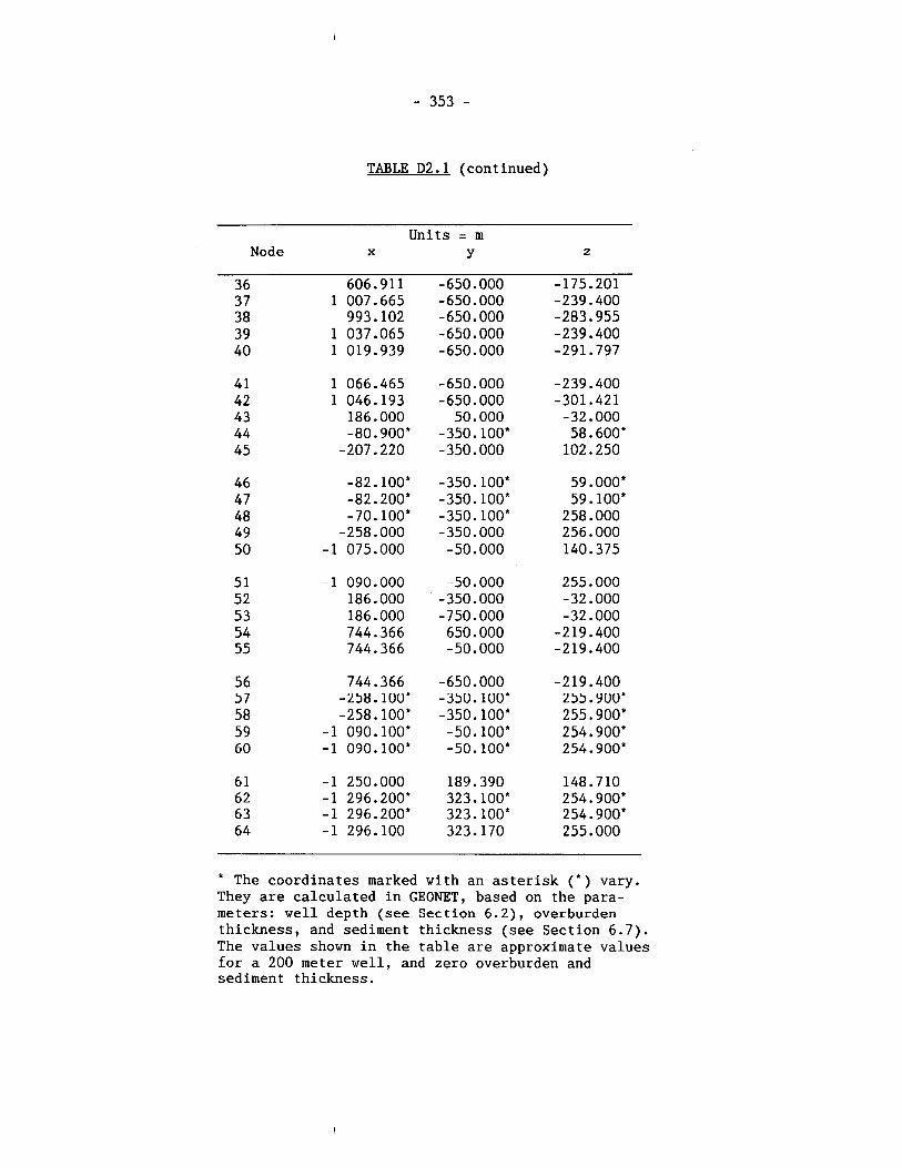
TABLE D2.1 (continued)
Units = m Node x Y
* The coordinates marked with an asterisk ( * ) vary. They are calculated in GEONET, based on the para- meters: well depth (see Section 6.2), overburden thickness, and sediment thickness (see Section 6.7). The values shown in the table are approximate values for a 200 meter well, and zero overburden and sediment thickness.

D. 2.2 SEGMENT AND ZONES, PHYSICAL & CHEMICAL PROPERTY CLASSES
Physical and chemical properties classes are assigned to each GEONET segment depending on the location of the segment in the MOTIF model.
The MOTIF model has four basic physical property classes, namely the lower rock zone, the intermediate rock zone, and the upper rock zone, and fracture zones. In addition, there are segments which are used to simulate overburden and compacted sediments. Some segments are simply used to re- route flow. These do not delay transport and are assigned to a "null" property class. In total, there are 9 classes (Table D2.2).
No segment is allowed to extend over more than one physical or chemical property class.
Network segments are assigned chemical property classes based on the following regions (Gascoyne and Kamineni 1992):
1. Lower Rock Layer (300-500 m). This is sparsely fractured grey granite and the groundwater flow paths from the vault to LD1 go through the poorly interconnected pore space and microfractures. Because there is very little data available on the pore water composition in this layer, the groundwater composition consistent with a depth of 500 m has been used.
Fracture Zone LD1. This zone represents a fracture zone that has been identified in the URL location of the Whiteshell Research Area. It has been split into three transport segments with dif- ferent chemical properties. The chemistry of each segment has been determined from mean and ranges of chemical compositions for the groundwaters and fracture infillings sampled from the URL lease area and WRA (Figure D2.2.1) and reflects the fact that groundwater salinity is expected to decrease along this fracture zone towards the surface.
3. Intermediate Rock Layer (150-300 m). The groundwater composition is determined from the upper part of the layer 2 envelope in Figure D2.2.1, and the rock composition is assumed to be represented by the grey granite analysis.
4 . Upper Rock Layer (0-150 m). This zone is characterized by inter- connected, subvertical fractures with calcite as the dominant mineral infilling. Considerable groundwater dilution occurs via localized recharge and an average composition from Layer 1 (Figure D2.2.1) has been taken to represent the chemistry of the fracture filling minerals in this layer.
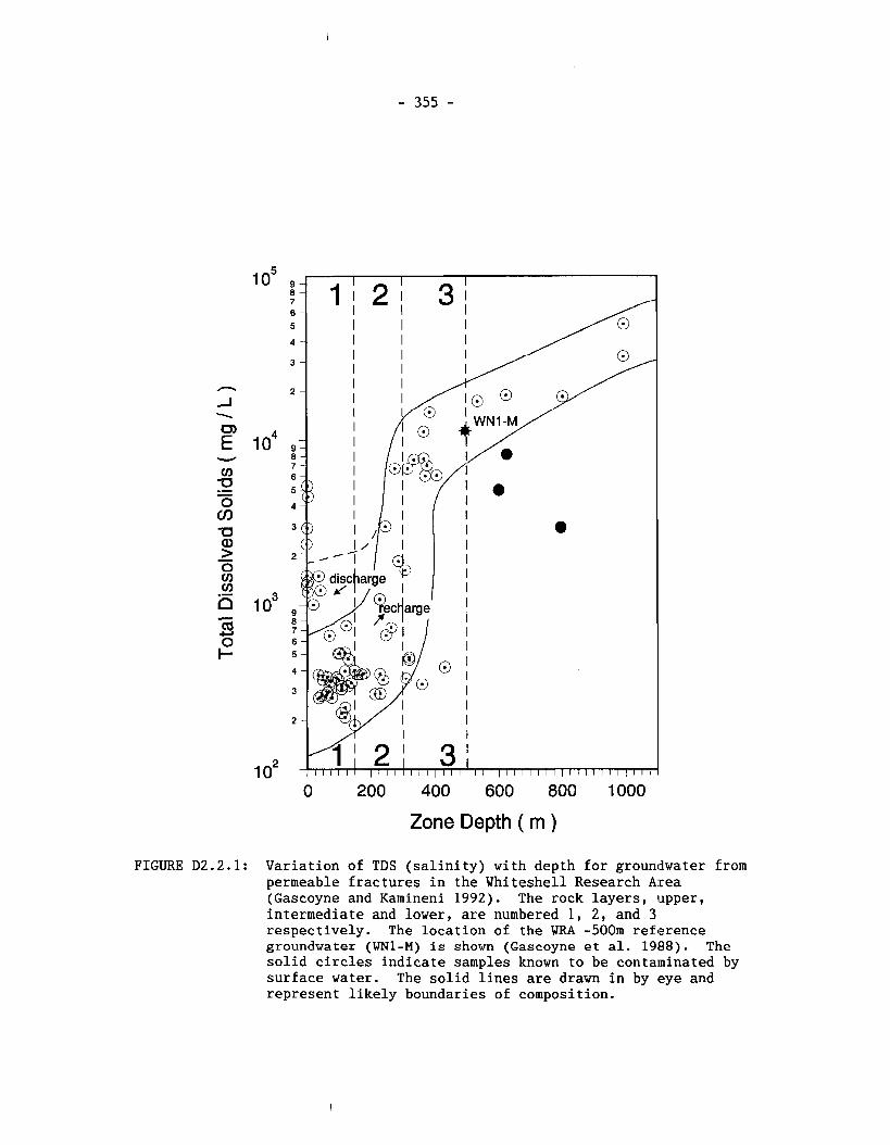
0 200 400 600 800 1000
Zone Depth ( m )
FIGURE D2.2.1: Variation of TDS (salinity) with depth for groundwater from permeable fractures in the Whiteshell Research A:rea (Gascoyne and Kamineni 1992). The rock layers, upper, intermediate and lower, are numbered 1, 2, and 3 respectively. The location of the WRA -500m reference groundwater (WN1-M) is shown (Gascoyne et al. 1988). The solid circles indicate samples known to be contaminated by surface water. The solid lines are drawn in by eye and represent likely boundaries of composition.
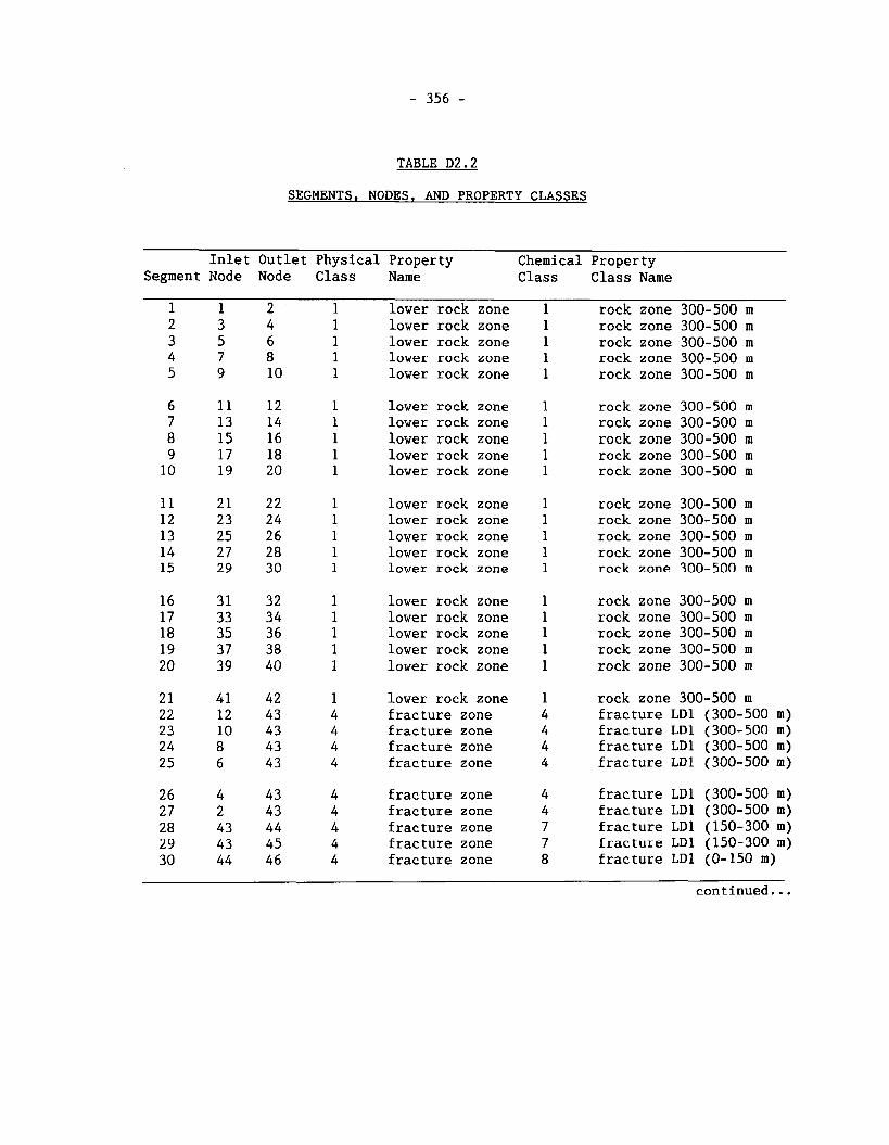
TABLE D2.2
SEGMENTS, NODES, AND PROPERTY CLASSES
Inlet Outlet Physical Property Chemical Property Segment Node Node Class Name Class Class Name
1 1 2 1 lower rock zone 1 rock zone 300-500 m 2 3 4 1 lower rock zone 1 rock zone 300-500 m 3 5 6 1 lower rock zone 1 rock zone 300-500 m 4 7 8 1 lower rock zone 1 rock zone 300-500 m 5 9 10 1 lower rock zone 1 rock zone 300-500 m
6 11 12 1 lower rock zone 1 rock zone 300-500 m 7 13 14 1 lower rock zone 1 rock zone 300-500 m 8 15 16 1 lower rock zone 1 rock zone 300-500 m 9 17 18 1 lower rock zone 1 rock zone 300-500 m 10 19 20 1 lower rock zone 1 rock zone 300-500 m
11 21 22 1 lower rock zone 1 rock zone 300-500 m 12 23 24 1 lower rock zone 1 rock zone 300-500 m 13 25 26 1 lower rock zone 1 rock zone 300-500 m 14 27 28 1 lower rock zone 1 rock zone 300-500 m 15 29 30 1 lower rock zone 1 rock zone 300-500 m
16 31 32 1 lower rock zone 1 rock zone 300-500 m 17 33 34 1 lower rock zone 1 rock zone 300-500 m 18 35 36 1 lower rock zone 1 rock zone 300-500 m 19 37 38 1 lower rock zone 1 rock zone 300-500 m 2 0 39 40 1 lower rock zone 1 rock zone 300-500 m
2 1 41 42 1 lower rock zone 1 rock zone 300-500 m 22 12 43 4 fracture zone 4 fracture LD1 (300-500 m) 23 10 43 4 fracture zone 4 fracture LD1 (300-500 m) 24 8 4 3 4 fracture zone 4 fracture LD1 (300-500 m) 2 5 6 4 3 4 fracture zone 4 fracture LD1 (300-500 m)
26 4 43 4 fracture zone 4 fracture LD1 (300-500 m) 27 2 4 3 4 fracture zone 4 fracture LD1 (300-500 m) 2 8 43 44 4 fracture zone 7 fracture LD1 (150-300 m) 2 9 43 45 4 fracture zone 7 fracture LD1 (150-300 m) 3 0 44 46 4 fracture zone 8 fracture LD1 (0-150 m)
continued...
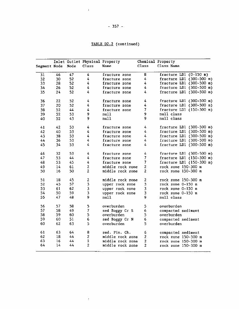
TABLE D2.2 (continued)
Inlet Outlet Physical Property Chemical Property Segment Node Node Class Name Class Class Name
3 1 46 47 4 fracture zone 8 fracture LD1 (0-150 m) 32 30 52 4 fracture zone 4 fracture LD1 (300-500 m) 33 28 52 4 fracture zone 4 fracture LD1 (300-500 m) 3 4 26 52 4 fracture zone 4 fracture LD1 (300-500 m) 3 5 24 52 4 fracture zone 4 fracture LD1 (300-500 m)
3 6 22 52 4 fracture zone 4 fracture LD1 (300-500 m) 3 7 20 52 4 fracture zone 4 fracture LD1 (300-500 m) 38 52 44 4 fracture zone 7 fracture LD1 (150-300 m) 3 9 52 53 9 null 9 null cla,ss 40 52 43 9 null 9 null cla,ss
4 1 42 53 4 fracture zone 4 fracture LD1 (300-500 m) 42 40 53 4 fracture zone 4 fracture LD1 (300-500 m) 4 3 38 53 4 fracture zone 4 fracture LD1 (300-500 m) 4 4 36 53 4 fracture zone 4 fracture LD1 (300-500 m) 4 5 34 53 4 fracture zone 4 fracture LD1 (300-500 m)
46 32 53 4 fracture zone 4 fracture LD1 (300-500 m) 47 53 44 4 fracture zone 7 fracture LD1 (150-300 m) 48 53 45 4 fracture zone 7 fracture LD1 (150-300 m) 4 9 14 61 2 middle rock zone 2 rock zon'e 150-300 m 5 0 16 50 2 middle rock zone 2 rock zone 150-300 m
5 1 18 45 2 middle rock zone 2 rock zon'e 150-300 m 52 45 57 3 upper rock zone 3 rock zone 0-150 m 53 61 62 3 upper rock zone 3 rock zonle 0-150 m 5 4 50 59 3 upper rock zone 3 rock zonle 0-150 m 5 5 47 48 9 null 9 null class
56 57 58 5 overburden 5 overburdlen 57 58 49 7 sed Boggy Cr S 6 compacted sediment 5 8 59 60 5 overburden 5 overburdlen 59 60 51 6 sed Boggy Cr N 6 compac tejd sediment 6 0 62 63 5 overburden 5 overburden
6 1 63 64 8 sed. Pin. Ch. 6 compacted sediment 6 2 18 44 2 middle rock zone 2 rock zone 150-300 m 63 16 44 2 middle rock zone 2 rock zone 150-300 m 6 4 14 44 2 middle rock zone 2 rock zone 150-300 m
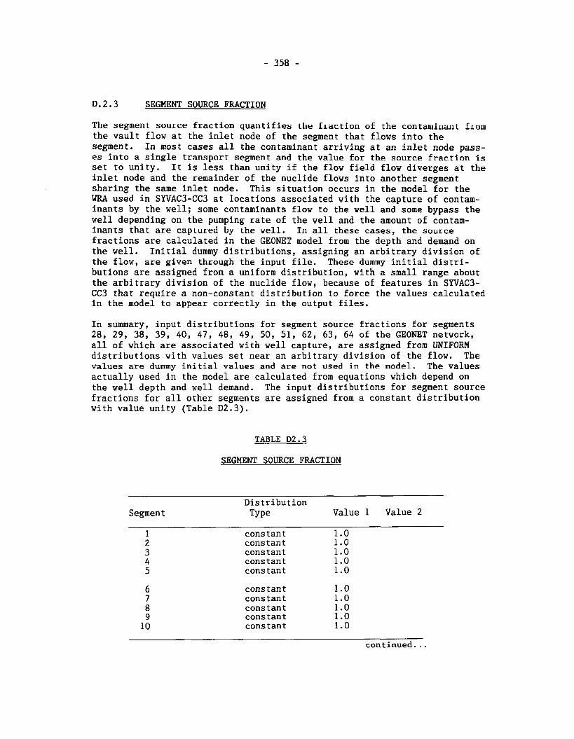
D.2.3 SEGMENT SOURCE FRACTION
The segment source fraction quantifies the fraction of the contaminant from the vault flow at the inlet node of the segment that flows into the segment. In most cases all the contaminant arriving at an inlet node pass- es into a single transport segment and the value for the source fraction is set to unity. It is less than unity if the flow field flow diverges at the inlet node and the remainder of the nuclide flows into another segment sharing the same inlet node. This situation occurs in the model for the WRA used in SYVAC3-CC3 at locations associated with the capture of contam- inants by the well; some contaminants flow to the well and some bypass the well depending on the pumping rate of the well and the amount of contam- inants that are captured by Lhe well. In all these cases, the source fractions are calculated in the GEONET model from the depth and demand on the well. Initial dummy distributions, assigning an arbitrary division of the flow, are given through the input file. These dummy initial distri- butions are assigned from a uniform distribution, with a small range about the arbitrary division of the nuclide flow, because of features in SYVAC3- CC3 that require a non-constant distribution to force the values calculated in the model to appear correctly in the output files.
In summary, input distributions for segment source fractions for segments 28, 29, 38, 39, 40, 47, 48, 49, 50, 51, 62, 63, 64 of the GEONET network, all of which are associated with well capture, are assigned from UNIFORM distributions with values set near an arbitrary division of the flow. The values are dummy initial values and are not used in the model. The values actually used in the model are calculated from equations which depend on the well depth and well demand. The input distributions for segment source fractions for all other segments are assigned from a constant distribution with value unity (Table D2.3).
TABLE D2.3
SEGMENT SOURCE FRACTION
Distribution Segment TY pe Value 1 Value 2
1 constant 1.0 2 constant 1 .O 3 cons tan t 1 .O 4 constant 1.0 5 constant 1.0
cons tan t 1.0 constant 1 .O constant 1.0 cons tan t 1 .O constant 1.0
continued ...
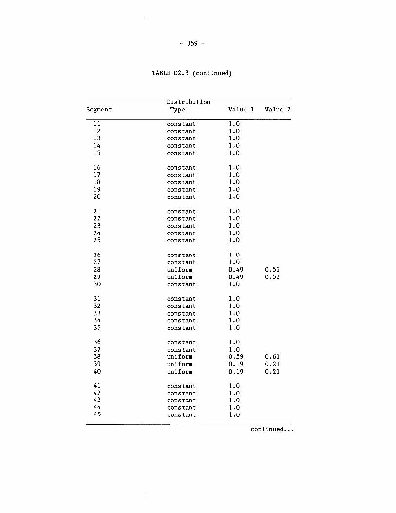
TABLE D2.3 (continued)
Segment Distribution TY pe Value 1 Value 2
11 constant 1.0 12 constant 1.0 13 cons tan t 1 .O 14 cons tan t 1.0 15 constant 1.0
cons tan t 1 .O constant 1.0 constant 1.0 constant 1.0 constant 1.0
2 1 constant 1.0 22 constant 1.0 2 3 constant 1.0 2 4 constant 1.0 2 5 constant 1.0
constant 1.0 cons tan t 1.0 uniform 0.49 0.51 uniform 0.49 0.51 constant 1.0
cons tan t 1.0 constant 1.0 cons tan t 1.0 constant 1.0 cons tan t 1.0
constant 1.0 constant 1.0 uniform 0.59 0.61 uniform 0.19 0.21 uniform 0.19 0.21
cons tan t 1 .O cons tan t 1 .O cons tan t 1.0 constant 1 .O constant 1 .O
continued...
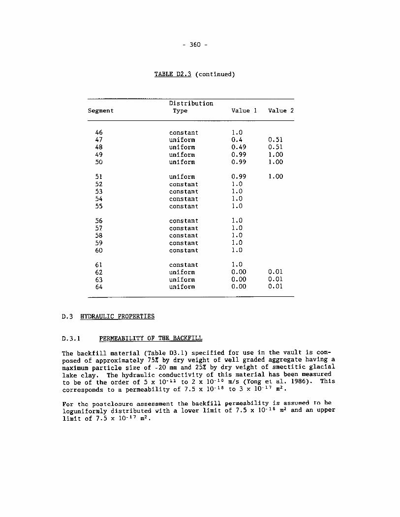
TABLE D2.3 (continued)
Segment Distribution Type Value 1 Value 2
cons tan t uniform uniform uniform uniform
uniform cons tan t constant constant cons tan t
cons tan t cons tan t constant constant constant
cons tan t uniform uniform uniform
D.3 HYDRAULIC PROPERTIES
PERMEABILITY OF THE BACKFILL
The backfill material (Table D3.1) specified for use in the vault is com- posed of approximately 75% by dry weight of well graded aggregate having a maximum particle size of -20 mm and 25% by dry weight of smectitic glacial lake clay. The hydraulic conductivity of this material has been measured to be of the order of 5 x 10-l1 to 2 x 10-lo m/s (Yong et al. 1986). This corresponds to a permeability of 7.5 x 10-la to 3 x 10-l7 m2.
For the postclosure assessment the backfill permeability is assumed to be loguniformly distributed with a lower limit of 7.5 x 10-la m2 and an upper limit of 7.5 x 10-l7 m2.
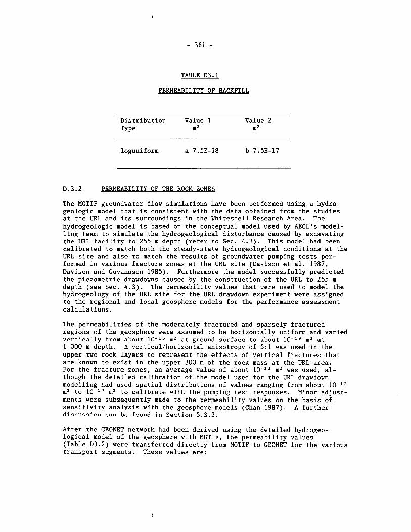
TABLE D3.1
PERMEABILITY OF BACKFILL
Distribution Value 1 Value 2 TY pe m2 m2
loguniform a=7.5E- 18 b=7.5E- 17
D.3.2 PERMEABILITY OF THE ROCK ZONES
The MOTIF groundwater flow simulations have been performed using a hydro- geologic model that is consistent with the data obtained from the studies at the URL and its surroundings in the Whiteshell Research Area. The hydrogeologic model is based on the conceptual model used by AECL's model- ling team to simulate the hydrogeological disturbance caused by excavating the URL facility to 255 m depth (refer to Sec. 4.3). This model had been calibrated to match both the steady-state hydrogeological conditions at the URL site and also to match the results of groundwater pumping tests per- formed in various fracture zones at the URL site (Davison et al. 1987, Davison and Guvanasen 1985). Furthermore the model successfully predicted the piezometric drawdowns caused by the construction of the URL to 255 m depth (see Sec. 4.3). The permeability values that were used to model the hydrogeology of the URL site for the URL drawdown experiment were assigned to the regional and local geosphere models for the performance assessment calculations.
The permeabilities of the moderately fractured and sparsely fractured regions of the geosphere were assumed to be horizontally uniform and varied vertically from about 10-l5 m2 at ground surface to about 10-l9 m2 at 1 000 m depth. A vertical/horizontal anisotropy of 5:l was used in the upper two rock layers to represent the effects of vertical fractures that are known to exist in the upper 300 m of the rock mass at the URL area. For the fracture zones, an average value of about 10-l3 m2 was used, al- though the detailed calibration of the model used for the URL drawdown modelling had used spatial distributions of values ranging from about 10-l2 m2 to 10- l 7 m2 to calibrate with the pumping test responses. Minor adjust- ments were subsequently made to the permeability values on the basis of sensitivity analysis with the geosphere models (Chan 1987). A further discussion can he found in Section 5.3.2.
After the GEONET network had been derived using the detailed hydrogeo- logical model of the geosphere with MOTIF, the permeability values (Table D3.2) were transferred directly from MOTIF to GEONET for the various transport segments. These values are:

Pathways Segment ~ermeabili ty (m2 )
Lower sparsely fractured rock zone
Middle rock zone 1.3 x 10⁻¹' - 1.7 x 10-l7
Upper moderately fractured 2.0 x 10-l5 - 5.0 x 10-l5 Rock zone
Fracture zones 0.87 x 10-l3 - 0.95 x 1 0 - 1 ~
Further discussion of the treatment of possible variations in the perme- ability distribution of the geosphere is given in Sec. D.3.6 (velocity scaling factor), Sec. D.5.2 (dispersivity) and in Chapter 5 (sensitivity analysis).
TABLE D3.2
PERMEABILITY IN ROCK ZONE SEGMENTS
Distribution Segment Type Value
m2
1 constant 0.10000E-18 2 cons tan t 0.10000E-18 3 cons tan t 0.10000E-18 4 cons tan t 0.10000E-18 5 cons tan t 0.10000E-18
constant 0.10000E-18 cons tan t 0.10000E-18 constant 0.10000E-18 constant 0.10000E-18 constant 0.10000E-18
constant 0.10000E-18 constant 0.10000E-18 constant 0.10000E-18 cons tan t 0.10000E-18 constant 0.10000E-18
cons tan t 0.10000E-18 constant 0.10000E-18 constant 0.10000E-18 constant 0.10000E-18 constant 0.10000E-18
continued ...
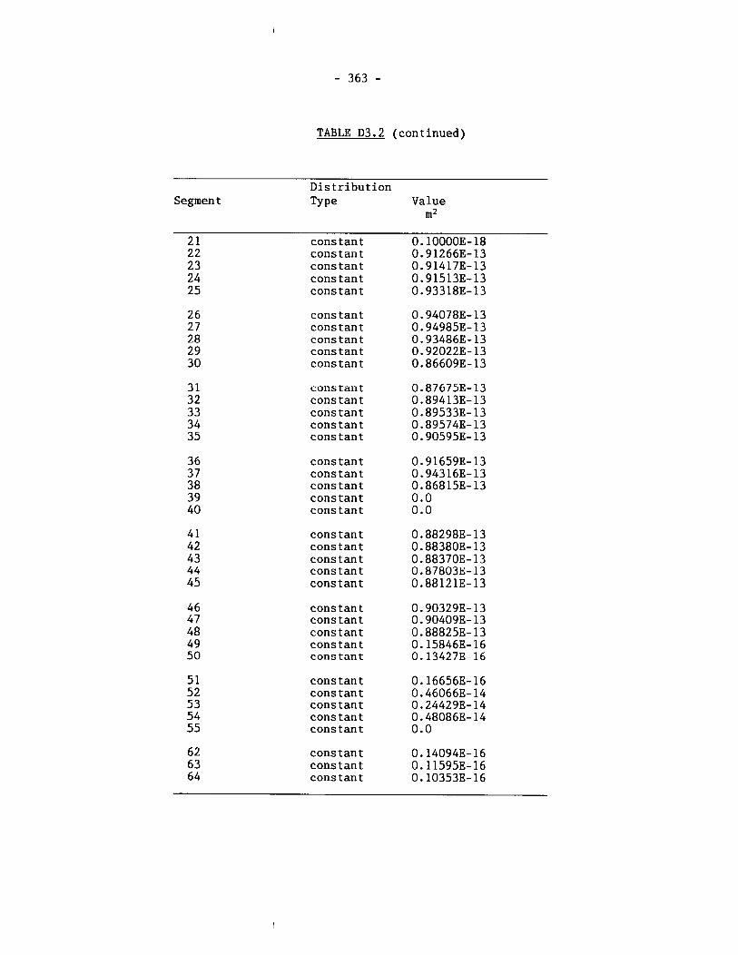
TABLE D3.2 (continued)
Distribution Segment TY pe Value
m2
2 1 cons tan t 0.100003-18 22 cons tan t 0.912663-13 2 3 constant 0.914173-13 24 cons tan t 0.915133-13 25 constant 0.933183-13
constant 0.940783-13 cons tan t 0.949853-13 constant 0.934863-13 constant 0.920223-13 constant 0.866093-13
constant 0.876753-13 cons tan t 0.894133-13 cons tan t 0.895333-13 cons tan t 0.895743-13 cons tan t 0.905953-13
cons tan t 0.916593-13 cons tan t 0.943163-13 constant 0.868153-13 constant 0.0 constant 0.0
cons tan t 0.882983-13 constant 0.883803-13 constant 0.883703-13 constant 0.878033-13 constant 0.881213-13
cons tan t 0.903293-13 constant 0.904093-13 cons tan t 0.888253-13 constant 0.158463-16 constant 0.134273-16
5 1 constant 0.166563-16 5 2 constant 0.460663-14 5 3 cons tan t 0.244293-14 5 4 cons tan t 0.480863-14 5 5 constant 0.0
constant 0.14094E-16 constant 0.11595E-16 constant 0.10353E-16
D.3.3 PERMEABILITY OF THE OVERBURDEN AND COMPACTED SEDIMENT
Hydraulic conductivity values for overburden deposits of the WRA were obtained from sixty-three single-well hydraulic response tests made in groundwater monitoring wells located on the URL lease area and at other grid areas at the WRA (Betcher 1983, Thorne 1990). The field test data were analyzed using the methods of Hvorslev (Freeze and Cherry 1979). Since these groundwater monitoring wells are completed in three of the major surficial deposit units of the WRA, clay, silty-clay, and till, they provide a representative estimate of the bulk hydraulic conductivity of overburden deposits. The hydraulic conductivity values have been converted to permeability values and these range from 8.55 x 10-l8 m2 to 3.15 x lO-I3 m2. They appear to be lognormally distributed with a geometric mean of 1.28 x 10-l5 m2 and a geometric standard deviation of 18.4.
For the postclosure assessment the overburden permeability has been assumed to be lognormally distributed with geometric mean of 1.28 x 10-Is m2, a geometric standard deviation of 18.4, a lower bound of between 1.60 x 10-l5 m2 and 4.78 x 10-l5 m2, and a upper bound of 2.1 x 10-l2 m2. (Table D3.3)
The reason for the lower bound is as follows: SYVAC3-CC3 assumes that the hydraulic head values at the ground surface and at the bottom of the upper- most rock zone calculated using MOTIF are unaffected when part of this rock zone is replaced by a layer of overburden or a layer of sediment. The groundwater velocities in all three layers are adjusted according to the permeability and thickness of the layers. If the overburden or sediment has lower permeability than the uppermost rock zone, then the groundwater velocity will be reduced. In reality, the hydraulic head at the bottom of the rock zone would become higher. In order to avoid under-prediction of the groundwater velocity through the geosphere by the GEONET model, it is necessary to limit the permeability of the overburden (or sediment) layers to values greater than or equal to that of the uppermost rock zone.
It must be noted that an error was made in assigning the lower bound for the overburden permeability at the Pinawa Channel. This error is of no consequence as the Pinawa Channel discharge has virtually no impact on the overall assessment. A value of 1.60 x 10-l5 m2 was used instead of the correct value of 2.44 x 10-l5 m2. The upper bound corresponds to the upper limit for the permeability of silt, as reported by Freeze and Cherry (1979).
The sediment permeability is assumed to be that for silty sand reported by Freeze and Cherry (1979) as no better estimates are available. The perme- ability is assumed to be lognormally distributed with a geometric mean of 10-l2 m2, a geometric standard deviation of 10 m2, a lower bound of 10-l4 m2, an upper bound of 10-10 m2, and is inversely correlated with the com- pacted sediment thickness with a correlation coefficient of -0.9.
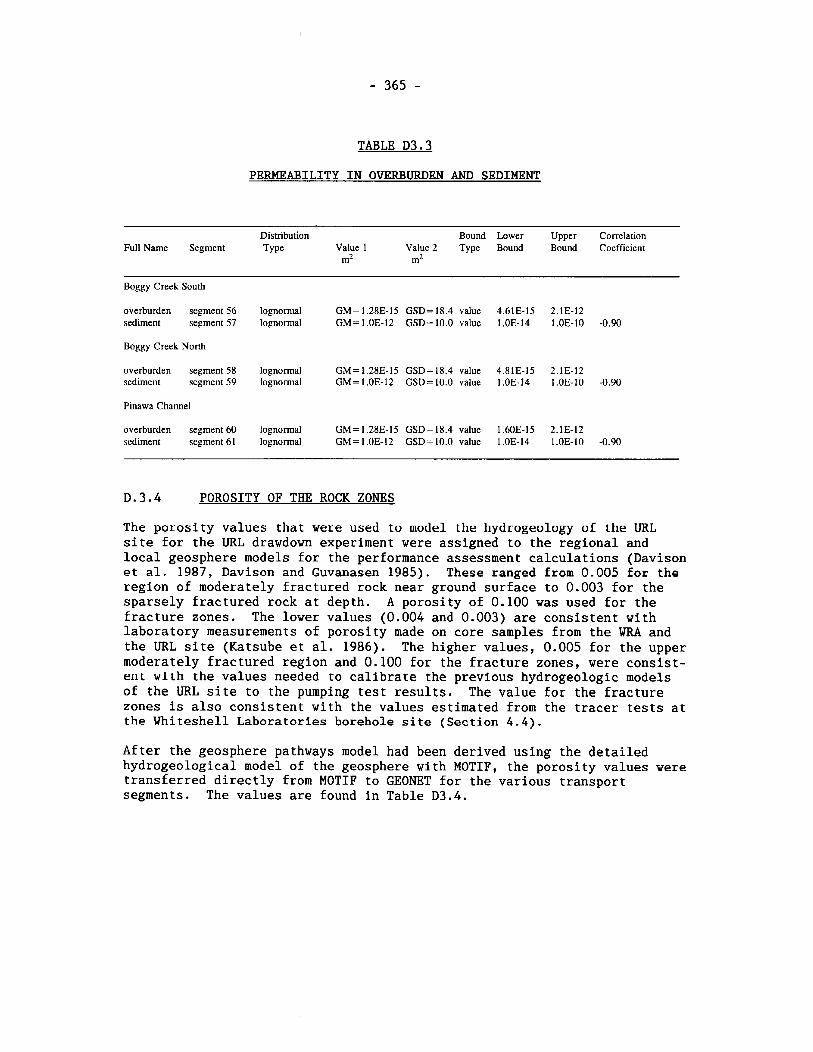
TABLE D3.3
PERMEABILITY IN OVERBURDEN AND SEDIMENT
Full Name Segment Distribution Type
Bound Lower Upper Correlation Value 1 Value 2 Type Bound Bound Coefficient
m2 m2
Boggy Creek South
overburden segment 56 sediment segment 57
Boggy Creek North
overburden segment 58 sediment segment 59
lognormal GM=1.28E-15 GSD=18.4 value 4.61E-15 2.1E-12 lognormal GM= 1.OE-12 GSD= 10.0 value 1.OE-14 1.OE-10 -0.90
lognormal GM= 1.28E-15 GSD= 18.4 value 4.81E-15 2.1E-12 lognormal GM= 1.OE-12 GSD= 10.0 value 1.OE-14 1.OE-10 -0.90
Pinawa Channel
overburden segment 60 lognormal CiM=1.28E-15 CiSD=18.4 value 1.60E-15 2.1E-12 sediment segment 61 lognormal GM= 1.OE-12 GSD=lO.O value 1.OE-14 1.OE-10 -0.90
D.3.4 POROSITY OF THE ROCK ZONES
The porosity values that were used to model the hydrogeology of the URL site for the URL drawdown experiment were assigned to the regional and local geosphere models for the performance assessment calculations (Davison et al. 1 9 8 7 , Davison and Guvanasen 1 9 8 5 ) . These ranged from 0.005 for the region of moderately fractured rock near ground surface to 0.003 for the sparsely fractured rock at depth. A porosity of 0.100 was used for the fracture zones. The lower values (0.004 and 0.003) are consistent with laboratory measurements of porosity made on core samples from the WRA and the URL site (Katsube et al. 1986). The higher values, 0.005 for the upper moderately fractured region and 0.100 for the fracture zones, were consist- ent with the values needed to calibrate the previous hydrogeologic models of the URL site to the pumping test results. The value for the fracture zones is also consistent with the values estimated from the tracer tests at the Whiteshell Laboratories borehole site (Section 4 . 4 ) .
After the geosphere pathways model had been derived using the detailed hydrogeological model of the geosphere with MOTIF, the porosity values were transferred directly from MOTIF to GEONET for the various transport segments. The values are found in Table D3.4.
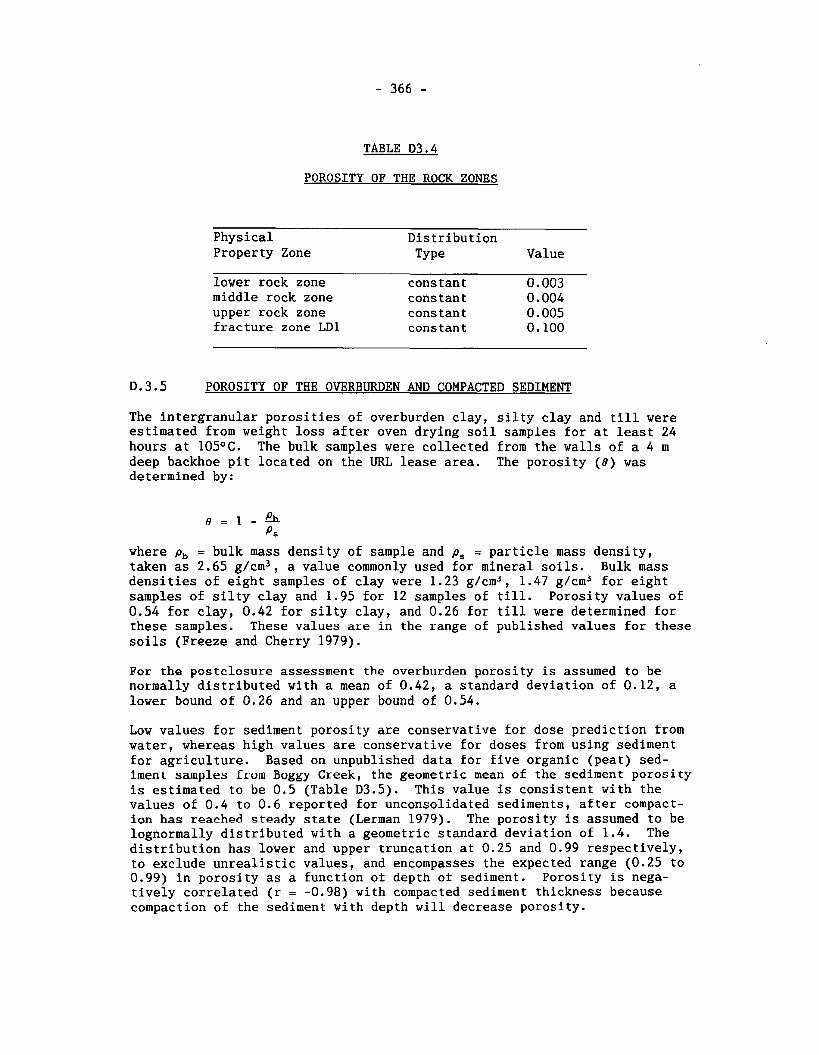
TABLE D3.4
POROSITY OF THE ROCK ZONES
Physical Distribution Property Zone TY pe Value
lower rock zone cons tan t 0.003 middle rock zone cons tan t 0.004 upper rock zone cons tan t 0.005 fracture zone LD1 cons tan t 0.100
D.3.5 POROSITY OF THE OVERBURDEN AND COMPACTED SEDIMENT
The intergranular porosities of overburden clay, silty clay and till were estimated from weight loss after oven drying soil samples for at least 24 hours at 105OC. The bulk samples were collected from the walls of a 4 m deep backhoe pit located on the URL lease area. The porosity ( 8 ) was determined by:
where p, = bulk mass density of sample and p, = particle mass density, taken as 2.65 g/cm3, a value commonly used for mineral soils. Bulk mass densities of eight samples of clay were 1.23 g/cm3, 1.47 g/cm3 for eight samples of silty clay and 1.95 for 12 samples of till. Porosity values of 0.54 for clay, 0.42 for silty clay, and 0.26 for till were determined for these samples. These values are in the range of published values for these soils (Freeze and Cherry 1979).
For the postclosure assessment the overburden porosity is assumed to be normally distributed with a mean of 0.42, a standard deviation of 0.12, a lower bound of 0.26 and an upper bound of 0.54.
Low values for sediment porosity are conservative for dose prediction from water, whereas high values are conservative for doses from using sediment for agriculture. Based on unpublished data for five organic (peat) sed- iment samples from Boggy Creek, the geometric mean of the sediment porosity is estimated to be 0.5 (Table D3.5). This value is consistent with the values of 0.4 to 0.6 reported for unconsolidated sediments, after compact- ion has reached steady state (Lerman 1979). The porosity is assumed to be lognormally distributed with a geometric standard deviation of 1.4. The distribution has lower and upper truncation at 0.25 and 0.99 respectively, to exclude unrealistic values, and encompasses the expected range (0.25 to 0.99) in porosity as a function of depth of sediment. Porosity is nega- tively correlated (r = -0.98) with compacted sediment thickness because compaction of the sediment with depth will decrease porosity.

- 367 -
TABLE D3.5
POROSITY OF THE OVERBURDEN AND SEDIMENT
Physical Distribution Bound Lower Upper Correlation Property Zone TY pe Value 1 Value 2 Type Bound Bound Coefficient
overburden Normal p=0.42 0=0.12 Value 0.26 0.54
sediment
Boggy Crcck North lognormal CM=0.5 GSD-1.4 valuc 0.25 0.99 0.98
Boggy Creek South lognormal GM=0.5 GSD= 1.4 value 0.25 0.99 -0.98
Pinawa Channel lognormal GM=0.5 GSD=1.4 value 0.25 0.99 -0 98
D.3.6 GKDUNDWATER VELOCITY SCALING FACTOR
The groundwater velocity scaling factor is used to deal with uncertainties in the groundwater velocities within the GEONET network. The network model is not a fully-coupled groundwater flow model. It is a groundwater path- ways model, representing those pathways through the geosphere from the vault that are determined by independent simulations with our fully-coupled groundwater flow model MOTIF. In order to ensure conservation of mass in our network model, we have specified that the groundwater velocities in the network model must be perfectly correlated, so that if the velocity is increased in one pathways segment, the velocities in connecting segments must be similarly increased. This ensures: 1) a fluid mass balance is maintained in GEONET calculations, and 2) the GEONET pathways always faith- fully represent the spatial arrangement of MOTIF pathways. If we allowed the groundwater velocity to vary independently in different GEONET seg- ments, fluid mass balance would not always be maintained and the GEONET pathways would not always be consistent with the groundwater flow paths determined by the MOTIF simulations of groundwater flow conditions in the geosphere.
Our detailed sensitivity analysis calculations with MOTIF show that the heat from the disposal vault will cause small changes in the groundwater velocities in the surrounding geosphere during the postclosure period (Chan et al. 1986). The velocity scaling factor allows these effects to be re- flected in the performance assessment calculations with GEONET. In ad- dition, the velocity scaling factor accounts for uncertainty in the ground- water velocity due to uncertainty in the permeability distribution used in MOTIF. This uncertainty in the permeability estimate is due to equipment and analysis methods.
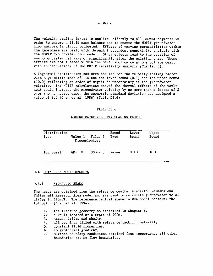
The velocity scaling factor is applied uniformly to all GEONET segments in order to ensure a fluid mass balance and to ensure the MOTIF groundwater flow network is always reflected. Effects of varying permeabilities within the geosphere are dealt with through independent sensitivity analysis with the MOTIF groundwater flow model. Other effects lead to the creation of new groundwater pathways or significantly alter the existing ones. These effects are not treated within the SYVAC3-CC3 calculations but are dealt with in discussions of the MOTIF sensitivity analysis (Chapter 6).
A lognormal distribution has been assumed for the velocity scaling factor with a geometric mean of 1.0 and the lower bound (0.1) and the upper bound (10.0) reflecting an order of magnitude uncertainty in the groundwater velocity. The MOTIF calculations showed the thermal effects of the vault heat would increase the groundwater velocity by no more than a factor of 2 over the nonheated case, the geometric standard deviation was assigned a value of 2.0 (Chan et al. 1986) (Table D3.6).
TABLE D3.6
GROUND WATER VELOCITY SCALING FACTOR
Distribution Bound Lower Upper Type Value 1 Value 2 Type Bound Bound
Dimensionless
lognormal GM=1.0 GSD=2.0 value 0.10 lU.U
D.4 DATA FROM MOTIF RESULTS
D.4.1 HYDRAULIC HEADS
The heads are obtained from the reference central scenario 3-dimensional Whiteshell Research Area model and are used to calculate groundwater velo- cities in GEONET. The reference central scenario WRA model contains the following (Chan et al. 1994);
the fracture geometry as described in Chapter 6, a vault located at a depth of 500111, access drifts and shafts, all openings filled with reference backfill material, constant fluid properties, no geothermal gradient, surface boundary conditions obtained from topography, all other boundaries are no flow boundaries,
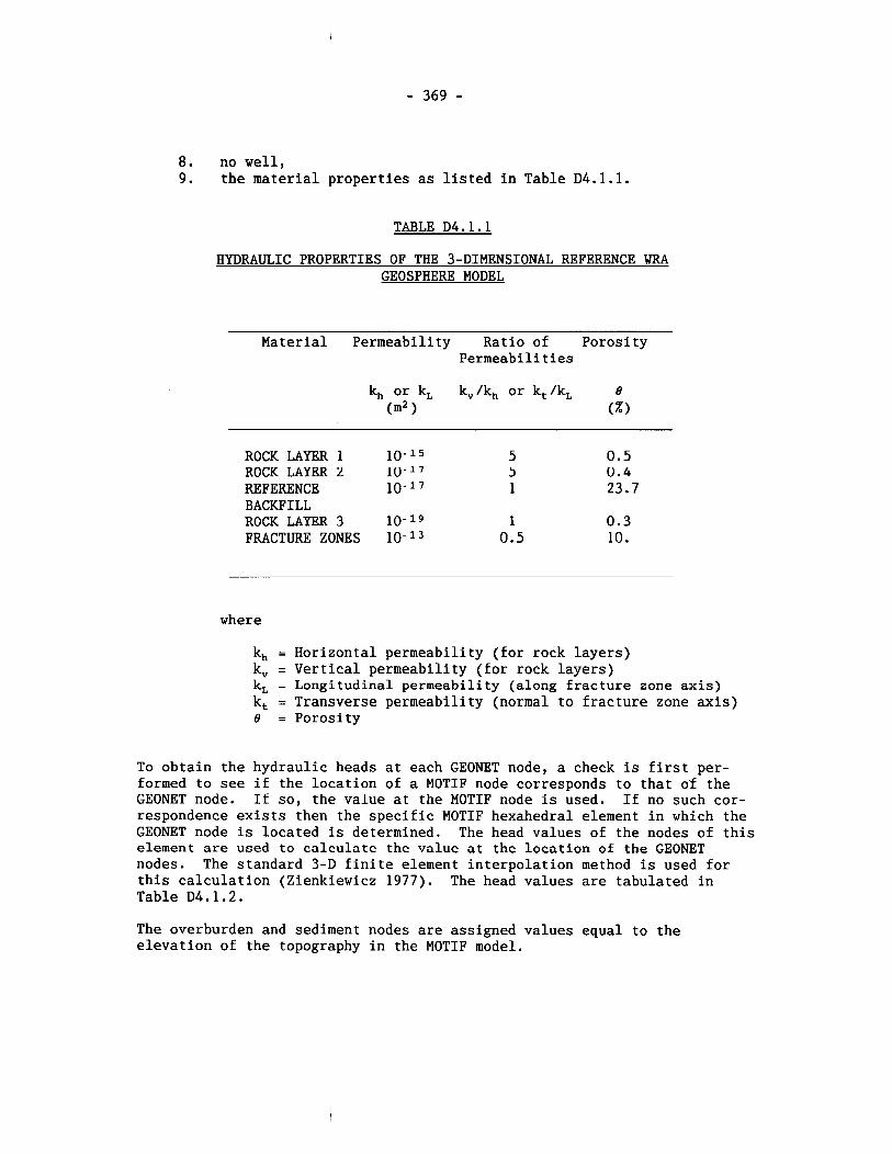
8. no well, 9. the material properties as listed in Table D4.1.1.
TABLE D4.1.1
HYDRAULIC PROPERTIES OF THE 3-DIMENSIONAL REFERENCE GEOSPHERE MODEL
Material Permeability Ratio of Porosity Permeabilities
ROCK LAYER 1 10-15 5 0.5 ROCK LAYER 2 10-l7 5 0.4 REFERENCE 10- 1 23.7 BACKFILL ROCK LAYER 3 10- l9 1 0.3 FRACTURE ZONES 10- 0.5 10.
where
kh = Horizontal permeability (for rock layers) k, = Vertical permeability (for rock layers) k, - Longitudinal permeability (along fracture zone axis) kt = Transverse permeability (normal to fracture zone axis) 6 = Porosity
To obtain the hydraulic heads at each GEONET node, a check is first per- formed to see if the location of a MOTIF node corresponds to tha,t o'f the GEONET node. If so, the value at the MOTIF node is used. If no such cor- respondence exists then the specific MOTIF hexahedral element in which the GEONET node is located is determined. The head values of the nodes of this element are used to calculate the value at the location of the GEONET nodes. The standard 3-D finite element interpolation method is used for this calculation (Zienkiewicz 1977). The head values are tabula.ted in Table D4.1.2.
The overburden and sediment nodes are assigned values equal to the elevation of the topography in the MOTIF model.
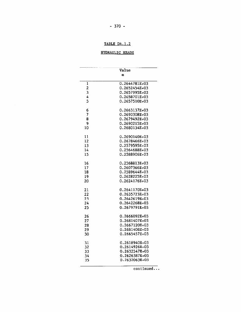
TABLE D4.1.2
HYDRAULIC HEADS
Value m
continued ...
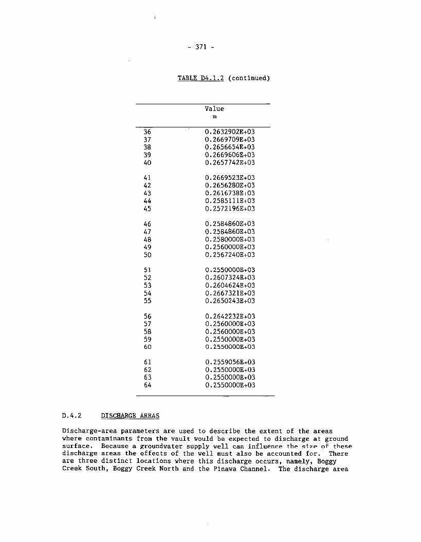
TABLE D4.1.2 (continued)
Value m
D.4.2 DISCHARGE AREAS
Discharge-area parameters are used to describe the extent of the areas where contaminants from the vault would be expected to discharge at ground surface. Because a groundwater supply well can influence the s ize of these discharge areas the effects of the well must also be accounted for. There are three distinct locations where this discharge occurs, namely, Boggy Creek South, Boggy Creek North and the Pinawa Channel. The discharge area
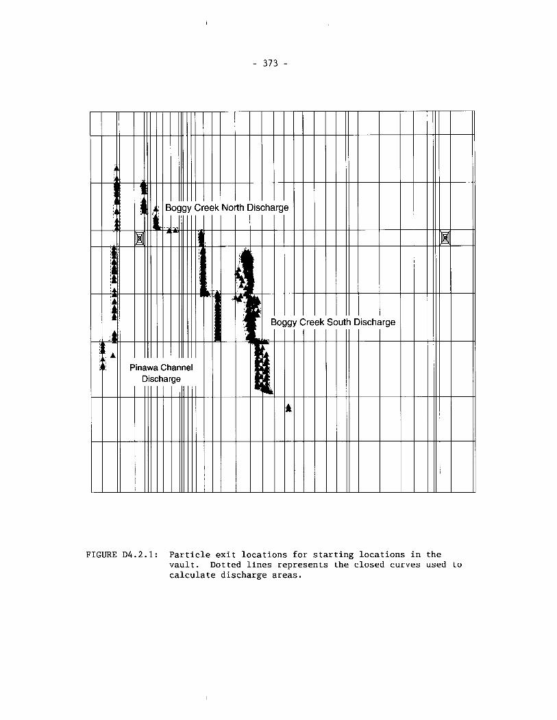
FIGURE D4.2.1: Particle exit locations for starting locations in the vault. Dotted lines represents Lhe closed curvtts used to calculate discharge areas.
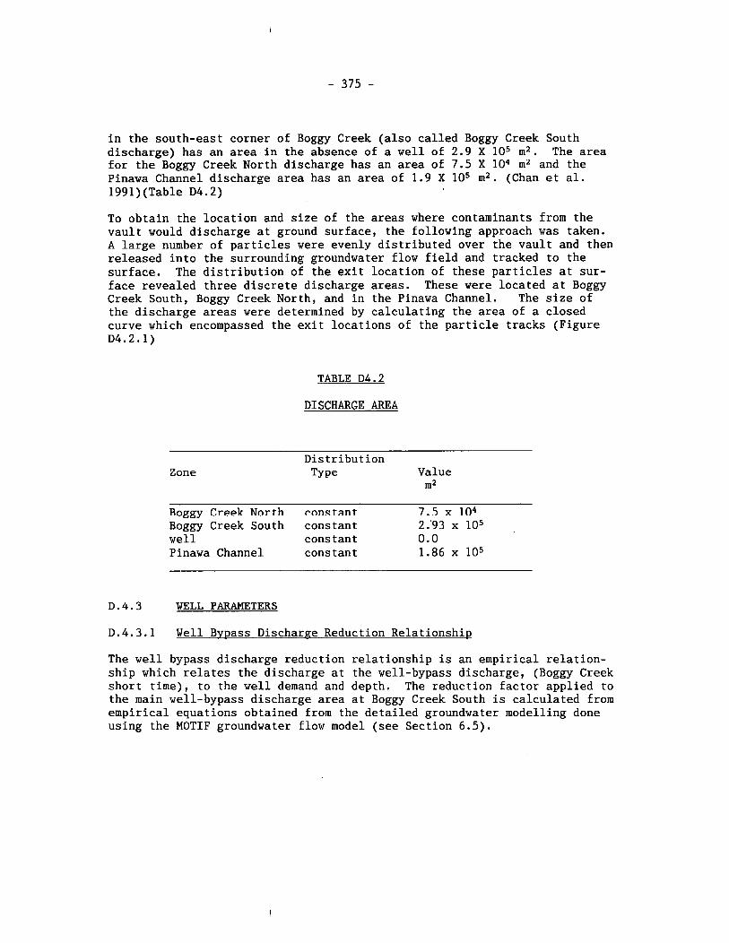
in the south-east corner of Boggy Creek (also called Boggy Creek South discharge) has an area in the absence of a well of 2.9 X 10⁵ m2. The area for the Boggy Creek North discharge has an area of 7.5 X lo4 m2 and the Pinawa Channel discharge area has an area of 1.9 X lo5 m2. (Chan et al. 1991)(Table D4.2)
To obtain the location and size of the areas where contaminants from the vault would discharge at ground surface, the following approach was taken. A large number of particles were evenly distributed over the vault and then released into the surrounding groundwater flow field and tracked to the surface. The distribution of the exit location of these particles at sur- face revealed three discrete discharge areas. These were located at Boggy Creek South, Boggy Creek North, and in the Pinawa Channel. The size of the discharge areas were determined by calculating the area of a closed curve which encompassed the exit locations of the particle track:; (Figure D4.2.1)
TABLE D4.2
DISCHARGE AREA
Distribution Zone Type Value
m2
Boggy Creek North constant 7.5 x lo4 Boggy Creek South constant 2.93 x lo5 well constant 0.0 Pinawa Channel constant 1.86 lo5
D.4.3 WELL PARAMETERS
D.4.3.1 Well Bypass Discharge Reduction Relationship
The well bypass discharge reduction relationship is an empirical relation- ship which relates the discharge at the well-bypass discharge, (Boggy Creek short time), to the well demand and depth. The reduction factor applied to the main well-bypass discharge area at Boggy Creek South is calculated from empirical equations obtained from the detailed groundwater modelling done using the MOTIF groundwater flow model (see Section 6.5).
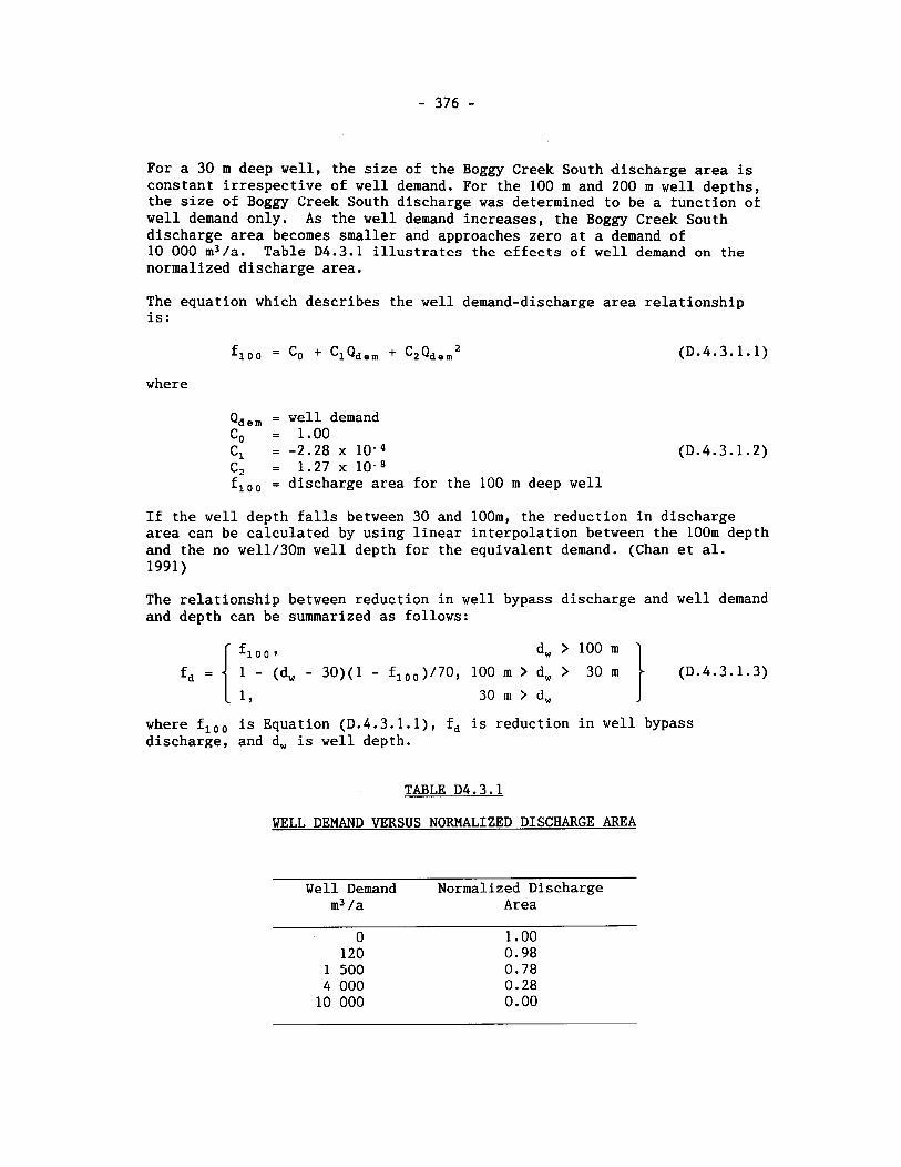
For a 30 m deep well, the size of the Boggy Creek South .discharge area is constant irrespective of well demand. For the 100 m and 200 m well depths, the size of Boggy Creek South discharge was determined to be a function of well demand only. As the well demand increases, the Boggy Creek South discharge area becomes smaller and approaches zero at a demand of 10 000 m3/a. Table D4.3.1 illustrates the effects of well demand on the normalized discharge area.
The equation which describes the well demand-discharge area relationship is:
where
Q d e m = well demand C, = 1.00 C, =-2.28~10-4 (D.4.3.1.2) C, = 1.27 x f,,, = discharge area for the 100 m deep well
If the well depth falls between 30 and loom, the reduction in discharge area can be calculated by using linear interpolation between the lOOm depth and the no well/30m well depth for the equivalent demand. (Chan et al. 1991)
The relationship between reduction in well bypass discharge and well demand and depth can be summarized as follows:
where f,,, is Equation (D.4.3.1.1), fd is reduction in well bypass discharge, and d, is well depth.
TABLE D4.3.1
WELL DEMAND VERSUS NORMALIZED DISCHARGE AREA
Well Demand Normalized Discharge m3 /a Area

D.4.3.2 Distance to Drawdown Nodes
The parameter values used tor the distances from the aquifer node in the fracture zone to the first and second drawdown nodes are 5 and 75 m res- pectively (Figure D4.3.2.1). These nodes are upstream of the well1 and are used to simulate the groundwater drawdown near the pumping well in the fracture zone. This particular choice of values was chosen to approximate the steepness of the drawdown cone in the vicinity of the well. Referring to Figure D4.3.2.1, which shows predicted hydraulic head versus distance along fracture zone LD1 and passing through the 200-m-deep well pumping at 30 000 m3/a, it is seen that the slope of the drawdown cone based on ana- lytical predictions (dashed line) is very steep near the well, but quite rapidly and asymtotically approaches the no-well slope further away. The exact choice of these two node locations is somewhat arbitrary. However the introduction of these two drawdown nodes significantly improves the accuracy by which groundwater velocity is calculated between the well node and the well collection node. This is demonstrated in Figure D4.3.2.1, where the average hydraulic gradients calculated over linear segments 1, 2 and 3, much more accurately mimics the profile of the drawdown cone than does the average hydraulic gradient calculated over the single segment 4 (Chan & Nakka 1994).
- _ - - - -
node First drawdown ',
No well - Analytical - - -
75 1 I I I I I I
0. I ---I
200 400 600 800 1000 1200 1400 1600 Distance along dip of fracture zone LD1 (rn)
FIGURE D4.3.2.1: Plot of hydraulic head versus distance along dip of fracture zone LD1 and passing through the 200-~n-deep well having a well demand of 30 000 m3/a. Analytical calculations are shown with the position of the well node, the well collection node and the two drawdown nodes.
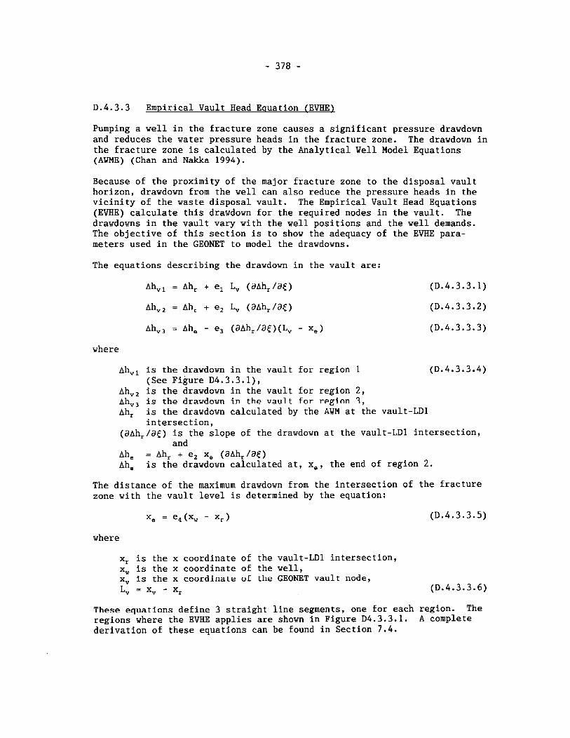
D.4.3.3 Empirical Vault Head Equation (EWE)
Pumping a well in the fracture zone causes a significant pressure drawdown and reduces the water pressure heads in the fracture zone. The drawdown in the fracture zone is calculated by the Analytical Well Model Equations (AWME) (Chan and Nakka 1994).
Because of the proximity of the major fracture zone to the disposal vault horizon, drawdown from the well can also reduce the pressure heads in the vicinity of the waste disposal vault. The Empirical Vault Head Equations (EVHE) calculate this drawdown for the required nodes in the vault. The drawdowns in the vault vary with the well positions and the well demands. The objective of this section is to show the adequacy of the EVHE para- meters used in the GEONET to model the drawdowns.
The equations describing the drawdown in the vault are:
Ah,, = Ah, + el L, (aAh,/aC)
Ah,, = Ah, + e2 L, (aAh,/a<)
Ah,, = Ah, - e, (aAh, /aC)(L, - x,)
where
Ahvl is the drawdown in the vault for region 1 (See Figure D4.3.3.1),
Ah,, is the drawdown in the vault for region 2, Ah,, is the drawdown in the vault for region 3, Ah, is the drawdown calculated by the AWM at the vault-LD1
intersection, (aAh,/aE) is the slope of the drawdown at the vault-LD1 intersection,
and Ah, = Ah, + e, x, (aAh, /aC) Ah, is the drawdown calculated at, x,, the end of region 2.
The distance of the maximum drawdown from the intersection of the fracture zone with the vault level is determined by the equation:
where
x, is the x coordinate of the vault-LD1 intersection, x, is the x coordinate of the well, x, is the x coordinate of the GEONET vault node, Lv = X, - X, (D.4.3.3.6)
These equations define 3 straight line segments, one for each region. The regions where the EVHE applies are shown in Figure D4.3.3.1. A complete derivation of these equations can be found in Section 7.4.
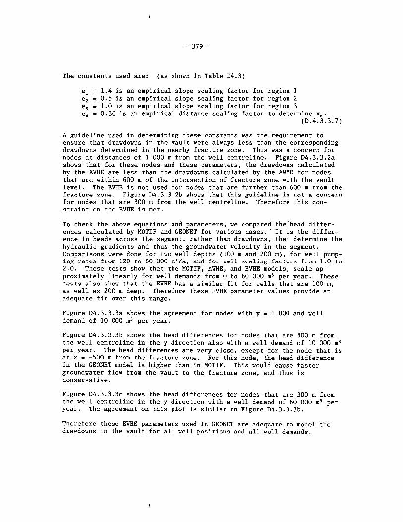
The constants used are: (as shown in Table D4.3)
el = 1.4 is an empirical slope scaling factor for region 1 e, = 0.5 is an empirical slope scaling factor for region 2 e3 = 1.0 is an empirical slope scaling factor for region 3 el = 0.36 is an empirical distance scaling factor to determine x,.
(D.4.3.3.7)
A guideline used in determining these constants was the requirement to ensure that drawdowns in the vault were always less than the corresponding drawdowns determined in the nearby fracture zone. This was a concern for nodes at distances of 1 000 m from the well centreline. Figure D4.3.3.2a shows that for these nodes and these parameters, the drawdowns ctalculated by the EVHE are less than the drawdowns calculated by the AWME for nodes that are within 600 m of the intersection of fracture zone with the vault level. The EVHE is not used for nodes that are further than 600 m from the fracture zone. Figure D4.3.3.2b shows that this guideline is not a concern for nodes that are 300 m from the well centreline. Therefore this con- straint on the EVHE is met.
To check the above equations and parameters, we compared the head differ- ences calculated by MOTIF and GEONET for various cases. It is the differ- ence in heads across the segment, rather than drawdowns, that determine the hydraulic gradients and thus the groundwater velocity in the segment. Comparisons were done for two well depths (100 m and 200 m), for well pump- ing rates from 120 to 60 000 m3/a, and for well scaling factors from 1.0 to 2.0. These tests show that the MOTIF, AWME, and EVHE models, scale ap- proximately linearly for well demands from 0 to 60 000 m3 per year. These tests also show that the EVHE has a similar fit for wells that are 100 m, as well as 200 m deep. Therefore these EVHE parameter values provide an adequate fit over this range.
Figure D4.3.3.3a shows the agreement for nodes with y = 1 000 and well demand of 10 000 m3 per year.
Figure D4.3.3.3b shows the head differences for nodes that are 300 m from the well centreline in the y direction also with a well demand of 10 000 m3 per year. The head differences are very close, except for the node that is at x = -500 m from the fracture zone. For this node, the head difference in the GEONET model is higher than in MOTIF. This would cause faster groundwater flow from the vault to the fracture zone, and thus is conservative.
Figure D4.3.3.3~ shows the head differences for nodes that are 2\00 m from the well centreline in the y direction with a well demand of 60 000 m3 per year. The agreement on this plot is similar to Figure D4.3.3.3b.
Therefore these EVHE parameters used in GEONET are adequate to model the drawdowns in the vault for all well positions and all well demands.
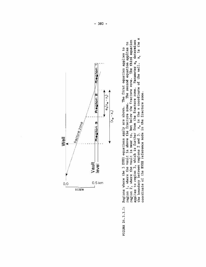
0.0 0.5 km - scale
h h 0 * w 7 0 aJ
aJ r u h C a J U 1 o c x r N r k u
W a J d 015 A h LI o a r w S A C r a r r e a J 0 P (d R ' * 5 h r o 3 w 7 k X . 2 n1 D w
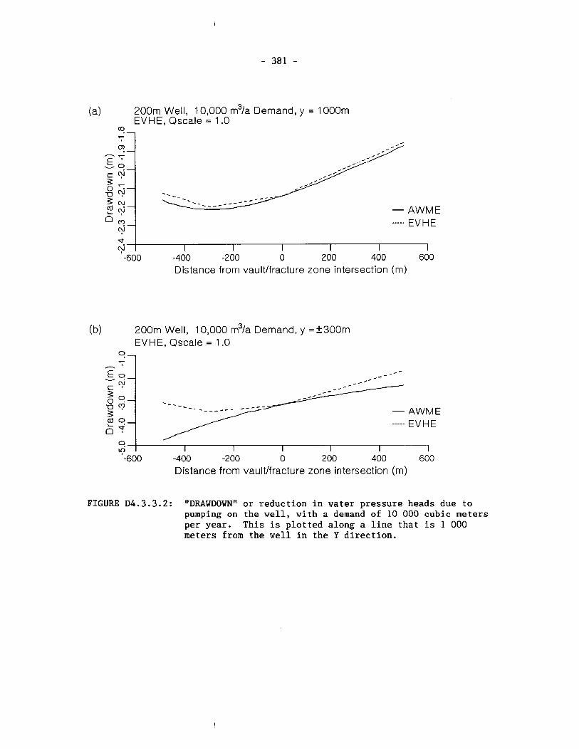
200m Well, 10,000 m3/a Demand, y = 1000m EVHE, Qscale = 1.0
-_-- - AWME ----- EV H E
-600 -400 -200 0 200 400 600 Distance from vaultlfracture zone intersection (m)
Distance from vault/fracture zone intersection (m)
(b) 200m Well, 10,000 m3/a Demand, y = t300m EVHE, Qscale = 1 -0
9-
FIGURE D 4 . 3 . 3 . 2 : l'DRAWDOWN" or reduction in water pressure heads due to pumping on the well, with a demand of 10 000 cubic meters per year. This is plotted along a line that is 1 000 meters from the well in the Y direction.
7
h
E - 9 - * - -
- - ,..-- c qJ g 9- n c? 3 - AWhllE 9 0- 0 P
----- EV H E
2
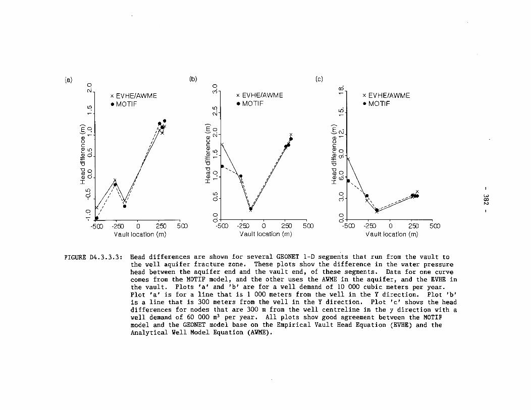
x EVHE/AWME MOTIF MOTIF
21 x EVHEIAWME
MOTIF
Vault location (m) Vault location (m) Vault location (m)
FIGURE D4.3.3.3: Head differences are shown for several GEONET 1-D segments that run from the vault to the well aquifer fracture zone. These plots show the difference in the water pressure head between the aquifer end and the vault end, of these segments. Data for one curve comes from the MOTIF model, and the other uses the AWME in the aquifer, and the EVHE in the vault. Plots 'af and 'b' are for a well demand of 10 000 cubic meters per year. Plot 'af is for a line that is 1 000 meters from the well in the Y direction. Plot 'b' is a line that is 300 meters from the well in the Y direction. Plot 'cf shows the head differences for nodes that are 300 m from the well centreline in the y direction with a well demand of 60 000 m3 per year. All plots show good agreement between the MOTIF model and the GEONET model base on the Empirical Vault Head Equation (EVHE) and the Analytical Well Model Equation (AWME).
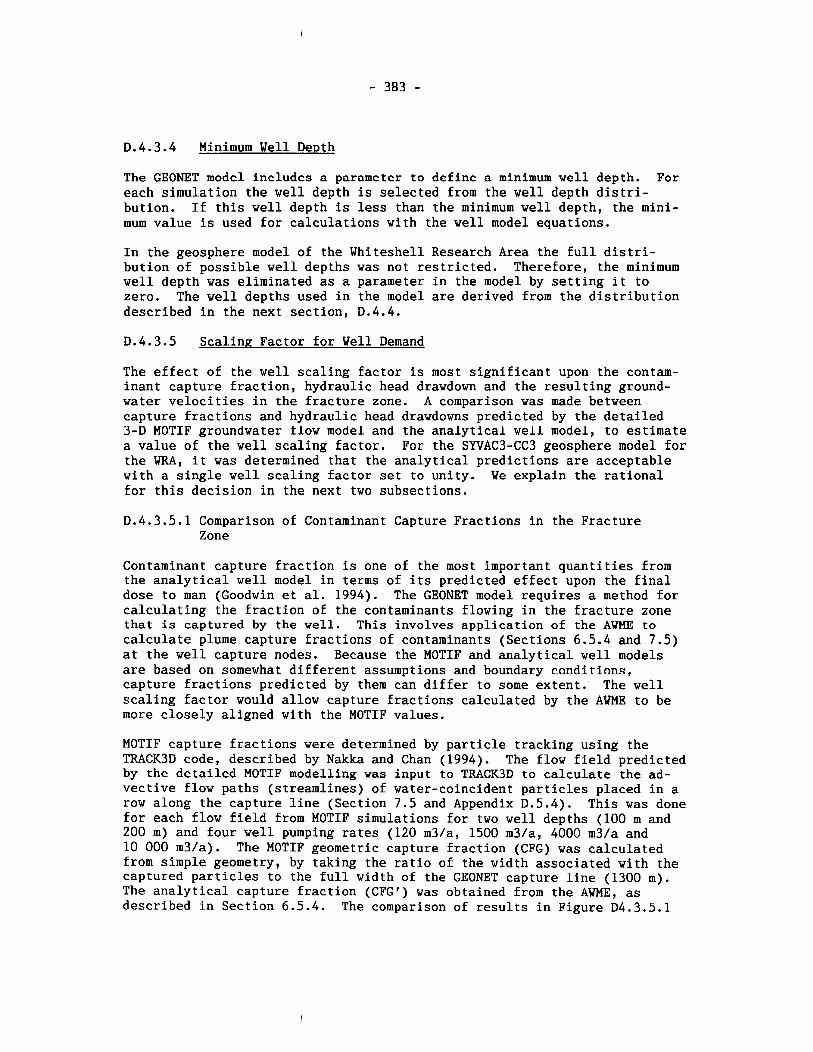
D.4.3.4 Minimum Well Depth
The GEONET model includes a parameter to dcfinc a minimum well depth. For each simulation the well depth is selected from the well depth distri- bution. If this well depth is less than the minimum well depth, the mini- mum value is used for calculations with the well model equations.
In the geosphere model of the Whiteshell Research Area the full distri- bution of possible well depths was not restricted. Therefore, the minimum well depth was eliminated as a parameter in the model by setting it to zero. The well depths used in the model are derived from the distribution described in the next section, D.4.4.
D.4.3.5 Scaling Factor for Well Demand
The effect of the well scaling factor is most significant upon the contam- inant capture fraction, hydraulic head drawdown and the resulting ground- water velocities in the fracture zone. A comparison was made between capture fractions and hydraulic head drawdowns predicted by the detailed 3-D MOTIF groundwater flow model and the analytical well model, to estimate a value of the well scaling factor. For the SYVAC3-CC3 geosphere model for the WRA, it was determined that the analytical predictions are acceptable with a single well scaling factor set to unity. We explain the rational for this decision in the next two subsections.
D.4.3.5.1 Comparison of Contaminant Capture Fractions in the Fracture Zone
Contaminant capture fraction is one of the most important quantities from the analytical well model in terms of its predicted effect upon the final dose to man (Goodwin et al. 1994). The GEONET model requires a method for calculating the fraction of the contaminants flowing in the fracture zone that is captured by the well. This involves application of the AWME to calculate plume capture fractions of contaminants (Sections 6.5.4 and 7.5) at the well capture nodes. Because the MOTIF and analytical well models are based on somewhat different assumptions and boundary conditions, capture fractions predicted by them can differ to some extent. 'The well scaling factor would allow capture fractions calculated by the AWME to be more closely aligned with the MOTIF values.
MOTIF capture fractions were determined by particle tracking using the TRACK3D code, described by Nakka and Chan (1994). The flow field predicted by the detailed MOTIF modelling was input to TRACK3D to calculate the ad- vective flow paths (streamlines) of water-coincident particles placed in a row along the capture line (Section 7.5 and Appendix D.5.4). This was done for each flow field from MOTIF simulations for two well depths (100 m and 200 m) and four well pumping rates (120 m3/a, 1500 m3/a, 4000 m3/a and 10 000 m3/a). The MOTIF geometric capture fraction (CFG) was calculated from simple geometry, by taking the ratio of the width associated with the captured particles to the full width of the GEONET capture line (1300 m). The analytical capture fraction (CFG') was obtained from the AWME, as described in Section 6.5.4. The comparison of results in Figure D4.3.5.1
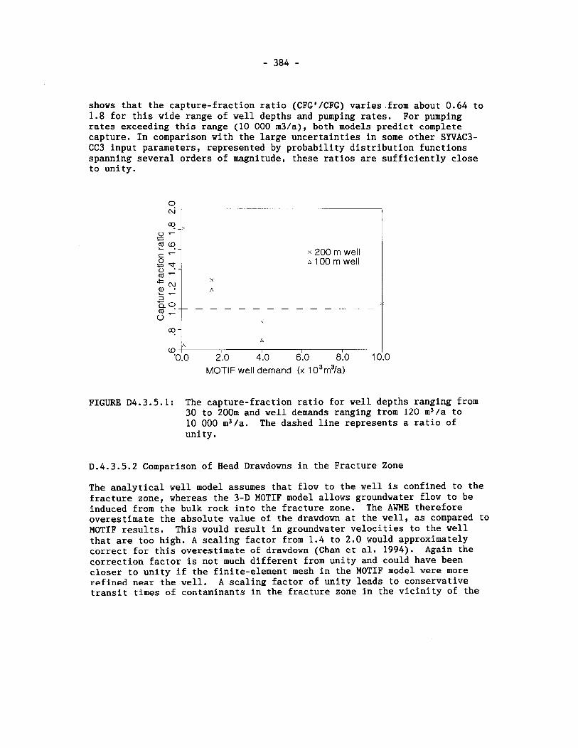
shows that the capture-fraction ratio (CFGP/CFG) varies.from about 0.64 to 1.8 for this wide range of well depths and pumping rates. For pumping rates exceeding this range (10 000 m3/a), both models predict complete capture. In comparison with the large uncertainties in some other SYVAC3- CC3 input parameters, represented by probability distribution functions spanning several orders of magnitude, these ratios are sufficiently close to unity.
x 200 m well A 100m well
FIGURE D4.3.5.1: The capture-fraction ratio for well depths ranging from 30 to 200m and well demands ranging from 120 m3/a to 10 000 m3/a. The dashed line represents a ratio of unity.
*-
D.4.3.5.2 Comparison of Head Drawdowns in the Fracture Zone
A A
The analytical well model assumes that flow to the well is confined to the fracture zone, whereas the 3-D MOTIF model allows groundwater flow to be induced from the bulk rock into the fracture zone. The AWME therefore overestimate the absolute value of the drawdown at the well, as compared to MOTIF results. This would result in groundwater velocities to the well that are too high. A scaling factor from 1.4 to 2.0 would approximately correct for this overestimate of drawdown (Chan et al. 1994). Again the correction factor is not much different from unity and could have been closer to unity if the finite-element mesh in the MOTIF model were more refined near the well. A scaling factor of unity leads to conservative transit times of contaminants in the fracture zone in the vicinity of the
*O.O I I I I
2.0 4.0 6.0 8.0 10.0 MOTIF well demand (x 1 03m3/a)
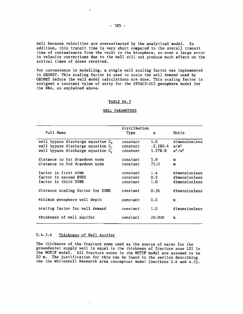
well because velocities are overestimated by the analytical model. In addition, this transit time is very short compared to the overall transit time of contaminants from the vault to the biosphere, so even a large error in velocity corrections due to the well will not produce much effect on the arrival times of doses received.
For convenience in modelling, a single well scaling factor was implemented in GEONET. This scaling factor is used to scale the well demand used by GEONET before the well model calculations are done. This scaling factor is assigned a constant value of unity for the SYVAC3-CC3 geosphere imodel for the WRA, as explained above.
TABLE D4.3
WELL PARAMETERS
Distribution Full Name TY pe a Units
well bypass discharge equation C, constant 1 .O dimensionless well bypass discharge equation C, constant -2.283-4 a/m3 well bypass discharge equation C2 constant 1.273-8 a2 /in6
distance to 1st drawdown node constant 5.0 m distance to 2nd drawdown node constant 75.0 m
factor in first EVHE factor in second EVHE factor in third EVHE
constant 1.4 dimensionless cons tan t 0.5 dimensionless constant 1 .O dimensionless
distance scaling factor for EVHE cons tan t 0.36 dimensionless
minimum geosphere well depth constant 0.0 m
scaling factor for well demand constant 1 .O dimc~nsionless
thickness of well aquifer constant 20.000 m
D.4.3.6 Thickness of Well Aquifer
The thickness of the fracture zone used as the source of water for the groundwater supply well is equal to the thickness of fracture zone LD1 in the MOTIF model. All fracture zones in the MOTIF model are assumed to be 20 m. The justification for this can be found in the section describing the the Whiteshell Research Area conceptual model (Sections 2.6 and 4.3).
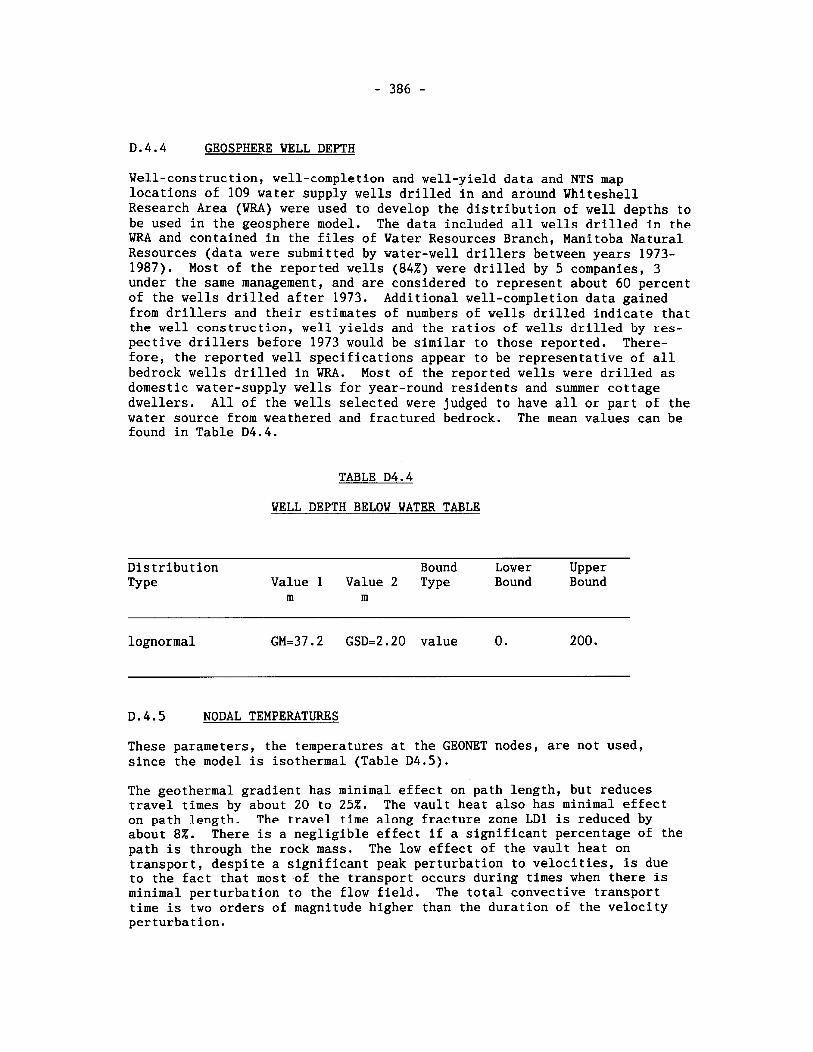
D.4.4 GEOSPHERE WELL DEPTH
Well-construction, well-completion and well-yield data and NTS map locations of 109 water supply wells drilled in and around Whiteshell Research Area (WRA) were used to develop the distribution of well depths t o be used in the geosphere model. The data included all wells drilled in the WRA and contained in the files of Water Resources Branch, Manitoba Natural Resources (data were submitted by water-well drillers between years 1973- 1987). Most of the reported wells (84%) were drilled by 5 companies, 3 under the same management, and are considered to represent about 60 percent of the wells drilled after 1973. Additional well-completion data gained from drillers and their estimates of numbers of wells drilled indicate that the well construction, well yields and the ratios of wells drilled by res- pective drillers before 1973 would be similar to those reported. There- fore, the reported well specifications appear to be representative of all bedrock wells drilled in WRA. Most of the reported wells were drilled as domestic water-supply wells for year-round residents and summer cottage dwellers. All of the wells selected were judged t o have all or part of the water source from weathered and fractured bedrock. The mean values can be found in Table D4.4.
TABLE D4.4
WELL DEPTH BELOW WATER TABLE
Distribution Bound Lower Upper TY pe Value 1 Value 2 Type Bound Bound
m m
lognormal GM=37.2 GSD=2.20 value 0. 200.
D.4.5 NODAL TEMPERATURES
These parameters, the temperatures at the GEONET nodes, are not used, since the model is isothermal (Table D4.5).
The geothermal gradient has minimal effect on path length, but reduces travel times by about 20 to 25%. The vault heat also has minimal effect on path length. The travel time along fracture zone LD1 is reduced by about 8%. There is a negligible effect if a significant percentage of the path is through the rock mass. The low effect of the vault heat on transport, despite a significant peak perturbation to velocities, is due to the fact that most of the transport occurs during times when there is minimal perturbation to the flow field. The total convective transport time is two orders of magnitude higher than the duration of the velocity perturbation.

A further explanation as to why the isothermal case was considered adequate for the geosphere model can be found in Sections 5.4 and 5.5.
TABLE D4.5
TEMPERATURES FOR ALL NODES
Distribution Full Name TY pe Value
' C
node temperature constant 6.000
TRANSPORT PROPERTIES
D.5.1 DIFFUSION COEFFICIENT AND TORTUOSITY FACTOR
D.5.1.1 Diffusion Coefficient
For the postclosure assessment the free water diffusion coeffici'ents for all dissolved species are selected from the same probability distribution. This is based on information presented in Robinson and Stokes (1959).
The values are assumed to be normally distributed with a mean of 0.047 m2/a, a s~andard deviation of 0.008 m2/a, a lower limit of 0.02 m2/a and an upper limit of 0.07 m2/a (Table D5.1).
D.5.1.2 Tortuositv Factor of the Rock Zones
Diffusion measurements have been made on rock samples taken from subsurface of the URL site and Katsube et al. (1986) have made measurements on a variety of rock samples taken from the drill cores from the WRA and the Atikokan Research Area. Measurements on Swedish and U.K. granite rock samples done by Skaguis and Neretnieks (1982, 1983) and by Bradbury et al. (1982) show a similar range of results. In the absence of a large amount of data on samples from the URL vicinity, the results on Canadia:n Shield granite samples, as reported in Katsube et al. (1986) were used to derive a distribution for the tortuosity values used in the geosphere model (Table D5.1).
Katsube et al. (1986) report tortuosity factor results for 14 samples from boreholes drilled into granitic rocks: 12 from the WN-1 and WN-2 boreholes at the WRA, 2 from the ATK-1 borehole at the Atikokan Research Area and 2 from the URL-2 borehole at the URL site of the WRA. They also report two

results for tonalite samples from the WN-2 borehole, but only the 14 samples identified as granite were used to derive a distribution for tortuosity factor for the granites at the URL site. These 14 tortuosity factor values are given in Table D5.1.2.1.
The 14 results were fitted by 7 different PDF types using a statistical fitting package known as FITDIS (Frech and OPConnor 1986) and to one additional distribution type (Triangular) by hand. The results of these fits are given in Table D5.1.2.2 and shown in Figures D.5.1.2.1 and D.5.1.2.2. In those PDFrs where a minimum value could be specified, the minimum tortuosity was assigned the value unity. This minimum value is designated by the attribute GAMMA in Table D5.1.2.2.
TABLE D5.1
DIFFUSION COEFFICIENT AND TORTUOSITY FACTOR
Physical Property Zone
Distribution Bound Lower Upper TY pe Value 1 Value 2 Value 3 Type Bound Bound
free water diffusion coefficient of all elements (m2/a) normal p=0.047 0=0.008 value 0.02 0.07
tortuosity factor
lower rock zone middle rock zone upper rock zone fracture zone LD1 overburden
triangular a=2.0 c=3.0 b=8.0 triangular a=2.0 c=3.0 b=8.0 constant a=1.0 constant a=1.0 constant a = 1.0
sediment Boggy Creek NW lognormal GM=1.2 GSD=l. l value 1.0 1.4 sediment Boggy Creek SE lognormal GM=1.2 GSD=l. l value 1.0 1.4 sediment Pinawa Channel lognormal ' GM=1.2 GSD=l. l value 1.0 1.4
The two distributions that best fit (lowest residual error) the data were the loguniform distribution and the triangular distribution. The log- uniform distribution, however, has the most probable value being the small- est value while the data should show fewer samples with the tortuosity factors of around 2 or less that are generally associated with more uncon- solidated media. This lower probability would likely become evident in the histogram if there were more samples, allowing a finer discretization of the histogram to which the distributions were fitted. For this reason, the triangular distribution was chosen as the best representation of the avail- able tortuosity data.
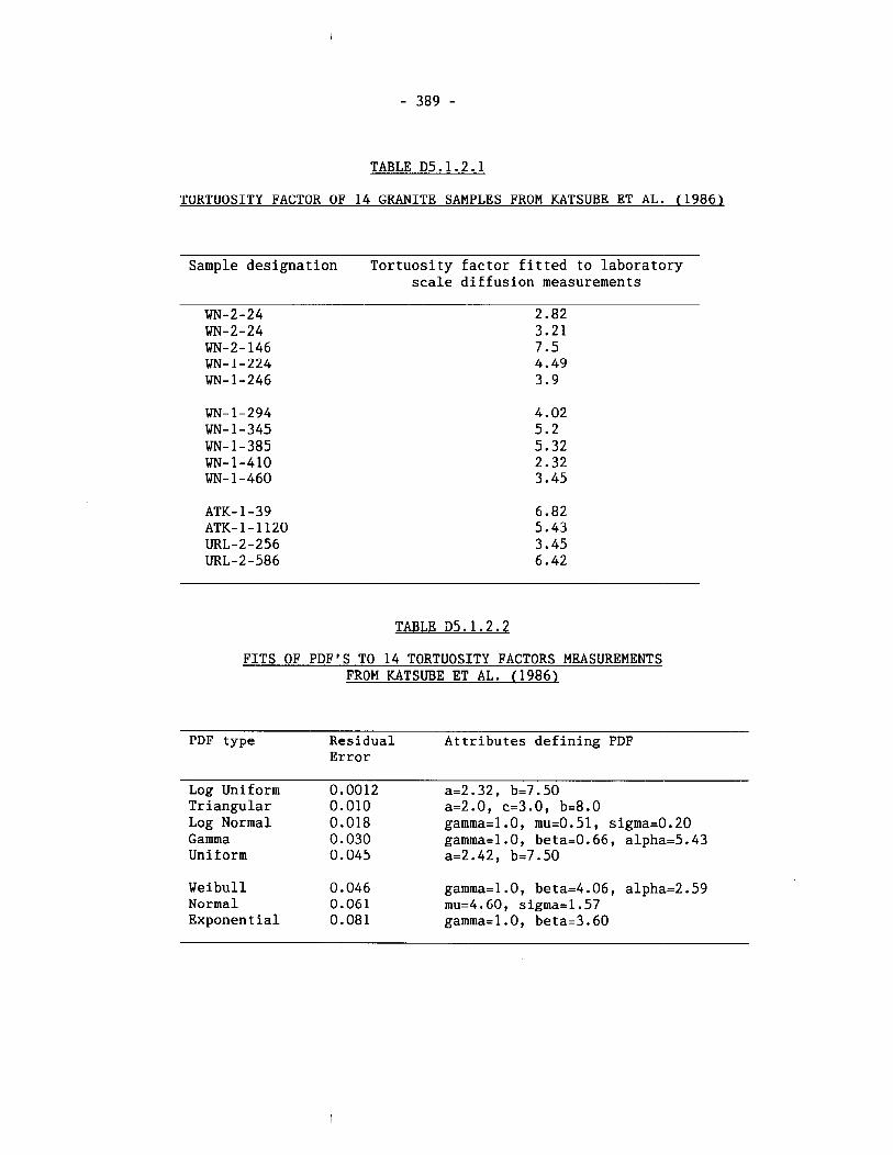
TABLE D5.1.2.1
TORTUOSITY FACTOR OF 14 GRANITE SAMPLES FROM KATSUBE ET AL. (1986)
Sample designation Tortuosity factor fitted to laboratory scale diffusion measurements
WN-2-24 2.82 WN-2-24 3.21 WN-2-146 7.5 WN- 1-224 4.49 WN-1-246 3.9
WN-1-294 WN- 1-345 WN-1-385 WN-1-410 WN- 1-460
ATK- 1-39 ATK-1-1120 URL-2-256 URL-2-586
TABLE 35.1.2.2
FITS OF PDF'S TO 14 TORTUOSITY FACTORS MEASUREMENTS FROM KATSUBE ET AL. (1986)
PDF type Residual Attributes defining PDF Error
Log Uniform 0.0012 a=2.32, b=7.50 Triangular 0.010 a=2.0, c=3.0, b=8.0 Log Normal 0.018 gamma=l.O, mu=0.51, sigma=O.20 Gamma 0.030 gamma=l.O, beta=0.66, alpha=5.43 Uniform 0.045 a=2.42, b=7.50
Weibull 0.046 gamma=l.O, beta=4.06, alpha=2.59 Normal 0.061 mu=4.60, sigrna=1.57 Exponential 0.081 gamma=l.O, beta=3.60
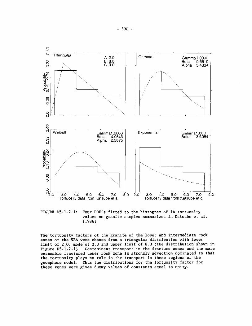
Gamma Gammal.OOOO
Alpha 5.4334
FIGURE D5.1.2.1: Four PDFrs fitted to the histogram of 14 tortuosity values on granite samples summarized in Katsube et al. (1986)
0
The tortuosity factors of the granite of the lower and intermediate rock zones at the WRA were chosen from a triangular distribution with lower limit of 2.0, mode of 3.0 and upper limit of 8.0 (the distribution shown in Figure D5.1.2.1). Contaminant transport in the fracture zones and the more permeable fractured upper rock zone is strongly advection dominated so that the tortuosity plays no role in the transport in these regions of the geosphere model. Thus the distributions for the tortuosity factor for these zones were given dummy values of constants equal to unity.
2 cu
2- & 56 - Cd
a3 i:: 8
9 a1
Tortuosity data from Katsube et at Tortuosity data from Katsube et al
weiball Gamma1 .OU00 Beta 4.0643 Alpha 2.5875
/rh\ \
I I
2.0 3.0 4.0 5.0 6.0 7.0
L
_
: : 1
8.0 2.0 3.0 4.0 5.0 6.0 7.0 8.0
Exponential Gammal.OOO Beta 3.5964
'1 1 -
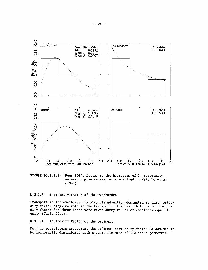
Log Normal Gamma 1.000 Mu 0.5 1 47
0
Sigma 1.5680 sigma2 2.461 6
00- 0 2.0 3.0 4.0 5.0 6.0 7.0
Tortuosity data from Katsube et al 2.0 3.0 4.0 5.0 6.0 7.0
Tortuosity data from Katsube et al
FIGURE D5.1.2.2: Four PDF's fitted to the histogram of 14 tortuosity values on granite samples summarized in Katsube et al. (1986)
D.5.1.3 Tortuosity Factor of the Overburden
Transport in the overburden is strongly advection dominated so that tortuo- sity factor plays no role in the transport. The distributions for tortuo- sity factor for these zones were given dummy values of constants equal to unity (Table D5.1).
D.5.1.4 Tortuosity Factor of the Sediment
For the postclosure assessment the sediment tortuosity factor is assumed to be lognormally distributed with a geometric mean of 1.2 and a geometric
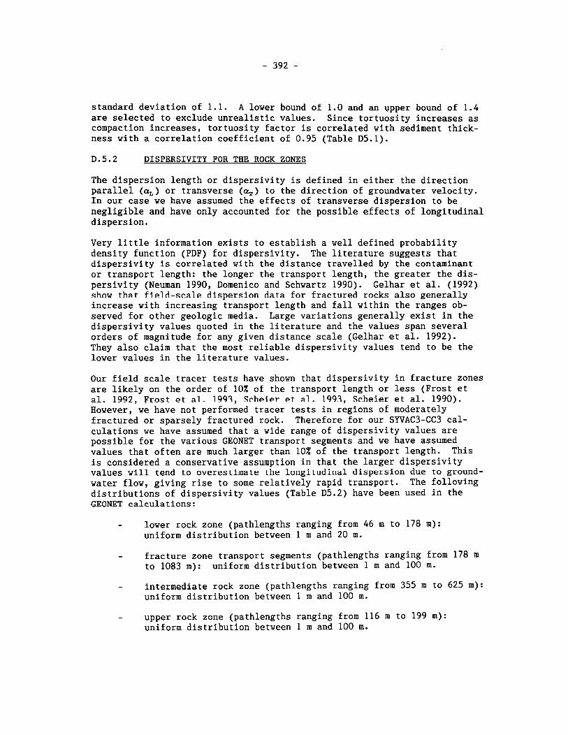
standard deviation of 1.1. A lower bound of 1.0 and an upper bound of 1.4 are selected to exclude unrealistic values. Since tortuosity increases as compaction increases, tortuosity factor is correlated with sediment thick- ness with a correlation coefficient of 0.95 (Table D5.1).
D.5.2 DISPERSIVITY FOR THE ROCK ZONES
The dispersion length or dispersivity is defined in either the direction parallel (a,) or transverse (a,) to the direction of groundwater velocity. In our case we have assumed the effects of transverse dispersion to be negligible and have only accounted for the possible effects of longitudinal dispersion.
Very little information exists to establish a well defined probability density function (PDF) for dispersivity. The literature suggests that dispersivity is correlated with the distance travelled by the contaminant or transport length: the longer the transport length, the greater the dis- persivity (Neuman 1990, Domenico and Schwartz 1990). Gelhar et al. (1992) show that field-scale dispersion data for fractured rocks also generally increase with increasing transport length and fall within the ranges ob- served for other geologic media. Large variations generally exist in the dispersivity values quoted in the literature and the values span several orders of magnitude for any given distance scale (Gelhar et al. 1992). They also claim that the most reliable dispersivity values tend to be the lower values in the literature values.
Our field scale tracer tests have shown that dispersivity in fracture zones are likely on the order of 10% of the transport length or less (Frost et al. 1992, Frost et al. 1991, Scheier et al. 1993, Scheier et al. 1990). However, we have not performed tracer tests in regions of moderately fractured or sparsely fractured rock. Therefore for our SYVAC3-CC3 cal- culations we have assumed that a wide range of dispersivity values are possible for the various GEONET transport segments and we have assumed values that often are much larger than 10% of the transport length. This is considered a conservative assumption in that the larger dispersivity values will tend to overesti~nate the lo~lgitudinal dispersion due to ground- water flow, giving rise to some relatively rapid transport. The following distributions of dispersivity values (Table D5.2) have been used in the GEONET calculations:
- lower rock zone (pathlengths ranging from 46 m to 178 m): uniform distribution between 1 m and 20 m.
- fracture zone transport segments (pathlengths ranging from 178 m to 1083 m): uniform distribution between 1 m and 100 m.
- intermediate rock zone (pathlengths ranging from 355 m to 625 m): uniform distribution between 1 m and 100 m.
- upper rock zone (pathlengths ranging from 116 m to 199 m): uniform distribution between 1 m and 100 m.
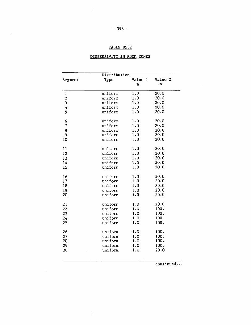
TABLE D5.2
DISPERSIVITY IN ROCK ZONES
Distribution Segment Type Value 1 Value 2
m m
1 uniform 1 .O 20.0 2 uniform 1 .O 20.0 3 uniform 1 .O 20.0 4 uniform 1.0 20.0 5 uniform 1.0 20.0
uniform 1.0 20.0 uniform 1.0 20.0 uniform 1.0 20.0 uniform 1 .O 20.0 uniform 1 .O 20.0
uniform 1 .O 20.0 uniform 1 .O 20.0 uniform 1 .O 20.0 uniform 1.0 20.0 uniform 1.0 20.0
n n i form 1.0 20.0 uniform 1.0 20.0 uniform 1.0 20.0 uniform 1.0 20.0 uniform 1.0 20.0
2 1 uniform 1.0 20.0 22 uniform 1.0 100. 23 uniform 1.0 100. 2 4 uniform 1 .O 100. 25 uniform 1.0 100.
2 6 uniform 1.0 100. 27 uniform 1.0 100. 2 8 uniform 1.0 100. 29 uniform 1 .O 100. 3 0 uniform 1 .O 20.0
continued...
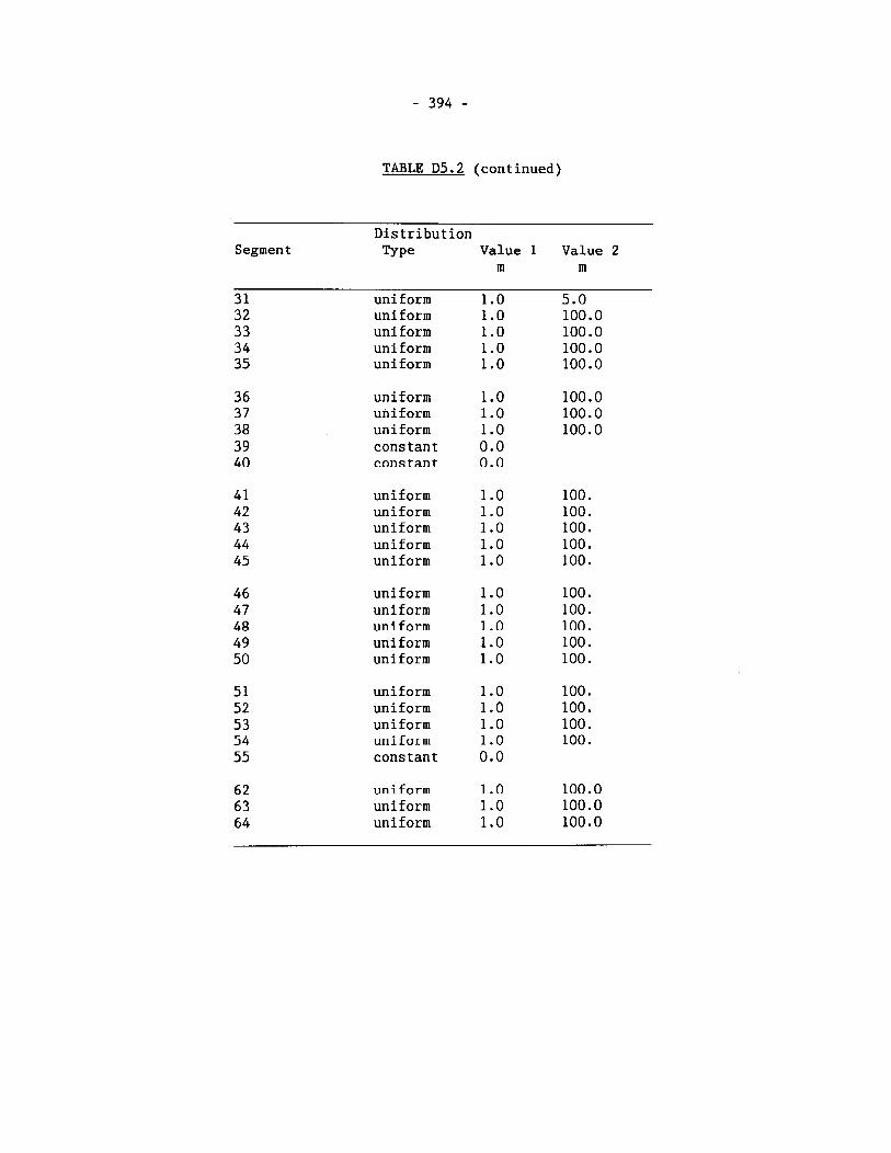
TABLE D5.2 (continued)
Distribution Segment Type Value 1 Value 2
m m
3 1 uniform 1.0 5.0 32 uniform 1.0 100.0 33 uniform 1.0 100.0 3 4 uniform 1 .O 100.0 3 5 uniform 1 .O 100.0
uniform 1.0 100.0 uniform 1.0 100.0 uniform 1 .O 100.0 constant 0.0 constant 0.0
uniform 1 .O 100. uniform 1 .O 100. uniform 1.0 100. uniform 1.0 100. uniform 1.0 100.
uniform 1.0 100. uniform 1.0 100. uniform 1.0 100. uniform 1 .O 100. uniform 1 .O 100.
5 1 uniform 1 .O 100. 52 uniform 1.0 100. 53 uniform 1.0 100. 5 4 uniform 1.0 100. 5 5 constant 0.0
uniform 1.0 100.0 uniform 1 .O 100.0 uniform 1 .O 100.0
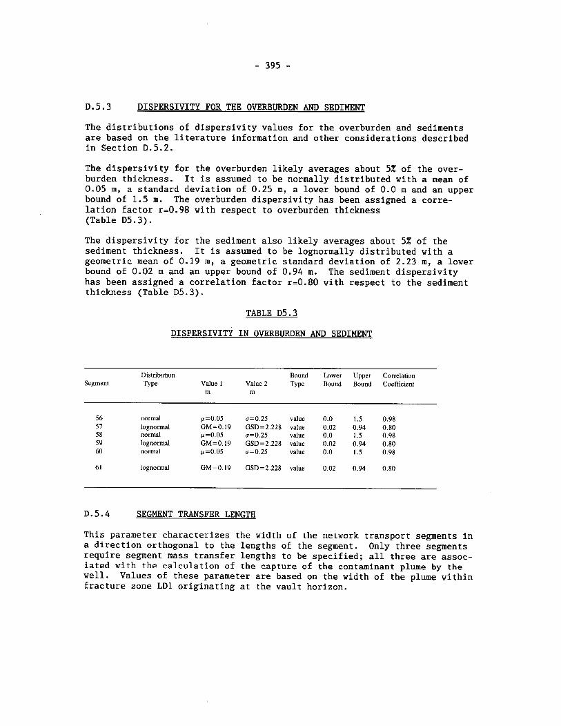
D.5.3 DISPERSIVITY FOR THE OVERBURDEN AND SEDIMENT
The distributions of dispersivity values for the overburden and sediments are based on the literature information and other considerations described in Section D.5.2.
The dispersivity for the overburden likely averages about 5% of the over- burden thickness. It is assumed to be normally distributed with a mean of 0.05 m, a standard deviation of 0.25 m, a lower bound of 0.0 m a.nd an upper bound of 1.5 m. The overburden dispersivity has been assigned a corre- lation factor r=0.98 with respect to overburden thickness (Table D5.3).
The dispersivity for the sediment also likely averages about 5% of the sediment thickness. It is assumed to be lognormally distributed with a geometric mean of 0.19 m, a geometric standard deviation of 2.23 m, a lower bound of 0.02 m and an upper bound of 0.94 m. The sediment dispersivity has been assigned a correlation factor r=0.80 with respect to the sediment thickness (Table D5.3).
TABLE D5.3
DISPERSIVITY IN OVERBURDEN AND SEDIMENT
Distribution Bound Lower Upper Correlation Segment TY pe Value 1 Value 2 Type Bound Bound Coefficient
m m
56 normal p=0.05 ~ = 0 . 2 5 value 0.0 1.5 0.98 57 lognormal GM=0.19 GSD=2.228 value 0.02 0.94 0.80 58 normal p=0.05 0=0.25 value 0.0 1.5 0.98 59 lognormal GM=0.19 GSD=2.228 value 0.02 0.94 0.80 60 normal p=0.05 u=0.25 value 0.0 1.5 0.98
b1 lognormal tiM=O.lY GSD=2.228 value 0.02 0.94 0.80
D.5.4 SEGMENT TRANSFER LENGTH
This parameter characterizes the width of the network transport segments in a direction orthogonal to the lengths of the segment. Only three segments require segment mass transfer lengths to be specified; all three are assoc- iated with the calculation of the capture of the contaminant plume by the well. Values of these parameter are based on the width of the plume within fracture zone LD1 originating at the vault horizon.
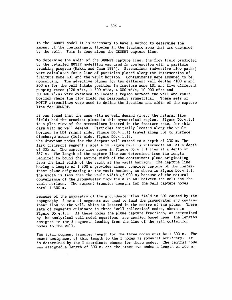
In the GEONET model it is necessary to have a method to determine the amount of the contaminants flowing in the fracture zone that are captured by the well. This is done along the GEONET capture line.
To determine the width of the GEONET capture line, the flow field predicted by the detailed MOTIF modelling was used in conjunction with a particle tracking program (Nakka and Chan 1994). Streamlines (advective flow paths) were calculated for a line of particles placed along the intersection of fracture zone LD1 and the vault horizon. Contaminants were assumed to be nonsorbing. The advective plumes for two different well depths (100 m and 200 m) for the well intake position in fracture zone LD1 and five different pumping rates (120 m3/a, 1 500 m3./a, 4 000 m3/a, 10 000 m3/a and 30 000 m3/a) were examined to locate a region between the well and vault horizon where the flow field was reasonably symmetrical. These sets of MOTIF streamlines were used to define the location and width of the capture line for GEONET.
It was found that the case with no well demand (i.e., the natural flow field) had the broadest plume in this symmetrical region. Figure D5.4.1.1 is a plan view of the streamlines located in the fracture zone, for this case with no well demand. Particles initially located along the vault horizon in LD1 (right side, Figure D5.4.1.1) travel along LD1 to surface discharge areas (left side, Figure D5.4.1.1). The drawdown nodes for the deepest well extend to a depth of 230 m. The last transport segment (label A in Figure D2.1.1) intersects LD1 at a depth of 335 m. The capture line shown in Figure D5.4.1.1 lies at a depth of 287 m. The length of the capture line was determined from the length required to bound the entire width of the contaminant plume originating from the full width of the vault at the vault horizon. The capture line having a length of 1 300 m provides almost complete capture of the contam- inant plume originating at the vault horizon, as shown in Figure D5.4.1.1. The width is less than the vault width (2 000 m) because of the natural convergence of the groundwater flow field in LD1 between the well and the vault horizon. The segment transfer lengths for the well capture nodes total 1 300 m.
Because of the asymmetry of the groundwater flow field in LD1 caused by the topography, 3 sets of segments are used to lead the groundwater and contam- inant flow to the well, which is located in the centre of the plume. These sets of segments culminate in three "well collection" nodes, shown in Figure D5.4.1.1. At these nodes the plume capture fractions, as determined by the analytical well model equations, are applied based upon the lengths assigned to the 3 segments leading from the line of the well collection nodes to the well.
The total segment transfer length for the three nodes must be 1 300 m. The exact assignment of this length to the 3 nodes is somewhat arbitrary. It is determined by the Y coordinate chosen for these nodes. The central node was assigned a length of 300 m, and the other two nodes a length of 500 m.
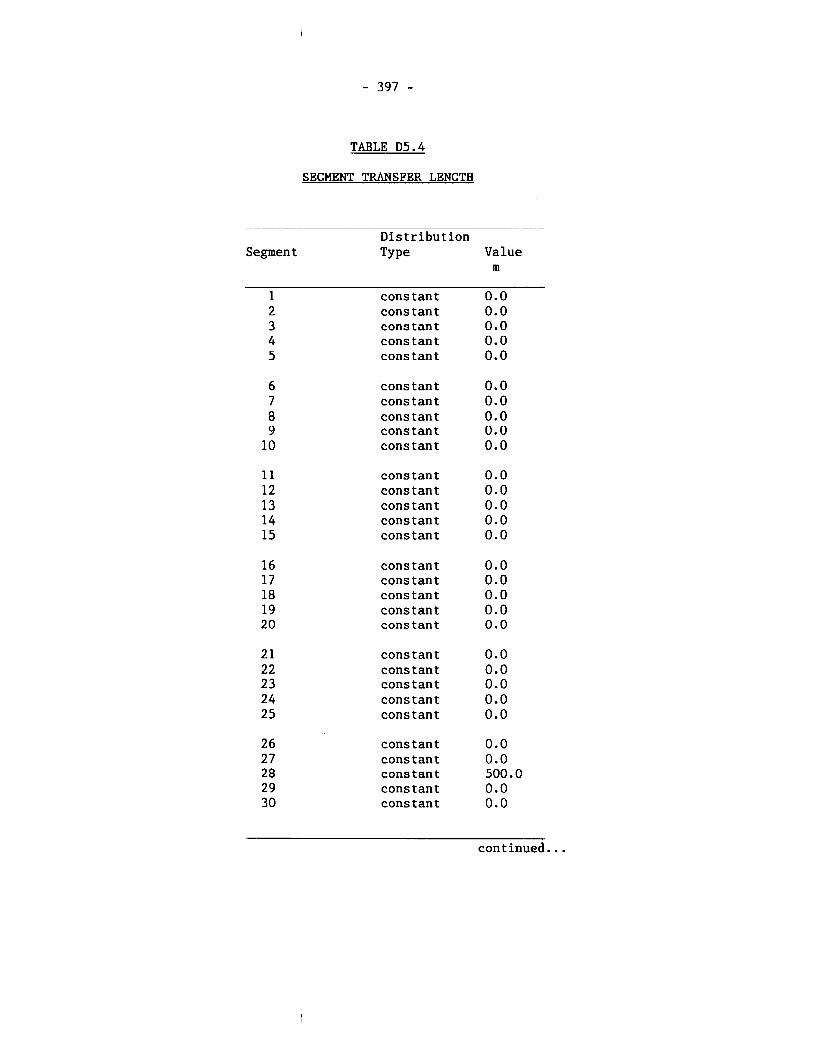
- 397 -
TABLE D5.4
SECMENT TRANSFER LENCTH
Segment Distribution TY pe Value
m
1 constant 0.0 2 constant 0.0 3 constant 0.0 4 constant 0.0 5 constant 0.0
constant 0.0 constant 0.0 constant 0.0 constant 0.0 constant 0.0
11 constant 0.0 12 constant 0.0 13 constant 0.0 14 constant 0.0 15 constant 0.0
constant 0.0 constant 0.0 constant 0.0 constant 0.0 constant 0.0
2 1 constant 0.0 22 constant 0.0 23 constant 0.0 24 cons tan t 0.0 2 5 cons tan t 0.0
cons tan t 0.0 constant 0.0 constant 500.0 constant 0.0 constant 0.0
continued...
TABLE D5.4 (continued)
Distribution Segment Type Value
m
3 1 cons tan t 0.0 3 2 cons tan t 0.0 3 3 constant 0.0 3 4 constant 0.0 3 5 constant 0.0
cons tan t 0.0 cons tan t 0.0 constant 300.0 constant 0.0 cons tan t 0.0
cons tan t 0.0 constant 0.0 constant 0.0 constant 0.0 cons tan t 0.0
cons tan t 0.0 cons tan t 500.0 constant 0.0 constant 0.0 constant 0.0
constant 0.0 constant 0.0 constant 0.0 constant 0.0 constant 0.0
cons tan t 0.0 constant 0.0 constant 0.0 cons tan t 0.0 cons tan t 0.0
constant 0.0 constant 0.0 constant 0.0 constant 0.0
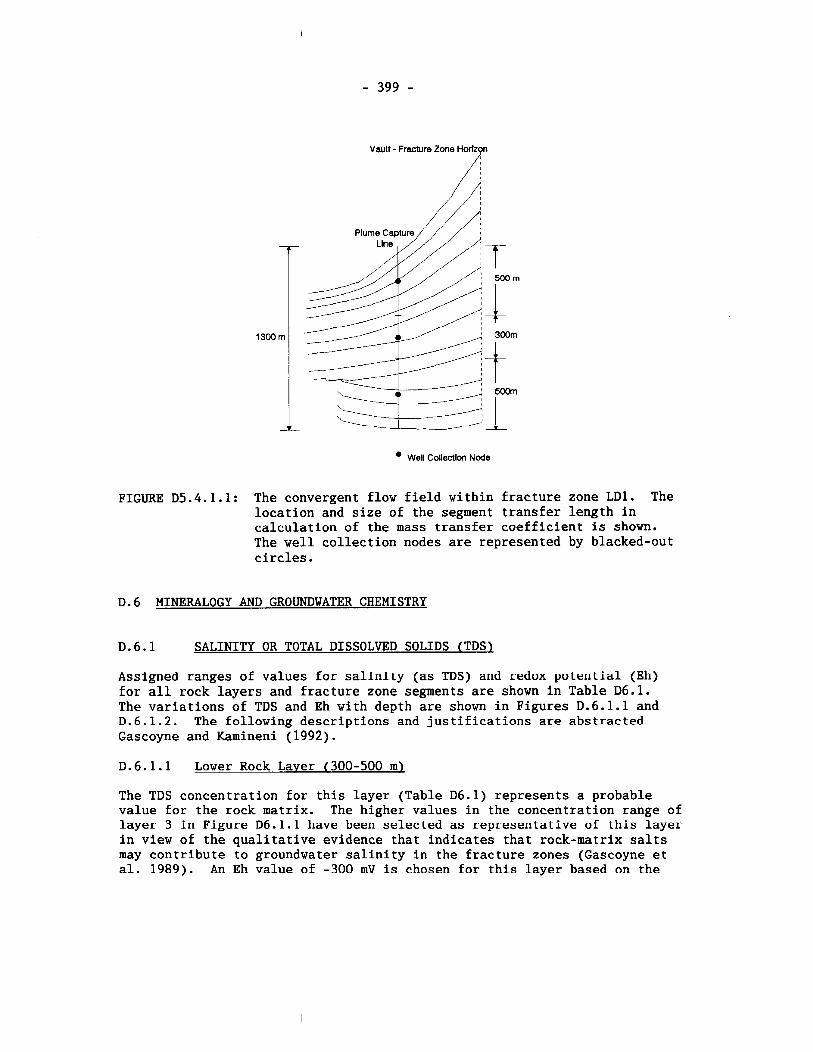
- 399 -
Vault - Fracture Zone
Well Collection Node
FIGURE D5.4.1.1: The convergent flow field within fracture zone LD1. The location and size of the segment transfer length in calculation of the mass transfer coefficient is shown. The well collection nodes are represented by blacked-out circles.
D.6 MINERALOGY AND GROUNDWATER CHEMISTRY
D.6.1 SALINITY OR TOTAL DISSOLVED SOLIDS (TDSL
Assigned ranges of values for salirii~y (as TDS) and redox potential (Eh) for all rock layers and fracture zone segments are shown in Table D6.1. The variations of TDS and Eh with depth are shown in Figures D.6.1.1 and D.6.1.2. The following descriptions and justifications are abstracted Gascoyne and Kamineni (1992).
D.6.1.1 Lower Rock Laver (300-500 m)
The TDS concentration for this layer (Table D6.1) represents a p1:obable value for the rock matrix. The higher values in the concentration range of layer 3 in Figure D6.1.1 have been selected as representative of this layer in view of the qualitative evidence that indicates that rock-matrix salts may contribute to groundwater salinity in the fracture zones (Gascoyne et al. 1989). An Eh value of -300 mV is chosen for this layer based on the
fact that magnetite is present in the rock matrix (the hagnetite-hematite redox boundary lies between -200 and -250 mV in the pH range 7-8.5).
D.6.1.2 Fracture Zone LD1 (300-500 m)
The mean composition selected for this segment (10 g/l) closely reflects the compositions of groundwaters in FZ1 at the URL (depth range 300-450 m), which tend to be more saline than indicated by the 300-500 m envelope in Figure D6.1.1. The lower value of the Eh range for this layer (Figure D6.1.2) is selected as the most representative because the groundwater is likely to have been least affected by atmospheric contamination during measurement. This result is also more consistent with down-hole sensor measurements (Ross and Gascoyne 1992).
D.6.1.3 Intermediate Rock Laver (150-300 m)
As in the case of the Lower Rock Layer, the composition of matrix solutions in this layer is assumed to be more saline than that in the fracture zones and the mean and distribution are taken from the upper part of the Layer 2 envelope in Figure D6.1.1. An Eh value of -300 mV is again chosen for this layer because magnetite is the stable Fe-bearing phase in the rock matrix.
D.6.1.4 Fracture Zone LD1 (150-300 ml
No data exists for this level of FZ1 at the URL because it lies outside the property boundary. The assumption is made, therefore, that similar geo- chemical evolutionary processes take place in groundwaters as they flow towards the surface, irrespective of which fracture zone they follow, and FZ2 and its lower splay (FZ1.5) at the URL may be used to determine the composition in LD1 for this layer. The mean value for Eh is chosen to reflect the trend of lower Eh seen in down-hole sensor measurements. These assumptions are supported by measurements in groundwaters from similar depth intervals for boreholes in permit areas elsewhere in the WRA.
D.6.1.5 Upper Rock Layer (0-150 m)
Groundwater flow in this layer is defined as occurring through intercon- nected, subvertical fractures containing calcite as the dominant infilling. Although the GEONET simulation only considers discharge flow paths in this layer (so that migration of the plume from the vault may be followed), considerable dilution of the plume occurs by localized recharge through these fractures. Therefore, an average of the data points in the Upper Rock Layer (Layer 1, Figures D.6.1.1, D.6.1.2) is used.
D.6.1.6 Fracture Zone LD1 (0-150 m)
Because this part of LD1 is not within the URL property and has not been investigated, compositions of the groundwater in FZ3 and near-surface FZ2 groundwaters at the URL have been used to estimate the groundwater composi- tion of this portion of the fracture zone. A slightly more saline
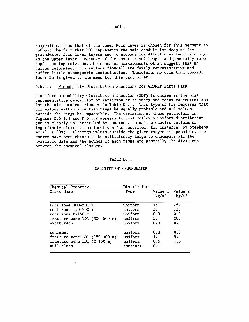
composition than that of the Upper Rock Layer is chosen for this segment to reflect the fact that LD1 represents the main conduit for deep saline groundwater from lower layers and to account for dilution by local recharge in the upper layer. Because of the short travel length and generally more rapid pumping rate, down-hole sensor measurements of Eh suggest that Eh values determined in a surface flowcell are fairly representative and suffer little atmospheric contamination. Therefore, no weighting towards lower Eh is given to the mean for this part of LD1.
D.6.1.7 Probability Distribution Functions for GEONET Input Data
A uniform probability distribution function (PDF) is chosen as the most representative descriptor of variation of salinity and rcdox concentrations for the six chemical classes in Table D6.1. This type of PDF requires that all values within a certain range be equally probable and all values outside the range be impossible. The variation of these parameters in Figures D.6.1.1 and D.6.1.2 appears to best follow a uniform distribution and is clearly not described by constant, normal, piecewise uniform or logarithmic distribution functions (as described, for instance, bly Stephens et al. (1989). Although values outside the given ranges are possible, the ranges have been chosen to be sufficiently large to encompass all the available data and the bounds of each range are generally the divisions between the chemical classes.
TABLE D6.1
SALINITY OF GROUNDWATER
Chemical Property Distribution Class Name Type Value 1 Value 2
kg/m3 kg/n13
rock zone 300-500 m rock zone 150-300 m rock zone 0-150 m fracture zone LD1 (300-500 m) overburden
sediment fracture zone LD1 (150-300 m) fracture zone LD1 (0-150 m) null class
uniform 15. 25. uniform 3. 13. uniform 0.3 0.8 uniform 5. 20. uniform 0.3 0.8
uniform 0.3 0.8 uniform 1. 5. uniform 0.5 1.5 constant 0.
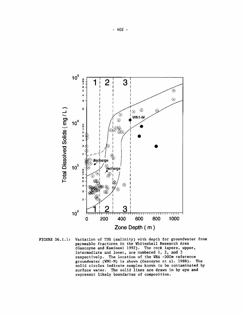
Zone Depth ( m )
FIGURE D6.1.1: Variation of TDS (salinity) with depth for groundwater from permeable fractures in the Whiteshell Research Area (Gascoyne and Kamineni 1992). The rock layers, upper, intermediate and lower, are numbered 1, 2, and 3 respectively. The location of the WRA -500m reference groundwater (WN1-M) is shown (Gascoyne et al. 1988). The solid circles indicate samples known to be contaminated by surface water. The solid lines are drawn in by eye and represent likely boundaries of composition.
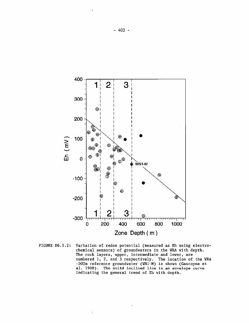
Zone Depth ( m )
FIGURE D6.1.2: Variation of redox potential (measured as Eh using electro- chemical sensors) of groundwaters in the WRA wit:h depth. The rock layers, upper, intermediate and lower, are numbered 1, 2, and 3 respectively. The location of the WRA -500m reference groundwater (WN1-M) is shown (Gascoyne et al. 1988). The solid inclined line is an envelope curve indicating the general trend of Eh with depth.
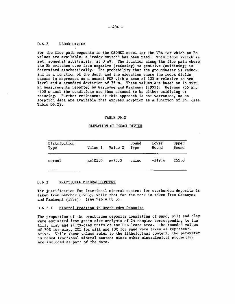
D.6.2 REDOX DIVIDE
For the flow path segments in the GEONET model for the WRA for which no Eh values are available, a "redox switch" has been used. This redox switch is set, somewhat arbitrarily, at 0 mV. The location along the flow path where the Eh switches over from negative (reducing) to positive (oxidizing) is determined stochastically. The probability that the groundwater is reduc- ing is a function of the depth and the elevation where the redox divide occurs is expressed as a normal PDF with a mean of 105 m relative to sea level and a standard deviation of 75 m. These values are based on in situ Eh measurements reported by Gascoyne and Kamineni (1992). Between 255 and -750 m asml the conditions are thus assumed to be either oxidizing or reducing. Further refinement of this approach is not warranted, as no sorption data are available that express sorption as a function of Eh. (see Table D6.2).
TABLE D6.2
ELEVATION OF REDOX DIVIDE
Distribution Bound Lower Upper TY pe Value 1 Value 2 Type Bound Bound
normal p=105.0 a=75.0 value -219.4 255.0
D.6.3 FRACTIONAL MINERAL CONTENT
The justification for fractional mineral content for overburden deposits is taken from Betcher (1983), while that for the rock is taken from Gascoyne and Kamineni (1992). (see Table D6.3).
D.6.3.1 Mineral Fraction in Overburden Deposits
The proportion of the overburden deposits consisting of sand, silt and clay were estimated from grain-size analysis of 24 samples corresponding to the till, clay and silty-clay units of the URL lease area. The rounded values of 70% for clay, 20% for silt and 10% for sand were taken as represent- ative. While these values refer to the lithological content, the parameter is named fractional mineral content since othcr mineralogical properties are included as part of the data.
D.6.3.2 Mineral Fraction in Rock
D.6.3.2.1 Lower Rock Layer (300-500 m)
Because the flow in this layer (in contrast to fracture zone LD1) is primarily through poorly interconnected pore space, retardation factors would be controlled by distribution coefficients for radionuclides on the pore surfaces. Actual K, (distribution coefficient) values of grey granite from the WRA are used for this layer, rather than coefficients based on the mineral components listed in Table D6.3.1.
D.6.3.2.2 Fracture Zone (LD1 (300-500 m)
The average volume percent of minerals present in this segment (Table D6.3.2) is obtained by study of samples collected from cored boreholes at the URL location of the Whiteshell Research Area (URL 1 to 8, 10 and 12). The samples represent material recovered from low-dip (<30°) faults corresponding to FZ-1 and -2.
D.6.3.2.3 Intermediate Rock Layer (150-300 ni)
The predominant rock mass in this segment is grey granite, but it generally has two orders of magnitude greater permeability than the Lower Rock Layer. As in the Lower Rock Layer, flow in this zone will be through interconnect- ed pores and, hence, a similar approach is adopted here in assigning the mineralogy, (i.e., coded as grey granite).
D.6.3.2.4 Fracture Zone LD1 (150-300 m)
This segment contains the same low-dip Iaults Lhat are encountered in the deeper regions (i.e., 300 to 500 m). Since no mineralogical variation is noted along the dip, the same mineralogical data as those of Fracture Zone LD1 (300 to 500 m) have been chosen (Table D6.3.2).
D.6.3.2.5 Upper Rock Layer (0-150 m)
In addition to a calcite infilling, many of these subvertical fractures contain slickenlines that are defined by the development of chlorite, which generally disintegrates forming residual minerals (iron oxides). The volume percent of major minerals for this flow segment are given in Table D6.3.3.
D . 6 . 3 . 2 . 6 Fracture Zone LD1 (0-150 m)
Core samples from boreholes (URL1 to 10) intersecting FZ-2 and -3 at shallow depths (0 to 150 m) were used to characterize the mineralogy of this segment. Again, calcite and iron oxides are the dominant infilling. The modal volume percent of these minerals is listed in Table D6.3.4.
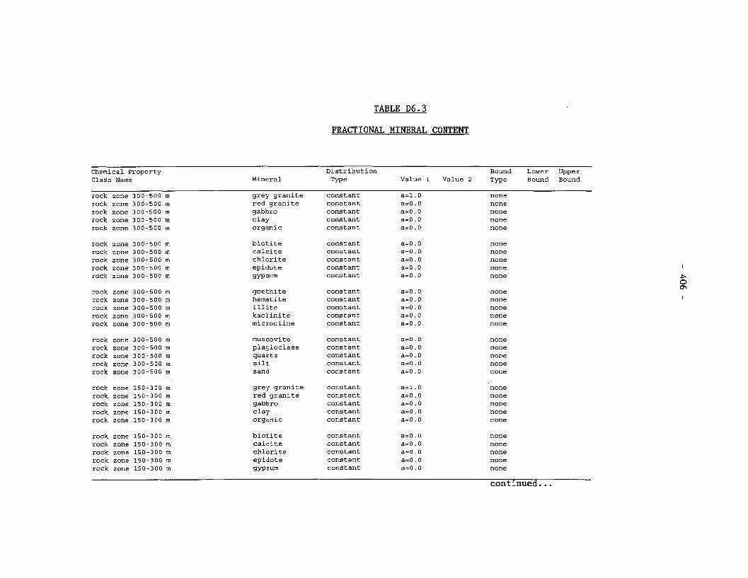
TABLE D6.3
FRACTIONAL MINERAL CONTENT
Chemical Property Distribution Bound Lower Upper Class Name Mineral Type Value 1 Value 2 Type Bound Bound - -
rock zone 300-500 m rock zone 300-500 m rock zone 300-500 m rock zone 300-500 m rock zone 300-500 m
rock zone 300-500 m rock zone 300-500 m rock zone 300-500 m rock zone 300-500 m rock zone 300-500 m
rock zone 300-500 m rock zone 300-500 m rock zone 300-500 m rock zone 300-500 m rock zone 300-500 m
rock zone 300-500 m rock zone 300-500 m rock zone 300-500 m rock zone 300-500 m rock zone 300-500 m
rock zone 150-300 m rock zone 150-300 m rock zone 150-300 m rock zone 150-300 m rock zone 150-300 m
rock zone 150-300 m rock zone 150-300 m rock zone 150-300 m rock zone 150-300 m rock zone 150-300 m
grey granite constant a A . 0 red granite constant a=O . 0 gabbro constant a=O .O clay constant a=O .O organic constant a=O .O
biotite constant a=O . 0 calcite constant a=O . 0 chlcrite constant a=O .O epidote constant a=O .O gypsum constant a=O .O
goethite constant a=O . 0 hematite constant a=O . 0 illite constant a=O . 0 kaolinite constant a=O . 0 microcline constant a=O .O
muscovite constant plasioclase constant quartz constant silt constant sand constant
grey granite cocstant a=1.0 red granite cor.stant a=O .O gabbro c o ~ s tant a=O .O clay constant a=O. 0 organic constant a=O . 0
biotite constant a=O .O calcite constant a=O .O chlorite constant a=O. 0 epidote constant a=O . 0 gypsum constant a=O .O
none none none none none
none none none none none
none none none none none
none none none none none
none none none none none
none none none none none
continued...
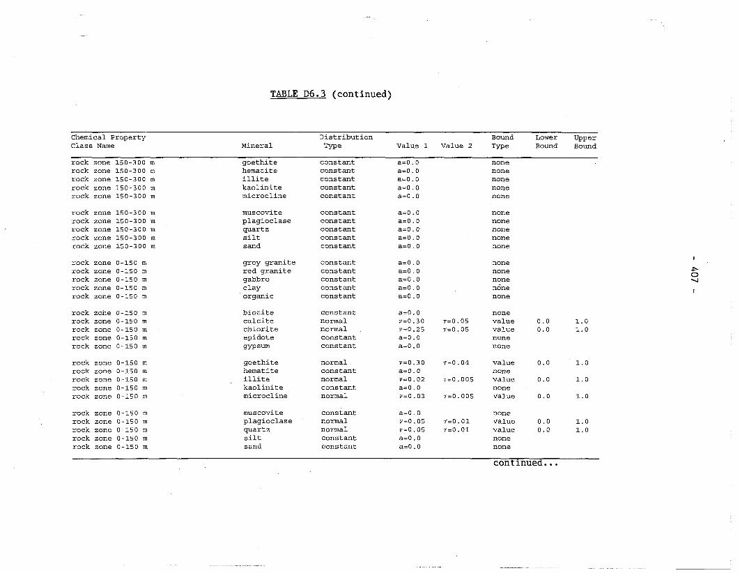
TABLE D6.3 (continued)
Chemical Property Distribution Bound Lower Upper Class Name Mineral Type Value 1 Value 2 Type Bound Bound
rock zone 150-300 m rock zone 150-300 m rock zone 150-300 m rock zone 150-300 m rock zone 150-300 m
rock zone 150-300 m rock zone 150-300 m rock zone 150-300 m rock zone 150-300 m rock zone 150-300 m
rock zone 0-150 m rock zone 0-150 m rock zone 0-150 rn rock zone 0-150 m rock zone 0-150 m
rock zone 0-150 m rock zone 0-150 m rock zone 0-150 m rock zone 0-150 m rock zone 0-150 m
rock zone 0-150 m rock zone 0-150 m rock zone 0-150 m rock zone 0-150 m rock zone 0-150 m
rock zone 0-150 m rock zone 0-150 m rock zone 0-150 m rock zone 0-150 m rock zone 0-150 m
goethite constant a=O . 0 hematite constant a=O. 0 illite constant a=O . 0 kaolinite constant a=O .O microcline constant a=O. 0
muscovite constant a=O. 0 plagioclase constant a=O.O quartz constant a=O . 0 silt constant a=O .O sand constant a=O . 0
grey granite constant a=O. 0 red granite constant a=O .O gabbro constant a=O . 0 clay constant a=O .O organic constant a=O .O
none none none none none
none none none none none
none none none ndne none
biotite constant a=O. 0 none calcite normal v=O .30 T=O. 05 value 0.0 1.0 chlorite normal v=O .25 T=O. 05 value 0.0 1.0 epidote constant a=O . o none gypsum constant a=O . 0 none
goethite normal v=O .30 T=O. 04 value 0.0 1.0 hematite constant a=O . 0 none illite normal v=0.02 ~=0.005 value 0.0 1.0 kaolinite constant a=O .O none microcline normal v=0.03 ~=0.005 value 0.0 1.0
muscovite constant a=O .O none plagioclase normal v=O .05 T=O. 01 value 0.0 1.0 quartz normal v=O .05 T=O. 01 value 0.0 1.0 silt constant a=O. 0 none sand constant a=O .O none
continued...
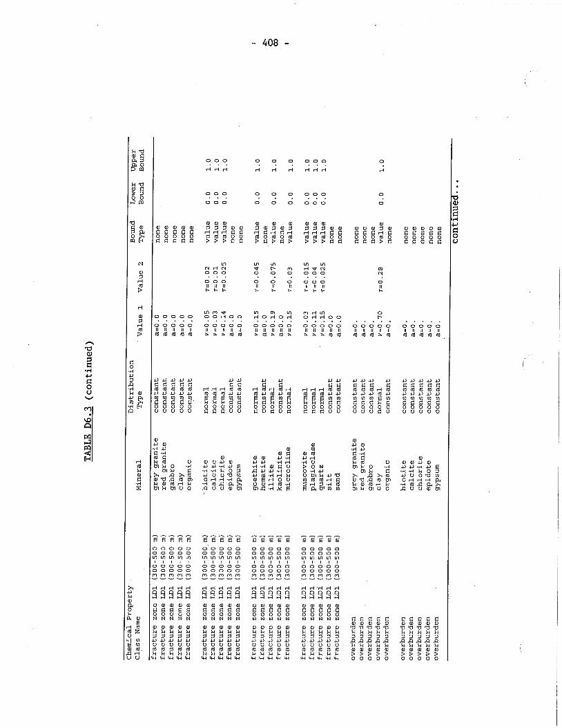
0 0 0 0 0 0 0 0 0 II II II t- C C
II I1 II II II II C C C C C C
m 0 al -4 +J
3 $4 a U 0 .d
h d 6-2 2 6 h QJ r d d h tnh t n U 0
U 3 2 h a
$ 2 n
.................... E E E E E E E E E E E E E E E E E E E E
U U U U U U U U U U U 6 6 d d 6 6 3 3 3 3 3 d r l r l m m d m r l r d r l r l r l r l m m
u u u u u m m m u u m u m u m m r d m ~ ~ f f l l l l f f l f f l u l d a a c c R E & % % E % R % & E E E % % 0 0 0 0 0 0 0 0 0 0 0 0 0 0 0 0 0 0 0 0 U U U U U d d d U U G U d U d C d C U U
0 0 0 0 0 0 0 0 0 0 0 0 0 0 0 0 0 0 0 0 0 0 0 0 0 0 0 0 0 0 0 0 0 0 0 0 0 0 0 0 m m m m m m m m m m m m m m m m m m m m I I I I I I I I I I I I I I I I I I I I 0 0 0 0 0 0 0 0 0 0 0 0 0 0 0 0 0 0 0 0 0 0 0 0 0 0 0 0 0 0 0 0 0 0 0 0 0 0 0 0 m m m m m m m m m m m m m m m m m m m m ----- ----- ----- --- --
a l m m m a l a l a l m a l m m m m m a l a l m m a l m d d d d f i d d d d d d d d d d d d d d d 0 0 0 0 0 0 0 0 0 0 0 0 0 0 0 0 0 0 0 0 N N N N N N N N N N N N N N N N N N N N
al al al al ar h h h h h 3 3 3 3 3 U U U U U U U U U U r d r d r d m m h h h h h W W W W W
a l a l a l a l a l h h h h h 3 3 3 3 3 U U U U U U U U U U m m m m m h h h h h W W W W W
a l a l a l a l a l h h h h h 3 3 3 3 3 U U U U U U U U U U rd m m m m h h h h h
W W W W W
U U U U U U $$$,s 3 3 3 3 3 U U U r n U U U U U U ffl ln ffl C C G E % % % % % % 0 0 0 0 0 0 0 0 0 0 U U U d U U U U U U
8 8 8 8 8 a a a a a h h h h h 3 3 3 3 3 %fl%Slfl al aJ al al al
g g g g g
8 8 8 8 8 a a a a a h h h h h 3 3 3 3 3 n n n n n h h h h h m a l a l a l a ,
g g g g g
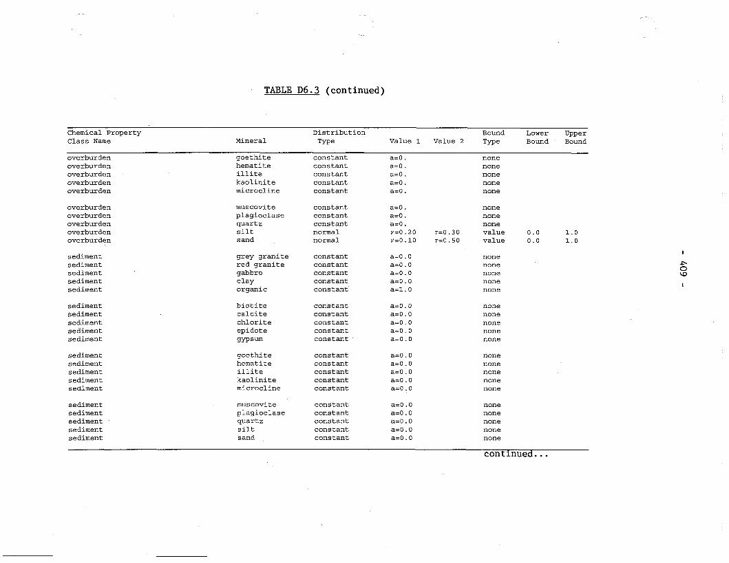
TABLE D6.3 (continued)
Chemical Property Class Name
Distribution Bound Lower Upper Mineral Type Value 1 Value 2 Type Bound Bound
overburden goethite constant a=O . none overburden hematite constant a=O . none overburden illite constant a=O. none overburden kaolinite constant a=O . none overburden microcline constant a=O . none
overburden overburden overburden overburden overburden
sediment sediment sediment sediment sediment
sediment sediment sediment sediment sediment
sediment sediment sediment sediment sediment
sediment sediment sediment sediment sediment
muscovite constant a=O . none plagioclase constant a=O . none quartz constant a=O . none silt normal v=0.20 7=0.30 value sand normal v=O .10 7=0.50 value
grey granite constant a=O .O red granite constant a=O. 0 gabbro constant a=O .O clay constant a=O .O organic constant a=1.0
biotite constant a=O . 0 calcite constant a=O .O chlorite constant a=O .O epidote constant a=O .O gypsum constant a=O. 0
goethite hematite illite kaolinite microcline
constant a=O . 0 constant a=O .O constant a=O .O constant a=O .O constant a=O. 0
muscovite constant a=O . 0 plagioclase constant a=O. 0 quartz constant a=O .O silt constant a=O . 0 sand constant a=O. 0
none none none none none
none none none none none
none none none none none
none none none none none
continued...
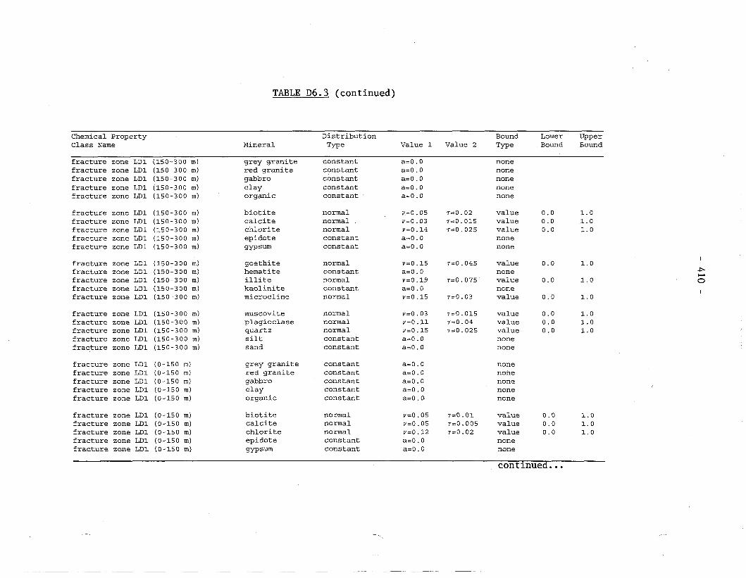
TABLE D6.3 (continued)
Chemical Property Distribution Bound Lower Upper Class Name Mineral Type Value 1 Value 2 Type Bound Bound
fracture zone LD1 (150-300 m) fracture zone LD1 (150-300 m) fracture zone LD1 (150-300 m) fracture zone LD1 (150-300 m) fracture zone LD1 (150-300 m)
grey granite red granite gabbro clay organic
const ant constant constant constant constant
none none none none none
fracture zone LD1 (150-300 m) fracture zone LD1 (150-300 m) fracture zone LD1 (150-300 m) fracture zone LD1 (150-300 m) fracture zone LD1 (150-300 m)
biotite calcite chlorite epidote gyPs'=m
normal normal normal constant constant
T = O . 02 value 0 . 0 1 . 0 T = O . 015 value 0 . 0 1 . 0 T = O . 025 value 0 . 0 1 . 0
none none
fracture zone LD1 (150-300 m) fracture zone LD1 (150-300 m) fracture zone LD1 (150-300 m) fracture zone LD1 (150-300 m) fracture zone LD1 (150-300 m)
goethite hematite illite kaolinite microcline
normal constant normal constant normal
T = O . 045 value 0 .0 1 . 0 none
~ = 0 . 0 7 5 value 0 .0 1 . 0 none
T = O .03 value 0 . 0 1 . 0
fracture zone LD1 (150-300 m) fracture zone LD1 (150-300 m) fracture zone LD1 (150-300 m) fracture zone LD1 (150-300 m) fracture zone LD1 (150-300 m)
muscovite plagioclase quartz silt sand
normal normal normal constant constant
T = O . 015 value 0 . 0 1 . 0 T = O .04 value 0 . 0 1 . 0 T = O . 025 value 0 . 0 1 . 0
none none
fracture zone LD1 (0-150 m) fracture zone LD1 (0-150 m) fracture zone LD1 (0-150 rn) fracture zone LD1 (0-150 m) fracture zone LD1 (0-150 m)
grey granite red granite gabbro clay organic
constant constant constant constant constant
none none none none none
fracture zone LD1 (0-150 m) fracture zone LD1 (0-150 m) fracture zone LD1 (0-150 m) fracture zone LD1 (0-150 m) fracture zone LD1 (0-150 m)
biotite calcite chlorite epidote gypsum
normal normal normal Constant constant
T = O . 0 1 value 0 . 0 1 . 0 T = O . 005 value 0 . 0 1 . 0 T = O . 02 value 0 . 0 1 . 0
none none
continued...

TABLE D6.3 (continued)
Chemical Property Distribution Bound Lower Upper Class Name Mineral Type Value 1 Value 2 Type Bound Bound -- --
fracture zone LD1 (0-150 m) fracture zone LD1 (0-150 m) fracture zone LD1 (0-150 m) [5-cture zone LD1 (0-150 m) fracture zone LD1 (0-150 m)
fracture zone LD1 (0-150 m) fracture zone LD1 (0-150 m) fracture zone LD1 (0-150 m) fracture zone LD1 (0-150 m) fracture zone LD1 (0-150 m)
null class null class null class null class null class
null class null class null class null class null class
null class null class null class null class null class
null class null class null class null class null class
goethite normal hematite constant illite normal kaolinite constant microcline normal
v=o. 20 T=o. 02 value 0.0 1.0 a=O. v=0. 21 0 T=O. 025 value none
0.0 1.0 a=O v=0 . .12 0 T=O. 015 none value
0.0 1.0
muscovite plagioclase quartz silt sand
normal v=0.02 T=O. 0025 value 0.0 1.0 normal v=O .08 T=O .01 value 0.0 1.0 normal v=0.15 T=O. 015 value 0.0 1.0 constant a=O . 0 none constant a=O . 0 none
grey granite constant a=O . red granite constant a=O. gabbro constant a=O. clay constant a=O . organic constant a=O .
biotite constant a=O . calcite constant a=O . chlorite constant a=O . epidote constant a=O. gypsum constant a=O .
goethite constant a=O . hematite constant a=O. illite constant a=O . kaolinite constant a=O . microcline constant a=O .
muscovite constant a=O . plagioclase constant a=O . quartz constant a=O. silt constant a=O . sand constant a=O .
none none none none none
none none none none none
none none none none none
none none none none none
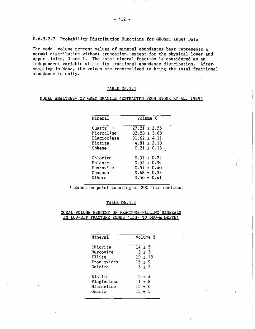
D.6.3.2.7 Probability Distribution Functions for GEONET .Input Data
The modal volume percent values of mineral abundances best represents a normal distribution without truncation, except for the physical lower and upper limits, 0 and 1. The total mineral fraction is considered as an independent variable within its fractional abundance distribution. After sampling is done, the values are renormalized to bring the total fractional abundance to unity.
TABLE D6.3.1
MODAL ANALYSES* OF GREY GRANITE (EXTRACTED FROM STONE ET AL. 19891
Mineral Volume %
Quartz Microcline Plagioclase Biotite Sphene
Chlorite Epido te Muscovite Opaques Others
* Based on point counting of 200 thin sections
TABLE D6.3.2
MODAL VOLUME PERCENT OF FRACTURE-FILLING MINERALS IN LOW-DIP FRACTURE ZONES (150- TO 500-m DEPTH)
Mineral Volume %
Chlorite 14 + 5 Muscovite 3 + 3 Illite 19 + 15 Iron oxides 15 t 9 CaPci te 3 + 2 Biotite 5 + 4 Plagioclase 11 t 8 Microcline 15 rt 6 Quartz 15 + 5
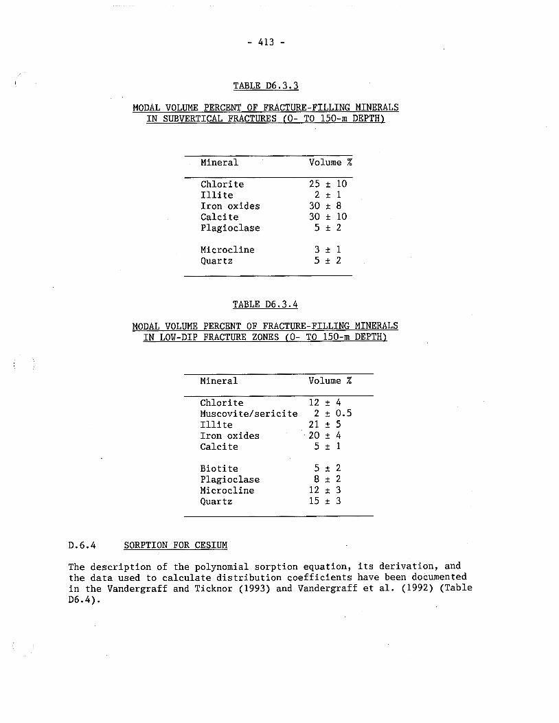
TABLE D6.3.3
MODAL VOLUME PERCENT OF FRACTURE-FILLING MINERALS IN SUBVERTICAL FRACTURES (O- TO 150-m DEPTH)
Mineral Volume %
Chlorite 25 + 10 Illi te 2 + 1 Iron oxides 30 + 8 Calcite 30 + 10 Plagioclase 5 + 2
Microcline 3 + 1 Quartz 5 2 2
TABLE D6.3.4
MODAL VOLUME PERCENT OF FRACTURE-FILLING MINERALS IN LOW-DIP FRACTURE ZONES (O- TO 150-m DEPTH)
Mineral Volume X
Chlorite 12 + 4 Muscovite/sericite 2 + 0.5 Illite 21 + 5 Iron oxides 20 + 4 Calcite 5 2 1
Biotite 5 + 2 Plagioclase 8 + 2 Microcline 12 + 3 Quartz 15 + 3
D.6.4 SORPTION FOR CESIUM
The description of the polynomial sorption equation, its derivation, and the data used to calculate distribution coefficients have been documented in the Vandergraff and Ticknor (1993) and Vandergraff et al. (1992) (Table D6.4).
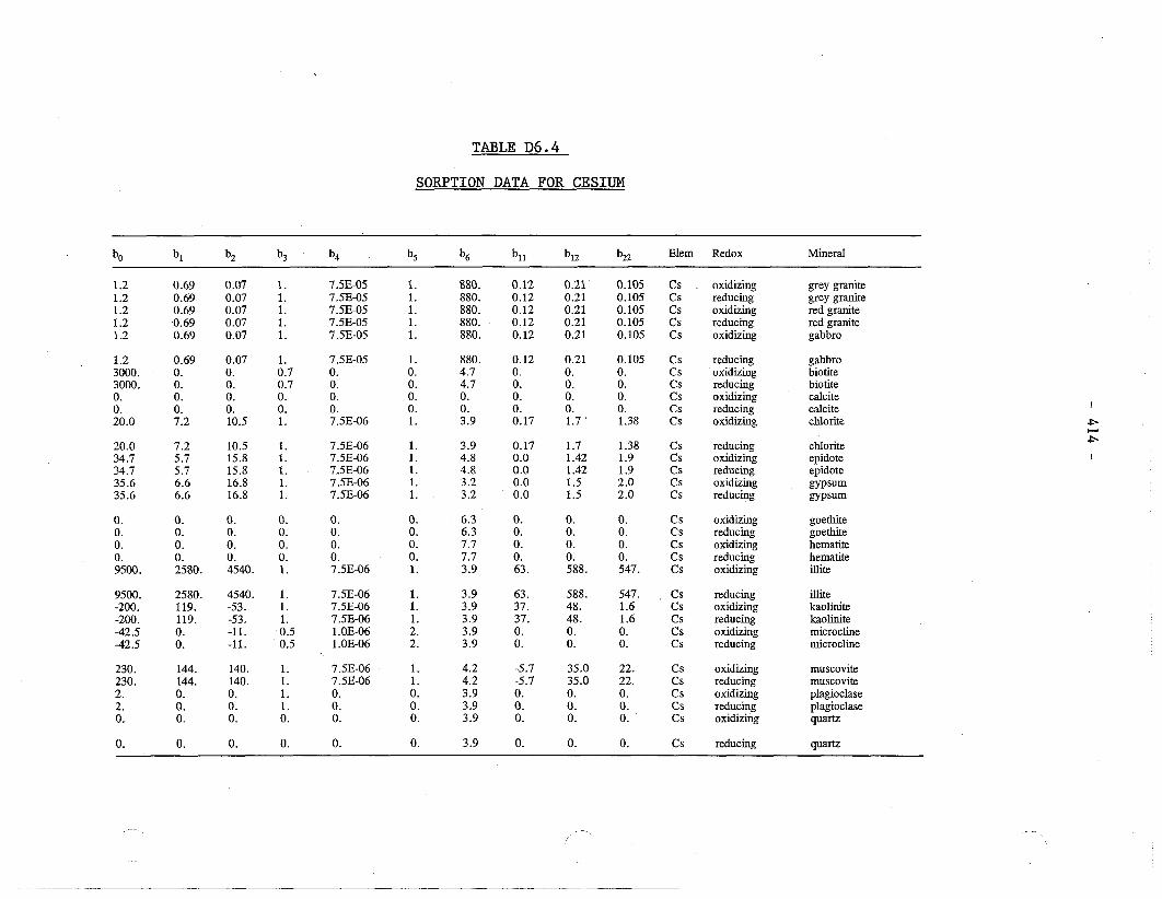
TABLE D6.4
SORPTION DATA FOR CESIUM
b5 b6 b~~ b,, bZ2 Elem Redox Mineral
1.2 0.69 0.07 1. 7.5E-05 1. 880. 0.12 0.21 0.105 Cs oxidizing grey granite 1.2 0.69 0.07 1. 7.5E-05 1. 880. 0.12 0.21 0.105 Cs reducing grey granite 1.2 0.69 0.07 1. 7.5E-05 1. 880. 0.12 0.21 0.105 Cs oxidizing red granite 1.2 0.69 0.07 1. 7.5E-05 1. 880. 0.12 0.21 0.105 Cs reducing red granite 1.2 0.69 0.07 1. 7.5E-05 1. 880. 0.12 0.21 0.105 Cs oxidizing gabbro
1.2 0.69 0.07 1. 7.5E-05 1. 880. 0.12 0.21 0.105 Cs reducing gabbro 3000. 0. 0. 0.7 0. 0. 4.7 0. 0. 0. Cs oxidizing biotite 3000. 0. 0. 0.7 0. 0. 4.7 0. 0. 0. Cs reducing biotite 0. 0. 0. 0. 0. 0. 0. 0. 0. 0. Cs oxidizing calcite 0. 0. 0. 0. 0. 0. 0. 0. 0. 0. Cs reducini calcite 20.0 7.2 10.5 1. 7.5E-06 1. 3.9 0.17 1.7 1.38 Cs oxidizing chlorite
20.0 7.2 10.5 1. 7.5E-06 1. 3.9 0.17 1.7 1.38 Cs reducing chlorite 34.7 5.7 15.8 1. 7.5E-06 1. 4.8 0.0 1.42 1.9 Cs oxidizing epidote 34.7 5.7 15.8 1. 7.5E-06 1. 4.8 0 .O 1.42 1.9 Cs reducing epidote 35.6 6.6 16.8 1. 7.5E-06 1. 3.2 0.0 1.5 2.0 Cs oxidizing gYP- 35.6 6.6 16.8 1. 7.5E-06 1. 3.2 0.0 1.5 2.0 Cs reducing gypsum
0. 0. 0. 0. 0. 0. 6.3 0. 0. 0. Cs oxidizing goethite 0. 0. 0. 0. 0. 0. 6.3 0. 0. 0. Cs reducing goethite 0. 0. 0. 0. 0. 0. 7.7 0. 0. 0. Cs oxidizing hematite 0. 0. 0. 0. 0. 0. 7.7 0. 0. 0. Cs reducing hematite 9500. 2580. 4540. 1. 7.5E-06 1. 3.9 63. 588. 547. Cs oxidizing illite
9500. 2580. 4540. 1. 7.5E-06 1. 3.9 63. 588. 547. . Cs reducing illite -200. 119. -53. 1. 7.5E-06 1. 3.9 37. 48. 1.6 Cs oxidizing kaolinite -200. 119. -53. 1. 7.5E-06 1. 3.9 37. 48. 1.6 Cs reducing kaolinite -42.5 0. -11. 0.5 1 .OE-06 2. 3.9 0. 0. 0. Cs oxidizing microcline -42.5 0. -11. 0.5 1 .OE-06 2. 3.9 0. 0. 0. Cs reducing microcline
230. 144. 140. 1. 7.5E-06 1. 4.2 -5.7 35.0 22. Cs oxidizing muscovite 230. 144. 140. 1. 7.5E-06 1. 4.2 -5.7 35.0 22. Cs reducing muscovite 2. 0. 0. 1. 0. 0. 3.9 0. 0. 0. Cs oxidizing plagioclase 2. 0. 0. 1. 0. 0. 3.9 0. 0. 0. Cs educing plagioclase 0. 0. 0. 0. 0. 0. 3.9 0. 0. 0. Cs oxidizing quartz
0. 0. 0. 0. 0. 0. 3.9 0. 0. 0. Cs reducing quartz
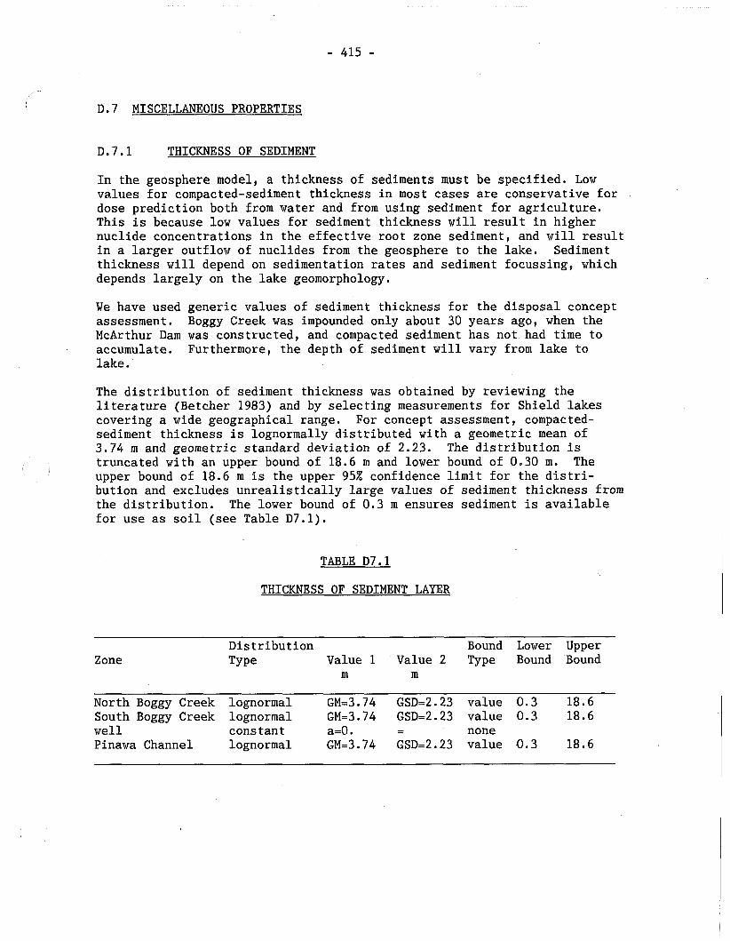
D.7 MISCELLANEOUS PROPERTIES
D.7.1 THICKNESS OF SEDIMENT
In the geosphere model, a thickness of sediments must be specified. Low values for compacted-sediment thickness in most cases are conservative for dose prediction both from water and from using sediment for agriculture. This is because low values for sediment thickness will result in higher nuclide concentrations in the effective root zone sediment, and will result in a larger outflow of nuclides from the geosphere to the lake. Sediment thickness will depend on sedimentation rates and sediment focussing, which depends largely on the lake geomorphology.
We have used generic values of sediment thickness for the disposal concept assessment. Boggy Creek was impounded only about 30 years ago, when the McArthur Dam was constructed, and compacted sediment has not had time to accumulate. Furthermore, the depth of sediment will vary from lake to lake.
The distribution of sediment thickness was obtained by reviewing the literature (Betcher 1983) and by selecting measurements for Shield lakes covering a wide geographical range. For concept assessment, compacted- sediment thickness is lognormally distributed with a geometric mean of 3.74 m and geometric standard deviation of 2.23. The distribution is truncated with an upper bound of 18.6 m and lower bound of 0.30 m. The upper bound of 18.6 m is the upper 95% confidence limit for the distri- bution and excludes unrealistically large values of sediment thickness from the distribution. The lower bound of 0.3 m ensures sediment is available for use as soil (see Table D7.1).
TABLE D7.1
THICKNESS OF SEDIMENT LAYER
Zone Distribution Bound Lower Upper Type Value 1 Value 2 Type Bound Bound
m m
North Boggy Creek lognormal GM=3.74 GSD=2.23 value 0.3 18.6 South Boggy Creek lognormal GM=3.74 GSD=2.23 value 0.3 18.6 well constant a=O . - - none Pinawa Channel lognormal GM=3.74 GSD=2.23 value 0.3 18.6

D.7.2 THICKNESS OF OVERBURDEN
The thickness of overburden deposits was determined from boreholes augered to refusal, normally bedrock, at the URL lease area and at another nearby grid area location at the Whiteshell Research Area. These two study areas are considered to have overburden deposits and topography representative of the WRA (Thorne 1986). They also have a dense network of boreholes which have been drilled into the overburden deposits. The borehole data were combined with field observations and airphotograph information to produce a map showing the distribution and thickness of overburden deposits. The isopach maps were digitized to determine the map area versus depth relationship. (Table D7.2).
TABLE D7.2
THICKNESS OF OVERBURDEN LAYER
Zone Distribution Bound Lower Upper Type Value 1 Value 2 Type Bound Bound
m m
Boggy Creek North normal p=l.O u=5.0 value 0.0 30.0 Boggy Creek South normal p4.0 u=5.0 value 0.0 30.0 well constant a=O . 0 - - none Pinawa Channel normal p=1 .O u=5.0 value 0.0 30.0
D. 7.3 RADIUS OF WELL CASING
The well data came from Manitoba Natural Resources Water Resources Branch files. All of these water supply wells (105 wells) were constructed into the bedrock for domestic purposes. About 80% of the well diameters were between 102 mm (4 inches) and 114 mm (4.5 inches); and 20% were between 127 mm (5 inches) and 152 mm. From this information, it may be considered that well-casing diameter lies between 102 and 152 mm in the Whiteshell Research Area. This would give a well radius that would lie between 51 and 76 mm.
The actual data used in the geosphere model of the Whiteshell Research Area were obtained from an earlier survey of domestic water supply wells. The data indicated that about 75% of the wells used 4 inch pipes for well casings, and 25% used 6 inch pipes. The tolerance of the pipe size is about 0.005 inches. The 4 inches diameter converts to a radius of 0.0508 meters, with the tolerance. The 6 inches becomes 0.0762 meters. A piecewise uniform distribution was used (see Table D7.3). This range of well radius covers the range found in the above survey of bedrock domestic wells.
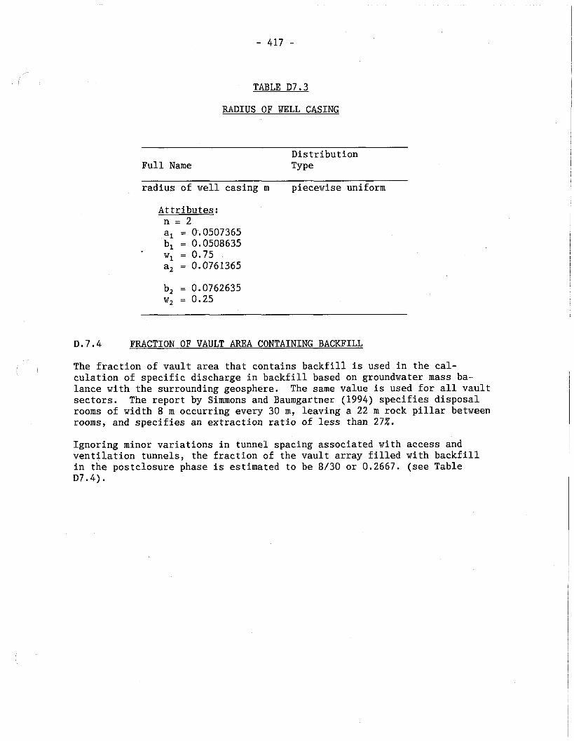
TABLE D7.3
RADIUS OF WELL CASING
Full Name Distribution Type
radius of well casing m piecewise uniform
Attributes: n = 2 a, = 0.0507365 b, = 0.0508635 w, = 0.75 a, = 0.0761365
D.7.4 FRACTION OF VAULT AREA CONTAINING BACKFILL
The fraction of vault area that contains backfill is used in the cal- l
culation of specific discharge in backfill based on groundwater mass ba- lance with the surrounding geosphere. The same value is used for all vault sectors. The report by Simmons and Baumgartner (1994) specifies disposal rooms of width 8 m occurring every 30 m, leaving a 22 m rock pillar between rooms, and specifies an extraction ratio of less than 27%.
Ignoring minor variations in tunnel spacing associated with access and ventilation tunnels, the fraction of the vault array filled with backfill in the postclosure phase is estimated to be 8/30 or 0.2667. (see Table D7.4).
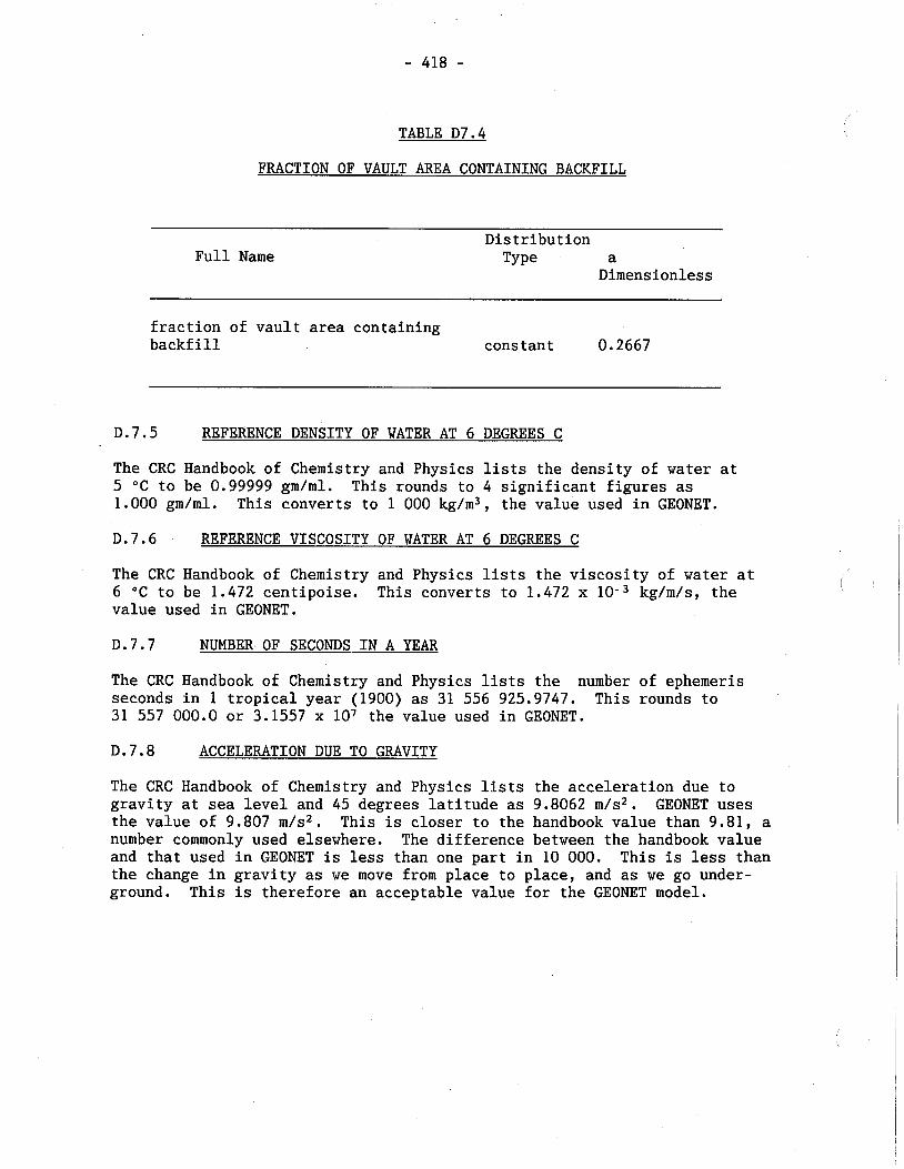
TABLE D7.4
FRACTION OF VAULT AREA CONTAINING BACKFILL
Distribution Full Name Type a
Dimensionless
fraction of vault area containing backfill cons tan t 0.2667
D.7.5 REFERENCE DENSITY OF WATER AT 6 DEGREES C
The CRC Handbook of Chemistry and Physics lists the density of water at 5 "C to be 0.99999 gm/ml. This rounds to 4 significant figures as 1.000 gm/ml. This converts to 1 000 kg/m3, the value used in GEONET.
D.7.6 REFERENCE VISCOSITY OF WATER AT 6 DEGREES C
The CRC Handbook of Chemistry and Physics lists the viscosity of water at 6 "C to be 1.472 centipoise. This converts to 1.472 x kg/m/s, the value used in GEONET.
D.7.7 NUMBER. OF SECONDS IN A YEAR
The CRC Handbook of Chemistry and Physics lists the number of ephemeris seconds in 1 tropical year (1900) as 31 556 925.9747. This rounds to 31 557 000.0 or 3.1557 x lo7 the value used in GEONET.
D.7.8 ACCELERATION DUE TO GRAVITY
The CRC Handbook of Chemistry and Physics lists the acceleration due to gravity at sea level and 45 degrees latitude as 9.8062 m/s2. GEONET uses the value of 9.807 m/s2. This is closer to the handbook value than 9.81, a number commonly used elsewhere. The difference between the handbook value and that used in GEONET is less than one part in 10 000. This is less than the change in gravity as we move from place to place, and as we go under- ground. This is therefore an acceptable value for the GEONET model.

REFERENCES:
Betcher, R.N. 1983. Geology and hydrogeology of surficial materials on the Underground Research Laboratory lease area. Atomic Energy of Canada Limited Technical Record, TR-219.
Bradbusy, M.H., D.A. Lever and D.V. Kinsey. 1982. Aqueous phase diffusion in crystalline rock. Atomic Energy Research Establishment, Harwell, U.K., Report AERE-R-10525.
Chan, T., N.W. Scheier and J.A.K. Reid. 1986. Finite-element thermohydro- geological modelling for Canadian nuclear fuel waste management. In Proceedings of the 2nd International Conference on Radioactive Waste Management, Toronto, Canadian Nuclear Society, 653-660.
Chan, T. 1987. An overview of groundwater flow and radionuclide transport modelling in the Canadian nuclear fuel waste management program. Proceedings of an AECL/USDOE Workshop on Geostatistical Sensitivity and Uncertainty Methods for Groundwater Flow and Radionuclide Transport Modelling, San Francisco, 1987 September 15-17.
Chan, T., D. Ophori and F.W. Stanchell. 1991. Sensitivity of Advective Contaminant Movement To Possible Pumping Near a Hypothetical Nuclear Fuel Waste Disposal Vault, World Environment, International Conference and Exhibition, Alberta, Canada, Apr 8-10.? Calgary, ACTA Press, 1991, 125-129.
Chan, T. and B.W. Nakka. 1994. A two-dimensional analytical well model with applications to groundwater flow and convective transport model- ling in the geosphere. Atomic Energy of Canada Limited Report, AECL- 10880, COG-93-215.
Chan, T., B.W. Nakka, P.A. O'Connor, D.U. Ophori, N.W. Scheier and F.W. Stanchell. 1994. Thermohydrogeological modelling of the Whiteshell Research Area. Atomic Energy of Canada Limited Report, AECL-10947, COG- 93-368.
CRC Handbook of Chemistry and Physics, 1987-1988, 68th edition, R.C. Weast (Editor), CRC Press, Inc., Boca Raton, Florida.
Davison, C.C. and V. Guvanasen. 1985. Hydrogeological characterization, modelling and monitoring of the site of Canada's Underground Research Laboratory: Presented at IAH 17th international congress on hydrogeo- logy of rocks of low permeability, Tucson, Arizona, January 7-11. Atomic Energy of Canada Limited Report, AECL-8676.
Davison, C.C., T. Chan and N.W. Scheier. 1987. Experimental activities of the Canadian nuclear fuel waste management program to validate geo- sphere models. In Proceedings of GEOVAL-87: A symposium on verifi- cation and validation of geosphere performance assessment models, Stockholm, Sweden, 1987 April 7-9.
Domenico, P.A. and F.W. Schwartz. 1990. Physical and Chemical Hydrogeo- logy. John Wiley and Sons Inc. 1990 Toronto.
Frech, K.J. and P.A. Orconnor. 1986. FITDIS User's Manual. Atomic Energy of Canada Limited Technical Record, TR-407.
Freeze, R.A. and J.A. Cherry. 1979. Groundwater; Prentice-Hall Inc., Englewood Cliffs, New Jersey.
Frost, L.H., N.W. Scheier, E.T. Kozak and C.C. Davison. 1992. Solute transport properties of a major shear zone in granite. In Proceedings of the 6th international symposium on water tracing by the Inter- national Association of Tracer Hydrology held in Karlsruhe, Germany, 1992 September 21-26.
Applied Geoscience Branch Report. 1990. Report of summary of the appendix B groundwater tracer test program at the WNRE borehole site, report of activities for the period 1989 April to 1990 March. Atomic Energy of Canada Limited. Prepared for: The Power Reactor and Nuclear Fuel Development Corporation in Japan.
Gascoyne, M., J.D. Ross, R.L. Watson and D.C. Kamineni. 1989. Soluble salts in a Canadian Shield granite as contributors to groundwater salinity. In proceedings of the 6th International Symposium on Water Rock Interaction, Malvern, U.K., 1989, 247-249.
Gascoyne, M. and D.C. Kamineni. 1992. Groundwater chemistry and fracture mineralogy in the Whiteshell Research Area: Supporting data for the Geosphere and Biosphere Transport Models. Atomic Energy of Canada Limited Technical Record, TR-516.
Gelhar, L.W., C. Welty and K.R. Rehfeldt. 1992. A critical review of data on field-scale dispersion in aquifers. Water Resources Research, Volume 28, No. 7, 1955-1974.
Goodwin, B.W., D.B. McConnell, T.H. Andres, W.C. Hajas, D.M. LeNeveu, T.W. Melnyk, G.R. Sherman, M.E. Stephens, J.G. Szekely, P.C. Bera, C.M. Cosgrove, K.D. Dougan, S.B. Keeling, C.I. Kitson, B.C. Kummen, S.E. Oliver, K. Witzke, L. Wojciechowski and A.G. Wikjord. 1994. The dis- posal of Canada's nuclear fuel waste: Postclosure assessment of a reference system. Atomic Energy of Canada Limited Report, AECL-10717, COG-93-7.
Katsube, T.J., T.W. Melnyk and J.P. Hume. 1986. Pore structure from dif- fusion in granitic rocks. Atomic Energy of Canada Limited Technical Record, TR-381.
Lerman, A. 1979. Geochemical processes: water and sediment environments. John Wiley and Sons, New York.
Nakka, B.W. and T. Chan. 1994. A particle-tracking code (TRACK3D) for convective solute transport modelling in the geosphere: Description and User's Manual. Atomic Energy of Canada Limited Report, AECL-10881, COG-93-216.
Neuman, S.P. 1990. Universal sealing of hydraulic conductivities and dispersfvities in geologic media. Water Resources Research, Volume 26, NO. 8, 1746-1758.
Robinson, R.A. and R.H. Stokes. 1959. Electrolyte solutions. Second Edition, revised. Butterworths, London, UK. Appendix 11.1.
Ross, J.D. and M. Gascoyne. 1992. Comparison of surface and downhole electrochemical measurements in Canadian Shield groundwaters. Atomic Energy of Canada Limited Technical Record, TR-478.
Scheier, N.W., L.H. Frost and C.C. Davison. 1990. Modelling activities for the groundwater tracer test program at the WNRE borehole site. Proceedings of GEOVAL-90: A symposium on validation of geosphere flow and transport models, 1990 May 14-17, Stockholm, OECD Publications, ' Paris, 148-156.
Scheier, N.W., L.H. Frost and C.C. Davison. 1993. Groundwater tracer experiments in a major fracture zone in granite. Proceedings of IAH 24th Congress on Hydrogeology of Hard Rocks held in Oslo, Norway, 1993 June 28 - July 2.
Simmons, G.R. and P. Baumgartner. 1994. The disposal of Canada's nuclear fuel waste: engineering for a disposal facility. AECL Report AECL- 10715, COG-93-5.
Skaguis, K. and I. Neretnieks. 1982. Diffusion in crystalline rocks of some sorbing and nonsorbing species. KarnBransleSakerhet Report, KBS- 82- 12.
Skaguis, K. and I. Neretnieks. 1983. Diffusion in crystalline rocks. KarnBransleSakerhet Report, KBS-83-15,
Stephens, M.E., B.W. Goodwin and T.H. Andres. 1989. Guidelines for defining probability density functions for SYVAC3-CC3 parameters. Atomic Energy of Canada Limited Technical Record, TR-479.
Stone, D., D.C. Kamineni, A. Brown and R. Everitt. 1989. A comparison of fracture styles in two granite bodies of the Superior province. Can. J. Earth Sci., 26, 387-403.
Thorne, G.A. 1986. Surface hydrology of two underground research labora- tory (url) sub-basins and the dead creek watershed. 1982-1983. Atomic Energy of Canada Limited Technical Record, TR-349.
Thorne, G.A. 1990. Hydrogeology of surficial materials of permit areas D and F and the Lee River Study area in the Whiteshell Research area. Atomic Energy of Canada Limited Technical Record, TR-498.
Vandergraaf, T.T. and K.V. Ticknor. 1993. A compilation and evaluation of radionuclide sorption coefficients used in the GEONET submodel of SYVAC for the Whiteshell Research Area. Atomic Energy of Canada Limited Report, AECL-10546, COG-92-59.
Vandergraaf, T.T., K.V. Ticknor and T.W. Melnyk. 1992. The selection and use of a sorption database for the geosphere model in the Canadian Nuclear Fuel Waste Management Program. Radionuclide Sorption from the Safety Evaulation Perspective. Proceedings of an NEA Workshop. Nuclear Energy Agency. Organization dor Economic Cooperation and Development. Paris 1992. 81-120. Atomic Energy of Canada Limited Report, AECL-10822, COG-93-00082
Yong, R.N., P. Boonsinsuk and G. Wong. 1986. Formulation of backfill material for a nuclear fuel waste disposal vault; Canadian Geotechnical Journal, 23(2), 216-228.
Zienkiewicz, O.C. 1977. The finite element method. Third edition, McGraw- Hill, London.
(TR- indicates unrestricted, unpublished reports available from SDDO, AECL Research, Chalk River Laboratories, Chalk River, Ontario KOJ 1LO.)
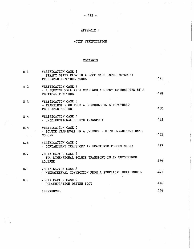
APPENDIX E
MOTIF VERIFICATION
CONTENTS
VERIFICATION CASE 1 - STEADY STATE FLOW IN A ROCK MASS INTERSECTED BY PERMEABLE FRACTURE ZONES
VERIFICATION CASE 2 - A PUMPING WELL IN A CONFINED AQUIFER INTERSECTED BY A VERTICAL FRACTURE 428
VERIFICATION CASE 3 - TRANSIENT FLOW FROM A BOREHOLE IN A FRACTURED PERMEABLE MEDIUM
VERIFICATION CASE 4 - UNIDIRECTIONAL SOLUTE TRANSPORT
VERIFICATION CASE 5 - SOLUTE TRANSPORT IN A UNIFORM FINITE ONE-DIMENSIONAL COLUMN
VERIFICATION CASE 6 - CONTAMINANT TRANSPORT IN FRACTURED POROUS MEDIA
VERIFICATION CASE 7 - TWO DIMENSIONAL SOLUTE TRANSPORT IN AN UNCONFINED AQUIFER
VERIFICATION CASE 8 - HYDROTHERMAL CONVECTION FROM A SPHERICAL HEAT SOURCE
VERIFICATION CASE 9 - CONCENTRATION-DRIVEN FLOW
REFERENCES
MOTIF VERIFICATION
A series of verification cases has been used to test the numerical solution techniques and coding in MOTIF, as well as to demonstrate some of the MOTIF analysis capabilities. The MOTIF solution for each verification case has been compared with corresponding analytical or numerical solution(s). Veri- fication cases (I), (2) and (9) outlined below are HYDROCOIN Level 1 veri- fication cases. The MOTIF solutions for these three verification cases, as well as verification cases (6) and (9) below, were compared with independ- ent analytical or numerical solutions in Chan et al. (1985). The MOTIF results for the HYDROCOIN Level 1 verification cases are also included in the HYDROCOIN Secretariat's compilation and comparison of results submitted by various project teams (The International HYDROCOIN Project - Level 1 Code Verification, 1988).
VERIFICATION CASE 1 - STEADY STATE FLOW IN A ROCK MASS INTERSECTED BY PERMEABLE FRACTURE ZONES
This verification case concerns a topographically driven, steady-state flow in a two-dimensional porous medium intersected by two inclined fracture zones with a relatively high permeability compared to that of the surround-
l ing rock. The fracture zones intersect each other at a given depth. Figure El.l shows a schematic representation of the geometry. This is the HYDROCOIN Level 1 Verification Case 2 problem.
The boundary conditions considered for the solution are:
At the top boundary (ground surface),
and
Along the two vertical boundaries (x = 0 m and x = 1600 m), and the bottom boundary, non-flow condition prevails. The bottom boundary (z = -1 000 m) is assumed to be impervious. The input parameter specifications are shown in Table El.l.
The MOTIF code was used to solve this verification case using three (3) different discretizations. The three discretizations used (XSP, XSO, FSO), are defined as follows;
XSP= coarse mesh with solid elements (matrix) and planar elements (fracture zones),
XSO=coarse mesh with solid elements only, FSO=fine mesh with solid elements only.
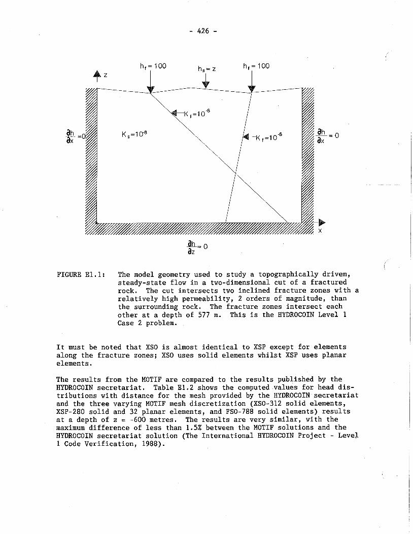
FIGURE El.l: The model geometry used to study a topographically driven, steady-state flow in a two-dimensional cut of a fractured rock. The cut intersects two inclined fracture zones with a relatively high permeability, 2 orders of magnitude, than the surrounding rock. The fracture zones intersect each other at a depth of 577 m. This is the HYDROCOIN Level 1 Case 2 problem.
It must be noted that XSO is almost identical to XSP except for elements along the fracture zones; XSO uses solid elements whilst XSP uses planar elements . The results from the MOTIF are compared to the results published by the HYDROCOIN secretariat. Table E1.2 shows the computed values for head dis- tributions with distance for the mesh provided by the HYDROCOIN secretariat and the three varying MOTIF mesh discretization (XSO-312 solid elements, XSP-280 solid and 32 planar elements, and FSO-788 solid elements) results at a depth of z = -600 metres. The results are very similar, with the maximum difference of less than 1.5% between the MOTIF solutions and the HYDROCOIN secretariat solution (The International HYDROCOIN Project - Level 1 Code Verification, 1988).
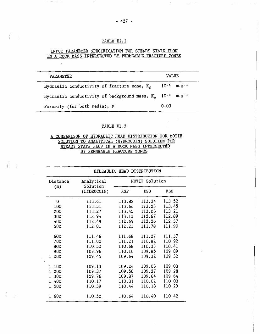
TABLE El. 1
INPUT PARAMETER SPECIFICATION FOR STEADY STATE FLOW IN A ROCK MASS INTERSECTED BY PERMEABLE FRACTURE ZONES
PARAMETER VALUE
Hydraulic conductivity of fracture zone, Kf lo-G m. s-
Hydraulic conductivity of background mass, K, m.s-l
Porosity (for both media), 6' 0.03
TABLE E1.2
A COMPARISON OF HYDRAULIC HEAD DISTRIBUTION FOR MOTIF SOLUTION TO ANALYTICAL (HYDROCOIN) SOLUTION FOR STEADY STATE FLOW IN A ROCK MASS INTERSECTED
BY PERMEABLE FRACTURE ZONES
HYDRAULIC HEAD DISTRIBUTION
Distance Analytical MOTIF Solution (m> Solution
(HYDROCOIN) XSP XSO FSO
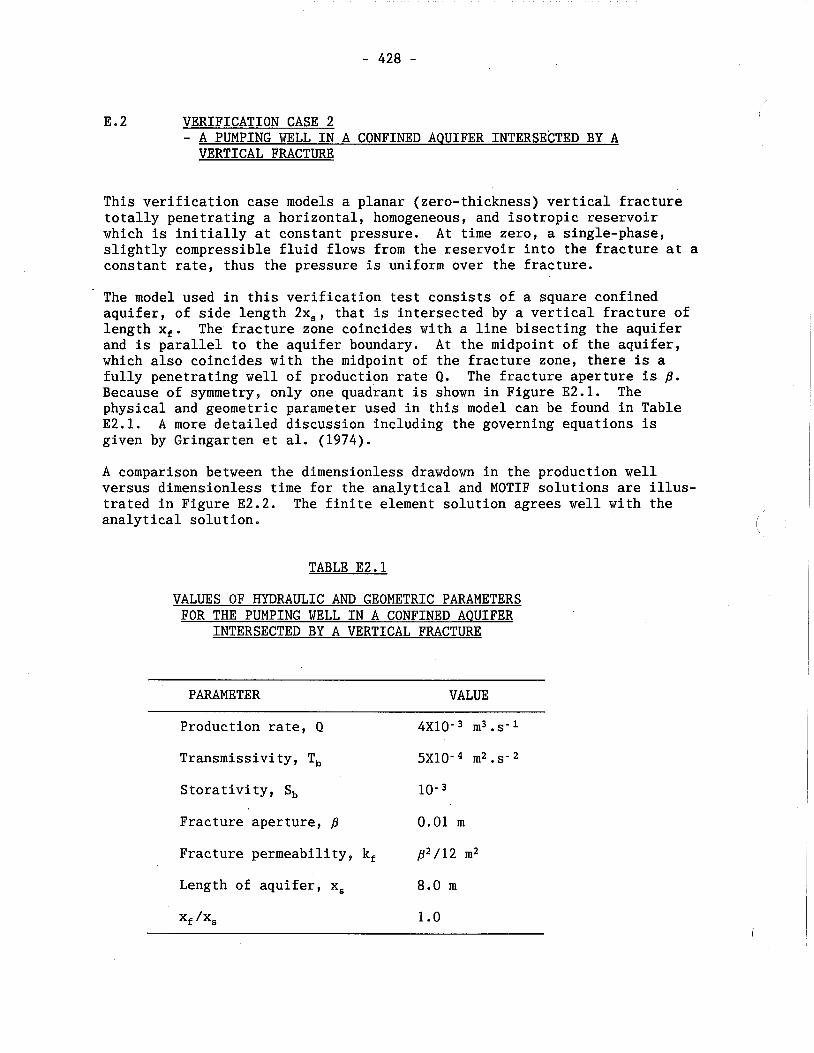
- A PUMPING WELL IN A CONFINED AQUIFER INTERSECTED BY A VERTICAL FRACTURE
This verification case models a planar (zero-thickness) vertical fracture totally penetrating a horizontal, homogeneous, and isotropic reservoir which is initially at constant pressure. At time zero, a single-phase, slightly compressible fluid flows from the reservoir into the fracture at a constant rate, thus the pressure is uniform over the fracture.
The model used in this verification test consists of a square confined aquifer, of side length 2x,, that is intersected by a vertical fracture of length xf. The fracture zone coincides with a line bisecting the aquifer and is parallel to the aquifer boundary. At the midpoint of the aquifer, which also coincides with the midpoint of the fracture zone, there is a fully penetrating well of production rate Q. The fracture aperture is 8 . Because of symmetry, only one quadrant is shown in Figure E2.1. The physical and geometric parameter used in this model can be found in Table E2.1. A more detailed discussion including the governing equations is given by Gringarten et al. (1974).
A comparison between the dimensionless drawdown in the production well versus dimensionless time for the analytical and MOTIF solutions are illus- trated in Figure E2.2. The finite element solution agrees well with the analytical solution.
TABLE E2.1
VALUES OF HYDRAULIC AND GEOMETRIC PARAMETERS FOR THE PUMPING WELL IN A CONFINED AQUIFER
INTERSECTED BY A VERTICAL FRACTURE
PARAMETER VALUE
Production rate, Q 4x10- m3 . s- Transmissivity, T, 5x10- m2 . s- Storativity, S, 10- 3
Fracture aperture, p 0.01 m
Fracture permeability, k, p2/12 m2
Length of aquifer, x, 8.0 m

Fracture I
I FIGURE EZ.l: The geometry of the problem with a production well within a
confined aquifer intersected by a vertical fracture (Xf/Xs = 1 .O)
FIGURE E2.2: Plot of dimensionless drawdown in a pumping well within a confined aquifer intersected by a vertical fracture plane (X,/Xs = 1.0), versus dimensionless time
- F -
S : 77 30 - e :, n r cn - cn - a, - - K T - 0 0 .- cn -: s z
2 : .- a'? -
0
oMOTl F -ANALYTICAL
r ,@I I l l l ; ~ ~ Z I I 1 1 1 I I
Dimensionless Time
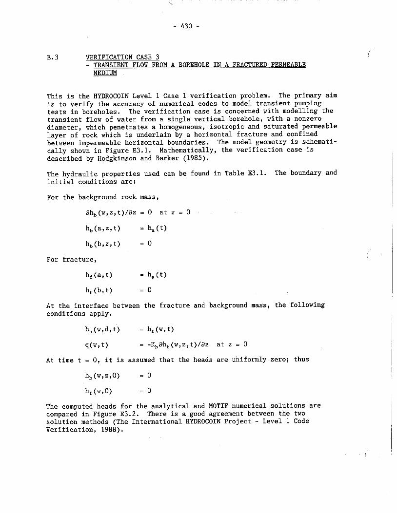
E. 3 VERIFICATION CASE 3 - TRANSIENT FLOW FROM A BOREHOLE IN A FRACTURED PERMEABLE MEDIUM
This is the HYDROCOIN Level 1 Case 1 verification problem. The primary aim is to verify the accuracy of numerical codes to model transient pumping tests in boreholes. The verification case is concerned with modelling the transient flow of water from a single vertical borehole, with a nonzero diameter, which penetrates a homogeneous, isotropic and saturated permeable layer of rock which is underlain by a horizontal fracture and confined between impermeable horizontal boundaries. The model geometry is schemati- cally shown in Figure E3.1. Mathematically, the verification case is described by Hodgkinson and Barker (1985).
The hydraulic properties used can be found in Table E3.1. The boundary and initial conditions are:
For the background rock mass,
For fracture,
At the interface between the fracture and background mass, the following conditions apply.
At time t = 0, it is assumed that the heads are uniformly zero; thus
The computed heads for the analytical and MOTIF numerical solutions are compared in Figure E3.2. There is a good agreement between the two solution methods (The International HYDROCOIN Project - Level 1 Code Verification, 1988).
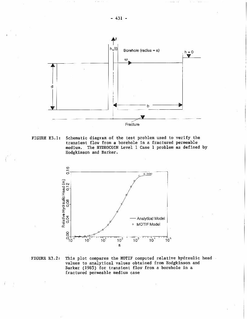
I I
Fracture
FIGURE E3.1: Schematic diagram of the test problem used to verify the transient flow from a borehole in a fractured permeable medium. The HYDROCOIN Level 1 Case 1 problem as defined by Hodgkinson and Barker.
- Analytical Model
0 MOTIF Model
FIGURE E3.2: This plot compares the MOTIF computed relative hydraulic head values to analytical values obtained from Hodgkinson and Barker (1985) for transient flow from a borehole in a fractured permeable medium case
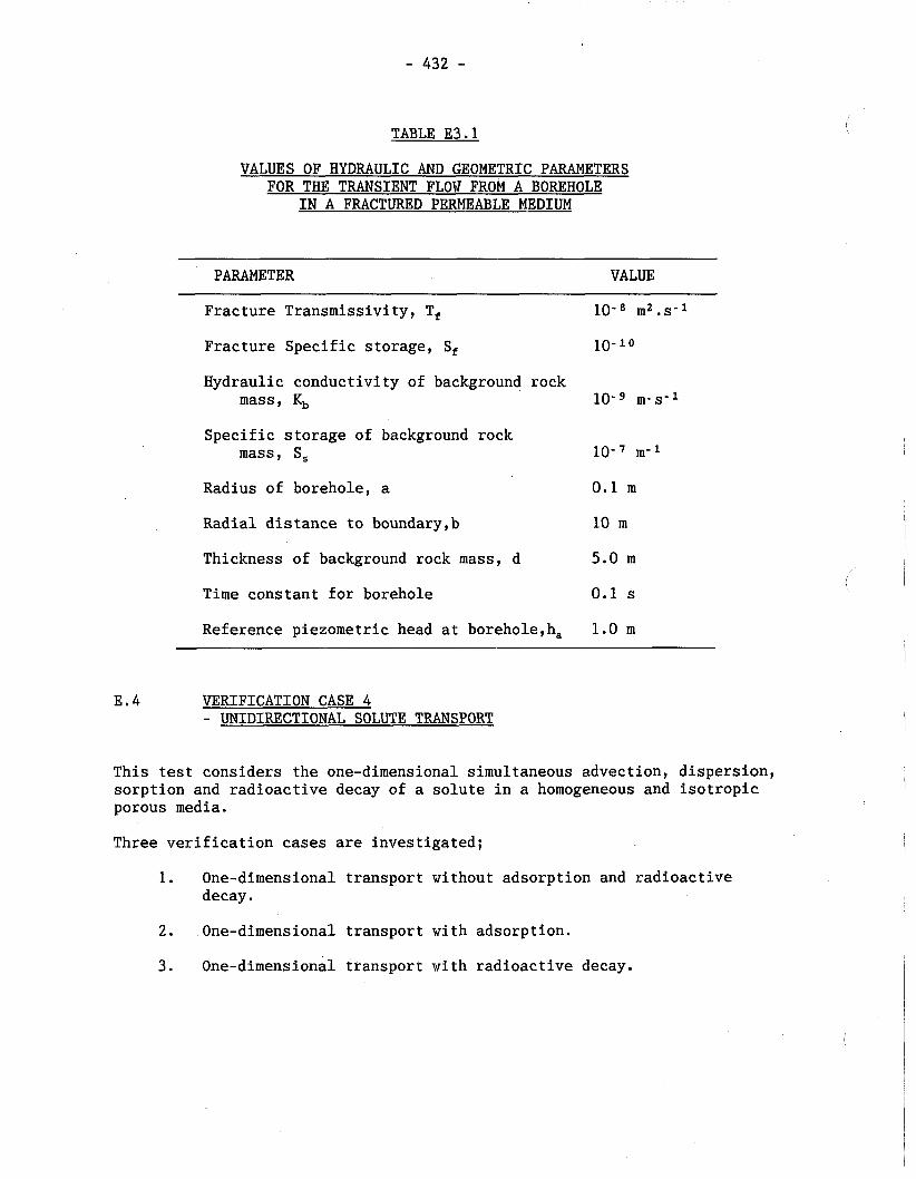
TABLE E3.1
VALUES OF HYDRAULIC AND GEOMETRIC PARAMETERS FOR THE TRANSIENT FLOW FROM A BOREHOLE
IN A FRACTURED PERMEABLE MEDIUM
PARAMETER VALUE
Fracture Transmissivity, Tf
Fracture Specific storage, Sf
Hydraulic conductivity of background rock mass, K,
Specific storage of background rock mass, S,
Radius of borehole, a
Radial distance to boundary,b
Thickness of background rock mass, d
Time constant for borehole
Reference piezometric head at borehole,h,
VERIFICATION CASE 4 - UNIDIRECTIONAL SOLUTE TRANSPORT
This test considers the one-dimensional simultaneous advection, dispersion, sorption and radioactive decay of a solute in a homogeneous and isotropic porous media.
Three verification cases are investigated;
1. One-dimensional transport without adsorption and radioactive decay.
2. One-dimensional transport with adsorption.
3. one-dimensional transport with radioactive decay.
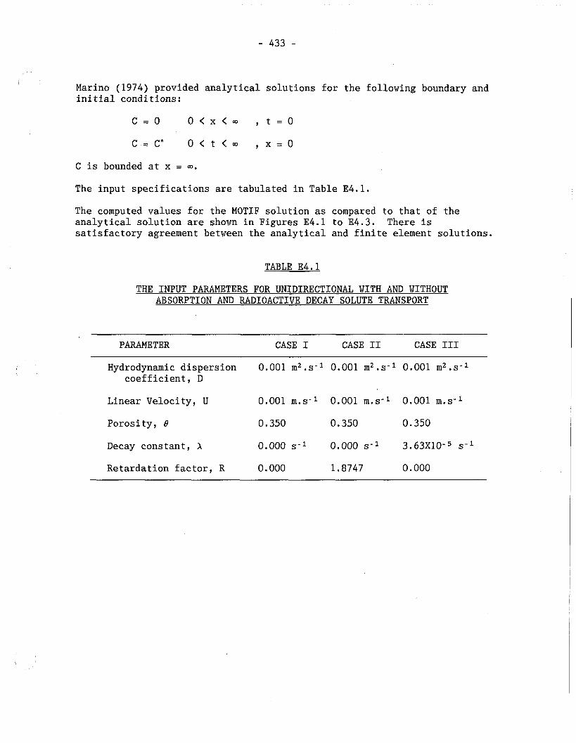
Marino (1974) provided analytical solutions for the following boundary and initial conditions:
C is bounded at x = Q.
The input specifications are tabulated in Table E4.1.
The computed values for the MOTIF solution as compared to that of the analytical solution are shown in Figures E4.1 to E4.3. There is satisfactory agreement between the analytical and finite element solutions.
TABLE E4.1
THE INPUT PARAMETERS FOR UNIDIRECTIONAL WITH AND WITHOUT ABSORPTION AND RADIOACTIVE DECAY SOLUTE TRANSPORT
PARAMETER CASE I CASE I1 CASE I11
Hydrodynamicdispersion 0.001m2.s-1 0.001m2.s-1 0.001m2.s-1 coefficient, D
Linear Velocity, U 0.001 m.s-I 0.001 m.s-I 0.001 m.s-I
Porosity, 6 0.350 0.350 0.350
Decay constant, X O.OOOS-~ O.OOOS-~ 3.63X10⁻⁵ s-I
Retardation factor, R 0.000 1.8747 0.000
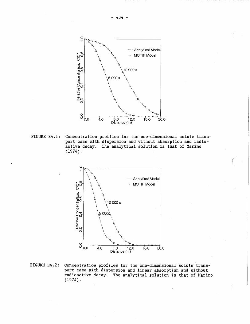
FIGURE E4.1: Concentration profiles for the one-dimensional solute trans- port case with dispersion and without absorption and radio- active decay. The analytical solution is that of Marino (1974).
FIGURE E4.2: Concentration profiles for the one-dimensional solute trans- port case with dispersion and linear absorption and without radioactive decay. The analytical solution is that of Marino (1974).
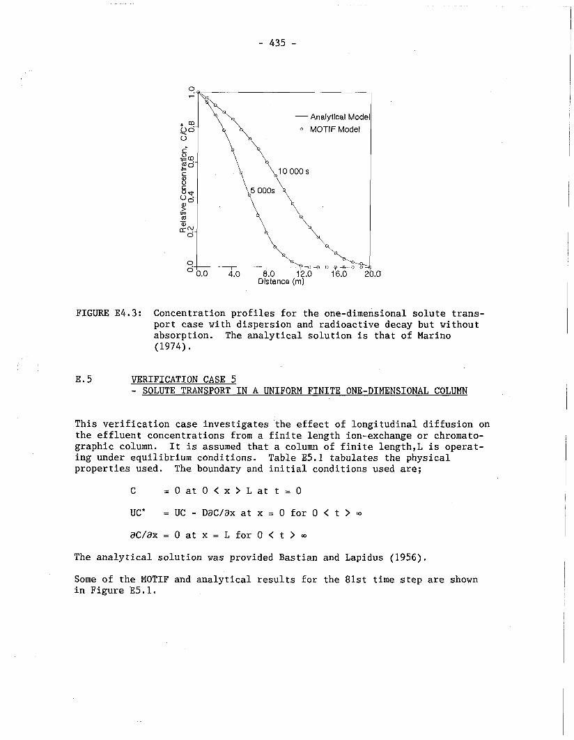
FIGURE E4.3: Concentration profiles for the one-dimensional solute trans- port case with dispersion and radioactive decay but without absorption. The analytical solution is that of Marino (1974).
E.5 VERIFICATION CASE 5 - SOLUTE TRANSPORT IN A UNIFORM FINITE ONE-DIMENSIONAL COLUMN
This verification case investigates 'the effect of longitudinal diffusion on the effluent concentrations from a finite length ion-exchange or chromato- graphic column. It is assumed that a column of finite length,L is operat- ing under equilibrium conditions. Table E5.1 tabulates the physical properties used. The boundary and initial conditions used are;
UC* = UC - DaC/ax at x = 0 for 0 < t > Q
aC/ax = 0 at x = L for 0 < t > Q
The analytical solution was provided Bastian and Lapidus (1956).
Some of the MOTIF and analytical results for the 81st time step are shown in Figure E5.1.
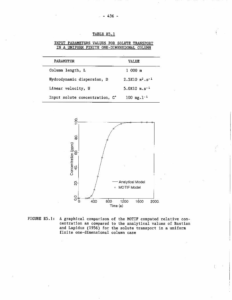
TABLE E5.1
INPUT PARAMETERS VALUES FOR SOLUTE TRANSPORT IN A UNIFORM FINITE ONE-DIMENSIONAL COLUMN
PARAMETER VALUE
Column length, L 1 000 m
Hydrodynamic dispersion, D 2.5X10 m2 .s-I
Linear velocity, U 5.OX10 m.s-l
Input solute concentration, C* 100 mg.1-l
Time (a)
FIGURE E5.1: A graphical comparison of the MOTIF computed relative con- centration as compared to the analytical values of Bastian and Lapidus (1956) for the solute transport in a uniform finite one-dimensional column case
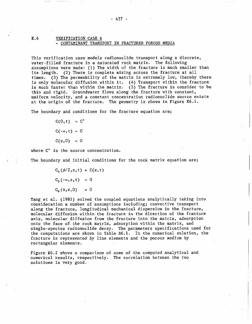
E. 6 VERIFICATION CASE 6 - CONTAMINANT TRANSPORT IN FRACTURED POROUS MEDIA
This verification case models radionuclide transport along a discrete, water-filled fracture in a saturated rock matrix. The following assumptions were made: (1) The width of the fracture is much smaller than its length. (2) There is complete mixing across the fracture at all times. (3) The permeability of the matrix is extremely low, thereby there is only molecular diffusion within it. (4) Transport within the fracture is much faster than within the matrix. (5) The fracture is consider to be thin and rigid. Groundwater flows along the fracture with constant, uniform velocity, and a constant concentration radionuclide source exists at the origin of the fracture. The geometry is shown in Figure E6.1.
The boundary and conditions for the fracture equation are;
where C* is the source concentration.
I The boundary and initial conditions for the rock matrix equation are;
Tang et al. (1981) solved the coupled equations analytically taking into consideration a number of assumptions including; convective transport along the fracture, longitudinal mechanical dispersion in the fracture, molecular diffusion within the fracture in the direction of the fracture axis, molecular diffusion from the fracture into the matrix, adsorption onto the face of the rock matrix, adsorption within the matrix, and single-species radionuclide decay. The parameters specifications used for the computations are shown in Table E6.1. In the numerical solution, the fracture is represented by line elements and the porous medium by rectangular elements.
Figure E6.2 shows a comparison of some of the computed analytical and numerical results, respectively. The correlation between the two solutions is very good.
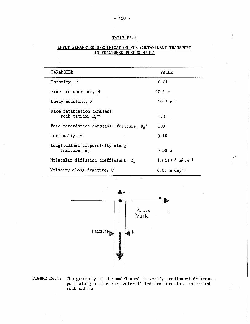
TABLE E6.1
INPUT PARAMETER SPECIFICATION FOR CONTAMINANT TRANSPORT IN FRACTURED POROUS MEDIA
PARAMETER VALUE
Porosity, B 0.01
Fracture aperture, p lo-4 m
Decay constant, X lo-g s-I
Face retardation constant rock matrix, R,*
Face retardation constant, fracture, R,* 1.0
Tor tuosi ty , 7 0.10
Longitudinal dispersivity along fracture, a, 0.50 m
Molecular diffusion coefficient, Do 1.6X10⁻⁹ m2.s-I
Velocity along fracture, U 0.01 m.day-l
FIGURE E6.1: The geometry of the model used to verify radionuclide trans- port along a discrete, water-filled fracture in a saturated rock matrix
I
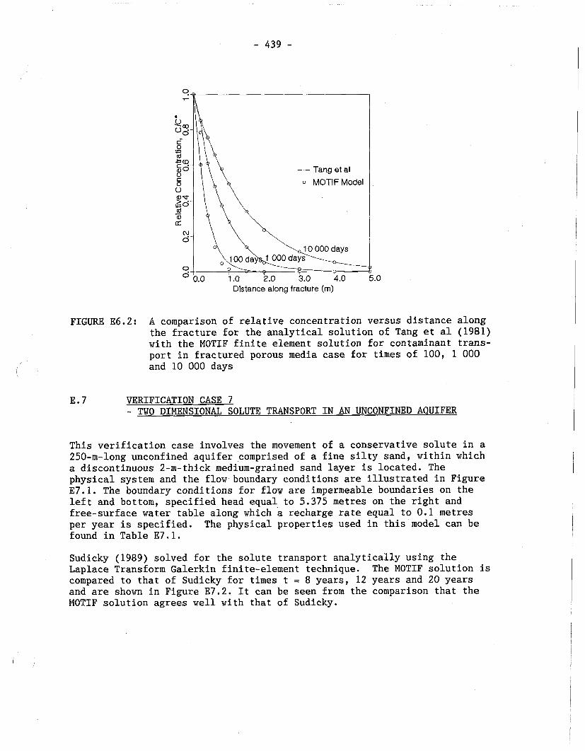
Distance along fracture (m)
FIGURE E6.2: A comparison of relative concentration versus distance along the fracture for the analytical solution of Tang et a1 (1981) with the MOTIF finite element solution for contaminant trans- port in fractured porous media case for times of 100, 1 000 and 10 000 days
I
E. 7 VERIFICATION CASE 7 - TWO DIMENSIONAL SOLUTE TRANSPORT IN AN UNCONFINED AQUIFER
This verification case involves the movement of a conservative solute in a 250-m-long unconfined aquifer comprised of a fine silty sand, within which a discontinuous 2-m-thick medium-grained sand layer is located. The physical system and the flow boundary conditions are illustrated in Figure E7.1. The boundary conditions for flow are impermeable boundaries on the left and bottom, specified head equal to 5.375 metres on the right and free-surface water table along which a recharge rate equal to 0.1 metres per year is specified. The physical properties used in this model can be found in Table E7.1.
Sudicky (1989) solved for the solute transport analytically using the Laplace Transform Galerkin finite-element technique. The MOTIF solution is compared to that of Sudicky for times t = 8 years, 12 years and 20 years and are shown in Figure E7.2. It can be seen from the comparison that the MOTIF solution agrees well with that of Sudicky.
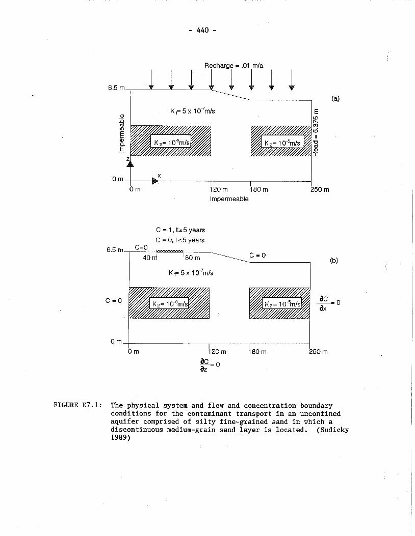
Recharge = .O1 m/a
6.5 m
Om I X I
Om 120 m 180 m 250 m Impermeable
C = 1, t25 years C = 0, t< 5 years
C = O (b)
FIGURE E7.1: The physical system and flow and concentration boundary conditions for the contaminant transport in an unconfined aquifer comprised of silty fine-grained sand in which a discontinuous medium-grain sand layer is located. (Sudicky 1989)
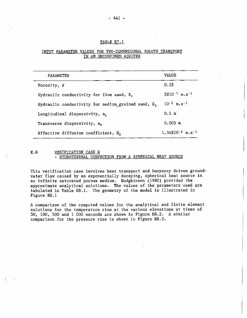
TABLE E7.1
INPUT PARAMETER VALUES FOR TWO-DIMENSIONAL SOLUTE TRANSPORT IN AN UNCONFINED AQUIFER
PARAMETER VALUE
Porosity, 0 0.35
Hydraulic conductivity for fine sand, K1 5X10⁻⁷ m.s-l
Hydraulic conductivity for medium-grained sand, K2 10- m. S-
Longitudinal dispersivity, a, 0.5 m
Transverse dispersivity, a, 0.005 m
Effective diffusion coefficient, Dd 1.34X10- m. s- l
E. 8 VERIFICATION CASE 8 - HYDROTHERMAL CONVECTION FROM A SPHERICAL HEAT SOURCE
This verification case involves heat transport and buoyancy driven ground- water flow caused by an exponentially decaying, spherical heat source in an infinite saturated porous medium. Hodgkinson (1980) provided the approximate analytical solutions. The values of the parameters used are tabulated in Table E8.1. The geometry of the model is illustrated in Figure E8.1
A comparison of the computed values for the analytical and finite element solutions for the temperature rise at the various elevations at times of 50, 100, 500 and 1 000 seconds are shown in Figure E8.2. A similar comparison for the pressure rise is shown in Figure E8.3.
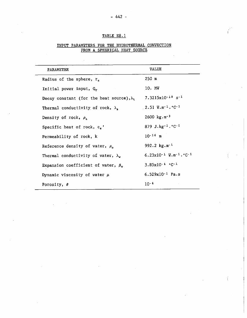
TABLE E8.1
INPUT PARAMETERS FOR THE HYDROTHERMAL CONVECTION FROM A SPHERICAL HEAT SOURCE
PARAMETER VALUE
Radius of the sphere, r,
Initial power input, Q,
Decay constant (for the heat source),X,
Thermal conductivity of rock, A,
Density of rock, p,
Specific heat of rock, c,'
Permeability of rock, k
Reference density of water, p,
Thermal conductivity of water, A,
Expansion coefficient of water, p,
Dynamic viscosity of water p
Porosity, 8
250 m
10. MW
7.3215~10-~O s-l
2.51 W.m-l. "C-I
2600 kg. m-
879 J.kg-l. "C- l
10-16 m
992.2 kg.m-I
6.23~10-I W.m-l. "C-I
3.85~10- "C- l
6.529~10-I Pa.s
10-
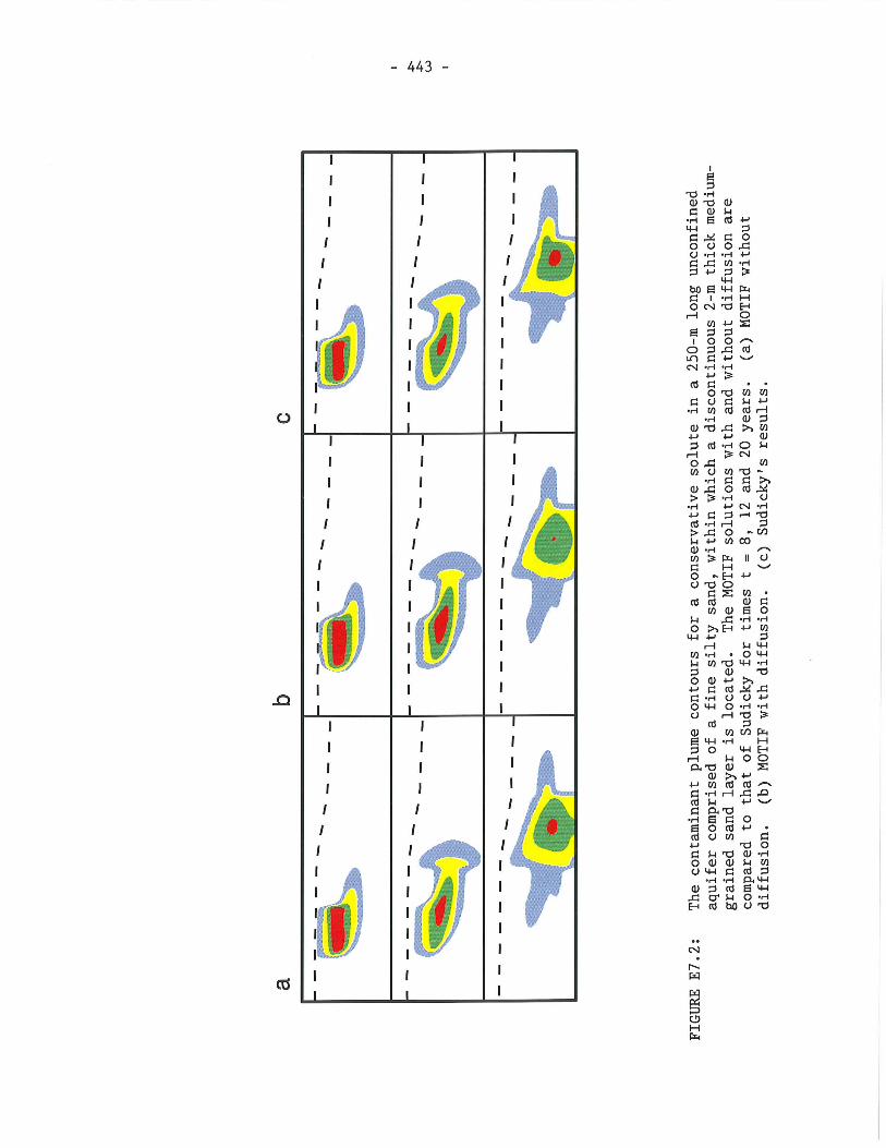
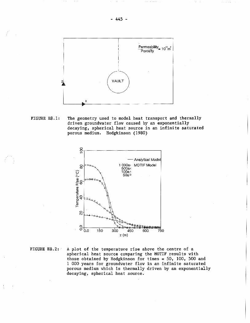
VAULT :: FIGURE E8.1: The geometry used to model heat transport and thermally
driven groundwater flow caused by an exponentially decaying, spherical heat source in an infinite saturated porous medium. Hodgkinson (1980)
- Analytical Model I 1 000ao MOTIF Model
500ax 1 0 0 a ~ 50ao
FIGURE E8.2: A plot of the temperature rise above the centre of a spherical heat source comparing the MOTIF results with those obtained by Hodgkinson for times = 50, 100, 500 and 1 000 years for groundwater flow in an infinite saturated porous medium which is thermally driven by an exponentially decaying, spherical heat source.
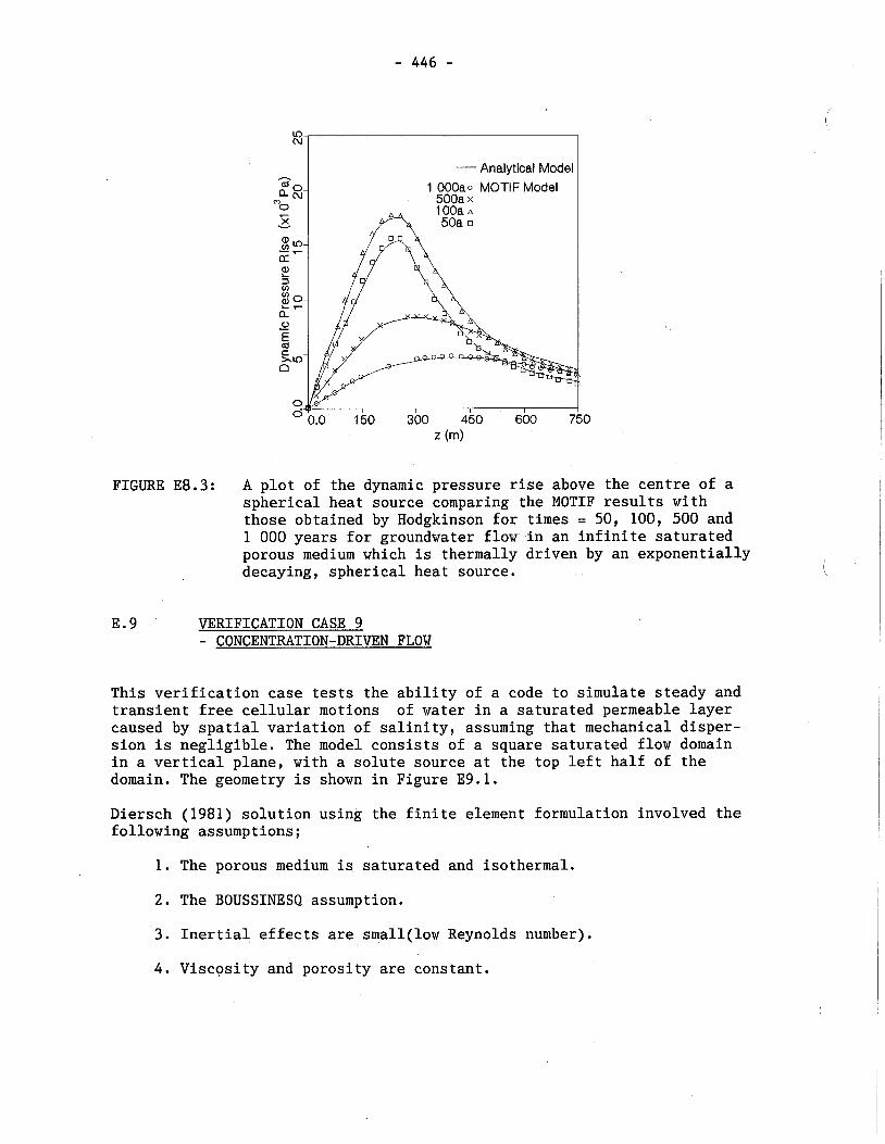
3
- Analytical Model h
*o a~ 1 000ao MOTIF Model m 0 7
X - 2 - E' 3 cn
?: a 0 .- S C X L O n
8 0.0 150 300 450 600 750
FIGURE E8.3: A plot of the dynamic pressure rise above the centre of a spherical heat source comparing the MOTIF results with those obtained by Hodgkinson for times = 50, 100, 500 and 1 000 years for groundwater flow in an infinite saturated porous medium which is thermally driven by an exponentially decaying, spherical heat source.
E.9 VERIFICATION CASE 9 - CONCENTRATION-DRIVEN FLOW
This verification case tests the ability of a code to simulate steady and transient free cellular motions of water in a saturated permeable layer caused by spatial variation of salinity, assuming that mechanical disper- sion is negligible. The model consists of a square saturated flow domain in a vertical plane, with a solute source at the top left half of the domain. The geometry is shown in Figure E9.1.
Diersch (1981) solution using the finite element formulation involved the following assumptions;
1. The porous medium is saturated and isothermal.
2. The BOUSSINESQ assumption.
3. Inertial effects are small(1ow Reynolds number).
4. Viscosity and porosity are constant.
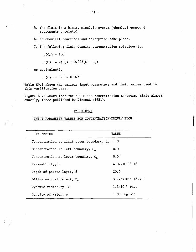
5. The fluid is a binary miscible system (chemical compound represents a solute)
6. No chemical reactions and adsorption take place.
7. The following fluid density-concentration relationship.
p(Co) = 1.0
p(C) = p(C,) + O.O25(C - C,)
or equivalently
Table E9.1 shows the various input parameters and their values used in this verification case.
Figure E9.2 shows that the MOTIF iso-concentration contours, mimic almost exactly, those published by Diersch (1981).
TABLE E9.1
INPUT PARAMETER VALUES FOR CONCENTRATION-DRIVEN FLOW
PARAMETER VALUE
Concentration at right upper boundary, C,
Concentration at left boundary, C,
Concentration at lower boundary, C,
Permeability, k
Depth of porous layer, d
Diffusion coefficient, D,
Dynamic viscosity, v
Density of water, p
1.0
0.0
0.0
4.07~10- lo m2
20.0
3.725~10- m2 . s- 1.3~10- Pa. s
1 000 kg.m-I
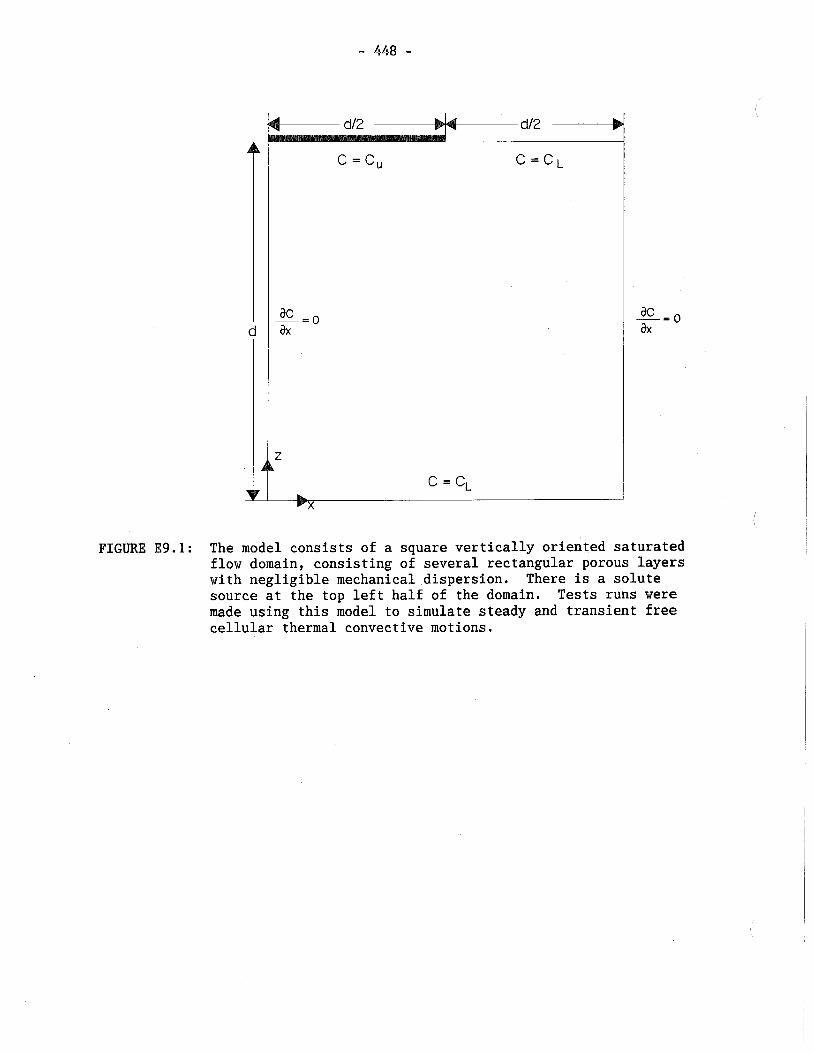
FIGURE E9.1: The model consists of a square vertically oriented saturated flow domain, consisting of several rectangular porous layers with negligible mechanical dispersion. There is a solute source at the top left half of the domain. Tests runs were made using this model to simulate steady and transient free cellular thermal convective motions.
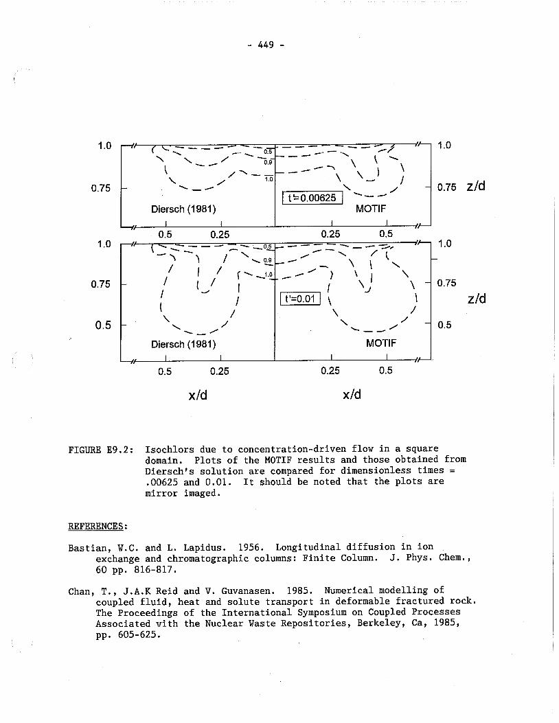
Diersch (1 981)
L Diersch ( I 981) / I I I
FIGURE E9.2: Isochlors due to concentration-driven flow in a square domain. Plots of the MOTIF results and those obtained from Dierschrs solution are compared for dimensionless times = ,00625 and 0.01. It should be noted that the plots are mirror imaged.
REFERENCES:
Bastian, W.C. and L. Lapidus. 1956. Longitudinal diffusion in ion exchange and chromatographic columns: Finite Column. J. Phys. Chem., 60 pp. 816-817.
Chan, T., J . A . K Reid and V. Guvanasen. 1985. Numerical modelling of coupled fluid, heat and solute transport in deformable fractured rock. The Proceedings of the International Symposium on Coupled Processes Associated with the Nuclear Waste Repositories, Berkeley, Ca, 1985, pp. 605-625.
Diersch, H.J. 1981. Primitive variable finite element solutions of free convection flows in porous media. Zeitschrift Fuer Angewandte Mathematik Und Mechanik, 61(7), pp. 325-337.
Gringarten, A.C., H.J. Ramey and R. Raghaven. 1974. Unsteady-state pressure distributions created by a well with a single infinite- conductivity vertical fracture. Society of Petroleum Engineers Journal, 14(4), pp. 347-360.
Hodgkinson, D. 1980. A mathematical model for hydrothermal convection around a radioactive waste depository in hard rock. Annals of Nuclear Energy, 7, pp. 313-334.
Hodgkinson, D. and J. Barker. 1985. Specification of a test problem for HYDROCOIN Level 1, case 1: Transient flow from a borehole in a fractured permeable medium , AERE-R11574, Harwell, Oxfordshier, U.K.
The International HYDROCOIN Project - Level 1: Code verification, organization for economic cooperation and development/nuclear energy agency (OECD/NEA) and Swedish nuclear power inspectorate (SKI), 1988.
Marino, M.A. 1974. Distribution of contaminants in porous media flow. Water Res. RES., 10(5), pp. 1013-1018.
Sudicky, E.A. 1989. The Laplace transform Galerkin technique: a time- continuous finite element theory and application to mass transport in groundwater. Water Res. Res.,25(8),1833-1846.
Tang, D.G., E.O. Frind and E.A. Sudicky. 1981. Contaminant transport in fractured porous media: analytical solution for a single fracture, Water Res. Res. 17, pp. 555.
(TR- indicates unrestricted, unpublished reports available from SDDO, AECL Research, Chalk River Laboratories, Chalk River, Ontario KOJ 1LO.)
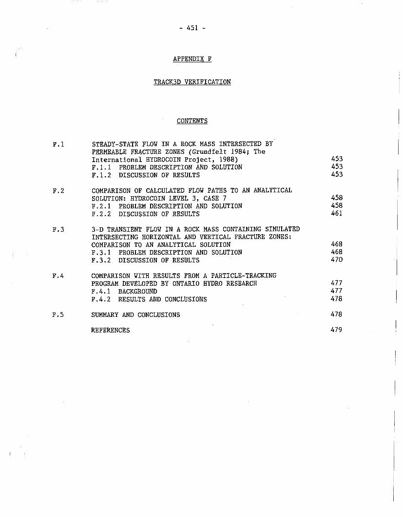
APPENDIX F
TRACK3D VERIFICATION
CONTENTS
F. 1 STEADY-STATE FLOW IN A ROCK MASS INTERSECTED BY PERMEABLE FRACTURE ZONES (Grundfelt 1984; The International HYDROCOIN Project, 1988) F.l.l PROBLEM DESCRIPTION AND SOLUTION F.1.2 DISCUSSION OF RESULTS
F.2 COMPARISON OF CALCULATED FLOW PATHS TO AN ANALYTICAL SOLUTION: HYDROCOIN LEVEL 3, CASE 7 F.2.1 PROBLEM DESCRIPTION AND SOLUTION F.2.2 DISCUSSION OF RESULTS
F.3 3-D TRANSIENT FLOW IN A ROCK MASS CONTAINING SIMULATED INTERSECTING HORIZONTAL AND VERTICAL FRACTURE ZONES: COMPARISON TO AN ANALYTICAL SOLUTION F.3.1 PROBLEM DESCRIPTION AND SOLUTION F.3.2 DISCUSSION OF RESULTS
F.4 COMPARISON WITH RESULTS FROM A PARTICLE-TRACKING PROGRAM DEVELOPED BY ONTARIO HYDRO RESEARCH F.4.1 BACKGROUND F.4.2 RESULTS AND CONCLUSIONS
F. 5 SUMMARY AND CONCLUSIONS
REFERENCES
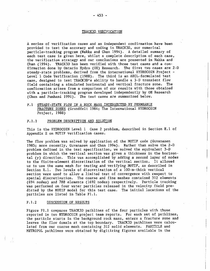
TRACK3D VERIFICATION
A series of verification cases and an independent confirmation have been provided to test the accuracy and coding in TRACK3D, our numerical particle-tracking program (Nakka and Chan 1994). A detailed summary of each test case is given here, whilst a complete description of each case, the verification strategy and our conclusions are presented in Nalcka and Chan (1994). TRACK3D has been verified with three test cases and a con- firmation done by Ontario Hydro cOH) Research. The first two cases are 2-D steady-state problems, derived from the international HYDROCOIN Project - Level 1 Code Verification (1988). The third is an AECL-formulated test case, designed to test TRACK3D1s ability to handle a 3-D transient flow field containing a simulated horizontal and vertical fracture zone. The confirmation arises from a comparison of our results with those obtained with a particle-tracking program developed independently by OH Research (Chan and Punhani 1991). The test cases are summarized below.
F.l STEADY-STATE FLOW IN A ROCK MASS INTERSECTED BY PERMEABLE FRACTURE ZONES (Grundfelt 1984; The International HYDROCOIN Project, 1988)
F.l.l PROBLEM DESCRIPTION AND SOLUTION
This is the HYDROCOIN Level 1 Case 2 problem, described in Section E.l of Appendix E on MOTIF verification cases.
The flow problem was solved by application of the MOTIF code (Guvanasen 1985; more recently, Guvanasen and Chan 1994). Rather than solve the 2-D problem defined in the test specification, we solved the equivalent 3-D problem in which the vertical section was given a thickness in the horizon- tal (y) direction. This was accomplished by adding a second layer of nodes to the finite-element discretization of the vertical section. It allowed us to use the same mesh for testing and verifying MOTIF, as described in Section E.1. Two levels of discretization of a 100-m-thick vertical section were used to allow a limited test of convergence with respect to spatial discretization. The coarse and fine meshes contained 312 elements (694 nodes) and 788 elements (1692 nodes) respectively. Particle tracking was performed on four water particles released in the velocity field pre- dicted by the MOTIF model for this test case. The initial locations of the particles are listed in Table F1.l.
F.1.2 DISCUSSION OF RESULTS
Figure F1.l compares TRACK3D pathlines of the four particles with those reported in two HYDROCOIN project team reports. For each set of pathlines, the particle starts in the background rock mass, enters a fracture zone and leaves the flow domain at the top boundary. TRACK3D pathlines were calcu- lated from our coarse mesh containing 312 solid elements. PARTICLE and METROPOL pathlines were obtained by digitizing figures available in the
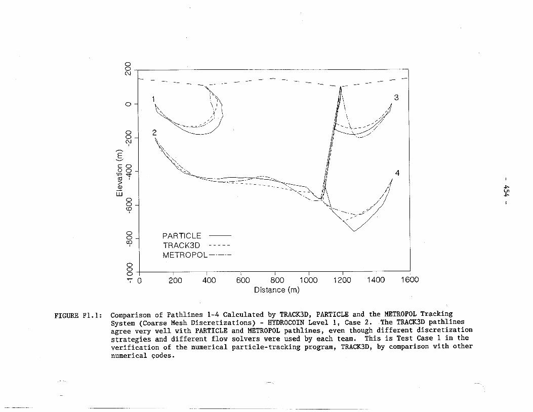
FIGURE F1.l: Comparison of Pathlines 1-4 Calculated by TRACK3D9 PARTICLE and the METROPOL Tracking System (Coarse Mesh Discretizations) - HYDROCOIN Level 1, Case 2. The TRACK3D pathlines agree very well with PARTICLE and METROPOL pathlines, even though different discretization strategies and different flow solvers were used by each team. This is Test Case 1 in the verification of the numerical particle-tracking program, TRACK3D, by comparison with other numerical codes.
0 0 0
METROPOL-----
I I I I I I I
7 0 200 400 600 800 1000 1200 1400 1600 Distance (m)
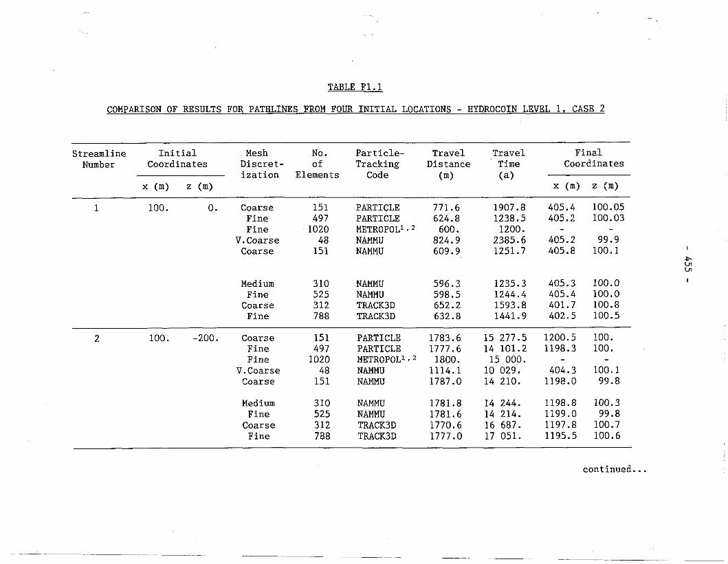
TABLE F 1.1
COMPARISON OF RESULTS FOR PATHLINES FROM FOUR INITIAL LOCATIONS - HYDROCOIN LEVEL 1, CASE 2
Streamline Initial Mesh No. Particle- Travel Travel Final Number Coordinates Discret- o f Tracking Distance Time Coordinates
ization Elements Code ("'1 (a) x (m) Z (m) x (m) = (m)
1 100. 0. Coarse 151 PARTICLE 771.6 1907.8 405.4 100.05 Fine 497 PARTICLE 624.8 1238.5 405.2 100.03 Fine 1020 METROPOL1r2 600. 1200. - -
V. Coarse 48 NAMMU 824.9 2385.6 405.2 99.9 Coarse 151 NAMMU 609.9 1251.7 405.8 100.1
Medium 310 NAMMU 596.3 1235.3 405.3 100.0 Fine 525 NAMMU 598.5 1244.4 405.4 100.0 Coarse 3 12 TRACK3D 652.2 1593.8 401.7 100.8 Fine 788 TRACK3D 632.8 1441.9 402.5 100.5
2 100. -200. Coarse Fine Fine
V. Coarse Coarse
Medium Fine Coarse Fine
PARTICLE PARTICLE METROPOL1n2 NAMMU NAMMU
NAMMU NAMMU TRACK3D TRACK3D
continued ...
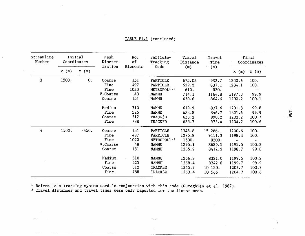
TABLE F1.l (concluded)
Streamline Initial Mesh No. Particle- Travel Travel Final Number Coordinates Discret- o f Tracking Distance Time Coordinates
ization Elements Code (m) (a> x (m> (m) x (m) (m)
3 1500. 0. Coarse Fine Fine
V. Coarse Coarse
Medium Fine Coarse Fine
PARTICLE PARTICLE METROPOL1 NAMMU NAMMU
NAMMU NAMMU TRACK3D TRACK3D
1500. -450. Coarse Fine Fine
V. Coarse Coarse
Medium Fine Coarse Fine
PARTICLE PARTICLE METROPOL1 NAMMU NAMMU
NAMMU NAMMU TRACK3D TRACK3D
Refers to a tracking system used in conjunction with this code (Gureghian et al. 1987). Travel distances and travel times were only reported for the finest mesh.
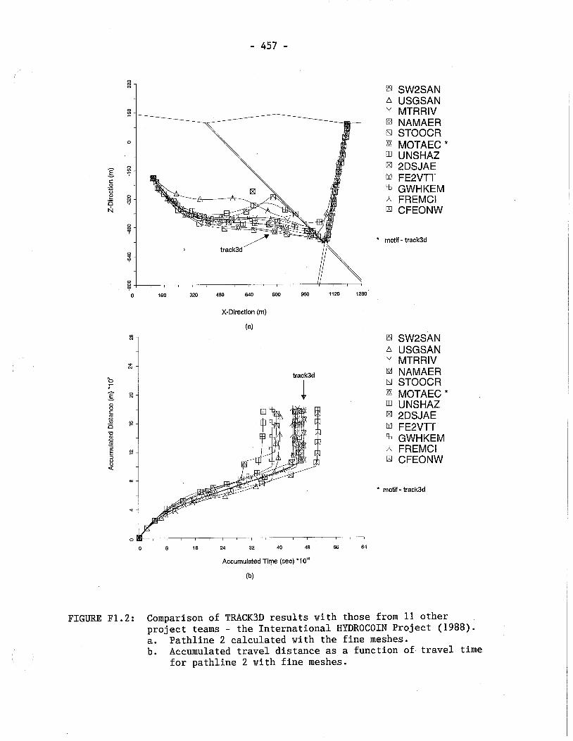
SW2SAN A USGSAN
X-Direction (m)
y MTRRIV NAMAER STOOCR MOTAEC * UNSHAZ 2DSJAE FE2VlT
% GWHKEM A FREMCI
CFEONW
rn SW2SAN A USGSAN y MTRRIV
NAMAER STOOCR MOTAEC * UNSHAZ
Ixl 2DSJAE FE2VlT
% GWHKEM A FREMCI
CFEONW
0 / I I I I I I / f I I I 1 l i l
0 8 16 24 32 40 48 56 64
Accumulated Time (sec) '10''
FIGURE F1.2: Comparison of TRACKSD results with those from 11 other project teams - the International HYDROCOIN Project (1988). a. Pathline 2 calculated with the fine meshes. b. Accumulated travel distance as a function of travel time
for pathline 2 with fine meshes.
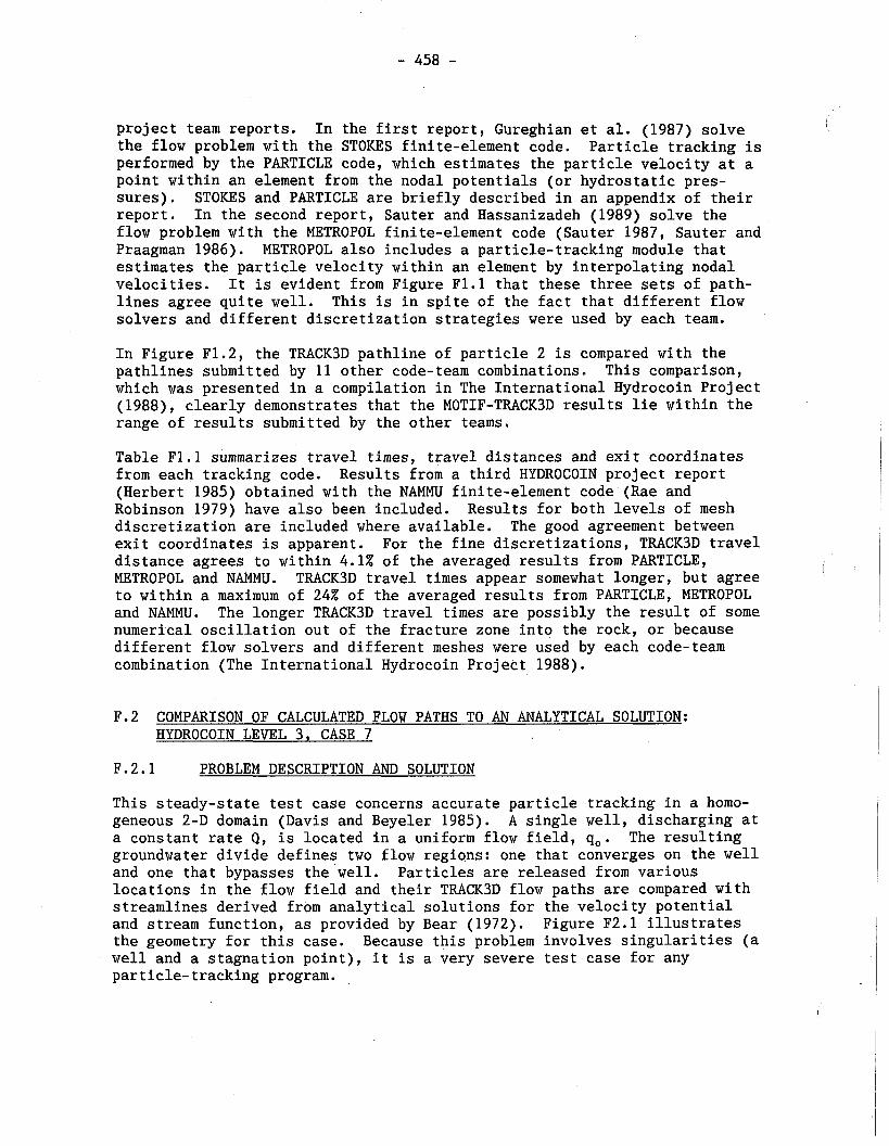
project team reports. In the first report, Gureghian et al. (1987) solve the flow problem with the STOKES finite-element code. Particle tracking is performed by the PARTICLE code, which estimates the particle velocity at a point within an element from the nodal potentials (or hydrostatic pres- sures). STOKES and PARTICLE are briefly described in an appendix of their report. In the second report, Sauter and Hassanizadeh (1989) solve the flow problem with the METROPOL finite-element code (Sauter 1987, Sauter and Praagman 1986). METROPOL also includes a particle-tracking module that estimates the particle velocity within an element by interpolating nodal velocities. It is evident from Figure P1.l that these three sets of path- lines agree quite well. This is in spite of the fact that different flow solvers and different discretization strategies were used by each team.
In Figure F1.2, the TRACK3D pathline of particle 2 is compared with the pathlines submitted by 11 other code-team combinations. This comparison, which was presented in a compilation in The International Hydrocoin Project (1988), clearly demonstrates that the MOTIF-TRACK3D results lie within the range of results submitted by the other teams.
Table F1.l summarizes travel times, travel distances and exit coordinates from each tracking code. Results from a third HYDROCOIN project report (Herbert 1985) obtained with the NAMMU finite-element code (Rae and Robinson 1979) have also been included. Results for both levels of mesh discretization are included where available. The good agreement between exit coordinates is apparent. For the fine discretizations, TRACK3D travel distance agrees to within 4.1% of the averaged results from PARTICLE, I METROPOL and NAMMU. TRACK3D travel times appear somewhat longer, but agree to within a maximum of 24% of the averaged results from PARTICLE, METROPOL and NAMMU. The longer TRACK3D travel times are possibly the result of some numerical oscillation out of the fracture zone into the rock, or because different flow solvers and different meshes were used by each code-team combination (The International Hydrocoin Project 1988).
F.2 COMPARISON OF CALCULATED FLOW PATHS TO AN ANALYTICAL SOLUTION: HYDROCOIN LEVEL 3, CASE 7
F.2.1 PROBLEM DESCRIPTION AND SOLUTION
This steady-state test case concerns accurate particle tracking in a homo- geneous 2-D domain (Davis and Beyeler 1985). A single well, discharging at a constant rate Q, is located in a uniform flow field, q, . The resulting groundwater divide defines two flow regions: one that converges on the well and one that bypasses the well. Particles are released from various locations in the flow field and their TRACK3D flow paths are compared with streamlines derived from analytical solutions for the velocity potential and stream function, as provided by Bear (1972). Figure F2.1 illustrates the geometry for this case. Because this problem involves singularities (a well and a stagnation point), it is a very severe test case for any particle-tracking program.
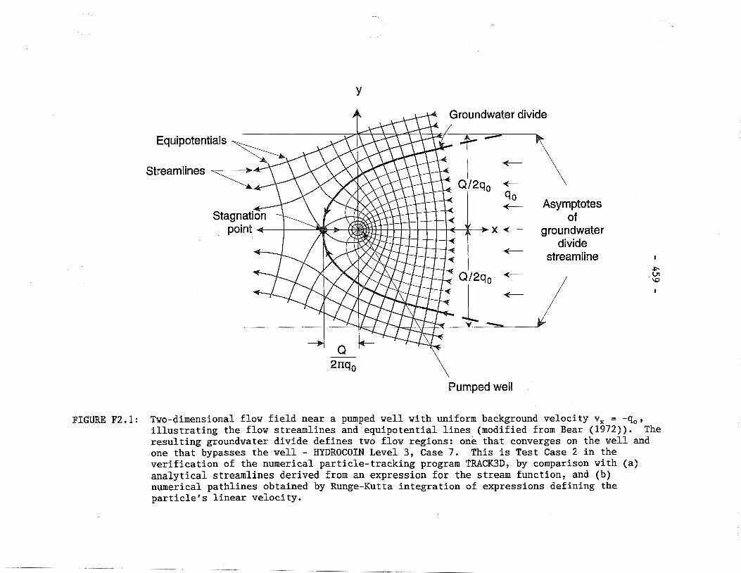
- Asymptotes
x t- groundwater
Pumped well
FIGURE P2.1: Two-dimensional flow field near a pumped well with uniform background velocity v, = -q,, illustrating the flow streamlines and equipotential lines (modified from Bear (1972)). The resulting groundwater divide defines two flow regions: one that converges on the well and one that bypasses the well - HYDROCOIN Level 3, Case 7. This is Test Case 2 in the verification of the numerical particle-tracking program TRACK3D, by comparison with (a) analytical streamlines derived from an expression for the stream function, and (b) numerical pathlines obtained by Runge-Kutta integration of expressions defining the particle's linear velocity.
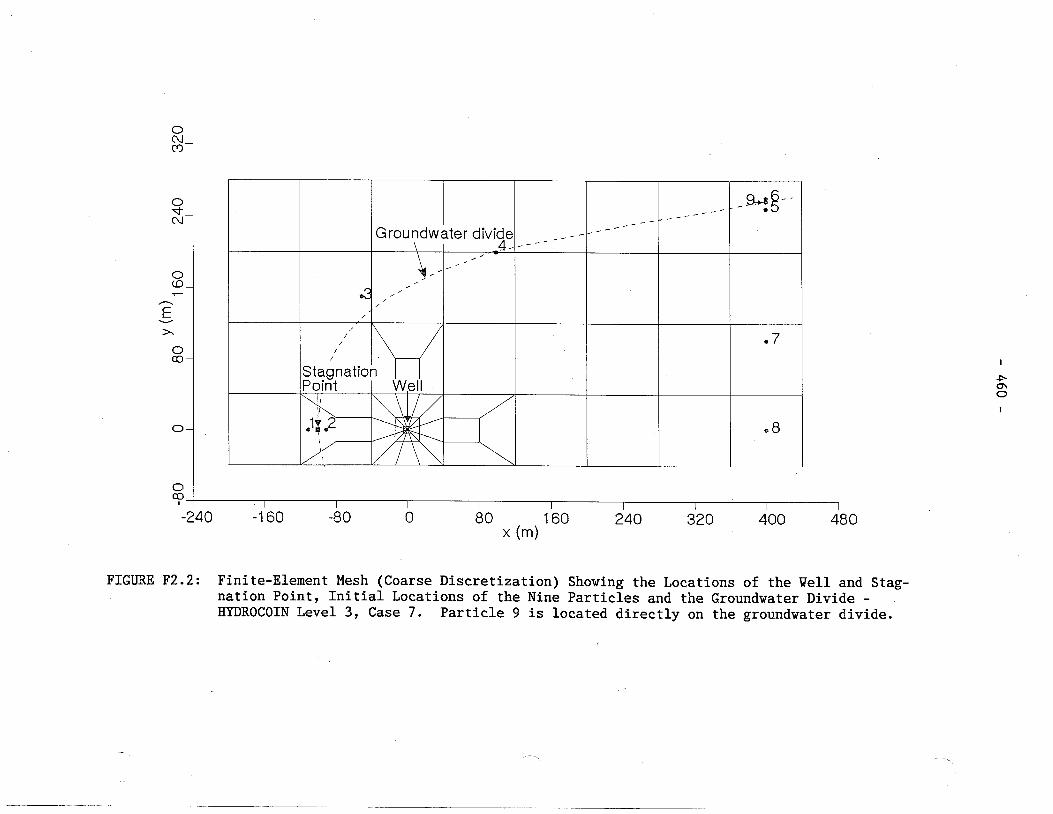
FIGURE P2.2: Finite-Element Mesh (Coarse Discretization) Showing the Locations of the Well and Stag- nation Point, Initial Locations of the Nine Particles and the Groundwater Divide - HYDROCOIN Level 3, Case 7. Particle 9 is located directly on the groundwater divide.
Finite-element meshes were constructed to allow MOTIF flow simulations and particle tracking for three levels of discretization. The coarse, medium and fine meshes contained 100, 599 and 2135 four-noded planar elements respectively. Each mesh consisted of a rectangular grid into which was introduced a large concentration of elements in the local vicinity of the well. The coarse mesh is shown in Figure F2.2; the medium and fine meshes are similar but have a finer grid structure away from the well. A well of 76 mm diameter was represented by twelve nodes placed symmetrically around the origin. In the discretization, no special consideration was given to the expected location of the stagnation point.
Following a MOTIF flow simulation, particle tracking was performed on nine water particles having initial locations shown in Table F2.1 and Figure F2.2. Particle 9 was placed directly on the groundwater divide, far from the stagnation point, to see how effectively TRACK3D can handle this situation. To provide a basis for the comparison, pathline estimates were obtained by two semi-analytical methods as described in Nakka and Chan (1994). In the first method, the analytical streamline is derived from a stream function expression given by Bear (1972). Because the expression is transcendental, a numerical technique was used to generate points on the analytical streamline. In the second method, the analytical expression for the velocity potential given by Bear (1972) was differentiated analytically to yield Cartesian components of the particle velocity. These, in turn, were temporally integrated by a Runge-Kutta technique to yield another numerical approximation of the pathline. A comparison was then made between pathlines obtained by TRACK3D and the other two methods.
DISCUSSION OF RESULTS
Figure F2.3 compares TRACK3D pathlines (solid lines) with analytical streamlines (dotted lines) obtained with our fine mesh. For the case shown, the flow field was created by evaluating expressions for the particle velocity at the centroid of each element. Pathlines are super- imposed onto contours of the hydraulic head (1 m spacing) to demonstrate qualitatively the expected result that TRACK3D pathlines are orthogonal to the hydraulic head contours. To produce these contours, an analytical expression for the hydraulic head was evaluated analytically at each node in the finite-element mesh. In general, the agreement between TRACK3D pathlines and analytical streamlines is very good. Discrepancies are evident (a) when the pathline curvature is large (where velocities are rapidly changing in direction), (b) when the particle is near the well (where velocities are rapidly changing in magnitude), and (c) near the stagnation point (which is overshot by the particle). The first two discrepancies demonstrate that in order to accurately estimate a pathline, TRACK3D requires a well-designed mesh that concentrates elements in regions where the velocity is rapidly changing. The third discrepancy demonstrates that in order to accurately track a particle placed directly on the ground- water divide, TRACK3D must be supplied with an accurate estimate of the flow field near the stagnation point. This requires that the stagnation point(s) be designed into the finite-element mesh.
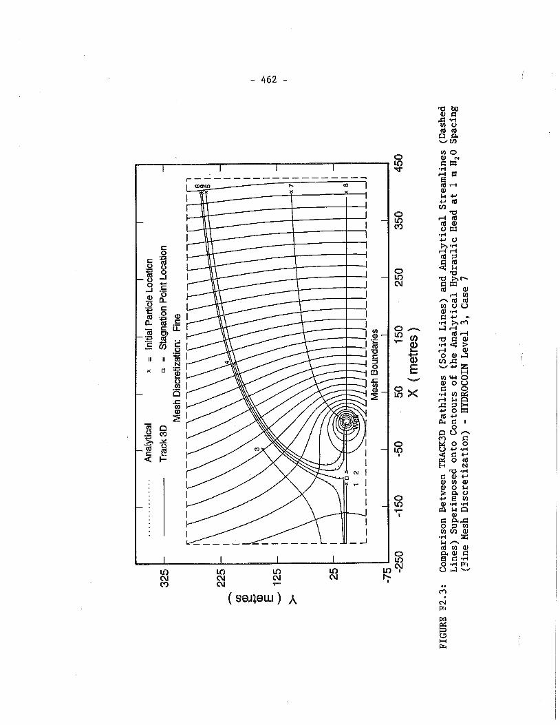
a M 4 0;
cd cd
5% 0
rn 0 aJ N
3 G a 2 a ! 4 9) k 4-J r cd m
0 a m rl cd m (d aJ
u la .rl r u h d rl 4 2
0 k
m a CU a h-
S W a J rl rA
n c d cd rn U U aJ .rl f i r -
.rl hn o n ;Id
ic. 0 a J l 4 m A g --2
H - r n w o 2 O g 55x . r l v l &
2 26' r O W cd r p l g 1
CaUn m C
0 9 8 E .:
2 % a .:
a J r n a J a J 0 M
0 $ a u w a r n
U3 aJ .rl .rl T"- m $ a I
G ad 0 3 rn r n m
.rl r, &4 n d rn a,
0 a a r c m g fi .A
U3 m m m u z 5 CU CU CU CU m CU 7
?- .. m
( saJ1alJ-J ) A N Fr
B Fi Fr
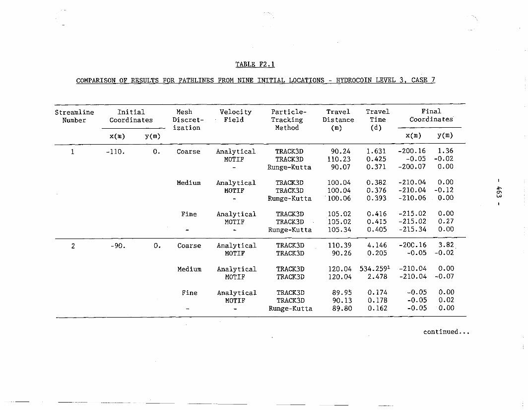
TABLE F2.1
COMPARISON OF RESULTS FOR PATHLINES FROM NINE INITIAL LOCATIONS - HYDROCOIN LEVEL 3, CASE 7
-- -
Streamline Initial Mesh Velocity Particle- Travel Travel Final Number Coordinates Discret- Field Tracking Distance Time Coordinates
ization Method (m) (d) x(m) Y (m) x(m> y(m>
- 110. 0. Coarse Analytical MOTIF
Medium Analytical MOTIF
Fine Analytical MOTIF
TRACK3D TRACK3D
Runge-Kutta
TRACK3D TRACK3D
Runge-Kut ta
TRACK3D TRACK3D
Runge-Kutta
2 - 90. 0. Coarse Analytical TRACK3D 110.39 4.146 -200.16 3.82 MOTIF TRACK3D 90.26 0.205 -0.05 -0.02
Medium Analytical TRACK3D 120.04 534.25g1 -210.04 0.00 MOTIF TRACK3D 120.04 2.478 -210.04 -0.07
Fine Analytical TRACK3D 89.95 0.174 -0.05 0.00 MOTIF TRACK3D 90.13 0.178 -0.05 0.02
- - Runge-Kutta 89.80 0.162 -0.05 0.00
continued ...
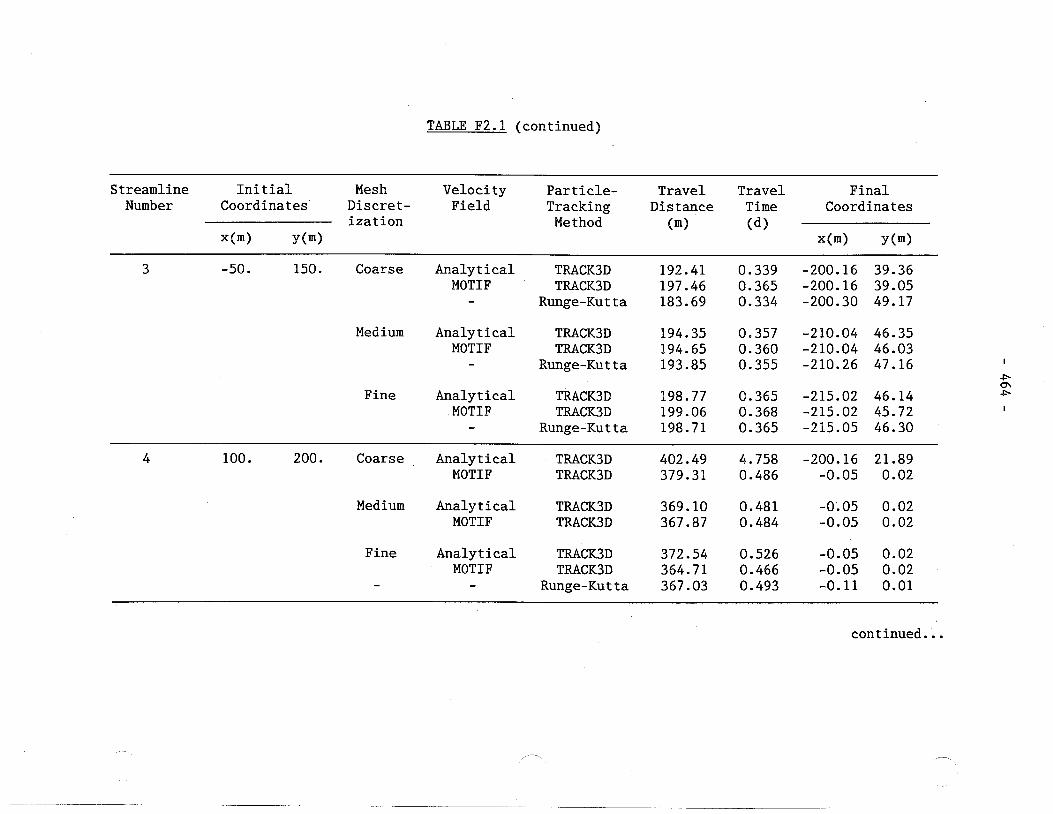
TABLE F2.1 (continued)
Streamline Initial Mesh Velocity Particle- Travel Travel Final Number Coordinates Discret- Field Tracking Distance Time Coordinates
ization Method (m> (d) x(m> Y ("'1 x(m> y(m)
3 -50. 150. Coarse Analytical MOTIF
Medium Analytical MOTIF
Fine Analytical MOTIF
-
TRACK3D TRACK3D
Runge-Kutta
TRACK3D TRACK3D
Runge-Kutta
TRACK3D TRACK3D
Runge-Kutta
4 100. 200. Coarse Analytical TRACK3D 402.49 4.758 -200.16 21.89 MOTIF TRACK3D 379.31 0.486 -0.05 0.02
Medium Analytical TRACK3D 369.10 0.481 -0.05 0.02 MOTIF TRACK3D 367.87 0.484 -0.05 0.02
Fine Analytical TRACK3D 372.54 0.526 -0.05 0.02 MOTIF TRACK3D 364.71 0.466 -0.05 0.02
- - Runge-Kutta 367.03 0.493 -0.11 0.01
continued...
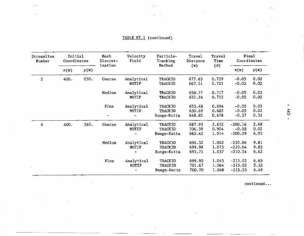
TABLE F2.1 (continued)
Streamline Initial Mesh Velocity Particle- Travel Travel Final Number Coordinates Discret- Field Tracking Distance Time Coordinates
ization Method (m) (dl x(m) Y (m) x(m> y(m)
5 400. 250. Coarse Analytical TRACK3D 677.63 0.729 -0.05 0.02 MOTIF TRACK3D 667.51 0.721 -0.05 0.02
Medium Analytical TRACK3D 658.77 0.717 -0.05 0.02 MOTIF TRACK3D 657.24 0.715 -0.05 0.02
Fine Analytical TRACK3D 653.48 0.694 -0.05 0.02 I
MOTIF TRACK3D 650.69 0.682 -0.05 0.02 .b a\ - - Runge-Kutta 648.82 0.678 -0.37 0.31 m I
6 400. 260. Coarse Analytical TRACK3D 687.93 2.652 -200.16 2.68 MOTIF TRACK3D 706.39 0.904 -0.05 0.02
- Runge-Kutta 685.45 1.014 -200.29 6.95
Medium Analytical TRACK3D 696.32 1.042 -210.04 9.81 MOTIF TRACK3D 699.98 1.075 -210.04 9.85
- Runge-Kutta 695.71 1.037 -210.54 6.62
Fine Analytical TRACK3D 699.90 1.043 -215.02 6.65 MOTIF TRACK3D 701.67 1.064 -215.02 5.32
- Runge-Kutta 700.70 1.048 -215.53 6.49
continued.. .
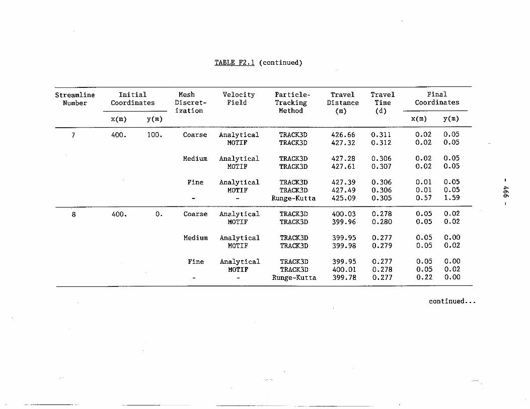
TABLE F2.1 (continued)
Streamline Initial Mesh Velocity Particle- Travel Travel Final Number Coordinates Discret- Field Tracking Distance Time Coordinates
ization Met hod (m) (d) Y (m) y(m)
-
7 400. 100. Coarse Analytical TRACK3D 426.66 0.311 0.02 0.05 MOTIF TRACK3D 427.32 0.312 0.02 0.05
Medium Analytical TRACK3D 427.28 0.306 0.02 0.05 MOTIF TRACK3D 427.61 0.307 0.02 0.05
Fine Analytical TRACK3D 427.39 0.306 0.01 0.05 I
MOTIF TRACK3D 427.49 0.306 0.01 0.05 .b m - - Runge-Kutta 425.09 0.305 0.57 1.59 m I
8 400. 0. Coarse Analytical TRACK3D 400.03 0.278 0.05 0.02 MOTIF TRACK3D 399.96 0.280 0.05 0.02
Medium Analytical TRACK3D 399.95 0.277 0.05 0.00 MOTIF TRACK3D 399.98 0.279 0.05 0.02
Fine Analytical TRACK3D 399.95 0.277 0.05 0.00 MOTIF TRACK3D 400.01 0.278 0.05 0.02
- - Runge-Kutta 399.78 0.277 0.22 0.00
continued ...
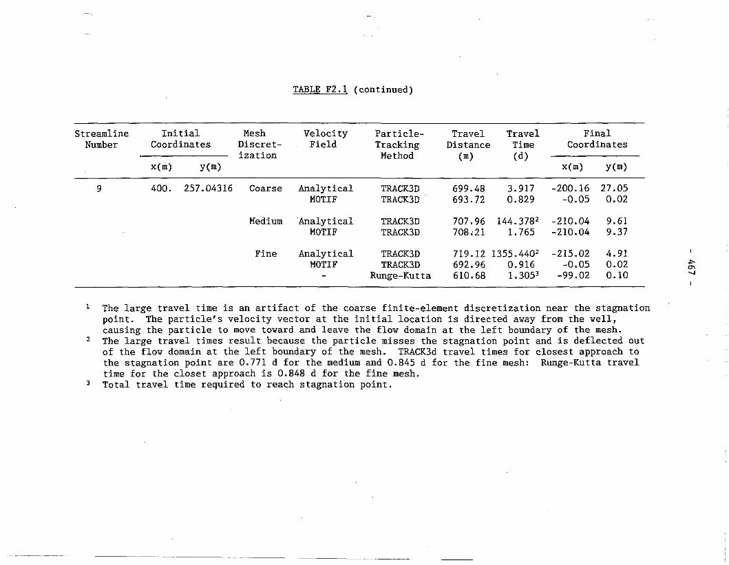
TABLE F2.1 (continued)
Streamline Initial Mesh Velocity Particle- Travel Travel Final Number Coordinates Discret- Field Tracking Distance Time Coordinates
ization Method (m) (dl x(m) Y (m) x(m> y(m)
- - - -
9 400. 257.04316 Coarse Analytical TRACK3D 699.48 3.917 -200.16 27.05 MOTIF TRACKSD 693.72 0.829 -0.05 0.02
Medium Analytical TRACK3D 707.96 144.3782 -210.04 9.61 ' MOTIF TRACK3D 708.21 1.765 -210.04 9.37
Fine Analytical TRACK3D 719.12 1355.4402 -215.02 4.91 MOTIF TRACK3D 692.96 0.916 -0.05 0.02
- Runge-Kutta 610.68 1.3053 -99.02 0.10
The large travel time is an artifact of the coarse finite-element discretization near the stagnation point. The particle's velocity vector at the initial location is directed away from the well, causing the particle to move toward and leave the flow domain at the left boundary of the mesh. The large travel times result because the particle misses the stagnation point and is deflected out of the flow domain at the left boundary of the mesh. TRACK3d travel times for closest approach to the stagnation point are 0.771 d for the medium and 0.845 d for the fine mesh: Runge-Kutta travel time for the closet approach is 0.848 d for the fine mesh.
3 Total travel time required to reach stagnation point.
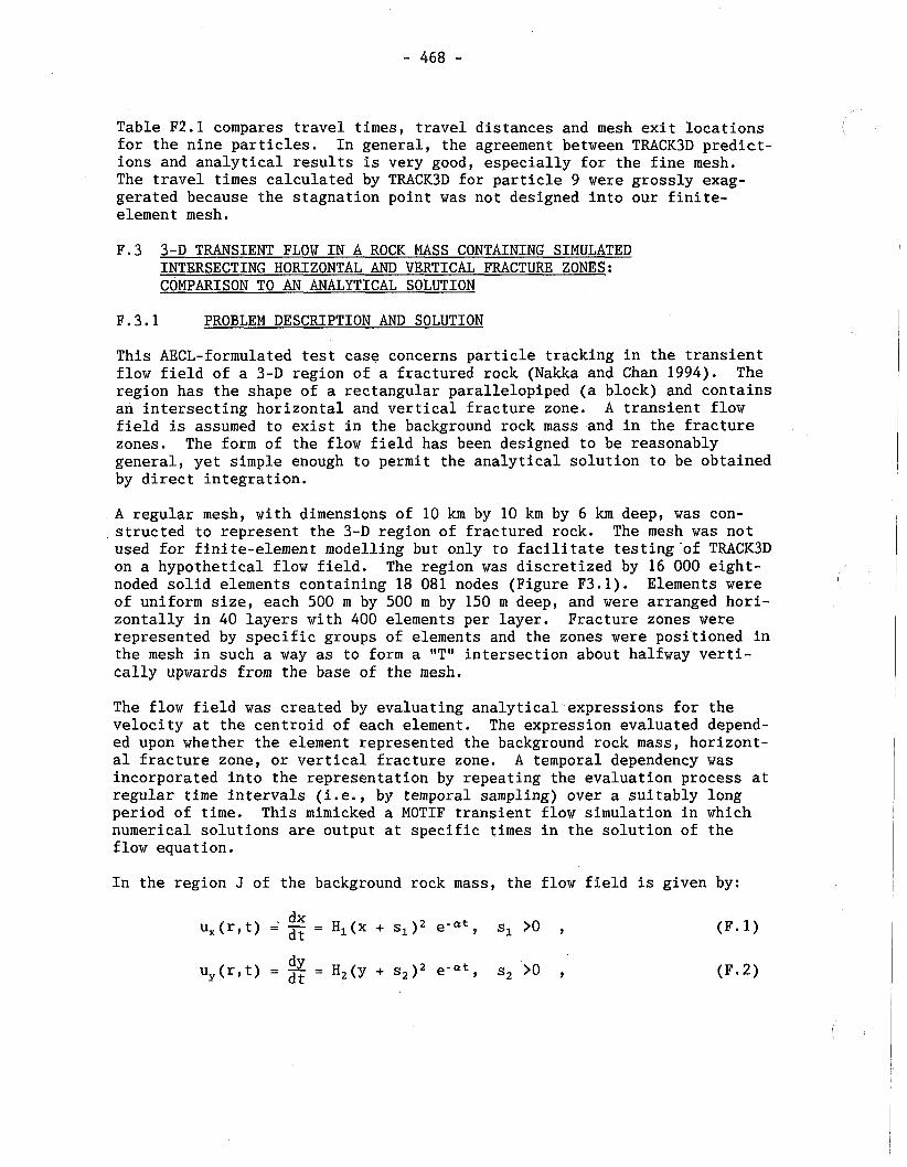
Table F2.1 compares travel times, travel distances and mesh exit locations for the nine particles. In general, the agreement between TRACK3D predict- ions and analytical results is very good, especially for the fine mesh. The travel times calculated by TRACK3D for particle 9 were grossly exag- gerated because the stagnation point was not designed into our finite- element mesh.
F.3 3-D TRANSIENT FLOW IN A ROCK MASS CONTAINING SIMULATED INTERSECTING HORIZONTAL AND VERTICAL FRACTURE ZONES: COMPARISON TO AN ANALYTICAL SOLUTION
F.3.1 PROBLEM DESCRIPTION AND SOLUTION
This AECL-formulated test case concerns particle tracking in the transient flow field of a 3-D region of a fractured rock (Nakka and Chan 1994). The region has the shape of a rectangular parallelopiped (a block) and contains an intersecting horizontal and vertical fracture zone. A transient flow field is assumed to exist in the background rock mass and in the fracture zones. The form of the flow field has been designed to be reasonably general, yet simple enough to permit the analytical solution to be obtained by direct integration.
A regular mesh, with dimensions of 10 km by 10 km by 6 km deep, was con- structed to represent the 3-D region of fractured rock. The mesh was not used for finite-element modelling but only to facilitate testing of TRACK3D on a hypothetical flow field. The region was discretized by 16 000 eight- noded solid elements containing 18 081 nodes (Figure F3.1). Elements were I
of uniform size, each 500 m by 500 m by 150 m deep, and were arranged hori- zontally in 40 layers with 400 elements per layer. Fracture zones were represented by specific groups of elements and the zones were positioned in the mesh in such a way as to form a "T" intersection about halfway verti- cally upwards from the base of the mesh.
The flow field was created by evaluating analytical expressions for the velocity at the centroid of each element. The expression evaluated depend- ed upon whether the element represented the background rock mass, horizont- al fracture zone, or vertical fracture zone. A temporal dependency was incorporated into the representation by repeating the evaluation process at regular time intervals (i.e., by temporal sampling) over a suitably long period of time. This mimicked a MOTIF transient flow simulation in which numerical solutions are output at specific times in the solution of the flow equation.
In the region J of the background rock mass, the flow field is given by:
dx u,(r,t) = - = Hl(x + sl)2 e-at, sl >O , dt (F.1)
u,(r,t) = % = H2(y + s2)' e-at, s2 >O , (Fa 2)
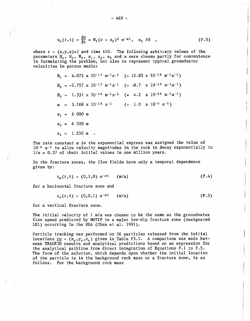
where r = (x,y,z)~J and time t>O. The following arbitrary values of the parameters HI, H,, H,, s,, s,, s, and a were chosen partly for convenience in formulating the problem, but also to represent typical groundwater velocities in porous media:
The rate constant a in the exponential express was assigned the value of a-I to allow velocity magnitudes in the rock to decay exponentially to
l/e - 0.37 of their initial values in one million years. In the fracture zones, the flow fields have only a temporal dependence given by:
for a horizontal fracture zone and
for a vertical fracture zone.
The initial velocity of 1 m/a was chosen to be the same as the groundwater flow speed predicted by MOTIF in a major low-dip fracture zone (designated LD1) occurring in the WRA (Chan et al. 1991).
Particle tracking was performed on 36 particles released from the initial locations ro = (xo,yo,zo) given in Table F3.1. A comparison was made bet- ween TRACK3D results and analytical predictions based on an expression for the analytical pathline from direct integration of Equations F.l to F.5. The form of the solution, which depends upon whether the initial location of the particle is in the background rock mass or a fracture zone, is as follows. For the background rock mass

For a horizontal fracture:
x(t) = x, 1
y(t) = yo + a (1 - e-") z(t) = z,
For a vertical fracture:
(F.9) (F. 10)
(F. 11)
(F. 12)
(F. 13)
(F. 14)
where x(t), y(t) and z(t) are the Cartesian coordinates of a point on the analytical pathline at time t>O. Analytical expressions for travel time, travel distance and particle exit location were also derived and are presented in Nakka and Chan (1994).
The effect of time step size on the accuracy of TRACK3Drs results was also examined by systematically varying FACTOR, described in Section 3.3 of the main text, from 0.025 to 1.0. This parameter controls how far a particle is moved through an element in one time step, with a value of unity corres- ponding to complete transit of the element.
DISCUSSION OF RESULTS
Tables F3.1 and F3.2 compare TRACK3D results with analytical predictions for the 36 particles tracked. Table F3.1 compares mesh exit locations, while Table F3.2 compares travel times and travel distances. The results show that errors in exit points, travel distances and travel times each average about 1% for most particles. Particle 9 had the largest error in exit point (16%), travel time (5.3%) and travel distance (14.6%). Part of the errors in Tables F3.1 and F3.2 can be attributed to the fact that while analytical predictions are based upon a flow field that is allowed to vary continuously with time, TRACK3D results are based on a MOTIF representation of the flow field, which varies discontinuously with time.

Plan view
I I I I I
-4000 -2000 0 2000 4000 x (m)
Side vlew I
8 . Front view I
FIGURE F3.1: Plan, Front- and Side-Elevation Views of the Mesh Showing the Simulated Horizontal and Vertical Fracture Zones. The fracture zones form a "T" intersection about halfway verti- cally upwards from the base of the mesh. Arrows in the fracture zones indicate the direction of the velocities. This AECL-formulated test case is concerned with particle tracking in the transient flow field of a 3-D region of rock containing two intersecting highly-permeable fracture zones. This is Test Case 3 in the verification of the numerical particle-tracking program, TRACK3D, by comparison with an analytical solution.
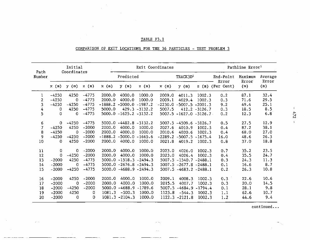
TABLE F3.1
COMPARISON OF EXIT LOCATIONS FOR THE 36 PARTICLES - TEST PROBLEM 3
Initial Exit Coordinates . Pathline Error1 Path Coordinates
Number Predicted TRACK3D1 End-Point Maximum Average Error Error Error
x (m) Y (m) z (m) x (m) Y (m) z (m) x (m) Y (m) z (m) (Per Cent) (m) (m)
continued ...
--

TABLE F3.1 (continued)
Initial Exit Coordinates Pathline Error1 Path Coordinates Number Predicted TRACK3D1 End-Point Maximum Average
Error Error Error x (m> Y (m) (m) x (m) Y ('=> (m) x (m) Y (m) (m) (Per Cent) (m) (m)
1 These values correspond to a time-step reduction factor (FACTOR) value of 0.05 and a time interval between velocity data blocks of 20 000 a.
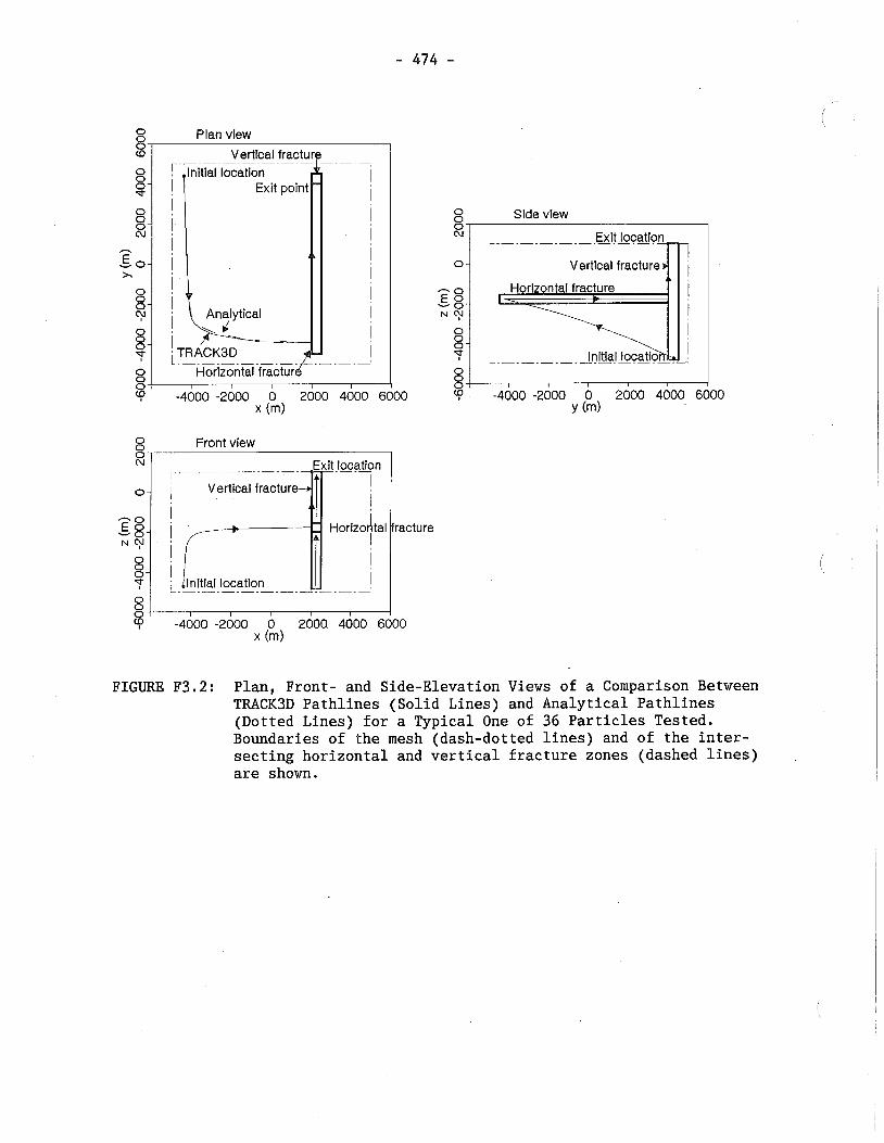
0 ,-, Plan vlew
1 Vertical fracture
L . -. - . - . - . - . - . 8 Horlzontal fracturk----.-' I -4doo -2000 a zooo 4000
x (m)
2 Front view
8 Slde view
Exit location r--.---.-.-.-.-.-.
I ~ e r t ~ c a ~ fractu r e C /
'acture
FIGURE F3.2: Plan, Front- and Side-Elevation Views of a Comparison Between TRACK3D Pathlines (Solid Lines) and Analytical Pathlines (Dotted Lines) for a Typical One of 36 Particles Tested. Boundaries of the mesh (dash-dotted lines) and of the inter- secting horizontal and vertical fracture zones (dashed lines) are shown.
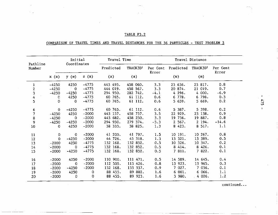
TABLE F3.2
COMPARISON OF TRAVEL TIMES AND TRAVEL DISTANCES FOR THE 36 PARTICLES - TEST PROBLEM 3
--
Initial Travel Time Travel Distance Pathline Coordinates Number Predicted TRACK3D1 Per Cent Predicted TRACK3D1 Per Cent
Error Error x (m> Y (m) (m) (a> (a> (m) (m>
continued ...
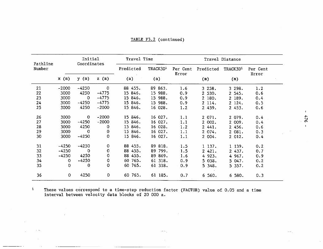
TABLE F3.2 (continued)
Initial Travel Time Travel Distance Pathline Coordinates Number Predicted TRACK3D1 Per Cent Predicted TRACK3D1 Per Cent
Error Error x (m) Y (m) (m) (a) (a) (m) (m)
These values correspond to a time-step reduction factor (FACTOR) value of 0.05 and a time interval between velocity data blocks of 20 000 a.
I
Figure F3.2 compares plan, front and side views of the TRACK3D pathline (solid line) with the analytical pathline (dotted line) for the first particle listed in Tables F3.1 and F3.2. Similar results were obtained with the other 35 particles. The figure shows a very good qualitative agreement between the two pathlines with the largest deviation between them occurring in the region of the background rock mass where their curvatures are the greatest.
F.4 COMPARISON WITH RESULTS FROM A PARTICLE-TRACKING PROGRAM DEVELOPED BY ONTARIO HYDRO RESEARCH
F.4.1 BACKGROUND
In order to provide an independent confirmation of results obtained with TRACK3D9 Ontario Hydro (OH) Research was requested to develop a particle- tracking program having similar capabilities. To assist in developing and testing their program, we supplied them with our finite-element meshes and steady-state velocity distributions from two MOTIF flow simulations. To allow them to judge if their program was performing properly, we supplied them with the initial coordinates of our test particles and the pathline coordinates and travel times predicted for them by TRACK3D. To ensure a truly independent effort, we did not supply them with any specific information on the operation of TRACK3D.
The program developed by OH Research implements an entirely different algo- rithm than the one in TRACK3D. TRACK3Drs algorithm is based on a time- stepping method, whereby particle is moved in small pathline increments through the elements. By contrast, the OH program is based on an element- stepping method. In this method, a particle is moved from one boundary of an element to another boundary of the same element according to the velocity in that element. At each boundary the validity of moving into the next element is considered. If the particle cannot move into the next element, because the velocity there is opposed to that in the last element, the particle is moved along a boundary. Depending upon the direction of the velocity in neighbouring elements, movement of the particle into an adjacent element may occur through the current element, along a face, or along an edge. Details of the mathematical background and the algorithm embodied in the OH program are given in Chan and Punhani (1991).
The data supplied to OH to develop their program was obtained from MOTIF flow simulations of the natural and pumped conditions of groundwater flow in the MOTIF WRA Local Flow Model, described in Section 5.6. Details re- lating to these flow simulations can also be found in Reid and Chan (1988). The first data set corresponds to a simulation in which a 100-m-deep well is pumped at 10 000 m3/a. Particle tracking is performed on 53 water particles placed within the 3-D steady-state velocity distribution predict- ed by the MOTIF model. The other data set corresponds to a simulation in which a 200-m-deep well is implemented in the mesh, but the well is not pumped, i.e., natural flow is simulated. Particle tracking is performed on a different row of 41 particles.
F.4.2 RESULTS AND CONCLUSIONS
Tables F4.1 and F4.2 compare exit locations and travel times predicted by both programs for a representative subset of the 53 and 41 particles respectively. A comprehensive listing is given in Nakka and Chan (1994). These tables are reproduced in part from Chan and Punhani (1991), where only travel times but not exit locations are compared. The results show that in most cases there is good agreement in predictions made by the two programs. TRACK3D travel times are typically longer than OH values by 1-5%. The largest difference is 9.7%. For the two particles in Table F4.1 that exhibit major discrepancies, our results are more defendable. The OH program suggests that these particles are Ifblockedff (cannot move) at their final locations and this is not consistent with physical reasoning. In addition, both programs are consistent in their prediction that every other nearby particle should enter the well. These discrepancies may disappear when a newer version of the OH program is tested. No major discrepancies between TRACK3D and OH results were observed in Table F4.2.
F.5 SUMMARY AND CONCLUSIONS
The accuracy and coding in our numerical particle-tracking program, TRACK3D, has been verified with three test cases and an independent con- firmation. Test cases include two HYDROCOIN 2-D steady-state problems and an AECL-formulated 3-D transient flow problem. The confirmation, performed independently by OH Research, is based on a comparison between results obtained with their particle-tracking program and our results obtained with TRACK3D. The comparison derives from particle tracking in the 3-D steady- state flow field from flow simulations in the MOTIF WRA Local Flow Model. Our conclusions based on the above tests are stated below.
1. Generally, TRACK3D results compare very favourably with those presented in the HYDROCOIN project team reports and with analytical predictions. TRACK3D travel times are typically 1-5% longer than values obtained by OH with their program, but by less than 9.7%. Best accuracy is achieved when the finite-element mesh is carefully designed to concentrate elements in regions where velocities are expected to change rapidly in magnitude or direction, such as near a well.
2. A judicious choice for the value of the time-step reduction factor (FACTOR, described in Section 3.3 of the main text), the parameter which directly controls the time-step size, is neces- sary to accurately define the pathline with the least number of calculated points. A small value of FACTOR, such as 0.05 or 0.1, is recommended especially when the velocity field in which the particle is moving is rapidly changing with time.
3. TRACK3D can accurately track a particle placed directly on the groundwater divide almost to the stagnation point. Near the stagnation point, substantial errors in pathline accuracy and travel time can result unless proper allowance has been made in the finite-element mesh to account for the presence of ' the stagnation point(s).
I
REFERENCES:
Bear, J. 1972. Dynamics of Fluids in Porous Media, American Elsevier, New York.
Chan, A.H.C. and A.L. Punhani. 1991. 3D Particle Tracking Algorithm To Model Radionuclide Transport, Ontario Hydro Research Division Report NO. 91-161-K.
Chan, T., Y.C. Jin, C. Kitson, T. Melnyk and P.A. OPConnor. 1991. Comparison of a 2-D finite element solute transport model with a 1-D network solute transport model. Joint International Waste Manage- ment Conference, 1991 Oct. 21-26, Seoul, ASME/KNS Volume 2, 283-290.
Davis, F. and W. Beyeler. 1985. Comparison of Calculated Flow Paths To An Analytical Solution, Proposal for a Test Problem for HYDROCOIN Level 3, Sandia National Laboratories, Albuquerque, New Mexico.
Grundfelt, B. 1984. Proposal for a Test Problem for HYDROCOIN Level 1, Case 2: Steady State Flow in a Rock Mass Intersected by Permeable Fracture Zones, KEMAKTA Consultants Co., Stockholm, Sweden.
Gureghian, A. Berge, Anthony Andrews, Shirley B. Steidl and Albin Brandstetter. 1987. Solutions to HYDROCOIN Level 1 Problems (Cases 1,2,4,7) Using STOKES and PARTICLE, Technical Report. Office of Crystalline Repository Developmemt, Battelle Memorial Institute, Columbus, OH.
Guvanasen, V. 1985. Development of a finite-element code and its appli- cation to geoscience research. J& Proc. 17th information meeting of the nuclear fuel waste management program. Atomic Energy of Canada Limited Technical Record, TR-299.
Guvanasen, V. and T. Chan. 1994. A finite element three-dimensional model of flow and transport in fractured/porous media (MOTIF): Mathematical formulation and user's manual. Atomic Energy of Canada Limited Report.
Herbert, A.W. 1985. Verification of NAMMU Using HYDROCOIN Level 1 Case 2: Steady-State Flow in a Rock Mass Intersected by Permeable Fracture Zones, AERE-R.11636, Theoretical Physics Division, Harwell Laboratory, Oxfordshire.
The International HYDROCOIN Project - Level 1: Code Verification, Organi- zation for Economic Cooperation and Development/Nuclear Energy Agency (OECD/NEA) and Swedish Nuclear Power Inspectorate (SKI), 1988.
Nakka, B.W. and T. Chan. 1994, A particle-tracking code (TRACK3D) for con- vective solute transport modelling in the geosphere: Description and User's Manual. Atomic Energy of Canada Limited Report, AECL-10881, COG-93-216.
I Rae, J. and P.C. Robinson. 1979. NAMMU: Finite-Element Program for Coupled Heat and Groundwater Flow Problems, AERE-R.9610.
Reid, J.A.K. and T. Chan. 1988. Simulation of Convective Contaminant Movement from a Nuclear Waste Vault Through a Domestic Well to the Surface, Proceedings of the Fourth CanadiadAmerican Conference on Hydrogeology-Fluid Flow, Head Transport and Mass Transport in Fractured Porous Media, Banff, Alberta, 1988, June 21-24.
Sauter, F.J. and S.M. Hassanizadeh. 1989. Verification of the METROPOL Code For Groundwater Flow in Inhomogeneous Porous Media. HYDROCOIN Project, Level 1, Cases 1 and 2. Report No. 728528001. National Institute of Public Health and Environmental Protection, Bilthoven.
Sauter, F. 1987. User's manual METROPOL, Mathematical description, RIVM- report 728514002, June 1987.
Sauter, F. and N. Praagman. 1986. A simulation model for the transport of radionuclides by groundwater in the vicinity of a salt-dome, 6th International Conference on Finite Elements in Water Resources, Lisboa, 1-5 June, 1986.
(TR- indicates unrestricted, unpublished reports available from SDDO, AECL Research, Chalk River Laboratories, Chalk River, Ontario KOJ 1LO.)
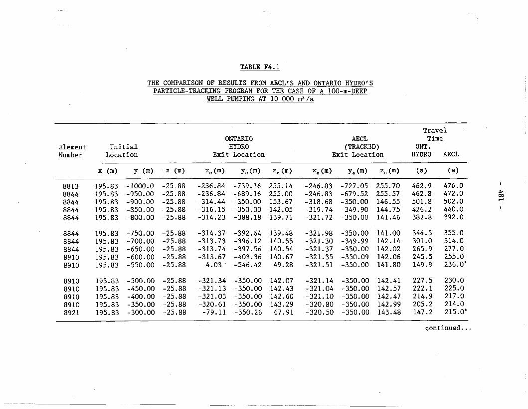
TABLE F4.1
THE COMPARISON OF RESULTS FROM AECL'S AND ONTARIO HYDRO'S PARTICLE-TRACKING PROGRAM FOR THE CASE OF A 100-m-DEEP
WELL PUMPING AT 10 000 m3/a
Element Initial Number Locat ion
ONTARIO HYDRO
Exit Location
Travel AECL Time
(TRACK3D) ONT . Exit Location HYDRO AECL
continued. ..

TABLE F4.1 (continued)
Element Initial Number Locat ion
ONTARIO HYDRO
Exit Location
Travel AECL Time
(TRACK3D) ONT. Exit Location HYDRO AECL
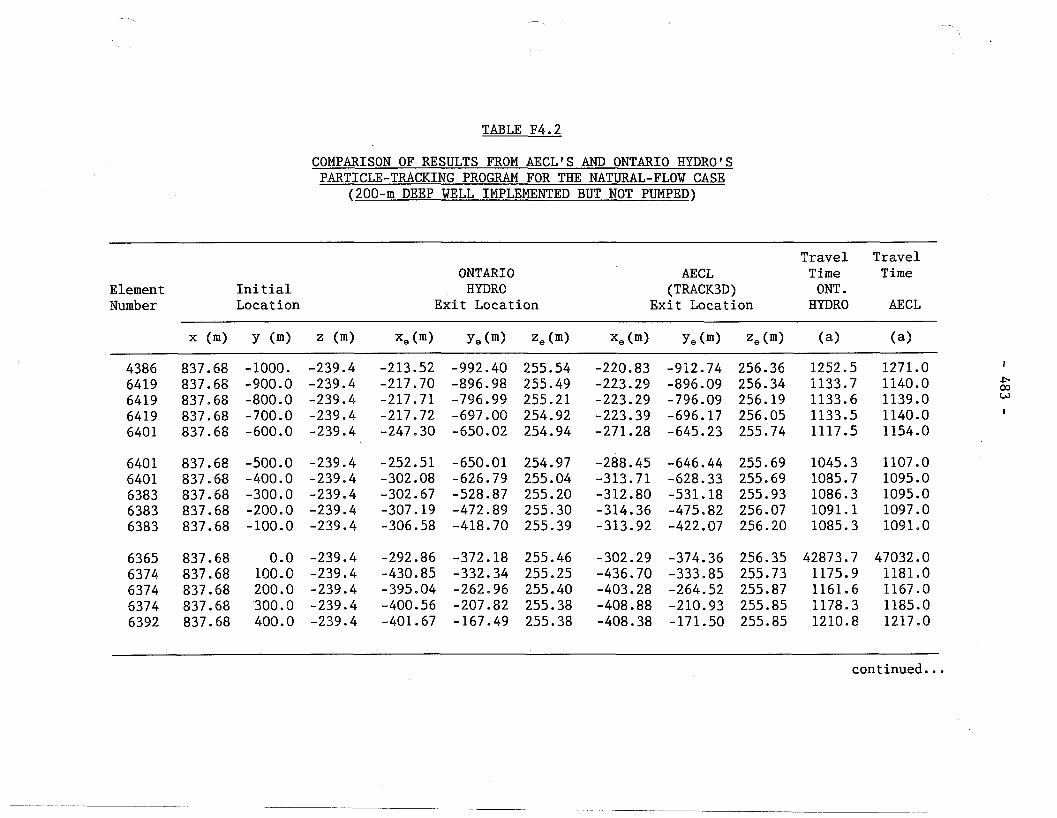
TABLE F4.2
COMPARISON OF RESULTS FROM AECLrS AND ONTARIO HYDRO'S PARTICLE-TRACKING PROGRAM FOR THE NATURAL-FLOW CASE
(200-m DEEP WELL IMPLEMENTED BUT NOT PUMPED)
Travel Travel AECL Time Time
(TRACK3D) O m . Exit Location HYDRO AECL
ONTARIO HYDRO
Exit Location Element Initial Number Location
- --
continued...
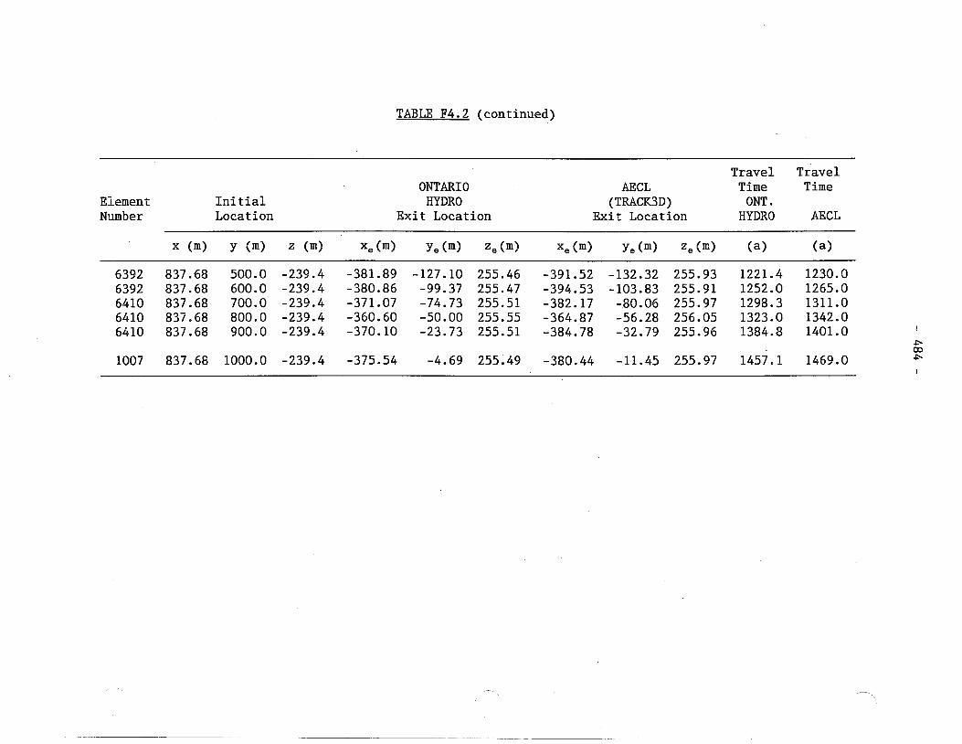
TABLE F4.2 (continued)
Element Initial Number Locat ion
ONTARIO HYDRO
Exit Location
Travel Travel AECL Time Time
(TRACK3D) ONT . Exit Location HYDRO AECL
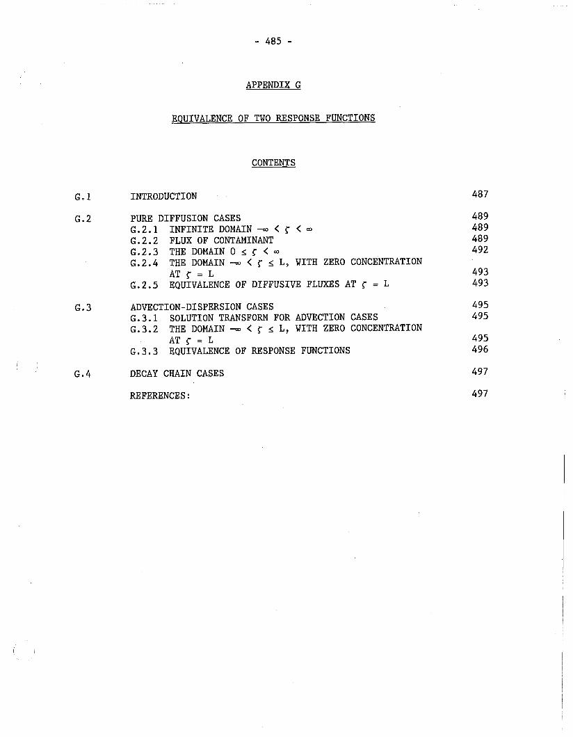
- 485 -
APPENDIX G
EQUIVALENCE OF TWO RESPONSE FUNCTIONS
CONTENTS
G. 1 INTRODUCTION
6.2 PURE DIFFUSION CASES G.2.1 INFINITE DOMAIN - < 3- < a G.2.2 FLUX OF CONTAMINANT 6.2.3 THE DOMAIN 0 5 < < a G.2.4 THE DOMAIN -W < 5 5 L, WITH ZERO CONCENTRATION
AT 3- = L G.2.5 EQUIVALENCE OF DIFFUSIVE FLUXES AT = L
6.3 ADVECTION-DISPERSION CASES G.3.1 SOLUTION TRANSFORM FOR ADVECTION CASES G.3.2 THE DOMAIN -W < 5 5 L, WITH ZERO CONCENTRATION
A T < = L G.3.3 EQUIVALENCE OF RESPONSE FUNCTIONS
I
G.4 DECAY CHAIN CASES
REFERENCES:
I
G.l INTRODUCTION
In this Appendix, we establish the equivalence at I = L of two flux response functions for an impulse source at r' = 0 and with;
1) domain extending 0 5 r < m and
2) domain extending -w < 5 L, with zero concentration at r = L.
We will restrict our attention to only one Cartesian spatial dimension, I. This restriction is consistent with the use of response functions described in Chapter 6 for transport of contaminants in segments of the GEONET model transport network, each of which considers one-dimensional transport.
The response functions described in Chapter 6 are solutions to the mass- balance partial differential equation for the transport of a contaminant coming from an impulse source. In this context, an impulse source repre- sents a slug of a unit amount of contaminant injected into the domain at < = <' and at t = 0, as shown in Figure G1.1, and is commonly referred to as a &-function. The impulse source can be considered (using different functional forms) to be in either the concentration of the contaminant or in the flux of the contaminant. The total amount of material associated with a 6-function in concentration is obtained by integration over the spatial coordinate; the total amount of material associated with a &-function in flux is obtained by integration over the time variable. In
, both cases the 6-function represents an impulse of a unit amount of contaminant.
In the cases presented here, we are interested in response function solutions with an impulse source occurring only at time t = 0. Hence, this impulse may be written either as a source term in the partial differential equation itself or, equivalently, as part of the initial condition. In general, as shown in Figure G1.1, we consider the impulse source to occur at some spatial position r', and we denote the &-function by 6 ( c . C , ) , ex- plicitly indicating the spatial dependence but dropping any notatlon for the time dependence. In some cases, we consider the impulse source to occur at a boundary of the medium (in particular at a boundary at = 0 ) . In these cases the source can be written equivalently as part of a boundary condition. In all cases, we want to determine the flux of contaminant at r = L as a function of time.
We first, in Section 6.2, examine solutions to the diffusion differential equation, partly as an illustration and simple example of the methodology we use for establishing the equivalence of the response functions for the two domains, and partly to derive results that we will use later. We then establish the equivalence for advection-dispersion cases in Section G.3. The domains considered in this Appendix are shown schematically in Figure G1.2.
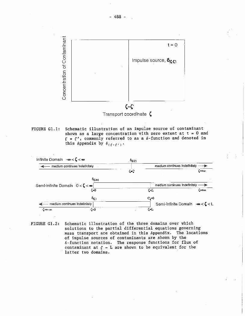
Impulse source, 6(C-C)
C=C' Transport coordinate C
FIGURE G1.l: Schematic illustration of an impulse source of contaminant shown as a large concentration with zero extent at t = 0 and c = c r , commonly referred to as a &-function and denoted in this Appendix by 6(r-r,,.
Infinite Domain -m < C 4cq)
C=C'
Semi-infinite Domain 0 < C < w 1 medium continues indefinitely + c=o C=L C*m
4c 1 c,=o Semi-infinite Domain -O < C < L
C=L
FIGURE G1.2: Schematic illustration of the three domains over which solutions to the partial differential equations governing mass transport are obtained in this Appendix. The locations of impulse sources of contaminants are shown by the 6-function notation. The response functions for flux of contaminant at = L are shown to be equivalent for the latter two domains.
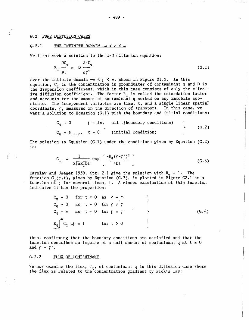
6.2 PURE DIFFUSION CASES
G.2.1 THE INFINITE DOMAIN -m < C < m
We first seek a solution to the 1-D diffusion equation:
over the infinite domain - ~ o < < m, shown in Figure G1.2. In this equation, Cq is the concentration in groundwater of contaminant q and D is the dispersion coefficient, which in this case consists of only the effect- ive diffusion coefficient. The factor Rq is called the retardation factor and accounts for the amount of contaminant q sorbed on any immobile sub- strate. The independent variables are time, t, and a single linear spatial coordinate, g, measured in the direction of transport. In this case, we want a solution to Equation (G.l) with the boundary and initial conditions:
C, + 0 r + +a, all t(boundary conditions) t
Cq = 6 ( r - c r ) t = 0 (initial condition)
The solution to Equation (G.l) under the conditions given by Equation (G.2) is:
Carslaw and Jaeger 1959, Cpt. 2.1 give the solution with Rq = 1. The function C (c,t), given by Equation (G.3), is plotted in Figure G2.1 as a function o? c for several times, t. A closer examination of this function indicates it has the properties:
RqPcq d< = i for t > 0 -m
thus, confirming that the boundary conditions are satisfied and that the function describes an impulse of a unit amount of contaminant q at t = 0 and = r'. G.2.2 FLUX OF CONTAMINANT
We now examine the flux, J,, of contaminant q in this diffusion case where the flux is related to the.concentration gradient by Fickrs law:
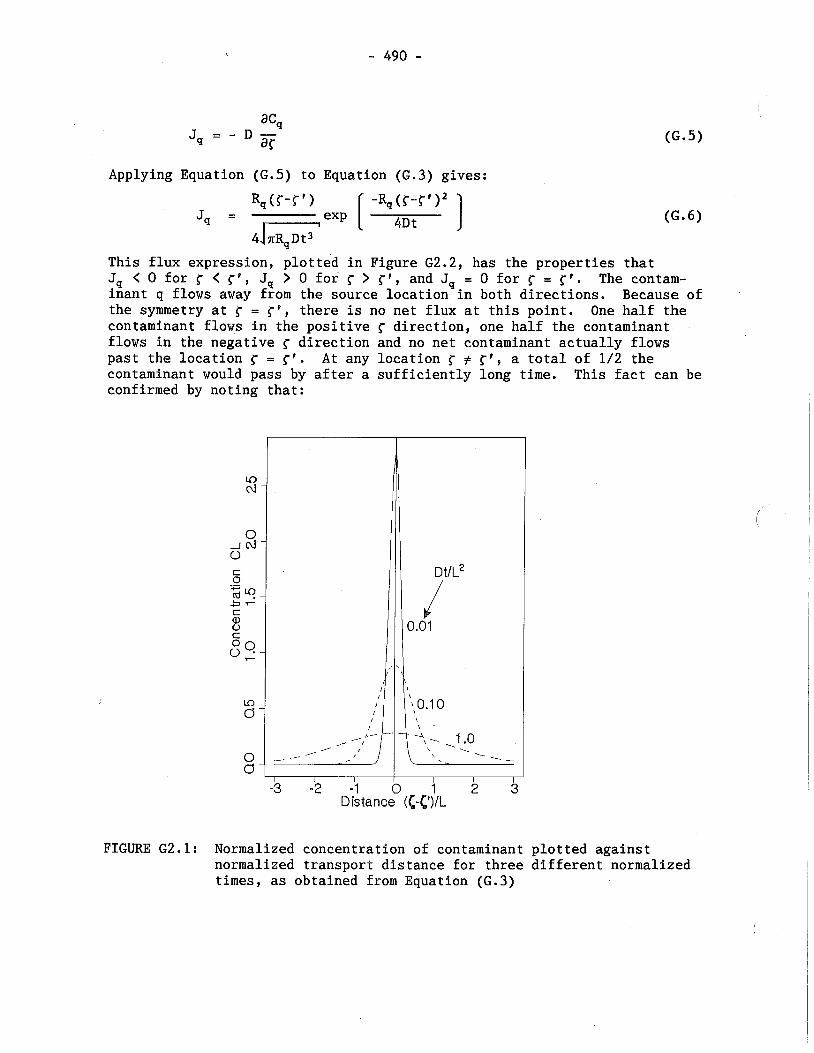
Applying Equation (G.5) to Equation (G.3) gives:
This flux expression, plotted in Figure G2.2, has the properties that Jq < 0 for r < c v , J, > 0 for r > r', and Jq = 0 for = r'. The contam- inant q flows away from the source location in both directions. Because of the symmetry at r = c v , there is no net flux at this point. One half the contaminant flows in the positive r direction, one half the contaminant flows in the negative r direction and no net contaminant actually flows past the location r = r'. At any location r # r', a total of 1/2 the contaminant would pass by after a sufficiently long time. This fact can be confirmed by noting that:
FIGURE G2.1: Normalized concentration of contaminant plotted against normalized transport distance for three different normalized times, as obtained from Equation (6.3)
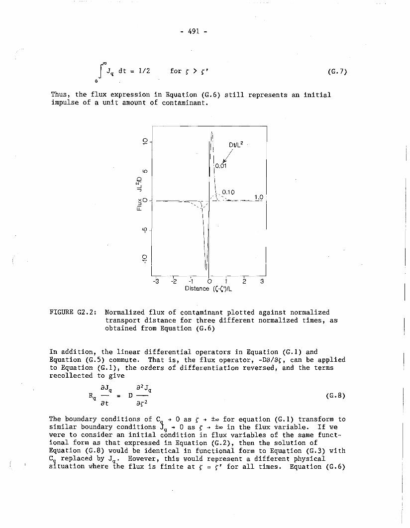
Thus, the flux expression in Equation ( G . 6 ) still represents an initial impulse of a unit amount of contaminant.
I I I I I I
-3 -2 -1 0 1 2 3 Distance ((;-(;')/L
FIGURE G 2 . 2 : Normalized flux of contaminant plotted against normalized transport distance for three different normalized times, as obtained from Equation ( G . 6 )
In addition, the linear differential operators in Equation ( G . l ) and Equation ( G . 5 ) commute. That is, the flux operator, -Da/ap, can be applied to Equation ( G e l ) , the orders of differentiation reversed, and the terms recollected to give
The boundary conditions of Cq + 0 as p + fm for equation ( G . l ) transform to similar boundary conditions Jq + 0 as p + fm in the flux variable. If we were to consider an initial condition in flux variables of the same funct- ional form as that expressed in Equation ( G . 2 ) , then the solution of Equation ( G . 8 ) would be identical in functional form to Equation ( G . 3 ) with C, replaced by J,. However, this would represent a different physical
I situation where the flux is finite at p = p r for all times. Equation ( G . 6 )
indicates that we seek a solution that has the property that the flux is zero at r = p v for all time. Applying this additional condition, the solution to Equation (G.8) is given by Equation (G.6).
This additional condition can be considered to be another boundary con- dition that breaks the domain into two subdomains -- s p < p' and I' s r < m with ltz the initial impulse in each subdomain. The boundary and initial conditions for the latter subdomain are:
J, -, 0 r + +*, all t (boundary condition)
J, = 0 = cf, t > 0 (boundary condition) (G .9A)
J, = l h h , r - r t , for t = 0 (initial condition)
Since the initial impulse occurs at the new boundary at p = r v , these conditions can be written equivalently as:
J, -, 0 r -, +-, all t (boundary condition) 1 J = & , (- = r', all t (boundary condition) I (G.98) J, = 0 I f I', t = 0 (initial condition)
This formulation of the problem for the semi-infinite subdomain p' 2 < -, using Equation (G.8) with flux as a variable, with boundary and initial / conditions similar to Equation (G.9B), is the formulation used by Heinrich and Andres (1985).
G.2.3 THE DOMAIN 0 < c < w
Consider now the semi-infinite domain 0 s p < - where the source is located at g' = 0, as shown in Figure G1.2. In the solution to the infinite domain case, with r' = 0, as described in the previous section, there is a sym- metry in the flow of contaminant at r = 0. One half of the contaminant introduced by the impulse source migrates in the positive (- direction, the other half migrates in the negative r direction and there is zero net flux at = 0. Thus, Equation (G.3) is the solution over this semi-infinite domain with a "half-strengthtf impulse source at I' = 0, and with zero flux at the boundary at r = 0. Hence, the solution to Equation (G.l) for this semi-infinite domain with a "full-strength" impulse source, expressed by the boundary and initial conditions:
C, -t 0 as g + +- (boundary conditions)
ac,/ar = 0 at p = 0 1 C = 6 4 ( c - o ) at t = 0 (initial condition)
is given by twice the solution of Equation (G.3), with I' = 0, or:
(G. 10)

(G. 11)
G.2.4 THE DOMAIN -m < C < L, WITH ZERO CONCENTRATION AT C = L
Consider the infinite domain again with an impulse source at r f = 2L. The solution to this case, as found from Equation (G.3), is:
C, = exp [ -Rqii;2Ll2 ] 2J-ZqE'
(G. 12)
Consider now two sources, one at r p = 0 and one at = 2L, together. Since the equations are linear, the solution to this composite case can be obtained by superposition; that is, by adding the individual solutions together. In making this sum, consider the source at r = 2L to be of ne- gative strength; that is, a sink rather than a source. This methodology of combining symmetrically placed sources is sometimes called the method of images. From Equation (G.3), the resulting solution for. the source + sink, plotted in Figure G2.3, is:
4D t 4D t (G. 13)
Consider now the location I = L. At this location, the concentration C, I has the value:
Thus, this solution has the property that C,(L,t) = 0 for all t, as shown in Figure G2.3.
If we consider the domain -m < < 5 L, with the location < = L on the bound- ary of the domain, as depicted in Figure G1.2, then Equation (G.13) can be considered the solution to Equation (G.l) over this domain, with boundary and initial conditions:
Cq -, 0 as < -t -m
(boundary conditions) C, = 0 at r = L 1 C, = &(1) at t = O (initial condition) j
expressing an impulse source within the domain at r ' = 0. This is the solution depicted in the left hand half of Figure G2.3; the right hand half of the plot, with the image sink, is ignored.
G.2.5 EQUIVALENCE OF DIFFUSIVE FLUXES AT t = L
Although the solutions over the domain 0 I < m, given by Equation (G.11), and over the domain -m < r 5 L, given by Equation (G.13), are different, we examine the fluxes at = L in both cases. The flux at r = L, given by
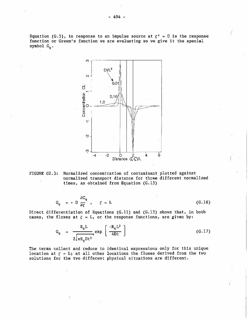
Equation (G.5), in response to an impulse source at P' = 0 is the response function or Green's function we are evaluating so we give it the special symbol G,.
FIGURE G2.3: Normalized concentration of contaminant plotted against normalized transport distance for three different normalized times, as obtained from Equation (G.13)
ac, G, = - D -
ay ' r = L (G. 16)
Direct differentiation of Equations (G.ll) and (G.13) shows that, in both cases, the fluxes at = L, or the response functions, are given by:
(G. 17)
The terms collect and reduce to identical expressions only for this unique location at = L; at all other locations the fluxes derived from the two solutions for the two different physical situations are different.
G.3 ADVECTION-DISPERSION CASES
G.3.1 SOLUTION TRANSFORM FOR ADVECTION CASES
We now consider the advection-dispersion equation:
(G. 18)
where D is a dispersion coefficient and U is the linear groundwater velo- city. We examine a form of a function that satisfies Equation (G.18) by letting:
(G. 19)
where C, is also a concentration of contaminant in groundwater. Different- iation of Equation (G.19) and direct substitution in Equation (G.18) results in:
ac, a2 c, Rq- = D- (G. 20)
at ar2
which is identical in form to Equation (G.l). Thus, C given by Equation (G. 19), satisfies Equation (6.18) if C, satisfies Equation (G. 1). Conversely, if we have a solution, C,, of Equation (G.l), then a solution of Equation (G.18) is given by Equation (G.19) with the boundary and initial conditions similarly transformed using Equation (G.19). We will apply this result together with the results obtained in Section G.2.4 in obtaining solutions to the advection-dispersion equation.
6.3.2 THE DOMAIN - < C < L, WITH ZERO CONCENTRATION AT C = L
We have shown in Section 6.2.4 that Equation (G.13) is a solution to Equation (G.l) for pure diffusion in the domain - < r s L with an impulse source at g' = 0 and with a zero concentration condition at r = L. The solution approaches zero as r + -. These boundary and initial conditions are formally expressed in Equation (G.15). Using the transformation of Equation (G.19) then
is a solution to the advection-dispersion differential equation, Equation (G.18), with the transformed boundary and initial conditions:
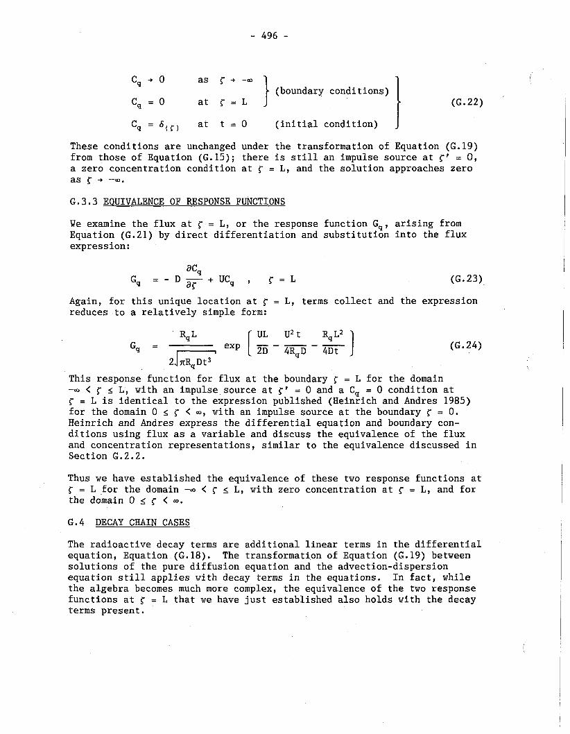
C, -, 0 as r + -Q (boundary conditions)
C, = 0 at g = L I (6.22)
C, = at t = 0 (initial condition)
These conditions are unchanged under the transformation of Equation (G.19) from those of Equation (G.15); there is still an impulse source at rf = 0, a zero concentration condition at { = L, and the solution approaches zero as + -. 6.3.3 EQUIVALENCE OF RESPONSE FUNCTIONS
We examine the flux at r = L, or the response function Gq, arising from Equation (G.21) by direct differentiation and substitution into the flux expression:
(G. 23)
Again, for this unique location at = L, terms collect and the expression reduces to a relatively simple form:
This response function for flux at the boundary < = L for the domain - < c 5 L, with an impulse source at r r = 0 and a C, = 0 condition at r = L is identical to the expression published (Heinrich and Andres 1985) for the domain 0 5 r < Q, with an impulse source at the boundary r = 0. Heinrich and Andres express the differential equation and boundary con- ditions using flux as a variable and discuss the equivalence of the flux and concentration representations, similar to the equivalence discussed in Section G.2.2.
Thus we have established the equivalence of these two response functions at r = L for the domain - < 5 L, with zero concentration at c = L, and for the domain 0 5 r < Q.
6.4 DECAY CHAIN CASES
The radioactive decay terms are additional linear terms in the differential equation, Equation (G.18). The transformation of Equation (G.19) between solutions of the pure diffusion equation and the advection-dispersion equation still applies with decay terms in the equations. In fact, while the algebra becomes much more complex, the equivalence of the two response functions at r = L that we have just established also holds with the decay terms present.
I REFERENCES:
Carslaw, H.S. and J.C. Jaeger. 1959. Conduction of Heat in Solids, Oxford University Press,
Heinrich, W.F. and T.H Andres. 1985. Response Functions of the Convection-Dispersion Equations Describing Radionuclide Migration in a Semi-Infinite Medium, Annals of Nuclear Energy, 12, 1985, 685-691.