LETTERdoi:10.1038/nature12376

Onset of deglacial warming in West Antarcticadriven by local orbital forcingWAIS Divide Project Members*

The cause of warming in the Southern Hemisphere during the mostrecent deglaciation remains a matter of debate1,2. Hypotheses for aNorthern Hemisphere trigger, through oceanic redistributions ofheat, are based in part on the abrupt onset of warming seen in EastAntarctic ice cores and dated to 18,000 years ago, which is severalthousand years after high-latitude Northern Hemisphere summerinsolation intensity began increasing from its minimum, approxi-mately 24,000 years ago3,4. An alternative explanation is that localsolar insolation changes cause the Southern Hemisphere to warmindependently2,5. Here we present results from a new, annuallyresolved ice-core record from West Antarctica that reconciles thesetwo views. The records show that 18,000 years ago snow accumula-tion in West Antarctica began increasing, coincident with increasingcarbon dioxide concentrations, warming in East Antarctica and cool-ing in the Northern Hemisphere6 associated with an abrupt decreasein Atlantic meridional overturning circulation7. However, signifi-cant warming in West Antarctica began at least 2,000 years earlier.Circum-Antarctic sea-ice decline, driven by increasing local insola-tion, is the likely cause of this warming. The marine-influenced WestAntarctic records suggest a more active role for the Southern Oceanin the onset of deglaciation than is inferred from ice cores in the EastAntarctic interior, which are largely isolated from sea-ice changes.

Exceptional records of Southern Hemisphere climate change comefrom Antarctic ice cores2,6,7. Most of these records are from high-altitude sites on the East Antarctic plateau. Questions about the reli-ability of the two previous deep West Antarctic ice-core records result inthose records often being excluded from reconstructions of Antarcticclimate4,8. Because the climate of West Antarctica is distinct from that ofinterior East Antarctica, the exclusion of West Antarctic records mayresult in an incomplete picture of past Antarctic and Southern Oceanclimate change. Interior West Antarctica is lower in elevation and moresubject to the influence of marine air masses than interior East Antarctica,which is surrounded by a steep topographic slope9,10. Marine-influencedlocations are important because they more directly reflect atmosphericconditions resulting from changes in ocean circulation and sea ice.However, ice-core records from coastal sites are often difficult to inter-pret because of complicated ice-flow and elevation histories. The WestAntarctic Ice Sheet (WAIS) Divide ice core (WDC), in central WestAntarctica, is unique in coming from a location that has experiencedminimal elevation change11, is strongly influenced by marine conditions9

and has a relatively high snow-accumulation rate, making it possibleto obtain an accurately dated record with high temporal resolution.

Drilling of WDC was completed in December 2011 to a depth of3,405 m. Drilling was halted ,50 m above the bedrock to avoid con-taminating the basal water system. WDC is situated 24 km west of theRoss–Amundsen ice-flow divide and 160 km east of the Byrd ice-coresite (Supplementary Fig. 1). The elevation is 1,766 m; the present-daysnow accumulation rate is 22 cm yr21 (ice equivalent) and the averagetemperature is approximately 230 uC. The age of the oldest recoveredice is ,68 kyr. The WDC06A-7 timescale is based on the identificationof annual layers to 29.6 kyr ago using primarily electrical measurements

(Methods). To validate WDC06A-7, we compare times of abrupt changesin atmospheric methane concentration (Supplementary Information)with the Greenland Ice Core Chronology 200512 (GICC05). We alsocompare the methane variations in WDC with abrupt changes in aspeleothem d18O record from Hulu Cave, China. The difference in agebetween the ice and gas at a given depth is calculated using a steady-state firn-densification model and is always less than 500 yr. The agedifferences between WDC06A-7 and GICC05 and between WDC06A-7and the Hulu Cave timescale are much less than the independent time-scale uncertainties (Supplementary Fig. 6).

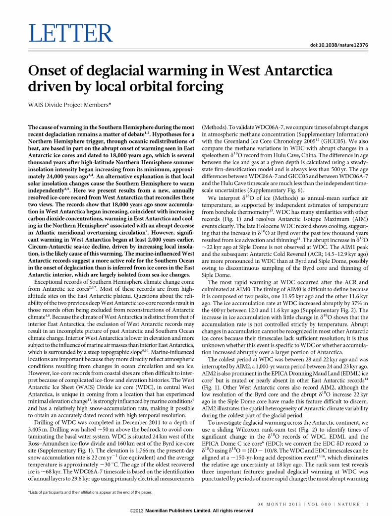
We interpret d18O of ice (Methods) as annual-mean surface airtemperature, as supported by independent estimates of temperaturefrom borehole thermometry13. WDC has many similarities with otherrecords (Fig. 1) and resolves Antarctic Isotope Maximum (AIM)events clearly. The late Holocene WDC record shows cooling, suggest-ing that the increase in d18O at Byrd over the past few thousand yearsresulted from ice advection and thinning11. The abrupt increase in d18O,22 kyr ago at Siple Dome is not observed at WDC. The AIM1 peakand the subsequent Antarctic Cold Reversal (ACR; 14.5–12.9 kyr ago)are more pronounced in WDC than at Byrd and Siple Dome, possiblyowing to discontinuous sampling of the Byrd core and thinning ofSiple Dome.

The most rapid warming at WDC occurred after the ACR andculminated at AIM0. The timing of AIM0 is difficult to define becauseit is composed of two peaks, one 11.95 kyr ago and the other 11.6 kyrago. The ice accumulation rate at WDC increased abruptly by 37% inthe 400 yr between 12.0 and 11.6 kyr ago (Supplementary Fig. 2). Theincrease in ice accumulation with little change in d18O shows that theaccumulation rate is not controlled strictly by temperature. Abruptchanges in accumulation cannot be recognized in most other Antarcticice cores because their timescales lack sufficient resolution; it is thusunknown whether this event is specific to WDC or whether accumula-tion increased abruptly over a larger portion of Antarctica.

The coldest period at WDC was between 28 and 22 kyr ago and wasinterrupted by AIM2, a 1,000-yr warm period between 24 and 23 kyr ago.AIM2 is also prominent in the EPICA Dronning Maud Land (EDML) icecore7 but is muted or nearly absent in other East Antarctic records14

(Fig. 1). Other West Antarctic cores also record AIM2, although thelow resolution of the Byrd core and the abrupt d18O increase 22 kyrago in the Siple Dome core have made this feature difficult to discern.AIM2 illustrates the spatial heterogeneity of Antarctic climate variabilityduring the coldest part of the glacial period.

To investigate deglacial warming across the Antarctic continent, weuse a sliding Wilcoxon rank-sum test (Fig. 2) to identify times ofsignificant change in the d18O records of WDC, EDML and theEPICA Dome C ice core6 (EDC); we convert the EDC dD record tod18O using d18O 5 (dD 2 10)/8. The WDC and EDC timescales can bealigned at a ,150-yr-long acid deposition event15,16, which eliminatesthe relative age uncertainty at 18 kyr ago. The rank sum test revealsthree important features: gradual deglacial warming at WDC waspunctuated by periods of more rapid change; the most abrupt warming

*Lists of participants and their affiliations appear at the end of the paper.

0 0 M O N T H 2 0 1 3 | V O L 0 0 0 | N A T U R E | 1

Macmillan Publishers Limited. All rights reserved©2013

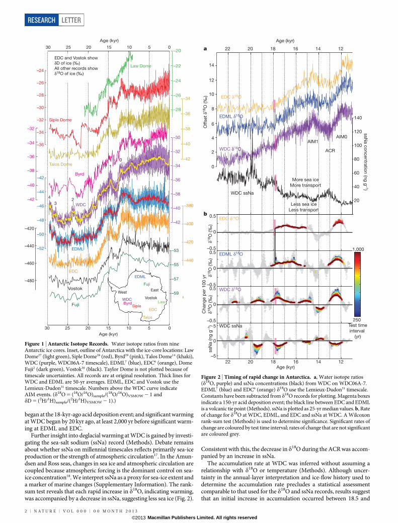
began at the 18-kyr-ago acid deposition event; and significant warmingat WDC began by 20 kyr ago, at least 2,000 yr before significant warm-ing at EDML and EDC.

Further insight into deglacial warming at WDC is gained by investi-gating the sea-salt sodium (ssNa) record (Methods). Debate remainsabout whether ssNa on millennial timescales reflects primarily sea-iceproduction or the strength of atmospheric circulation17. In the Amun-dsen and Ross seas, changes in sea ice and atmospheric circulation arecoupled because atmospheric forcing is the dominant control on sea-ice concentration18. We interpret ssNa as a proxy for sea-ice extent anda marker of marine changes (Supplementary Information). The rank-sum test reveals that each rapid increase in d18O, indicating warming,was accompanied by a decrease in ssNa, suggesting less sea ice (Fig. 2).

Consistent with this, the decrease in d18O during the ACR was accom-panied by an increase in ssNa.

The accumulation rate at WDC was inferred without assuming arelationship with d18O or temperature (Methods). Although uncer-tainty in the annual-layer interpretation and ice-flow history used todetermine the accumulation rate precludes a statistical assessmentcomparable to that used for the d18O and ssNa records, results suggestthat an initial increase in accumulation occurred between 18.5 and

EDML

EDC

Talos Dome

Byrd

–36

–34

–32

–30

–28

–26

–24

Siple Dome

–52

–50

–48

–46

–44

–42

–480

–460

–440

–420

–42

–40

–38

–36

–34

–32

Law Dome

–42

–40

–38

–36

–34

–32

–30

–42

–40

–38

–36

–34

–59

–57

–55

–53

–440

–420

–400

–380

–20

–22

–24

–26

–28

Vostok

Fuji

30 25 20 15 10 5 0

30 25 20 15 10 5 0

Age (kyr)

Age (kyr)

WDCByrd

EDCSiple

Law

Talos

Fuji

EDML

Vostok

WestEast

0

1

23

4

WDC

EDC and Vostok show

δD of ice (‰)

All other records show

δ18O of ice (‰)

Figure 1 | Antarctic Isotope Records. Water isotope ratios from nineAntarctic ice cores. Inset, outline of Antarctica with the ice-core locations: LawDome27 (light green), Siple Dome28 (red), Byrd29 (pink), Talos Dome14 (khaki),WDC (purple, WDC06A-7 timescale), EDML7 (blue), EDC6 (orange), DomeFuji2 (dark green), Vostok30 (black). Taylor Dome is not plotted because oftimescale uncertainties. All records are at original resolution. Thick lines forWDC and EDML are 50-yr averages. EDML, EDC and Vostok use theLemieux-Dudon31 timescale. Numbers above the WDC curve indicateAIM events. (d18O 5 (18O/16O)sample/(

18O/16O)VSMOW 2 1 anddD 5 (2H/1H)sample/(

2H/1H)VSMOW 2 1).)

22 20 18 16 14 12

EDML δ18O

Off

set δ1

8O

(‰

)

0

2

4

6

8

10

12

Age (kyr)

250

1,000

Test time

interval

(yr)

EDC δ18O

AIM1

20

40

60

80

100

120

140

ssN

a c

on

cen

tratio

n (n

g g

–1)

14

22 20 18 16 14 12Age (kyr)

0

0

0

0

5

–5

–0.5

–0.5

–0.5

0.5

0.5

0.5

Chang

e p

er

100 y

r δ18O

(‰

)δ1

8O

(‰

)

WDC δ18O

EDML δ18O

EDC δ18O

WDC ssNa

ssN

a (ng

g–1)

δ18O

(‰

)

a

b

WDC WDC δ1818OWDC δ18O ACRACR

AIM0AIM0

Less sea iceLess sea ice

Less transportLess transport

More sea iceMore sea ice

More transportMore transport

ACR

AIM0

WDC ssNa

Less sea ice

Less transport

More sea ice

More transport

Figure 2 | Timing of rapid change in Antarctica. a, Water isotope ratios(d18O, purple) and ssNa concentrations (black) from WDC on WDC06A-7.EDML7 (blue) and EDC6 (orange) d18O use the Lemieux-Dudon31 timescale.Constants have been subtracted from d18O records for plotting. Magenta boxesindicate a 150-yr acid deposition event; the black line between EDC and EDMLis a volcanic tie point (Methods). ssNa is plotted as 25-yr median values. b, Rateof change for d18O at WDC, EDML, and EDC and ssNa at WDC. A Wilcoxonrank-sum test (Methods) is used to determine significance. Significant rates ofchange are coloured by test time interval; rates of change that are not significantare coloured grey.

RESEARCH LETTER

2 | N A T U R E | V O L 0 0 0 | 0 0 M O N T H 2 0 1 3

Macmillan Publishers Limited. All rights reserved©2013

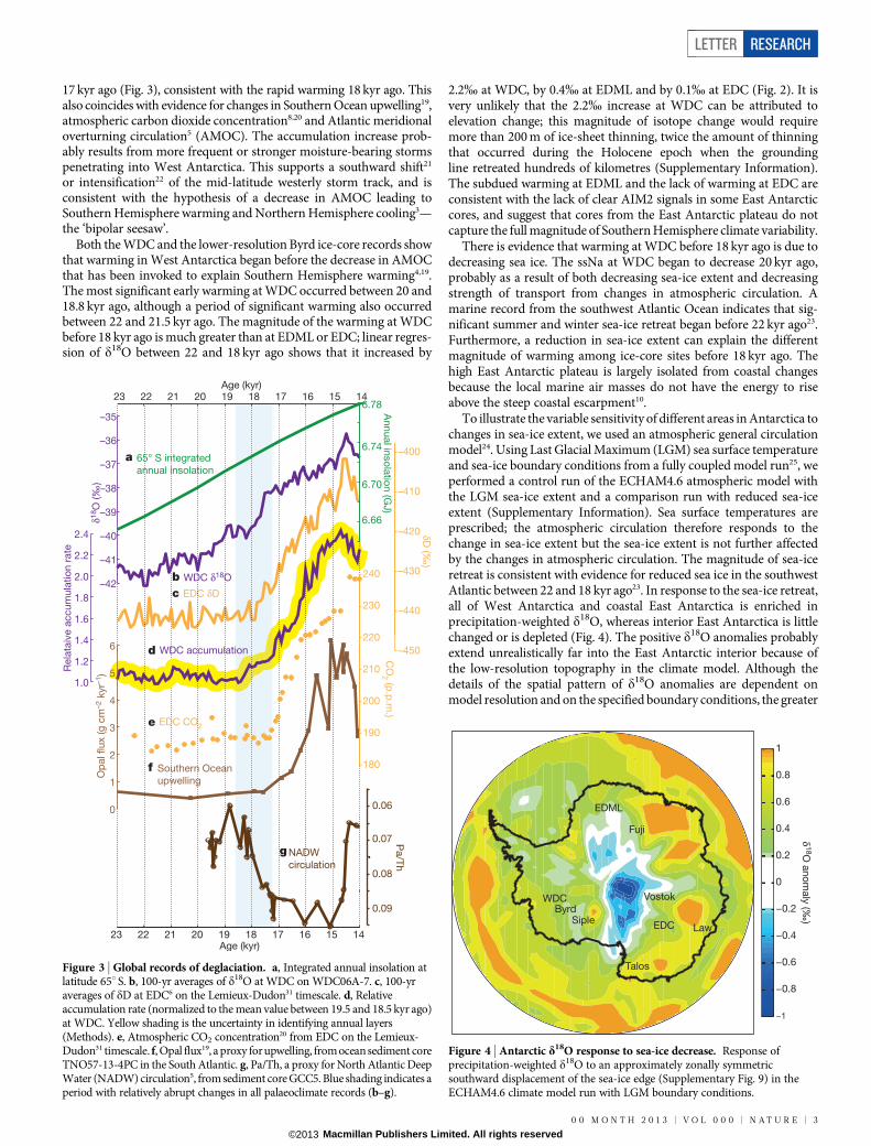
17 kyr ago (Fig. 3), consistent with the rapid warming 18 kyr ago. Thisalso coincides with evidence for changes in Southern Ocean upwelling19,atmospheric carbon dioxide concentration8,20 and Atlantic meridionaloverturning circulation5 (AMOC). The accumulation increase prob-ably results from more frequent or stronger moisture-bearing stormspenetrating into West Antarctica. This supports a southward shift21

or intensification22 of the mid-latitude westerly storm track, and isconsistent with the hypothesis of a decrease in AMOC leading toSouthern Hemisphere warming and Northern Hemisphere cooling3—the ‘bipolar seesaw’.

Both the WDC and the lower-resolution Byrd ice-core records showthat warming in West Antarctica began before the decrease in AMOCthat has been invoked to explain Southern Hemisphere warming4,19.The most significant early warming at WDC occurred between 20 and18.8 kyr ago, although a period of significant warming also occurredbetween 22 and 21.5 kyr ago. The magnitude of the warming at WDCbefore 18 kyr ago is much greater than at EDML or EDC; linear regres-sion of d18O between 22 and 18 kyr ago shows that it increased by

2.2% at WDC, by 0.4% at EDML and by 0.1% at EDC (Fig. 2). It isvery unlikely that the 2.2% increase at WDC can be attributed toelevation change; this magnitude of isotope change would requiremore than 200 m of ice-sheet thinning, twice the amount of thinningthat occurred during the Holocene epoch when the groundingline retreated hundreds of kilometres (Supplementary Information).The subdued warming at EDML and the lack of warming at EDC areconsistent with the lack of clear AIM2 signals in some East Antarcticcores, and suggest that cores from the East Antarctic plateau do notcapture the full magnitude of Southern Hemisphere climate variability.

There is evidence that warming at WDC before 18 kyr ago is due todecreasing sea ice. The ssNa at WDC began to decrease 20 kyr ago,probably as a result of both decreasing sea-ice extent and decreasingstrength of transport from changes in atmospheric circulation. Amarine record from the southwest Atlantic Ocean indicates that sig-nificant summer and winter sea-ice retreat began before 22 kyr ago23.Furthermore, a reduction in sea-ice extent can explain the differentmagnitude of warming among ice-core sites before 18 kyr ago. Thehigh East Antarctic plateau is largely isolated from coastal changesbecause the local marine air masses do not have the energy to riseabove the steep coastal escarpment10.

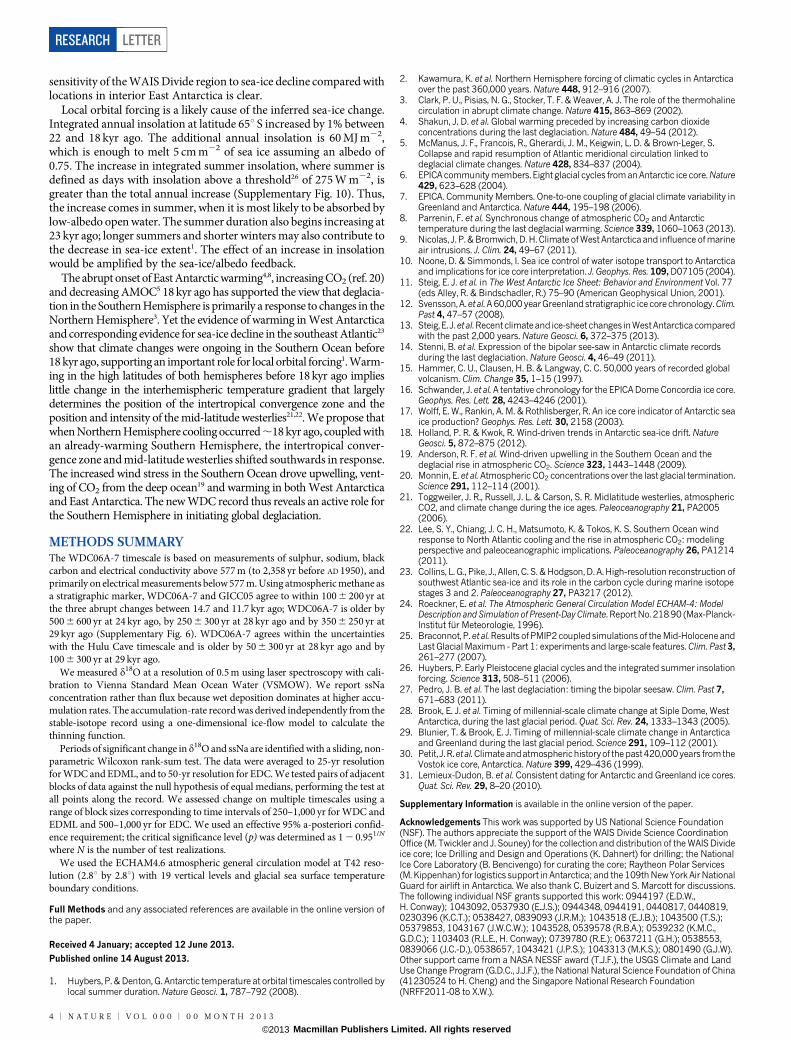
To illustrate the variable sensitivity of different areas in Antarctica tochanges in sea-ice extent, we used an atmospheric general circulationmodel24. Using Last Glacial Maximum (LGM) sea surface temperatureand sea-ice boundary conditions from a fully coupled model run25, weperformed a control run of the ECHAM4.6 atmospheric model withthe LGM sea-ice extent and a comparison run with reduced sea-iceextent (Supplementary Information). Sea surface temperatures areprescribed; the atmospheric circulation therefore responds to thechange in sea-ice extent but the sea-ice extent is not further affectedby the changes in atmospheric circulation. The magnitude of sea-iceretreat is consistent with evidence for reduced sea ice in the southwestAtlantic between 22 and 18 kyr ago23. In response to the sea-ice retreat,all of West Antarctica and coastal East Antarctica is enriched inprecipitation-weighted d18O, whereas interior East Antarctica is littlechanged or is depleted (Fig. 4). The positive d18O anomalies probablyextend unrealistically far into the East Antarctic interior because ofthe low-resolution topography in the climate model. Although thedetails of the spatial pattern of d18O anomalies are dependent onmodel resolution and on the specified boundary conditions, the greater

1.0

1.2

1.4

1.6

1.8

2.0

2.2

2.4

WDC δ18O

EDC δD

WDC accumulation

EDC CO2

Southern Ocean

upwelling

23 22 21 20 19 18 17 16 15 14

–450

–440

–430

–420

–410

–400δD

(‰)

CO

2 (p.p

.m.)

Op

al flux (g

cm

–2 k

yr–

1)

0.07

0.08

0.09

0.06

NADW

circulation

Pa/T

h

23 22 21 20 19 18 17 16 15 14

Rela

taiv

e a

ccum

ula

tio

n r

ate

65° S integrated

annual insolation

Age (kyr)

Age (kyr)

180

190

200

210

220

230

240

0

1

2

3

4

5

6

–42

–41

–40

–39

–38

–37

–36

–35

δ18O

(‰

) 6.70

6.66

6.74

6.78

Annual in

so

latio

n (G

J)

a

e

g

f

b

d

c

Figure 3 | Global records of deglaciation. a, Integrated annual insolation atlatitude 65u S. b, 100-yr averages of d18O at WDC on WDC06A-7. c, 100-yraverages of dD at EDC6 on the Lemieux-Dudon31 timescale. d, Relativeaccumulation rate (normalized to the mean value between 19.5 and 18.5 kyr ago)at WDC. Yellow shading is the uncertainty in identifying annual layers(Methods). e, Atmospheric CO2 concentration20 from EDC on the Lemieux-Dudon31 timescale. f, Opal flux19, a proxy for upwelling, from ocean sediment coreTNO57-13-4PC in the South Atlantic. g, Pa/Th, a proxy for North Atlantic DeepWater (NADW) circulation5, from sediment core GCC5. Blue shading indicates aperiod with relatively abrupt changes in all palaeoclimate records (b–g).

−1

−0.8

−0.6

−0.4

−0.2

0

0.2

0.4

0.6

0.8

1

δ1

8O a

no

maly

(‰)

EDML

Fuji

Vostok

LawEDC

Talos

SipleByrd

WDC

Figure 4 | Antarctic d18O response to sea-ice decrease. Response ofprecipitation-weighted d18O to an approximately zonally symmetricsouthward displacement of the sea-ice edge (Supplementary Fig. 9) in theECHAM4.6 climate model run with LGM boundary conditions.

LETTER RESEARCH

0 0 M O N T H 2 0 1 3 | V O L 0 0 0 | N A T U R E | 3

Macmillan Publishers Limited. All rights reserved©2013

sensitivity of the WAIS Divide region to sea-ice decline compared withlocations in interior East Antarctica is clear.

Local orbital forcing is a likely cause of the inferred sea-ice change.Integrated annual insolation at latitude 65u S increased by 1% between22 and 18 kyr ago. The additional annual insolation is 60 MJ m22,which is enough to melt 5 cm m22 of sea ice assuming an albedo of0.75. The increase in integrated summer insolation, where summer isdefined as days with insolation above a threshold26 of 275 W m22, isgreater than the total annual increase (Supplementary Fig. 10). Thus,the increase comes in summer, when it is most likely to be absorbed bylow-albedo open water. The summer duration also begins increasing at23 kyr ago; longer summers and shorter winters may also contribute tothe decrease in sea-ice extent1. The effect of an increase in insolationwould be amplified by the sea-ice/albedo feedback.

The abrupt onset of East Antarctic warming4,8, increasing CO2 (ref. 20)and decreasing AMOC5 18 kyr ago has supported the view that deglacia-tion in the Southern Hemisphere is primarily a response to changes in theNorthern Hemisphere3. Yet the evidence of warming in West Antarcticaand corresponding evidence for sea-ice decline in the southeast Atlantic23

show that climate changes were ongoing in the Southern Ocean before18 kyr ago, supporting an important role for local orbital forcing1. Warm-ing in the high latitudes of both hemispheres before 18 kyr ago implieslittle change in the interhemispheric temperature gradient that largelydetermines the position of the intertropical convergence zone and theposition and intensity of the mid-latitude westerlies21,22. We propose thatwhen Northern Hemisphere cooling occurred ,18 kyr ago, coupled withan already-warming Southern Hemisphere, the intertropical conver-gence zone and mid-latitude westerlies shifted southwards in response.The increased wind stress in the Southern Ocean drove upwelling, vent-ing of CO2 from the deep ocean19 and warming in both West Antarcticaand East Antarctica. The new WDC record thus reveals an active role forthe Southern Hemisphere in initiating global deglaciation.

METHODS SUMMARYThe WDC06A-7 timescale is based on measurements of sulphur, sodium, blackcarbon and electrical conductivity above 577 m (to 2,358 yr before AD 1950), andprimarily on electrical measurements below 577 m. Using atmospheric methane asa stratigraphic marker, WDC06A-7 and GICC05 agree to within 100 6 200 yr atthe three abrupt changes between 14.7 and 11.7 kyr ago; WDC06A-7 is older by500 6 600 yr at 24 kyr ago, by 250 6 300 yr at 28 kyr ago and by 350 6 250 yr at29 kyr ago (Supplementary Fig. 6). WDC06A-7 agrees within the uncertaintieswith the Hulu Cave timescale and is older by 50 6 300 yr at 28 kyr ago and by100 6 300 yr at 29 kyr ago.

We measured d18O at a resolution of 0.5 m using laser spectroscopy with cali-bration to Vienna Standard Mean Ocean Water (VSMOW). We report ssNaconcentration rather than flux because wet deposition dominates at higher accu-mulation rates. The accumulation-rate record was derived independently from thestable-isotope record using a one-dimensional ice-flow model to calculate thethinning function.

Periods of significant change in d18O and ssNa are identified with a sliding, non-parametric Wilcoxon rank-sum test. The data were averaged to 25-yr resolutionfor WDC and EDML, and to 50-yr resolution for EDC. We tested pairs of adjacentblocks of data against the null hypothesis of equal medians, performing the test atall points along the record. We assessed change on multiple timescales using arange of block sizes corresponding to time intervals of 250–1,000 yr for WDC andEDML and 500–1,000 yr for EDC. We used an effective 95% a-posteriori confid-ence requirement; the critical significance level (p) was determined as 1 2 0.951/N

where N is the number of test realizations.We used the ECHAM4.6 atmospheric general circulation model at T42 reso-

lution (2.8u by 2.8u) with 19 vertical levels and glacial sea surface temperatureboundary conditions.

Full Methods and any associated references are available in the online version ofthe paper.

Received 4 January; accepted 12 June 2013.

Published online 14 August 2013.

1. Huybers, P. & Denton, G. Antarctic temperature at orbital timescales controlled bylocal summer duration. Nature Geosci. 1, 787–792 (2008).

2. Kawamura, K. et al. Northern Hemisphere forcing of climatic cycles in Antarcticaover the past 360,000 years. Nature 448, 912–916 (2007).

3. Clark, P. U., Pisias, N. G., Stocker, T. F. & Weaver, A. J. The role of the thermohalinecirculation in abrupt climate change. Nature 415, 863–869 (2002).

4. Shakun, J. D. et al. Global warming preceded by increasing carbon dioxideconcentrations during the last deglaciation. Nature 484, 49–54 (2012).

5. McManus, J. F., Francois, R., Gherardi, J. M., Keigwin, L. D. & Brown-Leger, S.Collapse and rapid resumption of Atlantic meridional circulation linked todeglacial climate changes. Nature 428, 834–837 (2004).

6. EPICA community members. Eight glacial cycles from anAntarctic ice core. Nature429, 623–628 (2004).

7. EPICA. Community Members. One-to-one coupling of glacial climate variability inGreenland and Antarctica. Nature 444, 195–198 (2006).

8. Parrenin, F. et al. Synchronous change of atmospheric CO2 and Antarctictemperature during the last deglacial warming. Science 339, 1060–1063 (2013).

9. Nicolas, J. P. & Bromwich, D. H. Climate of West Antarctica and influence of marineair intrusions. J. Clim. 24, 49–67 (2011).

10. Noone, D. & Simmonds, I. Sea ice control of water isotope transport to Antarcticaand implications for ice core interpretation. J. Geophys. Res. 109, D07105 (2004).

11. Steig, E. J. et al. in The West Antarctic Ice Sheet: Behavior and Environment Vol. 77(eds Alley, R. & Bindschadler, R.) 75–90 (American Geophysical Union, 2001).

12. Svensson, A.et al.A 60,000 yearGreenlandstratigraphic ice core chronology.Clim.Past 4, 47–57 (2008).

13. Steig, E. J.et al.Recentclimateand ice-sheet changes inWestAntarctica comparedwith the past 2,000 years. Nature Geosci. 6, 372–375 (2013).

14. Stenni, B. et al. Expression of the bipolar see-saw in Antarctic climate recordsduring the last deglaciation. Nature Geosci. 4, 46–49 (2011).

15. Hammer, C. U., Clausen, H. B. & Langway, C. C. 50,000 years of recorded globalvolcanism. Clim. Change 35, 1–15 (1997).

16. Schwander, J. et al. A tentative chronology for the EPICA Dome Concordia ice core.Geophys. Res. Lett. 28, 4243–4246 (2001).

17. Wolff, E. W., Rankin, A. M. & Rothlisberger, R. An ice core indicator of Antarctic seaice production? Geophys. Res. Lett. 30, 2158 (2003).

18. Holland, P. R. & Kwok, R. Wind-driven trends in Antarctic sea-ice drift. NatureGeosci. 5, 872–875 (2012).

19. Anderson, R. F. et al. Wind-driven upwelling in the Southern Ocean and thedeglacial rise in atmospheric CO2. Science 323, 1443–1448 (2009).

20. Monnin, E. et al. Atmospheric CO2 concentrations over the last glacial termination.Science 291, 112–114 (2001).

21. Toggweiler, J. R., Russell, J. L. & Carson, S. R. Midlatitude westerlies, atmosphericCO2, and climate change during the ice ages. Paleoceanography 21, PA2005(2006).

22. Lee, S. Y., Chiang, J. C. H., Matsumoto, K. & Tokos, K. S. Southern Ocean windresponse to North Atlantic cooling and the rise in atmospheric CO2: modelingperspective and paleoceanographic implications. Paleoceanography 26, PA1214(2011).

23. Collins, L. G., Pike, J., Allen, C. S. & Hodgson, D. A. High-resolution reconstruction ofsouthwest Atlantic sea-ice and its role in the carbon cycle during marine isotopestages 3 and 2. Paleoceanography 27, PA3217 (2012).

24. Roeckner, E. et al. The Atmospheric General Circulation Model ECHAM-4: ModelDescription and Simulation of Present-Day Climate. Report No. 218 90 (Max-Planck-Institut fur Meteorologie, 1996).

25. Braconnot, P. et al. Results of PMIP2 coupledsimulations of the Mid-Holocene andLast Glacial Maximum - Part 1: experiments and large-scale features. Clim. Past 3,261–277 (2007).

26. Huybers, P. Early Pleistocene glacial cycles and the integrated summer insolationforcing. Science 313, 508–511 (2006).

27. Pedro, J. B. et al. The last deglaciation: timing the bipolar seesaw. Clim. Past 7,671–683 (2011).

28. Brook, E. J. et al. Timing of millennial-scale climate change at Siple Dome, WestAntarctica, during the last glacial period. Quat. Sci. Rev. 24, 1333–1343 (2005).

29. Blunier, T. & Brook, E. J. Timing of millennial-scale climate change in Antarcticaand Greenland during the last glacial period. Science 291, 109–112 (2001).

30. Petit, J. R.et al.Climateandatmospherichistoryof thepast420,000years fromtheVostok ice core, Antarctica. Nature 399, 429–436 (1999).

31. Lemieux-Dudon, B. et al. Consistent dating for Antarctic and Greenland ice cores.Quat. Sci. Rev. 29, 8–20 (2010).

Supplementary Information is available in the online version of the paper.

Acknowledgements This work was supported by US National Science Foundation(NSF). The authors appreciate the support of the WAIS Divide Science CoordinationOffice (M. Twickler and J. Souney) for the collection and distribution of the WAIS Divideice core; Ice Drilling and Design and Operations (K. Dahnert) for drilling; the NationalIce Core Laboratory (B. Bencivengo) for curating the core; Raytheon Polar Services(M. Kippenhan) for logistics support in Antarctica; and the 109th NewYork Air NationalGuard for airlift in Antarctica. We also thank C. Buizert and S. Marcott for discussions.The following individual NSF grants supported this work: 0944197 (E.D.W.,H. Conway); 1043092, 0537930 (E.J.S.); 0944348, 0944191, 0440817, 0440819,0230396 (K.C.T.); 0538427, 0839093 (J.R.M.); 1043518 (E.J.B.); 1043500 (T.S.);05379853, 1043167 (J.W.C.W.); 1043528, 0539578 (R.B.A.); 0539232 (K.M.C.,G.D.C.); 1103403 (R.L.E., H. Conway); 0739780 (R.E.); 0637211 (G.H.); 0538553,0839066 (J.C.-D.), 0538657, 1043421 (J.P.S.); 1043313 (M.K.S.); 0801490 (G.J.W).Other support came from a NASA NESSF award (T.J.F.), the USGS Climate and LandUse Change Program (G.D.C., J.J.F.), the National Natural Science Foundation of China(41230524 to H. Cheng) and the Singapore National Research Foundation(NRFF2011-08 to X.W.).

RESEARCH LETTER

4 | N A T U R E | V O L 0 0 0 | 0 0 M O N T H 2 0 1 3

Macmillan Publishers Limited. All rights reserved©2013

Author Contributions The manuscript was written by T.J.F., E.J.S. and B.R.M. K.C.T.organized the WAIS Divide Project. T.J.F., K.C.T and T.J.P. made the electricalmeasurementsanddeveloped theelectrical timescalewithK.C.M.E.J.S., J.W.C.W., A.J.S.,P.N., B.H.V. and S.W.S. measured the stable-isotope record. J.R.M., M.S., O.J.M. and R.E.developed the chemistry timescale and measured Na. E.J.B., T.S., L.E.M., J.S.E. and J.E.L.made the methane measurements. G.D.C. and K.M.C. measured the boreholetemperature profile. J.C.-D. and D.F. provided an independent timescale for the brittleice. Q.D., S.W.S. and E.J.S. performed the climate modelling. T.J.F., E.D.W., H. Conwayand K.M.C. performed the ice-flow modelling to determine the accumulation rate. H.Cheng, R.L.E., X.W., J.P.S. and T.J.F. made comparisons with the Hulu cave timescale.M.K.S., J.J.F., J.M.F., D.E.V. and R.B.A. examined the physical properties of the core. W.M.,J.J. andN.M.designed thedrill. G.H.designedcore-processing techniques. A.J.O., B.H.V.,D.E.V., K.C.T., T.J.P. and G.J.W. led collection and processing of the core in the field.

Author Information Reprints and permissions information is available atwww.nature.com/reprints. The authors declare no competing financial interests.Readers are welcome to comment on the online version of the paper.Correspondence and requests for materials should be addressedto T.J.F. (tjfudge@uw.edu).

WAIS Divide Project Members T. J. Fudge1, Eric J. Steig1,2, Bradley R. Markle1, SpruceW. Schoenemann1, Qinghua Ding1,2, Kendrick C. Taylor3, Joseph R. McConnell3,Edward J. Brook4, Todd Sowers5, James W. C. White6,7, Richard B. Alley5,8, HaiCheng9,10, Gary D. Clow11, Jihong Cole-Dai12, Howard Conway1, Kurt M. Cuffey13, JonS. Edwards4, R. Lawrence Edwards10, Ross Edwards14, John M. Fegyveresi5,8, DavidFerris12, Joan J. Fitzpatrick15, Jay Johnson16, Geoffrey Hargreaves17, James E. Lee4,Olivia J. Maselli3, William Mason18, Kenneth C. McGwire3, Logan E. Mitchell4, NicolaiMortensen16, Peter Neff1,19, Anais J. Orsi20, Trevor J. Popp21, Andrew J. Schauer1,

Jeffrey P. Severinghaus20, Michael Sigl3, Matthew K. Spencer22, Bruce H. Vaughn7,Donald E. Voigt5,8, Edwin D. Waddington1, Xianfeng Wang23 & Gifford J. Wong24

Affiliations for participants: 1Department of Earth and Space Sciences, University ofWashington, Seattle, Washington 98195, USA. 2Quaternary Research Center, Universityof Washington, Seattle, Washington 98195, USA. 3Desert Research Institute, NevadaSystem of Higher Education, Reno, Nevada 89512, USA. 4College of Earth, Ocean andAtmospheric Sciences Oregon State University, Corvallis, Oregon 97331, USA. 5Earth andEnvironmental Systems Institute, Pennsylvania State University, University Park,Pennsylvania 16802, USA. 6Department of Geological Sciences and Department ofEnvironmentalStudies, Boulder,Colorado80309,USA. 7INSTAAR, University ofColorado,Boulder, Colorado 80309, USA. 8Department of Geosciences, Pennsylvania StateUniversity, University Park, Pennsylvania 16802, USA. 9Institute of Global EnvironmentalChange, Xi’an Jiaotong University, Xi’an 710049, China. 10Department of Earth Sciences,University of Minnesota, Minneapolis, Minnesota 55455, USA. 11US Geological Survey,Geosciences and Environmental Change Science Center, Lakewood, Colorado 80225,USA. 12Department of Chemistry and Biochemistry, South Dakota State University,Brookings, South Dakota 57007, USA. 13Department of Geography, University ofCalifornia-Berkeley, Berkeley94720, USA. 14Department of Imaging and Applied Physics,Curtin University, Perth, Western Australia 6102, Australia. 15US Geological Survey,Denver, Colorado 80225, USA. 16Ice Drilling Design and Operations, Space ScienceEngineering Center, University of Wisconsin-Madison, Madison, Wisconsin 53706, USA.17US Geologic Survey, National Ice Core Laboratory, Denver, Colorado 80225, USA.18EMECH Designs, Brooklyn, Wisconsin 53521, USA. 19Antarctic Research Centre,Victoria University of Wellington, Wellington 6012, New Zealand. 20Scripps Institution ofOceanography, University of California, San Diego, La Jolla, California 92037, USA.21Centre for Ice and Climate, Niels Bohr Institute, University of Copenhagen, JulianeMaries Vej 30, 2100 Copenhagen, Denmark. 22Department of Geology and Physics, LakeSuperior State University, Sault Ste Marie, Michigan 49783, USA. 23Earth Observatory ofSingapore, Nanyang Technological University, Singapore 639798. 24Departmentof EarthSciences, Dartmouth College, Hanover, New Hampshire 03755, USA.

LETTER RESEARCH

0 0 M O N T H 2 0 1 3 | V O L 0 0 0 | N A T U R E | 5

Macmillan Publishers Limited. All rights reserved©2013

METHODSStable-isotope measurements of ice. Water isotope analyses were by laserspectroscopy32 at the University of Washington. Values of d18O represent thedeviation from Vienna Standard Mean Ocean Water (VSMOW) normalized11

to the VSMOW-SLAP standards and reported in per mil (%). The precision ofthe measurements is better than 0.1%. The data have not been corrected foradvection, elevation, or mean seawater d18O.Accumulation rates. The accumulation-rate record was derived independentlyfrom the stable-isotope record using an ice-flow model to calculate the thinningfunction. We use a transient one-dimensional ice-flow model to compute thevertical-velocity profile:

w zð Þ~{ _b{ _m{ _H� �

y zð Þ{ _m{ri

r zð Þ{1

� �_b ð1Þ

Here z is the height above the bed, _b is the accumulation rate, _m is the melt rate, _His the rate of ice-thickness change, ri is the density of ice, r(z) is the density profileand y(z) is the vertical velocity shape function computed as

y zð Þ~ fBzz(1=2) 1{fBð Þ(z2=h)ð ÞH{(h=2) 1{fBð Þð Þ for h§zw0

y zð Þ~ z{(h=2) 1{fBð Þð ÞH{(h=2) 1{fBð Þð Þ for H§zwh

following ref. 33. Here h is the distance above bedrock of the Dansgaard–Johnsen34

kink height, fB is the fraction of the horizontal surface velocity due to sliding overthe bed and H is the ice thickness. Firn compaction is incorporated through therightmost term in equation (1) and assumes a density profile that does not varywith time.

A constant ice thickness was specified because the thickness change near thedivide was probably small (,100 m) and the timing of thickening and thinning isnot well constrained; a 100-m thickness change would alter the inferred accumula-tion rate by ,3%. A constant basal melt rate of 1 cm yr21 and non-divide flowconditions, represented by a Dansgaard–Johnsen kink height of 0.2H, wereassumed. We also prescribed a sliding fraction of 0.5 of the surface velocity, whichapproximates effects of both basal sliding and enhanced shear near the bed, neitherof which is well constrained. To assess the possible range of inferred accumulationrates, we also used sliding fractions of 0.15 and 0.9 (Supplementary Fig. 2). Theinferred accumulation rate was only slightly affected for the Holocene part of therecord but differed by up to 16% for the oldest part of the record (29.6 kyr ago).Because the thinning function varies smoothly, the uncertainty in the timing of thechanges in accumulation rate is only weakly affected by the uncertainty in themagnitude of the accumulation rate. The main uncertainty in identifying thetiming of accumulation rate changes is the uncertainty in the timescale itself.During the deglacial transition, the uncertainty in the interpretation is estimatedat 8%. The yellow shading in Fig. 3 shows this uncertainty.WDC06A-7 timescale. The WDC06A-7 timescale is based on high-resolution(,1 cm) measurements of sulphur, sodium, black carbon and electrical conduc-tivity (ECM) above 577 m (2,358 yr before present (BP; AD 1950); ref. 35). Below577 m, WDC06A-7 is based primarily on electrical measurements: di-electricalprofiling was used for the brittle ice from 577 to 1,300 m (to 6,063 yr BP).Alternating-current ECM measurements were used from 1,300 to 1,955 m (to11,589 yr BP) and both alternating-current and direct-current ECM measurementswere used below 1,955 m. The interpretation was stopped at 2,800 m because theexpression of annual layers becomes less consistent, suggesting that all years maynot be easily recognized.

The upper 577 m of the timescale has been compared with volcanic horizonsdated on multiple other timescales35; the uncertainty at 2,358 yr BP is 619 yr. Forthe remainder of the timescale, we assigned an uncertainty based on a qualitativeassessment of the clarity of the annual layers. For ice from 577 to 2,020 m (2–12 kyrago), we estimated a 2% uncertainty based on comparisons between the ECM andchemical (Na, SO4) interpretations between 577 and 1,300 m, which agreed towithin 1% (Supplementary Fig. 4). The estimated uncertainty increased during thedeglacial transition owing to both thinner layers and a less pronounced seasonalcycle. We compared the annual-layer interpretation of the ECM records in an800-yr overlap section (1,940–2,020-m depth, corresponding to 11.4–12.2 kyr ago)with various high-resolution chemistry records (sodium and sulphur). We foundoverall good agreement (19 yr more in the ECM-only interpretation) but didobserve a tendency for the ECM record to ‘split’ one annual peak into two smallpeaks. We used this knowledge in the annual-layer interpretation of the ECMrecord. We increased the uncertainty to 4% between 2,020 and 2,300 m (12.2–15.5 kyr ago) and to 8% between 2,300 and 2,500 m (15.5–20 kyr ago). The glacialperiod had a stronger annual-layer signal than the transition, and we estimate a 6%

uncertainty for the rest of the glacial. The 150-yr acid deposition event, firstidentified in the Byrd ice core15, was found in WDC at depths of 2,421.75 to2,427.25 m. Because there is consistently high conductance without a clear annualsignal, we used the average annual layer thickness of the 10 m above and below thissection to determine the number of years within it. There are periods of detectableannual variations within this depth range, and they have approximately the sameannual-layer thickness as the 10-m averages. A 10% uncertainty was assumed.

We assess the accuracy of WDC06A-7 by comparing it with two high-precisiontimescales: GICC05 and a new speleothem timescale from Hulu Cave. Because theage of the gas at a given depth is less than that of the ice surrounding it, we firstneed to calculate the age offset (Dage). We use the inferred accumulation ratesand surface temperatures estimated from the d18O record constrained by theborehole temperature profile (Supplementary Information) in a steady-statefirn-densification model36. The model is well-suited to WDC because it wasdeveloped using data from modern ice-core sites that span the full range of pastWDC temperatures and accumulation rates. We calculate Dage using 200-yrsmoothed histories of surface temperature and accumulation rate, a surface den-sity of 370 kg m23 and a close-off density of 810 kg m23 (Supplementary Fig. 5a).The calculated present-day Dage is 210 yr, which is similar to the value, 205 yr,measured for WDC37. The steady-state model is acceptable for WDC because thesurface temperature and accumulation rate vary more slowly than in Greenland.Because our primary purpose is to assess the accuracy of the WDC06A-7 time-scale, calculation of Dage to better than a few decades is not necessary. The Dageuncertainty between 15 and 11 kyr ago is estimated to be 100 yr. The Dage uncer-tainty is estimated to be 150 yr for times before 20 kyr ago because of the coldertemperatures and lower and less certain accumulation rates.

Because methane is well mixed in the atmosphere and should have identicalfeatures in both hemispheres, we use atmospheric methane measurements fromWDC and the Greenland composite methane record33 to compare WDC06A-7and GICC05 at six times. The age differences are summarized in SupplementaryFig. 6 and the correlation and Dage uncertainties are shown in SupplementaryTable 1. In Greenland, methane and d18O changes are nearly synchronous38–40 andwe therefore assume no Dage uncertainty in the Greenland gas timescale at timesof abrupt change. An exception is at 24 kyr ago (Dansgaard–Oeschger event 2),when methane and d18O changes do not seem to be synchronous. We estimate thecorrelation uncertainty from the agreement of the methane records in Supplemen-tary Fig. 5.

Speleothems can be radiometrically dated with U/Th and have smaller absoluteage uncertainties than do annually resolved timescales in the glacial period37.Records of speleothem d18O show many abrupt changes that have been tied tothe Greenland climate record41,42. However, the physical link between d18O varia-tions in the caves and methane variations is not fully understood. Therefore, thereis an additional and unknown correlation uncertainty in these comparisons. Wecompare WDC06A-7 with the new record from Hulu Cave, China, which is thebest-dated speleothem record during this time interval. Comparisons can be madeat only three times; our best estimate of the age differences is 100 yr or less.

The EDC timescale can be compared with the WDC06A-7 at a ,150-yr-longacid deposition event15,16. The two timescales agree within 100 yr, and we thereforedo not adjust either timescale. The EDML timescale has been synchronized withthe EDC timescale using sulphate matches43. The sulphate match that occursduring the 150-yr acid deposition event is marked in Fig. 2.Sea-salt sodium measurements. Sea-salt sodium (ssNa) is the amount of Nathat is of marine origin. The Na record was measured at the Trace ChemistryLaboratory at the Desert Research Institute. Na is one of many elements measuredon the continuous-flow analysis system, which is coupled to two inductively coupledplasma mass spectrometers. The effective sampling resolution is ,1 cm. Details ofthe analytical set-up are described elsewhere35,44–47. Sea-salt Na is calculated assum-ing Na/Ca mass ratios of 26.3 for marine aerosols and 0.562 for average crustcomposition48. Sea-salt Na can be influenced by volcanic activity if the ratio of Nato Ca is different from the sea water and crustal ratios; the spike 20 kyr ago is part ofan Na-rich but Ca-poor volcanic event. We present ssNa concentration in the maintext instead of ssNa flux because wet deposition dominates at higher accumulationrates49. For comparison, the ssNa flux is shown in Supplementary Fig. 7.Methane measurements. The methane concentration was measured in discretesamples at Oregon State University (OSU) and Pennsylvania State University(PSU) using automated melt–refreeze extraction and gas chromatography, withfinal concentration values reported on the NOAA04 concentration scale50. OSUdata are corrected for gravitational fractionation, solubility and blanks as describedin ref. 37. The gravitation fractionation correction assumes that d15N of N2 is0.3%, a value based on late-Holocene measurements.

PSU methods were modelled on the basis of the OSU melt–refreeze system. Themajor difference between the OSU and PSU methods is the extraction cylinders;glass at OSU and stainless steel at PSU. Using stainless steel cylinders carries the

RESEARCH LETTER

Macmillan Publishers Limited. All rights reserved©2013

added problem of a blank associated with CH4 outgassing, which we have esti-mated to be 19 6 8 p.p.b. We have used a calculation similar to that derived inref. 37, to estimate the amount of CH4 left in the vessel after refreezing; we verifiedthis using artificially degassed ice samples over which standard air was introducedand processed. These results indicate a 3.8% reduction in the measured headspaceCH4 value relative to the original trapped air, owing to solubility effects. Theconstant solubility and blank corrections were applied to all PSU data. In general,replicate samples from each depth were run on separate days to ensure that thefinal averaged data were not aliased by day-to-day instrument drifts. The averagedifference between replicate analyses of 1,316 individual depths run over 4 yr was7 6 8 p.p.b. (1s). Finally, the PSU data were also corrected for gravitational frac-tionation by assuming that d15N of N2 is 0.3% throughout.

To ensure that the PSU and OSU CH4 data sets can be accurately merged into asingle record, we performed an inter-calibration exercise involving a 100-m sec-tion of the WDC06A core (400–500 m) where both labs sampled for CH4 every2 m. By interpolating the OSU data to compare with the PSU data, we determinedthe average difference between the two labs over this 100 m interval to be0.2 6 9.9 p.p.b. (1s). This result implies that we can merge CH4 data from thetwo labs without correcting for inter-laboratory offsets.Wilcoxon rank-sum test. Initial inspection of the WDC isotope record showedthat warming was pulsed. We applied a sliding Wilcoxon rank-sum statistical test51

to identify periods of significant change. A figure of the P values, for each indi-vidual Wilcoxon rank-sum test, is shown in Supplementary Fig. 8. A dashed lineindicates the effective critical P value. Insignificant P values are plotted in grey, andsignificant P values are plotted in colours that correspond to timespan (block size)as in Fig. 2. The Wilcoxon rank-sum test makes no assumption of normality withinthe data and has been shown to be robust when used in windowing algorithms forthe identification of periods of significant change in climate data52. Our windowingalgorithm can also be applied using the more common Student’s t-test. Thoughparametric, such an implementation has the benefit of a well-established methodfor correcting the degrees of freedom for autocorrelation within the data53.Applying either statistical test, we identify nearly identical periods of significantchange in the data sets.Climate modelling. To assess the effects of changing sea-ice conditions onprecipitation-weighted d18O in Antarctica, we used the ECHAM4.6 climatemodel24, implemented with the water isotope module54. Model simulations useda horizontal resolution of T42 (2.8u latitude by 2.8u longitude) with 19 verticallevels. The ECHAM4.6 model has been shown to reproduce Antarctic conditionsrealistically in the modern climate13,55. We used the sea surface temperatures fromthe PMIP2 fully coupled model experiments25 for LGM conditions ,21 kyr ago.Those sea surface temperatures are prescribed as a model boundary condition forthe atmospheric model runs with ECHAM4.6. We used a modern Antarctic ice-sheet configuration because the LGM configuration remains poorly known.

Model experiments were designed to test the sensitivity of d18O to changes insea-ice extent. In the control experiment, sea ice forms at 21.7 uC and the modelgrid cell is set to 100% concentration below this threshold. The latitude of sea-icecoverage is decreased by lowering the ocean surface temperature threshold atwhich sea ice forms in the model. For the run with decreased sea ice, the freezingpoint was lowered from 21.7 to 23.7 uC. The amount of sea-ice reduction is notzonally uniform around Antarctica because of asymmetric gradients in the pre-scribed sea surface temperature. We note that model sea surface temperatures donot change whether model sea ice is present or not. Newly formed open water inthe run with reduced sea ice is below the freezing point.

Integrated insolation. We calculate integrated annual insolation at latitude 65u Sfollowing the tables prepared in ref. 26. We also calculate integrated ‘summer’ and‘winter’ insolation using a cut-off of 275 W m22 (ref. 26; Supplementary Fig. 10).

32. Crosson, E. R. A cavity ring-down analyzer for measuring atmospheric levels ofmethane, carbon dioxide, and water vapor. Appl. Phys. B 92, 403–408 (2008).

33. Dahl-Jensen, D., Gundestrup, N., Gogineni, S. P. & Miller, H. Basal melt atNorthGRIP modeled from borehole, ice-core and radio-echo sounderobservations. Ann. Glaciol. 37, 207–212 (2003).

34. Dansgaard, W. & Johnsen, S. J. A flow model and a time scale for the ice core fromCamp Century, Greenland. J. Glaciol. 8, 215–223 (1969).

35. Sigl, M. et al. A new bipolar ice core record of volcanism from WAIS Divide andNEEM and implications for climate forcing of the last 2000 years. J. Geophys. Res.18, 1151–1169 (2013).

36. Herron, M.M.& Langway,C.C. Firn densification: anempirical model. J.Glaciol. 25,373–385 (1980).

37. Mitchell, L. E., Brook, E. J., Sowers, T., McConnell, J. R. & Taylor, K. Multidecadalvariability of atmospheric methane, 1000-1800 CE. J. Geophys. Res. 116, G02007(2011).

38. Huber, C. et al. Evidence for molecular size dependent gas fractionation in firn airderived from noble gases, oxygen, and nitrogen measurements. Earth Planet. Sci.Lett. 243, 61–73 (2006).

39. Kobashi, T., Severinghaus, J. P., Brook, E. J., Barnola, J. M. & Grachev, A. M. Precisetiming and characterization of abrupt climate change 8200 years ago from airtrapped in polar ice. Quat. Sci. Rev. 26, 1212–1222 (2007).

40. Severinghaus, J. P., Sowers, T., Brook, E. J., Alley, R. B. & Bender, M. L. Timing ofabrupt climate change at the end of the Younger Dryas interval from thermallyfractionated gases in polar ice. Nature 391, 141–146 (1998).

41. Fleitmann,D. et al.Timing andclimatic impactofGreenland interstadials recordedin stalagmites from northern Turkey. Geophys. Res. Lett. 36, L19707 (2009).

42. Cheng, H. et al. Ice age terminations. Science 326, 248–252 (2009).43. Ruth, U. et al. ‘‘EDML1’’: a chronology for the EPICA deep ice core from Dronning

Maud Land, Antarctica, over the last 150,000 years. Clim. Past 3, 475–484 (2007).44. Bisiaux, M. M. et al. Changes in black carbon deposition to Antarctica from two

high-resolution ice core records, 1850-2000 AD. Atmos. Chem. Phys. 12,4107–4115 (2012).

45. McConnell, J. R. Continuous ice-core chemical analyses using inductively coupledplasma mass spectrometry. Environ. Sci. Technol. 36, 7–11 (2002).

46. McConnell, J. R. et al. 20th-century industrial black carbon emissions altered arcticclimate forcing. Science 317, 1381–1384 (2007).

47. Pasteris, D. R., McConnell, J. R. & Edwards, R. High-resolution, continuous methodfor measurement of acidity in ice cores. Environ. Sci. Technol. 46, 1659–1666(2012).

48. Rothlisberger, R., Crosta, X., Abram, N. J., Armand, L. & Wolff, E. W. Potential andlimitations of marine and ice core sea ice proxies: an example from the IndianOcean sector. Quat. Sci. Rev. 29, 296–302 (2010).

49. Alley, R. B. et al. Changes in continental and sea-salt atmospheric loadings incentral Greenland during the most recent deglaciation: model-based estimates.J. Glaciol. 41, 503–514 (1995).

50. Dlugokencky, E. J. et al. Conversion of NOAA atmospheric dry air CH4 mole fractionsto a gravimetrically prepared standard scale. J. Geophys. Res. 110, D18306 (2005).

51. Wilcoxon, F. Individual comparisons by ranking methods. Biom. Bull. 1, 80–83(1945).

52. Mauget, S. A. Intra- to multidecadal climate variability over the continental UnitedStates: 1932-99. J. Clim. 16, 2215–2231 (2003).

53. Bretherton, C. S., Widmann, M., Dymnikov, V. P., Wallace, J. M. & Blade, I. Theeffective number of spatial degrees of freedom of a time-varying field. J. Clim. 12,1990–2009 (1999).

54. Hoffmann, G., Werner, M. & Heimann, M. Water isotope module of the ECHAMatmospheric general circulation model: a study on timescales fromdays to severalyears. J. Geophys. Res. 103, 16871–16896 (1998).

55. Ding, Q. H., Steig, E. J., Battisti, D. S. & Kuttel, M. Winter warming in West Antarcticacaused by central tropical Pacific warming. Nature Geosci. 4, 398–403 (2011).

LETTER RESEARCH

Macmillan Publishers Limited. All rights reserved©2013