Download - On detecting the large separation in the autocorrelation of stellar oscillation times series

arX

iv:0

909.

0782

v3 [

astr

o-ph

.SR

] 2

8 O

ct 2

009

Astronomy & Astrophysics manuscript no. 12944 c© ESO 2009October 29, 2009

On detecting the large separation in the autocorrelation of stellar

oscillation times series ⋆

B. Mosser1 and T. Appourchaux2

1 LESIA, CNRS, Universite Pierre et Marie Curie, Universite Denis Diderot, Observatoire de Paris, 92195 Meudoncedex, Francee-mail: [email protected]

2 Institut d’Astrophysique Spatiale, UMR8617, Universite Paris XI, Batiment 121, 91405 Orsay Cedex, France

Received 22 July 2009 / Accepted 7 October 2009

ABSTRACT

Context. The observations carried out by the space missions CoRoT and Kepler provide a large set of asteroseismic data.Their analysis requires an efficient procedure first to determine if a star reliably shows solar-like oscillations, second tomeasure the so-called large separation, third to estimate the asteroseismic information that can be retrieved from theFourier spectrum.Aims. In this paper we develop a procedure based on the autocorrelation of the seismic Fourier spectrum that is capableof providing measurements of the large and small frequency separations. The performance of the autocorrelation methodneeds to be assessed and quantified. We therefore searched for criteria able to predict the output that one can expectfrom the analysis by autocorrelation of a seismic time series.Methods. First, the autocorrelation is properly scaled to take into account the contribution of white noise. Then weuse the null hypothesis H0 test to assess the reliability of the autocorrelation analysis. Calculations based on solar andCoRoT time series are performed to quantify the performance as a function of the amplitude of the autocorrelationsignal.Results. We obtain an empirical relation for the performance of the autocorrelation method. We show that the precisionof the method increases with the observation length, and with the mean seismic amplitude-to-background ratio ofthe pressure modes to the power 1.5±0.05. We propose an automated determination of the large separation, whosereliability is quantified by the H0 test. We apply this method to analyze red giants observed by CoRoT. We estimatethe expected performance for photometric time series of the Kepler mission. We demonstrate that the method makesit possible to distinguish ℓ = 0 from ℓ = 1 modes.Conclusions. The envelope autocorrelation function (EACF) has proven to be very powerful for the determination ofthe large separation in noisy asteroseismic data, since it enables us to quantify the precision of the performance ofdifferent measurements: mean large separation, variation of the large separation with frequency, small separation anddegree identification.

Key words. Stars: oscillations - Stars: interiors - Methods: data analysis - Methods: analytical

1. Introduction

Asteroseismology is known to be an efficient tool to ana-lyze the stellar interior and to derive the physical laws thatgovern stellar structure and evolution. It benefits nowa-days from high-performance photometric data provided bythe space missions CoRoT (Baglin et al. 2006) and Kepler(Christensen-Dalsgaard et al. 2007). The amount of data ismuch higher than from the earlier ground-based observa-tions, even with the recent multi-site ground-based observa-tions (Arentoft et al. 2008), since space-borne instrumentsare able to simultaneously record long time series on nu-merous targets. The data analysis then must be efficientenough to rapidly extract seismic information from hun-dreds to thousands of stars.

⋆ The CoRoT space mission, launched on 2006 December 27,was developed and is operated by the CNES, with participationof the Science Programs of ESA, ESA’s RSSD, Austria, Belgium,

This task is principally carried out on the frequency pat-tern of the eigenmodes propagating inside the stars. Fortargets showing solar-like oscillations, this pattern followsthe asymptotic relation of Tassoul (1980) providing eigen-frequencies nearly equally spaced by ∆ν/2. The eigenfre-quency of radial order n and degree ℓ expresses νn,ℓ ≃[n + ℓ/2 + ε] ∆ν − ℓ(ℓ + 1)D0, ∆ν being called the largeseparation, D0 giving a measure of the small separation,and ε a constant term. The determination of the large sep-aration ∆ν is the first step of any seismic analysis. If thesignal-to-noise ratio is high enough, ∆ν can be detected byeye in the power spectrum. In many cases, this is not pos-sible, and the determination of ∆ν requires sophisticatedtools, as was the case for the first correct determinationof the large separation of Procyon (Mosser et al. 1998) andof the first CoRoT target observed with Doppler measure-ments (Mosser et al. 2005). For observations dealing witha single target, the tools used for the determination of ∆νare usually unautomated and involve parameters specificto the target. Most often, they require the visual inspec-

http://arxiv.org/abs/0909.0782v3

2 B. Mosser and T. Appourchaux: Large separation and autocorrelation function

tion of an image or a graph obtained by transforming theFourier spectrum using the asymptotic relation cited above(echelle diagram or comb response). This step can be auto-mated, but with great care, since the higher order terms ofTassoul (1980) complicate the stacking, as does, for exam-ple, the variation of the large separation reported in manyasteroseismic targets (e.g. Mosser et al. 2008).With the advent of space photometric missions, the use ofpipelines for the automatic detection of ∆ν is becomingmandatory (Mathur et al. 2009) since many targets havea low signal-to-noise ratio. A test to determine if the largeseparation is reliably detected is highly desirable, and a wayto estimate the asteroseismic content of a high-precisionphotometric time series will be very helpful.This paper proposes an original way to addressthese issues. It is based on a first report byRoxburgh & Vorontsov (2006) (hereafter RV06), whoanalyse solar-like oscillations via the square of the auto-correlation of the time series, calculated as the Fourierspectrum of the filtered Fourier spectrum. RV06 state thatthe method is useful when faced with low signal-to-noiseratio data, and might be useful in obtaining informationabout a star even when individual frequencies cannot beextracted. Roxburgh (2009) (hereafter R09) shows that itis possible, with basic and rapid computations, to attainmore complex objectives, such as measurement of thevariations of the large separation with frequency.Since it provides a rapid measurement of the large sepa-ration, the autocorrelation method fits perfectly with themain asteroseismic objective of the Kepler mission, thelarge separation being used as an independent measure-ment in extracting the radius of stars hosting exoplanets,as in Stello et al. (2009). The autocorrelation achieves thisgoal without fitting a complex mode pattern to the stellarpower spectrum. Therefore, it provides a simple tool to es-timate the asteroseismic information of a Fourier spectrumor to use with Kepler, which will produce numerous timeseries of stellar targets.We propose to quantify the relevance of the autocorrela-tion method with the null hypothesis, and to determinesimple criteria to assess its efficiency and predictive powerwhen analyzing an oscillation spectrum with a low signal-to-noise ratio. The method is also useful for extrapolatingthe performance obtained with a short time series to thatobtained with a 4-year long time series, as will be providedby the Kepler mission. The analysis relies on photometrictime series as observed by CoRoT (Baglin et al. 2006), plussimulations based on these CoRoT spectra with the addi-tion of noise. It also includes simulations derived from asolar oscillation spectrum observed in photometry by theVIRGO/SPM instrument of the SOHO mission.Section 2 introduces the envelope autocorrelation function(EACF) and the way we scale it to properly account for thenoise contribution. We show in Section 3 how the value ofthe main autocorrelation peak varies with different globalparameters of the stellar oscillation spectrum. A crucial pa-rameter is the mean seismic height-to-background ratio R,representing the smoothed height of the seismic power spec-tral density compared to the background. We introduce inSection 4 the H0 test, that allows us to examine and toquantify the performance of the method. The value of theEACF gives a reliable criterion to estimate the seismic out-put, from the determination of the mean large separationwhen the signal is poor to the possibility of precise mode fit-

ting in other cases. Discussion of various cases is presentedin Section 5. We propose an automated determination ofthe large separation; using the H0 test, we can quantify thereliability of this method. Section 6 is devoted to conclu-sions.

2. Autocorrelation

2.1. Calculation

RV06 proposes to perform the autocorrelation of the seismictime series as the Fourier spectrum of the filtered Fouriertransform of the time series. This directly gives the am-plitude of the envelope of the autocorrelation function, asshown in the Appendix. Instead of the canonical form,

C(τ) =

∫

x(t)x(t + τ) dt =

∫

X(ν)X∗(ν)ei2πντ dν (1)

with X(ν) the Fourier transform of x(t), the autocorrelationwith a filter F of width δνH centered on νc can be written:

C =

∫ νc+δνH

νc−δνH

X(ν)X∗(ν) F(ν) ei2πντ dν. (2)

We deal with the dimensionless square module of the auto-correlation:

A⋆ =∣

∣C(τ)2∣

∣ /∣

∣C(0)2∣

∣ . (3)

The choice of square module has no impact on the resultspresented below, but proved to be more convenient in manycases, such as the observed linear increase of A⋆ with theobserving time (see Eq. (8)).

2.2. Noise scaling

In order to compare different cases, it is preferable to ex-press the amplitude of the autocorrelation signal in noiseunits. The mean noise level in the autocorrelation can bederived from the fact that the noise statistic is a χ2 with 2degrees of freedom. It is expressed in the general case as:

σ =2

Nt

〈F2〉〈F〉2 (4)

with Nt the number of points in the time series. The noiselevel σ is inversely proportional to the number NH of fre-quency bins selected in the filter, when NH is measuredin a Fourier spectrum at the exact frequency resolutionδν = 1/T , T being the length of the observation, with-out oversampling. For a cosine filter (or Hanning function)of full-width at half-maximum δνH centered on νc, one gets:

σH =3

2 NH

. (5)

With such a cosine filter and the resulting noise level, wedefine the EACF:

A = A⋆/σH. (6)

We note that A∆ν = A(τ∆ν), the amplitude of the firstpeak in the autocorrelation function, at a time shift τ∆ν =2/∆ν. The first peak of the autocorrelation (Fig. A.1) isthe signature of the autocorrelation of a seismic wavepacketafter crossing the stellar diameter twice. As shon in RV06,measuring the time delay τ∆ν of this peak allows us tomeasure the large separation.

B. Mosser and T. Appourchaux: Large separation and autocorrelation function 3

Table 1. R and parameters of the p mode envelope for CoRoT targets

star type mV t νmax δνenv 〈∆ν〉 α γ R Amax

(day) . . . . (mHz) . . . . ( µHz)HD49385a G0IV 7.41 136.9 1.00 0.54 56 0.95 9.7 0.90 452HD49933b1 F5V 5.78 136.9 1.79 0.86 85 1.10 10.1 0.75 562HD49933b2 60.7 237HD175726c G0V 6.72 27.2 2.05 0.82 97 1.20 8.5 0.11 6.9HD181420d F2V 6.57 156.6 1.60 0.76 76 1.15 10.3 0.42 242HD181906e F8V 7.6 156.6 1.92 0.88 85 1.00 10.3 0.15 47HD181907f G8III 5.8 156.6 0.0286 0.0176 3.5 1.10 5.0 1.99 40

Sun/VIRGOg G2V 182.1 3.25 1.04 135 1.30 8.0 2.50 7.5 103

νmax is the location of the frequency of maximum power; δνenv is the full-width at half-maximum of the mode envelope; 〈∆ν〉is the mean value of the large separation; α represents the optimized filter width, in unit δνenv; γ represents δνenv in unit ∆ν;R measures the mean seismic amplitude in the time series compared to the noise, by the ratio in the Fourier spectrum, at themaximum-oscillation frequency, of the smoothed mode height to the background power density; Amax measures the EACF.References: aDeheuvels et al. 2009; b1Benomar et al. (2009); b2Appourchaux et al. (2008); cMosser et al. 2009;dBarban et al. 2009; eGarcia et al. 2009; fCarrier et al. 2009; gFrohlich et al. 1997.

Fig. 1. Contributions to the smoothed power density distri-bution for HD49933. The oscillation spectrum was slightlyand severely smoothed (solid thin and thick lines). Thedashed line represents the contributions of granulation andphoton noise. The dash-dot lines account for the Gaussianmodeling of the seismic envelope and the total contribution.

3. Analysis

We tested the variation of A∆ν with various parame-ters, in order to determine the relevant ingredients con-tributing to this signal. We based the analysis on solardata obtained with the VIRGO/SPM instrument onboardSOHO (Frohlich et al. 1997), and on the CoRoT data pro-vided on the solar-like targets HD49933 (Appourchauxet al 2008), HD49385 (Deheuvels et al. 2009), HD175726(Mosser et al. 2009), HD181420 (Barban et al. 2009) andHD181906 (Garcia et al. 2009). We also include the red gi-ant HD181907 observed by CoRoT (Carrier et al. 2009).All these targets are presented in Table 1. We also consid-ered a set of red giants observed in the exoplanetary fieldof CoRoT, already analyzed by Hekker et al. (2009).

3.1. Seismic amplitude-to-background ratio

The strength of the autocorrelation of the time series de-pends on the ratio of the mean seismic amplitude comparedto all other signal and noise. We can derive this signal-to-

noise ratio in the time series from the ratio estimated inthe oscillation spectrum. This ratio in the Fourier spec-trum does not depend on the frequency resolution whenthe modes are resolved, i.e. the observation time is longerthan the mode lifetime. In order to remove the influenceof unknown parameters, such as the star inclination or themode lifetime, we have to consider the ratio R of the modeheight to the background power density, at the maximum-oscillation frequency, in a smoothed power density spec-trum (Fig. 1).In order to estimate the background power, we have mod-eled the Fourier spectra with three components as inMichel et al. (2008): a low-frequency Lorentzian-like pro-file, a Gaussian mode envelope and a high-frequency noise.Figure 1 shows this modeling for HD49933. The smoothedpower density depends on the filter width. In order to avoidGibbs phenomenon-like structures, a Gaussian filter has tobe preferred to a boxcar average. The width has to be pro-portional to the large separation: a value of 3 ∆ν providesthe optimum smoothing and limits the influence of the vary-ing background level. Since, at this stage, the large separa-tion is a priori unknown, the value of the filter width canbe estimated with the help of the relation found betweenthe large separation and the maximum-power frequency de-rived from the solar-like CoRoT targets:

∆ν ≃ (0.24 ± 0.05) ν0.78±0.045max (frequencies in µHz). (7)

Table 1 gives R calculated for a set of CoRoT targets withsolar-like oscillations, with the location νmax of the maxi-mum PSD and the full-width at half-maximum δνenv of thepressure mode envelope. The precision of the determinationof R derived from these CoRoT targets is about 15%.

3.2. EACF as a function of time, filter width andsignal-to-noise ratio

The scaling (Eq. 6) permitted us to perform different treat-ments in order to analyze how the EACF varies with theobserving time t, the filter width δνH, the full-width at half-maximum of the mode envelope δνenv and R. With a lineardependence of t and the introduction of the reduced widthX = δνH/δνenv, we found:

A ≃ 19.2 R1.5

[

t] [

δνenv

]

X exp

(

− X )

. (8)


Fig. 2. Variation of the reduced amplitudeA∆ν t−1 R−1.5 δν−1

env as a function of the reduced fil-ter width δνH/δνenv. The light grey region indicates thevalidity of the global mean fit given by Eq. (8), withina ±20% precision. The dark grey region indicates thelocation of the maxima, within a ±15% precision exceptfor the double star HD 181906.

The amplitude A∆ν increases linearly with time, since σis inversely proportional to the observation time t accord-ing to Eq. (5). As an important consequence, despite thelimited lifetime of the modes, the precision of the seismicautocorrelation diagnosis increases linearly with t. This in-crease corresponds in fact to a decrease of σ and there-fore cannot saturate. The factor 1.05 in Eq. (8) is derivedfrom the comparison between a Gaussian envelope and theHanning filter: the best fit with such a filter requires a fullwidth at half maximum equal to 1.05 times the one of themode envelope.Figure 2 shows the global fit, valid for photometric data ofsolar-like stars obtained with CoRoT or with VIRGO/SPMonboard SOHO. All values are fit within ±20%, when δνH ≤2 δνenv, except the amplitudes for HD175726, which is thetarget with the lowest R; however, the maximum amplitudefor this star agrees with the others.We have verified that the exponent of the R dependencethat minimizes the dispersion of the different curves inFig. 2 is 1.5 ± 0.05. A theoretical analysis should be per-formed to assess this result. Such a work requires one totake into account the link between R and the star inclina-tion, the mode lifetime and the stellar noise.

3.3. Maximum autocorrelation signal

From Eq. (8), we can derive the maximum autocorrelationsignal, obtained for δνH = α δνenv. It varies as:

Amax ≃ 7.0 α R1.5

[

t

1 day

] [

δνenv

1 mHz

]

. (9)

The parameter α is derived from the location of the maxi-mum signal (Fig. 2). If α has not be determined, it shouldbe replaced by its typical value α ≃ 1.05 as used in Eq. (8).Figure 2 helps to identify Amax. For all solar-like singlestars but HD181906, the agreement with Eq. (9) is betterthan ±15%. The fact that HD181906 shows the lowest max-imum among solar-like stars is certainly due to its binarity(Bruntt 2009): R and Amax are corrupted by the unknowncontribution of the companion. The observed value of

for the red giant HD181907, not shown, is 2 times lowerthan expected. This is clearly related to the narrow enve-lope of its oscillation spectrum, expressed by γ = 5 com-pared to a mean value of 10 for solar-like stars (Table 1).The number of observed p modes is then twice as small andthe EACF is reduced.

4. Performance

The scaling of Amax with Eq. (6) allows us to test the reli-ability of the detection of the large separation with the H0

test, and then to estimate the scientific output of the EACF.The null hypothesis, term first coined by the geneticist andstatistician Ronald Fisher in Fisher (1935), consists here ofassuming that the correlation is generated by pure whitenoise. If the EACF is high enough, the H0 hypothesis isrejected, implying that a signal might have been detected(Appourchaux 2004).

4.1. H0 test

Assessing the reliability of the measurement of the largeseparation as proposed by RV06 implies applying a sta-tistical test as the null hypothesis H0. A priori informa-tion on the large separation may come from scaling laws(Christensen-Dalsgaard & Frandsen 1983), or may be de-rived from the location of the maximum signal, or fromthe initial guess of the stellar fundamental parameters. Thelarge separation is then searched for over a range ∆τ . Thenumber N of independent bins over the range ∆τ dependson the width of the cosine filter. It is proportional but notequal to the number of points NH selected by the filter inthe Fourier spectrum. It can be determined from the fullwidth at half-maximum δτ of the autocorrelation peaks.Then, N is:

N =∆τ

δτ. (10)

Therefore the rejection of the H0 hypothesis at probabilitylevel P implies a threshold value:

Alim ≃ − ln(P) + ln

(

∆τ

δτ

)

. (11)

This equation is only valid if P ≪ 1. Equation 11 showsthat the threshold increases with the searched range, butdecreases with the resolution δτ . We verified (see Eqs. A.2and A.3) that δτ is related to the width δνH of the cosinefilter. Then, N is

N =1

β∆τ δνH (12)

with β = 0.763. This number N can be estimated, evenif nothing is known about the target, since ∆τ and δνH

are both function of the large separation. The interval ∆τwhere the autocorrelation peak is to be found is measuredby the time shift τ∆ν . As a conservative value we may con-sider ∆τ = τ∆ν = 2/∆ν.As shown above, the width of the best filter giving the max-imum autocorrelation signal is proportional to the width ofthe seismic mode envelope, δνH = α δνenv, and the modeenvelope also varies almost linearly with the the large sepa-ration, δνenv = γ ∆ν. This gives δνH = αγ ∆ν. As a conse-quence, independent of the large separation, the number of


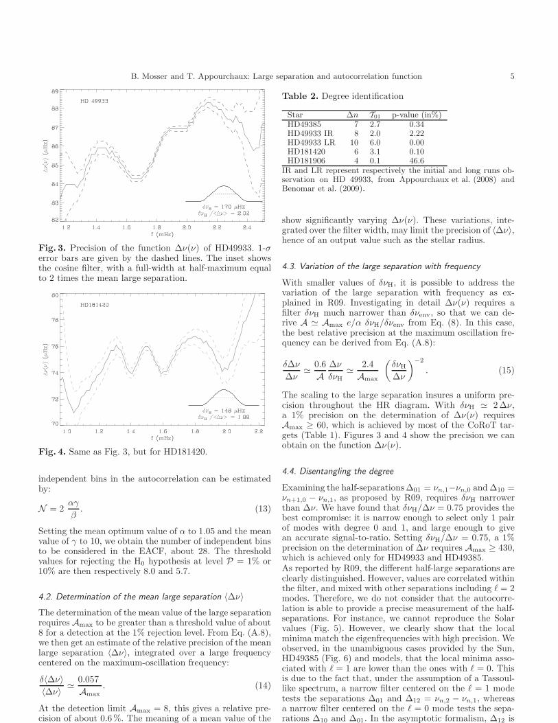
Fig. 3. Precision of the function ∆ν(ν) of HD49933. 1-σerror bars are given by the dashed lines. The inset showsthe cosine filter, with a full-width at half-maximum equalto 2 times the mean large separation.

Fig. 4. Same as Fig. 3, but for HD181420.

independent bins in the autocorrelation can be estimatedby:

N = 2αγ

β. (13)

Setting the mean optimum value of α to 1.05 and the meanvalue of γ to 10, we obtain the number of independent binsto be considered in the EACF, about 28. The thresholdvalues for rejecting the H0 hypothesis at level P = 1% or10% are then respectively 8.0 and 5.7.

4.2. Determination of the mean large separation 〈∆ν〉The determination of the mean value of the large separationrequires Amax to be greater than a threshold value of about8 for a detection at the 1% rejection level. From Eq. (A.8),we then get an estimate of the relative precision of the meanlarge separation 〈∆ν〉, integrated over a large frequencycentered on the maximum-oscillation frequency:

δ〈∆ν〉〈∆ν〉 ≃ 0.057

Amax

. (14)

At the detection limit Amax = 8, this gives a relative pre-cision of about 0.6%. The meaning of a mean value of thelarge separation is questionable, since most of the stars

Table 2. Degree identification

Star ∆n T01 p-value (in%)HD49385 7 2.7 0.34HD49933 IR 8 2.0 2.22HD49933 LR 10 6.0 0.00HD181420 6 3.1 0.10HD181906 4 0.1 46.6

IR and LR represent respectively the initial and long runs ob-servation on HD 49933, from Appourchaux et al. (2008) andBenomar et al. (2009).

show significantly varying ∆ν(ν). These variations, inte-grated over the filter width, may limit the precision of 〈∆ν〉,hence of an output value such as the stellar radius.

4.3. Variation of the large separation with frequency

With smaller values of δνH, it is possible to address thevariation of the large separation with frequency as ex-plained in R09. Investigating in detail ∆ν(ν) requires afilter δνH much narrower than δνenv, so that we can de-rive A ≃ Amax e/α δνH/δνenv from Eq. (8). In this case,the best relative precision at the maximum oscillation fre-quency can be derived from Eq. (A.8):

δ∆ν

∆ν≃ 0.6

A∆ν

δνH

≃ 2.4

Amax

(

δνH

∆ν

)−2

. (15)

The scaling to the large separation insures a uniform pre-cision throughout the HR diagram. With δνH ≃ 2 ∆ν,a 1% precision on the determination of ∆ν(ν) requiresAmax ≥ 60, which is achieved by most of the CoRoT tar-gets (Table 1). Figures 3 and 4 show the precision we canobtain on the function ∆ν(ν).

4.4. Disentangling the degree

Examining the half-separations ∆01 = νn,1−νn,0 and ∆10 =νn+1,0 − νn,1, as proposed by R09, requires δνH narrowerthan ∆ν. We have found that δνH/∆ν = 0.75 provides thebest compromise: it is narrow enough to select only 1 pairof modes with degree 0 and 1, and large enough to givean accurate signal-to-ratio. Setting δνH/∆ν = 0.75, a 1%precision on the determination of ∆ν requires Amax ≥ 430,which is achieved only for HD49933 and HD49385.As reported by R09, the different half-large separations areclearly distinguished. However, values are correlated withinthe filter, and mixed with other separations including ℓ = 2modes. Therefore, we do not consider that the autocorre-lation is able to provide a precise measurement of the half-separations. For instance, we cannot reproduce the Solarvalues (Fig. 5). However, we clearly show that the localminima match the eigenfrequencies with high precision. Weobserved, in the unambiguous cases provided by the Sun,HD49385 (Fig. 6) and models, that the local minima asso-ciated with ℓ = 1 are lower than the ones with ℓ = 0. Thisis due to the fact that, under the assumption of a Tassoul-like spectrum, a narrow filter centered on the ℓ = 1 modetests the separations ∆01 and ∆12 = νn,2 − νn,1, whereasa narrow filter centered on the ℓ = 0 mode tests the sepa-rations ∆10 and ∆01. In the asymptotic formalism, ∆12 issignificantly smaller than ∆ (by an amount of 4 ).


When the filter is not centered on an eigenmode, it mainlytests the separation ∆01 or ∆10. Therefore, we showthat a narrow frequency windowed autocorrelation allowsus to distinguish ℓ = 0 from ℓ = 1, which is a cru-cial issue since many observations have shown how dif-ficult it can be to distinguish them (Barban et al. 2009,Garcia et al. 2009). The test applied to the first initial runon HD 49933 (Fig. 7) shows that the former mode identi-fication of Appourchaux et al. (2008) cannot be confirmed,as also shown by Benomar et al. (2009) who analyze a sec-ond longer run.

A clear identification requires a signal-to-noise ratio highenough. Again, Eq. (15) allows us to estimate the auto-correlation amplitude required. In order to distinguish thesmall separation D0, and considering as a rough estimatethat in the mean case D0 represents about 2% of the largeseparation, a reliable determination based on a narrow fil-ter δνH = 0.75 ∆ν requires a maximum amplitude greaterthan about 200.

Table 2 summarizes the mean value of the difference δ01

between the local minima compared to the 1-σ uncertaintyδ∆ν/2 of the narrow frequency windowed autocorrelationfunction (Eq. 15):

T01 =1√∆n

∆n∑

i=1

δ01i

δ∆νi

(16)

with ∆n the number of pairs of modes above the thresh-old level A = 8. Table 2 also provides the probability ofobtaining a result as extreme as the observation assumingthat the null hypothesis is true.

This criterion helps to explain why the ridges can be un-ambiguously identified in HD 49385 (Deheuvels et al. 2009)and why scenario 1 for HD 181420 must be preferred(Barban et al. 2009): figures 7 and 8 show that the meandifference between the local minimal corresponding toℓ = 0 or 1 is greater than the error bar of ∆ν(ν). Onthe other hand, no answer can be given for HD 181906(Garcia et al. 2009): the low value of Amax hampers thecalculation of ∆ν(ν) with a narrow filter (Fig. 9). The lim-ited Amax ≃ 250 for the initial run on HD49933 and the lowvalue T01 help to explain the difficulties encountered withthe mode identification given in Appourchaux et al. (2008).

4.5. Ultimate precision on ∆ν(ν)

Obtaining the best time resolution in the EACF, namelythe time resolution δt of the time series, requires A ≥1.21/δνH δt for a filter width δνH (cf. Eq. A.10). This re-lation imposes a strong constraint on the maximum am-plitude. Furthermore, in order to investigate the variation∆ν(ν), the condition has to be satisfied in a frequency rangeas large as 2 δνenv around νc. This yields the condition:

A ≥ 4.9

δνH δt. (17)

According to this, high precision is easier to reach for highδνH values, hence for low mass stars with a higher large sep-aration. The decrease of the limit with increasing sampling

corresponds to a correlated decrease in resolution.

Fig. 5. Function ∆ν(ν) of the Sun, with a filter width equalto 0.75 times the mean large separation. The extrema of∆ν(ν)/2 do not correspond to the curves ∆01 and ∆10,plotted as dotted curves. The symbols 0 and 1 indicate thelocation of the eigenfrequencies on the ∆01 and ∆10 curves,and indicate also the corresponding local minima of ∆ν(ν).

Fig. 6. Function ∆ν(ν) of HD 49385, with a filter widthequal to 0.75 times the mean large separation. The region ingrey encompasses the values ± the 1-σ error bar. The localminima of ∆ν(ν), here marked by the degree, correspond tothe eigenfrequencies mentioned by Deheuvels et al. (2009).

4.6. Small separation

Roxburgh & Vorontsov (2006) proposed to make use of theautocorrelation function to obtain an independent estimateof the small separation. This method is based on the com-parison of the peak amplitude of even or odd orders inthe autocorrelation function. With An the amplitude of thepeak of order n, it consists of comparing the decreasing A2n

values to the increasing A2n+1 (see Fig. 4 of RV06). Notethat A∆ν corresponds to A2. Equality of the interpolatedcurves A2n and A2n+1 occurs for n of 3 or 4. Tests made onthe available CoRoT data show that values of A2n largerthan 15 are necessary to apply the method, therefore re-quiring very large values of A∆ν , larger than about 300.In the solar case, with the simulation including additionalphoton noise, the detection limit also occurs at 300.


Fig. 7. Function ∆ν(ν) of HD49933, with a filter widthequal to 0.75 times the mean large separation. Radial andℓ = 1 modes are identified. The two plots correspond to the2 runs: the initial run IR lasted 60.7 days and the long runLR 136.9 days.

Fig. 8. Same as Fig. 7, but for HD181420.

4.7. Threshold levels

Table 3 summarizes the threshold levels for the determi-nation of the seismic parameters with the EACF. At lowsignal-to-noise ratios, namely an Amax value lower than 8,the method cannot operate, according to the H0 test. Then,the domain where the autocorrelation is highly perform-ing is for Amax ranging from 8 (detection limit) to ≃ 50,when precise mode fitting becomes possible (HD181906,Garcia et al. 2009). With value up to 200, the EACF

Fig. 9. Same as Fig. 7, but for HD181906 and with abroader filter. The large uncertainty indicated by the broadgrey region shows that the identification for that star is notreliable.

Table 3. Threshold levels

Amax detection< 5.7 no detection (10 % rejection level)< 8.0 no detection (1% rejection level)

10 measurement of 〈∆ν〉 with 0.5 % precision≥ 50 fitting of the modes has proven to be possible

≥ 200 identifying the mode degree has proven to be pos-sible

≥ 300 possible estimate of the small separation as inRoxburgh & Vorontsov (2006)

The threshold values are given for a typical F dwarf. They can bemade precise for a given star, according to its specific parametersα and γ. Levels are lower for red giants (to be estimated withγ ≃ 4 instead of 10).

Fig. 10. Automatic search for the signature of a large sepa-ration for HD49933. The grey line indicates the location ofthe maximum peak, corresponding to the mean large sep-aration of the star. The horizontal segments indicate theranges corresponding to the 13 initial guess values ∆νc.

may be useful for identifying the degree of the modes, un-der the condition that the oscillation spectrum is close to aTassoul-like pattern. Larger Amax values allow a more de-tailed analysis with classical methods such as mode fitting(Appourchaux et al. 2006).


Table 4. Kepler performance

90-day run 4-year runstellar type B − V mV magnitude mV magnitudetype as 9 10 11 12 13 9 10 11 12 1 3HD181907 G8III 1.09 23 23 23 23 22 379 378 377 373 364HD 49385 G0IV 0.51 167 53 14 3.6 0.9 2709 864 233 58 14HD 49933 F5V 0.35 44 11 2.9 0.7 0.2 715 188 46 11 2.7HD181420 F2V 0.40 36 10 2.5 0.6 0.1 598 161 40 9.8 2.3HD181906 F8V 0.43 27 6.9 1.7 0.4 0.1 446 111 27 6.5 1.5HD175726 G0V 0.53 3.3 0.8 0.2 0.0 0.0 54 13 3.3 0.8 0.2

Maximum amplitude Amax for Kepler performance on CoRoT-like targets with varying magnitudes.

Fig. 11. Same as Fig. 10, but for HD175726. The dashedline indicates the 10% rejection limit.

Fig. 12. Same as Fig. 11, but for the red giant HD181907.The horizontal dashed lines indicate the 10% and 1 % re-jection limits. The vertical grey lines indicate the signatureat ∆ν and 2 ∆ν, the dotted line the spurious signatures ofthe day aliases, and the dot-dashed lines the CoRoT orbitalfrequency and first subharmonic.

5. Discussion

5.1. Automated determination of the large separation

Autocorrelation may provide an effective automatic deter-mination of the large separation when nothing is knownabout the star, as can be the case for a Kepler target. Asshown previously, testing the autocorrelation around τ∆ν

requires a cosine filter δνH = αγ ∆ν ≃ 10.5 ∆ν, near thefrequency . In order to perform the test in fully blind

conditions, in a frequency range simultaneously encompass-ing giant and dwarf stars, νmax is derived from the scalinglaw given by Eq. (7).The automatic test consists of analyzing the autocorre-lation of the time series for a set of time shifts τ∆νc ingeometrical progression. We performed the automatic au-tocorrelation test with 13 values of ∆νc = 2/τ∆νc, vary-ing from 3 to 192µHz with a geometric ratio G equal to√

2; ∆νc can be considered as an initial guess of the largeseparation. For each initial value ∆νc, we explored therange [∆νc/G, ∆νc G] of the autocorrelation for 3 frequencyranges of the Fourier spectrum centered respectively aroundνmax and νmax ± δνH/2. We finally derived the large sep-aration from the maximum amplitude Aauto calculated foreach ∆νc initial guess. Comparison of the different Aauto ismade possible by the scaling provided by Eq. (6). Figure 10shows the result for HD49933.We also tested the automatic test with the stars withthe lowest Amax, namely HD175726 and HD181907. ForHD175726, the single value exceeding the 10% rejectionlevel occurs at 97µHz (Fig. 11). This value of ∆ν agreeswith the solution proposed by Mosser et al. (2009). This de-tection is poor since a significance level of 10% means thatthe posterior probability of the null hypothesis is at least38% according to Appourchaux et al. (2009). However,the automatic detection can be refined with a dedicatedsearch with a more precise grid of analysis. In the case ofHD175726, the clear identification of an excess power cen-tered at 2mHz first allows us to better estimate the parame-ters for searching ∆ν and, second, gives a further indicationthat the measurement is reliable thanks to Eq. (7).The amplitude Aauto of the automatic test is found to beclose to the maximum amplitude Amax. Only limited finetuning around the automatically fixed parameters is neededto optimize the result. Mosser et al. (2009) have mentionedthe difficulty of determining the large separation with othermethods. The autocorrelation method proves to be pow-erful for a rapid estimate of the large separation; rapiditymeans here a few seconds of CPU time for the Fourier spec-trum of the CoRoT time series, followed by a few secondsof CPU time for the automatic search with the autocorre-lation, with a common laptop.We verified that the method is effective for all other solar-like targets: it gives one single answer for ∆ν, and does notdeliver any false positives. The case of red giants requiresa dedicated analysis.

5.2. Red giants

We tested the method on the CoRoT red giant target HD181907 (Carrier et al. 2009). With a large for this tar-


Fig. 13. Large separation, automatically measured for aset of 392 red giants analyzed in Hekker et al. (2009), as afunction of the maximum oscillation frequency νmax. Largeblack squares indicate positive detection; small grey squarescorrespond to unreliable cases. The dashed line indicate theglobal fit described by Eq. 18; a few cases correspond to theautomatic detection of twice the large separation.

get (about 2) and a large Amax autocorrelation signal, thelarge separation is easily found around 3.5 µHz, but thedetection is polluted by many values clearly above the 1%rejection limit (Fig. 12). All these spurious detections arecaused by artefacts: detection of the double of the largeseparation; detection of the diurnal frequency and its har-monics; detection of the CoRoT orbital frequency and halfits value. We checked that the detections at high harmonicsof the diurnal frequency are due to residuals of the windowfunction (Mosser et al. 2009); they are introduced by thelink between νmax and ∆ν indicated by Eq. 7.

For HD 181907, Eq. (9) is valid within 30%. As discussedin Section 3, the discrepancy compared to solar-like starsis due to the fact that the mode envelope of red giants isnarrower than in solar-like stars.

The automated determination of the large frequency hasbeen also tested on a set of 392 giants observed in theCoRoT field dedicated to exoplanetary science and ana-lyzed by Hekker et al. (2009). The method proves to beefficient and rapid. It provides a clear advantage since itgives a quantified reliability thanks to the use of the H0

test. We present in Figure 13 the results obtained for thesegiants. The maximum oscillation frequency was calculatedby Hekker et al. (2009). The amplitude of the autocorrela-tion signal allows us to clearly discriminate artefacts fromreliable detection (60% of the targets). The relative preci-sion in the mean large separation is much better than 1%,according to Eq. 14. After correction of the stars for whichthe double of the large separation is preferably automati-cally detected, we define from the fit of the relation betweenthe large separation and the location of the maximum sig-nal a power law varying as:

∆ν ≃ (0.26 ± 0.015) ν0.78±0.03max (frequencies in µHz). (18)

This law for giants is in agreement with Eq. (7) based ondwarfs and with Hekker et al. (2009).

5.3. Kepler data

The Kepler mission compared to CoRoT will providedifferent photometric performance, on dimmer targetsbut in some cases with longer observation duration(Christensen-Dalsgaard et al. 2007). According to Keplerperformance (Kjeldsen et al. 2008), the noise level is about0.92, 10.2 and 144ppm2 µHz−1 for targets of V magnituderespectively equal to 9, 11.5 and 14.We can extrapolate the performance obtained with Kepleron targets similar to the ones observed by CoRoT, but ofmagnitude 9 to 14, after a 4-year long observation. Table 4gives the amplitude Amax for targets observed during typ-ical 90-day or 4-year long runs. According to the expectedperformance in 90-day runs, the brightest F-type or theclass IV targets will have a signal-to-noise ratio high enoughto derive information on the large separation. In a 4-yearrun, the brightest G dwarfs will deliver a clean seismic sig-nature. On the other hand, faint F targets will have fullyexploitable Fourier spectra that will require a precise modefitting for the most complete seismic analysis. The perfor-mance for giants appears to be almost independent of themagnitude, since the contribution of photon noise is negli-gible at low frequency.We can compare this approach to the hare-and-hounds ex-ercises performed by Chaplin et al. (2008). The asteroseis-mic goal of Kepler is principally to derive information onstars hosting a planet, by the determination of the largeseparation. Compared to global fitting, the autocorrelationfunction gives a more rapid and direct answer.The autocorrelation benefits from the rapid cadence (32s) provided by CoRoT in the seismology field. Kepler willprovide 2 cadences, at 1 or 30min. This yields a lower res-olution in time, hence a lower precision on the expectedresults.

6. Conclusion

Roxburgh & Vorontsov (2006) have proposed a method forestimating large and small separations from the analysisof the autocorrelation function. Roxburgh (2009) has ex-tended the method to determine the variation of the largeseparation. In this paper, we have developed and quantifiedthe method, relating the amplitude of the correlation peakat time shift τ∆ν = 2/∆ν to various parameters.We have scaled the autocorrelation to the white noise con-tribution, so that we were able to relate the autocorrelationsignal to the mean seismic height-to-background ratio Rthat measures the relative power density of the signal com-pared to noise and to background signals. This empiricalrelation is precise to about 15% for solar-like stars. R ag-gregates the influence of unknown parameters such as themode lifetimes, the star inclination (that governs the modesvisibility) or the rotational splitting. On the other hand, allthese unknown parameters complicate and slow down thefitting of individual eigenfrequencies. Therefore, the EACFshows here a possible advantage in terms of speed.The EACF gives a direct measurement of the mean largeseparation. Compared to other methods, the estimate is ac-curate and simple, with an intrinsic threshold value, witherror bars, and without any modeling of the other com-ponents of the Fourier spectrum (granulation or activity).Furthermore, when the signal-to-noise ratio is high enough,the EACF allows the measurement of the variation of the


large separation with frequency, without any mode fitting.This is a key point for stellar radius measurement. Previousworks have shown the difficulty to disentangle ℓ = 0 fromℓ = 1 modes in oscillation spectra of F stars observed inphotometry. We have verified that, for high signal-to-noiseratio Fourier spectra, the autocorrelation analysis can pro-vide an unambiguous identification of the mode degree fora solar-like oscillation spectrum.We have defined a method for the automatic determinationof the large separation, which is efficient at low signal-to-noise ratio, even if no information is known for the star.We have determined that the width of the cosine filter usedin the method that optimizes the EACF is very close tofull-width at half-maximum of the mode envelope (ratioabout 1.05). We have also checked that the performanceof the method increases linearly with the duration of thetime series. With very limited CPU time (a few seconds),this method delivers the mean large separation of a target.It requires no information on the star; it just relies on theassumption that the location of the excess power and itswidth are related to the large separation by a scaling law,what is verified for red giants and solar-like stars. Finally,we were able to investigate in a simple manner the capabil-ity of Kepler.We are confident that the autocorrelation method willbe of great help in analyzing high duty cycle time seriesas a complement to the Fourier analysis. As noticed byFossat et al. (1999), the autocorrelation signal gives a clearsignature since the autocorrelation delay, namely four timesthe stellar acoustic radius (about 4 to 8 hours for an Fdwarf), is much shorter than the mode lifetime (a few days).This allows each wavepacket to properly correlate with it-self after a double travel along the stellar diameter, so thatthe autocorrelation integrates phased responses over thetotal duration time. In the Fourier spectrum, on the con-trary, interference between the short-lived wavepackets ob-served in the time series produce a complicated pattern.But Fourier analysis still remains required for the precisedetermination of the eigenfrequencies derived from an ac-curate mode fitting.

Appendix A: Performance of the autocorrelation

A.1. Square module of the autocorrelation

The EACF presented in Section 2 is defined to directlygive the envelope of the autocorrelation. Since negative fre-quencies are omitted, the EACF is related to the canonicalautocorrelation C±, that includes positive and negative fre-quencies of the Fourier spectrum, by:

A ∝ |C|2 and |C| =

√

C±2 + H(C±)2 (A.1)

where H is the Hilbert transform. Fig. A.1 shows the dif-ference between C and C±, both functions include the con-tribution of a narrow Hanning filter.

A.2. Autocorrelation peak

The shape of the autocorrelation peaks is given bythe Fourier transform of the Hanning filter, whichcan be expressed as the sum of 3 components(Max & Lacoume 1996):

( ) 2 sinc( )+ sinc( +1)+sinc( 1)(A.2)

Fig.A.1. Comparison of ± |C| (black curves) and C± (greyline), both normalized to 1 at time shift 0, calculated forthe narrow frequency windowed solar Virgo spectrum.

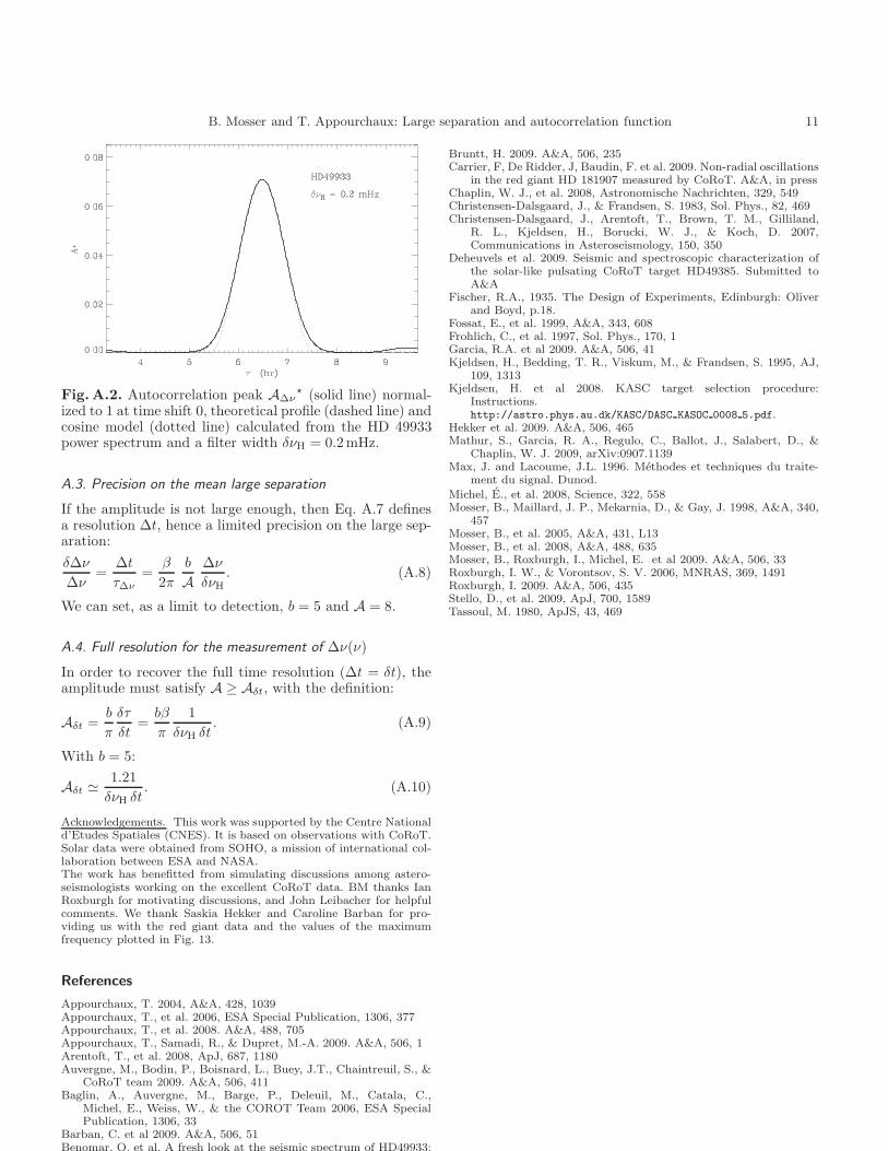
with sincX = sin(πX)/πX . This global shape may be moresimply modeled with a single cosine shape (Fig. A.2). Inorder to enhance the precision of the fit in the upper partof the autocorrelation peak, the full width at half maximumδτ of this cosine fit is:

δτ =β

δνH

with β ≃ 0.763. (A.3)

The flanks of the peak are not well fitted, which is unimpor-tant compared to the fact that the fit above half-maximumperforms well. δτ is much greater than the resolution timeδt.Precise determination of the large separation requires pre-cise location of the peak maximum. In order to estimatethe performance, we describe a peak as:

S(t) =A

2

[

1 + cosπt − τ∆ν

δτ

]

for |t| ≤ δτ,

S(t) = 0 for |t| > δτ.(A.4)

This fit shows variation:

dSA = − πA

2δτsin π

t − τ∆ν

δτdt. (A.5)

We can compare the variation of the signal peaking at am-plitude A to the maximum variation of a noise contributionof amplitude b. At a time shift ∆t from the maximum, thesignal variation and the maximum noise contribution are:

∆SA =A2

(

π∆t

δτ

)2

,

∆Sb =b

2

∆t

δτ.

(A.6)

The precise identification of the signal maximum requires∆SA ≥ ∆Sb, which translates into the condition:

π A ∆t ≥ b δτ. (A.7)

It is possible to interpret this condition as follows.


Fig.A.2. Autocorrelation peak A∆ν⋆ (solid line) normal-

ized to 1 at time shift 0, theoretical profile (dashed line) andcosine model (dotted line) calculated from the HD 49933power spectrum and a filter width δνH = 0.2mHz.

A.3. Precision on the mean large separation

If the amplitude is not large enough, then Eq. A.7 definesa resolution ∆t, hence a limited precision on the large sep-aration:

δ∆ν

∆ν=

∆t

τ∆ν

=β

2π

b

A∆ν

δνH

. (A.8)

We can set, as a limit to detection, b = 5 and A = 8.

A.4. Full resolution for the measurement of ∆ν(ν)

In order to recover the full time resolution (∆t = δt), theamplitude must satisfy A ≥ Aδt, with the definition:

Aδt =b

π

δτ

δt=

bβ

π

1

δνH δt. (A.9)

With b = 5:

Aδt ≃1.21

δνH δt. (A.10)

Acknowledgements. This work was supported by the Centre Nationald’Etudes Spatiales (CNES). It is based on observations with CoRoT.Solar data were obtained from SOHO, a mission of international col-laboration between ESA and NASA.The work has benefitted from simulating discussions among astero-seismologists working on the excellent CoRoT data. BM thanks IanRoxburgh for motivating discussions, and John Leibacher for helpfulcomments. We thank Saskia Hekker and Caroline Barban for pro-viding us with the red giant data and the values of the maximumfrequency plotted in Fig. 13.

References

Appourchaux, T. 2004, A&A, 428, 1039Appourchaux, T., et al. 2006, ESA Special Publication, 1306, 377Appourchaux, T., et al. 2008. A&A, 488, 705Appourchaux, T., Samadi, R., & Dupret, M.-A. 2009. A&A, 506, 1Arentoft, T., et al. 2008, ApJ, 687, 1180Auvergne, M., Bodin, P., Boisnard, L., Buey, J.T., Chaintreuil, S., &

CoRoT team 2009. A&A, 506, 411Baglin, A., Auvergne, M., Barge, P., Deleuil, M., Catala, C.,

Michel, E., Weiss, W., & the COROT Team 2006, ESA SpecialPublication, 1306, 33

Barban, C. et al 2009. A&A, 506, 51Benomar, O. et al. A fresh look at the seismic spectrum of HD49933:

Bruntt, H. 2009. A&A, 506, 235Carrier, F, De Ridder, J, Baudin, F. et al. 2009. Non-radial oscillations

in the red giant HD 181907 measured by CoRoT. A&A, in pressChaplin, W. J., et al. 2008, Astronomische Nachrichten, 329, 549Christensen-Dalsgaard, J., & Frandsen, S. 1983, Sol. Phys., 82, 469Christensen-Dalsgaard, J., Arentoft, T., Brown, T. M., Gilliland,

R. L., Kjeldsen, H., Borucki, W. J., & Koch, D. 2007,Communications in Asteroseismology, 150, 350

Deheuvels et al. 2009. Seismic and spectroscopic characterization ofthe solar-like pulsating CoRoT target HD49385. Submitted toA&A

Fischer, R.A., 1935. The Design of Experiments, Edinburgh: Oliverand Boyd, p.18.

Fossat, E., et al. 1999, A&A, 343, 608Frohlich, C., et al. 1997, Sol. Phys., 170, 1Garcia, R.A. et al 2009. A&A, 506, 41Kjeldsen, H., Bedding, T. R., Viskum, M., & Frandsen, S. 1995, AJ,

109, 1313Kjeldsen, H. et al 2008. KASC target selection procedure:

Instructions.http://astro.phys.au.dk/KASC/DASC KASOC 0008 5.pdf.

Hekker et al. 2009. A&A, 506, 465Mathur, S., Garcia, R. A., Regulo, C., Ballot, J., Salabert, D., &

Chaplin, W. J. 2009, arXiv:0907.1139Max, J. and Lacoume, J.L. 1996. Methodes et techniques du traite-

ment du signal. Dunod.

Michel, E., et al. 2008, Science, 322, 558Mosser, B., Maillard, J. P., Mekarnia, D., & Gay, J. 1998, A&A, 340,

457Mosser, B., et al. 2005, A&A, 431, L13Mosser, B., et al. 2008, A&A, 488, 635Mosser, B., Roxburgh, I., Michel, E. et al 2009. A&A, 506, 33Roxburgh, I. W., & Vorontsov, S. V. 2006, MNRAS, 369, 1491Roxburgh, I. 2009. A&A, 506, 435Stello, D., et al. 2009, ApJ, 700, 1589Tassoul, M. 1980, ApJS, 43, 469

http://arxiv.org/abs/0907.1139