


Bahasa
Halaman
Hukum


REPORT
Ocean circulation and terrestrial runoff dynamicsin the Mesoamerican region from spectral optimizationof SeaWiFS data and a high resolution simulation
L. M. Cherubin Æ C. P. Kuchinke Æ C. B. Paris
Received: 21 May 2007 / Accepted: 11 December 2007 / Published online: 7 January 2008
� Springer-Verlag 2008
Abstract The evolution in time and space of terrestrial
runoff in waters of the Mesoamerican region was examined
using remote sensing techniques combined with river dis-
charge and numerical ocean circulation models. Ocean color
SeaWiFS images were processed using a new Spectral
Optimization Algorithm for atmospheric correction and
ocean property retrieval in Case-2 waters. A total of 157
SeaWiFS images were collected between 1997 and 2006 and
processed to produce Colored Detrital Material images of the
Mesoamerican waters. Monthly terrestrial runoff load and
river discharge computed with a land-elevation model were
used as input to a numerical model, which simulated the
transport of buoyant matter from terrestrial runoff. Based on
land cover for years 2003–2004, modeling results showed
that the river discharge seasonality was correlated with the
image averaged CDM, and the simulated plume reproduces
the spatial patterns and temporal evolution of the observed
CDM plume. River discharge peaked in August and CDM
peaked from September to January. The buoyant matter
concentration was high from October to January, and was at
its lowest from March to April. Between October and
December the plume was transported out of the Mesoamer-
ican waters by a cyclonic gyre located north of Honduras.
Part of the runoff from Honduras was transported towards
Chinchorro Banks and the Yucatan Channel, part re-circu-
lated into the Gulf of Honduras, and part taken toward the
outside of the Mesoamerican Barrier Reef System. This
study shows that all the reefs of the MBRS, including the
most offshore atolls of the region, are under the influence of
terrestrial runoff on a seasonal basis, with maximum effect
during October to January, and minimum from March to
April. Furthermore, what is seen as a giant plume in satellite
images is in fact composed of runoffs of different ages.
Keywords Mesoamerican barrier reef system �SeaWiFS � CDM � ROMS � Passive tracer �Terrestrial runoff
Introduction
The Mesoamerican Region (MAR) consists of the oceanic
systems off Honduras, Guatemala, Belize and Mexico, and
contains one of the largest coral barrier reefs in the
Caribbean. Landward, this region has one of the largest
watershed networks of the Caribbean, with numerous rivers
flowing out to the coastal ocean. Until recently, there has
been little research focusing on the factors critical to the
conservation of biodiversity hotspots, such as coral eco-
systems at the interface between the land and its watershed,
and the ocean currents. Land use around the MAR, such as
the clearing of native vegetation and its replacement with
intensive agriculture and coastal development, has changed
the ecological interdependence of forest and waters, such
Communicated by Biology Editor M.P. Lesser.
L. M. Cherubin (&)
Division of Meteorology and Physical Oceanography,
Rosenstiel School of Marine and Atmospheric Science,
University of Miami, Miami, FL 33101, USA
e-mail: [email protected]
C. P. Kuchinke
Department of Physics, Rosenstiel School of Marine
and Atmospheric Science, University of Miami,
Miami, FL 33101, USA
C. B. Paris
Division of Marine Biology and Fisheries,
Rosenstiel School of Marine and Atmospheric Science,
University of Miami, Miami, FL 33101, USA
123
Coral Reefs (2008) 27:503–519
DOI 10.1007/s00338-007-0348-1

as the delivery of nutrients through estuaries and the uti-
lization of coastal habitat by marine species. In particular,
the transport of pollutants to the coastal ocean has
increased to a level many times the natural rate (Wilkinson
1999; McKergow et al. 2005). The altered water quality of
streams has led to degradation in the estuaries, coastal
waters, and coral reefs. Natural events such as hurricanes in
the MAR can induce flooding and extreme river run-offs
which reach the offshore coral reef barrier. Andrefouet
et al. (2002) and Sheng et al. (2007) showed how the
1,000 km of reefs of the MAR were connected by ocean
currents, carrying sediments and nutrients from the land to
the oceanic waters during hurricane Mitch. Excessive
sediments (suspended or deposited) and elevated nutrients
are almost universally recognized as having adverse effects
on reef communities (Spalding et al. 2001). The manage-
ment of coral reef environments, including reef-building
and non reef-building communities, would benefit from a
greater understanding of the degree of physical connec-
tivity between coral reefs and between land, watershed and
offshore reefs through the movement of water masses
carrying detrital material (Kleypas et al. 2001).
The MAR is located in the western Caribbean Sea where
the Caribbean Current flows from the Nicaraguan Rise
westwards towards the Yucatan peninsula, then veers north
toward the Yucatan Channel (Richardson 2005). To the
north and south lie two regions populated by eddies. In the
north, drifter trajectories collected from the Global Drifting
Buoy Data Assembly (http://www.aoml.noaa.gov/phod/
dac/dacdata.html) show the continuous presence of
cyclones and anticyclones while to the south, two large
cyclones (*100 km diameter) were sampled by drifters
(Richardson 2005). However, very few of these drifters
entered the MAR, and as a result, in situ observations are
limited within this region. The presence of a cyclonic cir-
culation in the Gulf of Honduras was recognized in two
numerical simulations (Ezer et al. 2005; Tang et al. 2006).
In the latter study, cyclones south of the Caribbean Current
were less visible than in Ezer et al. (2005), and the simu-
lated Caribbean Current was more to the south of the MAR
(16.5�N) than mean flow obtained from drifter trajectories
(18�N; Richardson 2005).
Observations from space-borne sensors have improved
spatial information on natural processes. The availability of
calibrated satellite ocean color data provides a unique data
set that helps explore spatial and temporal patterns of
connectivity between land processes and the coastal ocean.
Recent developments in bio-optical models contribute to
the quantification of suspended particulate matter concen-
trations (SPM; see Appendix) in coastal waters with an
absolute uncertainty \30%. There have been attempts to
quantitatively compare SPM fields from images and mod-
els (Jorgensen and Edelvang 2000; Durand et al. 2002), but
uncertainty on a number of parameters involved in the
SPM transport model prevents their generalization. Satel-
lite ocean color data has been used to explore patterns of
connectivity between reefs as well as between reef and land
in the MAR (Andrefouet et al. 2002; Sheng et al. 2007),
suggesting that pathways for pollutants and pathogens
within and among coral reef provinces could be inferred
realistically using satellite ocean color observations.
Recent numerical modeling approaches, merged with in
situ or remote sensing data analysis, have been effective in
studying sediment transport (Ouillon et al. 2004; Blaas
et al. 2007; Luick et al. 2007). Together with Geographic
Information Systems (GIS), they have improved investi-
gations into how marine and terrestrial environments are
related across large spatial and temporal scales.
The goals of this study are to investigate the interactions
between river runoff and open water in the MAR, and the
extent of the terrestrial influence on coral reefs under
various degrees of anthropogenic input. This is achieved by
(1) building a 3D hydrodynamic model of the region
coupled with a model of river runoff, (2) simulating the
transport of suspended sediments and dissolved nutrients
(hereafter Buoyant Matter (BM), see Appendix) with var-
ious scenarios of land use, and (3) assessing the spatial and
temporal linkages of satellite-derived measurements with
transport of river runoff to the reef areas.
Material and methods
Study area
A detailed description of the Mesoamerican Barrier Reef
System (MBRS) is given in Andrefouet et al. (2002).
Briefly, the MBRS extends over 1,000 km (Fig. 1) and
includes the Mexican Caribbean reefs and islands along the
Yucatan coast, the Belizean atolls and a large barrier reef,
and Honduran reefs around the Bay Islands. Guatemala has
a very short Caribbean coastline that is heavily influenced
by sediment-laden rivers, and thus has negligible coral
reefs. The shelf slope along the Belize Barrier Reef is very
steep, with depths of 1,000 m existing less than 3 km
seaward of the reef crest. The southeastern shelf slope rises
more gently such that the Honduran coast is oceanic to the
shore (Heyman and Kjerfe 2000).
The Gulf of Honduras is a receiving basin, where terres-
trial drainage is distributed by marine processes and impacts
ecosystem function. Over 80% of the sediment and half of
the nutrients (both nitrogen and phosphorus) delivered by
watersheds along the MAR originate in Honduras (Burke and
Sugg 2006). Guatemala is also a source of about one-sixth of
all sediments and about one-quarter of all nitrogen and
phosphorous. In comparison, relatively minor percentages of
504 Coral Reefs (2008) 27:503–519
123

the regional sediment load come from Belize and Mexico
(Burke and Sugg 2006). Belize contributes 10–15% of
nutrients and Mexico about 5% of the nutrients. Values for
Mexico are probably underestimated as the contribution of
underground rivers is not included.
Peak transport of freshwater and fluvial sediments
occurs in the wet season from July to October. Wet season
discharge usually exceeds dry season discharge by a factor
of 5–9 (Heyman and Kjerfe 2000; Burke and Sugg 2006;
Fig. 2). According to Heyman and Kjerfe (2000), the flux
of freshwater from the high rainfall areas in southern
Belize, Guatemala, and Honduras gives rise to easterly
flowing, density-driven surface currents that exit the inner
Gulf of Honduras. In contrast, and in response to occa-
sional southerly winds, Heyman and Kjerfe (2000) suggest
that deep, clear nutrient-rich oceanic waters from the
Cayman Trench enter the Gulf flowing westerly.
The three Belizean atolls have been assumed to be outside
the general influence of terrestrial runoff. Glovers Reef, the
southernmost atoll, is located more than 40 km from the
Belize coast and approximately 100 km from the Honduras
and Guatemala coasts. Glovers Reef has been used as a
control site, based on the assumption that it was free of
anthropogenic effects and terrestrial pollutants. For instance,
Wilkinson (1987) related sponge biomass to terrestrial run-
off along a transect in the Belize barrier reef, and Glovers
Reef was used as the lowest influence site even though it was
found to have an unexpectedly high biomass of sponges.
McClanahan and Muthiga (1998) explicitly considered
Glovers to lie beyond terrigeneous influence.
Ocean color data processing
Visible and near infrared (NIR) radiance in this study was
obtained from the passive Sea-viewing Wide Field-of-view
Sensor (SeaWiFS) on board the SeaStar polar orbiting
satellite. Data was processed using the latest available
calibration of the sensor. A major component of the current
NASA ocean color retrieval procedure is to retrieve the
aerosol properties, including optical depth and diffuse
transmittances, on a pixel by pixel basis, using a compar-
ison of the spectral variation between the two measured
NIR bands and a suite of scattering-only aerosol models.
This aerosol information is then interpolated across visible
wavelengths and removed from the total measured radiance
(Gordon and Wang 1994). The remaining water leaving
spectral radiance Lw(k) can then be used in a variety of
empirical bio-optical models to obtain information on
chlorophyll concentration C (e.g., O’Reilly et al. 1998). In
this study the standard ocean color algorithm (Gordon and
Wang 1994) was replaced with an alternate Spectral
Optimization Algorithm (SOA). This algorithm contains a
suite of absorbing aerosol models and a semi-analytic Case
2 bio-optical algorithm, both important for coastal
environments.
The SOA bio-optical model (Garver and Siegel 1997;
Maritorena et al. 2002), herein referred to as GSM,
retrieves both C and aCDM(443), the absorption coefficient
of Colored Detrital Material (CDM) at 443 nm. Here,
aCDM(443) = adp(443) + aCDOM(443), the sum of the
respective absorption due to detrital particles and colored
Fig. 1 Mesoamerican Region. Land elevation is shown is color, river
network in blue and reefs in magenta. Thick black lines show the
location of the transects labeled Tnumber
Mar Jun Sep Jan Apr Jul Oct Jan0
1
2
3
4
5
6
7x 10
10
Months
River DischargeCDM mean
m3 s
-1
Fig. 2 N-SPECT river discharge (dashed line) overlaid on the image
mean CDM absorption coefficient (solid line) from year 2003 to 2004
imagery to show interannual variability. The river monthly discharge
time series from Burke and Sugg (2006) is matched to the available
day of data of the SOA imagery, which creates a distortion in the
discharge profile
Coral Reefs (2008) 27:503–519 505
123

dissolved organic matter, respectively. They are combined
due to their similar spectral signatures. As a general rule,
aCDM in offshore waters may contain 80–90% aCDOM with
the remainder being adp. For waters very near to the coast
the % of aCDOM may decrease to as low as 40% (e.g.,
Chesapeake Bay in Magnuson et al. 2004). GSM spectral-
slope coefficients have not been developed for the coast of
Belize and Honduras. This would require optimization of
GSM with extensive in situ data collected at the ocean
surface. Instead, a developed set of coefficients from the
Santa Barbara Channel, CA, were used. Sensitivity analy-
ses showed that for CDM, use of incorrect coefficients in
coastal waters introduced an absolute error of less than 10–
20%, decreasing rapidly as we increase CDM. Relative
error is considered much less. Since CDOM and detrital
particles are components of DOC and POC respectively
(see Appendix) it is proposed that the spatial and temporal
trends in aCDM can be used as a surrogate for Buoyant
Matter (BM) in this study. From herein aCDM(443) is
referred to as CDM.
The SeaWiFS sensor has been operational since October
1997. A search of the entire SeaWiFS archive of High
Resolution Picture Transmission (HRPT) scenes was
undertaken up to June 2006 to evaluate the best images.
The coastlines of Belize and Northern Honduras are very
cloudy for most of the year, with the months of October to
March displaying, on average, about two clear days per
month. For the months of April to September there are few
cloud free days. For example, from May to July only two
usable cloud-free scenes were found in the entire archive
1997–2006. To maintain a processing data set of sufficient
size it was decided to accept images that contained at least
80% of clear sky for at least the first 50 km of ocean
bounding the East coast of Belize and the entire Northern
coast of Honduras. The filtering procedure resulted in 157
images from 1997 to 2006 for both Chlorophyll and CDM.
Most scenes were processed for 15.5�N–18.5�N; 81.0�W–
89.0�W, corresponding to an approximately square region
bounded by the bottom half of the East coast of Belize and
the entire Northern coast of Honduras. Few scenes dis-
played clear skies along the entire East coast of Belize.
Hence for these scenes the processing was extended to
latitude 23.0�N.
From the nine year dataset, only 157 days could be used
to build what we assume is climatological time series. This
was obtained by a weighted average of CDM in order to
account for the number of data per year. CDM were
averaged for each month to account for the varying number
of days per month. Because the years 2003 and 2004 were
the most complete, they were used along with the mean to
compute a standard deviation of CDM variability. In order
to compare SOA data with numerical model outputs, SOA
images were projected on a constant-space grid. Values on
transects perpendicular to the coast were then extracted to
build time series, and surface averaged CDM values for
each image were calculated in order to build a time series
of the global CDM content in the Mesoamerican region
(Fig. 2).
This method justifies the lag observed in Fig. 2 as the
changes are dependent on the CDM in the entire domain
and not only in coastal waters. In this study no attempt was
made to estimate the BM concentration from the CDM
absorption coefficient. Only the relative variation between
consecutive days was considered and this was compared
with values from a similar spatial and temporal analysis of
numerical model results. Figure 2 illustrates that CDM is a
good proxy for the terrestrial runoff transport since CDM
exhibits seasonal changes, which correlate with the river
discharge.
Numerical modeling
The Regional Ocean Modeling System (ROMS) is a 3D
hydrodynamic model, which simulates the spatial and time
evolution of ocean state variables and current. The model
domain is the wider Gulf of Honduras, which encompasses
the eastern coast of the Yucatan Peninsula and the northern
coast of Honduras (15.5–21.3�N, 89.1–84.3�W). It includes
the barrier reef, reef lagoon, and adjacent oceanic waters
and uses a 1 km resolution bathymetry from the World
Resources Institute (http://www.wri.org/). The horizontal
resolution of the simulation is 2 km and the model has
25 vertical layers. Model variables of the ocean state
(temperature, salinity) at the open ocean boundaries
were relaxed to the monthly Levitus ocean (http://ingrid.
ldeo.columbia.edu/SOURCES/.LEVITUS94/) climatology
(Word Ocean Atlas). Tides were set at the boundary by the
TPXO6 global tide model (http://www.esr.org/polar_tide_
models/Model_TPXO62_load.html). Monthly varying
surface fluxes (wind, rain, solar, radiative heat fluxes,
evaporation) were obtained from the Comprehensive Ocean
Atmosphere Dataset (http://icoads.noaa.gov/) (COADS)
climatology.
The river discharge and sediment load (used as a proxy
for suspended sediments and dissolved nutrients) in over
400 watersheds that discharge adjacent to the Mesoameri-
can barrier reef were provided by the Non-point Source
Pollution and Erosion Comparison Tool (N-SPECT)
developed by the US National Oceanographic and Atmo-
spheric Administration (NOAA), whose results are
analyzed in Burke and Sugg (2006). N-SPECT results were
validated by comparing river discharge and terrestrial run-
off load with in-situ data in several regions around the
world. Note Buoyant Matter (BM) is used in the ROMS
model as a substitute for suspended and dissolved material
506 Coral Reefs (2008) 27:503–519
123

here. Burke and Sugg (2006) used scenarios of land cover
change in the MAR until 2025 to evaluate the impact of
land cover change on river discharge, sediment and pol-
lutant delivery. Two land use scenarios were tested in this
study: the first one is called the Current Year scenario,
based on land cover of years 2003–2004. The second one,
called Sustainability First scenario, which could result in a
3–4% decline in nutrients and transported sediment to the
MAR.
During the Current Year scenario, Burke and Sugg
(2006) examined the relative accumulation of sediment and
nutrients at river mouths across the MAR. The Ulua
watershed (Honduras) appeared as the largest contributor
of sediment, nitrogen, phosphate, and total suspended sol-
ids. Other large contributors of sediment and nutrients were
the Rio Patuca (Honduras), Rio Motagua (in Guatemala
and Honduras), Aguan (Honduras), Rio Dulce (Guate-
mala), Belize River watershed (Belize), and Tinto o Negro
(Honduras).
BM load from the 400 watersheds was modeled as a
passive tracer by advection and diffusion. The diffusion
coefficient for all the simulations was fixed to 10 m2 s-1.
Each river discharge and BM load provided by the N-
SPECT model was individually entered into the model
domain for each month and kept constant for each month.
The BM inputs then follow the seasonal changes due to
rainfall and their spatial variability. Rivers were defined as
point sources of tracers with an exponential vertical dis-
tribution on the vertical. The higher inflow was in the upper
layer. The model did not simulate resuspension and
deposition of fine suspended sediments, which are known
to deposit in the first few hundred meters from estuaries,
whereas dissolved nutrient matter can spread much further
(Devlin and Brodie 2005). Therefore, the model produces a
climatology of the circulation and BM transport in the
Mesoamerican coastal and offshore waters, and reefs. In
order to reach passive tracer balance the model was first
operated for a year and subsequently reached its BM
equilibrium in January of the second and third year. Two
simulations are then compared, each one using run-off
inputs from the two land use scenarios described in Burke
and Sugg (2006). Moreover initial conditions for the
Sustainability First scenario were taken from hurricane
flooding event.
The accuracy of the MAR circulation in the ROMS
simulation coupled to the N-SPECT output was estimated
by first comparing seasonal variations of the plume dis-
persion patterns with the CDM dispersion patterns. A more
detailed comparison was undertaken by analyzing the
extent and evolution of time series of CDM and BM along
five transects perpendicular to the shore around the region.
Transects 1 and 2 are meridional, extending over one
degree of latitude west of Guaraja (85.7�W) and across
Utila Reef (87�W), north of Honduras. Transect 3 is zonal
and crosses Belize’s lagoon and reefs at 17�.13N. Transect
4 is meridional and crosses the Gulf of Honduras from
Guatemala to Belize. Transect 5 is zonal (1� of longitude
wide), and runs across Chinchorro Bank (Fig. 1).
Results
Satellite colored detrital material versus N-SPECT river
discharges
A 173-day lag was found between the increase of the river
run-off in March and the increase of CDM concentration in
September over the entire MAR (Fig. 2). Colored detrital
material concentration peaks on average 2–3 months
(September–December) after the peak in river run-off
(June–August). From one year to the next, this cycle
repeats itself. When the river discharge is minimum in
March–April, CDM content has been expelled from the
MAR and reaches its minimum from July to September.
This time lag is likely to be different in coastal waters,
which are under the direct influence of the runoff.
Seasonal evolution of the colored detrital material
concentration in the MAR
In order to analyze the seasonal variability of the CDM
spatial patterns, images were clustered by season. Due to
the limited number of clear days available, only October–
December, January–March, and April were identified.
Based on the river run-off seasonality (Fig. 2), one may
expect to see an increase in the CDM concentration on-
shore and to some extent off-shore, in the days and months
following the run-off maxima, which are September,
October, November, December and perhaps January of the
next year. Lowest month run-off should yield a limited
spreading of CDM and the lowest concentrations, from
April to June.
The highest concentration of CDM along the coast
occurs between October and December through offshore
transport by filaments. From November to December, the
concentration in coastal waters is increasing and filaments
are observed in the eastern Gulf of Honduras due to the
entrainment by the mesoscale circulation from the east of
the Honduras Peninsula (Fig. 3). Later in December, high
concentrations onshore are seen in the western Gulf and are
moved offshore by filaments north of the coastal waters of
Honduras (Fig. 3). A remnant plume offshore shows the
advection of CDM from Honduras heading northwest
toward Banco Chinchorro (Fig. 3, 1 March 2003; 6 March
1998) and reveal the presence of a cyclonic gyre carrying
Coral Reefs (2008) 27:503–519 507
123

CDM from eastern Honduras west north-west toward the
coast of Mexico. From January to March the CDM con-
centration has decreased in coastal waters of Honduras
whereas concentrations are still high in the Belize coastal
waters (Fig. 3, 1 March 2003–20 March 2006). The barrier
reef seems to prevent the circulation of mesoscale flow in
the coastal waters, as seen in Honduras waters. Offshore
dispersion continues by small filaments along the Honduras
coast. Later in March, clear waters in the gyre are observed
and short filaments continue to expel CDM from the coast
of Honduras (Fig. 3, 13 March 2006; 20 March 2006). In
April the weakest concentrations are seen onshore with
small filaments still contributing to the expelling of CDM
from Honduras coastal waters towards open waters (Fig. 3,
5–10 April 1999). Concentration has also decreased in the
Belize Coastal waters.
Mesoamerican region dynamics in the ROMS model
The climatology of the model circulation in the MAR is
characterized by the presence of a semi-permanent cyclo-
nic gyre in the monthly mean (Fig. 4). This gyre extends
from the Belize offshore waters to about 85�W, north of
Honduras. It carries coastal waters from this region of
Honduras northwards toward the Chinchorro Banks. Most
of the year, the current south of 18.5�N flows southward in
the channel between the coast and Chinchorro Bank
(87.7�W, 18.3�N, Fig. 5a). This result differs from Ezer
et al.’s (2005) model at the same location. However, fur-
ther north (87.5�W, 18.7�N, Fig. 5b) the ROMS simulation
shows a similar seasonal variability to the Ezer et al. (2005)
simulation at 87.7�W, 18.3�N. From January to March the
flow is southward, then reverses northward in March–
April, July, and August–September, and southward in
May–June and from October to December. Some recircu-
lation cells, cyclonic or anticyclonic, are observed in the
Gulf of Honduras but their life time is limited to a few
days. Model time series at the eastern side of Lighthouse
Reef (84.7�W, 17.13�N) show the high variability of the
meridional component of the current. The seasonal vari-
ability with peaks of northward velocity from January to
March and in May is similar to the estimated altimeter
velocity near Lighthouse Reef in Ezer et al. (2005). Further
east on the Honduras coast, model currents flow eastward
carrying coastal waters from Belize toward Honduras.
Nonetheless, cross-shore filaments entrained by small scale
eddies contribute to the offshore advection of coastal
waters as seen in the CDM imagery (Fig. 3). The cyclonic
gyre can be damped by the influence of the large scale
Fig. 3 Times series of CDM
absorption coefficient (m-1,
high values red, low values
blue) in the MAR where the
same month of different years is
shown for year to year
consistency. Color scale is
logarithmic. Red boxes on 2
November 1997 image show the
regions where CDM was
spatially averaged to produce
the times series of Fig. 8
508 Coral Reefs (2008) 27:503–519
123

Caribbean Current that will flow directly toward the coast
of Mexico and turn north in the Gulf of Honduras in place
of the cyclonic gyre. This is the dominant feature in Ezer
et al.’s (2005) model and the cyclonic gyre is smaller and
centered in the Gulf of Honduras. Based on their Fig. 10,
the gyre eastward extension reaches 87–86�W. In the CDM
imagery (Fig. 3) the gyre extends to 86�W for instance in
November 1997, March 1998, but also to 85� in November
2000 and March 2003. North of 19�N, current flows
northward along the coasts of Mexico as observed in drifter
trajectories by Richardson (2005). Therefore most of the
BM delivered by Mesoamerican watersheds is transported
out of the region as a result of the northward flow from the
eastern Honduras waters to the coast of Mexico. Then the
BM is taken north into the Yucatan Channel mostly in
October–December (Fig. 4).
Analysis of the changes between the current
and sustainability-first scenarios
There was less sediment load for the Sustainability First
scenario than for the Current Year scenario (Fig. 6).
However the initial state for the Sustainability First
Fig. 4 ROMS monthly mean of
passive tracer concentration
(kg m-3, high values brown,
low values blue) for the current
year scenario simulation. The
color scale is logarithmic
Coral Reefs (2008) 27:503–519 509
123

scenario was taken from a flooding scenario simulation,
which contains globally more BM than the Current Year in
January (Fig. 7a). Consequently, BM remains in the region
for longer during the Sustainability First scenario
simulation even though the sediment load is lower (Fig 7b,
c). No interruption is seen in the transport out of the MAR
of BM between Chinchorro Banks and the Yucatan Pen-
insula. The difference between the two simulations is
detailed in the analysis of the time series of the model
transects.
Seasonal buoyant matter changes on transects
Both the numerical model and the CDM data were used to
track the BM plume along the MAR coasts. A very similar
behavior to the CDM in the SeaWiFS data (Fig. 2) was
obtained in the model BM plume seasonal evolution. The
Jan Feb Mar Apr May Jun Jul Aug Sep Oct Nov Dec−1
−0.8
−0.6
−0.4
−0.2
0
0.2
0.4Chinchorro South (87.7W, 18.3N)
Jan Feb Mar Apr May Jun Jul Aug Sep Oct Nov Dec−0.6
−0.5
−0.4
−0.3
−0.2
−0.1
0
0.1
0.2North Chinchorro (87.5W, 18.7N)
a
b
c
Jan Feb Mar Apr May Jun Jul Aug Sep Oct Nov Dec
−0.4
−0.3
−0.2
−0.1
0
0.1
0.2
0.3
0.4
Lighthouse (87.4W, 17.13N)
cm s
-1
Fig. 5 ROMS surface current time series in the channel between
Mexico and Chinchorro Bank, a south at 87.7�W, 18.3�N, b north at
87.5�W, 18.7�N, and c east of Lighthouse Reef (87.4�W, 17.13�N)
2 4 6 8 10 120
2
4
6
8
Sed
imen
t loa
d (k
g)
2 4 6 8 10 120
2
4
6
8
Dis
char
ge (
m3 s
-1)
Dis
char
ge (
m3 s
-1)
Month
2 4 6 8 10 120
2
4
6
8
Sed
imen
t loa
d (k
g)
2 4 6 8 10 120
2
4
6
8x 109
x 1010
x 1010
x 109
Month
a
b
Fig. 6 Time series for the entire coastline of the sediment load (kg,
upper plot) and discharge (m3 s-1) from the NSPECT model for the
current year (a) and the sustainability first (b) scenarios
510 Coral Reefs (2008) 27:503–519
123

maximum of BM content in the MAR model was obtained
during the months of October–December with a peak in
September (Fig. 8a). In the real data, the peak time varies
with location and most likely from one year to the other. A
peak in CDM absorption coefficient was seen in September
2003 in the Gulf of Honduras (Fig. 8b) and later in
November 2003 on the northern coast of Honduras
(Fig. 8c), after being averaged in their respective box
shown in Fig. 3. The same lag was seen in 2004.
Here the CDM time series for the climatological year,
and years 2003 and 2004 are compared with both the
Current Year and the Sustainability First scenarios along
the five transects defined previously. Years 2003 and 2004
are used in this comparison because they contained most of
the variability seen in the nine year dataset (not shown).
Time series for each *1 km resolution (1 pixel) transects
of the mean CDM at 0–12 km (coastal), 13–24 km
Fig. 7 ROMS monthly mean of sediment concentration (kg m-3,
high values brown, low values blue) for January (a), May (b) and
December (c) in the Sustainability First scenario. Color scale is
logarithmic
0
0.05
0.1
3-Feb
3-M
ar
3-Apr
3-M
ay3-
Jun3-
Jul
3-Aug
3-Sep
3-Oct
3-Nov
3-Dec
3-Ja
n3-
Feb3-
Mar
3-Apr
3-M
ay3-
Jun3-
Jul
3-Aug
3-Sep
3-Oct
3-Nov
3-Dec
Jan 2003 - Dec 2004
Northern coast of Honduras
0
0.05
0.1
0.15
0.2
aC
DM
(443
) m
-1
meanmedian
Gulf of Honduras
J F M A M J J A S O N D0
100
200
300
400
500
600
700
800
Time (month)
Mea
n S
edim
ent C
once
ntra
tion
(kg/
m-3
)
a
b
c
Fig. 8 a Time series of the ROMS mean BM concentration for the
current year scenario. Each circle corresponds to a day and the bar
shows the standard deviation (kg m-3). b Mean (dot) and median
(open diamond) of the surface averaged CDM time series in the Gulf
of Honduras from Feb. 2003 to Dec. 2004 calculated in the left redbox shown in the first frame of Fig. 4. c Same as b on the northern
coast of Honduras (right red box on the first frame of Fig. 4
Coral Reefs (2008) 27:503–519 511
123

(inshore), 25–36 km (shelf), 39–50 km (shelf slope) and
50–70 km (off-shore) were computed.
Transect 1
Figure 9a, b shows the time series of mean CDM averaged
at different locations along the transect as defined above.
As seen in the images (Fig. 3), CDM was higher along the
coast year long; CDM decreased from January to April, and
increased from October to December. There were maxima
in January and from October to December and minima in
April–May. However, these extremes were subject to
interannual variability as shown by the times series from
2003 and 2004. CDM decreased from coastal to offshore
waters in general. In shelf slope and offshore waters, CDM
peaked in February rather than in January in more coastal
waters, whereas it peaked earlier between October and
December in offshore waters than in coastal waters.
Therefore, expelling of runoff is faster in offshore waters
ROMS boyant matter: Mean of 12 km slices - Transect 1
1.0E-06
1.0E-05
1.0E-04
1.0E-03
1.0E-02
1.0E-01
1.0E+00
1.0E+01
J F M A M J J A S O N D
Month - sustained
0-12 km
13-24 km
25-36 km
ROMS boyant matter: Mean of 12 and 20 km slices - Transect 1
1.0E-08
1.0E-07
1.0E-06
1.0E-05
1.0E-04
1.0E-03
J F M A M J J A S O N D
Month - sustained
37-50 km
51-70 km
ROMS buoyant matter: Mean of 12 km slices - Transect 1
1.0E-06
1.0E-05
1.0E-04
1.0E-03
1.0E-02
1.0E-01
1.0E+00
1.0E+01
J F M A M J J A S O N D
Month - current
Con
cent
ratio
n (k
g m
-3)
Con
cent
ratio
n (k
g m
-3)
Con
cent
ratio
n (k
g m
-3)
Con
cent
ratio
n (k
g m
-3)
0-12 km
13-24 km
25-36 km
ROMS buoyant matter: Mean of 12 and 20 km slices - Transect 1
1.0E-08
1.0E-07
1.0E-06
1.0E-05
1.0E-04
1.0E-03
J F M A M J J A S O N D
Month - current
37-50 km51-70 km
102
101
100
Mea
n aC
DM
(443
) (m
1 )
SOA: Mean of 12 km slices
Jan Feb Mar Apr May Jun Jul Aug Sep Oct Nov Dec
102
101
SOA: Mean of 12 and 20 km slices
Time (month)
0 12 km 13 24 km 25 36 km
37 49 km 50 70 km
a
b
c d
e f
Fig. 9 Transect 1, a SOA CDM
climatology averaged in
0–12 km (coastal, blue),
13–24 km (inshore, red),
25–36 km (shelf, black) strips.
b Same as (a) in 39–50 km
(shelf slope, blue) and
50–70 km (off-shore, black)
strips. Stars and crosses show
the standard deviation
associated with years 2003 and
2004. c Same as (a) for the BM
concentration in the Current
Year scenario. d Same as (b) for
the BM concentration in the
Current Year scenario. e Same
as (c) for the Sustainability First
scenario. f Same as (d) for
Sustainability First scenario
512 Coral Reefs (2008) 27:503–519
123
than in coastal waters, as it remains there for less time
(Fig. 9b).
In the ROMS model (Fig. 9c, d), the same trends were
seen during the Current Year simulation. BM concentration
peaked between October and December and was at the
lowest in April–May. On the shelf slope and offshore, the
BM concentration rapidly increases from April to Sep-
tember. This was an artifact of the transport to offshore
waters of terrestrial run-off input over shallower regions
during January–February maxima. During the Sustain-
ability First scenario (Fig. 9e, f), the initial presence of
high BM concentration contributes to an increased mean of
the BM concentration. In contrast to the Current Year
simulation, BM concentration decreased from October to
December after a peak in September. In both scenarios the
concentration decreased from coastal to offshore waters.
However, the change was not so drastic between January–
March and April–June in the Sustainability First scenario
ROMS buoyant matter: Mean of 12 km slices - Transect 2
1.0E-07
1.0E-06
1.0E-05
1.0E-04
1.0E-03
1.0E-02
1.0E-01
1.0E+00
J F M A M J J A S O N D
Month - current
0-12 km
13-24 km
25-36 km
ROMS buoyant matter: Mean of 12 km slices - Transect 2
1.0E-07
1.0E-06
1.0E-05
1.0E-04
1.0E-03
1.0E-02
1.0E-01
1.0E+00
J F M A M J J A S O N D
Month - sustained
0-12 km
13-24 km
25-36 km
ROMS boyant matter: Mean of 12 and 20 km slices - Transect 2
1.0E-08
1.0E-07
1.0E-06
1.0E-05
1.0E-04
1.0E-03
J F M A M J J A S O N D
Month - sustained
37-50 km
51-70 km
102
101
100
SOA: Mean of 12 km slices
Jan Feb Mar Apr May Jun Jul Aug Sep Oct Nov Dec
102
101
Time (month)
Mea
na CD
M(443
) (m
1 )
SOA: mean of 12 and 20 km slices
0 12 km 13 24 km 25 36 km
37 49 km 50 70 km
ROMS buoyant matter: Mean of 12 and 20 km slices - Transect 2
1.0E-09
1.0E-08
1.0E-07
1.0E-06
1.0E-05
1.0E-04
J F M A M J J A S O N D
Month - current
37-50 km
51-70 kmCon
cent
ratio
n (k
g m
-3)
Con
cent
ratio
n (k
g m
-3)
Con
cent
ratio
n (k
g m
-3)
Con
cent
ratio
n (k
g m
-3)
a
b
c d
e f
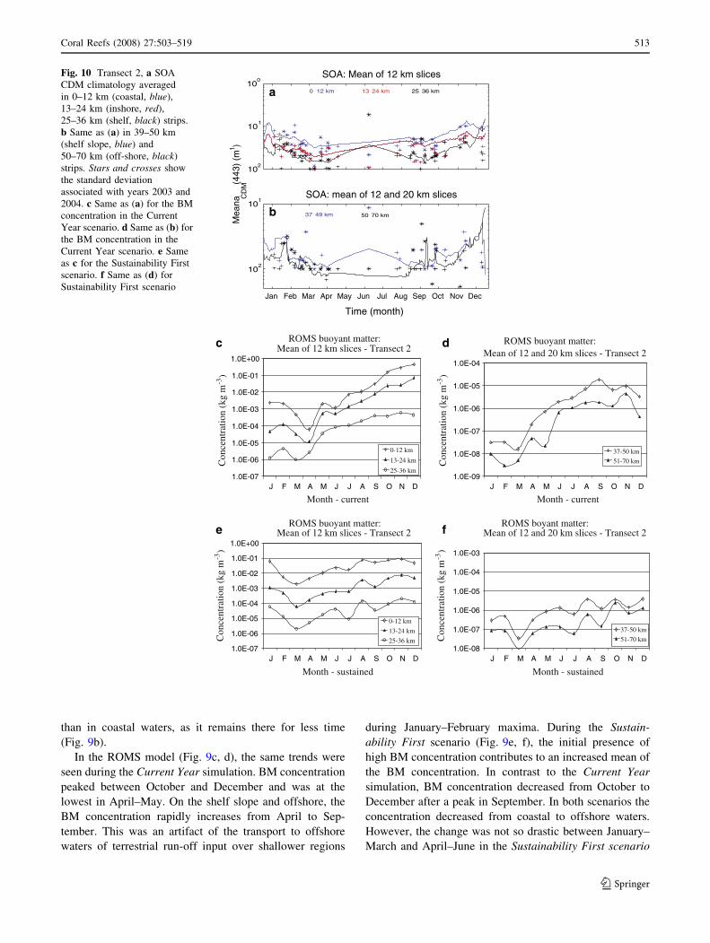
Fig. 10 Transect 2, a SOA
CDM climatology averaged
in 0–12 km (coastal, blue),
13–24 km (inshore, red),
25–36 km (shelf, black) strips.
b Same as (a) in 39–50 km
(shelf slope, blue) and
50–70 km (off-shore, black)
strips. Stars and crosses show
the standard deviation
associated with years 2003 and
2004. c Same as (a) for the BM
concentration in the Current
Year scenario. d Same as (b) for
the BM concentration in the
Current Year scenario. e Same
as c for the Sustainability First
scenario. f Same as (d) for
Sustainability First scenario
Coral Reefs (2008) 27:503–519 513
123

(on the shelf slope and offshore, although the transport to
offshore waters starts earlier, in March here). In both sce-
narios, the shelf slope and offshore waters have a slightly
different seasonality than in the observations. Instead of
having two periods of runoff expelling, they exhibit only
one, starting in April and lasting till October.
Transect 2
Seasonal changes in the first three strips were smaller
than those found at Transect 1, and although the same
trends were observed (Fig. 10a, b) the gradient across the
plume was weaker. In offshore waters, seasonal changes
were larger compared to Transect 1. Transport to off-
shore waters occurred in February, and also possibly
from July to November. Retention in offshore waters
appeared to take place after October as CDM rapidly
increases.
In the model time series, the plume gradient was
sometimes larger than at Transect 1 for the Current Year
scenario (Fig. 10c, d). However, changes between January
and June were smaller compared to Transect 1 but the
maximum was higher in October–December. Transport to
ROMS buoyant matter: Mean of 12 km slices - Transect 3
1.0E-08
1.0E-07
1.0E-06
1.0E-05
1.0E-04
1.0E-03
1.0E-02
1.0E-01
J F M A M J J A S O N D
Month - sustained
0-12 km
13-24 km
25-36 km
ROMS boyant matter: Mean of 12 and 20 km slices - Transect 3
1.0E-08
1.0E-07
1.0E-06
1.0E-05
1.0E-04
1.0E-03
J F M A M J J A S O N D
Month - sustained
37-50 km51-70 km
ROMS buoyant matter: Mean of 12 and 20 km slices - Transect 3
1.0E-09
1.0E-08
1.0E-07
1.0E-06
1.0E-05
1.0E-04
J F M A M J J A S O N D
37-50 km51-70 km
ROMS buoyant matter: Mean of 12 km slices - Transect 3
1.0E-08
1.0E-07
1.0E-06
1.0E-05
1.0E-04
1.0E-03
1.0E-02
1.0E-01
J F M A M J J A S O N D
Month - current Month - current
0-12 km
13-24 km25-36 km
102
101
100
SOA: Mean of 12 km slices
Jan Feb Mar Apr May Jun Jul Aug Sep Oct Nov Dec
102
101
Time (month)
Mea
n aCD
M(4
43) (
m1 )
SOA: Mean of 12 and 20 km slices 50 70 km 37 49 km
0 12 km 13 24 km 25 36 kma
b
c d
e f
Con
cent
ratio
n (k
g m
-3)
Con
cent
ratio
n (k
g m
-3)
Con
cent
ratio
n (k
g m
-3)
Con
cent
ratio
n (k
g m
-3)
Fig. 11 Transect 3, a SOA
CDM climatology averaged in
0–12 km (coastal, blue),
13–24 km (inshore, red),
25–36 km (shelf, black) strips.
b Same as (a) in 39–50 km
(shelf slope, blue) and
50–70 km (off-shore, black)
strips. Stars and crosses show
the standard deviation
associated with years 2003 and
2004. c Same as (a) for the BM
concentration in the Current
Year scenario. d Same as (b) for
the BM concentration in the
Current Year scenario. e Same
as (c) for the Sustainability First
scenario. f Same as (d) for
Sustainability First scenario
514 Coral Reefs (2008) 27:503–519
123

the shelf slope and offshore waters started earlier than at
Transect 1, between April and June, and peaked from July
to November. For the Sustainability First scenario, the
gradient across the plume was larger but BM concentration
changes were smaller than for the Current Year scenario
(Fig. 10e, f). In addition, transport to shelf slope and off-
shore waters was not as significant as Transect 1 (Figs. 9f,
10f). As at Transect 1, the seasonality of the shelf slope and
offshore waters differed between the model and the
observations, yet July–September expelling could realisti-
cally occur (Fig. 10b). To summarize, changes at Transect
2 were smaller than at Transect 1 in offshore waters as in
the SOA retrievals.
Transect 3
Strip widths defined for this transect were such that the
coastal and inshore strips are inside the Belize Barrier Reef
(BBR) and the shelf one outside this reef. Contrary to
Transect 1, CDM varied slightly between January and
March in coastal waters, and rose from April–December
(Fig. 11a). Inshore waters showed a strong increase in
April. Monthly river discharge time series (Fig. 6) showed
that a rise in coastal waters CDM coincided with a rise in
river discharge after April. Shelf water exhibited a maxi-
mum in August followed by a drop in September–October
and later, a slow rise. However, on the shelf slope and
offshore, seasonal variations were larger than in coastal
waters. Offshore waters here exhibited the same seasonal
variability as the same waters on Transects 1 and 2
(Fig. 11b).
BM concentration in the Current Year scenario
showed a much higher concentration in coastal waters
than elsewhere (Fig. 11c). The difference between
inshore and shelf waters was not as large but still sig-
nificant (an order of magnitude). Seasonal changes were
weaker than on Transects 1 and 2 and the lowest vari-
ability was seen in coastal waters, in agreement with the
SOA retrievals. Inshore water exhibited a minimum in
BM concentration in August, earlier than in the satellite
retrievals. On the shelf, which is in the vicinity of the
BBR, BM concentration increased after May, dropped in
August, and peaked in December, again as in the retri-
evals. On the shelf slope and offshore, seasonal changes
were larger than inside and just outside of the BBR
(Fig. 11d). Although the seasonal variations were dif-
ferent from observations in January–March, they were
similar between July and December (Fig. 11d). Varia-
tions seemed to be independent of the BM regime in
coastal waters, as expected due to the presence of the
BBR. In the Sustainability First scenario, the same
concentration difference between coastal and non-coastal
waters, and the same opposite trend between coastal and
offshore waters were obtained (Fig. 11e, f). In the latter,
seasonal changes were not as large as in the Current
Year scenario.
Jan Feb Mar Apr May Jun Jul Aug Sep Oct Nov Dec
102
101
100
Time (month)
Me
an
aC
DM(4
43
) (m
1 )SOA: mean, south to north of 5 km slices
0 6 km 7 12 km 13 20 km
21 26 km
ROMS buoyant matter: Intervals (south to north) of entire 26 km Transect 4
1.E-02
1.E-01
1.E+00
1.E+01
1.E+02
1.E+03
1.E+04
1.E+05
J F M A M J J A S O N D
Month - current
0-6 km
7-12 km
13-20 km
21-26 km
ROMS boyant matter: Intervals (south to north) of entire 26 km Transect 4
1.E-02
1.E-01
1.E+00
1.E+01
1.E+02
1.E+03
1.E+04
1.E+05
J F M A M J J A S O N D
Month - sustained
0-6 km7-12 km13-20 km21-26 km
Con
cent
ratio
n (k
g m
-3)
Con
cent
ratio
n (k
g m
-3)
Fig. 12 Transect 4. a SOA CDM climatology averaged in 0–6 km
(coastal, blue), 7–12 km (red, inshore), 13–20 km (shelf slope,
black), and 21–26 km (offshore, green) strips. b Same as (a) for the
BM concentration in the Current Year scenario. c Same as (b) for the
Sustainability First scenario
Coral Reefs (2008) 27:503–519 515
123

Transect 4
This transect crosses the Gulf of Honduras, from Honduras
to Belize (Fig. 1) and exhibited the highest CDM coeffi-
cient of all transects. Variations were strong over the year
and the plume exhibited strong seasonally varying mono-
tonic cross gradients (Fig. 12a). CDM was always higher
toward Guatemala than toward Belize. Minima were
observed in April of both years and CDM peaks sharply in
August and September (Fig. 12a).
In the ROMS scenarios, BM concentrations in the dif-
ferent strips were the highest of all transects and followed
the same seasonal changes, in both scenarios, as in the
observations (Fig. 12b, c). Concentrations were higher
towards Guatemala than near Belize between July and
November. Maxima were obtained between October and
December, as in the observations. Gradients across the
plume were not monotonic, and minima were observed in
waters between the two coasts (Fig. 12b, c).
Transect 5
Transect 5 is parallel to transect 3 and extends across
Chinchorro Bank where the transport of runoff by the gyre
along the coast of Mexico (toward the Yucatan Channel)
takes place (Figs. 3, 4). Since very few clear days were
available in this region only the model results are described
here. BM concentrations were of the same order of mag-
nitude in all strips between January and March, but lower
than the other transects. Later, between July and December,
concentration was the highest between the Bank and the
coast (Fig. 13a) than offshore (Fig. 13b). Nonetheless, in
that passage, BM concentration was higher in coastal
waters on both sides of the passage with a minimum in the
middle (Fig. 13a). The model showed an absence of BM in
the region between April and June for the Current Year
scenario. Minima were obtained between January and
March. BM concentrations peaked in September, three
months after the peak in offshore waters along Transect 3
(Fig. 11d). This suggests that the BM transport in the
vicinity of Transects 3 and 5 is not subject to the same
variability and current dynamics. Between September and
December, the BM concentration oscillated with a relative
minimum (maximum) in October (December). In the Sus-
tainability First scenario, seasonal changes were weaker
and no absence of BM was noticed during the year
(Fig 13c, d). The general trend showed an oscillatory
increase of the BM concentration over the year in all waters
with relative maxima in January, March, September and
ROMS buoyant matter: Mean of 12 km slices - Transect 5
1.0E-09
1.0E-08
1.0E-07
1.0E-06
1.0E-05
1.0E-04
1.0E-03
J F M A M J J A S O N D
Month - sustained
0-12 km
13-24 km
25-36 km
ROMS boyant matter: Mean of 12 and 20 km slices - Transect 5
1.0E-08
1.0E-07
1.0E-06
1.0E-05
1.0E-04
1.0E-03
J F M A M J J A S O N D
Month - sustained
37-50 km
51-70 km
ROMS buoyant matter: Mean of 12 km slices - Transect 5
1.0E-09
1.0E-08
1.0E-07
1.0E-06
1.0E-05
1.0E-04
1.0E-03
J F M A M J J A S O N D
Month - current
0-12 km
13-24 km
25-36 km
ROMS buoyant matter: Mean of 12 and 20 km slices - Transect 5
1.0E-09
1.0E-08
1.0E-07
1.0E-06
1.0E-05
1.0E-04
J F M A M J J A S O N D
Month - current
37-50 km
51-70 km
Con
cent
ratio
n (k
g m
-3)
Con
cent
ratio
n (k
g m
-3)
Con
cent
ratio
n (k
g m
-3)
Con
cent
ratio
n (k
g m
-3)
a b
c d
Fig. 13 Transect 5. a BM
concentration in the Current
Year scenario averaged in
0–12 km (coastal), 13–24 km
(inshore), and 25–36 km (shelf)
strips. b Same as (a) in
39–50 km (shelf slope) and
50–70 km (off-shore) strips.
c and d Same as (a) and (b) for
the Sustainability First scenario
516 Coral Reefs (2008) 27:503–519
123

December. As in the Current Year, BM concentration was
the highest on the shallow sides of the passage (Fig. 13c).
During this scenario, BM transport toward the Yucatan
Channel was continuous over the entire year.
Discussion
Due to the time series gaps in clear sky ocean color images
that prevail in cloudy tropical areas, numerical simulations
calibrated with realistic data could be an alternative to
understand the impact of continental runoff to the MBRS.
Only few recent studies (Andrefouet et al. 2002; Sheng
et al. 2007) have addressed this issue by using SeaWiFS
images to track the high concentration runoff plume after
hurricane Mitch landfall in November 1998. They were
able to show that the atolls and inshore reef are within
reach of terrestrial runoffs, and that they have been peri-
odically influenced, mostly during the rainy season. Most
of the seasonality of terrestrial runoff in coastal, inshore,
shelf, shelf slope, and offshore waters is driven by the
seasonality of the river discharge. This in turn is driven by
the rainfall, land use and land topography, resulting in soil
erodibility (Burke and Sugg 2006). The use of the ROMS
simulation of passive tracer in the MAR proved effective to
address the dynamics of terrestrial runoff and its season-
ality. The general circulation pattern of terrestrial runoff
was compiled with the analysis of time series of both CDM
(aCDM) and BM (Fig. 14). Based on these results, the
maximum terrestrial runoff content in the MAR occurs
between October and January (Figs. 2,8). Minima are
obtained in early April after runoffs have been transported
out of the MAR. Soon after the beginning of the rainy
season (June–July), river discharge reaches the coastal and
inshore water of Belize, Guatemala and Honduras. Along
the Honduras coast, the plume runoff drifts eastward and
spreads northward through filaments (Fig. 3). Maximum
concentration in eastern shelf, shelf slope and offshore
waters of Honduras occurs between October and Decem-
ber, arriving in September and leaving in January of the
next year. The diluted runoff is entrained northwestward
toward the MBRS south of Chinchorro Bank, which is also
reached between October and December. Some of this
diluted runoff re-circulates into the cyclonic gyre, while
some is entrained slowly toward the south of BBR, just
offshore in Belize’s waters. This explains the late increase
of runoff concentration outside the BBR between January
and March, while it remains almost constant inside
(Fig. 11a,b). Some of the runoff in western offshore Hon-
duras waters re-circulates spreading seaward west of the
Bay Islands and into the Gulf of Honduras, which contains
significant eddy mesoscale activity (not shown). The wes-
tern corner of the Gulf of Honduras exhibits the highest
concentration of terrestrial runoff, which peaks in Sep-
tember. Within the BBR, seasonal changes are not as large
as offshore. However, the maximum runoff concentration
peaks slightly between October and December as well.
This suggests that runoff expelling occurs at a slower rate
inside the BBR than in Honduras waters. Moreover the
southwestern corner of the Gulf of Honduras appears as a
retention area due to the mesoscale eddies.
Figure 14 shows a schematic of the spatial and tem-
poral evolution of the runoff plume in the MAR. It might
look like a giant synoptic plume from space but is in fact
composed of runoff of different ages. The results of this
study show that all the reefs of the region are connected
by the terrestrial runoff transport. This connectivity is not
only related to special events such as hurricanes (And-
refouet et al. 2002; Sheng et al. 2007) but occurs on a
regular basis each year. Therefore any change in the
landscape around the MAR will induce changes in the
vicinity of most of the reefs of the MBRS at different
times of the year.
Comparison between Current Year and Sustainability
First scenarios with CDM imagery of years 2003–2004
reveals that inter-annual variability in the CDM seasonal
Fig. 14 Summary of the time evolution of the terrestrial runoff
dispersion pattern in the MAR superimposed on the annual delivery
per basin from Burke and Sugg (2006). Black arrows show the coastal
transport, green the offshore circulation patterns and red the
remainder of the past year
Coral Reefs (2008) 27:503–519 517
123

cycle can be driven by events in the previous year that will
impact the following year until the excess of terrestrial
runoff is expelled from the region. Reducing the runoff
discharge contributes to lower BM content in coastal
waters after one year (Fig. 8c). This result leads to the
impact of hurricane activity to the MAR, which could take
a year before being dissipated. This finding is also critical
for management questions.
Model limitations
As shown by the comparison between the ROMS model
and the SOA time series, the behavior of the plumes is
not exactly reproduced by the ROMS, most likely because
the ROMS is a climatology with smooth seasonal trends
and no strong wind or rainfall events. This difference is
certainly increased in shallow regions where the ROMS
has a minimum constant depth of five meters imposed by
the resolution and the constraint of stability of numerical
schemes. Shallower minimum depth would require a
much higher resolution especially where the depths
changes are large. The BBR, which lies at the edge of the
shelf drop was not explicitly represented because of the
ROMS resolution and the lack of topographic data.
However, drop offs at the shelf prevent cross shelf
exchanges by nature (Huthnance 2004), explaining why
the ROMS simulates without them the presence of the
BBR. Other physical processes such as the contribution of
sediment deposition and resuspension were not accounted
for in this study and most likely contributed to the
discrepancies between ROMS and the SOA-processed
observations. Also, due to the few clear images available
for the entire dataset, comparison with the model clima-
tology needs to be viewed with a degree of caution.
Numerous gaps in the dataset prevented an accurate
comparison with the model’s climatology. Finally, the
lack of a defined relationship between the CDM absorp-
tion coefficient and the CDM concentration makes
estimation of terrestrial runoff concentration from satellite
imagery difficult. Direct measurements from water sam-
ples, which are not available yet, are necessary to get
such information.
These results can be applied to study pollutant transport
towards and across the reefs, which in this study are shown
to lie in the path of the runoff circulation repeatedly every
year. Using marine population connectivity techniques, the
stress level of the MBRS due to terrestrial runoff could be
examined in order to assess better land-use scenarios as
studied by Burke and Sugg (2006).
Acknowledgments This MAR modeling project was jointly funded
by the World Resources Institute (WRI) and The Nature Conservancy
(TNC). The authors are grateful to Lauretta Burke (WRI), Nestor
Vindevoxhel (TNC) and Alejandro Arrivillaga (TNC) for providing
the funding; to Villy Kourafalou for sharing computer resources at the
Rosenstiel School of Marine and Atmospheric Sciences (RSMAS) for
this project, and to Johnathan Kool (RSMAS) for technical assistance
with GIS processing. C.Paris was also funded by the World Bank/
GEF Coral Reef Target Research Program.
Appendix
River water transported to the oceans can be thought of as
being made up of, in addition to water, a number of
components:
1. PIC (Particulate Inorganic Carbon) = Al, Fe, Si, Ca, K,
Mg, Na and P. Alternate names: suspended inorganic
matter; sediment. The terms sediment is ambiguous. It
implies deposition which is dependent on velocity,
density and salinity.
2. Dissolved major species, comprising elements with no
gaseous phase in the atmosphere (e.g., Cl-, Na+,
HCO3-, Mg2+, K+) and elements with gaseous phases
(e.g., SO42-, HCO3
-), with the latter derived from
atmospheric gases (egg., SO2 and CO2, respectively),
as well as from rocks.
3. Dissolved nutrient elements N, P (and sometimes Si),
which are used biologically and whose concentrations
vary due to this.
4. DOC (Dissolved Organic Carbon). Alternate name:
dissolved organic matter. This is primarily sourced
from soils and plants.
5. POC (Particulate Organic Carbon) = phytoplankton
and detritus (plant material). Alternate name: sus-
pended organic matter.
6. Dissolved trace metals.
7. Suspended trace metals.
From the above list, Suspended Particulate Matter
(SPM) will contain PIC, POC and suspended trace metals,
the suspended terms.
Buoyant Matter will contain ALL terms; however the
amount of PIC will depend on the rate of deposition and re
suspension from the source.
The ROMS model will invariably replicate the transport
of Buoyant Matter.
The SOA model produces CDM, the absorption coeffi-
cient of Colored Detrital Material. This is comprised of two
components
1. The absorption coefficient of colored dissolved organic
matter (CDOM), one component of DOC.
2. The absorption coefficient of detrital particles, one
component of POC.
Therefore the spatial and temporal trends in CDM can
be used as a surrogate for Buoyant Matter.
518 Coral Reefs (2008) 27:503–519
123

References
Andrefouet S, Mumby PJ, McField M, Hu C, Muller-Karger FE
(2002) Revisiting coral reef connectivity. Coral Reefs 21:43–
48
Blaas M, Dong C, Marchesiello P, McWilliams JC, Stolzenbach KD
(2007) Sediment-transport modeling on Southern California
shelves: a ROMS case study. Cont Shelf Res 27:832–853
Burke L, Sugg Z (2006) Hydrologic modeling of watersheds
discharging adjacent to the Mesoamerican Reef. On the
watershed analysis for the Mesoamerican Reef, WRI/ICRAN.
http://www.wri.org/biodiv/pubs_description.cfm?pid=4256
Devlin MJ, Brodie J (2005) Terrestrial discharge into the great barrier
reef lagoon: nutrient behavior in coastal waters. Mar Pollut Bull
51:9–22
Durand N, Fiandrino A, Fraunie P, Ouillon P, Forget P, Naudin JJ
(2002) Suspended matter dispersion in the Ebro ROFI: an
integrated approach. Cont Shelf Res 22:267–284
Ezer T, Thattai DV, Kjerfe B, Heyman WD (2005) On the variability
of the low along the Meso-American barrier reef system: a
numerical model study of the influence of the Caribbean current
eddies. Ocean Dynam 55:458–475
Garver SA, Siegel DA (1997) Inherent optical property inversion of
ocean color spectra and its biogeochemical interpretation: 1
time series from the Sargasso Sea. J Geophys Res 102:18607–
18625
Gordon HR, Wang M (1994) Retrieval of water-leaving radiance and
aerosol optical thickness over the oceans with SeaWiFS: a
preliminary algorithm. Appl Optics 33:443–452
Heyman WD, Kjerfe B (2000) The Gulf of Honduras. In: Seelijer U,
Kjerfe B (eds) Coastal marine ecosystems. Marine ecosystems of
Latin America. Springer, Berlin, pp 17–32
Huthnance JM (2004) Ocean to shelf signal transmission: a parameter
study. J Geophys Res 109:C12029. doi:10.1029/2004JC002358
Jorgensen PV, Edelvang K (2000) CASI data utilized fro mapping
suspended matter concentrations in sediment plumes and veri-
fication of 2D hydrodynamic modeling. Int J Remote Sens
21:2247–2258
Kleypas JA, Buddemeier RW, Gattuso JP (2001) The future of coral
reefs in an age of global change. Int J Earth Sci 90:426–437
Luick JL, Mason L, Hardy T, Furnas MJ (2007) Circulation in the
great barrier reef lagoon using numerical tracers and in situ data.
Cont Shelf Res 27:757–778
Magnuson A, Harding LW Jr, Mallonee ME, Adolf JE (2004) Bio-
optical model for Chesapeake Bay and the middle Atlantic bight.
Estuar Coast Shelf Sci 61:403–424
Maritorena S, Siegel DA, Peterson AR (2002) Optimization of semi-
analytical ocean color model for global scale applications. Appl
Optics 41:2705–2714
McClanahan T, Muthiga N (1998) An ecological shift in a remote
coral atoll of Belize over 25 years. Environ Conserv 25:122–130
McKergow LA, Prosser IP, Hughes AO, Brodie J (2005) Regional
scale nutrient modeling: exports to the Great Barrier Reef world
heritage area. Mar Pollut Bull 51:186–199
O’Reilly JE, Maritorena S, Mitchell BG, Siegel DA, Carder KL,
Garver SA, Kahru M, McClain C (1998) Ocean color chloro-
phyll algorithms for SeaWiFS. J Geophys Res 103:24937–24953
Ouillon S, Douillet P, Andrefouet S (2004) Coupling satellite data
with in situ measurements and numerical modeling to study fine
suspended-sediment transport: a study for the lagoon of New
Caledonia. Coral Reefs 23:109–122
Richardson PL (2005) Caribbean Current and eddies as observed by
surface drifters. Deep Sea Res II 52:429–463
Sheng J, Wang L, Andrefouet S, Hu C, Hatcher BG, Muller-Karger
FE, Kjerfe B, Heymans WD, Yang B (2007) Upper ocean
response of the Mesoamerican barrier reef system to hurricane
Mitch and coastal freshwater inputs: a study using SeaWiFS
ocean color data and a nested-grid ocean circulation model.
J Geophys Res 112:C07016. doi:10.1029/2006JC003900
Spalding M, Ravilious C, Green EP (2001) World atlas of coral reefs.
University of California Press, Berkeley
Tang L, Sheng J, Hatcher BG, Sale PF (2006) Numerical study of
circulation. Dispersion, and hydrodynamic connectivity of sur-
face waters on the Belize shelf. J Geophys Res 111:C01003.
doi:10.1029/2005JC002930
Wilkinson CR (1987) Interocean differences in size and nutrition of
oral reef sponge populations. Science 236:1654–1657
Wilkinson CR (1999) Global and local threats to coral reef
functioning and existence: review and predictions. Mar Freshw
Res 50:867–878
Coral Reefs (2008) 27:503–519 519
123
Top Related
Copyright © 2022 FDOKUMEN

