Mesoamerican Reef Alliance ICRAN-MAR Project - PDF Server
360
Mesoamerican Reef Alliance ICRAN-MAR Project FINAL REPORT TO USAID Report of Project Activities and Results as of November 2, 2006 1 Contact: Liza Agudelo, Project Coordinator [email protected] February, 2007 1 Project activities to be completed by June 30, 2007.
-
Upload
khangminh22 -
Category
Documents
-
view
0 -
download
0
Transcript of Mesoamerican Reef Alliance ICRAN-MAR Project - PDF Server

Mesoamerican Reef Alliance ICRAN-MAR Project
FINAL REPORT TO USAID Report of Project Activities and Results
as of November 2, 20061
Contact: Liza Agudelo, Project Coordinator [email protected]
February, 2007
1 Project activities to be completed by June 30, 2007.

UNITED NATIONS ENVIRONMENT PROGRAMME
Caribbean Regional Coordinating Unit
CARIBBEAN ENVIRONMENT PROGRAMME
FINAL REPORT TO USAID
BACKGROUND INFORMATION.
Project Title: Mesoamerican Coral Reef Alliance UNEP Project Number: UNE-GLO-01-201J USAID Grant Number: 596-G-00-03-00215-00
Responsible Office: Regional Coordinating Unit Coordinating Agency/Supporting United Nations Foundation Organization: U.S Agency for International Development Project Starting Date: July 2004 Project Completion Date: July 2007 Total Budget (USD) USAID and UNF contribution: $3,000,000.00USD Relevant UNEP Programme of Work Component Number: MT/101-01-80 (UNE-GLO-01-201)
Mesoamerican Reef Alliance – Final Report to USAID – February, 2007 2

TABLE OF CONTENTS
ACRONYMS AND ABBREVIATIONS ............................................................................................................................................. 5
INTRODUCTION .............................................................................................................................................................................. 6
EXECUTIVE SUMMARY.................................................................................................................................................................. 6 PROJECT IMPLEMENTATION............................................................................................................................................................. 6 OVERALL PROJECT PERFORMANCE............................................................................................................................................... 11 PROJECT STATISTICS – OVERALL INDICATORS ............................................................................................................................... 13 PROJECT INDICATORS BY COMPONENT – STATUS AS OF DECEMBER, 2006...................................................................................... 19
I. PROJECT DESCRIPTION AND OBJECTIVES......................................................................................................................... 30 A. STRATEGIC OBJECTIVE AND INTERMEDIATE RESULTS................................................................................................................ 31
II. IMPLEMENTATION OF THE PROJECT COMPONENTS 2004-2006 ..................................................................................... 31 A. IMPROVED WATERSHED MANAGEMENT (IR1)............................................................................................................................ 32
1. Threats – Rationale for Component Design ................................................................................................................ 32 2. Description of Component Strategy – Dynamics over the Past 30 Months................................................................. 33 3. Major Achievements and Results – Impacts in the Region ......................................................................................... 34
Partnerships with agribusiness ............................................................................................................................................................... 34 Scope of Results – Relevance to the Region.................................................................................................................................... 37 Final Outputs at the End of the Project ............................................................................................................................................. 38
Watershed Analysis and modeling ......................................................................................................................................................... 39 Scope of Results – Relevance to the Region.................................................................................................................................... 40 Capacity Building............................................................................................................................................................................... 42 Information Dissemination................................................................................................................................................................. 43
4. Leveraged Support, Impacts and the Larger Scale – The Potential Way Ahead ........................................................ 44 Partnerships with agribusiness ............................................................................................................................................................... 44 Watershed Analysis and modeling ......................................................................................................................................................... 45
5. Lessons Learned and Recommendations ................................................................................................................... 48 Partnerships with agribusiness ............................................................................................................................................................... 48 Watershed Analysis and modeling ......................................................................................................................................................... 48
B. SUSTAINABLE FISHERIES (IR2)................................................................................................................................................. 49 1. Threats – Rationale for Component Design ................................................................................................................ 49 2. Description of Component Strategy – Dynamics over the Past 30 Months................................................................. 50 3. Major Achievements and Results – Impacts in the Region ......................................................................................... 54
Scope of Results – Relevance to the Region.................................................................................................................................... 55 Final Outputs at the End of the Project ............................................................................................................................................. 57
4. Leveraged Support, Impacts and the Larger Scale – The Potential Way Ahead ........................................................ 59 5. Lessons Learned and Recommendations ................................................................................................................... 60
C. SUSTAINABLE TOURISM (IR3) .................................................................................................................................................. 61 1. Threats – Rationale for Component Design ................................................................................................................ 61 2. Description of Component Strategy – Dynamics over the Past 30 Months................................................................. 62 3. Major Achievements and Results – Impacts in the Region ......................................................................................... 63
Scope of Results – Relevance to the Region.................................................................................................................................... 64 Final Outputs at the End of the Project ............................................................................................................................................. 66
4. Leveraged Support, Impacts and the Larger Scale – The Potential Way Ahead ........................................................ 67 5. Lessons Learned and Recommendations ................................................................................................................... 68
III. FINANCIAL STATUS ............................................................................................................................................................... 69
IV. TABLE OF ANNEXES ............................................................................................................................................................. 71
Mesoamerican Reef Alliance – Final Report to USAID – February, 2007 3

LIST OF TABLES AND FIGURES Table 1: Number of Institutions/Communities Involved Per Sector – See figures 1-7 below .......................................13 Table 2: Leveraged Funds - over $1,600,000 USD in support of activities under the three components ....................13 Table 3: Leveraged Impacts – originated from project objectives not contemplated in original project document .......15 Table 4: Project Products used by other institutions – raising the profile of the ICRAN-MAR project ..........................15 Table 5: Beneficiaries – over 1,000 direct beneficiaries through various activities in the 3 components .....................16 Table 6: Fisheries Component – Percentage of efforts invested by country – as of December 2006..........................53 Fig. 1. Type of Organizations Involved in the Project...............................................................................................17 Fig. 2. Government Agencies Participation by Country............................................................................................17 Fig. 3. Local NGOs Participation by Country............................................................................................................17 Fig. 4. Other NGOs/Regional Initiatives Participation by Country ............................................................................18 Fig. 5. Local communities Participation by Country .................................................................................................18 Fig. 6. National Institutions Participation by Country................................................................................................18 Fig. 7. Private Sector Participation by Country.........................................................................................................18
Mesoamerican Reef Alliance – Final Report to USAID – February, 2007 4

ACRONYMS AND ABBREVIATIONS AVHRR Advanced Very High Resolution Radiometer APESCA Asociación Pesquera del Caribe BERDS Biodiversity & Environmental Resource Data System of Belize clearinghouse BMP Better Management Practice BFCA Belize Fishermen Cooperative Association BTIA Belize Tourism Industry Association CAFTA Central America Free Trade Agreement CCAD Comisión Centroamericana de Ambiente y Desarrollo CELB The Center for Environmental Leadership in Business CI Conservation International CIAT Centro de Investigación Agrícola Tropical CLUE-S Conversion of Land Use and its Effects CONANP Comisión Nacional de Áreas Naturales Protegidas, México CONAP Consejo Nacional de Áreas Protegidas, Guatemala CORAL Coral Reef Alliance CST Certification for Sustainable Tourism CTO Caribbean Tourism Organisation CZMAI Coastal Zone Management Authority Institute, Belize FAO Food and Agriculture Organization of the United Nations FGDC Federal Geographic Data Committee G-CAP Guatemala – Central American Programs Mission, USAID GCRMN Global Coral Reef Monitoring Network GDA Global Development Alliance (USAID) GEF Global Environment Facility GEMS-GLORI Global Registration of Land-Ocean River Inputs ICRAN International Coral Reef Action Network ICRI International Coral Reef Initiative IGBP International Geosphere / Biosphere Program INEGI Instituto Nacional de Estadística, Geografía e Informática, México LOICZ Land-Ocean Interactions in the Coastal Zone MAR Mesoamerican Reef MBRS Mesoamerican Barrier Reef System MODIS Moderate Resolution Imaging Spectroradiometer MPA Marine Protected Area MSC Marine Stewardship Council N-SPECT Non-point Source Pollution and Erosion Comparison Tool OSPESCA Organización del Sector Pesquero y Acuícola Del Istmo Centroamericano PROARCA Programa Ambiental Regional Para Centroamérica (de USAID) RA Rainforest Alliance RC Reef Check SOSC Strategic Objective Steering Committee SRTM Shuttle Radar Topography Mission TNC The Nature Conservancy TOC Technical Oversight Committee UNEP United Nations Environment Programme UNEP-CAR/RCU UNEP Caribbean Regional Coordinating Unit UNEP/DTIE UNEP Division of Technology, Industry, and Economics UNEP-WCMC UNEP-World Conservation Monitoring Centre UNF United Nations Foundation USAID United States Agency for International Development WCS Wildlife Conservation Society WIDECAST Wider Caribbean Sea Turtle Conservation Network WRI World Resources Institute WMW ICRAN-MAR Watershed Management Workshop WWF World Wildlife Fund
Mesoamerican Reef Alliance – Final Report to USAID – February, 2007 5

INTRODUCTION The current report is submitted to USAID to meet final reporting requirements as indicated in the contractual agreement between USAID and UNF in support of the ICRAN Mesoamerican Reef Alliance (ICRAN-MAR), which expired as of November 2, 2006. While this is the final report to USAID, it is important to mention that project activities are scheduled to finalize by June 30, 2007 and further development and results are expected in the coming months. A terminal project report of the ICRAN Mesoamerican Reef Alliance will be submitted to the donors as of August 30, 2007.
Beginning with an executive summary that describes overall status of project components –including summarizing tables of project statistics and project indicators– the report moves on to describing detailed aspects of project implementation by component (please refer to Section II); these sections contain lessons learned and expected results as of June 30, 2007. Section III presents the financial status of the project as of November 2, 2006. A final table of relevant annexes is presented at the end of the document.
EXECUTIVE SUMMARY In recognition of the ecological and socio-economic richness and importance of the Mesoamerican Barrier Reef region (MAR), the ICRAN Mesoamerican Reef Alliance (ICRAN-MAR) project was designed in 2003 to contribute to the many local, national and regional-level resource conservation and sustainable development projects that had been initiated in the MAR region since 1990. Discussions among ICRAN representatives and conservation leaders in the MAR region had established that there were opportunities where ICRAN could, and should, become engaged.
As a result, ICRAN partners developed a 3-year initiative to address threats to the MAR under three components known for their potential to strongly impact the coastal and marine ecosystems: watershed management, sustainable fishing, and sustainable tourism. With the generous support of the United States Agency for International Development (USAID) and the United Nations Foundation (UNF), the ICRAN-MAR partners would conduct a set of inter-linked, complementary activities to enable the proliferation of good practices for coral reef management and conservation. The strategy of this Alliance would combine a conservation and sustainable management approach with the creation of partnerships with the private sector to leverage resources and talents to find long-term solutions.
Project implementing partners are the World Resources Institute (WRI), UNEP-World Conservation Monitoring Centre (WCMC), World Wildlife Fund (WWF), the Coral Reef Alliance (CORAL), UNEP-Division of Technology Industry and Economics (DTIE), and Reef Check. As of November 2, 2006, approximately 29 months after beginning project implementation, partners have achieved significant results, some of which have exceeded original expectations. A lead organization within ICRAN, UNEP-CAR/RCU manages project execution.
PROJECT IMPLEMENTATION The project has evolved since its original inceptions and over the course of the implementation phase. Earlier stages required significant investments to set up the necessary mechanisms to undertake planned activities and achieve project goals. This included, among others, gathering information and building relationships with local counterparts. Initial results provided a good platform not only to leverage further support from governments and the private sector but also to inform and influence decision makers in the region. During these years of implementation,
Mesoamerican Reef Alliance – Final Report to USAID – February, 2007 6

ICRAN-MAR partners have capitalized on lessons learned and strengthened channels of communication with project partners and other initiatives in the region.
As already indicated in previous progress reports, while the three components of the project are closely interlinked and designed to pursue the overall goal of contributing to the sustainable management and use of the Mesoamerican Reef, each component is independent and as such, each one has had particular characteristics and different levels of complexity. The high dynamism of the project activities and the challenges they have produced, have called for adopting an adaptive approach to allow addressing changes in the implementation mechanisms as appropriate. Under the supervision of the Project’s Coordinator and the guidance of UNEP-CAR/RCU this approach has facilitated the reorientation of investments —consequent with the project’s objectives— as necessary.
The spirit of creating alliances and consolidating societies with the private sector for the benefit of coral reefs in the Mesoamerican region has been the fundamental objective of the ICRAN-MAR Project. The positive results obtained by the project to date demonstrate that alliances are an effective mechanism that can bring great benefits for the handling of Marine resources. Nevertheless, coordinating efforts is not a simple task and requires commitment and joint work to identify the best strategies that involves relevant stakeholders and especially the local partners.
Please refer to Section II of the present report for more detailed information. Watershed Management This component is integrated by two complementary sub-components:
a) On one end, WWF has focused its efforts identifying sources of pollution and sediment from agricultural activities that have a negative impact on the marine environment, as well as on-the-ground activities with agricultural businesses to adopt a suite of “better management practices”. This work was designed to be carried out in three years, has produced concrete results over the past 2 years, and it is still ongoing.
b) On the other end, WRI and UNEP-WCMC have produced information and GIS tools for examining the potential impact of different land use and development options in the region and the associated impacts on water quality on the MAR. These hydrologic models and diagnostic tools help educate and encourage key stakeholders to implement better management practices to reduce impacts on the coastal and marine resources. This work was designed to be carried out during the first two years of the project. It is now almost complete, with only some further follow-up capacity building efforts to fulfill.
Under the leadership of WWF, the project has produced significant results following an innovative approach that has praised the importance of adopting better management practices (BMPs) in the agricultural sector, and highlighted the relevance of partnership building with the private sector for conservation efforts and better management. Aiming to achieve the project goal of identifying agricultural threats WWF managed to set up a bioaccumulation monitoring program, design a monitoring protocol, and leverage significant results from the private sector (e.g. Croplife) and other donors in the region (e.g. Summit Foundation) that help consolidate project results in the long-term. MoUs signed with major agricultural companies in the region (e.g. Chiquita, Dole) are now promoting the implementation of BMPs and speak of the industry’s willingness to participate in actions that can lower their impact on the environment while maintaining their economical benefits.
Mesoamerican Reef Alliance – Final Report to USAID – February, 2007 7

This innovative work combining bioaccumulation testing with actual field work in promoting sound and cost effective better management practices has allowed WWF to raise the profile of the ICRAN-MAR project in the region. The agriculture work done to date has created the basis for deploying BMPs with the potential to reduce pesticides use by commercial agriculture and therefore to reduce contamination threats to the MAR.
Collaboration between WRI and WCMC has provided the basis for an innovative and comprehensive watershed analysis for the Mesoamerican Reef that was recently released by WRI (data CD and analysis) providing significant insights on the connections between land-based sources of threat and impacts to the MAR. This hydrologic analysis tool works at many scales and allows identification and prioritization of the sub-basins which contribute the most sediment and nutrients to coastal waters along the MAR. This analysis provides region-wide results that should be considered preliminary and indicative of the overall pattern and magnitude of erosion and nutrient and sediment delivery across the region.
Results of this analysis show that relevant policy action at a national level to address the contributions from agricultural lands in the region need to be supported. There is great potential and interest in the region to use this tool and its preliminary results. Results can help identify areas in need of better agricultural management, as the analysis identifies vulnerable areas where conversion to an erosive land use should be avoided, or where converted conservation practices should be implemented. The analysis also identifies areas with high erosion and nutrient runoff, where better agricultural management practices should be targeted. In fact, throughout the project, WWF has used the analysis results to target interventions on improved agricultural management.
Sustainable Fisheries Early in the project, WWF carried out an analysis of the fisheries sector in the four MAR countries to determine needs and a protocol for action to successfully promote community-based fisheries management. Two main types of fishing were identified: 1) Lobster Fisheries, and 2) Finfish Fisheries.
After conducting field studies, several consultation workshops with experts in the region and local fishermen stakeholders, WWF was able to identify all the lobster fishing techniques in the MAR and to produce a comprehensive set of educational materials in support of Best Fishing Practices (BFPs) for lobster. A lobster Manual called “How to profit by practicing sustainable fishing: Lobster Fishing Practices Guidelines for the Mesoamerican Reef” was developed in coordination with local fishermen and has become the core of the project, guiding fishermen to adopt better fishing techniques. All this activities set the basis to achieve more ambitious goals, such as lobster fishery certification, or the establishment of a monitoring system of BFP that allows fishermen to guarantee that their lobsters have been caught using BFP (some seafood buyers have expressed their interest in buying this lobster at a preferential price).
An increasing number of communities have requested to participate in the initiative supporting the adoption of BFP and expressing their interest in engaging in sustainable and profitable alternative economic livelihoods. As the project continues, even more communities become aware of the significance and potential of their contribution to maintaining healthy reef ecosystems.
To address finfish fisheries, an Ecosystem-based fisheries management (EBFM) – with fishermen participation in field data gathering – was selected as the strategy to bridge the link between community-based management and ecological monitoring. The EBFM establishes a series of protocols for the use, monitoring and evaluation of the ecosystems where fishing takes
Mesoamerican Reef Alliance – Final Report to USAID – February, 2007 8

place. This strategy aims to reverse environmental degradation, and to provide socioeconomic benefits associated with fishing, and to help project partners understand the effects of human activities on ecosystems. The protocols developed have allowed partners to gather relevant scientific high quality information very useful in the designing of fisheries management.
The strategy to introduce the EBFM with fishermen participation is to identify marine protected areas (MPAs) with intense fishing activities; then organize workshops with fishermen and MPA authorities and design a monitoring program with fishermen participation. It is expected this monitoring program will be set up before the end of the project.
Implementation of Reef Check activities under the ICRAN-MAR project has served to produce continuous presence on the ground (and in the water) of RC trainers and trained divers in the monitoring of ecological and socio economical aspects of coral reef health. Allowing non-scientist to collect valuable data and educational support in areas where highly expensive and isolated scientific expeditions were lacking or had limited capacity. This can be easily measured in the vast amount of data collected over the life of the project, which has contributed valuable information for local managers, general public and to the Global Coral Reef Monitoring Network and that is available online free of charge. In addition, local dive centers have started to get the necessary tools to get involved in local reef conservation efforts while they receive financial incentives to offer an added value service to their clients. Sustainable Tourism Over the course of the past 2 years, project partners CORAL, UNEP-DTIE and WWF have promoted sustainable tourism in the region by: a) Fostering regional dialogues across a broad sector of industry stakeholders leading to collaborative action on embracing sustainable tourism, b) Facilitating the development of standards and a voluntary code of conduct that can be applied throughout the Mesoamerica region and potentially elsewhere in the Caribbean, and, c) Providing training and support for adoption of the code of conduct complete, leading to the private sector in the MAR being fully engaged in the practice and promotion of sustainable marine tourism. They have facilitated a stakeholder-led process in the marine tourism industry, resulting in the development of an innovative comprehensive set of conservation and safety standards for marine recreation activities such as scuba diving, snorkeling and boating operations.
Workshop trainings in three project pilot sites (Placencia-Belize, Roatan-Honduras, Playa del Carmen-Mexico) have improved the capacity of these communities to address coral reef threats by: a) increasing awareness of reef ecology and sustainable business practices, b) improving local capacity for collaborative coral reef conservation efforts through technical and financial assistance, and c) providing both a process and end product (standards) which will lead to implementation of a code of conduct for marine tourism operations. Over 300 stakeholders in the region have benefited from these activities.
After the standards were unanimously approved by a balloting process with participating of more than 160 local stakeholders (taskforce committee), project partners have initiated a standard testing process that will dictate the potential for replication in the region and elsewhere. 44 companies from across the region signed a letter of agreement to work with CORAL to participate in this process. It is expect that this program will provide a significant amount of data and anecdotal responses that reflect changes in industry practices, measure the effectiveness of the standards, and provide guidance for the future direction of the project.
Early findings allowed partners to identify that there has been very limited education and awareness training on many sustainable tourism and reef conservation issues, and both
Mesoamerican Reef Alliance – Final Report to USAID – February, 2007 9

individuals and associations in the project pilot sites are regularly requesting additional assistance from CORAL in addressing reef threats and promoting sustainable practices. While tremendous progress in securing buy-in to the process of standards development and implementation, it has become clear that it will require several years of work in the region to ensure widespread adoption of the standards and code of conduct. Partnership Building/strengthening
Seeking ways to promote long-term sustainability of the project’s outcomes, the coordinating and implementing partners have been engaged in leveraging and bringing the project to the attention of other stakeholders in the region. They have participated actively in several activities throughout the Mesoamerican region, such as the Tulum+8 meetings, that bring together a remarkable group of local communities, governments, NGOs, scientists, and the private sector to discuss ways by which conservation actions can be strengthened over the next 5 years. On the technical side, implementing partners have sought ways to enhance activities and leverage project impacts. One of such examples is Coral’s establishment of a pro bono agreement with Underwriters Laboratories Inc. for use of their online standards development software.
In addition to coordinating and supervising the implementation of the technical activities, efforts have been made to ensure that duplication of actions is avoided or minimized at best, and that the use of the available financial resources is optimized. This has been made possible through meetings and discussions with representatives of organizations and institutions in the region to identify opportunities for collaboration. The spirit of building alliances and leveraging partnerships in benefit of the coral reefs in the Mesoamerican region is a primary objective for the ICRAN-MAR project and therefore a priority for the project coordination.
Multiple efforts for approaching to different stakeholders of the MAR region have been done, particularly with other regional projects such as the Mesoamerican Barrier Reef System (MBRS), The Nature Conservancy (TNC), The Mesoamerican Reef Fund (MAR Fund), Rainforest Alliance, the Ecorregional Program of the World Wildlife Fund (WWF) and the Conservation of the Mesoamerican Reef Program from Summit Foundation; and with private industries as CropLife Latin America. To date, the level of collaboration/communication with these institutions has varied and in some cases it is still to be determined or identified. Actions continue to be made in this regard. Management and Administration – Coordination Support
Over the past two years the role of the coordination unit has been fundamental in supporting project performance. Overall project performance has benefited from the coordination’s role in facilitating close follow-ups, constant communication, and transparency with project partners and other stakeholders in the region.
Under the direct supervision of UNEP-CAR/RCU and ICRAN, the coordination unit based in Belize City – Project Coordinator and Project Assistant have been engaged, among others, in the following activities:
• Facilitating communication between project partners for the timely and coordinated execution of project activities
• Facilitating direct communications between partners and project coordinator to foster transparency and provide feedback
• Facilitating communications between donors and partners
Mesoamerican Reef Alliance – Final Report to USAID – February, 2007 10

• Following up on project performance by providing feedback to implementing partners on progress reports and participating at different field activities
• Preparing consolidated reports to donors • Providing logistical support to partners’ activities – workshops, events, etc. • Providing support to partners by securing endorsements for the project’s components
through follow up communications with other regional stakeholders with whom partners are building a relationship
• Attending different regional meetings to present project advances and raise the profile of the ICRAN-MAR project.
• Meeting with donors and other regional initiatives to brief on project advances • Seeking consolidation of collaboration with other partners in the region • Encouraging partners to participate at different venues to present project results • Updating project website and producing promotional materials for the project • Organizing meetings of the TOC and SOSC • Working with the project assistant in Belize and the financial assistant in Jamaica to ensure
proper and timely management of finances and reporting requirements. OVERALL PROJECT PERFORMANCE ICRAN-MAR partners have delivered project results as expected and in some instances they have produced more than originally requested in their project documents. Over the course of these years, they have managed to overcome roadblocks encountered during the development of the project to be able to produce the required deliverables. Some initial roadblocks included:
• Availability of tools to undertake their activities – not always ready or easy to find, • Need for coordination with other partners in the region – not easy to coordinate or to get
information from others, • Difficulties in timely coordination with other component counterparts – each organization
carries out other parallel activities and schedules not always coincided, • Receptiveness of local institutions and their willingness to provide information – level of
response from local partners or their capacity to become involved was different in every country,
• Lack of relevant/available information or data, • Insufficient project staff at any given time • Budget constraints – original budget envisioned organization of one regional workshop;
responses from regional stakeholders show that the project could have benefited from more resources for on-the-ground consultation and further capacity building.
• Overcoming confidentiality issues – such as in the case of agribusiness providing details about their industrial processes
Some of these difficulties were linked to the very nature of the processes partners were to implement (e.g. signing MoUs with agribusiness, or coordination with other regional initiatives). Others were related to shifts in staff responsibilities since times of project design and conception to actual implementation. In different instances program officers undertaking the planned
Mesoamerican Reef Alliance – Final Report to USAID – February, 2007 11
Mesoamerican Reef Alliance – Final Report to USAID – February, 2007 12
activities found that it was difficult to carry out activities or produce results as originally envisioned by their predecessors. Luckily, the adaptive management capacity of the project and the close communication with the coordination unit facilitated overcoming these roadblocks and project results have been achieved. The program has established and strengthened important alliances with partner organizations and projects (e.g. Conservation International, TNC and FFEM), major international corporations (e.g. Chiquita, Dole, Fyffes, etc.), local industries and local community groups (e.g. fishermen’s cooperatives). This mosaic of partnerships and alliances has positioned the project at a strategic point where there is potential to leverage major changes in policies and practices at national and regional levels. These changes are needed to reduce threats from expanding development activities and overall economic growth in the region.

PROJECT STATISTICS – OVERALL INDICATORS The following indicators are extracted from the project statistics tables below. For more details about particular aspects please refer to Section II of this report. Table 1: Number of Institutions/Communities Involved Per Sector – See figures 1-7 below
SECTOR QUANTITY (1) WM SF STGovt Agencies 34 16 8 15 Local NGOs 22 7 10 9 Other NGOs/Regional Initiatives 18 10 2 8 Local communities 58 0 56 4 National Institutions (2) 23 10 5 8Private Sector 115 20 20 77
Total 270 63 101 121
WM: Watershed Management SF: Sustainable Fisheries ST: Sustainable Tourism
(1) Approximate numbers; (2) e.g. Universities, research centers
Table 2: Leveraged Funds - over $1,600,000 USD in support of activities under the three components
LEVERAGED FUNDS - USD
SOURCE SPARTNER COMPONENT COPE/COMMENTS
$100,000 OakFoundation
CORAL ST Three-year matching grant
$20,000 SummitFoundation
CORAL ST In support of tourism stakeholder attendance and participation at the Tulum +8 conference in Cancun, Mexico.
$57,000 SummitFoundation
CORAL ST To facilitate execution of environmental performance assessments, training, and technical assistance with marine recreation providers on the island of Cozumel, Mexico, with a specific focus on cruise industry contractors. The project, to be executed jointly with Conservation International (CI), has the primary goal of minimizing impacts to Cozumel’s reef resulting from the rapid growth of cruise tourism on the island in recent years. While CI will engage the demand side of the tourism sector, CORAL will work directly with marine recreation providers, utilizing the ICRAN MAR standards as the primary assessment and training tool for application of better business practices.
$120,000 Bob Toth CORAL ST In-kind services provided by internationally renowned standards consultant Bob Toth for guidance in the standards development process
Mesoamerican Reef Alliance – Final Report to USAID – February, 2007 13

LEVERAGED FUNDS - USD
SOURCE PARTNER COMPONENT SCOPE/COMMENTS
$100,000 UnderwritersLaboratories
CORAL ST A pro-bono contract for use of online Collaborative Standards Development Software (CSDS) to facilitate the process of standards development.
$20,000 NationalMarine Sanctuary Foundation
CORAL ST To add San Pedro, Belize and Cozumel, Mexico as new tourism pilot sites in the MAR region. In each site, partners will engage stakeholders with the Sustainable Marine Recreation and Conservation in Action training series, and will further provide technical and financial support for locally led projects
$40,000 National Fishand Wildlife Foundation
CORAL ST To add San Pedro, Belize and Cozumel, Mexico as new tourism pilot sites in the MAR region. In each site, partners will engage stakeholders with the Sustainable Marine Recreation and Conservation in Action training series, and will further provide technical and financial support for locally led projects
$200,000 FFEM WWF SF For fisheries management in 3 Marine Protected Areas (Punta de Manabique, Cuero y Salado, Cayos Cochinos); promotion of best fishing practices, development of management plans.
$200,000 Water Fund WWF WM In Guatemala $30,000 Croplife WWF WM For activities to measure the impact and the bioaccumulation of agricultural effluents on targeted
species within the Mesoamerican Reef $36,000 FFEM WWF SF In support of EBFM, Alternative livelihoods, and Lobster BFP $45,000 Kukulcan
Plaza WWF SF In support of EBFM and Alternative livelihoods
$450,000 SummitFoundation
WWF WM Support for bioaccumulation monitoring of marine life within the Mesoamerican Reef to identify agricultural threats. $150,000/year throughout the life of the project. Support in the preparation of the Monitoring Protocol
$50,000 SummitFoundation
WWF SF In support of fishermen villages severely impacted by Hurricane Wilma, in November 2005. The purpose of these funds was to pay salaries of unemployed fishermen from Holbox and Chiquila in an ecological monitoring program leaded by WWF experts.
$50,000 SummitFoundation
WWF SF In support of EBFM activities
$51,150 SustainableFisheries Fund
WWF SF In support of MSC lobster certification activities
$75,000 Munson WWF SF In support of EBFM activities In-Kind UNEP UNEP-
WCMC WM Work on the GEO4 scenarios was co-opted for use in this project, leveraging the considerable
investment by UNEP in the regional to global scale scenarios process and models. WM: Watershed Management, SF: Sustainable Fisheries, ST: Sustainable Tourism
Mesoamerican Reef Alliance – Final Report to USAID – February, 2007 14

Table 3: Leveraged Impacts – originated from project objectives not contemplated in original project document
ORIGINAL ICRAN-MAR ACTIVITY
PARTNER ICOMPONENT MPACT
Identify agricultural threats to the MAR
WWF WM • Leveraged support from Summit to undertake bioaccumulation studies • Development of monitoring protocol to conduct toxic bioaccumulation testing in the region.
WWF has completed 4 rounds of testing in Chetumal Bay Mexico, Belize, and Honduras • This protocol has been used by NOAA in the monitoring of contamination after Katrina’s
hurricane in New Orleans, US. In addition, it has been adopted by the New Zealand government to monitor contamination of their reef.
Implement BMPs WWF WM SabMiller (The Coca-Cola Company), decided that its key sugarcane producer in Central America (AZUNOSA) signed a collaborative agreement with WWF to work together on BMPs
Implementation of better practices
WWF All WWF international wants to replicate the structure and holistic approach of the ICRAN-MAR in other parts of the world.
Community-based ecological and socio-economic monitoring
RC SF • Local communities empowered to be part of management actions being designed for the region
• Data serves to raise awareness of the coral reef crisis at a local level (reporting bleaching event 2005), making emphasis that these crisis occurs also at the global level. Data collected by participants can be viewed, analyzed and compared globally free of charge online at www.reefcheck.org/datamanagement
Good practices for marine recreation
CORAL ST Partnerships with other conservation organizations (e.g. CI) to replicate the strategy in other pilot sites in the region
WM: Watershed Management, SF: Sustainable Fisheries, ST: Sustainable Tourism Table 4: Project Products used by other institutions – raising the profile of the ICRAN-MAR project
OBJECTIVE URESULT PARTNER COMPONENT SED BY Identify agricultural threats to the MAR
Developed a Monitoring Protocol
WWF WM Project partners, NOAA, Government of New Zealand
Community-based ecological and socio-economic monitoring
Monitoring data
RC SF Provided data to NOAA Coral Reef Watch on the main 2005 Caribbean bleaching event; data from before, during, and immediately after the period June 2005-January 2006.
WM: Watershed Management, SF: Sustainable Fisheries
Mesoamerican Reef Alliance – Final Report to USAID – February, 2007 15

Table 5: Beneficiaries – over 1,000 direct beneficiaries through various activities in the 3 components
PEOPLE – BENEFICIARIES CCOMPONENT COUNTRY OMMENTS
25 people trained in the Modelling tools WM Regional Participation at Watershed Management Workshop More than 50 regional stakeholders informed in preliminary results of watershed analysis
WM Regional Participation at Watershed Management Workshop
More than 200 farmers of the Orange Walk District Division.
WM Belize Participation at training in the use of biological control to fight the sugar cane Froghopper (Aeneolamia spp.) using the fungus Metarhizium anisopliae
More than 150 local stakeholders trained in the Reef Check protocol
SF Regional Participation at various Reef Check trainings and workshops
Over 300 Fishermen from the 4 countries SF Regional Participation at various Best Fishing Practices studies, publications, workshops and trainings; EBFM; alternative livelihoods
Over 300 individuals from the MAR trained and sensitized on tourism best practices
ST Regional Training and participation in development of standards and codes of conduct for marine recreation activities, as well as on the value of coral reefs (including all national and first pilot workshops)
WM: Watershed Management, SF: Sustainable Fisheries, ST: Sustainable Tourism
Mesoamerican Reef Alliance – Final Report to USAID – February, 2007 16

Figures 1-7. Participation of various organizations by country and component. See Annex 2 for detailed tables
Fig. 1. Type of Organizations Involved in the Project
Govt Agencies 13%
Local NGOs8%
Private Sector 42% Other NGOs/Regional
Initiatives7%
Local communitiesNational Institutions21%9%
Fig. 2. Government Agencies Participation by Country
Belize 26%
Guatemala 12%
Honduras 12%
Mexico 47%
Other 3%
Fig. 3. Local NGOs Participation by Country
Belize41%
Guatemala18%
Honduras14%
Mexico 27%
Mesoamerican Reef Alliance – Final Report to USAID – February, 2007 17

(*) National Institutions: e.g. Universities, research centers
Fig. 4. Other NGOs/Regional Initiatives Participation by Country
Belize22%
a6%
Honduras22%
Mexico 17%
Othe
Guatemal
r33%
Fig. 5. Local communities Participation by Country
Belize16%
Guatemala44%
Honduras9%
Mexico 31%
Fig. tional Institutions(*) Participation by Country6. Na
Belize17%
Guatemala9%
Honduras13%
Mexico 39%
Other22%
Fig. 7. Private Sector Participation by Country
Belize32%
Guatemala1%
Honduras22%
Mexico43%
Other2%
Mesoamerican Reef Alliance – Final Report to USAID – February, 2007 18

PROJECT INDICATORS BY COMPONENT – STATUS AS OF DECEWatershed Management (Intermediate Result 1).
MBER, 20062 Partnerships created that produce relevant information and forecasting resulting in
improved watershed management in areas impacting the Mesoamerican Reef
SUB-RESULT 1.1. PARTNERSHIPS ESTAB AGRI-BUS ADOPTION AND IMPLEMENTATION OF BEST TICES.
LISHED WITH THE INESS COMMUNITY RESULTING IN PRAC
ACTIVITIES INDICATORS OF SUCCESS STATUS
Activity 1.1.1: Identification of best management practices:
- Develop partnerships with major agribusiness (e.g. Chiqumedium and small producers whose operations are carriedkey watersheds drainin into the Mesoamerican R
Identify key sta lders Maintain regular communication and conduct meetings with
leading companies Jointly develop language for MoUs
• MoUs (4) signed with major agricultural companies for the a n and implementation ness
• 100% Completed. Six MoUs already signed: Chiquita, Dole,
N, the Local Un n of sugarcane producers ULPCA-CNC from Chetumal Bay, Mexico
• 75 % MOU by Fyffes. To be finalized early 2007
ita) and out in doptio
of BMPs in agri-busig o
eef CropLife, AZUNOSA, ACISOiokeh
- Identification of agricultural threats: focusing on the 8 key threats
- Data collection on agricultural production cycles: to understand seasonal variations and feed data into the watershed modeling process
- Identify approp bio-indicators of agrochem ntamination in fluvial and marine ecosystems identified (this will be donsupport of the MAR Project with WWF counterpart funding frothe Summit Foundation).
Bioaccumulation study conducted and Ecotoxicology workshop convening experts from leading agro industry enterprises of the region and from agro chemicals-produtransnational co s
Conduct agric tural surveys
• Three key threats of each of the four agro-induthe heato information alreadRainforest Alliance.
• Key agro-chemical impacts on freshwatand marine organisms identified
• Protocol for pesticide monitoring in reef organisms dev d.
• Long-term monitoring of Bioaccumulation foreseen with funding from the Summit Foundation
• 100% completed (Herbicides, fungicides and insecticides
d – WWF-Ag blished).
Monitoring protocol developed. • Activity is ongoing until the end
of the projec
of each of the 4 agro-industries in the zone compared to those alread
stries identified that are most damaging to lth and integry documented by Rainforest Alliance ity of the MAR, compared
y documented by were identifieBrochure pu
er t riate ical co
e in m e elop
ction mpanie
ul- Inventory of agricultural practices. Review existing BMPs and
develop agricultural "better management practices" handbook for
- Develop specific targets for reduced impacts and identify the costs and financial impacts of implementing BMPs.
• Deagr
• BMPs for each of the agro-industries are identified; including analysis of environmental impacts, acceptable standards and financial
signing of MOUs. • An agriculture group, including
a representative from the
tailed documentation of existing icultural practices collected
• 50% completed. This activity depended mostly on the
bananas, citrus, oil palm and sugar cane
2 For indicators as of June 30, 2007 – end of the project, please refer to Section II of this report
Mesoamerican Reef Alliance – Final Report to USAID – February, 2007 19

SUB-RESULT 1.1. PARTNERSHIPS ESTABLISHED WITH THE AGRI-BUSINESS COMMUNITY RESULTING IN ADOPTION AND IMPLEMENTATION OF BEST PRACTICES.
ACTIVITIES INDICATORS OF SUCCESS STATUS Collect information on existing and proven better practices, costs associated with BMPs. government (SESCCO) was
agricultural practices, production and threats, the development of
and financial impacts of implementing
ative impacts and costs of each of
• Agricultural "best practices" selected and
palm and sugar cane developed site for
implementation of BMPs in one key watershed
l
implement “better practices” for watershed management
formed. The group is active.
Minister of Agriculture and ck and with Minister of l Resources and the
Environment.
specific measurable standards for reduced impacts, and the identification of the costs
guidelines handbook for bananas, citrus, oil • 50% MoU with Honduran
BMPs. Identify innovative producers who already employ better
practices Identify commodity-specific BMPs from different parts of the
world that might be relevant for adaptation to the MAR eco-region (utilizing the WWF, RA and ICRAN networks)
Conduct analysis on the relthe identified BMPs
• Established demonstration
• A constituency developed composed of locagovernment, private and public sector stakeholders to discuss scenarios and
LivestoNatura
• 100% MoU with FHIA – strengthen scientific base
ctivity 1.1.2: Implem- duct an ample consultation and a reCon gional meeting with the
-
-
- group meetings in addition to face-to-
face hers te the
- es together with community initiatives and key watershed demonstration
• MoUs or formal understandings with each of
•
•ne
e
ern nd Aguan River Valley.
•
nd
• ned by one Sugarcane Producer
• 90% MOU signed by the Citrus Grower Association, Belize
• 80% for San Alejo Valley • 90% for Sula Valley and
Aguan River Valley
agro industry to determine realistic scope of work and to develop concrete and specific standards Formalize key partnerships: Bring key participants together to review and assess the information collected and to negotiate agreements, Encourage governments in BMP-based policy making: Begin to sensitize government officials to the value of developing BMP-based regulatory and permitting systems Develop positive relationships with influential producers: Attend on-going producer
meetings with innovators, influential individuals and otthat need to be brought into the process in order to facilitadissemination of BMPs by producers Implement of best practic
conduct monitoring within onesite (determined with feedback from sub-results 1.2 and 1.3)
the key producer groups regarding adoptionand dissemination of BMPs and information about progress available on the web site. Promotion of BMPs with at least two
agribusiness and medium and small producers
Best management practices for watershed management, to be adopted by at least okey watershed
• Survey of palm oil plantations and databasand written report with interactive GIS map for: San Alejo Valley, Sula Valley, NorthHonduras, a
This is an ongoing activity. MOUs have been signed and WWF is working with agribusiness partners in identifying, implementing aevaluating BMPs.
• 25% MOU signed by one Palm Oil Producer 100% MOU sig
- Compilation of data on agricultural production cycles of other crops different from the five commodities under the coverage of this ongoing project.
• • ed Formal written report of findings 85 % (Report will be presentby June 2007)
- Research, financial analyses and documentation of BMPs onbanana, sugarcane, and citrus plantations.
• a
year to be released
Report of findings • On going activity. Final findings will take more than
A entation/Adoption of best practices
Mesoamerican Reef Alliance – Final Report to USAID – February, 2007 20

SUBRESULT: 1.2 TRENDS IN LAND USE INTEGRATED WITH SPATIAL, HYDROLOGICAL AND OCEANOGRAPHIC MODELS FOR USE IN MODELLING
ACTIVITIES INDICATORS OF SUCCESS STATUS A y 1.2.1. Predictions of future patterns of land cover cha
Make predictions of future land cover change in the MAR by assessing the current pattern of land use within the region, as well as historic changes over the past decade through analysis oexisting
• Land use and land cover changes from 19to 2000 determined
Complete
A ty 1.2.2. Definition of watersheds discharging along thctivi e MAR
- duct a detailed analysis and derive a comprehensive delineation of all the watersheds discharging to the MAR
Use of high-resolution digital elevation data (90 or 100 m reso
Con
using
•
• sults: other report(s) besides ICRAN-MAR internal reports
•
• A project summary report, GIS data and metadata are available on the project summary CD and on the web.
lution) - Refine preliminary watershed delineations with feedback from
project partners and through corrective measures such as improved data on river locations
• arger than 25 sq km dischargingalong the MAR defined. Production of the first comprehensive
database on watersheds for the region Delivery of re
Watersheds l • Complete Complete
Activity 1.2.3. Hydrologic and spatial analysis of impact of land-co e v r change on erosion and sediment delivery
- Evaluate changes in erosion, sediment and nutrient delivery bywatershed for all watersheds discharging along the MAR
Analysis t
o be conducted through coupling of hydrologic
- of impact of land-cover
e
• reas
• nd n acquired to integrate in hydrologic
• nt mouths conducted for over 400
• ns
•
•
e web.
networks and watershed boundaries through hydrologic model and Geographic Information Systems (GIS) techniques Undertake hydrologic and spatial analysischange on erosion and sediment delivery
Currently available hydrological models and data sets will bused to explore the dynamics of water and sediment transport within the MAR
Land cover change estimated for all land aalong the MAR Data sets on rivers, slope, soil type aprecipitatiomodeling Hydrological analysis of sediment and nutriedelivery to riverwatersheds along the MAR. Delivery of results: other report(s)/publicatiobesides ICRAN-MAR internal reports
Complete Complete Complete •
• A project summary report, GIS data and metadata are available on the project summary CD and on th
ctivity 1.2.4. Model calibration
- Outputs of hydrological modeling and watershed assessments will be evaluated and calibrated against compiled sources and data from satellite imagery.
• Models calibrated to predict impacts of land cover change for all land areas along the MAR
ugh a al
stakeholders.
• exas A&M collaborated on model
date the
• Models refined and validated throcollaborative network, including loc
Complete. WRI and T
calibration. • WRI collected data from
partners to valihydrologic model.
Activity 1.2.5. Estimation of dispersion of sediments and nutrients
Complete. Implemente
ctivit nges
-
f and scheduled land cover maps.
90 •
A
- Transport modeling conducted to estimate the extent and location • Dispersion of sediment and nutrients for all • d by
Mesoamerican Reef Alliance – Final Report to USAID – February, 2007 21

SUBRESULT: 1.2 TRENDS IN LAND USE INTEGRATED WITH SPATIAL, HYDROLOGICAL AND OCEANOGRAPHIC MODELS FOR USE IN MODELLING
ACTIVITIES INDICATORS OF SUCCESS STATUSof sediment and pollution plumes from river mouths
- Data on water chemistry to be obtained from an electronic • dispersion
database of riverine chemistry
land areas estimated Circulation model for the MAR region modified
• Watershed, hydrological and oceanographic models integrated such that predictions can be made
the Univ• Complete.
he University of Miami used data from the SeaWifs satellite to validate the circulation model results.
draining along the MAR
(or enhanced) to allow for modeling sediment dispersion
ersity of Miami.
• Complete. T
SUBRESULT: 1.3 SCIENTIFIC INFORMATION AND MOD LTS USED TO INFLUENCE D REGARDING LPO IES IN ORDER TO DECREASE THREATS TO CORAL R OF THE MAR
INDICATORS OF SUCCESS STATUSActivity 1.3.1 Development of scenarios
Scenarios of the possible and probpractices in MAR watersheds on coral reefs will be reviewed to produce a series of scenarios to inform and
- The workshop will convene external experts and local consultanfacilitating presentations, brainstorming on future scenarios, and development of scenarios and spatial illustration of scenarios
- Identification of regional key stakeholders to participate in the workshop
- In addition to sharing the information and scenarios that have been developed with the governments and NGOs partners are hoping to share the scenarios with the NASA project and regional GEF focal point for climate change
implementation, by illustrating the possible outcome of current trends, and by highlighting the implications
• Information offered to the governments and NGOs in the region to support them in decision mak
• Regional capacity strengthened by the development of a network of project partners including regional organizatioand data available through locally and regionally staff trained.
successfully. • Project resu
shared broa Network developed and
remains active even as project ends.
Activity 1.3.2 Strengthening of capacity within the region to undertake spatial analysis, modeling, and scenario building activities
- Development of a network of project partners, including a numbof organizations within the Meso-American region using project outputs
er
- Data and modelling tools transferred, and training provided, to staff of institutions such as the Coastal Zone Management Unit in
• within ugh local NGOs, government
institutions and universities. Analytical skills transferred used to improve
• d 06
a e on
and e been
distributed and adopted in Belize, and other relevant partners in the region.
•
• Capacity within the region strengthened to undertake spatial analysis, modeling and scenario building activities. Project-produced data institutionalizedthe region thro
watershed and coastal management long
25 people trained at Watersheanalysis/GIS training August/
• All project results, GIS datand metadata are availablthe project summary CDon the web. These hav
region.
ELING RESU ECISION-MAKER AND-USE
LIC EEF ACTIVITIES
- able impacts of land use
through a workshop process (to be held in 2006). ts
• Models applied to the MAR region, and used
influence policy development and
of different policy decisions.
ing.
ns. All outputs
• Complete. • Experts convened and
workshop executed
lts on CD and web; dly.
•
Mesoamerican Reef Alliance – Final Report to USAID – February, 2007 22

SUBRESULT: 1.3 SCIENTIFIC INFORMATION AND MODELING RESULTS USED TO INFLUENCE DECISION-MAKER REGARDING LAND-USE POLICIES IN ORDER TO DECREASE THREATS TO CORAL REEF OF THE MAR
ACTIVITIES INDICATORS OF SUCCESS STATUS after completion of this project. •
modeling
technical staff.
Many groups have been trained in the methods and some are beginning finer resolution analysis. Results have been provided to CZMAI in Belize, but they no longer have
Sustainable Fisheries (Intermediate Result 2) Local fishers’ and cooperatives’ capacity strengthened for sustainable fisheries management (through development of industry partnerships, promotion of “better practices”, training in financial management, resource management and alternati eneration strategies).
ISHERY MANAGEMENT IMPROVED THROUGH DEVELOPMENT OF APPROPRIATE PARTNERSHIPS WITH PRIV
ve income gSUBRESULT: 2.1. COMMUNITY-BASED F
ATE AND PUBLIC SECTOR.
ACTIVITIES INDICATORS OF SUCCESS STATUStivity 2.1.1 Promotion of "best practices" guide d grouper fisheries and implementation o ments / partnerships
production of brochure with guidelines Develop best practice guidelines for lobster and queen conch and finfish through wide consultation with industry,
•
government, academia, partner NGOs, other projects (PROARCA an
- Produce brochure featuring fisheries “best practices” guidelines, and other supplemental promotional materials (e.g. posters) to support community education efforts for the adoption of best practices
the region to educate on best fishing practices and to produce the guidelines
and fishing cooperatives and community associations
• 50% and on
- A regional sustainable fisheries taskforce of industry leaders will be created through the workshops to review and finalize the document and address any potential inter-country discrepanc
•
Ps guidelines encompassed in “How to profit while fishing in a sustainable way - Best Management Practices for the Mesoamerican
st fishing practices brochure distributed toeries coopersh atives, private industry (e.g
markets) target fishing communities, government artments, local NGO and international projects
st practiced guidelines used as the basis for thU’s to be established between private in
Fisheries cooperatives, industries, government departments and NGOs (such as Friends of Na
S, Greenreef Environmental Institute annservancy) are collaborating an
with the development of best practices. ree workshops to adopt lobster BFPs in Belize •
Two workshop to train Hondurans fishermen in lobster BFPs
• 100 % completed Spanish version. 75%Version.
• 100% completed. • Ongoi
Ac lines for lobster an f agree and
-
d MBRS in particular) and communities
- Conduct a series community meetings/ workshops throughout
ies
BM
Reef”. • Be
fi . seafood
dep . • Be e
Mo dustry
ture, WC d Nature Co d in agreement
Th•
English
ng. • 80% and ongoing. • 75% and ongoing • 50% and ongoing
going. • 75% and ongoing
Mesoamerican Reef Alliance – Final Report to USAID – February, 2007 23

SUBRESULT: 2.1. COMMUNITY-BASED FISHERY MANAGEMENT IMPROVED THROUGH DEVELOPMENT OF APPROPRIATE PARTNERSHIPS WITH PRIVATE AND PUBLIC SECTOR.
ACTIVITIES INDICATORS OF SUCCESS STATUS • Fis s and Guatemala
to Mexico • Publication: "Best fishing practices in coral reefs:
guidelines to gather information that support the ecosystem based fisheries management" (English and Spanish); Ecosystem Based Fisheries Management (EBFM) approach.
hermen exchange from Hondura
Activity 2.1.2 Expanding partnerships with major seafood buyers
- Approach private sector seafood purchasing and processing companies in the region to become involved with the use of best practices.
• Promotional material presenting the benefits of adopting BMPs will be printed and disseminated by
• 100% completed. • 60% and ongoing. Darden
- Dissemination of promotional material presenting benefits of adopting best practices
the four MAR countries, as well as in local restaurants and seafood sales centers
establishing partnership to
- Develop partnerships w ood buyers (Darden and
WWF and partners throughout the fishers’ villages in
• Purchasin the region involved i on of
• Agreements to trade BFPs lobster, signed by
•
and fishermen of Honduras
implement lobster traps previousl d by PROARCA.
ith major seafothers)
- Promote best practices and implement partnership agreements
“best practices” • 50%
g and processing companies inn the promotion and implementati
seafood buyers and fishermen cooperatives Pre-assessment MSC process for lobster caught in Banco Chinchorro and Sian Ka’an
y identifie
• 30%
SUBRESULT: 2.2. COMMUNITY-BASED ECOLOGICAL AUPPORT COMMUNITY ASSESSMENT AND MONITORING
O-ECONOMIC MONITORING IMPLEMENTED WHEEIR PROGRESS IN RESOURCE MANAGEMENT.
APPROPRIA
ACTIVITIES INDICATORS OF SUCCESS STATUSActivity 2.2.1 Select communities as centers for Reef Check ecol ide togical and socio-economic monitoring and prov raining
Communities sPROARCA and Partners to complement the MBRS monitoring programme as centers for Reef Check ecological and socioeconomic monitoring Conduct trainin
25 individualseach Reed Check session The communities, which will serve as RC ecological and socioeconomic centers, are selected and established. 15 people from the Tourism and Fisherare trained in the RC monitoring methodology.
• All 100 % completongoing
ND SOCI RE TE TO
S OF TH
- elected in collaboration with GEF/MBRS,
- g in socio-economic and natural resource monitoring and management techniques throughout the MAR. Training conducted once a year in coordination with WWF
- Identify and implement appropriate incentives to ensure monitoring sustainability
• from each of the 4 countries trained at
•
• ies Industries
ed and
Mesoamerican Reef Alliance – Final Report to USAID – February, 2007 24

SUBRESULT: 2.2. COMMUNITY-BASED ECOLOGICAL AND SOCIO-ECONOMIC MONITORING IMPLEMENTED WHERE APPROPRIATE TO SUPPORT COMMUNITY ASSESSMENT AND MONITORING OF THEIR PROGRESS IN RESOURCE MANAGEMENT.
ACTIVITIES INDICATORS OF SUCCESS STATUS Activity 2.2.2 Trainees responsible for assessing managed areas and adjacent unmanaged areas as controls
Team leaddata for demonstration, target and other communitData contributed to project databases in the regionas well as to the ReefBase global repository Trainees have conducted 20 standard RC surmanaged and unmanaged areas.
Activity 2.2.3 Demonstration sites edit and publish existing monit
Selected sites serving as monitoring demonstration sites Existing RSpanish and English and used by communities in the MAR and elsewhere in the Ca
Monitoring manuals in Spanish and English are edited, published and distributed to other communities in the MAR.
• 80% English version widely distributed; Spanish version is being published
ENED IN COLLABORATION WITH GEF/MBRS TO THE WIDER
OARCA/APDEMONSTRATE SUCCESSFUL COMMUNITY-BASE
INDICATORS OF SUCCESS ders from Mexico, Belize, Guatemala, Nicaragua, and
Increased support for marine
- Trainees collect information and assess their managed areas as well as adjacent unmanaged areas.
- Trainees assist nominated target communities through peer-to-peer exchanges
• ers processing and interpreting collected ies
•
• veys in
• 100% completed and ongoing. Data is of public domain and can be accessed through the Reef Check global data base
• 100% completed and ongoing. Over 60 surveys already conducted
oring manuals in Spanish and English
- - eef Check’s monitoring manuals published in
ribbean.
•
SUBRESULT: 2.3. KEY MARINE PROTECTED AREAS STRENGTH AND PR M (TO
D FISHERIES COMMUNITY)
ACTIVITIES STATUS Activity 2.3.1 Conduct at least four exchanges among CBO lea Honduras
- Organize and conduct exchanges of fishers among selected demonstration sites, including ICRAN demonstration sites of
Punta de Manabique, G alac, Mahaual and Hol
• protected areas, capacity for operating and managing cooperatives
Ecosyste t (EBFM)
• Ongoing. Fishermen exchanges are ongoing and
proach orted with
manage s • 50% Tw n
uras and one in
Hol Chan (Belize) and Sian Ka’an (Mexico), as well as from coastal communities bordering the Cayos Cochinos Reserve and other Bay Islands in Honduras, and communities near
and conducting sustainable fisheries • Fishermen trained in information gathering for
using the EBFM apMPAs will be supp
uatemala; XcBox, Mexico.
Hond
m Based-Fisheries Managemen ment plano workshops i
Guatemala on EBFM
UBRESULT: 2.4. LOCAL COMMUNITY MEMBER’S CAPACIOURISM IS INCREASED
TO ENGAGE IN ALTERNATE LIVELIHOODS SUCH A
ACTIVITIES INctivity 2.4.1 Specific training in sustainable economic al tives
- Organize and conduct trainings for selected communities / Prepare proposals for EBFM plans in Mexico, • 30%
S TY S COMMUNITY-BASED T
DICATORS OF SUCCESS STATUS A terna
Mesoamerican Reef Alliance – Final Report to USAID – February, 2007 25

SUBRESULT: 2.4. LOCAL COMMUNITY MEMBER’S CAPACITY TO ENGAGE IN ALTERNATE LIVELIHOODS SUCH AS COMMUNITY-BASED TOURISM IS INCREASED
ACTIVITIES INDICATORS OF SUCCESS STATUS fishermen in tour guidin e masters; sports fishing guides; birding and kayaking. The location of training
Guatemala an ific baand fishermen participation
g, including div
- Conduct cost-benefit study of the investment in capacity building and the potential benefit to each proposed pilot site
- Conduct capability analysis of the incorporation of trained individuals in alternative livelihoods (e.g. tourism) in the
g and
d Honduras, with strong scient ses
•
Provide realistic tools to fishermen that want to shift or combine fishing with other activities
de of
• e whale-
• 30%
sites will rotate among the countries and participants will be selected from all 4 MAR countries.
- Conduct analysis of tourism development viability of each proposed pilot site
economic development of their communities, in the mid term • Publication of a corrected version of the co- Conduct trainings in small business management, includin
finances, Market assessment skills for small businesses, identification of sustainable economic alternatives
• Monitoring campaigns with fishermen in three different MPAs from Mexico, Guatemala and Honduras Three studies on the state of commercial fish habitats (in Mexico, Guatemala and Honduras)
conduct for whale-shark snorkeling Feasibility study to make adjustments to thshark snorkeling activity
• 30% • 25%
ustainable Tourism (Intermediate Result 3)S Through partnerships established with the marine tourism sector, business guidelines and
bEHOLDERS LEADING TO COLLABORATIVE ACTION
ON EMBRACING SUSTA RISM
etter practices are refined and implemented, thus creating a sustainable industry minimizing threats to the MAR SUBRESULT: 3.1. REGIONAL DIALOGUES ACROSS A BROAD SECTOR OF INDUSTRY STAK
INABLE TOU
ACTIVITIES INDICATORS OF SUCCESS STATUS Activity 3.1.1 National Learning Workshops and Creating Netw ne Recrorks for Both Suppliers and Purchasers of Mari eation Activities
Conduct two national learning workshops on year 1 and two on year 3, in collaboration with GEF/MBRS and PROARCA, of marine recreation providers, NGOs, community leaders, bulk purchasers of marine recreation (such as cruise ships, inbound tour operators) and coral park managers creating a network of fina
1000+ compiled stakeholder contacts for the region
• 100% compl
Examples of media citations, including news articles, radio
stak• 100% co
citations, inc
d in 2005. 1,200+ compiled tacts for the region and ongoing. 10+ m
uding news articles, magaznterviews, and television ng the initiative.
-
ncially invested stakeholders in sustainable tourism and management of coral reefs.
- CORAL – will engage marine recreation providers and MPA
bulk purchasers, inbound operators and hoteliers tandards/best practices for contracting shore- oviders and creating
•
•
interviews, and television stories, promoting the initiative
• 200+ stakeholders attending national
reefs, best practices, standards and the volunta
e workshop evaluations ete and showing indicators of
eteeholder con
mplete edia l ine
awards, radio istories, promoti
• 100% completed in 2005. Three national ico,
ls from the MAR trained and sensitized on best practices, standards and onduct for marine recreation activiti ll as on the value of coral reefs (including all national and
lot worksho
managers to support and adopt best practices. - UNEP DTIE – will engage
learning workshops and informed and sensitized on the value of coral
learning workshops convened in MexBelize, Honduras. 300+ individua
on minimum sbased service pr
service agreements. • Threcompl
- Compile contact information on all identified groups (private
ry code of conduct.
success. pi
codes of ces, as we
ps.)
Mesoamerican Reef Alliance – Final Report to USAID – February, 2007 26

SUBRESULT: 3.1. REGIONAL DIALOGUES ACROSS A BROAD SECTOR OF INDUSTRY STAKEHOLDERS LEADING TO COLLABORATIVE ACTION ON EMBRACING SUSTAINABLE TOURISM
ACTIVITIES INDICATORS OF SUCCESS STATUS sector, MPAs, government officials etc). Invite all groups to workshop 1a - Mexico; 1b – Belize; 1c Honduras. Prepare and coordinate workshop for countries Distribute Handbook and Tourism G
-
- uidelines to participants ir
-
-
a, 2b)
(• duced
ple national workshop evaluations a owing significant
ort to the initiativ ; detailed results able in a rt 2005.
• 100% completed. Training materials eloped for the workshops including 5
m guidelines, Guide to Good Practice dbook, and Supply Chain Management
handbook (all in English and Spanish) g at the end of the project
oming at the end of the project
(Tourism Guidelines are for the providers to handout to theguests.
- Make handbook and guidelines materials available on CORAL website to download.
- Workshop 1a and 1b and evaluation complete. Follow-upswith all participants Invite all groups to workshop 2a and 2b. Prepare and coordinate workshop 2a and 2b. Workshop 2a & 2b and evaluation complete. Follow-up with all participants Report on indicators of success and evaluation
• Training materials distributed • Final National Workshops (2
• 100% com
conducted in year three of the project expected by May-June 2007) Final report pro
suppavail
devtourisHan
ted. 125 nalyzed sh
ennual repo
• Forthcomin• Forthc
SUBRESULT: 3.2. CREATION OF STANDARDS AND A VOLUNTARY CODE OF CONDUCT THAT WILL BE APPLIED THROUGHOUT THE MESOAMERICA REGION AND POTENTIALLY ELSEWHERE IN THE CARIBBEAN
ACTIVITIES INDICATORS OF SUCCESS STATUS Activity 3.2.1: Develop a regional sustainable tourism code of conduct for marine recreation providers and a mechanism for its regional implementation
tions, contcommitments from key organizations for support and create standards task group with
marine recreation providers snorkeling and boat operaticomplete with unanimous ap
representation from all stakeholder groups Establish and maintain on-line standard forum in coordination with regional on-line bulletin board and install and maintain standards development groupware Prepare draft standards
• Devemarinboat
• Estabasemari
- Working with standards task group and others, gain support of standards further develop and
softw
adopt - Post draft standards for public review, publicize
(regional network, in-country workshop 1 series), organize comments
interessup
- Compile approved standards into a regional code
rds and a voluntary code of cond
m nt of draft standards for four areas of ecreation activities: scuba diving, snorkelin
tions, beachfront g, Steering committee decided to postpone
pool and beach standards until
hment of a library of hard copies rences for existing best practices freation ntractual agreemen c t for online standa
trants on the standards and code SCT), representing a balanced set of ups in marine recreation, including
s • 100% completed. Pro-bono contract
secured for use of collaborative standards development software with Underwriters laboratories
• 100% completed. 191 total representing tourism associations, marine recreation providers, park managers, tour
s, purchasers and consumers, locy groups, and general interests.
leted. Standards f
of the project. • 100% completed. Library of examples o
best practices provided to stakeholdat national and pilot worksh
- Identify key organiza acts, and get
-
-
Regional standa uct for
lop ee ropera and poolside activities blis and web-d refe or ne rec
• Secured o rdare
• 160+ registaskforce (
t groplier al
communit
• 75% comp or scuba, ons; balloting
proval.
phase 2
f ers
ops
Mesoamerican Reef Alliance – Final Report to USAID – February, 2007 27

of conduct in English and Spanish - Report on indicators of success and evaluation
• Project partners trained in on site usage and technical support for online standards software.
• Taskforce reaches consensus around marine recreation standards and a voluntary code of conduct (will likel
dar ards (will bards on op
operators, NGOs, academics, local community groups, among others.
• 100% completed. Training finalized in multiple sites in the region.
view ards
y continue into 2006-2007). • Stan
bodyds published through international stand
e based on the timeline of when committee finalizes consensus stand
devel ed standards).
• Standard testing is Ongoing. Will continue until the end of the project.
• Not yet complete; awaiting public reand feedback gained from standtesting phase.
A 2.2: Handbook for Bulk Purchasers of Marinctivity 3. e Recre ion and Guidelines for Tourists at
Reprint CORAL tourist guidelinSpanish in coordination with GEF/MBRS and PROARCA
and gu
- Collaborate with GEF/MBRS on the “best practices” guidelines for MAR Market the Handbook (to be printed by UNEP-
sit
DTIE in English and Spanish and guidelines through workshops and regional network and use
t general outreach
• 100% completed and ongoing. Handbook published in English anSpanish and distributed at nationpilot site workshops, as well as t
- es in English and
-
Guide to Good Practice for marine recreation providers idelines for tourists.
• Handbook published in English and Spanish and supplied to all participants of national level and pilo
e workshops, with 200+ copies left in each region for follow up distribution.
• Tourism guidelines published in English and Spanish with 40,000 copies made available at national
d al and
hrough
• 100% completed and ongoing. 50,000 + guidelines distributed through national and pilot workshops and through general outreach for pilot sites etc.
- Report on indicators of success and evaluation workshops and 10,000 left in the region for follow up distribution.
AINING A THE CODE OF CONDUCT CO PRIVATMAR BEING FULLY ENGAGED IN THE PRACTICE AND PROMOTION OF SUSTAINABLE MARINE TOURISM
ACTIVITIES INDICATORS OF SUCCESS STATUS Activity 3.3.2: Pilot Testing Training and Technical/F d cinancial Assistance Program to improve adoption an ompliance of Code of Conduct
Discuss pilot projects and present at pilot Gather MPA and stakeholder support and se
eries 1 sites
• Compilations of baseline data reflectinpre and post-surveys analyzed and findings published and presented. - Create training materials in Spanish and English
Compile contact information on marine recreation and bulk purchasers to participate in pilot projects
viders
actices
• 50% of marine recreation providers thaattend workshops provide feedback,adhere
- Pre-study evaluation on co prplete
code of conduct. •- Training 1 for pilot site 1, 2, and 3 and evaluation
with both purchasers and providers Providepurchasers – continual Training 2 for pilot site 1, 2, and 3 with providers anevaluation complete
A and
development of a local plan for suchain management
• Successful completion of initiative-fconservation projects that suppoimplementation of standards a
100% completed. Preliminary report on pre-survey of industry practices produced in January, 2006.
100% compleby the majority of participants at all pilot site workshops; in total, 44 companies across 13 destinations signed letter of agreement to participate in thstandards testing program.
Incomplete. Ongoing. 40% Ongoing. Three proj
CORAL; one initiated in each pilot site. Each project involves participation from
SUBRESULT: 3.3. TR ND SUPPORT FOR ADOPTION OF MPLETE, LEADING TO THE E SECTOR IN THE
- workshop s- lect 3 pilot
- pro
ral reef health and industry com
- technical support and advice for providers and
- d MP
g
t and
to standards and the voluntary
Number of companies participating in the pply
unded rt
nd the
•
• ted. Evaluations complete
a formal e
•
• ects funded by
Mesoamerican Reef Alliance – Final Report to USAID – February, 2007 28

SU UPPORT FOR ADOPTION OF THE CODE OF CONDUCT COMPLETE, LEA THE MA CTICE A OURISM
BRESULT: 3.3. TRAINING AND SR BEING FULLY ENGAGED IN THE PRA
DING TO THE PRIVATE SECTOR INND PROMOTION OF SUSTAINABLE MARINE T
INDICATORS OF SUCCESS STATUS chnical voluntary code of conduct. Number of
companies, institutions, and organizations that have been provided
MPA and with technical
and financial assistance
- Report on indicators of success and evaluation and lessons learned
approximately 8 – 12 mariproviders, local Marine Protected Managers, and local NGOs; still awmicrogrant disbursement from WWF for second three projects; have leveraged resources to disburse microgrants in early 2007 to n
Cozumel, Mexico
ACTIVITIES - Identify projects with pilot sites and provide additional te
and financial assistance - Training 3 for pilot site 1, 2 and 3 with providers and
evaluation complete - Post - study evaluation on coral reef health and industry
practices
ne recreation Area
aiting
ew project pilot sites, including San Pedro, Belize and
Mesoamerican Reef Alliance – Final Report to USAID – February, 2007 29

I. PThesecandandecoandsigdesThepop In rMeMARresouregioMARbecom As a threeecosygeneUnitecompand cmanaresouprojethe parran ProjeCons(CORof Nohave Whilereporand rfollowresultinform
RO RIPTION AND OBJECTIVES Me f is the largest barrier reef system in the Western Hemisphere and the ond . It extends from the Yucatan Peninsula in Mexico through Belize Gu y Islands of Honduras. Its waters are home to 66 species of corals mo s of reef fish. The entire coastal system encompasses habitats and syst stal mangroves, seagrass beds ato o the survival of numerous marine and terrestrial species. Its
nifica tstanding example of a coral reef complex is reflected in its igna rld’s natural wonders, with some portions as World Heritage sites. ree tant source of economically valuable resources for many coastal u n in the North to Honduras in the South.
ec socio-economic richness and importance of the soamerican Barrier Reef region (MAR), the ICRAN Mesoamerican Reef Alliance (ICRAN-
) pro ed in 2003 to contribute to the many local, national and regional-level rc rvation and sustainable development projects that had been initiated in the MAR
n s 90. Discussions among ICRAN representatives and conservation leaders in the re d established that there were opportunities where ICRAN could, and should,
e d.
N partners developed a 3-year initiative to address threats to the MAR under known for their potential to strongly impact the coastal and marine rshed management, sustainable fishing, and sustainable tourism. With the of the United States Agency for International Development (USAID) and the undation (UNF), the ICRAN-MAR partners would conduct a set of inter-linked,
ctivities to enable the proliferation of good practices for coral reef management The strategy of this Alliance would combine a conservation and sustainable roach with the creation of partnerships with the private sector to leverage
s and talents to find long-term solutions. Project donors UNF and USAID signed the ct a e nt on November 2, 2003 and implementing partners initiated project activities in erio f July-September 2004 once technical, logistical, and individual contractual gem ts were finalized.
ct i e t p ers are the World Resources Institute (WRI), UNEP-World erv n n in entre (WCMC), World Wildlife Fund (WWF), The Coral Reef Alliance AL N -D si of Technology Industry and Economics (DTIE), and Reef Check. As vember 2, 2006, a roximately 29 months after beginning project implementation, partners ach e ig a esults, some of which have exceeded original expectations.
th t fin re D, it is important to mention that it is not the final project t. P e c ie e scheduled to finalize by June 30, 2007 and further development esu x te the coming months (See Annex 19 for Workplan 2007). The ing s highlights of project implementation up to date and present expected s a 2 . Please refer to previous annual reports for more detailed at je ctivities.
JECT DESCsoamerican Reelargest in the worldatemala, to the Bare than 400 specieems such as barrier and patch reefs, riverine and coalls that are critical tnce as a globally oution as one of the wof serves as an imporons from the Yucata
ition of the ecological and
lati
ogn
ject was designe conseince 19gion ha engage
ult, ICRAmponentsms: wate
s supportations Foentary a
servation.ment app
res coste
roud Nlemongerce
gred oen
mplatio), U
iev
is isrojlts ar sects of Jion ab
me
men MoEP
d s
he ct ae eions une out
ing itorivi
nific
al tivitpecpre30,pro
artng Con ppnt r
port to USAIs ard in
ent 007ct a
Mesoamerican Reef Alliance – Final Report to USAID – February, 2007 30

A. STRATEGIC OBJECTIVE AND INTERMEDIATE RESULTS
erican
or use in
t financial management, resource management, and alternative income
tor, actices are refined and implemented, thus creating a
. IMPLEMENTATION OF THE PROJECT COMPONENTS 2004-2006 he project has evolved since its original inceptions and over the course of the implementation
phase. Earlier stages required significant investments to set up the necessary mechanisms to
The unifying Strategic Objective (SO) of the ICRAN-MAR Alliance is:
Alliances built with the private sector that lead to the sustainable management and viabilityof the Mesoamerican Reef (MAR).
Intermediate Result (1): Partnerships created that produce relevant information and forecasting resulting in improved watershed management in areas impacting the MesoamReef. 1.1 Partnerships established with the agri-business community resulting in adoption and
implementation of best practices. 1.2 Trends in land use integrated with spatial, hydrological and oceanographic models f
modeling. 1.3 Scientific information and modeling results used to influence decision-makers regarding
land-use policies in order to decrease threats to coral reefs of the MAR. Intermediate Result (2): Local fishers’ and cooperatives’ capacity strengthened for sustainable fisheries management. (Through the development of industry partnerships, promotion of “bespractices”, training ingeneration strategies.) 2.1 Community-based fishery management improved through development of appropriate
partnerships with private and public sector. 2.2 Community-based ecological and socio-economic monitoring implemented where
appropriate to support community assessment and monitoring of their progress in resource management.
2.3 Key marine protected areas strengthened in collaboration with GEF/MBRS and PROARCA/APM (to demonstrate successful community-based fisheries to the wider community).
Intermediate Result (3): Through partnerships established with the marine tourism secbusiness guidelines and best prsustainable industry minimizing threats to the MAR. 3.1 Regional policy dialogues and multi-sectoral for strengthened for collaborative action on
embracing sustainable tourism by all stakeholders. 3.2 Refinement and adoption of sustainable tourism best practices that have been identified
and leveraged within the MAR and elsewhere in the Caribbean region. 3.3 A regional environmental code of conduct implemented for providers of recreation/tourism
practices affecting the MAR. 3.4 Use of demonstration sites, in addition to national level workshops, to train marine
recreation providers and suppliers in best practices. 3.5 Private and social sector operating in the MAR fully engaged in the promotion and
implementation of the best practices identified.
IIT
Mesoamerican Reef Alliance – Final Report to USAID – February, 2007 31
undertake planned activities and achieve project goals. This included, among others, gathering sults provided a good private sector but also to
foMAom e region.
ement and use of the Mesoamerican Reef, each component is independent and as such,
he he benefit
k to identify the best strategies that involves relevant
watershed management in areas impacting the Mesoamerican Reef
1. lteration of the natural landscape for development, road construction, or agriculture can have
nd are pineapple crop production. Eroded
ediments and fertilizer and pesticide residues used by farms drain through rivers and streams
emp nt of the Gross
majo iodiversity. Soils managed by farmers and ranchers are rbon,
and tions to the economy of the region, ues
and merican Reef. Consequently, appropriate nd-use practices are critical for the management of watersheds to ensure that the transport of
ediment, nutrients and other pollutants to coral reefs is minimized.
nitoring Centre
information and building relationships with local counterparts. Initial relatform not only to leverage further support from governments and the p
in rm and influence decision makers in the region. Over the course of these years, ICRAN-R partners have capitalized on lessons learned and strengthened channels of munication with project partners and other initiatives in thc
As already indicated in previous progress reports, while the three components of the project are closely interlinked and designed to pursue the overall goal of contributing to the sustainable
anagmeach one has had particular characteristics and different levels of complexity. The high dynamism of the project activities and the challenges they have produced, have called for adopting an adaptive approach to allow addressing changes in the implementation mechanisms as appropriate. Under the supervision of the Project’s Coordinator this approach has facilitated the reorientation of investments —consequent with the project’s objectives— as necessary.
spirit of creating alliances and consolidating societies with the private sector for tTof coral reefs in the Mesoamerican region has been the fundamental objective of the ICRAN-MAR Project. The positive results obtained by the project to date demonstrate that alliances are an effective mechanism for the handling of marine resources and can bring great benefits for the handling of Marine resources. Nevertheless, coordinating efforts is not a simple task and
quires commitment and joint worrestakeholders and especially the local partners. A. IMPROVED WATERSHED MANAGEMENT (IR1)
Partnerships created that produce relevant information and forecasting resulting in improved
Threats – Rationale for Component Design
Aadverse impacts on coral reefs through increased delivery of sediment, nutrients, and other pollutants to coastal waters. In the Mesoamerican region, over 300,000 hectares of laallocated to banana, oil palm, sugar cane, citrus, andsand enter coastal waters along the Mesoamerican reef.
As the largest industry within the Mesoamerican Reef, commercial and subsistence agricultureloy more than one million people and can generate more than ten perce
National Product in the MAR Countries. Pasture and cropland provide habitat and food for the rity of the region’s terrestrial b
integral to ecological processes like conserving and filtering freshwater, sequestering camaintaining biological diversity. With its deep connec
human societies, livelihoods and biodiversity, agriculture is one of the most important isschallenges for conservation of life on the Mesoa
las Partners World Resources Institute (WRI), UNEP-World Conservation Mo(WCMC) and World Wildlife Fund (WWF) have collaborated in this component to provide a
Mesoamerican Reef Alliance – Final Report to USAID – February, 2007 32

comprehensive watershed analysis to help decision making for improved watershed management in the MAR. 2. Description of Component Strategy – Dynamics over the Past 30 Months This component is integrated by two complementary sub-components:
c) On one end, WWF has focused its efforts identifying sources of pollution and sediment from
cal land use change and supplemented it by compiling statistical data to feed analysis of the land use change drivers; developed land
ets as input to the hydrologic modeling;
• WR gion, per along the MAR;
ral
seek feedback, identify opportunities
ydrology-Meteorology
agricultural activities that have a negative impact on the marine environment, as well as on-the-ground activities with agricultural businesses to adopt a suite of “better management practices”. This work was designed to be carried out in three years, has produced concrete results over the past 2 years, and it is still ongoing.
d) On the other end, WRI and UNEP-WCMC have produced information and GIS tools for examining the potential impact of different land use and development options in the region and the associated impacts on water quality on the MAR. These hydrologic models and diagnostic tools help educate and encourage key stakeholders to implement better management practices to reduce impacts on the coastal and marine resources. This work was designed to be carried out during the first two years of the project; although progress was made on many results during 2005, must results were finalized (ultimately achieved) during 2006. It is now almost complete, with only some further follow-up capacity building efforts to fulfill.
In summary:
UNEP-WCMC – conducted review of histori•
cover change scenarios and provided data s
I – implemented the watershed delineation and hydrologic analysis for the MAR reformed analysis of vulnerability to erosion, and coordinated a circulation modeling
• F – is leading the work with agri-business (banWW ana, pineapple, citrus and sugar) to implement better management practices, focused on reducing the presence of pesticides in the MAR marine environment and controlling soil erosion from major commercial agricultusectors.
Since the early stages of project implementation partners consulted extensively with regional experts, other regional partners, and the private sector tofor collaboration, and develop close relationships with the agroindustry for the adoption of better management practices. Data collection and information gathering was possible through collaboration with local institutions, other regional initiatives, and by building on previous work carried out in the region, such as the Reefs at Risk study led by WRI. Likewise, information wasshared and feedback was sought from regional counterparts like the USAID PROARCA program and the CCAD/GEF Mesoamerican Barrier Reef System (MBRS) Project. Taking into account the number of activities within the MAR region whose focus was on watersheds and analysis of land-based sources of threat to coral reefs, the ICRAN-MAR watershed theme partners made considerable efforts to coordinate such activities. Successful collaboration was achieved with the Belize Tropical Forest Studies, HDepartment, and the Coastal Zone Management Authority and Institute (CZMAI). Another significant activity focused on watersheds (specifically trans-boundary watersheds) was organized by the MBRS project and implemented by US National Oceanographic and
Mesoamerican Reef Alliance – Final Report to USAID – February, 2007 33

Atmospheric Administration (NOAA) and efforts were made to ensure linkages and fainformation sharing. See An
cilitate nex 2 for a comprehensive list of organizations involved.
to the end of the
potsumexe
The s weprethe promotion and adoption of Better Management Practices (BMPs). Along the way, they have
levant agribusiness and governments in the awareness and leverage support from other funding sources.
To pla key
cand legal issues.
• nts of collaboration with Chiquita, CropLife Latin America, Dole Food Company,
Fundación de Investigación Agrícola (FHIA), The Association of Citrus Producers from
as itate he
f
adopted by the New Zealand government to monitor contamination of its reef. Using this
3. Major Achievements and Results – Impacts in the Region The current section provides a narrative description of project results upagreement between UNF and USAID (November 2, 2006) and the impacts these have generated in the region. It also describes the expected results to the end of the project and the
ential opportunities for continuation beyond the life of the ICRAN-MAR project. For a marizing table of project indicators and status, please refer to the indicators section of the cutive summary in this report.
Partnerships with agribusiness Sub-result 1.1. Partnerships established with the agri-business community resulting inadoption and implementation of best practices.
work carried out under the leadership of WWF has undergone a process by which partnerre able to first set up the grounds for collaboration with local agribusiness, identifying most ssing threats, and then undertaking specific activities that are yielding significant results for
been able not only to create partnerships with reregion, but also to raise
date, WWF has achieved expected outputs from workplans 2005 and 2006 as originally nned despite slight variations in implementation due delays in signing agreements with
agroindustries. Signature of MoUs with agribusiness were possible after developing trust and learly discussing matters such as property rights, confidentiality issues, self-protectiveness,
Major achievements include:
Agreements (MOUs) signed with agribusiness for the promotion of BMPs. WWF has signed agreeme
Sonaguera, Honduras (ACISON), and Azucarera del Norte, S. A. (AZUNOSA) in NorthernHonduras. See Annex 3. In coordination with WWF, these corporations are finding new useful and cost-effective ways to sustain productivity and reduce any possible negative impacts that the use of pesticides has on their products, plants, water, soil, workers, nearby communities and the environment.
• An inventory of plantations and environmental impact assessment for the MAR watersheds. Using satellite images and other GIS tools, including the results from the Watershed Analysis carried out by partners WRI and WCMC (see following section), WWF hdetermined the type, extension, associated soil loss and other key information to facilthe selection of the areas, crops and stakeholders to work with, in order to maximize timpact and target key agricultural practices to reduce coastal water pollution and sedimentation in the MAR
• A Contaminant Monitoring Protocol was developed with co-funding from the Summit Foundation. See Annex 4. This protocol has been used by NOAA in the monitoring ocontamination after Katrina’s hurricane in New Orleans, US. In addition, it has been
Mesoamerican Reef Alliance – Final Report to USAID – February, 2007 34

protocol, WWF has completed four rounds of toxic bioaccumulation testing in Chetumal BMexico, Belize, and Honduras.
ay
Terms of reference for a collaborative agreement between WWF and The Citrus Growers Ass ke place in early February
om nterest
on,
sticides in the Mesoamerican Reef. WWF has implemented the biological control of Froghopper Aeneolamia postica Walker Homopterous: Cercopidae,
Bay, Mexico, Belize, and Northern Honduras. This practice sticides by 30% and reduce the cost of controlling the pest
by He n Belize and Honduras. From these
his program has been established at Dole, Chiquita, and AZUNOSA. Developed a collegial relationship with the sugarcane associations in Orange Walk and
WWF and the two associations have identified major priority areas to start work despite of not having a signed MOU in place. Areas identified in order of
•
sent a signed letter of commitment to make
•
and
wers to establish cover crops cultures. cing
•ociation of Belize have been developed and final signing will ta
2007. The Citrus Grower Association Officers showed a very important commitment frtheir part to work together on the citrus and pineapple issues and expressed a high iin signing this collaborative agreement.
• As part of the deployment of BMPs, and with the sponsorship of the Summit FoundatiICRAN-MAR, and CropLife Latin America, WWF is strengthening the Biological control as away to reduce the impact of pe
in sugarcane fields in Chetumalby itself will reduce the use of pe
50 percent. lped established two cover crops in Citrus fields i•
fields WWF will get key information – percent reduction of herbicide use, percent reduction in weed control cost, percent of soil retained by the crop practice, among others – to continue promoting BMPs among agroindustries in the MAR area.
• Engaging governments to promote implementation of BMPs to guarantee continuation of activities after the life of the project. The Minister of Agriculture and Livestock, and the Minister of Natural Resources and the Environment of Honduras have agreed uponlanguage of MoUs for mutual collaboration with WWF (See Annex 5). MoUs will be signed by early 2007.
• Leveraged support from Summit Foundation to complement the work in BMP disseminationby means of a Toxicology Units Program to reduce workers’ exposure to pesticide levels oftype I and II agrochemicals, which are the most toxic substances for humans and the environment; t
•Corozal Districts in Belize.
priority are: a) Weather and soil erosion monitoring, b) development of written procedure manuals for pesticide use and nutrition, c) crop estimation, d) SIG-Mapping of sugarcane fields, and e) biological control of major sugarcane pests. The Local Union of sugarcane producers ULPCA-CNC and the Civil Association of sugarcane producers from the Rio Hondo watershed (ACCPCA), Chetumal Bay, Mexico, agreed on the common language of MOUs to start collaborative work in identifying and implementing better management practices (BMPs). In addition, both associations in conjunction with San Rafael de Pucte sugar mill sure that they are willing to participate in adopting BMPs (See Annex 6) The Citrus Research and Education Institute (CREI) in Belize, is partnering with WWFimplementing a pilot project to reduce herbicide pollution and sedimentation from Belizean citrus production. The project focuses on improving knowledge of environmentally and economically beneficial weed management practices in Belizean citrus, educating farmersabout the environmental and economic benefits of alternative weed management,providing resources for gro
• To complement and promote long-term sustainability of project results, and with co-finanfrom Summit Foundation WWF has established the project “Climatic and Soil Monitoring
Mesoamerican Reef Alliance – Final Report to USAID – February, 2007 35

System in the MAR Agricultural Areas” by which WWF will monitor3 soil erosion and weather parameters in sugarcane, oil palm, and citrus plantations in Belize, Guatemala, and
l
gh the
Ste
•
• ging
• agricultural producers to odity
tion
• liminary to
Honduras. State of the art GSM-GPRS telemetric real-time weather stations (WS) and SoiCohesive Meter (SCM)4 have been purchased from cutting edge precision companies from Austria and England. Weather Stations will be configured to collect and deliver weather data to the PANDA server at La Lima’s (Honduras) WWF Linux OS. WWF has already started the process of installing four monitoring stations in the following locations: o Stann Creek District, Belize - the Citrus Growers Association’s citrus fields. o Orange Walk District, Belize - the Sugarcane Growers Association’s sugar cane fields. o Sonaguera, Colón, Honduras within the Citrus Growers Association’s citrus field. o El Progreso, Yoro, Honduras at an experimental station in HONDUPALMA, to monitor
weather parameters in oil palm plantations. Results will help to identify sites with high erosivity indexes and will complement WRI’s Watershed Analysis work; thus, soil BMPs can be deployed to reduce erosion and anticipate to potential erosion. Data will be graphically displayed using GIS mapping technologies and erosive risk-maps that will help to monitor, on a timely basis, the effect of implemented soil BMPs throuMAR and Collected information will be processed and analyzed using specialized software and distributed widely.
ps for achieving these results also have included:
Conducting an inventory of commercial crops produced in the MAR region to identify key agribusinesses and seek their collaboration through the signing of agreements to work together in reducing agrochemical contamination of the MAR. Gathering information about areas of production, agricultural production cycles, and identifying the agricultural threats –and main sources of pollution– that are most damato the health and integrity of the MAR.
• Conducting an inventory of agricultural practices carried out by the major agroindustry players and identifying better -and worst- management practices as well as producers who already implemented better practices. Collecting information on existing and proven BMPs, such as the biological control of the froghopper in sugarcane crops. Convening a series of meetings and workshops with majorestablish relationships and build trust. Meetings were held separately for each commbecause of confidentiality issues and property rights. Likewise, WWF attended on-going producer group meetings in addition to face-to-face meetings with innovators, influential individuals that needed to be brought into the process in order to facilitate the disseminaof BMPs by producers. Starting monitoring bioaccumulation of agrochemicals in marine life of the MAR. Preresults proved agribusinesses were indeed contributing, and agrochemicals were linkedspecific agroindustries such as bananas, sugarcane, citrus, pineapples, and palm oil. Data on agrochemicals being used was obtained from larger companies (Dole, Chiquita, and Fyffes) based on good relationships with WWF.
3 T e climatic and soil monitoring system program will be implemented in pineapple with Dole, the citrus growers
s ciation from Belize, the Citrus Growers Association in Honduras, the Sugarcane Growers association in Belize, oil palm in Honduras.
hA soand 4 Measures soil cohesive strength as an indication of erosivity under different agricultural practices
Mesoamerican Reef Alliance – Final Report to USAID – February, 2007 36

•
r
• educe c m sults, W Fi les nd
• rtimt
• scM
een able to bring the two sugarcane
•
SCO
Developing measurable soil and water standards. An Ecotoxicology workshop was organized in April 2005 to assist with development and implementation of monitoringprograms. Ecotoxicology experts from the leading regional agro-industry enterprises and from the transnational agro chemical-production companies discussed protocols for pesticide monitoring in reef organisms. As a result of these consultations, the protocol fopesticide monitoring in reef organisms was designed and produced. Focusing on the identification, implementation, and evaluation of specific BMPs to rhe ical pollution to acceptable levels. Based on bioaccumulation preliminary reW identified BMPs for banana, palm oil, sugarcane, and citrus production which once
mp mented will reduce key identified agricultural threats to acceptable, measurable ta ards.
Pa cipation at the Tulum+8 consultations (September, 2005), promoting an agriculture eeting where representatives from different agribusiness exchanged information about
heir management practices. With co-funding from The Summit Foundation developing a neutral, industry friendly-web ite to include most of the information and analysis produced by the project. This site will ontain information from the weather and soil parameters monitoring within the esoamerican Reef as well as success cases from BMP work.
Focus by country: • Mexico (Chetumal Bay) – sugarcane. WWF has b
growers associations and the sugar mill on board. • Belize – sugarcane and citrus. Partners are working with the two sugarcane growers
associations from Northern Belize and the Citrus growers association in the South. • Honduras – pineapple, citrus, banana, and sugarcane. Dole, Chiquita (bananas and
pineapple), and the citrus and sugarcane industries have signed collaborative agreements. Guatemala – banana. Dole and Chiquita have been engaged.
PE OF RESULTS – RELEVANCE TO THE REGION
already mentioned, activities under this sub-component will continue until the end of the ject and more results will be delivered (see next section for final outpu
As pro ts). However, results
it of the MARe• in
•
ms in support of adoption of better agricultural practices.
• Government involvement. The fact that government officials from Belize have started following the biological control of the cane fly in sugarcane fields5 and that the Honduran
achieved to date provide evidence of the relevance of conducting this work for the benefR. sults: Bioaccumulation monitoring. Acknowledge that agrochemical bioaccumulation occursmarine organisms and that this imposes potential harms in the different ecosystems’ life chains.
• Signature of MoUs. Speaks of the industry’s willingness to participate in actions that can lower their impact on the environment while maintaining their economical benefits. Leveraged funding and support. Speak of the interest by other donors and the private sector to invest in efforts that promote the health the MAR by supporting research, information gathering, and consolidating mechanis
5 Orange Walk and Corozal, Northern Belize
Mesoamerican Reef Alliance – Final Report to USAID – February, 2007 37

Ministers have expressed their commitments to these efforts, speak of the relevanceproject to the development priorities of the region.
s innovative work combining bioaccumulation testing with actual field work in promotinnd and cost effective better management practices has allowed WWF to raise the profile of ICRAN-MAR project in the region. The agriculture work done to date
of the
Thi g sou the has created the basis
Baybet in t
, andcol by agroindustries. They are convinced that by participating
t is b d at t y among the ch.
a significant impact already created by the program in Mexico, Belize, and ed
in tetter
anly
o
INAL OUTPUTS AT THE END OF THE PROJECT
for deploying BMPs with the potential to reduce pesticides use by commercial agriculture and therefore to reduce contamination threats to the MAR. Agroindustry producers from Chetumal
, Mexico, Belize, Guatemala, and Honduras partnering with the project have now a much ter understanding about environmental protection, specifically with regards to pesticide useheir production processes.
The fact that this is a voluntary-led process generates sympathy among NGOs, governments
agroindustries. The approach taken by the ICRAN-MAR Project to gather their laboration has been well taken
voluntarily the project will achieve measurable results on the ground. The ICRAN-MAR projecuilding capacity among agriculture producers with regards to environmental awareness, anhe same time, key producers from the different agroindustries are telling the stormselves, which translates into a good communication and outrea
Project partners seeHonduras, and to a lesser extent in Guatemala6. On the long run this impact will be measur
he field utilizing baseline data already compiled by WWF and comparing it with changes in agrochemical use from Dole, Fyffes, and Chiquita’s crops. With time, implementation of BM nagement Practices to reduce pesticide use will translate into a greater benefit for the Mesoamerican Reef ecoregion and for the nearby communities –and workers – that not opr fit from this activity, but who are continuously exposed to agrochemicals.
F
ry for a table with current status of indicators
palma (Oil palm in Honduras).
a base
d) ination lk
Belize. This document will contain present management practices in e
Refer to indicators section in the executive summa(as of December 2006). a) Signed MOUs with major agroindustry players regarding adoption and dissemination of
BMPs. Dole, Chiquita, Fyffes, CropLife Latin America, Citrus growers associations (Honduras and Belize), sugarcane growers associations (Honduras and Belize), and Hondu
b) Inventory of plantations and environmental impact assessment of palm oil plantations within San Alejo Valley, Atlantic Region, and Sula Valley, Northern Honduras. An Oil Palm Geo-referenced Map and data base will be available for distribution at the end of the project.
c) Inventory of plantations and environmental impact assessment of citrus plantations within The Aguan River Basin, Northern Honduras. A citrus Geo-referenced Map and datwill be available for distribution at the end of the project. Report on the identification of present sugarcane management practices and determof their environmental impact in Chetumal Bay, Quintana Roo, Mexico and Orange Waand Corozal Districts insugarcane production within the three areas; so that, we can identify and document goodand no so good practices; so that, we can deploy and implement better practices to reduc
6 As determined during project design and established in the Project Document. A greater percentage of activities
er the Caribbean are larger. would take place in the other 3 countries, whose coasts ov
Mesoamerican Reef Alliance – Final Report to USAID – February, 2007 38

the environmental impact, specifically the accumulation of agrochemicals in marine species in the Chetumal Bay and the MAR habitats.
e) Document of a base study on the change in use and regulations of pesticide use before and after the implementation of CAFTA-DR7 agreement in Honduras and Guatemala. The reporwill include a thorough analysis, statistics and changes produced by the incorporation of thetreaty. The final document will include specific information regarding the forecast of possibleeffects of pesticide bioaccumulation in MAR species due to the change in use pattern(s).
f) Preliminary report on the biological control of Froghopper (Aeneolamia postica Walker) in sugarcane in Chetumal Bay, Belize, and Honduras. This report will include a financial analysis to establish the feasibility of implementing the program elsewhere.
) Preliminary report on the use of cover crops to r
t
educe herbicide use and reduce soil erosion
analyzed using specialized software and distributed through the developing site www.wwfca-agriculture.org
gin citrus plantations in Belize and in Honduras. The report will include a financial analysis toestablish the feasibility of implementing the program in other places.
h) Climatic and Soil Monitoring System in the MAR Agricultural Areas in place and running. GSM-GPRS based weather stations (WS) and Soil Cohesive Meter (SCM) have been purchased from cutting edge precision companies from Austria and England. Weather Stations will be configured to collect and deliver weather data to the PANDA server at La Lima’s WWF Linux OS. Collected information will be processed and
Sub-result 1.3. Scientific information and modeling results used to influence decision- order to decrease threats to coral reefs of the
sub-results provided the basis for a comprehensive watershed is)
imp d prio
Stemil
• es with collaboration from regional
•
which is being built with Summit co-funding.
Watershed Analysis and modeling Sub-result 1. 2. Trends in land use integrated with spatial, hydrological and oceanographic models with strengthened capacity within the region for spatial analysisand scenario building activities, and
makers regarding land-use policies inMAR.
Activities under these twoanalysis for the Mesoamerican Reef that was recently released by WRI (data CD and analysproviding significant insights on the connections between land-based sources of threat and
acts to the MAR. This analysis tool works at many scales and allows identification anritization of the sub-basins which contribute the most sediment and nutrients to coastal
8waters along the MAR .
ps to produce this watershed analysis included the following intermediate results and estones:
Definition of all watersheds (400) of at least 5 sq km discharging along the MAR. These were developed by WRI, reviewed and revised several timexperts. Basins were delineated from 90m resolution NASA SRTM. Predictions of future patterns of land cover changes and development of scenarios for the MAR. This activity was led by WCMC and specific outputs were utilized to feed some of the
4 - Leveraged Support, Impacts and the Larger Scale – The Potential Way Ahead for more details. 7 See section 8 A full detailed report on the methodology and results, can be found in the “Watershed Analysis for the
. Mesoamerican Reef” data CD prepared by WRI. Contains medata that is also available through the SERVIR portalReport is available online through www.icranmar.org and reefsatrisk.wri.org and presented as Annex 10 of this report
Mesoamerican Reef Alliance – Final Report to USAID – February, 2007 39

hydrologic model analysis conducted by WRI. Please refer to Annual report 2005-2006 for more details about the methodology, and to Annex 7 for a full technical report on Land use
•
the l developed by
• to predict impacts of
• a
• al reefs in Belize and for all of the
Mesoamerican Reef. See Annex 8. MC and contribution from WRI, a collaborative network
and impacts on coa
• The watershed management workshop was successfully held in August Uniparmoexperts participating at this event. Information provided by these stakeholders allowed for
le t outputs were identified (e.g. overall land use planning, reporting to
and
p proceedings can be found in Annex 99 of this report.
SCO
change modeling for three scenarios for the MAR region. Development and validation of the CLUE-S land-use change model originally developed in Utrecht University (Netherlands) and adapted for this project. Final results for the four countries and the three scenarios were presented at a project watershed management workshop in August 2006.
• Using land cover scenario data produced by WCMC, WRI performed a hydrologic and spatial analysis of impact of land-cover change on erosion and sediment delivery, usingNon-point-Source Pollution and Erosion Comparison Tool (N-SPECT) modeNOAA. This public domain tool, was selected in the spirit of cooperation and collaboration with other projects; the MBRS project was using it for its trans-boundary study. WRI in collaboration with UNEP-WCMC and WWF, calibrated modelsland cover change. WWF reviewed model results and provided leads for data for calibration. WRI did the calibration in collaboration with Texas A&M University. WRI in collaboration with UNEP-WCMC and WWF, estimated dispersion of sediment andnutrients along the MAR. WRI managed a subgrant with University of Miami to implementcirculation model. WWF reviewed circulation model results. WRI produced the Belize Coastal Atlas, a rich data product that includes GIS data, metadata, reports, and maps of threats to cor
• Under the leadership of UNEP-WC a workshop were organized to evaluate scenarios of land cover change andstal ecosystems.
2006 at Galen versity in Belize. The workshop comprised 1.5 days oriented to policy-makers (40 ticipants), and 2.5 days of technical training in the use of the CLUE-S and NSPECT dels (25 participants). Significant inputs and feedback were obtained from regional
further validation and calibration of model results. • Both sessions provided a great opportunity for national specialists to acquire new
technological knowledge, coordinate activities, plan their modeling efforts, exchange experiences with colleagues from other countries, and acquire geospatial information developed by the ICRAN-MAR. In feedback provided at the workshop, numerous possibapplications of projecUNFCCC). Various potential improvements to datasets and methods were identified, enthusiasm expressed for potential take-up and adaptation of the models involved. Worksho
PE OF RESULTS – RELEVANCE TO THE REGION
This hydrologic analysis serves to integrate a wide range of data, and adapt modeling tools for an innovative, region-wide analysis for the MAR. The region-wide results presented in this
lysis should be considered preliminary and indicative of the overall pattern and magnitude of ana
9 Proceedings available online in English and Spanish, through www.icranmar.org, and www.unep-wcmc.org/assessments/mar
Mesoamerican Reef Alliance – Final Report to USAID – February, 2007 40

erocan
•
• of sediment and over half of all nutrients (both nitrogen and
•
• rge at d by a factor
r
The• r free markets and little policy regarding the
•
• on
Re at a national level to address the
can help ide ble areconero d. In fimp
ith regard to land use planning, the results also suggest that policies that support sustainable t can reduce sediment and nutrient delivery, thereby decreasing sediment and
UNEP-WCMC’s Belize-based GIS analyst presented on the ongoing work of the ICRAN-MAR’s activities to a group of regional climate change experts. Following the presentation, which
sion and nutrient and sediment delivery across the region. A detailed report of key findings be found in Annex 1010 of this report; mayor findings include:
The origin of sediments and nutrients reaching the MAR: Of the 400 watersheds in the MAR region, the Ulua watershed in Honduras was found to be
the largest contributor of sediment, nitrogen, and phosphorous. It is estimated that over 80%phosphorous) originate in Honduras.
• The modeling suggests that compared to the other countries, relatively minor percentages ofthe regional sediment load come from Belize and Mexico Guatemala was identified as a source of about one-sixth of all sediments and about one-quarter of all nitrogen and phosphorous entering coastal waters along the MAR
Runoff, erosion, and nutrient delivery to coastal waters are increasing:
As a result of human alteration of the landscape, runoff and associated river dischariver mouths has nearly doubled; sediment delivery at river mouths has increaseof 20; nitrogen delivery has increased by a factor of 3, and phosphorous delivery by a factoof 7. (Ratios are based on model results for current (2003/04) land cover and on hypothetical natural (unaltered) land cover.
potential impacts of development and land-use paths are varied: Under land-use scenarios which favoenvironment, nutrient delivery is likely to increase by about 10% by 2025, while sediment delivery might increase by 13% or more. If environmental policies that favor sustainable development are implemented, nutrient and sediment delivery are likely to be reduced by at least 5% from current levels, fostering recovery of degraded corals. Implementation of better agricultural management practices will yield additional reductions in sediment and nutrient delivery beyond those evaluated in this study, which has focused the effect of changes in land cover
sults of this analysis show that relevant policy action contributions from agricultural lands in the region need to be supported. These results
ntify areas in need of better agricultural management, as the analysis identifies vulneraas where conversion to an erosive land use should be avoided, or where converted servation practices should be implemented. The analysis also identifies areas with high sion and nutrient runoff, where better agricultural management practices should be targeteact, throughout the project, WWF has used the analysis results to target interventions on roved agricultural management.
Wdevelopmennutrients reaching the MAR. Results are applicable not only for agricultural policies, but for other sectors as well. At a September 2005 seminar held in Belize by the Caribbean Community’s Climate Change Centre,
10 Summary report available online in English and Spanish through www.icranmar.org, and reefsatrisk.wri.org
Mesoamerican Reef Alliance – Final Report to USAID – February, 2007 41

included demonstration of a possible land use scenario, the local UNEP-WCMC subcontractor was approached by the Chair of Belize’s national climate change committee about using the
roject’s scenario outputs for modeling the country’s future greenhouse gas emissions. This y the project and governmental
in
the ies are planning to do more detailed local analyses
hig applications, and – understanding a
w
ress covered the 50
n wbrieDe
n ring of these modeling tools to partners in the ce more detailed results
hed l
De
e
P
pdemonstrates both the relevance of the results achieved binterest in using project outputs and tools.
The final results were disseminated widely to government and non-government organizations region and several government agenc
using the tools provided on the data CD. The Hydrology-Meteorology Department of Belize has hlighted the relevance of these tools for several in-country
the logical limitations of the models – their potential to be used to inform in the preparation of ater management bill to establish a water commission for the country11.
Press coverage of the analysis results was excellent. The Associated PDecember 12, 2006 press conference in Belize City. The AP article was used by more than 1
e spapers, magazines, and radio/TV websites. WRI met with the Prime Minister of Belize to f him on the project on December 14th. He had seen the study results on local TV on
cember 12th.
important aspect of the project is the transferAMAR region so that they might apply them at higher resolution to produfor smaller areas within the MAR region. This has been done by means of the watersworkshop and subsequent communications with interested parties, such as the Meteorologica
partment in Belize, INEGI and CONANP in Mexico. This approach will allow for refinement and better calibration of the model to local circumstances within the region by the institutions int rested in the utility of these tools.
CA ACITY BUILDING
pacity building has been a fundamental element of this component. Project’s efforts are remely relevant to national capacity building,
Caxt particularly in Belize where significant impacts
-
sity of Belize, the Fisheries Department, the
C subcontractor engaged an electronic forum of Belizean spatial )
ewere realized through the presence of a committed UNEP-WCMC contractor in the earlierstages of the project. UNEP-WCMC initially subcontracted some of its work to a government agency in Belize, the Coastal Zone Management Authority and Institute (CZMAI). While the CZMAI has possessed spatial analytical capacity for the past decade, the work with the ICRANMAR continued to maintain human capacity by funding staff, and also strengthened capacitythrough continuous transfer of analytical methods and data. In addition, the local subcontractor spent significant time informally instructing personnel from a number of institutions in various aspects of spatial analysis and information management, and in sharing data. These
stitutions include Galen University, the UniverinForest Department, the Belize Audubon Society, and the Land Information Centre, among others12. n 2005, the local UNEP-WCMI
analysts seeking to both (a) repatriate crucial spatial data from foreign (mainly U.K.-basedsources such as the Ordnance Survey and Natural Resources Institute, and (b) continue to build capacity in the form of the national spatial data infrastructure. To this end, he played a key role 11 Ramon Frutos, Hydrology-Meteorology Department of Belize; intervention at the CD launch event, December 12, 2006, Radisson Hotel, Belize City 12 See Annex 2 for more institutions
Mesoamerican Reef Alliance – Final Report to USAID – February, 2007 42

in the organization of the first-ever Geographic Information Systems Day in Belize, an event celebrated annually around the world since 1987 that took place for the first time on Novembe16, 2005 at the campus of Galen University. Unfortunately, the analyst attached to CZM
r
AI resigned in December 2005, meaning that the plementation of these local capacity building functions for the remainder of the project had to
A’s WorldWind oftware.
e ional experts were trained and there was much interest for further training and
-country and long-distance support. As a result, UNEP-WCMC has requested that their
imbe redeployed elsewhere. However, the analyst is now working for the SERVIR Mesostor initiative at CATHALAC (Water Center for the Humid Tropics of Latin America and the Caribbean), and he has been of great help in ensuring that ICRAN MAR project outputs will be represented on this data portal. An ongoing cordial relationship has fostered links between the project and the broader Mesoamerican region; he attended the project workshop in August 2006, both assisting in facilitation and providing an implementation of NASs In addition to the above, the project also transferred data and analytical methodologies to the countries of the MAR through continued engagement of professionals in the region, and the coordination of the regional watershed management workshop held in August 2006. At thworkshop 25 reginimplementation period is extended to June 30 2007 to allow this ongoing interaction with users of the project outputs and models. Currently, a workplan is being refined to facilitate this further capacity building efforts.
INFORMATION DISSEMINATION
All project results have been made available to the wider public through final technical project ports, internet sites, and data CD. These resources can be found at:
ect website. www.icranmar.org
re • ICRAN-MAR proj • Project summary reports and maps. Reefs at Risk. reefsatrisk.wri.org • Workshop proceedings; pdfs of presentations given at the workshop; technical document on
Land use change modeling for three scenarios for the MAR region. See: http://www.un
ep-wcmc.org/assessments/mar.
• An electronic e-mail group was established to facilitate communication amongst regional partners using the land use and hydrology models for which training was provided at the August 2006 workshop. See: http://groups.google.com/group/mar-watersheds
• Maps prepared by the WCMC focal point in Belize in preparation for consultation with local (i.e. Belize) land use experts concerning the land use scenarios. See: www.biodiversity.bzo Comparison of national mangrove cover data for 1992 and 2004, showing areas
cleared for coastal development in that period (surprisingly only 3,600 acres clearedthe 12-year period): htt
in
p://www.biodiversity.bz/downloads/bz_mangrove_clearing_1992-04.pdf o Comparison of the 90m SRTM-derived slope data with that of our national soil / terrain
mapping project, conducted by U.K. Overseas Development Administration between 1986 and 1992: http://www.biodiversity.bz/downloads/bz_slope_maps_comparison.pdf
o Land cleared as of the period 1989-90-92 (from Belize's first national land use mapping project), showing 0.5 million acres (of 5.6 million acres) of converted lands: http://www.biodiversity.bz/downloads/bz_devt_1989-90-92.pdf
of converted lands: y.bz/downloads/bz_devt_2004.pdf
o Land cleared as of 2004 (the most recent national land use data available), showing over 1 million acres http://www.biodiversit
Mesoamerican Reef Alliance – Final Report to USAID – February, 2007 43
• GIS data are available online via the SERVIR web site at http://servir.nasa.cathalac.org ohttp://servir.nsstc.nasa.gov
r
4. Leveraged Support, Impacts and the Larger Scale – The Potential Way Ahead
Partnerships with agribusiness The agricultural work the ICRAN-MAR Alliance is supporting in the region under the leadersof WWF has proven to be innovative and is setting the basis for a solid long-term program that will benefit the Mesoamerican region. Evidence suggests there is interest and potential to replicate project strategies in other areas of the region and beyond. • Leveraged support13. Financial support from other institutions has been leveraged to
comple
hip
ment project activities and allowing consolidation of project results. Summit
Beyond project original activities. The original project goal of identifying agricultural ent of an agrochemical monitoring protocol that is now being
the countries have
s
•
ne • App A in the
nn
• te
top m riculture
foundation committed resources in support of bioaccumulation studies, monitoring and consolidation of BMPs. CropLife – Latin America made a pledge to contribute with funds toenhance the scientific base to demonstrate the persistence and the impacts of agrochemicals in the MAR. The fact that this additional support has been leveraged speaksof the relevance of this work for the benefit of the region. Their support to these efforts is strengthening and paving the way for the continuation and sustainability of this work beyondthe life of the ICRAN-MAR project. However, CropLife’s contribution will come to an end in 2007 and there is need to seek additional funding.
•
threats led to the developmused in other regions of the world. The development and execution of the Toxicology UnitsProgram supported by Summit constitutes a significant element in the consolidation of the Better Management Practices project that WWF carries out in the MAR.
• Filling gaps. The project is filling gaps that Agriculture Departments in
not fully addressed in the past. Through the ICRAN-MAR project Belizean and Mexican sugarcane growers are having the opportunity to improve their production techniques while producing sugar in a more environmental and economical sustainable way. Other exampleinclude the cover crop projects in Belize and Honduras.
Developing marketing linkages. WWF started ifluencing key investors in the region to improve their enterprises with the concept of BMP-based production. A clear example of this influence is the relationship that WWF-US developed with SabMiller (The CocaCola C m SA) o pany), which decided that its key sugarcane producer in Central America (AZUNOsig d a collaborative agreement with WWF to work together on BMPs.
lication of project results. The monitoring protocol has been used by NOAmo itoring of contamination after Katrina’s hurricane in New Orleans, US. In addition, it has bee adopted by the New Zealand government to monitor contamination of their reefs.
Po ntial for replication. Activities and results under the ICRAN-MAR project have been very well received and commended within the international WWF organization, so much that
anagement wants to implement it in other parts of the world. The Global Ag
le 1 in the executive summary for more information 13 See Tab
Mesoamerican Reef Alliance – Final Report to USAID – February, 2007 44

Network, in its January 20007 meeting in Berlin, Germany, will discuss potential places andapproaches to implement th
e program.
Cat the implementat
apple, citrus, palm oil, and sugarcane producers located in
l in the crop
egan
•
ies to promote agriculture BMPs in , h
orking group
Communication between
e
boratory for the
War
lonma • Benefits to the region. The close coordination of activities between WRI and UNEP-
ion. Their activities have filled up a critical
• alytic effects in the region. With the signature of MoUs with Dole and Chiquita for
ion of better management practices in their banana and pineapple operations, it is hoped that other banana, pinethe Mesoamerican Reef territory will join the initiative and implement BMPs in their production processes.
• Changes in national laws and regulations. Due to the formal adoption of the Centra
America Free Trade Agreement (CAFTA), and the anticipated influence distribution and pesticides use, WWF is developing the project “Analysis of the CAFTA impact in the importation and use of pesticides in the MAR Watersheds”. This activity bin Guatemala in June 2006 and aims to: a) identify the possible change in crops and pesticides use, b) determine the new pesticide use regulatory requirements under CAFTA, and c) forecast the possible environmental impacts due to anticipated changes in pesticides use and WWF’s current information on bioaccumulation in marine organisms. This study is being carried out under the leadership of the Guatemalan Clean Production Center and the main conclusions and strategic recommendations will become available early in 2007.
Strengthening scientific base. The partnership (MoU) with FHIA is of great relevance for the strengthening of joint scientific and research capabilitthe region. FHIA recently started the project “Citrus Producers in the Aguán River Basinand Palm Oil Producers in the Coastal Plains of Department of Atlántida, Honduras” whicwill develop the baseline information for the long term monitoring of the environmental impacts caused by this industry in the Aguán River Basin area and nearby marine ecosystems. This project will complement some of WWF’s strategy in agriculture by: a) developing a citrus producers data base, b) establishing a citrus grower wbased on the MoU already signed with WWF – whereby the industry is committed to implementing sustainable citrus production practices – and, c) developing a citrus threats analysis, a geo-referenced map and a preliminary report of recommended local better management practices.
Improving communication and information exchange.•industries within countries and industries among countries has improved. As a result, different BMPs among countries can be shared and there is interest in doing so. Sugarcangrowers from Mexico, who are the leaders in biological control of insects have expressed willingness of sharing this information with Belizean and Honduran sugarcane growers. TheSugar Mill officers from San Rafael de Pucte, Quintana Roo, Mexico, provided AZUNOSA inHonduras with blueprints and production costs for the construction of a laproduction of Metarhizium spp. There is potential for more information exchange.
tershed Analysis and modeling Th ough the development of these activities, a number of benefits to the region have been obtained, many of which have the potential to link with other ongoing activities to secure the
g-term sustainability of these results, and promote the conservation of the coastal and rine ecosystems of the MAR.
WCMC has yielded remarkable results in the reg
Mesoamerican Reef Alliance – Final Report to USAID – February, 2007 45

information niche by developing tools and producing data that no other initiatives had produced in the region. In addition, the wealth of expertise of the partners has been transmitted to other institutions and personnel in the region, thus providing significant
•
itiatives, regional initiatives, seek to reduce or mitigate threats to the MAR.
This analysis can help these initiatives to estimate their progress by giving them the
• e
watersheds using data provided or with the user’s own data. More detailed local modeling
•
ss ral
and
pe erican Reef. In presenting data and model outputs to these critical
decision-makers, opportunities for collaboration not originally envisioned are created.
• he
onal natural resource management can be strongly se. To mitigate and reduce the land-based threats to the
and works across borders and sectors, creating information that
allows productive discussion on threat origins and potential mitigation measures
transfer of information and capacity building.
Potential to link with other ongoing initiatives. Analyses such as these can help to evaluate progress in reducing land-based sources of threat. A number of national inas well as donor-funded
information they need to ensure they are moving in the right direction.
Potential to target policies. More detailed modeling is needed to create more accuratinformation at higher resolutions. Regional-scale analyses are useful for providing an overview and for prioritizing areas in which action is needed. However, local analysesprovide more detailed and accurate information that policymakers need in order to target their interventions. The tools provided on the data CD, Watershed Analysis for the Mesoamerican Reef, allow users to perform more detailed analyses of sediment and nutrient delivery within smaller areas in the MAR region, such as at the watershed level. More specifically, the model can be applied to individual watersheds or groups of
will improve the accuracy of the results, by using higher resolution data on slopes and land cover, and by calibrating the model to local soils and precipitation regimes.
Catalytic effects on other agencies. Government agencies in each of the four countries are interested in applying the modeling tools at higher resolution for local areas to addrespecific policy questions such as: a) Targeting of implementation of better agricultumanagement practices; b) Integrated watershed management; c) Reforestation; d) Evaluation of progress against policy indicators / objectives. Land use scenario data outputs can assist in guiding land use planning both at the regional/eco-regional scaleat the national level. The project has catalyzed key stakeholders’ thinking about land use planning by merely collating simple but relevant data on the changing physical landscasurrounding the Mesoam
Beyond agricultural sector. The land use scenarios outputs are also desired within tclimate change sector for modeling of potential changes to carbon stocks over time. These models can provide an indication of economic benefits that might possibly be lost by unregulated expansion of agricultural frontiers. This is particularly relevant to nations involved in Clean Development Mechanism (CDM) projects through the Framework Convention on Climate Change (UNFCCC), and potentially in any future avoided deforestation mechanism (currently under discussion within this Convention).
• Regional cooperation. Transnati
supported by analyses such as theMAR, constructive regional cooperation among a variety of stakeholders is necessary. Examples include the multilateral cooperation agreements among the four countries involved in this analysis, and agreements between the agriculture and tourism sectors civil society groups. This tool
Mesoamerican Reef Alliance – Final Report to USAID – February, 2007 46

•
om enefited from this research experience, and
can incorporate the lessons learned in other studies.
•
-through its
involvement in the project. Several improvements to the quality of the World Database of
• the
nt pact in y
, but also
mental Monitoring. Both the ICRAN-MAR project and SERVIR are USAID-supported initiatives
Fur
Beyond regional borders. WRI partnered with TNC to bring the University of Miami onboard to implement a circulation model for the MAR region to examine the transport of sediment (buoyant matter) to the Mesoamerican Reef. Not only the region benefited frthe knowledge gained, but the University also b
Data flow. Throughout the project, data has flowed not only from UNEP-WCMC and partners to the region, but also from the region to UNEP-WCMC and partners. As the biodiversity assessment arm of the United Nations Environmental Programme, UNEPWCMC is more easily able to access data on the Mesoamerican region
Protected Areas, which UNEP-WCMC manages, have been undertaken as a result.
Cross-fertilization. While both the improved watershed management component and project overall seek to provide decision-makers with results of analyses of impacts of curreactivities on the health of the Mesoamerican Reef, the project has had a welcome imthe region with regard to the support of environmental information systems (particularlspatial analysis). This is accomplished both through the development of information products which enrich the overall regional and national spatial data infrastructuresthrough the enrichment and cross-fertilization with existing mechanisms for information sharing and data analysis. A prime case in point is the hosting of the project’s spatial data products on SERVIR, the Mesoamerican System for Visualization & Environ
whose outputs are inter-related in terms of spatial data products. Not only does the data produced by the ICRAN-MAR project enrich SERVIR, but the wide dissemination of data through SERVIR has enhanced regional awareness of the project and its objectives.
ther needs and potential)
It would be valuable to extend the current analysis to include the effect of improved agricultural management practices on erosion and pollutant runoff. Such an extension would require detailed information on how each practice influences erosion rates and pollutant runoff. Once such information is available, it should be possible to use the model to evaluate reductions by treating each management intervention on each land cover t
•
ype e,
feed
• pacts unities
posits? It
y
g,
as a unique category with specific erosion and pollutant runoff characteristics. For examplcitrus groves with cover crops planted to reduce erosion might be treated as a separate category. It is expected that WWF, as a result of their on-the-ground work with agribusiness and through their continuous Ecoregional work, can provide this type of information to the model. The scope of the current project did not include a module to calculate/consider the imof this sediment and nutrient delivery on the coral reef: how do different reef command topographies respond? What are the drivers of vulnerability to sediment dewould be valuable to collaborate with experts on this issue.
• The scenario modeling undertaken during this project stretches to 2025. Minimal attention is paid to climate change within the modeling, though increased vulnerability is described within the narrative scenarios. Any further development of this work could consider: o The future impacts of climate change on terrestrial issues such as agricultural suitabilit
and fire frequency o The interaction between climate impacts on coral reefs (warming seas, coral bleachin
acidification) and sedimentation impacts
Mesoamerican Reef Alliance – Final Report to USAID – February, 2007 47

o An obvious next step would be to look at marine reserve planning and vulnerabilitexisting marine reserves in the context of climate change and sediment threats. For example, network design could optimize larval dispersal opportunities and to include more resilient reef types (Schuttenberg 2001)14.
There is scope for using this type of modeling approac
y of
• h in local to regional scale GEO exercises, and perhaps national scenario exercises, ideally with training sessions conducted
e a cess
5.
o enting rt
Par
•
•
• t r
potential funding opportunities.
Tec
in Spanish. Regional capacity building by involvement within the GEO process would buseful way to go about this. At least in Latin America, GEO already has some direct acto a broad range of policy makers
Lessons Learned and Recommendations st of the following lessons and recommendations come directly from the implemM
pa ners.
tnerships with agribusiness
Original assumptions in implementation time and in seeking collaboration within the agroindustries were imprecise. Gaining trust from an agribusiness sector that was beingattacked by environmentalists for contaminating the environment and depleting natural resources took longer than originally anticipated. It took time to make them understand the project’s strategy of voluntary engagement and sustainable use of resources. When planning, consideration needs to be given to the agroindustries’ willingness toparticipate and the different constraints and drawbacks they have in their agroindustries.Confidentiality and property rights have to be taken in consideration. Now that key agribusiness are on board and working voluntarily makes them feel as a parof the solution, project partners do not want to lose this momentum and are looking fo
Watershed Analysis and modeling hnical – activities
One of the major lessons to be drawn from the project is that of technology transfer. Whileinstitutions like the World Resources Institute and the World Conservation Monitoring Centre possess great analytical capacities, with proper engagement of local institutions and individuals, it is possible to build local capacity in meaningful ways. In the case of the work led by UNEP-WCMC, the decision was taken to hire both a skilled land use modeler as well as a spatial analyst from the project region, which served the dual purpose of gettingactivities do
•
M m
ne AND to simultaneously contribute to building capacity in the region. • The watershed theme included analytical components implemented by WRI and UNEP-
WCMC and on-the-ground activities lead by WWF. This combination of analytical and on-the-ground activities was very effective.
• Application of modeling tools that can be transferred to the region, such as the N-SPECT hydrological model, probably add more value than the very analytically-complex, computationally intensive models such as the circulation model run at the University of
ia i, which requires a UNIX system and cannot be transferred
hu nberg, H.Z. ed. 2001. Coral Bleaching: Causes, Co
International Coral Reef Symposium on “Coral Blea14 Sc tte nsequences and Response. Selected Papers presented at the 9th ching: Assessing and Linking Ecological and Socioeconomic Impacts, Future Trends and Mitigation Planning”. Coastal Resources Center, Univ. of Rhode Island.
Mesoamerican Reef Alliance – Final Report to USAID – February, 2007 48
• dmod l valid
•
ntial budget, to allow a scenario generation workshop as well as the e
al-scale scenarios produced from the GEO process had to be adapted for the MAR. imacy, the ideal situation is to develop the scenarios working
e results, and to be able to include their
Co
Mo el validation is an important part of model application. The hydrologic and circulation els were validated, but rather late in the project. Emphasis on data collection for modeation and execution of validation earlier in the project would be useful. ation of models is a vital component of a modelin• Valid g effort. It can take considerable time
to acquire appropriate data for validation. Collecting such data early in the project and doing preliminary validation as early as possible will help to identify potential errors in the model. A more conventional scenarios approach, with a narrative generation workshop prior to the modeling, would have helped maximize the relevance of the narratives to the region. This would have required a more substa
valuation and training workshop • The only workshop featured in the project plan is a scenario communication and training
workshop; a second modeling phase was not taken into account in the original design. RegionWhile these do have broad legittogether with the people who are interested in thfeedback after the first modeling round.
ordination and Management
During project design it should be necessary to make sure that all core partner• s have the e
ed
nvisioned. ct plans and results, it is advisable not to make project ther activities that do not have the time/interest/resources
B.
f
Fiscom he key rs are over exploited. This trend represents a global crisis related to coral reefs, and unsustainable fishing practices
staff and skills required for project execution. It took UNEP-WCMC approximately ninmonths to identify and hire consultants to begin their component of the project. This delaythe start of some key activities whose outputs were necessary for WRI and thus, compressed the time available for project execution.
• The ICRAN-MAR project strives to complement existing activities in the region. Significant effort was invested in trying to collaborate with the MBRS project, but unfortunately this was not possible to the extent originally e
• While it is important to share projeactivities dependent on groups or oto collaborate.
• Frequent reporting requirements have been found to be more time consuming than for most projects partners are involved in. It is consider that this has incurred costs in terms of staff and consultants’ time that could perhaps have been better spent on the work itself.
SUSTAINABLE FISHERIES (IR2) Local fishers’ and cooperatives’ capacity strengthened for sustainable fisheries management. (Through the development of industry partnerships, promotion o“best practices”, training in financial management, resource management, and alternative income generation strategies.)
1. Threats – Rationale for Component Design hing is probably the most socially and economically important activity for many coastal
munities in the MAR region. In the last decade, however, catches have decreased as t commercial species such as lobster, conch, snappers and groupe
are among the leading causes.
Mesoamerican Reef Alliance – Final Report to USAID – February, 2007 49

Adoption of better fishing practices (BFP) and monitoring of their potential effects contribute toalized management efforts. For the past two years, project partners World Wildlife Fund WF) and Reef Check have engaged community stakeholders in education an
loc(W d awareness
c
of iMA
Thicomloccom
p t obstacles that nonetheless have not prevented lts. Adjustments in project activities have been necessary
e realities of the region. These adjustments have been
u i Sub-result 2.1 Community-based fishery management improved through development of app lines for
MAR and ret
ies management in the different types of organizations (associations, c
used, the analysis of fisheries sectors in the four countries in the MAR, led to differentiate , and 2) Finfish Fisheries. Therefore, the way to fulfill the
for f
LobA di concluded that the main problems are: 1) the illegal catch of under-sized lobster (baby-lobster); 2) capture of egg-laying females; 3) the use g, or diving with compressor; 4) fishing
ent;
which were guided by the publication and promotion of the booklet: “How to profit by practicing sustainable fishing: Lobster Fishing Practices Guidelines for the Mesoamerican Reef” (See Annex 11).
activities on the need to adopt better fishing practices, and have trained them in ecological and so ioeconomic monitoring of reef health using the Reef Check protocol.
The main objective of this component has been to support the generation of tools and capacities for management to increase institutional capacity, dissemination of key information and creation
ncentives for users and stakeholder groups that identify sustainable use patterns of the R’s natural resources.
2. Description of Component Strategy – Dynamics over the Past 30 Months s component was designed around four original sub-results. Just like with the previous ponent, project partners have engaged in extensive consultations with regional experts,
al partners, and the private sector to identify opportunities for collaboration and potential mon grounds where to develop more specific activities. Over the course of project lementation partners have faced differenim
them from achieving significant resuto adjust the original proposal to threflected in each annual workplan and seeking approval from the donors and the coordinating
n t.
ropriate partnerships with private and public sector and best practice guidesustainable harvesting of principal MAR coral reef fisheries (To be led by WWF during the3 years of project implementation)
Considering that unsustainable fishing, particularly overfishing, is pervasive throughout the mains one of the major impediments to a healthy reef system, the challenge at
he beginning of the project was to develop a protocol for the community-based fishery management. This protocol should contain the guidelines to successfully promote the community-based fisherooperatives, etc) of the four MAR countries. An important element under this management
scheme was to develop partnerships with private and public sector, mostly with the seafood buyers. Because of their economic value, seasonality, domestic importance, and gears
two types: 1) Lobster Fisheriesfirst sub-result was to develop the guidelines for better management practices for lobster and
infish fisheries.
ster Fisheries
agnostic of the Lobster fisheries in the MAR
of unsustainable practices such as SCUBA divinwithout proper permits, and minimal government resources for monitoring and enforcem5) Honduras fisheries are legally over-exploited; and 6) Mexico and Belize fisheries are exploited at their maximum levels.
All these elements were considered in the design of activities for lobster Better Fishing Practices (BFP) development,
Mesoamerican Reef Alliance – Final Report to USAID – February, 2007 50

Finfish Fisheries
Finfish Fishery in the MAR is more complicated to address. Fishing in the MAR is carried oby more than 9,000 artisanal fishermen from hundreds of poorly organized communities and cooperatives, and with little control over access to fishery resources. Addressing this required a complex set of strategies, combining sub-results: 2.1. Com
ut
munity-based fishery
gical monitoring. The EBFM establishes a series of protocols for the use, monitoring and evaluation of the ecosystems where fishing takes place. This strategy aims
nt
ub-result 2.2 Community-based ecological and socio-economic monitoring
rts described above in the framework of the EBFM, Reef
allows park staff and college students to attend the training sessions as d and balanced group of novice and experience divers facilitates e and in turn increases the learning rate. Fishermen participants in the
er
assess the health of reef resources, enabling them in
f
management, and 2.2. Community-based ecological monitoring.
Ecosystem-based fisheries management (EBFM) – with fishermen participation in field data gathering – was selected as the strategy to bridge the link between community-based management and ecolo
to reverse environmental degradation, and to provide socioeconomic benefits associated with fishing, and to help project partners understand the effects of human activities on ecosystems. The protocols developed have allowed partners to gather relevascientific high quality information very useful in the designing of fisheries management.
The strategy to introduce the EBFM with fishermen participation is to identify marine protected areas (MPAs) with intense fishing activities; then organize workshops with fishermen and MPA authorities and design a monitoring program with fishermen participation. It is expected this monitoring program will be set up before the end of the project.
Simplemented where appropriate to support community assessment and monitoring of their progress in resource management. (To be led by Reef Check in collaboration with WWF during the 3 years of project implementation)
In addition to the monitoring effoCheck has engaged community stakeholders providing training in the socio economical andecological aspects of coral reef health, thus empowering them to be part of local solutions efforts to a global reef crisis.
Local communities and institutions were engaged since funding was provided for the implementation of the project. Local leaders and coral reef stakeholders in the four countries were approached and later identified as potential implementers of RC-ICRAN-MAR activities.Engagement of Guatemalan stakeholders was lagged for some time but is now up to date; communities in general have responded very positively as they now have the much neededtools to provide local solutions to a global problem.
Training of fishermen and tour operators in monitoring techniques usually takes place at the park facilities which well. Having a mixeknowledge exchangtraining activities are selected based on their level of involvement and use of park resources, as well as their interaction with park managers. By involving the fishermen there is a greatlikelihood for their involvement in management efforts.
Through these activities local fishermen, in general, feel that as important stakeholders they are being taken into account for any management actions being designed for the region.They feel they have the capacity tolooking at ecological trends in their own terms. Project partners are strongly supportive ogovernment-related strategies to conserve coral reefs, but also seek the empowerment of direct resource users that have a day-to-day impact on ecologically relevant species and
Mesoamerican Reef Alliance – Final Report to USAID – February, 2007 51

critical habitats. By getting involved in local conservation efforts, trained fishermen can then
Suan co
se less
men es, especially from Guatemala to Mexico (where fishermen associations are usually anized and have more expertise in community management, and in particular
rcome a f
Suliv -based tourism. (To be led by WWF during the 3 years of pro
a leading regional expert and trainer
otic
nvesting on it, and fishermen may be
%
be selected by managers for future work related to conservation in the area. b-result 2.3 Key marine protected areas strengthened in collaboration with GEF/MBRS d PROARCA/APM (to demonstrate successful community-based fisheries to the widermmunity). (To be led by WWF during the year one of project implementation) Fishermen exchanges facilitate learning by sharing information to solve problems that fishermen face on a daily basis. At the same time, these activities increase fishermen trust inconservation initiatives, and raise the profile of their knowledge and perspectives to be taken into account for future conservation actions.
With the goal of strengthening fishermen organizations and capacity-building among fishermen groups, WWF sponsored fishermen participation at the “1st Workshop on Sustainable Fisheries in the Mesoamerican Reef” fostered by the MBRS in Chetumal, Mexico on November 2004. Fishermen from Quetzalito, Puerto Barrios, Punta de Manabique, and the Network of Caribbean Fishermen gathered to share technical information and financial knowledge, and ranged from well organized fishermen to thoorganized from different countries and/or regions.
In addition to the above, during year one of implementation, WWF organized other fisherexchang
ore orgmfishermen from Punta Allen, Sian Ka’an). Fishermen from Punta Allen have ovehistory plagued with misfortunes, such as hurricanes, bankruptcy, and bad administration otheir resources; currently they are among the most organized and successful fishermen communities in the region and they are willing to share their experiences and lessons learned. With these experiences Guatemalan fishermen learned about fisheries management, community based management, and resource and nature conservation. b-result 2.4 Increased local community member’s capacity to engage in alternative elihoods such as communityject implementation) To strengthen the capacity of local fishermen communities, project partners have been engaged in facilitating different training exercises in support of alternative livelihoods. Early training activities included tour guide training courses for fishermen in Sarteneja (Belize), Sian Ka’an, and Xcalak (Mexico); as well as two workshops on the mariculture of seaweed for regional fishers in collaboration with Alan Smith, from CANARI in St. Lucia. However, alternative livelihoods seem to depend more on the market forces than on the capacity to provide good or services from the fishermen communities. Experts on mariculture suggested that international markets demand exspecies that could become invasive in the MAR. For that reason, seaweed culture may not be a competitive activity as alternative livelihood in the MAR.
Current trends in the economy of the region give signals that tourism will become the most important activity in the near future. Governments are ian important component of this new activity. More recent efforts under the ICRAN-MAR project report that whale-shark swimming service provided by fishermen from Holbox has become an important alternative livelihood for fishermen, and they have stopped fishing 50of their time, since high aggregations of whale-shark occur every year from May to September. Hundreds of visitors from U.S. and Europe demand the service paying a high price to experience this activity.
Mesoamerican Reef Alliance – Final Report to USAID – February, 2007 52

In spite of of the early tour guide trainings and the interest of fishermen for more training in alternative livelihoods, the ICRAN-MAR Fisheries Component has experienced some mitations in this front, producing little impact on the sector. Therefore until the end of the
ompleting mo based ancosta . In Belize for example, much attention has been paid totha rking wit ect. FoGu . The levful Ta
ras
liproject efforts will continue supporting fishermen involvement in the monitoring exercises.
The revised strategy pertaining to sub-results 2.1, 2.3, and 2.4 has contemplated c
st activities in Mexico15 by the second year of the project, where WWF’s project staff is d where there is a better understanding of the local circumstances. Field work in the other untries started analyzing particular situations and the general context to determine key keholders and the specific strategy per country
the establishment of no-take zones, and the government has advanced greatly on t front. Therefore, the Fisheries Department from Belize expressed little interest in woh the EBFM methodology being developed under the auspices of the ICRAN-MAR projr the past year, work has been carried out on a full time basis in Belize, Honduras and atemala, and the entire budget is being invested in the activities for those countriesel of advance in Belize, Honduras and Guatemala is good, and no problems are foreseen to fill the activities by the end of the project.
ble 6: Fisheries Component – Percentage of efforts invested by country – as of December 2006
Strategy Activities México Guatemala Belize Hondu
Workshops 100% -- 50% 33% Publication 100% -- 80%(1) -- Distr. Of Publications 100% 100% 10% 33%
obster (BFP)
Other meetings 100% -- 100% Workshops 100% 33% -- 33%
L
--
Publications 100% -- -- Distr. Of Publications 100% 100% 50% 50% Other meetings(2) 100% 100% 100% 100% Moni
Finfish (EBFM) torings 100% 0% -- 0%
Studies 100% 0% -- 0% Other 100% -- -- -- Fishermen Exchanges 100% 50% -- 50% Workshops 100% 100% -- -- Publications 100% -- -- --
lternative velihoods
Feasibility Studies 10% -- 10% 10% Reef Check Centers 100% 100% 100% 100% Trainings 100% 60% 100% 100% eef Check
onitoring Surveys 100% 30% 100% 100%
Ali
Rm
(1)-English version of Lobster BFP manual is under revision of (BFCA). The final version will be presented in a plenary workshop in Belize City, in the National Fishermen Federation facilities.
(2)-Meetings with domestic and regional authorities, private sector for partnership, MBRS and other NGO for coordination, key fishermen leaders, regional forums, universities, etc.
isheries sector has a higher level of organ15 F ization (as compared to the other countries of the MAR) in Mexico, and
it is where WWF’s Senior Fisheries Officer is based (reducing implementation costs)
Mesoamerican Reef Alliance – Final Report to USAID – February, 2007 53

3. Thag
e otential opportunities for continuation beyond the life of the ICRAN-MAR project. For a
efore it was printed (Spanish version)16, and in spite of its technical and scientific contents, the language it uses is rather simple, making it
fishermen to adopt better fishing techniques. It gives relevance to organization agreements, emphasizes the importance of abiding regul and fishe n theknowledge of the
• More than 1,200 ve been distribute r n , train ings, etc ugh th tivities ct partn ve
identified fisherm es and grouppractices and so are working t in the M ertificat hich wi an important conseq e ICRAN-MAR t.
• Production of oth terials (s ex 12 sticized s) • with ederation of erative Quinta o, Me
over 1,000 fisher ers – to adopt a mote th e of lobst• Alliances built between the private company n and f rmen orga zations fro
Honduras to initi ts to introduce enviro tal-friendly traps – developed by PROARCA – in a ial fishe Darde
the U.S anages the resta “Red r”. • ment of an EBFM methodology for t ion and duction of e book “Be
Fishing Practices Methods fo ecting ec gical data supporEcosystem-Base ement” ( nnex 1 is met gy wa
ully test Mexico, a urrican a hit H fisherThe boo oduced with direct ution fr cal fish throu ir
participation at various workshops, field monitoring exercises, and incorporating their inputs. • This ma
initiate t
Major Achievements and Results – Impacts in the Region e current section provides a narrative description of project results up to the end of the reement between UNF and USAID (November 2, 2006) and the impacts these have nerated in the region. It also describes the expected results to the end of the project and theg
psummarizing table of project indicators and status, please refer to the indicators section of the executive summary in this report. Major achievements include:
• A detailed study about all the lobster fishing techniques in the MAR. In cooperation with fishermen and local authorities identified the techniques that are more environmentally friendly, the ones that allow abiding to regulations, that reduce risks of illegal catching, and the ones that reduce the risk of health/security problems
• Development of lobster Manual “How to profit by practicing sustainable fishing: Lobster Fishing Practices Guidelines for the Mesoamerican Reef” (see Annex 11). The content of this book was discussed with fishermen b
an easy reading for fishermen. This booklet has become the core of the project, guiding
ations, educates rmen i resource. copies ha d among fishermen in workshops, fishe me
exchanges ing sessions, meet . Thro ese ac proje ers haen cooperativ
ens that are performing better management
me fisherm o obta SC c io wn, ll be uence of th projecer educational ma ee Ann for pla card
MoU signed the Regional F Coop s from na Ro xico – men memb nd pro e us er BFP
Darde ishe ni m ate pilo nmenrtisanal and industr ries17. n is the most important importer of
lobster in Develop
., and it m urants Lobstehe reg pro th st
in Coral Reefs; r coll olo that t the d Fisheries Manag See A 3). Th hodolo s
successfvillage.
ed in Yum Balam, fter H e Wilm olbox men k was pr contrib om lo ermen gh the
nual has been delivered to fishermen and MPA authorities, and the strategy is to he EBFM in five Marine Protected Areas (MPAs) before the project concludes.
16 English version waiting to be revised by Belizean stakeholders
nant female lobsters 17 Darden will give a grant to APESCA (chamber of industrial vessel owners) to produce the traps and will pay on-board observers who will certify that fishermen are no longer taking undersize and preg
Mesoamerican Reef Alliance – Final Report to USAID – February, 2007 54

• ef Check centers have been set up in the four ICRAN-MAR couRe ntries, providing trained ion of
leted
cal trainers, fishermen, Diving staff, students, park staff, and 2 for more information)
ram inside and outside MPAs. Training, m
Ste
•
• panish),
ganized, and over 1,000 printed materials distributed among
SCO
staff and educational materials in Spanish and English (See Annex 14 for English versRC protocol)
• Production of updated educational materials and data collecting and analysis tools in English and Spanish usable by non-scientist immediately after field surveys are comp
• Over 190 people trained in Reef Check’s socioeconomic and ecological monitoring of coral reef health. Trainees include logeneral public (See Annex
• Design and set up of a coral reef monitoring progdata collection and analysis are conducted locally by community stakeholders, making thepart of the solution of the global coral reef crisis.
ps for achieving these results also have included:
For the development and promotion of lobster BFP: 10 workshops organized, two studies carried out, three different publications released (English and Spanish), one fishermen exchange organized, over 3,000 printed materials distributed among fishermen and stakeholders, and two MOUs signed. For the development and promotion of EBFM: 10 workshops organized, five studies carried out, five monitoring exercises undertaken, two publications released (English and Sthree fishermen exchanges orfishermen and stakeholders.
PE OF RESULTS – RELEVANCE TO THE REGION
already mentioned, activities under this sub-componenAs t will continue until the end of the ver, results
he A
orgressec a less degree alternative
origcon Bes
ts hav he 1,000 km of coast, who are catching over 100 species using 50 different gears. The ICRAN-MAR project has been able to propose a potential way to successfully approach the sector: BMP for lobster coupled with community-based management using EBFM, and fishermen participation in ecological monitoring. Still, due to the nature and complexity of the problem, it
trate greater impacts. Current results
project and more results will be delivered (see next section for final outputs). Howeachieved to date provide evidence of the relevance of conducting this work for the benefit of tM R. Over the course of these years, the project concept has allowed developing a systematic
anization of relevant activities leading efforts toward the sustainable use of fisheries ources considering as much as possible the principles of building alliances with the private tors, community-based management, ecological monitoring, and to
livelihoods. It is important to note that impacts/changes have not been as immediate as inally anticipated, because due to the complexity of the problem it has taken partners siderable time to reach the current status.
t Fishing Practices – Community management
For many years, conservation efforts in the MAR have not been easy to address within the fisheries sector because of the lack of solutions that satisfy fishermen needs. Different projec
e not been able to satisfactorily reach out to the thousands of users spread throughout t
will take some time before these avenues can demons
Mesoamerican Reef Alliance – Final Report to USAID – February, 2007 55

under the ICRAN-MAR project nonetheless are paving the way for long-term conservation and munity management efforts in support of healthy reefs and healthy communities. com
en
s
the“ac tice some of those recommendations.
bio
orkshops organized in different villages to discuss BFP have allowed fishermen to express current techniques to BFP. While some or practicability of the BFP techniques,
. F scon nal Fed Roo, Mexico, to adopt and promote the use of BFP.
cergua
xp this lobster at a preferential price). In fact, in October 2006, WF and the Fishermen Federation from Quintana Roo requested a two-year grant from the
ratives20 R Best Fishing Practices resulted in a great
system-based management approach has been a novelty in the region. The project is laborating one of the first cases in the world where EBFM is applied to elaborate management
act in
al ites
ing the EBFM protocol with participation of PAs staff and fishermen. At the end of the project, the bases to continue the fisheries
ect partners expect to train 250 fishermen tem
The community participatory strategy followed by the project has been vital to gain fishermtru t and collaboration to achieve project results. Fishermen have welcomed the educational
18project materials on better practices that have been produced especially for them . Their active participation through discussions, workshops, studies, and drafts revisions for the elaboration of
se materials, give them a sense of ownership, a feeling that they are some of the main tors” in those books and they are more willing to prac
They enjoy discussing fish species names, abundances, sharing empirical ecological and logical information, and learning from scientists and from other fishermen.
Wtheir point of view regarding the possibility to shift theirfishermen19 understand and recognize the usefulness others express doubts about the efficiency of BFPs as compared to their traditional techniques
i hermen exchanges have served to change this perception and slowly more fishermen are sidering adopting BFP. A significant achievement is the commitment from the Regioeration of Cooperatives from Quintana
All this activities set the basis to achieve more ambitious goals, such as lobster fishery
tification, or the establishment of a monitoring system of BFP that allows fishermen to rantee that their lobsters have been caught using BFP (some seafood buyers have ressed their interest in buyinge
WSustainable Fisheries Fund to conduct a pre-assessment of six lobster fishing coopealong the Caribbean coast of Mexico. ICRAN-MAinterest from fishermen to pursue the Marine Stewardship Council certification. This MSC certification for lobster activity is ongoing and will have results at the end of 2007. The ecoeplans involving fishermen in scientific data gathering. This initiative has had a positive impMarine Protected Areas where fishing is an important activity. MPA’s authorities have welcomed the methodology to work with fishermen to produce the basic information that can lead to the establishment of a management plan. Five MPAs have requested to participate in this program: Yum Balam, Banco Chinchorro Biosphere Reserve, Cayos Cochinos NationPark, Cuero y Salado Wildlife Refuge, and Punta de Manabique Wildlife Refuge. These sare preparing to initiate ecological monitoring usMmanagement plans in the five sites will be set. Projand 20 biologists from MPAs, in ecological monitoring and elaborate 5 studies on the ecosysstatus and fish assemblages, with emphasis in finfish species (commercial species).
18 Such as the booklet “How to profit by practicing sustainable fishing”, plasticized cards, posters, or “Best Fishing Practices in Coral Reefs” 19 In Punta Herrero, Mexico, fishermen have stopped using the hook, and they are using shades and “hammo”. In different villages from Belize, fishermen are trying using shades and traps instead of hooks. 20 Six cooperatives with 255 fishermen who have concessions to catch lobster in the Biosphere Reserves Banco Chinchorro and Sian Ka’an
Mesoamerican Reef Alliance – Final Report to USAID – February, 2007 56

An increasing number of communities have requested to participate in the initiative supporting the adoption of BFP and expressing their interest in engaging in sustainable and profitable
lternative economic livelihoods. As the project continues, even more communities become
e region, this data
easured able twork
crisis
zed and
aaware of the significance and potential of their contribution to maintaining healthy reef ecosystems. Ecological and socio-economic monitoring
Monitoring results to date reflect the reality and current status of fisheries resources in the MAR region, documenting coral bleaching, and the scarcity of economically important species and reduced population levels of second-order reef fish species like parrot fish and snappers.
esides creating a scientific baseline on the current trends of reef health on thBcollection process not only serves to document the status of reefs, but also empowers the communities in the MAR region and raises local awareness and supports localized management efforts. Implementation of RC activities under the ICRAN-MAR project has served to produce continuous presence on the ground (and in the water) of RC trainers and trained divers in the monitoring of ecological and socio economical aspects of coral reef health. Allowing non-cientist to collect valuable data and educational support in areas where highly expensive and s
isolated scientific expeditions were lacking or had limited capacity. This can be easily min the vast amount of data collected over the life of the project, which has contributed valuinformation for local managers, general public and to the Global Coral Reef Monitoring Neand that is available online free of charge. In addition, local dive centers have started to get thenecessary tools to get involved in local reef conservation efforts while they receive financial incentives to offer an added value service to their clients. Training workshops are not only used to training local stakeholders in coral reef monitoring butalso to raise awareness of the coral reef crisis at a local level, making emphasis that these
ccurs also at the global level. Data collected by participants can be viewed, analyocompared globally free of charge online at www.reefcheck.org/datamanagement Collaboration with National Parks ensures that trainees are active users of coral reef resources in the MAR area. That is the case with “Parque Nacional Arrecifes de Cozumel”, which has been partnering with Reef Check to conduct training workshops and facilitate surveys in Mexic The involvement of the private sector has also been fundamental for the implementation of these activities; there is great interest from local tourism operators to get the necessary tools and develop the skills to participate in conservation and offer this added value to their costumers. Fishermen cooperatives have also being engaged, Punta Allen fishermen have strongly indicated their efforts in coral reef conservation as a mean to make fishing sustainablein the long term.
o.
INAL OUTPUTS AT THE END OF THE PROJECTF
Refer to indicators section of the executive summary for a table with current status of indicators
m Balam, Banco
(as of December 2006). a) 5 baseline studies of fish and benthic assemblages and coral reef condition, produced for
communities in Mexico, Honduras, and Guatemala by June 2007. In YuChinchorro (Mexico), Cuero y Salado, Cayos Cochinos (Honduras), and Punta de
Mesoamerican Reef Alliance – Final Report to USAID – February, 2007 57

Manabique (Guatemala), WWF will collaborate with fishermen to design and implement a baseline study of fish populations and status for each site that will serve as a basis for creating an EBFM plan. The first step is to train participating fishermen in the EBFM protocol. Once completed, these fishermen will have learned how to: (a) survey adalong a 5
ult fish 0 meter transect, (b) measure topographic complexity along the transect, (c) use
video to record the bottom along the transect, (d) count the number of coral colonies along using the intercept point technique, (f) record key
rom the ext step after creating the baseline analysis of fish populations and
nd other to
h assemblages and coral video recording. With these tools, MPA staff will be able to update the information that will be
d among
fishermen, fisheries and MPA authorities, and other key stakeholders in the region. These
n l
t clearly not all of them will achieve the BFP standards or the MSC certification.
(seafood buyers) and producers to trade lobster
g to the US, but there will be a strong
the transect, (e) sample benthic groupsinvertebrates along a band transect. Equipped with these skills, over the course of the next year, fishermen will be able to participate in the data collection and monitoring of fish populations and will have gained the knowledge needed to play a strong role in designingfuture management options that meet their needs and protect the MAR.
b) 242 fishermen involved and 90 trained in the monitoring protocol. Experience dictates that when fishermen actively participate in field work and provide basic data for scientific analysis, they will be more receptive to the recommendations that can emerge fscientific studies. The nstatus is to begin to formulate management recommendations like no-take zones adesignations. As the research progresses, WWF will present the findings of the research the fishermen and to get their input and reactions.
c) 12 technical staff from four Marine Protected Areas trained in the monitoring protocol. Withthe intention of transferring the monitoring protocol to MPA authorities, it will be necessary to train their staff in the same technique as fishermen, but in analytical skills too. The book “Best Fishing Practices in Coral Reefs; Methods for collecting ecological data that support the Ecosystem-Based Fisheries Management” has three sections of specialized contents in statistical and ecological analysis, as well as electronic spreadsheets programmed to perform ecological calculus after capturing data on fis
useful in developing fisheries management plans. d) Two printed books and electronic version in English and Spanish about lobster BFP and
EBFM monitoring protocol (5,000 copies distributed in the ecoregion). At the end of theproject, all the materials produced during the last two years, will be distribute
materials include the core books as well as supplementary publications such as pamphlets, brochures, and posters21.
) Two MOUs signed by Fishermen Organizations (Mexico and Belize) to promote the use of elobster BFP. These MOUs are very important to gain support from legitimized fishermeorganizations. The purpose of these MOUs is collaboration to perform joint and individuaactivities to achieve sustainable use of fisheries in the MAR. These MOUs establish the basis for cooperation between WWF and the fishermen organization to continue lobster BFP, and have a commitment from fishermen to support future lobster MSC certification process. Fishermen organizations form Belize and Mexico represent about 2,000 fishermen, bu
f) Two agreements between private sector BFP. Darden, a US company will provide a grant to start the use of BFP among Honduras fleet to catch lobster. It is obvious that under this scheme, Darden will not gain a certification on the products they are introducinpartnership and commitment between the vessels owners who participate in the project,
e Annex 12 for plasticized cards – lobster BFP 21 Se
Mesoamerican Reef Alliance – Final Report to USAID – February, 2007 58

and Darden. Another agreement will take place in the next “lobster season” (from July to February 2007) between a local restaurant based in Cancun and the fishermen from PuHerrero, who are using lobster BFP. They will agree to sell their product and WWF isdesigning a monitoring protocol to ensure that fishermen are catching lobster under BFP. Ready-to-use data sets available online and free of charge on socioeconomic and ecological parameters on coral reef health using the Reef Check protocol. Reef Check educational and training material both in English and Spanish for local stakeholders to use for local conservation efforts and to continue implementation after ICRAN-MAR project ends.
nta
g)
h)
Fishinno • L
cM grant to support artisanal fishermen flpP
• I ico
a r so he lobster manual. They have been h s.
• F e nsproducing sugar in a more environmental and economical sui
• Dse for l er c
• C tion with
other partners is very important to avoid dupsdg ate ft
4. Leveraged Support, Impacts and the Larger Scale – The Potential Way Ahead eries activities undertaken with the auspices of the ICRAN-MAR project have been vative and have created great expectation among fishermen and other stakeholders.
everaged support22. Financial support from other institutions has been leveraged to onsolidate project results and to continue some activities beyond the life of the ICRAN-AR project. Sustainable Fisheries Fund provided a
rom Banco Chinchorro and Sian Ka’an Biosphere Reserve in pursuing MSC certification for obster. Munson Foundation, Summit Foundation, Kukulcan Plaza, and FFEM have rovided support for EFBM activities and to complete the management plans in five Marine rotected Areas.
nternational forum. FAO (Food and Agriculture Organization) and GCFI (Gulf of Mexnd Caribbean Fisheries Institute) have a great interest in addressing the challenges foustainable fisheries in the Caribbean. There has been close communication with these rganizations for the production and application of telpful venues to approach private sector on environmental and marine resource problem
illing gaps. The project is filling gaps that Agriculture Departments in the countries havot fully addressed in the past. Through the ICRAN-MAR project Belizean and Mexican ugarcane growers are having the opportunity to improve their production techniques while
stainable way. Other examples nclude the cover crop projects in Belize and Honduras.
eveloping marketing linkages. Major seafood buyers like Darden are interested in upporting these BFPs by partnering with fishermen organizations to introduce nvironmental-friendly traps, support lobster certification processes and promote markets
obster obtained with BFPs. In time, it is expected that this first step will be followed by othompanies.
oordinating with other initiatives in the region. Communication and coordinalication of efforts and facilitate information
haring. Over the last two years partners have been successful in bringing leaders from ifferent key organizations to meetings where projects were discussed and information was athered. Feedback provided at these meetings allowed some organizations to delineuture actions and projects, improved cooperation, and duplication is decreasing with the ime.
ormation 22 See Table 1 in the executive summary for more inf
Mesoamerican Reef Alliance – Final Report to USAID – February, 2007 59

• R
f by sc lans), p training in o
• Clocal sta veys and trainings) on the long term, beyond the life of the ICRAN-MAR. At the same time, they now have the tools needed to support oth
stakeholders in current coral reef conservation educational and monitoring tools. One of the
ity
• seline
quency. The monitoring protocol that was designed by Reef Check has proven to be simple and yet scientific enough to be able to be used by anybody interested in
•
bleaching events ever recorded, and devastating effects are evident. Local volunteers are
f the egion and
nificant to detect changes in case of natural disasters (ie. Hurricanes) or human interventions in the long term.
5.
•
ations. Incorporating fishermen inputs is very important during all the process of field monitoring. It also helps build trust with the fishermen with respect to EBFM, and provides legitimacy with the fishing communities as their knowledge is taken into account when
educing open access. An important avenue to explore in the future is that of responsible isheries: It is fundamental to reduce open access in MAR fisheries, which can be donetrengthening current fishermen, providing them legal tools to avoid poaching (such as oncessions, community surveillance and enforcement programs, or management providing them scientific support for fisheries and ecological monitoring, andrganization or helping them to have their own financial support to keep those programs.
apacity building. The creation of RC centers at the four ICRAN-MAR countries enables
keholders to continue RC activities (sur
er project initiatives and leverage funds on their own with or without RC supervision. • Communities empowered. This project has served to strengthen and empower local
most important aspects of the Reef Check protocol is that it can be learned by the majorof community members in developing countries, where local capacity in using highly scientific monitoring protocols difficult if not impractical to achieve
Practical methodology. Reef Check Foundation and local partners are collecting bainformation on the status of coral reefs inside and outside of protected areas with unprecedented fre
coral reef conservation and basic snorkeling skills and no scientific background.
Contribution to global efforts. An important aspect of the implementation of the Reef Check surveys has been the documentation of the bleaching events that have been affecting coral reefs globally. During 2005 Caribbean reefs suffered one of the strongest
expecting to continue monitoring Caribbean reefs on a continued basis and they are prepared to document any other bleaching events. This documentation will support conservation efforts to address problems related to global warming. Project partners have already provided data to NOAA Coral Reef Watch for the compilation of information on the main 2005 Caribbean bleaching event.
• Continuous need. A lot more monitoring and training is needed to address the scale o
coral reef crisis, and this will take the efforts of many organizations in the MAR relsewhere. The ICRAN-MAR project has showed that it is possible to contribute implementing a volunteer-based program to monitor coral reef health in a frequency that would be sig
Lessons Learned and Recommendations
Given that fishermen ply their trade in areas they know well, their participation is fundamental to the process of identifying fishing sites to be monitored. Experienced fishermen have substantial empirical knowledge based on observations over many gener
building databases.
Mesoamerican Reef Alliance – Final Report to USAID – February, 2007 60

• Challenges may surface when adapting globally used educational materials to local names
•
• o
s
The human dimension in the protection of the MAR ecosystems is very important to achieve n
• e e of voluntarily protecting
•
ided, the
C.
. Threats – Rationale for Component Design
prindem ed rapid gro ly, theestimated 6 million tourists to Mesoamerica in 2004 alone.
ated activities has brought economic
disposal, and the pot nel the res Ovsta the marine tourism industry, resulting in the development of
and concepts to a non-scientific community. It is important to get timely contributions from local stakeholders to accurately overcome these challenges. More monitoring and training is needed to address the scale of the coral reef crisis. But it is possible to use a volunteer based program to contribute To pursue long-term sustainability of conservation efforts in the MAR region it is important tsupport the creation of solid local foundations providing tools and capacity building.
• Tuning private sector and fishermen to work together in a win-win relationship takes a significant amount of time. It requires raising fishermen standards to speak in the appropriate language, and convincing private sector on the importance of marine resourceconservation.
•successful results. Fishermen want to be part of the new processes that are emerging ithe region (domestic policy is promoting the development of other more profitable activities such as tourism). It is necessary to develop more regulatory management schemes, but at the same timdevelop processes by which fishermen are aware of the importancthe ecosystems. Future projects in the region must keep in mind the importance of providing fishermen with skills that help them perform economically feasible activities. In some countries in the future, fisheries management plans will become part of the MPA management plans. It will be a difficult but necessary step to determine the maximum number of fishermen that an MPA is capable to sustain with a minimum quality of life, without putting in risk the ecosystems and the biomass. If open access is not avocurrent trends of degradations produced by fisheries will continue until reaching dramaticcondition of coral reefs in the MAR.
SUSTAINABLE TOURISM (IR3) Through partnerships established with the marine tourism sector, business guidelines and better practices are refined and implemented, thus creating a sustainable industry minimizing threats to the MAR
1Tourism is the fastest growing industry in the MAR, with diving and coastal tourism as the
cipal socio-economic drivers in the majority of sites in the region. In response to the ands of increasing numbers of tourists in the region, many destinations experienc
wth and development of coastal infrastructure and marine recreation activities. Additional region has seen exponential growth of cruise ship tourism in recent years, bringing an
While this growth in tourism development and associbenefits to communities throughout the MAR, the area has simultaneously seen an increase in negative impacts to reef resources, including pollution, over-fishing, improper sewage
irresponsible marine recreation activities. Stakeholders in the tourism industry have ential to identify and implement best practices and models of sustainability that chanources of this sector in support of coral reef conservation and protection.
er the last two years, partners CORAL, UNEP-DTIE, and WWF have facilitated a keholder-led process in
Mesoamerican Reef Alliance – Final Report to USAID – February, 2007 61

comprehensive conservation and safety standards for marine recreation activities such as ba diving, snorkeling and boating operations. scu
Thi in the region by:
ean •
the MAR being fully engaged in the practice and promotion of sustainable
Initmu roughout the region, and recruit participants to develop the marine
regtou
fromfunnee thre
ue to limited resources for execution of this first phase of the project, partners focused their el Carmen, Mexico, Placencia, Belize, and Roatan, Honduras.
c n, 80% or direct work is in key
rogram the standards development rocess, broad measurement of current industry practices, and testing and implementation of
ps to
ously, under CORAL’s leadership nd with collaboration from WWF, the first training workshops in the pilot sites were conducted,
s conducted, nanimous approval of the three standards was achieved by members of the taskforce
strong
2. Description of Component Strategy – Dynamics over the Past 30 Months s component was designed to promote sustainable tourism
• Fostering regional dialogues across a broad sector of industry stakeholders leading to collaborative action on embracing sustainable tourism
• Facilitating the development of standards and a voluntary code of conduct that can be applied throughout the Mesoamerica region and potentially elsewhere in the CaribbProviding training and support for adoption of the code of conduct complete, leading to the private sector inmarine tourism
ially, project partners focused efforts heavily on outreach to both introduce the project to ltiple communities th
recreation standards. This early outreach culminated in three national learning workshops which realized excellent attendance and participation by a broad set of interest groups in the
ion, including tourism industry associations, marine recreation providers, boat captains and r guides, the cruiseline industry, non-governmental organizations and academics, bulk
purchasers of tourism activities, local community groups, and many others (See Annex 2). The national workshops helped project partners realize the broad level of interest in the initiative
across the region. Yet they also helped project partners realize the limited nature of ding for this first phase of the project. It became clear early that a concerted effort would d to be made, even with budget limitations, to engage the marine tourism sector beyond thee pilot sites that were eventually selected for the project.
Defforts in three pilot sites: Playa dWhile onsiderable effort has been expended to maintain a regional presence in the regio
more of our resources have been utilized on work in these select pilot sites. While carried out mostly in the pilot sites, partners maintain a regional approach to certa
matic elements, such as stakeholder involvement inppthe standards and code of conduct. Project partners capitalized on interest and momentum generated at the national workshomaximize recruitment for the standards development process, survey current industry practicesthroughout the region, and engage the taskforce steering committee (STC) to identify topics for standards development, set operating procedures in place, and launch the standards development process with the whole committee. Simultanearaising awareness on issues ranging from coral reef ecology, identification of local threats, establishment of locally driven solutions, and marketing conservation and sustainability. As partners moved into year two of the project, momentum was gained and widespread participation was realized in the development of three marine recreation standards, including scuba diving, snorkeling and boat operations. Surprisingly, when balloting waucommittee, which is rare in standards development. This unanimity gives the project
Mesoamerican Reef Alliance – Final Report to USAID – February, 2007 62

leverage as it moves into the testing phase for standards implementation (ongoing in early 2007). The second workshop series, ‘Conservation in Action’, was jointly planned and execute
locad by
l reef previous
duce the se workshops with the culmination of
reg of
thework with CORAL in an official capacity with this program. It is expect that the program will
rovide a significant amount of data and anecdotal responses that reflect changes in industry
d
results up to the end of the
t pilot sites (Placencia-Belize, Roatan-Honduras, Playa del Carmen-Mexico). In each pilot site, workshop trainings have improved the capacity of
f conduct
e
gh
g
CORAL and UNEP during this same time. The workshop was designed to reviewthreat assessments identified by industry stakeholders and MPA managers in theworkshop and identify, plan, and implement community-based conservation projects that re
se threats. Partners made a concerted effort to time thethe standards development process, so as to generate momentum and build capacity in the
ion for implementation of the standards and the code of conduct. In the summer and fall 2006, a major outreach effort was made to recruit companies for testing and implementation of
standards. A total of 44 companies from across the region signed a letter of agreement to
ppractices, measure the effectiveness of the standards, and provide guidance for the future direction of the project. While the project has been successful to date, there have been many challenges faced along the way that required adaptive management and creative solutions. For example, use of the online technology provided by Underwriters Laboratories appeared to dampen the expectelevel of participation by committee members throughout the region. In response to this challenge, partners conducted several trainings throughout multiple sites in the region so stakeholders gained familiarity and comfort with use of the system. 3. Major Achievements and Results – Impacts in the Region The current section provides a narrative description of projectagreement between UNF and USAID (November 2, 2006) and the impacts these have generated in the region. It also describes the expected results to the end of the project and the potential opportunities for continuation beyond the life of the ICRAN-MAR project. For a summarizing table of project indicators and status, please refer to the indicators section of the executive summary in this report. Major achievements include:
• Workshop trainings in three projec
the destination to address coral reef threats by increasing awareness of reef ecology and sustainable business practices, improving local capacity for collaborative coral reef conservation efforts through technical and financial assistance, and providing both a process and end product (standards) which will lead to implementation of a code ofor marine tourism operations.
• Production of tourism guidelines (English and Spanish) for diving, whale watching, underwater cleanup, snorkeling, turtle watching; over 50,000 disseminated throughout thregion. See Annex 15.
• Development and unanimous approval of three marine recreation standards (scuba, snorkeling, and boat operations) See Annex 16.
• Pilot sites’ capacity improved to address sustainability and reef conservation issues throueducational and highly interactive workshops, as well as technical and financial support for locally led conservation initiatives. In each pilot site, pioneering partnerships are improvin
Mesoamerican Reef Alliance – Final Report to USAID – February, 2007 63

infrastructure and collaborative relationships that lead to adoption of better business practices and improved marine protected area management.
e
ations. These include the Promotional Trust of the Riviera Maya, The n, and the Belize Tourism Board.
ion d
lay at their respective facilities. Given the size of these companies, CORAL estimates 2 million tourists a year are bei
Development of online computer software for standards development with support from . Software translated into Spanish.
• • m in
O
• Disbursement of micro-grants and technical support for locally led conservation initiatives, • Launching of the testing phase for standards implementation with operators throughout th
region. • The ICRAN-Mesoamerican reef alliance was awarded the “Best Environmental Initiative of
2005” by November 2005 issue of the Scuba Diving Magazine. • 44 companies from across the region have signed a letter of agreement to work with
CORAL in an official capacity with testing and implementation of the standards. • Leveraging of resources and expansion of program to new pilots sites (Cozumel-Mexico,
San Pedro-Belize) • Secured commitments from major tourism promotion institutions in each region to highlight
businesses participating in the program through press releases, written stories on the weband in tourism publicBelize Tourism Industry Associatio
• Partnerships with several companies throughout the region collaborating with CORAL to utilize the good practice guidelines to educate both staff and visiting tourists at their facilities and on their boats. Three of the largest marine recreation providers and one NGO of Quintana Roo, Mexico (including Scuba Caribe, Xel-Ha, and Xcaret – marine recreatproviders; Centro Ecologico Akumal - NGO) have created a poster size copy of the goopractices guidelines (including their logo) and have them on disp
ng educated by these guideline displays. Steps for achieving these results also have included:
• Dissemination of the English and Spanish version of the “Practical Guide to Good Practice: Managing Environmental Impacts in the Marine Recreation Sector” at the National Workshops. See Annex 17 and 18.
•Underwriters Laboratories
• CORAL, WWF and UNEP/DTIE facilitated the creation of Taskforce Groups for the elaboration of Codes of Conduct in three countries. Completion of final report on surveys of current industry practices in Mesoamerica Securing endorsements for project support from the office of the Secretary of TourisQuintana Roo, Mexico
SC PE OF RESULTS – RELEVANCE TO THE REGION
already mentioned, activities under this sub-component will continue until the end of the ject and more results will
As pro be delivered (see next section for final outputs). However, results
t of the
of gare
achieved to date provide evidence of the relevance of conducting this work for the benefiMAR. Since the inception of the ICRAN Mesoamerican Reef Alliance project, promotion and adoption
ood practices supporting economic and environmental sustainability in the marine tourism na across the region has improved rapidly. In 2004, virtually no work had been attempted on
Mesoamerican Reef Alliance – Final Report to USAID – February, 2007 64
the dev ndards and an overall code of
ill
allia reduce threats, support effective marine protected area management, and share
issue
of s logy, reef
n
Addstak plementation of
thecoll pro The art of tthe nts of the standards—and providing narrative
edback on the challenges they face in determining the attainability, affordability, and will utilize a similar assessment tool
al data on operator
chasus .
er ds and
pro em is recognition by stakeholders of s these
liar dditionally, stakeholders in each site showed limited experience and
tively on local conservation initiatives. Following the project’s in Action training series, stakeholders showed
of
he final six months of the project, marine recreation providers throughout the region will
regional level to engage stakeholders in a participatory process that would lead to theelopment, and eventual implementation, of good practices, sta
conduct for marine tourism. The project has made notable gains in this area. While there is sta tremendous amount of work to be done to ensure region wide buy-in and implementation of good practices, it is essential that this work be coupled with the development of conservation
nces thatbenefits with local communities.
Evaluations of the workshop trainings show that the project has raised awareness on the ustainable tourism and increased knowledge by stakeholders in the areas of eco
threats, and development of action plans for locally led solutions. Most impact and change ofbehavior is evident in the pilot sites, notably Placencia and Roatan, and to a lesser but still
ificant extent in Plasig ya del Carmen. As partners recently executed the first trainings in San Pedro, they are beginning to see behavior changes in this destination as well.
itionally, the Conservation in Action workshop series has improved the capacity of local eholders to work collaboratively on reef conservation initiatives and im
standards and an overall code of conduct. Partners are currently seeing the effectiveness of se trainings manifest in the region as stakeholders in each pilot site are working aboratively in pioneering partnerships to execute conservation initiatives funded by theject partners.
standards testing and implementation program was launched in December 2006. As phe testing process, participants will be required to submit two progress reports measuring ir own performance—based on the requireme
feeffectiveness of the standards. Additionally, partners engage in a third party, “anonymous shoppers” program to gain additionperformance. It is expect that the data gathered from this testing phase will both identify
llenges for widespread adoption of the standards, and guide the future direction on work on tainable marine recreation in the region
Th primary focus of the work with communities has been through execution of training
kshops, participatory development of standards, and disbursemwo ent of microgrant funtechnical support for locally led conservation initiatives. While each project pilot site has unique
blems and needs, the common thread which unites ththe existing threats to their reefs, and a common desire to work collaboratively to addresthreats. In all sites, evidence shows that, prior to the training workshops, there was a very mited understanding of issues such as reef ecology, sustainable business practices and
keting conservation. Amability to work collaboraSustainable Marine Recreation and Conservation a strong understanding of the threats their reefs are facing, and have a basic understanding how, as an industry, they can organize themselves and work collaboratively to address these threats.
uring tDtake their first concrete steps at testing and implementing the standards and code of conduct into their day to day business practices. 44 marine recreation providers across 13 destinations in the region have signed a letter of agreement to participate in an official capacity in this program. Data and anecdotal feedback gained during this time will be presented at the final
Mesoamerican Reef Alliance – Final Report to USAID – February, 2007 65

national learning workshops23, and will guide the future direction of the next phase of this initiative.
FINAL OUTPUTS AT THE END OF THE PROJECT
Refer to indicators section of the executive summary for a table with current status of indicators(as of December 2006).
glish ,
rce e, including scuba diving, snorkeling and boat operations
plete and increasing collaboration within industry
plementation and execution of conservation initiatives
a) Six national learning workshops convened in Mexico, Belize, and Honduras (three to launch
the project and three to culminate the first phase of the project) i. Over 400 people trained and sensitize on the economic and ecological value of coral
reefs, threats to reefs, sustainable business practices, standards and the code of conduct for marine recreation
ii. Widespread distribution of workshop training materials in Spanish and Eniii. Workshop evaluations reflected effectiveness of the trainings and stakeholder buy-in
development, and adoption of sustainable business practices b) Regional Marine Recreation Standards and a Code of Conduct unanimously approved by
stakeholders, and a mechanism developed for implementation i. Three marine recreation standards complete and unanimously approved by taskfo
committeii. Pilot testing and implementation phase complete with regional participation from
marine recreation providers demonstrating the affordability, attainability and effectiveness of the standards and code of conduct
c) Widespread distribution of Handbook and Guidelines for Good Practices for MarineRecreation Providers i. Handbook developed and distributed in English and Spanish ii. Guidelines developed and distributed in English and Spanish
d) Pilot site training and three to five private sector/business and park management conservation initiatives successfully comand between industry and park management authorities i. Completion of pre-survey of industry practices and preparatory steps taken for post-
survey analysis with over 100 marine recreation providers in multiple sites in Mexico, Belize and Honduras
ii. Completion of stakeholder trainings and pre-survey of reef health (in conjunction with Reef Check) in project pilot sites. Post surveys not complete.
iii. Completion of three sustainable marine recreation training workshops in pilot sites in Mexico, Belize, and Honduras. Workshop evaluations reflected an increase in participant knowledge of reef ecology, threats, solutions for sustainable business practices and marketing conservation
iv. Completion of three Conservation in Action training workshops, leading to identificationof locally led conservation initiatives, and development of action plans for standards im
v. Park infrastructure and marine education conservation initiative complete and expanding in Roatan, Honduras (mooring buoys, channel markers, taxi lanes, signage)
vi. Mooring buoy program complete and expanding in Placencia, Belize (30+ mooring) 23 To be conducted in Belize, Honduras, and Mexico
Mesoamerican Reef Alliance – Final Report to USAID – February, 2007 66

vii. Mooring buoy program complete and expanding in Playa del Carmen, Mexico (29m
ooring)
viii. Conservation initiatives identified, funded and launched in San Pedro, Belize and
isheries activities undertaken with the auspices of the ICRAN-MAR project have been
• L eF n d additUnderwriters Laboratories Inc., National Marine Sanctuary Foundation, N io to eand ally based stakeholders.
• A acquisition of resources to a l e gat ni n
• C
sparticipatory development of standards, and initiation of collaborative, locally led c s enefited from these a v
PtsA dicreacond ze industry support for effective marine protected area m
• C s
in ma ity of bothman ble tourism with local communities. Moreover, i ve lo
• R l
c sC
Cozumel, Mexico 4. Leveraged Support, Impacts and the Larger Scale – The Potential Way Ahead Finnovative and have created great expectation among fishermen and other stakeholders.
24ev raged support . In addition to major support received from the United Nations ou dation and United States Agency for International Development, CORAL has leverage
ional financial support for the project from Oak Foundation, R.B. Toth Associates, Summit Foundation,
at nal Fish and Wildlife Foundation. CORAL has successfully acquired resourcesxpand the number of pilot sites in the region where standards can be tested, partnerships
alliances developed, and conservation projects launched by loc
dditional pilot sites. Partners’ efforts in the region have led todd two new pilot sites to the project: Cozumel, Mexico and San Pedro, Belize. CORAL wiln ge in similar capacity building efforts in these sites, including workshop trainings,
ech ical and financial support for locally-led conservation initiatives, and creation of nce tives for standards implementation.
city building. Tremendous progress has been mad apa e in building capacity for ustainable marine recreation in select sites in the MAR through workshop trainings,
on ervation projects. Over 300 stakeholders in the region have bcti ities.
• otential for expansion. It is both imperative and timely not only to continue, but actually
o expand these efforts throughout the region. A growing number of businesses are who ing interest to adopt the standards and change their day to day business practices.
d tionally, park managers in each country of the region have shown a strong interest in ting dialogue with the marine recreation industry, and using the standards and code of uct as a tool to maximi
anagement.
atalytic effects. Not only can the standards be used to improve private sector operationrine protected areas, but supporting conservation initiatives can build the capac
of these groups to work collaboratively to reduce reef threats, improve effective agement, and share benefits of sustaina
t is ital to build upon the initial support given to the standards from the cruise lines, as the xp sive growth of this sector is causing widespread impacts on coral reefs in the region.
ep ication and collaboration. There is great potential for collaboration with otheron ervation organizations. In fact, Conservation International (CI) is partnering with
AL to facilitate execution of environmental performance assessments, training, and OR
rmation 24 See Table 1 in the executive summary for more info
Mesoamerican Reef Alliance – Final Report to USAID – February, 2007 67

technical assistance with marine recreation providers on the island of Cozumel, Mexico,cific focus
with a spe on cruise industry contractors. The project has the primary goal of
n the is rs. While CI will engage the demand side of the tourism sector, CORAL will work directly with marine recreation providers, utilizing the ICRAN-MAR standards apra
the
ns
Not
the process, but it serves to break down the acrimony that often exists between industry and outside forces (government, park
ment
• ansparency throughout the process. An effective aspect of the project’s strategy
has been to have a very open and transparent process in determining who would be
broad
te on
n initiatives that are building capacity for reef conservation and adoption of the standards and code of conduct.
• each
process, the action plans for standards implementation and conservation initiatives that al
efforts to increase economic and environmental sustainability of the marine tourism industry.
minimizing impacts to Cozumel’s reef resulting from the rapid growth of cruise tourism oland in recent yea
s the primary assessment and training tool for application of better business ctices. In addition to this, there is interest from the Mesoamerican Program of The
Nature Conservancy (TNC – MAR Program) to collaborate in the replication of theseexperiences and in using the tourism standards.
• Beyond the MAR. The high level of success achieved in the tourism component and
receptiveness and stakeholders’ willingness to be part of these efforts have opened the door for replication opportunities in other parts of the world. CORAL is currently taking lessolearned and identifying ways to improve the efficiency of the standards development and how to adapt it in Maui, Hawaii.
Lessons Learned and Recommendations 5.
• Cultivate industry ownership of the standards. Partners realized early on the importance of building a sense of industry ownership in both the development and eventual implementation of the standards. To date, this has proved a very effective strategy, asmany operators in the region feel that they are the ones who wrote these standards. only has this engendered trust and pride in
managers, etc.) that commonly impose rules and regulations that industry feels are burdensome. Both the grassroots process and the end product of standards developwill support implementation of good practices in the region for years to come.
Promote tr
involved in standards development, as well as how the participatory nature of the project was the guiding principle that would lead to a conservation tool which would benefit aset of tourism stakeholders. This transparency and openness has helped increase collaboration among groups that have had a previous history of distrust and acrimonious relationships. For example, both private industry and marine protected area managers nowrecognize the mutual benefit of the standards, and further, have begun to collaboralocal conservatio
Facilitate locally-based partnerships and coordination to implement standards and supporting conservation initiatives. It became apparent early on in the project, that inpilot site there was very little collaborative action taking place (whether within industry, or between industry and resource managers) on issues of sustainable tourism and reef conservation. Combined with the participatory nature of the standards development
were developed in each pilot site have both increased and improved the organizationability and desire for stakeholders to work together on mutual goals. Pioneering partnerships are now making great strides in each pilot site by engaging in collaborative
Mesoamerican Reef Alliance – Final Report to USAID – February, 2007 68

• comfort
al on-le
• ementation. As business people, marine
recreation providers need to see a return on their investment in adopting the standards into
ompanies make progress in implementing the standards, additional opportunities will arise to create incentives for marketing sustainable tourism and inst ct.
recreation
•
nd adjust to
working within the framework of a complex, multi-region and multi-partner project.
ThechaenoAdd s for exethedelacanexe lements remain incomplete, such as pre and post urveys on reef health, and distribution of microgrants to support locally led conservation
III. Fin 006: • •
Be prepared for challenges and delays in using online technology. Problems in the use of the UL online standards technology, combined with multiple language issues and disin the use of technology, hindered the partner’s ability to get early traction on the standardsdevelopment process. Partners learned from this by working closely with UL to fix the problems with its technology and improve usability of the system. Additionally, seversite trainings were conducted in the use of the online software with stakeholders in multipsites, and this improved the level of participation in the project.
Utilize incentives and momentum to promote impl
day to day business practices. CORAL has begun to create incentives by offering businesses who participate in the standards testing program a complimentary one year CORAL business membership, which allows promoting businesses as participants in a program aimed at improving the economic and environmental sustainability of marine recreation in Mesoamerica. As c
itutionalizing the standards and code of condu • There is a strong need for creation of dialogue between different sectors, most notably the
private sector and marine protected area managers. The standards for marinehave shown, however, that these two groups have mutual interests in protecting and conserving reefs, and in addition to improving business practices, the standards will likely serve as a bridge to improve relations between these two groups.
There have been many challenges in project execution, and as a result it has been necessary on several occasions to rethink the strategy. This has required adaptation of themanagement approach to both meet the needs of stakeholders on the ground, a
complex structure of a multi-organizational project has represented one of the most llenging aspects of this project component. The original project document did not provide ugh detail about the responsibilities and contractual obligations of each partner. itionally, it proved to be problematic that CORAL was given the majority of resourcecution of the tourism component, with limited resources provided to WWF and UNEP for ir respective roles. This left CORAL to complete the vast majority of work, often created ys in project execution, and left certain programmatic elements incomplete. And while
did conversations with partners were commonly helpful in resolving some issues of project cution, to date some programmatic e
sprojects.
FINANCIAL STATUS ancial reports presented to USAID as of the end of contractual obligation, November 2, 2Project Financial Expenditure report as of December, 2006 – See next page Financial Status Report SF269 Form – See Annex 1 attached.
Mesoamerican Reef Alliance – Final Report to USAID – February, 2007 69

GRANT No: 596-G-00-03-00215-00Implementing Unit: UNEP-CAR/RCU in coordination with UNEP/DTIE, UNEP/WCMC, WWF, WRI, ReefCheck, CORALProject Title: USAID/UNEP-CAR/R
emb 2, 20ecem
ment
%)
be re
M
flects expenses cov
CU er 2,06ber,
Mesoamerican Coral Reef Alliance
B
,122 463,962 881045 97,910 181145 35,376 60
0,924 104,104 173
935 205,145 283617 134,307 285544 0
0,200 7,382 2,000 18,587 20420 18,434 33100 9,328 10617 15,892 18,573 1,600 23246 36,267 47890 34,012 30
0,193 10,856,571 1,193,160 2,053429 59,658 102
.00 1,252,818.24$ 2,156,187.$ he specific object of expe diture
CumulatiProject
Expendituthrough Ja
2004 Sep30,2006
Budget for The Calendar Year
2006 (USAID+UNF)
et
th USA
Project commencing: ovem to 3
nnel a
e sup
s I,DTI MBR WC
quipble e
ET LIN
Novber0 D
nd
port
E)S*
MC
mentquip
E ITE
2003Project ending: NPeriod: 1 October 2006
A D E
934,372 -45187,846 -11
64,331 20 0
188,809 -8
315,620 -5329,715 -12
0 80 0
2,40420,734 -134,72910,29023,50524,923 -252,39832,755 -1
00
,222,432 -79111,122 -3
33,553.60 (833,5$
Budget Ba(USAID fun
funds.
Estimated ummulative
Project penditures uary 1, 2004 ec 30, 2006
Oct
28 15,348 6,095 1,7
005 13,0
62 27,086 16,6
00
043411 99098 1,854 481 -4,115 1,1
00
12 80,176 4,0
78 84,$ oject bu
e
s 1,
udget (column A
Estimated of Oc
Nov
7 21,9552 1469 1,62700 484
5 2,9838 11,4010 000 00 00 -3820 02 1,8852 4224 5,722
8290
047,072
2,354
49,426.22$
a
Coject Expenditures,2006 - Decembe
Dec
15,521 52,844100 6,298680 4,036
0 01,500 15,004
2,000 32,05815,840 43,929
0 00 0
0 00 0
800 1,3180 0
900 4,607425 1,269
3,699 5,317233 2,240
0 00 0
41,698 168,9202,085 8,446
3,783.16 177, 65.82$ $
lance (column E) do not include
Jto
or the period 0, 2006
Total Estimaded for
this quarter
1100 Project persobenefits 480 ,5 6 4,2501200 Consultants 68, ,5 5 9,8011300 Administrativ 91, ,2 2 6,8141400 Volunteers 01600 Travel 100 ,8 2 7,8852200 Sub-contract(WWF,CORAL,WR 256, ,5 7 8,6852201 Sub-contract- 204, ,7 8 5,0982202 Sub-contracts 84, 4,5443100 Fellowships 03200 Group training 1 ,4 -1,2043300 Meetings 3 ,7 7,7344100 Expendable e 25, ,4 0 -9,3094200 Non-expenda 13, ,2 2,8104300 Premises 21, ,8 2 -1,8885100 Operation 2 ,6 2 2,3505200 Reporting costs 46, ,0 0 -6,1525300 Sundry 21, ,5 78 0,8655400 Hospitality 0 05500 evaluation 7 0 7,193Total Direct Project Cost 1,428 ,5 49 2 3,861Programme Support costs (5 71, ,6 07 9,693
GRAND TOTAL 1,500,000$ 156.44 4$ 3 2,3 53.60)NB: The expenditures should ported in line with t n as per pr dget.
v rent
lance ding)
APPROVED BUDG
Total BudgUSAID
1. Current table re ered wi ID funds. Total B ) and Budget B UNF2. UNEP interprets "unliquidated obligations" to mean the same as "accruals"
C
Exan D
Pr ft 1 r 3
Project Financial Expenditure report as of December, 2006 - FOURTH QUARTER 2006
70

IV. TABLE OF ANNEXES
Annex 1 Financial Status Report SF269 Form Annex 2 Tables - Participation of various organizations by country Annex 3 MoUs with Agribusiness Annex 4 Contaminant Monitoring Protocol Annex 5 Agreement with Honduran Ministers in support of BMPs Annex 6 Letter of commitment Local Union of sugarcane producers, Chetumal Annex 7 Technical report on Land use change modeling for three scenarios for the
MAR region Annex 8 Belize Coastal Atlas Annex 9 Watershed Management Workshop proceedings Annex 10 Watershed Analysis for the Mesoamerican Reef; Report Annex 11 Lobster Manual – Spanish Annex 12 Losbter BFPs – Plasticized cards Annex 13 Best Fishing Practices in Coral Reefs – EBFM Manual Annex 14 Reef Check’s Monitoring Protocol – English Annex 15a Tourism Guidelines – English Annex 15b Tourism Guidelines – Spanish Annex 16a Marine recreation Standards – English Annex 16b Marine recreation Standards – Spanish Annex 17a Practical Guide to Good Practice: Managing Environmental Impacts in the
Marine Recreation Sector - English Annex 17b Practical Guide to Good Practice: Managing Environmental Impacts in the
Marine Recreation Sector - Spanish Annex 17c Practical Guide to Good Practice: Managing Environmental Impacts in the
Marine Recreation Sector - French Annex 18a Marine Checklist – English Annex 18b Marine Checklist – Spanish Annex 18c Marine Checklist – French Annex 19 ICRAN-MAR workplan 07
Other documents available: • Project promotional flyers • Press releases and other promotional materials • Letters of endorsement • Best Environmental Initiative - Scuba Diving Magazine November 2005 • Distribution lists – publications • Workshops’ individual reports • Tourism industry survey report • CSDS Tutorial Development of Standards • Circulation modeling report – Dynamics of buoyant matter in the MAR
Mesoamerican Reef Alliance – Final Report to USAID – February, 2007 71

ANNEX 2. Tables - Participation of various organizations by country 1. PARTICIPATION OF GOVERNMENT AGENCIES BY COUNTRY. – SEE FIGURE 2 EXECUTIVE SUMMARY
GOVT. AGENCIES COMPONENT COUNTRY COMMENTS Coastal Zone Management Authority and Institute (CZMAI)
WM/ST Belize Local Staff supported through project; participated in project activities for WM; Participation at National Learning workshop Belize
Department of Environment
WM Belize Participation at Watershed Management Workshop; Participation at National Learning workshop Belize
Fisheries Department WM Belize Participation at Watershed Management Workshop Government of Belize’s Geology & Petroleum Department
WM Belize Through capacity building efforts and information sharing with WCMC and WRI
Hydrology-Meteorology Department
WM Belize Participation at Watershed Management Workshop
Land Information Center WM Belize Participation at Watershed Management Workshop Ministry of Natural Resources
WM Belize Participation at Watershed Management Workshop
Sapodilla Cays Marine Reserve (SCMR)
ST Belize Participation at National Learning workshop Belize
US Embassy WM Belize Participation at Watershed Management Workshop Consejo Nacional de Areas Protegidas (CONAP)
WM Guatemala Participation at Watershed Management Workshop
Ministerio de Ambiente y Recursos Naturales
WM Guatemala Participation at Watershed Management Workshop; frequently briefed on ICRAN-MAR Activities
Unidad de Pesca WM Guatemala Participation at Watershed Management Workshop UNIPESCA SF Guatemala Participation at fishermen Exchange from Guatemala to Mexico Minister of Agriculture and Livestock
WM Honduras In process to sign MoU for support to the implementation of BMPs
Minister of Natural Resources and the Environment
WM Honduras In process to sign MoU for support to the implementation of BMPs
Ministry of Tourism ST Honduras Participation at National Learning workshop Honduras SERNA WM Honduras Participation at Watershed Management Workshop Área de protección de flora y fauna Yum Balam
ST Mexico Participation at National Learning workshop Mexico
Ayuntamiento Cozumel Ecologia
ST Mexico Participation at National Learning workshop Mexico
CONANP WM Mexico Participation at Watershed Management Workshop CONANP Isla Contoy ST Mexico Participation at National Learning workshop Mexico CONANP Parque Nacional Isla Mujeres
ST Mexico Participation at National Learning workshop Mexico
Direccion de turismo Benito Juarez
ST Mexico Participation at National Learning workshop Mexico
Direccion Medio Ambiente
ST Mexico Participation at National Learning workshop Mexico
INEGI WM Mexico Participation at Watershed Management Workshop Parque Marino Puerto Morelos
ST Mexico Participation at National Learning workshop Mexico
Parque Nacional Arrecifes de Cozumel
SF Mexico Serves as RF country focal point to conduct monitoring trainings
Parque Nacional Sistema Arrecifal Veracruz
ST Mexico Participation at National Learning workshop Mexico
Reserva de la Biosfera de Banco Chinchorro
ST Mexico Participation at National Learning workshop Mexico
Reserva de La Biosfera de Sian Ka’an CONANP
ST Mexico Participation at National Learning workshop Mexico
Secretaria de Turismo de Quintana Roo
ST Mexico Participation at National Learning workshop Mexico
Sian Ka’an biosphere Reserve Authority
SF Mexico Participation at fishermen Exchange from Guatemala to Mexico

GOVT. AGENCIES COMPONENT COUNTRY COMMENTS OSPESCA SF Nicaragua Organized a regional lobster fisheries management workshop -
collaboration with WWF
2. PARTICIPATION OF LOCAL NGOS BY COUNTRY. – SEE FIGURE 3 EXECUTIVE SUMMARY
LOCAL NGOS COMPONENT COUNTRY COMMENTS Belize Audubon Society WM/ST Belize Through capacity building efforts, with WCMC and WRI; Participation at
National Learning Workshop Belize
Belize Foundation for Research & Environmental Education
WM Belize Through capacity building efforts and information sharing with WCMC and WRI
Belize Tropical Forest Studies
WM Belize Through capacity building efforts, with WCMC and WRI
BELPO WM Belize Participation at Watershed Management Workshop Friends of Nature WM/SF/ST Belize Through capacity building efforts, with WCMC and WRI; facilitated RC
training; Participation at National Learning workshop Belize
Green Reef SF Belize Local Reef Check Center; collaboration with WWF for ecotourism training of fishermen
Programme for Belize WM Belize Through capacity building efforts and information sharing with WCMC and WRI
TIDE WM Belize Participation at Watershed Management Workshop TASTE ST Belize Participation at National Learning workshop Belize Asociación de Biología Marina de Guatemala (ABIMA)
SF Guatemala Local Reef Check Center
Fundacion Mario Dary (FUNDARY)
SF Guatemala Collaborates with RC training
FUNDAECO SF Guatemala Collaboration with workshops on sustainable fisheries in the MAR; fishermen exchanges from Guatemala to Mexico
FUNDARY SF Guatemala Participation at fishermen Exchange from Guatemala to Mexico Bay Island Conservation Association (BICA), Utila
ST Honduras Participation at National Learning workshop Honduras
Cayos Cochinos Reef Fund
SF Honduras Local Reef Check Center
Fundacion PROLANSATE
ST Honduras Participation at National Learning workshop Honduras
Amigos de Sian Ka'an SF/ST Mexico Participation at National Learning workshop Mexico Biosistemas Integrales SF Mexico Participation at Expert Group Meeting on Ecosystem Modeling of Coral
Reef Fish Communities
Centro Ecológico Akumal
SF/ST Mexico Trained in the Reef Check monitoring protocol; participation at National Learning workshop Mexico; promoting the good practice guidelines to educate both staff and visiting tourists at their facilities and on their boats.
Centro Mexicano de Derecho Ambiental
ST Mexico Participation at National Learning workshop Mexico
Fundacion Aviomar ST Mexico Participation at National Learning workshop Mexico Instituto Tecnológico de Chetumal
SF Mexico Participation at Expert Group Meeting on Ecosystem Modeling of Coral Reef Fish Communities
3. PARTICIPATION OF OTHER NGOS/REGIONAL INITIATIVES BY COUNTRY. – SEE FIGURE 4 EXECUTIVE SUMMARY
OTHER NGOS/REGIONAL INITIATIVES
COMPONENT COUNTRY COMMENTS
Healthy Reefs Initiative WM Belize Collaboration Mesoamerican Barrier Reef System (MBRS/SAM) Project
WM Belize Collaboration
TNC Belize WM Belize Collaboration Wildlife Conservation Society
WM/ST Belize Collaboration; Participation at National Learning workshop Belize
Gulf of Honduras Project SF Guatemala Participation at fishermen Exchange from Guatemala to Mexico

Proyecto de Manejo Ambiental de Islas de la Bahía (PMAIB)
ST Honduras Participation at National Learning workshop Honduras
SIDA WM Honduras Collaboration USAID/MIRA WM/ST Honduras Participation at Watershed Management Workshop; Participation at
National Learning workshop, Honduras USAID/MIRA – FUCSA WM Honduras Participation at Watershed Management Workshop PNUD SF Mexico Participation at fishermen Exchange from Guatemala to Mexico The travel foundation ST Mexico Participation at National Learning workshop Mexico Whale Shark and Oceanic Research Center
ST Mexico Participation at National Learning workshop Mexico
CATHALAC WM Panama Collaboration Rainforest Alliance ST Regional Participation at National Learning workshop Mexico TNC MAR program WM Regional Collaboration WWF-Central America WM Regional Collaboration Global Vision International
ST UK/USA Participation at National Learning workshop Mexico
Conservation International - CELB
ST USA Participation at National Learning workshop Belize; collaboration in the development of tourism standards
4. PARTICIPATION OFLOCAL COMMUNITIES BY COUNTRY. – SEE FIGURE 5 EXECUTIVE SUMMARY
LOCAL COMMUNITIES COMPONENT COUNTRY COMMENTS
Belize Fishermen Cooperative Association
SF Belize Training in mariculture; participation at various workshops and trainings on BFP; revising English version of Lobster Manual
National Fishermen Producers Cooperative Society Ltd.
SF Belize Ongoing collaboration for BFPs
Northern Fishermen Cooperative Society Ltd.
SF Belize Ongoing collaboration for BFPs
Placencia SF/ST Belize Participation at sustainable fisheries/ecotourism-related activities San Pedro SF/ST Belize Participation at sustainable fisheries/ecotourism-related activities Sarteneja Fishermen SF Belize Received practical Ecotourism Training for fishermen - training in marine
conservation, including copies of the CORAL guide “A Practical Guide to Good Practice: Managing Environmental Impacts in the Marine Recreation Sector”, and in Reef Check monitoring.
Tour Guide Assoc. - Northern Belize
ST Belize Participation at National Learning workshop Belize
Tour Guide/South Belize ST Belize Participation at National Learning workshop Belize Monkey River SF Belize Participation at sustainable fisheries/ecotourism-related activities Aldea Buena Vista Miramar
SF Guatemala Participation at sustainable fisheries/ecotourism-related activities
Aldea Cayo Quemado SF Guatemala Participation at sustainable fisheries/ecotourism-related activities Cabo Tres Puntas SF Guatemala Participation at sustainable fisheries/ecotourism-related activities Cooperative Río Dulce, Livingston
SF Guatemala Participation at fishermen Exchange from Guatemala to Mexico
Estero Lagarto SF Guatemala Participation at sustainable fisheries/ecotourism-related activities Fishermen from Livingston
SF Guatemala Trained in the Reef Check monitoring protocol
Fishermen from Puerto Barrios
SF Guatemala Trained in the Reef Check monitoring protocol and in capacity building for implementation of BFPs
Fishermen from Punta Manabique
SF Guatemala Trained in the Reef Check monitoring protocol and in capacity building for implementation of BFPs; Participation at the 1st Workshop on Sustainable Fisheries in the Mesoamerican Reef (2004)
Fishermen from Quetzalito
SF Guatemala Participation at the 1st Workshop on Sustainable Fisheries in the Mesoamerican Reef (2004)
Fishermen Network from Guatemala and Lago de Izabal, y Cayo Quemado
SF Guatemala Participation at fishermen Exchange from Guatemala to Mexico
Fishermen from Bocas de Polochic
SF Guatemala Participation at fishermen Exchange from Guatemala to Mexico

LOCAL COMMUNITIES COMPONENT COUNTRY COMMENTS
Fishermen from Cabo Tres Puntas
SF Guatemala Participation at fishermen Exchange from Guatemala to Mexico
Fishermen from Estero Lagarto
SF Guatemala Participation at fishermen Exchange from Guatemala to Mexico
Fishermen from Miramar SF Guatemala Participation at fishermen Exchange from Guatemala to Mexico Fishermen from Puerto Barrios
SF Guatemala Participation at fishermen Exchange from Guatemala to Mexico
Fishermen from San Francisco del Mar
SF Guatemala Participation at fishermen Exchange from Guatemala to Mexico
Garifuna Fishermen from Livingston
SF Guatemala Participation at fishermen Exchange from Guatemala to Mexico
La Graciosa SF Guatemala Participation at sustainable fisheries/ecotourism-related activities Quetzalito SF Guatemala Participation at fishermen Exchange from Guatemala to Mexico San Francisco del Mar SF Guatemala Participation at sustainable fisheries/ecotourism-related activities Santa Isabel SF Guatemala Participation at sustainable fisheries/ecotourism-related activities Trasmalleros Fishermen from Livingston
SF Guatemala Participation at fishermen Exchange from Guatemala to Mexico
Motagua SF Guatemala Participation at sustainable fisheries/ecotourism-related activities La Ceiba SF Guatemala Participation at sustainable fisheries/ecotourism-related activities Sambo Creek SF Guatemala Participation at sustainable fisheries/ecotourism-related activities Rio Esteban SF Guatemala Participation at sustainable fisheries/ecotourism-related activities Coordinación de la Red de Turismo y Pescadores de Cayos Cochinos APESCA
SF Honduras Active participation in activities to identify, adopt and implement Best Fishing Practices
Fishermen from Cayos Cochinos
SF Honduras Trained in the Reef Check monitoring protocol
Fishermen from East End.
SF Honduras Trained in the Reef Check monitoring protocol
Fishermen from Nueva Armenia
SF Honduras Trained in the Reef Check monitoring protocol
Nueva Armenia SF Honduras Participation at sustainable fisheries/ecotourism-related activities Banco Chinchorro SF Mexico Participation at sustainable fisheries/ecotourism-related activities Cancún SF Mexico Participation at sustainable fisheries/ecotourism-related activities Chiquilá SF Mexico Participation at sustainable fisheries/ecotourism-related activities Contoy SF Mexico Participation at sustainable fisheries/ecotourism-related activities Cooperativa de Producción Pesquera de Cozumel
SF Mexico Received RC training
Cooperative Vigía Chico SF Mexico Participation at sustainable fisheries/ecotourism-related activities; Participation at fishermen Exchange from Guatemala to Mexico
Federación de Cooperativas de Quintana Roo
SF Mexico Active participation in activities to identify, adopt and implement Best Fishing Practices
Federation of Fishermen from Quintana Roo
SF Mexico Participation at fishermen Exchange from Guatemala to Mexico
Fishermen from Cozumel
SF Mexico Trained in the Reef Check monitoring protocol
Fishermen from Xcalak SF Mexico Participation at ‘Ecotourism and environmental interpretation training course
Holbox fishermen village SF Mexico Testing of the EBFM methodology in Yum Balam, Mexico, after Hurricane Wilma hit Holbox fishermen village. Participation at sustainable fisheries/ecotourism-related activities
Isla Mujeres SF Mexico Participation at sustainable fisheries/ecotourism-related activities Mahahual SF Mexico Participation at sustainable fisheries/ecotourism-related activities Puerto Morelos SF Mexico Participation at sustainable fisheries/ecotourism-related activities Punta Allen fishermen SF Mexico Collaboration in community-based management and monitoring; promote
sustainable fisheries among fishermen
Regional Federation of Cooperatives from Quintana Roo
SF Mexico Signed an MOU to adopt and promote the use of BFP
Tulúm SF Mexico Participation at sustainable fisheries/ecotourism-related activities

LOCAL COMMUNITIES COMPONENT COUNTRY COMMENTS
Xcalak SF Mexico Participation at sustainable fisheries/ecotourism-related activities
5. PARTICIPATION OF NATIONAL INSTITUTIONS BY COUNTRY. – SEE FIGURE 6 EXECUTIVE SUMMARY
NATIONAL INSTITUTIONS COMPONENT COUNTRY COMMENTS
Belize Agriculture Health Authority (BAHA)
WM Belize Attended field day to learn about how the Mexican cane farmers have used biological control against the cane fly.
Galen University WM Belize Participation at Watershed Management Workshop Peace Corps volunteers SF Belize Trained in the Reef Check monitoring protocol University of Belize WM Belize Participation at Watershed Management Workshop Guatemalan Clean Production Center
WM Guatemala Participation in the “Analysis of the CAFTA impact in the importation and use of pesticides in the MAR Watersheds”
Universidad del Valle WM Guatemala Participation at Watershed Management Workshop Fundación de Investigación Agrícola (FHIA)
WM Honduras Signed MoU to consolidate the partnership with WWF to strengthen joint scientific and research capabilities to promote agriculture BMPs in the region
Instituto Hondureño de Turismo (IHT)
ST Honduras Participation at National Learning workshop Honduras
Roatan Institute for Marine Sciences (RIMS)
ST Honduras Participation at National Learning workshop Honduras
CANACO SERVITUR Playa del Carmen
ST Mexico Participation at National Learning workshop Mexico
CINVESTAV-Merida SF Mexico Participation at Expert Group Meeting on Ecosystem Modeling of Coral Reef Fish Communities
ECOSUR WM Mexico Participation at Watershed Management Workshop La Salle Centro de investigaciones turísticas
ST Mexico Participation at National Learning workshop Mexico
La Salle University, Cancun
SF Mexico Coordination with WWF to publish a Technical report describing the lobster marketing chain in the Mexican Mesoamerican Reef, including detailed data on producers, wholesalers, retailers, and importers from other countries
National Fisheries Institute
SF Mexico Participation at Expert Group Meeting on Lobster Fisheries
Universidad del Caribe ST Mexico Participation at National Learning workshop Mexico Universidad La salle Instituto de Investigaciones
ST Mexico Participation at National Learning workshop Mexico
Centro Geo WM México Participation at Watershed Management Workshop NOAA WM USA Provided feedback to modeling efforts; utilized monitoring protocol Sustainable Fisheries Fund
SF USA Leveraged support to conduct a pre-assessment of six lobster fishing cooperatives along the Caribbean coast of Mexico
University of Rhode Island
ST USA Participation at National Learning workshop Belize
University of Miami WM USA Subcontracted to do circulation modeling Washington and Lee University
ST USA Participation at National Learning workshop Mexico
6. PARTICIPATION OF PRIVATE SECTOR BY COUNTRY. – SEE FIGURE 7 EXECUTIVE SUMMARY Y
PRIVATE SECTOR COMPONENT COUNTRY COMMENTS
Ambergris Divers SF Belize Trained in the Reef Check monitoring protocol Amigos Del Mar SF Belize Trained in the Reef Check monitoring protocol Aqua Divers SF Belize Trained in the Reef Check monitoring protocol Belize Dive Connection ST Belize Participation at National Learning workshop Belize Belize Diving Adventures
SF Belize Trained in the Reef Check monitoring protocol
Belize Ocean Divers ST Belize Participation at National Learning workshop Belize

PRIVATE SECTOR COMPONENT COUNTRY COMMENTS
Belize Sugar Cane Farmers Association
WM Belize Collaboration in the adoption of BMPs
Belize Sugar Industries Ltd (BSI)
WM Belize Attended field day to learn about how the Mexican cane farmers have used biological control against the cane fly.
Belize Tourism Board ST Belize Participation at National Learning workshop Belize Boat Captain - Hustler Tours
ST Belize Participation at National Learning workshop Belize
Bottom Time SF Belize Trained in the Reef Check monitoring protocol Chuck & Robbie's SF Belize Trained in the Reef Check monitoring protocol Citrus Growers Association of Belize
WM Belize In process to sign MoU for the implementation of BMPs
Citrus Research and Education Institute (CREI)
WM Belize Implementing a pilot project to reduce herbicide pollution and sedimentation from Belizean citrus production.
Cruise Solutions ST Belize Participation at National Learning workshop Belize Discover Divers SF/ST Belize Trained in the Reef Check monitoring protocol; Participation at National
Learning workshop Belize
Ecologic Divers SF Belize Trained in the Reef Check monitoring protocol El Divino beach ST Belize Participation at National Learning workshop Belize Fyffes WM Belize In process to sign MoU for the implementation of BMPs Hamanasi ST Belize Participation at National Learning workshop Belize Hustler Tours ST Belize Participation at National Learning workshop Belize Muzamanzie ST Belize Participation at National Learning workshop Belize Parula Village ST Belize Participation at National Learning workshop Belize Ramon's Village SF/ST Belize Trained in the Reef Check monitoring protocol; Participation at National
Learning workshop Belize
Reef Adventure SF Belize Trained in the Reef Check monitoring protocol Reef Adventures ST Belize Participation at National Learning workshop Belize Rum Point Inn ST Belize Participation at National Learning workshop Belize Searious Adventures ST Belize Participation at National Learning workshop Belize Seasports Belize WM/ST Belize Participation at Watershed Management Workshop; Participation at
National Learning workshop Belize
Second Nature Divers ST Belize Participation at National Learning workshop Belize Splash Dive Shop ST Belize Participation at National Learning workshop Belize Sugar Industry Control Board
WM Belize Participation at training in the use of biological control to fight the sugar cane Froghopper (Aeneolamia spp.) using the fungus Metarhizium anisopliae
Sugarcane associations in Orange Walk and Corozal Districts
WM Belize Collaboration in the adoption of BMPs
TMM Bareboat Charters ST Belize Participation at National Learning workshop Belize Toadal Adventure ST Belize Participation at National Learning workshop Belize Turtle Inn ST Belize Participation at National Learning workshop Belize Whipray Caye Lodge ST Belize Participation at National Learning workshop Belize Pana Divers SF Guatemala Collaborates with RC training AGROTOR - Palm oil plantations from independent producers
WM Honduras Were visited to evaluate the risk of contamination. WWF concluded that herbicides are the major threat to the environment.
APESCA - chamber of industrial vessel owners
SF Honduras Manifested their interest in participating in a pilot project to introduce “environmentally friend traps” for lobster
Association of Citrus Producers from Sonaguera, (ACISON)
WM Honduras Signed MoU for the implementation of BMPs
Azucarera del Norte, S. A. (AZUNOSA)
WM Honduras Signed MoU for the implementation of BMPs
Bay Islands Beach Resort
ST Honduras Participation at National Learning workshop Honduras
Chiquita Brands Inc. WM Honduras Signed MoU for the implementation of BMPs Coral Cay Marine and Nature Park
ST Honduras Participation at National Learning workshop Honduras

PRIVATE SECTOR COMPONENT COUNTRY COMMENTS
Dockside Dive Center at Coco View Resort
ST Honduras Participation at National Learning workshop Honduras
Dole Food Company WM Honduras Signed MoU for the implementation of BMPs Grayline tours ST Honduras Participation at National Learning workshop Honduras Hondupalma - Palm oil plantations from independent Cooperatives
WM Honduras Were visited to evaluate the risk of contamination. WWF concluded that herbicides are the major threat to the environment.
Hotel Bella Vista ST Honduras Participation at National Learning workshop Honduras Island Pearl Hotel ST Honduras Participation at National Learning workshop Honduras Laguna Beach Resort ST Honduras Participation at National Learning workshop Honduras Luna Consultores ST Honduras Participation at National Learning workshop Honduras Palmetto Bay Plantation ST Honduras Participation at National Learning workshop Honduras Reef Guiders ST Honduras Participation at National Learning workshop Honduras RoatanBruce Show ST Honduras Participation at National Learning workshop Honduras SabMiller (The CocaCola Company)
WM Honduras Decided that its key sugarcane producer in Central America (AZUNOSA) signed a collaborative agreement with WWF to work together on BMPs
San Pedro Tour Guide ST Honduras Participation at National Learning workshop Honduras Sandy Bay-West End Marine Park
ST Honduras Participation at National Learning workshop Honduras
Sueno del Mar ST Honduras Participation at National Learning workshop Honduras Tyll's dive ST Honduras Participation at National Learning workshop Honduras Utila Dive Centre ST Honduras Participation at National Learning workshop Honduras Utila East End Newspaper
ST Honduras Participation at National Learning workshop Honduras
Akumal Dive Shop ST Mexico Participation in National Learning Workshop Aque Safari ST Mexico Participation at National Learning workshop Mexico Asociación de Prestadores de Servicios Acuáticos (APSA ). Cozumel
ST Mexico Participation in National Learning Workshop
Asociación Hoteles de la Riviera Maya (AHRM)
ST Mexico Participation at National Learning workshop Mexico
Asociación Nacional de Operadores de Actividades Acuáticas y Turísticas (ANNOAT). Cozumel
ST Mexico Participation in National Learning Workshop
Aventura Maya Expeditions
ST Mexico Participation at National Learning workshop Mexico
Aviomar ST Mexico Participation at National Learning workshop Mexico CAST ST Mexico Participation at National Learning workshop Mexico Ceibon Tours ST Mexico Participation at National Learning workshop Mexico Coop Turistica Isla Morena
ST Mexico Participation at National Learning workshop Mexico
Coop. Punta Allen ST Mexico Participation at National Learning workshop Mexico Coop. Turística ensueños del caribe
ST Mexico Participation at National Learning workshop Mexico
Cooperativa Chiquila ST Mexico Participation at National Learning workshop Mexico Cooperativa turistica Los Gaytanes
ST Mexico Participation at National Learning workshop Mexico
Cruceros Maritimos del Caribe
ST Mexico Participation at National Learning workshop Mexico
Deportes Acuáticos SF Mexico Trained in the Reef Check monitoring protocol EMEA SF Mexico Trained in the Reef Check monitoring protocol Empresas Turisticas Nacionales
ST Mexico Participation at National Learning workshop Mexico
Federation of tour operators
ST Mexico Participation at National Learning workshop Mexico
First Choice ST Mexico Participation at National Learning workshop Mexico Garrafon Natural Reef Park
ST Mexico Participation at National Learning workshop Mexico

PRIVATE SECTOR COMPONENT COUNTRY COMMENTS
Grupo Cacum SA de CV ST Mexico Participation at National Learning workshop Mexico Iberostar SF Mexico Trained in the Reef Check monitoring protocol ICM y L Puerto Morelos SF Mexico Trained in the Reef Check monitoring protocol Kukulcan Plaza Mall SF Mexico Through a foundation raised money to support conservation activities in
the MAR, particularly in Mexico. This foundation chose WWF-ICRAN-MAR project to give a grant in support of EBFM activities in two MPAs, as well as for printing whale-shark materials.
Local Union of sugarcane producers ULPCA-CNC, Chetumal Bay
WM Mexico Letter of commitment to participate in adoption of BMPs
LTU- Touristik ST Mexico Participation at National Learning workshop Mexico Mex-Atlantica Tours SA de CV
ST Mexico Participation at National Learning workshop Mexico
Mistic Diving Puerto Morelos
ST Mexico Participation at National Learning workshop Mexico
Mystic Diving Puerto Morelos
ST Mexico Participation at National Learning workshop Mexico
Parque Xcaret ST Mexico Participation at National Learning workshop Mexico Playa Maroma ST Mexico Participation at National Learning workshop Mexico Playa Mia Empresas Turisticas Nacionales
ST Mexico Participation at National Learning workshop Mexico
Royal Caribbean Cruises Intercontinental Cruises
ST Mexico Participation at National Learning workshop Mexico
San Pedro Tour Guide ST Mexico Participation at National Learning workshop Mexico San Rafael de Pucte sugar Mill
WM Mexico Agreed on the common language of MOUs to start collaborative work in identifying and implementing better management practices (BMPs). Sent a signed letter of commitment to make sure that they are willing to participate in adopting BMPs
Scuba Cancun ST Mexico Participation at National Learning workshop Mexico Scuba Caribe SF Mexico Trained in the Reef Check monitoring protocol Scuba Caribe ST Mexico Promoting the good practice guidelines to educate both staff and visiting
tourists at their facilities and on their boats.
Staff Divers SF Mexico Trained in the Reef Check monitoring protocol Staff Divers SF Mexico Trained in the Reef Check monitoring protocol Sugar Cane Production Committee of San Rafael de Pucte
WM Mexico Trained Belizean farmers in Biological control of the cane fly froghopper (Aeneolamia spp.) using the fungus Metarhizium anisopliae.
Tankh-ha Dive Center ST Mexico Participation at National Learning workshop Mexico The Civil Association of sugarcane producers from the Rio Hondo watershed (ACCPCA)
WM Mexico Agreed on the common language of MOUs to start collaborative work in identifying and implementing better management practices (BMPs). Sent a signed letter of commitment to make sure that they are willing to participate in adopting BMPs
World TUI ST Mexico Participation at National Learning workshop Mexico Xcaret – marine recreation provider
ST Mexico Promoting the good practice guidelines to educate both staff and visiting tourists at their facilities and on their boats.
Xel-Ha Actividades recreativas
ST Mexico Participation at National Learning workshop Mexico
Xiimbal Turismo Sustentable
ST Mexico Participation at National Learning workshop Mexico
CropLife LatinAmerica WM Regional Signed MoU for the implementation of BMPs Darden (Main lobster importer to the US)
SF USA Will give a grant to produce environmentally friendly traps for APESCA to use and will pay on-board observers who will certify that fishermen are no longer taking undersize and pregnant female lobsters
7. ORGANIZATIONS INVOLVED IN DIRECT CAPACITY BUILDING – WATERSHED MANAGEMENT
Capacity Building Component Country Comments
CZMAI WM Belize Local Staff involved Belize Audubon Society WM Belize Through capacity building efforts, with WCMC and WRI; Participation at
Watershed Management Workshop

Department of Environment
WM Belize Participation at Watershed Management Workshop
Fisheries Department WM Belize Through capacity building efforts, with WCMC and WRI; Participation at Watershed Management Workshop
Forest Department WM Belize Through capacity building efforts, with WCMC and WRI; Participation at Watershed Management Workshop
Galen University WM Belize Participation at Watershed Management Workshop Land Information Centre WM Belize Through capacity building efforts, with WCMC and WRI; Participation at
Watershed Management Workshop
Ministry of Natural Resources
WM Belize Participation at Watershed Management Workshop
University of Belize WM Belize Through capacity building efforts, with WCMC CONAP Guatemala WM Guatemala Participation at Watershed Management Workshop MARN WM Guatemala Participation at Watershed Management Workshop Unidad de Pesca WM Guatemala Participation at Watershed Management Workshop CONANP WM Mexico Participation at Watershed Management Workshop INEGI WM Mexico Participation at Watershed Management Workshop

Sampling, Biomarker and Contaminant Chemical Target Analysis Protocol
Assessing the Effectiveness of Agricultural
Better Management Practices in the Mesoamerican Reef
December 2005

PREFACE
While excess nutrients and over-fishing are widely recognized as a major contributors to global coral reef decline, the role of chemical pollutants, including those derived from agricultural activities, as potential agents of reef ecosystem decline has rarely been studied or recognized as a significant threat. However, recent studies within the largely offshore reef habitats of the Mesoamerican Reef of bioaccumulation of agrochemicals in a variety coral reef species have found that such contamination is present on offshore reefs. Our strategy, therefore, involves linking monitoring of bioaccumulation in marine organisms with the agrochemicals used by key industries in the agribusiness sector and our collaborative efforts to reduce those with the highest risks to marine life. The development of this monitoring protocol is in an effort to establish baseline conditions for subsequent monitoring of the success of these management interventions (better management practices or BMP’s) aimed at reducing the contamination. It is the first in a series of protocols, and will be followed by protocols for the incorporation of targeted biomarkers and eco-toxicology assays. Together these will help to establish ecological risk framework appropriate to this marine ecosystem. We encourage collaborations with researchers from conservation organizations, government and industry from the region and from the global community, who have similar aims and monitoring needs.
For More Information Contact: Craig Downs Executive Director Haereticus Environmental Laboratory 488 Little Lake Lane Amherst, Virginia 24521 U.S.A. Phone/Fax: 434-263-5740 Email: [email protected] Jose Vasquez Senior Agricultural Officer, WWF FHIA La Lima, Cortes P.O. Box 2067 San Pedro Sula, Cortes, Honduras Phone:(504)668-2470 668-2078 Email:[email protected]
Melanie McField Senior Marine Scientist, WWF PO Box 512 7 Fullers Court Belize City, Belize, Central America Phone: (501) 223-7680 Email: [email protected] Liza Agudelo ICRAN-MAR Project Coordinator Coastal Resources Building Princess Margaret Drive, Belize City, Belize, Central America Phone: (501) 223-4673/84 Email:[email protected]
Or Visit: www.wwfca.org; www.worldwildlife.org ;www.icranmar.org
This publication was made possible through support provided the Mesoamerican Reef Alliance of the International Coral Reef Action Network (ICRAN) with the kind support of the United States Agency for International Development (USAID) by the office of Guatemala-Central American Programs, Bureau for U.S. Agency for International Development and the United Nations Foundation (UNF) under the terms of Grant no.596-G-00-03-00163-00. The opinions expressed herein are those of the author(s) and a not necessarily reflect the views of the U.S. Agency for International Development or of UNEP.
Sampling, Biomarker, and Contaminant Chemical Target Analysis Protocols for Assessing the Effectiveness of Agricultural Better
Management Practices in the Mesoamerican Reef This document contains contaminant chemistry analysis protocols for organochlorine pesticides and polychlorinated biphenyls, including the collection and analysis of biological and sediment samples. It was prepared for WWF and the ICRAN MAR Alliance by Craig Downs, Executive Director of Haereticus Environmental Laboratory in collaboration with Melanie McField, WWF Centrral America.
Table of Contents Page
1.1.1. Materials 3 1.1.2. Sample Nomenclature 4 1.2. Sample Collection & Preparation for Coral 5 1.3. Sample Collection & Preparation for Queen Conch 11 1.4. Sample Collection & Preparation for White Grunt 14 1.5. Sample Collection of Sediment 18 2.1. Option 1 19 2.2 Option 2 19 3. Contaminant Chemistry Protocol 22 3.1 Normalization Methods 22 3.2 Example Protocol Method 25 3.3 Standards 27 3.4 Quality Control/Quality Assurance 29 3.5. Reporting of Contaminant Chemistry Analysis Data 32

WWF Protocol for Meso-American Coral Reef Initiative
Haereticus Environmantal Laboratory 3
Monitoring Protocol for Assessing the Effectiveness of Agricultural Better Management Practices in the Mesoamerican Reef
This document contains sample collection, preparation and analysis protocols that can be used on the target organisms of grunts, conch, and coral. It was prepared for WWF and the ICRAN MAR Alliance by Craig Downs, Executive Director of Haereticus Environmental Laboratory in collaboration with Melanie McField, WWF Central America.
Table of Contents Page Chapter 1 – Sampling Protocol for Biomarker & Contaminant Chemistry Analysis 1.1.1. Materials 4 1.1.2. Sample Nomenclature 5 1.1.3 Sample Protocol Strategy 5 1.2. Sample Collection & Preparation for Coral 6 1.3. Sample Collection & Preparation for Queen Conch 12 1.4. Sample Collection & Preparation for White Grunt 16 1.5. Sample Collection of Sediment 20 1.6. Option 1 Short-term Management of Samples 20 1.7 Option 2 Long-term Management of Samples 20 Chapter 2 – Biomarker Protocols 26 2.1. Sample Preparation and Sample Protocols for ELISA 26 2.2. Non-ELISA-based Biomarker Assays 40 2.2.1. Porphyria Species Assay 40 2.2.2. Ethoxyresorufin-O-deethylase (EROD) activity assay protocol 42 3.4. DNA Abasic Quantitative Lesion Assay 44 3.5. Acetylcholinesterase Activity Assay 48 Chapter 3 – Contaminant Chemistry Protocol 51 3.1. Normalization 51 3.2. Example Protocol of Method 54 3.3. Standards 55 3.4. Quality Control/Quality Assurance Criteria 57 3.5. Reports of Contaminant Chemistry Analysis 60

WWF Protocol for Meso-American Coral Reef Initiative
Haereticus Environmantal Laboratory 4
Chapter 1 Sampling Protocol for Contaminant Chemical & Biomarker Analysis
1.1.1 Materials Materials that are needed to collect Porites asteroides(coral), Strombus gigas (queen conch, mollusc), and Haemulon plumieri (white grunt, fish) for organic contaminant chemistry analysis. Units are suggested for a single sampling time-point for 4 sites Item Source Catalog # Units
1. Oak Ridge Centrifuge tube, 50 mL Nalgene Labware 3114-0050 8 2. Oak Ridge Centrifuge tube, 30 mL Nalgene Labware 3114-0030 60 3. Oak Ridge Centrifuge tube, 10 mL Nalgene Labware 3114-0010 60 4. Al Stohlman Brand Drive Punch 13/64” www.sbeartradingpost.com 35005-06 10 5. Stainless steel dissection probe Fisher Scientific NC9727105 10 6. Stainless steel scissors www.discountofficesupplies.com 1 7. Surgical scissors www.drinstruments.com 6SS 12 8. Stainless steel cutlery knife 1 9. Heavy duty aluminum Foil, clean VWR 29952-200 1 10. Hammer ? ? 2 11. Chisel, 5”(125) long x 5/16”(8.0) www.steritool.com 10280 8 12. Scalpel, stainless steel VWR BD-371030 15 13. Scalpel blades, stainless steel VWR BD-371111 1 case 14. Forceps VWR 25716-002 12 15. Forceps #2 VWR 25728-001 5 16. Nine-piece Dissecting kit VWR 25640-002 2 17. Acetone, GC-grade, 99.5% VWR VW0370-7 1 18. Nitric acid (50%) VWR VW3335-1 2 19. Mortar, 65 mL, case of 18 VWR 50420-223 2 20. Mortar, 145 mL, case of 12 VWR 50420-245 1 21. Pestle, case of 18 VWR 50420-427 2 22. Pestle, case of 12 VWR 50420-449 1 23. Nitrile gloves, small, box VWR 40101-344 2 24. Nitrile gloves, medium, box VWR 40101-346 2 25. Nitrile gloves, large VWR 40101-348 2 26. Hydrosorb 1 12x12, 150 count VWR 33344-044 1 27. MVE Doble 28 Cryo shipper MVE MVE11527730 2 28. MVE Doble 28 shipping container MVE ? 2 29. No.2 graphite pencil local store ? 10 30. Liqui-Nox Phosphate-Free Detergent VWR 21837-005 2 31. Double distilled water, 30L ? ? 32. Empty, black 35mm film canisters with lid 80 33. Cable ties, 6-8 cm in length 80 34. Cable ties, 30 cm in length 4 35. Aluminum carabiner 6-10 cm in length 4 36. Igloo Marine 54 cooler www.igloo-store.com 2 37. Collapsible fish trap 32 in. x 24 in. www.nylonnet.com FT-B 3 A listing of materials necessary for conducting assays will be found in each assay section. Need access to Liquid nitrogen and dry ice.

WWF Protocol for Meso-American Coral Reef Initiative
Haereticus Environmantal Laboratory 5
1.1.2 Sample Nomenclature Samples will be identified by three category designations: Site, Species, and order of collection. All sites are designated by a capital letter. For example, the site in Barbareta, Honduras will be referred to in all collections as “A”; the site in Turneffe, Belize will be designated as “C”. Species in the collection will be designated as “X”, “Y”, or “Z”.
“X” = Porites asteroids “Y” = Strombus gigas “Z” = Haemulon plumieri
Individual samples collected from each site from any species will be designated as a number; the designation reflected by the numerical order it was collected. For example, the first coral sample collected in Barbareta will be designated as “1”. The second coral sample collected in Barbareta will be designated as “2”, etc… The first grunt sample collected in Barbareta will be designated as “1”, etc… Hence, all samples in shipping/archival containers, notebooks, and manifests will be identified by the designation: [Letter (site), Letter (species), Number (sample)] For example, the first coral sample collected in Barbareta will be designated and labeled as [AX1]. The second coral sample collected in Barbareta will be designated and labeled as [AX2], etc… The first and second Queen Conch samples collected at Tuneffe will be designated and labeled [CY1] and [CY2], respectively. 1.1.3 Sampling Protocol Strategy The sampling protocol for biological samples assumes that an individual that is collected will be assayed for both biomarkers and contaminant chemical target analytes. If biological samples are collected only for biomarker analysis, or if financial constraints make it difficult to obtain Teflon tubes, then an alternative step is provided. This alternative step wraps the samples in acetone-rinsed aluminum foil and places the sample in a polypropylene tube (in place of the Teflon tube). Using aluminum foil is not an ideal alternative, because it does not exclude the possibility of cross contamination between samples, and in some cases, between sites if the samples are all stored in the same freezer or liquid nitrogen cryo-shipper. Additional acetone-rinsed pieces of aluminum foil should be collected at the time of sampling and placed in a separate polypropylene tube. This foil will act as a control to determine if any of the residual target analytes may have been derived from the aluminum foil or the polypropylene tube.

WWF Protocol for Meso-American Coral Reef Initiative
Haereticus Environmantal Laboratory 6
1.2 Sample Collection & Preparation for Coral
Operations Chart for Coral Collection & Preparation for Contaminant Chemistry
Analysis
Materials Needed: • Al Stohlman Brand Drive Punch 13/64” • Stainless steel dissection probe • Heavy-duty Aluminum Foil • 5 mm Teflon Layflat bags • 35 mm film canisters with lids • Both sizes of cable ties • Polypropelene Falcon Tube, 50 mL • Aluminum carabiner • Clip-n-seal, large • Liqui-nox detergent • Pencil • Acetone • Double Distilled water • Squirt bottle
1.2.1. Preparation for Cleaning Arrange equipment and materials so they can be easily accessed once you start the cleaning process. Once you start cleaning, do not touch any other equipment or surfaces with the gloves you are wearing. If you must, remove the gloves and put on a new pair of clean gloves. Any stray contamination introduced during the cleaning process will affect the subsequent analysis. 1. Fill a new Teflon-coated squirt bottle with acetone. Identify the bottle with “acetone”.
1.2.1 Clean instruments & prepare for field use
1.2.2 Collect coral biopsies
1.2.3 Field sample preparation
1.2.4 Freeze sample

WWF Protocol for Meso-American Coral Reef Initiative
Haereticus Environmantal Laboratory 7
2. Fill a new Telfon-coated squirt bottle with the distilled water. Identify the bottle with “water”.
3. Fill a new squirt bottle with a 70% solution of acetone (ratio of 70 ml acetone to 30 ml distilled water). Identify the bottle with “70%”.
4. Mix up a solution of 10% Liqui-nox detergent and place in a wash pan. 5. Place the roll of aluminum foil on a counter or table for cutting. 6. Cut a 30 cm x 30 cm section. In the top left-hand corner use a #2 pencil to inscribe an
“A”. The letter will let you know which side you have cleaned later. 7. Cut a piece of foil into 10 - 10 cm x 20 cm pieces. Use the pencil to inscribe an “A” in
one corner of each piece. 8. Cut a piece of foil into 24 – 6 cm x 6 cm pieces. Use the pencil to mark the middle of
each foil square with a sample designation number (e.g., [AX1], [AX2], [BX1], etc.) There should be 24 separate designation numbers.
9. Put on a clean pair of nitrile gloves. 10. Wash the side of the 30 cm x 30 cm piece of aluminum foil, with the “A”, with acetone
using the squirt bottle. Use acetone-cleaned forceps to manipulate the foil piece; handling of the aluminum piece with a gloved hand should be kept at a minimum.
11. Wash one side of each piece of 10 cm x 10 cm aluminum foil with acetone using the squirt bottle. Set the unwashed side face-down on a clean counter. Allow the foil to dry (15 minutes).
12. Rinse the forceps with acetone. Use the forceps to pick up each 6 cm x 6 cm piece of foil for cleaning. Wash both sides of the foil square with acetone using the acetone-squirt bottle. Allow to air dry on a 10 cm x 20 cm piece of acetone-rinsed aluminum foil.
13. Allow all pieces of foil to air dry, about 15 minutes. 14. Acetone-rinse four Oak Ridge 50 mL Teflon tubes/caps. Allow to air dry, then seal the
tube. 1.2.2 Clean Instruments & Prepare for Field Use 1. Wearing the nitrile gloves, wash the Drive Punches and Dissection probes in the 10%
Liqui-nox detergent. 2. Remove all residual detergent on the instruments by rinsing the instruments with
distilled water using the squirt bottle. 3. Rinse instruments with acetone using the squirt bottle. 4. Place instruments on acetone-cleaned aluminum foil and allow to completely dry. 5. Place one Drive Punch and one Dissection Probe onto a single 10 cm x 20 cm aluminum
foil piece (on the side of the foil that was washed with acetone). 6. Wrap the instruments with the acetone-cleaned aluminum foil. 7. Place one aluminum-covered instrument set into Teflon Layflat bag. 8. Seal the Layflat bag. 9. Punch a single hole in the lid of the 35 mm canister using the point of a sharp knife,
about 1 mm in diameter and about 4 mm from the edge of the lid.

WWF Protocol for Meso-American Coral Reef Initiative
Haereticus Environmantal Laboratory 8
10. Punch a single hole in the side of the 35 mm canister, about 1 mm in diameter, and about 5 mm below the lip of the canister.
11. Punch a single hole at the bottom of the 35 mm canister, about 2 mm in diameter, and in the center.
12. Loop the lid and canister together with the 6-8 cm long cable tie. Make sure not to constrict the cable tie loop too tightly. The lid must be able to come off, and be put back on, the canister easily.
13. Quickly rinse the inside of the canister and the inside of the lid with the 70% acetone solution, followed very quickly with washing with double distilled water. Acetone can melt plastic.
14. Allow to air dry, then cap the containers. 15. Number each canister with a number, from 1 to 6, by etching the number to the
outside of the canister with a sharp knife. 16. Assemble six canisters together by looping the 30 cm cable tie through the 6-8 cm
cable tie loop (see Figure 1). 17. Gather the six sample-foil squares that pertain to a single sampling site into a Teflon
Layflat bag that has been rinsed with acetone/air dried. Seal the bag. 18. Identify the four Oak Ridge 50 mL Teflon tubes/caps. Using a Dremmel with a fine
point or a knife, etch the site and species designation onto the side of the tube. Each tube should have a different designation code.
19. Finally, place a carabineer onto the 30 cm cable-tie loop (see Figure 1).
Figure 1. Basic configuration design of 35 mm film canister loop for coral sampling

WWF Protocol for Meso-American Coral Reef Initiative
Haereticus Environmantal Laboratory 9
1.2.2. Collection of Coral Biopsies
Collection of samples is assumed to be conducted by SCUBA diving off a boat. There should be three people for the collection, the two collection divers and the ‘boat person’.
1. Once collection divers have donned their dive gear, divers should put on nitrile
gloves. The ‘boat person’ will latch the 35 mm film canister to the wing diver’s buoyancy control device using the carabineer.
2. Remove a single set of drive punch/dissecting probe from its protective covering;
the drive punch and the hammer are taken by the lead diver.
3. The wing diver will bring with them the dissecting probe.
4. Once at the target site, the lead diver will place the drive punch on the apex of the coral colony. The apex of the coral is the area of the coral that is perpendicular to the surface of the water, and should receive the greatest amount of incident light (Figure 2). Do not collect the biopsy from the coral edge, as you may collect non-coral tissue, thereby introducing significant artifact into the study (Figure 3).
5. With several taps with the hammer, the drive punch should be driven into the
colony about 1 cm. The diver must go deep enough into the coral colony so that the biopsy contains all visible tissue (Figure 4). For most boulder corals, the tissue can extend into the skeleton from 1mm to as much as 10 mm. If boring sponge is present, try not to collect the sponge with your biopsy – resample from the same coral colony, or sample from a different coral colony. The coral biopsy will remain in the drive punch.
6. The lead diver hands the drive punch that contains the biopsy to the wing diver.
The wing diver, using the dissecting probe, pushes out the coral biopsy. Using a 5 cm x 5 cm square of acetone-cleaned aluminum foil, wrap the coral biopsy in the foil. Place foil-wrapped coral biopsy into the open 35 mm film canister. Once the biopsy is in the canister, seal the canister with the lid.
7. Wing diver will then return the drive punch to the lead diver.
8. Ideally, every sample should have a new drive punch/probe, though in most cases,
this many not be financially possible. If this constraint is present, repeat sampling procedure with the next coral colony using the same coring device for all colonies at a given site.

WWF Protocol for Meso-American Coral Reef Initiative
Haereticus Environmantal Laboratory 10
Figure 2. Place drive punch at the apex or very near the absolute apex of the coral colony. The biopsy lesion should be completely surrounded by healthy coral tissue. Unlike this picture, diver should wear nitrile gloves.
Figure 3. The biopsy SHOULD NOT be taken from tissue that is near the edge of the coral colony
Figure 4. The divot created by the biopsy should tell you whether or not your biopsy went deep enough into the coral skeleton. You should see that the bowl of the divet extends below the tissue layer by about 2-3 mm.

WWF Protocol for Meso-American Coral Reef Initiative
Haereticus Environmantal Laboratory 11
1.2.3. Field Sample Preparation
1. During the diver interval, the boat person should make ready the 6 cm x 6 cm foil squares, a clean surface area to work on (a sheet of acetone-washed aluminum foil laid across the top of the igloo marine cooler). Boat person should be wearing clean nitrile gloves.
2. At the surface, the wing diver hands the film canister loop to the boat person.
3. Opening a single film canister, the boat person removes the coral biopsy from the
canister using acetone-rinsed forceps. Remove the foil encasing the coral biopsy. Place biopsy on one of the 6 cm x 6 cm foil squares, place sample on top of the penciled number. Fold the foil square over the biopsy and crease with sharp edges and a rolled/pinched seal.
4. If coral is being used for contaminant chemistry analysis, place foiled biopsy into
the 50 mL Oak Ridge Teflon centrifuge tube; the tube that is designated for this sampling site. If coral is being used only for biomarker analysis, place foiled biopsy into a 50 mL polypropylene Falcon Tube that has a 1 mm whole drilled into its side. This whole prevents the tube from exploding when it is removed from the cryo-shipper.
5. All six samples from a single site should fit into the single centrifuge tube. If
worried about possible cross-contamination of target analytes if samples are placed in a single tube, then place samples in separate tubes.
6. Place the cap back onto the centrifuge tube, but only give the lid ¾ of a full
rotation. An air-tight seal on the centrifuge tube could result in an exploding tube when the tube is removed from the cryo-vapor shipper.
1.2.4. Freeze Sample
1. Place the tube in the cryo-vapor shipper or in the Igloo Marine Cooler that contains dry ice.

WWF Protocol for Meso-American Coral Reef Initiative
Haereticus Environmantal Laboratory 12
1.3. Sample Preparation & Collection for Queen Conch
Materials
• Stainless steel hammer with a sparred end or stainless steel chisel • Scalpel • forceps • Heavy-duty Aluminum Foil • Oak Ridge Centrifuge tube, 30 mL • Polypropylene Falcon Tube, 50 mL • 5 mm Teflon Layflat bags • Clip-n-seal, large • Liqui-nox detergent • Acetone • Double Distilled water
If you have a stainless steel hammer with sparred end, you do not need the stainless steal chisel, and vice versa. 1.3.1 Clean instruments & prepare for field use
1. Wear nitrile gloves during the entire procedure. 2. Wash one side of a 30 cm x 30 cm piece of aluminum foil with acetone using the
squirt bottle.
3. Allow sheet to air dry on the counter (15 minutes).
4. Wash the hammer/chisel, forceps and scalpel in 10% Liqui-nox detergent (dilute with double distilled water).
5. Remove all residual detergent on the instruments by rinsing the instruments with
double distilled water using the squirt bottle.
1.3.1 Clean instruments & prepare for field use
1.3.2 Dissection of Conch
1.3.3 Freeze sample

WWF Protocol for Meso-American Coral Reef Initiative
Haereticus Environmantal Laboratory 13
6. Rinse instruments with acetone using the squirt bottle.
7. Place instruments on acetone-cleaned aluminum foil, allow to completely dry.
8. Cut aluminum foil into 30 cm x 20 cm pieces. 9. Wash one side of each piece of aluminum foil with acetone using the squirt
bottle. Set the unwashed side face-down on a clean counter. Allow the foil to dry (15 minutes).
10. Place one hammer/chisel and one scalpel onto asingle 30x20 cm aluminum foil
piece (on the side of the foil that was washed with acetone).
11. Wrap the instruments with the acetone-cleaned aluminum foil.
12. Place aluminum-covered instrument set into Teflon Layflat bag.
13. Seal the Layflat bag.
14. Acetone rinse 32 Oak Ridge 30 mL Teflon tubes/caps. Allow to air dry, then seal the tube.
15. Using a dremmel with a fine point or a knife, etch the site, species, and sample
number designation onto the side of the tube. Each tube should have a different designation code.
1.3.2 Dissection of Conch
1. Once the conch has been collected, it can be placed in the cooler on dry ice or ice, or it can be dissected in the field.
2. Whether dissection occurs in the field or back in the lab, acetone clean one side of
a 30 cm x 30cm piece of aluminum foil, and place the uncleaned side down on a clean benchtop or Teflon cutting board.
3. Wear nitrile gloves.
4. Position the conch shell on a clean surface and puncture or “crack” the shell with
the stainless steel hammer or chisel at the location indicated in Figure 5.
5. With the scalpel, cut the retractor muscle off of the shell (Figure 6).
6. Pull the conch out of the shell.

WWF Protocol for Meso-American Coral Reef Initiative
Haereticus Environmantal Laboratory 14
7. Cut a 7 cm long x 1 cm in diameter swath of mantle tissue using the acetone-cleaned scalpel and forceps (Figure 7).
8. Place the mantel tissue into the labeled Oak Ridge Telfon 30 mL centrifuge tube
that is appropriately labeled. Alternatively, wrap the tissue with an acetone-rinsed piece of aluminum foil; then place the tissue in a 50 mL polypropylene Falcon tube.
9. Be consistent with the area from which you dissect the tissue from one sample to
another. 1.3.3 Freeze sample
1. Place the tube in the cryo-vapor shipper or in the Igloo Marine Cooler that contains dry ice.

WWF Protocol for Meso-American Coral Reef Initiative
Haereticus Environmantal Laboratory 15
Figure 5. Puncture or “crack” the shell at the location indicated in the figure. Use an acetone-cleaned stainless steel hammer with a spar or a stainless steel chisel.
Figure 6. Using the acetone-cleaned scalpel, cut the retractor muscle from the shell so that the conch can be removed easily from the shell.
Figure 7. Cut a 7 cm long and about a 1-2 cm wide swath of mantle tissue using the acetone-cleaned scalpel and forceps.

WWF Protocol for Meso-American Coral Reef Initiative
Haereticus Environmantal Laboratory 16
1.4. Sample Collection & Preparation for White Grunt
Materials
• Fish cages • Scalpel • Forceps • Surgical scissors • Heavy-duty Aluminum Foil • Oak Ridge Centrifuge tube, 10 mL • Polypropylene Falcon Tube, 50 mL • Teflon 12x12 cutting boards • 5 mm Teflon Layflat bags • Clip-n-seal, large • Liqui-nox detergent • Acetone • Double Distilled water
1.4.1 Clean instruments & prepare for field use
1. Wear nitrile gloves during the entire procedure. 2. Wash one side of a 30 cm x 30 cm piece of aluminum foil with acetone using the
squirt bottle. 3. Allow sheet to airdry on the counter (15 minutes). 4. Wash the surgical scissors, forceps, and scalpel in 10% Liqui-nox detergent
(dilute with double distilled water). 5. Remove all residual detergent on the instruments by rinsing the instruments with
double distilled water using the squirt bottle. 6. Rinse instruments with acetone using the squirt bottle. 7. Place instruments on acetone-cleaned aluminum foil, allow to dry completely. 8. Cut aluminum foil into 30 cm x 20 cm pieces.
1.4.1 Clean instruments & prepare for field use
1.4.2 Capture of White Grunt
1.4.3 Dissection of White Grunt
1.4.4 Freeze Sample

WWF Protocol for Meso-American Coral Reef Initiative
Haereticus Environmantal Laboratory 17
9. Wash one side of each piece of aluminum foil with acetone using the squirt bottle. Set the unwashed side face-down on a clean counter. Allow the foil to dry (15 minutes).
10. Place one surgical scissors, forceps, and scalpel onto a single 20x20 cm aluminum foil piece (on the side of the foil that was washed with acetone).
11. Wrap the instruments with the acetone-cleaned aluminum foil. 12. Place aluminum-covered instrument set into Teflon Layflat bag. 13. Seal the Layflat bag. 14. Acetone rinse 32 Oak Ridge 10 mL Teflon tubes/caps. Allow to air dry, then seal
the tube. 15. If only collecting samples for biomarker analysis, acetone rine 32 50 mL Falcon
tubes/caps. Allow to air dry, then seal the tube. 16. Using a dremmel with a fine point or a knife, etch the site, species, and sample
number designation onto the side of the tube. Each tube should have a different designation code.
1.4.2 Capture of White Grunt
1. Purchase bait from store. 2. Using an acetone-cleaned instrument, place approximately 5-10 grams of bait into
a Oak Ridge Telfon 10 mL tube, and etch onto the side of the tube, “Fish bait.” Freeze bait sample in -20C freezer or in the cryo-dry shipper.
3. When at the site location, place bait in trap. The fish-trap product suggested in this document was included because they were used in grunt studies in the Florida Keys. Other types of traps can be used, as long as they do not induce excessive stress on the fish. Excessive handling stress can cause artifactual results for some of the biomarker.
4. Have a diver set the trap at a location where a lot of white grunt are evident. 5. Allow trap to set for at least 30 minutes. 6. Seal entrance to trap, bring trap to surface. 7. Collect only White Grunts that are 25 cm and longer. 8. Wrap grunt in 36 x 36 cm aluminum foil square that has been acetoned-washed
and labeled. Place Grunt directly over penciled label. Wrap Grunt in the aluminum foil square, making sure of creased edges and rolled-pinched seal.
9. Freeze same in Igloo Marine cooler with dry ice in it. 10. The fish will most likely exhibit intensive physical activity when you try to wrap
the fish in foil, making it difficult and frustrating to carry out the procedure. There are a number of ways to reduce this effort. It is important to keep in mind that whatever method of reducing the physical exertion of the fish should be legally acceptable and institutionally approved. Placing the fish in an acetone cleaned tank with site water and a fish anesthetic may be the easiest and most socially acceptable method.
1.4.3 Dissection of White Grunt

WWF Protocol for Meso-American Coral Reef Initiative
Haereticus Environmantal Laboratory 18
1. Place acetone-cleaned 12 cm x 24 cm Teflon cutting board on a level and clean surface.
2. Partially thaw fish at room temperature (e.g., room temperature = 25°C-29°C). 3. Wear nitrile gloves. 4. Remove fish from aluminum foil covering and place on 12 cm x 24 cm Teflon
cutting board. 5. Head of fish should be facing to your right, the tail facing to your left. 6. Make an incision with the scalpel that run from the dorsal edge to the bottom of
the belly; the incision should be made in front of the pectoral fin (Figure 8). 7. Make a second incision that begins where the first incision ended at the fish’s
belly, and run along the belly to the vent (Figure 8; Figure 9). If it is easier for you, use the surgical scissors to make the cut.
8. Make a third incision from the vent across the side of the fish, ending the incision at the site of the beginning of the first incision (Figure 8; Figure 10).
First Incision
Second Incision
Third Incision
Figure 8. Make an incision along the blue line. The cut should only be deep enough to penetrate the muscle and break the gastrovascular fascia. DO NOT CUT into the organs. The yellow line is the second incision; again, penetrate the muscle and fascia, but do not cut into the organs. For the second incision, you may use your surgical scissors. The green line is the third incision; again, penetrate the muscle and fascia, but do not cut into the organs.

WWF Protocol for Meso-American Coral Reef Initiative
Haereticus Environmantal Laboratory 19
9. Identify the liver. It should be dark-red in color, and near the gills and immediately below the stomach (Figure 11).
10. Remove the liver with forceps and scalpel. 11. Place liver in acetone-cleaner Oak Ridge Telfon 10 mL centrifuge tube. Cap the
tube with the lid, making sure that the lid is NOT on tight. Alternatively, wrap the tissue in acetone-rinsed aluminum foil. Place the wrapped tissue in a 50 mL polypropylene Falcon tube.
1.4.4. Freeze Sample
1. Place sample in cryo-dry shipper or in a -20C freezer. Samples can only remain at -20C for 28 days.
Figure 9. Second incision along the belly Figure 10. Third incision along the side
Figure 11. Liver is dark-red in color, and between the stomach and the gills

WWF Protocol for Meso-American Coral Reef Initiative
Haereticus Environmantal Laboratory 20
1.5. Sample Collection of Sediment for Organic Contaminant Analysis Materials
• Sediment Jars, 500 mL Collection Procedures The particle composition and size of sediment may have an affect on the inferences that can be made from the contaminant chemistry data resulting from a sample site. The types of sediment at the sampling sites may vary from site to site. Oftentimes, inexperienced or uneducated sampling teams will sample sediments containing large sized stones (e.g., 1 centimeter or larger). Particulate size within a sediment sample should be, on average, smaller than two millimeters. Stones larger than 1 cm should be excluded from the sample. Exclusion of large stones requires that the sediment be resampled, and to not manually remove the stones from the sediment jar. It is also suggested that the divers make note in the field book a description of the texture, color and scent of the matrix of each sediment sample.
1. At each sampling site, place six jars into mesh bag. Jars should have lid on them. If you do not dive deeper than 15 meters, the pressure on the jar should not break the jar. Do loosen the lid on the jar so that it can be opened easily underwater.
2. Diver should wear nitrile gloves. 3. At depth, open jar above sediment, and scoop the sediment into the jar using the
lip of the jar. Only collect the top 1-2 centimeters of sediment. 4. Try to ensure that the jar is completely filled with sediment, and contains little
residual seawater. 5. Cap jar with lid. 6. Once on deck, label the jar with a permanent marker or with laboratory tape, and
chill the sample. Place jar in an Igloo cooler with normal ice – not DRY ICE. 7. If possible, open the jar and decant any excess seawater. 8. Once back in the lab, place the jar in a -20°C freezer.
If desired, grain size distribution for each sediment sample may be determined so that contaminants analysis results can be normalized against this grain size distribution. Grain size should be determined either by sieve fractionation or by gravimetric pipetting. The major fractions of particle distribution (based on the Wentworth scale) include the following classes:
• cobble (-6 phi and above) • gravel (-2 phi to -5 phi) • sand (+4 phi to -1 phi) • combination of both silt and clay (+5 phi and below)
Most coastal marine systems have a diversity of sediment types, and hence, normalization against a single grain size distribution may be unrealistic and fallacious. This is not to say that this information might not be beneficial during the final analysis.

WWF Protocol for Meso-American Coral Reef Initiative
Haereticus Environmantal Laboratory 21
1.6. Option 1 – Short-term management of samples Option 1 assumes that none of the samples will be archived or sent to a secondary analysis lab. Samples from all three species will be in their capped, centrifuge tubes frozen in the cryo-vapor shipper.
1. Create a manifest of all contents in the cryo-vapor shipper. 2. Obtain the necessary export CITES permits.
3. Obtain the necessary import CITES permits.
4. DO NOT USE DHL as a courier service. Use air freight with an airline, FEDEX,
or an air-freight service.
5. The day before shipping, make sure the cryo-vapor shipper is charged.
6. Notify the receiver five days in advance, then again at 48 hours in advance, and before the day the cryo-shipper is being sent to the receiver.
7. It is best that the receiver meets personally with the U.S Fish and Wildlife and the
U.S. Customs inspection agents during the inspection of the cryo-shipper to expedite the processing and ensure that the cryo-shipper is delivered to the receiver in a timely fashion.
1.7. Option 2 - Long-term management of samples Option 2 is a long-term management plan for samples collected as part of the Meso-American reef system. Option 2 is based on U.S. EPA’s split-sample analysis inter-laboratory program. Samples are collected and prepared (as described in Section 1) and shipped to a central processing and storage facility. Samples are ground frozen to a fine powder, and aliquoted into three separate tubes. The purpose of each tube is as follows:
• Tube 1 is sent to the primary analysis facility. • Tube 2 is archived for future reference. • Tube 3 can be sent to the secondary analysis facility if there is a dispute, or for
analysis of cellular end-points and contaminant target analytes that are not included in the primary biomarker and chemistry analysis.
Each tube will be given a new identification code that will ensure that all of the receiving facilities will be ‘blind’ to the true identification of the sample.
This Central Processing and Storage Facility is required to have the following items
• -80°C freezer or liquid nitrogen freezer storage • Back-up power supply for cryo/freezer storage

WWF Protocol for Meso-American Coral Reef Initiative
Haereticus Environmantal Laboratory 22
• Secure entry • System tracking of samples/identification • Sample preparation equipment and supplies
Procedures for Option 2 Clean Instruments and prepare for use
1. Ship samples to Central Processing and Storage Facility as in Option 1. 2. Samples processed by ID input into data management system and stored either in
a -80°C freezer or in a liquid nitrogen cryo-storage container.
3. Wear nitrile gloves for all instrument cleaning steps.
4. Mortar and pestles are washed in Liqui-nox detergent, rinsed in distilled water.
5. Optional: Mortar and pestles are set in a solution of 50% nitric acid for 2 hours, and then liberally rinsed in distilled water.
6. Mortar and pestles are rinsed with acetone.
7. Mortar and pestles are air-dried for five minutes, and then wrapped in acetone-
cleaned aluminum foil for storage.
8. Stainless steel spatulas are washed with Liqui-nox detergent, rinsed with distilled water, then washed with acetone and air-dried. Wrap spatulas in aluminum foil for storage.
Sample preparation
1. Wear nitrile gloves.
2. Unwrap mortars, pestles, forceps, and spatulas from their aluminum foil covering and place on a clean lab bench.
3. In the three 1.8 mL cryo-vials, appropriately label the side of each tube with the
Sample ID, and the storage tube Number (1-3). Labeling should be done with a black permanent marker or using printed cryo-tag labeling tape.
4. Place the three 1.8 mL cryo-vials into the tube racks, and place the racks in the
ceramic ‘cool’ box with dry ice in the box. This is so that once you put the ground, frozen sample into each of the tubes, the samples do not thaw.

WWF Protocol for Meso-American Coral Reef Initiative
Haereticus Environmantal Laboratory 23
5. Place the ‘cool’ box with tubes onto a clean lab bench. It is assumed that the cool box and the tube racks have been cleaned with Liqui-nox detergent and rinsed in distilled water.
6. Fill cryo-dewar with liquid nitrogen.
7. Remove the samples from the cryo-storage container and place in a second ‘cool’
box that is filled with dry ice.
8. Set the second ‘cool’ box with the sample in it onto the lab bench.
9. Pour liquid nitrogen into a mortar that has the pestle in it. Fill the mortar to the rim, and allow the mortar to boil off (Figure 12).
10. Again, pour liquid nitrogen into mortar that has the pestle in it. Fill the mortar to
the rim, and allow the mortar to boil off.
11. Rest the pestle on the lip of the mortar, and for the third time, pour liquid nitrogen into mortar (Figure 13).
12. As the liquid nitrogen is boiling in the mortar, remove the sample from its 3114
Oak Ridge Teflon Centrifuge tube with forceps, and place the entire sample into the mortar that has liquid nitrogen in it.
13. With the pestle, fracture the sample into smaller pieces before the liquid nitrogen
completely boils off.
14. With 1-4 mL of liquid nitrogen remaining in the mortar, quickly grind the sample into the mortar applying significant pressure. Continue to do this until about 5-10 seconds after the liquid nitrogen completely boils off from the mortar.
15. Carefully add liquid nitrogen into the mortar, filling it to 1/3 to ¼ full.
16. Carefully grind the samples into a powder that is of a granulated consistency
between ground sugar and finely milled flower (Figure 14).
17. With an acetone-clean, liquid-nitrogen cooled spatula, place contents of the mortar equally into the three cryo-vials that are in the ‘cool’ box that has dry ice in it (Figure 15).
18. Cap the samples, but do not make the seal air-tight, as nitrogen gas that is
escaping from the sample can build up pressure within the tube and burst the vial.
19. Place sample in -80°C freezer or cryo-storage facility.

WWF Protocol for Meso-American Coral Reef Initiative
Haereticus Environmantal Laboratory 24
Figure 12. Pour liquid nitrogen into the mortar/pestle configuration and fill to the brim of the mortar
Figure 13. For the third filling of quid nitrogen into the mortar, remove the pestle and rest the pestle on the lip of the mortar.
Figure 14. Grind samples into a fine powder, making sure that the sample never thaws. Be careful when pouring liquid nitrogen into the mortar with granulized sample, as the liquid will sometime splash the sample out of the mortar and onto the bench.
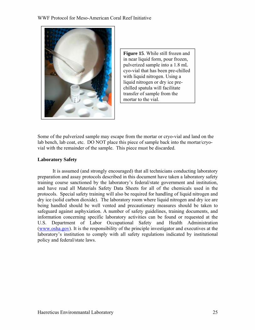
WWF Protocol for Meso-American Coral Reef Initiative
Haereticus Environmantal Laboratory 25
Some of the pulverized sample may escape from the mortar or cryo-vial and land on the lab bench, lab coat, etc. DO NOT place this piece of sample back into the mortar/cryo-vial with the remainder of the sample. This piece must be discarded. Laboratory Safety
It is assumed (and strongly encouraged) that all technicians conducting laboratory preparation and assay protocols described in this document have taken a laboratory safety training course sanctioned by the laboratory’s federal/state government and institution, and have read all Materials Safety Data Sheets for all of the chemicals used in the protocols. Special safety training will also be required for handling of liquid nitrogen and dry ice (solid carbon dioxide). The laboratory room where liquid nitrogen and dry ice are being handled should be well vented and precautionary measures should be taken to safeguard against asphyxiation. A number of safety guidelines, training documents, and information concerning specific laboratory activities can be found or requested at the U.S. Department of Labor Occupational Safety and Health Administration (www.osha.gov). It is the responsibility of the principle investigator and executives at the laboratory’s institution to comply with all safety regulations indicated by institutional policy and federal/state laws.
Figure 15. While still frozen and in near liquid form, pour frozen, pulverized sample into a 1.8 mL cyo-vial that has been pre-chilled with liquid nitrogen. Using a liquid nitrogen or dry ice pre-chilled spatula will facilitate transfer of sample from the mortar to the vial.

WWF Protocol for Meso-American Coral Reef Initiative
Haereticus Environmantal Laboratory 26
Chapter 2: Sample preparation and assays for biomarker analyses
2.1 Sample preparation and protocol criteria for ELISA
This document is not meant to introduce and instruct the novice laboratory technician. It is assumed that the technician has a minimal amount of education and training in biochemistry and molecular biology and has the ability to solve issues (trouble-shoot) concerning sample preparation and assay protocols. The purpose of Chapter 3 is to provide a basis for standardization of biomarker end-points used in the MAR study area as well as standardization of assay protocols. This document also assumes a level of competence in making diagnostic interpretations for the results of any of these biomarkers. Use of biomarkers should be conducted within a diagnostic context. It is beyond the scope of this document for the proper training and education in the theory of cellular diagnostics and biomarkers. 2.1.1 Homogenization of sample in Denaturing Buffer
1. Within two hours of commencing the homogenization of samples, prepare the Denaturing Buffer fresh, using the solid form of each ingredient, not a previous solubilized form of the ingredient.
2. All glassware, spatulas, and Teflon-coated magnetic stirrers should be cleaned
with Liquid Nox detergent and thoroughly rinsed with distilled water.
3. In a 50 mL Pyrex bottle, make up a 100 mM stock solution of Disodium ethylenediaminetetraacetate (EDTA). First add 25 mL of distilled water to the vessel, then a teflon-coated magnetic stir bar. Then add 1.86 grams of disodium EDTA. Slowly titrate with 4 M sodium hydroxide (NaOH) and monitor the pH of the solution with a pH meter. The final pH of the solution when all of the EDTA is dissolved will be about 8.0. Solubilizing by titration for this amount of EDTA should take about 10 minutes. This solution of EDTA should be good for about two weeks if kept at 4°C.
2.1.1 Sample homogenization
2.1.2 Phase partitioning
2.1.3 Protein concentration
2.1.4 ELISA

WWF Protocol for Meso-American Coral Reef Initiative
Haereticus Environmantal Laboratory 27
4. In a 15 mL polypropylene Falcon tube, add 0.138 grams of salicylic acid. Then
add 10 mL of distilled water to the tube, and mix until dissolved. This is a 10 mM solution of salicylic acid.
5. To a 100 mL Pyrex flask or Pyrex bottle, add 25 mL of distilled water.
6. To the vessel with water in it, add a small Teflon-coated magnetic stir bar. Place
vessel on magnetic stirrer.
7. To the vessel, add 0.48 grams of tris base (also known as Trizma base).
8. To the vessel, add 8 mL of 100 mM EDTA solution to the vessel.
9. To the vessel, add 0.185 grams of fresh dithiothreitol (DTT).
10. To the vessel, add 800 microliters of 10 mM salicylic acid solution.
11. Once the tris, salicylic acid, and DTT have been dissolved, titrate the solution to pH 7.8 using 3 N hydrochloric acid (HCl).
12. Add 1.6 grams of sodium dodecyl sulfate from a bottle purchased within the last
three months and has not been opened for more than five days.
13. To the vessel, add 800 microliters of dimethyl sulfoxide.
14. To the vessel, add 0.0015 grams of D-sorbitol.
15. If working with coral samples, add 2.4 grams of polyvinylpolypyrrolidone (PVPP) to the vessel.
16. Allow the solution to mix on the magnetic stirrer for about 15 minutes at a
temperature above 23°C.
17. Label your locking 2.0 mL microcentrifuge with the appropriate sample identification.
18. Purchase a protease inhibitor cocktail solution from any reputable commercial
source. The protease cocktail should contain the following ingredient and have a minimal stock concentration: 0.4 mM Bestatin, 0.1 mM E-64, 2 mM phenylmethylsulfonyl fluoride, 2 mM benzamidine, 5 mM a-amino-caproic acid, and 1 µg/100 µL pepstatin A.
19. Add 10-20 microliters of the protease inhibitor cocktail solution to the inside of
the open lid that caps the microcentrifuge tube. This location is on the side of the lid that closes within the microcentrifuge tube.

WWF Protocol for Meso-American Coral Reef Initiative
Haereticus Environmantal Laboratory 28
20. For each species, the volume or weight of the frozen ground sample powder that
will be homogenized in the microcentrifuge tube must be experimentally determined. The final total soluble protein concentration of the sample should not be more than 2 mg/ml and should not be less than 0.125 mg/mL.
21. Add the appropriate volume/weight of frozen powdered sample to the locking
microcentrifuge tube using a pre-chilled spatula (Figure 16).
22. Add 1,700 microliters of fresh denaturing buffer in which the PVPP has been maintained in a equally distributed, suspended state in the buffer.
23. Close the lid on the microcentrifuge tube and lock the lid.
24. Vortex the tube with a mechanical vortex for about 20 seconds (Figure 17).
25. Incubate the tube in a temperature-controlled metal block or water bath that is set
at 93°C for three minutes.
26. Vortex the sample tube for about 20 seconds.
27. Incubate the tube at 93°C for three minutes.
28. Set the tube out on the bench and allow cooling to room temperature (e.g., 25-28°C) for about 10 minutes.
Figure 16. Remove frozen, pulverized sample from cryo-vial with a pre-chilled spatula. Place sample on spatula into a locking microcentrifuge tube. Photograph courtesy of Phillip Dustan.

WWF Protocol for Meso-American Coral Reef Initiative
Haereticus Environmantal Laboratory 29
2.1.2 Phase partitioning of sample by centrifugation
1. Place the microcentrifuge tube into a microcentrifuge and centrifuge the tube at
about 12,000 g or higher for 10 minutes. 2. Three phases will be evident after centrifugation: the bottom phase is the
insoluble phase consisting predominantly of coralline skeleton, extra-cellular matrix, other insoluble tissue material and PVPP (Figure 18). The middle phase should be transparent, brownish (coral, conch) or reddish (fish) in color, and free of a whitish film that characterizes the top phase. The top phase is a very viscous matrix composed predominantly of cross-linked polysaccharides and fats.
3. Aspirate 200-300 µL of the middle phase; be careful not to collect any supernatant that may be contaminated with the whitish matrix that is the top phase.
4. Deposit the middle-phase supernatant into a new tube that is labeled with the same identification.
Figure 18. Three phases are formed after centrifugation of the sample. The bottom phase is insoluble debris, primarily calcium carbonate skeleton and insoluble PVPP. The middle phase should be relatively transparent and should be absent of residual mucus. It should be non-viscous. The top phase should be somewhat viscous and sticky, whitish in color. The demarcation between the middle and top phase is not always apparent, and care should be taken that when aspirating the middle phase, there should be no contamination from the top-phase matrix. From Downs, C.A. (2005) Cellular Diagnostics and its application to aquatic and marine toxicology. In: Techniques in Aquatic Toxicology, vol. 2: G. Ostrander (ed). CRC Press, Inc. Boca Raton, Florida. Pp 181-208.
Figure 17. Before 93°C incubation and after the third minute of incubating at 93°C, vortex the sample for about 20 seconds, insuring thorough mixing of the sample with the Denaturing Buffer. Photograph courtesy of Phillip Dustan.

WWF Protocol for Meso-American Coral Reef Initiative
Haereticus Environmantal Laboratory 30
2.1.3 Total soluble protein concentration determination of a sample Lowry-based, bicinchoninic acid-based, and coomassie blue-based spectrophotometic protein concentration assays cannot be used to determine the protein concentration in the samples because the concentrations for many of the components in the Denaturing Buffer will cause significant artifact for these assays. An alternative assay platform was developed by Dr. Sibdas Ghosh in the late 1980s to overcome interfering substances from plants (e.g., chlorophyll, xanthophylls) that used cuvette-based spectrophotometric protocols. This assay was later modified by Ghosh and Downs in the mid-1990s to account for high concentrations of dithiothreitol and sodium dodecyl sulfate in the Denaturing Buffer which significantly interferes with both copper and silver dyes from binding to proteins.
1. Two solutions should be made: Stain Solution and a Destain Solution. The recipe for both solutions are:
Stain Solution: • 200 mL of distilled water • 50 mL of glacial acetic acid • 250 mL of methanol • 4 g of Coomassie Blue RR 250
Destain Solution:
• 800 mL distilled water • 200 mL of glacial acetic acid • 1000 mL of methanol
Make each solution in a pyrex bottle with a plastic lid. The staining solution has a shelf life of about 20 days. The destain solution has a shelf life of about four months. Be careful with both solutions and conduct this assay in a well-ventilated area or under a chemical hood. Methanol is a cumulative poison. Inhalation of the vapors of both solutions should be avoided.
2. Place clean lab mat down on in the area on the lab bench where you will be conducting the protein concentration assay.
3. Wearing latex or nitrile gloves, take a piece of Whatman #5 filter paper using
forceps and the filter paper on the clean lab mat. Whatman filter paper disks that are 9 cm to 11 cm are the best to use.
4. With a #2 pencil, mark the filter paper indicating the location of the standards,
placement of the samples, and the identification of the project and the date, similar to that in Figure 19.
5. Using a 1-20 uL pippettor, place 1 uL of sample and standard in an ordered
fashion as indicated by the sample locations marked with pencil. Standards and samples should be spotted on the Whatman filter paper in triplicate (Figure 19).

WWF Protocol for Meso-American Coral Reef Initiative
Haereticus Environmantal Laboratory 31
The pipette tip should be changed for a new tip between spotting each sample and each standard. You can use the same tip for spotting the triplicate sample spots.
6. Allow the filter paper to air dry for about 20 minutes. You can accelerate the
drying process by using a hair dryer to dry the filter paper. Use forceps to hold the filter paper in place while using the hair dryer. Do not use your fingers.
7. Once dried, place the filter paper in an incubation boat that contains enough Stain
Solution to completely cover the filter paper.
8. Place the incubation boat on a rocker platform or hand agitate for 10 minutes (Figure 20).
9. After the 10 minute incubation, pour the Stain Solution back into its bottle.
10. Wash the filter paper with about 20 mL of Destain Solution. Decant the Destain
Solution into the sink or into the proper waste receptacle.
11. Incubate the filter paper in about 30 mL of Destain Solution for about five minutes, and then decant the Destain Solution. Repeat this procedure until the non-spotted filter paper is white (Figure 21).
12. Gently wash the filter paper in distilled water, then allow to incubate in water for
two minutes on the rocking platform or by hand agitation. This will remove the overwhelming smell of the acetic acid and allow the filter paper to be placed in the laboratory notebook.
13. Once the filter paper is dried, it can be scanned into a digital image by a scanner.
Optical densities for each replicate can be determined using a densitometry program such as NIH Image developed at the U.S. National Institutes of Health and available on the Internet at http://rsb.info.nih.gov/nih-image/.
Figure 19. Protein Concentration Assay. Results of protein concentration assay using a modified method of Ghosh et al. (1988). Concentration calibrants are plated on the Whatman No. 5 filter paper as in Columns A - E. Column A = 0.125 µg/µL. Column B = 0.250 µg/µL. Column C = 0.5 µg/µL. Column D = 1.0 µg/µL. Column E = 2.0 µg/µL. Samples done in triplicate indicated in columns 1-3. All calibrants and samples are plated (hence assayed) on the filter paper in triplicate. Assay paper can be scanned by a scanner to create a digital image. Optical densities for each replicate can be determined using a densitometry program such as NIH Image developed at the U.S. National Institutes of Health and available on the Internet at http://rsb.info.nih.gov/nih-image/. From Downs, C.A. (2005) Cellular Diagnostics and its application to aquatic and marine toxicology. In: Techniques in Aquatic Toxicology, vol. 2: G. Ostrander (ed). CRC Press, Inc. Boca Raton, Florida. Pp 181-208.

WWF Protocol for Meso-American Coral Reef Initiative
Haereticus Environmantal Laboratory 32
Once the protein concentration assay is done, Denatured Buffer-extracted samples can be frozen. The best temperature to preserve the samples is -80°C or colder. The samples can only be thawed once, so if you plan to conduct your ELISAs for more than a one-day time period, you need to aliquot the samples into new tubes so that a single tube can be removed from cold storage only once according to your work schedule. 2.1.4. Enzyme Linked Immuno-sorbent Assay (ELISA) There are a number of different ELISA methods that can be used. This document does not advocate a specific method, but only methods that have a measure of validation and quality control. Before an ELISA is run on a sample or a set of samples, the antibodies and solution reagents need to be optimized and validated. This should include, at the very least, testing of the samples and the reagents using an SDS-polyacrylamide gel electrophoresis (PAGE) and western-blotting assessment system. A detailed description of SDS-PAGE and western blotting for validation of the ELISA system can be found in Downs, C.A. (2005) Cellular Diagnostics and its application to aquatic and marine
Figure 20. Incubate the filter paper in an incubation boat. The boat can be anything: e.g., petri dish or weigh boat, and be made from plastic or glass. Stain solution should cover the filter paper either in its entirety or so that each rocking slant covers at least 50% of the filter paper in the Stain Solution.
Figure 21. There should be a distinct contrast between the blue of the sample and standard spots and the rest of the filter paper. The area of the filter paper that has not been spotted should be white. Be careful! It is possible to over destain the filter paper.

WWF Protocol for Meso-American Coral Reef Initiative
Haereticus Environmantal Laboratory 33
toxicology. In: Techniques in Aquatic Toxicology, vol. 2: G. Ostrander (ed). CRC Press, Inc. Boca Raton, Florida. Pp 181-208. Besides validation of the antibody and the ELISA reagents, SDS-PAGE/western blotting also helps in determining the integrity of the sample. Oftentimes, artifacts can befall a set of samples as a result of insufficient protease inhibition during the homogenization of the sample, freeze/thaw exclusion of SDS from proteins which results in protein aggregation, and adduction of target proteins with secondary compounds resulting in masking of epitopes and/or polymerization of heterogeneous protein species.
One of the least expensive methods to conduct an ELISA is a Dot-Blot/Direct ELISA method. A protocol for this method can be found Downs, C.A. (2005) Cellular Diagnostics and its application to aquatic and marine toxicology. In: Techniques in Aquatic Toxicology, vol. 2: G. Ostrander (ed). CRC Press, Inc. Boca Raton, Florida. Pp 181-208. This method requires a primary and secondary antibody. The secondary antibody can be conjugated to any number of different reporter enzymes that catalyze a colorimetric or chemiluminescent signal. Alternatively, the secondary antibody can also be conjugated with a fluorescent probe that can be used in a fluorescence detection system. The least expensive is a secondary antibody conjugated to either alkaline phosphatase or horseradish peroxidase that uses nitroblue tetrazolium and an electron donor compound. Samples and the standard calibrant curve should be replicated in triplicate (Figure 22). A five-point calibration curve should at least be used, especially when examining biomarkers such as heat-shock proteins and cellular damage products. These end-points can often have concentration differences of several fold to an order of magnitude.
A second type of ELISA method uses a polystyrene, 96-well microtiter plate.
This method often requires a microplate washer instrument and a microplate reader instrument. Samples and calibrant standards can be configured the same way as the dot-blot ELISA system (Figure 23). A good methodology resource for this ELISA method can be found in Crowther, J.R. (2001) The ELISA Guidebook: Methods in Molecular Biology. Humana Press. Totowa, New Jersey.
Figure 22. ELISA result using a 96-well dot blotter. # = calibrant standard curve. The calibrant with the highest concentration is plated in row 1, the calibrant with the lowest concentration is plated in row 8. Optimally, replicates of the standard curve should be evenly distributed across the dot blotter. In row 1, triplicate assays of sample 1, 9, 17. In row 2, triplicate assays of sample 2, 10, 19. In row 3, etc. In column a, replicate one of sample 1, 2, 3, etc... are plated. In column b, replicate two of samples 1, 2, 3, etc… are plated. In column c, replicate three of samples 1, 2, 3, etc… are plated. Plate represents data for the chloroplast small heat-shock protein in samples of the hard coral, Montastrea annularis.

WWF Protocol for Meso-American Coral Reef Initiative
Haereticus Environmantal Laboratory 34
It should be recognized that ELISA is based on the kinetic characteristics of its components (e.g., binding of sample to solid phase, primary antibody binding to target protein, secondary antibody binding to primary antibody, washes, etc.). Because of the nature of this assay platform, conducting an ELISA should not be conducted like a “cook book” exercise. Each step requires optimization to ensure consistency in assay repetition, confidence in raw data generation, and consistency for inter-laboratory assessment and validation. This optimization can only be done experimentally. 2.1.5 ELISA end-points (biomarkers) for grunt, conch, and coral samples The biomarkers in this section have been selected because changes in their concentration indicate a significant change in the physiological condition of an organism or a specific homeostatic response of that organism to environmental conditions. It must be cautioned that the life history of a specific organism/population must be considered when making a diagnostic interpretation using any of these biomarkers. For example, sampling during the reproductive season or mating season of an organism may produce a biomarker result that is determined, in part, not only by environmental conditions, but also because of life history conditions. The age of the organism may also influence biomarker results. A wise sampling assessment and monitoring design can overcome these hurdles: for example, collecting samples that are of the same age, or sampling a population outside of its spawning season. Another important issue that must be addressed is establishing a normal range for a biomarker. A “normal range” can be defined as the concentration or activity of a biomarker that can be found in a population that is in a physiologically healthy condition, or a homeostatic condition that is not responding to a stressor. Determining and defining the “normal range” can be accomplished by incorporating a reference population within the assessment or monitoring design. Criteria for a reference population may be based on aspects of physiological performance and environmental conditions. For example, a potentially good candidate reference population should possess a level of reproductive fitness that can sustain the population. Disease incidence should be relatively low.
1 2 31 2 3 Figure 23. ELISA result using a 96-well microtiter plate. 1,2,3 = calibrant standard curve. The calibrant with the highest concentration is plated in row 1, the calibrant with the lowest concentration is plated in row 8. Optimally, replicates of the standard curve should be evenly distributed across the microtiter plate. The three wells that are circled are the triplicate of sample #17. The detection system used here is based on a chemiluminescent reporter system. This is the most sensitive detection system you can use; The lower calibrant-curve detection limits are often in the range of 1 to 400 picomoles for a target.

WWF Protocol for Meso-American Coral Reef Initiative
Haereticus Environmantal Laboratory 35
Environmental conditions should be consistent with a habitat that has historically sustained populations. The ELISA biomarkers presented in this document include:
• Ubiquitin • Multiple Drug/Xenobiotic Resistance Protein • Cytochrome P450 2-class Proteins • Invertebrate Small Heat-shock Proteins (for corals and conch) • Fish Small Heat-shock Protein • Metallothionein • Cytochrome P450 6-class Proteins (invertebrates only)
A display in the levels of these biomarkers outside of their established normal range indicates a significant change in the physiological condition or homeostatic response of the organism/population. Any one of these biomarkers examined by itself, or with consideration of the any of the other ELISA-based biomarkers described in this section, is not meant to establish an etiology of pathology. These biomarkers are meant to be used as harbingers of physiological and population change if the organism/population remain in a persistent condition. Ubiquitin – This end-point can be assessed in all three target species most likely using the same antibody source. This is because of the extreme conservation of this polypeptide and its ubiquitous presence and function in all eukaryotes. Ubiquitin is a 76-residue protein found in most phyla of life and used in a process for marking proteins for rapid degradation (Hershko and Ciechanover, 1998. The ubiquitin system. Annu Rev Biochem 67: 425-479.). Ubiquinated proteins are degraded by proteolytic enzymes known as proteosomes (Hershko and Ciechanover, 1998. The ubiquitin system. Annu Rev Biochem 67: 425-479.). Proteins, during stress, are targeted for degradation usually because these proteins have undergone an irreversible denaturation (Iwai, K. 1999. Roles of the ubiquitin system in stress response. Tanpakushitsu Kakusan Kuso 44: 759-765). Increases in ubiquitin levels are an indication of increased levels of protein degradation, and hence, increased protein turnover (Goff et al., 1988. Protein breakdown and the heat-shock response. In Ubiquitin (ed. M. Rechsteiner). New York, NY: Plenum Press: 207-238.). Consequently, to compensate for decreased functional protein levels due to stress, the cell will increase production of these same proteins (Iwai, 1999). Thus, measurement of levels of ubiquitin is an index of the structural integrity of the protein component of the superstructure of the cell (Mimnaugh et al., 1999. The measurement of ubiquitin and ubiquinated proteins. Electrophoresis 20: 418-428). Increased ubiquitin levels above a normalized range indicates: (1) a protein denaturing stress is occurring; (2) increased expenditure of energy is required to compensate for this stressed-induced protein turnover; and (3) in comparison to baseline data of this parameter for a particular species, may act as an indicator of individual fitness (Hawkins, 1991. Protein turnover: a functional appraisal. Funct Ecol 5: 222-233).

WWF Protocol for Meso-American Coral Reef Initiative
Haereticus Environmantal Laboratory 36
For this assay, it is important to use an antibody that can recognize the ubiquitin monomer and polyubiquinated chains. Without this type of recognition, detecting changes in ubiquitin equilibrium may not be possible. Antibody to ubiquitin and purified ubiquitin can be purchased from over half-dozen commercial sources (e.g., Sigma-Aldrich). Multiple Drug/Xenobiotic Resistance Protein (ABC family of proteins) – This end-point will be measured in all three target species most likely using the same antibody source. This is because of the extreme conservation of this protein’s primary structure, function and its ubiquitous presence and function in all eukaryotes. P-glycoprotein plays a role in removing xenobiotics and toxins from the cell by acting to transfer intracellular xenobitics and toxins across the cytoplasmic membrane. Sustained exposure to certain xenobiotics causes an increase in the cellular level of P-glycoproteins. Animals deficient in P-glycoproteins are viable and do not exhibit any obvious abnormalities. The pharmokinetic activity and relative toxicity of several compounds are, however, altered in these P-glycoprotein-deficient animals. For example, P-glycoprotein in mammals plays a significant role in preventing certain xenobiotics from crossing the blood-brain barrier: a decrease in P-glycoproteins would result in an increase in the amount of xenobiotics reaching the brain. P-glycoproteins are members of a superfamily of proteins called the adenosine triphosphate binding cassette that act as channels and transporters of solutes across membranes. Induction of certain P-glycoproteins indicates a response to xenobiotic exposure. See Ueda et al., (1999). Comparative aspects of the function and mechanism of SUR1 and MDR1 proteins. Biochem. Biophys. Acta 1461: 305-313; Borst et al., (1999). The multidrug resistance protein family. Biochem. Biophys. Acta 1461: 347-357; Bard (2000) Multixenobiotic resistance as a cellular defense mechanism in aquatic organisms: a review. Aqua. Toxicol. 48: 357-389. A simplified interpretation for this biomarker is that if levels of this protein increase, it may mean that the organism is responding to an exposure of a xenobiotic or a toxin. As always, there are a number of caveats: some xenobiotics do not elicit an increase in P-glycoprotein levels, such as mercury. Cytochrome P450 2 homologue (CYP P450-2) – An antibody that cross-reacts with the mammalian homologue of cytochrome P450 2-class, but not CYP 1-class or CYP 3-class can be used to measure the accumulation of an antigenically similar CYPs in the three target species. Cytochrome P450 2-class enzymes are known to specifically oxidize ethanol to acetaldehyde via a monooxygenase mechanism, as well as other xenobiotics such as imidazole-based derivatives (Lieber, 1997. Cytochrome P-4502E1: its physiological and pathological role. Physiol Rev 77: 517-544). Cytochrome P450 2-class has both physiologically relevant oxidative and reductive reactions and is known to associate and catalyze as many as 60 xenobiotic-based substrates (Lieber, 1997). For example, it causes the demethylation of N, N-dimethylnitrosamine and the hydroxylation of p-nitrophenol and chlorzoxazone (Koop, 1992. Oxidative and reductive
Figure 24. Cytochrome P450 2-class from the liver of White Grunt

WWF Protocol for Meso-American Coral Reef Initiative
Haereticus Environmantal Laboratory 37
metabolism by cytochrome P450 2E1. FASEB J 6: 724-730). Reduction reactions include reduction of a number of different lipid types. This enzyme homologue is conserved in all three target species, though the function may be less conserved. This enzyme is known to be induced in all three species by a variety of crop protection products. This is not to say that these enzyme homologues function by detoxifying these crop protection products, though in some species they may play a central role in Phase I of Xenobiotic Transformation (e.g., Hanioka, N., Jinno, H., Tanaka-Kagawa, T., Nishimura, T., Ando, M., and Ogawa, K. 1998. In vitro biotransformation of atrazine by rat liver microsomal cytochrome P450 enzymes. Chem Biol Interact 116:181–198). Changes in the expression level from the nominal range for this biomarker indicate a changed physiological response, especially a changed endocrine and metabolic condition. Antibody to cytochrome P450 2-class is readily available from a number of commercial sources. Alternatively, this enzyme can oftentimes be assessed by enzymatic activity. Several commercial sources provide protocols and kinetic assay kits to analyze enzymatic activity. In-house production for an antibody against CYP P450 2-class homologues is also straightforward since this enzyme has three evolutionarily conserved domains that define this class of enzyme. Invertebrate sHsp (total small heat-shock protein isoforms) – This biomarker would only be used for the invertebrate target species, not for the grunt. αB-crystallin, Hsp22, Hsp23, Hsp26, and Hsp28 share domains of common homology to one another, but have different cellular functions (de Jong et al., 1993). In bivalves, as many as 5-6 major sHsp isoforms exist. Small Hsps from all phyla share a common motif near the carboxyl-terminal end of the protein, known as the “heat-shock domain” or α-crystallin domain (de Jong et al., 1993). Other areas of these proteins are not homologous and are specific to the sub-family of sHsps. In most cases, the small heat-shock proteins are not present during optimal growing conditions and are only elicited by stress (de Jong et al., 1993).αB-crystallin is a small heat-shock protein found only in the cytosol of animals, where it protects cytoskeletal elements during stress (Derham and Harding, 1999). Evidence indicates that Hsp22 localizes to neural-type cells and follicular cells in Drosophila melanogaster. Furthermore, this protein localizes to the mitochondria in arthropods and has been suggested to have a functional role similar to that of plant and mammalian mitochondrial sHsps (Downs & Heckathorn, 1998; Downs et al., 1999a). Thus, the presence and concentration of different small heat-shock proteins reflects the physiological status of several metabolic and structural pathways in the cell. In this study, it can be used as an indicator of a severe stress response. One caveat for this biomarker is that it has been shown to be expressed during spawning and at key
Figure 25. Invertebrate small heat-shock proteins 30 µg of total soluble protein from ribbed mussel * = multimeric structure
a = Hsp28 b = Hsp25W or Hsp26 c = Hsp23 d = Hsp22

WWF Protocol for Meso-American Coral Reef Initiative
Haereticus Environmantal Laboratory 38
stages of early development – extremely stressful events in-and-of themselves. Care should be taken not to sample target species during these developmental stages. Fish small heat shock protein – This biomarker could only be used for a fish species. Like the invertebrate small heat-shock proteins, this protein is usually induced only as a result of severe cellular stress. Less is known about the function of this protein as compared to other heat-shock proteins. Antibody for this protein will need to be manufactured “in-house” by the laboratory that is running this assay. The sequence to this gene is known from a number of species of fish and the epitope can be made against an evolutionarily conserved sequence in the carboxyl-terminal end of the protein known as the “crystalline” domain. This protein is usually absent during normal physiological conditions and is usually induced under extremely stressed conditions. Detection or an increased accumulation of this protein may signify that the population/individual is under metabolic duress. White CN, Hightower LE, Schultz RJ. 1994. Variation in heat-shock proteins among species of desert fishes (Poeciliidae, Poeciliopsis). Mol Biol Evol. 11(1):106-19.
Metallothionein – Metallothionein is often used as a biomarker of heavy metal exposure, though it is argued that this may be a misuse of this biomarker (e.g., Aspholm and Hylland, 1998; Soazig and Mark, 2003; Galloway et al., 2004). In the context of cellular diagnosis, changes in metallothionein levels can be interpreted as an indicator of broad changes in mitochondrial functional equilibrium. This position is based on recent work demonstrating that metallothionein type 1 localizes to the inter-membrane space of mitochondria and can regulate oxidative phosphorylation (Simpkins et al., 1994; Ye et al., 2001). Studies showing the interaction of zinc, metallothionein, and mitochondrial function further support the role of metallothionein as a regulator of cellular energy production and redox state (Maret, 2000; Coyle et al., 2003; Maret, 2003). This interpretation is further justified by toxicology studies with cadmium and metallothionein that demonstrate the interaction between cadmium and zinc metallothionein and mitochondrial dysfunction (e.g., Simpkins et al., 1998a; Klassen et al., 1999; Tang and Shaikh, 2001). Metallothionein can be induced by a number of different stressors, for example chronic oxidative stress; metallothionein gene expression in fish can be induced by exposure to chlorinated aromatic hydrocarbons (Gerpe et al., 1998).
Metallothionein gene sequences are known from a number of invertebrate species (including gastropods and cnidarians) and from more than 15 species of fish. Gene sequence can be aligned for the target phylum and be used to create an antigen that can be immunized into a host for antibody production (Figure 26).
Figure 26. Metallothionein Lane 1: 30 ug of total soluble protein from control Mytilus edulitus. Lane 2: 30 ug of total soluble proteim from Mytilus edulitus exposed to 50 uM CdCl2 for eight hours. Two-three bands appear, depending on the type of metal exposure. Detects novel copper-inducible isoform.

WWF Protocol for Meso-American Coral Reef Initiative
Haereticus Environmantal Laboratory 39
Figure 27. CYP P450-3 from liver of White Grunt
A simplified interpretation for this biomarker is that levels of this protein outside the nominal range for this organism indicate a homeostatic response to maintain mitochondrial oxidative phosphorylation equilibrium. This marker should not be used as a biomarker of exposure to heavy metals. Cytochrome P450 3 homologue (CYP P450-3) – An antibody that cross-reacts with the homologue of cytochrome P450 3, but not CYP 1A, CYP 2 or CYP 6 classes can be used to measure the accumulation of an antigenically similar CYP in all three target species. Cytochrome P450 3 homologues are known to play a role in steroidal biogenesis and porphryn metabolism. Induction of CYP P450-3 is oftentimes associated with cellular xenobiotic response. This may be true, but alterations in the accumulation and activity of this enzyme class can also result from changes in cellular demand for porphyrins and for steroid metabolism. The value of CYP P450-3 may not always be associated with it being a “biomarker of exposure”, but as a biomarker of effect. An antibody against CYP P450-3 homologues can be obtained from a number of commercial sources, but should be validated for each of the target species. Several polyclonal antibodies from at least three different commercial sources were tested by the author and found to work in all three of the target species. A simplified interpretation for this biomarker is that if levels are beyond the nominal range, this indicates a change in the endocrine and metabolic condition of the organism. Oftentimes, an increase in the level of this protein is associated with an organic-based xenobiotic exposure. Cytochrome P450 6 homologue (CYP P450-6) – This enzyme is specific to invertebrates and is recognized as a major contributor to insecticide resistance (Scott JG, Wen Z. 2001. Cytochrome P450 of insects: the tip of the iceberg. Pest Mang. Sci. 57:958-967). This class of CYP P450s is known to oxidize and be up-regulated by pesticides such as aldrin, dieldrin, diazinon, chlorpyrifos, deltamethrin, and a wide range of pyrethrin-like compounds. This enzyme has been used as both a biomarker of exposure and as a biomarker of effect. Assaying for this biomarker can only be done with coral and conch, not with White Grunt since vertebrates are not known to have this enzyme class. A simplified interpretation for this marker is that if levels of this protein are higher than the nominal range, this organism is potentially responding to a specific class of pesticides. Decrease of this protein below the nominal range may indicate a compromised metabolic condition.
Figure 28. CYP P450 6 class. From MontastreaAnnularis Courtesy: U.S. NOAA

WWF Protocol for Meso-American Coral Reef Initiative
Haereticus Environmantal Laboratory 40
2.2. Non-ELISA-based Biomarker Assays The following biomarkers are non-ELISA-based assays and will require additional equipment, different sample homogenization and preparation procedures, and different methods for detection. Like the ELISA-based biomarkers, these biomarkers display a dynamic quantitative range, and that the levels of these biomarkers outside of their established normal range indicate a significant change in the physiological condition or homeostatic response of the organism/population. Any one of these biomarkers examined by itself, or with consideration of the any of the other ELISA-based and non-ELISA-based biomarkers described in this section, is not meant to establish an etiology of pathology. These biomarkers are meant to be used as harbingers of physiological and population change if the organisms remain in a persistent condition. 2.2.1. Porphyria Species Assay Materials
• Fluorescent 96-well microplate reader or a spectrofluorospectrophotometer • Multichannel pipettor, 20-200 microliters • Single channel pipettor set • 3 N hydrochloric acid • Black-walled 96-well microtiter plates • Uroporhyrin standard (Porphyrin Products, Inc., Logan, Utah, U.S.A.) • Ethyl acetate (99% purity) • Sodium dodecyl sulfate • Trizma base • Sodium dodecyl sulfate
Porphyrins are prosthetic structures usually associated with proteins that contain a metal for functionality (Figure 29). A porphryin with an iron in it is heme. A porphyrin with a phytol chain and a manganese atom is chlorophyll. The porphyrin synthesis pathway begins in the cytosol and concludes within the mitochondria (Figure 30). At least six different enzymes are directly involved in the porphyrin synthesis pathway. Each one of these enzyme expresses differential sensitivity to the inhibitory power of environmental contaminants, such as heavy-metals, organochlorine compounds, organophosphorous compounds, and polycyclic aromatic hydrocarbons. A porphyrin synthesis enzyme inhibited by a toxicant results in the accumulation of precursor porphryn species. Accumulation of these precursors can lead to pathological effects - porphyria. Measurement of porphyria species is a classical clinical diagnostic test with straightforward diagnostic interpretation. Measurement of porphyrin-precursor (porphyria) species can be conducted in almost any coral reef species with little modification to the method. This method measures total porphyrin precursors and is unable to distinguish which porphyrin species is accumulating.
The method can be validly conducted using two protocols. The first method capitalized on the sample preparation conducted for ELISA. The second method can be employed on a sample independent of the ELISA-sample-preparation protocol. Both

WWF Protocol for Meso-American Coral Reef Initiative
Haereticus Environmantal Laboratory 41
methods should be conducted under dimmed light or a red light. Direct sunlight needs to be excluded from the laboratory. Concentration of Total Porphyria Species using ELISA sample preparation
1. One-hundred and fifty micrograms of total soluble protein from sample
supernatants prepared in Section 3.1.1. are diluted in a solution containing 1% SDS, Tris-HCl (pH 7.8), 5 mM EDTA into a volume of 310 microliters.
2. Dispense one-hundred microliter aliquots of each sample in triplicate to a clear-
bottom with black walls 96-well microtiter plate.
3. Dispense 50 uL of 3 N hydrochloric acid into each sample well.
4. Place plate in a container that exclude light and allow incubation for fifteen minutes.
5. Mix the contents in each sample well by gently rocking the plate.
6. Uroporphyrin standards can be obtained from Porphyrin Products (Logan, Utah,
U.S.A.), and diluted using an 8-point calibrant standard curve from 0 pmole of protoporphyrin to 1000 pmole of uroporphyrin. Dispense standard on the micro-titer plate in triplicate using a format similar to Figure 23.
7. Detect fluorescence signal using a fluorescent/luminescent microplate reader with
the excitation filter set for 405 nm and the emission filter set for 610 nm. Band length for both excitation and emission filter should be less than ±20 nm.
Figure 29. A precursor porphyrin species
Figure 30. Schematic of the porphyrin/heme synthesis pathway. Courtesy of medlib.med.utah.edu/ NetBiochem/hi3.htm

WWF Protocol for Meso-American Coral Reef Initiative
Haereticus Environmantal Laboratory 42
Concentration of Total Porphyria Species using ethyl acetate extraction
1. Take about 40 microliters of frozen sample powder from the sample cryovial using a pre-chilled spatula and place into a locking microcentrifuge tube.
2. Add 700 microliters of 99% pure ethyl acetate.
3. Vortex sample for about two minutes until semi-homogenized.
4. Add 700 microliters of 3 N hydrochloric acid to the sample tube.
5. Vortex sample for about two minutes.
6. Incubate in dark for five minutes
7. Vortex sample for one minute.
8. Centrifuge sample at 12,000 g or higher for five minutes.
9. Aspirate the acidified phase from the tube and place in a new tube. This volume
should be about 400 microliters. You will need to determine experimentally for your protocol which is the acidified phase. The acidified phase should be absent of any mucilage. Do not confuse the acidified phase with the ethyl acetate phase.
8. From the new tube, dispense one-hundred microliter aliquots of each sample in
triplicate to a clear-bottom with black walls 96-well microtiter plate. 9. Uroporphyrin standards can be obtained from Porphyrin Products (Logan, Utah,
U.S.A.), and diluted using an 8-point calibrant standard curve from 0 pmole of protoporphyrin to 1000 pmole of uroporphyrin. Dispense standard on the micro-titer plate in triplicate using a format similar to Figure 23.
10. Detect fluorescence signal using a fluorescent/luminescent microplate reader with
the excitation filter set for 405 nm and the emission filter set for 610 nm. Band length for both excitation and emission filter should be less than ±20 nm.
2.2.2 Ethoxyresorufin-O-deethylase (EROD) activity assay Materials
• Trizma Base • EDTA • Hydrochloric acid • Ethoxyresorufin • nicotinamide adenine dinucleotide phosphate, reduced form (NADPH) • acetonitrile

WWF Protocol for Meso-American Coral Reef Initiative
Haereticus Environmantal Laboratory 43
• Fluorescent microplate reader or spectrofluorophotometer
This biomarker can represent a number of different assessment end-points. In the literature, this biomarker is predominantly used as an end-point that reflects a receptor-mediated induction of cytochrome P450 mono-oxygenase activity. This putative receptor is usually identified as the aryl hydrocarbon receptor. This biomarker is also used as a “response indicator” to contaminant uptake; the contaminant most likely a hydrocarbon-based compound or mixture of compounds. Another value of the EROD assay is associated with its decline-in-activity behavior. A number of environmental contaminants and conditions can either inhibit enzyme activity directly or depress gene expression, potentially reducing protein expression of this enzyme. One caveat with this assay is that induction of EROD activity should not be confused with it being a reflection of toxicity. Activity may increase without any pathological symptoms. The catalysis of ethoxyresorufin by a cytochrome P450 monooxygenase action results in the production of resorufin – a compound that can be detected through spectrofluorimetric means (Figure 31). This biomarker should only be conducted in fish (White grunt). Though the assay has been tested in some invertebrate species, the EROD assay would need to undergo extensive validation in coral and conch. To derive the greatest sensitivity for the EROD assay, most protocols recommend purification of the microsomal fraction via differential sub-ultracentrifugation or ultra-centrifugation methods. Unfortunately, the microsomal integrity has been compromised as a result of the pulverization of the fish liver sample using the liquid nitrogen grinding technique. EROD activity is often normalized against total soluble protein of the microsomal fraction. Since this cannot be accomplished as a result of the initial sample preparation, EROD activity will be normalized against total soluble protein of liver tissue.
Ethoxyresorufin-O-deethylase (EROD) activity assay protocol Before conducting this protocol on the target species, the lab must conduct an optimization step before conducting this assay on field samples. Since the EROD assay is an enzymatic assay based on enzymatic kinetics, the Michaelis constant (Km) and maximum velocity (Vmax) must be determined for each species, since one cannot assume that the Km of EROD is the same for every species. This can be determined by keeping the total soluble protein of the sample constant while varying the substrate (ethoxyresorufin and NADPH) concentration. Final concentration of both substrates
Figure 31. Mechanism of catalysis of ethoxyresorufin to resorufin by Ethoxyresorufin-O-deethylase activity.

WWF Protocol for Meso-American Coral Reef Initiative
Haereticus Environmantal Laboratory 44
should be at least twice the Vmax concentration to account for varying concentrations of the field sample starting material. Kinetic behavior determination and kinetic modeling for EROD can be determined following principles set forth in Segal, I.H. 1975. Enzyme Kinetics: Behavior and Analysis of Rapid Equilibrium and Steady-State Enzyme Systems. John Wiley & Sons, Inc: New York, New York.
1. Add about 30 microliters of pulverized fish liver sample into a microcentrifuge tube.
2. Add 500 microliters of EROD buffer with is a solution of 50 mM Trizma base
and 20 mM EDTA that has been titrated to a pH of 7.8 with 1 M hydrochloric acid.
3. Vortex for 1 minute.
4. Add pre-determined volume of a fixed concentration of ethoxyresorufin solution
to the sample.
5. Vortex for 20 seconds.
6. Add pre-determined volume of a fixed concentration of NADPH solution to the sample.
7. Vortex for 20 seconds.
8. Incubate for sample to the experimentally determined time that equals the
catalysis of 25% of the available substrates.
9. Stop the reaction with 200 microliters of acetonitrile.
10. Centrifuge sample at 6,000 g for five minutes.
11. Aspirate one-hundred microliter aliquots of supernatant from each sample in triplicate to a clear-bottom with black walls 96-well microtiter plate.
12. Detect fluorescence signal using a fluorescent/luminescent microplate reader with
the excitation filter set for 530 nm and the emission filter set for 590 nm. Band length for both excitation and emission filter should be less than ±10 nm.
2.2.3. DNA Abasic quantitative lesion assay Materials:
• Multi-channel pipettor 20-200 microliter volume • Single-channel piepptors, 20-200 microliter & 100-1000 microliter • Double distilled water • N’-aminooxymethylcarbonylhydrazino-D-biotin

WWF Protocol for Meso-American Coral Reef Initiative
Haereticus Environmantal Laboratory 45
• Streptavidin conjugated to horseradish peroxidase • Luminol/hydrogen peroxide-based chemiluminescent solution or, • Horseradish peroxidase nitroblue tetrazolium dye • DNA AP quantitative standards • 96-well microplates • Spectrophotometric or luminescent/fluorescent 96-well microplate photometers
This system can also be purchased as a commercial kit for colormetric-based detection system from: Dojindo Molecular Technologies, Inc. 211 Perry Parkway, Suite 5 Gaithersburg, MD 20877 Phone: 301-987-2667 Fax: 301-987-2687 E-mail: [email protected] Web site: www.dojindo.com Dojindo Laboratories Kumamoto Techno Research Park 2025-5 Tabaru, Mashiki-machi, Kamimashiki-gun Kumamoto 861-2202, JAPAN Phone: +81-96-286-1515 Fax: +81-96-286-1525 E-mail: [email protected] Web site: www.dojindo.co.jp Copied with Permission from Dojindo Technologies, Inc, 2005. Oxidative damage to DNA is a result of the interaction of DNA with reactive oxygen species (ROS), in particular, the hydroxy radical which is converted from superoxide and hydrogen peroxide by the Fenton reaction. Hydroxy radicals produce a multiplicity of modifications in DNA. Oxidative attack by hydroxyl radical on the deoxyribose moiety will lead to the release of free bases from DNA, generating strand breaks with various sugar modifications and simple abasic sites (AP sites). In fact, AP sites are one of the major types of damage generated by ROS. It has been estimated that endogeneous ROS can result in about 2x10⁵ base lesions per cell per day. Aldehyde Reactive Probe (ARP) reagent (N’-aminooxymethylcarbonylhydrazino-D-biotin, Fig. 33) reacts specifically with an aldehyde group which is the open ring form of the AP sites. This reaction makes it possible to detect DNA modifications that result in the formation of an aldehyde group. After treating DNA containing AP sites with ARP reagent, AP sites are tagged with biotin residues. By using an excess amount of ARP, all AP sites can be converted to biotintagged AP sites. Therefore, AP sites can be quantified using avidin-biotin assay followed by a colorimetric detection of peroxidase or alkaline phosphatase conjugated to the avidin (Fig. 34). DNA Damage Quantification Kit contains all the necessary solutions, enabling the determination of 1 to 40 AP sites per 1x10⁵ bp.

WWF Protocol for Meso-American Coral Reef Initiative
Haereticus Environmantal Laboratory 46
Purification and quantitation of genomic DNA Several different methods and products are available for the isolation of genomic DNA from samples; such as the membrane binding method, the guanidine/detergent lysis method, and the polyelectrolyte precipitation method, to name just a few. Among these methods, the guanidine/detergent lysis method is simple, and it gives highly purified genomic DNA for the ARP-based abasic sites detection. During the purification process, avoid heating of the DNA solution. Contamination of DNA by protein and other UV absorbing compounds (e.g., polyphenols) should be determined using the 260 nm absorbance/280 nm absorbance spectrophotometric assay. This ratio should be higher than 1.7. The Absorbance 260nm method for determining DNA concentration is inaccurate and, thus, inappropriate to be used with the DNA AP site assay. A fluorescent-based method for determining double-stranded DNA concentration is much more accurate and precise. Double-stranded DNA quantification assay kits can be obtained from a number of commercial sources. ARP reaction with sample genomic DNA This method is based on the Dojindo AP assay kit system that uses a colormetric-based detection platform. If you use a chemiluminescent-based detection platform, the amount of DNA need per sample is three µg/mL for triplication (step 1 of section 3.3.2). 1) Mix 10 µl of purified genomic DNA solution (100µg/mL) and 10 µl of ARP Solution
in a 0.5 ml tube, and incubate at 37°C for 1 hour. 2) Wash the inside of the Filtration Tube cup with 100 µl of TE twice. 3) Add 380 µl of TE to the reaction solution, and transfer the solution to the Filtration
Tube. 4) Centrifuge the Filtration Tube at 2500 g for 15 min, and discard the filtrate solution.
Figure 32. Aldehyde Reactive Probe
Figure 33. Reaction of ARP with AP site.

WWF Protocol for Meso-American Coral Reef Initiative
Haereticus Environmantal Laboratory 47
Step i)Wash the cup with 100 µl TE (x 2). Put 400 µl ARP-labeled DNA solution into a Filtration Tube and spin at 2500 g for 15 min.
Step ii)Discard the filtrate, and add 400 µl of TE. Spin at 2500 g for 15 min.
spin
filtrate
spin
Add 380 µl of TE to the ARP-labeled DNA solution (20 µl)
Step iii)Add 200 µl of TE, and rinse the filter several times to dissolve DNA on the filter, and transfer the ARP-labeled DNA solution to a 1.5 ml tube. Repeat this step.
purified ARP-labeled DNA solution: 400 µlDNA concentration: 2.25 µg /ml
ARP-labeled DNA
cup
5) Add 400 µl of TE to the
Filtration Tube and resuspend the DNA on the filter with a pipette.
6) Centrifuge the Filtration Tube at 2500 g for 15 min. 7) Add 200 µl of TE to the
Filtration Tube to resuspend the DNA on the filter with a pipette.
8) Transfer the DNA
solution to the 1.5 ml tube, and add 200 µl of TE again to the Filtration Tube to transfer the ARP-labeled DNA on the filter completely to the 1.5 ml tube.
9) Store the ARP-labeled genomic DNA solution at 0°C to 5°C. Day 1: 1) Dilute 90 µl of the ARP-labeled genomic DNA with 310 µl of TE. 2) Add 60 µl of Standard ARP-DNA Solution per well. Use three wells per 1 standard solution (use the same format as in Figure 23). 3) Add 60 µl of the diluted ARP-labeled genomic DNA solution per well. Use at least three wells per 1sample. 4) Add 100 µl of the DNA Binding Solution to each well, then allow the plate to remain at roomtemperature overnight. 5) Discard the DNA Binding Solution in the wells, and wash the well with 250 µl Washing Buffer 5 times. 6) Add 150 µl of diluted HRP-avidin solution to each well, and incubate the plate at 37°C for 1 hour.
Figure 34
WWF Protocol for Meso-American Coral Reef Initiative
Haereticus Environmantal Laboratory 48
7) Discard the solution in the well, and wash the well with 250 µl Washing Buffer 5 times. After discarding the solution, invert the plate and tap it on a paper towel several times to remove the solution completely. 8) Add 100 µl of Substrate Solution to each well, and incubate at 37°C for 1 hour. 9) Measure the O.D. at 650 nm within 1 hour after the incubation is finished, and prepare a calibration curve using the data obtained with standard ARP-DNA solutions. 10) Determine the number of abasic sites in the genomic DNA using the calibration curve. 2.2.4 Acetylcholinesterase activity assay This assay can only be used on fish and conch. It will not work in corals. This protocol is a slight modification of the methods:
• Ellman, G. L., Courtney, K. D., Anders V., Jr., and Featherstone, R. M. (1961). A new and rapid coloremetric determination of acetylcholinesterase activity. Biochem. Pharmacol. 7, 88–95.
• Hamm, J. T., Wilson, B. W., and Hinton, D. E. (1998). Organophosphate induced acetylcholinesterase inhibition and embryonic retinal cell necrosis in vivo in the teleost (Oryzias latipes). Neurotoxicology 19, 853–869.
It should be noted that the Ellman method is very susceptible to artifact as a result of numerous factors. There are better, more accurate chemiluminescent-based and fluorescent-based assays that are commercially available. Materials
• Dounce microcentrifuge tube homogenizer, 2 mL (Teflon pestle) • Acetylthiocholine iodide • 5,5’-dithiobis-2-dinitrobenzoic acid (DTNB) • Tetra(monoisopropyl)pyrophosphor-tetramide (iso-OMPA) • Trizma base • Sodium chloride • Dithiothreitol • Disodium ethylenediaminetetraacetate (EDTA)
Fish sample preparation
1. Make up a Homogenization solution consisting of 50 mM Trizma base, 13 mM sodium chloride, 10 mM EDTA and 1 mM dithiothreitol. The solution should be titrated with 2 N hydrochloric acid for a final pH of 8.0.
2. Immediately prior to adding the pulverized fish sample, add 20 microliters of
solution containing 0.4 mM Bestatin, 2 mM phenylmethylsulfonyl fluoride, and 1 µg/100 µL pepstatin A.

WWF Protocol for Meso-American Coral Reef Initiative
Haereticus Environmantal Laboratory 49
3. With a pre-chilled spatula, place about 100 microliters of frozen pulverized fish
liver (from Section 2.2.2) into a microcentrifuge tube. 4. Add 1,200 microliters of homogenization buffer to the microcentrifuge tube.
5. Homogenize the sample using the Teflon homogenizer. Make sure that at the end
of the homogenization, each sample has the same consistency. Close the lid on the microcentrifuge tube.
6. Centrifuge the microcentrifuge tube at 7,000 g for five minutes.
7. Aspirate 400 microliters of supernatant with a pipettor and place supernatant in a
new tube. 8. Conduct protein concentration of soluble protein on each sample using the
modified Ghosh method described in section 3.1.3. 9. Sample should be flash frozen, and can be stored until you are ready to commence
the acetylcholinesterase activity assay. Conch sample preparation
1. Make up a Homogenization solution consisting of 50 mM Trizma base, 10 mM EDTA, 13 mM sodium chloride, and 1 mM dithiothreitol. The solution should be titrated with 2 N hydrochloric acid for a final pH of 8.0.
2. Immediately prior to adding the pulverized conch sample, add 20 microliters of
solution containing 0.4 mM Bestatin, 2 mM phenylmethylsulfonyl fluoride, and 1 µg/100 µL pepstatin A.
3. With a pre-chilled spatula, place about 100 microliters of frozen pulverized conch
(from Section 2.2.2) into a microcentrifuge tube. 4. Add 1,200 microliters of homogenization buffer to the microcentrifuge tube.
5. Homogenize the sample using the Teflon homogenizer. Make sure that at the end
of the homogenization, each sample has the same consistency. Close the lid on the microcentrifuge tube.
6. Centrifuge the microcentrifuge tube at 7,000 g for five minutes. 7. Aspirate 400 microliters of supernatant with a pipettor and place supernatant in a
new tube.

WWF Protocol for Meso-American Coral Reef Initiative
Haereticus Environmantal Laboratory 50
8. Conduct protein concentration of soluble protein on each sample using the modified Ghosh method described in section 3.1.3.
9. Sample should be flash frozen, and can be stored until you are ready to commence
the acetylcholinesterase activity assay. Acetylcholinesterase activity assay
1. Dilute samples to a concentration of 1.0 microgram/microliter with Homogenization solution.
2. To each well in the 96-well microplate, add 10 microliters of 0.8 mM iso-OMPA.
This compound inhibits non-specific cholinesterases.
3. Add 100 microliters of sample supernatant to a well in the 96-well microplate. Each sample will be triplicated, so you will need to add 100 microliters of sample to three well.
4. Incubate the microplate at 25°C for 15 minutes.
5. Add 100 microliters of a 300 µM of DTNB to each well with sample. Incubate the
microplate for five minutes.
6. Add 50 microliters of 90 mM acetylthiocholine iodide
7. Measure activity for five minutes in a microplate spectrophotometer at 415 nm.
8. Divide final O.D. by five to calculate concentration on a per minute basis.

WWF Protocol for Meso-American Coral Reef Initiative
Haereticus Environmantal Laboratory 51
Chapter 3 Contaminant Chemistry Protocol
Contaminant chemistry analysis for both tissue and sediment is assumed to be conducted using gas chromatography (GC) with an electron-capture detector. Extraction procedures for both tissue and sediment can be done using standardized liquid-solid extraction methods, such as the Soxhlet Extraction method (EPA Method 3540) or an Accelerated Solvent Extraction (ASE) method (EPA Method 3545). Other extraction methods can also be used, such as Microwave Accelerated Extraction Method (EPA Method 3546) and Super-Critical Fluid Extraction Method. The Soxhlet and ASE methods seem to predominate in labs within the Meso-American Reef system and it is suggested that participating laboratories use the Soxhlet or ASE methods. Samples will be normalized against wet weight and against lipid weight so that the data can be compared to the data in other studies. 3.1. Normalization 3.1.1. Gravimetric determination of lipid content of tissue sample As noted by the below quote from the EPA document (Guidance for Assessing Chemical Contaminant Data for Use In Fish Advisories. Volume 1: Fish Sampling and Analysis - Third Edition), standardization of an extraction solvent is paramount. Based on current accepted methods in the literature, the broad array of difference extraction methods, and the availability of obtaining pesticide-grade solvents in the Meso-American Region, North America, and South America, it is recommend that all laboratories that participate in this study use dichloromethane mix as the initial extraction solvent (EPA Method 8290 and 1613). It is recommended that a gravimetic method be used for lipid analysis. This method is easy to perform and is commonly used by numerous laboratories, employing various solvent systems such as chloroform/methanol (Bligh and Dyer,1959), petroleum ether (California Department of Fish and Game, 1990; U.S. FDA, 1990), and dichloromethane (NOAA, 1993a; Schmidt et al., 1985). The results of lipid analyses may vary significantly (i.e., by factors of 2 or 3), however, depending on the solvent system used for lipid extraction (Randall et al., 1991; D. Swackhamer, University of Minesota, personal communication, 1993; D. Murphy, Maryland Department of the Environment, Water Quality Toxics Division, personal communication, 1993). Therefore, to ensure consistency of reported results among fish contaminant monitoring programs, it is recommended that dichloromethane be used as the extraction solvent in all lipid analyses. In addition to the effect of solvent systems on lipid analysis, other factors can also increase the inter- and intralaboratory variation of results if not adequately controlled (Randall et al., 1991). For example, high temperatures have been found to result in decomposition of lipid material and, therefore, should be avoided during extraction.

WWF Protocol for Meso-American Coral Reef Initiative
Haereticus Environmantal Laboratory 52
Underestimation of total lipids can also result from denaturing of lipids by solvent contaminants, lipid decomposition from exposure to oxygen or light, and lipid degradation from changes in pH during cleanup. Overestimation of total lipids may occur if a solvent such as alcohol is used, which results in substantial coextraction of nonlipid material. It is essential that these potential sources of error be considered when conducting and evaluating results of lipid analyses. NOAA (National Oceanic and Atmospheric Administration). 1993c. Sampling and Analytical Methods of the National Status and Trends Program, National Benthic Surveillance and Mussel Watch Projects 1984-1992. Volume IV. Comprehensive Descriptions of Trace Organic Analytical Methods. NOAA Technical Memorandum NOS ORCA 71. Coastal Monitoring and Bioeffects Assessment Division, Office of Ocean Resources Conservation and Assessment, National Ocean Service, Silver Spring, MD. July. Randall, R.C., H. Lee II, R.J. Ozretich, J.L. Lake, and R.J. Pruell. 1991.Evaluation of selected lipid methods for normalizing pollutant bioaccumulation. Environ. Toxicol. Chem. 10:1431-1436. Due to the difference in laboratory equipment and extraction methods, a single standardized protocol may be difficult to implement. Instead, an example using a single method (one that is conducted in the author’s laboratory) is provided that demonstrates the principle of obtaining the parameter of wet weight and lipid weight.
• Measure out five grams of fish on a pre-tared aluminum weight dish or in a pre-tared 250 mL pre-cleaned glass beaker.
• Add five grams of ASE prep material (dionex p/n 062819) to the 250 mL pre-cleaned glass beaker with the fish tissue in it.
• Place mix in microwave for 2.5 minutes (depends on moisture content of sample). • Transfer dried sample to ASE extraction cell using acetone-cleaned stainless steel
spatula. • Conduct ASE extraction (dichloromethane, pressure at 1500 psi, 105 degrees
Celsius). • After ASE processing, transfer extract to 40mL pre-cleaned glass graduated vial • Dry extract to 10mL, measure precisely using. • Transfer 0.5 mL (10%) to pre-cleaned, pre-tared aluminum weighing dish. • Dry 0.5 mL to dryness and weigh dish for 10% weight of lipids from this five
gram sample. 3.1.2. Dry weight determination of tissue sample The purpose of this procedure is to be able to normalize the concentration of contaminants against a parameter that has consistency from one sample to another. All instruments and glassware should be cleaned with a phosphate-free micro-detergent, and acetone rinsed. Samples will be thawed, and using a cleaned spatula, one to three

WWF Protocol for Meso-American Coral Reef Initiative
Haereticus Environmantal Laboratory 53
grams of thawed material will be placed in a clean 10-25 mL beaker that has been pre-tared, and pre-dried (in the drying oven at the same temperature the samples will be dried at). The ‘wet-weight’ of the beaker is weighed, the amount recorded. Samples are then placed in a drying oven and incubated to dryness. Drying oven temperature should be between 100°C and 115°C. The temperature should be consistent for all incubation of samples. Samples in beakers are weighed again, the amount recorded. Ask for certification in the accuracy of all balances and thermometers used in this procedure. Accuracy of balances and thermometer should be checked before and after processing of the samples. Also ask for guarantee that the lab cleans all instruments and glassware appropriately so as prevent the occurrence of cross-contamination of samples. Equation for calculating the percent dry weight of a sediment sample.
3.1.3. Dry weight determination of sediments The purpose of this procedure is to be able to normalize the concentration of contaminants against a parameter that has consistency from one sample to another. All instruments and glassware should be cleaned with a phosphate-free micro-detergent, and acetone rinsed. Samples will be thawed, and about one to two grams of tissue be homogenized in a homogenizer. Once homogenized, the homogenate is transferred to a clean 10-25 mL beaker that has been pre-tared, and pre-dried (in the drying oven at the same temperature the samples will be dried at). The ‘wet-weight’ of the beaker is weighed, the amount recorded. Samples are then placed in a drying oven and incubated to dryness. Incubation should be between 24-36 hours. Drying oven temperature should be between 100°C and 115°C. The temperature should be consistent for all incubation of samples. Once samples are dried, they should be allowed to cool to room temperature. This should take less than one hour. Samples in beakers are weighed again, the amount recorded. Ask for certification in the accuracy of all balances and thermometers used in this procedure. Accuracy of balances and thermometer should be checked before and after processing of the samples. Also ask for guarantee that the lab cleans all instruments and glassware appropriately so as prevent the occurrence of cross-contamination of samples. Equation for calculating the percent dry weight of a sediment sample.

WWF Protocol for Meso-American Coral Reef Initiative
Haereticus Environmantal Laboratory 54
Sample is received and stored appropriately until extraction
Sample preparation and extraction
Sample clean-up
Lipid content determination Dry weight determination
Sample volume reduction and hexane replacement
Analysis by GC/ECD
3.2. Example Protocol of Method Because of the diversity of instruments and acceptable methods that can be used in the Analytical Laboratory for gas chromatography/electron capture detection, the document provides a single protocol for the extraction and detection of target analytes using a GC/ECD instrument. It can be used as a template for examining key attributes that any analytical laboratory’s methodology should possess. The extraction method and the instruments used in this example should not be taken as that every analytical laboratory must use this method and this specific instrument. Coral will used as the sample example. The flow of the process is diagrammed below.
3.2.1 Sample Preparation and Extraction
1. Corals are ground in liquid nitrogen in a mortar and pestle as described in Section 2.2.2. of this document and it is assumed that this process is being done by a competent technician in a clean lab with clean instruments.
2. About one gram of frozen powder is transferred to a clean container using a
frozen spatula for determination of dry-weight.
3. Frozen sample are then dried. This step can be done using a variety of methods, but most laboratories dry samples using Hydromatrix, a commercial chemical desscicant.
4. The dried sample is then loaded into a Dionex ASE (accelerated solvent
extraction) cell and using dichloromethane as the extractant solvent. All samples, blanks, matrix spikes, and reference samples are prepared in the same fashion.

WWF Protocol for Meso-American Coral Reef Initiative
Haereticus Environmantal Laboratory 55
5. The ASE cells are closed and loaded onto the Dionex ASE extraction instrument. 6. Extracts are collected into extraction vials, and then evaporated to a volume of
about 10 milliliters using a heating block or hot-water bath.
7. An aliquot of the sample is removed (usually 100 uL to 500 uL) to determine lipid content of the sample. The method for determining lipid concentration can be found in Section 3.1.1. of this document.
8. This extract is ‘cleaned’ of contaminating debris and lipid. Addition of samples
with high lipid content onto the GC can create significant artifact. ‘Clean-up’ of samples can be done using a variety of methods, and even a combination of methods. For this sample example, clean-up is conducted using alumina/silica gel chromatography columns from a commercial source that comes pre-packed and pre-equilibrated in dichloromethane. Columns are washed with a 1:1 solution of hexane:dichloromethane. The elutant is collected, and its volume reduced via evaporation. The final sample is diluted to 0.5 milliliters with hexane.
9. The sample is then transferred to a one milliliter vial and stored at -80°C until
analysis. 3.2.2. Sample Analysis Samples are loaded unto an autosampler that is attached to the gas chromatograph. The autosampler will inject a designated volume of a sample into the gas chromatograph. Besides the target samples, the autosampler will also inject method blanks, calibrant standards, matrix standards, internal standard, and the surrogate spiked standard in a single run. A run is defined as a set of samples and standards that are loaded onto the instrument over a discrete amount of time (usually 36 hours). 3.3. Standards There are four different standards that any analytical laboratory must have in their methods. These four standards are necessary to provide a reasonable level of confidence in the data generated for the samples. 3.3.1. Internal Standard This standard is added to all samples and quality control samples and is used to provide a reference for the calculation of analyte concentrations. Most often, the internal standard is a 1 nanogram/microliter concentration of tetrachloro-m-xylene. This compound can be obtain from a number of commercial sources and is certified/designated for use as an internal standard in contaminant chemistry analysis.

WWF Protocol for Meso-American Coral Reef Initiative
Haereticus Environmantal Laboratory 56
3.3.2. Surrogate Spiking Standard This standard is used to determine the efficiency of analyte recovery of the method used in the analytical laboratory. The surrogate spiked standard cannot be a target analyte (e.g., PCB 105), and can be compounds such as 4,4,’-dibromooctoflurobiphenyl, tetrachloro-m-xylene, and 2,2’,4,5’,6 pentachlorobiphenyl. This compound can be obtain from a number of commercial sources and is certified/designated for use as a standard in contaminant chemistry analysis. 3.3.3. Calibration Standards (aka working standards) The purpose of Calibration Standards is to calibrate the instrument and to determine the range of linearity for the instrument. These standards are purified/known concentration of the target analytes. They are obtained from a commercial source and are certified/designated for use as calibrant standards. The calibrants are actually a series of dilutions of a mastermix of target analytes are loaded directly into the GC-ECD instrument. Calibrants for each target analyte may range from 1 to 500 picograms/microliter. For organochlorine analysis that is usually analyzed in most U.S. EPA survey programs, the calibrant mastermix should contain the following target analytes: 1,2,4,5-tetrachlorobenzene 1,2,3,4-tetrachlorobenzene hexachlorobenzene α-HCH β-HCH γ-HCH δ-HCH pentachlorobenzene chlorpyrifos pentachloroanisole 2,4’-DDE 4,4’DDE 2,4,’DDT 4,4,’DDT
2,4’DDD 4,4’DDD Heptachlor Heptachlor epoxide Oxychlordane α-chlordane PCB66 PCB101 PCB105 PCB118 PCB128 PCB138 PCB153 γ-chlordane trans-nonachlor cis-nonachlor aldrin
dieldrin endrin mirex endosulfan II endosulfan sulfate PCB8 PCB18 PCB52 PCB170 PCB180 PCB187 PCB195 PCB206 PCB209 PCB28 PCB44

WWF Protocol for Meso-American Coral Reef Initiative
Haereticus Environmantal Laboratory 57
3.3.4. Matrix Spike Standard The purpose of the matrix spike standard is to determine the efficiency of the recovery of target analyte from an actual sample. To conform to U.S. EPA methods, a matrix spike duplicate should be included in the analytical laboratory’s methodology. The matrix spike duplicate is used to determine the precision of matrix recovery. These matrix spike standards can be obtained from a commercial source and are certified/designated for use as standards. The concentration of analytes in the matrix spike solution should be about 10 times greater the concentration of the methods detection limit. The matrix spike standards are added to a sample. The matrix spike solution usually contains the same target analytes found in the working standard solution or a subset of those target analytes. 3.3.5. Blanks Included in the Analysis Laboratory’s methodology should be a number of Laboratory Method Blanks. This blank, actually a set of blanks, includes components used for analysis. For example, one blank should include the analysis of the dichloromethane and hexane from the original reservoir. Glassware used during the extraction should also have a blank. The Teflon sample containers, and ever the aluminum foil used to contain some samples should have blanks of their own. To counter possible criticism, the the Hydrosorb wipes should be used to on ‘clean’ Teflon cutting boards, dissecting instruments, and counter-tops to determine the extent of possible sample preparation contamination. 3.3.6. Standard Reference Material Standard reference material is usually obtained from a government repository or some other certified source whose sample and sample matrix is similar to the samples. This material is processed through the entire extraction method, determined for lipid content and dry weight, and analyzed with the samples usually in the same batch of samples that are loaded onto the analytical instrument. 3.4. Quality Control/Quality Assurance Parameters Whatever laboratory is responsible for conducting the contaminant analysis for your samples, it should have a Quality Assurance (QA) program in place that meets the demands of specific Quality Control (QC) criteria. Quality Assurance is a ‘management strategy’ that meets the demands of the study for a level of confidence in the validity of the data being generated. As part of the Quality Assurance Program for the analysis laboratory, the laboratory should be able to provide you (on demand) documentation that addresses the following items (which is what expected as part of an US EPA QA/ QC program and is copied almost verbatim from Guidance for Assessing Chemical Contaminant Data for Use In Fish Advisories. Volume 1: Fish Sampling and Analysis - Third Edition appendix I):

WWF Protocol for Meso-American Coral Reef Initiative
Haereticus Environmantal Laboratory 58
1. Detailed descriptions of laboratory procedures for sample receipt,
storage, and preparation. 2. Detailed descriptions of the analytical methods used for quantitation of
target contaminants, dry weight of sample, and percent lipid determination. 3. Detailed descriptions of methods routinely used to assess data accuracy, precision,
and completeness. 4. Detailed descriptions of preventive maintenance procedures for sampling and
analysis equipment. 5. Detailed descriptions of calibration procedures for all measurement instruments,
including specification of reference materials used for calibration standards and calibration schedules.
6. Detailed descriptions of procedures for internal QC performance and/or systems audits for sampling and analysis programs.
7. Detailed descriptions of procedures for external QA performance and/or systems audits for sampling and analysis programs, including participation in certified QA proficiency testing or interlaboratory comparison programs
Every analysis laboratory should be able to meet five separate QC criteria. They can present their QC in different ways, but you should be able to feel satisfied that they have met these criteria.
1. Demonstration of capability – The laboratory must demonstrate that all of the instruments are in sound working order, that the technicians are competent, and that the lab has a quality assurance plan in place.
2. Laboratory background contamination – the laboratory must demonstrate that benchtop, the sample preparation instruments, solvents, the analytical instruments are free of traces of target analytes. The lab should provide method blank data and nonzero blanks for both sample analysis and analyte percent recoveries.
3. Determining surrogate and targeted analyte recovery – the laboratory must demonstrate that the surrogate and targeted analytes can be recovered within an acceptable range by the methods preparation in that laboratory. It is beyond the scope of this Protocol, but an excellent review for theory and application of surrogate and targeted recovery can be found in Loconto, P.R. (2005) Trace Environmental Quantitative Analysis: Principles, Techniques, and Applications, 2nd edition. CRC Press. Boca Raton. Pp 82-91. What you need to understand from the analytical laboratory is the range of recovery of a target analyte using the laboratory’s methods, and what you require to be an acceptable range of %recovery.
4. Experimental calibration and the range of linearity - The analytical laboratory will provide you with data that has quantitative units. There is a method for which they determined concentration of each target analyte. That method includes the addition of known concentrations of a target analyte that is analyzed by the analytical instrument. This data represent two characteristics: (1) the response of the instrument and (2) concentration of the analyte. This data can be represented as a relationship (quadratic relationship).

WWF Protocol for Meso-American Coral Reef Initiative
Haereticus Environmantal Laboratory 59
y = 0.6209x2 - 4.1628x - 62.694R2 = 0.9926
-1000
0
1000
2000
3000
4000
5000
6000
0 20 40 60 80 100 120
The correlation coefficient, r, of 0.9990 is the goal to achieve between the instrument response and the amount of analyte. The coefficient of determination, r2, is the measure of the variation of the instrument response (dependent variable) that can be accounted for by the concentration of the target analytes (independent variable). These two coefficients are necessary to determine the range of linearity and the goodness of fit in the calibration of an instrument for measuring the target analytes. The lab should establish what the linear dynamic range of their instrument is for a target analyte, whether the linear range be determined by a first-order least squares regressions or a second order least-squares regression (polynomial), you should understand that for your sample to have a validly determined concentration of a target analyte, the instrument’s response for your sample’s target analyte must fall within the linear range of the calibration curve. If your sample’s target analyte falls outside the linear range of the calibration curve, it produces an increased level of uncertainty in measuring accurately the true concentration of the analyte in that sample.
5. Precision and Accuracy – The laboratory should provide you documentation of
the precision of the method/instrument in measuring the target analyte in each sample, and the accuracy of the measurement. Precision can be evaluated by conducting replicate measurements on the same sample for the same target analyte. Most assays are conducted in triplicate so that a meaningful standard deviation can be determined for you sample, as well as determining the %coefficient of variation.
Concentration
Res
pons
e of
the
Inst
rum
ent

WWF Protocol for Meso-American Coral Reef Initiative
Haereticus Environmantal Laboratory 60
Accuracy can be determined by the use of a known, certified, reference standard. Your sample’s response/calculated concentration can be compared to the reference standard, and a standard error determined. The accuracy should be reported as a “% standard error.”
%Error=[Xi(unknown) – Xi(known)]/Xi(known)
3.5. Reports of contaminant chemistry analysis Following U.S. EPA suggestions for data reporting of contaminant chemistry analysis, documentation of analytical data for each sample or batch of samples should include the following information:
1. Study identification (e.g., project number, title, phase). 2. Description of the procedure used, including documentation and justification of
any deviations from the standard procedure. 3. Method for the detection and quantitation limits for each target analyte. 4. Method for the accuracy and precision for each target analyte. 5. Discussion of any analytical problems and corrective action taken. 6. Sample identification number. 7. Sample weight (wet weight). 8. Lipid content (as percent wet weight). 9. Final dilution volume/extract volume. 10. Date(s) of analysis. 11. Identification of analyst. 12. Identification of instrument used (manufacturer, model number). 13. Chromatograms for each sample analyzed by GC/ECD. 14. Raw data quantitation reports for each sample. 15. Description of all QC samples associated with each sample (e.g., reference
materials, field blanks, rinsate blanks, method blanks, duplicate or replicate samples, spiked samples, laboratory control samples) and results of all QC analyses. QC reports should include quantitation of all target analytes in each blank, recovery assessments for all spiked samples, and replicate sample summaries. Laboratories should report all surrogate and matrix spike recovery data for each sample; the range of recoveries should be included in any reports using these data.
16. Analyte concentrations with reporting units identified (as ppm or ppb wet weight and ppm or ppb lipid weight; two significant figures unless otherwise justified). Note: Reported data should not be recovery-corrected or blank-corrected.
17. Data qualifications (including qualification codes and their definitions, if applicable, and a summary of data limitations).

i
Mesoamerican Reef Alliance, ICRAN-MAR Project
Land use change modelling for three scenarios for the MAR region
Technical Report
Technical report on the collection of geographic data, the regression analysis of explanatory factors of land use patterns, the development of a set of three alternative scenarios, and the modelling of land use changes using the CLUE-S model. This work was carried out as part of the ICRAN-MAR project’s sub-result 1.2, “Trends in land use integrated with spatial, hydrological and oceanographic models for use in modelling”.
Joep Luijten, Lera Miles and Emil Cherrington UNEP World Conservation Monitoring Centre
5 October 2006

ii
This report was made possible through support provided by the office of Guatemala-Central American Programs, Latin America and Caribbean Bureau, U.S. Agency for International Development, under the terms of Grant No.596-G-00-03-00215-00. The opinions expressed herein are those of the author(s) and not necessarily reflect the views of the U.S. Agency for International Development or of UNEP.

iii
Table of contents
List of tables ............................................................................................................. v
List of figures.......................................................................................................... vii
Summary ................................................................................................................... 1
1 Data collection and preparation ....................................................................... 2
1.1 Outline of methodology and preparation steps ..........................................................2 1.1.1 Stage 1: Creation of ASCII grids with identical number of value cells ................2 1.1.2 Stage 2: Conversion to a text file for use by SPSS regression module..............3
1.2 Grid extent and grid resolution...................................................................................3 1.2.1 Creation of watershed boundaries shapefile ......................................................3 1.2.2 Conversion to raster masks ................................................................................4
1.3 Land use/land cover classification .............................................................................5 1.3.1 Reduced number of land cover classes..............................................................5 1.3.2 Sources of land cover data .................................................................................6 1.3.3 Output extent and cell size .................................................................................7 1.3.4 Reclassification methodology using ArcGIS .......................................................7 1.3.5 Calculation of area by country and land cover type............................................9 1.3.6 Land cover for use in N-SPECT .......................................................................10
1.4 Explanatory factors of land use patterns..................................................................10 1.4.1 Topographic factors - elevation and slope........................................................10 1.4.2 Demographic factors – population density........................................................13 1.4.3 Demographic factors – location of settlements.................................................13 1.4.4 Soil and geology factors ...................................................................................14 1.4.5 Climate factors - precipitation and length of dry season...................................15 1.4.6 Contextual factors – protected areas................................................................17 1.4.7 Contextual factors – access to roads and markets...........................................18 1.4.8 Contextual factors – tourist hotspots and areas of coastal development .........21
2 Analysis of drivers of land use change.......................................................... 22
2.1 Land Use Change Adjacent to the Mesoamerican Reef..........................................22 2.1.1 Mexico ..............................................................................................................22 2.1.2 Belize ................................................................................................................23 2.1.3 Guatemala ........................................................................................................25 2.1.4 Honduras ..........................................................................................................26 2.1.5 Regional Synthesis ...........................................................................................26
2.2 Statistical analysis of explanatory factors for land use patterns ..............................27 2.2.1 Methodology .....................................................................................................27 2.2.2 Evaluating statistical significance and goodness of fit ......................................28 2.2.3 Regression results ............................................................................................29
3 GEO-4 scenarios and the ICRAN MAR project .............................................. 34
3.1 Scenario summaries ................................................................................................34 3.1.1 About the GEO-4 scenarios..............................................................................34 3.1.2 Markets First .....................................................................................................35 3.1.3 Policy First ........................................................................................................37

iv
3.1.4 Sustainability First.............................................................................................38 3.2 Population and land cover change: comparisons between scenarios .....................39 3.3 Land cover quantification: the IFs and IMAGE models............................................44
3.3.1 Model background ............................................................................................44 3.3.2 Bringing the models together: methods ............................................................46
3.4 Future changes in protected areas ..........................................................................48
4 Modelling land use changes for scenarios using CLUE-S ........................... 52
4.1 Important aspects of model development ................................................................52 4.1.1 Land use data ...................................................................................................52 4.1.2 Probability Surfaces..........................................................................................52 4.1.3 Neighbourhood settings....................................................................................53
4.2 Input data preparation..............................................................................................53 4.2.1 Files used by CLUE-S ......................................................................................53 4.2.2 Land use requirements for different scenarios .................................................54 4.2.3 Main model parameters ....................................................................................56 4.2.4 Regression parameters ....................................................................................57 4.2.5 Conversion elasticities ......................................................................................59 4.2.6 Conversion matrix.............................................................................................60 4.2.7 Dynamic location factor grids: Protected Areas................................................62 4.2.8 Dealing with absence of pine forest in Mexico..................................................62
4.3 Simulation results.....................................................................................................63 4.3.1 Simulated changes in land use and in forest cover ..........................................63 4.3.2 Average and maximum deviation of solution ....................................................63
5 Workshop, conclusions and recommendations ........................................... 72
5.1 Technical Workshop ................................................................................................72 5.2 Conclusions and Recommendations .......................................................................72
5.2.1 Application of CLUE-S model to the MAR region .............................................72 5.2.2 Workshop and training......................................................................................73
6 References........................................................................................................ 74
7 Appendices....................................................................................................... 78
Appendix 1. Avenue script for NoData filling and filtering...................................................78 Appendix 2. Avenue script for creating dynamic protected areas grids..............................82 Appendix 3: Complete list of available spatial data ............................................................85 Appendix 4: Ecosystem Map land cover classification .......................................................93 Appendix 5. Land use requirements for future scenarios ...................................................94 Appendix 6. CLUE-S Training Package (Exercises).........................................................110

v
List of tables Table 1-1: Spatial extents for the raster datasets, by country. The coordinates are based on Universal
Transverse Mercator (UTM) projection for zone 16 with the NAD 1927 Central American datum. 4 Table 1-2: Land use classes used for the land use change modelling. The original Ecosystem Map
dataset had a more detailed classification that was reduced.......................................................... 5 Table 1-3: Total area (km2) of each land cover type in the reclassified and rasterized Ecosystem map
data (final version 4 created on 6th February 2006) ........................................................................ 6 Table 1-4: Reclassification table for the 2003 Ecosystem map using field DESCRIPTIO...................... 8 Table 1-5: Reclassification table for the 2004 Belize Ecosystem map using field ECOSYSTEM .......... 8 Table 1-6: Potential explanatory factors that will be included in the regression analysis and simulated
of land use changes. The number (#) has been used for numbering of the CLUE-S regression results parameter files and therefore starts at 0. Cost of access to roads was eventually left out from the analysis because it is strongly correlated to cost of access to markets. There weare no categorical explanatory factors...................................................................................................... 12
Table 1-7: Grid reclassification (resampling) scheme for the number of dry months............................ 16 Table 1-8: Prevailing designation types of WDPA areas in Mexico, Guatemala, Honduras and Belize.
....................................................................................................................................................... 18 Table 1-9: Friction values for land cover with 250 m grid cells. On land cover, average walking speed
was estimated at 4km/hr, but reduced to 3 km/hr in forest and increase to 5 km/hr in urban areas........................................................................................................................................................ 20
Table 1-10: Friction values for different road type with 250 m grid cells............................................... 20 Table 1-11: Friction multipliers for slope. There is no accounting for slope direction; it is assumed that
travelling both up-slope and down-slope incurs a reduction in travel speed................................. 21 Table 2-1: Summary of the logic regression analysis for Belize. For each dynamic land use, the
regression coefficients for all statistically significant explanatory location factors are listed, with the four most significant ones in bold. Note that the absolute value of a regression coefficient is no indicator of its level of significance, so even relatively small values may be in the top four. ... 30
Table 2-2: Summary of the logic regression analysis for Mexico. For each dynamic land use, the regression coefficients for all statistically significant explanatory location factors are listed, with the four most significant ones in bold. Note that the absolute value of a regression coefficient is no indicator of its level of significance, so even relatively small values may be in the top four. ... 31
Table 2-3: Summary of the logic regression analysis for Guatemala. For each dynamic land use, the regression coefficients for all statistically significant explanatory location factors are listed, with the four most significant ones in bold. Note that the absolute value of a regression coefficient is no indicator of its level of significance, so even relatively small values may be in the top four. ... 32
Table 2-4: Summary of the logic regression analysis for Honduras. For each dynamic land use, the regression coefficients for all statistically significant explanatory location factors are listed, with the four most significant ones in bold. Note that the absolute value of a regression coefficient is no indicator of its level of significance, so even relatively small values may be in the top four. ... 33
Table 3-1: Forest cover change by scenario ......................................................................................... 40 Table 3-2: Mapping of land cover types between IFs, IMAGE and CLUE-S ........................................ 46 Table 4-1: Input files used by CLUE-S. The “created” column indicates which software is used to
create the files and the “mandatory” column indicates whether the file is a minimum input data requirement. Files created using CLUE-S are plain text files and may also be edited in a text editor.............................................................................................................................................. 53
Table 4-2: Belize: Distribution of present land use and land demand for the scenarios. Blue coloured land use types were kept fixed at present values and not allowed to change over time. ............. 54
Table 4-3: Mexico: Distribution of present land use and land demand for the scenarios. Blue coloured land use types were kept fixed at present values and not allowed to change over time. Note that there is no pine forest in Mexico; this required some adjustments to the model. ......................... 54
Table 4-4: Guatemala: Distribution of present land use and land demand for the scenarios. Blue coloured land use types were kept fixed at present values and not allowed to change over time. The area savanna is very small but not exactly zero (the distinction is significant). ..................... 55

vi
Table 4-5: Honduras: Distribution of present land use and land demand for the scenarios. Blue=forced fixed at initial area, not allowed to changed over time. ............................................. 55
Table 4-6: Present land use distribution with red coloured values for those types for which the demand was kept constant over time because the demand changes were smaller than the iteration tolerance of CLUE-S, or so small that the model was prevented from reaching a solution. The required change in land was added to another land use type, as indicated within parenthesis. .. 56
Table 4-7a: Main model parameters as used for the simulations. ........................................................ 56 Table 4-8: Default conversion elasticities for the land use types. ......................................................... 60 Table 4-9: default conversion matrix. Note that some adjustments had to be made for all countries to
allow for sufficient change options, as indicated in blue in the next four tables............................ 60 Table 4-10: Modified conversion matrix for Belize conversion. The medium grey coloured rows and/or
columns are associated with land use types that were kept constant and did not change........... 61 Table 4-11: modified conversion matrix for Mexico. The medium grey coloured rows and/or columns
are associated with land use types that were kept constant and did not change. ........................ 61 Table 4-12: modified conversion matrix for Honduras. The medium grey coloured rows and/or
columns are associated with land use types that were kept constant and did not change........... 61 Table 4-13: modified conversion matrix for Guatemala. The medium grey coloured rows and/or
columns are associated with land use types that were kept constant and did not change........... 62 Table 4-15: mean and maximum deviation between demand and allocated land use, in percentage of
absolute area, for land use in the final simulated year, 2025 ). These statistics are calculated for every simulated year but presented here only for the final year). The maximums (2nd and 3rd columns) are specified in the main parameter file and are slight adjustments from the default settings in CLUE-S, respectively, 0.35% and 3.0%. In almost all cases the highest deviation applies to land use that occupies the least area and is not kept constant, which almost always is Urban............................................................................................................................................. 63

vii
List of figures Figure 1-1: Spatial extents and data area for raster datasets for the counties within the MAR region... 4 Figure 1-2: Rasterization of the Ecosystem map vector data on linked field NUM for the 2003
Ecosystem Map data (left) and the 2004 Belize Ecosystem Map (right) ........................................ 9 Figure 1-3: SRTM tile numbers that were downloaded. Tile 20_10 was included as the earlier versions
of the watersheds boundaries indicated that it extended more to the east and southeast. .......... 11 Figure 3-1: Role of three models used to simulate land cover change................................................. 40 Figure 3-2: National human population at 2005 and 2025 by scenarios (IFs) ...................................... 41 Figure 3-3: Percentage change in national populations, 2000 to 2025, by scenario (IFs).................... 42 Figure 3-4: Change in land cover, 2005 to 2025, all countries combined............................................. 42 Figure 3-5: Percentage change in land cover, 2005 to 2025, all countries combined .......................... 43 Figure 3-6: Land cover for watershed area at 2005; all countries combined ........................................ 43 Figure 3-7: Land cover for watershed area at 2025 by scenarios; all countries combined................... 44 Figure 3-8: Land cover at baseline year (2004 for Belize, 2000 for Guatemala, Honduras and Mexico)
....................................................................................................................................................... 45 Figure 3-9: Change in land cover for Belize, 2005 to 2025, scenarios ................................................. 49 Figure 3-10: Change in land cover for Guatemala, 2005 to 2025, scenarios ....................................... 49 Figure 3-11: Change in land cover for Honduras, 2005 to 2025, scenarios ......................................... 50 Figure 3-12: Change in land cover for Mexico, 2005 to 2025, scenarios.............................................. 50 Figure 4-1: Present land cover and simulated land cover for the three scenarios in 2025................... 64 Figure 4-2: Baseline (2000/2004) land use ........................................................................................... 65 Figure 4-3: Simulated land cover for scenario 1, Markets First, in 2025............................................... 66 Figure 4-4: Simulated land cover for scenario 2, Policy First, in 2025.................................................. 67 Figure 4-5: Simulated land cover for scenario 4, Sustainability First, in 2025 ...................................... 68 Figure 4-6: Simulated areas of change with 2025 land cover for scenario 1, Markets First ................. 69 Figure 4-7: Simulated area of change with 2025 land cover for scenario 2, Policy First ...................... 70 Figure 4-8: Simulated areas of change with 2025 land cover for scenario 4, Sustainability First......... 71 Figure 1: Spatial extents and mask for raster datasets for the four MAR counties. Coordinates are in
UTM zone 16 with NAD 1927 Central American datum.............................................................. 134

1
Summary Mesoamerica – the region in which the Mesoamerican Barrier Reef Systems fall – is recognized internationally for its biodiversity. For example, Conservation International has identified the area as a biodiversity hotspot, with a high proportion of endemic species (Myers et al. 2000). The area’s natural ecosystems are also recognized to be threatened. The World Bank-funded Central America Ecosystems Mapping Project, which concluded in 2002, estimated that 49% of Central American land had been converted to agriculture (Vreugdenhil et al. 2002). With a focus on the Mesoamerican Reef, the International Coral Reef Action Network’s Mesoamerican Reef Alliance (ICRAN-MAR) project is focusing its attention on how changing land use affects the health of the region’s reef ecosystems. The project region includes southern Mexico, and all of Belize, Guatemala, and Honduras. This report details the steps undertaken to map current and potential future land cover for this ICRAN MAR region. Geographic data was collated, three alternative land cover scenarios for 2005 to 2025 were developed, a regression analysis was undertaken to identify the strength of different factors affecting land use patterns and land use changes under these scenarios were modelled. The land cover maps for the present day and for 2025 were used as a key input to a hydrological model of watersheds discharging adjacent to the Mesoamerican Reef, prepared by the World Resources Institute (WRI). A hydrologic modelling report is also available on this CD. A workshop was held in August 2006 to disseminate project results and to provide training in the use of the models. A preliminary version of this report was distributed to workshop participants.

2
1 Data collection and preparation 1.1 Outline of methodology and preparation steps
To identify drivers of deforestation, a regression analysis was undertaken in SPSS. The method involves a comparison of land use with the explanatory factors on a cell-by-cell basis within a raster map. Consequently, it is important that all raster data associated with the explanatory factors are prepared consistently: all raster maps must have exactly the same extent, same cell size, and the same numbers of grid cells that are not Null (NoData). A difference of just one cell will cause an offset in the order in which the statistical analysis are carried out and results will be meaningless. To assure consistency across the raster inputs, the same preparation and conversion procedure was applied to every dataset. The data preparation involves two stages as follows.
1.1.1 Stage 1: Creation of ASCII grids with identical number of value cells
Stage 1 involves the creation of the raster datasets in Arc/Info ASCII format so that they can be used (i) by the CLUE-S model and (ii) for the subsequent Stage 2 processing steps.
1. Identify and acquire the best available and most suitable data, in vector or raster formats. Different data from different sources will be used.
2. Review the quality of the dataset, and edit the dataset to resolve any data errors or other problems (areas with missing data; non-adjacent polygons; misclassification of data). If necessary reclassify the data into a more appropriate system.
3. Create any derived datasets, if applicable. An example of this is the creation of a dataset for the number of dry months from monthly precipitation data.
4. Convert vector data or resample raster data to the same raster grid resolution and spatial extent (see Section 1.2).
5. Apply a focal mean filter (continuous data) or a focal majority filter (categorical data) to fill any occasional Null cells1 and “add a few grid cells width” of data on the edges of the maps. This critical step ensures that when data are clipped in the next step, there are absolutely no Null cells within the watershed boundaries. An Avenue script was developed for use in ArcView 3.3 (Appendix 1).
6. Clip all rasters to the MAR extent, and then clip them further to the individual extents of the countries (Table 1-1). This step can be carried out using the Raster Calculator in ArcMap.
7. Export all data from GRID to ASCII text format. This can be carried out using the conversion tools in ArcToolBox (Conversion Tools > From Raster > Raster to ASCII2)
1 IThe conversion of vector data to raster data sometimes results in Null cells where they would not be expected. This reason for this appears to be non-adjacency of polygons in the vector data. Grid cells are assigned as Null when their centre points fall in the empty area between the two polygons. 2 Step 7 – 10 required several Gigabytes of disk space because the ASCII files were quite large and there were many of them.

3
1.1.2 Stage 2: Conversion to a text file for use by SPSS regression module
Stage 2 involves the further processing of the output datasets from stage 2 into a number of different formats to obtain plain text files that can be imported by SPSS. The CLUE-S user manual and exercises (Verburg 2004, Verburg et al. 2004), offer a more detailed explanation.
8. Separate grids must be created for every land cover type because binary logistic regression analysis is used. This can be carried out using the Raster Calculator. For the ICRAN MAR region, there were 4 countries * 10 land use types = 40 different grids. Each grid is then converted to ASCII format, as in step 7.
9. Using the File Converter program that is supplied with CLUE-S, convert the ASCII grids to text files in which all raster values are listed in a single column, with no header. This must be undertaken for all land use types and all explanatory factors, creating a large number of files. For example, for 10 land use types and 15 explanatory factors, there are 4*(10+15) = 100 single-column files. A consistent file naming convention should be used to avoid confusion and mistakes.
10. Copy the contents of the single-column files into an overall file that can be loaded in SPSS (this file is called stats.txt by the CLUE-S File Converter). The total number of columns in this file must equal the sum of the number of land use types and the total number of explanatory factors. This file was created using the TextPad text editor (the option to create this file using the CLUE-S File Converter resulted in a runtime error, possibly as a result of the large grid size. Record the order of the data columns.
1.2 Grid extent and grid resolution
1.2.1 Creation of watershed boundaries shapefile
WRI provided a base watershed boundaries shapefile. This illustrates that not all the watersheds in the four MAR countries drain to and have a direct impact on the Mesoamerican Reef1, and is a vital component in analysing the impacts of land cover change on the reef system. A version delineated from the 90 m DEM was completed on 4 August 2005 and a version based on the 250 m DEM on 24 January 2006. Neither shapefile was readily usable in this exercise because WRI had removed watersheds less then 80 ha in size. This had resulted in an erratic boundary that did not correctly represent the water/land boundary. Furthermore, to retain flexibility in the final resolution used for modelling, it was considered undesirable to restrict the boundaries to a particular DEM extent. Several edits were carried out to create an improved and more flexible boundaries shapefile for preparation of data for the regression analysis and the land use modelling. The overall area of WRI’s 90 m and 250 m shapefiles (for inland boundaries) was combined it with the best land/water/country boundary shapefile (land_country_20july05.shp, used for the mask’s coastline). Next, the combined shapefile was improved in January 2006 by extensively editing the coastline of Mexico and Honduras so that it better matched the coastline from the Ecosystem map and the Landsat TM colour composites. The final MAR watershed shapefile MAR_BASIN_3B_RECLASSMASK_5FEB06.SHP was created. The shapefile was converted to a raster at 250 m resolution as BASIN250. This raster has NoData values outside the catchment area and has four different grid values: 1 for Mexico, 2
1 GIS analysis (using the WRI watershed delineations and the administrative boundaries provided by CCAD) reveals that all of Belize’s six districts, fourteen of Guatemala’s twenty-two departments, sixteen of Honduras’ eighteen departments and three of México’s thirty-two states possess lands in the hundred or so watersheds draining to the reef.

4
for Belize, 3 for Guatemala and 4 for Honduras. These values are used later on in the modelling process.
1.2.2 Conversion to raster masks
As mentioned above, it is critically important that all input data associated with the land use and the explanatory factors are prepared consistently, meaning that all grids must have the same extent, cell size and NoData area. A difference of just a single cell will render the results of the statistical analysis meaningless. In cooperation with the hydrological modeller, a grid cell size of 250 m was chosen1. The extent of the grids for the MAR watershed and every country is given in Figure 1-1.
Figure 1-1: Spatial extents and data area for raster datasets for the counties within the MAR region.
The regression analysis was carried out at 250 m. It should be noted that explanatory factors of land use changes can be scale dependent. That is, certain spatial relationships that may be observed (i.e., are statistically significant) at a certain scale, but may be less or not all significant at other scales. However, Kok and Veldkamp (2001) and Kok (2004) have concluded that changing the spatial resolution does not lead to major changes in the set of variables composing the equation that explain land use patterns in Central America. Table 1-1: Spatial extents for the raster datasets, by country. The coordinates are based on Universal Transverse Mercator (UTM) projection for zone 16 with the NAD 1927 Central American datum.
Country West(xmin)
East (xmax)
South(ymin)
North(ymax)
# Rows # Columns # Cells(not Null)
All of MAR 40 000 794 000 1 519 000 2 390 000 3 484 3 016 3 046 407 Belize 261 500 412 500 1 757 500 2 045 250 1 151 604 349 762 Mexico 213 250 528 750 1 971 250 2 389 750 1 674 1 262 886 433 Guatemala 41 250 368 750 1 596 500 1 972 250 1 503 1 310 542 309 Honduras 260 250 793 000 1 521 000 1 772 250 1 005 2 131 1 267 903
1 A minimum polygon size of about 150 ha was applied during the creation of the 2003 Central American Ecosystem map, and a minimum of 10 ha was used for the more detailed 2004 Ecosystem Map for Belize. A resolution of 250 m (6.25 ha grid cell) is thus small enough to preserve the data resolution.

5
From the raster BASIN250, a separate raster mask was created for each of the four countries. This involved three steps:
1. Set the appropriate analysis extent and cell size in the Spatial Analyst options menu. Use the values as specified in Table 1-1.
2. Use the raster calculator and the expressions below:
For MX, Con([basin250] == 1, 0 ,setnull([basin250])) For BZ, Con([basin250] == 2, 0, setnull([basin250])) For GT, Con([basin250] == 3, 0, setnull([basin250])) For HN, Con([basin250] == 4, 0, setnull([basin250]))
3. Save the output of the raster calculator permanently, using the names: MASK_MX_250, MASK_BZ_250, MASK_GT_250 and MASK_HN_250. Each of these grids only has zero values and can be used as analysis mask for further data preparation.
1.3 Land use/land cover classification
1.3.1 Reduced number of land cover classes
A reduced land cover classification with ten classes (Table 1-2) was developed for use by the CLUE-S land use model and the scenario analysis. The need for such a classification was outlined early in the project and a proposed classification in principle agreed upon during a conference call on 16 September 2005. The dataset was derived from the 2003 Ecosystem Map dataset for Central America and the 2004 update for Belize. Appendix 4 gives the legend used for the original and reduced classifications. Table 1-2: Land use classes used for the land use change modelling. The original Ecosystem Map dataset had a more detailed classification that was reduced.
0 – Other/Unknown1 5 – Savanna 1 – Broad-leaved forest 6 – Wetland/Swamp 2 – Pine forest 7 – Mangroves 3 – Agriculture/Pasture 8 – Urbanized 4 – Scrub 9 – Water
The ten land use classes represent different production systems that are distinctly different in terms of (i) natural and spectral characteristics, (ii) relevant national policies and key drivers of land use change in the past and future, and (iii) management practices and possible changes in those practices as they relate to the overall objective of the project. The proposed classification changed over time, during a total of four revisions: • In September, a seven-class system was proposed: Forest, Pasture, Scrub,
Cropland/Agriculture, Wetland, Savanna, and Other (includes urban, water bodies).
• During the 16 Sept 2005 conference call we agreed that mangroves should be added as a separate class and that forest should be split in two forest types (broad-leaved and pine forest). This brought the total to nine classes.
1 The “Other/Unknown” land use class includes any land cover types that cannot be reclassified as any other types. For the scenario simulations it is assumed that “Other/Unknown” remains constant over time (i.e., neither the total area, nor the spatial distribution changes over time. The Other and Water classes were not included in the statistical analysis of land use factors and the associated areas were not changed by the CLUE-S model.

6
• During the creation of the first reclassified raster, it was noticed that neither the 2003 Ecosystem Map nor the 2004 Belize Ecosystem map contained pasture as a separate category. Pasture may be included within the agricultural land class. Pasture was therefore dropped from the classification, resulting in a total of eight classes.
• Having reviewed the first reclassified dataset, Lauretta Burke suggested that urban and water should be included as two separate classes rather than be grouped in the “other” class. The final version is therefore composed of ten classes.
Table 1-3: Total area (km2) of each land cover type in the reclassified and rasterized Ecosystem map data (final version 4 created on 6th February 2006)
Mexico Belize Guatemala Honduras0. Other/Unknown 251.7 13.5 8.3 232.91. Broad-leaved forest 31 760.9 12 684.2 17 322.6 20 555.32. Pine forest 0.01 771.8 840.4 12 198.93. Agriculture/pasture 3 398.0 4 235.1 10 505.9 43 720.44. Scrub 14 990.6 274.8 4 292.3 151.65. Savanna 62.3 1 886.4 0.3 1 114.76. Wetland/Swamp 1 921.0 931.8 13.4 472.17. Mangroves 2 316.8 720.0 0.8 82.78. Urban 145.4 189.4 118.3 130.59. Water 555.4 153.2 792.2 584.8TOTAL 54 402.06 21 860.13 33 894.31 79 243.94
1.3.2 Sources of land cover data
For Mexico, Honduras and Guatemala, data were derived from the revised 2003 Ecosystem Map. For Belize: data were derived from the revised 2004 Ecosystem map for Belize. Both datasets contain a mangrove class. Emil Cherrington shared a separate mangrove dataset for Belize that is arguably more up-to-date. While this dataset appears more detailed (there are many more smaller polygons), it does not include all the mangrove areas within the 2004 Ecosystem map. As substituting the mangroves from the 2004 Ecosystem map with the improved mangrove data would result in data gaps, for which the land cover is unknown, this has not been undertaken. The 2003 Ecosystem map had various data quality problems, in particular non-adjacent polygons along the Belize/Mexico and Belize/Guatemala border and in locations where rivers form national boundaries. For example, an area of about 75 km long and just 400 m wide along the straight border was not classified. This resulted in some visible reclassification errors and gaps in the first version of the reclassified land cover raster. The 2003 Ecosystem map was extensively edited to fix these errors and improve polygon adjacency with the 2004 Belize ecosystem data (which was not edited). After review, it appeared that the second reclassified land dataset still contained errors, mostly in the form of single NoData cells. The original 2003 Ecosystem map was extensively edited (half a day) to fix these remaining problems via: better edge-matching of polygons along rivers; addition of numerous missing water bodies, particularly along the Mexican coastline; development of a script in Avenue to iteratively apply a 3x3 neighbourhood majority filter (Appendix 1). This script was applied to the ecosystem raster dataset, prior to clipping. 1 Total absence of a particular land use type, here pine forest in Mexico, is a special case that requires some tweaks/workarounds in the CLUE-S model to avoid runtime errors. See section 4.2.6 for details.

7
The known unresolved data quality issues with the land cover map are as follows: 1. In the 2003 ecosystem map, a very large part of Honduras has been classified as
‘Sistemas agropecuarios’, and in the 2004 Belize dataset there is a class ‘Agricultural uses‘. As this is likely to be a mixture of cropland and pasture, this class has been named “Agriculture/Pasture” to avoid confusion.
2. The errors that could be observed near the Belize/Mexico border in the first reclassified raster have been fixed. However, some other abnormalities in the Mexican Yucatan —the sudden land use changes at the 19th and 20th parallel and the 90th meridian— have not been resolved as these are problems with the source data, not the reclassification.
1.3.3 Output extent and cell size
A cell size of 250 m was chosen. Earlier in the project, it had been assumed that the entire country of Honduras would be included. WRI’s latest watershed shapefile (mar_basin_3b.shp, 4 August 2005) showed that not all of this country would be included, so the raster analysis extent was adjusted to avoid unnecessarily large grids. The final analysis extent is:
West: 40 000 (no changes) East: 794 000 (was 920 000 but eastern part of Honduras now excluded) North: 2 390 000 (was 2 400 000) South: 1 519 000 (was 1 430 000 but southern part of Honduras now excluded)
1.3.4 Reclassification methodology using ArcGIS
1.3.4.1 Step 1: Creation of clip/mask shapefile and grid An overall MAR watershed shapefile MAR_BASIN_3B_RECLASSMASK_4FEB06.SHP was created, based on the WRI version. It includes both sets of watershed boundaries that WRI delineated from the 90 m and 250 m DEM, which were completed on respectively 4th August 2005 and 24 January 2006, and also all smaller watersheds excluded by WRI. The coastline has been extensively edited to better match the coastline from the Ecosystem map data and the Landsat colour composites. The shapefile was converted to a raster at 250 m resolution: BASIN250, as described in section 1.2.1. This raster has NoData values outside the catchment area, and values inside the catchment area according to country: 1 for Mexico, 2 for Belize, 3 for Guatemala and 4 for Honduras.
1.3.4.2 Step 2: Creation of land cover reclassification tables Two reclassification tables (dbf files) were created for the ecosystem datasets: ECOMAP2003_RECLASS.DBF (Table 1-4) and ECOMAP2004BZ_RECLASS.DBF (Table 1-5).

8
1.3.4.3 Step 3: Reclassification & rasterization of the Ecosystem Map data The two reclassification tables were linked to their corresponding vector datasets in ArcMap. Next, the Feature to Raster tool was used to rasterize the ecosystem data (see Fig. 1-2).1
1.3.4.4 Step 4: Combining the rasterized 2003 and 2004 Ecosystem datasets The next step was the combination of the two grids created in the previous step in such a way that the ECOMBZ04_V3 values takes priority over ECOMAP03_V3. This was carried out using the following Raster Calculator expression, and the result saved as grid COMBRAW_V3.
Con(IsNull([ecombz04_v3]),[ecomap03_v3],[ecombz04_v3]) Table 1-4: Reclassification table for the 2003 Ecosystem map using field DESCRIPTIO
DESCRIPCIO (ecomap2003_reclass.dbf). NEWCLASS NUM Arbustales de coniferas Scrub 4Arbustales de latifoliadas Scrub 4Arbustales mixtos Scrub 4Arbustales xeromorficos subdeserticos Scrub 4Areas con escasa vegetacion Other 0Arrecifes coralinos Other 0Bosques deciduos de latifoliadas Broad-leaved forest 1Bosques manglares Mangroves 7Bosques semideciduos de latifoliadas Broad-leaved forest 1Bosques semideciduos mixtos Broad-leaved forest 1Bosques siempreverdes de coniferas Pine forest 2Bosques siempreverdes y semisiempreverdes de latifoliadas Broad-leaved forest 1Bosques siempreverdes y semisiempreverdes mixtos Broad-leaved forest 1Cuerpos de agua Water 9Otros Other 0Pantanos y humedales Wetland/Swamp 6Plantaciones forestales Broad-leaved forest 1Paramos Other 0Sabanas Savana 5Sin datos Other 0Sistemas agropecuarios Agriculture/Pasture 3Sistemas productivos acuaticos (camaroneras, salineras) Other 0Urbano Urbanized 8
Table 1-5: Reclassification table for the 2004 Belize Ecosystem map using field ECOSYSTEM
ECOSYSTEM (ecomap2004bz_reclass.dbf) NEWCLASS NUM Agricultural uses Agriculture/Pasture 3 Coral reef2 Water 9 Lowland broad-leaved dry forest Broad-leaved forest 1 Lowland broad-leaved moist forest Broad-leaved forest 1 Lowland broad-leaved wet forest Broad-leaved forest 1 Lowland pine forest Pine forest 2 Lowland savanna Savanna 5 Mangrove and littoral forest Mangroves 7 Open sea Water 9 Seagrass Water 9
1 It should be noted that these conversions could not be successfully completed in ArcGIS 9 (it hung the application). The reason for this is unknown. ArcView 3.3 was used instead. 2 Coral reef, sea grass and open sea are included in the original source data and were reclassified as Water, but these ecosystem types are not relevant to the land cover change analysis.

9
Shrubland Shrub 4 Sparse Algae Other 0 Submontane broad-leaved moist forest Broad-leaved forest 1 Submontane broad-leaved wet forest Broad-leaved forest 1 Submontane pine forest Pine forest 2 Urban Urban 8 Water Water 9 Wetland Wetland/Swamp 6
Figure 1-2: Rasterization of the Ecosystem map vector data on linked field NUM for the 2003 Ecosystem Map data (left) and the 2004 Belize Ecosystem Map (right)
1.3.4.5 Step 5: Application of a hole-filling majority filter The raster ECOMRAW_V3 had some imperfections. First, some apparently randomly located grid cells were Null where they would not be expected to be Null. This was traced back as the result of non-matching polygons in the original vector data, where the centre point of the grid cells fell exactly in the empty area between the two polygons. Even a grid cell that had >95% of its area covered by the vector data could still become NoData in this way. Second, the coastline of the Ecosystem Map dataset did not exactly match the coastline of the clip/mask shapefile. For the statistical analysis it is crucial that all datasets contain exactly the same number of value grid cells (not NoData cells). A hole-filling Avenue script (GRIDTOOLS, Fill NoData Holes in Grid) was used. This iteratively applies a majority filter. This script not only fills any single NoData cells, but also buffers the raster as described in section 1.1.1. A 1-cell thick buffer is added in each iteration and a total of five iterations were carried out. The resulting dataset was ECOMFILTER_V3.
1.3.4.6 Step 6: Clip to the watershed extent and coastline Lastly, the ECOMFILTER_V3 was clipped to the extent of the watershed using the mask grid BASIN250 and the result saved as ECOMAPFINAL_V4. This is the final land cover grid.
Con(IsNull([basin250]), SetNull([ecomfilter_v3]), [ecomfilter_v3])
1.3.5 Calculation of area by country and land cover type
This was easily carried out in the Raster Calculator using BASIN250 and ECOMFINAL_V4. Recall that BASIN250 has four different values for each country values (1=MX, 2=BZ, 3=GT and 4=HN) and the final land cover grid has values from 0 to 9. The expression below produces a grid that has unique values for each land cover type in each country.

10
([basin250] * 10) + [ecomfinal_v4]
The resulting grid was saved as CLS4CNTRY_V4. This grid’s attribute table lists the number of cells per land cover per country (Table 1-1). The grid values range from 10 (Other/Unknown in Mexico) to 49 (Water in Honduras). As each grid cell is 250 m, the area in km2 was calculated by dividing the Count value by 16.
1.3.6 Land cover for use in N-SPECT
The combined & reclassified land cover grid ECOMFINAL_V4 was developed for use as the “current” land cover by both the CLUE-S model and the N-SPECT model. It is important that the same land cover grid is used in by both models to allow accurate evaluation of the impacts of the land cover change simulated by CLUE-S on the results of the N-SPECT model. For N-SPECT, it is necessary to reclassify/remap the 10 different land cover types to 10 corresponding ones from the set of 22 land cover types supported and hard-coded into the N-SPECT model.
1.4 Explanatory factors of land use patterns
A set of potential explanatory factors was compiled on the basis of a literature review and other knowledge about the dominant factors that have affected the directions of land use changed in the past and/or affect the prevailing land use patterns. CLUE-S operates by extrapolating the current land use pattern and driving forces of change to the future (Kok & Veldkamp 2001, Wassenaar et al. 2005, Kok & Winograd 2002, Kok 2004, Cherrington 2005). Table 1-7 lists the factors that have been identified and for which data are available at this time. Each location factor is represented in the form of a grid that is clipped to the boundaries of the country based on the extents listed in Table 2. There is a separate grid for each country because the regression analysis and CLUE-S model runs are performed on a country basis. The main categories of explanatory factors are described below. It has been assumed that only factors on this list have to be accounted for; on the other hand, some of these factors may not be significant.
1.4.1 Topographic factors - elevation and slope
1.4.1.1 Data source The Shuttle Rader Topography Mission (SRTM) data provided the most consistent and highest resolution elevation data for Central America. CIAT has processed the original 90 m resolution STRM data to fill any NoData holes using digitized contours from topographic maps and other elevation products. These processed data were used in this project.
1.4.1.2 Data processing CIAT data were available in 5 x 5 degree tiles. A total of eight tiles covering 10-25N and 80-95 W (Fig. 1-3) were required to cover the entire MAR catchment .These were merged into a seamless mosaic, SRTMFULL, in geographic coordinates and WGS-1984 datum. This DEM was projected to UTM zone 17 using a modified Raster Project tool to a 250 m DEM, SRTM250_BL_CC. This name reflects the discovery that the bilinear and cubic convolution resampling methods both gave the same result as the grid resolution was increased from

11
0.0008333° (approximately 90 m) to 250 m. The factor grids for elevation and slope (degrees) were computed from this DEM. In the early stages of the project, a comprehensive accuracy assessment of the SRTM data was conducted along with a review of relevant geographic transformations and tools for projecting raster datasets in ArcGIS. The out-of-the-box Raster Project tool in ArcToolbox is that it cannot perform geographic transformation of raster datasets. This is a known issue with ArcGIS 9.0/9.1. Consequently, a modified, functional version of that tool was developed by Joep Luijten.
Figure 1-3: SRTM tile numbers that were downloaded. Tile 20_10 was included as the earlier versions of the watersheds boundaries indicated that it extended more to the east and southeast.

12
Table 1-6: Potential explanatory factors that will be included in the regression analysis and simulated of land use changes. The number (#) has been used for numbering of the CLUE-S regression results parameter files and therefore starts at 0. Cost of access to roads was eventually left out from the analysis because it is strongly correlated to cost of access to markets. There weare no categorical explanatory factors.
# Explanatory factor Data source Reference/suggested by Type Dynamic File prefix
Demographic 0 Population density GPW v3, CIAT LAC Kok & Veldkamp 2001, Wassenaar 2005 Float Likely POPDEN Soil / geology 1 Soil depth
SOTER LAC Wassenaar 2005, Kok & Veldkamp 2001 Float No SDEPTH
2 Soil drainage SOTER LAC Wassenaar 2005, Kok & Veldkamp 2001 Float, 0-1 No SDRAIN Climate 3 Mean annual rainfall CIAT WorldClim database
Wassenaar 2005, Kok & Veldkamp 2001 Int No RAINYR
4 Length dry period (consecutive months with < 60 mm rain)
Derived from Worldclim Wassenaar 2005, Kok & Veldkamp 2001 Int (0-7) No DRYMON
Topography 5 Altitude
SRTM DEM Kok & Veldkamp 2001 Int No ELEVAT
6 Slope SRTM DEM Wassenaar 2005; Kok & Veldkamp 2001 Float No SLPDGS Contextual 7 Cost of access to markets (cities with
population > 10 k)
Friction surface CIAT; Kok & Veldkamp 2001
Float Possibly ACSMKT
8 (Cost of) distance to roads Friction surface
Wassenaar 2005, Cherrington 2005 Float Possibly ACSRDS
9 Coastal, tourism hotspots
Selva Maya; WWF experts Cherrington 2005; http://www.selvamaya.org Int (0/1) Likely TOURIS
10 Protected areas (full protection) WDPA (Jan 06) Wassenaar 2005, Kok & Veldkamp 2001 Int (0/1)
Possibly WDPAR1
11 Protected area (partial protection) WDPA (Jan 06) Wassenaar 2005, Kok & Veldkamp 2001 Int (0/1) Possibly WDPAR2

13
1.4.2 Demographic factors – population density
1.4.2.1 Data sources There was a choice of two population density datasets, as follows: (i) CIAT and colleagues completed the third version of the Latin American and Caribbean (LAC) Population Database in March 2005 (CIAT et al. 2005). It contains vector population maps (population per administrative unit) and raster surfaces created with an accessibility model; (ii) CIESEN released the latest Gridded Population of the World (GPW) database v3, together with the Global-Rural Urban Mapping Project (GRUMP) data (Balk et al. 2004) in December 2005. A third dataset, Landscan 2004, was produced by the Oak Ridge National Laboratory, USA, but the project team was not able to obtain this dataset. When overlaying on a Landsat image, the LAC dataset is visibly less accurate than GPW v3. GPW’s actual population density for 1990, 1995 and 2000, estimated density for 2005, 2010 and 2015, and population density grid appears more accurate. This may be because CIAT used comparatively coarse road maps and urban areas data for population modelling. However, the GPW data do not show much spatial variation in population density in Belize, and to a lesser extent in the Mexican Yucatan. Belize City does not stand out at all in the GPW dataset, probably because population densities are averaged across administrative areas, of which there are only six in Belize (compared to 3 696 in Honduras). The LAC dataset is slightly better for Belize, although it still does not look accurate in the vicinity of Belize City.
1.4.2.2 Data processing The LAC dataset was selected for Belize and Mexico, and the GPW v3 dataset for Guatemala and Honduras. The original data at 1-km resolution were resampled to 250 m. No other processing was carried out. For actual (1990-2000) population data, the GPW3 “AG” grids (adjusted population density to match UN totals) were used.
1.4.3 Demographic factors – location of settlements
1.4.3.1 Data source As there was no available consistent urban point dataset with associated population information, a dataset was pieced together from four different sources data. Many of these were identified by Emil Cherrington. For Honduras, a dataset (HN_SETTLEMENTS_IGN-CCAD.SHP) from CCAD was used. For Belize a dataset (BZ_SETTLEMENTS_BTFS.SHP) from the Belize Tropical Forest Studies was used. For Mexico and Guatemala the settlements from the Selva Maya CD (see Table 1-6) were used (BZ-GT-MX_SETTLEMENTS_SELVA_C2000.SHP). El Salvador was included because it closely borders the MAR catchment; the GRUMP v1 settlement data were used here, even though they were not very accurate.
1.4.3.2 Data processing Each dataset was projected to UTM16 and the fields in the attribute table that contained the city/settlement name and population size were renamed, respectively, NAME and POPSIZE. The datasets were then merged. The Selva Maya data appeared quite inaccurate and so, where possible, alternative data were used. Guatemala City was missing and was added manually, with its location based on the ESRI and GRUMP settlements and ESRI world cities. The resulting shapefile MAR_SETTLEMENTS_POP.SHP has a field SOURCE that indicates were the point features originated from. It should be noted that the GRUMP dataset
14
is very small scale, but was useful for comparison to indicate whether any key cities are missing, rather than for precise pinpointing of locations.
1.4.4 Soil and geology factors
1.4.4.1 Data source The highest quality consistent soil dataset for Central America is the ‘Soil and Terrain database for Latin America and the Caribbean’ (SOTERLAC) and its associated SOTER-based soil parameters estimates (version 1). Both datasets were downloaded from http://www.isric.org/UK/About+Soils/Soil+data/Geographic+data/Regional/. The soil parameters dataset contained everything that was needed - shapefiles, legend files and a large MS Access database that contained all parameters for every soil profile ID (PRID) and unique SOTER unit (NEWSUID).
1.4.4.2 Data processing Essentially, the entire area has been characterized using 1585 unique SOTER units, corresponding with 5855 polygons, and the soils described using 1660 profiles. Each SOTER unit is associated with one or more profiles, each given a relative weight and totalling 100%. Each profile and its soil parameters are specified by up to five different layers (D1 = 0-20 cm; D2 = 20-40 cm; D3 = 40-60 cm; D4 =60-80 cm and D5 = 80-100 cm), but the deepest layers can be less than 20 cm thick. The soil parameters vary between soil profiles. The attribute data of the shapefiles only contained the soil parameters for the top layer (D1). To calculate the average soil depth and average drainage (over all soil layers), an aggregation had to be made across soil profiles and soil layers, as follows:
For soil depth and drainage:
◊ Opened SOTWIS_SOTERLAC_1.MDB and exported table SOTERsummaryFile to a SOTER_SUMMARY_FILE.DBF.
◊ Edit SOTER_SUMMARY_FILE.DBF and add a field ProfDepth (Number, 2 decimal places) to store the effective depth of that profile within a SOTER unit.
◊ Calculated the ProfDepth, in cm, as: 0.01 * ([BotDep] – [TopDep] * [Prop].
◊ Added a field ProfDrainage (Number, 4 decimal places) to store the effective drainage rates of that profile within a SOTER unit.
◊ Calculated the ProfDrainage, in cm, as: 0.01 * [Drain2] * [Prop].
◊ Summary on the Newsuid, taking the Sum of ProfDepth (which will be in between 0 and 100 cm) and the Average of ProfDrainage (which will be in between 0 and 1). The file was saved as CUMULATIVE_BY_NEWGUID.DBF.
◊ Linked CUMULATIVE_BY_NEWGUID.DBF to SOTERLAC2_SOTWIS.SHP and created a legend based on the cumulative soil depth (Sum_Cum_Depth).
◊ Convert feature to raster on the cumulative depth field and drainage field. The resulting grids were saved as SDEPTH and SDRAIN.
◊ Applied the majority filter 20 times to each grid (so many times to fill major gaps near the islands) and saved grid as SDEPTHFT20 and SDRAINFT20.

15
◊ Mask and clipped a total of 8 grids using the raster calculator:
Con([BASIN250] == 1, [SDEPTHFT20]) Saved as MXSDEPTH Con([BASIN250] == 1, [SDRAINFT20]) Saved as MXSDRAIN Con([BASIN250] == 2, [SDEPTHFT20]) Saved as BZSDEPTH Con([BASIN250] == 2, [SDRAINFT20]) Saved as BZSDRAIN Con([BASIN250] == 3, [SDEPTHFT20]) Saved as GTSDEPTH Con([BASIN250] == 3, [SDRAINFT20]) Saved as GTSDRAIN Con([BASIN250] == 4, [SDEPTHFT20]) Saved as HNSDEPTH Con([BASIN250] == 4, [SDRAINFT20]) Saved as HNSDRAIN
1.4.5 Climate factors - precipitation and length of dry season
1.4.5.1 Data source CIAT’s WorldClim database (http://biogeo.berkeley.edu/worldclim/worldclim.htm) was used. The database contains grids of monthly mean temperatures and precipitation in several resolutions (30 degree-seconds and 2.5, 5 and 10 degree-minutes). The finest resolution, 30 degree-seconds (about 1-km x 1-km), was considered more than sufficient for land use modelling.
1.4.5.2 Data processing WorldClim data at 30 degree-seconds resolution were downloaded for tiles #22 and #23 (the MAR catchment covers a small part of each tile). These monthly grids were mosaicked and stored as PREC_1, PREC_2, …, PREC_12. Each grid was then projected to UTM 16 NAD 1927 and clipped to the extent of the MAR. A bilinear interpolation was used. The resulting grids are stored as PRECIP1, PRECIP2, …, PRECIP12. A grid of annual precipitation ANNUALRAIN was computed by adding the 12 grids. The calculation of dry season length was more complex. Based on existing literature, a month with less than 60 mm of precipitation is considered a dry month. An inspection of the range of values of the monthly grids showed that November through May are generally the drier months. While the minimum value in both July and August is also below 60 mm, the much shorter period and very few grid cells with a value < 60 makes this insignificant compared to the other seven months. A short Avenue script was written as follows, to calculate a grid that indicates whether each of these seven months is a dry month. Note that the script is hard-coded to use the precipitation grids from months 11, 12, 1, 2, 3, 4 and 5. theProj = av.getProject
theView = theProj.finddoc("view1") r1 = theView.FindTheme("precip1").getGrid r2 = theView.FindTheme("precip2").getGrid r3 = theView.FindTheme("precip3").getGrid r4 = theView.FindTheme("precip4").getGrid r5 = theView.FindTheme("precip5").getGrid r11 = theView.FindTheme("precip11").getGrid r12 = theView.FindTheme("precip12").getGrid ' Only Nov-May are potentially dry months so leave out other months. g = 20000000.asgrid + (((r11 < 60.asgrid).Con(1.asgrid,0.asgrid)) * 1000000) + (((r12 < 60.asgrid).Con(1.asgrid,0.asgrid)) * 100000) +

16
(((r1 < 60.asgrid).Con(1.asgrid,0.asgrid)) * 10000) + (((r2 < 60.asgrid).Con(1.asgrid,0.asgrid)) * 1000) + (((r3 < 60.asgrid).Con(1.asgrid,0.asgrid)) * 100) + (((r4 < 60.asgrid).Con(1.asgrid,0.asgrid)) * 10) + (((r5 < 60.asgrid).Con(1.asgrid,0.asgrid)) * 1) gthm = gtheme.make(g) theView.addTheme(gthm)
The output grid has 8-digit numbers only. The first digit is always 2 and has no meaning: it exists solely to make sure that the first digit is not a 0 (resulting in a number less than 8 digits long). The 2nd through 8th digit indicate whether, in exactly the following order, the month of November, December, January, February, March, April, and May is a dry month (value=1) or not (value=0). A reclassification table was manually created (Table 1-6). Note that the number Dry_Months is the number of consecutive dry months. For example, a value of 20101010 is reclassified as 1 because there is a maximum of just one consecutive dry month (albeit it occurs three times), not three consecutive dry months. The resulting grid was saved as DRYMONTHS (Table 1-7). Table 1-7: Grid reclassification (resampling) scheme for the number of dry months.
Value Count DryMonths 20000000 59136 0 20000010 10397 1 20000011 104 2 20000100 18129 1 20000101 142 1 20000110 42598 2 20000111 187 3 20001000 2164 1 20001010 4224 1 20001100 5290 2 20001110 67622 3 20010110 25 2 20011000 14 2 20011100 1320 3
Value Count DryMonths 20011110 34593 4 20011111 6 5 20101000 2 1 20101010 4 1 20101100 10 2 20101110 4406 3 20111000 57 3 20111100 6604 4 20111110 61067 5 20111111 29 6 21111100 10403 5 21111110 114659 6 21111111 6930 7
Next, the majority filter was applied five times and the grids saved as ANNUALRAINFT and DRYMONTHSFT. Lastly, the grids were clipped using the raster calculator Con([BASIN250] == 1, [DRYMONTHSFL]) Saved as MXDRYMON Con([BASIN250] == 1, [ANNUALRAINFL]) Saved as MXRAINYR Con([BASIN250] == 2, [DRYMONTHSFL]) Saved as BZDRYMON Con([BASIN250] == 2, [ANNUALRAINFL]) Saved as BZRAINYR Con([BASIN250] == 3, [DRYMONTHSFL]) Saved as GTDRYMON Con([BASIN250] == 3, [ANNUALRAINFL]) Saved as GTRAINYR Con([BASIN250] == 4, [DRYMONTHSFL]) Saved as HNDRYMON Con([BASIN250] == 4, [ANNUALRAINFL]) Saved as HNRAINYR

17
1.4.6 Contextual factors – protected areas
1.4.6.1 Data source The World Dataset of Protected Areas (WDPA) that is maintained by UNEP-WCMC has been used. Initially the 18-May-2005 WDPA version was made available. A comparison with similar data from both CCAD and MesoStor showed major discrepancies, in particular for Honduras. There were obviously missing data in the WDPA dataset. Revisions were started during Emil Cherrington’s visit in December 2005 and an improved dataset for MX, GT, BZ and HN was made available in January 2006. A further revision was completed in May 2006, along with a hypothetical future protected area dataset for the scenarios. The only key difference between the Jan and May versions was the inclusion in May of a large area in Belize (Gallon Jug Estate). Table 1-8 lists the prevailing WDPA types in the four countries along with the number of polygons of each type.
1.4.6.2 Data processing The WDPA dataset contains protected areas with different types of designation (national parks, biological reserves, etc.). For the regression, the degree of protection from land use change is important. The IUCN category (IUCN 1994) was used to generate an estimate of protection level. The following assumptions were made. ◊ The areas are legally protected from land use change if they are in IUCN Categories I to
IV. There are some exceptions for category III (Natural Monument), but this general rule will be used in the CLUE-S model.
◊ The areas may be subject to some level of change (but certainly not complete change) if
they fall in IUCN categories V and VI.
◊ Any area that does not have a category assigned (115 areas for the MAR countries), was treated as if it was fully protected from change.
Data processing steps:
◊ Two new fields named PROTECTED1 and PROTECTED2 were added to the WDPA shapefile WDPA_MAR_SUBSET_UTM16.SHP. The field were of type integer.
◊ All polygons of the categories I to IV and the “unset” ones were given a value of 1 for PROTECTED1 (full protection). All polygons in categories V and VI were given a value of 1 for PROTECTED2 (partial protection).
◊ The shapefile was rasterized on both fields and the resulted grids saved under the same name as the fields, PROTECTED1 and PROTECTED2. Note that these grids have values only for the WDPA area, not for the entire country.
◊ Lastly, the following equations were used to created the final clipped grids:
Con(isNull([protected1 – protected1]),0,[protected1 – protected1]), saved as WDPAR1 Con(isNull([protected2 – protected2]),0,[protected2 – protected2]), saved as WDPAR2

18
Table 1-8: Prevailing designation types of WDPA areas in Mexico, Guatemala, Honduras and Belize.
Designation Type Areas 1 Designation Type Areas Anthropological Reserve
1 (1)
Multiple Use Reserve 1 (1) Archaeological Reserve 12 (12) National Park 121 (40) Archaeological Site 2 (1) National Park - Buffer Zone 1 (1) Area de Protección Especial 13 (5) Natural Monument 10 (3) Biological Reserve 12 (8) Natural Resources Protection Area 2 (0) Biosphere Reserve 47 (15) Nature Reserve 4 (4) Biosphere Reserve Core Zone 89 (8) Private Natural Reserve 53 (16) Bird Sanctuary 7 (3) Private Reserve 18 (18) Crocodile Reserve 1 (0) Protected Biotope 6 (4) Cultural Monument 7 (3) Regional Park 20 (8) Fisheries No Take Zone 11 (1) Reserva de Manantial 2 (2) Flora and Fauna Protection Area 402 (4) Sanctuary 28 (1) Forest Reserve 18 (17) Wildlife Refuge 20 (11) Mangrove Reserve 1 (0) Wildlife Sanctuary 9 (8) Marine National Park 1 (0) Zona de Amortiguamiento 27 (6) Marine Reserve 29 (4) Zona de Veda Definitiva 24 (4) Multiple Use Area 10 (5) Area Productora de Agua 1 (0)
1.4.7 Contextual factors – access to roads and markets
The accessibility of transportation links and markets are important explanatory factors of land use patterns and how land use changes. Accessibility is more than a measure of distance. It has been described as the ease with which a location may be reached from another location. The concept of accessibility has been used in rural development policy as an indicator or rural deprivation and as a variable in location analysis. Farrow and Nelson (2001) and Nelson (2000) developed a raster GIS-based methodology for calculating accessibility grids using cost-distance functions. The same methodology was used here for calculating accessibility of roads and markets.
1.4.7.1 Data source and data processing - roads Numerous roads datasets of varying quality and ground year were identified (Appendix 2). The best quality regional dataset was the one from MesoStor (RED_VIAL_LINE.SHP). In addition, other datasets, thought to be more accurate, were available for Belize. A national map was created by Jan Meerman, as an update of the Land Information Centre’s (LIC) roads dataset, using 2000-03 Landsat Imagery. Furthermore, Emil Cherrington made available a 2005 road dataset for southern Belize. The processing of the road data was cumbersome for several reasons. First, while all three datasets included a road classification, these classifications were different and needed to be reconciled. Second, overlaying the data for Belize showed that they were all different, though no single dataset seemed superior to the others. Some existing roads were missing in the MesoStor data included in the more recent Meerman data, but the opposite was true for other roads. The Belizean datasets were also most detailed, including many tracks.
1 Total number of WDPA areas in Mexico, Guatemala, Honduras and Belize. The number between parenthesis is the number of areas that are wholly or partially within the MAR catchment boundaries.

19
Thus, reconciling these differences and the creation of a single combined dataset was the first processing step. QuickBird Satellite imagery, viewed through Google Earth, was used to resolve discrepancies about the existence or precise location of roads. The combined dataset MAR_ROADS_MODELLING.SHP has the fields TYPE and SOURCE. The former field is used for symbology. For consistency between countries, tracks were omitted. The SOURCE field shows from shapefile each road originated.
1.4.7.2 Data source and data processing - markets It was assumed that markets exist in the larger cities, so a dataset of settlement locations with population data was needed. No such single dataset for the entire MAR or Central America existed, however, several other datasets that covered a country where available. The settlements data from the Selva Maya CD provided good coverage in Mexico, Belize and all but the southern part of Guatemala. Better data for Belize were available from the Belize Tropical Forest Studies project (http://www.green-hills.net/btfs/). Several datasets were available for Honduras and the one from IGN/CCAD was the most complete. The datasets were merged and reviewed, resulting in the combined dataset MAR_SETTLEMENTS_POP.SHP.
1.4.7.3 Data processing - accessibility The methodology described by Farrow and Nelson (2000) was followed, although their accessibility wizard (an Arcview GIS 3.2 extension) was not used, to retain control over all processes. Several new grids were prepared as an input to the cost-distance functions.
◊ To avoid edge effects that may be caused by the exclusion of roads that are just outside the MAR boundary, the catchment extent was buffered at 50 km and rasterized. This raster MASK50K was used as a temporary analysis extent (Xmin=-10 000; Xmax=844 000; Ymin=1 469 000, Ymax=2 440 000).
◊ The land cover raster was recreated to include the 50 km buffer zone. The resulting grid had the same 10 classes (Table 1-9) and was saved as ECOMAP50K. A value of 0 (unknown) was assigned to those areas that fall in the buffer zone and that do not have land. Note that the precise value doesn’t matter.
◊ Slope affects travel time. Slope in degrees was calculated from the DEM. Any areas not covered by the DEM and oceans were assigned a slope of 0. Again, the precise value of the additional areas in the buffer zone doesn’t matter. The resulting grid was saved as SLOPE50K.
◊ Roads were rasterized using four classes: 1=paved roads; 2=major roads; 3=major roads dry season only; 4=other roads (Table 1-10). Tracks were omitted. The source grid SRC-ROADS was reclassified to contain only zeros, SRC_ROADS_0.
◊ Settlements with a population of at least 5 000 and 10 000 were selected from MAR_POP_BUF_75KM.SHP and rasterized to SRC_POP5K and SRC_POP10K. The only grid value is 0.
◊ Next the friction surface was created. As the cell size is 250 m, friction values were expressed in seconds. This was a two-step process. First, three input grids (slope, land cover and roads) were reclassified to their friction values (see Tables 1-9 to 1-11), resulting in FRIC_ROADS, FRIC_SLOPE and FRIC_LAND.
◊ Next, the three reclassified “semi-friction” grids were combined into a single surface using the following expression. The output was saved as FRICTION, and had friction values from 8 to 2 700 seconds, indicating difficulty of passing through a 250 m grid cell.

20
FRICTION250 = ([fric_roads].isnull.Con([fric_land] * [Fric_slope],[fric_roads] * [Fric_slope])) The same friction surface, but expressed per map unit passed through: FRICTION = FRICTION250 / 250 Accessibility in terms of travel time, in hours, was calculated using ArcView 3, as: ACCESS_ROADS = [Src_roads_0].costdistance([friction],nil,nil,nil) / 3600 ACCESS_POP5K = [Src_pop5k].costdistance([friction],nil,nil,nil) / 3600 ACCESS_POP10K = [Src_pop10k].costdistance([friction],nil,nil,nil) / 3600
◊ Because of the strong interdependence between access to roads and access to market, only one of these factors (ACCESS_POP10) was ultimately included in the regression analysis. Lastly, the ACCESS-POP10K grid was masked and clipped to create four country-scale grids in the final format, using the raster calculator:
Con([BASIN250] == 1, [ACCESS_POP10K]), Saved as MZACSMRK Con([BASIN250] == 2, [ACCESS_POP10K]), Saved as BZACSMRK Con([BASIN250] == 3, [ACCESS_POP10K]), Saved as GTACSMRK Con([BASIN250] == 4, [ACCESS_POP10K]), Saved as HNACSMRK
Table 1-9: Friction values for land cover with 250 m grid cells. On land cover, average walking speed was estimated at 4km/hr, but reduced to 3 km/hr in forest and increase to 5 km/hr in urban areas.
Land cover type Speed(km/hr)
Friction value (sec per 250 m)
0. Other/Unknown 4 225 1. Broad-leaved forest 3 300 2. Pine forest 3 300 3. Agriculture/pasture 4 225 4. Scrub 4 225 5. Savanna 4 225 6. Wetland/Swamp 1 900 7. Mangroves 1 900 8. Urban 5 180 9. Water 0 10000
Table 1-10: Friction values for different road type with 250 m grid cells.
Road type Speed(km/hr)
Friction value (sec per 250 m)
1. Paved road 110 8 2. Major road 60 15 3. Major road (dry season only) 50 18 4. Other road 30 30
21
Table 1-11: Friction multipliers for slope. There is no accounting for slope direction; it is assumed that travelling both up-slope and down-slope incurs a reduction in travel speed.
Slope Friction value multiplier
0 – 5 degrees 1 5 – 10 degrees 2 10 – 20 degrees 3 > 20 degrees 5
1.4.8 Contextual factors – tourist hotspots and areas of coastal development
1.4.8.1 Data source The most relevant dataset was the tourism threat layer from the Selva Maya data CD, covering the Yucatan, Belize and the Peten region of Guatemala (the northern half). It is composed of hexagonal polygons of 100 ha, with an attribute “Qualification” (Calificacia) that indicates what part of the polygon is under threat. Nearly all of the areas under threat are predominantly mangroves. In addition, WWF (email from Melanie McField) supplied the approximate location of tourism hotspots, drawn on maps in a PowerPoint file. This confirmed the accuracy of the Selva Maya dataset, though Honduras was not covered by either. The two main tourist areas on mainland Honduras are the cities of La Ceiba and Trujillo. These cities were added to the Selva Maya dataset. While there is general consensus that urban development near tourist hotspots is a major threat to the land in those areas, its use as an explanatory factor in the statistical analysis difficult, because the impact of tourism is highly localized, whereas the statistical analysis and subsequent modelling is carried out at a national level. The problem can be split in two. First, coastal development can never be an explanatory factor for (urban) developed land that is not near the coast, particularly in Honduras, which has major urban areas inland. Second, the available data for tourism hotspots point out the areas that are under the greatest pressure, rather than actual areas of tourism-induced urban development. Overlaying the Selva Maya tourism threat layer with the ecosystem map land cover data shows that nearly all of the areas under threat are mangroves. Consequently, it is likely that a regression analysis between the land cover data and tourism hotspots will not show a significant relationship. However, the areas under threat from coastal development were included in the statistical analysis in order to confirm this suspicion.
1.4.8.2 Data processing
◊ A field named RECLASS was added to the Selva Maya shapefile and all polygons with a qualification > 100 (out of 1000) were given a value of 1. All other polygons were given a value 0. The shapefile was rasterized on the field and the resulted grid saved as COASTD.
◊ The following equation was used to created the final clipped grid:
Con(IsNull([coastd]),0,[coastd]), saved as TOURIS.

22
2 Analysis of drivers of land use change
2.1 Land Use Change Adjacent to the Mesoamerican Reef
This section reviews literature on land use changes in the project region over the past twenty or so years. It was originally released as a working document entitled “Drivers of Land Use Change Adjacent to the Mesoamerican Reef: A Preliminary Review, by Emil Cherrington, Coastal Zone Management Institute, Belize City, in August 2005. The individual Annotated Bibliographies compiled for the FAO’s 2000 Forest Resource Assessment for México, Belize, Guatemala and Honduras provide a great deal of additional insight into country-level environmental landscape changes in the respective countries (FAO 1999, FAO 2000a, FAO 2000b, FAO 2000c).
2.1.1 Mexico
The states of Campeche, Quintana Roo and the Yucatan fall in the MAR project area. . While national-level statistics are readily available on land cover change, GIS analysis is required to quantify changes within the project area. Considerable work on the drivers of land use change has been carried out for part of this area by the Southern Yucatan Peninsular Region (SYRP) project, a joint initiative between Mexico’s ECOSUR and the USA’s Harvard Forest (Harvard University) and Clark University. Land use change can be summarized over the past thirty years as the result of an expansion of agricultural activities and rapid increase in population. Change seems to have reduced in light of the Mexican government’s promotion of the regional Mundo Maya archaeo-ecotourism initiative, which has also seen the designation of a number of protected areas in the project region since the late 1980s. It is acknowledged that even ecotourism will continue to affect the local environment.
2.1.1.1 Historical Land Use Change Following a forestry (selective logging)-dominated period for the first half of the twentieth century which went bust by the late 1960s due to international market conditions, the Mexican government sought to use its southern frontier “as a release valve for land stress elsewhere in Mexico.” Peasant farmers were drawn to the area due to readily accessible land in the form of communally-owned ejidos, “the primary form of land tenure in Mexico,” created by Article 27 of the 1917 Constitution (Merrill 1996). Infrastructural development, such as the completion of Highway 186 in 1970, which connected the capitals of Campeche and Quintana Roo to the rest of the nation, also encouraged land use change. Emphasizing agriculture, Mexican governments of the 1970s and early 1980s sought to “[reshape the] forest frontier into a rice and cattle producing area.” Seasonal wetlands known as bajos were converted to large-scale rice paddies, but poor practices led to failure of this venture. The land has since been used for pastureland. Other agricultural activities include cattle ranching, fruit orchards, and the cultivation of chilli peppers, corn and beans. Trade liberalization in the 1990s accompanied land reforms in which farmers received formal title to ejidos, allowing them to sell and lease plots (if this is agreed to by their communities). Subsidies and price controls were eliminated, as was further distribution of land.

23
Mexican participation in the regional Mundo Maya initiative is currently being promoted by the government, which is seeking to capitalize on the region’s rich history. A number of protected areas have hence been designated since the late 1980s. According to WRI (2004), coastal development is a major issue due to resort developments, particularly on the Caribbean coast of Mexico.
2.1.1.2 Explicit / Implicit Drivers As indicated above, in the recent past, government agricultural policies in the form of subsidies, price controls and ready distribution of land encouraged deforestation in southern Mexico. These have been discontinued with trade liberalization and a new emphasis on tourism. However, even with nature-based tourism, in the archaeologically-rich inland and in coastal areas, a demand is placed on land resources. It remains to be seen how poverty and population growth also affect land use change in southern Mexico, although discontinued distribution of lands may lead communities to encroach on protected areas. The effort at making ejidos transferable by sale and lease is aimed at improving the economic situation of peasant farmers by proving them with access to credit. The elimination of subsidies for export crops should not impact demand in local markets for food, especially given steady population growth. Regional influences, such as Plan Puebla-Panama, are explored in section 2.1.5.
2.1.2 Belize
Land use change over the past twenty plus years of Belize’s history can be summarized as the continuous expansion of agriculture (including aquaculture), and infrastructural expansion driven by population growth (including immigration) and tourism. These changes have occurred after Belize’s attainment of independence from Great Britain in 1981. Despite a rapidly changing natural environment, deforestation was not acknowledged as an issue until resource assessments of the mid- to late-1990s which indicated that deforestation was occurring at rates of roughly 24 280 ha a year in the early 1990s (FAO 2000a). Whereas in the 1980s, Belize boasted 97% forest cover, the most recent (2004) assessment indicates that forest cover is closer to 63%, down from 72% in the beginning of the 1990s (DiFiore 2002, Fairweather & Gray 1994, Meerman 2005).
2.1.2.1 Historical Land Use Change For most of the past three hundred and fifty years of Belize’s history, forestry was the mainstay of the territory’s economy. Colonial masters intentionally suppressed agriculture to maintain forest resources, even as already-independent neighbouring republics had begun their phase of agricultural development. The 20th Century saw a gradual decline of forestry due to depressed prices on the world market, and the rise of a national economy founded on the export of agricultural and marine products. Passage of the Land Reform Ordinance in 1962 further shifted emphasis to agriculture, and between 1971 and 1982, 212 465 ha of land were transferred farmers. Plummeting prices for Belize’s agricultural exports starting in the late 1970s, even further spurred agricultural expansion and made once-independent subsistence farmers even more dependent on international market forces.

24
The mid-1960s also saw the gradual establishment of a tourist industry based largely on the territory’s offshore attractions though the industry, did not really take off until the post-Independent 1980s, following the creation of a Ministry of Tourism & the Environment whose efforts centred on marketing the nation as a Caribbean tourist destination (McMinn & Cater 1998). By the late 1990s, tourism began to displace agriculture as the major engine of economic growth, averaging 20.2% of GDP per year between 1997 and 2001 (GOB 2002). Although tourism relies on Belize’s natural assets, the industry has exerted its own impact on the national landscape, particularly in coastal areas, where the most rapid changes are believed to be occurring. 2.1.2.2 Explicit / Implicit Land Use Policies The Belizean Government continues to be the largest landowner in Belize, and almost 37% of the country’s land is vested in protected areas. Only a few of these are privately-owned. The government encourages small and large-scale enterprises in tourism or agriculture, in the face of ever-mounting foreign debt and continuing trade deficits. The implicit government policy has been support for the agricultural, aquacultural, and tourism sectors (over say forestry) because of the revenues and contribution to GDP generated. The main export crops include citrus, bananas, and sugarcane, while locally-consumed crops include beans, rice and corn. With regard to the export crops, sugarcane is cultivated mostly in the north of Belize, while citrus and bananas are cultivated in the centre and south of the country. In the 1970s, for instance, revenue from sugar exports accounted for roughly 70% of export revenue (Merrill 1992). While there was no formal agriculture policy until 2003, agriculture was and still is widely promoted, though there are questions as to the impact of trade liberalization. Traditionally there have been price guarantees for Belizean crops in the American and European markets, even though such support is now waning. Boles (2005) cites poverty as a significant driver of land use change, indicating that it has driven deforestation in southern Belize via slash and burn milpa agriculture. Some speculate that integration of Belize into the Caribbean Single Market & Economy (CSME) initiative may mean increased immigration from the Caribbean and hence greater demand for land. Belize has one of the most extensive protected areas systems in the world, and almost one protected area has been added to the national list each year. Nevertheless, there have been de-gazettements of protected areas and sections thereof in recent years. The ongoing National Protected Areas Policy & System Plan (NPAPSP) project seeks to define a national policy on protected areas, and to rationalize their future existence. The lack of an overarching, explicit land use policy and plan has resulted and continues to result in haphazard development. The National Lands Act encourages prospective landowners to ‘develop’ the land, whereby development is defined as modification of the land’s original cover. There is a continued outlook in some quarters that natural habitat as ‘useless’ land to be ‘developed,’ irrespective of its biophysical potential. Due to the continued importance of coastal areas to tourism, a continuous, largely unregulated development in coastal areas (on the coastal mainland and on offshore islands) led to the establishment both of a national Coastal Zone Management Authority and, more recently, guidelines for development in coastal areas. Some institutional weakening of the Coastal Zone Management Authority has, however, occurred since its initial sponsorship through the UNDP-GEF and EU ran out in mid-2004. A project in the pipeline through the UN Convention to Combat Desertification, includes the preparation of a national land use plan to guide future development efforts. An ongoing land titling initiative is occurring through the Land Management Programme, which is conducting cadastral surveys in the northern half of Belize. The LMP is intended to stimulate economic

25
growth through secure land tenure. It remains to be seen if the end result will be further emphasis on productive enterprises such as agriculture. In light of the above analysis, it seems that population growth, migration, coastal development, and agricultural / aquacultural expansion will be the main factors driving land use change in Belize in the near future.
2.1.3 Guatemala
While eight of Guatemala’s southern Pacific states1 fall outside in the MAR project area, most of the information available covers the whole country. The National Institute of Forestry (INAB) reports that in the 1980s, deforestation occurred at a rate of roughly 60 000 ha per year, while in the 1990s, the rate was roughly 90 000 ha per year (FAO 1999). This change seems to have driven jointly by agricultural expansion and human population dynamics, including migration to the largely forested eastern highlands of the Petén in northern Guatemala (FAO 1999). FAO (1999) further states that forest policy had changed three times over the twenty-year period, and that there has been competition between the forest and agricultural sectors, though since the 1990s, forestry has played a larger role in the economy.
2.1.3.1 Historic Land Use Change Large areas of land were converted to agriculture from the early 20th century onwards. Around the middle of that century, Guatemalan governments promoted agriculture as the major avenue of economic growth. Government policy was that the wide expanses of forest were essentially “useless” and should be converted to “productive” uses. In reality, some of the areas where such land conversion occurred, such as the Petén, are infertile. Land was openly distributed to peasant farmers, and promotion of agricultural activities took the form of subsidies, price guarantees and laws encouraging development via land conversion. Commercial, export-oriented agriculture has been practiced mostly in southern Guatemalan states (most of which fall outside of the project area), while shifting cultivation, cattle ranching (and illegal logging) have predominated in the Petén (FAO 1999). Shriar (2002) cites the Petén as being 70-80% forested in 1970, but only 50% forested by the late 1990s. The late 1980s through the mid-1990s saw the establishment of various protected areas such as the Maya Biosphere Reserve in the Petén, and institutional changes empowering the national Commission on Protected Areas (CONAP) and the INAB. The role of forests in the national economy has likewise changed, with the introduction of market incentives to prevent deforestation, including concessions, and exploration of carbon sequestration as options for revenue generation. FAO (1999) recognizes the increasing role of managed forests in the Guatemalan economy, but notes that there is a national debate as to whether agriculture has stabilized or will continue to expand, and on the effectiveness of protected areas in maintaining forest resources. CONAP has delegated management duties of various parks to NGOs.
2.1.3.2 Explicit / Implicit Drivers Shriar (2002) points to a growing population in areas such as the Petén, while FAO (1999) discusses the significance of “migration, colonization and dependency” on change. FAO
1 These are Escuintla, Huehuetenango, Jutiapa, Quezaltenango, Retalhuleu, San Marcos, Santa Rosa, and Suchitepequez. According to FAO (2001), these areas produce sugarcane, cotton and cattle for export.

26
(1999) also points to the emergence of forestry as a major player in the Guatemalan economy as being able to drive sustainable use of forests, particularly because of economic incentives coming from the government. Other factors mentioned by both Shriar (2002) and FAO (1999) are the availability of land (even despite protected area designations), and the incidence of rural poverty, which limits communities’ options economically.
2.1.4 Honduras1
While the other nations of the project area are acknowledged to be underdeveloped, Honduras is one of the few Highly Indebted Poor Countries in Latin America (Jansen et al. 2005). The nation has a more diverse topography than the rest of the region, with a large mountainous area and largely infertile soil (Merrill 1993). As with the other nations, agriculture is a major contributor to GDP. The World Bank figures cites the nation’s population growth at 2.6% per annum (World Bank 2004c).
2.1.4.1 Historical Land Use Change Martinez et al. (1999) indicate that almost half of the forests that existed in 1965 had been converted to other uses by 1992. FAO (2000b) and Merrill (1993) also indicate that large areas of forest land were converted to agriculture in the latter half of the twentieth century, continuing into the late 1980s. Farmers focused on the production of livestock, and the cultivation of coffee, bananas, sugar, and basic grains. Despite the poor soil of the nation’s mountainous landscape, agriculture has mainly expanded, rather than intensified, and resulted in the erosion of an estimated 2.3 million ha (FAO 2000b). In the 1990s, following trade liberalization, commercial agriculture declined. Other factors contributing to continuous land conversion have been population growth, and the incidence of natural disasters. Hurricane Mitch in 1998 had substantial impacts on both natural forests and human-dominated landscapes (FAO 2000b).
2.1.4.2 Explicit / Implicit Drivers The major cited drivers of deforestation have included expansion of agriculture & cattle-ranching, population growth & colonization, land tenure, energy production needs, competition between forestry and agricultural policies, forest fires, crop disease and natural disasters such as hurricanes (FAO 2000b). According to Jansen et al. (2005: 18), trade and market liberalization in the 1990s saw the discontinuation of “land distribution and rural credit provision,” agricultural extension services, consumer subsidies and guaranteed prices. In theory, this should have discouraged the expansion of export-based agriculture. The authors suggest that increased emphasis should be placed on intensification of existing agriculture as a means of poverty alleviation. They also recommend putting measures in place to limit population growth. Bonta (2005: 95) states that “by 2000, Honduras alone possessed over 100 protected areas…including 37…‘cloud forests’ that had been set aside by presidential decree in 1987”. He suggests that many Honduran protected areas are protected merely on paper.
2.1.5 Regional Synthesis
Certain cross-cutting themes seem to emerge from the four countries, including: 1 Only the southern departments of Choluteca and Valle are excluded from the project region.

27
(i) A strong emphasis on agricultural activities in the last few decades, at the expense of forest land. In the case of both Belize and Honduras, it appears that agriculture is expanding rather than intensifying
A former emphasis on forest management (excluding Honduras), faltering in the mid-20th Century due to the international market
(ii) An expansion of road networks and settlements driven by population dynamics of both growth and migration
2.1.5.1 Future Land Use Change A number of factors operating at national and regional scales can be expected to influence future land use changes. For one, each of the countries of the region are the signatories to some form of trade liberalization agreement, whether it be the Free Trade Agreement of the Americas, the Central America Free Trade Agreement or the Caribbean Single Market and Economy. The conventional wisdom is that these will discourage agricultural expansion by removing subsidies and price guarantees Other sources indicate that such liberalization will instead encourage agricultural expansion, because countries will have to export more products to maintain previous levels of revenue. Plan Puebla-Panamá can be expected to open up previously inaccessible areas to development. The regional fisheries & aquaculture policy advocated by the PREPAC project may in turn lead to increased aquacultural activities in coastal areas. Population growth and migrations will themselves exert pressures on national land resources. Such migrations may be within individual countries, or between nations in the region, such as expected to impact Belize through the CSME initiative. Tourism is expected to continue to grow, with a proportionate increase in demand for land in coastal areas and offshore islands. The influence of climate change on land suitability will also become increasingly important in the future. While the list of possible future causes of land use change can only go on, with regard to spatially explicit causes, infrastructural development and expansion of both settlements and roads, and expansion (rather than intensification) of agriculture and aquaculture seem like the most plausible factors.
2.2 Statistical analysis of explanatory factors for land use patterns
2.2.1 Methodology
One set of parameters for the CLUE-S land use change model is derived from regression equations that describe the relationship between each individual land use type and a relatively small but diverse number of “explanatory factors” or “location factors”. The regressions attempt to quantify the relationships between the location of all land cover types (dependent variables) and a set of explanatory factors (independent variables). These regression equations are used to compute the relative suitability of a particular location for each of the possible land use types during a simulated future scenario. The regression coefficients are then input as model parameters. The regression analysis is one of the most critical and comprehensive tasks during the preparation of the CLUE-S model. The regression analyses were completed using the statistical program SPSS v 11.5. A binomial (binary) logistic regression was used, as is appropriate when the dependent variable is a dichotomy (i.e. 0/1 values for each land cover class). Unlike OLS (ordinary least squares) regression, logistic regression does not assume linearity of the relationship

28
between the independent variables and the dependent, does not require normally distributed variables, does not assume homoscedasticity1, and in general has less stringent requirements. It does, however, require that observations are independent and that the logit (effect) of the independent variable is linearly related to the dependent. The spatial relationships between land use and the selected set of variables were quantified in a two-step procedure using binary logistic multiple regression analysis. Independence between variables is a prerequisite for this method. The use of a stepwise regression procedure solves multi-collinearity problems. In step one, significantly contributing variables were selected with a stepwise forward regression, using the 0.05 significance criterion. In step two, this set of variables was used to construct multiple regression equations. The regression analysis was performed separately for every land use type and stratified by dividing the study region into the four countries (or parts thereof). The CLUE-S user’s manual (Verburg 2004) and the associated exercise 4, “How to do the statistical analysis” (Verburg et al. 2004) explain how to conduct these analyses in SPSS. The guidelines provided in these documents provided the basis for the analysis, though additional online information proved useful.2
2.2.2 Evaluating statistical significance and goodness of fit
The output of a logistic regression in SPSS includes various statistics on the significance of the individual regression coefficient and the overall fit of the regression equation. These are found in the “Variables in the Equation” section of the output. The final regression model is the last step model for which adding another variable would not improve the model significantly.
2.2.2.1 Regression coefficients The standard regression coefficients (standardized betas) are used to indicate the relative importance of individual variables in a given equation. Note that you cannot compare the various coefficients for the partial factor across rows. That is, the absolute value of a regression coefficient is meaningless if it is not considered within the context of the total number of significant factors and their respective importance.
2.2.2.2 Wald test The Wald test is used to test the statistical significance of individual logistic regression coefficients (β coefficients) for each independent variable, i.e., to test the null hypothesis that a particular logit (effect) is zero. A Wald test calculates a Z statistic, which is B / SE. Values greater than zero indicate that their effect is not significant, and these independent variables may well be dropped from the model. Initially, all explanatory factors were included in the regression. When the results indicated that a factor(s) was not statistically significant, the insignificant factor(s) was specifically removed (i.e., not selected as an independent variable) and the regression analysis was repeated. This process was iterated until all Wald values were zero or near-zero.
1 Homoscedasticity = constancy of the variance of a measure over the levels of the factor under study. 2 Other useful sources included http://www2.chass.ncsu.edu/garson/PA765/logistic.htm and http://www.ats.ucla.edu/stat/spss/topics/logistic_regression.htm

29
2.2.2.3 R-squared The adjusted coefficient of determination (R2), reported in the SPSS regression output, serves as a measure for the amount of variation in the dependent variable that is explained uniquely or jointly by the independents. However, note that it is a pseudo-R2 that is not equivalent to the R2 found in Ordinary Least Squares (OLS) regression. Hence, this R2 statistic should be interpreted with great caution.
2.2.2.4 Relative Operating Characteristic (ROC) The ROC characteristic is a measure of the goodness of fit of a logistic regression model, similar to the R2 statistic in Ordinary Least Squares regression. A completely random model gives a ROC value of 0.5; a perfect fit results in a ROC of 1.0. The ROC was calculated only for Belize and Guatemala as these datasets are relatively small. Attempts to calculate the ROC for Mexico and Honduras resulted in the computer being locked for hours on end. The ROC values should also be interpreted with care. For example, the equation for savanna in Guatemala has an ROC of 1.0, which seems excellent, but is meaningless because the area of Savanna is extremely small, so the regression equation and ROC are not significant.
2.2.3 Regression results
The statistically significant regression coefficients along with the total number of significant location factors (NF) and the ROC statistics are listed in Table 2-1 to 2-4. The default number of decimal values in the SPSS output was increased from 3 to 4 because some coefficients –in particular for elevation and annual precipitation, which are relatively large numbers--- are significant only at the third or fourth decimal. There are no results for Water, because the regression analysis was not conducted for this land cover type. Also, note that the results for mangroves and savanna in Guatemala are not significant because the area of these land cover types is very small (respectively 0.8 and 0.3 km2). These data should be ignored, but are included here because the CLUE-S model requires regression coefficients for all land use type present.

30
Table 2-1: Summary of the logic regression analysis for Belize. For each dynamic land use, the regression coefficients for all statistically significant explanatory location factors are listed, with the four most significant ones in bold. Note that the absolute value of a regression coefficient is no indicator of its level of significance, so even relatively small values may be in the top four.
0 1 2 3 4 5 6 7 8 9 Unknown B.L. Forest. Pine forest Agr/Pasture Scrub Savanna Wetland Mangroves Urban Water
Constant 22.3069 -1.4571 -5.8352 -2.5870 -5.1061 -4.0898 +1.3174 -5.2436 -5.4260 -3.1271
0. POPDEN -0.1271 (2) +0.0078 -0.0400 -0.0782 (2) -0.0210 +0.0241 -0.0262 - +0.0060 -0.0470
1. SDEPTH - +0.0112 +0.0422 +0.0309 +0.0189 +0.0477 -0.0124 +0.0046 - -0.0167
2. SDRAIN -13.0878 +3.0685 -24.843 (4) +2.6108 +0.0003 -21.904 (2) -0.4416 -8.0568 -1.9926 -
3. RAINYR -0.0138 (1) -0.0004 (4) +0.0010 +0.0005 - +0.0011 -0.0008 (3) +0.0015 (3) +0.0024 (3) +0.0017 (2)
4. DRYMON -0.9545 -0.1538 - +0.1446 -0.3929 (3) +0.0993 - +0.6580 (4) +0.1273 -
5. ELEVAT -0.2195 (3) -0.0002 +0.0081 (1) -0.0003 -0.0017 (4) -0.0186 (3) -0.1676 (1) -0.1927 (1) - -0.0258 (4)
6. SLPDGS +0.4280 +0.0811 (3) +0.0140 - 0.0829 (2) -0.7204 (4) +0.4240 +0.0975 -0.0594 +0.2321
7. ACSMKT - +0.3888 (1) -0.9785 (2) -0.8834 (1) -0.2993 (1) -0.4508 (1) +0.2888 (2) +0.3880 (2) -3.7940 (1) -2.0572 (1)
8. ACSRDS
9. TOURIS -5.0293 (4) -0.4248 - -1.4025 - -1.1697 -0.5085 +0.7488 +2.3536 (2) +2.0064 (3)
10. WDPAS1 - +1.1660 (2) +1.1161 -2.1446 (3) +0.1790 +0.2115 +0.8526 (4) - -1.5865 (4) +0.9016
11. WDPAS2 - +0.6111 +1.5436 (3) -1.9867 (4) +0.3019 +0.9286 -0.7365 +0.1544 - -0.6708
Final N.F. (significant number of location factors)
7 11 9 10 9 11 10 9 8 9
ROC (relative operating characteristic)
0.986 0.790 0.914 0.856 0.746 0.877 0.944 0.949 0.930

31
Table 2-2: Summary of the logic regression analysis for Mexico. For each dynamic land use, the regression coefficients for all statistically significant explanatory location factors are listed, with the four most significant ones in bold. Note that the absolute value of a regression coefficient is no indicator of its level of significance, so even relatively small values may be in the top four.
0 1 2 3 4 5 6 7 8 9 Unknown B.L. Forest. Pine forest Agr/Pasture Scrub Savanna Wetland Mangroves Urban Water
Constant +6.8517 +0.7725 +3.3490 -4.3477 -1.4840 -0.3299 +2.4059 -0.5279 +3.9652
0. POPDEN -0.0087 -0.0037 -0.0044 +0.0038 -0.0080 +0.0004 -0.0006 +0.0032 (2) -
1. SDEPTH +0.0931 -0.0363 (1) +0.0368 (4) +0.0277 - -0.0360 +0.0465 (2) -0.0183 -0.0135
2. SDRAIN +8.1756 (2) +0.7826 +1.1185 +0.7621 -1.5481 -3.3492 (3) +2.3327 (4) - -3.2865
3. RAINYR -0.0096 (3) +0.0006 -0.0049 (2) +0.0008 -0.0025 (4) +0.0007 -0.0026 - -0.0028
4. DRYMON -1.0723 (4) -0.2020 (4) NOT +0.0315 +0.4965 (2) -0.3356 (3) -0.3577 (4) -0.5768 (3) -0.1976 (4) -0.1971
5. ELEVAT -0.2035 (1) +0.0032 (3) PRESENT +0.0004 +0.0082 (3) -0.0061 (2) -0.1152 (1) -0.2902 (1) +0.0134 (3) -0.1682
6. SLPDGS -0.3045 +0.0376 -0.1887 -0.1187 +0.3921 (1) +0.3671 +0.0974 -0.4270 +0.9935
7. ACSMKT -0.1832 +0.1108 (2) -0.8789 (1) -0.5194 (1) -0.0998 +0.1687 (2) +0.0558 -3.8397 (1) -0.8043
8. ACSRDS
9. TOURIS -0.3411 -0.1851 -0.8338 -4.4556 - -1.0558 +0.3901 - +0.3677
10. WDPAS1 -2.5142 -1.9277 -3.9602 - - - +1.5087 - +1.5022
11. WDPAS2 +1.4217 -0.3500 -1.2475 (3) -1.1183 (4) - +0.4964 - - +1.1391
Final N.F. (significant number of location factors)
11 11 11 10 7 10 10 6 10
ROC (relative operating characteristic)
0.960 0.643 0.772 0.755 0.696

32
Table 2-3: Summary of the logic regression analysis for Guatemala. For each dynamic land use, the regression coefficients for all statistically significant explanatory location factors are listed, with the four most significant ones in bold. Note that the absolute value of a regression coefficient is no indicator of its level of significance, so even relatively small values may be in the top four.
0 1 2 3 4 5 6 7 8 9 Unknown B.L. Forest. Pine forest Agr/Pasture Scrub Savanna1 Wetland Mangroves1 Urban Water
Constant 47.3927 -1.0271 -12.2485 -0.9537 -5.4976 -18.2304 -11.4624 -53.4470 -17.7335 +9.9883
0. POPDEN +0.0550 (2) +0.0004 -0.0016 (3) -0.0004 -0.0019 - +0.0063 (3) -0.5870 (3) +0.0013 (1) -0.0565
1. SDEPTH - -0.0037 +0.0998 (4) +0.0213 (4) +0.0287 - +0.0388 - +0.1074 -0.0300
2. SDRAIN - +1.3851 (4) -1.3376 -0.2118 -1.5277 +5.5433 (2) -7.7154 (4) - +1.3544 -
3. RAINYR -0.0325 (3) -0.0004 -0.0016 (2) -0.0001 +0.0006 - - - +0.0033 (3) -0.0011
4. DRYMON +0.7634 (4) -0.0506 -0.2201 -0.1077 +0.3530 (2) - - - +0.3273 -0.8731
5. ELEVAT -0.1978 (1) - +0.0025 (1) -0.0002 -0.0009 (1) +0.0030 (1) -0.0183 (1) - -0.0016 (4) -0.0349
6. SLPDGS - -0.0016 -0.0079 -0.0172 -0.0497 (4) - - - -0.3538 -0.9330
7. ACSMKT - +0.3799 (1) -0.0819 -0.3457 (1) -0.0578 - +0.5710 (2) -1.6120 (2) -6.5289 (2) -1.6897
8. ACSRDS
9. TOURIS - - - - - - - - - -
10. WDPAS1 - +1.9105 (2) - -1.3588 (3) -2.2227 - +2.0176 +6.6210 (1) - +0.4520
11. WDPAS2 - +1.3967 (3) +0.1446 -1.1538 (2) -1.1085 (3) - +2.1844 - - -
Final N.F. (significant number of location factors)
4 9 9 10 10 2 7 3 8 8
ROC (relative operating characteristic)
1.000 0.787 0.906 0.748 0.755 0.972 0.963 1.000 0.993 0.994
1 Results for savanna and mangroves are not significant and unreliable because the area of these land cover types in Guatemala is nil (respectively 0.3 and 0.8 km2).

33
Table 2-4: Summary of the logic regression analysis for Honduras. For each dynamic land use, the regression coefficients for all statistically significant explanatory location factors are listed, with the four most significant ones in bold. Note that the absolute value of a regression coefficient is no indicator of its level of significance, so even relatively small values may be in the top four.
0 1 2 3 4 5 6 7 8 9 Unknown B.L. Forest. Pine forest Agr/Pasture Scrub Savanna Wetland Mangroves Urban Water
Constant -10.2362 -2.4795 +1.5916 +1.4693 +15.7990 -14.6541 +5.2971 -6.0420 -5.8989 -14.8752
0. POPDEN -0.0007 - -0.0095 (4) - -0.0074 -0.1154 (2) - -0.0150 +0.0026 (1) -0.0059
1. SDEPTH +0.0511 +0.0177 -0.0059 -0.0089 - +0.0573 - - -0.0165 -0.0295
2. SDRAIN +1.8542 (4) -0.5031 +1.5214 -0.7989 -1.6502 +2.3869 -1.0514 - -2.9412 (4) +0.6983
3. RAINYR +0.0009 -0.0010 (4) -0.0026 (1) +0.0007 (3) -0.0105 (1) +0.0039 (3) -0.0031 (2) +0.0020 (4) +0.0016 +0.0066 (1)
4. DRYMON -0.1531 -0.7078 (2) +0.0444 +0.2402 (2) -1.2983 (3) -0.7053 -0.8714 (3) -0.8990 -0.2122 +1.5561 (3)
5. ELEVAT -0.0192 (2) +0.0017 (3) +0.0010 (2) -0.0011 (1) -0.0009 +0.0027 -0.0332 (1) -0.1165 (2/3) +0.0025 (3) -0.0064 (4)
6. SLPDGS -2.6805 +0.0476 +0.0048 - -0.2143 (4) -0.5584 (4) -0.1944 - - -0.1983
7. ACSMKT -0.1011 (1) +0.2286 (1) -0.0208 -0.2079 -0.4109 -0.2150 (1) +0.0625 (4) -0.2285 (1) -9.8104 (2) -0.2251 (2)
8. ACSRDS
9. TOURIS - - - -1.4446 - - - - +1.0999 -
10. WDPAS1 +1.1004 (3) +1.5334 -1.5463 (3) -0.6011 (4) +2.8179 (2) -6.3652 -1.4120 +1.6109 (2/3) - +0.5007
11. WDPAS2 - - - - - - - - - -
Final N.F. (significant number of location factors)
9 8 9 8 8 9 7 6 8 9
ROC (relative operating characteristic)

34
3 GEO-4 scenarios and the ICRAN MAR project Acknowledgements With thanks to the Latin American scenarios working group for GEO-4, Barry Hughes, Bas Eickhout, Joep Luijten, Lauretta Burke, Emil Cherrington, Jan Meerman, Gladys Hernandez, Igor Lysenko and the GEO-4 Outlook team. This chapter was originally released as: Miles, L., 2006. GEO-4 scenarios and the ICRAN MAR project. UNEP World Conservation Monitoring Centre. Project report. 14 August 2006.
3.1 Scenario summaries
Four scenarios for the ‘Latin America and the Caribbean’ UNEP region have been drafted in preparation for the publication of Global Environment Outlook 4 (GEO-4) in 2007. These narratives were developed by the LAC scenarios working group for GEO-4. The scenarios envisage differing social, political and economic trajectories, emphasising outcomes for the environment and human well-being. Three of the four draft scenarios have been selected for exploration of possible futures for land cover change within the ICRAN MAR project; the fourth scenario (Security First) is not presented here. The GEO scenarios consider the period from 2007 through to 2050 for the whole of Latin America and the Caribbean, and encompass the overall interaction between human development and the environment. The ICRAN MAR project considers the period up to 2025, for the watersheds draining directly onto the reef and focuses on the impact of land cover change on coral reefs. This chapter summarises and adapts the GEO scenarios with a focus on this topic and timescale. The scenarios published in GEO 4 and in the forthcoming GEO-LAC will therefore differ in many respects from those presented here. It is assumed that climate change and variability is not susceptible to further human influence up to 2025 – the change will occur has already been set in train. Changes in climate are therefore identical throughout the scenarios; what varies is the resilience and response of societies within each of the scenarios. For example, coral bleaching events can be expected to increase in frequency in every scenario; but the approach to and coordination in tackling the issue varies. A comparison of modelled population and land cover changes up to 2025 for the scenarios follows the narrative description; the methods are described in Sections 3.2 and 3.3.
3.1.1 About the GEO-4 scenarios
UNEP is working on the fourth Global Environment Outlook (GEO-4), for release in 2007, 10 years after the first GEO, and 20 years after the Brundtland report (WCSD, 1987). The Global Environment Outlook process was initiated by UNEP for global environmental assessment and reporting process, in response to several Decisions of the UNEP Governing Council. The aim is to ensure that environmental problems and emerging issues of wide international significance receive appropriate, adequate and timely consideration by governments and other stakeholders. Projects are undertaken under the GEO programme at global, regional and local scales. There are seven GEO regions, each divided into subregions for finer scale analysis and reporting. The Latin America and Caribbean (LAC or ALC) region is composed of the Caribbean, Meso-America and South America regions. The Meso-America subregion is the one relevant to the ICRAN MAR project, being composed of Belize, Costa Rica, El Salvador,

35
Guatemala, Honduras, Mexico, Nicaragua and Panama. Many GEO processes have been undertaken in the LAC region. The most relevant for the ICRAN MAR project are GEO LAC 20001, GEO LAC 20032, Caribbean Environmental Outlook (1999, 2005)3 (includes Belize), GEO Centroamerica 20044, GEO Biodiversidad (Centroamerica) 20035, GEO Guatemala 20036, GEO Honduras 20057 and GEO México 20048. GEO-3 presented a set of divergent global scenarios running from 2002 to 2032: Markets First, Policy First, Security First and Sustainability First (UNEP, 2002). These scenarios are being updated and extended to 2050 for GEO-4, with the global narratives being based on the work of seven regional working groups. Each regional scenario focuses on regional priorities defined by contributors to the GEO process. The LAC group met first as part of the global scenarios meeting in Bangkok, September 2005, and then in a follow-up meeting in Trinidad & Tobago, in February 2006. Each meeting included representatives from throughout the LAC region. In addition, feedback has been sought from a broader group including the regional team working on the state and trends section of GEO-4. The narratives will be represented in the GEO-4 report alongside a set of quantitative outcomes. A process of reconciliation of the assumptions made in the different regional scenarios and by the modelling team is currently underway, with the first order draft of GEO-4 being circulated for review in May 2006. It is anticipated that the adaptation of the GEO scenarios for the ICRAN MAR project will render the project outcomes more immediately accessible to policy makers who have already encountered the GEO work through UNEP’s outreach efforts. It also allows the ICRAN MAR project to benefit from the substantial amount of work undertaken through GEO, including the modelling of regional scale land-cover change within an integrated modelling framework. The MAR project has discarded the Security First scenario, which results in a level of land cover change in between those of Markets and Policy First. In the following sections, the global overview of each scenario is presented as described in GEO-3, and is followed by a regional summary based on the draft for GEO-4.
3.1.2 Markets First
3.1.2.1 GEO-3 scenario overview “Most of the world adopts the values and expectations prevailing in today’s industrialized countries. The wealth of nations and the optimal play of market forces dominate social and political agendas. Trust is placed in further globalization and liberalization to enhance corporate wealth, create new enterprises and livelihoods, and so help people and communities to afford to insure against — or pay to fix — social and environmental problems. Ethical investors, together with citizen and consumer groups, try to exercise growing corrective influence but are undermined by economic imperatives. The powers of state
1 http://www.unep.org/geo/regreports.htm 2 http://www.unep.org/geo/regreports.htm 3 http://www.unep.org/geo/regreports.htm 4 draft pdf obtained 5 pdf obtained 6 http://www.pnuma.org/dewalac_ingles/guatemala03_i.htm 7 http://www.serna.gob.hn/documentos/GEO_Honduras_2005.pdf 8 http://www.ine.gob.mx/ueajei/publicaciones/consultaPublicacion.html?id_pub=448

36
officials, planners and lawmakers to regulate society, economy and the environment continue to be overwhelmed by expanding demands.” (UNEP, 2002).
3.1.2.2 MAR region summary (based on GEO-4 draft) Economy and governance
• Public policy is geared towards supporting commercial interests and promoting the open exchange of goods and services. Social and environmental policies receive little attention or financial support; it is assumed that economic growth is in itself a sufficient route to progress.
• Remittances (funds sent home by migrant workers) are more important than foreign investment or aid; this is especially valuable for Mexico’s economy.
• New industrial parks are built to entice national and foreign investment. • Tourist visits to the MAR region increase until around 2025. With limited regulation, the
impact of tourism on coastal ecosystems also increases. Visits then start to drop off as a result of deteriorating habitats and increasing pollution.
Population and standard of living
• Populations increase, but the growth rate slows with falling birth rates. • For all MAR countries, the highest rates of urbanisation are seen under this scenario,
with 80% of the regional population living in urban areas by 2025. Most development is unplanned, and built on the coast or around the industrial parks.
• Social services are reduced, and inequity in resource distribution increases. • Emigration increases, with people from all countries of Central America moving
northwards. This is especially relevant for Mexico, which after 2010 sees a lower rate of national population growth within this scenario than in any other. Migration also occurs within the country, with agriculturalists moving from the dry central region to the south, including the Yucatan penisula.
Environmental impacts
• Although sustainable development is much discussed, this scenario sees the greatest rate of agricultural expansion. Rates of habitat loss, fragmentation and soil erosion increase. Comparing the MAR countries, the rate of agricultural expansion is greatest in Mexico, Belize and then Guatemala. However, Honduras sees the highest rates of decrease in natural habitats, because the area remaining is already substantially reduced1.
• Agrochemical pollution increases, despite the influence of emissions standards. • The terrestrial protected area network expands slightly by 2025, to encompass 10% of
all biomes. For 20% of the new sites, natural ecosystems are successfully protected from change over the scenario period. 60% are partially protected from change, and 20% fail to be protected (see Section 3-4).
• Water quality decreases and abstraction for tourism and agriculture increases, as a result of limited interest in promoting good watershed management practices.
• Both agricultural and natural ecosystems are vulnerable to an increasing frequency of climate extremes. Fire frequency increases, especially in the dry forests of Honduras and Guatemala.
1 56% of Honduras was already dedicated to agriculture by 2000, as opposed to 31% in Guatemala, in 19% in Belize and only 6% in Mexico.

37
3.1.3 Policy First
3.1.3.1 GEO-3 scenario overview “Decisive initiatives are taken by governments in an attempt to reach specific social and environmental goals. A coordinated pro-environment and anti-poverty drive balances the momentum for economic development at any cost. Environmental and social costs and gains are factored into policy measures, regulatory frameworks and planning processes. All these are reinforced by fiscal levers or incentives such as carbon taxes and tax breaks. International ‘soft law’ treaties and binding instruments affecting environment and development are integrated into unified blueprints and their status in law is upgraded, though fresh provision is made for open consultation processes to allow for regional and local variants. ” (UNEP 2002).
3.1.3.2 MAR region summary (based on GEO-4 draft) Economy and governance
• Whilst many policies are more reactive than strategic, governments take a close interest in social and environmental problems.
• Exports of primary goods continue to form a crucial part of the region’s economy, and the tourism sector grows significantly with public support.
• By 2025, this is the scenario with the highest GDP per capita growth rates for Guatemala, Belize and Honduras. For Mexico, Markets First has a slightly higher growth rate, partly as a result of increased remittances from North America.
Population and standard of living
• Equity increases, with progress towards the Millennium Development Goals on education, income and health. Emigration decreases as quality of life improves.
• Over the MAR region, population growth continues, but the rate of increase slows more rapidly than in Markets First, especially in Honduras and Guatemala.
• Urbanisation continues, but is subject to stronger planning constraints. Environmental impacts
• Land use becomes better regulated, especially around riverine corridors. Implementation is patchy, but the rate of deforestation decreases. Over the MAR region, deforestation continues to result in erosion and land degradation, but at a lesser rate than in the Markets First scenario. In Mexico, forest cover decreases only until 2010, when an ambitious national forestry plan reverses the trend. Mexican forest area surpasses 2000 levels by 2025.
• By 2015, cooperation on the management of transboundary watersheds develops in the MAR region. Water quality increases as a result.
• Certification schemes for timber, agriculture and fisheries are encouraged. • The terrestrial protected area network expands by 2025 to encompass 10% of all
biomes and all single-site endemic species by 2025. For 65% of the new sites, natural ecosystems are completely protected from change over the period. 25% are partially protected from change (allowing sustainable use), and 10% fail to be protected (see Section 3-4). The marine protected area network also grows, with a focus on enhancing resilience to coral bleaching1.
1 through reserve network design to optimise larval dispersal opportunities and to include more resilient reef types (Schuttenberg 2001)

38
• Research is undertaken into adaptation measures to cope with the changing climate. By 2025, more diverse agricultural systems are being encouraged with the aim of resilience to climate change impacts.
• Policies are adopted to assign economic values to coastal ecosystems such as mangroves that provide protection from sea surges. However, coastal developments continue to expand, and coastal degradation continues.
3.1.4 Sustainability First
3.1.4.1 GEO-3 scenario overview “A new environment and development paradigm emerges in response to the challenge of sustainability, supported by new, more equitable values and institutions. A more visionary state of affairs prevails, where radical shifts in the way people interact with one another and with the world around them stimulate and support sustainable policy measures and accountable corporate behaviour. There is much fuller collaboration between governments, citizens and other stakeholder groups in decision-making on issues of close common concern. A consensus is reached on what needs to be done to satisfy basic needs and realize personal goals without beggaring others or spoiling the outlook for posterity. ” (UNEP 2002).
3.1.4.2 MAR region summary (based on GEO-4 draft) Economy and governance
• Economic cooperation between the MAR countries increases. • Governments make a strong commitment to sustainable development. Efficiency in the
use of energy, land and material resources is promoted. There are efforts to adopt an ecosystem approach to land use planning, with particular attention to watershed protection. Awareness campaigns are directed both at industry and the general public, and help to change consumption patterns.
• The tourist industry continues to grow, but smaller packages become more popular, so that there are fewer large developments.
• For Belize, Guatemala and Honduras, GDP per capita growth rates are greater than those for Markets First, but are slightly smaller than for Policy First. Most other quality of life indicators are strongest under this scenario.
Population and standard of living
• Considerable resources are directed to poverty alleviation as the scenario progresses. Many of the Millennium Development Goals are achieved by 2015, and further progress is made by 2025.
• For Guatemala and Honduras in particular, this is the scenario with the lowest rate of population increase. The rate of population growth in this scenario for Mexico is therefore higher than in Markets First, partly because fewer people feel the need to migrate to find work. Overall, population growth rates decrease.
• There is less growth in urban area within this scenario than any other; most urban development is concentrated in medium and small cities.

39
Environmental impacts • A shared environmental agenda arises in the region. National regulation and incentives
develop further to control pollution and generate local payments for local environmental services such as water.
• At national to local scale, Agenda 21 gains strength, promoting involvement of community and business groups in areas such as integrated land management. The rate of loss and fragmentation of key habitats decreases.
• The move towards organic agriculture and the use of biological controls is unexpectedly assisted by rising oil prices, which increase the cost of agrochemical use. Extension services for these more sustainable practices develop. Food yields improve. The combined impact of increased efficiency of natural resource use and ecosystem restoration means that by 2025, agricultural area begins to decrease slightly in all MAR countries.
• Several large Clean Development Mechanism projects are implemented, with forest landscape restoration initiatives being particularly successful in Honduras.
• The terrestrial protected area system expands to represent all key regional ecosystems and species, including more transboundary reserves. It includes at least 10% of all biomes and all single-site endemic species by 2025. For 30% of the new sites, natural ecosystems are completely protected from change over the period. 65% are partially protected from change (allowing sustainable use), and 5% fail to be protected despite the best intentions (see Section 3-4). The marine protected area network also grows, with no-catch zones being established by local agreement to conserve fisheries.
3.2 Population and land cover change: comparisons between scenarios
This section summarises the population and land cover changes across the scenarios. Land cover change was modelled using a combination of three models (for methods, see next section). Figure 3-1 summarises the questions addressed using the different models. For Mexico, the annual rate of agricultural expansion within Markets First was multiplied by 1.5, to represent internal migration by farmers from the dry central parts of the country. The rate of land cover change under the different scenarios was estimated for the whole of the four countries based on results from IFs and IMAGE. The changes in land cover were then applied to the watershed area, assuming the rate of land cover change within the MAR model region would match that within the remainder of the countries. CLUE-S was used to allocate land cover within the region. Differences between the scenarios can more easily be seen by comparing the changes in human population or land cover (Figures 3-2, 3-3, 3-4 and 3-4) than by comparing the total population and area values (Figures 3-2, 3-5 and 3-6). Greater detail for land cover change is available in the Section 3.3. The population of all four countries continues to grow under all scenarios (Figures 3-2 and 3-3). The population figures shown here represent the whole countries, not just the MAR region. The highest growth rates are consistently found in Guatemala and Honduras, but there is high variation between scenarios. All except Mexico experience the smallest increase under Sustainability First; for Mexico, Markets First is smallest. Variation in growth rate between scenarios from 2005 to 2025 is smaller for Mexico than for other countries, with Markets First at 17% and the other three scenarios from 21 to 22%. For Belize, rates vary from 24% to 39%, for Guatemala from 44% to 68%, and for Honduras from 37% to 58%.
40
Figure 3-1: Role of three models used to simulate land cover change The greatest increases in urban and agricultural land are seen under Markets First, followed by Policy First. Where there is an increase in wildland under Sustainability or Policy First, it is usually scrubland, which may regenerate to forest in time. For Mexico, forest area increases under Policy First. To illustrate the variation between scenarios and countries in detail, change in forest cover can be examined. When considering total change in all forest classes, all countries lose most forest in Markets First (Table 3-1). However, there are differences between the response of the different countries to the different scenarios. Belize, Guatemala and Honduras all lose least forest in Sustainability First (in the case of Honduras, there is an increase in forest area), whilst Mexico still loses a substantial amount of forest to agriculture in that scenario. Whilst there is a gradual decrease in area devoted to agriculture (including pastureland), the major increase by 2025 is in the area of scrubland, rather than of forest (Figure 3-5). This is especially true in Mexico. Whilst these scenarios provide a range of outcomes, more radical changes are also be possible. For GEO Honduras, the Polestar model was used to quantify the scenarios. It simulated a decrease in forest area of ~20% by 2020 for the Markets-First equivalent, and an increase of 15% under the Sustainability-First equivalent. Table 3-1: Forest cover change by scenario
Percentage change, 2005 to 2025 Land unit Markets First Policy First Sustainability First
IMAGE Central America
-12.5 -5.1 +1.6
Belize -6.2 -2.2 -0.2 Guatemala -9.2 -3.9 -1.3 Honduras -14.1 -7.0 +0.8 Mexico -3.5 +1.7 -2.1
Within any country, the MAR modelling framework allocates an equal percentage change to broad-leaved forest, pine forest and mangroves between 2005 and 2025. However, the
CLUE-S Where does landcover occurwithin the MARwatershed?
Rate of changeper habitattype
IMAGE What is the rateof change in theregion? What proportionof changeoccurs in eachecosystem type?
IFs [Provides socioeconomic drivers to IMAGE] What proportion ofregional changeoccurs in eachcountry?
Baseline ecosystem map

41
percentage change in the area of each forest type over the whole of the four countries between 2005 and 2025 differs (Figures 3-9 through 3-12) because there is variation between countries in the baseline forest area belonging to the three categories (Figure 3-8) and in the percentage change allocated to that country.
Mar
kets
1st
Polic
y 1s
t
Sus
tain
abilit
y 1s
t
Mar
kets
1st
Polic
y 1s
t
Sus
tain
abilit
y 1s
t
Scenario
0
50
100
0
50
100
Mill
ion
peop
le
Country: Belize Country: Guatemala
Country: Honduras Country: Mexico
20052025
Figure 3-2: National human population at 2005 and 2025 by scenarios (IFs)1
1Belize population is modelled as 0.26 million at 2005, and at 2025 varies little, from 0.33 million (Policy First, Sustainabilty First) to 0.34 million (Markets First).

42
Beliz
e
Gua
tem
ala
Hon
dura
s
Mex
ico
Country
40
80
40
80
40
80
Incr
ease
in p
opul
atio
n, 2
005
to 2
025
(%)
Scenario: Markets 1st
Scenario: Policy 1st
Scenario: Sustainability 1st
Figure 3-3: Percentage change in national populations, 2000 to 2025, by scenario (IFs)
0.O
ther
1.Br
oad-
l for
est
2.Pi
ne fo
rest
3.A
g/pa
stur
e
4.Sc
rub
5.Sa
vann
a
6.W
etld
/Sw
amp
7.M
angr
oves
8.U
rban
9.W
ater
Country
-6000
-2000
2000
6000
-6000
-2000
2000
6000
-6000
-2000
2000
6000
Are
a (k
m2)
Scenario: Markets 1st
Scenario: Policy 1st
Scenario: Sustainability 1st
Figure 3-4: Change in land cover, 2005 to 2025, all countries combined

43
0.O
ther
1.B
road
-l fo
rest
2.P
ine
fore
st
3.Ag
/pas
ture
4.Sc
rub
5.Sa
vann
a
6.W
etld
/Sw
amp
7.M
angr
oves
8.U
rban
9.W
ater
Land cover
020406080
020406080
020406080
% c
hang
e in
are
a, 2
005
to 2
025
Scenario: Markets 1st
Scenario: Policy 1st
Scenario: Sustainability 1st
Figure 3-5: Percentage change in land cover, 2005 to 2025, all countries combined
0.O
ther
1.B
road
-l fo
rest
2.P
ine
fore
st
3.A
g/pa
stur
e
4.S
crub
5.S
avan
na
6.W
etld
/Sw
amp
7.M
angr
oves
8.U
rban
9.W
ater
Land cover
0
20000
40000
60000
80000
Are
a, 2
005,
km
2
Figure 3-6: Land cover for watershed area at 2005; all countries combined

44
0.O
ther
1.Br
oad-
l for
est
2.Pi
ne fo
rest
3.Ag
/pas
ture
4.Sc
rub
5.Sa
vann
a
6.W
etld
/Sw
amp
7.M
angr
oves
8.U
rban
9.W
ater
Land cover
0
40000
80000
0
40000
80000
0
40000
80000
2025
are
a, k
m2
Scenario: Markets 1st
Scenario: Policy 1st
Scenario: Sustainability 1st
Figure 3-7: Land cover for watershed area at 2025 by scenarios; all countries combined
3.3 Land cover quantification: the IFs and IMAGE models
3.3.1 Model background
Two of the models used in support of GEO are relevant to the MAR project. IMAGE-21 is a gridded integrated assessment model, operating at the global scale. It is able to simulate issues like the impact of global climate change on crop production. International Futures (IFs)2 is a ‘macro-agent’ based model, also operating at the global scale, but at the resolution of countries rather than on a spatial grid. It represents major agent classes (households, governments, firms), simulating relationships in a variety of global structures (demographic, economic, social, and environmental) (Hughes 2004). It is available online for use in scenario exploration and teaching. IFs provides the driver variables for the GEO-4 scenario. IMAGE projects land use based on these drivers and other interrelated factors, using a half-degree grid, but its outputs are intended to be interpreted on a regional scale. Within the ICRAN MAR project, the Conversion of Land Use and its Effects (CLUE-S) model has been selected for land cover change modelling on a 250-m grid. The GEO models are used to obtain percentage change in land cover types (rather than area of change) through time, to drive the CLUE-S model. Each model has been configured independently, so uses its own land cover classification. The land cover classes have been mapped onto one another to give a minimum set as shown in Table 3-2. The major assumptions are that (i) despite inconsistencies between land cover definitions, the ratio of change in land cover between countries and the Meso-America
1 http://www.mnp.nl/image/ 2 http://ifsmodel.org/; http://www.ifs.du.edu/

45
region within the IFs model is still a good proxy for the ratio within the IMAGE model; (ii) the relative change between land cover types within the IMAGE model is a reasonable indicator of the change between equivalent types within the CLUE-S model. The ‘other’ class within CLUE-S and the ‘other’ class within IFs represent rather different concepts, and do not map onto one another. The ‘other’ class within CLUE-S represents only 0.25% of the land area for the four countries at the baseline year, and is not allowed to change in area. In IFs, the ‘other’ class represents 18% and is subject to change. Here, the IFs class is used to assist in calculating change in the scrub, savanna, wetland and swamp categories within CLUE-S. The baseline year for Belize is 2004; for Mexico, Guatemala and Honduras it is 2000 (Figure 3-8). These are the years for which the latest Ecosystem Map land cover data was available (Meerman & Sabido 2001, Vreugdenhill et al. 2002). IMAGE simulates a historical 8.7% loss over the whole of Central America from 1990 to 2005. Looking into the future, IMAGE simulates a 12.5% loss in forest cover from 2005 to 2025 under Markets First, a 5.1% loss under Policy First and a 1.6% loss under Sustainability First. In IFs, forest area is initiated using FAO data, with simulated changes being dependent upon the rate of conversion to cropland and grazing area. This rate is driven by agricultural supply and demand, based upon factors such as human population and land development costs. Urban area expands into all other land cover classes equally. The IMAGE model, conversely, uses a terrestrial vegetation model factoring in impacts of climate and soils. As IMAGE does not model urban area changes, IFs values have been used for change to urban land.
0.O
ther
1.B
road
-l fo
rest
2.P
ine
fore
st
3.A
g/pa
stur
e
4.S
crub
5.S
avan
na
6.W
etld
/Sw
amp
7.M
angr
ove
8.U
rban
9.W
ater
0.O
ther
1.B
road
-l fo
rest
2.P
ine
fore
st
3.A
g/pa
stur
e
4.S
crub
5.S
avan
na
6.W
etld
/Sw
amp
7.M
angr
ove
8.U
rban
9.W
ater
Land cover
0
15000
30000
45000
7500
22500
37500
0
15000
30000
45000
7500
22500
37500
Are
a, k
m2
Country: Belize Country: Guatemala
Country: Honduras Country: Mexico
Figure 3-8: Land cover at baseline year (2004 for Belize, 2000 for Guatemala, Honduras and Mexico)

46
3.3.2 Bringing the models together: methods
The land cover values for the future scenarios as applied to CLUE-S are derived by allocating the percentage change as seen in IMAGE, distributed between countries according to the proportionate national changes in IFs. The land cover types differ between the three models, and are mapped onto one another as shown in Table 3-2. The resulting values are used to drive the CLUE-S land allocation routine as described in detail below. Table 3-2: Mapping of land cover types between IFs, IMAGE and CLUE-S
Land cover type (CLUE-S1)
Land cover type (IFs)
Land cover types (IMAGE) Assumptions for CLUE-S application
0. Other/Unknown (NO CHANGE))
N/a N/a CLUE-S requires no change to this class
1. Broad-leaved forest 2. Pine forest
7. Mangroves
Forest Carbon plantations Regrowth forest (abandoned) Regrowth forest (timber) Warm mixed forest Tropical woodland Tropical forest [On a global scale, this category would include other forest types not present in the Meso-America region]
Equal probability of change of CLUE-S types
Crop Food crops Biofuel crops 3. Agriculture/
pasture Grazing Grass and fodder
IFs types are subtypes of CLUE-S type
4. Scrub Other Scrubland
5. Savanna
6. Wetland/swamp
Other IMAGE savanna, desert, grassland/steppe [on basis that it will include wet grasslands]
Equal probability of change of CLUE-S types
8. Urban
Urban Excluded from IMAGE by reducing land area per cell accordingly; not modelled in future.
IFs increase in urban area is applied directly, with the expansion reducing the ‘other’ category.
9. Water (NO CHANGE)
N/a N/a CLUE-S requires no change to this class
1 The 10 land cover classes used by the CLUE-S model are not dictated by CLUE-S. Instead, this is a reduced classification of the land cover classes of the source ‘Ecosystem Map’ land cover dataset, which was developed and agreed upon by the watershed partners.

47
For any given year, scenario and IFs land cover type:
f = area for country in IFs (mill ha) F = area for region in IFs (mill ha) = Σf m = area for country equivalent to that in IMAGE (mill ha) [derived in this exercise] M = sum of area for appropriate categories from Table X for region in IMAGE (mill ha) = Σm c = area for country in CLUE-S (km2) [derived from map data for year 1, and for later years in this exercise] C = area of country
i) Estimation of area in IMAGE for country in year n Foe urban land (see Table 3-2) myn (urban) = fyn where fyn (urban) = fyn-1 (urban), smoothing was carried out to ensure percentage change in cover was not zero in alternate years (this was an issue for the very small amounts of urban land cover in Belize). For grazing, forest, crop land categories from IFs myn = Myn (fyn/F yn) For scrub and savanna / wetland categories from CLUE-S and IMAGE, taking national proportions from the Other category in IFs: myn = Myn (fyn/F yn) ii) Percentage change assigned to CLUE-S for year n = 100 (myn - m yn-1)/ myn-1 iii) Land cover assigned to equivalent CLUE-S categories for year n. Area per class is then normalised to country area, based on the fraction represented by that land cover class in that year for that country. The area belonging to ‘other’ and ‘water’ CLUE-S categories do not change between years. d yn = c yn-1 + c yn-1 ((myn - m yn-1)/ myn-1)
c yn = d yn + ((C - Σd yn all classes) * dyn) / C) Figures 3-9 through 3-12 show the calculated change in land demand for each land use type under all three scenarios. The land demand each year for each land use types is given in Appendix 5.

48
3.4 Future changes in protected areas
A protected area scenario dataset was created based on the scenario assumptions. These maps represent one hypothetical expansion of the network, rather than a recommended set of designations. No distinction is made between managed and unmanaged forests within CLUE-S, but a distinction can be made between the different protection categories. Existing and new protected areas are allocated to the following categories within the scenarios:
- Sustainable-use (probability of conversion is reduced by designation; driven by the logistic regression)
- No-use (no change after designation to natural ecosystems contained within the area) - Failed (no protection from land cover change)
The protected areas are implemented within CLUE-S as follows: 1) all no-use areas are designated at the start of the scenario period. No land use change occurs within the natural ecosystem cells inside these areas over the period. This category is applied to IUCN categories I–IV and uncategorised protected areas. 2) New sustainable-use areas may be designated at any time. These areas are applied within the model as a dynamic factor grid, which influences the probability of land cover change, rather than via rule-based restrictions. This is therefore a ‘partially protected’ rather than a strict ‘sustainable use’ designation. Applied to categories V-VI. In summary, areas are assigned to the scenarios as follows:
Markets First – expansion of terrestrial network to 10% of all biomes/countries by 2025; new sites allocated as 20% no-change, 60% sustainable-use, 20% failed
Policy First – expansion of terrestrial network to 10% of all biomes/countries + all single-site endemic species by 2025 and 20% of all biomes/countries by 2050; new sites allocated as 65% no-change, 25% sustainable-use, 10% failed
Sustainability First – expansion of terrestrial network to 10% of all biomes/countries + all single-site endemic species by 2025 and 20% of all biomes/countries by 2050; new sites allocated as 30% no-change, 65% sustainable-use, 5% failed
Failure indicates that there is no barrier to land use change in this protected area. In Policy First and Sustainability First, the new protected areas are first allocated to priority areas for biodiversity to attain at least 10 percent of each biome/country combination. Additional areas are then allocated to cover single-site endemic species that have not captured, based upon the Alliance for Zero Extinction point dataset. These additional areas are circles of equivalent size to the area required for that species (or for the mean area where this is not specified), thus giving an artificial appearance to the scenario data. The coverage of some biomes is therefore expanded to greater than 10 per cent by 2025 within these two scenarios. A number of protected areas were assigned outside the MAR region of Guatemala, Honduras and Mexico.

49
0.O
ther
1.B
road
-l fo
rest
2.P
ine
fore
st
3.Ag
/pas
ture
4.S
crub
5.Sa
vann
a
6.W
etld
/Sw
amp
7.M
angr
ove
8.U
rban
9.W
ater
Land use
-2000
-1000
0
1000
-2000
-1000
0
1000
-2000
-1000
0
1000
Cha
nge
in a
rea,
km
2
Scenario: Markets 1st
Scenario: Policy 1st
Scenario: Sustainability 1st
Figure 3-9: Change in land cover for Belize, 2005 to 2025, scenarios
0.O
ther
1.B
road
-l fo
rest
2.Pi
ne fo
rest
3.Ag
/pas
ture
4.Sc
rub
5.Sa
vann
a
6.W
etld
/Sw
amp
7.M
angr
ove
8.U
rban
9.W
ater
Land use
-2000
-1000
0
1000
-2000
-1000
0
1000
-2000
-1000
0
1000
Cha
nge
in a
rea,
km
2
Scenario: Markets 1st
Scenario: Policy 1st
Scenario: Sustainability 1st
Figure 3-10: Change in land cover for Guatemala, 2005 to 2025, scenarios

50
0.O
ther
1.Br
oad-
l for
est
2.Pi
ne fo
rest
3.A
g/pa
stur
e
4.S
crub
5.Sa
vann
a
6.W
etld
/Sw
amp
7.M
angr
ove
8.U
rban
9.W
ater
Land use
-2500-500
1500
3500
-2500-500
1500
3500
-2500-500
1500
3500
Cha
nge
in a
rea,
km
2
Scenario: Markets 1st
Scenario: Policy 1st
Scenario: Sustainability 1st
Figure 3-11: Change in land cover for Honduras, 2005 to 2025, scenarios
0.O
ther
1.B
road
-l fo
rest
2.Pi
ne fo
rest
3.Ag
/pas
ture
4.Sc
rub
5.Sa
vann
a
6.W
etld
/Sw
amp
7.M
angr
ove
8.U
rban
9.W
ater
Land use
-2000
-1000
0
1000
-2000
-1000
0
1000
-2000
-1000
0
1000
Cha
nge
in a
rea,
km
2
Scenario: Markets 1st
Scenario: Policy 1st
Scenario: Sustainability 1st
Figure 3-12: Change in land cover for Mexico, 2005 to 2025, scenarios

51

52
4 Modelling land use changes for scenarios using CLUE-S
4.1 Important aspects of model development
4.1.1 Land use data
In working with CLUE-S, it became clear that the Ecosystem Map land cover data use were not ideal for use by this model. The model had difficulty with the enormously skewed land use distributions and with the large homogenous areas, particularly in Honduras, which is in part a consequence of the relative large minimum mapping units that were used in the vector Ecosystem Map dataset (10 ha for Belize; 150 ha for the other countries). It is likely that the model would have had less trouble with a remotely sensed classification rather than raster data converted from vector data. It is therefore strongly recommended to use different, more detailed remotely sensed data if the study is to be undertaken or refined in the future.
4.1.2 Probability Surfaces
The single most important aspect of the model development process is to inspect and verify the probability surfaces that CLUE-S uses to allocate land. These surfaces are constructed from the regression parameters and they directly reflect the goodness of fit of the regression equations. They are extremely helpful in assessing whether the way the model is going to allocate land makes sense. If this is not the case, the regression equations should be inspected for any possible typographical errors or, in case they are not statistically significant, replaced by a better equation. Unfortunately, the Relative Operating Statistic (ROC, introduced in Section 2.2.) could be calculated only for Belize, so we do not know the goodness of fit for the equations for the other countries. Therefore, the manual inspection of probability surfaces is essential. Adjustments in the model were made where necessary. Not surprisingly, the probability surfaces for the Belize looked most plausible, whereas those for Honduras were worst, with Guatemala and Mexico in between. The simulation of Honduras posed a particular problem. The probability surfaces for all but Broadleaved Forest, Pine Forest, and Agriculture\Pasture looked quite unlikely or clearly incorrect. The cause is twofold. First, the three dominant land use types occupy over 95% of the total area, the remaining seven types occupy < 5% of the area. The regression results are not significant for those seven types. As a consequence, the model was not able to reach a solution, i.e., it was unable to properly allocate the demanded land-use based on the probability surfaces. Two workarounds were applied:
• If the difference in the calculated demand for a land use types hardly changed throughout the simulation period (2000/2004 to 2025), then the land demand was kept constant and the changes that should have occurred were added to another (most comparable) land use type to ensure that the total area remained the same. The regression equations were not changed, because by keeping the land demands equal the equations were essentially bypassed and not relevant.
• The regression equations for urban land in Mexico, Guatemala and Honduras were replaced by equations that made more sense. A generic regression equation based on population density, distance to markets and the presence of tourism hotspots was adopted. This is explained in more detail in Section 4.3.4.

53
4.1.3 Neighbourhood settings
The user manual and available parameters suggest that CLUE-S can allocate land use in a user-specified (e.g, a 3x3 or 4x4) neighbourhood. Specifying such neighbourhoods (in NEIGHMAT.TXT) and giving a weight of 1 to the neighbourhood suggests that the probability surface are constructed in a way that reflects the neighbourhood settings, and that new land use can only be allocated inside the that neighbourhood. This would be useful if you require new grid cells of, for example, forest or urban, to be adjacent to existing cells. However, Peter Verburg confirms that land allocation cannot be influenced in this way.
4.2 Input data preparation
4.2.1 Files used by CLUE-S
Table 4-1: Input files used by CLUE-S. The “created” column indicates which software is used to create the files and the “mandatory” column indicates whether the file is a minimum input data requirement. Files created using CLUE-S are plain text files and may also be edited in a text editor.
Filename Description Created MandatoryMAIN.1 Main parameters file. Listed on exactly 19 lines. Some
parameters settings will dictate whether the optional files must be specified or not.
CLUE-S yes
ALLOC1.REG Regression parameters. Length of file depends on number of land use types and location factors.
CLUE-S yes
ALLOC2.REG Neighbourhood results. These are additional regression parameters based on the enrichment factor equation. NOT USED
CLUE-S no
ALLOW.TXT Change matrix. The number of rows and columns equal the land cover types, here 10x10.
CLUE-S yes
NEIGHMAT.TXT Neighbourhood settings. Defines the shape and size (in the form of a small weight matrix) of the analysis neighbourhood for every land use type.
CLUE-S yes
REGI*.* Area restriction file. A grid that defines where land use changes can and cannot occur. The * is a wildcard here; it does not indicate the simulate year. All active cells must have the value 0, restricted cells a value of –9998, and all others cells –9999 (NoData).
ArcView no
DEMAND.IN* Land use requirements. Calculated at the aggregate level and organized by rows (simulated years starting at 0) and columns (for every land use types). The * denotes a unique number, not simulated year.
Excel
yes
COV_ALL.0 Initial land use. A grid of all land use types at the start (year 0). Grid values must match the land use codes listed in the main parameters file.
ArcView yes
SC1GR#.FIL Static location factor grid, where # is the number of the location factor; or
ArcView yes
SC1GR#.FIL (SAME AS ABOVE)
Land change restrictions grid. Grid that indicates whether a land use conversion can occur. The # does not denote a location factor. Instead it is a unique values that is also specified in the alloc1.reg.
ArcView no
SC1GR#.* Dynamic location factor grid, where # is the number of a location factor. The * is the simulated year starting at 0, not a wildcard. Note that also the file src1gr#.fill is
ArcView no

54
needed and it is identical to src1gr#.0. LOCSPEC#.FIL Location specific preference addition. Grid used to
increase the probability at specific locations. Must be specified for every land use type. NOT USED.
ArcView no
4.2.2 Land use requirements for different scenarios
4.2.2.1 Requirements calculated using IMAGE model Land use requirements were calculated by Lera Miles using outputs from the International Futures and IMAGE and GEO-4 models, as part of the scenario development process (Section 3.3).1 Tables 4-2 through 4-5 give the percentage area of each land use type at the present time along with future demands. The precise demand values for every land use type in every simulated year are given in Appendix 5. Table 4-2: Belize: Distribution of present land use and land demand for the scenarios. Blue coloured land use types were kept fixed at present values and not allowed to change over time.
Present Markets Policy Security Sustain.0. Other/Unknown 0.06% 0.06% 0.06% 0.06% 0.06%1. Broad-leaved forest 58.02% 54.33% 56.69% 55.16% 57.78%2. Pine forest 3.53% 3.31% 3.45% 3.36% 3.52%3. Agriculture/pasture 19.37% 23.20% 20.64% 22.70% 18.85%4. Scrub 1.26% 1.23% 1.13% 1.10% 1.37%5. Savanna 8.63% 8.23% 8.35% 8.11% 8.65%6. Wetland/Swamp 4.26% 4.07% 4.12% 4.01% 4.27%7. Mangroves 3.29% 3.08% 3.22% 3.13% 3.28%8. Urban 0.87% 1.79% 1.64% 1.68% 1.51%9. Water 0.70% 0.70% 0.70% 0.70% 0.70%
Table 4-3: Mexico: Distribution of present land use and land demand for the scenarios. Blue coloured land use types were kept fixed at present values and not allowed to change over time. Note that there is no pine forest in Mexico; this required some adjustments to the model.
Present Markets Policy Security Sustain.0. Other/Unknown 0.45% 0.45% 0.45% 0.45% 0.45%1. Broad-leaved forest 57.33% 54.35% 57.52% 56.78% 54.43%2. Pine forest 0.00% 0.00% 0.00% 0.00% 0.00%3. Agriculture/pasture 6.13% 8.00% 6.78% 7.65% 5.39%4. Scrub 27.06% 28.18% 26.05% 25.96% 30.84%5. Savanna 0.11% 0.11% 0.11% 0.11% 0.11%6. Wetland/Swamp 3.47% 3.45% 3.48% 3.48% 3.46%7. Mangroves 4.18% 4.02% 4.20% 4.14% 3.97%8. Urban 0.26% 0.43% 0.41% 0.42% 0.34%9. Water 1.00% 1.00% 1.00% 1.00% 1.00%
1 CLUE-S does not dictate a particular method for calculating the land use requirements. The use of IMAGE and International Futures was possible only because we had access to these models. Simpler methods are possible and recommended. For example, land use requirements could be calculated using appropriate economic demand models or, very simply, by setting hypothetical land use requirements for the scenarios end year and interpolating the land requirements between start year and end year using a linear or exponential growth model.

55
Table 4-4: Guatemala: Distribution of present land use and land demand for the scenarios. Blue coloured land use types were kept fixed at present values and not allowed to change over time. The area savanna is very small but not exactly zero (the distinction is significant).
Present Markets Policy Security Sustain.0. Other/Unknown 0.02% 0.02% 0.02% 0.02% 0.02%1. Broad-leaved forest 51.11% 45.76% 48.61% 46.63% 49.74%2. Pine forest 2.48% 2.22% 2.36% 2.26% 2.41%3. Agriculture/pasture 31.00% 36.27% 34.15% 36.64% 29.81%4. Scrub 12.66% 12.56% 11.76% 11.31% 14.97%5. Savanna 0.001% 0.001% 0.001% 0.001% 0.001%6. Wetland/Swamp 0.04% 0.04% 0.04% 0.04% 0.04%7. Mangroves 0.00% 0.00% 0.00% 0.00% 0.00%8. Urban 0.35% 0.79% 0.71% 0.76% 0.66%9. Water 2.34% 2.34% 2.34% 2.34% 2.34%
Table 4-5: Honduras: Distribution of present land use and land demand for the scenarios. Blue=forced fixed at initial area, not allowed to changed over time.
Present Markets Policy Security Sustain.0. Other/Unknown 0.29% 0.29% 0.29% 0.29% 0.29%1. Broad-leaved forest 25.94% 22.47% 24.42% 22.90% 26.64%2. Pine forest 15.39% 13.34% 14.49% 13.59% 15.81%3. Agriculture/pasture 55.17% 60.74% 57.59% 60.13% 53.74%4. Scrub 0.19% 0.18% 0.17% 0.16% 0.23%5. Savanna 1.41% 1.27% 1.32% 1.24% 1.50%6. Wetland/Swamp 0.60% 0.54% 0.56% 0.52% 0.63%7. Mangroves 0.10% 0.09% 0.10% 0.09% 0.11%8. Urban 0.16% 0.35% 0.32% 0.32% 0.32%9. Water 0.74% 0.74% 0.74% 0.74% 0.74%
4.2.2.2 Adjustments in land demands for CLUE-S model The initial plan was to use the calculated demands in Appendix 5 as the land demand files for CLUE-S. From the initial model runs, it became clear that the model could not always reach a solution. This was caused by some land use types that occupy only a small fraction of the total area and hardly change over time. The annual changes may be close to within the convergence criteria of the model. Examples include scrub and mangroves in Honduras (Table 4-5). This adds complexity to the model without yielding any benefits - the input data made it difficult for the model to reach a solution. Some adjustments were made to the land demands that provided a workaround for this issue. The adjustment was to keep the area of certain land use types constant, and adding the hectares that should have changed to those of the most similar land use type (so that total area remains constant). Note that the demand for Other and Water is always kept constant. Table 4-6 indicates which land use change demands were kept constant. For example, for Mexico, Savanna was fixed and the change in Savanna that should have occurred was allocated to Scrub (that is what the +#5 means). Wetland was also kept constant, with the change that should have occurred being added to mangroves. Table 4-6 shows that generally, along with Water and Other, the land use types that occupy < 0.5% of the total area were kept constant. Wetland in Mexico occupies a larger fraction (3.47%), but was kept constant as it hardly changes across all scenarios (Table 4-3). Note that Urban land was considered too important to keep constant, even though the area can be quite small. Instead, problems with the allocation of Urban land were tackled by modifying the regression equations.

56
Table 4-6: Present land use distribution with red coloured values for those types for which the demand was kept constant over time because the demand changes were smaller than the iteration tolerance of CLUE-S, or so small that the model was prevented from reaching a solution. The required change in land was added to another land use type, as indicated within parenthesis.
Belize Mexico Guatemala Honduras0. Other/Unknown 0.06% 0.45% 0.02% 0.29%1. Broad-leaved forest 58.02% 57.33% 51.11% 25.94%2. Pine forest 3.53% 0.00% 2.48% 15.39%3. Agriculture/pasture 19.37% 6.13% 31.00% (+#6,7) 55.17%4. Scrub 1.26% (+#5) 27.06% (+#5,6,7) 12.66% 0.19%5. Savanna 8.63% 0.11% 0.00% (+#4) 1.41%6. Wetland/Swamp 4.26% 3.47% 0.04% 0.60%7. Mangroves 3.29% (+#6) 4.18% 0.00% 0.10%8. Urban 0.87% 0.26% 0.35% 0.16%9. Water 0.70% 1.00% 2.34% 0.74%
4.2.3 Main model parameters
The main parameter file has 19 lines with numbers. For further details, please see the User’s Manual. Below are the main parameters used for Belize. Only lines 5, 6, 8 and 9 are different for the four countries. These parameters can be read from the header of the ascii grid files. Table 4-7a: Main model parameters as used for the simulations.
Line Parameters Description 1 10 Number of land use types 2 1 Number of regions 3 country-dependent Max number of independent variables in equation 4 12 Total number of driving factors 5 country-dependent Number of rows 6 country-dependent Number of columns 7 6.25 Cell area in ha (250 m grid) 8 country-dependent Xll coordinate of grids 9 country-dependent Yll coordinate of grids 10 0 1 2 3 4 5 6 7 8 9 Number coding land use types 11 1 .8 .8 .1 .4 .4 .8 .8 .9 1 Codes for conversion elasticities 12 country-dependent Iteration variables for land use types 13 20001 2025 Start and end year of simulation 14 1 11 Number and codes of dynamic explanatory factors 15 1 Output file choice 16 0 Region specific regression choice 17 1 15 Initialization of land use history 18 0 Neighbourhood calculation choice 19 0 Location specific preference addition.
1 The start year for Belize was 2004.

57
Table 4-7b: Country specific variables Belize Mexico Guatemala Honduras Line 3. nvariables 11 11 10 9 Line 5. nrows 1151 1674 1503 1005 Line 6. ncols 604 1262 1310 2131 Line 8. xllcorner 261500 213250 41250 260250 Line 9. yllcorner 1757500 1971250 1596500 1521000 Line 12. Iteration1 0.3 1.5 0.5 3.0 0.5 3.0 0.4 3
Some variables proved more challenging:
• Line 10: Number coding of land use types. In principle very straightforward, but note that the numbering must be without any gaps. Mexico has no pine forest (land use type 2) within the MAR, yet this land use must be included.
• Line 11: Conversion elasticities. Too many values of, or close to, 1 will stabilize the system and may prevent the model from reaching a solution. The elasticities had to be relaxed.
• Line 12: Iteration variables. Settings that are too relaxed could result in land use allocations different from the expected one (as specified in the land use requirements file), whilst settings that are too strict could significantly increase the simulation time --because more iterations are needed each time set—or cause the model to fail to reach the desired iteration2. The default settings (0.3 and 3.0) were a good starting point and only some minor adjustments had to be made.
• Line 18: Neighbourhood function. Was not used because there was insufficient information available about the potential influence within the neighbourhood. See section 4.1.3 for further information about neighbourhood settings.
• Line 19: Location-specific preference addition. A potentially powerful feature, which was not used because insufficient spatial data was available to support it.
4.2.4 Regression parameters
The regression equation parameters (Tables 2-2 through 2-4) were reformatted to ALLOC1.REG files for each country. Although this is, in principle, a straightforward task, initial model runs indicated that for all countries but Belize, the model was unable to reach a solution. The land use allocation module was not able to significantly change the land allocation even after thousand of iterations.
1 These iteration variables are the smallest settings with which the model was able to reach a solution. The variables are slightly different among countries, which is a reflection of the different country sizes, land distribution, and in particular smallest and largest (percentage wise) land allocation. 2 The model execution stops if no solution has been reached after 20 000 iterations for any simulated year.

58
Numerous tests runs with adjusted model parameters were run to identify the cause1. It was concluded that the problems were the combined effect of the following aspects of the model and the MAR data:
• Regression results for land use types with a small percentage of the area, such as Urban, were inaccurate because the sample size that the regression is based on is too small. One solution is to substitute a “common sense” equation.
• The land use distribution of all four countries is extremely skewed, with the most dominant land use type occupying over 50% of the area and the least dominant one less than 1%, and Mexico, Guatemala and Honduras have one or more land use type occupying less than 0.1% of the area (Table 4-6). The results of the regression analysis are naturally insignificant for the least dominant land use types and the probability maps that CLUE-S calculates for those land use types not significant either and in fact very incorrect. They have predominantly zero values.
• The CLUE-S allocation module seems restricted in that it may be unable to make simultaneous adjustments in allocated areas across a wide range2. For example, the model had problems making an adjustment of < 10 ha in one land use type and 5 000 ha in another land use type during the same iteration. Consequently, the model is unable to arrive at very small demand figures and the maximum allowed deviation of those land use types is almost always exceeded, causing the model to iterate until the maximum of 20 000 iterations is met.
The underlying problem may by relatively small iteration variables. These variables (the numbers between the “*” columns in the LOG.FIL) have only three decimal places, and if the operating values are only significant at the third decimal, it is very difficult for the model to make small adjustments. For example, if an iteration variable is 0.002 then a change to 0.003 represents a 50% adjustment in the area.
As a workaround the following changes were attempted:
• First, if initial model runs show that iteration variables are significant only at the third decimal place, the relative elasticities are reduced (this will increase the value of the iteration variable because TPROPI,U = PI,U + ELASu + ITERu)
• Second, the regression equations for land use types occupying less then 0.5% of the area were deemed inaccurate and insignificant, despite an apparently high ROC value. The regression coefficients were removed from the ALLOC1.REG files and replaced by a constant (probability) of 0.5. Whilst not a proper parameter setting, this change is insignificant because few grid cells are affected, and it allows the model to find a solution at last.
• Land use demands that change very little between the initial year and 2025 –for example, the area of Mangroves in Mexico, which are always around 0.09 – 0.11% of the total area (Table 4-6), were adjusted to remain constant (at the initial value), similar to the Water and Other/Unknown categories. The difference in area was allocated to the most similar land use type so that the total area remained the same.
1 Temporary adjustments in model parameters that were made include: (1) use of much larger iteration variables, in both absolute and relative mode, thus allowing the model to reach a solution quicker and reducing the number of iterations needed; (2) use of a change matrix composed only of 1s, thus providing the greatest flexibility by allowing any land use type; (3) replacement of the least accurate regression equations by a constant equation of 0.5. 2 This is not documented anywhere based on own experience using the model.

59
• For all countries, the regression coefficients for Urban were considered inaccurate and were replaced by a subjectively chosen function with a dependency on population density, access to markets, and tourist hotspots (-1 + 0.0005*LF0 –0.2*LF7 + 0.5*LF9). The parameters used in this function were slightly adjusted after inspection of the probability surfaces and test simulation runs.
• For Honduras, the following regression constants were changed:
o For Savanna, the regression constant was changed from –14.65 to –13.0. This did not expand the area with a non-zero probability, but it did increase the probability of areas that already had a non-zero probability. It was expected that this would made a conversion to Savanna more likely as its probability would now exceed that of (most importantly) Broadleaved Forest, and other types.
o For Other (#0), Scrub (#4), Wetland/Swamp (#6), Mangroves (#7) and Water (#9), the regression equation was replaced by a constant of 1 (the value is unimportant). These land use types were kept constant during the simulation.
o A new regression equation for Urban was selected: 0.5 + 0.005*LU0 –0.3*LU7. This produced a much-improved probability surface that is dependent on population density and accessibility to markets.
The neighbourhood function will ensure that no pixellated areas can exist.
4.2.5 Conversion elasticities
This parameter relates to the reversibility of the land use change. Land use types with a high capital investment (e.g., urban; permanent crops such as banana plantations) will not easily be converted in other uses as long as there is sufficient demand. Other land use types easily shift location when the location becomes more suitable for different land use types. Arable land often makes place for urban development, while expansion of agricultural land occurs at the forest frontier. For each land use type, a value needs to be specified that represents the relative elasticity to change, ranging from 0 (easy conversion) to 1 (irreversible change).
0: Means that all changes for that land use type are allowed, independent from the current land use of a location. This means that a certain land use type can be removed at one place and allocated at another place at the same time: for example, in shifting cultivation.
1: means that grid cells with one land use type cannot be added and removed at the same time. This is relevant for land use types that are difficult to convert, i.e., urban settlements and primary forests. This stabilizes the system, for example, preventing simultaneous deforestation and reforestation in different areas.
>0…<1: Means that changes are allowed, however, the higher the value the higher the preference that will be given to locations that are already under this land use type.
After initial trial and error runs, it was clear that the key was to use elasticities that are as high as possible, but that do not stabilise the system too much and would prevent the model from reaching a solution. Values of 1 stabilize the system and from the initial model runs it appeared that these values are too stringent, i.e., they can prevent CLUE-S from reaching a solution even after thousands of iterations. Changing a value of 1.0 to 0.95 makes the model significantly more flexible. Likewise, with values of 0 for more flexible land use types such as agriculture, the model changes land use too much throughout the area. Higher values such as 0.2 for agriculture and 0.5 for scrub gave model results that appeared more plausible, i.e.,

60
a less complete overhaul of the land use pattern. The suggested settings (Table 4-8) are based on expert knowledge of actual past land use patterns and observed model behaviour. Table 4-8: Default conversion elasticities for the land use types.
Land use type elasticity0. Other/Unknown 0.91. Broad-leaved forest 0.952. Pine forest 0.953. Agriculture/pasture 0.04. Scrub 0.25. Savanna 0.56. Wetland/Swamp 0.87. Mangroves 0.88. Urban 0.99. Water 1.0
4.2.6 Conversion matrix
Table 4-9 indicates the default conversion settings, and Tables 4-10 through 4-13 the actual values used for each country. Note that the conversion to and from Other/Unknown (#0) and Water (#9) are not allowed. The ‘demand’ for these land use types is unlikely to change, and the CLUE-S model operates better if conversions are prohibited. Per-country adjustments were made for those land use types that were artificially kept constant. For example, for Mexico, the rows and columns associated with Pine Forest (non existent) Savanna and Wetland/Swamp were constant 0s as well. Care had to be taken that there is always at least 1 “from” land use types for every “to” land use type (besides the “to” land use type itself), and vice versa; otherwise the model may be unable to reach a solution because no conversion can be carried out. Most importantly, in ALLOW.TXT the values in all rows and columns of all land use types kept constant had to be set to 0, except for the value on the same row and column. This adjustment in ALLOW.TXT is critical to prevent the model from starting calculations with these cells.1 Table 4-9: default conversion matrix. Note that some adjustments had to be made for all countries to allow for sufficient change options, as indicated in blue in the next four tables.
Current ↓ Future → 0 1 2 3 4 5 6 7 8 90. Other/Unknown 1 0 0 0 0 0 0 0 0 01. Broad-leaved forest 0 1 0 1 1 1 0 0 1 02. Pine forest 0 0 1 0 1 1 0 0 1 03. Agriculture/pasture 0 0 0 1 1 1 1 0 1 04. Scrub 0 1 1 1 1 1 0 0 1 05. Savanna 0 1 1 1 1 1 0 0 1 06. Wetland/Swamp 0 0 0 1 1 0 1 1 1 07. Mangroves 0 0 0 0 1 0 1 1 1 08. Urban 0 0 0 0 0 0 0 0 1 09. Water 0 0 0 0 0 0 0 0 0 1
1 This was found out by trial and error, and is not a documented model feature.

61
Table 4-10: Modified conversion matrix for Belize conversion. The medium grey coloured rows and/or columns are associated with land use types that were kept constant and did not change.
Current ↓ Future → 0 1 2 3 4 5 6 7 8 90. Other/Unknown 1 0 0 0 0 0 0 0 0 01. Broad-leaved forest 0 1 0 1 1 1 0 0 1 02. Pine forest 0 0 1 0 1 0 0 0 0 03. Agriculture/pasture 0 0 0 1 1 1 1 0 1 04. Scrub 0 1 1 1 1 1 0 0 1 05. Savanna 0 1 0 0 1 1 0 0 1 06. Wetland/Swamp 0 0 0 1 1 0 1 1 1 07. Mangroves 0 0 0 0 1 0 1 1 1 08. Urban 0 0 0 0 0 0 0 0 1 09. Water 0 0 0 0 0 0 0 0 0 1
Table 4-11: modified conversion matrix for Mexico. The medium grey coloured rows and/or columns are associated with land use types that were kept constant and did not change.
Current ↓ Future → 0 1 2 3 4 5 6 7 8 90. Other/Unknown 1 0 0 0 0 0 0 0 0 01. Broad-leaved forest 0 1 0 105 105 0 0 0 105 02. Pine forest 0 0 1 0 0 0 0 0 0 03. Agriculture/pasture 0 0 0 1 1 0 0 0 1 04. Scrub 0 1 0 1 1 0 0 1 1 05. Savanna 0 0 0 0 0 1 0 0 0 06. Wetland/Swamp 0 0 0 0 0 0 1 0 0 07. Mangroves 0 0 0 0 1 0 0 1 1 08. Urban 0 0 0 0 1 0 0 0 1 09. Water 0 0 0 0 0 0 0 0 0 1
Table 4-12: modified conversion matrix for Honduras. The medium grey coloured rows and/or columns are associated with land use types that were kept constant and did not change.
Current ↓ Future → 0 1 2 3 4 5 6 7 8 90. Other/Unknown 1 0 0 0 0 0 0 0 0 01. Broad-leaved forest 0 1 0 105 0 105 0 0 1 02. Pine forest 0 0 1 105 0 105 0 0 1 03. Agriculture/pasture 0 11 1 1 0 1 0 0 1 04. Scrub 0 0 0 0 1 0 0 0 0 05. Savanna 0 0 0 1 0 1 0 0 0 06. Wetland/Swamp 0 0 0 0 0 0 1 0 0 07. Mangroves 0 0 0 0 0 0 0 1 0 08. Urban 0 0 0 0 0 0 0 0 1 09. Water 0 0 0 0 0 0 0 0 0 1
1 Conversion from agriculture to broad-leaved and pine forest had to be allowed so that the model could reach a solution, whereas conversion from savanna to either forest type was not allowed to prevent large shifts in the location of savanna.
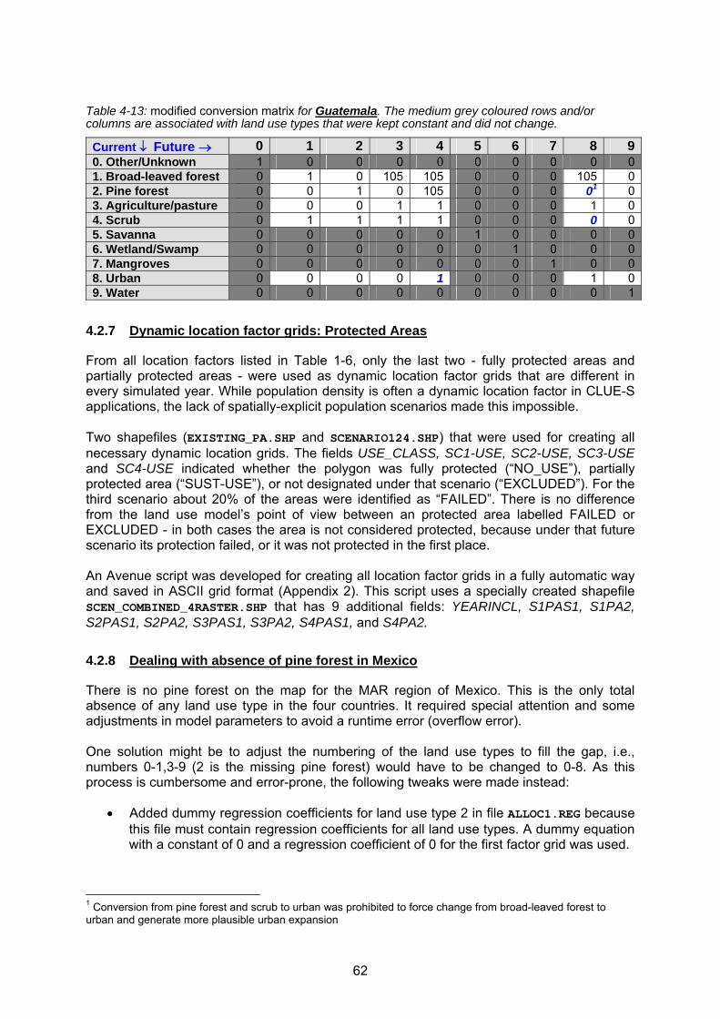
62
Table 4-13: modified conversion matrix for Guatemala. The medium grey coloured rows and/or columns are associated with land use types that were kept constant and did not change.
Current ↓ Future → 0 1 2 3 4 5 6 7 8 90. Other/Unknown 1 0 0 0 0 0 0 0 0 01. Broad-leaved forest 0 1 0 105 105 0 0 0 105 02. Pine forest 0 0 1 0 105 0 0 0 01 03. Agriculture/pasture 0 0 0 1 1 0 0 0 1 04. Scrub 0 1 1 1 1 0 0 0 0 05. Savanna 0 0 0 0 0 1 0 0 0 06. Wetland/Swamp 0 0 0 0 0 0 1 0 0 07. Mangroves 0 0 0 0 0 0 0 1 0 08. Urban 0 0 0 0 1 0 0 0 1 09. Water 0 0 0 0 0 0 0 0 0 1
4.2.7 Dynamic location factor grids: Protected Areas
From all location factors listed in Table 1-6, only the last two - fully protected areas and partially protected areas - were used as dynamic location factor grids that are different in every simulated year. While population density is often a dynamic location factor in CLUE-S applications, the lack of spatially-explicit population scenarios made this impossible. Two shapefiles (EXISTING_PA.SHP and SCENARIO124.SHP) that were used for creating all necessary dynamic location grids. The fields USE_CLASS, SC1-USE, SC2-USE, SC3-USE and SC4-USE indicated whether the polygon was fully protected (“NO_USE”), partially protected area (“SUST-USE”), or not designated under that scenario (“EXCLUDED”). For the third scenario about 20% of the areas were identified as “FAILED”. There is no difference from the land use model’s point of view between an protected area labelled FAILED or EXCLUDED - in both cases the area is not considered protected, because under that future scenario its protection failed, or it was not protected in the first place. An Avenue script was developed for creating all location factor grids in a fully automatic way and saved in ASCII grid format (Appendix 2). This script uses a specially created shapefile SCEN_COMBINED_4RASTER.SHP that has 9 additional fields: YEARINCL, S1PAS1, S1PA2, S2PAS1, S2PA2, S3PAS1, S3PA2, S4PAS1, and S4PA2.
4.2.8 Dealing with absence of pine forest in Mexico
There is no pine forest on the map for the MAR region of Mexico. This is the only total absence of any land use type in the four countries. It required special attention and some adjustments in model parameters to avoid a runtime error (overflow error). One solution might be to adjust the numbering of the land use types to fill the gap, i.e., numbers 0-1,3-9 (2 is the missing pine forest) would have to be changed to 0-8. As this process is cumbersome and error-prone, the following tweaks were made instead:
• Added dummy regression coefficients for land use type 2 in file ALLOC1.REG because this file must contain regression coefficients for all land use types. A dummy equation with a constant of 0 and a regression coefficient of 0 for the first factor grid was used.
1 Conversion from pine forest and scrub to urban was prohibited to force change from broad-leaved forest to urban and generate more plausible urban expansion

63
• In COV1.ALL, changed the value of four grid cells from 1 (broadleaved forest) to 2 (pine forest), thus introducing artificial pine forests. Four cells in the bottom-left corner of the grid were chosen solely because these cells are easy to identify. These cells were returned to broadleaved forest in the simulated land use grid COV22.ALL. Note that the change was made for 4 cells instead of 1 cell, so that the corresponding area has no significant decimal value, and CLUE-S will not make a rounding error when the demand figures are read in (the demand values in LOG.FIL suggest that they are rounded to 1 decimal place, although that may a formatting matter).
• In the demand file DEMAND1.FIL, replaced the 0 hectare value in the third column with 25. That is the area of the additional cell in ha. The values in the second column (broadleaved forest) are reduced by 25 hectares.
• In ALLOW.TXT, changed all values in the third row and third column to 0 except the value at position [3,3]. Thus, pine forest cannot change to anything else.
4.3 Simulation results
4.3.1 Simulated changes in land use and in forest cover
Figures 4-1 to 4-5 show the present and simulated land use patterns for 2025. These land cover raster data were shared with WRI on 20th July 2006 for use in the N-SPECT hydrological simulations. Figures 4-6 to 4-8 show the areas of change only, making the new areas of each land use class easier to identify. A minor anomaly in the simulated land use pattern near San Pedro Sula, Honduras can be seen, with some areas of forest “sandwiched” in between new urban land. The cause of this was identified (probability surfaces and regressions) but could not easily be resolved. It is merely a reflection of the probabilistic nature of the model and that the exact allocation by the model of land use at a local level cannot easily be influenced.
4.3.2 Average and maximum deviation of solution
The iterative allocation module never achieves an allocation that fully matches the demand. This is controlled by the iteration variables on line 12 of the main parameter file. A relative iteration mode with an average deviation of 0.5% and a maximum individual deviation (for any individual land use type) of 3.0% was used. Table 4-15 below gives the actual deviations that were achieved, which are always equal to or lower than the maximum values. Table 4-15: mean and maximum deviation between demand and allocated land use, in percentage of absolute area, for land use in the final simulated year, 2025 ). These statistics are calculated for every simulated year but presented here only for the final year). The maximums (2nd and 3rd columns) are specified in the main parameter file and are slight adjustments from the default settings in CLUE-S, respectively, 0.35% and 3.0%. In almost all cases the highest deviation applies to land use that occupies the least area and is not kept constant, which almost always is Urban
Maximums 1. Market First 2. Policy First 4. Sustain. First
Mean Max Mean Max Mean Max Mean Max
Belize 0.3% 1.5% 0.29% 1.00% 0.30% 1.08% 0.27% 0.80%
Mexico 0.5% 3.0% 0.31% 2.96% 0.31% 2.99% 0.34% 2.99%
Guatemala 0.5% 3.0% 0.48% 1.85% 0.47% 1.82% 0.48% 2.27%
Honduras 0.4% 3.0% 0.39% 1.58% 0.40% 2.03% 0.40% 2.87%

64
Baseline 2000/2004
Market First 2025
Policy First 2025
Sustainability First 2025
Figure 4-1: Present land cover and simulated land cover for the three scenarios in 2025.

65
Figure 4-2: Baseline (2000/2004) land use

66
Figure 4-3: Simulated land cover for scenario 1, Markets First, in 2025

67
Figure 4-4: Simulated land cover for scenario 2, Policy First, in 2025

68
Figure 4-5: Simulated land cover for scenario 4, Sustainability First, in 2025

69
Figure 4-6: Simulated areas of change with 2025 land cover for scenario 1, Markets First

70
Figure 4-7: Simulated area of change with 2025 land cover for scenario 2, Policy First
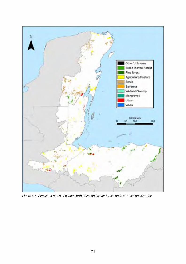
71
Figure 4-8: Simulated areas of change with 2025 land cover for scenario 4, Sustainability First

72
5 Workshop, conclusions and recommendations
5.1 Technical Workshop
A Workshop on Watershed Management, Land Cover Change Analysis, and Modeling of Land-based Sources of Pollution and Sediment Discharge to the MAR was held 15-18 August 2006 at Galen University, Belize. The workshop consisted of a policy session (1 ½ day) and a technical session (2 ½ days). Two presentations about the scenario development and the land use change modelling were given during the policy session, alongside presentations on the background of the land-use-change threats to the Mesoamerican Reef, and the policy implications of the MAR project. The last day of the workshop was dedicated to training in land use change modelling using the CLUE-S model. The training programme, exercises and further supporting information --all bundled in a 30 page training package—can be found in Appendix 6. Proceedings from the workshop have been compiled separately, and summarise feedback received from workshop participants.
5.2 Conclusions and Recommendations
The following conclusions and recommendations are compiled based upon Joep Luijten’s experience with the application of CLUE-S to the MAR region, and on feedback received during the workshop.
5.2.1 Application of CLUE-S model to the MAR region
The CLUE-S methodology has been successfully used to simulated land use changes in the MAR region over the next 25 years. A separate model was developed for each country. This was the correct approach, as it allows more accurate models that better capture the relevant (and different) explanatory factors in each of the countries.
Simulated land use changes in different directions under the three scenarios, with substantial conversion from forest to agricultural land under the Markets First and Policy First scenarios. Under the Sustainability First scenario, changes towards other land use types could be observed too; most notably changes towards scrub and new forest areas.
Whilst CLUE-S is a relatively easy model to use, the overall land use change modelling component of the project is quite complex. CLUE-S is not a model that can be quickly applied and run; preparation and implementation requires substantial time (months) and many data conversions. A significant portion of the hours required was spent on data collection and/or creation and quality assurance, data preparation for use in SPSS (regression analysis) and CLUE-S, and the regression analysis. Once the model was properly calibrated, the final simulation runs were a relatively straightforward task.
CLUE-S does not dictate any particular method for calculating the land use requirements. The use of IMAGE and International Futures was possible only because we had access to these models. Simpler methods are possible and recommended, especially where specific regional policies are to be applied. For example, land use requirements could be calculated using appropriate economic demand models or simply by setting hypothetical land use requirements for the final scenario year and interpolating the land requirements between the start year and end year using a linear or exponential growth model.

73
The regression analysis was a somewhat weak part of the study in that many relationships were not very significant and had to be manually tweaked or replaced by either a more logical regression equation (e.g., Urban), as detailed in Section 4.2.4. This is a direct consequence of the characteristics of the land use data that were used. The Ecosystem Map data were relatively coarse and polygon-based. It is believed that the regression analysis and the way CLUE-S allocates land based on the probability surfaces would give better results (and need fewer adjustments in model parameters and/or workarounds for the model not being able to reach a solution) if an original remote sensed raster dataset is used. Workshop participants knew of several recently released new land cover datasets, in particular for Guatemala.
Another potential approach for improving the regression analysis is to use a “balanced sample” dataset instead of the full dataset for the region. A balanced sample is a dataset for a region that clearly exhibits the relevant relationships between a particular land use type and one or more location factors. Only full datasets were used for the MAR study.
CLUE-S can be used if land use data from only a single year are available because the model is parameterized: in principle, based on the results of the regression analysis of the present land use pattern and a set of potential explanatory factors. However, it is always better if land use data for two or even three years are available, and these additional data can be used to improve the models. Having data for two years, y1 and y2, allows one to parameterize the models based on an regression analysis of the data for y1, then run the model from y1 to y2, compare the simulated land use pattern with the actual land use pattern at y2, and adjust (calibrate) the improve the model fit. If a third year y3 is available, then a simulation run from y2 to y3 can be undertaken for model verification.
5.2.2 Workshop and training
This overall work was covered during a 1-hour presentation during the policy part of the workshop and a 1-day training day in CLUE-S. The response to the questionnaires indicated that, in general, the participants found working with CLUE-S very useful.
The CLUE-S training was quite intense. Any future training should dedicate at least 2 or 3 days to CLUE-S, as that will allow participants to spend more time on three important aspects of the study: (i) in-depth understanding and hands-on working with the actual data for Belize, Mexico, Guatemala and Honduras; (ii) how to use their own datasets; and (iii) the regression analysis of location factors and methods for incorporating additional or different location factors into the model. Any follow-up training should include these aspects, as some attendees requested this in the questionnaires.

74
6 References Ankersen, T.T., Arriola, L. 2001. At the Crossroads of Conservation & Development: the
Challenge of the Maya Forest. Report to the Coalición de la Selva Maya and the Tropical Ecosystem Directorate of the United States Man & the Biosphere Program. 13 pp. http://conservation.law.ufl.edu/pdf/mayaforest.pdf. Accessed 14 September 2006.
Balk, D., Pozzi, F., Yetman, G., Deichmann, U., Nelson, A. 2004. The Distribution of People and the Dimension of Place: Methodologies to Improve the Global Estimation of Urban Extents (draft). Center for International Earth Science Information Network (CIESIN), Columbia University; International Food Policy Research Institute (IFPRI); The World Bank; and Centro Internacional de Agricultura Tropical (CIAT). http://sedac.ciesin.columbia.edu/gpw/docs/UR_paper_webdraft1.pdf. Accessed 4 October 2006.
Batjes, N.H., 2005. ISRIC-WISE global data set of desired soil properties on a 0.5 by 0.5 degree grid. Report 2005-08. ISRIC – World Soil Information. December 2005. http://www.isric.org/isric/webdocs/Docs/ISRIC_Report_2005_08.pdf. Accessed 14 September 2006.
Batjes, N.H., 2005. SOTER-based soil parameter estimates for Latin America and the Caribbean (version 1.0). Report 2005/02. ISRIC – World Soil Information. December 2005. http://www.isric.org/isric/webDocs/Docs/ISRIC_Report_2005_02.pdf. Accessed 14 September 2006.
Belize Tourism Board. No date. National Tourism Policy: Strategic Vision for Belize Tourism in the New Millennium. Ministry of Tourism, Government of Belize. Belize City, Belize. http://www.belizetourism.org/policy.html
Belize Tourism Board No date. Belize Cruise Tourism Policy. Ministry of Tourism, Government of Belize. Belize City, Belize. http://www.destinationsbelize.com/cruise_s.htm. Accessed 14 September 2006.
Boles, E. 2005. United Nations Convention on Biological Diversity: Thematic Assessment Report of Belize. National Capacity for Self-Assessment project, Ministry of Natural Resources. Belmopan, Belize. 58 pp.
Buck, M. 2002. Project Summary: Central American Project for Geographic Information: Honduras. Report to PROCIG, the Central American Geographic Information Project. http://www.procig.org/ing/procig-honduras.htm. Accessed 14 September 2006.
Central Statistical Office. 2001. Environmental Statistics for Belize: 2001. Environmental Statistics Unit, Central Statistics Office, Ministry of Budget Management, Investment and Public Utilities. Belmopan, Belize. 115 pp.
Central Statistical Office. 2005. Environmental Statistics for Belize: 2004. Environmental Statistics Unit, Central Statistical Office, Ministry of National Development. Belmopan, Belize. 219 pp.
Cherrington, E., 2005. Drivers of land use change adjacent to the Meso-american reef: a preliminary review. Unpublished report to UNEP-WCMC. August 2005.
Chomitz, K.M., Gray, D.A. 1996. Roads, Land Use, and Deforestation: A Spatial Model Applied to Belize. Poverty, Environment, and Growth Working Paper No. 5. International Food Policy Research Institute, World Bank. Washington, DC. 26 pp. http://www.worldbank.org/research/peg/wps03/roads.pdf. Accessed 14 September 2006.
CIAT, UNEP, CIESIN, Columbia University and the World Bank (2005) Latin American and Caribbean Population Database. Version 3. Centro Internacional de Agricultura Tropical (CIAT), United Nations Environment Program (UNEP), Center for International Earth

75
Science Information Network (CIESIN), Columbia University, and the World Bank. http://gisweb.ciat.cgiar.org/population/report.htm. Accessed 4 October 2006.
Deininger, K.W., Minten, B. 1996a. Poverty, Policies, and Deforestation: the Case of Mexico. Poverty, Environment, and Growth Working Paper No. 5. International Food Policy Research Institute, World Bank. Washington, DC. 54 pp. http://www.worldbank.org/research/peg/wps05/mexico.pdf. Accessed 14 September 2006.
Deininger, K.W., Minten, B. 1996b. Determinants of Forest Cover and the Economics of Protection: An Application to Mexico. Poverty, Environment, and Growth Working Paper No. 10. International Food Policy Research Institute, World Bank. Washington, DC. 22 pp. http://www.worldbank.org/research/peg/wps10/mxforest.pdf. Accessed 14 September 2006.
DiFiore, S. 2002. Remote Sensing and Exploratory Data Analysis as Tools to Rapidly Evaluate Forest Cover Change and Set Conservation Priorities along the Belize River, Belize. MS thesis, Department of Ecology, Evolution and Environmental Biology, Columbia University. New York, NY. 68 pp.
Fairweather, P.N., Gray, D.A. 1994. The Land Use of Belize: 1989/92. Land Information Centre, Ministry of Natural Resources. Belmopan, Belize. 15 pp.
Fairweather, P.N. 2002. Sistemas de Informacion Geografica en Belice [Geographic Information Systems in Belize]. Report to PROCIG, the Central American Geographic Information Project. http://www.procig.org/reunion-ctg/documentos/belice/belice-resumen.pdf. Accessed 14 September 2006.
FAO, 1999. FRA 2000 Annotated Bibliography. Forest Cover Change: Guatemala. Working Paper 13. Rome, Italy. 65 pp. ftp://ftp.fao.org/docrep/fao/005/ac631e/ac631e.pdf
FAO, 2000a. “FRA 2000 Annotated Bibliography. Forest Cover Change: Belize.” Working Paper 40. Rome, Italy. 38 pp. ftp://ftp.fao.org/docrep/fao/007/ad677e/ad677e00.pdf. Accessed 14 September 2006.
FAO, 2000b. FRA 2000 Bibliografía comentada. Cambios en la cobertura forestal: Honduras. Working Paper 44. Rome, Italy. 40 pp. ftp://ftp.fao.org/docrep/fao/007/ac768s/ac768s.pdf. Accessed 14 September 2006.
FAO, 2000c. FRA 2000 Bibliografía comentada. Cambios en la cobertura forestal: México. Working Paper 35. Rome, Italy. 35 pp. ftp://ftp.fao.org/docrep/fao/006/ad667s/ad667s00.pdf. Accessed 14 September 2006.
Farrow, A., Winograd, M. 2001. Land use modelling at the regional scale: an input to rural sustainability indicators for Central America. Agriculture, Ecosystems. & Environment 85: 249-268.
Farrow, A., Nelson, A. 2001. Accessibility modelling in ArcView 3. An extension for computing travel time and market catchment information. (User’s manual). CIAT. http://www.ciat.cgiar.org/access/index.htm. Accessed 14 September 2006.
Hughes, B.B. 2004. Introduction to International Futures (IFs). Graduate School of International Studies, University of Denver. http://www.du.edu/~bhughes/reports/Introduction%20to%20IFs%20V2_0.pdf. Accessed 1 June 2006.
Instituto Geografico Nacional, Guatemala. 2002. Guatemala Summary. Report to PROCIG, the Central American Geographic Information Project. http://www.procig.org/reunion-ctg/documentos/guatemala/resumen-actividades-ign-guatemala.pdf. Accessed 14 September 2006.
76
IUCN 1994. Guidelines for Protected Area Management Categories. CNPPA with the assistance of WCMC. IUCN, Gland, Switzerland and Cambridge, UK. 261pp. http://www.unep-wcmc.org/protected_areas/categories/index.html. Accessed 14 December 2005.
Iyo, J., Mendoza, P., Cardona, J., Cansino, A., Davis, R. 2003. An Overview of Land Administration & Management in Belize. Workshop on Land Policy, Administration and Management in the English – Speaking Caribbean, March 20003, Port of Spain, Trinidad. 50 pp. http://web.archive.org/web/20030520070825/http://www.mhtc.net/~terra/carib_workshop/pdf/belizecfs.pdf. Accessed 14 September 2006.
Jansen, H.G.P., Siegel, P.B., Pichon, F. 2005. Identifying the Drivers of Sustainable Rural Growth & Poverty Reduction in Honduras. DSGD Discussion Paper No. 19. Development Strategy & Governance Division, International Food Policy Research Institute. Washington, DC. 136 pp. http://www.ifpri.org/divs/dsgd/dp/papers/dsgdp19.pdf. Accessed 14 September 2006.
King, R.B., Baillie, I.C., Bissett, P.G., Grimble, R.J., Johnson, M.S., Silva, G.L. 1986. Land Resource Survey of Toledo District, Belize. Land Resource Development Centre. Tolworth, United Kingdom.
King, R.B., Baillie, I.C., Dunsmore, J.R., Grimble, R.J., Johnson, M.S., Wright, A.C.S. 1989. Land Resource Survey of Stann Creek District, Belize. Bulletin 19. Natural Resources Institute, Overseas Development Administration, Chatham, UK. 262 pp.
King, R.B., Baillie, I.C., Abell, T.M.B., Dunsmore, Gray, D.A., Pratt, J.H., Versey, H.R., Wright, A.C.S., Zisman, S.A. 1992. Land Resource Assessment of Northern Belize. Bulletin 43. 2 volumes. Natural Resources Institute, Overseas Development Administration, Chatham, United Kingdom. 513 pp.
King, R.B., Pratt, J.H., Warner, M.P., Zisman, S.A. 1993. Agricultural Development Prospects in Belize. Bulletin 48. Natural Resources Institute, Overseas Development Administration, Chatham, United Kingdom. 159 pp.
Kok, K., Winograd, M. 2002. Modelling land-use change for Central America, with special reference to the impact of Hurricane Mitch. Ecological Modelling 149: 53-69.
Kok, K., 2004. The role of population in understanding Honduran land use patterns. Journal of Environmental Management 72: 73-89.
Kok, K., Veldkamp, A. 2001. Evaluating impact of spatial scales on land use pattern analysis in Central America. Agriculture, Ecosystems & Environment 85: 205-221.
Loening, L.J., Markussen, M. 2003. Pobreza, Deforestación y Pérdida de la Biodiversidad en Guatemala. Discussion Paper No. 91. Ibero-America Institute for Economic Research. 44 pp. http://www.iai.wiwi.uni-goettingen.de/content/pdf/iai-db91.pdf. Accessed 14 September 2006.
Meerman, J., Sabido, W. 2001. Central American Ecosystems: Belize. Programme for Belize, Belize City. 2 volumes 50 + 88 pp.
Merrill, T (ed.). 1992. Belize: A Country Study. Call No. F2368.G893 1993. Federal Research Division, U.S. Library of Congress. http://lcweb2.loc.gov/frd/cs/bztoc.html. Accessed 14 September 2006.
Merrill, T. (ed.). 1993. Honduras: A Country Study. Call No. F1503.H75 1995. Federal Research Division, U.S. Library of Congress. http://lcweb2.loc.gov/frd/cs/hntoc.html. Accessed 14 September 2006.

77
Merrill, T.L., Miró, R. (eds.) 1996. Mexico: A Country Study. F1208.M5828 1997. Federal Research Division, U.S. Library of Congress. http://lcweb2.loc.gov/frd/cs/mxtoc.html. Accessed 14 September 2006.
Ministry of Agriculture & Fisheries. 2003. The National Food & Agriculture Policy (2002-2020). Government of Belize, Belmopan, Belize. 63 pp.
Myers, N., Mittermeier, R.A., Mittermeier, C.G., da Fonseca, G.A., Kent, J. 2000. Biodiversity hotspots for conservation priorities. Nature 403(6772):853-858.
Nelson, A., 2000. Accessibility, transport and travel time information. Internal document. CIAT, Cali, Colombia.
Sader, S.A., Hayes, D.J., Irwin, D.E., Saatchi, S.S. 2001. Preliminary Forest Cover Change Estimates for Central America (1990s), with Reference to the Proposed Mesoamerican Biological Corridor. Proceedings of the Year 2001 Annual Conference of the American Society of Photogrammetric Engineering and Remote Sensing. St. Louis, MO. 11 pp. http://wwwghcc.msfc.nasa.gov/corredor/mbr_asprs_paper.pdf. Accessed 14 September 2006.
Schuttenberg, H.Z. (ed). 2001. Coral Bleaching: Causes, Consequences and Response. Selected Papers presented at the 9th International Coral Reef Symposium on Coral Bleaching: Assessing and Linking Ecological and Socioeconomic Impacts, Future Trends and Mitigation Planning. Coastal Resources Center, Univ. of Rhode Island.
Turner II, B. L., Cortina Villar, S., Foster, D., Geoghegan, J., Keys, E., Klepeis, P., Lawrence, D., Macario Mendoza, P., Manson, S.M., Ogneva-Himmelberger, Y. 2001. Deforestation in the southern Yucatan peninsular region: an integrative approach. Forest Ecology and Management 154(3): 353-370.
UNEP 2002. Global Environment Outlook 3. United Nations Environment Programme, Nairobi, Kenya. http://www.unep.org/geo/geo3/. Accessed 14 September 2006.
Verburg, P.H., 2004. Manual for the CLUE-S model. September 2004. http://www.cluemodel.nl/. Accessed 14 September 2006.
Verburg, P.H., Veldkamp, T, Lessschen, J.P. 2004. Exercises for the CLUE-S model. http://www.cluemodel.nl/Ex4.pdf. Accessed 14 September 2006.
Vreugdenhill, D., Meerman, J., Meyrat, A., Gomez, L.D., Graham, D.J., 2002. Map of the ecosystems of Central America. Final report. World Bank, Washington, D.C.
Wassenaar, T., Gerber, P., Rosales, M., Ibrahim, M., Verburg, P.H., Steinfeld, H. 2005. Projecting land use changes in the Neotropics: the geography of pasture expansion into forest. Submitted.
WCSD, 1987. Our Common Future. World Commission for Sustainable Development / Oxford Paperbacks. 398pp.
White, W.A., Raney, J., Tremblay, T.A., Crawford, M.M., Smith, S.S. 1996. Deforestation in Belize 1989/92-1994/96. Bureau of Economic Geology, University of Texas. Austin, TX. 49 pp.
White, W.A., Raney, J., Tremblay, T.A., Crawford, M.M., Smith, S.S.. 1998. Remote Sensing Analysis of Land Cover & Land Use, Central Belize. Bureau of Economic Geology, University of Texas. Austin, TX. 39 pp.

Appendix 1 78
7 Appendices Appendix 1. Avenue script for NoData filling and filtering
The following Avenue script was created to fill NoData holes and to apply a majority filter to rasters, as mentioned in Section 1.1.1. This script removes any minor imperfections in the raster grids and adds a small buffer of value cells at the edge so that every raster being used for the statistical analysis has exactly the same number of value cells. The script can handle both mean filter and majority filters, and up to 10 iterations at once. ' SWBM.Grid.FillNodataGaps ' July 14, 2004. Joep Luijten ' This script was written fill the common Nodata cells in SRTM elevation ' data. The NoData cells are typically areas with steep gradients, river ' valleys, etc. The fill is done iteratively. See ESRI article 22853. ' http://support.esri.com/index.cfm?fa=knowledgebase.techarticles.articleShow&d=22853 ' The number of necessary iterations depends on how large the data gaps are. ' 4/1/06. Provide selection menu to choose focalstats type (MEAN ort MAJORITY) and ' output type (floating or integer). This enables to use this script also to fill ' gaps in classified data. The majority filter wasn't as straightforward, though. ' ' The use of the MajorityFilter() does correctly fill any NoData holes inside a grid ' providing that the second argument is set TRUE, however, it does not convert NoData ' cells to value cells at the edge. On the other hand, a FocalStats() of type ' GRID_STATYPE_MAJORITY does create value cells at the edge (1 cell wide per ' iteration). Hence, it was deemed necessary to implement a succession of both ' methods at each iteration step to achieve the desired result. theView = av.GetActiveDoc theTheme = theView.GetActiveThemes.Get(0) rawDem = theTheme.GetGrid titmsg = "Fill NoData gaps in GRID" ' Check to proceed if (MsgBox.YesNo("Fill NoData gaps in GRID theme" ++ theTheme.GetName + "?",titmsg, FALSE) = FALSE) then return nil end ' Method iMethodList = {"MEAN 3x3 filter, return floating grid", "MEAN 3x3 filter, return integer grid", "MAJORITY 3x3 filter, return integer grid"} iMethod = Msgbox.ListAsString (iMethodList, "Select FocalStats method", titmsg) if (iMethod = nil) then return nil else iMethodIndex = iMethodList.FindByValue(iMethod) if (iMethodIndex = 0) then bMean = true bFloat = true elseif (iMethodIndex = 1) then bMean = true bFloat = false elseif (iMethodIndex = 2) then bMean = false bFloat = false end end ' Prompt for number of iterations errorMsg = "You must enter a number between 1 and 10" while (true) Niter = MsgBox.Input("Number of iterations [1-10]:",titmsg,"3") if (nIter = NIL) then return nil end if (nIter.IsNumber.Not) then MsgBox.Warning(errorMsg,titmsg) else nIter = nIter.AsNumber if ((nIter < 1) or (NIter > 10)) then MsgBox.Warning(errorMsg,titmsg) else break

Appendix 1 79
end end end ' Check for any values < 0 or >= 32768 (in SRTM data, 32768 is used for NoData). gStats = rawDem.GetStatistics setMin = false if (gStats.Get(0) < 0) then setMin = Msgbox.YesNo("The grid contains negative values (as low as"++ gStats.Get(0).AsString ++ "). These are unusual --though not impossible-- elevation"++ "values that you may want to set to zero. Do you want to do this?",titmsg, TRUE) end setMax = false if (gStats.Get(1) >= 32768) then setMax = Msgbox.YesNo("The grid contains very high values that are unlikely elevations."++ "Note that SRTM data often contain values 32768 (NoData) and 95xxx (incorrect)."++ "You are strongly recommended to set these values to NoData. Okay?",titmsg, TRUE) if (setMax) then mxMsg = "You must enter a number between 0 and 100000" while (true) mxCut = MsgBox.Input("Maximum cutoff value (excluded):",titmsg,"32768") if (mxCut = NIL) then return nil end if (mxCut.IsNumber.Not) then MsgBox.Warning(mxMsg,titmsg) else mxCut = mxCut.AsNumber if ((mxCut < 0) or (mxCut > 100000)) then MsgBox.Warning(mxMsg,titmsg) else break 'Value is OK end end end end end ' Apply min and max values if (setMin and setMax) then g0 = ((rawDem < 0.asgrid).Con(0.asgrid,(rawDem >= mxCut.asgrid).SetNull(rawDem))) elseif (setMin and setMax.Not) then g0 = ((rawDem < 0.asgrid).Con(0.asgrid,rawDem)) elseif (setMin.Not and setMax) then g0 = ((rawDem >= mxCut.asgrid).SetNull(rawDem)) else g0 = rawDem end ' Perform iterative fill. Two methods in succession for the majority filter. theNbrHood = NbrHood.Make ' Default 3x3 rectangular neighborhood if (nIter >= 1) then if (bmean = true) then g1 = (g0.IsNull).Con((g0.FocalStats(#GRID_STATYPE_MEAN,theNbrHood,FALSE)),g0) else g1tmp = ((g0.IsNull).Con(g0.MajorityFilter(TRUE, TRUE),g0)) g1 = (g1tmp.IsNull).Con((g1tmp.FocalStats(#GRID_STATYPE_MAJORITY,theNbrHood,FALSE)),g1tmp) end if (nIter = 1) then gFinal = g1 end end if (nIter >= 2) then if (bmean = true) then g2 = (g1.IsNull).Con((g1.FocalStats(#GRID_STATYPE_MEAN,theNbrHood,FALSE)),g1) else g2tmp = ((g1.IsNull).Con(g1.MajorityFilter(TRUE, TRUE),g1)) g2 = (g2tmp.IsNull).Con((g2tmp.FocalStats(#GRID_STATYPE_MAJORITY,theNbrHood,FALSE)),g2tmp) end if (nIter = 2) then gFinal = g2 end end if (nIter >= 3) then if (bmean = true) then g3 = (g2.IsNull).Con((g2.FocalStats(#GRID_STATYPE_MEAN,theNbrHood,FALSE)),g2) else g3tmp = ((g2.IsNull).Con(g2.MajorityFilter(TRUE, TRUE),g2)) g3 = (g3tmp.IsNull).Con((g3tmp.FocalStats(#GRID_STATYPE_MAJORITY,theNbrHood,FALSE)),g3tmp)

Appendix 1 80
end if (nIter = 3) then gFinal = g3 end end if (nIter >= 4) then if (bmean = true) then g4 = (g3.IsNull).Con((g3.FocalStats(#GRID_STATYPE_MEAN,theNbrHood,FALSE)),g3) else g4tmp = ((g3.IsNull).Con(g3.MajorityFilter(TRUE, TRUE),g3)) g4 = (g4tmp.IsNull).Con((g4tmp.FocalStats(#GRID_STATYPE_MAJORITY,theNbrHood,FALSE)),g4tmp) end if (nIter = 4) then gFinal = g4 end end if (nIter >= 5) then if (bmean = true) then g5 = (g4.IsNull).Con((g4.FocalStats(#GRID_STATYPE_MEAN,theNbrHood,FALSE)),g4) else g5tmp = ((g4.IsNull).Con(g4.MajorityFilter(TRUE, TRUE),g4)) g5 = (g5tmp.IsNull).Con((g5tmp.FocalStats(#GRID_STATYPE_MAJORITY,theNbrHood,FALSE)),g5tmp) end if (nIter = 5) then gFinal = g5 end end if (nIter >= 6) then if (bmean = true) then g6 = (g5.IsNull).Con((g5.FocalStats(#GRID_STATYPE_MEAN,theNbrHood,FALSE)),g5) else g6tmp = ((g5.IsNull).Con(g5.MajorityFilter(TRUE, TRUE),g5)) g6 = (g6tmp.IsNull).Con((g6tmp.FocalStats(#GRID_STATYPE_MAJORITY,theNbrHood,FALSE)),g6tmp) end if (nIter = 6) then gFinal = g6 end end if (nIter >= 7) then if (bmean = true) then g7 = (g6.IsNull).Con((g6.FocalStats(#GRID_STATYPE_MEAN,theNbrHood,FALSE)),g6) else g7tmp = ((g6.IsNull).Con(g6.MajorityFilter(TRUE, TRUE),g6)) g7 = (g7tmp.IsNull).Con((g7tmp.FocalStats(#GRID_STATYPE_MAJORITY,theNbrHood,FALSE)),g7tmp) end if (nIter = 7) then gFinal = g7 end end if (nIter >= 8) then if (bmean = true) then g8 = (g7.IsNull).Con((g7.FocalStats(#GRID_STATYPE_MEAN,theNbrHood,FALSE)),g7) else g8tmp = ((g7.IsNull).Con(g7.MajorityFilter(TRUE, TRUE),g7)) g8 = (g8tmp.IsNull).Con((g8tmp.FocalStats(#GRID_STATYPE_MAJORITY,theNbrHood,FALSE)),g8tmp) end if (nIter = 8) then gFinal = g8 end end if (nIter >= 9) then if (bmean = true) then g9 = (g8.IsNull).Con((g8.FocalStats(#GRID_STATYPE_MEAN,theNbrHood,FALSE)),g8) else g9tmp = ((g8.IsNull).Con(g8.MajorityFilter(TRUE, TRUE),g8)) g9 = (g9tmp.IsNull).Con((g9tmp.FocalStats(#GRID_STATYPE_MAJORITY,theNbrHood,FALSE)),g9tmp) end if (nIter = 9) then gFinal = g9 end end if (nIter >= 10) then if (bmean = true) then g10 = (g9.IsNull).Con((g9.FocalStats(#GRID_STATYPE_MEAN,theNbrHood,FALSE)),g9) else g10tmp = ((g9.IsNull).Con(g9.MajorityFilter(TRUE, TRUE),g9)) g10 = (g10tmp.IsNull).Con((g10tmp.FocalStats(#GRID_STATYPE_MAJORITY,theNbrHood,FALSE)),g10tmp)

Appendix 1 81
end if (nIter = 10) then gFinal = g10 end end ' Make final grid if (bFloat = true) then gFinal2 = gFinal.Float sOper = "("+nIter.asstring++"pass)" else gFinal2 = gFinal.Int end ' Construct new title name if (bMean = true) then sname = theTheme.GetName++"("+nIter.asstring++"pass MEAN filter)" else sname = theTheme.GetName++"("+nIter.asstring++"pass MAJORITY filter)" end ' Add filled grid theme to view newGTheme = GTheme.Make(gFinal2) newGTheme.SetName(sname) theView.AddTheme(newGTheme) theView.Invalidate

Appendix 2 82
Appendix 2. Avenue script for creating dynamic protected areas grids
The script below was used to create dynamic location grids for the protected area scenarios. The script requires a view that contains five themes: the protected areas shapefile (SCEN_COMBINED_4RASTER.SHP) and the four mask grids for the countries (MASK_BZ_250, MASK_GT_250, MASK_MX_250, MASK_HN_250). The protected areas shapefile must have eight additional fields S1PA1, S2PA2, A1PA1, .., S4PA2, each with 0 and 1 values, indicating whether the polygon is a full or partially protected area. The scripts generates the grid SRC1G11.FIL (static fully protected areas), REGION_NO_USE_S1MKT.FIL (also static fully protected areas a value of –9998 for those areas) and SRC1G12.0, SRC1G12.1, …, through to SRC1G12.25 (dynamic partially protected areas). ' Create.Dynamic.ProtectedAreas.Grids ' Location factor numbers (as in CLUE-S regression files) locFacNum_fullProt = 11 locFacNum_partProt = 12 baseOutFolder = "D:\Work_WCMC\CLUES\dyndata\" ' Get active view theView = av.FindDoc("protected areas") thePrj = TheView.Getprojection if (theView.Is(View).Not) then msgbox.Info ("Active document must be a view","") return nil end ' Select country to process country = MsgBox.ListAsString({"BZ","MX","GT","HN"}, "Select country","") if (country = NIL) then return nil end ' select scenario to process scenario = MsgBox.ListAsString( {"1 Market First","2 Policy First","3 Security First","4 Sustainability First"}, "Select scenario","") if (scenario = NIL) then return nil else scenNo = scenario.Left(1).AsNumber end ' Select protected areas shapefile (modified to with special fields added) thmList = theView.GetThemes if (thmList.Count > 0) then wdpaThm = MsgBox.ListAsString(thmList, "Select the Protected Areas shapefile." + "The attribute table must include fields S"+scenNo.asstring+ "PA1 and S"+scenNo.AsString+"PA2.","") if (wdpaThm = NIL) then return nil else theFTab = wdpaThm.GetFTab fldList = theFtab.GetFields end else return nil end ' Output directory outDir = Msgbox.Input("Output folder","",baseOutFolder + country) if (outDir = NIL) then return NIL end if (scenNo = 1) then subdir = "s1mkt" elseif (scenNo = 2) then subdir = "s2pol" elseif (scenNo = 3) then subdir = "s3sec" elseif (scenNo = 4) then subdir = "s4sus" end outDir = outDir + "\" + subdir ' Get mask grid. If the hardcoded name not found the selection menu will be shown. maskName = "mask_" + country + "_250" maskThm= theView.FindTheme(maskName)

Appendix 2 83
if (maskThm <> NIL) then maskGrid = maskThm.Getgrid else if (thmList.Count > 0) then maskThm = MsgBox.ListAsString(thmList, "Select the mask grid for " + country,"") if (maskThm = NIL) then return nil else maskGrid = maskThm.Getgrid end else return nil end end ' Set analysis extent same to mask grid aRect = maskgrid.getExtent aCell = maskgrid.getCellSize Grid.SetAnalysisExtent (#GRID_ENVTYPE_VALUE, aRect) Grid.SetAnalysisCellsize(#GRID_ENVTYPE_VALUE, aCell) ' Create grid with only zeros for country extent zeroGrid = ((maskGrid.IsNull).setnull(0.asgrid)) ' **** STATIC LOCATION FACTOR FOR FULLY PROTECTED AREAS **** ' Filename for static location factor grid cluename = "Src1gr" + locFacNum_fullProt.asstring + ".fil" ' Query to select all WDPA to include fld1 = "S" +scenNo.asString + "pa1" expr = "(["+fld1+"] = 1)" theBitmap = theFTab.GetSelection theFtab.Query(expr, theBitmap, #VTAB_SELTYPE_NEW) theFTab.UpdateSelection ' Convert shape to grid. tmp1Grid = Grid.MakeFromFTab(theFTab,thePrj,nil,nil) tmp2Grid = (tmp1Grid.IsNull).Con(0.AsGrid,tmp1Grid) 'Grid with 0s and 1s finGrid = ((maskGrid.IsNull).setnull(tmp2grid)) 'Clip grid ' Save grid in ascii format theFn = (outdir + "\" + cluename).AsFileName if (File.Exists(theFn)) then File.Delete(theFn) end fingrid.SaveAsAscii(theFn) ' Also make a correspnding area restriction file. Active cells must have value ' of 0, restricted cells -9998, all other cells (NoData) -9999. resGrid = (finGrid = 1.asgrid).Con(-9998.asgrid,finGrid) theFn = (outdir + "\region_no_use_" + subdir + ".fil").AsFileName if (File.Exists(theFn)) then File.Delete(theFn) end resGrid.SaveAsAscii(theFn) resGrid = nil fingrid = nil tmp2grid = nil tmp1grid = nil ' **** DYNAMIC LOCATION GRIDS FOR PARTIALLY PROTECTED AREAS **** ' Number of years for which to save dynamic grids if (country = "BZ") then nYears = 21 '2004 to 2025 else nYears = 25 '2000 to 2025 end ' Save 2 WDPA location factor grid for each year for each i in 0..nYears ' New grid name cluename = "Src1gr" + locFacNum_partProt.asstring + "." + i.asstring ' Actual simulated year. First year will be 0 for grid naming convention. if (country = "bz") then year = 2004 + i else year = 2000 + i end ' Select field name fld1 = "S" +scenNo.asString + "pa2"

Appendix 2 84
fld2 = "Yearincl" ' Query to select all WDPA to include expr = "(["+fld1+"] = 1) and (["+fld2+"] <= "+year.asstring + ")" theBitmap = theFTab.GetSelection theFtab.Query(expr, theBitmap, #VTAB_SELTYPE_NEW) theFTab.UpdateSelection ' Convert shape to grid. tmp1Grid = Grid.MakeFromFTab(theFTab,thePrj,nil,nil) tmp2Grid = (tmp1Grid.IsNull).Con(0.AsGrid,tmp1Grid) 'Grid with 0s and 1s finGrid = ((maskGrid.IsNull).setnull(tmp2grid)) 'Clip grid ' Save grid in ascii format theFn = (outdir + "\" + cluename).AsFileName if (File.Exists(theFn)) then File.Delete(theFn) end fingrid.SaveAsAscii(theFn) fingrid = nil tmp2grid = nil tmp1grid = nil ' Add theme to view 'grdThm = GTheme.Make(finGrid) 'grdThm.SetName(cluename) 'theView.addTheme(grdThm) end zerogrid = nil

Appendix 3 85
Appendix 3: Complete list of available spatial data
Below is a complete list of all land cover/land use datasets and other spatial data that were identified during the data collection phase. Many of these data have also been downloaded. The yellow shaded rows indicate the datasets selected for this project. Informal notes on data availability and access have been left in the table in case of relevance to readers. LAND USE / LAND COVER DATASETS Dataset Name / Theme
Extent / Country
Years Resolution Classes Got data? Status / Comments / Constraints
GLOBAL/
REGIONAL
GLC2000 Global 2000 (Nov 1999 to Dec 2000)
1 km 22 Joep has 2000 Based on SPOT VEGETATION data. Good regional accuracy as local experts involved. May lack global consistency of Modis, less important for this project.
MODIS Land Cover
Global Oct 2000 to Oct 2001
1 km Globally consistent automated classification. No training sites in project region. Will be updated every six months and or a land cover change product provided. Gill contacted Boston University and EROS Data Center re next update/ release schedule.
FRA 2000 Global 2000 – based on 1992- 1996 images
1 km Only forest / open forest / non-forest in legend.
FRA control site data
Global network of 117 Landsat scenes
1980s, 1990s and around 2000
30 m (Landsat)
Used for calibration of the lower resolution data above. Three control sites are totally within the project area, three more are partially of interest. Dataset release is being investigated.
GeoCover Global (split into regions)
1990 (1989, 90 & 94) and
2000 (2000 & 2002)
30 m 13 Estimated costs are $650 per date layer. WRI experience suggests agricultural land under classified. Richard Borda ([email protected]) emailed Gill on 7/5/05 that 2000 data for Central America are now available. http://www.geocover.com/gc_lc/data_products/
Composites (band 742) from http://glcfapp.umiacs.umd.edu:8080/esdi/index.jsp show substantial patchy cloud coverage (and cloud shadows) throughout the region, particularly in eastern Belize and Guatemala. Therefore, this data is unlikely be very useful. Suggest not to use these data.

Appendix 3 86
NASA SERVIR Regional 2000, 2003, 2004 and 2005
30 m (Landsat)
Could use 2000 Landsat and STRM data as a baseline? Technical problems with Landsat mean data for 2004/5 is not available – recent MODIS data substituted. Other regional data layers available through MesoStor at http://servir.nsstc.nasa.gov.
Contacts = [email protected] and [email protected]
It seems that land cover data cannot be downloaded through MesoStor
Ecosystems map (CCAD)
2003 revision
Regional (Central America excluding Mexico)
Varies by country, 1993-99, both pre- and post-Mitch
Polygons, based on LandSat 5 data, 1:250 000
Modified UNESCO classification, 22 classes with Spanish legend
Joep has a copy
Detailed ecosystem legend (a modified UNESCO classification) contains one class for Agricultural Systems, one for Plantations and one for Urban Areas. This is the 2003 revision (the first version was released in 2001), which is still based on the same 1993-99 Landsat TM imagery, however the revised version corrects known errors on the map, includes a completely revised version of Costa Rica, and includes some changes to the classification system that resulted from agreements between the countries at a workshop in Guatemala in late 2002.
MANGROVES
UNEP-WCMC Mangroves
Pan Tropical but not MEXICO
Continuing Updates
Various Yes Only shows Mangroves, but is supposedly (!!) frequently improved and updated. Comparison with the Ecomap showed that the data is the same for Honduras (2003 version) but very different for Belize (2004 version). Lack of confidence in accuracy of WCMC data so suggest to not use them
Ecomap 2003 Mangroves
Yes Full coverage. Best option to use as source, except for Belize, for which more recent and more accurate data is available.
BZ Ecomap 2004 mangroves
Belize only see below Yes Relatively minor updates compared to the 2003 Ecomap. Assumed better. Best option for Belize.
CZMAI / Emil Mangroves
Belize only Emil says latest
Yes File: bz_mainland_mangrove_2004_c92_2. The data is generally more detailed and contains lots of small polygons. Also, the data appears to be converted from a raster but the source raster is unknown. Very different from the Mangroves in the 2004 Ecomap. The latter contain numerous areas classified as mangroves that are not included in this (Emil’s) dataset so we cannot just complement both data.
BELIZE
Fairweather & Gray (1994)
Belize 1989-90-92
SPOT XS 30 m, 1:76k
54 Detailed methodology available – see Land Use of Belize 1989-92.pdf

Appendix 3 87
Iremonger & Brokaw (1995)
Belize 1993 Landsat 1:250 000
52 Results of NARMAP project. Methodology available – provided to [email protected] in late June 2005.
Meerman & Sabido (2001)
Belize 1993-96-98 LandSat 1:250 000
83 Initial (2001) version of Ecosystem map. Now obsolete.
Meerman & Sabido 2001 - Vol 1.pdf
2004 Ecosystem Map of Belize
Belize Landsat TM 98-99-04 + many other sources
Landsat ETM 1:110 000
Total of 96. Default legend has 18 classes. Multiple agric.
Joep has a copy
Originally from 1998-99 TM imagery, but improved upon through fieldwork, additional TM imagery (Jan 04), etc. Also includes the reefs and islands. See NPAPSP Gap Analysis (public).pdf and ecosys_bze_2004.pdf http://biological-diversity.info/Ecosystems.htm
HONDURAS
CIAT Hurricane Mitch Atlas; CIAT indicators CD
Honduras (not full country coverage)
1986 and 1994 30 m, TM based
Joep has 1986 and 1994
http://gisweb.ciat.cgiar.org/cross_scale/atlas-mitch.htm
Contains recommended land use, capacity and forestry.
CIAT does not have more recent data.
Iremonger Vegetation data
Honduras Emil emailed Susan Iremonger for further information on data on 7th August 2005. I think this data is the Honduran part of the initial 2001 Ecosystem map.
2003 Ecosystem map
2 x 2/93, 2x 3/94, 1x12.98 (west) images + aerialphotos
SEE “GLOBAL/REGIONAL” SECTION FOR DETAILS.
Note that base TM imagery is the oldest used for the ecosystem map, though completed with aerial photos/verification./
MEXICO INEGI “Serie II” National Forest Inventory
Mexico 1993 125k / 30 m http://www.selvamaya.org
Mexican forest inventory of 1994. An update of mexico’s 1968-1986 land cover classification using 1993 Landsat TM images. Data made public in 2000 and re-processed by TNC for inclusion in Selva Maya CD
National Forest Inventory 2000
Mexico 2000 http://indy2.igeograf.unam.mx/ua_morelia/_private/2002/mapping_of_Mexico.PDF.

Appendix 3 88
2003 Ecomap
(not quite true)
1999, 2000 250 km 18 Joep has a copy
UNAM / INEGI / SEMARNAT. Conducted a complete land cover classification for Mexico Aerial photos also used, assessment of accuracy provided, covers whole country. Data set made available by CCAD as part of the 2003 revision of the Central American Ecosystem map. Note, however, that the original 2001 Ecomap didn’t include Mexico.
Mas et al. (2004)
Clark / Harvard / ECOSUR
Mexico, S. Yucatan, Campeche State
Modelling program already undertaken in area adjoining Petén in Guatemala. http://www.clarku.edu/departments/geography/research/sypr.shtml http://earth.clarku.edu/lcluc/
GUATEMALA
Maya Vegetation Map (CI)
Northern part GT, BZ, and some MX
1997-98 Landsat TM
30 m 12 classes, 1 of which agric.
Joep has a copy
Created by Conservation International from 1997-98 imagery, published in 2000. Daniel Juhn shared this data with Joep in 2001
Forest and Forest changes 1986-2002
Petén only up to 2002 Forest, agric, water + forest changes every two years
Joep has a copy
A continuation of the work undertaken by the Univ of Maine in 1996-97, this datasets was created by CEMEC-CONAP and WCS, Flores, Guatemala, using SPOT and LANDSAT ET+ data from March 2002. Very detailed and considered accurate but covers only Petén. Victor Hugo Ramos shared this data to Joep in April 2003, when the data was just completed.
MAGA Guatemala Complete 2001. Source image years unknown
250 km 24 Acquired by MBRS intern, cannot be shared at present. Metadata in BASE250.PRF suggest that this is the same as the ecosystem map, although an overlay of the polygons shows that it is not.

Appendix 3 89
OTHER DATASETS Dataset Extent Resolution /
Source year Received / Requested
Comments
ROADS
CCAD Roads Regional – in separate file for each country
Joep has a copy Roads stop at edge of cities – not good for network analysis. Also seems to haver an offset of about 100-200 m (all CCAD data suffer from this). http://www.ccad.ws/documentos/mapas.html
Selva Maya roads Regional VISA_COMUNICACION.SHP (from Selva Maya CD) and BZ-GT-MX_ROADS_SELVA_YR-UNKNOWN.SHP (from Emil). Same data, but with a bad offset of > 1 km, so it was decided not to use these data.
MesoStor Regional 1990s ? Joep has a copy (RED_VIAL_LINE) In principle the same as the CCAD data but doesn’t have a datum offset. Data have been reclassified in 5 classes: Highway-paved, Highway-unpaved (all year), Highway-unpaved (dry season only), Other road, and paths/tracks. Best available data, however, it remains a fairly low scale dataset. There are obvious discrepancies and missing roads when comparing with imagery (from Google Earth)
J. Meerman, E. Cherrington
Belize only 2000-03 Joep has a copy (BZ_ROADS_BTFS_2000-03) Received from Emil; according to the Belize Spatial Data Inventory (Dec 05) this is an updated of the Land Information Centre’s (LIC) roads dataset, using 2000-03 Landsat Imagery, by Meerman. A major visible change with the MesoStor/CCAD dataset is the inclusion of the major road from Belize City in northwest direction (as opposed to the one going in more northern direction from B.C.)
CZMAI Southern Belize 2005 Joep has a copy (BZ_SOUTH-ROADS_CZMAI_2005). Revised roads created by Emil Cherrington.
CIAT roads Honduras Joep has a copy From topographic maps.
CCAD Airports Regional Joep has a copy
CCAD Ports Regional Joep has a copy
POPULATION / URBAN EXTENT
CCAD Population Centres
Regional – in separate file for each country
Joep has a copy Contains data on district and town name, but no population data attached.
Latin America and Caribbean Pop. Database CIAT
Regional (LAC) 1960 – 2000; 1 km grid
Joep has a copy. From CIAT web site, http://gisweb.ciat.cgiar.org/population/. Contains vector population maps (pop. per admin unit) and raster surfaces created with an accessibility model. When compared to GPW v3 and overlaying on a Landsat image it becomes clear that this dataset is visibly less accurate than GPW.
GPW v3 Global and by country
1990 – 2015, in steps of 5 years. 1 km grid
Joep has a copy. Latest version 3 and final GRUMP data available in Dec 05. Actual population density for 1990, 1995 and 2000, and estimated for 2005, 2010 and 2015, and pop density grid appears more accurate than CIAT’s LAC. For the actual population, the “ag” grids were selected: adjusted population density to match UN totals. Datasets seem generally better

Appendix 3 90
than the LAC dataset, except for Belize.
Landscan 2004 Global Access requested but not yet received
GRUMP urban extent & settlements
Global Around 2000 Joep has a copy. Not very accurate. It may be better to digitize the polygons again from Landsat imagery. The settlements points from El Salvador were used to compile a MAR settlements dataset as no alternative data available for that country.
IGN/CCAD settlements
Honduras unknown Joep has a copy (HN_SETTLEMENTS_IGN-CCAD.SHP). The most detailed population point data for Honduras. Other dataset from INEGI and CCAD did not included population size. Received from Emil Cherrington
BTFS settlements Belize unknown Joep has a copy (BZ_SETTLEMENTS_BTFS.SHP). Settlements + population size from Belize Tropical Forest Studies, received from Emil.
Selva Maya settlements
MX, BZ and part of GT
Around 2000 Joep has a copy (BZ-GT-MX_SETTLEMENTS_SELVA_C2000.SHP) Settlements and population size from Selva Maya CD.
ELEVATION / SLOPE
STRM DEM for elevation and slope. (CIAT)
Regional Orginal 30 deg-sec (90 m), resampled to50 m.
Created by Joep from CIAT’s filled SRTM 90 data. Accurately projected to UTM 16/NAD 1927 using Joep’s customized Raster Project tool. (downloaded from http://srtm.csi.cgiar.org/)
CLIMATE
FAO Clim Global Some data from 1960 onwards
No Data from a global network of climatic stations (2 in Belize, ~ 100 in Honduras) available on CD-ROM (Copy was requested).
http://www.fao.org/sd/2002/EN1203_en.htm
CIAT Worldclim 1km Joep has a copy http://biogeo.berkeley.edu/worldclim/worldclim.htm. Considered the best data to use. Has monthly mean temperatures and precipitation in several resolutions (30 sec, 2.5, 5 and 10 min). 1 km resolution is more than sufficient for land use modelling.
SOILS SOTER LAC (Latin America and the Caribbean) with parameter estimates
Latin America 1:5 million Joep has a copy Can purchase from FAO ($44) but downloaded for free on 13/8/05 from ISRIC http://lime.isric.nl/index.cfm?contentid=162 A secondary dataset of soil parameters estimates was also obtained http://lime.isric.nl/index.cfm?contentid=%20452 These data can be linked to the SOTER GIS data
ISRIC WISEv3 Global December 2005; 0.5 degree grid
http://www.isric.org/UK/About+Soils/Soil+data/Thematic+data/Soil+Geographic+Data/. WISE dataset contains grid of man of the sae soil properties as the SOTERLAC but also has grid of soil depth

Appendix 3 91
IIASA GAEZ 2000 Global 10 km grid No Global Agro-Ecological Zoning 2000. Website states that better databases may be available elsewhere (i.e., SOTERLAC) (http://www.iiasa.ac.at/Research/LUC/gaez.html)
INEGI Mexico 1:250 k – 1M ?? Included on their map server http://galileo.inegi.gob.mx/website/mexico/viewer.htm, http://mapserver.inegi.gob.mx/map/datos_basicos/uso_suelo/. See metadata http://mapserver.inegi.gob.mx/dsist/Internet%202003/pagina1m.html
Selva Maya MX, BT, GT, but not Honduras
1: 250 k Yes Much more spatial detailed than the FAO SOTER. Emil thinks the classification were originally different in each country but were harmonized to FAO classification as part of the Selva Maya work (http://www.selvamaya.org). Lacks soil properties data so limited use.
CONAP / FAO (faosoil.shp)
200-250 k? From the Grunberg CD. Metadata indicate that FAO was the data source but they say that they do not have such a detailed regional map on record. The data appears to be in at a scale of 200-250 km because it has comparable detail to the Selva Maya data. However, they are absolutely different from the Maya soil data and the soil classes at various picked locations are also different from the SOTERLAC. Rejected for this reason.
ACCESSIBILITY
Accessibility to markets, roads
Joep created Created using CIAT’s Accessibility Wizard, using roads, cities data.
Accessibility to ports
RIVERS
MesoStor / CCAD Regional, split by country.
1:250 000 Joep has them http://servir.nsstc.nasa.gov/MesoStor/index.html . Same data on CCAD website as on MesoStor. Contains rivers names. Mostly digitized from 1:50 k-100 k topographic maps. Brief comparison with DCW (1:1m scale) shows that CCAD data are more detailed, but many small 1st order streams included in DCW are missing from the CCAD dataset. For Honduras doesn’t include as many secondary streams as CIAT”s “rios oficiales” data. Also, unlikely high stream density in central Belize—these are probably very small streams that we may not want to include.
WRI Regional More accurate datasets delineated from 90 m SRTM DEM. Locally burned in rivers will be identical to those from other (CCAD) datasets, though overall the DEM_delineated rivers should be more accurate than the older vector data.
CIAT Honduras 1:50 k Joep has them Official rivers (grouped by primary and secondary rivers) digitzed from 1:50 k topographic maps. Includes more secondary rivers than the CCAD data.
CZMAI Belize Joep has them Major rivers in Belize. Includes significantly fewers rivers than in the CCAD rivers data, though this seems more plausible and fits better with the rivers data for the other countries.

Appendix 3 92
PROTECTED AREAS
Mesostor / CCAD protected areas
Regional May 2003 Joep has a copy Mapa de Areas Naturales Protegidas de la región Mesoamericana. The data download from the CCAD website (http://www.ccad.ws/documentos/mapas.html) are the same as those from MesoStor. For Honduras also the same as CIAT’s data.
WDPA
(UNEP-WCMC)
Global, but only updated for MX, GT, HN and BZ
Updated Jan 2006 Joep has a copy The 18-05-2005 dataset showed significant differences compared to the CCAD dataset and well as CIAT’s dataset for Honduras. Major omissions and inaccurate boundaries in Honduras. Dataset updated by WCMC in January 2006 and this version appears to be complete and match the CCAD/MeSostor data. ICUN categories used.
CIAT Honduras 2000 - 2001 Joep has a copy On Honduras / Mitch data CD that Joep received from Andy Nelson in 2001. Data could be older than 2001, however, polygon boundaries are the same as those of Mesostor / CCAD dataset. Lacks attribute data and names of area so not very useful.
TOURISM HOTSPOTS
Selva Maya MX, BZ and Peten area of GT
2001 Joep has a copy. Tourism cost layer. It’s composed of hexagon-shaped polygons of 100 ha each and an attribute “Qualification” (Calificacia) that indicates what part of these 100 ha is under threat. Nearly all of the areas under threat are predominantly mangroves.

Appendix 4 93
Appendix 4: Ecosystem Map land cover classification
The table below shows the classifications for the original 2003 Ecosystem Map for Central America (22 classes), the 2004 Ecosystem Map for Belize (18 classes) and the reclassified and reduced classification that was adopted for the MAR land use change simulations.
2003 Ecosystem map Central America 2004 Ecosystem map Belize Reclassified / Reduced Classification

Appendix 5 94
Appendix 5. Land use requirements for future scenarios
The 16 tables below give the land use requirements, in ha, for all combinations of four scenarios and the four countries (the third scenario, Security First was not simulated but was calculated for assessment purposes). These land requirements were calculated using outputs from the International Futures and IMAGE models. Bear in mind that the reported areas apply to the parts of the countries that fall within the MAR region, not the whole countries (although for Belize that almost the same). Data are rounded to integer values so that they fit these tables better, however, in the source spreadsheet and CLUE-S input files the numbers have four decimals and the row totals are precisely identical each year. Belize – Markets First (1)
LUC 0 Unknown
1 B.L. forest
2 Pine for.
3 Agr/Past
4 Scrub
5 Savanna
6 Wetland
7 Mangroves
8 Urban
9 Water
YEAR 2000 1350 1268419 77175 423513 27481 188638 93175 72000 18944 15319 2001 1350 1268419 77175 423513 27481 188638 93175 72000 18944 15319 2002 1350 1268419 77175 423513 27481 188638 93175 72000 18944 15319 2003 1350 1268419 77175 423513 27481 188638 93175 72000 18944 15319 2004 1350 1268419 77175 423513 27481 188638 93175 72000 18944 15319 2005 1350 1266094 77034 424658 27701 189098 93403 71868 19489 15319 2006 1350 1264534 76939 426287 27622 188862 93286 71779 20036 15319 2007 1350 1262814 76834 427859 27539 188601 93157 71682 20858 15319 2008 1350 1261095 76729 429430 27456 188341 93029 71584 21679 15319 2009 1350 1259541 76635 431054 27377 188105 92912 71496 22224 15319 2010 1350 1257987 76540 432676 27298 187870 92796 71408 22769 15319 2011 1350 1254227 76312 437724 27166 186599 92168 71194 23954 15319 2012 1350 1250765 76101 442918 27039 185368 91560 70998 24595 15319 2013 1350 1247279 75889 448148 26912 184128 90948 70800 25240 15319 2014 1350 1243608 75665 453355 26781 182856 90319 70592 26168 15319 2015 1350 1239913 75441 458596 26648 181576 89687 70382 27101 15319 2016 1350 1234418 75106 463740 26539 181659 89728 70070 28084 15319 2017 1350 1228869 74769 468934 26429 181743 89770 69755 29076 15319 2018 1350 1222781 74398 473991 26307 181756 89776 69409 30926 15319 2019 1350 1217122 74054 479284 26195 181841 89818 69088 31942 15319 2020 1350 1211407 73706 484630 26082 181927 89860 68764 32968 15319 2021 1350 1206852 73429 489062 26230 181567 89683 68505 34016 15319 2022 1350 1202247 73149 493541 26380 181203 89503 68244 35076 15319 2023 1350 1197593 72866 498069 26532 180836 89321 67980 36148 15319 2024 1350 1192887 72579 502646 26686 180464 89138 67713 37231 15319 2025 1350 1187643 72260 507064 26830 180015 88916 67415 39201 15319

Appendix 5 95
Belize – Policy First (2)
LUC 0 Unknown
1 B.L. forest
2 Pine for.
3 Agr/Past
4 Scrub
5 Savanna
6 Wetland
7 Mangroves
8 Urban
9 Water
YEAR 2000 1350 1268419 77175 423513 27481 188638 93175 72000 18944 15319 2001 1350 1268419 77175 423513 27481 188638 93175 72000 18944 15319 2002 1350 1268419 77175 423513 27481 188638 93175 72000 18944 15319 2003 1350 1268419 77175 423513 27481 188638 93175 72000 18944 15319 2004 1350 1268419 77175 423513 27481 188638 93175 72000 18944 15319 2005 1350 1266863 77080 424586 27660 188608 93160 71912 19475 15319 2006 1350 1266174 77038 425261 27666 188298 93007 71873 20027 15319 2007 1350 1265486 76997 425936 27671 187988 92854 71833 20578 15319 2008 1350 1264797 76955 426611 27677 187679 92702 71794 21129 15319 2009 1350 1264109 76913 427285 27683 187370 92549 71755 21680 15319 2010 1350 1263260 76861 427905 27685 187037 92384 71707 22505 15319 2011 1350 1261364 76746 430321 27292 186154 91948 71600 23919 15319 2012 1350 1259950 76660 432909 26909 185340 91546 71519 24509 15319 2013 1350 1258532 76573 435505 26525 184525 91143 71439 25102 15319 2014 1350 1257110 76487 438107 26140 183706 90739 71358 25696 15319 2015 1350 1255684 76400 440717 25754 182886 90334 71277 26291 15319 2016 1350 1254525 76330 441286 25579 183098 90439 71211 26876 15319 2017 1350 1253202 76249 441798 25400 183287 90532 71136 27739 15319 2018 1350 1251877 76169 442311 25221 183476 90625 71061 28604 15319 2019 1350 1249742 76039 442539 25025 183546 90660 70940 30853 15319 2020 1350 1248574 75968 443110 24849 183760 90766 70874 31444 15319 2021 1350 1246838 75862 444761 24844 183533 90654 70775 32077 15319 2022 1350 1244933 75746 446362 24835 183282 90530 70667 32990 15319 2023 1350 1243020 75630 447969 24826 183029 90405 70558 33907 15319 2024 1350 1241098 75513 449582 24817 182776 90280 70449 34828 15319 2025 1350 1239169 75395 451203 24808 182521 90154 70340 35753 15319

Appendix 5 96
Belize – Security First (3)
LUC 0 Unknown
1 B.L. forest
2 Pine for.
3 Agr/Past
4 Scrub
5 Savanna
6 Wetland
7 Mangroves
8 Urban
9 Water
YEAR 2000 1350 1268419 77175 423513 27481 188638 93175 72000 18944 15319 2001 1350 1268419 77175 423513 27481 188638 93175 72000 18944 15319 2002 1350 1268419 77175 423513 27481 188638 93175 72000 18944 15319 2003 1350 1268419 77175 423513 27481 188638 93175 72000 18944 15319 2004 1350 1268419 77175 423513 27481 188638 93175 72000 18944 15319 2005 1350 1264703 76949 427174 27637 188452 93083 71789 19558 15319 2006 1350 1261107 76730 430766 27645 188321 93019 71585 20171 15319 2007 1350 1257329 76500 434322 27650 188166 92942 71370 21066 15319 2008 1350 1253531 76269 437896 27654 188009 92865 71155 21965 15319 2009 1350 1249876 76047 441546 27663 187876 92799 70947 22589 15319 2010 1350 1246201 75823 445216 27671 187743 92733 70739 23217 15319 2011 1350 1245291 75768 447368 27195 186551 92144 70687 24340 15319 2012 1350 1244706 75732 449635 26726 185408 91580 70654 24903 15319 2013 1350 1244121 75697 451901 26257 184265 91015 70621 25466 15319 2014 1350 1243536 75661 454167 25788 183123 90451 70588 26029 15319 2015 1350 1242952 75626 456433 25319 181981 89887 70554 26591 15319 2016 1350 1239775 75432 459462 25142 182032 89913 70374 27214 15319 2017 1350 1236422 75228 462443 24960 182060 89926 70184 28120 15319 2018 1350 1233057 75023 465435 24778 182088 89940 69993 29029 15319 2019 1350 1228870 74769 468132 24579 181996 89895 69755 31347 15319 2020 1350 1225640 74572 471208 24399 182048 89920 69572 31984 15319 2021 1350 1221861 74342 476170 24339 181130 89467 69357 32677 15319 2022 1350 1217893 74101 481105 24275 180181 88998 69132 33659 15319 2023 1350 1213895 73858 486076 24211 179226 88526 68905 34647 15319 2024 1350 1209868 73613 491083 24147 178263 88051 68676 35643 15319 2025 1350 1205812 73366 496127 24082 177293 87572 68446 36646 15319

Appendix 5 97
Belize – Sustainability First (4)
LUC 0 Unknown
1 B.L. forest
2 Pine for.
3 Agr/Past
4 Scrub
5 Savanna
6 Wetland
7 Mangroves
8 Urban
9 Water
YEAR 2000 1350 1268419 77175 423513 27481 188638 93175 72000 18944 15319 2001 1350 1268419 77175 423513 27481 188638 93175 72000 18944 15319 2002 1350 1268419 77175 423513 27481 188638 93175 72000 18944 15319 2003 1350 1268419 77175 423513 27481 188638 93175 72000 18944 15319 2004 1350 1268419 77175 423513 27481 188638 93175 72000 18944 15319 2005 1350 1265979 77027 423865 27964 189559 93630 71861 19460 15319 2006 1350 1265681 77008 423094 28313 189728 93714 71845 19961 15319 2007 1350 1265386 76990 422328 28661 189896 93797 71828 20458 15319 2008 1350 1265092 76973 421565 29007 190063 93879 71811 20954 15319 2009 1350 1264799 76955 420807 29351 190229 93961 71795 21446 15319 2010 1350 1264349 76927 420000 29689 190371 94031 71769 22207 15319 2011 1350 1263655 76885 420523 29394 189923 93810 71730 23424 15319 2012 1350 1263439 76872 421204 29110 189548 93625 71717 23827 15319 2013 1350 1263224 76859 421885 28827 189173 93440 71705 24230 15319 2014 1350 1263010 76846 422565 28544 188799 93255 71693 24633 15319 2015 1350 1262556 76818 423165 28255 188389 93052 71667 25441 15319 2016 1350 1263376 76868 421240 28605 188323 93020 71714 26198 15319 2017 1350 1264192 76918 419324 28954 188258 92988 71760 26951 15319 2018 1350 1265004 76967 417417 29300 188193 92956 71806 27700 15319 2019 1350 1265812 77016 415519 29645 188129 92924 71852 28446 15319 2020 1350 1266617 77065 413631 29989 188065 92892 71898 29188 15319 2021 1350 1265925 77023 413303 29968 188292 93004 71858 29970 15319 2022 1350 1265234 76981 412975 29947 188519 93117 71819 30751 15319 2023 1350 1264545 76939 412649 29926 188746 93229 71780 31530 15319 2024 1350 1263858 76897 412322 29905 188972 93340 71741 32307 15319 2025 1350 1263171 76856 411997 29884 189198 93452 71702 33083 15319

Appendix 5 98
Mexico – Markets First (1)
LUC 0 Unknown
1 B.L. forest
2 Pine for.
3 Agr/Past
4 Scrub
5 Savanna
6 Wetland
7 Mangroves
8 Urban
9 Water
YEAR 2000 25170 3176090 0 339800 1499060 6230 192100 231680 14540 55540 2001 25170 3164869 0 339063 1511370 6245 192561 230861 14531 55540 2002 25170 3153630 0 338325 1523649 6260 193019 230042 14576 55540 2003 25170 3142325 0 337578 1535875 6274 193471 229217 14759 55540 2004 25170 3131021 0 336831 1548078 6289 193923 228392 14966 55540 2005 25170 3119670 0 336078 1560235 6304 194370 227564 15279 55540 2006 25170 3119057 0 337553 1558890 6308 194515 227556 15621 55540 2007 25170 3118443 0 339036 1557542 6313 194662 227547 15957 55540 2008 25170 3117821 0 340525 1556187 6318 194809 227538 16302 55540 2009 25170 3117190 0 342021 1554826 6323 194956 227529 16656 55540 2010 25170 3116554 0 343524 1553460 6327 195103 227519 17012 55540 2011 25170 3112825 0 350335 1550771 6304 194392 227415 17458 55540 2012 25170 3109001 0 357280 1548046 6281 193671 227310 17910 55540 2013 25170 3105082 0 364362 1545286 6257 192941 227203 18369 55540 2014 25170 3101063 0 371585 1542490 6233 192201 227095 18833 55540 2015 25170 3096943 0 378952 1539656 6209 191452 226985 19304 55540 2016 25170 3091923 0 385853 1536920 6226 191984 226800 19794 55540 2017 25170 3086790 0 392901 1534145 6244 192524 226612 20284 55540 2018 25170 3081537 0 400097 1531329 6262 193073 226422 20781 55540 2019 25170 3076173 0 407450 1528477 6280 193630 226229 21261 55540 2020 25170 3070681 0 414961 1525581 6298 194197 226034 21749 55540 2021 25170 3059017 0 420449 1532633 6279 193606 225334 22181 55540 2022 25170 3047250 0 426018 1539762 6260 193013 224631 22567 55540 2023 25170 3035316 0 431653 1546938 6240 192411 223918 23024 55540 2024 25170 3023252 0 437366 1554181 6220 191804 223199 23477 55540 2025 25170 3011053 0 443157 1561490 6201 191192 222474 23934 55540

Appendix 5 99
Mexico – Policy First (2)
LUC 0 Unknown
1 B.L. forest
2 Pine for.
3 Agr/Past
4 Scrub
5 Savanna
6 Wetland
7 Mangroves
8 Urban
9 Water
YEAR 2000 25170 3176090 0 339800 1499060 6230 192100 231680 14540 55540 2001 25170 3167551 0 338953 1509124 6229 192064 231057 14522 55540 2002 25170 3159003 0 338104 1519148 6228 192026 230434 14558 55540 2003 25170 3150392 0 337248 1529106 6226 191983 229805 14739 55540 2004 25170 3141793 0 336394 1539035 6225 191940 229178 14935 55540 2005 25170 3133155 0 335535 1548908 6223 191893 228548 15238 55540 2006 25170 3131327 0 336049 1550242 6217 191703 228415 15547 55540 2007 25170 3129491 0 336563 1551576 6211 191514 228281 15864 55540 2008 25170 3127658 0 337078 1552914 6205 191324 228147 16174 55540 2009 25170 3125819 0 337593 1554252 6199 191134 228013 16491 55540 2010 25170 3123972 0 338108 1555589 6192 190943 227878 16817 55540 2011 25170 3133761 0 341959 1540817 6192 190943 228592 17235 55540 2012 25170 3143673 0 345856 1525869 6192 190943 229315 17650 55540 2013 25170 3153700 0 349800 1510738 6192 190943 230047 18078 55540 2014 25170 3163855 0 353793 1495425 6192 190943 230787 18504 55540 2015 25170 3174133 0 357835 1479924 6192 190944 231537 18934 55540 2016 25170 3178436 0 359441 1472715 6212 191535 231851 19311 55540 2017 25170 3182770 0 361058 1465463 6231 192130 232167 19681 55540 2018 25170 3187131 0 362684 1458167 6250 192728 232485 20054 55540 2019 25170 3191528 0 364322 1450830 6270 193332 232806 20413 55540 2020 25170 3195952 0 365970 1443447 6290 193938 233129 20774 55540 2021 25170 3194102 0 367852 1443411 6283 193737 232994 21120 55540 2022 25170 3192243 0 369744 1443375 6277 193536 232858 21467 55540 2023 25170 3190378 0 371646 1443341 6270 193333 232722 21809 55540 2024 25170 3188499 0 373558 1443305 6263 193129 232585 22160 55540 2025 25170 3186614 0 375481 1443271 6257 192924 232448 22505 55540

Appendix 5 100
Mexico – Security First (3)
LUC 0 Unknown
1 B.L. forest
2 Pine for.
3 Agr/Past
4 Scrub
5 Savanna
6 Wetland
7 Mangroves
8 Urban
9 Water
YEAR 2000 25170 3176090 0 339800 1499060 6230 192100 231680 14540 55540 2001 25170 3164761 0 342164 1508816 6229 192081 230854 14596 55540 2002 25170 3153312 0 344543 1518632 6229 192059 230018 14707 55540 2003 25170 3141689 0 346930 1528483 6228 192032 229171 14967 55540 2004 25170 3129968 0 349336 1538405 6227 192005 228316 15244 55540 2005 25170 3118097 0 351753 1548376 6226 191973 227450 15625 55540 2006 25170 3111864 0 354597 1551612 6233 192184 226995 16015 55540 2007 25170 3105581 0 357470 1554884 6240 192397 226537 16393 55540 2008 25170 3099238 0 360370 1558187 6247 192611 226074 16774 55540 2009 25170 3092834 0 363297 1561521 6254 192828 225607 17159 55540 2010 25170 3086373 0 366253 1564890 6261 193048 225136 17540 55540 2011 25170 3098032 0 370351 1547864 6261 193057 225986 17949 55540 2012 25170 3109842 0 374500 1530628 6261 193067 226848 18355 55540 2013 25170 3121800 0 378701 1513175 6262 193077 227720 18766 55540 2014 25170 3133909 0 382956 1495501 6262 193087 228603 19182 55540 2015 25170 3146173 0 387265 1477601 6262 193097 229498 19604 55540 2016 25170 3148485 0 390238 1471169 6281 193668 229666 19993 55540 2017 25170 3150829 0 393242 1464678 6300 194245 229837 20369 55540 2018 25170 3153197 0 396276 1458121 6318 194827 230010 20749 55540 2019 25170 3155594 0 399342 1451501 6338 195416 230185 21125 55540 2020 25170 3158020 0 402438 1444817 6357 196011 230362 21496 55540 2021 25170 3155586 0 406655 1443540 6335 195330 230184 21871 55540 2022 25170 3153125 0 410919 1442248 6312 194641 230005 22250 55540 2023 25170 3150642 0 415230 1440944 6290 193945 229824 22624 55540 2024 25170 3148132 0 419590 1439626 6267 193241 229641 23003 55540 2025 25170 3145598 0 423999 1438296 6244 192530 229456 23378 55540

Appendix 5 101
Mexico – Sustainability First (4)
LUC 0 Unknown
1 B.L. forest
2 Pine for.
3 Agr/Past
4 Scrub
5 Savanna
6 Wetland
7 Mangroves
8 Urban
9 Water
YEAR 2000 25170 3176090 0 339800 1499060 6230 192100 231680 14540 55540 2001 25170 3156301 0 336268 1523463 6244 192518 230237 14469 55540 2002 25170 3136665 0 332766 1547610 6257 192930 228804 14468 55540 2003 25170 3117149 0 329291 1571489 6270 193333 227381 14588 55540 2004 25170 3097804 0 325847 1595128 6283 193732 225969 14737 55540 2005 25170 3078590 0 322431 1618511 6296 194123 224568 14982 55540 2006 25170 3067062 0 319307 1634197 6284 193758 223727 15164 55540 2007 25170 3055652 0 316217 1649715 6272 193397 222895 15353 55540 2008 25170 3044366 0 313159 1665072 6260 193040 222071 15532 55540 2009 25170 3033193 0 310132 1680267 6249 192687 221256 15716 55540 2010 25170 3022137 0 307138 1695303 6238 192337 220450 15898 55540 2011 25170 3030211 0 308811 1684418 6245 192565 221039 16211 55540 2012 25170 3038337 0 310496 1673469 6253 192795 221632 16518 55540 2013 25170 3046513 0 312191 1662453 6260 193027 222228 16828 55540 2014 25170 3054743 0 313896 1651373 6268 193260 222828 17131 55540 2015 25170 3063023 0 315612 1640226 6275 193495 223432 17437 55540 2016 25170 3053430 0 312442 1654360 6250 192709 222733 17577 55540 2017 25170 3043955 0 309310 1668329 6225 191932 222041 17708 55540 2018 25170 3034595 0 306216 1682135 6200 191165 221359 17830 55540 2019 25170 3025346 0 303158 1695779 6175 190407 220684 17951 55540 2020 25170 3016213 0 300136 1709268 6151 189658 220018 18056 55540 2021 25170 3016022 0 299869 1709171 6162 190010 220004 18262 55540 2022 25170 3015836 0 299603 1709076 6174 190361 219990 18460 55540 2023 25170 3015654 0 299337 1708983 6185 190713 219977 18652 55540 2024 25170 3015475 0 299071 1708893 6196 191065 219964 18836 55540 2025 25170 3015301 0 298806 1708804 6208 191416 219951 19013 55540

Appendix 5 102
Guatemala – Markets First (1)
LUC 0 Unknown
1 B.L. forest
2 Pine for.
3 Agr/Past
4 Scrub
5 Savanna
6 Wetland
7 Mangroves
8 Urban
9 Water
YEAR 2000 825 1732256 84038 1050588 429225 31 1344 75 11831 79219 2001 825 1727615 83812 1051491 433175 31 1348 75 11840 79219 2002 825 1722851 83581 1052325 437101 31 1353 75 12070 79219 2003 825 1718051 83348 1053143 441025 32 1357 74 12356 79219 2004 825 1713246 83115 1053962 444954 32 1362 74 12642 79219 2005 825 1708377 82879 1054746 448873 32 1366 74 13040 79219 2006 825 1705308 82730 1058393 447985 32 1366 74 13500 79219 2007 825 1702261 82582 1062066 447103 32 1365 74 13906 79219 2008 825 1699178 82433 1065728 446210 32 1365 74 14368 79219 2009 825 1696061 82282 1069381 445309 32 1364 73 14886 79219 2010 825 1692936 82130 1073041 444406 32 1364 73 15406 79219 2011 825 1683917 81692 1084489 441814 31 1353 73 16018 79219 2012 825 1674867 81253 1096030 439213 31 1342 73 16578 79219 2013 825 1665701 80809 1107609 436581 31 1332 72 17254 79219 2014 825 1656504 80363 1119282 433938 31 1321 72 17877 79219 2015 825 1647219 79912 1131012 431271 30 1310 71 18562 79219 2016 825 1638214 79475 1141983 429025 30 1309 71 19281 79219 2017 825 1629121 79034 1153060 426757 30 1308 71 20006 79219 2018 825 1619912 78587 1164224 424459 30 1307 70 20797 79219 2019 825 1610614 78136 1175497 422139 30 1306 70 21594 79219 2020 825 1601224 77681 1186881 419797 30 1305 69 22400 79219 2021 825 1591320 77200 1195258 420970 30 1299 69 23241 79219 2022 825 1581344 76716 1203695 422152 30 1293 68 24089 79219 2023 825 1571269 76227 1212171 423335 30 1286 68 25000 79219 2024 825 1561149 75737 1220731 424534 30 1280 68 25860 79219 2025 825 1550927 75241 1229330 425734 30 1273 67 26785 79219

Appendix 5 103
Guatemala – Policy First (2)
LUC 0 Unknown
1 B.L. forest
2 Pine for.
3 Agr/Past
4 Scrub
5 Savanna
6 Wetland
7 Mangroves
8 Urban
9 Water
YEAR 2000 825 1732256 84038 1050588 429225 31 1344 75 11831 79219 2001 825 1728690 83864 1051060 432491 31 1345 75 11831 79219 2002 825 1725007 83686 1051462 435728 31 1346 75 12052 79219 2003 825 1721296 83506 1051847 438958 31 1346 75 12329 79219 2004 825 1717586 83326 1052231 442186 31 1347 74 12605 79219 2005 825 1713848 83144 1052597 445407 31 1348 74 12937 79219 2006 825 1710972 83005 1055067 445505 31 1346 74 13387 79219 2007 825 1708094 82865 1057538 445604 31 1344 74 13838 79219 2008 825 1705213 82726 1060012 445703 31 1342 74 14288 79219 2009 825 1702329 82586 1062487 445801 31 1339 74 14740 79219 2010 825 1699443 82446 1064965 445900 31 1337 74 15191 79219 2011 825 1696717 82313 1073311 439878 31 1332 73 15732 79219 2012 825 1694006 82182 1081718 433831 31 1326 73 16219 79219 2013 825 1691253 82048 1090149 427747 31 1321 73 16765 79219 2014 825 1688485 81914 1098624 421632 31 1315 73 17314 79219 2015 825 1685675 81778 1107122 415478 30 1310 73 17922 79219 2016 825 1683253 81660 1111849 412744 30 1311 73 18467 79219 2017 825 1680793 81541 1116575 409992 31 1313 73 19070 79219 2018 825 1678323 81421 1121320 407230 31 1315 73 19676 79219 2019 825 1675842 81301 1126085 404455 31 1317 73 20284 79219 2020 825 1673323 81178 1130850 401663 31 1318 72 20952 79219 2021 825 1668245 80932 1136153 401073 31 1315 72 21566 79219 2022 825 1663146 80685 1141478 400481 31 1312 72 22183 79219 2023 825 1657998 80435 1146806 399879 30 1309 72 22859 79219 2024 825 1652827 80184 1152156 399275 30 1305 72 23538 79219 2025 825 1647635 79932 1157528 398668 30 1302 71 24220 79219

Appendix 5 104
Guatemala – Security First (3)
LUC 0 Unknown
1 B.L. forest
2 Pine for.
3 Agr/Past
4 Scrub
5 Savanna
6 Wetland
7 Mangroves
8 Urban
9 Water
YEAR 2000 825 1732256 84038 1050588 429225 31 1344 75 11831 79219 2001 825 1723440 83610 1057614 431413 31 1342 75 11864 79219 2002 825 1714458 83174 1064607 433583 31 1340 74 12120 79219 2003 825 1705399 82735 1071621 435758 31 1337 74 12433 79219 2004 825 1696290 82293 1078673 437945 31 1335 73 12748 79219 2005 825 1687074 81846 1085726 440129 31 1333 73 13176 79219 2006 825 1679359 81471 1093292 440161 31 1332 73 13669 79219 2007 825 1671596 81095 1100905 440193 31 1331 72 14165 79219 2008 825 1663813 80717 1108584 440233 31 1329 72 14608 79219 2009 825 1655923 80334 1116275 440258 31 1328 72 15167 79219 2010 825 1648012 79951 1124033 440291 31 1327 71 15673 79219 2011 825 1646196 79862 1132191 433491 31 1321 71 16224 79219 2012 825 1644373 79774 1140387 426660 31 1315 71 16778 79219 2013 825 1642541 79685 1148619 419799 30 1309 71 17334 79219 2014 825 1640701 79596 1156889 412906 30 1302 71 17892 79219 2015 825 1638824 79505 1165175 405976 30 1296 71 18511 79219 2016 825 1634743 79307 1171696 403096 30 1296 71 19148 79219 2017 825 1630637 79108 1178257 400199 30 1297 71 19790 79219 2018 825 1626505 78907 1184858 397284 30 1297 70 20435 79219 2019 825 1622319 78704 1191480 394344 30 1297 70 21143 79219 2020 825 1618107 78500 1198143 391385 30 1297 70 21855 79219 2021 825 1610703 78141 1206793 389790 30 1289 70 22573 79219 2022 825 1603222 77778 1215477 388177 30 1280 69 23355 79219 2023 825 1595693 77412 1224216 386554 30 1271 69 24142 79219 2024 825 1588116 77045 1233012 384921 29 1262 69 24933 79219 2025 825 1580490 76675 1241865 383277 29 1253 68 25730 79219

Appendix 5 105
Guatamala – Sustainability First (4)
LUC 0 Unknown
1 B.L. forest
2 Pine for.
3 Agr/Past
4 Scrub
5 Savanna
6 Wetland
7 Mangroves
8 Urban
9 Water
YEAR 2000 825 1732256 84038 1050588 429225 31 1344 75 11831 79219 2001 825 1727351 83800 1047148 437810 31 1352 75 11821 79219 2002 825 1722339 83556 1043644 446351 32 1359 75 12032 79219 2003 825 1717308 83312 1040129 454868 32 1367 74 12297 79219 2004 825 1712286 83069 1036621 463369 32 1375 74 12562 79219 2005 825 1707245 82824 1033102 471846 32 1383 74 12882 79219 2006 825 1705087 82719 1028997 477795 32 1384 74 13298 79219 2007 825 1702967 82617 1024926 483729 32 1385 74 13658 79219 2008 825 1700826 82513 1020853 489633 32 1387 74 14071 79219 2009 825 1698693 82409 1016796 495513 32 1388 74 14482 79219 2010 825 1696569 82306 1012755 501370 32 1390 73 14892 79219 2011 825 1696163 82286 1017167 496929 32 1388 73 15349 79219 2012 825 1695755 82267 1021590 492477 32 1386 73 15807 79219 2013 825 1695318 82245 1026007 488006 32 1384 73 16321 79219 2014 825 1694908 82226 1030452 483532 32 1382 73 16782 79219 2015 825 1694468 82204 1034891 479039 32 1381 73 17298 79219 2016 825 1693259 82146 1030031 484714 32 1379 73 17754 79219 2017 825 1692082 82089 1025210 490371 32 1378 73 18153 79219 2018 825 1690883 82030 1020393 495994 32 1377 73 18604 79219 2019 825 1689661 81971 1015582 501584 32 1376 73 19108 79219 2020 825 1688473 81913 1010809 507157 32 1375 73 19555 79219 2021 825 1687962 81889 1010764 507229 32 1378 73 20061 79219 2022 825 1687422 81862 1010703 507292 32 1380 73 20622 79219 2023 825 1686910 81838 1010658 507364 32 1383 73 21129 79219 2024 825 1686396 81813 1010613 507436 32 1386 73 21638 79219 2025 825 1685854 81786 1010552 507500 32 1389 73 22201 79219

Appendix 5 106
Honduras – Markets First (1)
LUC 0 Unknown
1 B.L. forest
2 Pine for.
3 Agr/Past
4 Scrub
5 Savanna
6 Wetland
7 Mangroves
8 Urban
9 Water
YEAR 2000 23288 2055531 1219894 4372044 15156 111469 47213 8269 13050 58481 2001 23288 2059250 1222101 4365121 15320 112025 47448 8284 13076 58481 2002 23288 2062933 1224286 4358064 15484 112581 47684 8299 13295 58481 2003 23288 2066580 1226451 4350871 15649 113136 47919 8313 13707 58481 2004 23288 2070241 1228623 4343650 15814 113693 48155 8328 14120 58481 2005 23287 2073916 1230805 4336401 15980 114253 48392 8343 14536 58481 2006 23288 2072257 1229820 4338736 15933 114102 48328 8336 15113 58481 2007 23288 2070651 1228867 4341178 15887 113953 48265 8330 15496 58481 2008 23287 2068994 1227883 4343510 15840 113802 48201 8323 16072 58481 2009 23288 2067338 1226900 4345841 15793 113651 48137 8316 16648 58481 2010 23287 2065683 1225918 4348171 15746 113500 48073 8310 17224 58481 2011 23288 2048100 1215484 4377905 15595 112195 47520 8239 17586 58481 2012 23288 2030467 1205019 4407339 15444 110888 46967 8168 18333 58481 2013 23287 2012934 1194614 4436798 15293 109588 46416 8097 18885 58481 2014 23287 1995450 1184238 4466174 15143 108291 45867 8027 19436 58481 2015 23287 1978016 1173891 4495466 14993 106998 45319 7957 19985 58481 2016 23287 1957775 1161878 4527918 14852 106477 45098 7876 20751 58481 2017 23287 1937585 1149896 4560475 14712 105958 44879 7794 21326 58481 2018 23288 1917352 1137889 4592913 14571 105437 44658 7713 22092 58481 2019 23288 1897169 1125911 4625458 14431 104919 44438 7632 22667 58481 2020 23288 1876944 1113908 4657884 14290 104399 44218 7550 23433 58481 2021 23288 1857687 1102480 4689035 14288 103589 43875 7473 24199 58481 2022 23287 1838434 1091053 4720180 14286 102779 43532 7395 24965 58481 2023 23288 1819184 1079629 4751319 14284 101970 43189 7318 25731 58481 2024 23287 1799938 1068207 4782453 14282 101161 42847 7241 26496 58481 2025 23287 1780651 1056761 4813464 14280 100349 42503 7163 27453 58481

Appendix 5 107
Honduras – Policy First (2)
LUC 0 Unknown
1 B.L. forest
2 Pine for.
3 Agr/Past
4 Scrub
5 Savanna
6 Wetland
7 Mangroves
8 Urban
9 Water
YEAR 2000 23288 2055531 1219894 4372044 15156 111469 47213 8269 13050 58481 2001 23287 2060471 1222825 4363631 15296 111725 47321 8289 13066 58481 2002 23287 2065373 1225734 4355090 15436 111980 47429 8308 13275 58481 2003 23288 2070235 1228620 4346421 15575 112232 47536 8328 13677 58481 2004 23288 2075110 1231513 4337731 15715 112485 47643 8348 14079 58481 2005 23288 2079997 1234413 4329020 15856 112739 47751 8367 14482 58481 2006 23288 2079798 1234295 4329061 15855 112528 47661 8366 15058 58481 2007 23288 2079651 1234208 4329209 15855 112320 47573 8366 15442 58481 2008 23287 2079453 1234090 4329251 15855 112110 47484 8365 16017 58481 2009 23287 2079305 1234003 4329399 15855 111902 47396 8364 16400 58481 2010 23288 2079107 1233885 4329440 15855 111692 47307 8364 16975 58481 2011 23288 2069837 1228384 4345162 15586 110852 46951 8326 17527 58481 2012 23288 2060596 1222900 4360835 15318 110014 46596 8289 18076 58481 2013 23287 2051434 1217462 4376567 15052 109181 46244 8252 18433 58481 2014 23287 2042249 1212011 4392144 14785 108349 45891 8215 18980 58481 2015 23288 2033093 1206578 4407673 14520 107518 45539 8178 19525 58481 2016 23288 2025100 1201834 4420186 14389 107402 45490 8146 20078 58481 2017 23288 2017124 1197100 4432672 14258 107285 45441 8114 20631 58481 2018 23288 2009115 1192347 4445025 14128 107166 45390 8082 21372 58481 2019 23287 2001171 1187633 4457460 13997 107050 45341 8050 21922 58481 2020 23288 1993244 1182928 4469870 13868 106934 45292 8018 22471 58481 2021 23288 1981527 1175974 4488621 13816 106427 45077 7971 23212 58481 2022 23288 1969879 1169062 4507447 13764 105923 44864 7924 23761 58481 2023 23288 1958252 1162162 4526240 13713 105420 44651 7877 24310 58481 2024 23287 1946599 1155246 4544890 13661 104915 44437 7831 25047 58481 2025 23287 1935013 1148370 4563615 13610 104414 44225 7784 25594 58481

Appendix 5 108
Honduras – Security First (3)
LUC 0 Unknown
1 B.L. forest
2 Pine for.
3 Agr/Past
4 Scrub
5 Savanna
6 Wetland
7 Mangroves
8 Urban
9 Water
YEAR 2000 23288 2055531 1219894 4372044 15156 111469 47213 8269 13050 58481 2001 23288 2050113 1216678 4380899 15228 111259 47124 8247 13077 58481 2002 23288 2044621 1213419 4389684 15299 111046 47034 8225 13297 58481 2003 23288 2039057 1210117 4398397 15371 110830 46942 8202 13711 58481 2004 23288 2033469 1206801 4407145 15442 110612 46850 8180 14126 58481 2005 23288 2027859 1203471 4415930 15514 110394 46757 8157 14543 58481 2006 23288 2019251 1198363 4429521 15489 110104 46635 8123 15140 58481 2007 23288 2010676 1193273 4443249 15464 109817 46513 8088 15544 58481 2008 23288 2002033 1188144 4456896 15438 109526 46390 8054 16144 58481 2009 23287 1993422 1183034 4470681 15413 109238 46268 8019 16550 58481 2010 23287 1984744 1177884 4484384 15388 108946 46144 7984 17151 58481 2011 23288 1977435 1173546 4497318 15091 108024 45754 7955 17502 58481 2012 23288 1970111 1169200 4510082 14795 107105 45364 7925 18044 58481 2013 23287 1962868 1164901 4522899 14501 106192 44977 7896 18391 58481 2014 23288 1955610 1160593 4535548 14208 105280 44591 7867 18929 58481 2015 23288 1948384 1156305 4548139 13916 104372 44207 7838 19464 58481 2016 23288 1937390 1149781 4565638 13780 104112 44097 7794 20033 58481 2017 23288 1926453 1143290 4583234 13645 103855 43988 7750 20411 58481 2018 23287 1915478 1136776 4600703 13509 103596 43878 7705 20979 58481 2019 23288 1904512 1130268 4618158 13374 103336 43768 7661 21548 58481 2020 23288 1893509 1123738 4635484 13238 103075 43657 7617 22307 58481 2021 23288 1877794 1114412 4661557 13143 102066 43230 7554 22869 58481 2022 23287 1862101 1105099 4687596 13047 101058 42803 7491 23429 58481 2023 23288 1846383 1095771 4713485 12952 100050 42376 7427 24181 58481 2024 23288 1830732 1086482 4739454 12857 99045 41950 7364 24740 58481 2025 23287 1815058 1077180 4765271 12761 98039 41524 7301 25489 58481

Appendix 5 109
Honduras – Sustainability First (4)
LUC 0 Unknown
1 B.L. forest
2 Pine for.
3 Agr/Past
4 Scrub
5 Savanna
6 Wetland
7 Mangroves
8 Urban
9 Water
YEAR 2000 23288 2055531 1219894 4372044 15156 111469 47213 8269 13050 58481 2001 23288 2063188 1224438 4357898 15517 112537 47665 8300 13083 58481 2002 23288 2070832 1228974 4343575 15879 113608 48118 8330 13308 58481 2003 23287 2078463 1233503 4329074 16242 114681 48573 8361 13728 58481 2004 23288 2086132 1238055 4314501 16607 115759 49030 8392 14149 58481 2005 23288 2093839 1242628 4299855 16974 116843 49489 8423 14573 58481 2006 23288 2100999 1246877 4286923 17237 117294 49680 8452 15163 58481 2007 23287 2108217 1251161 4274086 17501 117749 49872 8481 15559 58481 2008 23288 2115389 1255417 4261130 17764 118201 50064 8510 16150 58481 2009 23288 2122620 1259709 4248268 18029 118656 50257 8539 16547 58481 2010 23288 2129806 1263973 4235289 18293 119109 50449 8568 17138 58481 2011 23287 2126064 1261753 4241690 18091 118699 50275 8552 17501 58481 2012 23287 2122281 1259507 4247966 17890 118287 50100 8537 18056 58481 2013 23288 2118562 1257300 4254328 17690 117880 49928 8522 18416 58481 2014 23288 2114802 1255069 4260564 17490 117470 49754 8507 18968 58481 2015 23287 2111054 1252845 4266782 17290 117062 49582 8492 19518 58481 2016 23288 2114174 1254696 4260809 17530 117192 49637 8505 20083 58481 2017 23288 2117290 1256545 4254844 17769 117321 49691 8517 20647 58481 2018 23288 2120453 1258423 4248992 18008 117453 49747 8530 21019 58481 2019 23288 2123560 1260266 4243045 18246 117582 49802 8542 21582 58481 2020 23288 2126662 1262107 4237106 18484 117711 49856 8555 22144 58481 2021 23287 2123524 1260245 4241333 18474 117872 49925 8542 22709 58481 2022 23288 2120390 1258385 4245555 18464 118034 49993 8530 23274 58481 2023 23288 2117259 1256527 4249773 18455 118195 50061 8517 23838 58481 2024 23288 2114132 1254671 4253986 18445 118356 50129 8504 24402 58481 2025 23288 2111007 1252817 4258194 18435 118517 50198 8492 24965 58481

Appendix 6
Appendix 6. CLUE-S Training Package (Exercises)
ICRAN-MAR Watershed Management Workshop
Training Course “Land cover change modelling using the CLUE-S model”
Friday 18 August
Dr. Joep Luijten Consultant to the UNEP World Conservation Monitoring Centre

Appendix 6 111
Land cover change modeling using the CLUE-S model Friday 18 August Training schedule (revised) 09:00 Introduction to land use change modelling and the CLUE-S model
• Different types of land use change models • History and applications of CLUE-S in the world • CLUE-S model structure and key input files • Separate regression analysis of driving factors in SPSS
10:00 Introduction to case study area (Sibuyan island, Philippines) 10:15 Break 10:30 Practical CLUE-S
• System requirements and installation. Demo vs full version • Exercise 1: Learning to know the user-interface and displaying results. • Overview of input data files and model parameters files • Exercise 2: Parameter files and simulating alternative scenarios
12:00 Lunch 13:00 Practical CLUE-S (continued)
• Regression equation parameters files and probability surfaces • Land use conversion matrix and conversion sequences • Creating land use requirement (demand) files • Spatial policies and area restriction files • Conversion elasticities and crop rotations • Exercise 3: Creating new area restriction and land requirement files
14:30 Background on the MAR land use change scenario simulations, and
CLUE-S data sets for Belize, Guatemala, Mexico and Honduras
• Separate data and simulation per country • Calculation of the land demand for different scenarios • Dynamic and static driving factors; protected areas data
14:45 Break 15:00 MAR simulations, continued
• Regression equations and probability surfaces • Exercise 4: Working with actual scenario data for Belize
16:30 End

Appendix 6 112
More information about CLUE-S model http://www.cluemodel.nl/ Software used For the training we will use the latest version of CLUE-S, also named Dyna-CLUE. This version was released in February 2006 is a further development of v2.4 For visualization we use ArcGIS 9.1 with Spatial Analyst extension (ArcView 3 with the Spatial Analyst extension can also be used in combination with CLUE-S). Further reading Below is a list of selected further reading related to the land use change modeling, technical documentation of CLUE-S and its applications, and the development and application of scenarios. All papers are included in PDF format on the data CD. The technical report that describes the MAR scenarios and land use modeling in detail is:
Luijten, J., L. Miles and E. Cherrington, 2006. Land use change modeling for scenarios for the MAR region. Technical report. ICRAN-MAR Project, UNEP-WCMC.
Land use change modelling (in general)
• Verburg, P.H., P.P. Schot, M.J. Dijst and A. Veldkamp, 2004. Land use change modelling: current practice and research priorities. GeoJournal 61: 309-324.
• Parker, D.C., S.M. Manson, M.A. Jansen, M.J. Hoffman and P. Deadman, 2003. Multi-agent systems for the simulation of land-use and land-cover change: A review. Annuals of the Association of American Geographers 93(2): 413-337.
• Verburg, P.H. and A. Veldkamp, 2005. Introduction to the Special Issue on spatial modelling to explore land use dynamics. Intl. J. of Geog. Info. Science 19(2) 99-102.
• Briassoulis, H, 2004. Analysis of Land Use Change: Theoretical and Modeling Approaches. In: The Web Book of regional Science.
Land use change modelling in Central America
• Farrow, A., M. Winograd, 2001. Land use modelling at the regional scale: an input to rural sustainability indicators for Central America. Agric. Ecosyst. & Environ. 85: 249-268.
• Kok, K., M. Winograd, 2002. Modelling land-use change for Central America, with special reference to the impact of Hurricane Mitch. Ecological Modelling 149: 53-69.
• Kok, K., A. Veldkamp, 2001. Evaluating impact of spatial scales on land use pattern analysis in Central America. Agric. Ecosyst. & Environ. 85: 205-221.
• Kok, K., 2004. The role of population in understanding Honduran land use patterns. J. of Environmental Management 72: 73-89.
• Wassenaar, T., P. Gerber, M. Rosales, M. Ibrahim, P.H. Verburg, H. Steinfield, 1996. Projecting land use changes in the Neotropics: the geography of pasture expansion into forest. Global Environmental Change (in press)

Appendix 6 113
CLUE-S and its applications
• Verburg, 2004. Manual for the CLUE-S model. Wageningen University, the Netherlands. • Verburg, P.H., W. Soepboer, R.L.V. Espaldon, 2002. Modeling the spatial dynamics of
regional land use: The CLUE-S model. Environmental Management 30(3): 391-405. • Verburg, P.H., C.J.E. Schulp, N. Witte, A. Veldkamp, 2005. Downscaling of land use
scenarios to assess the dynamics of European landscapes. In: Special issue: Future land use in Europe: Scenario based studies on land use and environmental impact.
• Verburg, P.H., K.P. Overmars, M.G.A. Huigen, W.T. de Groot, and A. Veldkamp, 2006. Analysis of the effects of land use change on protected areas in the Phillippines. Applied Geog. 26: 153-173.
• Verburg, P.H., A. Veldkamp, 2004. Projecting land use transitions at forest fringes in the Philippines at two spatial scales. Landscape Ecology 19 (1): 77-98 (2004).
Statistical analysis of land use change and explanatory factors • Koning, G.H.J., A. veldkamp, L.O. Fresco, 1998. Land use in Ecuador: a statistical
analysis at different aggregation levels. Agric. Ecosyst. & Environ. 70: 231-247. • Verburg, P.H., 2004. CLUE exercise - How to do the statistical analysis. September 2004.
Downloaded from http://www.cluemodel.nl/
• Lessschen, J.P., P.H. Verburg and S.J. Stall, 2005. Statistical methods for analysing the spatial dimension of changes in land use and farming systems. LUCC report series No. 7. ILRI and Wageningen University, Nairobi and Wageningen.
• SPSS 2004. SPSS Regression models 13.0.
Developing future scenarios and empowering stakeholders
• Miles, L., 2006. GEO-4 scenarios and the ICRAN MAR project. UNEP World Conservation Monitoring Centre. Project report. 14 August 2006.
• Verburg, P.H., C.J.E. Schulp, N. Witte, A. Veldkamp, 2006. Downscaling of land use change scenarios to assess the dynamics of European landscapes. Agriculture, Ecosystems and Environment 114: 39-56.
• Rounsevell, M.D.A. et al, 2006. A coherent set of future land use change scenarios for Europe. Agriculture, Ecosystems and Environment 114: 57-68.
• Potting, J. and J. Bakkes, J. (eds), 2004. The GEO-3 scenarios 2002-2032: Quantification and analysis of environmental impacts. UNEP-DEWA/RS.03-4 and RIVM 402001022.
Selected data for Central America
• Balk, D., M. Brickman, B. Anderson, F. Pozzi and G. Yetman, 2005. A global distribution of future population: Estimates to 2015. (GPW v3). CIESEN, Columbia University.
• Balk, D. and G. Yetman, 2004. The global distribution of population: Evaluating the gains in resolution refinement. (GPW v3). CIESEN, Columbia University.
• CIAT, 2005. Latin America and the Carribean (LAC) population database. International Center for Tropical Agriculture, Colombia.
• Vreugdenhill, D., J. Meerman, A. Meyrat, L.D. Gomez and D.J. Graham, 2002. Map of the ecosystems of Central America. Final report. World Bank, Washington, D.C.
• Meerman, J. and W. Sabido. 2001. Central American Ecosystems: Belize. Programme for Belize, Belize City. 2 volumes 50 + 88 pp. http://biological-diversity.info/Ecosystems.htm
• Batjes, N.H., 2005. SOTER-based soil parameter estimates for Latin America and the Caribbean (version 1.0). ISRIC – World Soil Information, Wageningen, the Netherlands.
PDF files for all readings ca be found in ..\ Training\Documentation\

Appendix 6 114
What is included on the CLUE-S training CD? Everyone who participates in the training on Friday will receive a data CD that includes the following files organized in several folders: Directory on CD Description Software
..\CLUE-S\Dyna_CLUE_full\
Installation package of the full Dyna-CLUE model (latest version of CLUE-S released in January 2006). It includes the sample data for Sibuyan Island.
..\CLUE-S\MAR_executable\ A specially compiled version of the Dyna-CLUE main executable for use in the ICRAN-MAR project. It has been optimized for memory usage and execution speed.
..\Other\ Installers for supporting software that we will used during the training: TextPad 4.7, WinZip 9, and Adobe Reader.
CLUES_BZ Complete Dyna-CLUE model (program files and all data files) for Belize, which will be used during the training.
Please note: If you copy this folder from CD, all files will be read-only. You must right-click the folder, select Properties, uncheck “read-only”, and apply it to all subfolders and files.
Documentation
..\MAR_Modeling\
Full technical report of the land use modeling for the MAR region, along with the CLUE-S user manual.
..\Readings\ Scientific publications and documents related to some source data that serve as (optional) further reading.
Scenario_results Land cover grid for the base year and for the three simulated scenarios in 2025. There are also three grids that show the areas of change in land cover.
Data ..\CLUE-S & ..\CLUE-S\MAR\
Location factor grids, dynamic factor grids, and land use grids for the entire MAR (in the subfolder), as separate files for Belize, Mexico, Honduras and Guatemala. These files are the actual input files for CLUE-S. Files have been compressed in *.zip files. Please note, metadata have been included with the combined MAR data, not the individual country datasets.
..\Clipmask\ Raster datasets of the precise spatial extent and resolution for the MAR and the four countries, as they were used to prepare (clip) all CLUE-S input data.
..\Basedata\ Vector and raster datasets that were used for creating the location factor grid for the MAR. These include original, third party data dataset and derived datasets. All data have been loaded in MAR Data Master.MXD
.\Avenue Scripts\ ArcView Avenue scripts for (i) creating dynamic factor grids for protected areas, (ii) calculating the length of the dry season, and (iii) for filling NoData gaps in grids.
Maps
PDF files of two large format (A0) maps.

Appendix 6 115
Background of the demonstration case study area, Sibuyan Island, the Philippines For the first two exercises the case study of Sibuyan Island is used. This is the same case study area for which data are included with the demo version of CLUE-S. The datasets are relatively small and simulations execute quickly, so it is ideal to start with.
Sibuyan Island is located in the Romblon Province in the Philippines. The island measures 28 km east to west at its widest point and 24 km north to south, with a land area of approximately 456 km2 surrounded by deep water. Steep mountain slopes covered with forest canopy characterize the island. The land surrounding the high mountains slopes gently to the sea and is mainly used for agricultural, mining and residential activities.
The island was selected as a case study because of its very rich biodiversity. About 700 vascular plant species live on Sibuyan Island including 54 endemic to the island and 180 endemic to the Philippine archipelago. Fauna diversity is low, but endemism is high. This makes the island a 'hot spot' for nature conservation and relevant for a detailed study of land use change. For this application a spatial resolution of 250 × 250 meter is used.
Location of Sibuyan Island

Appendix 6 116
Five different land use types are distinguished for the simulation (see table below). Important: for CLUE-S the land use numbering must start at 0, not 1. Land use types on Sibuyan Island. Land use code Land use type 0 1 2 3 4
Forest Coconut plantations Grassland Rice fields Others (mangrove/beach/villages/etc)
Four different files with land requirements (demand) scenarios have been created for the period from 1997 to 2011. The land requirements are not very realistic for this short time period, but allow us to clearly analyze the differences between the scenarios. Figure 2 summarizes the land requirements defined in the four scenarios: 1. Slow growth scenario, in this scenario a continuation of the land transformation rates
of the past ten years is assumed, meaning deforestation and an increase in the area of coconut plantations, grassland and rice-area.
2. Fast growth scenario, in this scenario a higher rate of land transformation is assumed, leading to rapid conversions of forest to coconut, grassland and rice fields.
3. Food-focus scenario, a high rate of land transformation is foreseen, however, compared to the 'fast growth scenario' relatively more land is dedicated to rice cultivation in order to supply food for the population of the island.
4. Export oriented scenario, the same high land conversion rate applies. However, it is assumed that high copra prices make it profitable to dedicate most land to coconut plantations and less land to food crops.
Demands for each land use type, for the base year (1997) and four scenarios. The combined demand of all land use types is the same each year (45162.5 ha).

Appendix 6 117
Exercise 1: Learning the CLUE-S user-interface and displaying results in ArcGIS Objective: This exercise makes you familiar with the user-interface of CLUE-S and how you can display the simulation results in ArcGIS/ArcMap. The precise definition of the different parameters and input files is discussed Exercise 2 and in the user manual. 1.0 INSTALLING CLUE-S CLUE-S (Dyna-CLUE) has been pre-installed on all computers in the training lab and the data on the training CD have been copied to the folder C:\Training\. If you are using your own laptop, or if want to install CLUE-S and the training data later in your office, then you can install them as follows:
Open Windows Explorer and browse to the training CD.
Double-click Clues_Training.exe and extract all files to a location on the hard disk. The default location is “C:” but you may specify another one.
Double-click setup.exe from the Training\Software\CLUE-S\Dyna_CLUE_Full\ to install CLUE-S. Keep the default destination directory of “C:\CLUES”.
[MAR simulations only]. A ‘tailored’ main executable was compiled for use in this project. Copy Training\Software\CLUE-S\MAR_executable\clues.exe to the installation directory and overwrite the existing file.
1.1 START CLUE-S CLUE-S can be started in two different ways: 1. Click Start | Programs | CLUE-S tools | CLUE-S 2. Open the directory where CLUE-S is installed with explorer and double-click ‘clues.exe’ The user-interface should appear on the screen (Figure 1-1). The “Neighborhood Result” and “Neighborhood setting” buttons only appear after checking the “Neighborhood variables” checkbox. These functions are not used in the exercises. A description of the functions can be found in the CLUE-S manual.
Figure 1-1. Interface of the CLUE-S v2.4 (Dyna-CLUE) model

Appendix 6 118
1.2 MAIN FUNCTIONS The user interface makes it possible to edit the main input files through a built-in text editor and allows the user to choose the scenario conditions. When all parameters are set the simulation can start by clicking the ‘Run CLUE-S’ button. Simulation results will be saved to output files that can be imported by a GIS for display and analysis (CLUE-S does not have any built-in graphical capabilities).
Figure 1-2. Explanation of the menu options of the CLUE-S interface Most commonly used menu options are
Main parameters: Edit the main settings of the model (file: main.1) Regression results: Edit the regression equations (alloc1.reg) Change matrix: Edit the land use conversion matrix (allow.txt) Calculate probability maps: Create probability maps for every land use types Neighborhood settings: Edit the neighborhood settings (neighmat.txt) Neighborhood results: Edit the neighborhood results (alloc2.reg)
1.3 START THE SIMULATION • Make sure that all input files are correctly defined (correct input files for Sibuyan Island
are supplied with both the demo version full version of CLUE-S) • Select an ‘area restriction’ input file
The ‘area restriction’ file indicates which cells of a rectangular grid are part of the case-study area and can also contain information on the locations that belong to an area with restrictions to land use conversion, e.g. a natural park. You must always create and select an area restriction file, even if there are no actual restrictions. In exercise 2 you will learn more about this file.
• Select a ‘land requirements’ (demand) input file
The ‘land requirements’ file contains for each year that is simulated the required area of the different land use types. These claims can be calculated in other models or can be based on trend extrapolation and demographic projections. Different land requirements are possible for different scenarios. The demand values must always be expressed in hectares.
• Click ‘Run CLUE-S’.

Appendix 6 119
The simulations will now start and the status bars show the progress (Fig. 1-3). NOTE: The status-bar for the iterative procedure shows the average difference between the allocated area of the different land use types and the required allocation of the different land use types. The simulation of one year is finished if the allocated area deviates less than the specified maximum allowed deviation. Only when one of the land use types exceeds the specified maximum deviation between allocation and requirements for one of the land use types the iterations will continue and a special indicator will appear on the screen.
Progress of iteration
Progress of years
Progress if the deviationbetween the allocated areaand required allocation
Pause or stop the modelduring simulation
Progress of iteration
Progress of years
Progress if the deviationbetween the allocated areaand required allocation
Pause or stop the modelduring simulation
Figure 1-3. Explanation of the CLUE-S model run and progress information 1.4 END OF THE SIMULATION When all simulations are made successfully the model will display the message ‘finished’ and a button that gives access to the LOG-file will appear (Fig. 1-4). The log file contains information on the input files and run-time information on the iterations and may be consulted when errors occur or unexpected results are found.
Figure 1-4. Interface after successfully finishing the simulation

Appendix 6 120
1.5 DISPLAY OF SIMULATION RESULTS & ASCII TO RASTER CONVERSION All results of the simulation are saved in the installation directory. To display the simulation results it is needed to use a GIS package. In this tutorial we will use ArcGIS 9.x with the Spatial Analyst Extension. CLUE-S saves the simulated land use data in ASCII GRID format. This can easily be imported in both ArcView 3.x and ArcGIS 8.x/9.x. The simulation results are stored in files called: cov_all.* where * indicates the year after the start of the simulation. Select the file you want, e.g. cov_all.14 and click ‘OK’. One minor complication is that CLUE-S does not save the files with an *.asc extension but with the year numbers as the extensions (.e.g, cov_all.0, cov_all.1, cov_all.2, …, cov_all.14, where year 0 is the start year and year 14 is the end year of the simulation). We have to manually add the extension .asc otherwise the GIS import routine will not recognize the file: ► Follow the steps below to display a land use map generated by the CLUE-S model:
• Rename the simulation output file: Go to My Computer and browse to the CLUE-S installation directory. Right-click the cov_all.* file that has the highest number and add “.asc”. For Sibuyan, you would rename cov_all.14 to cov_all.14.asc.
• Open ArcMap: Click Start | Programs | ArcGIS | ArcMap.
• Activate Spatial Analyst extension: Tools | Extensions | Check ‘Spatial Analyst’ | and click OK.
• Open ArcToolBox (the red icon on the Standard toolbar) and import the simulated land use grid: Conversion Tools | To Raster | ASCII to Raster. The menu shown in Fig. 1-5 will now appear. Specify the following information:
Input ASCII raster file: from the CLUE-S directory select a cov_all.*.asc file. Set File of Types to “File (*.ASC)
Output raster: you may specify any name, but make sure you use a temporary directory. It is important that you do not save the file in the CLUE-S directory because if you do that many times the directory becomes cluttered with temporary files and CLUE-S program files.
Output data type: keep the default setting INTEGER.
Click OK when all data have been entered.
Figure 1-5. Convert ASCII grid to raster using ArcToolBox
The result of the simulation can now be seen and analysed using ArcMap (Fig. 1-6).

Appendix 6 121
It is now possible to change the graphical presentation by changing the colours of the map into colors that are easily associated with the different land use type. For Sibuyan Island the suggested colors is the table below can be used. Table 1-1: Land use types and suggested colors for Sibuyan Island. Land use code Land use type Color 0 1 2 3 4
Forest Coconut plantations Grassland Rice fields Others (mangrove/beach/villages/etc)
Dark green Orange Light green Blue Red
Figure 1-6. Simulation result displayed in ArcMap ► Repeat the above steps for the results for different years of the simulation (for example, years 0, 5, 10 in addition to 14) with the Sibuyan data supplied with CLUE-S and see how results change over time. [End of exercise 1]

Appendix 6 122
Exercise 2: Parameter and input data files and simulating alternative scenarios Objective: In this exercise you will learn about the different parameter and region-specific data files used by CLUE-S. You will run simulations using different scenario data files and modify some parameters, and then compare the results in ArcMap. 2.1 PARAMETER AND OTHER DATA FILES USED BY CLUE-S CLUE-S stores model parameters and region-specific data files in various files. The table below gives an overview of all files that you may use. All files are plain text files that can be edited using CLUE-S or a text editor such as Notepad or TextPad. All files are located in the CLUE-S installation directory, C:\Clues. ► Please review the table below to get a general idea of the parameters being used. Table 2-1. Input files used by CLUE-S. The “created” column indicates what software is used to create the files and the “required” column indicates if the file is required. All files created CLUE-S are plain text files and may also be edited in a text editor.
Filename Description Created RequiredMain.1 Main parameters file. Listed on exactly 19 lines. Some
parameters settings will dictate whether the optional files must be specified or not.
CLUE-S yes
Alloc1.reg Regression parameters. The length of file depends on number of land use types and location factors.
CLUE-S yes
Alloc2.reg Neighbourhood results. Additional regression parameters based on the enrichment factor equation.
CLUE-S no
Allow.txt Change matrix. The number of rows and columns equal the land cover types, here 10x10.
CLUE-S yes
Neighmat.txt Neighbourhood settings. Defines the shape and size (in the form of a small weight matrix) of the analysis neighbourhood for every land use type.
CLUE-S no
Regi*.* Area restriction file. A grid that defines where land use changes can and cannot occur. The * is a wildcard here; it does not indicate the simulated year. All active cells must have the value 0, restricted cells a value of –9998, and all others cells –9999 (NoData).
ArcView yes
Demand.in* Land use requirements. Calculated at the aggregate level and organized by rows (simulated years starting at 0) and columns (for every land use types). The * denotes a unique number, not simulated year.
Excel / Textpad
yes
Cov_all.0 Initial land use. A grid of all land use types at the start (year 0). Grid values must match the land use codes in the main parameters file and numbering starts at 0.
GIS yes
Sc1gr#.fil Static location factor grid, where # is the number of the location factor;
GIS yes
Sc1gr#.* Dynamic location factor grid, where # is the number of a location factor. The * is the simulated year starting at 0, not a wildcard. Note that also the file src1gr#.fill is needed and it is identical to src1gr#.0.
GIS no

Appendix 6 123
2.1 SCENARIO CONDITIONS The CLUE-S model has a number of parameters that need to be specified before a simulation can be made. The setting of these parameters is dependent on the assumptions made for a particular scenario. In this exercise we will explore four different scenario conditions, i.e., one or more of these settings will be different among scenarios.
1. Land requirements 2. Spatial policies (area restrictions) 3. Conversion elasticity 4. Land use conversion sequences
Different scenarios allow the comparison of different possible developments and give insight in the functioning of the model. Such analysis is most easy by visual comparison or through the calculation of the differences between the two scenarios in a GIS. In this exercise you will first run the model with the baseline scenario: use the original settings of the ‘main parameters’, select ‘region_nopark’ and ‘demand.in1’. Import the results (e.g. for the start and end of the simulation, year 0 and year 14). Next, run the model again with four alternative settings as specified in the following sections (2.2 to 2.5). Compare the results in ArcView.
Figure 2-1. Simulation results for two different scenarios
Exercise 2: Simulate your own scenario

Appendix 6 124
2.2 LAND REQUIREMENTS (DEMAND) The land requirements are input to the model. For each year of the simulation these requirements determine the total area of each land use type that needs to be allocated by the model. The iterative procedure will ensure that the difference between allocated land cover and the land requirements is minimized. Land requirements are calculated independently from the CLUE-S model itself, which calculates the spatial allocation of land use change only. The calculation of the land use requirements can be based on a range of methods, depending on the case study and the scenario. The extrapolation of trends of land use change of the recent past into the near future is a common technique to calculate the land use requirements. When necessary, these trends can be corrected for changes in population growth and/or diminishing land resources. For policy analysis it is also possible to base the land use requirements on advanced models of macro-economic changes, which can serve to provide scenario conditions that relate policy targets to land use change requirements. For example, land demand for the Mesoamerican Barrier Reef (MAR) region were calculated using the IMAGE model. 2.2.1 Simulating scenarios with different land requirements Four different files with land requirements are provided with the model for the period from 1997 to 2011. The land requirements in these scenarios are not very realistic for this short time period but allow us to clearly analyse the differences between the scenarios. The scenarios are based on the following assumptions: demand.in1: Slow growth scenario, in this scenario a continuation of the land
transformation rates of the past ten years is assumed, meaning deforestation and an increase in the area of coconut plantations, grassland and rice fields.
demand.in2: Fast growth scenario, in this scenario a higher rate of land transformation is assumed, leading to rapid conversions of forest to coconut, grassland and rice fields.
demand.in3: Food-focus scenario, a high rate of land transformation is foreseen, however, compared to the 'fast growth scenario' relatively more land is dedicated to rice cultivation in order to supply food for the population of the island.
demand.in4: Export oriented scenario, the same high land conversion rate applies. However, it is assumed that high copra prices make it profitable to dedicate most land to coconut plantations and less land to food crops.
► Select one of the land requirement scenarios and run the model keeping all other settings equal to the first run of the model. Analyze the results in ArcMap through displaying the land use pattern at the start of the simulation and at the end of the simulation. Repeat this for another scenario of land requirements and compare the results. NOTE: Each simulation, the model will overwrite the results of a previous simulation. If you want to save the results, rename the output files or move the output files to another directory.

Appendix 6 125
2.3 SPATIAL POLICIES (AREA RESTRICTIONS) This option indicates areas where land use changes are restricted through spatial (land use) policies or tenure status. Maps that indicate the areas for which the spatial policy is implemented must be supplied. Some spatial policies restrict all land use change in a certain area, e.g., when in a forest reserve all logging is banned. Other land use policies restrict a set of specific land use conversions, e.g., residential construction in designated agricultural areas. In this exercise we will only address policies that restrict all land use changes in designated areas. With the DEMO version of the model we supply three area restriction files that can be selected through the user-interface. Each file contains a map designating the areas where land use change is restricted. The maps are shown in Figure 14 but can also be imported in ArcView as ASCII Raster file similar to the procedure used to import the results of the simulations. The files are located in the installation directory. Area restriction files:
region_nopark.fil: no spatial policies included
region_park1.fil: one large nature park following the boundaries of the Department of Environment and Natural Resources of the Philippines
region_park2.fil: instead of one large nature park protection is proposed for small areas which are assumed to face large land use change pressure.
Figure 2-2. Maps of restricted areas (in black)
► Run the CLUE-S model with the different area restriction files keeping all other settings equal to the first run of the model. Compare the results with the initial situation (1997, year 0) and compare the impact of the different area restrictions.
Q: Is strict protection of the nature reserve needed for the developments until 2011 as simulated by the model?
Q: Do the protected areas in ‘park 2’ protect areas that would otherwise be deforested? What is the consequence of strictly protecting these areas?
NOTE: Each simulation, the model will overwrite the results of a previous simulation. If you want to save the results, rename the output files or move the output files to another directory.

Appendix 6 126
2.4 CONVERSION ELASTICITY The conversion elasticity is one of the land use type specific settings that determine the temporal dynamics of the simulation. The conversion elasticity is related to the reversibility of land use changes. Land use types with high capital investment or irreversible impact on the environment will not easily be converted in other uses as long as there are land requirements for those land use types. Such land use types are therefore more ‘static’ than other land use types. Examples of relatively static land use types are residential areas, but also plantations with permanent crops (e.g., fruit trees). Other land use types are more easily converted when the location becomes more suitable for other land use types. Arable land often makes place for urban development while expansion of agricultural land can occur at the same time at the forest frontier. An extreme example is shifting cultivation: for this land use system the same location is mostly not used for periods exceeding two seasons as a consequence of nutrient depletion of the soil. These differences in behavior towards conversion of the different land use types can be approximated by the conversion costs. However, costs cannot represent all factors that influence the decisions towards conversion such as nutrient depletion, esthetical value etc. Therefore, in the model we have assigned each land use type a dimensionless factor that represents the relative elasticity to conversion, ranging from 0 (easy conversion) to 1 (irreversible change). The user should specify this factor based on expert knowledge or observed behaviour in the recent past. An extended explanation of the possible values of the conversion elasticity and how behaviour changes when the land requirements increase or decrease in time is given below. 0: Means that all changes for that land use type are allowed, independent
from the current land use of a location. This means that a certain land use type can be removed at one place and allocated at another place at the same time, e.g. shifting cultivation.
>0 and <1: Means that changes are allowed, however, the higher the value, the higher the preference that will be given to locations that are already under this land use type. This setting is relevant for land use types with high conversion costs.
1: Means that grid cells with one land use type can never be added and removed at the same time. This is relevant for land use types that are difficult to convert, e.g., urban settlements and primary forests. A value of one stabilizes the system and prevents that in case of deforestation other areas are reforested at the same time.
The conversion elasticities of all land use types are specified in the ‘Main Parameters’ input file (main.1, line 11) that can be edited through the user interface (click the ‘Main Parameters’ button). An explanation of all other parameters in this file can be found in the user manual). The first conversion elasticity corresponds with land use type 0, the second with land use type 1, etc. Table 2-3. Current settings of the conversion elasticities Land use code Land use type Conversion elasticity 0 1 2 3 4
Forest Coconut plantations Grassland Rice fields Others
1.0 0.8 0.2 0.2 1
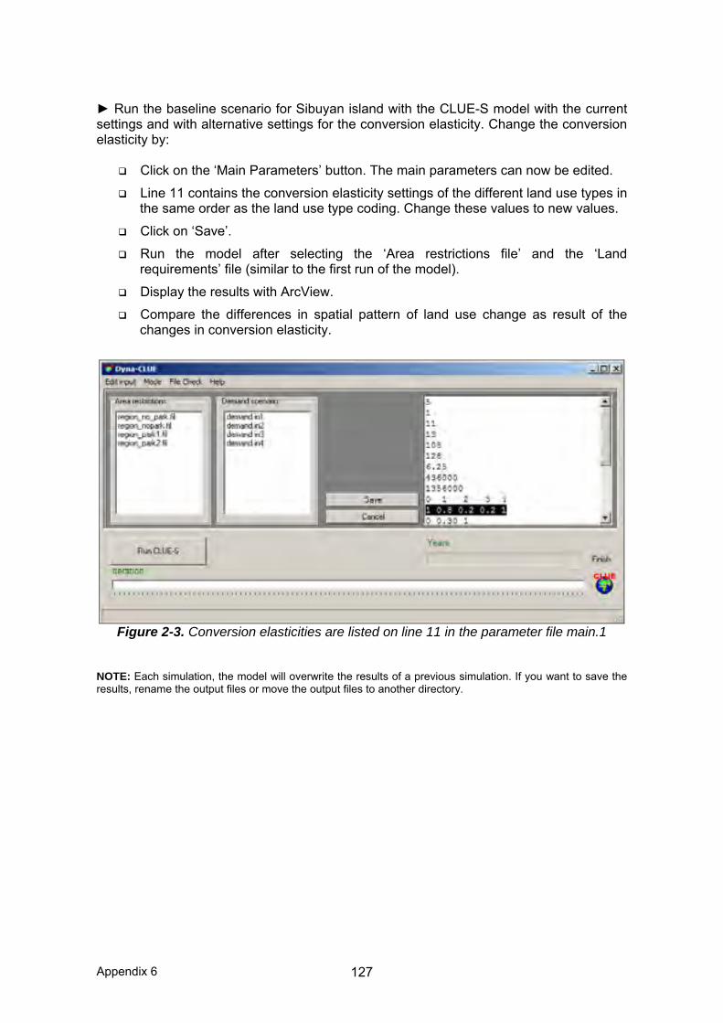
Appendix 6 127
► Run the baseline scenario for Sibuyan island with the CLUE-S model with the current settings and with alternative settings for the conversion elasticity. Change the conversion elasticity by:
Click on the ‘Main Parameters’ button. The main parameters can now be edited.
Line 11 contains the conversion elasticity settings of the different land use types in the same order as the land use type coding. Change these values to new values.
Click on ‘Save’.
Run the model after selecting the ‘Area restrictions file’ and the ‘Land requirements’ file (similar to the first run of the model).
Display the results with ArcView.
Compare the differences in spatial pattern of land use change as result of the changes in conversion elasticity.
Figure 2-3. Conversion elasticities are listed on line 11 in the parameter file main.1
NOTE: Each simulation, the model will overwrite the results of a previous simulation. If you want to save the results, rename the output files or move the output files to another directory.

Appendix 6 128
2.5 LAND USE CONVERSION SEQUENCES Not all land use changes are possible and some land use changes are very unlikely (e.g., arable land cannot be converted into primary rain forest). Many land use conversions follow a certain sequence or cycle, e.g. fallow land and forest regrowth often follow shifting cultivation. Figure 2-4 indicates a number of possible land use trajectories identified on Sibuyan island.
Figure 2-4. Possible land use trajectories on Sibuyan island. The conversions that are possible and impossible are specified in a land use conversion matrix. For each land use type it is indicated in what other land use types it can be converted during the next time step. Figure 2-5 provides a simplified example of a land use transition sequence. Forest can be converted in either agricultural land or grassland, while it is impossible to obtain new (primary) forest through the conversion of agricultural land or grassland directly. The figure also illustrates the translation of these conversion sequences into a land use conversion matrix, which can be used by the model. Depending on the definition of this conversion matrix and the time-steps chosen, complex land use sequences are possible.
Figure 2-5. Land use transition sequence The land use conversion matrix can be edited by clicking the ‘Change matrix’ button. It is also possible to use a text editor (e.g. Notepad) to edit the file ‘allow.txt’ in the installation directory. The rows of this matrix indicate the land use types during time step t and the columns indicate the land use types in time step t+1. If the value of a cell is 1 the conversion is allowed while a 0 indicates that the conversion is not possible. The rows and columns follow the number code of the land use types.

Appendix 6 129
Example: in the matrix below all conversion are possible except the conversion from coconut plantation into rice fields.
From ↓ To → Forest Coconut Grassland Ricefields Others Forest 1 1 1 0 1
Coconut 1 1 1 1 1 Grassland 1 1 1 1 1 Rice fields 1 1 1 1 1
Others 1 1 1 1 1 ► Run the baseline scenario for Sibuyan island with a different setting of the conversion matrix (keeping all other settings equal) and analyse the differences in outcome with ArcView. We suggest to compare a model run that allows all changes with a model run in which the conversion of grassland into agricultural land (coconut plantation and rice fields) is no longer possible due to soil degradation. Compare the results. Note: Some land use conversion settings will have no effect because they are overruled by the conversion elasticity and land requirement settings. In the baseline scenario we have assumed that the ‘others’ land use type is not changing and forest cannot ‘re-grow’ from other land use types as long as its total land area is decreasing. Consequently, changing the conversion settings for these land use types in the conversion matrix will have no effect on the simulation results. [End of exercise 2]

Appendix 6 130
Exercise 3: Defining spatial policies and creating new land requirements Objective: In this exercise you will learn how to prepare a new land requirements file and also a new area restrictions file. The combination of these new files represents a new scenario and you will then simulate your own scenario. 3.1 INTRODUCTION For some scenarios it is interesting to define areas where land use changes are restricted because of spatial policies, e.g. the conservation of nature. In the previous we have seen that spatial policies should be defined in an ‘area restriction’ file. This file contains a map of the study area indicating the extent of the case-study area and the zones of the case-study area where spatial restrictions apply. The ‘area restriction’ file is located in the installation directory and called ‘region*.fil’ where * can be defined by the user to indicate the conditions specified in the file. With the demo version of CLUE-S three different area restriction files are supplied, one without any spatial policy and two file indicating different extents of a nature reserve. ► Import these ‘area restriction’ files in ArcMap using the procedure as you used for the land cover grid in Exercise 1.5. It is best to copy these files to a temporary directory and then rename them there by adding “.asc” to the file.
Question: What are the different grid values in the area restriction files? What value is used for a restricted area? And what value for a non-restricted area?
3.2 PREPARATION OF A NEW AREA RESTRICTION FILE In this exercise you will create a new ‘area restriction’ file to simulate a scenario of the effects of a strict protection of all remaining lowland forest on Sibuyan island. Therefore we assume that during the simulations it is not possible to convert any of the remaining forest areas below an altitude of 100 meter. To make the area restriction file we need to identify: • The extent of the case study • The locations below 100 meter altitude • The locations with forest at the start of the simulations Therefore it is needed to import the land use map of year 0 (the start of the simulation) in ArcView. This land use map shows the extent of the study area (all grid-cells that are designated to a land use type) and the locations with forest at the start of the simulations. This land use map can be found in the installation directory (C:\Clues) and is called ‘cov_all.0’. To identify the locations below 100 meter an altitude map is needed. Since altitude is one of the location factors used in the simulations for Sibuyan island this map is already present in the installation directory. For this case study altitude is location factor number 7, so the elevation dataset in file ‘sc1gr7.fil’. ► Import both files using the ASCII to Raster option in ArcToolBox.

Appendix 6 131
Figure 3-1. Map query with the Raster Calculator in ArcMap In the ‘area restriction’ file the following coding should be used: 0 all grid cells that belong to the study area outside the ‘restricted
area’. These are the grid cells that are allowed to change.
-9998 all grid cells for which land use conversions are not allowed during the simulation (the ‘restricted area’)
-9999 (No Data) all other grid cells (outside the simulation area)
► Prepare an ‘area restriction’ file to prevent any forest areas below an altitude of 100 meter from changing. You can follow the steps below or use your own procedure:
Select all locations with forest located below an altitude of 100 meter at the start of the simulation by a ‘map query’ (Spatial Analyst | Raster Calculator) (Fig. 3-1). This will result in a new temporary theme ‘Calculation’ indicating all selected locations by a value of 1.
Classify the results of the previous step to the coding system of the area restriction file, as listed above (Spatial Analyst | Reclassify) (Fig. 3-2). This should create new temporary layer ‘Reclass of Calculation’ with values of –9998 and 0.
Export the result of the previous step as an ASCII file ‘region5.asc’ in the CLUE-S installation folder (ArcToolBox | Conversion Tools | From Raster | Raster to ASCII). Note that you must specify either a .txt or .asc extension
Using Windows Explorer browse to the installation directory and rename the file region5.asc to region5.fil (you may use a different number but you must use the region*.fil naming convention otherwise CLUE-S does not recognize it).

Appendix 6 132
Figure 3-2. Reclassifying a grid as an area restriction file.
► Restart the CLUE-S model and the new area restriction file should appear in the list of area restriction files and can be selected for the simulation. Run the model with this file and compare the result with a simulation without protection of forest resources. ► Prepare your own area restriction file based on a hypothetical spatial policy. You can also prepare area restriction files by delineating areas in ArcView that need to be converted to grid cells. Note: If the area restrictions violate the land requirements specified in the ‘land requirements’ file the model will not succeed in allocating land use changes and stop the simulation. This can occur when all forest is assumed to be protected while at the same time a decrease in land requirements for forest is specified. 3.3 CREATING YOUR OWN LAND REQUIREMENTS FILE ► You will now start defining your own scenario by generating a new land requirements input file for CLUE-S. Follow the steps and data guidelines below:
Open Microsoft Excel to facilitate the calculations.
Specify for each year (1997-2011) the land requirements of the different land use types in a table following the specifications below: Please note: Demand must always be expressed in hectares (10 000 m2).
Each row indicates a year; each column a land use type following the order of the land use coding.
Make sure to include also the land requirements for 1997 (year 0). These should be similar to the land use map of 1997 (29518.75, 7237.5, 5243.75, 1400, 1762.5 ha for respectively forest, coconut, grassland, rice and others).
The total land area required should equal the size of the island (45162.5 ha), i.e., the sum of the values on each row should equal 45162.5 for each year. Suggestion: you can temporarily add an extra column G or H and use a formula to verify that the row totals are always equal (for example: G2 = SUM(A2:F2)).

Appendix 6 133
We suggest not to change the land use requirements for the ‘others’ land use class and to create logical scenarios without sharp increases or decreases. This should prevent problems or very long run times during the simulation.
Figure 3-3. Entering land use requirements in a spreadsheet.
When all values have been defined, select the values (without land use type
names and year numbers) and paste the contents into a text editor (e.g. Notepad). Insert a line at the top of the file with the number of lines (years) for which the land requirements are specified (15 in our example).
Figure 3-3. Land use requirements copied to a text file demand.in*
Save this file in the installation directory as ‘demand.in*’ where * can be
defined by the users, e.g. demand.in5.
Restart the CLUE-S model; it is now possible to select the new land requirement file and simulate the land use changes.
Import and analyse the results in ArcMap.
[End of exercise 3]

Appendix 6 134
Background on the MAR Land Use Change Simulations In the previous exercises you worked with data for Sibuyan Island. This is a very small dataset and simulations ran very quickly, which made it very suitable for a relatively short training day and allowed you to quickly inspect the changes in simulation outcomes after you made adjustments in area restriction files, land demand and conversion elasticities. Now you will start working with some actual data for that we used for the MAR. The MAR catchment is approximately 190,400 km2 large, with 41% of the area in Honduras, 29% in Mexico, 18% in Guatemala and 12% in Belize. Those 12% represent the entire country of Belize whereas only parts of the other countries are included. Dataset prepared for each country First of all, it is important to know for that the regression analysis and the CLUE-S simulations were done separately for each country (or part of it). The reasons are:
Land use pattern and the drivers of land use change are different for the countries because of different policies, biophysical conditions or other factors, so performing a separate analysis allows a more accurate analysis.
Smaller data files by country facilitate easier data management. Nevertheless, these size of the data even for an individual country is much larger that for Sibuyan Island. For all four countries the smallest possible spatial extent was defined and the country grid were clipped to these extents. Size of the grid for Sibuyal Island and the MAR countries. Cell size is 250 m. Simulation times are observed on a laptop with a 2GHz Pent. M processor and 2GB of RAM Country # Rows
in grid # Columns
in grid# Data cells
(not Null)Average time fora simulation run
Sibuyal 108 128 7,226 < 10 seconds Belize 1151 604 349,762 ½ - 1 hour Guatemala 1503 1310 542,309 2 - 3 hoursMexico 1674 1262 886,433 3 - 4 hoursHonduras 1005 2131 1,267,903 4 - 5 hours All of MAR 3484 3016 3,046,407 N/A
West (xmin) East (xmax)Belize 261,500 412,500Mexico 213,250 528,750Guatemala 41,250 368,750Honduras 260,250 793,000 South (ymin) North (ymax)
Belize 1,757,500 2,045,250Mexico 1,971,250 2,389,750Guatemala 1,596,500 1,972,250Honduras 1,521,000 1,772,250
Figure 1: Spatial extents and mask for raster datasets for the four MAR counties. Coordinates are in UTM zone 16 with NAD 1927 Central American datum.

Appendix 6 135
GEO-4 Scenarios We adapted three of the four Global Environment Outlook 4 (GEO-4) scenarios Latin America and the Caribbean for use within the ICRAN MAR project. The scenarios envisage differing social, political and economic trajectories, emphasizing outcomes for the environment and human well-being. 1. Markets First: Under this scenario economic growth is prioritized over social and
environmental objectives. Everything becomes merchandise, including natural resources and basic goods such as water and culture. In general, regional environmental degradation continues to worsen.
2. Policy First: Environmental awareness develops within government more rapidly
than in the private sector or amongst the general public. The resource base is better managed, with policies being developed to alleviate the more serious environmental problems.
3. Sustainability First: In this world, economic, social and environmental
dimensions combine to shift the trajectory towards environmentally sustainable development. International cooperation within the region increases, with policies being directed to achievement of the Millennium Development Goals and sound natural resource management.
More details about the scenarios can be found in Miles (2006), which is included in the readings list and as a PDF file on the CD. Land requirements Land requirements for every scenario were calculated using the IMAGE model. In the next exercise we will focus on Belize. The table below gives the distribution of land use at present and the calculated land demand under the scenarios in 2025 for Belize. The total area is 21860.13 km2. The area of land use types 0 and 9 is assumed to remain constant. Land use distribution at present and for the scenarios in Belize. Present
(2004)
Markets First 2025
Policy First 2025
Sustainability First 2025
0. Other/Unknown 0.06% 0.06% 0.06% 0.06%1. Broad-leaved forest 58.02% 54.33% 56.69% 57.78%2. Pine forest 3.53% 3.31% 3.45% 3.52%3. Agriculture/pasture 19.37% 23.20% 20.64% 18.85%4. Scrub 1.26% 1.23% 1.13% 1.37%5. Savanna 8.63% 8.23% 8.35% 8.65%6. Wetland/Swamp 4.26% 4.07% 4.12% 4.27%7. Mangroves 3.29% 3.08% 3.22% 3.28%8. Urban 0.87% 1.79% 1.64% 1.51%9. Water 0.70% 0.70% 0.70% 0.70%
Appendix 6 136
Exercise 4: Working with actual scenario data for Belize Objective: In this exercise you will learn some of the actual data that were used for the Belize simulations, and how dynamic location factors were used. You will also create and review probability surfaces. At the end of the day you should have a sufficient knowledge of the data to simulate and analyze the actual different scenarios yourself. 4.0 COPY THE CLUE-S MODEL AND DATA FOR BELIZE FROM CD Using Windows Explorer, browse to the folder C:\Training\Data\CLUE-S\ on your
computer (or the CD). This folder has 4 zip files that contain all land use and location factor grids in regular grid and ASCII format.
Double-click BZ.ZIP and unzip (extract) the file in a temporary location on your computer, e.g., c:\temp. Remember where you extracted the file.
Also copy the entire CLUE_BZ folder from the CD to a place on the harddisk. Then right-click the folder, select Properties,uncheck “read-only”, and apply it to all subfolders and files. CLUE-S will give an error if the folder is read-only!
4.1 REVIEW OF THE LAND USE DATA The baseline land cover map was based on the 2004 version of the Belize Ecosystem Map and the revised 2003 Ecosystem Map for Central America land use data. The original land cover classification was reduced to 10 classes (Table 4-1) and the data was converted from a vector to a raster format with a 250 m grid cell size.
Note: CLUE-S requires that the land use numbering to start at 0, not 1.
Table 4-1: Reduced land use classification used for the MAR Value Land use type Value Land use type 0 1 2 3 4
Other/unknown Broad-leaved forest Pine forest Agriculture/pasture Scrub
5 6 7 8 9
Savanna Wetland/Swap Mangroves Urban Water
► Let’s now look at the reclassified 2004 land use data for Belize:
Open ArcMap and load the layer file ‘Belize Present land Cover (2004).lyr’ that is in the BZ data folder (the layer file source grid is ..\BZ\grid\bzecomap).
Review the land cover data. Keep in mind that these data were based on the 2004 Ecosystem Map for Belize (Meerman & Sabido. 2001), reclassified and converted from vector to raster data with a cell resolution of 250 m.
4.2 STATIC AND DYNAMIC LOCATION FACTORS For every region you must specify a number of driving factors of land use change. These ‘location factors’ were determined by a statistical regression analysis. Table 4-2 lists all location factors that were analyzed for the MAR. The numbering must starts at 0. A location factor can be static of dynamic, as is indicated in the last column of the table.
Static: the location factor is constant over the entire simulation grid. The grid is saved in ASCII format with the following naming convention: SRxGR.FIL

Appendix 6 137
Dynamic: the location factor changed over time. Instead of a single ASCII grid we have to prepared a grid for every year: SRxGRD.y
where x = the number of the location factor (0 to 11) y = the simulated year started at 0 (for belize, 0 to 21)
For the MAR land use simulations only one location factor was dynamic: No. 11, protected areas with partial protection. Of course, population density will also change over time, and accessibility to markets and road may also change if no roads are built. However, the scenario descriptions that were developed described the future changes for the country as a whole and did not provide sufficient details about exactly what, where and how changes might occur on a regional or local scale. Table 4-2: Location factors (LF) used for the MAR land use simulations.
No Description [unit] CLUE-S file
Original GRID file
Dynamic
0 Population density [# per km2] SC1GR0.FIL POPDEN No 1 Soil depth [meter] SC1GR1.FIL SDEPTH No 2 Soil drainage [0-1] SC1GR2.FIL SDRAIN No 3 Mean annual rainfall [mm] SC1GR3.FIL RAINYR No 4 Length dry period [consecutive months
with < 60 mm rain] SC1GR4.FIL DRYMON No
5 Elevation [meter] SC1GR5.FIL ELEVAT No 6 Slope [degrees] SC1GR6.FIL SLPDGS No 7 Accessibility to markets
[travel time in hours] SC1GR7.FIL ACSMKT No
8 Accessibility to roads
[travel time in hours]
SC1GR8.FIL ACSRDS No
9 Coastal area / tourism hotspots [0/1] SC1GR9.FIL TOURIS No 10 Protected areas / full protection [0/1] SC1GR10.FIL WDPAR1 No 11 Protected area / partial protection [0/1] (SC1GR11.FIL)
SC11GR.0 - - - - - SC11GRD.21
WDPAR2 Yes
► You will now review the location factor grids.
Browse to the ‘BZ’ folder that you just extracted. You should see two sub-folders, “ascii” and “grid”. Both folders contain the same dataset but in different formats. It is easier to work with the data in the “grid” folder because these data can be readily loaded as a layer in ArcMap.
Open a new ArcMap document and load location factor 8, “Accessibility to Markets” (bzACSMKT). The unit of this data is travel time in hours. It was calculated using a methodology developed by researchers at CIAT, Colombia. Do you think the travel times are fairly realistic?
Also load location factor grid 10 (bzWDPAR1) and 11 (bzWDPAR2). A grid value of 1 means that the grid cell is a protected area, a value of 0 not. Are you familiar with the protected areas in the country?
Load all other grids location factor (i.e., don’t load the “bzLUC_” grids – these are grids for individual land use types). Review all location factor grids and make sure that you understand these grids and their units.

Appendix 6 138
4.3 REGRESSION EQUATIONS AND PROBABILITY SURFACES Note: in this part of the exercise you will be learning about some of the more advanced features of CLUE-S. Nonetheless, you will need to understand these features if you are planning to use CLUE-S for actual simulation modeling of land use change. The allocation of land across the region is done by CLUE-S based on probabilities, which, in turn, are calculated using regression equations that account for the effect of one or more location factors. For example, the regression analysis showed a significant relationship with Urban land and three location factors, as follows:
Probability LU8 = 0.5 + 0.01 LF0 – 0.37 LF7 + 0.70 LF9
where LU8 = Land use type 8, Urban LF0 = Population density LF7 = Accessibility to markets LF9 = Coastal area / tourism hotspot
Note the negative relationship for LF7. Thus, the farther away a grid cell is from a market, the lower the probability that land use at that location changes to Urban.
► The regression equation above and similar equation for other land use types are specified in the file alloc1.reg. You will now briefly review that file.
Browse to the folder CLUE_BZ that contains all files for Belize.
Right-click on the file alloc.1reg and open the file in a text editor such as Notepad or Textpad. You can select NotePad by choosing “Open With” and the selecting Notepad from the list of available programs.
Scroll to the end of the file. Do you recognize the parameters from the equation above? Please refer to pages 22-23 of the CLUE-S user manual for more information about the precise format of this file.
The regression equations are important because during run-time CLUE-S uses these equations to create probability surface for every land use type. These surfaces show the probability of changes towards that land use type across the entire study area.
► Let’s look at some of these probability surfaces.
Using Windows Explorer, browse to the ..\Training/CLUES_BZ\ directory and double-click clues.exe to start the model.
Select “Calculate Probability Maps” from the Mode main menu.
Select one of the area restriction files and one of the demand files.
Press the “Run CLUE-S” button to start the model. The model will now only calculate the probability maps. This will take about 1-2 minutes. Press the “Calculations Finished” button but do not close the application.
Go back to Windows Explorer in the CLUE_BZ folder and refresh the contents of the folder view. You should now see the probability surfaces that were created with the names prob1_0.1, prob1_1.1, …, and prob1_9.1.
Rename the extension of all ten probability files from “.1” to “.asc”.
Open ArcMap and ArcToolBox. Use the “ASCII to Raster” tool to import the files prob1_6.asc (probability for Wetland) and prob1_8.asc (probability surface for Urban). Make sure to select “FLOAT” as the Output data type.
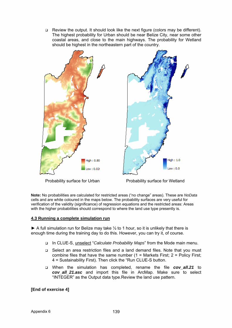
Appendix 6 139
Review the output. It should look like the next figure (colors may be different). The highest probability for Urban should be near Belize City, near some other coastal areas, and close to the main highways. The probability for Wetland should be highest in the northeastern part of the country.
Probability surface for Urban Probability surface for Wetland
Note: No probabilities are calculated for restricted areas (“no change” areas). These are NoData cells and are white coloured in the maps below. The probability surfaces are very useful for verification of the validity (significance) of regression equations and the restricted areas: Areas with the higher probabilities should correspond to where the land use type presently is. 4.3 Running a complete simulation run ► A full simulation run for Belize may take ½ to 1 hour, so it is unlikely that there is enough time during the training day to do this. However, you can try it, of course.
In CLUE-S, unselect “Calculate Probability Maps” from the Mode main menu.
Select an area restriction files and a land demand files. Note that you must combine files that have the same number (1 = Markets First; 2 = Policy First; 4 = Sustainability First). Then click the “Run CLUE-S button.
When the simulation has completed, rename the file cov_all.21 to cov_all_21.asc and import this file in ArcMap. Make sure to select “INTEGER” as the Output data type.Review the land use pattern.
[End of exercise 4]

ANNEX. 8. BELIZE COASTAL ATLAS

Mesoamerican Reef Alliance - ICRAN-MAR
Workshop on Watershed Management, Land Cover Change Analysis, and Modeling of Land-based Sources
of Pollution and Sediment Discharge to the MAR
Proceedings
Galen University
SAN IGNACIO, BELIZE, AUGUST 15-18, 2006
Eric van Praag, Consultant for UNEP-WCMC Joep Luijten, Consultant for UNEP-WCMC
Lauretta Burke, WRI Liza Agudelo, ICRAN-MAR
September, 2006

List of Acronyms
BMP Better Management Practices CATHALAC Water Center for the Humid Tropics of Latin America & the Caribbean CLUE-S The Conversion of Land Use and its Effects DEM Digital Elevation Model GIS Geographic Information System IABIN Inter-American Biodiversity Information Network ICRAN-MAR Mesoamerican Reef Alliance INEGI Instituto Nacional de Estadística, Geografía e Informática, México JICA Japan International Cooperation Agency LAC Latin America and the Caribbean LU/LC Land use/Land cover MAR Mesoamerican Reef MBRS Mesoamerican Barrier Reef System N-SPECT Nonpoint Source Polution and Erosion Comparison Tool SeaWifs Sea-viewing Wide Field-of-view Sensor (SeaWiFS) SERVIR Mesoamerican Regional Visualization and Monitoring System SIDA Swedish International Development Cooperation Agency SRTM Shuttle Radar Topography Mission UNEP United Nations Environment Programme UNF United Nations Foundation UNFCCC United Nations Framework Convention on Climate Change USAID U.S. Agency for International Development USGS U.S. Geological Survey WCMC UNEP World Conservation Monitoring Centre WRI World Resources Institute WWF World Wildlife Fund WRIScS Watershed-Reef Interconectivity Scientific Study
1

ACKNOWLEDGEMENTS Organizing this workshop would not have been possible without the help and the contributions provided by UNEP-WCMC, ICRAN, Galen University, WRI, USAID, UNF, CATHALAC and WWF. We also wish to thank the following individuals who made valuable contributions to the workshop, provided training, organized the logistics, and provided general workshop support: Lauretta Burke and Zachary Sugg (WRI), Lera Miles, Joep Luijten and Eric van Praag (UNEP-WCMC), Liza Agudelo and Armeid Thompson (ICRAN-MAR), Jose Vasquez (WWF), Emil Cherrington (CATHALAC), Melanie McField (Smithsonian), and Carlos Rivas (SIDA). Special thanks to Galen University (Cayo, Belize) and to Marion Cayetano, Rhondine Petrof, and Shannon Kenney for their kind support with organization details.
2

TABLE OF CONTENTS INTRODUCTION .............................................................................................................. 4 POLICY SESSION............................................................................................................. 5
SUMMARY OF BREAKOUT GROUP REVIEWS...................................................... 9 DISCUSSION AND RECOMMENDATIONS............................................................ 11
TECHNICAL SESSION................................................................................................... 15 APPENDIX 1. Workshop Agenda.................................................................................... 17 APPENDIX 2. Policy Session Participants ...................................................................... 21 APPENDIX 3. Technical Session Participants................................................................. 23 APPENDIX 4. Technical Session Evaluation Sheet......................................................... 24 APPENDIX 5. Summary of Technical Evaluation Results. ............................................. 26 APPENDIX 6. Technical Questionnaire........................................................................... 30 APPENDIX 7. Summary Of Results From Follow-Up Questionnaire............................. 31 APPENDIX 8. Useful Links ............................................................................................ 34
3

INTRODUCTION
ICRAN-Mesoamerican Reef Alliance (ICRAN-MAR) The International Coral Reef Action Network (ICRAN), was established in the year 2000 as an innovative and dynamic global partnership of many of the world's leading coral reef science and conservation organizations. It is a collaborative effort that operates at different levels to help to stop and reverse the decline in health of the world's coral reefs. ICRAN partners create alliances around the world to facilitate inter-linked and complementary actions in reef monitoring and management, at local, national, and global scales. In the ICRAN Mesoamerican Reef Alliance (ICRAN-MAR), several partners have come together in a three-year initiative to support regional efforts in response to the Tulum Declaration of 1997 for the conservation of the Mesoamerican Barrier Reef (Mexico, Belize, Guatemala, and Honduras). With the kind contribution of the United States Agency for International Development (USAID), and the United Nations Foundation (UNF), and under the overall supervision of the United Nations Environment program (UNEP), the ICRAN-MAR Alliance seeks to develop and facilitate innovative tools that promote the voluntary adoption of best management practices in the areas of Tourism, Fisheries and Watershed Management. The project therefore, offers a holistic approach that recognizes the strong relationship between these three components and their potential impact on the health of the Mesoamerican reef, and promotes and seeks cooperation with other institutions and initiatives in the region. The Watershed Management component of the ICRAN-MAR project was designed recognizing that appropriate land use practices are critical for proper management of watersheds in the Mesoamerican region, and to ensure that transport of sediment, nutrients and other pollutants to the coral reef system is minimized. Developing appropriate land use strategies requires gathering information on the potential impact of different land use and development options in the region, as well raising awareness and coordination with the different stakeholders. ICRAN-MAR partners in the Watershed Management component contribute to these regional efforts by forming alliances with the private sector to reduce the impact of agricultural activities on the reef, and by developing innovative Geographic Information Systems tools that can be used to simulate watershed dynamics and inform decision makers in the Mesoamerican region. With respect to the GIS tools, the work of the ICRAN-MAR project is complementary to the ongoing and past work of other regional initiatives such as the MBRS, SERVIR and IABIN-DGF projects. It is the first to engage a regional-scale analysis and spatial modeling of the environmental impacts of watersheds on the Mesoamerican Reef. This work also builds on the World Resources Institute’s Reefs at Risk of the Caribbean initiative. The current proceedings summarize the dynamics and outcomes of a successful workshop held in San Ignacio, Belize in August 2006, in which project partners presented the results of two years of project implementation and requested feedback from regional experts.
4

Watershed Management Workshop The objectives of the meeting were twofold: inform regional participants of the land use modeling results and the initial findings for the region, and train regional GIS technical experts who could in turn become trainers of other experts in their particular countries. The workshop was divided in two sessions: a Policy Session and a Technical Session. The policy session was geared towards senior managers and decision makers of participating institutions; its main objective was to help them understand the usefulness and applicability of the data products and models developed by ICRAN-MAR for watershed management. This session lasted for one and a half days and took place on August 15th and the morning of August 16th. The technical session’s objective was to allow specialists from participating countries to become familiar with and get hands-on training in the use of the data products and models aforementioned. This session lasted for two and a half days and took place on the afternoon of August 16th, and on August 17 th and 18th. Both sessions provided a great opportunity for national specialists to acquire new technological knowledge, coordinate activities, plan their modeling efforts, exchange experiences with colleagues from other countries, and acquire geospatial information developed or collated by ICRAN-MAR. The following sections provide an overview of the contents, results, discussions and resolutions attained in the course of the two sessions of the workshop.
POLICY SESSION The Policy Session was held on August 15 and the morning of August 16, 2003, at Galen University in San Ignacio, Belize (see workshop agenda in Appendix 1). Senior staff and specialists from national and regional institutions that deal with marine and coastal issues attended the meeting (see list of participants to policy session in Appendix 2). The objectives of the policy session were the following:
1) Inform policy makers and other potential information users of the information outputs and tools that have been developed under this project.
2) Learn about the ICRAN MAR watershed project and the analytical components on land cover change analysis, watershed delineation, hydrologic modeling and circulation modeling.
3) Review scenarios of land cover change and provide feedback on these scenarios.
4) Review results of predictive modeling of land-based sources of pollution and sediment discharge to the Mesoamerican Reef
5) Raise awareness of the linkages between human activities on the land and threats to the Mesoamerican Reef.
6) Identify policy questions/applications for the analytic tools, as well as future users of the analytic tools.
5

During the morning of August 15 an introduction to the ICRAN-MAR project and the role of its partners in the watershed component was offered, together with the following keynote presentations: Health of Corals and threats to the Mesoamerican Reef (by Melanie McField)
Dr. McField gave a thorough presentation on the most pressing threats (dredging, tourism, aquaculture-overfishing, poor port management and shipping, climate change, and natural disasters) to the Mesoamerican Reef (MAR). She discussed the concept of a “healthy” reef and the different reef attributes (structure and function) and human dimensions (drivers of change, social well being, and governance) that must be taken into account when defining the level of disturbance (i.e. health). Eventually we need to make use of the reef resources and we need to identify the best ways to do so.
Conceptual evolution of watershed management in the Mesoamerican Region (by Carlos Rivas)
Dr. Rivas presented the evolution of the watershed management efforts in the region during the last 20-30 years. He began by introducing the topographic characteristics of the region and the socio-economic drivers that have defined regional development models, and the traditional agricultural uses of the land. Extractive economy, poverty and expansion of the urban and agricultural frontiers have caused changes in the landscape and the watershed dynamics over the past decades. The need to control flooding and guarantee the provision of water resources to cover the increasing needs of the population and industry led to the early watershed management efforts imported from developed countries to the region. With time, there has been a shift from anthropocentric (‘rational/economic’) to more biocentric (‘sustainable’) rationales when developing strategies to manage watersheds. With this shift in mentality, the social component is included and participatory planning is encouraged; however, the strategies are not always economically attractive and very often conflicts arise. There is a generalized need for more government support and development of coherent policies for the sustainable use of the water resources.
Following the keynote presentations, Joep Luijten (UNEP-WCMC) and Lauretta Burke (WRI) respectively offered an overview of the different methodologies and results in land use change and hydrologic modeling1; immediately afterwards, Jose Vasquez (WWF) presented results of the on-the-ground work with agricultural companies for the adoption of better agricultural practices. Overview of scenario development (by Joep Luijten)
Joep Luijten began his presentation by explaining the concept and descriptive nature of the scenarios, and how they can inform policies. Scenarios are not predictions of the future, but rather present “different assumptions about how current trends will unfold, how critical uncertainties will play out and what new factors will come into play” (UNEP, 2002). The 3 scenarios developed for this project were adapted from the Global Environment Outlook 4 scenarios for LAC that will be released in 2007. These scenarios looked at the current regional situation of the natural resources and
1 Please refer to the Workshop Data CD for detailed documentation on the development of the scenarios, land use change modeling, and hydrologic and circulation modeling.
6

the potential situations by 2025 under three hypothetical world-wide and regional situations (Markets First, Policy First, and Sustainability First). These scenarios would have different impacts on the socio-economic and natural dimensions of the region and could serve to influence decision makers.
Overview land use change modeling (by Joep Luijten)
Once the descriptive scenarios were developed, a multi-scale modeling approach was applied to quantify the potential changes in land cover in the MAR. Three models were utilized (International Futures, IMAGE, and CLUE-S) to explain the dynamics of the different variables involved in land cover change processes. Thus, the International Futures model estimates the proportion of regional land use change that occurs in each country, and provides socio-economic drivers to the IMAGE model. IMAGE in turn, is a global integrated assessment model that simulates the rate of change in the region, and the proportion of change that occurs in each land use type. CLUE-S is the land use change (allocation) model and adds a spatial dimension that simulates where land cover change occurs within the MAR region. For quantification of the changes in land demand under each scenario the year 2000 was used as the base year because that was the year for which the latest land cover data were available for most countries.
Overview of Hydrologic and Circulation Modeling for the MAR (by Lauretta Burke) Lauretta Burke began her presentation highlighting that the purpose of this analytical modeling exercise of the ICRAN-MAR was to model present and future impact of land cover change and agricultural activities on coral reefs and identify land most vulnerable to erosion. The outcomes of the modeling exercises could eventually guide stewardship of vulnerable areas in the region. Likewise, the project sought to identify tools and a methodology that could be easily be transferred to analysts and land stewards in the MAR region for more detailed local application. The first step in this exercise was to delineate the watershed for the region. Basins were delineated from 90m resolution NASA SRTM data and 300 basins (of 5 km2 minimum size) were identified within the MAR region. This exercise took several months and was especially difficult for the Yucatan peninsula due to the geological characteristics of the terrain and the presence of underground rivers. She invited participants to provide inputs to improve the accuracy of the delineation. The following step was to run the “Nonpoint-Source Pollution & Erosion Comparison Tool” (N-SPECT) to evaluate sediment and pollutant delivery into coastal waters. The N-SPECT model, developed by NOAA, is in the public domain and is easy to run in ArcMAP. N-SPECT provides estimates of erosion across the landscape as well as sediment and pollutant (N and P) delivery and concentrations at the river mouths. Using the land cover scenarios from CLUE-S, coupled with the N-SPECT hydrologic model, sediment and pollutant delivery at 300 river mouths can be estimated. The University of Miami is implementing a high resolution 4-dimensional model to examine sediments and pollutants transport within the region’s lagoonal system. The sediment and nutrient transport predictions will be calibrated using the SeaWifs sensor. Lauretta commented that the hydrologic results need to be calibrated (and validated) using data from several sources. Project collaborators from Texas A&M University are taking sediment samples; WWF is taking sediment samples and is looking at
7

bioaccumulation of toxics in reef organisms. AGRRA reef assessments will be used to examine the location of sediment impacts on coral reefs. She discussed the limitations of the analysis and invited workshop participants to make recommendations for data to calibrate the model.
Results of Hydrologic and Circulation Modeling (by Lauretta Burke)
Keeping all inputs but land cover equal, WRI produced estimates for the present day and future scenarios of accumulated runoff, as well as accumulation and concentration of sediment, nitrogen, phosphorous, and total suspended solids. Annual model runs were implemented for current land cover, hypothetical natural land cover, and the three 2025 scenarios for the MAR region. Analysis of results allowed the identification of those areas with the highest sediment and nutrient delivery, and of how much sediment and nutrient delivery has increased due to human activities. It was also possible to see the influence that future land cover might have on sediment and nutrient delivery, as well as the areas that are the most vulnerable to erosion, and which parts of the MAR are affected by sediment and nutrients. Maps and summary tables were presented, and later discussed with workshop participants.
Activities with Agribusiness for the adoption of Better Management Practices (BMPs) (by José Vasquez).
José Vasquez presented the efforts WWF is leading in the region to raise awareness and persuade agricultural companies into the adoption of BMPs. He began by highlighting that agrochemicals (fertilizers and pesticides) are known for their effect on global reef health. In 2004 WWF conducted a preliminary monitoring analysis to identify the levels of toxic substances in marine organisms and identified the need to reduce the presence of particular ‘priority’ pesticides in the MAR. To accomplish this, and to control soil erosion, they have engaged in conversations with some of the major agricultural companies in the region, and are currently developing partnerships for the adoption of BMPs in banana, citrus, palm oil, pineapple and sugar cane crops. Based on the preliminary results presented by WRI and WCMC, WWF will select a pilot watershed to collect specific data to validate the models, and to pursue the implementation of BMPs.
In the afternoon participants broke into four national groups (Honduras, Belize, Mexico, and Guatemala) to review the modeling results by country Each group presented a summary of their observations and suggestions at the plenary session in the morning of August 16 (see summaries in the following section). Data dissemination through the Mesostor portal (by Emil Cherrington)
During the morning policy session on August 16, the representative from the Water Center for the Humid Tropics of Latin America & the Caribbean (CATHALAC) presented briefly on how the ICRAN-MAR Project’s data and information products will be disseminated through the USAID-supported Regional Visualization & Monitoring System (SERVIR) at: http://servir.nasa.cathalac.org or http://servir.nsstc.nasa.gov. Mr. Cherrignton mentioned that the MAR data will be added to the variety of public domain spatial datasets and satellite imagery already available through SERVIR for the Mesoamerican region. As such, long after project completion, researchers and decision-makers will continue to have access to the rich database developed by the ICRAN-MAR Project regarding land-based impacts on the Mesoamerican Reef
8

ecosystem. With regard to synergies between these two USAID-supported initiatives, SERVIR and the ICRAN-MAR Project have collaborated on data development, and SERVIR representatives provided technical support during the August 2006 Regional Watershed Modeling workshop in Belize.
During the discussion session, Dr. Barbara Best – Coastal Resources and Policy Advisor for the Office of Natural Resources Management with USAID, and Cognizant Technical Officer for the ICRAN-MAR Alliance – presented on opportunities for partnerships within the region and on a broader spatial scale. In particular she described the USAID Global Development Alliance, which works through public-private partnerships, and the Central America Free Trade Agreement (CAFTA), through which Central American countries could access financial support for follow-up activities in the region. She highlighted the emphasis these initiatives give to capacity building efforts, water issues, and tourism, and encouraged participants to communicate the results of this workshop’s discussions to their governments and seek additional funding for capacity building. As another opportunity for capacity building Dr. Best recommended linking US Universities with local Universities.
SUMMARY OF BREAKOUT GROUP REVIEWS BELIZE 1. The watershed boundaries look good, but must be re-drawn to reflect the 18 major
watersheds of Belize. Small coastal watersheds must be merged with larger ones rather than leaving them out. Note: In response to this, Lauretta Burke mentioned that N-SPECT calculates using much larger watersheds, with the smaller coastal watersheds being merged, though she emphasized that these larger watersheds are incorrect because they reflect the combined catchments of multiple rivers that drain into the sea.
2. N-SPECT outputs need to be explored further / validated. 3. Land Use scenarios – the group would like to know more about how the scenario
narratives were translated to IMAGE 2 outputs. 4. Numerous possible applications of project outputs exist (e.g. overall land use
planning, reporting to UNFCCC). 5. The results are good and reveal worthwhile / critical investment of effort.
MEXICO 1. Model validation is necessary and accurate data is missing. Mexican colleagues
encourage workshop participants to develop a campaign to collect field data to calibrate the models.
2. A legend should be added to the maps to clarify that the results are estimates. Mexican participants can contribute recent national data to jointly validate the models.
3. Some aspects of the N-SPECT and CLUE-S methodologies are not clear in particular with respect to concepts and variables. For example, it is not clear what were the criteria to reduce the LU/LC classes in the GEO scenarios.
9

4. Meteorological sporadic or extraordinary events should be incorporated into the N-SPECT model. Evaluate the possibility to run the model for different time periods (e.g., quarterly, monthly).
5. The Markets First and the Policy First scenarios showed similar results. Evaluate if a new or intermediate scenario can be created. The scenarios for a 25-year period don’t show drastically different results.
6. The Yucatan Peninsula should be treated as a special case in the N-SPECT model since its underground water flow is difficult to estimate. The Mexican group estimated that the preliminary model results are not representative of the real flow dynamics and should be taken out of the maps (or highlighted as preliminary). Need to incorporate the results of the JICA study on underground water flow into N-SPECT (when it becomes available).
7. The N-SPECT model does not show “real” results for Yucatan and can lead decision makers to judge that the sediment and pollution flow to the MAR is not significant.
8. Keep in mind that the Yucatan peninsula does not suffer from what is normally termed as soil erosion. Instead, if suffers from dissolution of the bedrock due to soil characteristics.
9. Consider including higher resolution data for the Rivera Maya to pinpoint the effects of large coastal developments (e.g., Cancun, Playa del Carmen).
10. Consider the development of a special N-SPECT model only for the Yucatan Peninsula.
GUATEMALA 1. First impression of the work is very good, but there is the need to incorporate more
detailed data and national datasets. 2. It is essential to calibrate the model and adjust its variables. 3. Results seem logical, but are they significant? 4. Recommendation to look at extreme events, not necessary a second Hurricane
Mitch, but something more dramatic than the monthly and annual data that the models have used. Looking at rainfall events could be a good first step.
5. Recommendation to create maps that better illustrate the differences between the scenarios. This is not clear from the maps presented, though maps highlighting the differences are presented in the CLUE-S technical report on the training CD.
6. Further information is needed about the assumptions that were made and restrictions of the models/methodologies. Joep Luijten mentioned that for CLUE-S some information of this nature can be found in the technical report on the training CD.
7. It must be made clear that if two scenarios show the same percentage land cover for a particular land use type, there could still be significant differences in the spatial distribution of land use. Thus, just having a table that lists the percentages of area covered by each land use type is misleading.
8. Need to include socio-economic variables in the models. For example, if the area of forest decrease with 5%, what is the $ value of the change? How much do the changes affect tourism?
9. Largest differences on forest and cropping. Application is useful for sustainable forest management and integrated watershed management.
10

HONDURAS 1. The delineation of watersheds looks good but small coastal watersheds should be
merged with larger adjacent ones so that the overall delineation better matches the country’s official watersheds.
2. Would like to see a method to include dams in the model. At present there is a hydro-power dam in the Ulua watershed and the Honduras team will be interested in calculating the accumulation of sediment behind the dam. How could this variable (i.e. existence of dams) be incorporated into the model?
3. Results will help the team prioritize areas where reforestation programs and soil conservation programs could take place.
4. The results are valuable for decision-makers in both the private and public sector. This would be an excellent tool for the land-use planning that recently started in Honduras.
5. Work collaboratively at the regional level to promote the use of the same GIS technologies for better management of natural resources.
6. The datasets and products provided by ICRAN-MAR in the workshop are not final; instead they should be viewed as intermediate products that need to be refined at the national level to provide scientific information useful for decision-making.
7. The model should include socio-economic data that can be presented to decision makers.
8. Participants should reach a formal compromise whereby they agree to apply and improve the models provided in accordance with the local capacities and existing informational needs.
9. Need to work at higher resolutions: 90 or 30 meters. It should be noted that such small resolution are not practical when the models are applied to a country or the MAR region as a whole because the required simulation times would be far too long.
DISCUSSION AND RECOMMENDTATIONS The policy session ended with a two-hour review, conducted by the whole group, on the ICRAN-MAR watershed component and the workshop results and follow-up activities; it centered on the need to inform policy makers in participating countries about the results of the ICRAN-MAR exercise, and on the need to provide follow-up support to agencies that decide to use the models and datasets produced by the watershed component of ICRAN-MAR.
A summary of the main issues raised during the review follows:
• Results are useful for some specific purposes. The MAR-drainage-wide watershed analysis was regarded as ambitious. Participants recognize the amount of effort that went into the analysis; appreciate the region-wide comparable results; but recommend that the results be shared with instructions about appropriate and inappropriate use. These are estimates of sediment and nutrient delivery from coastal watersheds given current land cover and given several scenarios of future land cover.
• Scenario results are not that different: Differences between the scenarios are not large; most participants had expected to see greater contrasts. This could be related to the relatively short time period (2000-25) or be because the scenarios
11

are too general and are unable to adequately reflect critical changes that appear on a local level or in the immediately coastal areas.
• Model results need to be validated. There is a need to better calibrate the models and validate model results. There is ongoing work with SeaWifs (with the University of Miami) and there are data from the WRISC project that can be used to evaluate the estimates for several watersheds. WRI asked participants to provide data for validation.
• Information can influence policy. A participant asked how ICRAN-MAR can use results to preserve forests. Lauretta Burke responded that having a good, integrated information infrastructure (to support sound spatial analysis) and having channels to decision-makers is key.
• Local application of modeling tools will produce the most useful, detailed results. Technology transfer and capacity building is an important part of the workshop. Participants will be able to use local data (as inputs and for validation), and therefore can do more detailed analysis and obtain more accurate results back in their agencies.
• Results are not final: The analysis results are not a final product. ICRAN-MAR needs to build capacity to use the models offered during the workshop within the region, so that people can use local information to refine results and validate the modeling.
• Extreme Events. The N-SPECT modeling focused on mean annual precipitation. Extreme events such as hurricanes and tropical storms are the major source of sediment. It would be valuable to model extreme events and the seasonality of discharge.
• Clarification on N-SPECT Units. The MBRS representative thought that the N-SPECT model outputs were “relative” and not in meaningful units. WRI’s experience is that N-SPECT output is in liters for discharge and kilograms for sediment and pollutants.
• Basin Delineation style. There was some discussion of the MAR basin delineation, focusing on the small coastal watersheds. Many participants would prefer to have these small watersheds lumped into the larger, adjacent basins. WRI cannot do such lumping, as it would be inconsistent with hydrologic flow within the DEM. However, N-SPECT uses an algorithm that does merge small adjacent watersheds. These results are provided on the data CD.
• Yucatan. WRI acknowledged that the basin delineation for the Yucatan is not very good due to underground rivers and few perennial surface rivers. The group from Mexico also pointed out this limitation, and mentioned that JICA is now working on estimating underground water flow. As policy-makers will dismiss the Yucatan results, they encouraged WRI to consider excluding the basins in the Yucatan from the results, or issue strong and appropriate disclaimers about the problems with the model in the Yucatan.
• Scenario results. The analysis of change in sediment between natural and current land cover is striking and clearly shows the extent of human impact. The results of the N-SPECT modeling for the three future land cover scenarios, however, do not look very different. This is because
12

a) the land cover scenario data sets are not so extremely different
b) the results are presented at the basin-level. WRI can explore presenting them at the sub-watershed level.
• Management Practices. Due to the lack of regional data on agricultural crops and the fact that the management practices module of the N-SPECT model is not yet implemented, WRI’s analysis focuses on the impact of land cover change on sediment and pollutant delivery. It would be very valuable to include management practices in the model in the future.
• Dams. Some participants asked WRI to look into the possibility of incorporating dams into the N-SPECT model as a sediment trap. WRI will research the issue further.
• Relevance of Results to Policy. There was discussion of the difficulty of moving from analysis results to changes in policy. The inclusion of socio-economic values was encouraged.
• Erosion monitoring. WWF is monitoring soil erosion on citrus, palm oil and sugar cane plantations. This data would be very valuable if WRI could, under a future project or future project phase, attempt to include different crops and management practices in the hydrologic analysis.
• Economic Valuation. Several participants encouraged including economic variables in the results, such as the value of lost soil, lost agricultural productivity, and damage to coral reefs. The models are very technical and the simulation results are very scientific. It is essential to make this information more accessible to decision-makers by adding monetary values to some of the results.
• National datasets: Participants pointed out that for some countries (and for certain regions inside countries) there are newer or more detailed datasets that could be incorporated into future versions of the models.
• Running models at a smaller scale. The models should be run at higher resolutions (30 meter or 90 meter) when operated in the countries. The Mexican participants highlighted the need of more detailed models for coastal areas to analyze the impact of coastal development (e.g., new golf courses, hotels).
• Land use demand for scenarios. Participants expressed the desire for more details about the use of the International Futures and IMAGE models for calculating the future demand (i.e., area) for each land cover type and why we chose to use these models. As these models were not covered during the training, participants wanted to know whether they could deploy these models themselves to analyze different parameters (e.g. different population growth rates). What alternative methods are available for calculating land demand?
• Explanatory factors (location factors). Participants struggled with the concepts and practical application of the explanatory factors (location factors) that were used as part of the land use modeling methodology. This is arguably the most complicated part of the CLUE-S model development. Participants wanted to know whether they could include additional location factors.
• Land Cover Validation. Participants asked whether the land cover data had been validated by WCMC. No validation was undertaken. It should be noted that WCMC used well-known land cover data from reputable sources. The Ecosystem
13

Map datasets were created as part of a multi-year, multi-partner effort. Validation of these third-party datasets was not part of the project plan.
• Follow-up activities. Participants expressed their desire to be part of a group that helps move this work forward. A participant mentioned that existing national groups dealing with water issues or geospatial issues could lead this task.
14
TECHNICAL SESSION The technical session was held at the GIS lab of Galen University on the afternoon of August 16 and on August 17 and 18. Twenty-two participants from Honduras, Guatemala, Belize, and Mexico attended (see the list of participants in Appendix 3). The objective of the technical session was to provide hands-on training so that participants can carry out their own watershed analyses in the future. Training was provided in hydrologic modeling using ArcMAP GIS, the Nonpoint Source Polution and Erosion Comparison Tool (N-SPECT) and the CLUE-S models, and as well as guidance on datasets developed by the watershed component of the ICRAN-MAR project. These tools allow users to delineate watersheds; model runoff and sediment and pollution loads at river mouths across the region, and simulate land use changes under alternative scenarios. SERVIR Viz software was also distributed to participants by Emil Cherrington on behalf of the Mesoamerican Regional System for Visualization & Monitoring (SERVIR), hosted at CATHALAC, Panama. During the first component of this session (afternoon of August 16) Lauretta Burke (WRI) explained and conducted an exercise on how to delineate watersheds using the SRTM 90-meter dataset and Spatial Analyst tools available in ArcMAP. A detailed explanation of how the MAR watersheds were delineated was offered. In addition, Lauretta guided an exercise on evaluating the vulnerability of land to erosion (on a grid cell basis). On August 17 Zachary Sugg (WRI) led a training session on the use of the N-SPECT model for estimating river runoff and sediment and pollutant loads. Participants ran the model using different land use scenarios for several MAR watersheds. WRI gave each participant a CD containing the model software, the results of running N-SPECT for different land use scenarios for the MAR region, and the complete MAR watershed delineation, together with a wide array of white papers and background documents that provide in-depth information about the model. On August 18 Joep Luijten (WCMC) gave training in land cover change modeling using the CLUE-S model. First he introduced the model and the different types of input parameters and the datasets that define different scenarios. Much of the day was spent in hands-on exercises. Initially a small sample dataset was used that allowed the participants to rapidly become familiar with the model’s user-interface and analyze the effects of changes in selected model parameters. In the afternoon participants looked at some more advanced model features and worked with the complete dataset for Belize. Joep provided to participants a CD that contained the CLUE-S model software, the complete datasets for Belize, Mexico, Guatemala and Honduras, the MAR GEO scenario results (25 year period), and background materials. An evaluation sheet presented to participants can be found in Appendix 4, and a summary of the results of the evaluation in Appendix 5. Participants also filled out another questionnaire designed to help ICRAN-MAR evaluate what type of follow-up activities are useful and can be supported by the project. Most participants clearly identified a need for additional training/outreach in the MAR countries, in the short term, at two different levels:
15

• LEVEL 1. Training/outreach seminars for managers and decision-makers: Participants recommended the organization of seminars targeted at managers and decision makers on the basic functionality and the usefulness of the models, emphasizing how their results can be incorporated into decision-making. The models should be tested using local and national data - at high resolutions – in order to improve their results and facilitate their use in the national context.
• LEVEL 2. Technical training for GIS and ICT specialists: Responses to the
questionnaire also clearly show that the countries could benefit from additional in-depth training in the models. Participants requested additional training that will reach a broader group of specialists on each country.
The following general recommendations were also offered by the technical group:
• Offer additional and more in-depth training on the CLUE-S and N-SPECT models that incorporates:
o the use of national and local datasets,
o detailed explanations of the parameters used,
o a review of the methodologies used for the creation of the model input datasets.
• Increase efficiency of the training by offering train-the-trainers workshops, where national specialists learn the basic operation of the models and are able to conduct seminars geared towards decision-makers.
• Support remote technical assistance to participants who implement the models in order to support their use in real scenarios.
• Assist in the creation of a technical users’ group whose core will be formed by workshop participants. The group can offer its members basic technical assistance and support on the use of the models provided in the workshop. ICRAN-MAR could support it with seed funding needed to start its operation.
WCMC and WRI will evaluate the feedback received from participants, will contact participants to ascertain their current needs, and will design and conduct follow-up activities to the extent possible with remaining ICRAN-MAR funds during the first semester of 2007. The follow-up evaluation sheet presented to participants can be found in Appendix 6, and a summary of the results of the evaluation can be found in Appendix 7.
16

APPENDIX 1. Workshop Agenda
PART 1: POLICY WORKSHOP Policy Workshop on Land-based threats to the Mesoamerican Reef (Duration: 1.5 days) Goals:
1) Inform policy makers and other potential information users of the information outputs and tools that have been developed under this project.
2) Learn about the ICRAN MAR watershed project and the analytical components on land cover change analysis, watershed delineation, hydrologic modeling and circulation modeling.
3) Review scenarios of land cover change and provide feedback on these scenarios. 4) Review results of predictive modeling of land-based sources of pollution and sediment
discharge to the Mesoamerican Reef 5) Raise awareness of the linkages between human activities on the land and threats to the
Mesoamerican Reef. 6) Identify policy questions / applications for the analytic tools, as well as future users of the
analytic tools. Day 1 - Tuesday August 15 (All-day Policy Workshop) Facilitator: Eric Van Praag, 08:30 Registration 09:00 National Anthem 09:03 Invocation. Father Kevin Nederman at the Sacred Heart Parish 09:05 Opening remarks, introduction to the ICRAN-Mesoamerican Reef Alliance (ICRAN-MAR
Project). Liza Agudelo, Project Coordinator 09:10 Workshop goals, introductions of participants and organizers. Eric Van Praag, UNEP-
WCMC Consultant 09:30 Key note presentation: Health of Corals and threats to the Mesoamerican Reef. Dr.
Melanie McField, Healthy Reefs Initiative. 09:50 Key note presentation: “Conceptual evolution of watershed management in the
Mesoamerican Region”. Dr. Carlos Rivas, Senior Advisor for Mesoamerica, Swedish International Development Cooperation Agency (SIDA).
10:10 Overview of the Watershed Theme (Component) of the ICRAN-MAR project. Lauretta Burke, World Resources Institute
10:20 Coffee/Tea Break
10:40 Overview of scenario development. Joep Luijten, UNEP-WCMC
• Scenario studies with regional land use change modeling • Adaptation of GEO-4 scenarios for the MAR region; storylines • Discussion/feedback
11:20. Overview land use change modeling. Joep Luijten, UNEP-WCMC • Quantification of change in land demand (IFS, IMAGE models) • Modeling the allocation of land over time and space (CLUE-S model) • Model results. Changes in land use distribution over time. • Discussion/feedback
12:15 Lunch
17

13:15 Overview of Hydrologic and Circulation Modeling for the MAR. Lauretta Burke, WRI
• Watershed delineation • Vulnerability analysis • Hydrologic analysis using N-SPECT • Circulation modeling • Model calibration
14:00 Results of Hydrologic and Circulation Modeling. Lauretta Burke, WRI • How much has sediment and nutrient delivery already increased due to human
activities? • Which coastal areas are most heavily impacted at present? • How much is sediment and nutrient delivery likely to increase under future scenarios?
14:30 Review of results by participants • Review of watersheds • Review of sediment and nutrient delivery estimates • Discussion
15:15 Coffee/Tea Break 15:40 Results from activities with Agribusiness for the adoption of Better Management
Practices. Jose Vasquez, WWF Honduras 16:00 Group Discussion. Four country breakout groups to:
• review of land cover change scenarios and hydrologic model results; • discussion of potential policy applications of the modeling tools; • discussion of alternative pathways of development for region
17:30 Close for day Day 2 - Wednesday August 16 (Policy Session - morning only) 09:00 Brief review of modeling results from previous day 09:15 Plenary:
Feedback from break groups (in open discussion format) on: • utility and validity of the land cover scenario modeling; • utility and validity of hydrologic / sediment transport modeling
10:00 Discussion • policy applications of these tools • alternative pathways for development in the region
10:30 Coffee/Tea Break 10:45 Introduction to the Data CD and data products 11:30. Closing Discussion 12:00 Lunch
PART 2: TECHNICAL WORKSHOP
Technical workshop on land cover change modeling and hydrologic modeling for different scenarios for the Mesoamerican Reef (Duration: 2.5 days) Goals:
1) Learn how to delineate basins (watersheds) from digital elevation data
18

2) Learn how to use ArcMAP Spatial Analyst to identify land most vulnerable to erosion. 3) Learn how to use the Nonpoint Source Pollution and Erosion Comparison Tool (N-
SPECT) extension to evaluate the impact of land cover change on sediment and nutrient delivery to the coastal zone.
4) Understand how to perform a statistical analysis of explanatory factors of land use patterns, and the different data that must be collected and prepared.
5) Learn how to install and use the CLUE-S model for analyzing different scenarios of land cover change (for this data for a smaller area will be used)
6) Learn how the data collection, data preparation and the use of the model as it been done for the MAR region, country by country, and review results.
Day 2 (Wednesday August 16) (Technical session - afternoon only) Overview and Watershed Delineation 13:30 Overview of Model Components \ Program and Workshop Goals.
a) Models and associated software b) Order of analysis
14:00 Introduction to Data CD for MAR region 14:30 Watershed Delineation (using Spatial Analyst)
• Includes discussion of Sinks, flow direction and flow accumulation, “burning of rivers,” delineation of basins, identification of pour points
• Prepare DEM for later use in N-SPECT delineation 15:30 Break 15.45 Spatial Analysis Erosion Vulnerability Analysis (using Spatial Analyst)
• Derive slope; • use map calculator to combine grids to map relative vulnerability to erosion • Summarize by watershed
17:30 Close for day Day 3 - Thursday August 17 – Erosion and Pollution Modeling using N-SPECT
9:00 Introduction to N-SPECT
a. Overview of the N-SPECT modeling Tool i. Capabilities / Functions ii. RUSLE iii. Where data and outputs live iv. Processing time estimates
10:00 Watershed Delineation Using N-SPECT b. Preparing the DEM c. Options d. Exercise on watershed delineation
11:00 Erosion and pollution analysis using N-SPECT e. Data requirements f. FACTORS g. Options h. Outputs
12:00 Lunch 13:00 Exercise on erosion modeling 14:00 Exercise on Local Effect modeling (RUSLE)
19

20
Break 15:00 Exercise on pollutant modeling 16:00 Discussion on implementation of other scenarios 17:00 Close
Day 4 (Friday 18th August) - Land cover change modeling and the CLUE-S model 09:00 Introduction to land use change modeling and the CLUE-S model
• Different types of land use change models • History and applications of CLUE-S in the world • CLUE-S model structure and key input files • Separate regression analysis of driving factors in SPSS
10:00 Introduction to case study area (Sibuyan island, Philippines) 10:15 Break 10:30 Practical CLUE-S
• System requirements and installation. Demo vs. full version • Exercise 1: Learning to know the user-interface and displaying results. • Overview of input data files and model parameters files • Exercise 2: Parameter files and simulating alternative scenarios
12:00 Lunch 13:00 Practical CLUE-S (continued)
• Regression equation parameters files and probability surfaces • Land use conversion matrix and conversion sequences • Creating land use requirement (demand) files • Spatial policies and area restriction files • Conversion elasticities and crop rotations • Exercise 3: Creating new area restriction and land requirement files
14:30 Background on the MAR land use change scenario simulations, and
CLUE-S data sets for Belize, Guatemala, Mexico and Honduras • Separate data and simulation per country • Calculation of the land demand for different scenarios • Dynamic and static driving factors; protected areas data
14:45 Break 15:00 MAR simulations, continued
• Regression equations and probability surfaces • Exercise 4: Working with actual scenario data for Belize
16:30 End

APPENDIX 2. Policy Session Participants
Name Organization Country EmailLiza Agudelo ICRAN-MAR Belize [email protected] Leonel Aquino MARN Guatemala [email protected] Best USAID US [email protected] Ed Boles University of Belize Belize [email protected] Lauretta Burke WRI US [email protected] Ramon Carcamo Fisheries Department Belize [email protected] Laura Carrillo ECOSUR Mexico [email protected] Castro CONAP Guatemala Guatemala [email protected] Shalini Cawich WWF Belize [email protected] Marion Cayetano Galen University Belize [email protected] Chan Belize Audubon Society Belize [email protected] Cherrington CATHALAC Panama [email protected] Edgar Ek Land Information Center Belize [email protected] Ramon Frutos Meteorological Department Belize [email protected] Jose Herrero USAID/MIRA – FUCSA Honduras [email protected] Hoare WCS Belize [email protected] Joshua Lopez Ministry of Natural Resources Belize [email protected] Joep Luijten UNEP-WCMC UK [email protected] Miguel Martínez Tuna WWF-Central America Guatemala [email protected] McField Healthy Reefs Initiative Belize [email protected],[email protected] Jan Meerman Belize Tropical Studies Belize [email protected] Meneses USAID/MIRA Honduras [email protected] Muñoz SERNA Honduras [email protected] Novelo US Embassy Belize [email protected]
21

Name Organization Country Email Juan Manuel Núñez Centro Geo México [email protected] Rios CONANP Mexico [email protected] Carlos Rivas SIDA Honduras [email protected] Julianne Robinson TNC Belize Belize [email protected] Jose Rodriguez Rocha INEGI Mexico [email protected] Victor Romero Benitez INEGI Mexico [email protected] Antonio Salaverria Unidad de Pesca Guatemala [email protected] Linda Searle Seasports Belize Belize [email protected] Zachary Sugg WRI US [email protected] Armeid Thompson ICRAN-MAR Belize [email protected],[email protected] Victor Valencia Universidad del Valle Guatemala [email protected] Eric van Praag UNEP-WCMC Venezuela [email protected] Enrique Vargas MARN Guatemala [email protected] Vasquez WWF Honduras [email protected] Mary Vasquez MBRS / SAM Belize [email protected] Mauricio Mejia WWF Belize [email protected] Ramadan Salazar CONANP Mexico [email protected] Roy E. Polonio TIDE Belize [email protected] Mauro Salazar WWF Guatemala [email protected] Candy Gonzalez BELPO Belize [email protected] Aldo Cansio (for Martin Alegria) Department of Environment Belize [email protected]
22

23
Name Organization Country EmailBarbara Best USAID US [email protected] Ramon Carcamo Fisheries Department Belize [email protected] Laura Carrillo ECOSUR Mexico [email protected] Cayetano Galen University Belize [email protected] Chan Belize Audubon Society Belize [email protected] Cherrington CATHALAC Panama [email protected] Ramon Frutos Meteorological Department Belize [email protected] Sergio Hoare WCS Belize [email protected] Joshua Lopez Ministry of Natural Resources Belize [email protected] Miguel Martínez Tuna WWF-Central America Guatemala [email protected] Meerman Belize Tropical Studies Belize [email protected] Meneses USAID/MIRA Honduras [email protected] Manuel Núñez Centro Geo México [email protected] Rios CONANP Mexico [email protected] Julianne Robinson TNC Belize Belize [email protected] Victor Romero Benitez INEGI Mexico [email protected] Antonio Salaverria Unidad de Pesca Guatemala [email protected] Victor Valencia Universidad del Valle Guatemala [email protected] Jorge Enrique Vargas MARN Guatemala [email protected] Vasquez WWF Honduras [email protected] Mary Vasquez MBRS / SAM Belize [email protected] Mauricio Mejia WWF Belize [email protected] Ramadan Salazar CONANP Mexico [email protected] Roy E. Polonio TIDE Belize [email protected] Aldo Cansino Department of Environment Belize [email protected]
APPENDIX 3. Technical Session Participants
APPENDIX 4. Technical Session Evaluation Sheet
EVALUACIÓN DEL TALLER Proyecto ICRAN-MAR
Taller sobre Manejo de Cuencas, Modelaje de Escenarios de Cambio en la Cobertura
Terrestre y Modelaje de Descarga Hídrica de Sedimentos y Nutrientes
San Ignacio, Belice, 15 – 18 de Marzo de 2006
Agradecemos su tiempo para responder algunas preguntas que nos permitirán mejorar aspectos del curso y evaluar su impacto. Utilice la siguiente escala de valores para responder a las preguntas: [1 = muy pobre, no adecuado, no útil, 5 = muy bueno, muy buena capacidad, muy útil] 1. El curso Marque con un círculo el valor de su respuesta ¿Qué tan útil resultó el taller para Ud.? 1 2 3 4 5 ¿Fueron valiosas las presentaciones de la Sección de Políticas? 1 2 3 4 5 Las sesiones teóricas fueron: 1 2 3 4 5 Las sesiones prácticas fueron: 1 2 3 4 5 El nivel de los instructores fue: 1 2 3 4 5 La calidad del entrenamiento fue: 1 2 3 4 5 ¿Fue el curso compatible con sus intereses, conocimiento previo y responsabilidades laborales?: 1 2 3 4 5 ¿Qué tan útil fue el entrenamiento en CLUE-S? 1 2 3 4 5 ¿Qué tan útil fue el entrenamiento en N-SPECT? 1 2 3 4 5 ¿Qué tan útil fue el componente sobre ArcMAP y herramientas hídricas? 1 2 3 4 5 2. Resultados del entrenamiento en N-SPECT ¿Ud. se siente capaz de?: Realizar una delimitación de cuencas 1 2 3 4 5 Calcular escorrentía (runoff) y acumulación de sedimentos 1 2 3 4 5 Calcular acumulación de contaminantes 1 2 3 4 5 Calcular local effects (erosión local) 1 2 3 4 5 Utilizar sus propios datos en el modelo N-SPECT 1 2 3 4 5 3. Resultados del entrenamiento en CLUE-S ¿Ud. se siente capaz de?: Entender los distintos datos y parámetros de entrada 1 2 3 4 5 Preparar los datos de entrada para CLUE-S 1 2 3 4 5 Visualizar los resultados de CLUE-S en un SIG 1 2 3 4 5 Preparar y comparar sus propios escenarios para CLUE-S (land demand, area restriction files) 1 2 3 4 5 Trabajar con los datos de su país contenidos en el CD 1 2 3 4 5 Calcular nuevos coeficientes de regresión utilizando software de estadísticas y el manual de CLUE-S 1 2 3 4 5
24

4. Desarrollo del curso Evalúe el curso de acuerdo a los siguientes criterios Habilidad de transmitir conocimiento de formar clara 1 2 3 4 5 Habilidad de generar interés en los temas 1 2 3 4 5 Capacidad de transmitir conocimiento sobre el modelo CLUE-S a otros especialistas 1 2 3 4 5 Capacidad de transmitir conocimiento sobre el modelo N-SPECT a otros especialistas 1 2 3 4 5 5. Recursos del curso Ofrezca su opinión sobre los siguientes recursos El salón de entrenamiento: 1 2 3 4 5 Los computadores: 1 2 3 4 5 El material audiovisual: 1 2 3 4 5 El material impreso: 1 2 3 4 5 El CD de entrenamiento: 1 2 3 4 5 La traducción simultánea (sesión de políticas) 1 2 3 4 5 La traducción en la sesión técnica 1 2 3 4 5 6. Agenda Agradecemos sus comentarios sobre la agenda del curso. ¿Le pareció correcta? ¿Se cubrieron los temas con el tiempo adecuado? ¿Hay temas que se debieron dar mas a fondo o mas rápido? ¿Qué aspectos de la agenda se pueden mejorar? (See summary of responses in Appendix 5) 7. Por favor especifique cómo los temas ofrecidos en el curso le apoyarán en su trabajo (See summary of responses in Appendix 5) 8. ¿Piensa que usará estos modelos en el futuro? Por favor especifique su respuesta para CLUE-S y N-SPECT y el tipo de aplicaciones donde los usaría? (See summary of responses in Appendix 5) 9. ¿Cómo visualiza que los resultados de los modelos serán presentados y explicados a tomadores de decisiones y autoridades? Favor explicar: (See summary of responses in Appendix 5)
10. Comentarios generales: (See summary of responses in Appendix 5)
25

APPENDIX 5. Summary of Technical Evaluation Results. Question 6: Please provide comments on the workshop agenda: was it appropriate? Did it offer enough time to cover each topic correctly? Are there topics that should have been covered in more detail? Can the agenda be improved? Summary of responses: Responses suggested that it would be useful to:
• Provide more information on the development of the scenarios and on the generation of the model parameters.
• Have additional time (i.e., longer workshop) to cover some of the topics in more detail. • Explain better where the models’ input data came from and how it was developed. • Provide more time to complete the exercises. • Give more time to explain the CLUE-S model. • Have the workshop in one language only or using instant translation. Too much time
was lost due to the need to translate to Spanish. Question 7: How will the training received help you in your work? Summary of responses:
• It supports some agencies’ mandate to monitor watersheds. • It offers tools useful for decision-making. • It is useful in evaluating the hydrological cycle and sedimentation patterns. • It complements one agency’s work, where satellite imagery is being used to model
hydrological resources. • It supports some agencies’ need to identify and measure threats to turtle nesting and
feeding sites. Question 8: Are you likely to apply these models? Please refer to CLUE-S and N-SPECT specifically and explain how these models could be used by your agency. Summary of responses:
• CLUE-S will be very useful for modelling vegetation cover in NPAs in Mexico. • N-SPECT won’t be useful for the Yucatan Peninsula, unless underground water flow is
incorporated into the model. • One respondee wishes to test both models in an area with great environmental
degradation and to evaluate the results. • The USAID MIRA project will use N-SPECT as part of its watershed project component. • Some agencies will use the models to simulate the impact of major climatic events. • N-SPECT will prove useful for the scientific community and general decision makers
who need better information on sedimentation and pollution patterns. • N-SPECT can be useful in estimating community health needs/status/trends in
Southern Belize. • The models will be most useful if national datasets can be incorporated and tested. • Some agencies will compare N-SPECT results with existing model results.
26

27
• Some agencies commented that further training in the use of CLUE-S is needed since the model is so complex.
• CLUE-S will be useful for planning land use in the framework of UN conventions such as UNCCD and UNFCCC.
• The set of models is useful for explaining the connections between forest cover and the health of the sea.
Question 9: How can the model results be presented and explained to senior management and decision makers? Summary of responses:
• ICRAN-MAR should train more specialists in the use of the models, who in turn will inform decision makers locally about the models’ benefits.
• The countries should run the models using national and local datasets in order to generate a greater impact when presenting to decision makers.
• In presenting the results, we should emphasize the economic impact of misguided management decisions, both through greater pollution and sedimentation, and through impacts of land cover changes on the tourism sector.
• Special care should be taken in explaining the “relative nature” of the results, lest decision makers consider the model results as absolute value predictions.
• There is a need to prepare training material for different types of seminars geared at users with different needs.
Question 10: General comments. Summary of responses:
• Need to incorporate socio-economic variables in the models. • Need to translate all the training and support material to Spanish. • Need to conduct follow-up activities. • Need to establish a MAR monitoring network that will allow for the calibration and
improvement of the models and for comparing the different outputs and scenarios.
Many of the responses commented on how useful the workshop was and thanked the organizers for conducting it.

28

29
Watershed Workshop Evaluations
0%
10%
20%
30%
40%
50%
60%
70%
80%Q
ue ta
n ut
il re
sulto
Las
sess
ione
s
El n
ivel
de
los
fue
el c
urso
Que
tan
util
fue
el
.0 U
d se
sie
nte
calc
ular
Cal
cula
r loc
al
ente
nder
los
Vis
ualiz
ar lo
s
Trab
ajar
con
los
4.0
Eva
lué
el
habi
lidad
de
Cap
acid
ad d
e
El s
alón
de
el m
ater
ial
el C
D d
e
la tr
aduc
ción
en
la
Evaluation Questions
% a
nsw
ered
5-Excellent4-Good3-Average2-Below Average1-Poor
APPENDIX 6. Follow-up Technical Questionnaire
EVALUACIÓN DE OPORTUNIDADES PARA CAPACITACIÓN Y SEGUIMIENTO
Proyecto ICRAN-MAR
Taller sobre Manejo de Cuencas, Modelaje de Escenarios de Cambio en la Cobertura Terrestre y Modelaje de Descarga Hídrica de Sedimentos y Nutrientes
San Ignacio, Belice, 15 – 18 de Marzo de 2006
Nombre: Institución: Teléfono: Email:
Agradecemos su tiempo para responder algunas preguntas que nos permitirán planificar potenciales actividades de capacitación posteriores al taller 1. ¿Qué tipo de entrenamiento adicional y complementario considera que se podría ofrecer a Ud. y
su institución relacionado con los temas cubiertos en el taller?
(See summary of responses in Appendix 7) 2. Por favor indique que instituciones de su país considera que podrían beneficiarse de una
capacitación similar a la ofrecida durante el taller actual (indique para cada una nombre de persona contacto y lista especialistas que deben asistir).
(See summary of responses in Appendix 7) 3. Por favor describa los beneficios que tendría una capacitación adicional para su institución y
para otras instituciones de su país. (See summary of responses in Appendix 7) 4. ¿Qué temas ofrecidos durante el taller considera de mayor interés para su institución (u otras
instituciones de su país) para una futura capacitación? Por favor describa. (See summary of responses in Appendix 7) 5. ¿Cuenta su institución con un laboratorio SIG adecuado para ofrecer capacitación similar a la
ofrecida en el taller? En caso contrario, por favor indique si conoce de otra institución que podría ofrecer un laboratorio adecuado para el entrenamiento.
(See summary of responses in Appendix 7) 6. ¿Qué entrenamiento adicional es requerido para garantizar que los resultados de los modelos
apoyen acciones concretas? (See summary of responses in Appendix 7)
30

APPENDIX 7. Summary of Results Follow-Up Questionnaire. The following table offers a summary of the responses to the following questions: 1. What additional training do you consider should be offered to your institution associated with the topics offered in the workshop? and, 6. What additional training is required to guarantee that the results of the models support concrete actions? Responses From In Mexico Support field data collection to improve the models UNIPESCA Organize a seminar for decision makers to explain the benefits of the models UNIPESCA
Centro GEO Development of scenarios CONANP Better explain the use of certain parameters and details of the model not covered during the training
CONANP
Basic GIS training for non-specialists to allow them to benefit from the models
CONANP
More detailed training of the models using local datasets to develop parameters appropriate to the MAR region
ECOSUR INEGI
Training on the generation of the model input datasets ECOSUR INEGI
In Honduras Training to develop better source data as input for models, such as precipitation grids or land cover maps.
USAID MIRA
In Belize Training to establish a methodology to validate N-SPECT using real data from selected MAR watersheds
Hydrology and Meteorology Service (HMS)
Assist to establish a national network that monitors erosion and sedimentation in river channels
Hydrology and Meteorology Service
Test the models incorporating local datasets. Ideally, have countries validate these datasets previously
TNC Belize
Guidelines to collect data for model calibration TIDE Belize Support the establishment of a regional network of specialists on the modeling tools
TIDE Belize
Obtain funding for additional follow-up support TIDE Belize Training in ArcGIS 9 and basic GIS data handling to improve the data input to the models
WCS Belize HMS
In Guatemala Economic valuation of the different model scenarios Univ. Valle Organize a seminar that shows how the results of the models can be used to solve real problems
Univ. Valle
Support policy formulation based on model results MARN Development of indicators to assist the testing of the models MARN Concept and context of general scenario development MARN
31

Summary of responses to Question No 2: Please indicate which institutions in your country can benefit from training such as the one offered in this workshop.
• Mexico: Universities (related to agronomy and environment), disaster management unit of the government. CONANP, CONAFOR, Amigos de Sian Koan, CINVESTAN (Merida), PRONATURA, UQROO, EPOMEX, Instituto Nacional de Ecología, Comisión Nacional de Agua, CONABIO, SEMARNAT, INEGI, Secretaría de Marina.
• Honduras: Dirección de Recursos Hídricos, COHDEFOR.
• Belize: Private sector (e.g., fruit growers). SATTIM, YATCHE, TASTE, TIDE, Belize Agricultural Health Authority, Agricultural Department, Department of Oil and Mining, Belize University, Program for Belize.
• Guatemala: Instituto de Hidrología, Vulcanología y Meteorología (INSIVUMEH), Secretarìa General de Planificación (SEGEPLAN), Instituto de Estadística (INE), Instituto Geográfico Nacional, Ministerio de Agricultura (MAGA), Instituto Nacional de Bosques (INAB), Consejo Nacional de Areas Protegidas, Ministerio del Ambiente (MARN).
Summary of responses to Question No 3: Please describe the benefits of further training to your institution and other institutions in your country.
Mexico:
• Spread of results to a wider public.
• Change of attitude by decision-makers. Development of sensitivity to themes such as water management.
• Better GIS capacity for technicians and planners.
• New users will improve the model results and will help improve the input datasets.
• Development of legislation using scientific data.
• Centro GEO could consider training trainers on the models to spread these technologies in Mexico.
Belize:
• Better developmental planning.
• Identify areas with threat from runoff.
• Establishment of mitigation measures for natural disasters.
Guatemala:
• Stimulus to use new technologies and methodologies at the national level.
Summary of responses to question No. 4: What topics offered in the workshop do you consider more important for future training.
Mexico:
• Pollution. • Deforestation. • CLUE-S (4 responses) and IMAGINE (1 response). • N-SPECT for watershed analysis (3 responses).
32

Honduras:
• N-SPECT.
Belize:
• CLUE-S (2 responses). • Development of better land use policies. • Water quality and monitoring of sedimentation. • Development of scenarios
Guatemala:
• N-SPECT.
Summary of responses to Question No 5: Which institutions in your country have GIS labs where additional training could be offered?
Mexico: Consejo Nacional de Áreas Protegidas, MAGA. Ministerio de Agricultura, ECOSUR, INEGI, Centro GEO.
Honduras: Zamorano.
Belize: TNC Belize, Land Information Center.
Guatemala: Universidad del Valle.
33

APPENDIX 8. Useful Links Introduction and Key Note Presentations:
• http://www.icranmar.org • http://www.healthyreefs.org/
Land Cover Modeling and Scenarios:
• http://www.ifsmodel.org/ • http://www.mnp.nl/image/ • http://www.cluemodel.nl/ • http://www.unep.org/geo • http://www.scenariosforsustainability.org
Hydrologic – Circulation Modeling:
• http://reefsatrisk.wri.org GIS data dissemination links
• Biodiversity and Environmental Resource Data System of Belize: http://www.biodiversity.bz
• Belize Clearing House Mechanism: http://www.chm.org.bz • The Mesoamerican Regional System for Visualization & Monitoring - SERVIR:
http://servir.nsstc.nasa.gov • N-SPECT page: http://www.csc.noaa.gov/crs/cwq/nspect.html
Watershed modelling discussion group
• http://groups.google.com/group/mar-watersheds
34

Alianza para el Arrecife Mesoamericano - ICRAN-MAR
Taller Sobre el Manejo de Cuencas, Análisis del Cambio de Cobertura Terrestre y Modelamiento de la
Contaminación Proveniente de Actividades en Tierra y de la Descarga de Sedimentos al MAR
Memorias
Universidad de Galen
SAN IGNACIO, BELICE, 15-18 de AGOSTO, 2006
Eric van Praag, Consultor para UNEP-WCMC Joep Luijten, Consultor para UNEP-WCMC
Lauretta Burke, WRI Liza Agudelo, ICRAN-MAR
Septiembre, 2006

Lista de Acrónimos
BMP Better Management Practices (Mejores Prácticas de Manejo) CATHALAC Centro del Agua del Trópico Húmedo para América Latina y el Caribe CLUE-S The Conversion of Land Use and its Effects (Conversión del Uso del
Suelo y sus Efectos) CMNUCC Convención Marco de las Naciones Unidas sobre el Cambio Climático DEM Digital Elevation Model (Modelo de Elevación Digital) IABIN Inter-American Biodiversity Information Network (Red Interamericana de
Información sobre Biodiversidad) ICRAN-MAR Mesoamerican Reef Alliance (Alianza para el Arrecife Mesoamericano) INEGI Instituto Nacional de Estadística, Geografía e Informática, México JICA Japan International Cooperation Agency (Agencia Japonesa de
Cooperación Internacional) LAC Latin America y el Caribe MAR Mesoamerican Reef (Arrecife Mesoamericano) MBRS Mesoamerican Barrier Reef System (Sistema Arrecifal Mesoamericano) N-SPECT Nonpoint Source Polution and Erosion Comparison Tool (Herramienta de
comparación de contaminación sin punto de origen y erosión) PMM Prácticas de Manejo Mejores PNUMA Programa de las Naciones Unidas para el Medio Ambiente SeaWifs Sea-viewing Wide Field-of-view Sensor (SeaWiFS) SERVIR Sistema Regional de Monitoreo y Visualización para Mesoamérica SIDA Swedish International Development Cooperation Agency (Agencia
Sueca de cooperación para el desarrollo internacional) SIG Sistema de Información Geográfica SRTM Shuttle Radar Topography Mission (Misión topográfica de Radar Shuttle) UNEP PNUMA en inglés UNEP-WCMC UNEP World Conservation Monitoring Centre (Centro Mundial de
Vigilancia de la Conservación del PNUMA) UNF United Nations Foundation (Fundación Naciones Unidas) USAID U.S. Agency for International Development (Agencia de los Estados
Unidos para el Desarrollo Internacional) US/CT Uso del Suelo/ Cobertura terrestre USGS U.S. Geological Survey WRI World Resources Institute (Instituto de los Recursos Globales) WWF World Wildlife Fund (Fondo Mundial para la Naturaleza) WRIScS Watershed-Reef Interconectivity Scientific Study (Estudio Científico
sobre la interconectividad Cuenca-Arrecife)
1

AGRADECIMIENTOS La organización de este taller no habría sido posible sin la ayuda y contribución de UNEP-WCMC, ICRAN, La Universidad de Galen, WRI, USAID, UNF, y WWF. También queremos agradecer a las siguientes personas por sus valiosas contribuciones al taller, a través de entrenamiento, organización de logística y brindando apoyo general en el taller: Lauretta Burke y Zachary Sugg (WRI), Lera Miles, Joep Luijten y Eric van Praag (UNEP-WCMC), Liza Agudelo y Armeid Thompson (ICRAN-MAR), José Vásquez (WWF), Emil Cherrington (CATHALAC), Melanie Mc Field (Smithsonian), y Carlos Rivas (SIDA). Agradecimientos especiales a la Universidad de Galen (Cayo, Belice) y a Marion Cayetano, Rhondine Petrof y Shannon Kenney por su amable colaboración con los detalles de organización.
2

TABLA DE CONTENIDO INTRODUCCIÓN ..............................................................................................................4
SESIÓN DE POLITICA .....................................................................................................5
RESUMEN DE LA REVISIÓN POR GRUPOS ...........................................................10
DISCUSIÓN Y RECOMENDACIONES...........................................................................12
SESIÓN TÉCNICA..........................................................................................................16
APÉNDICE 1. Agenda del Taller.....................................................................................18
APÉNDICE 2. Participantes a la Sesión de Política .......................................................23
APÉNDICE 3. Participantes en la Sesión Técnica..........................................................25
APÉNDICE 4. Hoja de Evaluación de la Sesión Técnica ...............................................26
APÉNDICE 5. Resumen de los Resultados de la Evaluación Técnica...........................28
APENDICE 8. Vínculos Útiles .........................................................................................36
3

INTRODUCCIÓN
ICRAN -Alianza para el Arrecife Mesoamericano (ICRAN-MAR) La Red de Acción Internacional de Arrecifes de Coral (ICRAN), fue establecida en el año 2000 como una sociedad, innovadora y dinámica, de varias organizaciones líderes en la ciencia y conservación de los arrecifes de coral. La red es un esfuerzo colaborativo que opera a diferentes niveles con el fin de contribuir a detener y retroceder el deterioro de la salud de los arrecifes de coral alrededor del mundo. Los socios de ICRAN crean alianzas, alrededor del mundo, para facilitar acciones interrelacionadas y complementarias en el monitoreo y manejo de los arrecifes, a escalas local, nacional y global. En el caso de ICRAN-Alianza para el Arrecife Mesoamericano (ICRAN-MAR), varios socios se han unido en una iniciativa de tres años, para apoyar esfuerzos regionales en respuesta a la Declaración de Tulum, de 1997, para la conservación del Arrecife Mesoamericano de Barrera (México, Belice, Guatemala, Honduras). Con la amable contribución de Agencia de los Estados Unidos para el Desarrollo Internacional (USAID), y la Fundación de las Naciones Unidas (UNF) y bajo la supervisión general del Programa de las Naciones Unidas para el Medio Ambiente, la Alianza ICRAN-MAR busca desarrollar y facilitar herramientas innovadoras que promuevan la adopción voluntaria de practicas de manejo mejores en las áreas de administración turística, pesquera y manejo de cuencas. Por tanto, el proyecto ofrece un enfoque holístico que reconoce la fuerte relación entre estos tres componentes y su impacto potencial en la salud del arrecife mesoamericano y, promueve y busca la cooperación de otras instituciones e iniciativas en la región. El componente de Manejo de Cuencas del proyecto ICRAN-MAR fue diseñado reconociendo que las prácticas adecuadas de uso de la tierra son críticas para el manejo apropiado de las cuencas en la región Mesoamericana, y para asegurar que el transporte de sedimentos, nutrientes y otros contaminantes hacia los sistemas arrecifales sea minimizado. El desarrollo de estrategias adecuadas de uso del suelo requiere reunir información sobre el impacto potencial de los diferentes usos del suelo y opciones de desarrollo en la región, así como crear conciencia y coordinación con los diferentes actores involucrados. Los socios de ICRAN-MAR en el componente de Manejo de Cuencas contribuyen con estos esfuerzos regionales formando alianzas con el sector privado, para reducir el impacto de las actividades agrícolas sobre el arrecife, y desarrollando herramientas innovadoras de Sistemas de Información Geográficas que puedan ser utilizadas para simular las dinámicas de las cuencas e informar a los tomadores de decisión en la región Mesoamericana. Con respecto a las herramientas de SIG, el trabajo del proyecto de ICRAN-MAR es complementario al trabajo de otras iniciativas regionales, como el Proyecto MBRS, SERVIR y el Proyecto IABIN-DGF. Es también el primero en impulsar un análisis a escala regional y un modelamiento espacial de los impactos ambientales de las cuencas sobre el Arrecife Mesoamericano. Este trabajo también se apoya en la Iniciativa Arrecifes del Caribe en Peligro liderada por el World Resources Institute.
4

Estas memorias resumen las dinámicas y productos de un exitoso taller realizado en San Ignacio, Belice, en agosto del 2006, donde los socios del proyecto presentaron los resultados de dos años de implementación del proyecto y pidieron retroalimentación a los expertos regionales.
Taller sobre Manejo de Cuencas La reunión tenía dos objetivos primordiales: informar a los participantes regionales sobre los resultados del ejercicio de modelamiento de uso del suelo y las conclusiones preliminares para la región, y, entrenar técnicos regionales, expertos en SIG, que a su vez podrían convertirse en capacitadores de otros expertos en sus respectivos países. . El taller se dividió en dos sesiones: una Sesión sobre Política y una Sesión Técnica. La sesión sobre política estaba dirigida a los rangos superiores y tomadores de decisiones de las instituciones participantes de los cuatro países. El objetivo principal era ayudarles a entender la utilidad y aplicabilidad de los datos producidos y modelos desarrollados por ICRAN-MAR para el manejo de cuencas. Esta sesión duró un día y medio y se llevó a cabo el 15 de agosto y la mañana del 16 de agosto. El objetivo de la sesión técnica era facilitar que los especialistas de los países participantes se familiarizaran y recibieran capacitación práctica en el uso de los datos producidos y de los modelos mencionados anteriormente. Esta sesión duró dos días y medio y se llevó a cabo en la tarde del 16 de agosto y durante el 17 y 18 de agosto. Ambas sesiones fueron una gran oportunidad para los especialistas nacionales de adquirir conocimiento tecnológico nuevo, coordinar actividades, planificar sus esfuerzos en modelamiento, intercambiar experiencias con colegas de otros países y obtener información geo-espacial desarrollada y/o recopilada por el ICRAN-MAR. Las siguientes secciones presentan un resumen de los contenidos, resultados, discusiones y resoluciones alcanzadas durante el curso de las dos sesiones del taller.
SESIÓN DE POLITICA La sesión de política se realizó durante el día 15 de agosto y la mañana del 16 de agosto del 2003 en la Universidad de Galen, en San Ignacio, Belice (ver agenda del taller en el Apéndice 1). Oficiales de cargos superiores y especialistas de las instituciones nacionales y regionales que trabajan en asuntos costeros y marinos asistieron a la reunión (ver lista de participantes a la sesión de política en el Apéndice 2). Los objetivos de la sesión de política eran los siguientes:
1) Informar a los encargados del desarrollo de políticas y a otros usuarios potenciales de la información, sobre los productos y herramientas que han sido desarrollados durante este proyecto.
2) Aprender sobre el proyecto de manejo de cuencas del ICRAN-MAR y sobre los componentes analíticos en el análisis del cambio cobertura terrestre, delineación de cuencas, modelamiento hidrológico y modelamiento de circulación.
3) Revisar los escenarios de cambio de cobertura terrestre y proporcionar
5

retroalimentación sobre estos escenarios 4) Revisar los resultados del modelo de predicción de las fuentes de contaminación
en tierra y descarga de sedimentos al arrecife Mesoamericano. 5) Crear conciencia sobre los vínculos entre actividades humanas en tierra y las
amenazas al Arrecife Mesoamericano 6) Identificar preguntas/aplicaciones de las políticas en las herramientas analíticas,
así como a futuros usuarios de las herramientas analíticas.
En la mañana del 15 de agosto se presentó una introducción del proyecto ICRAN-MAR y del papel de sus socios en el componente de cuencas, además de las siguientes presentaciones introductorias claves:
Salud de los Corales y Amenazas al Arrecife Mesoamericano (por Melanie Mc Field) La Dra. McField realizó una presentación detallada sobre las amenazas más críticas (dragados, turismo, sobrepesca-acuacultura, mal manejo de puertos y navíos, cambio climático y desastres naturales) al Arrecife Mesoamericano (MAR). Discutió el concepto de arrecife “saludable” y los diferentes atributos de los arrecifes (estructura y función) y dimensiones humanas (propulsores de cambio, bienestar social, y gobernabilidad) que deben ser considerados cuando se define el nivel de disturbio (i.e. salud). En definitiva, necesitamos hacer uso de los recursos del arrecife y necesitamos identificar las mejores formas de hacerlo. Evolución conceptual del manejo de cuencas en la Región Mesoamericana (por Carlos Rivas) El Dr. Rivas presentó la evolución de los esfuerzos del manejo de cuencas en la región durante los últimos 20-30 años. Empezó introduciendo las características topográficas de la región y los propulsores socioeconómicos que han definido los modelos de desarrollo regional y los usos agrícolas tradicionales del suelo. La economía extractiva, la pobreza y la expansión de las fronteras urbana y agrícola han ocasionado cambios en el paisaje y en las dinámicas de las cuencas durante las últimas décadas. La necesidad de controlar las inundaciones y de garantizar la provisión del recurso agua para cubrir las crecientes necesidades de la población y la industria, llevaron a la pronta adopción de modelos de manejo de cuencas importados de países desarrollados, a la región. Con el tiempo, ha habido un cambio de visión moviéndose de razones Antropocéntricas (“racional/económico”) a razones más biocéntricas (“sostenible”) cuando se desarrollan estrategias para el manejo de cuencas.. Con este cambio en la mentalidad, el componente social se incluye y se impulsa el manejo participativo; sin embargo, no siempre, las estrategias son atractivas económicamente y muy a menudo surgen conflictos. Hay una necesidad generalizada de mayor apoyo del gobierno y de desarrollar políticas coherentes para el uso sostenible del recurso agua.
Después de las presentaciones clave, Joep Luijten (UNEP-WCMC) y Lauretta Burke (WRI) ofrecieron un resumen sobre las diferentes metodologías y los resultados en cambio del uso del suelo y modelamiento hidrológico1, respectivamente. 1 Por favor referirse al CD de datos del taller para obtener documentación detallada en el desarrollo de escenarios, modelamiento del cambio de uso del suelo y modelamiento hidrológico y de circulación.
6
Inmediatamente después, José Vásquez (WWF) presentó los resultados del trabajo en campo con las compañas agrícolas para la adopción de mejores prácticas agrícolas.
Generalidades sobre el desarrollo de escenarios (por Joep Luijten) Joep Luijten inició su presentación explicando el concepto y la naturaleza descriptiva de los escenarios y, sobre como pueden ser utilizados para informar sobre políticas. Los escenarios no son predicciones del futuro, mas bien presentan “diferentes supuestos relacionados a como las tendencias actuales se desarrollarán, sobre el papel que jugarán incertidumbres críticas y que otros factores nuevos entraran en el juego” (UNEP, 2002). Los 3 escenarios desarrollados para este proyecto fueron adaptados de los escenarios del Global Environmental Outlook 4 para Latinoamérica y el Caribe (LAC) que será publicado en el 2007. Estos escenarios observan la situación actual de los recursos naturales en la región y las posibles situaciones para el 2025 según tres estados hipotéticos del mundo (Primero mercados, Primero política, Primero Sostenibilidad). Estos escenarios tendrían diferentes impactos en las dimensiones socioeconómicas y natural de la región y podrían servir para influir sobre los tomadores de decisión.
Generalidades sobre el modelamiento del cambio del uso del suelo (por Joep Luijten)
Una vez desarrollados los escenarios descriptivos, se aplicó un enfoque de modelamiento multiescala para cuantificar los cambios potenciales en la cobertura terrestre en MAR. Se utilizaron tres modelos (Futuros Internacionales, IMAGE, y CLUE-S) para explicar las dinámicas de las diferentes variables involucradas en los procesos de cambio de cobertura terrestre. Así pues, el modelo de Futuros Internacionales examina la proporción de cambio regional que ocurre en cada país y proporciona propulsores socio-económicos al modelo IMAGE. IMAGE a su vez, es un modelo de evaluación global integral que permite determinar la tasa de cambio en la región y la proporción de cambio que ocurre con cada categoría de uso del suelo. CLUE-S es el modelo de cambio en uso del suelo (asignación) y suma una dimensión espacial que permite determinar donde ocurre el cambio de cobertura del suelo dentro de la región MAR. Para la cuantificación de los cambios en la demanda de tierra para cada escenario y modelamiento, se utilizó el año 2000 como año base porque en ese año se produjeron los datos de cobertura del suelo más recientes y accesibles.
Generalidades sobre el Modelamiento Hidrológico y de Circulación en el MAR (por Lauretta Burke inició su presentación resaltando que el propósito de este ejercicio analítico de modelamiento de ICRAN-MAR era modelar los impactos, presentes y futuros, del cambio de la cobertura terrestre y de las actividades agrícolas en los arrecifes de coral e identificar los suelos más vulnerables a erosión. Los productos de los ejercicios de modelamiento podrían a la postre guiar en el manejo de zonas vulnerables en la región. Asimismo, el proyecto debería identificar herramientas y una metodología que pudiesen ser fácilmente transferidas a analistas y administradores territoriales de la región MAR, para una aplicación local más detallada.
7

El primer paso en este ejercicio era delinear la Cuenca (hoya hidrográfica) para la región. Las cuencas se delinearon con datos de NASA SRTM con resolución de 90m y se identificaron 300 cuencas (de 5 km2 de tamaño mínimo) a lo largo de MAR. Este ejercicio tomó varios meses y fue particularmente difícil en la península de Yucatán debido a las características geológicas del terreno y a la presencia de ríos subterráneos. Ella invitó a los participantes a contribuir para mejorar la precisión de la delineación. El paso siguiente fue correr la “Herramienta de comparación de la contaminación sin punto de origen y de la erosión” (“Nonpoint-Source Pollution & Erosion Comparison Tool”) (N-SPECT) para evaluar la descarga de sedimento y contaminantes en las aguas costeras. El N-SPECT, desarrollado por NOAA, es del dominio público y es fácil de ejecutar en ArcMap. N-SPECT proporciona estimaciones de erosión a lo largo del paisaje así como de descarga y concentración de sedimentos y contaminantes (N y P) en las desembocaduras de los ríos. Usando los escenarios de cobertura terrestre de CLUE-S acoplados con el modelo hidrológico de NSPECT, se pueden estimar las descargas de sedimentos y contaminantes en 300 desembocaduras de ríos. La Universidad de Miami está implementando un modelo de alta resolución de 4 dimensiones para examinar el transporte de sedimentos y contaminantes en el sistema lagunar de la región. Las predicciones de transporte de sedimentos y nutrientes serán calibradas usando el sensor SeaWifs. Lauretta comentó que los resultados hidrológicos deben ser calibrados (y validados) usando datos de varias fuentes. Colaboradores del proyecto, de la Universidad A&M de Texas, están tomando muestras de sedimento; WWF está tomando muestras de sedimento y observando la bioacumulación de tóxicos en organismos arrecifales. Las evaluaciones del arrecife de AGRRA se utilizarán para examinar la ubicación de los impactos de los sedimentos en los arrecifes de coral. Lauretta también discutió las limitaciones del análisis e invitó a los participantes del taller a hacer recomendaciones sobre datos para calibrar el modelo.
Resultados del Modelamiento Hidrológico y de Circulación (por Lauretta Burke)
Manteniendo todos los componentes iguales, menos la cobertura del suelo, el WRI produjo estimaciones de escorrentías acumuladas (para el momento actual y los escenarios futuros), así como acumulación y concentración de sedimento, nitrógeno, fósforo y sólidos suspendidos totales. Se practicaron ejecuciones anuales del modelo para la cobertura de la tierra actual, la cobertura natural hipotética, y para los tres escenarios de 2025 en la región MAR. El análisis de los resultados permitió identificar las áreas que presentan mayor descarga de sedimentos y nutrientes, y en que medida ha aumentado la descarga de sedimentos y nutrientes por las actividades humanas. También fue posible ver la influencia que podría tener, la cobertura de tierra en un futuro, en la descarga de sedimentos y nutrientes; así como las áreas que son más vulnerables a erosión, y que partes del MAR son afectados por sedimentos y nutrientes. Se presentaron mapas y tablas resumen, luego se discutió con los participantes al taller.
8

Actividades con compañías agrícolas para la adopción de Mejores Prácticas de Manejo (por José Vásquez).
José Vásquez presentó los esfuerzos que WWF está liderando en la región para crear conciencia y persuadir a las compañías agrícolas a adoptar Mejores Prácticas de Manejo (BMP). Empezó resaltando que los agroquímicos (fertilizantes y pesticidas) son conocidos por sus efectos en la salud global de los corales. En 2004 WWF realizó un análisis de monitoreo preliminar para identificar los niveles de substancias tóxicas en organismos marinos e identificó la necesidad de reducir la presencia de pesticidas prioritarios en MAR. Para lograr esto, y para controlar la erosión del suelo, han establecido conversaciones con algunas de las mayores compañías agrícolas de la región, y actualmente están desarrollando sociedades para la adopción de PMM en cultivos de banano, cítricos, aceite de palma, pina y cana de azúcar. Con base en los resultados premilitares presentados por el WRI y WCMC, WWF seleccionará una cuenca piloto para colectar datos específicos para validar los modelos, y para lograr la implementación de BMP.
En la tarde los participantes se dividieron en cuatro grupos nacionales (Honduras, Belice, México y Guatemala) para revisar los resultados de la modelación por país. Cada grupo presentó un resumen de sus observaciones y sugerencias durante la sesión plenaria en la mañana de agosto 16 (ver resúmenes en la siguiente sección). Diseminación de datos a través del portal Mesostor (por Emil Cherrington)
Durante la sesión de política de la mañana de agosto 16, el oficial representante del Centro del Agua del Trópico Húmedo para América Latina y el Caribe (CATHALAC), presentó brevemente sobre la forma como los datos y resultados de información del proyecto ICRAN-MAR serán diseminados a través del Sistema Regional de Visualización y Monitoreo para Mesoamérica (SERVIR) apoyado por USAID (http://servir.nasa.cathalac.org, o, http://servir.nsstc.nasa.gov). El señor Cherrington mencionó que los datos del ICRAN-MAR serán adicionados a la variedad de datos espaciales e imágenes satélite para la región del MAR que ya están disponibles a través de SERVIR y que son de dominio público. De esta manera, aún después de la terminación del proyecto, investigadores y tomadores de decisiones seguirán teniendo acceso a esta rica base de datos sobre impactos del uso del suelo en el ecosistema del MAR, desarrollada por el ICRAN-MAR. Con relación a las sinergias entre estas dos iniciativas apoyadas por USAID, SERVIR y el proyecto ICRAN-MAR han colaborado en el desarrollo de datos para esta iniciativa; adicionalmente, representantes de SERVIR facilitaron apoyo técnico durante el taller de Modelamiento de Cuencas en Agosto.
Durante la sesión de discusión, la Doctora Bárbara Best, Consejera de Política y Recursos Costeros para la Oficina de Manejo de Recursos Naturales de USAID, y Oficial Técnico para la alianza ICRAN-MAR, comentó sobre las oportunidades de alianzas en la región y a escala global. En particular hizo mención a la Alianza de Desarrollo Global de USAID, la cual funciona a través de alianzas públicas y privadas, y al Tratado de Libre Comercio entre Centroamérica y Estados Unidos (CAFTA), a través del cual los países Centroamericanos podrían tener acceso a ayudas financieras para actividades de seguimiento en la región. Resaltó el énfasis que estas iniciativas dan a los esfuerzos de desarrollo de capacidades, de manejo de agua y turismo, e invitó a los participantes a que comuniquen los resultados de las discusiones de este taller a sus gobiernos y busquen fondos adicionales para fortalecer capacidades. Como otra
9

oportunidad para crear capacidades, la doctora Best recomendó vincular a las universidades de los Estados Unidos con las universidades locales. RESUMEN DE LA REVISIÓN POR GRUPOS BELICE 1. Los límites de las cuencas se ven bien, pero deben ser re-dibujadas para reflejar las
18 cuencas principales en Belice. Las cuencas costeras pequeñas deben ser unidas con las más grandes en lugar de dejarlas por fuera. Nota: En respuesta a esto, Lauretta Burke mencionó que N-SPECT calcula cuencas mucho más grandes con la unión de las pequeñas cuencas costeras, aunque ella enfatiza que estas cuencas mayores son, de hecho, incorrectas por el reflejo combinado de captación de múltiples ríos drenando al mar.
2. Los productos de N-SPECT deben ser más explorados/validados. 3. Escenarios de uso del suelo - Al grupo le gustaría saber más sobre como las
narraciones de los escenarios se tradujeron a productos IMAGE 2. 4. Las aplicaciones posibles de los productos del proyecto son numerosas (e.g.
planificación general del uso del suelo, reportes a CMNUCC). 5. Los resultados son buenos y revelan una inversión de esfuerzo merecida/ critica.
MÉXICO 1. Es necesario validar el modelo y faltan datos precisos. Los colegas mexicanos
animaron a los participantes del taller a desarrollar una campaña para recoger datos en campo para calibrar los modelos.
2. Se le debería agregar una leyenda a los mapas para clarificar que los resultados son estimaciones. Los participantes mexicanos pueden contribuir con datos nacionales recientes para validar los modelos conjuntamente
3. Algunos aspectos de las metodologías de N-SPECT y CLUE-S no están muy claros, en particular con respecto a los conceptos y las variables. Por ejemplo, no es claro cual fue el criterio para reducir las categorías de US/CT en los escenarios GEO.
4. Los eventos meteorológicos esporádicos o extraordinarios deberían ser incorporados al modelo N-SPECT. Evaluar la posibilidad de ejecutar el modelo para diferentes periodos de tiempo (e.g. trimestralmente, mensualmente)
5. Los escenarios Primero Mercados y Primero Políticas arrojan resultados similares. Evaluar si un escenario nuevo o intermedio puede ser creado. Los escenarios para el periodo 25 años no muestran resultados drásticamente diferentes.
6. La Península de Yucatán debería ser considerada como un caso especial en el modelo N-SPECT ya que el flujo de aguas subterráneas es muy difícil de estimar. El grupo mexicano estimó que los resultados preliminares del modelo no son representativos de las dinámicas de flujo reales y deberían ser eliminados del mapa (o resaltados como preliminares). Se deben incorporar los resultados del estudio JICA, sobre flujo de aguas, subterráneas en el N-SPECT (cuando éste sea accesible)
10

7. El modelo N-SPECT no muestra resultados “reales” para Yucatán y puede llevar a los tomadores de decisión a interpretar que los flujos de sedimento y contaminación al MAR no son considerables.
8. Tener en cuenta que la Península de Yucatán no sufre de lo que se conoce comúnmente como erosión del suelo. En cambio, sufre de disolución del manto rocoso debido a las características del suelo.
9. Considerar incluir datos con mayor resolución para la Rivera Maya para determinar los efectos de los grandes desarrollos costeros (e.g. Cancún, Playa del Carmen).
10. Considerar el desarrollo de un modelo especial N-SPECT solo para la Península de Yucatán.
GUATEMALA 1. La primera impresión del trabajo es que es muy bueno, aunque es necesario
incorporar datos más detallados y bases de datos nacionales. 2. Es esencial calibrar el modelo y ajustar sus variables 3. Los resultados parecen lógicos pero, ¿son significativos? 4. Se recomienda revisar los eventos extremos, no necesariamente un segundo Mitch
pero algo más dramático que los datos mensuales y anuales que han sido utilizados en el modelo. Revisar los eventos de lluvias seria un buen primer paso.
5. Se recomienda crear mapas que muestren mejor las diferencias entre los escenarios. Esto no es claro en los mapas presentados, aunque mapas que resaltan las diferencias se presentan en el reporte técnico de CLUE-S que se encuentra en el CD de entrenamiento.
6. Se necesita más información sobre los supuestos que se hicieron y sobre las restricciones de los modelos/metodologías. Joep Luijten mencionó que se puede encontrar alguna información de este tipo para el CLUE-S, en el reporte técnico en el CD de entrenamiento.
7. Debe hacerse claro que si dos escenarios muestran el mismo porcentaje de cobertura terrestre para un uso particular del suelo, aun podrían existir diferencias significativas en la distribución especial del uso del suelo. Así pues, tener una tabla enlistando los porcentajes de área cubierta por cada tipo de uso del suelo, confunde.
8. Se deben incluir variables socio-económicas en los modelos. Por ejemplo, si el área de bosques disminuye un 5%, ¿cual es el cambio en valor monetario? ¿Cuánto afectan los cambios al turismo?
9. Grandes diferencias en bosques y cultivos. Su aplicación es útil para el manejo sostenible de bosques y el manejo integrado de cuencas.
HONDURAS 1. La delineación de las cuencas parece buena pero las cuencas costeras pequeñas
deberían unirse a las adyacentes de mayor tamaño para que la delineación total coincida mejor con las cuencas oficiales del país.
2. Les gustaría ver un método que incluya las represas en el modelo. Actualmente existe un embalse hidroeléctrico en la cuenca del Ulua y el equipo de Honduras estaría interesado en calcular la acumulación de sedimento detrás de la presa. ¿Cómo podría esta variable (i.e. la existencia de represas) ser incorporada en el modelo?.
11

3. Los resultados le ayudaran al equipo a priorizar áreas donde se deberían llevar a cabo proyectos de reforestación y conservación del suelo.
4. Los resultados son valiosos para los tomadores de decisión tanto en el sector público como en el privado. Esta sería una herramienta excelente para la planificación del uso del suelo iniciada recientemente en Honduras.
5. Trabajar en colaboración en el ámbito regional para promover el uso de las mismas tecnologías SIG para un mejor manejo de los recursos naturales.
6. El conjunto de datos y los productos proporcionados por ICRAN-MAR en el taller no están terminados; al contrario deberían ser vistos como productos intermedios que deben ser refinados a nivel nacional para proporcionar información científica útil a los tomadores de decisión.
7. El modelo debería incluir datos socioeconómicos que puedan ser presentados a los tomadores de decisión.
8. Los participantes deberían llegar a un compromiso formal en el cual acuerden aplicar y mejorar los modelos proporcionados de acuerdo con las capacidades locales y las necesidades de información existentes.
9. Debe trabajar a resoluciones mayores: 90 o 30 metros. Debería ser notado, y los participantes estaban al tanto de esto, que resoluciones tan pequeñas no son prácticas cuando los modelos son aplicados a un país o la región MAR como un todo, pues los tiempos de simulación requeridos serian demasiado largos.
DISCUSIÓN Y RECOMENDACIONES La sesión de política finalizó con una revisión de dos horas, realizada por todo el grupo, sobre el componente de cuencas de ICRAN-MAR, y los resultados del taller y actividades siguientes; se centró en la necesidad de informar a los encargados de la formulación de políticas en los países participantes sobre los resultados del ejercicio ICRAN-MAR, y en la necesidad de proporcionar apoyo con seguimiento a las agencias que decidan utilizar los modelos y los datos producidos por el componente de cuencas de ICRAN-MAR.
A continuación se presenta un resumen de los temas tratados durante la revisión:
• Los resultados son útiles para algunos propósitos específicos. El análisis de drenaje de cuencas para todo el MAR fue considerado como ambicioso. Los participantes reconocen la cantidad de esfuerzo incorporado a este análisis, aprecian los resultados comparativos a nivel regional, pero recomiendan que los resultados sean compartidos con instrucciones sobre usos apropiados e inapropiados. Estos son estimativos de descargas de sedimentos y nutrientes de las cuencas costeras según la cobertura de tierra actual y según varios escenarios futuros de cobertura terrestre.
• Los resultados de los escenarios no son tan diferentes: No existen grandes diferencias entre los escenarios; la mayoría de los participantes esperaban ver más contrastes. Esto puede deberse al relativamente corto periodo de tiempo (2000-25) o al hecho que los escenarios son demasiado generales y no pueden reflejar adecuadamente los cambios críticos que aparecen a nivel local o en las zonas costeras inmediatas.
12

• Los resultados del modelo tienen que ser validados. Es necesario calibrar mejor los modelos y validar los resultados del modelo. Existe un trabajo continuo con SeaWifs (con la Universidad de Miami) y hay datos del proyecto WRISC que pueden ser utilizados para evaluar las estimaciones para varias cuencas. El WRI pidió a los participantes proporcionar datos para la validación
• La información puede influir en la política. Un participante preguntó como ICRAN-MAR puede utilizar los resultados para preservar los bosques. Lauretta Burke respondió que teniendo una buena infraestructura de información integrada (para apoyar análisis espacial con detenimiento) y tener canales con los tomadores de decisión es clave.
• La aplicación local de las herramientas de modelamiento producirá los resultados detallados más útiles. La transferencia de tecnología y la capacitación es una parte importante del taller. Los participantes podrán usar datos locales (como aportes y para la validación), y por tanto podrán realizar un análisis mas detallado y obtener resultados más precisos al regresar a sus agencias.
• Los resultados no son finales: Los análisis de los resultados no son un producto final. ICRAN-MAR debe construir capacidad para usar los modelos ofrecidos durante el taller dentro de la región, así las personas pueden usar la información local para refinar los resultados y validar el modelo.
• Eventos extremos. El modelo N-Spect se centró en la precipitación anual promedio. Los eventos extremos como los huracanes y las tormentas tropicales son la mayor fuente de sedimentos. Seria valioso modelar los eventos extremos y la estacionalidad de la descarga.
• Clarificación de las Unidades N-SPECT. El representante de MBRS comentó que los resultados del modelo SPECT están en unidades “relativas” y no en significativas. La experiencia de WRI es que los productos de NSPECT son en litros de descarga y en kilogramos para sedimentos y contaminantes.
• Estilo de delineación de cuencas. Hubo discusión sobre la delineación de la cuenca MAR, enfocándose en las pequeñas cuencas costeras. Varios participantes preferirían haber visto estas cuencas pequeñas unidas a las cuencas adyacentes más grandes. El WRI no puede hacer esa unión, pues sería inconsistente con el flujo hidrológico dentro de DEM. Sin embargo, N-SPECT utiliza un algoritmo que si une a las cuencas pequeñas adyacentes. Estos resultados se proporcionan en el CD de datos.
• Yucatán. El WRI reconoció que la delineación de la cuenca para Yucatán no es muy buena debido a los ríos subterráneos y a algunos ríos perennes en la superficie. El grupo de México también señaló esta limitación y menciono que JAICA esta trabajando actualmente en la estimación del flujo de aguas subterráneas. Como los tomadores de decisión descartarán los resultados de Yucatán, ellos animaron a WRI a considerar excluir las cuencas en Yucatán de los resultados, o emitir una exoneración de responsabilidad adecuada y firme sobre los problemas del modelo en Yucatán.
• Resultados de los escenarios. El análisis del cambio de sedimento entre la cobertura del suelo actual y la natural es sorprendente, y muestra claramente el alcance del impacto humano. Sin embargo, los resultados del modelo N-SPECT
13

para los tres escenarios futuros de cobertura terrestre no se ven muy diferentes. Esto se debe a:
a) los datos de cobertura terrestre en los escenarios no son extremadamente diferentes
b) los resultados se presentan a nivel cuenca. El WRI puede explorar presentarlos a nivel sub-cuenca.
• Prácticas de Manejo. Debido a la ausencia de datos regionales sobre cultivos agrícolas y a que el módulo de prácticas de manejo, del modelo N-SPECT, no se ha implementado todavía, el análisis del WRI está enfocado en el impacto del cambio de la cobertura terrestre sobre la descarga de sedimentos y contaminantes. Seria muy valioso incluir las prácticas de manejo en el modelo en un futuro.
• Represas. Algunos participantes pidieron a WRI mirar la posibilidad de incorporar las represas en el modelo N-SPECT como trampas de sedimento. El WRI investigará más el tema.
• Pertinencia de los Resultados en la Política. Se dio una discusión sobre la dificultad de pasar de resultados del análisis a cambios en las políticas. Se animó a incluir valores socio-económicos.
• Monitoreo de la Erosión. La WWF está monitoreando la erosión del suelo en plantaciones de cítricos, aceite de palma y caña de azúcar. Estos datos serían muy valiosos si WRI pudiese, en un proyecto futuro o en una etapa futura del proyecto, intentar incluir los diferentes cultivos y las prácticas de manejo en el análisis hidrológico.
• Valoración Económica. Varios participantes recomendaron incluir variables económicos en los resultados, tales como el valor de la pérdida del suelo, la pérdida en la productividad agrícola, el daño a los arrecifes de coral. Los modelos son muy técnicos y los resultados de la simulación son muy científicos. Es esencial hacer más accesible esta información para los tomadores de decisiones, agregando valoraciones monetarias a algunos de los resultados.
• Datos nacionales. Los participantes señalaron que para algunos países (y para regiones particulares dentro de los países) existen datos más recientes y detallados que podrían ser incorporados en versiones futuras de los modelos.
• Ejecutar los modelos a escalas menores. Los modelos deberían ser ejecutados en resoluciones mayores (entre 30 y 90 metros) cuando se operen en los países. Los participantes mexicanos resaltaron la necesidad de modelos más detallados en las zonas costeras para analizar el impacto del desarrollo costero (e.g. canchas de golf nuevas, hoteles).
• Demanda del uso del suelo para los escenarios. Los participantes expresaron deseo por tener más detalles sobre el uso de los modelos Futuros internacionales e IMAGE para calcular la demanda en el futuro (i.e. área), para cada tipo de cobertura y, el motivo por el cual escogimos utilizar estos modelos. Como estos modelos no se trataron durante el entrenamiento, los participantes querían saber si ellos podrían utilizar estos modelos para analizar parámetros diferentes (e.g. diferentes tasas de crecimiento de población). ¿Qué otros métodos alternativos hay disponibles para calcular la demanda de tierra?
14

• Factores explicativos (factores de ubicación). Los participantes debatieron con los conceptos y la aplicación práctica de los factores explicativos (factores de ubicación) utilizados como parte de la metodología de modelamiento del uso del suelo. Esta es, discutiblemente, la parte más complicada del desarrollo del modelo CLUE-S. Los participantes querían saber si podrían incluir factores de ubicación adicionales.
• Validación de la cobertura terrestre. Los participantes preguntaros si los datos de cobertura terrestre habían sido validados por WCMC. No se hizo validación. Se debe destacar que WCMC utilizó datos bien conocidos de cobertura terrestre, de fuentes acreditadas. Los datos del Mapa de Ecosistemas se crearon como parte de un esfuerzo multi-anual con varios socios. La validación de los datos de estas terceras partes no fue parte del plan del proyecto.
• Actividades de seguimiento. Los participantes expresaron su deseo en ser parte de un grupo que ayude a continuar con este trabajo. Un participante mencionó que los grupos nacionales, existentes, que estén tratando temas referentes al agua o temas geoespaciales podrían liderar esta tarea.
15

SESIÓN TÉCNICA La sesión técnica se llevó a cabo en el laboratorio SIG de la Universidad de Galen durante la tarde del 16 de agosto y el 17 y 18 de agosto. Atendieron veintidós participantes de Honduras, Guatemala, Belice y México (ver lista de participantes en el Apéndice 3). El objetivo de la sesión técnica era proporcionar capacitación práctica para que en el futuro los participantes puedan realizar por sí mismos el análisis de las cuencas. Se capacitó en modelamiento hidrológico usando los modelos ArcMap SIG, Nonpoint Source Pollution (Contaminación sin punto de origen especifico), La Herramienta Comparativa de Erosión (N-SPECT) y el CLUE-S, también se guió en el conjunto de datos desarrollado por el componente de cuencas del proyecto ICRAN-MAR. Estas herramientas permiten a los usuarios delinear cuencas, modelar escorrentías y cargas de sedimentos y contaminación en las desembocaduras de los ríos a lo largo de la región y simular cambios en el uso del suelo bajo escenarios alternativos. El software de SERVIR Viz fue distribuido por Emil Cherrington a nombre del Sistema Regional de Monitoreo y Visualización para Mesoamérica (SERVIR), que opera en las oficinas de CATHALAC, Panamá. Durante el primer componente de la sesión (tarde del 16 de agosto) Lauretta Burke (WRI) explicó y realizó un ejercicio sobre como delinear cuencas utilizando el conjunto de datos SRTM de 90 metros y las herramientas de análisis espacial disponibles en ArcMap. Se ofreció una explicación detallada sobre cómo las cuencas de MAR fueron delineadas. Además Lauretta guió un ejercicio sobre la evaluación de vulnerabilidad a la erosión de la tierra (con base en grid cell). El 17 de agosto, Zachary Sugg (WRI) lideró la sesión de entrenamiento sobre el uso del modelo N-SPECT para estimar la escorrentía de los ríos y las cargas de sedimentos y contaminantes. Los participantes corrieron el modelo usando escenarios diferentes de uso del suelo para varias cuencas del MAR. WRI dio a cada participante, un CD con el programa del modelo, los resultados de ejecutar el N-SPECT en diferentes escenarios de uso de la tierra en la región MAR y la delineación completa de la cuenca MAR, además de una gran variedad de artículos y documentos de contexto que proporcionan información con más profundidad sobre el modelo. El 18 de agosto, Joep Luijten (WCMC) proporcionó entrenamiento sobre el modelamiento de cambio en la cobertura terrestre usando el modelo CLUE-S. Primero introdujo el modelo y los diferentes tipos de parámetros y los conjuntos de datos de definen los diferentes escenarios, aunque la mayor parte del día se utilizó haciendo ejercicios prácticos. Inicialmente se utilizo una pequeña muestra de datos que permitió a los participantes familiarizarse rápidamente con la interfase usuario del modelo y analizar los efectos de los cambios en los parámetros seleccionados del modelo. Durante la tarde los participantes vieron algunas características mas avanzadas del modelo y trabajaron con el conjunto de datos completo de Belice. Joep proporcionó a los participantes un CD con el programa del modelo CLUE-S, la base de datos completa para Belice, México, Guatemala y Honduras, los resultados del escenario GEO MAR (25 años) y materiales de contexto. La hoja de evaluación presentada a los participantes puede ser encontrada en el
16

Apéndice 4 y el resumen de los resultados de la evaluación en el Apéndice 5. Los participantes también llenaron un cuestionario diseñado para ayudar al ICRAN-MAR a evaluar el tipo de actividades de seguimiento que pueden ser útiles y que pueden ser apoyadas por el proyecto. La mayoría de los participantes identificaron claramente la necesidad de entrenamiento/alcance adicional en los países del MAR en el corto plazo y en dos niveles diferentes: :
• Nivel 1. Seminarios de entrenamiento/alcance para administradores y tomadores de decisiones. Los participantes recomendaron la organización de seminarios enfocados a administradores y tomadores de decisiones sobre la funcionalidad básica y la utilidad de los modelos, enfatizando cómo los resultados pueden incorporarse en la toma de decisiones. Los modelos deben ser probados utilizando datos locales y nacionales – a altas resoluciones – para poder mejorar los resultados y facilitar su uso en el contexto nacional.
• Nivel 2. Entrenamiento técnico para especialistas en SIG y ITC. Las respuestas al cuestionario también mostraron claramente que los países podrían beneficiarse de mayor entrenamiento y profundización en los modelos. Los participantes solicitaron entrenamiento adicional que abarque un rango más amplio de especialistas en cada país.
Las siguientes recomendaciones generales también fueron ofrecidas por el grupo técnico:
• Ofrecer entrenamiento adicional y profundización en los modelos CLUE-S y N-SPECT que incorporan:
o El uso de grupos de datos locales y nacionales o Explicaciones detalladas de los parámetros utilizados o Revisión de las metodologías utilizadas para la creación de los datos de
insumo para los modelos • Aumentar la eficiencia del entrenamiento al ofrecer talleres de “entrenamiento de
entrenadores”, donde especialistas nacionales aprendan la operación básica de los modelos y sean capaces de conducir seminarios dirigidos hacia tomadores de decisiones.
• Apoyar la asistencia técnica remota a los participantes que implementan los modelos para apoyar su uso en escenarios reales.
• Ayudar en la creación de un grupo de usuarios técnicos cuyo núcleo será conformado por participantes al taller. El grupo puede ofrecer a sus miembros asistencia técnica básica y apoyo en el uso de los modelos proporcionados en el taller. ICRAN-MAR podría apoyar con capital semilla para comenzar su operación.
WCMC y WRI evaluarán las observaciones recibidas de los participantes, los contactarán para determinar sus necesidades actuales y conducirán actividades de seguimiento en la medida de lo posible, utilizando los fondos restantes del ICRAN-MAR durante el primer semestre del 2007. La hoja de evaluación presentada a los participantes puede encontrarse en el Apéndice 6 y un resumen de los resultados de la evaluación se encuentra en el Apéndice 7.
17

APÉNDICE 1. Agenda del Taller
PARTE 1: TALLER SORE POLÍTICA Taller de Política sobre las amenazas de origen terrestre al Arrecife Mesoamericano (Duración: 1.5 días) Metas:
1) Informar a los formuladotes de políticas y a otros usuarios potenciales de la información, acerca de los productos y herramientas que han sido desarrollados durante este proyecto.
2) Aprender sobre el proyecto de cuencas de ICRAN MAR y los componentes analíticos en el análisis de cambio de cobertura del suelo, delineación de cuencas, modelamiento hidrológico y modelamiento de circulación.
3) Revisar escenarios de cambio de cobertura terrestre y proporcionar retroalimentación de dichos escenarios.
4) Revisar los resultados del modelo de predicción de fuentes de contaminación con origen terrestre y de descarga de sedimentos en el Arrecife Mesoamericano.
5) Crear conciencia acerca de los vínculos entre las actividades humanas en tierra y las amenazas al arrecife mesoamericano.
6) Identificar preguntas/aplicaciones de políticas para las herramientas analíticas así como usuarios futuros de las herramientas analíticas
Día 1 – Martes 15 de Agosto (Taller de política todo el día) Facilitador: Eric Van Praag, 08:30 Registro 09:00 Himno Nacional. 09:03 Invocación. Padre Kevin Nederman en la Parroquia del Sagrado Corazón 09:05 Comentarios de Apertura, introducción a la Alianza para el Arrecife Mesoamericano
ICRAN (Proyecto ICRAN-MAR) Liza Agudelo, Coordinadora del proyecto 09:10 Metas del taller, presentación de los participantes y los organizadores. Eric Van Praag,
UNEP-WCMC. Consultor 09:30 Presentación Clave: Salud de los Corales y amenazas al Arrecife Mesoamericano. Dr.
Melanie McField, Healthy Reefs Initiative. 09:50 Presentación Clave: “Evolución conceptual del manejo de cuencas en la región
Mesoamericana”. Dr. Carlos Rivas, Asesor Superior para Mesoamérica, Agencia Sueca de Cooperación y Desarrollo Internacional (Swedish International Development Cooperation Agency -SIDA)).
10:10 Generalidades del Tema Cuencas (Componente) en el proyecto ICRAN-MAR. Lauretta Burke, World Resources Institute
10:20 Descanso café/te
10:40 Generalidades sobre el desarrollo de escenarios Joep Luijten, UNEP-WCMC
• Estudios sobre escenarios con modelamiento en el cambio de uso del suelo regional • Adopción de los escenarios GO-4 para la región MAR; guiones • Discusión/retroalimentación
18

11:20. Generalidades sobre el modelamiento del cambio del uso del suelo Joep Luijten, UNEP-WCMC
• Cuantificación del cambio en la demanda de tierra (modelos IFS, IMAGE) • Modelamiento de la distribución de la tierra en tiempo y espacio (modelo CLUE-S) • Resultados del modelo. Cambios en la distribución del uso del suelo en el transcurso
del tiempo • Discusión/ retroalimentación
12:15 Almuerzo 13:15 Generalidades sobre el Modelamiento Hidrológico y de Circulación en el MAR. Lauretta
Burke, WRI • Delineación de cuencas • Análisis de vulnerabilidad • Análisis hidrológico utilizando NSPECT • Modelamiento de la circulación • Calibración del modelo
14:00 Resultados del Modelamiento Hidrológico y de Circulación. Lauretta Burke, WRI • ¿Cuánto ha aumentado la descarga de sedimentos y nutrientes como consecuencia
de actividades humanas? • ¿Cuales áreas costeras están más impactadas en el presente? • ¿Cuánto podría aumentar la descarga de sedimentos y nutrientes según los
escenarios del futuro? 14:30 Revisión de los resultados por parte de los participantes
• Revisión de las cuencas • Revisión de las estimaciones de descarga de sedimentos y nutrientes • Discusión
15:15 Descanso Café/Te 15:40 Resultados de las actividades con los Agronecocios para la adopción de Prácticas de
Manejo Mejores. José Vásquez, WWF Honduras 16:00 Discusión en grupo. División por país en cuatro grupos para:
• revisar los escenarios de cambio en cobertura terrestre y los resultados de los modelos hidrológicos;
• discutir sobre las aplicaciones potenciales de las herramientas de modelamiento en política;
• discusión de vías alternativas de desarrollo para la región.
17:30 Clausura por el día Día 2 – Miércoles, 16 de Agosto (Sesión de Política – únicamente en la mañana) 09:00 Resumen breve sobre los resultados del modelamiento del día anterior 09:15 Plenaria:
Retroalimentación de los grupos (en discusión abierta) sobre: • utilidad y validez del modelamiento de escenarios en cobertura de la tierra • utilidad y validez del modelamiento hidrológico/ transporte de sedimento
10:00 Discusión • Aplicaciones de estas herramientas en políticas • Vías alternativas para el desarrollo en la región
19

10:30 Descanso café/te 10:45 Introducción al CD de datos y a los datos producidos 11:30. Discusión de Clausura 12:00 Almuerzo
PARTE 2: TALLER TÉCNICO Taller técnico sobre el modelamiento del cambio en el uso del suelo y modelamiento hidrológico de escenarios diferentes en el Arrecife Mesoamericano (Duración: 2.5 días) Metas:
1) Aprender como delinear cuencas a partir de datos digitales de elevación 2) Aprender a usar el Análisis Espacial ArcMap para identificar los suelos más vulnerables
a erosión. 3) Aprender a usar la extensión de la Herramienta de Comparación de Contaminación sin
Punto de Origen y de Erosión (Nonpoint Source Pollution and Erosion Comparison Tool) (N-SPECT) para evaluar el impacto del cambio en la cobertura terrestre sobre la descarga de sedimentos y nutrientes en las zonas costeras.
4) Entender como realizar un análisis estadístico de factores descriptivos en los patrones de uso del suelo, y los datos diferentes que deben ser colectados y preparados.
5) Aprender a instalar y utilizar el modelo CLUE-S para analizar escenarios diferentes de cambio en la cobertura terrestre (para estos un área más pequeña se utilizará).
6) Aprender sobre la colección de datos, la preparación de datos y el uso del modelo como se ha hecho para la región MAR, país por país y revisar los resultados.
Día 2 – Miércoles, 16 de Agosto (Sesión Técnica – únicamente durante la tarde) Generalidad de la Delineación de Cuencas 13:30 Resumen de los Componentes del Modelo \ Programa y metas del taller.
a) Modelos y programas asociados (software) b) Orden del análisis
14:00 Introducción al CD de datos para la región MAR 14:30 Delineación de Cuencas (usando Análisis Espacial)
• Incluye discusión de sumideros, dirección y acumulación del flujo, “quema de ríos ”, delineación de cuencas, identificación de vertederos
• Preparar DEM para el posterior uso en la delineación de N-SPEC 15:30 Descanso 15.45 Análisis Espacial Análisis de la Vulnerabilidad a Erosión (utilizando Análisis Espacial)
• Dilucidar la pendiente; • Usar el map calculator (calculador del mapa) para combinar cuadriculas para trazar
un mapa con la vulnerabilidad relativa a la erosión • Resumen por cuenca
17:30 Clausura por el día Día 3 – Jueves 17 de agosto – Modelamiento de Erosión y Contaminación usando N-SPECT
9:00 Introducción a N-SPECT
20

a. Generalidades de la herramienta de modelamiento N-SPECT i. Capacidades / Funciones ii. RUSLE iii. Donde están los datos y los productos iv. Procesamiento de las estimaciones de tiempo
10:00 Delineación de Cuencas Usando NSPECT
b. Preparación de DEM c. Opciones d. Ejercicio en delineación de cuencas
11:00 Análisis sobre erosión y contaminación utilizando N-SPECT e. Datos requeridos f. FACTORES g. Opciones h. Productos
12:00 Almuerzo 13:00 Ejercicio sobre modelamiento de erosión 14:00 Ejercicio sobre modelamiento de efecto local (RUSLE) Descanso 15:00 Ejercicio sobre modelamiento de contaminación 16:00 Discusión sobre la implementación de otros escenarios 17:00 Clausura
Día 4 (Viernes 18 de agosto) – Modelamiento del cambio en la cobertura terrestre y el modelo CLUE-S 09:00 Introducción al modelamiento del cambio en el uso de la tierra y el modelo CLUE-S
• Diferentes tipos de modelos en cambio de uso del suelo • Historia y aplicaciones de CLUE-S en el mundo • Estructura del modelo CLUE-S y archivos de aporte claves • Análisis de regresión separado en SPSS sobre los factores propulsores
10:00 Introducción al área caso de estudio (Isla de Sibuyan, Filipinas) 10:15 Descanso 10:30 CLUE-S Práctico
• Requerimientos del sistema e instalación. Demo vs. Versión completa. • Ejercicio 1: Aprendiendo a conocer la interfase del usuario y visualización de
resultados. • Resumen de los archivos de datos de entrada y los archivos de parámetros del
modelo • Ejercicio 2: Archivos de parámetros y simulación de escenarios alternativos
12:00 Almuerzo 13:00 CLUE-S Práctico (continuación)
• Archivos de los parámetros de la ecuación de regresión y probabilidades de superficies
• Matriz de conversión de uso de la tierra y secuencias de conversión
21

22
• Archivos de creación de requerimientos de uso del suelo (demanda) • Archivos de políticas espaciales y de restricción de área • Conversión de elasticidades y rotación de cultivos • Ejercicio 3: Creación de archivos para restricciones nuevas en área y requerimientos
de tierra 14:30 Antecedentes de las simulaciones del escenario de cambio de uso del suelo en MAR y conjuntos de datos CLUE-S para Belice, Guatemala, México y Honduras
• Datos separados y simulación por país • Cálculo de la demanda de tierra para escenarios diferentes • Factores promotores dinámicos y estáticos; datos sobre áreas protegidas
14:45 Descanso 15:00 Simulaciones MAR, continuación
• Ecuaciones de regresión y probabilidades de superficies • Ejercicio 4: Trabajar con los datos del escenario actual para Belice
16:30 Fin

APÉNDICE 2. Participantes a la Sesión de Política
Nombre Organización País E-mailLiza Agudelo ICRAN-MAR Belice [email protected] Leonel Aquino MARN Guatemala [email protected] Best USAID US [email protected] Ed Boles Universidad de Belice Belice [email protected] Lauretta Burke WRI US [email protected] Ramon Carcamo Departamento de Pesquerías Belice [email protected] Laura Carrillo ECOSUR México [email protected] Castro CONAP Guatemala Guatemala [email protected] Shalini Cawich WWF Belice [email protected] Marion Cayetano Universidad de Galen Belice [email protected] Chan Belize Audubon Society Belice [email protected] Cherrington CATHALAC Panamá [email protected]
Edgar Ek Centro de información de tierra Belice [email protected]
Ramón Frutos Departamento metereológico Belice [email protected] José Herrero USAID/MIRA – FUCSA Honduras [email protected] Hoare WCS Belice [email protected]
Joshua López Ministerio de Recursos Naturales Belice [email protected]
Joep Luijten WCMC (Consultor) UK [email protected] Miguel Martínez Tuna WWF-Central América Guatemala [email protected] McField Healthy Reefs Initiative Belice [email protected],[email protected] Jan Meerman Belize Tropical Studies Belice [email protected]éstor Meneses USAID/MIRA Honduras [email protected] Muñoz SERNA Honduras [email protected]
23

Nombre Organización País E-mail Efraín Novelo Embajada USA Belice [email protected] Juan Manuel Núñez Centro Geo México [email protected] Rios CONANP México [email protected] Carlos Rivas SIDA Honduras [email protected] Julianne Robinson TNC Belize Belice [email protected] José Rodríguez Rocha INEGI México [email protected] Víctor Romero Benítez INEGI México [email protected] Antonio Salaverria Unidad de Pesca Guatemala [email protected] Linda Searle Seasports Belize Belice [email protected] Zachary Sugg WRI US [email protected] Armeid Thompson ICRAN-MAR Belice [email protected],[email protected] Victor Valencia Universidad del Valle Guatemala [email protected] Eric van Praag WCMC Venezuela [email protected] Enrique Vargas MARN Guatemala [email protected]é Vásquez WWF Honduras [email protected] Vásquez MBRS / SAM Belice [email protected] Mauricio Mejia WWF Belice [email protected] Ramadan Salazar CONANP México [email protected] Roy E. Polonio TIDE Belice [email protected] Mauro Salazar WWF Guatemala [email protected] Candy González BELPO Belice [email protected] Aldo Cansio (for Martín Alegria) Departamento del Ambiente Belice [email protected]
24

25
Nombre Organización País E-mailBarbara Best USAID US [email protected] Ramón Carcamo Departamento de Pesquerías Belice [email protected] Laura Carrillo ECOSUR México [email protected] Marion Cayetano Universidad de Galen Belice [email protected] Ivis Chan Belize Audubon Society Belice [email protected] Emil Cherrington CATHALAC Panamá [email protected]ón Frutos Departamento de Metereologia Belice [email protected] Hoare WCS Belice [email protected] Joshua López Ministerio de Recursos Naturales Belice [email protected] Miguel Martínez Tuna WWF-Central América Guatemala [email protected] Meerman Belize Tropical Studies Belice [email protected]éstor Meneses USAID/MIRA Honduras [email protected] Manuel Núñez Centro Geo México [email protected] Rios CONANP México [email protected] Julianne Robinson TNC Belize Belice [email protected] Víctor Romero Benítez INEGI México [email protected] Salaverria Unidad de Pesca Guatemala [email protected]íctor Valencia Universidad del Valle Guatemala [email protected] Jorge Enrique Vargas MARN Guatemala [email protected]é Vásquez WWF Honduras [email protected] Mary Vásquez MBRS / SAM Belice [email protected] Mauricio Mejia WWF Belice [email protected] Ramadan Salazar CONANP México [email protected] Roy E. Polonio TIDE Belice [email protected]
Aldo Cansino Departamento del Medio Ambiente Belice [email protected]
APÉNDICE 3. Participantes en la Sesión Técnica

APÉNDICE 4. Hoja de Evaluación de la Sesión Técnica
EVALUACIÓN DEL TALLER Proyecto ICRAN-MAR
Taller sobre Manejo de Cuencas, Modelaje de Escenarios de Cambio en la Cobertura Terrestre y Modelaje de Descarga Hídrica de Sedimentos
y Nutrientes San Ignacio, Belice, 15 – 18 de Marzo de 2006
Agradecemos su tiempo para responder algunas preguntas que nos permitirán mejorar aspectos del curso y evaluar su impacto. Utilice la siguiente escala de valores para responder a las preguntas: [1 = muy pobre, no adecuado, no útil, 5 = muy bueno, muy buena capacidad, muy útil] 1. El curso Marque con un círculo el valor de su respuesta ¿Qué tan útil resultó el taller para Ud.? 1 2 3 4 5 ¿Fueron valiosas las presentaciones de la Sección de Políticas? 1 2 3 4 5 Las sesiones teóricas fueron: 1 2 3 4 5 Las sesiones prácticas fueron: 1 2 3 4 5 El nivel de los instructores fue: 1 2 3 4 5 La calidad del entrenamiento fue: 1 2 3 4 5 ¿Fue el curso compatible con sus intereses, conocimiento previo y responsabilidades laborales?: 1 2 3 4 5 ¿Qué tan útil fue el entrenamiento en CLUE-S? 1 2 3 4 5 ¿Qué tan útil fue el entrenamiento en N-SPECT? 1 2 3 4 5 ¿Qué tan útil fue el componente sobre ArcMAP y herramientas hídricas? 1 2 3 4 5 2. Resultados del entrenamiento en N-SPECT ¿Ud. se siente capaz de?: Realizar una delimitación de cuencas 1 2 3 4 5 Calcular escorrentía (runoff) y acumulación de sedimentos 1 2 3 4 5 Calcular acumulación de contaminantes 1 2 3 4 5 Calcular local effects (erosión local) 1 2 3 4 5 Utilizar sus propios datos en el modelo N-SPECT 1 2 3 4 5 3. Resultados del entrenamiento en CLUE-S ¿Ud. se siente capaz de?: Entender los distintos datos y parámetros de entrada 1 2 3 4 5 Preparar los datos de entrada para CLUE-S 1 2 3 4 5 Visualizar los resultados de CLUE-S en un SIG 1 2 3 4 5 Preparar y comparar sus propios escenarios para CLUE-S (land demand, area restriction files) 1 2 3 4 5 Trabajar con los datos de su país contenidos en el CD 1 2 3 4 5 Calcular nuevos coeficientes de regresión utilizando
26

software de estadísticas y el manual de CLUE-S 1 2 3 4 5 4. Desarrollo del curso Evalúe el curso de acuerdo a los siguientes criterios Habilidad de transmitir conocimiento de formar clara 1 2 3 4 5 Habilidad de generar interés en los temas 1 2 3 4 5 Capacidad de transmitir conocimiento sobre el modelo CLUE-S a otros especialistas 1 2 3 4 5 Capacidad de transmitir conocimiento sobre el modelo N-SPECT a otros especialistas 1 2 3 4 5 5. Recursos del curso Ofrezca su opinión sobre los siguientes recursos El salón de entrenamiento: 1 2 3 4 5 Los computadores: 1 2 3 4 5 El material audiovisual: 1 2 3 4 5 El material impreso: 1 2 3 4 5 El CD de entrenamiento: 1 2 3 4 5 La traducción simultánea (sesión de políticas) 1 2 3 4 5 La traducción en la sesión técnica 1 2 3 4 5 6. Agenda Agradecemos sus comentarios sobre la agenda del curso. ¿Le pareció correcta? ¿Se cubrieron los temas con el tiempo adecuado? ¿Hay temas que se debieron dar mas a fondo o mas rápido? ¿Qué aspectos de la agenda se pueden mejorar? (Ver resumen de respuestas en el Apéndice 5) 7. Por favor especifique como los temas ofrecidos en el curso le apoyarán en su trabajo (Ver resumen de respuestas en el Apéndice 5) 8. ¿Piensa que usará estos modelos en el futuro? Por favor especifique su respuesta para CLUE-S y N-SPECT y el tipo de aplicaciones donde los usaría? (Ver resumen de respuestas en el Apéndice 5) 9. ¿Cómo visualiza que los resultados de los modelos serán presentados y explicados a tomadores de decisiones y autoridades? Favor explicar: (Ver resumen de respuestas en el Apéndice 5) 10. . Comentarios generales: (Ver resumen de respuestas en el Apéndice 5)
27

APÉNDICE 5. Resumen de los Resultados de la Evaluación Técnica. Pregunta 6: Agradecemos sus comentarios sobre la agenda del curso. ¿Le pareció correcta? ¿Se cubrieron los temas con el tiempo adecuado? ¿Hay temas que se debieron dar mas a fondo o mas rápido? ¿Qué aspectos de la agenda se pueden mejorar? Resumen de respuestas: Las respuestas obtenidas sugieren que sería de utilidad:
• Proporcionar más información sobre el desarrollo de los escenarios y sobre la generación de los parámetros de modelación
• Tener tiempo adicional (vg. taller más largo) para cubrir algunos de los tópicos en forma más detallada.
• Explicar mejor el origen de los datos de ingreso para los modelos y cómo fue desarrollado
• Proveer más tiempo para completar los ejercicios • Dar más tiempo para explicar el modelo CLUE-S • Conducir el taller en un solo idioma, o utilizando traducción simultaneas. Demasiado
tiempo se perdió debido a la necesidad de traducir al español. Pregunta 7. Por favor especifique como los temas ofrecidos en el curso le apoyarán en su trabajo Resumen de respuestas:
• Apoya el mandato de algunas agencias de monitorear las cuencas • Ofrece herramientas útiles para la toma de decisiones • Es útil para evaluar el ciclo hidrológico y los patrones de sedimentación • Complementa el trabajo de una agencia, donde imágenes satélite están siendo utilizadas
para modelar recursos hidrológicos • Apoya la necesidad de algunas agencias de identificar y medir las amenazas a sitios de
anidación de tortugas y sitios de alimentación Pregunta 8. Piensa que usará estos modelos en el futuro? Por favor especifique su respuesta para CLUE-S y NSPECT y el tipo de aplicaciones donde los usaría? Resumen de respuestas:
• CLUE-S será muy útil para modelar la cobertura de vegetación en áreas naturales protegidas de México
• N-SPECT no será útil para la península de Yucatán, a menos que el flujo de agua subterránea se incorpore en el modelo
• Un participante manifestó querer probar ambos modelos en un área con gran degradación ambiental y evaluar los resultados
• El proyecto USAID MIRA utilizará el N-SPECT como parte de su componente de cuencas
• Algunas agencias utilizarán los modelos para simular el impacto de eventos climáticos mayores.
• N-SPECT será útil para la comunidad científica y los tomadores de decisiones en general que necesiten mejor información sobre sedimentación y patrones de contaminación.
• N-SPECT puede ser útil para estimar las necesidades, estatus y tendencias de la salud comunitaria en el Sur de Belice
• Los modelos serán más útiles si los grupos de datos nacionales pueden ser incorporados y probados
• Algunas agencias compararán los resultados de N-SPECT con los resultados de modelos existentes
28

29
• Algunas agencias comentaron que se necesita entrenamiento adicional en el uso de CLUE-S debido a su complejidad
• CLUE-S será de utilidad para planeamiento territorial en el contexto de las convenciones de las Naciones Unidas tales como UNCCD y UNFCCC
• El grupo de modelos es util para explicar las conexiones entre cobertura boscosa y la salud del océano
Pregunta 9. ¿Cómo visualiza que los resultados de los modelos serán presentados y explicados a tomadores de decisiones y autoridades? Favor explicar. Resumen de respuestas:
• ICRAN-MAR debería entrenar más especialistas en el uso de los modelos, quienes a su vez informarán a los tomadores de decisiones locales acerca de los beneficios de los modelos
• Los países deberían correr los modelos utilizando grupos de datos nacionales y locales para producir mayor impacto cuando se presente a los tomadores de decisiones
• Al presentar los resultados, se debería hacer énfasis en el impacto económico de las decisiones de manejo mal enfocadas, que favorecen mayor contaminación y sedimentación, y los impactos de los cambios de cobertura sobre el sector turismo.
• Atención especial se debe dar cuando se explique la “naturaleza relativa” de los resultados, para que los tomadores de decisiones no consideren los resultados del modelo como predicciones de valor absoluto
• Es necesario preparar material de entrenamiento para diferentes tipos de seminarios enfocados a usuarios con diferentes necesidades.
Pregunta 10. Comentarios generales Resumen de respuestas:
• Es necesario incorporar variables socio-económicas en los modelos • Es necesario traducir al español todo el material de entrenamiento y apoyo • Es necesario conducir actividades de seguimiento • Es necesario establecer una red de monitoreo del MAR que permita la calibración y
mejoramiento de los modelos y para comparar los diferentes resultados y escenarios Muchas de las respuestas comentaron sobre la gran utilidad del taller y agradecieron a los organizadores por su realización.

EVALUACION DEL TALLER ICRAN MAR:5- excelente; 4-bueno; 3-promedio; 2- debajo del promedio y 1-malo
30

Watershed Workshop Evaluations
0%
10%
20%
30%
40%
50%
60%
70%
80%Q
ue ta
n ut
il re
sulto
Las
sess
ione
s
El n
ivel
de
los
fue
el c
urso
Que
tan
util
fue
el
.0 U
d se
sie
nte
calc
ular
Cal
cula
r loc
al
ente
nder
los
Vis
ualiz
ar lo
s
Trab
ajar
con
los
4.0
Eva
lué
el
habi
lidad
de
Cap
acid
ad d
e
el m
ater
ial
el C
D d
e
la tr
aduc
ción
en
la
Evaluation QuestionsTítulo de la gráfica: Evaluación del Taller sobre CuenEje X: Preguntas en la evaluación; Eje Y: % respuesta Leyenda: 5- excelente; 4-bueno; 3-promedio; 2- debajo del prom -
l
% a
nsw
ered
5-Excellent4-Good3-Average2-Below Average1-Poor
El s
alón
de
cas.
edio y 1
31

APÉNDICE 6. Cuestionario Técnico de Seguimiento
EVALUACIÓN DE OPORTUNIDADES PARA CAPACITACIÓN Y SEGUIMIENTO
Proyecto ICRAN-MAR
Taller sobre Manejo de Cuencas, Modelaje de Escenarios de Cambio en la Cobertura Terrestre y Modelaje de Descarga Hídrica de Sedimentos y Nutrientes
San Ignacio, Belice, 15 – 18 de Marzo de 2006
Nombre: Institución: Teléfono: Email:
Agradecemos su tiempo para responder algunas preguntas que nos permitirán planificar potenciales actividades de capacitación posteriores al taller 1. ¿Qué tipo de entrenamiento adicional y complementario considera que se podría
ofrecer a Ud. y su institución relacionado con los temas cubiertos en el taller?
(Ver resumen de respuestas en el Apéndice 7) 2. Por favor indique que instituciones de su país considera que podrían beneficiarse de
una capacitación similar a la ofrecida durante el taller actual (indique para cada una nombre de persona contacto y lista especialistas que deben asistir).
(Ver resumen de respuestas en el Apéndice 7) 3. Por favor describa los beneficios que tendría una capacitación adicional para su
institución y para otras instituciones de su país. (Ver resumen de respuestas en el Apéndice 7) 4. ¿Qué temas ofrecidos durante el taller considera de mayor interés para su institución
(u otras instituciones de su país) para una futura capacitación? Por favor describa. (Ver resumen de respuestas en el Apéndice 7) 5. ¿Cuenta su institución con un laboratorio SIG adecuado para ofrecer capacitación
similar a la ofrecida en el taller? En caso contrario, por favor indique si conoce de otra institución que podría ofrecer un laboratorio adecuado para el entrenamiento.
(Ver resumen de respuestas en el Apéndice 7) 6. ¿Qué entrenamiento adicional es requerido para garantizar que los resultados de los
modelos apoyen acciones concretas? (Ver resumen de respuestas en el Apéndice 7)
32

APÉNDICE 7. Resumen de los Resultados del Cuestionario de seguimiento La siguiente tabla presenta un resumen de las respuestas a las siguientes preguntas: Pregunta 1. ¿Qué tipo de entrenamiento adicional y complementario considera que se podría ofrecer a Ud. y su institución relacionada con los temas cubiertos en el taller? Y Pregunta 6. ¿Qué entrenamiento adicional es requerido para garantizar que los resultados de los modelos apoyen acciones concretas? Respuestas De En México Apoyo recolección de datos en campo para mejorar los modelos UNIPESCA Organizar un seminario para tomadores de decisiones y explicar los beneficios de los modelos
UNIPESCA Centro GEO
Desarrollo de escenarios CONANP Explicar mejor el uso de ciertos parámetros y detalles del modelo que no fueron cubiertos durante el entrenamiento
CONANP
Entrenamiento básico en SIG para no especialistas para que se puedan beneficiar de los modelos
CONANP
Entrenamiento más detallado en el uso de los modelos utilizando grupos de datos locales para desarrollar parámetros apropiados para la región del MAR
ECOSUR INEGI
Entrenamiento en la generación del grupos de datos de insumo para el modelo
ECOSUR INEGI
En Honduras Entrenamiento para desarrollar mejores fuentes de datos como insumo para los modelos, tales como las grillas de precipitación o mapas de cobertura
USAID MIRA
En Belice Entrenamiento para establecer una metodología para validar N-SPECT utilizando datos reales de cuencas del MAR seleccionadas
Hydrology and Meteorology Service (HMS)
Asistir en el establecimiento de una red nacional que monitoree la erosión y sedimentación en los canales de ríos
Hydrology and Meteorology Service
Probar los modelos incorporando datos locales. Idealmente, hacer que los países valides estos datos previamente
TNC Belize
Guías para recolectar datos para la calibración del modelo TIDE Belize Apoyar el establecimiento de una red regional de especialistas en las herramientas de modelación
TIDE Belize
Obtener financiación para apoyo adicional de seguimiento TIDE Belize Entrenamiento en ArcGIS 9 y manejo básico de datos SIG para mejorar el ingreso de los datos al modelo
WCS Belize HMS
En Guatemala Valoración económica de los diferentes escenarios del modelo Univ. Valle Organizar un seminario que presente cómo los resultados de los modelos pueden utilizarse para solucionar problemas reales
Univ. Valle
Apoyar la formulación de políticas basándose en los resultados del modelo MARN Desarrollo de indicadores para asistir en las pruebas del modelo MARN Concepto y contexto general del desarrollo de los escenarios MARN
33

Resumen de respuestas a la Pregunta 2. Por favor indique que instituciones de su país considera que podrían beneficiarse de una capacitación similar a la ofrecida durante el taller actual (indique para cada una nombre de persona contacto y lista especialistas que deben asistir)
• México. Universidades (relacionadas con agronomía y el ambiente), unidad de manejo de desastres del gobierno. CONANP CONANP, CONAFOR, Amigos de Sian Koan, CINVESTAN (Mérida), PRONATURA, UQROO, EPOMEX, Instituto Nacional de Ecología, Comisión Nacional de Agua, CONABIO, SEMARNAT, INEGI, Secretaría de Marina
• Honduras. Dirección de Recursos Hídricos, COHDEFOR. • Belice. Sector privado (vg. floricultores), SATTIM, YATCHE, TASTE, TIDE, Belize
Agricultural Health Authority, Agricultural Department, Department of Oil and Mining, Belize University, Program for Belize.
• Guatemala. Instituto de Hidrología, Vulcanología y Meteorología (INSIVUMEH), Secretaría General de Planificación (SEGEPLAN), Instituto de Estadística (INE), Instituto Geográfico Nacional, Ministerio de Agricultura (MAGA), Instituto Nacional de Bosques (INAB), Consejo Nacional de Áreas Protegidas, Ministerio del Ambiente (MARN)
Resumen de respuestas a la Pregunta 3. Por favor describa los beneficios que tendría una capacitación adicional para su institución y para otras instituciones de su país. México
• Difusión de los resultados a un público más amplio • Cambio actitud por parte de los tomadores de decisiones. Sensibilización hacia temas
como el manejo del agua • Mejor capacidad en SIG para técnicos y planificadores • Nuevos usuarios mejorarán los resultados del modelo y ayudarán a mejorar los datos de
insumo • Desarrollo de legislación utilizando datos científicos • Centro GEO podría considerar entrenar entrenadores en los modelos para difundir estas
tecnologías en México
Belice • Mejor planeación de desarrollo • Identificar áreas con amenazas por escorrentía • Establecimiento de medidas de mitigación a desastres naturales
Guatemala
• Estimulo para usar nuevas tecnologías y metodologías a nivel nacional •
Resumen de respuestas a la Pregunta 4. ¿Qué temas ofrecidos durante el taller considera de mayor interés para su institución (u otras instituciones de su país) para una futura capacitación? Por favor describa. México
• Contaminación • Deforestación • CLUE-S (4 respuestas) e IMAGE (1 respuesta) • N-SPECT para análisis de cuencas (3 respuestas) •
Honduras
• N-SPECT
34

Belice
• CLUE-S (2 respuestas) • Desarrollo de mejores políticas de uso del suelo • Calidad del agua y monitoreo de sedimentación • Desarrollo de escenarios
Guatemala
• N-SPECT Resumen de respuestas a la Pregunta 5. ¿Cuenta su institución con un laboratorio SIG adecuado para ofrecer capacitación similar a la ofrecida en el taller? En caso contrario, por favor indique si conoce de otra institución que podría ofrecer un laboratorio adecuado para el entrenamiento México: Consejo Nacional de Áreas Protegidas, MAGA. Ministerio de Agricultura,
ECOSUR, INEGI, Centro GEO. Honduras: Zamorano. Belice: TNC Belice, Land Information Center. Guatemala: Universidad del Valle.
35
APENDICE 8. Vínculos Útiles Introducción y presentaciones clave:
• http://www.icranmar.org • http://www.healthyreefs.org/
Modelamiento de la cobertura terrestre y escenarios:
• http://www.ifsmodel.org/ • http://www.mnp.nl/image/ • http://www.cluemodel.nl/ • http://www.unep.org/geo • http://www.scenariosforsustainability.org
Modelamiento hidrológico-circulación:
• http://reefsatrisk.wri.org Vínculos para la distribución de datos SIG
• Sistema de Datos sobre los recursos en Biodiversidad y Medio Ambiente de Belice: http://www.biodiversity.bz
• Centro de intercambio de información de Belice: http://www.chm.org.bz • Servicio de visualización y monitoreo para Mesoamérica - SERVIR:
http://servir.nsstc.nasa.gov • Página de N-SPECT: http://www.csc.noaa.gov/crs/cwq/nspect.html
Grupo de discusión
• http://groups.google.com/group/mar-watersheds
36