Download - Numerical Modeling of Mild Slope Equation with Finite Volume Method

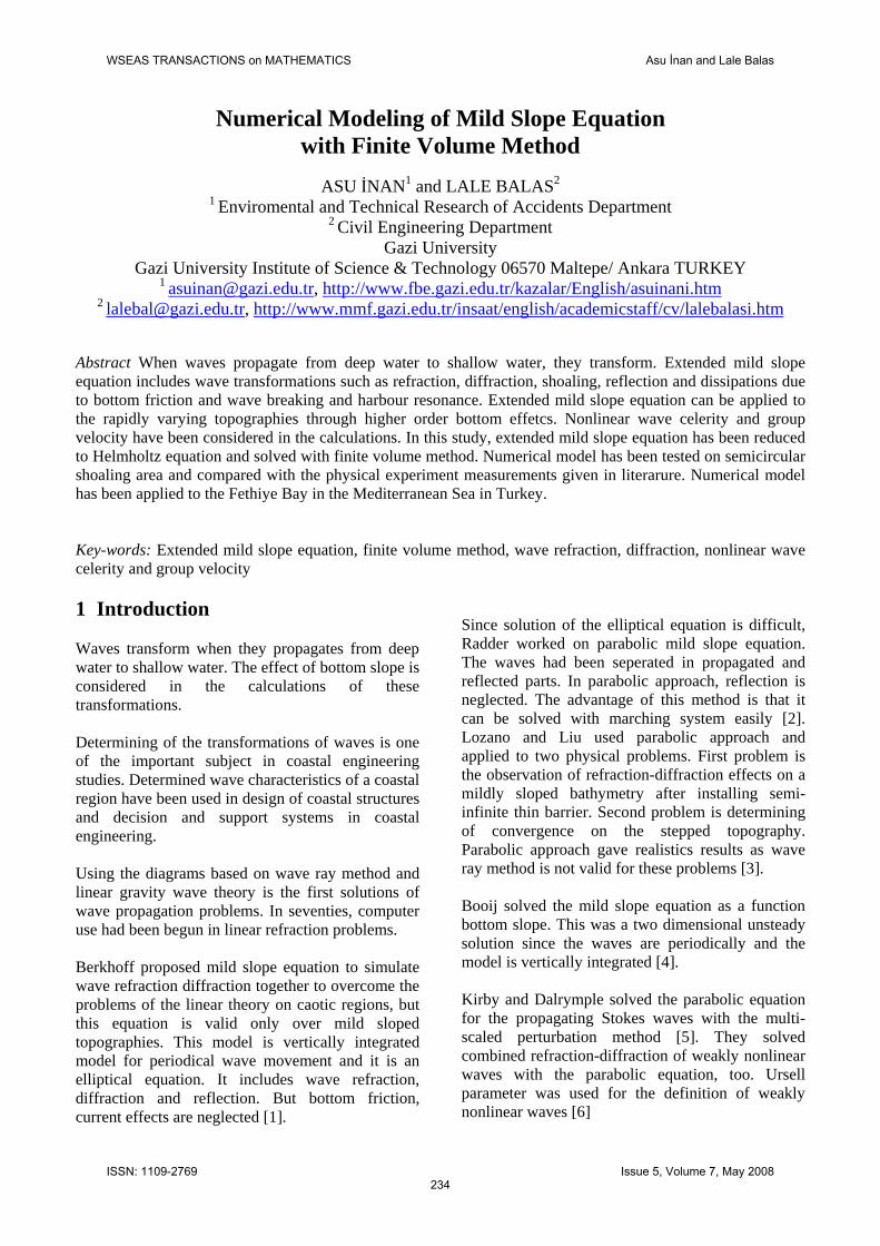
Numerical Modeling of Mild Slope Equation with Finite Volume Method

ASU İNAN1 and LALE BALAS2

1 Enviromental and Technical Research of Accidents Department 2 Civil Engineering Department

Gazi University Gazi University Institute of Science & Technology 06570 Maltepe/ Ankara TURKEY

1 [email protected], http://www.fbe.gazi.edu.tr/kazalar/English/asuinani.htm2 [email protected], http://www.mmf.gazi.edu.tr/insaat/english/academicstaff/cv/lalebalasi.htm

Abstract When waves propagate from deep water to shallow water, they transform. Extended mild slope equation includes wave transformations such as refraction, diffraction, shoaling, reflection and dissipations due to bottom friction and wave breaking and harbour resonance. Extended mild slope equation can be applied to the rapidly varying topographies through higher order bottom effetcs. Nonlinear wave celerity and group velocity have been considered in the calculations. In this study, extended mild slope equation has been reduced to Helmholtz equation and solved with finite volume method. Numerical model has been tested on semicircular shoaling area and compared with the physical experiment measurements given in literarure. Numerical model has been applied to the Fethiye Bay in the Mediterranean Sea in Turkey. Key-words: Extended mild slope equation, finite volume method, wave refraction, diffraction, nonlinear wave celerity and group velocity 1 Introduction Waves transform when they propagates from deep water to shallow water. The effect of bottom slope is considered in the calculations of these transformations. Determining of the transformations of waves is one of the important subject in coastal engineering studies. Determined wave characteristics of a coastal region have been used in design of coastal structures and decision and support systems in coastal engineering. Using the diagrams based on wave ray method and linear gravity wave theory is the first solutions of wave propagation problems. In seventies, computer use had been begun in linear refraction problems. Berkhoff proposed mild slope equation to simulate wave refraction diffraction together to overcome the problems of the linear theory on caotic regions, but this equation is valid only over mild sloped topographies. This model is vertically integrated model for periodical wave movement and it is an elliptical equation. It includes wave refraction, diffraction and reflection. But bottom friction, current effects are neglected [1].

Since solution of the elliptical equation is difficult, Radder worked on parabolic mild slope equation. The waves had been seperated in propagated and reflected parts. In parabolic approach, reflection is neglected. The advantage of this method is that it can be solved with marching system easily [2]. Lozano and Liu used parabolic approach and applied to two physical problems. First problem is the observation of refraction-diffraction effects on a mildly sloped bathymetry after installing semi-infinite thin barrier. Second problem is determining of convergence on the stepped topography. Parabolic approach gave realistics results as wave ray method is not valid for these problems [3]. Booij solved the mild slope equation as a function bottom slope. This was a two dimensional unsteady solution since the waves are periodically and the model is vertically integrated [4]. Kirby and Dalrymple solved the parabolic equation for the propagating Stokes waves with the multi-scaled perturbation method [5]. They solved combined refraction-diffraction of weakly nonlinear waves with the parabolic equation, too. Ursell parameter was used for the definition of weakly nonlinear waves [6]

WSEAS TRANSACTIONS on MATHEMATICS

Asu İnan and Lale Balas

ISSN: 1109-2769234

Issue 5, Volume 7, May 2008

mailto:[email protected]

http://www.fbe.gazi.edu.tr/kazalar/English/asuinani.htm

mailto:[email protected]

http://www.mmf.gazi.edu.tr/insaat/english/academicstaff/cv/lalebalasi.htm

An other approach for solving mild slope equation is hyperbolic approach where the elliptical mild slope equation has been trasformed in transient mild slope equation and the solution does not depend on time [7, 8, 9]. The advantages of this approach are that the solution is more quickly and reflection is considered. Li and Anastasiou solved the elliptical mild slope equation with the multi grid system so less nodal points are enough and CPU time has decreased. Current effects, shoaling, refraction and wave breaking had been considered together [10]. If bottom profile includes random and various holes and bumps, bottom curvature and square of bottom slope must be taken into account. Some researchers developed the mild slope equation for rapidly varying topographies. One of these researchers is Kirby who applied modified mild slope equation to the waves travelling on sinusodial bottom topographies for observing the reflection [11]. Massel worked on the transformations of waves propagating on the various bottom topographies [12]. A general equation was developed for the linear waves in shallow and transition regions. Galerkin- Eigenfunction method was applied. This equation includes higher order of bottom effects so it is applicable on bottom topographies where rapid changes are but this equation does not taken wave breaking into account. Chamberlain and Porter solved modified mild slope equation [13]. The results were compared with the equations applied on the two dimensional topographies. They underlined the need of using modified mild slope equation if sea bottom morphologically consist of sand waves. Modified mild slope equation includes general mild slope equation and extended mild slope equation proposed by Kirby [11]. Massel and Chamberlain & Porter developed extended mild slope equation [12, 13]. It implies bottom curvature and bottom slope so it can be applied to the rapidly varying topography. Suh et al., solved two different time dependent wave equation using different theoretical approaches (Green formulation method and Lagrangian formulations) [14]. First formulation transforms in the equation propesed by Smith and Sprinks and second formulation transform in the time dependent mild slope equation developed by Radder and

Dingemans when higher order bottom effects are neglected [15, 16]. For monochromatic waves, developed mild slope equation reduces into wave refraction-diffraction equation proposed by Massel [12], if there are only propagating waves. If reflection is considered they transform in the modified mild slope equation suggested by Chamberlain and Porter [13]. If the higher order bottom effects are neglected, the equations convert general mild slope equation of Berkhoff [1]. Lee et al., modeled extended mild slope equation with hyperbolic approach. Developed model includes bottom curvature and square of bottom slope. They decided that square of bottom slope can be neglected in deep water but not in transition and shallow region. Bottom curvature can be neglected in deep and shallow water but its effects have an important role in transition region [17]. Tang and Quellet, adapted nonlinear mild slope equation to multifrequency waves. The linear part of this equation includes mild slope equation and nonlinear part includes Boussinesq equation. This equation can be applied to nonlinear waves on changing depths. The equation was firstly simplified with parabolic approach and after that solved with Crank Nicolson Method [18]. Hsu and Wen extended the parabolic model suggested by Li taking total energy factor into account and modifiying traditional radiation boundary conditions. This model is valid in breaker zone, too [19, 20]. Saied and Tsanis considered the modified dispersion relationship, so the nonlinear effects were taken into account [21]. The extended mild slope equation proposed by Maa et al. has been examined in this study [22]. This equation includes wave refraction, diffraction, shoaling, reflection, harbour resonance and bottom friction and wave breaking dissipation factors. This extended mild slope equation has been reduced to Helmholtz equation and solved numerically. 2 Theory In this study, extended mild slope equation has been modeled to simulate wave transformations. Extended mild slope equation includes wave refraction, diffraction, shoaling, reflection, wave breaking and bottom friction dissipations and

WSEAS TRANSACTIONS on MATHEMATICS Asu İnan and Lale Balas

ISSN: 1109-2769235


harbour resonance [15, 19, 22]. Extended mild slope equation can be applied to rapidly varying topographies because higher order bottom effects like bottom curvature ans square of bottom slope have been taken into account. The extended mild slope equation proposed by Maa et al. is given in the equation (1) [22]. ( ) ( )

( )[ ] 0

1.2

22

1

2

=∇+∇

+++∇∇

φ

φφ

gkhfhgf

ifCCkCC bdgg (1)

( ) ( ) ( ) ( ) ( )

( ) ( )[ ]( )( )khkhkh

khkhkhkhkhkhkhkhkhf

2

3

2

1

cosh2tanh

2sinh2cosh8sinh8sinh3sinhcos4

−

++++−

= (2)

( )( )[ ]

( ) ( ) ( )( ) ( )

( ) ( )[ ] ( )[ ]⎪⎪⎭

⎪⎪⎬

⎫

⎪⎪⎩

⎪⎪⎨

⎧

++

+

−+

+=

khkhkhkhkhkh

khkhkh

khkhkhhf

2sinhsinh21122cos2sinh9

2sinh168

2sinh26sec

4

2

34

3

2

2

(3)

⎟⎠⎞

⎜⎝⎛ +=

khkhn2sinh

2121 (4)

1f is the bottom curvature coefficient, is the

coefficient of square of bottom slope, h is water depth, ∇ is horizontal operator, φ is velocity potential function, k is wave number,

2f

σ is wave frequancy, L is wave length, is wave celerity,

is group velocity, is bottom slope, is

bottom curvature, is bottom friction dissipation factor, is energy dissipation factor after breaking. is the sum of bottom friction dissipation factor and energy dissipation factor after breaking.

CgC h∇ h2∇

bf

df

bdf

An alternative method to solve extended mild slope equation is solving the equation after reducing to the Helmholtz equation. General Helmholtz equation has been given in the equation (5). The difference between general Helmholtz equation and reduced extended mild slope equation given in the equation (6) is effective wave number including higher order bottom effects, wave breaking and bottom friction dissipations.

022 =+∇ φφ ck (5)

( )( )[ ]

gg

g

bdc

CCgkhfhgf

CC

CC

ifkk2

22

12

22 1

∇+∇+

∇

−+=

(6)

To determine the bottom friction factor, the velocity in boundary layer must be defined with the consideration of momentum equation and boundary conditions. Bottom friction dissipation factor has been calculated with the equation (7). Here, fw is wave friction factor and σ is wave frequency.

khngaf

f wb 3

2

sinh34 σπ

= (7)

Jonsson and Carlsen recommended the equation (8) to obtain wave friction factor [23].

N

mf

ww ka

mff

11010 log

41log

41

+=+ (8)

a1m is semi distance of the movement of the fluid particle on bottom and kN is the Nikuradse roughness coefficient. After emprical studies, mf had been calculated as -0.08 by Jonsson and Carlsen [23]. If a1m/kN is less than 2, wave friction factor fw is 0.24. Otherwise the value calculated in the equation (8) is used in the numerical solution. Wave breaking dissipation factor has been calculated with the equation (9) [22, 24]. Γ and K are emprical constants and Γ=0.4, K=0.15.

⎟⎟⎠

⎞⎜⎜⎝

⎛−

Γ= 2

2

41

γK

khfd (9)

Breaker index ( bγ ) is calculated with the formulation of Isobe [25] given in the equation (10). γ is the ratio betweeen wave amplitude and water depth(γ=a/h).


ISSN: 1109-2769236


( )[ ]2

02/3

0

)1,0/(45exptan5

/3exp3,053,0

−−

+−−=

Lh

Lhb

β

γ (10)

The use of the breaker index proposed by Isobe and the wave breaking dissipation factor suggested by Dally et al. together give the minumum error as given in literature [24, 25]. The details can be found in the paper of Hsu and Wen [26]. So it is aimed to achieve more realistic results in breaker zone. γ and γb are calculated in each step and compared. If γ is less than bγ , fd is equalized to zero. Otherwise fd is calculated with the equation (9). 2.1. Nonlinear Celerity and Group Velocity Nonlinear celerity and group velocity should be considered to obtain more accurate results in wave propagation problem. Nonlinear effects come into prominence especially in the shallow regions where refraction is dominant. Kirby and Dalrymple suggested a method that is valid either in shallow region or in deep water [27]. This method transform into the equation proposed by Behrendt [28] in shallow water regions and into second order Stokes formulation in deep water. Dispersion relationship is used to obtain nonlinear celerity and group velocity [29]. The dispersionship equation has been given in equation (11) and the parameters of this equation have been shown in equations (12), (13), (14) and (15). After calculation of dispersion relationship, nonlinear wave celerity and group velocity can be easily determined with the equation (16) and (17).

( ) ( )⎟⎠⎞⎜

⎝⎛ ′+⎟

⎠⎞⎜

⎝⎛ ′+= khfkhDkhfgk 2*

2*1

2 tanh1 εεσ

(11)

ka=*ε (12)

( ) ( )( )

( ) ( ) ( )( )kh

khkhkhkh

khkhD

4

642

4

2

tanh8tanh2tanh13tanh129

sinh8tanh284cosh

−+−

=−+

=(13)

( ) ( )khkhf 51 tanh=′ (14)

( ) ( )

4

2 sinh ⎟⎟⎠

⎞⎜⎜⎝

⎛=′

khkhkhf (15)

kC σ= (16)

dkdCgσ

= (17)

3 Boundary Conditions Physical boundary conditions must be considered while investigating wave transformation in coastal engineering problems. There are four types of boundary conditions: Radiation boundary condition, partial reflective boundary condition, transmissive boundary condition and full reflective boundary condition. But generally full reflective, partial reflective and radiation boundary conditions are taken into account in mild slope equation problems. Chen et al. defined partial and full reflective boundary conditions with the equation (18) [30]. Here, KR is reflection coefficient, β is the phase difference between incident and approaching waves, θ is the angle between boundary normal ( )nx and

incident wave, is the wave amplitude on the boundary.

IA

( )( ) φββθφ

⎟⎟⎠

⎞⎜⎜⎝

⎛∂∂

++−

=∂∂

nA

AikKikKik

nI

IR

R 1exp1exp1cos (18)

First term on right of the equation (18) was proposed by Isaacson and Qu [31]. It indicates partial reflective boundary condition of incident waves with different approaching angles. Second term on right points out the effect of wave height gradient on boundary [30]. But this term based on linear theory, therefore it is not valid anymore when breaking occurs. It can be ignored. So partial reflection boundary condition can be written generally as given in equation (19) [31].

0* =+∂∂ φαφ k

n (19)

)( 21

* ααα i+= is complex tranmission coefficient and related to enegry transfer on boundary, wave


ISSN: 1109-2769237


height, wave phase and reflection coefficient. 1α and 2α are calculated with the equations (20) and (21), respectively.

βθβα

cos21cossin2

21rR

R

KKK

++= (20)

( )

βθαcos21

cos12

2

2RR

R

KKK++

−= (21)

Equations (20) and (21) show the relationship between transmission coefficient, reflection coefficient, the approach angle and phase difference between propagating and reflected waves which is generally neglected in the solutions of mild slope equation. Reflection coefficient and phase difference are equal to 1 and 0, respectively, when there is a full reflection. Reflection coefficient and wave phase difference are 0 in radiation boundary condition. So

is equal to 0 in full reclection condition and i in radiation boundary condition.

*α

Total potential function on the boundary of incident and reflected waves is given in the equation (22).

( )[ ]( )[ ⎭

⎬⎫

⎩⎨⎧

+−−++

=βθθ

θθφ

iyxikKyxik

AR sincosexp

sincosexp] (22)

Initial values of velocity potential of a wave with the height (H) and period (T) is calculated using the equation (16) with linear theory.

isg eigH

σφ

2= (23)

θcoskkx = (24)

θsinkk y = (25)

tykxks σθθ −−= 0000 sincos (26)

Wave number vector is related to wave phase.

sk ∇=r

(27)

Phase function (s) is determined with the equation (21) and wave angle is a function of wave phase.

( )( )⎟⎟⎠

⎞⎜⎜⎝

⎛= −

φφ

ReImtan 1s (28)

⎟⎠⎞

⎜⎝⎛

∂∂∂∂

= −

xsys

//tan 1θ (29)

After calculation of initial values, the iteration process begins. Until the error between calculated and foregoing velocity potential in whole mesh reaches a tolerable value, the iteration is continued. An other important point is the consistency in calculation of wave phase with the limitations of computer programming language. 4 Numerical Model Extendend mild slope equation reduced to Helmholtz equation has been solved by finite volume method. Finite volume (control volume) method is based on numerical integration. Finite volume method is applied in three steps: Grid generation, discretization and solution of equations. In recent years, finite volume method is widely used in fluid mechanics and coastal engineering problems [32, 33, 34]. The most important part of finite volume method is the discretization of the equations and adapting them into boundary conditions. The discrete forms of the extended mild slope equation reduced to Helmholtz equation have shown in equation (30) and (31) [35].

02**

**

=Δ+⎟⎟⎠

⎞⎜⎜⎝

⎛∂∂

−⎟⎟⎠

⎞⎜⎜⎝

⎛∂∂

+⎟⎠⎞

⎜⎝⎛∂∂

−⎟⎠⎞

⎜⎝⎛∂∂

Vky

Ay

A

xA

xA

cs

s

n

n

w

w

e

e

φφφ

φφ

(30)

02 =Δ+⎟⎟⎠

⎞⎜⎜⎝

⎛Δ−

Δ−⎟⎟⎠

⎞⎜⎜⎝

⎛Δ−

Δ

+⎟⎠⎞

⎜⎝⎛

Δ−

Δ−⎟⎠⎞

⎜⎝⎛

Δ−

Δ

Vky

xy

x

xy

xy

cSPPN

WPPE

φφφφφ

φφφφ

(31)

A* is cross-sectional area of the control volume,

VΔ is the volume, φ is average value of source φ over the control volume. P means nodal point, e, w, n, s indicate east, west, north and south,


ISSN: 1109-2769238


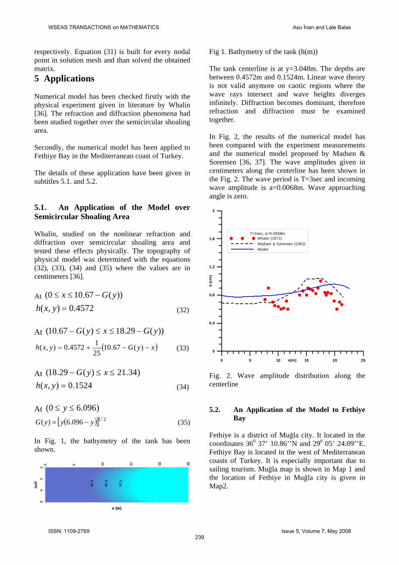
respectively. Equation (31) is built for every nodal point in solution mesh and than solved the obtained matrix. 5 Applications Numerical model has been checked firstly with the physical experiment given in literature by Whalin [36]. The refraction and diffraction phenomena had been studied together over the semicircular shoaling area. Secondly, the numerical model has been applied to Fethiye Bay in the Mediterranean coast of Turkey. The details of these application have been given in subtitles 5.1. and 5.2. 5.1. An Application of the Model over Semicircular Shoaling Area Whalin, studied on the nonlinear refraction and diffraction over semicircular shoaling area and tested these effects physically. The topography of physical model was determined with the equations (32), (33), (34) and (35) where the values are in centimeters [36]. At ))(67.100( yGx −≤≤

4572.0),( =yxh (32) At ))(29.18)(67.10( yGxyG −≤≤−

( )xyGyxh −−+= )(67.102514572.0),( (33)

At )34.21)(29.18( ≤≤− xyG

1524.0),( =yxh (34) At )096.60( ≤≤ y

([ 2/1096.6)( yyyG −= )] (35) In Fig. 1, the bathymetry of the tank has been shown.

Fig 1. Bathymetry of the tank (h(m)) The tank centerline is at y=3.048m. The depths are between 0.4572m and 0.1524m. Linear wave theory is not valid anymore on caotic regions where the wave rays intersect and wave heights diverges infinitely. Diffraction becomes dominant, therefore refraction and diffraction must be examined together. In Fig. 2, the results of the numerical model has been compared with the experiment measurements and the numerical model proposed by Madsen & Sorensen [36, 37]. The wave amplitudes given in centimeters along the centerline has been shown in the Fig. 2. The wave period is T=3sec and incoming wave amplitude is a=0.0068m. Wave approaching angle is zero.

0 5 10 15 20 25x(m)

0

0.4

0.8

1.2

1.6

2a

(cm

)

T=3sec, a=0.0068mWhalin (1971)Madsen & Sorensen (1992)Model

Fig. 2. Wave amplitude distribution along the centerline 5.2. An Application of the Model to Fethiye

Bay Fethiye is a district of Muğla city. It located in the coordinates 360 37’ 10.86’’N and 290 05’ 24.09’’E. Fethiye Bay is located in the west of Mediterranean coasts of Turkey. It is especially important due to sailing tourism. Muğla map is shown in Map 1 and the location of Fethiye in Muğla city is given in Map2.


ISSN: 1109-2769239


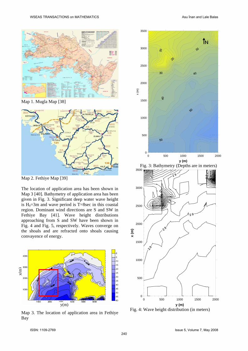
Map 1. Mugla Map [38]

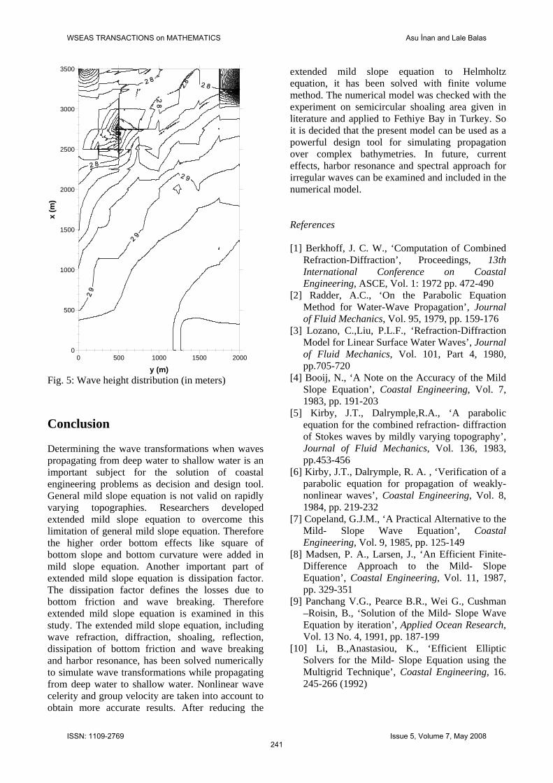
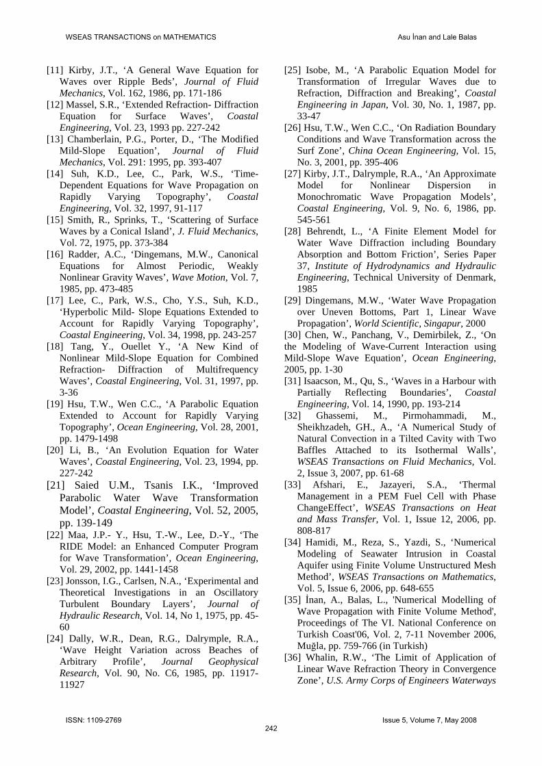
Map 2. Fethiye Map [39] The location of application area has been shown in Map 3 [40]. Bathymetry of application area has been given in Fig. 3. Significant deep water wave height is H0=3m and wave period is T=8sec in this coastal region. Dominant wind directions are S and SW in Fethiye Bay [41]. Wave height distributions approaching from S and SW have been shown in Fig. 4 and Fig. 5, respectively. Waves converge on the shoals and are refracted onto shoals causing convayence of energy.

Map 3. The location of application area in Fethiye Bay

0 500 1000 1500 2000

y (m)

0

500

1000

1500

2000

2500

3000

3500

x (m

)

Fig. 3: Bathymetry (Depths are in meters)

0 500 1000 1500 2000

y (m)

0

500

1000

1500

2000

2500

3000

3500

x (m

)

y(m)

x(m

)

Fig. 4: Wave height distribution (in meters)


ISSN: 1109-2769240


0 500 1000 1500 2000

y (m)

0

500

1000

1500

2000

2500

3000

3500

x (m

)

Fig. 5: Wave height distribution (in meters) Conclusion Determining the wave transformations when waves propagating from deep water to shallow water is an important subject for the solution of coastal engineering problems as decision and design tool. General mild slope equation is not valid on rapidly varying topographies. Researchers developed extended mild slope equation to overcome this limitation of general mild slope equation. Therefore the higher order bottom effects like square of bottom slope and bottom curvature were added in mild slope equation. Another important part of extended mild slope equation is dissipation factor. The dissipation factor defines the losses due to bottom friction and wave breaking. Therefore extended mild slope equation is examined in this study. The extended mild slope equation, including wave refraction, diffraction, shoaling, reflection, dissipation of bottom friction and wave breaking and harbor resonance, has been solved numerically to simulate wave transformations while propagating from deep water to shallow water. Nonlinear wave celerity and group velocity are taken into account to obtain more accurate results. After reducing the

extended mild slope equation to Helmholtz equation, it has been solved with finite volume method. The numerical model was checked with the experiment on semicircular shoaling area given in literature and applied to Fethiye Bay in Turkey. So it is decided that the present model can be used as a powerful design tool for simulating propagation over complex bathymetries. In future, current effects, harbor resonance and spectral approach for irregular waves can be examined and included in the numerical model. References [1] Berkhoff, J. C. W., ‘Computation of Combined

Refraction-Diffraction’, Proceedings, 13th International Conference on Coastal Engineering, ASCE, Vol. 1: 1972 pp. 472-490

[2] Radder, A.C., ‘On the Parabolic Equation Method for Water-Wave Propagation’, Journal of Fluid Mechanics, Vol. 95, 1979, pp. 159-176

[3] Lozano, C.,Liu, P.L.F., ‘Refraction-Diffraction Model for Linear Surface Water Waves’, Journal of Fluid Mechanics, Vol. 101, Part 4, 1980, pp.705-720

[4] Booij, N., ‘A Note on the Accuracy of the Mild Slope Equation’, Coastal Engineering, Vol. 7, 1983, pp. 191-203

[5] Kirby, J.T., Dalrymple,R.A., ‘A parabolic equation for the combined refraction- diffraction of Stokes waves by mildly varying topography’, Journal of Fluid Mechanics, Vol. 136, 1983, pp.453-456

[6] Kirby, J.T., Dalrymple, R. A. , ‘Verification of a parabolic equation for propagation of weakly- nonlinear waves’, Coastal Engineering, Vol. 8, 1984, pp. 219-232

[7] Copeland, G.J.M., ‘A Practical Alternative to the Mild- Slope Wave Equation’, Coastal Engineering, Vol. 9, 1985, pp. 125-149

[8] Madsen, P. A., Larsen, J., ‘An Efficient Finite- Difference Approach to the Mild- Slope Equation’, Coastal Engineering, Vol. 11, 1987, pp. 329-351

[9] Panchang V.G., Pearce B.R., Wei G., Cushman –Roisin, B., ‘Solution of the Mild- Slope Wave Equation by iteration’, Applied Ocean Research, Vol. 13 No. 4, 1991, pp. 187-199

[10] Li, B.,Anastasiou, K., ‘Efficient Elliptic Solvers for the Mild- Slope Equation using the Multigrid Technique’, Coastal Engineering, 16. 245-266 (1992)


ISSN: 1109-2769241


[11] Kirby, J.T., ‘A General Wave Equation for Waves over Ripple Beds’, Journal of Fluid Mechanics, Vol. 162, 1986, pp. 171-186

[12] Massel, S.R., ‘Extended Refraction- Diffraction Equation for Surface Waves’, Coastal Engineering, Vol. 23, 1993 pp. 227-242

[13] Chamberlain, P.G., Porter, D., ‘The Modified Mild-Slope Equation’, Journal of Fluid Mechanics, Vol. 291: 1995, pp. 393-407

[14] Suh, K.D., Lee, C., Park, W.S., ‘Time- Dependent Equations for Wave Propagation on Rapidly Varying Topography’, Coastal Engineering, Vol. 32, 1997, 91-117

[15] Smith, R., Sprinks, T., ‘Scattering of Surface Waves by a Conical Island’, J. Fluid Mechanics, Vol. 72, 1975, pp. 373-384

[16] Radder, A.C., ‘Dingemans, M.W., Canonical Equations for Almost Periodic, Weakly Nonlinear Gravity Waves’, Wave Motion, Vol. 7, 1985, pp. 473-485

[17] Lee, C., Park, W.S., Cho, Y.S., Suh, K.D., ‘Hyperbolic Mild- Slope Equations Extended to Account for Rapidly Varying Topography’, Coastal Engineering, Vol. 34, 1998, pp. 243-257

[18] Tang, Y., Ouellet Y., ‘A New Kind of Nonlinear Mild-Slope Equation for Combined Refraction- Diffraction of Multifrequency Waves’, Coastal Engineering, Vol. 31, 1997, pp. 3-36

[19] Hsu, T.W., Wen C.C., ‘A Parabolic Equation Extended to Account for Rapidly Varying Topography’, Ocean Engineering, Vol. 28, 2001, pp. 1479-1498

[20] Li, B., ‘An Evolution Equation for Water Waves’, Coastal Engineering, Vol. 23, 1994, pp. 227-242

[21] Saied U.M., Tsanis I.K., ‘Improved Parabolic Water Wave Transformation Model’, Coastal Engineering, Vol. 52, 2005, pp. 139-149

[22] Maa, J.P.- Y., Hsu, T.-W., Lee, D.-Y., ‘The RIDE Model: an Enhanced Computer Program for Wave Transformation’, Ocean Engineering, Vol. 29, 2002, pp. 1441-1458

[23] Jonsson, I.G., Carlsen, N.A., ‘Experimental and Theoretical Investigations in an Oscillatory Turbulent Boundary Layers’, Journal of Hydraulic Research, Vol. 14, No 1, 1975, pp. 45-60

[24] Dally, W.R., Dean, R.G., Dalrymple, R.A., ‘Wave Height Variation across Beaches of Arbitrary Profile’, Journal Geophysical Research, Vol. 90, No. C6, 1985, pp. 11917-11927

[25] Isobe, M., ‘A Parabolic Equation Model for Transformation of Irregular Waves due to Refraction, Diffraction and Breaking’, Coastal Engineering in Japan, Vol. 30, No. 1, 1987, pp. 33-47

[26] Hsu, T.W., Wen C.C., ‘On Radiation Boundary Conditions and Wave Transformation across the Surf Zone’, China Ocean Engineering, Vol. 15, No. 3, 2001, pp. 395-406

[27] Kirby, J.T., Dalrymple, R.A., ‘An Approximate Model for Nonlinear Dispersion in Monochromatic Wave Propagation Models’, Coastal Engineering, Vol. 9, No. 6, 1986, pp. 545-561

[28] Behrendt, L., ‘A Finite Element Model for Water Wave Diffraction including Boundary Absorption and Bottom Friction’, Series Paper 37, Institute of Hydrodynamics and Hydraulic Engineering, Technical University of Denmark, 1985

[29] Dingemans, M.W., ‘Water Wave Propagation over Uneven Bottoms, Part 1, Linear Wave Propagation’, World Scientific, Singapur, 2000

[30] Chen, W., Panchang, V., Demirbilek, Z., ‘On the Modeling of Wave-Current Interaction using Mild-Slope Wave Equation’, Ocean Engineering, 2005, pp. 1-30 [31] Isaacson, M., Qu, S., ‘Waves in a Harbour with

Partially Reflecting Boundaries’, Coastal Engineering, Vol. 14, 1990, pp. 193-214

[32] Ghassemi, M., Pirmohammadi, M., Sheikhzadeh, GH., A., ‘A Numerical Study of Natural Convection in a Tilted Cavity with Two Baffles Attached to its Isothermal Walls’, WSEAS Transactions on Fluid Mechanics, Vol. 2, Issue 3, 2007, pp. 61-68

[33] Afshari, E., Jazayeri, S.A., ‘Thermal Management in a PEM Fuel Cell with Phase ChangeEffect’, WSEAS Transactions on Heat and Mass Transfer, Vol. 1, Issue 12, 2006, pp. 808-817

[34] Hamidi, M., Reza, S., Yazdi, S., ‘Numerical Modeling of Seawater Intrusion in Coastal Aquifer using Finite Volume Unstructured Mesh Method’, WSEAS Transactions on Mathematics, Vol. 5, Issue 6, 2006, pp. 648-655

[35] İnan, A., Balas, L., 'Numerical Modelling of Wave Propagation with Finite Volume Method', Proceedings of The VI. National Conference on Turkish Coast'06, Vol. 2, 7-11 November 2006, Muğla, pp. 759-766 (in Turkish)

[36] Whalin, R.W., ‘The Limit of Application of Linear Wave Refraction Theory in Convergence Zone’, U.S. Army Corps of Engineers Waterways


ISSN: 1109-2769242


Experiment. Station, Vicksburg, Report No. H-71, 1971, pp. 329-351

[37] Madsen, P.A., Sorensen, O.R., ‘A new Form of the Boussinesq Equations with Improved Linear Dispersion Characteristics Part2. A Slowly Varying Bathymetry’, Coastal Engineering, Vol. 18, 1992, pp. 183-204

[38] www.mugla.gov.tr[39] www.fethiye.gov.tr[40] Küçükosmanoğlu, A., ‘Modeling of Water

Exchange in Enclosed Coastal Waters’’, M.Sc.

Thesis, Yüksek Gazi University Institute Science & Technology, Ankara, 2004 (in Turkish)

[41] Özhan, E., Balas (Hapoğlu) L., Balas, C.E., Öztürk, C., ‘Three Dimensional Mathematical Modelling of Hydrodynamics, Salinity, Temperature and Pollution Distribution of Coastal Lagoons”, Turkish National Council for Science and Technology Development, Report No: TÜBİTAK-İNTAG 821, 1998 (in Turkish)


ISSN: 1109-2769243


http://www.mugla.gov.tr/

http://www.fethiye.gov.tr/