


Bahasa
Halaman
Hukum


This article was downloaded by:[Jat, M. K.]On: 14 December 2007Access Details: [subscription number 788323329]Publisher: Taylor & FrancisInforma Ltd Registered in England and Wales Registered Number: 1072954Registered office: Mortimer House, 37-41 Mortimer Street, London W1T 3JH, UK
International Journal of RemoteSensingPublication details, including instructions for authors and subscription information:http://www.informaworld.com/smpp/title~content=t713722504
Modelling of urban growth using spatial analysistechniques: a case study of Ajmer city (India)M. K. Jat a; P. K. Garg a; D. Khare aa Indian Institute of Technology Roorkee, Roorkee, 247667 India
First Published on: 25 October 2007To cite this Article: Jat, M. K., Garg, P. K. and Khare, D. (2007) 'Modelling of urbangrowth using spatial analysis techniques: a case study of Ajmer city (India)',International Journal of Remote Sensing, 29:2, 543 - 567To link to this article: DOI: 10.1080/01431160701280983URL: http://dx.doi.org/10.1080/01431160701280983
PLEASE SCROLL DOWN FOR ARTICLE
Full terms and conditions of use: http://www.informaworld.com/terms-and-conditions-of-access.pdf
This article maybe used for research, teaching and private study purposes. Any substantial or systematic reproduction,re-distribution, re-selling, loan or sub-licensing, systematic supply or distribution in any form to anyone is expresslyforbidden.
The publisher does not give any warranty express or implied or make any representation that the contents will becomplete or accurate or up to date. The accuracy of any instructions, formulae and drug doses should beindependently verified with primary sources. The publisher shall not be liable for any loss, actions, claims, proceedings,demand or costs or damages whatsoever or howsoever caused arising directly or indirectly in connection with orarising out of the use of this material.
Dow
nloa
ded
By:
[Jat
, M. K
.] A
t: 02
:53
14 D
ecem
ber 2
007 Modelling of urban growth using spatial analysis techniques: a case
study of Ajmer city (India)
M. K. JAT*, P. K. GARG and D. KHARE
Indian Institute of Technology Roorkee, Roorkee, 247667 India
(Received 13 May 2006; in final form 5 February 2007 )
The concentration of people in densely populated urban areas, especially in
developing countries like India and China, calls for the use of sophisticated
monitoring systems, like remote sensing and Geographical Information Systems
(GIS). Time series of land use/cover changes can easily be generated using
sequential satellite images, which are required for the prediction of urban growth,
verification of growth model outputs, estimation of impervious area, para-
meterization of various hydrological models, water resources planning and
management and environmental studies. In the present work, urban growth of
Ajmer city (India) in the last 29 years has been studied at mid-scale level (5–
25 m). Remote sensing and GIS have been used to extract the information related
to urban growth, impervious area and its spatial and temporal variation.
Statistical classification approaches have been used to derive the land use
information from satellite images of eight years (1977–2005). The Shannon’s
entropy and landscape metrics (patchiness and map density) are computed in
order to quantify the urban form (impervious area) in terms of spatial
phenomena. Further, multivariate statistical techniques have been used to
establish the relationship between the urban growth and its causative factors.
Results reveal that land development (200%) in Ajmer is more than three times
the population growth (59%). Shannon’s entropy and landscape metrics has
revealed the spatial distribution of the sprawl.
1. Introduction
Urbanization is an inevitable process globally, and an important topic for the
planners, managers and environmentalists. After economic liberalization in 1991,
urban centres in India have grown at a faster rate due to increased economic and
developmental activities. The extent of urbanization or its growth is one such
phenomenon that drives the changes in land use pattern. These changes may have an
adverse impact on ecology, especially on hydro-geomorphology, water resources
and vegetation. Information on accurate urban growth is of great interest in urban
and suburban areas for diverse purposes, such as urban planning, water and land
resource management, market analysis, service allocation, etc. Unfortunately, the
conventional surveying and mapping techniques are expensive and time consuming
for the estimation of urban growth. As a result, increased research interest is being
directed to the mapping and monitoring of urban growth using remote sensing and
GIS techniques (Epstein et al. 2002).
*Corresponding author. Email: [email protected]
International Journal of Remote Sensing
Vol. 29, No. 2, 20 January 2008, 543–567
International Journal of Remote SensingISSN 0143-1161 print/ISSN 1366-5901 online # 2008 Taylor & Francis
http://www.tandf.co.uk/journalsDOI: 10.1080/01431160701280983
Dow
nloa
ded
By:
[Jat
, M. K
.] A
t: 02
:53
14 D
ecem
ber 2
007
Remote sensing is a cost effective, technologically sound and an increasingly used
technique for the analysis of urban growth (Sudhira et al. 2004, Yang and Liu 2005,
Haack and Rafter 2006). For nearly three decades, extensive research efforts have
been made for urban change detection using remotely sensed images (Toll 1985,
Royer et al. 1988, Singh 1989, Lo and Shipman 1990, Gomarasca et al. 1993, Green
et al. 1994, Yeh and Li 2001, Yang and Lo 2003, Haack and Rafter 2006). These
studies have been supported through either an image-to-image comparison or a
post-classification comparison. The post-classification comparison has the potential
to detect the nature of urban land use/cover changes (Jensen 1995). With the
availability of higher resolution images and the development of improved image
classification methods, greater details of urban land use/cover changes can be
mapped with a reasonable accuracy (Jensen and Cowen 1999).
The impervious area is generally considered as a parameter for quantifying the
urban growth (Torrens and Alberti 2000, Barnes et al. 2001, Epstein et al. 2002).
Here, impervious area includes residential, commercial and industrial complexes
along with paved ways, roads, markets, etc. Urban growth has been quantified by
considering the impervious area as the key feature, which can be obtained either
from physical survey or remotely acquired data.
There are a variety of techniques available to measure/estimate the area of
impervious surfaces. The time consuming and costly, but most accurate is manual
extraction of impervious surface features from remote sensing images through heads
up digitizing. Point sampling can be used as an alternative to digitizing, despite this
being time consuming and less accurate. Remote sensing pattern recognition
approaches, such as supervised, unsupervised and knowledge based expert system
approaches (Cibula and Nyquist 1987, Loveland et al. 1991, Franklin 1994, Harris
and Ventura 1995, Greenberg and Bradley 1997, Vogelmann et al. 1998, Stuckens
et al. 2000, Stefanov et al. 2001, Sugumaran et al. 2003, Lu and Weng 2005, Mundia
and Aniya 2005) have been used in the recent past to measure impervious area and
urban growth. These require both moderate to high resolution remote sensing data
as well as expertise to process and analyse. These data and analytical capabilities are
often beyond the reach of many planners and decision makers at a local level,
especially in developing countries.
Statistical techniques along with remote sensing and GIS have been used in many
urban growth studies (Lo 2001, Lo and Yang 2002, Weng 2001, Cheng and Masser
2003, Sudhira et al. 2004, Jat et al. 2006). Urban growth studies have been attempted
in several developed countries (Batty et al. 1999, Torrens and Alberti 2000, Barnes
et al. 2001, Epstein et al. 2002, Li and Weng 2005, Jantz et al. 2005, Yang and Liu
2005) and recently in developing countries like China (Yeh and Li 2001, Weng 2001,
Cheng and Masser 2003) and India (Lata et al. 2001, Sudhira et al. 2004, Jat et al.
2006). Statistical techniques like multivariate regression have been used to determine
the relationship between the percent impervious area and various urban develop-
ment parameters, such as road density, population density, land use type and size of
development units (Lo 2001, Lo and Yang 2002, Weng 2001, Cheng and Masser
2003, Sudhira et al. 2004). The convergence of GIS and database management
systems has helped in quantifying, monitoring, modelling, and subsequently
predicting the urban growth phenomenon. Characterizing urban growth patterns
involves detection and quantification with appropriate scales and statistical
summarization. There are scores of metrics available to describe the landscape
pattern. The landscape pattern metrics have been used for studying the forest
544 M. K. Jat et al.
Dow
nloa
ded
By:
[Jat
, M. K
.] A
t: 02
:53
14 D
ecem
ber 2
007
patches (Trani and Giles 1999, Civco et al. 2002) and detecting the urban growth
pattern in village clusters (Sudhira et al. 2004). Most of the indices are correlated
among themselves, because there are only a few primary measurements that can be
made from patches (patch type, area, edge and neighbour type). All metrics are then
derived from these primary measures. At the landscape level, GIS aids in calculating
the landscape metrics, like patchiness, density and diversity in order to characterize
the landscape properties in terms of spatial distribution and change (Trani and Giles
1999, Yeh and Li 2001, Civco et al. 2002, Sudhira et al. 2004). Such metrics have not
been determined yet for most of the urban centres of India (Sudhira et al. 2004).
Shannon’s entropy has been used in some of the studies to quantify the urban
forms, such as impervious area in terms of spatial phenomenon (Yeh and Li 2001,
Sudhira et al. 2004, Joshi et al. 2006). Shannon’s entropy is based on the concept of
information theory. It is a measure of uncertainty about the realization of a random
variable. Urban growth takes place in the form of impervious patches in newly
developed areas. A quantitative measure is required to monitor and identify this
fragmented urban growth. Developing this analogy, the mathematical representa-
tion of urban growth as a fragmented phenomena and the concept of entropy are
close (entropy is often used as a measure of dispersion) (Joshi et al. 2006). Shannon’s
entropy (Hn) is used to measure the degree of spatial concentration or dispersion
of geophysical variables (Xi) among n spatial units/zones. Entropy can also be used
to indicate the degree of urban growth/sprawl by examining whether the land
development in a city is dispersed or compact (Lata et al. 2001; Sudhira et al. 2004;
Joshi et al. 2006). Large value of Shannon’s entropy indicates the urban growth.
Despite these efforts, further research is needed in order to reinforce the absolute
and comparative relationship between the magnitude of change in landscape
imperviousness, type and intensity of urban land use/cover change and their
causative factors.
In India, currently 25.73% of the population (Census of India 2001) lives in urban
centres, while in the next 15 years it is projected to be around 33%. This indicates the
alarming rate of urbanization and the extent of urban growth that could take place.
Measurement and modelling of urban growth using satellite images have not been
well studied to date, especially in India (Sudhira et al. 2004). Such studies are vital
for the planning and management of urban infrastructure and water resources.
In this paper, an attempt has been made to investigate the usefulness of the spatial
techniques like remote sensing and GIS for urban growth detection and handling of
spatial and temporal variability of the same. The urban growth of Ajmer city
(situated in Rajasthan State of India) in the last 29 years has been estimated using
remote sensing images of eight different years ranging from 1977 to 2005. Remote
sensing and GIS techniques have been used to extract the information related to
urban growth, and its spatial and temporal variation is studied to establish a
relationship between urban growth (sprawl) and its causative factors. Statistical
image classification approach like Maximum Likelihood Classifier (MLC) has been
used for the analysis of satellite images obtained from Landsat MSS, TM, ETM +and IRS LISS-III sensor systems. Classified images have been used to understand
the dynamics of urban growth and to extract the area of impervious surfaces. In
order to quantify the urban forms such as impervious area in terms of spatial
phenomena, Shannon’s entropy (Yeh and Li 2001) and the landscape metrics
(patchiness, map density, etc.) are computed. The landscape metrics, normally used
in ecological investigations, are being extended to enhance understanding of the
Modelling of urban growth 545
Dow
nloa
ded
By:
[Jat
, M. K
.] A
t: 02
:53
14 D
ecem
ber 2
007
urban forms. Computation of these indices helped in understanding the process
of urbanization at a landscape level. Further, urban growth has been correlated
with its causative factors, like population, population density etc., using multivariate
regression analysis to arrive at a functional relationship. In addition, these
relationships are used to predict the future urban growth.
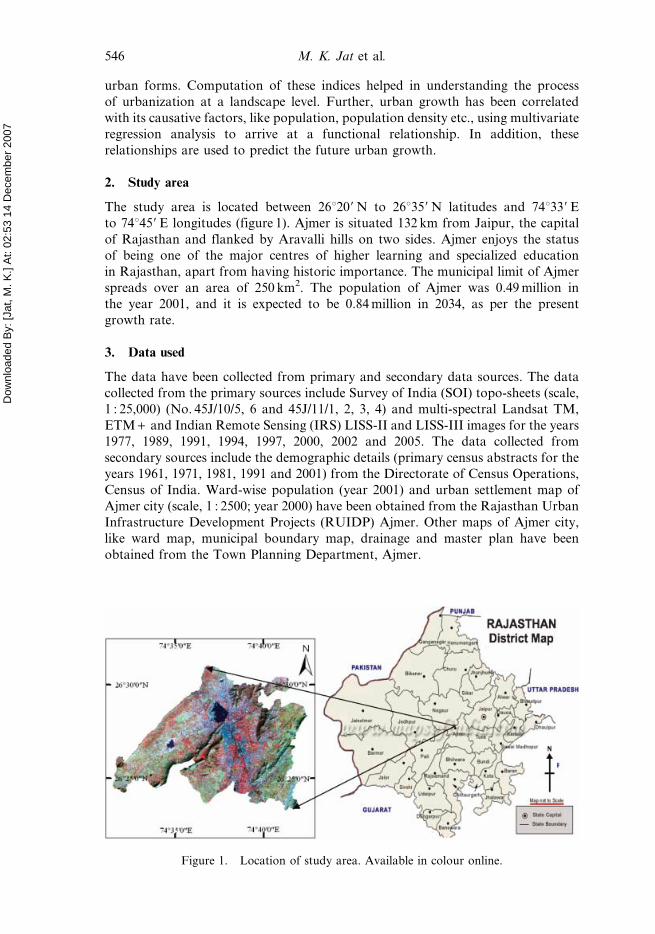
2. Study area
The study area is located between 26u209 N to 26u359 N latitudes and 74u339 E
to 74u459 E longitudes (figure 1). Ajmer is situated 132 km from Jaipur, the capital
of Rajasthan and flanked by Aravalli hills on two sides. Ajmer enjoys the status
of being one of the major centres of higher learning and specialized education
in Rajasthan, apart from having historic importance. The municipal limit of Ajmer
spreads over an area of 250 km2. The population of Ajmer was 0.49 million in
the year 2001, and it is expected to be 0.84 million in 2034, as per the present
growth rate.
3. Data used
The data have been collected from primary and secondary data sources. The data
collected from the primary sources include Survey of India (SOI) topo-sheets (scale,
1 : 25,000) (No. 45J/10/5, 6 and 45J/11/1, 2, 3, 4) and multi-spectral Landsat TM,
ETM + and Indian Remote Sensing (IRS) LISS-II and LISS-III images for the years
1977, 1989, 1991, 1994, 1997, 2000, 2002 and 2005. The data collected from
secondary sources include the demographic details (primary census abstracts for the
years 1961, 1971, 1981, 1991 and 2001) from the Directorate of Census Operations,
Census of India. Ward-wise population (year 2001) and urban settlement map of
Ajmer city (scale, 1 : 2500; year 2000) have been obtained from the Rajasthan Urban
Infrastructure Development Projects (RUIDP) Ajmer. Other maps of Ajmer city,
like ward map, municipal boundary map, drainage and master plan have been
obtained from the Town Planning Department, Ajmer.
Figure 1. Location of study area. Available in colour online.
546 M. K. Jat et al.
Dow
nloa
ded
By:
[Jat
, M. K
.] A
t: 02
:53
14 D
ecem
ber 2
007
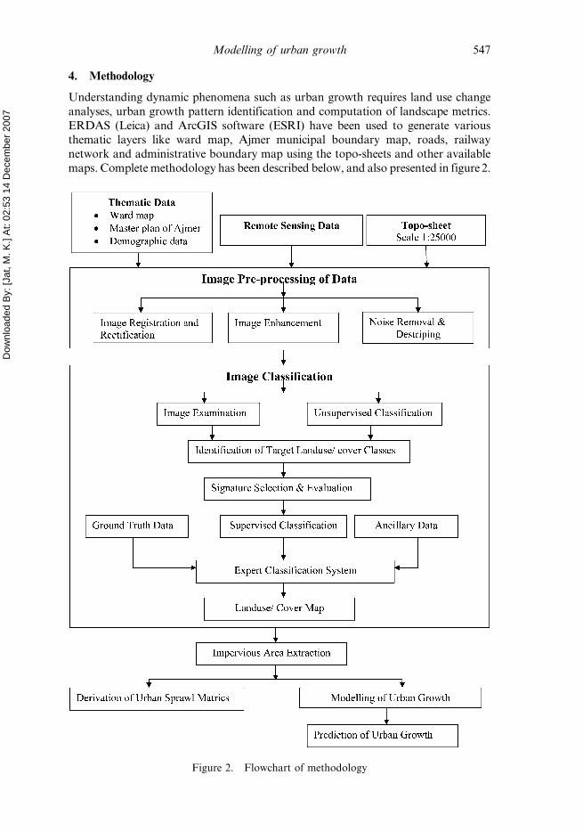
4. Methodology
Understanding dynamic phenomena such as urban growth requires land use change
analyses, urban growth pattern identification and computation of landscape metrics.
ERDAS (Leica) and ArcGIS software (ESRI) have been used to generate variousthematic layers like ward map, Ajmer municipal boundary map, roads, railway
network and administrative boundary map using the topo-sheets and other available
maps. Complete methodology has been described below, and also presented in figure 2.
Figure 2. Flowchart of methodology
Modelling of urban growth 547
Dow
nloa
ded
By:
[Jat
, M. K
.] A
t: 02
:53
14 D
ecem
ber 2
007
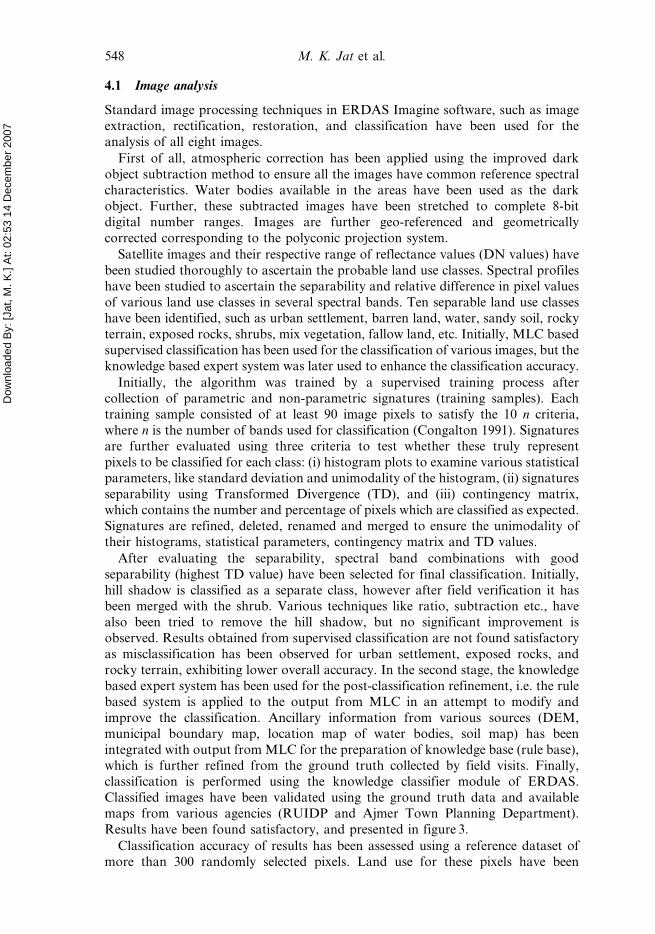
4.1 Image analysis
Standard image processing techniques in ERDAS Imagine software, such as image
extraction, rectification, restoration, and classification have been used for the
analysis of all eight images.
First of all, atmospheric correction has been applied using the improved dark
object subtraction method to ensure all the images have common reference spectral
characteristics. Water bodies available in the areas have been used as the dark
object. Further, these subtracted images have been stretched to complete 8-bit
digital number ranges. Images are further geo-referenced and geometrically
corrected corresponding to the polyconic projection system.
Satellite images and their respective range of reflectance values (DN values) have
been studied thoroughly to ascertain the probable land use classes. Spectral profiles
have been studied to ascertain the separability and relative difference in pixel values
of various land use classes in several spectral bands. Ten separable land use classes
have been identified, such as urban settlement, barren land, water, sandy soil, rocky
terrain, exposed rocks, shrubs, mix vegetation, fallow land, etc. Initially, MLC based
supervised classification has been used for the classification of various images, but the
knowledge based expert system was later used to enhance the classification accuracy.
Initially, the algorithm was trained by a supervised training process after
collection of parametric and non-parametric signatures (training samples). Each
training sample consisted of at least 90 image pixels to satisfy the 10 n criteria,
where n is the number of bands used for classification (Congalton 1991). Signatures
are further evaluated using three criteria to test whether these truly represent
pixels to be classified for each class: (i) histogram plots to examine various statistical
parameters, like standard deviation and unimodality of the histogram, (ii) signatures
separability using Transformed Divergence (TD), and (iii) contingency matrix,
which contains the number and percentage of pixels which are classified as expected.
Signatures are refined, deleted, renamed and merged to ensure the unimodality of
their histograms, statistical parameters, contingency matrix and TD values.
After evaluating the separability, spectral band combinations with good
separability (highest TD value) have been selected for final classification. Initially,
hill shadow is classified as a separate class, however after field verification it has
been merged with the shrub. Various techniques like ratio, subtraction etc., have
also been tried to remove the hill shadow, but no significant improvement is
observed. Results obtained from supervised classification are not found satisfactory
as misclassification has been observed for urban settlement, exposed rocks, and
rocky terrain, exhibiting lower overall accuracy. In the second stage, the knowledge
based expert system has been used for the post-classification refinement, i.e. the rule
based system is applied to the output from MLC in an attempt to modify and
improve the classification. Ancillary information from various sources (DEM,
municipal boundary map, location map of water bodies, soil map) has been
integrated with output from MLC for the preparation of knowledge base (rule base),
which is further refined from the ground truth collected by field visits. Finally,
classification is performed using the knowledge classifier module of ERDAS.
Classified images have been validated using the ground truth data and available
maps from various agencies (RUIDP and Ajmer Town Planning Department).
Results have been found satisfactory, and presented in figure 3.
Classification accuracy of results has been assessed using a reference dataset of
more than 300 randomly selected pixels. Land use for these pixels have been
548 M. K. Jat et al.
Dow
nloa
ded
By:
[Jat
, M. K
.] A
t: 02
:53
14 D
ecem
ber 2
007
determined using an urban settlement map (prepared from the aerial survey carried
out in the year 2000), and data collected from other maps (municipal boundary map,
soil map, location map of water bodies, SOI topo-sheets and forest cover maps). The
original satellite images have also been used for accuracy assessment to avoid errors
in the reference dataset for temporally sensitive classes (such as vegetation). A
settlement map of the city and geographical locations of some important features,
like type of vegetation at a particular location, important buildings, play grounds,
water bodies and drains, collected during the field visits have also been used as
ground truth data. Further, an accuracy report and Kappa Coefficient have been
generated using the ERDAS Imagine’s accuracy assessment utility. Urban growth
over a period of three decades (1977–2005) has been determined from the classified
images, and results are compared with the settlement maps prepared by Ajmer
Town Planning Department.
4.2 Landscape metrics
Shannon’s entropy, patchiness and map density metrics have been determined to
understand the urban growth pattern at ward (different administrative zones
demarcated by Municipal authorities) level. Landscape metrics have been calculated
using the demographical and built-up area statistics.
Shannon’s entropy (Yeh and Li 2001) has been computed considering the urban
growth in different wards to detect the form of urban growth phenomena. The ward
boundary map, obtained from the Municipal Corporation of Ajmer, is taken as the
base for evaluation of the urban growth pattern from 1977 to 2005. Shannon’s
entropy (Hn) is given by:
Hn~{X
Pi loge Pið Þ ð1Þ
Figure 3. Classified images of Ajmer fringe
Modelling of urban growth 549
Dow
nloa
ded
By:
[Jat
, M. K
.] A
t: 02
:53
14 D
ecem
ber 2
007
where, Pi is the proportion of the variable in the ith zone (ward), n is the total
number of zones. Pi refers to the impervious areas in ith wards, n represents total
number of wards (55) and log n refers to the upper limit of entropy (1.7403).
Shannon’s entropy has been calculated across all the wards considering each ward as
an individual spatial unit.
Patchiness or landscape diversity is the number of different land use classes within
the n6n window. It is a measurement of density of all land use class patches, or
number of heterogeneous land use/cover polygons over a particular area. The
greater the patchiness, the greater the heterogeneous landscape. In this study, the
density of patches among different land use categories has been computed by
moving a 565 size kernel on the classified image using the model maker utility of
the ERDAS Imagine software. Land use diversity in term of patchiness has been
determined using the respective classified images for years 1977, 1989, 1994, 2000
and 2005, which ranged from 1 to 8.
Map density values are computed by determining the number of impervious area
pixels out of total number of pixels in a 565 kernel. When this is applied to a
classified satellite image, it converts land use classes into 25 density classes. For
example, a density value of five for a pixel represents five impervious area pixels in a
565 kernel. Depending on the density levels, it is further classified into five
categories using the equal interval method, as very low, low, medium, high and very
high density classes, corresponding to the density values (number of built-up area
pixels out of 25 pixels) of 5, 10, 15, 20 and more than 20. Density landscape metrics
have been computed for all the five years (1977, 1989, 1994, 2000, and 2005).
Further, the relative percentage of each density category (percentage of total
impervious area in a particular category) has been computed, which enabled
identification of different urban growth centres and subsequently correlation of the
results with Shannon’s entropy.
4.3 Urban growth modelling
The population growth of Ajmer city has been evaluated using the demographic
data of four decades, i.e. 1961 to 2001 (Census of India). Population growth trends
are obtained for the decadal growth by studying different types of distribution, like
linear, logarithmic, exponential, power and polynomials. These distributions have
been tried to find out the best form of relationship representing the growth
phenomena. Such a relationship could be used for future prediction. The
distribution with the highest correlation coefficient has been chosen for further use.
Urban growth dynamics are analysed considering some of the basic causative
factors, like population (P), population density (PD) and population density for the
built-up area (a density, aD). The rationale behind this is to identify such factors
that play a significant role in the process of urbanization. Multivariate regression
analysis has been performed considering the urban growth in terms of percentage
impervious area (PB) as a dependent variable. Regression analysis has been
performed for two cases considering the urban area; (i) as a whole and (ii) at the
ward level (for year 2000 only). For other years, ward-wise population data are not
available.
The causative factors considered responsible for urban growth include P, aD, PD
and population growth rate (PAGR). The percentage impervious area of a ward is the
ratio of impervious to total area of ward (individual zone). The aD for a ward is the
ratio of the population in each ward to the impervious area of that ward. The PD for
550 M. K. Jat et al.

Dow
nloa
ded
By:
[Jat
, M. K
.] A
t: 02
:53
14 D
ecem
ber 2
007
a ward is the ratio of population to the total area of ward. The population has been
accepted as a key factor of urban growth. In the present study, PB, aD and PD are
computed and analysed for the whole urban area (Case I) as well as ward-wise
(categorized as a sub-zone) (Case II). The PAGR has been used for Case I only.
Ward-wise impervious area has been obtained from the classified satellite image.
PAGR for the whole urban area is computed from the available population data
(1961 to 2001). Population of in-between years has been obtained by linear
interpolation and fitted regression equation.
In order to identify the probable relationship of PB (dependent variable) and
individual causative factors, different distributions (linear, quadratic, exponential
and logarithmic) have been explored for Case I only. The regression analyses reveal
the individual contribution of causative factors on urban growth.
To assess the cumulative effect of causative factors, stepwise multivariate
regression analysis has been performed. In multivariate regression, it is assumed
that the relationship is linear, which is supported by a higher correlation coefficient
for all individual causative factors. The multivariate regression gives the cumulative
relationship between the variables.
5. Results and discussion
5.1 Image analysis
Signature separability results are presented in the form of TD values (Table 1).
Values of TD for different land use pair lie within the satisfactory limits. Average
values of TD for different images vary between 1941 and 2000, which indicate a
good separation (TD.1900). Minimum values of TD for different images lie
between 1714 and 1993 (table 1). Lower values of TD for some land use classes
(1714) indicate that separation is fairly good. Best band combination, corresponding
to the highest value of TD, has been selected for the supervised classification. From
the two separability evaluation criteria, it can be concluded that signatures are good
enough for separability. However, these signatures may represent the narrow range
of reflectance values for each land use class, as these have been refined to satisfy
various evaluation criteria. Separability is slightly poor for the urban settlement as it
is mixed with rocky terrain, exposed rocks and wet alluvium soil landuse classes.
This mixing of urban settlement and rocky land use classes is due to the
heterogeneous character (different type of construction material and different type
Table 1. Transformed Divergence (TD) for supervised classification of various years.
Year SensorSpatial
resolution (m)
No. ofspectralbands
Spectralbands
considered
Transformeddivergence (TD)
Minimum Average
1977 Landsat MSS 57 4 2, 3, 4 1802 19411989 Landsat TM 28.5 7 1, 3, 4, 5 1748 19801991 IRS 1A LISS-II 36 4 1, 2, 4 1714 19781994 IRS 1B LISS-II 36 4 1, 2, 4 1875 19911997 IRS LISS-III 23 4 1, 3, 4 1879 19962000 Landsat ETM + 28.5 & 14.5 6 1, 2, 4, 6 1997 20002002 IRS 1D LISS-III 23 4 1, 3, 4 1993 20002005 IRS PVI LISS-III 23 4 2, 3, 4 1941 1998
Modelling of urban growth 551
Dow
nloa
ded
By:
[Jat
, M. K
.] A
t: 02
:53
14 D
ecem
ber 2
007
of impervious surfaces) of the urban area and surrounding hilly topography
(exposed rocks and hills, where reflectance is similar to the built-up areas).
For all images, results of accuracy assessment have been presented in table 2.Results of rule based post-classification refinement have been found to be
satisfactory with good overall accuracy. Both user and producer accuracies are
almost the same (table 2) which indicate consistent classification accuracy. Overall
classification accuracy has been found to be more than 90% for all the images
(table 2). Highest accuracy of 94.98% has been obtained for LISS-III image of the
year 2002, while 90.12% accuracy is achieved for the LISS-II image of the year 1994.
Mix vegetation land use/cover class represents different types of vegetation like
patches of plantations, small vegetable fields (but not regular feature) and patches of
natural trees within municipal limits, which have similar spectral characteristics.
After the field visit, this type of land cover has been classified as mixed vegetation.
This category is spectrally overlapping to the shrub land cover class at some
locations, in some images. Location of this land cover category is also not fixed, as
small agricultural activities are shifting as per the availability of water.
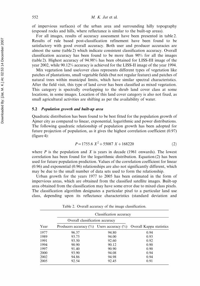
5.2 Population growth and built-up area
Quadratic distribution has been found to be best fitted for the population growth of
Ajmer city as compared to linear, exponential, logarithmic and power distributions.The following quadratic relationship of population growth has been adopted for
future projection of population, as it gives the highest correlation coefficient (0.97)
(figure 4):
P~1755:6 X 2z55087 Xz168220 ð2Þ
where P is the population and X is years in decade (1961 onwards). The lowestcorrelation has been found for the logarithmic distribution. Equation (2) has been
used for future population prediction. Values of the correlation coefficient for linear
(0.96) and exponential (0.96) relationships are also not significantly different, which
may be due to the small number of data sets used to form the relationship.
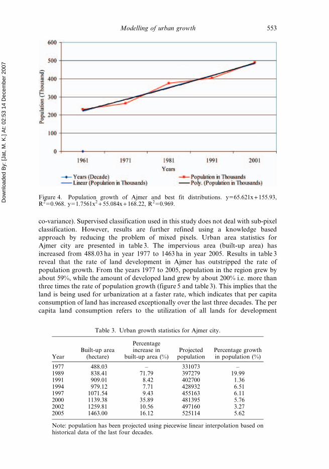
Urban growth for the years 1977 to 2005 has been estimated in the form ofimpervious areas, which are obtained from the classified satellite images. Built-up
area obtained from the classification may have some error due to mixed class pixels.
The classification algorithm designates a particular pixel to a particular land use
class, depending upon its reflectance characteristics (standard deviation and
Table 2. Overall accuracy of the image classification.
Year
Classification accuracy
Overall classification accuracy
Overall Kappa statisticsProducers accuracy (%) Users accuracy (%)
1977 96.37 94.80 0.941989 93.75 94.00 0.931991 93.50 92.60 0.921994 90.90 90.12 0.901997 91.40 90.90 0.902000 93.90 94.08 0.942002 94.86 94.98 0.942005 92.54 92.45 0.91
552 M. K. Jat et al.
Dow
nloa
ded
By:
[Jat
, M. K
.] A
t: 02
:53
14 D
ecem
ber 2
007
co-variance). Supervised classification used in this study does not deal with sub-pixel
classification. However, results are further refined using a knowledge based
approach by reducing the problem of mixed pixels. Urban area statistics for
Ajmer city are presented in table 3. The impervious area (built-up area) has
increased from 488.03 ha in year 1977 to 1463 ha in year 2005. Results in table 3
reveal that the rate of land development in Ajmer has outstripped the rate of
population growth. From the years 1977 to 2005, population in the region grew by
about 59%, while the amount of developed land grew by about 200% i.e. more than
three times the rate of population growth (figure 5 and table 3). This implies that the
land is being used for urbanization at a faster rate, which indicates that per capita
consumption of land has increased exceptionally over the last three decades. The per
capita land consumption refers to the utilization of all lands for development
Figure 4. Population growth of Ajmer and best fit distributions. y565.621x + 155.93,R250.968. y51.7561x2 + 55.084x + 168.22, R250.969.
Table 3. Urban growth statistics for Ajmer city.
YearBuilt-up area
(hectare)
Percentageincrease in
built-up area (%)Projected
populationPercentage growthin population (%)
1977 488.03 – 331073 –1989 838.41 71.79 397279 19.991991 909.01 8.42 402700 1.361994 979.12 7.71 428932 6.511997 1071.54 9.43 455163 6.112000 1139.38 35.89 481395 5.762002 1259.81 10.56 497160 3.272005 1463.00 16.12 525114 5.62
Note: population has been projected using piecewise linear interpolation based onhistorical data of the last four decades.
Modelling of urban growth 553
Dow
nloa
ded
By:
[Jat
, M. K
.] A
t: 02
:53
14 D
ecem
ber 2
007
initiatives, like commercial, industrial, educational, recreational and residential
establishments per person.
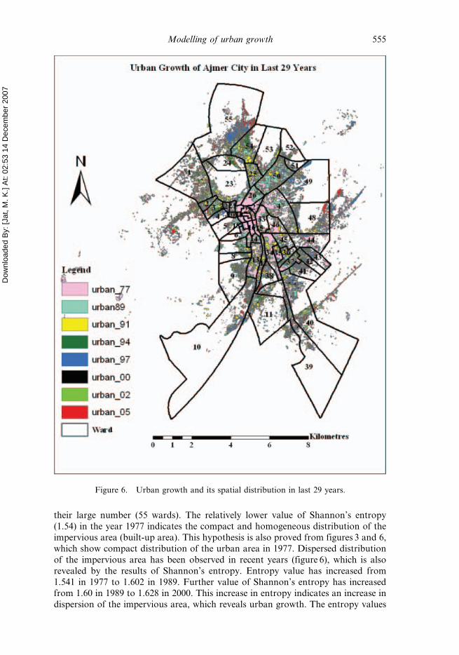
Spatial distribution of ward-wise urban growth (in the form of impervious area) inthe last 29 years is shown in figure 6. Here the impervious area (built-up area)
includes houses, industries, roads, etc. Urban growth is faster in the outer area
(ward number 1 to 6 and ward number 31 to 55) along the major roads as compared
to the central portion of the city, which is also substantiated by figures 6, 7 and
landscape metrics. Here the hypothesis is correct that improvement in economic
conditions relates to urban growth.
5.2 Metrics of urban sprawl
5.2.1 Shannon’s entropy (Hn). In the present investigation, Shannon’s entropy (Hn)
is used to measure the degree of spatial concentration or dispersion (homogeneity)
of a geophysical variable (impervious area) among n spatial units/zones (wards). In
the present study, ward-wise impervious area has been considered as the geophysicalvariable, which enables determination of urban growth. Entropy may range from 0
to log n, indicating a compact distribution of considered phenomena (urbanization)
for values closer to zero and dispersed distribution for the values closer to log n.
Values of entropy near to log n reveals the dispersion of the geophysical variable
(impervious area), which indicates the occurrence of urban growth.
Shannon’s entropy results for six years (1977, 1989, 1994, 2000, 2002 and 2005)
are presented in table 4. Entropy values have been calculated across all wards, and
are summed-up to represent the entropy for the whole urban area. Larger value ofentropy, more than 1.6 (table 4), reveals the occurrence and spatial distribution of
the variable (urban growth). Ward-wise results have not been presented here due to
Figure 5. Population and urban growth of Ajmer in the last 29 years.
554 M. K. Jat et al.
Dow
nloa
ded
By:
[Jat
, M. K
.] A
t: 02
:53
14 D
ecem
ber 2
007
their large number (55 wards). The relatively lower value of Shannon’s entropy
(1.54) in the year 1977 indicates the compact and homogeneous distribution of the
impervious area (built-up area). This hypothesis is also proved from figures 3 and 6,
which show compact distribution of the urban area in 1977. Dispersed distribution
of the impervious area has been observed in recent years (figure 6), which is also
revealed by the results of Shannon’s entropy. Entropy value has increased from
1.541 in 1977 to 1.602 in 1989. Further value of Shannon’s entropy has increasedfrom 1.60 in 1989 to 1.628 in 2000. This increase in entropy indicates an increase in
dispersion of the impervious area, which reveals urban growth. The entropy values
Figure 6. Urban growth and its spatial distribution in last 29 years.
Modelling of urban growth 555
Dow
nloa
ded
By:
[Jat
, M. K
.] A
t: 02
:53
14 D
ecem
ber 2
007
obtained are 1.541 in 1977, 1.602 in 1989, 1.621 in 1994, 1.622 in 2000, 1.616 in 2002
and 1.616 in 2005. These are closer to the upper limit of log n, i.e. 1.7403, showing
the degree of dispersion of built-up areas in the region.
The higher value of overall entropy for the whole urban area represents higher
dispersion of the impervious area, which is a sign of urban growth. The increase in
dispersion is due to new areas being added to the municipal boundaries and some of
the new housing schemes implemented by the Government. The degree of dispersion
has reduced marginally from 2000 to 2005, which indicates an increase in
homogeneity of the impervious area. Ward-wise impervious areas in different years
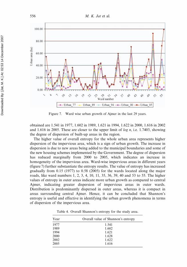
(figure 7) further substantiate the entropy results. The value of entropy has increased
gradually from 0.15 (1977) to 0.58 (2005) for the wards located along the major
roads, like ward numbers 1, 2, 3, 4, 10, 11, 35, 36, 39, 40 and 53 to 55. The higher
values of entropy in outer areas indicate more urban growth as compared to central
Ajmer, indicating greater dispersion of impervious areas in outer wards.
Distribution is predominantly dispersed in outer areas, whereas it is compact in
areas surrounding central Ajmer. Hence, it can be concluded that Shannon’s
entropy is useful and effective in identifying the urban growth phenomena in terms
of dispersion of the impervious area.
Figure 7. Ward wise urban growth of Ajmer in the last 29 years.
Table 4. Overall Shannon’s entropy for the study area.
Year Overall value of Shannon’s entropy
1977 1.5411989 1.6021994 1.6212000 1.6282002 1.6222005 1.616
556 M. K. Jat et al.
Dow
nloa
ded
By:
[Jat
, M. K
.] A
t: 02
:53
14 D
ecem
ber 2
007
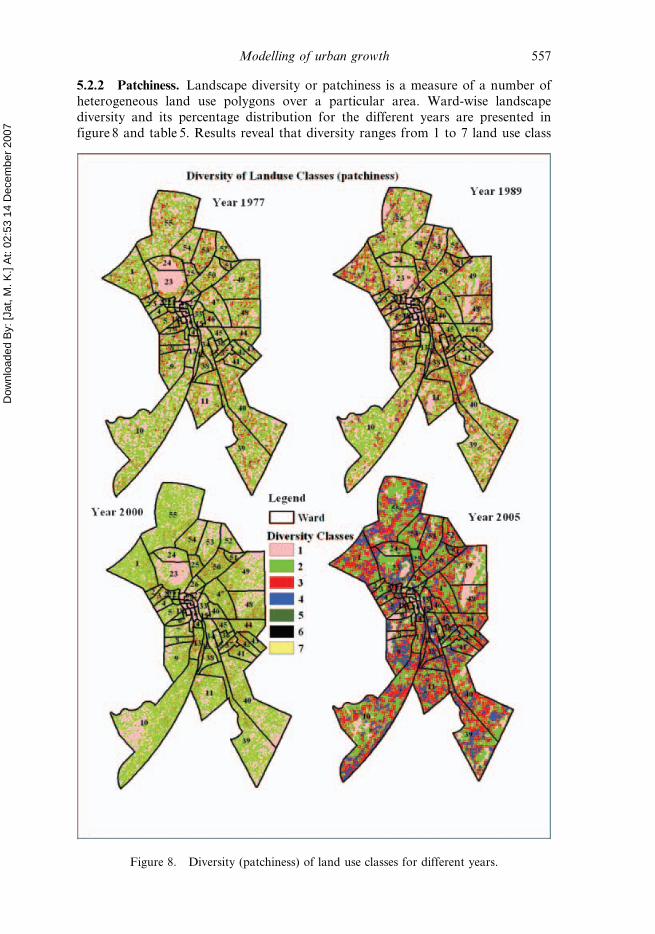
5.2.2 Patchiness. Landscape diversity or patchiness is a measure of a number ofheterogeneous land use polygons over a particular area. Ward-wise landscape
diversity and its percentage distribution for the different years are presented in
figure 8 and table 5. Results reveal that diversity ranges from 1 to 7 land use class
Figure 8. Diversity (patchiness) of land use classes for different years.
Modelling of urban growth 557

Dow
nloa
ded
By:
[Jat
, M. K
.] A
t: 02
:53
14 D
ecem
ber 2
007
categories. One land use class category represents that only one land use class is
available within the kernel, two land use class category represents that any two land
use classes are available within the kernel, corresponding to the central pixel of the
kernel. For all the years, one and two heterogeneous land use classes categories are
highest, whereas five to eight heterogeneous class categories have been found to be
the minimum (table 5). However, one land use class category has gradually increased
from 36.6% to 55.18% and two land use class categories have reduced from 50.85%
to 17.54% (except 2000). Category three has increased from 11.77% to 19.137%,
which indicates the continuous process of urbanization in new areas. This reveals
that the percentage of homogeneous area has increased gradually since 1977, while
the remaining area which is heterogeneous with patch class ranging from two to six
has reduced. Results of the diversity analysis are in good agreement with Shannon’s
entropy results.
5.2.3 Map density. Map density is another index which can be used to examine the
homogeneity/dispersion of any spatial phenomena, like urbanization. Distribution
of impervious areas, which indicates urban growth, has been studied using density
metrics. Results of built-up/impervious area density metrics are presented in figure 9.
Re-classified categories of the densities (in terms of percentage of the total
impervious area) are presented in table 6. Very high and high density of the built-up
area refer to cluster or the more compact nature of the built-up theme, while
medium density refers to relatively lower compact built-up areas, and low and very
low density indicate loosely or sparsely spread built-up areas.
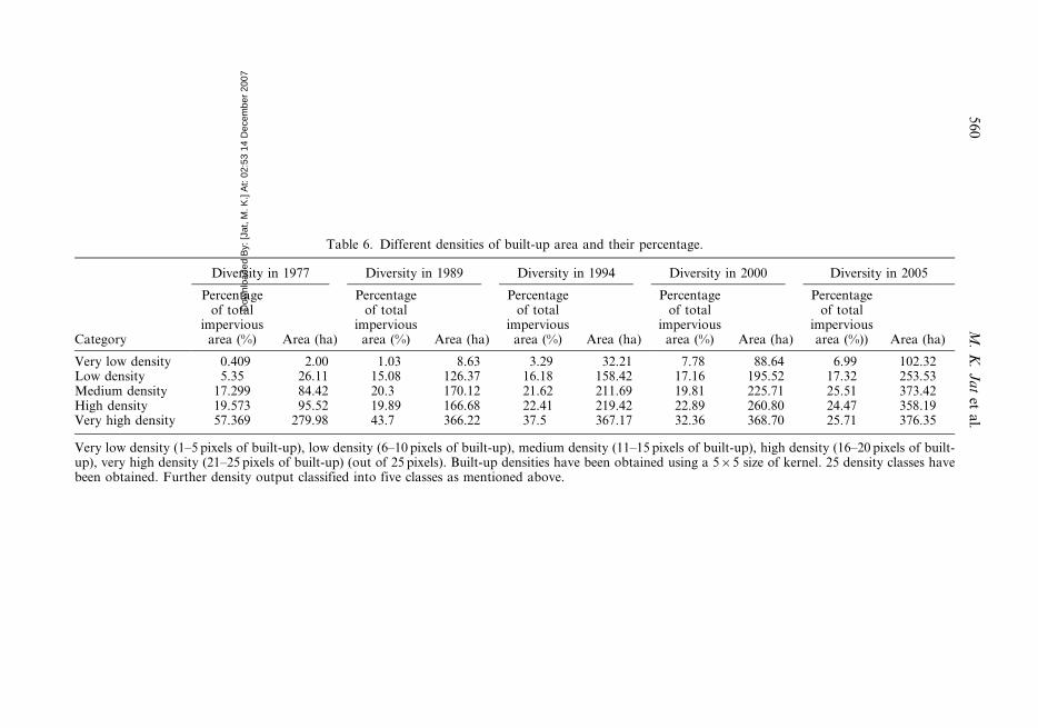
The percentage of high-density (built-up area) has gradually increased from
19.57% in 1977 to 24.47% in 2005. The percentage of very high-density built-up
areas is more than 40% until the year 1989, however it has reduced afterwards
(table 6). This revealed that percentage of more compact or highly dense built-up
areas is more up to 1989, and thereafter it has reduced on account of development of
new areas, which indicates dispersion. This reduction does not mean that impervious
areas have decreased since 1989. The relative share of very high compact built-up
areas has been reduced, though the total area under this category has not reduced.
In 1989, the area under very high density was 366.24 ha, which has increased to
376.14 ha in 2005. However, its percentage with respect to the total area under all
categories has been reduced. The increase in the value of very low, low, medium and
Table 5. Percentage distribution of patchiness for Ajmer urban area.
No. ofdiversityclass
Percentagedistribution
(1977)
Percentagedistribution
(1989)
Percentagedistribution
(1994)
Percentagedistribution
(2000)
Percentagedistribution
(2005)
1 36.604 31.234 52.883 53.102 55.1832 50.851 46.785 15.784 23.380 17.5413 11.771 18.699 14.961 14.960 19.1374 0.764 3.065 9.810 8.542 7.0855 0.009 0.213 5.001 0.015 0.9686 0.00 0.005 1.408 0.00 0.0827 0 0 0.149 0 0.0038 0 0 0.004 0 0
While deriving diversity of different landuse classes within Municipal boundary of the Ajmer,diversity function of the ERDAS Focal (Scan) model has been used considering 565 size ofkernel window.
558 M. K. Jat et al.

Dow
nloa
ded
By:
[Jat
, M. K
.] A
t: 02
:53
14 D
ecem
ber 2
007
high density categories reveal urban growth and new developmental activities.
Figure 9 reveals that more land development has taken place in outer areas (wardnumbers 1, 2, 3, 4, 5, 35, 39, 40, 53, 54 and 55) along the major roads and railway
line. An important inference could be drawn here that high and medium density is
Figure 9. Density of impervious area in different years.
Modelling of urban growth 559
Dow
nloa
ded
By:
[Jat
, M. K
.] A
t: 02
:53
14 D
ecem
ber 2
007
Table 6. Different densities of built-up area and their percentage.
Category
Diversity in 1977 Diversity in 1989 Diversity in 1994 Diversity in 2000 Diversity in 2005
Percentageof total
imperviousarea (%) Area (ha)
Percentageof total
imperviousarea (%) Area (ha)
Percentageof total
imperviousarea (%) Area (ha)
Percentageof total
imperviousarea (%) Area (ha)
Percentageof total
imperviousarea (%)) Area (ha)
Very low density 0.409 2.00 1.03 8.63 3.29 32.21 7.78 88.64 6.99 102.32Low density 5.35 26.11 15.08 126.37 16.18 158.42 17.16 195.52 17.32 253.53Medium density 17.299 84.42 20.3 170.12 21.62 211.69 19.81 225.71 25.51 373.42High density 19.573 95.52 19.89 166.68 22.41 219.42 22.89 260.80 24.47 358.19Very high density 57.369 279.98 43.7 366.22 37.5 367.17 32.36 368.70 25.71 376.35
Very low density (1–5 pixels of built-up), low density (6–10 pixels of built-up), medium density (11–15 pixels of built-up), high density (16–20 pixels of built-up), very high density (21–25 pixels of built-up) (out of 25 pixels). Built-up densities have been obtained using a 565 size of kernel. 25 density classes havebeen obtained. Further density output classified into five classes as mentioned above.
56
0M
.K
.J
at
eta
l.
Dow
nloa
ded
By:
[Jat
, M. K
.] A
t: 02
:53
14 D
ecem
ber 2
007
found all along the main roads (National Highway), railway station and the city
centre (near railway station and Anasagar lake area). Most of the high density is
found within the central portion of the city. Medium density is found along the city
periphery and on the highways. An increase in impervious surfaces (from 1977 to
2005) in outer areas (ward numbers 1, 2, 3, 4, 5, 35, 39, 40, 53, 54 and 55)
substantiate the results of density metrics. Further, density results substantiate the
results of Shannon’s entropy, which reveal an urban growth in outer areas. Hence,
these metrics are effective for the determination of urban growth and its spatial
distribution.
5.3 Dynamics of urban growth
Defining the dynamic urban growth phenomena and its future prediction is a greater
challenge than its quantification. Although different sprawl types are identified and
defined, there has been an inadequacy with respect to developing mathematical
relationships to define them. This necessitates the characterization and modelling of
urban growth, which may aid in regional planning, planning and development of
water resources and designing of urban drainage infrastructure. In the present
investigation, population and related densities are used as independent variables for
modelling the urban growth. Many other parameters, like socio-economic
conditions, governmental investments for public sector works, scope of industria-
lisation and tourist activities can also be considered in urban growth modelling for
future work. However, the availability of such data is a difficult task in developing
countries like India.
5.4 Modelling of urban growth
Initially, analysis has been performed considering the individual causative factor
(independent variables) to ascertain its significance (form of equation) on urban
growth. The regression analyses reveal the individual contribution of causative
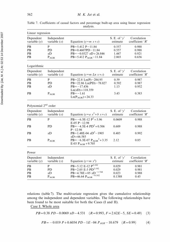
factors on urban growth. Various relationships and their statistical parameters have
been presented in table 7.
Relationships between PB and P have been found to be quadratic with the highest
correlation coefficient (0.988) and lowest standard error of estimate (SE50.06).
Relationships between PB and PD have been found to be linear. Linear regression
results show the highest correlation coefficient (0.988) and lowest standard error of
estimate (SE50.57) for PD. Relationships between PB and aD have also been found
to be quadratic with the highest correlation coefficient (0.99) and lowest standard
error of estimate (SE50.48). Relationships between PB and PAGR have been found
to be quadratic with the highest correlation coefficient (0.85) and lowest standard
error of estimate (SE52.12). The linear and quadratic regression analyses revealed
that the population and population density has a significant influence on PB. The
quadratic regression analyses revealed that aD and PAGR have a considerable role in
the urban growth phenomenon. The power law regression analyses reveal that the
population density has influenced the urban growth phenomenon, which is evident
from the value of the exponent. Annual population growth shows a positive
correlation with percentage built-up area, which is again a population derived
parameter.
In multivariate regression, it is assumed that the relationship between variables is
linear, which is supported by a higher correlation coefficient for linear and quadratic
Modelling of urban growth 561
Dow
nloa
ded
By:
[Jat
, M. K
.] A
t: 02
:53
14 D
ecem
ber 2
007
relations (table 7). The multivariate regression gives the cumulative relationship
among the independent and dependent variables. The following relationships have
been found to be most suitable for both the Cases (I and II).
Case I: Whole area
PB~0:38 PD{0:0069 aD{4:531 R~0:993, F~2:62E�5, SE~0:49ð Þ ð3Þ
PB~{0:019 Pz0:6054 PD{1E�04 PAGR{10:679 R~0:99ð Þ ð4Þ
Table 7. Coefficients of casual factors and percentage built-up area using linear regressionanalysis.
Linear regression
Dependentvariable (y)
Independentvariable (x) Equation (y5m x + c)
S. E. of ‘y’estimate
Correlationcoefficient ‘R’
PB P PB55.412 P211.84 0.557 0.988PB PD PB50.4607PD211.84 0.557 0.988PB aD PB520.0327 aD + 26.846 1.447 0.921PB PAGR PB55.412 PAGR211.84 2.803 0.656
Logarithmic
Dependentvariable (y)
Independentvariable (x) Equation (y5m Ln x + c)
S. E. of ‘y’estimate
Correlationcoefficient ‘R’
PB P PB522.8 Ln(P)2284.95 0.59 0.987PB PD PB522.86 Ln(PD)278.027 0.592 0.987PB aD PB5217.436
Ln(aD) + 118.3591.13 0.952
PB PAGR PB521.61Ln(PAGR) + 24.33
3.43 0.383
Polynomial 2nd order
Dependentvariable (y)
Independentvariable (x) Equation (y5a x2 + b x + c)
S. E. of ‘y’estimate
Correlationcoefficient ‘R’
PB P PB526.3E-12 P2 + 5.96E-05 P212.98
0.0609 0.988
PB PD PB524.5E-4 PD2 + 0.506P212.98
0.609 0.988
PB aD PB51.48E-04 aD221905aD + 66.585
0.485 0.992
PB PAGR PB526.3E-07 PAGR2 + 3.35
E-03 PAGR + 9.7052.12 0.85
Power
Dependentvariable (y)
Independentvariable (x) Equation (y5m xz)
S. E. of ‘y’estimate
Correlationcoefficient ‘R’
PB P PB55.12 E-12 P2.192 0.029 0.981PB PD PB52.05 E-3 PD2.192 0.029 0.981PB aD PB54.78E + 05 aD21.744 0.023 0.988PB PAGR PB546.64 PAGR
20.182 0.1388 0.45
562 M. K. Jat et al.

Dow
nloa
ded
By:
[Jat
, M. K
.] A
t: 02
:53
14 D
ecem
ber 2
007
Case II: At ward level
PB~{0:00395 Pz0:09524 PD{0:01144 aDz59:058
R~0:87, F~2:25E�15, SE~16:6ð Þð5Þ
Considering all the causative factors in the stepwise regression, equation (3) for
Case I and equation (5) for Case II have been found to be the best fit with highest
correlation coefficient, lowest standard error of estimate and lowest significance F.
In Case I, it is to be noted that the correlation coefficient is the same for
relationships (equation (4)) with other parameters, however the relationship of PB
with PD and aD is found to be most suitable as its significance F is smallest.Significance F is a statistical criterion which indicates the degree of relationship. The
smaller value of significance F indicates a good relationship. Equation (3) to
equation (5) confirms that the causative factors collectively have a significant role in
the urban growth phenomenon, which can be understood from the satisfactory
positive correlation coefficients.
5.5 Predicting scenarios of urban sprawl
Future predictions of urban growth can be made using Case I relationship, as ward-
wise population for a longer period is not available. The likely increase in the
impervious area (built-up area) is predicted using equation (4) as population,
population density and annual population growth rate can be obtained using
available historical data. To project the impervious area (built-up area) from 2011 to
2041 (decadal growth) within the notified municipal area, the corresponding
population has been computed using equation (2). It is estimated that the percentage
built-up area for 2011 and 2051 would be 17.98% and 33.95%, respectively(figure 10). This implies that by 2051, the built-up area in the municipal limits would
rise to 2889.81 ha, which may be nearly 97.53% more than the present built-up area
(1463 ha). Thus, the pressure on land would further grow and the vegetal areas, open
grounds and region around the highways are likely to become prime targets for
urban growth.
Remote sensing technology is indispensable for dealing with dynamic phenomenalike urban growth. Without remote sensing data, one may not be able to monitor
and estimate the urban growth effectively over a time period, especially for an
elapsed time period. This technology is also cost effective in dealing with phenomena
like urban growth, as other conventional data collection and surveying techniques
are found to be time consuming and expensive. Spatial and temporal variability of
land use/cover change can be monitored using remote sensing data. In the present
study, ward wise built-up areas have been determined over a period of 29 years,
which would not have been possible without the use of remote sensing data.Landscape metrics have been computed using satellite images to understand the
form and spatial distribution of urban growth.
6. Conclusions
Urban growth is seen as one of the potential threats to sustainable development
where urban planning with effective resource utilization, allocation of natural
resources and infrastructure initiatives are key concerns. The study has attempted tounderstand the urban growth of Ajmer city, quantified by defining important
metrics and modelling the same for future prediction. Remote sensing and GIS
Modelling of urban growth 563

Dow
nloa
ded
By:
[Jat
, M. K
.] A
t: 02
:53
14 D
ecem
ber 2
007
techniques have been used to demonstrate their application for the monitoring and
modelling of dynamic phenomena like urbanization. The spatial data along with the
attribute data of the region aided in analysing statistically and defining a few of the
landscape metrics.
Landscape metrics helped in understanding the urban growth form and its
pattern. Urban growth has been taking place continuously at a faster rate in outer
areas, bringing more area under built-up categories as revealed by metrics (dispersed
growth). The higher value of Shannon’s entropy substantiated the urban growth.
It is found that the change in built-up area over the period of nearly 29 years is
200%, and by 2051 the built-up area in the region would rise to 2889.81 ha, which
may be nearly 97.53% more than the current sprawl of 1463 ha. The rate of urban
growth would be about two times the population growth, if projected using the
present trend. Further, other causative factors, like socio-economic conditions,
governmental investments for public sector works, scope of industrialization and
tourist activities can also be considered for urban growth modelling in future
research work.
Acknowledgements
The first author greatly acknowledges the Rajasthan Urban Infrastructure Project
Authorities, PHED Ajmer, and Town Planning Department of the Government of
Rajasthan for providing data used in this work, and AICTE New Delhi and QIP
Centre of IIT Roorkee for providing financial support for this work. The first
author acknowledges Mr. Rohit Bhakar for helping in improving the English of this
manuscript. The authors sincerely thank the Editor and all Referees for their
suggestions to improve the manuscript.
Figure 10. Prediction of urban growth for Ajmer city.
564 M. K. Jat et al.
Dow
nloa
ded
By:
[Jat
, M. K
.] A
t: 02
:53
14 D
ecem
ber 2
007
ReferencesBARNES, K.B., MORGAN III, J.M., ROBERGE, M.C. and LOWE, S., 2001, Sprawl development:
its patterns, consequences, and measurement. Towson University, Towson.
BATTY, M., XIE, Y. and SUN, Z., 1999, The dynamics of urban sprawl, Working Paper Series,
Paper 15, Centre for Advanced Spatial Analysis, University College, London.
CENSUS OF INDIA 1971, District Census Handbook – Ajmer District, Series 14, Directorate of
Census Operations, Jaipur.
CENSUS OF INDIA 1981, District Census Handbook – Ajmer District, Series 9, Directorate of
Census Operations, Jaipur.
CENSUS OF INDIA, 1991. (http://www.censusindia.net).
CENSUS OF INDIA, 2001. (http://www.censusindia.net).
CHENG, J. and MASSER, I., 2003, Urban growth pattern modelling: a case study of Wuhan
City, PR China. Landscape and Urban Planning, 62, pp. 199–217.
CIBULA, W.G. and NYQUIST, M.O., 1987, Use of topographic and climatological models in a
geographical data base to improve Landsat MSS classification for Olympic National
Park. Photogrammetric Engineering and Remote Sensing, 53, pp. 67–75.
CIVCO, D.L., HURD, J.D., WILSON, E.H., ARNOLD, C.L. and PRISLOE, M., 2002, Quantifying
and describing urbanizing landscapes in the Northeast United States. Photo-
grammetric Engineering & Remote Sensing, 68, pp. 1083–1090.
CONGALTON, R.G., 1991, A review of assessing the accuracy of classification of remote
sensing data. Remote Sensing of Environment, 37, pp. 35–46.
EPSTEIN, J., PAYNE, K. and KRAMER, E., 2002, Techniques for mapping suburban sprawl.
Photogrammetric Engineering & Remote Sensing, 63, pp. 913–918.
FRANKLIN, S.E., 1994, Discrimination of sub-alpine forest species and canopy density using
digital CASI, SPOT PLA and Landsat TM data. Photogrammetric Engineering and
Remote Sensing, 60, pp. 1233–1241.
GOMARASCA, M.A., BRIVIO, P.A., PAGNONI, F. and GALLI, A., 1993, One century of land use
changes in the metropolitan area of Milan (Italy). International Journal of Remote
Sensing, 14, pp. 211–223.
GREEN, K., KEMPKA, D. and LACKEY, L., 1994, Using remote sensing to detect and monitor
land-cover and land-use change. Photogrammetric Engineering and Remote Sensing,
60, pp. 331–337.
GREENBERG, J.D. and BRADLEY, G.A., 1997, Analyzing the urban–wildland interface with
GIS. Journal of Forestry, 95, pp. 18–22.
HAACK, B.N. and RAFTER, A., 2006, Urban growth analysis and modelling in the Kathmandu
valley, Nepal. Habitat International, 30, pp. 1056–1065.
HARRIS, P.M. and VENTURA, S.J., 1995, The integration of geographic data with remotely
sensed imagery to improve classification in an urban area. Photogrammetric
Engineering and Remote Sensing, 61, pp. 993–998.
JANTZ, CLAIRE, A. and GOETZ, SCOTT, J., 2005, Analysis of scale dependencies in an urban
land-use-change model. International Journal of Geographical Information Science, 19,
pp. 217–241.
JAT, M.K., GARG, P.K. and KHARE, D., 2006, Assessment of urban growth pattern using
spatial analysis techniques. In Proceedings of Indo-Australian Conference on
Information Technology in Civil Engineering (IAC-ITCE), 20–21 February, 2006,
pp. 70.
JENSEN, J.R. and COWEN, D.C., 1999, Remote sensing of urban/suburban infrastructure
and socioeconomic attributes. Photogrammetric Engineering and Remote Sensing, 65,
pp. 611–622.
JENSEN, J.R., 1995, Introductory digital image processing: a remote sensing perspective
(New Jersey: Prentice-Hall).
JOSHI, P.K., LELE, N. and AGARWAL, S.P., 2006, Entropy as an indicator of fragmented
landscape. Current Sciences, 91, pp. 276–278.
Modelling of urban growth 565
Dow
nloa
ded
By:
[Jat
, M. K
.] A
t: 02
:53
14 D
ecem
ber 2
007
LATA, K.M., SANKAR RAO, C.H., KRISHNA PRASAD, V., BADRINATH, K.V.S. and
RAGHAVASWAMY,, 2001, Measuring urban sprawl: a case study of Hyderabad. GIS
Development, 5, pp. 8–13.
LI, G. and WENG, Q., 2005, Using Landsat ETM + imagery to measure population density in
Indianapolis, Indiana, USA. Photogrammetric Engineering and Remote Sensing, 71,
pp. 947–958.
LO, C.P., 2001, Modelling the population of China using DMSP operational Line scan
system nighttime data. Photogrammetric Engineering and Remote Sensing, 67,
pp. 1037–1047.
LO, C.P. and SHIPMAN, R.L., 1990, A GIS approach to land-use change dynamics detection.
Photogrammetric Engineering and Remote Sensing, 56, pp. 1483–1491.
LO, C.P. and YANG, X., 2002, Drivers of land-use/land-cover changes and dynamic modelling
for the Atlanta, Georgia Metropolitan Area. Photogrammetric Engineering and
Remote Sensing, 68, pp. 1062–1073.
LOVELAND, T.R., MERCHANT, J.W., OHLEN, D.O. and BROWN, J.F., 1991, Development of a
land-cover characteristics database for the conterminous U.S. Photogrammetric
Engineering and Remote Sensing, 57, pp. 1453–1463.
LU, D. and WENG, Q., 2005, Urban classification using full spectral information of Landsat
ETM + imagery in Marion County, Indiana. Photogrammetric Engineering and
Remote Sensing, 71, pp. 1275–1284.
MUNDIA, C.N. and ANIYA, M., 2005, Analysis of land use/cover changes and urban
expansion of Nairobi city using remote sensing and GIS. International Journal of
Remote Sensing, 26, pp. 2831–2849.
ROYER, A., CHARBONNEAU, L. and BONN, F., 1988, Urbanization and Landsat MSS albedo
change in the Windsor-Quebec corridor since 1972. International Journal of Remote
Sensing, 9, pp. 555–566.
SINGH, A., 1989, Digital change detection techniques using remotely-sensed data.
International Journal of Remote Sensing, 10, pp. 989–1003.
STEFANOV, W.L., RAMSEY MICHAEL, S. and CHRISTENSEN,, 2001, Monitoring urban land
cover change: an expert system approach to land cover classification of semiarid to
arid urban centers. Remote Sensing of Environment, 77, pp. 173–185.
STUCKENS, J., COPPIN, P.R. and BAUER, M.E., 2000, Integrating contextual information with
per-pixel classification for improved land cover classification. Remote Sensing of
Environment, 71, pp. 282–296.
SUDHIRA, H.S., RAMACHANDRA, T.V. and JAGADISH, K.S., 2004, Urban sprawl: metrics,
dynamics and modelling using GIS. International Journal of Applied Earth
Observation and Geoinformation, 5, pp. 29–39.
SUGUMARAN, R., PAVULURI, M.K. and ZERR, D., 2003, The use of high resolution imagery
for identification of urban climax forest species using traditional and rule based
classification approach. IEEE Transaction on Geosciences and Remote Sensing, 41,
pp. 1933–1939.
TOLL, D.L., 1985, Landsat-4 thematic mapper scene characteristics of a suburban and rural
area. Photogrammetric Engineering and Remote Sensing, 51, pp. 1471–1482.
TORRENS, P.M. and ALBERTI, M., 2000, Measuring sprawl, Working paper no. 27, Centre for
Advanced Spatial Analysis, University College, London.
TRANI, M.K. and GILES, R.H., 1999, An analysis of deforestation: metrics used to describe
pattern change. Forest Ecological Management, 114, pp. 459–470.
VOGELMANN, J.E., SOHL, T. and HOWARD, S.M., 1998, Regional characterizations of land
cover using multiple sources of data. Photogrammetric Engineering and Remote
Sensing, 64, pp. 45–57.
WENG, Q., 2001, A remote sensing–GIS evaluation of urban expansion and its impact on
surface temperature in the Zhujiang Delta, China. International Journal of Remote
Sensing, 22, pp. 1999–2014.
566 M. K. Jat et al.

Dow
nloa
ded
By:
[Jat
, M. K
.] A
t: 02
:53
14 D
ecem
ber 2
007
YANG, X. and LIU ZHI, 2005, Use of satellite derived landscape imperviousness index to
characterize urban spatial growth. Computers, Environment and Urban Systems, 29,
pp. 524–540.
YANG, X. and LO, C.P., 2003, Modelling urban growth and landscape changes in the
Atlanta metropolitan area. International Journal of Geographical Information Science,
17, pp. 463–488.
YEH, A.G.O. and LI, X., 2001, Measurement and monitoring of urban sprawl in a rapidly
growing region using entropy. Photogrammetric Engineering and Remote Sensing, 67,
p. 83.
Modelling of urban growth 567
Top Related
Copyright © 2022 FDOKUMEN

