


Bahasa
Halaman
Hukum

Electronic copy available at: http://ssrn.com/abstract=1963023
Innovative Capacity and the Asset Growth Anomaly*
Praveen Kumara Dongmei Lib
Abstract
Innovative capacity (IC) is the ability of firms to produce and commercialize a sequence of
innovations. Expected returns need not fall following asset growth by high IC firms because
investment can generate new growth options. Using patent intensity based IC measures we
provide the first analysis of the effects of IC on financial markets' response to asset growth. We
find that the well-known negative relation between asset growth and subsequent excess returns
holds only for firms with high asset growth and low IC and does so in a stronger and more robust
fashion than reported earlier. However, high IC firms with high asset growth not only do not
suffer negative excess returns but actually earn significantly positive subsequent excess returns.
Moreover, and as predicted by a model of optimal dynamic investment with sequentially arising
growth options, changes in the market risk loadings of firms following asset growth episodes are
positively related to their IC. The innovative capacity of firms, therefore, appears to play an
important role in the dynamics between their asset growth and returns, and in driving their time-
varying market risk.
* We thank Jonathan Berk, Wayne Ferson, Michael Fishman, Paolo Fulghieri, Richard Green, Dirk Hackbarth, David Hirshleifer, Kewei Hou, Ravi Jagannathan, Dirk Jenter, Nisan Langberg, Michael Lemmon, Jeremy Stein, Sheridan Titman, and Jianfeng Yu for valuable discussions and comments. We also thank Lu Zhang for sharing the investment and profitability factors returns.
a C.T. Bauer College of Business, University of Houston, Houston, TX 77204. Email: [email protected] b Rady School of Management, University of California, San Diego, La Jolla, CA 92093. Email: [email protected]

Electronic copy available at: http://ssrn.com/abstract=1963023
Innovative Capacity and the Asset Growth Anomaly
January 2012
Abstract
Innovative capacity (IC) is the ability of firms to produce and commercialize a sequence of
innovations. Expected returns need not fall following asset growth by high IC firms because
investment can generate new growth options. Using patent intensity based IC measures we
provide the first analysis of the effects of IC on financial markets' response to asset growth. We
find that the well-known negative relation between asset growth and subsequent excess returns
holds only for firms with high asset growth and low IC and does so in a stronger and more robust
fashion than reported earlier. However, high IC firms with high asset growth not only do not
suffer negative excess returns but actually earn significantly positive subsequent excess returns.
Moreover, and as predicted by a model of optimal dynamic investment with sequentially arising
growth options, changes in the market risk loadings of firms following asset growth episodes are
positively related to their IC. The innovative capacity of firms, therefore, appears to play an
important role in the dynamics between their asset growth and returns, and in driving their time-
varying market risk.
Keywords: Innovative capacity; Asset growth; Excess returns; Risk dynamics; Patents
JEL classification codes: G12, G32, O31
1
1. Introduction
The effects of capital investment and asset growth on stock returns have important
implications for both asset pricing and corporate finance. Recently, a number of empirical
studies highlight a negative relation between firms’ asset growth and subsequent abnormal stock
returns ─ the “asset growth anomaly” (Titman, Wei, and Xie, 2004; Anderson and Garcia-Feijoo,
2006; Cooper, Gulen, and Schill, 2008).1 In particular, Titman et al. (2004) document a negative
relation between large increases in capital investment and subsequent benchmark-adjusted
returns, and Cooper et al. (2008) show that this relation extends to the growth in total assets.
The asset growth anomaly has generated both behavioral and risk-based explanations. For
example, Titman et al. (2004) argue that investors underreact to empire building by managers
and show that the negative relation between capital investment and subsequent abnormal returns
is stronger for firms with greater investment discretion (i.e., firms with higher cash flows and
lower debt ratios), while Cooper et al. (2008) suggest an overreaction to asset growth and
interpret the negative abnormal returns as a correction to the initial overreaction. On the other
hand, a variety of models in the literature predict a negative equilibrium relation between
investment and future returns. In particular, real options models (e.g., McDonald and Siegel,
1986; Majd and Pindyck, 1987; Carlson, Fisher, and Giammarino, 2006) predict a decline in
systematic risk following the exercise of risky growth options. From this perspective, the
observed relation between asset growth and subsequent returns is not an anomaly and indeed a
number of recent papers present direct evidence supportive of the risk-based explanations (see
Cooper and Priestly, 2011). These alternative interpretations of the data have profoundly
1 Other studies on the asset growth anomaly include Xing (2008), Li and Zhang (2010), Titman, Wei, and Xie (2011), Lam and Wei (2011), Stambaugh, Yu, and Yuan (2011), and Watanabe et al. (2011), among others.

2
different implications. In particular, a systematic negative bias in the market's capitalization of
asset growth should have a major impact on corporate investment and financial policies; it also
suggests formulation of trading strategies to exploit this market inefficiency.
In this paper, we present new evidence on the dynamics between asset growth and stock
returns by building on the notion of innovative capacity (IC), which is a measure of firms' ability
to generate multiple growth options ─ for example, through a sequence of innovations based on
their patent holdings. We motivate the role of IC by noting the potential heterogeneity in the
effects of asset growth across different IC firms. Specifically, asset growth of high IC firms is
more likely related to innovation activities, such as construction of long-range research facilities
and purchase of machinery/materials for use on current and future R&D projects, or acquisition
of patents, or development of knowledge absorption capacities. This type of asset growth tends
to generate new growth options and investment opportunities because innovations are often the
source of new ideas and opportunities (Schumpeter, 1942; Maclaurin, 1953). In contrast, the
asset growth of low IC firms is more likely to reflect capital expenditures in traditional industries
where investment converts growth options to assets-in-place and lowers risk.
To fix ideas, consider a firm that has developed an innovation ─ for example, a new
smart-phone operating system or a new class of drugs or a more powerful resonance imaging
system ─ that potentially opens long run economic opportunities through multiple improvements
(“new generations”) of the basic innovation and creation of ancillary and support industries.
However, these new growth opportunities arise only if the firm maintains a technological lead
over imitators or rival technologies, which requires an effective innovation generation

3
infrastructure and additional investments over time.2 High IC firms with low asset growth may
therefore obtain only the benefits of the initial innovation, but high IC firms with high asset
growth will have the opportunity to generate and exploit new growth opportunities.
In sum, from the real options viewpoint, the predicted effects of asset growth on
subsequent expected returns should differ according to firms’ IC. Specifically, if the asset growth
of low IC firms mainly converts growth options to assets-in-place, then it should reduce the risk
premium or expected returns. In contrast, if the rapid asset growth of high IC firms is a precursor
to the generation of future growth options, then the expected returns should not subsequently
decline and may even rise. Meanwhile, from the behavioral viewpoint, mispricing of asset
growth may differ across IC groups if there is a negative correlation between IC and investment
discretion, or if there is a negative correlation between IC and valuation uncertainty since
psychological biases appear to be stronger among firms that are harder to value (e.g., Daniel,
Hirshleifer, and Subrahmanyam, 1998; Kumar, 2009). Therefore, examining the effects of IC on
the relation between asset growth and subsequent returns is of substantial interest from both the
rational and behavioral perspectives.
Building on the large literature that uses patent holdings as a measure of firms’ inventive
activity and available growth options (e.g., Pakes, 1986; Griliches, Hall, and Pakes, 1991), we
use patent intensity based measures of IC (i.e., recent annual patents granted to a firm normalized
by various measures of assets) for this study. To our knowledge, this is the first study of the
2 For instance, when a firm builds a laboratory or invests in technological infrastructure to enhance knowledge absorption capacities (Cohen and Levinthal, 1990), the fixed cost is capitalized and reflected as asset growth; yet, the firm is not exercising a pure growth option, but is setting up a generator of future growth options.
4
effects of innovative capacity on the response of financial markets to investment and asset
growth. We summarize the results of our analysis as follows.
Firms’ innovative capacity plays an important role in the asset growth anomaly. While
we confirm the negative correlation between asset growth and subsequent abnormal returns for
the overall sample, we find that this anomaly holds only for the subset of firms that exhibit high
asset growth and have low IC; i.e., the asset growth anomaly is essentially restricted to firms that
have low innovative capacity and exhibit high asset growth. Indeed, the asset growth anomaly
for the low IC firms is stronger and more robust to risk-adjustment than has been reported in the
literature (e.g., Cooper et al., 2008). On the other hand, for high IC firms with rapid asset growth
not only is there no significantly negative relation with subsequent abnormal returns, but we find
significantly positive abnormal returns in the fourth and fifth year after the asset growth events.
These results, which are based on independent (double) sorts of IC measures and asset growth,
are robust to benchmarking with the Fama and French (1992, 1993) three-factor model, the
Carhart (1997) four-factor model, and the investment-based three-factor model of Chen, Novy-
Marx, and Zhang (2011).
The positive influence of IC on the post-asset growth abnormal returns is confirmed by
the Fama-MacBeth (1973) regressions. For example, in the year after investment, higher patent
intensity dilutes significantly the negative effects of asset growth on subsequent returns
controlling for firms’ characteristics. In sum, the stylized fact of a negative relation between
asset growth and subsequent abnormal stock returns ─ that we confirm for our overall sample ─
masks considerable heterogeneity in the data, with the innovative capacity of firms playing an
important role.

5
These results are of interest from both the behavioral and rational perspectives. From the
behavioral viewpoint, our analysis indicates that the market appears to have a persistent or
systematic mispricing problem in evaluating high asset growth by low IC firms. But since
Titman et al. (2004) argue that the asset growth anomaly is consistent with investors’
underreaction to managers’ empire building, a natural question is whether the low IC firms also
tend to have high investment discretion. However, our data refute this conjecture because we
find that on average the low IC firms with high asset growth have negative cash flows and their
leverage is also not appreciably lower than the sample average. Furthermore, our results also do
not support the hypothesis that the low IC firms are harder to arbitrage than, say, the high IC
firms. And, from the overreaction viewpoint of Cooper et al. (2008), our results imply that
investors overreact only to low IC firms with high asset growth but not to the other firms, while
they underreact to the positive growth implications of asset growth by high IC firms. In addition,
we find that valuation uncertainty measures, such as age and idiosyncratic volatility, do not differ
significantly between low and high IC firms.
However, the heterogeneity across IC groups with respect to the abnormal returns
following asset growth uncovered by our analysis is along the lines suggested by the real options
framework. In particular, the negative effects of asset growth on abnormal returns are diluted by
firms’ IC, and asset growth by high IC firms can eventually lead to positive abnormal returns. If
the abnormal returns following asset growth are caused by missing risk factors instead of
mispricing, then the evidence is consistent with the hypothesis that the effect of asset growth on
firms’ systematic risk varies with their IC. The delay in observing the positive abnormal returns
(subsequent to the asset growth events) for the high IC firms could be due to the time-to-build
effect (Kydland and Prescott, 1982) on the development of new growth options.

6
We therefore examine further the effects of innovative capacity on the firm risk premium
following asset growth both theoretically and empirically. We develop this intuition by
constructing a theoretical sequential real options model where the optimal dynamic investment
policy of firms generates a time-varying risk premium for firms that depends on their IC. Firms
initially invest to build their long run IC, and then optimally and sequentially exercise growth
options that arrive at random times. Higher IC firms have both a greater likelihood of developing
a sequence (“new generations”) of innovations and higher expected cash flow growth conditional
on realizing the innovations. Our model demonstrates that the post-investment drop in
equilibrium firm risk premium will be lower (or diluted) for firms with higher IC compared with
low IC firms, and forms the basis of our empirical test design.3 Empirically, we predict that the
change in firms’ market betas (following asset growth events) will be positively associated with
their innovative capacity.
We test this prediction by examining the changes in firms’ market betas subsequent to the
asset growth events using independent portfolio sorts based on the IC measures and asset growth.
Consistent with the prediction, when we examine the change in betas between the first and the
fourth year following high asset growth, we find that market betas decrease for low IC firms but
increase for high IC firms. When we compare the pre- and post-asset growth betas, we find that
while market betas increase after high asset growth for both the high and low IC firms, the
increase in betas is significantly greater for the high IC firms.
The increase in market betas (for both high and low IC firms) subsequent to asset growth
appears contrary to the prediction of a variety of models where firms' systematic market risk
3 We emphasize that we do not restrict the sign of the post-investment change in stock returns (it may still be negative for high IC firms, for example). Rather, the prediction is that the change will be positively related to the IC.
7
declines subsequent to investment (see Section 2) and does not appear to have been documented
in the empirical literature.4 More generally, our analysis adds to the extensive literature that
identifies a variety of causes for time-varying betas (or systematic market risk of firms) --- from
business cycle variables to changes in estimation risk based on firm-specific information.5 In
particular, our results indicate that firms' IC is an important characteristic in explaining the time-
variation in their betas that occur due to pro-cyclical asset growth.
Our framework may also help reconcile the negative relation between asset growth (AG)
and returns with the observed positive relation between significant R&D growth and returns.
Eberhart, Maxwell, and Siddique (2004) identify positive dynamics between significant R&D
growth and subsequent stock returns and offer investor under-reaction as a possible explanation.
However, our results indicate that the relation between AG and returns of high IC firms is
significantly different (up-to a change of sign) from the overall negative relation. Because
significant R&D growth is most likely to be associated with high IC firms, the negative (positive)
relation between AG (significant R&D growth) and returns are not inconsistent with equilibrium
risk premia and correct market assessment of the implications of investment.
Finally, our paper is also related to the literature that examines the effects of innovation
activity on firms' market valuation (Griliches, Hall, and Pakes, 1987, 1991; Hall, Jaffe, and
Trajtenberg, 2005) and typically finds a positive relation between IC indicators and market value.
4 Cooper and Priestly (2011) find that for value-weighted returns loadings of one of the five (non-traded) Chen, Ross, and Roll (1986) factors declines significantly after rapid asset growth, while the loading on unexpected inflation actually increases significantly. However, we obtain significant results on the dynamics of market beta changes, when sorted on firms’ IC, using value-weighted returns. Thus, it appears that the effects of asset growth on loadings on market risk are quite different from its effects on loadings on non-traded factors. 5 Ferson, Kandel, and Stambaugh (1987), Ferson and Harvey (1991), Ferson and Schadt (1996), Jagannathan and Wang (1996), and Lettau and Ludvigson (2001), among others, relate the time-variation in betas to business cycle related variables. And Kumar et al. (2008) show changes in the betas following release of firm-specific information that affects estimation risk.

8
In contrast, we analyze the implications of IC on the abnormal returns and market risk changes
subsequent to asset growth. Our analysis indicates that patent intensities do not by themselves
have a significant influence on stock returns; rather, innovative capacity influences the abnormal
returns and market risk changes subsequent to asset growth. Thus, our results introduce another
dimension, so to speak, in evaluating the effects of innovative activity on stock returns.
We organize the paper as follows. Section 2 develops the concept of innovative capacity
and motivates the empirical measures. Section 3 describes the data and the empirical framework.
Section 4 discusses the results on the relation between IC and excess returns subsequent to asset
growth. Section 5 describes the empirical test design regarding the effects of IC on the changes
in firms' risk factor loadings following asset growth and presents the results. Section 6
summarizes the results and concludes.
2. The Asset Growth Anomaly and Innovative Capacity: Motivation
2.1 The Asset Growth Anomaly
The “asset growth anomaly” refers to the negative relation between capital investment
(and more generally asset growth) and subsequent abnormal stock returns that has been
uncovered by a number of recent studies. For example, Titman et al. (2004) use Carhart’s (1997)
four-factor model and find negative benchmark-adjusted returns following increased capital
investments. Because they find that this effect is more pronounced for firms with greater
investment discretion (i.e., firms with higher cash flows and lower leverage, and when hostile
takeovers are less prevalent), they argue that their results are consistent with investors reacting
slowly (or underreacting) to overinvestment by empire building managers. And using standard
models of risk-adjustment, Cooper et al. (2008) document a significant negative correlation
9
between firms’ total asset growth and subsequent abnormal returns (alphas). They then argue that
investors overreact to asset growth so that the observed negative post-AG abnormal returns are a
correction for the initial overreaction.
On the other hand, a number of theoretical models in the literature predict a negative
relation between investment and subsequent returns.6 Real options models (such as, McDonald
and Siegel, 1986; Majd and Pindyck, 1987; Berk, Green, and Naik, 1999; and Carlson, Fisher,
and Giammarino, 2006) predict a decline in systematic risk following the exercise of risky
growth options. In a related vein, Berk, Green, and Naik (2004) present a model where
investment resolves uncertainty with an attendant decline in the risk premium. Similarly, optimal
dynamic investment based on the neoclassical q-theory may lead to a negative relation between
investment and future returns (Liu, Whited, and Zhang, 2009; Li and Zhang, 2010).
From an empirical perspective, Cooper and Priestly (2011) present evidence that is
consistent with the rational or risk-based explanations of the asset-growth anomaly.
Complementary evidence is provided by recent papers indicating that an investment factor, i.e.,
the return on a portfolio of low investment stocks over the return on a portfolio of high
investment stocks, can help explain cross-sectional returns (e.g., Xing, 2008; Chen et al., 2011).
But clearly there is substantial heterogeneity in the effects of asset growth across firms.
Introspection suggests that the implications of one-time additions to manufacturing capacity
versus those of acquisition of patents ─ both of which are examples of asset growth in
accounting terms ─ are substantially different in terms of generating future growth options and
investment opportunities. Consequently, there should be heterogeneity in the relation between
6 Cooper and Priestly (2011) provide a good summary of these models.

10
asset growth and subsequent returns across firms based on their capacity to generate future
growth options from asset growth. We now develop this intuition.
2.2 Innovative Capacity: Concept and Measures
The chain of innovations and growth opportunities starts with inventions or new ideas
that, when developed for economic and commercial purposes, become innovations. Innovations
not only lead to new technologies and economic opportunities through development of new
markets, but are also often the source of new ideas that result in a sequence of innovations --- a
process that is central to economic growth (Schumpeter, 1942; Maclaurin, 1953). Building on
this, the literature on research and economic growth has developed the notion of national
innovative capacity, i.e., the ability of a country (or a geographical region) to produce and
commercialize a flow of innovative technology over the long term (Furman, Porter, and Stern,
2000, and onwards).
But, so defined, the concept of innovative capacity (IC) is also an important financial
characteristic at the level of the firm. To fix ideas, consider the well-known decomposition of
firm value into value from assets-in-place and value from growth options (Myers, 1977). Ceteris
paribus, firms with higher IC should have a greater ability to generate multiple growth options
and, therefore, IC should be positively associated with market value. But IC also has important
dynamic implications related to capital investment and asset growth. This is because investment
by higher IC firms is more likely to generate subsequent growth options and risky investment
opportunities compared with low IC firms. In particular, while investment by a low IC firm may
reflect exercising a non-replaceable growth option, for a high IC firm the capital investment may
be a precursor to the generation of new growth options and hence higher expected returns.

11
While innovative capacity, as a concept, may have interesting implications, its empirical
content depends on finding appropriate proxies or measures. Since firms benefit economically
from inventions only if they are protected or patented, the number of patents held by a firm (the
patent counts) indicates its potential to generate growth options over time through a sequence of
innovations. There is a long standing literature that uses patents as measures of firms' inventive
activity and growth options (Griliches, 1990; Pakes, 1986). More recently, the literature on IC at
the national and geographical levels also gives prominence to patent output (Furman et al., 2000).
In a related vein, Cohen and Levinthal (1990) and a large literature thereafter argue that firms
can develop knowledge creation and absorptive capacities, i.e., their ability to recognize,
assimilate, and apply new information to commercial benefit, that is reflected in higher IC.
R&D investment is highly uncertain and is an input to innovation, while patents reflect
innovation output and future growth options directly. We, therefore, take the patent counts as the
principal building block of our measures for firm IC. In addition, we argue that for our study
patent holdings are more appropriate and accessible than their citations because our interest is in
the forward looking aspects of inventive activity, i.e., the expected generation of future growth
options based on the invention levels achieved by the firm at any given time, whereas future
citations are not fully observable to investors as it takes time for patents to be cited (Hall et al.,
2005). Furthermore, patent counts are actually highly correlated with future citations as shown in
Hirshleifer, Hsu, and Li (2011).
3. Data and Innovative Capacity Measures
3.1 Data and Measures

12
Our sample consists of firms at the intersection of Compustat, CRSP (Center for
Research in Security Prices), and the NBER patent database. We obtain accounting data from
Compustat and stock returns data from CRSP. All domestic common shares trading on NYSE,
AMEX, and NASDAQ with accounting and returns data available are included except financial
firms, which have four-digit standard industrial classification (SIC) codes between 6000 and
6999 (finance, insurance, and real estate sectors). Following Fama and French (1993), we
exclude closed-end funds, trusts, American Depository Receipts, Real Estate Investment Trusts,
units of beneficial interest, and firms with negative book value of equity. To mitigate backfilling
bias, we require firms to be listed on Compustat for at least two years.
Patent-related data are from the updated NBER patent database originally developed by
Hall, Jaffe, and Trajtenberg (2001).7 This database contains detailed information on all U.S.
patents granted by the U.S. Patent and Trademark Office (USPTO) between January 1976 and
December 2006: patent assignee names, firms’ Compustat-matched identifiers, the number of
citations received by each patent, the number of citations excluding self-citations received by
each patent, application dates, grant dates, and other details. Patents are included in the database
only if they are eventually granted by the USPTO by the end of 2006. The NBER patent database
contains two time placers for each patent: its application date and grant date. To prevent any
potential look-ahead bias, we choose the grant date as the effective date of each patent and
measure firm i’s innovation output in year t as the number of patents granted to firm i in year t
(“patent counts”).
7 The updated NBER patent database is available at https://sites.google.com/site/patentdataproject/Home/downloads.

13
We use three proxies for innovative capacity (IC): patent counts scaled by total assets
(CTA), patent counts scaled by year-end market equity (CTME), and patent counts scaled by
book equity (CTBE). We construct these three IC proxies for each year from 1976 to 2006. Since
we focus on the effect of IC on the asset growth anomaly, we compute asset growth for the same
sample period.
3.2 Summary Statistics
At the end of June of each year t from 1977 to 2007, we sort firms independently into two
IC groups (“Low” and “High”) based on the median breakpoint of the IC measures in calendar
year t – 1 and asset growth deciles based on asset growth (AG) defined as percentage change in
total assets (Compustat item AT) from the fiscal year ending in calendar year t – 2 to fiscal year
ending in calendar year t – 1. Firms with missing IC measure are assigned to the low IC group.
The intersection of these portfolios forms twenty IC-AG portfolios. For each IC-AG portfolio,
Table 1 reports the time-series means of the cross-sectional averages of the following variables:
number of firms, book-to-market equity (BTM), market equity (size), innovative capacity, three-
year average innovative capacity, asset growth, leverage (the long-term debt to assets ratio, DA)
and cash flow (CF). Leverage and cash flow are defined in the same way as Titman et al. (2004).
Specifically, leverage is the ratio of long-term debt to the sum of long-term debt and year-end
market value of equity. Cash flow, which is scaled by lagged total assets, is operating income
before depreciation minus interest expenses, taxes, preferred dividends, and common dividends.
All variables are measured in the fiscal year ending in calendar year t – 1 except size, which is
market equity (in millions) at the end of June in year t.

14
In Table 1, we measure IC with CTA, CTBE, and CTME in Panels A, B, and C,
respectively. Panel A shows that the average number of firms in the low IC group is much higher
than that in the high IC group. This is consistent with the inclusion of firms with missing IC in
the low IC group. In general, BTM decreases with asset growth in both low and high IC groups,
suggesting that high asset growth firms tend to be growth firms, while low asset growth firms
tend to be value firms. Furthermore, each AG portfolio in the low IC group has higher BTM than
its counterpart in the high IC group. This pattern supports our claim that IC is a proxy of growth
options. The average size of low IC firms is smaller than that of high IC firms; a contributing
factor here may be the high market valuations of hi-tech firms during the 1980s and 1990s.
Within both IC segments (low and high), the relation between AG and firm size appears to be
hump-shaped, i.e., firms in the middle AG deciles tend to be larger on average than firms in the
extreme (very low and very high) AG deciles.
Panel A shows that in the low IC group, the average CTA is very low and does not vary
much across the AG deciles, ranging from 0.02% to 0.03%. In the high IC group, the average
CTA is much higher and varies with AG in a U-shape, ranging from 16.08% for the lowest AG
portfolio to 4.28% for the middle AG portfolio to 7.32% for the highest AG portfolio. In addition,
the level of IC tends to be persistent as low IC firms also have low CTA averaged over the prior
three years. The spreads in asset growth across the AG deciles in both IC groups are wide and
similar: Asset growth ranges from –0.27 to 1.60 in the low IC group and from –0.25 to 1.29 in
the high IC group. We will comment on the leverage and cash flow patterns in Section 4.
The summary statistics based on the other two proxies of IC are very similar as reported
in Panels B and C. For example, the average number of firms in each IC-AG portfolio is almost

15
identical across the three proxies of IC. The other characteristics are also very close, such as
BTM, size, and asset growth, i.e., the three IC measures are highly correlated with each other. In
addition, we find the results reported in the next two sections are also very similar across the
three IC measures. For brevity, we only report results based on CTA in the rest of the paper.8
4. Innovative Capacity and the Asset Growth Anomaly
In this section, we use both portfolio sorts and Fama-MacBeth (1973) cross-sectional
regressions to study the impact of innovative capacity on the asset growth anomaly documented
in the literature (e.g., Cooper et al., 2008). As discussed in the introduction, we expect a weaker
AG effect among high IC firms since the asset growth of such firms may generate new
investment opportunities and growth options.
Total assets used in computing asset growth includes not only tangible assets (such as,
property, plant, and equipment) resulting from capitalization of traditional investment, but also
tangible assets resulting from certain types of R&D investment and intangible assets, such as
patents. In general, under current GAAP (generally accepted accounting principles), R&D
investment is immediately expensed and included in R&D expenditures (Compustat item XRD)
and, therefore, is excluded from total assets and asset growth. However, R&D investment that
has usage for future R&D projects, such as investment in building research facilities and
purchase of machinery and materials for use on current and future R&D projects, is capitalized
and included in total assets and asset growth. Similarly, the acquisition costs for patents are
included in intangible assets and are a part of total assets and asset growth. This type of
8 The results for the other two innovative capacity proxies are available upon request.

16
innovation-related asset growth facilitates the generation of new growth opportunities instead of
simply exercising pre-existing growth options.
However, existing studies on the asset growth anomaly do not disentangle different types
of asset growth based on whether it is caused by traditional capital investment, which tends to
reduce growth options and risks, or by innovation-related investment, which can generate new
options and increase risks. We now examine how this differentiation sheds light on the asset
growth anomaly. Although these innovation-related investments are included in total assets, they
are not reported separately in Compustat. Therefore, we use firms’ innovative capacity to
differentiate between these two types of asset growth.
4.1 Portfolio Sorts
4.1.1 One-way Sort on Asset Growth
We first show in Table 2 the existence of the asset growth anomaly in our sample period
from July of 1977 to June of 2008, which is different from the sample period from 1968 to 2002
in Cooper et al. (2008). Following Cooper et al. (2008), we form asset growth deciles at the end
of June of each year t from 1977 to 2007 based on asset growth in fiscal year ending in calendar
year t – 1. We also form a high-minus-low AG portfolio, which buys firms in the highest AG
decile and sells firms in the lowest AG decile. We then hold these portfolios for the next 60
months and compute value-weighted monthly returns for each portfolio and report the time-
series mean and corresponding t-statistics (in parentheses) of these portfolios’ returns in Panel A
of Table 2.
We examine value-weighted portfolio returns for two main reasons. First, because all the
factors returns we use are value-weighted, using equal-weighted portfolio returns in the factor

17
regressions will induce a bias towards finding significant alphas. Second, we want to ensure that
our results are not driven by smaller firms that are likely to have higher patent intensity, i.e., we
want to ensure that the “innovative capacity effect” is not essentially a “small firm effect”.
Consistent with Cooper et al. (2008), we find a significantly negative relation between
AG and returns in the first post-sorting year. The value-weighted monthly average return of the
high-minus-low AG portfolio is –0.56% (t = –2.83) in the first post-sorting year. Cooper et al.
(2008) find a much larger return difference of –1.05% between the high and low AG deciles
using data from 1968 to 2002. However, our result is more consistent with Cooper and Priestley
(2011), who find a return difference of –0.46% using data from 1960 to 2009. In addition,
Cooper et al. (2008) find that the negative AG-return relation continues to be significant over the
second and third post-sorting years. But we find that this relation is insignificant over the second,
third, fourth, and fifth post-sorting years; these differences could also be due to the different
sample periods and the fact that high-tech firms become more prevalent after 1975.
We also compute risk-adjusted returns for these portfolios over the five post-sorting years
by regressing the time-series of portfolio excess returns on risk factor returns. The monthly
portfolio excess return is measured by the difference between the value-weighted portfolio return
and the one-month Treasury bill rate. We report the intercepts (alphas) from the Fama-French
(1993) three-factor model, the Carhart (1997) four-factor model, and the investment-based three-
factor model (Chen et al., 2011) in Panels B, C, and D of Table 2, respectively. The Fama-
French three-factor model contains the market factor (MKT), the size factor (SMB), and the
value factor (HML). The Carhart four-factor model contains the momentum factor (MOM) in
addition to the Fama-French three factors. The market factor is the return on the value-weighted

18
NYSE/AMEX/NASDAQ portfolio minus the one-month Treasury bill rate. The size factor and
the value factor are returns on the factor-mimicking portfolios associated with the documented
size effect and book-to-market effect (Fama and French, 1992). The momentum factor is return
on the factor-mimicking portfolio associated with the momentum effect (e.g., Jegadeesh and
Titman, 1993). The investment-based three-factor model contains the market factor, the
investment (INV) factor, and the return on equity (ROE) factor. The INV factor is the difference
between the return to a portfolio of low-investment stocks and the return to a portfolio of high-
investment stocks. The ROE factor is the difference between the return to a portfolio of stocks
with high ROE and the return to a portfolio of stocks with low ROE.9
Compared with Cooper et al. (2008) who focus on Fama-French alphas in the first post-
sorting year, we examine alphas from three different factor models over the five post-sorting
years. We find some interesting patterns over time. For example, the alphas of the high AG
portfolio and the high-minus-low AG portfolio become significantly positive in the fourth and/or
the fifth post-sorting years. We now discuss the results in more detail.
Panel B of Table 2 shows that the monthly Fama-French alpha for the high-minus-low
AG portfolio is negative and marginally significant in the first post-sorting year (–0.32%, t = –
1.70). However, it starts to weaken and turns to positive over the next four years. Specifically, it
becomes insignificant in the second post-sorting year (–0.19%, t = –1.02) and turns positive over
the next three years: 0.20% (t = 1.11), 0.40% (t = 2.04), and 0.30% (t = 1.40) for the third, fourth,
and fifth post-sorting years, respectively. This pattern is driven mainly by the high AG decile.
The monthly Fama-French alpha of the high AG decile is significantly negative in the first post-
9 We obtain Carhart’s (1997) four factors returns and the one-month Treasury bill rate from Kenneth French’s website: http://mba.tuck.dartmouth.edu/pages/faculty/ken.french/.
19
sorting year, –0.37% (t = –3.13). It increases over the next four years to 0.24% (t = 1.89) in the
fifth post-sorting year. In contrast, the Fama-French alpha of the low AG decile is always small
and insignificant over the five post-sorting years.
Panel C reports the monthly Carhart alphas for the AG portfolios over the five post-
sorting years. It shows a negative but insignificant Carhart alpha for the high-minus-low AG
portfolio in the first year (–0.17%, t = –0.87). In other words, the negative AG-return relation in
the full sample can be fully explained by the Carhart four-factor model during this sample period.
Furthermore, the Carhart alpha for the high-minus-low AG portfolio also increases over the next
four years to 0.45% (t = 2.12) in the fifth post-sorting year. Similar to the Fama-French alphas,
these patterns are also driven mainly by the high AG portfolio. For example, the Carhart alpha
for the high AG portfolio is significantly negative in the first year (–0.30%, t = –2.56) but
significantly positive in the fifth year (0.30%, t = 2.36). In contrast, the alphas for the low AG
portfolio are always small and insignificant.
In Panel D, we examine the explanatory power of the three-factor model motivated by the
investment-based asset pricing and find patterns similar to that of the other factor models. The
monthly alphas in the first post-sorting year are negative and marginally significant for the high
AG portfolio (–0.24%, t = –1.68) and the high-minus-low AG portfolio (–0.37%, t = –1.79). The
alphas also increase over time to 0.39% (t = 2.88) for the high AG portfolio and 0.57% (t = 2.71)
for the high-minus-low AG portfolio in the fifth post-sorting year. In fact, the alphas for the high
AG portfolio and the hedge portfolio become significantly positive as early as the fourth post-
sorting year: 0.33% (t = 2.02) and 0.48% (t = 2.21), respectively.

20
Overall, these results show a weakened asset growth anomaly in our sample period and
illustrate some new interesting dynamics of this anomaly over the five post-sorting years. We
now examine the interaction between the asset growth anomaly and firms’ innovative capacity.
For simplicity, we focus on risk-adjusted returns only.
4.1.2 Double Sorts on Innovative Capacity and Asset Growth
In this subsection, we study the impact of innovative capacity on the asset growth
anomaly through independent double sorts on IC and AG. Table 3 reports the value-weighted
monthly alphas (in percentage) for the AG deciles across the IC groups formed in the same way
as in Table 1. Specifically, at the end of June of each year t from 1977 to 2007, we sort firms
independently into two IC groups (“Low” and “High”) based on the median breakpoint of
innovative capacity in year t – 1 and asset growth deciles based on asset growth in fiscal year
ending in calendar year t – 1. Firms with missing IC measures are assigned to the low IC group.
We measure IC with patent counts scaled by total assets in Table 3 since the other two measures
of innovative capacity generate very similar results. The intersection of these portfolios forms
twenty IC-AG portfolios. Furthermore, we create a high-minus-low AG portfolio within each IC
group. We then compute the monthly value-weighted portfolio returns for all these portfolios
over the next 60 months and regress the time-series of portfolio excess returns on different sets
of factor returns in each of the five post-sorting years. The monthly portfolio excess return is
measured by the difference between the value-weighted portfolio return and the one-month
Treasury bill rate. We report the intercepts (alphas) in percentage from the Fama-French model,
the Carhart model, and the investment-based factor model in each of the five post-sorting years
in Panels A, B, and C of Table 3, respectively.

21
We find a sharp contrast in the AG anomaly across the IC groups. Panel A shows that the
AG effect differs dramatically across the two IC groups. In the low IC group, the AG effect is
significantly negative in the first post-sorting year. However, in the high IC group, the AG effect
is insignificant in the first post-sorting year and significantly positive in the fourth and fifth post-
sorting years. Specifically, in the low IC group, the monthly Fama-French alpha of the high-
minus-low AG portfolio is significantly negative in the first post-sorting year, –0.53% (t = –2.49),
but is small and insignificant over the next four years. The pattern is similar for the high AG
portfolio in the low IC group. The monthly Fama-French alpha for the high AG, low IC portfolio
is –0.57% (t = –3.73) and –0.29% (t = –2.25) in the first and second years, respectively, but is
small and insignificant over the next three years.
By contrast, in the high IC group, the monthly Fama-French alphas for the high AG
portfolio and the high-minus-low AG portfolio are insignificant in the first three post-sorting
years, but are significantly positive in the fourth and the fifth years. For example, the alphas for
the high-minus-low AG portfolio are 0.75% (t = 2.59) and 0.81% (t = 2.27) in the fourth and the
fifth years, respectively. Similarly, the alphas for the high AG portfolio are 0.58% (t = 2.82) and
0.52% (t = 2.62) in the fourth and fifth years, respectively.
This striking contrast in the AG effect between the low IC group and the high IC group is
robust to alternative factor models as shown in Panels B and C. For both the Carhart four-factor
model and the investment-based three-factor model, we find a significantly negative alpha only
for the high AG portfolio and the high-minus-low AG portfolio created in the low IC group in
the first post-sorting year, but a significantly positive alpha for the high AG portfolio and the
hedge portfolio created in the high IC group in the fourth and fifth post-sorting years.
22
Specifically, Panel B shows that in the low IC group, the monthly Carhart alphas for the high AG
portfolio and the hedge portfolio are –0.56% (t = –3.79) and –0.46% (t = –2.14), respectively, in
the first year, but are insignificant over the next four years. However, in the high IC group, the
monthly Carhart alphas in the first year are only –0.08% (t = –0.42) for the high AG portfolio
and 0.02% (t = 0.08) for the hedge portfolio, but the alphas in the fourth and fifth years are 0.59%
(t = 2.68) and 0.59% (t = 2.97) for the high AG portfolio and 0.64 (t = 2.24) and 0.98% (t = 2.68)
for the hedge portfolio, respectively.
Similarly, Panel C shows that in the low IC group, the monthly alpha estimated from the
investment-based three-factor model is –0.53% (t = –2.94) for the high AG portfolio and –0.74%
(t = –3.34) for the hedge portfolio in the first year, but is small and insignificant in the next four
years for these portfolios, ranging from –0.05% to 0.17%. However, in the high IC group, the
corresponding monthly alpha is only 0.06% (t = 0.27) for the high AG portfolio and –0.08% (t =
–0.28) for the hedge portfolio in the first year, but is 0.58% (t = 2.43) and 0.66% (t = 3.06) for
the high AG portfolio in the fourth and fifth years, respectively, and are 0.82% (t = 2.50) and
1.13% (t = 3.01) for the hedge portfolio in the fourth and fifth years, respectively.
Furthermore, the negative AG effect among low IC firms is stronger and more robust to
risk adjustment than that in the full sample. Specifically, Table 3 shows that the monthly Fama-
French alpha, the Carhart alpha, and the investment-based alpha for the high-minus-low AG
portfolio formed in the low IC group are all significantly negative in the first year: –0.53% (t = –
2.49), –0.46% (t = –2.14), and –0.74% (t = –3.34), respectively. In contrast, Table 2 shows that
the counterparts of these alphas for the hedge portfolio formed in the full sample are smaller and
either marginally significant or insignificant: –0.32% (t = –1.70), –0.17% (t = –0.87), and –0.37%
23
(t = –1.79), respectively. Similarly, the negative alphas of the high AG portfolio formed in the
low IC group are also more robust than those of the high AG portfolio formed in the full sample.
The three corresponding alphas in the first year for the low IC, high AG portfolio are
significantly negative at the 1% level: –0.57% (t = –3.73), –0.56% (t = –3.79), and –0.53% (t = –
2.94), respectively. In comparison, these alphas for the high AG portfolio formed in the full
sample are much smaller: –0.37% (t = –3.13), –0.30% (t = –2.56), and –0.24% (t = –1.68),
respectively.
This conspicuous contrast between the low IC group and the high IC group and the
contrast between the low IC group and the full sample illustrated above cannot be attributed to
the difference in the AG spread. As shown in Table 1, the low IC group and the high IC group
have very similar average AG spread between the highest and the lowest AG deciles: 1.87 vs.
1.54. In unreported results, we find the average AG spread in the full sample is also similar
(1.82). In addition, the rank of asset growth tends to be persistent. For example, the average asset
growth of the highest AG decile continues to be higher than that of the lowest AG decile over the
next three (five) years for the low (high) IC group. Therefore, the positive AG effect in the high
IC group in the fourth and fifth post-sorting years cannot be explained by the asset growth over
the post-sorting years.
These results illustrate the important role of innovative capacity in understanding the
asset growth anomaly. They suggest that the negative asset growth effect documented in the
literature is mainly driven by low IC firms. Among high IC firms, the asset growth effect is
insignificant in the first post-sorting year and turns significantly positive in the fourth and the
fifth post-sorting years.
24
4.2 Fama-MacBeth Regressions
In this subsection, we examine the interaction effect between innovative capacity and the
asset growth effect using Fama-MacBeth (1973) cross-sectional regressions to control for other
characteristics that can predict returns and to ensure that the impact of innovative capacity on the
asset growth effect documented in Section 4.1.2 is robust.
The first row of Table 4 reports results from regressions with stock returns in the first
post-sorting year as the dependent variable. Specifically, for each month from July of year t to
June of year t + 1, we regress monthly returns of individual stocks on ln(BTM), ln(Size),
Momentum, asset growth (AG), patent counts scaled by total assets (CTA), and an interaction
term, AG*CTA, to capture the effect of innovative capacity on the asset growth effect.10 BTM is
the ratio of book equity in the fiscal year ending in calendar year t – 1 to market equity at the end
of calendar year t – 1. Size is market equity at the end of June of year t. Momentum is the
cumulative return over the prior six months with a one-month gap to reduce the effect of short-
term reversal. AG and CTA are measured in the fiscal year ending in calendar year t – 1. The
minimum six-month lag between stock returns and BTM and AG ensures the accounting
variables are fully observable. We winsorize all independent variables at the 1% and 99% levels
to reduce the impact of outliers.
The first row reports the time series average intercepts and slopes (in percentage) and
their time-series t-statistics (in parentheses) from the series of monthly cross-sectional
regressions. The slope on AG*CTA is significantly positive, 0.04% (t = 2.62). This implies a
10 We get similar results in the Fama-MacBeth regressions when we control for industry dummies based on Fama and French’s (1997) 48 industries.
25
weaker AG effect in firms with higher CTA, which is consistent with the findings in portfolio
sorts in the first post-sorting year. Consistent with the literature, the slope on ln(BTM) is
significantly positive, 0.20% (t = 3.03), and the slope on ln(Size) is significantly negative, –0.16%
(t = –3.15). The slope on Momentum is positive but insignificant, 0.36% (t = 1.49).
We also conduct monthly cross-sectional regressions of stock returns in the second post-
sorting year (July of year t + 1 to June of year t + 2) on the same set of independent variables
used in the first row. We report the time series average intercepts and slopes (in percentage) and
their time-series t-statistics (in parentheses) from these regressions in the second row. Similarly,
the dependent variables in the third to the fifth rows are stock returns in the third post-sorting
year (July of year t + 2 to June of year t + 3), the fourth post-sorting year (July of year t + 3 to
June of year t + 4), and the fifth post-sorting year (July of year t + 4 to June of year t + 5),
respectively. The independent variables in these rows are the same as those used in the first row.
The sample period for stock returns is from July 1977 to June 2008.
Consistent with the results from portfolio sorts, the slope on the interaction term,
AG*CTA, is significantly positive at the 10% level in the third and the fourth post-sorting years:
0.03% (t = 1.80) and 0.03% (t = 1.72), respectively. However, the slope on AG*CTA in the fifth
year is insignificant. The slight difference between portfolio sorts and Fama-MacBeth (FM)
regressions may be due to the fact that we impose a linear relation in regressions and that AG
and CTA could be highly correlated with the interaction term, AG*CTA.11 Furthermore,
portfolio sorts control for loading on risk factors, while Fama-MacBeth regressions control for
11 To reduce the high correlation between the interaction term and its component variables, we use decile rank of AG and a rank variable for CTA (2 for firms above the median CTA and 1 for the other firms) in the regressions instead of the original variables. The interaction term, AG*CTA, is also constructed from the decile rank of AG and the rank variable for CTA.

26
characteristics. Overall, these FM regressions results support the analysis from portfolio sorts
because they indicate that the effect of asset growth on subsequent stock returns is influenced by
firms’ innovative capacity in a statistically and economically significant manner, especially in
the first year after the asset growth event.
To summarize the results of this section, we find that firms’ innovative capacity plays a
substantial role in the asset growth anomaly. The significantly negative AG effect documented in
the literature exists only among low IC firms in the first post-sorting year. Furthermore, the
negative AG effect among low IC firms is stronger and more robust to risk adjustment than that
in the full sample. For example, the Carhart four-factor model can fully explain the negative AG
effect in the full sample, but not among the low IC firms. In contrast, the AG effect among high
IC firms is insignificant in the first post-sorting year and turns significantly positive in the fourth
and fifth post-sorting years. In addition, the Fama-MacBeth regressions also show a significant
positive interaction effect between asset growth and innovative capacity on subsequent stock
returns; these results reinforce the inference from the portfolio sorting analysis that higher IC
significantly weakens, and even over-turns, the asset growth anomaly.
4.3 Implications and Relation to the Literature
We now relate our results to some of the main mispricing explanations presented in the
literature for the asset growth anomaly, and to the seemingly related net operating assets
anomaly considered by Hirshleifer et al. (2002). We also develop further the implications of our
results for the real options viewpoint.
27
4.3.1 Innovative Capacity and Investment Discretion
As we noted before, Titman et al. (2004) find that the negative relation between high
capital investment and abnormal returns is stronger for firms that have greater investment
discretion, i.e., firms with higher cash flows and lower debt ratios. They then relate investment
discretion to the moral hazard for managerial empire building and suggest that the anomaly may
be due to investors’ slow reaction to the empire building implications of high investment. Prima
facie, the fact that the asset growth anomaly appears to hold only for low IC firms may not be
inconsistent with the empire building explanation if low IC firms are highly represented in the
category of high investment discretion firms (e.g., “cash cow” firms). However, returning to
Table 1, we do not find support for the conjecture that firms in the low IC/high asset growth (AG)
group are also high investment discretion firms. In fact, this group has negative cash flows on
average and the average debt ratio is also not significantly lower than those of the other groups.
It is possible, of course, that the patent-based IC measures are very effective in
discriminating between firms with value-destroying asset growth (i.e., the low IC firms) and
potentially value-enhancing asset growth (i.e., the high IC firms), and our results may indicate
slow investor reaction to the unproductive investment of the low IC firms. If this is the case, then
our analysis is still of substantial interest because it would indicate that patent intensity is a
significant predictor of investment efficiency.
We note that the underreaction to empire building only explains the negative effect of AG
on subsequent stock returns. But this viewpoint does not appear to explain our finding that there
are positive abnormal returns for the high IC firms following rapid asset growth.

28
4.3.2 Innovative Capacity and the Limits to Arbitrage
Another possible reason for the mispricing of asset growth only for the low IC firms
(following rapid asset growth) could be that these firms are harder to arbitrage compared to the
high IC firms; i.e., the limits to arbitrage emphasized, for example, by Shleifer and Vishny (1997)
apply especially to the low IC/high AG group. However, in untabulated results we find that low
and high IC firms both have very similar average idiosyncratic volatility, a major measure of
limits to arbitrage (Ali and Hwang, 2003; Lam and Wei, 2011).12 We also note that the low IC
firms are smaller than the high IC firms on average and this may be a factor that exacerbates the
limits to arbitrage for this group. However, Cooper et al. (2008) show that the significantly
negative AG effect is robust to size and exists in firm size groups. Furthermore, the short leg of
the trading strategy exploiting the AG anomaly is the high AG/low IC group. The average size of
this group is $798 million, which is not very small (although it is smaller than the high AG/high
IC group). In addition, we find a strong interaction effect of IC and AG on stock returns in the
Fama-MacBeth regressions controlling for size in Section 4.2.
Finally, our analysis also poses a challenge to the overreaction hypothesis of Cooper et al.
(2008). From this perspective, our results imply that investors overreact only to low IC firms
with high asset growth, but not to other firms. Furthermore, if the positive post-AG alphas for
high IC/high AG firms are due to mispricing, then this suggests that investors underreact to the
positive effects of high asset growth by the high IC firms and the positive alphas reflect the
correction for that underreaction.
12 Idiosyncratic volatility is also a popular measure of valuation uncertainty (e.g., Kumar, 2009). In addition, we also find the average firm age (another measure of valuation uncertainty) does not vary significantly between the IC groups. Therefore, this evidence suggests that the difference in the AG effect across the IC groups is not driven by valuation uncertainty.
29
4.3.3 Innovative Capacity and the Net Operating Assets Anomaly
Hirshleifer et al. (2002) find a significantly negative relation between net operating assets
(NOA) and future abnormal stock returns, and interpret this evidence as consistent with the view
that investors with limited attention overvalue firms with bloated balance sheets, i.e., with high
NOA. We also examine how innovative capacity interacts with the NOA anomaly. In unreported
results, we find that while the NOA anomaly exists in both low and high IC firms, it is more
robust in low IC firms. However, while seemingly related, a closer examination indicates that
asset growth and the NOA are conceptually quite different, and this may help explain the
different effects of IC on AG versus NOA. Specifically, as noted by Hirshleifer et al. (2002), the
NOA is a cumulative measure of the deviation between operating income (accounting value-
added) and free cash flow (cash value-added) scaled by lagged assets.13 Indeed, the NOA can be
expressed as the sum of cumulative operating accruals and cumulative investments. In contrast,
asset growth is a flow variable because it reflects change in assets scaled by lagged total assets.
4.3.4 Innovative Capacity and Time-Varying Firm Risk Premium
Our results are potentially consistent with a framework where there is time-varying risk
premium driven by investment and where the change in the risk premium is positively related to
firms’ IC. From this viewpoint, asset growth of low IC firms mainly converts growth options to
assets-in-place and thereby reduces the risk premium or expected returns; hence, we observe the
significantly negative alphas of the high-minus-low AG portfolio and the high AG portfolio 13 The NOA is computed as the difference between operating assets and operating liability scaled by lagged total assets, where operating assets is the difference between total assets and cash and short-term investments (Compustat
item CHE) and operating liabilities is total assets – debt in current liabilities (item DLC) − long-term debt (item
DLTT) – minority interest (item MIB) – preferred stock (item PSTK) – common equity (item CEQ).
30
formed in the low IC group. In contrast, asset growth of high IC firms is likely related to
innovation activities that can generate new growth options and therefore increases the risk
premium and expected returns. And due to time-to-build effects (Kydland and Prescott, 1982),
we start to observe the positive abnormal returns only in the fourth and fifth years after the asset
growth event; this is reflected in the significantly positive alphas of the high AG portfolio and
the hedge AG portfolio formed in the high IC group.
In sum, if the alphas following asset growth are caused by missing risk factors instead of
mispricing, as would be suggested by an equilibrium asset pricing model with time-varying firm
risk premium, then our evidence is consistent with the view that high IC firms generate growth
options after rapid asset growth, while the low IC firms exercise non-replaceable growth options.
We turn now to explicating and testing the empirical implications of such a framework.
5. Innovative Capacity and Risk Dynamics
In this section, we further examine the hypothesis that asset growth in low IC firms tends
to exercise options and thereby reduce the risk premium, while asset growth in high IC firms
tends to generate new growth options and increase the risk premium. In Appendix A we present
a theoretical real options model where the optimal dynamic investment policy of firms generates
time-varying risk premium that depends on the firms’ IC. Firms with higher IC have both a
greater likelihood of developing new growth options and higher expected cash flow growth
conditional on realizing the innovations. In equilibrium, the change in firms’ market price for
risk subsequent to asset growth is positively associated with their IC (cf. Theorem 1).
To test this prediction, we examine the risk dynamics of the highest AG decile formed in
both IC groups. Specifically, we study the change in factor loadings between the first and the

31
fourth post-sorting years for the highest AG decile formed in the two IC groups. In addition, we
also study the change in factor loadings before and after high asset growth across the IC groups.
Our evidence supports the prediction of the equilibrium time-varying risk premium viewpoint.
In Table 5, we form the IC-AG portfolios using the method described in Section 4.1.2.
Specifically, at the end of June of each year t from 1977 to 2007, we sort firms independently
into low and high innovative capacity groups based on the median breakpoint of IC in calendar
year t – 1 and asset growth deciles based on asset growth in fiscal year ending in calendar year t
– 1. Firms with missing IC are included in the low IC group. We measure IC with the number of
patents granted (patent counts) scaled by total assets. We then compute monthly value-weighted
portfolio returns for the next five years for these portfolios. As shown in Table 3, the AG effect
in low IC firms is significantly negative only in the first post-sorting year, while the AG effect in
high IC firms is insignificant in the first post-sorting year and turns significantly positive as early
as the fourth post-sorting year. Furthermore, the AG effect is mainly driven by the highest AG
decile. Therefore, we only report the factor loadings in the first and the fourth post-sorting years
for the high AG and low IC portfolio (i.e., the highest AG decile formed in the low IC group)
and the high AG and high IC portfolio (i.e., the highest AG decile formed in the high IC group).
Table 5 reports the factor loadings along with changes in the factor loadings estimated
from regressing the time series of portfolio excess returns on different sets of risk factors returns
in the first (Year 1) and the fourth (Year 4) post-sorting years for the highest AG decile formed
in the low IC and the high IC groups. Similar to Tables 2 and 3, we estimate the factor loadings
from the Fama-French three-factor model, the investment-based three-factor model, and the
Carhart four-factor model. Since the fourth post-sorting year starts from 1980, the sample period

32
for stock returns is from July 1980 to June 2008 to ensure the same number of months for the
time series of Year 1 and Year 4 returns.
As there are still debates on whether the size (SMB), value (HML), momentum (MOM),
investment (INV), and profitability (ROE) factors capture systematic risk or mispricing, we
focus on the loading on the market (MKT) factor derived from general equilibrium models.
Furthermore, the investment-based factor model is motivated by the q-theory of investment and
contains an investment factor based on the change in net PPE (property, plant, and equipment)
plus change in inventory scaled by lagged total assets, which is a major component of asset
growth. This suggests that the investment-based model is the most appropriate benchmark in
examining the risk dynamics related to asset growth. However, for completeness, we also report
the loadings estimated from the other factor models.
Consistent with our conjecture that the effect of asset growth on options and risks for low
IC firms is different from that for high IC firms, we find that the loading on the market factor
decreases from Year 1 to Year 4 for the high AG and low IC portfolio, but increases for the high
AG and high IC portfolio. Specifically, for the high AG and low IC portfolio, the changes in
market risk estimated from the Fama-French model, the investment-based model, and the Carhart
model between Year 1 and Year 4 are negative: –0.08 (t = –1.83), –0.12 (t = –2.85), and –0.07 (t
= –1.69), respectively. In contrast, the counterparts of these changes in market risk for the high
AG and high IC portfolio are positive: 0.09 (t = 1.17), 0.16 (t = 2.45), and 0.11 (t = 1.42),
respectively.

33
Following Cooper and Priestley (2011), we also examine the change in risk around
investment.14 We define the pre- and post-investment portfolios in the same way as in Cooper
and Priestley (2011). A firm is assigned to the pre-investment portfolio in year t if it is ranked in
the highest asset growth decile in any one of years t + 2, t + 3, and t + 4. Following Cooper and
Priestley (2011), we exclude firms in the top AG decile in year t + 1 from the pre-investment
portfolio due to investment planning (e.g., Lamont, 2000) or time to build (Kydland and Prescott,
1982). A firm is assigned to the post-investment portfolio in year t if it is ranked in the highest
AG decile in year t – 1.
Finally, we sort firms independently into the low and high IC groups in year t based on
the median IC in year t – 1. Firms with missing IC are included in the low IC group. The
intersection of the two IC groups and the pre- and post-investment portfolios forms the low IC
pre- and post-investment portfolios and the high IC pre- and post-investment portfolios. We
measure IC with the number of patents granted (patent counts) scaled by lagged total assets.15
We then compute monthly value-weighted portfolio excess returns for these portfolios.
Table 6 reports the factor loadings along with changes in the factor loadings estimated
from regressions of the time series of portfolio excess returns on different sets of risk factors
returns in the pre- and post-investment periods. The t-statistics are reported in parentheses. The
sample period for stock returns is from July 1977 to June 2008. As in Table 5, we report factor
14 This exercise is mainly for comparison purposes only. In general, this analysis may not capture fully the risk dynamics around investment because firms assigned to the pre-investment portfolio can be very different from firms assigned to the post-investment portfolio in the same year. Furthermore, Cooper and Priestley (2011) examine loadings on non-traded factors, while we focus on traded factors. 15 We scale patent counts by lagged total assets to avoid the confounding effect of asset growth in the same year on the IC measure.

34
loadings estimated from the Fama-French three-factor model, the investment-based three-factor
model, and the Carhart four-factor model; as before, we focus on the market factor loadings.
The results show that the market beta increases after high asset growth for both high IC
firms and low IC firms. However, the increase in the market beta for high IC firms is much
larger than that for the low IC firms. Specifically, the increases in the market betas estimated
from the Fama-French model, the investment-based model, and the Carhart model for the high
IC firms are 0.18 (t = 3.07), 0.17 (t = 3.70), and 0.16 (t = 2.99), respectively. In contrast, the
counterparts of these increases for low IC firms are only 0.08 (t = 2.08), 0.13 (t = 3.45), and 0.08
(t = 2.02), respectively. The increase in market risk after asset growth for the low IC firms may
be because firms assigned to the pre-investment portfolio can be very different from firms
assigned to the post-investment portfolio (based on the method in Cooper and Priestley (2011)).
In sum, the evidence presented in this Section illustrates the effect of innovative capacity
on firms’ risk dynamics. In addition, the results indicate that the decline in loadings on non-
traded factors following high asset growth documented in Cooper and Priestley (2011) may not
generalize to traded factors.
6. Summary and Conclusions
The negative relation between asset growth and subsequent benchmark-adjusted stock
returns attracts much attention because it has profound implications for both market efficiency
and corporate investment policy. In particular, it may indicate mispricing or biased capitalization
of investment by financial markets, or it may indicate an efficient response to lower expected
returns following the exercise of growth options.

35
We motivate and document the importance of firms' innovative capacity (IC) in
understanding the response of financial markets to asset growth. Theoretically, innovative
capacity, which is the ability of firms to produce and commercialize a sequence of innovations,
should influence the evolution of equilibrium expected returns following asset growth. In
particular, expected returns need not fall following asset growth by high IC firms because
investment can generate new growth options. More generally, we construct a sequential growth
options model that predicts a positive relation between the changes in firms' market price of risk
subsequent to asset growth and their IC.
Using patent intensity based measures of innovative capacity, we analyze the effects of
IC on financial markets' response to asset growth and find evidence consistent with the real
options viewpoint. We find that the negative relation between asset growth and subsequent
excess returns holds only for the subset of firms with high asset growth and low IC. High IC
firms with high asset growth rates not only do not suffer negative excess returns subsequent to
asset growth, they actually earn significantly positive subsequent excess returns. Moreover,
changes in the market risk loadings of firms following asset growth episodes are positively
related to their IC. The innovative capacity of firms, therefore, appears to play an important role
in the dynamics between asset growth and returns and in driving the time-variation in their
market risk.

36
References
Ali, A., L.S. Hwang, and M.A. Trombley, 2003. Arbitrage risk and the book-to-market anomaly. Journal of Financial Economics 69, 355-373.
Anderson, C., and L. Garcia-Feijoo, 2006. Empirical evidence on capital investment, growth
options, and security returns, Journal of Finance 61, 171-194.
Berk, J., R. Green, and V. Naik, 1999. Optimal investment, growth options, and security returns, Journal of Finance 54, 1513-1607.
Berk, J., R. Green, and V. Naik, 2004. Valuation and return dynamics of new ventures, Review of Financial Studies 17, 1-35.
Carlson, M., A. Fisher, and R. Giammarino, 2006. Corporate investment and asset price
dynamics: Implications for SEO event studies and long-run performance, Journal of Finance 61, 1009-1034.
Carhart, M., 1997. On persistence in mutual fund performance, Journal of Finance 52, 57-82. Chen, N.F., R. Roll, and S. Ross, 1986. Economic forces and the stock market, Journal of
Business 59, 383-403. Chen, L., R. Novy-Marx, and L. Zhang, 2011. An alternative three-factor model, Working Paper,
Ohio State University. Cohen, W., and D. Levinthal, 1990. Absorptive capacity: A new perspective on learning and
innovation, Administrative Science Quarterly 35, 128-152. Cooper, M., H. Gulen, M. Schill, 2008. Asset growth and the cross section of stock returns,
Journal of Finance 63, 1609-1651. Cooper, I., and R. Priestly, 2011. Real investment and risk dynamics, Journal of Financial
Economics 101, 182-205. Daniel, K., D. Hirshleifer, and A. Subrahmanyam, 1998, Investor psychology and investor
security market under- and overreactions, Journal of Finance 53, 1839-1886. Eberhart, A., W. Maxwell, and A. Siddique, 2004. An examination of long-term abnormal stock
returns and operating performance following R&D increases, Journal of Finance 59, 623-650. Fama, E., and K. French, 1992. The cross-section of expected stock returns, Journal of Finance
47, 427-465.

37
Fama, E., and K. French, 1993. Common risk factors in the returns on stocks and bonds, Journal of Financial Economics 33, 3-56.
Fama, E., and K. French, 1997. Industry costs of equity, Journal of Financial Economics 43,
153-193. Fama, E., and J. MacBeth, 1973. Risk, return and equilibrium: Empirical tests, Journal of
Political Economy 81, 43-66. Ferson, W., S. Kandel, and R. Stambaugh, 1987. Tests of asset pricing with time-varying
expected risk premiums and market betas, Journal of Finance 42, 201-220. Ferson, W., and C. Harvey, 1991. The variation of economic risk premiums, Journal of Political Economy 99, 385-415. Ferson,W., and R. Schadt, 1996. Measuring fund strategy and performance in changing
economic conditions, Journal of Finance 51, 425-461. Furman, J., M. Porter, and S. Stern, 2000. The determinants of national innovative capacity,
Research Policy 31, 899-933. Griliches, Z., 1990. Patent statistics as economic indicators: A survey, Journal of Economic
Literature 28, 1661-1707. Griliches, Z., B. Hall, and A. Pakes, 1987. The value of patents as indicators of inventive activity.
In Economic Policy and Technological Performance (P. Dasgupta and P. Stoneman, ed.), Cambridge: Cambridge University Press.
Griliches, Z., B. Hall, and A. Pakes, 1991. R&D, patents, and market value revisited: Is there a
second (technological opportunity) factor? Economics of Innovation and New Technology, 1, 183-202.
Hall, B., A. Jaffe, and M. Trajtenberg, 2001. The NBER patent citation data file: Lessons,
insights and methodological tools, NBER Working Paper 8498. Hall, B., A. Jaffe, and M. Trajtenberg, 2005. Market value and patent citations, RAND Journal of
Economics 36, 16-38. Hirshleifer, D., K. Hou, S.H. Teoh, and Y. Zhang, 2004. Do investors overvalue firms with
bloated balance sheets? Journal of Accounting and Economics 38, 297-331. Hirshleifer, D., P. Hsu, and D. Li, 2011. Innovative efficiency and stock returns, Journal of
Financial Economics, Forthcoming.

38
Jagannathan, R., and Z. Wang, 1996. The conditional CAPM and the cross-section of expected returns, Journal of Finance 51, 3-53.
Jegadeesh, N., and S. Titman, 1993. Returns to buying winners and selling losers: Implications
for stock market efficiency, Journal of Finance 56, 699-720. Kumar, A., 2009. Hard-to-value stocks, behavioral biases, and informed trading. Journal of
Financial and Quantitative Analysis 44, 1375-1401. Kumar, P., S. Sorescu, B. Danielsen, and R. Boehme, 2008. Estimation risk and the conditional
CAPM: Theory and evidence, Review of Financial Studies 21, 1045-1082. Kydland, F., and E. Prescott, 1982. Time to build and aggregate fluctuations, Econometrica 50,
1345-1370. Lamont, O., 2000. Investment plans and stock returns, Journal of Finance 55, 2719-2745. Lam, E., and J. Wei, 2011. Limits-to-arbitrage, investment frictions, and the asset growth
anomaly, Journal of Financial Economics 102, 127-149 Li, D., and L. Zhang, 2010. Does Q-theory with investment frictions explain anomalies in the
cross-section of returns? Journal of Financial Economics 98, 297–314. Liu, L., T. Whited, and L. Zhang, 2009. Investment-based expected stock returns, Journal of
Political Economy 117, 1105-1139. Maclaurin, W., 1953. The sequence from invention to innovation and its relation to economic
growth, Quarterly Journal of Economics 67, 97-111. Majd, S., and R. Pindyck, 1987. Time to build, option value, and investment decisions, Journal
of Financial Economics 18, 7–27. McDonald, R., and D. Siegel, 1986. The value of waiting to invest, Quarterly Journal of
Economics 101, 707–727. Myers, S., 1977. Determinants of corporate borrowing, Journal of Financial Economics 5, 147-
175. Pakes, A., 1986. Patents as options: Some estimates of the value of holding European patent
stocks, Econometrica 54, 755-784. Schumpeter, J., 1942. Capitalism, socialism and democracy, New York: Harper. Shleifer, A., and R. Vishny, 1997. The limits of arbitrage, The Journal of Finance 52, 35-55.

39
Stambaugh, R., J. Yu, and Y. Yuan, 2011. The short of it: Investor sentiment and the short of it, Journal of Financial Economics, Forthcoming.
Titman, S., J. Wei, and F. Xie, 2004. Capital investments and stock returns, Journal of Financial
and Quantitative Analysis 39, 677-700. Titman, S., J. Wei, and F. Xie, 2011. Access to equity markets, corporate investments and stock
returns: international evidence, Working Paper, University of Texas. Watanabe, A., Y. Xu, T. Yao, and T. Yu, 2011. The asset growth effect: Insights from
international equity markets, Working Paper, University of Alberta. Xing, Y., 2008. Interpreting the value effect through the q-theory: An empirical investigation,
Review of Financial Studies 21, 1767-1795.
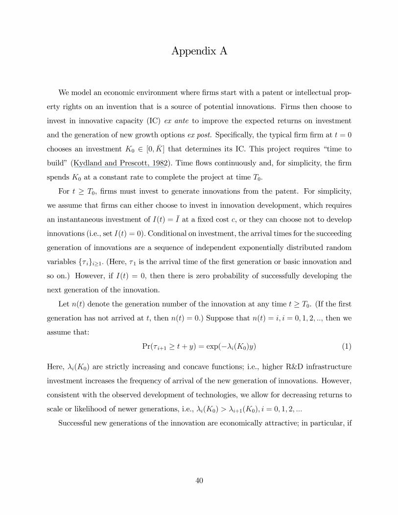
Appendix A
We model an economic environment where �rms start with a patent or intellectual prop-
erty rights on an invention that is a source of potential innovations. Firms then choose to
invest in innovative capacity (IC) ex ante to improve the expected returns on investment
and the generation of new growth options ex post. Speci�cally, the typical �rm �rm at t = 0
chooses an investment K0 2 [0; �K] that determines its IC. This project requires �time to
build�(Kydland and Prescott, 1982). Time �ows continuously and, for simplicity, the �rm
spends K0 at a constant rate to complete the project at time T0:
For t � T0, �rms must invest to generate innovations from the patent. For simplicity,
we assume that �rms can either choose to invest in innovation development, which requires
an instantaneous investment of I(t) = �I at a �xed cost c, or they can choose not to develop
innovations (i.e., set I(t) = 0): Conditional on investment, the arrival times for the succeeding
generation of innovations are a sequence of independent exponentially distributed random
variables f� igi�1: (Here, � 1 is the arrival time of the �rst generation or basic innovation and
so on.) However, if I(t) = 0; then there is zero probability of successfully developing the
next generation of the innovation.
Let n(t) denote the generation number of the innovation at any time t � T0. (If the �rst
generation has not arrived at t, then n(t) = 0:) Suppose that n(t) = i; i = 0; 1; 2; ::; then we
assume that:
Pr(� i+1 � t+ y) = exp(��i(K0)y) (1)
Here, �i(K0) are strictly increasing and concave functions; i.e., higher R&D infrastructure
investment increases the frequency of arrival of the new generation of innovations. However,
consistent with the observed development of technologies, we allow for decreasing returns to
scale or likelihood of newer generations, i.e., �i(K0) > �i+1(K0); i = 0; 1; 2; :::
Successful new generations of the innovation are economically attractive; in particular, if
40

n(t) = i; i = 1; 2::; then cash �ows Y (t) follow a geometric Brownian motion:
dY (t)
Y (t)= �i(K0)dt+ �dZ(t) (2)
�i(K0) = �(K0) +nXi=1
�i (3)
Here, �(K0) is a strictly increasing and concave function that is twice continuously di¤er-
entiable on (0; �K): Meanwhile, f�igi�1 are a sequence of independent non-negative random
variables with the cumulative distribution F (� j K0) such that F (� j K 00) strictly �rst order
stochastically dominates F (� j K") if K 0 > K": In sum, higher IC investment increases both
the likelihood of developing new generations of innovations and the expected growth of cash
�ows, conditional on the successful arrival of these innovations.
Turning to the risk characteristics, the cash �ow risk in (2) is systematic because we
assume that innovations in Z(t) are positively correlated with the innovations in the pricing
kernel that we will describe momentarily. However, the risk in the arrival date of the inno-
vations is a technical risk and is therefore taken to be idiosyncratic (Berk, Green and Naik,
2006).The existence of a pricing kernel, an assumption that requires only the nonexistence
of arbitrage, is described by the geometric Brownian motion where for t 2 [0;1) :
d�(t)
�(t)= �rdt+ �dW (t) (4)
Here, r is the instantaneous risk-free rate andW is a Brownian motion that has a correlation
of � > 0 with Z (cf. (2)). Then using standard arguments, the market price for this risk is:
! = ��� (5)
We can therefore represent project cash �ows through the risk-neutral pricing measure: If
n(t) = i; i = 1; 2:::; then
dY (t)
Y (t)= �i(K0)dt+ ~�dQ(t) (6)
�i(K0) � �i(K0)� ! (7)
41

where Q is the Brownian motion under the risk-neutral measure.
We let V (Y (t); n(t);K0) denote the equilibrium value of the �rm conditional on the cash
�ows Y (t) and the current innovation generation n(t), while taking as given the initial IC
investment K0. (If n(t) = i, we will use the notation V (Y (t); i;K0):) This �rm valuation
clearly depends on the optimal investment policy and is hence derived as follows. If the �rm
is subject to only cash �ow risk, i.e., I�(s) = 0, s � t, then standard arguments imply that
this valuation satis�es a continuous time version of the Gordon growth model,
V �(Y (t); i;K0) =Y (t)
r � �i(K0); i = 1; 2; :::; (8)
where �i(K0) is de�ned in (7). However, if the �rm is investing for development, i.e., i.e.,
I�(t) = �I; then it�s value function includes the options of generating the future genera-
tion of innovations. We will denote the market price of risk for the �rm�s cash �ows by
Rp�(Y (t); n(t);K0) (using Rp�(t;K0) for notational convenience). Then, conditional on con-
tinued development the value of the �rm and the risk-adjusted discount rate are determined
simultaneously and recursively by:
V +(Y (t); i;K0) = �i(K0)
24 1Zt
exp (�[Rp�(t;K0)(s� t) + �i(K0)s])�
fY (s)� c�I + V +(Y (s); i+ 1;K0)gds�
(9)
Rp�(Y (t); n(t);K0) =
�V +1 (Y (t); n(t);K0)Y (t)
V +(Y (t); n(t);K0)
�! (10)
And thus
V (Y (t); n(t);K0) = max(V�(Y (t); n(t);K0); V
+(Y (t); n(t);K0)� c�I) (11)
Note that by construction Rp�(t;K0) > ! as long as I�(t) = �I: To characterize the equilib-
rium evolution of risk-premia, we �rst characterize the �rm�s optimal innovation investment
policy. The next result shows that, under the assumption of strictly increasing wait times for
innovations, �rms optimally cease to invest in innovation development beyond some threshold
42

innovation generation, and this threshold level is conditional on Y (t) and K0:
Proposition 1 Conditional on (Y (t); K0), there exists i�(Y (t); K0) such that the optimal
investment policy for developing new generations of the innovation is I�(t) = �I if n(t) �
i�(Y (t); K0) but I�(t) = 0 otherwise. Moreover,i�(�; K0) is increasing in the IC investment
K0:
Proof: Because f�i(K0)g is a strictly decreasing sequence, it follows that for every
" > 0 there exists i"(K0) such that �j(K0) < " for every j > i"(K0). Therefore, the
expected arrival time for a successful innovation, namely, 1=�i(K0) exceeds 1=" for every
j > i"(K0), for any given " > 0:Now take any t with (Y (t); n(t)): Given that Rp� > !
and c > 0; it follows immediately from a comparison of (8) and (9) that there exists some
��(Y (t); K0) such that V �(Y (t); n(t);K0) = V+(Y (t); n(t);K0) if �i(K0) = ��(Y (t); K0) and
V �(Y (t); n(t);K0) > (<) V+(Y (t); n(t);K0) if �i(K0) < (>) ��(Y (t); K0): Hence,
i�(Y (t); K0) = min�j j �j(K0) < ��(Y (t); K0))
(12)
Moreover, i�(Y (t); K0) is incerasing in K0 because �i(K0) is strictly increasing for all i and
V +(Y (t); n(t);K0) is also strictly increasing in K0 in light of the assumption on �i(K0) (cf.
(3)).
It therefore follows from Proposition 1 that the evolution of the risk-premium satis�es:
Rp�(t;K0) =
8<:�V1(Y (t);n(t);K0)Y (t)V (Y (t);n(t);K0)
�! n(t) � i�(Y (t); K0)
! n(t) > i�(Y (t); K0)(13)
Hence, the change in the risk-premium subsequent to asset growth is:
�Rp�(t;K0)
� �I=
8<:dRp�(t;K0)
dtn(t) � i�(Y (t); K0)
!(1�Rp�(t;K0)) n(t) > i�(Y (t); K0)(14)
Note that the change in risk-premium is negative if n(t) = i�(Y (t); K0) for in this case
I�(t) = �I but E[ I�(s) = 0 j s > t]: Furthermore, Proposition 1 implies that:
Theorem 1 For each t and any given (Y (t); n(t)), �Rp�(t;K0
0)
� �I� �Rp�(t;K"0)
� �It if K 0
0 > K"0 :
43
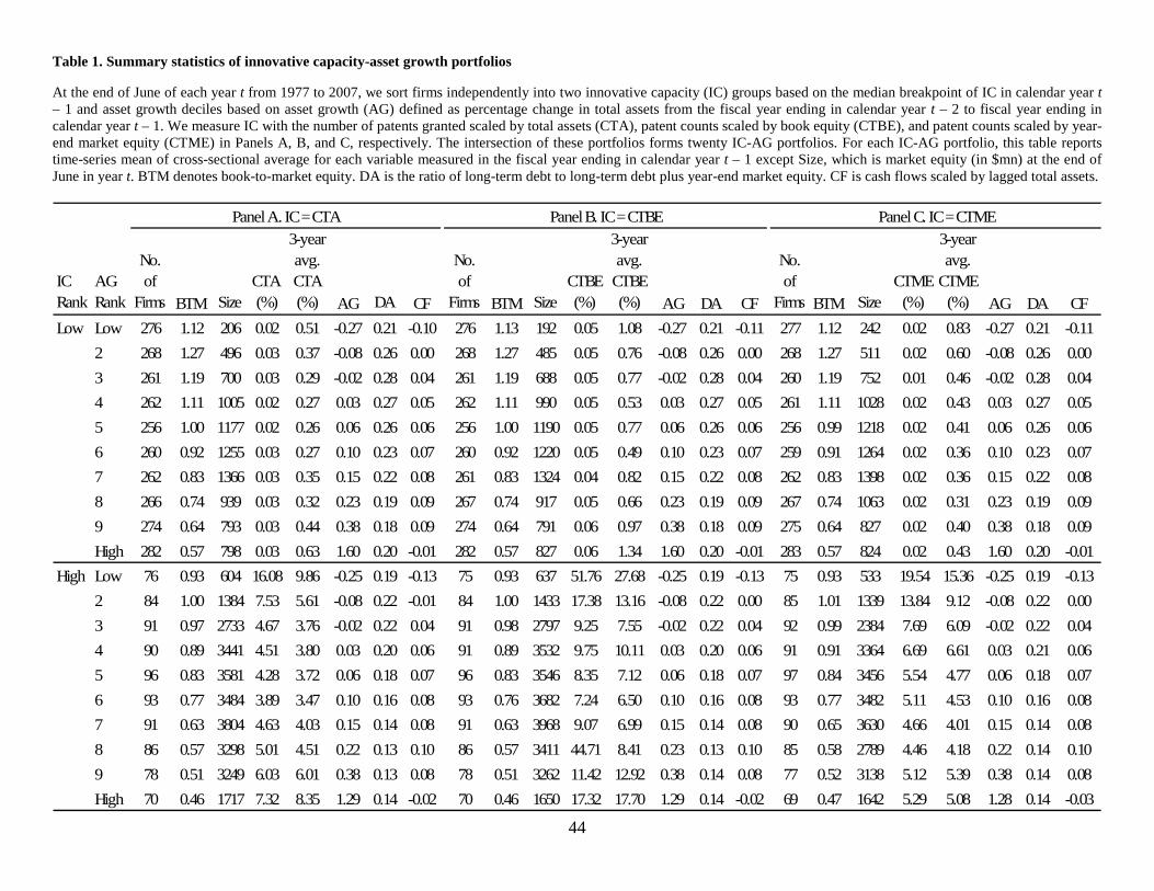
44
Table 1. Summary statistics of innovative capacity-asset growth portfolios
At the end of June of each year t from 1977 to 2007, we sort firms independently into two innovative capacity (IC) groups based on the median breakpoint of IC in calendar year t – 1 and asset growth deciles based on asset growth (AG) defined as percentage change in total assets from the fiscal year ending in calendar year t – 2 to fiscal year ending in calendar year t – 1. We measure IC with the number of patents granted scaled by total assets (CTA), patent counts scaled by book equity (CTBE), and patent counts scaled by year-end market equity (CTME) in Panels A, B, and C, respectively. The intersection of these portfolios forms twenty IC-AG portfolios. For each IC-AG portfolio, this table reports time-series mean of cross-sectional average for each variable measured in the fiscal year ending in calendar year t – 1 except Size, which is market equity (in $mn) at the end of June in year t. BTM denotes book-to-market equity. DA is the ratio of long-term debt to long-term debt plus year-end market equity. CF is cash flows scaled by lagged total assets.
IC Rank
AG Rank
No. of
Firms BTM SizeCTA (%)
3-year avg. CTA (%) AG DA CF
No. of
Firms BTM SizeCTBE (%)
3-year avg. CTBE (%) AG DA CF
No. of
Firms BTM SizeCTME (%)
3-year avg.
CTME (%) AG DA CF
Low Low 276 1.12 206 0.02 0.51 -0.27 0.21 -0.10 276 1.13 192 0.05 1.08 -0.27 0.21 -0.11 277 1.12 242 0.02 0.83 -0.27 0.21 -0.11
2 268 1.27 496 0.03 0.37 -0.08 0.26 0.00 268 1.27 485 0.05 0.76 -0.08 0.26 0.00 268 1.27 511 0.02 0.60 -0.08 0.26 0.00
3 261 1.19 700 0.03 0.29 -0.02 0.28 0.04 261 1.19 688 0.05 0.77 -0.02 0.28 0.04 260 1.19 752 0.01 0.46 -0.02 0.28 0.04
4 262 1.11 1005 0.02 0.27 0.03 0.27 0.05 262 1.11 990 0.05 0.53 0.03 0.27 0.05 261 1.11 1028 0.02 0.43 0.03 0.27 0.05
5 256 1.00 1177 0.02 0.26 0.06 0.26 0.06 256 1.00 1190 0.05 0.770.06 0.26 0.06 256 0.99 1218 0.02 0.41 0.06 0.26 0.06
6 260 0.92 1255 0.03 0.27 0.10 0.23 0.07 260 0.92 1220 0.05 0.490.10 0.23 0.07 259 0.91 1264 0.02 0.36 0.10 0.23 0.07
7 262 0.83 1366 0.03 0.35 0.15 0.22 0.08 261 0.83 1324 0.04 0.820.15 0.22 0.08 262 0.83 1398 0.02 0.36 0.15 0.22 0.08
8 266 0.74 939 0.03 0.32 0.23 0.19 0.09 267 0.74 917 0.05 0.66 0.23 0.19 0.09 267 0.74 1063 0.02 0.31 0.23 0.19 0.09
9 274 0.64 793 0.03 0.44 0.38 0.18 0.09 274 0.64 791 0.06 0.97 0.38 0.18 0.09 275 0.64 827 0.02 0.40 0.38 0.18 0.09
High 282 0.57 798 0.03 0.63 1.60 0.20 -0.01 282 0.57 827 0.06 1.34 1.60 0.20 -0.01 283 0.57 824 0.02 0.43 1.60 0.20 -0.01
High Low 76 0.93 604 16.08 9.86 -0.25 0.19 -0.13 75 0.93 637 51.76 27.68 -0.25 0.19 -0.13 75 0.93 533 19.54 15.36 -0.25 0.19 -0.13
2 84 1.00 1384 7.53 5.61 -0.08 0.22 -0.01 84 1.00 1433 17.38 13.16 -0.08 0.22 0.00 85 1.01 1339 13.84 9.12 -0.08 0.22 0.00
3 91 0.97 2733 4.67 3.76 -0.02 0.22 0.04 91 0.98 2797 9.25 7.55 -0.02 0.22 0.04 92 0.99 2384 7.69 6.09 -0.02 0.22 0.04
4 90 0.89 3441 4.51 3.80 0.03 0.20 0.06 91 0.89 3532 9.75 10.11 0.03 0.20 0.06 91 0.91 3364 6.69 6.61 0.03 0.21 0.06
5 96 0.83 3581 4.28 3.72 0.06 0.18 0.07 96 0.83 3546 8.35 7.12 0.06 0.18 0.07 97 0.84 3456 5.54 4.77 0.06 0.18 0.07
6 93 0.77 3484 3.89 3.47 0.10 0.16 0.08 93 0.76 3682 7.24 6.50 0.10 0.16 0.08 93 0.77 3482 5.11 4.53 0.10 0.16 0.08
7 91 0.63 3804 4.63 4.03 0.15 0.14 0.08 91 0.63 3968 9.07 6.99 0.15 0.14 0.08 90 0.65 3630 4.66 4.01 0.15 0.14 0.08
8 86 0.57 3298 5.01 4.51 0.22 0.13 0.10 86 0.57 3411 44.71 8.41 0.23 0.13 0.10 85 0.58 2789 4.46 4.18 0.22 0.14 0.10
9 78 0.51 3249 6.03 6.01 0.38 0.13 0.08 78 0.51 3262 11.42 12.920.38 0.14 0.08 77 0.52 3138 5.12 5.39 0.38 0.14 0.08
High 70 0.46 1717 7.32 8.35 1.29 0.14 -0.02 70 0.46 1650 17.32 17.70 1.29 0.14 -0.02 69 0.47 1642 5.29 5.08 1.28 0.14 -0.03
Panel A. IC = CTA Panel B. IC = CTBE Panel C. IC = CTME
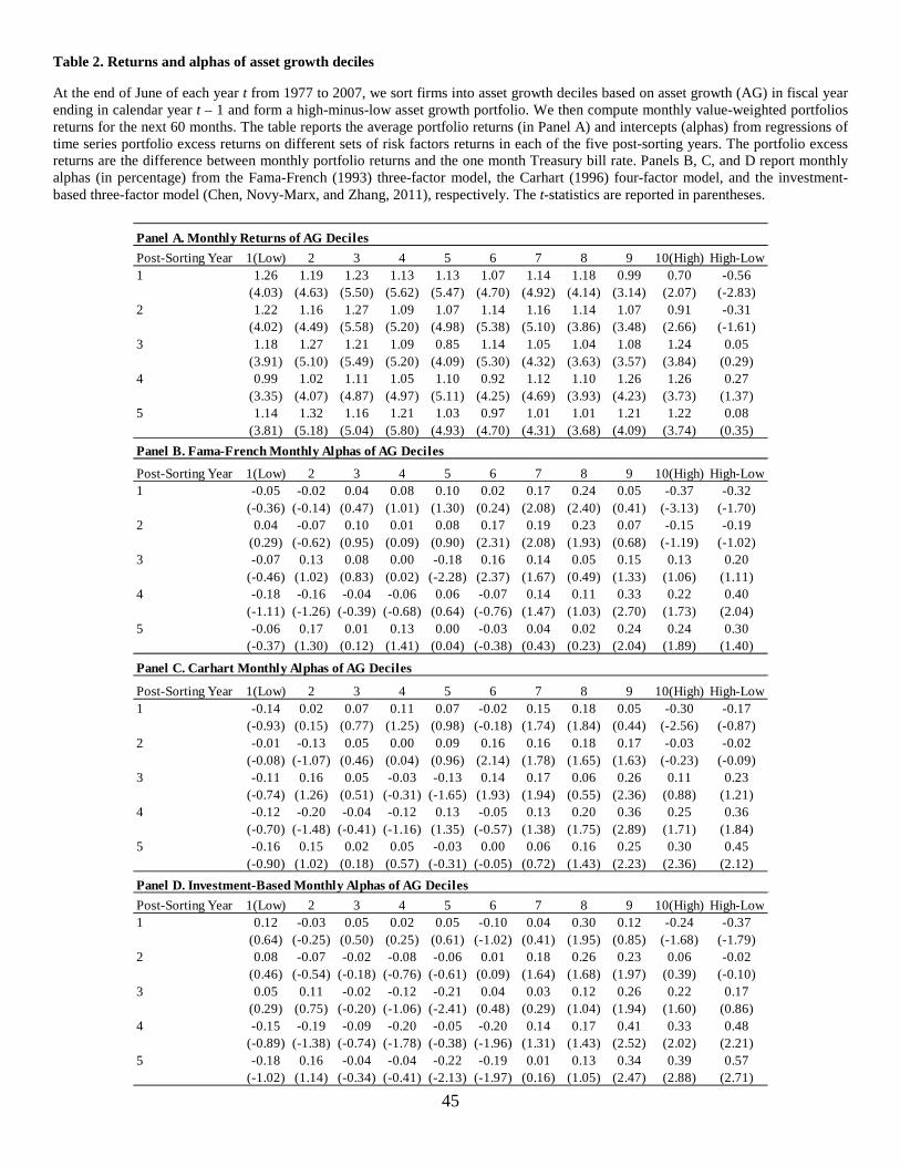
45
Table 2. Returns and alphas of asset growth deciles
At the end of June of each year t from 1977 to 2007, we sort firms into asset growth deciles based on asset growth (AG) in fiscal year ending in calendar year t – 1 and form a high-minus-low asset growth portfolio. We then compute monthly value-weighted portfolios returns for the next 60 months. The table reports the average portfolio returns (in Panel A) and intercepts (alphas) from regressions of time series portfolio excess returns on different sets of risk factors returns in each of the five post-sorting years. The portfolio excess returns are the difference between monthly portfolio returns and the one month Treasury bill rate. Panels B, C, and D report monthly alphas (in percentage) from the Fama-French (1993) three-factor model, the Carhart (1996) four-factor model, and the investment-based three-factor model (Chen, Novy-Marx, and Zhang, 2011), respectively. The t-statistics are reported in parentheses.
Panel A. Monthly Returns of AG Deciles
Post-Sorting Year 1(Low) 2 3 4 5 6 7 8 9 10(High) High-Low1 1.26 1.19 1.23 1.13 1.13 1.07 1.14 1.18 0.99 0.70 -0.56
(4.03) (4.63) (5.50) (5.62) (5.47) (4.70) (4.92) (4.14) (3.14) (2.07) (-2.83)2 1.22 1.16 1.27 1.09 1.07 1.14 1.16 1.14 1.07 0.91 -0.31
(4.02) (4.49) (5.58) (5.20) (4.98) (5.38) (5.10) (3.86) (3.48) (2.66) (-1.61)3 1.18 1.27 1.21 1.09 0.85 1.14 1.05 1.04 1.08 1.24 0.05
(3.91) (5.10) (5.49) (5.20) (4.09) (5.30) (4.32) (3.63) (3.57) (3.84) (0.29)4 0.99 1.02 1.11 1.05 1.10 0.92 1.12 1.10 1.26 1.26 0.27
(3.35) (4.07) (4.87) (4.97) (5.11) (4.25) (4.69) (3.93) (4.23) (3.73) (1.37)5 1.14 1.32 1.16 1.21 1.03 0.97 1.01 1.01 1.21 1.22 0.08
(3.81) (5.18) (5.04) (5.80) (4.93) (4.70) (4.31) (3.68) (4.09) (3.74) (0.35)
Panel B. Fama-French Monthly Alphas of AG Deciles
Post-Sorting Year 1(Low) 2 3 4 5 6 7 8 9 10(High) High-Low1 -0.05 -0.02 0.04 0.08 0.10 0.02 0.17 0.24 0.05 -0.37 -0.32
(-0.36) (-0.14) (0.47) (1.01) (1.30) (0.24) (2.08) (2.40) (0.41) (-3.13) (-1.70)2 0.04 -0.07 0.10 0.01 0.08 0.17 0.19 0.23 0.07 -0.15 -0.19
(0.29) (-0.62) (0.95) (0.09) (0.90) (2.31) (2.08) (1.93) (0.68) (-1.19) (-1.02)3 -0.07 0.13 0.08 0.00 -0.18 0.16 0.14 0.05 0.15 0.13 0.20
(-0.46) (1.02) (0.83) (0.02) (-2.28) (2.37) (1.67) (0.49) (1.33) (1.06) (1.11)4 -0.18 -0.16 -0.04 -0.06 0.06 -0.07 0.14 0.11 0.33 0.22 0.40
(-1.11) (-1.26) (-0.39) (-0.68) (0.64) (-0.76) (1.47) (1.03) (2.70) (1.73) (2.04)5 -0.06 0.17 0.01 0.13 0.00 -0.03 0.04 0.02 0.24 0.24 0.30
(-0.37) (1.30) (0.12) (1.41) (0.04) (-0.38) (0.43) (0.23) (2.04) (1.89) (1.40)
Panel C. Carhart Monthly Alphas of AG Deciles
Post-Sorting Year 1(Low) 2 3 4 5 6 7 8 9 10(High) High-Low1 -0.14 0.02 0.07 0.11 0.07 -0.02 0.15 0.18 0.05 -0.30 -0.17
(-0.93) (0.15) (0.77) (1.25) (0.98) (-0.18) (1.74) (1.84) (0.44) (-2.56) (-0.87)2 -0.01 -0.13 0.05 0.00 0.09 0.16 0.16 0.18 0.17 -0.03 -0.02
(-0.08) (-1.07) (0.46) (0.04) (0.96) (2.14) (1.78) (1.65) (1.63) (-0.23) (-0.09)3 -0.11 0.16 0.05 -0.03 -0.13 0.14 0.17 0.06 0.26 0.11 0.23
(-0.74) (1.26) (0.51) (-0.31) (-1.65) (1.93) (1.94) (0.55)(2.36) (0.88) (1.21)4 -0.12 -0.20 -0.04 -0.12 0.13 -0.05 0.13 0.20 0.36 0.25 0.36
(-0.70) (-1.48) (-0.41) (-1.16) (1.35) (-0.57) (1.38) (1.75) (2.89) (1.71) (1.84)5 -0.16 0.15 0.02 0.05 -0.03 0.00 0.06 0.16 0.25 0.30 0.45
(-0.90) (1.02) (0.18) (0.57) (-0.31) (-0.05) (0.72) (1.43)(2.23) (2.36) (2.12)
Panel D. Investment-Based Monthly Alphas of AG Deciles
Post-Sorting Year 1(Low) 2 3 4 5 6 7 8 9 10(High) High-Low1 0.12 -0.03 0.05 0.02 0.05 -0.10 0.04 0.30 0.12 -0.24 -0.37
(0.64) (-0.25) (0.50) (0.25) (0.61) (-1.02) (0.41) (1.95) (0.85) (-1.68) (-1.79)2 0.08 -0.07 -0.02 -0.08 -0.06 0.01 0.18 0.26 0.23 0.06 -0.02
(0.46) (-0.54) (-0.18) (-0.76) (-0.61) (0.09) (1.64) (1.68) (1.97) (0.39) (-0.10)3 0.05 0.11 -0.02 -0.12 -0.21 0.04 0.03 0.12 0.26 0.22 0.17
(0.29) (0.75) (-0.20) (-1.06) (-2.41) (0.48) (0.29) (1.04)(1.94) (1.60) (0.86)4 -0.15 -0.19 -0.09 -0.20 -0.05 -0.20 0.14 0.17 0.41 0.33 0.48
(-0.89) (-1.38) (-0.74) (-1.78) (-0.38) (-1.96) (1.31) (1.43) (2.52) (2.02) (2.21)5 -0.18 0.16 -0.04 -0.04 -0.22 -0.19 0.01 0.13 0.34 0.39 0.57
(-1.02) (1.14) (-0.34) (-0.41) (-2.13) (-1.97) (0.16) (1.05) (2.47) (2.88) (2.71)
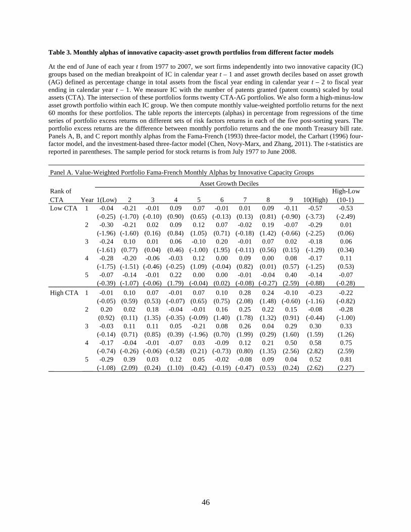
46
Table 3. Monthly alphas of innovative capacity-asset growth portfolios from different factor models
At the end of June of each year t from 1977 to 2007, we sort firms independently into two innovative capacity (IC) groups based on the median breakpoint of IC in calendar year t – 1 and asset growth deciles based on asset growth (AG) defined as percentage change in total assets from the fiscal year ending in calendar year t – 2 to fiscal year ending in calendar year t – 1. We measure IC with the number of patents granted (patent counts) scaled by total assets (CTA). The intersection of these portfolios forms twenty CTA-AG portfolios. We also form a high-minus-low asset growth portfolio within each IC group. We then compute monthly value-weighted portfolio returns for the next 60 months for these portfolios. The table reports the intercepts (alphas) in percentage from regressions of the time series of portfolio excess returns on different sets of risk factors returns in each of the five post-sorting years. The portfolio excess returns are the difference between monthly portfolio returns and the one month Treasury bill rate. Panels A, B, and C report monthly alphas from the Fama-French (1993) three-factor model, the Carhart (1996) four-factor model, and the investment-based three-factor model (Chen, Novy-Marx, and Zhang, 2011). The t-statistics are reported in parentheses. The sample period for stock returns is from July 1977 to June 2008.
Panel A. Value-Weighted Portfolio Fama-French Monthly Alphas by Innovative Capacity Groups
Rank of CTA Year 1(Low) 2 3 4 5 6 7 8 9 10(High)
High-Low (10-1)
Low CTA 1 -0.04 -0.21 -0.01 0.09 0.07 -0.01 0.01 0.09 -0.11 -0.57 -0.53(-0.25) (-1.70) (-0.10) (0.90) (0.65) (-0.13) (0.13) (0.81) (-0.90) (-3.73) (-2.49)
2 -0.30 -0.21 0.02 0.09 0.12 0.07 -0.02 0.19 -0.07 -0.29 0.01(-1.96) (-1.60) (0.16) (0.84) (1.05) (0.71) (-0.18) (1.42) (-0.66) (-2.25) (0.06)
3 -0.24 0.10 0.01 0.06 -0.10 0.20 -0.01 0.07 0.02 -0.18 0.06(-1.61) (0.77) (0.04) (0.46) (-1.00) (1.95) (-0.11) (0.56) (0.15) (-1.29) (0.34)
4 -0.28 -0.20 -0.06 -0.03 0.12 0.00 0.09 0.00 0.08 -0.17 0.11(-1.75) (-1.51) (-0.46) (-0.25) (1.09) (-0.04) (0.82) (0.01) (0.57) (-1.25) (0.53)
5 -0.07 -0.14 -0.01 0.22 0.00 0.00 -0.01 -0.04 0.40 -0.14 -0.07(-0.39) (-1.07) (-0.06) (1.79) (-0.04) (0.02) (-0.08) (-0.27) (2.59) (-0.88) (-0.28)
High CTA 1 -0.01 0.10 0.07 -0.01 0.07 0.10 0.28 0.24 -0.10 -0.23 -0.22(-0.05) (0.59) (0.53) (-0.07) (0.65) (0.75) (2.08) (1.48) (-0.60) (-1.16) (-0.82)
2 0.20 0.02 0.18 -0.04 -0.01 0.16 0.25 0.22 0.15 -0.08 -0.28(0.92) (0.11) (1.35) (-0.35) (-0.09) (1.40) (1.78) (1.32) (0.91) (-0.44) (-1.00)
3 -0.03 0.11 0.11 0.05 -0.21 0.08 0.26 0.04 0.29 0.30 0.33(-0.14) (0.71) (0.85) (0.39) (-1.96) (0.70) (1.99) (0.29) (1.60) (1.59) (1.26)
4 -0.17 -0.04 -0.01 -0.07 0.03 -0.09 0.12 0.21 0.50 0.58 0.75(-0.74) (-0.26) (-0.06) (-0.58) (0.21) (-0.73) (0.80) (1.35) (2.56) (2.82) (2.59)
5 -0.29 0.39 0.03 0.12 0.05 -0.02 -0.08 0.09 0.04 0.52 0.81(-1.08) (2.09) (0.24) (1.10) (0.42) (-0.19) (-0.47) (0.53) (0.24) (2.62) (2.27)
Asset Growth Deciles
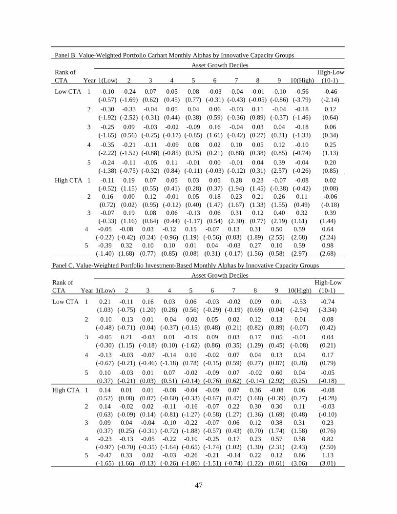
47
Panel B. Value-Weighted Portfolio Carhart Monthly Alphas by Innovative Capacity Groups
Rank of CTA Year 1(Low) 2 3 4 5 6 7 8 9 10(High)
High-Low (10-1)
Low CTA 1 -0.10 -0.24 0.07 0.05 0.08 -0.03 -0.04 -0.01 -0.10 -0.56 -0.46(-0.57) (-1.69) (0.62) (0.45) (0.77) (-0.31) (-0.43) (-0.05) (-0.86) (-3.79) (-2.14)
2 -0.30 -0.33 -0.04 0.05 0.04 0.06 -0.03 0.11 -0.04 -0.18 0.12(-1.92) (-2.52) (-0.31) (0.44) (0.38) (0.59) (-0.36) (0.89) (-0.37) (-1.46) (0.64)
3 -0.25 0.09 -0.03 -0.02 -0.09 0.16 -0.04 0.03 0.04 -0.18 0.06(-1.65) (0.56) (-0.25) (-0.17) (-0.85) (1.61) (-0.42) (0.27) (0.31) (-1.33) (0.34)
4 -0.35 -0.21 -0.11 -0.09 0.08 0.02 0.10 0.05 0.12 -0.10 0.25(-2.22) (-1.52) (-0.88) (-0.85) (0.75) (0.21) (0.88) (0.38) (0.85) (-0.74) (1.13)
5 -0.24 -0.11 -0.05 0.11 -0.01 0.00 -0.01 0.04 0.39 -0.04 0.20(-1.38) (-0.75) (-0.32) (0.84) (-0.11) (-0.03) (-0.12) (0.31) (2.57) (-0.26) (0.85)
High CTA 1 -0.11 0.19 0.07 0.05 0.03 0.05 0.28 0.23 -0.07 -0.08 0.02(-0.52) (1.15) (0.55) (0.41) (0.28) (0.37) (1.94) (1.45) (-0.38) (-0.42) (0.08)
2 0.16 0.00 0.12 -0.01 0.05 0.18 0.23 0.21 0.26 0.11 -0.06(0.72) (0.02) (0.95) (-0.12) (0.40) (1.47) (1.67) (1.33) (1.55) (0.49) (-0.18)
3 -0.07 0.19 0.08 0.06 -0.13 0.06 0.31 0.12 0.40 0.32 0.39(-0.33) (1.16) (0.64) (0.44) (-1.17) (0.54) (2.30) (0.77) (2.19) (1.61) (1.44)
4 -0.05 -0.08 0.03 -0.12 0.15 -0.07 0.13 0.31 0.50 0.59 0.64 (-0.22) (-0.42) (0.24) (-0.96) (1.19) (-0.56) (0.83) (1.89) (2.55) (2.68) (2.24)
5 -0.39 0.32 0.10 0.10 0.01 0.04 -0.03 0.27 0.10 0.59 0.98 (-1.40) (1.68) (0.77) (0.85) (0.08) (0.31) (-0.17) (1.56) (0.58) (2.97) (2.68)
Panel C. Value-Weighted Portfolio Investment-Based Monthly Alphas by Innovative Capacity Groups
Rank of CTA Year 1(Low) 2 3 4 5 6 7 8 9 10(High)
High-Low (10-1)
Low CTA 1 0.21 -0.11 0.16 0.03 0.06 -0.03 -0.02 0.09 0.01 -0.53 -0.74(1.03) (-0.75) (1.20) (0.28) (0.56) (-0.29) (-0.19) (0.69) (0.04) (-2.94) (-3.34)
2 -0.10 -0.13 0.01 -0.04 -0.02 0.05 0.02 0.12 0.13 -0.01 0.08 (-0.48) (-0.71) (0.04) (-0.37) (-0.15) (0.48) (0.21) (0.82) (0.89) (-0.07) (0.42)
3 -0.05 0.21 -0.03 0.01 -0.19 0.09 0.03 0.17 0.05 -0.01 0.04 (-0.30) (1.15) (-0.18) (0.10) (-1.62) (0.86) (0.35) (1.29) (0.45) (-0.08) (0.21)
4 -0.13 -0.03 -0.07 -0.14 0.10 -0.02 0.07 0.04 0.13 0.04 0.17 (-0.67) (-0.21) (-0.46) (-1.18) (0.78) (-0.15) (0.59) (0.27) (0.87) (0.28) (0.79)
5 0.10 -0.03 0.01 0.07 -0.02 -0.09 0.07 -0.02 0.60 0.04 -0.05(0.37) (-0.21) (0.03) (0.51) (-0.14) (-0.76) (0.62) (-0.14) (2.92) (0.25) (-0.18)
High CTA 1 0.14 0.01 0.01 -0.08 -0.04 -0.09 0.07 0.36 -0.08 0.06 -0.08(0.52) (0.08) (0.07) (-0.60) (-0.33) (-0.67) (0.47) (1.68) (-0.39) (0.27) (-0.28)
2 0.14 -0.02 0.02 -0.11 -0.16 -0.07 0.22 0.30 0.30 0.11 -0.03(0.63) (-0.09) (0.14) (-0.81) (-1.27) (-0.58) (1.27) (1.36) (1.69) (0.48) (-0.10)
3 0.09 0.04 -0.04 -0.10 -0.22 -0.07 0.06 0.12 0.38 0.31 0.23 (0.37) (0.25) (-0.31) (-0.72) (-1.88) (-0.57) (0.43) (0.70) (1.74) (1.58) (0.76)
4 -0.23 -0.13 -0.05 -0.22 -0.10 -0.25 0.17 0.23 0.57 0.58 0.82 (-0.97) (-0.70) (-0.35) (-1.64) (-0.65) (-1.74) (1.02) (1.30) (2.31) (2.43) (2.50)
5 -0.47 0.33 0.02 -0.03 -0.26 -0.21 -0.14 0.22 0.12 0.66 1.13 (-1.65) (1.66) (0.13) (-0.26) (-1.86) (-1.51) (-0.74) (1.22) (0.61) (3.06) (3.01)
Asset Growth Deciles
Asset Growth Deciles
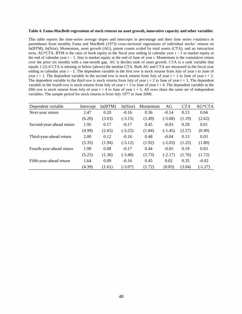
48
Table 4. Fama-MacBeth regressions of stock returns on asset growth, innovative capacity and other variables
This table reports the time-series average slopes and intercepts in percentage and their time series t-statistics in parentheses from monthly Fama and MacBeth (1973) cross-sectional regressions of individual stocks’ returns on ln(BTM), ln(Size), Momentum, asset growth (AG), patent counts scaled by total assets (CTA), and an interaction term, AG*CTA. BTM is the ratio of book equity in the fiscal year ending in calendar year t – 1 to market equity at the end of calendar year t – 1. Size is market equity at the end of June of year t. Momentum is the cumulative return over the prior six months with a one-month gap. AG is deciles rank of asset growth. CTA is a rank variable that equals 1 (2) if CTA is missing or below (above) the median CTA. Both AG and CTA are measured in the fiscal year ending in calendar year t – 1. The dependent variable in the first row is stock returns from July of year t to June of year t + 1. The dependent variable in the second row is stock returns from July of year t + 1 to June of year t + 2. The dependent variable in the third row is stock returns from July of year t + 2 to June of year t + 3. The dependent variable in the fourth row is stock returns from July of year t + 3 to June of year t + 4. The dependent variable in the fifth row is stock returns from July of year t + 4 to June of year t + 5. All rows share the same set of independent variables. The sample period for stock returns is from July 1977 to June 2008.
Dependent variable Intercept ln(BTM) ln(Size) Momentum AG CTA AG*CTANext-year return 2.47 0.20 -0.16 0.36 -0.14 0.13 0.04
(6.20) (3.03) (-3.15) (1.49) (-5.68) (1.19) (2.62) Second-year-ahead return 1.95 0.17 -0.17 0.45 -0.03 0.29 0.01
(4.99) (2.65) (-3.25) (1.84) (-1.45) (2.57) (0.49) Third-year-ahead return 2.00 0.12 -0.16 0.48 -0.04 0.13 0.03
(5.35) (1.94) (-3.12) (1.92) (-2.03) (1.25) (1.80) Fourth-year-ahead return 1.99 0.08 -0.17 0.44 -0.05 0.19 0.03
(5.25) (1.36) (-3.40) (1.73) (-2.17) (1.76) (1.72) Fifth-year-ahead return 1.64 0.09 -0.16 0.45 0.02 0.35 -0.02
(4.39) (1.61) (-3.07) (1.72) (0.83) (3.04) (-1.27)
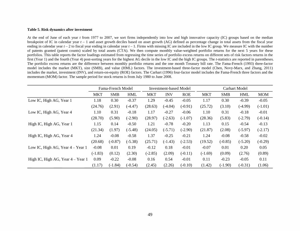
49
Table 5. Risk dynamics after investment
At the end of June of each year t from 1977 to 2007, we sort firms independently into low and high innovative capacity (IC) groups based on the median breakpoint of IC in calendar year t – 1 and asset growth deciles based on asset growth (AG) defined as percentage change in total assets from the fiscal year ending in calendar year t – 2 to fiscal year ending in calendar year t – 1. Firms with missing IC are included in the low IC group. We measure IC with the number of patents granted (patent counts) scaled by total assets (CTA). We then compute monthly value-weighted portfolio returns for the next 5 years for these portfolios. This table reports the factor loadings estimated from regressing the time series of portfolio excess returns on different sets of risk factors returns in the first (Year 1) and the fourth (Year 4) post-sorting years for the highest AG decile in the low IC and the high IC groups. The t-statistics are reported in parentheses. The portfolio excess returns are the difference between monthly portfolio returns and the one month Treasury bill rate. The Fama-French (1993) three-factor model includes the market (MKT), size (SMB), and value (HML) factors. The investment-based three-factor model (Chen, Novy-Marx, and Zhang, 2011) includes the market, investment (INV), and return-on-equity (ROE) factors. The Carhart (1996) four-factor model includes the Fama-French three factors and the momentum (MOM) factor. The sample period for stock returns is from July 1980 to June 2008.
MKT SMB HML MKT INV ROE MKT SMB HML MOM
Low IC, High AG, Year 1 1.18 0.30 -0.37 1.29 -0.45 -0.05 1.17 0.30 -0.39 -0.05
(24.76) (2.91) (-4.47) (28.63) (-4.04) (-0.91) (25.72) (3.10) (-4.99) (-1.01)
Low IC, High AG, Year 4 1.10 0.31 -0.18 1.17 -0.27 -0.06 1.10 0.31 -0.18 -0.01
(28.70) (5.90) (-2.90) (28.97) (-2.63) (-1.07) (28.36) (5.83) (-2.79) (-0.14)
High IC, High AG, Year 1 1.15 0.14 -0.50 1.21 -0.78 -0.20 1.13 0.15 -0.54 -0.13
(21.34) (1.97) (-5.48) (24.05) (-5.71) (-2.90) (21.87) (2.08) (-5.97) (-2.17)
High IC, High AG, Year 4 1.24 -0.08 -0.58 1.37 -0.25 -0.21 1.24 -0.08 -0.58 -0.02
(20.68) (-0.87) (-5.38) (25.71) (-1.43) (-2.53) (19.52) (-0.85) (-5.20) (-0.29)
Low IC, High AG, Year 4 – Year 1 -0.08 0.01 0.19 -0.12 0.18 -0.01 -0.07 0.01 0.20 0.05
(-1.83) (0.12) (2.30) (-2.85) (2.09) (-0.11) (-1.69) (0.09) (2.76) (0.89)
High IC, High AG, Year 4 – Year 1 0.09 -0.22 -0.08 0.16 0.54 -0.01 0.11 -0.23 -0.05 0.11
(1.17) (-1.84) (-0.54) (2.45) (2.26) (-0.10) (1.42) (-1.90) (-0.31) (1.06)
Fama-French Model Investment-based Model Carhart Model
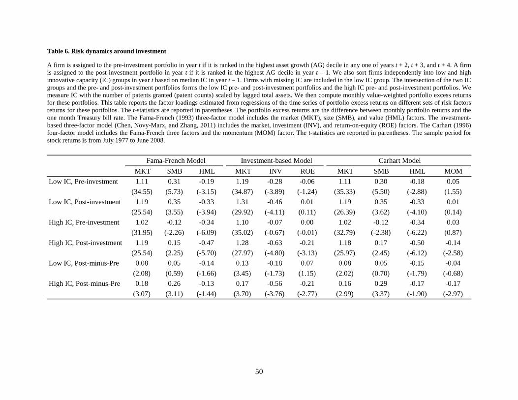
50
Table 6. Risk dynamics around investment
A firm is assigned to the pre-investment portfolio in year t if it is ranked in the highest asset growth (AG) decile in any one of years t + 2, t + 3, and t + 4. A firm is assigned to the post-investment portfolio in year t if it is ranked in the highest AG decile in year t – 1. We also sort firms independently into low and high innovative capacity (IC) groups in year t based on median IC in year t – 1. Firms with missing IC are included in the low IC group. The intersection of the two IC groups and the pre- and post-investment portfolios forms the low IC pre- and post-investment portfolios and the high IC pre- and post-investment portfolios. We measure IC with the number of patents granted (patent counts) scaled by lagged total assets. We then compute monthly value-weighted portfolio excess returns for these portfolios. This table reports the factor loadings estimated from regressions of the time series of portfolio excess returns on different sets of risk factors returns for these portfolios. The t-statistics are reported in parentheses. The portfolio excess returns are the difference between monthly portfolio returns and the one month Treasury bill rate. The Fama-French (1993) three-factor model includes the market (MKT), size (SMB), and value (HML) factors. The investment-based three-factor model (Chen, Novy-Marx, and Zhang, 2011) includes the market, investment (INV), and return-on-equity (ROE) factors. The Carhart (1996) four-factor model includes the Fama-French three factors and the momentum (MOM) factor. The t-statistics are reported in parentheses. The sample period for stock returns is from July 1977 to June 2008.
MKT SMB HML MKT INV ROE MKT SMB HML MOM
Low IC, Pre-investment 1.11 0.31 -0.19 1.19 -0.28 -0.06 1.11 0.30 -0.18 0.05
(34.55) (5.73) (-3.15) (34.87) (-3.89) (-1.24) (35.33) (5.50) (-2.88) (1.55)
Low IC, Post-investment 1.19 0.35 -0.33 1.31 -0.46 0.01 1.19 0.35 -0.33 0.01
(25.54) (3.55) (-3.94) (29.92) (-4.11) (0.11) (26.39) (3.62) (-4.10) (0.14)
High IC, Pre-investment 1.02 -0.12 -0.34 1.10 -0.07 0.00 1.02 -0.12 -0.34 0.03
(31.95) (-2.26) (-6.09) (35.02) (-0.67) (-0.01) (32.79) (-2.38) (-6.22) (0.87)
High IC, Post-investment 1.19 0.15 -0.47 1.28 -0.63 -0.21 1.18 0.17 -0.50 -0.14
(25.54) (2.25) (-5.70) (27.97) (-4.80) (-3.13) (25.97) (2.45) (-6.12) (-2.58)
Low IC, Post-minus-Pre 0.08 0.05 -0.14 0.13 -0.18 0.07 0.08 0.05 -0.15 -0.04
(2.08) (0.59) (-1.66) (3.45) (-1.73) (1.15) (2.02) (0.70) (-1.79) (-0.68)
High IC, Post-minus-Pre 0.18 0.26 -0.13 0.17 -0.56 -0.21 0.16 0.29 -0.17 -0.17
(3.07) (3.11) (-1.44) (3.70) (-3.76) (-2.77) (2.99) (3.37) (-1.90) (-2.97)
Fama-French Model Investment-based Model Carhart Model
Top Related
Copyright © 2022 FDOKUMEN

