


Bahasa
Halaman
Hukum

POLITECNICO DI TORINO
MASTER’S DEGREE IN MECHATRONICENGINEERING
DEPARTMENT OF CONTROL AND COMPUTER ENGINEERING
MASTER’S DEGREE THESIS
Dynamic modeling of induction motors indeveloping tool for automotive
applications
Academic Supervisors:Prof. Alberto TENCONI
Prof. Silvio VASCHETTO
Ing. Ornella STISCIA
Company Supervisor:Dott. Giulio BOCCARDO
Candidate:Roberta LE FOSSE
A.Y. 2020/2021


"Our greatest weakness lies in giving up. The most certainway to succeed is always to try just one more time"
Thomas Edison

AbstractThe current electrification processes involving hybrid and electric vehicles require increasinglyaccurate tools to evaluate electric powertrain performance and reliability. In this context, thevirtualization of electric powertrain components needs to be performed. In this way, severalanalyses like energetic assessments can be performed without using physical components,saving costs and development times.
Among the virtualization methods, an ever more used simulation approach in automotiveindustries consists of the Hardware in the Loop (HIL). The HIL is a real-time simulationmethod that allows testing one or more real components of an electric powertrain withoutthe need for the other hardware components usually connected to it. For example, usingHIL makes it possible to test a motor control unit without connecting to it a real electronicpower converter or even an electrical machine. Hence, the main advantages of this simulationapproach are evident.
In this thesis, the HIL simulation approach is used to virtualize the electric machine ofa hybrid or electric powertrain. The simulation hardware consists of the dSPACE rapidprototyping board and using the library “XSG Electric Library” provided by dSPACE. Thework activity has been developed through the cooperation between Politecnico di Torino andPOWERTECH ENGINEERING S.r.l., a consulting company specialized in simulation anddevelopment of conventional powertrains, and more recently, hybrid and electric ones, too.
This thesis focuses on the validation and analysis of dynamic models for electrical machinesusing dSPACE. The considered components are the Induction Machine (IM) and, like side-activity, the Voltage Source Inverter (VSI). Concerning the IM, it has been modeled usingthe following reference frames: phase values time-domain (abc), stationary axes (αβ0),and rotating rotor flux (dq) axes. The aim of the work was the comparison of the models,so the iron losses and the magnetic saturation were neglected. Also, to handle and figureout the models, their analysis and validation have been performed in the Matlab/Simulinkenvironment. Thus, comparing the obtained responses with those provided by dSPACE.Finally, the VSI has been modelled considering its average behaviour, without consideringthe Pulse Width Modulation (PWM), and so making the models’ simulations faster to beperformed.
A real IM has been tested on a dedicated test rig in Politecnico di Torino’s laboratories to geta preliminary validation of the proposed models. The IM parameters have been obtained byperforming the standard no-load and locked rotor tests.

Contents
Abstract
List of Figures iii
List of Tables v
1 Introduction 11.1 Hardware in the Loop . . . . . . . . . . . . . . . . . . . . . . . . . . . . . 31.2 Thesis goal . . . . . . . . . . . . . . . . . . . . . . . . . . . . . . . . . . 4
2 Induction motor modeling 52.1 Squirrel cage induction motor . . . . . . . . . . . . . . . . . . . . . . . . 52.2 Mathematical model in phase variable domain . . . . . . . . . . . . . . . . 62.3 Mathematical model in stationary reference frame (αβ ) . . . . . . . . . . . 102.4 Mathematical model in rotating reference frame (dq) . . . . . . . . . . . . 132.5 Equivalent circuit in rotating coordinates . . . . . . . . . . . . . . . . . . . 162.6 Induction machine model . . . . . . . . . . . . . . . . . . . . . . . . . . . 202.7 Test of induction machine . . . . . . . . . . . . . . . . . . . . . . . . . . . 21
2.7.1 No-load test . . . . . . . . . . . . . . . . . . . . . . . . . . . . . . 212.7.2 Locked-rotor test . . . . . . . . . . . . . . . . . . . . . . . . . . . 23
2.8 Mathematical model of Voltage Source Inverter (VSI) . . . . . . . . . . . . 24
3 Simulink and dSPACE comparisons in stationary reference frame (αβ ) 293.1 Overview on Simulink model . . . . . . . . . . . . . . . . . . . . . . . . . 303.2 dSPACE general description . . . . . . . . . . . . . . . . . . . . . . . . . 323.3 Overview on dSPACE model . . . . . . . . . . . . . . . . . . . . . . . . . 353.4 Simulink and dSPACE results comparison . . . . . . . . . . . . . . . . . . 41
3.4.1 Simulation: 220V - 50Hz . . . . . . . . . . . . . . . . . . . . . . . 423.4.2 Simulation: 380V - 40Hz . . . . . . . . . . . . . . . . . . . . . . . 47
4 Real-time simulations 524.1 FPGA build process . . . . . . . . . . . . . . . . . . . . . . . . . . . . . . 53
i
4.2 Comparison between Simulink and dSPACE real-time simulations (αβ ) referenceframe . . . . . . . . . . . . . . . . . . . . . . . . . . . . . . . . . . . . . 54
4.3 Comparison between Simulink and dSPACE real-time simulations (dq) referenceframe . . . . . . . . . . . . . . . . . . . . . . . . . . . . . . . . . . . . . 57
5 Validation of the dinamic model 655.1 Model of the system . . . . . . . . . . . . . . . . . . . . . . . . . . . . . . 655.2 Calculation of machine parameters . . . . . . . . . . . . . . . . . . . . . . 675.3 Validation of experimental data . . . . . . . . . . . . . . . . . . . . . . . . 70
6 Conclusions and next steps 75
Bibliography 78
List of Figures
1.1 POWERTECH Engineering. . . . . . . . . . . . . . . . . . . . . . . . . . 21.2 Workstation. . . . . . . . . . . . . . . . . . . . . . . . . . . . . . . . . . . 21.3 SCALEXIO LabBox and Oscilloscope. . . . . . . . . . . . . . . . . . . . 3
2.1 Structure of Induction machine (Rik De Doncker, 2011) [3]. . . . . . . . . 62.2 Winding distribution of three-phase Induction Motor. . . . . . . . . . . . . 82.3 Machine model in stationary reference frame (αβ ). . . . . . . . . . . . . . 102.4 Equivalent circuit in the (dq) rotor reference frame. . . . . . . . . . . . . . 172.5 Rotor flux vector in (dq) coordinates. . . . . . . . . . . . . . . . . . . . . . 182.6 Stator and Rotor current vectors in (dq) coordinates (steady-state conditions). 192.7 Equivalent circuit in (dq) reference frame. . . . . . . . . . . . . . . . . . . 202.8 Equivalent circuit of the no-load test. . . . . . . . . . . . . . . . . . . . . . 222.9 Equivalent circuit of the no-load test. . . . . . . . . . . . . . . . . . . . . . 232.10 Three-phase inverter. . . . . . . . . . . . . . . . . . . . . . . . . . . . . . 242.11 Voltage vectors. . . . . . . . . . . . . . . . . . . . . . . . . . . . . . . . . 262.12 Voltage Source Inverter. . . . . . . . . . . . . . . . . . . . . . . . . . . . . 272.13 Modulation indices. . . . . . . . . . . . . . . . . . . . . . . . . . . . . . . 282.14 Voltage. . . . . . . . . . . . . . . . . . . . . . . . . . . . . . . . . . . . . 28
3.1 Scheme of the model. . . . . . . . . . . . . . . . . . . . . . . . . . . . . . 303.2 Simulink (αβ ) model. . . . . . . . . . . . . . . . . . . . . . . . . . . . . 313.3 Induction Motor Simulink (αβ ) model. . . . . . . . . . . . . . . . . . . . 313.4 Mechanic Simulink model. . . . . . . . . . . . . . . . . . . . . . . . . . . 323.5 Single-Model Approach [7]. . . . . . . . . . . . . . . . . . . . . . . . . . 333.6 Double-Model Approach [7]. . . . . . . . . . . . . . . . . . . . . . . . . . 333.7 DS6602 FPGA Base Board [8]. . . . . . . . . . . . . . . . . . . . . . . . . 343.8 SCALEXIO LabBox [7]. . . . . . . . . . . . . . . . . . . . . . . . . . . . 353.9 dSPACE processor interface. . . . . . . . . . . . . . . . . . . . . . . . . . 363.10 dSPACE FPGA interface. . . . . . . . . . . . . . . . . . . . . . . . . . . . 363.11 Buffer2Register and Register2Buffer blocks [9]. . . . . . . . . . . . . . . . 373.12 Processor part and FPGA part direct communication [9]. . . . . . . . . . . 383.13 SCIM Machine block FPGA interface. . . . . . . . . . . . . . . . . . . . . 393.14 Mechanic block FPGA interface. . . . . . . . . . . . . . . . . . . . . . . . 403.15 Stator Currents ia - 220V-50Hz. . . . . . . . . . . . . . . . . . . . . . . . 443.16 Electrical and Mechanical Powers - 220V-50Hz. . . . . . . . . . . . . . . . 443.17 Motor Torque - 220V-50Hz - 220V-50Hz. . . . . . . . . . . . . . . . . . . 453.18 Rotor Speed - 220V-50Hz. . . . . . . . . . . . . . . . . . . . . . . . . . . 453.19 Rotor Flux - 220V-50Hz. . . . . . . . . . . . . . . . . . . . . . . . . . . . 46
iii
3.20 Stator Flux - 220V-50Hz. . . . . . . . . . . . . . . . . . . . . . . . . . . . 463.21 Stator Currents ia - 380V-40Hz. . . . . . . . . . . . . . . . . . . . . . . . 483.22 Electrical and Mechanical Powers - 380V-40Hz. . . . . . . . . . . . . . . . 493.23 Motor Torque - 380V-40Hz. . . . . . . . . . . . . . . . . . . . . . . . . . 493.24 Rotor Speed - 380V-40Hz. . . . . . . . . . . . . . . . . . . . . . . . . . . 503.25 Rotor Flux - 380V-40Hz. . . . . . . . . . . . . . . . . . . . . . . . . . . . 503.26 Stator Flux - 380V-40Hz. . . . . . . . . . . . . . . . . . . . . . . . . . . . 51
4.1 FPGA Setup and System Generator. . . . . . . . . . . . . . . . . . . . . . 534.2 ConfigurationDesk interface. . . . . . . . . . . . . . . . . . . . . . . . . . 534.3 ControlDesk interface. . . . . . . . . . . . . . . . . . . . . . . . . . . . . 544.4 FPGA model comment out. . . . . . . . . . . . . . . . . . . . . . . . . . . 554.5 Stator current Simulink and dSPACE real-time. . . . . . . . . . . . . . . . 564.6 Rotor speed Simulink and dSPACE real-time. . . . . . . . . . . . . . . . . 564.7 Simulink (dq) model. . . . . . . . . . . . . . . . . . . . . . . . . . . . . . 574.8 Induction Motor Simulink (dq) model. . . . . . . . . . . . . . . . . . . . . 584.9 Calculate of Mechanical Power dSPACE (dq) model. . . . . . . . . . . . . 604.10 Zoom on the blocks to calculate of Mechanical Power dSPACE (dq) model. 614.11 Mechanical Power dSPACE (dq) model block. . . . . . . . . . . . . . . . . 614.12 Stator current Simulink and dSPACE real-time (dq) model. . . . . . . . . . 624.13 Stator current d-axis Simulink and dSPACE real-time (dq) model. . . . . . 634.14 Stator current q-axis Simulink and dSPACE real-time (dq) model. . . . . . 634.15 Rotor Speed Simulink and dSPACE real-time (dq) model. . . . . . . . . . 64
5.1 HBM and Single-three phase power source 40kVA. . . . . . . . . . . . . . 665.2 Induction motor and Current transducers. . . . . . . . . . . . . . . . . . . 665.3 Schematic representation of the test bench. . . . . . . . . . . . . . . . . . . 675.4 Instrumentations used during the no-load and locked rotor tests. . . . . . . 685.5 Stator Current 30V - 50Hz with ramp acceleration. . . . . . . . . . . . . . 715.6 Zoom starting transient - Stator current 30V - 50Hz with ramp acceleration. 725.7 Zoom steady state - Stator current 30V - 50Hz with ramp acceleration. . . . 725.8 Stator Current 30V - 50Hz with step acceleration . . . . . . . . . . . . . . 735.9 Zoom starting transient - Stator current 30V - 50Hz with step acceleration. . 735.10 Zoom steady state - Stator current 30V - 50Hz with step acceleration. . . . 74
List of Tables
3.1 Characteristics of the motor. . . . . . . . . . . . . . . . . . . . . . . . . . 413.2 Parameters of the Induction Motor. . . . . . . . . . . . . . . . . . . . . . . 413.3 Parameters of the Mechanic block. . . . . . . . . . . . . . . . . . . . . . . 423.4 Steady-state Simulink simulation - 220V-50Hz. . . . . . . . . . . . . . . . 433.5 Steady-state dSPACE simulation - 220V-50Hz. . . . . . . . . . . . . . . . 433.6 Steady-state Simulink simulation - 380V-40Hz. . . . . . . . . . . . . . . . 473.7 Steady-state dSPACE simulation - 380V-40Hz. . . . . . . . . . . . . . . . 48
5.1 Data of the IM. . . . . . . . . . . . . . . . . . . . . . . . . . . . . . . . . 685.2 No-load test results. . . . . . . . . . . . . . . . . . . . . . . . . . . . . . . 695.3 Locked-rotor test results. . . . . . . . . . . . . . . . . . . . . . . . . . . . 695.4 Parameters of the Induction Motor FIMET HMA160L4. . . . . . . . . . . 705.5 Validation of experimental data. . . . . . . . . . . . . . . . . . . . . . . . 70
v
Chapter 1
Introduction
Electrification of transport has become an important argument in recent years. Due to
the emission of CO2, electric and hybrid vehicles are the most common challenges of the
current period. For this reason, electrical machines will play an important role to produce
zero-emissions vehicles [1].
In the industrial sector the three-phase Induction Motor (IM) is the most used machine, in
fact, it accounts for 85% of all motors [2]. IM is characterized by low cost, weight and it is
a very robust motor with respect to the DC motor.
To simulate electric motors are not used micro-controllers like CPU, but there is a need to
use advanced technologies like FPGA.
Field Programmable Gate Arrays (FPGA) is a reprogrammable silicon chips and it can be
configurated in a specific way and thanks to this the execution time is reduced.
It has interconnections between logic gates that are combined to form a combinatorial logic
block.
FPGA works with a very small time-step and in this work, the FPGA used works with a
time-step of 8 ·10−9 seconds.
FPGA can be used to simulate in real time (1 simulated second = 1 real second) complex
systems with very low timescale such as the electromagnetic phenomena that occur in electronic
and electric power motors. This allows to implement the Hardware in the Loop (HIL)
simulation.
1
CHAPTER 1. INTRODUCTION
Instead, standard Simulink models of electrical machines, which run on standard CPU, are
not in real-time (1 simulated second > 1 real second) and can not be used for HIL.
Real-time simulations were carried out in POWERTECH Engineering (PWT), an independent
consulting company in the field of CFD-3D, 1D and XIL simulation. POWERTECH Engineering
is a leading company in powertrain simulation engineering services. For several years, PWT
has been investing in HIL simulations for validation, testing and virtual calibration of the
ECU. To do this, it has equipped the dSPACE toolchain, strongly used for this type of
simulations.
Figure 1.1: POWERTECH Engineering.
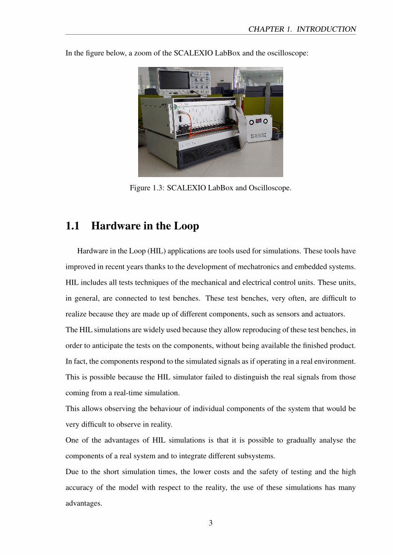
Thanks to the innovative workstation in PWT, it was possible to implement and validate
the Squirrel cage Induction motor model.
The workstation is as follows:
Figure 1.2: Workstation.
As is possible to see, on the left is the SCALEXIO LabBox and on the right the oscilloscope.
2
CHAPTER 1. INTRODUCTION
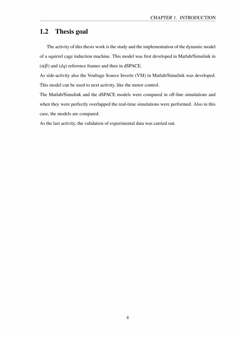
In the figure below, a zoom of the SCALEXIO LabBox and the oscilloscope:
Figure 1.3: SCALEXIO LabBox and Oscilloscope.
1.1 Hardware in the Loop
Hardware in the Loop (HIL) applications are tools used for simulations. These tools have
improved in recent years thanks to the development of mechatronics and embedded systems.
HIL includes all tests techniques of the mechanical and electrical control units. These units,
in general, are connected to test benches. These test benches, very often, are difficult to
realize because they are made up of different components, such as sensors and actuators.
The HIL simulations are widely used because they allow reproducing of these test benches, in
order to anticipate the tests on the components, without being available the finished product.
In fact, the components respond to the simulated signals as if operating in a real environment.
This is possible because the HIL simulator failed to distinguish the real signals from those
coming from a real-time simulation.
This allows observing the behaviour of individual components of the system that would be
very difficult to observe in reality.
One of the advantages of HIL simulations is that it is possible to gradually analyse the
components of a real system and to integrate different subsystems.
Due to the short simulation times, the lower costs and the safety of testing and the high
accuracy of the model with respect to the reality, the use of these simulations has many
advantages.
3
CHAPTER 1. INTRODUCTION
1.2 Thesis goal
The activity of this thesis work is the study and the implementation of the dynamic model
of a squirrel cage induction machine. This model was first developed in Matlab/Simulink in
(αβ ) and (dq) reference frames and then in dSPACE.
As side-activity also the Voultage Source Inverte (VSI) in Matlab/Simulink was developed.
This model can be used to next activity, like the motor control.
The Matlab/Simulink and the dSPACE models were compared in off-line simulations and
when they were perfectly overlapped the real-time simulations were performed. Also in this
case, the models are compared.
As the last activity, the validation of experimental data was carried out.
4
Chapter 2
Induction motor modeling
This chapter describes the model of the Induction Motor (IM), called also “asynchronous
machine”. The IM is the most used electric machine. It works directly connected to the
electric network, for this reason, it is low expensive, very reliable and robust.
The mathematical model of the IM will be explained. In particular, to simplify the model
the two-phase model will be obtained. We will see two reference frames:
• the fixed stator reference frame (αβ );
• the rotating synchronous reference frame with the rotor flux (dq).
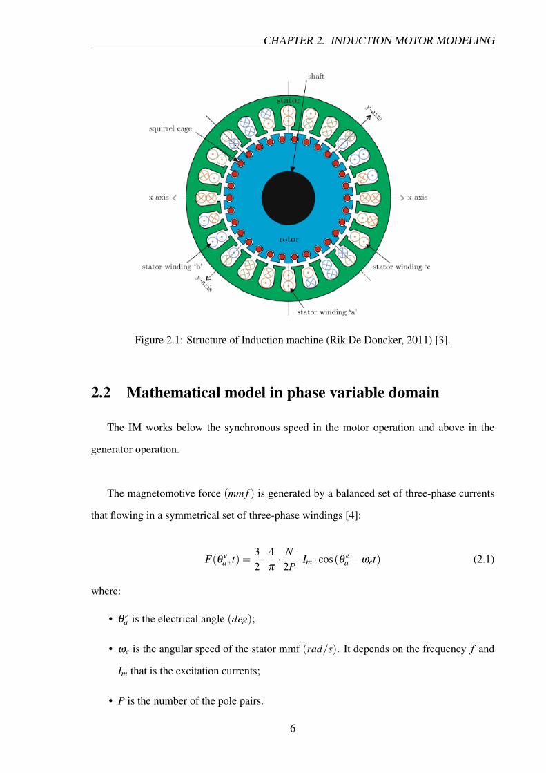
2.1 Squirrel cage induction motor
In the Figure is shown the structure of the squirrel cage induction motor (SCIM). The
SCIM is made by a conductors these are colour in red. These are short-circuited by a
conductive ring at both ends and has 4 poles. The stator circuit generates a magnetic field that
penetrates the rotor circuit. The purpose of this magnetic field is to create an asynchronous
speed respet at the stator speed at the alternating currents performed. These currents and
stator field will generate the torque of the motor.
5
CHAPTER 2. INDUCTION MOTOR MODELING
Figure 2.1: Structure of Induction machine (Rik De Doncker, 2011) [3].
2.2 Mathematical model in phase variable domain
The IM works below the synchronous speed in the motor operation and above in the
generator operation.
The magnetomotive force (mm f ) is generated by a balanced set of three-phase currents
that flowing in a symmetrical set of three-phase windings [4]:
F(θ ea , t) =
32· 4
π· N
2P· Im · cos(θ e
a −ωet) (2.1)
where:
• θ ea is the electrical angle (deg);
• ωe is the angular speed of the stator mmf (rad/s). It depends on the frequency f and
Im that is the excitation currents;
• P is the number of the pole pairs.
6
CHAPTER 2. INDUCTION MOTOR MODELING
In the next equation, we can see the synchronous speed (rad/s):
ωs =ωe
P(2.2)
To evaluate the revolution per minute (rpm):
ns =60 · f
P(2.3)
When the rotor is rotating there is also the rotor speed (rad/s). Between synchronous speed
and rotor speed, there is a slip. It is defined in the following way:
ωslip = ωs−ωr (2.4)
The slip speed can be expressed:
s =ωs−ωr
ωs=
ωe−ωr
ωe(2.5)
The slip speed can also be expressed as ωslip = s ·ωs and s can be positive and negative in
the generator operation because the rotor speed is higher than the synchronous speed.
When the rotor circuit is closed, the mm f generated the rotor voltages and these generate
currents. The magnitude of the currents depends on the induced rotor voltages and by the
rotor circuit impedance.
When the ωr is zero, the motor accelerates with the synchronous speed and the sleep
frequency decreases. Like the stator currents, also the rotor currents establish their mm f
revolving field with a speed equal to s ·ωs. The rotor has a speed equal to ωr, so the absolute
speed of the rotor mm f field is:
ωr + s ·ωs = ωs (2.6)
A constant torque will be produced in steady–state conditions, for the reason that the stator
7
CHAPTER 2. INDUCTION MOTOR MODELING
and the rotor mm f rotate at the same speed.
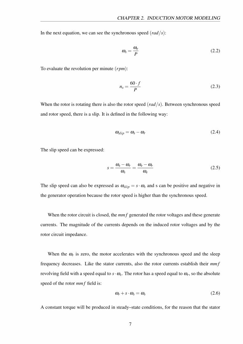
Now, we consider the magnetic stator and rotor circuit, as shown in Figure 2.2:
Figure 2.2: Winding distribution of three-phase Induction Motor.
The stator voltage equations are the following:
vs123 = Rs · is123 +dλs123
dt(2.7)
where Rs is the stator resistance, is123 = (is1, is2, is3)T is the stator current vector, λs123 =
(λs1, λs2, λs3)T is the stator flux linkage vector and
vs123 = (vs1, vs2, vs3)T is the stator voltage vector. All vectors are defined in 123 coordinates.
The superscript T indicates the transposed vector.
The rotor voltage equations are the following:
vr123 = Rr · ir123 +dλr123
dt(2.8)
where Rr is the rotor resistance, ir123 = (ir1, ir2, ir3)T is the rotor current vector and λr123 =
8
CHAPTER 2. INDUCTION MOTOR MODELING
(λr1, λr2, λr3)T is the rotor flux linkage vector. The vr123 = (vr1, vr2, vr3)
T is the rotor voltage
vector. Since the motor is a squirrel cage, it has an amplitude equal to zero, indeed it is v
vr123 = (0,0,0)T .
The equation of the flux linkage of the stator and rotor windings can be written:
λs123 = Lls · is123 +Mss123 · is123 +Msr
123 · ir123 (2.9)
λr123 = Llr · ir123 +Mrs123 · is123 +Mrr
123 · ir123 (2.10)
The matrix of the Mss123 and Mrr
123, winding inductances, are:
Mss123 = M ·
1 −1
2 −12
−12 1 −1
2
−12 −1
2 1
;Mrr123 = M ·
1 −1
2 −12
−12 1 −1
2
−12 −1
2 1
(2.11)
M is the mutual inductance, Lls and Llr are the stator and rotor leakage inductances. M can
be considered equal for both stator and rotor windings.
Msr123 and Mrs
123 depend on the rotor angle, so these can be written as:
Msr123 = [Mrs
123]T = M ·
cos(θr) cos(θr +
2π
3 ) cos(θr− 2π
3 )
cos(θr− 2π
3 ) cos(θr) cos(θr +2π
3 )
cos(θr +2π
3 ) cos(θr− 2π
3 ) cos(θr)
(2.12)
M is the magnetizing inductance and it can be defined as:
M =N ·N′
ℜt(2.13)
where N and N′ are the number of the equivalents turns and ℜt is the air gap reluctance.
9
CHAPTER 2. INDUCTION MOTOR MODELING
To facilitate the machine model, mathematical transformations are used:
• Clarke transformation (123 to αβ );
• Park transformation (αβ to dq).
These transformations are used to simplify the machine model.
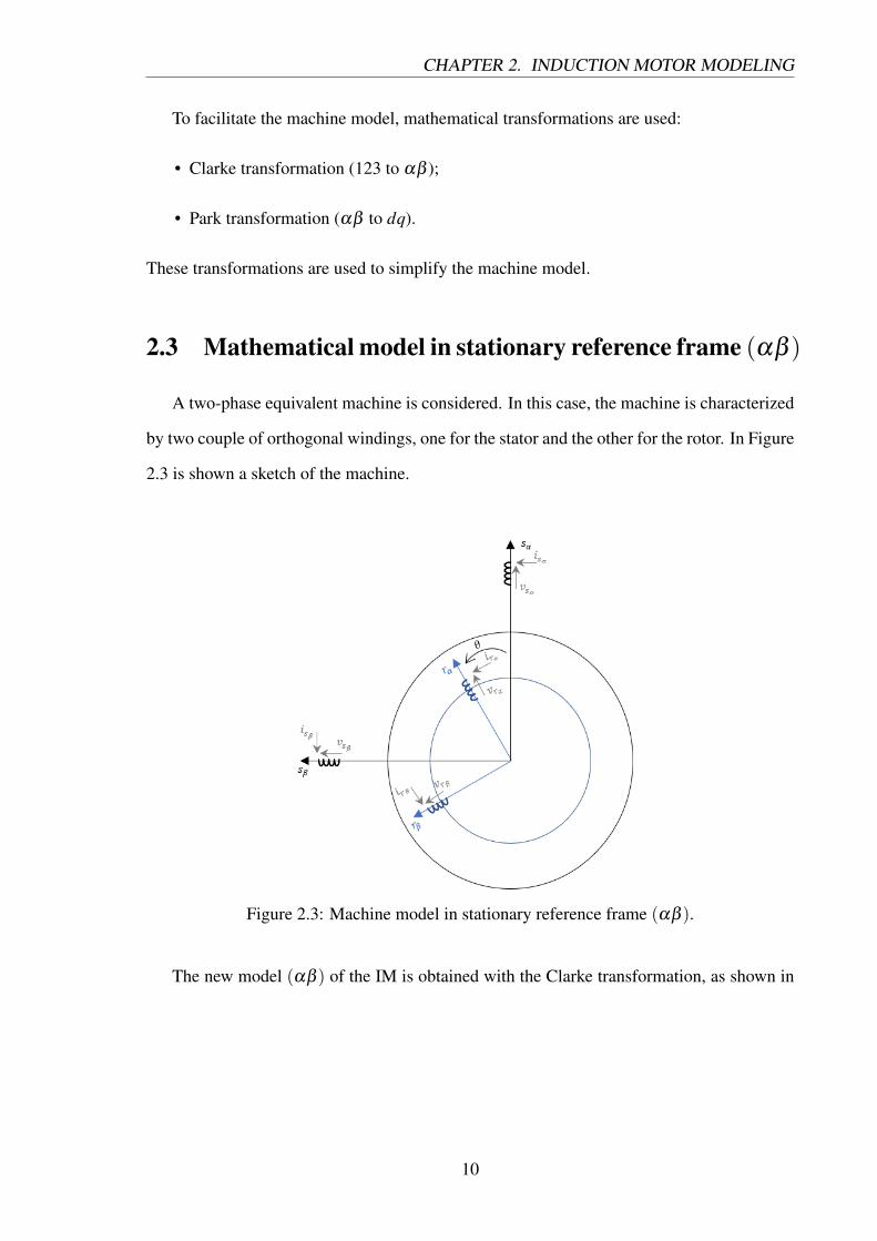
2.3 Mathematical model in stationary reference frame (αβ )
A two-phase equivalent machine is considered. In this case, the machine is characterized
by two couple of orthogonal windings, one for the stator and the other for the rotor. In Figure
2.3 is shown a sketch of the machine.
Figure 2.3: Machine model in stationary reference frame (αβ ).
The new model (αβ ) of the IM is obtained with the Clarke transformation, as shown in
10
CHAPTER 2. INDUCTION MOTOR MODELING
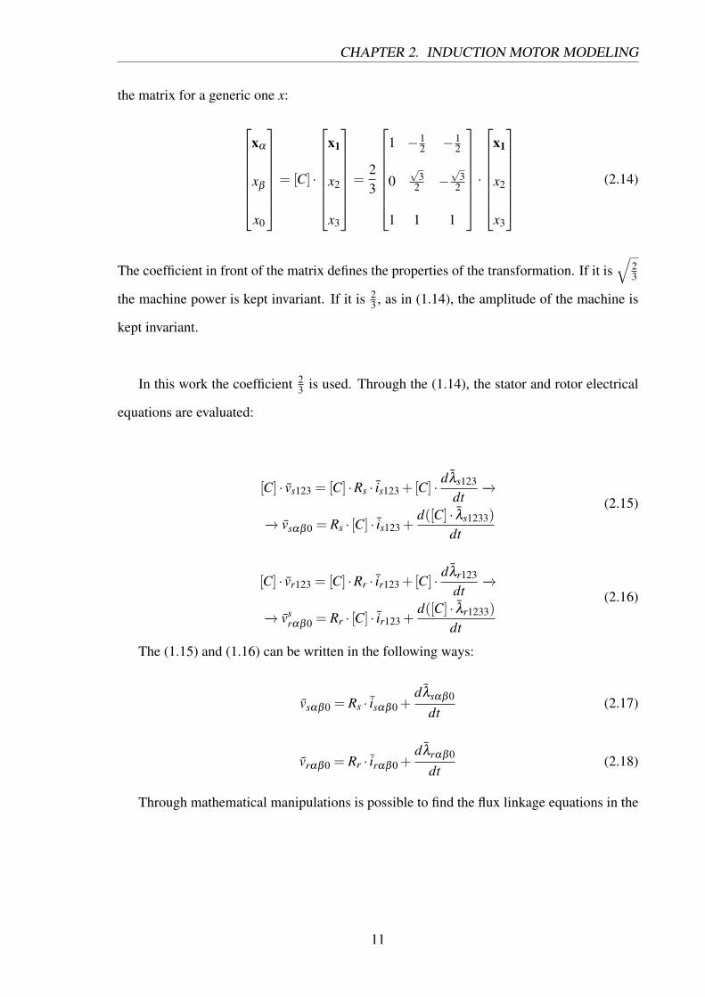
the matrix for a generic one x:
xα
xβ
x0
= [C] ·
x1
x2
x3
=23
1 −1
2 −12
0√
32 −
√3
2
1 1 1
·
x1
x2
x3
(2.14)
The coefficient in front of the matrix defines the properties of the transformation. If it is√
23
the machine power is kept invariant. If it is 23 , as in (1.14), the amplitude of the machine is
kept invariant.
In this work the coefficient 23 is used. Through the (1.14), the stator and rotor electrical
equations are evaluated:
[C] · vs123 = [C] ·Rs · is123 +[C] · dλs123
dt−→
−→ vsαβ0 = Rs · [C] · is123 +d([C] · λs1233)
dt
(2.15)
[C] · vr123 = [C] ·Rr · ir123 +[C] · dλr123
dt−→
−→ vsrαβ0 = Rr · [C] · ir123 +
d([C] · λr1233)
dt
(2.16)
The (1.15) and (1.16) can be written in the following ways:
vsαβ0 = Rs · isαβ0 +dλsαβ0
dt(2.17)
vrαβ0 = Rr · irαβ0 +dλrαβ0
dt(2.18)
Through mathematical manipulations is possible to find the flux linkage equations in the
11
CHAPTER 2. INDUCTION MOTOR MODELING
new frame (αβ ):
[C] · λs123 = [C] ·Lls · is123 +[C] ·Mss123 · is123 +[C] ·Msr
123 · ir123 −→
[C] · λs123 = Lls · ([C] · is123)+ [C] ·Mss123 · [C]−1 · ([C] · is123)+
+[C] ·Msr123 · [C]−1 · ([C] · ir123) (2.19)
[C] · λr123 = [C] ·Llr · ir123 +[C] ·Mrs123 · is123 +[C] ·Mrr
123 · ir123 −→
[C] · λr123 = Llr · ([C] · ir123)+ [C] ·Mrs123 · [C]−1 · ([C] · is123)+
+[C] ·Mrr123 · [C]−1 · ([C] · ir123) (2.20)
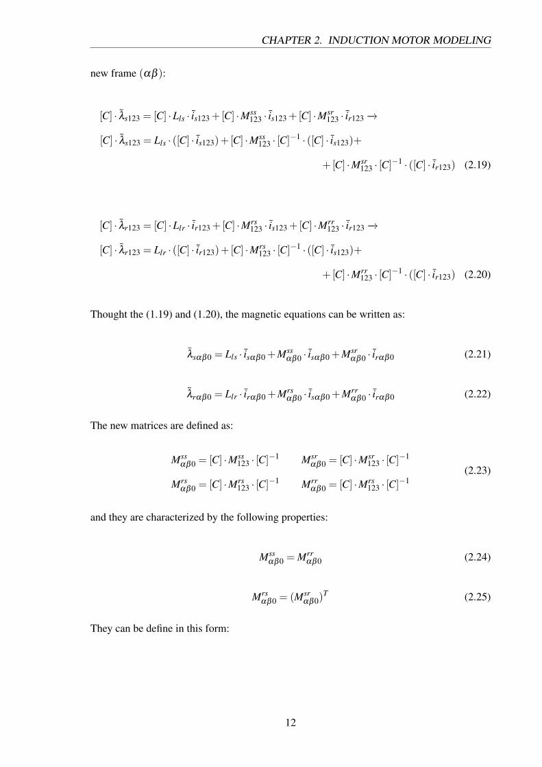
Thought the (1.19) and (1.20), the magnetic equations can be written as:
λsαβ0 = Lls · isαβ0 +Mssαβ0 · isαβ0 +Msr
αβ0 · irαβ0 (2.21)
λrαβ0 = Llr · irαβ0 +Mrsαβ0 · isαβ0 +Mrr
αβ0 · irαβ0 (2.22)
The new matrices are defined as:
Mssαβ0 = [C] ·Mss
123 · [C]−1 Msrαβ0 = [C] ·Msr
123 · [C]−1
Mrsαβ0 = [C] ·Mrs
123 · [C]−1 Mrrαβ0 = [C] ·Mrs
123 · [C]−1(2.23)
and they are characterized by the following properties:
Mssαβ0 = Mrr
αβ0 (2.24)
Mrsαβ0 = (Msr
αβ0)T (2.25)
They can be define in this form:
12
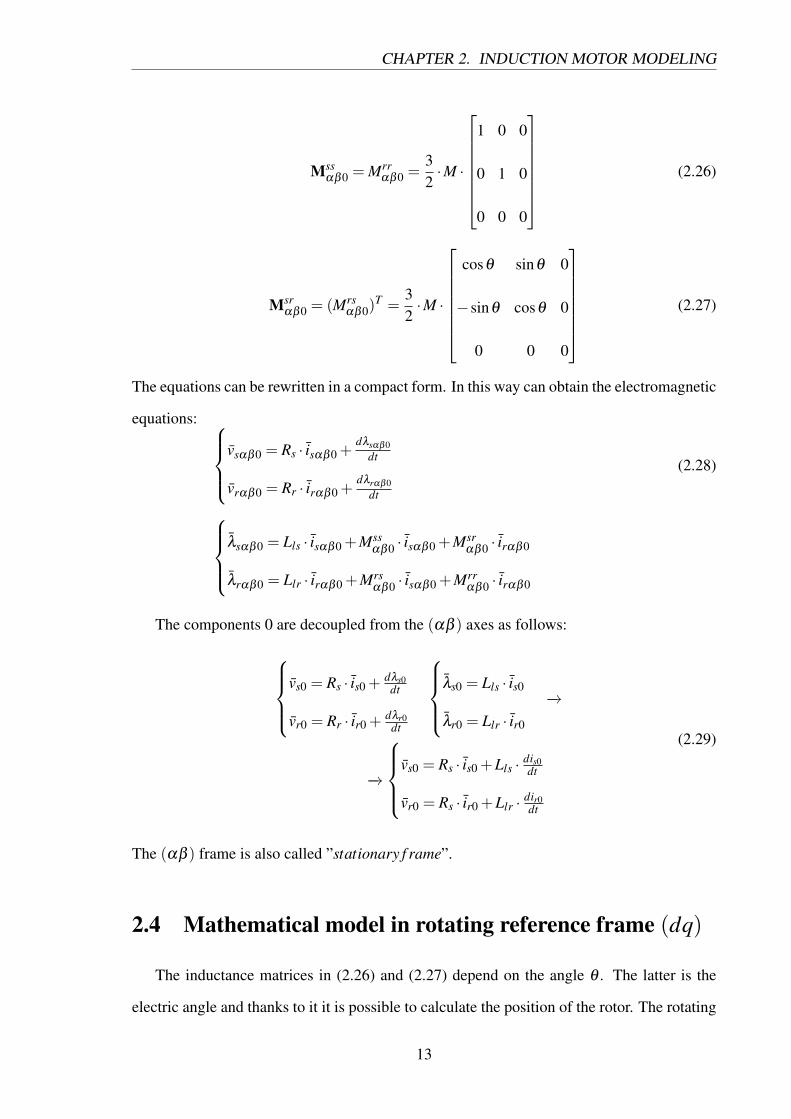
CHAPTER 2. INDUCTION MOTOR MODELING
Mssαβ0 = Mrr
αβ0 =32·M ·
1 0 0
0 1 0
0 0 0
(2.26)
Msrαβ0 = (Mrs
αβ0)T =
32·M ·
cosθ sinθ 0
−sinθ cosθ 0
0 0 0
(2.27)
The equations can be rewritten in a compact form. In this way can obtain the electromagnetic
equations: vsαβ0 = Rs · isαβ0 +
dλsαβ0dt
vrαβ0 = Rr · irαβ0 +dλrαβ0
dt
(2.28)
λsαβ0 = Lls · isαβ0 +Mss
αβ0 · isαβ0 +Msrαβ0 · irαβ0
λrαβ0 = Llr · irαβ0 +Mrsαβ0 · isαβ0 +Mrr
αβ0 · irαβ0
The components 0 are decoupled from the (αβ ) axes as follows:
vs0 = Rs · is0 +
dλs0dt
vr0 = Rr · ir0 +dλr0dt
λs0 = Lls · is0
λr0 = Llr · ir0
−→
−→
vs0 = Rs · is0 +Lls · dis0
dt
vr0 = Rs · ir0 +Llr · dir0dt
(2.29)
The (αβ ) frame is also called ”stationary f rame”.
2.4 Mathematical model in rotating reference frame (dq)
The inductance matrices in (2.26) and (2.27) depend on the angle θ . The latter is the
electric angle and thanks to it it is possible to calculate the position of the rotor. The rotating
13
CHAPTER 2. INDUCTION MOTOR MODELING
reference frame is used for the control of the machine.
The electromagnetic model is a generic reference frame, with a rotation ωk. The speed ωk is
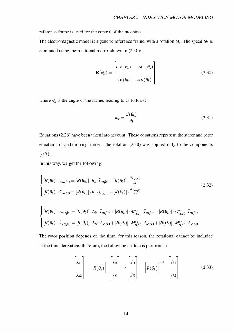
computed using the rotational matrix shown in (2.30):
R(θk) =
cos(θk) −sin(θk)
sin(θk) cos(θk)
(2.30)
where θk is the angle of the frame, leading to as follows:
ωk =d(θk)
dt(2.31)
Equations (2.28) have been taken into account. These equations represent the stator and rotor
equations in a stationary frame. The rotation (2.30) was applied only to the components
(αβ ).
In this way, we get the following:
[R(θk)] · vsαβ0 = [R(θk)] ·Rs · isαβ0 +[R(θk)] ·
dλsαβ0dt
[R(θk)] · vrαβ0 = [R(θk)] ·Rr · irαβ0 +[R(θk)] ·dλrαβ0
dt
(2.32)
[R(θk)] · λsαβ0 = [R(θk)] ·Lls · isαβ0 +[R(θk)] ·Mss
αβ0 · isαβ0 +[R(θk)] ·Msrαβ0 · irαβ0
[R(θk)] · λrαβ0 = [R(θk)] ·Llr · irαβ0 +[R(θk)] ·Mrsαβ0 · isαβ0 +[R(θk)] ·Mrr
αβ0 · irαβ0
The rotor position depends on the time, for this reason, the rotational cannot be included
in the time derivative. therefore, the following artifice is performed:
fk1
fk2
=
[R(θk)
]·
fα
fβ
−→ fα
fβ
=
[R(θk)
]−1
·
fk1
fk2
(2.33)
14
CHAPTER 2. INDUCTION MOTOR MODELING
As a result of the (2.32). It is possible to write:
vsk = Rs · isk +[R(θk)] · d([R(θk)]
−1·λsk)dt
vrk = Rr · irk +[R(θk)] · d([R(θk)]−1·λrk)
dt
(2.34)
λsk = Lls · isk +[R(θk)] ·Msr · ([R(θk)]
−1 · irk)+Mss · isk
λrk = Llr · irk +[R(θk)] ·Mrs · ([R(θk)]−1 · isk)+Mrr · irk
The product between the inductances matrices (Mss,Mrr,Msr,Mrs), the rotational matrix
R(θk) and its inverse, take the following form:
Mss = Mrr = Msr = Mrs =32·M ·
1 0
0 1
(2.35)
After performing mathematical manipulations, the equations in a generic reference frame
can be written as follows:
vs = Rs · is + dλs
dt + j ·ωk · λs
vr = Rr · ir + dλrdt + j · (ωk−ωr) · λr
(2.36)
λs = Ls · is +Lm · ir, Ls = Lls +Lm, Lm = 3
2 ·M
λr = Lm · is +Lr · ir, Lr = Llr +Lm, Lm = 32 ·M
where Lm is the magnetizing inductance and the 32 is the coefficient of the Clarke trasformation.
To evaluate the torque equation, we needed to start of the balance of the powers. The equation
of the electrical power is the follows:
Pe = vs · is + vr · ir = PJsr +Pm +Pme→
−→
vs · is = Rs · |is|2 + dλs
dt · is + j ·ωk · λs · is
0 = vr · ir = Rr · |ir|2 + dλrdt · ir + j · (ωk−ωr) · λr · ir
(2.37)
15
CHAPTER 2. INDUCTION MOTOR MODELING
where PJsr is the Joule power, Pm is the magnetizing power and Pem is the electromagnetic
power. These powers are defined in the following way:
PJsr = Rs · |is|2 +Rr · |ir|2
Pm =dλs
dt· is +
dλr
dt· ir
Pem = ( j ·ωk · λs) · is +( j ·ωk · λr) · ir− ( j ·ωr · λr) · ir
(2.38)
The Pem does not depend on the chosen reference frame. For this reason, it becomes:
Pem =−( j ·ωr · λr) · ir = ωr · (ir∧ λr) (2.39)
The torque equation can be written:
Tem =32· pp · (ir∧ λr) (2.40)
where pp is the number of pole pairs and 32 is the coefficient of the Clarke transformation.
By combining (2.36) with (2.40), the electromagnetic torque can be expressed as:
Tem =32· pp · (ir∧M · is) =
32· pp · (λs∧ is) (2.41)
2.5 Equivalent circuit in rotating coordinates
In this section, the equivalent circuit of the machine in rotating coordinates is provided.
Starting from (2.36):
• ωk = ωs: this means that synchronous speed is equal to the pulsation of the supply
voltage;
• all the time-derivatives are equal to zero; in this case, the steady-state condition is
provided.
16
CHAPTER 2. INDUCTION MOTOR MODELING
Hence, the electromagnetic equations can be written in rotating dq coordinates:
Vsdq = Rs · Isdq + j ·ωe · Λsdq
Vrdq = Rr · Irdq + j · (ωe−ωr) · Λrdq
(2.42)
−→
Λsdq = Ls · Isdq +Lm · Isdq
Λrdq = Lm · Isdq +Lr · Irdq
If the electrical equations are substituted in the magnetic ones, it is possible to obtain the
electromagnetic equations:
Vsdq = Rs · Isdq + j ·ωe ·Ls · Isdq + j ·ωe ·M · Irdq
0 = Rrs · Irdq + j ·ωe ·Lr · Irdq + j ·ωe ·M · Isdq
(2.43)
−→
Vsdq = (Rs + j ·ωe ·Ls) · Isdq + j ·ωe ·M · Irdq
0 = (Rrs + j ·ωe ·Lr) · Irdq + j ·ωe ·M · Isdq
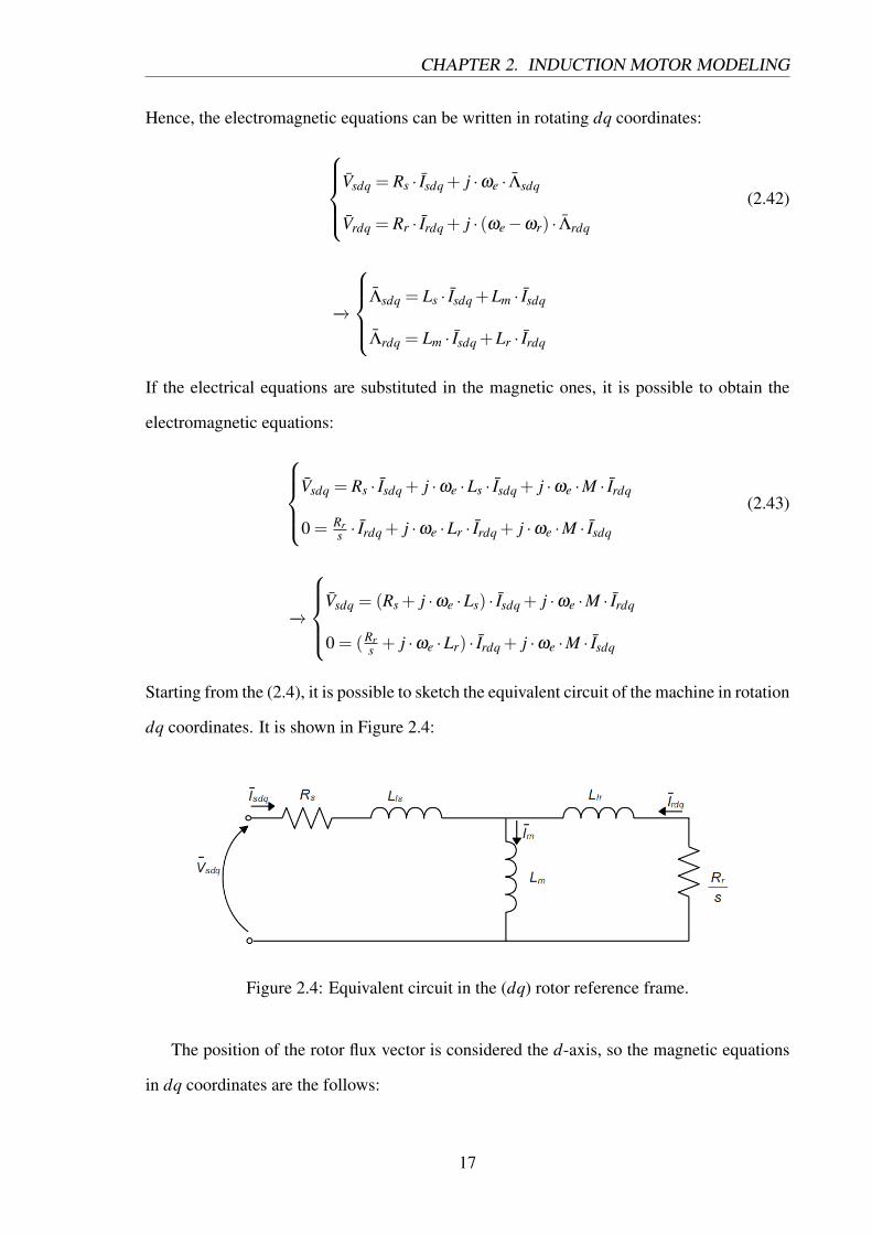
Starting from the (2.4), it is possible to sketch the equivalent circuit of the machine in rotation
dq coordinates. It is shown in Figure 2.4:
Figure 2.4: Equivalent circuit in the (dq) rotor reference frame.
The position of the rotor flux vector is considered the d-axis, so the magnetic equations
in dq coordinates are the follows:
17
CHAPTER 2. INDUCTION MOTOR MODELING
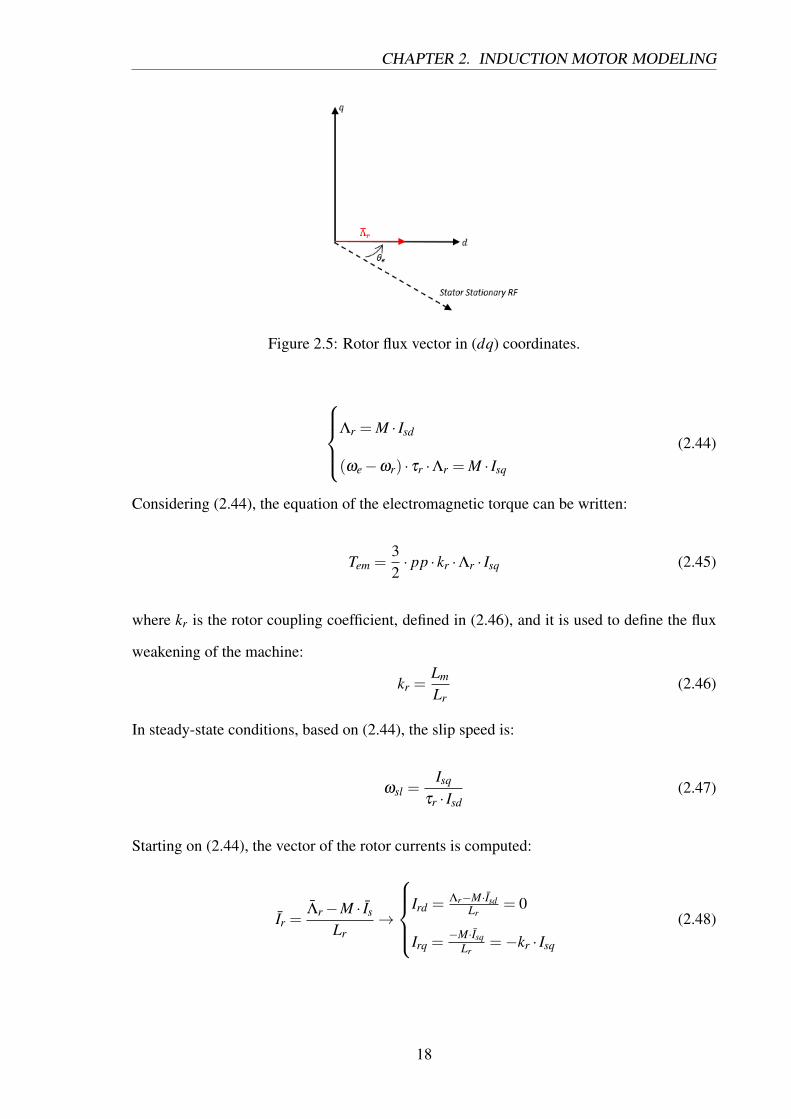
Figure 2.5: Rotor flux vector in (dq) coordinates.
Λr = M · Isd
(ωe−ωr) · τr ·Λr = M · Isq
(2.44)
Considering (2.44), the equation of the electromagnetic torque can be written:
Tem =32· pp · kr ·Λr · Isq (2.45)
where kr is the rotor coupling coefficient, defined in (2.46), and it is used to define the flux
weakening of the machine:
kr =Lm
Lr(2.46)
In steady-state conditions, based on (2.44), the slip speed is:
ωsl =Isq
τr · Isd(2.47)
Starting on (2.44), the vector of the rotor currents is computed:
Ir =Λr−M · Is
Lr→
Ird = Λr−M·Isd
Lr= 0
Irq =−M·Isq
Lr=−kr · Isq
(2.48)
18
CHAPTER 2. INDUCTION MOTOR MODELING
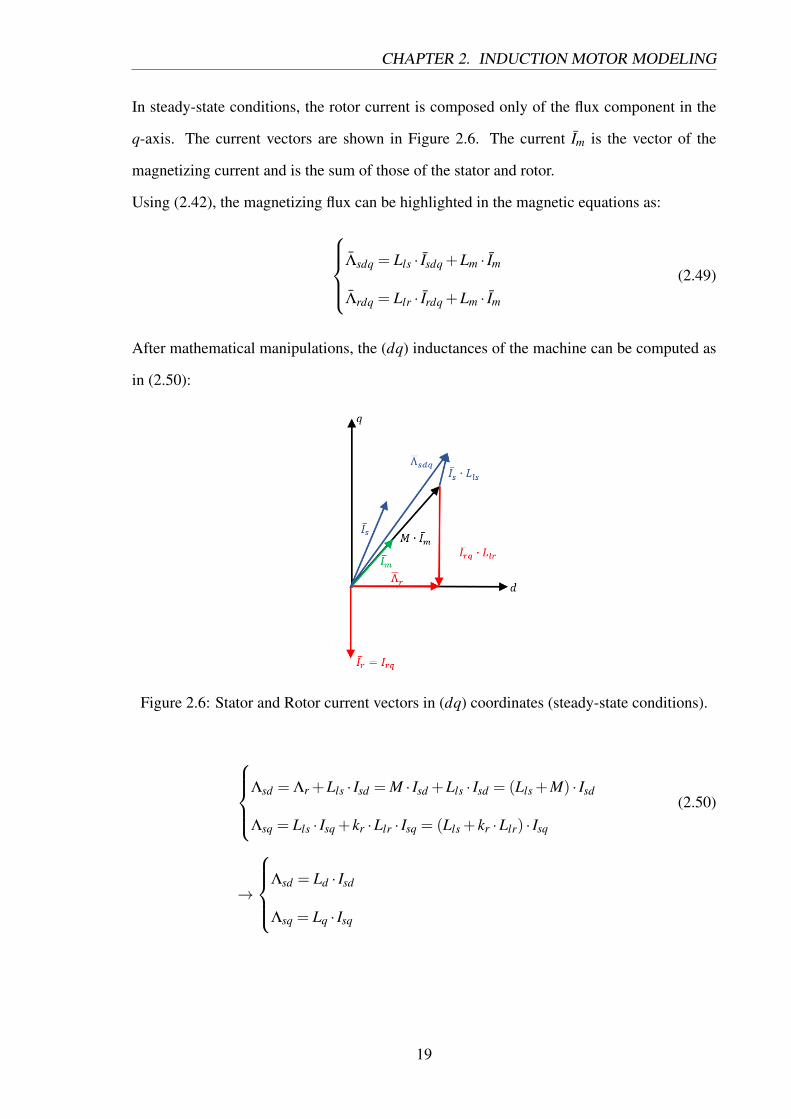
In steady-state conditions, the rotor current is composed only of the flux component in the
q-axis. The current vectors are shown in Figure 2.6. The current Im is the vector of the
magnetizing current and is the sum of those of the stator and rotor.
Using (2.42), the magnetizing flux can be highlighted in the magnetic equations as:
Λsdq = Lls · Isdq +Lm · Im
Λrdq = Llr · Irdq +Lm · Im
(2.49)
After mathematical manipulations, the (dq) inductances of the machine can be computed as
in (2.50):
Figure 2.6: Stator and Rotor current vectors in (dq) coordinates (steady-state conditions).
Λsd = Λr +Lls · Isd = M · Isd +Lls · Isd = (Lls +M) · Isd
Λsq = Lls · Isq + kr ·Llr · Isq = (Lls + kr ·Llr) · Isq
(2.50)
→
Λsd = Ld · Isd
Λsq = Lq · Isq
19
CHAPTER 2. INDUCTION MOTOR MODELING
The inductance along the q-axis is:
Lq = Lls + kr ·Llr = (Ls−M)+ kr · (Lr−M)
→ Lq = Ls · (1− ks · kr) = σ ·Ls
(2.51)
where σ is the overall decoupling coefficient.
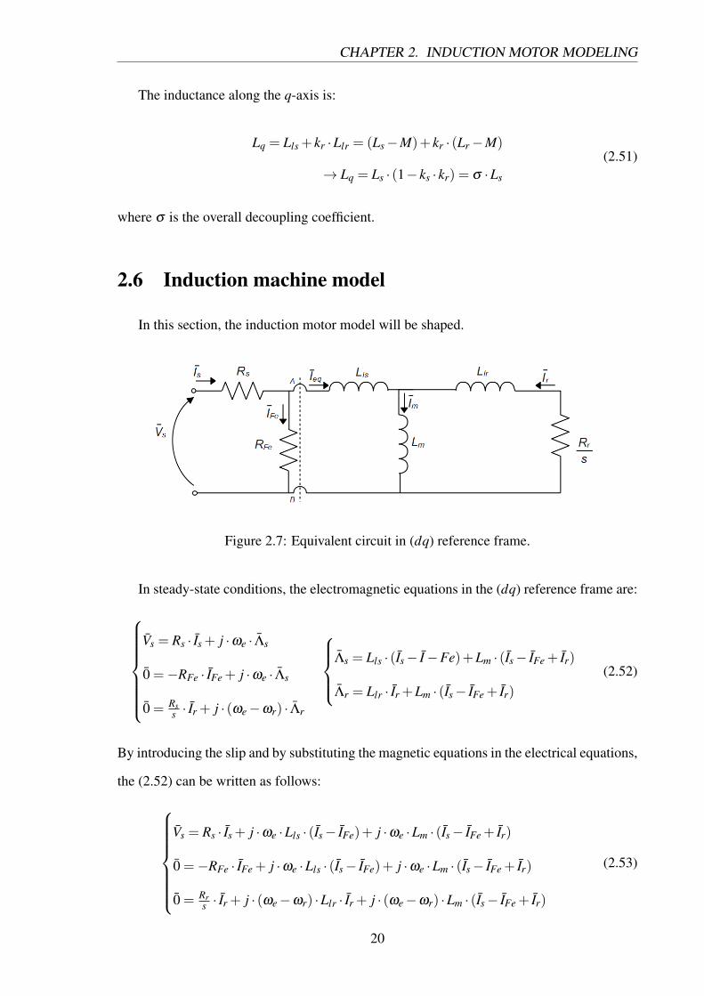
2.6 Induction machine model
In this section, the induction motor model will be shaped.
Figure 2.7: Equivalent circuit in (dq) reference frame.
In steady-state conditions, the electromagnetic equations in the (dq) reference frame are:
Vs = Rs · Is + j ·ωe · Λs
0 =−RFe · IFe + j ·ωe · Λs
0 = Rss · Ir + j · (ωe−ωr) · Λr
Λs = Lls · (Is− I−Fe)+Lm · (Is− IFe + Ir)
Λr = Llr · Ir +Lm · (Is− IFe + Ir)
(2.52)
By introducing the slip and by substituting the magnetic equations in the electrical equations,
the (2.52) can be written as follows:
Vs = Rs · Is + j ·ωe ·Lls · (Is− IFe)+ j ·ωe ·Lm · (Is− IFe + Ir)
0 =−RFe · IFe + j ·ωe ·Lls · (Is− IFe)+ j ·ωe ·Lm · (Is− IFe + Ir)
0 = Rrs · Ir + j · (ωe−ωr) ·Llr · Ir + j · (ωe−ωr) ·Lm · (Is− IFe + Ir)
(2.53)
20
CHAPTER 2. INDUCTION MOTOR MODELING
To simplify the model, we can apply the equivalent Thevenin circuit that runs to the AB
terminals and introduce an equivalent voltage Veq, an equivalent resistance Req and an equivalent
current Ieq. These quantities can be written as:
Req =Rs ·RFe
Rs +RFe; Veq = Vs ·
RFe
Rs +RFe; Ieq = Is− IFe (2.54)
According to the equivalent circuit shown in Figure 1.6, the equations become:
Veq = Req · Ieq + j ·ωe ·Λs
0 = Rrs · Ir + j · (ωe−ωr) · Λr
Λs = Ls · Ieq +Lm · Ir
Λr = Lr · Ir +Lm · Ieq
(2.55)
2.7 Test of induction machine
To evaluate the induction motor parameters, it is necessary to carry out the No-Load
test and the Locked-rotor Test. With the first test, it is possible to find the resistance that
model the iron losses RFe, the magnetizing inductance Lm, the iron IFe and magnetization Im
currents.
With the second test, the rotor resistance Rr, the stator Ls and the rotor r inductances are
calculated.
2.7.1 No-load test
The no-load test is conducted with a set frequency and with different voltage values, so
it is possible to evaluate the magnetic saturation law. If the test is performed at different
frequencies, the iron losses model is obtained.in this case, the slip is equal to 0
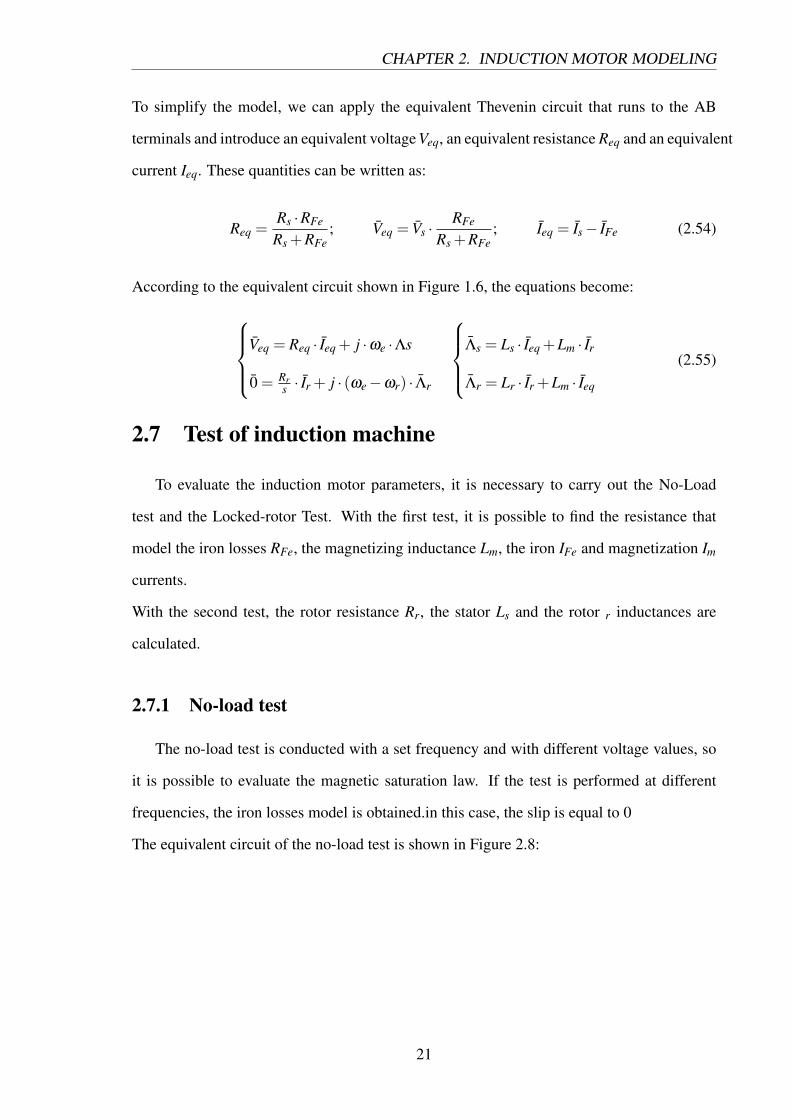
The equivalent circuit of the no-load test is shown in Figure 2.8:
21

CHAPTER 2. INDUCTION MOTOR MODELING
Figure 2.8: Equivalent circuit of the no-load test.
P0, V0 and I0 are respectively the input power, voltage and current related to the no-load
circuit. Initially, the test is performed with low voltage values, so it is possible to divide the
mechanical losses from those of the iron. The sum of the mechanical and iron losses can be
estimated by subtracting the stator Joule losses PJs and the input power P0.
Pmech+Fe = P0−3 ·Rs · I20 (2.56)
The iron losses can be neglected with low voltage values, so the (2.56) corresponds to the
mechanical power. With different frequency values, the mechanical power can be written
according to the machine speed. Furthermore, the mechanical power corresponds to the
torque loss that must be subtracted to that electromagnetic (2.45) in motoring mode and vice
versa in generating mode. In general, the mechanical losses are linked with the friction and
ventilation.
To search the parameters of the machine, it is necessary to start from the voltage Es0, as
shown below:
Es0 =√(V0−Rs · cos(φ0) · I0)2 +(Rs · sin(φ0) · I0)2, cos(φ0) =
P0
3 ·V0 · I0(2.57)
22
CHAPTER 2. INDUCTION MOTOR MODELING
To conclude, the parameters are calculated as follows:
RFe = 3 ·E2
s0PFe
; IFe =E2
s0RFe
; Im =√
I20 − I2
Fe; Xs = Xm +Xls =Es0
Im(2.58)
Xs is the stator reactance and it is the sum of the magnetizing Xm and leakage Xls reactances.
Xls is evaluated in the next paragraph from the locked-rotor test.
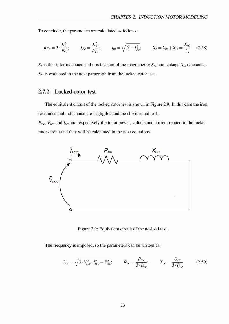
2.7.2 Locked-rotor test
The equivalent circuit of the locked-rotor test is shown in Figure 2.9. In this case the iron
resistance and inductance are negligible and the slip is equal to 1.
Pscc, Vscc and Iscc are respectively the input power, voltage and current related to the locker-
rotor circuit and they will be calculated in the next equations.
Figure 2.9: Equivalent circuit of the no-load test.
The frequency is imposed, so the parameters can be written as:
Qcc =√
3 ·V 2scc · I2
scc−P2scc; Rcc =
Pscc
3 · I2scc
; Xcc =Qcc
3 · I2scc
(2.59)
23
CHAPTER 2. INDUCTION MOTOR MODELING
Starting on the (2.58) and (2.59), the machine inductances Xr and Xs are evaluated as:
Xls = Xlr 'Xcc
2→ Lls = Llr '
12· Xcc
ωe
Xm = Xs−Xls→ Lm =Xm
ωe
Rr = Rcc−Rs
(2.60)
Finally, the parameters are evaluated.
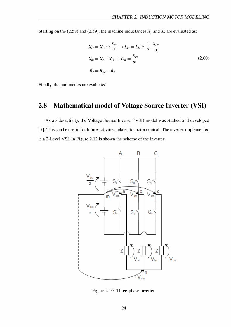
2.8 Mathematical model of Voltage Source Inverter (VSI)
As a side-activity, the Voltage Source Inverter (VSI) model was studied and developed
[5]. This can be useful for future activities related to motor control. The inverter implemented
is a 2-Level VSI. In Figure 2.12 is shown the scheme of the inverter;
Figure 2.10: Three-phase inverter.
24
CHAPTER 2. INDUCTION MOTOR MODELING
The VSI with ideal switches is connected to a symmetrical and balanced load, this load
is without neutral. The load is characterized by an impedance equal to Z.
The inverter shows in Figure 2.12 is made with six switches and it is possible to see three
branches A,B,C. These branches can be used to connect two switches in series and these
work in a complementary way.
Sa, Sb and Sc are the states of the branches and they can be only +1 or -1. These states
represent if and which switches are closed.
The voltage on branches is:
Vam = SA ·VDC
2(2.61)
Vbm = SB ·VDC
2(2.62)
Vcm = SC ·VDC
2(2.63)
The voltage on the load can be expressed as [6]:
Van =Vam−Vnm (2.64)
Vbn =Vbm−Vnm (2.65)
Vcn =Vcm−Vnm (2.66)
In the reality, the load voltage Vnm is not measured because the centre of the load is not
accessible, so the (2.69), (2.70) and (2.66) are not calculated and they are only theoretical
values. Vnm can be calculated as a function of voltages branches and can be written as:
Van +Vbn +Vcn =Vam +Vbm +Vcm−3 ·Vnm (2.67)
Considering a symmetrical and balanced load without neutral, Vnm can define by the (2.67)
and can be written as follows:
Van +Vbn +Vcn = 0→Vnm =Vam +Vbm +Vcm
3(2.68)
25
CHAPTER 2. INDUCTION MOTOR MODELING
By the (2.68) is possible to express the equations which describe the phase voltages; the
branch voltages are:
Van =23·Vam−
13· (Vbm +Vcm) (2.69)
Vbn =23·Vbm−
13· (Vam +Vcm) (2.70)
Vcn =23·Vcm−
13· (Vam +Vbm) (2.71)
These equations can be organized in vector form and can be written as:
Van
Vbn
Vcn
=VDC
2·
23 −1
3 −13
−13
23 −1
3
−13 −1
323
·
SA
SB
SC
(2.72)
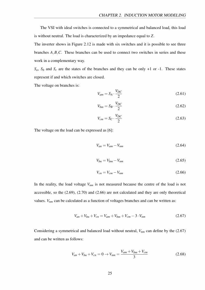
Considering that the leg states are 2 and that the three-phase inverter branches are 3, the
number of vectors that can be applied to the load are 23=8; it is shown below:
Figure 2.11: Voltage vectors.
The zero voltage vectors correspond to the two state in which the upper and lower
26
CHAPTER 2. INDUCTION MOTOR MODELING
switched of the three branches are closed.
The Figure 2.11 in literature is called hexagon of the output voltages of the three-phase
inverter.
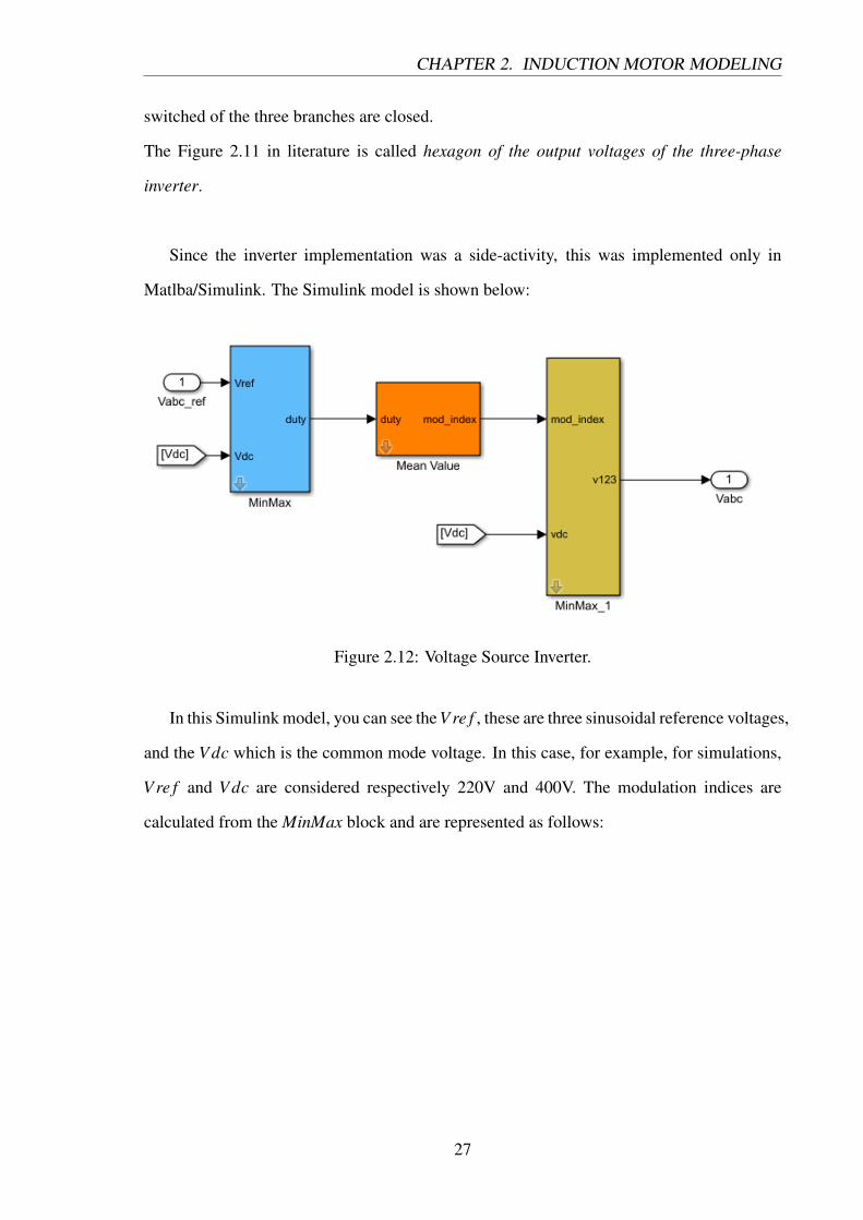
Since the inverter implementation was a side-activity, this was implemented only in
Matlba/Simulink. The Simulink model is shown below:
Figure 2.12: Voltage Source Inverter.
In this Simulink model, you can see the V re f , these are three sinusoidal reference voltages,
and the V dc which is the common mode voltage. In this case, for example, for simulations,
V re f and V dc are considered respectively 220V and 400V. The modulation indices are
calculated from the MinMax block and are represented as follows:
27
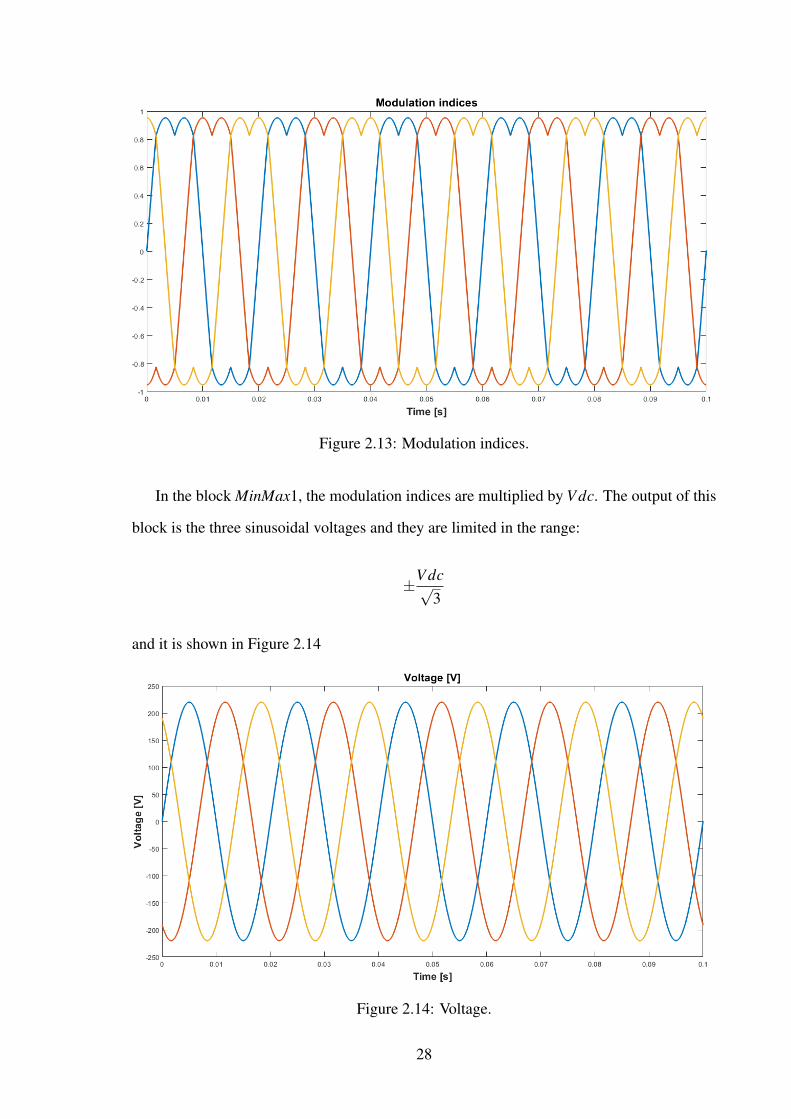
Figure 2.13: Modulation indices.
In the block MinMax1, the modulation indices are multiplied by V dc. The output of this
block is the three sinusoidal voltages and they are limited in the range:
±V dc√3
and it is shown in Figure 2.14
Figure 2.14: Voltage.
28
Chapter 3
Simulink and dSPACE comparisons in
stationary reference frame (αβ )
The purpose of the activity was to implement the Squirrel Cage Induction Motor (SCIM)
model in Simulink and dSPACE.
In this chapter, the two models are implemented in (αβ ) coordinates.
The Simulink model used as benchmark for the dSPACE – XSG model was inherited from a
model developed in dynamics of electrical machines course of Politecnico di Torino.
In Simulink and dSPACE the three-phase sinusoidal voltage generator, the induction motor
and the mechanic were implemented. The simulations were developed in open-loop. Open-
loop simulation is obtained by providing a known input and verifying that the outputs are
those expected and that they follow the desired behaviour.
First, the development of the Simulink (αβ ) model is analysed and an overview of the model
is providing.
After that, a description of dSPACE is given and also in this case an overview of the dSPACE
(αβ ) model is provided.
29
CHAPTER 3. SIMULINK AND DSPACE COMPARISONS IN STATIONARYREFERENCE FRAME (αβ )
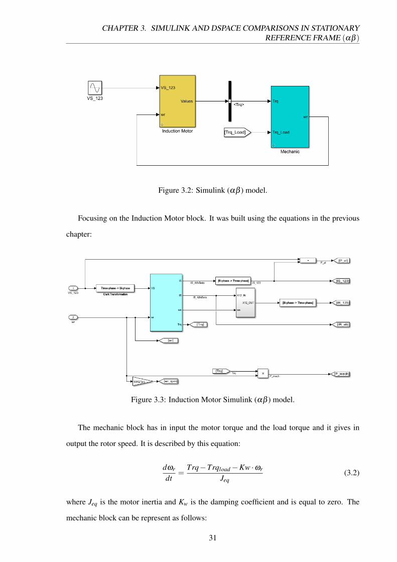
3.1 Overview on Simulink model
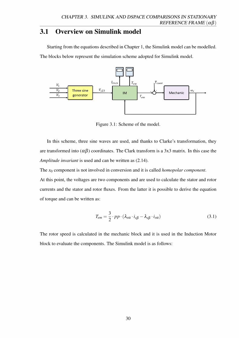
Starting from the equations described in Chapter 1, the Simulink model can be modelled.
The blocks below represent the simulation scheme adopted for Simulink model.
Figure 3.1: Scheme of the model.
In this scheme, three sine waves are used, and thanks to Clarke’s transformation, they
are transformed into (αβ ) coordinates. The Clark transform is a 3x3 matrix. In this case the
Amplitude invariant is used and can be written as (2.14).
The x0 component is not involved in conversion and it is called homopolar component.
At this point, the voltages are two components and are used to calculate the stator and rotor
currents and the stator and rotor fluxes. From the latter it is possible to derive the equation
of torque and can be written as:
Tem =32· pp · (λsα · isβ −λsβ · isα) (3.1)
The rotor speed is calculated in the mechanic block and it is used in the Induction Motor
block to evaluate the components. The Simulink model is as follows:
30
CHAPTER 3. SIMULINK AND DSPACE COMPARISONS IN STATIONARYREFERENCE FRAME (αβ )
Figure 3.2: Simulink (αβ ) model.
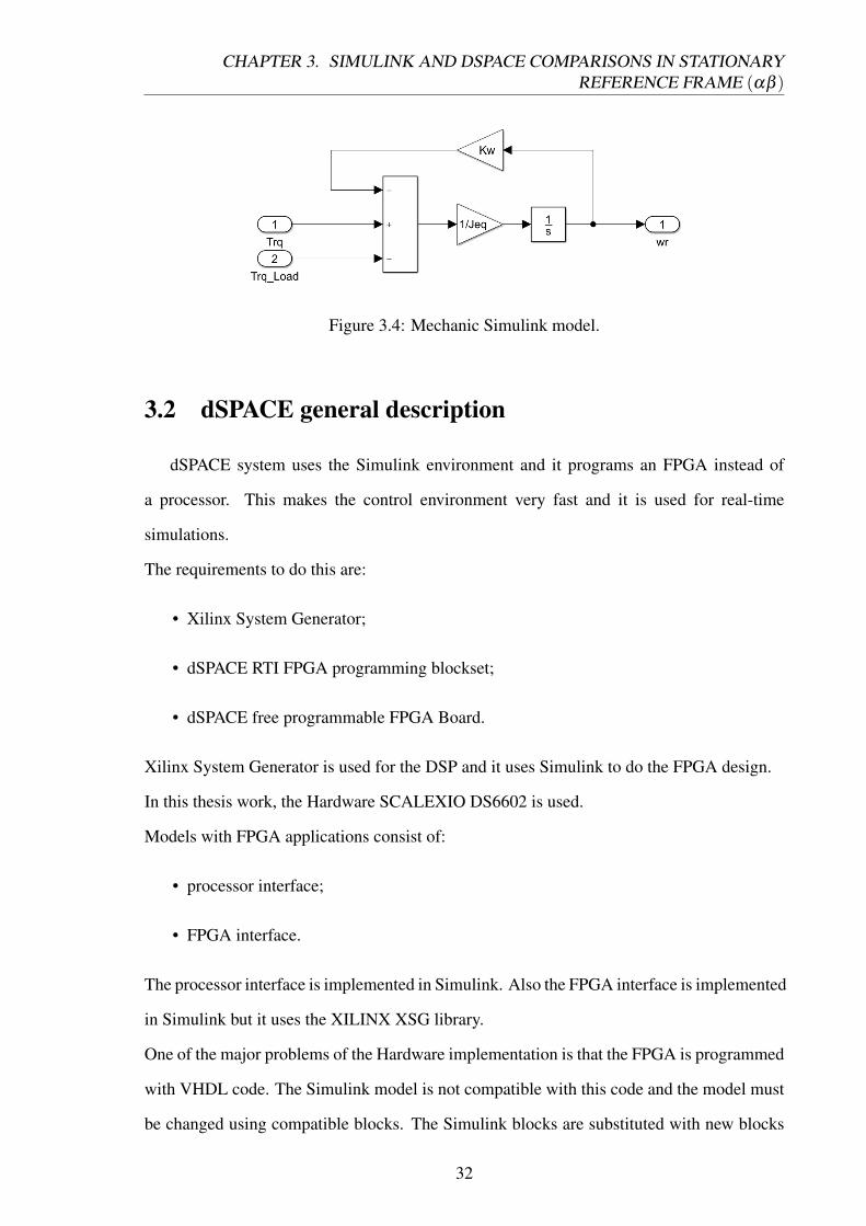
Focusing on the Induction Motor block. It was built using the equations in the previous
chapter:
Figure 3.3: Induction Motor Simulink (αβ ) model.
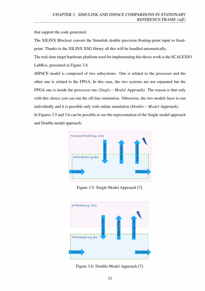
The mechanic block has in input the motor torque and the load torque and it gives in
output the rotor speed. It is described by this equation:
dωr
dt=
Trq−Trqload−Kw ·ωr
Jeq(3.2)
where Jeq is the motor inertia and Kw is the damping coefficient and is equal to zero. The
mechanic block can be represent as follows:
31
CHAPTER 3. SIMULINK AND DSPACE COMPARISONS IN STATIONARYREFERENCE FRAME (αβ )
Figure 3.4: Mechanic Simulink model.
3.2 dSPACE general description
dSPACE system uses the Simulink environment and it programs an FPGA instead of
a processor. This makes the control environment very fast and it is used for real-time
simulations.
The requirements to do this are:
• Xilinx System Generator;
• dSPACE RTI FPGA programming blockset;
• dSPACE free programmable FPGA Board.
Xilinx System Generator is used for the DSP and it uses Simulink to do the FPGA design.
In this thesis work, the Hardware SCALEXIO DS6602 is used.
Models with FPGA applications consist of:
• processor interface;
• FPGA interface.
The processor interface is implemented in Simulink. Also the FPGA interface is implemented
in Simulink but it uses the XILINX XSG library.
One of the major problems of the Hardware implementation is that the FPGA is programmed
with VHDL code. The Simulink model is not compatible with this code and the model must
be changed using compatible blocks. The Simulink blocks are substituted with new blocks
32
CHAPTER 3. SIMULINK AND DSPACE COMPARISONS IN STATIONARYREFERENCE FRAME (αβ )
that support the code generated.
The XILINX Blockset convert the Simulink double precision floating-point input to fixed-
point. Thanks to the XILINX XSG library all this will be handled automatically.
The real-time target hardware platform used for implementing this thesis work is the SCALEXIO
LabBox, presented in Figure 3.8.
dSPACE model is composed of two subsystems. One is related to the processor and the
other one is related to the FPGA. In this case, the two systems are not separated but the
FPGA one is inside the processor one (Single−Model Approach). The reason is that only
with this choice you can run the off-line simulation. Otherwise, the two models have to run
individually and it is possible only with online simulation (Double−Model Approach).
In Figures 3.5 and 3.6 can be possible to see the representation of the Single model approach
and Double model approach:
Figure 3.5: Single-Model Approach [7].
Figure 3.6: Double-Model Approach [7].
33
CHAPTER 3. SIMULINK AND DSPACE COMPARISONS IN STATIONARYREFERENCE FRAME (αβ )
The FPGA is a net of semiconductor devices that communicate with each other through
a parallel communication. Thanks to this, it works faster and can be used for real-time
simulation and thus for Hardware in the Loop (HIL) simulations. On the other hand, Simulink
can not be used for real-time (HIL) simulation due to its computational time.
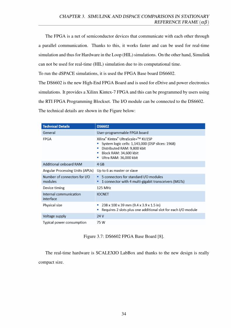
To run the dSPACE simulations, it is used the FPGA Base board DS6602.
The DS6602 is the new High-End FPGA Board and is used for eDrive and power electronics
simulations. It provides a Xilinx Kintex-7 FPGA and this can be programmed by users using
the RTI FPGA Programming Blockset. The I/O module can be connected to the DS6602.
The technical details are shown in the Figure below:
Figure 3.7: DS6602 FPGA Base Board [8].
The real-time hardware is SCALEXIO LabBox and thanks to the new design is really
compact size.
34
CHAPTER 3. SIMULINK AND DSPACE COMPARISONS IN STATIONARYREFERENCE FRAME (αβ )
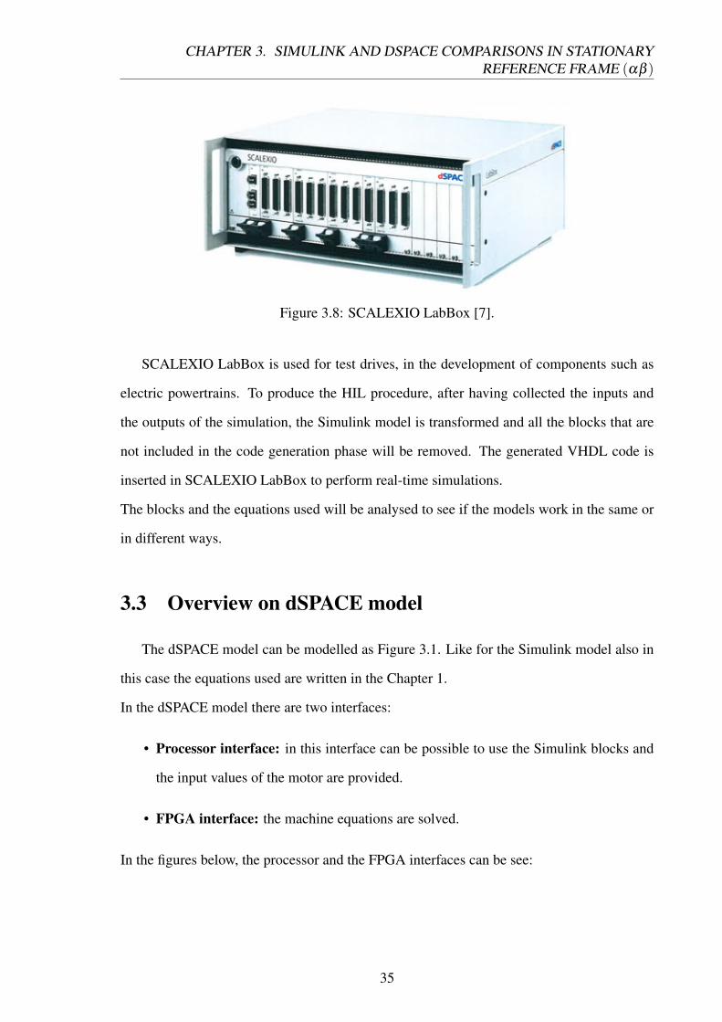
Figure 3.8: SCALEXIO LabBox [7].
SCALEXIO LabBox is used for test drives, in the development of components such as
electric powertrains. To produce the HIL procedure, after having collected the inputs and
the outputs of the simulation, the Simulink model is transformed and all the blocks that are
not included in the code generation phase will be removed. The generated VHDL code is
inserted in SCALEXIO LabBox to perform real-time simulations.
The blocks and the equations used will be analysed to see if the models work in the same or
in different ways.
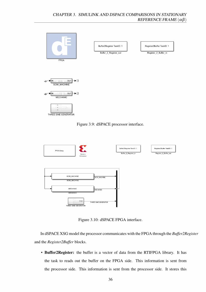
3.3 Overview on dSPACE model
The dSPACE model can be modelled as Figure 3.1. Like for the Simulink model also in
this case the equations used are written in the Chapter 1.
In the dSPACE model there are two interfaces:
• Processor interface: in this interface can be possible to use the Simulink blocks and
the input values of the motor are provided.
• FPGA interface: the machine equations are solved.
In the figures below, the processor and the FPGA interfaces can be see:
35
CHAPTER 3. SIMULINK AND DSPACE COMPARISONS IN STATIONARYREFERENCE FRAME (αβ )
Figure 3.9: dSPACE processor interface.
Figure 3.10: dSPACE FPGA interface.
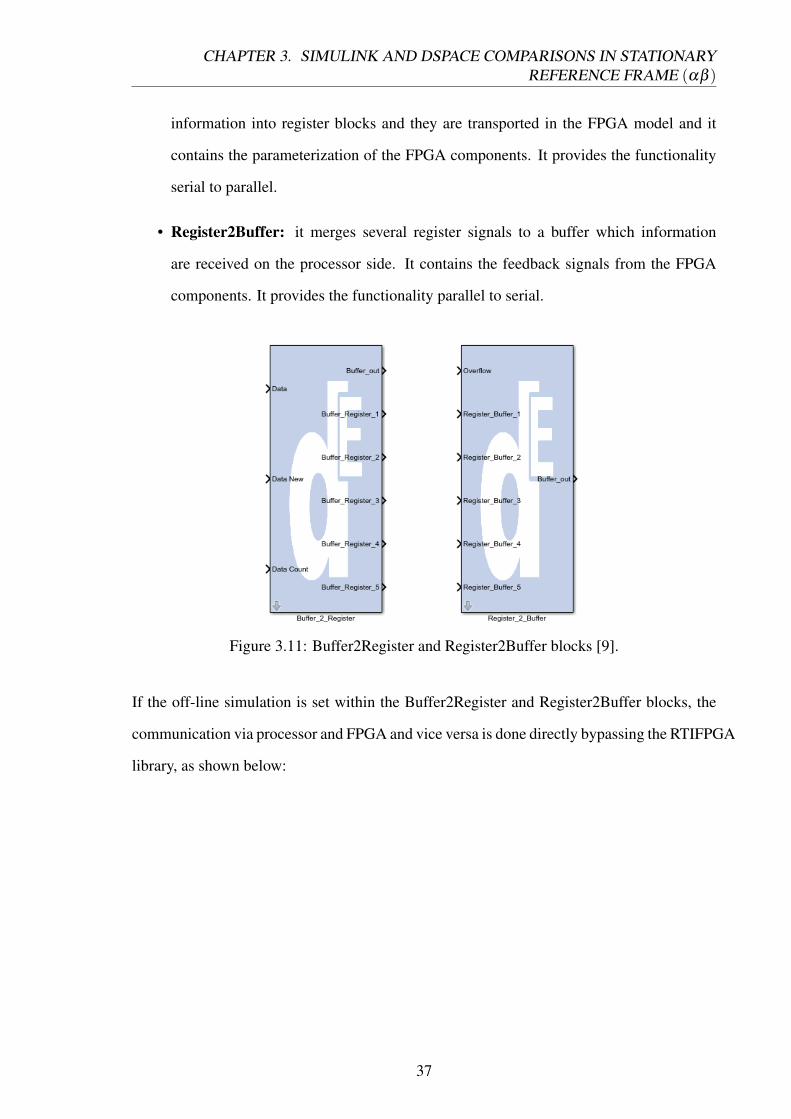
In dSPACE XSG model the processor communicates with the FPGA through the Buffer2Register
and the Register2Buffer blocks.
• Buffer2Register: the buffer is a vector of data from the RTIFPGA library. It has
the task to reads out the buffer on the FPGA side. This information is sent from
the processor side. This information is sent from the processor side. It stores this
36
CHAPTER 3. SIMULINK AND DSPACE COMPARISONS IN STATIONARYREFERENCE FRAME (αβ )
information into register blocks and they are transported in the FPGA model and it
contains the parameterization of the FPGA components. It provides the functionality
serial to parallel.
• Register2Buffer: it merges several register signals to a buffer which information
are received on the processor side. It contains the feedback signals from the FPGA
components. It provides the functionality parallel to serial.
Figure 3.11: Buffer2Register and Register2Buffer blocks [9].
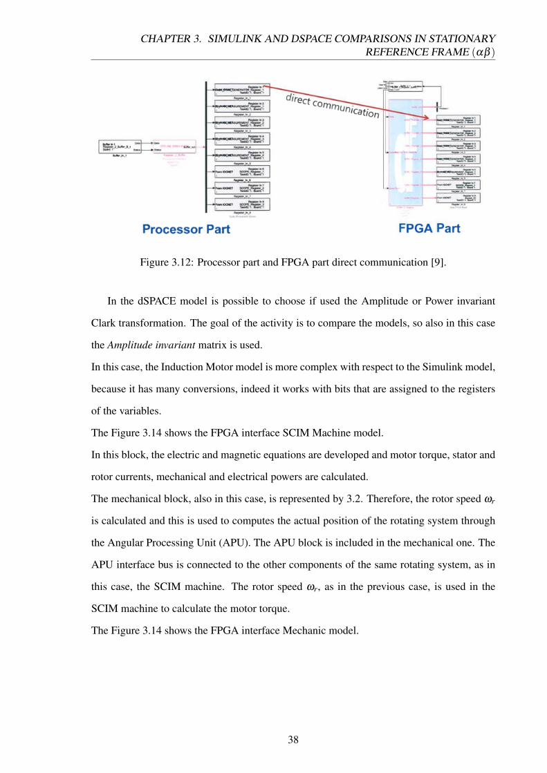
If the off-line simulation is set within the Buffer2Register and Register2Buffer blocks, the
communication via processor and FPGA and vice versa is done directly bypassing the RTIFPGA
library, as shown below:
37
CHAPTER 3. SIMULINK AND DSPACE COMPARISONS IN STATIONARYREFERENCE FRAME (αβ )
Figure 3.12: Processor part and FPGA part direct communication [9].
In the dSPACE model is possible to choose if used the Amplitude or Power invariant
Clark transformation. The goal of the activity is to compare the models, so also in this case
the Amplitude invariant matrix is used.
In this case, the Induction Motor model is more complex with respect to the Simulink model,
because it has many conversions, indeed it works with bits that are assigned to the registers
of the variables.
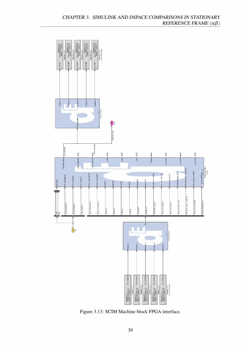
The Figure 3.14 shows the FPGA interface SCIM Machine model.
In this block, the electric and magnetic equations are developed and motor torque, stator and
rotor currents, mechanical and electrical powers are calculated.
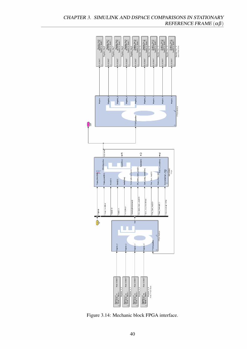
The mechanical block, also in this case, is represented by 3.2. Therefore, the rotor speed ωr
is calculated and this is used to computes the actual position of the rotating system through
the Angular Processing Unit (APU). The APU block is included in the mechanical one. The
APU interface bus is connected to the other components of the same rotating system, as in
this case, the SCIM machine. The rotor speed ωr, as in the previous case, is used in the
SCIM machine to calculate the motor torque.
The Figure 3.14 shows the FPGA interface Mechanic model.
38
CHAPTER 3. SIMULINK AND DSPACE COMPARISONS IN STATIONARYREFERENCE FRAME (αβ )
Figure 3.13: SCIM Machine block FPGA interface.
39
CHAPTER 3. SIMULINK AND DSPACE COMPARISONS IN STATIONARYREFERENCE FRAME (αβ )
Figure 3.14: Mechanic block FPGA interface.
40
CHAPTER 3. SIMULINK AND DSPACE COMPARISONS IN STATIONARYREFERENCE FRAME (αβ )
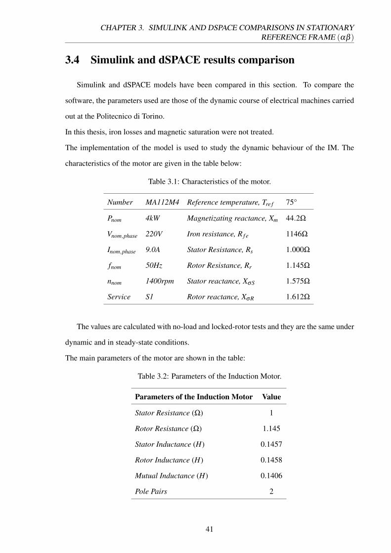
3.4 Simulink and dSPACE results comparison
Simulink and dSPACE models have been compared in this section. To compare the
software, the parameters used are those of the dynamic course of electrical machines carried
out at the Politecnico di Torino.
In this thesis, iron losses and magnetic saturation were not treated.
The implementation of the model is used to study the dynamic behaviour of the IM. The
characteristics of the motor are given in the table below:
Table 3.1: Characteristics of the motor.
Number MA112M4 Reference temperature, Tre f 75°
Pnom 4kW Magnetizating reactance, Xm 44.2Ω
Vnom,phase 220V Iron resistance, R f e 1146Ω
Inom,phase 9.0A Stator Resistance, Rs 1.000Ω
fnom 50Hz Rotor Resistance, Rr 1.145Ω
nnom 1400rpm Stator reactance, XσS 1.575Ω
Service S1 Rotor reactance, XσR 1.612Ω
The values are calculated with no-load and locked-rotor tests and they are the same under
dynamic and in steady-state conditions.
The main parameters of the motor are shown in the table:
Table 3.2: Parameters of the Induction Motor.
Parameters of the Induction Motor Value
Stator Resistance (Ω) 1
Rotor Resistance (Ω) 1.145
Stator Inductance (H) 0.1457
Rotor Inductance (H) 0.1458
Mutual Inductance (H) 0.1406
Pole Pairs 2
41
CHAPTER 3. SIMULINK AND DSPACE COMPARISONS IN STATIONARYREFERENCE FRAME (αβ )
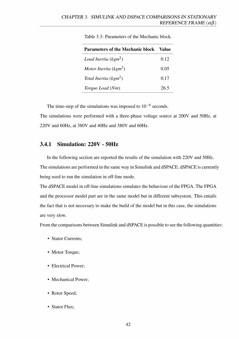
Table 3.3: Parameters of the Mechanic block.
Parameters of the Mechanic block Value
Load Inertia (kgm2) 0.12
Motor Inertia (kgm2) 0.05
Total Inertia (kgm2) 0.17
Torque Load (Nm) 26.5
The time-step of the simulations was imposed to 10−6 seconds.
The simulations were performed with a three-phase voltage source at 200V and 50Hz, at
220V and 60Hz, at 380V and 40Hz and 380V and 60Hz.
3.4.1 Simulation: 220V - 50Hz
In the following section are reported the results of the simulation with 220V and 50Hz.
The simulations are performed in the same way in Simulink and dSPACE. dSPACE is currently
being used to run the simulation in off-line mode.
The dSPACE model in off-line simulations simulates the behaviour of the FPGA. The FPGA
and the processor model part are in the same model but in different subsystem. This entails
the fact that is not necessary to make the build of the model but in this case, the simulations
are very slow.
From the comparisons between Simulink and dSPACE is possible to see the following quantities:
• Stator Currents;
• Motor Torque;
• Electrical Power;
• Mechanical Power;
• Rotor Speed;
• Stator Flux;
42
CHAPTER 3. SIMULINK AND DSPACE COMPARISONS IN STATIONARYREFERENCE FRAME (αβ )
• Rotor Flux.
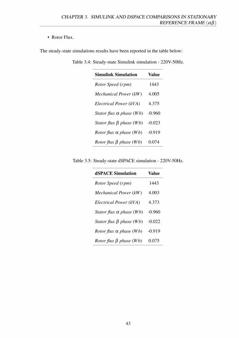
The steady-state simulations results have been reported in the table below:
Table 3.4: Steady-state Simulink simulation - 220V-50Hz.
Simulink Simulation Value
Rotor Speed (rpm) 1443
Mechanical Power (kW ) 4.005
Electrical Power (kVA) 4.375
Stator flux α phase (Wb) -0.960
Stator flux β phase (Wb) -0.023
Rotor flux α phase (Wb) -0.919
Rotor flux β phase (Wb) 0.074
Table 3.5: Steady-state dSPACE simulation - 220V-50Hz.
dSPACE Simulation Value
Rotor Speed (rpm) 1443
Mechanical Power (kW ) 4.003
Electrical Power (kVA) 4.373
Stator flux α phase (Wb) -0.960
Stator flux β phase (Wb) -0.022
Rotor flux α phase (Wb) -0.919
Rotor flux β phase (Wb) 0.075
43
CHAPTER 3. SIMULINK AND DSPACE COMPARISONS IN STATIONARYREFERENCE FRAME (αβ )
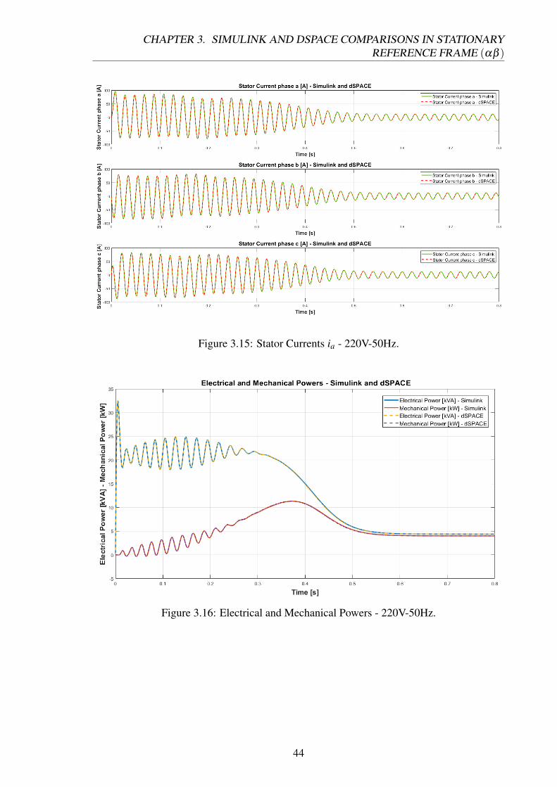
Figure 3.15: Stator Currents ia - 220V-50Hz.
Figure 3.16: Electrical and Mechanical Powers - 220V-50Hz.
44
CHAPTER 3. SIMULINK AND DSPACE COMPARISONS IN STATIONARYREFERENCE FRAME (αβ )
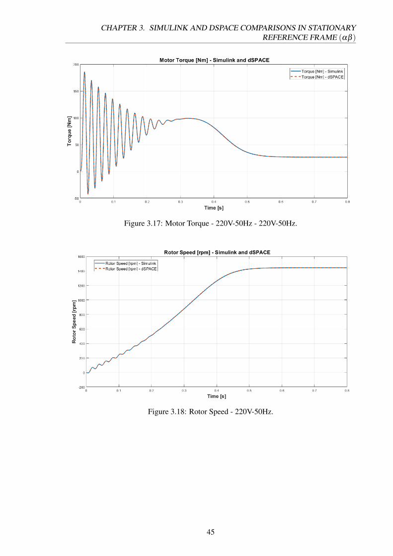
Figure 3.17: Motor Torque - 220V-50Hz - 220V-50Hz.
Figure 3.18: Rotor Speed - 220V-50Hz.
45
CHAPTER 3. SIMULINK AND DSPACE COMPARISONS IN STATIONARYREFERENCE FRAME (αβ )
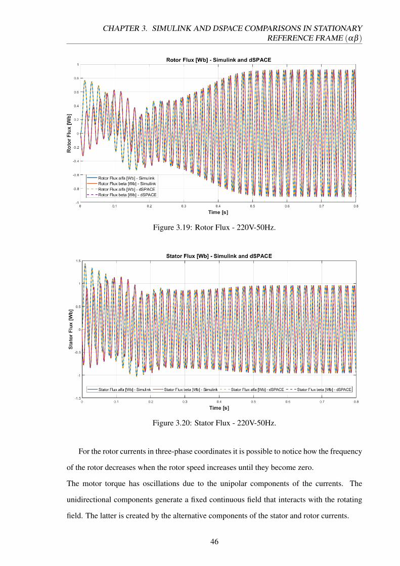
Figure 3.19: Rotor Flux - 220V-50Hz.
Figure 3.20: Stator Flux - 220V-50Hz.
For the rotor currents in three-phase coordinates it is possible to notice how the frequency
of the rotor decreases when the rotor speed increases until they become zero.
The motor torque has oscillations due to the unipolar components of the currents. The
unidirectional components generate a fixed continuous field that interacts with the rotating
field. The latter is created by the alternative components of the stator and rotor currents.
46
CHAPTER 3. SIMULINK AND DSPACE COMPARISONS IN STATIONARYREFERENCE FRAME (αβ )
When the unidirectional components became zero, the motor torque oscillations also become
zero. When the load torque is applied the motor slows down. In this way, the stator currents
are induced.
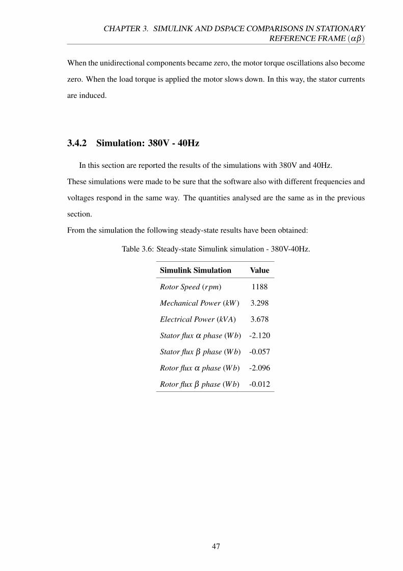
3.4.2 Simulation: 380V - 40Hz
In this section are reported the results of the simulations with 380V and 40Hz.
These simulations were made to be sure that the software also with different frequencies and
voltages respond in the same way. The quantities analysed are the same as in the previous
section.
From the simulation the following steady-state results have been obtained:
Table 3.6: Steady-state Simulink simulation - 380V-40Hz.
Simulink Simulation Value
Rotor Speed (rpm) 1188
Mechanical Power (kW ) 3.298
Electrical Power (kVA) 3.678
Stator flux α phase (Wb) -2.120
Stator flux β phase (Wb) -0.057
Rotor flux α phase (Wb) -2.096
Rotor flux β phase (Wb) -0.012
47
CHAPTER 3. SIMULINK AND DSPACE COMPARISONS IN STATIONARYREFERENCE FRAME (αβ )
Table 3.7: Steady-state dSPACE simulation - 380V-40Hz.
dSPACE Simulation Value
Rotor Speed (rpm) 1187
Mechanical Power (kW ) 3.299
Electrical Power (kVA) 3.678
Stator flux α phase (Wb) -2.120
Stator flux β phase (Wb) -0.055
Rotor flux α phase (Wb) -2.047
Rotor flux β phase (Wb) -0.010
Figure 3.21: Stator Currents ia - 380V-40Hz.
48
CHAPTER 3. SIMULINK AND DSPACE COMPARISONS IN STATIONARYREFERENCE FRAME (αβ )
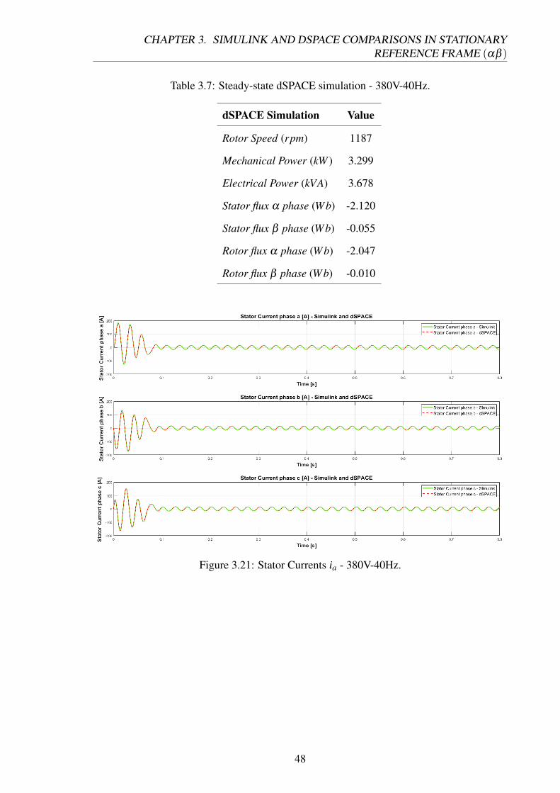
Figure 3.22: Electrical and Mechanical Powers - 380V-40Hz.
Figure 3.23: Motor Torque - 380V-40Hz.
49
CHAPTER 3. SIMULINK AND DSPACE COMPARISONS IN STATIONARYREFERENCE FRAME (αβ )
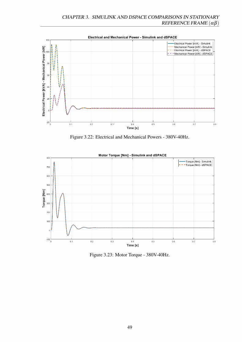
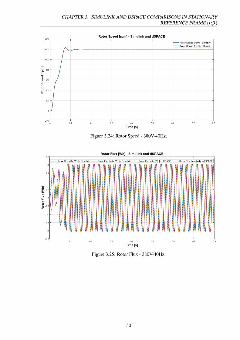
Figure 3.24: Rotor Speed - 380V-40Hz.
Figure 3.25: Rotor Flux - 380V-40Hz.
50
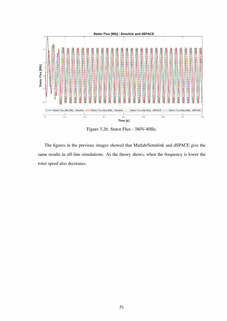
Figure 3.26: Stator Flux - 380V-40Hz.
The figures in the previous images showed that Matlab/Simulink and dSPACE give the
same results in off-line simulations. As the theory shows, when the frequency is lower the
rotor speed also decreases.
51
Chapter 4
Real-time simulations
The difference between real-time simulations and off-line simulations is the time of these.
In the electrical environment, real-time simulations are not a new idea. Hardware in the loop
(HIL) simulations of these systems require an innovative approach.
The real-time simulations can be divided into three groups: [10]
• fully digital simulation;
• controller HIL (CHIL) simulation;
• power HIL (PHIL) simulation.
The topics of this chapter are the real-time simulations of the model described in Chapter 3.
These simulations are made using the (αβ ) and the (dq) reference frame.
As it is possible to see in the previous sections, off-line comparisons are made only in (αβ )
reference frames.
This is because in dSPACE the (dq) reference frames use only time-step 8 · 10−9 seconds
and, in this case, the simulations are very slow.
Therefore, the idea is to create the (dq) model just for a real-time environment.
52
CHAPTER 4. REAL-TIME SIMULATIONS
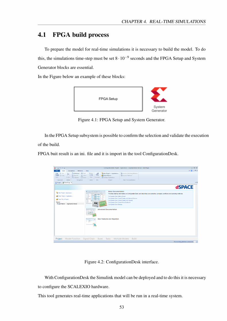
4.1 FPGA build process
To prepare the model for real-time simulations it is necessary to build the model. To do
this, the simulations time-step must be set 8 ·10−9 seconds and the FPGA Setup and System
Generator blocks are essential.
In the Figure below an example of these blocks:
Figure 4.1: FPGA Setup and System Generator.
In the FPGA Setup subsystem is possible to confirm the selection and validate the execution
of the build.
FPGA buit result is an ini. file and it is import in the tool ConfigurationDesk.
Figure 4.2: ConfigurationDesk interface.
With ConfigurationDesk the Simulink model can be deployed and to do this it is necessary
to configure the SCALEXIO hardware.
This tool generates real-time applications that will be run in a real-time system.
53
CHAPTER 4. REAL-TIME SIMULATIONS
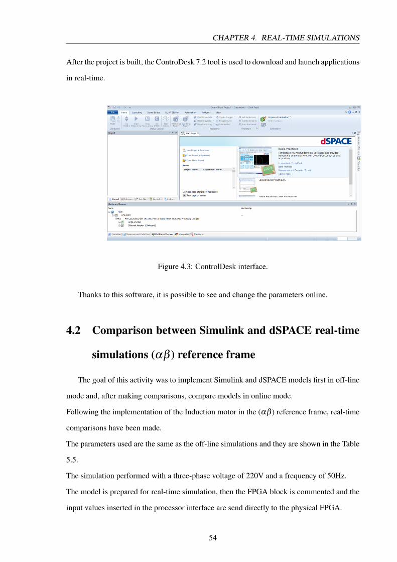
After the project is built, the ControDesk 7.2 tool is used to download and launch applications
in real-time.
Figure 4.3: ControlDesk interface.
Thanks to this software, it is possible to see and change the parameters online.
4.2 Comparison between Simulink and dSPACE real-time
simulations (αβ ) reference frame
The goal of this activity was to implement Simulink and dSPACE models first in off-line
mode and, after making comparisons, compare models in online mode.
Following the implementation of the Induction motor in the (αβ ) reference frame, real-time
comparisons have been made.
The parameters used are the same as the off-line simulations and they are shown in the Table
5.5.
The simulation performed with a three-phase voltage of 220V and a frequency of 50Hz.
The model is prepared for real-time simulation, then the FPGA block is commented and the
input values inserted in the processor interface are send directly to the physical FPGA.
54
CHAPTER 4. REAL-TIME SIMULATIONS
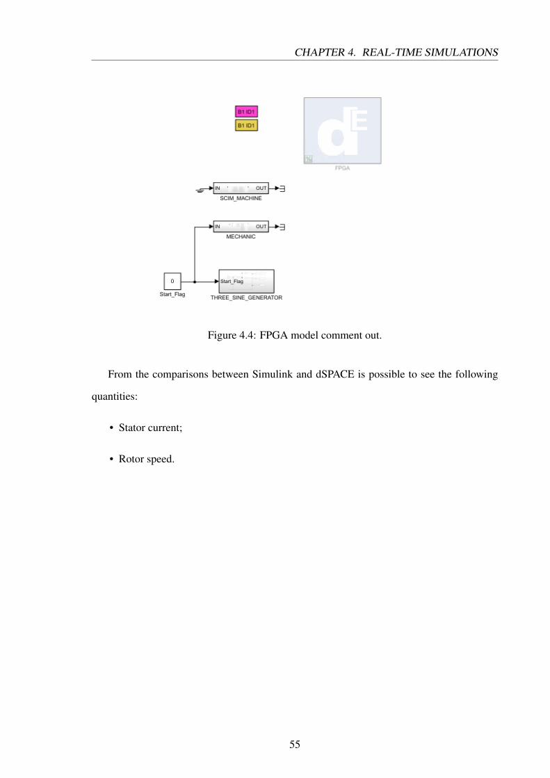
Figure 4.4: FPGA model comment out.
From the comparisons between Simulink and dSPACE is possible to see the following
quantities:
• Stator current;
• Rotor speed.
55
CHAPTER 4. REAL-TIME SIMULATIONS
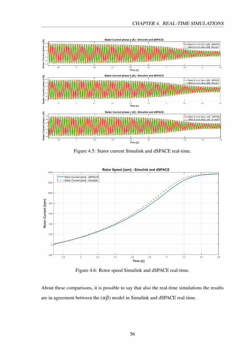
Figure 4.5: Stator current Simulink and dSPACE real-time.
Figure 4.6: Rotor speed Simulink and dSPACE real-time.
About these comparisons, it is possible to say that also the real-time simulations the results
are in agreement between the (αβ ) model in Simulink and dSPACE real-time.
56
CHAPTER 4. REAL-TIME SIMULATIONS
4.3 Comparison between Simulink and dSPACE real-time
simulations (dq) reference frame
As mentioned in the introduction, one of the thesis goals was to develop the model also
in (dq) reference frame, so as to evaluate the response in Matlab/Simulink and in dSPACE.
To make an off-line simulation with FPGA of this model has not been possible, since being
a little diffused model, it was necessary to change too much the dSPACE model. For this
reason, real-time simulations were made directly.
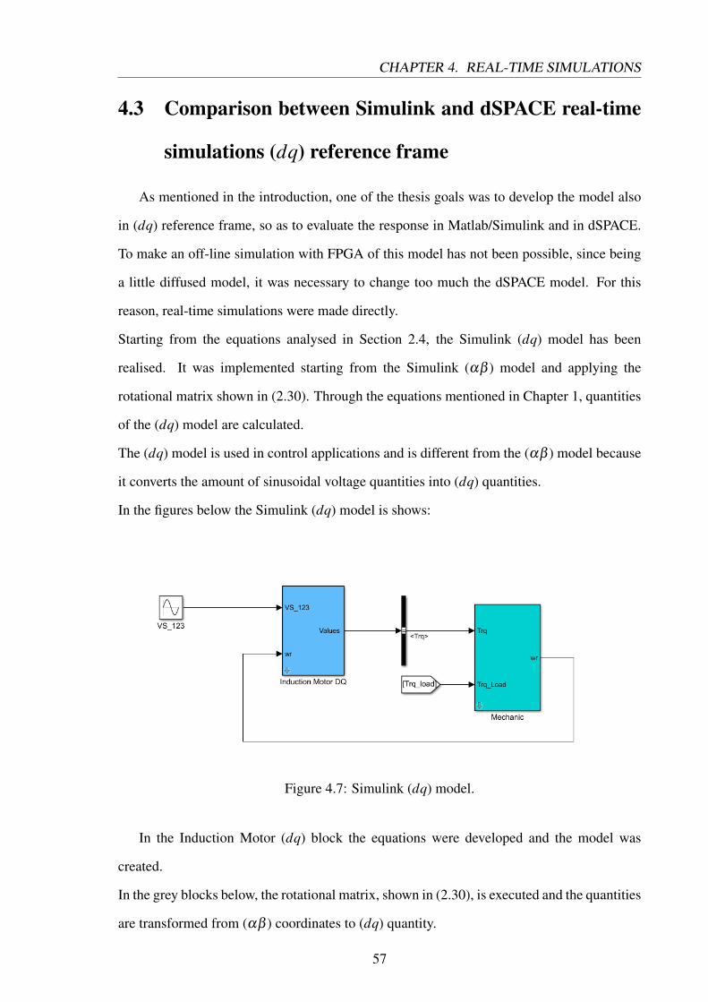
Starting from the equations analysed in Section 2.4, the Simulink (dq) model has been
realised. It was implemented starting from the Simulink (αβ ) model and applying the
rotational matrix shown in (2.30). Through the equations mentioned in Chapter 1, quantities
of the (dq) model are calculated.
The (dq) model is used in control applications and is different from the (αβ ) model because
it converts the amount of sinusoidal voltage quantities into (dq) quantities.
In the figures below the Simulink (dq) model is shows:
Figure 4.7: Simulink (dq) model.
In the Induction Motor (dq) block the equations were developed and the model was
created.
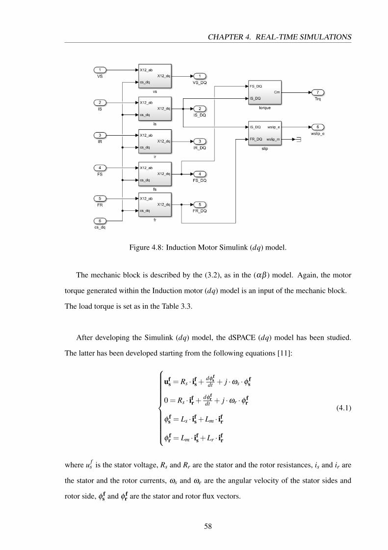
In the grey blocks below, the rotational matrix, shown in (2.30), is executed and the quantities
are transformed from (αβ ) coordinates to (dq) quantity.
57
CHAPTER 4. REAL-TIME SIMULATIONS
Figure 4.8: Induction Motor Simulink (dq) model.
The mechanic block is described by the (3.2), as in the (αβ ) model. Again, the motor
torque generated within the Induction motor (dq) model is an input of the mechanic block.
The load torque is set as in the Table 3.3.
After developing the Simulink (dq) model, the dSPACE (dq) model has been studied.
The latter has been developed starting from the following equations [11]:
ufs = Rs · ifs +
dφ fs
dt + j ·ωs ·φ fs
0 = Rs · ifr +dφ f
rdt + j ·ωr ·φ f
r
φ fs = Ls · ifs +Lm · ifr
φ fr = Lm · ifs +Lr · ifr
(4.1)
where u fs is the stator voltage, Rs and Rr are the stator and the rotor resistances, is and ir are
the stator and the rotor currents, ωs and ωe are the angular velocity of the stator sides and
rotor side, φ fs and φ f
r are the stator and rotor flux vectors.
58
CHAPTER 4. REAL-TIME SIMULATIONS
Lm is the mutual inductance, Ls is the stator inductance and Lr is the rotor inductance.
As in the stationary reference frame (αβ ) the not measurable rotor current as well as the
stator flux are eliminated.
Applying mathematical substitutions within the Equation 4.1, the following system is obtained:
disddt =−( 1
σ ·Ts+ 1−σ
σ ·Tr) · isd +ωs · isq +
1−σ
σ ·Tr·φ ′rd +
1−σ
σ·ω ·φ ′rq + 1
σ ·Ls·usd
disqdt =−ωs · isd− ( 1
σ ·Ts+ 1−σ
σ ·Tr) · isq− 1−σ
σ·ω ·φ ′rd +
1−σ
σ ·Tr·φ ′rq + 1
σ ·Ls·usq
dφ′rd
dt = 1Tr· isd− 1
Tr·φ ′rd +(ωs−ω) ·φ ′rq
dφ′rq
dt = 1Tr· isq− (ωs−ω) ·φ ′rd−
1Tr·φ ′rq
(4.2)
where:
• φ′rd = φrd
Lm
• φ′rq =
φrqLm
• ωr = ωs−ω
By fixing the rotor’s flux vector to the real axis of the coordinate system, the φrq is set to zero.
Debugging the dSPACE model, some inconsistencies appeared.
The clearest inconsistency is the following:
59
CHAPTER 4. REAL-TIME SIMULATIONS
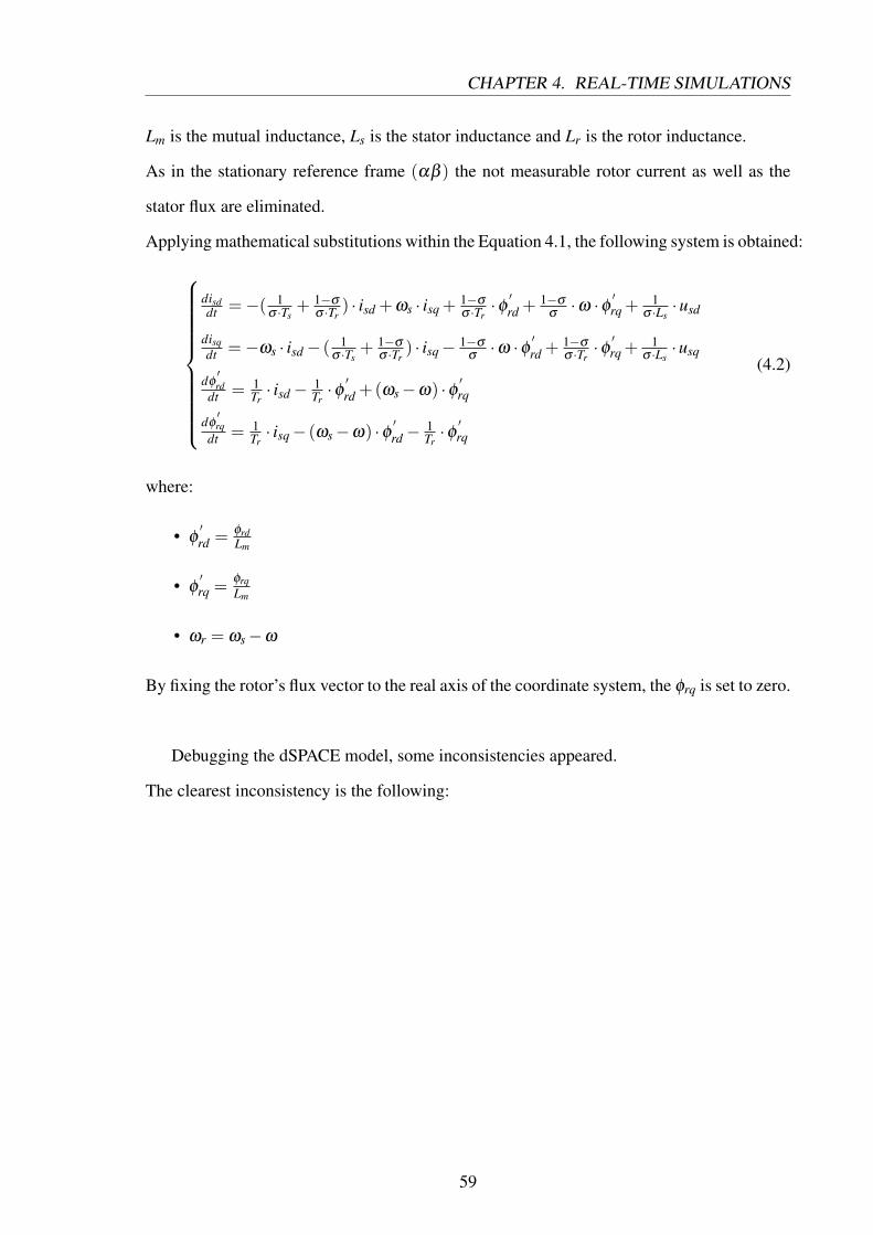
Figure 4.9: Calculate of Mechanical Power dSPACE (dq) model.
60
CHAPTER 4. REAL-TIME SIMULATIONS
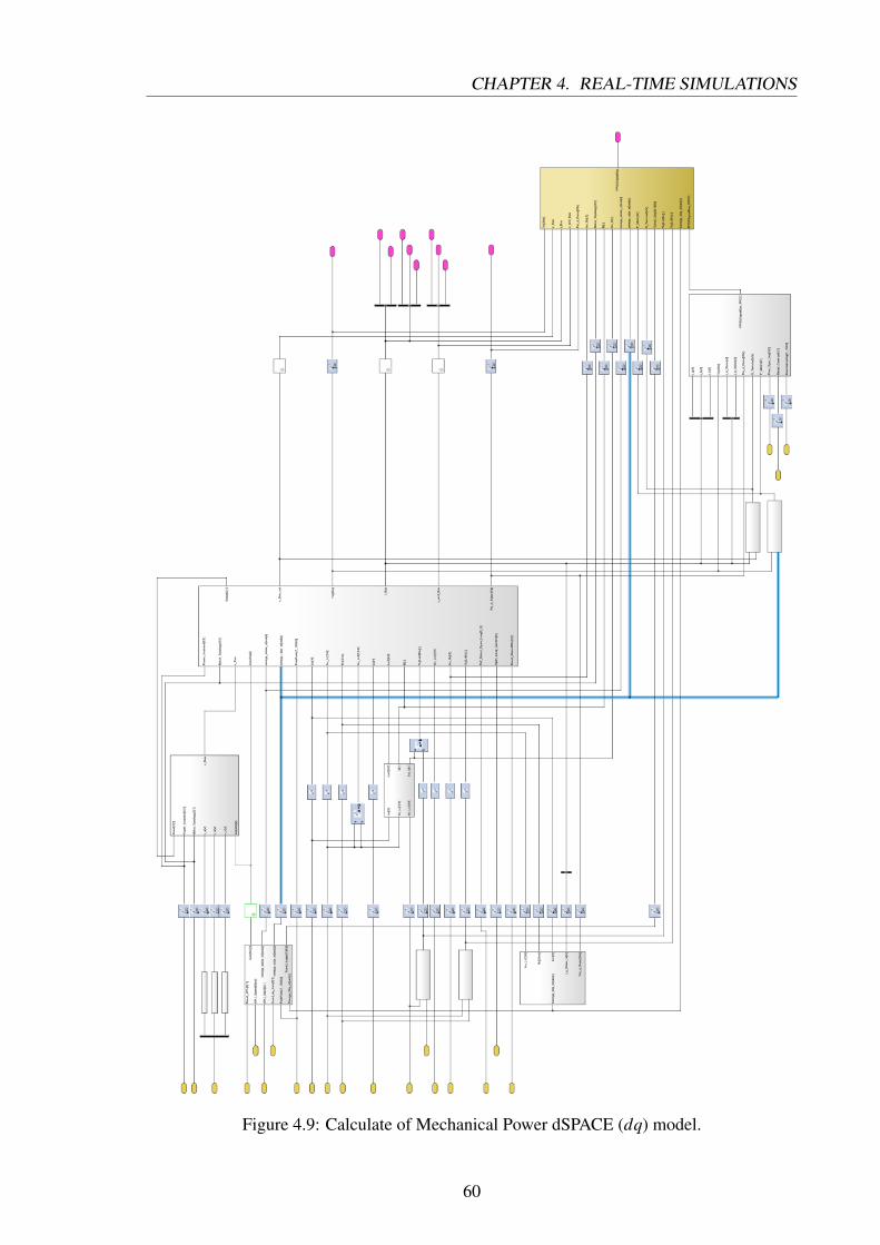
Figure 4.10: Zoom on the blocks to calculate of Mechanical Power dSPACE (dq) model.
Starting from the left block it is possible to notice that in this block are calculated
respectively the rotor electrical speed omega rotor el and the stator electrical speed omega
stator el. In Figure 4.10 are represented the enlarged blocks that dSPACE uses to calculate
the mechanical power.
The rotor speed ωr is equal to:
ωr =ωr(e)
pp(4.3)
where ωr(e) is the rotor electrical speed and pp is the number of Pole Pairs.
The (4.3) is used to evaluate the mechanical power, indeed it is equal to:
Pmech = Tem ·ωr (4.4)
where Tem is shown in the 2.45.
Pmech = Tem ·ωr (4.5)
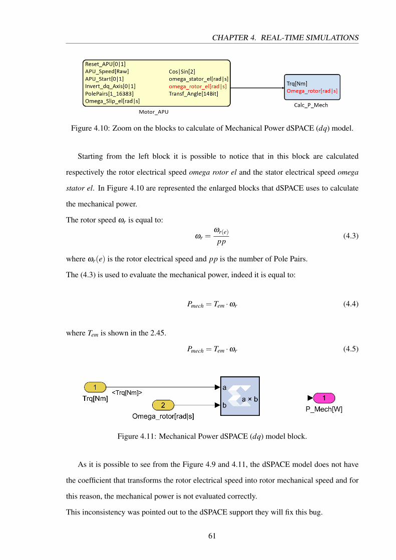
Figure 4.11: Mechanical Power dSPACE (dq) model block.
As it is possible to see from the Figure 4.9 and 4.11, the dSPACE model does not have
the coefficient that transforms the rotor electrical speed into rotor mechanical speed and for
this reason, the mechanical power is not evaluated correctly.
This inconsistency was pointed out to the dSPACE support they will fix this bug.
61
CHAPTER 4. REAL-TIME SIMULATIONS
The other inconsistency concerns the calculation of the stator voltage in the q axis.
Indeed debugging the model it is possible to see that the following term does not appear in
the calculation blocks:1−σ
σ ·Tr· isq (4.6)
To verify this theory, the dSPACE (dq) model was represented in Simulink. From this check,
it immediately became clear that there was an inconsistency in the dSPACE model.
Also in this case, the dSPACE support will provide the model without this bug.
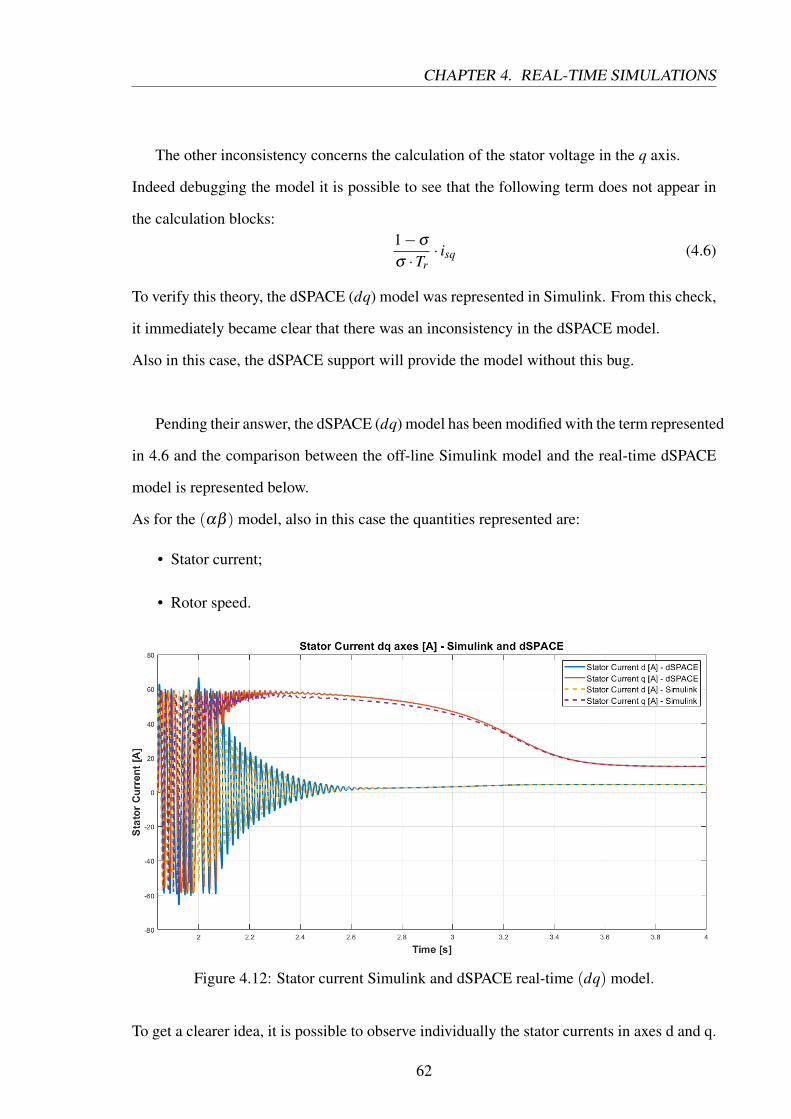
Pending their answer, the dSPACE (dq) model has been modified with the term represented
in 4.6 and the comparison between the off-line Simulink model and the real-time dSPACE
model is represented below.
As for the (αβ ) model, also in this case the quantities represented are:
• Stator current;
• Rotor speed.
Figure 4.12: Stator current Simulink and dSPACE real-time (dq) model.
To get a clearer idea, it is possible to observe individually the stator currents in axes d and q.
62
CHAPTER 4. REAL-TIME SIMULATIONS
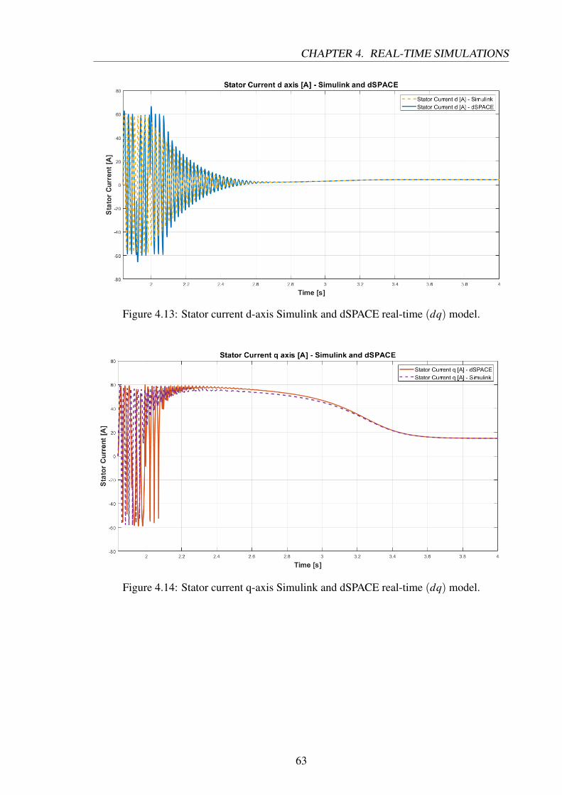
Figure 4.13: Stator current d-axis Simulink and dSPACE real-time (dq) model.
Figure 4.14: Stator current q-axis Simulink and dSPACE real-time (dq) model.
63
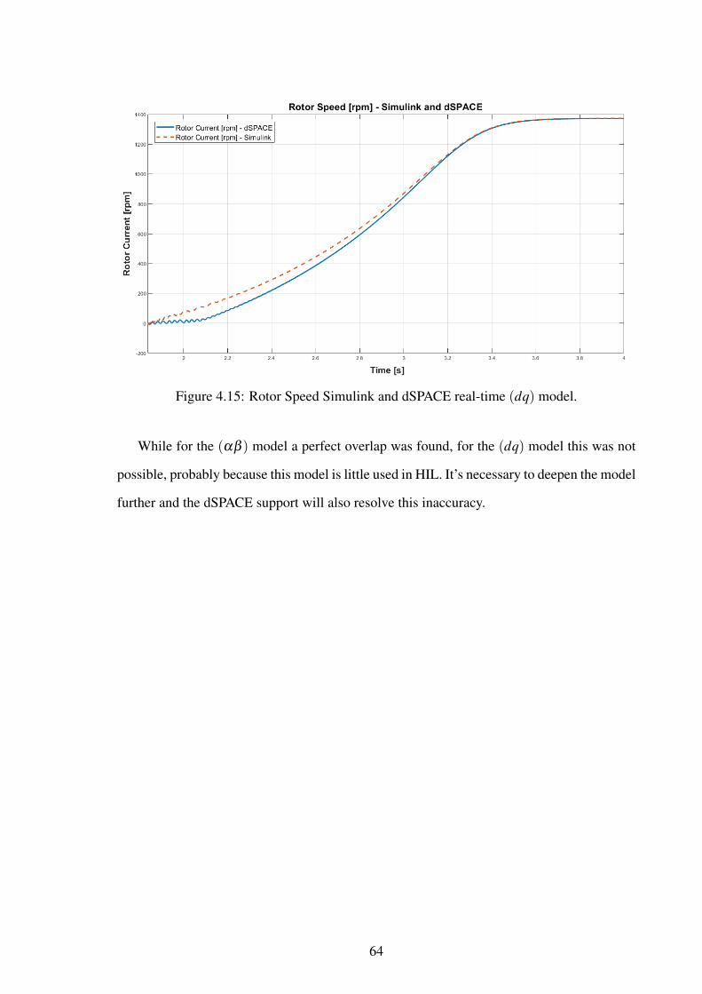
Figure 4.15: Rotor Speed Simulink and dSPACE real-time (dq) model.
While for the (αβ ) model a perfect overlap was found, for the (dq) model this was not
possible, probably because this model is little used in HIL. It’s necessary to deepen the model
further and the dSPACE support will also resolve this inaccuracy.
64
Chapter 5
Validation of the dinamic model
In this chapter, a real IM has been tested on a dedicated test bench in Politecnico di
Torino’s laboratories to get a preliminary validation of the proposed models. The values of
the induction motor are evaluated. These values are calculated with no-load and locked rotor
tests.
To make these tests, the instrumentation used is the induction motor, the TPS/T, the current
transducers and the HBM.
In order to study the dynamics of the system, the tests were carried out with no-load and with
different values of voltages and frequencies.
5.1 Model of the system
The instrumentation used is located in the Politecnico di Torino’s laboratories. The
system used to carry out the experimental tests is illustrated in the following figures.
65
CHAPTER 5. VALIDATION OF THE DINAMIC MODEL
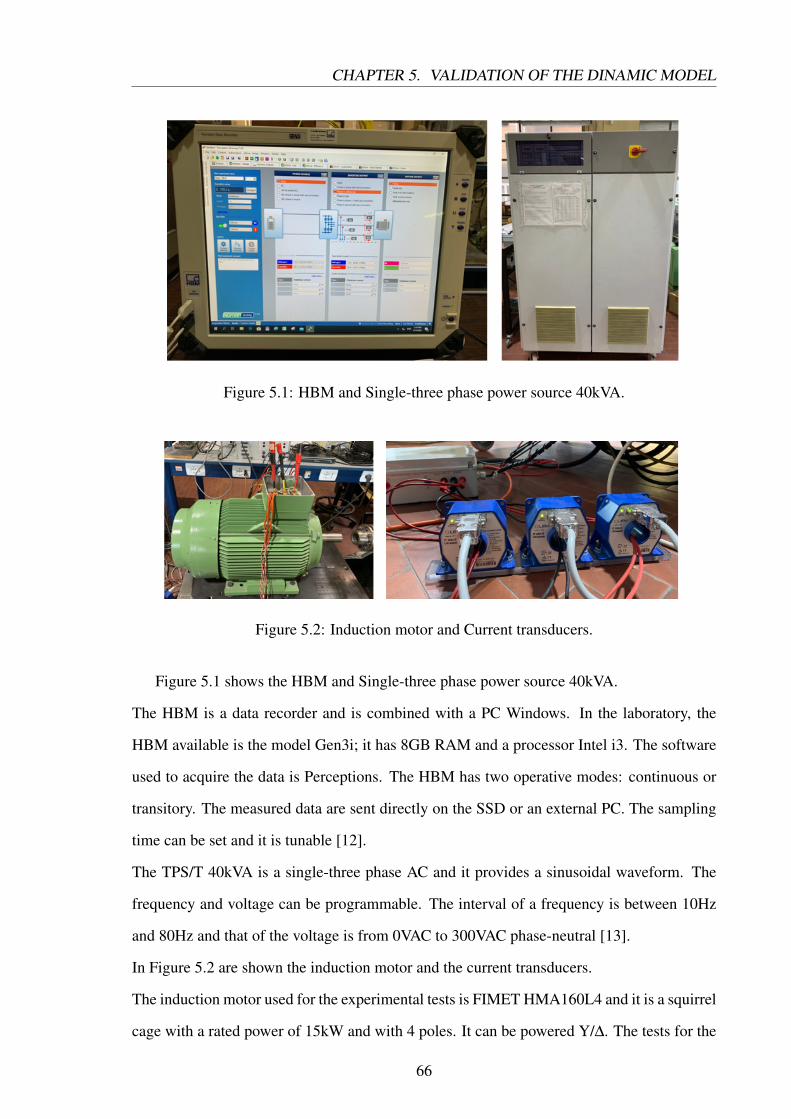
Figure 5.1: HBM and Single-three phase power source 40kVA.
Figure 5.2: Induction motor and Current transducers.
Figure 5.1 shows the HBM and Single-three phase power source 40kVA.
The HBM is a data recorder and is combined with a PC Windows. In the laboratory, the
HBM available is the model Gen3i; it has 8GB RAM and a processor Intel i3. The software
used to acquire the data is Perceptions. The HBM has two operative modes: continuous or
transitory. The measured data are sent directly on the SSD or an external PC. The sampling
time can be set and it is tunable [12].
The TPS/T 40kVA is a single-three phase AC and it provides a sinusoidal waveform. The
frequency and voltage can be programmable. The interval of a frequency is between 10Hz
and 80Hz and that of the voltage is from 0VAC to 300VAC phase-neutral [13].
In Figure 5.2 are shown the induction motor and the current transducers.
The induction motor used for the experimental tests is FIMET HMA160L4 and it is a squirrel
cage with a rated power of 15kW and with 4 poles. It can be powered Y/∆. The tests for the
66
CHAPTER 5. VALIDATION OF THE DINAMIC MODEL
comparisons are made with no-load and with different power supply.
The current transducers used to made the tests are three. The operating temperature is from
-40°C to 85°C. It is used for very high precision current measurements. The secondary
connector is characterized by 9 pin-D-sub [14].
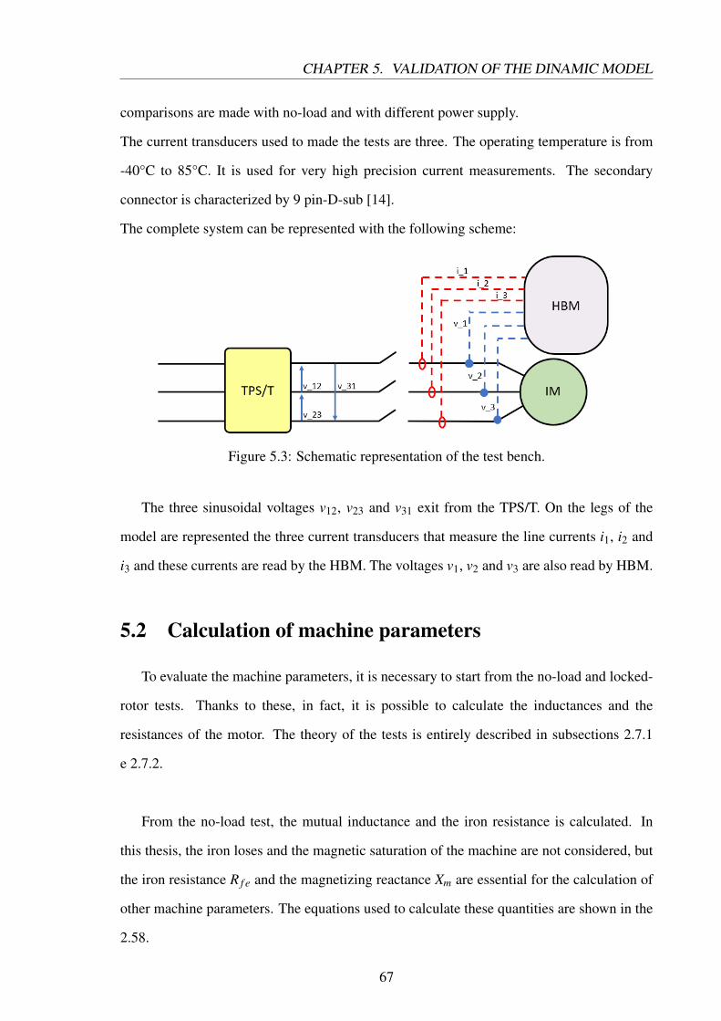
The complete system can be represented with the following scheme:
Figure 5.3: Schematic representation of the test bench.
The three sinusoidal voltages v12, v23 and v31 exit from the TPS/T. On the legs of the
model are represented the three current transducers that measure the line currents i1, i2 and
i3 and these currents are read by the HBM. The voltages v1, v2 and v3 are also read by HBM.
5.2 Calculation of machine parameters
To evaluate the machine parameters, it is necessary to start from the no-load and locked-
rotor tests. Thanks to these, in fact, it is possible to calculate the inductances and the
resistances of the motor. The theory of the tests is entirely described in subsections 2.7.1
e 2.7.2.
From the no-load test, the mutual inductance and the iron resistance is calculated. In
this thesis, the iron loses and the magnetic saturation of the machine are not considered, but
the iron resistance R f e and the magnetizing reactance Xm are essential for the calculation of
other machine parameters. The equations used to calculate these quantities are shown in the
2.58.
67
CHAPTER 5. VALIDATION OF THE DINAMIC MODEL
The other parameters of the motor are calculated with the locked-rotor test. As described
in subsection 2.7.2, the stator and rotor inductances, Xs and Xr, and the stator and rotor
resistances, Rs and Rr, are calculated from the no-load test. The equations used are the 2.59
and 2.60.
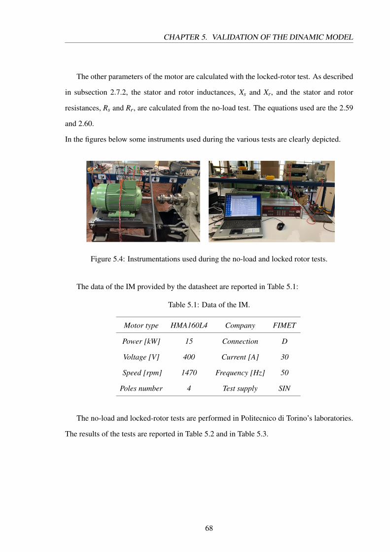
In the figures below some instruments used during the various tests are clearly depicted.
Figure 5.4: Instrumentations used during the no-load and locked rotor tests.
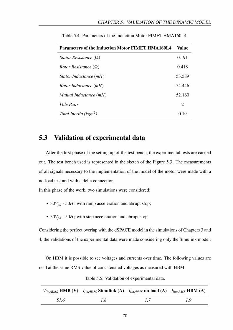
The data of the IM provided by the datasheet are reported in Table 5.1:
Table 5.1: Data of the IM.
Motor type HMA160L4 Company FIMET
Power [kW] 15 Connection D
Voltage [V] 400 Current [A] 30
Speed [rpm] 1470 Frequency [Hz] 50
Poles number 4 Test supply SIN
The no-load and locked-rotor tests are performed in Politecnico di Torino’s laboratories.
The results of the tests are reported in Table 5.2 and in Table 5.3.
68
CHAPTER 5. VALIDATION OF THE DINAMIC MODEL
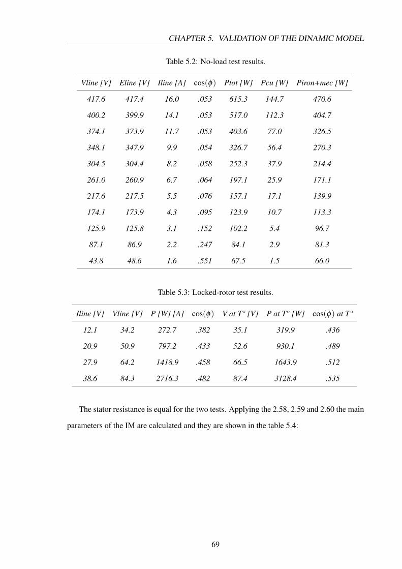
Table 5.2: No-load test results.
Vline [V] Eline [V] Iline [A] cos(φ) Ptot [W] Pcu [W] Piron+mec [W]
417.6 417.4 16.0 .053 615.3 144.7 470.6
400.2 399.9 14.1 .053 517.0 112.3 404.7
374.1 373.9 11.7 .053 403.6 77.0 326.5
348.1 347.9 9.9 .054 326.7 56.4 270.3
304.5 304.4 8.2 .058 252.3 37.9 214.4
261.0 260.9 6.7 .064 197.1 25.9 171.1
217.6 217.5 5.5 .076 157.1 17.1 139.9
174.1 173.9 4.3 .095 123.9 10.7 113.3
125.9 125.8 3.1 .152 102.2 5.4 96.7
87.1 86.9 2.2 .247 84.1 2.9 81.3
43.8 48.6 1.6 .551 67.5 1.5 66.0
Table 5.3: Locked-rotor test results.
Iline [V] Vline [V] P [W] [A] cos(φ) V at T° [V] P at T° [W] cos(φ) at T°
12.1 34.2 272.7 .382 35.1 319.9 .436
20.9 50.9 797.2 .433 52.6 930.1 .489
27.9 64.2 1418.9 .458 66.5 1643.9 .512
38.6 84.3 2716.3 .482 87.4 3128.4 .535
The stator resistance is equal for the two tests. Applying the 2.58, 2.59 and 2.60 the main
parameters of the IM are calculated and they are shown in the table 5.4:
69
CHAPTER 5. VALIDATION OF THE DINAMIC MODEL
Table 5.4: Parameters of the Induction Motor FIMET HMA160L4.
Parameters of the Induction Motor FIMET HMA160L4 Value
Stator Resistance (Ω) 0.191
Rotor Resistance (Ω) 0.418
Stator Inductance (mH) 53.589
Rotor Inductance (mH) 54.446
Mutual Inductance (mH) 52.160
Pole Pairs 2
Total Inertia (kgm2) 0.19
5.3 Validation of experimental data
After the first phase of the setting up of the test bench, the experimental tests are carried
out. The test bench used is represented in the sketch of the Figure 5.3. The measurements
of all signals necessary to the implementation of the model of the motor were made with a
no-load test and with a delta connection.
In this phase of the work, two simulations were considered:
• 30Vph - 50Hz with ramp acceleration and abrupt stop;
• 30Vph - 50Hz with step acceleration and abrupt stop.
Considering the perfect overlap with the dSPACE model in the simulations of Chapters 3 and
4, the validations of the experimental data were made considering only the Simulink model.
On HBM it is possible to see voltages and currents over time. The following values are
read at the same RMS value of concatenated voltages as measured with HBM.
Table 5.5: Validation of experimental data.
VlineRMS HMB (V) IlineRMS Simulink (A) IlineRMS no-load (A) IlineRMS HBM (A)
51.6 1.8 1.7 1.9
70
CHAPTER 5. VALIDATION OF THE DINAMIC MODEL
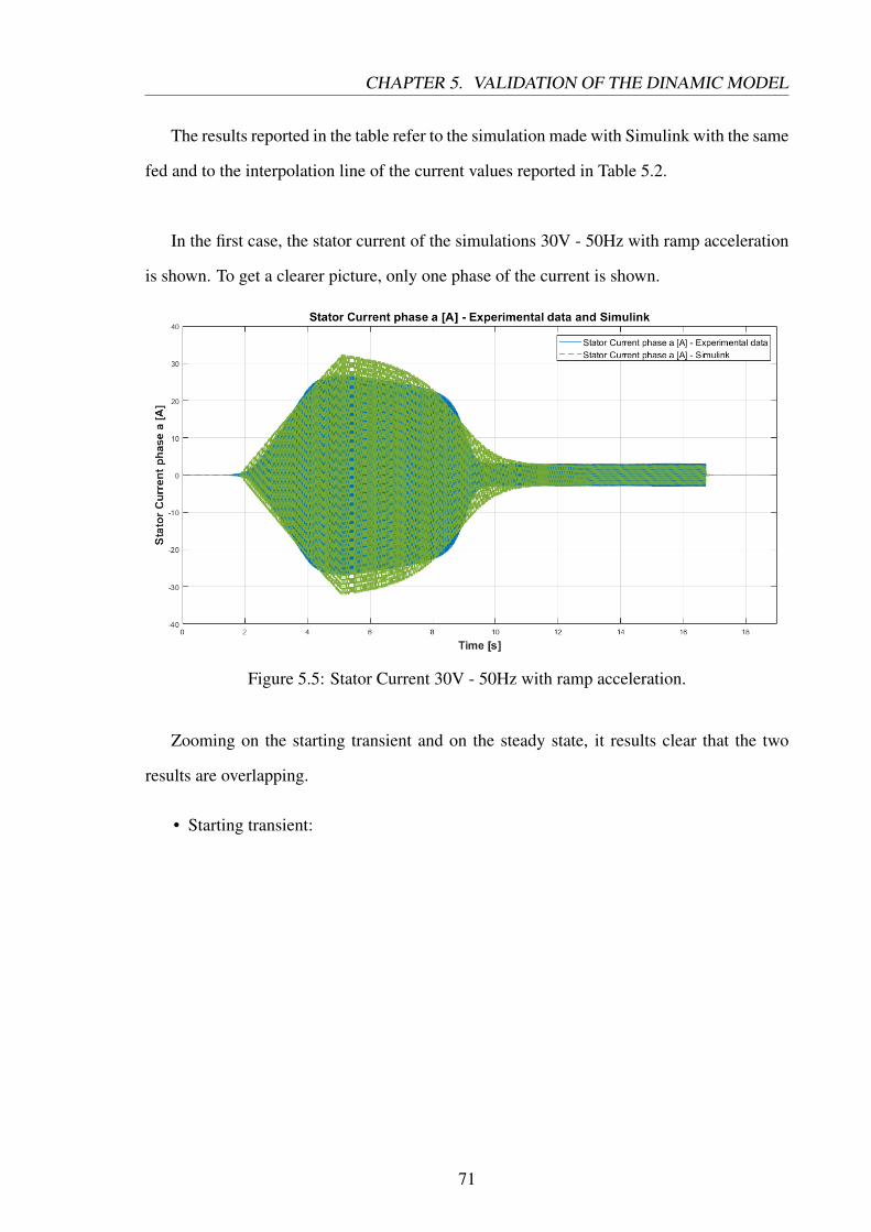
The results reported in the table refer to the simulation made with Simulink with the same
fed and to the interpolation line of the current values reported in Table 5.2.
In the first case, the stator current of the simulations 30V - 50Hz with ramp acceleration
is shown. To get a clearer picture, only one phase of the current is shown.
Figure 5.5: Stator Current 30V - 50Hz with ramp acceleration.
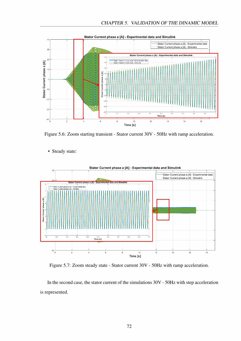
Zooming on the starting transient and on the steady state, it results clear that the two
results are overlapping.
• Starting transient:
71
CHAPTER 5. VALIDATION OF THE DINAMIC MODEL
Figure 5.6: Zoom starting transient - Stator current 30V - 50Hz with ramp acceleration.
• Steady state:
Figure 5.7: Zoom steady state - Stator current 30V - 50Hz with ramp acceleration.
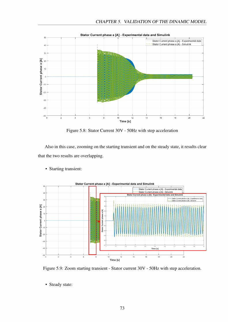
In the second case, the stator current of the simulations 30V - 50Hz with step acceleration
is represented.
72
CHAPTER 5. VALIDATION OF THE DINAMIC MODEL
Figure 5.8: Stator Current 30V - 50Hz with step acceleration
Also in this case, zooming on the starting transient and on the steady state, it results clear
that the two results are overlapping.
• Starting transient:
Figure 5.9: Zoom starting transient - Stator current 30V - 50Hz with step acceleration.
• Steady state:
73
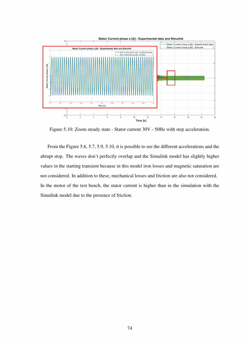
Figure 5.10: Zoom steady state - Stator current 30V - 50Hz with step acceleration.
From the Figure 5.6, 5.7, 5.9, 5.10, it is possible to see the different accelerations and the
abrupt stop. The waves don’t perfectly overlap and the Simulink model has slightly higher
values in the starting transient because in this model iron losses and magnetic saturation are
not considered. In addition to these, mechanical losses and friction are also not considered.
In the motor of the test bench, the stator current is higher than in the simulation with the
Simulink model due to the presence of friction.
74
Chapter 6
Conclusions and next steps
In this thesis work, the mathematical model of the Induction Motor (IM) is analysed and
the equations of the machine have been described. After this, the IM model was developed
in Matlab/Simulink and dSPACE environments. dSPACE is a software that is used for
Hardware in the Loop (HIL) simulations. Through the use of ControlDesk and ConfigurationDesk
it was possible to evaluate the behavior of the IM in real-time.
The first goal of this work was to model the IM in the (αβ ) reference frame in Matlab/Simulink
and later in dSPACE. Once this was done, the dSPACE model was analysed and the model
was debugged. After a careful analysis, it is possible to say that Matlab/Simulink and
dSPACE respond in the same way.
Then, the model was developed in the (dq) reference frame and, as for the model in the
(αβ ) reference frame, also in this case it was first modelled in Matlab/Simulink and then in
dSPACE. The debug of the dSPACE (dq) model of the IM was more complex since in the
model there were some incongruences, recognized by the dSPACE support. For these, the
Matlab/Simulink and the dSPACE models are not perfectly overlapped and this is due to the
many delays and bits dSPACE uses.
In Matlab/Simulink also the mathematical model of the Voltage Source Inverter (VSI) has
been developed. The VSI was used to feed the motor and see its behaviour.
In this work, the motor was developed without modelling the iron losses and the magnetic
saturation and no account was taken of the friction.
75

CHAPTER 6. CONCLUSIONS AND NEXT STEPS
In the future, to have a more complete machine modelling, it would be appropriate to make
an IM model with these characteristics.
One could think of feeding the IM with a Voltage Source Inverter (VSI) and not with three
sinusoidal voltages.
VSI can be useful for future activities related to engine control and can be implemented with
Pulse Width Modulation (PWM).
76

Bibliography
[1] Hussein Khreis, Deflorio Andrea, and Miguel Ruiz De Larramendi. Sensitivity Analysis
for Induction Machine Manufacturing Tolerances in EV and HEV. IEEE, 2015.
[2] Kavita B. Hunasikatti, Raghuram L Naik, and Basayya V Hiremath. Implementation
of FPGA Based Closed Loop V/f Speed Control of Induction Motor Employed for
Industrial Applications. IEEE, 2018.
[3] Rik De Doncker. Electric drives analysis, modeling, Control (power Systems). Springer,
2011.
[4] Andrea Cavagnino. Macchine Elettriche II. 2018.
[5] Antonino Fratta. Dispense del corso di Conversione Statica dell’Energia Elettrica.
1998.
[6] Sandro Rubino. Controllo di tensione Inverter Trifase VSI. 2020.
[7] dSPACE GmbH. XSG Electric Library. dSPACE GmbH, Version 19.2 - 01 2020.
[8] https://www.dspace.com/en/inc/home/products/hw/simulator_hardware/scalexio/ds6602-
fpga-base-board.cfm#175_55653.
[9] dSPACE GmbH. FPGA Basic Training. dSPACE GmbH, 2020.
[10] Xavier Guillaud, M. Omar Faruque, and Alexandre Teninge. Applications of Real-
Time Simulation Technologies in Power and Energy Systems. IEEE, 2015.
[11] Nguyen Phung Quang and Jörg-Andreas Dittrich. Vector Control of Three-Phase AC
Machines. System Development in the Practice. Springer, 2015. ISBN: 9783662469149.
[12] https://www.hbm.com/it/4483/genesis-highspeed-mainframes-with-integrated-pc/.
78

BIBLIOGRAPHY
[13] http://www.elettrotestspa.it/wp/wp-content/uploads/2015/03/Brochure-TPS40K.pd f .
[14] http://www.farnell.com/datasheets/2150002.pdf.
79
Top Related
Copyright © 2022 FDOKUMEN

