Download - A Polynomial Time Approximation Scheme for k-Consensus Clustering

A Polynomial Time Approximation Scheme for k-Consensus Clustering∗

Tom Coleman† Anthony Wirth‡

Abstract

This paper introduces a polynomial time approxima-tion scheme for the metric Correlation Cluster-ing problem, when the number of clusters returned isbounded (by k). Consensus Clustering is a funda-mental aggregation problem, with considerable applica-tion, and it is analysed here as a metric variant of theCorrelation Clustering problem. The PTAS ex-ploits a connection between Correlation Cluster-ing and the k-cut problems. This requires the intro-duction of a new rebalancing technique, based on mini-mum cost perfect matchings, to provide clusters of therequired sizes.

Both Consensus Clustering and CorrelationClustering have been the focus of considerable recentstudy. There is an existing dichotomy between thek-restricted Correlation Clustering problems andthe unrestricted versions. The former, in general, admita PTAS, whereas the latter are, in general, APX-hard.This paper extends the dichotomy to the metric case,responding to the result that Consensus Clusteringis APX-hard to approximate.

∗The authors acknowledge the support of the Australian

Research Council and the Stella Mary Langford scholarship fund.†The University of Melbourne‡The University of Melbourne

1 Introduction

In this paper, we present a polynomial-time approxima-tion scheme for the k-Consensus Clustering prob-lem. The interest in this problem, and our solution toit, lies in the following three areas.

Application Consensus Clustering, in whichwe are asked to produce a single clustering that bestsummarizes a number of input clusterings, is a naturalexample of an aggregation problem. It bears somesimilarity to Rank Aggregation, which is usefulfor combining the outputs of a collection of searchtools. There will be situations in which a user wishesto restrict the number of clusters returned from thisprocess, perhaps due to some prior knowledge, whichmotivates the study of k-Consensus Clustering.

Answering a theoretical question With theparticular metric we use to describe the distancebetween two clusterings, the Consensus Cluster-ing problem becomes a special case of the metric-Correlation Clustering problem. There is a di-chotomy between variants of the Correlation Clus-tering problem in which there is no restriction on thenumber of clusters returned, and those that have a (k-)bound on the number of clusters returned. The latterare frequently easier to approximate (see below), andwe show that this dichotomy extends to metric variants.There has been considerable recent interest in the ap-proximability of the Consensus Clustering [1] andRank Aggregation problems [6, 20]. In particular,Bonizzoni et al. showed that Consensus Clusteringis APX-hard [5]; our paper is a response to this result.

We have recently learnt that, in work simultane-ous to ours, two other papers have each produced aPTAS for k-Consensus Clustering [4, 19]. Boniz-zoni et al.’s result is an extension of Giotis and Gu-ruswami’s [16] PTAS for Correlation Clusteringon 0/1-weighted graphs. Karpinski and Schudy’s PTASis part of a broader study of PTASes for Constraint Sat-isfaction Problems. The PTAS in this paper extends tothe (more general) metric-Correlation Clusteringproblem.

Theoretical techniques This paper is the firstto develop an explicit link between results and proofapproaches to k-Cut problems and those for k-

729 Copyright © by SIAM. Unauthorized reproduction of this article is prohibited.

Correlation Clustering (also called k-CC) prob-lems. We observe that once the optimum cluster sizeshave been determined—in a k-restricted problem thiscan be done by guessing—we ought to be able to trans-form k-Cut-inspired algorithms to k-CC. Developingthe techniques to achieve this is the nub of this paper.

With these points in mind, we open the paper withsome background concerning the Consensus Clus-tering and Correlation Clustering problems, andtheir link to k-Cut problems.

2 Background

2.1 Problem definitions In the Consensus Clus-tering problem, we are given m input clusteringsC1, C2, . . . , Cm of some collection of items and a metric∆ on the clusterings. The task is to return a single clus-tering, C, of the collection that minimizes

∑i ∆(C, Ci),

that is, a median clustering.The Mirkin metric, commonly used in the theory

community, states that the distance between two clus-terings is the number of pairs of items that are separatedin one clustering yet co-clustered in the other cluster-ing. We now cast this as a graph problem and, there-fore, view pairs of items as edges in a graph. If we letwc(e) be the proportion of the Ci that separate theendpoints of e and wu(e) be the proportion that clusterthem together, then our objective is to minimize

(2.1)∑

e∈Ec(C)

wu(e) +∑

e∈Eu(C)

wc(e) ,

where Ec(C) are the edges that are cut by C and Eu(C)those not cut by C. In fact, Equation 2.1 is exactlythe min-CC objective [1]; we note in passing that thecomplementary max-CC objective is∑

e∈Ec(C)

wc(e) +∑

e∈Eu(C)

wu(e) .

Now, when the edge weights wu and wc are gener-ated from a Consensus Clustering instance, the wc

quantities obey the triangle inequality. We can thereforeview Consensus Clustering as a specific case of themetric version of min-CC, which is the problem thatwill be the principal focus of this paper. Henceforth, wewill refer to wc as δ and wu as 1 − δ. The Consen-sus Clustering min-CC and max-CC problems, andrelatives, can be specified to have an upper bound, k,on the number of clusters produced, which is of utmostrelevance to us here.

2.2 Our observations There has been some priorwork on PTASes for the metric k-Cut and min-k-uncut problems, which we introduce below. The stan-dard objectives for these problems are max-k-Cut(C) =

∑e∈Ec(C) δ(e) and min-k-Uncut(C) =

∑e∈Eu(C) δ(e).

The inspiration for the proof approach in this papercame from the following observation.

max-k-CC(C)

= 2∑Ec(C)

δ(e) +∑Eu(C)

(1− δ(e))−∑Ec(C)

δ(e)

= 2 max-k-Cut(C) + |Eu(C)| −∆

(2.2a)

min-k-CC(C)

= 2∑Eu(C)

δ(e) +∑Ec(C)

(1− δ(e))−∑Eu(C)

δ(e)

= 2 min-k-Uncut(C) + |Ec(C)| −∆ ,

(2.2b)

where ∆ is the sum of the edge weights:∑e δ(e) (a

constant). If we find a good approximation to min-k-uncut with the same cluster sizes (and thus thesame number of edges cut) as the optimal min-k-CCsolution, we have a good approximation to min-k-CC.The existing algorithms for the metric min-k-uncutproblem do not, however, provide a sufficient guaranteeconcerning the consequent cluster sizes.

As far as the authors are aware, there is no previ-ous work on metric min-k-uncut cut problems withconstrained cluster sizes. Fernandez de la Vega etal. [10] made some progress with a PTAS for the metric-min-Bisection problem; they conjecture that it couldlead to an algorithm for metric-min-2-uncut with con-strained cluster sizes.

Our contribution, therefore, is to add significantcomponents to these algorithms so that we can obtainappropriate cluster sizes. We achieve this principallythrough a novel re-balancing step, based on a BipartiteMatching problem, which we analyse in Section 5.3.There are many other technical details that we developto incorporate the re-balancing.

2.3 Applications Gionis et al. highlight a numberof applications of Consensus Clustering algorithms.These include: clustering categorical data, where weview each category as a separate clustering of the samedata, clustering heterogeneous data, dealing with miss-ing values in some attribute, inferring the correct num-ber of clusters (though not in the k-restricted case), de-tecting outliers, making more robust clusterings, andpreserving privacy [15]. Filkov and Skiena apply Con-sensus Clustering to the task of combining clusteringsolutions from diverse microarray data sources, incorpo-rating noise elimination [13].


2.4 Prior work on Consensus Clustering andCorrelation Clustering Table 1 summarizes the ap-proximation results for the variants of ConsensusClustering, providing a context for our contributions.We note a few results that are of particular relevance tothis paper.

The Correlation Clustering problem was firstintroduced to the theory community by Bansal et al. [3].Giotis and Guruswami [16] were the first to investigatethe fixed-k (number of clusters) case, providing a PTASfor 0/1 instances for both min-k-CC and max-k-CC. Itis was not clear to us how to extend their result to arbi-trary, or even metric or consensus-based weights; Boniz-zoni et al. were, however, able to exploit a connectionto the Giotis and Guruswami PTAS [4]. In the con-text of metric weights, Ailon et al. [1] showed that theirLP-based algorithm is a 2-approximation for generalmetric-min-CC and, further, an 11/7-approximation forConsensus Clustering. The minimisation versionof Consensus Clustering is known to be APX-hardeven with just three input clusterings [5].

2.5 Outline of paper In the next section, we thenprovide an overview of the theoretical techniques, beforedeveloping them in full in the remainder of the paper.In Section 4 we describe the algorithms in sufficientdetail to understand their operation. Their full details,and the justification of their properties, are developedin Section 5. The Appendix contains all proofs oftheorems, lemmas, et cetera that are not presented inthe main text.

3 Proof Techniques

In order to understand our PTASes for max-k-CC andmin-k-CC, we must grasp the basic intuition behind thePTASes for the metric min-k-uncut problem [18, 11].

3.1 Maximization The maximization PTAS formetric-max-k-cut was developed by Fernandez de laVega and Kenyon [12], based on (amongst others) thedense-Max-Cut PTAS of Arora et al. [2]. For k-CC,we can use another dense-max-k-cut PTAS, by Friezeand Kannan [14], in a straightforward way to give aPTAS for the metric-max-k-CC problem, exploitingthat PTAS’s ability to work on negatively-weighted in-stances. We demonstrate this approach in Section 4.1.

3.2 Minimization The idea is to employ a maxi-mization PTAS for a minimization problem. For someinstances, a good maximization approximation is notgood for the minimization objective, as the optimal min-imization objective is very low. However, such instanceshave (other) special properties. Indeed, Indyk [18], and

subsequently Fernandez de la Vega et al. [11], exploita well-separatedness quality of min-k-uncut instancesthat are not approximable by the max-k-cut PTAS.They show that an algorithm based on representativesampling will lead to a good-quality solution to themetric-min-k-uncut problem. In Section 5.4, we willshow that the pairs of clusters in min-k-CC instancesthat the max-k-CC PTAS does not approximate wellalso share the same well-separatedness quality, and thuscan be separated by representative sampling.

Phases of the PTAS Fernandez de la Vega et al.’salgorithm for metric min-k-uncut operates in threebasic phases. In phase one, they sample representativesin order to approximately separate large clusters fromone another.1 In phase two, they extract small clusters(which could not be obtained by sampling). In phasethree they apply a maximisation PTAS to properlyseparate the large clusters that could not be easilyseparated in phase one, because they were too close toone another.

For the min-k-CC problem, in addition to exploit-ing the closeness of the clusters, a PTAS would need tofollow Equation 2.2b. That is, the PTAS would needto ensure that the number of edges cut is the same asthe optimal solution; this is ensured by obtaining thecorrect cluster sizes. Fernandez de la Vega et al.’s al-gorithm makes no guarantee about cluster sizes, andthere is no straightforward way to ensure that it does.We therefore develop a new phase two, which achievesFernandez de la Vega et al.’s purpose (separating smallclusters), but has the additional, more important prop-erty of ensuring correct sizes of all clusters.

A Perfect Matching We achieve the correct clus-ter sizes in phase two by solving a perfect matchingproblem instance. In order to analyse this matchingand bound the cost of the clustering that it generates,we develop a novel approach, which could be used forany application of such a matching step. The idea is tobound the mistakes that the matching makes in assign-ing points to clusters.

The key technique here is the use of pairing func-tions. These functions pair a point v that, at the end ofphase two, should have, according to the optimal solu-tion, been in a particular cluster, but was not, with an-other point, p(v), that was placed in that cluster at theend of phase two, but should not have been. Throughjudicious choice of such a pairing function p, we ob-tain for each relevant mis-classified point, a small orbitof points that could be simultaneously re-classified toreach an alternative clustering that is also a potentialsolution to the matching problem. In this way, we can

1Concepts such as large will be defined carefully in Section 5.


Table 1: Summary of approximation results for k-CC and k-Cut type problems. Our contributions are indicatedby (∗). Note that in most cases a problem is APX-hard if the number of output clusters is not restricted, but hasa PTAS if there is a k-bound.

MAX MIN

unrestricted fixed-k unrestricted fixed-k

k-Cut N/A N/A` 0/1 0.878 [17, 21]` dense PTAS [2]` metric PTAS [12] PTAS [18, 11]

k-CC` 0/1 PTAS [3] PTAS [16] 3 [3, 7, 1] PTAS [16]

APX-hard [7]` weighted 0.7666 [7, 22] APX-hard [9, 7]

APX-hard [7]` metric PTAS (∗) 2 [1] PTAS (∗)` consensus PTAS (∗) 11/7 [1] PTAS (∗) [4, 19]

APX-hard [5]

make the smallest number of changes possible to theoptimal clustering in order to achieve the essential fea-tures of our output clustering (that is, the observanceof group boundaries).

4 The Algorithms

4.1 Maximization The first step for the max-k-CCalgorithm is to form a new set of edge weights (someof which may be negative) thus. Define G = (V,E, δ),where δ = 2δ − 1. The second step is to apply Friezeand Kannan’s PTAS for dense max-k-cut to G [14].

The following theorem of Frieze and Kannan, com-bined with the fact that the optimum solution must beat least |E|/2, shows that the two comprise a PTAS formetric max-k-CC.

Theorem 1. (Frieze and Kannan [14], Thm 1)There is an algorithm, that given a graph G = (V,E, w),with weight function w : E → [−1, 1], and a fixed ε > 0,computes in polynomial time a k-clustering C such that:

max-k-Cut(C) ≥ max-k-Cut∗−εn2

Corollary 1. If |E| ∈ Ω(n2), then the Frieze-Kannanalgorithm, acting on G provides a PTAS for max-k-CC(on G).

4.2 Minimization Recall that, following the style ofFernandez de la Vega et al.’s PTAS for min-k-uncut,our algorithm operates in a number of phases.

Phase Zero: Guess the size |Ci| of each cluster inthe optimal solution C; we assume |Ci| ≥ |Ci+1|.Given these sizes, let k0 be the number of clusters

that are large, also guessed. Guess a function gthat assigns the large clusters to groups; a groupconsists of a contiguous subsequence of the Ci inwhich Ci and Ci+1 are close. The small clustersare assigned to a single group, separate from thelarge clusters. For each large cluster Ci, uniformlysample a point ci ∈ V . If ci satisfies some centralityproperty, defined in Section 5, we say that ci isa representative of Ci. Section 5 shows that thishappens with sufficiently high probability for alllarge clusters.

Phase One: Define a clustering D1 by assigning eachpoint v ∈ V to the large cluster such that the quan-tity |Ci|δ(v, ci)—an estimate of

∑x∈Ci

δ(v, x)—isminimised.

Phase Two: Define D2 by solving the following Bi-partite Matching problem:

1. Guess the number of mistakes made by PhaseOne. That is, let Fii′ = Ci ∩ D1

i′ , and guessthe size of each Fii′ . For each i, i′ we thereforewish to place |Fii′ | points from D1

i′ in D2i .

2. The cost of placing v in D2i we define to be

δi(v) =

|Ci|δ(v, ci) if Ci is large, or0 if Ci is small.

3. We can choose a D2, subject to the |Fii′ |terms, to minimise the total δ using an ap-plication of Bipartite Matching.


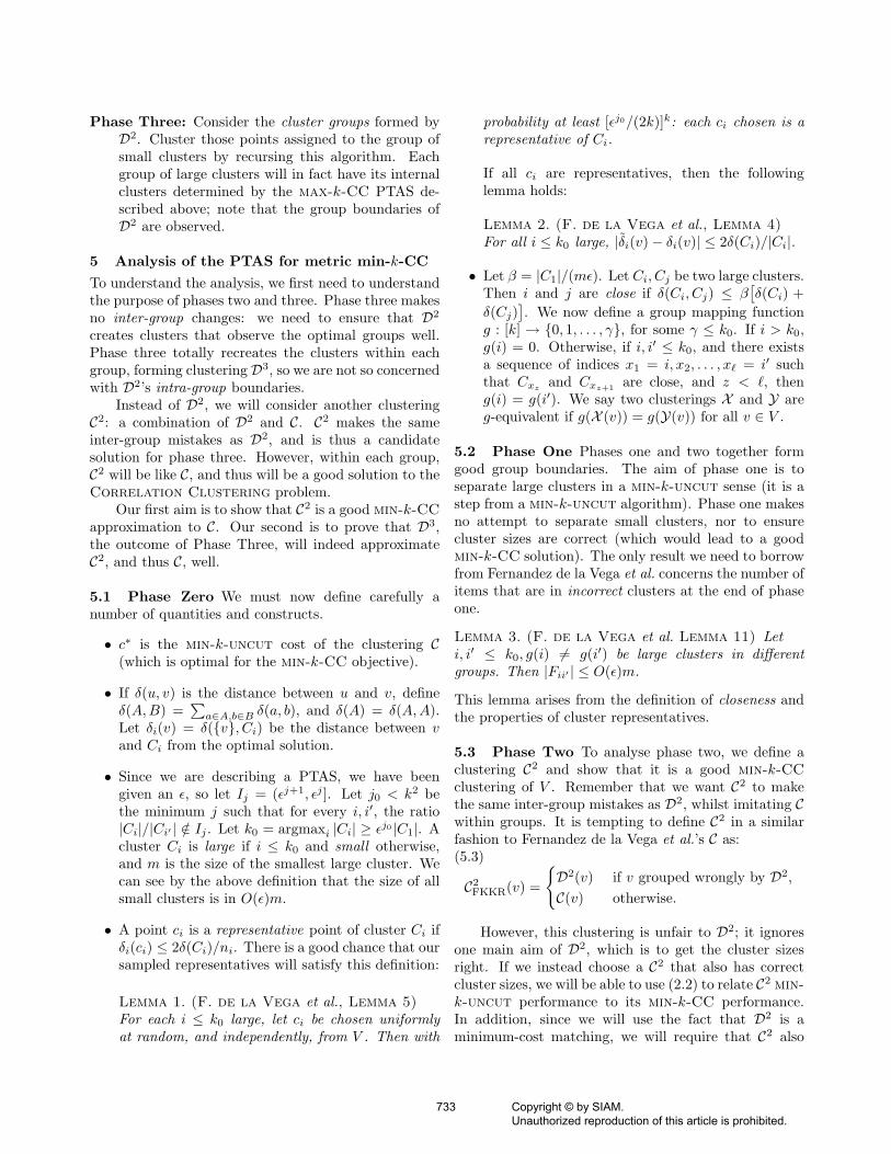
Phase Three: Consider the cluster groups formed byD2. Cluster those points assigned to the group ofsmall clusters by recursing this algorithm. Eachgroup of large clusters will in fact have its internalclusters determined by the max-k-CC PTAS de-scribed above; note that the group boundaries ofD2 are observed.

5 Analysis of the PTAS for metric min-k-CC

To understand the analysis, we first need to understandthe purpose of phases two and three. Phase three makesno inter-group changes: we need to ensure that D2

creates clusters that observe the optimal groups well.Phase three totally recreates the clusters within eachgroup, forming clustering D3, so we are not so concernedwith D2’s intra-group boundaries.

Instead of D2, we will consider another clusteringC2: a combination of D2 and C. C2 makes the sameinter-group mistakes as D2, and is thus a candidatesolution for phase three. However, within each group,C2 will be like C, and thus will be a good solution to theCorrelation Clustering problem.

Our first aim is to show that C2 is a good min-k-CCapproximation to C. Our second is to prove that D3,the outcome of Phase Three, will indeed approximateC2, and thus C, well.

5.1 Phase Zero We must now define carefully anumber of quantities and constructs.

• c∗ is the min-k-uncut cost of the clustering C(which is optimal for the min-k-CC objective).

• If δ(u, v) is the distance between u and v, defineδ(A,B) =

∑a∈A,b∈B δ(a, b), and δ(A) = δ(A,A).

Let δi(v) = δ(v, Ci) be the distance between vand Ci from the optimal solution.

• Since we are describing a PTAS, we have beengiven an ε, so let Ij = (εj+1, εj ]. Let j0 < k2 bethe minimum j such that for every i, i′, the ratio|Ci|/|Ci′ | /∈ Ij . Let k0 = argmaxi |Ci| ≥ εj0 |C1|. Acluster Ci is large if i ≤ k0 and small otherwise,and m is the size of the smallest large cluster. Wecan see by the above definition that the size of allsmall clusters is in O(ε)m.

• A point ci is a representative point of cluster Ci ifδi(ci) ≤ 2δ(Ci)/ni. There is a good chance that oursampled representatives will satisfy this definition:

Lemma 1. (F. de la Vega et al., Lemma 5)For each i ≤ k0 large, let ci be chosen uniformlyat random, and independently, from V . Then with

probability at least [εj0/(2k)]k: each ci chosen is arepresentative of Ci.

If all ci are representatives, then the followinglemma holds:

Lemma 2. (F. de la Vega et al., Lemma 4)For all i ≤ k0 large, |δi(v)− δi(v)| ≤ 2δ(Ci)/|Ci|.

• Let β = |C1|/(mε). Let Ci, Cj be two large clusters.Then i and j are close if δ(Ci, Cj) ≤ β

[δ(Ci) +

δ(Cj)]. We now define a group mapping function

g : [k] → 0, 1, . . . , γ, for some γ ≤ k0. If i > k0,g(i) = 0. Otherwise, if i, i′ ≤ k0, and there existsa sequence of indices x1 = i, x2, . . . , x` = i′ suchthat Cxz

and Cxz+1 are close, and z < `, theng(i) = g(i′). We say two clusterings X and Y areg-equivalent if g(X (v)) = g(Y(v)) for all v ∈ V .

5.2 Phase One Phases one and two together formgood group boundaries. The aim of phase one is toseparate large clusters in a min-k-uncut sense (it is astep from a min-k-uncut algorithm). Phase one makesno attempt to separate small clusters, nor to ensurecluster sizes are correct (which would lead to a goodmin-k-CC solution). The only result we need to borrowfrom Fernandez de la Vega et al. concerns the number ofitems that are in incorrect clusters at the end of phaseone.

Lemma 3. (F. de la Vega et al. Lemma 11) Leti, i′ ≤ k0, g(i) 6= g(i′) be large clusters in differentgroups. Then |Fii′ | ≤ O(ε)m.

This lemma arises from the definition of closeness andthe properties of cluster representatives.

5.3 Phase Two To analyse phase two, we define aclustering C2 and show that it is a good min-k-CCclustering of V . Remember that we want C2 to makethe same inter-group mistakes as D2, whilst imitating Cwithin groups. It is tempting to define C2 in a similarfashion to Fernandez de la Vega et al.’s C as:(5.3)

C2FKKR(v) =

D2(v) if v grouped wrongly by D2,C(v) otherwise.

However, this clustering is unfair to D2; it ignoresone main aim of D2, which is to get the cluster sizesright. If we instead choose a C2 that also has correctcluster sizes, we will be able to use (2.2) to relate C2 min-k-uncut performance to its min-k-CC performance.In addition, since we will use the fact that D2 is aminimum-cost matching, we will require that C2 also


be the result of a matching, albeit not one of minimumcost.

In order to achieve correct cluster sizes, we will haveto relax the condition (5.3) slightly. As D2 has correctcluster sizes, for each v that is mis-clustered acrossgroup boundaries from cluster i to cluster i′ by D2, thereis another point u (which we will later call p−1(v)) whichis mis-clustered into cluster i by D2. Although u maynot be mis-clustered across group boundaries, we willmake sure that C2 also mis-clusters u.

In the next section we will precisely define a set V1,with the property that

(5.4)v is placed in the wrong group by D2

⊆ V1

Then we define:

C2(v) =

D2(v) if v ∈ V1,C(v) otherwise.

Our main focus will be to ensure V1 is not too large—wewant C2 to be as similar to C as possible.

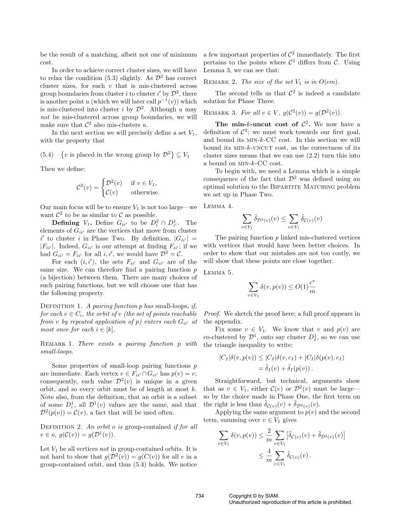
Defining V1. Define Gii′ to be D2i ∩ D1

i′ . Theelements of Gii′ are the vertices that move from clusteri′ to cluster i in Phase Two. By definition, |Gii′ | =|Fii′ |. Indeed, Gii′ is our attempt at finding Fii′ ; if wehad Gii′ = Fii′ for all i, i′, we would have D2 = C.

For each (i, i′), the sets Fii′ and Gii′ are of thesame size. We can therefore find a pairing function p(a bijection) between them. There are many choices ofsuch pairing functions, but we will choose one that hasthe following property.

Definition 1. A pairing function p has small-loops, if,for each v ∈ Ci, the orbit of v (the set of points reachablefrom v by repeated application of p) enters each Gii′ atmost once for each i ∈ [k].

Remark 1. There exists a pairing function p withsmall-loops.

Some properties of small-loop pairing functions pare immediate. Each vertex v ∈ Fii′ ∩Gii′ has p(v) = v;consequently, each value D2(v) is unique in a givenorbit, and so every orbit must be of length at most k.Note also, from the definition, that an orbit is a subsetof some D1

i , all D1(v) values are the same, and thatD2(p(v)) = C(v), a fact that will be used often.

Definition 2. An orbit o is group-contained if for allv ∈ o, g(C(v)) = g(D1(v)).

Let V1 be all vertices not in group-contained orbits. It isnot hard to show that g(D2(v)) = g(C(v)) for all v in agroup-contained orbit, and thus (5.4) holds. We notice

a few important properties of C2 immediately. The firstpertains to the points where C2 differs from C. UsingLemma 3, we can see that:

Remark 2. The size of the set V1 is in O(εm).

The second tells us that C2 is indeed a candidatesolution for Phase Three.

Remark 3. For all v ∈ V , g(C2(v)) = g(D2(v)).

The min-k-uncut cost of C2. We now have adefinition of C2; we must work towards our first goal,and bound its min-k-CC cost. In this section we willbound its min-k-uncut cost, as the correctness of itscluster sizes means that we can use (2.2) turn this intoa bound on min-k-CC cost.

To begin with, we need a Lemma which is a simpleconsequence of the fact that D2 was defined using anoptimal solution to the Bipartite Matching problemwe set up in Phase Two.

Lemma 4. ∑v∈V1

δD2(v)(v) ≤∑v∈V1

δC(v)(v)

The pairing function p linked mis-clustered verticeswith vertices that would have been better choices. Inorder to show that our mistakes are not too costly, wewill show that these points are close together.

Lemma 5. ∑v∈V1

δ(v, p(v)) ≤ O(1)c∗

m

Proof. We sketch the proof here; a full proof appears inthe appendix.

Fix some v ∈ V1. We know that v and p(v) areco-clustered by D1, onto say cluster D1

I , so we can usethe triangle inequality to write:

|CI |δ(v, p(v)) ≤ |CI |δ(v, cI) + |CI |δ(p(v), cI)

= δI(v) + δI(p(v)) .

Straightforward, but technical, arguments showthat as v ∈ V1, either C(v) or D2(v) must be large—so by the choice made in Phase One, the first term onthe right is less than δC(v)(v) + δD2(v)(v).

Applying the same argument to p(v) and the secondterm, summing over v ∈ V1 gives∑

v∈V1

δ(v, p(v)) ≤ 2m

∑v∈V1

[δC(v)(v) + δD2(v)(v)

]≤ 4m

∑v∈V1

δC(v)(v) .


The second inequality follows from an application ofLemma 4.

Finally, we use the fact that δi approximatesδi and the bound on |V1| along with the fact that∑v∈V δC(v)(v) = c∗ to complete the proof.

It is useful to split V1 into two different families ofsubsets:

Definition 3. For each i, let Ini = C2i \ Ci, and

Outi = Ci \ C2i , so that C2

i = Ci + Ini−Outi.

Note that V1 =⋃i∈[k] Ini =

⋃i∈[k] Outi, and that

Ini = p(v) | v ∈ Outi, and so |C2i | = |Ci|.

Lemma 6. C2 is a (1 + O(ε)) approximation to C interms of min-k-uncut cost. Equivalently,∑

i

δ(C2i ) ≤ (1 +O(ε))c∗ .

Proof. Again, we sketch the proof. We begin byexpanding δ(C2) in terms of Ini and Outi.

δ(C2) =∑i∈[k]

(δ(Ci) + 2 [δ(Ci, Ini)− δ(Ci,Outi)] +

[δ(Ini)− δ(Ini,Outi)] +

[δ(Outi)− δ(Outi, Ini)]).

Consider the second-last term,∑i∈[k]

δ(Ini)− δ(Ini,Outi) ≤∑i∈[k]

∑u∈Ini

∑v∈Ini

δ(v, p(v))

(by the triangle inequality)

≤ |V1|O(1)c∗

m≤ O(ε)c∗ .

(Remark 2 and Lemma 5).

We can bound the final term the same way. Nowconsider the second term, remembering the definitionsof Ini and Outi, and our notational conveniences:∑

i∈[k]

δ(Ci, Ini)− δ(Ci,Outi) =

∑v∈V1

[δC2(v)(v)− δC(v)(v)

]Now, we can split this sum into those v which are

clustered in large clusters by D2 and those which arenot. For the first group, we can use Lemma 2 and ourbound on |V1| to replace the δs with δs, followed by anapplication of Lemma 4 to form a bound. For the secondgroup, as the total number of points in small clusters isO(ε)m, we can use the triangle inequality and Lemma 5.

The min-k-CC cost of C2. Now that we haveestablished that C2 is a good min-k-uncut solution,and that |C2

i | = |Ci|, we can apply (2.2) to obtain thefollowing theorem:

Theorem 2. C2 is a (1 + O(ε)) approximation to C interms of min-k-CC cost.

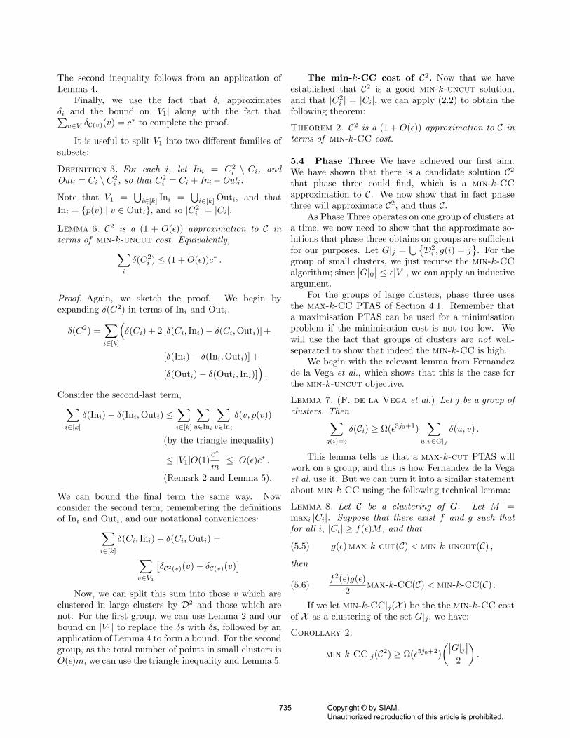
5.4 Phase Three We have achieved our first aim.We have shown that there is a candidate solution C2that phase three could find, which is a min-k-CCapproximation to C. We now show that in fact phasethree will approximate C2, and thus C.

As Phase Three operates on one group of clusters ata time, we now need to show that the approximate so-lutions that phase three obtains on groups are sufficientfor our purposes. Let G|j =

⋃D2i , g(i) = j

. For the

group of small clusters, we just recurse the min-k-CCalgorithm; since

∣∣G|0∣∣ ≤ ε|V |, we can apply an inductiveargument.

For the groups of large clusters, phase three usesthe max-k-CC PTAS of Section 4.1. Remember thata maximisation PTAS can be used for a minimisationproblem if the minimisation cost is not too low. Wewill use the fact that groups of clusters are not well-separated to show that indeed the min-k-CC is high.

We begin with the relevant lemma from Fernandezde la Vega et al., which shows that this is the case forthe min-k-uncut objective.

Lemma 7. (F. de la Vega et al.) Let j be a group ofclusters. Then∑

g(i)=j

δ(Ci) ≥ Ω(ε3j0+1)∑

u,v∈G|j

δ(u, v) .

This lemma tells us that a max-k-cut PTAS willwork on a group, and this is how Fernandez de la Vegaet al. use it. But we can turn it into a similar statementabout min-k-CC using the following technical lemma:

Lemma 8. Let C be a clustering of G. Let M =maxi |Ci|. Suppose that there exist f and g such thatfor all i, |Ci| ≥ f(ε)M , and that

(5.5) g(ε) max-k-cut(C) < min-k-uncut(C) ,

then

(5.6)f2(ε)g(ε)

2max-k-CC(C) < min-k-CC(C) .

If we let min-k-CC|j(X ) be the the min-k-CC costof X as a clustering of the set G|j , we have:

Corollary 2.

min-k-CC|j(C2) ≥ Ω(ε5j0+2)(∣∣G|j∣∣

2

).


Corollary 2 and the inductive argument about thegroup of small clusters show us that Phase Three willapproximate C2 within each group. Finally, we needanother technical lemma to ensure that a clusteringwhich is good on each group is good on the entiretyof V .

Lemma 9. Suppose X and Y are g-equivalent cluster-ings. If for each j,

min-k-CC|j(X ) ≤ (1 + f(ε))min-k-CC|j(Y)

Then, over all of V ,

min-k-CC(X ) ≤ (1 + f(ε)) min-k-CC(Y) .

Theorem 3. The algorithm in Section 4.2 is a PTASfor the min-k-CC problem.

Proof. Lemma 9 along with Corollary 2 is enough toshow that Phase Three will find a good approximationto the best solution g-equivalent to D2 that exists.Theorem 2 has shown that C2, which is g-equivalentto D2, is a good approximation to C. Thus we have therequired bound on the quality of the solution of D3. Therunning time of the algorithm is polynomial, as it is thecombination of PTASes, the guessing of O(k) values,and the solution of a Bipartite Matching problem.

6 Conclusions

The main contribution of this paper was a PTAS forthe metric-min-k-CC problem, a generalization of the k-Consensus Clustering problem, which has a numberof key applications. The minimization PTAS has a novelrebalancing step, involving a minimum-cost perfect bi-partite matching, and complements the APX-hardnessof Consensus Clustering. We anticipate that thisrebalancing technique will find application in other sit-uations where the sizes of clusters are constrained.

Naturally, the PTAS presented here, like that ofGiotis and Guruswami [16], is too slow to run inpractice. It would be fruitful, therefore, to look for local-search approaches that have approximation guarantees,as we have done in the past [8].

References

[1] Ailon, N., Charikar, M., and Newman, A. Aggre-gating inconsistent information: Ranking and cluster-ing. Journal of the ACM 55, 5 (2008), 1–27.

[2] Arora, S., Karger, D., and Karpinski, M. Poly-nomial time approximation schemes for dense instancesof NP-hard problems. Journal of Computer and Sys-tem Sciences 58, 1 (1999), 193–210.

[3] Bansal, N., Blum, A., and Chawla, S. Correlationclustering. Machine Learning 56, 1 (2004), 89–113.

[4] Bonizzoni, P., Della Vedova, G., and Dondi, R.A ptas for the minimum consensus clustering problemwith a fixed number of clusters. In Proceedings of theEleventh Italian Conference on Theoretical ComputerScience (2009).

[5] Bonizzoni, P., Della Vedova, G., Dondi, R., andJiang, T. On the approximation of correlation clus-tering and consensus clustering. Journal of Computerand System Sciences 74, 5 (2008), 671–96.

[6] Charbit, P., Thomasse, S., and Yeo, A. The min-imum feedback arc set problem is NP-hard for tourna-ments. Combinatorics, Probability and Computing 16,1 (2006), 1–4.

[7] Charikar, M., Guruswami, V., and Wirth, A.Clustering with qualitative information. Journal ofComputer and System Sciences 71, 3 (2005), 360–83.

[8] Coleman, T., Saunderson, J., and Wirth, A. Alocal-search 2-approximation for 2-correlation cluster-ing. In Proceedings of the Sixteenth Annual EuropeanSymposium on Algorithms (2008), pp. 308–19.

[9] Demaine, E., Emanuel, D., Fiat, A., and Immor-lica, N. Correlation clustering in general weightedgraphs. Theoretical Computer Science 361, 2-3 (2006),172–87.

[10] Fernandez de la Vega, W., Karpinski, M., andKenyon, C. Approximation schemes for metric bi-section and partitioning. In Proceedings of the Fif-teenth Annual ACM-SIAM Symposium on Discrete Al-gorithms (2004), pp. 506–15.

[11] Fernandez de la Vega, W., Karpinski, M.,Kenyon, C., and Rabani, Y. Approximationschemes for clustering problems. In Proceedings of thethirty-fifth annual ACM symposium on Theory of Com-puting (2003), pp. 50–8.

[12] Fernandez de la Vega, W., and Kenyon, C. Arandomized approximation scheme for metric max-cut. Journal of Computer and System Sciences 63,4 (2001), 531–41.

[13] Filkov, V., and Skiena, S. Integrating microarraydata by consensus clustering. In Proceedings of In-ternational Conference on Tools with Artificial Intelli-gence (ICTAI) (2003), pp. 418–25.

[14] Frieze, A., and Kannan, R. The regularity lemmaand approximation schemes for dense problems. InProceedings of the Thirty-Seventh Annual IEEE Sym-posium on Foundations of Computer Science (1996),pp. 12–20.


[15] Gionis, A., Mannila, H., and Tsaparas, P. Clus-tering aggregation. ACM Transactions on KnowledgeDiscovery from Data (TKDD) 1, 1 (2007).

[16] Giotis, I., and Guruswami, V. Correlation cluster-ing with a fixed number of clusters. Theory of Com-puting 2, 1 (2006), 249–66.

[17] Goemans, M., and Williamson, D. Improved ap-proximation algorithms for maximum cut and satisfia-bility problems using semidefinite programming. Jour-nal of the ACM 42 (1995), 1115–45.

[18] Indyk, P. A sublinear time approximation schemefor clustering in metric-spaces. In Proceedings of theFortieth Annual IEEE Symposium on Foundations ofComputer Science (1999), pp. 154–9.

[19] Karpinski, M., and Schudy, W. Linear time ap-proximation schemes for the Gale-Berlekamp game andrelated minimization problems. In Proceedings of theForty-First Annual ACM Symposium on Theory ofComputing (2009), pp. 313–22.

[20] Kenyon-Mathieu, C., and Schudy, W. How torank with few errors. In Proceedings of the Thirty-Ninth Annual ACM Symposium on Theory of Comput-ing (2007), pp. 95–103.

[21] Khot, S., Kindler, G., Mossel, E., andO’Donnell, R. Optimal inapproximability results forMAX-CUT and other 2-variable CSPs? In Proceedingsof the Forty-Fifth Annual IEEE Symposium on Foun-dations of Computer Science (2004), pp. 146–54.

[22] Swamy, C. Correlation clustering: maximizing agree-ments via semidefinite programming. In Proceedings ofthe Fifteenth Annual ACM-SIAM Symposium on Dis-crete Algorithms (2004), pp. 526–7.

A Proofs

A.1 Proof of max-k-CC PTAS First we provethat a solution to the negatively-weighted max-k-cutproblem that we set up in Section 4.1 will indeed providea solution to our max-k-CC problem. Note that ec(C)is defined to be |Ec(C)|, and eu(C) is |Eu(C)|.

Remark 4. Let G = (V,E, δ) be a weighted graph.Define G = (V,E, δ), where δ = 2δ − 1. Then, forany k-clustering C,

max-k-CC(G, C) = max-k-Cut(G, C) + |E| −∆ .

Proof.

max-k-CC(G, C) = max-k-Cut(G, C) + eu(C)−min-k-Uncut(G, C)

= max-k-Cut(G, C) +[|E| − ec(C)

]+[max-k-Cut(G, C)−∆)

]= 2 max-k-Cut(G, C)− ec(C) + |E| −∆

=∑

e∈Ec(C)

(2w(e)− 1) + |E| −∆

= max-k-Cut(G, C) + |E| −∆ .

Remark 4 tells us, for instance, that the optimal solutionto max-k-cut on G is the same as the optimal solutionof max-k-CC on G.

Proof of Corollary 1

Proof. Let C be the solution returned by algorithm FK,run on G, and C∗ be the optimal solution to max-k-CC.Then, by Remark 4,

max-k-CC∗ −max-k-CC(C)= max-k-cut(G, C∗)−max-k-cut(G, C)≤ max-k-cut(G)∗ −

[max-k-cut(G)∗ − εn2

]= εn2

and we are done, since max-k-CC* is in Ω(n2).

A.2 Proofs from Phase Two

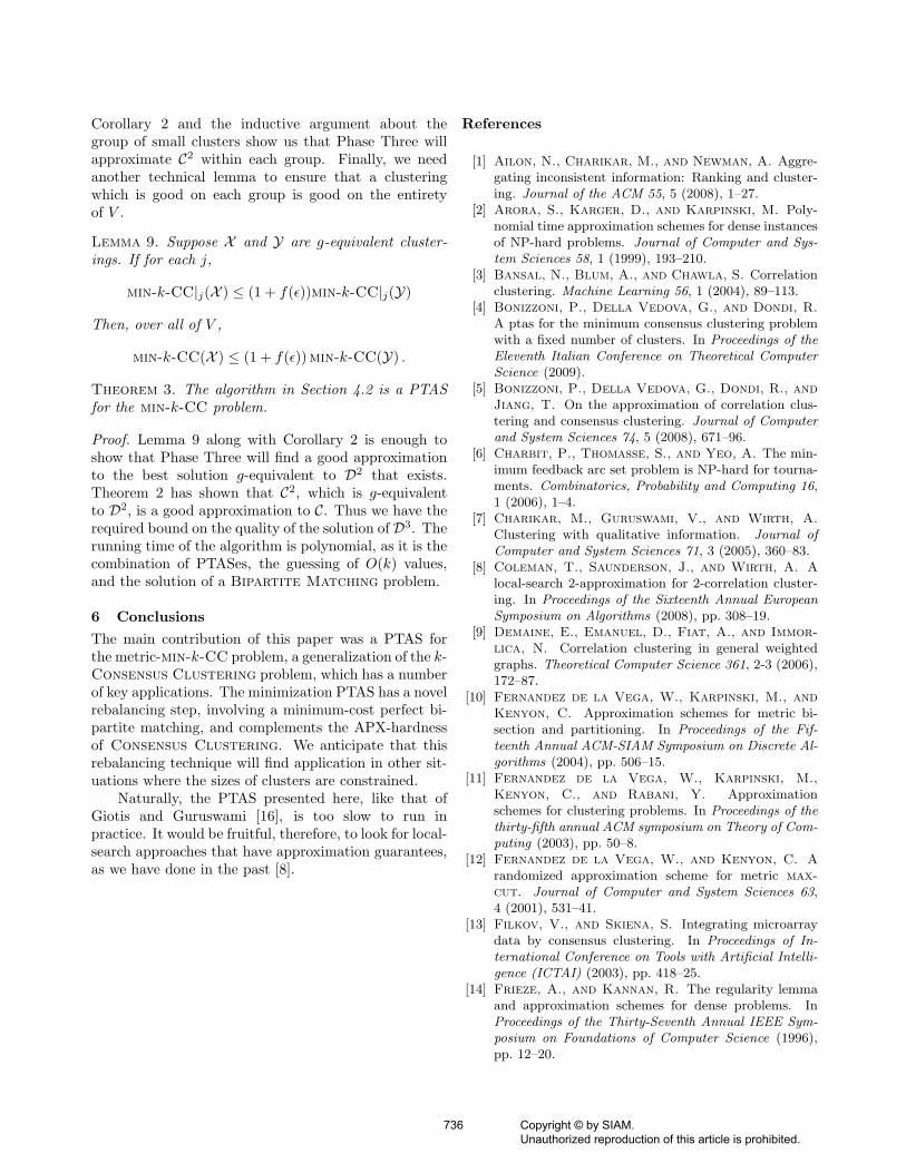
Proof of Remark 1

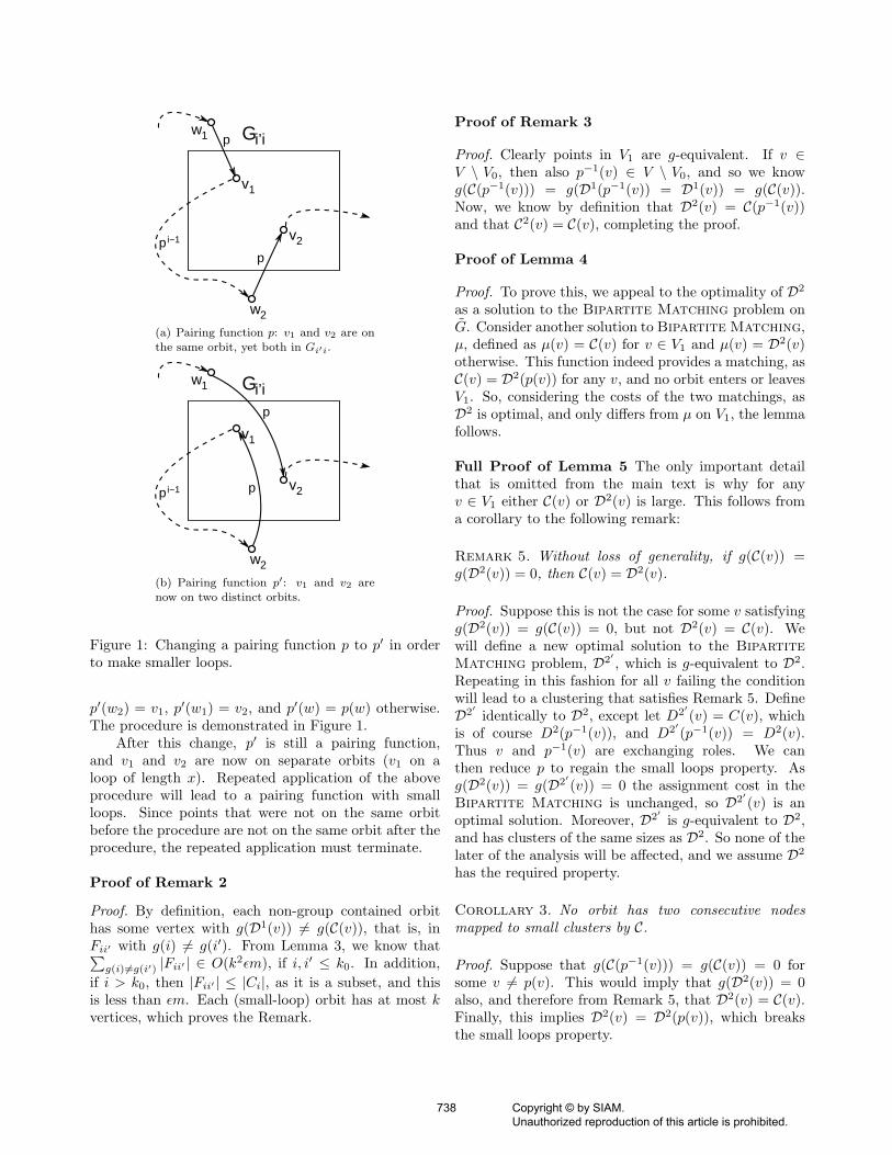
Proof. It is simple to find such a pairing function;suppose we have a pairing function p such that v1, v2 ∈Gi′i are in the same orbit. That is, px(v1) = v2 for somex. Then, as v1, v2 are both in Gi′i, there are two nodesw1, w2 ∈ Fi′i such that p(w1) = v1 and p(w2) = v2.Then we can define a new pairing function p′ such that


Gi’iw1

v1

v2

w2

p

pp i−1

(a) Pairing function p: v1 and v2 are on

the same orbit, yet both in Gi′i.

Gi’iw1

v1

v2

w2

p

pp i−1

(b) Pairing function p′: v1 and v2 are

now on two distinct orbits.

Figure 1: Changing a pairing function p to p′ in orderto make smaller loops.

p′(w2) = v1, p′(w1) = v2, and p′(w) = p(w) otherwise.The procedure is demonstrated in Figure 1.

After this change, p′ is still a pairing function,and v1 and v2 are now on separate orbits (v1 on aloop of length x). Repeated application of the aboveprocedure will lead to a pairing function with smallloops. Since points that were not on the same orbitbefore the procedure are not on the same orbit after theprocedure, the repeated application must terminate.

Proof of Remark 2

Proof. By definition, each non-group contained orbithas some vertex with g(D1(v)) 6= g(C(v)), that is, inFii′ with g(i) 6= g(i′). From Lemma 3, we know that∑g(i)6=g(i′) |Fii′ | ∈ O(k2εm), if i, i′ ≤ k0. In addition,

if i > k0, then |Fii′ | ≤ |Ci|, as it is a subset, and thisis less than εm. Each (small-loop) orbit has at most kvertices, which proves the Remark.

Proof of Remark 3

Proof. Clearly points in V1 are g-equivalent. If v ∈V \ V0, then also p−1(v) ∈ V \ V0, and so we knowg(C(p−1(v))) = g(D1(p−1(v)) = D1(v)) = g(C(v)).Now, we know by definition that D2(v) = C(p−1(v))and that C2(v) = C(v), completing the proof.

Proof of Lemma 4

Proof. To prove this, we appeal to the optimality of D2

as a solution to the Bipartite Matching problem onG. Consider another solution to Bipartite Matching,µ, defined as µ(v) = C(v) for v ∈ V1 and µ(v) = D2(v)otherwise. This function indeed provides a matching, asC(v) = D2(p(v)) for any v, and no orbit enters or leavesV1. So, considering the costs of the two matchings, asD2 is optimal, and only differs from µ on V1, the lemmafollows.

Full Proof of Lemma 5 The only important detailthat is omitted from the main text is why for anyv ∈ V1 either C(v) or D2(v) is large. This follows froma corollary to the following remark:

Remark 5. Without loss of generality, if g(C(v)) =g(D2(v)) = 0, then C(v) = D2(v).

Proof. Suppose this is not the case for some v satisfyingg(D2(v)) = g(C(v)) = 0, but not D2(v) = C(v). Wewill define a new optimal solution to the BipartiteMatching problem, D2′ , which is g-equivalent to D2.Repeating in this fashion for all v failing the conditionwill lead to a clustering that satisfies Remark 5. DefineD2′ identically to D2, except let D2′(v) = C(v), whichis of course D2(p−1(v)), and D2′(p−1(v)) = D2(v).Thus v and p−1(v) are exchanging roles. We canthen reduce p to regain the small loops property. Asg(D2(v)) = g(D2′(v)) = 0 the assignment cost in theBipartite Matching is unchanged, so D2′(v) is anoptimal solution. Moreover, D2′ is g-equivalent to D2,and has clusters of the same sizes as D2. So none of thelater of the analysis will be affected, and we assume D2

has the required property.

Corollary 3. No orbit has two consecutive nodesmapped to small clusters by C.

Proof. Suppose that g(C(p−1(v))) = g(C(v)) = 0 forsome v 6= p(v). This would imply that g(D2(v)) = 0also, and therefore from Remark 5, that D2(v) = C(v).Finally, this implies D2(v) = D2(p(v)), which breaksthe small loops property.


Full Proof of Lemma 6 To begin with, we prove thestatements made relating Ini to Outi:

Proof. Let X = p−1(v) | v ∈ Ini. If v ∈ Ini,then C2(v) = i 6= C(v) and v is not in a group-contained orbit. Let u = p−1(v), then u ∈ X, andC(u) = D2(p(u)) = D2(v) = C2(v) = i, which alsoimplies u 6= v. On the other hand, C2(u) 6= C2(v) = i,by the small loops property, so u ∈ Outi. Consequently,X ⊆ Outi. A similar argument in the other directionshows that Outi ⊆ X.

We break the sketch up into a few parts:

Remark 6.

δ(C2i )− δ(Ci) ≤ 2 [δ(Ci, Ini)− δ(Ci,Outi)] +O(ε)c∗ .

Proof. Expanding δ(C2i ) gives

δ(C2i ) = δ(Ci) + 2 [δ(Ci, Ini)− δ(Ci,Outi)]

+ [δ(Ini)− δ(Ini,Outi)]+ [δ(Outi)− δ(Outi, Ini)] .

Consider the second-last term,

δ(Ini)− δ(Ini,Outi) =∑u∈Ini

[δ(u, Ini)− δ(u,Outi)]

=∑u∈Iniv∈Outi

[δ(u, p(v))− δ(u, v)]

≤∑u∈Iniv∈Outi

δ(v, p(v))

(triangle inequality)

≤ |V1|∑v∈V1

δ(v, p(v))

(Ini,Outi ⊆ V1)≤ O(ε)c∗ .

(Remark 2 and Lemma 5)

We can bound the final term in the same way, whichcompletes the proof.

Remark 7.∑i∈[k]

δ(Ci, Ini)− δ(Ci,Outi)

=∑v∈V1


]

Proof. From the statements relating Ini and Outi:∑i∈[k]

δ(Ci, Ini)− δ(Ci,Outi)

=∑i∈[k]

∑v∈Ini

[δi(v)− δi(p−1(v))

]=∑i∈[k]

∑v∈Ini

[δC2(v)(v)− δC(p−1(v))(p−1(v))

]For a vertex u in V1 that is not in some Ini, p(u) = u,so the corresponding term inside the brackets above iszero. Therefore the right hand side is, after separatingthe terms,∑

v∈V1

δC2(v)(v)−∑v∈V1

δC(p−1(v))(p−1(v))

=∑v∈V1


δC(v)(v) ,

as v ∈ V1 implies p−1(v) ∈ V1.

Proof. [Proof of Lemma 6.] From Remarks 6 and 7,∑i

δ(C2i ) ≤

∑i

δ(Ci) +O(ε)c∗

+∑v∈V1


]Now, ∑

v∈V1g(C2(v))6=0


g(C(v))6=0

δC(v)(v)

≤∑v∈V1

g(C2(v))6=0


g(C(v))6=0

δC(v)(v)

+ |V1|4c∗

m∈ O(εc∗) ,

from Lemma 2, Lemma 4, and Remark 2. In contrast,∑v∈V1

g(C2(v))=0


g(C(v))=0

δC(v)(v)

=∑v∈V1

g(C(v))=0

δC(v)(p(v))−∑v∈V1

g(C(v))=0

δC(v)(v)

Now, an application of the triangle inequality showsthat δC(v)(p(v))− δC(v)(v) ≤ |CC(v)|δ(v, p(v)), so∑

v∈V1,g(C(v))=0

[δC(v)(p(v))− δC(v)(v)

]≤

∑v∈V1,g(C(v))=0

|CC(v)|δ(v, p(v))

≤ O(1)s

mc∗+ ≤ O(ε)c∗ ,


where the final inequality follows from Lemma 5 andthe facts that |CC(v)| ≤ s and s ≤ mε.

Proof of Theorem 2 The theorem is an applicationof the following Lemma:

Lemma 10. If f(ε) satisfies min-k-Uncut(C2) ≤ (1 +f(ε)) min-k-Uncut(C), then

min-k-CC(C2) ≤ (1 + 2f(ε)) min-k-CC(C) .

Proof. Note that, for any clustering X :

min-k-CC(X )= min-k-Uncut(X ) + ec(X )−max-k-Cut(X )= 2 min-k-Uncut(X ) + ec(X )−∆ .

Consider

min-k-CC(C2)−min-k-CC(C)= 2

(min-k-Uncut(C2)−min-k-Uncut(C)

)+ ec(C2)− ec(C)

≤ 2f(ε) min-k-Uncut(C))= f(ε) [min-k-CC(C)− (ec(C)−∆)]≤ 2f(ε) min-k-CC(C) .

The last inequality above follows from this reasoning

∆− ec(X )= min-k-Uncut(X ) + max-k-Cut(X )− ec(X )= min-k-Uncut(X ) + ec(X )−max-k-Cut(X )− 2(ec(X )−max-k-Cut(X ))

≤ min-k-CC(X ) ,

which is a consequence of

max-k-Cut(X )

=∑

e∈Ec(X )

δ(e) ≤∑

e∈Ec(X )

1 = ec(X ) .

A.3 Proofs from Phase Three

Proof of Lemma 8

Proof. For convenience, let

X = max-k-cut(C) W = ec(C)−XY = min-k-uncut(C) Z = eu(C)− Y ,

all positive quantities. Also, let f stand for f(ε) and gfor g(ε). Then

X +W = ec(C) =∑i<j

|Ci||Cj | ≥∑i<j

f2M2

≥ f2M2k

2,

And

Y + Z = eu(C) =∑i

(|Ci|2

)≤∑i

(M

2

)= k

(M

2

)≤ M2k

2.

Combining these, we have,

(A.1) X +W ≥ f2(Y + Z) ≥ f2Z

Consider the following:

f2g(X + Z)− 2(Y +W )

= g(f2Z) + f2gX − 2(Y +W )

≤ g(X +W ) + f2gX − (f2 + 1)Y − 2W(by (A.1), and f ≤ 1)

= (f2 + 1)(gX − Y ) + (g − 2)W < 0(as gX < Y , and g ≤ 1),

which completes the proof.

Proof of Lemma 9

Proof. Note that

min-k-CC(X ) =∑j∈[γ]

min-mj-CC(X|j)

+∑

g(X(u))6=g(X (v))

(1− δ(u, v)) ,

and similarly for Y. The g-equivalence of X and Y tellsus that the rightmost summation is common to bothclusterings, leading to the statement of the lemma.
