


Bahasa
Halaman
Hukum


Dt .J8RARY|sjA -: fGRADUATE SCHOOL
MOt iSREY CA 93943-5101


Approved for public release; distribution is unlimited
A Comparison of Ionospheric Propagation Mode DelayPredictions from Advanced PROPHET 4.3 with Measured Data
by
Jose L. NadalLieutenant, Peruvian Air Force
B.S., Peruvian Air Force Academy, 1988
Submitted in partial fulfillment of therequirements of degree of
MASTER OF SCIENCE IN ELECTRICAL ENGINEERING
from the
NAVAL POSTGRADUATE SCHOOLDecember 1992 -
// /]
issififvl
ty Classification of this page
REPORT DOCUMENTATION PAGEsport Security Classification: Unclassified lb Restrictive Markings
curity Classification Authority 3 Distribution/ Availability of Report
sclassification/ Downgrading Schedule Approved for public release; distribution is unlimited.
forming Organization Report Number(s) 5 Monitoring Organization Report Number(s)
ime of Performing Organization
il Postgraduate School
6b Office Symbol
(if applicable ) EC7a Name of Monitoring Organization
Naval Postgraduate School
idress (city, state, and ZIP code)
terey CA 93943-5000
7b Address (city, state, and ZIP code)
Monterey CA 93943-5000
ime of Funding/Sponsoring Organization 8b Office Symbol
(if applicable)
9 Procurement Instrument Identification Number
idress (city, state, and ZIP code) 10 Source of Funding Numbers
Program Element No Project No Task No Work Unit Accession P
tie (include security classification) A COMPARISON OF IONOSPHERIC PROPAGATION MODE DELAY PREDICTIONS FROM PROPHET 4.3
i MEASURED DATA
irsonal Author(s) NADAL. Jose L.
'ype of Report
ter"s Thesis
13b Time Covered
From To
14 Date of Report (year, month, day)
1992 DEC 15
15 Page Count
64
pplementary Notation The views expressed in this thesis are those of the author and do not reflect the official policy or position
e Department of Defense or the U.S. Government.
)sati Codes 18 Subject Terms (continue on reverse if necessary and identify by block number)
Group Subgroup High Frequency (HF); Ionospheric Propagation; ADVANCED PROPHET
istract (continue on reverse if necessary and identify by block number)
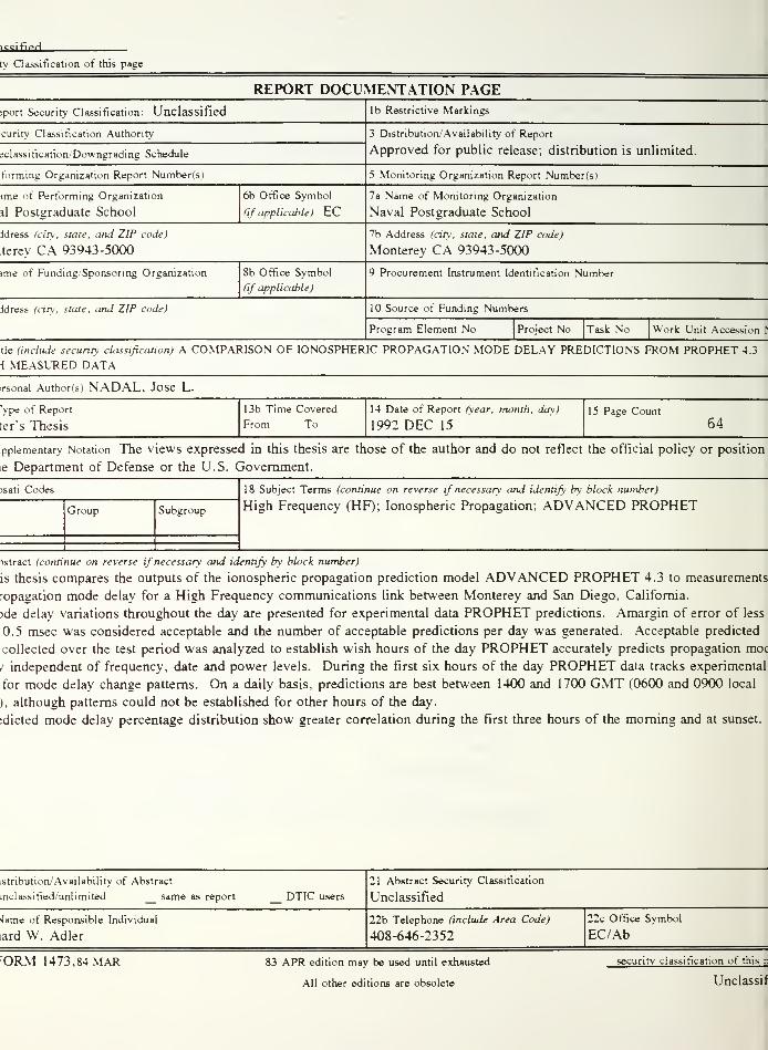
is thesis compares the outputs of the ionospheric propagation prediction model ADVANCED PROPHET 4.3 to measurements
'opagation mode delay for a High Frequency communications link between Monterey and San Diego, California.
)de delay variations throughout the day are presented for experimental data PROPHET predictions. Amargin of error of less
0.5 msec was considered acceptable and the number of acceptable predictions per day was generated. Acceptable predicted
collected over the test period was analyzed to establish wish hours of the day PROPHET accurately predicts propagation moc
/ independent of frequency, date and power levels. During the first six hours of the day PROPHET data tracks experimental
for mode delay change patterns. On a daily basis, predictions are best between 1400 and 1700 GMT (0600 and 0900 local
), although patterns could not be established for other hours of the day.
:dicted mode delay percentage distribution show greater correlation during the first three hours of the morning and at sunset.
stnbution/Availability of Abstract
inclassified/unlimited _ same as report DTIC users
21 Abstract Security Classification
Unclassified
Jame of Responsible Individual
ard W. Adler
22b Telephone (include Area Code)
408-646-2352
22c Office Symbol
EC/Ab
rORM 1473,84 MAR 83 APR edition may be used until exhausted
All other editions are obsolete
security classification of this p
Unclassif
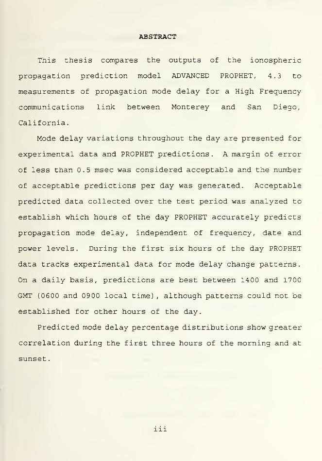
ABSTRACT
This thesis compares the outputs of the ionospheric
propagation prediction model ADVANCED PROPHET, 4.3 to
measurements of propagation mode delay for a High Frequency
communications link between Monterey and San Diego,
California.
Mode delay variations throughout the day are presented for
experimental data and PROPHET predictions. A margin of error
of less than 0.5 msec was considered acceptable and the number
of acceptable predictions per day was generated. Acceptable
predicted data collected over the test period was analyzed to
establish which hours of the day PROPHET accurately predicts
propagation mode delay, independent of frequency, date and
power levels. During the first six hours of the day PROPHET
data tracks experimental data for mode delay change patterns.
On a daily basis, predictions are best between 1400 and 1700
GMT (0600 and 0900 local time) , although patterns could not be
established for other hours of the day.
Predicted mode delay percentage distributions show greater
correlation during the first three hours of the morning and at
sunset
.
in
w
TABLE OF CONTENTS
I
.
INTRODUCTION 1
II
.
THEORETICAL BACKGROUND 3
A. THE IONOSPHERE 3
1
.
Photo- ionization 3
2
.
Recombination 3
3
.
Ionospheric Layers 5
4
.
Variations of the Ionosphere 6
5
.
Ray Tracing 9
6
.
Ray Paths in the Ionosphere 9
III. THE MONTEREY- SAN DIEGO COMMUNICATION LINK ... 11
A. LINK ANTENNAS 11
1
.
Transmitting Antenna 11
2
.
Receiving Antenna 12
3
.
Antenna Simulation 12
IV. COMPARISON OF EXPERIMENTAL DATA WITH PROPHETPREDICTIONS 2
A. EXPERIMENTAL DATA 2
B
.
ADVANCED PROPHET 4 . 3 RESULTS 29
1. Input Scenario Parameters for PROPHET... 29
2
.
Advanced PROPHET 4 . 3 Analysis 32
C
.
DATA COMPARISON 32
V. CONCLUSIONS AND RECOMMENDATIONS 5
iv
DUDLEY KNOX LIBRARYNAVAL POSTGRADUATE SCHOOLMONTEREY CA 93943-5101
LIST OF REFERENCES 52
INITIAL DISTRIBUTION LIST 54
v
LIST OF FIGURES
Figure 1. Photo- ionization of a neutral atom, A,by extreme ultraviolet light from the sun,yielding a positively charged ion, A+
, anda free electron, e. [Ref . 1] 4
Figure 2. Sketch of the various regions of the ionosphereas it appears during the day and night.[Ref. 1] 7
Figure 3. Diurnal variations of electron density andthe formation of ionospheric layers.[Ref. 6] 8
Figure 4. Raypaths for a fixed frequency. [Ref .4] 10
Figure 5. Monterey Multiband Dipole Antenna 13
Figure 6. San Diego Drooping Dipole Antenna 14
Figure 7. Elevation radiation patterns predicted by NECfor the Monterey Multiband Dipole Antenna 16
Figure 8. Elevation radiation patterns predicted by NECfor the San Diego Drooping Dipole Antenna 17
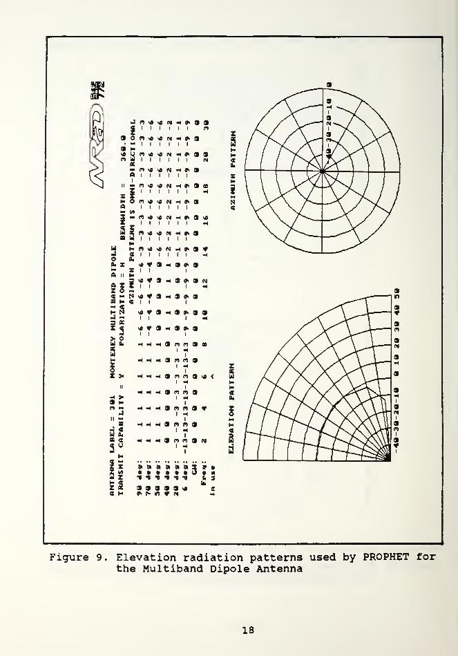
Figure 9. Elevation radiation patterns used by PROPHETfor the Monterey Multiband Dipole Antenna 18
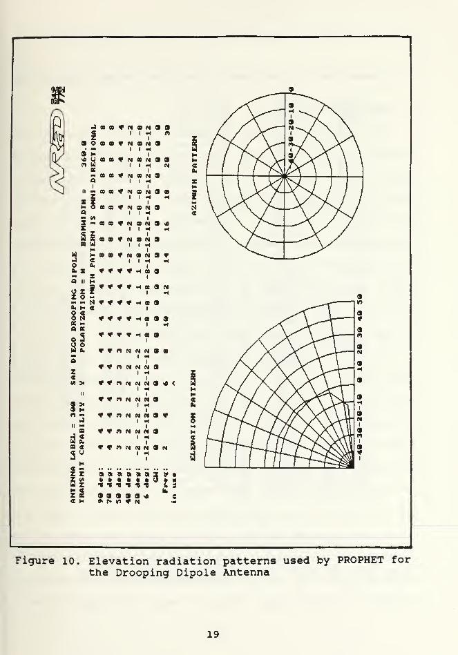
Figure 10. Elevation radiation patterns used by PROPHETfor the San Diego Drooping Dipole Antenna 19
Figure 11. Correlation vector plot that results from thecross correlation of the reference sequencewith the digitized HF data 21
Figure 12 . Measured Mode Delay for 2 8 Aug 92 23
Figure 13. Measured Mode Delay for 2 Oct 92.(5.604 MHz - 75 watts) 24
Figure 14 . Measured Mode Delay for 3 Oct 92 25
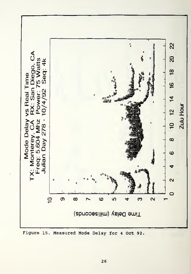
Figure 15 . Measured Mode Delay for 4 Oct 92 26
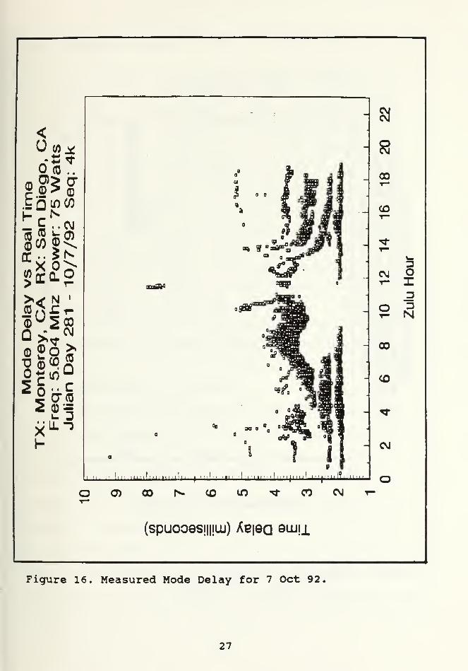
Figure 16. Measured Mode Delay for 7 Oct 92 27
VI
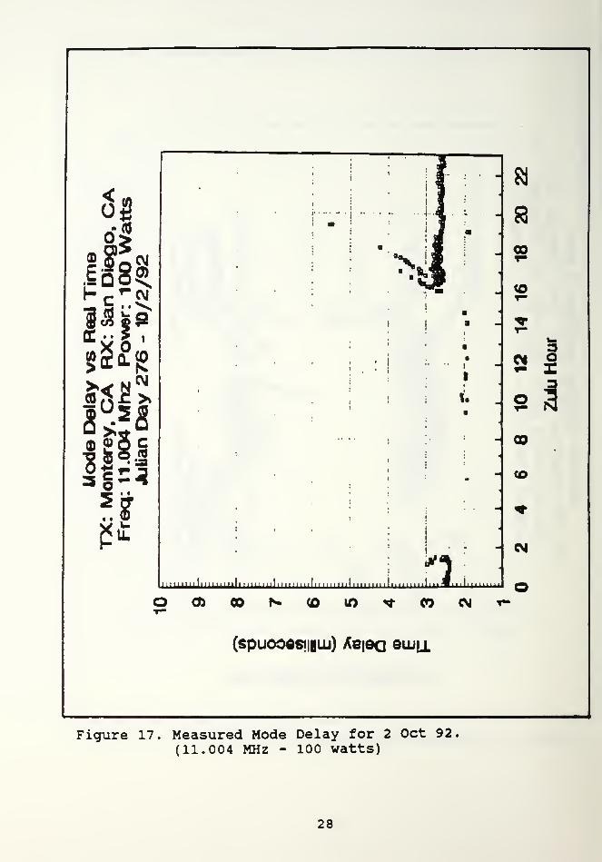
Figure 17. Measured Mode Delay for 2 Oct 92.(11.004 MHz - 100 watts) 28
Figure 18. Ray Paths predicted by ADVANCED PROPHET 3 3
Figure 19 . Alphanumeric output corresponding toRaytrace predictions 34
Figure 20. Comparison between experimental and PROPHETMode Delay predictions for 28 Aug 92 35
Figure 21. Comparison between experimental and PROPHETMode Delay predictions for 2 Oct 92.(5.604 MHz - 75 watts) 36
Figure 22 . Comparison between experimental and PROPHETMode Delay predictions for 3 Oct 92 37
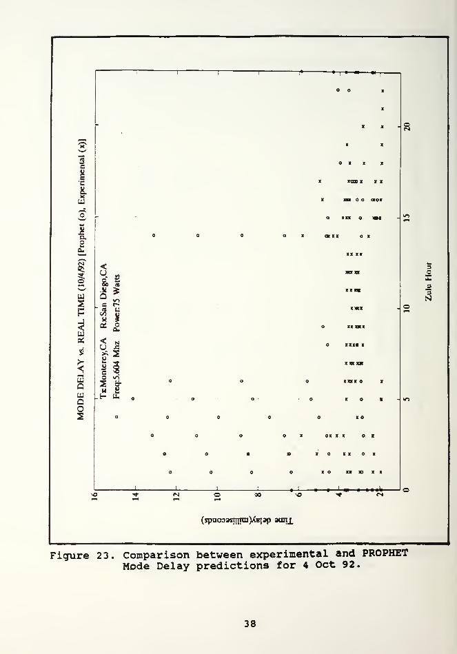
Figure 23. Comparison between experimental and PROPHETMode Delay predictions for 4 Oct 92 3 8
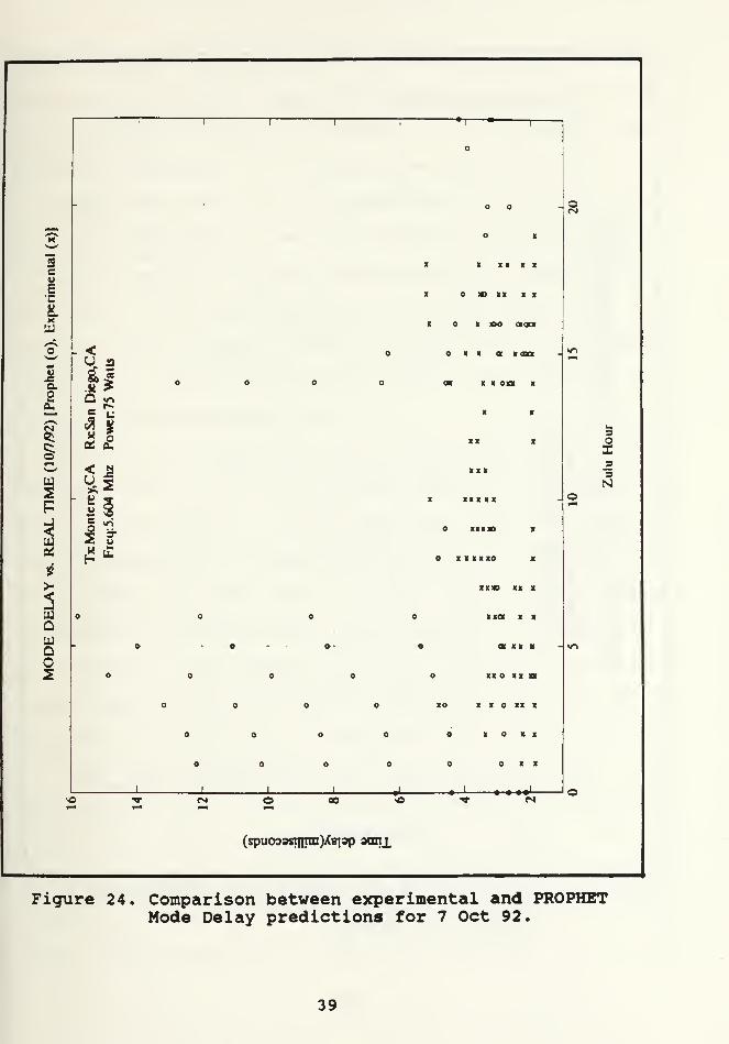
Figure 24. Comparison between experimental and PROPHETMode Delay predictions for 7 Oct 92 39
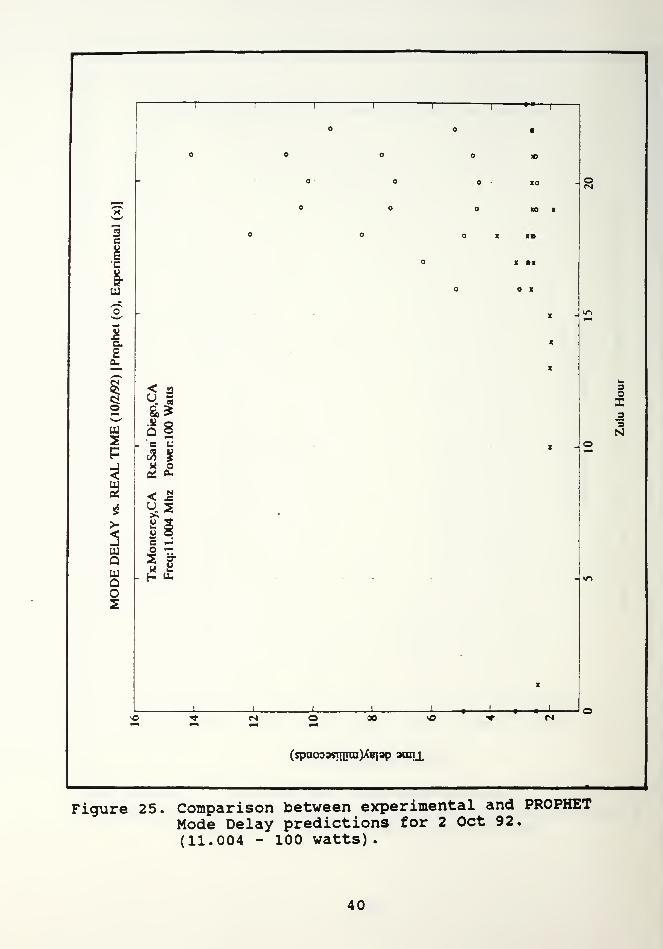
Figure 25. Comparison between experimental and PROPHETMode Delay predictions for 2 Oct 92.(11.004 MHz - 100 watts) 40
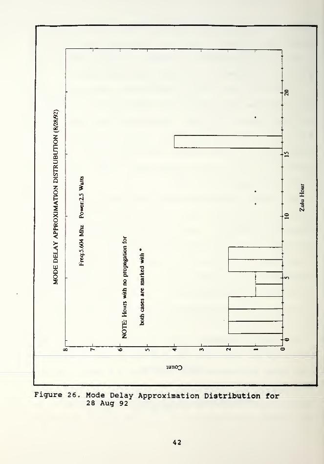
Figure 26. Mode Delay Approximation Distribution for28 Aug 92 42
Figure 27. Mode Delay Approximation Distribution for2 Oct 92, (5.604 MHz - 75 watts) 43
Figure 28. Mode Delay Approximation Distribution for3 Oct 92 44
Figure 29. Mode Delay Approximation Distribution for4 Oct 92 45
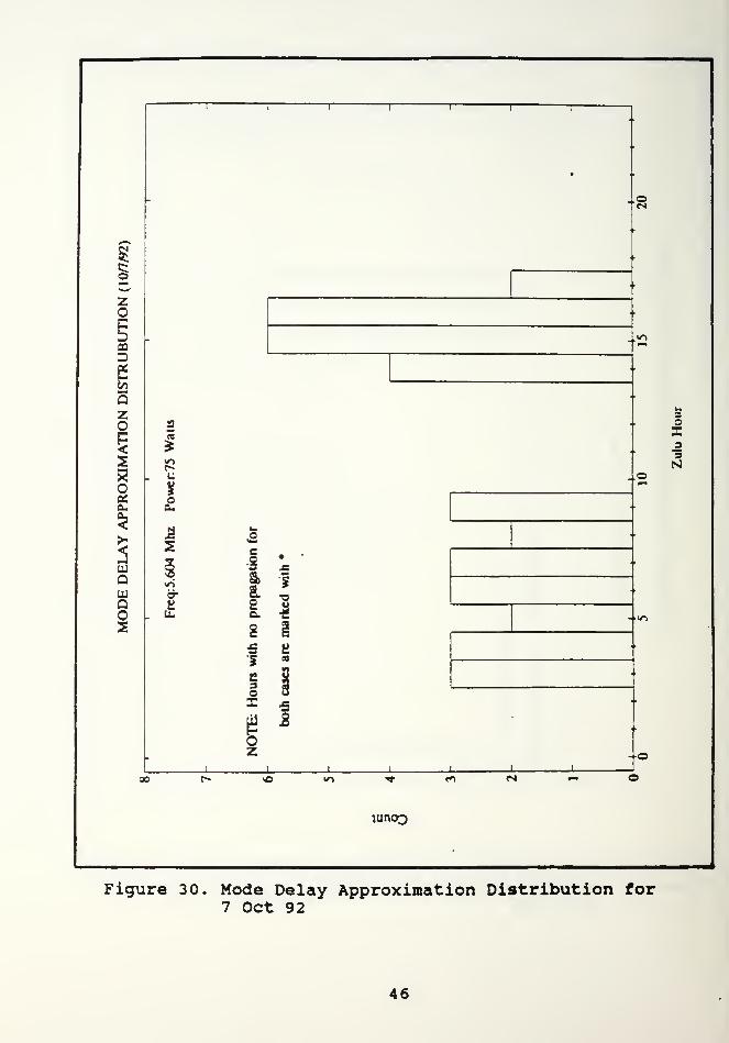
Figure 30. Mode Delay Approximation Distribution for7 Oct 92 46
Figure 31. Mode Delay Approximation Distribution for2 Oct 92, (11.004 MHz - 100 watts) 47
Figure 32. Mode Delay approximation percentagedistribution 49
vii

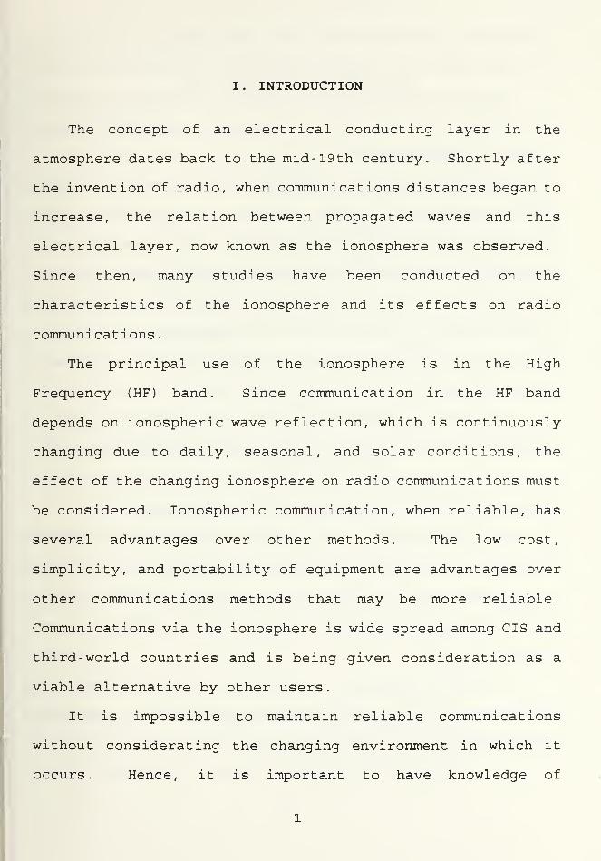
I . INTRODUCTION
The concept of an electrical conducting layer in the
atmosphere dates back to the mid- 19th century. Shortly after
the invention of radio, when communications distances began to
increase, the relation between propagated waves and this
electrical layer, now known as the ionosphere was observed.
Since then, many studies have been conducted on the
characteristics of the ionosphere and its effects on radio
communications
.
The principal use of the ionosphere is in the High
Frequency (HF) band. Since communication in the HF band
depends on ionospheric wave reflection, which is continuously
changing due to daily, seasonal, and solar conditions, the
effect of the changing ionosphere on radio communications must
be considered. Ionospheric communication, when reliable, has
several advantages over other methods. The low cost,
simplicity, and portability of equipment are advantages over
other communications methods that may be more reliable.
Communications via the ionosphere is wide spread among CIS and
third-world countries and is being given consideration as a
viable alternative by other users.
It is impossible to maintain reliable communications
without considerating the changing environment in which it
occurs. Hence, it is important to have knowledge of
ionospheric characteristics and the elements that affect it
such as time of day, season, location, and solar activity [1]
.
Computer models permit the analysis of HF wave propagation
parameters and can predict propagation channels that will
support communications.
A project named Polar Equatorial Near- Vertical Incidence
Skywave Experiment (PENEX) which acquires calibrated field
strength measurements from ionospheric radio transmissions is
creating a data base for comparison with different ionospheric
propagation prediction models. In addition, as part of the
PENEX project, a communication link has been established for
the purpose of equipment testing, calibration and experimental
methodology.
After this communication link between Monterey, CA. and
San Diego, CA. is tested, project PENEX will be expanded to
include a transmitter site in Alaska, and receiver sites in
Alaska, California, Pennsylvania and Washington.
This thesis uses one of the computer models, ADVANCED
PROPHET 4.3 to predict HF skywave propagation for comparison
and correlation to the experimental data obtained for mode
delays in the communication link between Monterey and San
Diego.
It is also important to note that due to limited data
availability, the research analysis of this thesis is somewhat
restricted.
II. THEORETICAL BACKGROUND
A. THE IONOSPHERE
The ionosphere is the region of the atmosphere which
extends between 50 to 600 km where sufficient ionization
occurs in layers to affect radio transmissions. The
ionosphere is an electrically neutral region, since if it had
a given excess charge, then electrical forces would prevent
the formation of stable layers [2]
.
1. Photo -ionization
Photo- ionization occurs when the sun produces extreme
ultraviolet (EUV) light waves which in turn detach electrons
from neutral atoms in the Earth's atmosphere. When this takes
place, the atoms become positive ions as illustrated in Figure
1.
Since the atmosphere is bombarded by EUV of different
frequencies, different layers are formed at different
altitudes; higher frequency EUV waves penetrate the atmosphere
deeper, producing layers at lower altitudes while lower
frequency EUV penetrates less, producing higher altitude
layers [3]
.
2 . Recombination
When collisions are produced between positive ions and
free electrons, neutral atoms are formed. Recombination can be
seen as the photo- ionization process in reverse.
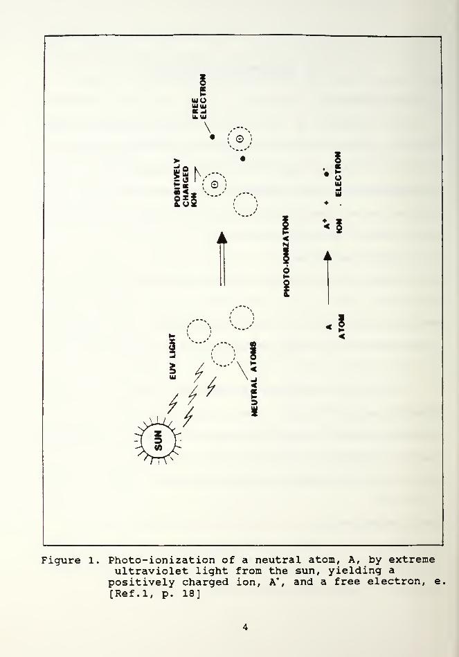
Figure 1. Photo-ionization of a neutral atom, A, by extremeultraviolet light from the sun, yielding apositively charged ion, A*, and a free electron, e
[Ref.l, p. 18]
Between dawn and dusk, photo- ionization exceeds
recombination and maximum density layers are formed affecting
radio communications in greater percentages than during the
hours after dusk when the effect is reversed.
3 . Ionospheric Layers
The ionosphere divides into three mayor layers, D, E ,
and F which is sub-divided into two others, Fl and F2
.
The lowest layer is the D- layer which spans from 50 to
90 km. In the D- layer low frequency (LF) waves are refracted
while Medium Frequency (MF) and High Frequency (HF) waves are
absorbed. There are two types of absorption that affect the
HF band: deviative and nondeviative. Deviative absorption
occurs when the refractive index approaches zero, generally at
the apex of the trajectory, while nondeviative absorption
takes place when the refractive index approaches one and the
product between electron density and electron collision
frequency is high [2] . Another aspect of the D- layer is that
it disappears after sunset due to rapid recombination.
The E- layer is located between 90 and 130 km and is also
known as the "Kenelly-Heaviside layer". This layer is
characterized by strong diurnal variations. Recombination is
rapid after sunset and the layer diminishes as the night
advances. The Sporadic E- layer also occurs near 120 Km and
exists throughout the day at lower (equatorial) latitudes and
during late night for higher (polar) latitudes. The E- layer
reflects signals up to 20 MHz providing communications at
distances up to 2500 km per reflection.
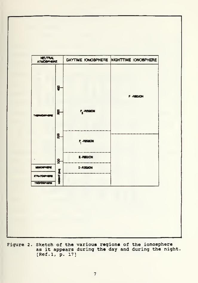
The F- layer is formed between 150 and 600 km. During
the daytime this layer divides into two layers, Fl and F2
,
located between 150 and 220 km and above 225 km, respectively.
Since these layers are at the highest altitudes, photo-
ionization occurs at the highest rate. At noon time in the
northern latitude winter, these layers are the closest to the
sun and the ionization rates are maximum. Because the
atmospheric density diminishes with altitude, the F-region
recombination process is relatively slow and at night the
F- layer is always present. Figure 2 shows the different
layers of the ionosphere.
4 . Variations of the Ionosphere
Since the ionosphere is created by the effect of solar
radiation upon the atmosphere, the ionosphere will also vary
with the time of the day, season, location on the earth, solar
activity, and other similar factors.
These variations that affect the ionosphere will also
affect HF communications. The principal variations of the
ionosphere are:
* Diurnal (throughout the day)
* Seasonal (throughout the year)
* Location (geographic and geomagnetic)
* Solar Activity (Solar cycle and disturbances)
* Height (different layers ) [1]
Figure 3 illustrates how diurnal variations affect the
tcunui.ATyOSffEWg
rn*t
*
DAYTIME IONOSPHERE
1
I-AS9DN
D-
NIGHTTIME IONOSPHERE
Figure 2. Sketch of the various regions of the ionosphereas it appears during the day and during the night[Ref.l, p. 17]
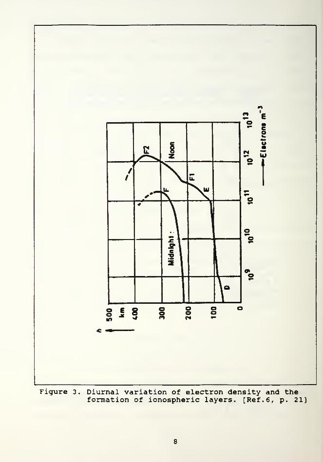
Figure 3. Diurnal variation of electron density and theformation of ionospheric layers. [Ref.6, p. 21]
formation of ionospheric layers.
5. Ray Tracing
In order to determine the amplitude, phase,
polarization, flight time, etc. of the transmitted wave, it is
necessary to determine the ray path between the transmitter
and the receiver. Determining the ray path seems to be a
simple task but in practice it is not. Factors affecting the
ray path are the orientation and intensity of the earth's
magnetic fields, the collision frequency of electrons and
electron density variations within the layers. Thus,
calculations are much more complex for the real -world than for
the assumption that the ionosphere is a homogeneous layer.
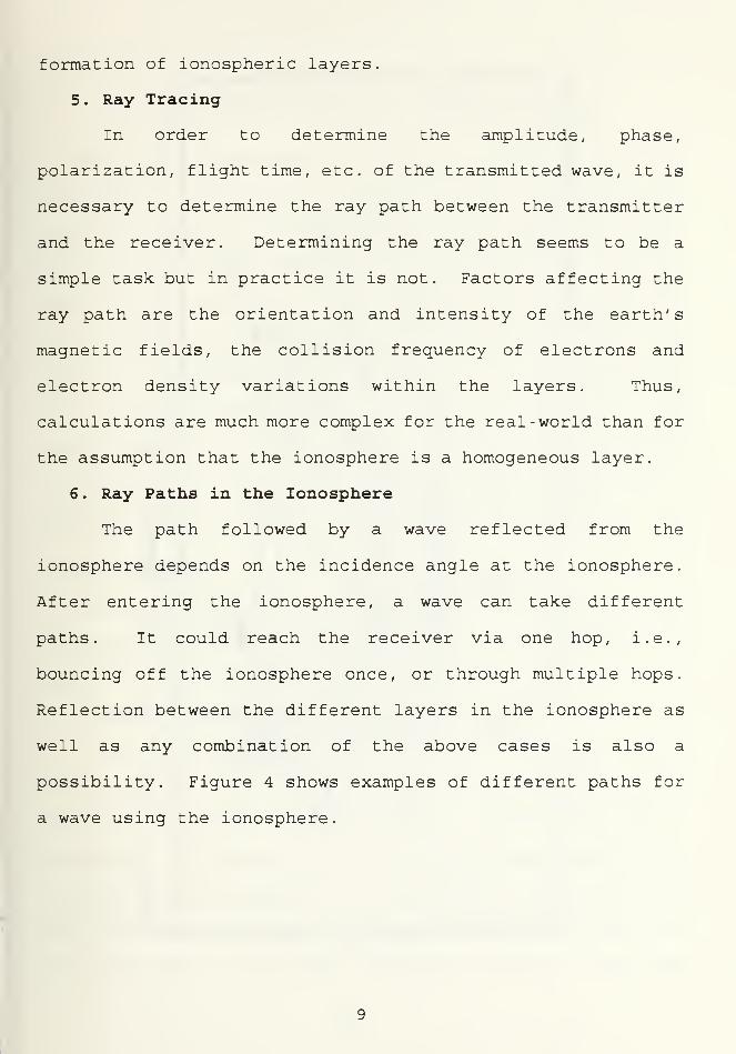
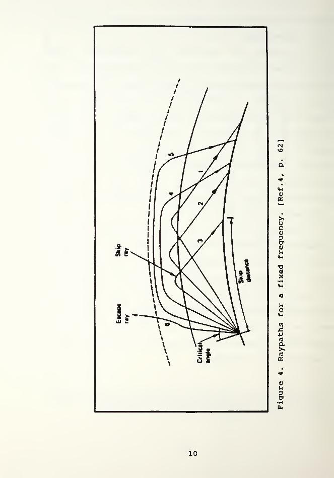
6 . Ray Paths in the Ionosphere
The path followed by a wave reflected from the
ionosphere depends on the incidence angle at the ionosphere.
After entering the ionosphere, a wave can take different
paths. It could reach the receiver via one hop, i.e.,
bouncing off the ionosphere once, or through multiple hops.
Reflection between the different layers in the ionosphere as
well as any combination of the above cases is also a
possibility. Figure 4 shows examples of different paths for
a wave using the ionosphere.
CM
<M
>1oc0)
0)
u
•o0)
X•H
«
o
W
(0
a(0
a
•H
10
III. THE MONTEREY-SAN DIEGO COMMUNICATION LINK
Before the polar region HF ionospheric communication link
for PENEX is installed, a test-bed link was established to
verify the operation of the equipment and software. For this
link, Monterey was designated as the transmitter site with San
Diego as the receiver site. The geographical latitude and
longitude used in the scenario files of ADVANCED PROPHET 4.3
are 36°37' N latitude and 121°55' W longitude for Monterey and
32°43' N latitude and 117°09' W longitude for San Diego. The
transmit power for the tests is 2.5, 75 and 100 watts and the
frequencies are 5.604 and 11.004 MHz. The methodology of
experimentation is described in detail in Chapter IV.
A. LINK ANTENNAS
The description of the antenna characteristics for the
transmitter and receiver sites are essential for modeling the
skywave propagation and for the link power budgets.
1. Transmitting Antenna
The transmitting antenna utilized is a multiband dipole
which consists of a group of three half -wavelength dipoles
connected to a common transmission line. The multiband dipole
is designed to operate on 5 . 6 , 11 and 16.8 MHz respectively.
For data collection purposes the antenna was operated at 5.604
and 11.004 MHz since 16 MHz propagation was very unlikely for
the test link. The data collected for the 11.004 MHz
11
frequency range was obtained for only one day, during the time
of this investigation.
Dipole lengths were 5.6, 11, and 16.8 MHz for 24.69,
13.05, and 8.53 meters, respectively. Since these dipoles are
center- fed, each has two elements half the dimensions given
above. Figure 5 shows the dipole antenna geometry details.
The separation between the dipoles is 0.3048 meters and the
upper and lower elements are at an elevation angle of 11.21°
and -11.21° respectively. The dipoles are fed by a 50 ohm
impedance coaxial cable connected to a 1:1 balun transformer.
2 . Receiving Antenna
The receiver antenna in San Diego is a dipole,
containing three half -wavelength dipoles on one structure,
drooping from the center at -34°. It is designed to operate
at the same frequencies as the transmitting antenna.
The half lengths of each element are 12.73 m. , 6.48
m. , and 4.24 meters for frequencies 5.6, 11, and 16.8 MHz
respectively. The separation between elements is 12.7 cm and
the feed line is a 50 ohm coaxial cable. Figure 6 shows the
details of the receiver antenna.
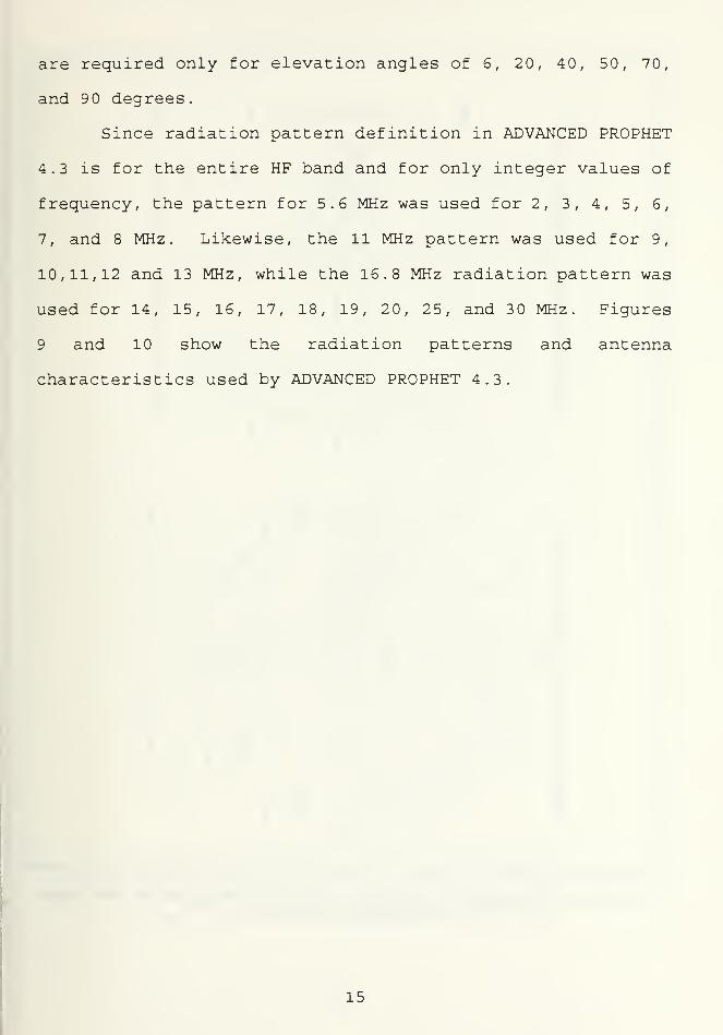
3 . Antenna Simulation
The transmit antenna designs were modeled by a Naval
Postgraduate School student using the Numerical
Electromagnetics Code (NEC) which in turn provided patterns
for ADVANCED PROPHET 4.3. Figures 7 and 8 show radiation
patterns from NEC. In ADVANCED PROPHET 4.3, these patterns
12
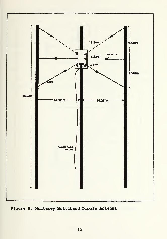
Figure 5. Mont«r«y Multiband Dipol* Ant«nna
13
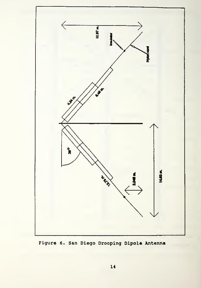
Figure 6. San Diego Drooping Dipole Antenna
14
are required only for elevation angles of 6, 20, 40, 50, 70,
and 9 degrees.
Since radiation pattern definition in ADVANCED PROPHET
4.3 is for the entire HF band and for only integer values of
frequency, the pattern for 5.6 MHz was used for 2, 3, 4, 5, 6,
7, and 8 MHz. Likewise, the 11 MHz pattern was used for 9,
10,11,12 and 13 MHz, while the 16.8 MHz radiation pattern was
used for 14, 15, 16, 17, 18, 19, 20, 25, and 30 MHz. Figures
9 and 10 show the radiation patterns and antenna
characteristics used by ADVANCED PROPHET 4.3.
15
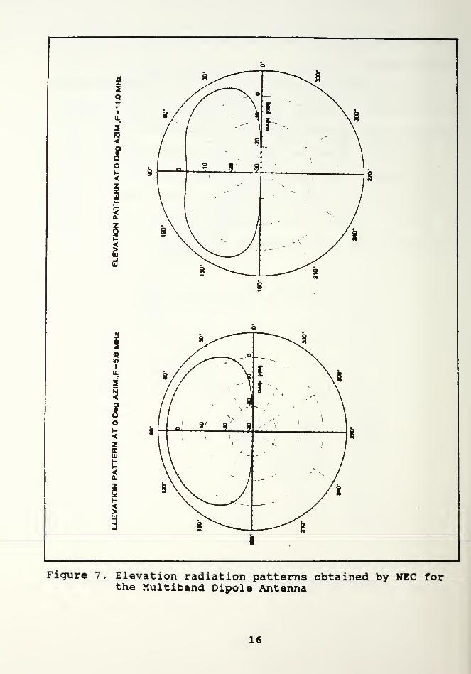
Figure 7. Elevation radiation patterns obtained by NEC forthe Multiband Dipole Antenna
16
Figure 8. Elevation radiation patterns obtained by NEC forthe Drooping Dipole Antenna
17
p J <">sfl«*«(Hff<9a
to !I I I i I I n
Zfy
9 « sC * N H 9* 91 1 1 1 1 1 a
9 H H*n
s1
ms6s0NH»aa1 1 1 1 1 1 N
<•> sfl * n -t * 9I I 1 I I I
«a.
Xii M m**N«4*Sa
i i i i i i h iz £ •-
H rt SB SO N H o>> a NO i i i i i i «mm 01
I«
1 1 1 1 1 1 H
2a 1 i i i i i i
u H rtsOsflNH»>9*j « 1 1 1 1 1 1 H
0.
fib X S0 v a H 9 «s aM X 1 1 1
a ii H
Si i**9h90>9nII 1 H
« - N -6 9 9 -i 9 * 9a h « 1 1 1
hS s«T9-<9»>99j - II 1 H?I
* * 9 * 9 *> 9
?! °1 1 1
Ul 0. HHHSnnScsa
1 Hi
H h h h s n n a5X >
1 Hi
-<-*H9«o9sfl<1 H
Z5
II 1
h h h a n n a «H > 1 H a.• H 1
1 H in -
i MMa h -* h 9 n n 9 H
u a.
a «
1 H1HH^annaN 3
« u 1 H1 d
H
i i a a a a a a z 7 •
•0 1 * 1 * * b 3? ^a z
ss h9 9 9 9 9s* e
« H ffs p» r> * M -
Figure 9. Elevation radiation patterns used by PROPHET forthe Multiband Dipole Antenna
18
JaafNeoMSS|
, I H „SOSafNCNl
• « I I HS H I
<*> U I I H NSK l
O I I HI Ill-»«»NC5N900
IHOaaVNiNl- «» i
X _ I I H HUKaafNaNt
W I I HU hasfNenilfrf ? I I H *0.x f * f f hoo ar s
'A II H
2Sl"'3
fiU H « I
O «on vvvvHaoaa§ S ' -
U flu vvnNNNSeas ' rtf n n nn9Z i -« I
I HII I3t » n N NN J> I -H
H I
J I HII - I
-J « I -*
U 0. I
ffl « V*mNNN9«lsv
rH
« -zz aa i i aai viZg «**«»«<J»mu z -a « * -a -a -a bszee 99999* e« h a*, p. in * n -
flu
Figure 10. Elevation radiation patterns used by PROPHET forthe Drooping Dipole Antenna
19
IV. COMPARISON OF EXPERIMENTAL DATA WITH PROPHET PREDICTIONS
A. EXPERIMENTAL DATA
The following data are collected via PENEX equipment and
software at the San Diego receiver site. The PENEX system
uses direct sequence spread spectrum modulation (DSSS)
,
specifically phase shift keying (PSK) , to transmit a reference
maximum length sequence. The system measures mode time delay
and signal strength using a quadrature -sampled, Fast Fourier
Transform (FFT) matched- filter signal processor. The time
delay measurements have a 25 millisecond (msec) resolution.
This system provides a precise time delay measurement as well
as consistent signal strength measurements.
Figure 11 shows an example of correlation vector plots
resulting from cross correlation of the reference sequence
with the digitized HF data. The upper plot is the raw vector
(linear form), of approximately 10 msec of data. Since the
digitizing rate is 39.0625 MHz, each bin is 25.6 microseconds.
In order to determine the mode delay, delta t, and the value
of the correlation peak, this vector is scanned to locate the
peaks, record the corresponding correlation peak values, and
find the distances between adjacent peaks (in terms of the
intervening bin count) . The number of intervening bins is
then multiplied by the 25.6 microsecond duration of each bin,
yielding the mode delay, delta t. Next, the value of the
20
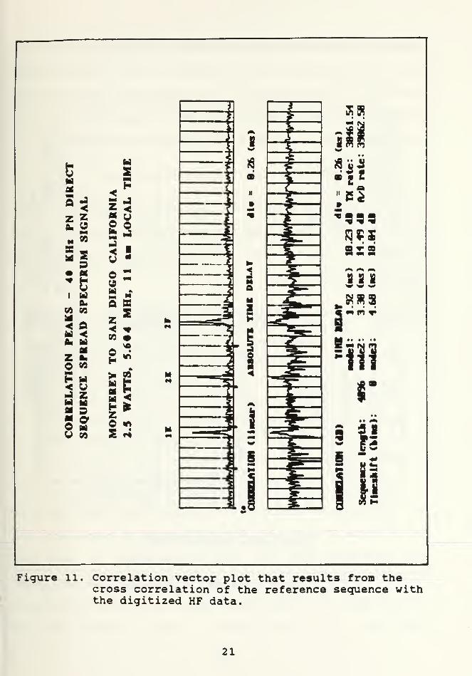
Figure 11. Correlation vector plot that results from thecross correlation of the reference sequence withthe digitized HF data.
21
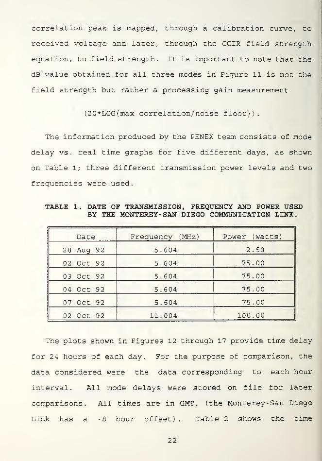
correlation peak is mapped, through a calibration curve, to
received voltage and later, through the CCIR field strength
equation, to field strength. It is important to note that the
dB value obtained for all three modes in Figure 11 is not the
field strength but rather a processing gain measurement
(20*LOG{max correlation/noise floor}).
The information produced by the PENEX team consists of mode
delay vs. real time graphs for five different days, as shown
on Table 1; three different transmission power levels and two
frequencies were used.
TABLE 1. DATE OF TRANSMISSION, FREQUENCY AND POWER USEDBY THE MONTEREY- SAN DIEGO COMMUNICATION LINK.
Date Frequency (MHz) Power (watts)
2 8 Aug 92 5.604 2.50
02 Oct 92 5.604 75.00
03 Oct 92 5.604 75.00
04 Oct 92 5.604 75.00
07 Oct 92 5.604 75.00
02 Oct 92 11.004 100.00
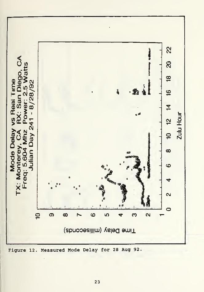
The plots shown in Figures 12 through 17 provide time delay
for 24 hours of each day. For the purpose of comparison, the
data considered were the data corresponding to each hour
interval. All mode delays were stored on file for later
comparisons. All times are in GMT, (the Monterey- San Diego
Link has a -8 hour offset). Table 2 shows the time
22
<
CO
I- r <MOO
®CO (DoO
T5 5S.S
5(7
h
9
4
III1
I
1
I, I I 1
O) 00 CO LO C5
(spuooesijiiai) Aejea emu
egc\j
8
00
CO
uCN O
5 3
CO
co
CM
oCNJ "r-
Figure 12. Measured Mode Delay for 28 Aug 92.
23
<
s op co
> T"
>4 N '
®£s£
I-a
U " ''"'' u
O 00 co \r> CO CM t-
(spuooesHiiuj) Aeieo 9W!±
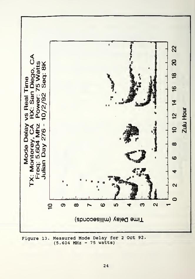
Figure 13. Measured Mode Delay for 2 Oct 92.
(5.604 MHz - 75 watts)
24
<
spy.SQiflCO
5n£s
(0
2£
*
00 °'
asP
qjfco
*
1"' " 111 I
CVJCVJ
S3
GO
CD
3
O 3
GO
CO
- CVJ
0) CO co m CO CVJ r-
(spuooesiiiiLu) Aeiea qwll
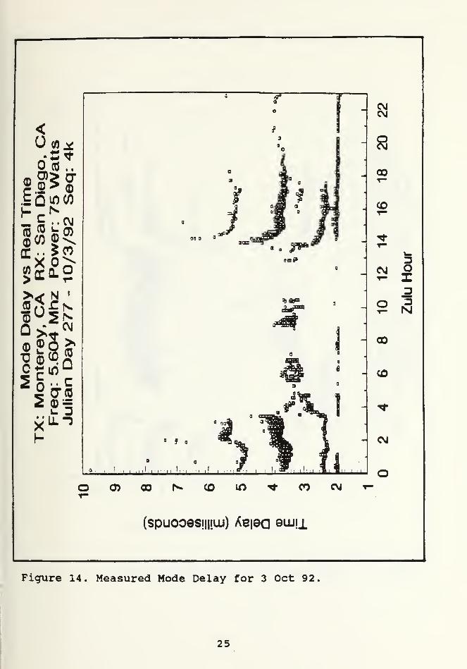
Figure 14. Measured Mode Delay for 3 Oct 92
25
<X«
O CO
EQflCO
CO 5©CO
o
eg
0)
5bc CL
><< N
5 c
Xh
00s
>(0CD
in
.. ccrco
IL-3
J,
1" ' "," '
I
'
I-*"
H Si
GO
CO
3CN O
O ^
00
CO
oOi 00 CO m CO CNJ
(spuooesjiijiu) Ab|9q aiuii
Figure 15. Measured Mode Delay for 4 Oct 92.
26
<
o co ..
0)
0"
©2g
5 CD*c\j
5
>2 JS
+- irt uc
ID
.. c^ tyco
h
nOP
i Hi i Ll MMtl' !.> .ill. nynl-...«ll .1: »'•' I "'J
Si
00
3CM O
O ^i= N
00
CO
CNJ
O 00 co in 00 CNJ r-
(spuooesiiijuj) Aeiea 0^j!1
Figure 16. Measured Mode Delay for 7 Oct 92.
27
SI
imeDiego.
CA
OO
Watts
/92
i J
w 9
8
00
MB
! |
- -
vOir
§ScLg1 •
i.
•i
•••;-3
s i
tin•
i i* . oJ5
.
Mode ontere 11.00 JUIian1
l
1 m
09
CO
*? . *
^ ''
\ .
iCM
jf+
o 0> CONttlD^COOJ*-(spuoo«sii8Lu) Aejec Qujij.
Figure 17. Measured Mode Delay for 2 Oct 92(11.004 MHz - 100 watts)
28
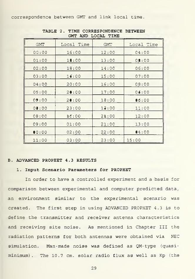
correspondence between GMT and link local time.
TABLE 2 . TIME CORRESPONDENCEGMT AND LOCAL TIME
BETWEEN
GMT Local Time GMT Local Time
00:00 16:00 12:00 04:00
01:00 17:00 13:00 05:00
02:00 18:00 14:00 06:00
03:00 19:00 15:00 07:00
04:00 20:00 16:00 08:00
05:00 21:00 17:00 09:00
06:00 22:00 18:00 10:00
07:00 23:00 19:00 11:00
08:00 00:00 20:00 12:00
09:00 01:00 21:00 13:00
10:00 02:00 22:00 14:00
11:00 03 :00 23 :00 15:00
B. ADVANCED PROPHET 4.3 RESULTS
1. Input Scenario Parameters for PROPHET
In order to have a controlled experiment and a basis for
comparison between experimental and computer predicted data,
an environment similar to the experimental scenario was
created. The first step in using ADVANCED PROPHET 4.3 is to
define the transmitter and receiver antenna characteristics
and receiving site noise. As mentioned in Chapter III the
radiation patterns for both antennas were obtained via NEC
simulation. Man-made noise was defined as QM-type (quasi -
minimum) . The 10.7 cm. solar radio flux as well as Kp (the
29
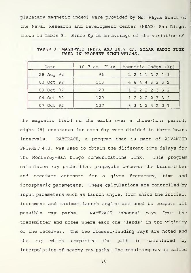
planetary magnetic index) were provided by Mr. Wayne Bratt of
the Naval Research and Development Center (NRAD) San Diego,
shown in Table 3. Since Kp is an average of the variation of
TABLE 3. MAGNETIC INDEX AND 10.7 cm. SOLAR RADIO FLUXUSED IN PROPHET SIMULATIONS.
Date 10.7 cm. Flux Magnetic Index (Kp)
2 8 Aug 9 2 96 2211221102 Oct 92 118 4644323203 Oct 92 120 1222233204 Oct 92 120 1222233207 Oct 92 137 33123221
the magnetic field on the earth over a three-hour period,
eight (8) constants for each day were divided in three hours
intervals. RAYTRACE, a program that is part of ADVANCED
PROPHET 4.3, was used to obtain the different time delays for
the Monterey- San Diego communications link. This program
calculates ray paths that propagate between the transmitter
and receiver antennas for a given frequency, time and
ionospheric parameters. These calculations are controlled by
input parameters such as launch angle, from which the initial,
increment and maximum launch angles are used to compute all
possible ray paths. RAYTRACE "shoots" rays from the
transmitter and notes where each one "lands" in the vicinity
of the receiver. The two closest- landing rays are noted and
the ray which completes the path is calculated by
interpolation of nearby ray paths. The resulting ray is called
30
a mode. The launch angle is then increased until a second
mode is obtained. The calculation process terminates when one
of the following conditions is met:
* The initial ray does not bounce off the ionosphere but
rather penetrates it.
* The launch angle reaches the maximum specified value.
* The maximum number of modes are reached by the program
itself
.
The user in ADVANCED PROPHET can define ionospheric
parameters such as:
* Critical frequency of the E- region (foE)
.
* foEs if the Sporadic E- layer is to be considered.
* Critical frequency of the Fl region, foFl
.
* Critical frequency of the F2 region, foF2
.
* F2- layer maximum density altitude, hmF2
.
* F2- layer semi- thickness , YmF2
.
When these parameters are specified, the ionosphere will be
assumed to be uniform throughout the region of propagation.
If these parameters are not user specified, ADVANCED PROPHET
uses internal models to calculate the parameters including
variations along the path due to time of day, solar activity
and the link geographical region [5]
.
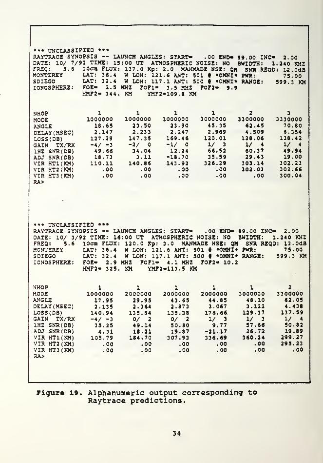
2. ADVANCED PROPHET 4.3 Data Analysis
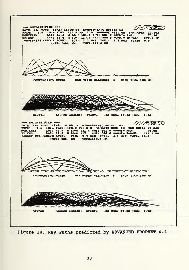
After all calculations are completed, two types of
output displays are generated. The first type of display
shows the parameters which defined the calculations and the
31
plots of the rays paths, as shown in Figure 18. The second
display details the results of the calculations in
alphanumerical fashion, as seen in Figure 19. For the
comparison process, the rubric, or unique descriptor,
corresponding to the mode delay (msec) was used to identify
the different mode path geometries; this delay is the total
calculated group delay.
To consider a propagation mode delay prediction valid
for the comparison, the signal to noise ratio (SNR) should be
greater than dB. From the alphanumeric output of the
Raytrace program the SNR can be determined for each of the
propagation mode delays. The other rubrics of the display
lists calculated propagation modes, such as number of hops,
ionospheric bounce region and trajectory losses. For the
analysis, data obtained from RAYTRACE alphanumeric output were
utilized.
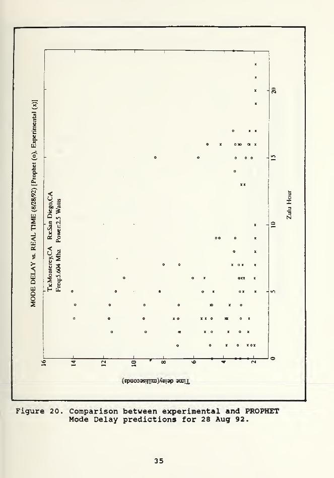
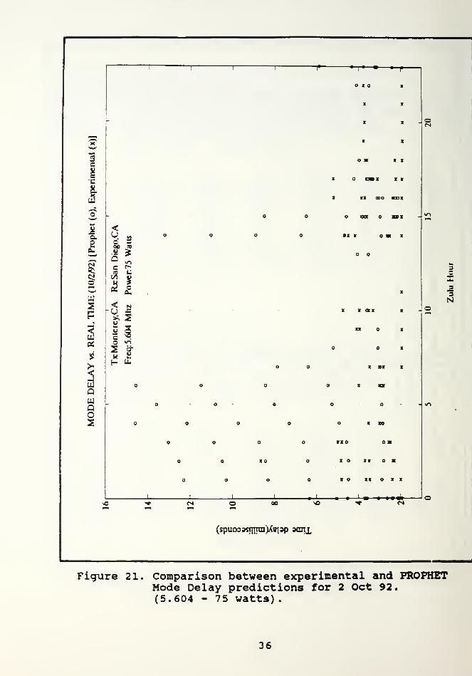
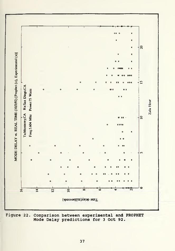
C. DATA COMPARISON
Figures 2 through 2 5 show experimental and ADVANCED
PROPHET 4.3 generated mode delay data. Data plotted for a
given day were assigned "o" and "x" corresponding to PROPHET
and experimental data respectively. There is a similarity
between the data, especially in the 2 - 7 msec time frame.
PROPHET predicts mode delays that are greater than 15 msec,
which are not observed in the experiment. In addition,
PROPHET shows increasing mode delays for the first six hours
of the day, 0000 through 0600 GMT (1600 through 2200, the
32
rzyT zw^•mm UNCLASSIFIED <mm>
DATE: 18W 7/92 TIME: 13:00 UT ATMOSPHERIC NOISK: HOFRTCOi 3.6 10OM fXUX: 137. Ky: 3.0 HANMADE HSE: QM SMK UQB: 12.1MONTEREY U»T: 36.4 U LON: 121.6 ANT: 301 O «OMNI» rum : 73 . OOSDIECO LAT: 32.4 U LON: 117.1 ANT: SOO «OMNI<» RANGE: 399.3 KMIONOSPHERE < ABOVE RCVR> : FOE= 2.3 HH3 fOFl* 3.3 MM3 FOFSa 9.9
MHF2= 344. KM Yt4F3 =109.S KM
PROPAGATING MODES MAX MODES ALLOWED*
ii 'i n ii i ii i'i i nn 1 1 r i nn i iii' n iiiim '
4 EACH TICa 184) KM
LAUNCH ANGLES
SZVT ZW^UNCLASSIFIEDDATE: lOV 3X92 TIMS: 14 :M UT ATMOSPHERIC NOISE:FREO: 3.4 10on FLUX: 120. • K»: JO MANMADE NSE: ON SNR RESDi 13 «ULSMONTEREY LAT: 34.4 H LON: 121.4 ANT: 301 «OMMI« PMR: 73.00S©ICCO LAT: 32.4 H LON: 117.1 ANT: 300 "OMHI* RANGE: 399.3 KMIONOSPHERE < ABOVE RCVR> : FOEs 2.9 HH3 FOFls 4.1 NHS FOFSa 10.
S
HHF23 323. KM YHTSallJ.S KM
PROPAGATING MODI
ii i ii 1
1
'ii iiiiiii' 1 1 n 1 1 1 1 r ii 1 1 m i i'
ALLOWED* 4 EACH TICa 100 KM
RAVFAN LAUNCH ANGLES*. STARTa S9.00 INCa 2.
Figure 18. Ray Paths predicted by ADVANCED PROPHET 4.3
33
*** UNCLASSIFIED ***RAYTRACE SYNOPSIS — LAUNCH ANGLES: START- .00 END- 89.00 INC- 2.00DATE: 10/ 7/92 TIME: 15:00 UT ATMOSPHERIC NOISE: MO BWIDTH: 1.240 KHZFREQ: 5.6 10cm FLUX: 137.0 Kp: 2.0 MANMADE NSE: QK SNR REQD: 12 . OdBMONTEREY LAT: 36.4 W LON: 121.6 ANT: 501 t *OMNI* PWR: 75.00SDIEGO LAT: 32.4 W LON: 117.1 ANT: 500 I *OMNI* RANGE: 599.3 KMIONOSPHERE: FOE- 2.5 MHZ FOF1- 3.5 MHZ FOr2- 9.9
HMF2- 344. KM YMF2-109.8 KM
NHOPMODEANGLEDELAY (MSEC)LOSS(DB)GAIN TX/RX1HZ SNR(DB)ADJ SNR(DB)VIR HTl(KM)VIR HT2(KM)VIR HT3(KM)RA>
1
100000018.652.147
127.29-4/ -349.6618.73
110.11.00.00
100000023.502.233147.35-2/34.043.11
140.86.00.00
100000023.902.247169.46-1/12.24
-18.70143.92
.00
.00
300000045.352.969
120.011/ 3
66.5235.59
326.29.00.00
330000062.454.509128.061/ 460.3729.43303.14302.03
.00
333000070.806.354
138.421/ 4
49.9419.00
302.23302.66300.04
*«* UNCLASSIFIED ***RAYTRACE SYNOPSIS — LAUNCH ANGLES: START- .00 END- 89.00 INC- 2.00DATE: 10/ 3/92 TIME: 16:00 UT ATMOSPHERIC NOISE: NO BWIDTH: 1.240 KHZFREQ: 5.6 lOca FLUX: 120.0 Kp: 3.0 MANMADE NSE: QM SNR REQD: 12. OdBMONTEREY LAT: 36.4 W LON: 121.6 ANT: 501 C •OMNI* PWR: 75.00SDIEGO LAT: 32.4 W LON: 117.1 ANT: 500 9 •OMNI* RANGE: 599.3 KMIONOSPHERE: FOE- 2.9 MHZ FOF1- 4.1 MHZ FOF2- 10.2
HMF2- 325. KM YMF2-113.5 KM
NHOPMODEANGLEDELAY (MSEC)LOSS(DB)GAIN TX/RX1HZ SNR(DB)ADJ SNR(DB)VIR HTl(KM)VIR HT2(KM)VIR HT3(KM)RA>
100000017.952.135140.94-4/ -335.254.31
105.79.00.00
200000029.952.364135.840/ 2
49.1418.21
184.70.00.00
200000043.652.873
135.380/ 2
50.8019.87
307.93.00.00
200000044.853.067
176.66.1/ 3
9.77-21.17336.69
.00
.00
300000048.103.122
129.371/ 3
57.6626.72
360.24.00.00
330000062.054.438
137.591/ 4
50.8219.89
299.27295.23
.00
Figure 19. Alphanumeric output corresponding toRaytrace predictions.
34
scVEc
LU
p
5100Ci90
u2p
uQuQO2
1 I i r 1 1— 1
—
X
X
X
X
XX
X xo at X
O
XX
1
Re
San
Diego.CA
Power.
2.5
Watts
00 X
-
:rey,CA
i4
Mhz•
X
X O X X
s 56O W)
2 '&
o
X 0X« I
1 OX X
X> X o
O o I o X X XX ox
i 1 „ J_
« « . X ox
I X ox
—
1
.—1——-—J
—
3OI
3N
r<
(spuoo3$ijnm)XBi3p aanj.
Figure 20. Comparison between experimental and PROPHETMode Delay predictions for 28 Aug 92.
35
c&
Q.
Sfiu
§
P
as
Q
QO2
11
!1
—1* '1
•
—
—f
0X0 X
X X
X X -
X X
It XX
* o cm i x x
X XX 0)0 CDI
- O XXI Dl
<
Qe
o ix x o m X
< 5 . _ X 1 an x
u—
e
2wH
2
El
BO X
O OXI OI I
o o x xai
- o o o
o o x xe
XX0 OK
10 X XX
1
e
i 1 1
10 XX X I
—1 « 1 » «»^l
3O
N
tM
(spuo33synnn)XB|3p aan^
Figure 21. Comparison between experimental and PROPHETMode Delay predictions for 2 Oct 92.(5.604 - 75 watts)
.
36
ac
'S
Q.
ea.
§
P
5>•
QUQO
<u&.Si
Qe
&
<Ua^.
fiueo2wE-
aOB
l:
£
5s
tu.
x o at o o ibi
I O I* O KO<
x or i
I O XI O I
10 IX. Oil ox
X XX X X
oX
3N
«s «s
(spaco3$nnraMBi3P 3°ni
Figure 22. Comparison between experimental and PROPHETMode Delay predictions for 3 Oct 92.
37
r 1 1 1 1* » |»—« m
|
X
X I ©
,
">? 1 1^^"
a X X Xe
1UJ
I rap > ix
x oa o o aox
o - o m o •! VI
iD. o o ox oxxx exos— XX XX/^
5o
< 3
So a
OXXX o
3
p
in "3
e r»XXII o
4 o ii aii
i 55 IIII X
£ & S> Si - XXXXJI
5- 9
uQ
<r>
1 1O IBI X
8_H u. o o o o I o x - <«
o2
1
0X0O OX OX I X X
• B XOIXOXo o o o i o a D k
' ' ' ' r ' — L os<5 •*" <M © 00 >0 •* «S1 »*
(spaoo9stnnn)Xei9p aanj.
Figure 23. Comparison between experimental and PROPHETMode Delay predictions for 4 Oct 92.
38
1aSa.
o
Hi
aUJ
QO5
—
r
i1 1 1 1 r—
o
o o
X
I * XX X I
I XO «I X I
i o x bo atom
u Jfl
o x i a xaa -
ae
1 ox xx on x
X 1
£ *
££ XX X
<Jg
XXXU 2
-fi ^r X XXX X X -
uco
wE-
a-
uXXX XO X
X X X X XO X
XXXD XX X
INI I I
- o e »- « a it i -
O XX X X XI
o o e XO X X XX s
e X X X
_i 1 1 i
o
—J-
X X
1 » » »»1
- ">
5oI
sN
<s
(spuo33sinnn)XB]3p semi
Figure 24. Comparison between experimental and PROPHETMode Delay predictions for 7 Oct 92.
39
i i r i ii
•*-i
c B
- o xo
1? XO X
•*w
3 o X IBc
C x ax
&u X
<"^</>
>~' X w*
iD. X
£a.^f Iy—
y
g * akm3oIci <->. 5o &* a*• k -
Q 23N
46 - c t; . x - ©p c3 g
**
<! 3£isi ^2 .
> ha O2
u 5u o —Q 3 S"
- H B. . w>
s
1 1 1 1 1 ,
I
1 • ' ^vO •* (N O QO <0 » <s
—i—i ««
(spaO03STnjlD)XB13p SOJTJ,
Figure 25. Comparison between experimental and PROPHETMode Delay predictions for 2 Oct 92.
(11.004 - 100 watts)
.
40
local time for San Diego) , which is similar in some aspects to
experimental results. Single and multihop propagation of up
to six hops are predicted by PROPHET. The experimental data
plotted in Figures 12 to 16 shows only three modes.
In Figure 25 for 2 Oct 92, PROPHET data obtained at 11.004
MHz with 100 watts is close to the experimental data, where in
the early hours of the day, propagation is not supported by
the path. Good correspondence between experimental and
PROPHET data is noted between 1600 and 2400 GMT. ADVANCED
PROPHET 4.3 predicts mode delays above 4 msec that are not
shown in the experimental data.
For further comparison between experimental and PROPHET
data, an hour by hour, day by day breakdown is provided in
Figures 26 through 31. These plots were created by counting
the times for which the experimental and predicted delays were
a different by less than 0.5 msec. All hours in which
propagation for both cases was not available are marked with
an asterisk. From Figures 26 to 31 it is seen that maximum
correlation between PROPHET and experimental data occurs in
the early hours of the day and between 1400 and 1900 GMT.
The third comparison was calculation of the total
percentage per hour, over the five day period, in which the
time delay differences were less than 0.5 msec. In this
manner a global comparison is performed to more fully
appreciate how the percentages are distributed throughout the
day. Table 4 and Figure 32 show this comparison. All of the
41
1 !
.o
jmt
8 •
|aoZ
•12•
CD
5
5 a
z i ao
5
•
•
> oXa
2 Si
3
- £ k©
OS NQu Jc
S s u
53 £wS
c.2
•
Q1" &
jS
5
QU. 2.
1"8
•IO
s 1
g5
c
a
83O 8I •5
»
gi
11 i i i i i
o3 r» sO ^ v tn <s i-i «3
JUnCQ
Figure 26. Mode Delay Approximation Distribution for28 Aug 92
42
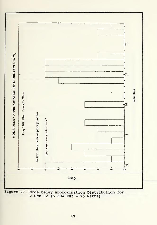
Figure 27. Mode Delay Approximation Distribution for2 Oct 92 (5.604 MHz - 75 watts)
43
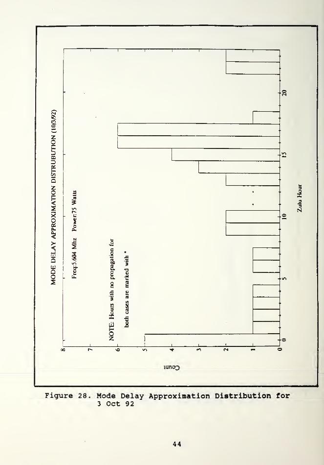
Figure 28. Mode Delay Approximation Distribution for3 Oct 92
44
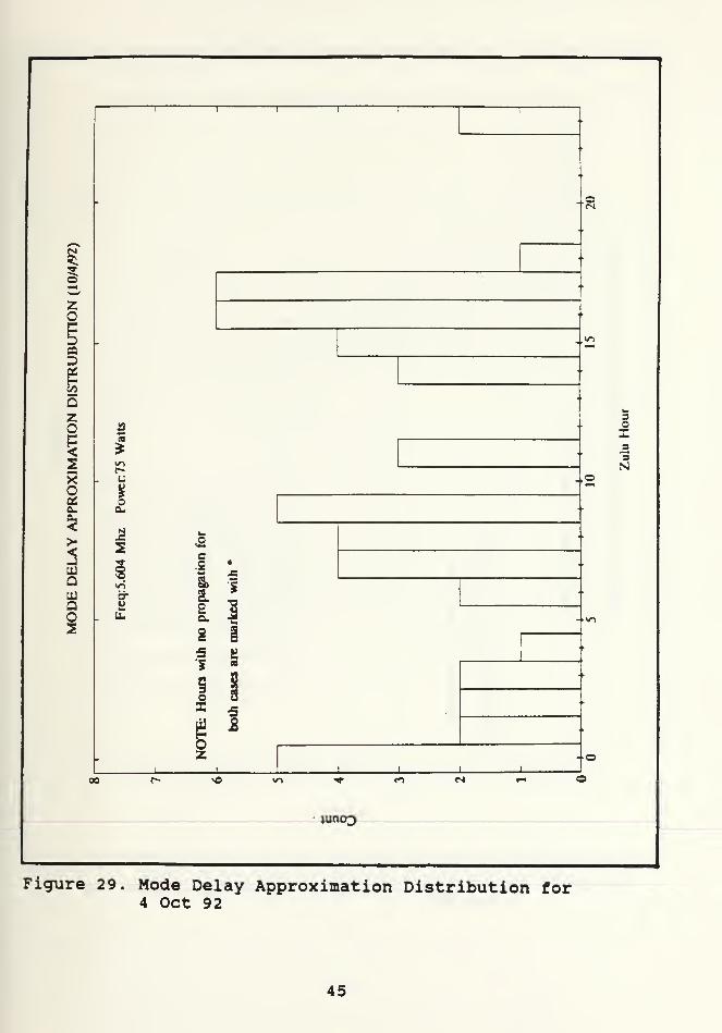
Figure 29. Mode Delay Approximation Distribution for4 Oct 92
45
o
Zo
CD
D
zO
aoa.
UQ_QO2
3O
_3"3
CM
JuncQ
Figure 30. Mode Delay Approximation Distribution for7 Oct 92
46
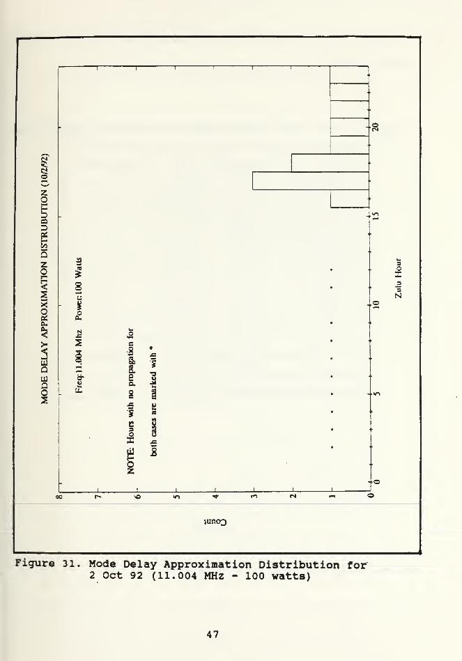
Figure 31. Mode Delay Approximation Distribution for2 Oct 92 (11.004 MHz - 100 watts)
47
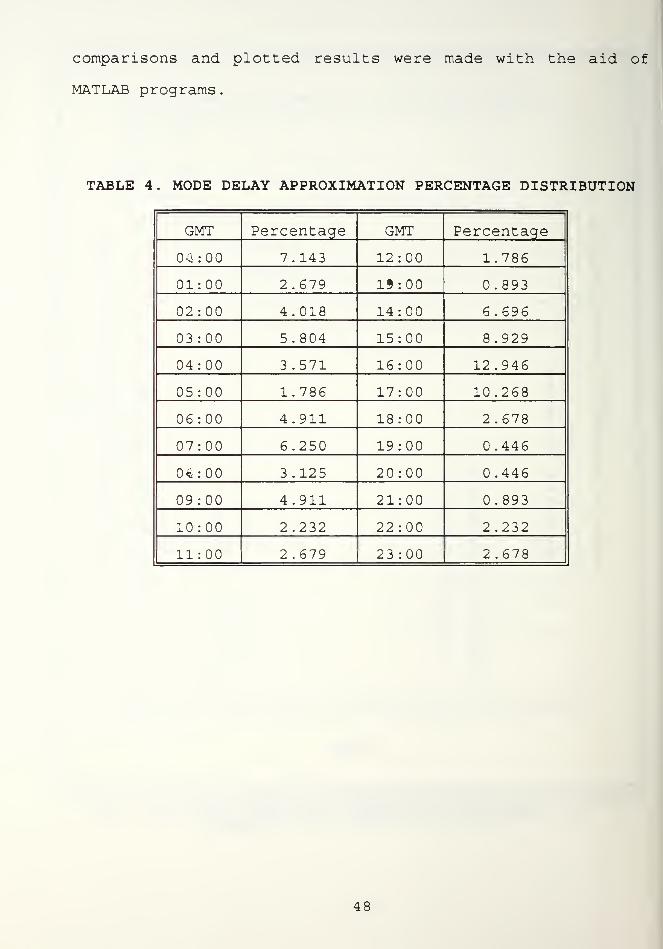
comparisons and plotted results were made with the aid of
MATLAB programs
.
TABLE 4. MODE DELAY APPROXIMATION PERCENTAGE DISTRIBUTION
GMT Percentage GMT Percentage
00:00 7.143 12:00 1.786
01:00 2.679 13:00 0.893
02:00 4.018 14:00 6.696
03:00 5.804 15:00 8.929
04:00 3 .571 16:00 12.946
05:00 1.786 17:00 10.268
06:00 4.911 18:00 2.678
07:00 6.250 19:00 0.446
08:00 3.125 20:00 0.446
09:00 4.911 21:00 0.893
10:00 2.232 22:00 2.232
11:00 2 .679 23 :00 2.678
48
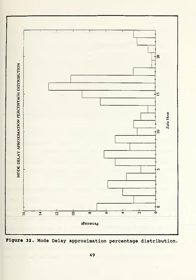
Figure 32. Mode Delay approximation percentage distribution,
49
V. CONCLUSIONS AND RECOMMENDATIONS
The field measurements indicate that the PROPHET
propagation predictions are most accurate for the early hours
of 1400 until 1700 GMT of each day. Data taken on 2 Oct 92 at
11.004 MHz show that when skywave propagation is supported,
the experimental and program predictions are almost identical,
for mode delays of less than 4 msec. As expected,
experimental and program results are similar also for the part
of the day when skywave propagation is not supported by the
ionosphere
.
Field data taken at 5.6 MHz showed good agreement with
PROPHET propagation predictions. Between 0000 and 0600 GMT,
PROPHET predicted six mode delay groups (multi-hop
propagation) with delays that exceed 15 msec. This same trend
was observed experimentally; however, only three mode delay
groups were present between 0000 and 0400 GMT.
It can be concluded that the best correspondence between
predictions and measurements occurs at 0000 GMT and between
1400 and 1700 GMT. Reasonable correspondence occurs for the
hours of sunset and midnight on the Monterey- San Diego path.
In comparing ADVANCED PROPHET 4.3 predictions with
experimental field data, it is preferable to input the values
of the required ionospheric variables corresponding to the
time the measurements were taken. Since these values were not
50
available for the data used in this research, approximate
values based on PROPHET'S internally generated parameter set
were used.
More data is needed, covering the entire HF band, and will
be collected as the equipment and software are refined. Once
the questionable CCIR recommendations for measuring signal
strength are resolved, SNR can be measured by standard
procedures and compared with PROPHET predictions. Additional
ionospheric propagation software such as IONCAP, ICEPAC, ASAPS
and AMBCOM should be evaluated along with PROPHET.
51
LIST OP REFERENCES
1. Leon F. McNamara, The Ionosphere: Communications,
Surveillance, and Direction Finding. Krieger Publishing
Company, Malabar, Florida, 1991.
2. Kenneth Davies, Ionospheric Radio Waves. Blaisdell
Publishing Company, 1969.
3. Yakov L. Al'pert, Radio Wave Propagation and the Ionosphere
V.l. Consultans Bureau, New York, 1973.
4. Nicholas M. Maslin, HF Communications: A Systems Approach.
Plenum Press, New York, 1987.
5. Operator's Manual for the ADVANCED PROPHET System. Delfin
Systems, Sunnyvale, California, 1991.
6. Gerhard Braun, Planning and Engineering of Short Wave
Links, Siemens, Berlin, 1986.
7. Jeffrey J. Burtch, A Comparison of High-Latitude
Ionospheric Propagation Predictions from ICEPAC with
Measured Data, Master's thesis, Naval Postgraduate School,
Monterey, CA, September 1991.
8. David J. Wilson, A Comparison of High-Latitude
Ionospheric Propagation Predictions from AMBCOM with
Measured Data, Master's thesis, Naval Postgraduate School,
Monterey, CA, March 1991.
9. Stefanos S. Gikas, A Comparison of High-Latitude
Ionospheric Propagation Predictions from ADVANCED PROPHET
52
4 . with Measured Data, Master's thesis, Naval Postgraduate
School, Monterey, CA, December 1990.
53
INITIAL DISTRIBUTION LIST
No Copies
1. Defense Technical Information Center 2
Cameron StationAlexandria, VA 223004-6145
2. Library, Code 52 2
Naval Postgraduate SchoolMonterey, CA 93943-5002
3. Chairman, Code EC 1
Department of Electrical and Computer EngineeringNaval Postgraduate SchoolMonterey, CA 93943
4. Professor R. W. Adler, Code EC/Ab 3
Department of Electrical and Computer EngineeringNaval Postgraduate SchoolMonterey, CA 93943
5. Professor Donald van Z. Wadsworth, Code EC/Wd 1
Department of Electrical and Computer EngineeringNaval Postgraduate SchoolMonterey, CA 93943
6. Dr. James K. Breakall 1
Penn State University306 EE EastUniversity Park, PA 16802
7. Nate C. Gerson 1
877 Oakdale CircleMillersville, MD 21108
8. Dr. Robert Hunsucker 1
R P Consultants1618 Scenic LoopFairbanks, AK 99709
9
.
George Lane 1
Voice of America/ESBA3 00 Independence Ave. SWWashington, DC 20547
10. Jane Perry l
1921 Hopefield RdSilver Spring, MD 20904
54
11. Robert M. RoseNaval Ocean Systems Center, Code 542San Diego, CA 92152-5000
55


DUDll ;3RARYNAVAL POSTGRADUATE SCHOOLMONTEREY CA 93943-5101
I
GAYLORD S

Top Related
Copyright © 2022 FDOKUMEN

