arX

iv:c

ond-

mat

/970

7341

v1 [

cond

-mat

.dis

-nn]

31

Jul 1

997

Zero Modes and Thermodynamics of Disordered Spin-1/2 Ladders

Alexander O. Gogolin1, Alexander A. Nersesyan2,3, Alexei M. Tsvelik4

and Lu Yu2,5

1Imperial College, Department of Mathematics, 180 Queen‘s Gate,London SW7 2BZ , UK ,

2International Centre for Theoretical Physics, P .O .Box 586 , 34100 , Trieste,Italy ,3Institute of Physics , Tamarashvili 6 , 380077 , Tbilisi , Georgia,4Department of Physics , University of Oxford , 1 Keble Road ,Oxford , OX1 3NP , UK

5Institute of Theoretical Physics, CAS , 100080 Beijing , China

Abstract

The influence of nonmagnetic doping on the thermodynamic properties

of two–leg S = 1/2 spin ladders is studied in this paper. It is shown that,

for a weak interchain coupling, the problem can be mapped onto a model

of random mass Dirac (Majorana) fermions. We investigate in detail the

structure of the fermionic states localized at an individual mass kink (zero

modes) in the framework of a generalized Dirac model. The low–temperature

thermodynamic properties are dominated by these zero modes. We use the

single-fermion density of states, known to exhibit the Dyson singularity in

the zero-energy limit, to construct the thermodynamics of the spin ladder.

In particular, we find that the magnetic susceptibility χ diverges at T → 0

as 1/T ln2(1/T ), and the specific heat behaves as C ∝ 1/ ln3(1/T ). The

predictions on magnetic susceptibility are consistent with the most recent re-

sults of quantum Monte Carlo simulations on doped ladders with randomly

distributed impurities. We also calculate the average staggered magnetic sus-

ceptibility induced in the system by such defects.

I. INTRODUCTION

Spin ladders have attracted considerable attention of theorists and experimentalists inrecent years [1]. The main distinctive feature of these systems is the existence of a spin gap

1

in the excitation spectrum (for ladders with even number of legs). The spin gap has exper-imentally been observed, for instance, in SrCu2O3 systems [2]. The spectrum of the spinladders is rather similar to that of (integer spin) Haldane chains and spin–Peierls systems.

Somewhat suprisingly, these gapped systems exhibit interesting behavior when doped bynonmagnetic impurities. In particular, La1−xSrxCuO2.5 compositions have been investigatedexperimentally and a metal-insulator transition was found [3]. In the low-doping regime(x ≤ 0.05) these systems show an insulating behavior, i.e., holes are localized. Later on,Zn doping has also been realized in the Sr(Cu1−xZnx)2O3 compounds and a transitionfrom the singlet state to antiferromagnetically (AF) ordered state was observed even atvery low dopings ( of the order 1%) [4]. These doped systems also exhibit a substantiallinear in T specific heat showing abundance of low-energy excitations. Very recently, theneutron scattering data on these doped compounds reveal a finite density of states at zeroenergies, being consistent with the specific heat data, while the amplitude of the spin gapitself remains almost unchanged [5].

Theoretically, the effects of non-magnetic doping in ladder compounds have been studiedextensively, using various numerical techniques [6–11], bosonization [12], real-space renor-malization group (RSRG) [13], nonlinear σ-model [14,15], Liouville quantum mechanics [16],the Berezinskii diagram technique [17], the supersymmetric method [18], etc. Intuitively,one might expect that, because of the spin gap, the impurities would be irrelevant andhave no significant effect. However, this is not true. The nonmagnetic impurities createlow–energy (in–gap) localized states which dominate the low–temperature thermodynamics.Up to now, there is already some consensus in the theoretical understanding of this issue(without making explicit references): The nonmagnetic impurity induces a spin 1/2 degree offreedom around it which leads to a Curie-like uniform susceptibility; the effective interactionbetween these ”free” spins can be ferromagnetic or AF, depending on the impurity configu-rations; there should be zero-energy states which show up in neutron scattering experimentsand give rise to additional specific heat; the AF-magnetic correlations are enhanced aroundthe impurity, etc.

However, there are still several important open questions: What is the exact form of theGriffiths singularity for the susceptibility (for which the RSRG analysis [13] and quantumMonte Carlo (QMC) simulations [11] gave very different results)? How to derive the ”zeromodes” assumed in several calculations? How to calculate the staggered susceptibility? Howto construct a self-consistent theory for the singlet-AF phase transition?

In this paper we present a more systematic theoretical study of the doping effect intwo-leg spin 1/2 ladders, based on symmetry analysis, bosonization technique and mappingon random mass Dirac(Majorana) fermion model. We will limit ourselves to the insulatingregime when doped holes are localized. We first introduce the bosonization technique andshow explicitly how the presence of holes will modify the motion of the spin degrees offreedom (first for a single spin 1/2 chain in Section II). Then in Section III we map the dopedspin ladder system onto a model of Majorana fermions with random masses. Moreover, inSection IV we investigate the symmetries and the states of the fermionic model with a singlemass kink to explicitly derive the zero modes. In Section V the thermodynamic functionsare evaluated and the calculated unform susceptibility is compared with the QMC results[11]. Furthermore, in Section VI we calculate the average staggered magnetic susceptibilitycaused by a defect. Finally, some concluding remarks are given in Section VII.

2

Some of the presented results are already known to some extent by now, especially inview of the similarity between the ladders and the spin-Peierls systems [19,20](althoughthere are some essential differences between these two cases). However, we believe our studysheds new light on the problem and provides justification for several assumptions made inearlier papers. The comparison with QMC results shows first evidence of nontrivial physicsin the problem–difference between ”typical” and ”average” behavior of the spin correlationsin systems with randomly distributed impurities, as will be explained later in Section V.

II. NONMAGNETIC IMPURITIES IN ITINERANT SPIN–1/2 CHAINS

Let Hbulk be a standard Hamiltonian for a one–dimensional interacting electron system.We shall not write Hbulk explicitly in terms of the electron field operators (its bosonizedversion is given below), referring the reader to the literature instead [21]. We assume thatinteraction is spin-rotationally invariant, and choose the interaction constants in such a waythat the spin sector of the model remains gapless, while charge excitations have a finite gap,a repulsive half–filled Hubbard model being a typical example. Although we will only bedealing with the spin degrees of freedom in this paper, it is very helpful to include explicitlythe charge degrees of freedom as will be clear from the later presentation. Then, at energieswell below the charge gap, Hbulk describes an itinerant SU(2)-symmetric spin–1/2 chain.The electron field operator is bosonized as

1√a0ψσ(x) → eikF xRσ(x) + e−ikF xLσ(x)

with

Rσ(x) → 1√2πa0

ei√

4πφRσ(x) , Lσ(x) → 1√2πa0

e−i√

4πφLσ(x) ,

a0 being the short–distance cutoff. The chiral Bose fields φR(L)σ combine in the standard wayto produce the charge phase field Φc and the spin phase field Φs, as well as the correspondingdual fields Θc(s). As usual, at low energies, the charge and spin degrees of freedom decouple inthe bulk: Hbulk = Hc +Hs. The charge Hamiltonian has the form of a quantum sine-Gordonmodel

Hc = H0 [Φc] −mc

πa0

∫

dx cos[

√

8πKcΦc(x)]

, (1)

where mc > 0 is the bare charge mass, and the phase field is rescaled according to Φc →√KcΦc, with Kc ≤ 1 being the charge exponent. Here H0 is the canonical Hamiltonian for

the Gaussian model

H0[Φc] =vc

2

∫

dx[

Π2c(x) + (∂xΦc(x))

2]

,

where Πc is the momentum canonically conjugate to Φc, and vc is the (charge) velocity. Upto a marginally irrelevant perturbation, the Hamiltonian for the spin degrees of freedom issimply

3

Hs = H0[Φs] (2)

with the appropriate spin velocity vs.In the rest of this Section we discuss the effect of impurities in a single chain. A single

nonmagnetic impurity in spin–1/2 chains has been studied, for localized spins, by Eggertand Affleck (EA) [22]. Let us start by summarizing their results. EA discovered that thereare impurities of two types:

(L) Impurities which violate the site parity PS. These impurities may or may not respectthe link symmetry PL. An example is an exchange constant modified on a single link. Suchimpurities are relevant and break the chain up. The infrared stable fixed point correspondsto an open boundary condition.

(S) Impurities which respect PS (hence violate PL). An example is two neighbouringexchange couplings modified by the same amount. These impurities are irrelevant, so thatat low energiers the chain “heals”.

The physical interpretation of EA’s findings is as follows. Given that the spin dimer-ization is the leading instability of the Heisenberg spin–1/2 chain, one can immediately seethat the dimerization order parameter can be locally pinned by the L-type impurities butnot by the S-type impurities. Another way around is to say that the dimerization operatorǫ(x) is invariant under PL but changes its sign under PS: a local relevant perturbation ǫ(0)is allowed for L-type impurities, but it is, by symmetry, prohibited for S-type impurities,with ∂xǫ(0) being the leading irrelevant operator.

In addition to EA’s considerations we need to trace the spatial behavior of the chargephase field Φc(x) in order to understand how the coupling between the chains is modified bythe presence of these irrelevant impurities. (We imply S-type impurities: see the discussionat the end of the Section.)

Let us first consider the case when the charge sector is gapless. The system admits anarbitrary electron charge induced by the impurity potential:

Q = e

√

2Kc

π

∫ ∞

−∞dx∂x〈Φc(x)〉 . (3)

For an impurity localized at the origin over a scale ∼ a0 it means that

〈Φc(x)〉 =

√

π

2Kc

Q

eθ(x) , (4)

θ(x) being the step function defined by θ(x < 0) = 0, θ(0) = 1/2, and θ(x > 0) = 1 [in thegapless case, an arbitrary constant can be added to Eq.(4)]. Eqs. (3) and (4) describe thewell-known charge fractionization in a Luttinger liquid [23].

On the other hand, when the charge sector is gapful (the case we are really interestedin), the ground state expectation value of the charge phase field should coincide with one ofthe Z∞-degenerate vacua of the potential in the sine-Gordon model (1):

〈Φc(x)〉 →√

π

2Kcn as x→ ±∞ , (5)

n being an integer. It is important to notice that no local impurity potential can overcomethe bulk energy of the system. Hence the asymptotic condition (5) must be satisfied for

4

any impurity scattering operator. The integer n, however, can vary and may be differentfor x→ −∞ and x→ +∞; this only involves a local alternation of the umklapp scatteringterm.

The condition (5) has an immediate effect on the value of the electron charge (3) thatcan be trapped by impurities in a gapped system. Indeed, comparing (4) and (5) one findsthat the charge is quantized

Q = em, (6)

with m being another integer number equal to the increase of n in going from x = −∞ tox = +∞.

For a single impurity it is natural to assume that m = 1 (m = −1), so that one electron(hole) is trapped around the impurity site [24]. If many such impurities are scattered alongthe system, then the charge phase field acquires an average value

〈Φc(x)〉 =

√

π

2KcN(x) , N(x) =

∑

i

θ(x− xi) . (7)

The bosonized form of the staggered magnetization is then given by [25]

nz(x) = −λ(x)

πa0

sin[√

2πΦs(x)]

, n±(x) =λ(x)

πa0

exp[

±i√

2πΘs(x)]

, (8)

with the function λ(x) defined as

λ(x) = 〈cos[

√

2πKcΦc(x)]

〉 . (9)

Using (7), one obtains

λ(x) = λ0 exp [iπN(x)] = λ0

∏

i

sign(x− xi) , (10)

where λ0 is a non–universal dimensionless constant equal to the average (9) in the absenceof the disorder.

Similarly, the spin dimerization operator acquires an identical x–dependent prefactordue to the alternation of the average value of the charge phase field by the nonmagneticimpurities:

ǫ(x) = (−1)nSn · Sn+1 →λ(x)

πa0cos

[√2πΦs(x)

]

. (11)

Thus, the only but important effect of S-type impurities on the single chain is the appearanceof the sign alternating factor in the definitions of the staggered component of the spin densityand dimerization field. The consequences of this factor for the model of coupled chains arediscussed in the next Section.

Here we would like to note that Sr doping of Ref. [3] probably leads to impurities ofthe type S. Indeed, Sr doping produces holes in the system. Given the similarity of thechemical composition of La − Cu − O chain systems and LaCu2O4 high-Tc compounds, it

5

is natural to assume that holes are localized on the oxygen ions (for they are known to belocalized on the oxygen ions in the high-Tc materials). The localized hole with spin 1/2represents then a “new” site in the magnetic chain. Since this effectively adds an extra siteas compared to the pure chain, the physical meaning of the staggered magnetization signchange becomes almost trivial. Since S-type impurities are irrelevant in the renormalizationgroup sense (i.e., the coupling of the hole spin to its neighbours flows toward the uniformexchange J), this change of the sign is the only effect of Sr doping.

On the contrary, the impurities of L type (like Zn doping of Ref. [4]) are relevant, so thatone may conclude that the chain segment model must be used. We would like to point outthat the last conclusion is not always correct. It is true that L–type impurities are relevantwith respect to the single chain ground state, but they are still irrelevant with respect tothe ladder ground state since the latter has a gap. Thus, for low concentrations, the L-type impurities should have the same effect as S-type impurities, the crossover to the chainsegment model occuring only at higher concentrations. (The crossover concentration is, ofcourse, exponentially small in the ratio of J to the spin gap.) Therefore, generically speaking,one should not consider severed chains as a realistic model for nonmagnetic dopings in spinladders.

III. DIRAC AND MAJORANA FERMIONS WITH RANDOM MASS

Let us now consider a model of two weakly coupled S = 1/2 Heisenberg chains – a two–legspin ladder. Its Hamiltonian,

H = H0 +H⊥ , (12)

consists of two terms. The first term,

H0 =∑

j=1,2

H0[Φj ] ,

describes two decoupled chains (the subscript s for the ‘spin’ is suppressed since we shallonly work with the spin phase fields in what follows). The second term

H⊥ = a−10

∫

dx [J⊥~n1(x)~n2(x) + Uǫ1(x)ǫ2(x)] , (13)

is responsible for the interchain interaction. Note that only the relevant interactions are re-tained while all the marginal terms, leading to renormalization of the masses and velocities,are neglected. J⊥ is the interchain exchange coupling. The second term in (13), which cou-ples dimerization order parameters of different chains, can either be effectively mediated byspin-phonon interaction [26] or, in the doped phase, generated by the conventional Coulombrepulsion between the holes moving in the spin correlated background [27].

Using the bosonization formulas (8) and (11) and introducing the symmetric and anti-symmetric combinations of the spin fields,

Φ± =1√2

[Φ1 ± Φ2] , Θ± =1√2

[Θ1 ± Θ2]

6

one easily finds that, like in the case of a pure spin ladder [28], the total Hamiltonian (12)factorizes into two commuting parts

H = H+ + H− ,

with H± given by

H+ = H0[Φ+] +u− 1

πa0

∫

dx m(x) cos[√

4πΦ+(x)]

(14)

and

H− = H0[Φ−] +∫

dx{

u+ 1

πa0m(x) cos

[√4πΦ−(x)

]

+2m(x)

πa0

cos[√

4πΘ−(x)]}

. (15)

Here u = U/J⊥ and

m(x) = mt(x), m =J⊥λ

20

2π, t(x) = exp

i∑

j=1,2

Nj(x)

. (16)

The function t(x) = ±1 changes its sign whenever one passes through a position of animpurity on either chain. If one assumes, as we shall do, that the positions of the impuritycenters are uncorrelated, then the function t(x) represents a random ‘telegraph process’characterized by the average density n0 of the impurities, a = 1/n0 being the mean distancebetween them. Thus the disorder manifests itself in multiplying the interaction term by thetelegraph signal factor t(x). This leads to a random mass fermion problem, as we shall seeshortly.

Since the scaling dimension of the interaction terms in the Hamiltonians H± is equal to1, these can conveniently be re-fermionized as in the pure case [25].

Let us start with H+. The chiral components of Φ+ can be related to chiral componentof a new Fermi field ψ by the standard bosonization formula

exp[

±i√

4πφ+,R(L)(x)]

=√

2πa0 ψR(L)(x) . (17)

In terms of this new Fermi field, H+ becomes

H+ = Hmt

D [ψ] =∫

dx{

−ivs

[

ψ†R(x)∂xψR(x) − ψ†

L(x)∂xψL(x)]

− imtt(x)[

ψ†R(x)ψL(x) − ψ†

L(x)ψR(x)]]}

, (18)

where mt = (1 − u)m. Thus, the Hamiltonian H+ describes Dirac fermions with a ran-dom (telegraph signal) mass. It is sometimes convenient to separate the real (Majorana)components of the Fermi field operator

ψR(L)(x) =1√2

[

ζ1R(L)(x) + iζ2

R(L)(x)]

7

so that

Hmt

D [ψ] =∑

a=1,2

Hmt

M [ζa] (19)

with

HmM [ζ ] = −

∫

dx{

ivs

2[ζR(x)∂xζR(x) − ζL(x)∂xζL(x)]

+ imt(x)ξR(x)ζL(x)} (20)

standing for the Hamiltonian of the random mass Majorana field.The Hamiltonian H− admits a similar re-fermionization procedure based, analogously to

(17), on the introduction of the Fermi field

exp[

±i√

4πφ,R(L)(x)]

=√

2πa0χR(L)(x) .

The only difference with (18) is the appearance of a ‘Cooper–type’ mass due to the presenceof the dual field (Θ−) in the interacting part of H−, Eq(15). This can easily be diagonalizedby directly passing to the Majorana components

χR(L)(x) =1√2

[

ζ3R(L)(x) + iζ0

R(L)(x)]

.

As a result the Hamitonian H− decomposes into two random mass Majorana models

H− = Hmt

M [ζ3] + Hms

M [ζ0]

with different amplitudes of the mass telegraph signal, mt and ms = −(3 + u)m.The total Hamiltonian can now be represented in the form

H = H+ +H− =3∑

a=0

Hma

M [ζa] (21)

(m0 = ms, m1,2,3 = mt) which, as in the pure case [29,25], reflects the spin rotationalsymmetry of the problem (SU(2) symmetry is, of course, preserved by the disorder). TheMajorana fields ζa with a = 1, 2, 3 correspond to triplet magnetic excitations, while ζ0

describes a singlet excitation. All these fields acquire random masses due to the presenceof disorder. (One should bear in mind that, when marginal interactions are included, themasses mt and ms get renormalized, and the velocities in the triplet and singlet sectorsbecome different: vs → vt, vs.)

The mass kinks create low–energy states within the spin gap. One therefore expectsthe low–temperature thermodynamic functions to be dominated by these states. Beforeconstructing the thermodynamics of the system (Section V), we investigate in detail thetheory with an isolated kink.

8

IV. ZERO MODES AND FERMION NUMBER IN A GENERALIZED DIRAC

MODEL

Let us consider a Dirac Hamiltonian H with the structure of H− in Eq. (15), assumingthat both the Dirac (CDW-like) and Cooper mass functions, m1(x) and m2(x), are of the”telegraph process” type but otherwise are independent. It is convenient to make a chiralrotation

R → R + L√2, L→ −R + L√

2(22)

under which only the kinetic energy term in (15) is modified (γ5 = σ3 → σ1):

H(x) = −iv(R†∂xL+ L†∂xR) + im1(x)(R†L− L†R)

+ im2(x)(R†L† − LR). (23)

We know that this generalized Dirac Hamiltonian factorizes into two decoupled massiveMajorana fields:

R =ξ+R + iξ−R√

2, L =

ξ+L + iξ−L√

2,

H = Hm+[ξ+] +Hm

−

[ξ−],

Hmσ(x) = −ivξs

R∂xξsL + imσ(x)ξs

RξsL, (σ = ±). (24)

wherem±(x) = m1(x) ±m2(x).

Using this correspondence, we would like to understand under what conditions the zeromodes of the original Dirac model (23) can appear, and what are the corresponding fermionnumbers [30].

Let us first make a few remarks on the symmetry properties of the model (23) and someof their implications. For m2 = 0, m1 6= 0, the Hamiltonian is invariant with respect toglobal phase transformations of the fermion fields, R → eiαR, L → eiαL, which amountsto conservation of the total particle number

N =∫

dx ψ†(x)ψ(x).

The continuous chiral symmetry R → eiγR, L → e−iγL, is broken by the Dirac mass, andthe current

J =∫

dx ψ†(x)γ5ψ(x)

is not conserved. Since N is conserved, the existence of zero modes for a solitonic shape ofm1(x) will lead to the appearance of fractional fermion number [30].

On the other hand, for m1 = 0, m2 6= 0, the global phase invariance is broken by theCooper-mass term, and N is not conserved. So, there is no nonzero fermion number inthis case. However, there is a continuous chiral (or γ5) symmetry which is respected by theCooper mass term, giving rise to conservation of the current J . Again, if zero modes exist,a fractional local current will appear.

9

This can be understood in two ways. The Cooper mass can be transformed to a Diracmass by a particle-hole transformation of one chiral component of the Dirac field, e.g. R →R, L→ L†. Under this transformation, N → J ; hence the quantized fractional current. Theother explanation is physical. For a solitonic shape of the Cooper mass m2(x), the existenceof a nonzero local vacuum current is a manifestation of the Josephson effect, because whenpassing the impurity point the gap function changes its phase (by π).

Consider now a more general situation, relevant to our discussion of disordered spinladders, when both mass functions m1(x) and m2(x) have single-soliton profiles with co-inciding centers of the kinks, say, at x = 0, but with arbitrary signs of the correspondingtopological charges and arbitrary amplitudes at x = ±∞. Before starting calculations, wecan anticipate the characteristic features of the solution. At m1(x), m2(x) 6= 0 none of theabove mentioned continuous symmetries survives, i.e. neither N nor J is conserved. Thereare only discrete symmetries present: one is the E → −E symmetry generated by transfor-mations R → R, L → −L, the other being charge conjugation or particle-hole symmetry:R → R†, L → L† : H → H. These symmetries imply that, if localized vacuum statesappear in the solitonic backgrounds of the masses m1(x) and m2(x), those are supposed tobe zero modes, i.e. localized states exactly at E = 0. Moreover, for massive Dirac fermions(m2 = 0), it is the charge conjugation symmetry that implies quantization of fermion number(see review article [30]): 〈N〉 = n/2, n ∈ Z. For our Hamiltonian (23) the first statementstill holds: if localized modes exist, they should be zero-energy modes. But the secondstatement is no longer correct: since N and J are not conserved, their local expectationvalues will not be quantized. Instead, the magnitude of the fermion number or current willdepend on the ratio of the amplitudes m0

1/m02 of the corresponding mass functions. Only in

the limiting cases m01/m

02 → ∞ and m0

1/m02 → 0 will the universal quantized values of the

charge and current be recovered.Let us now turn to calculations. We consider a single massive Majorana field described

by the Hamiltonian (24) for a fixed index σ. It can be represented as

Hm =1

2ξTHξ, (25)

where

H = pvσ1 −m(x)σ2

=

(

0, pv + im(x)pv − im(x), 0

)

. (26)

Here σ1 and σ2 are the Pauli matrices. Introducing a Majorana 2-spinor

u(x) =

(

uR(x)uL(x)

)

(27)

we get a pair of first-order equations:

(vd

dx+m(x))uR = iEuL, (v

d

dx−m(x))uL = iEuR. (28)

Let m(x) have a step-like jump at x = 0:

10

m(x) = m0sign x. (29)

For m0 > 0 we shall call configuration (29) a soliton (s); the case m0 < 0 corresponds to anantisoliton (s). It immediately follows from Eqs. (28) that in the case of a soliton

us(x) =

(

10

)

u0(x), (30)

whereas in the case of an antisoliton

us(x) =

(

01

)

u0(x). (31)

Here

u0(x) = λ−1/20 exp(−|x|/λ0), λ0 = v/m0, (32)

is the normalized zero-mode wave function for a bound state of the Majorana fermion,appearing at the discontinuity point of m(x).

Now we have to single out the contribution of zero modes in the spectral expansion ofthe Majorana field operator:

ξs(x) = d

(

10

)

u0(x) + ξs(x), (33)

ξs(x) = d

(

01

)

u0(x) + ξs(x) (34)

Here d is the Majorana operator for the zero mode, and ξ(x) is a contribution of the contin-uum of scattering states which, due to the E → −E symmetry, do not affect the expectationvalues of fermion number and current. This part of the Majorana field operator will not beconsidered below.

Let us now turn back to the Hamiltonian (23). The fermion number and current operatorscan be expressed in terms of the Majorana fields ξ± as follows:

N = i(ξ+Rξ

−R + ξ+

L ξ−L ) = i(ξ+)T ξ−, (35)

N5 = i(ξ+Rξ

−L + ξ+

L ξ−R) = i(ξ+)Tσ1ξ

−, (36)

(remember that γ5 = σ1). There are two qualitatively different cases.1) Both m+ and m− have solitonic (or antisolitonic) shapes.Choose, e.g. m0

+, m0− > 0. Then

ξ+(x) = d+

(

10

)

u+0 (x),

ξ−(x) = d−

(

10

)

u−0 (x).

In this case one finds that the local current vanishes, while the zero-mode fermion numberis given by

11

N = 〈N〉 =∫

dx 〈: ψ†(x)ψ(x) :〉 =i

cosh Θd+d−

=1

cosh Θ(a†a− 1

2). (37)

Here we have introduced a local complex fermion operator

a =d+ + id−√

2,

while

exp 2Θ = m0+/m

0−, (38)

(This parametrization assumes that bothm0+ andm0

− are positive, i.e. m01 ≥ m0

2.) The factor1/ cosh Θ represents the overlap integral between two zero-mode wave functions in the (+)and (−) channels, respectively. One finds that for a pure Dirac mass m0

2 = 0, m0+ = m0

−and Θ = 0. As a result, the fermion number is quantized:

N = a†a− 1

2, 〈N〉 = ±1

2.

2) m+ has a solitonic shape, while m− has an antisolitonic shape, or vice versa.We shall choose m0

+ > 0, m0− < 0. Then

ξ+(x) = d+

(

10

)

u+0 (x),

ξ−(x) = d−

(

01

)

u−0 (x).

In this case the situation is inverted: the vacuum fermion number vanishes, while the currentdoes not. The same calculations lead to

J =1

cosh Θ(a†a− 1

2). (39)

Let us now turn to the Hamiltonian H− in Eq. (15). In this Hamiltonian m+(x) =3m(x), m−(x) = −m(x), so that, for m(x) = m0 sign x with arbitrary sign of m0, we aredealing with the case of a nonzero local current (case 2)). Since cosh Θ = 2/

√3 in our case,

we get:

J =

√3

2(a†a− 1

2). (40)

These simple results can be immediately applied to the smooth parts of the spin densityat the impurity point. One easily finds that the total spin density

Sz+(x) = Sz

1(x) + Sz2(x) =

1

π∂xΦ+(x) =: ψ†(x)ψ(x) : (41)

while the realtive spin density

12

Sz−(x) = Sz

1(x) − Sz2(x) =

1

π∂xΦ−(x) =: χ†(x)χ(x) : (42)

So, 〈Sz+(x)〉 and 〈Sz

−(x)〉 coincide with fermion numbers in the (+) and (−) channels:

〈Sz+(x)〉 =

1

2σu2

m0(x), σ = ±1), (43)

〈Sz−(x)〉 = 0. (44)

Notice that the fermion number is quantized; hence the localized spin is 1/2 (as can bechecked by integrating 〈Sz

+(x)〉 over x).The spin current operators are defined as

j(x) = v[JR − JL], (45)

so that we have:

〈jz+(x)〉 = 0,

〈jz−(x)〉 = v σ u−m0

(x)u3m0(x), (46)

hence the integrated current

〈jz−〉 =

√3

2vσ. (47)

Therefore the spin current at the impurity point is not universal and it is determined by theratio of the singlet and triplet masses.

V. THERMODYNAMIC FUNCTIONS FOR DISORDERED SPIN LADDERS

A. Free energy

Since we shall be interested in the behavior of the system in a magnetic field, we startthis section by adding the magnetic field term to the Hamiltonian (in this paper only aspatially homogeneous magnetic field will be considered):

−µBH∫

dx [sz1(x) + sz

2(x)] = − µB√π

∫

dx∂xΦ+(x)

As follows from (17), the magnetic field appears as a chemical potential (equal to µBH) inthe refermionized version (18) of the H+ part of the Hamiltonian

Hmt

D [ψ] → Hmt;HD [ψ] = Hmt

D [ψ]

− µBH∫

dx :[

ψ†R(x)ψR(x) + ψ†

L(x)ψL(x)]

: (48)

(the normal ordering in this formula must be taken with respect to the ground state of thesystem without magnetic field).

13

The magnetic field breaks the spin rotational invariance of the problem. Hence it isconvenient to work with the Dirac version (18) rather than the Majorana version (19),(20)of the Hamiltonian H+. We thus rewrite the total Hamiltonian for the spin ladder in themagnetic field as

H = Hmt;HD [ψ] +Hmt

M [ζ3] +Hms

M [ζ0] . (49)

Assume that we know the exact, averaged over the disorder, free energy for the randommass Dirac fermions (Hm;H

D [ψ]) as a function of the magnetic field H and temperature T .This free energy, which we denote by Fm

D (T,H), will be actually calculated in what follows.Clearly the free energy of random mass Majorana fermions Fm

M (T ) can be inferred from theabove function (notice that there is no magnetic field term for a single Majorana fermion).Since Hm;H=0

D decomposes into two Hamiltonians HmM for independent Majorana fields and

the free energy is an extensive variable, we simply have

FmM (T ) =

1

2Fm

D (T, 0) .

The total free energy of the system (49) is therefore

F (T,H) = Fmt

D (T,H) +1

2Fmt

D (T, 0) +1

2Fms

D (T, 0) . (50)

In the following we shall focus on the function FmD (T,H). Since the fermions are nonin-

teracting, the regularized free energy can be written as

∆FmD (T,H) = Fm

D (T,H) − FmD (0, 0) = (51)

− T

0∫

−∞

dǫρD(ǫ) ln[

1 + eβ(ǫ−µBH)]

− T

∞∫

0

dǫρD(ǫ) ln[

1 + eβ(µBH−ǫ)]

,

where β is the inverse temperature, and ρD(ǫ) is the density of states for the Dirac fermions(18), averaged over the disorder [31].

In fact, ρD(ǫ) is a single particle density of states for the quantum mechanical problemof a Dirac particle with a random mass [32]. The wave–function of the latter, for which wekeep the same notation as for the field operator

ψ(x) =

[

ψR(x)ψL(x)

]

,

satisfies the Dirac equation of the form

[−ivtσ3∂x +m(x)σ2]ψ = ǫψ , (52)

[there is no chemical potential term in Eq. (52), for it has been explicitly separated in (51)].It is convenient to make the chiral rotation (22)

ψR,L(x) =1√2

[v(x) ± u(x)] ,

14

The spinor component u(x) then satisfies the Schrodinger–type equation

[

−∂2x + m2(x) − m′(x)

]

u = Eu , (53)

where m(x) = m(x)/vt and E = ǫ2/v2t . The spinor component v(x) satisfies Eq. (53) with

m(x) replaced by −m(x).The equation (53) is known as Witten’s toy model for supersymmetric quantum mechan-

ics [33]. To our great advantage, this problem with a telegraph signal m(x) has recentlybeen solved exactly by Comtet, Desbois, and Monthus (CDM) [34]. In particular, CDMcalculated the disorder-averaged integrated density of states N(E) for the problem (53).Comparing Eq.(53) and Eq.(52), one easily finds that the density of states for the Diracparticle we are interested in is related to the integrated density of states of Ref. [34] by

ρD(ǫ) =2ǫ

v2t

N ′(

ǫ2

v2t

)

. (54)

Thus we have, in principle, an exact solution for the free energy of the disordered spinladder. The analytical expression for the function N(E) found by CDM is, however, quitecomplicated. Therefore, instead of reproducing this expression here (an interested reader isreferred to the original paper [34]), we shall consider particular limiting cases.

B. Low energy thermodynamics

In this section we consider the thermodynamic functions of the disordered spin ladderat the lowest energy scale, ǫ≪ ǫ0, with ǫ0 to be determined later.

According to the CDM solution and Eq.(54), in the ǫ → 0 limit, the density of statestakes the form (see also discussion in the next section)

ρD(ǫ) ≃ 2σ0

ǫ ln3(1/ǫ), (55)

where

σ0 =m2

v2t n0

. (56)

The expression (55) is given in the leading logarithmic approximation.Using (51) together with the particle–hole symmetry of the problem, implying that

ρD(ǫ) = ρD(−ǫ), the magnetic moment of the system, M(T,H), induced by the externalmagnetic field is found to be

M(T,H) = µB

∞∫

0

dǫρD(ǫ) [f(ǫ− µBH) − f(ǫ+ µBH)] , (57)

where f(ǫ) =[

eβǫ + 1]−1

is the Fermi function.The linear magnetic susceptibility therefore is

15

χl(T ) =µ2

B

2T

∞∫

0

dǫρD(ǫ) cosh−2[

ǫ

2T

]

. (58)

As the temperature is lowered, the linear susceptibility diverges as

χl(T ) ≃ µ2Bσ0

2T ln2(1/T ). (59)

This can be interpreted as a Curie like behavior with a vanishing Curie constant, C(T ) ≃µ2

Bσ/2 ln2(1/T ).On the other hand, the zero–temperature magnetic moment is simply proportional to

the integrated density of states

M(0, H) = µBN

[

µ2BH

2

v2t

]

. (60)

For a weak magnetic field

M(0, H) ≃ µBσ0

ln2(1/H), (61)

leading to a nonlinear susceptibility

χn(H) =M(0, H)

H≃ µBσ0

H ln2(1/H), (62)

which diverges in the same way as the linear susceptibility (59) does. This indicates thatthe magnetic field scales as the temperature, as it should be for noninteracting particles.The differential susceptibility, however, directly measures the density of states

χd(H) =∂M(0, H)

∂H= µ2

BρD(µBH) ≃ 2µBσ0

H ln3(1/H). (63)

Interestingly, the low–temperature correction to the magnetic moment in a finite field is alsoa highly singular function of the field

M(T,H) −M(0, H) ≃ − π2σ0T2

µBH2 ln3(1/H). (64)

The zero–field free energy reads

∆FD(T, 0) = −2T

∞∫

0

dǫρD(ǫ) ln(

1 + e−βǫ)

. (65)

The low-temperature free energy correction is therefore

∆FD(T, 0) ≃ −2 ln 2σ0T

ln2(1/T ). (66)

An unusual behavior of the specific heat follows:

16

CV (T ) ≃ 8 ln 2σ0η

ln3(1/T ), (67)

where the parameter

η =3v2

s + v2t

4v2s

is a function of the ratio of the velocities in the singlet and the triplet sectors.The low-temperature entropy vanishes as

S(T ) ≃ 4 ln 2σ0η

ln2(1/T ), (68)

indicating a non–degenerate ground state. However, the entropy vanishes very slowly withtemperature reflecting the presence of ‘quasi–free moments’ in the system (see also the nextSection).

According to (67), the specific heat coefficient, CV (T )/T , diverges as T → 0. Yet thespecific heat coefficient is less divergent than the linear magnetic susceptibility (59). Hencea very large Wilson ratio

RW (T ) =Tχl(T )

CV (T )≃ µ2

B

16 ln 2ηln(1/T ) . (69)

We notice that if one instead associates the Wilson ratio with the differential magneticsusceptibility (63), then this modified Wilson ratio becomes a constant, only depending onthe ratio of the velocities:

RW (T ) =T χd(T )/µB

CV (T )=

µ2B

ln 2

v2s

3v2s + v2

t

(70)

C. Intermediate regime

The singularity in the density of states of the form (55) has been obtained by Dysonback in 1953 [35] for a model of disordered harmonic chain. In the electronic spectrum atthe centre of the Brillouin zone such a singularity was identified by Weissman and Cohan[36] for the case of a non–diagonal disorder (random hopping model). The latter model is infact directly related to the random mass Dirac problem through the notion of zero–modes(see Section IV and also below). The Dyson singularity in the density of states persists thecase of a half–filled electron band with random backscattering, as shown by A.A. Gogolinand Mel’nikov [37] who also obtained the low-temperature asymptotics for the magneticsusceptibility (59) to explain experimental data on TCNQ salts. A similar low-temperaturemagnetic susceptibility has been predicted by Fabrizio and Melin [20] for inorganic spin–Peierls compounds CuGeO3. It must be pointed out that the spin–Peierls systems, sharingwith the spin ladders the property of having the spin gap, behave in quite a similar wayunder doping [38].

17

The low energy behavior (55) is characteristic for various particle–hole symmetric modelsof disorder and most probably represents a universality class. For the random mass Diracproblem such a behavior was found by Ovchinnikov and Erikhman [39] assuming a Gaussianwhite noise distribution of the mass variable m(x). The advantage of the CDM solutionfor a telegraph signal mass, which incorporates the Gaussian distribution as a particularcase, is that it keeps track of the high–energy properties extrapolating between the universallow–energy regime (ǫ≪ ǫ0) effectively described by the Gaussian distribution, and the high–energy regime (ǫ ≫ m0) of almost free massless particles. This enables us to describe theintermediate regime (ǫ0 ≪ ǫ < m0). The latter only exists for low impurity concentration.Indeed, CDM found that for n0 → 0 the integrated density of states, after an initial increaseat low energies, saturates to the value

N(ǫ) ≃ n0

2at ǫ0 ≪ ǫ < m0 . (71)

Consequently, the density of states ρD(ǫ) almost vanishes in this region. From (55) and (71)we can roughly estimate the crossover energy as

ǫ0 ∼ m0 exp

(

−√

2m0

vn0

)

. (72)

Let us now consider the disordered spin ladder at temperatures ǫ0 ≪ T < m. FromEq.(58) for the magnetic susceptibility we obtain

χl(T ) ≃ µ2Bn0

4T. (73)

This is exactly equal to a magnetic susceptibility of free spins S = 1/2 with concentrationn0. This is in agreement with our discussion of zero modes in Section IV. Eqs (59) and (73)mean that the Curie constant, being almost temperature independent for ǫ0 ≪ T < m0, isquenched in the region of temperatures smaller than ǫ0. This behavior is different from theone found by Sigrist and Furusaki [13] who, in particular, predicted a finite Curie constantat T → 0. We will compare in Section VD the recent QMC results [11] with theoreticalpredictions which seems to show that our prediction is confirmed.

It is instructive to consider the free energy correction (65) at ǫ0 ≪ T < m, from whichit follows that the entropy

S(T ) ≃ 2 ln 2n0 . (74)

Bearing in mind that a local Majorana fermion has a residual entropy ln√

2, we conclude thatthe expression (74) indicates the presence of four local Majorana fermions at each impuritylocation. Clearly three of these local Majorana fermions originate from the bulk tripletmode, while the remaining one is due to the singlet mode. An effective Hamiltonian for thelocal Majorana fermions (which we denote as ξi

a) can be written on purely phenomenologicalgrounds. Indeed, the effective Hamiltonian, that respects all symmetries of (21), takes intoaccount the fact that the magnetic field couples to the a = 1, 2 components of the tripletmode, and finally preserves the quadratic nature of the problem, must be of the form

18

Heff =∑

i,j

[

3∑

a=1

τ ti,jd

iad

ja + τ s

i,jdi0d

j0

]

− µBH∑

i

di1d

i2 , (75)

where τt(s)i,j are the random hopping integrals related to the overlaps of the zero modes in the

triplet (singlet) sector, while di are the individual Majorana zero–modes operators studiedin Section IV. The expression (75) clarifies the relation of our random mass problem withthe non–diagonal disorder problem of Ref. [36] and hence with the original Dyson model[35].

D. Comparison of theory with quantum Monte Carlo simulations

We have derived above formulas for various thermodynamic quantities at low tempera-tures. It would be very important to check these formulas directly by experiments. Unfor-tunately, these experiments are very difficult to perform: one reason being the interferenceof various factors (lattice, other impurities, etc); another reason being the smallness of thelogarithmic corrections. On the other hand, there has been just performed a set of very niceQMC simulations on doping effect in two-leg ladders [11]. Those authors could simulatevery large systems (up to 2000 sites) and get down to very low temperatures (T = 0.005J).In particular, they could carry out random average over different impurity configurations(up to 20 realizations) which is a crucial factor in comparison with analytic theory (which,of course, assumes random distribution).

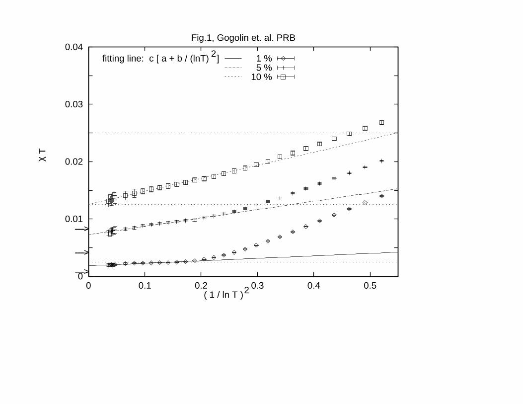
In Fig.1 we replotted their numerical data on uniform magnetic susceptibility (Fig. 2in their original paper) vs 1/(lnT )2 (The temperature T is measured in units of J). Thefitting formula is χT = c [ a + b/(lnT ))2], where c is the doping concentration, whilethe parameters a = 0.185(3), 0.145(2), 0.126(1), and b = 0.43(3), 0.29(1), 0.23(1) for c =0.01, 0.05, 0.1, respectively. It is important to note that according to RSRG considerations[13] a should be 1/12 at very low temperatures, and 1/4 at intermediate ones (as indicatedby arrows and dotted lines in Fig.1), whereas b should be zero. On the contrary, accordingto our analysis, eq. (59) a should be zero, while b should be 1/2. The numerical resultsdo clearly show the presence of the logarithmic term, but the effective Curie constant doesnot vanish entirely as T → 0: There is a finite intersection a 6= 0, and the slope b is lessthan 1/2 as expected. As mentioned in the previous subsection, the asymptotic logarithmicbehavior should be valid for T ≤ ǫ0, where ǫ0 is the low energy scale in the problem (roughlyspeaking, the soliton band width). Therefore, one should anticipate good agreement onlyat very low temperatures ( when 1/(lnT )2 ≪ 1). It is quite interesting to notice that thelinear fitting is better (over broader temperature range) for higher concentrations, where ǫ0is larger.

Our tentative interpretation for the absence of full agreement with the theoretical pre-diction is due to the fact that the random sampling in [11] is still not big enough to fullydemonstrate the anticipated behavior. To explain this point, let us recall the basic physicalpicture of the zero energy states in the Dirac model with random mass. Some of thesestates are genuinely localized, while the others are only ”quasilocalized”. The first categoryof states is ”typical”, while in taking random average the second category of states doescontribute in a substantial way. These features show up clearly in the spin-spin correlations

19

calculated using the Liouville quantum mechanics [16], the Berezinskii diagram technique[17], and the supersymmetric method [18]. The typical configurations for the spin correlationfunctions are exponentially decaying, whereas the average behavior has a power-law decay.The difference between the ”typical” and ”average” configurations is the nontrivial pieceof physics involved in randomly doped gapped spin systems (as well as some other randomsystems). The fact that the density of states shows the Dyson singularity and other thermo-dynamic quantities show logarithmic singularities are all due to the same reason. It is quiteremarkable that the signature of this behavior has shown up in the QMC simulations. Asclear from the above explanation, the logarithmic singularity will show up as ”full-fledged”only if the random sampling is really big. Otherwise, we will still see some constant terma as ”remnant” feature of the dominance of exponentially decaying states. Hopefully, withthe further improvement of the numerical techniques, this prediction can be checked moreprecisely. Namely, when the sampling becomes bigger and bigger, the intersection with thevertical axis (the remaining part of the Curie constant) should gradually vanish. To thebest of our knowledge, there is no explanation for this type of logarithmic singularities otherthan the one described above. Therefore the presence of this term per se in the numericalsimulations is already significant.

VI. STAGGERED MAGNETIZATION NEAR THE DEFECTS

In fact, in the continuous Majorana model there are two vacuum averages: the staggeredmagnetization and the smooth magnetization are both nonzero in the vicinity of the pointwhere m(x) changes sign. Unfortunately, we have not been able to calculate the staggeredmagnetization for the model with sign-changing m(x); we have done it only in the modelwith a sharp edge (that at the end of a broken chain). Nevertheless since this solution showsthe presence of zero modes we think that it gives a qualitatively correct description of thestaggered magnetization.

The calculation is based on two facts. The first one is that the order and disorderparameters in the Ising model are expressed in terms of fermion creation and annihilationoperators R(θ), R+(θ) as follows (T > Tc) [40]:

µ(τ, x) =: exp[1

2ρF (τ, x)] : σ(τ, x) =: ψ0(τ, x) exp[

1

2ρF (τ, x)] :

ρF (τ, x) = −i∫ ∞

−∞dθ1dθ2 tanh[(θ1 − θ2)/2] exp[(θ1 + θ2)/2]

× exp[−mτ(cosh θ1 + cosh θ2) − imx(sinh θ1 + sinh θ2)]R(θ1)R(θ2)

+terms with R+ (76)

ψ0(τ, x) =∫ ∞

−∞dθ{eθ/2 exp[−mτ cosh θ − imx sinh θ]R(θ)

+term with R+} (77)

These fermion operators satisfy the standard anticommutation relations:

20

[R(θ), R+(θ′)]+ = δ(θ − θ′)

which, in the case of the Ising model represent the simplest realization of the Zamolodchikov-Faddeev algebra.

Since the operators are normally ordered and < 0|R+(θ) = 0 in < 0|µ and < 0|σ we canomit all terms with R+:

< 0|µ(τ, x) =< 0| exp{−i2

∫ ∞

−∞dθ1dθ2 tanh(θ12/2) exp[(θ1+θ2)/2] exp[−mτ(cosh θ1+cosh θ2)

− imx(sinh θ1 + sinh θ2)]R(θ1)R(θ2)} (78)

< 0|σ(τ, x) = 〈0|∫ ∞

−∞dθ[eθ/2 exp[−mτ cosh θ − imx sinh θ]R(θ)

× exp{−i2

∫ ∞

−∞dθ1dθ2 tanh(θ12/2) exp[(θ1 + θ2)/2] exp[−mτ(cosh θ1 + cosh θ2)

−imx(sinh θ1 + sinh θ2)]R(θ1)R(θ2)} (79)

The second fact is that in the approach suggested by Ghoshal and Zamolodchikov [41]time and space coordinates are interchanged and the boundary is thought about as anasymptotic state at t → ∞. This out-state is denoted as |B >. Each integrable model hasits own |B >-vector. For the Ising model with free boundary conditions can be representedby the state vector is given by

|B >= [1 +R+(0)] exp{− i

2

∫ ∞

−∞dθ coth(θ/2)R+(−θ)R+(θ)}|0 > (80)

Notice that it contains a fermionic creation operator with zero rapidity; this operator cor-responds to the Majorana zero mode - a boundary bound state. This mode is the zeroenergy described in the previous sections. Since in the Ghoshal-Zamolodchikov formalismspace and time are interchanged, R+(0) formally creates a state with zero momentum.

Let us calculate a vacuum average of µ at point X:

< µ(t, X) >=< µ(τ = X, x = t)|B >

< 0| exp[−i∫ ∞

−∞dθ1dθ2A(θ1, θ2)R(θ1)R(θ2)] exp[− i

2

∫ ∞

−∞dθ coth(θ/2)R+(−θ)R+(θ)}|0 >

= exp[−1

2

∫ ∞

−∞dθA(θ,−θ) coth(θ/2)] (81)

where A(θ1, θ2) is defined in (78). Since the exponents commute on constant, we can usethe formula

eAeB = eBeAe[A,B] (82)

and obtain the following result:

21

< µ(X) >= exp(−1

8

∫ ∞

0dθ(1 + 1/ cosh θ)e−2mX cosh θ)

= exp{−1

8[K0(2mX) +K−1(2mX)]} (83)

< σ(X) >= exp(−m|X|) exp{−1

8[K0(2mX) +K−1(2mX)]} (84)

that is

n(X) =< µ1(X)σ2(X)σ3(X)µ0(X) >

= exp(−m|X|) exp{−1

8[3K0(2mX) +K0(6mX)3K−1(2mX) +K−1(6mX)]} (85)

This vacuum average behaves as X−1/2 at X << m−1 and decays exponentially at X >>m−1.

VII. CONCLUSIONS AND DISCUSSION

In this paper we have shown that doped spin-1/2 ladder systems are described by therandom mass Majorana (Dirac) fermion model. On the basis of this model, we have calcu-lated the thermodynamic functions for the spin ladders. In particular, we predict 1/T ln2 Tlow–temperature asymptotics for the linear magnetic susceptibility. This behavior is quitedifferent from the simple Curie law. As discussed in SectionVD, there is already goodevidence of this behavior in numerical simulations. Of course, we hope that more precise ex-perimental measurements would be able to distinguish these nontrivial disorder effects fromthe contributions of uncorrelated 1/2 spins induced by impurities. We would like also topoint out that the recent neutron data [5] have shown the existence of the gap states, whilethe magnitude of the gap itself does not change with doping. This is certainly consistentwith our theoretical results.

We did not attempt to discuss more complicated questions related to the behavior of thecorrelation functions in such disordered systems. We only note here that the divergency ofthe density of states (and of the localization length) in the middle of the gap makes thesesystems different from standard one-dimensional disordered systems giving rise to a non-trivial critical regime at low energies [37,31]. In fact, in the recent months, there has beenquite an impressive progress in the understanding of the correlation functions. For instance,some important insight into the zero energy properties of the random mass Dirac modelwas provided by mapping of this problem onto a Liouville quantum mechanics [16]. Aninterplay between the critical regime at low energies and the standard localization regimewas explored by Beresinskii’s diagram technique [17] and by the supersymmetry method[18].

However, the influence of the disorder on the staggered magnetic susceptibility in spinladders has been poorly studied so far. This quantity is important from the experimentalpoint of view. It is vital for the understanding of the apparent promotion of the antiferro-magnetic ordering upon doping, which was experimentally observed in both the spin ladderand the spin–Peiels systems [4,38]. It is our opinion that future theories of the antiferromag-netic transition in these systems will be based on the mapping onto the random mass fermion

22

model, presented in this paper, in conjunction with the theoretical progress in dealing withsuch fermionic models achieved in Refs [16–18].

VIII. ACKNOWLEDGMENTS

We are thankful to M. Fabrizio, D. Abraham and J. Gehring for illuminating discussionsand useful remarks. We also sincerely thank the authors of [11] for kindly sending us theirQMC data on uniform magnetic susceptibility and Dr. S.J. Qin for the help in making theplot. A.O.G. was supported by the EPSRC of the U.K. and part of this work has been doneduring his stay at the ICTP, Trieste, Italy. A.A.N. acknowledges the support from ICTP,Trieste, Italy and A. M. T. thanks ICTP for kind hospitality.

23

REFERENCES

[1] For a review, see E. Dagotto and T. M. Rice, Science 271, 618 (1996).

[2] M. Azuma, Z. Hiroi, M. Takano, K. Ishida and Y. Kitaoka, Phys. Rev. Lett. 73, 3463(1994).

[3] Z. Hiroi and M. Tanako, Nature 377, 41 (1995).

[4] M. Azuma, Y. Fujishiro, M. Tanako, M. Nohara, and H. Takagi, Phys. Rev. B 55, R8658(1997).

[5] M. Azuma, M. Takano, and R.S. Eccleston, Preprint cond-mat/9706170.

[6] Y. Motome, N. Katon, N. Furukawa, and M. Imada, J. Phys. Soc. Jpn 65, 1949 (1996).

[7] Y. Iino and M. Imada, J. Phys. Soc. Jpn 65, 3728 (1996).

[8] G.B. Martins, E. Dagotto, and J.A. Riera, Phys. Rev. B 54, 16032 (1996).

[9] G.B. Martins, M. Laukamp, J. Riera, and E. Dagotto, Phys. Rev. Lett. 78, 3563 (1997);M. Laukamp, G.B. Martins, C.J. Gazza, A.L. Malvezzi, E. Dagotto, P.M. Hansen, A.C.Lopez, and J. Riera, Preprint cond-mat/9707261.

[10] H.-J. Mikeska, U. Neugebauer, and U. Schollwock, Preprint cond-mat/ 9608100.

[11] T. Miyazaki, M. Troyer, M. Ogata, K. Ueda, and D. Yoshioka, Preprint cond-mat/9706123

[12] H. Fukuyama, N. Nagaosa, M. Saito, and T. Tanimoto, J. Phys. Soc. Jap. 65, 1183(1996).

[13] M. Sigrist and A. Furusaki, J. Phys. Soc. Jpn. 65, 2385 (1996).

[14] T.K. Ng, Phys. Rev. B 54, 11921 (1996); Preprint cond-mat/9610016.

[15] N. Nagaosa, A. Furusaki, M. Sigrist, and H. Fukuyama J. Phys. Soc. Jpn 65, 3724(1996).

[16] D. G. Shelton and A. M. Tsvelik, Preprint cond-mat/9704115.

[17] M. Steiner, M. Fabrizio, and A. O. Gogolin, Preprint cond-mat/9706096.

[18] L. Balents and M. P. A. Fisher, Preprint cond-mat/9706069.

[19] H. Fukuyama, T. Tanimoto, and M. Saito, J. Phys, Soc. Jpn 65, 1182 (1996).

[20] M. Fabrizio and R. Melin, Phys. Rev. Lett. 78, 3382 (1997).

[21] J. Solyom, Adv. Phys. 28, 201 (1979); V. J. Emery, in Highly Conducting One-

Dimensional Solids, Ed., J. T. Devreese, R. P. Evrard, and V. E. Van Doren (Plenum1979).

[22] S. Eggert and I. Affleck, Phys. Rev. B 46, 10 866 (1992).

[23] M. P. A. Fisher and L. I. Glazman, Preprint cond-mat/9610037 (to be published).

24

[24] The quantization of charge in the problem under consideration was first pointed out in[12]. However, ignoring one of the terms in their hamiltonian (1) breaks the spin SU(2)symmetry.

[25] D. G. Shelton, A. A. Nersesyan and A. M. Tsvelik, Phys. Rev. B 53, 8521 (1996).

[26] A. A. Nersesyan, A. M. Tsvelik, Phys. Rev. Lett. 78, 3939, (1997).

[27] D. G. Shelton and A. M. Tsvelik, Phys. Rev. B53, 14 036 (1996).

[28] H. Schulz, Phys. Rev. B 34, 6372 (1986).

[29] A. M. Tsvelik, Phys. Rev. B 42, 10 499 (1990).

[30] A. J. Niemi and G. W. Semenoff, Phys. Rep. 135, 99 (1986).

[31] It must be noted that the random mass Dirac problem turns out to be closely relatedto the random exchange spin model, studied via a real–space renormalization group byC. Dasgupta and S. K. Ma, Phys. Rev. B 22, 1305 (1980), and by D. Fisher, Phys. Rev.B 50, 3799 (1994); Phys. Rev. 51, 6411 (1995).

[32] A similar model was recently considered for quantum phase transitions in random XYspin chains; see R.H. McKenzie, Phys. Rev. Lett. 77, 4804 (1996).

[33] E. Witten, Nucl. Phys. B188, 513 (1981).

[34] A. Comtet, J. Desbois, and C. Monthus, Ann. Phys. 239, 312 (1995).

[35] F. J. Dyson, Phys. Rev. 92, 1331 (1953).

[36] M. Weissman and N. V. Cohan, J. Phys. C 8, 145 (1975).

[37] A. A. Gogolin and V. I. Mel’nikov, Zh. Eksp. Teor. Fiz. 73, 706 (1977) [Sov. Phys. JETP46(2), 369 (1977)], see also L. N. Bulaevskii, R. B. Lyubovskii, and I. F. ShchegolevPis’ma Zh. Eksp. Teor. Fiz. 16, 42 (1972) [Sov. Phys. JETP Lett. 16, 29 (1972)].

[38] J. P. Boucher and L. P. Regnault, J. Phys. I France 6, 1939 (1996).

[39] A. A. Ovchinnikov and N. S. Erikhman, Zh. Eksp. Teor. Fiz. 73, 650 (1977) [Sov. Phys.JETP 46, 340 (1977)].

[40] M. Jimbo, T. Miwa, M. Sato and Y. Mori. “Holonomic Quantum Fields”, Springer-Verlag (1980).

[41] S. Ghoshal and A. B. Zamolodchikov, Int. J. Mod. Phys. A 9, (1994).

25

FIGURES

The QMC simulation data of the doping effect on uniform magnetic susceptibility inspin ladders of Ref. [11] are replotted as a function of 1/(lnT )2 in comparison with Eq.(59).The temperature T is measured in units of J . The fitting formula is χT = c [ a +b/(lnT )2], where a = 0.185(3), 0.145(2), 0.126(1), and b = 0.43(3), 0.29(1), 0.23(1) fordoping concentrations c = 0.01, 0.05, 0.1, respectively. The dotted lines are expectationsfor uncorrelated free 1/2 spins induced by impurities, while the arrows on the left sideindicate the renormalized values, anticipated from the renormalization group analysis [13].

26

0

0.01

0.02

0.03

0.04

0 0.1 0.2 0.3 0.4 0.5

T

χ

( 1 / ln T )2

Fig.1, Gogolin et. al. PRB

fitting line: c [ a + b / (lnT) ]2

1 %5 %

10 %

------->

------->

------->