Yeshambel Melese v5.indd - DiVA-Portal

Doctoral Thesis supervisors:

Prof.dr.ir.P.M.Herder

Dr.ir.R.M.Stikkelman

Members of the Examination Committee:

Prof.dr. H.L.M. Bakker Delft University of Technology, the Netherlands

Prof.H.-P. Nee KTH Royal Institute of Technology, Sweden

Prof. P. Linares Comillas Pontifical University, Spain

Prof.dr.ir.D.M.J.Smeulders Eindhoven University of Technology, the Netherlands

Prof.dr. R.W. Künneke Delft University of Technology, the Netherlands

Prof. dr. K. Blok Delft University of Technology, the Netherlands, reserve member

TRITA -EE 2017:062

ISSN 1653-5146

ISBN 978-94-6361-002-5

This research was funded by the European Commission through the Erasmus Mundus Joint

Doctorate Program and Delft University of Technology.

Copyright © 2017 by Y.G.Melese

Printed by:Optima Grafische Communicatie

This dissertation has been approved by the

promotor: Prof.dr. ir. P.M.Herder copromotor: Dr.ir.R.M.Stikkelman

Composition of the doctoral committee:

Rector Magnificus, chairman Prof.dr. ir. P.M.Herder Delft University of Technology, the Netherlands Dr.ir.R.M.Stikkelman Delft University of Technology, the Netherlands

Independent members:

Prof.dr. H.L.M. Bakker Delft University of Technology, the Netherlands

Prof.H.-P. Nee KTH Royal Institute of Technology, Sweden

Prof. P. Linares Comillas Pontifical University, Spain

Prof.dr.ir.D.M.J.Smeulders Eindhoven University of Technology, the Netherlands

Prof.dr. R.W. Künneke Delft University of Technology, the Netherlands

Prof. dr. K. Blok Delft University of Technology, the Netherlands, reserve member

The doctoral research has been carried out in the context of an agreement on joint doctoral

supervision between Comillas Pontifical University, Madrid, Spain, KTH Royal Institute of

Technology, Stockholm, Sweden and Delft University of Technology, the Netherlands.

Keywords: Energy and industrial infrastructure networks; design under uncertainty; design

flexibility; risk sharing; cooperative game theory; real options.

ISBN 78-94-6361-002-5

Copyright © 2017 Y.G.Melese. All rights reserved. No part of the material protected by this

copyright notice may be reproduced or utilized in any form or by any means, electronic or

mechanical, including photocopying, recording or by any information storage and retrieval

system, without written permission from the author.

Printed in the Netherlands

118

Publication II

119

Publication II

120

Procedia Computer Science 28 ( 2014 ) 179 – 186

Available online at www.sciencedirect.com

1877-0509 © 2014 The Authors. Published by Elsevier B.V. Open access under CC BY-NC-ND license.Selection and peer-review under responsibility of the University of Southern California.doi: 10.1016/j.procs.2014.03.023

ScienceDirect

“Technical University of Delft, Energy and Industry Section, Jaffalaan 5, 2628BX Delft, The Netherlands”

E-mail address:

© 2014 The Authors. Published by Elsevier B.V. Open access under CC BY-NC-ND license.Selection and peer-review under responsibility of the University of Southern California.

121

180 Y.G. Melese et al. / Procedia Computer Science 28 ( 2014 ) 179 – 186

122

Y.G. Melese et al. / Procedia Computer Science 28 ( 2014 ) 179 – 186 181

Capital intensive

Evolving internal and external uncertainty

Long life time

Add or delete nodes or connections

Modify connections among the nodes

Modify the designs or properties of nodes or connections

123


Modelling capacity demand

Simulation model

Initial estimates (p10, p50, p90)

Initial distribution D (t0)

(mean, variance)

124


Decision rules

Evaluation of design options

125


126


0.000

0.200

0.400

0.600

0.800

1.000

0% 40% 80% 120% 160% 200% 240%

Commulativeprob

ability

NPV ( % of the Mean NPV of Design a)

Design a

Design b

Design c

127


European Journal of Operational Research,

Computers and Chemical Engineering

Int. J. Critical Infrastructures, ;

European Symposium on Computer Aided Process Engineering -15Journal

of Petroleum Science and Engineering, Networks, ;

Networks and Spatial economics,

129

International Journal of Greenhouse Gas Control 42 (2015) 16–25

Contents lists available at ScienceDirect

International Journal of Greenhouse Gas Control

journa l homepage: www.e lsev ier .com/ locate / i jggc

Exploring for real options during CCS networks conceptual designto mitigate effects of path-dependency and lock-in

Y.G. Melese ∗, P.W. Heijnen, R.M. Stikkelman, P.M. HerderDelft University of Technology, Faculty of Technology, Policy and Management, Department of Engineering Systems and Services, Jaffalaan 5, 2628BX Delft,The Netherlands

a r t i c l e i n f o

Article history:Received 31 October 2014Received in revised form 24 May 2015Accepted 14 July 2015Available online 13 August 2015

Keywords:CCS networksUncertainty analysisFlexibilityReal optionsGraph theory

a b s t r a c t

Carbon capture and storage (CCS) networks are expected to grow from small demonstration projectswith few emitters to large-scale networks of dedicated carbon dioxide (CO2) pipelines over the nextfew decades. Conventional design practices focus on implementing incremental expansions based ondeterministic requirements resulting in rigid networks. The design approaches do not proactively recog-nize future uncertainties in design requirements and operating environments. In this study, we present adesign method based on real options, graph theory and Monte Carlo techniques that reckons future uncer-tainties. The proposed method assesses initial design architectures and provides insights into potentialreal options and sets of strategies for implementing future expansions. We apply the method to a hypo-thetical CCS network design. The results reveal that this method helps to appraise the flexibility createdby redundant pipe capacity and length in an uncertain future. It also shows that embedding real optionsin expanding CCS networks could result in more emission reduction by encouraging other emitters toparticipate.

© 2015 Elsevier Ltd. All rights reserved.

1. Introduction

Carbon dioxide capture and storage (CCS) is widely promotedas a promising climate mitigation technology that can significantlyreduce carbon dioxide (CO2) emissions in the transition from afossil-based economy to a low-carbon future (IEA, 2010). The tech-nology involves capturing CO2 at large industrial sources, such ascoal-based power plants, transporting it in dedicated pipelines andstoring it in geological reservoirs, such as depleted oilfields andsaline aquifers. Recent projection shows that more than one-sixthof the desired CO2 emission reduction over the 2015–2050 periodcan be realised with CCS (IEA, 2014). To achieve this target, large-scale demonstration projects are being initiated and early planningof how the CO2 pipeline network may be designed in the long termwill help to control the total social costs (Austell et al., 2011).

CO2 pipeline networks, like other large-scale infrastructurenetworks, are developed in stages. They start with individual CO2sources and point-to-point pipeline connections. They expand byadding new sources and over time, a complex pipeline networkemerges. In many countries, small-scale demonstration projectsare considered starting points for a large-scale CCS. For example,

∗ Corresponding author. Tel.: +34631327121.E-mail address: [email protected] (Y.G. Melese).

CCS demonstration projects in the Rotterdam area, the Netherlands,are being built for supplying CO2 to greenhouses (RCI, 2011). Thesedemonstration projects are seen as the essential first steps in thefull-scale deployment of the technology.

Conventional CO2 pipeline-configuration design methods arebased on deterministic forecasts and assumptions of fixed designparameters (Flyvjberg et al., 2005; de Neufville and Scholtes, 2011).Designers use the most likely scenarios to generate design con-cepts and select design parameters that enable the network toperform optimally under those scenarios. Then standard economicevaluation techniques, such as discounted cash flow analysis, opti-misation and scenario planning are applied to achieve the bestoptimal design (de Neufville and Scholtes, 2011).

However, in the real world, this may not provide a design thatperforms best. First, it does not capture the range of technical,economic, regulatory and social uncertainties that will ultimatelyaffect the effectiveness of CCS networks (Koelbl et al., 2014; IEA,2012; van Os et al., 2014). A network that is designed to beoptimal in future achieves the expected performance only whenthe predicted scenario is realized. Besides, network expansionis inherently path-dependent (Silver and de Weck, 2007). Path-dependency refers to the notion that the state of an infrastructure atany given point depends on its development path until then. If thepredictions used in the design decisions do not realize, it may resultin rigid networks that cannot adapt to changing requirements.

http://dx.doi.org/10.1016/j.ijggc.2015.07.0161750-5836/© 2015 Elsevier Ltd. All rights reserved.

130

Y.G. Melese et al. / International Journal of Greenhouse Gas Control 42 (2015) 16–25 17

This situation could create ‘lock-ins’ in pipeline networks like CCS.Lock-in occurs when the cost of modification of an existing con-figuration exceeds the expected benefit1. Therefore, to mitigatelock-ins and sub-optimal performance of CCS networks, one needsa design approach that deals proactively with uncertainty.

In the field of systems engineering, a flexible systems designoffers one way to deal proactively with uncertainty (de Neufvilleand Scholtes, 2011; Silver and de Weck, 2007). Such a design con-cept provides an engineering system like CCS with the ability toadapt, change and be reconfigured (Cardin, 2014). It involves hav-ing a set of strategies on designing the engineering system withthe capability to adapt to changing circumstances; and on inte-grating a set of flexibility enablers into the physical design. Such adesign approach, which considers flexibility strategies and flexibil-ity enablers, is called the real options approach (Cardin, 2014; Lingand Ngah, 2009). It offers engineering system designers valuableclues about which flexible design elements are worth the cost (deNeufville, 2003). It thus provides a good rationale for specific typesof flexibilities to be designed in a system. However, the core issuein design flexibility, especially in infrastructure networks like CCS,is how to identify the most desirable sources of flexibility enablers(here after also called real options).

This paper aims to provide a useful design method for identify-ing valuable real options in the conceptual design of CCS networks.The method uses an exploratory uncertainty analysis on a graphtheoretical network simulation model. The method allows an easyand quick assessment of low-regret design options and identifica-tion of real options that could provide opportunities for flexibility.

The rest of the paper is organised as follows. The next sectionpresents a review of CCS network design methods. Section 3 intro-duces real options theory and real options-based design strategiesthat we consider contextually relevant to the understanding of thispaper. It also establishes the source of the real options identifica-tion problem in the case of CCS networks. The proposed method ispresented in Section 4. And in Section 5, the methodology is demon-strated for a hypothetical pipeline-based CCS network. Section 6concludes the paper.

2. Review of CCS network planning models

In recent years, CO2 pipeline transport planning methods havebecome more sophisticated. In a decade, they have evolved frommodelling just single pipeline connections to spatially and tem-porally complex networks. Modelling techniques include simpleto complex families of mathematical algorithms, such as linearoptimisation, non-linear optimisation and mixed-integer optimisa-tion. Kobos et al. (2007) developed an analytical model to optimisesimple networks with multi-stop pipelines using a simple linearoptimisation algorithm. It begins with a source and constructs apipeline of sufficient diameter to carry the entire CO2 volume tothe nearest reservoir. It then finds the next sink nearest to thefirst reservoir and constructs a pipeline sufficient to carry theremaining CO2 to it and so on, creating a ‘string of pearls’. Mostrecently, Knoope et al. (2014) have presented an economic opti-misation model to design simple networks. This model minimisesthe cost of pipeline configurations, taking into account inlet andoutlet pressure, pipeline length, steel grade and nature of the ter-rain. The planning models presented in the studies discussed aboveare applicable for single source-to-sink connections and simplenetworks. They also assume static situations and, therefore, do notaddress expansion in time.

1 In addition to economic reasons, CCS networks could be locked-in due to exter-nalities (due to their externally bounded interface with other sectors) (Economides,1996).

A compressive and scalable CCS infrastructure model calledSimCCS was presented by Middleton et al. (2007) and Middletonand Bielicki (2009). It is a geo-spatial economic-engineering modelthat simultaneously optimises all components of CCS infrastruc-ture, based on a mixed-integer linear programming algorithm. Themodel allows pipelines to branch and join to avoid duplication andtake advantage of economies of scale by creating trunk lines. It alsoallows for less than 100% of CO2 to be captured from CO2 sourcesand less than 100% of injection capacity to be used at CO2 sinks ifthat can reduce costs elsewhere in the system. SimCCS was furtherexpanded to integrate multiple independent decisions by Keatinget al. (2011). However, SimCCS is a static model as it assumes theentire CCS infrastructure network is built all at once and that theamount of CO2 being managed is constant over time.

Recently, CCS network models have been expanded to take intoaccount expansions over time. Mendelevitch et al. (2010) extendedthe SimCCS model to allow for CCS infrastructure network devel-opment decisions over time. van der Broek et al. (2010) has animproved model that takes into account the temporal componentof CCS infrastructure development, based on a linear optimisationalgorithm. Klokk et al. (2010) introduced a temporal CCS modelfor delivering CO2 for enhanced oil recovery. Middleton et al.(2012) introduced an advanced model called SimCCSTime, which isan improved version of SimCCS. SimCCSTime optimises the deploy-ment of CCS infrastructure across multiple periods. Both SimCCSand SimCCSTime are part of the ‘top-down’ optimisation approachesthat rely on a global optimisation algorithm of some kind anduse complete information about the system to find a global opti-mum. However, the model assumes a pre-defined pattern of futureemissions and CO2 management targets. The model also becomescomputationally cumbersome as the number of sources and sinksincrease.

A network model based on graph theory technique has beenproposed by Heijnen et al. (2014). The model conceptualises, on anabstract level, the design of a physical CCS structure as a network oflinks and nodes housing a certain flow that moves through the linksand is processed/consumed in the nodes. The model helps to finda minimum cost network layout by taking into account pipelinelength and capacity. However, the method considers deterministicand discrete scenarios of uncertainty parameters and finds an opti-mal network configuration for each pre-defined scenario. It doesnot fully address the stochastic and dynamic nature of uncertain-ties. It also does not address the issues of flexibility, of real optionsidentification integration as the network expands over time. In apreliminary work, Melese et al. (2014) presented a simple simula-tion framework based on a combination of Monte Carlo simulationand graph theory to design architecturally flexible networks undercapacity uncertainty. The framework uses a simplified flow uncer-tainty model to generate design alternatives and does not use theconcept of real options. Similar to the works by Heijnen et al. (2014)and Melese et al. (2014) this paper uses graph theory to model CCSnetworks. Stochastic process is used to model current and futureflow uncertainty of existing sources and multiple scenarios are usedto model the timing of future sources. Moreover, this paper usesthe concept of real options to appraise the flexibility created byredundant pipe capacity and length in an uncertain future.

3. Using real options to deal with uncertainty in CCSnetwork planning

The technical concept of an option is a right, but not an obli-gation, to do something at a certain cost within or at a specificperiod of time (Myers, 1984). From this definition, it follows thatthe key feature is exercising the ‘option’ of using one’s right to doan action, and the involvement of a cost that is somehow defined

131

18 Y.G. Melese et al. / International Journal of Greenhouse Gas Control 42 (2015) 16–25

in advance. It is in this sense that an ‘option’ has value and this fea-ture distinguishes it from a ‘choice’ or an ‘alternative’. The conceptfirst appeared in a field of finance called financial options, and hasentered the field of engineering systems in the modelling of designflexibility in realistic uncertain environments.

In engineering systems the term flexibility is widely used andreal options are a way to define the basic elements of flexibility(de Neufville et al., 2010; Wang, 2005). Options that involve tech-nical design features are referred to as real options ‘in’ engineeringsystems. On the other hand, options that involve financial deci-sions on engineering projects are referred to as real options ‘on’engineering systems (Wang, 2005). Real options ‘on’ engineeringsystems refer to managerial flexibility. Both real options ‘in’ and ‘on’engineering systems provide embedded flexibility and enable net-work developers to minimise downside risks and gain from upsideopportunities (de Neufville and Scholtes, 2011; de Neufville et al.,2006; de Weck et al., 2004). However, flexibility capabilities have tobe made possible by designers making intentional choices duringthe conceptual design stage (de Neufville et al., 2010). At this stage,network designers have more freedom to address proactively thevarying technical, economic and institutional dynamics.

The core question is: How to identify real options that couldenable cost effective expansion of CCS pipeline networks as futurecapacity requirement increases? There are two key difficultiesinvolved. First, there are the myriad design variables and param-eters that make real options identification and valuation difficult.Second, real options in engineering systems often exhibit complexpath-dependencies and interdependencies that standard optionstheory does not deal with de Neufville et al. (2010). They need anappropriate analytical framework. Existing options analysis meth-ods have to be adapted to the special features of real options inpipeline networks like CCS. To the authors’ knowledge, there is noprevious work on real options based design of CO2 transportationnetworks.

4. Methodology

In this paper, we propose a method for identifying valuablereal options when designing CCS networks under uncertainty. Itbuilds on existing design methods by giving designers some kindof model for estimating designs benefits and costs in some metric(such as capital expenditure and net present value). The objectiveis to provide a systematic method for fast and easy assessment ofnetwork design options under uncertainty and screen promisingdesigns that could provide cost effective expansion. The methodcould also provide network designers with important insights sothat they can systematically identify flexibility enablers and flexiblestrategies to mitigate lock-ins.

4.1. Step 1: Specification of the key sources of uncertainty

The first step in the design process is to identify key sources ofuncertainties. It includes a comprehensive accounting of all poten-tial sources of uncertainties that, over time, could affect the valueof the design. Major uncertainties can be identified through expertjudgment and a preliminary sensitivity analysis.

4.2. Step 2: Definition of likely future states over several stages

In this step, the evolutionary behaviour of selected uncertain-ties is defined. It includes defining the states of uncertain variablesover several stages. Stages, in this context, could refer to a suitableplanning period and depend on the type of system. For example,in the case of CCS networks, the stages could be long time periods(e.g. five years).

The future states can take continuous or discrete behaviour. Tomodel continuous behaviour, stochastic processes such as Geo-metric Brownian Motion (GBM) and Wiener processes are oftenused (Ibe, 2013). To model discrete behaviour, lattice model can beused (Albanese and Campolieti, 2006). An example of a continu-ous behaviour is the flow rate of CO2 from power plants with CO2capture units that vary power production because of the variabilityof electricity demand and the increasing use of renewable energysources in the electricity grid (Cohen et al., 2012; Domenichiniaet al., 2013). During variable power production, the amount of CO2captured and pumped through pipelines could vary within shortertime periods (hours and days). In addition, emitters could plan theircapture targets to increase step by step over a long period of time(years). These scenarios have to be explored in detail.

4.3. Step 3: Explorative uncertainty analysis

The objective in this step is to identify elements of the networkthat seem most promising for flexibility. This requires employingsome kind of network model to generate design concepts. In thisstudy, we employ a graph theoretical network model (explainedin Section 5.4.1). Scenarios of the selected uncertain variables areused as inputs to simulate the network model. The outputs of themodel include network configurations and their economic perfor-mance parameters (e.g. NPV and investment cost) for each set of theuncertainty scenarios. Design elements that vary across these setsof uncertain scenarios are those that may be good as real options.Conversely, those design elements that are insensitive to uncer-tainty do not present interesting real options.

This step is a preliminary stage for the identification of the bestopportunities for flexibility. The search for a valuable design couldinvolve many thousands of possibilities. For a proper search of thepromising configurations of the network, it is necessary to use low-fidelity models that can be run much faster than detailed, high-fidelity models.

4.4. Step 4: Identification and valuation of the real options

The goal here is to map real options to the sources of uncer-tainty, based on the results of the exploratory analysis. There areseveral real options strategies that might lead to flexibility. Someof the strategies relevant in the context of CCS networks includeoption to expand, option to defer, option to abandon, and option toswitch. Analysis of design alternatives is required to assess theabove-mentioned strategies.

The focus in this work is not to price the options. The focus ison the improved design; i.e. determining which parts of the net-work should be configured to provide the real options that willgive the network operators/designers the ‘right, but not the obliga-tion’ to change the size of the network. Such an analysis can aidnetwork designers in making rational (though optional) decisionsas to which flexible design elements can be incorporated into thedesign. It can also help designers and decision makers to determinethe relative cost of incorporating such flexible design element intonetworks.

5. Application

Our case study concerns the development of a hypotheticalpipeline-based CCS network. The hypothetical network is inspiredby a CCS project in the Rotterdam area, The Netherlands. The Rotter-dam CCS project is part of the national goal to reduce CO2 emissionfrom the port and other industrial activities. An effective and com-prehensive method to achieve this goal is to develop a large-scalepipeline network that connects spatially distributed emitters andstore CO2 in depleted offshore oil-and-gas fields in the Northern

132


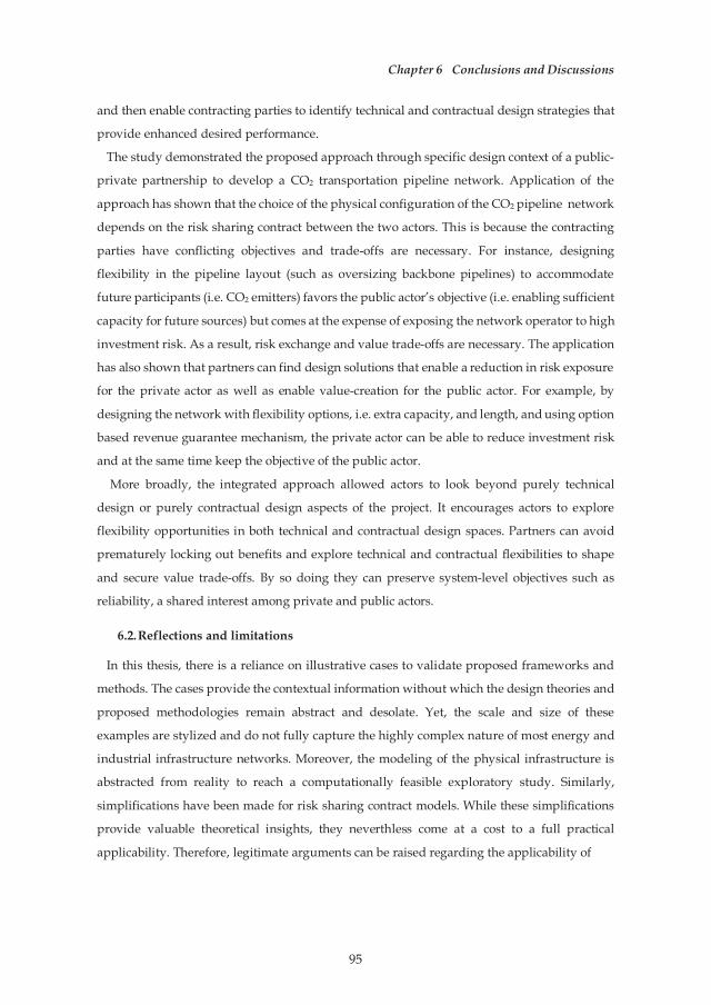
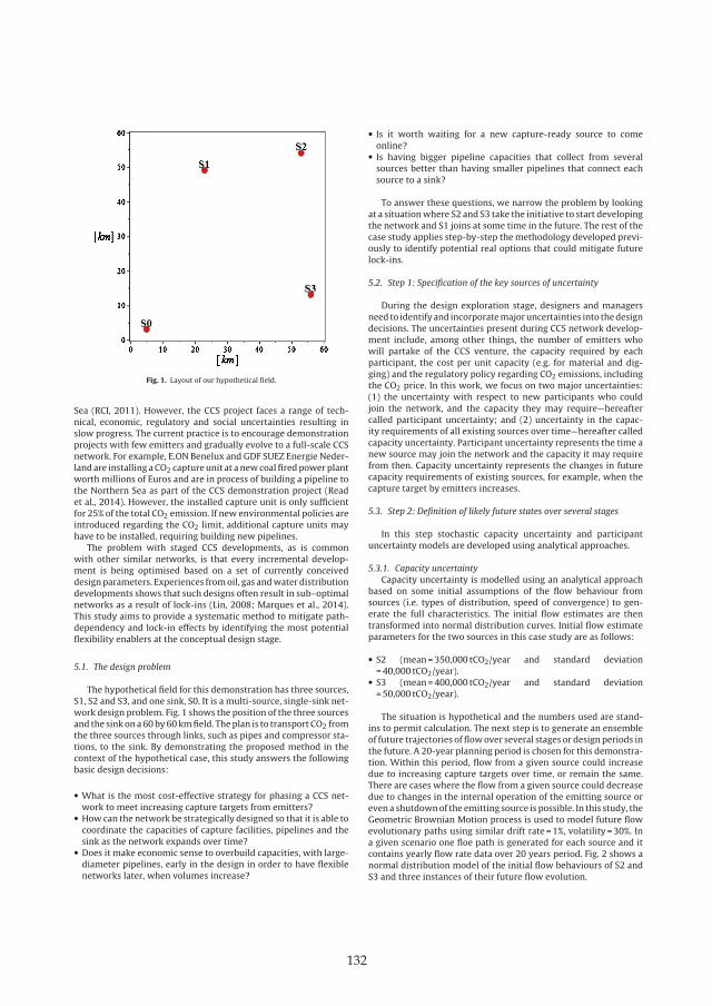
Fig. 1. Layout of our hypothetical field.

Sea (RCI, 2011). However, the CCS project faces a range of tech-nical, economic, regulatory and social uncertainties resulting inslow progress. The current practice is to encourage demonstrationprojects with few emitters and gradually evolve to a full-scale CCSnetwork. For example, E.ON Benelux and GDF SUEZ Energie Neder-land are installing a CO2 capture unit at a new coal fired power plantworth millions of Euros and are in process of building a pipeline tothe Northern Sea as part of the CCS demonstration project (Readet al., 2014). However, the installed capture unit is only sufficientfor 25% of the total CO2 emission. If new environmental policies areintroduced regarding the CO2 limit, additional capture units mayhave to be installed, requiring building new pipelines.

The problem with staged CCS developments, as is commonwith other similar networks, is that every incremental develop-ment is being optimised based on a set of currently conceiveddesign parameters. Experiences from oil, gas and water distributiondevelopments shows that such designs often result in sub–optimalnetworks as a result of lock-ins (Lin, 2008; Marques et al., 2014).This study aims to provide a systematic method to mitigate path-dependency and lock-in effects by identifying the most potentialflexibility enablers at the conceptual design stage.

5.1. The design problem

The hypothetical field for this demonstration has three sources,S1, S2 and S3, and one sink, S0. It is a multi-source, single-sink net-work design problem. Fig. 1 shows the position of the three sourcesand the sink on a 60 by 60 km field. The plan is to transport CO2 fromthe three sources through links, such as pipes and compressor sta-tions, to the sink. By demonstrating the proposed method in thecontext of the hypothetical case, this study answers the followingbasic design decisions:

• What is the most cost-effective strategy for phasing a CCS net-work to meet increasing capture targets from emitters?

• How can the network be strategically designed so that it is able tocoordinate the capacities of capture facilities, pipelines and thesink as the network expands over time?

• Does it make economic sense to overbuild capacities, with large-diameter pipelines, early in the design in order to have flexiblenetworks later, when volumes increase?

• Is it worth waiting for a new capture-ready source to comeonline?

• Is having bigger pipeline capacities that collect from severalsources better than having smaller pipelines that connect eachsource to a sink?

To answer these questions, we narrow the problem by lookingat a situation where S2 and S3 take the initiative to start developingthe network and S1 joins at some time in the future. The rest of thecase study applies step-by-step the methodology developed previ-ously to identify potential real options that could mitigate futurelock-ins.

5.2. Step 1: Specification of the key sources of uncertainty

During the design exploration stage, designers and managersneed to identify and incorporate major uncertainties into the designdecisions. The uncertainties present during CCS network develop-ment include, among other things, the number of emitters whowill partake of the CCS venture, the capacity required by eachparticipant, the cost per unit capacity (e.g. for material and dig-ging) and the regulatory policy regarding CO2 emissions, includingthe CO2 price. In this work, we focus on two major uncertainties:(1) the uncertainty with respect to new participants who couldjoin the network, and the capacity they may require—hereaftercalled participant uncertainty; and (2) uncertainty in the capac-ity requirements of all existing sources over time—hereafter calledcapacity uncertainty. Participant uncertainty represents the time anew source may join the network and the capacity it may requirefrom then. Capacity uncertainty represents the changes in futurecapacity requirements of existing sources, for example, when thecapture target by emitters increases.

5.3. Step 2: Definition of likely future states over several stages

In this step stochastic capacity uncertainty and participantuncertainty models are developed using analytical approaches.

5.3.1. Capacity uncertaintyCapacity uncertainty is modelled using an analytical approach

based on some initial assumptions of the flow behaviour fromsources (i.e. types of distribution, speed of convergence) to gen-erate the full characteristics. The initial flow estimates are thentransformed into normal distribution curves. Initial flow estimateparameters for the two sources in this case study are as follows:

• S2 (mean = 350,000 tCO2/year and standard deviation= 40,000 tCO2/year).

• S3 (mean = 400,000 tCO2/year and standard deviation= 50,000 tCO2/year).

The situation is hypothetical and the numbers used are stand-ins to permit calculation. The next step is to generate an ensembleof future trajectories of flow over several stages or design periods inthe future. A 20-year planning period is chosen for this demonstra-tion. Within this period, flow from a given source could increasedue to increasing capture targets over time, or remain the same.There are cases where the flow from a given source could decreasedue to changes in the internal operation of the emitting source oreven a shutdown of the emitting source is possible. In this study, theGeometric Brownian Motion process is used to model future flowevolutionary paths using similar drift rate = 1%, volatility = 30%. Ina given scenario one floe path is generated for each source and itcontains yearly flow rate data over 20 years period. Fig. 2 shows anormal distribution model of the initial flow behaviours of S2 andS3 and three instances of their future flow evolution.

133


Fig. 2. Capacity uncertainty model of S1 and S2; (a) initial flow estimate model of sources; and (b) three instances of the evolution of flow from S2 and S3 over a 20-yearperiod.

5.3.2. Participant uncertaintyTo account for the uncertainty in the timing that S1 will join

the network, we choose four scenarios over a 20-year investmentperiod: Year 4, Year 8, Year 12 and Year 16. In this case study, wechoose four years as a reasonable time for an emitter to installcapture units and be ready for connection. Similar to S2 and S3,the initial flow estimate of S1 is modelled as a normal distribu-tion based on an initial estimate (mean = 300,000 tCO2/year andstandard deviation = 50,000 tCO2/year), as shown in Fig. 3a. Thefuture evolution of CO2 flow from S1 is modelled using the GBMprocess with the same drift rate = 1% and volatility = 30%, see Fig. 3b.

Similar to S2 and S3, the future flow of S1 could increase,decrease, remain the same, or present a combination of all three.Multiple scenario representations of uncertain variables over timeallow one to generate and analyse multiple design possibilities andcan help arrive at a better decision.

5.4. Step 3: Explorative uncertainty analysis

To perform an exploratory analysis, the selected uncertain vari-ables have to be simulated using a network optimisation model.In this paper, we employ a network optimisation model based ongraph theory (Heijnen et al., 2014). The main inputs for the modelare flow rates from sources and the spatial positions of sourcesand sink nodes. The model generates minimum-cost tree-shapednetwork configurations connecting the sources to the sink. Theresulting networks are edge-weighted Steiner minimal trees. Anedge-weighted Steiner minimal tree network is a minimal cost net-work that takes into account the influence on the cost of both thecapacity and the length of the pipeline. Next, the core concepts ofthe model are presented.

5.4.1. Graph theoretical network modelIn a graph theoretical representation of networks, the sources

and sinks are nodes (e.g. emitters) and their connections are edges(e.g. pipelines). To generate an edge-weighted Steiner minimal net-work, the network algorithm uses the following cost function ofedges.

Ce = 1eqˇe (1)

In Eq. (1), le is the length and qe is the capacity of an edge e.ˇ is the cost exponent for the capacity with 0 ≤ ˇ ≤ 1 If ˇ=0, thecapacity of the pipelines has no influence on the cost. If ˇ=1, build-ing two pipelines of capacity 1 is just as expensive as building onepipeline of capacity 2. A value of ˇ=0.6 is commonly used (Heijnenet al., 2014), indicating that there are cost advantages to buildinghigh-capacity pipelines. Then, the total investment cost C(T) of a

network T is the sum of all connection (pipeline) costs as given inthe following equation:

C(T) =∑

∀e∈E(T)

leqˇe (2)

where E(T) is the set of all edges in a network tree T.In addition to cost, it is also necessary to calculate the expected

income of the network. A revenue model that calculates theexpected income as a linear function of capacity is used. Theassumption is that the network developer generates income bycharging a certain fee per unit capacity. The expected income (EI)from a network T is then given as

EI(T) = ˛∑

i∈V(T)/{s}qi (3)

In Eq. (3), qi is the used capacity by a source i in a network T,V(T) is the set of all nodes in the network T, s is the sink and ˛ is theconstant coefficient representing a constant price charged per unitcapacity of pipeline. In this demonstration, we assume ˛=1.

The total income from a given network in its lifetime is calcu-lated as a summation of discounted (using a certain interest rate, r)yearly income flows over a certain investment period. The summa-tion of discounted future cash flows (revenues) gives the presentvalue of income (PVI), see the following equation:

PVI(T) =n∑

t=0

∑EI(T)

(1 + r)t(4)

The Net Present Value (NPV) is used to evaluate the lifetimeperformance of a network under a given scenario of uncertainparameters as shown in the following equation:

NPV(T) = PVI(T) − C(T) (5)

5.4.2. Simulation outputsIn this step the network model is simulated using different

uncertain future scenarios. In one scenario 20 network configu-rations are generated (based on 20 yearly flow rate inputs fromeach source). Fig. 4a shows a density diagram consisting of 20 dif-ferent edge-weighted Steiner minimal network layouts. It showsthe layout of the network in phase 1. In phase 1 only S2 and S3are available to develop the CCS network. Fig. 4b shows networklayouts if all the sources are available at the beginning. However,since S1 joins the network later S1. Each network layout representsthe lowest cost connection between the sources and the sink. Thecapacities and the lengths of the edges and the points of connection(Steiner points) between edges is different for each layout.

134


Fig. 3. Flow model of S1: (a) initial flow estimate model of S1, (b) instances of evolutionary flow model of S1 over time. Each line indicates one instance of S1 flow path underthe four scenarios (Y stands for Year).

Fig. 4. Optimal network layouts of the CCS network in phase 1 (a) and phase 2 (b).

To determine the optimal network out of several designalternatives in a given scenario, the Present Worth Ratio (PWR)metric is used, see Eq. (6). PWR is the ratio of the expected revenueof the network to the initial outlay required for it. It illustrates theefficiency in the invested capital.

PWR = Expected Revenue − Investment costInvestment cost

(6)

Out of the 20 network layouts in each scenario, the layout withthe maximum PWR is selected. To generate multiple scenarios,Monte Carlo simulation is carried out. By simulating the networkmodel with several scenarios multiple layouts are generated forboth phase 1 and phase 2. We limit the number of simulation runsto 200. 200 simulation runs result in 200 network configurationswith their corresponding maximum PWR values. In phase 1, thePWR values follow a lognormal distribution with a mean of 2.7 andstandard deviation of 0.3. Similarly, in phase 2, the PWR valuesfollow a lognormal distribution with a mean of 3.5 and standarddeviation of 0.4. During the conceptual design stage, Monte Carlosimulation enables designers and decision makers to explore sev-eral scenarios and generate several design candidates. Therefore,the exploratory uncertainty analysis step serves a screening stepto identify promising network design concepts for the detail designstage. In the next step, the network with a maximum PWR, 2.7 inphase 1 and 3.5 in phase 2, are selected to identify best opportuni-ties for flexibility.

5.5. Step 4: Identification and valuation of real options

The objectives in this step are (1) to map uncertainties to part ofthe network that should be configured to provide network design-ers the ‘right, but not the obligation’ to change the network inthe future; (2) to calculate the value of having real options in thenetwork.

Based on the simulation outputs in the previous stage, the fol-lowing two design strategies are identified.

• Design strategy 1, (the baseline strategy). Under this strategy thenetwork will be developed by connecting S2 and S3 without tak-ing into account the future connection of S1. Expected capacityestimates of S2 and S3 are used to design the network.

• Design strategy 2. Under this strategy the network will be devel-oped after taking into account the possibility that S1 will join inthe future.

Fig. 5 shows design concepts based on design strategy 1 anddesign strategy 2.

In both design strategies the decision makers analyze two majoroptions: the option to defer (wait) and the options to expand.Table 1 shows the different types of uncertainties and the realoptions to mitigate their effect for both design strategies.

Developing the network based on design strategy 1 representsan investment opportunity. Therefore, it is a real option by itself. Ifa manager decided to invest, then the option is exercised by com-mitting to an initial cost in exchange for a real asset that may pay a

135


Fig. 5. Network layout concepts based on design strategy 1 (a) and design strategy 2 (b).

Table 1Mapping sources of uncertainty to real options strategies.

Uncertainty type Option to defer Options to expand

Design strategy 1 Design strategy 2 Design strategy 1 Design strategy 2

Participant uncertainty Yes (default) Yes No YesCapacity uncertainty Yes (default) Yes No Yes

stream of future cash flows. In the case of design strategy 2, thereis a freedom to exercise both real options. Similar to design strat-egy 1 the deferral option can be exercised in phase 1 and phase 2.In phase 2, if the investment opportunity of connecting S1 is notworthy, then it can be deferred.

As can be seen in Table 1 the major difference between the twodesign strategies is the expansion option. The expansion option ismade possible by embedding real options in the initial networkdesign. Real options require extra cost but could provide the net-work manager the right to accommodate S1 at lower overall cost.One real option can be embedded in the network by committinglarge-size pipes between nodes S0 and J2. Another real option canbe embedded by laying out pipeline J1–J2–S2 instead of J2–S2. Thisoption requires extra pipe capacity on line J2–J1 and extra length(i.e. the difference between J2–J1–S2 and J2–S2). Real options canalso be considered in edge S2–J1 and edge S3–J2 by having extracapacity.

5.5.1. Real options valuationTo value the expansion option both design strategies are simu-

lated using multiple scenarios of uncertain variables. The analysistakes the perspective of a network developer who invests in devel-oping the CCS network for a profit. NPV is used to measure theperformance of both design strategies. As shown in Eq. (5), NPVdepends on the flow from each source and the total cost of the net-work. The present value of revenue is calculated using Eq. (4). Itis a function of the total flow rate of CO2 which is uncertain. Thetotal flow model is obtained by adding the distribution of the threesources defined in step 2 (as shown in Figs. 2 and 3). Let St representthe distribution of the total flow. Since the sum of the independentnormal distributions is again a normal distribution, St has normaldistribution. The mean �t and variance vart of St are given as

�t = 1n

n∑i=1

�i and vart = 1n2

n∑i=1

vari, i ∈ (1, 2, 3) (7)

Fig. 6. Flow paths of St for the four scenarios (S1 joins at Year 4, Year 8, Year 12, orYear 16).

n=2 in phase 1 and n=2 in phase 2. Fig. 6 shows simulation of pathsof St (out of 200 paths, single sample paths are shown for clarity).

In phase 1, the total cost of the worth maximizing networksof both design strategies is calculated using Eq. (2). In phase 2, ifthe deferral option is not exercised, additional costs are made toconnect S1 to the network. Let Ct1 represent the cost of the worthmaximizing network in phase 1 and Cs1 represent the present valueof the cost made to connect S1. Then, the total cost of the networkin phase 2, CTt2 is calculated as

CTt2 = Ct1 + (C31)Y , Y ∈ (4, 8, 12, 16) (8)

In design strategy 1, C31 is the cost of edge S1–S0 and in designstrategy 2, C31 is the cost of S1–J1 (the dotted line). The value of C31depends on the year (Y) in which S1 is connected to the network.

The two design strategies are evaluated by simulating the net-work model using different scenarios of St. Both design strategieswere simulated for 200 times. We sorted the 200 NPV results of eachdesign strategy and plotted them as cumulative probability distri-bution curve, see Fig. 7. For this analysis we assume connection cost

136


80 90 10 0 110 120 130 14 0 1500

0.1

0.2

0.3

0.4

0.5

0.6

0.7

0.8

0.9

1

NPV of Design Statergies (% of ENPV of DS1 @Y16)

Freq

uenc

y

DS1 @Y8DS2 @Y8DS1 @Y12DS2 @Y12DS1 @Y4DS2 @Y16DS1 @Y16DS2 @Y4

Fig. 7. Cumulative probability distribution curve of NPVs (Y stands for Year, DS1 and DS2 stands for design strategy 1 and design strategy 2, respectively. For example,DS1@Y4 mean design strategy 1 and S1 join the network at Year 4)

Table 2ENPVs of design strategies 1 and 2 and EVRO (in 103 Euros) under the four timescenarios.

Year 4 Year 8 Year 12 Year 16

ENPV design strategy 2 126 ± 8 115 ± 7 106 ± 6 101 ± 3ENPV design strategy 1 103 ± 4 102 ± 5 101 ± 4 100 ± 3EVRO 23 ± 9 13 ± 8 5 ± 7 1 ± 3

of ˛ = 1 D /t and a real (i.e. excluding inflation) discount rate of 7%, afigure commonly used by the World Bank (Blanchard, 1993). Fromthe distribution of NPVs, the expected NPV (ENPV) is calculated.The ENPV based valuation technique adjusts for uncertainty by cal-culating NPVs under different scenarios and probability-weightingthem to get the most likely NPV. For the purpose of comparison theNPVs of the two designs are normalized against the expected netpresent value (ENPV) of design strategy 1 at year 16.

The expected value of the real options (EVRO) is calculated usingEq. (9). It is defined as the difference between the ENPV of designstrategy 2 and the ENPV of design strategy 1. Table 2 shows thenormalized ENPVs of the two design strategies and the expectedvalue of real options.

EVRO = ENPVdesign strategy 2 − ENPVdesign strategy 1 (9)

From Table 2 and Fig. 7, it can be seen that the ENPV (fre-quency = 0.5) of design strategy 2 is higher than design strategy1 in each of the four scenarios. This indicates that embeddingreal options in the physical design enables cost effective expan-sion as future capacity requirement increases. The real options arethe redundant pipe capacities in the edges and their extra lengthswhich enable cheaper expansion. However, the difference betweenthe two strategies decreases if S1 is connected later. For example,the EVRO decreases from 23 ± 9 at year 4 to 5 ± 7 at year 12. Thedecrease suggests that the economic value of those real optionsdiminish with time. Embedding extra capacity and length at thebeginning to connect S1 after 12 years becomes less worthy andeven could result to a loss. As the time horizon for consideringextra capacity requirement increases, the opportunity of cost ofthe real options investment (the premium) increases exceeding theexpected return.

In Fig. 7, it can be seen that the difference between the twodesign strategies increases when we move up from the expected

value. Since NPV is directly related to flow rate, the increasingdifference suggests that the value of the real options increases ifflow from sources is higher than expected. The lower part of thecurves shows that the difference between the two strategies con-tinues to decrease when flow is lower than expected. When flowrate is lower than expected there will be unused physical capac-ity and that decreases the value of the real options. In such cases,a valuable decision could be to decrease the size of extra capac-ity or deferring the investment. Waiting until better information isavailable about the future flow of existing sources and the timingof new sources could be worthy. However, it is also important tomention that the value of waiting could be at odds with the value ofearly strategic commitment. Decision makers also take into accountother strategic advantages in addition to the distribution of NPVs.For example, by investing in demonstration projects, ‘early movers’could take a strategic advantage on future opportunities related toCCS technology compared with ‘late comers’, even though ENPVtells otherwise.

The expected values of real options in Table 2 provide someinsight with regard to having expansion option decision withoutregrets. In commercial CO2 pipeline design the ‘no-regrets-period’of 10 years is used as a bench mark (Austell et al., 2011). Table 2shows that the ‘no-regrets-period’ could be between 8 and 12 years.However, this study considers only uncertainty in future capacityrequirements while other uncertain factors (e.g. discounting rate)are assumed as constant. If other uncertain factors, in addition toflow, are considered the ‘no-regrets-period’ is expected to decrease.On the contrary, the ‘no-regrets-period’ could increase, for exam-ple, if favourable governmental policy is in place and the cost ofCCS technology reduces in the future.

So far, the value of having real options is measured using eco-nomic metrics, which is commonly used by project managers.However, the flexibility value of a CCS network can be more thanits economic benefit to a single project owner. There can be addedbenefits for other subordinate stakeholders. For example, a flexi-ble CCS network that is able to accommodate future emitters couldmean less costly connections for the new emitters. In the case ofdesign strategy 2, when S2 and S3 design the pipeline S0–J2–J1 withextra capacity to accommodate future flow increases, it reduces thecost to connect S1 to the sink. At the same time, the real optionbuilt into the network (i.e. the extra pipe capacity) will encour-age the participation of new emitters like S1 by reducing some of

137


the barriers, such as obtaining land permits for an independentpipeline. The participation of more emitters in the CCS networkcan be considered an added value for an environmental agency likethe Rotterdam Climate Initiative whose objective is to reduce CO2emissions by creating a large-scale CCS network. If more emittersparticipate in the CCS network, it will lead to a reduction in the totalCO2 emissions.

6. Conclusions

The main aim of this paper is to provide a systematic designmethod to explore valuable real options in CCS networks to miti-gate the effects of lock-ins as they expand over time. By referencingrelevant literature, we show that the typical design and planningapproach tends to focus on pre-defined requirements and oftenleads to inflexible and sub-optimal networks. This paper arguesthat one way to deal with less inflexible CCS networks is to adopta real options-based design approach. In order to explore valuablereal options, the paper presents an exploratory uncertainty anal-ysis of network design architectures using a graph theory-basednetwork model. This model provides easy and fast generation andassessment of various network design architectures under differentuncertain scenarios. This is an advantage over most of the CCS net-work planning models, as were presented in Section 2 of this paper.This aspect of the network model is very helpful when designershave to assess thousands of design concepts under a combinationof uncertain design parameters.

The proposed method helps to identify design elements anddesign strategies most likely to provide worthwhile flexibilities tomitigate path-dependencies and lock-in effects. Using a hypotheti-cal CCS network for demonstration purposes, the method providesvaluable insights to designers and decision makers on how todesign CCS networks under capacity and participant uncertainty.It also helps to identify a need for extra capacity to accommo-date future increases in capture targets by emitters. In our specificcase study, we found out that building higher pipe capacity isvaluable if there is an increase in future capture by emitters. Ouranalysis also shows that the method proposed could provide valu-able insight into which parts of the network should include realoptions to accommodate future emitters. Physically built-in capa-bilities, such as extra pipe capacities and length, provide easy andcost-effective expansion option of the network when comparedwith a deterministic design approach (baseline). Another conclu-sion is that the value of identifying and imbedding real optionsin expanding CCS networks could extend beyond an improvementin an economic metric (e.g. an environmental value, by encour-aging more emission reduction) and beyond a single stakeholder(i.e. not only to initial developers of the network but also to futureparticipants).

The framework and methods introduced in this study can begeneralized to the application of other pipeline-based networkdesign problems such as gas pipeline networks, water distributionnetworks and district heating networks. These different networksare subject to distinct costs and benefits and faced with theirrespective sources of uncertainties; as a result, details of modellingand computation may need to be adjusted to suit the particularnetwork at hand.

The network model could be expanded at the moment to accom-modate multi-source, multi-sink CCS network design problems. Inlarge CCS networks, multiple storage sites could be used, i.e. CO2could be stored in abandoned oil fields, consumed for enhanced oilrecovery and consumed for agricultural and industrial purposes.Moreover, the utility of the network model can be improved byincluding CO2 and pipeline properties, and taking into consider-ation no-go areas such as parks and residential areas.

Acknowledgement

Yeshambel Melese has been awarded an Erasmus Mundus JointDoctorate Fellowship. The authors would like to express their grat-itude towards all partner institutions within the program as wellas the European Commission for their support.

References

Albanese, C., Campolieti, G., 2006. The binomial lattice model. In: Albanese, C.,Campolieti, G. (Eds.), Advanced Derivatives Pricing and Risk Management:Theory Tools and Hands-On Programming Application. Elsevier AcademicPress, London, San diego and Burlington, pp. 337–348.

Austell, M., et al., 2011. Development of Large Scale CCS in The North Sea viaRotterdam as CO2-hub, WP 4.1 Final Report. EU CO2 Europipe Consortium,Utrecht, Netherlands.

Blanchard, O.J., 1993. The vanishing equity premium. In: Finance and theInternational Economy 7 The Amex Bank Review. Oxford University Press,London.

Cardin, A.M., 2014. Enabling flexibility in engineering systems: a taxonomy ofprocedures and a design framework. J. Mech. Des. 136 (1), 1–14.

Cohen, M.S., Rochelle, T.G., Webber, E.M., 2012. Optimizing post-combustion CO2

capturein response to volatile electricity prices. Int. J. Greenhouse Gas Control8, 180–195.

de Neufville, R., 2003. Real options: dealing with uncertainty in systems planningand design. Integr. Assess. 4 (1), 26–34.

de Neufville, R., ASCE, L.M., Scholtes, L., Wang, S.T., 2006. Real options byspreadsheet: parking garage case example. J. Infrastruct. Syst. 12 (3),107–111.

de Neufville, R., de Weck, O., Lin, J., Scholtes, S., 2010. Identifying real options toimprove the design of engineering systems. In: Real Options in EngineeringDesign Operations, and Management. CRC Press, New York, NY, pp. 75–98.

de Neufville, R., Scholtes, S., 2011. Flexibility in Engineering Design. MIT Press,Cambridge, MA.

de Weck, O., de Neufville, R., Chaize, M., 2004. Staged deployment ofcommunications satellite constellations in low earth orbit. J. Aeros. Comput.Inf. Commun. 1 (4), 119–136.

Domenichinia, R., Mancusoa, L., Ferraria, N., 2013. Operating flexibility of powerplants with carbon capture and storage (CCS). Energy Procedia 37,2727–2737.

Economides, N., 1996. The economics of networks. Int. J. Ind. Organiz. 14,673–699.

Flyvjberg, M., Holm, M., Buhl, S., 2005. How (in)accurate are demand forecasts inpublic works projects? The case of transportation. J. Am. Plann. Assoc. 71 (2),131–146.

Heijnen, P.W., Ligtvoet, A., Stikkelman, R.M., Herder, P.M., 2014. Maximising theworth of nascent networks. Networks Spat. Econ. 14, 27–46.

Ibe, O.C., 2013. Markov Processes for Stochastic Modeling, second ed. Elsevier,London and Waltham.

IEA, 2010. World Energy Oulook. IEA Publications, Paris.IEA, 2012. Energy Technology Perspective 2012: Pathways to a Clean Energy

System. IEA Publications, Paris.IEA, 2014. Energy Technology Perspective 2014: Pathways to a Clean Energy

System. IEA Publications, Paris.Keating, G.N., et al., 2011. Mesoscale carbon squestration sirte screening and CCS

infratsructure analysis. Environ. Sci. Technol. 45, 215–222.Klokk, O., Schreiner, F.P., Pages-Bernaus, A., Tomasgard, A., 2010. Optimizing a CO2

value chain for the Norwegian continental shelf. Energy Policy 38, 6604–6614.Knoope, J.M., Guijt, W., Ramirez, A., Faaij, C.P., 2014. Improved cost models for

optimizing CO2 pipeline configuration for point-to-point pipelines and simplenetworks. Int. J. Greenhouse Gas Control 22, 25–46.

Kobos, P.H., Malczynski, L.A., Borns, D.J., McPherson, B.J., 2007. The ‘String ofPearls’: The Integrated Assessment Cost and Source-Sink Model. NETL,Pittsburgh, PA.

Koelbl, S.B., et al., 2014. Uncertainty in the deployment of Carbon Capture andStorage (CCS): a sensitivity analysis of techno-economic parameteruncertainty. Int. J. Greenhouse Gas Control 27, 81–102.

Ling, W.A., Ngah, C.N., 2009. Creating and Valuing Flexibility in SystemsArchitecting: Transforming Uncertainties into Opportunities Using RealOptions Analysis. Defence Science and Technology Agency, Singapore.

Lin, J., 2008. Exploring Flexible Strategies in Engineering Systems Using ScreeningModels. Massachusetts Institute of Technology, Cambridge, MA (Ph.D.Dessertation).

Marques, J., Cunha, M., Savic, A.D., 2014. Decision support for optimal design ofwater distribution networks:a real options approach. Procedia Eng. 70,1074–1083.

Melese, G.Y., Weijnen, W.P., Stikkelman, M.R., 2014. Designing networked energyinfrastructures with architectural flexibility. Procedia Comput. Sci. 28,179–186.

Mendelevitch, R., Herold, J., Oei, P.Y., Tissen, A., 2010. CO2 Highways for Europe:Modelling a Carbon Capture, Transport and Storage Infrastructure forEurope.CEPS Working Document no. 340. The Centre for European PolicyStudies, Brussels.

138


Middleton, R., Bielicki, J., 2009. A Scaleable infrastructure model for carbon captureand storage: SimCCS. Energy Policy 37, 1052–1060.

Middleton, R.S., et al., 2007. Optimization for Geologic Carbon Sequestration andCarbon Credit Pricing. NETL, Pittsburgh, PA.

Middleton, S.R., et al., 2012. A dynamic model for optimally phasing in CO2 captureand Storage infratsructure. Environ. Modell. Softw. 37, 193–205.

Myers, S., 1984. Finance theory and financial strategy. Interfaces 14 (1), 126–137.RCI, 2011. CO2 Capture and Storage in Rotterdam: A Network Approach. Rotterdam

Climate Initiative, Rotterdam, The Netherlands.Read, A., et al., 2014. Update on the ROAD project and lessons learnt. Energy

Procedia 63, 6079–6095.

Silver, R.M., de Weck, L.O., 2007. Time-expanded decision networks: a frameworkfor designing evolvable complex systems. Syst. Eng. 10 (2), 166–186.

van der Broek, M., et al., 2010. Designing a cost-effective CO2 storage infrastructureusing a GIS based linear optimization energy model. Environ. Modell. Softw.25, 1754–1768.

van Os, W.H., Herber, R., Scholtens, B., 2014. Not under our back yards? A casestudy of social acceptance of the Northern Netherlands CCS initiative.Renewable Sustainable Energy Rev. 30, 923–942.

Wang, T., 2005. Real Options “in” Projects and Systems Design: Identification ofOptions and Solutions to Path Dependency. Massachusetts Institute ofTechnology, Cambridge, MA (Ph.D. Dessertation).

140

An Approach for Integrating Valuable FlexibilityDuring Conceptual Design of Networks

Y. G. Melese1 & P. W. Heijnen1& R. M. Stikkelman1

&

P. M. Herder1

Published online: 31 May 2016# The Author(s) 2016. This article is published with open access at Springerlink.com

Abstract Energy and industrial networks such as pipeline-based carbon capture andstorage infrastructures and (bio)gas infrastructures are designed and developed in thepresence of major uncertainties. Conventional design methods are based on determin-istic forecasts of most likely scenarios and produce networks that are optimal underthose scenarios. However, future design requirements and operational environments areuncertain and networks designed based on deterministic forecasts provide sub-optimalperformance. This study introduces a method based on the flexible design approach andthe concept of real options to deal with uncertainties during conceptual design ofnetworks. The proposed method uses a graph theoretical network model and MonteCarlo simulations to explore candidate designs, and identify and integrate flexibilityenablers to pro-actively deal with uncertainties. Applying the method on a hypotheticalnetwork, it is found that integrating flexibility enablers (real options) such as redundantcapacity and length can help to enhance the long term performance of networks. Whencompared to deterministic rigid designs, the flexible design enables cost effectiveexpansions as uncertainty unfolds in the future.

Keywords Energy and industrial networks . Uncertaintymodeling . Flexibility . Realoptions . Graph theory

1 Introduction

Networked energy and industrial infrastructures, such as district heating systems,pipeline-based carbon capture and storage infrastructures and LNG distribution

Netw Spat Econ (2017) 17:317–341DOI 10.1007/s11067-016-9328-8

* Y. G. [email protected]

1 Department of Engineering Systems and Services, Delft University of Technology, Jaffalaan 5,2628 BX Delft, The Netherlands

141

networks, are often characterized by their long life span and huge societal impact asthey are intended to provide essential goods and services for society. They transport acommodity (in this case liquid and/or gas) from one or several sources to one or severalsinks. In some cases there are several sources and sinks involved and finding aconfiguration that maximizes value (e.g. lower cost) for developers is very difficult.In addition, during design exploration stage, not all participating sources and sinks northe capacities they require are fully known. On the other hand, important decisions suchas network architecture have to be made at the early stage and the presence ofuncertainties makes this task very challenging.

When designing infrastructure networks under uncertain situations, there are twomajor systems engineering approaches: robust design and flexible design (de Neufville2004). The robust design approach is a set of design methods intended to improve theconsistency of an engineering system function across a wide range of conditions. Oneof these methods is robust optimization which aims at finding a solution that is robustor insensitive to the uncertainty considered and is thus an efficient solution practice(Mulvey et al. 1995; Ordóñez and Zhao 2007; Chung et al. 2011). The focus of robustoptimization is to search for an optimal network that satisfies a fixed set of objectivessuch as shortest path and minimum cost (Desai and Sen 2010; Roy 2010; Chen et al.2013; Tarhini and Bish 2015; Li et al. 2011). The method is widely applied to designinfrastructure networks such as pipeline networks (Heijnen et al. 2014; van der Broeket al. 2010) and road networks (Szeto et al. 2013; Li et al. 2015). While optimization forcost is a required objective, a solution that is optimized based on fixed requirements isoften found to be rigid and does not perform well when uncertainty is high (Goel et al.2006; Zhao et al. 2015). On one hand, if future uncertainty turns out to be favorable, itwill be difficult to easily expand and modify point-optimized solutions, which willamount to a lost opportunity. On the other hand, if the future turns out to be unfavor-able, point-optimized solutions cannot easily be reduced in scale, which will amount toa waste of capital.

Another approach that recognizes and embraces the effect of uncertainty is flexibledesign (de Neufville and Scholtes 2011). Flexible design approach is a design conceptthat provides an engineering system with the ability to adapt, change and bereconfigured, if needed, in light of uncertainty realizations. The concept could be ofhelp in the design of networks with the capability to pro-actively deal with uncer-tainties. In such sense, the concept of flexibility is similar to the concept of real options,which is defined as Bthe right, but not the obligation, to change a project in the face ofuncertainty^ (de Neufville 2003). Real options are flexibility enablers that providecapabilities to operationalize flexibility. When real options are embedded in the phys-ical design of the network, they enable network developers to adapt the network in theface of uncertainty by utilizing the upside opportunities and minimizing the downsiderisks (de Neufville et al. 2006; de Neufville and Scholtes 2011). Moreover, (Cardin etal. 2015) real options analysis provides analytical tools to quantitatively assess thevalue of flexibility by allowing for objective evaluation of design concepts (deNeufville 2003). Therefore, unlike the robust design approach, which de-sensitizesdesign to future fluctuations and inherently encourages a reactive response, the flexibledesign approach is characterized by considering a wide range of possible futurescenarios and by taking pro-active actions to mitigate and exploit uncertainty. Thereare several examples on applications of the flexible design approach in large-scale

318 Y. G. Melese et al.

142

infrastructure systems (Babajide et al. 2009; Buurman et al. 2009; Deng et al. 2013; Linet al. 2013; Cardin et al. 2015), thus demonstrating that incorporating flexibilityconsiderably improves life cycle performance of engineering systems.

While the flexible design approach using the concept of real options is philosoph-ically appealing and has been applied to various engineering systems, an efficient andeffective flexible design generation and evaluation method is not apparent or readilyavailable in the case of energy and industrial infrastructure networks. Networks have aspecial character in that they develop in stages and grow from simple to complexnetworks over several years. Therefore, network development is inherently path de-pendent. To this end, this article presents a method to systematically integrate flexibilityin energy and industrial infrastructure networks based on the real options perspective.The method proposed involves three steps: exploratory uncertainty analysis, designflexibility analysis and sensitivity analysis. The three steps are based on simulation of agraph theoretical network model. The proposed method should be able to providedesigners and decision makers with insights, early in the conceptual design stage, intohow to design better (in economic value) networks in the face of uncertainty.

The rest of the paper is organized as follows. Section 2 discusses the motivation forapplying the real options perspective to design flexible networks by reviewing therelevant literature. Section 3 presents the details of the proposed methodology. Insection 4 the proposed methodology is demonstrated on a hypothetical pipeline-basednetwork. Section 5 concludes the paper.

2 Literature Review

2.1 The Real Options Framework for Enabling Flexibility

As pointed out in the introduction section, energy and industrial networks havelong life time and the future is more uncertain and difficult to forecast in long-term projects. On one hand, forecasts on long-term projects are ‘always wrong’ inthat actual design requirements and the future environment will always vary fromwhat has been anticipated (Flyvjberg et al. 2005). On the other hand, develop-ment activities that last long time give network developers considerable scope todecide on the size and timing of investments and to thus optimize and increasethe targeted value of the project. The real options concept is based on a rationalethat when the future is uncertain there is a value in having the Bright, but not theobligation^ to adapt future changes without making deterministic early commit-ments (de Neufville 2003). It provides a systematic framework for designers tomake rational (though optional) decisions as to which flexible design elementsand specific or combined flexibility types can be incorporated into the engineer-ing system. (Zhao and Tseng 2003) apply the real options concept to the size thefoundation of a parking garage when future demand is uncertain. The value of theparking garage with extra sizing includes not only its present value, but also thevalue associated with the option to add the extra floors (Wang 2006) used the realoptions concept to define the basic elements of flexibility in hydropower design(de Neufville et al. 2008) used the real options framework to increase the value oftransportation systems.

An Approach for Integrating Valuable Flexibility 319

143

Designing for flexibility involves defining a strategy and an enabler in design andmanagement (Cardin 2014). A strategy represents aspects of the design concept thatcaptures flexibility, or how the network is designed to adapt to changing circumstances.An enabler represents what is done to the physical infrastructure design and manage-ment to provide and use the flexibility in operations. In the context of engineeringsystems enablers are the real options. There are two major types of real options (Wang2006). Options that involve technical design features are referred to as real options ‘in’engineering systems and options that involve financial decisions on engineering pro-jects are referred to as real options ‘on’ engineering systems (Wang 2006).

2.2 Identifying Valuable Real Options

Multiple sources of flexibilities (real options) exist in the design and management ofinfrastructure networks. These real options should be integrated into the network at theearly stage of the design process to enhance the value of the network. The task ofidentification and integration of real options requires exploring and evaluating largesets of potential design configurations by generating different scenarios of uncertainvariables. Depending on the scenarios, huge number of design alternatives can begenerated. In networks, the temporal and spatial dimensions of future scenarios producea large number of possibilities of designing the network and implementing flexibilitydecisions. Therefore, a method that enables designers to generate several initial designarchitectures before the final detailed design is required.

A set of procedures has been proposed in relation to designing and evaluatingflexibility from real options perspectives (Ajah and Herder 2005) presented the adop-tion of the real options approach in the conceptual design stage of energy and industrialinfrastructures, and provided a systematic procedure for real options integration.However, the paper does not provide a clear method on how to identify and screenthe real options and how to define the added value of flexibility (Hassan and deNeufville 2006) presented a practical procedure for using real options valuation inthe design optimization of multi-field offshore oil development under oil price uncer-tainty. To manage the large number of possible combinations and fine the optimalconfiguration a Genetic Algorithm is used. However, the procedure results in anoptimal design, which tends to be robust for uncertainties and focuses very much onthe value (price) of the options to select designs and only a little on how to identify andintegrate the options.

A two-step procedure for identifying real options for offshore multi-oilfield devel-opment is presented by (Lin 2008). The procedure involves developing a screeningmodel and a simulation model. The screening model is a non-linear programming, lowfidelity model for identifying the elements of the system that seem most promising foroptions. The simulation model tests the candidate designs from runs of the screeningmodel. It is a high fidelity model whose main purpose is to examine candidate designsunder technical and economic uncertainties, the robustness and reliability of thedesigns, and their expected benefits. Both ways of identifying real options are meantsimplifying the task of an early search for the most promising flexible design. Morepertinent to our work, in terms of their approach for integrating flexibility, are themethods proposed by (Deng et al. 2013) for urban waste management system and foron-shore LNG production design. At the center of the proposed methods by the two


144

papers is a design flexibility analysis procedure to improve the lifecycle performance ofthe design under uncertainty. However, both works deal with design problems that donot have network characteristics and do not provide enough insight for the kinds ofproblems that have spatial and temporal characteristics.

A method for addressing the problem of design under uncertainty for energy andindustrial networks is presented by (Heijnen et al. 2014). The method proposed is anovel combination of graph theory and concepts of exploratory modelling for theanalysis of most likely paths that maximizes the value of network designs. The methodconceptualizes the design as a network problem by which the physical infrastructure isabstracted as consisting of nodes (e.g. producers and/or consumers) and links (e.g.pipelines). It takes into account uncertainty about the participants (participating or not),the location of participants and the capacity they require. The most important utility ofthe method is that it allows easy and fast assessment of low-regret options and quick re-assessment of these options should new information arrive that narrows down orexpands these options. However, the method considers deterministic and discretescenarios of uncertainty parameters and finds an optimal network configuration foreach pre-defined scenario. Moreover, the method does not fully address the stochasticand dynamic nature of uncertainties and most importantly does not address the issue offlexibility: i.e. defining flexible strategies and identifying flexibility enablers.

In summary, a systematic methodology to integrate flexibility based on the conceptof real options is missing in network design and management. Building on the networkmodel developed by (Heijnen et al. 2014), this paper expands it by adding a moresophisticated uncertainty analysis and a design flexibility analysis procedures. Thedetails of the method are presented in the next section.

3 Methodology

This paper introduces a method to integrate flexibility in the design of energy andindustrial networks. The procedure consists of three concrete steps: exploratory uncer-tainty analysis, design flexibility analysis and sensitivity analysis. The objective of theproposed method is to enhance the value of networks by identifying and integratingvaluable flexibility elements. Figure 1 shows the proposed method.

3.1 Step 1: Exploratory Uncertainty Analysis

This step consists of characterization of major uncertainties, modelling and simulationthe network, and design analysis.

Exploratory uncertainty analysis

• Characterization of major uncertainties • Network modelling • Monte Carlo simulation and design

analysis

Multiple runs

Sensitivity analysis

• Evaluation of selected designs to changes in major

assumptions

Design Flexibility Analysis

• Define flexible strategy • Identify and integrate real options • Design evaluation

Fig. 1 Proposed method for flexible design of networks


145

3.1.1 Characterization of Major Uncertain Variables

The objective of uncertainty characterization is to model initial distributions andfuture trajectories of selected uncertain variables. In order to define initial distri-butions of selected uncertain variables two approaches are often employed: data-driven and an analytical. Data-driven approach requires large quantity of historicaldata and applies statistical methods (e.g. regression) to fit the empirical model.The analytical approach is more useful in the absence or limitation of fullhistorical data the analytical. It requires making initial estimations on the behaviorof uncertain variables (i.e. types of distribution and speed of convergence). Theinitial estimates are then transformed to a probability distribution, such as anormal distribution, characterized by a vector containing the moments of thedistribution (means and variances).

Modelling the future trajectories of uncertain variables requires defining their statesover a planning period of the network. The future states can take continuous or discretebehavior. To model continuous behavior, stochastic processes such as GeometricBrownian Motion (GBM) and Wiener processes are often used (Ibe 2013). To modeldiscrete behavior, lattice model can be used (Albanese and Campolieti 2006).

3.1.2 Network Modeling, Simulation and Design Analysis

To generate network design concepts a network model is developed and explor-atory simulations of uncertain variables are carried out. In this study a graphtheoretical network model (Heijnen et al. 2014) is employed. The model iseffective in conceptualizing energy and industrial infrastructures as networksconsisting of nodes (e.g. production and/or consumption sites) and links (e.g.pipelines). Monte Carlo simulation of uncertain variables over the network modelis carried out to generate multiple network design concepts. The main inputs ofthe model are the spatial positions of source and sink nodes and flow rate fromsources. The outputs of the simulation are minimum-cost tree-shaped networkconfigurations. The resulting network configurations are edge-weighted Steinerminimal tree-shaped networks. An edge-weighted Steiner minimal tree network isa minimum cost network that takes into account the effect on the cost of both thecapacity and the length of edges. The details of the graph theoretical networkmodel employed are explained in section 4.2.2.

3.2 Step 2: Design Flexibility Analysis

In this step the concept of flexibility is employed to improve the life cycle performanceof network designs selected in step 1. It involves defining flexible strategies, identifyingreal options to enable these flexible strategies and evaluating designs. Flexible strate-gies are the actions decision makers can take when a particular path of uncertainties isrealized (e.g. expand the capacity of a network if a new participant joins the network infuture) (Jablonowski et al. 2011). The actions of decision makers are defined asdecisions rules in the network model. The decision rules are triggering mechanismsor Bif^ statements that specify clearly when flexible strategies will be exerciseddepending uncertainty realizations (Cardin et al. 2013).


146

To enable flexible strategies, it is necessary to identify and integrate valuable realoptions. There are several real options that might lead to flexibility. We listed some ofthe real options relevant in the context of networks.

& Option to expand/contract: the option to expand/contract seems useful vis-à-visthe flexibility needs of infrastructure networks as they are often developed inphases. For example, overbuilding the capacity of a large-diameter pipeline inearlier period in order to have the flexibility to accommodate increasing capacityrequirements in later period.

& Option to defer: in the presence of irresolvable uncertainty (at least within thedecision time frame) it could be interesting to wait and invest later. This is a typical(wait and see) real option which projects managers exercise often when informationabout important uncertain variable(s) is not well known.

& Options to abandon: is it at any point in time possible to abandon the investment?This includes options not to commit further assets.

& Options to switch: What are the main inputs and outputs of this project? Is itpossible to accommodate multiple inputs or outputs so that it is possible to switchlater? For example, is the pipeline material able to handle liquid and gas phasesubstances as required?

The final activity in this step is to evaluate designs with real options. The evaluationhelps to determine the cost of implementing real options for the desired flexibility andto decide the appropriate time to exercise the real options. In literature, different kindsof methods are proposed to evaluate real options (de Weck et al. 2004) applied binomialtree approach to obtain the value of real options in stage deployment of communicationsatellites (Babajide et al. 2009) used decision tree method to evaluate the value offlexibility in oil deployment projects. The binomial approach has limitations in that itassumes path-independency which does not hold in engineering systems and decisiontree analysis suffers from intractable computations as the number of decision-makingperiods and states increases. Recently, simulation based methods are being adopted forvaluing flexibility in oil field developments (Lin 2008; Jablonowski et al. 2011), andwater management systems (Deng et al. 2013). In this work a simulation approach isadopted as it can be more generally applied, since it has fewer restrictions on thenumber of time periods and the distribution of uncertainties. Besides, the simulationapproach considers decision rules as explicit variables in the modelling framework, sothat the model itself can be more easily modified to capture more diverse designconfigurations.

3.3 Step 3: Sensitivity Analysis

In this step, sensitivity analysis is performed in order to examine how the resultsobtained following the above steps respond to changes in underlying assumptions.This step can be seen as a way to test the robustness of the design alternatives inresponse to the variation that may happen to the assumptions. There are standardmathematical (Czitrom 1999), statistical (Saltelli et al. 2000) and graphical (Canonand McKendry 2002) methods to perform sensitivity analysis. These sensitivity anal-ysis methods can be carried out on global or local variables. One-factor-at-a-time


147

method (Czitrom 1999), which addresses the parameter sensitivity relative to the pointestimates chosen for the parameters held constant, is used in this work. The one-factor-at-a-time method is more convenient than the other methods because it enables toanalyze the effect of one parameter on the dependent variable at a time by keeping otherparameters constant.

4 Application

This section demonstrates the proposed simulation framework by applying it on ahypothetical pipeline based network. The hypothetical case is inspired from an initia-tive to collect carbon from distributed emitters using pipeline network in Rotterdamarea, the Netherlands. However, the case could represent any network consistingmultiple sources and a single sink such as district heating networks and (bio)gasnetworks to mention a few.

4.1 Description of the Design Problem

The hypothetical field has three sources S1, S2 and S3 and one sink S0. Figure 2 showsthe position of the three sources and the sink on a 60 by 60 Km field. The objective is tobuild a pipeline network which transports material X1 from supply points (sources) to asingle demand point (physical sink). The design problem takes the perspective of aprivate developer whose objective is to make profit by connecting the spatiallydistributed sources to a sink. During the design exploration phase the future flow ratesof existing sources and the capacities they require are uncertain. Moreover, the timingand flow rate of future sources is also uncertain. For example, in carbon capturenetworks, connected emitters increase their CO2 capture targets with time. Moreover,most carbon capture networks are expected to expand by adding more emitters in thefuture.

The demonstration tries to answer the following design questions that could beasked by network designers and network developers.

1. What is the most cost-effective strategy for phasing the network to meet increasingflow from existing and future sources?

2. How to strategically design the network to be able to coordinate the capacities ofsource facilities, pipelines, and the sink as the network expands over time with newsources joining the network?

3. Is overbuilding capacities with large-diameter pipeline early in the design in orderto accommodate future flow increase from sources making economic sense?

4. Is it worthy to wait a new source to join the network and for how long?

The objective of this work is then to design networks that provide enhanced valuefor the investor given the uncertainty in flow rate from existing sources and future newsources.

1 By material we mean flowing matter in gas or liquid state.


148

In order to answer the above questions we specify the design problem scenario suchthat S2 and S3 are existing sources and S1 will join at some unspecified future time.The economic lifetime of the network is limited to 10 years. The rest of this demon-stration is to apply the methodology proposed in the previous section with the aim todesign a network that provide enhanced value for the investor given the uncertainty (1)in flow rate from existing sources (i.e. S2 and S3); and (2) timing and flow rate of thefuture new source (i.e. S1).

4.2 Step 1: Exploratory Uncertainty Analysis

The objective of this step is to model the major uncertainties and explore their effect onthe performance of design alternatives. In this study we focus on two major uncer-tainties: (1) stochastic behavior of flow rate from existing sources, hereafter called flowuncertainty, and (2) the uncertainty in new source(s) that may join the network in thefuture called participant uncertainty. Flow uncertainty represents flow rate changesfrom existing sources over the economic lifetime of the network, for example, increasein capture targets from CO2 emission sources. Participant uncertainty represents theuncertainty in the timing of new sources and their flow rates.

4.2.1 Characterization of Major Uncertainties

Flow Uncertainty Flow uncertainty is due to the stochastic nature of volume flowrates of sources over the life time of the network. An evolutionary path of volume flowrate over time is an external variable that can influence the capacity of the pipe requiredfor connecting a source. It could vary with time given the long life time of suchprojects. For example, flow from a CO2 producing power plant may increase due to

Fig. 2 Layout of the hypothetical field


149

stage-wise increases in emission reduction targets; and flow from a bio-gas producingfield could decease due to reduction of substrate. Flow uncertainty model is used togenerate possible future trajectories of volume flow rates from sources. First, the flowbehavior of the three sources at a given instant in time is modelled using a normaldistribution. Initial flow estimates of sources are:

& S1: mean 100 m3 tone/year and standard deviation 20 m3 tone/year.& S2: mean 400 m3 tone/year and standard deviation 100 m3 tone/year.& S3: mean 350 m3 tone/year and standard deviation 70 m3 tone/year.

Next, Geometric BrownMotion (GBM) process is used to model the evolution of flowrate from the three sources over an investment period life time of 10 years. Initial valuesare taken by randomly sampling from the initial. To generate the evolutionary paths theexpected drift rate of 1 % and volatility of 30 % are assumed for all the three sources. Ineach simulation, the GBMmodel produces future flow evolution volume flow rate values.Figure 3 shows initial flow estimate model of the three sources and one instance of thefuture flow rates of the three sources over a 10 year time period. The sink is assumed tohave significant capacity to absorb all flows from existing as well as future new sources.

Participant Uncertainty Participant uncertainty represents the uncertainty arising fromnew source(s) that may join the network in the future. The uncertainty originates from twodimensions: spatial and temporal. Spatially, the new participant could assume any geo-graphical position relative to the existing network. Temporally, the new source could jointhe network at any time within the technical life time of the network. For designers, bothdimensions of participant uncertainty could result in infinite possibilities of networkconfiguration alternatives. As a result, the identification and evaluation of design optionsis extremely difficult, if not computationally intractable. For simplification, we assumethat the new participant will be S1 and this will avoid the spatial uncertainty. With thissimplification the uncertainty will be in the time S1 will join the network.

Figure 4 shows 3 instances (years 3, 5 and 7) of the flow evolutionary path of S1. Itrepresents a model of the uncertainty in the year S1 may be connected to the network.The objective is to explore for value maximizing configuration of the network if S1does not exist at the beginning but appear after sometime within the 10 years period.

Fig. 3 Initial flow estimate model of sources (left) and one instance of the evolution of flow of the threesources over a 10 year period (right)


150

4.2.2 Network Modelling

As indicated in the methodology section, in this study we developed a network modelbased on the concept of graph theory. In a graph theory representation of networks,sources and sinks are nodes (e.g. bio-gas fields and gas consumption sites) and theirconnections are edges (e.g. pipelines). To determine the investment cost of the networkthe model uses flow-dependent model, as in (Heijnen et al. 2014). Hence, to generate aminimum-cost edge-weighted Steiner minimal network, the network algorithm uses thefollowing cost function of edges as in.

Ce ¼ leqβe ð1Þ

In Eq. 1, le is the length and qe is the capacity of an edge e. β is the cost exponent for thecapacity with 0≤β≤1: If β ¼ 0, the capacity of the pipelines has no influence on the cost.If β ¼ 1, building two pipelines of capacity 1 is just as expensive as building one pipelineof capacity 2. Avalue of β ¼ 0:6 is commonly used (Heijnen et al. 2014), indicating thatthere are economies of scale to building high-capacity pipelines. Then, the total invest-ment cost C Tð Þ of a network T is sum of all connection costs as given in Eq. 2.

C Tð Þ ¼X

∀e∈E Tð Þleqβe ð2Þ

where E Tð Þ is the set of all edges in a network tree T .In addition to cost, it is also necessary to calculate the expected income of the

network. A revenue model that calculates the expected income as a linear function ofcapacity required by the source is used. The assumption is that the network developergenerates income by charging a certain fee per unit capacity. The expected income (EI)from a network T is then given as:

EI Tð Þ ¼ αX

i∈V Tð Þ% sf gqi ð3Þ

Fig. 4 One instance of S1 joining a network at year 3, 5 and 7 and its flow evolutionary path


151

In Eq. 3, qi is the used capacity by a source i in a network T , V(T) is the set of allnodes in the network T, s is the sink and α is the constant coefficient representing, forinstance, a constant fee per a unit volume of liquid/gas charged by the networkdeveloper. In this demonstration we assumed α ¼ 1 (see section 4.4 for a sensitivityanalysis with varying α).

The total income from a given network in its life time is calculated as a summationof discounted yearly income flows over the 10 years period. The interest rate of r=8 %is used for this demonstration. The sum of the discounted cash flows is the presentvalue of income (PVI).

PVI Tð Þ ¼ αX n

t¼0

Pqi

1þ rð Þt ð4Þ

The life time performance of a network under a given scenario of an uncertainparameter is evaluated using the Net Present Value (NPV) metric.

NPV Tð Þ ¼ PVI Tð Þ−C Tð Þ ð5Þ

4.2.3 Monte Carlo Simulation and Design Analysis

In this section, Monte Carlo simulation of the network model is carried out byvarying flow scenarios. Given the low flow rate from S1 at the beginning and theuncertainty in the time it may join the network, the following two design strategiesare proposed: committing design strategy (CDS) and abandoning design strategy(ADS). Under the CDS the network will be designed by connecting all the threesources and in the case of ADS the decision is to connect S2 and S3 only byabandoning S1. The inputs of the model are yearly flow rate values from eachsources over 10 year period and the spatial position of the sources and the sink.The simulation results in minimum-cost tree-shaped network configurationsconnecting source nodes to the sink.

Figure 5 (left) and Fig. 6 (left) show density diagrams of 10 network configurationsbased on a single flow evolutionary path (scenario) under CDS and ADS respectively.Each network configuration is an edge-weighted Steiner tree generated by taking flowrate values at each year of a single flow evolutionary path. The simulation outputsprovide designers a better insight into what would be the optimal configuration of thenetwork, not only based on the values of design variables at the time of design but alsoin multiple future stages.

However, in practice networks are path-dependent, i.e. the state of a givennetwork at later stage is dependent on the decisions made in earlier stage. Networkdevelopers will not build one network in year 1 and another network in years afterthat. Then, the question becomes, how to select the network that provide maxi-mum value over a given scenario?

One way to select the network that maximizes value among several design alterna-tives is to use a preliminary economic evaluation technique the Present Worth Ratio(PWR), as in (Heijnen et al. 2014). The PWR illustrates the efficiency in the invested


152

capital by taking into account the investment cost and the expected revenue of anetwork over a fixed period of time.

PWR ¼ Expected revenue−Investment costInvestment cost

ð6Þ

Figure 5 (right) and Fig. 6 (right) show the network that maximizes value out of the10 configurations under CDS and ADS respectively. The thickness of edges indicatestheir capacity. Monte Carlo simulations of the network model results in multiple valuemaximizing networks and their respective economic performances (i.e. cost and PWRvalues). 200 different flow path scenarios are simulated resulting 200 optimal networksfor each design strategy. Then, the value maximizing network with a highest PWR isselected. This step is used to screen network design alternatives that make economicsense given the future evolution of flow. It serves a preliminary design exploration step

Fig. 6 Network configurations under the abandoning design strategy: density diagram of multiple networkconfigurations (left) and value maximizing network (right)

Fig. 5 Network configurations under the committing design strategy: density diagram of multiple networkconfigurations (left) and the value maximizing network (right)


153

by simulating different uncertain scenarios. Exploring multiple design concepts usingmultiple scenarios provides decision makers with a better insight into the effects ofuncertainty compared to a deterministic design based on a single scenario or a few pre-defined scenarios.

Once the networks with the highest PWRs are selected for both design strate-gies, their life-time economic performances are evaluated over multiple uncertainscenarios. Net Present Value (NPV) metric is used to evaluate the economicperformance in this study. 200 Monte Carlo simulation runs were carried out tocompare the economic performance of both design strategies. The 200 NPVs ofboth design strategies are plotted as cumulative distributions, or also known astarget curves, see Fig. 7. Moreover, from NPVs of each design strategy, thecorresponding expected net present values (ENPVs) are calculated. The ENPV isthe most likely NPV (i.e. NPV at 50 % probability in the cumulative distributioncurve) calculated by probability-weighting NPVs. The two design strategies arealso compared using other economic metrics as shown in Table 1. For the purposeof comparison, the NPVs of the two designs are normalized against the expectednet present value (ENPV) of the abandoning design strategy.

From Fig. 7 and Table 1 it is clear to see that the committing design strategy resultsin a better NPV than the abandoning design strategy. The value enhancement suggeststhat the revenue obtained from S1under the committing design strategy outweighs theavoided cost of connecting S1 under the abandoning design strategy. Even thoughabandoning design strategy helps to avoid revenue risk due to the low flow rate of S1 atthe early years, it loses the opportunity that may be obtained due to future flow rateincreases. However, this conclusion is only valid under flow uncertainty. Underparticipant uncertainty abandoning design strategy is the only realistic solution of thetwo strategies. If the network is developed based on abandoning design strategy and anew source wants to join after some years, then the design will not be able toaccommodate it. The only possibility is to make a connection directly to the sink. Insuch a case, the cost will increase and the overall performance of the network will evenfurther decrease.

In addition to NPV (ENPV, minimum NPV and maximum NPV), Capital expendi-ture (CAPEX) can provide valuable insight during decision making. For example, theNPVof the network under CDS is higher than ADS. However, ADS requires a lowerCAPEX than CDS and that can be a factor in decision making.

00.10.20.30.40.50.60.70.80.9

1

50 60 70 80 90 100 110 120 130 140

CDS

ADS

Net present value (as % of ENPV ADS)

Fig. 7 Target curves for the two design strategies (connection fee a = 1)


154

4.3 Step 2: Flexibility Analysis

The objective of this step is to further enhance the life time performance of the networkgiven the two uncertainties defined in step 1. It involves defining flexible strategies,identifying real options to enable these flexible strategies and evaluation of designswith real options. A stage-wise development of the network with expansion options isdefined as a flexible design strategy (FDS).

4.3.1 Identification of Real Options

To enable the flexible design strategy two real options are identified: expansion optionto accommodate future flow increases from all sources and an option to delay theconnection of S1. The two real options enable the network to pro-actively manage flowand participant uncertainties. If S1 exists but its flow rate remains low in the futuredelaying its connection could be valuable. If S1 exists and its flow rate increases in thefuture or if S1 does not exist at the beginning but appear later in the future theexpansion option could be valuable. The expansion option is made possible byembedding redundancy in the length and capacity of the network. Having the expan-sion option may require more initial capital but could give the network manager theright to accommodate future connection of S1 at lower overall cost.

Figure 8 (left) shows 10 different layouts of the network connecting the three sourcepoints with the sink. It can be seen that S1 is not connected to the network all the time.The simulation showed that connecting S1 is not worthwhile before year 5 given its lowflow rate. One strategy to design the network is to start by connecting S2 and S3 withan option to connect S1 in the future. We call this strategy as the flexible designstrategy. Figure 8 (right) shows the layout of the network under the flexible designstrategy. A dotted line is used between node S1 and node J1 to represent futureconnection of S1. Real options are embedded in the network by committing large-size pipes between nodes S0 and J2, i.e. laying out line J1-J2-S2 instead of J2-S2. Bothoptions require extra pipe capacity on line J2-J1 and extra length (i.e. the differencebetween J2-J1-S2 and J2-S2). Real options can also be considered in line S2-J1 and S3-J2 by having extra capacity to handle future flow rate increases. When the flow from S1makes an economic benefit the developer can build the pipeline J1- S1. The redundantpipeline capacities and lengths embedded in the network enable the network developerto exercise stage-wise expansion strategy.

4.3.2 Design Evaluation

The performance of the three design strategies is evaluated using flow andparticipant uncertainty scenarios define in step 1. NPV is used to compare the

Table 1 Summary of statistics for the two designs strategies (% of ENPVor as % of initial CAPEX of ADS)

Parameters ENPV Min NPV Max NPV Initial CAPEX Min CAPEX Max CAPEX

Committing design strategy 106 ± 6 72 ± 6 134 ± 6 116 ± 8 110 ± 8 128 ± 8

Abandoning design strategy 100 ± 4 64 ± 4 119 ± 4 100 ± 5 95 ± 5 108 ± 5


155

performance of the three design strategies. 200 Monte Carlo simulations arecarried out resulting in 200 NPVs for each design strategy. Then, target curvesare plotted based on the 200 NPVs. Moreover, from NPVs of each design strategy,the corresponding expected net present values (ENPVs) are calculated. The ENPVis the most likely NPV (i.e. NPV at 50 % probability in the cumulative distributioncurve) calculated by probability-weighting NPVs. In addition to ENPV, decisionmakers also use capital expenditure (CAPEX) to evaluate design strategies.Table 2 shows ENPV and CAPEX of the three design strategies.

Under Flow Uncertainty From Fig. 9 and Table 2 it can be seen that the flexibledesign strategy performs much better than the two rigid design strategies. Thesources of improvement in performance are from the flexibility that enabled by thereal options built in the edges and lengths of the flexible design strategy. The realoptions help to reduce down side risks such as commitment to big pipelinecapacity when flow from S1 is low. They also help to capitalize on the upsideopportunity when the flow from S1 increases. Therefore, the improvement inperformance of the flexible design strategy when compared to the other twodesign strategies can be considered as the value of the real options (VoRO). Thevalue of the real options is calculated by subtracting the ENPV of the rigid design

Fig. 8 Density diagram of network layouts (left) and the layout of the network under the flexible designstrategy (right)

Table 2 Summary of statistics for the three designs strategies (expressed as % of ENPVADS or as % ofinitial CAPEX of ADS)

Parameters ENPV Min NPV Max NPV InitialCAPEX

MinCAPEX

MaxCAPEX

Flexible design strategy 144 ± 10 111 ± 10 174 ± 10 105 ± 6 98 ± 6 112 ± 6

Committing design strategy 106 ± 6 72 ± 6 134 ± 6 116 ± 8 110 ± 8 128 ± 8

Abandoning design strategy 100 ± 4 64 ± 4 119 ± 4 100 ± 5 95 ± 5 108 ± 5


156

strategies from the flexible design strategy, see Eq. 7. Appendix shows how costand revenue are calculated to decide the value of real options.

VoRO ¼ ENPVflexible design−ENPVrigid designs ð7Þ

From Table 2 it can be seen that the flexible design requires a lower initial CAPEXwhen compared to the committing design strategy but a higher initial CAPEX whencompared to the abandoning design strategy. The committing design strategy is themost expensive of the three. Initial CAPEX could be an important factor whenevaluating designs and the flexible design strategy reduces costly initial commitmentswhen uncertainty about the future flow evolution of S1 is higher.

The initial CAPEX of ADS is comparatively smaller than the other two designstrategies largely due to the fact that there is no connection to S1. Even though, thestrategy minimizes investment cost in the early years compared to the CDS and FDS, itloses significant revenue from future increases in flow rate of S1. However, in ADS S1may join the network when information about S1 is known. However, under suchscenario connecting S1 requires building dedicated pipeline directly to sink. As a resultof such practice, the network could provide much inferior value when compared to theFDS and the CDS.

Under Participant Uncertainty The time a new participant could join the network hasan effect on the value of the overall network. A comparison is made between the FDSand ADS, as the CDS is not realistic solution, in this case. The analysis is carried outfor scenarios on which the new source (S1) joins the network in years 3, 5 and 7. Theperformance of the two design strategies is shown using cumulative probabilitydistribution of NPV, see Fig. 10.

It can be seen from Fig. 10 that the ENPVof the FDS is higher than the ADS in eachof the three scenarios. However, the superiority of FDS over ADS diminishes as thetime for connecting S1 is delayed. The curve below P50 (i.e. the lower half of the targetcurve) shows that the risk of FDS increases faster than the risk of ADS if the connectionto S1 is further delayed from Y5 to Y7. In such cases, it does not make economic senseto build a real option that can be exercised only after a long period of time as the valueof the option diminishes with time.

00.10.20.30.40.50.60.70.80.9

1

50 70 90 110 130 150 170 190

FDS

CDS

ADS

Net present value (as % of the ENPV of ADS)

Fig. 9 Target curves of NPVs of the three design strategies (connection fee a = 1)


157

In real pipeline network design, decision regarding the time period to consider extracapacity to accommodate future new sources is called ‘no-regrets-period’. The ‘no-regrets-period’ depends on the profitability of the fluid flowing through the network and variesfrom one case to another. In carbon capture networks, the ‘no-regrets-period’ for havingredundant pipe capacity extends up to 10 years based on the current CO2 price (Austell etal. 2011). In natural gas networks, the ‘no-regrets-period’ can extend beyond 15 years.

The analyses of the design strategies under flow uncertainty and participant uncer-tainty show that there are values to be gained from flexibility. Mainly, there are twoflexibility enablers (real options) that can built in the physical design. The first is theextra diameter in edges, required for accommodating future flow rate increases fromexisting sources and new connections. The second is the extra length that is built in theconfiguration. These real options anticipate increases in flow rate from existing sourcesthat are not financially feasible to connect at the beginning due to their low flow rateand from new sources that could join in the future. Flexibility would not be possible ifdesigners do not plan and embed those real options at the early stages of the designprocess.

4.4 Step 3: Sensitivity Analysis

In this step sensitivity analysis is carried out to examine how the three design strategiesdepend on assumptions. Specifically, the sensitivity of the performance of the threedesign strategies to the connection fee (α) and the initial flow estimate are considered.

4.4.1 Sensitivity to the Connection Fee

The connection fee value is varied to check its effect on the performance of the flexibledesign compared to the rigid designs. The connection fee is the amount paid by sourcesper unit capacity. In other words the connection fee is the price that is charged by thenetwork developer. Figure 11 shows the relative performance (in terms of NPV) of thethree design strategies at various connection fee values. The network model is simu-lated 200 times for each connection fee values. For the purpose of comparison theNPVs of the three designs are normalized against the ENPVof the abandoning designstrategy at α=1.

0

0.2

0.4

0.6

0.8

1

20.00 40.00 60.00 80.00 100.00 120.00 140.00

Flex. Design -Y3Abandon strategy -Y3Flex. Design -Y5Abandon strategy -Y5Flex. Design -Y7Abandon strategy -Y7

Net present value (as % of ENPV of ADS)

Fig. 10 Target curves for the two design strategies for year 3, 5 and 7. (NB: Y3 – year 3, Y5-year 5, Y7-year7)


158

Figure 11 it is clear to see that the difference between the flexible design strategy andthe abandoning design strategy increases when the connection fee increases. The cause ofthis relationship is mainly due to the increase in revenue as α has a linear relationship withrevenue. At low α the difference between the committing design strategy and theabandoning design strategy becomes negative. The negative value implies that, as theconnection fee decreases, the abandoning design strategy becomes more valuable than thecommitting design strategy for the network developer. On the other hand, the flexibledesign strategy performs better than the abandoning design strategy on all α values.However, as α decreases the difference between the flexible design strategy and theabandoning strategy decreases. Another observation from Fig. 11 is that the differencebetween the flexible and the committing design strategies decreases when the connectionfee increases. The decreasing trend is due to the fact that as α increases its effect on therevenue increases. That means the value of early commitment increases with increasingα.

4.4.2 Sensitivity to Initial Flow Estimate

In this section the effect of initial flow estimates is analyzed. Specifically, the meanvalue of S1 is varied as S1 is used to make the case for uncertainty analysis in previoussteps (low flow rate in case of flow uncertainty and new source in case of participantuncertainty). As the abandoning design strategy does take into account S1, the analysisis focused on the flexible and the committing design strategies. The analysis carried outfor flow uncertainty and participant uncertainty.

Figure 12 shows the performance of the flexible and the committing design strate-gies versus the mean value of S1. It is clear to see that both design strategies increase

-30-20-10

01020304050607080

0 0.5 1 1.5 2 2.5

FDS-CDS

FDS-ADS

CDS-ADS

connection fee (α) [€/ton]

EN

PV

(€)

Fig. 11 Effect of connection fee on the performance of design strategies

0

40

80

120

160

200

240

0 100 200 300 400 500 600

FDS

CDS

Mean value of S1 [m3 tone/year]

NPVs

(€)

Fig. 12 Sensitivity of flexible and committing design strategies to the mean value of S1


159

with increasing mean value of S1. This is due to the linear relation between flow rateand revenue. Up to a mean value of 400 m3 tone/year, the flexible design strategyperforms better than the committing design strategy. However, above 400 m3 tone/yearthe committing design strategy appears to be better than the flexible design strategy.The above observations indicate that at higher mean value of S1 early commitment isvaluable than investing on real options.

One the other hand, one can expect that the abandoning design strategy to haveconstant value since there is no connection to S1. However, the lost opportunity due toa potential increase in flow rate of S1 or avoided risk due to low flow rate from S1 bythe abandoning design strategy can be implicitly inferred by comparing it against theother two design strategies. If the mean value of S1 increases, then the opportunity lostby the abandoning design strategy increases. Conversely, if the mean flow of S1decreases the risk avoided by the abandoning design strategy increases and at muchlower mean value, the abandoning strategy can become better than the committingstrategy.

The effect of the initial estimate is very strong for the case of participant uncertainty.Figure 13, shows the effect of initial mean value of S1 on the performance of theflexible and the abandoning design strategies. The performance of the flexible strategycompared to the abandoning strategy largely depends on the time S1 is connected. If S1joins the network early in the investment period, the value of the flexible strategyincreases or decreases proportional to the mean value of S1. Conversely, if S1 joins thenetwork later in the investment period, the value of the flexible design strategydiminishes with increasing mean value of S1. For instance, if S1 joined the networkin year 7, the flexible strategy provides inferior value compared to the abandoningstrategy. The cost of having the real options for flow rate of 500 m3 tone/year is higherthan the cost for 100 m3 tone/year. At higher flow rate, the size of extra capacity toaccommodate flow increases will be larger. Moreover, as shown in Fig. 10, the value ofhaving the real options would be higher if S1 joins the network at year 3 than at year 7.As a result, the value of the option with higher initial flow rate at year 7 becomes lowerthan with lower initial flow rate. On the other hand, the performance of the abandoningdesign strategy is the same as it does not depend on S1. Therefore, at year 7, thedifference between the flexible design strategy and the abandoning design strategydecreases with increasing initial flow rate of S1.

0

500

1000

1500

2000

2500

0 100 200 300 400 500 600

Y = 3

Y=5

Y=7

FD

S-A

DS

(€

)

Mean value of S1 [m3 tone/year]

Fig. 13 The effect of the initial estimate of S1 on the performance of the flexible and the abandon designstrategies


160

5 Conclusions

This paper introduces a method to enhance the value of networks by identifyingand integrating flexibility enablers under uncertainty. In the paper, we arguedthat one way to design flexible networks is to adopt a real options-based designapproach. The proposed method uses a graph theoretical network model tocarryout out exploratory uncertainty analysis of design alternatives. The aimof the exploratory analysis is to screen out promising design concepts out ofseveral alternatives. Once candidate designs are selected, design flexibilityanalysis is carried out to improve the life cycle performance of networks byconsidering uncertainties. The design flexibility analysis uses the concept ofreal options to enhance the value of the network. The proposed design ap-proach contrasts with the typical design and planning approach which tends tofocus on pre-defined requirements and often leads to inflexible and sub-optimalnetworks.

Using a hypothetical pipeline-based network for demonstration purposes, themethod provides valuable insights to designers and decision makers on how todesign flexible networks under capacity and participant uncertainty. We foundout that building higher pipe capacity is valuable if flow rate increases fromexisting sources and/or if new sources join the network in the future. Moreover,the proposed method could provide valuable insight into which parts of thenetwork should designers include real options. Results reveal that physicallybuilt-in capabilities, such as extra pipe capacities and lengths, provide easy andcost-effective expansion option of the network when compared with a deter-ministic design approach.

The procedure introduced in this study generally can be applied to mostpipeline-based network design problems including natural and bio gas pipelinenetworks, water distribution networks and district heating networks. However,different networks are subject to distinct costs and benefits and faced with theirrespective sources of uncertainties; as a result, details of modelling and com-putation may need to be adjusted to suit the particular network at hand.

Future works in this research include expanding the network model to multiplesources and multiple sinks, cases other than pipelines such as electricity transmissionlines which have a different governing physics. Moreover, the utility of the proposedmethod could be further increased by applying it on real case studies, and by taking intoconsideration no-go areas such as parks and residential areas.

Acknowledgments Yeshambel Melese has been awarded an Erasmus Mundus Joint Doctorate Fellowship.The authors would like to express their gratitude towards all partner institutions within the program as well asthe European Commission for their support. The authors would also like to thank all the anonymous NETSreviewers whose comments greatly help to improve this work.

Appendix: Cost and Revenue calculations

Investment cost and revenue calculation is required for making decisions weather tomake a connection to a given source or not.


161

Cost Calculation

If a connection to S1 is delayed to year t, the present value of the cost of building thenetwork is the summation of the cost of edges in year 1 and the discounted value of thecost for connecting S1 at year t as shown i’n Eq. A.1.

C Tð Þ ¼ C Tð Þy¼1 þ Cy¼t ðA:1Þ

where y stands for year, C Tð Þ y¼1 is the summation of the costs of edges in year 1, andCy¼t is the cost of pipeline from S1 to junction point j1 at time of connection t. C Tð Þy¼1 and Cy¼t are mathematically expressed as follows:

C Tð Þy¼1 ¼ ∑le*qβe ðA:2Þ

Cy¼t ¼ lS1; j1*qβS1; j1 ðA:3Þ

Expected Revenue Calculation

Revenues are calculated as the product of the volume flow rate and the price pervolume flow rate. The price could also be the service charge (e.g. connection fee) for aunit pipe capacity required for connection. Revenues are calculated every year anddiscounted to a present value using a discount rate of r. The summation of the

Fig. 14 Configuration of a network with option for future expansion


162

discounted revenues from all sources over investment time of the project gives theexpected revenue of the network, Er.

Er ¼ αX y

1

Ft

1þ rð Þy ðA:4Þ

where Ft is the summation of flow rates from all existing sources.As noted, the decision rule checks if the connection to S1 is worthy by comparing the

cost incurred for enabling connection of S1 (summation of cost of the edge from junctionpoint to S1 and the extra cost of pipeline from junction point to the sink to accommodateS1) with the expected revenue from S1. If the expected revenue from S1 is greater than thecost for its connection, then S1 will be connected. However, if the flow is small in earlyyears, a case for differing the connection to S1 may be relevant. This means that thealgorithm has to check for delaying and abandoning strategies. In the cases of delayingstrategy, the algorithm checks for building real options in the capacity and the length of thepipe. This requires calculating the cost of the options and comparing it against theexpected revenue from S1. The cost of taking real options for enabling the network tobe flexible for future connections and increases in flow rate is given as:

Coption ¼ C Tð Þy¼1 þCy¼t

1þ rð Þt ðA:5Þ

where Coption is the cost of the option.The expected revenue from S1 (Ers1Þ is calculated as

Ers1 ¼ αX y¼n

y¼t

Fs1

1þ rð Þy ðA:6Þ

where Fs1 is the flow from S1.If the expected revenue is greater than the cost of the real option built in, the algorithm

results in a network configuration with an option for future expansion. If the delayingstrategy is not worthy, the algorithm will choose the abandoning strategy. That means:ifCoption > Erð Þ s1, do not built an option, else if Coption < Erð Þ s1, build the option.

Open Access This article is distributed under the terms of the Creative Commons Attribution 4.0 InternationalLicense (http://creativecommons.org/licenses/by/4.0/), which permits unrestricted use, distribution, and repro-duction in any medium, provided you give appropriate credit to the original author(s) and the source, provide alink to the Creative Commons license, and indicate if changes were made.

References

Ajah AN, Herder PM (2005) Addressing flexibility during process and infrastructure systems conceptualdesign: real options perspective. IEEE, WaiKoloa, pp 3711–3716

Albanese C, Campolieti G (2006) The binomial lattice model. In: Advanced derivatives pricing and risk manage-ment: theory, tools and hands-on programming application. Elsevier Academic Press, London, p 337–348

Austell M et al (2011) Development of large scale CCS in The North Sea via Rotterdam as CO2-hub, WP 4.1Final report, s.l.: EU CO2 Europipe Consortium


163

Babajide A, de Neufville R, Cardin M-A (2009) Integrated method for designing valuable flexibility in oildevelopment projects. Soc Pet Eng 4:3–12

Buurman J, Zhang S, Babovic V (2009) Reducing risk through real options in systems design: the case ofarchitecting a maritime domain protection system. Risk Anal 29(3):266–379

Canon AJ, McKendry IG (2002) A graphical sensitivity analysis for statistical climate models: application toIndian Monsoon Rainfall prediction by artificial Neural Networks and Multiple Linear Regression. Int JClimatol 22(13):1687–1708

Cardin M-A (2014) Enabling flexibility in engineering systems: a taxonomy of procedures and a designframework. J Mech Des 136(1):1–14

Cardin M-A et al (2013) Emperical evaluation of procedures to generate flexibility in engineering systems andimprove lifecycle performance. Res Eng Des 24(3):277–295

Cardin M-A, Ranjbar-Bourani M, de Neufville R (2015) Improving the lifecycle performance of engineeringprojects with flexible strategies: example of on-shore LNG production design. Syst Eng 18(3):253–268

Chen BY et al (2013) Finding reliable shortest paths in road networks under uncertainty. Netw Spat Econ13(2):123–148

Chung BD, Yao T, Xie C (2011) Robust optimization model for a dynamic network design problem underdemand uncertainty. Netw Spat Econ 11(2):371–389

Czitrom V (1999) One-factor-at-a-time versus designed experiments. Am Stat 53(2):126–131de Neufville R (2003) Real options: dealing with uncertainty in systems planning and design. Integr Assess

4(1):26–34de Neufville R (2004) Uncertainty managment for engineering systems planning and design. Monograqph:

Engineering System Symposium, MIT, Cambridgede Neufville R, Scholtes S (2011) Flexibility in engineering design. MIT Press, Cambridgede Neufville R, Scholtes S, Wang T (2006) Real options by spreadsheet: parking garage case example. J

Infrastruct Syst 12(2):107–111de Neufville R, Hodota K, Sussman J, Scholtes S (2008) Real options to increase the value of intelligent

transportation systems. Transp Res Rec 2086:40–47de Weck O, de Neufville R, Chaize M (2004) Staged deployment of communications satellite constellations in

low earth orbit. J Aerosp Comput Inf Commun 1(4):119–136Deng Y et al (2013) Valuing flexibilities in the design of urban water managment systems. Water Res 47:

7162–7174Desai J, Sen S (2010) A global optimization algorithm for reliable network design. Eur J Oper Res 200:1–8Flyvjberg M, Holm M, Buhl S (2005) How (in)accurate are demand forecasts in public works projects? The

case of transportation. J Am Plann Assoc 71(2):131–146Goel V, Grossmann IE, El-Bakry AS, Mulkay EL (2006) A novel branch and bound algorithm for optimal

development of gas fields under uncertainty in reserves. Comput Chem Eng 30:1076–1092Hassan R, de Neufville R (2006) Design of engineering systems under uncertainty via real options and

heuristic optimization. Real Options Conference, New YorkHeijnen PW, Ligtvoet A, Stikkelman RM, Herder PM (2014) Maximising the worth of nascent networks.

Netw Spat Econ 14(1):27–46Ibe OC (2013) Markov processes for stochastic modeling, 2nd edn. Elsevier Inc., LondonJablonowski C, Ramachandran H, Lasdon L (2011) Modeling facility-expansion options under uncertainty.

Soc Pet Eng 6(4):239–247LiM,Gabriel SA, ShimY,AzarmS (2011) Interval uncertainty-based robust optimization for convex and non-convex

quadratic programs with applications in network infrastructure planning. Netw Spat Econ 11(1):159–191Li T, Wu J, Sun H, Gao Z (2015) Integrated co-evolution model of land use and traffic network design. Netw

Spat Econ: 1–25Lin J (2008) Exploring flexible strategies in engineering systems using screening models. Massachusets

Institute of Technology, CambridgeLin J, de Weck O, de Neufville R, Yue HK (2013) Enhancing the value of offshore developments with flexible

subsea tiebacks. J Pet Sci Eng 102:73–83Mulvey JM, Vanderbei RJ, Zenois SA (1995) Robust optimization of large scale systems. Oper Res 43(2):

264–281Ordóñez F, Zhao J (2007) Robust capacity expansion of network flows. Networks 50(2):127–180Roy RK (2010) A primer on the taguchi method, 2nd edn. SME, DearbornSaltelli A, Chan K, Scott M (2000) Senstivity analysis: gauging the worth of scientific models, 1st edn. Wiley,

New YorkSzeto WY, Jiang Y, Wang DZ, Sumalee A (2013) A sustainable road network design problem with land use

transportation interaction over time. Netw Spat Econ 15(3):791–822


164

Tarhini H, Bish DR (2015) Routing strategies under demand uncertainty. Netw Spat Econ: 1–21van der Broek M et al (2010) Designing a cost-effective CO2 storage infrastructure using a GIS based linear

optimization energy model. Environ Model Softw 25:1754–1768Wang T (2006) Real options Bin^ projects and systems design: identification of options and solutions to path

dependency. Dissertation, Massachusets Institute of Technology: CambridgeZhao T, Tseng C-L (2003) Valuing flexibility in infrastructure expansion. J Infrastruct Syst 9(3):89–97Zhao F et al (2015) Population-driven urban road evolution dynamic model. Netw Spat Econ: 1–22


166

Cooperation under uncertainty: Assessing the value of risksharing and determining the optimal risk-sharing rule for agents

with pre-existing business and diverging risk attitudes

Yeshambel Melese a,⁎, Sara Lumbreras b, Andrés Ramos b, Rob Stikkelman a, Paulien Herder a

a Delft University of Technology, Department of Infrastructure Systems and Services, The Netherlandsb Comillas Pontifical University, Institute for Research in Technology, Madrid, Spain

Received 9 May 2016; received in revised form 15 November 2016; accepted 30 November 2016Available online 14 December 2016

Abstract

The allocation of risk among the cooperating parties in a shared project is an important decision. This is especially true in the case oflarge infrastructure investments. Existing risk allocation methods are either simplistic or do not consider the effect of the agents' pre-existingbusinesses. In this paper, we model and analyse the effect of risk sharing when two agents want to co-develop an energy infrastructure project in anuncertain environment. The cooperating agents have a pre-existing risky business, and the new common project has a deterministic initial cost butrandom revenue potential. Our analysis shows that the optimal risk-sharing rule depends not only on the agents' risk aversions but also on thevolatility of the common project profit, the volatilities of the agents' pre-existing businesses and the correlation of each agent's pre-existingbusiness with the common project. An illustrative example based on energy infrastructure is used to show the implications of the sharing rule forpartners.© 2016 Elsevier Ltd. APM and IPMA. All rights reserved.

Keywords: Energy infrastructure investment; Risk sharing; Cooperation; Contracts; Uncertainty; Risk averse agents

1. Introduction

The selection of partners in a joint venture and the allocationof risk among them are important decisions that have a deepimpact on the success of the project. However, the existingmethods in the literature only consider the agent's risk aversion,leading to the least risk-averse agent taking a higher share ofthe risk. However, determining the best risk-sharing approachshould take other factors into account such as the agent'spre-existing businesses. This paper answers this question,developing a model to determine the value of risk sharing –that is, how much value the coalition brings with respect tothe project being developed by a single partner. Contrary to

existing approaches, our developed value of risk sharing considersthe agents' pre-existing business and their correlation to the jointventure, together with their risk attitudes. The model providesvaluable insights for the most favourable design of a coalition andthe risk-sharing contract in order to get the most of the benefitsof cooperation.

Cooperation is even more important in infrastructure projectsgiven their high capital intensity, which makes it necessary toform partnerships face the needs for investment in an efficientway. Specifically, the energy sector has recently experiencedan increased need for cooperation which we would like tohighlight, as it provides a further specific context for this need.Agents in the energy sector are increasingly seeking cooperationto cope with the competitive and complex energy landscapecaused by forces such as liberalization, deregulation, renewableenergy integration, and climate policies (Ligtvoet, 2013). Thiscan be seen in several large scale joint infrastructure project

⁎ Corresponding author.E-mail address: [email protected] (Y. Melese).

www.elsevier.com/locate/ijproman

http://dx.doi.org/10.1016/j.ijproman.2016.11.0070263-7863/00/© 2016 Elsevier Ltd. APM and IPMA. All rights reserved.

Available online at www.sciencedirect.com

ScienceDirectInternational Journal of Project Management 35 (2017) 530–540

167

initiatives and plans. For example, in the USA, regional trans-mission operators are cooperating to develop inter-regionalelectricity transmission lines to facilitate the integration ofrenewable energy sources that span across multiple regions(MIT Energy Initiative, 2011). In Europe, bordering transmis-sion operators are cooperating to invest in cross-border trans-mission to facilitate electricity market integration (BrancucciMartínez-Anido, 2013). Moreover, new regulatory frameworksare being introduced to encourage cooperation in electricitymarkets integration (Böckers et al., 2013), renewable energyintegration (EU Commission, 2006), electricity and gas in-frastructure development and upgrade (Henry et al., 2014;Brancucci Martínez-Anido, 2013), energy efficiency (Nauleauet al., 2015), and CO2 emission reduction (RCI, 2011).

The rationale for cooperation in infrastructure projects ismultiple: it enables agents to minimize the effects of uncertaintyby aligning their interests (Ligtvoet, 2013); provides strategicadvantages such as the ability to achieve objectives faster,getting access to know-how or to markets, cost advantages,transfer or complementarity of technologies, and economies ofscale (Williamson, 1979; Bronder and Pritzl, 1992; Guoa et al.,2014). However, cooperation is not always straightforward, andvarious uncertain factors expose parties to different kinds ofrisks (Lam, 1999; EU Commission, 2006). On the one hand,large-scale infrastructure projects are particularly subject to riskdue to large initial costs, high irreversibility (sunk costs), andlong-term durability of assets (Lam, 1999; Boatenga et al.,2015). On the other hand, cooperation involving infrastructure(and energy infrastructure in particular) is complex as multipleagents are involved with different objectives and constraints. Byits own nature, cooperation is a multi-motive game. Because eachparty displays a rational behaviour, there are considerable costsand risks involved in the decision to join a project (Williamson,1979; Nooteboom, 2000). The presence of endogenous uncer-tainty (e.g. strategic behaviour) (Berger and Hershey, 1994;Grundy, 2000) and exogenous uncertainty (e.g. technology,market, regulatory changes) often lead to a deadlock in whichdecision-making stagnates as parties become increasingly riskaverse and are afraid to ‘bet on the wrong horse’ (McCarter et al.,2010; Gong et al., 2009). Therefore, with incentives on onehand and costs and risks on the other, the challenges in mostinfrastructure development cooperation projects are: (1) Howwill the associated risk and value be shared among the partners?(2) How should we structure contracts to enhance synergies at anacceptable level of risk?

In the strategic management literature, the discussion onthe allocation of benefits and risks from cooperation underuncertainty is based on two perspectives: a value-creationperspective and a risk-sharing perspective. The value-creationperspective takes the view that agents cooperate to gain valueand hence focuses on the allocation of value from cooperation(Folta and Miller, 2002; Holta et al., 2000). In that respect,real-options valuation is receiving increasing attention as a tool toanalyse the value of cooperation, see for example (Kogut, 1991;Liu et al., 2014; Park et al., 2013). The risk-sharing perspectiveuses the concept of risk sharing to explain the motive forcooperation and allocation of risk among cooperative agents

(see for example Allen and Lueck, 1999; Medda, 2007; Blenmanand Xu, 2009).

Regarding the allocation of value from cooperation, theliterature has also come a long way from deterministic cooperativegame theory models of Nash (1950), Nash (1953) and Shapley(1953) to models for stochastic payoffs (Suijs et al., 1999; Savvaand Scholtes, 2005). The literature on optimal risk sharing betweentwo parties was first analysed by Borch for the specific caseof insurance contracts (Borch, 1962). Later, Wilson led theresearch for efficient risk sharing in syndicates (Wilson, 1968)and more recently this was advanced by Pratt (Pratt, 2000).Various risk-sharing allocation techniques have been presented forinfrastructure investments. (Lam et al., 2007) used qualitativerisk allocation for construction projects using a fuzzy inferencemechanism. Medda (2007) used a game theoretical approach tothe allocation of risks in transport public-private partnerships.Other techniques applied to this problem include Artificial NeuralNetworks (Jin and Zhang, 2011) or fuzzy system dynamics(Nasirzadeha et al., 2014). However, all these previous workslargely focus on closed contracts where the only payoff comesfrom the joint investment, and the effects of the agents' pre-existingbusinesses are ignored. Moreover, the methods used to model theuncertainty in the future performance of the common projectare either deterministic or relatively simplistic, while the futurerevenues from most infrastructure investments are stochastic.

In this study, we deal with stochastic revenue and considerthe correlation of the pre-existing businesses of cooperatingagents with the common project. We use concepts from therisk-sharing literature to model a risk-sharing contract betweentwo risk-averse agents who invest in a common project.Then, we apply cooperative game theory to analyse the synergyeffects of risk sharing. A stylized case example loosely inspiredby a joint venture created to develop a merchant electricityinterconnector between the Netherlands and the UK, known asBritNed (BritNed, 2015) is used to illustrate the implications ofthis research.

This paper adds to the existent literature in two ways: westudy the value of cooperation considering that the participantshave pre-existing businesses that are correlated with the jointventure and that these agents can have diverging risks attitudes.We also develop the rule for optimal risk sharing –i.e. howmuch of the risk should be borne by each agent-. These resultscan be used to select among possible partners so that the valueof cooperation is better and to support negotiations.

The paper is organized as follows. Section 1 introduces thework. Section 2 provides the basic model set-up and assumptions.Section 3 solves for the optimal linear contract between the twoagents. Section 4 introduces uncertainty in the form of differencein contract design between cooperating parties and solves for thereal option value of risk sharing. Section 5 presents computa-tional results and analysis of optimal risk share and values of risksharing.

2. Modelling revenue and profit

Let's take two agents (i=1 ,2) who intend to create a jointventure to share the development cost and future profit of an

531Y. Melese et al. / International Journal of Project Management 35 (2017) 530–540

168

energy infrastructure project. Each agent has a pre-existingrisky business before the possibility of investing in the commonproject is considered. Moreover, agents agree to share theprofit risk associated with the common project. We assume thatcooperating agents observe the evolution of the joint cooper-ative project's value and they have symmetric information. Allparties have access, ex-post, to the true realized returns of thecommon project. All profits of the new venture will be sharedbetween the two agents. The applicability of the proposedmodel is general but throughout the paper a joint project todevelop a merchant transmission line is used as an illustrativecase.

We assume that the future performance of the commonproject is uncertain and follows a stochastic process. Forexample, in merchant power interconnectors1, the dailyrevenue is stochastic due to the random nature of congestionrevenue, which depends on daily electricity demand and nodalprices (Salazar et al., 2007). There is an array of approaches(e.g., Brownian motion, mean reverting process) that can beused to model the revenue time series (Dixit and Pindyck,1994). Geometric Brownian Motion (GBM) processes arefrequently applied to model stochastic price and revenuebehaviours. Salazar et al. (2007) and Fleten et al. (2011)employed a GBM process to model electricity prices for aneconomic analysis of merchant power interconnectors. Brandaoand Saraiva (2008) and Carbonara et al. (2014) used GBMprocess to model revenue in infrastructure projects.

Although GBM is preferred for the purposes of pricemodelling, it fails to effectively model profit and cash flows asit does not allow for negative realizations. Arithmetic BrownianMotion (ABM) processes are frequently used to modeleconomic performance measures that can become negative(e.g. profits) (Copeland and Antikarov, 2001). Since therevenue of merchant interconnector project depends on pricedifferences between the connected markets, ABM can be usedto model its dynamics over time. Moreover, if the price of eachindividual price region is modelled using a GBM process, thedynamics of the difference can be reasonably approximatedusing an ABM process (Carmona and Durrleman, 2003).Therefore, in this study, we assume that the investment-flowreturns follow an ABM process.

An ABM process representation of profit p(t) at any time isgiven by

p tð Þ ¼ p0 þ μt þ σW tð Þ; ð1Þwhere p0 is the initial value, μ is the expected return (the drift),and σ is the volatility of profit.

To illustrate the risk-sharing rule, we consider the followingcooperation scenario. The agents agree on creating the jointventure S at time t=0. Then, at time t= τ b T, the partnersdecide to sign a risk-and-profit-sharing agreement based on the

discounted value2 of the common project's profit for the period[τ,T]. Therefore, we are interested in the distribution ofthe present value of the profit of the three entities: i.e. thecommon project and the two pre-existing business of theagents. Mathematically, the present value of an ABM processcan be reasonably approximated using a normal distribution(Ross, 1999; Cartea and González-Pedraz, 2012). Therefore, atime = τ b T, the profits of the common project and the agents'pre-existing businesses are denoted as follows:

▪ xi0ðτÞ = the discounted value of the profit from agent i'sexisting business.

▪ xi1ðτÞ = the discounted value of the profit if either of theagents invests on the joint venture alone.

▪ x(τ) = the discounted value of the profit from the commonproject.

▪ xi(τ) = the discounted value of the profit from the jointventure received by agent i.

The expressions of the distributions of the pre-existingbusiness and the common project are shown as follows.

xi0 τð Þ � N μ0

i ;σ0i

� � ð2Þ

x τð Þ � N μs;σsð Þ ð3Þ

Whether the agents decide to take up the new project as asingle investor or together as a joint project, it is important todefine the relationship between the joint venture and theirexisting projects. Since the two agents have some existing riskybusinesses, their decision whether to invest in the sharedinfrastructure project or not depends on their pre-existingbusiness and the characteristics of the new shared project. Forexample, if two neighbouring countries jointly invest in anelectricity interconnector, the electricity prices in both countrieswill be affected and that in turn will affect the revenue oftransmission operators and generators in each country (Parail,2009). As a result, neighbouring countries (at least thetransmission operators and generators in the high electricityprice market) have the interest to keep the two electricitymarkets separate (Kristiansen and Rosellón, 2010; Parail,2010). In order to take into account the influence of thenew common project, we consider its correlation with thepre-existing businesses of the two agents.

The dependence between the pre-existing businesses andthe common project is determined by a linear correlationcoefficient ρi (Pastore, 1988). This correlation coefficienttakes a value between 0 and 1, i.e. −1≤ρi≤1. If ρi=0,then the common project and the pre-existing business areindependent. If 0bρib1, then the two are positively correlatedand if −1bρib0, then they are negatively correlated.

The sum of two dependent normal distributions (whichcan each describe the present value of an ABM-cash-flow) is

1 Merchant electricity interconnector, also called non-regulated transmissioninvestment, is an arrangement where a third party constructs and operateselectric transmission lines between unrelated electricity markets, often acrossborders. Interconnectors are the physical links which allow the transfer ofelectricity across borders.

2 In a continuous-time game the payoffs are realized along the time of thecooperation. However, we assume that agents evaluate the worth of cooperation(i.e. their individual share) by discounting the sum of future payoffs at the timeof entering into the cooperation.

532 Y. Melese et al. / International Journal of Project Management 35 (2017) 530–540

169

a normal distribution (Pastore, 1988). By this principle, wecan define the distribution parameters of xi1 and xi(τ) based onEqs. (2) and (3).

If one of the agents carries out the investment alone3, the totaluncertain payoffs can be obtained by adding the payoff fromthe existing business and the payoff from the common project.

xi1 τð Þ ¼ xi

0 τð Þ þ x τð Þ ð4ÞTherefore, xi1ðτÞ is given as

xi1 τð Þ � N μ1

i ;σ1i

� � ð5Þ

where μi1 =μi

0 +μs and σ1i ¼

ffiffiffiffiffiffiffiffiffiffiffiffiffiffiffiffiffiffiffiffiffiffiffiffiffiffiffiffiffiffiffiffiffiffiffiffiffiffiffiffiffiffiffiðσ0

i Þ2 þ σ2s þ 2ρiσ

0i σs

q.

Similarly, if the agents cooperate the total value of eachagent's payoff from engaging in the joint venture is the sum ofthe uncertain payoff from the existing business and a shareφi∈ [0, 1] of the uncertain payoff from the joint venture. Herewe define the risk-sharing contract to be a rule to calculate thepercentage share of the equity stake in the common project.Therefore, if the agents cooperate in developing the project thecash flow depends on the contractually agreed share rule φi.

xi τð Þ ¼ xi0 τð Þ þ φix τð Þ ð6Þ

xi τð Þ � N μi;σið Þ ð7Þ

where μi=μi0 +φiμs and σi ¼

ffiffiffiffiffiffiffiffiffiffiffiffiffiffiffiffiffiffiffiffiffiffiffiffiffiffiffiffiffiffiffiffiffiffiffiffiffiffiffiffiffiffiffiffiffiffiffiffiffiffiffiffiffiðσ0

i Þ2 þ φ2i σ2

s þ 2ρiφiσ0i σs

q.

The probability density distribution of a normal distributionfunction x with mean μ and variance σ2 is expressed as

f x;μ;σð Þ ¼ 1

σffiffiffiffiffiffi2π

p e−x−μð Þ22σ2 ð8Þ

Inserting the mean and variances of Eqs. (5) and (7) inEq. (8) we get a probability density distribution of for xi1ðτÞand xi(τ).

f xi1 τð Þ� � ¼ 1ffiffiffiffiffiffiffiffiffiffiffiffiffiffiffiffiffiffiffiffiffiffiffiffiffiffiffiffiffiffiffiffiffiffiffiffiffiffiffiffiffiffiffiffiffiffiffi

2π σ2i þ σ2

s þ 2ρiσiσs

� �q e−

xi1− μiþμsð Þð Þ2

2 σ2iþσ2sþ2ρiσiσsð Þ ð9Þ

f xi τð Þð Þ ¼ 1ffiffiffiffiffiffiffiffiffiffiffiffiffiffiffiffiffiffiffiffiffiffiffiffiffiffiffiffiffiffiffiffiffiffiffiffiffiffiffiffiffiffiffiffiffiffiffiffiffiffiffiffiffiffiffiffiffi2π σ2

i þ φ2i σ

2s þ 2φiρisσiσs

� �q e−

xi1− μiþφiμsð Þð Þ2

2 σ2iþφ2

iσ2sþ2φiρisσiσsð Þ

ð10ÞThe expressions in Eqs. (9) and (10) respectively show

the probability distribution of profit for each agent if theyinvest in the common project alone and if they invest jointly.Determining the profit distributions in Eq. (9) requires onlycalculating the correlations (ρi) between the profit from theagents' pre-existing businesses and the profit from newcommon project, given their distribution is known. However,

determining the profit distributions in Eq. (10) requires derivingthe optimal risk sharing ratio (φi) in addition to correlation. Inthe next section we use utility theory to derive the optimal riskshare ratio.

3. Optimal risk-sharing rule

In the previous section, we define the uncertain profit agentswill receive when they engage into a shared investment.However, the value of the uncertain payoff depends on the riskpreference of the agent. Without loss of generality, we assumeboth agents are risk averse. A risk-averse agent is reluctant toaccept a bargain with an uncertain payoff compared to anotherbargain with a more certain, but possibly lower, expectedpayoff (Pratt, 2000). We model the payoff preference of agentsusing expected-utility functions (Schoemaker, 1982), i.e. party iprefers an uncertain payoff X over an uncertain payoff Y ifE[Ui(X)]NE[Ui(Y)] where Ui is a suitable utility function (Pratt,1964). The underlying assumption is that the agents' perceptionof risk can be fully captured by the expected utility function,which reflects the value of the payoff share from the commonproject. Utility function translates each of the possible payoffs intoa non-monetary measure known as utility. For tractability reasons,we consider a negative exponential utility function assuming theagents that the risk preference of each firm is governed by aconstant absolute risk aversion (CARA)4 utility function.

U Xð Þ ¼ −e−γX; ð11Þwhere U(X) represents the utility function, X is the evaluationmeasure (such as profit or cost), γ is a constant that describes riskaversion. The degree of risk aversion that is appropriate depends,for instance, on the nature of the agent or on its asset position(Pratt, 1964). CARA means that, if we change a uncertain payoffX by adding a fixed additional amount of money to the agent'spayoff in all possible outcomes of the gamble, then the certaintyequivalent of the gamble should increase by this same amount.Constant risk aversion is widely used for practical decisionanalysis due to its convenience (Myerson, 2004). Moreover,constant risk aversion allows us to evaluate independent uncertainpayoffs (i.e. P(t) and Pi0ðtÞ) separately.

For a CARA utility function shown in Eq. (11), the expectedutility of Eq. (8) is given by5

EU xð Þ ¼ −e−γ μ−γσ22

� �ð12Þ

Using the same formulation xi(τ) can be given by

E U xið Þð Þ ¼ −e−γi μ0

i þφiμs−γiσ0ið Þ2þφ2

iσ2sþ2ρiφiσ

0iσs

2

� �

ð13Þ

Eq. (13) shows that the expected utility of the discountedvalue of the joint venture for agent i is a function of her share

3 However, for reasons of risk and other regulatory barriers, they are notwilling to do it alone or not allowed by law. This is often the case for cross-border power transmission investment.

4 The assumption of CARA utility function may seem far from realitycompared to constant relative risk aversion (CRRA). However, the kind ofutility function that describes the average is still controversial.5 See Sargent and Heller (1987) for the proof.


170

from the joint venture and the correlation of her existingbusiness to the new joint venture.

For CARA utility function, γiN0 implies that agents arerisk averse. Therefore, for each random xi, an agent prefersreceiving the expected payoff E[xi] with certainty to receiving therandom payoff xi. Moreover, agent 1 is more risk averse than agent2 if γ1Nγ2

6.Therefore, we can define the certainty equivalent(CE) of a random payoff xi by CEi (xi)= Ui

−1 (E(Ui (xi))),provided that the expected utility exists. Then, for all theserandom payoffs xi, E(Ui(CEi(xi)) ≡Ui(CEi(xi)) = E(Ui(xi)) holds.Since the expected utilities equal one another, agent i isindifferent between the random payoff xi and the deterministicpayoff CEi(xi). Therefore, the certainty equivalent expression ofdistributed xi is given by

CEi xið Þ ¼ μ0i þ φiμs−γi

σ0i

� �2 þ φ2i σ

2s þ 2ρiφiσ

0i σs

2ð14Þ

Individual rationality dictates that each agent will try tomaximize their expected utility. Then the question becomes:what is the optimal contract for two agents to efficiently sharethe risks involved in a cooperative project?

To derive the optimal risk-sharing rule, we assumed thatparties act cooperatively and have symmetric information aboutthe characteristics of the venture. The returns to the venture arealso verifiable ex-post, and the management of the joint ventureacts to maximize the joint venture profits. It is also rational tothink that both firms prefer to take up as little risk as possiblewhile trying to increase their own gain. However, for risk-averse firms with a concave utility function, marginal gainsdecrease as risk taking decreases. Furthermore, this rate ofreduction of marginal gains will be different for both players inview of their differing risk aversion levels. Therefore, the taskfor a rational firm in such situation is to optimize the amount ofrisk-taking in relation to the amount of gain.

The maximum total value of the joint venture will beobtained at a risk-sharing rule where the marginal value oftaking up some infinitesimal fraction of the risky venture is thesame for both agents (Bolton and Dewatripont, 2005). Ifthe marginal gains were different for the two agents, it wouldbe possible to add to the total value by taking away aninfinitesimal amount of risk from the firm with the smallermarginal gain and giving it to the firm with a larger marginalgain. Therefore, the first optimality condition equates themarginal gains of the uncertain payoff of the two agents (Borch,1962).

ddφ1

CE1 x1ð Þ þ ddφ2

CE2 x2ð Þ ¼ 0Xi¼1;2

φi ¼ 1ð15Þ

where, φ1 is the share of agent 1 and the share of agent 2 is1−φ1. The expression in Eq. (15) means that the risk sharing

problem is given as a maximum of the sum of the certaintyequivalents of the two agents.

x τð Þ� ¼ maxφ1

CE1 x1ð Þ þ CE2 x2ð Þ½ � ð16Þ

Inserting Eqs. (14) in (15) and rearranging, we get the optimalshare of the risk φ1⁎ for agent 1.

φ�1 ¼

γ2γ1 þ γ2

þ ρ2sγ2

γ1 þ γ2

σ02

σs−ρ1s

γ1γ1 þ γ2

σ01

σsð17Þ

With 0bφi⁎b1 and∑i¼1;2φ�i ¼ 1:

Note that the optimal risk-sharing rule does not depend onthe mean rate of the returns of the pre-existing businesses(μ1 and μ2). Only the risk aversion of the two parties, thevolatilities of the pre-existing businesses and the correlations ofthe pre-existing businesses with the joint venture affect theoptimality conditions. There is no risk-sharing agreement whenφ1⁎=0,φ2⁎=1, or equivalently

γ1γ2¼ σsþρ2sσ2

ρ1sσ1; or φ2⁎=1,φ2⁎=0, or

equivalently γ1γ2¼ ρ2sσ2

ρ1sσ1þσs. The condition that 0bφi⁎b1 can be

equivalently expressed as 0bγ2(σs+ρ2sσ2)−γ1ρ1sσ1b (γ1+γ2)σs.This condition is expressed with the parameters that representthe distribution of profit from the agents' existing businesses andthe common project, and the agents' risk aversions.

Let us define the following variables that depend on riskaversion, correlation, and volatility:

K1 ¼ γ2γ1

;K2 ¼ ρ1sσ1

σs; and K3 ¼ ρ2s

σ2

σs; for ∀γ1;∀σs ≠ 0

Then, the condition for the existence of a feasible risk sharingagreement is given as:

K1N0K2 bK1 1þ K3ð ÞK2NK1K3−1

ð18Þ

An important feature of expression (17) is that it is time-invariant. This implies that after the risk-sharing contract hasbeen agreed neither party will have an incentive for dynamicre-negotiation of their respective risk share unless these correla-tions and volatilities change.

3.1. The effect of correlation

In expression (17) we can see that the optimal amountof risk an agent is willing to take partly depends on thecorrelation of the agents' existing projects with the commonproject. If there is no correlation between the common projectand the agents' existing businesses the optimal risk share isonly a function of the agents´ risk aversions ( for instance foragent 1, φ�

1 ¼ γ2γ1þγ2

). In such case, the certainty equivalent of

agent i is given by:

CEi ¼ μ0i þ φ�

i μs−γiσ0i

� �2 þ φ�i

� �2σ2s

2ð19Þ6 By changing the signs of the parameter γi, the utility function becomes

convex and, as a consequence, the player will be a risk-seeker.


171

If the pre-existing businesses and the new common projectare correlated the agents' certainty equivalents can be found byusing Eq. (20).

CEi ¼ μ0i þ φ�

i μs−γiσ0i

� �2 þ φ�i

� �2σ2s þ 2ρi φ

�i σ

0i σs

2ð20Þ

Then, the effect of correlation can be obtained by subtractingEq. (19) from Eq. (20) as shown in Eq. (21).

CEi−CEi ¼ μs φ�i −φ

�i

� �−γiσ

2s

2φ�

i

� �2− φ�i

� �2� �−γiρiφ

�i σ

0i σs

ð21ÞIt can be seen that the correlation coefficient (i.e. ρiN0

or ρib0) affects the value of the right-hand side of Eq. (21).Using expression (21) agents can get valuable insight, at least atexploratory stage of cooperation, about the effect of the newproject to their overall expected utility.

3.2. The value of risk sharing

In this section, we derive the value of risk sharing that canbe obtained from cooperation. We treat cooperation in thejoint venture as an investment option that can be exercisedby committing some given capital. As with any investment,cooperation in the joint venture comes with its own risks. Asa result, at the conceptual stage of the cooperation agentshave three options: exercise the investment in the projectthrough cooperation, invest in the project alone or do nothing.We refer to the first one as cooperation option. The solo investmentand the abandoning options are referred as non-cooperationoptions.

If agent i neither cooperates or invests alone (i.e. carry outonly existing project), the certainty equivalent of the uncertainpayoff from the existing project xi

0 is given by

CE0i ¼ μ0

i −γi

σ0i

� �22

: ð22Þ

If either of the agents invests alone, then the certaintyequivalent of the uncertain profit xi

1 is given by

CE1i ¼ μ0

i þ μs−γiσ0i

� �2 þ σ2s þ 2ρiσ

0i σs

2: ð23Þ

In this case, the value of risk sharing for each agent, VoRsi,can be obtained by comparing the utility agent i gets from thecooperation option with that of the non-cooperation options.The value of cooperation via risk sharing can be obtained bysubtracting the maximum of the certainty equivalent values ofthe two non-cooperation options from the cooperation.

VoRsi ¼ CEi−max CE1i ;CE

0i

� � ð24ÞExpression (24) allows us to define the condition under

which partners will choose cooperation to undertake a projectwhen there is a background risk (from their existing business)and project risk (from the common project), provided that they

can also consider investing on their own. It shows the minimumof the value that the agent gets as a result of cooperation.Theoretically, the minimum VoRsi should be greater than zerofor the agent to engage into cooperation. Otherwise, the agentcould compare the maximum of CE1 and CE0 to either invest inthe project alone or not invest at all. Expression (24) can also beused by individual agents to select a cooperating partner to setup a joint venture for a project. Different agents are most likelyto have different background risks, resulting in an increase inthe value of risk sharing. Using expression (24), agents cancompare the amount of value they obtained by sharing the riskof the common project with the different kinds of prospectivepartners who have different background risk.

3.3. The risk-sharing zone

In expression (24), we present a model to determine thevalue agents get if they take an optimal share of the risk. Thedirect takeaway from Eq. (24) is that depending on the VoRsagents can decide whether to engage in cooperation or not.However, cooperation could be possible if one agent has apositive VoRs and can transfer a portion of the surplus tothe other agent with negative VoRs. In this section, we checkwhether cooperation is possible via a side payment. We assumethat agents agree on the cooperation at time t=0. Then, afteruncertainty is resolved, they decide to exercise the cooperativeoption t= τ b T and receive an instant payoff. The core of acooperative game is the set of payoff allocations that make bothpartners better off than if they were to go it alone. i.e.

CEi≥CEi1

Xi¼1;2

CEi ¼ CE:

A payoff for either firm is in the core if

CEi1≤CEi≤CE: ð25Þ

The focus now is to define the risk-sharing-value core inwhich cooperation is possible. In this core, partners can agree tomaximize the sum of their certainty equivalents by sharing therisky returns in proportion to their respective risk tolerances.We will focus on linear contracts, i.e. agreements involving adeterministic cash payment Di and a share φi of an uncertainpayoff CE at t =τ. The total payoff of agent i from the jointproject will be

CEi ¼ Di þ φiCE: ð26Þ

Linear contracts are very common in most joint-venturerevenue-and-cost-sharing arrangements (Bolton and Dewatripont,2005; Savva and Scholtes, 2005). In Eq. (17) we derived theoptimal share of risk when two agents cooperate to maximizetheir joint certainty equivalents. However, the optimal risk-sharing rule only specifies how much risk each player will takeand does not determine the optimal payoff for each agent fromthe cooperation. This is because the deterministic amount Di that


172

the two agents exchange is not constrained and is determinedthrough negotiation.

To know the amount of Di let us define the sharing rule in asituation where agent 1 owns the option to develop the projectalone. For agent 2, there is always the alternative of notparticipating in the project with a zero payoff. The best sharingrule for agent 1 would be one that maximizes 1's certaintyequivalent subject to the constraint that 2's certainty equivalentshould not be less than zero. The best sharing rule can beachieved by sharing in the optimal proportions, to maximizethe sum of the each agent's certainty equivalents, with anadditional payment from agent 2 to agent 1 on the conditionthat 2's certainty equivalent should be equal or greater thanzero. The best possible sharing rule for agent 1 would be to sellagent 2 an optimal share of the project which is φ2⁎. Themaximum price of the optimal share of the investment is equalto φ2⁎*CE. Agent 1´s overall certainty equivalent is equal to(φ1⁎*CE)+ (φ2⁎*CE). This value is the maximum sum ofcertainty equivalent that the two partners can get from theproject and it is allocated to agent 1.

However, agent 2 would prefer to pay less than φ2⁎*CE foran optimal share φ2⁎. Agent 2 may try to negotiate for lowerprice. The negotiated price that is given from agent 2 to agent 1for an optimal share of the project is the cash D. Although D isdetermined through negotiation it has minimum value thatagent 1 can accept. At the minimum, D should make agent 1´scertainty equivalent better than owning 100% of the projectalone. Hence, the conditions for the core of the cooperationgame, subject to optimal sharing, is given as

CE1 þ D≥CE11

CE2≥DXi¼1;2

φ�i ¼ 1:

The first two conditions guarantee that the optimal sharevalue, as estimated by each agent, is at least as good as goingit alone and the third condition will ensure efficient risksharing. Then, the core of the cooperation game captures therisk exchange zone. In this case, the risk exchange zone isdetermined by the amount of D that is exchanged between thetwo agents. It is given as follows:

CE11−CE1≤D≤CE2 ð27Þ

It can be seen from Eq. (27) that the core of the cooperationgame is non-empty as long as D is positive7. A non-empty coreindicates that there are gains to be made by cooperating via risksharing. In other words, the risk-sharing zone is the risk-sharingcore of the contract. It can also be seen from expression (27)that the size of the risk sharing core depends on the riskaversion γi of the two agents in addition to the variances σ1, σ2

of the pre-existing businesses and the correlations ρ1 and ρ2 ofthe pre-existing businesses with the joint venture.

So far, we have seen the value that risk sharing providesfor risk-averse agents seeking cooperation. We showed that fora stochastic cooperative joint venture between agents with aCARA utility function, linear contracts provide Pareto-efficientpayoff allocation and allow an optimal risk-sharing rule. Weassumed that agents maximize their joint welfare and under thatassumption, linear contracts can provide optimal risk sharingmechanism. The optimal risk sharing contract is determined bythe exchange of a negotiated cash payment from one party toanother. It is dependent not only the parameters that affectthe optimal risk share (i.e. risk aversion γi, volatilities σ1, σ2 ofthe pre-existing businesses and the correlations ρ1 and ρ2 ofthe pre-existing businesses with the joint venture), but alsothe agents' relative bargaining power (Choi and Triantis, 2012;Murnighan et al., 1988).

4. Illustrative example

In this section, we provide an example of our results forillustration purposes. Specifically, we present analyses of theeffect of correlation on the optimal risk share and the valuerisk sharing for cooperating partners. A stylized joint invest-ment on merchant electricity interconnector is used fordemonstration. We provide some background that presents theneed for analysing the value of risk sharing in this specificsituation. However, the example should be taken only as anillustration rather than a numerically accurate case study. Fittingmodel parameters would require access to confidential infor-mation and interactions with the agents in order to extractaccurately their risk preferences, and it would not add to theillustration intended, which considers many different possiblevalues for the parameters.

4.1. Problem background

The current electricity infrastructure across the EU is outdatedand inefficient and bottlenecks prevent efficient transmission ofelectricity from one part of Europe to the other and from onecountry to another (Norton Rose Fulbright, 2014). The lack ofmuch new public interconnection investment has induced theEuropean legislator to opt for merchant transmission projects(Parail, 2009). Merchant projects could be carried out by newactors as in the case of East–West cables and by incumbenttransmission system operators (TSOs) as in the case of BritNed(Supponen, 2011). However, investment by new actors toconnect different market regions is discouraged by the protectiontendencies of incumbent TSOs on both sides of the market(Kristiansen and Rosellón, 2010). As a solution, regulators allowincumbent TSOs of both regions to invest in the interconnectionas merchant project. A notable example is BritNed merchantinterconnector between the UK and the Netherlands (BritNed,2015).

There is a conflicting choice between national and companyinterests in cross-border transmission investments (Supponen,2011). From the national perspective, the motivation forinterconnector investment originates from a need to improvethe security of supply, facilitate renewable energy integration or

7 Individual rationality is the boundary condition for having non-empty coreof the cooperative game.


173

electricity price reduction (Kristiansen and Rosellón, 2010).For example, the major motivation for expanding the Germany-Netherland interconnector capacity is Germany's increasingshare of electricity from wind which can be exported toNorway. The major motivation for constructing the NorNedcable is the security of supply, since Norway is almost entirelydependent (99%) on hydro generation, and the Nederland ispredominantly thermal. BritNed has been undertaken becauseof security-of-supply issues and the European Commission'sdesire to link electricity markets. However, from a TSOperspective, the project is risky. For instance, historicallythe Netherlands has been a higher-priced country (especiallyduring peak hours) relative to its neighbours. From an orga-nizational perspective Tennet (the Dutch TSO) has an incentiveto isolate the market, while the Dutch regulator's objectiveis to introduce renewable energies in an otherwise thermal-dominated system. On the one hand, there are national interestsand associated incentives to cooperate. On the other hand,there are costs and associated risks. Therefore, TSOs need tounderstand the effect of cooperation: i.e. the share of riskduring cooperation, the potential value of cooperation and theeffect of the interconnector on their existing business. Next,a simplified Numerical analysis is presented to demonstratethese issues.

4.2. Major assumptions of the case study

The main parameter values defining the performance ofthe three entities and the risk aversion of the agents are shownbelow, in annual terms.

• Initial cost of the common project Cs=15• Distribution of revenue of the common project μs=40,σs=20

• Distribution of revenue of the agent 1 μ1=400, σ1=100• Distribution of revenue of the agent 1 μ2=250, σ2=50• Risk aversion of agent 1 = 0.1• Risk aversion of agent 2 = 0.3

As highlighted above, although this case study is inspiredby BritNed, the situation is hypothetical, and the estimatedparameter values are intended for illustration only.

4.3. Effect of correlation on the risk sharing ratio

Fig. 1 shows agent 1's optimal share of risk as a functionof correlation coefficients assuming constant risk aversion. InFig. 1a it can be seen that, for ρ1sN0, agent 1's share of riskdecreases linearly as the correlation between its pre-existingbusiness and the common project increases. On the other hand,for ρ1sb0, the optimal share of risk for agent 1 increases as itscorrelation increases. Fig. 1a also shows that the risk share ofagent 1 depends on ρ2s as well. It can be said that the risk shareof agent 1 increases as the correlation of agent 2 shifts fromnegative to positive. However, it is important to notice thatfor a given correlation coefficient of agent 2, the correlationcoefficient of agent 1 should be between certain value rangefor optimal risk sharing to exist. For example, if ρ2s=0.5, theoptimal risk sharing between the two agents, is possiblewhen 0.2≤ρ1s≤1 for the assumed risk aversion and volatilityparameters. The optimal risk share of agent 1 steeply decreasesfrom 90% at ρ1s=0.2 and ρ2s=0.5 to 10% at ρ1s=1 and ρ2s=0.25.In Fig. 1b it can be seen that the risk share of agent 2 linearlyvaries with the correlation of its pre-existing business with thecommon project.

In a particular case where the correlations coefficients ofboth agents are equal to zero agents 1 and 2 take 75% and 25%of the risk respectively. The more risk-averse agent takes asmaller share of the risk and vice versa. However, Fig. 1 showsthat the agents can take a higher or lower share of the risk whenthe correlations of their pre-existing businesses are considered.If agent 1’s pre-existing business profit is positively correlatedto the projected revenue of the common project and agent 1knows that agent 2's pre-existing business is negativelycorrelated to the common project revenue, then it is optimalfor agent 1 to take a lower share of the risk than the one obtainedat zero correlation.

Fig. 1. Optimal risk share as function of correlation coefficients: (a) agent 1, and (b) agent 2.


174

Therefore, considering correlation provides a deeper insightfor agents regarding their optimal share of risk in cooperativeventures. Previous approaches only considered that the shareof risk taken by a partner is higher for lower risk aversion.However, we show how the optimal risk share depends greatlyon the correlation of the joint venture with the agent's pre-existing businesses.

4.4. The value of cooperation via risk sharing

In the previous section, we showed that the optimal stakeof risk is influenced by the correlation of the pre-existingbusinesses with the common project. However, the optimal riskratio only informs how much stake of the risk each playerwill take and does not provide information about the valueof cooperation via risk sharing. Fig. 2 shows the value ofcooperation via risk sharing (VoRs) as a function of correlationcoefficients. In Fig. 2a it can be seen that the value ofcooperation for agent 1 is positive when her pre-existingbusiness is positively correlated to the common project.However, the value of risk sharing depends also on thecorrelation coefficient of agent 2. If agent 1 has a positivecorrelation, the value of risk sharing increases as agent 2’scorrelation increases. The effect of the correlation of agent 1'sbusiness on its value of risk share can be clearly observed whenthe correlation coefficient of agent 2 is fixed. For example, inFig. 2a it can be seen that for ρ2s=0.5 the VoRs1 increasesfrom close to zero at ρ1s= −0.2 to 27.5 million Euros at ρ1s=1.

Similarly, for agent 2, the value of risk sharing is influencedby the correlation of its pre-existing business with the commonproject, in addition to the correlation coefficient of agent 1. InFig. 2b it can be seen that for ρ1sb0 the value of risk sharing foragent 2 decreases as his pre-existing business is morenegatively correlated to the common project. On the otherhand, if ρ1sN0, the value of cooperation for agent 2 decreasesas her/his existing business is more positively correlated to thecommon project. If the VoRs for both agents is positive, itindicates that partners with divergent risk attitudes and correlation

coefficients can gain more synergies from risk sharing inuncertain environments.

It is likely that different agents have different backgroundrisk from their pre-existing businesses. If an agent knows aboutthe performance of the co-partner's businesses profit, then itis possible to calculate the share of risk and the value ofcooperation with another agent. However, symmetry informa-tion among partners is required regarding the performance ofthe common project and their pre-existing businesses. If anagent has information about the pre-existing businesses ofpotential candidate partners, she/he can use that information todetermine worthy co-investors. This is particularly importantat the exploratory stage of the co-investment and during con-tract negotiation stages. Having a better understanding of theeconomic implications of committing contractual agreements,especially when the new venture has implications on the per-formance of the pre-existing business, could help build resilientpartnerships and avoid problems.

5. Conclusions

The exploratory phase of a joint infrastructure projectentails uncertainties to cooperating agents with respect to thevalue of the project and the optimal share of risk. Uncertaintyoften leads to a deadlock situation in which decision-makingstagnates. To address uncertainty in such situations, anapproach is required that allows the assessment of the riskand gain of cooperation for each agent. In this paper, weanalyse the effect of risk sharing when two risk-averse agentsco-develop an energy infrastructure project under uncertainenvironment. The two agents have background risks from theirpre-existing businesses, and the joint project is represented bya risky cash flow. The cooperating partners are risk-averse butneed not have the same risk aversion. We assume that thepartners will act cooperatively to maximize their joint welfareand there is information symmetry on the common projectperformance. The models and numerical analyses providevaluable managerial insights.

Fig. 2. Values of risk sharing as function of correlation coefficients: (a) agent 1, (b) agent 2.


175

First, agents with divergent risk attitude can gain moresynergies from risk sharing in uncertain investment environ-ments. This is in agreement with earlier work (Savva andScholtes, 2005) and implies that cooperating with a partnerwith a different risk attitude can be very beneficial. As shown inEq. (27), risk-sharing opportunities increase the risk exchangezone (i.e. the synergy set) from traditional economies of scaleand scope. This could encourage uncertain agents to engage incooperation to develop vital energy infrastructures.

Secondly, agents can structure better risk-sharing contracts.Conventionally, the risk preference of cooperating agents de-scribed with their respective risk aversion is used to allocate riskoptimally. In this study, we found that the optimal share dependsalso on the future projection (i.e. volatility) of the new commonproject and the agent's pre-existing businesses. Furthermore,the optimal risk share depends on the correlations between theagents' pre-existing businesses and the new common project.These additional insights can help agents understand better theeconomic implications of long lasting contractual agreements andbuild enduring partnerships.

Last, the model can help agents to select the most suitablepartner for a project. Agents can carry out an exploratory assess-ment of the value risk sharing with the different prospectivepartners. Different agents have a different background (pre-existing business) and risk attitudes, and the developed model cansupport the selection of a partner.

Finally, the modelling framework and the numerical analysispresented in this paper invite opportunities for future work. Onearea of future work could involve extending the model formultiple agents and considering the relative negotiation powerof agents. Moreover, a real case study would make the modelmore relevant for practical deal negotiations.

Conflict of interest statement

There is no conflict of interest.

Acknowledgment

The corresponding author has been awarded an ErasmusMundus Joint Doctorate Fellowship. The authors would like toexpress their gratitude towards all partner institutions within theprogram as well as the European Commission for their support.

References

Allen, D.W., Lueck, D., 1999. The role of risk in contract choice. J. Law Econ.Org. 15 (3), 704–736.

Berger, L.A., Hershey, J.C., 1994. Moral hazard, risk seeking, and free riding.J. Risk Uncertain. 9 (2), 173–186.

Blenman, L.P., Xu, M., 2009. Joint ventures and risk sharing. J. Bus. Entrep. 21(1), 96–107.

Boatenga, P., Chen, Z., Ogunlana, S.O., 2015. An analytical network processmodel for risks prioritisation in megaprojects. Int. J. Proj. Manag. 33 (8),1795–1811.

Böckers, V., Haucap, J., Heimeshoff, U., 2013. Benefits of an Integrated EuropeanElectricity Market: the Role of Competition. European Union, Brussels.

Bolton, P., Dewatripont, M., 2005. Contract Theory. MIT Press, Massachusetts.

Borch, K., 1962. Equilibrium in a reinsurance market. Econometrica 30, 424–444.Brancucci Martínez-Anido, C., 2013. Electricity without Borders: The Need for

Cross-Border Transmission Investment in Europe. (PhD Thesis). DelftUniversity of Technology, Delft.

Brandao, L., Saraiva, E., 2008. The option value of government guarantees ininfrastructure projects. Constr. Manag. Econ. 26 (11), 1171–1180.

BritNed, 2015. BritNed. Retrieved February 9, 2015, from. http://www.britned.com.Bronder, C., Pritzl, R., 1992. Developing strategic alliances: conceptual

framework for successful co-operation. Eur. Manag. J. 10, 412/421.Carbonara, N., Costantino, N., Pellegrino, R., 2014. Concession period for

PPPs: a win–win model for a fair risk sharing. Int. J. Proj. Manag. 32 (7):1223–1232. http://dx.doi.org/10.1016/j.ijproman.2014.01.007.

Carmona, R., Durrleman, V., 2003. Pricing and hedging spread options. Soc.Ind. Appl. Math. 45 (4), 627–685.

Cartea, Á., González-Pedraz, C., 2012. How much should we pay forinterconnecting electricity markets? A real options approach. EnergyEcon. 34, 14–30.

Choi, A., Triantis, G., 2012. The effect of bargaining power on contract design.Virginia Law Rev. 98 (8), 1665–1743.

Copeland, T.E., Antikarov, V., 2001. Real Options, a Practitioner's Guide.Texere LLC, New York.

Dixit, A., Pindyck, R.S., 1994. Investment under Uncertainty. Princeton UniversityPress, Princeton.

EU Commission, 2006. Commission of the European Communities: RenewableEnergy Road Map: Renewable Energies in the 21st Century: Building aMore Sustainable Future. Communication from the Commission to theCouncil and the European Parliament 848. EU Commission, Brussels.

Fleten, S., Heggedal, A., Siddiqui, A., 2011. Transmission capacity betweenNorway and Germany—a real options analysis. J. Energy Mark. 4 (1),121–147.

Folta, T.B., Miller, K.D., 2002. Real options in equity partnerships. Strateg.Manag. J. 23 (1), 77–88.

Gong, M., Baron, J., Kunreuther, H., 2009. Group cooperation under uncertainty.J. Risk Uncertain. 39, 251–270.

Grundy, T., 2000. Strategic project management and strategic behaviour. Int.J. Proj. Manag. 18 (2), 03.

Guoa, F., C-Richardsb, Y., Wilkinson, S., Li, T.C., 2014. Effects of projectgovernance structures on the management of risks in major infrastructureprojects: a comparative analysis. Int. J. Proj. Manag. 32 (5), 815–826.

Henry, S., Panciatici, P., Parisot, A., 2014. Going green: transmission grids asenablers of the transition to a low-carbon European economy. IEEE PowerEnergy Mag. 12 (2), 26–35.

Holta, G.D., Love, P.E., Li, H., 2000. The learning organisation: toward aparadigm for mutually beneficial strategic construction alliances. Int. J. Proj.Manag. 18 (6), 415–421.

Jin, X.-H., Zhang, G., 2011. Modelling optimal risk allocation in PPP projectsusing artificial neural networks. Int. J. Proj. Manag. 29 (5), 591–603.

Kogut, B., 1991. Joint ventures and the option to expand and acquire. Manag.Sci. 37 (1), 19–33.

Kristiansen, T., Rosellón, J., 2010. Merchant electricity transmission expansion:a European case study. Energy 35, 4107–4115.

Lam, P., 1999. A sectoral review of risks associated with major infrastructureprojects. Int. J. Proj. Manag. 17 (2):77–87. http://dx.doi.org/10.1016/S0263–7863(98)00017-9.

Lam, K.C., Wang, D., Lee, P.T., Tsang, Y.T., 2007. Modelling risk allocationdecision in construction contracts. Int. J. Proj. Manag. 25 (5):485–493.http://dx.doi.org/10.1016/j.ijproman.2006.11.005.

Ligtvoet, A., 2013. Images of Cooperation— A Methodological Exploration inEnergy Networks. (PhD Thesis). Delft University of Technology, Delft.

Liu, J., Yu, X., Cheah, C.Y., 2014. Evaluation of restrictive competition in PPPprojects using real option approach. Int. J. Proj. Manag. 32 (3):473–481.http://dx.doi.org/10.1016/j.ijproman.2013.07.007.

McCarter, M.W., Rockmann, K.W., Northcraft, G.B., 2010. Is it even worth it?The effect of loss prospects in the outcome distribution of a public goodsdilemma. Organ. Behav. Hum. Decis. Process. 111, 1–12.

Medda, F., 2007. A game theory approach for the allocation of risks intransport public private partnerships. Int. J. Proj. Manag. 25 (3):213–218.http://dx.doi.org/10.1016/j.ijproman.2006.06.003.


176

MIT Energy Initiative, 2011. The Future of Electricity Grid. MassachusettsInstitute of Technology, Cambridge, MA.

Murnighan, J.K., Roth, A.E., Schoumaker, F., 1988. Risk aversion in bargaining:an experimental study. J. Risk Uncertain. 1, 101–124.

Myerson, R., 2004. Probability Models for Economic Decisions. first ed. DuxburyPress, Chicago, Illinois.

Nash, J., 1950. The bargaining problem. Econometrica 18 (2), 155–162.Nash, J., 1953. Two person cooperative games. Econometrica 21 (1),

128–140.Nasirzadeha, F., Khanzadi, M., Rezaie, M., 2014. Dynamic modelling of the

quantitative risk allocation in construction projects. Int. J. Proj. Manag. 32(3):442–451. http://dx.doi.org/10.1016/j.ijproman.2013.06.002.

Nauleau, M.-L., Giraudet, L.-G., Quirion, P., 2015. Energy efficiency subsidieswith price-quality discrimination. Energy Econ. 52, S53–S62.

Nooteboom, B., 2000. Institutions and forms of coordination in innovativesystems. Organ. Stud. 21, 915–939.

Norton Rose Fulbright, 2014. European Energy Infrastructure OpportunitiesProjects of Common Interest. Norton Rose Fulbright, UK.

Parail, V., 2009. Can Merchant Interconnectors Deliver Lower and More StablePrices? The Case of NorNed: EPRG Working Paper 0926. University ofCambridge, Cambridge.

Parail, V., 2010. Properties of Electricity Prices and the Drivers ofInterconnector Revenue: EPRG Working Paper1033. University of Cam-bridge, Cambridge.

Park, T., Kim, B., Kim, H., 2013. Real option approach to sharingprivatization risk in underground infrastructures. J. Constr. Eng. Manag.139 (6), 685–693.

Pastore, M.H., 1988. Mean–variance analysis of portfolios of dependentinvestments: an extension. J. Econ. Bus. 40 (2), 147–157.

Pratt, J., 1964. Risk aversion in the small and in the large. Econometrica 32 (1/2),122–136.

Pratt, J.W., 2000. Efficient risk sharing: the last frontier. Manag. Sci. 46 (12),1545–1553.

RCI, 2011. CO2 Capture and Storage in Rotterdam: A Network Approach.Rotterdam Climate Initiative, Rotterdam, Netherlands.

Ross, S., 1999. An Introduction toMathematical Finance. Cambridge UniversityPress, Cambridge, U.K, New York.

Salazar, H., Liu, C.C., Chu, R.F., 2007. Decision analysis of merchant transmissioninvestment by perpetual option theory. IEEE Trans. Power Syst. 22 (3),1194–1201.

Sargent, T.J., Heller, S., 1987. Macroeconomic Theory (Economic Theory,Econometrics, and Mathematical Economics Series). second ed. EmeraldGroup Publishing Limited, Bingley, UK.

Savva, N., Scholtes, S., 2005. Real Options in Partnership Deals: The Perspectiveof Cooperative Game Theory. Real Options, Paris.

Schoemaker, P.J., 1982. The expected utility model: its variants, purposes,evidence and limitations. J. Econ. Lit. 20 (2), 529–563.

Shapley, L.S., 1953. A Value for N-Person Games. In: Kuhn, A.W., Tucker,H.W. (Eds.), Contributions to the Theory of Games II. Princeton UniversityPress, pp. 307–317.

Suijs, J., Borm, P., De Waegenaere, A., Tijs, S., 1999. Cooperative games withstochastic payoffs. Eur. J. Oper. Res. 113, 193–205.

Supponen, M., 2011. Influence of National and Company Interests on EuropeanElectricity Transmission Investments. Aalto University, Helsinki, Finland(PhD Dissertations).

Williamson, O.E., 1979. Transaction cost economics: the governance of contractualrelations. J. Law Econ. 22, 233–261.

Wilson, R., 1968. The theory of syndicates. Econometrica 36 (1) (199–132).


178

Contents lists available at ScienceDirect

International Journal of Greenhouse Gas Control

journal homepage: www.elsevier.com/locate/ijggc

An approach for flexible design of infrastructure networks via a risk sharingcontract: The case of CO2 transport infrastructure

Yeshambel Melese⁎, Petra Heijnen, Rob Stikkelman, Paulien HerderDepartment of Engineering Systems and Services, Delft University of Technology, PO Box 5015, 2600 GA, Delft, The Netherlands

A R T I C L E I N F O

Keywords:CCS networksFlexibilityPublic-private partnershipUncertaintyRisk sharing

A B S T R A C T

This paper presents a systematic design analysis method based on the flexible design approach and the conceptof real options to support decision-makers during conceptual design of infrastructure public–private partnershipprojects under uncertainty. It employs probabilistic and simulation methods to model uncertainty and flexibledesign concept to generate flexible design strategies within the physical layout and the contractual structure.Monte Carlo simulation is used to compare the value effects of design strategies. Illustrated on a stylized pub-lic–private partnership to develop a carbon capture and storage infrastructure, it was found that partners couldfind design solutions that not only reduce risk exposure but also enable value-creation. For example, by de-signing the physical network with flexibility options such as extra capacity and length coupled with flexiblerevenue guarantee contract, partners can be able to reduce risk and enhance their respective value in the face ofcapacity demand uncertainty. Such a design strategy can be a promising way to realize multi-user carbon captureand storage investments.

1. Introduction

Carbon capture and storage (CCS) is considered as one of the bestoptions currently available for mitigating global greenhouse gas emis-sions, especially given the reality that fossil fuels will remain the pri-mary sources of energy for the foreseeable future (IEA, 2015). For ex-ample, the EU climate and energy framework stated CCS as the “onlyoption available” to reduce direction emission at large scale (EuropeanCommission, 2014). The framework also considers CCS as key tech-nology for emisison reduction from fossil fuel-based power generation(European Commission, 2014). Yet, currently, carbon capture and sto-rage (CCS) is not being deployed on a commercial scale.

One of the key challenges to achieving large-scale deployment ofCCS is the development of the infrastructure necessary to transport andpermanently store CO2 (Austell et al., 2011). Several techno-economicstudies have demonstrated that the most cost effective way to developlarge-scale CCS networks is to connect multiple CO2 sources and storagesites via networks of pipelines (Middleton et al., 2012; Melese et al.,2015; Chrysostomidis and Zakkour, 2008). Multi-user pipeline net-works facilitate more CCS projects deployment, as CO2 emitters that donot have the capacity (technically and/or financially) to build theirfront-to-end pipeline will be able to gain access to a network (Austellet al., 2011). By reducing unit transportation costs as well as entry costsfor new entrants, multi-user pipeline networks will especially help

smaller emitters which may not able to bear the cost of building anindividual pipeline (Austell et al., 2011).

However, in the current situation, developing multi-user CO2 pi-peline networks would expose developers to significant first-mover riskand additional up-front costs (Chrysostomidis and Zakkour, 2008;Bowen, 2011). The first-mover risk is greater during the demonstrationstage of CCS (Bowen, 2011). But, the risk could gradually phase out asthe pipeline networks start to develop by adding new emitters. Never-theless, at its current stage, CCS investment faces substantial risks anduncertainties (Lupion and Herzog, 2013; Global CCS Institute, 2014). Asa result, currently, CCS network deployment projects are mostly limitedto point-to-point connections.

The high risk of building CCS raises an argument that governmentsupport may be required. Risk sharing in the form public-privatepartnership (PPP) is a common form of public support mechanism usedto improve the financial viability of infrastructure investments (Cruzand Marques, 2013a,b). An infrastructure PPP bundles investment andservice provision in a single long-term contract (Engel et al., 2013). Thecontract allows the concessionaire (the private actor) to manage andcontrol the assets, usually in exchange for user fees and governmentpayments (e.g. subsidy), which compensate for investment and othercosts. In the case of CCS, government support for multi-user CO2 pi-peline network investments can be justified on the basis that takingadvantage of economies of scale can reduce the overall cost of

⁎ Corresponding author.E-mail address: [email protected] (Y. Melese).

179

mitigating greenhouse gas emissions to society (Mikunda et al., 2011).Furthermore, public support can be justified on the basis that mitigationof CO2 emissiones is a form of public good in which governments have avital role to play (Chrysostomidis and Zakkour, 2008). Studies sub-stantiate the use of public funds to realize large-scale deployment ofCCS technology (DECC, 2010; Chrysostomidis and Zakkour, 2008;Groenenberg and de Coninck, 2008). A study done by Boston Con-sulting Group (BCG) for Global CCS Institute suggests that considerablegovernment involvement is required to overcome the current com-mercial realities of CCS (Global CCS Institute, 2010). The same view issupported by the evidence from the case study by Environmental Re-source Management (Chrysostomidis and Zakkour, 2008).

Deployment of CCS infrastructure PPPs is very challenging fornumber of reasons. Firstly, infrastructure PPPs are generally longlasting contracts involving massive and irreversible capital investmentsunder a highly uncertain environment. Secondly, infrastructure PPPshave intrinsic characteristics that make them particularly vulnerable toexogenous uncertainty related to the macroeconomic scenarios, tech-nological changes, regulatory changes, competition or emergence ofsubstitute services (Shen et al., 2006). Finally, infrastructure PPPs arevulnerable to opportunistic behavior as they require cooperation be-tween actors with different and often conflicting objectives(Williamson, 1979; Hart, 2003; Guasch and Straub, 2009). Private ac-tors are mostly concerned with the financial feasibility of the invest-ment as they are particularly susceptible to revenue risk, whereas thepublic actor is concerned with cost overruns, guarantee payments, andreliability of the service provided by the infrastructure.

Related to the last reason, synchronizing the interest of the publicactor with that of the private actor is important factor for effectivedeployment of multi-user CCS. Private network operators usually investin smaller capacity to save the sunk cost (Global CCS Institute, 2010).Moreover, private network operators charge a very high tariff and thatis considered as one of the reasons that discourage emitters from par-ticipating in a CCS project (Global CCS Institute, 2010). On the otherhand, public actors want to ensure that sufficient capacity is availablefor existing and future emitters (Austell et al., 2011). Therefore, from adesign perspective, deployment of CCS via public-private partnershipinvolve both engineering and contractual design dimensions that maylead to conflicts. These design issues are more visible and impactful atthe initial stage of the design process commonly called the conceptualdesign stage (de Neufville, 2004).

Conventionally, PPP contractual arrangements involving large in-frastructure projects are based on deterministic demand forecasts andcost estimations (Cruz and Marques, 2013a,b). However, several studieshave shown that demand forecasts and cost estimations are often in-accurate (de Neufville, 2004; Flyvjberg et al., 2005). As a remedy,contracting parties ‘overwrite’ contracts in order to reduce the degree ofexposure to situations out of the forecast (Marques and Berg, 2010).However, such kind of contract design approach emphasizes riskminimization and in the process undermines the ability to adapt tochanging circumstances (Cruz and Marques, 2013a,b). Moreover, thedynamic nature of uncertain factors and the inability of contractingparties to write complete contingent contracts, in essence, underscoresthat risk management activity should be dynamic (Chiara andKokkaew, 2009).

Flexibility is a design concept that captures the adaptability of adesigned solution to uncertainty (de Neufville and Scholtes, 2011; Cruzand Marques, 2013a,b). It is an attribute of the designed system (i.e. aphysical infrastructure or a contract), alongside reliability, robustness,

availability, and maintainability (Saleh et al., 2003). The concept offlexible design has gained increasing attention for designing large-scaleengineering systems that can better accomodate uncertainty (Cardin,2014; Melese et al., 2016). Similarly, the idea of contractual flexibilityis gaining momentum in contracts involving large-scale infrastructures(Chiara and Kokkaew, 2009; Tan and Yang, 2012; Cruz and Marques,2013a,b; Domingues et al., 2014).

Infrastructure PPPs involve engineering and contractual dimensionsthat may provide opportunities to design flexibility. From an en-gineering design perspective, the physical infrastructure can be de-signed with flexibility capabilities that will allow it to adapt to changes,e.g. demand (de Neufville and Scholtes, 2011; Zhao and Tseng, 2003).From a contractual design perspective, opportunities exist to in-corporate flexibilities, e.g. flexible concession period, revenue guaran-tees, options to defer or abandoning the project (Cruz and Marques,2013a,b).

To date, several CCS infrastructure models have been proposed inthe literature that tried to address the spatial and temporal uncertaintyfacing large-scale CCS deployment. (Mendelevitch et al., 2010) devel-oped a model that considers multi-stage deployment of the CCS net-work. (Middleton et al., 2012) introduced an improved model that al-lows an optimal deployment of CCS over multiple periods. The model isdesigned to be flexible regarding how much CO2 is captured, trans-ported, and stored in each period. (Melese et al., 2015) introduced adesign procedure that deals with temporal and spatial uncertaintiesfacing the deployment of CCS networks. The design procedure usesgraph theory to model CCS networks and uses exploratory modelingand the concept of flexible design to search for design strategies thatwould allow cost-effective expansion of a multi-user network. Theworks above represent advanced approaches that provide insights intothe economics of integrated CCS deployment. However, all thesemethods focus on the physical design of the infrastructure and im-plicitly or explicitly assume a single actor (investor), whereas a CCS PPPinvolves multiple actors and requires modeling of both the physical andthe contractual structures.

To this extent, in this study, an integrated design analysis frame-work that models both engineering and contractual structures of in-frastructure PPPs is presented. The framework is used to explore thevalue effects of different physical and contractual design strategies bysimulating the model under different uncertain scenarios. A public-private partnership for deployment of CCS networks is used as a casestudy to demonstrate the proposed framework.

The rest of the paper is organized as follows. In Section 2, theproposed methodological framework is presented. In Section 3, theproposed method is demonstrated on a PPP arrangement for deploy-ment of a hypothetical CCS network. Section 4 concludes the paper.

2. Proposed methodological framework

By blending ideas presented in (Melese et al., 2015) on engineeringdesign of CCS networks with those of (Brandao and Saraiva, 2008) and(Engel et al., 2013) on concession contractual design, this paper pre-sents a systematic design analysis framework for a conceptual design ofa CCS PPP. The framework is used to study the value effects of differentdesign stratgies at the conceptual stage of the design process. It involvesthree major steps as shown in Fig. 1: Identify and characterize relevantuncertain design variables; generate technical and the contractual de-sign concepts of the PPP; and Monte Carlo simulation and design ana-lysis.

Fig. 1. Proposed framework for systematic design analysis.

Y. Melese et al.

180

2.1. Step 1:- identify and characterize relevant uncertain design variables

As highlighted in the introduction section, uncertainty, in the con-text of infrastructure PPP design, reflects the fact that many assumedinputs could change over time. Therefore, the first task in the designprocess is to identify uncertain design variables that could affect theperformance of the PPP and the values of partners. These includemarket uncertainty, raw material input uncertainty, cost uncertainty,productivity uncertainty, technological uncertainty, regulatory un-certainty, etc.

Once the relevant uncertain variables are identified, they must becharacterized appropriately. Characterization involves modeling initialdistributions and future states of the selected uncertain variables.Uncertainties can be modeled using a number of different methods, andthe choice of a particular method depends on the information available.When sufficient historical data is available, statistical methods (e.g.regression) can be used to fit empirical data and derive future states(Agarwal and Aluru, 2010). When there is a lack of historical data,analytical approaches could be more helpful as they allow the use ofassumptions on the initial behavior of the uncertain variable (i.e. typesof distribution and speed of convergence) (Sankararaman et al., 2014).

Once the initial distribution of the selected variable is defined, fu-ture states over several stage or design period should be modeled. Astage or design period in this context would be a suitable planningperiod (i.e. months, years). The future states can be generated usingcontinuous stochastic models such as Geometric Brownian Motion(GBM) and Wiener processes, or discrete models such as the binomialtrees (Lin, 2008).

2.2. Step 2:- generate technical and the contractual design concepts of thePPP

In this step, designers generate flexible design concepts of both thephysical and the contractual structures to deal proactively with chan-ging design requirements identified in step 1. Flexible design conceptgeneration involves defining strategies necessary to determine how thephysical network and contractual arrangement will adapt in the face ofuncertainty (Cardin et al., 2013). Examples of flexibility strategies intechnical design and management include (Trigeorgis, 1996): (1) deferinvestment until favourable conditions arise, (2) staged or phased de-ployment of asset, (3) change operation and management by expandingor contracting production capacity, (4) abandon or opt-out of a project,(5) switch inputs and/or outputs to capture emerging new require-ments, (6) or combination of the above. Flexible duration contract,flexible revenue guarantee, step-in rights are some common forms offlexible design strategies for contracts (Cruz and Marques, 2013a,b).

Generating flexible design concepts require developing a model ofthe designed system at hand. Therefore, designers need to develop a

model of the PPP including the configuration of physical infrastructureand the contractual relationship between the partners. In the case ofCCS networks, the physical configuration of the network includes de-sign variables such as capacity, length, and flow rate. Contractual de-sign variables include tariff, contractual period and the share of risk andbenefits.

2.3. Step 3:- Monte Carlo simulation and design analysis

The objective of this step is to evaluate, analyze and compare theperformance of different combinations of physical and contractual de-sign strategies by simulating them under different uncertain scenarios.Monte Carlo simulation is a commonly used means to assess the value ofdesign concepts to distributions of uncertainty. The inputs are theevolution of the uncertain parameters and the flexible design strategies.The result is a distribution of the project value, for example, its netpresent value (NPV). Then compare the resulting distributions, alongwith aggregate statistics of interest, to get an understanding of the valueeffect of the different design solutions for the partners.

3. Illustration – carbon capture and storage networks

3.1. Design problem

For the purpose of illustration, we formalized a stylized designproblem that resembles a real-world network design context but is moreabstract and general. The problem involves the conceptual design of aCCS network. The field has two existing CO2 sources, S1 and S2, andone potential source, S3, that could join in future. All existing and fu-ture new sources will be connected via a pipeline network to a singlesink S0 (e.g. storage site). Fig. 2 shows the spatial location of the threesources and the sink.

A partnership is created between a private firm who will own andoperate the network, hereafter called, network operator; and a gov-ernment agent, hereafter called, public actor to develop the CCS net-work. The network operator invests in the network and the public actorshares investment and operational risk with the network operator via along-term concession contract. It is assumed that the network operatorwill not invest in the network without the risk-sharing contract. Thenetwork operator will build and operate the network for the period ofthe concession.

The two actors have different objectives which define their value inthe partnership. The objective of the public actor is to ensure the publicinterest- reduction of CO2 emission by facilitating the availability of apipeline based CO2 transport infrastructure which can provide suffi-cient capacity for existing and future CO2 sources. To meet its objective,the public actor provides subsidy payments for the network operator inthe form of minimum revenue guarantee (MRG). On the other hand, thenetwork operator’s objective is profit. Therefore, there are three di-mensions of value in this design problem: contractual payments (publicactor’s view of the problem), profit (network operator’s view of theproblem), and availability of sufficient capacity which trades off theother two values and relates the outcomes to both actors.

The values of the two actors in the partnership depend on thephysical configuration of the network and the contract arrangementbetween them. Under CO2 supply uncertainty, the reliability of thenetwork is its ability to provide the required capacity as and when CO2

supply increases over time. Therefore, the design strategy will influencethe reliability as some design configurations may be more reliable thanothers.

The concession contract is used as a mechanism for the exchange ofvalues for the actors. It also provides a legal framework for the riskallocation provision to manage the CO2 supply (or capacity utilization)risk. For example, the contractual connection tariff term and other risksharing provisions determine the payments that the public actor makesto the network operator.

Fig. 2. Layout of the Field.

Y. Melese et al.

181

By integrating the physical and contractual design, this case studyinvestigates the effects of architectural flexibility, i.e. extra capacity,and length, in the physical domain and connection fee/tariff and rev-enue guarantee in the contractual domain. Each of these design di-mensions presents difficult choices given the uncertainty in CO2 supplyand changing regulations. In this context, the goal of this paper is topropose a systematic design analysis framework that enables valuecreation through improved physical design of the CCS network andvalue exchange (risk sharing) through improved contractual design. Aspointed out in the introduction, the literature often treats these twotypes of designs separately, and in this study, we demonstrate how anintegrated design approach that considers both physical and con-tractual structures shapes value creation and exchange during con-ceptual design of CCS networks. A step by step illustration of the fra-mework is presented next.

3.2. Step 1 – identify and characterize uncertain design variable

Designers face a number of uncertainties in the initial design stageof a multi-user CO2 pipeline network. Some of the prevalent un-certainties are: the exact number of emission sources who are willing tojoin network and the capacities they require, the cost per unit capacity(e.g. material and digging costs), the availability and capacity of sto-rage sites, competition from alternative technologies, and regulatorypolicy regarding CO2 emissions including the CO2 price. Collectively,these uncertainties have an impact on the investment decision of thenetwork operator. They also have an effect on the decision to invest inthe integrated network or just point-to-point pipeline (Knoope et al.,2015).

In this study, we focus on capacity demand uncertainty, a majordesign variable, that makes the deployment of an integrated CCS net-work very challenging (Austell et al., 2011). The uncertainty over ca-pacity demand originates from two sources: (1) from existing partici-pants whose demands may change over time; and (2) from participantswho may be interested in joining the network in the future. The prof-itability of the CCS network investment highly depends on the capacityrequirement as well as the tariff charged by per unit volume of CO2.Therefore, the uncertainty of capacity demands of future and existingsources should be clearly quantified and considered in the investmentdecision.

3.2.1. Capacity demand uncertainty of existing sourcesAnalogous to (Melese et al., 2015), the uncertainty over the capacity

demand of existing sources is modeled using an analytical approach.The capacity demand of a CO2 source is related to its CO2 flow.Therefore, to model the initial capacity demand uncertainty of the twoexisting sources (S2 and S3) a normal distribution model is used.

• S2 (mean = 350 kt CO2/year and standard deviation = 40 kt CO2/year)

• S3 (mean = 400 kt CO2/year and standard deviation = 50 kt CO2/year)

Next, future states of CO2 flow over several stages of the planningperiod is quantified. In this study, the planning period is set for 20years, which is a reasonable time horizon for a progressive CCS de-ployment strategy (Asian Development Bank, 2015). To model the fu-ture states of CO2 flow, Geometric Brownian Motion (GBM) process isused. The parameters of the GBM process for both sources are driftrate = 5% and volatility = 7.5%. With the initial assumptions, driftrate and volatility, the GBM process generates yearly flow data over theplanning period. Fig. 3 shows initial flow estimate model and flowevolution pathways for sources S2 and S3.

3.2.2. Capacity demand uncertainty of future sourcesTiming and capacity demand of future sources present another

challenge for an integrated CCS network deployment. In this study, weonly consider one future source, S1.

Theoretically, S1 could be CCS ready and join the network at anytime over the planning period. However, in reality, it takes years toinstall a CO2 capture unit and to be ready to join a CCS network. In thisstudy, four timing scenarios are considered with a time step of fouryears: Year 4, Year 8, Year 12 and Year 16. A time period of four years isconsidered reasonable for an emitter to install a capture unit and con-nect to a network.1 The capacity demand of S1 is modeled in a similarway to that of S2 and S3 with initial flow estimate modeled as shown inFig. 4a with mean = 300 kt CO2/year and standard deviation = 50 ktCO2/year. Then, GBM process is used to model future yearly CO2 flowrates. Parameters of the GBM process are, drift rate = 5% and volati-lity = 7.5%.

3.3. Step 2 – generate technical and the contractual design concepts of thePPP

The objective of this step is to generate flexible design concepts ofthe physical CCS network as well as the risk sharing contract. To fa-cilitate the generation of flexible design concepts models of the physicalCCS infrastructure and the contractual relationship is developed. Thesemodels help to analyze the value effects different design concepts underdifferent uncertainty scenarios.

3.3.1. The physical network design modelA graph theory-based network modeling technique is used to model

the physical layout of the CO2 transport infrastructure. The technique iseffective in modeling the layout of spatially distributed and connectedinfrastructures as networks consisting of nodes and links (Heijnen et al.,2014). CCS involves transporting CO2 from of CO2 capture stations(source nodes) to an injection site (sink node) through pipelines (links).

In CCS pipeline network design, various goals may be pursued.Minimization of investment cost and availability of sufficient capacityare probably the most important and evident. In this study, the goal isto maximize the present worth ratio (PWR) the network investment.The PWR of the network will be maximized when investment cost ofbuilding the network are low and expected revenues are high.

= −PWR expected revenue investment costinvestment cost (1)

The investment cost of the CCS network depends on the length andcapacity of the pipeline. The inputs of the model are flow rates ofsources to determine capacity and the spatial positions of sources andsink nodes to determine length. The spatial positions of the threesources and the sink node are fixed as shown in Fig. 2. The total cost ofa network N is the sum of all the costs of edges

=C N l f q( ) Σ ( )e E

e eϵ (2)

where E is the set of all edges in a network N, le is the length of an edge eand f(qe)is the cost per unit length of building an edge e with a flowcapacity of qe. The flow capacity is assumed to be given by

= ≤ ≤f q q( ) with 0 β 1.e eβ

(3)

where β is the exponent taking account capacity variation on the cost.The cost exponent takes into account the capacity factor in the cost

calculation. The lower the cost exponent, the more beneficial it is interms of construction costs. An empirical cost exponent value of 0.6 iscommonly used in pipeline networks models (Heijnen et al., 2014). Thecost exponent indicates that building high-capacity pipelines have costadvantages. The network model then produces edge-weighted Steiner

1 The actual instllation time of a capture ready plant could vary depending on the sizeof the capture unit, the type of capture technology, and other project specific factors (IEAGHG, 2007).

Y. Melese et al.

182

minimal trees2 that take into account both the capacity and the lengthof the pipeline.

In addition to cost, expected revenue over the planning periodshould also be modeled. For this purpose, the expected revenue ismodeled as a linear function of flow rate. It is assumed that the networkoperator generates revenue by charging a connection tariff from CO2

sources. Hence, the revenue Rt of a network N in year t is given as,

=∈

R N α q( ) ΣtN s ii V( ) \ { } (4)

where qi is the used capacity by CO2 supplier i in a network N, V(N) isthe set of all nodes in the network N, s is the sink and α is the constantcoefficient representing the tariff.

Searching for the worth maximizing network involves simulation ofthe network model with different uncertainty scenarios. The simulationwill result in thousands of design possibilities. Advantage of the net-work model is that it is simple low-fidelity and therefore can be runmuch faster than detailed high-fidelity models. This characteristic ofthe model comes in handy when one tries to search and screen for a fewpromising design concepts out of thousands of possibilities.

3.3.2. The contractual structure design modelThe objective of the contract model is to structure the allocation of

risk between the two actors given the uncertainty in capacity demandfrom existing and future sources. As shown in Eq. (4) revenue dependson uncertain CO2 supply/capacity utilization [in units of cubic meters/year] and the constant tariff level [in euros per cubic meter]. When theprofitability of the network project is weak, the public actor provides a

revenue guarantee to the network operator.Let Pt be the minimum revenue guaranteed by the public actor in

year t. If we assume a constant connection fee (tariff), the actual rev-enue (Rt) resembles the stochastic process of CO2 supply, qi. Taking intoaccount the guarantee, the effective revenue It for the network operatorin year tcan be given as:

It = max (Rt, Pt) (5)

Adding discounted values future incomes over the planning periodgives the present value of total revenue (PVR). The connection cost ortariff is assumed to be 1 €/t CO2. It is also assumed that the real dis-count rate,3 r, to be 8%.

∑= +=PVR N

I Nr

( ) ( )(1 )t

tt

0

20

(6)

Eq. (6) is critical in defining the contractual relationship betweenthe network operator and the public actor. From the perspective of thenetwork operator, the performance of a given network design over itslifetime can also be analyzed based on the Net Present Value (NPV)valuation, as shown in Eq. (7).

NVP(N) = PVR(N) − C(N) (7)

At the conceptual design stage, Eq. (7) can be used by the networkoperator to explore the economic performance of different networkdesign choices.

On the other hand, the public actor is concerned with the amount ofsubsidy to be paid to the network operator. The value of the guarantee,

Fig. 3. Sources capacity demand model. Initial flow estimate model (a) and three instances of future trajectories of flow (b).

Fig. 4. Capacity demand model of S1: (a) initial flow estimate, (b) instances of flow trajectories over time. Each trajectory represents one instance of S1 flow path. Y stand for Year.

2 A Steiner minimal tree is a tree connecting points in a plane using lines of shortestpossible total length (Gilbert and Pollak, 1968).

3 Different discount rates are used in different studies: 7.5% (Chrysostomidis andZakkour, 2008), 10% by (Knoope et al., 2015)

Y. Melese et al.

183

V(t) in year tis given as:

V(t) = max (0, Pt − Rt) (8)

The total present value of payments over the concession period canbe calculated by discounting V(t) over the concession period. Thepresent value of Eq. (8) is the value of the option in each year. The totalsum of the option gives total value of guarantee payment, VGf.

∑= +=

= V tr

VG ( )(1 )f

t

t T

t1 (9)

The expressions in Eqs. (7) and (9) model the objectives of thenetwork operator and the public actors. The network operator’s ob-jective is to maximize the NPV or PWR and the public actor is interestedin minimizing the amount of VGf. The conflict arises because the publicactor main objective is to provide sufficient capacity for existing andfuture sources. These design objectives are affected by the way thenetwork designed, i.e. le and qe, and the way the contract is designed,i.e. Pt and α. Therefore, both actors should analyze the value effects ofdifferent design concepts in the face of capacity demand uncertainty.

3.3.3. Design conceptsThe choice of flexible design concepts should take into account the

evolution of capacity demand uncertainty and the effect on the value ofthe contracting partners. At the conceptual design stage, the networkoperator and the public actor have two degrees of freedom to integrateflexibility: the layout of the physical network, i.e. capacity and length ofthe network and the structure of the risk-sharing contract, i.e. the levelof the floor and ceiling levels. By playing with these two degrees offreedom, the two actors can find combinations of design strategies thatenhance their value under capacity demand uncertainty.

From an engineering design perspective, two network design stra-tegies are considered. The first design strategy is to develop the networkby connecting the two existing sources S2 and S3 but without takinginto account the future source S1. It is normally considered as the basecase design strategy by which the network operator develops the net-work with the only information available during the conceptual designstage. We name this design strategy as the deterministic design strategy.The expected capacity demands of S2 and S3 are the basis for the de-terministic design strategy.

The second design strategy is to develop the network by connectingthe two existing sources S2 and S3 and taking into account the possi-bility that S1 will join the network sometime in the future. We call thisdesign strategy as the flexible design strategy. Moreover, the flexibledesign strategy takes into account variations in the capacity demands ofexisting sources (i.e. S2 and S3). Fig. 5 shows the design concepts of thetwo design strategies.

In the face of capacity demand uncertainty, the network operatorcan satisfy her/his participation constraint (i.e. expected net present

value, ENPV > 0) by carefully selecting the technical and contractualdesign variables. At the same time, the network operator may also beconcerned that capacity shortage will not only reduce revenues but alsodamages reputation. Therefore, it is assumed that the network operatorshares the value of public actor to minimize the capacity shortage forexisting and future sources. The network operator can try to accomplishthis by finding a suitable combination of the physical design inputs. Tosummarize, the network operator has to try to find a combination ofboth physical and contractual design inputs that best accomplishes thestated objectives.

One the other hand, the public actor’s primary interest is ensuringthe availability of sufficient capacity for current and future CO2 emit-ters. The public actor can try to accomplish this objective by finding asuitable combination of the physical and contractual designs. However,the public actor faces a trade-off between providing sufficient capacityand contractual payments that must be made to the network operator.Since revenue to the network operator depends on the capacity utili-zation which is uncertain, if it falls below MRG, the public actor willhave to pay a subsidy to the network operator to bring its revenue backto the MRG level.

The value of guarantee payment not only depends on the level of Ptbut also on the design configurations. Some design configurations couldcost more than others. Moreover, the way the network is designedcloses or opens options for cost-effective expansion of the network overits lifespan. Therefore, the public actor has to find the combination ofboth physical and contractual design inputs that will help to accomplishthe stated objective, i.e. reduce capacity shortage and minimize subsidypayment.

To deal with the risk of excessive subsidy payments, the public actormay include a revenue ceiling (Engel et al., 2013). The joint modelingof the MRG and ceiling can be seen as a compound options by which thetwo options are mutually exclusive and can be modeled by assumingthat the actual revenue will fall in either of the three positions: belowthe revenue floor (i.e. MRG level), between the revenue floor and therevenue ceiling or above the revenue ceiling. The inclusion of the floorand ceiling in the contract provides flexibility for both actors and im-pose bounds on the risk associated with unpredictable revenue streams.(Quiggin, 1996) suggested the use of options concept in PPP contractsto provide flexibility and mitigate exposure to risk associated withunpredictable revenue streams.

Similar to work by Brandao and Saraiva (2008), in this paper, therisk-sharing contract model is structured as a composition of aminimum revenue guarantee and a maximum revenue ceiling. Theminimum revenue guarantee can make the CCS project more attractivefinancially to the network operator since it ensures a minimum level ofincome. On the other hand, the maximum revenue ceiling works like acap for total revenue on the upper side, allowing the public actor tocontrol for higher-than-expected returns by the network operator.

Fig. 5. Network design concepts based on the de-terminstic design stratgey (a), and the flexible designstrategy (b).

Y. Melese et al.

184

However, the ceiling does not restrict the direct revenue amount ob-tained from CO2 sources. Therefore, the contract model has an optionlike characteristics; it is exercised when the actual revenue falls belowthe minimum level of revenue or above the maximum revenue ceiling(Jun 2010).

In the case of revenue floor and ceiling contractual structure, theeffective revenues IGt received by the network operator (i.e. observedfrom tariff and subsidy) in each period t are given by:

IGt = min{max (Rt,Pt), Qt} (10)

where Qt is the revenue ceiling levelThe public actor can limit exposure opportunistic behavior by using

the revenue ceilings, where payments terminate once a ceiling isreached. With revenue ceiling, the value of the option in each year isdetermined as shown in Eq. (10), but the cumulative sum of all pay-ments made by the public actor is limited to the cap. Then, under therevenue floor and ceiling arrangement, the total value of guaranteepayment, VGfc such as shown in Eq. (11).

VGfc =min{VGf, Cap} (11)

VGfc depends on the choice of the cap. In practice, the cap will takeinto account the type and size of the investment and the maximum riskexposure the public actor is willing to have on the CCS project, and itsimpact on the effectiveness of the MRG (Tan and Yang, 2012). In rea-lity, the effect of the cap is limited because it affects only the totaloutlays of at the highest end of the revenue, which are the ones thathave the lowest probability of occurring. On the other hand, including acap on the amount of revenue can help to eliminate the uncertaintyover the maximum exposure by the public actor in the project.

3.4. Step 3 – Monte Carlo simulation and design analysis

This step involves evaluating, analyzing and comparing the per-formance of different combinations of physical and contractual designstrategies. In Section 3.4.1, the performances of the two physical designstrategies are compared in a situation where the network operator in-vests without a risk sharing arrangement. Profit (i.e. NPV) and capacityshortage are used to compare the two physical design strategies. Thenetwork operator is mainly concerned about profit but still considersreducing capacity shortage as a secondary objective. Then, in Section3.4.2, the outcomes of two physical design strategies are comparedunder a risk-sharing contract arrangement. Profit, capacity shortage,and subsidy payment are evaluated at different revenue guaranteelevel, and their implications for the network operator and the publicactor are analyzed and compared.

3.4.1. Comparing physical design strategies without risk sharingarrangement

The performances of the two physical design strategies are eval-uated for different uncertainty realizations defined in step 1. The ana-lysis is carried out for the scenarios on which the new source (S1) joinsthe network in years 4, 8, and 12. The connection fee/tariff level paidby the sources is set at 0.6 €/ton of CO2. Monte Carlo simulation iscarried out resulting in distributions of NPVs and capacity shortagevalues for each design strategy. Then, NPVs are sorted and plotted ascumulative distribution function, otherwise known as value-at-risk-gain(VARG) curve (de Neufville and Scholtes, 2011). Fig. 6 shows cumu-lative probability distribution curve of the two design strategies.

From Fig. 6a it can be seen that both physical design strategiespresent, in varying degree, a major risk for the network operator.However, comparing the two design strategies the flexible designstrategy performs better than the rigid design strategy if S1 joins at year4 or earlier. The flexible design strategy enables the network operatorto capitalize from future CO2 flow increases from existing sources S2and S3, and the new source S1. The redundant pipe capacities in edge

S0-J1 and edge J1–J2 and the proximity of the connection node J1 tosource S1 enable cheaper expansion of the network. In contrary, therigid design strategy cannot allow accommodation of S1 and potentialflow increases from existing sources. Under the given problem defini-tion, if the network developed based on rigid design strategy, S1 mayhave to build in individual connection directly to sink (i.e. a line fromS1 to S0), which would be much more expensive than building a linefrom S1 to J1.

However, the performance of the flexible design strategy decreaseswhen S1 joins later, as seen in year 8 and year 12 scenarios. Moreover,when S1 joins the network at year 8 and year 12, the flexible designstrategy performance lower than the rigid design strategy. The decreasein the performance of the flexible design strategy suggests that theeconomic value of having oversized capacity diminishes with time.Therefore, the economic viability of designing the network with over-sized capacity is contingent on the timing of the future sources joiningthe network. Unused capacity locks capital and imposes a great risk forthe network operator. In commercial CO2 pipeline investment, the term‘no-regret-period’ is used to indicate anticipatory extra capacity in-vestment decisions. At tariff level of 0.65€/ton, the ‘no-regret-period’for the flexible design strategy is around 4 years. Currently, in com-mercial CO2 pipeline investments ‘a no-regrets-period’ is around 10years (Austell et al., 2011).

Another, perhaps, less interesting, performance evaluation measurefor the network operator is the capacity shortage. From Fig. 6b it isclear to see that the flexible design strategy minimizes capacityshortage compared to the rigid design strategy. It shows that includingoversized pipelines in critical links of the network enables cost effectiveaccommodation of future CO2 flow increases from existing sources andnew sources. Moreover, since the flexible design strategy allows an-ticipatory capacity availability, it may encourage other emitters (i.e.CO2 sources) to invest in CO2 capture technologies. Therefore, theflexible design strategy could be interesting for potential future parti-cipants and the public actor as it allows realization of integrated CCSnetwork. However, such a design strategy could have a negative eco-nomic incentive for the network operator as shown in Fig. 6b.

However, from the network operator’s perspective, the economicperformance the flexible design strategy can be improved by increasingtariff paid by CO2 sources. Fig. 7 shows the expected net present value(ENPV) of the two design strategies at different tariff level. It can beseen that when the tariff level is increased from 0.65€/ton to 1.5€/ton,the flexible design strategy provides better economic performance thanthe rigid design strategy. The improvement in ENPV also provides avaluable insight with regard to ‘no-regret’ anticipatory capacity in-vestments. The ‘no-regrets-period’ increases from 4 years to 8 and 12years depending on the tariff level. For example, at tariff level of 0.65€/ton, the flexible design strategy performs better for scenarios that S1joins the network at year 4 or earlier. When the tariff level is increasedto 1 €/ton, the flexible design strategy performs better than the rigiddesign strategy for a scenario that S1 joins the network at year 8. As thetariff level is increased to 1.5 €/ton, the no-regrets period for theflexible design strategy increases to 12 years. However, the resultshown in Fig. 7 is only based on uncertainty in future capacity demand.Other factors (e.g. discounting rate, tax) could increase the cost of in-vestment and, therefore, reduce the no-regrets period. The no-regretsperiod could increase if policies that encourage CCS investment andreduce the capital cost of CCS are in place.

Tariff level could also have an effect on capacity shortage. A highertariff level means that the flexible design strategy becomes economic-ally viable than the rigid design strategy. In such cases, the networkoperator could be willing to invest in extra capacity, and that will re-duce capacity shortage. However, a higher tariff level may discourageemitters from engaging in CO2 reduction investments. In such situa-tions, government support in the form of a risk sharing could be ne-cessary.

Y. Melese et al.

185

3.4.2. Comparing physical design strategies with a risk sharing arrangementSimilar to the preceding section, the performances of the two phy-

sical design strategies are evaluated for different uncertainty realiza-tions: i.e. the new source (S1) joins the network in years 4, 8, and 12.The connection fee/tariff level is set at 0.6 €/ton of CO2. However,unlike the previous case, the public actor shares revenue risk in theform of minimum revenue guarantee (MRG). If revenue falls belowMRG (which is set based on the expected CO2 flow rate), the publicactor will have to pay a subsidy to the network operator to improverevenue risk. We analyze how the values of each actor are affectedunder such situations.

The network operator requires MRG rate that can satisfy her/hisparticipation constraint (i.e. NPV> 0). Fig. 8 shows the effect ofMRG rate on the expected profit (ENPV) of the flexible designstrategy. It indicates that the MRG rate that is required to satisfy theparticipation constraint of the network operator depends on thetiming of the new source S1. The required MRG rate increases ap-proximately from 9% to 43% when the participation time of S1increase from 4 years to 12 years. One other hand, the requiredguarantee rate for the rigid design is between 25% and 30%. Withthe rigid designs strategy, the network operator enjoys surplusprofit above 30% MRG rate.

Although a higher MRG rate implies increased profit for the networkoperator, it has negative implications for the public actor, specifically,regarding subsidy payments. Fig. 9 shows the effect of different MRGrate on the expected subsidy payments for both physical design stra-tegies. It can be seen that subsidy payment depends on the physicaldesign strategies and the level of MRG. Up to 25% MRG rate, there is nogovernment guarantee payment implying that the network operatordirect revenue from tariff is higher than the guarantee level. However,above 25% MRG rate, the guarantee level exceeds the direct revenuefrom the tariff resulting in subsidy payments by the public actor. For theflexible design strategy, the amount of subsidy payment over the con-cession period depends on the timing of the new source. For example,for 50% MRG rate, the subsidy payment doubles when connection timeof the S1 changes from year 4 to year 12. On the other hand, subsidypayment for the rigid design strategy does not vary with the timing ofthe new source because the revenue of such design strategy dependsonly on the flow from the existing two sources. However, by compar-ison, the government pays more for the rigid design strategy than theflexible design strategy for the same MRG rate. Although a higher MRGrate increases the network operator’s profit, it presents a huge risk forthe public actor. Therefore, intuitively one can say that, if the networkoperator chooses the rigid design strategy, the MRG rate that would be

Fig. 6. Cumulative probability distribution curve of NPVs (a) and capacity shortage (b).

Fig. 7. Expected net present value of the two design strategies at different tariff level.

Y. Melese et al.

186

acceptable by the public actor is expected to be lower than what itwould be for the flexible design strategy.

As shown in Eq. (11), the public actor can guard itself against ex-cessive subsidy payments using revenue cap. For example, in the case ofthe rigid design strategy, the public actor could negotiate a fixed rev-enue cap level that will limit the cumulative sum of all governmentoutlays. Therefore, using the real options pricing method provides arealistic valuation of the guarantee payments than the tradition dis-counted cash flow method. The valuation of revenue guarantee usingoptions pricing method allows the public actor to determine the valueof future contingent liabilities. It also enables the public actor to defineguarantees that are high enough to allow economically feasible CCSdeployment by network operator but low enough not to burden publicfunds.

The public actor’s main objective is to provide sufficient capacity forexisting and future sources at reasonable subsidy payments. So, far wehave seen the effect of design choices on profit and subsidy payments,but not on capacity shortage. A better impression of the value space canbe seen by drawing all the three performance measures in a three-di-mensional axis. The value space can reveal physical and contractualdesign combinations that provide high outcomes(i.e. low capacityshortage, high profit, low subsidy payments) and provide an indicationof the feasible solution region that satisfies both actors. It can alsoprovide value insight regarding value trade-offs for different con-tractual and physical design strategies. Depending on the realization offlow and participation uncertainty some design combinations providelow performances on all measures. Although these designs are not likelychoices for the actors, they are feasible designs and represent a part ofthe trade-off surface in the value space. Many physical and contractualdesign combinations deliver intermediate as well as high outcomes, i.e.[high profit, low subsidy payments, and low capacity shortage]. Likelydesign choices for the actors are those who resulted in a low capacityshortage and positive NPV.

Fig. 10 shows all the three value combinations (profit, capacityshortage, and subsidy payment) for both physical design strategies. Itcan be seen that it is impossible to recommend a single Pareto-optimalsolution that is best for both actors. Instead, it is possible to identify aset of design combinations (physical and contractual design strategies)that could be acceptable for both actors. For example, a flexible designstrategy with 50% MRG rate risk sharing contract would improve profitfor the network operator while providing extra capacity for future newsources. MRG rate higher than 50% could expose the public actor tohuge subsidy payment for a small increase in capacity availability (orslight decrease in capacity shortage). On the other hand, MRG ratemuch less than 50% would expose to the network operator to revenuerisk. Moreover, it could make the extra capacity investment un-attractive and could force the network operator to choose the rigiddesign strategy. Such a situation would be far more likely if the newsource joins the network far in the future (e.g. > 12 years). In general,it can be said that a risk sharing arrangement with MRG rates higherthan 25% but less than 75% with a flexible physical design strategyconstitute a set of design choices that could be selected by both actors.Within this set, actors have the opportunity to make value trade-offsand find synergies. However, the set of design combinations could varydepending on the tariff level. Intuitively, one can expect the level ofMRG to decrease when the tariff level increases. Higher tariff level in-creases real revenue for the network operator keeping it above the MRGfloor for most of the time, and vice-versa.

4. Conclusions

This paper discusses the use of flexible design concept for deploy-ment of large-scale CCS infrastructures via PPP arrangement under CO2

supply uncertainty. A framework for a flexible design approach ispresented for design and value analysis different physical and con-tractual design strategies. The approach employs probabilistic and

Fig. 8. Effect of MRG rate on the expected profit (ENPV): (a) the flexible design strategy, (b) rigid design strategy.

Fig. 9. The effect of different MRG rate on the expected subsidy payments: (a) flexible design strategy, (b) rigid design strategy.

Y. Melese et al.

187

simulation methods to anticipate a range of future CO2 supply sce-narios. Then, Monte Carlo simulation is employed to compare the valueeffects of design strategies under different CO2 supply scenarios.

The analysis revealed some valuable insights. It is found that thechoice of the physical configuration of the physical network and thecontract structure affects values of the two actors differently. For ex-ample, oversizing the capacity of critical links of the network favors thepublic actors objective but comes at the expense of exposing the net-work operator to high revenue risk. However, the two actors can finddesign solutions that not only able to change the risk exposure of thenetwork operator but also enable value-creation and value-exchangewith the public actor. For example, by designing the network withflexibility options, i.e. extra capacity, and length, and using optionbased revenue guarantee mechanism, the two actors not only able toreduce risk but also enhance value, in the face of uncertainty. Morebroadly, the framework enables to two actors to iteratively exploredifferent design solutions in the face of CO2 supply uncertainty andconverge on a design that is acceptable to both of them.

It must be pointed out that practical deployment of CCS networksdepends on other uncertainty factors in addition to CO2 supply un-certainty. For example, the kind of incentive offered for reducing CO2

emissions will likely influence the progressive deployment of individualCCS projects and the final layout of the CCS network. An improved costfunction (including, for example, pumping cost, the thickness of thematerial, the terrain of the landscape, and operation and maintenancecost) for the network model would provide better insight regardingdesign and investment decisions. Future research should take into ac-count these issues.

Acknowledgments

Yeshambel Melese has been awarded an Erasmus Mundus JointDoctorate Fellowship. The authors would like to express their gratitudetowards all partner institutions within the program as well as theEuropean Commission for their support.

References

Agarwal, N., Aluru, N.R., 2010. A data-driven stochastic collocation approach for un-certainty quantification in MEMS. Int. J. Numer. Methods Eng. 83 (5), 575–597.

Asian Development Bank, 2015. Roadmap for Carbon Capture and Storage Demonstrationand Deployment in the People’s Republic of China. Asian Development Bank, Manila.

Austell, M., et al., 2011. Development of Large-Scale CCS in The North Sea via Rotterdamas CO2-hub, WP 4.1 Final Report, s.l. EU CO2 Europipe Consortium.

Bowen, F., 2011. Carbon capture and storage as a corporate technology strategy chal-lenge. Energy Policy 39, 2256–2264.

Brandao, L., Saraiva, E., 2008. The option value of government guarantees in infra-structure projects. Constr. Manage. Econ. 26 (11), 1171–1180.

Cardin, M.-A., et al., 2013. Empirical evaluation of procedures to generate flexibility inengineering systems and improve lifecycle performance. Res. Eng. Des. 24 (3),277–295.

Cardin, M.-A., 2014. Enabling flexibility in engineering systems: a taxonomy of proce-dures and a design framework. J. Mech. Des. 136 (1), 1–14.

Chiara, N., Kokkaew, N., 2009. Risk analysis of contractual flexibility in BOT negotia-tions: a quantitative approach using risk flexibility theory. Int, J. Eng. Manage. 1 (1),71–79.

Chrysostomidis, I., Zakkour, P., 2008. Assessment of the Range of Potential Funds andFunding Mechanisms for CO2 Transportation Networks, s.l. Environmental ResourcesManagement.

Cruz, C.O., Marques, R.C., 2013a. Flexible contracts to cope with uncertainty in pub-lic–private partnerships. Int. J. Project Manage. 31, 473–483.

Cruz, C.O., Marques, R.C., 2013b. Infrastructure Public-Private Partnerships: Decision,Management and Development. Springer, London.

de Neufville, R., Scholtes, S., 2011. Flexibility in Engineering Design. MIT Press,Cambridge, MA.

de Neufville, R., 2004. Uncertainty Managment for Engineering Systems Planning andDesign. Monograqph: Engineering System Symposium MIT, Cambridge, MA.

DECC, 2010. Developing Carbon Capture and Storage Infrastructure. Department ofEnergy and Climate Change, London URN 10D989.

Domingues, S., Zlatkovic, D., Roumboutsos, A., 2014. Contractual Flexibility in TransportInfrastructure PPP. Frankfurt, European Transport Conference.

Engel, E., Fischer, R., Galetovic, A., 2013. The basic public finance of public–privatepartnerships. J. Eur. Econ. Assoc. 11 (1), 83–111.

European Commission, 2014. Policy Framework for Climate and Energy in the Periodfrom 2020 to 2030. European Commission, Brussels.

Flyvjberg, M., Holm, M., Buhl, S., 2005. How (in)accurate are demand forecasts in publicworks projects? The case of transportation. J. Am. Plan. Assoc. 71 (2), 131–146.

Gilbert, E.N., Pollak, H.O., 1968. Steiner minimal trees. SIAM J. Appl. Math. 16 (1), 1–29.Global CCS Institute, 2010. Financial and Commercial Workstream, Discussion Paper, s.l.

Global CCS Institute.Global CCS Institute, 2014. Financing Large Scale Integrated CCS Demonstration Projects,

s.l. Global Carbon Capture and Storage Institute.Groenenberg, H., de Coninck, H., 2008. Effective EU and member state policies for sti-

mulating CCS. Int. J. Greenh. Gas Control 2, 653–664.

Fig. 10. Performance measures for different risk sharing and physical design strategies.

Y. Melese et al.

188

Guasch, J.L., Straub, S., 2009. Corruption and concession renegotiations evidence fromthe water and transport sectors in Latin America. Util. Policy 17 (2), 185–190.

Hart, O., 2003. Incomplete contracts and public ownership: remarks, and an applicationto public-private partnerships. Econ. J. 486 (113), C69–C76.

Heijnen, P.W., Ligtvoet, A., Stikkelman, R.M., Herder, P.M., 2014. Maximising the worthof nascent networks. Netw. Spat. Econ. 14, 27–46.

IEA GHG, 2007. CO2 Capture Ready Plants, s.l. IEA Greenhouse Gas R & D Programme(IEA GHG).

IEA, 2015. Energy Technology Perspective 2015: Pathways to a Clean Energy System. IEAPublications., Paris.

Jun, J., 2010. Appraisal of combined agreements in BOT project finance: focused onminimum revenue guarantee and revenue cap agreements. Int. J. Strategic Prop.Manage. 14 (2), 139–155.

Knoope, M.M., Ramírez, A., Faaij, A.P., 2015. The influence of uncertainty in the de-velopment of a CO2 infrastructure network. Appl. Energy 158 (15), 332–347.

Lin, J., 2008. Exploring Flexible Strategies in Engineering Systems Using ScreeningModels. Massachusetts Institute of Technology, MA Boston.

Lupion, M., Herzog, H.J., 2013. NER300: lessons learnt in attempting to secure CCSprojects in Europe. Int. J. Greenh. Gas Control 19, 19–25.

Marques, R.C., Berg, S., 2010. Revisiting the strengths and limitations of regulatorycontracts in infrastructure industries. J. Infrastruct. Syst. 16 (4), 334–342.

Melese, Y.G., Heijnen, P.W., Stikkelman, R.M., Herder, P.M., 2015. Exploring for realoptions during CCS networks conceptual design to mitigate effects of path-de-pendency and lock-in. Int. J. Greenh. Gas Control 42, 16–25.

Melese, Y.G., Heijnen, P.W., Stikkelman, R.M., Herder, P.M., 2016. An Approach forIntegrating Valuable Flexibility During Networks Conceptual Design. Networks and

Spatial Economics.Mendelevitch, R., Herold, J., Oei, P.Y., Tissen, A., 2010. CO2 Highways for Europe:

Modeling a Carbon Capture, Transport and Storage Infrastructure for Europe. CEPSWorking Document No.340. The Centre for European Policy Studies, Brussels.

Middleton, S.R., et al., 2012. A dynamic model for optimally phasing in CO2 capture andstorage infrastructure. Environ. Modell. Softw. 37, 193–205.

Mikunda, T., et al., 2011. Legal, Financial and Organizational Aspects of CO2 PipelineInfrastructures (WP3.3 Report), s.l. EU CO2Europipe Consortium.

Quiggin, J., 1996. Private sector involvement in infrastructure projects. Aust. Econ. Rev.113, 51–64.

Saleh, J.H., Daniel, H.E., Newman, D.J., 2003. Flexibility in systems design and im-plications for aerospace systems. Acta Astronaut. 53, 927–944.

Sankararaman, S., Daigle, M.J., Goebel, K., 2014. Uncertainty quantification in remaininguseful life prediction using first-order reliability methods. IEEE Trans. Reliab. 63 (2),603–619.

Shen, L., Platten, A., Deng, X.P., 2006. Role of public-private partnerships to manage risksin public sector projects in Hong Kong. Int. J. Project Manage. 24 (7), 587–594.

Tan, Z., Yang, H., 2012. Flexible build-operate-transfer contracts for road franchisingunder demand uncertainty. Transp. Res. Part B 46, 1419–1439.

Trigeorgis, L., 1996. Real Options: Managerial Flexibility and Strategy in ResourceAllocation. The MIT Press, Cambridge, MA.

Williamson, O.E., 1979. Transaction cost economics: the governance of contractual re-lations. J. Law Econ. 22, 233–261.

Zhao, T., Tseng, L.C., 2003. Valuing flexibility in infrastructure expansion. J. Infrastruct.Syst. 9, 89–97.

Y. Melese et al.

189

Curriculum Vitae

Yeshambel Melese was born on February 24th, 1983 in Lay Birr, Ethiopia.

He attended high school at Damot Senior Secondary School from 1998-2001

(1990-1993 Ethiopian Calendar), which he concluded with the matriculation

exam.

Subsequently, Yeshambel joined The College of Natural Sciences (4-kilo campus) at Addis

Ababa University to study his Bachelor Degree. After a year he decided to focus his study on

Chemical Engineering and joined The school of Chemical Engineering at The Addis Ababa

Institute of Technology. In 2006, he graduated with a Bachelor Science degree in Chemical

Engineering. Right after that, he started working at the school of chemical engineering as a

Graduate Assistant until June 2010, during which time, he conducted research, lectured multiple

courses and counseled undergraduate students.

In September 2010, Yeshambel started an Erasmus Mundus Joint Masters program in

Environomical Pathways for Sustainable Energy Systems at the Royal Institute of Technology

(KTH) in Stockholm, Sweden. After two semesters, he decided to specialize in solar energy

technology and joined the Technical University of Eindhoven (Eindhoven, The Netherlands),

where he obtained a Masters in Sustainable Energy Technologies.

In January 2011, he began an Erasmus Mundus Joint Doctorate in Sustainable Energy

Technologies and Strategies (SETS) at the Delft University of Technology in Delft, The

Netherlands. As part of the SETS program, he spent a year at Comillas Pontifical University in

Madrid, Spain. His research was focused on the design of multi-actor nascent energy and

industrial infrastructure networks under uncertainty. During his research, Yeshambel published

three journal articles, presented at international conferences and collaborated with researchers.

Yeshambel Melese v5.indd - DiVA-Portal

Documents

Transcript of Yeshambel Melese v5.indd - DiVA-Portal