\A/OT - oaK

XWi'f- D 6 i /a 12

232.4 B5 TE

T E S T I N G O F S O L A R P U M P S E T S

Andre" Peeters Weem

Enschede, March 1985

Dutch Interchurch Aid

SOH/DIA

P.O.Box 405

2260 AK Leidschendam

the Netherlands

corr: WOT, T.H.Twente

P.O.Box 217

7500 AE Enschede

the Netherlands

Z32.L/-#5T£^j DO

C o n t e n t s

1 Introduction

2 Testing of the solar panels 2. 1 General 2.2 Testing 2.3 conclusions

page

3

4 4 4 5

Performance of the Grundfoss pumps 3.1 General 3.2 Testing 3.3 Results

6 6 6 7

Annexes

Al Description of the set-up for testing of the solar panels

A2 Test results, solar panels

A3 Frequency distribution of artificial light and of sunlight

A4 Pump test stand

A5 Results of the pump tests,

A6 Results of the pump tests,

A7 AC-power measurements

A8 Equipment used

A9 Literature

,st 1 pumpset 2 pumpset

8

9

15

16

20

27

30

33

34

1

1. Introduction

In the course of 1984 Dutch Interchurch Aid (SOH/AID) ordered three solar pumpsets for use in the Solar Energy Experimentation Programme (SEE). This programme is part of the Rajshahi Agricultural Development Project (RADP) of the Christian Committee for Development in Bangladesh (CCDB).

In december 1984 the solar pumpsets have been tested, prior to their shipment to Bangladesh. This report describes the results of those tests.

All solar panels for these three pumpsets were tested. Of the pumps however one could not be included because it could not be delivered in time.

The pumpsets were tested at the laboratory of the windmillgroup of the Twente Ur-'verity of Technology (TUT), being a member of the Consultancy Services Windenergy Developing Countries (CWD) . The tests are executed by Andre" Peeters Weem, who is also the author of this report.

Apart from all who contributed to the testing with valuable advice and actual assistance special thanks are due to the Working Group on Development Techniques (WOT), the TUT,and the CWD for the use that could be made of the solar panel test equipment , the measuring instruments and the pump test stand.

We wish the CCDB lots of succes with the following steps in the SEE-programme,

Andrg Peeters Weem

Klaas Kieft

2 TESTING of the SOLAR PANELS

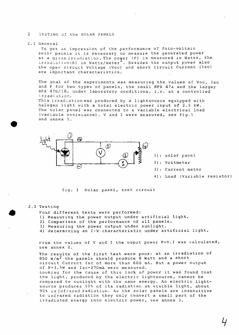
1 General To get an impression of the performance of foto-voltaic

solar panels it is necessary to measure the generated power at a given irradiation. The power (P) is measured in Watts, the irradiation(E) in Watts/meter . Besides the output power also the open, circuit Voltage (Voc) and short circuit Current (Isc) are important characteristics.

The goal of the experiments was measuring the values of Voc, Isc and P for two types of panels, the small BPX 47a and the larger BPX 47b/18, under laboratory conditions, i.e. at a controlled irradiation. This irradiationwas produced by a lightsource equipped with halogen light with a total electric power input of 2.5 kW. The solar panel was connected to a variable electrical load (variable resistance). V and I were measured, see fig.l and annex 1.

iivM

e i )

2)

3)

4)

solar panel

Voltmeter

Current meter

Load (Variable resistor)

fig. 1 Solar panel, test circuit

2 . 2 Testing

Four different tests were performed: 1) Measuring the power output under artificial light. 2) Comparison of the performance of all panels. 3) Measuring the power output under sunlight. 4) determining an I-V characteristic under artificial light,

From the values of see annex 2.

The results of the 850 W/m 2 the panel circuit Current Is of P = 3 . 5W and Isc = Looking for the ca the light, produce compared to sunlig source produces 10 90% is Infrared rad to infrared radiat irradiated energy

V and I the ouput power P=V.I was calculated,

first test were poor: at an irradiation of s should produce 8 Watt and a short c of more than 600 raA. But a power output 270mA were measured. use of this lack of power it was found that d by the electric lightsource, cannot be ht with the same energy. An electric light-% of its radiation as visible light, about iation. As the solar panels are insensitive ion they only convert a small part of the into electric power, see annex 3.

V

Given the fact that measurements under artificial light cannot be compared to measurements using sunlight, all the panels were tested under electric light and Isc and Voc were measured and for two panels I-V characteristics were recorded. The results of the second test were good. There appeared to be only a small difference in performance between the panels, see annex 2-

On a sunny day (solar irradiation up to 600 w/m 2) two panels were tested outdoors. The results are given in table 1 and in fig.3- In table 1 also the manufacturers specifications are given.

Table 1, Solar panels, results of outdoor tests

panel type; 3 P X 4 7a BPX 47b/18

manufacturers specifications:

E=1000W/m / : E=1000W/m 2 :

P= 1 1W Isc= 720mA

E=1000W/m2 E=1000W/m 2

P= 16W Isc= 2. 1A

test results

E= 300W/m; E= 530W/m:

P= 3W Isc= 400mA

E= 630W/m 2

E= 600W/m 2 P = 10.3W Isc= 1.36A

The temperature of the panels during the tests: T= 20 C

The test results can be compared to the manufacturers specifica­tions because Isc increases proportional to the irradiation.

For more results see annex 2.

Conclusions:

The panels are performing well, there are only small differences between the panels. The expected output of the small panels (BPX 47a) is 10 Watt at an irradiation of 1000W/m2. The ouput Voltage for maximum power ranges from 14 to 15 V and output current from 650 to 700 mA. The expected output value of the large panels (BPX 47b/18) at 1000W/m2 is 16 Watt at an output Voltage between 7 and 8 V and an ouput current between 2 and 2.1A. These numbers are calculated for a panel temperature of 25 c. If this temperature rises to 60 C (maximum temperature of the panels) the output (P and Voc) will drop 10% according to manufacturers specifications.

3 Performance of the Grundfoss pumps

3.1 General Two deepwell pumps o:: the type Grundfoss SP 8-4 and two Grundfoss inverters were tested on a test stand. With this test stand elevation-heads from 2 to 25 meters could be simulated. I: was equipped with a flow- and a pressuremeter in the watercircuit so the hydraulic power output of the pump could be measured.

The electric power input of the pump-inverter combination was monitored by using Voltage and currentmeters. The electric output of an array of solar cells was simulated by a DC powersupply that was connected to the inverter. This Grundfoss inverter changes the DC input into a three-phase AC output. The frequency of the output changes with the DC input power. Because of this changes in frequency also the speed (revolutions per minute) of the pump will change which means that the power, used by the pump changes. In this way the power output of the pump is depending on the power produced by the solar cells. The DC Volt produced by the solar panels is kept at a constant value by the inverter, only the current changes. This is done to keep the panels working under optimal conditions, i.e. at values of Voltage and current that are the most efficient.

age

3 . 2 Testing

Several tests h of the pumps. The flow (q) is elevation head power (Pdc).(te The flow is als power at a cons Voltage is fixe the input curre Also the effici is measured (te only (test 5 ) , (test 3) and th current were me These tests wer the other has a

ave been done to determine the performance

determined as a function of the (H) for different values of the input st 1) o measured as a function of the input tant elevation head. Because the input d at 98V q is given as a function of nt, Idc. (test 2) ency of the combination pump-inverter st 4 ) , the efficiency of the inverter the starting of the pump is examined e frequency and phase-angle of the AC-asured (test 6 ) . e done for one pump-inverter combination, lso been tested in the same way (test 7 ) .

3 Results The results of these tests indicate that the Grundfoss pump-inverter combination performs well. See annex 5. The maximum efficiency that was measured is 50% for the combination at an electric power input of 400 Watt. At lower inputs the efficiency decreases.

42 Solar panels of the type BPX 47a are capable of delivering 420 Watts. According to the test results the SP 8-4 pump should deliver 160 liters of water per minute over 7 meter elevation head at this power input of 420 W. The minimum power that is needed to lift water over 7 meter is 120 Watts, the flow will be very low at this powerinput.

Annex 1

Al Description of the set-uv for testing of the solar panels.

A 1.1 The light source used in the teststand (see drawing,fig. 2) consisted of a parabolic reflector with halogen lights in the focal line.The electric ;;ower of the light was 2. 5kW, the colortemperature of the artificial light is 3000K. The light was not evenly spread over the surface because the reflector did not have a perfect parabolic shape. For this reason 13 spots on the lighted surface were measured and the irradiation was determined. The intensity of the light is the mean value of the 13 measured intensities E=850 W/m .

fc_ _

1) : light source

2) : solar panel

3): supports (to allow cooling air under the panel)

4) : electrical connections

fig. 2 Test stand for photo-voltaic cells

Al.2 The intensity of the irradiation is measured using a Kipp-solarimeter, type CM 5. This solarimeter is equipped with a small black surface which heats up because of the incident radiation. The rise in temperature is transmitted to a thermocouple, which produces a voltage, increasing with temperature. The solarimeter was calibrated at giving 11.28 mV at lkw/ra^. This voltage was measured with a digital galvanometer (Keithley 177) with an inter'nal resistance of lMegohm/Volt. The solarimeter is sensitive to radiation with a wavelength between 0.3.10-6 and 2.5.10_6m. This means that the solarimeter is sensitive to Infrared and visible light.

A1.3 Electric circuit

The solar panel was connected to an electric load. A variable resistor was used as load. The voltage was measured with a digital H&E Voltmeter, current 'was measured with an Unigor A43 unimeter. See fig.l.

<9

Annex 2

A2 Test results, solar panels

A2 . T

During the measurements the intensity of the radiation from the lightsource was measured, it was found that it remained constant at 850 W/m 2 .

test First Panel: BPX 47a (nr. E=850 W/m 2, T 1 =

results: Voc=17.2V Isc=2 86 mA

-. 2 6 0 5 0) 25°C.

According to the specifications the panel should give a Voc=20V and an Isc=650mA at E=850W/m 2. The cause of the lack, of performan.ee of the panel is the frequency distribution of the light,produced by the lightsource, (see annex 3 ) .

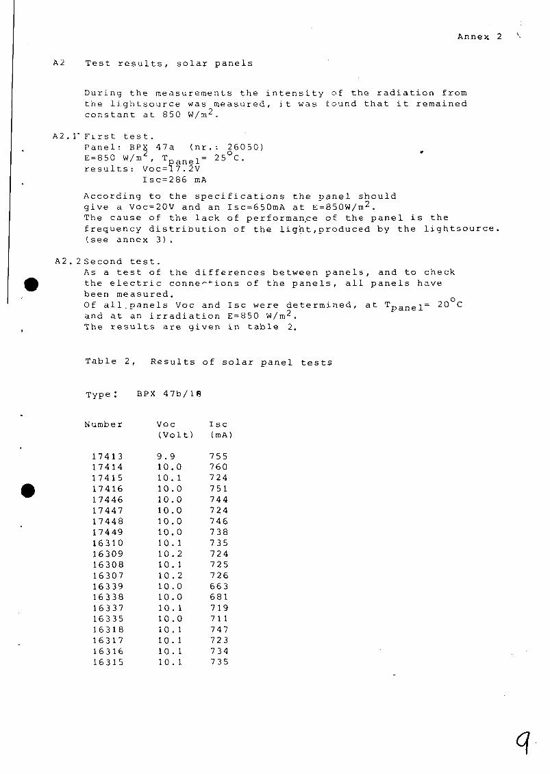
A2.2Second test. As a test of the differences between panels, and to check the electric connections of the panels, all panels have been measured. Of all,panels Voc and Isc were determined, at T and at an irradiation E = 850 W/m . The results are given in table 2.

pane 1 = 20°C

Table 2, Results of solar panel tests

Type BPX 47b/18

umber

17413 17414 17415 17416 17446 17447 17448 17449 16310 16309 16308 16307 16339 16338 16337 16335 16318 16317 16316 16315

Voc (Volt)

9.9 10.0 10. 1 10.0 10.0 10.0 10.0 10.0 10.1 10.2 10. 1 10.2 10.0 10.0 10. 1 10.0 10. 1 10. 1 10. 1 10. 1

Isc (mA)

755 760 724 751 744 724 746 738 735 724 725 726 663 681 719 71 1 747 723 734 735

<?

Table 2, results of solar panel tests, continued

Type; BPX 47a ( E= 850 W/m2, T= 20°C

Annex 2

Numbe r

26050 26051 26049 22377 23956 23790 23798 23801 23803 23818 23824 23825 23985. 24436 24435 24434 24433 24432 24431 24430 24429 24428 24427 23900 23901 23902 23903 23904 23905 23906 23907 23908 23909 20906 20904 20894 20961 20891 20890 20889 20881 20960

Voc (Volt)

17.5 18.7 18.9 18.8 18.9 19 . 0 19.0 18.9 18.9 19 .0 19.0 18. 9 19. 1 19. 0 19.0 19. 0 19.0 19. 1 19. 1 19. 1 19. 1 19. 1 19 . 1 19 . 2 19. 2 19. 1 19 . 2 18.6 19. 2 19. 2 19 . 2 19 . 2 19. 3 19. 0 19. 1 19.0 19 .0 19. 0 18.9 19.0 19. 0 19. 0

I sc (mA

272 263 259 275 273 2 74 272 262 267 269 °67 270 266 269 258 256 260 261 267 267 266 266 270 279 278 270 266 267 270 268 267 264 281 260 262 265 261 264 253 256 257 265

Number

20958 22378 22379 22406 22403 23698 23696 23699 22398 23700 22394 23890 2389 1 23892 23893 23894 23895 23896 23897 23898 23899 24039 20991 2 1012 18792 21010 20956 24D40 24051 24078 24079 20909 20910 22261 22262 22190 22 193 22194 22196 22198 22216 26050

Voc (Volt)

19 .0 18.8 18.9 18.9 18.9 18.9 18.9 19. 1 18.9 19.0 18. 8 18.9 19. 1 19. 1 18.9 19.0 18.9 19 .0 18.9 18.7 19. 0 19 .0 18.9 19. 0 19. 1 18.9 18.9 19. 1 19.0 19.0 19 .0 19 .0 19. 0 19. 0 19. 0 19.0 19.0 19 .0 18.9 19. 1 19.0 18. 8

I sc (mA)

265 268 270 269 269 260 271 263 268 267 269 270 273 271 273 278 274 276 275 273 279 261 253 259 258 264 266 261 258 257 254 255 266 275 274 269 270 274 275 281 275 268

10

Annex 2

rsi

<3-CO

03

X

m

c (0

ft

x:

O o

c o

+J ITS

• H 0 </l

c o

••4

•U Ul

•H

d) •P U ia n xl u

> I

M-l

i- O

-e- ^

% o UN

o

5

r

t i^

0

H

Annex

Third test Two panels, avai1 able su Test set-up: The panels- w leve L in sue incident sun The solarime The electric tests (see f Because the and changed solarimeter so the sunli situation di is 1arge, by the error in

one of each type, were tested outdoors using the nlight.

ere put against the front of a building on ground-h a way that they were perpendicular to the light. ter was placed parallel to the panels. circuit was the same as with the laboratory

ig. 1) . intensity of the sunlight was not very constant rapidly there occurred a small problem. The needed about 15 seconds to give a stable reading ght had to be stable for at least 15 seconds. This d not occur much. The deviation between the results taking mean values it is possible to reduce the readings.

Table 3, Results of outdoor tests of panel BPX 47a

Lig

a) b) c) d) e) f)

g) h) i) j) k) 1) m)

htintensi ty E (w/m2) 195

266 288 301 293 257 266 293 301 355 532 372

Voltage (V) 18.9 19. 3 15.1 17.6 18.3 19. 3 0 0

17.3 19. 1 0 0 0

Current (mA)

0 0

176 154 110

0 190 162 132

0 163 400 300

Power (Watt)

2. 7 2. 7 2.0

2. 3

These results are used to draw a I-V characteristic (fig.3) for the BPX 47a panel.

The values of Isc (Current at V=0) are used to calculate a value of Isc for E=300 W/m . As Isc is proportional to E this can be done in the following way : At 1000W/m2: Isc = 720 mA so Isc = .72 mA per W/m 2 (from specifi At 266 W/m 2: Isc = 162 mA. (measured) At 300 W/m 2: Isc = 162.(300/266) = 183 mA (calculated)

This way al five values of Isc can be used to calculate I S O ^ Q Q

The result is: At 300 Watt/m 2 : Isc = (222+183+138+225+242)= 202 mA

The results of measurements d,e,f,i,j and the calculated value ofIsc are used to draw the graph in fig.3. As can be seen in fig. 3 this method is not perfect, it is difficult to draw the line through the points that were found.

Annex

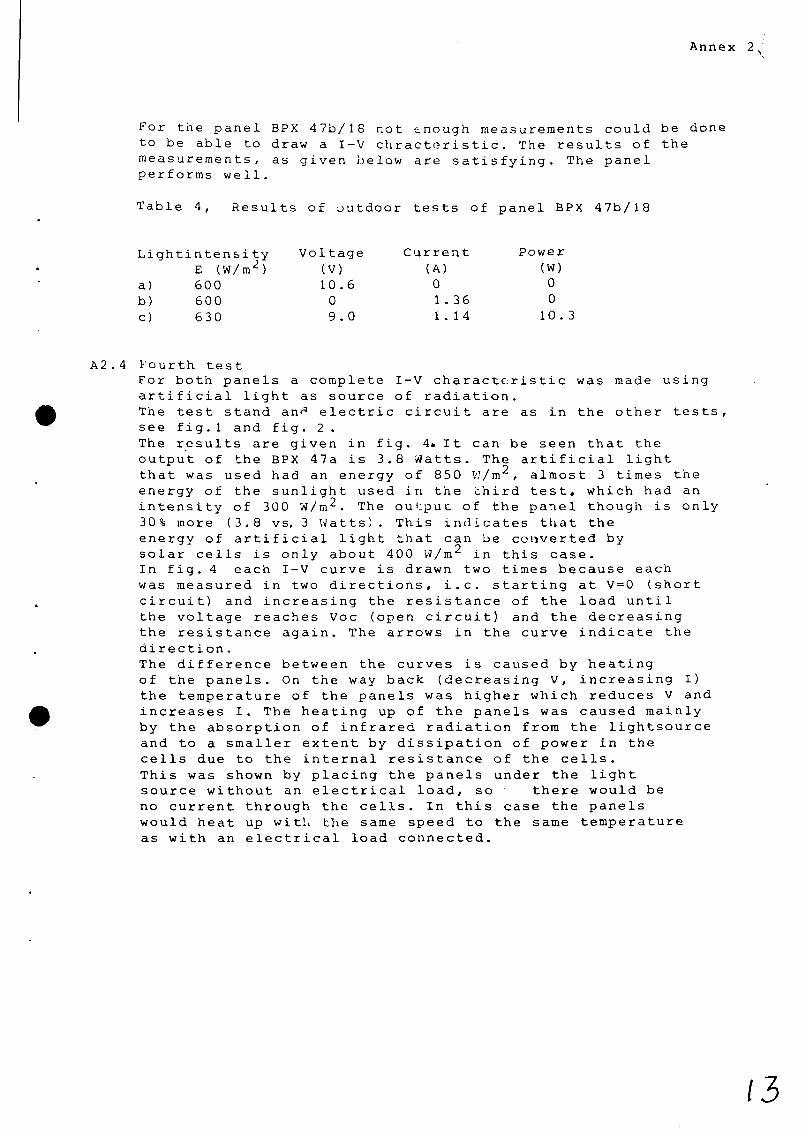
For the panel BPX 47b/18 not enough measurements could be done to be able to draw a I-V chracteristic. The results of the measurements, as given below are satisfying. The panel performs we 11.

Table 4, Results of outdoor tests of panel BPX 47b/18

Lightintensity Voltage Current Power E (W/m2) (V) (A) (W)

a) 600 10.6 0 0 b) 600 0 1.36 0 c) 630 9.0 1.14 10.3

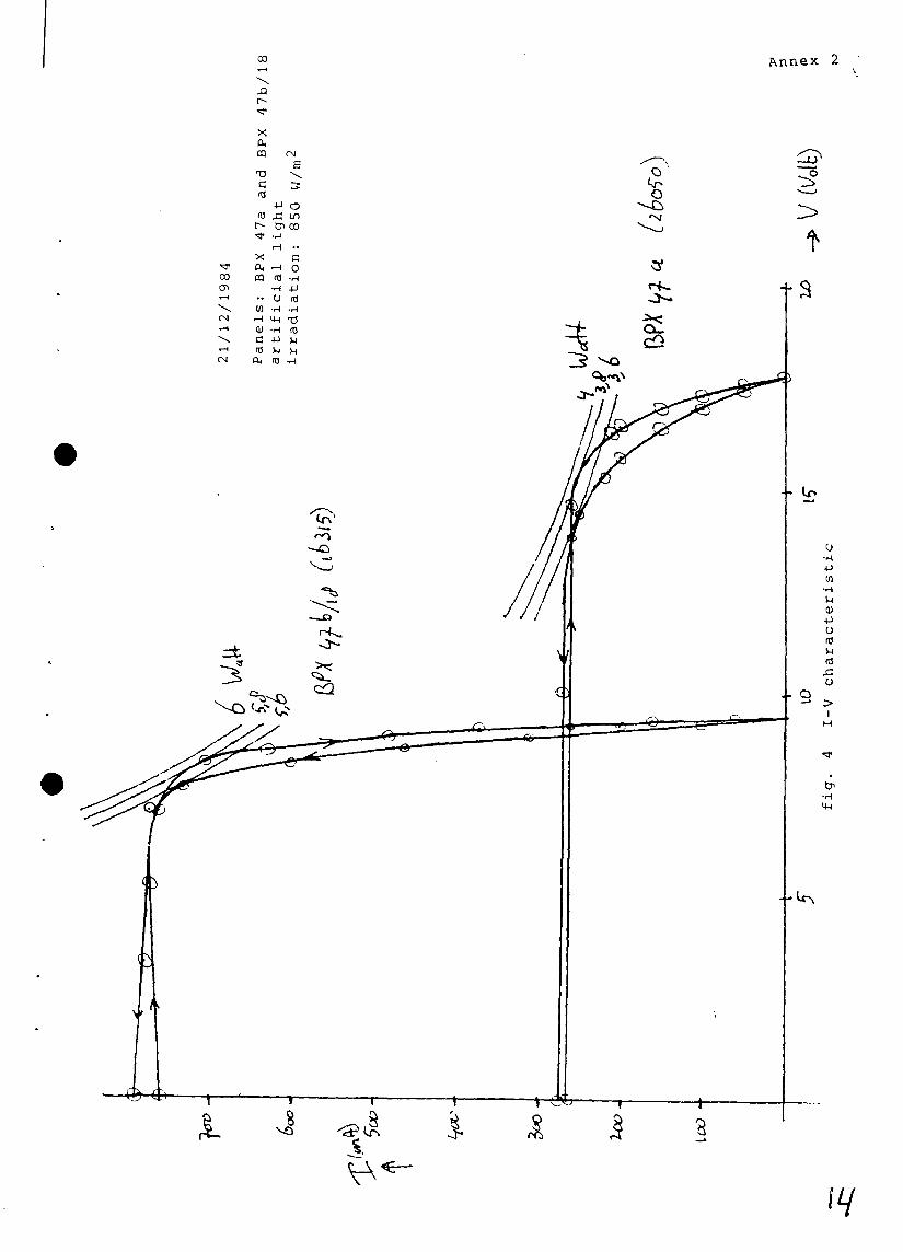
Fourth test For both panels a complete I-V characteristic was made using artificial light as source of radiation. The test stand an^ electric circuit are as in the other tests, see fig.l and fig. 2 . The results are given in fig. 4. It can be seen that the output of the BPX 47a is 3.8 Watts. The artificial light that was used had an energy of 850 VJ/m , almost 3 times the energy of the sunlight used in the third test, which had an intensity of 300 W/m 2. The output of the panel though is only 30% more (3.8 vs. 3 Watts) . This indicates that the energy of artificial light that can be converted by solar cells is only about 400 W/m^ in this case. In fig. 4 each I-V curve is drawn two times because each was measured in two directions, i.e. starting at V=0 (short circuit) and increasing the resistance of the load until the voltage reaches Voc (open circuit) and the decreasing the resistance again. The arrows in the curve indicate the direction. The difference between the curves is caused by heating of the panels. On the way back (decreasing V, increasing I) the temperature of the panels was higher which reduces V and increases I. The heating up of the panels was caused mainly by the absorption of infrared radiation from the lightsource and to a smaller extent by dissipation of power in the cells due to the internal resistance of the cells. This was shown by placing the panels under the light source without an electrical load, so there would be no current through the cells. In this case the panels would heat up with the same speed to the same temperature as with an electrical load connected.

co A n n e x 2

X 0 , CQ

T>

C S

+J O

r~ D> co

co

x c 1 H O CQ (tj -H

-H 4-) •• U (0

»H TJ • H (d

a. nj

IV

Annex

frequency distribution of artificial light and of sunlight.

Looking for t panels under of an electri To illustrate and the sensi The colortemp From this fig only to light The artificia of 3000K. Thi most of it's wavelength gr is produced b but if it is it will be ab long wave reg As the solari up to 2 . 5 . 1 of visible li "see" .a lot o the measureme

he reason of the lack the lightsource it wa c lightsource cannot this the spectral di

tivity of the panels erature of sunlight i ure it can be seen th with a wavelength sh

1 lightsource produce s indicates that an e radiation in the infr eater than 1.10_6m. E y the used halogen li in the same amount as out 90% of the radiat ion. meter is sensitive to radiation with a wavelength 0~ m it cannot be used to determine the amount ght inciding on the solar panels because it will f infrared radiation aud this will influence nts .

of power produced by the s found that the light be compared to sunlight, stribution of sunlight are given in fig. 5. s 5500K. at the panels are sensitive orter than 1.10 °m. s light with a colortemperature lectric lightsource produces ared region with a xact data on how much infrared ghts were not available, normal electric light

ed energy that is in the

sola' radiation

0 6 -

02

f i g

0 -1 1 1 1 1 1—i—r—j

0 2 0 4 0.6 0 8 1

Spectral transmission of a 40 mm waterlayer

2 3 0.4 0.6 08 1 2 3 4

Solar radiation spectral distribution and spectral sensitivity of BPX 47a.

Some experiments have been done to reduce the amount in the light of the lightsource. A layer of water can be used as a filter. The spectral absorption of a layer of water is given in fig.5b.As it was impossible to

echanical solution to the problem of putting a water-of ^m^ between the lightsource

of infrared

40mm find

mm over an area a m« l a y e r O f 4 U mm »~» v ^ .1. can a .1. c ti w A. « iu . ^ w w . . ^ — . . *~..^- - ^ . ~ ~ . . «~w~~~-~-w

and the solarpanel this kind of filter could not be used. If a waterlayer of 30 mm was placed between the solarimeter and the lightsource the reading of the solarimeter was reduced with a factor 2.5. This means that about 70% of the radiation is absorbed by the waterlayer, which indicates that at least 70% of the artificial light has a wavelength greater than 1 . 10"6m.

Annex

A4 Pump test stand

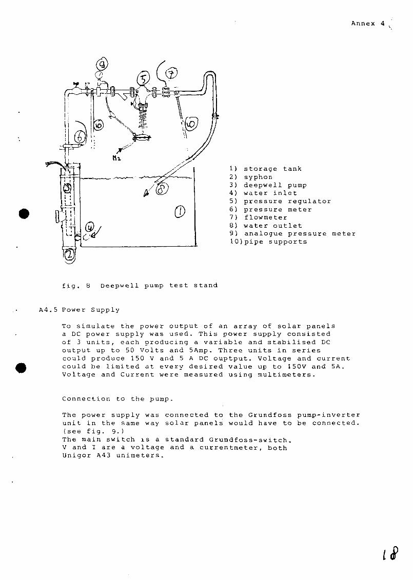
A4. 1 The test stand used to measure the characteristics of the pump existed of a watertank (volume 2m ) to which a syphon was placed. In this syphon the pump was mounted. The outlet of the pump is connected to a pressure-regulating valve. With this valve an elevation head up to 25m could be simulated by increasing the waterpressure In the watercircuit also a flowmeter, an analogue and an electronic pressuremeter are used.

1) syphon 2) waterinlet 3) inspection window 4) deepwell pump 5) water outlet 6) storage tank

Deepwell pump test stand

A4 . 2 Calibration of the meters

Flowmeter. The flowmeter was calibrated by filling a vessel with water, at a constant flow, and by measuring the weight of the amount of water and the time needed to fill the vessel. The flow can be calculated by dividing the weight by the time. The values found like this are compared with the reading of the flowmeter and with the analogue outputvoltage of the flowmeter. The results, given in table 5 , are mean values of two measurements.

Table 5, Calibration of the flowmeter

reading flowmeter

1/min

30 60 90 120 150

ar Vout flowme ter

Volt

0.21 0. 45 0.71 0 .92 1. 16

weight o f water

kg

10 10 71

filling time

sec.

16. 5 9 36

flow cal c .

1/min

36 67 1 18

deviation

%

20 1 1 30

Annex 4

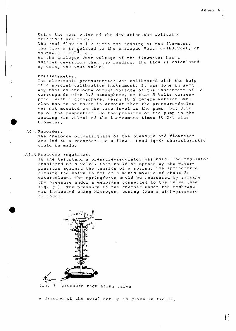
Using the mean value of the deviation,the following relations are found: The real flow is 1.2 times the reading of the flowmter. The flow q is related to the analogue Vout: q=160.Vout, or Vout=6.3 . 10~ 3. q . As the analogue Vout voltage of the flowmeter has a smaller deviation than the reading, the flow is calculated by using the Vout value.

Pressuremeter. The electronic pressuremeter was calibrated with the help of a special calibration instrument. It was done in such way that an analogue output voltage of the instrument of corresponds with 0.2 atmosphere, or that 5 Volts corres­pond with 1 atmosphere, being 10.2 meters watercolumn. Also has to be taken in account that the pressure-feeler was not mounted on the same level as the pump, but 0.5m up of the pumpoutlet. So the pressure on the pump is the reading (in Volts) of the instrument times 10.2/5 plus 0.5meter.

IV

A4.3 Recorder. The analogue outputsignals of the pressure-and flowmeter are fed to a recorder, so a flow - Head (q-H) characteristic could be made.

A4.4 Pressure regulator. In the teststand a pressure-regulator was used. The regulator consisted of a valve, that could be opened by the water-pressure against the tension of a spring. The springforce closing the valve is set at a minimumvalue of about 2m watercolumn. The springforce could be increased by raising the pressure under a membrane connected to the valve (see fig. 7 ) . The pressure in the chamber under the membrane was increased using nitrogen, coming from a- high-pressure ci U n d e r .

fig. 7 pressure regulating valv«

A drawing of the total set-up is given in fiq. 8

/

Annex 4

*"WJ 1) storage tank 2) syphon 3) deepwell pump 4) water inlet 5) pressure regulator 6) pressure meter 7) flowmeter 8) water outlet 9) analogue pressure meter 10)pipe supports

fig. 8 Deepwell pump test stand

A4.5 Power Supply

To simulate the power output of an array of solar panels a DC power supply was used. This power supply consisted of 3 units, each producing a variable and stabilised DC output up to 50 Volts and 5Amp. Three units in series could produce 150 V and 5 A DC ouptput. Voltage and current could be limited at every desired value up to 150V and 5A. Voltage and Current were measured using multimeters.

Connection to the pump.

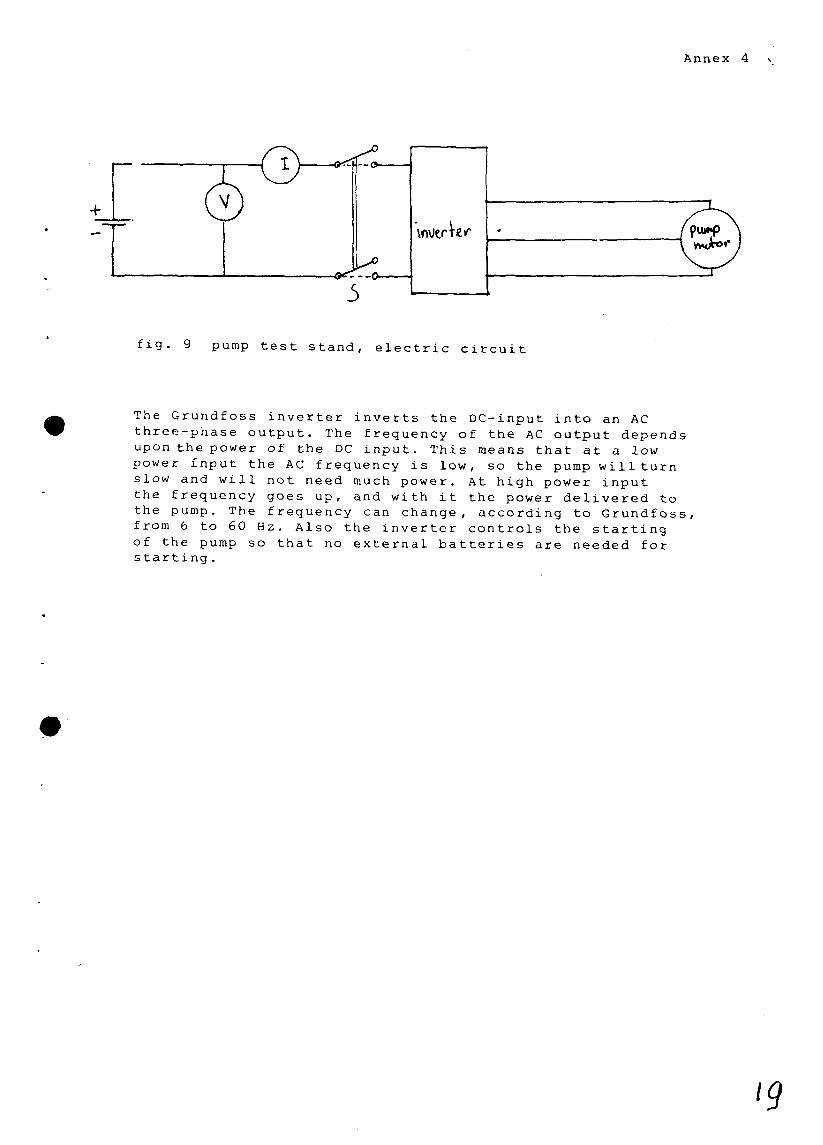
The power supply was connected to the Grundfoss pump-inverter unit in the same way solar panels would have to be connected. (see fig. 9.) The main switch is a standard Grundfoss-switch. V and I are a voltage and a currentmeter, both Unigor A43 unimeters.

iS

Annex 4

fig. 9 pump test stand, elect ric circuit

The Grundfoss inverter inverts the DC-input into an AC three-phase output. The frequency of the AC output depends upon the power of the DC input. This means that at a low power input the AC frequency is low, so the pump will turn slow and will not need much power. At high power input the frequency goes up, and with it the power delivered to the pump. The frequency can change, according to Grundfoss, from 6 to 60 Hz. Also the inverter controls the starting of the pump so that no external batteries are needed for starti ng.

Annex

s t Results of the puraptests, 1 pumpset

The tests 1 to 6 have been done with the same inverter-pump combination.Annex 6 gives the results of the tests with the other combination.

1 q-H characteristic The flow q at a given elevation head H is an indication for the performance of the pump. A q-H curve is measured for four different values of the input power Pdc. As Vdc is constant (98V) only the input current, Idc, changes from 1 up to 4 Amp. The results are given in fig.10. The curves for constant hydraulic power that are drawn in fig.10 are calculated the following way: Phydr. = m.g.h where m=mass, g=gravity, h=heigth, t=time

t or: Phydr = q.O.g.H, where q=flow (m-Vs) , f =density (kg/mJ)

and g-gravity(m/s^), H=elevation head (m) Phydr •} .

q = —-- m°/s

f .g.H

for instance: assume Phydr= 180 Watt

q = Phydr m 3/s = 60 . 180 f . g ., H 1 . 9 . 8 . H

The hyperbolic curve that is described in this equation for q is drdwn in fig. 10. By determining the point of intersection between the q-K curve for the pump and the curve for constant power the point of the maximum power output is found. This seems to be at 9 meter Head, for the 4Anip curve, with an output of 190 Watt. The exact output at this head can be calculated: P = 130 . 1 . 9.8 . 9 = 191 Watt.

60 With this value of Phydr the efficiency of the inverter-pump combination can be calculated. The efficiency T|_ =Phydr . 100% as Pdc is the power input.

Pdc Pdc = Vdc . Idc = 98 . 4 = 392 Watt So the maximum efficiency 1) max = 191 = 48% for this po^er inpu

392

5.2 q = f (I) • At a constant head the flow was determined as a function of the input power, which is proportional to the input current Idc. The results are given in fig. 11* The first figure is determined by measuring q at constant value of H and for different values of I.

Annex 5

2 8 / 1 2 / 1 9 8 4

- •Head (m)

f i g . 10 q - H c h a r a c t e r i s t i c

II

Annex 5

&>°-

Wi~

1 ia

bH 3

do-

bH-

HS-

3>

ih-

<L IC£)

O ! i 3 V

fig. 11 Flow as a function of the DC power input, at a constant head.

pump 1, inverter 1

22

Annex

The elevation head of 7 meter was chosen because it was said that the pump is going to be used to pump water over 7m. From the figure it can be seen that the pump needs at least 1.2 A to start against 6.9 m watercolumn. The flow will be almost nothing.

With the use of this graph q = f(I) it is possible to determine the amount of sunlight needed to give a certain flow at a civen head. For instance: H = 7 m. Say q = 25 1/min. from the figure it can be seen that the needed input current Idc = 1.5 A. Let's assume that BPX 47a solar panels are used in a 6 x 7 matrix. The panels give an ouput of 720 mA at an irradiation of 1000 W/m 2. The output voltage is constant at 14.4 V. Then each panel should give:

Idc = 1. 5

= 250 mA.

To produce this an irradiation E is needed: 1000

250 720

This gives the result: E = 340 W/m . E is the intensity of the sunlight that will make the solar pump deliver 25 1/min at an elevation head of 7 m.

3 Starting behaviour of the pump The exact Voltage needed to start the pump was determined for different current-values. The watercolumn against which the pump had to start was only 2 m. It was found that the pump starts at Vdc *? 102 V (or more) . Immediately after starting the Voltage Vdc dropped to 98 V, which value then remained constant, independent of changes in current. It was impossible to make the pump start if the Voltage over the inverter Vdc was only 101 V. The value of Idc had no influence on the starting behaviour

4 Efficiency The hydraulic pump-inverter The hydraulic The efficincy

power output and the efficiency of the ccmbiuation are determined, power is Phydr = q . <J . g is : 0r = Phydr/Pel . 100%

H

Pel The power input

So the efficiency is

The results are in fig

Vdc Idc

I Vdc.Idc

12 .

100%

From this figure it can be seen that the efficiency reaches a maximum value at a certain flow. This is caused by the hydraulic efficiency of the pump, which reaches a maximum for a certain rotation speed.

<#> o o *-H

« n •o >J u £\-V a|a,

1

4J 3 a. 4-> 3 0

u a> 5 0 ft

u •H r-{

3 <a s-i

T3 > B

•P

3 ft C •H

M (1) 3 0 ft

0 •H

M •P

O 0)

r-<

<u

'3 o ©

Annex 5

3 ft C

an

>-x>

0

- £

« * r»

H

-o <o

4

j -v O

- <*> J *

- f>»

I _£ <=V

crV 'N 1

c 0

•r-l

•P

ombina

u

rter

> c •H 1

a

urn flow

0)

ft A

<u x: 4-)

4-1 0

> i 0 c 0)

•rH

U

<W

w

•P

U-t

o

c 0

•p

u c 3 l*-l

10

w (0

«-H

H

•P H

> c

-H

*• «-t

ft a 3 ft

lO

o 1st

o

1 0 o

»

o

4- o

F* ^ ^ 2V

Ann

5 efficiency of the inverter The efficiency of the inverter is the power output compared to the power input, or:

Pac °l = Pdc 100'

Pdc is the power input, direct current. Pdc = Vdc . Idc Vdc and Idc were measured with a dc voltmeter and a dc current-meter, both Unigor A43.

Pac is the power output, three phase alternating current Pac = Vac . lac . cos<p . 3 , for three phase current. Pac can be determined by measuring Vac, lac and the phase-angle <p , but as there was no phase angle meter available Pac had to be measured direct, using a Wattmeter.

The powermeter used was a single-phase Feedback EW 604 Wattmeter. It was connected as in figure 13. The total (three phase) powe. output of the inverter is three times the reading of the single-phase Watt-meter. Also see annex 7.

. c . AC-pover measurements, electric circuit'

The results are; Pdc = 392 W Pac = 9 0 . 3 = 360 W Then the efficiency is: *r\_ = 360/392 . 100 = 92%. After the electric circuit was optimized (shorter cables, better connectors, etc.) the following results were found for different power inputs. Table 6

Efficiency of the inverter for different values of the input power and the flow..

— - ^ flow q (1/min) :

power input —

Pdc = Vdc . Idc

Pdc = 420 W

Pdc = 392 W

Pdc = 196 W

Pac(W)

Pac(W)

% ( % )

Pac(W)

15b

410

98

380

97

200

100

115

415

99

380

97

200

1 100

72

410

98

380

97

200

100

34

400

102

215

109

An

The electric efficiency gets higher with decrea Both , decreasing power slower, meaning that th gets lower. It seems al increases with decreasi But as the efficiency e flow it is also possibl well for low frequencie little bit optimistic, done to find the cause it was clear that they could be seen from the pump-inverter.

of the inverter is very high, it sing power and with decreasing flow. and flow, mean that the pump rotates

e output frequency of the inverter so that the efficiency of the inverter ng frequency of the AC output, xceeds 100% for low power and low e that the powermeter is not working s, or that it is overall a No further investigations have been of this somewhat high results, because were only a little bit too high as efficiency of the combination

Frequency and phase-angle The frequency of the AC current was determined as a function of the electric power. An oscilloscope was used to measure the. wavelength, and so to calculate the frequency. Also the phase-angle was determined. The results are: Power input: Vdc = 98 V. Idc = 2 A. Pdc = 196 W. Power output: Pac = 180 W. Frequency f= 29 cycles/sec, phase-angle <f = 55°

Power input: Vdc = 98 V. Idc = 4 A. Pdc = 392 W, Pac = 360 W. Frequency: f = 41 cycles/sec, phase angle <p 45^

It can be seen that the frequency increases with the input power, the phase angle (the shift between Voltage and current) decreases. The power output has also been determined for the inverter, and it can be seen that the efficiency is 92%, which is less than the result of test 5, see table 6.

Annex

Results of the pumptests, 2 pumpset

For the second pump and second inverter also flow - Head characteristics have been made. It showed that the second pump performs little better than the first. The results are given in fig.14. The second inverter does not have any influence on the output, it performs exactly in the same way as the first inverter.

The hydraulic power output of the second pump is 200 W, as can be seen in fig. 15. As the power input was 400 W, DC, this gives an efficiency for the combination of 50%. As the inverter had no influence, compare fig. 14 and fig.15, the pump must be performing

better. This can be caused by small differences between the two pumps. It is also possible that this difference gives the error in the testresults, which would mean that with this set up it is not possible to measure the hydraulic performance of a pump more precise than with a 2% margin. The latter is very well possible as certain effects, such as the influence of the waterlevel in the watertank, were not known.

m i n . }

Annex 6

'6 J

F i g . 14 q - H c h a r a c t e r i s t i <

1&

Annex 6 ,

176-

lt Amp. Amp. Amp .

fig. 15 q - H characteristic

29

Annex 7

A7 AC-power Measurements

These measurements have been performed with two different types of power meter. Both gave problems during the tests.

A7.1 Three-phase power measurement: A NIEAF three-phase Watt-meter was used, it was connected as in fig. 16.

O-f1

Jht W W " 1 '

— - i

P3 ~\ • \

r --^-^

I K W ' V <wota

P3 = Wattmeter

Fig. 16, Three phase power measurements.

The results of the test are: Pdc = Vdc . Idc = 98 . 4 = 392 Watts Pac = 340 Watts (direct reading of the Watt-meter.

Then: 7^ = 340/392 . 100 = 87%.

This is much less than the manufacturer gives as the efficiency of the inverter, the conclusions is that the Watt-meter might not be working well, because the pump is performing sufficiently.

A7.2 Single-phase powermeasurements. The same NIEAF meter was used as a single-phase powermeter The electric circuit is given in fig. 17.

Fig. 17. Single phase power measurement, Wattmeter

Three coils are connected to the power leads to the pumpmotor to create a neutral lead. This neutral lead is necessary for the NIEAF meter to measure the single-phase Voltage. The impedance of the coils was very high so there would be no powerloss. The current in one phase is measured direct.

30

Annex 7

The results are: Pdc = 392 W. Measured output: 90 Watts for one phase, so: Pac = 3 . 90 = 270 Watts.

Then: y[ = 270/392 . 100 = 69%.

This value is obviously wrong because the efficiency of the pump-inverter combination reaches 50%. It is not clear why this powarmeter did not function properly, the results were not usable.

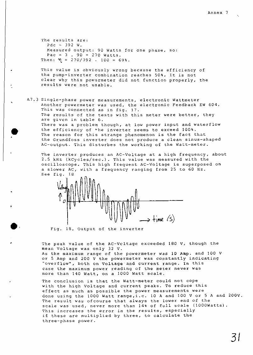
A7. 3 Single-phase power measurements, electronic Wattmeter Another powermeter was used, the electronic Feedback EW 604. This was connected as in fig. 17. The results of the tests with this meter were better, they are given in table 6. There was a problem though, at low power input and waterflow the efficiency of fhe inverter seems to exceed 100%. The reason for this strange phenomenon is the fact that the Grundfoss inverter does not produce a clean sinus-shaped AC-output. This disturbes the working of the Watt-meter.

The inverter produces an AC-Voltage at a high frequency, about 2.5 kHz (kCycles/sec.). This value was measured with the oscilloscope. This high frequent AC-Voltage is superposed on a slower AC, with a frequency ranging from 25 to 60 Hz. See fig. 18

A n

W /s) Fig , Output of the inverter

The peak value of the AC-Vcltage exceeded 180 V, though the mean Voltage was only 32 V. As the maximum range of the powermeter was 10 Amp. and 100 V or 5 Amp and 200 V the powermeter was constantly indicating "overflow", both on Voltage and current range. In this case the maximum power reading of the meter never was more than 140 Watt, on a 1000 Watt scale.

The conclusion is that the Watt-meter could not cope with the high Voltage and current peaks. To reduce this effect as much as possible the power measurements were done using the 1000 Watt range,i.e. 10 A and 100 V or 5 A and 200V The result was ofcourse that always the lower end of the scale was used, never more than 14% of full scale (lOOOWatts). This increases the error in the results, especially if these are multiplied by three, to calculate the three-phase power.

31

Annex 7

The error in the readings of the Wattmeter is obviously large enough to produce efficiency numbers that exceed 100%. It is possible that the error in the Watt-meter increases with increasing phase-angle ore decreasing frequency. The phase-angle increases with decreasing power (=decreasing frequency), see annex 5. This may account for the toe high values of the efficiency at low power-input of the inverter (table 6). This was not further inverstigated.

The power output of the inverter can also be measured by measuring Vac, lac and the phase-angle. As there was no phase-angle meter available the oscilloscope was used to determine the phase-angle <y Because of the very complicated output it was not possible to make an accurate reading reading of © , see annex 5. Because of this it was not possible to determine Pac more accurate than with a powermeter.

Equipment used:

Function*.

Voltage meter

Voltage meter

Current meter

Watt meter

Watt meter

Pressure meter

Os c i1los cope

X - Y recorder

Flow meter

DC-power supply

Solarimeter

Voltage meter

Type, specifications'.

Unigor A43, multimeter

H&B , digital voltmeter

Unigor A43, multimeter

NIEAF 1 phase and 3 phase wattmeter

Feedback Electronic Wattmeter, EW 604

Elan Abgleichautomat MBS 5102 Elan TF messverstarker MBS 5204 Elan Anzeige-einheit MBS 5405

HP 1200 A oscilloscope, 100 V, dual trace

Kipp BD 91 x-y-y' recorder

MM 50 PVC transmitter LMELA-30 monitoring instr.

Delta Electronica TPS 050-5, 50V, 5A (three uni ts)

Kipp CM 5/6, 11.28 | V per W/m 2

Keithley 177 microvolt, digital voltmeter

Annex 9

Literature used

Electriciteit uit Zonncstraling ATOL, Leuven, Belgium (1980)

New and Renewable Energies, U. Meier and U. Rentsch, SKAT/ENDA, St. Gallen, Switzerland (1981)

Zonnecellen, F.Juster, Kluwer, Deventer (1980)

Solar Panels for Terrestrial Applications, H.Dijkstra and C. Franx, Technical Information 052 (1978)

Interim Report on the Electrical Transmission Project, F.Eilering, CWD, Enschede (1984)

3^