WTS1 Series II Belt Scale Operation and Installation Manual
168
WTS1 Series II Belt Scale Operation and Installation Manual Web Tech Australia Pty Ltd PO Box 4006 11 Electronics St Eight Mile Plains, QLD, 4113 Ph: 1800 777 906 Fax: 61 7 3841 0005 E-mail: [email protected]
-
Upload
khangminh22 -
Category
Documents
-
view
1 -
download
0
Transcript of WTS1 Series II Belt Scale Operation and Installation Manual

WTS1 Series II Belt Scale
Operation and Installation Manual
Web Tech Australia Pty Ltd PO Box 4006 11 Electronics St Eight Mile Plains, QLD, 4113 Ph: 1800 777 906 Fax: 61 7 3841 0005 E-mail: [email protected]

i
WTS1S2 – OPERATION AND INSTALLATION MANUAL
Contents
Introduction .................................................................................................................................................... 1
Web-Tech Belt Scale Range ............................................................................................................................. 2
Theory of Operation ........................................................................................................................................ 3
Theory of Operation – Weighframe ................................................................................................................ 4
Pivoted Type Belt Scales .......................................................................................................................... 4
Fully Floating Weighframe ...................................................................................................................... 4
Theory of Operation – Speed Sensor .............................................................................................................. 5
Belt Speed Sensor .................................................................................................................................... 5
Belt Travel Sensor .................................................................................................................................... 5
Theory of Operation – Integrator .................................................................................................................... 6
Integrator Location .................................................................................................................................. 6
Theory of Operation – Calibration .................................................................................................................. 7
Material Test ........................................................................................................................................... 7
Calibration Chain / Train Test .................................................................................................................. 7
Static Weight Test ................................................................................................................................... 7
Electronic Simulation Test ....................................................................................................................... 7
Theory of Operation – Conveyor Design ......................................................................................................... 8
Weighframe Location .............................................................................................................................. 8
Conveyor Inclination ............................................................................................................................... 8
Concave and Convex Curves.................................................................................................................... 8
Conveyor Take-up ................................................................................................................................... 8
Belt Loading ............................................................................................................................................. 8
Belt Type .................................................................................................................................................. 8
Belt Tracking ............................................................................................................................................ 8
Conveyor Idlers........................................................................................................................................ 8
Theory of Operation – Conveyor Design ......................................................................................................... 9
Idler Alignment ........................................................................................................................................ 9
Conveyor Stringers .................................................................................................................................. 9
Environmental Protection ....................................................................................................................... 9
Theory of Operation – Accuracy.................................................................................................................... 10
Theory of Operation – Maintenance ............................................................................................................. 11
Mechanical Installation ................................................................................................................................. 12
Weighframe Location ............................................................................................................................ 12
Lifting of Belt ......................................................................................................................................... 12
Weighframe Installation ........................................................................................................................ 12

ii
WTS1S2 – OPERATION AND INSTALLATION MANUAL
Contents
Electrical Installation – Encoder Speed Sensor ............................................................................................. 18
Description ............................................................................................................................................ 18
Mechanical installation ......................................................................................................................... 18
Electrical Installation ............................................................................................................................. 18
Part Number .......................................................................................................................................... 18
Electrical Installation – Magnetic Pickup Speed Sensor ................................................................................ 19
Description ............................................................................................................................................ 19
Mechanical installation ......................................................................................................................... 19
Electrical Installation ............................................................................................................................. 19
Part Number .......................................................................................................................................... 19
Electrical Installation – Proximity Switch ...................................................................................................... 20
Description ............................................................................................................................................ 20
Mechanical installation ......................................................................................................................... 20
Electrical Installation ............................................................................................................................. 20
Part Number .......................................................................................................................................... 20
Electrical Installation – Integrator Optimus .................................................................................................. 21
Belt Scale Electronics ............................................................................................................................. 21
Enclosure Mounting .............................................................................................................................. 21
Cables .................................................................................................................................................... 21
Cable Terminations ............................................................................................................................... 21
Start Up ................................................................................................................................................. 21
Start Up Steps ........................................................................................................................................ 21
Masterweigh Optimus – Installation and Operation Manual ................................................................ 22
Appendix A – WTS1S2 General Arrangements ................................................................................................ A
Appendix B – Wiring Diagrams ........................................................................................................................ B
Appendix C – Electrical Enclosure GAs ............................................................................................................ C
Appendix D – Belt Scale Positioning Guide .....................................................................................................D
Appendix E – Optimus Datasheets .................................................................................................................. E

1
WTS1S2 – INSTALLATION AND OPERATION MANUAL
Introduction
The model “WTS1S2” belt scale is one of Web Tech AutoWeigh’s “process” type conveyor belt scales, and is suitable for applications most applications. Accuracies in the order of ±1% are achievable. The WTS1S2 conveyor belt scale is a heavy-duty one idler fully suspended weighframe particularly suitable for the mining industry. Incorporating four load cells, it is available to suit belt widths from 450mm to 2400mm. The weighframe can be supplied in either mild steel galvanised, or stainless steel construction. Standard idler spacing’s of 1000mm, 1200mm and 1500 mm are available.
WTS1S2 Cal Bar
WTS1S2 In-Situ
WTS1S2 In-situ in Conveyor 1000mm Idler Spacing, 1000mm Belt Width

2
WTS1S2 – INSTALLATION AND OPERATION MANUAL
Web-Tech Belt Scale Range
Model Description Typical Applications Accuracy
E40 Universal type scale, simplest installation, dual load cell.
Aggregate plants, Feeder control
±, 1 – 5 %
WTE11 Single idler, single load cell process scale with mechanical tare, belt widths up to 1050 mm.
Aggregate plants, Timber plants, Gold ore plants
±, 1 – 3 %
WTE12 Single idler, dual load cell process scale with mechanical tare, suitable for belt widths up to 1600 mm.
Aggregate plants, Timber plants, Gold ore plants
±, 1 – 3 %
WTE21 Dual idler, single load cell process scale with mechanical tare, belt widths up to 1050 mm.
Aggregate plants, Timber plants, Gold ore plants
±, 0.5 – 1 %
WTE22 Dual idler, dual load cell process scale with mechanical tare, suitable for belt widths up to 1600 mm.
Aggregate plants, Timber plants, Gold ore plants
±, 0.5 – 1 %
WTS1 Single idler, dual load cell heavy duty suspended weighframe, suitable for belt widths from 450 to 2400 mm.
All mining applications ±, 1 %
WTS2 Dual idler, dual load cell heavy duty suspended weighframe, suitable for belt widths from 450 to 2400 mm.
All mining applications ±, 0.5 %
WTS4 Four idler, four load cell, fully suspended weighframe, suitable for belt widths up to 2400 mm.
High accuracy loadouts, Material transfers
±, 0.25 – 0.5 %
WTS6
Six idler, four load cell, heavy duty suspended weighframe, suitable for belt widths up to 2400 mm, high belt tension areas.
High accuracy product transfers such as shiploaders
±, 0.1 – 0.25 %
WTS8
Eight idler, four load cell, heavy duty suspended weighframe, suitable for belt widths up to 2400 mm, high belt tension areas.
High accuracy product transfers such as shiploaders
±, 0.1 – 0.25 %

3
WTS1S2 – INSTALLATION AND OPERATION MANUAL
Theory of Operation
Belt scales enable material to be weighed on a conveyor whilst in motion. A belt scale differs from a static weighing system, such as a bin weighing system, in that the belt scale is required to measure two variables. The first variable is the weight on the conveyor belt, and the second variable is the belt speed or belt travel. The weight of material on the conveyor belt is obtained by measuring the load on one or more idlers. This load can then be expressed in terms of kg/metre of belt. The belt speed or belt travel is measured by using a device which gives an output proportional to the belt speed or belt travel. The flow "rate" of material passing over the belt scale can be expressed as:
Flow Rate = Weight ( Weighframe ) × Speed ( Belt Speed Sensor )
Total Weight = Weight ( Weighframe ) × Belt Travel ( Belt Speed Sensor ) Belt scale manufacturers use either the belt speed (flow rate) or belt travel (total weight) methods depending on their design philosophy. Those that use the belt speed (flow rate) method use a high frequency speed sensor (up to 1 kHz), the output of which is proportional to the belt speed. The integrator primarily calculates the "rate" passing over the belt scale, from which the "total" is then derived. Those that use the belt travel (total weight) method generally use a low frequency speed sensor, which delivers a number of pulses per unit of belt length. The integration primarily calculates the "total" weight, from which the flow "rate" is then derived. Due to the availability of high-speed processors, most modern belt scales use the "rate" method as the basis for their electronic design. Whilst the mathematics used by the belt scale electronics may appear to be relatively simple, the tasks required of the electronics are more complex. Not only must the electronics be capable of receiving and processing the signals from the weighing mechanism and belt speed / travel device, it must also be capable of the following:
Display Rate and Total readings
Provide stable power supplies to the weighing and belt speed / travel elements
Provide analogue and digital outputs for remote equipment
Provide Automatic Zero and Span calibration facilities
Provide serial communications for remote computers
Carry out "Auto Zero" routines when the belt is empty
Provide alarm functions
Provide control functions
Interface with the operator The measurement of the weight on the conveyor belt and the belt speed / travel also present some physical problems which must be overcome. The accuracy of the weight measurement is dependent on a number of factors such as belt tension, belt construction, weighframe location, troughing angle and material loading. The degree of accuracy and ways of improving the accuracy are discussed in further detail in the following sections.

4
WTS1S2 – INSTALLATION AND OPERATION MANUAL
Theory of Operation – Weighframe
Belt Scales consist of four main components these being: 1. Weighframe and associated weigh idlers 2. Belt speed / travel sensor 3. Electronic Integrator 4. Calibration device
The function of the weighframe is to support the weigh idler(s) and conveyor belt, and to convert the weight of the material within the weigh area to an electrical signal, which can be processed by the electronics. Weighframes are varied in design, however the majority of the designs incorporate one or more transducers, most typically strain gauge load cells .The weighframe is usually self-contained, low profile, and designed to be installed within the limits of the conveyor structure. The number of idlers used is dependent upon the accuracy required, and the conveyor parameters. Various weighframe designs exist, each with their own perceived advantages. Most belt scale manufacturers use either a "pivoted" design or a "fully floating" design. With a pivoted design, one or more idlers are mounted on a frame, which is pivoted at one end by some form of fulcrum point. The fulcrum point is designed to as frictionless as possible and to require as little maintenance as possible. Early pivot designs included knife edges and bearings or ball bearings, however due to the perceived maintenance problems, and the advent of transducers with very small amounts of movement, these were replaced with components such as torque tubes, flexures or rubber trunnions. The "fully floating" design comprises one or more idlers mounted on frame, which is in turn supported at each corner by a transducer. Horizontal and transverse restrainers limit the movement of the weighframe in any direction, except that perpendicular to the belt line. The advantages of both types of design are as follows: Pivoted Type Belt Scales
Requires less transducers
Better sensitivity from the transducers. As the pivoted design can be counterweighted allowing the “deadweight” of the belt and idles to be removed.
Less calibration weights required
Fully Floating Weighframe
Same design as used in high accuracy static weighing systems
Do not use pivots, which could influence measurements
Forces acting on weigh idlers act directly on transducers
Calibration weights represent the same weight regardless of where they are placed on weighframe
Belt Scale Idler
Load cell
Counterweight Mechanism
Torsion Bar Pivot
Belt Scale Idler
Load Cell

5
WTS1S2 – INSTALLATION AND OPERATION MANUAL
Theory of Operation – Speed Sensor
As previously discussed, a sensor is supplied to provide a signal to the electronic integrator as to the actual belt speed or belt travel. Belt Speed Sensor Belt speed sensors can be supplied in several arrangements. The most common method is for a "rotary" type sensor to be mounted in an enclosure and then to be connected to a "live" shaft pulley, usually the tail pulley. As the pulley rotates, the speed sensor shaft is also rotated, which in turn produces a pulse output. The frequency of the pulse output is proportional to the rotational speed of the pulley. Typical frequencies fall within the range of 100 - 1000 Hz. Belt speed sensors should not be connected to the drive pulley, as any slippage between the drive pulley and conveyor belt will not be measured. A second type of belt speed sensor involves mounting a sprocket at the end of a conveyor roll, and sensing its rotational speed with the use of a "Magnetic Pick-up". The magnetic pick-up counts the number of sprocket teeth that pass by a sensing element, and therefore produces a frequency proportional to the speed. This system is not normally used on applications where the conveyor rolls are subject to material build-up, as this will change the diameter of the roll and therefore the indicated belt speed. However on some applications where the idler rolls appear to be carrying build-up, closer inspection will show that the area of idler roll in contact with the belt remains clean. The advantages of using the idler roll / sprocket type of sensor is that they are relatively simple and robust, and can be situated close to the weighframe. When installed close to the weighframe, the belt speed being measured is the actual belt speed at the weighframe. A third type of system still popular with some manufacturers / customers is the use of a pivoted "trailing" arm with a wheel in contact with the return belt. The wheel is attached to a rotary sensor similar to that used with the tail pulley method. The disadvantages of this method are: The wheel is prone to bounce when a disturbance in the belt surface such as a splice passes under it. This will cause a variation in frequency output, and therefore the measured belt speed. The wheel is usually mounted on the return belt adjacent to the weighframe. This can be a long distance away from the weighframe (by belt travel), and therefore the belt speed measured may not be the same belt speed at the weighframe. Belt Travel Sensor A belt travel sensor usually consists of one or more "flags" welded to a pulley, usually the tail pulley, and a proximity probe. As the flags pass by the proximity probe they are counted, and this relates to the amount of conveyor belt that has passed around the pulley. The advantage of this type of system is that it is relatively simple and robust. However the disadvantage is that it is low frequency in output, and therefore the resolution can be coarse.
PXT Speed Sensor PXT Speed Sensor

6
WTS1S2 – INSTALLATION AND OPERATION MANUAL
Theory of Operation – Integrator
The electronic integrator is designed to carry out the following basic functions:
Provide supply voltages to weighframe transducers and belt speed / travel sensors
Measure and integrate the instantaneous weight on weighframe and instantaneous belt speed / travel which calculates the mass rate and mass total passing over the conveyor respectively
Provide analogue and digital outputs for remote equipment
Provide facilities for calibration The electronic integrator may also provide the following options:
Provide P.I.D. control output
Provide serial communications for remote computers
Provide rate alarm outputs
Provide batching facilities Most modern integrators are microprocessor based with computing power similar to a personal computer. Each manufacturer engineers their own software, which incorporates their own design philosophies. Whilst all integrators may look similar at first glance, the methods used by the various manufacturers to achieve the end-result, can vary significantly. The current "state of the art" integrators are designed to make operation / calibration easier for site personnel, and great emphasis should be placed on the ease of use. Many sites will prefer the belt scale supplier to carry out routine maintenance and calibration, however in an emergency situation, there is nothing worse than having to wade through a manual, attempting to understand what a displayed code means. Integrator Location The electronic integrator does not have to be located adjacent to the weighframe. Some customers may wish to mount the integrator in a nearby motor control centre or in a control room. Whilst this is possible the following points should be considered when selecting the location:
The weighframe transducers produce very low voltage levels and therefore if long cables are used voltage drops may occur
The longer the cable run, the greater the chance of picking up electrical noise on the cables
Long distances between weighframe and integrator increases the time required when carrying out calibrations
Is the proposed area classified as Dust Ignition Proof or Hazardous? It is Web-Tech's belief that the best location for the integrator is adjacent to the weighframe where possible. The output signals can be used to provide information to remote equipment. The integrator should be mounted so that it is free from vibration, not subject to direct sunlight and rain. If installed outdoors it is suggested that rain / sun hoods are used. When selecting a belt scale system, the following integrator features should be investigated:
Are the operation /calibration functions displayed / entered in plain English or in code form?
Is the circuit design truly digital or does it require potentiometer adjustments in its setup?
Are service and fault finding functions available?
Does the integrator maintain its accuracy over a wide temperature range, typically 0 to 40oC
Are the analogue and pulse outputs "isolated"?
Is the integrator enclosure suitable for the environment?
Does the system provide automatic zero and calibration facilities?
Are the integrator outputs compatible with remote equipment?
Is the integrator supplied with filters on the mains input?
Can the integrator be easily serviced?

7
WTS1S2 – INSTALLATION AND OPERATION MANUAL
Theory of Operation – Calibration
There are basically four methods that can be used to calibrate a belt scale system:
Material Test
Calibration Chain / Train
Static Calibration Weights
Electronic Simulation Material Test A material test is the best form of test that can be done. The test involves collecting an amount of material that has passed over the belt scale, and weighing it on an accurate static weighing system such as a weighbridge or bin weighing system. Other methods of testing simulate material loading, however only a material test duplicates the actual operating conditions of the conveyor. With regard to the amount of material required for a test, a general rule of thumb is a test of 10 minutes duration. When considering the installation of a belt scale system, a method of diverting material from the process should be investigated. It is essential when carrying out a material test that it can be guaranteed that all of the material that has passed over the belt scale has been collected. Calibration Chain / Train Test A calibration chain / train is a device that sits on the conveyor belt above the weighframe approach and retreat idlers. It is restrained in position whilst the conveyor is run, and simulates material loading. A calibration chain consists of a series of interconnected steel rolls, which is manufactured to represent approximately 80 % of the maximum belt loading. A calibration train is similar to a chain, except that it consists of a series of interconnected carriages, which can be loaded with weights to simulate various belt loadings. The disadvantages of calibration chains / trains are as follows:
They are generally expensive, sometimes more expensive than the belt scale they are testing
They require additional personnel to set up
They have to be stored above the conveyor and therefore a storage structure has to be built
They require maintenance Static Weight Test Static weight tests are the most common form of testing carried out on Belt Scales. All belt scale manufacturers offer calibration weights as an option with the system, the weight and quantity sized to approximate 75 - 80 % of maximum belt loading. The calibration weights are applied directly to the weighframe, the belt is run, and material loading is simulated. This is the method Web-Tech generally uses to calibrate our belt scales. The advantages of this method are as follows:
Can be applied by one person, and for high belt loadings, permanent weights that can be jacked on / off the weighframe can be installed
If a material test can be initially carried out, they can be referenced to the material test results
Repeatability tests are easy to carry out
This is generally the cheapest method The disadvantages of static calibration weights are as follows:
They cannot exactly duplicate the running conditions of the conveyor
They sit directly on the weighframe, and therefore do not duplicate the belt effects
They tend to be lost Electronic Simulation Test Electronic Simulation tests are carried out without the use of weights, material or chains. When the test is initiated, a "shunt" resistor is applied across the transducer input, which creates an offset. The value of the resistor is usually calculated to represent approximately 75 - 80 % of maximum belt loading. A test value is initially established at the time of commissioning, which can then be used to check the repeatability of the system. This method of testing does not obviously take into account the belt effects or conveyor running conditions. Web-Tech provides this method of testing as a standard feature, however we do not place great emphasis on its use.

8
WTS1S2 – INSTALLATION AND OPERATION MANUAL
Theory of Operation – Conveyor Design
Conveyors are designed to transport material from one location to another, and not specifically for the benefit of a belt scale. A belt scale is often an afterthought, and therefore the conveyor design may be less than ideal for accurate and repeatable results. The following is a summary of recommended conveyor design. Weighframe Location The weighframe should be located in a position where the belt tension and belt tension variations are minimal. Generally speaking this location is at the tail end of the conveyor at the loading point. However sufficient distance from the loading point should be provided to allow the material to be settled, and be travelling at the same velocity as the belt. Typically for most products, this is approximately 6 idler widths or from 6-9 metres. Conveyor Inclination Ideally the conveyor would be horizontal to provide for more consistent belt tensions, however this is not generally practical. The conveyor inclination angle should not be so great as to allow the product to roll back. This will cause a positive error (some material will be weighed twice) from the belt scale. Concave and Convex Curves Concave curves should be avoided where possible. The weighframe should be located as far away as possible from the tangent point of the curve, and no closer than 20 metres. Convex curves are less of a problem, however the weighframe should be located no closer than 6 metres from the tangent point of the curve. Conveyor Take-up The conveyor should preferably be fitted with gravity take-up on the return belt. Gravity take-ups located on the tail pulley are acceptable, however less desirable. Screw take-ups on short conveyors (less than 15 metres) may be acceptable, however not preferred. Belt Loading Belt loading should be uniform and consistent. Belts should be sized so that they are volumetrically 75 - 80 % full. Belt Type The selected belt type should use the minimum number of plies possible. Additional plies add to the stiffness of the belt and therefore reduce the achievable accuracy. Steel cored belts are the least desirable due to the stiffness of these belts. Conveyor belts should be uniform in weight, with a minimum of splices. Metal clip fasteners should not be used. Belt Tracking Belt tracking should be central to the idlers regardless of belt loading. Training idlers should not be used any closer than 5 idler spacings from the weighframe. Conveyor Idlers It is more desirable to use idlers with shallow troughing angles. Idlers with 20o angle are better than 30o angle, and 30o is better than 35o. Idlers with 45o troughing angle can be used, however errors due to belt tension changes are more significant. The steepness of the troughing angle determines the planar moment of inertia of the belt, which determines how susceptible the Belt Scale is to belt tension variations and misalignment. Idlers on the weighframe, two approach and two retreat idlers should be:
In-Line "Weigh Quality"
Rolls should be machined concentric to provide 0.13 mm Total Indicated Runout
Rolls to be balanced within 0.011 Nm
Rolls to be fitted with some form of height adjustment On some low accuracy applications, some of the above requirements may not be required.

9
WTS1S2 – INSTALLATION AND OPERATION MANUAL
Theory of Operation – Conveyor Design
Idler Alignment The mechanical alignment of the weigh approach and retreat idlers is critical. The height misalignment in this area should be no greater than ± 0.4 mm. Mechanical misalignment of these idlers will cause the accuracy of the system to vary depending on belt tension variations. It is advisable to have the belt scale supplier assist in the mechanical installation. Conveyor Stringers The conveyor stringers should be rigid, free from vibration and capable of supporting the load without deflection. The weighframe’s and approach / retreat idlers should not be installed where joins in the stringers exist if this is not possible, stringers should be welded together using "fish" plates. The stringers should be suitably supported in the area of the weighframe / approach / retreat idlers so that the total deflection within the weigh area does not exceed 0.25 mm. Environmental Protection Where the conveyor is exposed to the elements, errors may be induced by external influences such as wind. Errors equivalent to 30 tonnes per hour have been measured on large conveyors subject to high wind velocities. These errors can be minimised by installing guards, which protect the weighframe and 5 metres of conveyor in each direction. Where possible, supply the belt scale manufacturer with a detailed arrangement drawing of the proposed installation with as many parameters as known.
WTS1S2 Belt Scale in Operation
10
WTS1S2 – INSTALLATION AND OPERATION MANUAL
Theory of Operation – Accuracy
Most belt scale manufacturers can supply a number of different model weighframes and electronic integrators. Some models may appear to duplicate each other in regard to accuracy specifications and general features. For example, two different model weighframes may be specified at an accuracy of ± 0.5 %. However one model may be designed for medium duties with relatively light belt loadings and the other for heavy-duty applications with high belt loadings. When you examine the construction of the weighframe, will it stand up to the duty? The accuracy of the system will be determined by the weighframe type, as the same model electronics will normally be used regardless of the accuracy requirements. More than one model electronics may be available, however this is generally because they offer various options. When specifying a desired accuracy for the belt scale system, the application should be investigated thoroughly. Like most equipment, the higher the accuracy specified the more expensive the system will be. Belt scale accuracy depends on a number of factors such as belt tension, belt type, location and belt loadings. However they are usually categorised into one of three groups. SINGLE IDLER Used for general purpose process scales, with typical accuracies in the order of 1% to 3%. DUAL IDLER Used for inventory purpose scales with typical accuracies of 0.5%. MULTI IDLER Used for high precision systems such as ship loaders and scales for payment purposes. Accuracies typically 0.25% or lower. However in some applications it may be necessary to use a four idler weighframe to achieve 1% accuracy. On other applications, a single idler weighframe may achieve 0.5% accuracies. The belt scale supplier will require certain information regarding the application, which should be detailed on their "Application Data" sheets. It may be preferable to allow the supplier to review the data and advise what options are available in regard to the possible accuracy versus the costs, rather than specifying the accuracy.
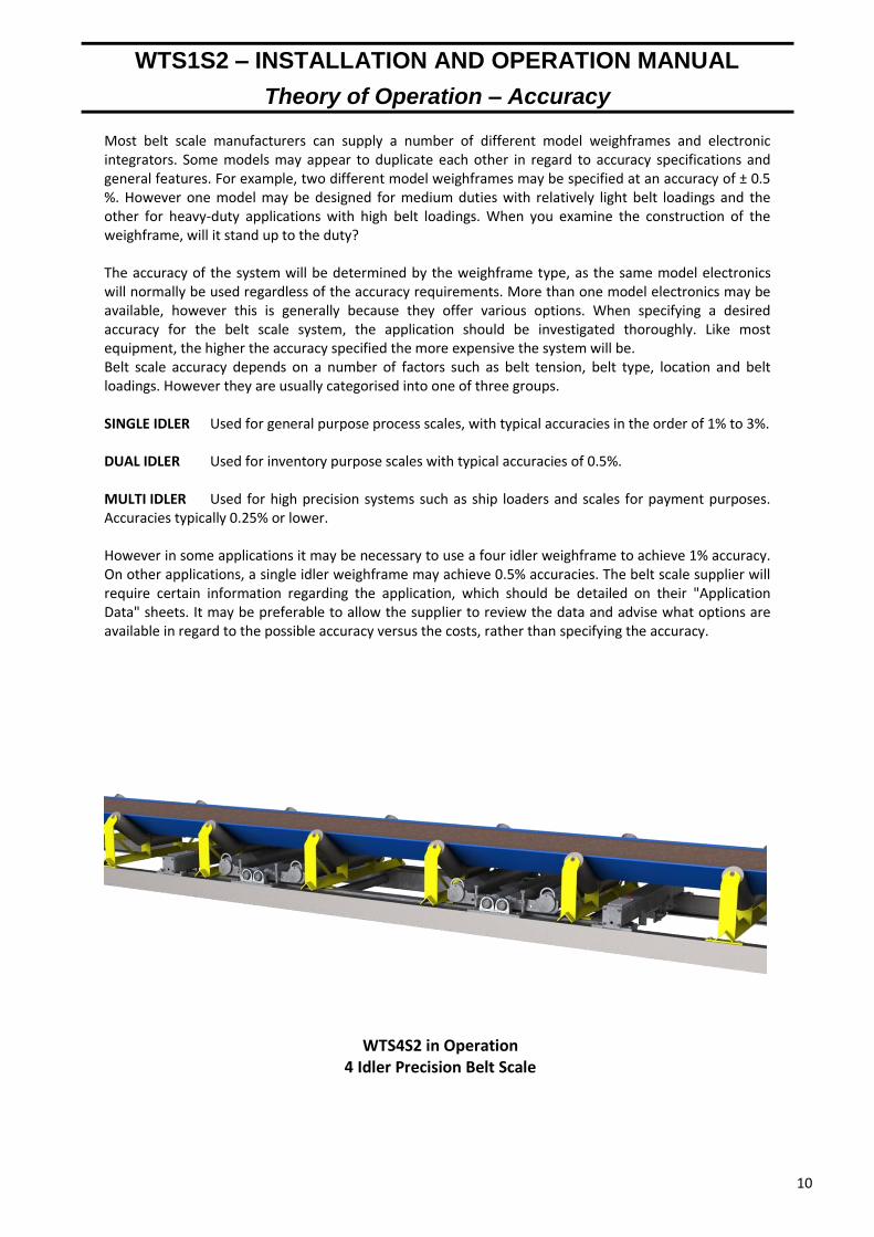
WTS4S2 in Operation 4 Idler Precision Belt Scale

11
WTS1S2 – INSTALLATION AND OPERATION MANUAL
Theory of Operation – Maintenance
Many belt scale installations are ignored until a problem exists. Like all equipment a minimum of maintenance will assist in providing long-term reliability. For multiple installations at the one site it may be worth contracting the Belt Scale supplier to carry out the maintenance and regular calibrations. These visits can also be used to provide basic training for the site personnel in the event of an emergency breakdown situation. These site visits are normally scheduled at three monthly intervals. The following work should be carried out on a regular basis:
Clean down of build-up on weighframe and removal of spillage
Inspection and cleaning of idler rolls
Zero calibrations
Inspect belt tracking
Inspect belt wear The following work can be carried out less frequently:
Span calibrations
Check mechanical alignment
Balance transducers (where necessary)
Check cabling and junction boxes Apart from the general housekeeping of the installation, the other important aspect that should be addressed is the record keeping for each installation. Most modern belt scale electronics store all data in battery backed or non-volatile memory, however in the case of catastrophic failure this data will probably be lost or not accessible. At these times it is essential that accurate records be available for reprogramming purposes. Accurate records also allow review of the belt scale performance and possible problems that may require attention.

12
WTS1S2 – INSTALLATION AND OPERATION MANUAL
Mechanical Installation
The mechanical installation of a WTS1 Series II belt scale comprises the following work:
Lifting of conveyor belt in proposed weighframe location
Installation of weighframe and support beams
Installation of weigh idlers on weighframe
Installation of approach and retreat idlers
Aligning the height of the weigh, approach and retreat idlers Refer to drawings: Calibration Bars WTS1S200 & WTS1S210 In situ Calibration Weight WTS1S211 & WTS1S212 In situ Calibration Weight Billet WTS1S213 & WTS1S214 Weighframe Location The weighframe location may have been previously nominated after discussions with Web-Tech. If not refer to the "Belt Scale Selection and Installation Guide" section of this manual for guidance, or contact Web-Tech to confirm the position. BEFORE CARRYING OUT ANY WORK ON THE CONVEYOR, ISOLATE THE CONVEYOR DRIVE AS REQUIRED. Lifting of Belt The conveyor belt (if fitted) will be required to be lifted off the idlers in the area of the installation. The belt should be lifted so that access is available for approximately 5 metres either side of the weighframe centre. The belt should be lifted approximately 600 mm above the idlers, and the belt should be lifted by means of placing pipe or timber under the belt, which will keep the belt flat. If the conveyor is fitted with a gravity take-up, it will be necessary to lift the take-up weight first. Ensure that the belt is supported securely before commencing any work. Weighframe Installation The weighframe is robust in design, however care should be exercised when lifting and installing it into position. The weighframe should be lifted with web slings, do not use chains.
1) If standard idlers already exist, remove 5 sets from the conveyor.
Existing Conveyor
Conveyor with Lifted Belt

13
WTS1S2 – INSTALLATION AND OPERATION MANUAL
Mechanical Installation
2) Mark out the centre of the space created, and this will be the centre of the weighframe.
3) Remove the weighframe from the packing crate. 4) Lift the weighframe into the conveyor so that the weighframe mounting feet are sitting on the
stringers. Position the weighframe so that the centre of the weighframe is in line with the previously marked out centre of the space.
5) Measure and mark the centre of the centre (horizontal) roll on the first of the existing idlers in each
direction. Tie a stringline between these centre points.
6) Measure and mark the centre of the weighframe crossbeams. Square the weighframe up so that the
centre of the crossbeams are in line with the stringline. 7) Mark out the position of the weighframe mounting holes on the conveyor stringers. Drill 18 mm
holes, for M16 bolts. Install bolts, washers and nuts and tighten down. Ensure that spring washers are used.
Centre of Gap Marking
Weighframe Installed
Conveyor Centre Stringline

14
WTS1S2 – INSTALLATION AND OPERATION MANUAL
Mechanical Installation
8) If the belt scale being installed uses calibration bars ignore this step. Web-Tech supplies a custom set of calibration weights for each belt scale. Install the calibration weight bearings as specified by Web-Tech. The actual weights will be installed later. It is important to bearings are aligned so that they enable to the calibration weights to make clean contact with the “V” blocks welded to the weighframe.
9) Locate one of the In-Line Weigh Quality idlers. Sit the idler frames across the weighframe on the idler
mounting plates. Install centre rolls into the idler frames (wing rolls not required at this stage). Ensure that grub screws in roll shafts are not protruding from the bottom of the shaft. Measure and mark the centre of the centre roll face.
10) Position the idlers so that they are:
In line with the stringline
Are dimensionally laid out as shown on the installation drawing. When the idlers are positioned correctly, the idler base is to be welded to the mounting plates on the weighframe.
NOTE: THE LOADCELLS ARE PREINSTALLED IN THE WEIGHFRAME AND COULD BE DAMAGED BY IMPROPER WELDING PRACTICES. ENSURE THAT WELDING EARTH STRAP IS CONNECTED AT THE POINT OF WELDING.
4 x Inline Weigh Quality Idler Frames With Centre Roll Installed
Centre Roll Grub Screw and Nyloc Nut
15
WTS1S2 – INSTALLATION AND OPERATION MANUAL
Mechanical Installation
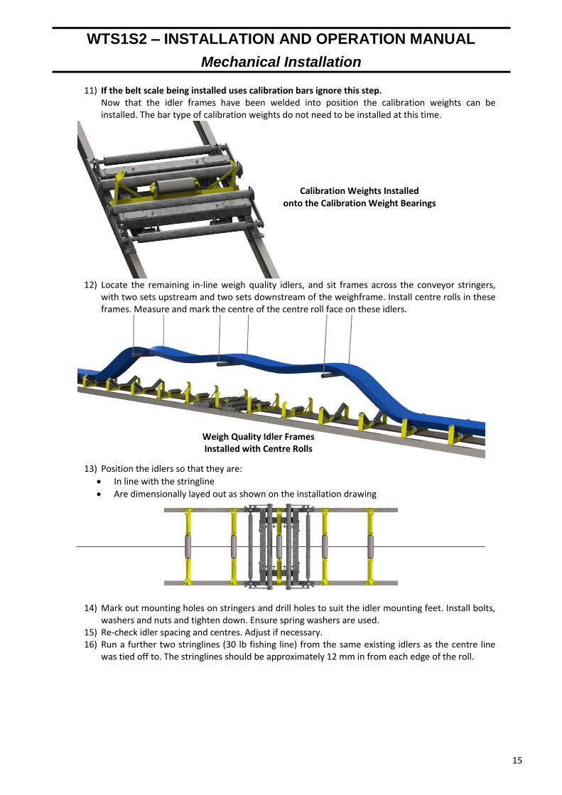
11) If the belt scale being installed uses calibration bars ignore this step. Now that the idler frames have been welded into position the calibration weights can be installed. The bar type of calibration weights do not need to be installed at this time.
12) Locate the remaining in-line weigh quality idlers, and sit frames across the conveyor stringers,
with two sets upstream and two sets downstream of the weighframe. Install centre rolls in these frames. Measure and mark the centre of the centre roll face on these idlers.
13) Position the idlers so that they are:
In line with the stringline
Are dimensionally layed out as shown on the installation drawing
14) Mark out mounting holes on stringers and drill holes to suit the idler mounting feet. Install bolts,
washers and nuts and tighten down. Ensure spring washers are used. 15) Re-check idler spacing and centres. Adjust if necessary. 16) Run a further two stringlines (30 lb fishing line) from the same existing idlers as the centre line
was tied off to. The stringlines should be approximately 12 mm in from each edge of the roll.
Calibration Weights Installed onto the Calibration Weight Bearings
Weigh Quality Idler Frames Installed with Centre Rolls

16
WTS1S2 – INSTALLATION AND OPERATION MANUAL
Mechanical Installation
17) Carefully lower the weighframe shipping bolts so that the weighframe now sits on the load cells.
18) Go to the first in-line idler (shown as +C2). Place a spirit level across the top of the centre roll.
Adjust the idler roll using the grub screws, so that it is level. If the amount of adjustment required is more than approximately 5 mm, it is better to use a packer under the idler mounting foot.
19) Go to the last in-line idler (shown as -C2) and level centre roll. 20) The in-line idlers should be higher than the existing offset idlers due to their design. The levelled
centre rolls should already be in contact with the two stringlines at the edge of the rolls. The in-line idlers should never be lower than the standard existing idlers. If they are, they will require packers to be installed under all mounting feet.
21) The two reference stringlines should be clear of the centre rolls in the other idler frames (+C1,
W1 & -C1). If not, adjust the grub screws on +C2 and -C2 idlers by equal amounts until both stringlines are clear of all centre rolls. When this has been completed, ensure locknuts are tightened. Permissible tolerance is +0.4, -0.0 mm.
22) Proceed to adjust the remaining centre rolls until they just touch the stringlines. Ensure all locknuts have been tightened after adjustment. After all rolls have been adjusted, recheck all rolls are still in contact with the stringlines.
Shipping Bolts Signified by their red heads
Offset Idlers vs Inline Idlers
Offset Idlers with Packer Plates vs Inline Idler
Inline Idler
Offset Idler

17
WTS1S2 – INSTALLATION AND OPERATION MANUAL
Mechanical Installation
23) Locate the remaining idler rolls and install all wing rolls. Ensure that grub screws in roll shafts are not protruding from the bottom of the shaft.
24) Run a further two string lines on both sides of wing rolls similar to the centre rolls.
25) Starting on one side of wing rolls, the same procedure is required to be carried out as the centre
rolls. Adjust the wing rolls on +C2 and - C2 idlers evenly so that they are clear of all remaining wing rolls.
26) Go through and adjust all rolls so that they are just touching the stringlines. When this has been completed, ensure that all locknuts are tightened. Permissible tolerance is +0.4, 0.0 mm.
27) Review all adjustments, and if satisfied, remove all stringlines. 28) Carefully lower the conveyor belt. Do not drop the belt onto the weighframe.
All Wing Rollers Installed
All Stringlines
-C3 -C2 -C1 W1 +C1 +C2 +C3
Stringlines
Belt Scale Completely Installed

18
WTS1S2 – INSTALLATION AND OPERATION MANUAL
Electrical Installation – Encoder Speed Sensor
Description The belt speed sensor supplied with the belt scale is a digital incremental encoder. It produces a square wave output, the frequency of which is proportional to the belt speed. The encoder should be connected to a non-driven pulley i.e. not a drive pulley. This is because there could be some slippage between the drive pulley and the belt. The encoder is typically connected to the tail pulley or a “snub” pulley. The encoder is available in the following models: 100 PPR 200 PPR 500 PPR The model supplied for your application has been based on the belt speed, and pulley diameter information that was provided. For slower belts, an additional pulse multiplier board may be supplied. This board is located in the belt speed sensor junction box. It allows the pulses from the encoder to be multiplied X1, X2 or X4. The frequency range is typically 80 to 500 Hz. Mechanical installation The installation of the encoder can be either by direct connection to the pulley shaft using a solid coupling, or on a separate bracket and spring coupling. If using a solid coupling, the encoder must use a restraining arm, which is in contact with a fixed part of the conveyor. This will prevent the encoder from rotating with the pulley shaft. If using the spring coupling method (most common), the spring coupling alignment must be within 1 mm in all axes. If the coupling is not correctly aligned, it will eventually break. Provision must be made so that if the pulley position is changed, the encoder bracket can also be moved to maintain accurate alignment. See drawing “” in Appendix B to see typical installation arrangements. Electrical Installation The encoder is provided with a three (3) core cable approximately 1 metre long. Therefore the belt speed sensor junction box must be installed within its reach. The cable should be mechanically protected. Refer to drawing “JB010017” (Appendix B) for termination details. Part Number The part number(s) for the encoder include the PPR output of the encoder. The typical P/No. is “WXT-XXX” where “XXX” is the PPR. Therefore a 100 PPR encoder would have the P/No. “WXT-100”.
WXT Encoder With Spring Coupling on Tail Pulley

19
WTS1S2 – INSTALLATION AND OPERATION MANUAL
Electrical Installation – Magnetic Pickup Speed Sensor
Description The belt speed sensor supplied with the belt scale is a stainless steel magnetic pick-up. It is not a proximity switch, and does not require a supply voltage. It produces a sinusoidal output, the frequency of which is proportional to the belt speed. The amplitude of the voltage output is proportional to the rotational speed of the idler roll/sprocket, and the proximity of the magnetic pick-up to the sprocket. A sprocket is also supplied with the sensor, which is installed on the end of an idler roll. If the sprocket has not been fitted by Web- Tech, it is extremely important that the sprocket be fitted centrally to the idler roll. We suggest that the sprocket be fitted, then rotated in a lathe to check its concentricity. Mechanical installation The installation of the magnetic pick-up should be on an idler adjacent to the weighframe. The idler roll used should be the horizontal centre roll The magnetic pick-up should be adjusted so that the sensor “nib” is 0.5 mm from the sprocket tooth. After adjustment and the locknut tightened, the idler roll should be rotated by hand to ensure that no teeth on the sprocket come into contact with the sensor nib. Electrical Installation The magnetic pick-up is provided with a two (2) core cable approximately 2.5 metres long. Therefore the belt speed sensor junction box must be installed within its reach. The cable should be mechanically protected. Part Number The P/No. for the magnetic pick-up is:
BS-013-01 BS-013-02
Mag Pickup and Target Disk on Pulley

20
WTS1S2 – INSTALLATION AND OPERATION MANUAL
Electrical Installation – Proximity Switch
Description The belt speed sensor supplied with the belt scale is a proximity switch. It is used in conjunction with “flags” on a pulley, or specifically designed sprocket. It produces a square wave output, the frequency of which is proportional to the belt speed. A “pull-up” resistor is provided, which is installed in the belt speed sensor junction box. Sufficient flags must be installed so that the frequency output is not less than 10Hz at the slowest belt speed. Mechanical installation The installation of the proximity switch should be typically 3 mm to 5 mm from the metal flags. The maximum sensing distance of the switch supplied is 15 mm. The minimum clearance between the face of the switch and any metal past the flags should be twice the sensing distance (30 mm). Ensure that the face of the proximity switch will not come in contact with any of the flags. After adjustment tighten any locknuts. Electrical Installation The proximity switch is provided with a three (3) core cable approximately two (2) metres long. Therefore the belt speed sensor junction box must be installed within its reach. The cable should be mechanically protected. Part Number The part number for the switch supplied is as follows:
BS-014-02
Proximity Switch and Stainless Steel Target Disk Installed on Spiral Tail Pulley
21
WTS1S2 – INSTALLATION AND OPERATION MANUAL
Electrical Installation – Integrator Optimus
Electrical connection diagrams for the belt scale electronics, load cell and belt speed sensor junction boxes are located in Appendix B of this manual. Electrical installation comprises the following work:
1) Install and connect the “Optimus” integrator to mains supply (See “WFOPTIMUS03”, Appx. B). 2) Install and connect load cell wiring between weighframe and load cell. 3) Install and connect cable between load cell junction box and electronics. 4) Install and connect cable between belt speed sensor junction box and electronics. 5) Install cable between electronics and PLC (if required) for output signals.
Belt Scale Electronics The belt scale is supplied with the following model electronics: The appropriate electrical connection drawing or the electronics supplied is located in the drawings section of the manual. Enclosure Mounting The electronics enclosure is an IP66 RFP or stainless steel enclosure. The enclosure should be located so that:
1) It is not in direct sunlight (install sunshield if located outdoors). 2) Is not subject to direct washdown. 3) Is not installed in close proximity to high power cables, variable speed drives or vibratory feeder
controllers. 4) Not more than 5 metres from the weighframe. Having the electronics located close to the
weighframe reduces the chances of electrical interference on the cables. It also makes it easier when carrying out calibrations and fault finding. The weighframe has been supplied with an integral 5 metre cable for connection to the electronics.
Cables All cables between the load cell/belt speed sensor junction boxes and the electronics should be proper screened instrumentation quality. As the signal levels from these devices are very low, any cable runs between the weighframe/speed sensor and electronics should be carried out so that these cables are not installed close to power cables. Suggested cable type for each application is as follows: Load Cell – 4 core overall screened, Belden type 8723 or equivalent. Belt Speed Sensor – 3 core overall screened, Belden type 8770 or equivalent. Ensure that all cable entries into the electronics enclosure and junction boxes use the correct size waterproof glands. Cable Terminations Load Cell junction box – Refer to drawing “LJBL-01” in Appendix B of this manual. Speed sensor junction box – Refer to drawing “JB010017” in Appendix B of this manual. Start Up Prior to turning on the equipment, or operating the belt scale, ensure the following has been done:
Double check all electrical connections are correct.
All mechanical installation has been completed and no tools have been left on the belt. Start Up Steps When starting up the system for the first time, use the following steps:
1) Turn on the electronics, and ensure it displays the Mass Rate, Mass Total (MRMT). 2) Start the conveyor. If using variable speed drive, set it in local and ramp the frequency up to
50Hz. 3) The load cell output can be directly read from the electronics. Refer to the electronics manual for
the appropriate menu for reading the load cell voltage. The belt speed sensor output can be read directly from the electronics. Refer to the electronics manual for the appropriate menu for reading the belt speed sensor frequency output. Run the conveyor and ensure that there is a stable output from the speed sensor ±3 Hz

22
OPERATION MANUAL
Masterweigh Optimus
Web-Tech Australia Pty Ltd
Head Office: 11 Electronic Street PO Box 4006 EIGHT MILE PLAINS QLD 4113 EIGHT MILE PLAINS
BRISBANE QLD 4113 Phone: (07) 3841 2844 AUSTRALIA Fax : (07) 3841 0005

Index.
CAD Computer I:/Manuals/Optimus-Belt
1
1. General Description. 4.
2. Specifications and On Site Requirements. 5 - 6.
3. Enclosure Specifications 7.
4. Theory of Operation. 8.
5. Printed Circuit Board Description/Location. 9.
6. Power and Field Wiring PCB. 10-11.
7. Key Board Description. 12.
8. Power Up. 13.
9. Main Display MRMT Description. 14-15.
10. Getting Started. 16.
11. System Setup / system configuration. 17-20.
12. System Setup / display, time & date. 21-25.
13. System Setup / PID Loop Control / PID overview. 26-27.
14. System Setup / PID Loop Control / setpoint origin. 28-29.
15. System Setup / PID Loop Control / output control / status. 30.
16. System Setup / PID Loop Control / pid parameters. 31-34.
17. System Setup / PID Loop Control / pid loop tuning. 35-36.
18. System Setup / PID Loop Control / pid mass rate filter. 37-38.
19. System Setup / PID Loop Control / volumetric restart. 39-40.
20. System Setup / PID Loop Control / reset integral. 41.
21. ?System Setup / PID Loop Control / mass rate & pid output trend. 42.
22. System Setup / Auto Zero Tracking / overview. 43.
System Setup / Auto Zero Tracking / enable : disable. 44.
23 System Setup / Auto Zero Tracking / threshold. 45-46.
24 System Setup / Auto Zero Tracking / delay. 47.

Index.
CAD Computer I:/Manuals/Optimus-Belt
2
25 System Setup / Auto Zero Tracking / period. 48.
26 System Setup / Auto Zero Tracking / current contribution. 49.
27 System Setup / Rate Deadband . 50.
28 System Setup / Rate Display Filters. 51.
29 System Setup / Rate Display Filters / time constant. 52.
30 System Setup / Rate Display Filters / fast track threshold. 53-54.
31 System Setup / Save & Load Setup. 55-56.
32 System Setup / Chute Level Control. 57-59.
33 I/O (Input & Output) / Current Loop Inputs. 60-67.
34 I/O (Input & Output) / Current Loop Outputs. 68-74.
35 I/O (Input & Output) / Digital Inputs. 75.
36 I/O (Input & Output) / Digital Outputs 76-82.
37 I/O (Input & Output) / RS-232 Configuration. 83-84.
38 I/O (Input & Output) / RS-485 Configuration. 85-86.
39 Load Cell & Tachometer. 87.
40 Device Net. 88.
41 Theory of Operation/Steps in the Calibration Procedure. 89-92.
42 Calibration / Pulses per Revolution. 93.
43 Calibration / Manual Entry of belt revolutions & Zero Calibration 94.
44 Calibration / Auto Zero Tracking. 95.
45 Calibration / Target Weight. 96.
46 Calibration / Pulses per Revolution / auto capture. 97-98.
47 Calibration / Zero. 99-100.
48 Calibration / Span / static weight test. 101-102.
49 Calibration / Span / empirical. 103-104.

Index.
CAD Computer I:/Manuals/Optimus-Belt
3
50 MRMT Screen / Trend. 105.
51 MRMT Screen / Clear Total. 106.
52 MRMT Screen / Info Screen. 107.
53 Notes & Firmware Updates. 108.
54 Electrical / Electronic Notes / digital outputs. 109.
55 Electrical / Electronic Notes / digital inputs. 110.
56 Inlet Boot hopper setup 111.

Optimus. General Description.
4
CAD Computer I:/Manuals/Optimus-Belt
Optimus is a powerful, microprocessor based weighbelt integrator. By design it can be used in
a “stand alone” mode or slaved to a PLC or other plant supervisory system. Communication
between the plant controller and Optimus being effected by one of the following Profi -Bus®,
Device-Net®, TCP-IP, 4/20 mA, a range of digital inputs and outputs and relays (clean
contacts). When used in the stand alone mode, control of the weighbelt feeder and associated
equipment, valves, slide gates and conveyors is performed by Optimus.
The electronics are house in an IP67- NEEMA 4 rated enclosure, suitable for use in most
industrial environments. However it is advisable that the package be shielded from continuous
sun light and running water. The use of high pressure hoses to wash down the enclosure is not
recommended. The electronics can be accessed through the accessed door which can be
either latched, latched and padlocked or the latches removed and screw closed.
The Central Processing Unit (CPU) printed circuit board (PCB) is a six layers and contains all
the main electronic components. In the unlikely event and Optimus fails, field fault finding is
made easy as CPU, PCB is easily changed.
The Terminal PCB has been made extra thick (3mm) to provide a mechanically secure
platform for the angled connectors.
The Power PCB is fitted with an auto voltage and frequency select power supply that makes
Optimus suitable for use in most countries in the world. A switch and fuse provide a suitably
qualified technician with a convenient method of mains power isolation and fuse checking.
All functions are made available through the front interface keypad and a (240 x 64 dot) LED
back lit display. Optimus uses “state of the art” electronic components and programming
techniques. It has been designed to operate with a the entire range of Web-Tech and other
manufacturers weighbelt and conveyor belt scales.
At the heart of the controller is an eLAN 520, 32 bit microprocessor, running at 100mHz
connected to a highly accurate and stable three channel analogue to digital converter (A/D
converter). Optimus is supplied with a generous amount of 32 mbytes of SDRAM . This allows
for future firmware expansion and customers specific custom software. Some of this storage
is used for firmware, default variables and customer specific variables.
Should firmware upgrades be made available, Web-Tech will make the program available on
Compact Flash modules, that simply plug into a socket on the CPU printed circuit board and
automatically download the program. The Compact Flash module also serves as a storage
device for the data logging feature incorporated in Optimus. The logged data can be sent back
to Web-Tech for analyses should there be a problem with the system.
The analogue inputs from the load cells are channelled through a 24 bit analogue to digital
converter specifically designed for use with load cells in an industrial environment.
Six auxiliary 12 (4096 values) bit analogue inputs, locally programmable as 4/20mA -
0/20mA - 0/25mA & 0/50mA . along with six digital outputs provide Optimus with the ability to
monitor other processes associated with the feeder and process.
Five digital outputs provide voltage free contacts for use with PLC and SCADA systems.
One digital output (solid state switch) provides a means of indicating weight accumulation at
low and high speed rates.

5
CAD Computer I:/Manuals/Optimus-Belt
OPTIMUS OPERATIONAL MANUAL. Specifications and Site Requirements.
Power Requirements.
Main Board.
240V AC +/- 10% 50/60 Hz
117V AC +/- 10% 50/60 Hz.
2amps @ 240V
4amps @ 117V
AMD Elan SC520 microprocessor running at 100 MHz.
8 Mb DRAM.
1 Mb soldered-down flash memory (expandable up to 4 Mb).
Compact Flash card type I or II header (supports any density
CompactFlash cards).
Socket for up to 1Mb Flash or PROM BIOS (can replace soldered down
flash).
Industry standard PC/104 expansion header with: 13 redirectable
interrupts, 2 DMA channels and 8/16 bit I/O and memory interface.
Watchdog timer
Voltage supply brownout protection and reset generation.
Industry standard JTAG boundary scan interface for board testing &
debugging.
High efficiency 3.3V and 2.5V on-board power supply for digital logic.
User Interface.
Support for up to 28 front panel keys.
¼ VGA (320 x 240 pixel) LCD screen support with digitally adjustable
CCFL backlighting and screen contrast.
Internal switch for locking of calibration settings (for weights & measures
laws).
Loadcell Interface.
Supports up to three independent loadcell channels.
22 bit (4.2 million values) analogue to digital converter (ADC)
on each channel.
Temperature compensated / self calibrating ADC.
Fourth order digital filter attenuates interference at the sampling frequency
and its harmonics by 160dB, e.g. 50 & 60Hz sampling rate negates mains
power interference.
Sampling rate up to 1kHz (with slightly reduced effective resolution
– 19 bits).
Ultra stable loadcell drive circuitry capable of driving 8 loadcells in parallel.
Loadcell interface is shielded in a metal can.
Current loop input and output.
Supports up to 8 0-25mA inputs (circuit presents 200 ohm load).
Supports up to 8 0-25mA outputs (drives up to 1k ohm load).
Loop input sampling rate up to 200kHz.
Loop output data rate up to 100kHz.
12 bit (4096 values) ADC resolution on both inputs and outputs.
Optically isolated from rest of circuit.

6
CAD Computer I:/Manuals/Optimus-Belt
OPTIMUS OPERATIONAL MANUAL. Specifications and Site Requirements.
Serial Input/Output.
Optically isolated full/half duplex RS485 at up to 38400 baud.
RS232 port with RTS/CTS handshaking signals at up to 115200 baud.
Up to six optically isolated 24V digital inputs (PLC interface).
Up to eight digital output lines to drive relays on wiring board
12V relay activation supply to wiring board
Dual channel tachometer inputs
Initial Setup and debugging interface.
Four pole DIP configuration switch.
Reset pushbutton.
Four configurable LED status lights (Red).
HDD (compact flash) activity LED (Red).
Voltage rail monitor LEDs (Green).
Current loop output monitor LEDs (Orange).
Digital input monitor LEDs (Yellow).
Options.
High volume (92dB @ 10cm) full bridge driver for an internal piezo speaker
Battery backup for real-time clock and calendar – CR2032 coin cell.
1.5 Mbaud IrDA transciever.
Optically isolated half duplex RS485 at up to 38400 baud (for relay
controller/expansion).
Isolated, current limited 1.5W 12V supply for relay controller/expansion
power.
Temperature sensor - can be used for monitoring/alarms and for
automatically changing the contrast of the LCD screen with ambient
temperature variations.
256 byte EEPROM for storing configuration and setup data.
Terminal PCB.
5mm pitch screw terminations for all inputs, outputs and shields.
Clear labelling for each connection on PCB.
Support for up to eight relays for digital outputs (either 24V PLC type or
240V mains type) with 12V coil drive.
Support for up to eight relays for digital outputs (either 24V PLC type or
240V mains type) with 12V coil drive.
Power Board.
5mm pitch screw terminations for Active, Neutral & Earth.
Universal voltage supply with no voltage selection required 85VAC to
285VAC, 50/60 Hz.
Regulatory agency approvals on switch mode modules.
Input filtering.
Supplies +5V, +12V, -12V at 25W max total to main board.
Supplies +24V at 25W max to main board.

7
CAD Computer I:/Manuals/Optimus-Belt
OPTIMUS OPERATIONAL MANUAL. Enclosure Specifications.
Manufacturer.
Application.
Hoffmann.
Designed for use a an instrumentation housing enclosure, for use in highly
corrosive environments including oil refineries, coal mines, chemical
processing plants, waste water treatment and marine installation,
electroplating plants, agricultural environments and food or animal
processing plants.
Construction.
Moulded fibreglass polyester has outstanding chemical and temperature
resistance and exhibits excellent weather-ability and physical properties.
Seamless foam-in-place gasket assures watertight and dust-tight seal.
Polyester mounting feet and stainless steel attachment screws.
Scratch-resistant GE LEXAN MARGARD® permanently bonded in place
window.
Quick releases latches with corrosion resistant polyester latches located in
corners which provides unobstructed access to enclosure.
Hinge and bail are corrosion resistant monel.
Knock out padlock provisions included in each latch.
Industry Standards.
NEMA / EEMAC (Type 4, Type 4X, Type 12 and Type 13).
UL 508 (Type 4, Type 4X, Type 12, and Type 13).
Enclosure flammability rating UL94-5V
CSA Type 4 and Type 12.
IEC 529 , IP66

8
CAD Computer I:/Manuals/Optimus-Belt
OPTIMUS OPERATIONAL MANUAL. Theory of Operation.
In general a weighbelt feeder consists of the following key components that are directly
associated with the weighing function.
Load Cell.
Weigh Zone / (weigh deck)
Tachometer / (Encoder).
Electronic Integrator.
Optimus’s primary roll is combine the weight of product carried by a conveyor belt and the
speed of that belt and produce a variety of associated process control signals.
An electronic load cell is used sense the weight of product and an electronic encoder is used
to provide a speed signal.
The tachometer/encoder is a device that is connected to a roll, that is contact with the belt and
will rotate as the belt passes over it. The encoder shaft will then rotate and produce a series of
pulses which Optimus uses to calculate the belt speed.
The load cell is situated in a position so that it able to sense the weight of the belt, product and
the belt support. This position is generally referred to as the weigh area. The weight signal is
usually in milli-volts and in the range of 0 mV to approximately +30 mV.
Optimus is a microprocessor based precision, high speed electronic integrator. The mV signal
from the load cell is digitised by a precision, high resolution analogue to digital converter in
Optimus and combined with the encoder output to produce an accurate MASS RATE. From
this mass rate the total is computed as well as all other functions provided by Optimus.
BELT TRAVEL DIRECTION
HEAD PULLEY WEIGH AREA TAIL PULLEY
LOAD CELL MOUNTED & SHOWING
CONNECTION TO LOAD PICK UP ASSEMBLY TACHOMETER/ENCODER

9
CAD Computer I:/Manuals/Optimus-Belt
OPTIMUS OPERATIONAL MANUAL. Printed Circuit Board location.
Optimus comprises three printed circuit boards (PCB). Main processor PCB, field wiring PCB
and power PCB.
Main Processor PCB. The main processor PCB is located on the door of the enclosure. Generally there is no field
wiring to be connected to this board. However if a communications package is to be used,
wiring will be required to be connected to the PC 104 communications PCB. This PCB is
piggy backed onto the main PCB.
Field Wiring PCB. This card is located in the main portion of the enclosure, below the main processor PCB (when
the door is closed) and above the power PCB. This PCB will be loaded with connectors strips
and relays that are required for the application. Any parts not loaded have been deliberately
omitted. This PCB along with the power PCB has been designed to be easily removed for
servicing, if required. This PCB is reasonably robust by design, it has been made from a
thicker than normal fibreglass, under normal operating conditions a reasonable amount of
torque can be applied to the terminal screws with out damage occurring, however damage will
occur if too much force is applied.
As space within the enclosure is limited, all wiring should be neat and trimmed to suit.
See drawing at the rear of this manual for field wiring details.
Power PCB. (DANGER MAINS VOLTAGE MAY BE PRESENT) This PCB is located under the Field Wiring PCB. A cut out in the has been provided in the
Field Wiring PCB so that access to can be provided to the main supply terminal strip, the fuse
and local on/off switch.
Installer / Electrician Note.
Care must be taken when cutting holes in the enclosure to provide cable access. It is
recommended that the Power & Field Wiring PCB be removed prior cutting holes. Take note of
cable entry with respect to PCB when re installed.
All cables should enter the enclosure via site approved cable glands.
The entry of water into this enclosure will damage the electronics and void and warranty.

OPTIMUS OPERATIONAL MANUAL. Power & Field Wiring PCB.
CAD Computer I:/Manuals/Optimus-Belt
Battery Seiko Cr 2032 or
equivalent. This battery is
used to hold up the
information stored in the
screen “System Information”
All operating variables are
stored in non volatile
memory, which does not
require battery power.
CPU PCB.
The 5 yellow LED’s
when lit, show that
the operating
voltages required
by Optimus and it’s
sub-assemblies are
all healthy.
+24V
+12V
-12v
+5V
+3.3V
Optional
communications card.
TCP-IP, Profibus,
DeviceNet
Optional RS 232
Output
Power & Terminal PCB. Optional RS
485 Output
Generally Digital
Inputs.
Generally analogue
outputs.
Generally Analogue
Inputs.
Generally Relay I/O
Fuse
Load Cell Inputs
Channel 1-3
Local On/Off Switch.
Lower PCB.
Multi Voltage/Frequency
Mains Input.
10 Lower PCB.

OPTIMUS OPERATIONAL MANUAL. Power & Field Wiring PCB.
11
CAD Computer I:/Manuals/Optimus-Belt
Optimus can power up to eight (8) individual load cells. (350O). Generally these load cells are
paralled up, in marshalling boxes in the field. However some continuous weighing systems
application require that individual load cells are digitally summed in Optimus. This allows special
mathematical algorithms to be applied to the load cell signals prior to integration. On occasion
Optimus may be required to read the out put of a load cell that is positioned up stream of the weigh
area in order that product can be accurately pre fed onto the weigh belt.
Belt weighing systems / weigh feeders usually do not employ more than one channel input.
If the load cell cable runs are long, it is possible to have a voltage drop at the load cell. Optimus
provides for the reading of the supply voltage at the load cell via the load cell sense wires (where
fitted). If the sense wires are connected and the jumpers are set as shown below. Any voltage
drop will be corrected for.
No Sense Used
Sense Used
J1 J2 J3
Local Remote Local Remote Local Remote
J1 J2 J1
Local Remote Local Remote Local Remote

12
CAD Computer I:/Manuals/Optimus-Belt
OPTIMUS OPERATIONAL MANUAL. Keypad Description.
Mass Rate [kg/hr]
Mass Total [kg]
0.0
702.0
SP Local
SP Rem
AZT On
PID Manual
PID Auto CAL I/O TREND CLEAR SETUP INFO
SET
Takes the user back to
MRMT & updates all
entered variables
Cancels the current
operation & takes the
user back to MRMT.
Saves any changes and
moves the screen
forward one.
Cancels current action
and forces display back
to previous screen.
Scrolls curser
up.
Scrolls curser
down.
Saves any changes and
moves the screen
forward one.
The above function (f) keys are associated with the boxed message
displayed directly above the f key.

13
CAD Computer I:/Manuals/Optimus-Belt
OPTIMUS OPERATIONAL MANUAL. Power Up.
Once Optimus has been connected up as per the drawings in the rear of this manual and with
reference to the chapter Printed Circuit Board location. The unit can be powered up, it should
be noted that Optimus has a power supply that will accept most common supply voltages and
frequencies, found around the world . The unit has a local power switch located on the power
PCB, this should now be moved to the on position. Optimus will now power up, load the
operating software and perform a series of self diagnostic routines. During this time the Web-
Tech logo will be displayed. Following a successful power up the screen display will change to
the following.
Start Up Display
The screen shown below is the screen that should be displayed whilst Optimus Plus is
running. We call this particular screen Mass Rate, Mass Total (MRMT) and is the default
screen. Take time to make yourself familiar with the data that is available on this screen and
how it interacts with the keypad.
See over for detailed description of functions available from this screen.
Mass Rate Mass Total (MRMT) Display
Mass Rate
[kg/hr]
Mass Total
[kg]
950.0
702.0
SP Local
SP Rem
AZT On
PID Man
PID Auto
CAL I / O TREND CLEAR SETUP INFO
Masterweigh Opti m u s.

14
CAD Computer I:/Manuals/Optimus-Belt
OPTIMUS OPERATIONAL MANUAL. Main Display MRMT Description.
Displays Selected Mass Rate Units
CAL I / O TREND CLEAR SETUP INFO
The above function (f) keys are associated with the boxed message displayed in the display
directly above the f key. Pressing any of these keys will take you to the associated functions.
CAL. Pressing the CAL F1 key takes the user to the screens that provide for
calibrating Optimus.
I/O. Pressing the I/O F2 key takes the user to the screens that provide for
configuring current loops in and out. The digital inputs and out puts. The
RS 232 & 485 serial communications.
The load cell entry point provides a method of easily viewing the load cell and
tachometers output.
TREND. Entering the Trend F3 screen provides the user with a 2 minute trend of the
instantaneous mass rate and control over the setpoint.
CLEAR. Pressing the clear F4 clears the local displays running total.
SETUP. Pressing the Setup F5 key takes the user to the menus associated with
configuring Optimus.
INFO. Activating the Info F6 displays the Information screen where details of Optimus
software can be viewed.
Mass Rate
[kg/hr] 0.0
SP Local
SP
AZT
Rem
On
Mass Total
[kg] 702.0 PID Man
PID Auto
CAL I / O TREND CLEAR SETUP INFO
Displays the instantaneous Mass Rate
Displays Selected Mass Total Units
Function Button Designators
Allocates new function to key. Displays Mass Total

15
CAD Computer I:/Manuals/Optimus-Belt
OPTIMUS OPERATIONAL MANUAL. Main Display MRMT Description.
Mass Rate
[kg/hr]
Mass Total
[kg]
0.0
702.0
SP Local
SP Rem
AZT On
PID Man
PID Auto
CAL I / O TREND CLEAR SETUP INFO
ON
OFF
When active, feeder setpoint is generated at the key………………….…...
When active, feeder setpoint is generated by an external device……..……..
When active, the Auto Zero Tracking is operating………………….……..
When active, the PID loop is Off and controlled through keyboard…….….…
When active, the PID loop is On & functioning under the control algorithm.…
SP Local
SP Rem
AZT On
PID Man
PID Auto
Discards changes made on current screen and moves back one screen.
The Tick key accepts the input data. Stores the data into a working memory
and returns the cursor to the main menu if data was entered in a sub menu.
ABORT
Gives the user the option to discard all configuration changes they have made.
Pressing ’ABORT’ again discards any changes and reverts to the MRMT
screen. Pressing ’HOME’ will save any configuration and reverts back to
MRMT screen.
ENTER The ‘ENTER’ key is used to enter menu’s and scroll through preset menu’s.
HOME Gives the user the option to save all configuration changes they have made.
Pressing ‘HOME’ again will save changes and revert to MRMT screen.
Pressing ‘ABORT’ will discard any changes made and revert to MRMT screen.

16
CAD Computer I:/Manuals/Optimus-Belt
OPTIMUS OPERATIONAL MANUAL. Getting Started.
Optimus is generally termed an integrator. It has been designed to work with most conveyor
belt scales, weighfeeder’s and various “in motion weighing mechanisms”.
Prior to operating Optimus it has to be setup and calibrated. Web-Tech advise that these operations be performed by qualified
technicians who have been trained in the operation of Optimus and the weighfeeder. Web-Tech can’t warrant the accuracy and operation of our
equipment if the system is incorrectly installed.
The procedure is as follows:-
1 Setup
2 Define the required I/O
3 Calibrate
4 Setup and tune the PID algorithm and control loop.
The Setup procedure customises the electronics to suit your application.
Defining the Input/Output allocates relays analogue outputs etc to Optimus functions.
The Calibration procedure is required to force Optimus to convert the instrument's raw data (i.
e. milli volts from the load cell/cells & tachometer frequency) into the physical units (i.e. Tons/
hour kg/hr and their corresponding totalised values).
Setting up the PID is required so that the mathematical algorithm (PID) is loaded with
variables that produce the required mass rate control response.

17
CAD Computer I:/Manuals/Optimus-Belt
OPTIMUS OPERATIONAL MANUAL.
Setup / system configuration.
SETUP (Configuring Optimus).
Prior to calibrating Optimus, the instrument must be configured to suit the application. Units
selected and the input and output functions defined.
Following power up, Press SETUP (F5) key .The display will change to that shown below.
SYSTEM CONFIGURATION SCREEN
Select “System Configuration” by pushing the “ENTER” key.
The display will change to that shown below.
The arrow shaped cursor will point to the Units of Measurement.
The units of measurement can be set by pushing the “ENTER” key. There are 7 sets of
predefined units of mass rate. All of which can be accessed by pressing the “ENTER” key
and scrolling through the list using the “ENTER” key.
The following units are available :-
Tonnes per hour.
Kg per minute.
Kg per hour.
Pounds per minute.
Pounds per hour.
Tons per hour.
Units of measurement = kg/min
Belt capacity = 100.0 kg/min
Resolution = 0.1
Belt length = 2.915 meters
Maximum belt loading = 10.0 kg/meter
1. System Configuration
2. Display and Time/Date
3. PID Loop Control
4. Auto Zero Tracking
5. Rate Deadband
6. Rate Display Filters
7. Save/Load Setup
8. Chute Level Control

18
CAD Computer I:/Manuals/Optimus-Belt
OPTIMUS OPERATIONAL MANUAL. System Setup / system configuration.
Belt Capacity. Advance the cursor to belt capacity entry point by using the right or left arrow keys. Pressing the
“ENTER” key here will display a dedicated input menu, where the max design capacity of the
feeder, should be entered. This data can be found in the design data sheet supplied by Web
Tech during the feeder/belt scale design phase. The value entered is captured by Optimus
following the pressing of either the “ENTER” or tick F3 key.
This variable is used to scale the analogue outputs.
Press the “ENTER” key when the cursor is pointing at the “Belt capacity” and the screen will
change to the Belt Capacity entry screen. Enter the feeders maximum capacity here. Press the
tick key to force Optimus to read the entered value.
Belt capacity ( in kg/min )
Current value 60.0
New value —
DEL CLEAR
Using either the left or right arrow keys, go to the entry point for “Resolution”.
The resolution can be changed to one of the preset precision values. The values offered here
are based on the capacity that was previously entered and can be accessed by pressing the
“ENTER” key until the required value is found from the list. The value entered here will be re-
flected in the MRMT screen’s precision.
Units of measurement = kg/min
Belt capacity = 100.0 kg/min
Resolution = 0.1
Belt length = 2.915 meters
Maximum belt loading = 10.0 kg/meter
Units of measurement = kg/min
Belt capacity = 60.0 kg/min
Resolution = 0.1
Belt length = 2.915 meters
Maximum belt loading = 10.0 kg/meter

19
CAD Computer I:/Manuals/Optimus-Belt
OPTIMUS OPERATIONAL MANUAL. System Setup / system configuration.
Units of measurement = kg/min
Belt capacity = 100.0 kg/min
Resolution = 0.1
Belt length = 2.915 meters
Maximum belt loading = 10.0 kg/meter
Belt Length. Use the left or right arrow keys to move the cursor to the ‘Belt Length’ entry point. Optimus
needs to accurately know the belt length in order to perform the Span and Zero routines. Note :The belt length is not used by Optimus to calculate the Mass Rate and Mass Total. The
belt length can be found in the design data sheet.
Press the ‘ENTER’ key to access the ‘Belt Length’ entry routine. Enter the belt length here and
press the tick key to force Optimus to read in the value.
Belt length ( in meters )
Current value 2.915
New value —
DEL CLEAR
Belt Length Units. Use the left or right arrow keys to move the cursor to the ‘Belt Length Units’ entry point. Press
the ‘ENTER’ key to scroll through the available units.
Units of measurement = kg/min
Belt capacity = 100.0 kg/min
Resolution = 0.1
Belt length = 2.915 meters
Maximum belt loading = 10.0 kg/meter

20
CAD Computer I:/Manuals/Optimus-Belt
OPTIMUS OPERATIONAL MANUAL. System Setup / system configuration.
Maximum Belt Loading. This data entry point sets up an analogue output to reflect the instantaneous belt loading,
if required. Generally Optimus will perform all the calculations required to successfully set up the
instrument. However this requires user input and calculation. See below for calculation details.
Use the left or right arrow keys to move the cursor to the ‘Maximum Belt Loading’ entry point.
Press the ‘ENTER’ key to access the data entry screen. The data entered here has to be
calculated by the user. See below.
Maximum Belt Loading ‘Data Calculating’. Optimus needs to know the maximum expected belt loading in the units shown in the screen
below. So that the 20mA point can be scaled against the belt loading 4/20mA output signal.
Max belt loading (in kg/meters
4.0
DEL CLEAR
Use the following to calculate the Maximum Belt Loading.
From the conveyor design data document. Obtain the following :-
Maximum Belt Capacity. (units to be in those previously selected)
Belt Speed. (BS). (m/S)
Belt Loading =
E.g.
BS X
Belt Capacity
(Use 60 if mass rate is displayed in Units/minute)
(Use 3600 if mass rate is displayed in Units/hour)
Capacity 60 kg/minute
Belt Speed. 0.25m/S
Belt Loading =
60
0.25 X 60
4 kg/metre (enter this, into data entry screen).
Units of measurement = kg/min
Belt capacity = 100.0 kg/min
Resolution = 0.1
Belt length = 2.915 meters
Maximum belt loading = 10.0 kg/meter

21
CAD Computer I:/Manuals/Optimus-Belt
OPTIMUS OPERATIONAL MANUAL. System Setup / display, time & date.
Backlight.
Optimus is supplied with a Liquid Crystal, Light Emitting Diode (LED) back lit screen.
The use of back lighting is essential, if the screen is to be viewed in low light
conditions. Use the scroll forward key to position the cursor along side the “Display
and Time/Date screen entry point.
System Configuration Screen.
Press the “ENTER” key to access the display setup screen.
Use the “ENTER” key to scroll through the predefined list of timed / un -timed Backlight
settings.
Always On; Off after 2 mins; Of f after 5 mins; Off after 10 mins; Off after 30 mins;
Off after 60mins; Always off.
It should be noted that Optimus electronic s package has been fitted into a closed
environment. The back light draws considerable power from the power supply. The
longer the back light is on for any given brightness the greater the heat given off from
the power supply module.
When the ambient temperatures are high Optimus may not be able to conduct this heat
away as efficiently as required. We suggest that the ba ck light be set to “Off” after 2 or 5
minutes. The back light will re -activate on pressing any key if any of the timed off se t-
tings are used.
Backlight = always on.
Contrast = 2
Brightness = high
Date
Time
10 May 2003
06 : 12 : 00
1. System Configuration
2. Display and Time/Date
3. PID Loop Control
4. Auto Zero Tracking
5. Rate Deadband
6. Rate Display Filters
7. Save/Load Setup
8. Chute Level Control
1. System Configuration
2. Display and Time/Date
3. PID Loop Control
4. Auto Zero Tracking
5. Rate Deadband
6. Rate Display Filters
7. Save/Load Setup
8. Chute Level Control
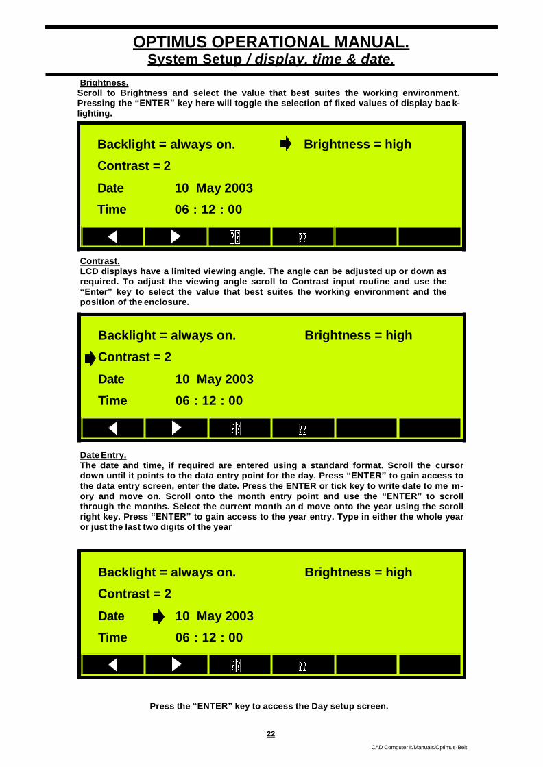
22
CAD Computer I:/Manuals/Optimus-Belt
OPTIMUS OPERATIONAL MANUAL. System Setup / display, time & date.
Brightness.
Scroll to Brightness and select the value that best suites the working environment.
Pressing the “ENTER” key here will toggle the selection of fixed values of display bac k-
lighting.
Contrast.
LCD displays have a limited viewing angle. The angle can be adjusted up or down as
required. To adjust the viewing angle scroll to Contrast input routine and use the
“Enter” key to select the value that best suites the working environment and the
position of the enclosure.
Date Entry.
The date and time, if required are entered using a standard format. Scroll the cursor
down until it points to the data entry point for the day. Press “ENTER” to gain access to
the data entry screen, enter the date. Press the ENTER or tick key to write date to me m-
ory and move on. Scroll onto the month entry point and use the “ENTER” to scroll
through the months. Select the current month an d move onto the year using the scroll
right key. Press “ENTER” to gain access to the year entry. Type in either the whole year
or just the last two digits of the year
Press the “ENTER” key to access the Day setup screen.
Backlight = always on.
Contrast = 2
Brightness = high
Date
Time
10 May 2003
06 : 12 : 00
Backlight = always on.
Contrast = 2
Brightness = high
Date
Time
10 May 2003
06 : 12 : 00
Backlight = always on.
Contrast = 2
Brightness = high
Date
Time
10 May 2003
06 : 12 : 00

23
CAD Computer I:/Manuals/Optimus-Belt
OPTIMUS OPERATIONAL MANUAL. System Setup / display, time & date.
Press the “ENTER” key to access the Day entry screen.
Day
Current value 10
New value —
DEL CLEAR
Press the “ENTER” or tick key to lock in the day. Forward scroll to the month entry point
use the “ENTER” key to scroll through the month selection. Press the scroll forward to
access the year entry screen.
Select the month and scroll on to year entry position.
Press the “ENTER” key to access the data entry screen and enter the year. Press the tick
key to lock in the year data and return to .
Year
Current value 2004
New value —
DEL CLEAR
Backlight = always on.
Contrast = 2
Brightness = high
Date
Time
10 May 2003
06 : 12 : 00
Backlight = always on.
Contrast = 2
Brightness = high
Date
Time
10 May 2003
06 : 12 : 00

24
CAD Computer I:/Manuals/Optimus-Belt
OPTIMUS OPERATIONAL MANUAL. System Setup / display, time & date.
Scroll forward to the time (hour) entry position and press the “ENTER” key to access the
hour entry screen.
Select the month and scroll on to year entry position.
Hours
Current value 10
New value —
DEL CLEAR
Enter the current hour (24 hour clock) format. Press the tick key to lock in the data. Scroll
on to the minute entry point and p ress the “ENTER” key to access the minute entry
screen
Enter the current minute and press the tick key to lock in the data and return to the time/
date entry screen.
Minutes
Current value 12
New value —
DEL CLEAR
Backlight = always on.
Contrast = 2
Brightness = high
Date 10 : 12 : 00
Backlight = always on.
Contrast = 2
Brightness = high
Date
Time
10 May 2003
06 : 12 : 00
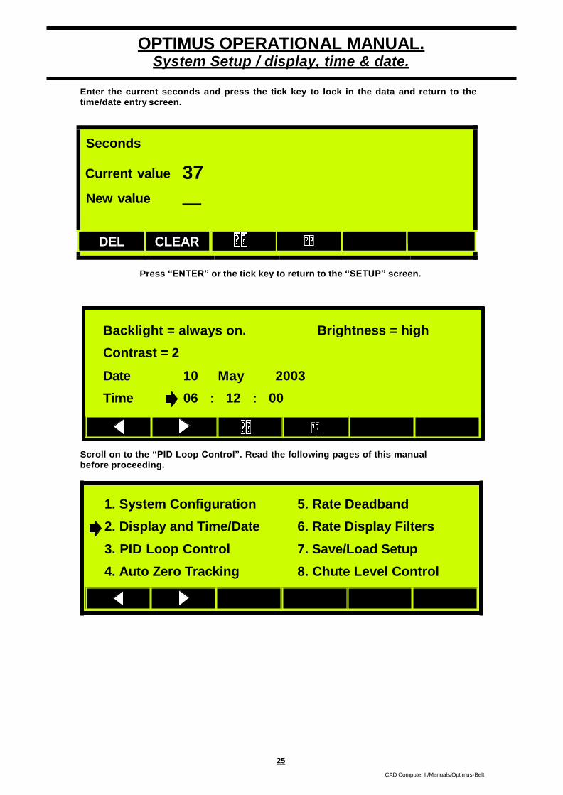
25
CAD Computer I:/Manuals/Optimus-Belt
OPTIMUS OPERATIONAL MANUAL. System Setup / display, time & date.
Enter the current seconds and press the tick key to lock in the data and return to the
time/date entry screen.
Seconds
Current value 37
New value —
DEL CLEAR
Press “ENTER” or the tick key to return to the “SETUP” screen.
Scroll on to the “PID Loop Control”. Read the following pages of this manual
before proceeding.
1. System Configuration
2. Display and Time/Date
3. PID Loop Control
4. Auto Zero Tracking
5. Rate Deadband
6. Rate Display Filters
7. Save/Load Setup
8. Chute Level Control
Backlight = always on.
Contrast = 2
Brightness = high
Date
Time
10 May 2003
06 : 12 : 00

26
CAD Computer I:/Manuals/Optimus-Belt
OPTIMUS OPERATIONAL MANUAL. System Setup / PID Loop Control / overview.
0
PID Parameters.
Generally weighfeeders are used primarily to set and control the flow of bulk solids into
a process. The flow control should be automatic, without user intervention. If the bulk
density or flow characteristics change, the feeder must be abl e to correct the flow. The
correction should be as smooth and quick as possible or to a predefined action. Weigh
belt weighfeede rs generally can only increase or decrease the belt speed in order to
increase or decrease the mass rate. The speed control is u sually done by a variable
speed drive unit connected to the drive motor. By judicial use of the variables
introduced into the Proportional, Integral, Derivative (PID) algorithm. An effective
automatic control output to the variable motor speed controller c an be produced. This
manual does not cover the theory behind PID control or the methodology used in
setting up the algorithm. It is assumed that the user is well versed in this area of
industrial control. Generally the values preset in Optimus will provide reasonable
control response, however tuning will improve the overall control action.
Optimus uses a PID algorithm modified to suit belt weighfeeders, to control the operation
of the feeder in gravimetric mode.
Expressed in analogue form, the PID algorithm used by the Optimus is:
OP (t ) OS FF SP (t ) 100 t E (t ) RR E (s )ds K dE (t )
PB D
dt
where E(t ) SP(t ) MR(t )
and SP(t) is the setpoint, MR(t) is the mass rate, E(t) is the deviation, OP(t) is the PID
output, OS is the output offset, FF is the feed-forward term, PB is the pr oportional band,
RR is the reset rate, KD is the derivative gain and t is time.
Equation (1) is expressed as a function of cont inuous time. The Optimus Plus
implements this equation in discretized form:
with OP(t ) OS FF SP(t )
100 E (t k ) RR E(t ) t K E (tk ) E(tk 1 )
k k PB
k i
i 0
D t
where ?t is the sampling interval, and X(tk) is the value of signal X(t) at the k-th sample
time.

27
CAD Computer I:/Manuals/Optimus-Belt
OPTIMUS OPERATIONAL MANUAL. System Setup / PID Loop Control / overview.
Proportional Gain.
The contribution of the proportional term to the PID output is determined by the propo r-
tional band PB. Decreasing PB increases the contribution of the proportional term. I n-
creasing PB decreases the contribution of the proportional term. PB is expressed in
units of %. When PB=100%, the effective ga in applied to the error term is 1.
Decreasing PB will result in faster response and reduce the error signal (so that the
mass rate more closely matches the set point signal), but will simultaneously increase
the system’s tendency to overshoot, hunt and even oscillate.
Integral Gain.
The contribution of the integral term to the PID output is determined by the reset rate
RR. The reset rate has units of resets/sec. Increasing RR increases the contribution of
the integral error term. Decreasing RR decreases the contribut ion of the integral error
term.
Decreasing RR will cause the PID loop to reduce the offset error (the difference between
the mass rate and the set point) to near zero. The smaller RR, the more rapidly the PID
loop will reduce an offset error to zero. Decreasing RR to very small values will i n-
Integral Lower Limit.
The integral lower limit specifies the maximum negative value the integral term may
reach. If the calculated integral term is less than the integral lower limit, it is replaced
with the integral lower limit in computations of the PID output.
Derivative Gain.
The contribution of the derivative term to the PID output is determined by the derivative
gain KD. The derivative gain has units of seconds. Increasing KD increases the contr i-
bution of the derivative error term. Decreasing KD decreases the contribution of the d e-
rivative error term.
Increasing KD reduces the hunting and tendency to oscillate which results from d e-
creasing PB. KD does not act to correct offset error.
Output Offset.
The output offset, OO, is defined as the percentage offset to add onto the control
output, and has units of percent.
Feed Forward Gain.
The feed-forward gain, FF, is defined as the percentage of the setpoint to add on
to the control output, and has units of percent.

28
CAD Computer I:/Manuals/Optimus-Belt
OPTIMUS OPERATIONAL MANUAL.
PID loop setpoint = local
Local setpoint = 50.00% =
Remote setpoint = 0% =
30.0 kg/min
0.0 kg/min
System Setup / PID Loop Control / setpoint origin.
PID Loop Control.
For Optimus to effectively control the feed rate of material travelling over the weigh area.
A three term control algorithm is used (PID). This algorithm has to be loaded with
variables that satisfy the process. Entering this menu provide s data input screens, where
variables for the PID algorithm can be entered, changed and monitored.
On selecting Menu 3 PID Loop Control the screen changes to that shown below.
The “SETUP” (F3) key takes the user back to the main setup menu.
With the cursor positioned as shown, the setpoint source can be toggled between
“LOCAL” & “REMOTE” using the “ENTER” key.
If Local is selected, the set point can be changed either by adjusting the percentage of
set point as shown below. Or by scrolling rig ht and setting it as an absolute value. When
in the local mode the remote setpoint (if any) is suppressed.
Use the “ENTER” key to access the data entry screen where the local setpoint can be
adjusted as a %. Or an absolute mass rate.
1. Setpoint origin/status
2. Output control/status
3. PID parameters
4. PID loop tuning
5. PID mass rate filter
6. Volumetric Restart
7. Reset Integral Contribution
8. MR-PID trend
1. System Configuration
2. Display and Time/Date
3. PID Loop Control
4. Auto Zero Tracking
5. Rate Deadband
6. Rate Display Filters
7. Save/Load Setup
8. Chute Level Control

29
CAD Computer I:/Manuals/Optimus-Belt
OPTIMUS OPERATIONAL MANUAL.
PID loop setpoint = remote
Local setpoint = 50.00% =
Remote setpoint = 0%
30.0 kg/min
0 kg/min
System Setup / PID Loop Control / setpoint origin / status.
Local setpoint (% of belt capacity)
50.0
New value —
DEL CLEAR
Use the tick key to accept the entered data.
If setpoint data needs to be entered as an absolute mass rate scroll the cursor onc e more
until the cursor is positioned as show below.
From this point access the data entry screen and enter the mass rate required.
Local setpoint ( in kg/min)
75.0
New value —
DEL CLEAR
Press the tick key to lock in the data and return to the setup screen.
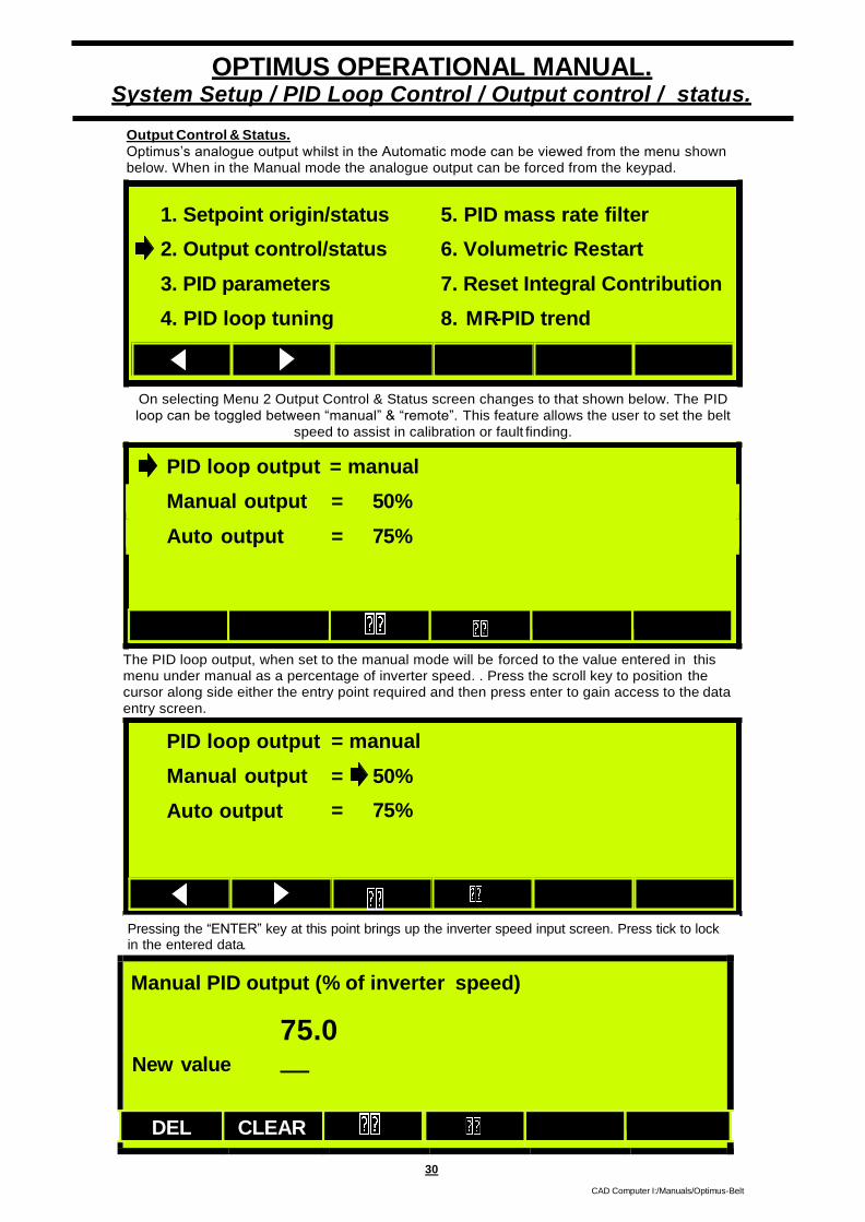
30
CAD Computer I:/Manuals/Optimus-Belt
OPTIMUS OPERATIONAL MANUAL. System Setup / PID Loop Control / Output control / status.
PID loop output = manual
PID loop output
Manual output
Auto output
= manual
=
=
50%
75%
Pressing the “ENTER” key at this point brings up the inverter speed input screen. Press tick to lock in the entered data.
Output Control & Status.
Optimus’s analogue output whilst in the Automatic mode can be viewed from the menu shown
below. When in the Manual mode the analogue output can be forced from the keypad.
On selecting Menu 2 Output Control & Status screen changes to that shown below. The PID
loop can be toggled between “manual” & “remote”. This feature allows the user to set the belt
speed to assist in calibration or fault finding.
Manual output = 50%
Auto output = 75%
The PID loop output, when set to the manual mode will be forced to the value entered in this
menu under manual as a percentage of inverter speed. . Press the scroll key to position the
cursor along side either the entry point required and then press enter to gain access to the data
entry screen.
Manual PID output (% of inverter speed)
75.0 New value —
DEL CLEAR
1. Setpoint origin/status
2. Output control/status
3. PID parameters
4. PID loop tuning
5. PID mass rate filter
6. Volumetric Restart
7. Reset Integral Contribution
8. MR-PID trend

31
CAD Computer I:/Manuals/Optimus-Belt
OPTIMUS OPERATIONAL MANUAL. System Setup / PID Loop Control / pid parameters.
The screens and menu entry points associated with the “PID Parameters” allow suitably
qualified personnel to load the PID algor ithm with variables that best suit the operation
of the feeder. It should be noted that a good understanding of process control loops is
required for successful tuning of a weighbelt feeder.
Press the “ENTER” key to access the PID variable adjust screen.
On selecting Menu 3, PID Parameters, the screen changes to that shown below.
PID proportional band (%)
+160.0
New value —
DEL CLEAR
Enter the value required for the Proportional screen and press the Tick key to accept and
return to the PID screen.
Prop band
Integral lower limit
Derivative time=
Feed forward
=200.0% Reset rate = +0.100 resets/s
=-50.0% Upper limit = +50.0%
=+0.00s
=1.00 Output offset = +0.00
SETUP
1. Setpoint origin/status
2. Output control/status
3. PID parameters
4. PID loop tuning
5. PID mass rate filter
6. Volumetric Restart
7. Reset Integral Contribution
8. MR-PID trend

32
CAD Computer I:/Manuals/Optimus-Belt
OPTIMUS OPERATIONAL MANUAL. System Setup / PID Loop Control / pid parameters.
Use the scroll keys to access the Integral (reset rate) data entry point.
Use the “ENTER” key to access “I” (reset rate) data entry screen.
PID reset rate ( resets/sec)
+0.100
New value —
DEL CLEAR
Use the “ENTER” key to access the Integral Lower Limit data entry screen.
In many applications it is often beneficial if the PID integral is restrained. As the working
“integral” can be either positive or minus value. The limits can be set in the following data entry
screens. Note the F5 key is now configured as a sign entry key.
PID integral lower limit (%)
-50.0
New value —
DEL CLEAR +/-
Use the Tick key to lock in the Integral Lower Limit.
Prop band
Integral lower limit
Derivative time=
Feed forward
=200.0% Reset rate = +0.100 resets/s
=-50.0% Upper limit = +50.0%
=+0.00s
=1.00 Output offset = +0.00
Prop band =200.0% Reset rate = +0.100 resets/s
Integral lower limit
Derivative time=
Feed forward
=-50.0% Upper limit = +50.0%
=+0.00s
=1.00 Output offset = +0.00

33
CAD Computer I:/Manuals/Optimus-Belt
OPTIMUS OPERATIONAL MANUAL. System Setup / PID Loop Control / pid parameters.
Use the scroll keys to access the Integral Lower Limit.
Use the “ENTER” key to access the Integral Upper Limit data entry screen.
PID integral upper limit (%)
+50.0
New value —
DEL CLEAR +/-
Scroll to the Derivative using the scroll keys.
Use the “ENTER” key to gain access to the Derivative time data entry screen.
PID derivative time (secs)
+0.000
New value —
DEL CLEAR
Use the “ENTER” key to lock in the derivative time data and return to PID screen.
Prop band
Integral lower limit
Derivative time=
Feed forward
=200.0% Reset rate = +0.100 resets/s
=-50.0%
=+0.00s
=1.00
Upper limit = +50.0%
Output offset = +0.00
Prop band
Integral lower limit
Derivative time=
Feed forward
=200.0% Reset rate = +0.100 resets/s
=-50.0%
=+0.00s
=1.00
Upper limit = +50.0%
Output offset = +0.00

34
CAD Computer I:/Manuals/Optimus-Belt
OPTIMUS OPERATIONAL MANUAL. System Setup / PID Loop Control / pid parameters.
Use the scroll keys to access the Feed forward term.
Use the “ENTER” key to access the Feed Forward term.
PID feed forward factor
1.000
New value —
DEL CLEAR
Use the “ENTER” key to lock in the feed Forward term data and return to PID screen.
With the cursor pointing at the “Output offset” press the “ENTER” key to gain access to
the data input screen.
PID output offset term
+0.000
New value —
DEL CLEAR
Press the tick key to lock in the data. The display will then return to the main PID setup
screen
Prop band
Integral lower limit
Derivative time=
Feed forward
=200.0% Reset rate = +0.100 resets/s
=-50.0%
=+0.00s
=1.00
Upper limit = +50.0%
Output offset = +0.00
Prop band
Integral lower limit
Derivative time=
Feed forward
=200.0% Reset rate = +0.100 resets/s
=-50.0%
=+0.00s
=1.00
Upper limit = +50.0%
Output offset = +0.00

35
CAD Computer I:/Manuals/Optimus-Belt
OPTIMUS OPERATIONAL MANUAL. System Setup / PID Loop Control / pid loop tuning.
SP =
OP =
PB =
PC =
MR =
25.0%
85.0%
+200.0%
+10.0%
24.0%
FF =
IL =
RR =
IC =
LC =
1.000 OS =
-50.0% IU =
+0.100% DT =
+0.000 DC =
2.854mV TC =
0.000%
+85.0%
+0.000 s
+0.000
220Hz
PID Loop Tuning.
Following the loading of the PID algorithm with the required variables. Optimus
provides the user with a convenient method of adjusting and viewing the PID algorithm.
Scroll to the PID Loop Tuning menu and press the “ENTER” key to gain acc ess.
On selecting Menu 4 PID Loop Tuning the screen changes to that shown below.
PLOT LOC
PID Loop Tuning Screen.
From this screen the user can tune the PID loop without having to change screens. All
variables associated with the control loop are accessible from this screen as are the ou t-
puts from the load cell and tachometer. The cursor under control of the (F1 & F2) keys
will take the user to all the changeable variables. All other data displayed is for viewing
only.
1 SP Set Point. (As a percentage of belt capacity).
2 FF Feed Forward Term.
3 OS PID Output Offset Term.
4 OP PID Analogue Output.
5 IL PID Integral Lower Limit.
6 IU PID Integral Upper Limit.
7 PB PID Proportional Term.
8 RR PID Integral Term.
9 DT PID Derivative Term.
10 PC Proportional contribution.
11 IC Integral contribution.
12 DC derivative contribution.
13 LC Load Cell output in milli-volts.
14 TC Tachometer output in hertz.
SETUP
1. Setpoint origin/status
2. Output control/status
3. PID parameters
4. PID loop tuning
5. PID mass rate filter
6. Volumetric Restart
7. Reset Integral Contribution
8. MR-PID trend

36
CAD Computer I:/Manuals/Optimus-Belt
OPTIMUS OPERATIONAL MANUAL. System Setup / PID Loop Control / pid loop tuning.
PID Loop Tuning. (Continued)
PLOT (F5) Pressing the PLOT (F5) key provides the user with a plot screen the
Mass Rate and PID o ut being plotted.
LOC (F6) Pressing the LOCAL (F6) toggles Optimus between the setpoint being
set remotely or locally.
Select “PLOT” to go to the TREND screen where the set point can be ramped up and
down and the feeder response viewed..
100%
PID MR
50%
0%
BACK CLEAR
SP =
OP =
PB =
PC =
MR =
25.0%
85.0%
+200.0%
+10.0%
24.0%
FF =
IL =
RR =
IC =
LC =
1.000 OS = 0.000%
-50.0% IU = +85.0%
+0.100% DT = +0.000 s
+0.000 DC = +0.000
2.854mV TC = 220Hz
PLOT LOC
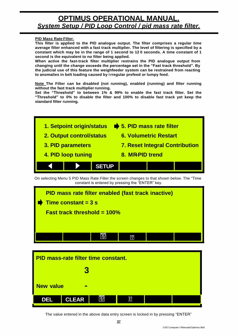
37
CAD Computer I:/Manuals/Optimus-Belt
OPTIMUS OPERATIONAL MANUAL. System Setup / PID Loop Control / pid mass rate filter.
PID mass rate filter enabled (fast track inactive)
Time constant = 3 s
Fast track threshold = 100%
PID Mass Rate Filter.
This filter is applied to the PID analogue output. The filter comprises a regular time
average filter enhanced with a fast track multiplier. The level of filtering is specified by a
constant which may be in the range of 1 second to 12 0 seconds. A time constant of 1
second is the equivalent to no filter being applied.
When active the fast-track filter multiplier restrains the PID analogue output from
changing until the change exceeds the percentage set in the “Fast track threshold”. By
the judicial use of this feature the weighfeeder system can be restrained from reacting
to anomalies in belt loading caused by i rregular prefeed or lumpy feed.
Note The Filter can be disabled (not running), enabled (running) and filter running
without the fast track multiplier running.
Set the “Threshold” to between 1% & 99% to enable the fast track filter. Set the
“Threshold” to 0% to disable the filter and 100% to disable fast track yet keep the
standard filter running.
On selecting Menu 5 PID Mass Rate Filter the screen changes to that shown below. The “Time
constant is entered by pressing the “ENTER” key.
PID mass-rate filter time constant.
3
New value -
DEL CLEAR
The value entered in the above data entry screen is locked in by pressing “ENTER”
SETUP
1. Setpoint origin/status
2. Output control/status
3. PID parameters
4. PID loop tuning
5. PID mass rate filter
6. Volumetric Restart
7. Reset Integral Contribution
8. MR-PID trend
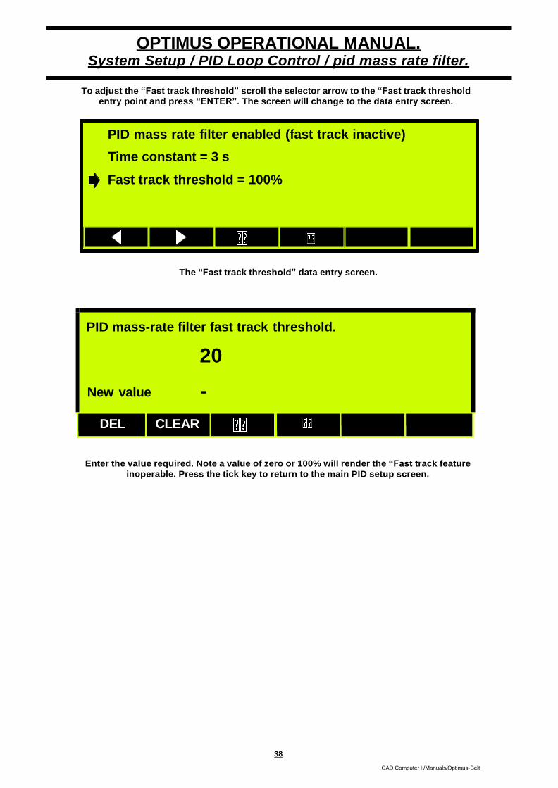
38
CAD Computer I:/Manuals/Optimus-Belt
OPTIMUS OPERATIONAL MANUAL. System Setup / PID Loop Control / pid mass rate filter.
To adjust the “Fast track threshold” scroll the selector arrow to the “Fast track threshold
entry point and press “ENTER”. The screen will change to the data entry screen.
The “Fast track threshold” data entry screen.
PID mass-rate filter fast track threshold.
20
New value -
DEL CLEAR
Enter the value required. Note a value of zero or 100% will render the “Fast track feature
inoperable. Press the tick key to return to the main PID setup screen.
PID mass rate filter enabled (fast track inactive)
Time constant = 3 s
Fast track threshold = 100%
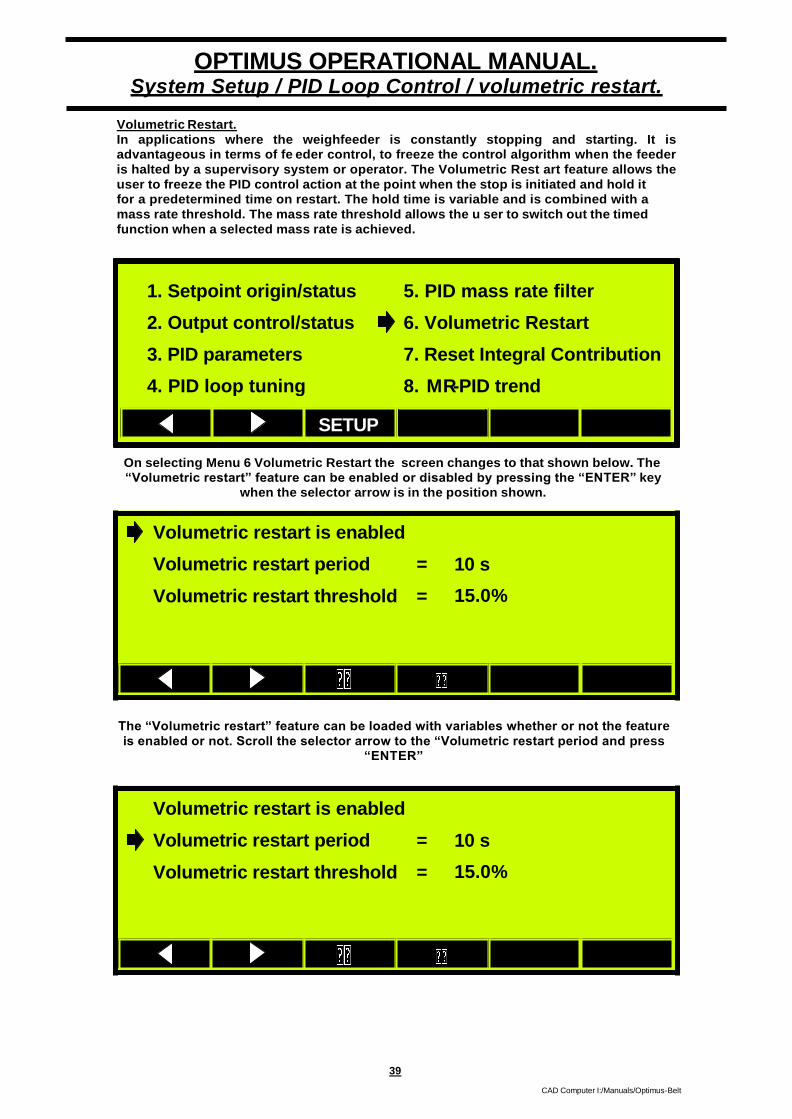
39
CAD Computer I:/Manuals/Optimus-Belt
OPTIMUS OPERATIONAL MANUAL. System Setup / PID Loop Control / volumetric restart.
Volumetric Restart.
In applications where the weighfeeder is constantly stopping and starting. It is
advantageous in terms of fe eder control, to freeze the control algorithm when the feeder
is halted by a supervisory system or operator. The Volumetric Rest art feature allows the
user to freeze the PID control action at the point when the stop is initiated and hold it
for a predetermined time on restart. The hold time is variable and is combined with a
mass rate threshold. The mass rate threshold allows the u ser to switch out the timed
function when a selected mass rate is achieved.
On selecting Menu 6 Volumetric Restart the screen changes to that shown below. The
“Volumetric restart” feature can be enabled or disabled by pressing the “ENTER” key
when the selector arrow is in the position shown.
The “Volumetric restart” feature can be loaded with variables whether or not the feature
is enabled or not. Scroll the selector arrow to the “Volumetric restart period and press
“ENTER”
Volumetric restart is enabled
Volumetric restart period =
Volumetric restart threshold =
10 s
15.0%
Volumetric restart is enabled
Volumetric restart period =
Volumetric restart threshold =
10 s
15.0%
SETUP
1. Setpoint origin/status
2. Output control/status
3. PID parameters
4. PID loop tuning
5. PID mass rate filter
6. Volumetric Restart
7. Reset Integral Contribution
8. MR-PID trend

40
CAD Computer I:/Manuals/Optimus-Belt
OPTIMUS OPERATIONAL MANUAL. System Setup / PID Loop Control / volumetric restart.
The value entered in the “Volumetric restart period” screen. Is the time period that
Optimus will use to time out the freezing o f the PID algorithm, prior to recalculating the
new process variable and out putting the signal to the analogue PID output.
Volumetric restart period (in seconds)
10
New value -
DEL CLEAR
Following the entry of the required delay, press the “ENTER” key to lock in the data.
Scroll on the selector arrow to the “Volumetric restart threshold” and press “ENTER” to
gain access.
The “Volumetric restart threshold” acts in conjunction with the “Volumetric restart
period”. It will override the volumetric restart period, if enabled and the mass rate is
calculated as being within percentage set in this menu. This provides for a fast re sponse
from the PID algorithm should the mass rate come up to set point prior to the volumetric
restart period timing out after a belt stoppage. The values in this menu should be entered
after observing the system in normal field operation.
Volumetric restart threshold (% of belt capacity)
15.0
New value -
DEL CLEAR
Press the “TICK” key to lock in the selected value.
+ -
Volumetric restart is enabled
Volumetric restart period =
Volumetric restart threshold =
10 s
15.0%

41
CAD Computer I:/Manuals/Optimus-Belt
OPTIMUS OPERATIONAL MANUAL.
System Setup / PID Loop Control / reset the integral contribution.
Reset Integral Contribution.
When tuning a feeder it is often advantageous to be able to manually reset the integral
contribution to the PID loop output. Pressing the “ENTER” key when the selector arrow
is opposite the Reset Integral Contribution when forc e the integral to be reset.
1. Setpoint origin/status 5. PID mass rate filter
2. Output control/status 6. Volumetric Restart
3. PID parameters 7. Reset Integral Contribution
4. PID loop tuning 8. MR-PID trend
SETUP

OPTIMUS OPERATIONAL MANUAL. System Setup / PID Loop Control / mass rate & pid output trends.
CAD Computer I:/Manuals/Optimus-Belt
Mass Rate / PID Trend.
This screen allows the user to view the relationship between the mass rate and the
control function outpu t. With the selector arrow opposite the MR -PID trend press
“ENTER” to access the trend screen.
On selecting Menu 8 changes to that shown below. There are two traces, Mass Rate
(MR) and PID output (PID). To exit this menu u se the F1 key (BACK) to clear the trace use
the F2 key (CLEAR). The F3 key ( SP) reduces the setpoint, the F4 key ( SP) increase s
the setpoint. The arrow attached to the vertical cursor depicts the set point.
Setpoint Cursor
When finished with this screen press the F1 key “BACK” to return to the PID Loop.
To return to the “SETUP” menu’s press the F3 “SETUP key. Scroll the cursor on to Auto Zero Tracking (AZT). Prior to entering data in this menu read the AZT explanation on following page.
1. System Configuration
2. Display and Time/Date
3. PID Loop Control
4. Auto Zero Tracking
5. Rate Deadband
6. Rate Display Filters
7. Save/Load Setup
8. Chute Level Control
42
SETUP
1. Setpoint origin/status
2. Output control/status
3. PID parameters
4. PID loop tuning
5. PID mass rate filter
6. Volumetric Restart
7. Reset Integral Contribution
8. MR-PID trend
SETUP
1. Setpoint origin/status
2. Output control/status
3. PID parameters
4. PID loop tuning
5. PID mass rate filter
6. Volumetric Restart
7. Reset Integral Contribution
8. MR-PID trend
100%
PID
50%
MR
0%
BACK CLEAR SP SP

OPTIMUS OPERATIONAL MANUAL. System Setup / Auto Zero Tracking / overview.
43
CAD Computer I:/Manuals/Optimus-Belt
Prior to describing the use of the Auto Zero Tracking (AZT) function, the user should be
familiar with certain terminology.
Manual Zero is the belt zeroing which is invoked by an operator. The function is
automatic but has to be manually invoked. As distin ct from the AZT function which is
performed automatically without user intervention.
Auto Zero Tracking. (This function should be set up after the scale has be calibrated)
The weight of the weigh belt and the weigh area can change with time. The weight
changes can be generally attributed to, wear and tear, product build upon the belt and
product build up on the weigh area. If th e scale was a static system weighing in batches
for instance, the scale could be automatically zeroed each time the previous loa d was
removed. The action being triggered by the output of the load cell dropping to a pre -
programmed value.
Continuous weighing systems are more complex and require more conditions to be
satisfied prior to an AZ being performed. The function can be enabl ed or disabled by
toggling the ’ENTER’ key when the sect arrow is along side the field.
Optimus allows the user to select a load cell output below which the AZ function will be
invoked (Threshold). It is important this load cell output is carefully selecte d. It can only
be accurately selected after the system has been manually zeroed, calibrated and the
mass rate observed over a minimum of one whole belt revolution. The Auto Zero
Threshold level should be set to approximately 5% higher than the highest valu e
displayed when the belt is running empty.
The delay value is provided so that the AZ function will only be invoked after the d elay
has timed out. This function is used when the process is subject to constant no flow
conditions. The period allows the use r to select the number of whole belt revolution that
the zero will performed over. A good knowledge of the process is necessary to enter a
value here.
E.g. If the no flow condition is available for a period of greater than one belt revolution
but less tha n two belt revolution, use one revolution here and so on.
The value shown in the “Current Contribution” field display the offset that Optimus has
applied to the manual zero found during the manual zero process. It is reset after each
manual zero has been performed.
Whole belt revolution
Whole belt revolution
Whole belt revolution
The Mass rate that has to be <= the set value prior to the AZT starting. Average Zero.
Whole belt revolution Whole belt revolution
Delay implemented after the threshold has been satisfied
Ma
ss R
ate
as %
or
absolu
te v
alu
e.

44
CAD Computer I:/Manuals/Optimus-Belt
OPTIMUS OPERATIONAL MANUAL. System Setup / Auto Zero Tracking.
Toggling the “ENTER” key here will either enable or disable the Auto Zero Tracking
function (AZT).
Use the scroll key to access the Threshold setting screen. The Threshold can be set as a
percentage of the belt capacity or as a mass rate. The user should be aware of result of
the AZT threshold being set too high or too low. If it is set too high Optimus could invoke
the Auto zero routine and zero out the belt with material on it, or never completely
perform an AZT because the de ad weight effect of the belt switches out the function
before a full belt revolution can be completed. Use an input that means something to you
and observe the process prior to setting up this screen.
Press the “ENTER” key to adjust the AZT Threshold.
Auto zero threshold (% of belt capacity)
5.0
New value —
DEL CLEAR
Press the tick key to lock in the new threshold level
Auto-Zero tracking disabled
Threshold =
Delay =
10.0% =
10 secs
1.00 kg/min
Period = 2 revs
Current contribution = 0.00
Auto-Zero tracking disabled
Threshold =
Delay =
10.0% =
10 secs
1.00 kg/min
Period = 2revs
Current contribution = 0.00

45
CAD Computer I:/Manuals/Optimus-Belt
OPTIMUS OPERATIONAL MANUAL. System Setup / Auto Zero Tracking / threshold.
The Threshold is the point at which Optimus will perform an AZT assuming that the Delay
period has been satisfied. The threshold can be set either as a % of the of maximum
mass rate (as specified in the setup). Or as an absolute value, in the specified unit s. Use
the scroll keys to
access the Threshold and press “ENTER” key to gain access to data entry screen for e i-
ther % or units.
Pressing the “ENTER” key here will bring up the threshold percent data entry screen.
Auto zero threshold ( in kg/min)
10.0
New value —
DEL CLEAR
Press the tick key to accept and exit to the previous screen. Or the Cross key to exit to
the previous screen
Auto-Zero tracking disabled
Threshold =
Delay =
10.0% =
10 secs
1.00 kg/min
Period = 2revs
Current contribution = 0.00

46
CAD Computer I:/Manuals/Optimus-Belt
OPTIMUS OPERATIONAL MANUAL. System Setup / Auto Zero Tracking / threshold.
As with the previous screen the AZT threshold can be set by scrolling to the absolute
value entry point as shown below. Pressing the “ENTER” key will gain access to the data
entry field.
Pressing the “ENTER” key here will bring up the threshold percent data entry screen.
Auto zero threshold ( in kg/min)
10.0
New value —
DEL CLEAR
Press the tick key to accept and exit to the previous screen. Or the Cross key to exit to
the previous screen.
Auto-Zero tracking disabled
Threshold =
Delay =
10.0% =
10 secs
1.00 kg/min
Period = 2 revs
Current contribution = 0.00

47
CAD Computer I:/Manuals/Optimus-Belt
OPTIMUS OPERATIONAL MANUAL. System Setup / Auto Zero Tracking / delay.
Some processes are cyclic and the belt can be running empty (below the threshold) the
AZT will activate only to be halted when more material is presented to the belt. The delay
allows the user who has a knowledge of the process to suppress the start of an AZT until
the threshold has been active longer than any normal cyclic process.
Press the “ENTER” key with the cursor opposite the delay to gain access to the delay data
input screen.
Delay before auto zeroing (in seconds)
10.0
New value —
DEL CLEAR
Press the tick key to accept the new value for the delay of the AZT feature
Auto-Zero tracking disabled
Threshold =
Delay =
10.0% =
10 secs
1.00 kg/min
Period = 2revs
Current contribution = 0.00

48
CAD Computer I:/Manuals/Optimus-Belt
OPTIMUS OPERATIONAL MANUAL. System Setup / Auto Zero Tracking / period.
A user initiated Zero will be performed over the number of belt revolutions that were d e-
fined during the calibration process. When a AZT is initiated the number of belt revol u-
tions that the user wishes to have the AZT performed over can be more or less than the
number defined in the calibration process. This is allowed in order that a zero can be
completed within a “widow” of opportunity. A knowledge of the process is required prior
to selecting the “PERIOD”. Scroll the cursor to the “PERIOD” data entry point and press
“ENTER”.
Enter the number of belt revolutions that the AZT should use to update the current average zero
Auto zero period ( in belt revolutions)
5
New value —
DEL CLEAR
Press the tick key to accept and exit to the previous screen. Or the Cross key to exit to the
previous screen
Auto-Zero tracking disabled
Threshold =
Delay =
10.0% =
10 secs
1.00 kg/min
Period = 2 revs
Current contribution = 0.00

49
CAD Computer I:/Manuals/Optimus-Belt
OPTIMUS OPERATIONAL MANUAL. System Setup / Auto Zero Tracking / current contribution.
ing is enabled.
0% 1.000 kg/min
Period = 2 revs
ution = 0.000
track
ld = 10.
0 secs
ontrib
Over time the AZT contribution to the average zero may drift out of limits that can be
termed normal. This value will be differe nt for all systems and depends on the working
environment, feeder design, product and belt wear. In order that the user can moni tor
performance of the AZT routine Optimus has been provide with a viewing port, where the
AZT calculated zero can be reviewed and rese t. Note this value is automatically reset
each time an operator initiated zero is performed.
Press the “RESET” key (F5). To gain access to the AZT reset.
Auto-Zero tracking disabled
Threshold =
Delay =
10.0% =
10 secs
1.00 kg/min
Period = 2revs
Current contribution = 0.00
! Set auto-zero offset to 0 mV?
Press ENTER to proceed
Press ABORT to skip
Auto-zero
Thresho
Delay = 1
Current c
RESET
RESET
Auto-zero tracking is enabled.
Threshold = 10.0%
Delay = 10 secs
1.000 kg/min
Period = 2 revs
Current contribution = 0.000

50
CAD Computer I:/Manuals/Optimus-Belt
OPTIMUS OPERATIONAL MANUAL. System Setup / Rate Deadband / .
Rate deadband (in kg/min)
1.8
New value —
DEL CLEAR
CLEAR
Mass rate deadband =
=
Mass rate =
Maximum mass rate =
0.2% of belt capacity
1.2 kg/hour
350 kg/hour
600 kg/hour
CLEAR
Mass rate deadband =
=
Mass rate =
Maximum mass rate =
0.2% of belt capacity
1.2 kg/hour
350 kg/hour
600 kg/hour

51
CAD Computer I:/Manuals/Optimus-Belt
OPTIMUS OPERATIONAL MANUAL. System Setup / Rate Display Filters.
Mass rate deadband = 0.2% of belt capacity
= 1.2 kg/hour
Mass rate = 350 kg/hour
Maximum mass rate = 600 kg/hour
CLEAR
Rate deadband (as % of belt capacity)
2.0
New value —
DEL CLEAR
1. System Configuration
2. Display and Time/Date
3. PID Loop Control
4. Auto Zero Tracking
5. Rate Deadband
6. Rate Display Filters
7. Save/Load Setup
8. Chute Level Control

52
CAD Computer I:/Manuals/Optimus-Belt
OPTIMUS OPERATIONAL MANUAL.
System Setup / Rate Display Filters / time constant.
The analogue Mass Rate output signal can be filtered. Scroll to Rate Display Filter and
press “ENTER” to show the menu for mass Rate Filtering.
Press the “ENTER” key to gain access to the Mass Rate Filter menu.
Mass rate display filter enabled (fast track active)
Time constant = 20s Fast track threshold = 20%
Mass rate trend filter enabled (fast track active)
Time constant = 10s Fast track threshold = 20%
Press the “ENTER” key to gain access to the Mass Rate data entry screen.
Display filter time constant
10
New value —
DEL CLEAR
Enter the value required for the time constant in the above screen and press the Tick key to
accept and return to the PID screen.
1. System Configuration
2. Display and Time/Date
3. PID Loop Control
4. Auto Zero Tracking
5. Rate Deadband
6. Rate Display Filters
7. Save/Load Setup
8. Chute Level Control

53
CAD Computer I:/Manuals/Optimus-Belt
OPTIMUS OPERATIONAL MANUAL.
System Setup / Rate Display Filters / fast track threshold & time.
The Mass Rate Filter.
This feature allows the user to dampen the Mass Rate analogue output. Mass rate filter
has fast tracking facility associated with it. The filter can be switched off by
Setting the “Threshold” to 0% . If the filter is required without the fast track feature, set
the “Threshold” to 100%.
Mass rate display filter enabled (fast track active)
Time constant = 20s Fast track threshold = 20%
Mass rate trend filter enabled (fast track active)
Time constant = 10s Fast track threshold = 20%
Display filter fast track threshold
1.0
New value —
DEL CLEAR
Mass rate display filter enabled (fast track active)
Time constant = 20s Fast track threshold = 20%
Mass rate trend filter enabled (fast track active)
Time constant = 10s Fast track threshold = 20%
Trend filter time constant
5.0
New value —
DEL CLEAR

54
CAD Computer I:/Manuals/Optimus-Belt
OPTIMUS OPERATIONAL MANUAL.
System Setup / Rate Display Filters time constant / fast track threshold.
Mass rate display filter enabled (fast track active)
Time constant = 20s Fast track threshold = 20%
Mass rate trend filter enabled (fast track active)
Time constant = 10s Fast track threshold = 20%
Trend filter fast track threshold
20
New value —
DEL CLEAR

55
CAD Computer I:/Manuals/Optimus-Belt
OPTIMUS OPERATIONAL MANUAL.
System Setup / Save / Load Setup.
- - - - - - - - - - - - - - - - - - -
- - - - - - - - - - - - - - - - - - -
- - - - - - - - - - - - - - - - - - -
- - - - - - - - - - - - - - - - - - -
- - - - - - -
- - - - - - -
- - - - - - -
- - - - - - -
Save/Load Setup.
Optimus can be fitted with an optional compact “Flash Card” (32 M B). The card fits into a
flash card carrier on the main pcb. The flash card is used to install software (firmware)
updates and store Optimus setup and configuration data. The card can accepts 8 setup
and configuration data sets. This data can be used to setup Optimus quickly and acc u-
rately should the main pcb fail.
Scroll on to save/Load Setup.
The screen will change to the one shown below. This screen shows the compact flash
memory is empty (8 dotted lines). The cursor is positioned next to the first entry
File 00. Press the F3 “SAVE” key to load flash card memory with the configuration and
setup data.
Optimus will now save the data to the next available file. In this case File 00, there will be
a small delay between pressing F3 “SAVE” and the screen shown below presenting.
Press “ENTER” to lock in the data to the compact flash memory.
! File 00 saved
Press ENTER to proceed
Files on card
SAVE LOAD ERASE
SAVE LOAD ERASE
Files on card - - - - - - - - - - - - -
- - - - - - - - - - - - -
- - - - - - - - - - - - -
- - - - - - - - - - - - -
- - - - - - - - - - - - -
- - - - - - - - - - - - -
- - - - - - - - - - - - -
- - - - - - - - - - - - -
1. System Configuration
2. Display and Time/Date
3. PID Loop Control
4. Auto Zero Tracking
5. Rate Deadband
6. Rate Display Filters
7. Save/Load Setup
8. Chute Level Control

56
CAD Computer I:/Manuals/Optimus-Belt
OPTIMUS OPERATIONAL MANUAL.
System Setup / Save / Load Setup.
- - - - - - - - - - - - - - - - - - -
- - - - - - - - - - - - - - - - - - -
- - - - - - - - - - - - - - - - - - -
- - - - - - - - - - - - - - - - - - -
- - - - - - -
- - - - - - -
- - - - - - -
- - - - - - -
The card has been loaded with setup and configuration data, which can be used later or
sent to Web-Tech for evaluation if there setup is a problem.
To down load previously stored data, select the file required by placing the cursor along
side the file and press the F4 “LOAD” key.
When the screen indicates that the file has loaded press “ENTER” to update Optimus.
To Erase Files, select the file to erase by placing the cursor along side it. Then Press F5
“ERASE” it.
! File loaded
Press ENTER to proceed
Files on card
SAVE LOAD ERASE
SAVE LOAD ERASE
Files on card File 00
- - - - - - - - - - - - -
- - - - - - - - - - - - -
- - - - - - - - - - - - -
- - - - - - - - - - - - -
- - - - - - - - - - - - -
- - - - - - - - - - - - -
- - - - - - - - - - - - -

57
CAD Computer I:/Manuals/Optimus-Belt
OPTIMUS OPERATIONAL MANUAL.
System Setup / Chute Level Control.
Some processes require that the weighfeeder be pre -fed by means other than a choked
supply (overhead bin or silo). Generally a vo lumetric screw feeder is used. This type
feeder is unable to control the rate at which product is supplied to a regular weighfee der
inlet chute. A standard weighfeeder inlet chute will have little volumetric capacity and
therefore will be subject to the va garies of the plant demand. As a weighfeeder can only
adjust the feed rate by means of belt speed variation, any abnormal deviations from se t-
point can result in over supply or under supply to the feeder. This will result in the weig h-
feeder being either being under supplied or over supplied and the feeder being able to
supply a stable mass rate. By increasing the volume of the inlet chute in the horizontal
sense and measuring the volume in the extended horizontal chute, Optimus can va ry the
speed of the pre -feed device. Web-tech manufacture feeder’s that have an extended hor i-
zontal inlet chutes fitted with material sensing probes. These probes provide Optimus
with a map of the volume of product in th e inlet chute and therefore the ability to control
the rate of product supply to the feeder. By setting up the following menu correctly, O p-
timus can provide a control signal to control the pre -feed device.
Chute level control is an optional extra and is suitable for use with feeders manufactured
with a custom designed material inlet chute.
Scroll to Chute Level Control, press ENTER to set up and modify the chute level control
action. At this point assigned probes can be associated with a output speed function.
Generally the weighfeeder will have been fitted with three probes prior to despatch . They
are referred to as Low, Mid, High. The Low probe is the probe nearest the inlet chute, the
High probe is the probe nearest to the shear gate on the feeder and the Mid probe is
situated in between the High and Low. None refers to no probe active, al l probes out of
product. The Ratio refers to the percentage output from the assigned current loop on a c-
tivation of that probe.
In the following example with no probe active, the current loop driving the prefeed inve r-
tor will be driven to 20mA, 100% output. With just the Low probe active and the inlet
chute approximately 1/3 full the current l oop will be driven to 18.4 mA. When the Low &
Mid probes are on the current loop out put will be 16.0 mA and with all three prob es on
the out put will be 12 mA.
Pressing ENTER will provide the user with an input screen where each probe can be a s-
signed with an output ratio function.
Probe On
None
Low
Mid
High
(No probe active.)
(Low probe active.)
(Middle probe active.)
(High probe active.)
Ratio
100.00%
90.00%
75.00%
50.00%
1. System configuration
2. Display and Time/Date
3. PID Loop Control
4. Auto Zero Tracking
5. Rate Deadband
6. Rate display Filters
7. Passwords
8. Chute Level control.

OPTIMUS OPERATIONAL MANUAL.
System Setup / Chute Level Control.
58
CAD Computer I:/Manuals/Optimus-Belt
No probe chute output ratio (in %)
100.0
New value —
DEL CLEAR
Observe the process and assign a mA output to the assigned current loop that best
satisfies the process requirement, when the chute has become empty. Press the tick key
to lock in the data and return to the probe assignment screen.
Scroll on to the “Low” probe and assign an output to the current loop.
Low probe chute output ratio (in %)
90.0
New value —
DEL CLEAR
Scroll on to the “Mid” probe and assign an output to the current loop.
Probe On
None
Low
Mid
High
Ratio
100.00%
90.00%
75.00%
50.00%
Probe On
None
Low
Mid
High
Ratio
100.00%
90.00%
85.00%
50.00%

59
CAD Computer I:/Manuals/Optimus-Belt
OPTIMUS OPERATIONAL MANUAL.
System Setup / Chute Level Control.
Assign a current output to the activation of the “Mid” probe.
Mid probe chute output ratio (in %)
85.0
New value —
DEL CLEAR
Press the tick key to lock in the data and move back to the probe assignment screen.
Scroll on to the “High” probe current output assignment and press the “ENTER” key gain
access to the data entry screen.
High probe chute output ratio (in %)
50.0
New value —
DEL CLEAR
Enter the current output required when the chute probe “High” is on and press the tick
key to lock in the data and return to the probe assignment screen.
Probe On
None
Low
Mid
High
Ratio
100.00%
90.00%
75.00%
50.00%

60
CAD Computer I:/Manuals/Optimus-Belt
OPTIMUS OPERATIONAL MANUAL.
I/O (Input/Output) / Current Loop Inputs.
Optimus provides six for (6) analogue input circuits. One is reserved or the Remote
Rate Input. The remaining five are re -assignable. Optimus's analogue inputs are current
and can be configured to be one of the following.
4/20mA - 20/4mA - 0/20mA - 20/0mA - 5/25mA - 25/5mA - 0/25mA - 25/0
From the MRMT screen select the Input / Output ( I/O ) F2 key
Press the “ENTER” key to gain access to the Current Loop Inputs.
Press the “ENTER” key to gain access to the Current Loop 1 Setup screens.
Loop 1 Remote Setpoint
Loop 2 Temperature
Loop 3 Ratio
Loop 4 Inclinometer
Loop 5 not used
Loop 6 not used
1. Current Loop Inputs
2. Current Loop Outputs
3. Digital Inputs
4. Digital Outputs
5. RS-232 Configuration
6. RS-485 Configuration
7. Load cell and tacho
8. DeviceNet
Mass Rate
[kg/min]
Mass Total
[kg]
CAL
950.0
702.0
SP Local
SP Rem
AZT
PID
On
Man
PID Auto
I / O TREND CLEAR SETUP INFO

61
CAD Computer I:/Manuals/Optimus-Belt
OPTIMUS OPERATIONAL MANUAL.
I/O (Input/Output) / Current Loop Inputs.
Loop 1 Setup
Note Current Loop Input 1 is reserved for the remote Setpoint input. This is indicated by
selection cursor changing from a filled cursor to an outline of a cursor.
The Input display shows the current input signal.
Loop input 1 is Remote Setpoint Input = 4.00mA
Type is 4-20 mA Parameters Filtering
Calibrate 0% Current 0% 20.00mA
Calibrate 100% Current 100% 0.00mA
Use the scroll key to advance the cursor to “Type is” Press “ENTER” to gain access to
the pre-defined input types. Scroll through the six types of current inputs until you find
the one that suites the device that is generating the remote setpoint.
Scroll on to the “Parameters”
Loop input 1 is Remote Setpoint
Type is 20-0 mA
Calibrate 0%
Calibrate 100%
Parameters
Current 0%
Input = 0.00mA
Filtering
20.00mA
Current 100% 0.00mA
Loop input 1 is Remote Setpoint
Type is 4-20 mA
Calibrate 0%
Calibrate 100%
Parameters
Current 0%
Input = 0.00mA
Filtering
20.00mA
Current 100% 0.00mA

62
CAD Computer I:/Manuals/Optimus-Belt
OPTIMUS OPERATIONAL MANUAL.
I/O (Input/Output) / Current Loop Inputs.
A number of Optimus units can, if required act as a stand alone ratio controllers.
The units can be linked via their individual analogue input and output current loops and
provide a master slave ratio control over the resultant output from a number of fee ders.
The following screen provides the user with the means to set up the feeder ratios. In the
example below the feeder will produce 60 kg/min at 20mA.
Loop input 1 remote setpoint parameters
Master capacity = 60 kg/minute
Slave % = 100% of master
Input = 60 kg/minute
Master capacity (in kg/min)
100.0
New value —
DEL CLEAR
Slave output (% of master capacity)
100.0
New value —
DEL CLEAR
Loop input 1 remote setpoint parameters
Master capacity = 60 kg/minute
Slave % = 100% of master
Input = 60 kg/minute

63
CAD Computer I:/Manuals/Optimus-Belt
OPTIMUS OPERATIONAL MANUAL.
I/O (Input/Output) / Current Loop Inputs.
Loop filter enabled (fast track active)
Time constant =
Loop filter enabled (fast track active)
Time constant =
Fast track threshold =
Fast track threshold =
5s
15%
5s
15%
Use the scroll forward key to move the cursor on to the Filtering entry point.
Press the “ENTER” key to gain access to the current loop input filtering, reserved for
remote setpoint (“REM SET” as shown on t he connection pcb). Scroll on to “Time
Constant”
Press “ENTER” to gain access to the data input screen.
Input filter time constant
5.0
New value —
DEL CLEAR
Enter the time filtering constant required and press the tick key to lock in the data and return to
the loop filter setup screen. Press the scroll forward key to access the Fast Track Threshold.
Loop input 1 is Remote Setpoint
Type is 4-20 mA
Calibrate 0%
Calibrate 100%
Parameters
Current 0%
Input = 4.00mA
Filtering
20.00mA
Current 100% 0.00mA

64
CAD Computer I:/Manuals/Optimus-Belt
OPTIMUS OPERATIONAL MANUAL.
I/O (Input/Output) / Current Loop Inputs.
Loop filter enabled (fast track active)
Time constant =
Fast track threshold =
4s
15%
The “Fast Track Threshold” can be activated by entering a value greater than zero into the
screen. The “Fast Track Threshold” works by limiting the filter to working in a band that has
been established around the current input. If the input current moves up or down by a value
which exceeds the “Fast Track Threshold” the filter time constant will be switched out until a
new threshold can be established.
Press the “ENTER” key to gain access to the “Fast Track Filter” data entry screen.
Input filter fast-track threshold
15.0
New value —
DEL CLEAR
Press the tick key to lock in the data and return to the loop filter setup screen.
All I/O supplied with Optimus is calibrated by the factory. However the current loop inputs may
have to be field calibrated. Scroll on to the “Calibrate 0%” and press the “ENTER” key.
Loop input 1 is Remote Setpoint
Type is 4-20 mA
Calibrate 0%
Calibrate 100%
Parameters
Current 0%
Input = 4.00mA
Filtering
20.00mA
Current 100% 0.00mA
Loop input 1 is Remote Setpoint
Type is 4-20 mA
Calibrate 0%
Calibrate 100%
Parameters
Current 0%
Input = 4.00mA
Filtering
20.00mA
Current 100% 0.00mA

65
CAD Computer I:/Manuals/Optimus-Belt
OPTIMUS OPERATIONAL MANUAL.
I/O (Input/Output) / Current Loop Inputs.
ut 1 is Remote Setpoint Input = 0.
-0 mA Parameters Fi
0% Current 0% 2
100% Current 100%
At this point the current sending device should be forced to send 4 mA. When the loop is set to
4 mA, pressing the “ENTER” key will signal Optimus to calibrate zero.
Scroll on to “Current 0%” . This input screen allows the user to enter the “zero” current as a
percentage.
Press the “ENTER” key to access the data entry screen. Using a DVM or other accurate current
measuring device read the current flowing in the circuit when at 0 (4mA) and enter it into the
screen.
0% current (in mA)
0.0
New value —
DEL CLEAR
Press the tick key to lock in the data and return to the “Current Loop Setup” screen.
Scroll on to “Calibrate 100%” and press “E NTER” to gain access.
Loop input 1 is Remote Setpoint
Type is 20-0 mA
Calibrate 0%
Calibrate 100%
Parameters
Current 0%
Input = 0.00mA
Filtering
0.00mA
Current 100% 0.00mA
Loop input 1 is Remote Setpoint
Type is 20-0 mA
Calibrate 0%
Calibrate 100%
Parameters
Current 0%
Input = 0.00mA
Filtering
0.00mA
Current 100% 0.00mA
Loop inp
Type is 20
Calibrate
Calibrate
Apply 0% input current
Press ENTER to proceed
Press ABORT to cancel
00mA
ltering
0.00mA
0.00mA

66
CAD Computer I:/Manuals/Optimus-Belt
OPTIMUS OPERATIONAL MANUAL.
I/O (Input/Output) / Current Loop Inputs.
ut 1 is Remote Setpoint Input = 20.
-0 mA Parameters Fi
0% Current 0% 2
100% Current 100% 2
Loop inp
Type is 20
Calibrate
Calibrate
Apply 100% input current
Press ENTER to proceed
Press ABORT to cancel
00mA
ltering
0.00mA
20.00mA
At this point the current loop should be forced to 20mA.
When the current has been forced to 20mA. Press the “ENTER” key to calibrate the 20mA point
Press the tick key to the calibration constant and return to the current loop setup screen.
Scroll on to the “Current 100%”. At this point the current flowing in the loop should be measured
using an accurate DVM and the reading entered into the screen.
100% current (in mA)
0.00
New value —
DEL CLEAR
Pressing the “ENTER” key locks in the calibration constant and returns the user to the loop
setup screen.
Loop input 1 is Remote Setpoint
Type is 20-0 mA
Calibrate 0%
Calibrate 100%
Parameters
Current 0%
Input = 20.00mA
Filtering
0.00mA
Current 100% 20.00mA
Loop input 1 is Remote Setpoint
Type is 20-0 mA
Calibrate 0%
Calibrate 100%
Parameters
Current 0%
Input = 20.00mA
Filtering
0.00mA
Current 100% 20.00mA

67
CAD Computer I:/Manuals/Optimus-Belt
OPTIMUS OPERATIONAL MANUAL.
I/O (Input/Output) / Current Loop Inputs.
The remaining 5 analogue input circuits are setup as Loop 1 Remote Setpoint. However the
remaining loops can be assigned to pre-assigned labels. Scroll forward to loop 2 and press
“ENTER” to gain access to the setup screen for “Loop 2”
On entering the “Loop 2” setup screen press “ENTER” key to gain access to the range of pre-
assigned labels. Inclinometer, Temper ature, Ratio.
Press the tick key to lock in the data. Continue to set up the remainder of the current loop input
as previously shown
Loop input 2 is Temperature.
Type is 20-0 mA
Calibrate 0%
Calibrate 100%
Parameters
Current 0%
Current 100%
Input = 12.00 mA
Filtering
0.00mA
20.00mA
Loop 1 Remote Setpoint
Loop 2 Not used
Loop 3 Not used
Loop 4 Not used
Loop 5 not used
Loop 6 not used

68
CAD Computer I:/Manuals/Optimus-Belt
OPTIMUS OPERATIONAL MANUAL.
I/O (Input/Output) / Current Loop Outputs.
Optimus provides six (6) analogue output signals.
Channel 1 is pre -assigned to Mass Rate.
Channel 2 is pre -assigned to PID Output.
Channel 3 is assignable.
Channel 4 is assignable.
Channel 5 is assignable.
Channel 6 is assignable.
To begin assigning current output loops position the cursor along side Current Loop Outputs.
Loop one is permanently assigned to the Mass Rate. Press “ENTER” to access loop
parameters.
Loop output 1 is Rate
Type is 4/20 mA Parameters Filtering
Calibrate 0% Current 0% 4.00mA
Calibrate 100% Current 100% 20.00mA
The de-highlighted cursor arrow as seen above indicates that associated parameter is
inaccessible. Scroll on to the select type of analogue output.
Loop 1 Rate
Loop 2 PID
Loop 3 Belt Loading
Loop 4 Belt Speed
Loop 5 not used
Loop 6 not used
1. Current Loop Inputs
2. Current Loop Outputs
3. Digital Inputs
4. Digital Outputs
5. RS-232 Configuration
6. RS-485 Configuration
7. Load cell and tacho
8. DeviceNet

69
CAD Computer I:/Manuals/Optimus-Belt
OPTIMUS OPERATIONAL MANUAL.
I/O (Input/Output) / Current Loop Outputs.
With the cursor pointing at the loop type press the “ENTER” key to change the loop to one of
the pre-assigned. (4-20mA : 20-4mA : 0-20mA : 20-0mA : 5-25mA : 25-5mA : 0-25mA : 25-0mA)
Scroll on to the parameters. Parameters are not editable and therefore the cursor is de-
highlighted and the screen is unavailable.
Loop output 1 is Rate
Type is 4/20 mA Parameters Filtering
Calibrate 0% Current 0% 4.00mA
Calibrate 100% Current 100% 20.00mA
Scroll the cursor on to “Filtering where filters can be applied to the selected loop.
Select the “Time constant” input screen.
Loop out filter enabled (fast track active)
Time constant = 1s
Fast track threshold = 10%
Loop output 1 is Rate
Type is 4/20 mA
Calibrate 0%
Calibrate 100%
Parameters
Current 0%
Current 100%
Filtering
4.00mA
20.00mA
Loop output 1 is Rate
Type is 4/20 mA
Calibrate 0%
Calibrate 100%
Parameters
Current 0%
Current 100%
=
=
Filtering
4.00 mA
20.00 mA

70
CAD Computer I:/Manuals/Optimus-Belt
OPTIMUS OPERATIONAL MANUAL.
I/O (Input/Output) / Current Loop Outputs.
Enter the filter time constant required. The value entered here will generally have been selected
after observing the process and the response of rate monitoring instrumentation.
Output filter time constant
5
New value —
DEL CLEAR
Press the tick key to lock in the data and return to the main filter parameter selection screen.
Scroll forward to the “Fast Track Threshold” entry point and press the “ENTER” key to gain
access.
The “Fast Track Threshold” when active removes the time average filter from the current loop
output, when the output current exceeds the “Fast Track Threshold” value.
Assume that the feeder has a capacity of 60 kg/min and the feeder is running at a steady rate of
30 kg/min. If the rate is increased to 45 kg/min. The Mass Rate current output will exceed the
8% threshold. ( 8% of 60 kg/min = 4.8 kg/min) The filter on the current loop output will be
cancelled and the output will immediately rise to 16 mA. (45 kg/min). When Optimus receives
two consecutive readings that fall within 10% of each other, the “Fast Track Threshold” will be
switched on again.
Output filter fast-track threshold
8.0
New value —
DEL CLEAR
Enter the “Fast Track Threshold” value required and press the tick key to lock in the data and
return to the current loop output setup screen.
Loop out filter enabled (fast track active)
Time constant = 5s
Fast track threshold = 8%

71
CAD Computer I:/Manuals/Optimus-Belt
OPTIMUS OPERATIONAL MANUAL.
I/O (Input/Output) / Current Loop Outputs.
Loop output 1 is Rate
Type is 20-0 mA Parameters Filtering
Calibrate 0% Current 0% 20.00mA
Calibrate 100% Current 100% 0.00mA
A Parameters
Current 0%
Current 100%
F
0-0 m
0%
100%
Loop output 1 is Rate
Type is 20-0 mA
Calibrate 0%
Calibrate 100%
Parameters
Current 0%
Current 100%
Filtering
4.00mA
20.00mA
At the time of manufacture and testing all Optimus’s input and output facilities are tested against
our bench test equipment. Should it become necessary the output current loops can be
calibrated. With the cursor opposite “Select calibrate 0%” press “ENTER” to select the
“Calibrate 0%” screen.
With suitable test equipment connected across the loop output terminals. Use either the F1 or
F2 keys to increase or decrease the output of the circuit until the desired output is achieved.
The output will increment or decrement by 0.006 mA per key stroke.
Following the completion of the test press the “ENTER” key to update the working memory and
return to the loop parameters. Pushing the cursor’s advance key will position the cursor along
side the “Current 0%” Use the data entry screen associated with this screen to enter the
absolute milliamp value required.
Press the “ENTER” key to access the data entry screen or the + or - key to vary the analogue
output in 0.005 mA steps.
Loop output 1 is Rate Output forced to 0%
Type is 2
Calibrate
Calibrate ! Press F1 to decrement
Press F2 to increment
Press ENTER to accept
iltering
4.00mA
20.00mA
Loop output 1 is Rate
Type is 4/20 mA
Calibrate 0%
Calibrate 100%
Parameters
Current 0%
Current 100%
Filtering
4.00mA
20.00mA

72
CAD Computer I:/Manuals/Optimus-Belt
OPTIMUS OPERATIONAL MANUAL.
I/O (Input/Output) / Current Loop Outputs.
A Parameters
Current 0%
Current 100%
F
2
0-0 m
0%
100%
From this screen the absolute value for the required output can be entered rather than the
predefined steps provided in previous menu’s. Type in the value required and press the tick key
to lock the data in. The data will only be locked in when the “HOME” key is pressed.
0% current (in mA)
4.0
New value 4.123
DEL CLEAR
Press the tick key to lock in the data and scroll forward.
Following the setting of the low side of the current loop. Press the Scroll forward key to access
the high end of the current loop. The procedure associated with incrementing and decrementing
the output of the high end is the same as decrementing the low end.
Loop output 1 is Rate Output forced to 100%
Type is 2
Calibrate
Calibrate ! Press F1 to decrement
Press F2 to increment
Press ENTER to accept
iltering
0.00mA
0.00mA
Loop output 1 is Rate
Type is 4/20 mA
Calibrate 0%
Calibrate 100%
Parameters
Current 0%
Current 100%
Filtering
4.00mA
20.00mA

73
CAD Computer I:/Manuals/Optimus-Belt
OPTIMUS OPERATIONAL MANUAL.
I/O (Input/Output) / Current Loop Outputs.
If the predefined steps do not suit the application requirements then use the screen shown
below to adjust the top end using absolute units.
Press the “ENTER” key to access the data entry screen and typing the required value.
100% current (in mA)
20.00
New value 20.456
DEL CLEAR
Use the tick key lock in the data and return the display to the rate setup screen.
Following the setting up of the Rate Loop parameters the PID Loop parameters can be set up. Only the Rate signal and PID out puts are permanently assigned to Rate O/P & PID O/P as
marked on the connection pcb (Analogue Outputs 1 & 2 ). The PID loop and the non pre-
assigned loops are set up in the same manner as the rate. Press the tick key to go to the Loop
Select screen.
Loop output 1 is Rate
Type is 4/20 mA
Calibrate 0%
Calibrate 100%
Parameters
Current 0%
Current 100%
Filtering
4.00mA
20.00mA
Loop output 1 is Rate
Type is 20-0 mA
Calibrate 0%
Calibrate 100%
Parameters
Current 0%
Current 100%
Filtering
20.00mA
0.00mA

74
CAD Computer I:/Manuals/Optimus-Belt
OPTIMUS OPERATIONAL MANUAL.
I/O (Input/Output) / Current Loop Outputs.
All the remaining current loops are setup in the same way as the Rate. Use the scroll keys to
access the loops. Loops 3, 4, 5, & 6 can be assigned from 8 pre-assigned labels.
Mass Rate.
PID.
Belt Speed.
Belt Loading.
Chute PID.
Hopper Weight.
Ratio Out.
Manual.
Loop 1 Rate
Loop 2 PID
Loop 3 not used
Loop 4 not used
Loop 5 not used
Loop 6 not used

75
CAD Computer I:/Manuals/Optimus-Belt
OPTIMUS OPERATIONAL MANUAL.
I/O (Input/Output) / Digital Inputs.
Digital Inputs.
Optimus has 6 digital inputs. Each of which can be assigned to a pre-assigned label. The digital
inputs have a working voltage of 12-60 VDC. The primary function of these inputs is route
weighfeeder status to the optional data network. eg Optional belt drift switch. Generally these
inputs are used in conjunction with an optional field bus systems. (Device-Net, Profi-Bus, or
Either-Net).
Each of the six digital inputs can be assigned a label. From the factory the labels are pre-
assigned as follows:-
Input 1 Feeder Stop
Input 2 Reset Total
Input 3 Low Probe
Input 4 Mid Probe
Input 5 High Probe
Input 6 Not Used.
The interconnect PCB uses the notation “DIG IP1” / “DIG IP6”
The digital Inputs can be assigned names, from a built in pre assigned selection.
Radio button active,
filled button.
Radio button in-
active, button open.
Use the “ENTER” key to assign the digital input with one of the pre-assigned labels. The radio
buttons when filled indicate an active input. In the above screen digital Input 1 Feeder Stop is
active.
Input 1
Input 2
Input 3
Input 4
Feeder Stop
Low Probe
Mid Probe
High Probe
Input 5
Input 6
not used
not used
1. Current Loop Inputs
2. Current Loop Outputs
3. Digital Inputs
4. Digital Outputs
5. RS-232 Configuration
6. RS-485 Configuration
7. Load cell and tacho
8. DeviceNet

76
CAD Computer I:/Manuals/Optimus-Belt
OPTIMUS OPERATIONAL MANUAL.
I/O (Input/Output) / Digital outputs.
1. Current Loop Inputs
2. Current Loop Outputs
3. Digital Inputs
4. Digital Outputs
5. RS-232 Configuration
6. RS-485 Configuration
7. Load cell and tacho
8. DeviceNet
Optimus has been fitted with 6 digital outputs. Each of which has been pre-assigned a label.
The labels are interchangeable. However output one and two are permanently assigned to the
“Totaliser” and “System Healthy” function.
From the factory the labels are:-
1 Totaliser. (Activated on totaliser output.)
2 System Healthy (Activated on electronic fault detected)
3 Load Cell Alarm. (Activated on load cell output)
4 Deviation Alarm. (Activated depending on mass flow)
5 Chute Alarm. (Activated on inlet chute condition)
6 Rate Alarm. (Activated on rate condition)
These outputs must be configured as follows prior to correct operation.
Scroll to “Digital Outputs” and press the “ENTER” key to access the output configuration
screens. Relay 1 has been pre-assigned to the Totaliser. Relay 2 has been pre-assigned to the
“System Healthy”
Relay number 1
Type = Totaliser
Parameters
Polarity = normally open
Relay number 1
Type = Totaliser
Parameters
Polarity = normally open

OPTIMUS OPERATIONAL MANUAL.
I/O (Input/Output) / Digital outputs.
set the polarity, use the setting that suites your application. Normally Open / Normally Closed
77
CAD Computer I:/Manuals/Optimus-Belt
Press the “ENTER” key to enable or disable the Totaliser output function.
With the function enabled press the scroll forward down to “Emit pulse” function. There are
preset output’s.
100
10
1
0.1
0.01
0.001
Scroll on to the “Pulse Width” selection screen to access the preset pulse widths. There are 10
pulse widths to choose from 100m/S - 1000m/S. Choose the pulse width that best suites the
application.
Consideration should be given to the response time of the receiver unit (PLC) and the ability of
Optimus to output the signal in real time. During the configuration of the outputs Optimus will
compute the maximum mass rate achievable for any configuration of Optimus. The reslt being
shown on the line “Maximum mass rate = XXXX kg/min”
Relay number 1
Type = Totaliser
Parameters
Polarity = normally open
Totaliser pulse enabled
Emit pulse every 1.0 kg
Pulse width = 1000 ms
Maximum mass rate = 50 kg/min
Totaliser pulse enabled
Emit pulse every 1.0 kg
Pulse width = 1000 ms
Maximum mass rate = 50 kg/min

OPTIMUS OPERATIONAL MANUAL.
I/O (Input/Output) / Digital outputs.
set the polarity, use the setting that suites your application. Normally Open / Normally Closed
78
CAD Computer I:/Manuals/Optimus-Belt
Use the scroll forward screen to access the relay output polarity. The “ENTER” key is used to

OPTIMUS OPERATIONAL MANUAL.
I/O (Input/Output) / Digital outputs.
78
CAD Computer I:/Manuals/Optimus-Belt
Relay 1
Relay 2
Relay 3
Relay 4
Relay 1
Relay 2
Relay 3
Relay 4
Relay 1
Relay 2
Relay 3
Relay 4
Relay number 3
Totaliser
Totaliser
System Healthy
Not used
Deviation Alarm
Totaliser
System Healthy
Rate Alarm
Deviation Alarm
Type Parameters Polarity
Relay 5
Relay 5
Relay 6
Relay 5
Relay 6
=
System Healthy Relay 6
Rate Alarm
Deviation Alarm
Speed Alarm
Load Cell Alarm
Speed Alarm
Load Cell Alarm
Rate Alarm
Speed Alarm
Load Cell Alarm
= energise above level
There is no access to this relay. It is energised on power up and is de-energised on power down
or an electronic fault condition.
Relay’s No 3-6 can be configured against preset labels. Scroll to Relay No3 and press the
“ENTER” key to enter the screens.
Scroll through the predefined labels to select the one that fits the application. Each label has
different parameters associated with it. Scroll to Type and select Rate Alarm.
Scroll on to the parameters entry point.
Scroll on to the parameters entry point.

OPTIMUS OPERATIONAL MANUAL.
I/O (Input/Output) / Digital outputs.
79
CAD Computer I:/Manuals/Optimus-Belt
Alarm is enabled
Alarm is enabled
Alarm is enabled
On entering the parameters screen. The function can be enabled or disabled using the
“ENTER” key. Select enabled and scroll on to the delay set up.
Delay = 2 sec Level = 110% of belt capacity
= 106 kg/min
Observe the process and apply the filter time that best suites the application.
Delay = 2 sec Level = 110% of belt capacity
= 106 kg/min
Observe the process and apply the filter time that best suites the application. Press “ENTER”
key to access the data entry screen
Alarm delay (in seconds)
2
New value _
DEL CLEAR
Type in the filter delay required and press the tick key to lock in the value. On returning to the
parameters screen scroll on to the level.
Delay = 2 sec Level = 110% of belt capacity
= 106 kg/min

OPTIMUS OPERATIONAL MANUAL.
I/O (Input/Output) / Digital outputs.
80
CAD Computer I:/Manuals/Optimus-Belt
Alarm is enabled
Relay 1
Relay 2
Relay 3
Relay 4
Relay number 4
Type
Parameters
Polarity
Totaliser
System Healthy
Rate Alarm
Deviation Alarm
=
Relay 5
Relay 6
Deviation Alarm
Speed Alarm
Load Cell Alarm
= Energised outside band
On entering the parameters screen. The function can be enabled or disabled using the
“ENTER” key. Select enabled and scroll on to the delay set up.
Alarm threshold (% of belt capacity)
110
New value _
DEL CLEAR
Use the tick key to lock in the entry and return to the parameters screen. Optimus will now
calculate and display the mass rate level at which the relay will operate.
Delay = 2 sec Level = 110% of belt capacity
= 106 kg/min
Use the tick key to lock in the parameters and return to the relay select screen. Scroll on to
relay 4 and allocate it to “Deviation Alarm”
Use the “ENTER” key to scroll through relay allocation labels. Select Deviation Alarm, then
scroll on to the “Parameters” screen select entry point.

OPTIMUS OPERATIONAL MANUAL.
I/O (Input/Output) / Digital outputs.
81
CAD Computer I:/Manuals/Optimus-Belt
Alarm is enabled
Alarm is enabled
Alarm is enabled
Delay Deviation
Delay Deviation
= = +/-
= +/-
= = +/-
= +/-
4 sec 5% of belt capacity 3 kg/min
4 sec 5% of belt capacity 3 kg/min
On entry to relay 4 parameters screen enable the alarm, using the “ENTER” key to select the
enable label.
Scroll onto the delay before relay operation setting. Observe the process and select the
operation delay to suit the application.
Scroll onto the delay before relay operation setting. Observe the process and select the
operation delay to suit the application.
Alarm delay (in seconds)
Current value 4
New value _
DEL CLEAR
Scroll on to the deviation entry point and enter the screen.
Delay = 4 sec Deviation = +/- 5% of belt capacity
= +/- 3 kg/min

OPTIMUS OPERATIONAL MANUAL.
I/O (Input/Output) / Digital outputs.
82
CAD Computer I:/Manuals/Optimus-Belt
Alarm is enabled
Relay number 4
Type
Parameters
Polarity
Relay 1
Relay 2
Relay 3
Relay 4
Delay Deviation
=
Totaliser
System Healthy
Rate Alarm
Deviation Alarm
= = +/-
= +/-
Deviation Alarm
Relay 5
Relay 6
4 sec 6.0% of belt capacity 4 kg/min
=
Speed Alarm
Load Cell Alarm
Energised outside band
Enter the value that suites the application. Press the tick key to lock in the selected value.
Alarm threshold (% of belt capacity)
Current value 5
New value 6
DEL CLEAR
Following the entry of a deviation value, the display will return to the parameter entry screen.
The deviation value will be shown and directly below this display, Optimus will display the mass
rate deviation in the selected units.
Press the tick key to return to relay No4 input screen. Scroll on to the polarity and set the
polarity required. Use the “ENTER” key to select either Energised outside band or energise
inside band.
When done press the tick key to lock in the data and return to the main relay setup screen.

83
CAD Computer I:/Manuals/Optimus-Belt
OPTIMUS OPERATIONAL MANUAL.
I/O (Input/Output) / RS-232 Configuration.
Baud rate
Data Bits
Parity
Stop bits
9600
8
none
1
Handshake RTS/CTS
Baud rate
Data Bits
Parity
Stop bits
9600
8
none
1
Handshake RTS/CTS
1. Current Loop Inputs
2. Current Loop Outputs
3. Digital Inputs
4. Digital Outputs
5. RS-232 Configuration
6. RS-485 Configuration
7. Load cell and tacho
8. DeviceNet

84
CAD Computer I:/Manuals/Optimus-Belt
OPTIMUS OPERATIONAL MANUAL.
I/O (Input/Output) / RS-232 Configuration.
Baud rate
Data Bits
Parity
Stop bits
9600
8
none
1
Handshake RTS/CTS
Baud rate
Data Bits
Parity
Stop bits
9600
8
none
1
Handshake RTS/CTS
Baud rate
Data Bits
Parity
Stop bits
9600
8
none
1
Handshake RTS/CTS

85
CAD Computer I:/Manuals/Optimus-Belt
OPTIMUS OPERATIONAL MANUAL.
I/O (Input/Output) / RS-485 Configuration.
RS 485 is an optional output. Generally Web-Tech will supply special firmware to support the
customers requirements. To set up the link scroll onto the “RS-485 Configuration” data entry
point and press the “ENTER” key.
Press the “ENTER” key to select the required baud rate from pre-assigned values.
Scroll on to the “Data Bits” entry point and use the “ENTER” key to select the required data bits
from the two values available. (7 & 8)
Scroll onto the “Parity” selection entry point and use the “ENTER” key to select either none or
even.
Baud rate
Data Bits
Parity
Stop bits
9600
8
none
1
Handshake RTS/CTS
Baud rate
Data Bits
Parity
Stop bits
9600
8
none
1
Handshake RTS/CTS
Baud rate
Data Bits
Parity
Stop bits
9600
8
none
1
Handshake RTS/CTS
1. Current Loop Inputs
2. Current Loop Outputs
3. Digital Inputs
4. Digital Outputs
5. RS-232 Configuration
6. RS-485 Configuration
7. Load cell and tacho
8. DeviceNet

86
CAD Computer I:/Manuals/Optimus-Belt
OPTIMUS OPERATIONAL MANUAL.
I/O (Input/Output) / RS-485 Configuration.
Use the “ENTER” key to select either 1 or 2 stop bits.
Scroll onto the “Handshake” setting entry point. Use the “ENTER” key to scroll between “full
duplex or half duplex”.
Following the completion of the setup for the RS-485 specification. Press the tick key to lock in
the data and return to the main I/O screen selection.
Baud rate
Data Bits
Parity
Stop bits
9600
8
none
1
Handshake RTS/CTS
Baud rate
Data Bits
Parity
Stop bits
9600
8
none
1
Handshake RTS/CTS

87
CAD Computer I:/Manuals/Optimus-Belt
OPTIMUS OPERATIONAL MANUAL.
I/O (Input/Output) / Load Cell and Tachometer.
The “Load Cell and Tacho” screen allows the user to view the output of the load cell and
tachometer/encoder. This screen is for viewing and there are no data entry points.
This screen is used as an aid in maintenance. The load cell output and input are shown along
with the encoder. The data should be compared with that shown on the system data sheet
shipped with the feeder.
Load Cell Output 15.125mV Excitation = 10.065V
Tacho frequency 245Hz
1. Current Loop Inputs
2. Current Loop Outputs
3. Digital Inputs
4. Digital Outputs
5. RS-232 Configuration
6. RS-485 Configuration
7. Load cell and tacho
8. DeviceNet

88
CAD Computer I:/Manuals/Optimus-Belt
OPTIMUS OPERATIONAL MANUAL.
I/O (Input/Output) / DeviceNet.
Baud rate Mac ID
Baud rate Mac ID DeviceNet control
500kHz 10
500kHz 63 Disabled
Press CONFIG to configure card with parameters
Press CONFIG to configure card with parameters
Device Net. (Optional Supply)
If Optimus has been supplied with a DeviceNet Card (optional extra) then the following data
input screen is used to set up Optimus to communicate over the network. Prior to setting up
Optimus to sit on your DeviceNet, network. It is assumed that the installer has a good working
knowledge of the DeviceNet protocol and the physical structure of the network.
Press ENTER to access the DeviceNet setup screens.
CONFIG
Pressing the ENTER key will toggle the baud rate between 125 kHz / 250 kHz / 500 kHz
Pressing the either of the two direction arrows will allow the user to select a Mac ID.
CONFIG
A DeviceNet network may have up to 64 (0-63) Media Access Control Identifiers or Mac IDs
(node addresses). Each node can support an infinite number of I/O. The user should assign an
ID that suits the plant network The ID can be typed directly into the screen. Pressing the tick key
locks in the ID selection. Optimus is shipped with a default Mac ID of 63.
1. Current Loop Inputs
2. Current Loop Outputs
3. Digital Inputs
4. Digital Outputs
5. RS-232 Configuration
6. RS-485 Configuration
7. Load cell and tacho
8. DeviceNet

89
CAD Computer I:/Manuals/Optimus-Belt
OPTIMUS OPERATIONAL MANUAL. Theory of Operation/ Steps in the Calibration Procedure.
Prior to calibrating Optimus it is suggested that the (I/O & Setup) procedures be completed.
Calibration of Optimus
1) Enter the number of belt revolutions that Optimus will perform the “manual zero” & span
over.
2) Perform a manual Zero
3) Apply roller Calibration Chain / Static Bar Weight and perform span.
4) On completion Optimus is calibrated.

90
CAD Computer I:/Manuals/Optimus-Belt
OPTIMUS OPERATIONAL MANUAL. Theory of Operation/ Steps in the Calibration Procedure.
When calibrating a continuous weighing system it should be remembered that the procedure
must always be conducted over whole belt revolutions and that the same number of belt
revolutions are always used when performing a zero (operator initiated) or span.
To make sure the Zero and Span calibration functions are performed over whole belt
revolutions, it is necessary at the time of commissioning to enter the number of revolutions that
the procedures require. Generally Web-Tech will enter this data into Optimus for you. However
some systems may need to be set up in the field by our customers, the following procedures
describe what needs to be taken into consideration before entering the belt revolutions.
Generally Web-Tech recommend that the following guide be used for selecting the belt
revolutions.
The Zero and Span functions work at their optimum, when the process takes 5 minutes or
longer, or a minimum of 5 belt revolutions are used. We therefore recommend that the belt
speed be set to the normal operating speed. (Set the inverter to 50 Hz if variable speed is
used) Count the belt revolutions that occur within a 5 minute period and if the belt is part way
through a whole belt revolution include this revolution. If the number of belt revolution do not
add to 5 then wait and use 5 belt revolutions.
These revolutions will be used by Optimus, when ever a Zero or Span is carried out. The
number or revolutions entered here should also be used when an empirical test be performed.
Note: A stop watch is required to execute the following procedure.
The diagram above shows the load cell output over 5 belt revolutions. Optimus computes the
average zero over the 5 belt revolutions. This format also provides a convenient bases for
computing the span. Note that the 5 minute period occurred during the 5th belt revolution and
therefore the timed period has been extended by the remainder of the belt revolution.
When a manual Zero is initiated, Optimus gathers load cell data points (one every 5mS ) over
the number of belt revolutions selected. At the completion of the assigned belt revolutions
Optimus will compute the average zero.
Whole belt revolution
No1
Whole belt revolution
No2
Whole belt revolution
No3
Whole belt revolution
No4
Whole belt revolution
No5
5.0
4.0 These peaks represent the weight increase Average Zero. Owing to the belt join. Computed by Optimus
3.0
2.0
1.0
5 Minutes
Time taken to complete
final whole belt rev.
Zero & Span duration
Lo
ad
Ce
ll O
utp
ut
in m
illiv
olts (
ind
ica
tive
)

91
CAD Computer I:/Manuals/Optimus-Belt
OPTIMUS OPERATIONAL MANUAL. Theory of Operation/ Steps in the Calibration Procedure.
Following the zero computation, Optimus will require calibrating. If Web-tech has supplied the
mechanical components of the package, a calibration weight or calibration chain will have been
provided. The calibration weight/chain will have been sized to suit the application. Generally the
calibration device will have been sized to between 30% & 70% of the maximum mass rate that the
feeder was designed for.
Optimus allows for three methods of calibrating. Roller chain with various numbers of strands,
anchored over the belt and weigh area during calibration. Static weights in the form of flat or round
bar fitted to the weigh deck, under the belt. Or Empirical, where product passing over the feeder is
compared with an accurate ‘static scale’. A method of calibration will have been selected by Web-
Tech technical staff that best suits the application.
To successfully calibrate Optimus using a calibration roller chain or static weight. A target weight
has to be calculated for the feeder. The method of calculating this target weight for both roller
chain and static weight are shown below.
TARGET WEIGHT CALCULATION FOR WEIGHFEEDERS USING CALIBRATION CHAIN.
TARGET WEIGHT CALCULATION FOR WEIGHFEEDERS USING CALIBRATION WEIGHTS.
BELT TRAVEL DIRECTION
Head Pulley Carry bar/roll WEIGH AREA
Tail Pulley
Weighfeeder
Carry bar/roll
Weigh bar/roll Carry bar/roll
= Dist = Dist
Weigh Area Model 735 = 225mm
Model 1200 = 225mm
Model 1700 = 450mm
Weigh area length (m) X weight (kg) X Belt Length (m) X No Belt Revolutions
Chain weight (kg/m) X No of Belt Revs X Belt length (m)

92
CAD Computer I:/Manuals/Optimus-Belt
OPTIMUS OPERATIONAL MANUAL. Theory of Operation/ Steps in the Calibration Procedure.
Load Cell Output with the
calibration weight in place.
13.0
12.0
11.0
10.0
9.0
8.0
7.0
6.0
5.0
4.0 Average Zero.
Computed by Optimus
3.0
2.0
Whole belt revolution Whole belt revolution Whole belt revolution Whole belt revolution Whole belt revolution No1
1.0
No2 No3 No4 No5
5 Minutes
Zero & Span duration
Time taken to complete
final whole belt rev.
Lo
ad
Ce
ll O
utp
ut
in m
illiv
olts (
ind
ica
tive
)

93
CAD Computer I:/Manuals/Optimus-Belt
OPTIMUS OPERATIONAL MANUAL. Calibration / Pulses per Revolution.
Prior to entering the pulses per revolution and the number of revolutions that the Zero and Span will be working over, (see Steps in the “Calibration Procedure”) preceding this page and
familiarise yourself with the concepts. Optimus provides two methods for acquiring the pulses
per revolution. An automatic method and a manual method. The automatic method should be
used where possible. To proceeded press the CAL key (F1)
The manual procedure for entering the pulses per revolution, has been provided, to provide
flexibility that technicians may require when changing electronic parts. Or should the memory
become corrupted and the main pcb needs replacing. If the user has maintained the calibration
records associated with Optimus, the manual data entry provides a quick method of bring the
replacement part on line. Press the CAL button (F1) and the screen will change to the one
shown below. Scroll the cursor to the “Pulses per rev” and press the “ENTER” key to access the
data input screen. The pulses per revolution can now be entered. Press the tick key to lock in
the data and move the cursor on.
Press ENTER to gain access to the screen where pulses per revolution can be entered.
Pulses per revolution
2000
New value —
DEL CLEAR
The data entered here must have come from a previous calibration.
Note Incorrect data entry here can invalidate previous calibra tion!
Pulses per rev = 7697
Zero calibration = 3.16
Span calibration = 56.0
Belt revolutions = 20
AZT = 2.238
Speed = 0.00m/s
Calibration target = 196 kg
LENGTH ZERO SPAN
Mass Rate
[kg/min] 950.0
702.0
SP Local
SP
AZT
Rem
On
Mass Total
[kg]
CAL
PID Man
PID Auto
I / O TREND CLEAR SETUP INFO

94
CAD Computer I:/Manuals/Optimus-Belt
OPTIMUS OPERATIONAL MANUAL.
Pulses per rev = 7697
Zero calibration = 3.16
Span calibration = 56.0
Belt revolutions = 20
AZT = 2.238
Speed = 0.00m/s
Calibration target = 196 kg
LENGTH ZERO SPAN
Calibration / Manual Entry of belt revolutions & Zero Calibration.
Scroll on to the manual belt revolution entry and enter the data entry screen by pressing
the “ENTER” key.
Press “ENTER” to access the manual data entry screen.
Number of belt revolutions to average over
20
New value —
DEL CLEAR
The data entered here must have come from a previous calibration.
Note Incorrect data entry here can invalidate previous calibra tion!
Scroll on to the Zero calibration entry and enter the data entry screen by pressing the
“ENTER” key. Enter the average zero dur ing the last automatic calibration or use
previous data. If this is not available, perform an automatic calibration. This value can’t
be found any other way other than Optimus computing it.
Zero calibration (in mV)
2.283
New value —
DEL CLEAR
Pulses per rev = 7697
Zero calibration = 3.16
Span calibration = 56.0
Belt revolutions = 20
AZT = 2.238
Speed = 0.00m/s
Calibration target = 196 kg
LENGTH ZERO SPAN
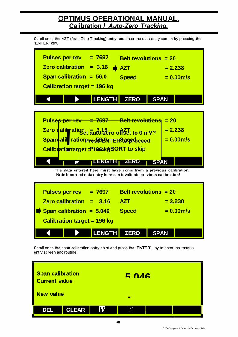
95
CAD Computer I:/Manuals/Optimus-Belt
OPTIMUS OPERATIONAL MANUAL.
rev = 7697 Belt revolutions
ation = 3.16 AZT
ration = 56.0 Speed
target = 196 kg
es per
alibr
calib
ration
SPAN
Span calibration
52.871
New value —
c
! Set auto-zero offset to 0 mV?
Press ENTER to proceed
Press ABORT to skip
Puls
Zero
Span
Calib
= 20
= 2.238
= 0.00m/s
LENGTH ZERO
Calibration / Auto-Zero Tracking.
Scroll on to the AZT (Auto Zero Tracking) entry and enter the data entry screen by pressing the
“ENTER” key.
The data entered here must have come from a previous calibration.
Note Incorrect data entry here can invalidate previous calibra tion!
Scroll on to the span calibration entry point and press the “ENTER” key to enter the manual
entry screen and routine.
Span calibration 5.046
Current value
New value -
DEL CLEAR
Pulses per rev = 7697
Zero calibration = 3.16
Span calibration = 5.046
Belt revolutions = 20
AZT = 2.238
Speed = 0.00m/s
Calibration target = 196 kg
LENGTH ZERO SPAN
Pulses per rev = 7697
Zero calibration = 3.16
Span calibration = 56.0
Belt revolutions = 20
AZT = 2.238
Speed = 0.00m/s
Calibration target = 196 kg
LENGTH ZERO SPAN

96
CAD Computer I:/Manuals/Optimus-Belt
OPTIMUS OPERATIONAL MANUAL.
Calibration / Target Weight.
The calibration target weight should be entered here. Web-Tech will normally supply the
target weight along with the static weights or calibration chain required to produce a
target weight. The target weight is that weight that that Optimus should equate t o when
the belt is run over the prescribed number of belt revolution with either a static weight or
calibration chain. See “Theory of Operation/ Steps in the Calibration Procedure.”
To enter the target weight modify screen, press the “ENTER” key when the selector arrow is
along side the entry point.
Calibration target (in kg)
Current value 5.046
New value —
DEL CLEAR
At this point enter the new target weight and press the tick key to lock in the value.
No access is provided to the speed display. As the belt speed is a derived variable.
Pulses per rev = 7697
Zero calibration = 3.16
Span calibration = 56.0
Belt revolutions = 20
AZT = 2.238
Speed = 0.00m/s
Calibration target = 196 kg
LENGTH ZERO SPAN
Pulses per rev = 7697
Zero calibration = 3.16
Span calibration = 56.0
Belt revolutions = 20
AZT = 2.238
Speed = 0.00m/s
Calibration target = 196 kg
LENGTH ZERO SPAN

97
CAD Computer I:/Manuals/Optimus-Belt
OPTIMUS OPERATIONAL MANUAL. Calibration / Pulses per Revolution / auto capture.
Automatic Capture of Pulses per Revolution.
(Note Web-Tech will have done the following prior to delivery)
At this point the user who is calibrating the system should identify or make a easy to see mark
on the belt. The mark in conjunction with a fixed reference point on the weigher will be used as
a visual aid in determining the point where Optimus will be commanded to start counting pulses
This pulses come from the encoder/tachometer. The mark passing the static reference point
Press the “LENGTH” F3 key to go to the pulse acquisition routine. The screen will change to the
one shown below.
This calibration is carried out with the belt moving. The number of complete belt revolutions
over a time period are counted by the operator, and the Optimus counts the pulses returned
from the speed sensor device the number or belt revolutions being entered in an other screen.
The screen below is a pause screen allowing the operator to ready before starting the routine.
Use a mark on the belt to reference the belt revolutions
START BACK
Press the “START” button, the F1 key, when the mark on the belt coincides with the stationary
reference point. The display will change to the one shown below and Optimus will be capturing
pulses. When the belt has travelled at least 5 belt revolutions with a minimum time of 5
minutes. Stop the count when the mark on the belt coincides with the static reference.
Press STOP after an exact number of belt revolutions
Elapsed time = 360 secs
Pulses counted = 8700
START BACK
Pulses per rev = 7697
Zero calibration = 3.16
Span calibration = 56.0
Belt revolutions = 20
AZT = 2.238
Speed = 0.00m/s
Calibration target = 196 kg
LENGTH ZERO SPAN

98
CAD Computer I:/Manuals/Optimus-Belt
OPTIMUS OPERATIONAL MANUAL. Calibration / Pulses per Revolution / auto capture.
After using the STOP key (F1) the screen will change to the one shown below. The screen
shows all the relevant data relating to the pulse input and provides the link to the entry Pressing
the “ENTER”
Tachometer calibration is now complete!
Belt revolutions = 20 Belt revolutions = 20
Calibration time = 300s Pulses per rev = 5400
At this point the number of belt revolutions over which Optimus captured the pulses must be
entered.
Note Only whole belt revolutions must be used and the exact number of revolutions must be
entered. Press the tick key to proceed.
At this point Optimus has the data required in order to perform a “manual zero and span”
Pulses per rev = 7697
Zero calibration = 3.16
Span calibration = 56.0
Belt revolutions = 20
AZT = 2.238
Speed = 0.00m/s
Calibration target = 196 kg
LENGTH ZERO SPAN

99
CAD Computer I:/Manuals/Optimus-Belt
OPTIMUS OPERATIONAL MANUAL. Calibration / Zero.
Calibration Zero
At this point pressing the F4 key located under the “LENGTH”, will take the user to the screen
where the weigher can be readied for zeroing.
Enter the “Zero” screen by pressing the “ZERO” (F4) button.
Press START to begin zero calibration. Press BACK to return to calibration menu. Belt must be empty during zero calibration.
Load cell = 3.856 Rate = 0.189kg/min
START BACK
The zero function will not start until the F1 key located under the “START”
The Zero will now be calculated over the number of belt revolutions previously entered.
The Number of belt revolutions performed, the percentage of the test completed , the load cell
output and calculated rate is displayed during the test.
When the test is complete, at the end of the prescribed number of belt revolutions the display
will stop updating.
BACK
Press BACK to return to the calibration menu. Make sure there is no material on the belt during test.
Belt revolutions = x.x Calibration x% complete
Load cell = x.xx mV Rate x.xxkg/hour
Instantaneous Loadcell output Percent Cal
Completed. Number of revs Completed.
Mass rate before zero cal is complete
Pulses per rev = 7697
Zero calibration = 3.16
Span calibration = 56.0
Belt revolutions = 20
AZT = 2.238
Speed = 0.00m/s
Calibration target = 196 kg
LENGTH ZERO SPAN

100
CAD Computer I:/Manuals/Optimus-Belt
OPTIMUS OPERATIONAL MANUAL. Calibration / Zero.
Following the completion of the zero test. The screen will change to the one shown below. The
three top lines of text will be alternating. If for any reason the test was deemed to be invalid
(material falling onto the belt during test etc) pressing the cross button will cancel the result.
On pressing the tick key thee alternating. If for any reason the test was deemed to be invalid
(material falling onto the belt during test etc) pressing the cross button will cancel the result.
Load Cell Zero Cal is now complete. Press?? to save new calibration.
Press to discard new data.
Totaliser Error = x.xxx kg Zero Cal = xx.xx mV. AZT Contribution = xx.xx mV.
CALIBRATION SCREEN.
Pulses per rev = 7697
Zero calibration = 3.16
Span calibration = 56.0
Belt revolutions = 20
AZT = 2.238
Speed = 0.00m/s
Calibration target = 196 kg
LENGTH ZERO SPAN

101
CAD Computer I:/Manuals/Optimus-Belt
OPTIMUS OPERATIONAL MANUAL. Calibration / Span Static Weight Test.
Enter the “SPAN” screen by pressing the “ZERO” (F5) button.
The screen will change the one shown below. The test will not start until the
“START” (F1) key has been pressed. Prior to starti ng the test the belt must be running
and the weight positioned on the weigher. At this point Optimus provides for two
methods of spanning. An empirical method or simulated load (fixed weight or calibration
chain). Select either by pressing the “START” (F1) key for fixed weight or “EMP” for
empirical. The following explains simulated load, (fixed weight / roller calibration chain).
Place calibration weights in position. Press BACK to return to return to calibration menu.
Press EMP to perform material calibration. Press START to begin span calibration.
Calibration period = 25 revs Calibration target = xx.xxkg. Mass rate = xx.xxkg/min.
START BACK EMP
Press the “START” (F1) key to start the test, if the simulated load, (fixed weight / roller
calibration chain), static weight te st is to be performed.
The screen will change to the one shown below.
Calibration rate = xx.xx kg/min
Belt revolutions = x.x x% complete
Calibration total = x.xx kg
Calibration target = xx.xx kg
BACK
The screen displays the current mass rate, the number of belt revolutions completed, the
% of the test completed. The total achi eved in real time and the total that the test should
achieve (Target Weight). On completion of the test Optimus will change the screen.
Pulses per rev = 7697
Zero calibration = 3.16
Span calibration = 56.0
Belt revolutions = 20
AZT = 2.238
Speed = 0.00m/s
Calibration target = 196 kg
LENGTH ZERO SPAN
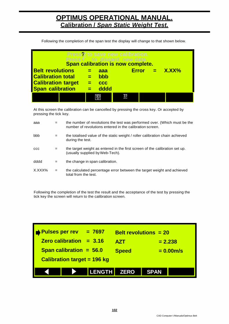
102
CAD Computer I:/Manuals/Optimus-Belt
OPTIMUS OPERATIONAL MANUAL. Calibration / Span Static Weight Test.
Following the completion of the span test the display will change to that shown below.
Press?? to save new calibration. Press to discard new data. Span calibration is now complete.
Belt revolutions = aaa Error = X.XX% Calibration total = bbb Calibration target = ccc Span calibration = dddd
At this screen the calibration can be cancelled by pressing the cross key. Or accepted by
pressing the tick key.
aaa = the number of revolutions the test was performed over. (Which must be the
number of revolutions entered in the calibration screen.
bbb = the totalised value of the static weight / roller calibration chain achieved
during the test.
ccc = the target weight as entered in the first screen of the calibration set up.
(usually supplied by Web-Tech).
dddd = the change in span calibration.
X.XXX% = the calculated percentage error between the target weight and achieved
total from the test.
Following the completion of the test the result and the acceptance of the test by pressing the
tick key the screen will return to the calibration screen.
Pulses per rev = 7697
Zero calibration = 3.16
Span calibration = 56.0
Belt revolutions = 20
AZT = 2.238
Speed = 0.00m/s
Calibration target = 196 kg
LENGTH ZERO SPAN

103
CAD Computer I:/Manuals/Optimus-Belt
OPTIMUS OPERATIONAL MANUAL. Calibration / Span Empirical.
The “EMPIRICAL” span test allows the user to run material over the belt and adjust the span
against the actual weight passed. The preferred methodology is to pass material over the belt
and collect it for weighing on an accurate static scale. This weight “total from an other source” is
entered in Optimus
Place calibration weights in position. Press BACK to return to return to calibration menu.
Press EMP to perform material calibration. Press START to begin span calibration.
Calibration period = 25 revs Calibration target = xx.xxkg. Mass rate = xx.xxkg/min.
START BACK EMP
Press the F3 “EMP” key which will open the screen shown below.
Press the “ENTER” key in the above screen to enter the data input screen.
Total from other source (in Kg)
Current value ZZZ.ZZ
New value YYY.YY
DEL CLEAR
At this screen enter the weight that passed over the weigher and that was weighed on an
accurate static weigher. (bench scale/weigh bridge etc). Press the tick key to proceed. Optimus
will return to the screen shown below. Press the F2 “NEXT” key to go to the data entry point.
Where the total obtained by Optimus is to be entered.
PREV NEXT
Enter total from an other source then press NEXT
Press PREV to return to previous screen.
Total from other source = xxx.xx kg
PREV NEXT
Enter total from an other source then press NEXT
Press PREV to return to previous screen.
Total from other source = xxx.xx kg

104
CAD Computer I:/Manuals/Optimus-Belt
OPTIMUS OPERATIONAL MANUAL. Calibration / Span Empirical.
PREV
PREV
NEXT
NEXT
Enter total from an other source then press NEXT
Press PREV to return to previous screen.
Enter belt scale total then press NEXT
Press PREV to return to previous screen.
Total from Optimus = xxx.xx kg
Total from Optimus = xxx.xx kg
At this point a new span needs to be generated. Press the F2 “NEXT” key to generate the new span and move on to the screen shown below.
Press the “ENTER” key to go to the data entry screen where the total obtained by Optimus can
be entered.
In the screen shown below enter the total obtained by Optimus
Total from Optimus (in Kg)
Current value UU.UU
New value VV.VV
DEL CLEAR
Press the tick key to lock in the data and move to the previous screen.
Empirical span now complete !
Press “” to save new calibration data.
Press “” to discard new calibration data.
Old span calibration = xx.xxx
New span calibration = yy.yyy
PREV
The above screen shows the new and old spans and allows for the acceptance or rejection of
the data. On pressing the tick key Optimus goes back to the calibration screen. The
EMPIRICAL span is now complete. Press the “HOME” key to transfer the data to working
memory.

105
CAD Computer I:/Manuals/Optimus-Belt
OPTIMUS OPERATIONAL MANUAL. MRMT SCREEN / Trend.
Optimus provides the user with a graphical view of the mass rate for the last two minutes. To
view the last two minutes of material flow press the “TREND” (F3) key to access the viewing
On entering the mass rate trend screen the last two minutes trend can be cleared by pressing
the “CLEAR” (F1) key.
Pressing the “HOME” key will return Optimus to MRMT.
100%
50%
0%
CLEAR
Mass Rate
[kg/min]
Mass Total
[kg]
CAL
950.0
702.0
SP Local
SP Rem
AZT On
PID
PID
Man
Auto
I / O TREND CLEAR SETUP INFO

106
CAD Computer I:/Manuals/Optimus-Belt
OPTIMUS OPERATIONAL MANUAL. MRMT SCREEN / Clear Total.
Rate
min] 950.0 Total
702.0 g]
The running total can be reset by pressing the “CLEAR” (F4) key.
Prior to clearing the total Optimus will ask for confirmation, prior to acting on the clear
command. Press “ENTER” to continue and clear the total. Or press the “ABORT” key if the total
should not be cleared.
SETUP INFO
! Clear accumulated mass total?
Press ENTER to proceed Press ABORT to skip.
Mass
[kg/
SP Local
SP Rem
AZT On
Mass
[k
CAL
PID Man
PID Auto
I / O TREND CLEAR
Mass Rate
[kg/min]
Mass Total
[kg]
CAL
950.0
702.0
SP Local
SP Rem
AZT
PID
On
Man
PID Auto
I / O TREND CLEAR SETUP INFO

107
CAD Computer I:/Manuals/Optimus-Belt
OPTIMUS OPERATIONAL MANUAL. MRMT SCREEN / Info Screen.
Turned on x times
Reset X times
Loaded defaults X times
Internal temperature xx.x° C
The Optimus firmware (operating software) is under constant review. As the firmware is
upgraded it’s build number is updated along with the date that it was completed. It may be
necessary to view this data from time to time. Press the “INFO” (F6) key to access the
information screen.
The screen bellow shows that the firmware release number was 125, dated 21 September 2003
Pressing the “RESET” (F1) from this screen will bring up the following screen. This screen
displays the number of times Optimus has had the power removed since the data was last
cleared. This is a useful tool if a faulty power supply (mains power) is suspected.
The reset display the number of times the reset button on the main CPU pcb has been
activated. Generally this button is used if the Optimus firmware has locked up, owing to a noise
spike or other severe transients. Pressing the reset will restart the firmware and increment this
counter.
If a “flash memory” card has been purchased and the firmware requires upgrading. The default
variables that were established during the calibration and setup can be stored in the flash card
and uploaded following the successful firmware upgrade.
CLEAR
The internal temperature is not the ambient air temperature in the cabinet. It is the temperature
at the core of the Central Processing Unit (CPU) / computer. The absolute max temp for this
device is 55°C. Do not exceed this temperature. Move the enclosure to a cooler environment.
Optimus MW1 Build 129 15-April-2003
© 2003 Web-Tech Australia Pty Ltd
RESET
Mass Rate
[kg/min] 950.0
702.0
SP Local
SP
AZT
Rem
On
Mass Total
[kg]
CAL
PID Man
PID Auto
I / O TREND CLEAR SETUP INFO

OPTIMUS OPERATIONAL MANUAL. Inlet Boot Hopper Setup
1
SETUP
Inlet Boot Hopper Setup
The following steps will ensure you have setup the Inlet boot hopper correctly
Following power up, Press SETUP (F5) key .The display will change to that shown below. The first entry to this portion of the menu structure will bring up the following screen. If no password has been selected, or the electronics is new, pressing the “ENTER” key will return the operator to MRMT screen where a subsequent entry to the Set Up menu will allow the user without a password to enter the menu structure.
Use the F1 / F2 keys to advance the curser to “9 Inlet Boot Hopper. Press the “ENTER” key to gain access.
1. System Configuration
2. Display and Time/Date
3. PID Loop Control
4. Auto Zero Tracking
5. Rate Deadband
6. Rate Display Filters
7. Save/Load Setup
8. Chute Level Control
F5
CAL I / O CLEAR SETUP
Mass Rate
[kg/hr] 0.0
Mass Total
[kg] 0.0
SP Local
SP Rem
AZT On
PID Man
PID Auto
TREND INFO
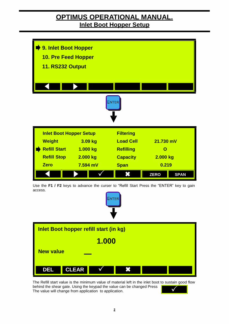
OPTIMUS OPERATIONAL MANUAL. Inlet Boot Hopper Setup
2
Inlet Boot hopper refill start (in kg)
1.000
New value —
Use the F1 / F2 keys to advance the curser to “Refill Start Press the “ENTER” key to gain access.
DEL CLEAR
The Refill start value is the minimum value of material left in the inlet boot to sustain good flow behind the shear gate. Using the keypad the value can be changed Press The value will change from application to application.
Inlet Boot Hopper Setup
Weight
Refill Start
Refill Stop
Zero
3.09 kg
1.000 kg
2.000 kg
7.594 mV
Filtering
Load Cell
Refilling
Capacity
Span
21.730 mV
O
2.000 kg
0.219
ZERO SPAN
9. Inlet Boot Hopper
10. Pre Feed Hopper
11. RS232 Output

3
OPTIMUS OPERATIONAL MANUAL. Inlet Boot Hopper Setup
Use the F1 / F2 keys to advance the curser to “Refill Stop. Press the “ENTER” key to gain access.
The Refill stop value is the maximum value of material left in the inlet boot to sustain good flow behind the shear gate. Using the keypad the value can be changed Press The value will change from application to application.
The material silhouette below shows a typical feed scenario.
Inlet Boot hopper refill stop(in kg)
2.000
New value —
DEL CLEAR
ZERO
Inlet Boot Hopper Setup
Weight
Refill Start
Refill Stop
Zero
3.09 kg
1.000 kg
2.000 kg
7.594 mV
Filtering
Load Cell
Refilling
Capacity
Span
21.730 mV
O
2.000 kg
0.219
SPAN

4
OPTIMUS OPERATIONAL MANUAL. Inlet Boot Hopper Setup
zero
SPAN
Inlet Boot hopper calibration weight (in kg)
New value —
Inlet Boot Hopper ZERO
Before running a zero calibration ensure that the inlet boot hopper is empty and the calibration weight is
removed.
To run a zero calibration on the inlet boot hopper. Firstly depress the key
Press ENTER when all weights are removed or ABORT to skip
The ‘Zero’ mV value will update in the left column.
Inlet Boot Hopper SPAN
Before running a span calibration ensure you have a weight approx 75% of the total hopper capacity.
To run a SPAN calibration on the inlet boot hopper. Firstly depress the key
DEL CLEAR
Place the calibration weight between the two arrows marked on the inlet boot.
Enter the weight of the calibration weight and press ENTER
ZERO SPAN
Inlet Boot Hopper Setup
Weight
Refill Start
Refill Stop
Zero
3.09 kg
1.000 kg
2.000 kg
7.594 mV
Filtering
Load Cell
Refilling
Capacity
Span
21.730 mV
O
2.000 kg
0.219
Perform hopper zero calibration? Press ENTER to Proceed
! Press ABORT to skip
ZERO SPAN
Inlet Boot
Hopper
Setup
Weight
3.09 kg
Filtering
Load Cell
21.730 mV
Refilling
O

To install a PC/104 DeviceNet card in Optimus
1. Install the DeviceNet module on the PC/104 stack. Use the four M3x6mm screws and
washers provided to hold the card firmly on the stack.
2. Wire the 5-pin plug to the DeviceNet cable as shown.
3. You must ensure that 1200.5W termination resistors are installed between CAN HI
and CAN LO at the two ends of the DeviceNet network. If the Optimus is the last device on the network, install the termination resistor directly into the plug.
4. Configure the DeviceNet MAC-ID and baud rate by entering screen 22 from the SETUP menu.
a. The MAC-ID can be set to any number between 1 and 63. Each device on the DeviceNet network must be assigned a unique MAC-ID.
b. The baud rate may be set to a speed of 125kHz, 250kHz or 500kHz. All devices on the DeviceNet network must be configured to used the same baud rate; the baud
rate chosen will depend on cable length and quality.
If you change either the MAC-ID or baud rate, you must press the CONFIG button in
order to write your changes to the Optimus DeviceNet module. Pressing TICK or HOME
will not save these settings. Once configured, the settings will be retained between
powerups.
GND
CAN LO
SHIELD
CAN HI
+24VDC

OPTIMUS OPERATIONAL MANUAL.
108
CAD Computer I:/Manuals/Optimus-Belt
Notes/Firmware Updates.

OPTIMUS OPERATIONAL MANUAL.
109
CAD Computer I:/Manuals/Optimus-Belt
Electrical / Electronic Notes/ digital outputs.
SSR Relay.
The Solid State Relay (SSR) is permanently assigned to the “Totaliser” output. The relay can be
physically configured to output +5VDC / +24VDC. The voltage is selected by means of jumpers
located at the bottom right hand corner of the “Terminal pcb (JP4) . The use of a solid state relay
provides for high frequency counts. However consideration should be given to the receivers ability
to handle high frequency counts.
All components mounted
on terminal pcb.
A D1
K D2
TB 19
Voltage selected
using JP4.
+5VDC / +24VDC.
PU / Pull Up, output.
Common.
Common.
N.O. Normally Open.
N.O. Normally Open.
Ground for 5&24VDC. RELAY 1 (SSR) Totaliser Output.
Electro-mechanical Relays. (RLY2 - 5)
Relays 2-6 are assigned via the keyboard (I/O / 4 Digital Outputs). When active the local red LED
will illuminated.
The relays can be used as “clean contacts” or supplied with on board +24VDC. Link between +24V
and COM. The return is to be terminated on GND.
All components mounted
on terminal pcb.
N.C.
N.O.
Relay (typical)
1 amp 240VAC resistive.
2 amp 110VAC resistive.
+24 VDC. Max 0.1 amp PLC
Inputs etc.
Common.
+24VDC.
Ground.
Ground.
+24V Selected. +5V
Common
+24V
+5V Selected.
+24V
+5V
Common
JP 4 JP 4

OPTIMUS OPERATIONAL MANUAL.
110
CAD Computer I:/Manuals/Optimus-Belt
TB 18 Digital inputs 1 / 6.
All components mounted on terminal pcb.
Electrical / Electronic Notes /digital inputs.
Digital Inputs.
Optimus has 6 general purpose digital inputs. They can be assigned to a range of pre– assigned
labels ((I/O) 3-Digital inputs). There electrical status can also be observed there also. The applied
voltage should not exceed 60VDC and the minimum switching voltage is 5 VDC. These inputs are
generally used for monitoring the status of the feeder.
The basic circuit along with an example of a typical connection is shown below.
SCREEN
5 +60 VDC INPUT
0 V
+5 - 48 VDC
Optimus 24VDC
Is available
P/S
TB 18 Digital inputs 1 / 6.
Feeder limit
switch/door etc
(typical)
All components mounted on terminal pcb. GND

SECTION 6 - CALIBRATION
The weighfeeder has been programmed and calibrated at the factory. However, due to changes that may have occurred during transit and installation, the weighfeeder calibration should be checked. The calibrations once initiated are automatic and only require the pressing of acceptance key(s).
The two basic calibration steps are the
“Zero” calibration and the “Span” calibration.
Zero Calibration
The zero calibration is established by
running the weighfeeder empty of a programmed number of belt revolutions and calculating the average load cell output during this period. The weighfeeder electronics will automatically calculate the zero value when the test has been initiated and completed. Refer to the electronics manual supplied with your WT1200 (Masterweigh 1/Masterweigh 5 or Optimus) for the section called “Load Zero Calibration” for the procedure. The weighfeeder must be able to be run empty during this test, and the number of belt revolutions programmed for its duration can be found on the calibration sheets at the end of this manual.
Span Calibration
The span calibration is generally carried out
on a model WT1200 weighfeeder with the use of calibration “chains”. The calibration chain consists of one or more strands of roller chain attached to a restraining bracket. The size of the chain and number of strands has been calculated by us to simulate approximately 75% of the maximum capacity. The calibration chain is placed on the belt and attached to the inlet chute (or rear wall for horseshoe inlet). The weighfeeder is run and the test is carried out over the same number of belt revolutions as the zero test. The result is compared to a value (Target Weight) calculated by us at the time of factory commissioning. The procedure for carrying out the test can be found in the “Fixed Weight Calibrate” menu of the electronics manual. The “Target Weight” can be found on the calibration sheets in this manual.
Material Test
We strongly suggest that a material test be
carried out where possible. A material test involves weighing product on an accurate static scale prior to, or after it has passed over the weighfeeder. When carrying out a material test, the following should be considered:
1. The amount of material required for the test(s) must be proportional to the weighfeeder capacity. A rule of thumb quantity would be a minimum of 3 minutes of running time at maximum capacity e.g. if the capacity is 10 tph, the amount of material would be 10 0000 kg/60 x 3 = 500 kg. A smaller amount could be used, however it must be understood that the accuracy achievable may be diminished due to the resolution used.
2. It must be guaranteed that all of the material used in the test is collected, or have passed over the weighfeeder.
3. The material feed over the weighfeeder must be continuous and consistent.
When the test(s) have been carried out any
correction to the calibration can be carried out in the “Emperical Calibration” menu of the electronics (refer to the electronics manual section).
Any changes to the calibration should be
recorded on the calibration sheets for future reference

A
OPTIMUS – INSTALLATION AND OPERATION GUIDE
Appendix A – WTS1S2 General Arrangements

2

3

4

5

B
WTS1S2 INSTALLATION AND OPERATION MANUAL
Appendix B – Wiring Diagrams

3

4

5

6

7

8

9

C
WTS1S2 – INSTALLATION AND OPERATION MANUAL
Appendix C – Electrical Enclosure GAs

4

5

6

D
WTS1S2 – INSTALLATION AND OPERATION MANUAL
Appendix D – Belt Scale Positioning Guide

5

6
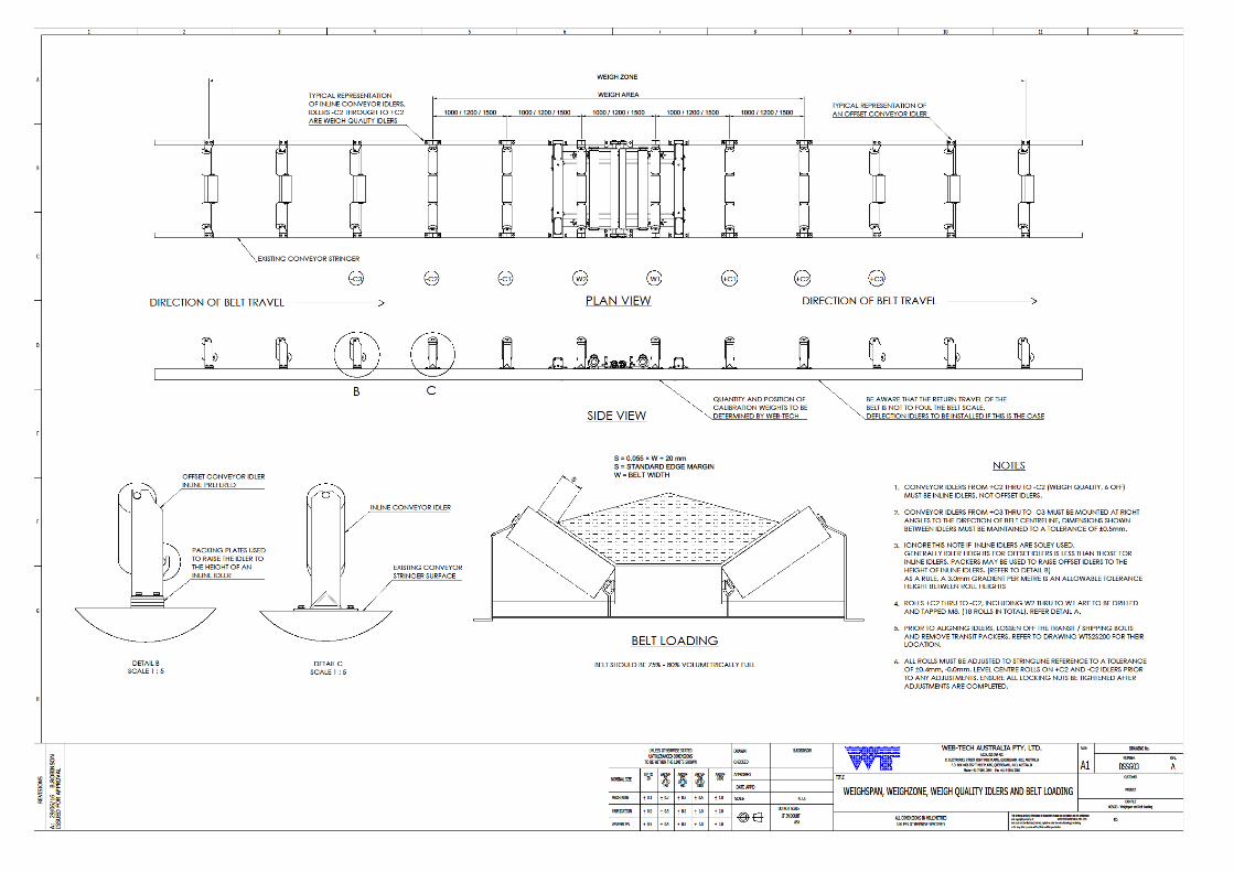
7

8

9

E
WTS1S2 – INSTALLATION AND OPERATION MANUAL
Appendix E – Optimus Datasheets
WEB-TECH WEIGHFEEDER DESIGN DATA
SHEET
CLIENT : DATE :
DESIGNATION : MODEL
CALIBRATION METHOD : BAR(S) / CHAIN
CALIBRATION BAR(S)
1. CALIBRATION BAR QTY AND TOTAL WEIGHT =
2. IDLER PITCH
3. TOTAL WEIGH AREA metres
4. EQUIVALENT LOADING/M WITH CAL BAR(S) (Item 1 x 1/Item 3) =
5. BELT SPEED m/s
6. SIMULATED MASS RATE (Item 4 x Item 5 x 3600 ) = kg/hr
7. BELT LENGTH metres
8. No. OF BELT REVOLUTIONS FOR TEST
9. TARGET WEIGHT ( Item 4 x Item 7 x Item 8 ) = kgs
CALIBRATION CHAIN
1. WEIGHT OF CALIBRATION CHAIN PER STRAND kg/m
2. No. OF STRANDS
3. TOTAL WEIGHT OF CALIBRATION CHAIN (Item 1 x Item 2 ) kg/m
4. BELT LENGTH m
5. No. OF BELT REVOLUTIONS FOR TEST
4. TARGET WEIGHT ( Item 3 x Item 4 x Item 5 ) = kgs

OPTIMUS CALIBRATION DATA Customer : Conveyor Designation :
Material : Model :
Load Cell: Tacho :
Serial No: Software Build :
Date :
Data By :
Contract No :
SETUP MENU
1. System Configuration Units of Measurement:
Belt Capacity
Resolution
Belt Length
Maximum Loading
kg/m
2. Time & Date Backlight
Brightness
Contrast
Date
Time
3. PID Parameters 1 Setpoint Origin / Status
2 Output Status
3 PID Parameters
Prop Band
Integral Lower Limit
Derivative Time
Feed Forward
5 PID Mass Rate Filter
Time Constant
Fast Track Threshold
6 Volumetric Restart
Restart Period
Restart Threshold
Reset Rate
Integral Upper Limit
Output Offset
4. Auto ZeroTracking Auto Zero Tracking
Threshold
Delay
Current Contribution
Period
5. Rate Deadband Mass Rate Dead Band Belt Capacity
6. Rate Display Filters Mass Rate Display Filter
Time Constant
Mass Rate Trend Filter
Time Constant
Fast Track Threshold
Fast Track Threshold
8. Chute Level Control
None
Low
Mid
High
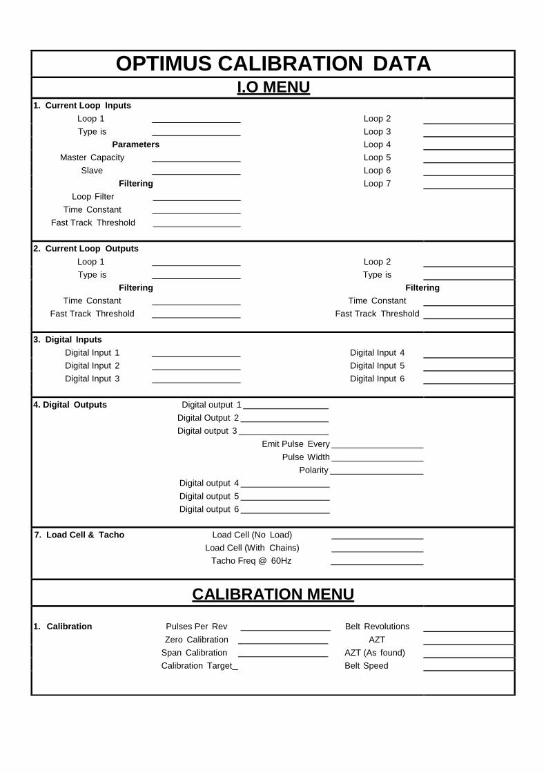
OPTIMUS CALIBRATION DATA I.O MENU
1. Current Loop Inputs
Loop 1 Loop 2
Type is Loop 3
Parameters Loop 4
Master Capacity Loop 5
Slave Loop 6
Filtering Loop 7
Loop Filter
Time Constant
Fast Track Threshold
2. Current Loop Outputs
Loop 1 Loop 2
Type is Type is
Filtering Filtering
Time Constant Time Constant
Fast Track Threshold Fast Track Threshold
3. Digital Inputs
Digital Input 1 Digital Input 4
Digital Input 2 Digital Input 5
Digital Input 3 Digital Input 6
4. Digital Outputs Digital output 1
Digital Output 2
Digital output 3
Emit Pulse Every
Pulse Width
Polarity
Digital output 4
Digital output 5
Digital output 6
7. Load Cell & Tacho Load Cell (No Load)
Load Cell (With Chains)
Tacho Freq @ 60Hz
CALIBRATION MENU
1. Calibration Pulses Per Rev Belt Revolutions
Zero Calibration AZT
Span Calibration AZT (As found)
Calibration Target Belt Speed