Worst-case Structural Analysis

Qingnan Zhou∗, Julian Panetta†, and Denis Zorin‡New York University

Input Modal Analysis Weak Region Extraction Stresss Optimization Weakness Map

Figure 1: Overview of the steps of the algorithm

Abstract

Direct digital manufacturing is a set of rapidly evolving technolo-gies that provide easy ways to manufacture highly customized andunique products. The development pipeline for such products isradically different from the conventional manufacturing pipeline:3D geometric models are designed by users often with little or nomanufacturing experience and sent directly to the printer. Structuralanalysis on the user side with conventional tools is often unfeasibleas it requires specialized training and software. Trial-and-error, themost common approach, is time-consuming and expensive.

We present a method that would identify structural problems inobjects designed for 3D printing based on geometry and materialproperties only, without specific assumptions on loads and manualload setup. We solve a constrained optimization problem to deter-mine the “worst” load distribution for a shape that will cause highlocal stress or large deformations. While in its general form this op-timization has a prohibitively high computational cost, we demon-strate that an approximate method makes it possible to solve theproblem rapidly for a broad range of printed models. We validateour method both computationally and experimentally and demon-strate that it has good predictive power for a number of diverse 3Dprinted shapes.

CR Categories: I.3.5 [Computer Graphics]: Computational Ge-ometry and Object Modeling—[Physically based modeling]; J.6[Computer-Aided Engineering]: Computer-aided design—.

Keywords: structural analysis, digital manufacturing

Links: DL PDF

∗e-mail: qnzhou@cs.nyu.edu†e-mail: jpanetta@cs.nyu.edu‡e-mail: dzorin@cs.nyu.edu

1 IntroductionWe present an algorithm approximating the solution of the follow-ing problem: From the shape of an object and its material proper-ties, determine the easiest (in terms of minimal applied force) waysto break it or severely deform it.Our work is largely motivated by applications in 3D printing. Thecost of 3D printing has come down significantly over the past fewyears, and the industry is undergoing a rapid expansion, makingcustomized manufacturing in an increasingly broad variety of ma-terials available to a broad user base. While many of the users areexperienced creators of digital 3D shapes, engineering design ex-pertise is far less common, and widely used 3D modeling tools lackaccessible ways to predict mechanical behavior of a 3D model.There are a number of reasons why a 3D model cannot be manu-factured or is likely to fail:(1) the dimensions of thin features (walls, cylinder-like features,etc.) are too small for the printing process, resulting in shape frag-mentation at the printing stage;(2) the strength of the shape is not high enough to withstand gravityat one of the stages of the printing process;(3) the printed shape is likely to be damaged during routine han-dling during the printing process or shipment;(4) the shape breaks during routine use.In most cases, the first problem is addressed by simple geometricrules ([Telea and Jalba 2011]), and the second is a straightforwarddirect simulation problem. Our focus is on the other two problems.On the one hand, many 3D printed objects are manufactured witha specific mechanical role in mind, and full evaluation is possibleonly if sufficient information on expected loads is available. On theother hand, jewelry, toys, art pieces, various types of clothing, andgadget accessories account for a large fraction of products shippedby 3D printing service providers. These objects are often expectedto withstand a variety of poorly defined loads (picking up, acciden-tal bending or dropping, forces during shipping, etc.).To predict structural soundness of a printed object, we look forworst-case loads, within a suitably constrained family, that are mostlikely to result in damage or undesirable deformations. A direct for-mulation results in difficult nonlinear and nonconvex optimizationproblems with PDE constraints. We have developed an approxi-mate method for this search, reducing it to an eigenproblem and asequence of linear programming problems.We demonstrate experimentally that our approach predicts thebreaking locations and extreme deformations quite well. While pri-marily designed for 3D printing applications, our method can be

applied in any context where loads are unpredictable and structuralweaknesses need to be identified.

2 Related workComputational analysis of structural soundness of mechanical partsand buildings is broadly used, but almost always in the context ofknown sets of loads. While engineers routinely need to evaluatesoundness of structures and mechanisms under worst-case scenar-ios, in most cases, worst-case loads are designed empirically forspecific problems (e.g., construction of buildings to withstand loadsfrom flooding or earthquakes). Automatic methods are less com-mon: an important set of methods in the context of modeling un-der uncertainty is based on the idea of anti-optimization (e.g., [El-ishakof and Ohsaki 2010]), our work is partially inspired by theseconcepts.In aerospace engineering, filter-based methods were developed topredict worst-case gusts and turbulence encountered by an airplane.E.g., [Zeiler 1997; Fidkowski et al. 2008] model the aircraft’s re-sponse to turbulence as a linear filter’s response to Gaussian whitenoise. From this model, a worst-case noise sample and resultingstrain are obtained.In the context of analysis tailored for 3D printing applications of thetype considered in this paper, the closest work to ours is [Stava et al.2012]. The paper proposes to evaluate 3D shapes in two main sce-narios to discover structure weakness: applying gravity loads andgripping the shape using 2 fingers at locations predicted by a heuris-tic method. This set of fixed usage scenarios is often insufficient toexpose the true structure weakness for many printed shapes, as dis-cussed in greater detail in Section 5. The paper also describes meth-ods for automatic improvement of objects. [Telea and Jalba 2011]focuses on purely geometric ways to evaluate whether a structureis suitable for 3D printing based on empirical rules formulated bythe 3D printing industry ([Z CORPORATION 2011], [Shapeways2011]).Structural stability for simple furniture constructed from rigidplanks connected by nails is analyzed at interactive rates in[Umetani et al. 2012]. Their system also suggests corrections whenshapes with poor stability are detected.A number of recent works address various aspects of computationaldesign for 3D printing. [Bickel et al. 2010] provide a pipeline toprint objects in a composite material that reproduces desired defor-mation behavior. To achieve this goal, the authors accurately modelthe nonlinear stress-strain relationship of their printing materialsand how printed models will respond to imposed loads. The spaceof deformations is a user-supplied input, and structural soundnessof the design with respect to other loads is not considered. Whilesome specialized work on CAD for 3D printing exists, (e.g., thesystem for heterogeneous material design [Kou and Tan 2007]),overwhelmingly, standard tools with little or no analysis supportare used.[Luo et al. 2012] proposes a framework to decompose 3D shapesinto smaller parts that can be assembled without compromising thephysical functionality of the shape so that larger objects can beprinted using printers with a small working volume. They use astandard finite element simulation to estimate stress of the inputshape under gravity in a user specified upright orientation. Otherworks aim to print articulated models that maintain poses undergravity but do not require manual assembly. [Calı et al. 2012] de-signs and fits a generic, parametrized printable joint template basedon a ball and socket joint. Their joint provides enough internal fric-tion and strength to hold poses and survive manipulation, but theytune its parameters experimentally instead of using a physically-based optimization. [Bacher et al. 2012] designs a similar ball andsocket joint and a hinge joint. An approximate geometric optimiza-tion of stresses is performed by maximizing certain cross-sectionalareas of the joint.3D printing has also been used to reproduce appearance: [Hasan

et al. 2010] and [Dong et al. 2010] optimize the layering of basematerials in a 3D multi-material printer to print objects whose sub-surface scattering best matches an input BSSRDF.Our method relies on using eigenmodes of the shape. Modal analy-sis has proven useful in many contexts. The use of Laplacian eigen-modes of simple shapes for computation predates computers [Tim-oshenko and Woinowsky-Krieger 1940] and has a long history inmodel order reduction for a variety of applications including non-linear elasticity (e.g., [Nickell 1976]). In graphics literature, [Pent-land and Williams 1989] first introduced eigenmodes as a basissuitable for simulation applications, and more recently, a numberof deformation-related algorithms based on eigenmode bases wereproposed, e.g., [Hauser et al. 2003; Barbic and James 2005; Barbicand James 2010].At the same time, experimental modal analysis (applying periodicforces with different frequencies and measuring displacements atvarious points) is broadly used to detect structural damage [Ewins2000].Finally, [Pratt et al. 1998] presents an overview of several simu-lations and experiments exploring how printing parameters (buildorientation, layer thickness, scan path and speed, temperature, etc.)affect the accuracy and strength of simple shapes. The goal of theseworks is to evaluate and improve printing technology itself ratherthan detecting or fixing deficiencies in the input shape.

2.1 3D printing processes

To motivate the design of our structural analysis process, we brieflyreview the most commonly used 3D printing processes and thetypes of structural problems one can expect. The most relevant as-pects of 3D printing processes for structural analysis are the me-chanical characteristics of materials produced at different stagesand typical loads on the object during and after the production pro-cess.Common single-stage 3D printing processes either deposit the liq-uid material only in needed places (e.g., FDM) or deposit materialin powder form layer-by-layer and then fuse or harden it at pointsinside the object (e.g., stereolithography uses photosensistive poly-mers, and laser sintering fuses regular polymers by heat).These processes typically use flexible polymers with large elas-tic and plastic zones in their stress-strain curves. These polymersrarely break if geometric criteria for printability are satisfied, butthey can undergo large plastic deformations.Printing metal, ceramics, and composite materials often involvesmultiple stages. For example, the object may be printed layer-by-layer in metal powder with polymer binder. At the next stage, thebinder is cured in a furnace, resulting in a green state part, andat the last stage, the metal is fused in a furnace and extra metalis added. Green state is brittle and has low strength, so parts inthis state are easily damaged. A simpler multistage process is usedfor relatively brittle composite materials, e.g., gypsum-based mul-ticolor materials; a second curing stage is used to give the materialadditional strength. Both the green state and the final material arerelatively brittle. Whenever binding polymer is mixed layer-by-layer with a different material, the resulting material is likely to behighly anisotropic.To summarize, both brittle and ductile materials are of importance.The former requires predicting where the material is likely to break,and the latter requires predicting extreme deformations likely to be-come plastic. Due to the layer-by-layer nature of the printing pro-cess, anisotropy is common and needs to be taken into account.Some of the loads even during production stages are hard to predictand quantify.Goals. These considerations lead to several possible structural anal-ysis goals, unified by a common theme of identifying worst-caseloads in a family of loads satisfying some constraints (bounds ontotal force, pressure, direction etc.). The worst-case load is under-stood to be the one that leads to maximal damage, which can be

measured by a norm of stress, maximal displacements, and variousfunctions of these quantities.

3 Worst-case structural analysisNext, we present a formal description of the problem. This formula-tion is computationally intractable, but it is needed as a foundationfor a practical approximate version described in Section 4.Linear elasticity. We use an anisotropic linear material model andthe linear elasticity equations to model object behavior for the pur-poses of determining weak spots and worst-case force distributions.This model is adequate for some materials used in 3D printing,but nonlinear models may be necessary for others, as discussed ingreater detail in Section 6. We emphasize that a distinction shouldbe made between simulation with given loads used to determineprecise stress distributions and computation used to determine ap-proximate worst-case loads: lower accuracy is acceptable for thelatter. We briefly review the standard elasticity equations to intro-duce notation. The stress-strain relationship is linear, and stress isrelated linearly to displacement:

σ = C : ε ε =1

2

“∇u +∇uT

”(1)

where ε is the strain tensor, σ is the stress tensor, and u is the dis-placement. C is the rank-4 elasticity tensor, Cijlm, and the no-tation C : ε denotes application of this tensor to the strain tensorε,

Pl,m Cijlmεlm. We discuss the choice and effects of elasticity

tensor C in greater detail in Section 6. We assume an orthotropicmaterial, for which the tensor Cijlm has up to 9 independent pa-rameters. In a coordinate system aligned with material axes, if werepresent C as as a 6 × 6 matrix acting on vectors of componentsof the symmetric strain tensors [ε11, ε11, ε33, 2ε23, 2ε31, 2ε12], itsinverse is given by26664

1Y1

− ν21Y2

− ν31Y3

0 0 0

− ν12Y1

1Y2

− ν32Y3

0 0 0

− ν13Y1

− ν23Y2

1Y3

0 0 0

0 0 0 1/G23 0 00 0 0 0 1/G31 00 0 0 0 0 1/G12

37775where Yi are directional Young’s moduli, Gij are shear moduli, andνij are Poisson ratios for different pairs of directions, satisfyingνij/Yi = νji/Yj .For dynamic linear problems with volume force density F , theequation of motion is

∇ · σ = F + ρu, (2)

where ρ is the density, and the dot signifies the time derivative. Weare primarily interested in static problems, but as we use modalanalysis at an intermediate stage, we retain the term ρu.Equation 2 is subject to boundary conditions: we primarily use asurface force density FS , which is captured by the condition σn =−FS on the boundary of the object. If the object is attached to arigid support, Dirichlet conditions u = 0 can be imposed on a partof the boundary.If the equation of motion (2) is written directly in terms of displace-ment u, we get

∇ ·„

C :1

2(∇u +∇uT )

«:= Lu = F + ρu. (3)

Rigid motion, torque and translation constraints for staticproblems. If the object is not fixed at least at 3 non-collinear points,an arbitrary force distribution will result in motion of the whole ob-ject. As we are interested in considering unknown forces with noassumptions on attachment, we need to be able to eliminate global

motion. We achieve this by imposing zero total force and zero totaltorque constraints, which can be written as

ZΩ

FdV +

Z∂Ω

FSdA = 0,ZΩ

F × (x− xc)dV +

Z∂Ω

FS × (x− xc)dA = 0.

(4)

Displacements enter into this system only in the form Lu, and theoperator L has infinitesimal rigid motions in its nullspace. To havea unique solution in u, we impose a zero rigid motion constraint,similar to total torque and force constraints:Z

Ω

udV = 0,

ZΩ

u× (x− xc)dV = 0. (5)

Surface force model. In cases of interest, the only volume forceis gravity. In all but most extreme cases, gravity does not have amajor effect, so we concentrate on surface forces. We restrict theforces in three ways.• Only positive normal forces allowed: FS = −pn, where n

is the surface normal, and p is pressure, thus ignoring fric-tion. This is an important assumption, as for most situationsdescribed in Section 2.1, friction forces are likely to be signif-icantly lower than normal forces. At the same time, it is hardto model the bounds on ratios between normal and tangentialcomponents accurately in the absence of detailed knowledgeof loads and surfaces. Without such bounds, any optimizationis likely to produce unrealistic tangential results. Similarly,negative surface forces (e.g., electrostatic attraction), are notlikely to play a major role and are excluded.

• Pointwise pressure is bounded: p < pmax. If a pressure maybe unbounded, an arbitrarily high stress may be produced ata point on the surface. While highly concentrated forces arepossible, these are rare, and we assume that a realistic boundon surface pressure is available.

• The total force is fixed. Again, by increasing the total force,arbitrarily high stresses can be obtained.

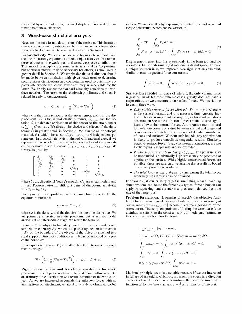
For example, if our primary target is simulating manual handlingsituations, one can bound the force by a typical force a human canapply by squeezing, and the maximal pressure is derived from thesize of the finger tips.Problem formulation. It remains to specify the objective func-tion. One commonly used measure of interest is maximal principalstress, maxΩ maxi=1,2,3 |σi|, where σi are the eigenvalues of thestress tensor. The complete problem of finding the worst-case forcedistribution satisfying the constraints of our model and optimizingthis objective function, has the form

maxΩ

maxi=1,2,3

|σi| → max;

Lu = 0 on Ω, C : (∇u +∇uT )n = pn on ∂Ω,Z∂Ω

pndA = 0,

Z∂Ω

pn× (x− xc)dA = 0,ZΩ

udV = 0,

ZΩ

u× (x− xc)dV = 0,

0 ≤ p ≤ pmax on ∂Ω,

Z∂Ω

pdA = Ftot.

(6)

Maximal principle stress is a suitable measure if we are interestedin failure of materials, which occurs when the stress in a directionexceeds a bound. For plastic transition, the norm or some otherfunction of the deviatoric stress, σ − 1

3trσI , may be of interest.

We make an interesting observation when the material is isotropicand C can be written as Y C, where Y is the Young’s modulus, andC is nondimensional, depending only on the Poisson ratio. Thenmaximal stress does not depend on Y but only on the Poisson ratio.Solving this problem yields the worst-case principal stress and, im-portantly, the pressure distribution on the surface resulting in thisstress. The maximal stress makes it possible to evaluate the like-lihood of damage during the production process, shipping or use.Examining the pressure distribution makes it possible to evaluatehow likely such loads would be and determine how the structure ofthe object can be strengthened.We observe that all constraints in this problem are linear equalityand inequality constraints, i.e., the constraints are convex. At thesame time, the functional is highly non-linear (in fact, not smooth)and non-convex. Replacing maximal principal stress with anotherpoint measure maximized over the surface does not change the na-ture of the problem.A brute-force solution can be obtained by solving a sequence ofproblems in which the objective functional max |σi|2 is maximizedfor every point and then taking the maximum of all results. Becausewe are interested in maximizing the norm, even these simpler per-point problems remain nonconvex and nonlinear.We conclude that solving the optimization problem in general formis impractical, and due to non-linearities and non-convexity, anyoptimization is likely to get stuck in local minima.Extension to displacements. An obvious extension of the algo-rithm is optimizing for maximal displacements. The main changeis replacing σ with u in the functional: maxΩ |u| → max. Thisformulation is more relevant for flexible materials.

4 Efficient approximate algorithm

Overview. Figure 1 shows the main components of the efficientapproximate algorithm for solving (6).There are two problems we need to address to make the solution of(6) practical: (1) the need to solve an optimization problem for eachpoint of the object to determine which one results in minimal stress;and (2) the nonlinearity and nonconvexity of each subproblem.To address the first problem, we use a modal-analysis based heuris-tic that we found to work remarkably well. The second problem issolved by using tr σ as the linear objective functional. The reasonsthis substitution is possible for a broad range of cases are discussedin detail below.Modal analysis and weak regions. A crucial ingredient of ourmethod is modal analysis, which we use to restrict the part of theobject where we need to maximize the stress or another functional.Computational modal analysis refers to computing eigenvectors(eigenmodes) ui and eigenvalues λi of L:

Lui = λiui, i = 1, 2 . . . (7)

It is widely used in engineering and graphics for a variety of pur-poses. In the context of structural analysis, the most common ap-plication of modal analysis is to predict possible damage or defor-mations in presence of vibrations.Our idea is similar in spirit, however there is a significant differ-ence. We do not consider vibrations, i.e., periodically changingloads; rather, we consider static or quasi-static loads. We make thefollowingAssumption 1: Examining a small number of eigenmodes allowsus to find all regions of an object where the stress may be highunder arbitrary deformation. While this observation is difficult toprove mathematically, physical intuition suggests that vibrations ofan object at different frequencies will result in high stress in allstructurally weak regions of the object. Weak regions are those

where high maximal stress can be obtained with low energy den-sity relative to other parts of the object.

To validate this assumption, we have performed a brute-force opti-mization on a number of models (Figure 7) and compared with theresults obtained using weak regions only. We obtain a remarkablygood agreement in all cases.

We search for locations of potentially high stress by computing anumber, Mm, of eigenmodes and considering a fraction 1 − ε ofpoints with highest stress under these deformations.

We define weak regions to be the connected components of this set.Each mode has multiple weak regions, typically associated withlocal stress maxima. For each mode we select Mr weak regions.

Approximate convex problem. The second important change tothe problem is to replace the functional in (6) with a functional thatcan be optimized efficiently and that is minimized by a similar pres-sure distribution, p, to the original. We focus on the maximal stress,although a similar approach can be used for other functionals. Weobserve that almost invariably for any deformation and any com-pressible material with Poisson ratio ν sufficiently different from1/2:

For points where a principal stress is maximal, other principalstresses are small relative to the principal stress.

We have performed a validation of this observation by running sim-ulations with a variety of loads and computing the ratio of the max-imal principal stress to |tr σ|. Over 36 models tested, the averageratio is 0.96 with standard deviation 0.25. Figure 2 illustrate thatthe distributions of trace and maximal principle stress are visuallysimilar.

Figure 2: The top 10% volume of largest principal stress (left) andlargest trace (right) are visually similar

We observe that when this is true, the difference between |σmax| =maxi=1,2,3|σi| and |

P3i=1 σi|, i.e., |tr σ| is small, and we can ap-

proximate the maximal principal stress with the absolute value ofthe trace.

As weak regions correspond to the highest stress area, and esti-mated stress tends to have a significantly lower accuracy vs. dis-placement, we use a weighted average of the stress over each weakregion. The choice of weighting, as long as it falls off towards theboundary of the region, has relatively small effect on the result. Wechoose the L2 norm of the stress computed from the eigenmode asthe weight w for averaging the stress trace over each weak region.We also predict whether each point will stretch or compress underthe worst-case load by computing tr σ under the modal displace-ment. We choose w’s sign to match this quantity.

We finally arrive at the following approximate problem formula-tion:

For each eigenmode i, i = 1 . . . Mm and each of its weak regions,Dij , j = 1 . . . Mr , we solve the following linear programmingproblem:

Zwtr σdV → max w.r.t. u and p;

Lu = 0 on Ω, C : (∇u +∇uT )n = pn on ∂Ω,Z∂Ω

pndA = 0,

Z∂Ω

pn× (x− xc)dA = 0,

0 ≤ p ≤ pmax on ∂Ω,

Z∂Ω

pdA = Ftot.

(8)

Unlike the original problem, this problem has a unique solution thatcan be computed efficiently using a convex solver.Discretization and additional optimizations. We discretize theproblem in the simplest conventional way, using piecewise-linearfinite elements. The downside of this approach is that a suitabletetrahedral mesh needs to be generated for each input. For 3Dprinted models, the task is somewhat simplified: as the cost of print-ing is dominated by the amount of material used, almost all objectsprinted in practice are effectively thick shells to the extent this isallowed by the structural requirements. For this reason, tet mesh-ing does not increase the number of vertices used to represent theobject as much as one would expect.Let n be the number of vertices, nb ≤ n be the number of boundaryvertices, and m be the number of elements. The discretized quan-tities are: p the vector of pressures defined at boundary vertices ofdimension nb; and u, the vector of displacements of dimension 3n.In discrete formulation, we optimize the functional

wT V DBu. (9)

In this formula, V is a 6m×6m matrix, with the volume of elementj repeated 6 times on the diagonal for the 6 components of the stresstensor. D is a 6m× 6m block-diagonal matrix. For each element,the corresponding 6 × 6 block is the rank-4 tensor C in matrixform. B is a 6m×3n applying the FEM discretization of∇+∇T .Finally, wT is a vector that computes and weights the stress tensortraces, so that wT V x discretizes

RΩ

wtr xdV .The discretized static elasticity equation combined with boundaryconditions takes the form

−Ku + NAp = 0, (10)

where K is the standard FEM 3n × 3n stiffness matrix, K =BT V DB. The matrix N is a 3n × nb matrix of components ofsurface normals, returning per-vertex components of external forces(0 for internal vertices, pn for the boundary), and matrix A is thenb × nb diagonal vertex area matrix.The discretized formulation of the total force and torque constraintsare:

ΣNAp = 0, ΣTNAp = 0, (11)

where Σ is the 3× 3n matrix, summing n 3D vectors concatenatedinto a 3n vector, and T is 3n×3n block-diagonal matrix computingthe torques of the surface force vectors.Putting all these together, the discretized optimization problem is:

w · (V DBu) → max w.r.t. u and p;−Ku + NAp = 0,

ΣNAp = 0, ΣTNAp = 0,

Σvu = 0, ΣvTvu = 0,

0 ≤ pi ≤ pmax for all i,ΣsAp = Ftot,

(12)

where Σs sums scalars on the surface, Σv sums vectors in the vol-ume Ω, and Tv computes torsion for each point. The total dimen-sion of the problem is nb + 3n.Eliminating displacements. As most of the degrees of freedomin the system are displacements, but the quantities of interest arepressures p, eliminating u results in significant speedups (u can beeliminated even for the displacement maximization problem). Theelasticity equation −Ku + NAp = 0 is not sufficient for this; ithas a nullspace of dimension 6 corresponding to the rigid motiondegrees of freedom, so we need to consider the constraints for zero

total rigid motion, Ru = 0, where R =

»Σv

ΣvT

–. Rewriting this

system in the standard constrained system form,»K RT

R 0

–| z

C∗

»uλ

–=

»NAp

0

–, (13)

where λ is the Lagrange multiplier for the constraint Ru = 0. It isclear from physical considerations that this system is invertible. Let

S be the selection matrix»

I3n×3n

0

–. Then, we can express u as

u = ST C∗−1SNAp. In this form, the objective of (12) becomes

w · V DBu = wT V DBST C∗−1SNA| z

fT

p = fT p.

The displacement-free optimization problem is

fT p → max w.r.t. p,

ΣNAp = 0, ΣTNAp = 0,

0 ≤ pi ≤ pmax for all i,ΣsAp = Ftot.

(14)

While the final system has only sparse constraint matrices, it mayappear that computing fT for the objective functional requires in-verting C∗; we observe however that wT V DBST C∗−1SNA =fT can be rewritten as f = (SNA)T q, where q is the solution ofthe equation

C∗Tq = SBT DT V T w. (15)

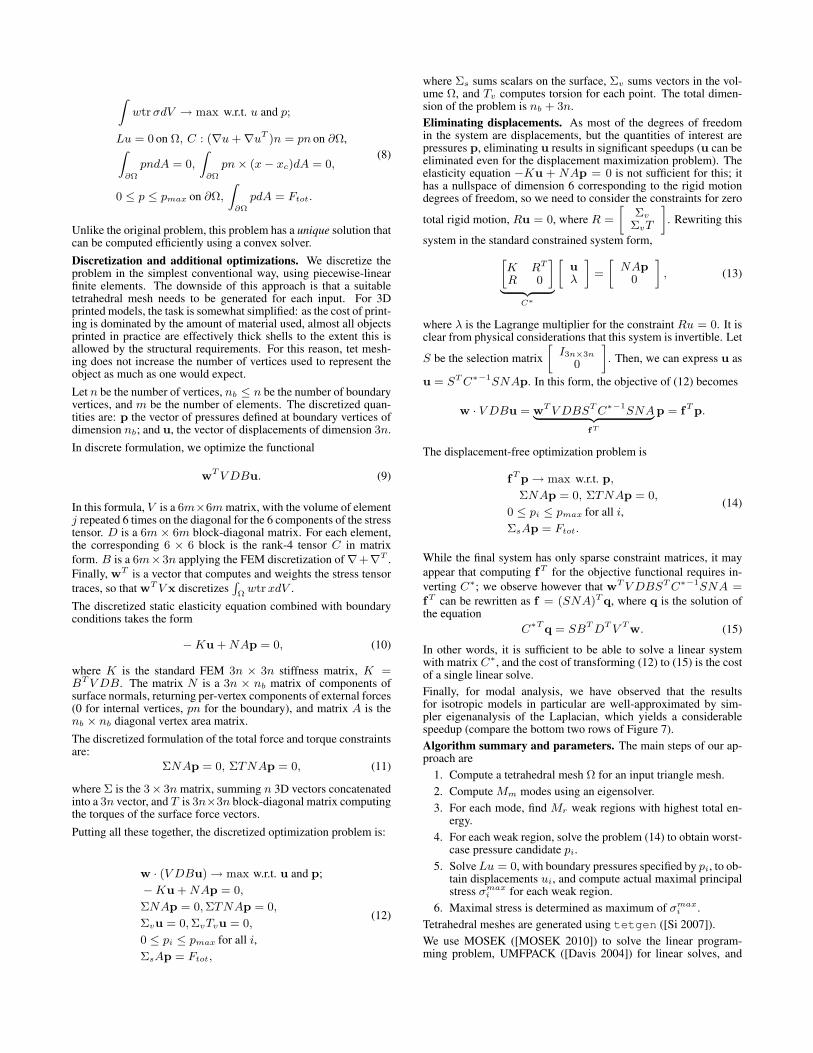
In other words, it is sufficient to be able to solve a linear systemwith matrix C∗, and the cost of transforming (12) to (15) is the costof a single linear solve.Finally, for modal analysis, we have observed that the resultsfor isotropic models in particular are well-approximated by sim-pler eigenanalysis of the Laplacian, which yields a considerablespeedup (compare the bottom two rows of Figure 7).Algorithm summary and parameters. The main steps of our ap-proach are

1. Compute a tetrahedral mesh Ω for an input triangle mesh.2. Compute Mm modes using an eigensolver.3. For each mode, find Mr weak regions with highest total en-

ergy.4. For each weak region, solve the problem (14) to obtain worst-

case pressure candidate pi.5. Solve Lu = 0, with boundary pressures specified by pi, to ob-

tain displacements ui, and compute actual maximal principalstress σmax

i for each weak region.6. Maximal stress is determined as maximum of σmax

i .Tetrahedral meshes are generated using tetgen ([Si 2007]).We use MOSEK ([MOSEK 2010]) to solve the linear program-ming problem, UMFPACK ([Davis 2004]) for linear solves, and

0

5

10

15

20

25

30

35

0 20 40 60 80 100 120 140 160

Weakest Region's Mode Index

Figure 3: Histogram of the mode number (horizontal axis) in whichthe weakest region appears for the first time.

0

5

10

15

20

25

1 2 3 4 5 6

Weakest Region Rank

Figure 4: Histogram of the rank of the weakest region in the weakregion list sorted by decreasing energy.

ARPACK ([Lehoucq et al. 1998]) for computing eigenvectors andeigenvalues.The parameters of the algorithm include Mm, Mr , the choice ofthreshold 1− ε for weak regions, and a user-defined maximal pres-sure pmax (the latter can be regarded as a part of the definition ofthe force model).To determine reasonable choices of Mm and Mr , we have runmodal analysis for a large number of modes (150) and a large num-ber of weak regions per mode for a collection of objects. For eachobject and each mode, we found the weakest region and checked inwhich mode it first appears. We also computed its rank in the list ofthat mode’s weak regions sorted by decreasing energy. The results(Figure 3 and Figure 4) indicate that 15 modes and 5 weak regionsper mode are sufficient in over 80% of cases.We use ε = 0.025 in all cases; the dependence of the size of weakregions for one mode on ε is shown in Figure 5.Figure 6 shows two final results of the algorithm. Red arrows aretotal forces obtained by summing nearby per-vertex force values(pressures are typically concentrated in small areas). Colormaps onthe deformed surfaces show weakness maps.

Figure 5: Weak regions extracted from three modes with weaknesslevel cutoff, ε = .10, .05, .03, .01.

Figure 6: Optimal force vectors and weakest regions on the left,resulting deformations and stresses on the right. The gray imagesin the background show the undeformed state.

5 ValidationWe performed validation of our algorithm in several computationaland experimental ways.Comparison with direct search for the weakest region. Insteadof using the modal analysis stage to identify weak regions and us-ing averaged stress or displacement over weak regions as the targetquantity to optimize, we can run the same optimization process di-rectly, treating each tetrahedron as a potential weak region.We define the weakness map as a scalar field on the surface mappingeach point to the maximal principal stress at this point obtained byapproximate optimization. Using our method yields a partial weak-ness map on the union of all weakness regions we consider. Fig-ure 7 shows a comparison of a complete weakness map, computedusing the brute-force approach, with the weakness map obtained byour method. We observe a close agreement between these for all ex-amples in areas where the partial map is defined and never observehigh stress values elsewhere.

# Tets Brute Force (s) Weak Region (s) Speedup

2723 681.367 1.089 625.939 x2869 793.362 1.087 729.907 x2904 894.610 0.641 1396.071 x5332 2120.361 1.171 1810.199 x11020 11029.721 2.729 4042.403 x12853 11334.362 1.694 6692.546 x14163 27775.900 3.373 8234.925 x16008 19917.838 1.892 10527.388x

Table 1: Stress analysis timings for brute force optimization vs.weak region optimization. While speedups are already dramatic forextremely small element counts, the higher asymptotic complexity ofbrute force causes a rapidly increasing speedup for larger models.

Dependence on tetrahedral mesh resolution. To keep the costof computation low, especially in the context of interactive appli-cations or processing large number of objects at a printing facility,using coarse tetrahedral meshes is desirable. As Figure 8 shows,weakness maps for different resolutions are similar, so higher reso-lution may be used only at the last stage, after the weakest spots areidentified.Drop test. To verify our method for brittle materials, we performeda randomized deformation test by dropping printed models ontohorizontal pegs. We dropped the models from 1m high, ensuringa nearly random impact orientation and force application. The testsetup is pictured in Figure 9. All models were printed with materialzp150.Specific breakages may have two origins: high point forces, whichcan break even relatively strong spots near the impact point and willvary across drops, and smooth deformations, which are likely tobreak weak regions consistently. The former does not correspond totypical usage scenarios, which feature distributed bounded forces.Thus, we consider only fractures occurring frequently across drops.The test results, displayed in Figure 10, confirm that the weak re-gions determined by our method generally agree with the areas with

Brute force

Laplacian

Stiness

Analysis Type Star Star Pendant “Test 2”

Brute Force 18.300 MPa 36.767 MPa 73.298 MPaLaplacian 15.593 MPa 34.151 MPa 71.689 MPaStiffness 16.208 MPa 35.939 MPa 70.588 MPa

Figure 7: Comparison of the similar optimum stresses found bybrute force, Laplacian-based weak region analysis, and stiffness-based weak region analysis. The table reports 99.75 percentile (byvolume) element stresses. An isotropic metal material was used forthis comparison.

Figure 8: For 5 different mesh resolutions (from left to right, thevertex counts are 5K, 13K, 24K, 36K, 50K), the algorithm generatesconsistent weakness maps.

highest occurrence of fracture. Notice in particular the legs of thecow (3rd row, left), the notches of the gear (5th row, left), the armsof the dancer (1st row, right), and the inner piece of the powercogpendant (6th, row left). These are all regions of high weakness mapvalue that break consistently.

Figure 9: We used models printed in green state “sandstone” forthe drop tests. The testing models often are covered with a looselayer of powder that shakes off upon impact (see the dust in theright image).

Displacement test. For the objects printed in ductile materials, weperformed a different test. We placed the shapes into a cardboardbox filled with packaging material and applied pressure to the box’sexterior. This pressure permanently deformed the models inside.We took photographs of the deformed models in a registered po-sition and compared them to the 3D model from which they wereprinted. We observe good agreement with the computed map ofmaximal displacements, i.e., the map similar to the weakness map,but for the displacement maximization problem (see Figure 11).

Reference

Deformed

Figure 11: Simulation results (left) are compared to the deformed3D printed model (green) overlaid on an undeformed one (blue).Our algorithm predicts likely regions (red) of large deformationunder normal handling. For the blade earring, we confirm thatthe largest blade deforms little relative to the hook and shaft: afteraligning the shafts to be parallel, the largest blades are also roughlyparallel (see the yellow parallelograms). The second largest bladeis displaced more. Note that the upper right pin of the deformedspinnoloid (middle row, green) was broken during printing.

Comparison with [Stava et al. 2012]. We compare to the approachdescribed in [Stava et al. 2012], as they also aim to predict the loadsthat a printed model is likely to experience. The authors use a morespecific force model: pinch grips. They present an empirical modelto predict how the object will be gripped with two fingers. Thereare many designs for which such a grip does not capture typical usecases or mishaps. Figure 12 demonstrates shapes whose worst-caseloads cannot be applied or approximated using only a pinch grip.Figure 13 shows three examples for which the authors of [Stavaet al. 2012] have provided us their force application points. Their“cup” example (left) is an excellent candidate for the pinch grip;the highest stress achieved with a fixed total force agrees with oursand even exceeds it. However, the other two objects do not fit theirmodel as well. The “UFO” pinch grip is clearly suboptimal, andthe forces applied to the bracelet would have much more leverageif they were moved to the open endpoints. In all three cases, ourmethod generates efficient force vectors.

Figure 10: Results for a drop test. Model volume is shaded with its weakness map percentile: 90% 99%

Figure 12: Models where pinch grips cannot generate worst-caseloads. Our method finds highly intuitive force vectors, regardless.The additional arrows on the top of the Skyrim dragon arise to bringthe total force and torque to zero.

An interesting observation about the “cup” model is that our methodproduces a triangle of forces (perhaps at the expense of higherstress) rather than a pair of opposite forces. One possible reasonfor this is the pressure bound requiring the force to be distributedover a larger area.

Figure 13: Comparison against [Stava et al. 2012]. Our algo-rithm’s force distribution (top) better identifies structural weakness,especially for the ufo (middle) and bracelet (right).

Timings. Though our pipeline has not yet reached interactivespeeds, it is already fast enough to be included in a 3D printingpipeline. For the sizes of models most commonly sent to 3D print-ing services (see distribution in Figure 15: sizes on the order of100K vertices are most common), our full algorithm takes only afew minutes:

# Tets Structural Analysis (mins)

2723 0.02842900 0.30870356 0.382155383 2.566322398 9.601414894 4.490

Analyzing the algorithm’s scaling behavior is complicated by itsdependence on structural properties—a separate linear program isrun for each weak region that is extracted. To make sense of the tim-ings, they have been separated by stage. Modal analysis and weakregion extraction are run only once per model, and Figure 14 showshow their execution times depend on element count. The time spentsetting up and solving the linear programs (“weakness analysis”) isaveraged over all weak regions so that it can be plotted against thesame x axis. Note that there is one further cost not shown: the singlesparse UMFPACK factorization. This timing depends strongly onmatrix structure (despite using fill-in reducing permutations), andadds noise to curves when included. Factorization time is includedin the timing table above.

0 2 4 6 8

10 12 14 16 18

0 50 100 150 200 250 300 350 400 450

Time (secon

ds)

Thousands of Elements

Weak Region Computa:on Time

Modal Analysis

Extrac9on

0.1

2.1

4.1

6.1

8.1

10.1

12.1

14.1

16.1

0 50 100 150 200 250 300 350 400 450

Time (secon

ds)

Thousands of Elements

Weakness Analysis Time Per Region

Figure 14: The top plots shows how modal analysis and weak re-gion extraction scale with the number of tetrahedra. The dominantcost is the eigensolve. The bottom plots shows the average cost ofsetting up and running the linear program for each weak region. Itexcludes the UMFPACK factorization of C∗ that only must be runonce.

0

500

1000

1500

2000

2500

3000

0K 120K 240K 360K 480K Vertex Count

Model Size Sta2s2cs

Figure 15: Model vertex counts tabulated from 2781 models or-dered from Shapeways.

6 Material properties

Material parameters defining the elasticity tensor C must be mea-sured for each of the 3D printers’ materials. We have observedthat the computed maximal stress does not depend on the magni-tude of the Young’s modulus in the isotropic case. However, in theanisotropic case, it does depend on the ratios of directional elasticitymoduli, which can be significant (Figure 16). To predict breakageor plastic deformations under loads, the additional material param-eters tensile strength and yield strength are needed.In this section, we present the Youngs modulus ratio measurementsfor three different 3D printing materials that we used to computeour simulation’s elasticity parameters. In addition, we discuss theextent to which various materials match our assumptions on stress-strain linearity and what accuracy one can expect from predictions

of the maximal stress to tensile strength ratio. In all cases, we as-sume a Poisson ratio of 0.3.

Figure 16: Different ratios of directional Young’s moduli can leadto different weakest regions. We show the weakest region found fora truss with a Young’s modulus that is five times higher in the X(left), Y (middle), and Z (right) directions.

We have tested three materials used in 3D printing: nylon (PA2200 by EOS Electro Optical Systems), “sandstone” (zp150 usedin the ZPrinter series by 3D Systems), and green state stainlesssteel (420SS powder bound with proprietary binder used by Ex-One). They also represent different classes of materials (brittle vs.ductile, isotropic vs anisotropic).To determine their properties, we conducted a three point bendingtest consistent with ASTM standard D5032 ([ASTM 2007]), us-ing the Instron 5960 universal testing machine with a ±100N loadcell and a support span of 40mm. Figure 17 illustrates the testingsetup. The testing samples are rectangular bars with length 60mmand thickness between 1mm and 5mm. A relatively thin test barwas chosen because structurally weak models are likely to containthin features.

Figure 17: Three-point bending test on green state stainless steel.

0

1e+06

2e+06

3e+06

4e+06

5e+06

6e+06

7e+06

0 0.001 0.002 0.003

Stre

ss

Strain

0

5e+06

1e+07

1.5e+07

2e+07

2.5e+07

3e+07

3.5e+07

4e+07

4.5e+07

0 0.02 0.04 0.06

Stre

ss

Strain

Figure 18: Left: Stress vs strain curve measured on samples ingreen state stainless steel. The colors indicate different samplethickness (1.5mm red, 2mm green, 3mm blue). Right: Stress vsstrain plots for nylon testing samples of thickness 1.5mm and 2mm.The samples printed in different orientation are marked with differ-ent colors (red: X, green: Y, blue: Z).

Among the three materials tested, green state stainless steel fits thedefinition of brittle material the best. Stress grows linearly with

strain for all samples tested (Figure 18 left). Bending tests in per-pendicular directions show that elastic moduli in these directionsare close, with the average Young’s modulus 3.59GPa and standarddeviation 0.27GPa. Figure 19 shows critical stress extracted frommeasurements, which is mostly consistent for all samples, with theaverage 6.88MPa and 0.62MPa standard deviation. Overall, thismaterial is consistent with our model for stress optimization.

0

3e+06

6e+06

9e+06

1.5 2 2.5 3 3.5 4 4.5 5 5.5

Criti

cal S

tres

s

Thickness

Figure 19: The critical stress distribution of green state metal forsamples with thickness 1.5mm up to 5mm.

Models printed in nylon are known to withstand a large range ofdeformations. Figure 18 (right) shows the stress vs strain curve for18 nylon samples. Half of them are 1.5mm thick, and the other halfare 2mm. For each thickness group, sets of 3 samples were printedalong each of X,Y and Z directions. From the results, we observedthat nylon samples typically have a very large elastic deformationrange before entering the plastic stage. We also note a moderatebut obviously present degree of anisotropy (the Young’s modulusfor X is 0.80GPa with 0.13GPa deviation, for Y is 1.02GPa with0.18GPa deviation, and for Z is 0.98GPa with 0.12GPa deviation).See Figure 18, right.

The most complex material we tested is the “sandstone.” Though,like green state metal, it has a relatively low tensile strength, itexhibits a significant plastic region (Figure 20) and very high de-gree of anisotropy: we measured X, Y, and Z Young’s moduliof 1.22GPa (standard deviation 0.13GPa), 0.68GPa (standard de-viation 0.07GPa), and 0.234GPa (standard deviation 0.02GPa) re-spectively, with more than 5 times difference between the largestand smallest values. Thus, we model it as an orthotropic materialwith a distinct Young’s modulus per printing axis. We obtain ourshear moduli using a standard formula from [SolidWorks 2011]:Gxy =

ExEy

Ex+Ey+2Eyνxy. Note that “sandstone” exhibits a large

variability of tensile strength, even for a single direction. Thismeans only very conservative predictions are possible. Neverthe-less, we observe that our weak region detection works well (Figure10).

0

1e+06

2e+06

3e+06

4e+06

5e+06

0 0.005 0.01

Stre

ss

Strain

Figure 20: Stress vs. strain measurements on rectangular barsprinted with green state “sandstone” along the printer X (red),Y(green) and Z (blue) direction. Different printing directions influ-ence the material properties significantly.

7 ConclusionsWe have presented an efficient approximate method for determiningworst-case loads for a geometric object based on its geometry andmaterial properties only. The method is quite reliable (it relies ona linear solver, an eigensolver, and a convex solver, which all canprovide convergence guarantees), efficient, and approximates wellworst-case stress and displacement distributions.At the same time, there is clearly a number of limitations. Mostimportantly, only linear elasticity is considered, and the optimizedsolution at the second stage may not match reality for large plasticdeformations. We note, however, that the robustly obtained approx-imate solution can serve as a starting point for a nonlinear solver.More generally, 3D printed materials exhibit a broad range of com-plex behaviors, some of which may exhibit considerable variationeven for the same printing process. Using computational modelsreflecting material complexity and uncertainty is an important fu-ture direction. From the point of view of robustness of the method,tetrahedral mesh generation is the bottleneck. Meshless techniquesmay yield a fully robust pipeline using only surface geometry asinput.

8 AcknowledgementsWe are grateful to the authors of [Stava et al. 2012] for sharingtheir data. We also thank Professor Yu Zhang (NYU Dental School)and Professor Nikhil Gupta (NYU Poly), who allowed us to usetheir facilities for material testing and Professor Alan T. Zehnder(Cornell) for his helpful discussions regarding these tests. Finally,we thank Shapeways for initiating the project and providing rawmaterials and the many designers whose shapes we tested:Stava et al.: soccer cup (Fig 13); improbablecog: flora (Fig 1,10),powercog (Fig 10), blade earring (Fig 11); Novastar Design: skyrim(Fig 12), heart (Fig 2); unellenu: butterfly (Fig 10), spinnoloids (Fig11); kspaho: scorpion (Fig 11); TerryDiF: turret (Fig 6,10); JuliaBoersma: trilobyte (Fig 10); Aim@Shape: cow (Fig 10), dilo (Fig10), dancer (Fig 8, 10, 12), wood chair (Fig 5, 10).This work was partially supported by NSF awards IIS-0905502,OCI-1047932, and DMS-0602235.

ReferencesASTM. 2007. D5023-07 standard test method for plastics: Dy-

namic mechanical properties: In flexure (three-point bending).In American Society for Testing and Materials.

BACHER, M., BICKEL, B., JAMES, D., AND PFISTER, H. 2012.Fabricating articulated characters from skinned meshes. ACMTransactions on Graphics (TOG) 31, 4, 47.

BARBIC, J., AND JAMES, D. 2005. Real-time subspace integrationfor st. venant-kirchhoff deformable models. In ACM Transac-tions on Graphics (TOG), vol. 24, ACM, 982–990.

BARBIC, J., AND JAMES, D. 2010. Subspace self-collision culling.ACM Transactions on Graphics (TOG) 29, 4, 81.

BICKEL, B., BACHER, M., OTADUY, M., LEE, H., PFISTER, H.,GROSS, M., AND MATUSIK, W. 2010. Design and fabricationof materials with desired deformation behavior. ACM Transac-tions on Graphics (TOG) 29, 4, 63.

CALI, J., CALIAN, D., AMATI, C., KLEINBERGER, R., STEED,A., KAUTZ, J., AND WEYRICH, T. 2012. 3d-printing of non-assembly, articulated models. ACM Transactions on Graphics(TOG) 31, 6, 130.

DAVIS, T. 2004. Algorithm 832: Umfpack v4. 3—an unsymmetric-pattern multifrontal method. ACM Transactions on Mathemati-cal Software (TOMS) 30, 2, 196–199.

DONG, Y., WANG, J., PELLACINI, F., TONG, X., AND GUO, B.2010. Fabricating spatially-varying subsurface scattering. ACMTransactions on Graphics (TOG) 29, 4, 62.

ELISHAKOF, I., AND OHSAKI, M. 2010. Optimization and anti-optimization of structures under uncertainty. World Scientific.

EWINS, D. 2000. Modal testing: theory, practice and application,vol. 2. Research studies press Baldock.

FIDKOWSKI, K., KROO, I., WILLCOX, K., AND ENGELSON, F.2008. Stochastic gust analysis techniques for aircraft conceptualdesign. AIAA paper 2008-5848.

HASAN, M., FUCHS, M., MATUSIK, W., PFISTER, H., ANDRUSINKIEWICZ, S. 2010. Physical reproduction of materi-als with specified subsurface scattering. ACM Transactions onGraphics (TOG) 29, 4, 61.

HAUSER, K., SHEN, C., AND O?BRIEN, J. 2003. Interactivedeformation using modal analysis with constraints. In GraphicsInterface, vol. 3, 16–17.

KOU, X., AND TAN, S. 2007. A systematic approach for in-tegrated computer-aided design and finite element analysis offunctionally-graded-material objects. Materials & design 28, 10,2549–2565.

LEHOUCQ, R., SORENSEN, D., AND YANG, C. 1998. ARPACKusers’ guide: solution of large-scale eigenvalue problems withimplicitly restarted Arnoldi methods, vol. 6. SIAM.

LUO, L., BARAN, I., RUSINKIEWICZ, S., AND MATUSIK, W.2012. Chopper: Partitioning models into 3D-printable parts.ACM Transactions on Graphics (Proc. SIGGRAPH Asia) 31, 6(Dec.).

MOSEK, A., 2010. The mosek optimization tools manual. version6.0., 2010.

NICKELL, R. 1976. Nonlinear dynamics by mode superposition.Computer Methods in Applied Mechanics and Engineering 7, 1,107–129.

PENTLAND, A., AND WILLIAMS, J. 1989. Good vibrations:model dynamics for graphics and animation. ACM SIGGRAPHComputer Graphics 23, 3, 207–214.

PRATT, M., MARSAN, A. L., KUMAR, V., AND DUTTA, D. 1998.An assessment of data requirements and data transfer formats forlayered manufacturing. Tech. rep., National Institute of Stan-dards and Technology.

SHAPEWAYS, 2011. Things to keep in mind when designing for 3dprinting. .

SI, H. 2007. Tetgen: A quality tetrahedral mesh generatorand a 3d delaunay triangulator. Weblink: http://tetgen. berlios.de/(accessed on: March 31, 2012).

SOLIDWORKS, 2011. Solidworks simulation reference, 2011.STAVA, O., VANEK, J., BENES, B., CARR, N., AND MECH, R.

2012. Stress relief: improving structural strength of 3d printableobjects. ACM Transactions on Graphics (TOG) 31, 4, 48.

TELEA, A., AND JALBA, A. 2011. Voxel-based assessment ofprintability of 3d shapes. In Proceedings of the 10th interna-tional conference on Mathematical morphology and its applica-tions to image and signal processing, Springer-Verlag, Berlin,Heidelberg, ISMM’11, 393–404.

TIMOSHENKO, S., AND WOINOWSKY-KRIEGER, S. 1940. The-ory of plates and shells. Engineering Societies Monographs, NewYork: McGraw-Hill.

UMETANI, N., IGARASHI, T., AND MITRA, N. J. 2012. Guidedexploration of physically valid shapes for furniture design. ACMTransactions on Graphics (Proceedings of SIGGRAPH 2012)31, 4.

Z CORPORATION, 2011. Architectural design guide - printing3d architectural models. .

ZEILER, T. 1997. Matched filter concept and maximum gust loads.Journal of aircraft 34, 1, 101–108.