Worst-Case Performance Analysis of Feed-Forward Networks
172
Worst-Case Performance Analysis of Feed-Forward Networks – An Efficient and Accurate Network Calculus Thesis approved by the Department of Computer Science of the University of Kaiserslautern (TU Kaiserslautern) for the award of the Doctoral Degree Doctor of Engineering (Dr.-Ing.) to Steffen Bondorf Date of the viva : 12 July 2016 Dean: : Prof. Dr. Klaus Schneider PhD committee Chairperson : Prof. Dr. Heike Leitte Reviewers : Prof. Dr. Jens B. Schmitt Prof. Dr. Roland Meyer Dr. Marc Boyer D 386
-
Upload
khangminh22 -
Category
Documents
-
view
2 -
download
0
Transcript of Worst-Case Performance Analysis of Feed-Forward Networks

Worst-Case Performance Analysis ofFeed-Forward Networks –
An Efficient and Accurate Network Calculus
Thesis approved
by the Department of Computer Science
of the University of Kaiserslautern (TU Kaiserslautern)
for the award of the Doctoral Degree
Doctor of Engineering (Dr.-Ing.)
to
Steffen Bondorf
Date of the viva : 12 July 2016
Dean: : Prof. Dr. Klaus Schneider
PhD committeeChairperson : Prof. Dr. Heike LeitteReviewers : Prof. Dr. Jens B. Schmitt
Prof. Dr. Roland MeyerDr. Marc Boyer
D 386

Abstract
Distributed systems are omnipresent nowadays and networking them is fundamental forthe continuous dissemination and thus availability of data. Provision of data in real-time is one of the most important non-functional aspects that safety-critical networksmust guarantee. Formal verification of data communication against worst-case deadlinerequirements is key to certification of emerging x-by-wire systems. Verification allowsaircraft to take off, cars to steer by wire, and safety-critical industrial facilities to oper-ate. Therefore, different methodologies for worst-case modeling and analysis of real-timesystems have been established. Among them is deterministic Network Calculus (NC), aversatile technique that is applicable across multiple domains such as packet switching,task scheduling, system on chip, software-defined networking, data center networkingand network virtualization. NC is a methodology to derive deterministic bounds on twocrucial performance metrics of communication systems:
(a) the end-to-end delay data flows experience and(b) the buffer space required by a server to queue all incoming data.
NC has already seen application in the industry, for instance, basic results have beenused to certify the backbone network of the Airbus A380 aircraft.
The NC methodology for worst-case performance analysis of distributed real-time sys-tems consists of two branches. Both share the NC network model but diverge regardingtheir respective derivation of performance bounds, i.e., their analysis principle. NC wascreated as a deterministic system theory for queueing analysis and its operations werelater cast in a (min,+)-algebraic framework. This branch is known as algebraic NetworkCalculus (algNC). While algNC can efficiently compute bounds on delay and backlog, thealgebraic manipulations do not allow NC to attain the most accurate bounds achievablefor the given network model. These tight performance bounds can only be attained withthe other, newly established branch of NC, the optimization-based analysis (optNC).However, the only optNC analysis that can currently derive tight bounds was proven tobe computationally infeasible even for the analysis of moderately sized networks otherthan simple sequences of servers.
This thesis makes various contributions in the area of algNC: accuracy within the ex-isting framework is improved, distributivity of the sensor network calculus analysis isestablished, and most significantly the algNC is extended with optimization principles.They allow algNC to derive performance bounds that are competitive with optNC. More-over, the computational efficiency of the new NC approach is improved such that thisthesis presents the first NC analysis that is both accurate and computationally feasibleat the same time. It allows NC to scale to larger, more complex systems that requireformal verification of their real-time capabilities.
iii


Acknowledgements
I would like to thank my parents, Rita and Hans-Georg, for their endless support thatallowed me to achieve my goals. My heartfelt gratitude inevitably goes to my significantother Elena, who supported me during this entire time. You have continuously encour-aged me throughout this research effort and without you this dissertation would not havebeen possible.
I am thankful to Prof. Jens Schmitt for being my mentor, my friend. Your decisionto push me to network calculus when our paths crossed in 2008 shaped my academic lifeever since. Thank you for guiding me through the endeavors of a bachelor’s thesis, amaster’s thesis and finally this PhD thesis. Thank you for believing in me.
I would also like to thank Prof. Roland Meyer for helping me as a co-supervisor sincethe start of my doctorate studies and Marc Boyer for all the discussions we had at thevarious network calculus events. Thank you both for providing valuable suggestions.
My sincere appreciation belongs to everyone I met at DISCO and who made my timeworthwhile. I want to thank all the former and current team members, namely MatthiasSchäfer, Daniel Berger, Michael Beck, Hao Wang, Matthias Wilhelm, Wint Yi Poe, AdamBachorek, Nicos Gollan, Ivan Martinovic and Paul Nikolaus. You certainly had an im-pact on me and my research. My special gratitude is also extended to our associatedstaff Markus Fuchs, Steffen Reithermann and Barbara Erlewein.
Thank you all,Steffen
v


Contents
Contents
Abstract iii
Acknowledgements v
1 Introduction 11.1 Worst-Case Performance Analysis . . . . . . . . . . . . . . . . . . . . . . . 11.2 Network Calculus . . . . . . . . . . . . . . . . . . . . . . . . . . . . . . . . 21.3 Thesis Contribution . . . . . . . . . . . . . . . . . . . . . . . . . . . . . . 31.4 Thesis Organization . . . . . . . . . . . . . . . . . . . . . . . . . . . . . . 4
2 State of the Art in Network Calculus 72.1 Network Description . . . . . . . . . . . . . . . . . . . . . . . . . . . . . . 7
2.1.1 Data Arrivals, Forwarding Service and Performance Characteristics 72.1.2 The Network Model . . . . . . . . . . . . . . . . . . . . . . . . . . 92.1.3 (min,+)-algebraic Operations and Performance Bounds . . . . . . . 10
2.2 Analysis Principles . . . . . . . . . . . . . . . . . . . . . . . . . . . . . . . 132.3 Algebraic Analyses . . . . . . . . . . . . . . . . . . . . . . . . . . . . . . . 14
2.3.1 Total Flow Analysis . . . . . . . . . . . . . . . . . . . . . . . . . . 142.3.2 Separate Flow Analysis . . . . . . . . . . . . . . . . . . . . . . . . 162.3.3 Pay Multiplexing Only Once Analysis . . . . . . . . . . . . . . . . 17
2.4 Optimization-based Analysis . . . . . . . . . . . . . . . . . . . . . . . . . . 202.4.1 The Linear Programming Analysis . . . . . . . . . . . . . . . . . . 21
3 Accuracy of Algebraic Network Calculus 233.1 Compositional Analysis of Feed-forward Networks . . . . . . . . . . . . . . 233.2 Problems . . . . . . . . . . . . . . . . . . . . . . . . . . . . . . . . . . . . 25
3.2.1 Problems Caused by Compositionality . . . . . . . . . . . . . . . . 253.2.2 Problems Caused by Tandem Analyses . . . . . . . . . . . . . . . . 26
3.3 Derivation of Cross-traffic Arrival Bounds . . . . . . . . . . . . . . . . . . 283.3.1 Segregated Cross-flow Arrival Bounding . . . . . . . . . . . . . . . 293.3.2 Aggregate Cross-traffic Arrival Bounding . . . . . . . . . . . . . . . 293.3.3 Deconvolution for ↵ 2 FmTB with � 2 FmRL . . . . . . . . . . . . . 313.3.4 Distributivity of ↵ over + . . . . . . . . . . . . . . . . . . . . . . . 323.3.5 Ranking of PBOO Arrival Bounding Alternatives . . . . . . . . . . 373.3.6 Accuracy Evaluation . . . . . . . . . . . . . . . . . . . . . . . . . . 40
3.4 Cross-traffic Burstiness Reduction . . . . . . . . . . . . . . . . . . . . . . . 423.4.1 An Alternative Output Bound . . . . . . . . . . . . . . . . . . . . 43
vii

Contents
3.4.2 TFA-assisted aggrPBOOAB . . . . . . . . . . . . . . . . . . . . . . 463.4.3 Accuracy Evaluation . . . . . . . . . . . . . . . . . . . . . . . . . . 51
4 Distributed Sensor Network Calculus Analysis 554.1 Arrivals, Service, (min,+)-Operations and Performance Bounds . . . . . . 554.2 The Network Model . . . . . . . . . . . . . . . . . . . . . . . . . . . . . . 574.3 Compositional Sink-tree Analysis . . . . . . . . . . . . . . . . . . . . . . . 57
4.3.1 Flow of Interest Analysis . . . . . . . . . . . . . . . . . . . . . . . . 574.3.2 Cross-traffic Arrival Bounding . . . . . . . . . . . . . . . . . . . . . 60
4.4 Improving SensorNC Analysis . . . . . . . . . . . . . . . . . . . . . . . . . 614.4.1 The Generalized Concatenation for SensorNC . . . . . . . . . . . . 614.4.2 The New SensorNC Cross-traffic Arrival Bounding . . . . . . . . . 654.4.3 Accuracy Evaluation . . . . . . . . . . . . . . . . . . . . . . . . . . 674.4.4 Effort Evaluation . . . . . . . . . . . . . . . . . . . . . . . . . . . . 68
4.5 Distribution of the SensorNC Analysis Procedure . . . . . . . . . . . . . . 70
5 Limitations of Linear Programming Analysis 755.1 Scalability Issues . . . . . . . . . . . . . . . . . . . . . . . . . . . . . . . . 755.2 A Tradeoff between Accuracy and Efficiency . . . . . . . . . . . . . . . . . 76
5.2.1 The Unique Linear Programming Analysis . . . . . . . . . . . . . . 775.3 Evaluation of Accuracy and Effort . . . . . . . . . . . . . . . . . . . . . . 78
5.3.1 The Non-Nested Tandem . . . . . . . . . . . . . . . . . . . . . . . 785.3.2 The Square Network . . . . . . . . . . . . . . . . . . . . . . . . . . 815.3.3 Feed-forward Networks . . . . . . . . . . . . . . . . . . . . . . . . . 84
6 Optimization Principles in Algebraic Network Calculus 896.1 Exhaustive Aggregate Cross-traffic Arrival Bounding . . . . . . . . . . . . 89
6.1.1 Accuracy Evaluation . . . . . . . . . . . . . . . . . . . . . . . . . . 936.1.2 Effort Considerations . . . . . . . . . . . . . . . . . . . . . . . . . . 97
6.2 The Tandem Matching Analysis . . . . . . . . . . . . . . . . . . . . . . . . 976.2.1 Matching Tandems . . . . . . . . . . . . . . . . . . . . . . . . . . . 986.2.2 Related Work . . . . . . . . . . . . . . . . . . . . . . . . . . . . . . 1016.2.3 Accuracy Evaluation . . . . . . . . . . . . . . . . . . . . . . . . . . 1036.2.4 Effort Considerations . . . . . . . . . . . . . . . . . . . . . . . . . . 105
6.3 Combining Search Spaces of Optimization Principles . . . . . . . . . . . . 106
7 Efficiency of Algebraic Network Calculus Analysis 1097.1 Analysis Execution Efficiency . . . . . . . . . . . . . . . . . . . . . . . . . 109
7.1.1 Convolution of Intermediate Arrival Bounds . . . . . . . . . . . . . 109
viii

Contents
7.1.2 Caching of Intermediate Arrival Bounds . . . . . . . . . . . . . . . 1107.2 The Efficient TMA Algorithm . . . . . . . . . . . . . . . . . . . . . . . . . 111
7.2.1 Effort Evaluation . . . . . . . . . . . . . . . . . . . . . . . . . . . . 1147.3 Network Calculus on Compact Domains . . . . . . . . . . . . . . . . . . . 116
7.3.1 Related Work . . . . . . . . . . . . . . . . . . . . . . . . . . . . . . 1187.3.2 Deriving Compact Curve Domains . . . . . . . . . . . . . . . . . . 1197.3.3 Accuracy and Effort Evaluation . . . . . . . . . . . . . . . . . . . . 125
8 The New State of the Art in Network Calculus 1298.1 Numerical Experiments I: Erdős-Rényi Networks . . . . . . . . . . . . . . 1308.2 Numerical Experiments II: General Linear Preference Networks . . . . . . 1328.3 Case Study: Avionics Full-Duplex Ethernet . . . . . . . . . . . . . . . . . 137
9 Conclusion 1419.1 Concluding Remarks . . . . . . . . . . . . . . . . . . . . . . . . . . . . . . 1419.2 Future Research Directions . . . . . . . . . . . . . . . . . . . . . . . . . . 142
Nomenclature 147
List of Figures 148
List of Tables 149
References 151
List of Publications 159
CV 161
ix


1 Introduction
1.1 Worst-Case Performance Analysis
A fundamental problem in the analysis of real-time networks is the derivation of deter-ministic performance bounds. The most important measures are the delay data flowsexperience when they traverse a network from their respective source to their sink andthe backlog they experience at the individual servers they cross. The latter is required todimension buffers sufficiently large to avoid overflows and thus the loss of data. Lost ordropped data needs to be retransmitted and increases the delay between a flow’s initialcreation and its eventual delivery. Depending on the payload, this delay might be decisivefor a safety-critical real-time system. Therefore, worst-case performance bounds play acrucial role in different areas, ranging from verification of hard real-time communicationcapabilities to quality of experience assurance for end users. In case of safety-critical sys-tems, formally verified delay and backlog bounds are even required for certification. I.e.,for larger systems such as aircraft that rely on an embedded real-time communicationnetwork, they are crucial for the entrance into service.
Networks that are required to guarantee for real-time communication have been de-ployed in safety-critical environments for decades. These networks are verified to keepcertain deadlines when transmitting information. However, they are oftentimes specifi-cally built for a single purpose and to operate under unalterable conditions only – and sois their evaluation customized to this setting. Nowadays, we observe the trend to employcommercial off-the-shelf technologies. For instance, cable harnesses with their dedicatedconnections have been replaced by shared-access to a vehicle bus systems like CAN (ISO11898). For multiple reasons such as complexity, development time and costs, the in-dustry developed communication network standards based on Ethernet (IEEE 802.3), awidely used standard for local area networks. Airbus, a manufacturer of aircraft, basedits Avionics Full-Duplex Switched Ethernet (AFDX: ARINC 664) on this standard, theautomotive industry developed Audio Video Bridging (AVB: IEEE 802.1BA, 802.1AS,802.1Qat, 802.1Qav) from the IEEE 802 family and in industrial facilities, usage of Time-Triggered Ethernet (TTEthernet: SAE AS6802) emerges. CAN has also be amended bya time-triggered variant to increase its real-time capabilities (TTCAN: ISO 11898-4:2004)[33, 27, 39, 24, 28, 63].
Embedded into a safety-critical system such as a vehicle, networks based on one ofthese standards must warrant hard real-time guarantees. Formal verification is key toobtain deterministic worst-case bounds on delay and backlog and thus to the certificationof the entire system. Simulation is not sufficient. Changing requirements and emergingtechnologies employed in such systems demand extensibility and flexibility from a for-mal performance evaluation methodology. There are various approaches for specification
1

1 Introduction
and verification of real-time systems, yet, only few are powerful w.r.t. their modelingcapabilities such that they can be applied to diverse environments, e.g., switched Ether-nets [32], wireless sensor networks [71, 43, 8, 65], network on chip [56, 67, 61], Internetof Things [88, 5, 62], software-defined networking and network virtualization [39, 62],data centers [89] as well as network simulation [47]. Moreover, the analysis based on themodel must be able to scale to large, complex systems that require formal verification oftheir real-time capabilities. One of most versatile techniques that promises both of theseproperties is Network Calculus (NC) [25, 26, 23, 50], a methodology for the derivation ofworst-case bounds on flow delay and server backlog.
1.2 Network Calculus
NC provides a mathematical framework to derive deterministic bounds on a flow’s end-to-end delay when crossing a network and the buffer size requirement at the traversedservers, i.e., the bound on their maximum backlog at any time. NC has been widelyadopted in research as well as industry – for example, the switched Ethernet backbonenetwork used in the Airbus A380 has been certified using NC.
The evolution of the NC methodology resulted in two branches that only share theNC system description: On the one hand, there is the algebraic NC (algNC) branch. Itsanalysis of networks free of cyclic dependencies (feed-forward property) is based on theextension of results for sequences of servers, the so-called tandems. AlgNC establishedthree distinct analyses to compute performance bounds, TFA, SFA and PMOOA. Eachof these analyses defines, among other aspects, a specific way to decompose the networkinto tandems, their order of analysis and the applied operations. Unfortunately, thesecompositional algNC analyses are not able to derive tight bounds, i.e., the most accuratebounds are known to be out of their reach. In terms of bound accuracy, algNC has beensuperseded by the optimization-based NC (optNC) branch. While this work started witha compositional analysis as well, the most recent approach abandoned the decompositionprocedure. It aims at a network-wide, global optimization: The entire network descrip-tion is transformed into a set of linear programs to solve. This constitutes the onlyanalysis currently known to achieve tight bounds on end-to-end flow delays and serverbacklog in general feed-forward networks. However, the amount of linear programs tosolve grows super-exponentially with the network size. The analysis is shown to be NP-hard with no algorithm known to solve the underlying problem efficiently (extension ofa partial order to the set of all compatible total orders). Therefore, the optNC branchis commonly represented by an analysis variant circumventing this problem. Tightnessis traded against computational feasibility by reducing the amount of linear programsto a single one. Naturally, this optNC analysis does not capture interference patterns of
2

1.3 Thesis Contribution
flows as exhaustively as the tight one. It is, however, believed to be both, efficient andaccurate. The former is concluded from decades of research on optimization and its toolsupport, the latter from the attained global view of the optimization. Yet, neither ofthese assumptions was profoundly evaluated.
Therefore, only algNC has seen application in the industry. It was applied to analyzenetworks designed from scratch for delay sensitive employment. Especially the avionicsindustry has embraced the algNC methodology. Examples can be found in the analysisof HCS (Heterogeneous Communication System) [80] and AFDX (Avionics Full-DuplexSwitched Ethernet). The latter has continuously seen attention in order to verify againsttiming constraints for these networks [32, 20, 38, 54, 19]. Current Airbus aircraft’s AFDXbackbone was certified using the algebraic techniques provided by NC.
The application of algNC has also resulted in diverse tool support. It ranges fromopen-source tools provided by academia [18, 2, 7], to a freely available closed-source tool-box [86], to a commercial offering [21] and others [57, 17]. Moreover, several companiesare known to employ NC and develop internal tool support – for example Rockwell Collins(ConfGen [36]), Hirschmann Automation and Control (DelayLyzer [69]) and SIEMENS(NC Engine [44]) to name a few.
Theoretical and practical enhancements of algNC are in the focus of this thesis.
1.3 Thesis Contribution
This thesis makes several contributions in the area of NC feed-forward analysis, underthe assumption of arbitrary multiplexing: First, the accuracy of current state-of-the-artalgNC analysis is improved with two distinct enhancements. In addition to the impact onperformance bounds, this contribution also highlights that algNC’s potential has not beenfully exploited before. Moreover, the algebraic properties accessible during the algNCanalysis also allow for features not attained by current optNC analyses: assessment ofintermediate results and distributed execution. This thesis contributes an extension to aprocedure for distributed algNC analysis that enables for in-network performance bound-ing. It can be employed for distributed admission control as well as monitoring taskswithin self-modeling sensor networks. OptNC’s reliance on optimization software intro-duces a black-box view on the analysis that prohibits such features. Indeed, we also showthat every optNC analysis imposes computational effort on this software that renders itsapplication nearly impossible – even for moderately sized networks as found embeddedinto systems such as aircraft that are currently in operation. These observations re-veal that existing NC analyses can be distinguished regarding their fundamental tradeoffbetween efficiency and accuracy:
1. AlgNC is computationally efficient and possesses the potential to provide useful
3

1 Introduction
features like distributed in-network execution. However, accuracy of attained per-formance bounds is not competitive with optNC.
2. OptNC, on the other hand, theoretically allows for the derivation of tight bounds.Yet, this thesis shows that in practice neither tight nor accurate bounds are com-putationally feasible to derive with an optNC analysis.
Therefore, we contribute a novel NC analysis that is based on algNC but incorporatesoptimization principles in order to achieve highly accurate bounds. In particular, it ex-ploits the idea to consider the entire feed-forward network in the search for performancebounds instead of focussing on individual tandem solutions only. The analysis can makeuse of a vast search space but this optimization principle at the core of the new approachresults in computational effort similar to optNC. Yet, in contrast to the back-box viewimposed by optimization software, algNC grants access to the entire inner workings of theanalysis procedure. We show how this knowledge can be used for multiple efficiency im-provements, both fundamentally and implementation-wise. They allow for a fast searchfor performance bounds in the search space defined by our new NC analysis approach.In an extensive evaluation, we demonstrate that this is the first NC analysis to achievethe high degree of accuracy previously exclusively attributed to optNC while demand-ing computation times that are several orders of magnitude below optNC. This thesistherefore provides the first efficient and accurate NC analysis applicable to large-scalefeed-forward networks.
1.4 Thesis Organization
In Section 2, we provide an in-depth depiction of NC with a focus on the propertiesrequired for the later contributions. We start with the curves bounding worst-case flowarrivals and worst-case forwarding service that are common to all NC analyses (Sec-tion 2.1). Then, we present the network model that NC analyses are applied to andjustify the focus on arbitrary multiplexing in server queues, i.e., we assume that flowscan be reordered arbitrarily when they share a queue. The foundations of NC are con-cluded by the (min,+)-algebra algNC is based on. We cover operations that manipulatecurves such that the worst-case model is retained as well as the derivation of deterministicbounds on flow delays and server backlog. We then depict the known NC analysis prin-ciples (Section 2.2) followed by the algNC tandem analyses and the optNC feed-forwardanalysis that implement these principles (Sections 2.3 and 2.4).
Section 3 is dedicated to the accuracy of current algNC. After contributing a genericcomposition scheme that allows algNC tandem analyses to derive performance bounds infeed-forward networks, we identify the problems caused by compositionality (Sections 3.1and 3.2). Then, we focus on improvements to algNC’s accuracy within this approach. In
4

1.4 Thesis Organization
Section 3.3, we improve the overall procedure that derives bounds on cross-traffic arrivalsand Section 3.4 is dedicated to the specific aspect of cross-traffic burstiness.
Non-functional properties of the algNC analysis are addressed in Section 4. For sensornetwork calculus (SensorNC), a specialized variant of algNC (Sections 4.1 and 4.2), weaugment the sink-tree analysis it applies (Section 4.3) with a tailored sink-tree procedureto bound cross-traffic arrivals that can also be executed in a distributed fashion (Sec-tion 4.4). In Section 4.5, we conclude this work on non-functional aspects with a schemethat allows algNC performance bounds to be computed in the sensor network itself.
After we improved several aspects of algNC, we turn to optNC in Section 5. Ananalysis of its limited scalability is provided in Section 5.1 and Section 5.2 presents thetradeoff between accuracy and computational efficiency suggested in the literature. Wecomprehensively benchmark this tradeoff against algNC analyses in Section 5.3 in orderto gain insight on the gap in accuracy that algNC has to close.
In Section 6, we incorporate optimization principles into the algNC analysis. We con-tribute two approaches to establish a hybrid NC analysis: First, we depict an extensionof the search space for cross-traffic arrival bounding (Section 6.1). Secondly, we identifypreviously not applied but potentially beneficial sequences of algebraic operations thatextend the search space of the entire algNC analysis (Section 6.2). Finally, we combineboth search spaces in Section 6.3 to obtain accurate performance bounds.
Section 7 is dedicated to the computational efficiency of algNC. We contribute twoimprovements that reduce computational effort and thus allow the analysis – includingour extensively searching new approach – to scale to network sizes previously infeasibleto analyze with NC (Sections 7.1 and 7.2). In Section 7.3, we investigate performancebound improvements caused by a more accurate network modeling and derive a solutionto the vast increase in effort such an accurate model imposes on the algNC analysis.
Section 8 provides an extensive comparison of the previous state of the art in NCand the new one established by the contributions of this thesis. Section 9 concludes thethesis and provides directions for future research on the topic of efficient and accuratefeed-forward network analysis with NC.
5


2 State of the Art in Network Calculus
This section provides an introduction to the modeling and analysis capabilities of NC.Within the comprehensive possibilities NC offers, we are concerned with analyzing sys-tems that retain the order of data within a flow. This property is known as FIFO perµFlow [25, 64, 70]. When multiplexing multiple flows, however, we do not assume anyknowledge about the resulting order among the different flows. I.e., in a subsequentqueue their data can be arranged in any order. This behavior is known as arbitrary mul-tiplexing or blind multiplexing. Other behaviors that are analyzed in the NC literatureare First In, First Out (FIFO) multiplexing, Strict Priority (SP) multiplexing or the lackof FIFO per µFlow, i.e., even the order of data within an individual flow may changearbitrarily. FIFO multiplexing is a special case of arbitrary multiplexing and non-FIFOper µFlow is a generalization of our assumed setting. We will discuss the case of differingassumptions where it is helpful for further reading.
2.1 Network Description
2.1.1 Data Arrivals, Forwarding Service and Performance Characteristics
Flows are characterized by functions cumulatively counting their data. They belong tothe set F0 of non-negative, wide-sense increasing functions that pass through the origin:
F0 =
�f : R! R+
1��
f (0) = 0, 8t t : f(t)f (t)
,
R+1 :
= [0, +1) [ {+1} .
We are particularly interested in the functions A(t) and A
0(t) cumulatively counting a
flow’s data put into a server s and put out from s, both from the start of operation upuntil time t. We further demand servers and flows to preserve causality by fulfilling theflow constraint, i.e., 8t 2 R+
: A(t) � A
0(t). Then, these functions allow performance
characteristics of a queuing system to be defined in a straight-forward manner.
Definition 2.1. (Backlog and Delay) Assume a flow with input function A traverses aserver s and results in the output function A
0.• The backlog of the flow at time t is defined as
B(t) = A(t)�A
0(t).
• The (virtual) delay for a data unit arriving at s at time t is defined as
D(t) = inf
�⌧ � 0
��A(t) A
0(t + ⌧)
.
7

2 State of the Art in Network Calculus
Note, that the FIFO per µFlow assumption is crucial for the virtual delay definition.It argues that the expected delay is caused by data that entered s before the data unitunder analysis and is therefore served before it. In the defined setting, this data can onlybelong to the analyzed flow. The backlog bound, in contrast, does not relate A and A
0
at different times. Thus, it is not influenced by the server behavior between these timeinstances, i.e., the backlog derivation is independent of the FIFO per µFlow assumption.
NC models data arrivals with curves (from F0) that bound behavior in the interval timedomain, i.e., whereas the function value A(t) returns the data cumulated in the interval[0, t], the NC arrival curve for A(t), ↵(d), returns an upper bound on data arrivals forany duration of length d, e.g., d = t� 0.
Definition 2.2. (Arrival Curve) Let a flow have input function A 2 F0, then ↵ 2 F0 isan arrival curve for A iff it bounds A in any time interval of duration d, i.e.,
8t 8d, 0 d t : A(t)�A(t� d) ↵(d).
We additionally demand that arrival curves fulfill ↵(0) = 0, i.e., there are no instanta-neous arrivals.
A useful basic shape for arrival curves is the so-called token bucket. These curves arefrom the set FTB ✓ F0,
FTB =
8<:�
r,b
| �
r,b
(d) =
8<:0 if d = 0
b + r · d otherwise, r, b 2 R+
1
9=; ,
where r denotes the maximum arrival rate and b is the maximum burstiness (bucketsize). A common generalization if FTB is the set of multi-token-bucket curves FmTB
FmTB =
(n^
i=1
�
r
i
,b
i
| �
r
i
,b
i
2 FTB
)✓ F0.
They are able to represent different traffic constraints for different time scales [87], eachdefined by a token bucket.
Scheduling and buffering at a server result in the output function A
0(t). NC captures
the minimum forwarding capabilities that lead to A
0 in interval time as well.
Definition 2.3. (Service Curve) If the service provided by a server s for a given input A
results in an output A
0, then s is said to offer a (simple) service curve � 2 F0 iff
8t : A
0(t) � inf
0dt
{A(t� d) + �(d)}.
8

2.1 Network Description
A number of servers fulfill a stricter definition of service curves by considering theirinternal state in addition to their input A.
Definition 2.4. (Backlogged Period) A server s is backlogged at time t if A(t)�A
0(t) > 0
and it is backlogged during period (t, t) if 8t, t < t < t | A(t)�A
0(t) > 0 .
Servers offering strict service curve guarantees have a higher output during backloggedperiods.
Definition 2.5. (Strict Service Curve) If, during any backlogged period of durationd = t� t, a server s with input A guarantees an output of at least �(d), it is said to offera strict service curve � 2 F0.
A basic shape for service curves is the rate-latency curve defined by the set FRL ✓ F0,
FRL =
��
R,T
���
R,T
(d) = max {0, R · (d� T )} , R, T 2 R+1
,
where R denotes the minimum service rate and T is the maximum latency. Multi-rate-latency curves are defined by the pointwise maximum over a set of rate latencies
FmRL =
8<:m_j=1
�
R
j
,T
j
���
R
j
,T
j
2 FRL
9=; ✓ F0.
2.1.2 The Network Model
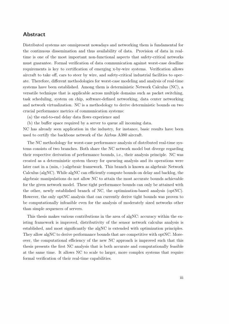
Topology Data communication networks are commonly modeled as graphs where nodesrepresent individual devices like a router or a switch. These devices can have multipleoutputs to connect to other devices (Figure 2.1a). This common depiction does, however,not suit NC’s queueing analysis well. NC therefore transforms such a device graph toits so-called server graph representation. Assuming that a device’s input buffer is servedat line speed, queueing effects manifest at the output buffers. These are modeled by theserver graph’s nodes [6, 8] (see Figure 2.1b). Figure 2.1 also illustrates that informationabout the device’s sub-components is lost during the transformation from a device graphto a server graph. Especially the highly optimized switching fabric inside network devicesthat connects inputs with outputs is, however, crucial for our considerations. Althoughthe servers most likely work off queued data in a FIFO manner, this fabric interconnectinginput ports with output ports can rearrange flows arbitrarily [29]. In the server graph,however, device ports (i.e., servers) do not share a common switching fabric component;they are directly connected to each other. The impact of switching fabrics can thus onlybe captured by departing from FIFO multiplexing towards the more general arbitrarymultiplexing assumption. Data units of individual flows do not overtake each other in
9
2 State of the Art in Network Calculus
�
�
... ...
�
�
... ...
�
�
... ...
(a) Device Graph. (b) Server Graph.
Figure 2.1: A graph of network devices with output buffering (a) and its transformationto directly connected servers (b).
switching fabrics, i.e., the FIFO per µFlow property is retained. We assume directedlinks in both graph representations, i.e., full duplex links need to be split up into twodirected links before the device graph can be transformed [80].
Data Flows and The Feed-forward Property NC also has some restricting assumptionsconcerning flows routed through the server graph. Firstly, the end-to-end analyses of NCassume unicast data flows. Secondly, these advanced NC analyses require the absence ofcyclic dependencies between flows. Work departing from this assumption can be foundin [68, 41] but is not covered by this thesis. Instead, we focus on networks that guaranteethe feed-forward property by design. We use the Turn Prohibition (TP) algorithm [79]to break potential cycles when transforming the device graph into the server graph [34]1.
In this thesis, we will use the term network to refer to a server graph and the dataflows traversing it.
2.1.3 (min,+)-algebraic Operations and Performance Bounds
Network calculus [25, 26] was cast in a (min, +)-algebraic framework in [50, 23]. Thefollowing operations manipulate arrival and service curves while retaining their worst-casesemantic.
1A “turn” is a device’s input/output connection, i.e., it corresponds to a link in the server graphrepresentation [34]. Prohibiting turns results in a cycle-free server graph. TP does not consider theroute of flows in the device graph. Therefore, flows must be routed in the turn-prohibited servergraph in order not to break their paths. Note, that shortest paths in the turn-prohibited servergraph might not coincide with the shortest path in the device graph.
10

2.1 Network Description
Definition 2.6. ((min,+)-Operations) The (min,+) aggregation, convolution and de-convolution of two functions f, g 2 F0 are defined as follows:
Aggregation: (f + g) (t) = f(t) + g(t)
Convolution: (f ⌦ g) (t) = inf
0tt
{f(t� t) + g(t)}
Deconvolution: (f ↵ g) (t) = sup
u�0{f(t + u)� g(u)}
A flow aggregate is thus a combination of flows that does not preserve informationabout the aggregated flow individually. The service curve definition translates to A
0 �A ⌦ �, the arrival curve definition to A ⌦ ↵ � A, and performance characteristics canbe bounded using the deconvolution ↵↵ �. The algebraic properties of these operationscan be found in [50]. Table 2.1 provides the more comprehensive notation scheme for NCperformance bounding we use in this thesis.
Theorem 2.1. (Performance Bounds) Consider a server s that offers a service curve�. Assume a flow f with arrival curve ↵
f traverses the server. Then, we obtain thefollowing performance bounds for f :
(Flow) Delay Bound: 8t 2 R+: D
f
(t) sup
u�0
�inf
�⌧ � 0 | ↵
f
(u) �(u + ⌧)
= inf
�⌧ � 0
�� �↵
f ↵ �
�(�⌧) 0
= h
�↵
f
, �
�=
:
D
f
Backlog Bound: 8t 2 R+: B
f
(t) sup
r�0
�↵
f
(r)� �(r)
=
�↵
f ↵ �
�(0)
= v
�↵
f
, �
�=
:
B
f
Output Bound: 8d 2 R+:
�↵
f
�0(d) =
8<:0 if d = 0�↵
f ↵ �
�(d) otherwise
h(↵
f
, �) denotes the (maximum) horizontal deviation between ↵ and � and v(↵
f
, �) de-notes their (maximum) vertical deviation. We abbreviate delay and backlog bounds withD
f and B
f , respectively, as they are valid independent of parameter t. Note, that ↵
0 isan arrival curve for A
0 and thus it is required to pass through the origin2.
Consider an aggregate of flows F with arrival curve ↵
F. The aggregate’s delay when2In a slight abuse of notation, we will use the symbol ↵ for both, deconvolution and output bounding.
11

2 State of the Art in Network Calculus
Quantifier Definitionfoi Flow of interest, the flow under analysisF Aggregate of flows
[f
n
, ..., f
m
] Flow aggregate containing flows f
n
, ..., f
m
F (s) Set of flows at server s
Fsrc (s) Set of flows entering the network at server s
x(f), x (F) Cross-traffic of flow f , aggregate Fhs
x
, . . . , s
y
i Tandem of consecutive servers s
x
to s
y
P (f) Path of flow f
↵
f , ↵
F Arrival curve of flow f , set of flows F at their (common) source↵
f
s
, ↵
Fs
Arrival bound at server s
↵
s
Abbreviation for ↵
F (s)s
, i.e., arrivals of all flows at s
�
s
Service curve of server s
�
l.o.f , �
l.o.F Left-over service curve
Table 2.1: Network calculus notation for flows, arrivals and service.
crossing a server s with strict service curve � is bounded by:
(Flow Aggregate) Delay Bound:8t 2 R+
: D
F(t) max
�0, sup
�t� t
�� 8t 2 (t, t). ↵(t)� �(t) > 0
= bp(↵
F, �) =
:
D
F
where bp
�↵
F, �
�is maximum backlogged period of � w.r.t. ↵
F.
Under arbitrary multiplexing assumptions, the lack of knowledge about ordering offlows within the aggregate requires a different delay bounding for F. Whereas FIFOassumptions (per µFlow and when aggregating flows) allow NC to bound the delay withh
�↵
F, �
�, potential reordering of flows may lead to a worse delay bound. Therefore, we
bound the delay of flow aggregates with bp
�↵
F, �
�. Note, that the maximum backlogged
period derivation requires a strict service curve.
NC also offers operations for compound analysis of servers as well as the separateanalysis of individual flows.
Theorem 2.2. (Concatenation of Servers) Consider a flow (aggregate) F crossing atandem of servers T = hs1, . . . , sni and assume that each s
i
, i 2 {1, . . . , n}, offers a
12

2.2 Analysis Principles
service curve �
s
i
. The overall service curve offered to F is their concatenation
�
s1 ⌦ . . .⌦ �
s
n
=
nOi=1
�
s
i
= �T .
The service resulting from the concatenation of strict service curves, �T , is not nec-essarily strict. It cannot be used to derive a backlogged period bound of the compoundsystem [11, 31]. This imposes challenges if the FIFO per µFlow property cannot be as-sumed [64, 70]. Also note, that convolution is commutative, i.e., the order of servers inhs1, . . . , sni cannot be reconstructed from �T .
The worst-case share of data a flow (aggregate) receives from a server is lower boundedby the left-over service curve:
Theorem 2.3. (Left-Over Service Curve) Consider a server s that offers a strict servicecurve �
s
. Let s be crossed by flow (aggregate) F0 and flow (aggregate) F1 with arrivalcurves ↵
F0 and ↵
F1 , respectively. Then F1’s worst-case residual service share under ar-bitrary multiplexing at s, i.e., its left-over (simple) service curve at s, is
�
l.o.F1s
= �
s
↵
F0
where (� ↵) (d)
:
= sup0ud
{(� � ↵) (u)} denotes the non-decreasing upper closure of(� � ↵) (d).
For arbitrary multiplexing servers, the result of this subtraction is not necessarilystrict, i.e., consecutive left-over operations are not permitted. However, aggregating ar-rival curves before subtraction from service is backed by the NC theory. In the analysisof different multiplexing disciplines, namely SP or FIFO, consecutive application of theirrespective left-over service curve operation is permitted. For SP, the left-over servicecurve derivation is �
s
↵
F0 as well [11]. Theorem 2.3 can also be used for FIFO mul-tiplexing servers as arbitrary multiplexing is more general. However, there is a left-overservice curve derivation for FIFO servers: �
l.o.F1s,✓
(d) =
h�
s
(d)� ↵
x(F1)s
(d� ✓)
i+ · 1{d>✓},[·]+ = max {·, 0}, ✓ � 0 [50].
2.2 Analysis Principles
Application of NC evolved from the analysis of single servers crossed by a single flowto the analysis of feed-forward networks of servers crossed by multiple flows that canbe entangled arbitrarily. During this evolution, two fundamental principles have beenidentified. They express behavior observable in a realistic network and thus should beimplemented in the NC analysis in order to improve the quality of bounds, i.e., accuracyof delay and backlog bounds.
13

2 State of the Art in Network Calculus
Pay Burst Only Once An analyzed flow of interest (foi) possess a certain worst-case burstiness. In the NC description, this manifests in its arrival curve’s burst termlim
d!0+ ↵(d). Due to the FIFO per µFlow property, data units within the foi cannotovertake each other. I.e., the burst cannot be delayed by other data of the foi and occuragain in an multiplexing-enforced store-and-forward behavior. Burstiness levels off atthe first server and thus the foi’s burst term should only appear once in the end-to-endperformance bound derivation for its entire path. This principle is called Pay BurstsOnly Once (PBOO).
Pay Multiplexing Only Once The service available to the foi depends on its cross-traffic. Deriving the left-over service thus requires arrival curves for cross-flows, so calledcross-traffic arrival bounds. In case cross-flows share multiple consecutive hops with thefoi, their arrival bound burstiness should not impact the delay bound derivation toooften – the same reasoning as with the PBOO principle applies. I.e., from the foi’sperspective, multiplexing should only be paid for once and therefore this principle iscalled Pay Multiplexing Only Once (PMOO).
2.3 Algebraic Analyses
An algebraic NC (algNC) analysis takes the network and compiles it into an equation– either for bounding of a specific foi’s performance characteristics or those of a server.These equations consist of (min,+)-algebraic operations and they must retain the worstcase established by the network description in order to derive valid bounds. In thissection, we provide the foremost NC analyses. They are the result of effort towardsimplementing the above principles. Each analysis defines a different order of operationsfor its respective equation. The following analyses all assume lossless transmissions andinfinite buffer space.
Figure 2.2 will serve as a running example in this section. We chose a tree network tocircumvent a comprehensive transformation of the device graph to the server graph. Intrees, there is only one potential next hop and thus each network device has only a singleoutput buffer. Note, that Figure 2.2 in fact depicts a sink-tree network. However s6 isnot the sink of the device graph but corresponds to the device that is directly connectedto it. At the sink-device, there is no output buffer to cross and thus it does not appearin the network as a sink-server after s6.
2.3.1 Total Flow Analysis
The Total Flow Analysis (TFA) [26] directly applies the basic results from Definition 2.6,aggregation and deconvolution, as well as Theorem 2.1: It takes the totality of flows
14

2.3 Algebraic Analyses
s6
s0 s1
s3
s5
s2
s4
f0
f2
f1
Figure 2.2: Tree network, i.e., server graph with flows, serving as a running example.
(a flow aggregate) present at a server and the server’s service curve to bound delay andbacklog. I.e., the TFA operates from a server’s point of a view by aggregating all incomingtraffic. The delay bound is thus valid for all flows crossing the server and the backlogbound denotes the server’s buffer requirement for serving them.
Assume server s
i
is crossed by the flow aggregate F (s
i
) and let ↵
s
i
be the aggregatedarrival curve of all flows. Then, we get the server-local TFA bounds:
D
s
i
=
8<:h (↵
s
i
, �
s
i
) if |F (s
i
)| = 1 (FIFO per µFlow)
bp (↵
s
i
, �
s
i
) otherwise, B
s
i
= v (↵
s
i
, �
s
i
) .
The delay bounds on the foi’s path P (foi), from its source server to its destinationserver, can be used to derive a flow delay bound:
D
TFAP (foi) =
Xs
i
2P (foi)
D
s
i
For instance, the TFA delay bound derivation for flow f1 in Figure 2.2 proceeds as follows:
D
TFAP (f1)
= D
s0 + D
s1 + D
s2 + D
s5 + D
s6
= h
⇣↵
f1s0
, �
s0
⌘+ bp
⇣↵
[f1,f0]s1
, �
s1
⌘+ bp
⇣↵
[f1,f0]s2
, �
s2
⌘+ bp
⇣↵
[f1,f0,f2]s5
, �
s5
⌘+ bp
⇣↵
[f1,f0,f2]s6
, �
s6
⌘= . . .
= h
⇣↵
f1, �
s0
⌘+ bp
⇣⇣↵
f1 ↵ �
s0
⌘+ ↵
f0, �
s1
⌘+ bp
⇣⇣⇣↵
f1 ↵ �
s0
⌘+ ↵
f0
⌘↵ �
s1 , �
s2
⌘+ bp
⇣⇣⇣⇣⇣↵
f1 ↵ �
s0
⌘+ ↵
f0
⌘↵ �
s1
⌘↵ �
s2
⌘+
⇣⇣↵
f2 ↵ �
s3
⌘↵ �
s4
⌘, �
s5
⌘+ bp
⇣⇣⇣⇣⇣⇣↵
f1 ↵ �
s0
⌘+ ↵
f0
⌘↵ �
s1
⌘↵ �
s2
⌘+
⇣⇣↵
f2 ↵ �
s3
⌘↵ �
s4
⌘⌘↵ �
s5 , �
s6
⌘
15

2 State of the Art in Network Calculus
Although the TFA is based on per-server bounds, replacing a single server yields largerecomputation effort. The output boundings (deconvolution operations ↵) required toderive all arrivals at the servers create dependencies between them. For instance, replac-ing �
s0 results in a complete recomputation of the above D
TFAP (f1)
. Moreover, accuracyis compromised by the occurrences of (entire) arrival curves ↵
f0 , ↵
f1 and ↵
f2 at everyserver they cross. Each arrival curve contributes a burst term to the server-local delayderivation – neither the PBOO nor the PMOO principle are implemented in the TFA.
2.3.2 Separate Flow Analysis
The Separate Flow Analysis (SFA) departs from computing per-server bounds that arevalid for the totality of flows. Instead, SFA derives an end-to-end left-over service curvefor the foi and uses it to bound only the foi’s performance characteristics. For NC, thisstep from server analysis to end-to-end flow analysis constitutes a big evolutional leapforward. Building the delay analysis around the foi shifted its view directly to the tandemof servers on its path P (foi) – the SFA is a tandem analysis. Separating the foi allows NCto make use of its FIFO per µFlow property, i.e., its end-to-end delay is always boundedwith the horizontal deviation h (↵, �). In [74], it was shown that this method strictlyoutperforms TFA with the bp (↵, �). Note, however, that the backlog bound, v (↵, �),has a different semantic in the SFA. It does not bound the backlog at a server but thefoi’s data in transit.
The SFA is a straight-forward, server-by-server application of Theorems 2.1, 2.3 and 2.2 [50]:it bounds cross-traffic arrivals (cf. TFA, not depicted), subtracts them from the servers’service curves, concatenates the resulting left-over service curves and finally bounds thefoi’s performance characteristics.
�
l.o.fois
i
= �
s
i
↵
x(foi)s
i
, �
l.o.SFAfoiP (foi) =
Os
i
2P (foi)
�
l.o.fois
i
.
D
foi= h
⇣↵
foi, �
l.o.SFAfoiP (foi)
⌘, B
foi= v
⇣↵
foi, �
l.o.SFAfoiP (foi)
⌘.
Executing the operations in this order can be directly proven to result in a valid end-to-end left-over service curve. Bounding the delay with the horizontal deviation insteadof the maximum backlogged period size relaxes the strict service curve requirement.
Using a single, end-to-end left-over service curve, the foi’s arrival curve ↵
foi appearsonly once in the equation for delay bound computation. I.e., the SFA implements thePBOO principle. In case cross-flows are present at multiple consecutive hops, theirarrivals appear multiple times. We illustrate this problem with the �
l.o.SFAf1
P (f1)-computation
16

2.3 Algebraic Analyses
for Figure 2.2:
�
l.o.SFAf1
P (f1)= �
l.o.f1s0
⌦ �
l.o.f1s1
⌦ �
l.o.f1s2
⌦ �
l.o.f1s5
⌦ �
l.o.f1s6
= �
s0 ⌦⇣�
s1 ↵
f0
⌘⌦⇣�
s2 ↵
f0s2
⌘⌦⇣�
s5 ↵
[f0,f2]s5
⌘⌦⇣�
s6 ↵
[f0,f2]s6
⌘= . . .
= �
s0 ⌦⇣�
s1 ↵
f0
⌘⌦⇣�
s2 ⇣↵
f0 ↵ �
s1
⌘⌘⌦⇣�
s5 ⇣⇣⇣
↵
f0 ↵ �
s1
⌘↵ �
s2
⌘+
⇣⇣↵
f2 ↵ �
s3
⌘↵ �
s4
⌘⌘⌘⌦⇣�
s6 ⇣⇣⇣⇣
↵
f0 ↵ �
s1
⌘↵ �
s2
⌘+
⇣⇣↵
f2 ↵ �
s3
⌘↵ �
s4
⌘⌘⌘↵ �
s5
⌘In this SFA equation, ↵
f1 does not appear, yet, ↵
f0 and ↵
f2 are found multiple times.Every occurrence adds the respective cross-flow’s burst term; the derivation is not ableto capture how these level off in a realistic system. From f1’s point of view, multiplexingwith cross-traffic is paid for multiple times.
The presented �
l.o.SFAf1
P (f1)is also a bound on the left-over service for SP multiplexing
and FIFO multiplexing tandems of servers because the foi is assumed to have lowestpriority among all flows. A more accurate SP left-over service curve can be derivedwith a simple adaptation: Flows of lower priority than f1 need not be subtracted fromthe service curve. For FIFO multiplexing, the FIFO left-over service curve can be usedinstead of the arbitrary multiplexing one. The equation will have multiple parameters✓
i
, one for each server s
i
, and a subsequent optimization step is required. In contrastto the arbitrary multiplexing SFA, per-server knowledge is not sufficient to derive theend-to-end left-over service curve [51]. For non-FIFO per µFlow analysis, implementingthe PBOO principle requires a different notion of service curve that guarantees an upperbound on the dwell period of a data unit traversing a tandem of servers [70].
2.3.3 Pay Multiplexing Only Once Analysis
The SFA’s �
l.o.SFAf1
P (f1)derivation reveals that cross-traffic arrival curves appear at every
server they need to be subtracted. Therefore, implementing the PMOO principle followsthe idea to convolve the analyzed tandem of servers before subtracting the cross-trafficarrivals3. This order of operations allows the NC analysis to capture the leveling off ofcross-flow bursts on the subpath shared with the analyzed foi [30]. The PMOO analysis(PMOOA) implements this order of operations. In this thesis, we use two differentvariants of the PMOOA, depending on the interference pattern of cross-traffic.
3Application of algebraic operations in this order is not backed by NC theory. Service curve strictnessis required for subtraction but the result of convolution is not provably strict [31]. Yet, [74] providesa proof that the resulting curve is indeed a valid lower bound for the tight left-over service curve.
17

2 State of the Art in Network Calculus
Definition 2.7. (Flow Nesting) Let T be a tandem of servers and f
a
and f
b
two flowscrossing some servers of this tandem. Then, flows are related in one of these ways:
• Flow f
a
is nested into f
b
on T , f
a
�T f
b
, iff all servers f
a
consecutively crosses onT are also consecutively crossed by f
b
.
• Flow f
b
is nested into f
a
on T , f
b
�T f
a
, iff all servers f
b
consecutively crosses onT are also consecutively crossed by f
a
.
• Flows f
a
and f
b
are not related on T iff they do not share any servers on thistandem.
• Flows f
a
and f
b
overlap on T if neither of the above is true.
Note, that servers can only be crossed in one direction due to the directed links in theserver graph and that, by definition, all cross-flows of an analyzed foi are nested into itspath, i.e., T = P (foi).
Definition 2.8. (Interference Pattern [52]) Let foi be the flow of interest and let x(foi)be the set of its cross-flows. The foi’s cross-traffic interference pattern is called nestedif, on the foi’s path P (foi), there is either a nesting relation between all pairs of flows inx(foi) or no relation at all. If there are at least two cross-flows that overlap on P (foi),the entire cross-traffic interference pattern is called non-nested.
The first PMOOA variant is exclusively applicable to tandems with a nested cross-traffic interference pattern. The second one defines a new operation, a left-over servicecurve computation for an entire tandem, that is applicable to tandems with non-nestedinterference patterns. However, it requires that arrival curves are from FmTB and servicecurves are from FmRL.
The PMOOA for Nested Interference This interference pattern guarantees a hierar-chical nesting relation between all flows on P (foi). This relation can be expressed witha nesting tree with the foi at its root [52, 53]. The tree defines the order of algebraicNC operations to be applied: Starting from the tree’s leaf nodes, i.e., the flows withoutothers nested into them, flow paths are convolved and the according flow traversing it issubtracted. These two steps result in (not necessarily end-to-end) left-over service curvesfor flows on the next level in the nesting tree. Convolution and subtraction are repeated,level for level in the nesting tree, until only the foi and its end-to-end left-over servicecurve remain.
18
2.3 Algebraic Analyses
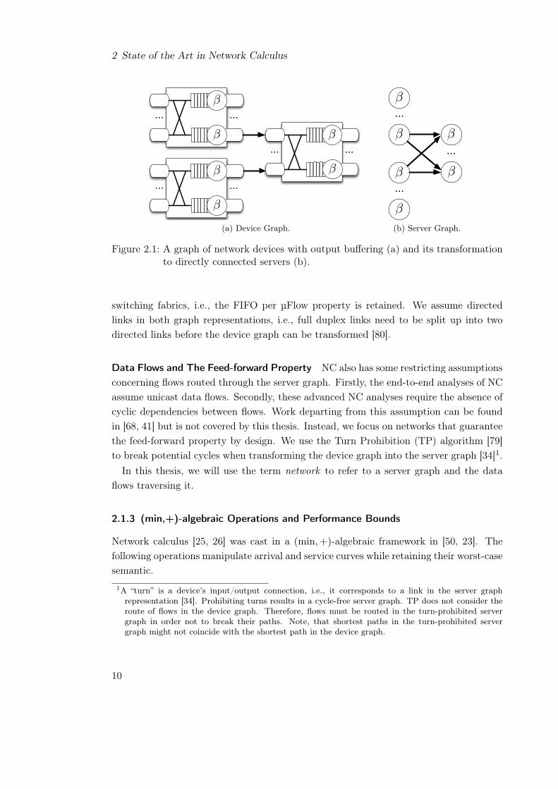
The nesting tree for the network of Figure 2.2 is f2 �P (f1) f0 �
P (f1) f1. It results in
�
l.o.PMOOf1
P (f1)= �
l.o.PMOOf1
hs0,s1,s2,s5,s6i
=
⇣⇣⇣(�
s5 ⌦ �
s6) ↵
f2s5
⌘⌦ (�
s1 ⌦ �
s2)
⌘ ↵
f0
⌘⌦ �
s0
=
⇣⇣⇣(�
s5 ⌦ �
s6) (↵
f2 ↵ �
s3 ↵ �
s4)
⌘⌦ (�
s1 ⌦ �
s2)
⌘ ↵
f0
⌘⌦ �
s0
and f1’s performance bounds are, similar to the SFA,
D
f1= h
⇣↵
f1, �
l.o.PMOOf1
P (f1)
⌘, B
f1= v
⇣↵
f1, �
l.o.PMOOf1
P (f1)
⌘.
For the analysis of nested FIFO-multiplexing tandems, this procedure constitutes thefundamental aspect of the least upper delay bound (LUDB) analysis [3].
The PMOOA Left-over Service Curve for non-Nested Interference The second vari-ant of the PMOOA addresses the problem of non-nested interference patterns [75]. It pro-vides a single-step left-over service curve derivation �
l.o.PMOOfoiP (foi) . This non-nested-PMOO
operation has an additional requirement on the shape of curves: The strict service curvesmust belong to the class of multi-rate-latency curves FmRL and arrival curves must befrom the class of multi-token-bucket curves FmTB. Moreover, for the concrete derivationof �
l.o.PMOOf1
P (f1), we need to maintain distinguishable partial curves after the decomposition
into partial curves from FmRL and FmTB:
�
s0 =
n
hWh=1
�
R
s0,h, T
s0,h, �
s1 =
n
iWi=1
�
R
s1,i, Ts1,i,
�
s2 =
n
jWj=1
�
R
s2,j , Ts2,j, �
s5 =
n
kWk=1
�
R
s5,k, T
s5,k,
�
s6 =
n
lWl=1
�
R
s6,l, T
s6,l,
↵
f0s1 = ↵
f0=
n
pVp=1
�
r
f0s1,p, b
f0s1,p
, ↵
f2s5 =
�↵
f2 ↵ �
s3
�↵ �
s4 =
n
qVq=1
�
r
f2s5,q , b
f2s5,q
.
Then we get the following left-over service curve:
�
l.o.PMOOf1
P (f1)= �
l.o.PMOOf1
hs0,s1,s2,s5,s6i
=
n
h_h=1
n
i_i=1
n
j_j=1
n
k_k=1
n
l_l=1
n
p_p=1
n
q_q=1
�
R
l.o.h,i,j,k,l,p,q
, T
l.o.h,i,j,k,l,p,q
19

2 State of the Art in Network Calculus
with
R
l.o.h,i,j,k,l,p,q
= R
s0,h ^⇣R
s1,i � r
f0s1,p
⌘^⇣R
s2,j � r
f0s1,p
⌘^⇣R
s5,k � r
f0s1,p
� r
f2s5,q
⌘^⇣R
s2,l � r
f0s1,p
� r
f2s5,q
⌘and
T
l.o.h,i,j,k,l,p,q
= T
s0,h + T
s1,i + T
s2,j + T
s5,k + T
s6,l (2.1)
+
b
f0s1,p + b
f2s5,q
R
l.o.h,i,j,k,l,p,q
(2.2)
+
r
f0s1,p · (T
s1,i + T
s2,j + T
s5,k + T
s6,l) + r
f2s5,q · (T
s5,k + T
s6,l)
R
l.o.h,i,j,k,l,p,q
(2.3)
The three parts of the left-over service curve’s latency are distinguishable on the right-hand side of T
l.o.h,i,j,k,l,p,q
:
• The original latencies of the crossed servers (Term 2.1),
• the additional latency due to first working off bursts of cross-traffic (Term 2.2), and
• the added latency for working off data that was queued while waiting for the servers’latency (Term 2.3).
Only the second part holds the cross-flows’ burst terms and by taking the minimum overthe combinations of token buckets and rate latencies, cross-traffic burstiness is paid foronly once in the overall derivation. The analyzed flow’s performance bounds are, again,derived with this service curve (see nested PMOOA).
For FIFO multiplexing, a single-step derivation akin to the non-nested PMOOA doesnot exist. Instead, the analyzed tandem is cut into sub-tandems with nested interferencepatterns. Each sub-tandem’s left-over service curve is computed with the nested PMOOAvariant and they are convolved to an end-to-end left-over service curve. In case there aremultiple alternatives to cut the tandem, all are tested and the best result, i.e., the leastdelay bound, is returned by the LUDB analysis [3]. This approach does not necessarilyimplement the PMOO principle to its fullest extent.
2.4 Optimization-based Analysis
The PMOOA was considered strictly superior to the SFA w.r.t. delay bounding as itimplements the eponymous principle for end-to-end analysis. However, [74] shows thatthe SFA can arbitrarily outperform the PMOOA. Due to the convolution’s commutativity,
20

2.4 Optimization-based Analysis
PMOOA cannot benefit from large residual service at the end of the analyzed (convolved)tandem. This is expressed on the right-hand side the above equation, Terms 2.2 and 2.3,where the minimum end-to-end left-over rate is in the denominator. I.e., the per-serverservice rate is not available to the analysis.
Additionally, an optimization-based bounding method that implements the PMOOprinciple is provided in [74]. It transforms the NC network description to an optimizationproblem; departing from the algebraic methodology to overcome the problematic propertyof convolution. This method shares the PMOOA’s requirement on arrival and servicecurves to be from FmTB and FmRL, respectively, and derives a superior left-over servicecurve from these. Hence, [74] also proves that the PMOOA’s �
l.o.PMOOfoiP (foi) is valid despite
its order of operations that cannot be directly proven to be resulting in a valid left-overservice curve.
2.4.1 The Linear Programming Analysis
The seminal work on optimization-based NC inherited some crucial aspects from algNC.Most importantly, it composes tandem-local results when analyzing a feed-forward net-work. This approach is known to enforce worst-case assumptions in the analysis offeed-forward networks that may lead to a loss of result accuracy [53]. Optimization does,however, not require a compositional analysis. Based on these insights, an optimization-based, tight feed-forward analysis was proposed in [12]: the Linear Programming Analysis(LPA). Intuitively, LPA delay analysis proceeds as follows:
1. Starting from the foi’s sink server, flows as well as their respective cross-flows arerecursively traced towards their sources. For every link traversed backwards, thestart of backlogged periods at the link’s source and its destination are related.This step terminates as soon as all flows are traced to their sources. The resultis a partial order where, for example, there is no given order between the startsof backlogged periods for servers in different branches of a tree (e.g., s2 and s4 inFigure 2.2).
2. The second step is to extend the partial order to the set of all compatible totalorders. This procedure enumerates all potential entanglements of the start of back-logged periods at the network’s servers. In the above example, the entanglementon distinct branches of the tree network are enumerated such that all outcomes areconsidered at the later servers s5 and s6. Special care must be taken of relationscaused by rejoining flows [53].
3. This step transforms each total order to one linear program. The order betweenthe start of backlogged periods as well as the NC network description (strict service
21

2 State of the Art in Network Calculus
curves, arrival curves, non-decreasing curves, non-negativity, flow constraint) areused to derive the constraints of each linear program. Like most analyses, theLPA requires arrival curves from FmTB and service curves from FmRL. They aredecomposed as shown above; each token bucket and each rate latency is convertedinto one constraint.
4. The LPA’s set of linear programs models all potential entanglements of flows asthey gradually progress on their path through the network; not only the worst-case one(s). Therefore, all linear programs must be solved in the final step. Themaximum among their solutions is a valid worst-case bound for the foi’s delay. I.e.,the LPA is an all-or-nothing analysis approach.
Step 2 constitutes the main drawback of the LPA: The amount of different linear programsand thus the computational complexity of the LPA grows possibly (super-)exponentiallywith the network size. The authors prove that their approach to obtain tight bounds isin fact NP-hard.
For other multiplexing disciplines, similar optimization-based NC analyses have beenprovided in the literature: SP feed-forward-networks [13], FIFO tandems [14] and FIFOfeed-forward networks [15]. The latter one is most similar to the LPA, yet, it replacesstep 2 with a different technique to encode multiplexing and demultiplexing of flows thatlead to parallel paths. It introduces integer variables, i.e., it transforms the NC networkdescription into a single mixed-integer linear program instead of a set of ordinary linearprograms. There is no optimization-based analysis for tandems of servers that do notretain the FIFO per µFlow property.
22

3 Accuracy of Algebraic Network Calculus
This section presents the problem of flow segregation arising in algNC analysis of feed-forward networks. We provide two countermeasures to it: aggregate arrival bounding andarrival bound burstiness reduction. AlgNC can derive delay, backlog and output boundsfor tandems of servers in a straight-forward fashion. For the analysis of feed-forwardnetworks, we present the generic concepts to decompose the network into tandems andrecompose tandem-local analysis results to the flow of interest’s performance bounds.
Section 2.2 presented the state of the art in NC; work that was mainly dedicated tothe step from a single server analysis to a tandem of servers. We have established theframework that allows a tandem analysis to compute performance bounds in generalfeed-forward networks. This framework, called the compositional feed-forward analysis(compFFA), is presented in Section 3.1. It defines how the tandem-local results arecomposed to a network-global analysis – a step not required in the LPA. Investigating thecompFFA procedure allows us to identify the causes for inaccurate results in algNC’s feed-forward analysis (Section 3.2). Improvements to the algNC are presented in Sections 3.3and 3.4.
3.1 Compositional Analysis of Feed-forward Networks
The LPA’s approach to the feed-forward analysis imposes considerable effort to attaina network-global view on flow scheduling and cross-traffic (de-)multiplexing, renderingit NP-hard (Section 2.4.1). The tandem analyses of algNC cannot follow this approach.For the analysis of a feed-forward network, they must follow a compositional divide-and-conquer approach, the compFFA. It consists of two steps [7, 8].
1. Cross-traffic Arrival Bounding:The first compFFA step abstracts from the feed-forward network to the foi’s path –a tandem of servers that can be analyzed with one of the existing procedures. Afterthis step, a bound on the worst-case shape of cross-flows is known at the locations ofinterference with the foi. Then, the following step need not consider the part of thenetwork traversed by these flows nor the potentially complex interference patternsthey are subject to (see Figure 3.1). In detail, this step proceeds as follows:
a) Starting at the locations of interference with the foi, cross-flows are back-tracked to their sources. This procedure derives the dependencies betweenthe foi, its cross-flows, their cross-flows, etc., in a recursive fashion. A newinstance of this sub-step is started for any cross-flow of the current cross-flowunder consideration. Due to the network’s feed-forward property, the recur-sion is guaranteed to terminate.
23

3 Accuracy of Algebraic Network Calculus
Figure 3.1: CompFFA: abstraction from a feed-forward network, possibly a tree, to theservers on the flow of interest’s path.
b) Next, the dependencies are converted into an equation, i.e., a sequence of alge-braic operations, that capture the transformation of worst-case flow arrivals.
c) Finally, the equations are solved to obtain the bounds on cross-traffic arrivals.
2. Flow of Interest Performance Bounding:The foi’s end-to-end delay bound in the feed-forward network is derived with a lesscomplex tandem analysis.
The second step of the compFFA procedure has seen much treatment in the literature(see Section 2.3 as well as [10, 31] for recent overviews). The first step of the feed-forward network analysis, bounding the cross-traffic, has so far been largely neglected.Most work starts directly with the tandem analysis or suggests to use straightforwardtechniques from basic NC results (more details are given in Section 3.3). An exceptioncan be found in [29], where, for a single node under arbitrary multiplexing of severalflows, tight output descriptions are derived for a single flow. However, when targetinga feed-forward network, we need to bound cross-flows that may have traversed severalservers with potentially many other flows joining and leaving it. The literature neitherprovides an in-depth analysis of compFFA’s shortcomings nor work to improve analysisaccuracy through step 1. This thesis will focus on the first step of the compFFA as wellas the interdependencies between both steps in order to improve the accuracy of algNCperformance bounds.
24

3.2 Problems
3.2 Problems
3.2.1 Problems Caused by Compositionality
The compFFA’s compositionality causes a fundamental problem: Cross-flows arrivalsat different locations of interference are bounded independently from each other withseparate instances of compFFA step 1. In every instance, the flow under considerationis bounded with flow-local worst-case assumptions; the compositional analysis suffersfrom a cross-flow segregation effect. Each of the segregated flows computes a left-overservice curve by considering any other traffic to interfere with it in the worst case. Thecross-flow segregation negatively impacts compFFA if, during independent backtrackingsof step 1a, servers are traversed multiple times. I.e., they appear in the equation ofstep 1b more than once, with different settings of flows to subtract (left-over servicecurve operation) and different flows for arrival bounding. Rejoining interference with thefoi is an instance of this problem [53]4 that also motivates the LPA [12]. A similar instanceof the problem is used for evaluating the LPA: the square network (see Figure 3.2a). Itimposes segregation in a transitive fashion when analyzing flow f1: The flows at server s1
(service �
s1) are in two separate backtracking instances, one started for at server s3 andone started at server s4 that, in turn, requires to bound f2 at server s2. I.e., at s1,both flows assume worst-case mutual interference by a left-over service curve derivationwith their respective flow-local worst-case assumptions. Service �
s1 is segregated into�
l.o.f2s1 = �
s1 ↵
f3 and �
l.o.f3s1 = �
s1 ↵
f2 (Figure 3.2b) – two left-over service curvesthat cannot be attained simultaneously in a realistic network. As a consequence, theresult of compFFA step 1a, i.e., the internal model it creates, does not necessarily equalthe server graph. We formulate this problem in a novel principle to be implemented byfeed-forward NC analyses, similar to PBOO and PMOO (Section 2.2).
The Pay Segregation Only Once (PSOO) principle If the arrivals of two flows have tobe bounded segregately in the compositional feed-forward analysis and these flows bothcross the same server before interfering with the foi, then they should not be segregatedin a way that imposes the worst-case mutual interference assumptions on both. In thealgebraic analysis equation, segregated flows should not have to consider each otherfully in their respective arrival bounding. Although this leads to a valid upper bound,the according behavior is not attainable by a realistic system and thus the eventualperformance bound cannot be tight. Segregation of cross-flows should only be paid foronce by the ensemble of the two flows.
4In the earlier work of [73] ”eliminate rejoining interfering flows” means that the analysis internallycreates a new flow for every location of interference with the flow of interest. The arrivals of theseflows are bounded with compFFA step 1, i.e., the cross-flow segregation problem persists.
25

3 Accuracy of Algebraic Network Calculus
�s1 �s2
�s3 �s4↵
f1
↵
f2
↵
f3
↵
f4
(a) The Square Network. (b) CompFFA-internal model of the network.
Figure 3.2: Cross-flow segregation in the square network.
The LPA is not compositional, it is the only NC analysis implementing the PSOOprinciple in addition to PBOO and PMOO.
3.2.2 Problems Caused by Tandem Analyses
We found an interdependency between compFFA step 2 and compFFA step 1 that canenforce segregation of cross-flows. We derived the minimal network setting that exhibitsthe problem (Figure 3.3a). Interestingly, it is the non-nested tandem as already usedin [74] to motivate the use of optimization, yet, flows take different roles. The foi doesnot cross the entire tandem, instead, we analyze the flow crossing only the two serversat the end of the tandem.
Bounding the foi’s end-to-end delay depends on the choice of tandem analysis appliedto it5. I.e., the actual decomposition into left-over service curve and output boundoperations in step 1 depends on the analysis chosen for in step 2.
• The SFA first decomposes the foi’s paths into single servers to apply Theorems 2.3and 2.2 (Figure 3.3c). Thus, it starts an cross-traffic arrival bounding instance forevery server.
• The PMOOA does not decompose the foi’s path into smaller units of operation thanthis tandem itself. I.e., it tries to operate on longest tandems possible (Figure 3.3b).
We have identified crucial problems that arise from either of these two alternatives ofalgNC. They enforce a segregation of cross-flows and with their distinct cause, they canoccur in addition to the segregation problem illustrated with the square network.
5We will not consider the TFA for delay analysis as it will result in strictly inferior bounds.
26

3.2 Problems
s0 s1 s2
xf1
xf2
foi
(a) Minimal network suffering from composition penalty.
xf1
xf2
�
l.o.xf1s0
�
l.o.xf2s0
�
l.o.foi�s1,s2�foi
(b) Figure 3.3a’s PMOOA-internal model.
(c) Figure 3.3a’s SFA-internal model.
Figure 3.3: The minimal network imposing a PSOO principle violation due to the tandemanalysis applied in compFFA step 2.Interpretation: Boxes depict tandems for �
l.o. derivation and arrows depictflows. Flows pointing at a box are subtracted from � and crossing a boxmeans using the �
l.o. for output bounding.
Cross-flow Segregation Enforced by Subpath Sharing Considerations The PMOOAwas constructed to consider shared subpaths between the foi and its cross-flows. It de-mands a distinct arrival curve for each cross-flow (aggregate) sharing a specific subpath.I.e., if two cross-flows xf1 and xf2 interfere on two different subpaths, they require seg-regate arrival boundings [9]. This procedure causes problems in case these cross-flowsshare hops apart from the foi’s path – similar to the known problem cause by the comp-FFA procedure. There, they cannot be aggregated; they must be considered mutualinterference. Figure 3.3b illustrates this problem. Cross-flows xf1 and xf2 fulfill the cri-teria for segregated arrival bounding and their respective left-over service curves at s0
are �
l.o.xf1s0 = �
s0 ↵
xf2 and �
l.o.xf2s0 = �
s0 ↵
xf1 . The cross-traffic arrival bound deriva-tion will have more than one cross-traffic burstiness for each of the interfering flows xf1
and xf2, the PSOO principle is violated. Both of the PMOOA variants presented in
27
3 Accuracy of Algebraic Network Calculus
Section 2.3.3 suffer from this problem.
Cross-flow Segregation Enforced by Tandem Decomposition The SFA can have var-ious degrees of aggregation and separation within its equation, i.e, its internal modelof the network. The SFA proceeds server-by-server; in terms of the PMOOA’s subpathsharing point of view, it can aggregate all cross-flows sharing a single hop on the foi’spath. Consider Figure 3.3a’s network again: On the foi’s first hop, s1, SFA allows toaggregately bound the arrivals of xf1 and xf2 in a single instance of compFFA step 1.Then, the left-over service curve of the cross-flow aggregate [xf1, xf1] crossing server s0
is �
l.o.[xf1,xf1]s0 = �
s0 . In this case, aggregation supersedes segregation and thus no explicitimplementation of the PSOO principle is required. However, the SFA’s decompositioninto individual servers also requires an arrival bounding instance for xf2 at s2. Here,mutual interference between xf1 and xf2 has to be assumed. At s0, we get the same�
l.o.xf1s0 and �
l.o.xf2s0 as in the PMOOA – the PSOO principle must be violated to retain
the worst case. At s1, we additionally get �
l.o.xf2s1 = �
s1 ↵
xf1s1 , i.e., another burst term
appears in the derivation due to violating the PMOO principle.
Decisions on Incomplete Knowledge In [74], the authors show that knowledge of thecrossed servers’ sequence is lost in the PMOOA’s tandem analysis. The SFA, in contrast,retains this knowledge due to its server-by-server procedure. This allows the SFA tooutperform the PMOOA on tandems where �
l.o. curves get considerably faster towardsthe end. In feed-forward networks, either applying the SFA or the PMOOA is the firstdecision to take. That means, the decision does not have the �
l.o. curves at its disposal– they remain unknown until the first step of the compFFA resulted in the cross-trafficarrival bounds. Thus, eventually concluding the analysis can exploit the sequence ofservers triggers another feed-forward analysis of the network.
We summarize all the above problems in the composition penalty of algNC.
3.3 Derivation of Cross-traffic Arrival Bounds
We identified segregation of flows to cause inaccuracy in the algNC analysis. In thissection, we present a new, recursive algorithm implementing an arrival bounding forcompFFA step 1 that maximizes aggregation of flows. Thus, we reduce the compositionpenalty of compFFA’s step 1. Unaware of the drawbacks of segregation, the literaturesuggest to execute SFA with a cross-traffic arrival bounding that applies maximum seg-regation [10]. It operates on longest possible tandems. We prove that our approachoutperforms the one of the literature if (min,+)-deconvolution distributes over addition.
28

3.3 Derivation of Cross-traffic Arrival Bounds
3.3.1 Segregated Cross-flow Arrival Bounding
NC analyses previously focused on improved end-to-end view on the tandem in the sec-ond compFFA step in order to tighten the delay bound. The generic way to computeperformance bounds in feed-forward networks [10] is in line with this approach. It de-rives the SFA-like cross-traffic arrival bound for each flow at each system. Cross-flowsare segregated from each other such that every cross-flow can be analyzed with a SFA ona maximum length tandem, i.e., source-to-interference location. This cross-flow bound-ing implements the PBOO principle for the segregated flows. Therefore, we call thisprocedure to decompose a feed-forward network into a sequence of tandem analyses thesegregated PBOO arrival bounding, segrPBOOAB.
Figure 3.4 illustrates this method: At both servers crossed by the foi, s1 and s2, anew instance of compFFA step 1 is started for every cross-flow. The enforced segregationresults in a violation of the PSOO principle:
�
l.o.fois1
= �
s1 ⇣↵
xf1s1
+ ↵
xf2s1
⌘= �
s1 ⇣⇣
↵
xf1 ↵⇣�
s0 ↵
xf2
⌘⌘+
⇣↵
xf2 ↵⇣�
s0 ↵
xf1
⌘⌘⌘The arrival bounding at s1 is equal to Figure 3.3b’s derivation; the segrPBOOAB
suffers from the same problem as the analysis considering subpath sharing. Moreover, ats2 it suffers from the decomposition of the analyzed tandem into server-by-server left-overderivations and another cross-flow segregation at s0 (cf. Figure 3.3c). Next, we presentour alternative cross-traffic arrival bounding for the compFFA.
3.3.2 Aggregate Cross-traffic Arrival Bounding
In our alternative arrival bounding for compFFA step 1, we prioritize maximum aggrega-tion of cross-flows over the analysis of maximum length tandems. We apply Theorem 2.1,output bound, to cross-traffic aggregates – moving along the topology, starting from thelocation of interference with the foi and terminating at the sources of cross-flows. Thus,aggregation results in a different decomposition of the network into tandems than theprocedure of Section 3.3.1. It also reduces the PSOO violations by circumventing segre-gation as much as possible. In order to benchmark this change against the segrPBOOAB,we implement the PBOO principle on the tandems shared by all flows in a cross-trafficaggregate. We call this procedure the aggregate PBOO arrival bounding, aggrPBOOAB.
The derivation of the left-over service curve for s1 in Figure 3.3a’s network changes to(see Figure 3.3c):
�
l.o.fois1
= �
s1 ↵
[xf1,xf2]s1
= �
s1 ⇣⇣
↵
xf1+ ↵
xf2
⌘↵ �
s0
⌘The crucial difference is located at s0. As both of the cross-flows, xf1 and xf2, share this
29

3 Accuracy of Algebraic Network Calculus
xf1
�
l.o.xf2s1
xf2
�
l.o.fois1
�
l.o.fois2
�
l.o.xf1s0
�
l.o.xf2s0
foi
Figure 3.4: Figure 3.3a’s SFA-internal model as presented in [10]. In contrast to Fig-ure 3.3c, it does not aggregate cross-traffic arrivals at server s1.
server, their output can be bounded aggregately. Information of per-cross-flow arrivals,i.e., a segregated bounding, is not necessary and thus the PSOO principle need not beimplemented.
The aggrPBOOAB is not as straight-forward as the segrPBOOAB. Therefore, we de-veloped the principle to maximize aggression into an algorithm for compFFA step 1.It integrates the three distinguishable substeps, backtracking, derivation of the analysisequation and solving it, into a recursive solution for efficient computation. This algorithmwas implemented in the DiscoDNC tool [7].
Algorithm 3.1. (Recursive aggrPBOOAB) The foi’s cross-traffic arrival bound at servers is derived as follows. Starting from s, paths of cross-flows are backtracked via links; eachlink l connects a source server l
src and a destination l
dest. The function dest(s) returnsthe set of links whose destination is s, x (foi, l) = F (l
src) \ F
�l
dest� \ x (foi) returns thecross-flows of foi on l and for a set of links L we define x (foi,L) =
Tl2L x (foi, l). We get,
for instance, x (x (foi, l)) =
�F (l
src) \ F
�l
dest�� \ x (foi, l). Note, that flow sets might berestricted by location, e.g., ↵
x(foi)s
x
= ↵
x(foi)\F (sx
)s
x
, and that in an expression x (foi, l), thefoi need not cross l.
↵
x(foi)s
=
Xl12dest(s)
⇣↵
x(foi,l1)l
src1
↵ �
l.o.x(foi,l1)l
src1
⌘+ ↵
Fsrc(s)\x(foi)
=
Xl12dest(s)
⇣↵
x(foi,l1)l
src1
↵⇣�
l
src1 ↵
x(x(foi,l1))l
src1
⌘⌘+ ↵
Fsrc(s)\x(foi)
=
Xl12dest(s)
(
0B@ Xl22dest(lsrc1 )
⇣↵
x(foi,{l2,l1})l
src2
↵ �
l.o.x(foi,{l2,l1})l
src2
⌘+ ↵
Fsrc(lsrc1 )\x(foi,l1)
1CA↵⇣�
l
src1 ↵
x(x(foi,l1))l
src1
⌘)
+ ↵
Fsrc(s)\x(foi)
30

3.3 Derivation of Cross-traffic Arrival Bounds
=
Xl12dest(s)
(
0B@ Xl22dest(lsrc1 )
⇣↵
x(foi,{l2,l1})l
src2
↵ �
l.o.x(foi,{l2,l1})l
src2
⌘+ ↵
Fsrc(lsrc1 )\x(foi,,l1)
1CA↵
0B@�
l
src1
Xl22dest(lsrc1 )
⇣↵
x(x(foi,{l2,l1}))l
src2
↵ �
l.o.x(x(foi,{l2,l1}))l
src2
⌘1CA)
+ ↵
Fsrc(s)\x(foi)
= . . .
The recursion of Algorithm 3.1 is exemplarily unfolded to illustrate the backtrack-ing of interference in a feed-forward network. Initially, the foi’s cross-traffic ↵
x(foi)s
issplit into the sum of flow arrivals from incoming links and those originating at s itself,↵
Fsrc(s)\x(foi). Next, the left-over service curves at the sources of incoming links are de-rived in order to separate the foi’s cross-traffic that has to be bounded, x(foi, l1), from thecross-traffic it experiences, x(x(foi, l1)), i.e., there are two directions to further backtrackflows by unfolding the term. Both directions require a new instance of compFFA step 1in the following steps and will thus operate with independent worst-case assumptions.The PSOO violation depicted in Section 3.2.1 can still occur. Step 3 of Algorithm 3.1proceeds towards the sources of x(foi, l1) and step 4 proceeds towards x(x(foi, l1)). Thebacktracking will eventually terminate at the flows’ sources.
3.3.3 Deconvolution for ↵ 2 FmTB with � 2 FmRL
AggrPBOOAB heavily relies on the output bounding operation of algNC, i.e., the decon-volution ↵. In [17], an algorithm for the deconvolution of two piecewise linear functionsis provided. It can be applied to curves of a class more general than F0. In this thesis,we are concerned with analyses that are restricted to multi-token-bucket arrival curves↵ 2 FmTB and multi-rate-latency service curves � 2 FmRL. We provide an algorithm fordeconvolution that is tailored to these curves.
Recall the definition of deconvolution (Definition 2.6):
(↵↵ �) (d) = sup
u�0{↵(d + u)� �(u)}
Our explicit solution for the deconvolution of ↵ 2 FmTB with � 2 FmRL relies on twoobservations:
1. The inflection points of arrival and service curves are crucial for the result [75].
2. We can split up the supremum into several suprema applied in sequence [17]. Wefirst derive the set of potential solution curves by computing a result candidate for
31

3 Accuracy of Algebraic Network Calculus
each inflection point ↵ and �. Then, we take the pointwise supremum over the allresult candidates.
Lemma 3.1. (Deconvolution of ↵ 2 FmTB with � 2 FmRL) Let ↵ 2 FmTB and � 2FmRL. Further, let I
↵
be the set of locations of inflection points of ↵ and I
�
be the setof locations of inflection points of �. By definition t = 0 is in the set I
�
. Then, thedeconvolution of ↵ with � is
(↵↵ �) (d) = sup
(sup
i
�
2I�
{↵(d + i
�
)� �(i
�
)} , sup
i
↵
2I↵
{↵(i
↵
)� �(i
↵
� d)})
.
As mentioned above, the supremum has been split up [17]. Derivations tailored to inflec-tions points of ↵ and � are inside the outer supremum and each inflection point createsa result candidate curve. I.e., the amount of candidates the outer supremum is appliedto is equal to the amount of ↵’s inflection points |I
↵
| plus �’s inflection points |I�
|.
3.3.4 Distributivity of ↵ over +
In the aggrPBOOAB, aggregation of cross-traffic is followed by a deconvolution withthis aggregate’s left-over service curve on the subsequently traversed tandem. See Algo-rithm 3.1, step 3, where the term inside the outer sum follows the pattern
Pi
(↵
i
) ↵ �.This pattern will occur with every recursion level required for aggrPBOOAB. Based onLemma 3.1, we derive conditions for the distributivity of ↵ over +.
Lemma 3.2. (Deconvolution of ↵ 2 FmTB with � 2 FmRL) Let ↵
f1, ↵
f2 2 FmTB
bearrival curves and let � be a service curve. Then, the deconvolution distributes over theaggregation, ⇣⇣
↵
f1+ ↵
f2
⌘↵ �
⌘(d) =
⇣⇣↵
f1 ↵ �
⌘+
⇣↵
f2 ↵ �
⌘⌘(d),
if, for the result candidates of Lemma 3.1, it holds that result candidates for inflectionpoints i
↵
F 2 I
↵
F , i
↵
F T and i
�
2 I
�
, i
�
T are greater equal to the candidates fori
↵
F 2 I
↵
F , i
↵
F > T and i
�
2 I
�
, i
�
> T , where T denotes the service curve’s latency.The condition especially holds for � = �
R,T
2 FRL and max {I
↵
F} T (e.g., ↵ 2 FTB).
Proof. We apply Lemma 3.1 and get⇣⇣↵
f1+ ↵
f2
⌘↵ �
⌘(d) =
sup
(sup
i
�
2I�
n⇣↵
f1+ ↵
f2
⌘(d + i
�
)� �(i
�
)
o, sup
i
↵
F2I↵
F
n⇣↵
f1+ ↵
f2
⌘(i
↵
F)� �(i
↵
F � d)
o)(3.1)
32
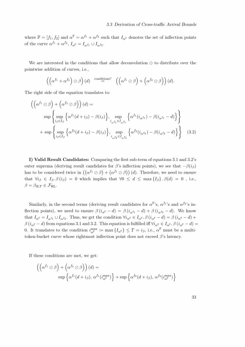
3.3 Derivation of Cross-traffic Arrival Bounds
where F = [f1, f2] and ↵
F= ↵
f1+ ↵
f2 such that I
↵
F denotes the set of inflection pointsof the curve ↵
f1+ ↵
f2 , I
↵
F = I
↵
f1 [ I
↵
f2 .
We are interested in the conditions that allow deconvolution ↵ to distribute over thepointwise addition of curves, i.e.,⇣⇣
↵
f1+ ↵
f2
⌘↵ �
⌘(d)
conditions?=
⇣⇣↵
f1 ↵ �
⌘+
⇣↵
f2 ↵ �
⌘⌘(d).
The right side of the equation translates to:⇣⇣↵
f1 ↵ �
⌘+
⇣↵
f2 ↵ �
⌘⌘(d) =
sup
(sup
i
�
2I�
n↵
f1(d + i
�
)� �(i
�
)
o, sup
i
↵
f12I
↵
f1
n↵
f1(i
↵
f1 )� �(i
↵
f1 � d)
o)
+ sup
(sup
i
�
2I�
n↵
f2(d + i
�
)� �(i
�
)
o, sup
i
↵
f22I
↵
f2
n↵
f2(i
↵
f2 )� �(i
↵
f2 � d)
o)(3.2)
I) Valid Result Candidates: Comparing the first sub-term of equations 3.1 and 3.2’souter suprema (deriving result candidates for �’s inflection points), we see that ��(i
�
)
has to be considered twice in��
↵
f1 ↵ �
�+
�↵
f1 ↵ �
��(d). Therefore, we need to ensure
that 8i�
2 I
�
. � (i
�
) = 0 which implies that 80 d max {I
�
} . �(d) = 0 , i.e.,� = �
R,T
2 FRL.
Similarly, in the second terms (deriving result candidates for ↵
F’s, ↵
f1 ’s and ↵
f2 ’s in-flection points), we need to ensure � (i
↵
F � d) = � (i
↵
f1 � d) + � (i
↵
f2 � d). We knowthat I
↵
F = I
↵
f1 [ I
↵
f2 . Thus, we get the condition 8i↵
F 2 I
↵
F . � (i
↵
F � d) = � (i
↵
F � d) +
� (i
↵
F � d) from equations 3.1 and 3.2. This equation is fulfilled iff 8i↵
F 2 I
↵
F . � (i
↵
F � d) =
0. It translates to the condition i
max↵
F :
= max {I
↵
F} T = i
�
, i.e., ↵
F must be a multi-token-bucket curve whose rightmost inflection point does not exceed �’s latency.
If these conditions are met, we get:⇣⇣↵
f1 ↵ �
⌘+
⇣↵
f2 ↵ �
⌘⌘(d) =
sup
n↵
f1(d + i
�
), ↵
f1(i
max↵
F )
o+ sup
n↵
f2(d + i
�
), ↵
f2(i
max↵
F )
o
33

3 Accuracy of Algebraic Network Calculus
From i
max↵
F i
�
and t � 0 we know that ↵
f
i
(d + i
�
) � ↵
f
i
�i
max↵
F�, i 2 {1, 2} such that⇣⇣
↵
f1 ↵ �
⌘+
⇣↵
f2 ↵ �
⌘⌘(d) =
sup
(sup
i
�
2I�
n↵
f1(d + i
�
)� � (i
�
)
o, sup
i
↵
f12I
↵
f1
n↵
f1(i
↵
f1 )� � (i
↵
f1 � d)
o)
+ sup
(sup
i
�
2I�
n↵
f2(d + i
�
)� � (i
�
)
o, sup
i
↵
f22I
↵
f2
n↵
f2(i
↵
f2 )� � (i
↵
f2 � d)
o)
(Condition � = �
R,T
2 FRL)
= sup
(↵
f1(d + T ) , sup
i
↵
f12I
↵
f1
n↵
f1(i
↵
f1 )� � (i
↵
f1 � d)
o)
+ sup
(↵
f2(d + T ) , sup
i
↵
f22I
↵
f2
n↵
f2(i
↵
f2 )� � (i
↵
f2 � d)
o)�Condition i
↵
f
i
i
max↵
F T
�= sup
(↵
f1(d + T ) , sup
i
↵
f12I
↵
f1
n↵
f1�i
max↵
F�o)
+ sup
(↵
f2(d + T ) , sup
i
↵
f22I
↵
f2
n↵
f2�i
max↵
F�o)
�Condition i
max↵
F T
�= ↵
f1(d + T ) + ↵
f2(d + T )
(Condition � = �
R,T
2 FRL)
= ↵
f1(d + i
�
) + ↵
f2(d + i
�
)
=
⇣↵
f1+ ↵
f2
⌘(d + i
�
)
=
⇣↵
f1+ ↵
f2
⌘(d + i
�
) + 0
= sup
i
�
n⇣↵
f1+ ↵
f2
⌘(d + i
�
)� � (i
�
)
o�Condition i
max↵
F i
�
�= sup
(sup
i
�
2I�
n⇣↵
f1+ ↵
f2
⌘(d + i
�
)� � (i
�
)
o,
⇣↵
f1+ ↵
f2
⌘ �i
max↵
F�� �
�i
max↵
F � d
�)
34

3.3 Derivation of Cross-traffic Arrival Bounds
�Condition I
↵
F 3 i
↵
F i
max↵
F�
= sup
(sup
i
�
2I�
n⇣↵
f1+ ↵
f2
⌘(d + i
�
)� �(i
�
)
o, sup
i
↵
F2I↵
F
n⇣↵
f1+ ↵
f2
⌘(i
↵
F)� �(i
↵
F � d)
o)
=
⇣⇣↵
f1+ ↵
f2
⌘↵ �
⌘(d)
II) Invalid Result Candidates without Impact: The above conditions were de-rived by matching the outcome of equivalent parts of equation 3.1 and equation 3.2. I.e.,if the conditions on ↵
f1 , ↵
f2 , ↵
F, and � are met, the candidate curves derived by theinner terms are equal and so is the result of the outer supremum.
This approach is, however, deriving too strong conditions. The outer supremum’simpact needs to be considered in more detail. This operation has the ability to “re-move” invalid result candidates where the distributivity does not apply, i.e., where��
↵
f1+ ↵
f2�↵ �
�(d) 6= ��
↵
f1 ↵ �
�+
�↵
f2 ↵ �
��(d). From the conditions above we
know that invalid candidates are derived for the following inflection points of curves:• 8i
↵
F 2 I
↵
F . i↵
F > T
• 8i�
2 I
�
. i
�
> T , i.e., � 2 FmRL with latency T
If these invalid result candidate curves are smaller than the supremum of valid candi-dates, the outer supremum in equation 3.2 removes them such that they do not impactthe final result. To check if we can distribute a deconvolution over an addition of twomulti-token-bucket curves, we need to split the derivation into two parts, according tothe location of inflection points:
1. The part deriving valid candidates for inflection points on [0, T ] and
2. the part deriving invalid candidates for inflection points on (T, +1).
Then, we need to check if the supremum of invalid result candidates is smaller thanthe supremum of valid result candidates. We either require
��↵
f1 ↵ �
�+
�↵
f2 ↵ �
��(d)
with⇣⇣↵
f1 ↵ �
⌘+
⇣↵
f2 ↵ �
⌘⌘(d)
���iT
:
=
sup
(sup
I
�
3i�
T
n↵
f1(d + i
�
)� �(i
�
)
o, sup
I
↵
f13i
↵
f1T
n↵
f1(i
↵
f1 )� �(i
↵
f1 � d)
o)
+ sup
(sup
I
�
3i�
T
n↵
f2(d + i
�
)� �(i
�
)
o, sup
I
↵
f23i
↵
f2T
n↵
f2(i
↵
f2 )� �(i
↵
f2 � d)
o)
35

3 Accuracy of Algebraic Network Calculus
and⇣⇣↵
f1 ↵ �
⌘+
⇣↵
f2 ↵ �
⌘⌘(d)
���i>T
:
=
sup
(sup
I
�
3i�
>T
n↵
f1(d + i
�
)� �(i
�
)
o, sup
I
↵
f13i
↵
f1>T
n↵
f1(i
↵
f1 )� �(i
↵
f1 � d)
o)
+ sup
(sup
I
�
3i�
>T
n↵
f2(d + i
�
)� �(i
�
)
o, sup
I
↵
f23i
↵
f2>T
n↵
f2(i
↵
f2 )� �(i
↵
f2 � d)
o),
leading to
8t � 0 :
⇣⇣↵
f1 ↵ �
⌘+
⇣↵
f2 ↵ �
⌘⌘(d)
���iT
�⇣⇣
↵
f1 ↵ �
⌘+
⇣↵
f2 ↵ �
⌘⌘(d)
���i>T
or we require��
↵
f1+ ↵
f2�↵ �
�(d) with⇣⇣
↵
f1+ ↵
f2
⌘↵ �
⌘(d)
���iT
:
=
sup
(sup
I
↵
F3i↵
FT
n⇣↵
f1+ ↵
f2
⌘(d + i
�
)� �(i
�
)
o, sup
I
↵
F3i↵
FT
n⇣↵
f1+ ↵
f2
⌘(i
↵
F)� �(i
↵
F � d)
o)
and⇣⇣↵
f1+ ↵
f2
⌘↵ �
⌘(d)
���i>T
:
=
sup
(sup
I
↵
F3i↵
F>T
n⇣↵
f1+ ↵
f2
⌘(d + i
�
)� �(i
�
)
o, sup
I
↵
F3i↵
F>T
n⇣↵
f1+ ↵
f2
⌘(i
↵
F)� �(i
↵
F � d)
o)
leading to
8t � 0 :
⇣⇣↵
f1+ ↵
f2
⌘↵ �
⌘(d)
���iT
�⇣⇣
↵
f1+ ↵
f2
⌘↵ �
⌘(d)
���i>T
.
Lemma 3.2 can be extended to flow aggregates of arbitrary sizes > 2 by iterativeapplication.
36

3.3 Derivation of Cross-traffic Arrival Bounds
3.3.5 Ranking of PBOO Arrival Bounding Alternatives
Lemma 3.2 allows us to rank both PBOO cross-traffic arrival bounding methods, segr-PBOOAB and aggrPBOOAB.
Theorem 3.1. (Accuracy of PBOO Cross-traffic Arrival Bounding) Cross-traffic arrivalbounding with aggrPBOOAB is more accurate than segrPBOOAB if the conditions ofLemma 3.2 are fulfilled.
Proof. Without loss of generality (detailed explanation follows after the proof), we provethis statement by showing that there are no beneficial effects of bounding long tandems(Figure 3.5b) that are more advantageous than bounding both flows aggregately onshorter tandems (Figure 3.5c).
First, we derive the segregated cross-flow arrival bounds at s1, i.e., ↵
xf
n
s1 , n 2 {1, 2},and aggregate the results to ↵
[xf1,xf2]s1 = ↵
xf1s1 + ↵
xf2s1 .
↵
xf
n
s1= ↵
xf
n
s0n↵ �
l.o.xfn
hs0n,s0i = ↵
xf
n
s0n↵⇣�
s0n ⌦⇣�
s0 ↵
xf
n
s0
⌘⌘= ↵
xf
n
s0n↵⇣�
s0n ⌦⇣�
s0 ⇣↵
xf
n
s0n↵ �
l.o.xfn
s0n
⌘⌘⌘= ↵
xf
n
s0n↵⇣�
s0n ⌦⇣�
s0 ⇣↵
xf
n
s0n↵ �
s0n
⌘⌘⌘where n denotes the opposite cross-flow’s index, i.e., 1 = 2 and 2 = 1. Therefore,
↵
[xf1,xf2]s0
= ↵
xf1s01↵⇣�
s01 ⌦⇣�
s0 ⇣↵
xf2s02↵ �
s02
⌘⌘⌘+ ↵
xf2s02↵⇣�
s02 ⌦⇣�
s0 ⇣↵
xf1s01↵ �
s01
⌘⌘⌘(3.3)
Next, we derive the aggregate cross-traffic arrival bound ↵
[xf1,xf2]s0 according to Algo-
rithm 3.1.
↵
[xf1,xf2]s0
=
⇣↵
xf1s0
+ ↵
xf2s0
⌘↵ �
l.o.[xf1,xf2]s0
=
⇣⇣↵
xf1s01↵ �
s01
⌘+
⇣↵
xf2s02↵ �
s02
⌘⌘↵ �
s0 (3.4)
Last, we show that the former arrival bound cannot be smaller than the latter one, i.e.,(3.4) (3.3) holds. This step relies on Lemma 3.2 and thus we inherit its conditions inthis theorem. For (3.4), distributivity of ↵ over + results in:⇣⇣
↵
xf1s01↵ �
s01
⌘+
⇣↵
xf2s02↵ �
s02
⌘⌘↵ �
s0 =
⇣↵
xf1s01↵ �
s01
⌘↵ �
s0 +
⇣↵
xf2s02↵ �
s02
⌘↵ �
s0
and (3.4) (3.3) translates to
37

3 Accuracy of Algebraic Network Calculus
s02s01
s0
s1foi
↵
xf1↵
xf2
(a) Sample network.
s0
s02s01
s1foi
�
l.o.xf1
�s01,s0� �
l.o.xf2
�s02,s0�
s1foi
�
l.o.xf1
�s01,s0� �
l.o.xf2
�s02,s0�
↵
xf1↵
xf2
↵ ↵
+
(b) Segregated cross-flow arrival bounding segrPBOOAB.
(c) Aggregate cross-traffic arrival bounding aggrPBOOAB.
Figure 3.5: Decomposition of a network for PBOO cross-traffic arrival bounding:(b) depicts the segregation of cross-flows (segrPBOOAB) and (c) illustratesour aggregation approach (aggrPBOOAB) resulting in shorter tandems.
⇣↵
xf1s01↵ �
s01
⌘↵ �
s0 +
⇣↵
xf2s02↵ �
s02
⌘↵ �
s0
↵
xf1s01↵⇣�
s01 ⌦⇣�
s0 ⇣↵
xf2s02↵ �
s02
⌘⌘⌘+ ↵
xf2s02↵⇣�
s02 ⌦⇣�
s0 ⇣↵
xf1s01↵ �
s01
⌘⌘⌘.
We now compare each segregated cross-flow’s impact on the final arrival bound. Thisresults in two sub-terms:⇣
↵
xf
n
s0n↵ �
s0n
⌘↵ �
s0 ↵
xf
n
s0n↵⇣�
s0n ⌦⇣�
s0 ⇣↵
xf
n
s0n↵ �
s0n
⌘⌘⌘Next, we can apply the composition rule for ↵ ([50], Theorem 3.1.12) and use ⌦’s com-mutativity to reformulate the terms to
↵
xf
n
s0n↵ �
s0n ↵ �
s0 ↵
xf
n
s0n↵ �
s0n ↵⇣�
s0 ⇣↵
xf
n
s0n↵ �
s0n
⌘⌘.
38

3.3 Derivation of Cross-traffic Arrival Bounds
These equations reveal that the crucial difference between both arrival bounding alter-natives is the respective (left-over) service curve at server s0. It defines the differencebetween both arrival bounds; potential end-to-end effects are superseded by the negativeimpact of PSOO violation.
Finally, as all curves are from F0, we know that
�
s0 � �
s0 ⇣↵
xf
n
s0n↵ �
s0n
⌘,
i.e., aggrPBOOAB’s service curve is larger, and for 8�s
x
, �
s
y
2 FmRL and 8↵ 2 FmTB inparticular, we know that
�
s
x
� �
s
y
) (↵↵ �
s
x
) �↵↵ �
s
y
�,
i.e., a larger service curve leads to a smaller output bound.Therefore, aggrPBOOAB outperforms segrPBOOAB under the conditions of Lemma 3.2.
Note, that equality between both arrival bounding alternatives only holds for the trivialcases where the service �
s0 is infinitely large, i.e., �+1,0, or ↵
xf
n
s0n (↵xf
n
) is zero.Last, let us clarify why the seemingly simple scenario of Figure 3.5a allows for our rank-
ing of aggrPBOOAB over segrPBOOAB in general feed-forward (subject to Lemma 3.2’spreconditions). Any more involved feed-forward network can be decomposed into a com-bination of variants of the network shown in Figure 3.5a, retaining Theorem 3.1’s validity:
Intermediate tandems instead of single servers s0, s01, or s02 can be assumed toconsist of multiple servers in tandem that were convolved into single servers for analysis(see Theorem 2.2). Then, the above proof as well as Algorithm 3.1 (aggrPBOOAB)virtually move across the network tandem-by-tandem instead of server-by-server.
Cross-traffic of cross-traffic AggrPBOOAB compromises on the source-to-interferenceview of segregated cross-flow arrival bounding. Tandems are restricted to sequencesof servers shared by all flows in the respective cross-traffic aggregate. If an aggregatehad its own cross-traffic (see x(x(foi, l1)) above), another PBOO left-over service curvederivation (Theorem 2.3) and thus an arrival bounding (of x(x(foi, l1))) would be needed.This new instance of compFFA step 1 operates with its own worst-case assumptions forx(x(foi, l1)). In the best case for segregated arrival bounding, when it is able to derive thesame ↵
x(x(foi,l1)) as aggregate arrival bounding, Theorem 3.1’s proof remains unchanged.In any other case, segrPBOOAB even operates on worse left-over service curves thanaggrPBOOAB.
39

3 Accuracy of Algebraic Network Calculus
Further cross-traffic with the same interference pattern Assume another cross-flow(aggregate) xf3 merges with the existing cross-traffic [xf1, xf2] at server s0, entering froma different server (or convolved tandem of left-over service curves) s03. Then, equa-tions containing the segregated flows’ impact on arrival bounds are expanded with xf3’sinfluence
↵
xf1s01↵ �
s01 ↵ �
s0 � ↵
xf1s01↵ �
s01 ↵⇣�
s0 ⇣↵
xf2s02↵ �
s02 + ↵
xf3s03↵ �
s03
⌘⌘,
↵
xf2s02↵ �
s02 ↵ �
s0 � ↵
xf2s02↵ �
s02 ↵⇣�
s0 ⇣↵
xf1s01↵ �
s01 + ↵
xf3s03↵ �
s03
⌘⌘and a similar equation for xf3’s impact on the aggregate arrival bound is added
↵
xf3s03↵ �
s03 ↵ �
s0 � ↵
xf3s03↵ �
s03 ↵⇣�
s0 ⇣↵
xf1s01↵ �
s01 + ↵
xf2s02↵ �
s02
⌘⌘.
Neither adaptation impacts the proof’s core statement; s0 still constitutes the crucialbottleneck server where aggregation outperforms segregation.
Further cross-flows with different interference patterns Assume s0, s01, and s02 ac-tually consisted of tandems of servers and there were further cross-flows of the foi, i.e.,in x(foi), merging and demultiplexing somewhere on these tandems. In this case, theabove reasoning would have to be repeated recursively for every backtracking required –similar to cross-traffic of cross-traffic, yet, with a SFA tandem analysis for the derivationof the left-over service instead of Theorem 2.3. Again, each recursion level constitutes anindependent instance of arrival bounding, with its own bottleneck server where aggrega-tion outperforms segregation due to the former’s violation of the PSOO principle. Theeffect causing aggregation’s superiority is thus amplified in more involved feed-forwardnetworks.
3.3.6 Accuracy Evaluation
In our numerical experiments, we use the aSHIIP topology generator [84] to randomlycreate Erdős-Rényi device graphs following the G (n, p)-model with p = 0.1. We evaluatethe impact of improved arrival bounding in flat and hierarchical network topologies with32 devices resulting in 114 servers (flat) as well as 73 servers (hierarchical). The amountof flows is continuously increased in steps of 50 randomly routed unit size flows (↵ = �1,1)until reaching the network’s capacity limit6. Each resulting network is analyzed with anSFA with segrPBOOAB as suggested in [10] as well as the aggrPBOOAB we contributedin this section.
6The flat network could route up to 1200 flows, the hierarchical network could route at most 900 flows.
40

3.3 Derivation of Cross-traffic Arrival Bounds
In this accuracy evaluation, we aim to gain insight on the impact of our aggrPBOOABon the compFFA, more precisely, Section 3.3.5’s crucial insight: amplification of aggre-gate bounding’s superiority when the number of bottlenecks as well as their utilizationincreases. Our measure is the so-called network delay bound. It is the worst-case end-to-end delay bound occurring in a network, i.e., it is globally valid for all flows in theanalyzed network. Our results are shown in Figure 3.6. Both figures depict the net-work delay bounds for network utilizations between 50% and 100%, both relative to thelargest network in terms of flows and bounded delays. We express the improvement fromthe new result’s point of view by the measure suggested for the LPA in [12]. This im-provement factor is defined as D(segrPBOOAB)
D(aggrPBOOAB) . A value of 1.0 denotes parity, a value in(0, 1) indicates a worsened network delay bound and values > 1.0 measure the improve-ment. Note, that the actual impact of an improvement depends on the context. Evenlarge improvement factors might not suffice to reach a required level of delay guaranteewhereas a relatively small one in a different network could be decisive for schedulabilityof a critical task. Therefore, we focus our presentation of improvement factors or delaybound reductions in % instead of the comparison of absolute values such as the deriveddelay bounds themselves.
In both networks, our aggrPBOOAB achieves a considerable network delay boundimprovement. All improvement factors are > 1.0 (see Figure 3.6, dashed line with crosses,right y-axis of each plot). In the flat ER network with the medium utilization of 50%,we achieve an improvement of factor 1.18, which already reduces the delay bound byabout 15%. With growing utilization and fast growing delay bounds, the factor increasesto 3.15 (reduction of 68%, Figure 3.6a). The hierarchical network possesses a set ofpredefined bottleneck links – those links connecting the levels of the hierarchy. TheaSHIIP generator creates a relatively static amount of levels, 5 to 6 in our experiments.Randomly routed flows are likely to cross levels and we can observe considerable gains.At 50% network utilization, the factor is at 1.62 (38% reduction) and it grows to a factorof 12.3 (91% reduction) at 100% due to the asymptotic growth of delay bounds. At theevaluated hierarchical networks with a utilization of more than 66%, the delay boundcould always be at least halved with aggrPBOOAB (see Figure 3.6b).
Our experiments reveal these general trends:
• The aggrPBOOAB method for compFFA allows algNC to compute more accuratenetwork delay bounds than segrPBOOAB, independent of the network utilization.The highest gains are achieved when the network reaches its capacity limit.
• The predefined bottleneck links of the hierarchical ER topology lead to a higherimpact of aggregate arrival bounding than in the flat network topologies.
• The cross-traffic arrival bounding method itself does not affect the network delay
41

3 Accuracy of Algebraic Network Calculus
50 55 60 65 70 75 80 85 90 95 100
050
100
150
Network utilization [%], relative to largest network with bounded delays
SFA
netw
ork
dela
y bo
und
[s]
● ● ● ● ● ● ● ● ● ●●
●●
●
●
11.
52
2.5
33.
5
−x−
Impr
ovem
ent f
acto
r●
Cross−flow segregationCross−traffic aggregationDelay bound improvement by cross−traffic aggregation
(a) Flat ER network.
50 55 60 65 70 75 80 85 90 95 100
010
020
030
040
0
Network utilization [%], relative to largest network with bounded delays
SFA
netw
ork
dela
y bo
und
[s]
● ● ● ● ● ● ● ●●
●
●
12.
55
7.5
1012
.5
−x−
Impr
ovem
ent f
acto
r●
Cross−flow segregationCross−traffic aggregationDelay bound improvement by cross−traffic aggregation
(b) Hierarchical ER network.
Figure 3.6: Accuracy evaluation of ER networks with 32 devices each: SFA with twodifferent cross-traffic arrival bounding alternatives, segrPBOOAB and aggr-PBOOAB.
bound’s asymptotic growth pattern when utilization is increased. However, thegrowth rate is slowed down considerably and in cases of a large bottleneck uti-lization, our aggrPBOOAB achieves network delay bounds that are multiple timesmore accurate than the segrPBOOAB ones.
3.4 Cross-traffic Burstiness Reduction
In the following, we prove a counterintuitive property of algNC analysis: By assuminga worse network setting, better delay bounds can be derived. To be precise, we as-sume worse interference with the foi by aggregating its cross-traffic with other flows inthe network. The analysis does not only bound the burstiness of actual cross-flows but
42

3.4 Cross-traffic Burstiness Reduction
additionally that of flows not directly interfering with the foi. In return, the analysiscan aggregate the totality of flows like the TFA. We prove that this overly pessimisticaggregation can be beneficial to the analysis nonetheless. The pessimism can becomeless impactful than the aggregation’s positive effects and therefore we are able to reducethe derived cross-traffic burstiness. Worst-case burstiness is the crucial characteristicof cross-traffic arrivals. In the foi analysis of compFFA step 2, it defines the latencyincrease in both left-over service curve derivations of algNC, i.e., SFA and PMOOA.Whereas the previous section improved the overall cross-traffic arrival bounding methodby circumventing the segregation problem, this section presents an improvement explic-itly targeting the worst-case cross-traffic burstiness.
3.4.1 An Alternative Output Bound
The output bound operation, i.e., the deconvolution, is applied to derive the burstinessand the rate of flow arrivals (see Algorithm 3.1). Therefore, we first derive a novel outputbound that is based on the input/output-relation of a server. It does not rely on thedeconvolution.
Let A, A
0 be input and output to/from a server. We assume to have an arrival curve↵ for the arrivals A and a service curve � offered by the server. Let us further assumethat the arrival curve ↵ is such that for d > 0 it can be written as
↵(d) = ↵̃(d) + ↵(0
+),
with ↵̃ being a sub-additive curve (defined for d > 0 by the above equation and with↵̃(0) = 0), and ↵(0
+) = lim
d!0+ ↵(d). Clearly, this means that ↵ is also a sub-additivefunction. Further note that, for instance, any concave piecewise-linear arrival curve meetsthis condition, hence it is not restrictive in practice.
Noting that we can bound the backlog for any given arrival process A by
B(t) = A(t)�A
0(t) A(t)� (A⌦ �)(t) = sup
0ut
{A(t)�A(u)� �(t� u)},
we provide the alternative output bound in the following theorem.
Theorem 3.2. Under the above assumptions and notations, an output bound on thedeparture flow (aggregate) A
0 can be calculated as
↵
0(d) = ↵(d) + (v(↵, �)� ↵(0
+)) · 1{d>0}.
43

3 Accuracy of Algebraic Network Calculus
Proof. Let s < t:
A
0(t)�A
0(s) = A(t)�A(s) + B(s)�B(t)
A(t)�A(s) + B(s)
A(t)�A(s) + sup
0us
{A(s)�A(u)� �(s� u)}
= sup
0us
{A(t)�A(u)� �(s� u)}
sup
0us
{↵(t� u)� �(s� u)}
= sup
0us
{↵̃(t� u) + ↵(0
+)� �(s� u)}
sup
0us
{↵̃(t� s) + ↵̃(s� u) + ↵(0
+)� �(s� u)}
= ↵̃(t� s) + sup
0us
{↵(s� u)� �(s� u)}
↵̃(t� s) + v(↵, �)
= ↵(t� s) + v(↵, �)� ↵(0
+) = ↵
0(t� s).
For s = t : A
0(t)�A
0(s) = 0 = ↵
0(t� s).
Note, that this result resembles a known basic result that can be found in Chang’stextbook in Lemma 1.4.2 [23]. This lemma states that for a server with a bound on thequeue q̄ and a �
r,b
-constrained input, an output bound can be given as �
r,b+q̄
.
Lemma. ([23], Lemma 1.4.2) Let A, A
0 be input and output to/from a server s. If ↵ isan arrival curve for A and B
s
a bound on the backlog of s, then the output of s, A
0, isbounded by ↵ + B
s
.
Proof. Let u t, then we know that A(u) � A
0(u) B
s
and that A
0(t) A(t) (flow
constraint). This leads to
A
0(t)�A
0(u) A(t)�A(u) + B
s
↵(t� u) + B
s
Besides generalizing this lemma, we point out that we actually improve it, as webasically get rid of the burst term and would obtain �
r,q̄
as an output bound underChang’s assumptions.
Next, we show that our alternative output bound can be used to bound the output ofindividual flows of an aggregate that crosses a server.
44

3.4 Cross-traffic Burstiness Reduction
Corollary 3.1. (Application of Theorem 3.2 to individual flows of an aggregate) Let s
be a server crossed by two flows f1 and f2. Then, the output of each individual flow f
i
,i 2 {1, 2}, is bounded by ↵̃
f1+ v
�↵
[f1,f2], �
�.
Proof. Let the flows f1, f2 have input functions A1, A2 and output functions A
01, A
02.
Assume that ↵
f
i is an arrival curve for flow f
i
, i 2 {1, 2}, and that ↵
[f1,f2] is an arrivalcurve for the flow aggregate [f1, f2], i.e., for A = A1+A2. Further, let ↵
f
i meet the abovecondition ↵
f
i
(d) = ↵̃
f
i
(d) + ↵
f
i
(0
+) with ↵̃
f
i being a sub-additive curve. B
i
: R ! R+
is the backlog function of flow f
i
, i.e., B
i
(t) = A
i
(t)� A
0i
(t). Then, we get for u t thefollowing output of the flow aggregate [f1, f2] from s:�
A
01(t)�A
01(u)
�+
�A
02(t)�A
02(u)
�= ((A1(t)�B1(t))� (A1(u)�B1(u))) +
�A
02(t)� (A2(u)�B2(u))
�= A1(t)�B1(t)�A1(u) + B1(u) + A
02(t)�A2(u) + B2(u)
(remove �B1(t))
A1(t)�A1(u) + A
02(t)�A2(u) + (B1(u) + B2(u))
Now, let B1 + B2 be the backlog function of the flow aggregate [f1,f2], i.e.,
(B1 + B2) (u) sup
0ru
{A(u)�A(r)� �(u� r)} ,
to get
A1(t)�A1(u) + A
02(t)�A2(u) + (B1(u) + B2(u))
A1(t)�A1(u) + A
02(t)�A2(u)
+ sup
0ru
{A(u)�A(r)� �(u� r)}
(expand A to A1 + A2 )
A1(t)�A1(u) + A
02(t)�A2(u)
+ sup
0ru
{A1(u) + A2(u)�A1(r)�A2(r)� �(u� r)}
= A1(t) + A
02(t) + sup
0ru
{�A1(r)�A2(r)� �(u� r)}
= A
02(t) + sup
0ru
{A1(t)�A1(r)�A2(r)� �(u� r)}
= A
02(t) + sup
0ru
n↵
f1(t� r)�A2(r)� �(u� r)
o
45

3 Accuracy of Algebraic Network Calculus
We now have
A
01(t)�A
01(u) + A
02(t)�A
02(u)
A
02(t) + sup
0ru
n↵
f1(t� r)�A2(r)� �(u� r)
oShifting A
02(t)�A
02(u) to the right yields
A
01(t)�A
01(u) A
02(u) + sup
0ru
n↵
f1(t� r)�A2(r)� �(u� r)
o.
From the decomposition of ↵
f
i and sub-additivity of ↵̃
f
i , we get
↵
f1(t� r) = ↵
f1(0
+) + ↵̃
f1(t� r)
↵
f1(0
+) + ↵̃
f1(t� u) + ↵̃
f1(u� r)
= ↵̃
f1(t� u) + ↵
f1(u� r)
and
A
01(t)�A
01(u) A
02(u) + ↵̃
f1(t� u) + sup
0ru
n↵
f1(u� r)�A2(r)� �(u� r)
o.
Since ↵
f2 is an arrival curve, we know that �A2(r) ↵
f2(u� r)�A2(u) and finally get
A
02(u) + ↵̃
f1(t� u) + sup
0ru
n↵
f1(u� r)�A2(r)� �(u� r)
o A
02(u) + ↵̃
f1(t� u) + sup
0ru
n↵
f1(u� r) + ↵
f2(u� r)�A2(u)� �(u� r)
o= A
02(u)�A2(u) + ↵̃
f1(t� u) + sup
0ru
n↵
f1(u� r) + ↵
f2(u� r)� �(u� r)
o A
02(u)�A2(u) + ↵̃
f1(t� u) + v
⇣↵
f1+ ↵
f2, �
⌘ ↵̃
f1(t� u) + v
⇣↵
f1+ ↵
f2, �
⌘
3.4.2 TFA-assisted aggrPBOOAB
Next, we demonstrate how to exploit the basic insight about the alternative output char-acterization from the previous section. It gives us the choice between the existing PBOOarrival bounding (aggrPBOOAB), which applies the conventional output bound, and anapproach where we use a backlog bound for the cross-traffic and apply Theorem 3.2. Thisbacklog bound is obtained from TFA, i.e., it actually considers flows that demultiplex
46

3.4 Cross-traffic Burstiness Reduction
Figure 3.7: Sample network.
from cross-traffic and do not interfere with the foi. In the following we discuss why andwhen this can actually lead to an improvement.
Consider the network configuration of Figure 3.7 where f is the analyzed foi, xf is itscross-flow and xxf is the cross-traffic of xf . Although the network is depicted as a tandem,we cannot apply a simple tandem analysis because the foi f does not cross all servers,i.e., cross-traffic arrival bounding is necessary in this network: Deriving f ’s performancebounds with the SFA requires bounding xf ’s arrival at s2, ↵
xf
s2 , with compFFA step 1,aggrPBOOAB, first. Its result is used to separate f by computing f ’s left-over servicecurve at s2 that is then used to derive f ’s delay bound (compFFA step 2).
AggrPBOOAB retains the worst-case when arbitrarily multiplexing flows, i.e., in con-trast to FIFO multiplexing, data of xf may always be served after xxf ’s data – indepen-dent of their relative arrival times. Thus, burstiness of ↵
xf
s2 , denoted by b
xf
s2 :
= ↵
xf
s2 (0+),
increases when more data of xxf arrives in shorter intervals, i.e., its arrival curve ↵
xxf in-creases. In our illustrative numerical evaluation of this section, service curves are chosento be rate latency functions �
R,T
= �20,20 and arrival curves are token buckets ↵ = �
r,10
where the rate r is variable. In this parameterized homogeneous setting, ↵
xxf increaseswith parameter r that we use to illustrate xf ’s worst-case burstiness increase with agrowing network utilization.
Figure 3.8 shows the utilization’s impact on the aggrPBOOAB burstiness of f ’s cross-traffic, b
xf
s2 , and on the TFA backlog bound at server s1, B
TFAs1
. TFA considers all flowsat s1 and derives the backlog bound based on their aggregate arrival curve. Being thebacklog of all incoming traffic at the server, i.e., a superset of f ’s cross-traffic xf , B
TFAs1
is also a backlog bound for xf . In Figure 3.8, B
TFAs1
scales linearly whereas b
xf
s2 scalessuper-linearly with the utilization. Consequently, both curves intersect and b
xf
s2 exceedsB
TFAs1
, such that using the TFA backlog bound and Theorem 3.2 indeed achieves animprovement over aggrPBOOAB. This can be explained by the derivation of the two
47
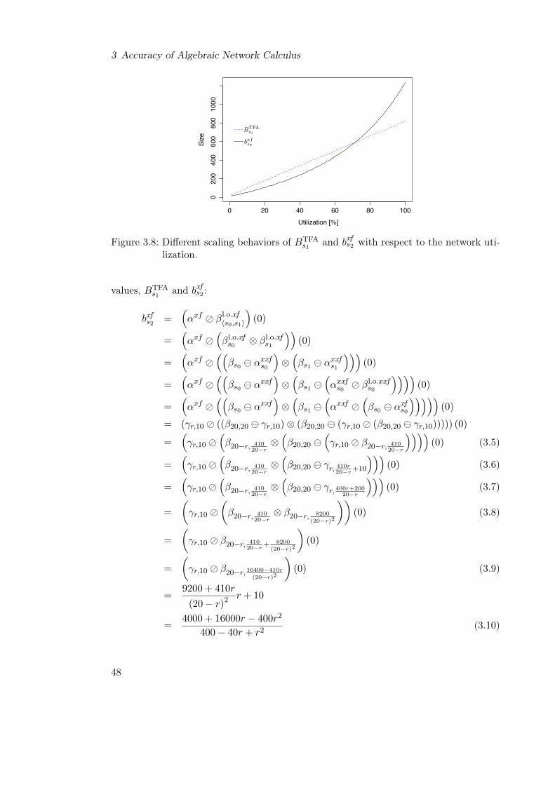
3 Accuracy of Algebraic Network Calculus
0 20 40 60 80 1000
200
400
600
800
1000
Utilization [%]
Size
Figure 3.8: Different scaling behaviors of B
TFAs1
and b
xf
s2 with respect to the network uti-lization.
values, B
TFAs1
and b
xf
s2 :
b
xf
s2=
⇣↵
xf ↵ �
l.o.xfhs0,s1i
⌘(0)
=
⇣↵
xf ↵⇣�
l.o.xfs0
⌦ �
l.o.xfs1
⌘⌘(0)
=
⇣↵
xf ↵⇣⇣
�
s0 ↵
xxf
s0
⌘⌦⇣�
s1 ↵
xxf
s1
⌘⌘⌘(0)
=
⇣↵
xf ↵⇣⇣
�
s0 ↵
xxf
⌘⌦⇣�
s1 ⇣↵
xxf
s0↵ �
l.o.xxfs0
⌘⌘⌘⌘(0)
=
⇣↵
xf ↵⇣⇣
�
s0 ↵
xxf
⌘⌦⇣�
s1 ⇣↵
xxf ↵⇣�
s0 ↵
xf
s0
⌘⌘⌘⌘⌘(0)
= (�
r,10 ↵ ((�20,20 �
r,10)⌦ (�20,20 (�
r,10 ↵ (�20,20 �
r,10))))) (0)
=
⇣�
r,10 ↵⇣�20�r,
41020�r
⌦⇣�20,20
⇣�
r,10 ↵ �20�r,
41020�r
⌘⌘⌘⌘(0) (3.5)
=
⇣�
r,10 ↵⇣�20�r,
41020�r
⌦⇣�20,20 �
r,
410r20�r
+10
⌘⌘⌘(0) (3.6)
=
⇣�
r,10 ↵⇣�20�r,
41020�r
⌦⇣�20,20 �
r,
400r+20020�r
⌘⌘⌘(0) (3.7)
=
✓�
r,10 ↵✓
�20�r,
41020�r
⌦ �20�r,
8200(20�r)2
◆◆(0) (3.8)
=
✓�
r,10 ↵ �20�r,
41020�r
+ 8200(20�r)2
◆(0)
=
✓�
r,10 ↵ �20�r,
16400�410r(20�r)2
◆(0) (3.9)
=
9200 + 410r
(20� r)
2 r + 10
=
4000 + 16000r � 400r
2
400� 40r + r
2(3.10)
48

3.4 Cross-traffic Burstiness Reduction
We can see that b
xf
s2 monotonically increases because the numerator is larger as well asfaster growing than the denominator and the stability condition for bounded performancecharacteristics, r 10, leads to an always positive denominator.
Next, let us see how the polynomial expression’s degree builds up during the abovederivation. Multiplication by the arrival rate is required to compute the burstiness of anoutput arrival curve, i.e., every time we deconvolve – see steps from (3.5) to (3.6) andfrom (3.9) to (3.10). Subsequent left-over service curve operations, e.g., from (3.7) to(3.8), retain the rate in the latency term’s denominator, as does the convolution of servicecurves in the step from (3.8) to (3.9). Deconvolution is required for output bounding andthus occurs at every level of the recursive arrival bounding procedure. In this example,xf is bounded in the first recursion level and it requires bounding xxf in a second level;hence, we obtain a rational function of degree 2 (with a pole at r = 20).
The TFA backlog bound derivation for server s1 proceeds as follows:
B
TFAs1
= v
⇣↵
xf
s1+ ↵
xxf
s1, �
s1
⌘(3.11)
= v
⇣⇣↵
xf
s0+ ↵
xxf
s0
⌘↵ �
l.o.[xf,xxf ]s0
, �
s1
⌘= v
⇣↵
[xf,xxf ]s0
↵ �
s0 , �
s1
⌘(3.12)
= v ((�
r,10 + �
r,10)↵ �20,20, �20,20) (3.13)
= v (�2r,20 ↵ �20,20, �20,20) (3.14)
= v (�2r,20+2r·20, �20,20) (3.15)
= 80r + 20
The derivation takes advantage of aggregation in (3.11) and (3.13), which prevents re-cursive cross-traffic arrival bounding in our example – in fact, the TFA implements thePSOO principle, yet, by assuming too much cross-traffic of f . However, xxf is not con-sidered cross-traffic of xf as both belong to the same flow aggregate and therefore noaction has to be taken to derive the left-over service curve at s0 in (3.12). The only rel-evant deconvolution in B
TFAs1
’s derivation is found in the computation of the aggregate’soutput bound after crossing s0. The deconvolution in the backlog bounding operationv
⇣↵
xf
s1 + ↵
xxf
s1 , �
s1
⌘executed in the step from (3.14) to (3.15) is, in contrast to the b
xf
s2 -derivation, not affecting the polynomial expression’s degree because its latency is notdepending on r. Thus, the entire term grows linearly with the flow arrival rate.
Remark 3.1. It is not possible to improve xf ’s output bound by using the backlog boundfor flow xf at server s1, i.e., B
xf
s1 , because B
xf
s1 and b
xf
s2 are equal due to [50], Theorem
49

3 Accuracy of Algebraic Network Calculus
0 20 40 60 80 100
050
100
150
200
Utilization [%]
, T=0, T=106
% o
f
(a) Influence of the service curve latency T .
0 2 4 6 8 10
050
100
150
200
Arrival curve burstiness
, Util 100%, Util 72%, Util 59%
% o
f
(b) Influence of the arrival curve burstiness b.
Figure 3.9: Relative difference between the TFA backlog bound at s1, B
TFAs1
, and xf ’sworst-case burstiness derived at s2, b
xf
s2 .
3.1.12, Rule 12:
B
xf
s1=
⇣⇣↵
xf ↵ �
l.o.xfs0
⌘↵ �
l.o.xfs1
⌘(0)
=
⇣↵
xf ↵⇣�
l.o.xfs0
⌦ �
l.o.xfs1
⌘⌘(0) = b
xf
s2
From this reformulated derivation of b
xf
s2 we obtain another explanation for its functionbeing of degree 1 in the above example: there is only one deconvolution.
Remark 3.2. Theorem 1.4.5 in Le Boudec and Thiran’s text book [50] presents conditionsfor tight output arrival bounds. These are satisfied in both our derivations above, yet,we improve xf ’s output bound by incorporating B
TFAs1
. At first glance, this may seemlike a contradiction, however, we gain tightness from additional considerations of a feed-forward analysis that are not addressed in [50], Theorem 1.4.5. It remains valid, yet onlywith respect to the given service curves that, in turn, might be tightness-compromisingleft-overs like in Remark 3.1.
In a more involved feed-forward network, we often have multi-level recursions for cross-traffic of cross-traffic in the arrival bounding phase of the derivations [9] – also for thebacklog bound at a server – and therefore polynomial expressions of higher degrees occurin both alternative bounds on the output burstiness. For the ease of presentation, wecontinue to illustrate the impact of the differing scaling behaviors as well as the servicecurve latency and the initial burstiness of flows in the simple network from Figure 3.7.In Section 3.4.3, we extend our evaluation to more involved feed-forward networks.
Above, we discussed that left-over service curve computations retain the arrival rate intheir results’ latency term. For instance, the left-over latency at server s0 is T
s0 ·Rs0+b
xxf
R
s0�r
xxf
=
50

3.4 Cross-traffic Burstiness Reduction
T
s0 +
r
xxf ·Ts0+b
xxf
R
s0�r
xxf
, i.e, it consists of a fixed and a variable part. The fixed part is definedby the service curves’ initial latency T
s0 = T
s1 = T
s2 =
:
T (equal for all servers inour homogeneous sample network) whose influence on the total burstiness we evaluate –increasing T decreases the impact of the variable part containing the crucial factor r.We check T = 0, i.e., the natural lower limit of the latency, and T = 10
6, a value severalorders of magnitude larger than the service rate R = 20 and thus safe to be assumed as arealistic upper bound on T . The resulting range of T ’s impact is depicted by the relativedifference between B
TFAs1
and b
xf
s2 in Figure 3.9a. Most notably, the network utilizationrequired for the TFA backlog bound to outperform the separated flow’s output burstinessis between 59% to 72% – that is, it always exists and resides at utilizations considerablylower than the network’s capacity limit. Moreover, b
xf
s2 ’s relative benefit of 50% overB
TFAs1
for low utilizations is in fact small in absolute values (cf. Figure 3.8) whereas itsdisadvantage (right of the intersection) grows fast to become large in absolute numbers.
Last, we evaluate the impact of the remaining variable parameter besides utilizationand the service curve latency: the initial burstiness of flows in the homogeneous network,b. We reduced the service curve latency’s influence by assigning � = �20,0.1. Arrivalcurves are ↵ = �
r,b
where r is defined by the network utilization (i.e., relative to the servicerate R) and b is slowly increased from 0 to the previously used value of 10. Figure 3.9bdepicts the relative difference between B
TFAs1
and b
xf
s2 for three levels of network utilization:59% and 72% (the intersections of both values in the latency evaluation of Figure 3.9a)as well as 100%. We can see that the TFA backlog bound at server s1 is in fact alwayswithin the output burstiness of the same utilizations found for the latency (Figure 3.9a)– for 59%, B
TFAs1
is an asymptote when increasing b, and for 72% the b
xf
s2 -value startsat the server backlog bound. The impact of initial burstiness of flows is similar to thelatency’s impact. For the maximum network utilization, b
xf
s2 always exceeds B
TFAs1
by atleast 50% in our sample network, i.e., utilization remains most impactful.
Based on these observations, we propose to improve the arrival bound of a flow (ag-gregate) with the TFA backlog bound and Theorem 3.2 applied at the last hop of thisflow (aggregate) – of course, only if it actually improves the bound. We call this newmethod: TFA-assisted aggrPBOOAB.
3.4.3 Accuracy Evaluation
The potential improvement of cross-traffic bounds can be quite considerable in the smallscenario of Section 3.4.2. Now we turn to the investigation of the impact on the end-to-end delay bound of flows traversing larger feed-forward networks. That is, we evaluate theimprovements gained by reduced cross-traffic interference that ultimately tightens delaybounds. We use the SFA to benchmark the new TFA-assisted aggrPBOOAB against the
51

3 Accuracy of Algebraic Network Calculus
0 100 200 300 400 500 600
020
4060
80
Flow ID, ordered by the delay bound of SFA with aggrPBOOAB
Del
ay b
ound
02
46
8
Impr
oved
(int
erm
edia
te) a
rriva
l bou
nds
[%]
●●●●●●●●●●●●●●●●●●●
●
●●●●●●●
●●●●
●●
●●●
●
●●
●
●
●
●●●
●
●●●●●
●
●●●●●●
●
●●●●
●●●●●●●●●●●
●●
●
●
●
●●●
●●●
●
●
●
●
●
●●
●●
●
●●●●
●●●
●
●
●
●
●
●●●●●●●●●●●●●●●●●●●●●
●
●●●●●●●●●●●●●
●●●●●
●
●
●●●●●
●●●
●●●
●●●
●
●●
●●●●●●●
●
●●●●●●●●●●●●●●●●●●●●●●●●
●●●
●
●
●●
●●
●●●●●●
●●
●●●●
●●●
●
●
●
●
●●
●●●
●
●
●
●●
●
●
●●
●
●
●●●●●
●●●
●
●●
●●
●●●
●●
●●●●●●●●●●●●●●●
●●
●
●
●
●●●
●●
●●●●
●
●●
●
●
●
●
●
●●
●
●●
●
●
●
●
●●●●
●
●
●●●
●●
●●
●●
●
●
●
●
●●
●
●
●●●●●●●●●●●●
●●●●
●
●
●●
●
●
●●
●
●
●
●
●
●
●
●●
●
●
●●
●●
●
0 100 200 300 400 500 600
020
4060
80
Del
ay b
ound
●
SFA with aggrPBOOABSFA with TFA−assisted aggrPBOOABImproved (intermediate) arrival bounds
(a) TFA assistance (Theorem 3.2).
0 100 200 300 400 500 600
020
4060
80
Flow ID, ordered by the delay bound of SFA with aggrPBOOAB
Del
ay b
ound
02
46
8
Impr
oved
(int
erm
edia
te) a
rriva
l bou
nds
[%]
●●●● ●●●●●●●●●●●●●●●●●●●●●●●●●● ● ● ●●●●●●●●●●● ●●●●●● ●●●●●●●●●●●●●●●●● ●●●● ●●● ●● ●●●●●●●●●●●●●●●● ●●●●●●●●●●●
0 100 200 300 400 500 600
020
4060
80
Del
ay b
ound
●
SFA with aggrPBOOABSFA with Chang's LemmaImproved (intermediate) arrival bounds
(b) Chang’s Lemma [23] did not yield significant improvements, the linesfor both SFAs are indistinguishable.
Figure 3.10: Delay analysis with aggrPBOOAB and cross-traffic burstiness improve-ments.
existing aggrPBOOAB without this improvement (plain aggrPBOOAB of Section 3.3).
Dense Network The first exemplary network we generated for evaluation consists of 150
homogeneous servers with service curves �
R,T
= �200,0.1. 600 flows with random pathsand arrival curve ↵ = �2,0.1 were added to the network, i.e., it was chosen to be very densein order to provoke the effect and thus illustrate the potential of our improvement. Theyare supposed to randomly generate hotspots of considerable, yet, uncontrolled utilizationfor the evaluation. These hotspots see the highest numbers of flows such that the impactof separation vs. aggregation can be observed – similar to heterogeneous networks wheresome flows outweigh others. We chose a small initial burstiness to additionally check theabove claim that unavoidable burstiness increases are sufficient to cause impact of the
52
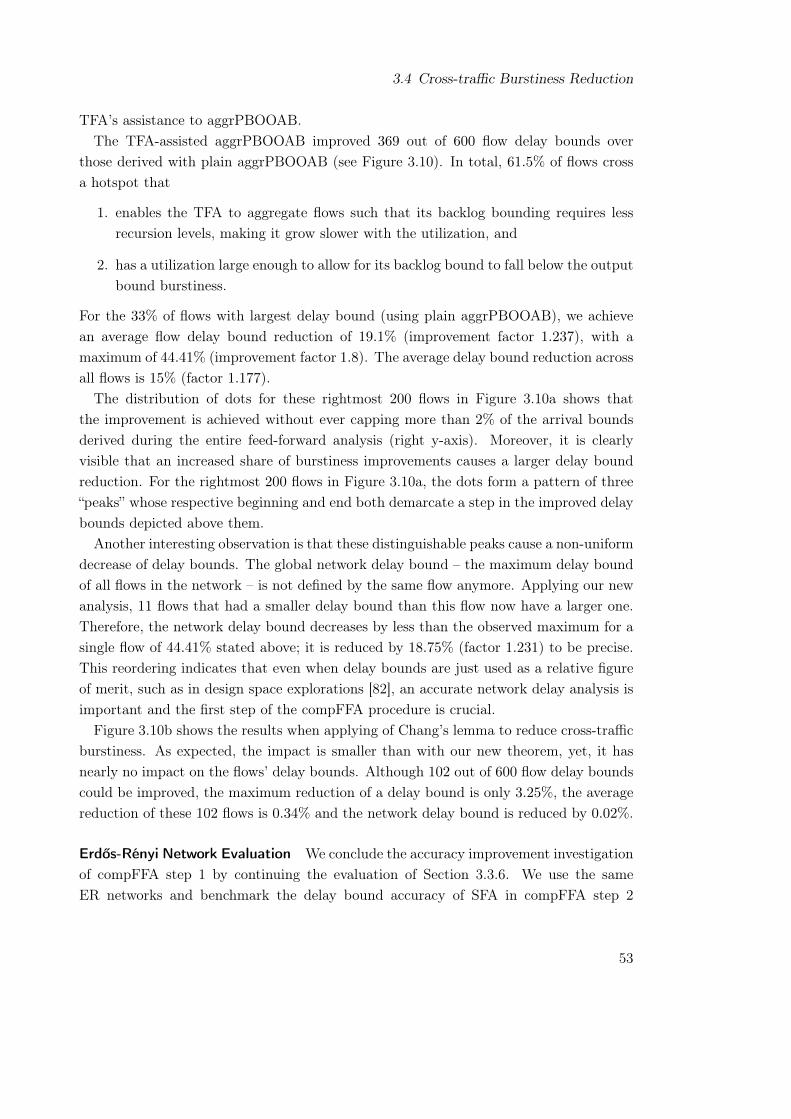
3.4 Cross-traffic Burstiness Reduction
TFA’s assistance to aggrPBOOAB.The TFA-assisted aggrPBOOAB improved 369 out of 600 flow delay bounds over
those derived with plain aggrPBOOAB (see Figure 3.10). In total, 61.5% of flows crossa hotspot that
1. enables the TFA to aggregate flows such that its backlog bounding requires lessrecursion levels, making it grow slower with the utilization, and
2. has a utilization large enough to allow for its backlog bound to fall below the outputbound burstiness.
For the 33% of flows with largest delay bound (using plain aggrPBOOAB), we achievean average flow delay bound reduction of 19.1% (improvement factor 1.237), with amaximum of 44.41% (improvement factor 1.8). The average delay bound reduction acrossall flows is 15% (factor 1.177).
The distribution of dots for these rightmost 200 flows in Figure 3.10a shows thatthe improvement is achieved without ever capping more than 2% of the arrival boundsderived during the entire feed-forward analysis (right y-axis). Moreover, it is clearlyvisible that an increased share of burstiness improvements causes a larger delay boundreduction. For the rightmost 200 flows in Figure 3.10a, the dots form a pattern of three“peaks” whose respective beginning and end both demarcate a step in the improved delaybounds depicted above them.
Another interesting observation is that these distinguishable peaks cause a non-uniformdecrease of delay bounds. The global network delay bound – the maximum delay boundof all flows in the network – is not defined by the same flow anymore. Applying our newanalysis, 11 flows that had a smaller delay bound than this flow now have a larger one.Therefore, the network delay bound decreases by less than the observed maximum for asingle flow of 44.41% stated above; it is reduced by 18.75% (factor 1.231) to be precise.This reordering indicates that even when delay bounds are just used as a relative figureof merit, such as in design space explorations [82], an accurate network delay analysis isimportant and the first step of the compFFA procedure is crucial.
Figure 3.10b shows the results when applying of Chang’s lemma to reduce cross-trafficburstiness. As expected, the impact is smaller than with our new theorem, yet, it hasnearly no impact on the flows’ delay bounds. Although 102 out of 600 flow delay boundscould be improved, the maximum reduction of a delay bound is only 3.25%, the averagereduction of these 102 flows is 0.34% and the network delay bound is reduced by 0.02%.
Erdős-Rényi Network Evaluation We conclude the accuracy improvement investigationof compFFA step 1 by continuing the evaluation of Section 3.3.6. We use the sameER networks and benchmark the delay bound accuracy of SFA in compFFA step 2
53

3 Accuracy of Algebraic Network Calculus
with the three cross-traffic arrival boundings presented in this thesis, segrPBOOAB,aggrPBOOAB and TFA-assisted aggrPBOOAB (Figure 3.10). The factor on the righty-axis shows the improvement from aggrPBOOAB to TFA-assisted aggrPBOOAB. Forthe improvement from segrPBOOAB to aggrPBOOAB, please refer to Figure 3.6. In theflat ER network, improvements only start at a very high network utilization of > 85%and reach a relatively small factor of 1.09 – a reduction of 8.25% of the network delaybound closest to the asymptote. In contrast, the hierarchical ER network experienceslarger improvements, showing the potential of the TFA assistance: At a utilization of 2
3 ,the improvement is at 1.111 (delay bound reduction of 10%), it grows to factor 1.25
(reduction of 20%) at a utilization of 56 and to factor 1.69 (reduction of 40.8%) at the
maximum utilization.
50 55 60 65 70 75 80 85 90 95 100
020
4060
8010
0
Network utilization [%], relative to largest network with bounded delays
SFA
netw
ork
dela
y bo
und
[s]
● ● ● ● ● ● ● ● ●●
●
●
●
●
●
11.
025
1.05
1.07
51.
1
−x−
Impr
ovem
ent f
acto
r●
segrPBOOABaggrPBOOABTFA−assisted aggrPBOOABDelay bound improvement by TFA assistance
(a) Flat ER network,
50 55 60 65 70 75 80 85 90 95 100
050
100
150
200
Network utilization [%], relative to largest network with bounded delays
SFA
netw
ork
dela
y bo
und
[s]
● ● ● ● ●●
●●
●
●
●1
1.2
1.4
1.6
1.8
−x−
Impr
ovem
ent f
acto
r●
segrPBOOABaggrPBOOABTFA−assisted aggrPBOOABDelay bound improvement by TFA assistance
(b) Hierarchical ER network.
Figure 3.11: Accuracy evaluation of ER networks with 32 devices each: SFA with threedifferent cross-traffic arrival bounding alternatives, segrPBOOAB, aggr-PBOOAB and TFA-assisted aggrPBOOAB.
54

4 Distributed Sensor Network Calculus Analysis
In this Section, we advance Sensor Network Calculus (SensorNC) by transforming therecursive arrival bounding of Section 3.3 into a more efficient iterative algorithm. Finally,we show how the entire SensorNC analysis can now be deployed within a sensor network.This allows for a distributed in-network performance modeling and admission controlscheme that does not require any additional protocol, only small payload additions.
Sensor Network Calculus (SensorNC) is a framework for worst-case analysis of wire-less sensor networks and as such allows to derive upper bounds on end-to-end delayfor sensor-to-sink data flows as well as the maximum buffer requirements for sensornodes. SensorNC is strongly based on algNC, but partially slims it down (specific arrivaland service curves are used) and partially extends it (compositional sink-tree analy-sis). Since the initial proposal in [71], it has been extended in several aspects: multiplesinks [76], in-network processing [77], improved delay analysis [35, 77], and [48]. Itwas applied for diverse purposes, e.g., to model and analyze cluster-tree based IEEE802.15.4 networks [43, 48], to evaluate traffic splitting in meshed Wireless Sensor Net-works (WSNs) [78], or to plan the trajectories of multiple mobile sinks in a large-scale,time sensitive WSN [60].
4.1 Arrivals, Service, (min,+)-Operations and Performance Bounds
Definition 4.1. (SensorNC Arrival and Service Curves) Arrival curves in SensorNC arefrom the set FTB and SensorNC service curves are from the set FRL.
These restrictions on curves slim down the complexity of SensorNC compared to algNC,yet, they are still effective for modeling WSNs. E.g., sensors reporting measurementvalues may generate packets of size b that are periodically sent with a minimum inter-arrival time t
�
. Then, the data flow has a maximum data arrival rate of r =
b
t
�
and itcan be modeled with the single token bucket �
r,b
. Service curves of FRL have been usedto model TDMA channel access [35] and duty cycling sensor of nodes [6].
With these simplifications, we can explicitly solve the operations relevant for a SensorNCanalysis:
Corollary 4.1. (Arrival Curve Aggregation in SensorNC) For the aggregation of n ar-rival curves of FTB it holds that
nXi=1
�
r
i
,b
i
= �
Pn
i=1 ri,P
n
i=1 bi.
55

4 Distributed Sensor Network Calculus Analysis
Corollary 4.2. (Concatenation of Servers) Consider a flow (aggregate) F crossing atandem of servers T = hs1, . . . , sni and assume that each s
i
, i 2 {1, . . . , n}, offers a ser-vice curve �
s
i
= �
R
i
,T
i
2 FRL. The overall service curve offered to F is the concatenationof service curves
�T = �
s1 ⌦ . . .⌦ �
s
n
=
nOi=1
�
s
i
=
nOi=1
�
R
i
,T
i
= �mini
{Ri
},P
i
T
i
.
Corollary 4.3. (SensorNC Left-Over Service Curve) Consider a server s that offers astrict service curve � = �
R,T
2 FRL. Let s be crossed by flow (aggregate) F0 and flow(aggregate) F1 with arrival curves ↵
F0, ↵
F1 2 FTB. Then F1’s worst-case residual serviceshare under arbitrary multiplexing at s, i.e., its left-over service curve in SensorNC at s,is
�
l.o.F1= � ↵
F0
= �
R,T
�
r
F0,b
F0
= �
R�r
F0, T+ b
F0+r
F0 ·TR�r
F0.
Corollary 4.4. (Performance Bounds in SensorNC) Consider a server s that offers aservice curve � = �
R,T
2 FRL. Assume a flow f with arrival curve ↵
f
= �
r
f
,b
f
2 FTB
traverses the server. Then, we obtain the following performance bounds for f :
(Flow) Delay Bound: 8t 2 R+: D
f
(t) T +
b
f
R
= h
�↵
f
, �
�=
:
D
f
Backlog Bound: 8t 2 R+: B
f
(t) b
f
+ r
f · T
= v
�↵
f
, �
�=
:
B
f
Output Bound: 8d 2 R+:
�↵
f
�0(d) =
��
r
f
,b
f
˙↵�
R,T
�(d)
=
8<:0 if d = 0
�
r
f
, b
f + r
f ·T (d) otherwise.
The omitted delay bound for flow aggregates (cf. Theorem 2.1) is not required inSensorNC. Its delay analysis always proceeds end-to-end, i.e., source-to-sink, of a singleflow. We marked the “deconvolution” with a dot above the operator to indicate that itis explicitly solving SensorNC output bounding operation, i.e., in contrast to the generic
56

4.2 The Network Model
↵ of Section 2.1.3, it is closed in F0.
4.2 The Network Model
In addition to a restriction of the arrival and service curves, SensorNC also typicallyassumes a restriction on the topology space: Network topologies, i.e., device graphs, arelimited to sink trees with a single sink (see Figure 4.1). While multiple sinks have beenaddressed in [76], such topologies can be transformed into a set of sink trees with onesink each. This transformation follows the justification of Section 3.3.5’s sample net-work. Apart from this restriction, we aim for the greatest possible amount of generality.Therefore our considerations neither require sensors to be homogeneous nor impose anyrestriction on the outdegree or maximum distance to the sink as found in [71, 65, 72, 35].We use the term node synonymously with server and sensor because we assume thatevery node provides both functionalities, sensing data and relaying incoming flows. Thisis in contrast to previous work such as [48] and [43] that assume cluster trees. Theyexplicitly distinguish between nodes in the role of a sensor and those acting as servers.Each role has its respective restrictions on aspects like connectivity.
The topology restriction has another simplifying indication: Each node only possessesa single, well-defined next hop in the device graph. Therefore, the conversion to theserver graph is straight-forward. Each device corresponds to a server, except the sinkdevice. Flows do not cross an output queue at this device. In the following, we assumean unrestricted sink, i.e., a sink device that offers infinite service [6, 8]. Thus, it behaveslike a neutral element in the analysis and we can assume that device and server graphare indeed equal in SensorNC.
In WSNs, nodes usually possess a single transceiver, i.e., received data flows need notcross a switching fabric to reach the output buffer. This consideration seems to invali-date our justification for arbitrary multiplexing analysis presented in Section 2.1.2. Yet,arbitrary multiplexing analysis with SensorNC was validated using real-world experi-ments with MicaZ sensor nodes [65]. The attained performance bounds are shown to beaccurate such that it is justified to continue relying on this analysis assumption.
4.3 Compositional Sink-tree Analysis
4.3.1 Flow of Interest Analysis
The sink-tree networks of SensorNC guarantee for nested interference in the foi analysisof compFFA step 2. In this setting, we can apply the according PMOOA which is knownto outperform the SFA. In fact, in [74] it is shown that the PMOOA actually results inthe tight delay bounds if the left-over service rates on the foi’s path are monotonically
57

4 Distributed Sensor Network Calculus Analysis
αiβ
α'si
si
Sensed input
Fsrc(si)
αsiF(si)\Fsrc(si)
si
Forwarded sensor data
Figure 4.1: Sensor Network Model [71].
Quantifier Definitionup(s) Set of servers 1 hop upstream of s, i.e., further away from the sink
P (f, i) Server at location (index) i on f ’s pathL(f, s) Location (index) of server s on f ’s path P (f)
Table 4.1: Sensor Network Calculus Notation extending Table 2.1.
decreasing and cross-traffic arrival bounds are tight as well. SensorNC provides a special-ized PMOOA that exploits the sink-tree nesting [35, 77] where multiplexed cross-flowsdo not demultiplex from the foi. Table 4.1 summarizes the notation required to preciselyquantify all parameters involved.
Algorithm 4.1. (SensorNC Sink-tree PMOOA Left-over Service Curve) Let a networkwith unrestricted sink be crossed by flow foi and let P (foi) = hs0, . . . , s
k
i be its path fromits source s0 to the sink s
k
. Then, the SensorNC sink-tree PMOOA left-over service curveis derived as follows:
�
l.o.foi= �
l.o.fois0
,
�
l.o.fois
i
=
⇣�
l.o.fois
i+1⌦ �
s
i
⌘ 0@
↵
Fsrc(si
)\fois
i
+
Xs
j
2up(si
)\si�1
↵
0s
j
1Awhere• i 2 {0, . . . , k � 1},• �
s
i
denotes the service curve at server s
i
,
• the sink’s service curve �
s
k
is �0(t) =
8<:0 if t = 0
+1 otherwise,
58

4.3 Compositional Sink-tree Analysis
Flow of interest
(a) Abstraction by cross-traffic arrival bounding.
0 200 400 600 800 1000
020
4060
8010
0
Network size [sensors]Shar
e cr
oss−
traffi
c ar
rival
bou
ndin
g [%
]
(b) Observed share of total analysis time.
Figure 4.2: Cross-Traffic Arrival Bounding: (a) tandem abstraction by cross-traffic arrivalbounding; (b) observed share this step takes of the total analysis time (meanof 40 (5, 20)-constrained random sink trees growing in size [72]).
• ↵
Fsrc(si
)\fois
i
is the arrival of cross-flows originating at s
i
, and•P
s
j
2up(si
)\si�1
↵
0s
j
is the sum of cross-flow arrivals from servers one hop upstreamof s
i
but not crossed by the foi itself, s�1 :
= s0. Each ↵
0s
j
is currently computed withAlgorithm 3.1, aggrPBOOAB.
The SensorNC PMOOA �
l.o. thus differs from generic nested-interference PMOOAfor the sink tree of Figure 2.2 (Section 2.3.3). Applying Algorithm 4.1, the derivationproceeds from the foi’s source server to the sink, server-by-server, (foi :
= f1):
�
l.o.foi= �
l.o.fois0
= �
l.o.fois1
⌦ �
s0
=
⇣��
l.o.fois2
⌦ �
s1
� ↵
f0
⌘⌦ �
s0
=
⇣���
l.o.fois5
⌦ �
s2
�⌦ �
s1
� ↵
f0
⌘⌦ �
s0
=
⇣⇣⇣⇣��
l.o.fois6
⌦ �
s5
� ↵
f2s5
⌘⌦ �
s2
⌘⌦ �
s1
⌘ ↵
f0
⌘⌦ �
s0
=
⇣⇣⇣⇣((�0 ⌦ �
s6)⌦ �
s5) ↵
f2s5
⌘⌦ �
s2
⌘⌦ �
s1
⌘ ↵
f0
⌘⌦ �
s0
=
⇣⇣⇣⇣(�
s6 ⌦ �
s5) ↵
f2s5
⌘⌦ �
s2
⌘⌦ �
s1
⌘ ↵
f0
⌘⌦ �
s0
Using the commutativity of ⌦, we can, however, rearrange the service curves to matchSection 2.3.3’s term
⇣⇣⇣(�
s5 ⌦ �
s6) ↵
f2s5
⌘⌦ (�
s1 ⌦ �
s2)
⌘ ↵
f0
⌘⌦ �
s0 .
59

4 Distributed Sensor Network Calculus Analysis
4.3.2 Cross-traffic Arrival Bounding
In contrast to the SensorNC sink-tree PMOOA for compFFA step 2, there is no spe-cialized SensorNC cross-traffic arrival bounding for step 1. As implied by the originalSensorNC paper [71], it is assumed to be performed in a recursive manner, which canactually yield sub-optimal bounds [73]. Algorithm 4.2 depicts this cross-traffic arrivalbounding. It is a simplified version of Algorithm 3.1 but it is not tailored specificallyto SensorNC. Moreover, cross-traffic arrival bounding in sink trees actually consumes ahigh fraction of the computation time when analyzing a network. To illustrate this, wecreated 40 different (5, 20)-constrained random sink trees, i.e., sink trees with a maxi-mum outdegree of 5 and a maximum depth of 20, that we grew from 10 servers to 1000
servers with a stepsize of 10 servers. Figure 4.2b shows the fraction cross-traffic arrivalbounding took on average over the 40 equally sized and constrained networks. It canbe observed that arrival bound computations consume roughly 80% of the overall run-time of the analysis – independent of the network size. Thus, improvements in the arrivalbound computation are a very promising candidate to tune the performance of SensorNCcomputations.
Algorithm 4.2. (Recursive Aggregate Sink-Tree Arrival Bounding) We derive ↵
Fs
, i.e.,a bound on flow aggregate F at server s. Without loss of generality we assume that↵
Fs
= ↵
s
and that server s has at least one subtree with at least two levels. Also letn = max
f2F {L (f, s)}. Then, the recursive aggregate arrival bound is computed as
↵
s
=
Xs12up(s)
�↵
s1˙↵�
s1
�+ ↵
Fsrc(s)
=
Xs12up(s)
0@0@ Xs22up(s1)
�↵
s2˙↵�
s2
�+ ↵
Fsrc(s1)
1A˙↵�
s1
1A+ ↵
Fsrc(s)
. . .
=
Xs12up(s)
0@. . .
0@ Xs
n
2up(sn�1)
�↵
s
n
˙↵�
s
n
�+ ↵
Fsrc(sn�1)
1A. . .
˙↵�
s1
1A+ ↵
Fsrc(s)
When the topology is traversed, intermediate arrival bounds have to be computed atevery server where flows merge. This needs to be done recursively, in a separate compFFAstep 1. Note, that although the PSOO principle cannot be violated in sink trees, the LPAcan derive more accurate delay bounds than the compositional algNC analysis. It relatesthe start of backlogged periods on different branches instead of relying on worst-caseassumptions.
60

4.4 Improving SensorNC Analysis
4.4 Improving SensorNC Analysis
In this section, we generalize the classical concatenation theorem (Theorem 2.2) that isonly applicable to a limited set of networks: The tandem of servers that is crossed byflows entirely from end to end. Otherwise the binary (min,+)-convolution ⌦ cannot beused within the analysis. Naturally, networks are more complex than such simple 1 : 1
input/output systems and decomposition into tandems is required (Section 3.1).We pro-vide a generalized version of the concatenation theorem for arbitrary sink-tree networksin SensorNC – exactly accounting for flow entanglement in these n : 1 input/outputsystems while preserving accuracy and achieving a high reduction of complexity andcomputational effort.
4.4.1 The Generalized Concatenation for SensorNC
We use the following two corollaries. First, we show that the SensorNC output bound ˙↵is distributive w.r.t. +.
Corollary 4.5. (Distributivity of ˙↵ with respect to +) For any ↵
f1, ↵
f2 2 FTB and� 2 FRL it holds that ⇣
↵
f1+ ↵
f2
⌘˙↵� = ↵
f1˙↵� + ↵
f2˙↵�.
Proof. This is a direct consequence from the general distributivity of↵ over + (Lemma 3.2).Nonetheless, we provide a streamlined proof for the restricted set of curves in SensorNC.
Let ↵
f1= �
r1,b1 , ↵
f2= �
r2,b2 and � = �
R,T
. From Corollary 4.4 it follows that⇣⇣↵
f1+ ↵
f2
⌘˙↵�
⌘(d) =
�(�
r1,b1 + �
r2,b2)˙↵�
R,T
�(d)
=
��
r1+r2, b1+b2˙↵�
R,T
�(d).
If d = 0 we have ↵
f1˙↵↵
f2(d) = 0 and for d > 0 we get�
�
r1+r2, b1+b2˙↵�
R,T
�(d) =
��
r1+r2, (b1+b2)+(r1+r2)·T�(d)
= (�
r1+r2, b1+r1·T+b2+r2·T ) (d)
= (�
r1, b1+r1·T + �
r2, b2+r2·T ) (d)
= (�
r1, b1+r1·T ) (d) + (�
r2, b2+r2·T ) (d)
=
��
r1,b1˙↵�
R,T
�(d) +
��
r2,b2˙↵�
R,T
�(d)
=
⇣↵
f1˙↵�
⌘(d) +
⇣↵
f2˙↵�
⌘(d).
61

4 Distributed Sensor Network Calculus Analysis
The composition rule of ˙↵ follows from f↵g↵h = f↵(g ⌦ h) [50] by an argumentationakin to Corollary 4.5.
Corollary 4.6. (Composition of ˙↵) For f, g, h 2 F0 it holds that
f
˙↵g
˙↵h = f
˙↵ (g ⌦ h) .
Theorem 4.1. (SensorNC Concatenation Theorem) Consider a set of flows F, |F| =
n, with arrival curves ↵
f1, . . . , ↵
f
n 2 FTB. For the purpose of aggregate output boundcomputation from their sink, the share of service offered to each flow f 2 F within thisaggregate is the concatenation of the service curves on its path. Then, the entire flowaggregate’s output is bounded by
↵
0sink =
Xf2F (sink)
0@↵
f
˙↵L(f,sink)O
i=0
�
P (f,i)
1A.
Applying Corollary 4.4, we can rephrase the equation to
↵
0sink = �
r
0sink,b
0sink
with
r
0sink =
Xf2F (sink)
r
f
b
0sink =
Xf2F (sink)
0@b
f
+ r
f ·L(f,sink)X
i=1
T
P (f,i)
1A.
Proof. First, we apply Corollary 4.4 to derive the tree’s output bound from the flows atthe sink.
↵
0sink =
Xf2F (sink)
⇣↵
f
sink˙↵�sink
⌘Next, we virtually separate all flows from each other and establish a tandem topology intheir respective point of view. We recursively apply Corollaries 4.4, 4.5 and 4.6 to thesubtree defining the involved output arrival bounds. Note, that every server sees all flowscrossing the subtree above as there is no demultiplexing in sink trees (see Figure 4.3a).We start with the separation of a single flow f : Without loss of generality assumeL (f, sink) � 2 and let the path of f be P (f) =
Ds
f
n
, . . . , s
f
0
E, with s
f
0 = s0 = ssink (For
62

4.4 Improving SensorNC Analysis
the ease of presentation, server numbering is reversed compared to Algorithm 4.1).
↵
0sink = ↵
0s0
= ↵
s0˙↵�
s0
=
0B@↵
Fsrc(s0)+
Xs12up(sf0 )
�↵
s1˙↵�
s1
�1CA ˙↵�
s0
(Separate the path taken by f)
=
0B@↵
Fsrc(s0)+ ↵
s
f
1
˙↵�
s
f
1+
Xs12up(sf0 )\s
f
1
�↵
s1˙↵�
s1
�1CA ˙↵�
s0
(Distributivity of ˙↵ w.r.t. +: Separate f from the aggregate)
=
⇣↵
s
f
1
˙↵�
s
f
1
⌘˙↵�
s0 +
0B@↵
Fsrc(s0)+
Xs12up(sf0 )\s
f
1
�↵
s1˙↵�
s1
�1CA ˙↵�
s0
= ↵
s
f
1
˙↵⇣�
s
f
1⌦ �
s
f
0
⌘+
0B@↵
Fsrc(s0)+
Xs12up(sf0 )\s
f
1
�↵
s1˙↵�
s1
�1CA ˙↵�
s0
= ↵
s
f
1
˙↵1O
i=0
�
s
f
i
+
0B@↵
Fsrc(s0)+
Xs12up(sf0 )\s
f
1
�↵
s1˙↵�
s1
�1CA ˙↵�
s0
(Backtrack f only)
= ↵
f
˙↵L(f,sink)O
i=0
�
s
f
i
+
0@↵
Fsrc(sn)+
Xs
n+12up(sfn
)
�↵
s
n+1˙↵�
s
n+1
�1A˙↵L(f,sink)O
i=0
�
s
f
i
. . .
+
0B@↵
Fsrc(s0)+
Xs12up(sf0 )\s
f
1
�↵
s1˙↵�
s1
�1CA ˙↵�
s0
(Distributivity of ˙↵ w.r.t. +: Aggregate flows other than f)
= ↵
f
˙↵L(f,sink)O
i=0
�
s
f
i
+ ↵
F (s0)\fs0
˙↵�
s0
This separation of a single flow leads to an intermediate view on the sink tree as
63

4 Distributed Sensor Network Calculus Analysis
(a) (b) (c)
Figure 4.3: Cross-flow separation in a sink-tree network with Theorem 4.1:(a) starting with a network that aggregates flows towards the sink,(b) to separating a single flow,(c) to the separation of all flows from each other.Separation crucially differs from segregation as it does not require left-overservice derivations.
depicted in Figure 4.3b. An alternative derivation can be found in [8].Next, we repeat the separation for the remaining flows in F (sink) until we finally reach:
↵
0sink =
Xf2F (sink)
0@↵
f
˙↵L(f,sink)O
i=0
�
P (f,i)
1A.
This view on the network corresponds to Figure 4.3c.The SensorNC specific calculation follows from Corollaries 4.1 and 4.4:
↵
0sink = �
r
0sink,b
0sink
=
Xf2F
�
0r
f
sink,bf
sink
= �Pf2F
⇣r
f
sink
⌘0,
Pf2F
⇣b
f
sink
⌘0
with
Xf2F (sink)
⇣b
f
sink
⌘0=
Xf2F (sink)
0@b
f
+ r
f ·L(f,sink)X
i=0
T
P (f,i)
1A.
The simple tandem topology lacking any nesting of flows is a special sink-tree network
64

4.4 Improving SensorNC Analysis
where the n : 1 input/output relation is instantiated with n = 1. In this case, thegeneralized concatenation theorem for SensorNC is specialized to
↵
0sink = ↵
f
˙↵L(f,sink)O
i=0
�
P (f,i) ,
i.e., the output bound of Theorem 2.1 with the concatenated service curve for tandemsof servers (Theorem 2.2).
Note, that we virtually separated the flows from each other within the analysis, whichis different to the cross-flow segregation of Section 3.3.1. It does no require to deriveleft-over service curves, i.e., the flows do not suffer from mutual interference assumptionsthat violate the PSOO principle and thus decrease accuracy. We call this new propertyflow-locality. As we show next, it transforms the iterative cross-traffic arrival boundingof Algorithm 4.2 into a two-tier iteration over the cross-flows and their respective paths.
4.4.2 The New SensorNC Cross-traffic Arrival Bounding
In this section, we exploit the SensorNC concatenation theorem. First, we need to ex-tend its capabilities to derive bounds for subsets of flows in order to fulfill the PMOOA’srequirement to only analyze a specific foi – similar to our new output theorem of Sec-tion 3.4.1 that has been extended by an according corollary.
Corollary 4.7. We can apply Theorem 4.1 to a subset of flows F ✓ F (sink) with
�↵
F
sink�0
=
Xf2F
0@↵
f
˙↵L(f,sink)O
i=0
�
P (f,i)
1Aif the remaining flows in F (sink)\F have a lower priority than those in F .
In arbitrary multiplexing tandem analyses of compFFA step 1, such as the PMOOA,the foi is always considered to have the lowest priority among all flows. This assumptionpreserves the worst-case semantic of (Sensor)NC.
Equipped with the new SensorNC sink-tree concatenation theorem and Corollary 4.7,we derive a novel iterative algorithm to perform the aggrPBOOAB in SensorNC.
Theorem 4.2. (SensorNC Arrival Bounding) Given the flow of interest foi, we canderive its cross-traffic arrival bound at any server s on its path P (foi) = hs
n
, . . . , s0i,s0 = ssink, as follows:
↵
x(foi)s
=
Xf2x(foi)\Fsrc(s)
0@↵
f
˙↵L(f,s)Oi=1
�
P (f,i)
1A+ ↵
Fsrc(s)\x(foi)
65

4 Distributed Sensor Network Calculus Analysis
Applying Theorem 4.4, we can rephrase the equation to
↵
x(foi)s
= �
r
x(foi)s
, b
x(foi)s
with
r
x(foi)s
=
Xf2x(foi)
r
f
b
x(foi)s
=
Xf2x(foi)\Fsrc(s)
0@b
f
+ r
f ·L(f,s)Xi=1
T
P (f,i)
1A+ b
Fsrc(s)\x(foi).
Proof. The cross-traffic aggregate at s, ↵
x(foi)s
, consists of the sum of all cross-flows ar-riving from the subtrees upstream from s as well as the cross-flows originating at s:
↵
x(foi)s
=
Xs12up(s)
0@ Xf2F (s1)\x(foi)
0@↵
f
˙↵L(f,s1)Oi=0
�
P (f,i)
1A1A+ ↵
Fsrc(s)\x(foi)
=
Xf2x(foi)\Fsrc(s)
0@↵
f
˙↵L(f,s)Oi=1
�
P (f,i)
1A+ ↵
Fsrc(s)\x(foi)
Using the new bounding method from Theorem 4.2 instead of the conventional one fromAlgorithm 4.2 has several practical advantages. We conclude this section by discussingthe most important advantages before evaluating their impact.
Faster Computation The arrival bounds for cross-traffic, ↵
x(foi)s
i
, s
i
2 P (foi), naturallydepend on the foi. In a self-modeling WSN, a sensor node needs to compute these boundsfor each flow to keep track of their state. With Theorem 4.2, we reduce the computationaleffort of arrival bounding by exploiting flow-locality. Aggregation of individual cross-flowarrival bounds is virtually shifted from servers in the subtree above s
i
to s
i
itself, wherethe bound is required. There, flow-local results are simply aggregated. This allowsSensorNC to reuse these results in the derivation of any other foi’s cross-traffic arrivalbounds at s
i
. In contrast, the recursive Algorithm 4.2 is tightly interwoven with thetopology such that it is generally not possible to share any results between the derivationsfor different fois.
Lower Communication Overhead Flow-locality also enables to overcome the need foran additional data dissemination protocol such as Deluge [40] that distributes the infor-
66

4.4 Improving SensorNC Analysis
mation required to derive ↵
x(foi)s
i
. If virtually separated, a flow’s arrivals at any server s
i
can be calculated in a server-by-server fashion without compromising accuracy (Corol-lary 4.6). A flow can carry information about its current arrival bound as payload,pushing the information to all sensors concerned. Thus, the state is updated on demand,i.e., independent of a polling interval, resulting in much less communication (more detailswill be presented in Section 4.5).
Quick Reaction to Changes The flow-locality also affects the recomputation effort incase of parameter modifications. Using the conventional method based on Algorithm 4.2,locality of a modified parameter did not matter much due to the tree structure of flowaggregation locations; a change to a single parameter always invalidated a large amountof the derivation’s intermediate results and triggered expensive recomputations, usuallyof the entire subtree. Theorem 4.2 prevents such an invalidation from spreading to flowsnot directly affected by a change, e.g., flows not crossing a sensor that adapted its rate,and thus enables a quick reaction to changes.
4.4.3 Accuracy Evaluation
In this section, we benchmark our results against existing SensorNC analysis. The evalua-tion setting is as follows: As the PMOOA outperforms SFA in sink trees, we compute theSensorNC sink-tree PMOOA left-over service curve (Algorithm 4.1) to derive the delaybound (compFFA step 2). In the compFFA’s first step, we execute three different alterna-tives, the conventional aggrPBOOAB (Algorithm 3.1), our new SensorNC aggrPBOOAB(Theorem 4.2), and a segregated PMOO cross-traffic arrival bounding, segrPMOOAB.The latter one was chosen to illustrate the difference between separation and segregation.Segregation also results in bounds possessing flow-locality, but not a flow-local deriva-tion. I.e., their derivation violates the PSOO principle and thus illustrates the negativeimpact of the mutual interference problem in the composition penalty. Figure 4.4 showsthe resulting delay bounds for a random (5, 20)-constrained, i.e., maximum outdegreeof 5 and maximum depth of 20 [72], homogeneous sink tree with 100 servers, unit sizearrivals ↵ = �1,1 and sufficiently large service � = �75,1.
Figure 4.4 shows the following results: Despite being flow-local, the generalized, con-catenation-based aggrPBOOAB preserves the tightness of the recursive version whereassegrPMOOAB results in a significant increase of flow delay bounds. The first observationis a consequence of Corollary 4.5 and Theorem 4.1. The second one, segrPMOOAB’sinferiority arises from segregating cross-flows and violating the PSOO principle: Thereis no prioritization among flows in a cross-traffic aggregate. Therefore, they need to beconsidered to mutually interfere in the worst possible way when applying segrPMOOAB.
67

4 Distributed Sensor Network Calculus Analysis
0 20 40 60 80 100
510
1520
2530
Flows, ordered by aggrPBOOAB
Del
ay b
ound
segrPMOOAB
aggrPBOOAB, conventionalaggrPBOOAB, new
Figure 4.4: Delay bounds using different cross-traffic arrival bounding methods.
That leads to overly pessimistic cross-traffic arrivals and thus compromises accuracy ofdelay bounds.
4.4.4 Effort Evaluation
SensorNC analyses have usually been carried out by a central entity due to the knowledgeabout and control over the information needed to derive bounds. The most prominentexample is design space exploration that evaluates the effect of different system configu-rations on the performance, measured by the network delay bound. We investigate theimpact of Theorem 4.2 on the execution time of an end-to-end analysis of all flows in thenetwork. We have created 40 random (5, 20)-constrained sink trees that we grew from10 servers to 1000 servers with a stepsize of 10 servers. Each server offers a strict servicecurve �1000,1 and generates a flow shaped to the arrival curve ↵0.001,0.1. This settingguarantees for bounded delays in all our networks. All computations were executed on aserver equipped with an Intel Xeon E5420 CPU and 12 GB of RAM.
Relative Improvements Figure 4.5a shows the improvement factor for computationtimes. Starting with small network sizes, the effort needed to bound cross-traffic arrivalsnaturally increases with the number of servers and therefore the gain by our new methodis getting larger, too. However, after this initial phase it slowly decreases, reaching avalue of ⇠ 4.84 as the mean over our 40 networks with 1000 servers each. On average(over all experiments) the new SensorNC analysis was ⇠ 5 times faster.
Figure 4.5b illustrates the according reduction of the arrival bounding’s share of theoverall network analysis time: from 80% to less than 15%. Especially for small sink treesthe reduction highly depends on the actual shape of the tree, which explains the visibleoscillations at the beginning.
68

4.4 Improving SensorNC Analysis
0 200 400 600 800 1000
12
34
56
Network size [sensors]
Impr
ovem
ent f
acto
r
(a) Improvement factor w.r.t. computation time
0 200 400 600 800 1000
020
4060
8010
0
Network size [sensors]
Shar
e cr
oss−
traffi
c ar
rival
bou
ndin
g [%
]
aggrPBOOAB, conventional
aggrPBOOAB, new
(b) Share of aggrPBOOAB on the network analysis time.
Figure 4.5: Evaluation of the computation time of cross-traffic arrival bounding in ran-dom (5,20)-constrained sink trees.
Absolute Improvements Figure 4.6 compares the scaling behavior of the PMOOA withalternative aggrPBOOABs. Both react similar to changes of o (Figure 4.6a) and d (Fig-ure 4.6b). While our new method’s run-time still scales super-linearly with the increasingnetwork size, it does so much slower. This generates a noticeable, widening gap betweenthe conventional and the new analysis. This improvement is probably the best one couldhope for when improving SensorNC analysis without compromising on the tightness ofthe results.
Note, that Figure 4.6 shows the computation times for the analysis of a single networksize averaged over 40 randomly created instances. When varying the configuration itis not only sensible to experiment with different values for o and d or test multiple de-ployments complying with the resulting (o, d)-constraint, but also to test heterogeneousnetwork configurations by varying the two defining parameters of flows and sensors in-
69

4 Distributed Sensor Network Calculus Analysis
0 200 400 600 800 1000
010
2030
40
Network size [sensors]
Com
puta
tion
time
[s]
Conventional, o=2Conventional, o=5New, o=2New, o=5
(a) Altering the maximum out degree o.
0 200 400 600 800 1000
010
2030
40
Network size [sensors]
Com
puta
tion
time
[s]
Conventional, d=10Conventional, d=20New, d=10New, d=20
(b) Altering the maximum depth d.
Figure 4.6: Scaling behavior of the improved SensorNC analysis.
dependently. Thus, a design space exploration can easily consist of tens of thousands ofdistinct analyses to be executed. The overall execution time clearly has to scale in thisnumber. Therefore, the small absolute analysis run-times we report here are crucial.
4.5 Distribution of the SensorNC Analysis Procedure
The probably larger impact of our novel SensorNC arrival bounding algorithm is in itssuperior structure. From the perspective of a distributed application of the SensorNC, itcan be applied in an in-network (sensing) task admission control system as it would bedesirable for large-scale WSNs. In particular, using the conventional, recursive arrivalbounding method for a distributed SensorNC requires detailed knowledge at each nodeabout large subtrees of the network, including paths of flows as well as their merginglocations. All this information is required to backtrack flows, bound cross-traffic arrivals
70

4.5 Distribution of the SensorNC Analysis Procedure
and eventually carry out the analysis that results in the delay bound deciding upon theadmission of the new (sensing) task. Moreover, even small changes in the network’s defin-ing parameters would lead to the dissemination of lots of data and the recomputationsof all bounds, even if the change was only server- or flow-local.
In contrast, using the new iterative aggrPBOOAB allows SensorNC to virtually sep-arate cross-flows from the aggregate they are merged into and separately bound theirimpact on it. The separation shifts the aggregation of cross-flows to the server wherethey influence a different flow’s performance characteristics. Thus, our analysis estab-lishes locality such that we do not require access to topological information on a cross-flow’s path, i.e., every flow can collect all the parameters defining its effect. Moreover,this flow-locality makes SensorNC much more resilient to recalculations as the impact ofparameter variations does not propagate to flows not directly depending on this param-eter. For resource constrained wireless sensor networks, these are critical non-functionalaspects of the analysis.
Neither the conventional, recursive aggrPBOOAB nor the segrPMOOAB allow fordistribution of the execution over the sensor network. It would essentially be equal tothe centralized execution and thus imposed the need to gather all the required informationat each sensor; a characteristic we conceptually evaluate in this section.
The SensorNC aggrPBOOAB’s flow-locality can be used for dissemination of the in-formation for compFFA step 1:
• Flows carry their current arrival bound as payload such that it eventually reachesall the servers the flow traverses.
• Servers store each incoming flow’s arrival bound and then adapt it according totheir own service curve (Corollary 4.4, output bound).
For the second step of compFFA, i.e., bounding the delay of flow f on the path P fromits source up to server s (and eventually up to the network’s sink), some additionalinformation in the payload of f suffices:
• f ’s left-over service curve on P , �
l.o.fP
. Note, that Algorithm 4.1 proceeds in aforward fashion along f ’s path, i.e., it starts at f ’s source and moves server-by-server towards the network’s sink. Thus, a valid left-over service curve for f ’sprevious path can be derived at any server, especially �
l.o.fP
at s.
• f ’s original arrival curve ↵
f that is required to compute its delay bound whentraversing P (Corollary 4.4).
In compFFA step 1, we reverse the aggrPBOOAB’s working direction: It is not back-tracking in a recursive fashion (compFFA step 1a) anymore. Applying our procedure,
71

4 Distributed Sensor Network Calculus Analysis
each server is provided with all information about cross-traffic arrivals and flow delaysafter an initial setup phase. Both can then be used for task admission control.
Note, that in SensorNC the derivation as well as the curves involved are lightweight.The former is depicted in Corollary 4.4, the latter can be explained as follows. Eachcurve ↵ = �
r,b
2 FTB and � = �
R,T
2 FRL can be efficiently stored with two values each:the rate r and the bucket size b or the rate R and the latency T , respectively. In fact,our procedure for the distributed SensorNC analysis only adds a total of five values toevery flow’s payload. A flow’s arrival curve and arrival bound always possess the samerate such that three values suffice in addition to the left-over service curve’s two values.
Next, we exemplarily evaluate the impact of the above scheme. We consider a self-modeling WSN providing a task admission control scheme based on delay bounds. Assoon as a new task is supposed to be added to the network, the WSN checks if it canschedule the task’s data flow without compromising any other flow’s delay constraint. Inorder to do so, it is necessary to derive each flow’s delay bound under the hypotheticalnew configuration. For simplicity of the comparison, assume the sink is not unconstrainedand a new task is supposed to be added to it. Moreover, we assume a fully occupied(o, d)-constrained sink tree, i.e., maximum outdegree of o and maximum depth of d areboth attained by the tree. This setting allows us to compare the conventional, recursiveaggrPBOOAB and the new, SensorNC aggrPBOOAB.
In such a sink tree, there are N
:
=
o
d+1�1o�1 � 1 nodes above the sink, all of which hold
information necessary to derive delay bounds. Whereas the above scheme distributesthis information during normal operation, the previous, recursive scheme requires twopreceding phases to acquire it. In the request phase, there is communication to N serversto query their parameter settings (Figure 4.7a) and in the reporting phase N flows answerthe query (Figure 4.7b). These 2·N temporary flows should not interfere with the regulartraffic, i.e., they need to be scheduled at a lower priority so that they do not force existingflows to violate their deadlines. Thus, termination of the two phases is not guaranteed.In the new SensorNC scheme, neither of the two phases is required, there is no suchcommunication overhead, only a small additional payload.
Second, we compare the storage demand at a node. In the conventional aggrPBOOAB,it was required to store all N service curves of a subtree’s nodes, N arrival curves of theflows originating in it and the N output arrival curves of flow aggregates at each sensornode. In order to derive the latter values, it is also necessary to have exhaustive knowledgeabout the network: Where do flows originate? Which paths do flows take? Where doflows aggregate? (see Figure 4.3a) Further, a node needs to store the cross-traffic arrivalbound for each flow f crossing it after deriving it from the topological knowledge. Incontrast, the new analysis only requires the arrival curves of all N flows, their left-overservice curves as well as their arrival bounds at the sensor node. Concerning cross-traffic
72

4.5 Distribution of the SensorNC Analysis Procedure
Task
(a)
Task
(b)
Figure 4.7: Task admission control in a (2, 3)-constrained sink tree: (a) request phaseand (b) reporting phase.
arrivals, a node simply derives the required bound by adding up already stored values.Thus, our new scheme considerably reduces the storage demand to execute SensorNCinside the network.
Regarding the computational effort, a sensor node previously had to bound cross-trafficarrivals at all non-leaf nodes above it, i.e., execute N � o ·d operations, and compute theoutput arrival curve at all upstream nodes [71, 65], i.e., execute another N operations. Inthe new scheme, a node only computes the output arrival curve of flows crossing it, i.e., itjust executes N operations. In the next analysis step, deriving aggregate PBOO arrivalbounds, the computational effort is reduced from a repetitive execution of the operationsfor each flow, considering the unique aggregation on its path that defines ↵
x(f), to addingup the flow-local bounds that were derived only once. This reduction in complexity ofthe analysis leads to faster computation times as discussed in Section 4.4.4.
With the SensorNC aggrPBOOAB we can keep the communication overhead low,decrease storage demands and reduce computational effort. All of this is achieved witha simple scheme that can be deployed with the network.
73


5 Limitations of Linear Programming Analysis
This section provides a comprehensive analysis and evaluation of optNC. In contrast toalgNC, the optNC’s current analyses, LPA and ULPA, directly derive an optimizationformulation from the entire feed-forward network description. I.e., an optimization anal-ysis has global knowledge about the network. While this guarantees for best attainableresults, the analysis effort becomes prohibitive in reasonably sized networks. We are thefirst to show that this is also true for the less accurate, more efficient of both optimizationanalyses, the ULPA. In extensive evaluations we also show that the improvement overthe algebraic PMOOA is not necessarily large.
The previous section already addressed that the LPA can derive more accurate delaybounds than algNC. In addition to the contribution of [74], the LPA exploits its globalview on the network to relate the entanglement of starts of backlogged periods on distinctpaths to implement the PSOO principle. Such paths are, e.g., different branches of atree network. It does not need to assume the worst case (see Section 2.4.1, step 2). ForSensorNC, the non-functional aspects of algNC were vital, yet, in general feed-forwardnetwork analysis, delay bound tightness might be more important. Therefore, we analyzethe linear programming analysis in this section.
5.1 Scalability Issues
The initial proposal of an optimization-based NC analysis [74] was evaluated in [45, 46].It was shown that computational hardness arises from the decomposition of arrival curvesinto token buckets and service curves into rate latencies and their subsequent analysis.For each combination, a new optimization has to be executed, resulting in computationalinfeasibility to analyze tandems of servers when curves become more complex than simpletoken buckets and rate latencies. The LPA does not decompose curves in order to firstoperate on pairs of simpler curves before combining partial results. Its NP-hardnessresults from the extension of a partial order to the set of all compatible total orders – adifferent source for combinatorial explosion. It does not affect tandem topologies. There,the order derived by the LPA’s backtracking step is the only total order. This is thebest case for the LPA. In the previous section we saw that the algNC sink-tree analysisscales very well. We will use these topologies to investigate the scalability issues of theLPA. In the worst case for the LPA, we have a so-called fat tree with a root node andn� 1 leaf nodes directly connected to it, resulting in (n� 1)! total orders that each willbecome one linear program. In a full binary tree, the number of linear programs is lowerbounded by ⌦
��n
2
�!
�. The latter fact can be derived from a result by Ruskey [66]:
Assume a sink tree with n nodes that are numbered 1 to n, starting from the sink.Let k
i
denote the number of nodes upstream of node i, including i itself. In a binary
75

5 Limitations of Linear Programming Analysis
sink-tree network N2 the amount of total orders is
Tot(N2 ) =
n!
k1 · k2 · · · kn
=
n!Qn
i=1 k
i
.
For a fully occupied binary tree of depth d, N 02 , the amount of total orders can be
bounded as follows:
Tot�N 0
2
�=
n!
k1 · k2 · · · kn
(on level d, k
i
= 1) =
n · (n� 1) · · · ⌃n2 ⌥ · · · 1n · k2 · · · kdn
2 e+1 · 1 · · · 1
(left fraction �1) =
n · (n� 1) · · · ⌃n2 ⌥+ 1
n · k2 · · · kdn
2 e·⌃n
2
⌥ · · · 11 · · · 1
�⌃n
2
⌥ · �⌃n2 ⌥� 1
� · · · 11 · · · 1
�⇣
n
2
⌘! 2 ⌦
⇣⇣n
2
⌘!
⌘(Stirling’s formula) ⇠ p
⇡n
⇣n
2e
⌘n
2
For fully occupied (o, d)-constrained sink trees, i.e., sink trees with maximum outdegreeof o and maximum depth of d, this formula can be generalized to
n!Qd
i=2
⇣jo
i�1o�1
k⌘o
d�i
.
In general, calculating the number of total orders being compatible with a given partialorder is itself not a simple problem. One solution is the Varol-Rotem algorithm [85]; weimplemented this algorithm to provide some numbers for the case of full d-ary trees inTable 5.1. It is obvious that the computational effort to solve such large numbers of linearprograms becomes quickly prohibitive even for moderate network sizes. In feed-forwardnetworks other than trees, this is, however, not the final set of linear programs. The LPAimplements the PSOO principle by adapting the total orders. It requires to iterate overthe set of total orders to apply modifications.
5.2 A Tradeoff between Accuracy and Efficiency
The authors of the LPA were aware that the extension of partial orders is prone to acombinatorial explosion that prohibits the analysis of feed-forward networks. On theother hand, they observed that the single total order derived for a tandem network could
76

5.2 A Tradeoff between Accuracy and Efficiency
be solved in a small amount of time. Therefore, they provide an analysis that is based ontheir derivation of the optimization formulation, yet, results in a single linear programfor any feed-forward network.
5.2.1 The Unique Linear Programming Analysis
In contrast to the algNC, the LPA approaches the tight delay bound from the regionof invalid result candidates. Only a subset of the linear programs derived by the LPAproduces a valid (the tight) bound. As the bound is unknown until the end, the LPAcannot be terminated before taking the maximum over all its result candidates or evenbe restricted to a subset of linear programs from the start. I.e., the LPA constitutes anall-or-nothing analysis approach. It is, however, possible to reduce the analysis to theset of constraints that are shared among all linear programs of the LPA. In practice, thismeans skipping the extension of the partial order to the set of compatible total orders.Obviously, this circumvents the combinatorial explosion in the number of linear programs.Instead, it results in a single, the unique LPA (ULPA). The ULPA neither relates thebacklogged periods of (partially) parallel paths, e.g., between different branches of a tree,nor does it implement the PSOO principle. However, worst-case modeling of NC ensuresvalid upper bounds and in [12] the ULPA was shown to stay very close to the LPAin an example network. This observation raises hope for computational feasibility andperformance bound accuracy in larger networks.
Improving the ULPA The ULPA constitutes the return to accurate, yet, untight boundsfor general feed-forward networks. We know that the ULPA has less constraints thanany of the LPA’s linear programs. Improving the ULPA’s result can only be achievedby adding more constraints to it. The addition of constraints found in a total ordercan, however, result in a linear program that produces an invalid bound. Identifyingconstraints that improve the derived bound while guaranteeing to retain its validity is
Depth d
Outdegree o
0 1 2 31 1 1 1 12 1 2 80 21,964,8003 1 6 7,484,400 3.54 · 10
37
4 1 24 3.89 · 10
151.12 · 10
110
5 1 120 3.41 · 10
285.88 · 10
246
Table 5.1: Number of linear programs to solve for fully occupied (o, d)-constrained sinktrees of moderate size. For instance, for a depth d = 3 and outdegree of o = 4,the tree has n =
o
d+1�1o�1 = 85 nodes but already yields 1.12 · 10
110 programs.
77

5 Limitations of Linear Programming Analysis
an open research topic of optNC.
5.3 Evaluation of Accuracy and Effort
The literature presents an evaluation of the two networks posing problems for algNC,but are solved with the LPA [12, 42, 10, 16]. On the one hand, there is the tandemwith non-nested interference of cross-flows as already used in the first paper to motivateoptimization in NC [74]. On the other hand, the authors derive bounds for the squarenetwork in order to evaluate the impact of the PSOO principle (cf. Figure 3.2a), akey strength of the LPA. In both networks, the compositional analysis procedure ofSection 3.1 enforces cross-flow segregation that leads to mutual interference assumptions.In this section, we want to address the question of accuracy of the existing NC analyses.For the ULPA, we strive for insight on the impact of not implementing the PSOO principleand how the analysis compares to the compositional algNC. As the LPA lacks tool supportfor general feed-forward networks due to its limited applicability, we need to restrict ourevaluation to the aforementioned networks. In the tandem network, we use the ULPAimplementation provided by the literature as the LPA and the ULPA coincide. For thesquare network, we use the provided set of linear programs [12]. For algNC, we providethe equations created by different analyses in order to understand where the compositionpenalty causes overly pessimistic assumptions. An exception is the Total Flow Analysis(TFA) that neither implements the PBOO principle nor the PMOO principle. Its delaybounds are strictly inferior to the SFA bounds and will not be analyzed in detail. Werestrict the presentation to results derived with the DiscoDNC [7] in order to illustratethe negative impact of this lack of analysis principle implementation.
5.3.1 The Non-Nested Tandem
Analyzing tandem networks with the optNC is made possible with a tool provided withthe (U)LPA [12]. It transforms a text file describing the tandem (servers and servicecurves; flows, their paths and arrival curves) into the (U)LPA – given as a LpSolvelp file. In [12], the tandem with overlapping interference, a non-nested interferencepattern, is analyzed. It consists of a sequence of n servers crossed by the foi (P (foi) =
hs1,s2, . . . , sn�1, sni) and overlapping interference of cross-flows such that there are threeflows at every server (see Figure 5.1). This tandem constitutes a standard example inNC; it has already been used for introducing the PMOOA [75].
Two investigations are carried out: one that evaluates the impact of increasing tandemlength, and another one varying the utilization for the tandem of length 20.
Arrival curves and service curves are provided by [12]: Both evaluations assign rate-latency service �
R,T
= �10, 110
. The evaluation with varying utilization u 2 {0.1, . . . , 0.9}
78

5.3 Evaluation of Accuracy and Effort
Figure 5.1: Tandem network with overlapping interference.
assigns token-bucket arrival curves of ↵ = �
r,b
= � 10u3 ,1 where 10u
3 is rounded to twodecimal digits. The derivation of results for increasing tandem length is carried out atan utilization of 0.2 [12], i.e., all arrivals are shaped to ↵ = �0.67,1.
Separate Flow Analysis First, we derive the foi’s end-to-end left-over service curve(compFFA step 2):
�
l.o.foiP (foi) = �
l.o.fois1
⌦ �
l.o.fois2
⌦ . . .⌦ �
l.o.fois
n
=
⇣�
s1 ⇣↵
xf1s1
+↵
xf2s1
⌘⌘⌦⇣�
s2 ⇣↵
xf2s2
+↵
xf3s2
⌘⌘⌦. . .⌦
⇣�
s
n
⇣↵
xf
n
s
n
+↵
xf
n+1s
n
⌘⌘(5.1)
=
⇣�
s1 ⇣↵
xf1+↵
xf2
⌘⌘⌦⇣�
s2 ⇣↵
xf2s2
+↵
xf3
⌘⌘⌦. . .⌦
⇣�
s
n
⇣↵
xf
n
s
n
+↵
xf
n+1
⌘⌘(5.2)
In this derivation, we can see that the PMOO principle is not implemented. We need topay for xf
m
arrivals, m 2 {2, . . . n} at both servers a cross-flow shares with the foi. Forthis reason, the SFA results are expected to be worse than the PMOOA results in thenon-nested tandem.
Before we provide delay bounds for benchmarking against the LPA, we first needto compute the arrivals of xf
m
at their respective second server of interference withthe foi (compFFA step 1, Equation 5.2: ↵s with server indices). For each server s
i
,i 2 {2, . . . , n}, cross-traffic arrivals are derived as follows:
�
s
i
⇣↵
xf
i
s
i
+ ↵
xf
i+i
s
i
⌘=
⇣�
s
i
⇣⇣
↵
xf
i ↵ �
l.o.xfi
s
i�1
⌘+ ↵
xf
i+1
⌘⌘=
⇣�
s
i
⇣⇣
↵
xf
i ↵⇣�
s
i�1 ↵
xf
i�2s
i�1
⌘⌘+ ↵
xf
i+1
⌘⌘=
⇣�
s
i
⇣⇣
↵
xf
i ↵⇣�
s
i�1 ⇣↵
xf
i�2 ↵⇣. . .
⇣�
s1 ↵
xf1
⌘. . .
⌘⌘⌘⌘+ ↵
xf
i+1
⌘⌘(5.3)
At every server, the cross-traffic arrival bounding demands to recursively backtrack cross-flows of cross-flows. The recursion terminates when the sources of flows are reached. See
79

5 Limitations of Linear Programming Analysis
Equation 5.3 where ↵s do not have server indices as we know ↵
xf1s1 = ↵
xf1 , ↵
xf
n+1s
n
= ↵
xf
n+1
and ↵
xf
m
s
m�1 = ↵
xf
m for m 2 {2, . . . n} from the network description.
Pay Multiplexing Only Once Analysis We start with the left-over service curve deriva-tion of the PMOOA:
�
l.o.foiP (foi) = �
R
l.o.foiP (foi),T
l.o.foiP (foi)
(5.4)
R
l.o.foiP (foi) =
⇣R
s1 � r
xf1 � r
xf2
⌘^⇣R
s2 � r
xf2 � r
xf3
⌘^ . . . ^
⇣R
s
n
� r
xf
n � r
xf
n+1
⌘(5.5)
T
l.o.foiP (foi) = T
s1 + T
s2 + . . . + T
n
+
b
xf1s1 + b
xf2s1 + b
xf3s2 + . . . + b
xf
n
s
n�1 + b
xf
n+1s
n
R
l.o.foiP (foi)
+
⇣r
xf1s1 + r
xf2s1
⌘· T
s1 +
⇣r
xf2s2 + r
xf3s2
⌘· T
s2 + . . . +
⇣r
xf
n
s
n
+ r
xf
n+1s
n
⌘· T
s
n
R
l.o.foiP (foi)
(5.6)
In contrast to the SFA, xf burstiness terms only appear once in the �
l.o.foiP (foi)-derivation.
I.e., the PMOOA does not demand a cross-flow arrival bounding with compFFA step 1like the SFA does. From the foi’s point of view, multiplexing with cross-traffic is payedfor only once.
LPA and Comparison The results for the LPA are depicted alongside the PMOOA,SFA and TFA delay bounds in Figures 5.2a and 5.2b. Most notably, PMOOA and LPAresults are equal. Moreover, the TFA exhibits a super-linear growth of delay bounds –when increasing the tandem length and when increasing the utilization of the 20-serverstandem. The SFA, PMOOA and the LPA, in contrast, show a linear growth w.r.t.the tandem length (Figure 5.2a), the PBOO principle implemented by all of them isresponsible for this improvement. In the utilization-focused analysis (Figure 5.2b), wesee that PMOOA and LPA delay bounds grow super-linearly as well. Yet, the PMOOprinciple implemented by both leads to a much smaller growth than in TFA and SFA(Figure 5.2b). These analyses pay multiplexing twice for every cross-flow xf
m
, m 2{2, . . . , n}. For both parts of this non-nested tandem evaluation, the PMOOA performsequal to the LPA.
After manually deriving the SFA (Equations 5.1 to 5.3) and the PMOOA (Equa-tions 5.4 to 5.6), we can contribute an in-depth explanation of this observation:
80

5.3 Evaluation of Accuracy and Effort
Tandem length
Del
ay b
ound
0 4 8 12 16 20
01
23
45
67
8
TFASFAPMOOALPA
(a) Delay bounds depending on the tandem length.
Utilization
Del
ay b
ound
0 20 40 60 80 100
010
110
210
3 TFASFAPMOOALPA
(b) Delay bounds for a tandem of 20 servers, depending on the utilization.
Figure 5.2: Delay bound evaluation results for the non-nested tandem with maximallyoverlapping interference of cross-flows.
The PMOO principle was designed to counteract bursts being considered in the foianalysis multiple times. Therefore, PMOOA performs better on the non-nested tan-dem than SFA. The utilization increase distributes uniformly over the servers such thatPMOOA and LPA delay bounds increase in equal steps, starting from the same value;the PMOOA’s weakness is known to only surface in tandems with unbalanced (left-over)service rates [74].
5.3.2 The Square Network
For the square network in [12] (see Figure 3.2a), the LPA’s linear programs as well asthe ULPA’s one are provided as LpSolve lp files by Bouillard et. al. For this evaluation,service curves remain �
s
i
= �
R,T
= �10, 110
, i 2 {1, 2, 3, 4}, and arrival curves are again
81

5 Limitations of Linear Programming Analysis
adapted to the utilization u 2 {0.1, . . . , 0.9}. As there are only two flows per server, thissetting translates to ↵
f
j
= �
r,b
= � 10u2 ,1, j 2 {1, 2, 3, 4}.
Separate Flow Analysis
We start with the SFA left-over service curve derivation for all utilizations:
�
l.o.f1hs3,s4i = �
l.o.f1s3 ⌦ �
l.o.f1s4 =
⇣�
s3 ↵
f2s3
⌘⌦⇣�
s4 ↵
f4s4
⌘(5.7)
Cross-traffic arrivals are bounded as follows (aggrPBOOAB as well as segrPBOOAB):
↵
f2s3 = ↵
f2 ↵ �
l.o.f2s1
↵ �
s2 = ↵
f2 ↵⇣�
s1 ↵
f3
⌘(5.8)
↵
f4s4 = ↵
f4 ↵ �
l.o.f4s2
= ↵
f4 ↵⇣�
s2 ↵
f3s2
⌘= ↵
f4 ↵⇣�
s2 ⇣↵
f3 ↵ �
l.o.f3s1
⌘⌘= ↵
f4 ↵⇣�
s2 ⇣↵
f3 ↵⇣�
s1 ↵
f2
⌘⌘⌘(5.9)
The cross-traffic arrival bounding shows the mutual interference assumption already de-picted in Figure 3.2b: We have to compute �
s1 ↵
f3 and �
s1 ↵
f2 , both will be inthe SFA left-over service curve derivation of Equation 5.7 – the PSOO principle is notimplemented. This derivation illustrates the different approaches applied by algNC tomodel the foi’s worst-case setting in a feed-forward network. On the foi’s path P (foi)(i.e., the foi tandem analysis of step 2), the left-over service curve derivation assumeslowest priority for the foi (cf. Theorem 2.3). In the arrival bounding, each flow’s worstcase is modeled individually. Therefore, at server s1, flows f2 and f3 are considered tobe mutual interference: �
l.o.f2s1 =
��
s1 ↵
f3�
and �
l.o.f3s1 =
��
s1 ↵
f2�. For rejoining
interference with the foi (see Diamond network in [12]) this means the foi is assumed tointerfere with its own cross-flows during their arrival bounding, i.e., the PSOO principlecan even impact the analysis on the foi’s path. The lowest priority modeling applied incompFFA step 2 is not carried over to cross-traffic arrival bounding of step 1, i.e., algNCanalysis does not assign lowest priority to the foi within the entire feed-forward networkbut depending on the current compFFA step (see Section 3.1).
Pay Multiplexing Only Once Analysis
The PMOO left-over service curve is derived as follows:
82

5.3 Evaluation of Accuracy and Effort
�
l.o.f1hs3,s4i = �
R
l.o.f1hs3,s4i
,T
l.o.f1hs3,s4i
(5.10)
R
l.o.f1hs3,s4i =
⇣R
s3 � r
f2
⌘^⇣R
s4 � r
f4
⌘(5.11)
T
l.o.f1hs3,s4i = T
s3 + T
s4 +
b
f2s3 + b
f4s4 + r
f2s3 · T
s3 + r
f4s4 · T
s4
R
l.o.f1hs3,s4i
(5.12)
The mutual interference modeling persists. It can be seen in the cross-flow burst termsb
f2s3 and b
f4s4 in Equation 5.12 that equal the one of the according arrival bounds ↵
f2s3
and ↵
f4s4 used in the SFA. Cross-traffic is bounded with Equations 5.8 and 5.9, again,
as it belongs to compFFA step 1. I.e., the PMOOA left-over service curve derivation ofEquation 5.10 will violate the PSOO principle due to Equation 5.12.
LPA, ULPA and Comparison
Based on the derivation of the algNC analysis equations, i.e., the internal model of thenetwork these analyses operate on, we can already predict the relative performance ofNC analyses in the square network:
The TFA analysis performs far worse than the other analyses. This can be explainedas follows: Not implementing the PBOO principle results in the foi’s burst terms appear-ing multiple times in the derivation – at every server an independent worst-case delaybounding is executed (instances of compFFA step 1). This translates to a behavior thatcan neither be attained by a realistic system nor is it assumed by any other analysis. TheTFA proceeds as if the foi’s burst does not level off but overtakes itself in a subsequentqueue. With increasing network utilization, the foi’s worst-case burstiness increases andthus the negative assumption becomes more impactful. The result of this escalationis partially depicted in Figure 5.3, the TFA computes a delay bound of ⇠ 13.58 at autilization of 90%.
The LPA approach enumerates all potential entanglements of flows by extending thepartial order (defined by consecutive hops of flows) to the set of all compatible totalorders. For the square network, this extension already results in 11 linear programs. TheULPA, in contrast, is solely based on the partial order, the extension step is omitteddue to its potential combinatorial explosion. This results in a single linear program witha smaller set of constraints as the potential entanglements of f2 and f3 at s1 are notexhaustively modeled anymore. Instead, they are assumed to constitute the respectiveflow’s worst case. Based on this insight, it is not surprising that the ULPA actually doesnot beat the PMOOA in the square network (see Figure 5.3). In fact, even the SFAyields the same results. The reason for SFA’s equal accuracy is the lack of multi-hop
83

5 Limitations of Linear Programming Analysis
Utilization
Del
ay b
ound
0 20 40 60 80 100
0.0
1.0
2.0
3.0
● ● ●●
●●
●
●
●
●
TFASFAPMOOAULPALPA
Figure 5.3: Delay bounds in the square network.
interference. The effect captured with the PMOO principle does not manifest in thisnetwork. Our evaluation shows that the ULPA may model the worst-case interferencebetween f2 and f3 in the same way as algNC.
Finally, Figure 5.3 also illustrates the impact of implementing the PSOO in the LPAanalysis: The improvement it achieves over the other analyses varies between 1.01% ata utilization of 10% and 7.79% at a utilization of 80%.
These evaluation results are promising for algNC analyses, however, in Section 3.2 wederived the composition penalty and in Section 3.1 we showed that it affects algNC. Thesquare network is not sufficiently complex to evoke it – even the SFA performs equal tothe ULPA in the square network. In the last part of this section, we will provide the firstcomprehensive evaluation of the ULPA in feed-forward networks. It finally verifies [12]’sconclusion: The ULPA considerably outperforms the SFA w.r.t. flow delay bounds.
5.3.3 Feed-forward Networks
For our numerical investigation, we decided to scale to larger networks and depart fromthe previous ER topology generation. Instead, we created Internet-like topologies accord-ing to the general linear preference (GLP) model [22]7. Traffic was created with a fixedserver-to-flow ratio of 1:4 to generate load in all networks. Table 5.2 shows the devices,servers and flows for all of the GLP networks we evaluate in this thesis. Service curvesresemble transmissions via 10Gbps full duplex links. Flows are routed on the shortestserver graph path between two randomly chosen network devices. Their arrival curvesare uniformly shaped to token buckets with rate 5Mbps and bucket size 5Mb.
7We applied the default GLP parameter setting (m0 = 20, m = 1, p = 0.4695, �GLP = 0.6447) andused the aSHIIP tool [84] to generate these device graphs.
84

5.3 Evaluation of Accuracy and Effort
Devices Servers Flows20 38 15240 118 47260 164 65680 282 1128100 364 1456120 398 1592140 512 2048160 572 2288180 646 2584
Devices Servers Flows200 740 2960220 744 2976240 882 3528260 976 3904280 994 3976300 1124 4496400 1478 5912500 1876 75041000 3626 14504
Table 5.2: GLP network sizes (amount of devices) and their respective number of serversand flows.
We employ the DiscoDNC for the compFFA (SFA with aggrPBOOAB). Moreover, wealso extended the DiscoDNC to derive the ULPA for arbitrary feed-forward networks –the linear program can be formatted to be either solved with the open-source solverLpSolve or with IBM CPLEX. We used the DiscoDNC 2.2.3, Java 8, LpSolve 5.5.2.0 andCPLEX 12.6.2. All computations were executed on identical servers, each equipped withan Intel Xeon E5420 CPU with four physical cores and 12GB of RAM.
Accuracy Figure 5.4 depicts the reduction of delay bounds the ULPA achieves comparedto the algNC analyses with aggrPBOOAB. Due to the composition penalty’s “decision onincomplete knowledge” aspect, we ran both, SFA and PMOOA. The statistics compriseof all flows in GLP networks of sizes 20 to 180, i.e., 12376 analyzed flows in total.
Compared to the SFA, the ULPA could reduce delay bounds by an average of 15.18%(improvement factor 1.203), however, more than 30% of SFA flow delay bounds could bereduced by more than 20% with the ULPA and the maximum improvement we observedis as high as 72.65%, i.e., the ULPA bound is smaller than one third of the SFA’s delaybound. Clearly, the conclusion of [12], that the ULPA considerably outperforms the SFAin feed-forward networks, is correct.
Compared to the PMOOA, the ULPA does not perform equally well. It only reduceddelay bounds by 1.23% on average. Figure 5.4 illustrates that most delay bounds arewithin close distance of the PMOOA, however, there are some outliers: 32 delay boundsare reduced by the ULPA by more than 3%, three by more than 5% and two by morethan 7%. The maximum can be found at 7.63%. This seems to suggest to always executea PMOOA, i.e., the decision to take on incomplete knowledge seems rather simple. Yet,for 517 out of the 12376 flows the SFA computed a better delay bound than the PMOOA,
85

5 Limitations of Linear Programming Analysis
Delay bound reduction by the ULPA [%]
Den
sity
[%]
010
2030
4050
[0,1
)
[1,2
)
[2,3
)
[3,4
)
[4,5
)
[5,1
0)
[10,
15)
[15,
20)
[20,
25)
[25,
30)
[30,
35)
[35,
40)
[40,
45)
[45,
50)
>=50
vs. PMOOA with aggrPBOOABvs. SFA with aggrPBOOAB
Figure 5.4: Delay bound reduction distribution: ULPA’s improvement over flow delaybounds of algNC with aggrPBOOAB in GLP networks of sizes 20 to 180, i.e.,comparison of 12376 flows analyses.
and for another 453 flows the results were equal8.
Computational Effort Last, let us extend our reflection of NC analyses to computa-tional effort. It is the very reason for the step away from tight LPA delay bounds, backto an accurate analysis. Figure 5.5 depicts how, in our sample, the time to analyze anentire GLP network scales with their size.
These results defeat the hope that the ULPA is an efficient optimization-based anal-ysis for feed-forward networks. Employing LpSolve, that was found to perform well ontandems, already yielded problems in the smallest network of this numerical evaluation.There, LpSolve fails to solve one of the linear programs, reporting it to be unboundedafter an extensive period of computations. In the GLP network with 40 devices, LpSolvefails with a larger number of linear programs, reporting “unbounded” or “failed”. Theentire analysis of this small network devices took more than 129 hours. IBM CPLEXperforms considerably better, however, at 180 devices it suffers from a network analysistime of ⇠ 13 days. Thus, the ULPA becomes computationally infeasible to apply, eventhough it is by far more efficient than the LPA it was derived from.
The network analysis time for algNC also grows with the network size, yet, where theULPA requires ⇠13 days, SFA finishes in less than 30 minutes and PMOOA takes ⇠22.5
8Not accounting for potential double rounding errors that may increase this number.
86

5.3 Evaluation of Accuracy and Effort
Network devices
Net
work
ana
lysi
s tim
e [h
ours
]
20 40 60 80 100 120 140 160
012
2436
48
ULPA, LpSolve
ULPA, CPLEX
PMOOA, aggrPBOOABSFA, aggrPBOOAB
Figure 5.5: Benchmarking NC feed-forward analyses w.r.t. the network analysis time:OptNC’s ULPA computation time strongly depends on the employed opti-mization software, yet, for networks of reasonable size, it cannot competewith algNC’s SFA or PMOOA.
minutes.
The observations of this section reveal that NC analyses can be distinguished regardingtheir fundamental tradeoff between efficiency and accuracy:
1. AlgNC is computationally efficient, however, accuracy of attained delay bounds isnot consistently competitive with current optNC analyses. We could ultimatelyprovide evidence that this conclusion is especially correct for the SFA. However,the PMOOA does perform quite well on average. This might be due to the worst-case assumptions of the ULPA. They seem to constrain its search space to a regionsimilar to the algNC. Nonetheless, in some cases the PMOOA performs noticeablyworse than optNC’s ULPA. Particularly in the context of schedulability decisions,these outliers can be decisive and should be reduced as much as possible.
2. OptNC theoretically allows for the derivation of tight bounds. Yet, in practiceneither tight nor accurate bounds are computationally feasible to derive with thecurrent analyses LPA and ULPA. Moreover, the ULPA’s accuracy cannot be im-proved easily and its computational performance strongly depends on the employedoptimization software.
87


6 Optimization Principles in Algebraic Network Calculus
We know from the previous section that compositional algNC analysis can be competitive,especially if the PMOOA is applied in compFFA step 2, the foi’s tandem analysis. Nowwe extend the current algNC analyses with optimization principles. Our new analysesconsider a larger search space for the algNC solution and thus become competitive withoptNC in more general feed-forward networks as well.
6.1 Exhaustive Aggregate Cross-traffic Arrival Bounding
In our first contribution that incorporates optimization principles into algNC, we derivean algorithm to exhaustively compute aggregate cross-traffic arrival bounds. It searchesthrough all possibilities of applying either SFA or PMOOA on the compFFA’s tandems.This approach maximally counteracts the composition penalty’s segregation problemswith the two current algNC tandem analyses. In evaluations, we show significantlyimproved delay bounds over the literature’s cross-flow segregation but also prohibitiveeffort in moderately sized feed-forward networks.
The search space algNC traverses to find the best delay bound is not yet maximized,i.e., it can still be further exhausted within the compFFA framework. We already sawthat the composition penalty’s “decisions on incomplete knowledge” aspect results in anextended search: In compFFA step 2, SFA and PMOOA are both used to analyze thefoi. We now derive a scheme to extend the search in compFFA step 1, the cross-trafficarrival bounding, to an equally exhaustive scheme.
In section 3.3.2, we provide Algorithm 3.1 for aggrPBOOAB. It proceeds server-by-server in order to derive left-over service curves for cross-traffic aggregates. E.g., inFigure 6.1a the arrival bounding of xf2 at the right-most server requires both its left-overservice curves �
l.o.xf2s0 and �
l.o.xf2s1 . While this implements the PBOO principle, multiplex-
ing with xf2’s cross-traffic on these two consecutive servers might have to be payed formultiple times. The PMOO principle can, however, only be implemented on tandems.For single servers, the interference pattern will always be nested and left-over servicecurve computations of the SFA and the PMOOA coincide. Therefore, Algorithm 3.1must be extended to backtrack through the network in a tandem-by-tandem fashion.The step from Figure 6.1a to Figure 6.1b illustrates this conversion with xf2’s arrivalbound derivation at server s2:
↵
xf2s2
= ↵
xf2s0↵ �
l.o.xf2s0
↵ �
l.o.xf2s1
= ↵
xf2s0↵⇣�
l.o.xf2s0
⌦ �
l.o.xf2s1
⌘= ↵
xf2s0↵ �
aggrPBOOl.o.xf2hs0,s1i
89

6 Optimization Principles in Algebraic Network Calculus
(a) SFA with aggrPBOOAB (cf. Figure 3.3c).
(b) SFA with aggrPMOOAB.
Figure 6.1: Extending aggrPBOOAB to aggrAB.
where �
aggrPBOOl.o. denotes the aggrPBOOAB left-over service curve as employed by theSFA. In order to implement the PMOO principle, we replace �
aggrPBOOl.o. with its PMOOcounterpart �
aggrPMOOl.o., the left over service curve of the PMOOA (see Section 2.3).This results in the following derivations for SFA delay bounding (Figure 6.1a):
• �
l.o.fois1
⌦ �
l.o.fois2
= �
l.o.foihs1,s2i is the SFA foi analysis of compFFA step 2.
• �
l.o.[xf1,xf2]s0 exploits aggregate cross-traffic bounding at s1, circumventing mutual
interference assumptions between xf1 and xf2 at s0 in compFFA step 1.
• �
l.o.xf2hs0,s1i is the tandem analysis that bounds ↵
xf2s2 . It is an independent instance of
compFFA step 1.
Overall, we see that fundamental problems of compFFA persist: In case �
l.o.xf2hs0,s1i =
�
aggrPBOOl.o.xf2hs0,s1i , the PSOO principle is violated at s0. Moreover, the left-over derivations
for cross-traffic arrival bounding operate with their independent worst-case assumptionsthat are contradicting in the global view: �
l.o.[xf1,xf2]s0 aggregated both cross-flows whereas
�
l.o.xf2hs0,s1i always considers xf1 cross-traffic of xf2. Exhausting the cross-traffic arrival bound-
ing thus doubles the alternatives on every tandem to be analyzed in compFFA step 1.We abbreviate the exhaustive aggregate cross-traffic arrival bounding with aggrAB andwill apply it to both analyses, SFA and PMOOA. But first we demonstrate that it canyield delay bound improvements in the example given in Figure 6.1.
Example 6.1. (Exhaustive Aggregate Cross-traffic Arrival Bounding) Consider the twoalternative cross-traffic arrival bounding procedures for ↵
xf2s2 depicted in Figures 6.1a
and 6.1b (network of Figure 3.3). Note, that there are no further alternatives as the
90

6.1 Exhaustive Aggregate Cross-traffic Arrival Bounding
remaining left-over service curves �
l.o.[xf1,xf2]s0 , �
l.o.fois1
and �
l.o.fois2
are all single-server ones.Therefore, the difference in the foi’s delay bound is solely defined by the �
l.o.fois2
’s latencyT
l.o.s2
that, in turn, is defined by the only cross-flow at s2: xf2. Its arrivals differ in bothalternatives as follows:
↵
aggrPBOOxf2s2
= ↵
xf2 ↵ �
l.o.xf2s0
↵ �
l.o.xf2s1
= ↵
xf2 ↵⇣�
s0 ↵
xf1
⌘↵⇣�
s1 ↵
xf1s1
⌘= ↵
xf2 ↵⇣�
s0 ↵
xf1
⌘↵⇣�
s1 ⇣↵
xf1 ↵ �
l.o.xf1s0
⌘⌘= ↵
xf2 ↵⇣�
s0 ↵
xf1
⌘↵⇣�
s1 ⇣↵
xf1 ↵⇣�
s0 ↵
xf2
⌘⌘⌘,
↵
aggrPMOOxf2s2
= ↵
xf2 ↵ �
l.o.xf2hs0,s1i
= ↵
xf2 ↵⇣(�
s0 ⌦ �
s1) ↵
xf1
⌘,
i.e., they can both outperform each other, depending on the left-over rate at s1 dueto ⌦’s commutativity. Therefore, the composition penalty’s “decisions on incompleteknowledge” also applies to cross-traffic arrival bounding. Note, that s1 is the first serveron the foi’s path, yet, the last server crossed by xf2. As a result, the observation made in[74] that SFA can outperform PMOOA if the latter servers are faster must be generalizedin feed-forward networks. Here, even fast servers at the front impose problems for thePMOOA due to cross-traffic arrival bounding.
Figure 6.2 illustrates the impact of this observation. As depicted, different alternativesof foi analysis (compFFA step 1, including PMOOA) and cross-traffic arrival bounding(compFFA step 2) can yield the best delay bound.
• In example 1 (Figure 6.2a), we chose the following parameter setting: ↵
xf1= ↵
xf2=
↵
foi= �1,0, �
s0 = �5,1, �
s1 = �
R
s1 ,0, and �
s2 = �5,0, i.e., R
s1 is varied.
• In example 2 (Figure 6.2b), we set �
s0 = �25,5, �
s1 = �25,0, �
s2 = �3,5, ↵
foi= �0.5,5,
↵
xf1= �2.5,bxf1 , ↵
xf2= �2.5,5 and increase b
xf1 .
Summing up, we showed that neither of the two algebraic alternatives to derive the left-over service curve strictly outperforms the other one in general feed-forward networks.Moreover, their results depend on actual parameters of strict service curves and cross-traffic arrival bounds. Whereas the service curves are known, the arrival bounds need tobe computed first. When decomposing the server graph into left-over service derivations,the superior �
l.o. is thus still unknown. For this reason, we propose to apply all alternativederivations from the start and on each level of the cross-traffic arrival bounding recursion.
91

6 Optimization Principles in Algebraic Network Calculus
0.5
1.0
1.5
2.0
2.5
3.0
Server 1's rate
Del
ay b
ound
3 5 10 15 20
SFA, aggrPBOOABSFA, aggrPMOOABPMOOA
(a) Delay bounds under increasing R
s1 .
200
300
400
500
600
xf1's burst
Del
ay b
ound
1 10 20 30 40 50
SFA, aggrPBOOABSFA, aggrPMOOABPMOOA
(b) Delay bounds under increasing b
xf1 .
Figure 6.2: Delay bound comparison for different parameter settings (see Example 6.1).
Finally, we check every combination for its result in order to find the best delay bound.We call this method the exhaustive aggregate arrival bounding aggrAB. It is implementedin Algorithm 6.1 where lowercase letters denote variables and blackboard bold lettersdenote sets of variables. The algorithm proceeds as follows:
The objective is similar to Algorithm 3.1 and so is the entry point – a set of flows Fto bound and a server s to bound their arrivals at. Like the non-exhaustive algorithm,we first iterate over the inlinks of s (lines 2 to 6) and then add the arrivals of flowsoriginating at s (lines 8 to 10). A difference to the previous recursive approach residesin line 7: AggrAB returns two bounds per inlink, one for aggrPBOOAB and one foraggrPMOOAB. The exact amount of returned bounds depends on the tandems that areanalyzed deeper in the recursion, i.e., in the following instances of compFFA step 1.
Inlinks define the locations where recursive cross-traffic bounding may be required for(subsets of) the currently analyzed flows or their respective cross-traffic must be bounded.In both cases, new instances of compFFA step 1 are required to derive aggrPBOOABand aggrPMOOAB results – these may violate the PSOO principle. For every inlink,the arrival bound is computed by first searching for the longest tandem flows traverseaggregately (Tshared, line 13), then recursively deriving the cross-traffic arrivals for thistandem (lines 14 to 17), applying the SFA and PMOOA left-over service curve derivation(line 18, see Section 2.3) and computing the flow aggregate’s output from Tshared (lines19 to 23). Moreover, the TFA assistance to cap cross-traffic burst at the output of Tshared
is implemented in aggrAB as well (lines 21 and 24).
92

6.1 Exhaustive Aggregate Cross-traffic Arrival Bounding
Algorithm 6.1: AggrAB Computation.Input : Set of flows F to bound at server s
Output: Set of arrival bounds AFs
1ArrivalBoundsAtServer(Server s, Flow set F)2foreach Link l 2 s.getInLinks() do3F
l
= F \ F (l);4AF
l
= ArrivalBoundsOnLink(l, Fl
);5AF
inlinks.put(l, AFl
);6end7AF
s
= getABCombinations(AFinlinks);
8foreach ↵ 2 AFs
do9↵ += Fsrc(s) \ F;
10end11return AF
s
;
12ArrivalBoundsOnLink(Link l, Flow set F)13Tshared = getSharedPathTo(F, l.getSource());
14foreach Server s 2 Tshared do15Fx(F)
s
= F (s) \ F;16Ax(F)
Tshared.put(s, ArrivalBoundsAtServer(Fx(F)
s
));17end
18Bl.o.FTshared
= LeftOverBetas(Tshared, Ax(F)Tshared
);19source = Tshared.getSource();20AF
source
= ArrivalBoundsAtServer(source, F);
21B
TFA = TFAbacklogBound(l.getSource())
22foreach � 2 Bl.o.FTshared
do
23AFl
.addAll(AFsource
↵ �);
24AFl
.capAll(BTFA);25end26return AF
l
;
6.1.1 Accuracy Evaluation
We continue to incrementally evaluate the impact of improvements with a numericalevaluation. In addition, we provide a case study that depicts our overall progress.
Note, that in an exhaustive accuracy evaluation of network delay bounds, we do notsimply compute min
�D
SFA, D
PMOOA� where D
SFA denotes the network delay bound ofan SFA with aggrAB and D
PMOOA the respective PMOOA one – a straight-forward
93

6 Optimization Principles in Algebraic Network Calculus
extension of previous analysis proceedings. Both of these network delay bounds arevalid so their minimum is a valid network delay bound as well. However, this coun-termeasure to the composition penalty only finds the best solution if we have a singlecross-traffic arrival bounding alternative. Therefore, we do not consider this limitedsearch an implementation of optimization principles. It lacks exhaustiveness. Instead,we compare both alternative delay bounds for every individual flow in order to deriveD
exh. Let us illustrate the difference in a small example with three flows, f1, f2 andf3. Assume that their delay bounds derived by SFA are D
f1SFA = 5, D
f2SFA = 4 and
D
f3SFA = 4. For PMOOA let them be D
f1PMOOA = 4, D
f1PMOOA = 4 and D
f1PMOOA =
6. Then we get min
�D
SFA, D
PMOOA�= min (min (5, 4, 4) , min (4, 4, 6)) = 5 whereas
D
exh= min (min (5, 4) , min (4, 4) , min (4, 6)) = 4, i.e., D
exh< min
�D
SFA, D
PMOOA�.We observed this benefit of our more exhaustive procedure in the following evaluations,especially in networks approaching their utilization limits.
Numerical Experiments In this accuracy evaluation, we use the same networks as inSection 3.3.6, i.e., we benchmark the scaling behavior w.r.t. an increasing utilizationin two randomly created Erdős-Rényi networks – a flat one and an hierarchical one.Figure 6.3 shows the results. We compare the latest algNC analysis without optimizationprinciples, the SFA with TFA-assisted aggrPBOOAB, with the results of the exhaustivebounding procedure (SFA and PMOOA in compFFA step 2, each with TFA-assistedaggrAB in step 1).
In both networks, the maximum delay bounds for the respective network utilization areimproved. In contrast to the previous evaluation, the reduction of bounds decreases whenthe utilization becomes large and the delay bounds approach their asymptote. At 100%,the improvement factor of both networks is at ⇠1, i.e., the network delay bounds are(almost) identical. For the range of network utilizations where algNC derives small delaybounds, the exhaustive bounding procedure even improves the results. Its improvementfactor is almost always above 1.25, in the hierarchical ER network where results areusually more pronounced, it even reaches values above 2.
Moreover, we could observed that D
exh< min
�D
SFA, D
PMOOA�. In the flat ER net-work it only occurred in the highest utilization setting, but in the hierarchical networkthis was the case for every network delay bound we computed for utilizations above 7
9 .
AFDX Case Study Next, we evaluate the algNC improvements contributed in thisthesis in an industrial avionics case study. The network we exemplarily analyze is di-mensioned similarly to the AFDX (Avionics Full-Duplex Switched Ethernet) backbonenetwork in the Airbus A380. It has a dense core of 16 switches that connect a total of125 end-systems in the network periphery. Each server has a service curve resembling a
94

6.1 Exhaustive Aggregate Cross-traffic Arrival Bounding
0 20 40 60 80 100
010
2030
40
Network utilization [%], relative to largest network with bounded delays
Net
work
del
ay b
ound
[s]
● ● ● ● ● ● ● ● ● ● ● ● ● ●● ●
● ●●
●
●
●
●
11.
251.
51.
75
−x−
Impr
ovem
ent f
acto
r
●
SFA with TFA−assisted aggrPBOOABExhaustive bounding procedureDelay bound improvement by exhaustive analysis
(a) Flat ER network with 32 devices.
0 20 40 60 80 100
010
2030
40
Network utilization [%], relative to largest network with bounded delays
Net
work
del
ay b
ound
[s]
● ● ● ● ● ● ● ● ●●
●●
●
●
●
●
●
●
11.
52
2.5
33.
5
−x−
Impr
ovem
ent f
acto
r
●
SFA with TFA−assisted aggrPBOOABExhaustive bounding procedureDelay bound improvement by exhaustive analysis
(b) Hierarchical ER network with 32 devices.
Figure 6.3: Network delay bounds for flat and hierarchical Erdős-Rényi networks withn 2 {32, 64} devices.
100Mbps Ethernet link. We created a representative AFDX topology according to thealgorithm presented in [20]. This topology generation scheme has some random factorsin it, i.e., from an industrial point of view, the network we analyze here corresponds toa single alternative in a pre-deployment design space exploration.
According to the current AFDX specification, flows are routed within so-called virtuallinks (VLs). Each VL connects a single source end-system to multiple sink end-systems(in the device graph) with fixed resource reservation on the path between these systems.In the view of current NC analyses, VLs correspond to multicast flows that reserve largeresource shares. An examination of the problems due to VLs’ coarse granularity canbe found in [55]. Moreover, NC does not provide a specialized analysis for multicastcommunication that implements the PBOO or even the PMOO principle. Implementingthem to some degree requires another network transformation before the actual analysis:
95

6 Optimization Principles in Algebraic Network Calculus
50 55 60 65 70 75 80 85 90 95 100
010
020
030
040
0
Network utilization [%], relative to largest network with bounded delays
Net
work
del
ay b
ound
[s]
● ● ● ● ● ● ● ● ● ●● ●
●
●
●
11.
52
2.5
33.
5
−x−
Impr
ovem
ent f
acto
r●
SFA with segrPBOOABExhaustive bounding procedureDelay bound improvement by exhaustive procedure
Figure 6.4: Network delay bounds in the AFDX topology, minimum of SFA and PMOOAwith segrPBOOAB or aggrAB.
Each multicast flow is converted into a set of independent unicast flows; one for everysource-sink pair of connected devices in order to model the network. This step, however,constitutes a flow segregation similar to the ones mentioned earlier. For this reasons, werestrict our evaluation to the immutable part of AFDX: The already deployed networks’common topology design.
The evaluation proceeds like the ER one (cf. Section 3.3.6): We continuously add unitsize flows, routed in the server graph between two randomly chosen network devices fromthe device graph. Figure 6.4 shows the impact of improved arrival bounding as derivedin this thesis.
The AFDX topology can benefit much from our method. Starting at an improvementfactor of 1.1, the gap between old and new network delay bound grows fast until it reachesthe bottleneck capacity and factor 3.36. Each of the 250 links to and from an end-systemgets congested easily, similar to the few bottlenecks connecting different levels in thehierarchical Erdős-Rényi network. Moreover, AFDX’s flat core is very small and thusprone to the dynamic bottleneck emergence already observed in the flat Erdős-Rényinetwork. Therefore, the results are particularly pronounced in the AFDX topology.The network delay bound as well as the improvement both grow super-linearly withthe bottleneck utilization but aggrAB reduces the network delay bound compared tosegrPBOOAB by 70%.
Further, we observed D
exh< min
�D
SFA, D
PMOOA� in the AFDX topology for allnetwork utilizations of 87.5% or larger, i.e., different flows define the respective networkdelay bound.
96

6.2 The Tandem Matching Analysis
Flows, ordered by amount of left−over service curves
Amou
nt o
f lef
t−ov
er s
ervi
ce c
urve
s pe
r flo
w
0 50 100 150 200 250 300
010
2010
4010
6010
8010
100
100 Flows
200 Flows
300 Flows
(a) Flat ER network with 32 devices.
0 50 100 150 200
Flows, ordered by amount of left−over service curves
Num
ber o
f lef
t−ov
er s
ervi
ce c
urve
s pe
r flo
w
010
5010
100
1015
010
200
1025
0
100 Flows
150 Flows
200 Flows
(b) Hierarchical ER network with 32 devices.
Figure 6.5: Amount of each flow’s of left-over service curves derived with aggrAB. Grow-ing a network in size by adding flows reveals the combinatorial explosion thisapproach already suffers from in the small sample networks.
6.1.2 Effort Considerations
We already pointed out that this optimization principle is prone to a combinatorialexplosion. Next, we evaluate the extent by counting the left-over service curves derivedfor the foi. The amount of these curves is a good indicator for the analysis effort. Itdoubles with every new instance of compFFA step 2 and the involved operations to derivea curve can be implemented efficiently (O(1), see [17]).
Figure 6.5 depicts the total number of curves for each analyzed flow in one hierarchicalas well as one flat ER network of our set of networks for evaluation. We show threedifferent network sizes in terms of number of flows to indicate scalability of the exhaustiveapproach. Neither of the networks exhibits the efficiency of algNC anymore, applying theexhaustive search for best cross-traffic arrival bounds renders this approach infeasible,even in small networks. I.e., the composition penalty continues to demand to decideupon a small subset of alternative analyses for cross-traffic arrival boundings to retaincomputational feasibility.
6.2 The Tandem Matching Analysis
The section contributes the tandem matching analysis (TMA). It is more flexible w.r.t.the conceptual compFFA procedure for feed-forward networks (Section 3.1); demarca-tion between flow of interest analysis and cross-traffic arrival bounding as well as therestriction to either applying SFA or PMOOA are relaxed. Our evaluations show thatTMA delay bounds become very competitive with the optimization-based ULPA, deviat-ing only by an average of 1.16% in our comprehensive tests with Internet-like topologies.
97

6 Optimization Principles in Algebraic Network Calculus
Moreover, we show that the TMA generalizes Section 6.1’s aggrAB that was developedto adhere to compFFA’s restrictions. Last, we demonstrate that this generalization re-tains the problem of combinatorial explosion and thus prohibitive effort before Section 7contributes countermeasures.
We propose a feed-forward network analysis that achieves more accurate delay boundsby compiling the system description into a model best suited for compFFA. I.e., weconsider algNC analysis’ strengths and weaknesses presented in Section 3.1 in order tominimize the composition penalty. We call this optimization principle Tandem Matching(TM). The according foi analysis implementing TM in compFFA step 2 is the TandemMatching Analysis (TMA). The TMA does not create a new analysis in the sense of analternative solution for the left-over service curve derivation or the direct computation ofbounds. We rather provide an entirely new analysis procedure consisting of (a preceding)step that incorporates optimization principles into the algNC analysis.
6.2.1 Matching Tandems
Currently, there is no generic tandem decomposition scheme for algebraic tandem anal-yses. The procedure mainly depends on the choice of analysis (recall Section 3.1 as wellas Figures 3.3c and 3.3b). The SFA first matches shortest possible sub-tandems in apreceding step, whereas the PMOO starts with the foi’s entire path. The decision foreither must be taken without knowing which alternative is superior. Moreover, neitherof both actually guarantees for the best alternative as this example illustrates:
Example 6.2. (Tandem Matching Analysis) Consider the network in Figure 6.6a thatdepicts the same sample network as in Section 3.4 but with a different foi to analyze.The foi crosses all three servers of the tandem. Figure 6.6b shows the SFA’s server-by-server decomposition for analysis and Figure 6.6c shows the PMOOA analyzing theentire tandem at once. As before, we assume that the arrival curves are from FTB andthe service curves are from FRL. We get the following left-over service curve derivations:
�
SFAl.o.foi= �
l.o.fois0
⌦ �
l.o.fois1
⌦ �
l.o.fois2
=
⇣�
s0 ↵
xf1
⌘⌦⇣�
s1 ⇣↵
xf1 ↵ �
s1
⌘⌘⌦⇣�
s2 ↵
xf2
⌘�
PMOOAl.o.foi= �
R
l.o.,T
l.o. with
R
l.o.=
⇣R
s0 � r
xf1
⌘^⇣R
s1 � r
xf1
⌘^⇣R
s2 � r
xf2
⌘T
l.o.= T
s0 + T
s1 + T
s2 +
b
xf1+ b
xf2+ r
xf1 · (T
s0 + T
s1) + r
xf2 · T
s2
R
l.o.
In the derivation of �
SFAl.o.foi, multiplexing with cross-flow xf1 is payed for twice and in
98

6.2 The Tandem Matching Analysis
(a) Sample Network.
(b) Figure 6.6a’s SFA-internal model.
(c) Figure 6.6a’s PMOOA-internal model.
(d) An additional TM alternative.
Figure 6.6: Sample network and tandem decompositions of different analysis approaches.
�
PMOOAl.o.foi we cannot benefit from fast residual service rates on the foi’s path P (foi) asboth cross-traffic bursts (and their respective increase) are served with R
l.o., the minimumover all three servers on the tandem.
We see, both current alternatives to match tandems onto P (foi) in order to define theleft-over service curve have their respective composition penalty. However, these alterna-tives only demarcate the search space of the tandem matching onto P (foi). Figure 6.6dshows an additional alternative that we analyze in an exhaustive TMA9. It matches atandem to the first two servers in order to benefit from implementing the PMOO principle
9We omit the fourth alternative to match on s0 and hs1, s2i for brevity. It is valid but does notcontribute to this example: �
PMOOAl.o.foihs1,s2i
��
s1 ↵
xf1s1
�⌦
��
s2 ↵
xf2s2
�= �
SFAl.o.foihs1,s2i . The inequality
holds due to PMOOA’s left-over rate problem mentioned above.
99
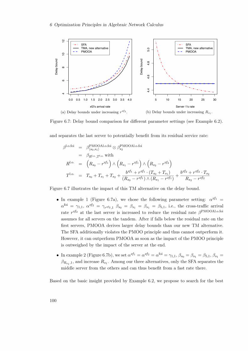
6 Optimization Principles in Algebraic Network Calculus
46
810
12
xf2's arrival rate
Del
ay b
ound
0.0 0.5 1.0 1.5 2.0 2.5 3.0 3.5 4.0
SFATMA, new alternativePMOOA
(a) Delay bounds under increasing r
xf2 .
4.4
4.6
4.8
5.0
Server 1's rate
Del
ay b
ound
5 10 15 20 25 30
SFATMA, new alternativePMOOA
(b) Delay bounds under increasing R
s1 .
Figure 6.7: Delay bound comparison for different parameter settings (see Example 6.2).
and separates the last server to potentially benefit from its residual service rate:
�
l.o.foi= �
PMOOAl.o.foihs0,s1i ⌦ �
PMOOAl.o.fois2
= �
R
l.o.,T
l.o. with
R
l.o.=
⇣R
s0 � r
xf1
⌘^⇣R
s1 � r
xf1
⌘^⇣R
s2 � r
xf2
⌘T
l.o.= T
s0 + T
s1 + T
s2 +
b
xf1+ r
xf1 · (T
s0 + T
s1)
(R
s0 � r
xf1) ^ (R
s1 � r
xf1)
+
b
xf2+ r
xf2 · T
s2
R
s2 � r
xf2
Figure 6.7 illustrates the impact of this TM alternative on the delay bound.
• In example 1 (Figure 6.7a), we chose the following parameter setting: ↵
xf1=
↵
foi= �1,1, ↵
xf2= �
r
xf2,1 �
s0 = �
s1 = �
s1 = �5,1, i.e., the cross-traffic arrivalrate r
xf2 at the last server is increased to reduce the residual rate �
PMOOAl.o.foi
assumes for all servers on the tandem. After if falls below the residual rate on thefirst servers, PMOOA derives larger delay bounds than our new TM alternative.The SFA additionally violates the PMOO principle and thus cannot outperform it.However, it can outperform PMOOA as soon as the impact of the PMOO principleis outweighed by the impact of the server at the end.
• In example 2 (Figure 6.7b), we set ↵
xf1= ↵
xf2= ↵
foi= �1,1, �
s0 = �
s1 = �5,1, �
s1 =
�
R
s1 ,1, and increase R
s1 . Among our three alternatives, only the SFA separates themiddle server from the others and can thus benefit from a fast rate there.
Based on the basic insight provided by Example 6.2, we propose to search for the best
100
6.2 The Tandem Matching Analysis
delay bound considering all combinations a tandem can be decomposed into, i.e., amongall tandem matchings onto it. As every link can be the start and the end of two adjacenttandems of a TM alternative, this will result in a total of 2
|L| alternatives where |L|denotes the amount of links. Again, the delay bound derived with one of the the alterna-tives depends on the actual parameters. Therefore, the best tandem matching alternativecannot be derived from the given network description in a static fashion. Cross-trafficarrival bounds, in turn, depend on an accurate, recursively derivation themselves. In or-der to maximize the search space, TMA should be accompanied by a Tandem MatchingArrival Bounding (TMAB) that also exhaustively matches to the tandems that are de-rived during aggrAB. Exhaustive tandem matching, i.e., TMA for compFFA step 2 andTMAB for compFFA step 1, generates the entire set of TM alternatives for a feed-forwardnetwork. On the individual tandems, we apply the PMOOA left-over service curve – theserver-by-server matching of SFA is now explicitly executed by the exhaustive tandemmatching. I.e., TMA generalizes all existing algebraic tandem analyses by making thestep from the network description to the analysis’ internal model explicit. In our searchspace for algNC, we then try to find the alternative with the minimal composition penalty– similar to optimization searching for the best result in the constrained region of results.This approach is inspired by the LPA but in contrast to it, the TMA with TMAB doesnot generate invalid delay bounds. It does not constitute an all-or-nothing approach.Our new method is applicable to any feed-forward network. If not explicitly mentioned,we use the term TMA to refer to the entire TM-based analysis that consists of TMA forcompFFA step 2 with TFA-assisted TMAB for compFFA step 1.
6.2.2 Related Work
In this section, we rely on the PMOOA left-over service curve for arbitrary multiplexingof flows, i.e., the worst-case remaining service capturing any possible scheduling order offlows at a server. NC also offers a left-over service curve for FIFO-multiplexing servers:�
l.o.✓
[50]. Like the arbitrary multiplexing one given in Theorem 2.3, it is only applicableto a server. Thus, it allows for an analysis akin to the SFA presented in Section 2.3.Again, this raises the problem of paying multiplexing more than once if cross-flows sharemultiple consecutive servers with the analyzed foi. Effort focussed on improved analysisfor sub-path sharing, however, an algebraic end-to-end FIFO analysis that reduces payingfor cross-traffic multiplexing to a single location on the tandem does not exist. The mostadvanced algebraic tandem FIFO analysis is the so-called Least Upper Delay Bound(LUDB) [53]. In case of nested cross-traffic interference patterns, the LUDB suggests toconvolve servers before removing cross-flows, subject to the nesting relation of flows. Thelatter is done by computing the FIFO left-over service curve. In Figure 6.6a, servers s0
and s1 are convolved before xf1’s arrivals are removed, resulting in �
l.o.✓1,hs0,s1i. Next, the
101

6 Optimization Principles in Algebraic Network Calculus
left-over service curve at s2, �
l.o.✓2,s2
, is derived and both are convolved to the foi’s end-to-end service curve. Finally, the delay bound can be derived which, in turn, requires to findthe optimal solution for ✓1 and ✓2. Note, that this approach enforces segregated cross-flowarrival boundings according to the nesting, i.e., the composition penalty presented for thePMOOA in Section 3.2 also applies to the LUDB. If paths are not nested, this approachcannot be executed, e.g., if xf2 additionally crossed s1. In this case, [53] suggests to cutthe tandem into several sub-tandems such that each sub-tandem sees nested interferenceonly. Then, the foi’s delay is derived for every sub-tandem; they are added up to theend-to-end delay bound. If there are multiple alternatives to cut a tandem (in case ofprolonging xf2 both links), all alternatives, i.e., all tandem matchings, are tested in anexhaustive fashion and the least among all resulting delay bounds is the final result.Unfortunately, the approach adding up partial delay bounds does not implement thePBOO principle. Therefore, the authors of the LUDB adapted their analysis in a follow-up article [3]. There, the foi is not cut anymore. Only cross-flows are cut such that theinterference pattern is converted into a nested one. Then, an end-to-end left-over servicecurve can be derived for the foi. While this implements the PBOO principle, PMOO isnot implemented as cutting cross-traffic requires deriving its arrival bound to be used atthe cut.
The sub-tandem cutting of these approaches and the tandem matching of our newanalysis are similar, yet, they also differ in some key aspects. First, our TMA does notrequire to result in tandems with nested interference because the PMOOA can handleoverlapping sub-paths of cross-flows10. Our exhaustive approach thus results in moresub-tandem matching alternatives than the LUDB’s cutting. Secondly, [53] and [3] areconcerned with a tandem analysis only. They do not address the composition penaltyof the compFFA we presented in Section 3.2, yet, both LUDB approaches are based onthe idea of sub-path sharing and thus suffer from it, too. Moreover, they do not providea technical solution for the potential problem of combinatorial explosion problem; [3]rather presents a heuristic to trade accuracy against computational effort. Applying theLUDB in the exhaustive tandem matching of this work, is, however, possible.
An optimization-based NC approach for tight FIFO-multiplexing feed-forward networkanalysis exists as well [15]. It transforms the NC description of the network into aMixed Integer Linear Program (MILP) where the integer constraints encode branchingof flows. This circumvents the step of explicitly extending a partial order to the setof all compatible total orders. However, the computational effort to solve the MILPfor large networks does not seem computationally feasible either. Instead, the authors10Here, we exclusively refer to the non-nested PMOOA left-over service curve of [75] on every tandem,
independent of the actual cross-traffic interference pattern. Note, that the nested variant would havederived delay bounds equal to the TM alternative in Example 6.2, however, it is not applicable inslightly more involved networks. The TMA thus additionally solves searching for nesting patterns.
102

6.2 The Tandem Matching Analysis
0 20 40 60 80 100
010
2030
40
Network utilization [%], relative to largest network with bounded delays
Net
work
del
ay b
ound
[s]
● ● ● ● ● ● ● ● ● ● ● ● ● ●● ●
● ●●
●
●
●
●
11.
251.
51.
75
−x−
Impr
ovem
ent f
acto
r
●
SFA with TFA−assisted aggrPBOOABTMA with TFA−assisted TMABDelay bound improvement by TMA
(a) Flat ER network with 32 devices.
0 20 40 60 80 100
010
2030
40
Network utilization [%], relative to largest network with bounded delays
Net
work
del
ay b
ound
[s]
● ● ● ● ● ● ● ● ●●
●●
●
●
●
●
●
●
11.
52
2.5
33.
5
−x−
Impr
ovem
ent f
acto
r
●
SFA with TFA−assisted aggrPBOOABTMA with TFA−assisted TMABDelay bound improvement by TMA
(b) Hierarchical ER network with 32 devices.
Figure 6.8: TMA accuracy improvements in the ER sample networks.
advise to remove all constraints with integer variables in order to obtain an ordinaryLP formulation that derives an upper bound. I.e., tightness is traded for computationaleffort; similar to the ULP.
6.2.3 Accuracy Evaluation
Numerical Experiments 1: Network Delay Bounds in ER Networks As with theevaluation of aggrAB in Section 6.1.1, we first benchmark TMA, our second proposalfor optimization principles in algNC, against the latest results we reported for algNC,the SFA with TFA-assisted PBOOAB. Note, that TMA uses the TFA-assisted TMABfor compFFA step 1 and the TMA for step 2. For comparability, we use the same ERnetworks, a flat and an hierarchical one.
Figure 6.8 shows the results: Maximum delay bounds for the respective network uti-
103

6 Optimization Principles in Algebraic Network Calculus
Flow, ordered by the TMA delay bound
Del
ay b
ound
[ms]
0 500 1000 1500 2000 2500
050
100
150
200
SFA with aggrPBOOAB
ULPA ≈ TMA
Figure 6.9: Flow delay bounds in the GLP network with 180 devices.
lization are improved. Similar to the previous evaluation, this reduction decreases withincreasing utilization and thus increasing delay bounds. At 100%, the delay bounds be-come nearly identical and the improvement factor of both networks is at ⇠ 1. For smallerutilizations, the TMA achieves an improvement factor between ⇠ 1.25 and 1.75 in theflat network and between 1.5 and 2.75 in the hierarchical network. Both factors lead toconsiderable delay bound reductions.
Numerical Experiments 2: Flow Delay Bounds in GLP Networks Next, we extendthe evaluation of Section 5.3.3 with our new TMA. I.e., we depart from the network delaybounds and investigate the impact on individual flow delay bounds.
Figure 6.9 shows analysis results for an Internet-like network with 180 devices. All the2584 flows’ end-to-end delay bounds are depicted. Sorting the bounds ascending by theirTMA delays reveals two important observations:
• The ULP and the TMA delay bounds increase pretty much in lockstep and stayclose to each other. I.e., the TMA does not have to compromise much on the delaybound accuracy. This holds true for all smaller network sizes as well.
• The SFA results oscillate wildly with a large amplitude. This behavior can beobserved across all network sizes. In contrast to the TMA, the lack of consistencyin the SFA’s gap to the ULP bounds even prohibits using it as a proxy metric foraccurate flow delay bounds.
Both observations are confirmed by the overall results of our experimental investigation.Figure 6.10 shows all evaluation results for GLP networks of sizes up to 180 devices, i.e.,the delay bounds of 12376 flows across all network sizes shown in Table 5.2, left. TheTMA accuracy is stable across the network size and stays within a small deviation from
104

6.2 The Tandem Matching Analysis
Delay bound reduction by the ULPA [%]
Den
sity
[%]
05
1015
2025
3035
[0,0
.5)
[0.5
,1)
[1,1
.5)
[1.5
,2)
[2,2
.5)
[2.5
,3)
[3,3
.5)
[3.5
,4)
[4,4
.5)
[4.5
,5)
[5,1
0)
[10,
15)
[15,
20)
[20,
25)
[25,
30)
[30,
35)
[35,
40)
[40,
45)
[45,
50)
>=50
vs. TMAvs. PMOOA with aggrPBOOABvs. SFA with aggrPBOOAB
Figure 6.10: Flow delay bounds relative to the ULPA across nine network sizes compu-tationally feasible to analyze with the ULPA (Table 5.2, left).
the ULP. Compared to the evaluation of the PMOOA in Section 5.3.3, Figure 5.4, we seethat the accuracy has improved: The three leftmost TMA bars have increased while thefollowing bars that depict larger deviations all decreased. Consequently, the amount ofoutliers has been reduced as well. Except for a single outlier, all derived bounds are atmost 5% larger, mean and median are both at only 1.16%. The outlier deviates 8.23%from the ULP and thus is still more accurate than most of the SFA delay bounds.
6.2.4 Effort Considerations
The computational effort of exhaustive tandem matching becomes apparent when con-structing the set of all TM alternatives, i.e., the entire TMA-internal model of the net-work that is used to derive the delay bound. We exemplify the construction on a tandemnetwork with n servers and m flows; Figure 6.11 illustrates the steps we take and theamount of tandem matching alternatives in several, repeating steps of this procedure.Assume the worst case where each server is crossed by every flow, yet, equal to the SFA,cross flows are not aggregately bounded. Let us start on the foi’s path P (foi) – we callthis tandem Torig = hs1, . . . , sni. The number of different matching alternatives for Torig
is already 2
n�1. As such an alternative derives the foi’s end-to-end delay bound, eachhas between 1 and n distinct sub-tandems in order to cover all servers on Torig. In ourexample, we always proceed with tandem matching alternatives that separate the lasthop and we bound a single segregated cross-flow’s arrivals at this server. In the following
105

6 Optimization Principles in Algebraic Network Calculus
Figure 6.11: Search tree [1] for the n servers, m flows sample tandem representing allrequired arrival boundings.
step (level 2), TMAB is executed. The foi has m�1 cross-flows, defining the search spacein the first TMAB step. To bound a single cross flow’s arrival at level 2, a TMAB isapplied to its path of length n�1, resulting in 2
n�2 TM alternatives (level 3). Again, it isnecessary to bound this flow’s cross-traffic arrivals recursively (level 4). As the cross-flowunder consideration does not interfere with itself and as we are on the foi’s path, there arem� 2 cross-flows to bound. In contrast to the shortening path lengths, this number willnot decline until the arrival bounding terminates. We skip the remaining steps as theyare repetitions of level 3 (with increasing x n in 2
n�x) and level 4. Continuing on thistrajectory through the search tree, bounding a single cross-flow of a single sub-tandem ofa single TMA alternative of Torig already triggers (m� 1)+ (n� 1) · (m� 2) TMABs onthe evenly numbered levels. Levels with odd numbers (� 3) scale this number by 2
(n�2)!
TM alternatives until we eventually reach the end of the tandem.Obviously, TMA is prone to a combinatorial explosion similar to the extension of
partial orders to compatible total orders as required for the LPA. However, in contrastto LPA, each trajectory starting from Torig enables to derive a valid arrival bound. Inprinciple, this would allow for a simple, yet flexible tradeoff between computational effortand delay bound accuracy. However, we opted for the exhaustive tandem matching anddesigned an efficient algorithm which keeps the computational effort still tolerable byexploiting the compositionality of the TMA (Section 7).
6.3 Combining Search Spaces of Optimization Principles
Last, we compare both optimization principles. Figures 6.3 and 6.8 showing the respectiveapproach’s improvement factor over the same algNC analysis reveal quite similar impactof the approaches; the pattern followed by the improvement factor is quite similar inboth network types. Only the delay bounds in the hierarchical ER network show a visible
106

6.3 Combining Search Spaces of Optimization Principles
0 20 40 60 80 100
020
4060
8010
0
Network utilization [%], relative to largest network with bounded delays
Net
work
del
ay b
ound
[s]
● ● ● ● ● ● ● ● ● ● ● ● ● ● ● ● ● ● ●●
●
●
●
●
●
11.
021.
041.
061.
08
−x−
Impr
ovem
ent f
acto
r
●
Exhaustive bounding procedureTMA with TFA−assisted TMABDelay bound improvement by TMA
(a) Flat ER network with 32 devices.
0 20 40 60 80 100
010
2030
4050
Network utilization [%], relative to largest network with bounded delays
Net
work
del
ay b
ound
[s]
● ● ● ● ● ● ● ● ● ●●
●●
●
●
●
●
●
11.
051.
11.
15
−x−
Impr
ovem
ent f
acto
r
●
Exhaustive bounding procedureTMA with TFA−assisted TMABDelay bound improvement by TMA
(b) Hierarchical ER network with 32 devices.
Figure 6.12: Delay bound accuracy comparison for the algNC with different optimizationprinciples.
difference. In Figure 6.12, we depict the relative performance of TMA and the exhaustiveanalysis. The improvement factor was chosen from the TMA’s point of view. It does notfall below 1, i.e., TMA performs at least as good as the exhaustive analysis with aggrAB.This can be explained with a comparison of the search spaces covered by each principle.To be precise, we can deduce that the search space of exhaustive aggrAB is a subset of theTMA’s one. The TMA exhaustively tests every TM alternative. Matching to the longestpossible tandem coincides with the PMOOA; matching to the smallest possible tandems,i.e., single servers, coincides with the SFA. Transferring this approach to the TMABmeans embedding it into the recursive aggregate cross-traffic arrival bounding scheme.There, the two special cases of TMAB coincide with aggrPMOOAB and aggrPBOOAB,the two alternatives defining aggrAB. Therefore, the TMA’s search space completelycovers the aggrAB’s one. Not only does this explain the superiority of TMA delay
107

6 Optimization Principles in Algebraic Network Calculus
bounds but also indicates larger effort for finding them.
In this section, we contributed insight on where to search for tightness improvements inalgNC by identifying parts of its search space that have been neglected previously. As aresult, delay bounds improve but the effort for algNC increases to the level of optNC – theanalysis approaches become computationally infeasible. In fact, the accuracy evaluationsshown in this section cannot be obtained with pure computational performance. In thenext section, we provide efficiency improvements allowing us to derive delay bounds withalgNC that incorporates optimization principles.
108

7 Efficiency of Algebraic Network Calculus Analysis
This chapter is dedicated to the efficient computation of algebraic network calculus anal-yses. First, we present two general enhancements for the feed-forward analysis: 1) Re-duction of intermediate results by convolution of arrival bounds and 2) caching of inter-mediate arrival bounds. Both allow for a more efficient computation without sacrificingaccuracy of results. Then, in Section 7.2, we implement these improvements in an al-gorithm for the TMA. In fact, without these improvements, the delay bounds presentedin the previous section could not have been computed. We benchmark our new algo-rithm against ULPA, SFA and PMOOA. We show run times several orders of magnitudesmaller than the ULPA.
The accuracy improvements for algNC presented in this thesis all require additionaleffort. AlgNC does, in contrast to the LPA, provide valid bounds in case the effort to beput into an analysis must be reduced. I.e., trading accuracy against effort is achievable ina straight-forward fashion; exhaustive approaches can be scaled back easily. However, weaim for the theoretically achievable bounds where exhaustive algNC procedures belongto the category of computationally infeasible analyses. This section provides work onefficiency of the algNC analysis such that effort vastly shrinks and accurate NC analysisfinally becomes scalable.
7.1 Analysis Execution Efficiency
We reinforce the integration of the three substeps of compFFA step 1: backtrackingdependencies, deriving the analysis equation and executing the computation. This in-tegration still allows us to access all the useful intermediate results – a key differenceto optimization-based analysis of optNC. The ULPA must execute separate steps forbacktracking and computation in order to interface NC with the external linear programsolver. We already showed in Section 5.3.3 that the choice of optimization software iscrucial for the analysis performance and will also continue to investigate improvabilityof it.
7.1.1 Convolution of Intermediate Arrival Bounds
The first efficiency improvement to counteract combinatorial explosion in our algNCanalyses strives for a reduction of intermediate results. As depicted in Figure 6.11, eachTMAB matches tandems (oddly numbered levels), i.e., it derives alternative cross-trafficarrival bounds, one for every TM alternative. These arrival bounds are used to derivealternative left-over service curves that, in turn, are used to derive the arrival boundsrequired on the previous recursion level. In the integrated scheme we propose, the arrival
109

7 Efficiency of Algebraic Network Calculus Analysis
bounds at every level of the recursion of compFFA step 1 are known. Moreover, it holdsthat for two alternative arrival curves ↵1 and ↵2 for a flow f , ↵1⌦↵2 is also an arrival curvefor f . Exploiting this insight, we need not traverse all trajectories through the searchtree as we do not rank alternatives by the delay bound they eventually compute. Thisis in contrast to the LUDB and the straight-forward implementation of our optimizationprinciples for algNC that compare alternative delay bounds at the end of the search.In fact, we do not rank alternative intermediate results at all, we combine them byconvolution. This feature is unique to algNC as it retains the semantics of the NC modelwhereas the (U)LPA does not. Reduction to a single arrival bound per recursion levelinhibits a combination any two adjacent levels’ results. Thus, we strongly counteract thecombinatorial explosion; potential search trajectories are narrowed down, search treesare thinned out.
7.1.2 Caching of Intermediate Arrival Bounds
The second improvement we propose is of technical nature. We extended the DiscoDNCwith a caching mechanism for intermediate arrival bounds. Prerequisite for the retrievalof cached arrival bounds is their unique identification. The following parameters arerequired to identify an intermediate cross-traffic arrival bound:
Bounded Flows The set of flows whose arrivals are bounded by the curve.
Server The server at which flows are bounded with the cached curve. Remember that weneed to segregate cross-flows according to the inlink they arrival on. Therefore, wemay cache multiple arrival bounds per set of flows and per server. Separate entriesaccording to the inlink help to maximize reuse and thus minimize derivation effort –similar to the considerations for an in-network SensorNC procedure (Section 4.5).
Flow of Interest The foi must be known in case the arrival bounding is started on itspath and immediately proceeds with servers on it. This special case applies to theSFA and the TMA, e.g., see ↵
f0s2 in Section 2.3.2. This property must be indicated
as these arrival bounds cannot be safely reused in any other case. There, the foiwill be considered interference with the flows to bound, i.e., the arrival bound willbe larger due to a violation of the PSOO principle.
We do not require the tandem analysis applied in compFFA step 2 to identify an arrivalbound. In fact, the cache thus even allows algNC to share results between SFA andPMOOA with aggrAB (Section 6.1).
The cache fosters termination of recursive cross-traffic arrival bounding before reachingthe source servers of flows – the previous termination condition segrPBOOAB as wellas Algorithms 3.1, 4.2 and 6.1 (implementations of compFFA step 1). The search trees
110

7.2 The Efficient TMA Algorithm
presented in the previous section thus become shorter as the length of search trajectoriesis reduced.
Convolution and caching of arrival bounds supplement each other well: The formerensures that a single arrival bound is derived on every recursion level of the compositionalprocedure of algNC. Therefore, it reduces the amount of intermediate bounds the cachehas to store. Moreover, it allows the TMA algorithm to operate on a single, largesearch plane instead of the separate search tree branches shown in Figure 6.11. This“search plane” represents the same search space as before – the network remains thesame – but it inhibits redundancies when searching it. Remember, that the TMA definesthe most comprehensive search space of our algNC analyses incorporating optimizationprinciples. In the remainder of this section, we will investigate the impact of our efficiencyimprovements on this analysis.
7.2 The Efficient TMA Algorithm
In this section, we provide a fast algorithm that integrates the transformation of thesystem description to all TM alternatives into the analysis itself. That is, TM is notexecuted statically in a step preceding the analysis. Intermediate results can then be usedto dynamically reduce the amount of matching combinations as shown above. Althoughthis reduces computational effort, our efficient TMA depicted in Algorithm 7.1 does notpay for this efficiency gain with less accurate delay bounds. It guarantees for the mostaccurate algNC bounds in feed-forward networks.
Algorithm 7.1 derives a foi’s alternative end-to-end service curves for the TMA. Nomen-clature follows Algorithm 6.1, i.e., lowercase letters denote variables and blackboard boldletters denote sets of variables. First, getBl.o.F
Torig
is invoked with the foi’s path P (foi),i.e., Torig :
= P (foi), and the foi itself – the algorithm needs to reverse the conceptual twosteps of an analysis presented in Section 3.1. P (foi) constitutes the first tandem to matchwith 2
n�1 disjoint sub-tandems, where n denotes the number of server on P (foi). Forevery sub-tandem we then derive the cross-traffic arrivals with TMAB (lines 32 – 37).Thus, we derive all TM alternatives within this recursive arrival bounding method. Afterthe arrival bounding recursion has terminated (guaranteed by the cycle-free feed-forwardnetwork and flows of finite length), its result is used to derive the foi’s left-over servicecurves by convolving the matched sub-tandems’ �
l.o. curves – similar to SFA but �
l.o. arenot necessary single server left-over service curves. In a subsequent step (not depicted inAlgorithm 7.1), we derive delay bounds for all alternative end-to-end service curves forthe foi on P (foi). In contrast to the individual linear programs of the LPA, all are valid.I.e., we chose the smallest result as final delay bound.
111

7 Efficiency of Algebraic Network Calculus Analysis
Algorithm 7.1: Efficient TMA Algorithm.1getBl.o.F
Torig
(Tandem Torig
, Flow set F)
2{T1, . . . , T2n�1} = getSubtandems(Torig
); /* Disjoint divisions of Torig */
3foreach Subtandem sequence T 2 {T1, . . . , T2n�1} do4foreach Subtandem T 2 T do5AF
T
= TMArrivalBounding(T,F);6�
l.o.FT
= PMOO�l.o.
(T, AFT
);7�
l.o.FT ⌦= �
l.o.FT
;8end9Bl.o.F
Torig.put(�l.o.F
T );10end11return Bl.o.F
Torig
12TMArrivalBounding(Tandem T , Flow set F)
13try{ return getCacheEntry(T, F) } /* Check for cached AFT
*/
14G = xtxSegregation(T,F); /* Cross-traffic segregation */
15foreach xtxGroup G 2 G do16AG
src = getSourceFlow↵s(G); /* Arrival curve for G’s source flows */17AF
T
.put(AG
src);
18/* Flow aggregation requires equal inlinks */19foreach Link l 2 T .getInLinks() do20s = l.getSource();21↵
G
T
=�↵
G
s
�0 = OutputBound(s, G);22AF
T
.put(↵G
T
);23end24end
25addCacheEntry�AF
T
�/* Cache AF
T
*/26return AF
T
27OutputBound(Server s, Flow set F)
28Tshared = getSharedServers(s,F); /* Aggregate flows on shared servers */
29Bl.o.FTshared
= getBl.o.FTorig
(Tshared,F);
30↵Tshared = ↵
G
Tshared.getSource(); /* Arrival bound of flows in G at Tshared’s start */
31B
TFA = TFAbacklogBound(s)
32foreach �
l.o.FTshared
2 Bl.o.FTshared
do33
�↵
Fs
�0 ⌦= ↵Tshared ↵ �
l.o.FTshared
; /* Complexity reduction: Convolve all ↵
0 */
34↵Tshared .cap(BTFA); /* TFA assistance */35end36return
�↵
Fs
�0
112

7.2 The Efficient TMA Algorithm
Network devices
Net
work
ana
lysi
s tim
e [h
ours
]
20 40 60 80 100 120 140 160 180 200 220 240 260 280 3 ⋅ 102 4 ⋅ 102 5 ⋅ 102 103
012
2436
48
● ● ●
● ●
●
●
● ● ● ● ● ● ● ● ● ● ● ● ● ● ●● ●
●
ULPA, LpSolve
PMOOA,aggrPBOOABnoCache
SFA,aggrPBOOABnoCache
TMA
ULPA, CPLEX, max 4 threads
●ULPA, CPLEX, max 1 thread
Figure 7.1: Computational Effort Evaluation: Graphical comparison of network analysistimes of optNC (ULPA), and algNC without (SFA, PMOOA) and withoutour improvements (TMA).
Computational Effort Reduction Access to intermediate results, i.e., the output ofthe three individual functions in Algorithm 7.1, allows the TMA to implement severalefficiency improvements:
1. The aggregate cross-traffic arrival bounding on tandems shared by multiple flows(lines 32 – 43, Tshared) naturally counteracts cross-traffic segregation. Aggregatelybounding cross-flows prevents the PSOO effect to arise and the principle to be vi-olated by the TMA. From the computational efficiency point of view, less mutualinterference assumption means less cross-traffic arrival bounding instances. I.e., itprevents recursively bounding cross-flows of cross-flows; all with exhaustive TMAB.This vastly reduces the effort as our considerations concerning combinatorial ex-plosion show (Section 6.2.4).
2. Every recursion level has its Tshared that TMAB matches tandems to. Each of theresulting left-over service curves yields a cross-traffic arrival bound to be used inthe previous recursion level. The second efficiency improvement is to convolve allof the alternative arrival bounds when Tshared is analyzed (lines 39 – 42).
3. The third improvement is arrival bound caching that allows for storage and retrievalof intermediate results (lines 15 and 30) which are plentiful in the compositionalanalysis. It impacts the TMA when alternative matchings share sub-tandems thatrequire equal cross-traffic arrival boundings.
113
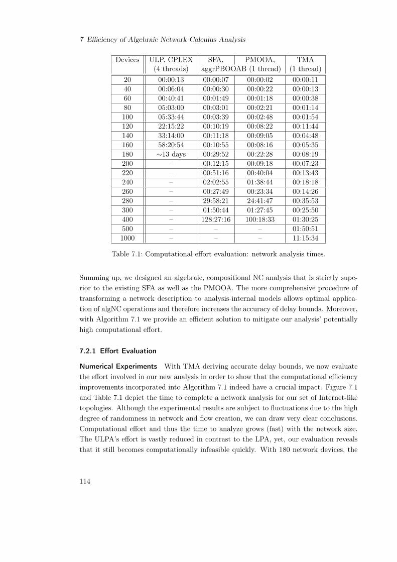
7 Efficiency of Algebraic Network Calculus Analysis
Devices ULP, CPLEX SFA, PMOOA, TMA(4 threads) aggrPBOOAB (1 thread) (1 thread)
20 00:00:13 00:00:07 00:00:02 00:00:1140 00:06:04 00:00:30 00:00:22 00:00:1360 00:40:41 00:01:49 00:01:18 00:00:3880 05:03:00 00:03:01 00:02:21 00:01:14100 05:33:44 00:03:39 00:02:48 00:01:54120 22:15:22 00:10:19 00:08:22 00:11:44140 33:14:00 00:11:18 00:09:05 00:04:48160 58:20:54 00:10:55 00:08:16 00:05:35180 ⇠13 days 00:29:52 00:22:28 00:08:19200 – 00:12:15 00:09:18 00:07:23220 – 00:51:16 00:40:04 00:13:43240 – 02:02:55 01:38:44 00:18:18260 – 00:27:49 00:23:34 00:14:26280 – 29:58:21 24:41:47 00:35:53300 – 01:50:44 01:27:45 00:25:50400 – 128:27:16 100:18:33 01:30:25500 – – – 01:50:511000 – – – 11:15:34
Table 7.1: Computational effort evaluation: network analysis times.
Summing up, we designed an algebraic, compositional NC analysis that is strictly supe-rior to the existing SFA as well as the PMOOA. The more comprehensive procedure oftransforming a network description to analysis-internal models allows optimal applica-tion of algNC operations and therefore increases the accuracy of delay bounds. Moreover,with Algorithm 7.1 we provide an efficient solution to mitigate our analysis’ potentiallyhigh computational effort.
7.2.1 Effort Evaluation
Numerical Experiments With TMA deriving accurate delay bounds, we now evaluatethe effort involved in our new analysis in order to show that the computational efficiencyimprovements incorporated into Algorithm 7.1 indeed have a crucial impact. Figure 7.1and Table 7.1 depict the time to complete a network analysis for our set of Internet-liketopologies. Although the experimental results are subject to fluctuations due to the highdegree of randomness in network and flow creation, we can draw very clear conclusions.Computational effort and thus the time to analyze grows (fast) with the network size.The ULPA’s effort is vastly reduced in contrast to the LPA, yet, our evaluation revealsthat it still becomes computationally infeasible quickly. With 180 network devices, the
114

7.2 The Efficient TMA Algorithm
Share of ULPA derivation on the analysis time [%]
Den
sity
[%]
[0,1
0)
[10,
20)
[20,
30)
[30,
40)
[40,
50)
[50,
60)
[60,
70)
[70,
80)
[80,
90)
[90,
100]
15
1015
2055
60
Figure 7.2: Share of the DiscoDNC linear program creation on the ULPAs.
analysis execution already took ⇠ 13 days. The larger the network, the more effort isrequired to trace the influence of flows on each other. Yet, among the two steps of theULPA, deriving the constraints for the linear program with the DiscoDNC and optimizingit with CPLEX, the latter takes on average 81.53% of the time (cf. Figure 7.2). FasterULPA optimization could not be achieved with CPLEX; increasing the parallelism from1 to 4 threads11 even yielded slightly slower overall network analysis times due to theoverhead for thread synchronization. Figure 7.1 depicts the single-threaded CPLEXversion (dotted line). As mentioned, it is slightly below the ULPA line (blank diamond)that shows the results when running CPLEX with up to 4 threads. The ULPAs seemto become very complex. The ULPA file sizes may hint at its complexity; we observedCPLEX lp files of several gigabytes in size.
Analyzing large feed-forward networks in practice remains solely possible with alge-braic, compositional NC analyses. However, Figure 7.1 and Table 7.1 also show thatthe SFA with aggrPBOOAB becomes computationally infeasible at 400 network devices(994 servers, 3976 flows; 13 days for analysis) – although the aggregate arrival boundingreduces the effort compared to the segrPBOOAB. Our TMA scales best with the networksize thanks to the improvements of Algorithm 7.1: Aggregate bounding of cross-trafficas well as the convolution and caching its intermediate arrival bounds. The TMA notonly outperforms the other analyses, it also seems more resilient to the random factorsof our network creation. Most notable are the changes in network analysis times whenincreasing the amount of devices from 260 to 300 in a stepsize of 20 devices. The first
11Note, that among the tools employed in this evaluation, only CPLEX offers an option for parallelexecution. We chose four threads to match the number of CPU cores.
115

7 Efficiency of Algebraic Network Calculus Analysis
increase only adds 18 servers and 72 flows to the network but the entanglement of flows isconsiderably more complex such that the SFA run-time grows by an order of magnitude,from ⇠ 30 minutes to ⇠ 30 hours. The next step increases the amount of servers by130 and the flows by 520, however, this seven times larger growth of the network sizeresults in a large decrease of the SFA run-time, down to ⇠2 hours. The PMOOA revealsa nearly equal behavior but the TMA, on the other hand, has only a small oscillation,jumping from 15 minutes to 36 minutes and back to 26 minutes. The TMA scales muchbetter with the network size and outperforms the other analyses by several orders ofmagnitude. It is now possible to analyze a GLP network with 1000 devices. The samplenetwork of this size had 3626 servers and 14504 flows, i.e., more flows than analyzed withthe ULPA in total in ⇠18 days, yet, all in a single network with more comprehensive de-pendencies to backtrack and convert into an analysis equation. This makes the TMA byfar the fastest accurate algNC analysis and enables algNC to analyze large feed-forwardnetworks.
7.3 Network Calculus on Compact Domains
As a last efficiency improvement, we propose a solution to the problem of explodingcurve complexity in an algNC. If a (min,+)-operation is applied to pseudo-periodic inputcurves f and g, then the resulting output curve h’s period grows to the least commonmultiple (hyperperiod) of f and g’s periods. Hence, subsequent operations on h becomemore complex. In a network analysis, this growth of complexity results in prohibitiveeffort fast. Our solution to this problem is based on the following insight from theliterature [37]: The eventual performance bound derivation only requires a finite, initialpart of the curve. We propose a solution to derive more accurate upper bounds on exactlythis part of curves. Moreover, our solution achieving this is more general, allowing forthe application to SFA and PMOOA with nested interference. We evaluate our findingswith the case study of an avionics in-cabin network.
One of the main assumptions of this thesis so far was that arrivals are shaped to multi-token-buckets, ↵ 2 FmTB, and service curves belong to the set of multi-rate-latencycurves, � 2 FmRL. These curves are widely used in practice, yet, they may alreadybe the first accuracy tradeoff. For instance, a different approach to characterize thearrivals of task activations is the (p, j, t
�
)-model where p denotes the period, j the jitterand t
�
the minimum inter-arrival time. The parameters are used to create a staircasearrival curve ↵
p,j,t
�
(d) = min
⇣ld+j
p
m,
ld
t
�
m⌘2 F0 [81, 59]. For (strict) service curves,
the TDMA can be best described with the (k, c, b)-model where k is the slot lengthavailable for submission, c is the TDMA cycle length this slot is embedded into, and b
is the total bandwidth [58]. This resource model results in a service curve �
k,c,b
(d) =
116

7.3 Network Calculus on Compact Domains
⇣j[d�c+k]+
c
k· k + min
�[d� c + k]
+mod c, k
�⌘ · b. Bounding these curves with a multi-token bucket or a multi-rate latency, respectively, constitutes an overapproximation. Theinaccurate model thus forces the NC analysis to account for data arrivals that are actuallyknown not to occur but are within the region bounded by ↵. Moreover, the approximatedservice prevents NC from exploiting capabilities not captured in �. Therefore, accuracyof NC bounds also depends on the accuracy of the model, i.e., even the LPA only derivestight bounds within the given network description. The optNC analyses strictly relyon ↵ 2 FmTB and � 2 FmRL, so does the non-nested PMOOA. The left-over servicecurve of Theorem 2.3, in contrast, does not. It allows the SFA as well as the nested andthe sink-tree PMOOA to analyze networks with arrival and service curves are from F0.However, for practical reasons this potential has not yet been exploited.
The Hyperperiod Problem The above curves, ↵
p,j,t
�
and �
k,c,b
, are piece-wise linear(PWL) and pseudo-periodic. Due to the former, we have ↵
p,j,t
�
/2 FmTB and �
k,c,b
/2FmRL and the latter causes the hyperperiod problem [17]. Let ↵
p,j,t
�
and �
k,c,b
be theinput curves to a (min,+)-algebraic operation, then the resulting curve is PWL andpseudo-periodic, yet, its period is the least common multiple of the input curves’ periods.I.e., with the provided curve models we get an output curve period of lcm(p, c). In thealgNC cross-traffic equation derived in compFFA step 1b and solved in step 1c as wellas the foi equation of step 2 (Section 3.1), the hyperperiod problem renders the analysiscomputationally intractable. It can be alleviated with overapproximated curves. E.g.,multi-token buckets and multi-rate latencies circumvent it and aligning the periodicity ofcurves such that they result in a small lcm inhibits uncontrolled growth. However, thesecountermeasures compromise on model accuracy and thus eventually on performancebound accuracy as well.
The Compact Domains Solution Closure of this class of curves is shown in [17], wherethe authors also show that NC operators suffer from the hyperperiod problem. Yet,in our work, we observe that this complete characterization is rarely required whenbounding delay or backlog. The bounds are commonly found on the initial parts of curves.Therefore, we propose to alleviate the hyperperiod problem by using NC on compactdomains, i.e., restricting curves to a bounded domain [0, K] instead of [0, +1). The sizesof a curve’s compact domain is crucial for both of the aspects in the focus of in this thesis:delay bound accuracy and computational effort. On the one hand, compact domains needto be sufficiently large such that performance bounds are not negatively affected. On theother hand, we want to decrease computational effort and thus strive for small compactdomains. We achieve a balance between these aspects by analyzing the algNC analysisequation and then deriving a bound on the domain length ensuring that delay and backlog
117

7 Efficiency of Algebraic Network Calculus Analysis
(a) Sample Sink-Tree Network.
↵↵
f3
�s3
↵
f4
�s4
↵
+
↵
f5
�s5
↵ ↵
f6
�s6
↵
D
f3s1
↵�s1 ↵�s2
D
f3s3
D
f3s0 �s0
↵
D
f3= D
f3s3
+ D
f3s1
+ D
f3s0
(b) TFA Delay. (c) Nested PMOOA Delay.
Figure 7.3: Sample network and its analysis equations for TFA and nested PMOOA.
bounds are enclosed. This initial domain bound is then used to derive the required domainlengths of curves occurring in the entire equation. Maintaining a domain of sufficientlength for each of these curves is crucial, as they all influence the final performancebound calculation. Any loss in precision, therefore, affects the accuracy of the derivedperformance bounds. Here, we make use of the backtracking scheme of compFFA step 1ato propagate the restrictions through the analysis equation. In the remainder of thissection, we derive the compact domain required for each operation’s input curves inorder to guarantee for the known domain requirement at its output. This makes ourapproach applicable to any algNC analysis using the operations of Section 2.1.3. It iskey for significant improvements in the computational efficiency of these analyses withoutsacrificing the accuracy of the NC network model.
7.3.1 Related Work
Reducing precision of curves to finite intervals has been introduced and empirically eval-uated in the work of [80, 81]. It is, however, preliminary, as it lacks proofs for the preser-vation of accuracy of performance bounds. [37] derived conditions for the lengths of finiteintervals and proved that they preserve accuracy of the performance bounds. However,these proofs only hold for the input A / output A
0 relations of the greedy-processingcomponent (GPC) commonly used in Real-Time Calculus (RTC) [83]. Although algNCand RTC are based on the same dioid algebra, the component-level of abstraction in theproofs imposes crucial limitations for application in algNC. The nested PMOOA that im-plements the PBOO and the PMOO principle does not preserve the component-structureof the network (Figure 7.3c). The only analysis preserving it is the TFA (Figure 7.3b).It can directly exploit the work of [37], however, TFA is known to derive inferior delaybounds (see Sections 5.3.1 and 5.3.2).
118

7.3 Network Calculus on Compact Domains
(a) Arrival curves ↵ and PMOOA �
l.o.f3 : stepsfunctions (blue, green); linear (red, black).
Steps LinearTFA 38 42.5
PMOO 25 28ULP – 28
(b) Delay Bounds of the Example.
Figure 7.4: Input curves and computed delay bounds.
Example 7.1. We derive the delay bounds for the small sink tree example of Figure 7.3.All arrival curves were set to ↵
p,j,t
�
= ↵7,12,0(d) as this parameter setting results in thecurves’ first step to be as long as the following ones. Therefore, the token bucket arrivalcurve �
r,b
= � 17 ,7
is a tight overapproximation. It passes though all starting points of eachstep of ↵
p,j,t
�
. See Figure 7.4a where ↵7,12,0 and � 17 ,7
are depicted. Strict service curveswere set to �1,0, i.e., only the overapproximation of arrivals causes the difference in results.Table 7.4b shows the delay bounds derived by different NC analyses for the respectivecurve settings12. Even in this simple example, there is a ⇠ 10% difference between theend-to-end delay bounds of the accurate model and the linear overapproximation. Asexpected, the TFA performs worse than the PMOOA that, in turn outperforms the ULPif executed with the more precise step functions.
7.3.2 Deriving Compact Curve Domains
In this section, we introduce the idea of compact domains for algNC by departing fromthe component-wise view. Instead, we derive domains on the actual operations appliedin algNC equations.
Preliminaries First, we need to transform the left-over service curve derivation of The-orem 2.3 to apply the (max,+)-convolution instead of the non-decreasing upper closure.The (max,+)-convolution, denoted as ⌦, is defined as
(f⌦g) (d) = sup
0⌧d
{f(d� ⌧) + g(⌧)}
12The DiscoDNC does not support PWL, pseudo-periodic step functions. Therefore, we used the MPAtoolbox [58] in this section.
119

7 Efficiency of Algebraic Network Calculus Analysis
and with it, we can compute the left-over service curve as
�
l.o.F1s
= �
s
↵
F0=
⇣�
s
� ↵
F0
⌘⌦�0
with �0(t) = 0:⇣⇣�
s
� ↵
F0
⌘⌦�0
⌘(d) = sup
0sd
n⇣�
s
� ↵
F0
⌘(d� s) + �0(s)
o= sup
0sd
n⇣�
s
� ↵
F0
⌘(d� s) + 0
o= sup
0sd
n⇣�
s
� ↵
F0
⌘(d� s)
o(s
:
= d� u)
= sup
0(d�u)d
n⇣�
s
� ↵
F0
⌘(d� (d� u))
o= sup
0(d�u)d
n⇣�
s
� ↵
F0
⌘(u)
o(reverse the supremum’s search direction)
= sup
0ud
n⇣�
s
� ↵
F0
⌘(u)
o=
⇣�
s
↵
F0
⌘(d) .
Next, we define the compact domain as well as arrival and service curves compactedto this closed interval.
Definition 7.1. Let D = [0, K] be a closed and bounded interval. If a curve providesa mapping : [0, K] ! R+
1, we denote D as its compact domain.
In this setting we define the following notation:
• Arrival curves ↵ and strict service curves � of F0 operate on an unrestricted domain,they provide a mapping R! R+
1 (Section 2.1.1).
• The corresponding curves ↵
K and �
K are restricted to the compact domains [0, K
↵
]
and [0, K
�
].
For unrestricted curves ↵ and �, we define the following approximations:
• An arrival curve ↵ is an overapproximation of an unrestricted arrival curve ↵ if8d 2 R : ↵(d) � ↵(d).
• A service curve � is an overapproximation of an unrestricted service curve � if8d 2 R+
1 : �(d) �(d).
120

7.3 Network Calculus on Compact Domains
The intuition for these overapproximations is as follows: Arrival curve ↵ allows more dataarrivals than originally specified with ↵ and in case of a service curve �, the assumedservice applied to a flow is decreased when compared to the original service curve �. Viceversa, underapproximations ↵ and � are more optimistic than original curves and thuscan only lower bound these. They are defined analogously.
In the following, the concrete form of approximations is irrelevant as long as the aboveconditions are met, e.g., one could use specific traffic patterns as proposed in [59, 8],approximations based on single linear segments [81], or minimum-composed sets of linearsegments [49]. The only assumption we have is that, in the long term, there is enoughservice available to process all inputs.
Enclosure of Backlog and Delay Bounds Deriving a performance bound, backlog ordelay, constitutes the eventual step of any NC analysis; see 7.3b and 7.3c. Workingon compact domains, we need to guarantee that these are large enough to enclose thebounds. Otherwise, the bounds derived on the compact domain are not valid. Thefollowing corollary is a direct consequence of Theorem 2.1. It ensures enclosure of delayand backlog bounds.
Corollary 7.1. (Backlog and Delay Bound Enclosure) Assume the delay and backlogbound for an unrestricted arrival curve ↵ and an unrestricted service curve � to be known.That means we also know the values of the parameters u, s and r for which the supremain Theorem 2.1 are assumed. Then, we can derive the domains of the restricted curves↵
K and �
K by
K
↵
= max (u, r) , K
�
= max (u + ⌧, r) .
Corollary 7.1’s prerequisite to know the performance bounds for ↵ and � a priori iscrucial. Clearly, both are only known a posteriori, i.e., after we carried out the analysiswith unrestricted curves. Yet, the analysis with unrestricted arrival and service curvesimposes a high analysis effort, when being performed with accurate network models. Thisrequirement is thus contradicting our aim to execute the analysis with less computationaleffort, it constitutes a seemingly vicious circle.
We break this circle by evaluating delay and backlog bounds both with linearly under-approximated and overapproximated arrival and service curves. Figure 7.4a providesan example for such an arrival curve overapproximation (for the underapproximation, itis simply shifted to the opposite side of the step function). This step can be executedvery efficiently if the chosen approximations are token buckets for arrival curves and ratelatencies for service curves. We execute an entire analysis with approximated curves inorder to obtain ↵, ↵ as well as � and � that are required to bound delay and backlog.
121

7 Efficiency of Algebraic Network Calculus Analysis
More precisely, we can compute approximations for delay and backlog and use these tobound the domains of ↵ and �:
1. With the pair ↵ and �, we compute the estimates D and B for bounding thedelay and backlog. As the involved curves ↵ and � are underapproximations of theunrestricted curves ↵ and �, these estimates are lower bounds.
2. For the bounds D and B, we compute the largest value of d, such that for thefunction values beyond d only smaller delay and backlog bounds can be derived.This is the domain bound required to enclose D and B computed from the originalcurves.
3. With the pair ↵ and �, we similarly compute the estimates D and B that denoteupper bounds on the delay and backlog that would have been derived with ↵ and�.
We formalize the domain bound finding as follows:
Theorem 7.1. We define the following variables:
U
:
= sup
�d � 0 : ↵(d) � �(d + D)
and
R
:
= sup
�d � 0 : ↵(d)� �(d) � B
.
For K
↵
� max(U, R) and K
�
� max(U +D, R) the domain bounds K
↵
and K
�
aresufficiently large such that accurate delay and backlog bounds can be computed with ↵
K
and �
K .
Proof. We defined the largest pseudo-inverse of the lower delay and backlog bound asfollows:
u
⇤:
= sup
⇢u � 0 : D sup
u�u
�inf
�⌧ � 0 : ↵
0(u) �
0(u + ⌧)
�,
r
⇤:
= sup
⇢r � 0 : B sup
r�r
�↵
0(r)� �
0(r)
�.
Sub- and superadditivity of curves ↵ and �, together with D D implies that u
⇤ U .Thus, U is a safe upper bound for guaranteeing delay bound enclosure in curve ↵.
Exploiting u
⇤ U together with the inequality D D yields u
⇤+D U +D U +D.
Note that D is a bound on ⌧ in Theorem 2.1. This implies that U +D is an upper boundfor guaranteeing delay bound enclosure in curve �.
With r
⇤ being bounded by R, we get that K
↵
= max(U, R) and K
�
= max(U+D, R)
also guarantee backlog bound enclosure. It can be found if ↵ and � are restricted to[0, K
↵
], resp. [0, K
�
], i.e., with the curves ↵
K and �
K .
122

7.3 Network Calculus on Compact Domains
An alternative bound on the domain size that could also be used here is given in [37].The authors propose to use the maximum backlogged period bound bp(↵, �). However,this leads to significantly larger domain sizes K
↵
and K
�
, especially when the utilizationis high.
Propagating Compact Domains to the Network Description’s Curves We now knowhow to efficiently derive a bound on the compact domains for arrival and service involvedin bounding delay and backlog. Next, we want to use this insight to increase the com-putational efficiency of the entire analysis. We aim to derive the compact domain foreach arrival and service curve of the network description. The smaller these domains,the faster the analysis can be executed in comparison to the unrestricted curves becausedomain restrictions prevent ever growing hyperperiods. The part growing over the com-pact domain is simply cut off. This requires to backtrack through the analysis equation,i.e., in our integrated scheme for cross-traffic arrival bounding (compFFA step 1) an-other backtracking through the network. Either way, we traverse the servers and thusthe algNC operations in the opposite direction of the analysis. We can take the domainbound required at the output of an operation, i.e., for its output curve, and derive thedomain bounds for this operation’s input curves. We start this scheme with the abovebounds guaranteeing the enclosure of delay and backlog bound.
Let � be a binary algNC-operator, i.e., � 2 {⌦,⌦,↵, min, +,�}, and let be theoutput curve of the operation. When backtracking, we know the bound for the compactdomain of output curve , K
. Moreover, from the backtracking itself equation we know(↵� �) (d) = (d), i.e., the actual operation � and both its input curves ↵ and �
13. Inthe following, we derive the conditions for (↵
K � �
K
)(d) = (d), i.e., the domain lengthK
↵
and K
�
such that remains defined on its domain K
. This directly implies that8d 2 [0, K
] :
K
(d) = (↵
K � �
K
)(d) = (↵ � �)(d) = (d) and that the eventuallyderived performance bounds are safely enclosed.
Compact Domains for � 2 {⌦,⌦, min, +,�} Given the operation (↵��)(d) =
K
(d)
and � 2 {⌦,⌦, min, +,�}, we can compact the domains of ↵ and � to K
↵
= K
�
= K
.This is a direct consequence from the operator definitions; computing (d) = (↵� �)(d)
only requires to evaluate ↵ and � on [0, d] and from
K we know that d K
.
Compact Domains for ↵ Deriving the compact domains of the (min,+)-deconvolutionis more involved.
13For, e.g., aggregation both curves might be arrival curves. This does not impact the derivations givenin this section. Therefore, we refrain from a detailed distinction of cases for the ease of presentation.
123

7 Efficiency of Algebraic Network Calculus Analysis
Theorem 7.2. (Domain bounds for min-plus deconvolution) As before, let K
be thedomain size of the output curve. We define U to be the largest input value for which↵(U + K
) � �(U), i.e.,
U
:
= min
�0, sup{d � 0 : ↵(d + K
)� �(d) � 0}� .
This yields that for K
↵
= U + K
, K
�
= U and 8d 2 [0, K
], we have�↵
K ↵ �
K
�(d) =
(↵↵ �) (d).
Proof. For the output curve , we are only interested in function values for the compactdomain [0, K
]. By exploiting U as defined above, we obtain that
8d K
: sup
u>U
{↵(d + u)� �(u)} < 0.
This shows that function values from ↵ and � that are beyond U + K
, resp. U , turnirrelevant as ↵(d+u)��(u) becomes negative for these input values. Hence, the positivesupremum of ↵
K
(t + u) � �
K
(u) can only be found for input values to ↵ and � fromthe compact domain [0, K
↵
:
= U + K
], resp. [0, K
�
:
= U ]. As ↵
K coincides with ↵ ford 2 [0, K
↵
] and �
K coincides with � for d 2 [0, K
�
], the above construction yields thatfor d K
: (↵
K ↵ �
K
)(d) = (↵↵ �)(d).
As an example, we show how the domain bounding parameter U can be found whenusing overapproximations from FTB for arrival curves and FRL for service curves. Ac-cordingly, we define an overapproximation ↵(t) to an input curve ↵ as:
↵(d) ↵(d) =
8<:max (0, N
↵
+ ⇢ · d) if ↵ > 0
0 otherwise
and let �(t) be defined analogously with an rate-latency curve such that �(t) � �(t)
holds. The slope of �(t) is denoted � and the intersection with the y-axis is N
�
. In thissetting, we bound U for a constant K
as follows:
↵(u + d)� �(u) � 0
with ↵(d) ↵(d) and �(d) � �(d) we have↵(u + d)� �(d) � ↵(u + d)� �(u) � 0 .
With 0 d K
we get↵(u + K
)� �(u) � ↵(u + d)� �(d) .
The definitions of the linear bounding functions yield:
N
↵
+ ⇢(u + K
)� (N
�
+ �u) � 0
124

7.3 Network Calculus on Compact Domains
thus u N
�
�N
↵
+K
·⇢⇢��
and for N
�
< N
↵
and ⇢ < � this is equal tou N
↵
�N
�
+K
·⇢��⇢
such that for U =
N
↵
�N
�
+K
·⇢��⇢
we get u U .
For d K
and u > U : ↵(u + d) � �(u) < 0, the requested bounds are U + K
K
↵
and U K
�
. Beyond this compacted domain, the (min,+)-deconvolution yields negativevalues. Hence, the function value of (d) for any d 2 [0, K
] takes its source in thecompact domains of the input curves [0, K
↵
] and [0, K
�
].
Server
NAC12 NAC13NAC11 NAC14
NAC22 NAC23NAC21 NAC24
NAC32 NAC33NAC31 NAC34
NAC42 NAC43NAC41 NAC44
DEV4411 DEV4421 DEV4431 DEV4441
DEV4412 DEV4422 DEV4432 DEV4442
DEV4413 DEV4423 DEV4433 DEV4443
DEV4414 DEV4424 DEV4434 DEV4444
DEV4411LQHQ
●
●
●
●
●
●
●
●
●
●
●
●
●
●
●
●
●
●
●
●
●
●
●
●
●
●
●
●
●
●
●
●
●
●
●
●
●
●
●
●
●
●
●
●
●
LQ
●
●
●
●
●
●
●
●
●
LQ
●
●
●
●
●
●
●
●
●
●
●
●
●
●
●
●
●
●
●
●
●
●
●
●
●
●
●
●
●
●
●
●
●
●
●
●
●
●
●
●
●
●
●
●
●
HQ
●
●
●
●
●
●
●
●
●
●
●
●
●
●
●
●
●
●
●
●
●
LQ
●
●
●
●
●
●
●
●
●
●
●
●
●
●
●
●
●
●
●
●
●
Topline 1
Topline 2
Topline 3
Topline 4
●
●
●
●
●
●
●
●
●
●
●
●
●
●
●
●
●
●
●
●
●
cam
cam
cam
cam
cam
camE
nd
dev
ice
da
isy
cha
in
backbone backbone backbone backbone
Figure 7.5: Topology of the studied distributed heterogeneous communication system.
7.3.3 Accuracy and Effort Evaluation
We illustrate the impact of NC on compact domains with an avionics case study. Weanalyze a so-called distributed heterogeneous communication system (HCS) by EADSInnovation Works14, an in-cabin network architecture alternative to AFDX. A detaileddescription of this network as well as a RTC model that we use for algNC analysis canbe found in [81]. Figure 7.5 depicts its topology and Figure 7.6 provides the details
14Now Airbus Group Innovations.
125

7 Efficiency of Algebraic Network Calculus Analysis
(a) Backbone model shown for topline 3.
FIFO
Eth.
PTP
DEV1114
event
background
FIFO
Eth.
PTP
DEV1113
event
background
FIFO
Eth.
PTP
DEV1112
event
background
FIFO
Eth.
PTP
DEV1114
event
background
NAC
(b) Model of an end device daisy-chain of topline 1.
Figure 7.6: Case study network model
of its NC model: two abstraction levels, the topline and the device daisy-chain. Thenetwork consists of one central server, 16 network access controllers (NAC), 232 end-devices (DEV) such as speakers, buttons, etc. as well as 6 video cameras for either highquality (HQ) or low quality (LQ) video streaming. Among the network traffic, timesynchronization messages of the IEEE Precision Time Protocol (PTP) has the highestreal-time demands as it, e.g., synchronizes local times at speakers which is crucial toprevent distorted playback of audio messages. In our case study, we will focus on thePTP traffic from the end-devices to the server. The network for this analysis is a sinktree, i.e., we can apply the sink-tree PMOOA of Section 4.3 and thus we can compactthe curve domains.
For the experiments, we used the MPA-toolbox [58], adapted to work on compactdomains according to the results from Section 7.3.2. The experiments were carried outwith Matlab R2013a running on a 2.2GHz Intel Core i7 with 8GB DRAM and MacOS10.7.5. Table 7.2 presents the run-times when using the MPA standard implementation ofpiece-wise linear (PWL), pseudo-periodic curves, overapproximated curves (FTB, FRL)and when using the compact domains for the analysis. The second column presentsthe rounded computation time for one analysis run. Column three reports the worst-case delay of a PTP message sent from an end-device of NAC 4 in topline 1 to the
126

7.3 Network Calculus on Compact Domains
Curve Model Analysis Time PTP Delay BoundPWL, pseudo-periodic curves 282.33s 6.1250ms
Approximated curves 0.36s 17.2979msCompact domains 1.13s 6.1250ms
Table 7.2: PMOOA run-time and delay bounds for PTP messages sent to the server.
server. Table 7.2 illustrates that the use of compact domains drastically decreases thecomputation run-time, getting very close to the linear overapproximation, while retainingthe delay bound accuracy of the precise modeling approach using PWL, pseudo-periodiccurves.
127


8 The New State of the Art in Network Calculus
We conclude the presentation of contributions made in this thesis with a comparisonof the previous state of the art in Network Calculus (NC) and our new algebraic NC(algNC) with optimization principles. The former is demarcated by the optimization-based NC analysis (optNC) applicable to feed-forward networks, i.e., the Unique LinearProgramming Analysis (ULPA), and the algNC analysis from the same literature, theSeparate Flow Analysis (SFA) that applies a segregate PBOO cross-traffic arrival bound-ing (segrPBOOAB) [10].
The eventual new state of the art contributed by this thesis is the Tandem MatchingAnalysis (TMA) for the derivation of the analyzed foi’s delay bound, accompanied bythe Tandem Matching Arrival Bounding (TMAB) with TFA-assistance. It belongs to thenewly established category of compositional, algebraic analyses that implement optimiza-tion principles. With the burstiness reduction aspect added to the TMAB, we concludethe integration of optimization principles, i.e., extension of the search space for of algNC.It can improve intermediate arrival bounds derived by the TMAB as the matching of mul-tiple sub-tandems onto another tandem introduces the explicit derivation of burstiness –similar to the aggrPBOOAB. Executing this TFA assistance with the TMAB itself ex-tends the search space of our analysis into the direction of larger cross-traffic aggregates.This method counteracts the problem all compositional algNC analyses and the ULPAshare: Violation of the newly established PSOO principle. Therefore, the presented delaybound benchmarks evaluate the accuracy gap between global optimization applied uponthe NC network description and the composition of tandem-local, algNC analyses – theso-called composition penalty (Section 3.2). We express this gap by the improvementfactor [12]: a value of 1.0 denotes parity, a value in (0, 1) indicates a worsened networkdelay bound and values > 1.0 measure the improvement.
In this thesis, we also shifted the attention to the computational effort of NC, to beprecise, to the user-facing metric of experienced analysis computation time. We saw thatthis is the very reason to depart from the only analysis that can theoretically derivetight bounds for the NC network of a feed-forward network15. In order to provide aself-contained comparison, let us briefly repeat the common analysis setting assumedto obtain the following results. They are especially crucial for the presented analysisrun-times.
For topology generation, we employed existing tool support. The result is a devicegraph that we load into the Disco Deterministic Network Calculator (DiscoDNC, [7]) forfurther processing: First, the device graph is transformed into a server graph. Next, we
15If strict service curves are decomposable into the maximum of a set of rate latencies and arrival curvescan be decomposed into the minimum of token buckets
129

8 The New State of the Art in Network Calculus
applied turn prohibition [34, 79] to enforce the feed-forward property by removing linksfrom the server graph. The device graph and its corresponding turn-prohibited servergraph are used to route flows: We randomly choose source and sink devices in the devicegraph and then route the flow defined by it via the shortest path in the server graph.Note, that the server graph’s feed-forward property prevents cyclic dependencies betweenflows and that none of the sink device’s servers is crossed. These steps to create a networkfor analysis, i.e., a server graph with flows, are common to all analyses. Therefore, we donot measure the time they take in our reported computation times. These times comprisethe following parts that the respective analyses take to calculate results:
• For algNC analyses, we measure the entire time to execute all steps of the composi-tional feed-forward analysis with the DiscoDNC – our integrated cross-traffic arrivalbounding that backtracks dependencies through the network, transforms them intoan algebraic equation and solves it. Then, the cross-traffic arrival bounds are usedto derive the foi’s delay bound.
• For the optimization-based ULPA, we use the DiscoDNC for the backtracking ofdependencies and the conversion into a linear program, formatted to be eithersolved with the open-source LpSolve or IBM CPLEX.
Our experiments were carried out on identical servers, each equipped with an Intel XeonE5420 CPU with four physical cores and 12GB of RAM, running Ubuntu 14.04 LTS.The DiscoDNC is a Java-based library that requires a Java Runtime Environment. Weemployed the DiscoDNC version 2.2.3 and Oracle Java SE Runtime Environment 8. Fur-ther, we used LpSolve version 5.5.2.0 and IBM CPLEX version 12.6.2. Note, that theDiscoDNC was programmed to run single-threaded only. LpSolve exhibits the same be-havior whereas CPLEX can be configured to run with up to a specified number of threads.This does, however, introduce thread synchronization overhead. In multi-threaded mode,CPLEX offers two different types of thread synchronization. As we are concerned withthe deterministic analysis of potentially safety-critical real-time systems, we chose thedeterministic parallel search mode over the opportunistic one.
In this setting, we obtained the following benchmark results between the previous stateof the art in NC and the new state of the art contributed by this thesis.
8.1 Numerical Experiments I: Erdős-Rényi Networks
In our first numerical experiments, we randomly create Erdős-Rényi device graphs fol-lowing the G (n, p)-model with p = 0.1. We evaluate the impact of improved arrivalbounding in flat and hierarchical16 network topologies with n = 32 devices, resulting in16Hierarchy retrofitted by the aSHIIP tool.
130

8.1 Numerical Experiments I: Erdős-Rényi Networks
0 20 40 60 80 100
020
4060
8010
0
Network utilization [%], relative to largest network with bounded delays
Net
work
del
ay b
ound
[s]
● ● ● ● ● ● ● ● ● ● ● ● ● ● ● ● ● ● ● ● ●●
●
●
●
11.
52
2.5
33.
54
−x−
Impr
ovem
ent f
acto
r
● ● ● ● ● ● ● ● ● ● ● ● ● ● ● ● ● ● ● ● ● ●● ●
●
●
SFA with segrPBOOABTMA with TFA−assisted TMABULPADelay bound improvement TMA vs. SFADelay bound improvement ULPA vs. TMA
(a) Flat network.
0 20 40 60 80 100
020
4060
8010
012
0
Network utilization [%], relative to largest network with bounded delays
Net
work
del
ay b
ound
[s]
● ● ● ● ● ● ● ● ● ● ● ● ● ● ● ● ●
●
●
15
1015
2025
−x−
Impr
ovem
ent f
acto
r● ● ● ● ● ● ● ● ● ● ● ● ● ● ● ● ●
●
●
●
SFA with segrPBOOABTMA with TFA−assisted TMABULPADelay bound improvement TMA vs. SFADelay bound improvement ULPA vs. TMA
(b) Hierarchical network.
Figure 8.1: Delay bounds and improvement factors in Erdős-Rényi networks of size 32.
114 servers (flat) as well as 73 servers (hierarchical). The amount of flows is continuouslyincreased in steps of 50. With this approach, bottlenecks build up randomly in the flatnetwork whereas the hierarchical network possesses a set of predefined bottleneck links –those links connecting the levels of the hierarchy. Each flow has an unit sized arrival curve↵ = �1,1. The network capacity in our experiments were 1200 flows (flat) and 900 flows(hierarchical). A further increase of 50 flows resulted in flows whose delay could not bebounded. We evaluate the network delay bound, i.e., the maximum delay bound amongall analyzed flows. Each flow’s delay is bounded with the three analyses mentioned above:SFA with segrPBOOAB, TMA with TFA-assisted TMAB and ULPA. Delay bounds aredecreasing in this order. Therefore, we defined two improvement factors. The first one
131

8 The New State of the Art in Network Calculus
illustrates the contribution made in this thesis, relative to the previous algebraic anal-ysis. It is defined by D(SFA with segrPBOOAB)
D(TMA with TFA-assisted TMAB) . The second improvement factor isdefined from the ULPA’s point of view and compares its delay bounds with the TMAdelay bounds, i.e., we derive D(TMA with TFA-assistance)
D(ULPA) .Figure 8.1 depicts the results of numerical experiments with Erdős-Rényi networks.
All delay bounds show an asymptotic growth when the network’s capacity is approached.However, the SFA with segrPBOOAB is considerably outperformed by the TMA and theULPA. In the flat ER network of Figure 8.1a, we improved algNC delay bounds withthe TMA by a factor of at least 1.3 and at most 3.6. In contrast, the improvementfrom TMA to ULPA always resided between 1.026 and 1.435, i.e., the TMA broughtalgNC delay bounds close to those of optNC. In the hierarchical ER network, resultsare similar, yet, more pronounced due to the set of predefined bottleneck links. In thisnetwork (Figure 8.1b), the improvement factor that TMA achieves over SFA is alwaysabove 2.0, it even exceeds 5.0 for many utilizations and eventually reaches a factor of23. Departing from algNC and applying the ULPA of optNC results in a nearly invertedsituation. Compared to the TMA, improvements of a factor larger than 2.0 can only beobserved once (factor 2.084). For most of the utilizations we evaluated, the improvementfactor even stays below 1.5. These observations reveal that the TMA we contribute inthis thesis can derive delay bounds within a small deviation from the ULPA bounds. Wewill further investigate this aspect in the following.
8.2 Numerical Experiments II: General Linear Preference Networks
For our second set of numerical experiments, we decided to investigate large networksand depart from the previous ER topology generation. Instead, we created Internet-liketopologies the with the aSHIIP tool, according to the general linear preference (GLP)model [22]. We used the default GLP parameter setting m0 = 20, m = 1, p = 0.4695,�GLP = 0.6447 to generate these device graphs, independently for each network size.Traffic was created with a fixed server-to-flow ratio of 1:4 to generate load in all networks.As before, flows are routed between randomly selected devices and their arrival curvesare uniformly shaped to token buckets with rate 5Mbps and bucket size 5Mb. Table 8.2cshows the amount of devices, servers and flows for all of the GLP networks we evaluate inthis thesis. Service curves resemble full-duplex links with a transmission rate of 10Gbps.
Delay Bound Accuracy Assessment of delay bound accuracy is performed with respectto the most accurate results that are computationally feasible to derive with NC. Weanalyze networks of sizes 20 to 180 with the ULPA, i.e., our evaluation is based onthe analysis of 12376 flows across 9 independently created GLP networks of differentsizes. For these flows, Figure 8.2a illustrates the reduction of delay bounds achieved by
132

8.2 Numerical Experiments II: General Linear Preference Networks
Delay bound reduction by the ULPA [%]
Den
sity
[%]
05
1015
2025
3035
[0,0
.5)
[0.5
,1)
[1,1
.5)
[1.5
,2)
[2,2
.5)
[2.5
,3)
[3,3
.5)
[3.5
,4)
[4,4
.5)
[4.5
,5)
[5,1
0)
[10,
15)
[15,
20)
[20,
25)
[25,
30)
[30,
35)
[35,
40)
[40,
45)
[45,
50)
>=50
vs. TMA with TFA−assistancevs. SFA with segrPBOOAB
(a) Flow Delay Bound Deviation from the ULPA.
Network devices
Net
work
Del
ay B
ound
[ms]
20 40 60 80 100 120 140 160 180 200 220 240 260 280 300 400 500 1000
010
020
030
040
0
●
●
●●
●
●
●●
●
●
●
●
●
●
●
●
●
●
●
SFA with segrPBOOABTMAULPA
(b) Network Delay Bounds.
Devices Servers Flows20 38 15240 118 47260 164 65680 282 1128100 364 1456120 398 1592
Devices Servers Flows140 512 2048160 572 2288180 646 2584200 740 2960220 744 2976240 882 3528
Devices Servers Flows260 976 3904280 994 3976300 1124 4496400 1478 5912500 1876 75041000 3626 14504
(c) Network sizes.
Figure 8.2: Delay Bounds in Internet-like GLP networks.
133
8 The New State of the Art in Network Calculus
the ULPA over the two algebraic analyses, SFA with segrPBOOAB and the TMA withTFA-assistance. This measure is similar to the improvement factor, yet, it is depictedon a percentage scale instead of (0,1). We show the density of reduction to provide anunified depiction of the relative delay bound performance across different networks.
The SFA variant of [10] can be considerably improved by the optimization-based ULPA.We observe, that only 17.32% of delay bounds are close to the ULPA ones, that is ableto reduce them by at most 5%. The mean reduction is at 15.63% but more than 8.68%of delay bounds can even be improved by at least 30%. The maximum is as large as 73%.This high variation is caused by the different network sizes as well as the randomness intheir creation. Flow entanglements and therefore the backtracking of dependencies canbecome a significant factor for the SFA, especially in this variant that was proposed inthe literature as it enforces cross-flow segregation during arrival bounding. These insightsalso explain the inferior performance of the SFA with respect to the network delay bound.The most important observations in Figure 8.2b are:
• The absolute network delay bounds are smaller than in Figure 8.1, i.e., the networkis operating at a low network utilizations, especially at large sizes.
• Between 20 and 100 devices, the network delay pattern of the SFA and the ULPAcrucially differ. Whereas the ULPA shows a nearly linear growth with the networksize, the SFA oscillates. It would rank these five networks differently than theULPA. The cause for this behavior is the higher network utilization in the smallnetworks.
• With smaller utilizations (networks � 120 devices), the SFA can rank networksequal to the ULPA but its delay bounds remain worse. It may be required toanalyze the networks ranked best by SFA with a more accurate analysis in orderto validate against strict deadlines.
The TMA we contribute in this thesis performs well compared to the ULPA. It is depictedmostly on the left side of Figure 8.2a where we adapted the step size accordingly. Exceptfor a single outlier at 7.57%, none of the delay bounds could have been improved by morethan 4.2% by the ULPA. In fact, the mean is at 1.142%, the median is at 1.146% andthe 99th quantile at 2.48%. Overall, the TMA shows that, in contrast to previous belief,the algNC branch is able to derive competitively accurate delay bounds. This conclusionis confirmed by the evaluation of network delay bounds depicted in Figure 8.2b. TheTMA results are a close match to the ULPA ones. Neither the second nor the thirdobservations we made concerning the SFA is valid for the TMA. It is not significantlyimpacted by network size or utilization and thus ranks the different GLP networks equalto the ULPA – a result that agrees with the flow delay evaluation in ER networks of
134

8.2 Numerical Experiments II: General Linear Preference Networks
Section 6.2.3. They show that, for individual flows, the TMA derives delay bounds thatare within a bounded deviation from the ULPA.
In our numerical accuracy evaluations for different network types, sizes and utilizations,we demonstrated that our new algNC analysis, the TMA with TFA-assisted TMAB, de-rives delay bounds that are highly competitive with those of the ULPA, the representativeof NC’s optimization branch. Next, we turn to the computational effort required to ex-ecute these alternatives.
Computational Effort The computational effort required to execute the NC analysesthat define the state of the art in the literature and the newly proposed analysis aredepicted in Figure 8.3. Ranking the three major alternatives with respect to this metricyields a very different result than the accuracy evaluation. The ULPA represents theoptimization branch of NC as it is the most efficient analysis of it. However, relative tothe algNC analyses, it does not perform competitively. At a network size of 180 devices,the ULPA already took ⇠ 13 days. The larger the network, the more effort is requiredto trace the influence of flows on each other, yet, remember that the fixed server to flowratio of 1:4 seemingly resulted in small utilizations in larger networks (the SFA’s networkdelay bound did not oscillate compared to the other analyses). With higher utilizationsand thus a more flows in networks exceeding 100 devices, tracking their entanglementand optimizing the assumed impact on each other becomes more complex, rendering theULPA computationally infeasible earlier. Therefore, we rely on this small server to flowratio in order to provide computation run-times for our investigation.
The SFA with segrPBOOAB performs better, yet, it also reaches its limit soon afterthe ULPA. Figure 8.3 shows that the SFA becomes computationally infeasible at 280
network devices. Analyzing the 3976 flows in this network with 994 servers takes morethan 14 days17. The major reason for this behavior is its worst-case segregation ofcross-flows. Massive computational effort is required to bound all cross-flows’ mutualinterference. Moreover, the SFA network analysis times oscillate heavily, again. The twoindependently created networks with 200 and 220 devices do not differ much in termsof their respective server graphs’ size; the latter is just 4 servers and 16 flows larger.Analyzing it with the SFA takes ⇠10.5 hours, i.e., 4
23 as much time. Significantly faster
analysis of larger networks is also possible: See the 260 devices network that is analyzedin ⇠4.5 hours albeit consisting of 30% more flows.
Our TMA does not suffer from these problems thanks to the conceptual improvement17Note, that we did not facilitate the early termination of backtracking of cross-flows by employing
arrival bound caching. In [4], results of the cached version of this SFA variant can be found. Theyare nearly identical to the shown results. Segregate arrival bounding does not seem to benefit fromcaching. With it, the analysis of the 280 devices network still takes ⇠13 days instead of ⇠14 days.
135

8 The New State of the Art in Network Calculus
Network devices
Net
work
ana
lysi
s tim
e [h
ours
]
20 40 60 80 100 120 140 160 180 200 220 240 260 280 3 ⋅ 102 4 ⋅ 102 5 ⋅ 102 103
012
2436
48
● ● ● ● ● ● ● ● ● ● ● ● ● ● ●● ●
●ULPA, CPLEX, max 4 threads
SFA,segrPBOOAB,
no Cache
● TMA, TFA−ass.
PMOOA,SFA,aggrAB,
TFA−ass.,cached
(a)
Devices ULPA, CPLEX SFA, segrPBOOAB TMA, TFA-ass.(max 4 threads) (1 thread) (1 thread)
20 00:00:13 00:01:16 00:00:1340 00:06:04 00:03:39 00:00:1660 00:40:41 00:25:01 00:00:4880 05:03:00 00:30:42 00:01:34100 05:33:44 00:44:36 00:02:31120 22:15:22 01:53:31 00:03:41140 33:14:00 02:22:59 00:05:58160 58:20:54 01:48:05 00:07:05180 ⇠13 days 05:11:18 00:10:27200 – 02:16:38 00:10:13220 – 11:04:04 00:18:23240 – 19:41:46 00:23:59260 – 04:28:52 00:19:22280 – ⇠14 days 00:45:32300 – – 00:34:10400 – – 01:47:39500 – – 02:14:311000 – – 13:45:52
(b)
Figure 8.3: Computational Effort in Internet-like GLP networks.
136

8.3 Case Study: Avionics Full-Duplex Ethernet
of this thesis: aggregate bounding of cross-traffic as well as the convolution and cachingof its intermediate arrival bounds. Implementing them, we achieve more resilience tochanging factors of the analysis, e.g., where the SFA effort increased by a factor 4
23 , the
TMA only takes 1.8 times as long. The analysis scales much better than the others, suchthat it is possible to accurately analyze networks that could not be analyzed with NCbefore. For example, the largest network of our evaluation has 1000 devices. Boundingthe delay of all its 14504 flows with the TMA was faster than the ULPA analysis of thenetwork with 120 devices or the SFA in 240 or 280 devices networks.
Last, we also provide the impact of the efficiency improvements on other algNC analy-ses. Namely, the SFA and the PMOOA with aggrAB. Their arrival bounding implementsa different optimization principle that results in a smaller search space than the TMA,i.e., they potentially derive less accurate delay bounds. However, the smaller search spacealso allows them to derive delay bounds faster than the TMA. Growing the network sizeeven larger, a tradeoff might be necessary to obtain delay bounds at all; the TMA effortgrows to 13
34 hours in the 1000 devices network and sacrificing the TFA-assistance only
decreases this time to 11
14 hours (see Table 7.1). The results shown on the far right of
Figure 8.3a suggest that compromising accuracy for less computational effort should bedone incrementally:
1. From TMA to SFA and PMOOA (they have nearly identical analysis times),
2. from SFA and PMOOA to only executing the PMOOA with aggrAB that is usuallymore accurate than SFA and then
3. finally to a less sophisticated cross-traffic arrival bounding like aggrPBOOAB, butnot to segrPBOOAB.
The exact run-time of a NC analysis depends on many factors and predicting it is still anopen research topic. However, relative comparisons reveal significant differences; betweenoptNC and algNC and among the algNC analyses. Analyzing large feed-forward networksin practice remains solely possible with algebraic, compositional NC.
8.3 Case Study: Avionics Full-Duplex Ethernet
We conclude with a final evaluation of an AFDX topology. It is dimensioned similarto backbone network in the Airbus A380 aircraft. Device graph creation followed thealgorithm presented in [20] in order to result in a representative AFDX topology. It hasa dense core of 16 switches that connect 125 end-systems. All links resemble full-duplexEthernet connections with a speed of 100Mbps. For the transmission of data, the current
137

8 The New State of the Art in Network Calculus
0.0
0.5
1.0
1.5
2.0
2.5
Flows, ordered by their TMA delay bound
Del
ay b
ound
[s]
0 100 200 300 400 500
SFA with segrPBOOAB
ULPA ≈ TMA with TFA−ass.
(a) Flow Delay Bounds.
Flows, ordered by their ULPA analysis run time
Flow
ana
lysi
s ru
n tim
e [m
s]
0 100 200 300 400 500
10−2
110
2
ULPA, CPLEX, max 4 threadsSFA with segrPBOOABTMA with TFA−assistance
(b) Computational Effort.
Figure 8.4: Case Study Results for an AFDX Topology.
AFDX specification defines so-called virtual links (VLs) that connect a single source end-system to multiple sink end-systems (in the device graph). They reserve a fixed amountof resources on the path between these systems that is, in turn, used to serve flows. ForNC, VLs correspond to multicast flows that reserve large resource shares. This coarsegranularity introduces problems to the network [55]. Moreover, NC does not provide aspecialized analysis for multicast flows that implements the PBOO principle or even thePMOO principle – both are essential for accurate performance bounds. Therefore, we skipthe VL abstraction layer in our evaluation. Consistently with our previous evaluations,we focus on flow delays in order to evaluate the impact of our findings on the immutableAFDX topology. We added 500 flows with arrival curve ↵ = �1,1 to this topology for a
138

8.3 Case Study: Avionics Full-Duplex Ethernet
flow delay evaluation.Figure 8.4a depicts the individual flow delays. Our observations from the ER and
GLP networks also apply to the AFDX topology. Delay bounds of the TMA with TFA-assistance are in very close range of the optimization-based results of the ULPA. TheSFA with segrPBOOAB, on the other hand, performs worse. Its delay bounds show agap to the other analyses that tends to grow on average. Additionally, the SFA delaybounds oscillate compared to the ULPA and TMA bounds, such that this analysis isnot suitable to confidently rank AFDX design alternatives regarding their network delaybounds. The SFA would also rank flows vastly different regarding their individual delaybound, i.e., could result in a falsely assumed delay bound violation for some flows.
From the perspective of the computed delay bounds, TMA and ULPA both seemsuited for a design space exploration. We next turn to the effort aspect of analysis effort.Figure 8.4b shows the time it takes to analyze each flow in the network. This per-floweffort can differ more than four orders of magnitude within the SFA and within theULPA. For the same set of analyses, the TMA per-flow computation times only differtwo orders of magnitude. This fact may seem surprising at first as the AFDX topologyhas such a small network diameter. However, the reason can be found in our efficiencyimprovements: The backtrackings of SFA and ULPA terminate at the sources of flowswhereas the TMA benefits from caching. Therefore, the TMA’s effort stays within amuch smaller range. In absolute terms, the TMA outperforms ULPA and SFA run timesby multiple orders of magnitude – an advantage that can become decisive in large designspace explorations.
139


9 Conclusion
In Section 8, we benchmarked to the previous state of the art in NC and the new onedefined by the contributions of this thesis to provide a conclusive evaluation. In thissection, we provide some concluding remarks on the contributions and an outlook tofuture research directions.
9.1 Concluding Remarks
This thesis contributes a fast and accurate NC solution for the derivation of end-to-enddelay bounds in general feed-forward networks. Moreover, it can be easily employed toderive the backlog bound of servers. We followed a compositional approach which turnedout key for the computational efficiency and, in contrast to previous belief, did not leadto noncompetitive results.
OptNC’s source for tightness that has not been exploited by algNC before seems to beits attempt to attain a global view on the network. The optNC analysis that makes use ofthe maximum amount of global knowledge to derive its constraints, the LPA, was alreadyshown to be NP-hard with no algorithm known to solve the underlying problem efficiently.Reducing the amount of constraints leads to the more feasible, yet not tight, approachof the ULPA. We showed that the ULPA relies on worst-case assumptions that aresimilar in impact to those of algNC. Moreover, we showed that the ULPA is nonethelessstill more computationally demanding than the analyses of algNC. Therefore, this thesistakes one step back in order to take two steps forward. AlgNC follows a divide-and-conquer scheme that computes global performance bounds in a feed-forward network bycomposing tandem-local results. Whereas the “conquer”-part has been investigated in theliterature, leading to different tandem analysis principles as well as analyses implementingthem, the “divide”-aspect has not seen much treatment. By shifting our focus to thispart of a compositional feed-forward analysis, we could show that considerable accuracyimprovements are indeed possible. The Tandem Matching Analysis (TMA) contributedin this thesis is greatly influenced by the insights gained from optNC. With a morecomprehensive decomposition of the feed-forward network into individual tandems toanalyze, we attain a vast increase of the search space for the analysis – resulting in asignificant gain in delay bound accuracy. The delay bounds we derive are very competitiveto those obtained with ULPA.
The second step forward we take is w.r.t. computational efficiency of NC. We provideevidence that optNC’s ULPA is computationally infeasible even for moderate networksizes. In contrast, the TMA can be improved such that it scales to network sizes previ-ously out of reach for a NC analysis – a contribution we demonstrate with the open-sourcetool that was developed during work on this thesis, the DiscoDNC [7]. Building on the
141

9 Conclusion
fact that all tandem matchings of the TMA deliver valid bounds, we can actually scalealgNC to much larger networks than presented here by trading off the TMA’s accuracy.
Although we restricted our presentation to arbitrary multiplexing analysis, the frame-work defined by the TMA can be combined with other NC tandem analyses. For instance,the algebraic FIFO tandem analyses of [53, 3] and the optimization-based ones of [74]seem suitable. Integrated into the TMA procedure, they can benefit from improvedaccuracy and the computational effort reduction that we contribute in this thesis.
9.2 Future Research Directions
One direction of future work is the investigation of real hybrid analyses. Whereas theTMA incorporates optimization principles, both branches of NC can be interfaced as well.For instance, algebraic cross-traffic arrival bounding such as TMAB can virtually shrinkthe network to be analyzed by the (U)LPA. The opposite direction is not yet possible asneither the LPA nor the ULPA derives an output bound. This prevents the integration ofthese analyses into the TMA framework. In contrast, the seminal optimization analysisof [74] derives a left-over service curve and thus can bound all three performance char-acteristics: Delay, backlog and output. It can be embedded into the TMA frameworkto replace the PBOO and the PMOO procedures on each tandem. I.e., we can replacethe two competing analyses that constitute the potential combinatorial explosion with asingle one. While this enables for better evaluation of the composition penalty in theory,the optimization allowing for it was shown to suffer from computational infeasibility aswell [45, 46]. Nonetheless, in practice it could be started alongside the algebraic tandemanalyses, yet, equipped with a time-out mechanism that enforces termination soon afterthe algNC analyses computed their results on the respective tandem. This scheme re-quires the employed tool to spread the computation for a specific tandem over multiplethreads; tool support is another direction of future research.
Besides the multi-threaded compositional analysis, a promising research direction fortool support is the applied caching strategy. In this thesis, we only cache arrival bounds.For the computation of a left-over service curve, all the required arrival bounds needto be identified, requested from the cache, aggregated and subtracted from the originalservice curve. Extending the cache to also hold left-over service curves circumvents thiseffort, yet, it also increases the memory demand – a potential bottleneck not affectingthe TMA paired with the current caching scheme.
Last, let us depict a potential research direction for optNC. The LPA is computation-ally infeasible and thus it cannot be used to exactly evaluate how close the accurateanalyses, either algNC or optNC, are to the tight delay bound that can be computedfrom a given NC network model. What can be done instead, is deriving a lower bound on
142

9.2 Future Research Directions
the delay in order to demarcate the region where the tight bound must reside – similar tothe lower bounds used for compact domain computation. A narrow region simply meansthat the derived upper delay bound can be assumed close to the tight one, i.e., accuratein absolute terms. Remember, that the LPA approaches the tight delay bound from theregion of invalid results – each of the individual LPs it derives computes a lower boundon the delay. Extension of the partial order of backlogged periods to a single compatibletotal order should thus, in principle, allow for the derivation of an optimization-basedlower bound on the delay. However, a total order consists of more relations than the par-tial order, i.e., the derived linear program will possess more constraints and will thereforemost probably require more computational effort to solve. A combination of simulation,best-case or average-case assumptions and optimization might, nonetheless, lead to afeasible approach to lower bounds on the delay. Although this thesis provides an algNCanalysis that is fast and accurate, optNC can still play a role in the future of NetworkCalculus.
143


Nomenclature
Nomenclature
↵ Arrival curve↵
0 Output arrival curve↵
f , ↵
F Arrival curve of flow f , flow aggregate F↵
f
s
, ↵
Fs
Arrival bound of flow f , flow aggregate F at server s
↵
s
Abbreviation for ↵
F (s)s
� Service curve�
l.o.fs
, �
l.o.Fs
Left-over service curves for flow f , flow aggregate F at server s
�
R,T
Rate-latency curve with rate R and latency T
�
s
, �T Service curve of server s, tandem T�
r,b
Token-bucket curve with rate r and bucket size b
hsx
, . . . , s
y
i Tandem of consecutive servers s
x
to s
y
F, G Flow aggregates, denoted by blackboard bold lettersF0 Set of non-negative, wide-sense increasing functions that pass through
the originFmRL Set of multi-rate-latency curves, a subset of F0
FmTB Set of multi-token-bucket curves, a subset of F0
FRL Set of rate-latency curves, a subset of FmRL
FTB Set of token-bucket curves, a subset of FmTB
T Tandem of servers Non-decreasing upper closure, a binary operator↵ (min,+)-deconvolution, a binary operator, also used for output bounding⌦ (min,+)-convolution, a binary operator↵ Upper bound on arrival curve ↵
� Upper bound on service curve �
⌦ (max,+)-convolution, a binary operatorB Upper bound on the backlog boundD Upper bound on the delay bound↵ Lower bound on arrival curve ↵
� Lower bound on service curve �
B Lower bound on the backlog boundD Lower bound on the delay boundB Backlog boundD Delay boundF (s) Set of flows at server s
Fsrc(s) Set of flows entering the network at server s
L(f, s) Location (index) of server s on f ’s path P (f)
145

Nomenclature
P (f, i) Server at location (index) i on f ’s path P (f)
up(s) Set of servers 1 hop upstream of s
x(f), x(F) Cross-traffic of flow f , flow aggregate FAFDX Avionics Full-Duplex Switched EthernetaggrAB Aggregate arrival boundingaggrPBOOAB Aggregate PBOO arrival boundingaggrPMOOAB Aggregate PMOO arrival boundingalgNC Algebraic Network CalculusCLPEX A commercial linear program solver developed by IBMcompFFA Compositional Feed-Forward AnalysisDiscoDNC Disco Deterministic Network CalculatorEADS European Aeronautic Defence and Space company, now Airbus GroupER Erdős-Rényi graphFIFO First In, First Out multiplexingfoi The flow of interest analyzed by the analysisGLP General Linear Preference topology generationHCS Heterogeneous Communication SystemLP Linear ProgramLPA Linear Programming AnalysisLpSolve An open-source linear program solverLUDB Least Upper Delay BoundNC Network CalculusNetwork A graph connecting servers and routing flowsoptNC Optimization-based Network CalculusPBOO Pay Bursts Only Once principlePMOO Pay Multiplexing Only Once principlePMOOA Pay Multiplexing Only Once AnalysisPSOO Pay Segregation Only Once principlePWL Piecewise linearsegrPBOOAB Segregated PBOO arrival boundingSFA Separate Flow AnalysisSP Strict priority multiplexingTDMA Time Division Multiple AccessTFA Total Flow AnalysisTM Tandem MatchingTMA Tandem Matching AnalysisTMAB Tandem Matching Arrival BoundingULPA Unique Linear Programming Analysis
146

List of Figures
List of Figures
2.1 NC network model: Device graph and server graph . . . . . . . . . . . . . 102.2 Sample tree network . . . . . . . . . . . . . . . . . . . . . . . . . . . . . . 153.1 Sample network for compFFA illustration . . . . . . . . . . . . . . . . . . 243.2 PSOO violation enforced by compFFA . . . . . . . . . . . . . . . . . . . . 263.3 PSOO violation enforced by SFA and PMOOA with aggrPBOOAB . . . . 273.4 PSOO violation enforced by SFA with segrPBOOAB . . . . . . . . . . . . 303.5 Minimal network illustrating different analysis proceedings of segrPBOOAB
and aggrPBOOAB . . . . . . . . . . . . . . . . . . . . . . . . . . . . . . . 383.6 Network delay bound comparison of SFA with segrPBOOAB or aggr-
PBOOAB in ER networks . . . . . . . . . . . . . . . . . . . . . . . . . . . 423.7 Sample network for beneficial TFA-assisted aggrPBOOAB . . . . . . . . . 473.8 Comparison of server backlog and flow burstiness under increasing utiliza-
tion, absolute difference . . . . . . . . . . . . . . . . . . . . . . . . . . . . 483.9 Comparison of server backlog and flow burstiness under increasing utiliza-
tion, relative difference . . . . . . . . . . . . . . . . . . . . . . . . . . . . . 503.10 Flow delay bound comparison of SFA with plain aggrPBOOAB and SFA
with aggrPBOOAB with cross-traffic burstiness improvement, tailorednetwork . . . . . . . . . . . . . . . . . . . . . . . . . . . . . . . . . . . . . 52
3.11 Network delay bound comparison of SFA with segrPBOOAB, aggrPBOOABor TFA-assisted aggrPBOOAB in ER networks . . . . . . . . . . . . . . . 54
4.1 SensorNC network model . . . . . . . . . . . . . . . . . . . . . . . . . . . 584.2 Cross-traffic arrival bounding in SensorNC . . . . . . . . . . . . . . . . . . 594.3 New cross-traffic arrival bounding in SensorNC . . . . . . . . . . . . . . . 644.4 Flow delay bound comparison of conventional and new aggrPBOOAB in
SensorNC . . . . . . . . . . . . . . . . . . . . . . . . . . . . . . . . . . . . 684.5 Computation time comparison of conventional and new aggrPBOOAB in
SensorNC, relative improvements . . . . . . . . . . . . . . . . . . . . . . . 694.6 Computation time comparison of conventional and new aggrPBOOAB in
SensorNC, absolute improvements . . . . . . . . . . . . . . . . . . . . . . . 704.7 SensorNC task admission control, conventional aggrPBOOAB . . . . . . . 735.1 Tandem network with overlapping interference . . . . . . . . . . . . . . . . 795.2 Delay bounds in the tandem with overlapping interference . . . . . . . . . 815.3 Delay bounds in the square network . . . . . . . . . . . . . . . . . . . . . 845.4 Delay bound reduction, ULPA vs. SFA and PMOOA with aggrPBOOAB
in GLP networks . . . . . . . . . . . . . . . . . . . . . . . . . . . . . . . . 86
147

List of Figures
5.5 Computation time comparison of ULPA, PMOOA and SFA with aggr-PBOOAB in GLP networks . . . . . . . . . . . . . . . . . . . . . . . . . . 87
6.1 PSOO violation enforced SFA with segrPBOOAB with aggrPMOOAB . . 906.2 Delay bound scaling of different analyses and cross-traffic arrival bounding
alternatives . . . . . . . . . . . . . . . . . . . . . . . . . . . . . . . . . . . 926.3 Network delay bound comparison of SFA with TFA-assisted aggrPBOOAB
and the exhaustive bounding procedure in ER networks . . . . . . . . . . 956.4 Network delay bound comparison of TFA-assisted aggrPBOOAB and ex-
haustive delay bounding in an AFDX topology . . . . . . . . . . . . . . . 966.5 Number of left-over curves in sample ER networks . . . . . . . . . . . . . 976.6 Tandem matching alternatives in a sample network . . . . . . . . . . . . . 996.7 Delay bound scaling of different tandem matching alternatives . . . . . . . 1006.8 Network delay bound comparison of SFA and TMA with TFA-assisted
aggrPBOOAB in ER networks . . . . . . . . . . . . . . . . . . . . . . . . 1036.9 Flow delay bounds in the GLP network with 180 devices. . . . . . . . . . 1046.10 Delay bound reduction, ULPA vs. TMA, SFA and PMOOA with aggr-
PBOOAB in GLP networks . . . . . . . . . . . . . . . . . . . . . . . . . . 1056.11 Sample search tree for the TMA . . . . . . . . . . . . . . . . . . . . . . . 1066.12 Network delay bound comparison of TMA and the exhaustive bounding
procedure in ER networks . . . . . . . . . . . . . . . . . . . . . . . . . . . 1077.1 Computation time comparison of ULPA, SFA, PMOOA (aggrPBOOAB)
and TMA in GLP networks . . . . . . . . . . . . . . . . . . . . . . . . . . 1137.2 Share of LP creation on the ULPA computation time in GLP networks . . 1157.3 Sample tree network and its SFA and PMOOA . . . . . . . . . . . . . . . 1187.4 Results for the sample tree network . . . . . . . . . . . . . . . . . . . . . . 1197.5 HCS network model . . . . . . . . . . . . . . . . . . . . . . . . . . . . . . 1257.6 HCS network model . . . . . . . . . . . . . . . . . . . . . . . . . . . . . . 1268.1 Network delay bound comparison of old and new state of the art, ER
networks . . . . . . . . . . . . . . . . . . . . . . . . . . . . . . . . . . . . . 1318.2 Flow and network delay bound comparison of old and new state of the
art, GLP networks . . . . . . . . . . . . . . . . . . . . . . . . . . . . . . . 1338.3 Computation time comparison of old and new state of the art, GLP networks1368.4 Flow delay bound and computation time comparison of old and new state
of the art, AFDX topology . . . . . . . . . . . . . . . . . . . . . . . . . . . 138
148

List of Tables
List of Tables
2.1 NC notation scheme . . . . . . . . . . . . . . . . . . . . . . . . . . . . . . 124.1 SensorNC, additional notation . . . . . . . . . . . . . . . . . . . . . . . . . 585.1 Amount of the total orders in trees . . . . . . . . . . . . . . . . . . . . . . 775.2 Size of GLP networks . . . . . . . . . . . . . . . . . . . . . . . . . . . . . 857.1 Computation times of ULPA, SFA, PMOOA (aggrPBOOAB) and TMA
in GLP networks . . . . . . . . . . . . . . . . . . . . . . . . . . . . . . . . 1147.2 HCS evaluation results . . . . . . . . . . . . . . . . . . . . . . . . . . . . . 127
149


References
References
[1] A. Biondi, G. Buttazzo, and S. Simoncelli. Feasibility analysis of engine controltasks under edf scheduling. In Proc. Euromicro ECRTS, pages 139–148, July 2015.
[2] L. Bisti, L. Lenzini, E. Mingozzi, and G. Stea. DEBORAH: A Tool for Worst-caseAnalysis of FIFO Tandems. In Proc. ISoLA, 2010.
[3] L. Bisti, L. Lenzini, E. Mingozzi, and G. Stea. Numerical Analysis of Worst-CaseEnd-to-End Delay Bounds in FIFO Tandem Networks. Springer Real-Time SystemsJournal, 48(5):527–569, 2012.
[4] S. Bondorf, P. Nikolaus, and J. B. Schmitt. Delay bounds in feed-forward networks –a fast and accurate network calculus solution. arXiv:1603.02094 [cs.NI], Mar. 2016.
[5] S. Bondorf and J. Schmitt. The discodnc v2 – a comprehensive tool for deterministicnetwork calculus. EAI Endorsed Transactions on Internet of Things, 15(4), dec 2015.
[6] S. Bondorf and J. B. Schmitt. Statistical Response Time Bounds in RandomlyDeployed Wireless Sensor Networks. In Proc. IEEE LCN, 2010.
[7] S. Bondorf and J. B. Schmitt. The DiscoDNC v2 – A Comprehensive Tool forDeterministic Network Calculus. In Proc. ValueTools, 2014.
[8] S. Bondorf and J. B. Schmitt. Boosting Sensor Network Calculus by ThoroughlyBounding Cross-Traffic. In Proc. IEEE INFOCOM, 2015.
[9] S. Bondorf and J. B. Schmitt. Calculating Accurate End-to-End Delay Bounds –You Better Know Your Cross-Traffic. In Proc. ValueTools, 2015.
[10] A. Bouillard. Algorithms and Efficiency of Network Calculus. Habilitation thesis,ENS, 2014.
[11] A. Bouillard, L. Jouhet, and E. Thierry. Service curves in Network Calculus: dosand don’ts. Research Report RR-7094, INRIA, 2009.
[12] A. Bouillard, L. Jouhet, and E. Thierry. Tight Performance Bounds in the Worst-Case Analysis of Feed-Forward Networks. In Proc. IEEE INFOCOM, 2010.
[13] A. Bouillard and A. Junier. Worst-case Delay Bounds with Fixed Priorities UsingNetwork Calculus. In Proc. ValueTools, 2011.
[14] A. Bouillard and G. Stea. Exact Worst-Case Delay for FIFO-Multiplexing Tandems.In Proc. ValueTools, 2012.
151

References
[15] A. Bouillard and G. Stea. Exact Worst-Case Delay in FIFO-Multiplexing Feed-Forward Networks. IEEE/ACM Transactions on Networking, 2014.
[16] A. Bouillard and G. Stea. Worst-Case Analysis of Tandem Queueing Systems UsingNetwork Calculus in Quantitative Assessments of Distributed Systems, chapter 6,pages 129–173. Wiley, April 2015.
[17] A. Bouillard and E. Thierry. An Algorithmic Toolbox for Network Calculus. JDEDS,2008.
[18] M. Boyer. NC-maude: a rewriting tool to play with network calculus. In Pro-ceedings of the 4th international conference on Leveraging applications of formalmethods, verification, and validation - Volume Part I, ISoLA’10, pages 137–151,Berlin, Heidelberg, 2010. Springer-Verlag.
[19] M. Boyer and C. Fraboul. Tightening end to end delay upper bound for afdx networkcalculus with rate latency fifo servers using network calculus. In IEEE InternationalWorkshop on Factory Communication Systems (WFCS), pages 11–20, 2008.
[20] M. Boyer, N. Navet, and M. Fumey. Experimental Assessment of Timing VerificationTechniques for AFDX. In Proc. ERTS, 2012.
[21] M. Boyer, N. Navet, X. Olive, and E. Thierry. The pegase project: precise and scal-able temporal analysis for aerospace communication systems with network calculus.In ISoLA, ISoLA’10, pages 122–136, 2010.
[22] T. Bu and D. Towsley. On Distinguishing between Internet Power Law TopologyGenerators. In Proc. IEEE INFOCOM, 2002.
[23] C.-S. Chang. Performance Guarantees in Communication Networks. Springer, 2000.
[24] D. B. Chokshi and P. Bhaduri. Performance Analysis of FlexRay-based SystemsUsing Real-time Calculus, Revisited. In Proc. ACM SAC, 2010.
[25] R. L. Cruz. A Calculus for Network Delay, Part I: Network Elements in Isolation.IEEE Transactions on Information Theory, 1991.
[26] R. L. Cruz. A Calculus for Network Delay, Part II: Network Analysis. IEEE Trans-actions on Information Theory, 1991.
[27] R. Cummings, K. Richter, R. Ernst, J. Diemer, and A. Ghosal. Exploring Use ofEthernet for In-Vehicle Control Applications: AFDX, TTEthernet, EtherCAT, andAVB. In SAE 2012 World Congress, 2012.
152

References
[28] J. A. R. De Azua and M. Boyer. Complete modelling of avb in network calculusframework. In Proc. of the 22nd International Real-Time Networks and SystemsConference (RTNS), 2014.
[29] J. Echagüe and V. Cholvi. Tight Arrival Curve at the Output of a Work-ConservingBlind Multiplexing Server. Informatica, 2010.
[30] M. Fidler. Extending the Network Calculus Pay Bursts Only Once Principle toAggregate Scheduling. In Proc. QoS-IP, 2003.
[31] M. Fidler. Survey of deterministic and stochastic service curve models in the networkcalculus. Communications Surveys Tutorials, 2010.
[32] F. Frances, C. Fraboul, and J. Grieu. Using Network Calculus to Optimize AFDXNetwork. In ERTS, 2006.
[33] F. Geyer and G. Carle. Network engineering for real-time networks: comparison ofautomotive and aeronautic industries approaches. IEEE Communications Magazine,54(2):106–112, February 2016.
[34] C. J. Glass and L. M. Ni. The turn model for adaptive routing. In Proc. of the 19thACM International Symposium on Computer Architecture (ISCE), ISCA ’92, 1992.
[35] N. Gollan and J. B. Schmitt. Energy-Efficient TDMA Design Under Real-TimeConstraints in Wireless Sensor Networks. In Proc. IEEE/ACM MASCOTS, pages80–87, October 2007.
[36] J. Grieu. Analyse et évaluation de techniques de commutation Ethernet pourl’interconnexion des systèmes avioniques. PhD thesis, INPT, 2004.
[37] N. Guan and Y. Wang. Finitary real-time calculus: Efficient performance analysisof distributed embedded systems. In Proc. of IEEE RTSS, 2013.
[38] T. Hamza, J.-L. Scharbarg, and C. Fraboul. Priority Assignment on an AvionicsSwitched Ethernet Network (QoS AFDX). In Proc. IEEE WFCS, 2014.
[39] P. Heise, N. Tobeck, O. Hanka, and S. Schneele. Safdx: deterministic high-availability ring for industrial low-cost networks. In Proc. of 7th International Work-shop on Communication Technologies for Vehicles (Nets4Cars-Fall), pages 40–44,Oct 2014.
[40] J. W. Hui and D. Culler. The dynamic behavior of a data dissemination protocolfor network programming at scale. In ACM SenSys, pages 81–94, November 2004.
153

References
[41] B. Jonsson, S. Perathoner, L. Thiele, and W. Yi. Cyclic Dependencies in ModularPerformance Analysis. In Proc. ACM EMSOFT, 2008.
[42] L. Jouhet. Algorithmique du Network Calculus. PhD thesis, École NormaleSupérieure de Lyon, November 2012.
[43] P. Jurcik, A. Koubâa, R. Severino, M. Alves, and E. Tovar. Dimensioning andWorst-Case Analysis of Cluster-Tree Sensor Networks. ACM Transactions on SensorNetworks, pages 14:1–14:47, September 2010.
[44] S. Kerschbaum, K.-S. J. Hielscher, U. Klehmet, and R. German. A Frameworkfor Establishing Performance Guarantees in Industrial Automation Networks. InGI/ITG MMB & DFT, 2014.
[45] A. Kiefer. Computation of Tight Bounds in Networks of Arbitrary Schedulers.Diploma (Master’s) thesis, University of Kaiserslautern, March 2009.
[46] A. Kiefer, N. Gollan, and J. Schmitt. Searching for Tight Performance Bounds inFeed-Forward Networks. In GI/ITG MMB and DFT, 2010.
[47] H. Kim and J. Hou. Network Calculus Based Simulation for TCP Congestion Con-trol: Theorems, Implementation and Evaluation. In Proc. IEEE INFOCOM, pages2844–2855, March 2004.
[48] A. Koubâa, M. Alves, and E. Tovar. Modeling and Worst-Case Dimensioning ofCluster-Tree Wireless Sensor Networks. In Proc. IEEE RTSS, pages 412–421, De-cember 2006.
[49] K. Lampka, S. Perathoner, and L. Thiele. Component-based system design: analyticreal-time interfaces for state-based component implementations. Software Tools forTechnology Transfer (STTT), 2012.
[50] J.-Y. Le Boudec and P. Thiran. Network Calculus: A Theory of DeterministicQueuing Systems for the Internet. Springer, 2001.
[51] L. Lenzini, E. Mingozzi, and G. Stea. Delay bounds for FIFO aggregates: a casestudy. Computer Communications, 28(3):287 – 299, 2005.
[52] L. Lenzini, E. Mingozzi, and G. Stea. End-to-end Delay Bounds in FIFO-multiplexing Tandems. In Proc. ValueTools, 2007.
[53] L. Lenzini, E. Mingozzi, and G. Stea. A Methodology for Computing End-to-EndDelay Bounds in FIFO-Multiplexing Tandems. Elsevier Performance Evaluation,65(11–12):922–943, 2008.
154

References
[54] X. Li, J.-L. Scharbarg, and C. Fraboul. Improving End-to-End Delay Upper Boundson an AFDX Network by Integrating Offsets in Worst-Case Analysis. In Proc. IEEEConference on Emerging Technologies Factory Automation (ETFA) 2009, 2010.
[55] R. Mancuso, A. V. Louis, and M. Caccamo. Using Traffic Phase Shifting to ImproveAFDX Link Utilization. In Proc. ACM EMSOFT, 2015.
[56] A. Maxiaguine, S. Kunzli, S. Chakraborty, and L. Thiele. Rate analysis for streamingapplications with on-chip buffer constraints. In Design Automation Conference,2004. Proceedings of the ASP-DAC 2004. Asia and South Pacific, pages 131–136,2004.
[57] A. Mifdaoui and H. Ayed. Wopanets: A tool for worst case performance analysis ofembedded networks. In Computer Aided Modeling, Analysis and Design of Commu-nication Links and Networks (CAMAD), 2010 15th IEEE International Workshopon, pages 91–95, Dec 2010.
[58] Modular Performance Analysis Framework. www.mpa.ethz.ch.
[59] S. Perathoner, K. Lampka, and L. Thiele. Composing heterogeneous componentsfor system-wide performance analysis. In Proc. of Design, Automation and Test inEurope (DATE), 2011.
[60] W. Y. Poe, M. A. Beck, and J. B. Schmitt. Achieving High Lifetime and Low Delayin Very Large Sensor Networks using Mobile Sinks. In Proc. IEEE DCOSS, pages17–24, May 2012.
[61] Y. Qian, Z. Lu, and W. Dou. Applying network calculus for worst-case delay boundanalysis in on-chip networks. In Proc. of 4th International Conference on DesignTechnology of Integrated Systems in Nanoscal Era (DTIS), pages 113–118, 2009.
[62] Z. Qin, G. Denker, C. Giannelli, P. Bellavista, and N. Venkatasubramanian. Asoftware defined networking architecture for the internet-of-things. In Network Op-erations and Management Symposium (NOMS), 2014 IEEE, pages 1–9, May 2014.
[63] R. Queck. Analysis of ethernet avb for automotive networks using network calculus.In Vehicular Electronics and Safety (ICVES), 2012 IEEE International Conferenceon, pages 61–67, July 2012.
[64] G. Rizzo and J.-Y. Le Boudec. “Pay Bursts Only Once” does not hold for non-FIFOGuaranteed Rate Nodes. Elsevier Performance Evaluation, 62(1–4):366 – 381, 2005.
155

References
[65] U. Roedig, N. Gollan, and J. B. Schmitt. Validating the Sensor Network Calculus bySimulations. In Proc. Performance Control in Wireless Sensor Networks Workshopat WICON, October 2007.
[66] F. Ruskey. Combinatorial Generation. 2003.
[67] A. Saggio, G. Du, X. Zhao, and Z. Lu. Validating Delay Bounds in Networks onChip: Tightness and Pitfalls. In Proc. IEEE ISVLSI, 2015.
[68] H. Schiøler, J. J. Jessen, J. D. Nielsen, and K. G. Larsen. Network Calculus for RealTime Analysis of Embedded Systems with Cyclic Task Dependencies. In Computersand Their Applications, 2005.
[69] M. Schmidt, S. Veith, M. Menth, and S. Kehrer. DelayLyzer: A Tool for AnalyzingDelay Bounds in Industrial Ethernet Networks. In GI/ITG MMB & DFT, 2014.
[70] J. B. Schmitt, N. Gollan, S. Bondorf, and I. Martinovic. Pay Bursts Only OnceHolds for (Some) non-FIFO Systems. In Proc. IEEE INFOCOM, 2011.
[71] J. B. Schmitt and U. Roedig. Sensor Network Calculus – A Framework for WorstCase Analysis. In Proc. IEEE DCOSS, 2005.
[72] J. B. Schmitt and U. Roedig. Worst Case Dimensioning of Wireless Sensor Networksunder Uncertain Topologies. In Proc. Workshop on Resource Allocation in WirelessNetworks at IEEE WiOpt, April 2005.
[73] J. B. Schmitt and F. A. Zdarsky. The DISCO Network Calculator – A Toolbox forWorst Case Analysis. In Proc. ValueTools, October 2006.
[74] J. B. Schmitt, F. A. Zdarsky, and M. Fidler. Delay Bounds under Arbitrary Mul-tiplexing: When Network Calculus Leaves You in the Lurch ... In Proc. IEEEINFOCOM, 2008.
[75] J. B. Schmitt, F. A. Zdarsky, and I. Martinovic. Improving Performance Boundsin Feed-Forward Networks by Paying Multiplexing Only Once. In Proc. GI/ITGMMB, 2008.
[76] J. B. Schmitt, F. A. Zdarsky, and U. Roedig. Sensor Network Calculus with MultipleSinks. In Proc. of the Performance Control in Wireless Sensor Networks Workshopat the IFIP NETWORKING, pages 6–13, May 2006.
[77] J. B. Schmitt, F. A. Zdarsky, and L. Thiele. A Comprehensive Worst-Case Calculusfor Wireless Sensor Networks with In-Network Processing. In Proc. IEEE RTSS,pages 193–202, December 2007.
156

References
[78] H. She, Z. Lu, A. Jantsch, D. Zhou, and L.-R. Zheng. Performance Analysis of Flow-Based Traffic Splitting Strategy on Cluster-Mesh Sensor Networks. InternationalJournal of Distributed Sensor Networks, 2012.
[79] D. Starobinski, M. Karpovsky, and L. A. Zakrevski. Application of Network Cal-culus to General Topologies Using Turn-Prohibition. IEEE/ACM Transactions onNetworking, 2003.
[80] U. Suppiger, S. Perathoner, K. Lampka, and L. Thiele. Modular performance analy-sis of large-scale distributed embedded systems: An industrial case study. TechnicalReport 330, ETH Zurich, Nov 2010.
[81] U. Suppiger, S. Perathoner, K. Lampka, and L. Thiele. A simple approximationmethod for reducing the complexity of modular performance analysis. TechnicalReport 329, ETH Zurich, Aug 2010.
[82] L. Thiele, S. Chakraborty, M. Gries, and S. Künzli. Design Space Explorationof Network Processor Architectures. In In Network Processor Design: Issues andPractices, Volume 1, pages 30–41. Morgan Kaufmann Publishers, 2002.
[83] L. Thiele, S. Chakraborty, and M. Naedele. Real-Time Calculus for Scheduling HardReal-Time Systems. In Proc. ISCAS, March 2000.
[84] J. Tomasik and M.-A. Weisser. Internet Topology on AS-level: Model, GenerationMethods and Tool. In Proc. IEEE IPCCC, 2010.
[85] Y. L. Varol and D. Rotem. An Algorithm to Generate all Topological SortingArrangements. The Computer Journal, 24(1), 1981.
[86] E. Wandeler, L. Thiele, M. Verhoef, and P. Lieverse. System Architecture EvaluationUsing Modular Performance Analysis - A Case Study. Software Tools for TechnologyTransfer (STTT), 8(6):649 – 667, 2006.
[87] D. Wrege and J. Liebeherr. Video traffic characterization for multimedia networkswith a deterministic service. In Proc. IEEE INFOCOM, volume 2, pages 537–544vol.2, Mar 1996.
[88] D. Wu, D. I. Arkhipov, E. Asmare, Z. Qin, and J. A. McCann. UbiFlow: Mobilitymanagement in urban-scale software defined IoT. In Proc. of IEEE INFOCOM,pages 208–216, April 2015.
[89] T. Zhu, A. Tumanov, M. A. Kozuch, M. Harchol-Balter, and G. R. Ganger. Priori-tyMeister: Tail Latency QoS for Shared Networked Storage. In ACM SOCC, pages1–4, 2014.
157


Publications
List of Publications This thesis revises and extends on the following previous publications:
Conference Proceedings 2016 Achieving Efficiency Without Sacrificing Model Accuracy:
Network Calculus on Compact Domains Kai Lampka, Steffen Bondorf and Jens B. Schmitt
In Proc. to the IEEE International Symposium on Modelling, Analysis and Simulation of Computer and Telecommunication Systems (MASCOTS ‘16), September 2016. Section 7.3.
2016 Should Network Calculus Relocate? An Assessment of
Current Algebraic and Optimization-based Analyses Steffen Bondorf and Jens B. Schmitt
In Proc. of the International Conference on Quantitative Evaluation of Systems (QEST ‘16), August 2016. Sections 3.2 and 5.
2016 Improving Cross-traffic Bounds in Feed-Forward Networks –
There is a Job for Everyone Steffen Bondorf and Jens B. Schmitt In Proc. of the 18th International GI/ITG Conference on Measurement, Modelling and Evaluation of Dependable Computer and Communication Systems (MMB & DFT ’16), April 2016. Section 3.4.
2015 Calculating Accurate End-to-End Delay Bounds – You Better Know Your Cross-Traffic
Steffen Bondorf and Jens B. Schmitt In Proc. of the 9th EAI International Conference on Performance Evaluation Methodologies and Tools (ValueTools ‘15), December 2015. Sections 3.3 and 6.1.
2015 Boosting Sensor Network Calculus by
Thoroughly Bounding Cross-Traffic Steffen Bondorf and Jens B. Schmitt
In Proc. of the 34th IEEE International Conference on Computer Communications (INFOCOM ‘15), April 2015. Section 4.

Publications
2014 The DiscoDNC v2 – A Comprehensive Tool for Deterministic Network Calculus
Steffen Bondorf and Jens B. Schmitt In Proc. of the 8th EAI International Conference on Performance Evaluation Methodologies and Tools (ValueTools ‘14), December 2014. Section 3.1.
2011 Pay Bursts Only Once Holds for (Some) Non-FIFO Systems
Jens B. Schmitt, Nicos Gollan, Steffen Bondorf and Ivan Martinovic In Proc. of the 30th IEEE International Conference on Computer Communications (INFOCOM ‘11), April 2011. Section 2.
2010 Statistical Response Time Bounds in
Randomly Deployed Wireless Sensor Networks Steffen Bondorf and Jens B. Schmitt In Proc. of the 35th IEEE Conference on Local Computer Networks (LCN), October 2010. Section 4.
Web-Based Publications
2016 Delay Bounds in Feed-Forward Networks –
A Fast and Accurate Network Calculus Solution Steffen Bondorf, Paul Nikolaus and Jens B. Schmitt In arXiv 1603.02094 [cs.NI], March 2016. Sections 6.2, 7.1 and 7.2.
2015 On the Potential to Improve Accuracy of Network Calculus Analyses
Steffen Bondorf and Jens B. Schmitt Technical report 392/15, University of Kaiserslautern, October 2015. Sections 3.2 and 5.

Curriculum Vitae PERSONAL INFORMATION Name Steffen Bondorf Nationality German EDUCATION PhD Computer Science, University of Kaiserslautern, 2016,
Thesis title: Worst-Case Performance Analysis of Feed-Forward Networks – An Efficient and Accurate Network Calculus
Supervisor: Jens B. Schmitt (University of Kaiserslautern) Additional Reviewers: Roland Meyer (University of Kaiserslautern), Marc Boyer (ONERA, France)
M.Sc. Computer Science, University of Kaiserslautern, 2012,
Thesis title: Performance Modeling of Energy-Harvesting Wireless Sensor Networks
Supervisor: Jens B. Schmitt B.Sc. Computer Science, University of Kaiserslautern, 2009,
Thesis title: Statistical Performance Bounds in Wireless Sensor Networks with Random Topology
Supervisor: Jens B. Schmitt HONORS AND GRANDS 2016 Postdoctoral scholarship, Carl Zeiss Foundation. 2016 ACM SIGMETRICS / IFIP Performance student travel grant. 2016 Best Presentation Award, 3rd Workshop on Network Calculus. 2012 PhD scholarship,
Computer Science Department, University of Kaiserslautern. 2011 IEEE INFOCOM student travel grant. 2010 PhD graduate scholarship,
Computer Science Department, University of Kaiserslautern. 2010 Admissions to the PhD program for talented students. 2006 Freshman scholarship, University of Kaiserslautern. 2005 Admission to B.Sc. studies (CS) before finishing secondary education
(Frühstudium), first student at the University of Kaiserslautern.

TALKS 2016 Bounding Flow Arrivals in Feed-forward Networks
3rd Workshop on Network Calculus, GI/ITG MMB & DFT Workshops, April 2016.
2015 Network Calculus: The Quest for Tight Delay Bounds and the Struggle with Computational Effort
Uppsala University, Programming for Multicore Architectures Research Center, UpMarc Seminar, October 2015.
2015 Network Calculus Tool Support – Expectations and Reality Leibniz Center for Informatics, Dagstuhl Seminar 15112, March 2015.
2015 Worst-Case Performance Analysis with Network Calculus, CS department talk series, University of Kaiserslautern, January 2015.
2014 Cross-Traffic Arrival Bounds 2nd Workshop on Network Calculus, GI/ITG MMB & DFT Workshops, March 2014.
2013 The DISCO Network Calculator: Design, Capabilities and Future Airbus Group Innovations, Munich, June 2013.
RESEARCH EXPERIENCE 2016 Integrated End-to-End Modeling and Analysis of Heterogeneous Distributed
Systems with Real-time Constraints, lead researcher, 2-year project funded by the Carl Zeiss Foundation.
2015 Research visit to Kai Lampka, Embedded Systems Group, Uppsala University, Sweden.
2012 A Calculus for Networks with Flow Transformations, researcher, 3-year project funded by the German Research Foundation, ended in 2015.
2010 PhD Program, Computer Science Department, University of Kaiserslautern.
2010 Ambient Systems, federal state main research field, researcher. 2008 Developing a Calculus for Performance Analysis of Wireless Sensor Networks,
undergraduate research assistant, 3-year project funded by the German Research Foundation, ended in 2009.