WL I delft hydraulics - Vlaams Instituut voor de Zee
81
Final version of the estmorf model Final version 4.00 June 1998 Z2262 WL I delft hydraulics
-
Upload
khangminh22 -
Category
Documents
-
view
2 -
download
0
Transcript of WL I delft hydraulics - Vlaams Instituut voor de Zee

Final version of the estmorf model
Final version 4.00
June 1998
Z2262 WL I delft hydraulics

Archive Prof.Ir.j.j. Peters
Watefttouwkundig Latw^atonufi. BofgertKHit ^
BIBLIOTHEEK
WL I delft hydraulics
CLIENT: Directie Zeeland
TITLE: Final version of the ESTMORF model
ABSTRACT:
The ESTMORF model is developed to simulate the impact of human interference on the morphology of estuaries. An ESTMORF model of the Western Scheldt was developed in a series of studies, which is concluded by the calibration of the present study.
This report contains a description of the model results and the extension of the model equations for morphological equilibrium. A technical reference for the model equations is contained in an appendix.
REFERENCES:
REV. ORIGINATOR DATE REMARKS REVIEW APPROVED BY dr. R. Fokkink drs. A. v.d. Week
25/2/98 dr. Z.B. Wang ir. T. Schilperoort
dr. R. Fokkink drs. A. v.d. Week
22/4/98 dr. Z.B. Wang ir. T. Sehilperoort
dr. R. Fokkink drs. A. v.d. Week
4/6/98 dr. Z.B. Wang ir. T. Schilperoort
dr. R. Fokkink drs. A. v.d. Week
22/6/98 dr. Z.B. Wang
"KËYWÖRDF
^ ^
ir. T. Sehilperoort
CONTENTS STATUS morphology dredging/dumping Western Scheldt
TEXT PAGES: TABLES: FIGURES: APPENDICES
39 7 20 2
D PRELIMINARY n DRAFT Kl FINAL
PROJECT IDENTIFICATION: Z2262

RnalverjioooftheESTMORFmodd Z2262 23 June, 1998
Contents
1 Introduction 1
1.1 Background and previous results 1
1.2 The contents of the present study 2
2 Morphological development of the Western Scheldt in the period from
1970 to 1990 4
2.1 Introduction 4
2.2 Morphology of the Western Scheldt 4
3 Extension of the ESTMORF model 6
3.1 A more general way to define equilibrium profiles 6 3.2 The values for the new equilibrium relation in the Western Scheldt
model 7
4 Calibration of the equilibrium constants using a frozen tide 10
4.1 Introduction 10
4.2 Step 1 10
4.3 Step 2 14
4.4 Step 3 15
4.5 Conclusion 18
5 The calibration of the physical parameters 19
5.1 The development of the channel volumes 19
5.2 The development of the flats 23
5.3 Conclusion 28
5.4 The change of the equilibrium constants 29
6
WL I delft hydraulics i

Final version of the ESTMORF modd Z2262 23 June, 1998
Conclusions and recommendations 31
6.1 Conclusions 31
6.2 Recommendations: 31
7 References 33
Appendices
A Technical reference for the new equilibrium constants 34
B The model principles 35
WL I delft hydraulics i i

FinaJ version of the ESTMORF model Z2262 23 June, 1998
I Introduction
I . I Background and previous results
The Dutch National Institute for Marine and Coastal Management (RIKZ) and the Directie Zeeland of the Ministry of Transport and Public Works are interested in morphological models of the Western Scheldt to assess the impact of dredging and dumping activities on the estuary. In this context, the dynamic-empirical model ESTMORF has been developed. The present study concerns the final version of the ESTMORF model for the Western Scheldt, as well as some improvements of the model.
At this moment three different morphological models of the Western Scheldt are developed by WLIDELFT HYDRAULICS. These models are:
• ESTMORF This is a dynamic-empirical model which uses an advection-diffusion equation for the sediment transports (dynamic) and empirical relations to determine the morphological equilibrium (empirical). The model distinguishes channels, low flats and high flats. The Western Scheldt model is calibrated on data from the period 1968-93.
• ASMITA This is a dynamic-empirical model, based on the same concepts as ESTMORF but on a larger spatial and temporal scale. Contrary to ESTMORF, asmita considers the development of the outer delta and the coastal development, but it does not include the full interaction of the water flow and the morphology. The asmita model has been calibrated from the period 1955-94 and has been used to assess the impact of future dredging operations (Wang et ai, 1997).
• EENDMORF This is a dynamic model, which simulates the total-load sediment transport and the water flow. The morphological development follows from sand balance. Unlike the other two model, EENDMORF does not use empirical relations to define a morphological equilibrium. It uses nodal point relations for the sediment distribution over bifurcating channels, to control the development of individual channels. For the current Western Scheldt model simulations of the response to human interference have been carried out over the period 1968-78 (Fokkink, 1998).
In previous studies the ESTMORF model has already been calibrated against measured data. The morphological development of the model agrees well with the measurements if they are compared on a very large scale. On a small scale, the morphological development of the ESTMORF model is too slow compared to the data, i.e. the model time scale is too long. In a previous study (Fokkink, 1997) the model time scale has been improved for a 'frozen tide', which means that the hydrodynamic conditions are invariant throughout the simulation. The model results for a frozen tide were promising, although they should be improved in particular for the western part of the estuary.
WL I ddft hydraulics I

Rnal version of the ESTMORF model 22262 23 June, 1998
1.2 The contents of the present study
The ESTMORF model was designed in 1993 in a study of the operational morphological models which are state-of-the-art (Karssen and Wang, 1993). The model concepts were taken from morphological models of Di Silvio and Eysink, which were combined in the ESTMORF model. In a subsequent study the model was programmed and calibrated for the Friesche Zeegat and the Western Scheldt (Karssen, 1994). For the Western Scheldt, this was only a first step towards a definitive calibration as it concerned only data for 6 large regions in the estuary, without going into more detail.
The calibration on individual channels and flats in the Western Scheldt (Fokkink, 1996) showed that the time scales in the ESTMORF model were too long. The time scale was shortened by increasing the sediment transports, but then some of the individual channels silted up. In particular, at bifurcations one of the channels silted up while the other eroded. This problem was studied in the EENDMORF study, where nodal point relations were defined which distribute the sediment over bifurcating channels. In nature, the distribution depends on local flow conditions, which is simulated in the model by nodal point relations which depend on hydrodynamic parameters. A general nodal point relation was included in the ESTMORF model, but the model results remained unsatisfactory. In a subsequent study (Fokkink, 1997) it was found that the nodal point relations do not work as well for ESTMORF as for morphodynamic models, because of two reasons:
1. ESTMORF only uses a tidally averaged flow, while a morphodynamic model uses the full tidal flow. Therefore, the hydrodynamic parameters contain more information in a morphodynamic model than in ESTMORF.
2. The morphological development in ESTMORF is determined by the empirical relations and sediment transports determine the time scales. In a morphodynamic model the sediment transports determine the morphological development. Therefore nodal point relations exercise more control in a morphodynamic model than in ESTMORF.
Although nodal point relations can be useful to calibrate the sediment transports in ESTMORF, they do not solve the problem of channels which silt up. The time scales can only be shortened by adjusting the empirical relations. This is the first step in the present study, as described in Chapter 3, which enables a much improved calibration, as described in Chapter 4 and 5.
The report starts out with a general description of the morphology of the Western Scheldt in Chapter 2. This chapter outlines the findings of some of the morphological experts of the estuary. Chapter 3 describes how the equilibrium relations have been extended in this study.
Technical information on the new equilibrium constants is contained in Appendix A. A description of the ESTMORF model equations is given in Appendix B.
WL I delft hydraulics 2

Final version of the ESTMORF model Z2262 23 June. 1998
The calibration has been carried out in two steps:
1. A calibration of the equilibrium coefficients. These coefficients relate discharge to channel cross section, such as has been established in many estuaries around the world. In the previous studies, the 1968 bathymetry was supposed to be in equilibrium, to determine the equilibrium coefficients, hi reality, the 1968 bathymetry is disturbed by human interference and by changing natural conditions. In the present study, the equilibrium coefficients were determined by comparing the 1968 bathymetry to the 1993 bathymetry. This is described in Chapter 4.
2. A calibration of the parameters for the sediment transports, i.e., the model time scale. This is described in Chapter 5.
There have been some difficulties with the data of the flats. The initial data set delivered by Rijkswaterstaat appeared to be incorrect upon inspection of the results in the draft report. The data set has been corrected but it was impossible to do a full recalibration on the flat development. That is why the results for the flat development are not yet optimal and can be improved upon in future model simulations.
WL I delft hydraulics 3

Final veraon of the ESTMORF model Z2262 23 June, 1998
2 Morphological development of the Western Scheldt in the period from 1970 to 1990
2.1 Introduction
A standard has to be set to evaluate ESTMORF's simulation of the morphological developments in the Western Scheldt. Therefore an overview of these developments in the period 1970 - 1990 (= the period used for the calibration of the model) is given in this chapter. This overview is based on a limited literature survey.
Figure 2-1 shows the topography of the Western Scheldt.
Figure 2-1 Topography of the Western Scheldt (after Van den Berg et al., 1996)
2.2 Morphology of the Western Scheldt
The morphological development of the Western Scheldt in the period from 1970 to 1990 is dominated by both natural processes and human interference. The natural processes are characteristic for an estuary: movement of meandering and deep ebb channels and the development of straight and shallow flood channels, bars and tidal flats. Human interference in this period is dominated by the deepening of the main shipping route from the North Sea to Antwerp. The natural depth of this shipping route is several meters less than required, especially at the channel bars. Continuous dredging operations are required to maintain the desired depth. Dredged material is spoiled at several locations in the estuary itself, to avoid negative consequences for the overall equilibrium of the estuary.
WL I delft hydraulics 4

Final version of the ESTMORF model Z2262 23 June, 1998
It is probable that a very strong recirculation exists between dredging and dumping sites. As a consequence of both natural development and human interference the ebb channels became deeper in the period 1970 - 1990 and the flood channels and tidal bars became shallower (Van den Berg et al. 1996). A few local exceptions to this general rule are present.
Eastern part
The eastern part of the Western Scheldt (Hansweert to the Belgian-Dutch border) is dominated by the dredging and dumping operations. The channel bars of Bath, Valkenisse and Hansweert (figure 2-1) require continuous maintenance. Dredged material is disposed a few kilometres from the dredging sites, i.e. in the Schaar van Valkenisse, the Zuidergat and the Appelzak. In the period 1967 - 1982 the main channel bars were deepened with several meters. In this period the amount of maintenance dredging roughly doubled. In the period 1982 - 1993 a dynamic equilibrium between dredging and recirculation developed. In general, in this part of the estuary sediment transports and morphological developments are ruled by human activities during the entire period from 1967 to 1990 (Uit den Bogaard, 1995). Close to the Belgian - Dutch border, the morphological developments are limited by a long training wall across the Appelzak flood channel and the adjacent tidal flat Ballastplaat.
Middle part
The middle part of the Western Scheldt (Temeuzen to Hansweert) is characterised by both dredging operations and natural developments. Dredging is required to keep the Overloop van Hansweert on a navigable depth. Dumping of the dredged material takes place in several flood channels in the area. In the period 1970 - 1990 important natural developments took place when the function of the Middelgat as the main ebb channel was taken over by the Gat van Ossenisse. The morphology of these two parallel channels changed considerably during this period. Remarkable is the fact that, although the tidal volume of both channels together did not change in this period, the cross sectional area of the two channels together decreased. A possible explanation for this is the decreasing dominance of ebb and flood currents in parts of the channels (Van Kleef, 1994).
Western part
The western part of the Western Scheldt is relatively stable. Some dredging is carried out to maintain the channel bar of Borssele on the required depth. Dredged material is dumped in the nearby channels Everingen and the Ebschaar van de Spijkerplaat (figure 2-1). In spite of the relative untouched character of this area, the main ebb channels are widening and the flood channels and tidal flats are filling up with sjind (Uit den Bogaard, 1995).
From a more detailed analysis of the area it appears that within morphological units as the Pas van Temeuzen, variation in morphological behaviour exists on a small scale. Channel parts that are widening in the examined period, alternate with channel parts that are silting up. These differences point at morphological instability, maybe caused by natural reactions to human interference.
WL I delft hydraulics 5

Final version of the ESTMORF model Z2262 23 June. 1998
Extension of the ESTMORF model
ESTMORF is extended with new options to define the equilibrium. The model computes a morphological equilibrium which depends on the hydrodynamic conditions. A priori, it is not obvious that the model reaches an equilibrium. If the bathymetry alters, so does the water flow, hence so does the equilibrium. This may go on forever, like in nature where the morphological evolution also goes on forever. However, dumped material in the Western Scheldt always returns to a place of dredging, which is why there are continuous dredging operations and why dumping sites can be used for a long time. Therefore, the model should at least have the capability to reach an equilibrium. To this end nodal point relations were built in the model (Fokkink, 1997), however with limited success. In the present study the equilibrium relations are extended.
3.1 A more general way to define equilibrium profiles
It is known from field observations that an estuary tries to maintain a balance between size and exchange volumes. There are general empirical relations, given by various authors, which relate tidal volumes to channel volumes or cross-sectional areas of a channel (e.g., Eysink, 1992). Such empirical relations were used in the model equations of ESTMORF.
In previous versions of the ESTMORF model, each model branch was assigned an equilibrium profile based on the computed tidal volume in that branch. This definition is extended in the final version. In the final version, the equilibrium profile depends on the tidal volume transported through a cross section of the estuary, where the user may determine this section. This is sketched in Figure 3.1.
Branch 1 VI
Branch 2
V2
V1+V2
entire cross section
Figure 3.1 In the previous ESTMORF model, the equilibrium profile of branches 1 and 2 depended on VI and V2, now both equilibrium volumes depend on V1+V2
In the notation of Figure 3.1, the equilibrium area A of the cross section used to be defined as follows
A,^ = ky, and A,^ = k,V, (1)
(the index number denotes the branch and the e denotes that this is an equilibrium value) whereas in the present version of the model it can now be defined as
K = k;{V,+V,)andA,^=k,{V,+V,) (2)
WL I delft hydraulics 6

Rnal version of the ESTMORF model Z2262 23 June, 1998
(the old definition is still possible by defining the cross section to be equal to a single channel!). The constants k in (1) and (2) are equilibrium constants, which relate the tidal volume to the equilibrium area. These constants have to be determined by the user.
In this study, the ESTMORF model has been extended so it is possible to define the equilibrium as in equation (2). The implementation is such that it can be applied for all ESTMORF models and it is not a special application for the Western Scheldt model. The implementation is described in the appendix.
3.2 The values for the new equilibrium relation in the Western Scheldt model
The idea to define the equilibrium profile in the ESTMORF model was based on field observations, which showed a strong correlation for channel size and tidal volume. The equilibrium profile of a channel was related to the tidal volume transported by that channel. In the final version of the model the empirical relations are extended, so it is possible to define the equilibrium profile of a single channel by relating it to the tidal volume transported by an entire cross section of the estuary. The idea is that this makes the model more stable, because the tidal volume transported by a cross section is less variable than the volume transported by a single channel.
The new definition of equilibrium can be evaluated by assuming that the initial bathymetry of 1968 is in equilibrium. The major dredging operations only started after 1968. Under this assumption it is possible to determine the equilibrium constants k per model branch.
In the model, sections are defined across the Western Scheldt. The tidal volume through the section is used to determine the equilibrium of the branches behind that section. The sections were defined at points where the IMPLIC model admits a clear cut. In total 9 cross sections were defined, as shown in Figure 3.2. The equilibrium size of a branch depends on the tidal volume through the cross section in front, i.e., in the direction of the sea boundary.
Figure 3.2 The cross sections in the model
WL I delft hydraulics 7

Final version of the ESTMORF model Z2262 23 June, 1998
The branches are numbered from west to east. The ninth cross section is used for all branches beyond the Belgian border, which are of less importance since the morphological changes are small.
The size of the channels gets gradually smaller in the east west direction and so do the tidal volumes. However, the tidal volumes are only measured at the 9 cross sections. This will give discontinuities in the equilibrium constants. Observe that the distance between consecutive sections is in the order of ten kilometres, so a single channel can be far from the cross section which gives the channel its equilibrium size.
If the initial bathymetry of 1968 is in equilibrium, the constant k of a model branch is the ratio of the area A and the tidal volume through the entire section V, so k=AJV. The value of these K% is shown in Figure 3.3 for the branches in the Dutch part of the estuary.
Value of the new equilibrium constants
7 c_r»c _
6. E-05
^ 5.&05
O 4.&05 Ü
equ
ilib
riu
rr
ro
CO
1.E-05-
f
I • •
•
0 20
per cross section
X
X /
•
X • +
X + / X •
, - I . • A
40 60 80 100
IIMPLIC brancli number
«
-»» ""
-
"
120
• 1 2
3
X4
+ 6
• 7
. 8
Figure 3.3 The value of the equilibrium constants
Figure 3.3 clearly shows the influence of taking a tidal volume through a cross section which is far away from the individual channel.
If only the main branches are considered, the equilibrium constants only get marginally closer to a uniform constant, see Figure 3.4. There is no obvious difference between ebb channels and flood channels.
WL I delft hydraulics 8
Rnal vfersion of the ESTMORF model Z2262 23 June, 1998
Equilibrium constants for the main channels
6.E-05 -
5.E-05 •
4.E-05 i
3.E-05 -
2.E-05 -
1.E-05 -
O.E+00 -
•
f
• • •
yp * •
• ebb channels
• flood channels
•
• % l
. - " • «
•
ë
• •
• •
^ ' * — 1 1 1 1
•
• • • •
•
•
•
• — ^
•
• •
• •
* • • •
20 40 60 80 100
IMPLIC branch num ber
120
Figure 3.4 The equilibrium constant for the main channels
In the previous ESTMORF studies, the equilibrium constants were closer to a uniform constant because the channel size and the tidal volume were taken at the same place. By defining more cross sections than the 9 in the present study, the equilibrium constants will get closer to a uniform constant.
WL I delft hydraulics 9

Final version of the ESTMORF model Z2262 23 June, 1998
4 Calibration of the equilibrium constants using a frozen tide
The bathymetry of the model is contained in a map at the end of this report.
In this chapter the equilibrium constants for the channels are set. The calibration of the physical parameters for the sediment transport and for the development of the flats is carried out in the next chapter. The equilibrium constants determine the direction of the morphological development, while the physical parameters determine the time-scales.
4.1 Introduction
The equilibrium constants k for the cross section area, as discussed in the previous chapter, have to be calibrated. In the previous studies the initial bathymetry of 1968 was always supposed to be in equilibrium. This is only approximately true as the dredging operations already started before 1968.
In this chapter, the tidal flow in the model is 'frozen', i.e., the model computes the tidal flow only once, so that the tidal volumes and the tidal amplitudes are invariant. In this way, the morphological equilibrium is fixed and the model seeks to restore the equilibrium once this is disturbed by dredging and dumping. In this way the effect of the equilibrium constants is the most obvious.
The calibration of the equilibrium constants is carried out by comparing the simulated 1993 bathymetry to the measured 1993 bathymetry. The calibration is carried out in three steps, going from a large scale to a small scale:
1. A calibration of the sedimentation and erosion patterns over the period 1968-1993 by adapting the equilibrium constants over large areas.
2. A calibration of the sedimentation and erosion pattern over the period 1968-93 by adapting the equilibrium concentration and the dispersion in the model. These parameters determine the time scale.
3. A calibration of the sedimentation and erosion pattern per individual model branch.
In the calibration the 1993 bathymetry is compared to the 1968 bathymetry. The difference between the bathymetries measures the direction of the morphological development and this is exactly what is needed to determine the equilibrium coefficients. The data that is used for the calibration has been processed from GIS maps of the estuary delivered by RIKZ, with the special purpose to calibrate the ESTMORF model.
4.2 Step I
Step 1 considers only the volumetric change of the bathymetry in 1993 compared to 1968. The starting point of step 1 is the ESTMORF run of the previous study (Fokkink, 1997), which is called run 0. In step 1 the parameter setting of run 0 is adapted in such a way that the model reproduces the sedimentation and erosion pattern as well as possible.
WL I delft hydraulics 10

Final version of the ESTMORF model Z2262 23 June. 1998
Figure 4-1 shows all the model branches for which the volumetric change is larger than 1 million m .
Volumetric change 1968-93
VD/ mm sedimentation > 1 million m3
H I erosion > 1 million m3
Figure 4-1 Morphological changes in the Western Scheldt, expressed as volume change per model branch
The question is what caused the morphological changes: natural development of dredging activities? To answer this question, the accumulated dredging and dumping volumes are given in figure 4.2.
Dredging and dumping 1968-93
dumping > 1 million m3
Figure 4-2 Dredging and dumping activities in the Westerschelde during 1968-93 expressed per model branch
By comparing figure 4-1 and figure 4-2 it can be seen which changes are due to human interference and which changes are due to natural development. For instance, figure 4-1 shows erosion in the channel of Everingen, while figure 4-2 shows only dumping activities in that channel. The difference between figure 4-1 and figure 4-2 is summarised in Table 4.1:
WL I delft hydraulics I I

Final version of the ESTMORF model Z2262 23 June. 1998
Table 4-1 Comparison of figures 3-1 and 3-2
Morphological unit
Wielingen / Honte
Spijkerplaat
Everingen
Pas van Terneuzen
Middelgat
Gat van Ossenisse
Schaar van Valkenisse
Zuidergat
Overloop van Valkenisse / Nauw van Bath / Schaar van Noord / Appelzak
volumetric change
sedimentation
erosion
erosion
erosion
sedimentation
sedimentation
sedimentation
erosion
erosion
dredging / dumping
dredging
dumping
dumping
dredging
dredging
dumping
dumping
dredging
dredging
natural development
sedimentation
erosion
erosion
sedimentation
Table 4-1 gives a rough description of the morphological development of the Western Scheldt over the last 30 years, but the impact of human interference and natural development is clear. The dredging and dumping activities dominate the eastern part of the Westerschelde, while the natural development dominates the western part.
The calibration in this step is only global. In step 1, the parameters of run 0 are changed per morphological unit in Table 4-1. In particular, the equilibrium parameter k which relates tidal volume V to cross-sectional area as A = A:V is adjusted. Each model branch has its own equilibrium parameter. Per morphological unit, the equilibrium parameters are changed in the same way for all model branches.
In run 0 the initial bathymetry is in equilibrium, so run 0 does not consider the natural development. By adapting the equilibrium constants in a way consistent with table 4-1, it is possible to simulate the natural development, improving the sedimentation and erosion pattern. The parameters are adapted in a number of runs. The runs are numbered by their chronological following order. Some runs proved not to be logical and thus are not reported. The physical parameters in step 1 are unchanged.
vn. I delft hydraulics 12

Final version of the ESTMORF model Z2262 23 June, 1998
Table 4-2 ESTMORF runs for the first calibration step
Run
0
2
3
4
5
Adapted parameter
Equilibrium constant k reduced by 10% for all model branches in the Middelgat
Equilibrium constant k for Terneuzen and Wielingen / Honte reduced by 5%; for Spijkerplaat increased by 5%
Equilibrium constant for the Schaar van Valkenisse reduced by 10%
Equilibrium constant for the Schaar van Valkenisse reduced by 5% compared to run 4
Purpose and results
Reference run of the previous study
To get net sedimentation similar to the natural development. The model results improve significantly for Middelgat
Similar motivadon as run 2. Again the model results improve
The reduction of 5% in run 5 gives better results than the reduction of 10% in run 4.
Physical parameters
equilibrium concentration CE = 0.0001
fall velocity Wi = 0.01ni/s
dispersion in channels Dt=500 m /s
dispersion across flats D/=lm^/s
power law for transport n=4
unchanged
unchanged
unchanged
Unchanged
Run 5 shows a sedimentation/erosion pattern which is similar to the measurements, see figure 4-3.
Volume changes in model
volume decreases > 1 million m3
volume increases > 1 million m3
Figure 4-3 The sedimentation/erosion pattern in run 5.
Locally the sedimentation and erosion pattern is not yet perfect, but globally the results have improved. The model results are refined in calibration steps 2 and 3 on the level of individual branches.
WL I delft hydraulics 13

Final version of the ESTMORF model Z2262 23 June, 1998
The overall pattern of run 5 is similar to the measured sedimentation and erosion pattern. The only morphological unit which does not show the proper trend in run 5 is the Gat van Ossenisse. The model result for this unit is improved in step 2.
The ESTMORF model is developed primarily to simulate the response to dredging and dumping. To present the results, we introduce the following terminology. The morphological response is defined as dredged volume minus volume change (dumped volumes are negative). So if the dredging operations are 1 million m^ over the period 1968-93 while the volumetric change is 0.5 million m^ over that period, the morphological response is 0.5 million m . A positive response represents sedimentation and a negative response represents erosion. The response of the Western Scheldt with the emphasis on dredging/dumping is presented in figure 4.4.
Figure 4-4 Morphological response to dredging and dumping activities
Figure 4-4 (left) compares the measured response of the Western Scheldt on the x-axis to the simulated response in ESTMORF on the y-axis (for each model branch). The results show the right trend. Almost all model branches are in the first or the third quadrant, which means that the sign of the response is correct. Figure 4-4 (right) also compares the morphological response to the dredged volumes. It is clear that the largest volume changes are caused by dredging/dumping. For the smaller volume changes, the relation between dredging and morphological response is much more scattered than the relation between simulated and measured response.
4.3 Step 2
We are moving to the finer scale of individual channels. Step 2 is a rough check of the model time scales, before calibrating the equilibria of individual channels in step 3. A proper calibration of the time scales is carried out in the next chapter. In ESTMORF the time scale depends on the parameters Dc, CE and n. These are respectively the dispersion for the sediment transport in the channels, the overall equilibrium concentration and the power of the sediment transport formula. The power n is taken from the Engelund-Hansen formula and is fixed in the model simulations. The parameters CE and D^ were varied as shown in the table below.
WL I ddft hydraulics 14

Final version of the ESTMORF model Z2262 23 June. 1998
Table 4-3 Physical parameters for step 2
Run
0/5
6
7
8
CE
10-
10-
10'*
5 10"
Dc
500
250
1000
250
The results for run 8 were slightly better than the results for the other two runs, so the physical parameters were taken from this run.
4.4 Step 3
Step 3 concerns the development of individual branches in the model. The equilibrium coefficients of individual channels were changed by trial and error in different simulations for a few channels at a time. The final simulation was stored as run 9.
Figure 4-5 The echo-sounding parts of the Western Scheldt (region 7 - Saeftinge - has not been used in the calibration)
In step 3 the individual channels were grouped according to the division of the Western Scheldt in 6 large regions as shown in figure 4.5. The model results were analysed in scatter plots of the individual channels in these regions. The final parameter setting of run 9 is contained in Table 4.5, where it is shown how much the equilibrium coefficient is changed with respect to the value if the 1968 bathymetry is assumed in equilibrium.
VA. I delft hydraulics IS

FinaJ version of the ESTMORF mode) Z2262 23 June. 1998
Table 4-4 Adjusted equilibrium concentration constants for model run 9
Area
1 2
3
(large adjustment to increase the sedimentation in the Middelgat and the Gat van Ossenisse)
4
5
Adjusted branch
121 70 71 72 69 53 54 55 56 58 59 60 61 62 63
39 42 43 13 16
Equilibrium parameter
increased 20% 1 decreased 5% 1 decreased 5% decreased 5% increased 5% decreased 10% 1 decreased 10% decreased 20% decreased 20% decreased 10% decreased 5% decreased 5% decreased 5% decreased 5% decreased 10% decreased 5% 1 decreased 10% decreased 10% increased 10% increased 10% |
In most cases the equilibrium parameter is decreased, which gives extra sedimentation in the model branch. A major adjustment was made in area 3 (this area consists of the Middelgat and Gat van Ossenisse), which is morphologically the most active region. In most branches in Table 4.5, the adjustment is relatively small. So for the overall behaviour of the model, run 9 is the same as run 8. The result of run 9 is exhibited per echo-sounding part in figure 4-6. The x-axis shows the measured volume change over 1968-93 and the y-axis shows the simulated volume change.
WL I delft tiydraulics 16

Final version of the ESTMORF mode) Z2262 23 June. 1998
Figure 4-6 Model results for different parts of the Western Scheldt
The results of run 9 in figure 4-6 shows that the results for the areas which are subject to dredging and dumping (areas 1, 2 and 4) are better than the areas without these activities (areas 3, 5 and 6).
The morphological response of the model in run 9 is shown in figure 4.7. Compared to the morphological response of run 5, the result is roughly the same. This is because the changes of the equilibrium parameter in run 9 are relatively small compared, so the morphological response remains roughly the same.
WL I delft hydraulics 17

Final version of the ESTMORF model Z2262 23 June, 1998
4E7
2E7
Similated i response (m3) 0 h
-2E7 i
-4E7
•4EJ -mj 0 2E7 4E7 3
Measured response (m3)
Figure 4-7 Computed response to human activities against measured response to human activities
The model simulates the channel volume changes in the period from 1968 to 1993 in a satisfactory way.
4.5 Conclusion
The model has been calibrated on the equilibrium constants, in three steps going from a large scale down to a small scale. The calibration has been carried out for a frozen tide, so that the model equilibrium does not change. The results are the best for the areas in the estuary which are subjected to dredging and dumping, in the eastern part. This is to be expected. In these areas, the morphological development is in fact a response to the human operations. For a frozen tide, the ESTMORF model simulates a response only because the equilibrium does not change. In the next chapter the model will be calibrated including the interaction of the morphological development and the flow.
Morpholc^cal response 1968-93
Dredged volume minus vdume change (run 9)
WL I ddft hydraulics 18

Final version of the ESTMORF model Z2262 23 June. 1998
5 The calibration of the physical parameters
This chapter extends the calibration of chapter 4, only now the emphasis is on the physical parameters, which determine the model time-scales. Contrary to the calibration in chapter 4, the model now simulates the water flow for each morphological time step. Also contrary to the calibration in chapter 4, not only the bathymetry of 1993 is considered, but also the development over the period 1968-93. The calibration is first carried out for the channel volumes and then for the channel flats.
Figure 5.1 is included at the end of the report. It contains the simulated development of the channel volumes, compared to the data.
5.1 The development of the channel volumes
First the model is calibrated on the development of the individual channels. The following model runs were made
Table 5.1 The runs on the calibration of the channel volume development
Run
run 9
run 10
run 11
run 12
run 14
run 15
changed parameter
none
dispersion/settling velocity dispersion/setUing velocity equilibrium constants
dispersion
parameter change with respect to reference run 13
none
D = 500 m^/s. Wj O.OOS m/s D=1250mVs, Ws=0.002 m/s k changed with respect to run 9 for the branches 38, 60,65,66,71-73, 115-119 D = 1 mVs for branches 13, 15, 17,47,49-51,58.
purpose
reference run (final run of chapter 3) inclusion of the interaction of morphology-hydrodynamics sensitivity analysis
sensitivity analysis
improve the final volume in 1993
Distinction between main channels and cross channels
Run 10 is the same as run 9, only run 10 simulates the interaction of the morphological changes and the water flow, while run 9 used a frozen tide. It turns out that this has only minor consequences for the simulated morphological response.
WL I delft hydraulics 19

Final version of the ESTMORF mode) Z2262 23 June, 1998
Model results versus field measurements (Run 10) echo sounding map 1 (Bath)
1 •
' • ' Lv
•map) 1 map2 map3 map 4 mapk5
map 6 map 7
-1 3E407 -7 5E-K)6 2 5E+06 2 5E-M)6 7 5E+06
measured Uianncl volume (m3)
Model results versus field measurements (Run 10) echo sounding map 2 (Valkenisse)
3 -ZSE+Oö • y
••
• • •
•
• • •
• •
map 1 Brmp2
map 3 map 4 map 5
map6
map7
1 3E+07 7 5E+06 2 5E-f06 2 5E+06 7 5E*06
measured channel volume (m3)
I 3E+07
Model results versus field measurements (Run 10) echo sounding map 3 (Hansweert)
• • •
« . < - • • 1
• • •
• • ' •
-
•
map I miip2
Hmjp3
m<ip4 mjp 5
mjp6
map 7
1 3E-t07 -7 5E-t06 2 5E+06 2 5E-tfl6 7 5E+fl6
measured channel volume (m3)
Model results versus Geld measurements (Run 10) echo sounding map 4 (Temeuzen)
7 5E+06
•5 •^ 2 5E+06 = 3
•3 • | 2 5E+ )6
=
7 5E*06
• •
i W I • •
•
•
map 1 map 2
map 3 Bmap4
map 5
map 6
map 7
-I 3E+07 7 5E+06 2 5E+06 2 5E-M>6 7 5E-M)6
measured channel volume (m3)
Model results versus Geld measurements (Run 10) echo sounding map 5 (Borssele)
_ •
• • . •
sL"" •
•
•
map 1 map2
map 3 map 4
>map5
map 6
map7
-1 3E<07 7 5E<06 2 5EtO<i 2 5Et06 7 5Et06
measured uianncl volume (m3)
Model results versus field measurements (Run 10) echo sounding map 6 (Vlissingen)
"i 2 5Et06 E
*i
:
•
i • ,
•
map 1 m ^ 2
map 3 map4 map S
Bmap6 map 7
I 3E-f07 7 5E*06 2 5E*06 2 5E»06 7 5E«06 I 3E*fl7
measured (.hannel volume (m3)
Figure 5.2 Model results for different areas (echo sounding parts) of the Western Scheldt.
WL I dalft hydraurics 20

Final version of the ESTMORF model Z2262 23 June. 1998
The result is similar to run 9 (see chapter 4). The results have improved slightly for region 3.
In chapter 4 the settling velocity w, was set at a constant 0.01 m/s, which has been derived from measurement. This value has been used in all previous calibrations of the model. In the model equations, the settling velocity represents a net effect of sedimentation and resuspension. So the value may be lower than the measured velocity and therefore this parameter is reduced in run 11 and 12. A reduction of w, gives longer time scales and to compensate this the dispersion coefficient D is increased in run 11 and 12. Compared to run 10, the results are slightly better for run 12 than for run 10, so the parameters of run 12 are used for the subsequent runs.
In run 14 and 15, the model is calibrated on the development of individual channels. It turned out that some small channels had the greatest difference between simulated and measured development (branches no. 13, 15, 49, 51, 52, 53, 60). In the 1968 bathymetry, these are branches which have hardly or no channel section and a large flat area. The typical development of these branches is more or less the same. The simulated time scale in run 12 is too short as shown in figure 5.3 for branch 13. To improve the results for these channels, their equilibrium constants are changed in run 14 and their dispersion coefficients are reduced in run 15 to give longer time scales. The dispersion coefficient is decreased to simulate that it takes more time to transport sediment to these small branches.
volume (m3)
l .E+07
Channel volume of model branch 13
9.E+06 - -
8.E+06 •
7 .E+06- -
6.E+06
5.E+06
4.E+06
3.E+06 -
2.E+06 - -
l .E+06
O.E+00
'run 12 • data~*~run 15
1965 1970 1975 1980 1985 1990 year
1995
Figure 5.3 The development of model branch 13 in two different runs
Some problems cannot be eliminated because the model is one-dimensional and the morphological development is three-dimensional. Figure 5.3 shows that the model behaviour improves in run 15, but it still is not optimal. The trend of the data first is constant and then after 1980 it seems like the branch is exponentially getting larger, which might be explained by the function of branch 13. It is a small tidal flat in between two channels. It is possible that the channels are migrating, which would explain why branch 13 suddenly gets larger, transforming from a flat to a channel. This is a 2D process which cannot be modelled in ESTMORF.
WL I delft hydraulics 21
Rnal version of the ESTMORF model Z2262 23 June, 1998
volume (ni3)
l.E+07
9.E+06 •
8.E+06 -
7.E+06
6.E^6
5.E+06
4.E+06 -
3.E+06 •
2.E+06
l.E+06
O.E+00
Channel volume of model branch 71
'run 12 data' 'run 15
1965 1970 1975 1980 year
1985 1990 1995
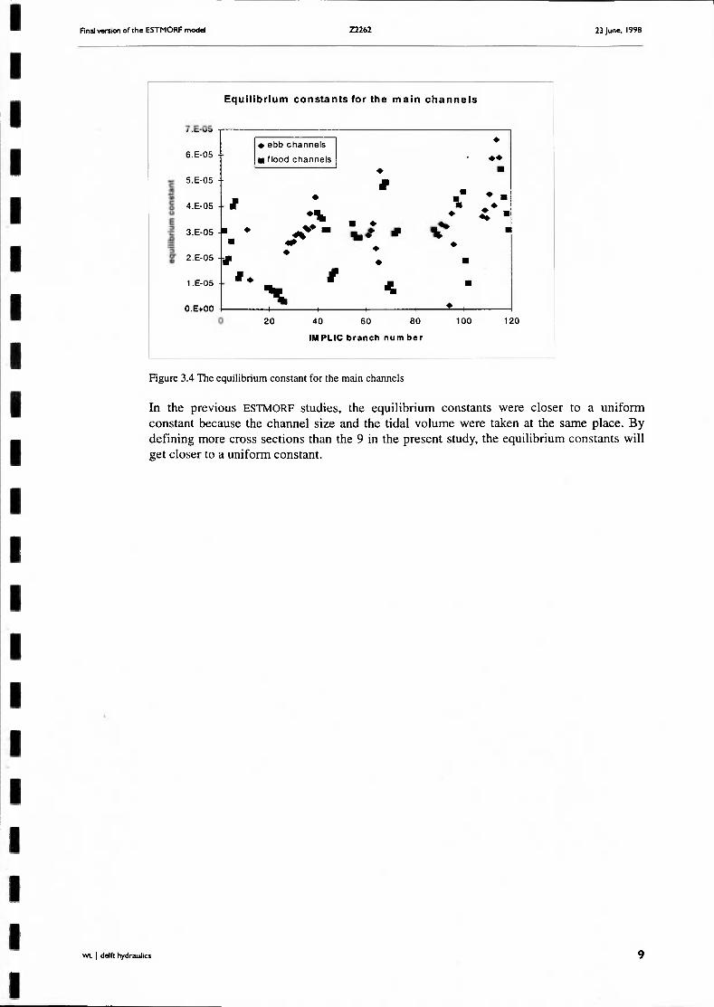
Figure 5.4 The development of model branch 71 in two different runs
Similar problems occur for branch 71, 72 and 73 which form a flood channel south of the Plaat van Ossenisse. The model results are compared to the data in Figure 5.4. Again the data first shows a constant trend which suddenly changes exponentially since 1985. The model behaviour is just to settle in a new equilibrium. The behaviour of branch 71 appears to be unstable, the channel silts up. There is a solution to model such behaviour in ESTMORF
by using nodal point relations, but this option has not been used in the present study.
Final results
The results of the model are presented in figure 5.1 for model run 15, see the end of this report. The overall morphological behaviour of the model is quite satisfactory. With the exception of a few individual branches, like the ones mentioned above, the model reproduces the data.
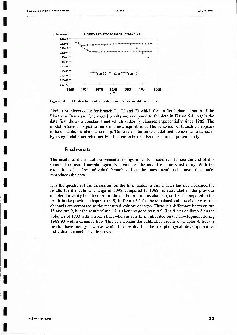
It is the question if the calibration on the time scales in this chapter has not worsened the results for the volume change of 1993 compared to 1968, as calibrated in the previous chapter. To verify this the result of the calibration in this chapter (run 15) is compared to the result in the previous chapter (run 9) in figure 5.5 for the simulated volume changes of the channels are compared to the measured volume changes. There is a difference between run 15 and run 9, but the result of run 15 is about as good as run 9. Run 9 was calibrated on the volumes of 1993 with a frozen tide, whereas run 15 is calibrated on the development during 1968-93 with a dynamic tide. This can worsen the calibration results of chapter 4, but the results have not got worse while the results for the morphological development of individual channels have improved.
WL I delft hydraulics 22
Rnal version of the ESTMORF model 22262 23 June. 1998
"
iv^^
J •
P ^ 7
• •
•
• •
• «
V • -
•
7«:*f1* l^F-UV, J'C.4T* T^P^JM 1 »P*J»7
. . -u ,^ . . . .™
. ..i
•
•
11PW.7
• •
•
•
7 ^P*nft 7 <P4JM J «FWM 7 «F. 'M 1 ti.^n
Figure 5.5 A companson of run 15 and run 9
5.2 The development of the flats
The calibration was focused on the evolution of the flat areas. The flat area is of main importance for the ecology of the Western Scheldt, more than the height or the volume of the flats. However, in ESTMORF there is no empirical relation for the areas of the flats, but only for the height of the flats, which complicates the calibration a little bit. Furthermore, the calibration is carried out under a boundary condition of an average tide. The sea level rise and the variation of the tidal amplitude are not yet included in the calibration of the present study.
The data used in this calibration is data on the areas of the low flats as collected by Huijs, which has also been used in the ASMITA study (Wang 1997).
The bathymetry of the ESTMORF model has not been designed for a morphological purpose. That is why some model branches contain parts of different morphological units. For instance, branch number 65 contains a large part of both the Plaat van Ossenisse and the Rug van Baarland. In ESTMORF, each model branch has two parts, channel and flat. So the fact that the model branch contains parts of two different flats is not recognized.
This complicates modelling the morphological behaviour. It also complicates the evaluation of the model results, because it is not possible to reconstruct precisely the morphological units from the model results.
As for the calibration of the channel volumes, the calibration of the flat areas is carried out in a few steps. In the first two runs the time scales are calibrated by variation of the dispersion coefficient for lateral transports. In the next runs the equilibrium constants for the flat heights are calibrated, globally at first and then locally by variation for the morphological units.
WL I ddfc hydraulics 23

Final verïicxi of the ESTMORF model Z2262 23 June. 1998
Table 5.2
Run
run 15
run 16
run 17
run 18
run 19
run 20
run 21
parameter
dispersion coefficient for the flats equilibrium constants
equilibrium constants
equilibrium constants
equilibrium constants
equilibrium constants
dispersion coefficient
parameter change with respect to reference run 13 10
increased by 5% for the high flats and by 20% for the low flats increased by 5% both for the high flats and the low flats
increased by 8% both for the high flats and the low flats increased by 8% for the high flats (same as run 19), by 12% for the low flats same as run 19, only increased by 20% for the low flats and 8% for the high flats for the Platen van Valkenisse D|=20 mVs for the flux to the low flat DeSmVs for the flux to the high flat
purpose
calibration of the time scale
increase so that the average value corresponds to the empirical values found by Tank (199?) the total area in run 16 increased too much, so the equilibrium values were chosen relatively smaller the total area decreased in run 16, so the values were increased
the area of the low flats still decreased, so the values were increased the area of the Platen van Valkenisse decreases in run 19 while it increases in nature, so the equilibrium values were increased shorter time scale for the low flats, longer time scale for the high flats
The result of run 21 is given in Figure 5.6 for the total area of the low flats, compared to the data.
Total area of the low flats in the Western Scheldt
6.0E+07
5.0E+07
4.0E+O7
2 3.0E+O7
2.0E+07
1.0E+O7 •
O.OE+00
- Pleasured
• estmorf
1955 1960 1965 1970 1975 1980 1985 1990 1995 year
Figure 5.6 The area of the low flats, ESTMORF compared to the data
Vrt. I ddfc hydraulics 24

Final version of the ESTMORF model Z2262 23 June, 1998
There is a difference between the measured and the modelled development of the total flat area. The trend of the model simulation is correct but the low flat area in the model is about 1.5 times the area according to the data of Huijs. For the individual units, there is a much greater difference between the trends of the simulated and the trends of the measured development, as can be seen in Figure 5.7.
1 2E+06
1.0E+06
8.0E+O5
£ 6.0E+05 eg
4.0E+05
2 0E+O5
area of the low flat
PLAAT V A N SAEFTINGE
0 0E4O0
1950 1960 1970 1980 year
1990 2000
18E406
1.6E+06 •
1.4E+06 •
1 2 & 0 6
1.0E*06
8 0E+05
6 OE+05
4 0E+05
2 OE+05 •
O.OE-fOO
area of the low flat
BALLAST
' ' \ .
1950 1970 1980 year
1990 2000
area of the low flat
VALKENISSE
OOE+00
6 2E406
4 1E+06 •
2 1E+06
area of the low flat
OSSENISSE
OOE+OO
1950 1970 1980 year
1990 2000 1950 1960 1970 1980 1990 2000 year
1 2E+07
area of the low flat
PLAAT V A N BAARLAND
1 0E-tO7 - •
8 0E406
6 0E+06
4 0E+06
2 0E+06
OOE+OO
4 0E+06
• 2.0E+O6 •
O.OE+00
area of the low flat
RUG VAN BAARLAND
1970 1980 year
1950 1960 1970 1980 year
1990 2000
9 0E+06
8.0E+06 •
7 OE+08 - •
6 0E+06
S.OE+06 - •
4 OE+06
3 OE+06 -
2 OE+06 •
1 OE+06 •
O.OE+00
area of the low flat
MIDDELPLAAT
1970 1980 year
1 2E+07
1 OE+07
a OE+06
S 6 OE+06 • m
4 OE+06 •
2.0E+O6
area of the low flat
HOOGE PLATEN
0 OE+OO
^ - V ^
-data
- estmorf
1950 1970 1980 year
2000
Figure 5.7 Development of the flat areas per morphological uni (area in m2).
WL I deift hydraulics 25

Final version of the ESTMORF model Z2262 23 June, 1998
It is obvious that there is a difference between the data and the model simulations. Partly this can be explained by the fact that the data is taken from a GIS map using fixed levels between -2 m and 0 m NAP. The model results are taken between the levels of Mean Low Water and Mean Water Level which vary per model branch. This difference between the modelled area and the measured area of the low flats should be studied further by comparing the geometry of the model to the GIS maps of the Western Scheldt.
Total area of the high flats in the Western Scheldt
4.00E+07
3.00E+07
2.00E+07
1.00E+O7
1955 1960 1965 1970 1975 1980 1985 1990 1995
year
Figure 5.8 The development of the high flat area in run 21 compared to the data
For the high flats the simulated trend is correct for the development from 1972 onwards and so is the absolute value of the area. Again, for the individual units there are differences, as shown in Figure 5.9 below.
estmorf
measured
_ l \ I I I I L-
WL I delft hydraulics 26

Final version of the ESTMORF model Z2262 23 June, 1998
6.0E«O5
4 OEtOS
2.0E+O5
area of the high flat
PLAAT VAN SAEFTINGE
O.OEtOO
1950 1960 1970 19B0 1990 2000 year
i.oEfOe
8 OE+05
S 6.0E+05
4.0E-t05
2.0E+05
O.OE+00
area of the high flat
BALLAST
1 J— f J ^ --v-'"'"^
1950 1960 1970 1980 1990 2000 year
1.3E+07
area of the high flat
VALKENISSE
O.OE+00
1950 1960 1970 1980 1990 2000 year
4.1Et06
9 2 1E+06
area of the high flat
OSSENISSE
area of the high flat
PLAAT VAN BAARLAND
4 0E+06
2.0EtO6 •
O.OEtOO
2.0EtO6
area of the high flat
RUG VAN BAARLAND
O.OE+OO
1950 1960 1970 1980 1990 2000 year
1950 1960 1970 1980 1990 2000 year
6.0E+O6
5.0E+06
4.0EtO6
3.0E+06 -
2.0E+O6
1.0E+O6
area of the high flat
MIDDELPLAAT
O.OE+00
1950 1960 1970 1980 1990 2000 year
1 0E4O7
8.0E+06
6 0E+06
2.0E+06
OOE+OO -
area of the high flat
HOOGE PLATEN
^ '"-v r"'* • « '
—•—data
• estmorf
— \ 1
1950 1960 1970 1980 1990 2000 year
Figure 5.9 The area of the high flats per morphological unit
WL I ddft hydraulics 27

Final version of the ESTMORF model Z2262 23 June, 1998
Observe that the Hooge Platen contain by the largest area by far and that the downward trend in the simulated area between 1968 and 1972 is caused by the downward trend of the Hooge Plaaten. Observe furthermore that the simulated area of the low flat area of the Hooge Plaaten has an upward trend (Figure 5.7). The simulated trends are exactly opposite to the trends found in the data.
The relatively small areas of the Plaat van Saeftinge and Ballast increase in the simulations while they decrease, or are almost zero, in the data. For the Plaat van Saeftinge, the total area of the low flat and the high flat develops similarly to the total area found in the data.
The simulated trend for the area of Valkenisse is the same as the measured trend. For Ossenisse the simulated trend of the low flat area is to remain constant while it decreases slightly in the data. The simulated trend for the high flat is slightly decreasing while it is increasing for the data. A further calibration may improve the results here.
For the Plaat van Baarland and the Rug van Baarland the simulated trend is correct but there is a large difference between the modelled area and the measured area.
5.3 Conclusion
For the channel volumes, the simulations in the present chapter show that the model is in good agreement with the data for most of the individual branches. The development of the flat areas is seemingly not reproduced that well by the model. One problem is that the data set and the model do not coincide, which can partly be explained from a different method of analysis of the data and problems to distinguish between morphological units in the IMPLIC bathymetry. The model results are likely to improve if sea level rise and the development of the tidal amplitude are included.
As pointed out in section 5.2, ESTMORF uses an empirical relation for flat heights. It is recommended to use an empirical relation for flat areas instead of flat heights, as in the ASMITA model.
It is obvious that the initial flat area in the model is not the same as the measured area. We do not have a full explanation for this and it can only be given by comparing the GIS data, the IMPLIC model and the method of analysis for the measured data, which is beyond the scope of the present study. Two reasons can be given which partly explain the discrepancy:
1. The measured data give the flat area between -2 m NAP and NAP. The model results give the area between MLW and MSL.
2. In the IMPLIC bathymetry, some branches contain parts of different morphological units, in particular channels in between the units. Therefore it is not possible to distinguish between separate units exactly from the IMPLIC branches.
There are differences between the trend of the model and the of the data. In the present study, the development of the flats received less attention than the development of the channels. It may be possible to improve these results if sea level rise and the variation of the tidal amplitude are included in the calibration.
WL I delft hydraulics 28

Final version of the ESTMORF model Z2262 23 June, 1998
5.4 The change of the equilibrium constants
In all the calibration steps, the equilibrium constants have been changed. The initial choice of the constants in the first run was such that the 1968 bathymetry was in equilibrium. In run 21 the equilibrium constants have been changed for all the model branches. This is shown in the table below.
Table 5.3
equilibrium constants
branch
1 2 3 4 5 6 7 8 9 10 11 12 13 14 15 16 17 19 20 21 22 23 24 26 27 28 29 30 31 32 33 34 35 36 37 38 39 40 41 42 43 44 45 46 47 48 49 50 51 52 53 54 55 56 57 58 59 60
»
CHANNEL AREA 1968
3.03E-05 1.97E-05 2.12E-05 2.82E-05 4.20E-05 4.15E-05 1.18E-05 1.37E-05 9 56E-06 5 36E-06 3.25E-05 1.22E-05 4.36E-06 1.89E-05 4.56E-06 9.41 E-06 2.34E-06 9.26E-06 9.38E-06 8.39E-06 8.02E-06 6 50E-06 5.71 E-06 3.88E-06 2.84E-06 2.21 E-05 2.56E-05 2.57E-05 2.62E-05 2.86E-05 2.94E-05 2.91 E-05 2.83E-05 3.16E-05 3.24E-05 3.30E-05 3.15E-05 4.81 E-05 4.16E-05 3.30E-05 3.24E-05 2.84E-05 2.82E-05 1.07E-05 1.23E-05 1.36E-05 3.06E-06 6.91 E-06 4.03E-06 4.36E-06 9.13E-06 1.82E-05 3.93E-05 3.47E-05 3.27E-05 3.26E-05 5.48E-06 2.69E-06 4.83E-05
run 21
3.08E-05 1.85E-05 2.00E-05 2.67E-05 4.01 E-05 4.22E-05 1.20E-05 1.39E-05 9.72E-06 5.46E-06 3.11 E-05 1.15E-05 8.00E-06 1.78E-05 1.44E-05 1.04E-05 2.12E-06 8.47E-06 8.59E-06 7.68E-06 7.34E-06 5.61 E-06 7.20E-06 3.90E-06 2.87E-06 2.23E-05 2.59E-05 2.59E-05 2.65E-05 2.90E-05 2.97E-05 2.94E-05 2.85E-05 3.19E-05 3.11 E-05 3.73E-05 3.24E-05 4.38E-05 3.78E-05 3.58E-05 3.53E-05 3.11 E-05 3.12E-05 1.18E-05 1.39E-05 1.5OE-05 1.33E-06 6.29E-06 3.00E-06 2.62E-06 9.23E-06 1.68E-05 3.34E-05 2.92E-05 2.80E-05 2.82E-05 4.68E-06 1.31 E-05 4.93E-05
%
102% 94% 94% 95% 95% 102% 102% 101% 102% 102% 96% 94% 184% 94% 316% 111% 90% 91% 92% 9 1 % 91% 86% 126% 100% 101% 101% 101% 101% 101% 101% 101% 101% 101% 101% 96% 113% 103% 91% 91% 108% 109% 110% 111% 110% 113% 111% 43% 91% 74% 60% 101% 92% 85% 84% 86% 86% 85% 487% 102%
LOW FLAT 1968
0.76 0.75 0.75 0.75 0.82 0.68 0.70 0.82 0.88 0.73 0.73 0.75 0.75 0.73 0.75 0.50 0.74 0.74 0.85 0 68 0.62 0.70 0.79 0.60 0.58 0.54 0.60 0.55 0.55 0.75 0.66 0.63 0.64 0.63 0.64 0.69 0.71 0.74 0.52 0.52 0.61 0.73 0.76 0.64 0.64 0.76 0.64 0.75 0.62 0.60 0.61 0.57 0.71 0.62 0.61 0.62 0.60 0.54 0.67
run 21
0.82 0.81 0.81 0.81 0.88 0.73 0.76 0.89 0.95 0.79 0.79 0.81 0.81 0.79 0.81 0.54 0.80 0.80 0.71 0.74 0.67 0.75 0.85 0.65 0.63 0.58 0.64 0.59 0.59 0.81 0.72 0.68 0.69 0.68 0.69 0.74 0.77 0.80 0.56 0.56 0.66 0.78 0.82 0.69 0.69 0.82 0.69 0.80 0.66 0.65 0.66 0.61 0.77 0.67 0.66 0.67 0.65 0.58 0.73
%
108% 108% 108% 108% 108% 108% 108% 108% 108% 108% 108% 108% 108% 108% 108% 108% 108% 108% 108% 108% 108% 108% 108% 108% 108% 108% 108% 108% 108% 108% 108% 108% 108% 108% 108% 108% 108% 108% 108% 108% 108% 108% 108% 108% 108% 108% 108% 108% 108% 108% 108% 108% 108% 108% 108% 108% 108% 108% 108%
HIGH FLAT 1968
0.15 0.25 0.25 0.25 0.22 0.27 0.26 0.26 0.26 0.36 0.33 0.25 0.25 0.29 0.25 0.16 0 28 0.31 0 27 0.27 0.17 0.34 0.26 0.31 0.30 0.34 0.23 0.18 0.31 0.23 0.32 0.24 0.24 0.27 0.18 0.24 0.24 0.23 0.24 0.27 0.31 0.27 0.25 0.23 0.30 0.12 0.26 0.25 0.27 0.31 0.28 0.21 0.27 0.22 0 28 0.24 0.26 0.22 0.31
run 21 0.17 0.29 0.29 0.29 0.26 0.31 0.30 0.29 0.30 0.42 0.38 0.29 0.29 0.34 0.29 0.25 0.33 0.35 0.31 0.31 0.19 0.39 0.30 0.36 0.34 0.39 0.26 0.21 0.35 0.26 0.37 0.27 0.27 0.31 0.21 0.28 0.28 0.27 0.28 0.32 0.35 0.31 0.29 0.27 0.34 0.13 0.29 0.29 0.31 0.35 0.32 0.24 0.31 0.25 0.32 0.27 0.30 0.26 0.35
%
115% 115% 115% 115% 115% 115% 115% 115% 115% 115% 115% 115% 115% 115% 115%
162% 115% 115% 115% 115% 115% 115% 115% 115% 115% 115% 115% 115% 115% 115% 115% 115% 115% 115% 115% 115% 115% 115% 115% 115% 115% 115% 115% 115% 115% 115% 115% 115% 115% 115% 115% 115% 115% 115% 115% 115% 115% 115% 115%
WI. I delft hydraulics 29

•^ 5^ >!> >^ >^ ' -P >P ^P • . o*- 5^ è^ 5^ o^
i-'.--r-T-T-r-'i-i-T--r-'T-i-a)C\JC\JC\ICNJC>ICviC*iO)OJCOC0CyC>JCNjC\JCNiC>JCvJCvJOJT-i-T-T-,-.r-i-T--.-T-T^ in in ib m I
oo)co-^co'<tcocor^cocj)ooo)i-Ti-r^oocDO)NcococDincnrocD^r^'^o>^^cMr^'^ooo) »-,.^v^v»v..v,-^»-^..'^coc>jcgc\jcococ\jc\icvjcvic>jCNjcocnco^c^^cnco^cO''-rjcocaojcocnc\Jt^cocococ\jcüc\jcj
ö ö ö ö ööööööööööööööööö ööööööööööööööööööööööööööööööööööö
r j i - " . - ! ^ T t O O O O O C N J C N J C J t O O O O O O O O c o c o c o n cr)co»-r3coc*3cnc\icjcoc>jcvicNj
^ c v i r ^ ' ^ o o o j ^ c n e n o i o i - ' - • C J - « t i - ; c r ) C M C N J
ööö ö d
o O O o o o o o o O O O O O O O O O O O O O O O O O O O O O O O O O O O O O O O O O O O O O O O O O O O O O O O O O O O O
cocoooto c o c o c o o o c o c o o o c o f f l o o o o o o o c v j o c r ) c o o o o o o o o o o c o c o g D & g p c o c o o o g o o o g o c o c o c o c o c o c o c p c o G O ö ) O c o c v g o c o c o c o o o o o 0 0 0 0 0 0 0 0 0 - < - r - T - T - T - T - f - ^ T - - r - i - - . - T - T - T - T - T - T - - . - ' r - O O O O O O O O O O O O O O O O O O O O O t - O r - 0 0 0 0
O O O O O O O O O O O O O O o o o o o o O O O O O O O O o o o o o O o o o o o O o o o o O O O O O O O O O O O O O O O O O
) i n o o c 7 ) c o o > c D O h - ' - ^ c D o i n o c j r ^ t o m j r ^ h - c q r ^ i o < p i o r ^ c D o q c q c q t p c q i n i n u^to S p o c o r j ' ^ c o h . ( D ' < j - o c ^ O ) i n » ~ u i t D ' - - c \ j c o c \ j i n o c o h - " * c M 5 h . c o i n o o o o < D C D ^ i n i n
ö ö ö ö ödo ö ö ö ööööö ö ö ööööö ö ö ö ööööööööööööö VW \iJ y j y*J MJ (^« ( ^ V*J l " U / \W Uy | - * vu VAJ VAJ U J VU "A." " V U / M * " J J W U ^ H / r"* l "» VJ,< M J I J J IJU )"* \AJ I "» M * I-« l-» VJU i •* W* lA^ l*-* I ~ i •* u / P-» U* «AJ " J J l*.! !•* 1"^ !•»
ö ö ö ö ööööööööööööööööö ööööööööööööööööööööööööööö öö ö ö ö ö
S? S? S? S ^ CM ,>^ in ^ N o o ^ w
"8 E
u.
o z
i n i n i n i n L n i n i n m i n t n t o t o i n i n L O L n i o i n i o c o t o co CpCDC>C3 GGCDOOOOOOOGGOGCDGO O U J U J I Ï J I Ï J UJlÜlÜlÜlÜlÜUJlL l i jL iJLiJLiJUJlLJUJUJUJ UJ -- - - - c n ^ ^ O l c : > c : ï c n ^ * ( n T ^ c ^ J C ^ J l 0 ^ ^ c s l C 0 • ^ O h ^
LUuJUJLLI UJUJI IJUJUJUJUJUJLIJLLIL IJUJLIJUJUJUJUJ UJ LU | ] | U' ^}f l i l " ' UI " I C O C M h - ^ C O ^ C J ï Q O O O h ^ C O - ^ C M C v j m r ^ C M C O ^ O h " i - ü ï h - . C n C 3 ï r - C O C 0 C0OC400 o c D < 7 i O ï ' ' - c \ j ' « - c j i i n o o h . ' - ^ o i n ' - i n c \ i c v j C M c o O ' < t T - o c o r ^ c\i ei P5 •^ oi iO ' ^ '« f i - ' r - :o i c \ i cococv jc \ iT - 'T^T-^cD i r i cdcriodcócd cd có oj c j
8 ' r - C M C 0 ^ l / ) C 0 F ^ 0 0 0 ) O L 0 C 0 N C 0 0 ) O O * " N C 0 ^ l 0 h * O O O O O O O O O O i - ^ t - t - T - T - C V O D C O C O O O C Ö O O C O Ö ï
c o i o c o t p cocQcoco. r-f^.r--. [> .r>..r> r- .r> h* rv^co <x> co CD co co oo co en o? o) o) en O) o> o (?) O) r" r^ y- y- ?- r- 77- T- T- ^ y,.»- ^ ^ •^ »" r ' / r T~ ^ ^ ^ . •^ / ^
c

Final version of the ESTMORF model Z2262 23 June, 1998
6 Conclusions and recommendations
6.1 Conclusions
In this study the ESTMORF Western Scheldt model is calibrated on the morphological development over the period 1968-1993. The calibration is carried out mainly on the development of the channel volumes. The development of the tidal flats has also been calibrated, but it could not be carried out in detail yet because there are large differences between the model and the data sets. Furthermore the sea level rise and the variation of the tidal amplitude were not included, both of which are important for the development of the flats.
The equilibrium equations in ESTMORF have been extended so now it is possible to relate the volume size to the tidal volume through an entire cross section. This extension has been made from a technical viewpoint, so as to get more control over the model behaviour. In this way it was possible to control the interaction of tidal flow and morphological development, as opposed to previous model runs (Fokkink, 1997) in which the tidal flow was fixed.
The results of the calibration are satisfactory for morphological development of the individual channels. There are a few branches for which this development is reproduced less well, but most of these branches are small and consist mainly of flats without channels. The ESTMORF model handles such branches less well, since a proper ESTMORF cross section contains both a channel and a flat. These problems are due to the fact that the bathymetry of the model was developed for hydrodynamic purposes only.
The results of the calibration are not yet conclusive for the development of the flats. The development of the total flat area of the Western Scheldt is reproduced by the model, but for the individual morphological units there is a large off set. Partly this can be explained by the fact that the ESTMORF schematisation does not really distinguish morphological units. Many branches contain parts of flats from two different units. Partly the difference can be explained by the fact that the model runs did not include some important effects, such as sea level rise and the variation of the tidal amplitude.
6.2 Recommendations:
1. The ESTMORF model should be installed at Rijkswaterstaat so that morphological experts with a thorough knowledge of the Western Scheldt may use it and improve the current calibration. It should be noted that the ESTMORF model now runs on PC.
2. The bathymetry of the Western Scheldt is taken from a hydrodynamic model. It would be preferable to design a bathymetry which is more suitable for a morphological model (more streamlined). The software for designing ID network models has improved a lot over the last years. The effort to design a new bathymetry is outweighed greatly by the benefit.
WL I delft hydraulics 3 I

Final version of the ESTMORF mode) Z2262 23 June. 1998
3. Only 9 cross sections were used to define the equilibrium constants which relate the tidal volume through a cross section to the equilibrium size of an individual channel. Consequently, there are great differences between the constants per channel. This can be improved by defining more cross sections, which is easier if the bathymetry of the model is more apt for morphological purposes.
4. The calibration of the flats can be improved by taking into account sea level rise and the variation of the tidal amplitude. Furthermore, the difference between the data set and the IMPLIC bathymetry should be analysed.
5. The functionality of the model can be improved if it is based on empirical relations for the flat area, as in the ASMITA model, instead of the flat height. The flat area is also more important for ecological evaluations than the flat height.
6. A validation of the Western Scheldt model is still lacking. It would be possible to validate the model by defining two different bathymetries for the same network (more apt to morphological modelling). One bathymetry of 1968, or close to that year, and one bathymetrie of the estuary before 1968.
7. Morphodynamic simulations with the same model bathymetry (Fokkink, 1998) have shown that if the model is extended with the outer delta (beyond Vlissingen) this will improve the model behaviour near the boundary.
8. Rijkswaterstaat has observed that the echo-loading of 1968 is not so accurate. It would be preferable to design a model of an earlier date so that more accurate data can be used for the initial condition.
WL I delft hydraulics 32

Final version of the ESTMORF model Z1162 23 June. 1998
7 References
Allersma, E. (1993) Geulen in estuaria, ID modellering van evenwijdige geulen, WL I Delft Hydraulics report H1828/H1970.
Berg, J.H. van den, C.J.L. Jeuken & A.J.F, van der Spek (1996). Hydraulic processes affecting the morphology and evolution of the Westerschelde estuary. Estuarine Shores: Evolution, Environments and Human Alterations.
Eysink, W.D. (1992) Impact of Sea level rise on the morphology of the Wadden Sea in the scope of its ecological function, WL I Delft Hydraulics report HI300.
Fokkink, R.J. (1996). An evaluation of the ESTMORF model, WL I Delft Hydraulics report Z667.
Fokkink, R.J. (1997). Analysis of the ESTMORF model. WL I Delft Hydraulics report Z2039.
Fokkink, R.J. (1998). Morphodynamic network simulations of the Westerschelde. WL I Delft Hydraulics report Z919.
Karssen, B. (1994) A dynamic empirical model for the long term morphological development of estuaries, development of the model, WL I Delft Hydraulics, report Z715.
Karssen, B. (1995) Evaluation of Estmorf, WL I Delft Hydraulics, report Z891.
Karssen, B., Wang, Z.B. (1991), Morphological modelling in estuaries and tidal inlets, Part I literature survey, WL I Delft Hydraulics, report Z473.
Karssen, B. and Wang, Z.B. (1992) A dynamic empirical model for the long term morphological development of estuaries, part 1 physical relations, WL I Delft Hydraulics, report Z622.
Kleef, A.W. van (1994). Verklaring voor de veranderingen in de grootschalige zandbalans van het gebied rond het Middelgat, Westerschelde. Rijkswaterstaat Directie Zeeland, afdeling NWL.
Uit den Bogaard, L.A. (1995). Resultaten zandbalans Westerschelde 1955 -1993. IMAU report R 95-08.
Wang, Z.B., P.M.C. Thoolen & R.J. Fokkink (1997). Studie naar morfologische effecten van storten en baggeren in de Westerschelde. WL I Delft Hydraulics report Z2310.
WL I delft fiydraulics 33

Final version of the ESTMORF model Z2262 23 June, 1998
A Technical reference for the new equilibrium constants
The equilibrium relation in the model has been extended. Essentially only routine in ESTMORF was changed (the 'volumes' routine). In the old routine, the equilibrium of a branch depended on the tidal volume in that branch. In the new routine it can depend on the tidal volumes in many branches. The user determines these branches. For instance, in Figure 3.1 of the report, the user may decide to let the equilibrium area Aj depend on V;, which is the old definition, or on V1+V2 such as in equation (2) below that figure.
The user has to define an input file CROSS.INP which is a free formatted ASCII file. Each line contains the following information, in this order: (1) the branch number for which the equilibrium is defined (2) the number of branches for which the tidal volumes are added (3) the IMPLIC numbers of these branches. For example, if CROSS.INP for the branches in Figure 3.1 is:
1 2 1 2 2 2 1 2
then both equilibrium areas A] and A2 depend on V1+V2. If the input file is
1 1 1 2 1 2
then the areas depend on Vj and V2 respectively.
The user defines the equilibrium constant k in the input file EQUIAREA.OUT. The same file was used in the previous version of the model to define the constant, only now the constant may depend on different tidal volumes. There is one modification for the new model. Per model branch it is possible to define 2 equilibrium constants. One constant is used if the residual flow is directed to the sea boundary (ebb channel), the other constant is used if it is directed to the river boundary (flood channel). This option is built in for future studies, so the model can simulate a functional change of flood channel to ebb channel.
WL I ddft hydraulics 34

Final version of the ESTMORF model Z2262 23 June, 1998
B The model principles
ESTMORF is a dynamic-empirical model which simulates the morphological development of a channel network in an estuary. It is coupled to a hydrodynamic model to simulate the water flow. The empirical part of the model relates the water flow to equilibrium profiles of the channels. From this information, an equilibrium concentration field is derived. The dynamic part of the model computes a sediment concentration field and the natural morphological development of the estuary is a consequence of the difference between the sediment concentration and the equilibrium concentration.
ESTMORF computes the development of three parts of a channel: main channel, low flat and high flat. In fact ESTMORF is only concerned with the area A of a cross section. The area is divided into three parts: the area for the main channel Ac and the area for the flats A| and Ah. The changes of these three quantities are computed and by some geometric relations, this is translated into changes of the entire cross section.
There are two factors which determine the morphological development: the natural, undisturbed development and human interference. The natural development is computed from the concentration field and the human interference has to be specified by the user.
The simulation can be represented by a flow chart.
equilibrium profiles
+ equilibrium concentration
1 1
concentration field
1 1
human interference
1 1
changes of
water flow II
hydrodynamic || model 1
geometric Ac Al Ah I 1 relations for |=
new bathymetry
WL I ddfc hydraulics 35

Final version of the ESTMORF model Z2262 23 June, 1998
ESTMORF profiles
The ESTMORF cross section contains 7 levels, as illustrated in Figure 1. The profile is symmetric and therefore the model works with "half profiles". Point 1-2 represent the channel, point 2-3-4 represent the low flat, point 4-5-6 represent the high flat. Point 7 is a reference point which is fixed during the computations. The area of the cross section is divided into the 3 sub-areas: Ac, A| and Ah.
A channel A flats
Figure 1 ESTMORF profile
The points 2, 4 and 6 are related to the flow. Point 2 marks the lowest water level over a tidal period (MLW = Mean Low Water). Point 4 marks the average water level over a tidal period (MSL = Mean Sea Level). Point 6 marks the highest water level over a tidal period (MHW = Mean High Water). The points 1, 3 and 5 are related to the channel morphology. Point 1 marks the depth of the channel and points 3 and 5 mark the height of the flats.
ESTMORF computes the development of the areas Ac, A|, Ah, which is translated into a change of profile. Points 2, 4 and 6 move along the profile if the water levels change. Points 1, 3 and 5 move so that the areas are in order.
Equilibrium profiles and equilibrium concentration
The model distinguishes three parts of the cross section and the equilibrium of each part is related to the water flow. These are empirical relations which do not link the water flow directly to the model parameters Ac, A|, Ah, but to other quantities which describe the channel and the flats. These quantities are: the area of the cross section below the average water level AMSL (this is the area below point 4 in Figure 1), the height of the low flat h| and the height of the high flat hh.
WL I ddlt hydraulics 36

Final version of the ESTMORF modd Z2262 23 June. 1998
The tidal volume V is related to the equilibrium area AMSUB by
Amu = c,V» 1
where the constants Ci and C2 are empirical constants, with the exponent C2 mostly close to 1. The equilibrium flat heights are related to the amplitude of the tide Ah, that is the difference between MHW and MLW, by
where the constants a and b are empirical constants. These relations give equilibrium values for the area below MSL and the flat heights, which are translated into equilibrium values of the cross sections Ace, Aj», Ahe-
Figure 2 flat height; point 3 is on the diagonal opposite to point 2 and 4
The cross section tries to adapt to the equilibrium values by sedimentation and erosion. The sedimentation flux S depends on the fall velocity w, and the difference between equilibrium concentration Cg and actual concentration c.
S = Ws(ce-c)
The equilibrium concentration is given by
(
where the exponent HA is to be determined by the user, as is the global equilibrium concentration CE- If Ac < Ace the equilibrium concentration increases, which induces erosion, and if Ac > Ac, the equilibrium concentration goes down, which induces sedimentation. Similarly, for the flats the equilibrium concentration depends on the difference between the actual flat height and the equilibrium flat height
<Ch- CE
WL I delft hydraulics 37
Final version of the ESTMORF model Z2262 23 June. 1998
Concentration field
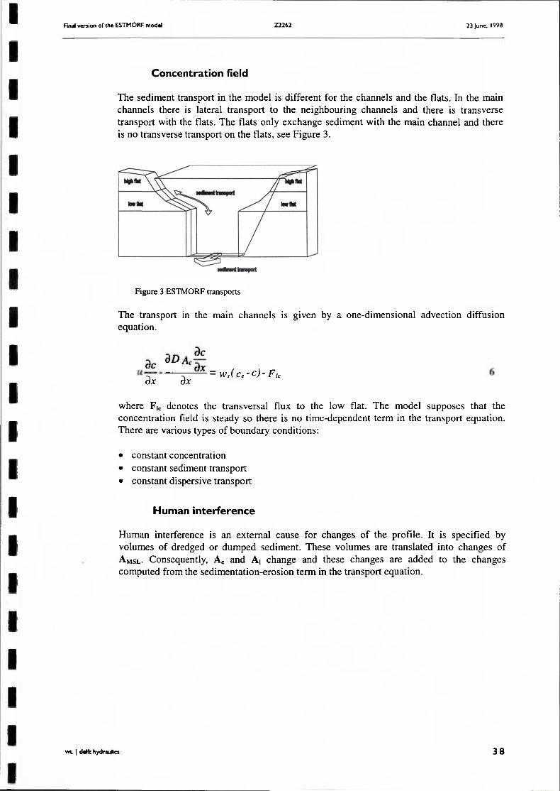
The sediment transport in the model is different for the channels and the flats. In the main channels there is lateral transport to the neighbouring channels and there is transverse transport with the flats. The flats only exchange sediment with the main channel and there is no transverse transport on the flats, see Figure 3.
Figure 3 ESTMORF transports
The transport in the main channels is given by a one-dimensional advection diffusion equation.
dx dx - Ws(Ce-c)- Flc
where Fic denotes the transversal flux to the low flat. The model supposes that the concentration field is steady so there is no time-dependent term in the transport equation. There are various types of boundary conditions:
• constant concentration • constant sediment transport • constant dispersive transport
Human interference
Human interference is an external cause for changes of the profile. It is specified by volumes of dredged or dumped sediment. These volumes are translated into changes of AMSL- Consequently, Ac and Ai change and these changes are added to the changes computed from the sedimentation-erosion term in the transport equation.
WL I ddft hydraulics 38

Final version of the ESTMORF model 22262 23 June. 1998
Profile changes
The profile changes are computed from sedimentation and erosion. For each part of the cross section, its change depends on the sedimentation flux given in Equation 3 and the size of the cross section
dt
where L denotes the length of channel (for Ac) and it denotes the length of the flat (for Ai and Ah).
Geometric relations for the new bathymetry
An ESTMORF profile has 7 points, of which 1 is fixed. The model computes three area changes, which have to be translated into changes of the remaining 6 points (12 degrees of freedom). Therefore, 9 relations are needed to close the equations. The relations are:
• The levels of 2, 4 and 6 depend on water levels and the points move along the profile (6) • The sedimentation/erosion is distributed evenly over the channel (1) • The points 3 and 5 represent the flat height (2).
WL I delft hydraulics 39

4.75E+07
4.70E+07
<g 4.65E+07
= 4.60E+07
1 4.55E+07
® 4.50E+07
4.45E+07
A Af\C ^ m
Run 22: Channel volume branch 1
• run 15 • data # dredging
•
^^•*-^i'"i
J^^0mm9^——*^**^***^
1965 1970 1975 1980 1985 1990 1995
time in years
J.lXJt,+U/
2.90E+07 -
^2.80E+07 -
^2.70E+07 -
' |2.60E+07 -
£2.50E+07 '
'^140E+07 -
2.30E+07 •
T onn ._r\-7 .
Run 22: Channel volume branch 2
• run 15 • data —•—dredging
• * • • • • • • • • • • • * * *
A tt A tt tt fl H'^
m m
m •
1965 1970 1975 1980 1985 1990 1995
time in years
3.70E+07 - •
3.60E+07 - -
f)3.50E+07 - -
.S3.40E+07 - -
|3.30E+07 -
®3.20E+07 -
3.10E+07 -
1 ftfMj . _ m .
Run 22: Channel volume branch 3
• run 15 • data —•—dredging
• •
• . . . -1965 1970 1975 1980 1985 1990 1995
time in years
Simulated development of the channel volume Run 22 compared to the measured data
WL 1 DELFT HYDRAULICS
Figure 5.1
Z2262
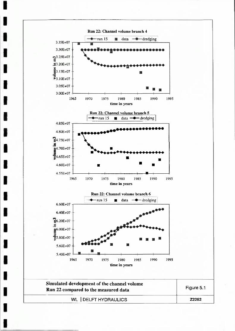
Run 22: Channel volume branch 4
3.35E+07
3.30E+07 - -
W3.25E+07 S .S3.20E+07 u |3.15E+07
°3.10E+07
3.05E+07 -
3.00E+07
•run 15 data • dredging
1965 1970 1975 1980 1985 time in years
1990 1995
Run 22: Channel volume branch 5
A S^P-u07 -,
4.80E+07 -
g4.75E+07 -
«4.70E+07 -
O4.65E+07 -
4.60E+07 -
4.55E+07 -
•V \
-
• run 15 •
• ^ ' ^ • • ^ ^
• H \
data
A ^ .
•
H
• dredging
• • •
, •—1
1965 1970 1975 1980 1985
time in years
1990 1995
Run 22: Channel volume branch 6
6.60E+07 ^
6.40E+07
g6.20E+07
«6.00E+07 -B S •Ö5.80E+07 - ->
5.60E+07 -
5.40E+07
- •—run 15 • data —•—dredging
1965 1970 1975 1980 1985
time in years
1990 1995
Simulated development of the channel volume Run 22 compared to the measured data Figure 5.1
WL I DELFT HYDRAULICS Z2262

Run 22: Channel volume branch 7
2.00E+07
1.98E+07 -•
nl .%E+07 -E .S1.94E+07 --at | l .92E+07 -
®1.90E+07 +
1.88E+07
1.86E+07
1965
2.85E+07
2.80E+07
ro2.75E+07 - -E .E2.70E+07 - -u
|2.65E+07 - -
*2.60E+07 - -
2.55E+07 -
•run 15 data • dredging
1970 1975 1980 1985
time in years 1990 1995
Run 22: Channel volume branch 8
•run 15 • data —•—dredging
2.50E+07
1965 1970 1975 1980 1985
time in years
1990 1995
1 ooC-Lm
1.20E+07 -
nl . l8E+07 E .S1.16E+07 -
| l . l4E+07 -
*1.12E+07 -
l.lOE+07 -
1.08E+07
^
•
Run 22: Channel volume branch 9
. , ' * * * * * * * * ^ ^ '
• • •
• — 1 1 1 \ 1
1965 1970 1975 1980 1985
time in years
1990 1995
Simulated development of the channel volume Run 22 compared to the measured data Figure 5.1
WL I DELFT HYDRAULICS Z2262

1.20E+07
l.OOE+07 -
g8.0OE+06
«6.00E+06 - -CS s O4.00E+06
2.00E+06
O.OOE+00
Run 22: Channel volume branch 10
•run 15 data • dredging
>é>tiêminin»iaiitnn
1965
• •
-+- -+- -+-1970 1975 1980 1985
time in years
1990 1995
6.10E+07 -|
6.05E+07 -
f'ió.OOE+O? -E
.S5.95E+07 -
|5.90E+07 -
*5.85E+07 -
5.80E+07
5.75E+07 -
Run 22: Channel volume branch 11
\
-
-
-
•
V _,*A-5*>-^ • ^ • • • • t ^ ' ^ * ^ ^
! • l" • 1965 1970 1975 1980 1985
time in years
1990 1995
Run 22: Channel volume branch 12
3.40E+07
3.30E+07 -
3.20E+07
e3.10E+07 -
.S3.OOE+O7
E2.90E+07 - -s O2.80E+07 - -
2.70E+07 - -
2.60E+07 - -
2.50E+07
•run 15 • data —•—dredging
1965 1970 1975 1980 1985
time in years 1990 1995
Simulated development of the channel volume Run 22 compared to the measured data Figure 5.1
WL I DELFT HYDRAULICS Z2262

i.uuc+u/ -
9.00E+06 -
g8.00E+06 -e
•|7.00E+06 -9
16.00E+06 -
5.00E+06 -
/I n n c j _ n s .
Run 22: Channel volume branch 13
• run 15 • data—•—dredging
• -
^ ^ J l ^ ^ ^ ^ ^ , ^ 4 ^ M - > ^ ^ ^ ^ ^ ^ * ^
J ^ ^ ^ ^ ^ "
tflIl«Ma««aa«aaaaaa•••••••• ^r««««««*«|««««a«««***«»«««
1
1965 1970 1975 1980 1985 1990 1995
time in years
5.30E+07 -|
5.20E+07 -
5.10E+07 -
S5.OOE+O7 -
'Ü4.90E+07 -
£4.80E+07 -0 '^4.70E+07 -
4.60E+07 •
Run 22: Channel volume branch 14
• luii i j • uata • arcaging
„W^"^*"'"™^"^ T-
• %-V • • •
-
•
1965 1970 1975 1980 1985 1990 1995
time in years
1 n A C 1 m
1.80E+07 -
^1.60E+07 -
11.40E+07 -
«1.20E+07 -
= 1.00E+07-0
*• 8.00E+06 -
6.00E+06 -A fincj_f\/;
Run 22: Channel volume branch 15
—v^iuii i j • aata —w arcaging
• • • •
^^^^^^ •'•a •>•••-»-•'• •
V ^ * * ^ ^
•/!«...!.... ^ * * * * * » » * « «
1965 1970 1975 1980 1985 1990 1995
time in years
Simulated development of the channel volume Run 22 compared to the measured data
WL 1 DELFT HYDRAULICS
Figure 5.1
Z2262

Run 22: Channel volume branch 16
3.30E+07
3.20E+07 - -
3.10E+07 -(*) S3.OOE+O7 - -G «2.90E+07 +
52.80E+07 + o
*"2.70E+07 -
2.60E+07 -
2.50E+07 1965 1970 1975 1980 1985
time in years
1990 1995
Run 22: Channel volume branch 17
9.00E+06
8.00E+06
B 7 . 0 0 E + 0 6 +
ió.OOE+Oó +
"o >
5.00E+06
4.00E+06
1965 1970 1975 1980 1985
time in years
1990 1995
4.00E+07 -|
3.90E+07 -
E3.80E+07 -
4J3.70E+07 -E O3.60E+07 -
3.50E+07 -
3.40E+07 -
1
-
-
: " ^
1
hin 22: Channel volume branch 19
. . - - * • " * * * *
f******^
V — — * ^
S^, r^^^.tiTt....*, \ \ \ X - m
1965 1970 1975 1980 1985 1990
time in years
1995
Simulated development of the channel volume Run 22 compared to the measured data Figure 5.1
WL I DELFT HYDRAULICS Z2262

Run 22: Channel volume branch 20
1.65E+07
1.60E+07 --
1.55E+07 -
gl.50E+07 -
.S1.45E+07
E1.40E+07 s
11.35E+07 +
1.30E+07 -
1.25E+07 -
1.20E+07 1965 1970 1975 1980 1985 time in years
1990 1995
Run 22: Channel volume branch 21
2.50E+07
2.25E+07
E _s '«2.00E+07 S 3 ^1.75E+07
1.50E+07
1965 1970 1975 1980 1985
time in years
1990 1995
Run 22: Channel volume branch 22
6.40E+06 ^
6.30E+06
E6.20E+06 -
«6.10E+06 -s
•36.00E+06 >•
5.90E+06
5.80E+06
1965 1970 1975 1980 1985
time in years
1990 1995
Simulated development of the channel volume Run 22 compared to the measured data Figure 5.1
WL I DELFT HYDRAULICS Z2262

1.50E+07 -
gl.40E+07 -s |1.30E+07 -
s •Ö1.20E+07 -
l.lOE+07 -
l.OOE+07
• ^ %
•
-
Run 22: Channel volume branch 23
• run 15 • data
• • • * * * * * ^ r * * *
>f-" •
1 1 1
—•— dredging
• > • •
1 1
1965 1970 1975 1980 1985 time in years
1990 1995
o o n e . m
^2.00E+07 -
S s «1.80E+07 -
1 *'l.60E+07 -
1.40E+07 -
J / ,
•
Run 22: Channel volume branch 24
—•—run 15
^ ^ ^ ^ ^ • ^
• •
H 1
•
* ^
. ^ A
j . ^ j j •
••••••S.i.l.i. • • • • • • • • • • • • • *
H \ 1
1965 1970 1975 1980 1985 1990 1995
time in years
6.50E+06 -
B 6 . 0 0 E + 0 6 -
i5.50E+06 -
1 5.0OE+O6 •
4.50E+06 -
J •
•
Run 22: Channel volume branch 26
—•—run 15
r^ T r%/vv
• • •
1 1
• — ' - » •
data • dredging
• •
• •
• 1 1 1
1965 1970 1975 1980 1985
time in years
1990 1995
Simulated development of the channel volume Run 22 compared to the measured data Figure 5.1
WL I DELi=T HYDRAULICS Z2262

Run 22: Channel volume branch 27
2.80E+06
2.60E+06
s e
"Z 2.40E+06 E a 'S >
2.20E+06 - -
2.00E+06
• ^
—•—run 15
•
•
a A
data —•—dredging
•
• •
• h - 1 \ \ 1
1965 1970 1975 1980 1985
time in years
1990 1995
2.40E+07 -(*) es 2.30E+07 -
i2.20E+07 -"0 >
2.10E+07 -
2.00E+07 -
-
^ ^ 9m
•
Run 22: Channel volume branch 28 ^ , £ . J ^ ^ J J -
. . ^ ^ ^ ^ • • • • • ^
^ ^ ^ ^ . • • ^ • • • • • • • • • • • • ^ f i ^ ^ . . - . * - ^
• •
, " - , , , , 1965 1970 1975 1980 1985
time in years
1990 1995
Run 22: Channel volume branch 29
2.20E+07
_2.10E+07 -E
'«2.00E+07 -B
a
*'l.90E+07 -
1.80E+07
1965 1970 1975 1980 1985
time in years
1990 1995
Simulated development of the channel volume Run 22 compared to the measured data Figure 5.1
WL I DELFT HYDRAULICS Z2262

Run 22: Channel volume branch 30
3.20E+07
3.10E+07 --
s 'Z 3.0OE+07 +
s a •s ^ 2.90E+07 +
2.80E+07
1965
3.50E+07
3.45E+07 -
r<i3.40E+07 -
.S 3.35E+07
Ë3.30E+07 --s
®3.25E+07 -
3.20E+07 3.15E+07
1970 1975 1980 1985
time in years
1990 1995
Run 22: Channel volume branch 31
1965 1970 1975 1980 1985
time in years
1990 1995
2.95E+07
2.90E+07
E2.85E+07 -
«2.80E+07 -
s ö 2.75E+07 >
2.70E+07
2.65E+07
'd
Run 22: Channel volume branch 32
/
• run 15 • data
•
• _ H — m - ^ ^
m m m
m
— 1 1 1
1965 1970 1975 1980 1985
time in years
1990 1995
Simulated development of the channel volume Run 22 compared to the measured data Figure 5.1
WL I DELFT HYDRAULICS Z2262

Run 15: Channel volume branch 33
3.00E+07 •run 15 • d a t a — • ^ d r e d g i n g
2.95E+07 -
1 '«2.90E+07 +
1 2.85E+07 - -
2.80E+07
«••ttinn:»»»
1965 1970 1975 1980 1985 time in years
1990 1995
J.jUt+U/ -
3.45E+07 -
E s |3.40E+07 -s 1
3.35E+07 -
3.30E+07 -
Run 22: Channel volume branch 34
—•—run 15 • data - - dredging
\ . \
•
-
^ ^ ^ T " •
• •
-J \ 1
• • • i
•
,
1965 1970 1975 1980 1985
time in years
1990 1995
Run 22: Channel volume branch 35
5.15E+07 5.10E+07 -5.05E+07 •
'g5.00E+07 -g4.95E+07 -«4.90E+07 i4.85E+07 14.80E+07 -
4.75E+07 - -4.70E+07 4.65E+07
1965 1970 1975 1980 1985
time in years
1990 1995
Simulated development of the channel volume Run 22 compared to the measured data Figure 5.1
WL DELf=T HYDRAULICS Z2262

Run 22: Channel volume branch 36
4.00E+07
3.95E+07
3.70E+07 1965
6.20E+07
6.10E+07
6.00E+07
^5.90E+07 - -
.S5.80E+07 - -
S5.70E+07 3
15.60E+07
5.50E+07
5.40E+07
5.30E+07 1965
7.60E+07
7.40E+07
w 7.20E+07 - -E
.S7.00E+07 -u |6.80E+07 --s
°6.60E+07 -
6.40E+07 - -6.20E+07
1970 1975 1980 1985 time in years
1990 1995
Run 22: Channel volume branch 37
1970 1975 1980 1985
time in years
1990 1995
Run 22: Channel volume branch 38
1965 1970 1975 1980 1985
time in years
1990 1995
Simulated development of the channel volume Run 22 compared to the measured data Figure 5.1
WL I DELFT HYDRAULICS Z2262

Run 15: Channel volume branch 39
1.65E+07
1.60E+07 --
1.55E+07 --
Ë1.50E+07
«1.45E+07
.21.40E+07 o
^'l.SSE+O? --
1.30E+07 -
1.25E+07 1965
•run 15 data • dredging
1970 1975 1980 1985 time in years
1990 1995
Run 15: Channel volume branch 40
4.30E+07
4.25E+07
E 4.20E+07
'Ü 4.15E+07 -c
•3 4.10E+07 >•
4.05E+07
4.00E+07
•run 15 data —•—dredging
1965 1970 1975 1980 1985
time in years
1990 1995
Run 22: Channel volume branch 41
7.20E+07
7.10E+07 -
7.00E+07 --
E 6.90E+07 -
•S 6.80E+07 -
I 6.70E+07 -
•3 6.60E+07
6.50E+07 -
6.40E+07 --
6.30E+07
1965 1970 1975 1980
time in years
1985 1990 1995
Simulated development of the channel volume Run 22 compared to the measured data Figure 5.1
WL I DELFT HYDRAULICS Z2262

Run 22: Channel volume branch 42
5.00E+07 4.90E+07 4.80E+07
fg 4.70E+07 - 4.60E+07 +
4.50E+07 -4.40E+07 -4.30E+07 -4.20E+07 4.10E+07 4.00E+07
1965
7.30E+07
7.25E+07
7.20E+07 +
7.15E+07
« 7.10E+07 +
= 7.05E+07 -o
*• 7.00E+07 -
6.95E+07 -
6.90E+07
•run 15 data —•—dredging
1965
1970 1975 1980 1985
time in years
1990 1995
Run 22: Channel volume branch 43
1970 1975 1980 1985
time in years
1990 1995
Run 22: Channel volume branch 44
3.80E+07
3.75E+07
fg 3.70E+07 -
.S 3.65E+07 -w I 3.60E+07 - -
T 3.55E+07 --
3.50E+07 -
3.45E+07
1965 1970 1975 1980 1985
time in years
1990 1995
Simulated development of the channel volume Run 22 compared to the measured data Figure 5.1
WL I DELFT HYDRAULICS Z2262

Run 22: Channel volume branch 45
<; nnPj.n7 -,
4.90E+07 -
^ 4.80E+07 -e '1 4.70E+07 -
"ö 4.60E+07 -
4.50E+07
4.40E+07 -
-
* A 4 • V
•
—•—run 15 •
r : : : ^ ^ : •
• •
1 1
data —•—dredging
• • • • • • • • • • • I
•I 1 \
1965 1970 1975 1980 1985
time in years
1990 1995
0 Qnc_i.m
2.70E+07 -
s e 2.50E+07 -
1 2.30E+07 -
1 2.10E+07 -
1.90E+07 -
Run 22: Channel volume branch 46
—•—run 15 • data -
• -
• •
f ' ^ • • • • • • • • • •
1 1 1
• •
•
ü! ^ ^ —1 1
1965 1970 1975 1980 1985
time in years
1990 1995
Run 22: Channel volume branch 47
2.90E+07
2.70E+07 -
«g 2.50E+07 -
•S 2.30E+07 -
E 2.10E+07 -s
® 1.90E+07 -
1.70E+07 -
1.50E+07 1965
•run 15 data —•—dredging
1970 1975 1980 1985
time in years
1990 1995
Simulated development of the channel volume Run 22 compared to the measured data Figure 5.1
WL I DELFT HYDRAULICS Z2262

Run 22: Channel volume branch 48
8.00E+06
7.00E+06
g 6.00E+06 - -B
Ï 5.00E+06 + E
o 4.00E+06 -
3.00E+06 + 2.00E+06
1965
8.OOE+06
7.00E+06
E 6.00E+06 -
2J 5.00E+06 -E
o 4.00E+06 - -
3.00E+06 2.00E+06
1965
•run 15 data • dredging
1970 1975 1980 1985
time in years
1990 1995
Run 22: Channel volume branch 49
i 1
t ' T '" 1 '' t "
, , , ; • • -1970 1975 1980 1985
time in years
1990 1995
i . Ijfc+U/ -
2.10E+07
^ 2.05E+07 -
1 2.00E+07 1 1.95E+07 -
= 1.90E+07
' 1.85E+07 -
1.80E+07 -
1.75E+07 •
Run 22: Channel volume branch 50
• run 15 m data • dredging
• \
^ t ^ ^ . t . t t « t & x t » O M t t t t •
1965 1970 1975 1980 1985
time in years
1990 1995
Simulated development of the channel volume Run 22 compared to the measured data Figure 5.1
WL DELFT HYDRAULICS Z2262

Run 22 Channel volume branch 51
8.00E+06
^ 7.00E+06 -B a
'Z 6.00E+06 + S s
1 5.00E+06
4.00E+06
1965
8.00E+06
^ 7.00E+06 - -E _c ' I 6.00E+06 - -a "o ^ 5.00E+06 4-
4.00E+06
•run 15 • data • dredging
1970 1975 1980 1985
time in years
1990
Run 22: Channel volume branch 52
•run 15 data —•—dredging
1965 1970 1975 1980 1985
time in years
1990
1995
1995
Run 22: Channel volume branch 53
2.40E+07
2.30E+07
'S 2.20E+07 E
.E 2.10E+07 (U
E 2.00E+07 -s
* 1.90E+07
1.80E+07
1.70E+07
•run 15 data • dredging
1965 1970 1975 1980 1985
time in years
1990 1995
Simulated development of the channel volume Run 22 compared to the measured data Figure 5.1
WL DELFT HYDRAULICS Z2262

Run 22: Channel volume branch 54
4.00E+07
3.50E+07 --a a « 3.00E+07 cs >
2.50E+07 • -
•run 15 • data —•—dredging
2.00E+07
1965 1970 1975 1980 1985 1990 1995
time in years
Run 22: Channel volume branch 55
3.20E+07 1
2.40E+07
1965 1970 1975 1980 1985
time in years
1990 1995
Run 22: Channel volume branch 56
S
B s
5.80E+07 5.70E+07 5.60E+07 5.50E+07 5.40E+07 5.30E+07 5.20E+07 5.10E+07 5.00E+07 4.90E+07 4.80E+07 4.70E+07
1965
•run 15 • data —•—dredging
1970 1975 1980
time in years
1985 1990 1995
Simulated development of the channel volume Run 22 compared to the measured data Figure 5.1
WL I DELFT HYDRAULICS Z2262

Run 22: Channel volume branch 57
5.60E+07 •run 15 data • dredging
5.40E+07 --
5.20E+07 -
5.00E+07 -
4.80E+07 --
4.60E+07 -
4.40E+07 --
4.20E+07
1965
8.80E+07
8.60E+07 -
8.40E+07
8.20E+07
8.(X)E+07 +
7.80E+07
7.60E+07 +
7.40E+07
l.lOE+07 ^
^ l.OOE+07 B e
"Z 9.00E+06 cs a > 8.00E+06 -
7.00E+06
1965
-+- -f-
1970 1975 1980 1985
time in years
Run 22: Channel volume branch 58
—I—
1990 1995
•run 15 data • dredging
1965 1970 1975 1980 1985
time in years
1990 1995
Run 22: Channel volume branch 59
•run 15 data • dredging
1970 1975 1980 1985
time in years
1990 1995
Simulated development of the channel volume Run 22 compared to the measured data Figure 5.1
WL DELFT HYDRAULICS Z2262

Run 22: Channel volume branch 60
5.50E+06
5.00E+06
4.50E+06
g 4.00E+06
•S 3.50E+06 -I-
E 3.00E+06 s o 2.50E+06 >
2.00E+06 -
1.50E+06 --
l.OOE+06
•run 15 data - dredging
1965 1970 1975 1980 1985
time in years
1990 1995
Run 22: Channel volume branch 61
6.50E+07
6.00E+07
f2 5.50E+07
E .E 5.00E+07 --a Ë 4.50E+07 --s
> 4.00E+07 - -
3.50E+07 -
•run 15 data • dredging
3.00E+07
1965 1970 1975 1980 1985
time in years
1990 1995
E e « E s "3 >
3.60E+07
3.40E+07 -
3.20E+07
3.00E+07 +
2.80E+07
2.60E+07
2.40E+07 --
2.20E+07 --
2.00E+07 -
1.80E+07
Run 22: Channel volume branch 62
•run 15 data • dredging
1965 1970 1975 1980 1985 1990 1995
time in years
Simulated development of the channel volume Run 22 compared to the measured data Figure 5.1
WL I DELFT HYDRAULICS Z2262

Run 22: Channel volume branch 63
2.55E+07
2.50E+07 -
2.45E+07 -
E 2.40E+07
•S 2.35E+07 - -
E 2.30E+07 - -3
"3 2.25E+07 + >
2.20E+07 - -
2.15E+07 -
2.10E+07
•run 15 • data • dredging
1965 1970 1975 1980 1985
time in years
1990 1995
Run 22: Channel volume branch 64
2.60E+07
2.55E+07
2.50E+07
2.45E+07 -
2.40E+07 -
2.35E+07 -
2.30E+07
•run 15 • data • dredging
2.25E+07
1965 1970 1975 1980 1985
time in years
1990 1995
Run 22: Channel volume branch 65
3.60E+07
3.40E+07 --m E
C 3.20E+07 -
E
•run 15 • data • dredging
3 3.00E+07 --
2.80E+07 -
2.60E+07
1965 1970 1975 1980 1985
time in years
1990 1995
Simulated development of the channel volume Run 22 compared to the measured data Figure 5.1
WL DELFT HYDRAULICS Z2262

Run 22: Channel volume branch 66
1.50E+07 •run 15 data • dredging
s
S
1.40E+07 --
1.30E+07 --
1.20E+07 -
l.lOE+07
l.OOE+07 +
9.00E+06 -+- •+•
1965 1970 1975 1980 1985
time in years
1990 1995
Run 22: Channel volume branch 67
E
1.84E+07
1.82E+07
1.80E+07
1.78E+07 -
1.76E+07 --
1.74E+07 --
1.72E+07
1.70E+07 +
1.68E+07
1.66E+07
•run 15 data —•—dredging
1965 1970 1975 1980 1985
time in years
1990 1995
Run 22: Channel volume branch 68
E
1.80E+07
1.75E+07
1.70E+07 -
1.65E+07 -
1.60E+07
•run 15 data • dredging
1.55E+07 •+•
1965 1970 1975 1980 1985
time in years
1990 1995
Simulated development of the channel volume Run 22 compared to the measured data Figure 5.1
WL I DELFT HYDRAULICS Z2262

8.50E+07
8.00E+07 --
f 7.50E+07 -E
,S 7.00E+07
I 6.50E+07
* 6.00E+07
5.50E+07
5.00E+07
1965
4.50E+06
4.00E+06
B e 3.50E+06 +
E 3.00E+06 +
2.50E+06
2.00E+06
1965
1.05E+07 ^
9.50E+06
E _B 8.50E+06 + w
E 7.50E+06 +
6.50E+06
5.50E+06
1965
Run 22: Channel volume branch 69
•run 15 • data •dredging
1970 1990 1975 1980 1985
time in years
Run 22: Channel volume branch 70
•run 15 data • dredging
1970 1975 1980 1985
time in years
1990
Run 22: Channel volume branch 71
•run 15 data • dredging
1995
1995
1970 1975 1980 1985
time in years
1990 1995
Simulated development of the channel volume Run 22 compared to the measured data Figure 5.1
WL I DELFT HYDRAULICS Z2262

Run 22: Channel volume branch 72
9.00E+06 •run 15 data • dredging
E 8.0OE+O6 -
« 7.00E+06 -E 3
6.00E+06
5.00E+06
1965 1970 1975 1980 1985
time in years
1990 1995
Run 22: Channel volume branch 73
5.00E+07
4.50E+07
^ 4.00E+07
> 2.50E+07 -
2.00E+07 -
1.50E+07
1965 1970 1975 1980 1985 1990 1995
time in years
Run 22: Channel volume branch 74
1.80E+07 -|
1.60E+07 -
Ë 1.40E+07 -
.s g 1.20E+07 -1
•B l.OOE+07 -
8.00E+06 -
6.00E+06 -
—•—run 15
• " * ^ ^
•
-
1 1
•
. • ^ 1
••^^••'^JJ^J*
^ ^ • « ^
^ ^ H^ • • • H 1 1
1965 1970 1975 1980 1985
time in years
1990 1995
Simulated development of the channel volume Run 22 compared to the measured data Figure 5.1
WL I DELFT HYDRAULICS Z2262

2.50E+07
2.00E+07
E e 1.50E+07 -
i l.OOE+07 --ö
5.00E+06 -
O.OOE+00
1965
1.20E+07
l.OOE+07 +
E a 8.00E+06
J 6.00E+06 "o
4.00E+06
2.00E+06
1965
E s
1.15E+07
l.lOE+07 -
1.05E+07 -
l.OOE+07 -
« 9.50E+06
= 9.00E+06 -o
*• 8.50E+06 -
8.00E+06 -
7.50E+06 1965
Run 22: Channel volume branch 75
- •—run 15 data —•—dredging
-f- -+-1970 1975 1980 1985
time in years
1990 1995
Run 22: Channel volume b ranch 76
•run 15 data • dredging
• • ^ • • • • ^
1970 1975 1980 1985 1990 1995
time in years
Run 22: Channel volume b ranch 77
•run 15 data • dredging
1970 1975 1980 1985 1990 1995
time in years
Simulated development of the channel volume Run 22 compared to the measured data Figure 5.1
WL I DELFT HYDRAULICS Z2262

1.50E+07 1.45E+07 -1.40E+07 -1.35E+07 -1.30E+07 1.25E+07 -1.20E+07 -1.15E+07 -l.lOE+07 -1.05E+07 --l.OOE+07 9.50E+06
1965
9.00E+06
^ 8.00E+06 E
'Z 7.00E+06 5 a "ö ^ 6.00E+06
Run 22: Channel volume branch 78
•run 15 data • dredging
1970 1975 1980
time in years
1985 1990
Run 22: Channel volume branch 79
•run 15 data • dredging
1995
5.00E+06
1965 1970 1975 1980 1985
time in years
1990 1995
Run 22: Channel volume branch 80
7.00E+06
6.50E+06
^ 6.00E+06 - -
.S 5.50E+06 - -
E 5.00E+06 s
> 4.50E+06 - -
4.00E+06 - -
3.50E+06
-•—run 15 data • dredging
1965 1970 1975 1980 1985
time in years
1990 1995
Simulated development of the channel volume Run 22 compared to the measured data Figure 5.1
WL I DELFT HYDRAULICS Z2262

E
s "o >
2 OOE+06 -1 1.80E+06 -1.60E+06 -
1.40E+06 -1.20E+06 -
l.OOE+06 8.00E+05 -
6.00E+05 ^ 4.00E+05 -2.00E+05 -O.OOE+00 -
^
• -•
,
-
Run 22: Channel volume branch 81
—•—run 15
• » » » » • • !
\ •
V ^ u • • ^
1 1
• MMN
•
• • • ^
• • • . — 1 1 \
1965 1970 1975 1980 1985
time in years
1990 1995
Run 22: Channel volume branch 88
E a v S s
"o >
3.20E+06
3.00E+06 - •
2.80E+06 - -
2.60E+06 -
2.40E+06 -
2.20E+06 -
2.00E+06 - -
1.80E+06
1.60E+06
1.40E+06
•run 15 data • dredging
1965 1970 1975 1980 1985
time in years
1990 1995
Run 22: Channel volume branch 89
2.60E+06
2.40E+06 -
E s 2.20E+06 -
i 2.00E+06 -•©
>
1.80E+06 -
1.60E+06 1965 1970 1975 1980 1985
time in years
1990 1995
Simulated development of the channel volume Run 22 compared to the measured data Figure 5.1
WL I DELFT HYDRAULICS Z2262

3.80E+06 -
3.60E+06 -
«2 3.40E+06 -
= 3.20E+06 -
1 3.00E+06
> 2.80E+06 -
2.60E+06
2.40E+06 -
• -
V V
Run 22: Channel volume branch 90
• run 15 • data —•—dredging
• T . . . . . . * ^
^ ^ ^ f » » » » » » ^ " ^ " • ' • H 1 1 1 \ •
1965
4.50E+07
^ 4.00E+07 E
"Z 3.50E+07 B 9 "o " 3.0OE+07
2.50E+07
1965
2.60E+07
^ 2.40E+07 E a
'Z 2.20E+07 c s
^ 2.00E+07 -
1.80E+07
1970 1975 1980 1985
time in years
1990
Run 22: Channel volume branch 91
•run 15 data - dredging
•run 15 • data —•—dredging
• •
1995
1970 1975 1980 1985 1990 1995
time in years
Run 22: Channel volume branch 92
1965 1970 1975 1980 1985
time in years
1990 1995
Simulated development of the channel volume Run 22 compared to the measured data Figure 5.1
WL I DELFT HYDRAULICS Z2262

Run 22: Channel volume branch 93
•run 15 data • dredging 2.50E+07
2.00E+07 +
E B 1.50E+07
E l.OOE+07
5.00E+06 -
O.OOE+00
• • • • « •
1965
1.20E+07
l.OOE+07
Ë 8.00E+06 -
"Z 6.00E+06 S
•f 4.00E+06 >
2.00E+06 +
O.OOE+00
«••tsttttfu^Hf^f^
-f- -+-1970 1975 1980 1985
time in years
1990 1995
Run 22: Channel volume branch 94
•run 15 data —•—dredging
1965 1970 1975 1980 1985
time in years
1990 1995
3.50E+06
^ 3.00E+06 -
c 2.50E+06 -
1 2.00E+06 -9 ^ 1.50E+06
l.OOE+06 -
5.00E+05 -
^ - •
.
-
•
Run 22: Channel volume branch 95
—•—run 15 • data —•—dredging
^ • • • • V ^ ^ ^ • m
^ -• - .-.w^ ^ \ V
%
\ . — 1 1 1 1 \
1965 1970 1975 1980 1985
time in years
1990 1995
Simulated development of the channel volume Run 22 compared to the measured data Figure 5.1
WL I DELFT HYDRAULICS Z2262
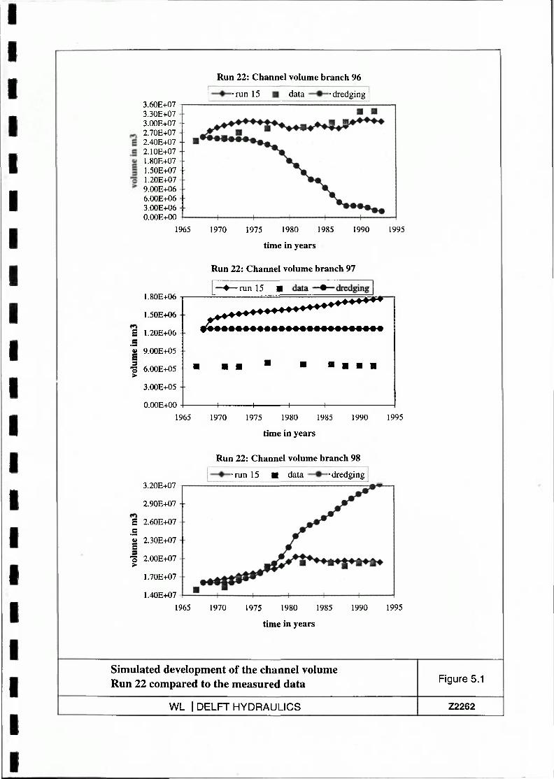
Run 22: Channel volume branch 96
3.60E+07 3.30E+07 3.(X)E+07 2.70E+07 -2.40E+07 -2.10E+07 -1.80E+07 1.50E+07 + 1.20E+07 9.00E+06 6.00E+06 -3.00E+06 -O.OOE+00
•run 15 data • dredging
1965 1970 1975 1980 1985
time in years
1990 1995
Run 22: Channel volume branch 97
1.80E+06 1
1.50E+06
S 1.20E+06 -
'Z 9.00E+05 -
•f 6.00E+05 ->
3.00E+05 -
O.OOE+00 -
—•—run 15 •
Jf^***********^***^^^. w^
. m
-
• • •
H 1
• • • • •
1 1 1
1965 1970 1975 1980 1985
time in years
1990 1995
Run 22: Channel volume branch 98
3.20E+07
2.90E+07 +
E 2.60E+07
a 'Z 2.30E+07 -c •3 2.00E+07 >
1.70E+07
1.40E+07
-run 15 • data • dredging
1965 1970 1975 1980 1985
time in years
1990 1995
Simulated development of the channel volume Run 22 compared to the measured data Figure 5.1
WL I DELFT HYDRAULICS Z2262

4.00E+07
E
E
3.00E+07 -
2.00E+07
l.OOE+07 -!—••'
1965
1.50E+07
E
O)
E s "3 >
1.40E+07 -
1.30E+07
1.20E+07 -
l.lOE+07 -
I.OOE+07 -
9.00E+06 -
8.00E+06
1965
E
E
1.50E+07
1.30E+07 --
l.lOE+07
9.00E+06 -
Run 22: Channel volume branch 99
•run 15 data • dredging
1970 1975 1980 1985
time in years
1990 1995
Run 22: Channel volume branch 100
•run 15 data • dredging
1970 1975 1980 1985
time in years
1990 1995
Run 22: Channel volume branch 101
-run 15 • data • dredging
> 7.00E+06 -
5.00E+06
1965 1970 1975 1980 1985 1990 1995
time in years
Simulated development of the channel volume Run 22 compared to the measured data Figure 5.1
WL I DELFT HYDRAULICS Z2262

Run 22: Channel volume branch 102
9.00E+04
1965
1.50E+07
^ 1.30E+07 -E
'Z l.lOE+07 E
9.00E+06
7.00E+06
1970 1975 1980 1985
time in years
1990 1995
Run 22: Channel volume branch 103
_! H 1 i
• • • •
1965 1970 1975 1980 1985
time in years
1990 1995
3.(X)t+Uo -
4.50E+06 -
S 4.00E+06 -
"Z 3.50E+06 -
3 "0 3 OOE+06 ->
2.50E+06
2.00E+06
-
-
. J #1
•
Run 22: Channel volume branch 104
—•—run 15 • data • dredging
• . •
•
. , , ^ . > ^ ^ ^ . A ^ » * » * » » » » ^ ^ ^ ^ ^
'^^^^^^ • • • • • • • • • • • • • • • • •
, 1 1 1 ,
1965 1970 1975 1980 1985 time in years
1990 1995
Simulated development of the channel volume Run 22 compared to the measured data Figure 5.1
WL I DELFT HYDRAULICS Z2262

Run 22: Channel volume branch 105
E
2.60E+06
2.
2,
•run 15 data —•—dredging
2.'
£ 1 o ^ 1
1
1
40E+06 - -
20E+06 -
OOE+06 - -
80E+06 -
60E+06 -
40E+06
20E+06 +
OOE+06
1965
1.80E+07
1.70E+07 -
E c 1.60E+07
E 3 1.50E+07
1.4OE+07 -
1.30E+07
1965
6.50E+06
6.00E+06 f ) E c 5.50E+06 -a»
J 5.00E+06
4.50E+06
4.00E+06
1970 1975 1980 1985
time in years
1990 1995
Run 22: Channel volume branch 106
•run 15 data • dredging
1970 1975 1980 1985
time in years
1990 1995
Run 22: Channel volume branch 107
•run 15 data —•—dredging
1965 1970 1975 1980 1985
time in years
1990 1995
Simulated development of the channel volume Run 22 compared to the measured data Figure 5.1
WL I DELFT HYDRAULICS Z2262

Z.ÖUE+UO -
2.60E+06 -
c 2.40E+06
1 2.20E+06 ->
2.00E+06 -
1 oncj^nA _
Run 22: Channel volume branch 108
^ ^ • • • • ^ ^ ' ^ ' ^ ^ ^ ^ ^ . ^ • • • • • • • ^
^•^^
• •
• - • • ^ 1
1965 1970 1975 1980 1985 1990 1995
time in years
Run 22: Channel volume branch 109
T e n e . nt:
^ 2.25E+06 -E .a 'Z 2.00E+06 -
=* 1.75E+06 -
1 ^ncj^n/; _
• -
•
^ i..***
".-ntntAtC;^ 1 , 1 1 1
1965 1970 1975 1980 1985 1990 1995
time in years
Run 22: Channel volume branch 110
,1 oriT? . nc
4.40E+05 -f » E 4.00E+05 -
« 3.60E+05 -
• | 3.20E+05 ->
2.80E+05
T /incj.rK .
>
•
-J, -•.f • # . # • . * ? • V TTülülüüüüti^^.. • A
TT ^
1965 1970 1975 1980 1985 1990 1995
time in years
Simulated development of the channel volume Run 22 compared to the measured data
WL 1 DELFT HYDRAULICS
Figure 5.1
Z2262

Run 22: Channel volume branch 115
4.80E+07 4.40E+07 4.00E+07 -
'S 3.60E+07 -e 3.20E+07 --
2.80E+07 2.40E+07 + 2.00E+07 1.60E+07 + 1.20E+07 8.00E+06
1965
l.OOE+07
9.50E+06 -
fj 9.00E+06 - -
.S 8.50E+06
I 8.00E+06
? 7.50E+06
7.00E+06 - -
6.50E+06
1965
•run 15 data —•—dredging
1970 1975 1980 1985
time in years
1990
Run 22: Channel volume branch 116
•run 15 data • dredging
1995
1970 1975 1980 1985
time in years
1990 1995
Run 22: Channel volume branch 117
6.00E+06
^ 5.50E+06 E
« 5.00E+06 E
*• 4.50E+06
•run 15 • data —•—dredging
4.00E+06
1965 1970 1975 1980 1985 1990 1995
time in years
Simulated development of the channel volume Run 22 compared to the measured data Figure 5.1
WL I DELFT HYDRAULICS Z2262

Run 22: Channel volume branch 118
1.30E+07
^ 1.20E+07 E
"Ü l.lOE+07 S
•run 15 • data —•—dredging
l.OOE+07 -
9.00E+06
1965
1.70E+07
^ 1.60E+07 S
4j 1.50E+07 E
1.40E+07
1.30E+07
1965
1970 1975 1980 1985 1990 1995
time in years
Run 22: Channel volume branch 119
^ ,
•
—•—run 15
.m^^^jt
y^' •
1 1
• data —•—dredging
^^v^r^^J^^T-
— 1 — 1 — 1 —
1970 1975 1980 1985
time in years
1990 1995
Run 22: Channel volume branch 184
5.40E+07
5.20E+07 -
5.00E+07 -
Ë 4.80E+07 -
•S 4.60E+07
S 4.40E+07
S 4.20E+07
4.00E+07 -
3.80E+07 -
3.60E+07
1965
•run 15 data • dredging
1970 1975 1980 1985
time in years
1990 1995
Simulated development of the channel volume Run 22 compared to the measured data Figure 5.1
WL I DELFT HYDRAULICS Z2262

Run 22: Channel volume branch 185
E
3.00E+07
2.50E+07
•run 15 • data • dredging
« 2.00E+07
1.50E+07
I.OOE+07
1965 1970 1975 1980 1985
time in years
1990 1995
Run 22: Channel volume branch 187
•run 15 data •dredging
S
E s 'S
>•
3.50E+06
1965 1970 1975 1980 1985
time in years
1990 1995
Run 22: Channel volume branch 190
•run 15 data • dredging 1.20E+07
E
E
l.OOE+07 -
8.0OE+06 -
6.00E+06 -
4.00E+06
2.00E+06
c » m
•+•
1965 1970 1975 1980 1985
time in years
1990 1995
Simulated development of the channel volume Run 22 compared to the measured data Figure 5.1
WL I DELFT HYDRAULICS Z2262
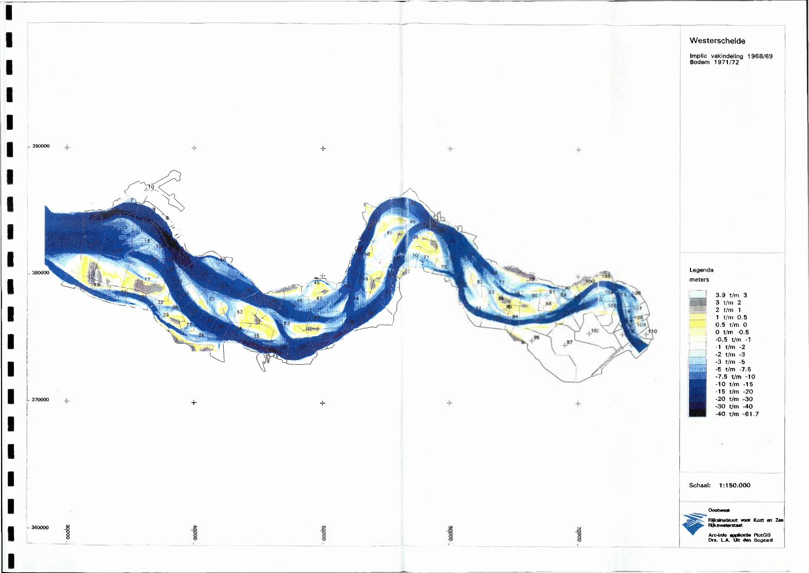
390000 -^
380000
370000 -h -\-
360000 -i o o
Westerschelde
Implic vakindeling 1968/69 Bodem 1971/72
Legenda
meters
3.9 t/m 3 3 t/m 2 2 t/m 1 1 t/m 0.5 0,5 t/m O O t/m -0.5 -0.5 t/m -1 -1 t/m -2 -2 t/m -3 -3 t/m -5 -5 t/m -7 -7.5 t/m -10 t/m -15 -15 t/m -20 -20 t/m -30 -30 t/m -40 -40 t/m
5 10
61.7
Schaal: 1:150.000
003t«««3t
R^ciinstituut voor Kust en Zee n]kswMarataat
Arc4itfo t|]|)icatte PlotGIS Drs. L.A. UH den Bosaard


![Budj get Wl UIK > add! “ Jiiiiil. £S-> $lBti HI ] edu XEsu morati ...](https://static.fdokumen.com/doc/165x107/631c63736c6907d36801485f/budj-get-wl-uik-add-jiiiiil-s-lbti-hi-edu-xesu-morati-.jpg)