WL-TR-95-3061

I

QUANTITATIVE FEEDBACK THEORY (QFT) FOR THE ENGINEER A Paradigm for the Design of Control Systems for uncertain Nonlinear Plants

Dr. C. H. Houpis, Editor Professor of Electrical Engineering Air Force Institute of Technology

& Senior Research Associate Control Systems Development Branch Flight Control Division

June 1995

Approved for Public Release; Distribution unlimited

19950814 069 FLIGHT DYNAMICS DIRECTORATE WRIGHT LABORATORY AIR FORCE MATERIAL COMMAND WRIGHT-PATTERSON AIR FORCE BASE, OHIO 45433-7521

DTIC QUALITY INSPECTED 1

NOTICE

When Government drawings, specifications, or other data are used for any purpose other than in connection with a definitely Government-related procurement, the United States Government incurs no responsibility or any obligation whatsoever. The fact that the government may have formulated or in any way supplied the said drawings, specifications, or other data, is not to be regarded by implication, or otherwise in any manner construed, as licensing the holder, or any other person or corporation; or as conveying any rights or permission to manufacture, use, or sell any patented invention that may in any way be related thereto.

t

This report is releasable to the National Technical Information Service (NTIS). At NTIS, it will be available to the general public, including foreign nations.

This technical report has been reviewed and is approved for publica- tion.

a Dr. C.H. HOUPIS Senior Research Associate

'/<r" *^

'thief, Flight

S K. RAMAGE Control Systems Development Branch Control Division

'M h DAVID P. LEMASTER Chief, Flight Control Division Flight Dynamics Directorate

Aooession WOT

mis sRä&i EK DTIC SAB D UnarmoUÄceü O Jus t i fIo at1on

Distribution/.

Availability Codei

Avail and/or Spaofdl

if* -I •Ifc If your address has changed, if you wish to be removed from our mailing

list, or if the addressee is no longer employed by your organization please notify WL/FIGS _, WPAFB, OH 45433-7521 to help us maintain a current mailing list.

Copies of this report should not be returned unless return is required by security considerations, contractual obligations, or notice on a specific document.

* V

3

•I

REPORT DOCUMENTATION PAGE Form Approved

OMB No. 0704-0188

Public reoortmg burden for This collection of information ,s estimated to average 1 hour per response, including the time for reviewing instructions searching existing data sources n^hV,1^ö%a^m^ithe<iat»^edeö and completing and reviewing the collection of information. Send comments regarding this burden estimate or anyother aspect of this ™n2£ion nMnformat or1i includina suaqe« ons f or reducing this burden, to Washington Headquarters Services. Directorate for information Operations and Reports 1215 Jefferson D°av!fr^hway S^ Office of Management and Budget. Paperwork Reduction Project (0704-0188). Washington. DC 20503.

1. AGENCY USE ONLY (Leave blank) 2. REPORT DATE JUNE 1995

3. REPORT TYPE AND DATES COVERED

QUALITATIVE FEEDBACK THEORY (QFT) FOR THE ENGINEER A Paradigm for the Design of Control Systems for Uncertain

Nonlinear Plants

| 6. AUTHOR(S) jDr. C.H. Houpis ^Other Authors: Dr. M. Pachter, Capt S. Rasmussen,

\ Capt D. Trosen, R. Sating 7. PERFORMING ORGANIZATION NAME(S) AND ADDRESS(ES)

Flight Dynamics Directorate Wright Laboratory Air Force Materiel Command Wright Patterson AFB OH 45433-7625

9. SPONSORING/MONITORING AGENCY NAME(S) AND ADDRESS(ES)

Flight Dynamics Directorate Wright Laboratory Air Force Materiel Command Wright Patterson AFB OH 45433-7625

5. FUNDING NUMBERS

PE 62201 PR 2403 TA 06 WU 65

8. PERFORMING ORGANIZATION REPORT NUMBER

10. SPONSORING/MONITORING AGENCY REPORT NUMBER

WL-TR-95-3061

11. SUPPLEMENTARY NOTES

| 12a. DISTRIBUTION /AVAILABILITY STATEMENT

I APPROVED FOR PUBLIC RELEASE: DISTRIBUTION UNLIMITED

12b. DISTRIBUTION CODE

13. ABSTRACT (Maximum 200 words) /„„„N • -, <. 4.u „,,«.„ ^-F The report brings the Quantitative Feedback Theory (QFT) material up to the state-of- the-art level and aims to provide students and practicing engineers a document that presents QFT in a unified and logical manner and which addresses the real-world control problems. QFT is a unified theory using the available measurable states that is applied to the design of multiple-input multiple-output (MIMO) systems. It incor- porates the multivariable nature of control systems' structured plant uncertainties, variation, robustness performance requirements, cross-coupling and external disturb- ance attenuation requirements, nonlinearities in the plant model, and requirements for decoupled outputs. The document also presents the fundamentals of system identific- ation and discusses the vital MIMO QFT CAD package.

j 14. SUBJECT TERMS

QUANTITATIVE FEEDBACK THEORY (QFT) MULTIPLE-INPUT MULTIPLE-OUTPUT (MIMO) STATE-OF-THE-ART LEVEL AND AIMS

CROSS-COUPLING SYSTEMS

117. SECURITY CLASSIFICATION OF REPORT

;l Hnr-lacci f i orl NSN 7540-01-280-5500

18. SECURITY CLASSIFICATION OF THIS PAGE

TTWPT.ASSTFTTÜD

19. SECURITY CLASSIFICATION OF ABSTRACT

UNCLASSIFIED

15. NUMBER OF PAGES

307 16. PRICE CODE

20. LIMITATION OF ABSTRACT

UL Standard Form 298 (Rev. 2-89) Prescribed by ANSI Std. Z39-18 298-102

QUANTITATIVE FEEDBACK THEORY (QFT) FOR THE ENGINEER

A Paradigm for the Design of Control Systems for Uncertain Nonlinear Plants

2nd Edition

PREFACE

Since the publication in 1987 of the 1st edition of this technical report, great strides have been made in exploiting the full potential of the Quantitative Feedback Theory (QFT) technique. The catalyst that has propelled QFT to the level of being a major multiple-input multiple- output (MIMO) control system design method has been the development and availability of viable QFT CAD packages. Through the close collaboration of Professor Isaac M. Horowitz, the developer of the QFT technique, with Professor C. H. Houpis and his graduate students during the 1980's and the early part of the '90s, successful QFT designs involving structured parameter uncertainty have been completed and published by AFIT MS thesis students. During this period the first multiple-input single-output (MISO) and MIMO QFT CAD packages were developed at AFIT. Another major accomplishment was the successful implementation and flight test of two QFT designed flight control systems, by Captain S. J. Rasmussen, for the LAMBDA unmanned research vehicle in 1992 and 1993. Also, Dr. Charles Hall of North Carolina State University, on April 28, 1995 announced that four successful flight tests of QFT flight controllers have been accomplished. Based upon these solid accomplishments, Lockheed Advanced Development Co. and British Aerospace Ltd have begun applying the QFT design method.

This second edition brings the material up to the state-of-the- art level, and, like the first edition, aims to provide students and practicing engineers a document that presents QFT in a unified and logical manner. Refinements based upon the class testing of the first edition, are incorporated. The material in Chapters II through V and Appendix A is based upon the numerous articles written by Professor Horowitz and the numerous lectures that he presented at the Air Force Institute of Technology.

The Editor would like to express his appreciation for the support and encouragement of Professor Pachter during the preparation of this technical report. His wealth of knowledge of the flight control area has enhanced the value of this revision.

Acknowledgement is made of the support and encouragement, during the 1980's, of Mr. Evard Flinn, Branch Chief, AFWAL/FIGL, and his colleagues Mr. James Morris and Mr. Duane Rubertus. This support and encouragement was maintained by Mr. Max Davis, WL/FIG, and Mr. James Ramage and Mr. Rubertus, WL/FIGS. Further acknowledgement must be made of the support given by AFOSR/EOARD during these past many years.

IX

4

TABLE OF CONTENTS

Preface 1X

« QFT Standard Symbols & Terminology x

PAGE NO.

%

CHAPTER

I. introduction 1

I. l Quantitative Feedback Theory 1

1.1.1 Why Feedback? 1

1.1.2 What Can QFT Do 2 1.1.3 Benefits of QFT 3

1.2 The MISO Analog System 4

1.2.1 MISO Analog Control System 5 1.2.2 Synthesize Tracking Models 6 1.2.3 Disturbance Model 7

1.2.4 J LTI Plant Models 8 1.2.5 Plant Templates of Pt(s) , QfP(jUi) 8 1.2.6 Nominal Plant 10

1.2.7 U-Contour (Stability bound) 10 1.2.8 Optimal Bounds B0(jw) on L0(jw) 11

1.2.8.1 Tracking Bounds 11 1.2.8.2 Disturbance Bounds 12 1.2.8.3 Optimal Bounds 12

1.2.9 Synthesizing (or Loop Shaping) L0(s) and F(s) 14

1.2.10 Prefilter Design 15

1.2.11 Simulation 15

1.3 The MISO Discrete Control System 16

1.3.1 Introduction 16

1.3.2 The MISO Sampled-data Control System 17 1.3.3 w' -Domain 17

1.3.4 Assumptions 18

» 1.3.5 Nonminimum Phase L0(w) 18 1.3.6 Plant Templates 3P (jv) 21 1.3.7 Synthesizing L^w) 21 1.3.8 Prefilter Design 24

3.9 w-Domain Simulation 25

*

I. 1.3.10 z-Domain 25

in

f a

1.3.10.1 Comparison of the Controller's w- and z-Domain Bode Plots 25

1.3.10.2 Accuracy 25

1.3.10.3 Analysis of Characteristic Equation Qt (z) 26

1.3.10.4 Simulation and CAD Packages 26

1.4. Summary 26 *

II. Basics of System Identification 27

II. 1 Introduction 27 II.2 Classical Route to Identification 28 II. 3 Linear Regression 29 II. 4 SID Approaches 30 II. 5 Linear Regression (LR) 31 11.6 Linear Regression for System

Identification 1 33 11.7 Linear Regression for System

Identification 2 36 11.8 Identification of Dynamic Systems

with Process Noise Only 39

II. 8.1 Discussion 41

II. 9 Example 41

II. 9.1 Identification Experiment 48

11.10 "Crimes" of System Identification (SID) 51

II. 10.1 Theory 51 II. 10.2 Experimental 54

II. 11 Static Identification 56 11.12 Summary 59

III. Multiple-Input Multiple-Output (MIMO) Plants: Structured Plant Parameter uncertainty 60

III. 1 Intoduction 60 111.2 The MIMO Plant 61 m 111.3 Introduction to MIMO Compensation 67 ^ III. 4 MIMO Compensation 69 III.5 Introduction to MISO Equivalents 71

III .5.1 Effective MISO Equivalents 71 *

xv

ft

<

111.6 Effective MISO Loops of the MIMO System 76

111.6.1 Example: The 2x2 plant 77 111.6.2 Performance Bounds 80 111.6.3 QFT Design Method 2 85

111.6.4 Summary 87

111.7 Constraints on the Plant Matrix 88 111.8 Basically Non-Interacting (BNIC) Loops 93 III. 9 Summary 94

III. 10 Problems 95

IV. Design Method - The Single-Loop (MISO) Equivalents.

IV.6 Summary.. IV.7 Problems.

98

IV. 1 Introduction 98

IV.2 Design Example "

IV. 2.1 Performance Tolerance 100 IV.2.2 Sensitivity Analysis 100 IV.2.3 Simplification of the Single-loop

Structures 104

IV. 3 High Frequency Range Analysis 107 IV.4 Stability Analysis 108

IV. 5 Equilibrium and Trade-offs HO

IV.5.1 Trade-off in High Frequency Range 115 IV.5.2 Some Universal Design Features 118 IV. 5. 3 Examples—Bounds Determination 120

128 128

V. MIMO System Design Method Two-Modified Single-Loop Equivalent 131

V. 1 Introduction l3i V.2 Design Equations for the 2x2 System 132 V.3 Design Guidelines I34

V.4 Reduced Overdesign I36

V.5 3x3 Design Equations I36

V.6 Example V.l — 3x3 System Design Equations... 139 V.7 mxm System, m > 3 • I40 V.8 Conditions for Existence of a Solution 141

V.8.1 Conditions for Existence of a Solution.. 142 V.8.2 Applications of Sec. V.8.1 to Design

Method 2 I45 V. 8.3 Inherent Constraints 147

V. 9 Nondiagonal 6 149 V.10 Achievability of a m.p. Effective Plant

det P 150 V. 11 Summary 157

H

VI. MIMO System With External Disturbance Inputs 159

VI. 1 Introduction 159 t

VI. 1.1 Aerial Refueling Background 159 VI. 1.2 Problem Statement 160 VI. 1.3 Assumptions 160 VI. 1.4 Research Objectives 161 VI. 1.5 Scope 161 VI. 1.6 Methodology 162 VI. 1.7 Overview of Chapter 162

VI.2 Air-to-Air Refueling FCS Design Concept 162

VI.2.1 C-135B Modeling. 163 VI. 2.2 Disturbance Modeling 164

VI. 3 Plant and Disturbance Matrices 165 VI. 4 Control Problem Approach 165 VI.5 MIMO QFT with External Output Disturbance 169 VI. 6 AFCS Design 177

VI. 6.1 Introduction 177 VI.6.2 Disturbance Rejection Specification 177 VI. 6.3 Loop Shaping 178 VI.6.4 Channel 2 Loop Design 179 VI.6.5 Channel 1 Loop Design 180 VI. 6.6 Channel 3 Loop Design 185 VI. 6.7 Closed Loop Lm Plots 185

VI.7. Air-to-Air Refueling Simulations 188

VI. 7.1 Linear Simulations 189 VI. 7.2 Nonlinear Simulations 191

VI. 8 Summary 194

VII Now the "Practicing Engineer Takes Over" 195

VII. 1 Introduction 195 VII. 2 Transparency of QFT 196 VII.3 Body of Engineering QFT Knowledge 198 VII.4 Nonlinearities — The Engineering Approach... 202 * VII.5 Plant Inversion 203 *" VII. 6 Invertibility 205

vx

VII.7 Psuedo-Continuous-Time (PCT) System 206 VII.8 Summary. 207

\ VIII MIMO QFT CAD Package (Version 3) 208

VIII. 1 Introduction • • • • • 208

VIII.2 Introduction: Overview of Multivariable » Control ■ 210

VIII.3 Continuous-Time vs Discrete-Time Design 210 VIII.4 Overview of the Multivariable External

Disturbance Rejection Problem 211 VIII. 5 Open-loop Structure 212

VIII.6 Formation of Plant Models for Tracking Control Problems 215

VIII. 7 Inverse of P 216 VIII.8 MISO Loops of the Tracking Control Problem.. 217 VIII.9 MISO Loops of External Disturbance

Rejection Problems 218 VIII. 10 Q Matrix Validation Checks 219 VIII. 11 Improved Method 220 VIII. 12 Specifications. 221

VIII.12.1 Stability Specifications—:•••: 221

VIII.12.2 Tracking Performance Specifications.. 221 VIII.12.3 External Disturbance Rejection

Performance Specifications 222 VIII. 12 .4 Gamma Bound Specifications 222

VIII. 13 Bounds on the NC 223

VIII.13.1 Stability Bounds 223 VIII. 13.2 Cross-Coupling Bounds 223 VIII.13.3 Gamma Bounds 225 VIII. 13.4 Allocated Tracking Bounds 225 VIII.13.5 External Disturbance

Rejection Bounds 226 VIII. 13 . 6 Composite Bounds 227

VIII. 14 Compensator Design 227 VIII. 15 Prefilter Design 228

VIII. 16 Design Validation 229

VIII. 17 Summary 23°

I ix. Development Implementation & Flight Test of a MIMO Digital Flight Control System foran Unmanned Research Vehicle 232

r IX. 1 Introduction 232

IX.2 Objective 233

IX.3 First Design Cycle 234

Vll

IX. 3.1 Requirements 234 IX. 3. 2 Specifications 234 IX.3.3 Aircraft Model 234 IX. 3.4 FCS Design 235 0 IX.3.5 Linear Simulations 235 ^ IX. 3. 6 Nonlinear Simulations 235 IX.3.7 Hardware-in-the-Loop Simulation 235 IX. 3 . 8 Flight Test 236

IX.4 Second Design Cycle 236 "

IX. 4.1 Requirements 236 IX. 4.2 Specifications 236 IX.4.3 Aircraft Model 237 IX.4.4 FCS Design 237 IX.4.5 Linear, Nonlinear, and Hardware-

in-the-Loop Simulation 237

IX.4.6 Flight Test 237

IX.5 Third Design Cycle 239

IX. 5.1 Requirements 239 IX. 5.2 Specifications 239 IX.5.3 Aircraft Model 239 IX. 5. 4 FCS Design 240 IX.5.5 Linear, Nonlinear, and Hardware-in-

the-Loop Simulations 240 IX.5.6 Flight Test 240

IX. 6 Fourth Design Cycle 241

IX. 6.1 Requirements 241 IX. 6.2 Specifications 241 IX.6.3 Aircraft Model 241 IX.6.4 FCS Design 242 IX.6.5 Linear, Nonlinear, and Hardware-in-

the-Loop Simulation 242 IX.6.6 Flight Test 242

IX. 7 Conclusion 243

Appendix A Design Examples 244

A. 1 MISO Design Problem 244 v

A. 2 MIMO Design Problem 249

r

Vlll

Appendix B Longitudinal Handling Qualities Approximations & Bandwidth Minimization 269

» B. 1 Introduction 2 69

i. B. 2 Background 2 69 B.3 Desired Handling Qualities 271 B.4 Modification of the QFT Design Procedure... 274 B.5 Remarks by Dr. I. M. Horowitz 278

| B.6 Summary 281

Ref erences 282

R. 1 References for the TR 282

R.2 References for Other Pertinent Articles.... 288 R.3 Additional References 290

<

r

XX

Bi

Bu= LmT^

*L = Lm TRL

Bs

f

OFT Standard Symbols & Terminolgv

Symbol

ap — The specified peak magnitude of the disturbance response for the MISO system

a.l. - Arbitrarily large

a.s. — Arbitrarily small

ay = Lm Ty - The desired lower tracking bounds for the MIMO system

by = Lm Ty - The desired upper tracking bounds for the MIMO system

aL — The desired modified lower tracking bound for the MIMO system:

a- = a.- + x

b'.. — The desired modified upper tracking bounds for the MIMO system

bu = bu- \„

BD(ja>i), BR(jo>i), B0(ja>i) - The disturbance, tracking, and otimal bounds on Lm L(jwi) for the MISO system

Bh ~ Ultra high frequency boundary (UHFB) for analog design

— Ultra high frequency boundary (UHFB) for discrete design

— The Lm of the desired tracking control ratio for the upper bound of the

MISO system

— The Lm of the desired tracking control ratio for the lower bound of the

MISO system « >

— Stability bounds for the discrete design

BW -- Bandwidth t »-

zcä -- Allotted portion of the ij output due to a cross-coupling effect for a

9 MIMO system

» i 5D(jwi) -- The (upper) value of Lm TD(jo>i) for MISO system

5hf(jwi) - The dB difference between the augmented bounds of By and BL in the

<* high frequency range for a MISO system

SRÖ'WL) - The dB difference between Bu and BL for a given w; for a MISO

system

AT - The difference between bü amd a^ i.e., AT = bü - a^

cü - The interaction or cross-coupling effect of a MIMO system

D -- MISO and MIMO system external disturbance input

D = {D} - Script cap dee to denote the set of external disturbance inputs for a MIMO system D = {D}

F, F = {fj - The prefilter for a MISO system and the tXt prefilter matrix for a MEMO system respectively

FOM - Figures of merit (see Reference 15)

G, G = {gij} ~ The compensator or controller for a MISO system and the 1X1 compensator or controller matrix for a MIMO system, respectively. For a diagonal matrix G = {&}

h.f. -- High frequency

h.g. ~ High gain

7, 7i - The phase margin angle for the MISO system and for the i* loop of the MIMO system, respectively

* 7s ~ A function only of the elements of a square plant matrix P (or PJ

< k ~ A running index for sampled-data systems where k = 0,1,2, ...

r kT — The sampled time

X - The excess of poles over zeros of a transfer function

xi

4» K — The optimal loop transmission function for the MISO system and the i* loop of the MIMO system, respectively

LHP — Left-half-plane i

LTI — Linear-time-invariant

MIMO — Multiple-input multiple-output; more than one tracking and/or external disturbance inputs and more than one output

MISO — Multiple-input single-output; a system having one tracking input, one or more external disturbance inputs, and a single output

*V ML, — The specified closed-loop frequency domain overshoot constraint for the MISO system and for the i* loop of a MIMO system, respectively. This overshoot constraint may be dictated by the phase margin angle for the specified loop transmission function

m.p. ~ Minimum-phase

n.m.p. — Nonminimum-phase

NC — Nichols chart

J — The number of plant transfer functions for a MISO system or plant matrix for a MIMO system that describes the region of plant parameter uncertainty where i = 1, 2, ..., J denotes the particular plant case in the region of plant parameter uncertainty

«b — the symbol for bandwidth frequency of the models for TRV ,TRL,andT= fy}

«V w* — phase margin frequency for a MISO system and for the iith loop of a MIMO system, respectively

«. — Sampling frequency

P t

— MISO plant with uncertainty >

^ - {(P,M — mxl MIMO plant matrix where (pyX is the transfer function relating the i* output to the j* input for plant case i >

xii

<

f

ö> ~ Script cap pee to denote a set that represents the plant uncertainty for J cases in the region of plant uncertainty, i.e., (P = {P.} for a MEMO system

— md x m MIMO external disturbance matrix

~ Plant model for a tracking and external disturbance input system which is partioned to yield Pe and Pd

— The inverted plant matrix for plant case i where I = m

— The mxm effective plant matrix when Pt is not a square plant matrix

and W is an txm weighting or a squaring-down matrix

— Quantitative feedback design based on quantitative feedback theory

~ An txl matrix whose elements are given by (qjj) = l/(qjj)i

— Script cap que to denote a set that represents the plant uncertainty for a MIMO system, i.e., Q = {Q}

R, R = {r;} - The tracking input for a MISO system and the tracking input vector for a MIMO system, respectively

RHP — Right-half-plane

T — Sampling time

3P(jw.} — Script cap tee inconjunction with P or (qy) denotes a template, i.e., 3fP(j«i) and 3QG"i) frequency, for a MISO and MIMO plants respectively

-•

Pd

* PF

P;1 = «PVJ

Pe = PXW

QFD

& = {(qij)}

Q

l*u

l*L

The desired MISO tracking control ratio that satisfies the specified

upper bound FOM

The desired MISO tracking control ratio that satisfies the specified

lower bound FOM

TD - The desired MISO disturbance control ratio which satisfies the specified FOM

• T , 7 — The MISO tracking and disturbance conrol ratios for case i

Tt = {(tjjX) - The mxm MIMO tracking control ratio matrix for plant case i

xm

Td = {(td)} — The mxm MIMO external disturbance control ratio matrix

5R ~ The script cap tee denotes the set that represents the tracking control ratios for J cases, i.e OR = {T^} for the MISO system and

\ = t(7yil for the MIMO system

3D — The script cap tee denotes the set that represents the disturbance control ratios for J cases, i.e., S§D = {TD} for the MISO system and sc = K7^} for the MIMO system

7;J — A set of assigned tolerances on tj,- where a- and b- and TC are the assigned tolerances for tracking and cross-coupling rejection, respectively

U — The mxl controller input vector

UHFB — The ultra high frequency boundary

v, v — The MISO prefilter output and the mxl MEMO prefilter output vector, respectively

V — linv,.,,, {Lm P,^ - Lm P,^} is the dB limiting value for a MISO plant

V; - lima^« {Lm (q^^ - Lm (q^^} is the i* loop template dB limiting value for a MIMO plant

W = {wjj} — The weighting or squaring-down or mixer matrix

w' = u + jv — w'-domain variable; the use of u and v must be interpreted in context

Y, Y = {y;j} — The output of a MISO system and the output matrix of a MEMO system, respectively, where y^- = yr + yc

y — The mxl plant output vector

yTi — Is that portion of the i* output due to the i* input v*

yc — Is that portion of the i^output due to cä (cross-coupling effect or interaction of the other loops)

*

xiv

9

EDITOR and COLLABORATOR

Dr. Constaatine H. Houpis Professor of Electrical Engineering Air Force Institute of Technology

& Senior Research Associate

Control Systems Development Branch Flight Control Division (WL/FIGS)

Wright Laboratory

COLLABORATORS

Chapter I

Chapter II

Chapters III thru V

Chapter VI

Chapter VII

Chapter VIII

Chapter IX

Dr. C. H. Houpis

Dr. Meir Pachter, Associate Professor of Electrical Engineering, Air Force Institute of Technolgy

Dr. C. H. Houpis

Dr. C. H. Houpis and Captain Dennis W. Trosen, Control System Development Branch (WL/FIGS)

Dr. C. H. Houpis & Dr. M. Pachter

Mr. Richard Sating, Research Associate, Department of Electrical & Computer Engineering, Air Force Institute of Technology

Captain Steven J. Rasmussen, Development Branch (WL/FIGS)

Control System

r ■4

ACKNOWLEDGEMENT

The illustrations which enhanced the technical report were produced by the tireless and professional efforts of

Mr. Jim Coughlin Industrial Graphic Designer

UNC-Lear Siegler MSC

XV

rfriHpt-gT- I Int roduct ion

1.1 Quantitative Feedback Theory

l

QFT has achieved the status46 as a very powerful design technique

for the achievement of assigned performance tolerances over specified

• ranges of structured plant parameter uncertainties without and with

control effector failures. It is a frequency domain design technique

utilizing the Nichols chart (NC) to achieve a desired robust design over

the specified region of plant parameter uncertainty. This chapter

presents an overview to QFT analog and discrete design techniques for

both multiple-input single-output (MISO)15'19'47 control systems. For an

in-depth presentation of the MISO QFT design technique the reader is

referred to References 15 and 47. QFT CAD packages are readily

available to expedite the design process. The purposes of this

technical report are: (1) to provide a basic understanding of the MIMO

QFT design technique, (2) to provide the minimum amount of mathematics

necessary to achieve this understanding, (3) to discuss the basic design

steps, and (4) to present two practical examples. The list of

references is divided into two sections: the first section are listed

the QFT articles referenced in this Technical Report (TR), and the

second section is a partial list of other individuals who have published

articles in the QFT area. The reader is encouraged to review the

articles in both sections.

I.1.1 Whv Feedback?

For the answer to the question of "Why do you need QFT?" consider

the following system. The plant P of Fig. 1.1 responds to the input r(t)

with the output y(t) in the face of disturbances dx(t) and d2(t). If it

* is desired to achieve a specified system transfer function T(s) [=

Y(s)/R(s)] then it is necessary to insert a prefilter, whose transfer

function is T(s)/P(s), as shown in Fig. 1.2. This compensated system

produces the desired output as long as the plant does not change and

there are no disturbances. This type of system is sensitive to changes

in the plant (or uncertainty in the plant), and the disturbances are

reflected directly into the output. Thus, it is necessary to feed back

the information in the output in order to reduce the output sensitivity

to parameter variation and attentuate the effect of disturbances on the

plant output.

x

Fig. 1 An open-loop system (basic plant).

-K>* P -►Ö*' Fig. 1.2 A compensated open-loop system.

In designing a feedback control system, it is desired to utilize a

technique that:

a. Addresses all known plant variations up front.

b. Incorporates information on the desired output tolerances.

c. Maintains reasonably low loop gain (reduce the "cost of

feedback").

This last item is important in order to avoid the problems associated

with high loop gains such as sensor noise amplification, saturation, and

high frequency uncertainties.

1.1.2 What Can QFT Do

Assume that the characteristics of a plant, that is to be

controlled over a specified region of operation, vary, that is, a plant

with plant parameter uncertainty. This plant parameter uncertainty may

be described by the Bode plots of Fig. 1.3. This figure represents the

range of variation of plant magnitude (dB) and phase over a specified

frequency range. The bounds of this variation, for this example, can be

described by six LTI plant transfer functions. By the application of

QFT, for a MISO control system containing this plant, a single

compensator and a prefilter may be designed to achieve a specified robust design.

V

•o

V •o S «-> e « s

<•. n V V u M V

■o

o n 0

0.

40

20

0

-20

-40

-60

-80

-100

-90

-100

-110

-120

-130

-140

-150

-160

-170

-180

vnt"'Ktr.-~.

~"~ "'««aw

*

: Plant

I Plant

: Plant

r Plant I plant

"^^^C!^"""--S^ :::::;-:::— 2 ^^^^^---^r^^"-----:::--:::::: ." ;::::v^::; 3 '^"^""""■""""■••■■■■^^

4 —-^*-^^"""""*----i:T::

5 """""--»^^

6 , , i i .i.ii 1 J 1 1 1 1—L_I_J 1

Plant

1 10 100 Frequency (w)

... Plant 1,2

**"*--... Plant 3.6 ""**-.., Plant 4,5

E- ^\

1 10 100 Frequency (w)

Fig. 1.3 The bode plots of six LTI plants that represent the range of the plant's parameter uncertainty.

1.1.3 Benefits of QFT

The benefits of QFT may be summarized as follows:

a. The result is a robust design which is insenstitive to plant

variation.

b. There is one design for the full envelope (no need to verify

plants inside templates).

c. Any design limitations are apparent up front,

d. There is less development time for a full envelope design.

e. One can determine what specifications are achievable up early in the design process. j,

f. One can redesign for changes in the specifications quickly.

g. The structure of compensator (controller) is determined up front.

1.2 The MISO Analog Control System15

As is discussed in Chap. Ill, an m x m feedback control system can

be represented by an equivalent m2 MISO feedback control systems shown

in Fig. 1.4. Reference 15 and 47 present an in-depth presentation of

the MISO QFT design technique for analog and discrete-time systems,

respectively. Thus, this chapter presents an overview of the QFT

technique for MISO feedback control system. it is assumed that the

reader has the QFT background presented in these references.

-1 -1 -1

Fig. 1.4 m2 MISO equivalent of a 3x3 MIMO feedback control system.

V

Fig. 1.5 A MISO plant.

1.2.1 MISO Analog Control System 15

The overview of the MISO QFT design technique is presented in terms

of the minimum-phase (m.p.) linear time-invariant (LTD MISO system of

Fig. 1.5. The control ratios for tracking (D = 0) and for disturbance

rejection (R = 0) are, respectively,

= F(0)O(8)P(0) = F(8)L(8) * 1 + 6(8) P(8) 1 + L{8)

Ci.l)

_ Pie) D 1 + G(B)P(B)

P(0) l + Us)

(1.2)

The design objective is to design the prefilter F(s) and the compensator

G(s) so the specified robust design is achieved for the given region of

plant parameter uncertainty. The design procedure to accomplish this

objective is as follows:

r

Step 1: Synthesize the desired tracking model.

Step 2: Synthesize the desired disturbance model.

Step 3: Specify the J LTI plant models that define the boundary of

the region of plant structured parameter uncertainty.

Step 4: Obtain plant templates, at specified frequencies, that

pictorial described the region of plant parameter uncertainty

on the NC.

Step 5: Select the nominal plant transfer function PQ(s). *

Step 6; Determine the stability contour (U-contour) on the NC.

Steps 7-9; Determine the disturbance, tracking, and optimal bounds on ^

the NC.

Step 10: Synthesize the nominal loop transmission function LQ(s) =

G(s)P0(s) that satisfies all the bounds and the stability

contour.

Step 11: Based upon Steps 1 through 10 synthesize the prefilter F(s).

Step 12: Simulate the system in order to obtain the time response

data for each of the J plants.

The following sub-sections illustrate this design procedure.

1.2.2 Synthesize Tracking Models

The tracking thumbprint specifications, based upon satisfying some

or all of the step forcing function figures of merit for underdamped

(My tp' ts, tr, Km) and overdamped (t8, tr, l^) responses, respectively, for a simple-second system, are depicted in Fig. 1.6(a). The Bode plots

corresponding to the time responses y(t)n [Eq. (1.3)] and y(t)L [Eq.

(1.4)] in Fig. 1.6(b) represent the upper bound Bv and lower bound BL,

respectively, of the thumbprint specifications; i.e., an acceptable

response y(t) must lie between these bounds. Note that for the m.p.

plants, only the tolerance on I TR(jo>±)l need be satisfied for a

satisfactory design. For nonminimum-phase (n.m.p.) plants, tolerances >

on LT^iju^ must also be specified and satisfied in the design

process.19,32 It is desirable to synthesize the tracking control ratios

t

*

(co*/a) (s + a)

82 + 2£<x>B8 + to.

TR = (fl - Oj (S - 02) (8 - 03)

(1.3)

(1.4)

corresponding to the upper and lower bounds TRU and T^, respectively,

so that öR(jwi) increases as o± increases above the 0 dB crossing

frequency of TRU. This characteristic of öR simplifies the process of

synthesizing a loop transmission L0(s) = 6(s)P0(s) that requires the

determination of the tracking bounds B^j^) which are obtained based

upon öR(j&)i). The achievement of the desired performance specification

is based upon the frequency bandwidth BW, 0 < o < wh, which is

determined by the intersection of the -12 dB line and the B^ curve in

Fig. 1.6(b).

Thumbprint LmTfi Specifications

,Bu=LmlRu=LmBRu

*Ü)

ßrLmTfiL=Lr%

(a) Thumbprint specifications (b) Bode plots of TR

Fig. 1.6 Desired response characteristics: (a) Thumbprint specifications, (b) Bode plot of TR.

1.2.3 Disturbance» Model

The simplest disturbance control ratio model specification is

| T (ja)! = | Y(j(l))/D(jw)l < otp a constant [the maximum magnitude of the

output based upon a unit step disturbance input (Dx of Fig.I.l)]. Thus

the frequency domain disturbance specification is Lm TD(jw) < Lm ap over

the desired specified BW. Thus the disturbance specification is

represented by only an upper bound on the NC over the specified BW.

1.2.4 J LTI Plant Models

The simple plant

PAs) = . ** . (1.5) 3 8(8 + a)

where K s {1,10} and a £ {1,10}, is used to illustrate the MISO QFT

design procedure. The region of plant parameter uncertainty is

illustrated by Fig. 1.7. This region of uncertainty may be described by

J LTI plants, where i = 1,2, ... J. These plants lie on the boundary of

this region of uncertainty. That is, the boundary points 1, 2, 3, 4, 5,

& 6 are utilized to obtain 6 LTI plant models that adequately define the

region of plant parameter uncertainty.

1-2.5 Plant Templates of P^s), gP(i(o±l

With L = GP, Eg. (1.1) yields

(1.6) Lm TR = Lm F - Lm 1 + L

The change in TR due to the uncertainty in P, since F is LTI, is

r L A (im T-) = LmTs-LmF=Lm 1 + L

(1.7)

By the proper design of L = LQ and F, this change in TR is restricted so

that the actual value of Lm TR always lies between B^ and BL of Fig. 1.6. The first step in synthesizing an LQ is to make NC templates which

characterize the variation of the plant uncertainty (see Fig. 1.8), as

described by i = 1,2, ..., J plant transfer functions, for various

values of wi over a specified frequency range. The boundary of the

plant template can be obtained by mapping the boundary of the plant >

parameter uncertainty region, Lm PlXiwi) vs Z.Pl(jo)i), as shown on the

Nichols chart (NC) in Fig. 1.8. A curve is drawn through the points 1,

2, 3, 4, 5, and 6 where the shaded area is labeled SP(jl), which can be

represented by plastic a template. Templates for other values of Q± are

obtained in a similar manner. A charcteristic of these templates is

8

»

that, starting from a "low value" of <i>i# the templates widen (angular

width becomes larger) for increasing values of u± then as a>L takes on

larger values and approaches infinity they become narrower and

eventually approach a staight line of height V dB [see Eg. (1.9)].

Guidelines for template determination are given in the following

sections: Sec. VII.2, Sec. VII.3 (E.L.3), and Sec. IX.5.4.

Region of plant parameter uncertainty

0 1 5 10

Fig. 1.7 Region of plant uncertainty

K = 10

* ■*

a = 10

0.04 dB

Fig. 1.8 The template 3P (j1).

1.2.6 Nominal Plant

While any plant case can be chosen it is an accepted practice to «

select, whenever possible, a plant whose NC point is always at the lower -*

left corner for all frequencies for which the templates are obtained.

1.2.7 U-Contour (Stability bound) ♦

The specifications on system performance in the frequency domain

[see Fig. 1.6(b)] identify a minimum damping ratio £ for the dominant

roots of the closed-loop system which becomes a bound on the value of

Mp - Mm- On the NC this bound on a^ = ML [see Figs. 1.6(b) and 1.9]

establishes a region which must not be penetrated by the templates and

the loop transmission function L(jw) for all a. The boundary of this

region is referred to as the universal high-frequency boundary (UHFB) or

stability bound, the U-contour, because this becomes the dominating

constraint on L( jo) . Therefore, the top portion, efa, of the ML contour

becomes part of the U-contour. For a large problem class, as w -+ oo, the

limiting value of the plant transfer function approaches

^[P(jco)] = 4 (1.8)

where X represents the excess of poles over zeros of P(s). The plant

template, for this problem class, approaches a vertical line of length equal to

A A (S^yi** P»»* " *» Pmln] = *"» *^x - Lm K^ = V dB (1.9)

If the nominal plant is chosen at K = Kmin, then the constraint ML gives

a boundary which approaches the U-contour abcdefa of Fig. 1.9.

»

>

10

4.

M-contour (LmM^)

U-contour

Bu-boundary

Fig. 1.9 U-contour construction.

1.2.8 npfimal Bounds Fu(j") on Lo(i(0)

The determination of the tracking B^jc^) and the disturbance

Bj^jöi) bounds are required in order to yield the optimal bounds B0(1o±)

on L0(3<i>±) .

1.2.8.1 Tracking Bounds

The solution for B^jc^) requires that the condition

(actual) ATR(jw±) < öR(jw±) dB (see Fig. 1.6(b)

must be satisfied. Thus it is necessary to determine the resulting

constraint, or bound BR(j(o±), on L( j(D±). The procedure is to pick a

nominal plant PQ(s) and to derive tracking bounds on the NC, at

specified values of frequency and by use of templates or a CAD package,

on the resulting nominal transfer function L0(s) = G(s)P0(s). That is,

along a phase angle grid line on the NC move the nominal point on the

template SPt^) up or down, without rotating the template, until it is

tangent to two M-contours whose difference in M values is essentially

equal to öR. When this condition has been achieved the location of the

nominal point on the template becomes a point on the tracking bound

B (jv±) on the NC. This procedure is repeated on sufficient angle grid

lines on the NC to provide sufficient points to draw BR(jv±) and for all

values of frequency for which templates have been obtained.

11

1.2.8.2 Disturb«™™* urmnH«

The general procedure for determining disturbance bounds for the

MISO control system of Fig. 1.5 is outlined as follows but more details

are given in Reference 15. From Eq. (1.2) the following equation is

obtained:

TD =

*♦*

o W (I.10)

where W = (PQ/P) + LQ. From Eq. (1.10), setting Lm TD = öD =

following relationship is obtained:

Lm W = La P„ - 5n

Lm a , the

(I.11)

For each value of frequency for which the NC templates are obtained the

magnitude of I WU^)! is obtained from Eq. (1.11). This magnitude in

conjuction with the equation WUG^) = [P0( jw±)/P( j<D±) ] are utilized to

obtain a graphical solution for B^jc^) as shown in Fig. I.1015. Note

that in this figure the template is plotted in rectangular or polar

coordinates.

Iwc/ayl

-/-£-£?£ ,

Fig. 1.10 Graphical evaluation of BD(/0D/)

1.2.8.3 optimal Bounds

For the case shown in Fig. 1.11 B0(jo)i) is composed of those

portions of each respective bound Bjjjo^) and BD(j(o±) that have the

largest dB values. The synthesized L0(ja)i) must lie on or just above the

bound B0jwi) of Fig. I.11.

12

4

r

-180" 140° -100°

Fig. 1.11 Bounds Bo(jC0|) and loop shaping.

13

1.2.9 Synthesizing (or Loop Shaping) Lp(s) and F(s)

The shaping of L0(jü) is shown by the dashed curve in Fig. 1.11. A

point such as Lm L0(j2) must be on or above B0( j2) . Further, in order 2

to satisfy the specifications, L0(jo>) cannot violate the U-contour. In

this example a reasonable L0(jw) closely follows the U-contour up to <o

= 40 rad/sec and must stay below it above w = 40 as shown in Fig I.11.

It also must be a Type 1 function (one pole at the origin) .

Synthesizing a rational function LQ(s) which satisfies the above

specification involves building up the function

L0(ju>) = Lojt(ja» =P0(jo>) n [KkGk{ju)] <I-12) k=o

where for k = 0, 60 = 1Z.00, and K = D^=0Kk- In order to minimize the

order of the compensator a good starting point for "building up" the

loop transmission function is to initially assume that Lo0(J6>) = P0(jw)

as indicated in Eq. (1.12). L0(j<o) is built up term-by-term or by a CAD

loop shaping routine,8 in order (1) that the point L^jo^) lies on or

above the corresponding optimal bound B0(jwi) and (2) to stay just

outside the U-contour in the NC of Fig. I.11. The design of a proper

L0(s) guarantees only that the variation in I TR(jwi)l is less than or

equal to that allowed, i.e., öR(j<*±) . The purpose of the prefilter F(s)

is to position Lm [T(jw)] within the frequency domain specifications,

i.e., that it always lies between Bv and BL [see Fig. 1.6(b)] for all J plants. The method for determining F(s) is discussed in the next

section. Once a satisfactory LQ(s) is achieved then the compensator is

given by G(s) = L0(s)/P0(s). Note that for this example L0(ju) slightly

intersects the U-contour at frequencies above G>h. Because of the *

inherent overdesign feature of the QFT technique, as a first trial

design, no effort is made to fine tune the synthesis of LQ(s). If the

simulation results are not satisfactory then a fine tuning of the design -»

can be made. The available CAD packages simplify and expedite this fine

tuning.

«

■*,-

14

1.2.10 Prefliter Design15'19'32

Design of a proper L0(s) guarantees only that the variation in

* I TR(jo))l is less than or equal to that allowed, i.e., [Lm TR(jw)] <

öR(jw). The purpose of the prefilter F(s) is to position

* IM nM - IM 1 *<ffia) „.«,

within the frequency domain specifications. A method for determining

the bounds on F(s) is as follows:

Step It Place the nominal point of the a>± plant template on the

JM0(6O±) point on the L0(jw) curve on the NC (see Fig. 1.12).

Step 2: Traversing the template, determine the maximum Lm Tj,^ and the

minimum Lm Tmin values of Eq. (1.13) are obtained from the M-

contours.

Step 3t Based upon obtaining sufficient data points within the desired

frequency bandwidth, for various values of <a±, and in

conjunction with the data used to obtain Fig. 1.6(b) the plots

of Fig. 1.13 are obtained.

Step 4t Utilizing Fig. 1.13, the straight-line Bode technique and the

condition

LJ%F(S) =1 (I-")

for a step forcing function, an F(s) is synthesized that lies within the

upper and lower plots in Fig. 1.13.

« 4 1.2.11 fi-irniilat-inn

r The "goodness" of the synthesized LQ(s) and F(s) is determined by

♦ simulating the QFT designed control system for all J plants. MISO QFT

CAD packages, as discussed in Chap, vill, are available that expedite

this simulation phase of the complete design process.

15

Desired M-contour

L/-contour

3P(yü);)

mTmin

LmL0(/(D)

ImF

^ ^ LmTfi-LmT„ LmTfit-LmTmin

Fig. 1.13 Frequency bounds on F (s).

Fig. 1.12 Prefilter determination.

1.3 The MISO Discrete Control System47

1.3.1 Introduct ion

The bilinear transformation, z-domain to the W-domain and vice-

versa, is utilized in order to accomplish the QFT design for both MISO

and MIMO sampled-data (discrete) control system design in the w'-domain.

This transformation enables the use of the MISO QFT analog design

technique to be readily used, with minor exceptions, to perform the QFT

design for the controller G(w'). If the w'domain simulations satisfy

the desired performance specification then by use of the bilinear

transformation the z-domain controller G(z) is obtained. With this z-

domain controller a discrete-time domain simulation is obtained to

verify the goodness of the design. The QFT technique requires the

determination of the minimum sampling frequency (<os)min bandwidth that

is needed for a satisfactory design.30,47 The larger the plant

uncertainty and the narrower the system performance tolerances are, the

larger must be the value of (ws)min. Although, hencefoth, the prime is

omitted from w' whenver the symbol w is used it is be interpreted as w'.

16

Fig. 1.14 A MISO sampled-data control system.

1.3.2 The MISO g«mpi«»ri-data Control System

Figure 1.14 represents the MISO discrete control, having plant

uncertainty, that is to be designed by the QFT technique. The equations

that described this system are as follows:

p,M = Gj-M - (i-x-'>[^] - (i-*-'>.M (I15)

L(z) = G!0P(z)Cl(z). P^^f- . P,(z) = Zp^] =Z[Pe) (1.16) 1

For a unit step disturbance: D(s) = -

Pe(s) = P(s)D(s),Pe(z) =Z[P(s)D(s)] =PD(z)

T _F(z)L(z) _ PD(z) D 1+L(z) R 1+L(z)

= rL(z)F(z)l rPD(z)l^_ nZ) Ll+L(z) rKZ) + Ll+L(z)]D{z)

= YR(z) +YD(z) = TR(z)R(z) +YD(z)

(1.17)

(118)

(1.19)

1.3.3 y'-TVwna-iTi

as follows:

— The pertinent s-, z-, and w-plane relationships are

17

,2 - oT\2

< 2, 0)T * 0.297

s = a + j(i>, (a) sr = u + jv -m z - 1 s + 1 (b)

(1.20)

(1.21)

z = Tw + 2 -Tw + 2

(a) V = ■(i) tan car 2

7t tan C07t

to.

u _ 2tanh(or/2) (c)

(Jb) (1.22)

(x>B = 2n/T, z = eoTlo)T = \z\loT (1-23)

1.3.4 As sumpt ions

The following assumptions are assumed:

a. Minimum-phase (mp) stable plants

b. The analogue desired models, Eqs (1.3) and (1.44), yield the

desired time response characteristics for the discrete-time system.

c. The sampling time T is small enough so that over the BW,

0 < o) < coh, Eq. (1.23) is valid permitting the approximation

s ~ w and in-turn

TR(V) * lTx(s)lg=w (1.24)

Both the upper and lower bound w-domain tracking models are obtained in

this manner. The disturbance specification is the same as for the analog case.

1.3.5 Nonminimum Phase I«0(w)

It is important to note that in the w domain any practical L(w) is

18

nonminimum phase (n.m.p.) containing a zero at 2/T (the sampling zero).

This result is due to the fact that any practical L(z) has an excess of

at least one pole over zeros. Thus, the design technique for a stable

* uncertain plant is modified30 to incorporate the all-pass filter (apf)

r r

~ 2

A(V) = £. = -A'(W)

T

_T

— + w T

(1.25)

as follows: Let the nominal loop transmission be defined as:

A, = " L^MAiw) = ZfedriA'dr) (1.26)

From Eq. (1.26) it is seen that

IL^Uv) = LL0{jv) - LA'(jv) (1.27)

where

- /.A'(jv) = 2 tan1^ > 0 (1.28) 2

An analysis of Eqs. (1.26) through (1.28) reveals that the bounds

B^jVi) on L0(jv) become the bounds B^jv^ on L^jv) by shifting, over

the desired BW# BX(jv) positively (to the right on the NC) by the angle

LA'(jv±), as shown in Fig. 1.15. The U-contour (B£) must also be

shifted to the right by the same amount, at the specified frequencies

vi# to obtain the shifted U-contour B^ jv±) . The contour B£ is shifted

to the right until it reaches the vertical line /-Limo^R* = °°- The

s value of vK, which is function of as and the phase margin angle as shown

♦ in Fig. I.15,47 is given by

2tan-4^ = 180° - Y (I'29)

It should be mentioned that loop shaping or synthesizing L0(w) can be

done directly without the use of an apf.

19

Maximum shift to the right of ÜicML contour

dB 0

-40 -180° -90'

Note: Curves drawn approximately to scale,

Fig. 1.15 The shifted bounds on the NC.

*

"• V

20

1.3.6 Plant T^mpi««-*>« ^Hv^

The plant templates in the w-domain have the same characteristic as

those for the analog case (see Sec. 1.2.5) for the frequency range 0 <

(o± < 6)s/2 as shown in Fig. 1.16 (a). In the frequency range o>s/2 < o± <

oo the w-domain templates widen once again then eventually approach a

vertical line as shown in Fig. 1.16(b).

dB 20 hin -20«

10

^v

sf—

-40-

dB*>r

100

120

V= 3820

= 7839>¥= 15,279

'M

V v= 38,197t,

_ v=78J94

100(5=2401 v= 381,972 ^ X

60* 120» 180*

(b)

Fig. 1.16 w-domain plant templates.

-180* -120Ä

Phass angls

(a)

1.3.7 Synthesizing L^w)

The frequency spectrum can be divided into four general regions for

purpose of synthesizing an L^w) (loop shaping) that will satisfy the

desired system performance specifications for the plant having plant

parameter uncertainty. These four regions are:

Region It For the frequency range where Eq. (1.23) is satisfied use

the analog templates; i.e. SP(jw±) - SP(jv±) . The w-domain

tracking, disturbance and optimal bounds and the u-contour are

essentially the same as those for the analog system. The templates

are used to obtain these bounds on the NC in the same manner as for

the analog system.

v0.25 < vi * v* where a^ <. Region 2t For the frequency range 0.25os, use the w-domain templates. These templates are used to

obtain all 3 types of bounds, in the same manner as for the analog

21

system, in this region and the corresponding B£(JV±)-contours are

also obtained.

Region 3; For the frequency range vh < v± <. vK, for the specified

value of ög, only the B^-contours are plotted. »

Region 4; For the frequency range vh > vK use the w-domain

templates. Since the templates $§BB(jv±) broaden out again for v± > vR/ as shown in Fig.1.16, it is necessary to obtain the more

stringent (stability) bounds Bs shown in Fig. 1.17. The templates

are used only to determine the stability bounds Bs.

The synthesis (or loop shaping) of L^w) involves the synthesizing the following function:

w L^Uv) = Peo[jv) JJ lKkGkUv)l (1.30)

Jt=0

where the nominal plant Peo(w) is the plant from the J plants that has

the smallest dB value and the largest (most negative) phase lag

characteristic. The final synthesized L^w) function must be one that

satisfies the following conditions:

1. In Regions I and II the point on the NC that represents the dB

value and phase angle of L^Uv^ must be such that it lies on or

above the corresponding B^jv^ bound (see Fig. 1.15).

2. The values of Eq. (1.30) for the frequency range of Region III

must lie to the right or just below the coreespondingB^-contour I

(see Fig. 1.15).

3. The value of Eq. (1.30) for the frequency range of Region IV

must lie below the Bs contour for negative phase angles on the NC (see condition 4).

22

Mutimuin ihift lo OK rifhl of Ikcif^ contour

dB 0

hSU 15.280)

%(/1528)

Bj(725.7)

B5(/152,800)

(/1.528.000)

152,800'

650.000 ^"H 1.528,000

.go» _45e 0C 45° 90°

Note: Curves drawn approximately to scale.

Fig. 1.17 A satisfactory design: Lmo(jv) at(Ds=240.

23

4. In utilizing the bilinear transformation of Eq. (1.21), the w-

domain transfer functions are all equal order over equal order.

i 5. The Nyquist stability criterion dictates that the l^0(jv) plot ^

is on the "right side" or the "bottom right side" of the B^jv^-

contours for the frequency range of 0 < v± < vK. It has been shown that .36 *

(a) Lmodjv) must reach the right-hand bottom of B^jv^, i.e.,

approximately point K in Fig. 1.17, at a value of v < vK, and

(b) ZIimo(jvK) < 0° in order that there exists a practical L^

which satisfies the bounds B(jv) and provides the required stability.

6. For the situation where one or more of the J LTI plants, that

represent the uncertain plant parameter characteristics, represent

unstable plants and one of these unstable plants is selected as the

nominal plant, then the apf to be used in the QFT design must

include all right-hand-plane (rhp) zeros of P„„. This situation is

not discussed. Note: for experienced QFT control system designers

L0(v) can be synthesized without the use of apf. This approach

also is not covered in this chapter. The loop shaping technique of

the MIMO QFT CAD package, discussed in Chap. VIII, does not involve the use of an apf.

The synthesized ^^w,) obtained following the guidelines of this section, is shown in Fig. 1.17.

1.3.8 Prefilter Design

The procedure for synthesizing F(w) is the same as for the analog

case (see Sec. 1.2.10) over the frequency range 0 < v± < vh. In order

to satisfy condition 4 of Sec. 1.3.7, a nondominating zero or zeros

("far-left" in the w-plane) are inserted so that the final synthesized

F(w) is equal order over equal order.

24

*

*

1.3.9 w-Domain Simulation

The "goodness" of the synthesized Lmo(w) [or LQ(w)] and F(w) is

determined by first simulating the QFT w-domain designed control system

for all J plants in the w-domain (an "analog" time domain simulation) .

See Chap. VIII for MISO QFT CAD packages that expedite this simulation.

1.3.10 z-Domain

The two tests of the goodness of the w-domain QFT designed system

is a discrete-time domain simulation of the system shown in Fig. 1.14.

To accomplish this simulation, the w-domain transfer functions G(w) and

F(w) are transformed to the z-domain by use of the bilinear trans-

formation of Eq. (1.21). This transformation is utilized since the

degree of the numerator and denominator polynomials of these functions

are equal and the controller and prefilter do not contain a zero-order-

hold device.

1.3.10.1 Comparison of the Controller's w- and z-Domain Bode Plots

Depending on the value of the sampling time T, warping may be

sufficient to alter the loop shaping characteristics of the controller

when it is transformed from the w-domain into the z-domain. For the

warping effect to be minimal the Bode plots (magnitude and angle) of the

w- and z-domain controllers must essentially lie on top of one another

within the frequency range 0 < o> < [(2/3) (as/2) ] . If the warping is

negligible then a discrete-time simulation can proceed. If not, a

smaller value of sampling time needs to be selected.

1.3.10.2 Accuracy

The CAD packages that are available to the designer determines the

degree of accuracy of the calculations and simulations. The smaller the

value of T the greater the degree of accuracy that is required to be

maintained. The accuracy can be enhanced by simulating G(z) and F(z) as

a set of G's and F's cascaded transfer functions, respectively; that is

25

G(z) = G1(z)G3(z) ■■ Gff(z) , F(z) = F^z)F2(z) ■■ Ff{Z) (1.31)

1.3.10.3 Analysis of Characteristic Equation Qt(z)

Depending on the value of T and the plant parameter uncertainty,

the pole-zero configuration in the vicinity of the -1 + jO point in the

z-plane for one or more of the J LTI plants can result in an unstable

discrete-time response. Thus before proceeding with a discrete-time

domain simulation an analysis of the characteristic equation Ql(z) for

all J LTI plants must be made. If an unstable system exists an analysis

of Ql(z) and the corresponding root-locus may reveal that a slight

relocation of one or more controller pole in the vicinity of the -1 + jO

point toward the origin may ensure a stable system for all J plants

without essentially effecting the desired loop shaping characteristic of

G(z).

1.3.10.4 Simulation and CAD Packages

With the "design checks" of Sees. 1.3.10.1 through 1.3.10.3

satisfied then a discrete-time simulation is performed to verify that

the desired performance specifications have been achieved. In order to

enhance the MISO QFT discrete control system design procedure that is

presented in this chapter the reader is referred to the CAD flow chart

of Chap. VIII.

1.4 Summary

As stated in the introduction, the purpose of this chapter is to

provide the reader, who is famaliar with the MISO QFT analog and

discrete design techniques,15'47 an overview of the basic MISO design

procedures.

■v

26

*

Phaphpr n Basics of System Identification

Nomenclature

AEMAX -- Auto Regressive Moving Average with eXogeneous inputs

ARX -- Auto Regressive with eXogeneous inputs

BW -- Bandwidth

EKF — Extended Kaiman Filter

LR -- Linear Regression

LS -- Least Squares

MV -- Minimum Variance

RLS -- Recursive Least Squares

SID -- System Identification

SNR -- Signal to Noise Ratio

II.1 Int roduct ion

Basic problems in System Identification (SID) are elucidated in

this chapter and a viable approach to their solution is presented.

Determining the controlled ''plant's" (the dynamical system's)

parameters from its noise corrupted input and output measurements is,

what SID is all about. As such, SID stands out in stark contrast to the

mathematical modeling based approaches to dynamical system elucidation,

so engrained in physics and engineering practice, for SID embraces an

empiricism based route to modeling. Therefore SID is a basic scientific

tool, for it entails a "black box" approach to modeling, viz., a model

of the dynamical sytem is being matched to the input data and the

measured output of the sytem.

Linear discrete-time SISO control systems are considered and their

transfer function

U(z) i - axz_1 - a^-2 - - aaz'D

is identified, viz., the n+m coefficients ax,a2,—an'bi'--*bm are

determined. The corruption of the input (u) and the output (y) by

27

measurement noise is a major concern and therefore SID entails a

statistical approach to modeling. Hence, it should come as no surprise

that the methods of statistics have a strong bearing on SID, as

expounded in this chapter.

Roughly speaking, SID is the xxdynamic" counterpart of the

*xstatic" Linear Regression (LR) method of statistics, whose broad *

fields of application encompass the x* softer", i.e., with less

structure-endowed, disciplines of economics and the social sciences.

Hence, due to its statistical foundations, SID is applicable to a wide

variety of economic, scientific, and engineering problems. However, if

SID would be a straightforward task, the dependence on mathematical

modeling, and indeed, on physics, would be significantly reduced.

Unfortunately, though, the SID xxstepping stone" requires that careful

attention be given to it.

II.2 Classical Route to Identification

The classical route to the identification of a (linear) control

system's parameters entails the estimation of the state of an augmented

and nonlinear dynamical system, and hence, it would appear that system

identification falls into the Extended Kaiman Filtering (EKF) area61.

Thus, the system's parameters and the system's state are jointly

estimated by the EKF. In Extended Kaiman Filtering a linearization

concept is employed. However, when the state estimation error is, or

becomes, large this linearization- based approach loses its validity and

the estimation algorithm fails. In addition, the emphasis in Kaiman

Filtering is on recursive algorithms, and, at the same time, the

complete measurement time history is used. While the recursive approach

to estimation is most compatible with using an ever expanding data set,

the latter has the delitirious effect of precluding the estimation of ^

time-varying parameters, and, in particular, parameters subject to

jumps, as is the case in systems subject to possible failure. Ad-hoc XAforgetting factors", or, the inclusion of parameter drift in the ^

filter dynamics type of fixes could possibly handle slowly varying

parameters, but would require a lot of tuning to accommodate parameter

28

4

jumps. Moreover, EKFs must be initialized. When no prior information

about the system's state and parameters is available and the filter is

initialized accordingly, it might take a long time for the erroneous

prior information to be ^washed out". In conclusion, this identifi-

cation method suffers from the well known deficiencies of Extended

Kaiman Filters. Therefore, in the controls community linear regression

based approaches for the identification of the parameters of linear

control systems, where the linear structure of the dynamics is directly

exploited and the system's parameter only (without the system's state)

is estimated, are used.

If either the system under consideration is static, as is the case

in the linear regression paradigm of statistics, or, if dynamical

systems with process noise but with no measurement noise are considered,

then Auto Regressive with eXogeneous inputs (ARX) models are obtained.

Now, the problem of estimating the parameters of an ARX model leads to

a linear regression formulation, whose solution is given by a Least

Squares (LS) estimate. Therefore, the identification of the parameters

of an ARX model is a relatively simple task. These models are

oftentimes discussed in the controls literature. Unfortunately, ARX

models are not very interesting in control work, due to the dynamic

nature of control systems and the ubiquity of measurement noise.

II.3 Linear Regression

Linear regression based system identification algorithms applied to

the identification of discrete-time dynamical systems with measurement

noise yield Auto Regressive Moving Average with eXogeneous inputs

(ARMAX) models. Thus, it is important to recognize that notwithstanding

the linear structure of the LR, the identification of an ARMAX model is

a nonlinear filtering problem. The LR like formulation of the equations

that need to be solved in order to identify (determine) the parameter

vector, only serves to mask the inherently nonlinear nature of the

original SID problem. Thus, in ARMAX models measurement (or sensor)

noise is responsible for the introduction of correlation into the

^equation error" of the ensuing XXLR." Correlation causes the LS based

parameter estimates to be x*biased", i.e., the parameter estimates are

29

bad. Hence, when ARMAX models are used it is important to recognize the

correlation inherent in the LR's equation error, and it is therefore

required to calculate the Minimum Variance (MV) estimate of the para-

meter, which estimate incorporates the equation error covariance

information. In conclusion, the notorious correlation phenomenon

encountered in the xxLinear" Regression formulation of the problem of

identifying ARMAX models is just an alternative manifestation of the

difficult nature of the nonlinear filtering problem.

II.4 SID Approaches

The elucidation of the basic difficulties of system identification

points to the following avenues of approach, which have been explored

with a varied degree of success. Roughly speaking, a tradeoff between

computational effort and instrumentation hardware has arisen, resulting

in the following two approaches:

1. The identification problem of dynamic systems in the presence

of sensor noise can be transformed into a static estimation

problem, provided that additional variables are being measured.

Hence, this approach is viable, provided that additional sensors

are used. This affords the use of ARX models for the identifi-

cation of dynamic systems with sensor noise. Thus, the inclusion of

additional sensors reduces the computational effort. This approach

is therefore particularly suitable for on - line SID, as required

in adaptive and reconfigurable control. This approach is success-

fully pursued in Refs. 61-63.

2. Treat the ARMAX models associated with dynamic SID. Thus, a

rather careful analysis of the attendant stochastic problem is

required. Parsimonious measurements are used, however the

algorithms developed are iterative and computationally intensive.

In this chapter the second approach is pursued. In Sec. II.5 the

mathematics of Linear Regression are discussed. The results of this

section are applied to the identification of ARX and ARMAX models in

Sees. II.6 and II.7, respectively. When applied to ARMAX models, the

30

*

1»

*

SID algorithms derived in Sec. II.6 for ARX models give poor estimates.

Hence, in Sec. II.7 a careful derivation of a SID algorithm for ARMAX

models is given, and in Sec. II. 8 a mathematically correct (but

physically meaningless) interpretation of a dynamic SID problem

involving the ARX model of Sec. II.6 is presented. In Sec. II.9, the

concepts developed in Sees. II.6 - II.8 are illustrated in the context

of a first-order dynamical system, where the measurements are corrupted

by noise. In Sec. 11.10 the broader aspects of SID are discussed in the

light of the insights provided in Sees. II.6 - II.8. The alternative

static approach to (dynamic) SID is briefly discussed in Sec. 11.11,

followed by concluding remarks in Sec. 11.12.

II. 5 Linear Regression (LR)

The simplest estimation problems are static. Static estimation

problems are the object of statistics and are referred to as LR

problems. Thus, consider the static LR problem where the parameter

vector 6 e Rn needs to be estimated by:

Z = -H9 + V (II.1)

The ^measurement vector" is Z e RN, and the known regressor H is an Nxn

matrix. The statistics of the ^equation error», or measurement noise,

V e RN are specified: V is a zero-mean Gaussian random vector whose

known covariance matrix is:

R = E(W*) (II.2)

R is an NxN real, symmetric and positive definite matrix.

« The MV parameter estimate is

Öw= (fl^ifl -WR^Z ("-3>

and the estimation error covariance is given by

31

E( (9 - 9) (9 - 9) T) = Pw

where the nxn real, symmetric and positive definite matrix is given by ,

Pm = (A21*-1*)"1 (II. 4)

The following is an important special case: the covariance matrix of the *

equation error is a scaled identity matrix, i.e.,

*-rIM

where r is a positive number. In this case, the parameter estimate is

particularly simple, viz.,

9^ = (ifm^lfZ (II.5)

and the estimation error covariance is

PLS = rUFW-1 (II. 6)

The estimate, Eq. (II.5), is also referred to as the least squares (LS)

estimate.

The crucial advantage of the LS parameter estimate of Eq. (II.5) is

its independence from the covariance of the equation error, which in

this case is solely determined by the measurement noise intensity r.

Furtheremore, note that in this important special case where the

measurement's error covariance matrix is a scaled identity matrix, the

LS estimate is in fact the MV estimate.

The SID route to parameter estimation is rooted in the statistical

method of LR7 which is basically a batch-type algorithm. Hence, the SID *

algorithms developed in the sequel are readily adaptable to a x ^moving ^

window" type of algorithm, and hence, are most adept at estimating

time-varying parameters and parameters subject to jumps. The following

is a useful rule of thumb from statistics: It is ^good" to have a

large number of measurements, viz., the batch size N = n2. The batch

data processing approach to SID is strongly recommended in this chapter.

32

#

.4k

II.6 Linear Regression for System Identification 1

An n'th order SISO control system is considered. The dynamical

system is:

Vk+l = aiYk + a2Vk-l + - + aa>Wl + bXUk + b2Uk-X + - + bmUk-m+X> k = 1,2

The measurement is:

zk*X ~ Yk+X + vk*X

(II.7)

(II.8)

where the measurement noise vk+1 is a Gaussian random variable with a

variance of a2. The measurement noise is white, viz., E(vkvf) = 0 for

all k * t (i.e., there is no correlation).

A naive LR approach to SID entails the ^substitution" of Eq.

(II.8) into Eq. (II.7), whereupon

* ¥

Vk+l = aiVk + azYk-X + - + a^k-n*X + bXUk + b2Uk-l + - + bmuk-m+X> k ~ 1'2' -

(II.9)

is obtained. Unwittingly, an ARX model has been arrived at.

Concatenating N measurements yields the LR

yk+x

yk+N\

Yk Vk-x - yk-n+x Uk Uk-X u

u y*+i Yk - Yk-n+2 Uk*X Uk

Yk+N-X Yk+N-2 "' yk*N-D Uk+N-X Uk+N-2 '" Uk-m*N-X.

' ax ' Vk+X

k-m*X • Vk+2

lk-m*2 an bx

+ •

:-m+N-Xm •

•

.V Vk*N-X .

(11.10)

Next, define

33

Vk+i

yk+2

z = (JJ.ll)

'Jc+1

'k+2

V = (11.12) *

yk+N

and

Nxl

E =

yk yk-i - yk-n+i

yk+i yk - yk-.

v.

uk

uk-i

n+2 uk+l U,

k+N ■INXl

U k-m+1

U k-BH-2

yk+N-l yk+N-2 *" yk+N-n Uk*N-X Uk+N-2 '" Uk-m+N Nx(m+n)

(11.13)

The parameter vector is

e = bi

m Hm*n)xl

Thus, the LR model is Eq. (II.1) is obtained, where the covariance

of the ^measurement error" is a scaled unity matrix, i.e.,

R = E(WT) = a2I„

Hence, the Minimum Variance estimate is the Least Squares estimate given

by Eq. (II.5). The estimation error covariance is given by Eq. (II.6).

In the conventional SID literature, a lot of attention is being

34

* ±

*

given to the recursive (on the number of recorded measurements N) form

of the above result. One then refers to Recursive Least Squares (RLS)

System Identification. The latter is readily derived using the Bayes

formula. Thus, given the parameter estimate ©N and the estimation error

covariance matrix PN which were arrived at after a data record of length

N has been processed, the latest N+l measurement satisfies the scalar

equation

where the row vector

hlx(m*n) = (^W' yk+N-l' - ' yk+N-n+l' UW - ' Uk-m*N^ (H-15)

The (N+l)'th measurement is integrated into the estimation algorithm as

follows: The N+l based measurements estimate is

Ä™ « fiW + JtoWx - **-> (II*16)

where the Kaiman gain is given by

K- * 2P^r (11.17)

and the covariance of the updated estimation is

. ^Vl ^N 1

hPjrtl7, + a2 PjJlThPs (11.18)

Note that additional measurements help to improve the parameter

estimate, viz., PN+1 < PN, as expected. At the same time, the parameter

estimate supplied by the RLS algorithm at time N is identical to the

parameter estimate arrived at by applying the batch LR algorithm to the

very same data record (of length N) , provided that the recursive

algorithm was initialized at some earlier time N« < N using the estimate

and the estimation error covariance supplied by an application of the

batch algorithm to an initial data record of length N«. This result

follows from the application of the Matrix Inversion Lemma11.

35

Next, insert Eq. (11.19) into Eq. (II.7). Furthermore, define the zero

mean Gaussian random variable

»

Now, RLS or LS - based SID algorithms are widely used in the

controls community to identify the parameters of control systems

[specified by Eqs. (II.7) and (II.8)]. At the same time, their

estimation performance is more often than not deficient, viz., the

parameter estimate is euphemistically referred to as x>biased": RLS or *

LS - based SID ,xdoes not work". The root cause for the failure of the

RLS or the LS identification algorithms of Eqs. (11.16) through (11.18)

or Eqs. (II.5) and (II.6), respectively, is the sloppy ^derivation" of *

the LR in Eq. (II.9). Hence, in the next section, a proper analysis is

undertaken.

II.7 Linear Regression for System Identification 2

In this Section the identification of an ARMAX model is dicussed.

Hence, a careful stochastic analysis of the parameter estimation process

is required. In this respect, the distinction between the true output

of the control system at time k, yk, and the actually recorded

measurement zk is crucial. Thus, yk is an internal variable governed by

the dynamics Eq. (II.1) and is not directly accessible to the observer.

The observer records the measurements zk, which are related to the

internal variable yk according to the measurement given by Eq. (II.8).

It is here assumed that the input variable uk is noiseless.

Use the measurement matrix of Eq. (II.8) to backout the internal

variable y,, for I = k-n+1, —, k+N [see, e.g., Eq. (II.7)]. Thus

Xfc-n+l = zk-n+l ~ vk-n * 1

Vk+1 = Zk+1 ~ ^ (11.19) Yk= zk~ vk

Yk*N = Zk+N ~ Vk*N ■*■

36

vt = vt - a^v^ - a2vt. - a^n, where t = k+l, ... , k+N (11.20)

« *

4P-

Hence, the novel LR obtained is:

zl+1 = axzt + a2zt.x + ... + aazt.n+1 + b^ + bzu\_x + ... + iyWi + v-«+1,

I = k,...., k+N - 1

(11.21)

The LR, Eq. (11.21), is in appearance similar to the LR of Eq. (II.9).

However, the entries of the Z and H matrices now consist of the actual

measurements/observables z, and not the unavailable internal variables

Z =

-k+l

-k*2

-k+N

(VII.22a)

NXl

H =

=■*-!

-k+l

t-k+N-l *k+N-2

-k-n+1 Uf U

zk-n+2 Uk+1

zk+N-n uk+N-l uk+N-2

k-1 U k-m+1

U k-m+2

U k-m+N Nx(mxn)

Moreover, the **equation error" in Eq.

Gaussian random variable

V = 'in

/l+N

(II.22b)

(11.21) is the zero-mean

(11.23)

Now, the calculation of the MV estimate of the parameter associated with

the LR of Eq. (11.21) requires the evaluation of the covariance of the

equation error. Hence, the expectation

37

~»

R = E{VV*) (11.24)

needs to be calculated. The elements of the real symmetric and positive

(semi)definite R matrix are calculated by invoking Eq. (11.20). Thus,

the diagonal elements of the matrix R are all equal, viz., *

Riti = E(vi+1) = £((vw - a^,., anvk+i.n)2) = r = o2(l + 2 a|) k=l *

(11.25)

for all i = 1,...,N. The off diagonal elements of the symmetric

equation error covariance matrix are

Ri.l = E(vk+1vk+j) = oH-a.-j +n i akai_j+k) (11.26)

for all i = 1,...,N, j = 1,...,N and i > j. For example, the 1,2

element of the equation error covariance matrix is

*i,2 = *2.i = E(vk+1vk+2) = E< <**♦! ~ axvk - a2vk_x - - - anvk_D+1) (vk+2 - axvk+1 -

a2vk - - - anvk_n+2))

= o2(-a1 + axa2 + a2a3 + - + an_xan)

The off diagonal elements of R no longer vanish. In other words, the

equation error random vector v is not white, e.g.,

E{VXV2) * 0

and there is correlation in y. Correlation is responsible for the fact

that the LS and MV estimates are no longer identical because in Eq.

(II. 3) the matrix R is not a scaled identity matrix. Hence the LS *

formula Eq. (II.5) no longer yields the MV. That's why the widely used

and easy to calculate LS estimate of Eq. (II.5) is ^biased", viz., is .%

incorrect. The MV estimate of 0 in Eq. (II.3) should be used instead. v

>

The calculation of the MV estimate requires the knowledge of R.

38

Unfortunately, R is not a priori known and in addition to the expected

dependence on the given sensor's measurement error a, R is also

determined by the (as yet unknown) coefficients of the system's transfer

function denominator. Thus, it is important to realize that [see, e.g.,

Eqs. (11.25) and (11.26)]:

R = a2R' (6)

This calls for an iterative calculation of the MV estimate. Thus, in

Eqs. (11.25) and (11.26) the prior estimate ©0 of the parameter is used

to estimate the covariance matrix R, following which an improved MV

estimate of the paramete 6, is obtained from Eq. (II.3). Strictly

speaking, the prior estimates of the parameters of the system's dynamics

only, which are encapsulated in the coefficients a„...,a„ are used.

Thus,

JZ = o2R' (11.27)

This process is repeated, and the convergence of the obtained parameter

estimate sequence e,. is gauged.

-4.

Numerical experimentation shows that when the above process

converges then the so obtained parameter estimate closely approximates

the true parameter.

H.8 Identification of Dynamic Systems with Process Noise Only

In this section the identification of the parameters of a

legitimate ARX model is dicussed. The dynamics are:

39

Vk +1 aiVk + a2Vk-l + - + ar7k-n+l + bluk +

£2"*-l + b„u 'm^k-m+l + MTV. k = 1,2, (11.28)

The process noise wk is a Gaussian random variable with a variance of a2.

The process noise is white, viz., E(wkw£) = 0 for all k 5* £ (i.e., there

is no correlation). The *xmeasurement" equation is however

-k+l = Vk+i (11.29)

i.e., no measurement error is incurred. Equation (11.29) allows to

directly replace yk.n+1, ...,yk+N in Eq. (11.28) by the respective

observables zk.n+1,... ,zk+N. Hence, the LR is:

Z = fie + W (11.30)

where the vector Z and the Regressor matrix H are given by Eq. (11.22)

in Sec. II.7, or Eqs. (11.11) and (11.13) in Sec. II.6. Indeed, the LR

in Eq. (11.30) is very similar to the LR's obtained in Sees. II.6 and

II.7. The main difference is in the equation

error vector, viz.,

W =

w±

wk+ Jc+l

W, k*N-l

(11.31)

» *

The statistics of the vector W are however identical to the statistics

of the vector V in Sec. II.6, viz.,

EiWW) = o2Ia (11.32)

The point is that now, the LR of Eq. (11.30) renders a legitimate

rendition of the dynamical system given by Eqs. (11.28) and (11.29), as

opposed to the development in Sec. II. 6 where the entries of the

measurement vector Z and of the regressor matrix H entailed a misrepre-

sentation of the physical reality of the situation as modelled by the

dynamics of Eqs. (II.7) and (II.8). Hence, a veritable ARX model has

40

*

now been obtained and the LS solution given by Eqs. (II.5) and (II.6),

which was incorrectly "derived" in Sec. II.6, is indeed valid for the

dynamical system of Eqs. (11.28) and (11.29). In conclusion, in ARX

models the LS and MV estimates coincide and hence it is easy to identify

the parameter 9.

II.8.1 Discussion

Unfortunately, the dynamical system of Eqs. (11.28) and (11.29),

while mathematically plausible is, in a SID context, physically

meaningless. This is due to the absence of measurement noise in the

stochastic system used in Sec. II.8. Now, measurement noise is a

physical fact of life whenever an experiment is performed, and certainly

so in SID. Therefore, measurement noise should not be ignored in SID

work where the empirical approach to modelling is taken. The stochastic

model in Sec. II.8 nevertheless represents a mathematically (albeit, not

physically) plausible situation where white Gaussian process noise is

entering as a disturbance into the dynamical system. Now, process noise

does not induce correlation into the equation error, whereas measurement

noise does induce correlation into the measurement error. This is why

the LS's estimate is unbiased, viz., the LS approach is mathematically

correct and SID appears to "work" in digital computer "experiments"

involving ARX models where random effects are introduced into the

dynamics in the form of process noise only. But, the LS parameter

estimate is invariably biased in the case where measurement noise is

present, in which case the correlation in the measurement error causes

R not to be a scaled unity matrix, and consequently the LS formula, Eq.

(II.5), no longer yields the MV estimate Eq. (II.3). Hence, ARX

modelling and the ensuing LS parameter estimation formulae should not be

applied to dynamical systems with measurement noise - see, e.g., Eqs.

(II.7) and (II.8).

II.9 Example

The concepts presented in the previous sections are illustrated in

the context of the identification of a first-order control system whose

dynamics are:

41

Yk+i = aVk + buk' k = 1'2' (11.33)

At time k+1 the measurement equation is

Zk+1 = Yk+1 + vk*l (11.34)

The measuremnt noise vk+J is a zero mean Gaussian random variable with

variance a2. The measurement errors vk and v, are temporally uncorrelated

for all k ?* I.

The data record for time k, k+1,... ,k+N is considered and following

the analysis in Sec. II.7, the LR is obtained as follows:

zk+i = azk + buk + ^k+i

Zk+2 = aZk+l + buk+l + %+2

zk*N = azk+N-l + buk+N-l + ^k+N

(11.35)

Let

Z =

-k+1

-k+2

-k+N

H =

u.

Zk+l u. k+1

zk+N-l uk+N-l

V =

'k+1

'k+2

V, k+N

(11.36)

and the parameter vector is

e = a b

The covariance matrix of the NXequation error" is

42

R = E

'k+±

V, k+2

V, k+N

[ ?Je+l ?J k+2 ?JwJ (11.37)

Hence,

R = E

Vjc+1 - aVk

Vk+2 ~ 3Vk+Z

Vk+S aVk+N-l

[vk+1 - avk vk.2 - avk+1 - vk.N - av^J

E((vk+1-avk) (vk+1-avk)) E( (vk+1-avk) (vk+2-avk))

E( (vk+2-avk+1) (vk+1-avk)) E( (vk+2-avk+1) (vk+2-avk+1))

E( (vM-avM-i> (vk,x-avk)) E( (vk+N-avk+N.x) (vk+2-avk+1)) .

(11.38)

Thus, the equation error covariance is the tridiagonal NxN matrix:

R = a2

1+ a2 -a 0 0

a l + a2 -a 0

0 -a 1+ a2 -a

0 0 0 0

0 0 0 0

0 0 o

0 0 o 0 0 o

-a l + a2 -a

0 -a 1 + a2

(11.39)

R is invertible, since for a ^ 1

det [JZ] = a2 - 1

4

and for a ^ 1 det [R] = N + 1

*• f

Hence, in order to identify the parameters a and b of the above ARMAX

model, and as outlined in Sec. II.7, the following iteration for the

estimation of the control system's parameters is obtained:

43

*i+l

yi+l

= (

1+äf -ä 0 0 0 0

Zk ZJc+l '

Uk UJc+l •

Zk+N-1

' Uk+N-1

-Si 1+äf ■

0 0

-ä± 0 0 0

0 X

0 0 0 0 -äi 1+äj

Zk Uk

Zk*l Uk+1 r1 Z

k Zk*X

Uk UJc+l

*" Zk+N-1

Uk+N-1 X

Zk*N-l Uk+N-1

'l+äj -ä± 0 0

-äi 1+äf -äj 0

0

0

0

0

-i

zJc+l

Zk+2

0 0 0 0 1+äj -äi Zk+N

0 0 0 0 "äi 1+äj

*

Furthermore, the estimation error's covariance matrix is

(11.40)

P = o2? (11.41)

where the 2x2 matrix P' is:

>

44

zk zk+l -k*N-l

U k*N-l,

1+ä2 -a" 0 0 0 0

-ä 1+ä2 -ä 0 0 0

0 -ä 1+ä2 -ä 0 0

0 0 0 0 0 0

0 0 0 0 -ä 1+c

u*

&lc+l u Jr+1

?Jc+tf-l U£+ff-l

(11.42)

For example, if two measurements are taken (N = 2), the following

explicit parameter estimation formulae for a first-order ARMAX model are

obtained:

P = (1 + a2 + ä4) (ukzk+1 - uk^zk)

-P" (11.43)

where the elements of the 2x2 P" matrix are:

p[x = (1 + ä2) (ul + uf+1) + 2äukuk+1

p"12 = - (1 + ä2) (ukzk + uk+1zk+1) - ä(ukzk+1 + uk+1zk)

p"21 = - (1 + ä2) (ukzk + uk+1zk+x) - ä(ukzk+1 + uk+1zk)

p"22 = (1 + ä2) (zl + z|+1) + 2äzkzk^

-A.

and the parameter estimates are:

aÄVi« [(1 + ä\ + ä\) (ukzk+1 - uk+1zk) (ukzk+2 - uk+1zk+1) +

(IT. 44a)

(ukzk+x - uk+1zk)2

2äi(l + ä2) (ukzk+l + uk+1zk+2) (ukzk+1 + uk+1zk)]

45

Sm = — [ (1 + a2) (zl + z|+1) + 2azkzk + J x ^kZk*X ~ uk+1zk)2

[(1 + a2) (u^z^ + uk+1zk+2) + a(ukzk+2 + uk+1zk+1)] -

[(1 + a2) (i^z* + uk+1zk+1) - a(ukzk+1 + zkuk+1) ] x

[(1 + a2) (z^i+1 + 2^2^) + a(zkzk+2 + z|+1)] <JJ.44i>)

The estimation errors cr's are:

-Yd + ä2) (uf + u|+1)

OK =

UJtZJc+l UJc-HZJc

a )/(! + ä2) [zl + zl+1) + 2äzkzk

(11.45)

b 77-Z —T, 7~V VJ- a ' v^* **+l/ ^'^Jc+l

It is appreciated that the source of difficulty in SID is correlation.

The latter is caused by measurement (sensor) noise, not process noise.

Hence, it is most instructive to reconsider the identification of this

first-order control system in the case where a disturbance, viz.,

process noise, enters the system and there is no measurement noise. As

discussed in Sec. II.8, this yields a legitimate ARX model.

The system dynamics are

yk+1 = ayk + buk + wk, k = 1,2,- (11.46)

The process noise is a zero mean Gaussian random variable with variance

a2 and the process noise sequence is white, viz., E(wkw£) = 0 for all k

^ 1. The measurement equation is

zk+i = yjc.i (11.47)

Since yk = zk and yk+1 = zk+1, the following holds:

zk*i = azk + buk + wk (11.48)

Hence, according to the development in Sec. II.8, the following LR is

obtained:

46

■»

*k+l

zk+2

-k+N

-k+l

Ui

Uk+ k+1

^k+N-1 Uk+N-1

a b

WY.

Wfc*l

W, k+N-l

Define

Z =

'k+l

'k+2

'k+N

, H = 'k+l

Ut

U k+l

*k+N-l Uk+N-1 .

Jf =

W*

"k+ k+l

W> k+N-l

Now

R = E(mP) = o2ia (11.49)

viz., the covariance matrix of the equation error is a scaled identity

matrix. Hence, the LS estimate is correct, namely the parameter

estimate is:

= (jra-^z

V» „2 yiN L>i=lzk+i-l Zji=l~ k+i-lUk+i-l

=1-1* Jc+i-lUJ:+i-l VN 2

+i-l

■1 r

Zk+1

zk zk+l ' Zk+N-1 zk+2

"* «*♦! • ' Uk+N-1

_Zk+N.

(11.50)

Thus, the explicit formulae for the LS parameter estimates are

*£*- = SJLxUJU^Si.gZje+iZjfri-1 - ^'1i=l^k+i-lZk+i-l^lZk+iUk+i-l

SN „2 v\N _2 _ iyN _ \2 i^Ujc+i-l^ i=lzk+i-l ^^i=luk+i-l^k+i-l'

47

ß = ^^l^*^-1 i=1 ■fc-'-iU*+i-l Zli=luJc*i-lzJc->-i-l-^i=lz.fc+izJc+i-l

%i=luk+i-l%i=lzk+i-l ~ ^ i=Xuk+i-XZk*i-l)

yLS

No iterations are required.

(11.51)

Moreover, the estimation error covariance is

P = a2 (£ftO _1

^i=lzk+i-X * i=Xzk+i-XUk+i-X

^i=lzk+i-lUk+i-l ^i=Xuk+i-l

= a2

viz., the a of the estimation error of the system's a and b parameters

is:

aa = a

ob = a

ft*iK 2

LUk*i-l

vfe luk*i -l2ii= lzk+i-l - (Sf. lUJc+i -XZk*i- -x)2

fit- lZ£+i-l

V^i=lUic+i-l2i=i2:i+i-i - (Si=iU^+i_1ZJc+i_1)

(VII.52)

Finally, it is most instructive to compare the direct LS estimate of

Eqs. (11.51) and (11.52), and the MV estimate of Eqs. (11.44) and

(11.45) .

II.9.1 Identification Experiment

Simulation experiments validate the above insights and derivation.

The truth model's parameters are:

a = 0.95 and b = 1

and the intensity of the measurement noise is determined by a = 0.1.

The input signal is

*- *

r

48

uk = sin(0.1 k) , k = 0,1,...,9

* and the prior information is

ä0 = 0.8 B0 = 1.2

(11.53)

or

ä0 = 0.5 B0 = 1.5

(11.54)

The LS estimate is given by Eqs. (11.51) and (11.52), viz.,

ä = 0.9390 B = 1.0257

(11.55)

and the estimation error sigma's are

aa = 0.022 ob = 0.065

(11.56)

The MV parameter estimate is iteratively determined according to

formulae Eqs.(II.40)-(II.42). The (fast) convergence of the estimates

is graphically illustrated in Figs. II. 1 and II. 2 for the prior

information of Eqs. (11.53) and (11.54), respectively. The

identification results are summarized in Table II.1.

* *

äo Bo ^ 4 ä B

0.8 1.2 0.9425 1.0177 0.9427 1.0173

0.5 1.5 0.9415 1.0200 0.9427 1.0173

Table II.1 Estimation Performance

49

1.2 " Parameter estimates vs. time (sigma = 0.1)

1.15 _\

1.1

+" 1.05

Ä 1

— <° 0.95 — _

©••• -.^....^.-T^.--Q.-T:.Ty:.-^--0-.-Q- --0

0.9 /

0.85

0.8, —1 " L _ 1 _1 8 2 4 6

time (s)

Fig. 1.1 Iterated Parameter Estimates (a = 0.8, £ =1.2)

10

* *

1.4

1.3

1.2

1.1

1

0.9

0.8

0.7

0.6

0.5*

r Parameter estimates vs. time (sigma = 0.1)

— \ + -b

- \ btrue

+.... —+- •+• •+- H 1- ••+ 1 1 r-

- / O -a

"■ • atnie

—I 1 1 1 J 10 2 4 6 8

time, s Fig. 1.2 Iterated Parameter Estimates (a = 0.5, b= 1.5)

The estimation error sigma's are

<ja = 0.042 and ab = 0.108

and

aa = 0.05 and ab = 0.14

(11.57)

(11.58)

50

0

for the prior information Eqs. (11.53) and (11.54), respectively.

The experimental results show that

1. The MV estimates are superior to the LS estimates.

2. The calculated confidence level in the MV estimates is

lower than in the LS estimates.

Item 2 suggests that the SID scheme based on MV estimation is less prone

to the notorious xxdivergence" of EKF's. Indeed, it is most reasonable

to gauge the estimation performance of a SID algorithm using the

following metric:

l*-a| + l*-*l

The conclusion can be made, based upon these two items, that the

performance of the SID scheme that is based on MV estimation is superior

to the LS based SID, as is to be expected.

11.10 "Crimes" of System Identification (SID)

Pathological work in SID is performed on two fronts: theory and

experimental, as is discussed in this section.

II.10.1 Theory

In the SID literature there is a strong emphasis on LS estimation,

in particular, of the recursive variety. While randomness is included

in many investigations, this is done by introducing process noise into

the dynamics. Hence, correlation is absent and ARX models are analyzed.

Therefore, the LS parameter estimate will be unbiased, i.e., the LS

estimate is correct and SID is then easy. Unfortunately, the absence of

measurement noise in SID, which inherently is of an empirical and

experimental nature, strongly detracts from the physical motivation of

this line of work.

51

It is important to recognize that SID resides in the realm of

nonlinear filtering. This is true even for linear dynamical sytems with

measurement noise. This is in contrast to the state estimation problem

in linear systems, which is a linear filtering problem. Now, the

situation is further obscured by the use of LR models in SID. This

brings about a superficial similarity of the state estimation and SID

problems and causes the distinction between the two paradigms to be

blurred. Wheres LS estimation is correct in the linear problem of state

estimation, the sloppy transposition of the LS method to the nonlinear

problem of SID has disastruous consequences. In SID the MV estimation

method, augmented by iterations, must be used.

It is even more unfortunate that this ^*research" can be success-

fully conducted on digital computers. It is too easy to simulate

dynamical systems on digital computers where no measurement error is

incurred. Indeed, in the double precision environment of MATLAB and/or

MATRIXX the Signal to Noise Ratio (SNR) of numerical noise is very high

and is approximately 340 dB. Hence, the digital computer provides a

very clean, almost sterilized and unreal environment, where physically

infeasible experiments that entail no measurement noise, as described in

Sec. II.8, can be conducted - for, after all, the digital computer is a

mathematical (or thinking) machine. In contrast, in the analogue world,

namely, in physical hardware and in the real world, the best achievable

SNR is approximately 60 dB which is a far cry from the clean environment

of the digital computer. Hence, these theoretical numerical investiga-

tions, which oftentimes are *^validated" by digital simulations, have

little bearing on engineering applications.

It is unfortunate that a lot of emphasis is being put in the

litera- ture on xxnumerically stable" algorithms for SID. It is

maintained that this is tantamount to *xbarking up the wrong tree".

These comments apply to both static and dynamic models. While it is

true that the regressor matrix needs to be inverted, it is maintained

that relatively unsophisticated numerical matrix inversion algorithns

should suffice for the purpose of SID. Namely, there is no need for

matrix inversion algorithms that can contend with very high regressor

52

*

*

*

f

condition numbers where even the very low level of machine induced

numerical noise can cause problems. To see this point, consider the

static problem of LR of Eq. (II.1). Attention is called to the result

from numerical analysis

A9 m £ K

AZ (11.59)

which relates the norm of the parameter estimation error to the norm of

the equation error (the latter is directly related to the measurement

error intensity a and to the condition number K of the regressor matrix

H. The expression given by Eq. (11.59) provides an estimate of the

parameter accuracy. Due to the relatively low SNR (approximately 60

dB) and therefore high noise levels encountered in the (real) physical

world, the estimation results will become very inaccurate at regressor

condition numbers less than a couple of hundreds. Consequently, one

need not bother with the inversion of ill conditioned regressor matrices

which are difficult to invert because their condition number is in the

1015, where the conditions are ripe for even the very small numerical

noise (of approximately 0.3xl017) to induce large computation errors.

The emphasis and insistence on recursive, as opposed to batch, SID

algorithms is most unfortunate. This is for the following reasons:

1. Recursive estimation requires initialization of the algorithm.

If no prior information is available or the prior information is

inaccurate, it might contaminate the data driven parameter esti-

mate. Furthermore, it might take a long time for the so caused bad

estimates to x *wash out of the system".

* 2. In SID the temporal extent of the data record must be commen-

surate with the dynamical system's bandwidth in order for the SID

experiment to be conducted under conditions of xxgood excitation",

and consequently for the parameter estimate to be reliable. This

mandates that the length of the data window in batch SID algorithms

must be sufficiently long. While the parameter estimate arrived at

the end of a recursive computation using the data in the batch

53

algorithm's window is identical with the batch SID algorithm

supplied estimate, the intermediate parameter estimates generated

by a recursive algorithm are obviously based on too short a data w

record and are therefore unreliable and useless. *

II.10.2 Experimental v

As explained in Sec. II.10.1, process noise is benign compared to

correlation inducing measurement noise. If no correlation is present

the LS estimate is correct. It is therefore deplorable that oftentimes

SID algorithms are proposed and then xValidated" in a totally

noiseless, i.e., in a deterministic environment. Almost every SID

algorithm will work in a deterministic environment (in particular, if

measuremnt noise is absent). This ^research" is made possible by the

sterilized environment of the digital computer with double precision

arithmetic. The exercise of these xxSystem Identification" algorithms

in an environment where measurement noise has been introduced has a

dramatic effect, and the consequences for identification are disastruous.

Furthermore, since in a deterministic environment the only noise

present is numerical noise, and the latter is of a very low intensity,

the required * * identification" interval is very short. This observation

has some consequences as far as robust control is concerned. Indeed,

the current robust control paradigms are deterministic. Since feedback

control is used in robust control, i.e., the sytem's output is being

measured, one could argue that in robust control everything is in place

for indirect adaptive control; in other words, all the data is available

for a quick and accurate identification of the plant's parameters.

Hence, after a very short initial time interval, the plant parameters

will be known and the need for robust control which addresses plant

uncertainty, is obviated. Obviously, the possible presence of

unmodelled input disturbances stands in the way of the proposed

approach, even though these could be easily identified in a *

deterministic (with no measurement noise) environment.

In conclusion, xAexperiments" with no measurement noise make no

54

>

»

*

physical sense, neither in SID, nor in robust and/or adaptive control.

Not only is the nonlinear nature of SID not fully appreciated, but so is

its inverse problem facet. To be concise, under conditions of mediocre

excitation, vastly different plants, when subject to the same input,

could yield output signals which are very close. In other words, the

condition number of the regressor matrix could be relatively large, say

a couple of hundreds. Therefore, the following often used "experiment»

is flawed and does not help to validate a proposed SID algorithm.

1. Given the input/output pair, invoke the SID algorithm and

identify the plant.

2. Apply the input to the so identified plant and calculate (viz.,

simulate) the output.

3. Verify that the simulated output is indeed close to the output

signal used in the identification process.

Based on this "experiment" it is claimed that this is proof that the

proposed SID algorithm "works", viz., it is believed that the

identified parameters must be close to the true parameters. In reality,

this is just a manifestation of an elevated condition number of the

linear operator H, and the identified parameters could be far off the

true parameters.

Unfortunately, naively derived (e.g., LS based) SID algorithms

don't work. To see this, choose a new input signal and use the

identified plant in a simulation in order to obtain a new output signal.

Give the new input-output pair to the proposed SID algorithm. In most

cases a new plant will be identified which, unfortunately, has little in

\ common with the originally identified plant. Hence, obtaining a small

output error is no proof that a Sid algorithm works.

* The following is a correct validation process for the determination

of the effectiveness of a SID algorithm. Thus, as in Sec. II.9.1, the

following controlled experiment should be performed:

55

1. Chose a plant. Thus, the true values of the plant's parameters are known to the experimenter.

2. Chose an input signal and apply it to the known plant. Thus, a

simulation is performed in order to obtain the plant's output signal.

Remark: At this stage, also process noise may be injected into the control system.

3. Corrupt the recorded output signal with measurement noise.

4. Give the chosen input signal and the noise corrupted output

signal to the SID algorithm and obtain the identified plant's parameters.

5. To assess the performance of the proposed SID algorithm,

compare the identified parameters with the original plant parameters used in the simulation.

In light of the above recommended validation procedure for SID, it is

sad to see that sometimes the correctness of an identification algorithm

is claimed in the literature based on the realization of a small output

error and the use of x^real" data - where, experimentally obtained data

in fact excludes the availbility of an underlying dynamical model, and

thus absolves the author of the paper from any meaningful evaluation of the proposed SID algorithm's performance.

11.11 Static Identification

The approach presented in this section differs from the standard

formulation of the SID problem in the controls literature, in that the

ARMAX model is not used. Instead, and as mentioned in Sec. II.l, a

static approach is opted for, which gives rise to an easy to identify

ARX model. The algorithmic respite is acquired not without a price, because additional sensors are required.

56

Strictly speaking, it is postulated that direct measurements of the

state vector and its derivatives are available. Obviously, these

signals are sampled, but the continuous time dynamical system is not

discretized. This measurements - rich scenario is conductive to the

elimination of correlation and allows the posing of a static estimation

problem - as opposed to the standard ARMAX dynamical model. This then

opens the way to directly and rigorously employing the linear LR

statistical method, which exclusively applies to static models. The

static nature of the LR formulation, in turn, ensures that measurement

(or sensor) noise does not ^bias" the estimate - as is the case in

ARMAX models.

Also in static SID the measurement error covariance matrix R is not

known, for it is 9 dependent, and the parameter 6 has yet to be identi-

fied. However, a careful stochastic analysis of the static SID method

reveals that viz., R is a scaled unity matrix, and hence the MV estimate

of 6 can be readily determined using the LS method and is independent of

9. Hence, no iterations are required. Moreover, the measurement error's

intensity a can be empirically estimated. Finally, the estimates § and

a are used in Eq. (II.4) to obtain the parameter estimation error

covariance.

Indeed, the inherently nonlinear SID problem is being transformed

into a linear parameter estimation problem. In addition, the vast body

of statistical methods and knowledge7 can be brought to bear on the

static SID method. Hence, the following insights are arrived at.

Concerning the number of parameters to be identified, the

identification accuracy will increase if the number of parameters to be

identified is decreased. Indeed, the net effect of including prior

information in the identification algorithm is equivalent to a reduction

in the number of parameters subject to identification. In this respect,

realize that prior information encompasses the following.

(a) Direct prior information:

57

(1) Order of system, e.g., in flight mechanics, and for fixed

wing aircraft9, the order of the xxpitch channel» is four.

(2) In flight control work relationships among the parameters

from, e.g., flight mechanics are advantageously employed.

(b) Indirect prior information!

Knowledge of the system's bandwidth is instrumental in the

selection of the length of the identification interval.

Even at the price of introducing a modelling error, the reduction

in the number of parameters to be identified proves beneficial. For

example, in flight control9, when the small phugoid stability derivatives

are equated to zero, an improvement in the short period stability and

control derivatives estimates is recorded - provided that the duration

of the identification interval is commensurate with the short period

(and not the long duration of the phugoid).

Light is shed on the somewhat nebulous notion of *xexcitation."

High amplitude inputs to linear systems enhance the ^excitation" level,

for the SNR is obviously increased. However, * ^excitation" has more far

reaching consequences in SID than the above mentioned direct scaling

effect. Excitation is in part determined by the physical length of the

identification time interval and not necessarily by the number of

measurements. While it is true that for a predetermined SNR, increasing

the number of measurements will reduce the calculated estimation error

variance, under poor ^excitation" the latter might in fact impair the

quality of the identified parameter, and bring about ^divergence".

Furthermore, the physical length of the identification interval is

determined by the bandwidth (BW) of the recorded signals. ^Slow"

signals require a long identification time interval. Indeed, time scale

considerations are important in Dynamical Systems and in System

Identification work. Specifically, in the flight control context reference is made to:

58

BW of short period v.s. phugoid and

BW of a and q variables (a is the angle of attack and q is the

pitch rate) in the respective (normal force) Z and M (moment)

equations.

In conclusion, the static approach to SID is particularly suitable

for on-line work, and has successfully been applied to indirect adaptive

and reconfigurable control. In Refs. 62-64 static SID is applied to a

flight control problem where the challenge of accommodating time varying

plant parameters, and indeed, abrupt changes brought about by a control

surface failure, is met. For a general reference on adaptive control

see, e.g., Reference 4.

11.12 Summary

Insights into the most fundamental aspects of SID have been

obtained. It is true that in the absence of measurement noise (SNR -»•

oo), the identification of a discrete time system using a digital

computer is an easy task. Almost any identification algorithm will work

in the absence of measurement noise. In practice, however, measurement

noise causes correlation and unaccounted for correlation is responsible

for **bias" in the estimated parameters. Hence, the all important

correlation problem, which is induced by measurenment noise in dynamical

systems, needs to be directly addressed. This is the main theme of this

chapter. A LR - based MV algorithm with iterations has been developed.

Furthermore, the identification accuracy is determined by the

measurements' SNR, and also by the number of parameters to be

identified, and by the level of xxexcitation" of the identification

* *experiment". These can be summarized as follows:

• Min time to ID = f(BW, number of parameters, excitation, SNR)

• Quality of estimate = f(Window length = N, SNR)

• Constraints improve estimate and shorten the identification time

59

Chapter III Multiple-Input Multiple-Output (MIMO) Plants;

Structured Plant Parameter uncertainty

III.l Introduction

The quantitative feedback theory (QFT) synthesis technique for

highly structured uncertain linear-time-invariant (LTT) MIMO plants has

the following features32

1. It is quantitative in nature. The extent of parameter uncer-

tainty is defined a priori and so are the tolerances on the system

responses to the cross-coupling interaction Cy and to external

disturbance functions (de);j.

2. The synthesis problem is converted into a number of single-loop

problems, in which structured parameter uncertainty, external dis-

turbance, and performance tolerances are derived from the original

MIMO problem. The solutions to these single-loop problems are

guaranteed to work for the MIMO plant. It is not necessary to

consider the system characteristic equation. Any technique may be

used for the single-loop design problems — state space, frequency

response, or even cut and try.

3. The design is tuned to the extent of the uncertainty and the

performance tolerances. The design for a MIMO system, as stated

previously involves the design of an equivalent set of MISO system

feedback loops. The design process for these individual loops is

the same as the design of a MISO system described in Chap. I. In

general, an mx£ open-loop MIMO plant can be represented in matrix

notation as

jr(t) = Pu(fc) (III.l)

where y(t) = m-dimensional plant output vector

u(t) = £-dimensional plant input vector ♦,

P = mx£ plant transfer function matrix relating u(t)

to y(t)

60

>

Consider the MIMO plant of Fig III.l for which P is a member of (P (P e

<P) , the set of all plant transfer functions relating each input to each

output. When a system has variable parameters, which are known or un-

known, the transfer function matrix of the plant may be represented by

the associated set {pu p2, }. This set of transfer function matrices

is contained in (P. The design method requires that the uncertainty in

P be known or is at least bounded. In any MIMO system with m inputs

there are at most m outputs which can be independently controlled18.

Therefore, the same dimensions, £ = m, are used for both the input and

output vectors in the design procedure presented here. If the model

defines an unequal number of inputs and outputs, the first step is to

modify the model so that the dimensions of the input and output are the

same. The system is then defined as being of order mxm.

u2

u,

yi y2

• •

'm

Fig.H.1 A MIMO plant.

Horowitz has shown, (see Sec. III.6) by using fixed point theory21,23

that the MIMO problem for an mxm system can be seperated into m equiva-

lent single-loop MISO systems and m2 prefilter/cross-coupling problems,

which are each designed as outlined in Chap,

is akin to the disturbance D of Fig. 1.5.

-17,32 The cross-coupling

III. 2 The MIMO Plant

The P matrix may be formed from either the system state space

matrix representation or from the system linear differential equations.

The state space representation for a LTI MIMO system is:

61

±(t) = ÄX(t) + Bu(t)

y(ü) = Cx(t) (III.2)

where the A, B and C are constant matrices. The plant transfer function

matrix P is evaluated as

P(s) = C[sl - A]_1B (III.3)

If the plant model consists of m coupled linear-time-invariant

differential equations, the general plant model for a MIMO system with

two inputs and two outputs has the form:

a(s)y1(s) + b(s)y2(s) =^(3) + gu2(s) c(s)y1(s) + d(s)y2(s) = hu^is) + iu2(s) (III.4)

where a(s) through d(s) are polynomials in s, f through i are constant

coefficents, yj(s) and y2(s) are the outputs, and ux(s) and u2(s) are the

inputs. In matrix notation the system is represented by:

a(s) b(s) c(s) d(s)

Y(s) = f g h i

U(S) (III.5)

This is defined as a 2x2 system. In the general case with m inputs and

m outputs, the system is defined as mxm. Let the matrix premultiplying

the output vector Y(s) be D(s) and the matrix premultiplying the input

vector U(s) be N. Equation (III.5) may then be written as:

D(s)Y(S) = NU(s) (III.6)

The solution of Eq. (III. 6) for the output Y(s), where D must be *

nonsingular, yields:

Y(s) = D~1(s)NU(s) = P(s)U(s) (III.7)

Thus, the mxm plant transfer function matrix P(s) is:

62

P(s) = D~1(S)N (III.8)

* +■ This plant matrix P(s) = [Pjj(s)] is a member of the set (P = {P(s)} of

possible plant matrices which are functions of the structured

uncertainty in the plant parameters. In practice, only finite set of P

matrices are formed, representing the extreme boundaries of the plant

uncertainty under varying conditions. Only LTI systems are considered

in this text.

Example III.l — The Kirchoff's Voltage law is applied to the

electrical network of Fig. III.2 to yield the following

differential equations (the "D" operator notation is used):

Fig. IDE .2 An electrical network

ex(t) = (Rx + Ri + LD)i1(t) - (i?4 + LD)i2(t)

e2 (t) = - (J?4 + LD)i1(t) + (i?2 + i?3 + i?4 + LD) i2 (t)

(JTJ.9)

(ITJ.10)

or

0

(R1 + Rt + Ls)I1(s) - (Rt + Ls)I2(s) = E1(s) (R4 + LS) J^S) + (R2 + R3 + i?4 + LS) I2(s) = E2{s)

Let

(JJI.ll) (JIT. 12)

63

u1 ©i XJ = =

[ usJ [ ez\ m Inputs 0

41

and

y*.

m Outputs

Thus, Eqs. (III.11) and (III.12) are of the form:

d11(s)Y1(s) + d12(s)Y2(s) =n11(s)U1(s) + n12(s)U2(s) (JJJ.13)

d21(s)Y1(s) + d22(s)Y2(s) = n2^{s)U^{s) +n22(s)U2(s) (JZT.14)

where, for this example, n12 = n21 = 0. These equations are of the

general form:

d11(s)Y1(s) + - + dim(s)Ym(s) = 12^(3)^(3) + ... + nim(s)Um(s) (III. 15)

where i =1, 2, - ,m

D =

dll d12

d2i d: 22

dml dm2

4-\m

*2.m (JJJ.16a) N = ^21 ^22

^ml nm2

n. la

il 2m

fl»

( JJJ. 162>)

Thus, Eqs. (III.13) and (III.14) can be expressed as follows:

" Fi ' u,

D y2 = # u2

mxm .y«.

mxm .u«.

(III.17)

mxl inxl

64

Which is of the form of Eq. (III.6). For this example, based on

Eq. (III.7) and where m = 2, the expression for Y is:

Y(s) = P21(s) P22(s) U2(s)

p^sjOiCs) +p12{s)U2(s)

p21(s)Ux{s) +p22(s)U2(s)

Suppose that pup22 = p12P2i/ resulting in

P = Pll Pl2

P21 P22

(III.18)

(III.19) = P11P22 - P12P21 " °

Thus, for this example, |P| is singular. Equation (III.18) yields:

Y2 = p^U, + p22U2 = p21U, + [E^]U2

(III.20)

= P2l(PllUl +Pl2^2) =

Pll *"i

Equation (III.20) reveals that Y1 and Y2 are not independent of each

other. Thus, they can not be controlled independently, i.e., an

uncontrollable system. Therefore, when P is singular the system is

uncontrollable.

From Eq. (III.18) the signal flow graph (SFG) of Fig. 111.3(a) is

obtained which represents a plant with structured plant parameter

uncertainty with no cross-coupling effects. Figure 111.3(b) is the SFG

of the compensated MIMO closed-loop control system where the compenstor

and prefilter matrices are, respectively:

G(s) = STu ^12

^21 ^22

F(s) = -11 ■L12

-21 X22

65

1»

4

(b)

Fig.ni.3 The signal flow graph of: (a) Eq. (BI.14), and (b) the compensated MIMO control system.

The control ratio matrix T is:

T = fcll fc12

^21 ^22

(III.21) *

where ty = yj^ and the tolerance matrix element is given by

by > ty > ay

66

III.3 Introduction to MIMO Compensation

Figure 111.3(b) has the mxm closed-loop MIMO feedback control

structure of Fig. III.4 in which P, G, P, T are each mxm matrices, and

(P = {P} is a set of matrices due to plant uncertainty. There are m2

closed-loop system transfer functions (transmissions) t^s) relating the

outputs y;(s) to the inputs r^s), i.e., y^s) = tjfsJrjCs). In a

quantitative problem statment, there are tolerance bounds on each tj(s),

giving m2 sets of acceptable regions ^(s) which are to be specified in

the design, thus t;j(s) e r^s) and 3(s) = {TS(S)}. The application of QFT

to 2x2 and 3x3 systems has been highly developed and is illustrated in

later sections of this chapter.

Fig. IH.4 MIMO feedback structure.

0

From Fig. III.4 the following equations can be written:

y = Px w = Gu u = v - y v = Fr

In these equations P(s) = [p^s)] is the matrix of plant transfer

functions, G(s) is the matrix of compensator transfer functions and is

often simplified so that it is diagonal, that is, G(s) = diag {g^s)},

and F(s) = {fij(s)} is the matrix of prefilter transfer functions which

may also be a diagonal matrix. The first two expressions yield:

y = PGu

which is utilized with the remaining two expressions to obtain

y = PG[v - y] = PG[Fr - y]

This equation is rearranged to yield:

67

y = [I + PGj^PGFr (III.22)

where the system control ratio relating r to y is:

T = [I + PG]-*PGF (III.23)

To appreciate the difficulty of the design problem, note the very

complex expression for tn given by Eq. (III.24) , for the case m = 3 with

a diagonal G matrix. However, the QFT design procedure systematizes and

simplifies the manner of achieving a satisfactory system design.

tlx = ( [P11fligi + PX2f2l92

+ Pl3fZl^ fd + P2Z92) (1 + P33ff3 ~ P23P32Sr29r3l

" [PjiAiSi + P22f2l92 + P2ZfZl^ tP^S^d + P33^3) " P12P1392&J

+ iP31fllSTl + P22f2&2 + P32f21^ lP23Pl2&2&3 ~ <1 + P22&2> Pl3^ > /

( (l + pxlgx) [(l + p22g2) (l + pZ2g2) - P23P32g2g3l

- P2igiiP12ff2^1 + P33^ " P32Pl3Sr2Sr3] + Psi^l tPl2P23Sr2Sr3

" PisS^1 + P229r2)])

(III.24)

There are m2 = 9 such t;j(s) expressions (all have the same denominator),

and there may be considerable uncertainty in the nine plant transfer

functions Py(s). The design objective is a system which behaves as

desired for the entire range of uncertainty. This requires finding nine

fij(s) and three g;(s) such that each ty(s) stays within its acceptable

region TS(S) no matter how the p;j(s) may vary. Clearly, this is a very

difficult problem. Even the stability problem alone, ensuring that the

characteristic polynomial [the denominator of Eq. (III.24)] has no

factors in the RHP for all possible Py(s) , is extremely difficult. Most

design approaches treat stability for fixed parameter set, neglecting

uncertainty, and attempting to cope with the plant uncertainty by trying

to design the system to have conservative stability margins. Two highly

developed QFT design techniques, Method 1 and Method 2. exist for the

design of such systems and are presented in this chapter. In both

68

»

approaches the MIMO system is converted into an equivalent set of

single-loop systems. Method 1 utilizes the MISO design method of Chap.

I. Method 2, "the improved method," is an outgrowth of Method 1 in

which the designed components of the previously designed loop that is

(are) designed are used in the design of the succeeding loops.

III.4 MIMO Compensation

The basic MIMO compensation structure for a two-by-two MIMO system

is shown in Fig. III.5. The structure for a three-by-three MIMO system

is shown in Fig. III.6. They consist of the uncertain plant matrix P,

the diagonal compensation matrix G, and the prefilter matrix F. This

chapter considers only a diagonal G matrix, though a non-diagonal G

matrix allows the designer much more design flexibility.29 These

matrices are defined as follows:

G =

g1 o ... o

0 g2| ... 0

0 0... g m

F =

I "I I f11 f12 •*• f1m

f21 f22l *•* f2m

P = • •

• •

• •

ml m2... mm

P11 P12 ••• P1m

P21 P22l***P2m

pm1 pm2.. .'mm

—I (III.25)

r(t)

-^-

Fig.m.5 MIMO control structure (two-by-two system).

69

o- r(t)0

O-

Fig. HI .6 MIMO control structure (three-by-three system).

0

Fig. HI.7 Two-by-two MIMO system signal flow graph.

'11

1.21

■12.

'22

'33

"3— J31

■u

/ 9i R.1 \

^ V ■r /%> ^^

T ^? ^2^%

31J 133

-1

Fig. HI.8 Three-by-three MIMO signal flow graph.

70

The dashes in Eq. (III.25) denote the G, F, and P matrices for a 2x2

system. Substituting these matrices into Eq. (III.23) yields the t^s)

control ratios relating the i* output to the j* input. From these t;j(s)

expressions the SFG of Fig. III.7 is obtained. The SFG of Fig. III.8

for a 3x3 system is obtained in a similar manner.

III.5 introduction to MISO Equivalents

From Eq. (III.23) obtain

(cof[I + PG])TPGF det|J + PG\

For a 3x3 plant and a diagonal G matrix, the denominator of this

equation becomes:

detlJ + PG\ =

1 + Pllffl Pl2&2 -Pis^s

Pllffl X + ^22^2 ^23^3

P31ffl P329r2 1 + ^33^3

which is a very "messy" equation for the purpose of analysis and

synthesis in achieving a satisfactory design of the control system. In

analyzing Eq. (III.23), it is noted that if |P(j«)6(jw)| » I then T «

P and the system becomes insensitive to the parameter variations in P.

III.5.1 Effective MISO Equivalents^

The objective of this section is to find a suitable mapping that

permits the analysis and synthesis of a MIMO control system by a set of

equivalent MISO control systems. This mapping results in m2 equivalent

systems, each with two inputs and one output. One input is designated

as a "desired" input and the other as an "unwanted" input (cross-

coupling effects and/or external system disturbances). First, Eq.

(III.23) is premultiplied by [I + PG] to obtain

[J + PG] T = PGF (III.26)

71

When P is nonsingular, then premultiplying both sides of this equation by p1 yields

[P_1 + G] T = GF

Let

p-i =

Pll Pl2 * *

P21 P22

Pirn

Pirn

* * Pml Pm2

The m2 effective plant transfer functions are formed as

qiJ - uph - ^^

The Q matrix is then formed as

Q =

9ii (3ri2

«321 «22 Q2m

Qml Qm2

Adj±jP

1/Pll 1/Pl*2

1/P2*1 1/P2*2

I/PL

I/PL

l/Pmi 1/PJ I/PIJ

where

P = [Pi,] , P"1 = [p*,] = [l/g..] , Q = [g..] = [1/pT,] '2JJ 2JJ ^J"1

The matrix P"1 is partitioned to the form

P-1 = iplj] = [l/g^l = A + B

(III.27)

(III.28)

(III.29)

(III.30)

(III.31)

where A is the diagonal part and B is the balance of P"1, thus Xü = l/gü

= Pu 1 bü = °i and by = i/Vij = PiJ for i^ j- Next, rewrite Eq. (III.27) using *

Eq. (III.31) and with G diagonal. This yields [A + 6]T = GF - BT which

produces

72

T = [A + G] -x [GF - BT] (III.32)

This is used to define the desired fixed point mapping where each of the

m2 matrix elements on the right side of Eg. (III.32) can be interpreted

as a MISO problem. Proof of the fact that design of the individual MISO

feedback loops will yield a satisfactory MIMO design is based on the

Schauder fixed point theorem.21 This theorem is described by defining

a mapping on S as follows:

Y{T±) s [A + G] ^[GF - BTJ = Tj (III.33)

where each T is from the acceptable set S. If this mapping has a fixed

point, i.e., T^Tj £ S such that Y(Ti) = Tj (see Fig. III. 9), then a

solution to the robust control problem has been achieved yielding a

solution in the acceptable set S. Recalling that

Enclosure of all acceptable TeS

YO!)

Fig.m.9 Schauder fixed point mapping.

A and G in Eq. (III.32) are both diagonal, the 1,1 element on the right

side of Eq. (III.33) for the 3x3 case, for a unit impulse input, yields

the output

yn = <?u

1 + ^i<?ii ^ - te * a (III.34)

This corresponds precisely to the first structure in Fig. III. 10 and is

the control ratio that relates the ith output to the jth input, where

i = j = 1 in Eq. (III.34). Similarly each of the nine structures in

13.

Fig. III.10 corresponds to one of the elements of Y(T) of Eq. (III.32).

The general transformation result of m2 MISO system loops is shown in

Fig. III.11. Figure III.10 shows the four effective MISO loops (in the *

boxed area) resulting from a 2x2 system and the nine effective MISO

loops resulting from a 3x3 system.32 The control ratio, for unit impulse

inputs, for the mxm system of Fig. III. 11 obtained from Eq. (III. 33) ♦ have the form

Vij = wij(vij + Cij) (III.35)

where

and

wa = qü/(l + gfla)

v = gif s

(111.36)

(111.37)

ca k*i tu <?ik

k = 1,2, 727 (III.38)

Equation (III.38) reprents the interaction between the loops.

Fig. IE.10 Effective MISO loops two-by-two (boxed in loops) and three-by-three (all 9 loops).

74

y« r*

• • •

-1 ■■«

Fig. Itt.11 Effective MISO loops (in general).

Thus, Eq. (III.35) represents the control ratio of the i* MISO loop

where the transfer function w^- relates the i* output to i* "desired"

input rj and the transfer function wacs relates the i* output to the j*

"cross-coupling effect" input Cg. The transfer function of Eq. (III.35)

can thus be expressed, with r;(s) = 1 fa unit impulse function) . as

Ya = (Vij) zj + (y«) ij ij> Cij ~ y^ + ycu (III.39a)

or

t±j - tx±i * tCii (III.39b)

-* where

try = yl3 = WiiVi V (III.40a)

tC„ = YCii = WuCy (III.40b)

and where now the upper bound, in the low frequency range is expressed

75

as

*>a =b'u + ^dj (III.40O

Thus

* ^=^ii -b'u (III.40d)

represents the maximum portion of b;j allocated towards cross-coupling

effect rejection and b'-. represents the upper bound for the tracking

portion of t^. For any particular loop there is a cross-coupling effect

input which is function of all the other loop outputs. The object of

the design is to have each loop track its desired input while minimizing

the outputs due to the cross-coupling effects.

In each of the nine structures of Fig. III. 10 it is neccessary that

the control ratio Vij(s) , with r(s) = 1, must be a member of the

accceptable set ty- e ^(s) (see Fig. III.9). All the g;(s) , fy(s) must be

chosen to ensure that this condition is satisfied, thus constituting

nine MISO design problems. If all of these MISO problems are solved,

there exists a fixed point, and then yy(s) on the left side of Eq.

(III.33) may be replaced by a ty and all the elements of T on the right

side by tkj. This means that there exist nine tj. and tkj/ each in its okay

set, which is a solution to Fig. III.4. If each element is 1:1, then

this solution must be unique. A more formal and detailed treatment is

given in Reference 21. Note that if the plant has transmission zeros in

the right-half-plane (r.h.p.) it only indicates that qy- may be n.m.p. or

the det P may have zeros in the r.h.p.

>

III.6 Effective MISO Loops of the MIMO System *

There are two design methods for designing MIMO systems. In the >

first method each MISO loop in Figs. III.10 and III.11 is treated as an

individual MISO design problem, which is solved using the procedures

explained in Chap. I and References 15 and 47. The fy(s) and g;(s) are

76

»

the compensator elements of the F(s) and 6(s) matrices decribed

previously.

The cross-coupling effect c;j(s) expressed by Eq. (III.38) represents

the interaction between the loops, i.e.,

cij ~ k*i *>v <3ik

k = 1, 2, 127 (III.41)

where the numerator by is the upper response bound, (2^ or TD in Fig.

1.6.), for the respective input/output relationship. These are obtained

from the design specifications.32 The first subscript k refers to the

output variable, and the second subscript j refers to the input

variable. Therefore, by is a function of the response requirements on

the output yk due to the input r}. The lower bound akj needs defining only

when there is a command input.

III.6.1 Example; The 2x2 plant

For this example a diagonal G matrix is utilized. Using a diagonal

matrix results in restricting the design freedom available to achieve

the desired performance specifications. This is offset by simplifying

the design process. The elements of a diagonal G are denoted with a

single subscript, i.e., g;. The P and P1 matrices are, respectively:

P = Pll Pl2

P21 P22

(III.42)

**-i P22 ~Pl2

-P2I Pll

(III.43)

0 0

where A = p„Pa ~ PMPM- From ES- (IH-29):

77

-1 _

1 1

Ski Si.2 1 1

S21 <?22

(III.44) m

where

SLI =

S21 =

P22

P2]

<?12 =

<?22 =

-A

P12

A

P11

(III.45)

Substituting Eq. (III.44) into Eq. (III.27) yields:

+ 9i *ii ^12

221 S22

"ll "12

^-21 **22

SlAl 3^12

52-^21 ^2-^22

(III.46}

The responses due to input 1, obtained from Eq. (III.46), are:

9ii STi)t.

-21 11 = gxf: 11

Ü2 (III.47)

-11

<32! <322

+ 92) t 2' "21 S^: 21

The responses due input 2, obtained from Eq. (III.46), are:

Qii + Si) t l' <-12 £ " *< 12

L12

*21

+ (77- + 5T2)t22 = <72^: ^22

(III.48)

22

These equations are rearranged to a format that readily permits

the synthesis of the g's and the f^-'s that will result in the MIMO

control system achieving the desired system performance specifications.

Equations (III.47) and (III.48) are manipulated to achieve the following format:

78

fl^ll - For input r.,: tlx =

0n

^12

For input r„: t12 =

L21

0L2

^22

012

t2l =

^22

<?11 ffl

9zfzi til

021

1

022

02*22

+ ^2

*"12

021

1 + 92

(III.49)

Multiplying the tn and t12 equations by gn and the t21 and t22 equations by

qj2 in Eq. (III.49), respectively, yields the equations shown in Fig.

III.12. Associated with each equation in this figure is its

corresponding SFG.

* *

C 11

1l9lf11 +^12^11 r* *11 1 + a^ti

(in.5o)-^

■-1 ►=c

«21=-

*12="

(—) 1-2 *21 + ^ "21 ' "22

1 + L2

v^=q g

(n.5i) ->•

(in.52)-^

t22=-

L2 f22+v q21 / M22

1 + Lo (n.53)-^

Fig.HE.12 2x2 MISO structures and their respective^ equations.

79

Equations (III.50) through (III.53) are of the format of Eqs.

(III.35) through (III.40). Note:

1. Can automatically obtain t22 and t21 from the expressions for tn *

and t12 by interchanging 1 -► 2 and 2 ->• 1 in the equations for tn and tj2.

2. The Cjj term in these equations represent the cross-coupling

effect from the other loops. These terms are functions of

the other tkj*s and the structured parameter uncertainty of

the plant.

3. Theorectically, by making |LJ(JCO) | "large enough," so that

Cjj = 0 a "decoupled system" is achieved.

In a similar fashion, the ta expressions and their corresponding SFG may

be obtained for any mxm control system.

III.6.2 Performance Bounds

Based upon unit impulse inputs, from Eq. (III.39) obtain:

Let

t±i = tr + t. (III. 54)

(J)^- be the actual value of t^ T, be the actual value of tr

T- be the actual value of tr

A 2x2 control system is used to illustrate the concept of

performance bounds. The "actual value" expression corresponding to the

tu expression of Eq. (III.50) is ^

<t>n = *ril + ^

where the Tr term represents the transmission due to input rx and the *

TC term represents the transmission due to the cross-coupling effects.

For LTI system, the linear superposition theorem is utilized in

80

*

the development of the performance bounds.

For all P e (P and ^ e T21, and ca = -t21/q12, the output <f>n must

satisfy the performance specifications on tu. Thus, it is necessary to

apriori specify the closed-loop transfer functions tä. Consider the

specifications on bu and an on tn, as illustrated in Fig. III.13 [see

Eqs. (111.40c) and (III.40d)] for m.p. system. Only magnitudes need be

considered for m.p. system since the magnitude determines the phase.

Fig.m.13 Upper and lower tracking bounds.

Thus, in terms of the actual values:

*ii * rii (jo) | £ blz(jui)

t <. lower bound

+ T <^i'

upper bound

(III.55)

Since the relative phases of the T•s are not known and not required for

m.p. systems, then to ensure the achievement of the desired performance

specifications Eq. (III.55) is expressed as follows:

axl(jw) <. | |xr | - |xe | | — the smallest bound (III.56)

and

xr I + I ^ft, I * bi:L(jo) — the largest bound (III.57)

This represents an overdesign since it is more restrictive. A pictorial

representation of Eqs. (III.56) and (III.57), for w = &?;, is shown in

81

Fig. III. 14. Note that the r's in this figure and the remaining

discussion in this section represent only magnitudes. From this figure

the following expression is obtained:

AT = Axrii + 2TCII = bxx - alx (III.58)

In the "low frequency range" the bandwidth (BW) of concern, 0 < « < wh,

AT is split up based upon the desired performance specifications. As is

discussed later, for the high frequency range only an upper bound is of

concern thus there is no need to be concerned with a "split." In Fig.

III.14, for illustrative purposes only, TC = 0.02 and ATr = 0.2 at a = ar

Fig. IE .14 Allocation for tracking and cross-coupling specifications for tw responses.

Example III.2 — Consider the bound determinations BR, Bc, and B0 on

Lj = g1qa, for a 2x2 system. Thus, br , based upon

a'ij = (T )L ^ |tXiJ ^ (*z)u = bij (III.59)

and Fig. III. 14, for tu can be determined in the same manner as for

a MISO system (see Chap. I). Referring to Fig. III.12 and to Eq. »

(III.50), the bound on the cross-coupling effect, is determined as

follows:

82

ItcJ ■ cll^l 1 + Lx

<. T_ = xc =0.05 (III.60)

where for the cross-coupling effect the upper bound for tCi is given

by

It...I = |t„ I £ br_ = bc„ where i = j = 1 =u< cn' _ ~" c« cn

Substituting the expression for cu into Eq. (III. 60) and then

manipulating this equation the following constraint on MJO;) is

obtained:

1 + £, * Ciiftil.... = 20 11 x. = 0.05

C2lflj 21*11

ft ia = 20 *>2lft 21*11

ft.2 (III.61)

where the upper bound b21 is inserted for t21. It is necessary to

manipulate this equation in a manner that permits the utilization

of the Nichols Chart (NC) . This is accomplished by making the

substitution of L = 1/t into this equation. Thus,

(III.62) -t = 1 + «!

* 20 *>2ift,i

«1 ft.2

Inverting this equation yields:

k '■55

ft.2

1 + «! ■&2iflii

(III.63)

which is of the mathematical format that allows the use of the NC

for the graphical determination of the cross-coupling bound bcn.15

Equations (III.61) and (III.62) and Eq. (III.63) are, respectively,

of the following mathematical format:

|A| * |£| (a)

Id * \D\ (b) (III.64)

In determining this bound, it is necessary to insert the actual

83

plant parameters into these equations. That is, for each of the J

plant models, Pt (i = 1, 2, ... , J) , insert the corresponding plant

parameters into these equations and determinine the magnitudes At,

Bt/ Ct, and Dt. The following magnitudes, for each value of uif are

used from these J sets of values to determine the cross-coupling

bound:

Wmin * l^iLax (III.65)

"High bounds" on the NC require h.g., thus, in order to minimize

the required compensator gain, the optimum choice of the

Axr , T_ (III.66)

specifications are the ones that result in achieving essentially

the same tracking and cross-coupling bounds, i.e.,

bc ~ Jb_ (III.67) cii xii * #

A recommended method for determining an appropriate set of

constraints (specifications) on Eq. (III.66) is to initially do a

design based on the following assumption:

AxXii = i?!! - a'lx

With this design, determine how big TCU is and then, by trial and

error if a CAD package is not available, adjust TCU until the

condition

Axr - 2x_

is satisfied. The MIMO/QFT CAD discussed in Chap. VIII automates

this procedure. This procedure is illustrated in Fig. III.15.

Depending on the starting quantities, by decreasing (increasing)

one quantity and increasing (decreasing) the other quantity expe-

dites achieving the condition of Eq. (III.67). By the procedure

just described, the optimal bound b0t is given by Eq. (III.67).

84

In a similar manner determine the other bounds required for

the other L;'s, using QFT design Method 1. This may require trial

and error; i.e., in loop shaping Llf based on Eqs. (III.40) and

(III.52), it is necessary to obtain the bounds for L0i which satisfy

the specifications for both tn and t,2. Once these specifications

are satisfied then proceed to do the looping shaping to determine

K- 32

Trial 1

8R()0)/)=21 db

Trial 2

Result

3 db—»J« Xc xc dominates

15db«—ATR

3db—4«-

Easier on Xc but harder on AXR but Xc still dominates.

Trial 3

AXnnow dominates

Thus iterate AXR and Xc values between Trial 2 and 3 until BR~ Bc within the range ()•«= 00,^(0,,

Fig. DI .15 Procedure pictorial representation to achieve BR***BC

III.6.3 OFT Design Method 2

* *

The QFT design Method 2, for many problems, may yield a better

control system design. This method is an improvement over Method 1 in

that it utlizes the resulting designed g/s and fy's of the first MISO

equivalent loop that is designed in the design of the succeeding loops,

etc. This feature of Method 2 reduces the overdesign in the early part

85

of the design process. Method 2 may involve a trade-off in the design

parameters. The final MISO equivalent loop to be designed uses the

exact transfer functions of the previously designed g;'s and f^'s thus

this loop has the least amount of overdesign.32

The order in which the MISO loops are designed is important. Any

order may be chosen but some orders may produce less overdesign (lower

bandwidth) than others. The general rule in the choice of the design

order of the loops is that the most constrained loop is chosen as the

starting loop. That is, choose the "starting" loop i for which it is

most important to minimize the BW requirements. Some of the factors

involved in determining the BW requirements are:

1. Sensor noise

2. Loop i has severe bending mode problems that other loops do

not have.

3. The "high frequency gain" (h.f.g.) uncertainty of qH may be very

much greater than for the other loop. The h.f.g. uncertainty may

effect the size of the templates.

Professor Horowitz provides the following insight:

(1) Analyze the various qü templates over a reasonable range of

frequencies: almost vertical at low and high (for the analog case)

frequencies. For the discrete case, up to the frequency range in

which the templates first narrow, before widening again for coj >

ws/2 (CJS sampling frequency) , rather than the final frequency range

(coj > ws/2) in which the templates approach a vertical line.47

(2) If the feedback requirements per loop are roughly the same,

which indicates the tü specifications are about the same, and the

tjj, i j£ j, also roughly similar for the different loops, then the

loop with the smallest qü templates should be the "starting loop."

That is, the loop with the smallest amount of feedback should be

86

chosen as the starting loop. The reason for this choice is that

there is a tendency towards BW propagation as the design proceeds

from the first loop to the final loop that is designed. Thus, the

second loop to be designed should be the one having the second

smallest feedback requirement. Also, see the discussion on page

196.

All of these factors emerge from the transparency of QFT which

helps to reduce the trial and error that is involved in achieving a

satisfactory design. If, in choosing the loop with the most severe BW

limitation causes a design problem in the suceeding designed loops, then

try a different starting loop selection. This is based on the

knowledge, that in general, the B.W. of the succeeding designed loops

are higher than the BW of the previously designed loops. Further

insight into satisfying the BW requirement is given in Chap. VII.

If Method 2 can not satisfy the BW requirements for all loops then

Method 1 must be used, assuming the diagonal dominance condition (see

Sec. III.7) is satisfied. If Method 1 can not be used then it is

necessary to reevaluate the performance specifications, etc.

III.6.4 summary

For the cross-coupling effect rejections problem, the responses

must be less than some bound, that is:

Thus the loop equations become

T = > (v..) = Ci^gjil , (III.68) *ij * iyjca |i + giqil\

where g^ = X4. Equation (III.68) is manipulated to yield:

l +ü,| a fiii^ii (III.69)

Substituting Eq. (III.41) into Eq. (III.69) yields:

87

|1 + üj ;> I fei I

-u (III.70)

For example, in 3x3 system for the first loop, L.,, where i = l, j = 2,

and in the first term k = 2 and in the second term k = 3, Eq. (III.70)

becomes:

|1 +LX\ *

'22 '32

9"l2 *13 Uli (III.71)

Remember to use only the magnitude in the cross-coupling calculations.

This assumes the worst case.

III.7 Constraints on the Plant Matrix .21

In order to use the QFT technique the following critical condition must be satisfied.

Condition 1: P must be nonsingular for any combination of possible plant

parameters, thus P"1 exists.

In the high frequency range yz (j<*>) approches zero as d> -+• oo.

Therefore, Eq. (III.39) can be approximated by

tH a yCii (III.72)

Thus from Eqs. (III.35), (III.36) and (III.41), with impulse input

functions, Eq. (III.72) can be expressed as

Vc cii<lii

U 1 + STiQu (III.73)

Consider first the 2x2 plant, i.e., m = 2. Specifying that

\y<hiI * ba (the given upper bound in the high frequency range) , Eqs. *

(III.41) and (III.73) yield, for i = j = 1:

88

fr ft

bxl z -*21 9u 9« 1 +2^

(III.74)

For i = 2, j = 1, where it is specified that (yc)2i < b21 (the given cross-coupling upper bound)*, Eqs. (III.41) and (III.75) yield:

^21 * -*u 922

921 1 + L2

(III.75)

Equations (III.74) and (III.75) are rearranged to

i+i,h Jzx yn

ill

9i2 (III.76)

II + ^1 * h 11

21

92:

921

(III.77)

Multiplying Eqs. (III.76) by Eq. (III.77), where 1^

high frequency range, results in

= L2 — 0 in the

1 ;> 9n922

9x29j 21

(III.78)

*. •r

Since

P = P11 P12

P21 P22 F* - [py - 4. P11 -P12

-P21 P11 , Q = [9^] =

and

9ii Ph

9n 9i2

9ai 922

*■

then

»Henceforth, the cross-coupling bound notation bc„ is simplified to b;j for

i * j.

89

/•

= _JL = _A- g - 1 - "A Pll P22 P12 P12

(III.79)

^ = 1 = -A ^ = 1 = A

P21 P21 £>22 -^11

Substituting Eqs. (III.79) into Eq. (III.78) yields Condition 2.

Condition 2 (2x2 plant) : As w -► °°

IP11P22I > IP12P21I (a)

or (III.80)

IP11P22I - IP12P21I > 0 (b)

Since pu and p22 are elements of the principal diagonal of P, then Eq

(III.80) is the diagonal dominance condition for the 2x2 plant.

Equation (111.80(a)) must also be satisfied for all frequencies. This

condition is obtained considering only the left column of the MISO loops

for the 2x2 plant of Fig III.10. This condition may also be obtained by

using the right column of the MISO loops in Fig III.10 since the loop

transmissions Lx and Lj are again involved in the derivation. If Eq.

(III.80) is not satisfied then refer to Item 3 on page 127.

Next consider the 3x3 plant, i.e., m = 3. For i = j = 1 (the left

column of Fig. III. 10), where Lj = L2 = L3 = O as o> -* °o and where it is

specified that

|y"cj * *>ii' \yaJ * i>21. \ycJ <L b31

Eqs. (III.41) and (III.73) yield, for i = 1,2,3 respectively, *

90

1 i 9ii h2X

Si.2 + *31

«"13

•

1 ;> 922

*>21

*>11

921 + *S1

923

(III.81)

(III.82)

1 * 3»

*>31

*11

93i + Ail

«32

(III.83)

Letting

1 _ ^21 JL-£i ii 'ii

(III.84)

Equations (III.81) through (III.83) become, respectively,

1 * piil f K S-12

+ ^13

(III.85)

*i * P22I 1

921 +

«23

(III.86)

*2 * |933| 1

«31 + *1

932

(III.87)

From Eqs. (III.86) and (III.87) and using

13 i=2 9239J2 J'=3

(III.88)

the following expressions for Xj and X2 are obtained

*

X,*

«22

921

922933

923933

1 - Y 23

(III.89)

91

K *

933

93i + 9229"33

921932

I: L - Y23l

(III.90)

Substitute Eqs. (III.89) and (III.90) into Eq. (III.85) to obtain

9n

912

922

921

+ . 922933 + 92393i

9ii

913

933

931 + 933922

■

921933

(III.91) * |1 - Y 23 I

Substituting q±i = l/plj into Eq. (III.91) yields:

P12

Pll

P21

P22 + P23P31

P22P33

Pl3

Pll

P31

P33

P21P32

P22P33

1 ~ P23P32

P22P33

(III.92)

Multiplying Eq. (III.92) by

P11P22P33 ~ P123

yields Condition 3.

Condition 3 (3x3 plant; applies only for QFT design Method 1)

As u -* 00

|Pl23| * |Pl2 [ |P2lP«| + IP23P31I ] +

\PU\ [ IP22P31I + IP21P32I ] + IP11P23P32I

(III.93)

*-

See Reference 21 for higher order plants. This condition is necessary

92

t

only if Eq. (III.8) is used to generate the plant.

Condition 1 ensures controllability of the plant since the inverse

* of P produces the effective transfer functions used in the design. If

the P matrix, resulting from the original ordering of the elements of

the input and output vectors does not satisfy Condition 2, then a

* reordering of the input and output vectors may result in satisfying

these conditions.

III.8 Basically Non-Interacting (BNIC) Loops

A basically non-interacting (BNIC) loop32 is one in which the output

yk(s) due to the input rj(s) is idealy zero. Plant uncertainty and loop

interaction (cross-coupling) makes the ideal response unachievable.

Thus, the system performance specifications describe a range of

acceptable responses for the commanded output and a maximum tolerable

response for the uncommanded outputs. The uncommanded outputs are

treated as cross-coupling effects (akin to disturbances).

For an LTI plant, having no parameter uncertainty, it is possible

to essentially achieve zero cross-coupling effects. That is, the output

yk s 0 due to c8. This desired result can be achieved by postmultiplying

P by a matrix W to yield:

P„ = PW = [Pa ] where p±j = 0 for i * j

resulting in a diagonal Pn matrix for P representing the nominal plant

case in the set (P. With plant uncertainty the off-diagonal terms of

Pn will not be zero but »very small" in comparison to P, for the non-

nominal plant cases in (P. In some design problems it may be necessary

or desired to determine a Pn upon which the QFT design is accomplished.

Doing this minimizes the effort required to achieve the desired BW and

minimizes the cross-coupling effects. Since |t8(jw) | < b^ju), i * j,

for all a?, it is clearly best to let

93

fii = 0, for i ji- j . Thus,

t±i = t„ -« = fuqu for all i

1 *Ln * J

This was done on an AFTI-16 design by Professor I. Horowitz as

shown in Fig. III. 16. In general, an upper bound bi}, i ^ j, is

specified in order to achieve the performance specification:

* b„ for all P e 9 -ij1 a

A system designed to this specification is called BNIC.

'21

> t

Fig. IH.16 Output time response sketches for a 2x2 plant: a - aileron deflection, q - pitch rate, e - elevator deflection, and p - roll rate.

III.9 Summary

This chapter describes the mutliple-input multiple-output

closed-loop system and the plant matrix. Guidelines for finding

the P matrix, which relates the input vector to the output vector,

are given.

94

The method of representing a MIMO system by an equivalent set

of MISO systems is presented using P"1. Two design approaches,

which are discussed in detail in Chaps. IV and V, respectively, are

available in which the equivalent MISO loops are designed according

to the MISO design method outlined in Chap. 1815 and Chap. 1647.

Since the g/s are the same for all m MISO systems in each row of

FIG. III.11, the compensator must be "good enough" (large enough

gain over the desired BW) to handle the "feedback needs" of the

worst of the m systems for each value of «; within the BW. If it

is possible to find the f;j«s and the g's which satisfy the

performance specifications for the m2 systems then it is guaranteed

that these prefilters and compensators, when used as elements in

the MIMO systems of Fig. III.7 or III.8, satisfy the design

specifications of the original MIMO system. Thus, the mxm MIMO has

been converted into m design problems.

III.10 Problems

PiU.l The plant matrix and the desired control ratio matrix for

a 2x2 system are:

P = 8 + 1 0.5

S + 1

0.2 (s + 1) (s

0.5s + 2)

(s + 1) (s + 2)J T =

S + 2

0

0

2 S + 2

The one degree of freedom is shown in the figure where I

is the identity matrix and I = F

(a) Determine P"

95

(b) Determine G that results in achieving the desired T.

(c) Suppose the actual compensator transfer function is: •

(0.5 + ej s

G = S + 2 -'12

-(0.5 + e2) S - 0.2

where e, > 0, e, > 0

Determine tn(s) and t21(s) . Do these control ratios yield

stable responses? Hint: Analyze T = [I + P Gj'PG,

especially PG.

(d) For this part assume tn(s) = t22(s) = (s - 2)/[(s +

2) (rs + 1)] and tn(s) = t21(s) = 0 where r > 0. Determine

G(s) and compare it with G of part (b).

PIII.2. In 2x2 MIMO system, the system poles due to feedback, are

the zeros of A = det[I + PG] . Assume that G is a

diagonal matrix. Prove that the zeros of interest are

those of

A' = = (1 + srigil) (1 + g2q22) - -^i

Hint: show that (A/pn) = (A'/qn)«

PHI.3. Let Fig. III.l represent a 2x2 MIMO plant where the plant

is described by:

yx + Ayx + Byx + Cy2 = Exux + E2u1 + Ezu2

Jy2 + Kyx + Hyx = Qu2

(a) Determine P.

(b) Determine P"1 directly from P. Suppose P has the form

where A = nnn22 - nj2n21. By dividing d into A you should

obtain the quotient EiQs + E2Q and no remainder. This

96

• p =

%1 -"12

■"21 ^22 thus P"1 =

n ■22 -n 12 -n '21 n 'ii

reveals that for most practical MIMO plants of the above

form if P"1 is derived from P then the common poles of the

elements of P should not appear as common zeros of the

elements of P"1.

(c) Utilizing Eq. (III.6) prove that the remainder is

zero. Hint: P = M^N and U = P_1y-

«

•

97

Chapter IV Design Method - The Single-loop (MISO) Equivalents17

IV.1 Introduction

Let Ty(s) be the set of acceptable transfer functions ty(s) =

y;(s)/rj(s) [output y;(s) in response to the command input rj(s) in Fig.

III.4] . Let the plant inverse matrix P"1 = [1/qy] , so the plant set P"1

generates sets of <?y = {qy} . Replace the mxm MIMO problem by m single

loops and m2 prefilters (see Fig. III. 10 for m = 3) . In Fig. III. 10, P"1

= [1/qy] , and the uncertainty in P generates sets Q = {qy} . The cross-

coupling effect

hi) C« " -fe + "^ I ^eT*' (IV'1}

in Fig. III. 10 is any member of a set cn generated by the tkl in ru and

the qjj. in ^jj., k = 2,3.

In general in Fig. III.10,

•=y = W' CU " " Ä(^)' C«

e T« (IV*2)

for the set of acceptable tkj transfer functions. For the top row of

MISO loops in Fig. III.10, the MISO design problem is to find Lt = giqn and fn such that the output is a member of the set TH for all qn in <in

and for all cn in c. Similarly, for the middle MISO loop in the top row

of Fig. III. 10 find Lj = giqu and f12 so that its output is in T12 for all

qu in <?n and all cn in Cj2, etc. Note that Lj is the same for all the

MISO structures in the first row of Fig. III.10, etc. In each of these

three structures, the uncertainty problem (due to the sets <ilif c.^) gives

bounds on the level of feedback 1^ needs, and so the toughest of these m

98

*

bounds must be satisfied by L^ That is, for each row there will exist,

assuming a diagonal prefilter matrix F, three cross-coupling bounds and

one tracking bound; thus, the toughest portions of these four bounds are

combined to form the optimal bound to be used in loop shaping L;.

If the designer designs these MISO systems to satisfy their above

stated specifications, then it is guaranteed that these same fijr g;

satisfy the MIMO uncertainty problem. It is not necessary to consider

the highly complex system characteristic equation [denominator of Eq.

(III.24)] with its uncertain Pij plant parameters. System stability (and

much more than that) for all P in (P is automatically guaranteed. It is

easier to present the important ideas by means of a design example.

IV.2 Design Example

The power of the technique is illustrated by presenting the results

of Reference 32, done as a Master's thesis by a typical graduate student

who like nearly all control graduates, has had no courses dealing with

uncertainty. The plant and uncertainties are

Pa = a*ij + Bij

13 s2 + ES + F

A1X 6 [2,4]

A31 e [-0.8,-1.8]

B1X e [-0.15,1]

B13 e [1,4]

B21 e [1,2]

Bzl e [-1,-2]

B32 e [10,20]

Ee [-0.2,2]

A., e [-0.5,1.1] *12

all other A±j = 0

B12 e [-1,-2]

A,2 e [5,101]

B22 e [5,10]

B32 e [15,25]

F e [0.5,2]

£,, e [-1,4] ■>23

(IV.3)

Note that p,2 is always nonminium phase (n.m.p.) and pu is also n.m.p.

for part of the structured parameter uncertainty range. Also, the plant

is unstable for part of the parameter range. At small a> there is no

99

diagonal dominance in any row, nor in columns 1,2. Hence, Rosenbrock's

technique68 cannot be used even if there was no parameter uncertainty.

Since the MISO plants in Fig. III.10 are q„ = [det P]/[Adjü P], it

follows that if det P(s) has right-half-plane (RHP) zeros, the

equivalent single-loop transmissions are n.m.p. (see Sec. V.10). The

technique can still be used, but success can be guaranteed only if the

performance tolerances are compatible with the n.m.p. character, just as

in the single-loop system (see App. A.2).37,47 For this design example,

det P(s) has all its zeros in the interior of the left-half-plane (LHP),

so this problem does not arise.

IV.2.1 Performance Tolerances

Performance tolerances are on the magnitudes of the elements of the

3x3 closed loop system transmission matrix T = [tjj(s)], in the frequency

domain |"t„(jo>) | which suffices when they are minimum-phase (m.p.). In

fact, as previously noted20, time-domain specifications on the system

output and on as many of its derivatives as desired, may then be

achieved by means of bounds on |t;j(ju) |. They are shown in Fig. IV. 1(a)

for |tä(jw)|f i = 1,2,3, and in Fig. IV.1(b) for |t12|, |t32|. The four

remaining specifications are |ty(jo?) | < 0.1 for all a>. The first five

are called interacting and the latter four basically non-interacting

(BNIC) , because ideally zero t13, t21, t^, t31 are desired for all w. But

this is impossible because of parameter uncertainty, so upper bounds

must be assigned. The matter of m.p. or n.m.p. character of the BNIC

elements is of no concern; t12, t32 are deliberately chosen inter- acting

in order to obtain a design problem with considerable variety. The func-

tions which satisfy the assigned tolerances on t;j constitute a set T;j.

IV.2.2 Sensitivity Analysis

An important aspect in the design of a control system is the

insensitivity of the system outputs to items such as: sensor noise,

parameter uncertainty, cross-coupling effects, and external system

disturbances. The effect of these items on system performance can be

100

*

*

I 1 1" —i—i—r

-

0.4 \*\* b32 ~

0.2 - a12'a32^

~

0 1 1 1 I > ..._L L 125 12 510 20 1251 25 10 20

03 <D

(a) (b)

(c) Fig. K.1 Tolerances (a) on|t„(ja>)|, (b) on|t12|, |t32(ja>)| , and (c)

allocation.

expressed in terms of the sensitivity function15

an CT _ 8 db

(IV.4)

* *-

where S represents the variable parameter in T. Figure IV.2 is used for

the purpose of analyzing the sensitivity of a system to three of these

items.

Using the linear superposition theorem, where

Y = YR + Yc + YN

and L = GP, the following transfer functions and sensitivity functions

* are obtained, respectively:

101

R F HO—> ku +

+,

-*Y

Qf-N Fig. Bf .2 An example of system sensitivity analysis

4

1

-*

db

Fig. Bf .3 Frequency response characteristics for system of Fig. Bf .2

Ti •* R _

T=±£ =

R

V£ C

FL 1 + L

P 1 + L

(a)

(c)

-Z. Lff AT 1 + L

(i>) (IV.5)

SP = FG

1 + L

1 1+ L

(a), öP -G

1+ L

(c)

(2?)

(IV.6)

Since sensitivity is a function of frequency, it is necessary to

achieve a slope for Lm L0(jw) that minimizes the effect on the system due

to sensor noise. This is the most important case, since the "minimum

BW" of Eq. (IV.5(b)) tends to be greater than the BW of Eq. (IV.5(a)),

as illustrated in Fig. IV.3. Based on the magnitude characteristic of

m

102

L0 for low and high frequency ranges, then:

For the low frequency range, from Eq. (IV.6(b)) —

*

51" ~ P ~

-1 P(JO))

(IV.7)

For the high frequency range, from Eq. (IV.6(b)) —

S? * |-0(jo>] -I>(jo) P(j<d)

(IV.8)

The BW characteristics, with respect to sensitivity, are illustrated in

Fig. IV.4. As seen from this figure, the low frequency sensitivity

given by Eq. (IV.7) is satisfactory but the high frequency sensitivity

given by Eq. (IV.8) is unsatisfactory since it can present a serious

noise rejection problem.

*

Sensor noise at 1 plant input

|L(ia»|»i-*i«—|L(]0))|«I Fig. IS .4 Bandwidth characteristics of Fig.EZ.2

103

Based upon the analysis of Fig. IV.4, it is necessary to try to

make the phase margin frequency a^ (the loop transmission BW) , small

enough in order to minimize the sensor noise effect on the system's 4

output. For most practical systems n > w + 2 and *

flog [sj] do = 0 (IV. 9) Jo

For

|flj*| < 1 - log[fl?] < 0 (a „ „ (IV.10)

flj'l > 1 - log [5?| > 0 (Jb)

Thus, the designer must try to locate the condition of Eq. (IV. 10(b)) in

the "high frequency" (h.f.) range where the system performance is not of

concern, i.e., the noise effect on the output is negligible.

The analysis for external disturbance effect (see Chap. VI) on the

system output is identical to that for cross-coupling effects. For

either case, low sensitivity is conducive to their rejection.

IV.2.3 Simplification of the Single-loop Structures

For the second row of Fig. III. 10 y;j(s) has the two components due

to Tj(s) = 1 and to Cjj(s) . Their respective outputs are:

y = fVLi (a) yc = CijQi± (b)

11 1 + Li ' ycu 1 + L± (IV. 11)

where L± = g^^ (c)

At a fixed P e <P (and hence m2 qg) \Yc.\*ax occurs at

I Cij Lax

■4

104

t

The relative phases of the ty/q* are not known so the extreme magnitude

of

'Ulmax k*i qik

~V Jkj

k*i q^ (IV. 12)

resulting from among the J plants must be used in the design. That is,

where bü and by represent the upper bounds of the control ratio tü and t^,

respectively, in Fig. IV. 1(a) and (b) , respectively. Also shown in this

figure are the corresponding lower bounds aü and a^, respectively.

There are two kinds of performance tolerances, i.e., tolerances on

ta and on t;j for i * j (BNIC) . For the BNIC (k,i = 1,3; 2,1; 2,3; etc.)

it is necessary that

(JV.13) l^lmax = \*'

because the relative phase of the two terms is not known, so it is

clearly best to force T;j = 0 by setting fä = 0 (i * j) in Eq. (IV. 11)

for (1,3; 2,1; 2,3; 3,1). Let some fixed P be chosen as the nominal

plant matrix P„ = [ps], generating a nominal P0_1 = [l/qijo] and the nominal

loop transmissions 1^, = gq^, so ^ = Lio<3ii/<3üo- In tnis example, the

nominal plant parameters of Eq. (IV.3) are chosen as:

■*

*

A1± = 2 B1± = 0. 1 A12 = 1.1

#12 = "I B13 = 4 S21 = 2

■"22 = ^ B22 = 5 £23 =4

A31 = 1.8 B31 = 1 S32 = 20

B33 = 10 E = 2 F = 2

(IV.14)

Using Eqs. (IV.11(b)) and (IV.12) the condition given by Eq. (IV.13) can

now be written (for the BNIC t;j) to yield the following design

specification:

105

specification:

1 *>a

1 10 <Tiio K*i 3k*

bkl

(IV.15)

Specification type described by Eq. (IV.15) is denoted as a D-type,

specifically Dy. "4

The specifications on the interacting tg terms (all tü and t12, t32)

are, using Eq. (IV.11),

3^.(0) <. \xi:j(ju) + xCiJt(j'co) I ^2)^(0))

with ay, by being the designated bounds shown in Fig. IV.1. Suppose that

due to the uncertainty in qu, |TJJ| of Eq. (IV. 11) is in the interval

[aij'jbij'] [see Fig. IV.1(c)] . Since the relative phases of of T^, Tcij are

not a priori known, it is necessary that:

|*i- + *cj * b±j, \a'±j - TCJ :> a±j (IV.16)

From Eq. (IV.11) the above may be summarized by Eq. (IV.16) and

*l (a) 1 £

T^

max

Tc«

1 + L± 1 + Ls cH<lii k*i

max

[b)

(IV.17)

Equation (IV. 17 (a)) is denoted as Ay-, Eq. (IV. 17(b)) as B;j. Note that

Eq. (IV.17(b)) is almost the same as D{j of Eq. (IV.15) except that TC is

not known and must be suitably chosen together with aLbi- subject to Eq.

(IV.16). The results of this section are summarized in Table IV.1.

IV.3 High Frequency Range Analysis *

The analysis in the h.f. range, for the case of i = j, can be

106

*

based upon the fact that the filter fü when designed to yield the desired

response has the value |fa(jw)| - 0. Thus, \ in Eq. (III.27) can be

neglected. For a 2x2 system, consider the bounds shown in Fig. IV.5,

for i = j = 1. Based upon the knowledge of the control system to be

designed, the designer selects the value of co^. above which the cross-

coupling effects have no effect on system performance. Thus, as shown

in Fig. IV.5, the lower bound au is "dropped" to zero and only the upper

bound bn is used — eliminating the need to determine b'n. Thus, from

Eq. (III.76):

|1 + Lx\ * |S! ■'-'li

«Til = X ffn ffia ff«

where X = bzi ■'n

(IV.18)

In a similar manner, for Lj, from Eq. (III.77), obtain:

1 + L. b.

™*h ii

21

^22

«21

1 X

^22

921 (IV.19)

Remember that these equations apply in the h.f. range where the lower

bounds are neglected.

Note: (1) t21 still needs to be specified even when f21 = 0; (2) the

X ratio can be anything; and based upon the location of "noisey sensors"

might require a trade-off in the phase margin frequency specification

for each loop.

* Fig. E.5 High-frequency (h.f) cut-off for air

107

Multiplying Eg. (IV.18) by Eg. (IV.19) yields:

|1 +1^111 + L2| ;> Sll^M = PllPll

9"l2^21 PllP22 (IV.20)

i

For the 2x2 plant, the diagonal dominance condition, for co -»• 00 (say co > ^

0?!,) is given by:

P3.2P: 21

P11P: 22 < 1 (IV.21)

which must be true over the entire range of P e (P. Let

(IV.22)

Remember that

P = P11 P12

P21 P22 -. p-i =

detP P22

-P21

-P12

P11

and

<?n = detP = PHP22 ~ P12P2I _

detP P22

<322 =

P22

= p22(1 - Y)

= Pll(l - Y) (a)

(b) ylX

(IV.23)

Thus/ it is the zeros of the g's which determine if the system is m.p.

not the zeros of the p's.

IV.4 Stability Analysis

A 2x2 plant is used to discuss the stability analysis for a MIMO

system. The Nyguist stability criterion15 should be applied in the polar

plot domain, especially for n.m.p. g's. By substituting the eguation *

108

* m CD U 0 4J O

s 4J CO

o H

I a) en a

-H m 4J Ö a>

iH

>

3 a)

3 Ö o CD

a -H (Ö

4-> CD a o u

> H <P H X) CO

Pi

v|

■J!

en es

«VI

es CM <

en CN

CM en CM CM

Pi o| en en

CM •-4

CS CS ol ol

«s cs

cs C1

*s cs ol ol

cs en

cs «■4

cs cs ol ol

v|

JT

«s I cs \ cs \\ es

x> I a vl

CS

cs ►Jl

+ ^-t

cs Xt

cs CO cs cs

ol ol

en xi

CM »H

*!« CM oi ol

v!

CM

->l

en en

ca

en en <

cs en

<

CM en

Q

en en

en es en en

ol ol en cs

en en

Ol en

ol

v|

en

cnl en i m I » en X> I CS

es «n

v|

en Jl en Jl + •■H

en cs en en ol o|

cs cs x>

«s en +

■a H en «—*

«n en ol ol

en XI

en en

o|

CM en

ol

cs x>

en ~« en en

ol o-l

v|

109

for t21 into the equation for tn in Eq. (III.50), with f;j = 0 for i ^ j,

yields:

tu = f^L^l + L2)

(1 + Lx) (1 + L2) - Yl2 (IV.24) 4

Thus, the denominator of Eq. (IV.24) yields the characteristic equation:

(1 + Lx) (1 + L2) - y12 = 0 (IV.25)

At "low" frequencies |LJ| and |L2| are both » (-y121 and at h.f. |LJ =

- 0 -» 1 - 712 = 0.

-180

Locus of (l+L^Cl + L^ä))) for all P€P

Fig. 32.6 Polar plots of Eq. (E.25)

Figure IV. 6 shows the polar plot of (1 + Lt) (1 + L2) for all P e (P

(shaded area) and the locus of critical points represented by yn> For

a LTI plant, with no parameter uncertainty, whose characteristic

equation is G(s)H(s) +1=0 the "locus of critcal points" is the -1 +

jO point. Thus, for this 2x2 plant the polar plot in Fig. IV.6 can not

encircle the yn locus for P e (P or (1 + Lj) (1 + L2) - y12 can not encircle

the origin. Since the diagonal dominance condition must be satisfied,

i.e., as 0} -* °o |pnp22| » |P12P211' then the magnitude |Y12| better be < 1 or

the yu locus will be encircled resulting in an unstable system.

IV. 5 Equilibrium and Trade-Offs

There are interactions between the rows of Fig. III. 10 via the

110

specifications b^. Consider the following two examples.

Example IV.1 — Trade-off Example #1

The SFG for a 2x2 plant is shown in Fig. IV.7. For this example assume It^ = by and let the 0's represent the actual values of the outputs (see Sec. III.6.2).

Column 1 Column 2 C12-*22/T12

Row 2

Fig. BT.7 Equilibrium and trade-offs for a 2x2 plant.

(a) Consider — Suppose, for a fixed value of aj;:

012 "dominates" in the first row of Fig. IV.7, i.e.

dominates Lt and

02l »dominates" in the second row, i.e., dominates 1^

then if the value of the specification b22 is lowered it

helps 012 which decreases the demand on Lj.

*

(b) Assume the terms that dominate in each row are in different

columns. Thus, it is possible to ease the design by being

concerned with one or more by's. For example:

111

Column 1

- zhi

-b

cxi =

C21 = 11

^21

Column 2

-12

-22

-b 22 ffl2

-^12

921

Row 1

-Rov 2

If the 1,1 and 2,2 terms dominate then it is possible to ease

the design by decreasing b21 and b12.

Example IV.2 — Trade-off Example #2

For Row 1, Column 1, from the SFG of Fig. III. 10 for a 3x3

plant:

(b. Cn = "

21

^9l2

■^31

«■is, c2i = "I

V 9"21 ^23y

'11 C31 =

J\\

The same process, as done in Example IV.1, is used here in doing a

"trade-off" on the specifications for one or more b;j in order to

hopefully achieve the desired dominance through the analysis of:

1 + LA > knl " *21 + b3\ , > kzzl

*>21

|"*n ^31 " , >

kssl *>31

[>, H ►Al k32l_ *n \ <?12 1 kislj [knl IfelJ [l *31 1

For example, suppose b21 is decreased from 0.1 to 8. (Decrease of b21

is permissible because the BNIC |t2i| < b21 is required.) This

decreases 'ii I and '311 in Fig. III.10, which eases the burden on

Lt and L3 for satisfying yn e TU and y31 e T31, assuming that yn and

y31 dominate Lj and L3, respectively. But it makes it harder on 1^,

because now | y211 < S instead of 0.1. This does not matter if y22

dominates 1^. If so, b21 can be decreased until say y2J imposes the

same burden on L2 as does y22, denoted by y2i~y22« Any further

decrease of b21 involves 'trade-off, i.e., sacrifice of 1^ for the

sake of Lx and/or 1^. However, it is conceivable that before y2i~y22

occurs, either yi2 (or yi3)~yn, or y32 (or y33)~y3i« There are a

bewildering multitude of possibilities and options. *

As illustrated by these examples, it may be possible to modify one

112

or more b;j until the dominant terms lie in the same column. To

accomplish this may require a »trade-off» in one or more of the system's

performance specifications. There are a bewildering multitude of

possibilities and options. Is there a simple rule for determining when

•free' easing of burdens is no longer possible, and only 'trade-off is

available? This question is partly answered by the following definition

c and theorem.

Definition

Equilibrium exists when it is impossible to reduce the burden on

any Lif without increasing it on some other Lj.

Theorem

A necessary and sufficient condition for equilibrium is when all

the L; are dominated by the members of the same column, i.e. y^,

i = 1,2, ... ,m dominate the 1^, with j any fixed column. This does

not preclude ys, ~ yk " ... for one or more i,k. See Reference 32

for proof.

Clearly, a number of equilibria can exist, as any column may be

chosen. This variety offers the designer very useful design freedom.

He may wish to economize on some I*, according to the circumstances - for

example, if the sensor on yx is noisier than the others, or q^ has

elastic modes in a rather low a range, so it is important to reduce

|Lx(ju)| rapidly compared with «. It is also emphasized that all the

above discussion is at a fixed o>; value. It may be desirable and it is

certainly possible to have different columns dominating at different U;

values, and the design technique offers this kind of flexibility. The

potential profit to be gained by exploiting column dominance is greater

at high frequency because the SR tolerances are greater in this range of

w, i.e., SR = ba - aü is greater than in the "low frequency" range.

The above analysis led to the low and medium frequency bounds on L^

shown in Fig. IV.8.

113

Bi(P) 20 B,(j2)

7\ B,<J4) dB

-180° -90°'A_ ■j-30

-10 iLJl0» 460

50Q, „.

-Moo -20 *

J<200

•^300

-10

-20

21 -W

B2(i

2) 20f- 4^_ B,(]4)

v 2(j4) 104_ 8*X

dB 15A- +

-140 +30 -9

/IOO

^50

^200

Fig. ff.8 Bounds in Nichols Chart on Ljo(j(D), i = 1,2,3, and L, designed

* t

Trade-off

After equilibrium has been reached, it is still possible and may be

desirable to do 'trade-off» — that is, sacrifice one or more Lio for

others, e.g., in the situations noted above. Thus, say column 1

dominates all L; but it is highly desirable to reduce Lj. In Fig. III. 10

one or both of b21,b31 may be reduced thereby decreasing |cn| but making

the specifications harder on y2i,y3i. Assuming that yn = y,2 then it is

also necessary to reduce one or both of b22,b32. At low CJ values, the

amount of such improvement is quite limited, because br > ar (in the

interacting y^) , and the difference between b;j and a;j is small at low a?

(see Figs. IV.5 (a) and (b)) . Also, as bs -> a;j, the sacrifice of Lj - oo,

for the sake of very small improvement of some other L. In serious

situations, the designer can then consider modifying the (ar,br)

tolerances. This is another of the valuable insights offered by the

design technique. The trade-off situation is radically different in the high frequency range.

114

IV.5.1 Trade-off In High Frequency Range

* At large u, the a^co) of the interacting t;j of Figs. IV. 1(a) and (b)

* become so small that they can be made zero. Hence, the A, in Table IV. 1

can be ignored and each ^ = b9, so all the constraints in the table are

* now of the D type, i.e., replace the Bs by Ds. There is now no limit on

the permissible reduction of the b;j and the problems of 'equilibrium' and

'trade-off become so simplified, as to permit analytical derivation of

the bounds Bj( jw) on !*,( jw) . First the claim that the by are optimally

chosen so that D^D«, ... , D^-D^-, for all i,j is easily proven.

Suppose, (with no loss of generality), that Dn dominates Lt. Reduce b12

(recall it has replaced TCJ until D12~Dn. This certainly doesn't hurt

Lt and helps Dül i * 1. Hence, if any D^ dominates L; this reduction of

b12 helps Li. If not, a single D^ does so, then there is at least no harm

in this reduction of b12. Similarly, reduce b13, until D13"D12"Dn. Using

exactly the same argument, one can deduce that D23"D22"D21, etc., for each

row.

The above result applies even if the |q1i/q12|«« are different in the

elements of row 1, etc. However, if they are the same, as they are in

this case then let v;j A Iqu/q«!™* which appear in row i of Table IV. 1

The above give

bn = hi = —hi— A ^ ^12^21 + ^31 ^12^22 + ^13^32 ^23 + ^13^33 (IV.27)

bkl = bk2 = ... A X k (IV.28)

Consider the m equations

bkl - = Xk foik = 1,2, - ,m (iv.29)

£^ 115

which constitute a linear homogeneous set in the m bkl. For a solution

to exist the determinant of the coefficient matrix must be zero. This

matrix, denoted by <f> has Vy for its off-diagonal and \ as its diagonal

elements. Exactly the same matrix results by taking any a value in the

set of m eguations

The choice of the Xk is up to the designer but he or she can choose only

m - 1 of them. The condition det 0=0, determines the last X value.

In this way, the designer can deliberately sacrifice some loops in order

to help others.

For any fixed j, the above set of m eguations in by (k = 1, ... ,

m) is homogeneous, so the ratios by/by k = 2, ... ,m are determined by

the choice of the Xk. Even if the by/by emerge very large, one can

always make the by small enough so that the by satisfy the tolerances.

Hence, it is not necessary to solve the eguations for the by/by. Of

course, this is true only because all akj = 0. If the above approach is

used at lower CJ, where some or all akj ^ 0, the by/by should be

calculated, in order to be certain that the tolerances are not violated.

Example IV.3 — Trade-off Example #3

Eguations (III.38) - (III.41) for the 2x2 plant, where f^ = 0

(i ;* j), in the high freguency range simplify to:

Column 1 Column 2

Ä2K-1 fcn * -Yrf * *>u (a) t12 * Cl2Ql1 <; b12 12 1 + Lx 12 (b)

&&L2. t21 * -^f- £ b21 (c) t22 « f"3» * b2Z (d)

(IV.31)

Substitute into these eguations the expressions for Cy-'s from

116

* i

bkx = kk, k = l,2,-,m (IV.30) „ E vkibia

Example IV.1 to obtain the following set of equations:

Row 1

ROW 2

Column 1

1 + L, 4 b. ii (a)

1 + L, £ jb51 (c) ■^l

J>22$ll/$12 1 + IM

Column 2

^12^22/^21 ^ 2,

1 + L,

12 (Jb)

'22 <d)

(IV.32)

The equations in Eq. (IV.32) are rearranged, in order to perform

a frequency domain analysis, as follows:

Column 1

RQWl |1 + £j *

ftoy 2 |l + Lai *

$12

$22

$21

"Al *11

-^11

b2X

(a)

(c)

Column 2

|1 + Lj a:

|1 + L2\ Z

$11

$12

$22

$21

"*22

*12

"*12

■^22

(b)

(d)

(TV. 33)

Suppose that

l*il = *il > *>22

*u *« = IX, (IV.34)

and

|l/*il = *11 < *a

*»1 2>22 = I1/A2 (IV.35)

then the 1,1 term [Eq. (IV.33 (a))] dominates over the 1,2 term [Eq.

(IV.33(b))] and the 2,2 term [Eq. (IV.33(d))] term dominates over

the 2,1 term [Eq. (IV.33(c))]. Thus a diagonal dominance exists.

The objective is to balance the dominance across all columns. For

example, in this case, b22 is increased until both terms match,

i.e.,

\ ~ ~b2l/bll = -t)22/b12 = X2 = X

then

117

|1 + L | * «11 ff«

for the 1,1 and 1,2 terms of Eg. (IV.33) and

|1 + L2| Q22

%i

JL

for the 2,1 and 2,2 terms of Eq. (IV.33). Thus the dominance is

now "balanced" across all columns for this 2x2 plant.

Note that in the high freguency range the problems of eguilibrium

and trade-off become simplified. This simplification permits an

analytical derivation of the bounds B;(jco) on Lio( jco) .

IV.5.2 Some universal Design Features

For a 3x3 system the bounds B^jco) on L^tjco) tend to be

significantly larger (more stringent) than those on L1O, L2o in the low

and middle co range, where the trade-off opportunities are limited

because the interacting a^- ^ 0. In the higher co range, when Egs. (IV.27)

and (IV.28) apply, there is much greater scope for such trade-off. This

was utilized to help L3 in the higher co range by setting Xt = X2 = X, and

solving det $ = 0 for X3. As the Vy are functions of co, det * = 0 gives

a relation between the X; which is also a function of to. The result is

shown in Fig. IV.9 for co > 100, for which the v^jco) are fairly constant

with co. Given |l + LJ"1 < X;, and L; = L^qy/q^, one can find the bounds

on Ljo, which of course depend on the set Q = {qü}. The results are shown

in Fig. IV.10, where: Fig. IV.10(a) corresponds to \t = X2 = 1, X3 = 2.3

dB; Fig. IV. 10(b) corresponds to \^ = X2 = 0.7, X3 = 2.7 dB; and Fig.

IV.10(c) corresponds to Xj = X2 = 0.5, X3 = 3dB. The qa(joo) are almost

constant with co for co; > 100, so these bounds apply for all coj > 100.

As expected, the larger X becomes, the easier it is on L1OL2O and the

harder it is on L^. The big difference in the bounds in Fig. IV.10 is

due to the small X compared with the large X3 that were deliberately

used. For this reason the actual L^jco) was able to reach its final

asymtotic slope at co ~ 250 (see Fig. IV. 11) compared with - 450, 230 for

118

4

•» *

LlofL2o even though |L3O| is much more than |L1O| , |L2O| at low and medium w.

The LJO chosen to satisy the bounds are shown in Fig. IV. 11. Design

simulation results were highly satisfactory and are shown in Fig. IV. 12

for extreme plant parameter combinations.

4

Fig. E.9 Optimum relation between X%=X2 and A,3 ford) > 100.

A.

LmL

A. -180° -150° |

' ^7/ -24 -vi>4y

Lml.20 j^r -28 dB jjs^"^

-180° -150°

LmL.

(a) (b) (c) Fig.B?.10 The resulting bounds on Liofor various lvalues for CD > 100.

Fig. H.11 Bode plots of L!o(jCD)

119

STEP RESPONSE (32) o o p p p

o '-> to u ft ill

STEP RESPONSE (22) p o p o ->

3 M ft <3> CO Ö

STEP RESPONSE (11) o o o o ->

o io ft <a bo ö

STEP RESPONSE (33) p p p p ^

o ro ft eo co ö OIVJ-H 1 1 r-

STEP RESPONSE (23)

STEP RESPONSE (31)

STEP RESPONSE (12) o o o o o

o -> k) to ft ci

STEP RESPONSE (13) o o o o

2 o to o

o o ft *? f^ ■j-l ■*

to ^ f ft

en I STEP RESPONSE (21)

o ft o to o

o to

M y -

ft ■ - 01 - -

00 ■

Fig. B?.12 Simulation results for representative step responses.

IV.5.3 Examples — Bounds Determination

Example IV.4 — 2x2 Plant

Consider the 1,1 MISO equivalent of Fig. III.10, with rx ^ 0

and r2 = 0. Thus:

fcll = tx + tc

LJ: li

where

^ll0!! -t. 1 + Lx 1 + Lx

cn = 21

<3l2

The 1,1 cross-coupling expression for the bound determination

120

becomes:

9iicii 1 + Lx

£ T, (IV.36)

This expression is rearranged to the following format:

|1 + Lj * ff«eu = Sil SL2 Tclx

■^21

=ii

(IV.37)

where |T21| = b: 21"

Next, consider the 2,1 MISO equivalent of Fig. III.10, with

f21 = 0. For this example, since

Coi /w *~r '21

then the upper bound for tc^ is b2l, i.e.,

*C21 = *21 *

C2lff22

1 + L,

This expression is rearranged to the following format:

H + L>\ * h li

21

^22

92: (IV.38)

where the maximum magnitude bu, from Fig. IV.1(c) is used for tn.

Equations (IV.37) and (IV.38) are inverted, respectively, to

yield the following equations:

(IV.40)

1 £

£

912

9n

9"21

«22

11 £ M b21 *

(a)

(2>)

1 + Lt

1 1 + L2

121

By letting tt =1/1^ and l2 = 1/1^, these equations become

k 1 +

*^ (a) 1 +

ZM^ (b) (IV.41)

which are now of the mathematical format required in order to use

the N.C. Note that:

(IV.42) a = -iL

Thus, based on Eqs. (IV.41) and (IV.42), the rotated or inverse NC

must be used in conjunction with the templates to determine the

cross-coupling effect bounds Bcl(jaj;) and Bc2(jco) for Zt and Z2l

respectively.15 These bounds are transposed to the regular NC to

become bounds for Lt and L2, respectively.

Example IV.5 — Boundary Determination for Example IV.4

Consider for Eqs. (IV.40(b)) and (IV.41(b)) that:

-4

Lm 'b„\ 21

'"■/

= -40 dB Lm «21

*22,

= Lm q2, - Lm q. 22 Lm g21 = 4 dB

Thus

Lm 1 = Lm \ ** 1 i1 + «.J 1 + L2 £ -40 dB + 4 dB - Lm q22

= -36 dB - Lm q22 <. Lm M^

(IV.43)

For this example, Bc2 is determined in the high frequency range

where the templates are essentially a straight line. Assume for

this example that q21 is independent of q22 (not true in flight

control). The graphical technique for determining this boundary is

illustrated in Fig. IV.13 as follows:

122

*

Fig. JZ.13 Cross-coupling bound determination for LmL on the inverse Nichols Chart.

Trial 1: From Eq. (IV.43)

First trial

value for q->->

;

Lm q22h = -36 dB - (-18 dB)

Lm q22i = -36 dB - ( -2 dB)

Actual value

of

-18 dB * Lm q22h = +6 dB

-34 dB ^ Lm q22, = -20 dB

Trial 2;

Lm q22h = -36 dB - (-42 dB) =

Lm q22, = -36 dB - (-16 dB) =

-6 dB = Lm q22h = +6 dB

-20 dB = Lm q22, = -20 dB

123

P«,0'»i>] 932 =

then L2o must lie on above this boundary.

For Prob. IV.1, in trying to satisfy the requirements for both Lx

and L2, Eqs. (IV.37) and (IV.38), respectively, assume that the speci-

fications are met for Lj and not for L2. Thus, for this situation by

reducing bn allows a reduction in b21 proportionaly to maintain the

requirement of Eq. (IV. 37) and in turn satisfy Eq. (IV. 38) for a

satisfactory Lj since for this example it is stipulated that the q's are

independent. When the q's are not independent then it is necessary to

obtain the templates

in order to determine the bounds.

♦

In Trial 2 the trial and actual values agree resulting in obtaining

a point on Bc2. In a similar manner other points for this boundary

can be obtained. This procedure is automated in the MIMO QFT CAD

package of Chap VIII. *

Usually the dominating case(s) on a grid line are quickly

found. Thus, the optimal L2o must lie on or below the boundary *

-BCa (JCDJ) vs It,

on the inverted NC where the values

-B^ijOi) vs Z«2

for various values of -/t2 ~ ZL2/ are plotted on the regular NC to

obtain the boundary

124

* *■

Example IV. 6 — cross-coupling Boundary Determination for a

3x3 Plant

Consider the 3x3 MIMO control system of Fig. III.10. From Eq.

(IV.14) obtain

<3ii + 9i

<?21

1

<?31

<3"i2

1 92

^32

<?13

1

<3b

<333 ^3

tu *12 ^13 AiSi ■f12flri

^21 ^22 t23 = AiSTa ■^22^2

t3l t32 t33 ■^31^3 ^32^3

■^23^2

^33^3

The first row of Eq. (IV.44) yields:

(IV.44)

til = 1 + L,

-<3xi °21

<?12

^

*13

1 + L, = t^+l+L.

*ii*ii = <- + <,

(IV.45)

In a similar manner the expressions for the 1,2 and 1,3 expressions

for row one of Fig. III.10 are obtained.

Given that It^^ = b^ and assume, for Itul,»« = bn, that

<pn (the actual control ratio) is satisfied. Thus, for this situa-

tion it might be difficult to satisfy 022, 033, etc. If this is the

case, then the designer needs to do a »trade-off" in trying to

achieve the best performance possible. Performing the design in

the high frequency range simplifies the task as discussed in

Example IV.5. The equations for the determination of the cross-

coupling bounds are:

For the first row of Fia. III.10;

125

|1 + L±\ Z «ill

'11

'21

|3-i2l

(a)

'31

*13l

«111

'12

'22

112 1

(b)

'32

H3I

Uli

'13

(C)

'23

H2I

'33

«13 I

For the second row:

(IV.46)

* -*

^I

'ii

fell

(a)

^31

»23 1 , £

1322

'22

bli + ,^2

fell

(2?)

fe3l

. I g22 1 r ^23

(C)

For the third row:

|1 + L3\ * I 933 I

^31

'11

I 9311 (a)

'21

1932 , a ( >, * < )

b) (c)

(IV.47)

(IV.48)

Consider the interactions between the rows of Fig. III.10 via

the b;j specifications. For example, suppose b21 is decreased from

0.1 to a S value. The decrease is okay because for BNIC | t2J | < b21

is required. This decrease in turn decreases |cn| and |c31| which

eases the burden on Lj and L, for satisfying yn e 8U and y31 e S31.

This is based upon the fact that yn and y3J dominate Lj and 1^,

respectively. Thus, the design for 1^ is more difficult because

lv2i| ^ s instead of 0.1. This may not matter if y22 dominates 1^.

If so, b21 can be decreased until, for example, y21 imposes the same

burden on 1^ as does y22 (y21"y22) . Any further decrease in b21 may

involve a "trade-off." i.e., requiring a sacrifice on the specifi-

cations on 1^ for the sake of L, and/or L3. However, it is conceiv-

able that before Y2i~Y22 occurs, either y^Co^ Yn)~Yn or Y32(or Y33)~Y3i' There are other trade-offs that may be possible to investigate.

In summary, for the h.f. range, the main factors to keep in

mind in trying to achieve column dominancy are:

126

1. Adjust the by's until one column dominates.

2. Once Item 1 is accomplished, try to make the nondominant

elements in each row equal the dominant ones by reducing the by's

in each denominator. This will make all three columns equal and

allows one to use any column as the constraining column. This

reduces the 3x3 matrix of constraints to a single constraint on

each loop, i.e.,

|1 + L±\ * A, |1 + L2\ Z B, |1+ L3| * C

3. From Sec. III.7, with respect to Condition 2 (e.g. a 2x2

plant) if

PiaP; '21

P11A2 < 1

is not true then renumber the output terminals. For

example:

4>i - $2 <l>2 "* 4>i

Thus, for the original 2x2 plant:

* ♦i .♦aj

= [ Pi. 3 ij

Ui

vu PllUl + Pl2U2

P21U1 + P22U2

For the renumbered system:

* = 4>i <J>2

P21U1 + P22U2

PllUl + Pl2U2

/ _/ P2I P22

~/ ^' Pll Pl2

U,

U,

which results in Condition 2 being satisfied, i.e.,

127

P22PH > 1

4. Items 1-3 apply to an mxm plant as well.

IV.6 summary

The reader is urged, in performing a QFT design, to constantly

refer to Chap. VII. This chapter discusses the case of plants having

r.h.p. zeros and/or poles. It should be noted that if each p^ of P does

not have the same value of excess of poles over zeros then as w -*■ °o the templates may not be straight lines.

IV.7 Problems

IV. 1 In a 2x2 MIMO system rx ^ 0 and r2 = 0, thus only tu ant t2j

are involved in the design. The specifications on tn are:

0) 0.1 0.2 0.5 1 2 5 10

bn 1.02 1.07 1.09 0.97 0.65 0.25 0.05

an 0.95 0.92 0.80 0.55 0.20 0 0

The specification on t21 is that b21 = 0.01 for all values of o> and

the specification on each L; satisfies

Lm 1 + L<

Z 2.3 dB

The plant is described as follows:

128

4

9n ~ -^11' 9l2 ~~ -^12' 921 ~~ "^21' <3I22 *". 22

0.2^^1, 0.5 £ Jc12 S 2, 2 Z k21 * 5, 0.1 <, k22 <. Q.5

Note: the q's are assumed as real numbers (gain uncertainty only)

thus 7max = [(1) (0.5)]/[(0.5) (2)] = 0.5. Choose the following

nominal values:

<3ii_ = 0.2 *22„ 0.1

(a) Find the bounds on Llo at w = 0 1, 0.2, 0.5, 1 and 2.

(b) Use

1 + L,

( a ^

,922

to find the bounds on L2o for the same values of o as in part (a)

Hint: use the "inverse NC" for this purpose, i.e, let

l2 = 1/L2 to obtain the form £2/ (1 + £2) •

IV.2 Given T = [I + PGJ^PGF whose poles are given by

(i + Pngi) (i + P22ga) - PngaPaigi

Prove that instead, one can consider the zeros of

911922 d + <3iiflri> (1 + 922^) - 9i29; 21

for determining the stability of the system.

129

IV.3 Given a 2x2 plant whose Q matrix is

S

kxl kX2

■^21 -^22 where

1 <. klx £ 2, 0.5 £ k12 <. 2, 5 <. k21 <. 10, 0.5 <. k22 £ 1

knSial < ISiaSiil as s - oo, Zl(t) =0

The specifications based upon input r2(t) are:

|ti2| < 0.1 for all co

and for Lm t22(jco)

Ct> 0 0.5 1 2 5 10 20

Lm b(jco) 0 1 1 0 -4 -10 -20

Lm a(jw) 0 -2 -4 -8 -20 —oo —oo

Additional specifications on Lj and 1^, respectively, are

Lm 1 + ü.

£ 3 dB Lm 1 + L.

<; 3 dB

(a) Design Lj(s) and L^s) by designing L^s) first and letting

f12 = 0.

(b) Redesign L^s) where 0.5 < k22 < 1.2 and LjCs) of part (a)

is not affected by the change in k22.

130

4

«F

Chapter V MIMO System Design Method Two-Modified

Single-Loop Equivalents1722,79

y.l Introduction

The design technique of Chap. IV inherently involves some over-

design, as seen from Eq. (IV. 1) , in which tn, t31 can be any members of

their acceptable sets r21, T31 and q12, q13 any members of their uncertainty

sets. As noted in Sec. IV.2, it is therefore necessary to use the worst

case values which leads to overdesign. Actually, in the real world,

there is a correlation between the t21, t31 and the q„, q13, etc, that is,

it is possible that q12 is large when t21 is large, etc. Such correlation

can only help make cu smaller. Thus, for Method One, it is not possible

to use this correlation, and so one must take the largest t2j, the

smallest q12,etc. This is the price paid for converting the MIMO problem

into the much simpler MISO problems, and avoiding having to work with

the horrendous denominator in Eq. (III.24).

Another disadvantage of Method One is that there emerges a certain

inequality (see Sec. III.7, the diagonal dominance condition) which must

be satisfied by the plant elements: for m = 2, as w ^ oo it is:

'ii (jo))p22(jo>) | > |p12(jo>)p21(j'o>) I for all pe 9 (V.l)

or vice versa. (Rosenbrock's68 dominance condition is tougher. It

requires this inequality to be satisfied over the entire frequency

range, not just as s -+ «. His method can therefore not be used for the

3x3 example of Chap. IV). The equivalent of Eq. (V.l) f or m = 3, as co

-+ oo, is

|Pl23| = |PllP22P33l > |PllP23P32l + |Pl2P2*iP3*3| + \pl2P23Pzi I + (y>2)

|Pl3P2*2^3*i I + |Pl3P2*lP3*2 I

It turned out that Eq. (V.2) was not satisfied by the FY-16CV 3x3

131

lateral system for any p e (P. Thus, it was necessary to seek a

modification of the technique that succeeds in avoiding the condition of

Eq. (V.2), and involves less over design than Method One. This *

modification lead to the development of Method Two22. The necessary *

constraints for Method Two are discussed in Sec. V.6 and in Appendix A.

In summary, Method One is used when the diagonal dominance *

condition can be satisfied and when the BW constraints can not be

satisfied by Method Two (this BW constraint is discussed in a latter

section). Method Two is used when the diagonal dominance condition can

not be satisfied and/or where overdesign needs to be minimized. The

MIMO QFT CAD package (Chap. VIII) has implemented both design methods.

V.2 Design Equations For The 2x2 System

In Method Two the same design equations as before are used for tn,

t12 or alternatively t21/ t22 (as in Fig III. 10 for m = 2) . Thus, for Fig.

V.l and for an impulse input, Eqs. (III.35) through (III.38) yield:

^= y* = fljLi I If11 <*> ii-^ü <*>

CU = 012

(V.3)

(c) t2j e T2J. (d) P-1 = [P;j = [l/qji] (e)

-1 Fig. 3L1 MISO structure for t,,

(1=1,2), Eq.CZ*) 1J

C*ie

no »J —Q *£—^o t£i

-1

Flg. Y.2 MISO structure for t2l

0=1,2), Eq. (¥.4) J

132

*

The objective is to choose f„(s), fj2(s) , gt(s) such that the y,j(s)

has no right-half-plane (RHP) poles, and satisfy the tolerances on

* |tg(j«) |, V P e (P and V ^ e T2j appearing in cVr These are precisely the

* MISO design problems of Sec. III.6 through III.8.

When ty is substituted for y^ in Eq. (V.3) , the resulting equations

are exact. Hence, if indeed y„ e ry for all t2j (of c1}) e T2j, P e (P, then

the design objectives for ty have been achieved by the fn, ln, qx but

only if actually t2j e T2j.

The final step, in the 2x2 system, is to choose f21, f^, g2 to

ensure that the t2v(s) have no RHP poles and that t2v e T2V P e (P. In

Sees III. 6 and III.7 the design equations are again Eq. (V.3) with 2

replacing 1 and the c2v containing tlv. Instead, here, there are used

equations independent of the tlv, by simply finding t2j from

T = (I + PG)_1PGF:

1- - fvL*° + cv (a) L = era = g2Q22il + L±) (Jb) 2j ~ 1 +L2e U) L2e 92Q22e 1 - Yia + ^i

Y.. . EuEiA (c) c2j - ^^(1"Tu) (d) (v*4>

'H^DD

P = iPjJ (e)

with the MISO structures of Fig. V.2. This design is done after the

design of Eq. (IV.17 (a)) has been completed by means of Eqs. (V.3(a-d)),

so that L,, fu, and f12 are known (Use L, not Ll0 ~ see Appendix A). It

is then necessary to find g2, f21, and f22 so that in Fig. V.2 the outputs

y21 and yn are stable and satisfy the tolerances on |y21| and It^l,

respectively. These are single-loop problem similar to Fig. V.l, except

that only the uncertainty P e (P need be considerd, as the c2j in Eqs.

(V.4(a-e)) are not functions of the elements of Ty, which they are in

Eqs. (V.3(a-d)). At each step, design execution is that of a MISO

single-loop system — which is what makes this design procedure so

tractable.

133

The theoretical justification of the above design procedure is as

follows:

1. The design specifications are satisfied for t2v of Fig. V.2, by ^

the proper choice of the f2v and g2 for the given flv and g^

2. Thus, the design is satisfactory for t21 and t^ because Egs. *

(V.4(a-b)) are exactly the expressions for t21 and t22, (even if

the specifications for t,2 and tu are not satisfied) .

3. Now Fig. V.l has been designed [via Eqs. (V.3(a-d))] so that yu and y12 are stable and satisfy the specifications on tn and

t12 VP e (P, if the t?j appearing in cXj are in T3j (which they are) .

4. The equations for yn and y12 correspond precisely to those for tu and t12/ respectively.

Thus, no fixed point theory is needed to rigorously justify this design

procedure, although the idea and approach are motivated by the fixed

point method in Method One. There, the design equations for t2J and t^

are of the same form as Eqs. (V.3(a-d)), with the c2j functions of tljf so

fixed point theory is required to justify Method One.

V.3 Design Guidelines

The following items are intended to provide the reader with a

heuristic insight to the design process.

1« Designation of the order of loop shaping — The order in which

the loops are to be designated and designed, i.e., Ll7 1^, etc,

in order to achieve arbitrarily small (a.s.) sensitivity22, is v based upon the following:

-* (a) Choose the loop that satisfies >

134

~. = —tetP bemmP, (v.5) Ql1 (AdjP) „

as LOOP 1 -* qü = qn- Note: for non-square plants the use

of a weighting matrix W = {w;j} is required in order to

achieve an effective square plant matrix Pe = PW

since a square plant is required for a QFT design (see

Sec. V.10). If Eq. (V.5) is not satisfied, see Constraint

1 in Sec. V.8.1, then an adjustment of the "weighting"

factors Wy may result in satisfying this requirement.

Even if this requirement is not achievable a satisfactory

design may still be possible depending upon the

application (see Appendix B).

(b) When applying Method Two, if qn is m.p. then q^, etc.

will all be m.p.

(c) When applying Method Two, in general, if more than one

loop can be m.p. choose the loop that has the toughest or

most stringent specifications as Loop 1.

Template width — If 3coh e for all w > u* so that the width of

3qu(ju) does not exceed 180° - 7, where 7 is the desired phase

margin angle 7, then it is possible to achieve a.s. tolerances.

If this condition is not satisfied then it is impossible to

achieve a.s. tolerances for co > wh. This prevents a.s. sensi-

tivity if

Qn = - ^TT (g + *v> (v.6)

n (*+ PJ

with gain k (a ± uncertainty value) is independent of the signs

of zv and/or pu. Must exclude numerator or denominator factors

of the form (1 + Ts) where T has a ± uncertainty value and is

135

independent of other parameters. See Constraint 2 in Sec.

V.8.1.

-r 3. For the 2x2 plant if *■

(a) 7 is "small" then q22c — q22* ^

(b) 7ji is "large, i.e., \y^\ = 1 then q22e can be unstable.

This may be okay but may lead to a wide BW for 1^.

4. If there are transmission zeros in the RHP it only indicates

that cjij may be n.m.p. or the det P may have zeros in the RHP.

V.4 Reduced Over design17

Figures V.l and V.2 are the same as Fig. III. 10 (for 2x2 system)21

in which t2j and t22 appear in the cross-coupling cn and c12, respectively.

There is inherent overdesign in Fig. V.l because in reality there is a

correlation between the t21 and t22 and the q^ of P"1. This correlation is

not being exploited. The uncertainties in t21 e T21 and t22 e Ta are

assumed independent of P e <P in Figs. V.l and V.2. But such overdesign

does not exist in Fig. V.2 because c21 and c22 are not functions of the

elements of any Ty. In Fig. III. 10, for the second row of the 2x2

system, the design for t21 and t22, by Method One involved overdesign

precisely as in the first row of this figure and in Fig. V.l. The above

procedure can, of course be reversed with y21 and y22 using Eq. (V.3) with

1 replaced by 2 and with tn and t12 using Eqs. (V.4) by exchanging

numbers 1,2.

V.5 3x3 Design Equations *-

Let yjj, j = 1,2,3, be the same as in Sees. III. 6 and III.7, that is: ^ >

136

4

yij= _ fiA + cijgn

1 + L, £-1 = S^n- cu = -St*j/gr1A (V.7)

r giving MISO problems. L, and the three fy are chosen so that y„ are

stable and satisfy the tolerances on ty for all tkj e Tkj appearing in Cij

in Eq. (V.5(c)) and for all P e <?. The equations for y2j are obtained

from the second row of Fig. III. 11 in which tu and t3j appear, but the ty

are replaced by the yy of Eq. (V.7), giving for j = 1,2,3

y-. ^2jL2a + C2J 92Q22

2J

'23

1 + ■Z* Vci; , ■^2 ~

•1 _ Yl2 1 + L±

e LxP2l P21 " 1 + ^

(C) , I*2a = Sz<l2Za

/ r ■I \ L2

^ k

P21P13 ■ P23 - fxjPzi

> ^2 .Pl*l(l + Lx)

p-1 = Iplß (f)

(2>),

(d),

(e), (V.8)

again resulting in MISO problems. 1^ and the fy are known from the

designs of Eqs. (V.7). In Eqs. (V.8) the f2j and L* are chosen so that

y2j are stable for all t3j e T3j appearing in c2j and, of course, for all

P e (P. Although the forms for c2j and L* in Eqs. (V.8) are different from

those in Eqs. (V.7), they are otherwise identical in form, so the design

techniques for both are basically the same, as detailed in Reference 22.

Finally, MISO design equations for t3j are obtained by finding t3j

from T = [I + PG^PGF, or from the third row of Fig. III. 10 for i = 3

and eliminating tH and t2i by means of Eqs. (V.7) and (V.8). Thus, the

resulting equations are:

137

fc3i = fZf3; l C2j ^ > L2e = "A (jb) ' L3 = ^3<?33 (C) ,

C = (1 + LJ (1 + L2a) - Yl2 (d)

A = Y23(1 + LJ + y13(i + L2 ) - (Yl2|A2 + Yi3^3) (e)

* *

H2 = ^ <*>, H3 = ^ <*>, (V.9) P21P33 P31P22

r - AjI>1g33T11 + f2jL2 g33T12 C3J. £ - A ^' /

ni = Q22pZlP32 ~ Pzi U + L2J (i) ,

^2 = <3llPl2P31 - P3*2(l + il) (j)

Note: See Eq. (III.88) for the expressions for the 7;j terms of Eq. (V.9).

Since Llf 1^, fy, and f2j are known, the only unknowns in the Eq.

(V.9) are the f3j and g3. These equations constitute single-loop

uncertainty problems, for which the technique of Chap. I15-47 applies, i.e.

they are chosen so that the t3j are stable and satisfy the tolerances T3j.

Note, again, that at each step, design execution is that of MISO single-loop systems.

The justification of the above design approach is the same as for

the 2x2 case. Suppose the nine f;j and three g; in Eqs. (V.9(a-j)) are

such that the t3j are stable and their tolerances are satisfied, which is

so by definition here. Now the design based on Eqs. (V.8(a-e))

guarantees that the t2j tolerances are satisfied, providing the t3j

appearing in c2j are e T3J - which is the case here. Hence, the t2j

tolerances are also satisfied. Finally, the design based on Eqs.

(V.7(a-c)) guarantees that the ty tolerances are satisfied, providing

that the t2j and t3j, appearing in Cy are e r2j and r3j, respectively, which

have been established. In the above, there is some overdesign in Eqs.

(V.7(a-c)) because the t;j e Tkj, (k = 2,3), (j = 1,2,3) appear as cross-

coupling effects uncorrelated to the plant uncertainty. In Eqs. (V.8(a-

f)) there is less overdesign because only the t3j so appear, while there

is no such overdesign in Eqs. (V.9(a-j)). Of course, the order can be

138

* h

changed and equations of the form of Eqs. (V.7(a-c)) are used for the

second or third channel, etc.

y.6 Example v.i — 3x3 System Design Equations

Consider the design of a 3x3 control system for which r^t) * 0 and

ra(t) = r3(t) = o (thus, fB = fB = 0). This example entails four parts:

part (1) — the set-up of the pertinent equations, and parts (2)-(4) —

the design approach. It is assumed that the loop to be designed first is

row 1 of Fig. III.10.

Part (i) The pertinent equations are (refer to Figs. III.10 and

III.12):

RQMJL

f^-^t + ^ (a), t12 = -p^- (b) ,

t„ = -E12S1L (c) -13 1 + Lj_

(V.10)

ROW 2

fcll ■ fc31 f^~H^+ gj (a)/ t22 = -^% U», (v.ii) t21 = rtj- - ™> <- 1 + Lz J2

^23^22 ( j 23 1 + L2

flow 3

^21 . fcll

. ^"H*. * gj (a), t^-^dk <j», (v.i2) '31 1 + L3

v ' 32 1 + L3

= 33^1 (c) '33 1 + L,

139

Part (2) Utilizing Method One, the fc^'s are substituted into Eq.

(V.10) in order to yield the fn and g! that satisfy the design

specifications. In general, it is necessary that Lj and fr be

designed so that the yy's are stable and satisfy the specifi-

cations on ty for all ttj e Tkj in c^ and for all P e (P.

Part (3) Substitute tn obtained in Part (2) into Egs. (V.ll)

and (V.12). Apply Method Two to design f21 and g2 [see Eg.

(V.8)]. In general, design f2j and L^ so that the y2j's are stable

for all t3j e T3j in c2j and for all P e (P.

Part (A) Substitute tn and t21 obtained in Parts (2) and (3)

into Eq. (V.12). Apply Method Two to design f3, and g3 [see Eq.

(V.9)]. Thus, it is now possible to obtain t31, that hopefully

meets the specifications, in terms of only the parameters, that

is, the b;j's are not involved in the design of f31 and g3. This

is the concept of Method Two which results in Eg. (V.12) having only two unknowns: f31 and g3.

Note that one may initially start the design with a diagonal prefilter

P matrix in order to simplify the design process. If the design speci-

fications can not be achieved with a diagonal prefilter then it will be

necessary to utilize a non-diagonal prefilter matrix.

V.7 mxm System, m > 3

The procedure for generating the design eguations for mxm MIMO

systems with m > 3, should be clear from the preceding sections. One

uses for any channel (say the first) design equations in which all the

t;j (i 9^ 1) appear as cross-coupling effects. Denote these as Eqs. A.

These equations can be derived or obtained from Reference 21, Eqs.

(4a,b) with u = 1. For the next chosen channel (say the second), the

design starts with Eqs. (4a,b) of Reference 21, with u = 2, in which all

the ty and t2j are eliminated by means of Eqs. A. Denote the resulting

design equations as Eqs. B. For the next chosen channel (say the

third), start again with Eqs. (4a,b) of Reference 14, with u = 3, but

140

eliminate all the tV} and t2j by means of Eqs. A and B. The process

continues until the end, and the theoretical justification is the same

» as given previously for m = 2,3. 4

Mixtures of the first and second techniques may also be used. For

example, for the 3x3 system, Egs. (V.7) type equations are used for the

first two rows of Fig. III.10 for both channels 1, 2 and Eqs. (V.9(a-j))

for channel 3. The theoretical justification is now as follows: the

design for channel 3 is correct by definition then the fixed point

theory, precisely as in Reference 21, is used to justify the designs for

channels (1,2). This method was used for the 3x3 FY16-CCV lateral

design modes44.

The two sets of design equations for tti and t2j are taken as the

mappings on the acceptable sets T, and the third set of mappings is

simply t3j e r3j. The nine fs and the three g, have been chosen so that

these mappings map TS into themselves, etc., so a fixed point exists,

etc., as in (Reference 21). For larger m, it is clear that a larger

variety of mixtures is possible, giving the designer useful flexibility.

However, the designer must understand MISO design theory used in the

design execution, which reveals the cost of feedback and the available

tradeoffs among the loops, in order to be able to exploit this

flexibility to its fullest extent.

There are additional important advantages in Method Two since the

diagonal dominance conditions given by Eqs (V.l) and (V.2) are no longer

necessary. Instead the principal condition to be satisfied [to achieve

«abitrarily small (a.s.) sensitivity»] is that det P has no RHP zeros.

The reader is referred to Reference 22 for details.

y.8 conditions for Existence of a Solution

This section considers the conditions required for the applica-

bility of the QFT design technique. Also, it considers the inherent,

irreducible conditions applicable for LTI compensations in general, and

141

compares the two sets of conditions. This is done for a.s. sensitivity

which is defined as the BW achievement of a.s. sensitivity of the t^ over

arbitrarily large (a.l.) BW. Such a.s. sensitivity also achieves

attenuation over a.l. BW of external disturbances acting on the plant.

This problem has also been studied in an abstract setting by Zames and

Bensoussan 80

if

In Fig. V.l, it is required that yn e TU and y12 e rn for all

P 6(P, t21 e T21 and t22 e T22. In the general m case, the cross-coupling

component in, for example, yn is:

Vc -lj^ii

i + sr& ii ~k*l ( (AdjP) lk/ (AdjP)

'kl

1 + detP ii

9l [AdjP)lx )\

(V.13)

RHP poles of (Adj P) ik are normally cancelled by similar poles in det P,

since (Adj P)lk is a term in the expansion of det P. RHP zeros of

(Adj P)n are, of course, normally cancelled by similar ones in the

denominator. There may be exceptional cases when in det P, for example,

a RHP pole of (Adj P),k is cancelled by an identical zero of p% and does

not appear in the other terms of det P. Such cases are excluded.

V.8.1 Conditions For "a.s. Sensitivity" In Single-Loop Design

In Eqs. (V.3), it is seen that a.s. tolerances over a.l. BW (i.e.

"a.s. sensitivity") for tn, tI2 are achievable if 1^ = g^n can be made

a.l. over a.l. BW. Indeed this is at least theoretically possible, if

qn satisfies certain constraints. These have been detailed in Appendix

1 of Reference 21 so are only qualitatively described here by means of

Fig. V.3.

Figure V.3 is the extended logarithmic complex plane (NC). Since

P ranges over <9, the set {Lj = gi(jw)qn(jo))} is not a single complex

number (at any fixed a>) in the NC but a region, denoted as Q?p[L(jw)], the

template of LIf which is the same as $p[qn(joj) ] but translated vertically

142

by 20log[g1(jo>) ] dB and horizontally by Zgi(jco) degrees, because

Li = giQn« In a design with significant plant uncertainty 3p[Li(jw)] must

lie relatively high up, above the zero dB line as shown in Fig. V.3 for

ü)l. This is so over the important w range of tn and t12 (their bandwidths

generally), in order to achieve the desired sensitivity reduction. Such

large values for SpCMJw) ] can be maintained theoretically for any

finite w range, if qn is m.p. For those o for which SpCMJw)] is so

located, the uncertainty in the magnitude and phase of qn(jw) (i.e., the

area of 3p[qu(jco) ], can be a.l. [Note, however, that in order to

maintain SpCMJco) ] above the zero dB line, any zeros of qn(ju) on the jo

axis must be known and finite in number in order for g^s) to be assigned

poles there. (Obviously, transcendental compensation can be used for

special countable cases.) If the range of such jo? axis zeros is

uncertain, then the specifications

a±j{j(x>) <. It^O'u)! <. b±j(jui) , VPeP (V.14)

Tii = ti-jO'w) = set of accetable ^-(jo)) 'U ~u (V.15)

must be modified to permit such zeros of t^.

-Si rf S* -IS? k Ar „ Wo

X SpL/jCD.,)

dB fjm^

/SpLßBiJ J u

°-i °1 ( /~ °2

3PL/K»4)

v-i V1 V2

Fig.Y.3 Templates of L.(jC0) on logorithmic complex plane (Nichols Chart).

143

k

Sooner or later LJ(JCJ) must decrease and -* 0 as w -» <». Stability

over the range of (P requires that SptL^ju)] move downward in between the

vertical lines Vj and V2 without the points ... 0.10102, ... lying in any ,

of the SpCLjCjoj)]. This appears to allow (360° - 27) degrees phase width

for $p[qn(ja>) ], with phase margin angle 7. However, ZLi(Jw) must be

negative, on the average, in order for ^(jo) | to decrease. So in

practice only (180° - 7) phase width is tolerable in this range. As u

increases and the 3p[Li( ja>) ] descend lower on the chart below the zero dB

line, clearly their width may increase again, but it is essential that

the points ... O^Oj, ... never be a part of any SptL^jw) ]. Unstable qn are included in the above discussion and don't require separate

treatment. It follows from the above that the manageable uncertainties

depend on the assigned tg tolerances, but two important constraints (also

see Sec. V.3), for m < 3, are stated here for the case of "a.s.

sensitivity":

Constraint 1

qn = det P/(Adj. P)n must be m.p.

If this constraint is not satisfied, for Method Two, the theorecti-

cally attainable benefits of feedback are limited. They may

nevertheless suffice for the specific system being designed (see

References 30, 37, and 42).

Constraint 2

Suppose 3o)h, 3 for all w > ov the width of SpCqut jo) ] exceeds (180°

- 7), 7 being a desired phase margin angle, then it is impossible

to achieve a.s. tolerances for CJ > cjh. This prevents "a.s.

sensitivity" if »-

_ km s * zv)

with the k uncertainty including a sign change which is independent

144

*

of the signs of the zv and pu. Also excluded is a factor (1 + TS)

in the numerator or denominator of qü, with the uncertainty in T

including a sign change which is independent of other parameters.

A good way to apply this constraint, for Method Two, is to obtain:

Lim GJ-x»

det P det P g

where P0 represents the nominal plant matrix. This ratio must not change

sign over the range of uncertainty, i.e., P e (P. This automatically

takes care of all loops. If this condition is not satisfied then it is

impossible, by the usual LTI design techniques, to achieve significant

sensitivity reduction.

y.8.2 Applications of See. V.8.1 to Design Method Two

constraints 1 and 2 therefore apply to the q;; = det P/fAdj P)«

of the first channel i. used in the design technique of Sees. V.2 and

y.5. So from Constraint 1, qü must be m.p. VP e (P (RHP poles are

tolerable), for "a.s. sensitivity" design. Suppose P = [p;j] has each p8

-» kr/sx as s -^ oo. For m - 2:

PllP22 ~ P12P2I _ -^11^22 ~ -^12-^21 g" = D k~TX (V.16) Pjj KjjS

Let K = [k;], so Constraint 2 states that there may be no change in the

sign of det K/k^ as P ranges over (P. In this chapter it is assumed that

all kr > 0 for all P e (P, so Constraint 2 gives kuk^ > k12k21 VP e (P, or

vice versa. To remove the ambiguity it is also assumed that the plant

terminals are numbered so that for at least one P e (P, knk22 > k12k21, so

Constraint 2 yields

k±1k22 > k12k21 VPeP (V.17)

This is a diagonal dominance condition as s -* °° which applies only to

the first channel being designed when applying Method Two. Zames and

145

Bensoussan80 have defined a diagonal condition as s -* <», in more abstract

form.

The above applies to the first channel, say no. 1, for which Eqs.

(V.3) are used. Equations (V.4) are used for the second channel. The

m.p. condition of Constraint 1 therefore applies to q22(l + LJ , most of

which is not new because m.p. (1 + 1^) and det P are already required.

As for Constraint 2, there are two extremes. "A.s. sensitivity" can be

achieved by Lt BW » that of l^ [denoted by BWCLJ » BWfLj)], and then

Eq. (V.4(b)) implies Constraint 2 applies to q22. It can also be

achieved by the opposite strong inequality, and then Constraint 2

applies to p^. For the condition assumed with Eqs. (V.16) and (V.17),

with no sign changes in the k;j, the results are the same. It may also

be so in the general case but this would require consideration of

simultaneous sign changes among the kjj, which is not done here.

For m = 3 the application of the contraints to the first channel

makes it applicable to qn. Application to the second, Eqs. (V.8), gives

the same results as for the m = 2 case, because L^ has the same form in

both cases [compare to Eqs. (V.4(b)) and (V.8(b))]. If "a.s. sensi-

tivity" is achieved (as it may be) by BW(Li)» BW^)» BW^) , the result

is that the constraints of Sec. V.8.1 apply to qn, q22, qjj. If the

opposite is done, in the notation of Eq. (V.9), they apply to qn, q22/(l

- 7n) , and

<?33 (1 " Yi2>

*

1 " <Yi2 + Y23 + Y13) + (Y12H2 + Y13H3)

It has not been assertained whether these two sets of constraints are

identical. However, Sec. V.8.3 shows that the constraints of Sec. V.8.1

must always apply to each qü/ i = 1 to m. Constraints for m > 3 may be »

similarly developed.

When BW is a specification it is important that one template for »

each loop be obtained at their respective loop BW specification.

146

V.8.3 inherent constraints

p It is important to determine whether the constraints in Sec. V.8.2

* are due to the specific design technique or are inherent in the problem

itself. For this purpose examine Eq. (V.4(a)) for t^,. How can "a.s.

sensitivity" of t^ be achieved despite large uncertainty in P? Clearly

by large L^, the usual feedback method. Large L^ is achieved by large

g2q22 because large Lj (needed likewise for small tu sensitivity) gives

L2c = 92922- The latter also attenuates c22, which may not be small because

of gj in its numerator. This same principle applies to all tijf and is

basically the same as that derived from examination of Eg. (V.3), i.e.,

there is need for a.l. I*, and Lx over a.l. BW in order to achieve "a.s.

sensitivity". But do the constraints of Sec. V.8.1 apply to q22 and qn?

This is indeed so, and proven by Eq. (V.3 (a)) and its analog for t2j

(by interchanging 1,2), by simply asking whether a stable tn is possible

if 1 + L, has RHP zeros? For if not, and since a.l. Lt over an a.l. BW

is needed, it follows that L! (and 1^) must satisfy the constraints.

Suppose (1 + Lj) has RHP zeros. These are RHP poles of tn, unless in Eq.

(V.3(a)), for i = 1, the numerator of tn has these same zeros. Suppose

it has them, and there is a small change in f21. Since F is outside the

feedback loops, system stability is unaffected. The zeros of 1 + g^n

in Eq. (V.3(a)) are thereby unaffected, so neither should the zeros of

the numerator of Eq. (V.3 (a)) , for i = 1. The term fng,qu is unaffected,

but t2i is affected [see Eqs. (V.4) with i = 1]. Hence, the hypothesis

(1 + Lj) has RHP zeros is untenable, so the constraints apply to qn and

922 •

Comparing these results with Sec. V.8.2, the conclusion is that

j, "a.s. sensitivity" may be achieved by design Method Two, with plant

* constraints which are inherent and irreducible, i.e., not more severe

than inherently necessary. This is achieved by letting BW(Li) » BW(L2)

» BW(L3), wherein Constraints 1 and 2 are the only constraints applic-

able to q„, q22, q33, which have been shown to be inherent. This is

associated with the following design order: first Lj [Eqs. (V.7) ], second

L2 [Eqs (V.8)] , third Lj [Eqs. (V.9)]. The design procedure is facili-

147

tated by such inequalities, because then in Eq. (V.8(b)), L^ -»■ Lj = g2q22

over its important design range, and 1^ -+ L3 = g3q33. If other factors are

equal ($p[qü3) tolerances on tij; i = 1,2,3 for each i, there is a natural «

tendency for this order of the inequalities because of the inherent *

greater overdesign of Llf lesser of Lj , and least of L, (recall Sec. V.4

and the last paragraph in Sec. V.5). ^

However, the above is rather of theorectical, academic interest,

because it applies only for "a.s. sensitivity", defined at the beginning

of Sec. V.8. Thus, it applies if one is given a plant with specific

uncertainty range and is challenged to achieve a.s. performance

tolerances over a.l. bandwidths. However, given a MIMO plant set (P and

sets of tolerances T;j (i,j = m) , it is conceivable that the latter are

not achievable by Method Two, but are inherently achievable. The reason

(e.g., for m = 2) is that in Eqs. (III.35) through (III.38), the demand

on Lt to achieve the desired sensitivity reduction, may be greater than

is inherently needed, because of the overdesign, discussed in Sec. V.4,

and is therefore unachievable, because of tha nature of (P (e.g., it has

some n.m.p. elements). Thus, a specific problem may be incompatible

with the constraints only due to this overdesign. There may exist as

yet undiscovered better methods with reduced demand on Ll7 which renders

them compatible with the constraints. From See. V.4, it is clear that

the best method is achieved with Eqs. (V.3) by maximum use of the

correlation which exists between the (P uncertainty and the t2j e T2J in

Eqs. (V.3). A sugestion for this purpose has been given in Reference

21. One subdivides the plant set into subsets (Pj which are correlated

with the subsets Tiju of T{]. Equations (V.3), similarly Eqs. (V.7) and

(V.8) , are now applied to these pairs <PU, riju separately for each u. This

approach, to the knowledge of the authors, has not as yet been attempted

in any numerical problem.

■»-

It is worth noting that the constraints of the diagonal dominance

type as s -♦ 00, appear in the design technique of Reference 21. However,

they are always present there,even if "a.s. sensitivity" is not *

attempted. In design Method Two the constraints are in effect only for

"a.s. sensitivity." Hence, it is possible that a specific synthesis

148

problem with given TS, (P sets may not be solvable by Method One, but is

solvable by Method Two. This is the case in Reference 21.

V.9 Nondiaaonal G

The constraints on P in Sec. V.8 are deduced on the assumption that

G is diagonal. Are these constraints eased if a nondiagonal G is used?

To answer this question, let H be a fixed LTI pre-compensator matrix

inserted ahead of the plant and let V = PH be the new effective plant in

the set v = {PH, P e (?}. The design techniques with diagonal G, are now

applied to set v instead of set (P. If H is helpful in overcoming some

constraint, then it is necessary that the constraint violated by (P, is

not violated by v. The contraint det P is m.p. VP e <P is not eased at

all, because det V = (det P)(det H), and obviously cancellation of RHP

zeros of det P by det H cannot be done for many reasons. The other

important contraint involving diagonal dominance as s -» «>, is also not

eased, because it applies to the sign of det V not changing, as s - «>.

Thus, the constraints on (P for "a.s. sensitivity" are not eased by a

non-diagonal G.

However, H may be very helpful in reducing the amount of feedback

needed to achieve specified tolerance sets given by Eqs. (V.14) and

(V.15), for a given plant set (P, so that a design unachievable by

diagonal G (say, because of n.m.p. P or sensor noise problems) may be

achievable via H. For example in Eq. (V.4(a)), L* must handle the

uncertainties due to L* itself and attenuate the effective cross-

coupling set {c2j}. For basically noninteracting tolerances on tkj (k *

i) , fs is made zero, so only the latter need exist. It may be possible

to considerably reduce | c2j| „^ by means of H, by making V = PH quasi-

diagonal, even though P has large non-diagonal components.

■«

Off diagonal plant elements appear in all the design Eqs. (III.39)

through (III.41), Eq. (V.4), and Eqs. (V.7) through (V.9) in the «cross-

"" coupling' components, so their reduction via H is desirable. How is

this systematically done in the case of significant P uncertainty? For

m = 2, let the normalized H have 1 for its diagonal elements and h12 = M/

149

h21 = v. Then v12 = MPn + Pn and v21 = p21 + up22. The objective is to

minimize over (P max|v12|, |v21| at each co. Sketches of the sets

Pi2U<*)\ fP22(jw) Pn(j'w) P2i(jw)

in the complex plane, are clearly very helpful in choosing p(ju>) , i/(jo>) .

However, one should check the effect on the resulting sets of vn = P11 + yPn/ v22 = MP21 + P22/ because of the obligations on the loop

transmissons due to their uncertainties. The final choice depends on

the relative importance of the two terms in the numerators of Yiity2- in

Eqs. (V.3) and (V.4). (See Reference 21, Sees. 3.2,4 for discussion relevant to this topic).

If the elements of P have a RHP pole in common, i.e.,

P = Pj/(s - p), then one should not try to diagonalize P by means of

PH = A diagonal, because in practice H =P1"1A with Pa

_1 ^ P"1 exactly, giving

PH = PP^A with RHP dipoles. Instead, one tries to diagonalize P! by

means of PXH = A, giving H = Pla_1A, and PH and P^A/Cs - p) .

V.10 Achievability of a m.p. Effective Plant det P

For some control systems (e.g., flight control) there are often

available more control inputs (£) than outputs (m) . The inputs and

outputs or an aircraft may be selected in such a manner as to yield the

mxm aircraft plant matrix P(s). If the constraint det P(s) be m.p. is

not satisfied then it may be possible to achieve a m.p. det Pe(s) for an

effective mxm plant Pe(s) by augmenting the basic mx£ plant Pb by a ixm

gain matrix W = [w^] or a frequency sensitivity matrix W = [w^jo?)] as *

shown in Fig. V.4. The expression for the output y(s) may be obtained by two different approaches:

150

1 ■

r " £

W pb

• *

*>

Ui

Um V/ _J

m

Pe Fig. Y.4 An mxm Effective Plant I* (s)

Case A From the differential equations describing the system of Fig.

V.4 obtain

D(s)y(s) =N(s)u(s) (V.18)

where D(s) and N(s) are mxm matrices of polynomials and the output y(s)

and input u(s) are mxl vectors. Equation (V.18) is manipulated to yield

y(s) = D~1N(s)u(s) = P0u(s) (V.19)

where the effective plant matrix is given by

Pe(s) = D~1(s)N(s) (V.20)

Thus from Eq. (V.20) the following expressions are obtained:

D(s)Pe(s) = N(s) (V.21)

det D(s) det P„(s) = det N(s) (V.22)

det Pm{s) = ne(s) ~djJT

(V.23)

151

where ne(s) = det N(s), dc(s) = det D(s), and ne(s) and de(s) are

polynomials. Thus, ne(s) must not have any RHP zeros in order for Eq.

(V.23) to be m.p. and satisty the constraint that det Pe(s) be m.p. *

Case B From the block diagram of Fig. V.4, where v(s) is a £xl vector

and W is only a gain matrix the following expressions are obtained:

y(s) = Pbv(s) (V.24)

v(s) = mi(s) (V.2S)

y(s) = Pb(s)W(s)u(s) (V.26)

From Eqs. (V.19) and (V.26) it is seen that the effective plant matrix

can also be expressed by

Pe(s) = Pb(s)W (V.27)

where Pb(s) = [pu(s)], p^s) = n;j(s)/d(s), W = [ws], n;j(s) and d(s) are

polynomials, m < I, and w^ is a gain to be determined in order to try to

achieve a m.p. det Pe(s) . Note that although in this section all the

Pij(s) are considered to have a common denominator, i.e., d(s) = d^s),

in general the p;j elements of Pb(s) can have different denominators

By use of the Binet-Cauchy formula46 Eq. (V.27) may be expressed as

follows:

det P,(s) =det[Pb(s)m =^ipi(s)wi] (V.28) i

where p;(s) and w; are the determinants of appropriate mxm submatrices of

Pb(s) and W(s) , respectively. A sufficient condition for det [Pbs)W] to

be m.p. is that at least one p;(s) be m.p. A short proof of this fact

is as follows: let p;(s) be the determinant of the mxm submatrix of Pb(s)

152

f

*

-*

formed by the columns indexed by iu ..., im. Assume that this Pi(s) is

m.p. Choose W so that the mxm submatrix formed by the rows indexed by

i,, ..., im, is the identity matrix while all remaining rows are zero.

Then, clearly det [P„(s)W] = Pi(s) . The number of terms in the summation

of Eq. (V.28) is given by

a = *! (V.29) z (« - m) \m\

Let the submatrices of Pb and W, of Eq. (V.28), be represented,

respectively, by Pb and Wbw where w = 1, 2, ..., az. The det Pe(s)

obtained from Eq. (V.28) is

det Pm(s) = detP^detW^ + detP^detW^ + -

+ detP„ detWL + - + detPb detWL

where

*».= ndj(s)„

d(s)

and

153

(V.30)

(V.31)

^ = [*U] (V'32)

Thus each term in Eq. (V.30) can be expressed as

det Pbw det Wbw = -=^-rdat {n^is)w\ det \wijv\ (V.33) a \ s)

which permits Eq. (V.30) to be written as follows:

det p#(s) = d^b)~£(det lr^(s)11 det l^ll + det |ni:/(s)2| det |ViJ.J + ... t

+ det K,(s)e | det \w„ |) = fiifl (V.34)

where ne'(s) is a polynomial. Since Eq. (V.23) and (V.34) represent the

same open-loop system ot Fig. V.4 then

njs) ni(s) (v>35)

de(s) da(s)

which results in de(s) = d(s) and

n(s) = n'e{S) (V.36) dm~1(s)

Based upon Eqs. (V.34) through (V.36) dml(s) must be a factor of ns(s)w.

The following development illustrates that a sufficient

condition for the existence of a m.p. det Pe(s) is that at least

one det Pb(s) must be m.p. Assume

det |niJ-(s)1|det |wyj = det ^(s) JJq (V.37)

in Eg. (V.34) is m.p. where kx = det \wg J is a scalar. Factor out dm"x(s)

from every term in Eq. (V.36) and let

*i<tet(f!ffi

1'-w>

Also, let the summation of the remaining terms, after factoring out

154

d^s) from each term, be expressed as

k^iS) - d=^G7 [ d6t '^(S)2|det ^ + "• (V.39, + det |i2i:,(s)aJdet \w±J \ ]

where k2 is a scalar. Note: klf k2, and N2(s) are now functions of ws

which are to be selected in order to try to achieve a m.p. Pe(s). Based

upon Eqs. (V.38) and (V.39), Eg. (V.29) can be expressed as follows:

det P.(s) = -rfrt k^is) + k2N2(s) ] (V.40) • d(s)

In order for det Pe(s) to be m.p. then the zeros of

kjNj.ia) + k2N2(s) = 0 (V.41)

must all be in the LHP. Equation (V.41) is manipulated to the

mathematical format of

NX(S) N,(S)

= -i (V.42)

which permits a root-locus analysis of Eq.(V.40). Since the zeros of

Eq. (V.42) are in the LHP then the weighting factors w;j are selected in

hopes that all roots of Eq. (V.41) lie in the LHP for all Pb e P. This

assumes that throughout the region of plant parameter uncertainty, the

•* initially chosen m.p. submatrix in Eq. (V.34) is m.p. for all Pb e P and

be expressed by Eq. (V.38). To enhance the achievability of m.p. det

^ Pe(s) the following guidelines may be used: 0'

1. Determine the number ay submatrices of Pbw of Eq. (V.34) that are

m.p.

155

2. Select one of the m.p. submatrices to be identified as Eq.

(V.38).

3. The values of w;; of Whw associated with

(a) The remaining ay - 1 m.p. Pbw be altered in such a manner

as to increase the values of their corresponding det Wbw.

(b) The az - ay non m.p. Pbw be altered in such a manner as to

decrease the value of their corresponding det Wbw.

By changing the values of the gains Wy in the manner described will

result in the ay - 1 m.p. terms of Eq. (V.39) to dominate in the result-

ing expression for N2(s) . This dominance of the ay - 1 terms in N2(s) may

result in N2(s) being m.p. Also, It may enhance the achieveability of

a m.p. Pe(s) by the analysis of Eq. (V.42).

Once the n;j(s) and w^ are specified, in order to simplify the

root-locus computational effort, it is necessary to factor out d(s) from

the numerator polynomials of Eqs. (V.38) and (V.39). Depending upon the

CAD package that is utilized in determining d(s) and the numerator

polynomials of these equations, a perfect factoring may not exist.

Now consider the most general case, i.e.,

det Pb = det nii<s)w dij(s)w

nw(s) djs)

(V.43)

and

det Wb = det wi^s)w

h±j{s)w

ww{s) ~ ~hjs)

(V.44)

« w

where the djj(s) and h^s) are not all the same and where n^s) , dw(s) ,

ww(s) and tvfs) are scalar polynominals. Hence

156

det Pe(s) = ^ n„(s) ww(s) dw(s)hw(s)

(V.45)

»

r

*

For each value of w, n^sj/d^s) has a range of uncertainty which

may be correlated with that of the remaining a2 - 1 submatrices of P(s).

Thus for the general case some or all of the n^sj/d^s) may have RHP

zeros and/or poles. The problems now becomes one of trying to choose

fixed ww(s) and h^s) polynomials so that the det Pe(s) has no RHP zeros

over the entire range, or failing that to have them as relatively "far-

off"; as possible. This problem has been studied by several researchers

and the resulting techniques may be used for this purpose27-114.

Thus, the Binet-Cauchy formula permits the determination if an

m.p. effective plant det Pe(s) is achievable over the region of plant

uncertainty.

v.ll summary

This chapter has presented synthesis techniques for highly uncer-

tain mxm MIMO LTI feedback systems with output feedback, with the

following features:

(a) There is detailed control over the m2 individual system

transfer functions.

(b) The MIMO uncertainty problem is rigorously converted into a

number of MISO uncertainty problems. Solutions of the latter

are guaranteed to be satisfactory for the former. Relatively

* simple MISO single loop feedback techniques can be used to

solve the MISO problems.

* (e) For "arbitrary small sensitivity" over arbitrary large

bandwidth (BW), the technique in Sees. V.2 throuqh V.5, give

constraints on the plant which are inherent and irreducible,

i.e. every LTI compensation technique has these constraints.

157

(d) Part of the constraints (at infinite s) in (c) were always

present in the previously developed MISO eguivalent technique21,

i.e., even if "a.s. sensitivity" was not required. They are *

present in the new techniques only for a.s. sensitivity. Also, *"

fixed point theory is not required for justification of the new

technique. ^

(e) The overdesign inherent in the fixed point techniques21, has

been reduced but some overdesign is still present.

(f) These techniques are applicable to the design of a reconfi-

urable aircraft with surface failures26.

The reader is urged, in performing a QFT design, to constantly refer to

Chap. VII and to Appendix A.

158

fr ■4

Chapter VI MIMO System With External Disturbance Inputs77

VI.1 Introduction

Previous chapters have dealt with MIMO tracking control systems

with no external disturbances being applied to the plant. This chapter

considers the analysis and design of a MIMO external disturbance rejec-

tion control system. The literature has not thoroughly treated this

disturbance rejection problem. The material in this chapter is

extracted from an AFIT Master's thesis77 dealing with the air-to-air

aerial refueling flight control problem. Although this chapter

addresses the specific aerial refueling problem, the design procedures

can be applied to other MIMO external disturbance problems.

VI.1.1 Aerial Refueling Background

The United States Air Force (USAF) maintains a fleet of large

cargo/transport aircraft. Refueling these aircraft during flight

provides unlimited range of operation for this fleet of aircraft.

However, long flights and multiple air-to-air refuelings can seriously

strain and fatigue the pilot, decreasing flight safety, and extending

recovery time between missions. Hence, automatic control of the

receiving aircraft during aerial refueling operations is most

beneficial.

Cargo/transport aircraft are generally large and have high moments

of inertia. Piloting a large, high inertia aircraft during air-to-air

refueling requires intense concentration. The pilot must maintain a

very precise position relative to the tanker. He/she maintains position

visually, applying the appropriate control inputs when changes in

position occur. The pilot must compensate for changes in aircraft

dynamics due to taking on fuel, specifically, movements in center-of-

gravity and changes in the moments of inertia 1^ and Iyy. Besides

dynamic changes, the pilot must contend with maintaining position in the

presence of wind gusts. Since these aircraft can take on large amounts

of fuel, up to 250,000 pounds, air-to-air refueling can take up to 30

159

minutes. Compound this over long flights and multiple refuelings, and

"the pilot's fatigue level increases and can reach an unsafe level.

This could endanger the flight crew, and possibly impact USAF's •

capability to perform its mission. r

One way to ease the pilot workload is to implement an automatic

flight control system (AFCS) for air-to-air refueling. The AFCS needs *

to be able to maintain a precise position of the receiving aircraft

(receiver) relative to the tanker in the presence of such disturbances

as wind gusts, and in the changes of mass and moments of inertia. This

AFCS is designed to precisely regulate position relative to the tanker

by applying the control synthesis techniques of Quantitative Feedback

Theory (QFT). For the regulation problem, a MIMO QFT design method is

developed to address the rejection of the disturbances entering the

system at the output.

VI.1.2 Problem Statment

During air-to-air refueling, the receiver aircraft will change

position relative to the tanker. The pilot must pay close attention and

take corrective action to maintain position. Excessive changes in

position will disconnect the refueling boom from the receiver. An AFCS

must be designed to regulate the receiver's position, thus reducing the

pilot workload and fatigue factor. By using MIMO QFT, an AFCS is

designed that operates throughout the range of the changing aircraft

dynamics and rejects disturbances including those at the output.9

VI.1.3 Assumptions

The following assumptions are made: ■*

• Only the desired outputs are of interest for final performance.

• Position of the receiver aircraft relative to the tanker during »

air-to-air refueling can be accurately measured.

160

-* *

• The CAD packages used, MIMO/QFT, EASY5X, MATRIXx and Mathematica

are adequate for the design process.

The first assumption is required in applying MIMO QFT. The second

assumption is required because no sensors are currently in place to

measure the position of the receiver relative to the tanker. The third

assumption is concerned with the limits of CAD packages and their

numerical robustness.

VI.1.4 Research Objectives

The research objectives of this chapter are: (1) to utilize the

aircraft models, developed in Reference 77, for the QFT design process

using a published document75 containing C-135 cargo aircraft stability

derivatives tables and plots; (2) to present a design for multi-channel

control laws using MIMO QFT for several flight conditions with special

emphasis on aircraft center-of-gravity and weight changes; (3) to

simulate the design for linear and nonlinear performance on MATRIXx, and

nonlinear performance on EASY5x; (4) to evaluate the new control law;

and (5) to validate the MIMO QFT design with disturbances at the output.

VI.l.5 Scope

This chapter applies the MIMO QFT technique to the design of an

AFCS regulator for the automatic maintenance of the three-dimensional

separation (x, y, and z) of a receiver aircraft relative to a tanker.

The AFCS controls the receiver and is independent of the tanker in as

much as the tanker is used as the point of reference. MIMO QFT design

techniques are developed for disturbances at the system output. The

MIMO/QFT CAD package (see Chapter VIII) is utilized to achieve this

design. The AFCS is designed to reject disturbances at the x, y, and z

outputs in order to keep the receiver aircraft in a volume specified as

the area of boom operation75. Models are developed for disturbances due

to wind gusts and received fuel. The MIMO QFT plant is the bare-

aircraft model augmented by a typical Mach-hold, altitude-hold, wing-

leveler autopilot. QFT compensators control the reference signal of the

161

autopilot to maintain "formation" during air-to-air refueling. The

control system is simulated for linear performance in MATRIXx. A full

six-degree-of-freedom nonlinear simulation is performed in EASY5x.

VI.1.6 Methodology

The design approach requires six steps:

• Generate linear time-invariant (LTI) state-space models of the

aircraft for different weights and center of gravity.

• Implement a Mach-hold, altitude-hold, wing leveler autopilot

that operates for all aircraft models.

• Model the disturbance due to wind gusts and refueling.

• Design the AFCS using QFT.

• Simulate the design on MATRIXx and EASY5X to validate the AFCS

design.

VI.1.7 Overview of Chapter

Section VI.2 discusses how the external disturbances are incor-

porated into the 6 DOF aircraft equations. The MIMO QFT mathematical

expressions are reformulated based upon these modified aircraft

equations. The air-to-air refueling AFCS concept is discussed in Sec.

VI.3. The AFCS design process is shown in Sec. VI.4 followed by Sec.

VI.5 which presents the linear and nonlinear simulations.

VI. 2 Air-to-Air Refueling FCS Design Concept

The aircraft (A/C) modeled in this chapter is the cargo variant of the C-135 class aircraft (C-

135B). This A/C is chosen because of the availability of the aerodynamic data75. This chapter

describes the modeling of the C-135B. A Mach-hold, altitude hold, and wing-leveler autopilot is

included in the C-135B model9. Wind gusts and fuel transfer disturbance models are developed in this

162

♦

chapter, as well as the AFCS concept.

VI.2.1 C-135B Modeling

EASY5x is used to develop the state-space six-degrees-of-freedom bare (uncontrolled) A/C model.

EASY5x is a computer aided design (CAD) tool written by Boeing Computer Services used to model,

simulate, and analyze dynamic systems. The user need only provide A/C stability derivatives, flight

conditions, and desired input/outputs. Sixteen bare A/C plants are developed to account for the

uncertainty of the C-135B during air-to-air refueling. The 16 models are based on two different

coefficients of lift, CL = 0.2, 0.6, for eight different A/C weights. The Mach 0.69 at 28,500 feet flight

condition is considered. These discrete values are selected based on the availability of data, normal

refueling speed and altitude, and represent weights ranging from empty/low fuel to loaded/full fuel A/C.

Typically, during air-to-air refueling, the C-135B will have a CL between 0.27 and 0.4575. Therefore,

the 16 plant models envelop the structured uncertainty of the C-135B during air-to-air refueling.

The six-degrees-of-freedom state-space models, generated by EASY5x, are loaded into MATRTXX.

MATRIXX is used to design the autopilot using root-locus design techniques. The autopilot is designed

to control all 16 plant cases. The bare aircraft and autopilot are shown in Fig. VI. 1. An autopilot is

used for two reasons: (1) autopilots reduce the high frequency cutoff of the aircraft, and (2) all aircraft

have autopilots. Lowering the cutoff frequency of the aircraft reduces high frequency parameter

uncertainty which in turn reduces the size of the QFT templates. Since autopilots are available, using

it in the QFT design eliminates duplication of a control system to provide input to the bare aircraft,

reducing cost and overhead. The inputs to the autopilot are thrust, elevator, aileron, and rudder

commands. The outputs are z-position (altitude), x-position, and y-position in a local inertial reference

frame where x is positive out the nose of the aircraft, y out the right wing, and altitude is positive up.

The three outputs frame of reference is translated from the aircraft center of gravity (eg) to the

approximate location of the air-to-air refueling receptacle on the top of the aircraft.

The Mach hold command input is used to control the x position, altitude hold controls altitude, and

the rudder command is used to control the y position. Mach and altitude are self evident, rudder is

chosen over aileron because the rudder does not roll the aircraft. By using the rudder for the QFT

163

controller, good performance is obtained while leaving the aileron controller to handle wing leveling.

VI.2.2 Disturbance Modeling

Disturbance models are generated by developing augmented state-space models of the aircraft in the

presence of wind gusts and fuel transfer inputs. The development in Chapter 3 of Reference 77, based

upon external disturbance inputs represented by the vector d, considers three disturbance components:

pitch plane wind induced disturbance T^, lateral channel wind induced disturbance Tht, and refueling

disturbance rrf. Total disturbance modeled is

r d = r^d^ + r^ + Trfdrf (VI.1)

where rpit£h and Trf augment the state-space equation containing the states that identify pitch plane flight

behavior. In the same manner, rbt augments the lateral channel states. The state-space equation now

takes on the form

Fig.M.I C-135B bare aircraft with autopilot -*

164

*

» ■4.

x=Ax+Bu+rd (VI.2) y= Cx

Note, as the disturbances are applied to the bare aircraft, they enter into the inner most loop, around

which the autopilots, and later, the QFT loops are closed.

VI.3 Plant and Disturbance Matrices

Based on zero initial conditions, then from Eq. (VI.2)

SX = AX + BU+ Td (VI.3)

X= [Si- Aj-'But [si- A]"1 Td <VI'4>

y = Cx = C[Sl - A]-xBu + C[sl - AyTd

= P(s)u + Pd(s)d (VI.5)

where

P(S) = C[sl- A]_1B

Pd(s) = c[si-A]-»r = {PdJ (VI.6)

and where the plant model PF is partitioned into the two matrices P(s) and Pd(s), P(s) = P6(s) for a

square plant matrix P(s), and the matrix Pd(s) models the transmission from the external disturbance

inputs to the output of PF. If P(s) is not a square matrix then a weighting matrix W(s) must be used

to yield Pe(s) = P(s)W. Equation (VI.5) is represented in Fig. VI.2. Thus the QFT formulation of

Sec. VI. 5 is applicable for this problem.

VI.4 Control Problem Approach

The tanker's position is assumed fixed and hence the receiver aircraft's position is measured from

this frame of reference. In this approach the control problem can be viewed as a formation flying

165

Fig. W.2 QFT controller with output external disturbance.

problem. The receiver maintains the total obligation of regulating its position. The tanker is free to

change course, altitude, and velocity while the receiver compensates for these changes and maintains

relative position. Equations are developed that identify perturbations from the set position. These

perturbations are viewed as disturbances by the receiver. The perturbations are caused by wind gusts

and disturbances due to refueling. Other, unmodeled, disturbances may include the tanker changing

course. The control problem's goal is to minimize the perturbations to be within a specified volume of

space where the refueling boom can operate. Normal boom operating position and length defines this

volume.

*

The KC-135 tanker refueling boom has the following operational constraints: (1) nominal boom

operation position is 30 degrees down from horizontal, (2) the boom can move as much as four degrees

up and down from normal position and continue delivering fuel, (3) it can move as much as ten degrees

up and down from normal position and maintain its connection to the receiver, but cannot deliver fuel,

(4) horizontal movement is limited to 10 degrees left and right while maintaining fuel flow, (5) the

disconnect limit horizontally is 15 degrees left and right, (6) nominal boom length is 477.5 inches (39.8

ft), (7) it can expand or constrict 13.5 inches and maintain refueling, (8) it can expand or constrict as

much as 73.5 inches and maintain contact but not refueling75. These dimensions provide a maximum

perturbation from nominal boom position of approximately 2.85 feet up or down, 7 feet left or right,

in order to maintain fuel flow. In order to maintain connection, the maximum perturbation can be 7.5

feet up or down, and 11.5 feet left or right.

4

166

Hinge Point (Tanker)

*

•

^ Receptacle (Receiver)

Fig. "21.3 Control problem geometry. Using the tanker as the point of reference, the relationship in Fig. VI.3 can be used to develop the

equations required to define the regulation control problem. R is the nominal boom length measured

from the boom hinge point on the tanker. Z is the vertical distance between the boom hinge point and

receiver aircraft's refueling receptacle. X is the horizontal distance between these same points. Y

measures the distance between the center line of the boom hinge point and receiver receptacle.

The following equations are derived

R2= X2+ Y

2+ Z

2 (VI.7)

where

R= R+ r X= X+ x Y= Y+ y Z= Z+ z

(VI.8)

» which are the sums of the nominal positions (overbar terms) and perturbations (lower case terms).

Substituting Eq. (VI.8) into Eq. (VI.7) and squaring the terms, yields

R2+ 2rR + r2= X^H- 2xX + x2+ Yz+ 2yY + Y + z + 2zZ + z" (VI.9)

167

Since r, x, y, z < < R, x, Y, z respectively, Eq. (VI.9) is approximated as

Rz+ 2rR= Xz+ 2xX + Yl+ 2yY+ Z2 + 2zZ (VI.10) I

•r

Taking the derivative with respect to time where the overbar terms are constant yields

R^£=X^+Y^Z+ z££ dt dt dt dt (VI.11)

»

Integrating, rearranging, and setting r = 0 yields:

r = Sx + Xy + -Lz = 0 R R R

(VI.12)

defining

y= yT- yR z - zT- ZR

T- Tanker R- Receiver (VI.13)

Thus, r = 0 if and only if, x = y = z = 0. Therefore, the control problem is to design the

compensator G of Fig. VI.4 that will satisfy Eqs. (VI. 12) and (VI. 13).

Xem<= o

Zcm„= o

■^o

^Q- Ä

Fig. ¥T.4 Control problem.

fR -A+

yT

K>H

168

0.

VI.5 MIMO OFT with External Output Disturbance

Output disturbance rejection is the primary design criterion in this chapter. Previous discussions

of MIMO QFT did not consider external disturbance in the calculation of disturbance rejec-tion bounds.

Therefore, equations including the external disturbance are developed in this chapter. The following

development quantifies external uncertain disturbances. Figure VI.2 represents an mxm MIMO closed-

loop system in which F(s), G(s), P(s), and Pd(s) are mxm matrices. (P(s) = {P(s)} and <Pd(s) = {Pd(s)}

are sets of matrices due to plant and disturbance uncertainties respectively. The objective is to find

a suitable mapping that permits the analysis and synthesis of a MIMO control system by a set of

equivalent MISO control systems.

From Fig. VI.2, the following equations are written

y= P(s)u+ PjCsJd^ u= G(s)v v=r-y (VI.14)

For the regulator case with zero tracking input

r = [0, 0, Of (VI.15)

From Eqs. (VI. 14) and (VI. 15,) where henceforth the (s) is dropped in the continuing development,

v= - y u= - Gy (VI.16)

* which yields

y = -PGy+Pddert (VI.17)

Equation (VI. 17) is rearranged to yield:

169

y = [I + PGj^Pdd^ (VI.18)

Based upon unit impulse disturbance inputs for d^, the system control ratio relating (L^ to y is

i

Td = [I + PG]-'P (VI. 19)

Premultiply Eq. (VI. 19) by [I + PG] yields

I + PG]Td = Pd (VI.20)

Premultiplying both sides of Eq. (VI.20) by P"1 results in

[ P-1 + G] Td = p-»Pd (VI.21)

Let

-i _

• * Pll Pn - Pirn

• * . P21 Pll - Pirn

* * Pml Pm2 ••■ Pre

(VI.22)

The m2 effective plant transfer functions are formed as

= _L det P ' P; " ^^T

(VI.23)

the Q matrix is then formed as

170

<?2\ <?22 - <?2m

Qml Qml — Qmm

1/Pll 1/P12 - 1/Pl«

I/P21 1/P22 ». VPta

1/Pm/ 1/Pm2 ». 1/P«L»

(VI.24)

where P = [p,], P"1 = [p%] = [1/ftl, and Q = fa,] = [1/p,]. Partition the P ' matrix as follows:

P-1 = [ PM 3 = t l/^ ] = A + B (VI.25)

where A is the diagonal part of P"1 and B is the balance of P"1. Thus Xa = Vqtt = p\, h - 0, and

b- = \lq- = p'~ for i * j. Substituting Eq. (VI.25) into Eq. (VI.21) with G diagonal, results in

[A + B + G ]Trf = [A + B ]Pd (VI.26)

Rearranging Eq. (VI.26) produces

Td = [ A + G Vl[ APd + BPd -BTd] = {t^} (VI.27)

This equation defines the desired fixed point mapping, where each of the m2 matrix elements on

the right side of Eq. (VI.27) are interpreted as MISO problems. Proof of the fact that the design of

each MISO system yields a satisfactory MIMO design is based on the Schauder fixed point theorem 21.

The theorem defines a mapping Y(T,j)

Y(Td) = [ A + G yl[ APd + BPd - BTd ] (VI.28)

where each member of Td is from the acceptable set 3d. If this mapping has a fixed point, i.e.

Td E 9fd, then this Td is a solution of Eq. (VI.27).

171

-1 -1 -1

Fig. M.5 3x3 MISO Equivalent Loops for External Output Disturbance (r = 0).

Figure VI.5 shows the effective MISO loops resulting from a 3x3 system. Since A and G in Eq.

(VL27)) are diagonal, the (1,1) element on the right side of Eq. (VL28) for the 3x3 case, for a unit

impulse input, provides the output

Yä„ = <?!!

1 + 9i?n Eh. + E± Pä„

<?11

31 __

<?12 gH <in <?i3 (VI. 29)

Equation (VI.29) corresponds precisely to the first structure in Fig. VI.5. Similarly, each of the nine *

structures in this figure corresponds to one of the elements of YCTJ of Eq. (VI.28). The control ratios

for the external disturbance inputs d^ and the corresponding outputs y; for each feedback loop of Eq. ^*

(VI.28) have the form

172

yä = wä( de>) (VI.30)

* where wü = c^/(l + giqO and

I A Pa, A tcv x = number of disturbance inputs - 2- TT ~ 2> 77" jn= dimension of square MIMO system

k = 1 y* Mi "

(VI.31)

Thus, Eq. (VI.31), the interaction term, not only contains the cross-coupling interaction but also the

external disturbances, i.e.:

0

(rfext) ij = X

Pdy

Cij =

m

rr..

(VI.32)

where (dext)ij represents the external disturbance effects and c, represents the cross-coupling effects.

Additional equations, quantifying both the external disturbance (dext)ij and the internal cross-coupling

effects Cjj, are derived to utilize the improved method QFT design technique. These equations are used

to define the disturbance bounds for subsequent loops based on the completed design of a single loop.

For this development, the equations for the case of a 2x2 MIMO system are presented.

From Eq. (VI.30) and for the 1-2 loop case, which is the output of loop 1 due to disturbance input

2, including the cross-coupling terms from loop 2, yields, for unit impulse inputs, the following control

ratio:

173

td,, = Yi2 = wn ( de ) = qn

1 + L, E± + Eh - lh 5ll 5i2 5l2

Substituting in for t^

(VI.33)

•

t„ = HI

1 + L,

Pd^ + Pd, _ q22dea

qn q12 (1 + L2)q12

(VI.34)

t„ = «111 1 + L,

Pd^1 + L2)qi2+ Pda(1 + L2)qn - q22qnd

e

(1 + L2)q„q12

(VI.35)

(1 + Lj) (pduq12 + p^qn) - q22qn

t„ = £^ + Eh - S ^21 q22 q2i

(1 + L,)(l + L2)q12

(VI.36)

rearranging, and substituting in for de^ yields

t* -

(1 + Lj) (pd q12 + P^qn) " - qnPd^ + 2 ^21 ^21

(1 + 1^(1 + L2)q12

(VI.37)

t _ (i + Lz) (Pdjin + Vijin)<hi ~ q22qiiPda - q^iPd» + q22qntda

d* " (1 + L,)(l + L2)q12q21

(VI.38)

174

*

where yu = qxi<bil<bAn- Solving for t^ yields

(1 + L2) (PdB<Ji2 + Pd^n) tdi2((l +LX)(1 +1^)) = — (VI.39)

- 5^ - 7l2pdE + y12täa 4l2

td ((1 + 1^(1 + Lj) - 7i2) =

(1 + I*)^«,, + (1 + ^Pd, " I^Pd. - 7i2Pdu

(VI.40)

«In ^TT*-» + (1 + ^ " ^2)P-, (VI.41)

d* Lx(l + Lz) + 1 + L2 " 7«

Equation (VI.41) is rearranged as follows:

T qHr, ^-^-Pd.

4- - l+i2-7i2 * ^ i^ L^l+Lj)

(VI.42)

1 + L2 - 7l2

From Eq. (VI.42) the effective plant is defined as:

a s q"(1 + ^ (VI.43) 4n- 1 + L2 - 7i2

Substituting Eq. (VI.43) into Eq. (VI.42), yields:

^Pd^n

t _ q12(l+i;) +Pd" <VI'44>

♦ d* 1 + giqu<

' Thus, in general, for the 2x2 case, the improved method control ratio of the/ interaction input to

the i* system output is

175

Lkpdßü

= ga(i + Lk) Pä.

1 + 90« where i = l, 2 and k ^ i

(VI.45)

The interaction bounds (the optimal bounds for a pure regulator control system), representing the cross-

coupling and the external disturbance effects, are calculated at a given frequency to satisfy

<BD)fZ\t4

LkPdßu.

1 + 9ßu. where i = 1, 2 and k ^ i

(VI.46)

or

1 + 9Gu I * <BZ>,

Lkpdßü

gÄ(l + Lt) ^ where i=l,2 and k j£ i

(WAT)

The improved QFT method uses these equations to reduce the overdesign inherent in the original

design process. The order in which loops are designed is important. Any order can be used, but some

orders produce less overdesign (less bandwidth) than others. The last loop designed has the least

amount of overdesign, therefore the most constrained loop is done first by the original method. Then

the design is continued through the remaining loop by the second method. The first loop is then

redesigned using the improved method.

At this point it is important to point out that when the interaction term specification is considered,

the designer must decide how much is to be allocated for the cross-coupling effects and how much for

the external disturbance effects. In other words, the designer can "tune" the external disturbance

rejection specification depending on the nature of the interaction term for a particular loop. For

example, if one loop is only affected by external distrubance, the interaction term specification would

consider external disturbance effects only. But if the loop interaction term is a mix of cross-coupling

and external disturbance, the designer must then "tune" the interaction term specification accordingly.

Since each loop may not exhibit the same interaction characterisitics, interaction term specification

176

0

tuning provides flexibilty in the QFT design process .

VL6 AFCS Design

This section applies the QFT design technique to a real-world problem. The intent of this chapter

is to present to the reader a design problem, with as much details as space permits, from the onset of

the specification of the control problem to the verification of the design results by means of a linear and

nonlinear simulations.

VI.6.1 Introduction

The details for the QFT AFCS design are now presented. First the disturbance rejection

specification is identified. Next, design of the loop transmissions for all three channels is described.

Previous chapters provide the detailed step-by-step guide for the QFT design process.

VI.6.2 Disturbance Rejection Specification

The primary goal in designing the AFCS system is to regulate the position of the aircraft receiving

fuel relative to the tanker. As discussed in Sec. VI.5, any deviation from the nominal set position is

considered a disturbance. Hence a disturbance rejection specification is determined based on modeled

disturbance inputs and the basic QFT design pretense of unit impulse inputs. Since the most severe

disturbance is due to wind, the disturbance specification is "tuned" to the wind input of 10 ft/sec. A

maximum deviation from the nominal set position of 2 feet in any direction is specified which will

confine the receiving aircraft to a volume that permits continued fuel delivery. Therefore the following

disturbance specification is derived. Given an impulse input of magnitude 10 feet/sec, the system

response will deviate no more than 2 ft. Additionally, the system will attenuate to half the maximum

deviation in less than 1 second. Equation (VI.48) identifies the transfer function for the disturbance

rejection specification, and Fig. VI.6 shows the disturbance rejection model response to an 10 ft/sec

impulse input.

177

Disturbance rejection model = 400s (s + 1) (s + 5) (VI.48)

An analysis of the Lm plot of the disturbance rejection specification which is superimposed over

the Lm P(s) MISO loop plots (see Fig. VI.7) reveals77 that MISO loops {2,1}, {3,1}, {3,2}, {1,3}, and

{2,3} are below the disturbance specification before compensation is applied.

VI.6.3 Loop Shaping

The order of loop shaping is determined by the amount of cross coupling each MISO loop exerts

on each other. Since channel 2 couples strongly into channel 1 it is designed first. The improved

method is applied to utilize the known g2 to recalculate the disturbance bounds for channel 1. Channel

1 is then designed. Channel 3 is designed last since it is completely decoupled and thus a 1x1 SISO

system.

The bandpass of the plants are relatively low, a benefit of the autopilot. In shaping the loops the

overall system bandpass is designed to remain approximately equal to the plant bandpass. This

requirement may require tradeoffs on meeting certain higher frequency bounds.

Time (sec) Fig.xl.6 Disturbance rejection model response to 10/sec impulse.

178

0

%^°9.^%%tiittttttit ttttt ° £ä$8°i<if$$gSf

• ?•••>■■:••• •:• -AX

1 jf

7Y

iiü^ij:!:-

/ \:

I:..:.-V.......•...:...:..

:":::::::":!: =

:«•>* w -\ : : : :

s N ° M M ^ !lf *«0^?^l§lll

: '/ : : ]/i* iiiiiiiiijf .../'—i. ..* ft} a-

.•*::::;::: r':::: =

::i|:::-.!::::!>;J^::i: :r;:;;;:. ..-•:;. -

x. — — ..*r. — I::!;::::;::::«::::::::::::

E ! H1! rkiO M1 ■! HI! M1! n! 1 -1 ;":::-;:!:^:-:: 3

....:... .1... .P...:...

tW)»«H : Vf

» ° M M I ^ ! i f «°i?#??l^|8? * s ° «if ? $ I * I i IS§ 3 £ f

Fig. 71.7 P(s) Log magnitude plot.

VI.6.4 Channel 2 Loop Design

For channel 2 plant case 2 is chosen to be the nominal loop. Plant 2 is chosen because through

initial design attempts it proved to be the most difficult to shape around the stability contour. A

successful shaping of plant case 2 guarantees stability for all plant cases. Templates, stability and

disturbance boundaries are calculated and composite bounds are formed in the MIMO QFT CAD

179

disturbance boundaries are calculated and composite bounds are formed in the MIMO QFT CAD

Package. The channel 2 plants are 360 degrees out of phase between the plants derived from the

aircraft plant with CL = 0.2 and CL = 0.6. This is evident from the 360 degree wide templates and

the stretching of the bounds over 360 degrees. The phase difference does not present a problem as the

MIMO CAD Package is able to accommodate this scenario. Compensator g2 poles and zeros are added

to shape the loop. Channel 2 is relatively easy to shape and proved to have the lowest order

compensator, g2.

As shown in Fig. VI.8, the channel 2 loop easily satisfies all QFT loop shaping requirements for

composite bound and stability contours, guaranteeing a stable design satisfying the disturbance rejection

specification. Fig. VI.9 shows the loop shapes on the NC for all 16 plants. From this figure the 360

degree phase difference in some plants is evident. Though there is a phase difference, each plant

correctly goes around the stability contour indicating a stable design for all plant cases. The following

compensator is designed for this channel:

n _ (s + 0.25) {s + 0.75) (s + 1.2) (s + 1.3) S(S + 0.98 ± jl) (S + 10) (S + 20) (S + 120)

(VI.49)

VI.6.5 Channel 1 Loop Design

After g2 is designed the improved method (Method 2) is applied using the equations derived in Sec.

VI.5. Utilizing the known structure of g2 a more accurate calculation of the cross-coupled disturbance

from the compensated channel 2 to the uncompensated channel 1 is achieved. The disturbance and

hence the composite bounds are generated, based upon Eq. (VI.43). These have smaller magnitude

compared to those obtained by Method 1, thus overdesign is reduced.

For the same reason as in channel 2, the nominal loop for channel 1 is given by plant case 2.

Again, as in channel 2 the templates show a 360 degree phase difference between the two plant cases

of CL = 0.2 and 0.6. But unlike channel 2 there is a magnitude uncertainty evident in the channel 1

templates, see Appendix E in Reference 77. The magnitude uncertainty arises due to the strong

180

0

Open Loop Transmission for Channel 2

^40 -320. -300. -280. -260. -240. -220. -200. -180. -160. -140. -120. -100.

Fig. ¥[.8 Channel 2 loop shaping P0 = plant case 2.

coupling from channel 2 into channel 1, and also from the difference in the effect of wind disturbance

between the 2 classes of aircraft plants based on CL. The plants of CL = 0.6 have a larger wind

induced disturbance as shown in Appendix D of Reference 77. Therefore these plants have not only

more external disturbance, but also larger cross coupling disturbance.

181

s-Domain Open Loop Transmissions for Channel 2

ft2OKKB8(86€B4(i!2€B0ffi8(E6(24€E2CB0a8a6a4a2a008O^O:4O:20.0. 20.40.60.8010a.2CL4a6a8020Q22Q240.

Fig. ¥1.9 Channel 2 Nichols plot all plant cases.

The loop shaping is more difficult for channel 1. The loop tends to curl at certain frequencies as

shown in Fig. VI. 10. The curling causes a large change in phase with little or no change in magnitude.

This type of behavior makes it difficult to shape a loop that is stable, satisfies the composite bound

criteria, and maintains a low system bandpass. The loop for channel 1 is shaped with a compromise

182

on the bandpass. A lag-lead compensator is used to "stretch" the low frequency curl. Additional lag-

lead compensators are tried to further "stretch" the curl but caused the loop to increase in magnitude

as the frequency increased. A loop shape is finally achieved that satisfies the lower frequency bounds,

stability, and slightly increases the system bandpass. The channel 1 compensator, gu has a higher order

than the channel 2 compensator. This is an indicator of the difficulties in achieving a loop shape that

satisfies design criteria.

Open Loop Transmission for Channel 1

4.

£80. ""36ÖT ^240. -220. -200. -180. -160. -140. -120. -100. -80. -60.

Fig. "H .10 Channel 1 loop shaping P0= plant case 2.

183

The Nichols plot of all 16 plants in Fig. VI. 11 shows the uncertainty in the low frequency range

of the plants. Though there is large phase and magnitude differences between the plants the QFT

method is able to achieve a design that satisfies stability and disturbance rejection for all plant cases. "* •

The following compensator is designed for channel 1:

(s + 0.3) (s + 0.25 ± J0.433) (s + 3) (s + 9)(s + 1.14 ± J3.747) (s + 20; « -71

S(S + 2) (S + 0.32 ± j'3.184) (s + 90) (s + 135 ± J65. 38) (s + 1100) *

(VI.50)

s-Domain Open Loop Transmissions for Channel 1 121).

0.5

■18 ■24

*

V

I

11U.

100.

90. 80. 70.

■T 60. -^-- \ 50.

40. 30.

"f 0.5 ~t —->s> ̂ JjV 20. -I

**_

) 6 < ^-T"

-T?" *■»*]

-10. -18 -20. -i4 -30.

/ ^ -40.

^ -5U. ^ -ou.

-7U. r -öU.

-9U.

-1UU.

-11U.

-IZU.

-13U.

-14U.

-IJU.

-loU.

-1 /U.

-loU.

-190.

-Zw.

-21U.

•l ZU.

-2% )0T480460^

Fi

KM;

g.

10M )0T3$

.11

50r3(!

c 50-.*

ha nn

>0r3(

el

X)r2$

1

]

5(K2<

Ni(

[84

30^2^

:hc

KW:

)ls

>0:2(

Pi

KM*

ot

JOrie

al

30:1^

1 P

KM:

lar

>0:1(

It 4

)0.-8

:aj

0.-6

>es

0.-4

•

0.-2 0. C

VI.6.6 Channel 3 LOOP Design

Channel 3 exhibits none of the channel 1 or channel 2 characteristics. The channel 3 templates have

relatively small phase and magnitude uncertainty. There is no coupling from channels 1 or 2 into

channel 3. The external disturbances have similar effects on channel 3 for all plant cases.

The lack of cross coupling disturbance and relatively certain external disturbance is evident in Fig.

VI. 12 where the bounds collapse around the stability contour. The channel 3 loop has a tendency to

curl up as the frequency increases. The main difficulty is to add compensation to shape the loop around

the bounds and stability contour at +180 degrees and then add further compensation to keep the loop

from penetrating the stability region at -180 degrees. To achieve stability the very low frequency

bounds are penetrated. This tradeoff is considered acceptable since channel 3, y position has the largest

margin of disturbance allowed, 7.5 feet, as detailed in Sec. VI.4.

The Nichols plot of Fig. VI. 13 shows a very tight grouping of all plant cases. Again, further

evidence of relatively small uncertainty in channel 3. Notice the large change in phase with no

decrease in magnitude. This is deemed acceptable since it occurs below the zero dB line at frequencies

below the cutoff. The transfer function for the channel 3 compensator is:

(g + 0.05) (s + 0.1) (S + 0.2) (s + 0.6) (s + 1.5 ± J2.6) (s + 5) (s ■ ^3 - s{8 + 0.00025) (s + 0.6 ± jl.91) (S + 10) (s + 35 ± J35.707) (s + 37 .5 =

(VI.51)

VI.6.7 Closed LOOP Lm Plots

The overall equivalent MISO system closed loop Lm plots are shown in Fig. VI. 14. From these

plots you can easily see that disturbance rejection specification is met for all MISO loops except for as

noted in the low frequency portion of the MISO loop {3,3}. The closed loop MISO plots of Fig. VI. 14

are an excellent indicator of success in meeting the design specification.

185

lift Open Loop Transmission for Channel 3 *

100

V

(j 01- ft-fl i -0 M- 0.0 90

L—

8ft I 70 \

60 \

\

TA K- fH- —1 H- \ 1 fl-4 50.

40 \

30

20

1ft

0 äji If

-10

Ks'. ■H J

£ r^yj P -20

— *j~ TT*

).5 ""^*l../

-30

-<10 /

-*ift /

-60 /

-70 /

-80 /

90

100

11(1 1 1 -36 034932030928926024922020918

Fig. ¥[ .12 Cha 916914912910O.80.-60.-40.-20. 0. 20.4C

tnnel 3 loop shaping 1

186

.60

3 o

.80 J(X

Pi

)12(

ar )14(

It

)1«

Cc

)18(

IS(

)20< 3221

2.

324( 326 3.

V

V

0

s-Domain Op en Loop Transmissions for Channel 3 90.

80.

70.

60.

50.

40.

30. 3.5 0.5

,i.s

-

20. "l -i. -2

vä^ K

10.

-6 it )' ■

0. ^ f'

f -10.

18 ^ -20.

-30.

-24 -:

-40.

-50.

-60.

-70.

-80.

-90.

100.

110.

120, fjra ACH ■)cn nop RO> «p &er> ion noi R01 fS01 401 ?«1 rxv? ,(W rf)-4 to--; n f ) ? n 4 0 6 08 Olf 1017 ov ■OW »01J= ,0?f w: >W.t KP.fi

Fig. ¥1.13 Channel 3 Nichols plot all plant cases.

187

MISO loop {1,1} 60.

40

20.

0

-20.

-40.

-60.

MISO loop {1,2} MISO loop {U} 2 3

::::::: : : §

9.

^^? '. :::::: : :::::

p| .X_ ...._

::E ::: '.Z~.

EE I".: IE EE :ife

EE ::: '.'.-■

{{uifccj 01 4U„ X Jo. I*

* »

*:::^(UT^5 ^Bo"ip{2if- ^'"^■^1'""«fc'iPiii "^

•200. •220. •240. •260. •280. •300.

2^>UsoiWf M^^ "«*

Fig. "21.14 MISO equivalent system Lm plots.

VI.7 Air-to-Air Refueling Simulations

In this section the compensators designed in the previous sections are installed in the AFCS and

simulations are run to analyze their performance. Linear simulations are run for all plant cases in

MATRIXX. Nonlinear simulations are for two plant cases, one for each CL = 0.2 and 0.6, are

performed in EASY5x.

188

VI.7.1 Linear Simulations

Linear simulation are performed in MATRIXX with the modeled external disturbances forcing the

system to deflect from the set point. The simulations are executed in the presence of all external

disturbances simultaneously. The results of the linear separation for channel 1 (Z separation)

demonstrate excellent results with very little perturbation from the set point. Figure VI. 15 presents the

channel 1 response. The plots demonstrate two distinct responses corresponding to the aircraft lift

coefficient CL. The aircraft with CL = 0.2 show a maximum perturbation of approximately 0.0025 feet.

Also the response dampens faster for the aircraft modeled with CL = 0.2. The aircraft with CL = 0.6

deflected to a maximum value of approximately 0.008 feet with slower dampening.

.01

a o

•p. *> CJ V C t) o N

-.01

4 5 6 Time (sec)

10

t f

Fig. Ifl .15 Linear simulation - Z separation deflections all plant cases.

189

The channel 2 (X separation) linear simulation demonstrates similar characteristics for response

based on CL. Again, excellent rejection of external disturbance is achieved as shown in Fig. VI. 16.

CL = 0.2 aircraft have a maximum deflection of approximately 0.025 feet, while CL = 0.6 aircraft

deflect approximately 0.425 feet from the set point. Recall that the aircraft with CL = 0.6 have a larger

uncompensated perturbation due to external wind disturbance.

Channel 3 (Y separation) has the largest perturbation from the set point in the linear simulation, see

Fig. VI. 17. The maximum perturbation in channel 3 is approximately 1.9 feet. Though considerably

larger than channels 1 and 2, the channel 3 perturbation remains within the design specification.

VI.7.2 Nonlinear Simulations

The nonlinear simulation are performed in EASY5x. EASY5x has a Dryden wind gust model

preprogrammed in the CAD package. The Dryden wind gust model is used in the nonlinear simulations

Fig. ¥1.16 Linear simulation-X position deflection all plant cases.

190

4

V

a e u V C V a

1.8 -

1.6

1.4 -

1.2

■y'~4—y I -s*-

X /\ ■:»*"■••! S~ ..y«......:r:......^.'.

y : ' .*. '' .••'"

A

^ V— ^s....rf.^:.^r....-t,..'t-~... -i f -- -f ••< ^c.-.'-r..-->-' ; \A

/*,}?■■■. ■/iff- .ji,.r-«

!'-«~-»K-i-;;1:

Time (sec)

Fig. VI .17 Linear simulation -Y position deflection all plant cases.

versus the disturbance model developed in Sees. VI.2.2 and VI.4. Two nonlinear simulations are run.

One representing an aircraft with CL = 0.2 and the second for CL = 0.6. The nonlinear simulations

require considerable time to setup and perform, therefore, time limitation prevented performing a

nonlinear simulating for each plant case.

«

The nonlinear simulations demonstrate the same excellent results that are achieved in the linear

simulation. The nonlinear results are consistent with the linear results, namely very small perturbations

for channels 1 and 2, with a larger deflection in channel 3, are recorder as shown in Figs. VI. 18 and

VI.20. As in the linear simulations, the nonlinear simulations are within the design specifications.

Also presented in the nonlinear simulation plots, Figs. VI. 19 and VI.21, are the control surface and

thrust response of the autopilot. The aileron, rudder, and elevator responses are well within the

physical capability of these devices. On the other hand the thrust requirements are probably beyond

191

thrust response of the autopilot. The aileron, rudder, and elevator responses are well within the

physical capability of these devices. On the other hand the thrust requirements are probably beyond

engine response capability. The engine response is most likely due to the autopilot design. The

autopilot is a "text book" design and is not very sophisticated. A QFT design using the actual C-135B

autopilot can probably achieve similar results without extreme engine response requirements.

6 8 Time (sec)

10 12 14 16

Fig. ¥L18 Nonlinear simulation - X, Y, Z position deflection, plant 1CL = 0.2 .

*

192

* 0

16 2 4 6 8 10 12 14 Time (sec)

Fig. H .19 Nonlinear simulation - control surface and throttle response, plant 1.

3 "3 Q

X

3 "3 a

3 « a

o

-.2

-.4 .5

.4

.3

.2

.1

0

-.1 1.5

6 8 Time (sec)

Fig. "3.20 Nonlinear simulation - X, Y, Z position deflection, plant 2 CL= 0.6

193

6000

O 3000

9

M t)

h O a > s M

u

■o

S

M «> ■O

-3000

10

5

-30

-40

y^v

s /M/ -

6 8 Time (sec)

10 12 14 16

Fig. 1ZI .21 Nonlinear simulation - control surface and throttle response, plant 2.

VI.8 Summary

This chapter presents the development of the improved QFT method to include the effects of

external input disturbances on the system's outputs. Equations to calculate the new optimal bounds,

which is the interaction bound for a pure regulator system for the improved method, are presented.

This results of this development are applied to the design of a real-world problem: the AFCS. Each

loop shaping is detailed, covering the particular difficulties in shaping the loops for each channel. Also

the inherent nature of QFT's ability in handling large plant uncertainties is discussed. Finally the Lm

of closed loop MISO system is shown, indicating a successful design given the tradeoffs made.

The compensators designed in this chapter are integrated into the air-to-air refueling AFCS. Linear

and nonlinear simulations are performed with excellent results. The system response is within design

specification. The QFT design process worked extremely well in designing the AFCS in the presence

of external output disturbance.

*

194

Chapter VII Now the "Practicing Engineer Takes Over"

t VII.1 Introduction

The scientific method uses mathematical methods to gain insights

into, to generalize, and to expand the state-of-the-art, in many areas

' of science and technology. Quite often this requires the proof of

theorems, corollaries, and lemmas. At this stage, in general, the

researcher (1) is not concerned with whether his or her efforts will

result in the solution of "real world problems," and (2) applies linear

analysis and synthesis techniques, although most of the real world

problems are nonlinear. The scientific method is necessary in order for

the researcher to be able "to see the trees from the forest," and thus

to be able to achieve positive results.

Once the scientific approach has successfully advanced the state-

of-the-art, and where applicable, the engineer must take over and apply

the new results to real world problems. The engineer is at the

"interface" of the real world, and the body of knowledge and theoretical

results available in the technical literature.

Isaac M. Horowitz applied the scientific method in the development

of his Quantative Feedback Theory (QFT) approach to the engineering

design of robust control systems (see articles in Reference R.l).

Professors F. Bailey, 0. D. I. Nwokah, et al (see articles in Reference

R.2) have used the scientific method to enhance the mathematical rigor

of the QFT technique, in order to help the engineer to bridge the

"interface" gap. The goal of these researchers is to establish

theorems, corollaries, and lemmas that can tell the designer at the

onset whether, given the required performance specifications, and in the

Z face of parametric uncertainty, is a QFT solution feasible. This body

of knowledge must be coupled with "the body of engineering knowledge"

pertaining to the application, when dealing with nonlinear systems and

0 real world problems. This requires that the engineer have a good

understanding of the physical characteristics of the plant to be

controlled.

195

« V

In conclusion, the control system design task is a multi-stage

process which entails many steps, say from A to Z. Mathematics is most

helpful in taking the engineer through some of these steps, say from P

to S. It however behooves the engineer to make the required modelling

assumptions, hypotheses, and simplifications that are needed for him or

her to proceed from A to 0, so that the mathematical problem is

tractable and the existing theory can be applied. Finally, steps T to

Z entail extensive simulations where the validity of the model is

verified, the implementation issues are addressed, and the design is

validated. In Reference 118 an honest rendition of a flight control

system design using QFT is presented.

VII.2 Transparency of OFT

The elements resulting from the application of the scientific

method which provide the "transparency" of the QFT design technique and

that enhance its ability to solve real world problems are:

1. Template — The size of the template (width and height) tells

the engineer at the onset of the design process whether a fixed

compensator G can be synthesized that will yield the desired system

performance in the face of the prevailing structured uncertainty.

If only the template's height is the problem then the engineer

needs to employ straight gain scheduling. When control effector

failures need to be accommodated, the width of template can become

excessive and a successful design won't be possible. In this

situation the designer needs to eliminate the effector failure

case(s), in order to reduce the width of the template. Section

IX.5.4 provides an example of how an engineer utilizes his or her

knowledge of plant parameters, and performance characteristics and

specifications, to select a set of J plants that ensures a template »

shape which represents as accurately as possible the extent of

plant parameter uncertainty.

2. Phase margin frequency — In order to ensure that the value of

the specfied phase margin frequency co^ is not exceeded by any of

the plants in the set then, when all J plants in (P are stable,

196

4

4.

select the nominal plant pt to be the plant lying at the "top"

vertex of the template. This assumes that this plant always lies,

for all template frequencies, at the top of the templates. In the

event that one or more plants in the set (P are unstable, then the

design engineer must select as the nominal plant the plant pt that

has the highest degree of instability (the plant whose unstable

pole lies furthest to the right in the s-plane) as the "worst case

plant." This rule for the selection of the nominal plant will

facilitate the achievement of the specified value of co^. Also, see

the discussion on page 86. It is advisable that one of the

templates, for each loop, be obtained at the respective BW(L;)

frequency.

3. Signal flow graph (SFG) For y = Peu = PWu — Figure VII. 1

represents a MIMO QFT control system structure. Having the SFG for

the portion of Fig. VII. 1 that represents Pe can be helpful in the

initial selection of the values of w^ and modifying some of these

values during the simulation phase of the design process. This

selection of values, etc, can be further enhanced by the engineer's

firm understanding of the interrelationship of the plant outputs

with the inputs to the W matrix.

■9

R Pe Y »• • • •

rcmd . ^

G

b« :

w

8ar > i i »>'

»• •

> • •

* Cfcmd *_ r~

i

«• :

6er5ep" D - * *

• fcmd ».^

r t i

5r : K+* r*

-1

k* $ry -if

i

Fig."HI.1 MIMO QFT Control Structure, Block Diagram.

4. Minimum order compensator (controller) G — Why are high-order

compensators unacceptable? The implementation of an m-order

compensator in a digital flight control system (FCS) yields an m-

197

order discrete-time dynamical system. The latter is equivalent to

a first order dynamical system with m-time delays. Hence, during

the first m-1 time instants the input has a somewhat limited effect

on the output, for the output is partially determined by the m *

initial conditions. Thus, the control action is delayed.

Example Consider a 60 Hz FCS sampling rate and a 20th *

order Hw compensator. The FCS's time delay is 20/60 = 1/3 s

which is unacceptable. In general, the time delay caused by

an m-order controller is m/60 s.

Another factor that must be considered in maintaining low-

order controllers is that on board flight control computers have

limited capacity due to other non-control related computing

requirements. As a rule, about 30% of the computer capacity is

allocated to the FCS and 70% for non FCS requirements.

To achieve this desideratum some designers, or design methods,

have recourse to plant P, and in-turn Pe, "doctoring" or "padding"

by inserting additional poles and/or zeros into P. This results in

an "augmented" plant matrix P^ which these designers base their

design on in order to achieve a so-called "minimum-order" 6.

In QFT, in order to achieve the minimum size compensator G,

during loop shaping, the poles and zeros of the nomimal plant qüo

are put to good use in synthesizing a satisfactory loop shaping

transfer function Lüo. Doing so yields the minimum-order

conpensator g = Wq^.

Some or all of these elements, or comparable ones, are not available in

other, optimization based, multivariable control system design tech-

niques. This minimizes their ability to achieve, in a relatively "short *

design time," a design that meets all the performance specifications

that are specified at the onset of the initial design effort. j

VII.3 Body of Engineering OFT Knowledge

Through the many years of applying the QFT robust control design

198

V

technique to many real world nonlinear problems, the following

Engineering Lemmas have evolved:

E.L.-l Weighting Matrix ~ When a weighting matrix W = {w^} is

required to achieve a square equivalent plant, it is desired to

know at the onset if it is possible to achieve m.p. qü's by the

proper selection of the ws elements. Now, m.p. qü plants are most

desirable for they allow the full explotation of the "benefits of

feedback," i.e., high gain. It turns out that one can apply the

Binet-Cauchy theorem (see Chap V) to determine if m.p. qü's are

possible. Also, it may be desireable to obtain complete decoupling

for the nominal plant case, i.e.,

' ediMr

Pn o ... 0

0 p22 ••• o

0 0 - pmr

= PW (VII.1)

Although for the non-nominal plants complete decoupling, in

general, will not occur, the degree of decoupling will have been

enhanced. This greatly facilitates the QFT design process, for

less attention needs to be given to cross-coupling effects (Cy)

rejection. Method 1 is then more readily applicable, with the

additional benefit of reduced closed-loop BW.

f

E.L.2 n.m.p. g::'s — For cfc's that are n.m.p. one must determine

if the location of the RHP zero(s) is in a region which will not

present a problem for the real-world design problem being

considered. For manual flight control systems,, if a RHP zero

happens to be "close" to the origin, this is not necessary

deleterious since the pilot inputs a new command before its effect

is noticeable; in other words, it is assumed that the unstable pole

is outside the closed loop system's lower bandwidth. If this RHP

zero is "far out" to the right, it is outside the bandwidth of

concern in manual control and it does not present a problem. For

these cases a satisfactory QFT design may be achievable.

199

'*

E.L.3 Templates — The adage "a picture is worth a thousand

words" applies to the preliminary task of determining if a robust

control solution exists, bearing in mind the need to satisfy track-

ing specifications, external disturbance and cross-coupling effects *-

rejection, and satisfying the stability bounds. If the theorems,

corollaries, and/or lemmas pertaining to these bounds, obtained by

the scientific method, reveal that no loop shaping solution exists v

then one must be attuned to stepping back and doing a "trade-off"

in which some specifications are relaxed in order to achieve a

solution, or one must be willing to live with a degree of gain

scheduling. Thus, a graphical analysis can reveal the following:

(a) The maximum template height, in dB, is too large, forcing

one or more (tracking, cross-coupling rejection, external

disturbance rejection, or stability) bound or the composite

bound violation. One can then decide if gain scheduling is

required and is feasible in order to yield a design that

satisfies all the bounds.

(b) The situation where the templates are too "wide" (the

magnitude of phase angle width) thus prohibiting a QFT solu-

tion or a solution by any other multivariable design technique

(see Sec. V.3). This is especially true for real-world

control problems that involve control effector failures

accommodation. In these design problems, generally, the worst

failure case is the culprit in generating this large "angle

width." Thus, in order to achieve a solution one needs to

relax the requirement that the "worst failure case" be accommo

dated. Naturally, when this situation arises, it is necessary

to stipulate for what failure case or cases a successful

design is achievable. In determining "reasonable failure

cases" that can be accommodated by robust (not adaptive)

control — one must consider if 10%, 25%, 50%, 80% failure

still permits enough control authority! This % of failure can

only be determined by a person who is knowledgeable of the

physical plant to be controlled. In general, knowledge of the

plant (application) "is king" when it comes to the design of

200

4

a feedback compensator or controller for the said plant.

(c) In Sec. IX.5.4 it is shown how the engineer's insight

into the plant's physics helps to efficiently determine the

boundary of the template (where the parametric uncertainty is

represented).

As stated in Sec. IV.6, if all the ps's of P do not have the same

value of X (excess of poles over zeros) then as u -► °o the templates may not become straight lines. A possible method of reducing the

size of the templates is given by E.L.8.

E.L.4 Design Techniques — No matter what design method one uses,

performance specifications must be realistic and commensurate with

the real world plant being controlled. Situations have occurred

where the conclusion was reached that no acceptable design was

possible. For these situations when one "stepped back" and asked

the pertinent question "was something demanded that this plant

physically cannot deliver regardless of the control design

technique?", it was determined that some or all of the prescribed

performance specifications were unrealistic.

E.L.5 OFT Method 2 — By arbitrarily picking the wrong order of

the loops to be designed (loop closures) by Method Two, can result

in the nonexistence of a solution due to the chosen order of clo-

sures. This may occur if the solution process is based on satisfy-

ing an upper limit of the phase margin frequency a* for each loop.

The proper order of the loops to be designed by Method Two, entails

picking the loops in the order of increasing values of the desired

co^; i.e., first close loop 1, then loop 2, etc where L<t>x < l<p2 < ^>3

< ... . Indeed, by Method Two it is known that the w+ of the suc-

ceeding designed loop is larger than the previously designed loops.

E.L.6 Minimum order Compensator ^Controller) ~ In order to ensure

the smallest possible order compensator/controller, one starts the

loop shaping process by using the loop's nominal plant LO1 = qUo, and

then zeros and poles are successively added in order to obtain the

201

required loop shape, resulting in:

L0l(s ~ zx) - <s ~ ZJ L„ = -A- i—, r-=- (VII.2) (s -p^-ts -pv

A

Finally, the compensator is obtained from gt = L0/qUo. Thus, the

nominal plant's poles and zeros are being used to shape the loop.

This insures that the ensuing compensator/controller is of the x

lowest order, which is highly desirable.

E.L.7 Minimum Compensator Gain — To minimize the effects of

noise, satuation, etc., it is desireable to minimize the amount of

gain required in each loop i, while at the same time meet the

performance specifications in the face of the given structured

uncertainty. To achieve this goal, a control system designer, with

a good understanding of the Nichols Chart and a good interactive

QFT CAD package, can use his "engineering talent" to make use of

the "dips" in the composite Boi(jo)j) . The designer by shaping L^ to

pass through these dips, where feasible, can ensure achieving the

minimum compensator gain that is realistically possible. To

achieve this by an automatic loop shaping routine may be difficult.

E.L.8 Basic mxm Plant P Preconditioning — When appropriate,

utilize unity feedback loops for the mxm MIMO plant P which will

yield an mxm preconditioned plant matrix PP. The templates SPP( jo);),

in general can be smaller in size than the templates $P(ju;). This

template reduction size is predicted by performing a sensitivity

analysis (see Sec. 14.2 of Ref. 15). The QFT design is performed

utilizing the preconditioned matrix PP. This concept has been used

in a number of MIMO QFT designs56-77'78'121 (see Sec. VI.2.1).

■it

E.L.9 Nominal Plant Determination — It is easy to determine the

phase margin angle 7, the gain margin, and the phase margin fre-

quecy 0^ of a feedback control system using the NC. Thus, QFT

affords the robust establishment of these FOM. Indeed, by choosing ^

the nominal plant: (a) to correspond to the maximum dB plant on the

o^i = BW(Lj) template ensures that o?fi < BWfL;) for all plants; (b) for

202

*

0

the achievement of a robustlv guaranteed gain margin is easily

accomplished provided the nominal plant is uniformly the maximum dB

plant for all templates; and (c) which is the "left-most" plant on

all templates ensures that the desired 7 is robustly achieved.

E.L. 10 Simulation Run Time — In many real-world manual feedback

linear or nonlinear control problems, the goodness of the design is

judged on a prespecified planning time horizon beyond which the

performance is less important since the human operator will inject

new inputs to the system. For example, in manual flight control

the time horizon is determined by the aircraft's short period

dymanics, e.g., 5 seconds and there is no interest in the long time

intervals commensurate with the slow phugoid dynamics.

E.L. 11 Asymptotic Results — Asymptotic results by mathematical

analysis are not as useful as they seem to be. Consider the manual

control disturbance rejection case where fast disturbance attentua-

tion is more desireable than total disturbance rejection which

entails a very long "settling time."

VII.4 Nonlinearities — The Engineering Approach

All the current robust control design methods, including QFT, yield

linear compensators for linear, but uncertain, plants. Hence, the

achieved robust performance applies to "small signals" only. The intrin-

sic scalability property which is afforted by linearity breaks down in

the face of nonlinearity. The worst offenders are saturation type non-

linearities. The latter are encountered in actuators, which, unfortu-

nately, are invariably located at the plant inputs. Both displacement

and rate saturations significantly reduce the achievable benefits of

(high gain) feedback. Thus, consider the extreme case of zero inputs to

linear plants: the output will always be zero, irrespective of the (lin-

ear) plant, and so infinite robustness is achieved. The lack of robust-

ness becomes evident when the plant is being driven hard (with a large

input signal — it is "slewed") and nonzero inputs are applied. This is

also generally true in robust feedback control systems once significant

slewing is attempted, and is due to nonlinearity and saturation. Fur-

203

thermore, nonlinearity and saturation need to be addressed when feedback control is used to stablize open-loop unstable plants. Indeed, from a "small signal" point of view saturation is equivalentA to opening the feedback loop. This will have catastrophic consequences, for it will cause instability and departure.

Hence, when saturation is encountered during simulations of the designed feedback control system, actuator "anti-windup" schemes must be employed. One might want to relax the robustness requirements and subsequently employ a limited degree of gain scheduling. Another possibility is to somewhat relax the tracking performance specifications and reduce the BW of the prefilter. This results in the tracking not being as tight as initially desired. However the error signal will be ramped into the compensator, thus delaying or eliminating the onset of actuator saturation.

VII.5 Plant Inversion

Given an m-output vector y, an m-input vector u, the LTI plant

transform equations can be written in the form (see Sec. III.l)

D(s)y = N(s)u (VII.3)

with D(s) = [djj(s)] and N(s) = [n;j(s) ] being mxm polynomial matrices9 in

s. The resulting plant matrix P (y = Pu) is

P = D^N = UfJ' D2 N = [p±As)] (VII.4)

Suppose that the inverse plant

P-1 = [pljl = [1/ffy] (VII.5)

is needed , for example, as in some of the QFT techniques. The designer

can obtain it either from Eq. (VII.3), i.e., since u = P_1y,

p-i = ^D - (AdjXID (VII. 6) * det N

or from the state equations i.e.: -*

X = Ax + Bu (a) y = Cx (b) (VII.7)

that describe the nth-order plant,where the matrices A, B, C are nxn,

204

nxm, and mxn, respectively, and which, in turn, yields the following

expressions:

9 y = C[SI - AyiBu (VII.8)

In other words,

P = C[sl

i.

_A]-xB = {^z} <VII'9>

where nr and d are polynomials of degree I and n, respectively, in s; I

< n and d is the characteristic polynomial of A.

For the numerical calculation of P_1 it is much better to use Eq.

(VII.6) rather than Eq. (VII.9). The reason why is best illustrated by

considering a 2x2 (m = 2) plant utilizing the second approach. Thus,

from Eq. (VII.9):

MO 1ni AdJ \d] _ AdJ faij}/d = d2Ad3 W det {nj/d2 ~ det inj/d2 d det {n±jl

(VII.10)

In general, for the mxm control system:

p-i = dm ÄdJ faJ (VII. 11)

dm~x det ui,J 'ID

Thus, if F1 is obtained from Eq. (VII.11), rather than directly

from Eq. (VII.6), then m - 1 cancellations of polynomials from the nu-

merator in Eq. (VII.9) with the m - 1 polynomials in its denominator is

required. The numerical poles/zeros cancellations will of course not be

exact, because of the inevitable computer round-off. Note that m - 1

such cancellations of each zero of the numerator with the m - 1 poles of

* the denominator must occur. Thus, in order to recover numerical

accuracy one must factor all the numerator and denominator polyno-

* mials of F1 and then check out the inevitable inexact cancellations. 4

Conclusion — Evaluate det P and F1 directly from Eq. (VII.3).

To do this, one needs the plant equations in the form of Eq. (VII.3),

205

X

which may not be readily available from the state space form. Therefore,

the designer is very strongly advised at the very onset of the design

process to obtain the data in the form of Eg. (VII.3).

VII.6 Invertibility

The question is often asked: "How does one know that P(s) is

invertible?" Obvioulsy, the plant needs to be square, i.e., P is mxm.

Then, bearing in mind that the entries of P are not real numbers but

instead are (rational) functions in the dummy variable s, formal

invertibility is almost guaranteed. Indeed, the following holds:

Theorem — The mxm matrix P(s) in Eq. (VII.9) is invertible iff the

system (A, B, C) is controllable and observable. Moreover, in the

formulation of Eq. (VII.10) no "pole/zero" cancellations occur iff

the above system is controllable and obervable.

Proof outline — If the plant is not controllable and observable

then even a formal inversion of P won't be possible because some of

the rows and/or columns of P will be linearly dependent over the

real field.

Finally, controllability and obervability of the control system are

"a given" in the real world.

VII.7 Psuedo-Continuous-Time (PCT) System

In Chap. I an overview of the QFT design method applied to MISO

sampled-data (S-D) control systems47 is presented. As pointed out in

this chapter, a m.p. s-domain plant becomes a n.m.p. plant in the w-

domain. Also, as is well known, in converting an analog system whose

stability, in general, is determined by the value of the open-loop gain *

K, to a S-D system, its stability is now determined not only by the

value of K but is also a function of the sampling-time T. In general, t

in converting an analog system to a S-D system the degree of system v

stability is decreased. Because of this w-domain n.m.p. characteristic,

as noted in Figs. 1.15 and 1.16, there is a "restricted" frequency band

206

»

Aw = wK - Wi, wK > w; (or vK > v;) , in which loop shaping must be

accomplished while satisfying all the bounds. Such a "restricted" frequency band does not exist for analog systems. Thus, for S-D systems

* this "restricted" frequency band makes loop shaping a little more * difficult to accomplish. Finally, systems which are strictly proper in

the s-domain are proper, but not strictly proper in the w-domain.

' A technique for "by-passing" the restricted frequency band problem

for a w-domain QFT S-D system design is to convert this S-D system to a psuedo-continuous-time (PCT) system.47 The criteria47 for converting a given S-D system to a PCT system must be satisfied in order to accom- plish a satisfactory QFT design. The QFT design is then accomplished in the s-domain for the PCT system. The resulting s-domain controllers and prefilters are then transformed into the z-domain by use of the Tustin transformation.47 The PCT QFT design approach was used to design a MIMO digital flight control system for an unmanned research vehicle120 (see Chap. IX) . This approach was also used to design a MIMO digital robotic control system.113 Both designs were successful and met all desired

performance specifications.

VII.8 Summary Engineers are applying the results of the scientific method to

achieving solutions for real world problems. As an example, British Aerospace Ltd has stated to Professor M. Grimble, University of Strathcldye, the following: "The QFT approach has the obvious advantage that it is close to engineers' existing experience on classical design methods. However, it provides facilities to deal with uncertainty which are not available in traditional methods. More recent tools such as H«> design also show promise but are very different to the existing procedures used in parts of the Aerospace industry. The QFT approach therefore appears to have the attractive features of providing a link with existing techniques whilst at the same time providing many of the advanced features needed for the 90's high performance systems. What

* might be needed are tools for the future which combine the attractive features of QFT and H«> approaches. In this chapter guidelines are provided to the control engineer on how to interface between the

T scientific method and engineering. In conclusion, an attempt is made to bridge the often lamented about gap between theory and practice.

207

■A.

Chapter VIII MIMO OFT CAD Package (Version 3)15,47,48,69-71

VIII.1 introduction

This chapter presents the up-dating of Version 2 of the MIMO/QFT

CAD package. This updating entails the implementation of algorithms for

the design of a robust multivariable control system that, in addition,

rejects external disturbance signals. Both analog- and discrete-time

MIMO tracking control systems are considered. Version 3 of the CAD

package is capable of carrying through a robust control design from

problem setup, through the design process, to a frequency domain

analysis of the compensated MIMO system. For analog control problems,

the design process is performed in the s-plane, while for discrete

control problems the plants are discretized and the design process

proceeds in the w'-plane. The package automates: the selection of the

weighting matrix; the discretization of the plants; the formation of the

square effective plants; the polynomial matrix inverse required to form

the equivalent plants; the generation of templates; the selection of a

nominal plant; the generation of stability, tracking, cross-coupling

disturbance, external disturbance rejection, gamma, and composite

bounds; the loop shaping; and the design of the prefilter elements.

This is followed by a frequency-domain analysis of the completed design,

and export of this design to the MATLAB SIMULINKR toolbox in order to

validate the frequency domain design by time-domain simulations. The

bound generation routines and graphics have been enhanced. The

allocation of the degree of the cross-coupling effects rejection is

automatically performed, while in the process of generating the tracking

bounds. Gain scheduling may be included in the weighting matrix. The

improved (second) method may be applied for the general case of an mxm

effective plant for both external disturbance rejection and tracking

control problems. The MIMO QFT CAD package is implemented using r i

Mathematica and is hosted on Sun Work- station platforms. The CAD

package can also be used to perform a QFT design for the special case of

a MISO control system. A PC version of this CAD package is available. -*

208

ß

*

Start 1

1 Define Control system structure

1 Load P SOURCE

plant models

Load sensor and actuator

models

Select WSENS

Form P(s)

7 Binet-Cauchy Theorem

8 Select W

I

10 Define Sample Time

11 P(s)—P(w)

Form Pe(w)

J>

N

N

17 Define Specifications

¥

Discrete Design?*. N

Form Po(s)

1

9 18 Choose feedback loop

to be designed

N ^x^improved" ^Method-».

Form Templates

22 Select nominal

Generate bounds

Design g,

T 25 For discrete 9j

compare 9i(w), g,(2)

26 For each plant

case form

Design fn

29 Compare fn(w), fü(2)

for discrete fj;

N

31 Testing and simulation

Fig."2ni.1 MIMO/QFT flow chart for analog 209

—r^ End

and discrete control systems.

VIII.2 Introduction: Overview of Multivariable Control

The CAD package (Version 3), as outlined in Fig. VIII.1, is a

design tool for applying the Quantitative Feedback Theory (QFT)

technique to analog and digital multivariable tracking control and

external disturbance rejection design problems involving MIMO plants

having structured plant parameter uncertainty. For tracking control

problems, a MIMO square effective plant Pe with m inputs and m outputs

is to be controlled by use of a diagonal compensator G and a diagonal

prefilter P in the feedback structure shown in Fig. VIII.2. For

external disturbance rejection problems, see Fig. VIII.3, a diagonal

compensator G is designed such that the system rejects outside

disturbances which are projected to the outputs of Pe through the

disturbance plant model Pd, as shown in Fig. VIII.4. The system

structure of Fig. VIII.3 can be used for a control problem specifying

both tracking and external disturbance rejection requirements. For both

classes of control problems the closed-loop system is required to meet

appropriate stability and performance (tracking or external disturbance

rejection) specifications.

I __Z_ I Fig.W.2 MIMO QFT controller block diagram.

VIII.3 Continuous-Time vs. Discrete-Time Design (see blocks 9 and

10 in Fig. VIII.1)

The design for a continuous-time system is done in the s-domain by

the well defined analog QFT design process. These same procedures, as

shown in Fig. VIII.1, are utilized for discrete-time systems that are

described in the w1-domain (referred to in this sequel as the w-domain) .

.4

210

I 1 Fig.lSniE.3 MIMO QFT controller block diagram, (r = 0)

~?---^-—, —I I—■*— '-►oy,

Fig. 5111.4 Partitioning of PF.

As indicated in Block 9, the user selects the analog or discrete design

CAD package route. Once F(w) and 6(w) are synthesized, they are

transformed into the z-domain for implementation by a digital computer.

Thus, the following sections, although they refer to the s-domain

design, apply equally well to a w-domain design.

VIII.4 overview of the Multivariable External Disturbance

Rejection Problem

-*

Using the QFT design technique, external disturbances applied to

the uncertain MIMO plant PF are to be rejected by use of a diagonal

compensator G in the feedback structure shown in Fig. VIII.3 such that

the closed loop system meets stability and performance specifications.

Obviously, a prefilter F is not required for pure external disturbance

rejection problems in which it is assumed that the tracking command

input is zero in Fig. VIII.3. Thus the mdxm SISO equivalents of the n^xm

MIMO external disturbance rejection system are shown in Fig. VIII.5 for

211

the case in which md = m = 3. The plant model PF is partitioned into two

distinct plant models Pe and Pd as shown in Fig. VIII.4 for the QFT

design process. The plant Pd models the transmission from the external

disturbance inputs to the outputs of PF and features only the external

disturbance rejection problems. Pd does not affect the closed-loop

stability of the m feedback loops in Fig. VIII.3. The plant Pe models

the open-loop transmission of PF in the feedback loop; Pe takes the place

of PF in pure tracking control problems.

Fig. MH.5 3x3 MISO Equivalent Loops for External Output Disturbance (r = 0).

VIII.5 Open-loop Structure

When the plant matrix P is not square, then a square mxm plant Pe

is formed from the mx£ plant P by use of the £xm weighting matrix W as

shown in the block diagram in Fig. VIII.6 for analog designs, and Fig.

VIII.7 for discrete designs. Even if m = £ one may still use the

weighting matrix W for the purpose of gain scheduling if needed. Thus:

p = pW (VIII.1)

212

Fig. M.6 Formation of analog effective plant Pe

Fig. "HU .7 Formation of discrete effective plant Pe.

The open-loop plant P is in general constituted by four component

parts. A block diagram showing the placement of the loaded plant model

PL/ the actuator dynamics TACT, the sensor dynamics TSEN, and the sensor

gain matrix WSEN is shown in Fig. VIII.8. The expression for the plant

matrix P, of dimension mx£, which in general is not square,is:

P = TSBKff3EHPLW (VIII. 2)

0 The disturbance plant model Pd is in general constituted by three

component parts. A block diagram showing the placement of the loaded

model P.JL, the sensor dynamics TSEN, and the sensor gain matrix WSEN is

213

shown in Fig. VIII.9. The plant Pd of dimension mxmd is, in general, not

square. The expression for Pd is therefore:

°d Tsss]WsssPd (VIII.3)

According to the partitioning of the disturbance rejection system in *

Figs. VIII.3 through VIII.9, the bare plant is composed of two transfer *

function models PL and P,^ as shown in Fig. VIII. 10. These transfer

function matrices, which may not be square, are loaded by the designer

'ACT,»)

'ACT,»)

LESEIJ—? ' X,

Actuators *

Fig. SHE .8 Components of the Plant P.

<J, TsENS, J

TsENSj

1 ' TSENSn

1 J Sensors

Fig. 531.9 Components of the Plant PD.

^-Oy,

X)y.

<o

Fig. SIE.10 Partitioning of bare plant model.

V

214

•

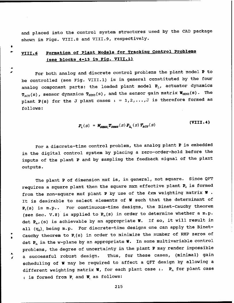
and placed into the control system structures used by the CAD package

shown in Figs. VIII.8 and VIII.9, respectively.

VIII.6 Formation of Plant Models for Trackina control Problems

(see blocks 4-13 in Fig. VIII.1)

For both analog and discrete control problems the plant model P to

be controlled (see Fig. VIII.1) is in general constituted by the four

analog component parts: the loaded plant model PL, actuator dynamics

TACT(s) , sensor dynamics TSENS(s) , and the sensor gain matrix WSENS(s) . The

plant P(s) for the J plant cases i = 1,2,...,J is therefore formed as

follows:

, s „ , V» / N (VIII.4) P*(S) = WSESS?aES3(8)PLi(s) TACT(S)

For a discrete-time control problem, the analog plant P is embedded

in the digital control system by placing a zero-order-hold before the

inputs of the plant P and by sampling the feedback signal of the plant

outputs.

The plant P of dimension mx£ is, in general, not sguare. Since QFT

requires a sguare plant then the sguare mxm effective plant P6 is formed

from the non-square mx£ plant P by use of the £xm weighting matrix W .

It is desirable to select elements of W such that the determinant of

Pe(s) is m.p.. For continuous-time designs, the Binet-Cauchy theorem

(see Sec. V.8) is applied to Pa(s) in order to determine whether a m.p.

det Ptt,(s) is achievable by an appropriate W. If so, it will result in

all (qüK being m.p. For discrete-time designs one can apply the Binet-

Cauchy theorem to Pt(s) in order to minimize the number of RHP zeros of

det P^ in the w-plane by an appropriate W. In some multivariable control

problems, the degree of uncertainty in the plant P may render impossible

a successful robust design. Thus, for these cases, (minimal) gain

scheduling of W may be required to affect a QFT design by allowing a

different weighting matrix W, for each plant case i. Ptt for plant case

i is formed from Pt and Wt as follows:

215

Pet =[PüL = Pi*i (VIII. 5)

•

For discrete-time control problems, each plant P,(s) is discretized

as each Pa, is formed. To discretize p,(s) an exact z-transform is

performed, followed by the z- to w- transformation resulting in w-plane

transfer functions, i.e.: "*■

Px(z) - Pl(w) (VIII. 6)

The QFT design process then proceeds in the s-domain for a continuous

design or in the w-domain for a discrete design using exactly the same

design steps unless stated otherwise.

The effective plant matrix P^ must have full rank, viz., controll-

ability and observability are assumed, and have diagonal elements that

have the same sign for all plant cases as a -* oo. These are conditions

that any of the usual LTI design techniques must satisfy (see Sec. V.8) ;

they are not unique to QFT. The CAD package therefore allows the sign

of the m diagonal plants to be examined for the J plant cases as a -» oo

in table form. The CAD package also allows the designer to list the

determinant of Pe, one plant case at a time.

A non-zero determinant is indicative of full rank. The numerator

factors of the determinant, which are zeros of the q^, are examined as

well. Thus, these determinants determine the m.p. or n.m.p. character of

the effective plants (<&),. If any Pa is unacceptable based on the above

criteria, the weighting matrix is revised, P^ is recomputed, and the

tests are applied again.

c

VIII.7 Inverse of Pr (see blocks 14 and 15 in Fig. VIII. 1)

The polynomial matrix inverse is performed using the Mathematica *

inverse function:

216

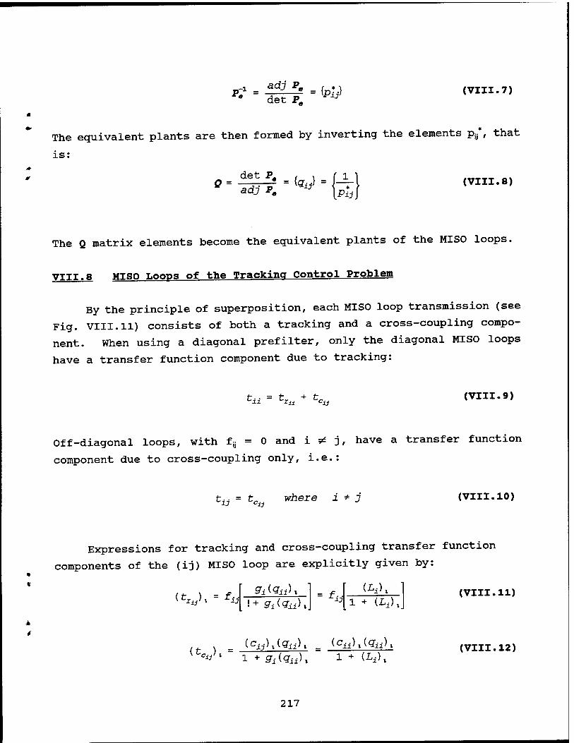
p* . *LZ - <Py det P.

(VIII.7)

* *•

The equivalent plants are then formed by inverting the elements p^*, that

is:

det P0

adj Pe = W = iy ta (VIII.8)

The Q matrix elements become the equivalent plants of the MISO loops.

VIII.8 MISO LOOPS of the Tracking Control Problem

By the principle of superposition, each MISO loop transmission (see

Fig. VIII.11) consists of both a tracking and a cross-coupling compo-

nent. When using a diagonal prefilter, only the diagonal MISO loops

have a transfer function component due to tracking:

ta = ^ + ^ (VIII.9)

Off-diagonal loops, with fs = 0 and i * j, have a transfer function

component due to cross-coupling only, i.e.:

£,•-,• = te„ where i * j (VIII.10)

Expressions for tracking and cross-coupling transfer function

components of the (ij) MISO loop are explicitly given by:

< fcx J i = f: *i] 13 Si(9ii)i

!+ 9iiQa), = fii

<£i>» 1 + (Li) ,

(VIII.11)

t

KZ^U l +sri(gii)1 i + Ui), (VIII.12)

217

where the index i specifies one of the J LTI plants, i.e., t = 1,2,

...,J, and where L; = g;qu. The cross-coupling effect input, a function

of all other controlled outputs, can be expressed by the equation:

cdj = - 2 m S **

Qik

(VIII.13)

13

9i

% '13

-1

22

%2 '22

133

33

93

133 '33

Fig. MI .11 3x3 MISO Equivalent Loops for External Output Disturbance (r = 0).

VIII.9 MISO Loops of External Disturbance Rejection Problem

For external disturbance rejection problems, each SISO loop

transmission (see Fig. VIII.11) consists of only a disturbance

component due to cross-coupling effects and the external disturbance

forcing function:

t,, = t. "ij a±i (VIII.14)

i

The transfer function Td relating the disturbance input of the (i,j) SISO

loop to its output, [see Eqs. (VI.27), (VI.30), and (VI.31)], is given

by:

4

218

*

_ (deii) Ma) > _ (deij)x(qn)x (VIII.15)

(C%)x 1 + ffiiqu), 1 + (I-i)»

where the index i specifies which LTI plant is being considered, i.e.,

i = 1,2,..,J, and where L; = g^. In comparing Eq. (VIII. 15) to Eqs.

(VI.25) through (VI.27) the following relationship holds:

P = Pe = (A + B)-1

The SISO loop disturbance input, a function of the external disturbance

input and all other controlled outputs (cross-coupling), is expressed

[see Eqs. (VI.31) and (VI.32)] by the equation:

m

wheie [P^Pd]^

fcJci

Qik (VIII.16)

is the (ij) element of the transfer function matrix product P^Pd-

VIII.10 O Matrix Validation Checks (see block 16 in Fig. VIII.1)

For analog and discrete tracking and external disturbance rejection

problems, the Q matrix elements are tested to verify that the condition

of diagonal dominance is satisfied. If diagonal dominance holds for all

plant cases, then a QFT Method 1 design may be used. Otherwise, a QFT

Method 2 (improved method) design must be used. If the results of this

test are not satisfactory, then the weighting matrix W can be modified,

and the Q matrix recomputed.

Additional tools for examining the equivalent plants qü of the Q

matrix include a Bode plot function and a transfer function display

* subroutine. The Bode plot for a Q matrix element can be displayed for

a specified set of plant cases or for all J plant cases together. The

Bode plot for the set of J plant cases is useful for displaying

219

variation in equivalent plant transmission as an aid in selecting

representative template frequencies. Also, the CAD package allows the

Q matrix transfer function elements to be displayed in factored form for

any selected plant case.

To reduce the order of the Q matrix transfer functions the package

performs automatic pole/zero cancellation, canceling nearly identical

pole-zero pairs based on a user specified ratio of the distance between

the pole-zero pair to the distance of the zero from the origin in both

the right-half and left-half plane.

VIII.11 Improved Method (see blocks 19 and 20 in Fig. VIII.1)

The improved QFT Method 2, takes into account any correlation

between the uncertainty in the designed MISO loops and the next row of

MISO loops for which a design is to be performed. The standard approach

of QFT Method 1 assumes worst case conditions and does not take this

design information into account. The improved method requires the

derivation of the equivalent q plant transfer function for the next MISO

loops yet to be designed. For both tracking and external disturbance

rejection problems, the new set of transfer functions required by the

improved method are generated using the equation:

Qijein+l) Qijeln) 1 + Lk

1 + Lk - Y * ' ij (n) .

(VIII.17)

where the compensator gk for row k of the MISO loops has been designed (Lj. is known) , and where:

ijc = S^juteta, (VIII. 18)

Yiiw = q**™q&™ (VIII. 19)

and q^o) = q^ are generated during the matrix inversion of Pe. The

220

*

m

*

>

»

4

number in parentheses in the subscript of the improved method plants

indicates the number of times this method has been applied to generate

the plant transfer function. For example, the plant qkke(Xi is obtained by

applying the improved method once, and qije(n) in Eq. (VIII. 17) is obtained

after applying the improved method n times, (i.e., n compensator

elements of the matrix G were designed, and the improved method was

applied after each design is completed.) Improved method plants are

generated for all plant cases and for each row of MISO loops for which

the compensator has not yet been designed. The notation k on 1^ is not

to be confused with the standard notation i on L=. The notation k, as

used here, denotes the index of the loop most previously designed, i.e.,

k = i-i if loops are designed sequentially.

VIII.12 Specifications (see blocks 17 in Fig. VIII.1)

VIII.12.1 Stability Specifications

A stability margin is specified for each row of MISO loops. The

stability margin may be specified in terms of the gain margin gm, the

phase margin angle 7 or the corresponding ML contour. The two remaining

specifications are calculated from the one specification that has been

entered. Only the ML contour stability specification is stored in

memory.

VIII.12.2 Trackina Performance Specifications

Frequency domain performance specifications are defined in the form

of LTI transfer functions. For the diagonal MISO loops upper and lower

bounds are specified as follows:

* ai± <; \tu\x <; bu for i = l,2 J (VIII.20)

' For the off-diagonal MISO loops the following upper bound is specified:

221

It^SJbjy fox 1 = 1,2,...,J" (VIII. 21)

VIII.12.3 External Disturbance Rejection Performance Specifications

For all MISO loops the following upper bound is specified:

\tti\x <. b±j for i*j, 1 = 1,2, ...,<J (VIII.22)

This upper bound is determined based upon Eqs. (VI.46) and (VI.47) in

Chapter 6. (Note that upper case letters for the bounds are used

therein.)

For analog design problems, all performance specifications are

defined as s-domain transfer functions. In the case of a digital

control problem, the performance specifications are approximated in the

bandwidth of interest by making the substitution s -»• w. If the sampling

rate is not sufficiently high for the above assumption to hold, the

s-domain transfer functions yielding the desired performance specifica-

tions, are transformed to the z-domain and then transformed into the

w-domain.

VIII.12.4 Gamma Bound Specifications

The improved method requires the derivation of the effective q

plant transfer function, i.e. Eq. (VIII.17). By proper design of each

compensator gk, new RHP poles will not be introduced in qüe. By requiring

the magnitude of the denominator of Eq. (VIII. 17) be larger than a small

value ek, sign changes in the denominator are prevented and new RHP poles

are not introduced. This constraint is given by:

e* <; |i + Lk - Yyl (VIII.23)

A unique minimum value ek is specified by the designer for each of the

k = l,2,...,m channels.

222

VIII.13 Bounds on the NC (see block 23 in Fig. VIII.1)

For a given row i of MISO loops, and for a template frequency w =

a);, several bounds may be included in the set plotted on the NC. These

bounds include a stability bound, an allocated tracking bound, cross-

coupling bounds, external disturbance bounds, and gamma bounds when

using the improved method. The allocated tracking and cross-coupling

bounds are generated such that the proper reduction in overdesign is

achieved when using the improved method. This set of bounds can be

replaced by a single composite bound before beginning a design.

VIII.13.1 Stability Bounds

A stability bound is generated for each template. The stability

bounds constrain the maximum closed-loop transmission of the MISO loop

with unity gain prefilter to have a bounded magnitude of:

S^SiiK 1 + ffi^ii)y

£ Mr (VIII.24)

The bound is plotted for a given frequency by plotting the path of the

nominal point while traversing the ML contour with the template generated

for that frequency.

VIII.13.2 Cross-Coupling Bounds

For tracking problems, cross-coup ling bounds are generated for each

template, one for each off-diagonal MISO loop in the row of MISO loops

for which the compensator is to be designed. Each bound is generated

based on the constraint:

'iil 'Ü 1 + LJ <L b

3-3 for i * j (VIII.25)

223

which is a function of all other cross-coupling controlled outputs. The

specifications dictate that c;j is less than an upper bound for each plant

case i: *

m (ICijLxK = 7

S , k*j [ Iffikli.

(VIII.26)

When the improved method has been applied, overdesign is substantially

reduced by modifying Eq. (VIII.26) as follows:

Lk, fkj unknown

Jkj\

\<3ik(a) + k*ifor

Lj-tf^ unknownl Wikia) u. JJc' ^kj

-kj\

(VIII.27)

where fkj = 0 when k ^ j for the case of a diagonal prefilter F required

by the MIMO QFT CAD package.

Based on Eqs. (VIII.25) - (VIII.27), a lower bound is placed on

ll + L:| as follows:

|1 + L±\ * lgijLaxlgiil \b±j\

(VIII.28)

By substituting L} = 1/m into Eq. (VIII.28), the latter is transformed

such that the bound is plotted on the inverse NC, i.e.,

m 1 + m (I ci* Lax)» I ffii 11

(VIII.29)

Equation (VIII.29) is the basis upon which the cross-coupling bounds on r

Lio are generated. The bounds are generated such that the correlation

between m and qü in Eq. (VIII.29) is properly taken into account over the A

range of the plant parameter uncertainty which is outlined by the

template when the nominal loop transmission does not violate these bounds.

224

* it

VIII.13.3 fiamma Bounds

Gamma bounds are generated for each template, where the compensator

for row j is to be designed after the compensator for row i of the MISO

loops is designed. It is desired that the magnitude of the denominator

of the effective plant q22e calculated using Eq. (VIII. 17) for an improved

method design, not be smaller than a specified minimum value despite

plant uncertainty. Thus, the gamma bound is generated based upon

satisfying:

|1 +J4-T«! *•* (VIII.30)

where I* and 7^ are given, respectively, by Eqs. (VIII. 18) and (VIII. 19).

Satisfying the constraint in Eq. (VIII.30) prevents a sign change

(preventing the introduction of RHP poles) in the characteristic

equation of the improved method plants' of Eq. (VIII. 17). This enhances

the ability to design a stabilizing compensator for each successive

feedback loop. Given the range of plant uncertainty defined by the

templates and variation of 7^ among the plant cases, each gamma bound is

generated such that Eq. (VIII.30) is satisfied when the nominal loop

transmission Lio does not violate the gamma bound.

VIII.13.4 Allocated Trackina Bounds

For tracking problems, allocated tracking bounds are used to

insure that variation in closed loop frequency domain transmission tü of

the diagonal MISO loop does not exceed the variation <SR permitted by the

performance specifications. Variation in the closed loop transmission

of the diagonal MISO loop results from both uncertainty in the response

* due to tracking and from the presence of the cross-coupling effects:

tu = t,« + tc« (VIII.31)

*

where tÄ and t^ are given, respectively, by Eqs. (VIII. 11) and

(VIII. 12). The constraint on Lj used to determine a point on the

225

tracking bound is:

LmiTj, + tc ) - Lm(T„ - t_ ) <; 8Ä (VIII.32) •"max ciiaax ^min ^liasx R

where the transmission TR, with unity gain prefilter, is:

TD = —— (VIII. 33) R 1 + L±

and the most extreme transmission due to cross-coupling effects is:

= |gfi,J 1^1 (VIII.34)

Because points on the cross-coupling bound (if generated) are identical

to those on the allocated tracking bound for the value of c^ in Eq.

(VIII.34), only an allocated tracking bound is generated for diagonal

MISO loops. By constraining L; to be above the bound, the actual

variation in t:; is less than t . -ii

VIII.13.5 External Disturbance Rejection Bounds

External disturbance bounds are plotted for each template, one for

each MISO loop in the row of MISO loops for which the compensator is to

be designed [see Eqs. (VIII.14) and (VIII.15)]. The disturbance

entering the (ij) MISO loop resulting from the external disturbance

entering through Pd and from the cross-coupling transmissions is given

by Eq. (VIII. 16). The specifications dictate that de^ is less than an

upper bound for each plant case t in the set of J plants; i.e.:

m I**,! Iffttk

(VIII.35)

For a Method 2 design in which the improved method has already

been applied, (say n times so far) the calculation of

226

*

X

(KJmax),

is modified as follows: by replacing the term | tkj| / |q^11 in the summation

above (a) with | by | / | q^ 11 which is utilized when the improved method has

not yet been applied, and (b) with

Igt^P«1]*;! (VIII.36)

when the improved method has been applied to take into account the

designed open loop transmission I*.

VIII.13.6 Composite Bounds

A set of composite bounds is formed based on any or all of the

tracking, stability, cross-coupling effects, external disturbance

rejection, and gamma bounds. The composite bound for a given frequency

is formed by retaining the most restrictive portion of the bounds for

the given frequency for which the composite bound is formed.

VIII.14 compensator Design (see blocks 24-25 in Fig. VIII.1)

The compensator for an analog system (a controller for a discrete

system) is designed to satisfy design specifications for the entire row

of MISO loops in which the compensator is used. Since Lj0 = g^o is the

same for all MISO loops in a given row, bounds for all MISO loops are

plotted together on the NC. The compensator design may thus be

performed for an entire row of MISO loops using a single design

iteration based on composite bounds plotted on the NC.

The open-loop transmission is shaped by adding, deleting, or

modifying the poles and zeros of the compensator and by allowing

> adjustment of the gain until an acceptable loop shape is obtained.

Stabiliy is checked during loop shaping by examining the nominal closed-

loop MISO transmission in factored form. All closed-loop s- or w-domain

227

poles should be in the left-half-plane. For a discrete design, g;(w) is

transformed by a bilinear transformation to g;(z). As a validation

check, the Bode plots of g;(w) and g;(z) are compared for 0 < o> <

2/3(ws/2). If very close, then one can proceed, since robustness will

be maintained in the z-domain. Next, proceed with the formation of A;(z)

= Li(z)/[1 + L;(z)] in order to ensure that all the poles of Aj(z) are

inside the unit circle (see block 26 in Fig. VIII.1). If not, q{ needs

to be modified in order to achieve a stable system for all cases.

VIII.15 Prefilter Design (see block 28 in Fig. VIII.1)

The proper design of the compensator guarantees that the

variation in closed loop transmission due to uncertainty for tü is

acceptable, but does not guarantee that the transmission is within the

upper and lower performance tolerances aü and bH. The prefilter is

therefore required to translate the closed loop transmission tü such that

it satisfies the upper and lower performance tolerances.

The prefilter design begins with the determination of TR,^ and TR,^,

the maximum and minimum closed loop transmission due to tracking TR with

unity gain prefilter, respectively, at each template frequency W; using

Eq. (VIII.33). As is the case for tracking bounds on the NC, a portion

of the permitted range of variation of tü is allocated to the cross-

coupling effects. Thus, restricted tolerances are placed on tri

i>u=i>u- |tCiiJ (VIII.37)

aii=aii + \tc I (VIII. 38)

and the filter bounds on the nominal tri are as follows:

*

*

Lm (jbii) - Lm (r^J (VIII.39) t

Lm (a'a) - Lm (T^J (VIII.40)

228

r

Once the filter bounds are generated, a prefilter is synthesized

such that the Bode plot of the nominal tri lies between the two filter

bounds and satisfies tri(s) = 1 in the limit as s -> 0. For a discrete

design, F(w) is transformed by a bilinear transformation to F(z). As a

validation check, the Bode plots of F(w) and F(z) are compared for 0 <

a < 2/3(OJS/2) (see block 29 in Fig. VIII.1) . If very close, then one can

proceed, since robustness will be maintained in the z-domain.

VIII.16 Design Validation (see blocks 25-31 in Fig. VIII.1)

The CAD package provides a number of tests to validate that the

completed MIMO design meets the stability and performance specifications

for the J plant cases. First (block 27), poles of 4 for each feedback

loop i are checked to validate that all poles of the characteristic

equation are stable. If some plants are n.m.p., one cannot rely on the

loop shapes on the N.C.

For the second test (block 31) , an array of the J open-loop MI SO

loop transmissions (L;)t = g^cfe), for all plant cases i = 1,2,...,J are plotted on the NC along with the ML contour to validate that the

stability requirements are satisfied for each feedback loop i. If no

open loop transmission violates the ML contour, then the stability

specifications are satisfied.

For tracking control problems an mxm array of Bode magnitude plots

is generated for the mxm matrix of elements t;j of the closed-loop

transfer function matrix T, where:

T = [J + Pe&\-xPeGF (VIII. 41)

where I is the identity matrix, and Pe, F, and G are the mxm plant

matrix, the mxm diagonal prefilter matrix, and the mxm diagonal

compensator matrix, respectively.

Each Bode plot illustrates the frequency domain transmission t;j/ for

the set of J plant cases along with the tracking performance

229

specifications, to allow the designer to validate that performance

specifications placed on the closed-loop system have been met over the

frequency range of interest. For each diagonal tü, J Bode magnitude

plots are plotted along with the performance bounds a„ and bü. For each

off-diagonal ty, J Bode magnitude plots are plotted along with the

performance bound b^.

For external disturbance rejection problems, a set of J Bode

magnitude plots are plotted for each t;j, along with the external

disturbance rejection specifications by. The mxm closed-loop transfer

function matrix T, whose elements ty are the transmissions plotted on the

Bode plots, is formed for the J plant cases based on the equation:

T = [J + PjS\^Pa (VIII. 42)

where I is the identity matrix, and Pd, Pe, and G are the mxmd external

disturbance plant matrix, the mxm effective plant matrix, and the mxm

diagonal compensator matrix, respectively.

For the final validation, MATLAB SIMULAB models are generated based

on the completed design, one for each of the J plant cases. The

designer can then insert nonlinear elements such as saturation or rate

limits, and add anti-windup protection. The model is then simulated to

verify that the time domain figures of merit specifications are

satisfied. For a continuous control problem, an analog simulation is

performed. For a discrete control problem, a hybrid simulation is

performed based on the s-domain effective plants P^Cs), and the z-domain

compensator G(z), and prefliter F(z).

VIII.17 Summary

*

v

Version 3 of the MIMO/QFT CAD package has been developed for both

analog- and discrete-time control system design based on Mathematica.

The design procedure is automated. This includes problem setup, *

equivalent plant formation, compensator and prefilter design and design

validation for mxm MIMO systems. Bound generation routines have been

230

*

optimized to reduce overdesign. The package has been extended to handle

in a unified way external disturbance rejection problems as well as c tracking control problems.

* r

231

CBapter IX Development, Implementation & Flight Test Of A Mimo Digital

Flight Control System For An unmanned Research Vehicle

IX.1 Introduction

The intent of this chapter is to provide the reader with an insight

into the development of a QFT FCS and into the trials and tribulations

in achieving successful flight tests. In this respect, this chapter is

different from most papers that concentrate only on the theoretical

aspects of a flight control system design. Thus, a discussion of the

development, implementation, and successful flight test of a flight

control system, designed using QFT techniques, is presented in this

chapter. The flight control system was designed for and flown on the

Lambda Unmanned Research Vehicle (URV), Fig. IX.1. It is a remotely

piloted aircraft with a wingspan of 14 feet. It is operated by Wright

Laboratory for research in flight control technology .

A

j «@»

7V

USAF

k o Fig. K.1 Lambda unmanned research vehicle.

4

232

IX.2 Objective

The objective of the project was twofold. First, develop a robust

flight control system using QFT, and take the design through flight

test. Second, implement an inner loop FCS on the Lambda URV that would

be part of an autonomous flight control system. During the project the

first objective was accomplished and then, because of hardware improve-

ments, a second design was developed and flight tested. This second

design was accomplished to better meet the requirements of the second

objective. The FCS design process used is shown in Fig. IX.2. As

indicated by the heavy dashed line one complete FCS design cycle covers

the process through the flight test and then back to the redesign stage.

During this project there were four cycles around this loop. Two of the

cycles produced unsuccessful flight tests and two produced successful

flight tests.

Flight Control System f Design -Cycle

Fig. K.2 Flight control system design process.

233

IX.3 First Design Cycle

IX.3.1 Requirements

There were two major design requirements for this project. The

first was a desire to develop a robust flight control system using QFT,

and take the design through flight test. The second was a need for an

inner loop FCS on Lambda that would interface with a autonomous waypoint

directed autopilot.

IX.3.2 Specifications

The time response specifications were selected base on the open

loop response of Lambda. The pitch rate is an underdamped response that

settles fairly quickly. Overshoot and settling time were chosen to be

25% and one second for pitch rate response. Roll rate is an over-damped

response that settles quickly, and the settling time was chosen to be

one second. Yaw rate is also underdamped, but it doesn't reach steady

state as fast as the other two. Yaw rate overshoot and settling time

were chosen to be 15% and two seconds, respectively. These specifica-

tions were transformed into thumbprints.

IX.3.3 Aircraft Model

The aircraft model developmental process began with the use of

Digital Datcom, a computer program which predicts stability and control

derivatives for aerospace vehicles based on the physical characteristics

of the vehicle. Datcom information formed the baseline model of the

aircraft. This baseline model was refined by using system identifica-

tion software to estimate the aerodynamic derivatives from actual flight

test data74. Maximum likelihood identification was used to identify the

natural frequency and damping ratios of the short period and roll modes.

This information combined with the Datcom information provided a working

model for the flight control system design. *

« r

234

*

IX.3.4 FCS Design

Much of the preliminary QFT design work was accomplished at the Air

Force Institute of Technology56-78. The first56 was based on the DATCOM

model of lambda alone. The second78 design was based on the DATCOM model

with the refinements made with system identification. The latter design

used linearized transfer functions to represent Lambda in various flight

conditions, covering the entire proposed flight envelope, to accomplish

the design and for linear simulations.

IX.3.5 Linear Simulations

All FCS designs were simulated using MATRIXX and linear time

invariant state space models representing the full flight envelope of

Lambda. After successful linear simulations, nonlinearities such as

control surface travel limits were introduced into the linear

simulation.

IX.3.6 Nonlinear Simulations

During the same period, a nonlinear simulation was developed at

Wright Laboratory. This simulation incorporated a six degree of freedom

simulation, automatic trim calculation, air vehicle kinematics, and

control surface saturation. While this design produced the desired

responses in the linear simulation, when implemented in the nonlinear

simulation, the original control system exhibited undesirable behavior.

The assumptions about allowable gain had been made that were not valid

and had to be corrected. Thus, the allowable gain was modified to

obtain the redesigned controller.

IX.3.7 Hardware-in-the-Loop Simulation

Software from the nonlinear simulation was used to develop a

hardware-in-the-loop simulation65. This simulation allowed the

* implemented FCS, which was programmed on a EPROM chip, to be tested in

the aircraft. When the FCS was implemented in this simulation, it was

discovered that the angular rate sensors had high levels of noise, on

235

the order of 0.5 deg/sec. The FCS amplified this noise and this

effectively masked any control command signal. The noise was recorded

and incorporated into the nonlinear simulation. By this time, a new QFT

computer-aided-design program was developed by AFIT for designing

control systems which allowed for a rapid redesign to minimize the noise

problem. The FCS was redesigned, tested in all three simulations and

then test flown.

IX.3.8 Flight Test

Two major difficulties caused the first flight test to fail, the

first was reversed polarity on an angle sensor and the second was a

integrator wind-up limiter scheme that did not work. Since the inner

loop FCS was to be implemented as a part of an autonomous system, turn

coordination logic was implemented around the inner loop FCS that relied

on the roll angle. Post flight analysis of the flight test video and

data showed that the polarity of the roll angle sensor was backward,

thus, when the aircraft was commanded to bank, the rudder was commanded

to deflect in the wrong direction. The FCS was turned off and testing

involving the lateral control channel was terminated. Later, during the

same flight test, when the FCS pitch channel was turned on, the aircraft

developed a high pitch rate. This test was terminated and post analysis

revealed that the scheme used to limit integrator wind-up had caused a

numerical instability.

IX.4 Second Design Cycle

IX.4.1 Requirements

The requirements for the second design cycle did not change from

the original requirements. An additional requirement involved the *•

design of an improved integrator wind-up limiter.

A. IX.4.2 Specifications »

The specifications for the second design cycle did not change from

the original requirements.

236

•

IX.4.3 Aircraft Model

The aircraft model for the second design cycle did not change from

the original requirements.

ix.4.4 res Design

Since the problems encountered in the first test didn't have

anything to do with the QFT designed FCS, the FCS remained unchanged for

the second flight test. During the second flight test, there was no

attempt to use a turn coordination algorithm. The implementation

involved a major change in the FCS design. The integrator wind-up

limiter involved a different form of implementation for the second

design cycle. In this cycle the FCS's controller was implemented by

factoring the s-domain compensator Gc(s) into poles and zeros, i.e.,

grouping individual poles with zeros to form w first- or second-order

cascaded compensators, which are then transformed individually into the

z-domain (see Fig. IX.3). The individual z-domain transfer functions

were each then implemented to obtain the complete FCS transfer

functions. This implementation allowed limitations to be placed only on

those pieces of the FCS that contained pure integrators. Also, it

provides a higher degree of accuracy in the software implementation.

IX.4.5 Linear. Nonlinear. Hardware-in-the-Loop Simulation

All simulations consisted of checking out the new implementation of

the FCS. There were no problems encountered during any of these

simulations.

IX.4.6 Flight Test

On 20 Nov 92, the temperature was in the 60s with winds at five to

seven mph. Lambda was flown stick to surface for take-off, setup, and

V landing. Due to problems with the first flight test the FCS was engaged

only during the test maneuvers and disengaged. The maneuvers performed

consisted of unit step commands in all three axes. This set of

237

!(«)- ÜClS) D(s)

0(s)

(a) The designed compensator

I(S)- Gi(s)=Tui)

0,(8)

Gw(s)= Nw(s)

wV ' Dw(s)

Ow(s)=0(s)

(b) s- domain w cascaded compensators

l(z)- 0,(2)

0,(3)

Gw(z) 0w(z) = 0(z)

(c) z-domain w cascaded controllers

Fig. K.3 s - domain to z - domain formulation for implementation of the G(z) controller.

o 0) co ■L a> a ■ a a» a» u D> <v

■D

a» 10 c o a n (V tx

40

30

20

10

0

-10

-20

q (pitch rate)

: TRUq (upper)

: TRLq (lower)

-30

/ / /

///

<'! -t-?i—

V^.-.tffWjU»^

12 V

' ' ' ' I ' ' ' ' I ' ' ' ' ■ ■ ' 10 11 12 13

time (sec) 14 15

Fig. K.4 Response to pitch-down command.

maneuvers was first performed with the QFT FCS and then with the open

loop aircraft. The response of the controller was very good in that it

performed as it was designed. Figure IX.4 represents the response of

Lambda to a step pitch down command. The dotted lines in the plot

represent the specified response thumbprint. It is important to note

that during this maneuver the aircraft covered most of its flight

envelope by varying in forward airspeed from 75 kts to 110 Jets.

238

* ^

% V

IX.5 THIRD DESIGN CYCLE

IX.5.1 Requirements

The requirements for the third design cycle had not changed from

the original requirements. This cycle involved the design of an inner

loop FCS that had intrinsic turn coordination. After the second flight

test, the sensor noise problem had been reduced by an order of magnitude

by the addition of a hardware noise filter on the output of the sensors.

This allowed a redesign of the FCS to improve the system performance.

IX.5.2 Specifications

Sideslip Command For this iteration of the design a sideslip angle command was

incorporated as part of the inner loop controller. Since Lambda has a

sideslip sensor, a sideslip command was used to cause the aircraft to

intrinsically fly coordinated turns. That is, the goal of turn

coordination is to reduce the amount of sideslip angle during a turn by

using the proper amount of rudder deflection during the turn.

Yaw Damper Changing to sideslip command allowed the use of the yaw rate sensor

to implement a yaw damper to reduced the phugoid mode oscillations.

This yaw damper was implemented by adding a- washout filter, designed

through the use of a root locus plot. The yaw damper was designed and

then incorporated in the aircraft model for a FCS design.

Specification Change During the second flight test the pilot felt that the aircraft's

roll rate response was too slow. Therefore, the roll rate response was

change to match that of the pitch rate.

IX.5.3 Aircraft Model

Sensor Improvement After the second flight test, the problem of sensor noise was

239

fixed, reducing the noise by an order of magnitude.

Model Refinement

During the system identification work for the second aircraft

model, some of the parameters had been scaled incorrectly. This caused

some modeling errors. After the second flight test these errors were

corrected through the use of system identification applied to flight

test data.

IX.5.4 FCS Design

MATRIXX was used to develop linearized plant models about flight

conditions in the flight envelope. An attempt was made to choose flight

conditions in such a way as to fully describe the flight envelope with

the templates. To do this a nominal flight condition was chosen to be

50 kts forward velocity, 1,000 feet altitude, 205 pounds, and center of

gravity at 29.9% of the mean aerodynamic cord. From this nominal trim

flight condition, each parameter was varied, in steps, through maximum

and minimum values, while holding the other parameters at their nominal

trim values. These variations produced a initial set of templates. On

these templates variation corresponding to each parameter was identi-

fied. Each variation when translated, on the template, identified an

expanded template area of the flight envelope that required more plants

for better definition, see Fig IX.5.

IX.5.5 Linear, Nonlinear, and Hardware-in-the-Loop Simulations

The refined Lambda model was implemented in all three simulations.

The FCS was implemented in cascaded method outlines previously. All

simulations produced the desired responses to given stimulus.

IX.5.6 Flight Test

aircraft exhibited an uncontrolled pitching, or porpoising, behavior.

While the post flight test analysis was inconclusive, a longitudinal

bending mode at 13.2 radians/second seemed to be the likely cause.

j

*

a

During the third flight test, when the FCS was engaged, the * t

240

A

0) ■ö 3

C o (0

O nominal variation cases • extended cases

/ \ variation in parameter #1 /""\ variation in parameter #2

x^TTp initial template

expanded template

Nominal Flight Condition

Phase

Fig. EL5 Template expansion process.

IX.6 FOURTH DESIGN CYCLE

IX.6.1 Requirements

The requirements for the Second flight test had not changed from

the original requirements, but involved a refinement in the aircraft

model to incorporate a bending mode.

IX.6.2 Specifications

The specifications for the fourth design cycle were the same as

those for the third.

IX.6.3 Aircraft Model

i A model of the porpoising behavior encountered in the third flight

test was identified by assuming that the behavior was caused by an

unmodeled effect. Various models were incorporated into the nonlinear

model and simulated. This simulation used the flight test inputs as

241

■w

simulation inputs and compared the simulated outputs to the flight test

data. Using this procedure, a violation of the gain margin was ruled

out by increasing the inner loop gain in the model and observing the ■* response. Instability caused by actuator rate limiting was ruled out by

inserting severe rate limited actuator models in the nonlinear

simulation. When a bending mode, modeled as a lightly damped pair of s

poles, was inserted in the model, the simulated responses were very *

similar to the flight test results.

IX.6.4 FCS Design

MATRIXX was used to develop linearized plant models about the given

flight conditions and the FCS was redesigned based on the model

containing the bending mode. Note, when the FCS from design cycle three

was inserted in the loop with the aircraft model with the bending mode,

there were violations of stability criteria in the frequency domain.

IX.6.5 Linear, Nonlinear, and Hardware-in-the-Loop Simulation

The new model was implemented in all three simulations and tested.

The new model was tested with both the FCS cycle 3and the FCS cycle 4.

As expected the porpoising behavior occurred with the FCS cycle 3. The

FCS cycle 4 responded within specifications.

IX.6.6 Flight Test

The fourth flight test occurred in September 1993. The field

conditions were a little gusty, but within acceptable limits for the

experiment. During the flight the FCS was engaged and then left engaged

for the entire series of tests. The FCS performed as designed. The

intrinsic turn coordination scheme worked as designed. The pilot was y

pleased with the handling qualities and felt comfortable flying with the

FCS engaged at all times. His one criticism was that the roll rate was

too slow. Since our roll rate was limited by the maximum roll rate v

detectable by the rate sensors, the problem was unavoidable. When the

data was examined, it was found that all of the 60 hz data had been

242

data showed that the FCS did cause Lambda to respond within the

specified envelope, during onset of the command, but, in some cases,

Lambda's response exhibited more overshoot and longer settling time than

^ specified. These problems could be attributable to the gusty

conditions, since no gust disturbance was specified during the design

process. More flight testing of this FCS will be required to answer

it. this questxon.

IX.7 Conclusions

This series of FCS design cycles has highlighted many of the

benefits of using a robust design technique, such as QFT, to design and

implement FCSs. Some of those benefits are:

a. The result is a robust design which is insensitive to plant

variation.

b. There is one design for the full envelope (no need to verify

plants inside templates).

c. Any design limitations are apparent up front.

d. There is less development time for a full envelope design.

e. One can determine what specifications are achievable up early

in the design. One can redesign for changes in the

specifications quickly.

f. The structure of controller is determined up front.

* The goals of this program were to reveal the benefits of QFT as a robust

control technique, and to prove that a robust flight control system

could be implemented. It is felt that these goals were successfully

** achieved.

243

Appendix A Design Examples

A.l MISO Design Problem

Given the plant transfer function:

k Pis) = s + a

with the structured parameter uncertainty of

1 <. k <; 100, -3 <; a <; 3

Specifications on |TR(JO>) | is given in the following table:

Cd 0 0.5 1 2 5 10 20

Lm b(jco) 0 1 1 0 -4 -10 -20

Lm a(jcj) 0 -2 -4 -8 -20 (-40) oo

(-80) oo

ML < 3 dB X > 3 No specifications on TD

Nominal Plant: P0(s) = 1/s (k = 1, a = 0)

Problem: Design L0(s) and F(s) to meet the specifications.

Solution:

A. Template Generation — The set of J plant transfer functions P^a^lq) ,

where Pf e (P and i = l, 2, ... , J, used to obtain the templates are:

P!(3,l), P2(0,1), P3(-3,l), P4(-3,100), P5(0,100), and P6 (3,100 )

The templates all have the shape shown in Fig. A.l where V = 40 dB and

as &) increases the templates become narrower. It is left to the reader

to obtain the templates in order to verify the solution to this problem.

244

«

V=40dB y>,(jo>,)

Rg. A.1 Template SP^jOO,)

B. Determination of Boundaries BJia) — The templates are used to

determine the boundaries BR(ju;) and, along with the values of Lm ML and

V, to determine the U-contour as shown in Fig. A.2.

C. Determination of L„fs) The design of an optimum L0(s) is not

unique. Two possible designs of an L0(s) are shown in Fig. A.2. The

designs at the onset should be based upon a qualitative analysis of

L(s) = G(s)P(s) = ^G(g) s + a

(A.l)

* *

and

245

»

* *

200° -180° -160° -140° -120° -100° -80° -60° -40° -201

Fig. A.2 Plots of BR(jOO,) and Lo(j(ü)

246

-*

*•

•

LAS) = G(S)P0(S) = = kG^ (A.2)

s

Trjal i — A type 0 L0(s) function requires the compensator to be

of the format of:

G{s) ~ "i nn r

which from Eqs. (A.l) and (A.2) results in, respectively:

Llg) = *g< > "• ( > (A.4) L{S) (s + a) ( ) - ( )

and

L {s) = Ml LJ^J I (A.5)

When a ^ 0, Eq. (A.4) results in

r^(s, = *&l ) > "( < } ]F(s) (A. 6)

and im ^(jw) = - » dB which is unacceptable.

Trial 2 — A Type 1 L0(s) requires the compensator to be of the

format:

Gi8) = £1 LzJ L (A.7) GKS) ()••()

which from Eqs. (A.l) and (A.2) results in, repectively:

L{g) = **< )_^J > (A.8) L{S) (s + a) ()•••( )

and

L {s) = m >_ij i (A.9)

* When a = 0, TR(s) corresponds to a Type 1 system and when a * 0 TR(s)

corresponds to a Type 0 system. Assuming this is acceptable an L0(s) is

synthesized, as shown fn Fig. A.2, and results in

247

Gl v = 8.504xl06(s + 1) (s + 12) (S + 120) (A 1Q) (S + 2) (S + 10) (s + 26.5) (S + 720 ± JS50)

In order to achieve the desired specification e(°o) = r(a>) - c(») = o,

for r(t) = u.i(t), then the compensator G(s) must be a Type 1 transfer

function in order to yield a Type 1 system for a ^ 0 and a Type 2 system *

for a = 0. The synthesized loop transmission function is

= W ) - ( ) (A.11} °> s2 ()•••( )

for which three points (denoted by X) are shown in Fig. A. 2. It is left

to the reader to complete the synthesis of an L0(s).

D. Design of Ffs) Based upon the design procedure in Chap. I15, the

following nonunique filter Is obtained:

F(s) = 1-5 c (A.12) s + 1.5

E. Simulation of Design A simulation of the system for L0(s) is made

for each P^a^) , where i = 1,....,6, based upon Eqs. (A.10) and (A.12).

The simulations indicate that all the specifications on |TR(j«)| are met

except, as expected, when a 5* O and co = 0. The reader can simulate the

system utilizing his L0(s) .

A

« y

248

A.2 MIMO Design Problem

Given: A 2x2 plant where

Q(s) = JL S

•^11 ^12

■^21 "^22

(A. 13)

has the following independent structured plant parameter uncertainties:

1 <; kzl <; 2

5 s k21 <> 10

0.5 <. k12 <; 2

0.5 z k22 z 1

The diagonal dominance condition (Sec. III.7) requires, as o - ~, that

|ffii««| <|5i2ff2i| - 2 < 2.5

Specifications:

(a) There is only one command input: r2(t)

(b) |t12| < -20 dB for all w

(c) For |t22|:

Table A.l

0) 0 0.5 1 2 5 10 20

Lm b22(jo) 0 1 1 0 -4 -10 -20

Lm a22(jw) 0 -2 -4 8 20 —00

(-40) —oo

(-80)

» The values of a22(ju) are considered to be zero for w > 5, and thus

4

Lm £s ta»^'")] - -

(d) For Lj = gjqn and L2 = g2q22, respectively:

249

Lm ML < Lm

Lm M, < Lm

1 + L, < 3 dB

1 + i, < 3 dB

(A.14)

(A.15)

»

tr

Problem: Design LK(s) , L2(s) , and f22(s) .

A. L^js) Design For loop one design, see Fig. A.3, let f12 = 0

(i.e., decouple output 1 from input 2). With fn = 0 then the loop 1

design becomes strictly a cross-coupling rejection problem (see Fig

III.11).

Fig. A.3 Loop one

Thus, from Eqs. (III. 35) through (III. 41) and Eqs. (III.53), where for an impulse input t^ = y^-:

(III.50) through

tu -

u

gll(%^12 + C12> = gllC12 1 + gr,gn 1 + g1gn

(A.16) * y

Based upon the given disturbance rejection specification

250

-12 1 gnci2

1 + 9&n < 0.1 (A.17)

which is rearranged to

i + sr,g„| ^ <Inci2 0.1

(A. 18)

Since

c12 = -t22/g: 22 (A. 19)

Equation (A.19) is substituted into Eq. (A.18) to yield

11 + STiSii I ^ <?12

(A.20)

Applying the maximum tracking specification value for ItJ yields:

|1 + gtful * lOJb^g,,

^12

(A.21)

i

Thus, this constraint imbeds the cross-coupling rejections bounds

specifications on y„(t). As a consequence the cross-coupling bounds

B (ja,) become the composite bounds B0(>,.) • For the plant uncertainty

a template can be generated for qu which is good (for this particular

design problem) for all a. The template is simply a 6 dB vertical line.

Also, from the specification Lm M^ < 3 dB and the uncertainty in qu at

a, = oo, the universal high frequency boundary can be drawn as shown in

Fig. A.4. The nominal plant qn is chosen to be the i which is at the

bottom of the 6 dB template. Thus,

<?u(s) = - (A.22)

251

a *

Fig. A.4 L| (s) design A

252

Generally, for lower values of oo, since |giqn| » 1 then Eq. (A. 21) can

be simplified to:

1*1 * lOJb. 22

STl2 (A.23)

» Multiplying both sides of Eq. (A.23) by qu yields:

I Li I = ISTignl * 10*>22grn

gfn

(A.24)

•

where Lt = gign>. The worst case scenario must be chosen from the

specifications in order to apply Eq. (A.24). Therefore, for

~ _ 0.5 „ - „ _ 1

Eq. (A.24) becomes

l-Lj | > |20Jb. '22 1

or

Lm Lt > 26 + Lm b^ = B0 (ju,)

(A.25)

(A.26)

Thus Eq. (A.26) reveals that for this example the composite bounds B

0l(ju) are straight lines whose magnitudes are a function of frequency.

Based upon Eq. (A.26) and the given specifications on t.22 in Table A.l

the bounds are:

Table A.2

«i 1 0.5 1 2 5 10 20

Lm B0(jü>i) 26 27 27 26 22 N/A N/A

Since the value of b22(jo) is very small for w > 5, the tracking

frequency range is effectively 0 < w < 5. The value Lm a22(ja>) yields

253

Mjw) = Lm b22(jw) - Lm a22(jM) -co dB for w > 5 and the tracking problem

will always be satisfied in this frequency range. It is therefore

necessary to shape the loop transmission \(ja) only for 0 < w < 5.

Only the cross-coupling rejection problem remains for a > 5.

Since the p.. elements of P, and in turn all the elements of Q, and

the nominal g11# are Type 1 functions then L1#(s) should be chosen as a

Type 1 or higher function. A Type 1 function is chosen for LJs). An

initial simple \(s) design containing only one pole at the origin, one

complex-pole pair, and one zero resulted in «, = 65 rps. In order to

reduce the value of the phase margin frequency the following L, (s) ±s

synthesized:

L, (s) = 54038(s + 25) S(S + 10) (S + 84 ± J112) IA.Z7J

where un = 14 0 rps and is shown in Fig. A.4. Note that the approximation

made in Eq. (A.24) is justified because all the values in Table A.2 are

at least a magnitude above one. Since Lx = g1gn then

9i(s) = Ll'[S\ = - 540838(s + 25) <Ju,(s) (s + 10) (s + 84 ± J112) IA.28)

B- \ Design (Improved Method) The equations for loop 2, see Fig.

A.5 and Eqs. (III.35) through (III.38) and Eq. (III.53), are

*» - 1 + g2g22 <A'29>

where c22 = -t12/q21 and

t„ = ?nC 12 12 - TTg^ (A.30)

254

»

4 v

'22

»

*

Fig. A.5 Loop 2

Instead of making the necessary substitutions and performing the

associated algebra the following generalized loop 2 equations, see Eq.

(V.4), are utilized in the design.

92l9l2 (A.31)

„ _ ^22(1 + LJ 922. ~

1 + Ll ~ 7l2 (A.32)

and

C22.

L2. = 92922.

S^wPzif1 ~ 7w) _ 1 - In + Li

= 0

(A.33)

(A.34)

since f„ = 0. Thus loop 2 is only a tracking problem (see Fig. III. 10).

Before generating the templates for <?22, it is necessary to

ascertain whether all the poles and zeros of g22, lie in the LHP s-plane

over the region of uncertainty. The proper design of Lx(s) guarantees

that the zeros of 1 + Ms) are in the LHP. Since a m.p. plant is

assumed, then g22,(s) will also be m.p. However, it is possible for

255

1 + Li(s) - 712(s) of Eq. (A.32) to have RHP zeros which become RHP poles

of <J22 (s) and therefore of L2(s) . This possibility must be verified

before proceeding with the design. The knowledge of the presence of RHP *

poles is necessary in order to correctly interpret the data for

1^22 (Jwi) I and ^922.(Jwi) over the frequency range of interest (see Sec.

18.22 of Reference 15).

Plant uncertainty case 10 of Table A.3 represents an unstable

plant. At low frequencies the templates are rectangles 6 dB in height

«-

*

256

Table A.3

Combinations usina plant maximums and minimums Case kn k21 k22 Comments

1. 1 .5 5 .5

2. 1 .5 5 1

3. 1 .5 10 .5

4.

5.

1 .5 10 1

1 2 5 .5

6. 1 2 5 1

7. 1 2 10 .5

8.

9.

1 2 10 1

2 .5 5 .5

10. 2 .5 5 1 *- unstable plant

11. 2 .5 10 .5

12. 2 .5 10 1

13. 2 2 5 .5

14. 2 2 5 1

15. 2 2 10 .5 «- nominal plant

16.

Rando

2 2 10 1

m Point s

17. 1.5 1 7 1

18. 2 1.5 9 .75

19. 1.75 .75 6 .75

20. 1.25 1.25 8 .5

257

*

and essentially 360° wide. That is, the template for co = 0.5 is

essentially 6 dB in height and 360° wide, and for co = 20 rps it is 6 dB

in height, 345° wide at the top and 352° wide at the bottom. The

templates for w = 130 rps and co = 150 rps are approximately 180° and 138° *

wide respectively. It is thus apparent, in order to have a negative

phase angle at all frequencies for 2^ (jco) , templates must be generated

for high enough frequencies such that they shrink in width sufficiently *

in order to allow a gap on the right side of the U-contour f orI«2 (jco)

to "squeeze1' through and achieve the desired value of y = 45° (for this

example). This analysis of the plant template data reveals: (1) that

the width (change in angle) of the templates is the crucial factor in

the shaping of I>2< of the template, and (2) that the template shapes go

from being "very wide" (essentially rectangular), as shown in Fig. A.6,

at "low" frequencies to the shape shown by the shaded area in Fig. A.6

at "high" frequencies. As shown in Fig. A.6, that in going from co = 0.5

to co = 300 rps the templates start to "droop" down to the right. This

droop becomes more exagerated if more template points are plotted from

other unstable plants within Q. These unstable plants occur for this

example, when the condition

7x2 = £^ > 0-5 (A.35)

is satisified. This can be seen be partitioning the characteristic

equation of Eq. (A.32) to yield Li/(1 - yn) = -1 for which a root-locus

analysis can be made as the value of yn is varied. The "very wide"

characteristics of some of these templates can best be appreciated by

the reader by plotting a positive and negative real pole (a and -a) in

the s-plane. The reader is then urged to analyze the angular contri-

bution of Z[l + j (co/a) ] and Z[l + j (co/-a) ] as the frequency is varied from *

zero to infinity. *

In order to simplify the process of generating the bounds 4

rectangular (solid curve) templates are used as shown in Fig. A. 6. k

Although making this assumption yields an overdesign.

258

*

Fig. A.6 Template shape

The data for the templates (see Fig. A.7) that play the key role in

achieving the desired value of 7 is given in Table A.4. Note that at

<a = 500 the template is 20 dB in height which the value of V(UHFB) used

to obtain the U-contour.

Table A.4

0) A dB Ae°

150 14.5 138

170 15.8 81

180 15 61

200 16.6 37

300 18 10

500 20 ~0

The templates are used to obtain the B^(jü),.) = B0^ja{) bounds of

Fig. A.8 for the loop 2 design. Note that for w < 150 rps the bounds

are considered to be essentially straight lines. That is, these bounds

are represented by the straight line tangent to the top of the Lm ML contour since all the templates for GJ < 150 rps are greater than 135° in

259

r

to=150

<j"300

Rg. A.7 Tracking Templates for Loop 2 (using a rectangular approximation)

■*

4

260

*

* *

Fig. A.8 BR (jCO,) and L 2 (j(D) plots oq

261

*

width. A stable plant is chosen to be the nominal plant, see Table A.3,

and is located at the lower right-hand corner of the templates. Thus

the plant gain values, ky, for the nominal plant are: kn = 2, k12 = 2,

k2i = 10, and k^ = 0.5. For these nominal values, where yn = 0.05, let r

a = 1 - 712 = 0.95 (A.36)

thus from Eqs. (A.27), (A.31) through (A.34), and (A.36) obtain

k^fs4 + 178s3 + 21280s2 + (196000 + 540838kn)s + 13520950kn] q~~ — ———-

' s[as4 + 178as3 + 21280as2 + (196000a + 540838kn)s + 13520.95kn]

0.5263158(s4 + 178s3 + 21280s2 + 1277676s + 27041900 s5 + 178s4 + 21280s3 + 667303.1579s2 + 14232578.955s

0.5263158(s + 49.2349 ± J6.0882)(s + 39.7651 ± J96.9859) S(S + 17.3915 ± J24.9674) (s + 71.6085 ± J101.2169) (A.37)

In order to make g2(s) "fairly simple" the nominal plant is used in Eq.

(A.33) which results in a nonunique g2 being designed rather than

L2 where

I>24(S) = 9"2(S)922.(S) (A.38)

A synthesized (nonunique) L2(s) is shown in Fig. A. 8. The hump in I<2>

in the vicinity of a= 150 rps is caused by the complex zeros (con = 104.8

rps) of the nominal plant. These zeros have a low damping ratio ( f =

0.38) which causes the "rapid" change in the phase angle. Usually a

complicated g2(s) results when adjusting I^U«) so that it crosses the *

Bo(jl50) bound near the right side of the NC with I^(jco) being on the

corresponding B0#(jw,) bound. However, in order to obtain a simpler g2(s) , 4

the approach in this example is to design g2(s) so that L2(s) crosses the

first few bounds at a phase angle of approximately -90°. As it turns

262

•

4

*

<*

m

out, for this example, g2(s) does not contribute very much to the phase

angle at the B0(j<at) crossing for CJ < 150 rps; i.e., the phase angle is

due essentially to the nominal plant. The resultant g2(s) is:

„ ,„, _ 3.3155xl010(s + 1000) (A.39) 92K ' (s + 500) (s + 3500 ± J6062.1778)

where wn = 7000 and f = 0.5. A second design for g2(s) can be made by

choosing smaller values for the real pole and zero of Eq. (A.39) in

order to have L2(s) track down the right side of the U-contour more

closely. In general,a more complicated g2(s) may be synthesized that

approaches the optimal loop transmission function

L2(j^)opt = °(» = l°(» lZ°(» (A*40)

whose magnitude lies on B.{j<at) , for each value of w,. , and whose phase

angle Zo(jcd;) lies on the right side of the U-contour.

C. Prefilter f^fs^ Design The prefilter design procedure of Chap. I15

requires the use of the templates to obtain the values of

Lm t2 and Lm t2^ where t2 = L2/(l + L2) over the frequency range 0 < u <

20 rps. In this frequency range, for this example, the templates are

between 345° and 360° wide. As a consequence, the location on the NC

where these templates are placed result in small positive values for

Lm t2( < 0.1 dB). Thus, small variations exist for Lm t2, i.e.,

At, = Lm t, - Lm t, will be a very small number in the range 0 < w < 20

* rps. For example, the bottom of the template, for w = 20, would be

placed on the Lm L2 curve at the Lm L2(j20) =38.2 dB point to yield

Lm t, = 0.1 dB and a value for Lm t2 something less than 0.1 dB. Thus

* for a) < 20 At2 is a very small number and |t2| = 1 for (P = {P}.

Therefore, the corresponding figures of Fig. 1.13, for this example, are

obtained by plotting the data from Table B.l, i.e.,

263

Lm TRv - Lm T^ = Lm b^ and Lm T^ - Lm Taim = Lm a^

The filter chosen is:

*»(s) = S + 1 (A.41)

Note: care must be taken in determining the location of the pole of

Eq. (A.41) since it may be necessary to lower the value of |f22| at large

values of w( > 10), where a22 = 0, since this affects the value of |t12|,

etc. [(see Eqs. (A.19) through (A.21)].

D. Simulation The computer data for y22 for a number of plants from

(P resulted in |tj| = 1 for 0 < w < 20. Table A.5 presents the time

response characteristics of y22(t), for a unit step forcing function, for

three cases from Table A.3. These cases are chosen on the following

basis:

Table A.5

Case M tp, s t„ s Final Value Figure

10 1.000 (unstable plant)

3.91574 2.19709 1.000 A.10

15 1.000 (nominal)

3.91276 2.19726 1.000 A.9

16 1.000 (high gain)

3.91276 2.19722 1.000 A.11

(1) Nominal plant The loop transmission is obtained based upon

the nominal plant.

(2) Unstable plant A "worst" case situation representive of the

unstable plant region of (P .

■*

264

(3) High gain plant A high gain plant is chosen because it is

representative of the top of the templates on the "nominal plant

side."

Since all the other cases of Table A.3 are extremely similar to one of

the three cases of Table A.5 they are not simulated.

The frequency domain specifications, as demonstrated by the

simulation, are met for loop 2. Although time response specifications

are not prescribed, y22(t) exhibits respectable rise and settling times.

Because of the gross over design any other plant from the plant

paramenter space P should meet the specifications.

In designing loop one the cross-coupling rejections bounds are

dropped to an arbitary low value for the shaping of Lt . The synthesized

TIME RESPONSE - t^- UNIT STEP - NOMINAL PLANT

i i

0.00 0.75 1.50 2.25 3.00 3.75 TIME (SECONDS)

4.50 5.25 6.00

Fig. A.9 Time response y22 (t) for r2(t) = u^t): nominal plant case.

265

TIME RESPONSE - t^- UNIT STEP - UNSTABLE PLANT

i i r 0.00 0.75 1.50 2.25 3.00 3.75

TIME (SECONDS) 4.50 5.25 6.00

Fig. A. 10 Time response y (t) for r ft) unstable plant case.

= «.&

* r

TIME RESPONSE - t^- UNIT STEP - CASE 16

"i 1 r 0.00 0.75 1.50 2.25 3.00 3.75

TIME (SECONDS) 4.50 5.25

Fig. A. 11 Time response y (t) for r2(t) = u^ft): high gain case.

6.00

*

266

ii for w = 20 lies on Bo(j20) = 6 dB but for o> = 10 Lm MJ10) « 14.5 dB

< Bo(jl0) = 16 dB. Thus, a check on the cross-coupling rejection t12(ja))

% performance for loop one is made. From Eqs. (A.16) and (A.19) obtain:

9 * *-12

-t. 22

<3i2

*11

1 + Lx

st. 22

\L2

Sii 1 + L,

(A.42)

where qJ2 = k12/s, c22 = 0, and

^ _ ga(ST2f22 ~ C22) -22

f22L2.

1 + i, (A.43)

Substituting Eq. (A.43) into Eq. (A.42) yields

t12 = " ^22^2

1 + L, 12

" <?11 1 1 + LJ

(A.44)

9

Only the plant parameters associated with the unstable q22. plant (case

10) are used in Eq. (A.43) for a simulation. No other plants are

simulated to determine if the cross-coupling rejection specification are

met. The frequency response plot for Eq. (A.44) using the parameters

for the unstable plant is shown in Fig. A.12. As seen from this figure

the -20 dB specification is met. The simulation yields t12(tp) = -0.0579

at t * 0.026 s, |t122(ts) | = 0.002 (2% of the specified maximum magnitude

of 0.1) at ts = 2.61 s, and t12(°o) = 0.

E. Summary In some problems yn « 1 and therefore g22> - g22 [see Eq.

(A.32)] which simplifies the design. For the example of this

appendix yl2tasx =0.8. Thus for 0.5 < ya < °-8 there will exist an

unstable g22, i.e., g22> will have RHP poles. An unstable plant with a

pole Pi > 0 requires a loop transmission with a crossover frequency

267

co, = > 2p 115 Therefore, 1^ has to have a large crossover frequency.

In order for I<2> to have a lower value for its w0 it is necessary to

design Lj so that 1 + Lj - yn does not have RHP zeros. This makes 1^

costlier, the benefit going to £2# (or g2) . This freedom can be used as

a trade-off feature to be used according to the relative sensor noises,

etc.

• r

-0.00

-100.00

DISTURBANCE REJECTION - t,

10 10 10' 10"

FREQUENCY (RAD/SEC)

10 10

Fig. A. 12 Frequency response t12 (jCO): an unstable case.

268

Appendix B Longitudinal Handlina Qualities Approximations &

Bandwidth Minimization115

•i

»

B.l Introduction

In designing automatic flight control systems for modern aircraft

several concerns confront the design engineer. How to include

MIL-STD-1797A specifications in the design? Will the design be robust

enough to handle the uncertainties, not only in the approximations used

to realize a design, but also in the conditions the system will see once

placed into the "real" world? How large will the required system

bandwidths be, and what are the chances of exciting spurrious modes

(unmodelled high frequency dynamics)?

One of the areas of interest that faces these issues is the design

of fixed-compensation controllers for reconfigurable flight control

systems13'14. A desired design will stabilize the aircraft (A/C) in case

of failure until the source can be determined and corrected for. The

salient features of this control law are:

Robust Fixed Compensation

MIL-STD-1971A HQ for Healthy Aircraft

Stability for Large Failure Set

Satisfaction of these requirements can lead to large system bandwidths,

leading to noise corruption, actuator saturation, and spurrious mode

excitation, any of which can be serious for reduced static stability

aircraft.

This appendix addresses the factoring of handling qualities (HQ)

I and bandwidth (BW) considerations into the QFT design method to

formulate a more reasonable point to start off practical design work.

e B.2 Background

QFT relies on shaping the loop transmission L to meet certain

269

restrictions(bounds) placed upon it by desired system responses and

cross-coupling effects rejection levels. QFT is used extensively for

investigations into robust automatic flight control system (AFCS) design *

resulting in fixed compensation without extensive failure r

detection/identification (FDI) routines. From the flying qualities

specifications12-60 Level 1 A/C are the "good" planes that all designers f

desire, Level 2 have deficiencies which should be corrected, and *

Level 3 are barely controllable. In this presentation the term "flying

qualities" (FQ) is assumed the same as HQ. This isn't quite true since

FQ is a subset of HQ but it suffices for the design presented in this

appendix. During AFCS synthesis using the m.p. QFT design technique it

is hard to guarantee Level 1 (MIL-STD-1797A) HQ for healthy A/C while

trying to control the same A/C with failures within reasonable loop

bandwidths. This stems from two basic assumptions/steps in design. The

inclusion of the no-fail plant into the same set as all the failed

plants, and assuming the output(s) are controllable, but not Level 1 (it

is normal to relax the tracking specifications a bit for failures to

reduce actuator demands). The design becomes concerned with the

response of the set rather than that one individual plant lost in its

midst. Some of those plants may meet the stricter Level 1 demands, or

they may not. Reducing the size of the plant set will decrease the

"distance" (in a frequency response sense) between plants, but it also

reduces the total number of situations the controller can handle. The

acceptable outputs could be limited a priori Level 1; however, this

would lead to controllers having unrealistic gains and bandwidths trying

to force a crippled A/C to fly like a healthy one. Compensation could

be scheduled, but now some sort of FDI routine is required (which is the

reason for fixed compensation in the first place). For Reduced Static

Stability aircraft (RSS) the problem is compounded further since any

actuator rate/position saturation resulting from over zealous

compensation can lead to loss of control.5'6,58 ,

What is required is a logical method by which the designer can

factor in HQ criteria while loop shaping and at the same time keep loop »

bandwidths reasonable. From an engineering standpoint it should be

simple as possible and provide "feedback" to the designer during

270

* •

synthesis. Some way should be devised such that the particular military

specifications can be included into the design process to begin with,

thus avoiding control "kluges" when the design fails to work properly.

Closed-loop checks of the actuator states can provide insight into

saturation.

* * B.3 Desired Handlina Qualities

In order to set the proper frequency responses for control

synthesis they must first be defined from the requisite specifications.

A typical desired longitudinal short-period response to a pilot stick

input is a second-order system with a closed-loop transfer function of

.2

TF(S) = -^ 5- i£*AI

co is the short period natural frequency Sp

£ is the short period damping ratio

The damping ratio and natural frequency vary for the type of A/C, type

of task, and the n/a factor. It is assumed that the A/C is an advanced

fighter configuration in a landing scenario, with n/a as the independent

variable. With the task, aircraft, and n/a fixed, an approximate range

of co and f can be determined from MIL-STD-1797A. Background documents

to the spec give actual experimental data on ranges of ay and ^ from various A/C simulations and test flights. Figure B.l shows such a

chart. The points A-H denote the boundary of Level 1 flight. The to^

and f for these points are averaged over numerous charts of similar A/C

doing similar tasks. The result is a representative group of short-

period frequencies and damping ratios which denote the borders of Level

1 flight. From these a representative group of transfer functions are

developed. The set of transfer functions developed for the conditions

271

I CO CO

SO o

I CO to — o m CD

C3 >■ —I s>

o

73 m -n m

m z o m m

N3

-o -O N> za co o >• —» O CO nz .

3 NS

II —

a>

«Tr

-o O

O

Cür 'SP

RAD/SEC

-r i—r en

i i i ->l O

l

X a o

CD OJ T 01 <T> OJ

1 i. "ü" 5 -0*

o > r >.

a en

»

o

o i» as =s - o

— -n oz - "O O <Q —I <= — 5» -1 ITJ O

la N5 O -J= VTV

Tl > OJ CO O «—» Tl Q

CO 3 -

3

"n — m ii • 33 —■

m o

"nSP~ RAD/SEC — ro tf en ->i Q ¥ i i i i—i

x a o

P1 P* T CD CD OJ

CD Oi *"" Ü1

o O O "0 m X) x> >,

o c/>

T

D Q O

O a O _-^ c 0 o

0 0 r m r i '_ ■o >mm

0 X 0 m <

r- m O r

. Q_ .,r,ro :Öo -n

□

Rg. B.1 Example of ranges of short period frequency and damping ratio used to develop the acceptable set of closed loop transfer functions. (MIL - F - 8785C).

* *

272

above are in Table B.l. From these transfer functions, and from those

developed for Level 3 flying qualities, frequency bound can be plotted

to define the range of each. Figure B.2 shows a magnitude versus

frequency plot of these bounds for Level 1 and Level 3 HQ. This plot is

required later on when the synthesis procedure is modified.

-100 .01

LEVEL I HQ

0.1 I 10 FREQUENCY (RAD/SEC)

100

Fig. B.2 Frequency bounds (approximate) on Level 1 and Level 3 HQ for fighter A/C landing task.

273

Table B.l Closed-loop Transfer Functions Representing The

Boundaries For Level 1 HQ.

Point Transfer Function

A 27 s2 + 3.54s + 27

B 27 S2 + 12.5s + 27

c 1.44 s2 + 0.82s + 1.44

D 1.44

S2 + 2.88s + 1.44

E 27 S2 + 6.76s + 27

F 14.4 S2 + 2.56s + 14.4

G 14.4 s2 + 9.12S + 14.4

H 1.44 S2 + 1.56s + 1.44

t

B.4 Modification of the OFT Design Procedure

This section addresses the problem of insuring handling qualities

for a given subset of the total plant set, where this subset is assumed

as a small part of the plant set. To do this, the QFT design process is

slightly altered to take advantage of the difference in stability and

tracking criteria for the plant set in question. Before this is done,

however, the whole concept of robust control for reconfigurable flight

control systems requires examination so the "task" of the controller is

well defined.

274

What are the causes of unrealistic, high bandwidths in the QFT

design process? Large plant uncertainty and tight tracking/cross-

-* coupling rejection tolerances. Does that uncertainty in the plant lead

* to large plant templates even at "high" frequencies? Does the strict

tolerances place too much of a burden on compensation for a plant with

failures? Normally, given a problem with strict tolerances and large # plant uncertainty one would expect »healthy" loop bandwidths. To get

around this one could limit the amount of uncertainty dealt with,

leaving some situations uncontrollable. Or, the system specifications

could be relaxed for the total plant set, ending up with a sluggish

and/or noisy system. The goal is to do a little of both, compromising

to insure stability and tracking performance.

Obviously, a pilot wants to fly a Level 1 A/C all the time, but

most pilots are practical and will accept HQ degradation for failures as

a fact of life. To take advantage of this in the design process relax

the idea of initial acceptable tracking responses from Level 1 to Level

2 or minimum control conditions, Level 3. This meets one of the goals:

FOR ROBUST CONTROL IN THE FACE OF SURFACE FAILURES IT IS DESIRED TO

SIMPLY KEEP THE PLANE IN THE AIR LONG ENOUGH FOR THE FDI SYSTEM TO

EFFECT AN OPTIMAL SOLUTION (or get the pilot out)!

For this Level 1 HQ is not required, Level 3 qualities are acceptable.

Relaxing tracking requirements as shown in Fig. B.3 can significantly

increase the area of acceptable tracking responses, likewise pushing the

tracking bounds lower on the NC, reducing loop BW. Now the reader is

saying at this point, "Sure you've lowered the loop BW (ignoring cross-

coupling effects), but the tracking response could be terrible for

healthy plants." True; however, the desired tracking response for those

^ plants in the subset of interest will be recovered later in the design

process, the loop compensation is insuring stability while the

prefiltering will give the required tracking response. In addition to

I using the lowest acceptable HQ for failed A/C as initial tracking bounds

the cross-coupling rejection should be moved from "desired" to

"acceptable" levels to arrive at the lowest practical cross-coupling

bounds.

275

rvfl AREA OF ACCEPTABLE Vu STABLE SYSTEM RESPONSES

E3 LEVEL I RESPONSES

IKH

ou (RAD/SEC)

Fig. B.3 Acceptable frequency response areas for flight stability and controllability, and Level 1 flying qualities.

r(t)=^F(jü))=(>Q=^>

Fig. B.4 QFT system configuration

The approach taken here is to use QFT almost exactly as before, but

relaxing a few tolerances, and making others stricter. Figure B.4 shows

the system configuration used in the QFT design process. P is the plant

to be controlled, G is the loop compensator, and F is the prefilter.

The input and output dimensions are assumed the same, the plant being

observable and controllable.

v

%

The first step is to break the entire plant set (P into two subsets,

the plants which should fly Level 1, P', and those that can fly a worse

HQ level, P~. Two sets of plant templates are required, those for (P,

and those for P'. Using the tracking specifications for Level 3 and the

required cross-coupling rejection, develop loop bounds on the NC with

the templates for (P. Once the bounds are on the NC a loop transfer

is shaped in the normal way. The nominal plant used to plot the bounds

and to shape the loop is a member of P', preferably the plant which flys

276

4

f

the most. Calculate G in the normal manner. Note that the loop has

been designed for stability: the compensator G has now resulted in a

-* range of stable plants that may, or may not, meet the tracking

requirements for Level 1 - no guarantees, all that is known is that they

are stable and, if the design process is continued, they will fly Level

3. Normally at this point in the design, the prefilter is derived from

♦ the original tracking bounds. All this does is guarantee possible bad

responses for P', stable, but not Level 1. Going back to the original

premise, only Level 1 responses are desired for the plants in P' (not

caring much about P~ as long as it's stable and controllable) . Thus the

prefilter is synthesized for just that, agreeing to accept whatever

responses for the other (non P') plants arise.

One has to insure that the prefilter modifies the system such that

a chosen subset of the original plant set have closed-loop responses

within a specified range on a Bode plot. The modification results in

Level 1 HQ for the chosen set, but can't guarantee good HQ for the rest

of the plant set (but it is reasonable to assume some performance

degradation for A/C with failures). This method insures stability and

a level of controllability with failures (which is what is desired for

a damaged A/C). Since the prefilter is placed ahead of the closed loop,

the problem now is a simple cascade compensation, or how best to pick

the prefilter. The prefilter is chosen using just the data from P'

recognizing that only the loop transfers of P' are of concern. So

working just with those plants:

a. Derive templates using only the plants inP'. These templates

have a smaller area than the templates for the entire plant set,

and thus contain less uncertainty.

I b. "Run" the new templates along L0(jw), noting the maximum and

mininimum values (as would be done normally with the entire plant

template for the set (P) . Use the stricter Level 1 boundaries (Fig.

« B.2) to calculate the prefilter limits.

c. Shape the prefilter the normal way.

277

The prefilter(s) thus designed insure that the particular plants of

interest P' have Level 1 HQ while at the same time the loop

compensator(s) G guarantee stability for the entire plant set. Note *.

that the(se) prefilter(s) have larger bandwidth(s) than ones designed *

using QFT and the original, looser tracking bounds for Level 3. This

increase should not cause problems since all uncertainty, instability,

and cross-coupling effects are contained in the compensated loop *

previously designed, besides they are lower in BW than prefilters

designed assuming Level 1 for all plants in (P. The actual time responses

for the non-P' plants can not be predicted, but then again they are not

of concern as long as they are stable and controllable.

B.5 Remarks by Dr. I. M. Horowitz

I. The idea of using Level 3 performance specifications is certainly

sound and worth pursuing in any tough problem where physical limitations

such as when practical sampling frequency CJS47 and loop bandwidths are in

conflict. Apriori, one can (at the very onset) define several sets of

bounds on |T(ja>) | (or even more) . There are a variety of possibilities:

1. Determine only one set of bounds on L0, i.e., such that for any

set (?! bounds B, [on |T(JCJ) |] are satisfied and for set (P2 bounds B2 [on |T(j«)|] are satisfied.

2. For all (P (i.e., (PjlXPj) the bounds Bj are satisfied giving one

set of bounds on L0. Likewise, for all (P, B2 are satisfied, etc.

Possibility 1 appears to be more reasonable.

It is a good idea to see the templates before spending a great deal r

of time on formulating Bj and B2. The templates pretty well push you in *

a certain direction in formulating the lesser desirable B;.

* For difficult problems, one should economize as much as possible on »

the bounds B(jw) on IT(jw)I as follows:

278

"♦

0

(a) For any T(jw) [tü, t8 (i * j)] consider the actual typical time response characteristics (see MIL specifications). For example, a

pitch-rate response usually allows for large overshoot with a v reasonable settling time, i.e., Fig. B.5(a) is okay but not Fig.

B.5(b). A second-order Tü(s) results in the q^t) response which

is not satisfactory for a qj(t) time response. A pole-zero pattern

» for an acceptable Tü(s) is shown in Fig. B.6. If the constraints

on the parameters of Fig. B.7 are specified, then synthesize a

pole-zero pattern which will yield this desired response and use it

to |Tij(J0) | bounds. Thus, the |T(jo>) | bounds are being tuned to

the natural system response which can result in a maximum economy

in bandwidth.18

(b) In loop shaping there is often a dominant bound, e.g., BL(j2)

in Fig. B.8 (solid lines) dominates. By analyzing the plant

templates and the bounds on |T(JW)|, shown in Fig. B.9 (a), an

improvement in BW may be achieved, if it is possible, by widening

the bounds at w = 2 and narrowing them at a = 4 as shown in Fig.

B.9 (b). What is the resulting effect on the time response range?

The time-frequency relation is via an integral. If Fig. B.9(b)

gives the dashed bounds in Fig. B.8 then an improvement has been

achieved. This approach is worth trying where an improvement in BW

is desired.

II. The possibility of scheduling the high-frequency gain factor

through air data measurements (aerodynamic data for each flight

condition mach vs altitude, which is apparently quite reliable, should

be considered. Even if the air data measurements are quite inaccurate,

say 1 ± 0.25, then the uncertainty factor (which is the length of the

UHFB) is now only 1.25/0.75 (< 6 dB) instead of possibly 30 dB. However,

this scheduling is the same as for the failure cases (see Reference 3).

III. More advanced approaches should be considered such as:

1. Using a n.m.p. MIMO plant and allowing one row of t^ to suffer.

If available, select an output variable which can be sacrificed in

order that the others are m.p.

279

A«('> iq(i)

Fig. B.5 Pitch-rate time responses: (a) acceptable; (b) unacceptable

H iCU

s-plane

-X ©- ->>cr

Fig. B.6 Pole-zero pattern for an acceptable Ts ^9- B-7 An interaction response

i *

Fig. B.8 L bounds

dBALmT(jw)

-►Cü

I (a)

+ I 0 ^"

Fig. B.9 Upper and lower bounds on T(jü))

r

280

2. Doing a preliminary design with smaller BW, which only

stabilizes the system, i.e., the bounds on only Lm [L/(l + L)] < 3

or 4 dB. Then doing a second design with the resulting new

■* effective plant (which includes the compensation of the preliminary

design) for achieving the desired performance. -«

1 3. An oscillating adaptive system was used by Minneapolis-Honeywell

on the X-15 but they never developed an analytic design technique.

This was done by some PHD students at Weizmann Institute of

Science.115

4. Nonlinear compensation (non-identification — strickly passive

nonlinear compensation) for loop BW economization should be

investigated.

B.6 Summary

This appendix has presented a method by which compensation that

guarantees specific (Level 1) HQ for a subset of a larger plant set

containing both healthy and failed plants can be derived using QFT.

Since only a few plants must exhibit good HQ, the BW penalties for

forcing A/C with failed actuators to fly the same as healthy A/C are

diminished, leading to more realistic compensation (or a larger amount

of plant uncertainty being controllable given a specific BW and

actuation). Thus, healthy A/C can be included into the design as

before, but now with the guarantee that they will fly Level 1, while at

the same time insuring robust behavior of the control system. The

modifications to QFT are minimal: relax the initial acceptable tracking

and cross-coupling responses to the bare minimum for controllable

flight, use the loop compensation to guarantee stability, and develop

the prefilter to give Level 1 HQ for the specific plants chosen. This

• method has yet (1985115) to be tried out in earnest, but synthesis-

simulation work needs to be undertaken to verify the approach taken in

, this design.

281

References

R.l References for the TR v

1. Abrams, C. R., "A Design Criterion for Highly Augmented Fly-by- * Wire Aircraft," U. S.Naval Air Dev. Centre, Warminister, PA., 1982.

2. Arnold, P. B., "Flight Control System Reconfiguration Using t Quantitative Feedback Theory," M.S. Thesis, AFIT/GE/ENG/84D-15, * Graduate School of Engineering, Air Force Institute of Technology, 1994.

3. Arnold, P. B., I. M. Horowitz, and C. H. Houpis, "YF16CCV Flight Control System Reconfiguration Design Using Quantitative Feedback Theory," Proceedings of the IEEE 1985 National Aerospace and Electronics Conference (NAECON), Vol. 1, pgs 578-585, 1985.

4. Astrom, K. J. and B. Wittenmark, Adaptive Control, 2nd Ed., Addison Wesley, 1995.

5. Beaufrere, H., "Limitations of Statically Unstable Aircraft Due to the Effects of Sensor Noise, Turbulence, and Structural Dynamics," AIAA, Aug. 1986.

6. Beaufrere, H. and S. Soeder, "Longitudinal Control Requirements for Statically Unstable Aircraft," NAECON Proceedings, May 1986.

7. Belsley, D. A., etal, Regression Diagnostics, Wiley, 1980.

8. Betzold, R. W., "Multiple Input-Multiple Output Flight Control Design with Highly Uncertain Parameters, Application to the C-135 Aircraft," M.S. Thesis, AFIT/GE/EE (83D-11), Graduate School of Engineering, Air Force Institute of Technology, Wright-Patterson Air Force Base, OH, Dec. 1983.

9. Blakelock H. John, Automatic Control of Aircraft and Missiles 2nd Ed., Wiley-Interscience, 1991.

10. Bode, H. W., Network Analysis and Feedback Amplifier Design. Van Nostrand, 1945

11. Brogan, W. L., Modern Control Theory, Quantum Publishers, Inc., pp 48-49, 1974.

12. Chalk, C. R., et al. Background Information and User Guide for , MIL-F-8785B (ASG), "Military Specification-Flying Qualities of Piloted Airplanes", AFFDL-TR-69-72, Aug. 1969.

13. Chandler, P. R., "Self-Repairing Flight Control System * Reliability and Maintainability Program Plan," Air Force Wright * Aeronautical Laboratories, Wright-Patterson AFB OH, Feb. 1984.

282

*

14. Chandler, P. R. and D. W. Potts, "Shortcomings of Modern Control as Applied to Fighter Flight Control Design," Control and Decision Conference, 1983.

* 15. D'Azzo, J. J. and C. H. Houpis, Linear Control System Analysis and Design. McGraw-Hill Book Co., 4th Ed., 1995.

16. East, D. J., "A New Approach to Optimum Loop Synthesis," Int. J. J Control, Vol. 34, pp 731-748, 1981.

17. Horowitz, I.M., "Advanced Control Theory and Applications," The Weizmann Institute of Science, Rehovot, Israel, unpublished notes, 1982.

18. ibid, Synthesis of Feedback Systems. Academic Press, 1963.

19. ibid, "Optimum Loop Transfer Function in Single-Loop Minimum Phase Feedback Systems," Int. J. Control, Vol. 22, pp 97-113, 1973.

20. ibid, "Synthesis of Feedback Systems with Non-Linear Time Uncertain Plants to Satisfy Quantitative Performance Specifications," IEEE Proc., Vol. 64, pp 123-130, 1976.

21. ibid, "Quantitative Synthesis of Uncertain Multiple Input-Output Feedback Systems," Int. J. Control, Vol. 30, pp 81-106, 1979.

22. ibid, "Improved Design Technique for Uncertain Multiple Input- Output Feedback Systems," Int. J. Control, Vol. 36, pp 977-988, 1982.

23. ibid, "A Synthesis Theory for Linear Time-Varying Feedback Systems with Plant Uncertainty," IEEE Trans, AC-20, pp 454-463, 1975.

24. ibid, "Improvement in Quantitative Nonlinear Feedback Design by Cancellation," Int. J. Control, Vol 34, pp 547-560, 1981.

25. ibid, "Feedback Systems with Nonlinear Uncertain Plants," Int. J. Control, Vol 36, pp 155-172, 1982.

26. ibid, "A Quantitative Inherent Reconfiguration Theory for a Class of Systems," Int. J. Sys. Sei., Vol 16, pp 1377-1390, 1985.

27. ibid, "The Singular-G Method in Unstable Nonminimum-phase Feedback Systems," Int. J. Control, Vol 44, pp 533-541, 1986.

28. Horowitz, I. M. and M. Breiner, "Quantitative Synthesis of Feedback Systems with Uncertain Nonlinear Multivariable Plants," Int. J. Sys. Sei., Vol 12, pp 593-563, 1981.

29. Horowitz, I. M. and T. Kopelman, "Multivariable Flight Control Design with Uncertain Parameters," The Weizmann Institute of Science, Rehovot, Israel, Final Report, Oct. 1981.

283

30. Horowitz, I. M., and Y. K. Liao, "Limitations of Nonminimum Phase Feedback Systems," Int. J. Control, Vol. 40, pp 1003-1013, 1984.

31. ibid, "Quantitative Feedback Design for Sampled-Data System," * Int. J. Control, Vol. 44, pp 65-675, 1986. t

32. Horowitz, I. M. and C. Loecher, "Design of a 3x3 Multivariabe Feedback System with Large Plant Uncertainty," Int. J. Control, Vol. 33, pp 677-699, 1981. f

33. Horowitz, I. M., and P. Rosenbaum, "Nonlinear Design for Cost of Feedback Reduction in Systems with Large Plant Uncertainty," Int. J. Control, Vol 21, pp 977-1001, 1975.

34. Horowitz, I. M. and U. Shaked, "Superiority of Tranfer Function Over State-Variable Methods in Linear, Time Invariant Feedback System Design," IEEE Trans., AC-20, pp 84-97, 1975.

35. Horowitz, I. M. and D. Shur, "Control of a Highly Uncertain Van der Pol Plant," Int. J. Control, Vol 32, pp 199-219, 1980.

36. Horowitz, I.M., and M. Sidi, "Synthesis of Feedback Systems with Large Plant Ignorance for Prescribed Time Domain Tolerance," Int. J. Control, Vol. 16, pp 287-309, 1972.

37. ibid, "Optimum Synthesis of Nonminimum-Phase Feedback Systems with Parameter Uncertainty," Int. J. Control, Vol. 27, pp 361- 386, 1978.

38. ibid, "Synthesis of Cascaded Multiple-Loop Feedback Systems with Large Plant Parameter Ignorance," Automatica, Vol 9, pp 589-600, 1973.

39. Horowitz, I. M. and T. S. Wang, "Quantitative Synthesis of Multiple-Loop Feedback Systems with Large Uncertainty," Int. J. Sys. Science, Vol 10, pp 1235-1268, 1979.

40. ibid, "Quantatitive Synthesis of Uncertain Cascade Feedback System with Plant Modification," Int. J. Control, Vol 30, pp 837- 862, 1979.

41. Horowitz, I. M., B. Golubev, and T. Kopelman, "Flight Control Design Based on Nonlinear Model with Uncertain Parameters," AIAA J. Guidance and Control, 3, No. 2, pp 113-118, March-April, 1980.

42. Horowitz, I. M., S. Oldak, and O. Yaniv, "Important Property of £ Nonminimum Phase MIMO Feedback Systems," Int. J. Control, Vol. 44, pp 677-688, 1986.

43. Horowitz, I. M., et al., "Research in Advanced Flight Control * Design," AFFDL-TR-79-312 0, Air Force Wright Aeronautical * Laboratories, Wright-Patterson Air Force Base, OH., 1979.

284

44. Horowitz, I. M., et al, "Multivariable Flight Control Design with Uncertain Parameters (YF16CCV)," AFWAL-TR-83-3036, Air Force Wright Aeronautical Laboratories, Wright-Patterson Air Force

* Base, OH, 1982.

45. Horowitz, I. M., et al, "A Synthesis Technique for Highly Uncertain and Interacting Multivariable Flight Control Systems," Proceeding of NAECON Conference, pp 1276-1283, 1981.

* 46. Houpis, C. H. and P. R. Chandler, "Quantitative Feedback Theory Symposium Proceedings," WL-TR-92-3063, Wright Laboratories, Wright-Patterson AFB OH, 1992.

47. Houpis, C. H., and G. Lamont, Digital Control Systems: Theory, Hardware. Software, 2nd Edition, 1992

48. Houpis, C. H., R. R. Sating, S. Rasmussen, and S. Sheldon, "Quantitative Feedback Theory Technique and Applications," Int. J. of Control, 59, pp 39-70, 1994.

49. ibid, "Design of Feedback Systems with Nonminimum-Phase Unstable Plants," Int. J. Sys. Science, Vol 10, pp 1025-1040, 1979.

50. ibid, "Nonlinear Uncertain Feedback Systems with Initial State Values," Int. J. Control, Vol 34, pp 749-764, 1981.

51. ibid, "Quantitative Synthesis of Uncertain Nonlinear Feedback Systems with Nonminimum-Phase Inputs," Int. J. Sys. Sei., Vol 12, pp 55-76, 1981.

52. ibid, "Synthesis of a Class of Uncertain Multiple-Loop Feedback Systems," Int. J. Control, Vol 29, pp 645-668, 1979.

53. Kochenburger, R. J., "Limiting in Feedback Central Systems," Trans. AIEE, pt II. Appl. Ind., p 180, 1972.

54. Krishnan, K. and A. Cruickshanks, "Frequency Domain Design Feedback Systems for Specified Insensitivity of Time-Domain Response to Parameter Variation," Int. J. Control, Vol 25, pp 609-620, 1977.

55. Laban, M., "Feedback System with Uncertain Nonlinear Plant," M.Sc. Thesis, The Weizmann Institute of Science, Rehovot, Israel, 1981.

2 56. Lacey, D. J. Jr., "A Robust Digital Flight Control System for an Unmanned Research Vechicle Using Discrete Quantitative Feedback Theory," MS Thesis, AFIT/GE/ENG/91D, Graduate School of Engineering, Air Force Institute of Technology, Wright-Patterson

* AFB, OH, Dec. 1991.

57. Lancaster, P., Theory of Matrices, Academic Press, 1969.

285

58. Lapins, M., et al, "Control Definition Study for Advanced Vehicles," NASA Contractor Report 3738, Nov. 1983.

59. Migyanko, B. S., "Design of Integrated Flight/Propulsion Control * Laws of a STOL Aircraft During Approach and Landing Using fr Quantitative Feedback Theory," M.S. Thesis, AFIT/GE/ENG/86D-33, Graduate School of Engineering, Air Force Institute of Technology, 1986.

f 60. Military Specification-Flying Qualities of Piloted Airplanes. *

MIL-F-8785C.

61. Pachter, M., and P. R. Chandler, "Universal Linearization Concept for Extended Kaiman Filters," IEEE Trans. On Aerospace and Electronic Systems, Vol. 29, pp 946-961, July 1993.

62. Pachter, M., P. R. Chandler, and M. J. Mears, "On Line Optimizing Networks for Reconfigurable Control," Proceedings of the American Control Conference, San Francisco, CA, pp 3141-3144, June 1993.

63. ibid, "Constrained Linear Regression for Flight Control System Failure Identification," Proceedings of the American Control Conference, San Francisco, CA, pp 3141-3144, June 1993.

64. ibid, "A Hopfield Neural Network for Adaptive Control," Proceedings of the 1993 AIAA Conference on Guidance, Navigation and Control, Monterey, CA, pp 276-284, Aug. 1993.

65. Ramage, J. K., C. R. Abrams, and J. H. Watson, "AFTI/F-16 Digital Flight Control Systems Development Status," presented at 4th AIAA/IEEE Digital Avionics Systems Conf., St. Louis, MO., Nov. 17-19, 1981.

66. Robertson, S. D., "A Real-Time Hardware-in-the-Loop Simulation of an Unmanned Aerial Research Vehicle," Technical Report WL-TR-93- 9005, Wright Laboratory, Wright-Patterson AFB, OH, Aug. 1992.

67. Rosenbaum, P., "Reduction in the Cost of Feedback in Systems with Large Parameter Uncertainties," D. E. E. Thesis, The Weizmann Institute of Science, Rehovot, Israel, 1977.

68. Rosenbrock, H. H., Computer-Aided Control System Design, Academic Press, 1974.

69. Sating, R. R., "Development of an Analog MIMO Quantitative Feedback Theory (QFT)CAD Package," MS Thesis, AFIT/GE/ENG/92J- r

% 04, Graduate School of Engineering, Air Force Institute of Technology, Wright-Patterson AFB OH, June, 1992.

70. ibid, "Development of an Analog MIMO QFT CAD Package," *■ Quantitative Feedback Theory Symposium Proceedings, WL-TR-92- * 3063, Dayton, OH, WL/FIGS, Aug. 1992.

286

71 Sating, R. R., I. M. Horowitz, and C. H. Houpis, "Development of a MIMO QFT CAD package (Version 2)," Air Force Institute of Technology (AU), Wright-Patterson AFB OH, USA, Proceedings of the

* American Control Conference, Vol. 3, pp 3081-3084, San Francisco i, CA, June, 1993.

72 Schneider, D. L., QFT Digital Flight Control Design as Applied to > the AFTI/F-16, M.S. Thesis, AFIT/GE/ENG(86D-4), Graduate School * of Engineering, Air Force Institute of Technology, Wright-

Patterson Air Force Base, OH, Dec. 1986.

73. Sidi, M., "Synthesis of Feedback Systems with Large Plant Uncertainty," Ph.D. Thesis, The Weizmann Institute of Science, Rehovot, Israel 1972.

74. Swift, G. A., "Model Identification and Control System Design for the Lambda Unmanned Research Vehicle," MS Thesis, AFIT/GAE/ENG/91S, Graduate School of Engineering, Air Force Institute of Technology, Wright-Patterson AFB, OH, Sept. 1991.

75. The Boeing Company, "Summary of the Stability, Control and Flying Qualities Information for All the -135 Series Airplanes," Technical Report D3-9090 REV LTR A, Wichita KS, Oct. 1973.

76. Thompson, D. F. and O. D. I. Nwokah, "Optimal Loop Synthesis in Quantitative Feedback Theory," Proceed, of the American Control Conference, San Diego, CA, pp 626-631, 1990.

77. Trosen, D. W., "Development of an Prototype Refueling Automatic Flight Control System Using Quantitative Feedback Theory," MS Thesis, AFIT/GE/ENG/93-J-03, Graduate School of Engineering, Air Force Institute of Technology, Wright-Patterson AFB OH, Jan. 1993.

78. Wheaton, D. G., "Automatic Flight Control System for an Unmanned Research Vechicle Using Discrete Quantitative Feedback Theory," MS Thesis, AFIT/GE/ENG/90D, Graduate School of Engineering, Air Force Institute of Technology, Wright-Patterson AFB, OH, Dec. 1990.

79. Yaniv, O. and I. M. Horowitz, "A Quantitative Design Method for MIMO Linear Feedback Systems Having Uncertain Plants," Int. J. Control, Vol 43, pp 401-421, 1986.

t 80 Zames, G. and D. Bensoussan, "Multivariable Feedback Sensitivity and Optimal Robustness," IEEE Trans, AC-28, pp 1030-1035, 1983.

81. Zeevi, G., "Design and Simulation of a Nonlinear Feedback -* System," M. Sc. Thesis, The Weizmann Institute of Science, * Rehovot, Israel, 1981.

287

R.2 References for Other Pertinent Articles

82. Bailey, F. N., J. W. Helton and 0. Merino, "Alternative Approaches in Frequency Domain Design of Single Loop Feedback * Systems with Plant Uncertainty," Proceedings of the American ;> Control Conference, Baltimore, MD, June 1994.

83. Bailey, F. N., D. Panzer and G. Gu, "Two Algorithms for Frequency f Domain Design of Robust Control Systems," Int. J. of Control, * Vol. 48, No. 5, pp 1787-1806, 1988.

84. Bailey, F.N. and C. H. Hui, "A Fast Algorithm for Computing Parametric Rational Functions," IEEE Transactions on Automatic Control, Vol. 34, No. 11, pp 1209-1212, 1989.

85. Freudenburg, J. S. and D. P. Looze, "Frequency Domain Properties of Scalar and Multivariable Feedback Systems," Springer Verlag, NY, 1987.

86. Gallagher, J. E., "Quantitative Feedback Design of a Robust Control System for an Aircraft Engine," MS Thesis, Purdue University, West Lafayette, IN, May 1992.

87. Gera, A. and I. Horowitz, "Optimization of the Loop Transfer Function," Int. J. of Control, 31(2):389-398, 1980.

88. Horowitz, I. M., "Survey of Quantitative Feedback Theory," Int. J. of Control, 53:255-291, 1991.

89. Jayasuriya S. and Y. Zhao, "Stability of Quantitative Feedback Designs and the Existence of Robust QFT Controllers," In C. H. Houpis and P. R. Chandler, editors, Quantitative Feedback Theory Symposium, pp 503-541, Wright-Patterson AFB, OH, Aug. 1992. USAF.

90. ibid, "Stability of Quantitative Feedback Designs and the Existence of Robust QFT Controllers," Int. J. of Robust and Nonlinear Coantrol, 1993.

91. Kharitonov, V. L., "Asymptotic Stability of Equilibrium Position of a Family of Linear Differential Equations," Differential Equations, 14:1483-1485, 1979.

92. Kidd, P. T., "Design of a Controller for a Multivariable System « with Varying Parameters Using the Extended Direct Nyquist Array," Int. J. of Control, 43(3):901-920, 1986.

93. Kouvaritakis B. and J. M. Edmunds, "The Characteristic Frequency * and Charactaeristic Gain Design Method for Multivariable Feedback * systems," In M. K. Sain, J. L. Peczkowski and J. L. Melsa, editors, Alternatives for Linear Multivariable Control, pp 2229- 246, National Engineering Consortium, Chicago, 1978.

288

94. MacFarlane A. G. J. and J. J. Belletrutti, "The Charactristic Locus Design Method," Automatica, 9:575-588, 1973.

* 95. Nordgren, R. E., 0. D. I. Nwokah and M. A. Franchek, "New 4 Formulations for Quantitative Feedback Theory," Int. J. of Robust

and Nonlinear Control, 4:47-64, 1994. Also in Proceedings of the American Control Conference, San Francisco, CA, pp 1716-1720, 1993.

* 96. Nwokah, 0. D. I., "Synthesis of Controllers for Uncertain Multivariable Plants for Described Time Domain Tolerances," Int. J. of Control, 40:1189-1206, 1984.

97. ibid, "Strong Robustness in Uncertain Multivariable Systems," IEEE Conference on Decision and Control, Austin, TX, Dec. 1988.

98. Nwokah, O. D. I., S. Jayasuriya and Y. Chait, "Parametric Robust Control by Quantitative Feedback Theory," AIAA J. of Guidance, Control and Dynamics, 15(1):207-214, 1992.

99. Mwokah, O. D. I., R. E. Nordgren and G. S. Grewal, "Optimal Loop Transmission Functions in SISO Quantitative Feedback Theory," Proceedings of the American Control Conference, Baltimore, MD, June 1994.

100. Nwokah O. D. I and D. F. Thompson, "Algebraic and Topological Aspects of Quantitative Feedback Theory," Int. J. of Control, 50:1057-1069, 1989.

101. Nyquist, H., "Regeneration Theory," Bell Systems Technical Journal, 11:126-147, 1932.

102. Ostrowski, A., "Über Die Determinatem Überwiegender Hauptidiagonale," Commet. Math. Helv., 10:69-96, 1937.

103. Perez, R. A., and 0. D. I. Nwokah, "Full Envelope Multivariable Control of a Gas Turbine Engine," Proceedings of the American Control Conference, pp 735-740, Boston, MA, June 1991.

104. Punyko, A. J. and F. N. Bailey, "A Delta Transform Approach to Loop Gain-Phase Shaping Design of Robust Digital Control Systems," In C. H. Houpis and P. R. Chandler, editors. Quantitative Feedback Theory Symposium, pp 49-73, Wright- Patterson AFB, OH, Aug. 1992. USAF.

105. Rosenbrock, H. H., State-Space and Multivariable Theory. Wiley, New York, 1970.

" 106. Skelton, R. E., Dynamic Systems Analysis. Academic Press, New * York, 1979.

107. Skira, C. A. and M. Agnello, "Control Systems for the Next Century's Fighter Engines," ASME J. of Engineering for Gas Turbines and Power, 114:749-754, 1992.

289

108. Skira, C. A. and R. L. DeHoff, "A Practical Approach to Linear Model Analysis for Multivariable Turbine Engine Control Design," International Forum on Alternatives for Multivariable Control, pp 29-44, National Engineering Consortium, 1977. <$■

109. Stevens, A. L. and J. N. Ridley, "An Efficient Method for Calculating Plant Uncertainty Templates in QFT," Int. J. of Control (under review), 1995.

f 110. Thompson, D. F., "Optimal and Sub-Optimal Loop Shaping in *

Quantitative Feedback Theory," PhD Thesis, Purdue University, West Lafayette, IN, Aug. 1990.

111. Yau, C. H. and 0. D. I. Nwokah, "Almost Decoupling of Uncertain Multivariable Systems," Int. J. of Control, 58(6):1385-1408, 1994.

112. Yau, C. H-, J. E. Gallagher and O. D. I. Nwokah, "A Model Reference Qiuantitative Feedback Design Theory with Application to Turbomachinery," Int. J. of Robust and Nonlinear Control, 4:181-210, 1994.

R.3 Additional References

113. Bossert, D. E., "Design of Pseudo-Continuous-Time Quantitative Feedback Theory Robot Controllers," MS Thesis, AFIT/GE/ENG/89D-2, Graduate School of Engineering, Air Force Institute of Technology, Wright-Patterson AFB, OH, Dec. 1989.

114. Boyum, K. E., M. Pachter, and C. H. Houpis, "Evaluation of Moderate Angle of Attack Roll of a Dual Engine Thrust Vectoring Aircraft Using Quantitative Feedback Theory,"13th IFAC Symposium Automatic Control in Aerospace-Aerospace Control 1994, Palo Alto, CA, Sept. 1994.

115. Clough, B. T., "Reconfigurable Flight Control System for a STOL Aircraft Using Quantitative Feedback Theory," MS Thesis, AFIT/GE/ENG/85D-8, Graduate School of Engineering, Air Force Institute of Technology, Wright-Patterson AFB, OH, Dec. 1985.

116. Horowitz, I. M., "Quantitative Feedback Theory," Proceedings of the IEE, Vol. 129D, No. 6, Nov. 1982.

r 117. ibid, "Design of Feedback Systems With Nonminimum-Phase Unstable % Plants," Int. J. Sys. Sciences, Vol. 10, pp 1025-1040, 1979.

118. Kang, F. H., "Electro-Hydrostatic Actuator Controller Design Using Quantitative Feedback Theory," MS Thesis, AFIT/GE/ENG/94D- 18, Graduate School of Engineering, Air Force Institute of ' Technology, Wright-Patterson AFB, OH, Dec. 1994.

119. Keating, M. S., "Design of a Flight Controller for an Unmanned Research Vehicle Using Quantitative Feedback Theory," MS Thesis,

290

AFIT/GE/ENG/93D-18, Graduate School of Engineering, Air Force Institute of Technology, Wright-Patterson AFB, OH, Dec. 1993.

* 120. Rasmussen, S. J. and C. H. Houpis, " Development, Implementation 4 & Flight Test of a MIMO Digital Flight Control System for an

Unmanned Research Vehicle Using Quantitative Feedback Theory," Proceedings of the ASME Dynamic Systems & Control, Winter Annual Meeting of ASME, Chicago, IL., Nov. 1994.

f 121. Reynolds, 0. R., M. Pachter, and C. H. Houpis, "Full Envelope Flight Control System Design Using QFT," Proceedings of the American Control Conference, Baltimore, MD, pp 350-354, June 1994.

121. Robertson, S. D., "A Real-Time Hardware-in-the-Loop Simulation of an Unmanned Aerial Research Vehicle," Technical Report WL-TR-93- 9005, Wright Laboratory, Aug. 1992.

291