1

WINE QUALITY PREDICTION

MODEL USING MACHINE

LEARNING TECHNIQUES

Rohan Dilip Kothawade

Supervisor: Huseyin Kusetogullari

Examiner: Vicenc Torra Reventos

Master Degree Project in Informatics

With a specialization in Data Science

Spring term 2021

II

ABSTRACT

The quality of a wine is important for the consumers as well as the

wine industry. The traditional (expert) way of measuring wine quality

is time-consuming. Nowadays, machine learning models are

important tools to replace human tasks. In this case, there are several

features to predict the wine quality but the entire features will not be

relevant for better prediction. So, our thesis work is focusing on what

wine features are important to get the promising result. For the purpose

of classification model and evaluation of the relevant features, we used

three algorithms namely support vector machine (SVM), naïve Bayes

(NB), and artificial neural network (ANN). In this study, we used two

wine quality datasets red wine and white wine. To evaluate the feature

importance we used the Pearson coefficient correlation and

performance measurement matrices such as accuracy, recall,

precision, and f1 score for comparison of the machine learning

algorithm. A grid search algorithm was applied to improve the model

accuracy. Finally, we achieved the artificial neural network (ANN)

algorithm has better prediction results than the Support Vector

Machine (SVM) algorithm and the Naïve Bayes (NB) algorithm for

both red wine and white wine datasets.

Keywords— Classification, Support Vector Machine, Naïve Bayes,

Artificial Neural Network.

III

Table of Contents 1. Introduction .......................................................................................... 1

2. Background........................................................................................... 3

2.1. Classification algorithm ................................................................ 3

2.1.1. Support Vector Machine ....................................................... 3

2.1.2. Naive Bayesian ..................................................................... 4

2.1.3. Artificial Neural Network ..................................................... 4

2.2. Related Work ................................................................................ 6

3. Problem ................................................................................................ 8

3.1. Problem Definition ....................................................................... 8

3.2. Research Aim ............................................................................... 8

4. Method and Approach .......................................................................... 9

4.1. Data Description ........................................................................... 9

4.2. Feature selection ......................................................................... 10

4.3. HyperParametr tuning ................................................................ 10

4.4. Evaluation ................................................................................... 11

5. Experimental design ........................................................................... 14

5.1. Unbalanced Data ........................................................................ 14

5.2. Feature Selection ........................................................................ 15

5.3. Data Standardization .................................................................. 17

5.4. Data Separation .......................................................................... 17

5.5. HyperParameter tuning ............................................................... 17

5.6. Model and Evaluation ................................................................. 19

6. Results and Discussions ..................................................................... 20

6.1. Feature Selection result .............................................................. 20

6.2. Model Results ............................................................................. 21

6.3. Discussion................................................................................... 23

7. Conclusions and Future Work ............................................................ 26

7.1. Conclusion .................................................................................. 26

IV

7.2. Future Work................................................................................ 27

References .................................................................................................. 28

V

List of Figures

Figure 1: Support Vector Machine (Gandhi, 2018) .......................... 3

Figure 2: Artificial Neural Network (says, 2020) .............................. 5

Figure 3: Distribution of Red & White wine quality ....................... 14

Figure 4: Effect of balancing dataset .............................................. 15

Figure 5: correlation matrices red wine .......................................... 16

Figure 6: correlation matrices white wine ...................................... 16

Figure 7: Red wine performance analysis of the feature model ...... 20

Figure 8: white wine performance analysis of the feature model .... 20

VI

List of Tables

Table 1: Attribute description ............................................................ 9

Table 2: Hyperparameter tuning for SVM Model ............................ 18

Table 3: Hyperparameter tuning for ANN Model ............................ 18

Table 4: Red wine Unbalanced class performance. ........................ 21

Table 5: White wine unbalanced class performance. ...................... 22

Table 6: Red wine balanced class performance. ............................. 22

Table 7: White wine balanced class performance. .......................... 23

1

1. Introduction

The quality of the wine is a very important part for the consumers as

well as the manufacturing industries. Industries are increasing their

sales using product quality certification. Nowadays, all over the world

wine is a regularly used beverage and the industries are using the

certification of product quality to increases their value in the market.

Previously, testing of product quality will be done at the end of the

production, this is time taking process and it requires a lot of resources

such as the need for various human experts for the assessment of

product quality which makes this process very expensive. Every

human has their own opinion about the test, so identifying the quality

of the wine based on humans experts it is a challenging task.

There are several features to predict the wine quality but the entire

features will not be relevant for better prediction.

The research aims to what wine features are important to get the

promising result by implementing the machine learning classification

algorithms such as Support Vector Machine (SVM), Naïve Bayes

(NB), and Artificial Neural Network (ANN), using the wine quality

dataset.

The wine quality dataset is publically available on the UCI machine

learning repository (Cortez et al., 2009). The dataset has two files red

wine and white wine variants of the Portuguese “Vinho Verde” wine.

It contains a large collection of datasets that have been used for the

machine learning community. The red wine dataset contains 1599

instances and the white wine dataset contains 4898 instances. Both

files contain 11 input features and 1 output feature. Input features are

based on the physicochemical tests and output variable based on

sensory data is scaled in 11 quality classes from 0 to 10 (0-very bad to

10-very good).

2

Feature selection is the popular data preprocessing step for generally

(Wolf and Shashua, 2005). To build the model it selects the subset of

relevant features. According to the weighted of the relevance of the

features, and with relatively low weighting features will be removed.

This process will simplify the model and reduce the training time, and

increase the performance of the model (Panday et al., 2018). We pay

attention to feature selection is also the study direction. To evaluate

our model, accuracy, precision, recall, and f1 score are good indicators

to evaluate the performance of the model.

The report is divided into 7 sections, including this one. In Section 2

we discuss the background and related work. In Section 3 we

formulate our research question and hypothesis. Section 4 describes

the methodologies. Section 5 discusses the experimental design. In

Section 6 results and discussion of the whole work. In Section 7 we

discuss the conclusions and future work.

3

2. Background

A wide range of machine learning algorithms is available for the

learning process. This section describes the classification algorithms

used in wine quality prediction and related work.

2.1. Classification algorithm

2.1.1. Support Vector Machine

The support vector machine (SVM) is the most popular and most

widely used machine learning algorithm. It is a supervised learning

model that can perform classification and regression tasks. However,

it is primarily used for classification problems in machine learning

(Gandhi, 2018).

The SVM algorithm aims to create the best line or decision boundary

that can separate n-dimensional space into classes. So we can put the

new data points easily in the correct groups. This best decision

boundary is called a hyperplane.

Figure 1: Support Vector Machine (Gandhi, 2018)

4

The support vector machine selects the extreme data points that

helping to create the hyperplane. In Figure 1, two different groups are

classified by using the decision boundary or hyperplane:

The SVM model is used for both non-linear and linear data. It uses a

nonlinear mapping to convert the main preparing information into a

higher measurement. The model searches for the linear optimum

splitting hyperplane in this new measurement. A hyperplane can split

the data into two classes with an appropriate nonlinear mapping to

suitably high measurements and for the finding, this hyperplane SVM

uses the support vectors and edges (J. Han et al., 2012). The SVM

model is a representation of the models as a point in space, the

different classes are isolated by the gap to mapped with the aim that

instances are wide as would be careful. The model can perform out a

nonlinear form of classification (Kumar et al., 2020).

2.1.2. Naive Bayesian

The naive Bayesian is the simple supervised machine learning

classification algorithm based on the Bayes theorem. The algorithm

assumes that the feature conditions are independent of the given class

(Rish, 2001). The naive Bayes algorithm helps to build fast machine

learning models that can make a fast prediction. The algorithm finds

whether a particular portion has a spot by a particular class it utilizes

the probability of likelihood (Kumar et al., 2020).

2.1.3. Artificial Neural Network

The artificial neural network is a collection of neurons that can process

information. It has been successfully applied to the classification task

in several industries, including the commercial, industrial, and

scientific filed (Zhang, 2000). The algorithm model is a connection

between the neurons that are interconnected with the input layer, a

hidden layer, and an output layer (Hewahi, 2017).

5

The neural network is constant because while an element of the neural

network is failing, it can continue its parallel nature without any

difficulties (Mhatre et al., 2015).

Figure 2: Artificial Neural Network (says, 2020)

The implementation of the artificial neural network consists of three

layers: input, hidden, and, output as shown in Figure 2. The function

at the input layer is mapped the input attribute which passes input to

the hidden layer. The hidden layer is a middle layer where all input

with the weights is received to each node in the hidden layer. The

output layer is mapped to the predicted elements (says, 2020).

The connection among the neurons is called weights, it has numerical

values and this weight among the neurons are determining the learning

ability of the neural network. The activation function is used to

standardize the output from the neurons and these activation functions

are evaluate the output of the neural network in the mathematical

equations. Each neuron has an activation function. The neural network

is hard to understand without mathematical reasoning. Activation

functions are also called the transmission function and also helps to

standardize the output range between -1 to 1 or 0 to 1.

6

2.2. Related Work

Kumar et al. (2020) have used prediction of red wine quality using its

various attributes and for the prediction, they used random forest,

support vector machine, and naive Bayes techniques (Kumar et al.,

2020). They have calculated the performance measurement such as

precision, recall, f1-score, accuracy, specificity, and misclassification

error. Among these three techniques, they achieved the best result

from the support vector machine as compare to the random forest and

naive Bayes techniques. They achieved the accuracy of the support

vector machine technique is 67.25%.

Gupta, (2018) has used important features from red wine and white

wine quality using various machine learning algorithms such as linear

regression, neural network, and support vector machine techniques.

They used two ways to determine the wine quality. Firstly the

dependency of the target variable on the independent variable and

secondly predicting the value of the target variable and conclusion that

all features are not necessary for the prediction instead of selecting

only necessary features to predict the wine quality (Gupta, 2018).

Dahal et al., (2021) has predicted the wine quality based on the various

parameters by applying various machine learning models such as rigid

regression, support vector machine, gradient boosting regressor, and

multi-layer artificial neural network. They compare the performance

of the models to predict wine quality and from their analysis, they

found gradient boosting regressor is the best model to other model

performances with the MSE, R, and MAPE of 0.3741, 0.6057, and

0.0873 respectively(Dahal et al., 2021).

Er, and Atasoy, (2016) has proposed the method to classify the quality

of the red wine and white wine using three machine learning algorithm

such as k-nearest-neighborhood, random forest, and support vector

machine. They used principal component analysis for the feature

7

selection and they have achieved the best result using the random

forest algorithm (Er, 2016).

Lee et al., (2015) has proposed a method decision tree-based to predict

the wine quality and compare their approach using three machine

learning algorithm such as support vector machine, multi-layer

perceptron, and BayesNet. They found their proposed method is better

compared to other stated methods (Lee et al., 2015).

P. Appalasamy et al., (2012) have predicted the wine quality based on

the physiochemical data. They used both red wine and white wine

datasets and applied the decision tree and naive Bayes algorithms.

They compare the results of these two algorithms and conclude that

the classification approach can help to improve the wine quality during

production (P. Appalasamy et al., 2012).

8

3. Problem

3.1. Problem Definition

Based on the articles reported in section 2.2, the significance of each

feature for the wine quality prediction is not yet quantified. And in

terms of performance, the current accuracy is about 67.25%. Thus, in

this thesis, we considered two aspects of the problems mentioned

above. The first one is the study of the importance of the features for

the prediction of wine quality. The secondly, performance of the

prediction model can be improved using a neural network with other

ordinary classifiers used by the articles cited above.

3.2. Research Aim

The following research question and hypothesis are formulated.

1. What wine features are important to get a promising result?

The researchers have used a neural network for the regression task but

for the classification task neural network was never used.

Hypothetically, the current prediction model that has been obtained by

researchers will be improved by using the neural network.

To address the research question the following objectives are

formulated :

To balance the dataset.

To analyze the impact of the features.

To optimize the classification models through hyperparameter

tuning.

To model and evaluate the approaches.

9

4. Method and Approach

4.1. Data Description

The red wine and white wine datasets have been used in this paper

which is obtained from the UCI machine learning repository it

contains a large collection of datasets that have been used for the

machine learning community. The dataset contains two excel files,

related to red wine and white wine variants of the Portuguese “Vinho

Verde” wine (Cortez et al., 2009). The red wine dataset contains 1599

instances and the white wine dataset contains 4898 instances. Both

datasets have 11 input variables (based on physicochemical tests):

fixed acidity, volatile acidity, citric acid, residual sugar, chlorides, free

sulfur dioxide, total sulfur dioxide, density, pH, sulfates, alcohol, and

1 output variable (based on sensory data): quality. Sensory data is

scaled in 11 quality classes from 0 to 10 (0-very bad to 10-very good).

Below Table 1 description of the attributes.

Table 1: Attribute description

Attributes Description

fixed acidity Fixed acids, numeric from 3.8 to 15.9

volatile acidity Volatile acids, numeric from 0.1 to 1.6

citric acid Citric acids, numeric from 0.0 to 1.7

residual sugar residual sugar, numeric from 0.6 to 65.8

chlorides Chloride, numeric from 0.01 to 0.61

free sulfur dioxide Free sulfur dioxide, numeric: from 1 to 289

total sulfur dioxide Total sulfur dioxide, numeric: from 6 to 440

density Density, numeric: from 0.987 to 1.039

pH pH, numeric: from 2.7 to 4.0

sulfates Sulfates, numeric: from 0.2 to 2.0

alcohol Alcohol, numeric: from 8.0 to 14.9

quality Quality, numeric: from 0 to 10, the output target

10

4.2. Feature selection

Feature selection is the method of selection of the best subset of

features that will be used for classification (Fauzi et al., 2017). Most

of the feature selection method is divided into a filter and wrapper, the

filter uses the public features work individually from the learning

algorithm and the wrapper evaluates the features and chooses

attributes based on the estimation of the accuracy by using a search

algorithm and specific learning model (Onan and Korukoğlu, 2017).

In this study, for a better understanding of the features and to examines

the correlation between the features. The Pearson correlation

coefficient is calculated for each feature in Table 1, this shows the

pairwise person correlation coefficient P, which is calculated by using

the below formula (Dastmard, 2013).

𝑃𝑥,𝑦 =cov (X, Y)

𝜎𝑋, σY

Where the 𝜎 is the standard deviation of the features X and Y and cov

is the covariance. The range of the correlation coefficient from -1 to

1. Point 1 value implies linear equation is describes the correlation

between X and Y strong positive, which is all data points are lying on

a line for Y increases as X increases. Where point -1 value indicates

that strong negative correlations between data points. All data points

lie on a line in which Y decreases as X increases. And point 0 indicates

that there is an absence of correlation between the points (Dastmard,

2013).

4.3. HyperParametr tuning

The grid search is a basic method for hyperparameter tuning. Perform

an inclusive search on the hyperparameter set specified by the user.

Grid search is suitable for several hyperparameters with limited search

space. The grid search algorithm is straightforward with enough

resources, the most accurate prediction can be drawn and users can

11

always find the best combination (Joseph, 2018). Running grid search

in parallel is easy because each test is run separately without affected

by the time series. The results of one experiment are independent of

the results of other experiments. Computing resources can be allotted

in a very flexible way. In addition, grid search can accept a limited

sampling range, because too many settings are not suitable. In

practice, grid search is almost preferable only when the user has

enough knowledge with these hyperparameters to allow the definition

of a narrow search space, and it is not necessary to adjust more than

three hyperparameters simultaneously. Although other search

algorithms may have more useful features, grid search is still the most

widely used method due to its mathematical simplicity (Yu and Zhu,

2020).

4.4. Evaluation

The performance measurement is calculated and evaluate the

techniques to detect the effectiveness and efficiency of the model.

There are four ways to check the predictions are correct or incorrect:

True Positive: Number of samples that are predicted to be

positive which are truly positive.

False Positive: Number of samples that are predicted to be

positive which are truly negative.

False Negative: Number of samples that are predicted to be

negative which are truly positive.

True Negative: Number of samples that are predicted to be

negative which are truly negative.

Below listed techniques, we use for the evaluation of the model.

1. Accuracy – Accuracy is defined as the ratio of correctly

predicted observation to the total observation. The accuracy

can be calculated easily by dividing the number of correct

predictions by the total number of predictions.

12

Accuracy =True Positive + True Negative

True Positive + False Positive + False Negative + True Negative

2. Precision – Precision is defined as the ratio of correctly

predicted positive observations to the total predicted positive

observations.

Precision =True Positive

True Positive + False Positive

3. Recall – Recall is defined as the ratio of correctly predicted

positive observations to all observations in the actual class.

The recall is also known as the True Positive rate calculated

as,

Recall =True Positive

True Positive + False Negative

4. F1 Score – F1 score is the weighted average of precision and

recall. The f1 score is used to measure the test accuracy of the

model. F1 score is calculated by multiplying the recall and

precision is divided by the recall and precision, and the result

is calculated by multiplying two.

F1 score = 2 ∗Recall ∗ Precision

Recall + Precision

Accuracy is the most widely used evaluation metric for most

traditional applications. But the accuracy rate is not suitable for

evaluating imbalanced data sets, because many experts have observed

that for extremely skewed class distributions, the recall rate for

minority classes is typically 0, which means that no classification rules

are generated for the minority class. Using the terminology in

information retrieval, the precision and recall of the minority

categories are much lower than the majority class. Accuracy gives

more weight to the majority class than to the minority class, this makes

it challenging for the classifier to implement well in the minority class.

13

For this purpose, additional metrics are coming into widespread usage

(Guo et al., 2008).

The F1 score is the popular evaluation matric for the imbalanced class

problem (Estabrooks and Japkowicz, 2001). F1 score combines two

matrices: precision and recall. Precision state how accurate the model

was predicting a certain class and recall state that the opposite of the

regrate misplaced instances which are misclassified. Since the

multiple classes have multiple F1 scores. By using the unweighted

mean of the F1 scores for our final scoring. We want our models to

get optimized to classify instances that belong to the minority side,

such as wine quality of 3, 8, or 9 equally well with the rest of the

qualities that are represented in a larger number.

14

5. Experimental design

5.1. Unbalanced Data

Visualize the quality class label in the red wine and white wine dataset

as follows:

Figure 3: Distribution of Red & White wine quality

Figure 3 shows that the quality class of the red wine and white wine

dataset shows that its distribution and we can see the most value is 5

in red wine and 6 in white wine, and all class values are in between 3

to 8 in red wine and 3 to 9 in white wine.

The datasets are the imbalanced distribution of red wine and white

wine where the separate classes are not equally represented. This

imbalanced data can lead to overfitting and underfitting algorithms.

The red wine's highest quality class 5 instances are 681 and white wine

highest quality class 6 instances are 2198. Both datasets are

unbalanced with the number of instances ranging from 5 in the

minority class up to 681 in red wine and ranging from 6 in the minority

class up to 2198 in the majority class. The highest quality scores are

rarely paralleled to the middle classes. By using resampling this

problem can be solved, the resampling is by adding copies of examples

from the under-represented class of unnaturally creating such

instances (over-sampling) or either by removing from the over-

represented class (under-sampling). Mostly, it will be better to over-

15

sample unless you have sufficiently of data. However, there are some

disadvantages to over-sampling it increases the instances of the

dataset, so the processing time is increasing to build the model. Over-

sampling can lead to overfitting when putting the extremes

(Drummond and Holte, 2003). Therefore the resampling is preferred.

A good way to deal with the imbalanced datasets by applying the

supervised synthetic minority oversampling technique (SMOTE) filter

(Chawla, 2005). SMOTE is an over-sampling technique in which a

lesser amount of classes in the training set is over-sampled and

creating the new sample form to relieve the class imbalance.

Therefore, to solve the data imbalanced problem we used the SMOTE

technique.

Figure 4: Effect of balancing dataset

After applying the SMOTE technique to balance the dataset as shown

in Figure 4, the default and non-default amount of instances are the

same, that is 681 instances in the red wine and 2198 instances in the

white wine.

5.2. Feature Selection

For a better understanding of the features and to examines the

correlation between the features. We use the Pearson coefficient

correlation matrices to calculate the correlation between the features.

16

Figure 5: correlation matrices red wine

From Figure 5 red wine correlation matrix we ranked the features

according to the high correlation values to the quality class such as

freatures are 'alcohol', 'volatile acidity', 'sulphates', 'citric acid', 'total

sulfur dioxide', 'density', 'chlorides', 'fixed acidity', 'pH', 'free sulfur

dioxide', 'residual sugar'.

Figure 6: correlation matrices white wine

17

Similarily, from Figure 6 white wine correlation matrix we ranked the

features according to the high correlation values to the quality class

such as freatures are 'alcohol', 'density', 'chlorides', 'volatile acidity',

'total sulfur dioxide', 'fixed acidity', 'pH', 'residual sugar', 'sulphates',

'citric acid', 'free sulfur dioxide'.

5.3. Data Standardization

Scikit-learn is a python module, it integrates the newest machine

learning algorithm for supervised and unsupervised problems

(Pedregosa et al., 2011).

The data standardization technique can scale the features among 0 and

1, it will be useful for learning the model, by applying it to all the

numeric features and then separating data by standard derivation

(Pedregosa et al., 2011). So, we use this technique to standardize the

data.

The formula of standardization is :

zi = xi – u

σ

σ is the standard derivation, xi is each value, and u is the mean value

of the array x.

5.4. Data Separation

The scikit-learn library is splitting the data into a training and testing

set. So we split the dataset test size is equal to 0.2. The train test split

method randomly splits the sample data into the testing set and the

training set, so this will avoid the unseen division of the sample data.

5.5. HyperParameter tuning

To improve the performance of the support vector machine model we

used hyperparameters, the number of observations, and the outcome

of each observation, mentioned below in Table 2.

18

Table 2: Hyperparameter tuning for SVM Model

Parameter Observations Red wine

outcome

White wine

outcome

C 0.1, 0.2, 0.3, 0.4, 0.5, 0.6,

0.7, 0.8, 0.9, 1, 2, 3, 4, 5,

10

3 5

kernel ‘linear, ‘rbf’, ‘sigmoid’ ‘rbf’ ‘rbf’

gamma 0.1, 0.2, 0.3, 0.4, 0.5, 0.6,

0.7, 0.8, 0.9, 1, 2, 3, 4, 5,

10

0.4 2.2

Similarly, to improve the performance of the artificial neural network

model we used hyperparameters, the number of observations, and the

outcome of each observation, mentioned below Table 3.

Table 3: Hyperparameter tuning for ANN Model

Parameter Observations Red wine

outcome

White wine

outcome

hiden_layer

_sizes

[100, 50], [200, 100],

[300, 200], [400, 200]

[200, 100] [400, 200]

activation ‘tanh’, ‘relu’, ‘logistic’ ‘tanh’ ‘tanh’

solver ‘lbfgs’, ‘adam’, ‘sgd’ ‘adam’ ‘adam’

Max_iter 200, 300, 400, 500, 700,

1000

300 400

random_

state

0, 1, 2, 3, 4, 5, 6, 7, 8, 9,

10

4 6

learning_

rate_init

0.001, 0.002, 0.003, ….,

0.01

0.006 0.006

19

5.6. Model and Evaluation

For the implementation of the model, we used machine learning

algorithms such as support vector machine (SVM), naïve Bayes (NB),

and artificial neural network (ANN). To adobe algorithms, we use the

scikit-learn python machine learning libraries (scikit-learn, 2021).

The evaluation results were achieved from each implementation of the

classification algorithm calculated. As mentioned in the Evaluation

sub-section.

20

6. Results and Discussions

6.1. Feature Selection result

To evaluate the performance of each feature, a Pearson correlation

coefficient technique was implemented and obtained results. Above

red wine Figure 5, and white wine Figure 6 shows the importance of

each feature and according to the high relationship with the quality,

the features were ranked.

Figure 7: Red wine performance analysis of the feature model

Figure 8: white wine performance analysis of the feature model

Therefore, the analysis of groups of features from left to right is

implemented, shown in Figure 7 and Figure 8 from both datasets first

21

10 features are selected and the last feature is excluded because there

is no improvement and it is decreasing the performance of the model.

'residual sugar' feature from red wine datasets and 'free sulfur dioxide'

feature from the white wine dataset is excluded for the final

implementation of the models. The above red wine performance

analysis Figure 7 and white wine performance analysis Figure 8 show

a clue that the prediction models achieved better results with their

selected 10 features.

6.2. Model Results

The importance of the features are identified and from both dataset's

first 10 features were selected and the last feature was excluded, above

red wine performance analysis Figure 7 and white wine performance

analysis Figure 8 shows that the performance in terms of accuracy.

Firstly, these selected features were implemented on the unbalanced

classes, Figure 3 shows the unbalanced classes and the performance

of the prediction model, in terms of accuracy, precision, recall, and F1

score is examined, as expressed in Table 4 red wine and Table 5 white

wine.

Table 4: Red wine Unbalanced class performance.

SVM NB ANN Class

Pre

cisi

on

Rec

all

F1

sco

re

Pre

cisi

on

Rec

all

F1

sco

re

Pre

cisi

on

Rec

all

F1

sco

re

3 0.00 0.00 0.00 0.00 0.00 0.00 0.00 0.00 0.00

4 0.00 0.00 0.00 0.17 0.50 0.26 0.00 0.00 0.00

5 0.79 0.79 0.79 0.73 0.60 0.66 0.70 0.82 0.76

6 0.60 0.60 0.60 0.54 0.53 0.54 0.57 0.62 0.59

7 0.62 0.62 0.62 0.32 0.43 0.37 0.62 0.23 0.33

8 0.00 0.00 0.00 0.00 0.00 0.00 0.00 0.00 0.00

Accuracy 69.06 54.06 64.37

22

Table 5: White wine unbalanced class performance.

SVM NB ANN Class

Pre

cisi

on

Rec

all

F1

sco

re

Pre

cisi

on

Rec

all

F1

sco

re

Pre

cisi

on

Rec

all

F1

sco

re

3 0.00 0.00 0.00 0.00 0.00 0.00 0.00 0.00 0.00

4 0.53 0.21 0.30 0.31 0.28 0.30 0.36 0.10 0.16

5 0.72 0.65 0.68 0.53 0.58 0.55 0.56 0.54 0.55

6 0.66 0.81 0.72 0.54 0.36 0.43 0.55 0.66 0.60

7 0.68 0.54 0.60 0.33 0.66 0.44 0.39 0.34 0.36

8 0.86 0.40 0.54 0.17 0.02 0.04 0.00 0.00 0.00

9 0.00 0.00 0.00 0.00 0.00 0.00 0.00 0.00 0.00

Accuracy 67.83 45.55 52.65

Then these selected features were implemented on the balanced class,

Figure 4 shows that the balancing of each class and the performance

of the prediction model, in terms of accuracy, precision, recall, and f1

score is examined, as expressed in Table 6 red wine and Table 7 white

wine.

Table 6: Red wine balanced class performance.

SVM NB ANN Class

Pre

cisi

on

Rec

all

F1

sco

re

Pre

cisi

on

Rec

all

F1

sco

re

Pre

cisi

on

Rec

all

F1

sco

re

3 1.00 1.00 1.00 0.53 0.80 0.63 0.99 1.00 1.00

4 0.91 0.94 0.92 0.43 0.31 0.36 0.91 0.98 0.94

5 0.79 0.66 0.70 0.54 0.40 0.46 0.82 0.65 0.72

6 0.60 0.60 0.60 0.29 0.21 0.24 0.64 0.57 0.60

7 0.82 0.87 0.84 0.48 0.41 0.44 0.81 0.96 0.88

8 0.91 1.00 0.95 0.53 0.84 0.65 0.94 1.00 0.97

Accuracy 83.52 46.33 85.16

23

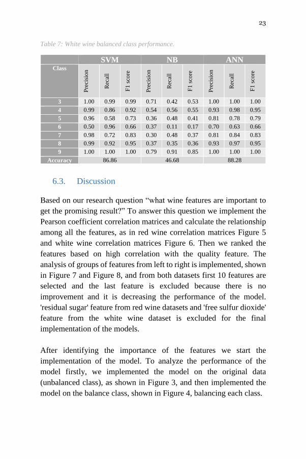
Table 7: White wine balanced class performance.

SVM NB ANN Class

Pre

cisi

on

Rec

all

F1

sco

re

Pre

cisi

on

Rec

all

F1

sco

re

Pre

cisi

on

Rec

all

F1

sco

re

3 1.00 0.99 0.99 0.71 0.42 0.53 1.00 1.00 1.00

4 0.99 0.86 0.92 0.54 0.56 0.55 0.93 0.98 0.95

5 0.96 0.58 0.73 0.36 0.48 0.41 0.81 0.78 0.79

6 0.50 0.96 0.66 0.37 0.11 0.17 0.70 0.63 0.66

7 0.98 0.72 0.83 0.30 0.48 0.37 0.81 0.84 0.83

8 0.99 0.92 0.95 0.37 0.35 0.36 0.93 0.97 0.95

9 1.00 1.00 1.00 0.79 0.91 0.85 1.00 1.00 1.00

Accuracy 86.86 46.68 88.28

6.3. Discussion

Based on our research question “what wine features are important to

get the promising result?” To answer this question we implement the

Pearson coefficient correlation matrices and calculate the relationship

among all the features, as in red wine correlation matrices Figure 5

and white wine correlation matrices Figure 6. Then we ranked the

features based on high correlation with the quality feature. The

analysis of groups of features from left to right is implemented, shown

in Figure 7 and Figure 8, and from both datasets first 10 features are

selected and the last feature is excluded because there is no

improvement and it is decreasing the performance of the model.

'residual sugar' feature from red wine datasets and 'free sulfur dioxide'

feature from the white wine dataset is excluded for the final

implementation of the models.

After identifying the importance of the features we start the

implementation of the model. To analyze the performance of the

model firstly, we implemented the model on the original data

(unbalanced class), as shown in Figure 3, and then implemented the

model on the balance class, shown in Figure 4, balancing each class.

24

In terms of the performance of the prediction model accuracy,

precision, recall, and f1 score is examined, as expressed in Table 4 red

wine and Table 5 white wine performance analysis results for

unbalanced classes for each model is examined, and Table 6 red wine

and Table 7 white wine performance analysis results for the balanced

classes for each model is examined.

From these unbalancing and balancing classes, we achieved a better

performance result on the balanced class for all the models.

Among the three algorithms, the artificial neural network (ANN)

algorithm achieved the best performance result from both red and

white wine datasets as compare to the support vector machine (SVM)

and naïve Bayes (NB) algorithm.

There is other related work that was mentioned in section 2.2, but they

differ from this project in different ways.

Kumar, (2020) paper is similar in that they used similar performance

measurements and similar machine learning algorithms such as

support vector machine and naïve Bayes. The difference is that they

trained the model on unbalanced classes and they used all features for

the prediction of the model. In terms of performance analysis, they

achieved the best of 67.25% accuracy from the support vector machine

on the red wine dataset, Er and Atasoy, (2016) has been achieved the

best accuracy result from the random forest on 69.90% in the red wine

and 71.23% white wine datasets and use the principal components

analysis technique for feature selection. Gupta, (2018) has been

proposed that all features are not necessary for the prediction instead

of selecting only necessary features to predict the wine quality. For

that, they used linear regression for determining the dependencies of

the target variable. Whereas our model achieved 69.06% accuracy in

the red wine dataset and 67.83% accuracy in the white wine dataset

from the support vector machine. Then after training, the model on the

balanced data and selecting the best hyperparameters the performance

25

of the model is improved and achieved 83.52% accuracy in the red

wine and 86.86% accuracy in the white wine. In addition, our model

achieved the best 85.16% accuracy in the red wine and 88.28%

accuracy in the white wine from the artificial neural network model

by applying the Pearson coefficient correlation matrices for the feature

selection.

26

7. Conclusions and Future Work

7.1. Conclusion

This report uses the two types of wine dataset red and white, of

Portuguese “Vinho Verde” wine to predict the quality of the wine

based on the physicochemical properties.

First, we used oversampling to balance the dataset in the data

preprocessing stage to optimize the performance of the model. Then

we look for features that can provide better prediction results. For this,

we used Pearson coefficient correlation matrices and ranked the

features according to the high correlation among the features. After

applying the sampling datasets which is balancing dataset the

performance of the model is improved. In general, removing irrelevant

features of the datasets improved the performance of the classification

model. To conclude that the minority classes of a dataset will not get

a good representation on a classifier and representation for each class

can be solved by oversampling and undersampling to balance the

representation classes over datasets.

The accuracy of the support vector machine (SVM) algorithm is

83.52% from the red wine and 86.86% from the white wine, the naïve

Bayes (NB) algorithm is 46.33% from the red wine and 46.68% from

the white wine, and the artificial neural network (ANN) is 85.16%

from the red wine and 88.28% accuracy from the white wine. Among

these three machine learning algorithms, we achieved the best

accuracy result from the artificial neural network (ANN) on both red

and white wine datasets.

Therefore, in the classification algorithms by selecting the appropriate

features and balancing the data can improve the performance of the

model.

27

7.2. Future Work

In the future, to improve the accuracy of the classifier, it is clear that

the algorithm or the data must be adjusted. We recommend feature

engineering, using potential relationships between wine quality, or

applying the boosting algorithm on the more accurate method.

In addition, by applying the other performance measurement and other

machine learning algorithms for the better comparison on results. This

study will help the manufacturing industries to predict the quality of

the different types of wines based on certain features, and also it will

be helpful for them to make a good product.

28

References Chawla, N.V., 2005. Data Mining for Imbalanced Datasets: An Overview,

in: Maimon, O., Rokach, L. (Eds.), Data Mining and Knowledge

Discovery Handbook. Springer US, Boston, MA, pp. 853–867.

https://doi.org/10.1007/0-387-25465-X_40

Cortez, P., Cerdeira, A., Almeida, F., Matos, T., Reis, J., 2009. Modeling

wine preferences by data mining from physicochemical properties.

Decis. Support Syst. 47, 547–553.

https://doi.org/10.1016/j.dss.2009.05.016

Dahal, K., Dahal, J., Banjade, H., Gaire, S., 2021. Prediction of Wine

Quality Using Machine Learning Algorithms. Open J. Stat. 11,

278–289. https://doi.org/10.4236/ojs.2021.112015

Dastmard, B., 2013. A statistical analysis of the connection between test

results and field claims for ECUs in vehicles.

Drummond, C., Holte, R.C., 2003. C4.5, Class Imbalance, and Cost

Sensitivity: Why Under-sampling beats Over-sampling. pp. 1–8.

Er, Y., Atasoy, A., 2016. The Classification of White Wine and Red Wine

According to Their Physicochemical Qualities. Int. J. Intell. Syst.

Appl. Eng. 4, 23–26. https://doi.org/10.18201/ijisae.265954

Er, Y., Atasoy, Ayten, 2016. The Classification of White Wine and Red

Wine According to Their Physicochemical Qualities. Int. J. Intell.

Syst. Appl. Eng. 23–26. https://doi.org/10.18201/ijisae.265954

Estabrooks, A., Japkowicz, N., 2001. A Mixture-of-Experts Framework for

Learning from Imbalanced Data Sets, in: Hoffmann, F., Hand, D.J.,

Adams, N., Fisher, D., Guimaraes, G. (Eds.), Advances in

Intelligent Data Analysis, Lecture Notes in Computer Science.

Springer Berlin Heidelberg, Berlin, Heidelberg, pp. 34–43.

https://doi.org/10.1007/3-540-44816-0_4

Fauzi, M., Arifin, A.Z., Gosaria, S., Prabowo, I.S., 2017. Indonesian News

Classification Using Naïve Bayes and Two-Phase Feature

Selection Model. Indones. J. Electr. Eng. Comput. Sci. 8, 610–615.

https://doi.org/10.11591/ijeecs.v8.i3.pp610-615

Gandhi, R., 2018. Support Vector Machine — Introduction to Machine

Learning Algorithms [WWW Document]. Medium. URL

https://towardsdatascience.com/support-vector-machine-

introduction-to-machine-learning-algorithms-934a444fca47

(accessed 6.6.21).

Guo, X., Yin, Y., Dong, C., Yang, G., Zhou, G., 2008. On the Class

Imbalance Problem, in: 2008 Fourth International Conference on

Natural Computation. Presented at the 2008 Fourth International

Conference on Natural Computation, pp. 192–201.

https://doi.org/10.1109/ICNC.2008.871

29

Gupta, Y., 2018. Selection of important features and predicting wine

quality using machine learning techniques. Procedia Comput. Sci.

125, 305–312. https://doi.org/10.1016/j.procs.2017.12.041

Hewahi, N.M., Abu Hamra E, 2017. A Hybrid Approach Based on Genetic

Algorithm and Particle Swarm Optimization to Improve Neural

Network Classification. J. Inf. Technol. Res. JITR 10, 48–68.

https://doi.org/10.4018/JITR.2017070104

J. Han, Micheline Kamber, Jian Pei, 2012. Data Mining: Concepts and

Techniques 3rd Edition. DATA Min. 560.

Joseph, R., 2018. Grid Search for model tuning [WWW Document].

Medium. URL https://towardsdatascience.com/grid-search-for-

model-tuning-3319b259367e (accessed 6.6.21).

Kumar, S., Agrawal, K., Mandan, N., 2020. Red Wine Quality Prediction

Using Machine Learning Techniques, in: 2020 International

Conference on Computer Communication and Informatics

(ICCCI). Presented at the 2020 International Conference on

Computer Communication and Informatics (ICCCI), IEEE,

Coimbatore, India, pp. 1–6.

https://doi.org/10.1109/ICCCI48352.2020.9104095

Lee, S., Park, J., Kang, K., 2015. Assessing wine quality using a decision

tree, in: 2015 IEEE International Symposium on Systems

Engineering (ISSE). Presented at the 2015 IEEE International

Symposium on Systems Engineering (ISSE), IEEE, Rome, Italy,

pp. 176–178. https://doi.org/10.1109/SysEng.2015.7302752

Mhatre, M.S., Siddiqui, D.F., Dongre, M., Thakur, P., 2015. Review

paper on Artificial Neural Network: A Prediction Technique 6, 3.

Onan, A., Korukoğlu, S., 2017. A feature selection model based on genetic

rank aggregation for text sentiment classification. J. Inf. Sci. 43,

25–38. https://doi.org/10.1177/0165551515613226

P. Appalasamy, N.D. Rizal, F. Johari, A.F. Mansor, A. Mustapha, 2012.

Classification-based Data Mining Approach for Quality Control in

Wine Production [WWW Document].

https://doi.org/10.3923/jas.2012.598.601

Panday, D., Cordeiro de Amorim, R., Lane, P., 2018. Feature weighting as

a tool for unsupervised feature selection. Inf. Process. Lett. 129,

44–52. https://doi.org/10.1016/j.ipl.2017.09.005

Pedregosa, F., Varoquaux, G., Gramfort, A., Michel, V., Thirion, B.,

Grisel, O., Blondel, M., Prettenhofer, P., Weiss, R., Dubourg, V.,

Vanderplas, J., Passos, A., Cournapeau, D., 2011. Scikit-learn:

Machine Learning in Python. Mach. Learn. PYTHON 6.

Rish, I., 2001. An Empirical Study of the Naïve Bayes Classifier. IJCAI

2001 Work Empir Methods Artif Intell 3.

says, D. shafei, 2020. Artificial Neural Network - Applications, Algorithms

and Examples [WWW Document]. TechVidvan. URL

30

https://techvidvan.com/tutorials/artificial-neural-network/

(accessed 6.6.21).

scikit-learn, developer, 2021. scikit-learn: machine learning in Python —

scikit-learn 0.24.2 documentation [WWW Document]. URL

https://scikit-learn.org/stable/ (accessed 5.31.21).

Wolf, L., Shashua, A., 2005. Feature Selection for Unsupervised and

Supervised Inference: The Emergence of Sparsity in a Weight-

Based Approach 33.

Yu, T., Zhu, H., 2020. Hyper-Parameter Optimization: A Review of

Algorithms and Applications. ArXiv200305689 Cs Stat.

Zhang, P., 2000. Neural Networks for Classification: A Survey. Syst. Man

Cybern. Part C Appl. Rev. IEEE Trans. On 30, 451–462.

https://doi.org/10.1109/5326.897072