Real-time crash prediction of urban highways using machine learning algorithms

by

Mirza Ahammad Sharif

B.S., University of Asia Pacific, 2011

M.S., University of Wyoming, 2015

AN ABSTRACT OF A DISSERTATION

submitted in partial fulfillment of the requirements for the degree

DOCTOR OF PHILOSOPHY

Department of Civil Engineering

Carl R. Ice College of Engineering

KANSAS STATE UNIVERSITY

Manhattan, Kansas

2020

Abstract

Motor vehicle crashes in the United States continue to be a serious safety concern for state

highway agencies, with over 30,000 fatal crashes reported each year. The World Health

Organization (WHO) reported in 2016 that vehicle crashes were the eighth leading cause of death

globally. Crashes on roadways are rare and random events that occur due to the result of the

complex relationship between the driver, vehicle, weather, and roadway. A significant breadth of

research has been conducted to predict and understand why crashes occur through spatial and

temporal analyses, understanding information about the driver and roadway, and identification of

hazardous locations through geographic information system (GIS) applications. Also, previous

research studies have investigated the effectiveness of safety devices designed to reduce the

number and severity of crashes. Today, data-driven traffic safety studies are becoming an essential

aspect of the planning, design, construction, and maintenance of the roadway network. This can

only be done with the assistance of state highway agencies collecting and synthesizing historical

crash data, roadway geometry data, and environmental data being collected every day at a

resolution that will help researchers develop powerful crash prediction tools.

The objective of this research study was to predict vehicle crashes in real-time. This

exploratory analysis compared three well-known machine learning methods, including logistic

regression, random forest, support vector machine. Additionally, another methodology was

developed using variables selected from random forest models that were inserted into the support

vector machine model. The study review of the literature noted that this study’s selected methods

were found to be more effective in terms of prediction power. A total of 475 crashes were identified

from the selected urban highway network in Kansas City, Kansas. For each of the 475 identified

crashes, six no-crash events were collected at the same location. This was necessary so that the

predictive models could distinguish a crash-prone traffic operational condition from regular traffic

flow conditions. Multiple data sources were fused to create a database including traffic operational

data from the KC Scout traffic management center, crash and roadway geometry data from the

Kanas Department of Transportation; and weather data from NOAA. Data were downloaded from

five separate roadway radar sensors close to the crash location. This enable understanding of the

traffic flow along the roadway segment (upstream and downstream) during the crash. Additionally,

operational data from each radar sensor were collected in five minutes intervals up to 30 minutes

prior to a crash occurring.

Although six no-crash events were collected for each crash observation, the ratio of crash

and no-crash were then reduced to 1:4 (four non-crash events), and 1:2 (two non-crash events) to

investigate possible effects of class imbalance on crash prediction. Also, 60%, 70%, and 80% of

the data were selected in training to develop each model. The remaining data were then used for

model validation. The data used in training ratios were varied to identify possible effects of training

data as it relates to prediction power. Additionally, a second database was developed in which

variables were log-transformed to reduce possible skewness in the distribution.

Model results showed that the size of the dataset increased the overall accuracy of crash

prediction. The dataset with a higher observation count could classify more data accurately. The

highest accuracies in all three models were observed using the dataset of a 1:6 ratio (one crash

event for six no-crash events). The datasets with1:2 ratio predicted 13% to 18% lower than the

1:6 ratio dataset. However, the sensitivity (true positive prediction) was observed highest for the

dataset of a 1:2 ratio. It was found that reducing the response class imbalance; the sensitivity

could be increased with the disadvantage of a reduction in overall prediction accuracy. The

effects of the split ratio were not significantly different in overall accuracy. However, the

sensitivity was found to increase with an increase in training data. The logistic regression model

found an average of 30.79% (with a standard deviation of 5.02) accurately. The random forest

models predicted an average of 13.36% (with a standard deviation of 9.50) accurately. The

support vector machine models predicted an average of 29.35% (with a standard deviation of

7.34) accurately. The hybrid approach of random forest and support vector machine models

predicted an average of 29.86% (with a standard deviation of 7.33) accurately.

The significant variables found from this study included the variation in speed between

the posted speed limit and average roadway traffic speed around the crash location. The

variations in speed and vehicle per hour between upstream and downstream traffic of a crash

location in the previous five minutes before a crash occurred were found to be significant as

well.

This study provided an important step in real-time crash prediction and complemented

many previous research studies found in the literature review. Although the models investigate

were somewhat inconclusive, this study provided an investigation of data, variables, and

combinations of variables that have not been investigated previously. Real-time crash prediction

is expected to assist with the on-going development of connected and autonomous vehicles as the

fleet mix begins to change, and new variables can be collected, and data resolution becomes

greater. Real-time crash prediction models will also continue to advance highway safety as

metropolitan areas continue to grow, and congestion continues to increase.

Real-time crash prediction of urban highways using machine learning algorithms

by

Mirza Ahammad Sharif

B.S., University of Asia Pacific, 2011

M.S., University of Wyoming, 2015

A DISSERTATION

submitted in partial fulfillment of the requirements for the degree

DOCTOR OF PHILOSOPHY

Department of Civil Engineering

Carl R. Ice College of Engineering

KANSAS STATE UNIVERSITY

Manhattan, Kansas

2020

Approved by:

Major Professor

Eric J. Fitzsimmons

Copyright

© Mirza Ahammad Sharif 2020

Abstract

Motor vehicle crashes in the United States continue to be a serious safety concern for state

highway agencies, with over 30,000 fatal crashes reported each year. The World Health

Organization (WHO) reported in 2016 that vehicle crashes were the eighth leading cause of death

globally. Crashes on roadways are rare and random events that occur due to the result of the

complex relationship between the driver, vehicle, weather, and roadway. A significant breadth of

research has been conducted to predict and understand why crashes occur through spatial and

temporal analyses, understanding information about the driver and roadway, and identification of

hazardous locations through geographic information system (GIS) applications. Also, previous

research studies have investigated the effectiveness of safety devices designed to reduce the

number and severity of crashes. Today, data-driven traffic safety studies are becoming an essential

aspect of the planning, design, construction, and maintenance of the roadway network. This can

only be done with the assistance of state highway agencies collecting and synthesizing historical

crash data, roadway geometry data, and environmental data being collected every day at a

resolution that will help researchers develop powerful crash prediction tools.

The objective of this research study was to predict vehicle crashes in real-time. This

exploratory analysis compared three well-known machine learning methods, including logistic

regression, random forest, support vector machine. Additionally, another methodology was

developed using variables selected from random forest models that were inserted into the support

vector machine model. The study review of the literature noted that this study’s selected methods

were found to be more effective in terms of prediction power. A total of 475 crashes were identified

from the selected urban highway network in Kansas City, Kansas. For each of the 475 identified

crashes, six no-crash events were collected at the same location. This was necessary so that the

predictive models could distinguish a crash-prone traffic operational condition from regular traffic

flow conditions. Multiple data sources were fused to create a database including traffic operational

data from the KC Scout traffic management center, crash and roadway geometry data from the

Kanas Department of Transportation; and weather data from NOAA. Data were downloaded from

five separate roadway radar sensors close to the crash location. This enable understanding of the

traffic flow along the roadway segment (upstream and downstream) during the crash. Additionally,

operational data from each radar sensor were collected in five minutes intervals up to 30 minutes

prior to a crash occurring.

Although six no-crash events were collected for each crash observation, the ratio of crash

and no-crash were then reduced to 1:4 (four non-crash events), and 1:2 (two non-crash events) to

investigate possible effects of class imbalance on crash prediction. Also, 60%, 70%, and 80% of

the data were selected in training to develop each model. The remaining data were then used for

model validation. The data used in training ratios were varied to identify possible effects of training

data as it relates to prediction power. Additionally, a second database was developed in which

variables were log-transformed to reduce possible skewness in the distribution.

Model results showed that the size of the dataset increased the overall accuracy of crash

prediction. The dataset with a higher observation count could classify more data accurately. The

highest accuracies in all three models were observed using the dataset of a 1:6 ratio (one crash

event for six no-crash events). The datasets with1:2 ratio predicted 13% to 18% lower than the

1:6 ratio dataset. However, the sensitivity (true positive prediction) was observed highest for the

dataset of a 1:2 ratio. It was found that reducing the response class imbalance; the sensitivity

could be increased with the disadvantage of a reduction in overall prediction accuracy. The

effects of the split ratio were not significantly different in overall accuracy. However, the

sensitivity was found to increase with an increase in training data. The logistic regression model

found an average of 30.79% (with a standard deviation of 5.02) accurately. The random forest

models predicted an average of 13.36% (with a standard deviation of 9.50) accurately. The

support vector machine models predicted an average of 29.35% (with a standard deviation of

7.34) accurately. The hybrid approach of random forest and support vector machine models

predicted an average of 29.86% (with a standard deviation of 7.33) accurately.

The significant variables found from this study included the variation in speed between

the posted speed limit and average roadway traffic speed around the crash location. The

variations in speed and vehicle per hour between upstream and downstream traffic of a crash

location in the previous five minutes before a crash occurred were found to be significant as

well.

This study provided an important step in real-time crash prediction and complemented

many previous research studies found in the literature review. Although the models investigate

were somewhat inconclusive, this study provided an investigation of data, variables, and

combinations of variables that have not been investigated previously. Real-time crash prediction

is expected to assist with the on-going development of connected and autonomous vehicles as the

fleet mix begins to change, and new variables can be collected, and data resolution becomes

greater. Real-time crash prediction models will also continue to advance highway safety as

metropolitan areas continue to grow, and congestion continues to increase.

x

Table of Contents

List of Figures .............................................................................................................................. xiii

List of Tables ............................................................................................................................... xvi

Acknowledgments....................................................................................................................... xvii

Introduction .................................................................................................................. 1

1.1 Background ............................................................................................................... 1

1.2 Real-Time Crash Prediction Modeling ..................................................................... 6

1.3 Study Objectives ....................................................................................................... 8

1.4 Thesis Outline ........................................................................................................... 9

Literature Review ....................................................................................................... 10

2.1 Logistic Regression Models .................................................................................... 10

2.2 Machine Learning Algorithms ................................................................................ 16

2.2.1 Random Forest ................................................................................................. 17

2.2.2 Support Vector Machine .................................................................................. 20

Methodology .............................................................................................................. 23

3.1 Logistic Regression ................................................................................................. 23

3.1.1 Interpretation of Odds Ratio ............................................................................ 25

3.1.2 Variable Selection ............................................................................................ 25

3.1.2.1 Backward Selection .................................................................................. 26

3.1.2.2 Forward Selection ..................................................................................... 26

3.1.2.3 Stepwise Selection .................................................................................... 26

3.1.2.4 Akaike Information Criterion ................................................................... 27

3.2 Random Forest ........................................................................................................ 27

3.2.1 Random Forest Algorithm ............................................................................... 30

3.2.2 Validation and Performance of Random Forest ............................................... 31

3.2.3 Mean Decrease Accuracy................................................................................. 32

3.3 Support Vector Machine ......................................................................................... 33

3.3.1 SVM Model Formulation ................................................................................. 33

3.3.2 Support Vector Machine Kernels ..................................................................... 35

3.3.2.1 Linear Kernel ............................................................................................ 36

xi

3.3.2.2 Polynomial Kernel .................................................................................... 36

3.3.2.3 Sigmoid Kernel ......................................................................................... 36

3.3.2.4 Radial Basis Function ............................................................................... 37

3.3.3 Cross-Validation and Grid Search ................................................................... 37

3.4 Comparative Parameters ......................................................................................... 40

Data ............................................................................................................................ 44

4.1 Data Collection ....................................................................................................... 45

4.1.1 Traffic Crash Data ............................................................................................ 45

4.1.2 Traffic Operations Data ................................................................................... 47

4.1.3 Weather Data.................................................................................................... 50

4.1.4 Road Geometry Data ........................................................................................ 51

4.2 Sample Size for Analysis ........................................................................................ 52

4.3 Data Fusion ............................................................................................................. 53

4.3.1 Sensor Identification ........................................................................................ 54

4.3.2 Traffic, Weather, and Roadway Geometry Data Identification ....................... 58

4.4 Descriptive Analysis of the Selected Crashes ......................................................... 67

4.5 Variables Transformation ....................................................................................... 70

Analysis and Results .................................................................................................. 73

5.1 Logistic Regression Models .................................................................................... 74

5.2 Random Forest Models ........................................................................................... 84

5.3 Support Vector Machine Models ............................................................................ 92

5.4 Models Comparison ................................................................................................ 98

Summary, Conclusions, and Recommendations ...................................................... 106

6.1 Executive Summary .............................................................................................. 106

6.2 Significant Findings .............................................................................................. 111

6.2.1 Logistic Regression Models ........................................................................... 111

6.2.2 Random Forest Models .................................................................................. 113

6.2.3 Support Vector Machine Models & RF+SVM Models ................................. 114

6.2.4 Best Performing Model .................................................................................. 115

6.3 Recommendations for Future Research ................................................................ 116

6.4 Contributions to Highway Safety ......................................................................... 118

xii

References ................................................................................................................................... 120

Appendix A - R Codes used for Model Development ................................................................ 132

Appendix A.1. 1: R codes of Logistic Regression Model .......................................... 132

Appendix A.1. 2: R codes of Random Forest Model .................................................. 134

Appendix A.1. 3: R codes of SVM Model ................................................................. 138

xiii

List of Figures

Figure 1.1 Rural vs urban crash trends in Kansas (2012–2016) ..................................................... 3

Figure 1.2 Rural vs urban fatal crashes in Kansas (2012–2016) .................................................... 3

Figure 3.1 Decision tree (courtesy of Mohd. Noor Abdul Hamid, Universiti Utara, Malaysia) .. 28

Figure 3.2 Random forest tree ..................................................................................................... 29

Figure 3.3 Random forest voting process ..................................................................................... 31

Figure 3.4 Graphic representation of the SVM model (courtesy of (Z. Li et al., 2012)) .............. 34

Figure 3.5 An example of five-fold cross-validation .................................................................... 38

Figure 3.6 Overfitting classifier and a better classifier (courtesy of (Yang et al., 2015)) ............ 39

Figure 3.7 ROC curve (courtesy of (C. Xu et al., 2013)) ............................................................. 41

Figure 4.1 Aggregation of database system .................................................................................. 44

Figure 4.2 KDOT motor vehicle accident report .......................................................................... 46

Figure 4.3 KC Scout system in Kansas City, Kansas ................................................................... 48

Figure 4.4 Flowchart of sensor sequence identification ............................................................... 57

Figure 4.5 Layout of KC Scout data request page (Courtesy of KC Scout Data Portal) .............. 62

Figure 4.6 Layout of KC Scout query output page (Courtesy of KC Scout Data Portal) ............. 63

Figure 4.7 Flowchart of matching traffic data with sensor data ................................................... 65

Figure 4.8 Distribution of selected crashes during the study period............................................. 68

Figure 4.9 Distribution of selected crashes against the days ........................................................ 68

Figure 4.10 Distribution of selected crashes against the months .................................................. 68

Figure 4.11 Selected crashes on the map ...................................................................................... 69

Figure 4.12 Final input data for the models .................................................................................. 71

Figure 5.1 Analysis Design ........................................................................................................... 73

xiv

Figure 5.2 Optimum cutoff value selection (60:40 split) .............................................................. 78

Figure 5.3 Prediction accuracy of logistic regression models (60:40 split) .................................. 79

Figure 5.4 Prediction accuracy of logistic regression models (70: 30 split) ................................. 79

Figure 5.5 Prediction accuracy of logistic regression models (80:20 split) .................................. 79

Figure 5.6 Prediction accuracy of logistic regression on test data ................................................ 79

Figure 5.7 Model sensitivity based on the split ratios .................................................................. 82

Figure 5.8 Model sensitivity based on the datasets....................................................................... 82

Figure 5.9 ROC curve of log 1:2 model (80:20 split ratio) .......................................................... 83

Figure 5.10 Selection of optimal mtry parameter for random forest model ................................. 85

Figure 5.11 Selection of optimal maxnodes parameter for random forest model ......................... 85

Figure 5.12 Selection of optimal ntree parameter for random forest model ................................ 86

Figure 5.13 Variable importance plot .......................................................................................... 87

Figure 5.14 Prediction accuracy of random forest models (60:40 split)....................................... 89

Figure 5.15 Prediction accuracy of random forest models (70: 30 split)...................................... 89

Figure 5.16 Prediction accuracy of random forest models (80:20 split)....................................... 89

Figure 5.17 Prediction accuracy of random forest models on test data ........................................ 89

Figure 5.18 Sensitivity of the random forest models based on the dataset ................................... 91

Figure 5.19 Sensitivity of the random forest models based on the split ratio ............................... 91

Figure 5.20 Prediction accuracy of SVM models (60:40 split) ................................................... 94

Figure 5.21 Prediction accuracy of SVM models (70:30 split) ................................................... 94

Figure 5.22 Prediction accuracy of SVM models (80:20 split) ................................................... 94

Figure 5.23 Prediction accuracy of test data using SVM models ................................................ 94

Figure 5.24 Prediction accuracy of RF+SVM models (60:40 split) ............................................ 95

xv

Figure 5.25 Prediction accuracy of RF+SVM models (70:30 split) ............................................ 95

Figure 5.26 Prediction accuracy of RF+SVM models (80:20 split) ............................................ 95

Figure 5.27 Prediction accuracy of test data using RF+SVM models .......................................... 95

Figure 5.28 Sensitivity of the SVM models based on the dataset ............................................... 97

Figure 5.29 Sensitivity of the RF+SVM models based on the dataset ........................................ 97

Figure 5.30 Sensitivity of the SVM models based on the split ratio ............................................ 97

Figure 5.31 Sensitivity of the RF+SVM models based on the split ratio .................................... 97

Figure 5.32 Accuracy and sensitivity of all the models (60:40 split) ........................................... 99

Figure 5.33 Accuracy and sensitivity of all the models (70:30 split) ........................................... 99

Figure 5.34 Accuracy and sensitivity of all the models (80:20 split) ......................................... 100

xvi

List of Tables

Table 1.1 Traffic fatalities and fatality rates for 2016 (NHTSA, 2018) ......................................... 2

Table 3.1 Sensitivity and specificity ............................................................................................. 40

Table 4.1 Kansas crash data .......................................................................................................... 47

Table 4.2 Kansas reportable crashes ............................................................................................. 47

Table 4.3 Weather variables reported by NOAA .......................................................................... 51

Table 4.4 Roadway geometry variable categories ........................................................................ 52

Table 4.5 Sequence of the sensor IDs for each route and direction .............................................. 56

Table 4.6 Temporal data points for each crash incident (only shown for VPH and for C sensor) 60

Table 4.7 Temporal and spatial data points for one crash incident (only shown for VPH and at

the crash time) ....................................................................................................................... 64

Table 4.8 Weather variables for each crash incident (for all sensor) ............................................ 66

Table 4.9 The new variables from the ‘Modified Dataset’ (only shown for VPH and at the crash

time) ...................................................................................................................................... 70

Table 4.10 Number of observations in each split ratio ................................................................. 72

Table 5.1 Stepwise regression output of 1:2 ratio of the modified dataset (60:40 split) .............. 75

Table 5.2 Summary of logistic regression model (1:2 ratio) of the modified dataset (60:40 split)

............................................................................................................................................... 76

Table 5.3 Optimum cutoff values for class prediction .................................................................. 77

Table 5.4 Logistic regression model accuracy .............................................................................. 80

Table 5.5 Sensitivity and specificity of the logistic regression models ........................................ 81

Table 5.6 AUC values of the logistic regression models .............................................................. 84

Table 5.7 Accuracies of the random forest models ....................................................................... 88

Table 5.8 Sensitivity and specificity of the random forest models ............................................... 90

Table 5.9 Accuracy of training and testing data from the SVM models ...................................... 93

Table 5.10 Sensitivity and specificity of the SVM and RF+SVM models ................................... 96

Table 5.11 Test prediction accuracy, sensitivity, and specificity of all models ......................... 103

xvii

Acknowledgments

The completion of this study would not have been possible without the expertise and

support of my advisor Dr. Eric Fitzsimmons. I would also take this opportunity to thank my

committee member Dr. William Hsu for sharing his insights on different sections of the analysis.

I am grateful to Dr. Sunanda Dissanayake, who helped during the project selection and guided

me in the right direction. I also thank the Kansas Department of Transportation for sharing the

data used in this analysis. The analysis would not have been possible without the data from

KDOT.

I would also like to thank Yeling Hu, Lei Luo, and Sandeep Dasari from the Department

of Computer Science for providing help during data processing. Special thanks to my colleagues

Blake Moris, Peng Wang, Jack Cunningham, and Benjamin Nye, for their help over the years.

I am indebted to my wife Sadia and daughter Arya for their unconditional support over

the years. I would also like to acknowledge my mother and siblings for their encouragement and

supports.

1

Introduction

1.1 Background

Traffic Crashes negatively impact communities and highway agencies throughout the

world. In fact, in 2010, the World Health Organization (WHO) reported road injury as the tenth

leading cause of death worldwide, increasing to the eighth leading cause of death in 2016 as the

number of vehicles on roadways increased (WHO, 2018). In 2016, crashes accounted for

approximately 1.3 million deaths worldwide (WHO, 2018). The Centers for Disease Control and

Prevention (CDC) reported that vehicle crashes were responsible for more than 32,000 fatalities

in the United States in 2013, or 10.3 fatalities per 100,000 people, the highest fatality rate among

similarly developed countries (CDC, 2016). According to the National Highway Traffic Safety

Administration (NHTSA), approximately 37,461 deaths in the United States were attributed to

vehicle crashes in 2016, while the Kansas Department of Transportation (KDOT) reported that

429 drivers and passengers were killed on Kansas roadways in the same year (approximately

1.1% of the national total). NHTSA reported that, compared to the national average, Kansas has

a higher vehicle fatality average when the data are normalized (NHTSA, 2018). Table 1.1

compares national fatality rates and fatality rates for Kansas per population, number of licensed

drivers, number of registered vehicles, and vehicle miles traveled. The fatality rates per 100,000

people and licensed drivers in Kansas are much higher than the national average. Additionally,

16.19 fatalities are reported per 100,000 registered vehicles in Kansas, whereas, the average is

only 13.01 in the U.S. Fatalities per 100 million vehicles miles traveled in Kansas is 1.34, which

is higher than the average of 1.18 across the U.S.

2

Table 1.1 Traffic fatalities and fatality rates for 2016 (NHTSA, 2018)

Traffic

Fatalities

Fatality Rates per

100,000

Population

100,000

Licensed

Drivers

100,000

Registered

Vehicles

100 Million Vehicle

Miles Traveled

United

States

37,461 11.59 16.90 13.01 1.18

Kansas 429 14.76 21.13 16.19 1.34

Since 2012, more than 60% of total vehicle crashes in Kansas, approximately 35,000

crashes per year, have occurred in urban areas (Figure 1.1). Among these crashes, 8.4% occurred

on urban interstates and crashes on the urban principal and minor arterial roadways combined to

account for 39.4% of total crashes in Kansas. Consequently, crash minimization in urban areas

would reduce the total number of vehicle crashes throughout the state. Although urban crash

rates are higher than rural crash rates, rural crashes have higher fatality rates since most urban

crashes result in property damage only (PDO), crashes over $1000 in cost. In 2016, KDOT

reported 48,095 PDO crashes and 13,365 injury crashes, resulting in 18,406 injuries. Figure 1.2

shows that rural roadways were responsible for more than 70% (231) of fatal crashes in Kansas

in 2016.

3

Figure 1.1 Rural vs urban crash trends in Kansas (2012–2016)

Figure 1.2 Rural vs urban fatal crashes in Kansas (2012–2016)

0.00%

20.00%

40.00%

60.00%

80.00%

100.00%

120.00%

0

5000

10000

15000

20000

25000

30000

35000

40000

45000

2012 2013 2014 2015 2016

Per

centa

ge

of

Cra

shes

Num

ber

of

Cra

shes

Year

Rural vs Urban Crashes in Kansas

Rural (%) Urban (%) Rural Urban

0

50

100

150

200

250

300

2012 2013 2014 2015 2016

Num

ber

of

Fat

al C

rash

es

Year

Rural vs Urban Fatal Crashes in Kansas

Rural Urban

4

Vehicle crashes also have significant economic impacts, including lost wages, medical

expenses, and loss of workforce productivity. NHTSA reported a $242 billion direct economic

loss, or 1.6% of the U.S. gross domestic product, due to vehicle crashes in 2010, and estimated a

$594 billion indirect economic loss due to loss of life and decreased quality of life (NHTSA,

2015). NHTSA also estimated that vehicle crashes in Kansas in 2010 resulted in a $2.445 billion

economic loss, a loss that increases annually due to inflation and increasing numbers of crashes

(NHTSA, 2015).

Previous transportation studies have shown that traffic characteristics, weather

conditions, geometric design, and human behavior are common primary factors affecting a crash

occurrence. Various studies have developed the relationship between crash severity and these

factors, and other studies have predicted crash frequency based on these factors, but not in real-

time. However, real-time crash prediction, defined as the prediction of an imminent crash event,

could significantly decrease the number of vehicle crashes. Real-time crash prediction can be

defined as the prediction of a crash event going to happen in the near future. Real-time

predictions must be made 5, 10, 15, or 30 minutes before a crash occurs so traffic management

authorities can take preventive measures to diffuse a potential crash situation. Authorities

involved with traffic management should be given enough time to handle the situation before a

crash happen. Because real-time crash prediction is dependent on real-time traffic data, the

availability of real-time data from Kansas City urban highways determined the roadway

segments used for this study. KC Scout, a Kansas and Missouri bi-state traffic management

system, collects traffic data on major highways in the Kansas City area, including average speed,

occupancy, and count. The data are aggregated every 5 minutes, 15 minutes, 30 minutes, and

hourly. Chapter 4 fully explains these data.

5

Researchers worldwide have utilized a variety of methods to study crash occurrences.

Some studies have focused on real-time traffic flow predictions (Golob & Recker, 2003); others

have concentrated on crash injury severity predictions (M. A. Abdel-Aty & Abdelwahab, 2004).

Researchers have recently begun to study real-time crash predictions using machine learning

approaches. One important practical implication of real-time crash prediction models is the

identification of hazardous traffic conditions that may lead to a crash (Hossain & Muromachi,

2011). These models may also improve traffic operation efficiency and traffic safety as well as

allow evaluation of operations using traffic congestion data and the study of traffic safety via

crash analysis. The study of crash variables such as traffic, weather, and geometric conditions

prior to a crash may provide insight that could be used for future crash predictions. The rapid

advancement of intelligent transportation systems (ITS) in the past decade has enabled traffic

agencies to collect traffic parameters such as traffic volume, speed, and occupancy in real-time.

This traffic data is advantageous if properly analyzed and utilized in proactive or advanced

traffic management systems. Many states are using variable speed limits (VSL) (Lee, Hellinga,

& Saccomanno, 2006) and ramp metering (Lee, Hellinga, & Ozbay, 2006) to improve traffic

safety.

Real-time crash prediction is still a relatively new field of traffic safety research, with

only limited research in real-time crash prediction. Previous studies have focused specifically on

traffic data, weather data, or geometric data, but this study is the first to combined weather,

geometric, crash, and traffic data in real-time crash prediction. The next section describes real-

time crash predictions and the methodology of previous real-time crash prediction related

researches.

6

1.2 Real-Time Crash Prediction Modeling

Real-time crash prediction can be summarized as an approach to predict crashes based on

real-time traffic data (Hossain & Muromachi, 2009). The term was first used in an academic

research paper in 1995 (Madanat & Liu, 1995). Previous studies had estimated crash likelihood

using traffic, vehicle, and human factors, but this study included environmental factors in the

model to estimate crashes in real-time. Bayesian-type incident detection algorithms were applied

for incident-likelihood predictions. Study results showed that accounting for environmental

factors increases the accuracy of the likelihood estimates, and combining model predictions with

traditional traffic measurements reduces incident detection times.

A later study used real-time traffic data from inductive loop detectors to estimate the

likelihood of traffic crashes on freeways (C. Oh et al., 2001). Results showed that one unstable

factor, such as environment, traffic conditions, vehicle, or human behavior, makes the traffic

flow unstable and leads to a crash; therefore, pre-crash traffic dynamics may provide information

regarding that crash. However, because human behavior heavily influences traffic behavior but

human factors cannot be predicted accurately with mathematical models, so real-time crash

prediction approaches have assumed that traffic flow data are the indirect representation of

human factors (Hossain & Muromachi, 2009).

A study in 2003 developed a probabilistic real-time crash prediction model to estimate

the crash potential of various traffic flow characteristics (Lee et al., 2003). The study introduced

and defined crash precursors as traffic conditions that exist prior to a crash event. The study

concluded that the speed difference between an upstream sensor and a downstream sensor was

significantly higher when a crash occurred. Other researchers followed similar approaches using

7

crash precursors to estimate crash risk in real time. Identification of crash precursors is essential

for accurate real-time crash prediction since misinterpretation of crash precursors may lead to

erroneous prediction results.

The accuracy of real-time crash prediction models also depends on the selection of

appropriate input variables. A study in 2006 developed a crash-likelihood model using real-time

traffic flow data and rain data prior to and during a crash (M. A. Abdel-Aty & Pemmanaboina,

2006). The study accurately predicted 59% of the crash data. A rainfall index based on historical

rain data demonstrated a positive impact on crash probability. Another study in Minnesota

captured video of 110 live crashes, including traffic and weather conditions prior to and during

the crash event (Hourdos et al., 2006). A crash-likelihood model, developed using the binary

logistic regression model, identified the relationships between real-time traffic conditions and

crash likelihood. Speed variability, lighting, and sun position were confirmed to affect crash

likelihood. The model was tested on real-time data, and 58% of the crashes were detected

accurately.

A study in 2009 investigated use of the statistical approach versus artificial intelligence

on real-time crash prediction (Hossain & Muromachi, 2009). The study concluded that a real-

time crash prediction model should have model calibration flexibility, fast prediction capability,

and high model accuracy. The study also compared prediction accuracy based on artificially

generated data, revealing that the Bayesian network predicted 18% more crash-prone conditions

than the logistic regression model. As mentioned, previous research of real-time crash

predictions was based on traditional or modified statistical approaches. In the last decade,

however, many researchers have begun utilizing artificial intelligence and machine learning

8

algorithms for real-time crash predictions due to their rapid computational ability and high

prediction power.

1.3 Study Objectives

The objective of this research was to evaluate the application of the common statistical

approach and machine learning algorithms on real-time crash prediction using real-time traffic

data and other variables. Logistic regression, random forest, support vector machine (SVM), and

a hybrid combination of random forest and SVM were utilized. Logistic regression is commonly

used in various aspects of traffic studies, and recently new machine learning techniques have

shown promises as an overall classifier. Classification models can be used for real-time crash

predictions to verify their ability to classify crashes accurately. These models were tested using

fused data (traffic operations, roadway geometry, and weather) from the KC Scout traffic

operations center, KDOT, and the National Oceanic and Atmospheric Administration (NOAA).

A review of the literature showed that machine learning algorithms are being introduced into

various aspects of transportation studies. A model with increased prediction accuracy can

provide a better understanding of crashes, which may help with crash reduction, incident

management, and identification of crash-prone locations.

Four secondary objectives were also identified:

• Develop an aggregated database of crash-related variables

Primary Objective: Evaluation of three machine learning algorithms’ application in

real-time crash predictions.

9

• Develop predictive models for real-time crash predictions

• Develop a hybrid model of random forest and SVM

• Compare the machine learning algorithms for crash prediction

1.4 Thesis Outline

Following this introduction, Chapter 2 contains a review of the literature focused on real-

time crash predictions. Based on the literature review, matched case-control logistic regression,

SVM, and random forest methods are often used for real-time crash prediction. Chapter 2 also

reviews the use of three proposed methods for various aspects of transportation safety and real-

time crash prediction and justifies the use of the proposed methods. Chapter 3 presents the

methodology of each proposed statistical method, including details of each methodology and its

interpretation. The comparative parameters are also discussed, and the receiver operating curve

(ROC), measurement of accuracy, and sensitivity analysis are used to compare the proposed

models. Chapter 4 describes the methodology, including the data collection procedure, and a

framework for future work. Chapter 5 includes a sample analysis with three preliminary models

developed with a small sample data set to confirm that the proposed models have predictive

power. The results are interpreted to draw conclusions from the sample analysis. Chapter 6

explains the scientific contribution of this study, including technology transfer and how agencies

can efficiently utilize study findings.

10

Literature Review

Many studies have investigated crash prediction and crash severity, and various statistical

approaches have been proposed and studied. Researchers commonly use binary/multinomial

logit, ordered probit, and nested logit models (Miaou & Lum, 1993; Ossenbruggen et al., 2001;

Shankar et al., 1996); neural networks (Abdelwahab & Abdel-Aty, 2001); fuzzy ARTMAP (M.

A. Abdel-Aty & Abdelwahab, 2004); the log-linear model (Kim et al., 1995; Lee et al., 2003);

the nonparametric Bayesian model (J.-S. Oh et al., 2005); discriminate analysis (Chengcheng Xu

et al., 2013); the multivariate statistical model (Golob & Recker, 2003); and matched case-

control logistic regression (M. A. Abdel-Aty & Abdelwahab, 2004; Hossain & Muromachi,

2011; Zheng et al., 2010). However, recent studies have utilized machine learning algorithms,

and artificial intelligence to predict crash risks related to crash factors and traffic flow

characteristics (Chong et al., 2005; X. Li et al., 2008; Yuan & Cheu, 2003). The following

sections broadly discuss the application of traditional statistical methods and machine learning

methods in traffic safety studies, including real-time crash predictions.

2.1 Logistic Regression Models

Regression models have been widely used in traffic safety for many years, and

transportation researchers have often applied various forms of logistic regression for crash

analysis, injury severity analysis, and identification of crash contributing factors. Binary logistic

regression and multinomial logistic regression are the most commonly used approaches (Donnell

& Mason, 2004). Researchers have also used matched case-control logistic regression (M.

Abdel-Aty et al., 2004) This section summarizes the most common regression models used in

transportation studies.

11

Miaou et al. analyzed two linear regression models and two Poisson regression models to

investigate the relationship between traffic crashes and highway geometric designs. They

concluded that conventional linear regression models lack distributional properties that properly

define random, discrete, nonnegative, and generally sporadic traffic crashes; therefore,

probabilistic statements and test statistics from linear regression models are doubtful. Poisson

regression models, however, allow better relationships between crash events and other variables

even though overdispersed data may overstate or understate the likelihood of traffic crashes on

roadways (Miaou & Lum, 1993).

Kim et al. developed a log-linear model to identify the relationship between driver

characteristics, crash severity, and injury severity. Odds multipliers were calculated from the

model to estimate if certain variables increase or decrease the odds of severe crash or injury.

Results showed that driver age and gender are not strong predictors of crash or injury severity.

However, young drivers tend to engage in behaviors associated with more severe crashes and

injuries. Alcohol and drug usage were shown to contribute to severe crashes significantly, and

lack of seatbelt usage was shown to increase the odds of severe injuries in a crash (Kim et al.,

1995).

Shankar et al. analyzed crash severity likelihood using nested logit formulation. Four

levels of injury severity were used in the prediction model: PDO, possible injury, evident injury,

and disabling injury or fatality. A 61-km section of rural interstate in Washington state was used

for analysis, and data were collected over a 5-year period. Roadway geometry, weather, and

human factors were found to be significant factors for developing a probabilistic model (Shankar

et al., 1996).

12

Ossenbruggen et al. used logistic regression to identify statistically significant factors

associated with crash and injury severity Results showed that land use activity, presence of

sidewalks, traffic control device usage, and traffic flow are the most significant factors that

determine if a site is more hazardous than other sites. Of the three types of sites studied (village,

shopping, and residential areas), residential and shopping sites were shown to be more hazardous

than village sites because village sites typically have low operating speeds and pedestrian-

friendly areas (Ossenbruggen et al., 2001).

Oh et al. initially investigated the relationship between real-time traffic parameters and

crash incidents. They developed a Bayesian model with traffic data (average and standard

deviation of traffic flow, occupancy, and speed at 10-seconds intervals). The data consisted of 52

crashes, and traffic conditions were categorized as normal traffic conditions or disruptive traffic

conditions. Normal traffic condition is a 5-minutes period that occurs 30 minutes before the

crash incident; disruptive traffic condition is the 5-minutes period right before a crash event.

Study results showed that a 5-minutes standard deviation of speed is a significant variable that

can be used to estimate crash likelihood. Although only a small sample size was used in the

analysis, a relationship between traffic parameters and the crash prediction was evident (C. Oh et

al., 2001).

Bedard et al. developed a multivariate logistic regression model to determine the

contributions of driver, crash, and vehicle characteristics to driver fatality risks. Data from the

Fatality Accident Reporting System (FARS) for single-vehicle crashes involving fixed objects

were used for analysis. The study reported an odds ratio of 4.98 for drivers over 80 years old

compared to drivers 40–49 years old. Also, female drivers and Blood Alcohol Content (BAC)

(more than 0.30) were found to be significant variables associated with high fatality odds.

13

Increasing seatbelt usage, reducing speed, and reducing the number and incident of driver-side

impact was shown to potentially prevent fatalities (Bedard et al., 2002).

Sohn et al. used algorithms to investigate the relationship between crash severity and

environmental driving factors. They applied classifier fusion, ensemble, and the clustering

method to improve the classifier for two categories of crash severity in Korea. The neural

network and decision tree had previously been used as classifiers. Results showed that

classification-based clustering performs better if observation variation is relatively large (Sohn &

Lee, 2003).

Lee et al. proposed a probabilistic log-linear model to predict real-time crashes based on

traffic flow characteristics. The study suggested a rational method to identify crash precursors

based on experimental results and then tested the performance of the crash prediction model.

They used real-time traffic flow data to explain traffic performance characteristics during crash

events. Crash frequency was a function of traffic and environmental characteristics, external

factors, and exposure. The authors identified three parameters as crash precursors: average

variation of speed difference across adjacent lanes, traffic density, and difference of speeds at

upstream and downstream ends of road sections. The study found that the speed difference

between the upstream detector and the downstream detector was significantly higher during the

crash. In addition, the study concluded that abrupt speed drops at the upstream detector are a

significant parameter for real-time crash predictions. However, the effect of the average variation

of speed across adjacent lanes was found to be insignificant (Lee et al., 2003).

Another study used nonlinear canonical correlation analysis to find a pattern between

crash characteristics and traffic flow characteristics while controlling for lighting and weather

14

parameters. They also compared the nonlinear canonical analysis method to the principal

component analysis method using three data sets: segmentation by lighting and weather, accident

characteristics, and traffic flow characteristics. Results showed that collision type is related to

median speed, and lane variations of speed and that crash severity is inversely related to the

traffic volume. Study results suggested that moderate traffic and relatively constant speed can

lead to increased crash severity (Golob & Recker, 2003).

A study in Pennsylvania used logistic regression models to predict the severity of

median-related crashes. Researchers developed models to predict the probabilities of fatal,

injury, and PDO crashes. Traffic operations, geometric conditions, and weather conditions were

used as independent variables to determine their relationship to crash severity. The study found

that the presence of curvilinear alignment and drivers’ use of drugs or alcohol increases the

chance of fatality in a cross-median crash. In addition, the presence of an interchange entrance

ramp, roadway surface conditions, and traffic volume increases the severity of a median crash.

Study results concluded that the geometric design of the roadway must be considered in real-time

crash prediction to increase prediction accuracy (Donnell & Mason, 2004).

One study used matched case-control logistic regression to explore the effects of traffic

flow parameters on the effects of other confounding variables (i.e., location, time, and weather).

Every crash in a matched case-control study is considered a case, and every non-crash event is a

control. Loop detectors on Florida freeways collected the data used in this study. The 5-minutes

average occupancy and 5-minutes coefficient of variation in the speed at the upstream and

downstream stations (5–10 minutes before the crash) were found to be the most significant

variables affecting crash likelihood. A threshold value of 1.0 for the log-odds ratio was proposed

and evaluated, leading to accurate identification of 69.4% crashes (M. Abdel-Aty et al., 2004).

15

Zheng et al. used case-controlled data to similarly develop a matched case-control logistic

regression model to estimate the impacts of speed variance from oscillating traffic state on the

likelihood of crash occurrence using case-controlled data (Zheng et al., 2010).

Hossain and Muromachi developed a Bayesian network-based crash prediction model for

ramp vicinities and basic freeway segments, reporting a unique set of contributing factors for

each area. The mean and the difference between standard deviations of traffic flow between

adjacent lanes were found to be significant factors for higher crash risk in basic freeway

segments, whereas variation in speed between upstream and downstream detector stations was

found to be the most significant factor in ramp vicinities (Hossain & Muromachi, 2011, 2012).

Although traditional statistical approaches are often used in transportation studies related

to crash injury severity analysis and crash detection analysis, they require assumptions about data

distribution and usually a linear function form between response and independent variables (Z.

Li et al., 2012). Violations of these assumptions may lead to erroneous estimation and incorrect

inferences (Mussone et al., 1999).

Therefore, researchers have proposed non-parametric methods and machine learning

methods for real-time crash prediction and crash injury severity analysis. A primary advantage of

using machine learning models is that they do not require a predefined underlying relationship

between response and independent variables. In previous studies, researchers have reported that

non-parametric studies provide a better statistical fit than traditional parametric models (de Oña

et al., 2011; Fish & Blodgett, 2003).

16

2.2 Machine Learning Algorithms

Researchers have recently begun applying machine learning algorithms to significant

variables in order to analyze traffic crashes (Abdelwahab & Abdel-Aty, 2001; Chong et al.,

2005; Z. Li et al., 2012) . Machine learning algorithms are also being used for crash prediction

(M. M. Ahmed & Abdel-Aty, 2012a; Qu et al., 2012, 2012; C. Xu et al., 2013). Due to their

efficiency in dealing with classification and regression problems, two non-parametric models,

random forest and SVM, have recently been used in real-time crash prediction studies (Z. Li et

al., 2012). Random forest is an efficient technique for variable evaluation and importation

ranking, as well as crash prediction. Previously, the random forest had been used to identify

significant variables (Harb et al., 2009; Hossain & Muromachi, 2011) and traffic flow prediction

(Hamner, 2010). However, the random forest can also be used for prediction in new data (Beshah

et al., 2011; Krishnaveni & Hemalatha, 2011). SVM has been used in transportation studies,

including traffic flow prediction (Cheu et al., 2006; Zhang & Xie, 2008), incident detection

(Yuan & Cheu, 2003), travel mode choice modeling (Zhang & Xie, 2008), crash frequency

prediction (X. Li et al., 2008), crash injury severity analysis (Z. Li et al., 2012), and real-time

crash prediction (Qu et al., 2012; Yu & Abdel-Aty, 2013, 2014).

Abdelwahab et al. used two artificial neural network methods, multilayer perceptron, and

fuzzy adaptive resonance theory, to investigate the relationship between driver injury severity

and driver, vehicle, roadway, and environmental characteristics. Traffic crashes at signalized

intersections in Florida were analyzed in this study. The adaptive nature and learning capabilities

of the neural networks allowed high classification accuracies of 65.6% and 60.4% for training

17

and testing data sets, respectively, in the multilayer perceptron model, and the fuzzy adaptive

resonance theory was shown to provide a classification accuracy of 56.2% (Abdelwahab &

Abdel-Aty, 2001).

Despite their high classification accuracies, however, neural networks require a large

number of hyperparameters, neural network results are not reproducible due to randomness, and

computation time is usually higher than other models. In addition, neural networks have shown

an overfitting tendency. As a result, researchers have started using advanced machine learning

methods such as random forest, SVM, classification and regression tree (CART), and

discriminant analysis. Although each method has advantages and disadvantages, based on a

thorough literature review and study of prediction and interpretation powers, random forest and

SVM were chosen for this study.

2.2.1 Random Forest

A majority of random forest traffic safety studies have identified significant variables that

were then used to develop other models. Harb et al. conducted one of the first applications of the

random forest to explore pre-crash maneuvers using classification trees and random forest. The

random forest technique was used to determine the importance of independent variables’

rankings for various accident types. The researchers chose to use a random forest because it can

extract variable importance information that is not readily available in the classification tree

method. Although output from the classification tree may provide important variable rankings,

the variables may be correlated with each other, leading to misinterpretation of the results.

Therefore, after analyzing the data using the classification tree method, the variables were ranked

18

using the random forest for various types of crashes, including angle accidents, head-on

collisions, and rear-end accidents (Harb et al., 2009).

The random forest method has also been used to predict travel times by modeling local

and aggregate traffic flow. One study attempted to predict future traffic flow in order to predict

approximate future travel time. The random forest method was employed to predict future traffic

speeds from the training data (Hamner, 2010).

A study in Portugal used the random forest to identify highway rear-end crash risk using

disaggregated data. The study classified traffic situations as non-crash and pre-crash using the

random forest method. A threshold between 0 and 1 was defined to classify pre-crash and non-

crash scenarios. If the predicted output fell below the threshold value, the response was classified

as a non-crash event, and if the likelihood was greater than the threshold, the response was

recorded as a pre-crash event. The research used a 67:33 ratio of the data for the training and test

sets. The training set was used to develop the model, and the test set was used to evaluate model

performance. The results accurately predicted 81.1% of pre-crash and 86.7% of non-crash events

after data calibration. The variable importance ranking showed that speed variations in the right

lane, the speed difference between two adjacent lanes, and the left lane’s standard deviation of

headway are critical factors for rear-end crashes in various highway traffic conditions (Pham et

al., 2010).

The random forest has also been utilized for real-time crash prediction and explaining

crash mechanisms in urban expressways. Basic freeway segments and ramp segments were

analyzed using 32 and 31 independent variables, respectively. Data from one upstream and one

downstream sensor were used for analysis, and 1-minute average speed, 5-minutes average

19

vehicle count, 5-minutes average occupancy, 5-minutes SD of speed, count, and occupancy data

were collected in addition to other traffic-related data (Hossain & Muromachi, 2011).

Very few transportation studies have used the random forest for prediction, but one such

study employed random forest for the classification of variables in traffic crashes using traffic

data from the transport department of Hong Kong. The study analyzed one data set using five

machine learning methods: naive Bayes, adaptive boosting, decision tree, partial decision tree,

and random forest. Results showed that random forest outperformed the other four methods in

the classification of variable levels. A similar approach could be used to classify crash and non-

crash events (Krishnaveni & Hemalatha, 2011).

Another study utilized random forest for pattern recognition and increased understanding

of traffic crash data. The study compared the performance of CART and random forest methods

for classifying injury severity level. A binary response was used for classification. Random

forest accurately predicted 73.45% of injury severity and 99.74% of PDO crashes, and the

random forest technique produced a lower error rate than the CART model. The values of the

area under the curve (AUC) in a ROC curve were 0.8873 and 0.9000 for the CART model and

the random forest model, respectively. However, both models more accurately predicted PDO

crashes over injury crashes (Beshah et al., 2011). The study did not report the reason behind the

improved prediction, but the inference can be made that the proportion of injury and PDO data

may play a role. Other studies also showed that the models more accurately predict PDO crashes

than injury-related crashes, a fact that should be considered during data set selection. Previous

studies also reported that common contributing factors, such as a large speed difference between

adjacent lanes (M. Ahmed et al., 2012a; Hossain & Muromachi, 2012) and compression waves

20

that abruptly change traffic flow (M. M. Ahmed & Abdel-Aty, 2012b), increase the likelihood of

traffic crashes.

2.2.2 Support Vector Machine

Yuan et al. initially employed the SVM method for incident detection and incident

classification. They used three nonlinear-based kernel functions (radial, polynomial, and linear),

and a model was built by separating the data into testing and training sets. However, the linear

kernel was still able to be used with other data sets since data distribution may significantly

affect kernel performance. The linear SVM failed to classify incidences from non-incidences.

Study results showed that the SVM has a low misclassification rate, high accuracy in incident

detection, low false alarm rate, and faster detection time than the neural network method (Yuan

& Cheu, 2003).

Chong et al. examined four machine learning techniques to find an accurate model for

injury severity prediction. The four examined models were artificial neural network using hybrid

learning, decision trees, SVMs, and hybrid decision tree-artificial neural network. They were

among the first to analyze five classes of injury severity instead of just two classes

(injury/fatality versus no injury) as in traditional studies. Crash data were collected from the

General Estimates System (GES) from 1995 to 2000. Each model showed different accuracies

when classifying each level of severity. The decision tree predicted no injury and possible injury

classes more accurately, but the hybrid approach more accurately classified non-incapacitating

injury, incapacitating injury, and fatal injury classes (Chong et al., 2005).

Li et al. developed a crash prediction model using an SVM algorithm. The study also

developed a negative binomial regression model, a common approach used in transportation

21

studies. Two models were developed and compared based on data from approximately 2000

crashes on rural frontage roads in Texas. Study results showed a more accurate performance for

the SVM model than the negative binomial regression model and the neural network model. The

SVM model is advantageous because it does not overfit the data, which is a common problem

when applying negative binomial regression (X. Li et al., 2008).

Li et al. used SVM and an ordered probit model to analyze crash injury severity on 326

freeway diverging areas. A radial basis function (RBF) kernel was used for the SVM model.

Study results showed better prediction accuracy from the SVM model than the ordered probit

model: SVM predicted 48.8% injury severity correctly, whereas the ordered probit model

predicted 44%. The researchers also used sensitivity analysis to evaluate the effect of

explanatory variables on crash injury severity. The analysis showed that ramp length and

shoulder width of the freeway significantly affect injury severity in crashes on diverging ramps

(Z. Li et al., 2012).

Yu et al. compared an SVM model and Bayesian logistic regression model to evaluate

their applications for real-time crash risks. The data set was categorized as training and test, and

significant independent variables were selected via CART models. The CART models found

average downstream speed, crash location average speed, crash location standard deviation of

occupancy, and crash location standard deviation of volume as significant variables that were

used to develop the prediction model. Two commonly used kernels, linear, and RBF, were

considered for the model to compare kernel performance. The study concluded that the SVM

model with the RBF kernel provided the best goodness-of-fit. In addition, the nonlinear

relationship between the response variable and independent variables was best explained with the

SVM model with the RBF kernel. The study showed a promising application of SVM in traffic

22

safety for small sample sizes on newly built roadways or freeways with recently implemented

ITS systems (Yu & Abdel-Aty, 2013).

Chen et al. used polynomial and RBF kernels to develop an SVM model to investigate

driver injury severity in rollover crashes. They also utilized a CART model to identify significant

variables. Study results showed that the polynomial SVM outperformed the RBF SVM and that a

trained SVM classifier is most advantageous for no-injury events and least helpful for

incapacitating/fatal injury events. Sensitivity analysis used to interpret results from the SVM

analysis showed that Driving Under the Influence (DUI) was the most significant variable as it

causes incapacitating or fatal injuries. In addition, a large number of travel lanes, the use of a

traffic control device, and unpaved roadways were shown to increase the severity of a rollover

crash (Chen et al., 2016).

Based on the literature review, logistic regression was chosen to study because it is most

commonly used, and random forest and SVM were evaluated because they outperformed other

approaches in previous traffic safety studies. Chapter 3 details the procedures, advantages, and

disadvantages of the selected methods.

23

Methodology

This chapter describes each selected model, including its procedures and how results are

interpreted. The chapter also explains logistic regression model assumptions and modifications,

including the variable selection procedure, as well as random forest and SVM model

development, including model procedures.

3.1 Logistic Regression

Logistic regression analysis is commonly used to analyze a binary response variable. The

response variable used in logistic regression takes the form of success/failure (1/0), where ‘1’

generally denotes success, and ‘0’ denotes failure. The success/failure form can be changed to

match any binary response (M. Abdel-Aty et al., 2004; Shankar et al., 1995; Yan et al., 2005).

The general linear model assumes that responses and error terms are normally Gaussian

distribution, and the observations are independent (Hilbe, 2011). When binary data are modeled

using this method, however, the first two assumptions are violated because the binary response

variable is derived from Bernoulli distribution, whereas normal regression is based on the

Gaussian probability distribution function (pdf).

Nelder and Wederbrum proposed the generalized linear model (GLM), which utilizes a

single algorithm for estimating models based on the exponential family of distributions. GLM

methods are commonly used to estimate logistic, probit, and count response models, such as

Poisson and negative binomial regression (Nelder & Wedderburn, 1972).

The logit, or natural logarithm of an odds ratio, is the central mathematical concept

underlying logistic regression. The logistic model predicts the logit of Y from X. The odds can be

24

defined as the ratios of probabilities (π) of success of Y to probabilities of failure of Y. The

simple logistic regression model can be written in the following form (Peng et al., 2002):

𝑙𝑜𝑔𝑖𝑡 (𝑌) = ln𝜋

1−𝜋= 𝛽0 + 𝛽1𝑥1 + 𝛽2𝑥2 + ⋯ 𝛽𝑛𝑥𝑛 = 𝛽0 + ∑ 𝛽𝑖 𝑥𝑖 , (3.1)

where π is the probability of success, x1…….xn represents independent variables in the

model, and β represents the regression coefficient for each variable. Once both sides of the

equation are converted with antilog, the equation takes the following form:

𝜋 = 𝑃(𝑌 = 1) =𝑒𝛽0+𝛽1𝑥1+𝛽2𝑥2+⋯𝛽𝑛𝑥𝑛

1+𝑒𝛽0+𝛽1𝑥1+𝛽2𝑥2+⋯𝛽𝑛𝑥𝑛, (3.2)

where π is the probability of success (Y = 1). Although Equation 3.1 presents a linear

relationship between logit (Y) and X, Equation 3.2 shows the relationship between Y and X to be

nonlinear. Therefore, the natural log transformation of the odds must be used to make a linear

relationship between categorical response and predictors. The β coefficient is used to interpret

the direction of the relationship between X and logit (Y). A large β value (β > 0) means that the

large logit (Y) is associated with large X values and vice versa. In contrast, small (β < 0) means

that small logit (Y) is associated with large X values and vice versa.

The maximum likelihood method is often used to predict β in a logistic regression model

to maximize the likelihood of reproducing the data given the parameter estimates. The null

hypothesis for full models indicates that all βs are zero. If the null hypothesis is rejected, at least

one β is not zero, which implies the logistic regression model predicts the probability of the

outcome better than the mean of the dependent variables.

25

Final interpretations of the results are made using the odds ratio of the predictors (Peng,

Lee, & Ingersoll, 2002). The odds ratio is a measure of association between an exposure and an

outcome (Szumilas, 2010), as derived from exp (β); if an independent variable experience a one-

unit increase with other factors remaining constant, then the odds ratio increases by a factor of

exp (β). An odds ratio greater than 1 (less than 1) represents exposure associated with higher

(lower) odds of outcome for a unit increase in the independent variable. A 95% confidence

interval of the odds ratio is also often used to evaluate the result; a large confidence interval

represents a low level of precision. It can be used as a proxy to find statistical significance if the

confidence interval does not include an odds ratio of 1 in the interval. The odds ratio can be used

to compare levels of individual independent variables (Szumilas, 2010; Hosmer, Lemeshow, &

Sturdivant, 2013).

3.1.1 Interpretation of Odds Ratio

• An odds ratio of 1 indicates no difference between groups and no association between

tested levels.

• An odds ratio greater than 1 suggests that the odds of exposure are positively

associated with the success rather than the failure.

• An odds ratio less than 1 indicates that the odds of exposure are negatively associated

with the success as compared to the failure.

3.1.2 Variable Selection

The selection of the best subset of variables, which consequently increases accuracy,

requires a proper variable selection method. Unnecessary variables in the model add noise to the

26

estimation. In addition, too many insignificant variables in the model cause collinearity and

make the model difficult to explain. Prediction accuracy increases when insignificant variables

are removed from the model. Common procedures used for variable selection in logistic

regression are described in the following sections.

3.1.2.1 Backward Selection

Backward selection is the simplest of the variable selection methods used in logistic

regression analysis. All variables are in the model at the beginning of the procedure, and then the

variable with the highest p-value is removed, and the data is refitted. The procedure is repeated

until no variables to remove, or all the variables have p-values smaller than the critical p-value.

The critical p-value is defined before the procedure begins. The drawback of backward selection

is that any of the removed variables could be significant in future steps when other variables are

removed from the model.

3.1.2.2 Forward Selection

Forward selection starts with no variable in the model and then adds variables with p-

values less than the critical p-value. The steps are repeated until no more variables with p-values

lower than the critical p-value remain, ending the procedure. Variables selected during the

process are used in the final model to fit the data.

3.1.2.3 Stepwise Selection

Stepwise selection is a combination of backward and forward selection. A variable is

added in each step of the stepwise regression, and verification is made that no insignificant

27

variable is dropped from the model. This procedure requires two critical values: one for variable

selection and another to remove a variable from the model.

3.1.2.4 Akaike Information Criterion

Akaike information criterion (AIC) is a regression technique that selects a model based

on how close its fitted values are to the true expected values. AIC can be defined as

AIC = -2 (log likelihood - number of parameters in model). (3.3)

The optimal model has the most fitted values close to the true expected probabilities (Agresti,

2003). However, AIC penalizes a model for including too many variables.

3.2 Random Forest

Leo Breiman proposed a supervised machine learning algorithm called ‘random forest’,

also known as an ensemble approach, as a promising procedure for extracting rankings of

variable importance. The random forest method can be used for both classification and

regression problems (Breiman, 2001). The main principle behind the ensemble method is that a

group of weak learners can combine to build a strong learner. The method builds a forest, or

ensemble, of decision trees often trained with the bagging method that combines learning models

to increase the accuracy of the overall result. In other words, the random forest builds multiple

decision trees and merges them together to obtain an accurate, stable prediction.

The random forest begins when a decision tree takes input at the top and uses different

variables to travel down. As the tree grows, the size of the branches gets smaller. Decision trees

can handle numerical and categorical data, and they demonstrate rapid performance on large data

28

sets. The root or topmost node of the tree is the decision node that splits the data set using a

variable or feature, resulting in an evaluation of the best splitting metric or each subset or class in

the data set. The decision tree learns by recursively splitting the data set from the root onwards.

Each internal node represents a test on an attribute, each branch represents the test outcome, and

each leaf node represents a class label. A node with no children is called a leaf. Figure 3.1 shows

the components of a decision tree.

Figure 3.1 Decision tree (courtesy of Mohd. Noor Abdul Hamid, Universiti Utara,

Malaysia)

Two well-known methods used in classification and regression problems are boosting

(Schapire et al., 1998) and bagging (Breiman, 1996). Boosting gives extra weight to points

incorrectly predicted from successive trees by earlier predictors. Bagging, however, does not

depend on earlier trees because each tree is individually constructed using a bootstrap sample of

the data set, and then a majority vote is taken for prediction (Liaw & Wiener, 2002). Random

forest was built using the bagging method with added features. For example, random forest adds

a layer of randomness, and it splits each node using the best variables among a subset of

29

predictors randomly chosen at that node instead of splitting each node using the best split among

variables as in standard decision trees. Decision trees are also prone to overfitting, especially

when a tree is particularly deep, but trees in random forest are constructed based on a certain

number of trees, and then results from all the trees are aggregated. Another disadvantage of the

bagging tree method is that it uses the entire set of variables while creating splits, so if some

variables are indicative of certain predictors, the forest could be comprised of correlated trees,

thereby increasing biasness and reducing variance. Random forest aims to de-correlate and prune

the trees by setting a stopping criterion for node splits. The random forest algorithm introduces

extra randomness into the model while a tree is constructed, and instead of searching for the best

variable when splitting a node, the algorithm, searches for the best feature among a random

subset of features. This process creates diversity, which generally results in a better model as

shown in Figure 3.2.

Figure 3.2 Random forest tree

30

A random forest consists of a combination of classifiers where each classifier contributes

a single vote for the most frequent class of the input vector (x) (Rodriguez-Galiano et al., 2012):

𝐶𝑟𝑓𝐵 ̂ = 𝑚𝑎𝑗𝑜𝑟𝑖𝑡𝑦𝑣𝑜𝑡𝑒 {𝐶�̂�(𝑥)}𝐵, (3.4)

where 𝐶�̂�(𝑥) is the class prediction of the random forest tree. Random forest increases

randomness by building trees from training data subsets created by bagging or bootstrapping

(Breiman, 1996). Bootstrapping aggregation creates a training data set by resampling original

data with randomly chosen replacement data. Consequently, some data may be used more than

once, while other data may never be used, leading to increased classifier stability (Breiman,

2001).

3.2.1 Random Forest Algorithm

The random forest algorithm consists of two steps. The first step creates the random

forest, and the second step makes predictions from the created random forest. The process for the

first step requires the following procedure:

1. Randomly select n features from total k features, where n << k.

2. Among the n features, calculate node d using the best split point.

3. Split the nodes into children nodes using the best split.

4. Repeat steps 1–3 until I number of nodes are reached.

5. Build forest by repeating steps 1–4 m number of times to create m number of trees.

As shown in Figure 3.3, the second stage of the random forest requires the following steps:

1. Use the rules from each randomly created test feature to predict the outcome and store the

predicted outcome.

31

2. Calculate votes for each predicted outcome.

3. Designate the highest voted predictors as the final prediction from the random forest

algorithm.

Figure 3.3 Random forest voting process

3.2.2 Validation and Performance of Random Forest

CART selects the best set of predictors using a variety of impurity or diversity measures

(e.g., Gini, twoing, ordered twoing, and least-squares deviation) (Kurt et al., 2008). The most

commonly used metrics in the random forest are Gini impurity, which is used for classification

problems, and variance reduction, which is used for regression problems (Degenhardt et al.,

2017). Gini impurity is the measure of impurity of a set of variables; it calculates the probability

of being wrong. The Gini impurity at node t, g(t) is defined as

𝑔(𝑡) = ∑ 𝑝(𝑗|𝑡)𝑝(𝑖|𝑡)𝑗≠𝑖 , (3.5)

32

where i and j are categories of the target variable. The Gini index equation can be written

as

𝑔(𝑡) = 1 − ∑ 𝑝2(𝑗|𝑡)𝑗 . (3.6)

Therefore, when node cases are evenly distributed across categories, the Gini index uses

its maximum value of 1-(1/k), where k is the number of categories for the target variable. If all

cases in the node belong to the same category, the Gini index equals 0 (Breiman, 2017; Kurt et

al., 2008).

3.2.3 Mean Decrease Accuracy

The mean decrease accuracy index measures variable importance by permuting out-of-

bag (OOB) error and computing the importance of the variables (Han et al., 2016). Breiman’s

original implementation of the random forest algorithm trained each tree on approximately two-

thirds of the training data (Breiman, 2001). Consequently, as the forest is built, each tree can be

tested on the samples not used in the building tree, creating the OOB error estimate, or the

internal error of a random forest as it is constructed. It is used to estimate the prediction error and

evaluate variable importance. The prediction error (classification error rate) on the OOB portion

of training data is recorded for each tree, and the process is repeated after permuting each

independent variable. The difference between the two is then averaged over all the trees. The

general equation can be rewritten as

𝑉𝐼𝑗 = 1

𝑛𝑡𝑟𝑒𝑒∑ (𝐸𝑃𝑡𝑗−𝐸𝑡𝑗)𝑛𝑡𝑟𝑒𝑒

𝑡=1 , (3.7)

33

where ntree is the number of trees in the forest, Etj is the OOB error on tree t before

permuting the values of Xj, and EPtj is the OOB error on tree t after permuting the values of Xj

(Han et al., 2016). Larger mean decrease accuracy indicates increased importance of the variable.

3.3 Support Vector Machine

SVM, one of the most popular and powerful machine learning algorithms for

classification and regression, is based on statistical learning theory for two-group classification

problems (Cortes & Vapnik, 1995). The method determines decision boundary locations to

produce an optimal classification. In a two-class pattern recognition problem, one linear decision

boundary is selected, producing the highest margin between two classes. However, if data are

nonlinearly separated, a hyperplane is selected to maximize the margin (Pal, 2005). A positive

user-defined parameter C (C > 0) controls the trade-off between margin and misclassification

error (Cortes & Vapnik, 1995; Yang et al., 2015). Although SVM was initially designed for two-

class problems, multiclass problems can also be solved with advanced techniques (Cristianini &

Shawe-Taylor, 2000).

3.3.1 SVM Model Formulation

Figure 3.4 shows that an SVM model can map input vector X into a high-dimensional

feature space. Using nonlinear apriori mapping, SVM can construct an optimal separating

hyperplane in the high-dimensional space to classify the outcome into groups while maximizing

the margin between linear decision boundaries.

34

Figure 3.4 Graphic representation of the SVM model (courtesy of (Z. Li et al.,

2012))

SVM model specifications divide a data set into training and test sets. The SVM model

constructs a learning model based on the training set and predicts the test set. Training input can

be defined as 𝑥𝑖 ∈ 𝑅𝑛 for i = 1, 2, 3, ……N, which represents the full set of variables, and

training output is defined as 𝑦𝑖 ∈ 𝑅𝑛, which represents the classes of response variables. The

hyperplane of separating hyperplane can be written as the set of points X, satisfying

𝑊. 𝑋 − 𝑏 = 0 , (3.8)

where . (dot) denotes the dot product and vector W is the normal vector perpendicular to

the hyperplane. For a two-category classification problem, given a training set of instance label

pairs (𝑥𝑖 , 𝑦𝑖), the SVM model must solve the following optimization problem (Cortes & Vapnik,

1995):

35

min𝑤,𝑏,𝜉

1

2𝑤𝑇𝑤 + 𝐶 ∑ 𝜉𝑖

𝑁𝑖=1 , (3.9)

subject to 𝑦𝑖(𝑤𝑇𝜙(𝑥𝑖) + 𝑏) ≥ 1 − 𝜉𝑖, 𝜉𝑖 ≥ 0, where 𝜉 are slack variables measuring

misclassification errors, and C is the penalty factor to errors introducing additional capacity

control within the classifier. In the above approach, however, coefficient C must be determined.

This constraint, along with function minimization, can be solved using Lagrange multipliers:

min max {1

2𝑤𝑇𝑤 + 𝐶 ∑ 𝜉𝑖

𝑁𝑖=1 − ∑ 𝛼𝑖[𝑦𝑖(𝑤𝑇𝜙(𝑥𝑖) + 𝑏) − 1 + 𝜉𝑖]

𝑛𝑖=1 − ∑ 𝛽𝑖𝜉𝑖

𝑛𝑖=1 } ,

(3.10)

where αi βi > 0 are Lagrange multipliers.

3.3.2 Support Vector Machine Kernels

The SVM algorithm is typically implemented using a kernel, or a function that maps the

data to a high dimension in which the data are separable. A kernel is a way of computing the

product of two vectors X and Y feature space. A kernel function, also known as generalized dot

product, is a similarity function that compares two objects to determine similarity scores. The

success of training a dataset is strongly dependent on the choice of kernel. The general kernel

function is

𝐾(𝑥𝑖, 𝑥𝑗) = ∅𝑥𝑖𝑇∅𝑥𝑗 , (3.11)

where function ∅ maps training vectors xi, into a higher dimensional space.

The most common kernels are described in the following sections (Goel & Srivastava,

2016).

36

3.3.2.1 Linear Kernel

The linear kernel is the simplest kernel function. The dot product is the similarity or

distance measured between new data and the support vectors because the distance is a linear

combination of inputs (Hsu et al., 2003). The linear kernel can be defined as

𝐾(𝑥𝑖, 𝑥𝑗) = 𝑥𝑖𝑇𝑥𝑗 . (3.12)

However, the linear kernel does not provide desired results when the classes are separable by

curved or complex lines.

3.3.2.2 Polynomial Kernel

A polynomial kernel is a non-stationary kernel particularly suited for problems in which

all the training data are normalized. The polynomial kernel allows for curved lines in the input

space. The following equation defines a polynomial kernel (Smits & Jordaan, 2002):

𝐾(𝑥𝑖, 𝑥𝑗) = (𝛾𝑥𝑖𝑇𝑥𝑗 + 𝑟)𝑑, 𝛾 > 0, (3.13)

where ϒ is a kernel parameter, which is the slope, and d is the polynomial degree. When d = 1,

the polynomial kernel is equivalent to the linear kernel.

3.3.2.3 Sigmoid Kernel

The sigmoid kernel, also known as the hyperbolic tangent kernel, is primarily used in

neural networks. The sigmoid kernel function is defined as follows (Lin & Lin, 2003):

𝐾(𝑥𝑖, 𝑥𝑗) = 𝑡𝑛𝑎ℎ(𝛾𝑥𝑖𝑇𝑥𝑗 + 𝑟), (3.14)

37

where r is the shifting parameter that controls the threshold of mapping. If r is not properly

chosen, the output could be erroneous. In general, the linear function and the radial basis

function (RBF) are better than the sigmoid kernel in terms of accuracy (Keerthi & Lin, 2003).

3.3.2.4 Radial Basis Function

The RBF kernel is most commonly used in traffic-related studies (Chen et al., 2016;

Chong et al., 2005; X. Li et al., 2008). The RBF is defined as

𝐾(𝑥𝑖, 𝑥𝑗) = 𝑒𝑥𝑝(−𝑦 ∥ 𝑥𝑖𝑇 − 𝑥𝑗 ∥2), 𝛾 > 0 . (3.15)

In general, the RBF is the first choice for SVM because this kernel nonlinearly maps

samples into a high dimensional space so it can handle the nonlinear relationship between class

labels and attributes. Because the linear kernel and sigmoid kernel behave like RBF for certain

parameters, it is often more efficient to start with the RBF kernel, especially since it offers fewer

numerical difficulties (Yang et al., 2015). When the number of features is very large, however,

the linear kernel may be more accurate than the RBF kernel (Goel & Srivastava, 2016; Yang et

al., 2015).

3.3.3 Cross-Validation and Grid Search

The RBF kernel contains two parameters, C and ϒ, but the best values of these

parameters are not known beforehand (Yang et al., 2015). These values are selected through

model selection procedures to identify proper (C, ϒ) so that the classifier can accurately predict

the testing data set. The data set is commonly divided into training and testing data, in which

prediction accuracy obtained from the testing data set more accurately represents the

38

classification performance of a predictor data set. An improved version of this procedure is

known as cross-validation.

In v-fold cross-validation, the training data set is divided into v subsets of equal size.

Repeatedly, one subset is tested using the classifier trained on the remaining v-1 subsets. Each

instance of the entire training set is predicted once, so cross-validation accuracy is the percentage

of data that are correctly classified. An example of cross-validation is presented in Figure in 3.5.

Figure 3.5 An example of five-fold cross-validation

One advantage of cross-validation is that overfitting can be controlled. Figure 3.6 (a) and

(b) show a binary classifier overfitting on training and testing data sets, respectively, which leads

to low accuracy. However, cross-validation on training and testing data sets improves accuracy

and prevents overfitting, as shown in Figure 3.6 (c) and (d), respectively (Refaeilzadeh et al.,

2009; Yang et al., 2015).

39

Figure 3.6 Overfitting classifier and a better classifier (courtesy of (Yang et al.,

2015))

Cross-validation employs a grid search technique to find the best pair of (C, ϒ); a range

of C and ϒ are provided, and the pair with best cross-validation accuracy is selected for the

model. Previous studies showed that an exponentially growing sequence of C and ϒ more

efficiently selects good hyperparameters (for C: 2-5, 2-3, 2-1,….……….., 215; and for ϒ: 2-15, 2-13,

2-11, …….. 23) (Huang et al., 2003).

40

3.4 Comparative Parameters

This study sought to compare the proposed models to identify the most suitable method

of crash and injury severity prediction. Researchers have previously employed approaches such

as ROC curve analysis, sensitivity analysis, and accuracy and mean comparison to compare

models. The objective of this study is to use all three of the previous methods for analysis. Table

3.1 lists all the features of a confusion matrix, sensitivity, and specificity.

Table 3.1 Sensitivity and specificity

Predicted Crash

Data

Historical Crash Data

Crash No-Crash

Crash TP FP

No-Crash FN TN

As shown in the table, true positive (TP) refers to when an actual crash event is predicted

by the model, and false positive (FP) denotes when a non-crash event is predicted as a crash

event. True negative (TN) represents non-crash events when they are predicted as non-crash, and

false negative (FN) refers to when a crash event is predicted as a non-crash event.

Sensitivity, also known as true-positive rate, is the conditional probability of predicting a

crash event given that it was an actual crash event, written as

𝑆𝑒𝑛𝑠𝑖𝑡𝑖𝑣𝑖𝑡𝑦 =𝑇𝑟𝑢𝑒 𝑃𝑜𝑠𝑖𝑡𝑖𝑣𝑒

𝑇𝑟𝑢𝑒 𝑃𝑜𝑠𝑖𝑡𝑖𝑣𝑒+𝐹𝑎𝑙𝑠𝑒 𝑁𝑒𝑔𝑎𝑡𝑖𝑣𝑒=

𝑇𝑃

𝑇𝑃+𝐹𝑁 . (3.16)

Specificity, also known as true-negative rate, is the conditional probability of predicting a

non-crash event given that it was an actual non-crash event, written as

41

𝑆𝑝𝑒𝑐𝑖𝑓𝑖𝑐𝑖𝑡𝑦 =𝑇𝑟𝑢𝑒 𝑁𝑒𝑔𝑎𝑡𝑖𝑣𝑒

𝑇𝑟𝑢𝑒 𝑁𝑒𝑔𝑎𝑡𝑖𝑣𝑒+𝐹𝑎𝑙𝑠𝑒 𝑃𝑜𝑠𝑖𝑡𝑖𝑣𝑒=

𝑇𝑁

𝑇𝑁+𝐹𝑃 . (3.17)

The trade-off between sensitivity and specificity cannot be avoided. For example, when a

low cut-off point is selected, sensitivity increases while specificity decreases. This issue,

however, can be remedied using the receiver operating characteristics ROC curve, which can

compare the accuracies of two or more tests and show the trade-off between sensitivity and

specificity as the cut-off point varies. The ROC curve has been successfully utilized in previous

crash prediction related studies (M. Ahmed et al., 2012b; C. Xu et al., 2013; Yu & Abdel-Aty,

2014).

The ROC curve is constructed by plotting sensitivity against the false positive rate (1-

specificity). The higher the sensitivity and specificity of a test, the further the curve is pushed

toward the top left corner of the plot. Figure 3.7 shows ROC curves for two models using

sensitivity and 1-specificity.

Figure 3.7 ROC curve (courtesy of (C. Xu et al., 2013))

A test with no discriminating ability has equal TP and FP rates, as indicated by the

diagonal straight line in Figure 3.7. The ability of each method to distinguish between crashes

42

and non-crashes can be quantified by calculating the AUC, which varies from 0.5 (no predicting

ability) to 1.0 (perfect accuracy).

Measure of Effectiveness/ Accuracy:

Accuracy is defined as the percentage of correct predictions, which is used to compare

model prediction performance. Accuracy can be calculated as

𝐴𝑐𝑐𝑢𝑟𝑎𝑐𝑦 =𝑡ℎ𝑒 𝑛𝑢𝑚𝑏𝑒𝑟 𝑜𝑓 𝑐𝑜𝑟𝑟𝑒𝑐𝑡 𝑝𝑟𝑒𝑑𝑖𝑐𝑡𝑖𝑜𝑛

𝑁 , (3.20)

where N is the number of observations.

In this study accuracy was calculated and compared between models. Also, the sensitivity

of the models were compared.

This chapter summarizes the backgrounds of each machine learning method that was

used in this study. Logistic regression can be used for binomial and multinomial classifications.

In this study, the outcome or the dependent variables were ‘crash’ vs. ‘no-crash,’ which are

binomial. As a result, binomial logistic regression was used to predict the probabilities and

classify the outcome. SVM method is an algorithm that is implemented by using a function that

maps the data to a high dimension where the data are separable. The kernel function compares

two objects by the similarity scores. The kernel calculates the score by a similarity function. The

choice of the kernel is vital in training the dataset, a right kernel trains the data well and

increases the prediction power on the test dataset. Random forest was another method used in

this study for prediction. This method is widely used for variable selection. However, the

technique can be used for prediction as well. In this study, besides variable selection, the random

forest was used to predict crash probabilities in a given situation. The random forest method

43

creates multiple forests of decision trees. In each decision tree, it takes a given number of inputs

at the top and travel downs to predict the outcome. Finally, a vote is taken from each tree, and

the class getting majority votes from the forest of decision trees is considered as the final

prediction.

The following chapter describes the data used in the analysis. The data used in the

analysis were taken from different agencies then processed and merged with crashes, and no

crashes events using temporal and spatial parameters. All these processes are discussed in the

next chapter.

44

Data

This chapter describes how the data were collected and processed for the analyses in this

study. A key innovation of this research was the successful fusion of traffic crashes, road

geometry, traffic operations, and weather data. This effort required collecting, processing, and

combining these four data streams into a workable database based on a common spatial unit of

time. KDOT assigned each recorded vehicle crash a unique identification number, and the

crashes were marked to the roadway centerline using a recorded latitude and longitude that could

be spatially located using GIS. The police crash report for each vehicle crash also provided the

time of the crash, which was used as a key variable to fuse the traffic operational data and

weather data. The weather and traffic operations data collected at the time of the crash were also

assigned to the identified crash. Figure 4.1 illustrates the datasets used in database development.

Figure 4.1 Aggregation of database system

Crash Weather

Road Geometry Traffic

Database

45

4.1 Data Collection

The data used for this study was collected from various Kansas agencies. Since the study

focused on roadways in the Kansas City metropolitan area, KC Scout (Kansas City’s traffic

management system) was the primary source of traffic operations data. KC Scout has recorded

traffic data in the Kansas City area since 2003. Traffic operational data for this study included

data streams from cameras, Wavetronix sensors, and inductive loop sensors that have been

operational in the metropolitan area since 2007. Roadway and crash data from 2006 to 2015 were

acquired from KDOT, and weather data were obtained from the National Oceanic and

Atmospheric Administration (NOAA) database for the Kansas City International Airport (MCI).

The following section details the data collection and processing steps.

4.1.1 Traffic Crash Data

A police officer typically collects crash data for KDOT for each reported crash event in

Kansas. Figure 4.2 shows an example page from a KDOT accident report (KDOT, 2019). KDOT

uses the Kansas Accident Records System (KARS) to record all crashes that involve a fatality,

injury, or property damage only (PDO) of $1,000 or more. The KDOT accident report form

collects data such as crash information about drivers, passengers, and vehicles, truck/bus/hazmat

supplement; additional occupants or pedestrian supplements; and a code sheet. Table 4.1 details

the major types of information collected in each accident form, and Table 4.2 details the

categories of reportable crashes in Kansas. A volunteer from the Kansas Correctional Institute

(KCI) then edits and inputs data collected at the crash location and a comprehensive designation

of crash location. KDOT reviews the data before finalizing the dataset for KARS.

46

Figure 4.2 KDOT motor vehicle accident report

47

Table 4.1 Kansas crash data

Accident Level

Information

Accident severity, milepost, road name, posted speed limit, date, time,

latitude, longitude, light conditions, weather conditions, accident

location/class, intersection type, work zone type/category, collision with

other vehicle, fixed object type, traffic controls, surface type/condition,

number of lanes, road characteristics

Driver and

Passenger

Information

Age, gender, driver’s license class/type/state, DUI

Vehicle Data

Year, make, model, body style/type, registration state, vehicle damage,

damage location area, vehicle sequence of events

Table 4.2 Kansas reportable crashes

Criteria Reportable

Fatal only Yes

Injury only Yes

PDO >= $1,000 Yes

PDO < $1,000 No

Fatal & Private Property Yes

All other private property combinations No

4.1.2 Traffic Operations Data

Traffic management centers quickly identify hazards and notify drivers to minimize

traffic congestion. KC Scout was initiated as a bi-state traffic monitoring system to decrease

reoccurring and non-reoccurring traffic congestion by improving peak-hour traffic speeds and

volumes (KC Scout, 2020). The traffic management center collaborates with the state highway

patrol, emergency medical services (EMS), and roadside assistance. When a crash occurs on the

48

network, upstream drivers can be notified of a slow-down, the crash location, and potential

hazards. Driver alerts may also include AMBER and Silver alerts. As of 2020, KC Scout

monitors more than 300 miles of primarily U.S. and state highways, with more than 300 traffic

cameras and sensors in the Kansas City metropolitan area. Figure 4.3 shows the locations of all

active KC Scout highway counters as of 2018.

Figure 4.3 KC Scout system in Kansas City, Kansas

• Traffic Counters

49

The KC Scout system primarily relies on traffic sensors for data. Inductive loops were

initially used and then later replaced in many locations by side-fire Wavetronix microwave

radar-based monitors that can record data for up to 16 lanes of traffic. These devices, which are

typically mounted to poles along a roadway outside the clear zone, use frequency modulated

continuous wave (FMCW) sensing to capture occupancy, spot speed, and volume information of

a roadway. KC Scout initially utilized 277 sensors, but over time, old sensors were removed, and

new locations were added in conjunction with highway reconstruction projects. The sensors

monitor specific roadway segments 24 hours every day of the week except for during times of

routine maintenance and calibration. Raw data collected by the sensors are aggregated into 5-

minutes, 15-minutes, 30-minutes, and 1-hour intervals. The processed data are then uploaded to

the KC Scout servers, which can be quarried using specific roadway mileposts, dates, and times.

A user selects a specific sensor to initiate a database search and then enters specific dates, date

ranges, or a list of days (e.g., every Wednesday). A user can also enter specific times or duration

of time based on a 24-hours span; the data are reported in the time interval the user selects. One

sensor or a group of sensors can be analyzed simultaneously, allowing a user to explore spatial

trends in data along a roadway or corridor (assuming vehicles remain on the specified roadway).

The user also must select which variables need to be extrapolated by the database servers. These

variables can include spot speed, spot count, spot lane occupancy, or vehicles per hour (vph) for

each lane or segment, with a segment defined as a group of sensors.

KC Scout’s traffic operations database was the primary database used in this project to

extract specific variables. KC Scout data collection and information associated with a known

crash is explained in section 4.3.

50

4.1.3 Weather Data

Weather data were extracted from the NOAA National Centers for Environmental

Information (NCEI) hourly surface data (DS3505). These records are typically collected every

hour at MCI, approximately 15 miles north of the center of the study area. Unfortunately, KDOT

does not have roadside weather information stations (RWIS) with usable or historical data that

can be utilized within 15 miles or less of the study area. Therefore, the weather was assumed to

remain constant throughout the metropolitan area, an assumption which is one of the

recognizable limitations of this study. Hourly weather data extracted from the NCEI database

were converted into 30-minutes intervals to match KC Scout’s database time interval. This

conversion measured the underlying data so that key variables, including temperature, were

repeated twice, while variables such as precipitations and snow depths, were divided by two to

match 30-minutes intervals.

Similar to the crash and traffic operations data, the weather data also extended from 2006

to 2015, with variables such as wind direction, wind speed, wind gust, visibility, temperature,

precipitation, and snow depth. This project hypothesized that these specific weather variables

might impact driver behavior or change roadway conditions, potentially increasing the chances

of a crash. Table 4.3 shows the selected variables used in this study. The data fusion section

describes how the data were processed and prepared to match the crash data.

51

Table 4.3 Weather variables reported by NOAA

Weather Variables

Wind direction, wind speed (mph), wind gust

(mph), cloud ceiling (in hundreds of feet), sky

cover, cloud type, visibility (miles to nearest

tenth), temperature (Fahrenheit), sea level

pressure (mbar), amount of precipitation

(inches), snow depth (inches)

4.1.4 Road Geometry Data

Road geometry data for the study area were extracted from KDOT’s geographic

information system (GIS) roadway database. Because roadways under investigation may have

been upgraded, reconstructed, or closed during the study period, yearly roadway geometry data

were essential. However, data relating to temporary work zones were not included due to the

difficulty of quantifying changes in traffic conditions or identifying exact work zone dates.

KDOT also provided GIS maps that included database fields pertaining to route direction,

median barrier type, number of lanes, width of lanes, turn lanes, medians, shoulder width, and

shoulder type. Curve radii (measured in degrees) for horizontal curves were calculated from the

polyline data. KDOT also provided a GIS map that included roadway elevation information,

which allowed roadway slope determination. Slope values were combined with traffic flow

direction information so that downhill flows of traffic could have negative slopes and uphill

flows could have positive values. A database containing all the information used in the GIS maps

were also provided.

An individual identification number (ID) was used to distinguish roadway geometric

characteristics for each roadway segment. The IDs consisted of 10 numbers and two letters. The

first three digits represented the county number, the next five digits were route numbers, and the

52

last two digits identified a unique route. The two letters represented the direction of the route.

For example, an ID of 021I00700-EB is a road segment in county number 021, and the segment

is eastbound. The “I” identifies the route as an interstate. For other types of highways, “U”

means U.S. routes and “K” means Kansas routes. The major categories of the roadway geometry

data are provided in Table 4.4.

Table 4.4 Roadway geometry variable categories

Location Data Begin county milepost, end county milepost, begin state

milepost, end state milepost, route direction, route type

Median Information Median type, median width

Lane Information Lane class, average lane width,

Shoulder Information Shoulder type, inside shoulder width, right shoulder width,

inside shoulder slope, right side shoulder slope

Curvature Information Degree of the curve, curve radius

4.2 Sample Size for Analysis

One of the most critical aspects of this study was determining a suitable sample size to

increase the accuracy of real-time crash prediction and provide realistic results. Previous

research studies used various ratios of the crash and no-crash events to find a suitable sample

size. A review of the literature revealed that the most common ratio was one crash event for

every five no-crash events. Although a sample with a large number of no-crash events usually

increases prediction accuracy for no-crash events (Hossain & Muromachi, 2011; C. Oh et al.,

2001), improved accuracy in crash prediction cannot be guaranteed. Oh et al. used 52 crashes

and 4787 no-crash events to achieve prediction accuracies of 55.8% for crashes and 72.1% for

no-crash events (C. Oh et al., 2001). Aty et al. achieved accuracies of 69.4% and 52.8% for crash

and no-crash prediction using 375 crash events and 2,857 no-crash events, respectively (M. A.

53

Abdel-Aty & Abdelwahab, 2004). Ahmed et al. accurately predicted 72.9% crashes and 57.9%

no-crash events using 447 crashes and 178 no-crash samples (M. Ahmed et al., 2012a), and Xu et

al. used a 1:10 ratio for the crash to no-crash samples to obtain prediction accuracies of 61% for

crashes and 80% for no-crash events (C. Xu et al., 2013).

Based on previous research studies, this study was designed to test and analyze the results

of three ratios of crash and no-crash sample sizes. For each crash event on selected highway

sections, two, four, and six no-crash events were selected and analyzed. The data extraction

process is described in the following section.

4.3 Data Fusion

KARS, the crash database used in this research study, contained all vehicle crashes in

Kansas from 2011 to 2015 for the five-year study period. These years were the latest verified

data available for data fusion at the time of the study. Although more recent crash datasets were

available, verified crash data were determined to be the most robust and easiest to work with

since the data had already undergone an extensive data cleaning process. Temporal and spatial

identification within GIS was then used to fuse data from this date range to the roadway

geometry, traffic operations, and weather datasets.

The Kansas City metropolitan area was utilized for this study due to the area’s robust

data streams, high volumes of interstate traffic and stable traffic flows throughout the year. The

study also focused on highways covered by KC Scout, meaning the research highlighted

Johnson, Wyandotte, and Leavenworth counties. The KARS database identifies the county of

each crash using KDOT codes of Johnson (046), Wyandotte (105), and Leavenworth (052).

Results showed that approximately 298,964 crashes occurred in the entire state of Kansas

54

between 2011 and 2015, while county data showed that approximately 78,553 crashes, or 26%,

of all crashes in Kansas, occurred between 2011 and 2015 within the study area of the KC Scout

system. However, because KC Scout generally covers only multilane state and federal roadways

in the Kansas City area, the crashes from local roadways had to be screened out. Following this

criterion, more than 60 thousand crashes were eliminated, which resulted a total of 15,334

crashes, or 5%, of all crashes in Kansas between 2011 and 2015. In addition, since this study

focused on real-time prediction using real-time data, crashes in which human factors contributed

directly to the outcome or were identified on the crash report were removed, including variables

such as driving under the influence (DUI) or distracted driving. This filtering resulted in 14,785

crashes for analysis for the study period of 2011–2015.

The filtered crashes were mapped and identified in ArcMAP, and each crash incident was

identified with a set of geographical coordinates (e.g., latitude, longitude). Using these spatial

coordinates, each crash was plotted to its approximate location on a highway segment, generally

along the centerline of the roadway. Additional verifications were made to prevent any outlier

data or errors in spatially locating crashes, as well as to validate the completeness of the dataset.

4.3.1 Sensor Identification

The KC Scout traffic management system was utilizing approximately 244 traffic

recording sensors within the study area in Kansas City during the study period. Many

interchanges had multiple sensors, while some had only one or two. The sensors used for

interstate ramps were not considered during data extraction because they did not fall under the

scope of this study. The 244 sensors were mapped in ArcMAP. Detailed information from KC

Scout for each sensor was collected and cataloged, including latitude, longitude, KDOT ID, year

55

of installation, physical location along the highways, and sensor properties. One complication

that arose in this study was that many roadway sensors were upgraded during the study period,

so old and new information had to be fused to minimize breaks in the database.

Five sensor datasets for a single crash were collected and analyzed to recreate the traffic

flow (or traffic conditions) along the segment at, before, and after the time of the crash. A

computer program was created in Python that used the k-nearest neighbors (KNN) method to

identify nearby KC Scout system sensors for each of the 14,785 crashes. The KNN algorithm

uses similarity measures to classify a data point based on how the neighbors around that point are

classified. Each crash was linked with a sensor from the system based on its physical

geographical coordinates. The crash coordinates were then matched with the sensor coordinates.

The crash dataset also contained a directional variable for identifying upstream and

downstream sensors listed in Table 4.5. If a crash occurred on a specific highway in a specific

direction, the sensor ID closest to the crash location could be identified. Once the location and

order of sensors along a roadway in a certain direction were known, data could be extracted from

sensors prior to and after the crash to determine traffic conditions and how the crash may have

affected the roadway’s level of service. The procedure used by the Python program to extract

data is shown in Figure 4.4.

For a vehicle crash to be considered for this study, the crash had to have traffic operations

data from five successive sensors in the direction of travel. The five sensors included the crash

sensor (C), one downstream sensor (D), and three upstream sensors (Ui (i = 1,2,3). Each upstream

sensor was labeled 1, 2, or 3 based on the distances from C, with the nearest upstream sensor

being U1 and the furthest upstream sensor being U3. The Python program identified only 3,641 of

56

the 14,785 crashes that included complete data from five sensors. Once traffic data from the five

sensors were extracted and verified, the other data sources were fused with the vehicle crash and

traffic operations data.

Table 4.5 Sequence of the sensor IDs for each route and direction

Route Direction Sensor ID

I-70 EB W-E (EB) 8342 8281 8285 8275 7882 7879 7873 7865 7858 8289 8291

8277 8279 8293 8304 8301 8297 8299

I-70 WB E-W (WB) 8300 8298 8302 8303 8294 8280 8278 8292 8290 7859 7866

7871 7880 7881 8276 8286 8282 8343

I-35 NB S-N (NB)

8261 8259 8257 8255 8253 8251 8249 8247 8245 8243 8240

8241 8263 8265 7828 7830 8382 8373 7478 7653 7445 7654

8353 7655 8080 7657 8349 7658 7659 7660 7661 7662 7663

8347 7664 8351 7665 7666 7821 7667 7668 8344 7822 7824

7827 7724 7725 7726

I-35 SB N-S (SB)

7732 7731 7730 7826 7825 7823 8345 7428 7819 8346 7427

7426 8352 8348 7425 7424 7423 7422 7479 7678 8350 7447

7677 7978 7676 7675 8354 7674 7673 7672 8374 8383 7671

7829 8266 8264 8242 8239 8244 8246 8248 8250 8252 8254

8256 8258 8260 8262

I-635 NB S-N (NB) 7834 7616 7883 7627 7631 7651 7837 7839 7846 7853 7856

7923 7934 7936 7940 7942 7946 7950 7952 7958 7960

I-635 SB N-S (SB) 7961 7956 7951 7947 7943 7941 7937 7933 7935 7932 7857

7851 7848 7840 7838 7635 7632 7628 7622 7617 7835

I-435 SB W-E (SB)

8333 8331 8329 8327 8312 8310 8307 8306 8325 8323 8321

8319 8317 7891 7896 7893 7429 7637 7638 7457 7642 7442

7643 7644 7645 7646 7647 8333 8331 8329 8327 8312 8310

8307 8306 8325 8323 8321 8319 8317 7891 7896 7893

I-435 NB E-W (NB)

7493 7597 7594 7591 7590 7589 7430 7587 7793 7565 7648

7894 7895 7890 8316 8318 8320 8322 8324 8305 8308 8309

8311 8326 8328 8330 8332 7894 7895 7890 8316 8318 8320

8322 8324 8305 8308 8309 8311 8326 8328 8330 8332

*EB = Eastbound Traffic, WB = Westbound Traffic, NB = Northbound Traffic, SB = Southbound Traffic

57

Figure 4.4 Flowchart of sensor sequence identification

Start

Find Route Number (Crash)

Find Traffic Direction (Crash)

Select Route Number (Sensor)

Select Traffic Direction (Sensor)

Match Geocoordinates of Crash with

Sensor Geocoordinates

Identify the Sensor

Nearest to the Crash

Sensor List of the Matched Route and

Direction

Identify the Next

Sensor in the

Traffic Direction

Sensor List of the Matched Route and

Direction

Identify Three Upstream

Sensors in the Traffic

Direction

Make a List of the Sensors

End

58

4.3.2 Traffic, Weather, and Roadway Geometry Data Identification

Although useable traffic operations data were extracted from five KC Scout system

sensors around the crash locations, the following quality control check was performed on the

data to identify possible discrepancies, errors, or unrealistic conditions prior to running a

prediction program.

• Some of the sensors were upgraded over the study period time and therefore did

not have data for the crash period, even though the program recognized the

sensor as being close to the crash; these crashes were removed from the dataset.

• Crash locations occasionally had multiple sensors at the same physical location,

meaning two sensors were collecting data, the sensor produced a data collection

error, or the server provided inaccurate data; these crashes were removed from

the dataset.

• Identified sensors may have been in appropriate locations, but they were not

collecting data due to downtime, replacement, or neglect; these crashes were

removed from the dataset.

The quality control procedure resulted in a final dataset of 475 crashes that had complete and

clean traffic operations data and could provide the most accurate prediction model.

Traffic operations data from the 475 crashes were then downloaded from the KC Scout

servers. KC Scout provides traffic operations data in interval of 5-minutes, 15-minutes, 30-

minutes, or 1-hour intervals. For this study, the traffic operations data were set to 5-minutes

intervals to provide the highest resolution to capture the immediate impact of a crash. In general,

59

an immediate traffic pattern more significantly impacts a crash incident than a pattern that

occurred further in the past. Data were collected up to 30 minutes prior to a crash event (a known

time based on the crash report) in 5-minutes intervals. For example, for a single crash event,

seven sets of data were collected for each of the five sensors: at crash time, 5 minutes before, 10

minutes before,….., and 30 minutes before the crash occurred. The traffic data included count (5-

minutes average), vph, occupancy, speed (5-minutes average) for the traffic direction and

aggregated data of each lane combined. Specific lane data were also collected but not used in this

study because information about the exact lane of the crash was unavailable.

The setup of a crash prediction system must include the collection of six non-crash events

for every crash event (475 in this study) at a location to allow a predictive model to be trained

with both sets of data. The outcome of the model was binary (1 = crash, 0 = no crash). After a

review of the literature and available KC Scout data, a 1:6 ratio for the crash and no-crash events

were selected for this study, including three consecutive weeks before and three consecutive

weeks after the crash. Table 4.6 shows the format of the data structure and how the dates were

selected for each crash. For example, for a crash on Sunday, September 27, 2015, six dates

chosen for no-crash were other Sundays between September 6, 2015, and October 18, 2015 (i.e.,

September 6, September 13, September 20, October 4, October 11, and October 18, 2015). To

verify that another crash did not occur in the same location, the removed crashes were also

checked against the final crash dataset. If a no-crash date had a crash within 1 hour of the

focused time, that date was not selected; instead, a date was chosen from the next available

week.

In addition, the time to be used as crash had to be adjusted for each crash since a crash

can occur at any time but traffic data are available only in 5-minutes intervals. Therefore, crash

60

time was rounded up or down to the nearest 5-minutes increment to reflect most of the traffic

pattern before the crash. For example, if a crash occurred at 4:11 p.m., 4:10 p.m. was the new

adjusted crash time. The closest available data was determined to be used to achieve the study

objective. Thirty minutes of data from the crash time were collected for each sensor for crash

incidents and no-crash dates. Table 4.6 shows a sample crash dataset for 5-minute aggregated

VPH variable and C sensor data during the crash time along a roadway section. Each variable for

one crash incident had a 6x7 data points relating to one sensor, and for all the five studied

sensors, the number of data points increased to 5 sets of 6x7 data points for that same variable.

Table 4.6 Temporal data points for each crash incident (only shown for VPH and

for C sensor)

Date Crash VPH

(0)

VPH

(-5)

VPH

(-10)

VPH

(-15)

VPH

(-20)

VPH

(-25)

VPH

(-30)

September 6, 2015 No x x x x x x x

September 13, 2015 No x x x x x x x

September 20, 2015 No x x x x x x x

September 27, 2015 Yes x x x x x x x

October 4, 2015 No x x x x x x x

October 11, 2015 No x x x x x x x

October 18, 2015 No x x x x x x x

Traffic data for each crash were downloaded manually from the KC Scout server using a

web-based interface. A layout of the KC Scout data request web page is shown in Figure 4.5. A

list of sensors associated with each crash was provided in the query with the crash date and time

range. For example, a crash occurred on September 27, 2015, at 4:10 p.m., and the data

extraction time was 3:00–5:00 p.m. The aggregation level was selected at 5-minutes intervals for

the count, vph, speed, occupancy, and data quality variables. Figure 4.6 shows an output page

61

from the KC Scout data portal as the input information was inserted into the query page. The

output page reports the data sequentially for the date and time range provided in the query. For

each of the 475 crash incidents, data were manually extracted via the KC Scout server, and the

individual output files were stored with the associated unique crash ID.

Once the raw data were downloaded from the KC Scout system and cataloged, another program

was written in Python to query the downloaded data from the output file according to date, time,

and sensors as desired for this study. The data also followed the sequence of the sensors. For this

study, it was needed to extract data for a 30-minutes period starting from crash time. At first, the

program would identify the crash time listed from the selected crash database to pick which 30

minutes period will be kept from the database. Only, the closest 30 minutes data were kept and

relabeled in the specific column for each 5-minutes intervals.

The python program provided the sequence of the sensors using the labeling described in section

4.3.1. The program ran the grouped data for each sensor and crash and recoded the values in a

comma-separated values (CSV) file. The traffic data from each sensor, based on the crash time,

was listed for each variable with ‘0’ time of that variable, and the sensor label (e.g., C, D, or

U1…) and variable names (vph, speeds, and others) were added. Referring to the Table 4.6, the

data from sensor C for the VPH variable had seven columns, starting with VPH (C) (0), which

denotes the vph data at the time of the crash at the crash sensor. The variable list was created

using a “for” loop for each variable to create a new column for the number intervals.

62

Figure 4.5 Layout of KC Scout data request page (Courtesy of KC Scout Data Portal)

63

Figure 4.6 Layout of KC Scout query output page (Courtesy of KC Scout Data Portal)

64

Similarly, as shown in Table 4.7, the program developed and filled in new columns for

the other sensors. For example, the VPH (-30) (U1) column provided the vph data of upstream

sensor 1, the closest upstream sensor, 30 minutes before the crash occurred.

Table 4.7 Temporal and spatial data points for one crash incident (only shown for

VPH and at the crash time)

Date Crash VPH (0)

(C)

VPH (0)

(D)

VPH (0)

(U1)

VPH (0)

(U2)

VPH (0)

(U3)

September 6, 2015 No x x x x X

September 13, 2015 No x x x x x

September 20, 2015 No x x x x x

September 27, 2015 Yes x x x x x

October 4, 2015 No x x x x x

October 11, 2015 No x x x x x

October 18, 2015 No x x x x x

Figure 4.7 shows the flowchart used in this program. Two datasets were inputted for each

run with the crash dataset, including the date, time, and crash ID related to one sensor, as well as

another dataset with grouped traffic data for that sensor. The program ran in a “for” loop for five

sensors, filling the data for each sensor until it ran all the provided sensors in the code. When all

the crashes had been run against the sensor information, the traffic dataset was ready for each

crash and relevant traffic information for 30 minutes and five sensors.

65

Figure 4.7 Flowchart of matching traffic data with sensor data

A Python program was also developed to evaluate the five-year weather dataset using

crash and no-crash timestamps. For each time and date listed in the input file, the program

selected the closest 30-minutes intervals from crash time and saved them in an output file. As

described in section 4.1.3, weather data were collected from only one location, meaning the

program used only temporal data. All sensor locations had the same weather data during the

Start

Find Crash Date & Time (Crash Data)

Create an Array for six no-crash dates

Create New Columns for Variables

Extract Traffic Data for Sensor

(Traffic Data)

Next Sensor

Save Data in new File

Extract Data

for all 5

Sensor

End

66

same time period. The collected weather data was then merged with the previously identified

traffic data at the same time period. The selected weather variables are shown in Table 4.8

Table 4.8 Weather variables for each crash incident (for all sensor)

Date Crash Visibility

(0)

Snow Depth

(0)

Precipitation

(0)

Temperature

(0)

September 6, 2015 No x x x x

September 13, 2015 No x x x x

September 20, 2015 No x x x x

September 27, 2015 Yes x x x x

October 4, 2015 No x x x x

October 11, 2015 No x x x x

October 18, 2015 No x x x x

Roadway geometry data were extracted manually from the roadway geometry inventory

and maps provided by KDOT. Section 4.1.4 describes the variables included in that dataset. The

four variables used in the roadway geometry dataset were median width, inside shoulder width,

right side shoulder width, and curvature of the roadway. Lane width data were not included in

the study since all the roadway segments were on the interstate system with constant lane widths

of 12 ft.

In addition to latitude and longitude, the crash data consisted of highway mileposts to

identify physical locations of crashes. The milepost information was also used to identify

specific interstate road segments that experienced crashes, and then the geometric information of

those segments was merged with the traffic and weather data.

67

4.4 Descriptive Analysis of the Selected Crashes

The following section provides a descriptive analysis of the selected 475 crashes. Figures

4.8–4.10 illustrate the characteristics of the 475 identified crash incidents over the study period

of 2011–2015. Approximately 80% of the crashes occurred between 2013 and 2015, with the

highest number of crashes in 2014 and the lowest number of crashes in 2011. Most months had

similar numbers of recorded crashes, except for May and December, which had 54 and 57

crashes, respectively. Similarly, daily crash distribution was very consistent except for the

weekends. The number of crashes from Saturdays and Sundays were 38 and 45, respectively.

The percentages of PDO and injury crashes were 75.8% and 24.1%, respectively. The dataset

included only one fatal crash, which was not preselected or manipulated and did not create a

concern for the analysis. According to KDOT, among the 59,533 total vehicle crashes that

occurred in Kansas in 2014, 46,162 crashes, or approximately 77.5%, were PDO. Based on a

review of literature, fatal and injury crashes are often combined to conduct statistical modeling

when there are number of fatality observations are very small in percentage in the data. Crash

times as peak/off-peak periods were also identified and then used in the model as variables.

Crashes that occurred at 7:00–9:00 a.m. and 4:00–6:00 p.m. were considered peak-hour crashes;

crashes occurring at other times were considered off-peak crashes. In the data, 26% of selected

crashes occurred during peak hours.

68

Figure 4.8 Distribution of selected crashes during the

study period

Figure 4.9 Distribution of selected crashes against the days

Figure 4.10 Distribution of selected crashes against the months

38

73 80 8173

85

45

0

20

40

60

80

100

Nu

mb

er o

f C

rash

es

Days

Number of Crashes vs Days

43 4144

30

54

3036

22

3640 42

57

0

10

20

30

40

50

60

Jan Feb Mar Apr May Jun Jul Aug Sep Oct Nov Dec

Nu

mb

er o

f C

rash

es

Months

Number of Crashes for Every Month

45 49

102

146133

0

20

40

60

80

100

120

140

160

2011 2012 2013 2014 2015

Nu

mb

er o

f C

rash

es

Year

Number of Crashes Every Year

69

The 475 crashes and sensors were then mapped in ArcMAP, as shown in Figure 4.11. In

the figure, the black star symbol shows the nearest sensors around those crashes. The crashes are

identifiable by years as well. Most of the selected crashes occurred on I-35, followed by I-70 and

I-635.

Figure 4.11 Selected crashes on the map

I-70

I-35

I-635

70

4.5 Variables Transformation

This section describes how the data were processed for input into the model. To develop

the models for real-time crash prediction, various sets of data were used to increase prediction

accuracy. The data, which included the variables (e.g., speed, vph, etc.) for each sensor, were

collected in a 1:6 crash versus no-crash ratio. The final input variables used in the analysis were

the modified dataset from the original data. A new set of variables was generated from the

original data to make another data set, which is called ‘modified data’ in figure 4.13. The dataset

was used for each method described in the previous chapter.

The differences in vph and speed between subsequent sensors were calculated and used

as new variables, as shown in Table 4.9, where C refers to the crash sensor and D refers to the

downstream sensor. The VPH (0) CD column shows the differences in vph between the sensors

at the time of the crash. Similarly, the VPH (0) U2U3 column shows the differences in vph

between the second and third upstream sensors.

Table 4.9 The new variables from the ‘Modified Dataset’ (only shown for VPH and

at the crash time)

Date Crash VPH (0)

(CD)

VPH (0)

(CU1)

VPH (0)

(U1U2)

VPH (0)

(U2U3)

September 6, 2015 No x x x x

September 13, 2015 No x x x x

September 20, 2015 No x x x x

September 27, 2015 Yes x x x x

October 4, 2015 No x x x x

October 11, 2015 No x x x x

October 18, 2015 No x x x x

71

A similar analysis was done using 1:4 and 1:2 crash and no-crash data. Different ratios of

data were used to cope with the class imbalance issue. As the ratios get higher, the class

imbalance in the dependent variable shows overfitting issues in the prediction as well. One class

gets predicted more than others. To identify the changes in the prediction accuracy due to class

imbalance, we decided to use three different ratios. In addition to that, this data using the same

ratios were transformed into a log scale. The log transformation was introduced to reduce the

skewness in the distributions of the data. During the literature review, various studies were

identified using the log-transformed data besides raw data to reduce the skewness. So, it was

decided to analyze the similar data pattern to compare with previous studies. All three modified

datasets were transformed, which were named as modified (log-transformed). The following

Figure 4.12 shows all the datasets used for analysis.

Figure 4.12 Final input data for the models

Raw

Dat

a

Modified Data

1:6 ratio

1:4 ratio

1:2 ratio

Modified Data (log-transformed)

1:6 ratio

1:4 ratio

1:2 ratio

72

Table 4.10 shows the number of observations in each dataset. The dataset 1:6 contained

six no crash incidents for one crash incident, and similarly, 1:2 dataset contained only no crash

data from seven days before and after the crash. In the 1:4 dataset, they were extended to 14 days

before and after the crash incident in seven days interval. The table also shows the number of

observations in the training and test datasets for different splits.

Table 4.10 Number of observations in each split ratio

Datasets Total 60:40 70:30 80:20

Training Test Training Test Training Test

1:6 3325 1995 1330 2328 997 2660 665

1:4 2375 1425 950 1663 712 1900 475

1:2 1425 855 570 998 427 1140 285

Log 1:6 3325 1995 1330 2328 997 2660 665

Log 1:4 2375 1425 950 1663 712 1900 475

Log 1:2 1425 855 570 998 427 1140 285

In summary, the selected crashes were matched with no-crash data on 1:6, 1:4, and 1:2

ratios of crash and no-crash, respectively. The nearby sensor was identified using spatial

information of the crash data. Later, traffic information of selected sensors was manually

extracted from the KC Scout system for each crash and no-crash sample. Weather variables were

also extracted for each crash using date and time. Separate programs were used to filter the data

to match crash date and time. The geometry data were collected manually and then merged with

the previously collected traffic and weather data. Besides using the raw dataset by combining all

the gathered variables, new datasets were created using the differences in subsequent sensors and

by performing a log transformation. The following chapter discusses the significant findings

from the analysis.

73

Analysis and Results

This chapter includes analysis of the datasets developed in chapter 4 and significant

findings. The dependent variable, “status,” was classified as crash or no-crash, and 63

independent variables, including vph, speed, weather, and geometric variables, were used to

predict if a specific traffic and weather conditions could lead to a crash. Figure 5.1 illustrates the

analysis design.

Figure 5.1 Analysis Design

Eighteen analyses were conducted for each method using six datasets of modified data

and modified data with log transformation that were divided into three additional datasets using

1:6, 1:4, and 1:2 ratios of crash and no-crash events. Each ratio was analyzed using three splits

(60:40, 70:30, and 80:20) of training and testing datasets, but only the training datasets were used

to develop the prediction model. The prediction model was then applied to the test data to

calculate prediction accuracy. The test data were new to model because they had not been

Lo

gis

tic

Reg

ress

ion

Ran

do

m F

ore

st

S

VM

Modified Data

1:6 ratio60:40, 70:30,

80:20 split

1:4 ratio60:40, 70:30,

80:20 split

1:2 ratio60:40,. 70:30,

80:20 split

Modified Data (log-transformed)

1:6 ratio60:40, 70:30,

80:20 split

1:4 ratio60:40, 70:30,

80:20 split

1:2 ratio60:40, 70:30,

80:20 split

60:40, 70:30,

80:20 split as

training and test

data

74

considered during model development. This primary analysis was developed to determine model

effectiveness and to understand how each model works. The following sections describe the data

and model performances.

5.1 Logistic Regression Models

All the models were produced using various packages of statistical software R, which

applied stepwise regression methods on the training data set. All variables were used as input,

and stepwise regression was run to find the significant variable set. A log-likelihood ratio test

was conducted to determine if eliminating variables improved model performance. Akaike

information criterion (AIC) was used to identify significant variables in stepwise regression; a

model with low AIC was preferred. As stepwise regression added and dropped variables, the

model with the lowest AIC was selected as the final model. Table 5.1 shows the output from

stepwise regression (i.e., 60:40 split of 1:2 ratio of modified data) of the variables used to fit the

final model. The subset of the variable was then fit again to determine model estimates, as shown

in Table 5.2.

75

Table 5.1 Stepwise regression output of 1:2 ratio of the modified dataset (60:40 split)

Variables df Deviance AIC

None 948.55 990.55

vph difference 20 mins before (C and D/S sensor) 1 950.61 990.61

speed difference 25 mins before (C and U/S1 sensor) 1 950.93 990.93

speed difference at the crash time (U/S2 and U/S1 sensor) 1 951.27 991.27

speed difference 30 mins before (U/S2 and U/S3 sensor) 1 951.45 991.45

vph difference 30 mins before (U/S2 and U/S1 sensor) 1 952.13 992.13

vph difference 20 mins before (U/S2 and U/S1 sensor) 1 952.48 992.48

vph difference 25 mins before (U/S2 and U/S3 sensor) 1 952.48 992.48

vph difference 5 mins before (C and U/S1 sensor) 1 954.42 994.42

vph difference 5 mins before (U/S2 and U/S3 sensor) 1 954.44 994.44

vph difference 15 mins before (U/S2 and U/S1 sensor) 1 954.75 994.75

vph difference 5 mins before (U/S2 and U/S1 sensor) 1 956.07 996.07

speed difference 20 mins before (C and D/S sensor) 1 958.3 998.3

vph difference 20 mins before (C and D/S sensor) 1 958.33 998.33

vph difference 25 mins before (U/S2 and U/S1 sensor) 1 960.16 1000.16

vph difference at crash time (C and U/S1 sensor) 1 961.66 1001.66

speed difference 5 mins before (C and U/S1 sensor) 1 962.89 1002.89

speed difference from posted speed limit at crash time (U1) 1 967.68 1007.68

vph difference at crash time (U/S1 and U/S2 sensor) 1 968.06 1008.06

vph difference at crash time (C and D/S sensor) 1 977.97 1017.97

speed difference from posted speed limit at crash time (C) 1 999.56 1039.56

In Table 5.2, the first variable, pcs0, refers to the difference in average speeds of traffic

and posted speed limit at the crash sensor at the time of a crash. One-unit change in the speed

difference decreased the probability of a crash by 12%. However, one-unit change in the speed

difference between the posted speed limit and average traffic speeds in the nearest upstream

sensor increased the crash probability by 8%, meaning the upstream traffic speed difference

between posted speed limits and on-road traffic may increase the crash probability on the road

segment ahead.

76

Table 5.2 Summary of logistic regression model (1:2 ratio) of the modified dataset

(60:40 split)

Estimate Std. Error z value Pr(>|z|) Odds Ratio

(Intercept) 1.062 0.096959 10.962 < 2e-16 ***

pcs0 -0.121 0.01926 -6.319 2.62E-10 0.88 ***

pu1s0 0.0787 0.019162 4.111 3.94E-05 1.08 ***

cdv20 -0.00035 0.000244 -1.431 0.152512 0.99

cdv15 -0.00075 0.000246 -3.057 0.002239 0.99 **

cdv0 0.0013 0.000253 5.164 2.42E-07 1.00 ***

cu1v5 -0.00048 0.000202 -2.402 0.016296 0.99 *

cu1v0 0.00073 0.000207 3.554 0.00038 1.00 ***

u1u2v20 -0.00042 0.000217 -1.954 0.050658 0.99 .

u1u2v15 0.00057 0.000234 2.439 0.014742 1.00 *

u2u3v25 -0.00046 0.000235 -1.967 0.049236 0.99 *

u2u3v15 0.00059 0.000247 2.402 0.016296 1.00 *

cds20 0.0354 0.011372 3.117 0.001825 1.03 **

cu1s25 -0.0226 0.014788 -1.533 0.12517 0.97

cu1s5 -0.0698 0.019225 -3.632 0.000281 0.93 ***

u1u2v30 0.0415 0.022137 1.879 0.060292 1.04 .

u1u2v25 -0.075 0.0227 -3.304 0.000953 0.92 ***

u1u2v5 -0.0611 0.022922 -2.669 0.007597 0.94 **

u1u2v0 0.0889 0.021115 4.211 2.54E-05 1.09 ***

u2u3s20 -0.0276 0.016301 -1.695 0.09009 0.97 .

u2u3s0 0.0281 0.017117 1.644 0.100089 1.02

Significance levels:

*** 99.99%,

** 99%,

* 95%,

. 90%

Variable cdv0 in Table 5.2 refers to a potential change in traffic volume between the

downstream sensor and crash sensor; crash probability was shown to increase by 1.3% for a one-

unit change in the vph category. Similarly, the vph difference between the crash sensor and

upstream sensor was significant at a 99.99% confidence level. One-unit change in the vph data of

these two locations may increase the crash probability of 0.7%. The speed difference between the

5-minutes-before-crash sensor and the upstream1 sensor also was shown to significantly

decrease the crash probability; one-unit change in speed difference decreased the crash

77

probability by 7%. Similarly, a one-unit change in vph between upstream sensors 1 and 2 at the

crash time was shown to increase the crash probability by 9%.

All the variables were used to predict the test dataset. Although the logistic regression

model predicts the probability of an outcome, it does not directly predict the class of the response

variables. Therefore, this study utilized a cutoff value to separate the classes and convert the

probabilities into a prediction. Cutoff values were uniquely selected for each model, as shown in

Table 5.3.

Table 5.3 Optimum cutoff values for class prediction

Split 60:40 70:30 80:20

Data

1:6 0.8 0.75 0.75

1:4 0.6 0.75 0.7

1:2 0.5 0.5 0.5

log 1:6 0.75 0.75 0.75

log 1:4 0.7 0.7 0.7

log 1:2 0.5 0.55 0.7

Each cutoff value was selected using a grid search. Prediction probabilities were bound

by 0 and 1, so all values were ranged between 0.1 and 0.9 in intervals of 0.05. Figure 5.2 shows

the process of optimum cutoff value selection. As the cutoff value increased, the sensitivity or

prediction of true positive cases also increased. However, because a sharp decrease in the

prediction of specificity, or true negative cases, was observed, an optimum value was selected to

increase sensitivity without significantly decreasing specificity values. For the example shown in

Figure 5.2, 0.7 was the cutoff value, with sensitivity and specificity values of 35.78% and

88.64%, respectively. If the cutoff value increased by 0.1, the sensitivity increased by 16%, and

the specificity decreased by 21%.

78

Figure 5.2 Optimum cutoff value selection (60:40 split)

Figures 5.3–5.5 illustrate the prediction accuracy of all the scenarios used in the analysis,

and Figure 5.6 compares the test datasets of each variation. Minimal variation was observed

between training accuracy and testing accuracy, and most of the models similarly predicted the

test data and the training dataset. For example, the dataset of the 1:6 ratio on 60:40 splits

demonstrated an 81.49% accuracy on the training and 81.78% accuracy on the test dataset. This

prediction was the cumulative prediction of both classes: crash and no-crash. These results were

investigated further to find the sensitivity and specificity of the test prediction, which are

described in the next sections. Improved training accuracies were observed when additional data

was analyzed in the dataset. The 1:6 ratio and log 1:6 ratio had 86.27% and 83.07% accuracies,

respectively, when 80% of the data were used in training. As the numbers of observations

decreased in the training dataset, the accuracies also decreased.

0

0.2

0.4

0.6

0.8

1

1.2

0.1 0.2 0.3 0.4 0.5 0.6 0.7 0.8 0.9

Optimum Cutoff Values

Optimum Cutoff Value Selection

Sensitivity

Specificity

Selected Cutoff

79

Figure 5.3 Prediction accuracy of logistic regression

models (60:40 split)

Figure 5.4 Prediction accuracy of logistic regression

models (70: 30 split)

Figure 5.5 Prediction accuracy of logistic regression

models (80:20 split)

Figure 5.6 Prediction accuracy of logistic regression

on test data

0

20

40

60

80

100

1:6 1:4 1:2 log 1:6 log 1:4 log 1:2Pre

dic

tion A

ccura

cy (

%)

60:40 Split

Training Test

0

20

40

60

80

100

1:6 1:4 1:2 log 1:6 log 1:4 log 1:2Pre

dic

tion A

ccura

cy (

%)

70:30 Split

Training Test

0

20

40

60

80

100

1:6 1:4 1:2 log 1:6 log 1:4 log 1:2Pre

dic

tion A

ccura

cy (

%)

80:20 Split

Training Test

0

20

40

60

80

100

1:6 1:4 1:2 log 1:6 log 1:4 log 1:2Pre

dic

tion A

ccura

cy (

%)

Prediction Accuracy of Test Data

60:40 70:30 80:20

80

The prediction accuracies are also listed in Table 5.4. As shown in Figures 5.3–5.5, the

lowest accuracies were observed in 1:2 and log 1:2 datasets, which had contained only 33% of

the data from the original 1:6 dataset. Similarly, the highest accuracy was observed when more

data was used in the test data set. For example, the 80:20 split of the 1:6 dataset accurately

predicted 83.26% of the data. Vertical comparisons of the accuracies indicated that, as increasing

numbers of observations were available to test, the prediction accuracy also increased, as

demonstrated in all three splits (Figure 5.6). However, no direct trend was observed when results

were compared within the group of datasets. On the other hand, results showed decreased

prediction accuracies of the 1:4 dataset, with the lowest accuracy in the 70:30 split. The dataset

with log 1:2 also showed an increasing pattern as the training data contained more observations.

Analysis of the overall accuracies of the logistic regression models revealed that prediction

accuracy increased as additional data were used. Models with high numbers of observations

more accurately predicted test data than models with low ratios of observations.

Table 5.4 Logistic regression model accuracy

Split 60:40 70:30 80:20

Training Test Training Test Training Test

1:6 81.49 81.78 83.96 83.63 86.27 83.26

1:4 82.02 79.22 77.3 74.82 79.18 78.11

1:2 71.58 70.18 71.24 69.79 70.8 70.88

log 1:6 83.05 82.61 82.59 81.22 83.07 81.63

log 1:4 77.95 75.21 78.87 75.39 77.56 78.27

log 1:2 71.7 67.19 70.74 69.09 68.51 71.93

Similarly, the highest accuracy was observed when there is more data in the test data set.

80:20 split of the 1:6 dataset predicted 83.26 % of the data accurately. The model with the

dataset of 1:2 and log 1:2 performed poorly in comparison to the datasets with higher

observations. If the accuracies are compared vertically between the total observations, there is a

clear indication that as more observations are available to test, the prediction accuracy increases

81

with that. The same pattern was observed in all three splits, as shown in Figure 5.6. However,

when the results are compared within the group of the datasets, there is no direct trend found.

Dataset of 1:6 ratio shows a pattern of increase in accuracies as the training is made with a higher

number of observations. In opposite, we see a reduction in accuracies of the 1:4 dataset, where

the lowest accuracy was observed in 70:30 split. The dataset with log 1:2 also shows an

increasing pattern as the training data contains more observations. An analysis of the overall

accuracies of the logistic regression models shows that the prediction accuracy increases as there

are more data used in the analysis. Models with a higher number of observations predicted more

test data than models with a lower ratio of observations.

Study analysis also tested each model’s crash prediction accuracy. Each model’s class

prediction of the test dataset was produced to obtain the sensitivity and specificity of the model,

and the predicted probabilities were divided into specific classes of observations. Using optimum

cutoff values, the predicted probabilities were classified as a crash or no crash. Table 5.5 shows

the sensitivity and specificity of each logistic regression model.

Table 5.5 Sensitivity and specificity of the logistic regression models

Splits 60:40 70:30 80:20 Sensitivity

Average

S

SD Sensitivity Specificity Sensitivity Specificity Sensitivity Specificity

1:6 36.31 89.36 23.23 93.67 30.52 92.07 30.02 5.35

1:4 25.78 92.61 37.32 84.18 35.79 88.68 32.96 5.11

1:2 32.63 88.95 27.46 90.87 32.63 90 30.90 2.43

log 1:6 24.21 92.35 25.32 90.51 29.47 90.33 26.33 2.26

log 1:4 28.94 86.8 28.87 86.99 35.79 88.91 31.20 3.24

log 1:2 26.31 87.63 31.69 87.72 42.11 86.84 33.37 6.55

Sensitivity

Average 29.03 28.98

34.38

30.79

SD 4.22 4.57 4.19 5.02

82

In addition, Figures 5.7 and 5.8 show that sensitivity increased with increased split ratios

for each model. Except for the 1:6 and 1:4 ratios, all the models showed an increase in sensitivity

as the split ratio increased. The highest sensitivity was observed for the log 1:2 dataset with a

80:20 split ratio, while the lowest test accuracy was observed for the log 1:6 dataset with a 60:40

split ratio. As before, the highest overall accuracy was observed in the 1:6 and log 1:6 datasets.

Figure 5.7 Model sensitivity based on the split ratios

Figure 5.8 Model sensitivity based on the datasets

0

10

20

30

40

50

60:40 70:30 80:20

Sen

siti

vit

y (

%)

Split Ratio

Sensitivity of the Models

1:6

1:4

1:2

log 1:6

log 1:4

log 1:2

0

10

20

30

40

50

1:6 1:4 1:2 log 1:6 log 1:4 log 1:2

Sen

siti

vit

y (

%)

Dataset

Sensitivity of the Models

60:40

70:30

80:20

83

Based on logistic regression, the model that demonstrated the highest overall accuracy

contained the 1:6 dataset with a 70:30 ratio, and the model with the highest sensitivity for crash

prediction was the 1:2 dataset with an 80:20 split ratio. AUC - ROC values were also calculated

for each model. All the ROC curves except the one from the 1:2 dataset with an 80:20 split are

shown in Figure 5.9.

Figure 5.9 ROC curve of log 1:2 model (80:20 split ratio)

AUC values of all the logistic regression models are listed in Table 5.6. As shown in the

table, when AUC was approximately 0, the model reciprocated the classes, meaning the model

predicted negative classes as positive classes and vice versa. An AUC value of 0.5 was the

worst-case scenario when the model had no discriminating capacity to distinguish between

positive and negative classes. For example, an AUC of .6187 indicated a 61.87% chance that the

model could distinguish between positive and negative classes. The highest AUC value occurred

for the log 1:2 dataset with an 80:20 split ratio. All the models produced AUC values higher than

0.5, with a mean of 0.61879 and SD = 0.01404.

84

Table 5.6 AUC values of the logistic regression models

Area Under Curve (AUC)

60:40 70:30 80:20 Average SD

1:6 0.6376 0.6105 0.6007 0.6163 0.0156

1:4 0.6138 0.6159 0.6082 0.6126 0.0032

1:2 0.6151 0.6194 0.6144 0.6163 0.0022

log 1:6 0.6237 0.5999 0.6381 0.6206 0.0157

log 1:4 0.6223 0.6309 0.6389 0.6307 0.0067

log 1:2 0.6171 0.5905 0.6412 0.6162 0.0207

Average 0.6223 0.6113 0.6240 0.6187

SD 0.0080 0.0131 0.0163 0.01404

5.2 Random Forest Models

The random forest model was developed in R. Random forest model development of each

model included data preparation, a grid search to identify parameters, training of the model,

construction of an accuracy function, and output visualization. The significant subset of the

parameters were identified using a grid search approach, as described in the methodology

chapter, in which a range is given for a parameter; using a loop a loop all the values in the range

were sued in the model, and the value with the highest accuracy was selected and used in the

final model. The grid search approach was used to select mtry, maxnodes, and ntree parameters

in the random forest models, and then the final model was run with those selected values. Figures

5.10–5.12 show the optimal values for each parameter. As shown in Figure 5.11, the optimal

accuracy of 70% was obtained when 5 was the mtry value. Although the highest accuracy of

72.43% was obtained for maxnodes when a value of 40 was used, a value of 16 was applied,

85

resulting in decreased processing time while maintaining a 72.04% prediction accuracy. Figure

5.12 shows the optimal value of ntree to be 300 with the highest prediction accuracy of 72.04%

Figure 5.10 Selection of optimal mtry parameter for random forest model

Figure 5.11 Selection of optimal maxnodes parameter for random forest

model

66%

68%

70%

72%

0 5 10 15 20 25 30 35

Acc

ura

cy (

%)

mtry

mtry Selection

68%

69%

70%

71%

72%

73%

0 10 20 30 40 50 60 70

Acc

ura

cy (

%)

maxnodes

maxnodes Selection

86

Figure 5.12 Selection of optimal ntree parameter for random forest model

Random forest models have often been used to identify significant variables using mean

decrease accuracy (MDA). The MDA utilizes permuting out-of-bag samples to compute variable

importance and show model accuracy reductions when the variable is omitted. The larger the

MDA value, the more significance the variable has on the classification. This index ranks the

variable in terms of importance; their absolute values can be disregarded. Figure 5.13 shows the

significant variables in a variable importance plot. The most significant variables were pcs0,

cu1s0, pds0, pu1s0, and cds0.

Variables names beginning with “p” highlight speed differences between the posted

speed limit and the average speed limit. Variable names beginning with “c,” “u1,” or “d” refer to

sensor locations, as described in chapter 4. A “0” at the end of the variable name indicates that

the data was the aggregation of the last minutes of traffic at the time of the crash. As shown in

Figure 5.13, all five significant variables were related to speed, meaning the difference between

the posted speed limit and the average traffic speed during the last 5-minute interval was

significant on the day of the crash. Also, cds0 and cu1s0 variables refer to the speed difference

70%

71%

71%

72%

72%

72%

0 500 1000 1500 2000 2500

Acc

ura

cy (

%)

ntree

ntree Selection

87

between the downstream traffic sensor and the crash sensor, respectively. When a crash

occurred, the speed difference in the previous 5 minutes differed significantly from regular

traffic flow on other days.

Figure 5.13 Variable importance plot

Table 5.7 shows the prediction accuracies obtained from the random forest model for

each dataset and each split ratio. The highest prediction accuracy, 86.67%, was obtained using a

60:40 ratio of training and test data from 1:6 datasets. For all combinations, 1:6 and log 1:6

datasets provided higher crash prediction accuracies for all split ratios. As the number of

observations decreased, the overall accuracies of the test data also decreased. Among the datasets

of 1:6, 1:4, and 1:2, the highest accuracy was observed for the 1:6 dataset, and the lowest

Mean Decrease Accuracy

88

accuracy was observed for the 1:2 dataset. However, the accuracies varied less than 2% between

the various split ratios.

Table 5.7 Accuracies of the random forest models

Split 60:40 70:30 80:20

Training Test Training Test Training Test

1:6 88.01 86.67 88.05 86.45 87.28 86.45

1:4 85.75 82.04 85.01 81.15 84.67 82.28

1:2 79.42 70.35 79.86 70 79.3 71.23

log 1:6 87.31 85.39 87.23 85.64 86.68 86.14

log 1:4 84.06 80.49 84.05 80.45 83.83 81.22

log 1:2 78.95 69.82 79.26 69.56 79.04 69.47

These study results confirm that the split ratio did not affect overall accuracies of the

model prediction when using random forest models. However, as shown in Figures 5.14–5.17,

the number of observations (size of the dataset) used in the analysis affected the overall accuracy

of the predictions

89

Figure 5.14 Prediction accuracy of random forest

models (60:40 split)

Figure 5.15 Prediction accuracy of random forest models

(70: 30 split)

Figure 5.16 Prediction accuracy of random forest

models (80:20 split)

Figure 5.17 Prediction accuracy of random forest

models on test data

0

20

40

60

80

100

1:6 1:4 1:2 log 1:6 log 1:4 log 1:2Pre

dic

tion A

ccura

cy (

%)

60:40 Split

Training Test

0

20

40

60

80

100

1:6 1:4 1:2 log 1:6 log 1:4 log 1:2

Pre

dic

tion A

ccura

cy (

%)

80:20 Split

Training Test

0

20

40

60

80

100

1:6 1:4 1:2 log 1:6 log 1:4 log 1:2Pre

dic

tion A

ccura

cy (

%)

Prediction Accuracy of Test Data

60:40 70:30 80:20

0

20

40

60

80

100

1:6 1:4 1:2 log 1:6 log 1:4 log 1:2

Pre

dic

tion A

ccura

cy (

%)

70:30 Split

Training Test

90

This study also calculated the sensitivity and specificity of the predicted values to

investigate the effects of split ratios and the number of observations on predictions (Table 5.8).

Contrary to the previous finding that more observations result in increased accuracies, an

opposite trend was observed when the sensitivity and specificity values were analyzed. Crash

and no-crash data with 1:6 ratios showed that class imbalance resulted in improved prediction

accuracy of no-crash class and decreased accuracy for the crash class. Datasets with many no-

crash observations failed to accurately predict actual crash events but demonstrated very high

prediction accuracy of no crash class. The average sensitivity of 1:6 and log 1:6 datasets was

6.50% (SD = 1.08) and 2.08% (SD = 0.88), respectively, for all split ratios. Sensitivity increased

slightly when the class imbalance decreased by 33% in 1:4 and log 1:4 datasets, and predicted

sensitivity were 12.94% (SD = 1.64) for the 1:4 dataset and 8.02% (SD = 0.29) for the log 1:4

dataset. Figures 5.18 and 5.19 show the results of the test dataset prediction. The highest

sensitivity accuracy was observed with the 1:2 and log 1:2 datasets; the averages were 28.21%

(SD = 2.84) and 23.30% (SD = 2.08), respectively.

Table 5.8 Sensitivity and specificity of the random forest models

Split 60:40 70:30 80:20 Sensitivity

Average SD Sensitivity Specificity Sensitivity Specificity Sensitivity Specificity

1:6 7.9 99.8 6.33 99.7 5.26 99.9 6.50 1.08

1:4 13.68 99.2 9.8 98.9 12.63 99.73 12.04 1.64

1:2 28.42 91.05 24.64 92.98 31.58 91.05 28.21 2.84

log 1:6 1 99.56 2.1 99.53 3.15 99.9 2.08 0.88

log 1:4 7.9 98.68 7.74 98.6 8.42 99.47 8.02 0.29

log 1:2 25.26 92.1 20.42 94.03 24.21 92.11 23.30 2.08

Sensitivity

Average 14.03 11.84 14.21 13.36

SD 9.82 8.00 10.33 9.50

91

Figure 5.18 Sensitivity of the random forest models based on the dataset

Figure 5.19 Sensitivity of the random forest models based on the split

ratio

Results of the random forest analysis proved that, although the number of observations

had a significant effect on the overall accuracy of the prediction, the split ratios did not

significantly affect overall accuracy predictions. In contrast, overall accuracies decreased by

16.90% for all split ratios when the dataset was reduced from 1:6 ratio to 1:2.

0

5

10

15

20

25

30

35

1:6 1:4 1:2 log 1:6 log 1:4 log 1:2

Sen

siti

vit

y (

%)

Dataset

Sensitvity of the Models

60:40

70:30

80:20

0

5

10

15

20

25

30

35

60:40 70:30 80:20

Sen

siti

vit

y (

%)

Split Ratio

Sensitvity of the Models

1:6

1:4

1:2

log 1:6

log 1:4

log 1:2

92

An opposite trend was observed during sensitivity analysis, however. Models with low

numbers of observations, especially models using 1:2 and log 1:2 datasets, achieved higher

sensitivity, whereas models with high numbers of observations overfitted the no-accident class

and demonstrated lower sensitivity. Therefore, results showed that sensitivity increased as class

imbalance, and overall accuracy decreased.

5.3 Support Vector Machine Models

An R package, e1071, was used to develop the SVM model in this study. The model was

built using an RBF kernel, and the preliminary SVM model utilized all default parameters.

Because the results showed limited predictive power, the parameters were tuned, such that a set

of C = (0.01, 0.1, 1, 10, 100, 1000) and ϒ = (10^ (-3:3)). After running with these values, the

model provided the optimal combination of C = 100 and ϒ = 1. The final model used these

parameters on the training dataset and then to predict the test dataset. To meet study objectives,

another set of SVM models, RF+SVM models, were developed using 10 significant variables

that were identified in the random forest models. Table 5.9 lists the accuracies found from the

SVM models for training and test datasets. All the models showed high accuracy in the training

datasets and decreased accuracy in the test dataset. No significant changes were observed in

prediction accuracy of the test dataset in the same split ratio. For example, prediction accuracy

only varied by 1.48% between split groups in the 1:4 dataset.

93

Table 5.9 Accuracy of training and testing data from the SVM models

Split 60:40 70:30 80:20

Training Test Training Test Training Test

1:6 99.2 81.85 99.9 82.33 99.9 82.23

1:4 99.01 74.89 99.98 75.95 98.7 76.37

1:2 99.01 63.86 99.9 65.81 99.9 64.56

log 1:6 99.09 79.29 99.8 80.52 99.97 78.92

log 1:4 99.7 70.68 99.4 70.89 99.9 71.94

log 1:2 99.6 57.54 99.8 57.61 99.8 54.39

However, results from the SVM models showed that decreased numbers of observations,

as from the 1:6 to 1:2 datasets, decreased the overall accuracy of crash predictions. For example,

a 17.77% reduction in overall prediction accuracy was observed when the observations were

reduced by 66% in the split group 80:20 from the 1:6 dataset to the 1:2 dataset. Similarly, overall

prediction accuracy decreased by 5.96% for the same split when moving from the 1:6 dataset to

the 1:4 dataset.

Overall accuracies of test prediction were lower in log-transformed datasets than the

original data. For example, accuracies for the 1:2 and log 1:2 datasets for a 60:40 split were

63.86% and 57.54%, respectively. A similar pattern was observed in the other log-transformed

groups as well. Figures 5.20–5.23 show the training, and test accuracies for each dataset and split

groups. RF+SVM model accuracies are plotted in Figures 5.24–5.27, which show an increase in

prediction accuracies when variables selected from random forest models were used in the SVM

models. All test prediction accuracies increased by a mean of 5.6% (SD = 2.79%), with

minimum and maximum changes of 1.4% in the 1:6 dataset with a 70:30 split ratio and 12.28%

in the log 1:2 dataset with an 80:20 split ratio, respectively.

94

Figure 5.20 Prediction accuracy of SVM models

(60:40 split)

Figure 5.21 Prediction accuracy of SVM models

(70:30 split)

Figure 5.22 Prediction accuracy of SVM models

(80:20 split)

Figure 5.23 Prediction accuracy of test data using

SVM models

0

20

40

60

80

100

120

1:6 1:4 1:2 log 1:6 log 1:4 log 1:2

Acc

ura

cy (

%)

60:40 Split

Training Test

0

20

40

60

80

100

120

1:6 1:4 1:2 log 1:6 log 1:4 log 1:2

Acc

ura

cy (

%)

70:30 Split

Training Test

0

20

40

60

80

100

120

1:6 1:4 1:2 log 1:6 log 1:4 log 1:2

Acc

ura

cy (

%)

80:20 Split

Training Test

0

20

40

60

80

100

1:6 1:4 1:2 log 1:6 log 1:4 log 1:2

Acc

ura

cy (

%)

Prediction Accuracy of Test Data

60:40 70:30 80:20

95

Figure 5.24 Prediction accuracy of RF+SVM models

(60:40 split)

Figure 5.25 Prediction accuracy of RF+SVM models

(70:30 split)

Figure 5.26 Prediction accuracy of RF+SVM models

(80:20 split)

Figure 5.27 Prediction accuracy of test data using

RF+SVM models

0

20

40

60

80

100

1:6 1:4 1:2 log 1:6 log 1:4 log 1:2

Acc

ura

cy (

%)

60:40 Split

Train Test

0

20

40

60

80

100

1:6 1:4 1:2 log 1:6 log 1:4 log 1:2

Acc

ura

cy (

%)

70:30 Split

Train Test

0

20

40

60

80

100

1:6 1:4 1:2 log 1:6 log 1:4 log 1:2

Acc

ura

cy (

%)

80:20 Split

Train Test

0

20

40

60

80

100

1:6 1:4 1:2 log 1:6 log 1:4 log 1:2

Acc

ura

cy (

%)

Prediction Accuracy of Test Data

60:40 70:30 80:20

96

The results confirmed that variables selected from the random forest analysis

demonstrated higher crash prediction accuracies than variables from the SVM model. By

following this step in SVM model development, the RF+SVM model could more efficiently

process the data and increase prediction accuracy. The SVM and RF+SVM models were

analyzed to determine the sensitivity and specificity of each model (Table 5.10).

Table 5.10 Sensitivity and specificity of the SVM and RF+SVM models

SVM

Splits 60:40 70:30 80:20 Sensitivity

Average SD

Sensitivity Specificity Sensitivity Specificity Sensitivity Specificity

1:6 23.68 91.56 28.17 91.34 25.26 91.74 25.71 1.86

1:4 28.94 86.41 25.35 88.57 33.68 87.07 29.32 3.41

1:2 39.47 76.05 42.96 77.19 36.84 78.42 39.76 2.51

log 1:6 19.47 89.80 22.53 90.16 21.05 91.03 21.02 1.25

log 1:4 23.68 82.45 21.83 83.13 27.36 83.11 24.29 2.30

log 1:2 28.94 71.84 35.92 68.42 43.16 60.00 36.01 5.81

Sensitivity

Average 27.36 29.46 31.23 29.35

SD 6.34 7.62 7.46 7.34

RF+SVM

Splits 60:40 70:30 80:20 Sensitivity

Average SD

Sensitivity Specificity Sensitivity Specificity Sensitivity Specificity

1:6 21.05 95.51 19.01 94.49 24.2 94.02 21.42 2.13

1:4 25.78 92.61 23.94 91.74 29.47 91.82 26.40 2.30

1:2 40 85.53 40.85 82.46 44.21 85.79 41.69 1.82

log 1:6 22.63 93.85 24.64 92.62 26.31 94.02 24.53 1.50

log 1:4 30.52 89.84 26.76 91.1 27.36 91.3 28.21 1.65

log 1:2 36.84 77.11 38.03 80.35 35.8 82.11 36.89 0.91

Sensitivity

Average 29.47 28.87 31.23 29.86

SD 7.04 7.87 6.84 7.33

Table 5.10 also reports the averages for each model with their standard deviations. The

SVM models had an average sensitivity of 29.35% (SD = 7.34), and the RF+SVM models had a

similar average sensitivity of 29.86% (SD = 7.33). Figures 5.28–5.329 show the effects of

97

dataset in the SVM and RF+SVM models. Similarly, the effect of split ratios on the sensitivity

are shown in Figures 5.30-5.31 The highest sensitivity was achieved with the least number of

observations.

Figure 5.28 Sensitivity of the SVM

models based on the dataset

Figure 5.29 Sensitivity of the RF+SVM

models based on the dataset

Figure 5.30 Sensitivity of the SVM

models based on the split ratio

Figure 5.31 Sensitivity of the RF+SVM

models based on the split ratio

As shown in the Figures 5.28-5.29, the 1:2 dataset produced higher sensitivity in both

methods, with an average sensitivity of 39.76% (SD = 2.50) in the SVM model and 41.69% (SD

= 1.81) in the RF+SVM model. The lowest sensitivity was observed in models with 1:6 and log

0

10

20

30

40

50

60:40 70:30 80:20

Sen

siti

vit

y (

%)

Sensitvity of the RF+SVM Models

1:6

1:4

1:2

log 1:6

log 1:4

log 1:2

0

10

20

30

40

50

1:6 1:4 1:2 log

1:6

log

1:4

log

1:2S

ensi

tivit

y (

%)

Sensitvity of the RF+SVM Models

60:40

70:30

80:20

0

10

20

30

40

50

1:6 1:4 1:2 log

1:6

log

1:4

log

1:2

Sen

siti

vit

y (

%)

Sensitvity of the SVM Models

60:40

70:30

80:20

0

10

20

30

40

50

60:40 70:30 80:20

Sen

siti

vit

y (

%)

Sensitvity of the SVM Models

1:6

1:4

1:2

log 1:6

log 1:4

log 1:2

98

1:6 datasets in all split ratios. Figures 5.30 and 5.31 show the effects of the split ratios on the

models and datasets. For example, in the SVM models, log 1:2 datasets showed an upward trend

as the split ratios increased, while sensitivity in the model with the 1:2 dataset increased with

60:40 and 70:30 ratios but decreased in the higher split ratio of 80:20. In the RF+SVM models,

however, the model with the 1:2 dataset demonstrated a 4.21% increase in sensitivity with

increased training data, while the model with the log 1:2 dataset had the highest accuracy with

the 70:30 split ratio. The other four datasets performed similarly in all split ratios in both

methods.

5.4 Models Comparison

This section compares the models from all methods to identify an optimum model for

crash prediction. In addition to the 18 models developed for each method using all datasets and

split ratios, six RF+SVM models were developed using variables from the random forest and

SVM models, for a total of 72 models. Each model’s training and test accuracies were calculated

and plotted, as well as their sensitivities (true positive prediction) and specificities (true negative

prediction). Figures 5.32–5.34 show the accuracies and sensitivities of all the models with each

of the split ratios. The specific portion of data was used to train or develop the model, and then

the model was used to predict the test dataset. The test data were completely new data to the

model, and these data were set aside at the beginning of the study.

99

. .

Figure 5.32 Accuracy and sensitivity of all the models (60:40 split)

. .

Figure 5.33 Accuracy and sensitivity of all the models (70:30 split)

0

20

40

60

80

100

1:6 1:4 1:2 log 1:6 log 1:4 log 1:2

Acc

ura

cy (

%)

Model

60:40

Logistic Regresison Random Forest SVM RF + SVM

0

10

20

30

40

50

1:6 1:4 1:2 log 1:6 log 1:4 log 1:2

Sen

siti

vit

y (

%)

Model

60:40

Logistic Regresison Random Forest SVM RF + SVM

0

20

40

60

80

100

1:6 1:4 1:2 log 1:6 log 1:4 log 1:2

Acc

ura

cy (

%)

Model

70:30

Logistic Regresison Random Forest SVM RF + SVM

0

10

20

30

40

50

1:6 1:4 1:2 log 1:6 log 1:4 log 1:2S

ensi

tivit

y (

%)

Model

70:30

Logistic Regresison Random Forest SVM RF + SVM

100

. .

.

Figure 5.34 Accuracy and sensitivity of all the models (80:20 split)

0

10

20

30

40

50

1:6 1:4 1:2 log 1:6 log 1:4 log 1:2

Sen

siti

vit

y (

%)

Model

80:20

Logistic Regresison Random Forest SVM RF + SVM

0

20

40

60

80

100

1:6 1:4 1:2 log 1:6 log 1:4 log 1:2

Acc

ura

cy (

%)

Model

80:20

Logistic Regresison Random Forest SVM RF + SVM

101

The accuracy plot of Figure 5.32, which highlights accuracy results of all the models with

the 60:40 split ratio, shows obvious decreased accuracy with decreased sample size, meaning

overall accuracy in the 1:6 and log 1:6 datasets was higher than other datasets in this split ratio.

Although SVM model prediction was lowest, random forest and RF+SVM models had higher

prediction accuracies of test datasets. As mentioned, datasets with high numbers of observations

are imbalanced in the response class, meaning a high ratio of case and control result in high

imbalance in the class. However, the classes with more observations can be overfitted, as

confirmed by the sensitivity and specificity of the predicted values in this study.

The sensitivity plot in Figure 5.32 shows that the models accurately classified the crash

percentages. Contrary to the accuracy plot, however, sensitivity was higher with fewer

observations, indicating a low class imbalance. In the 60:40 split, the 1:2 and log 1:2 datasets

accurately predicted more crashes than models with higher numbers of observations. Although

random forest models demonstrated better overall accuracy, sensitivity predictions from the

random forest models were lowest among all the models. The RF+SVM models demonstrated

highest sensitivity in the 1:2 dataset, accurately predicting 40% of the crashes, more than any

other model in the 60:40 split ratio. Although they had the lowest prediction accuracies, the

SVM models demonstrated high sensitivity accuracies for all the datasets, with a 27.36% (SD =

6.34) average sensitivity for split group 60:40. The logistic regression models (mean = 29.3%,

SD = 4.22), meanwhile, surpassed the random forest models (mean = 14.02%, SD = 9.82) in

sensitivity prediction.

Similarly, Figure 5.33 shows that datasets with high numbers of observations achieved

higher overall accuracies but low sensitivity for the split ratio 70:30. Logistic regression model

sensitivities were 20%–30% for all the datasets, except the 1:4 dataset, which had a sensitivity of

102

37.32%. The plot shows that random forest sensitivity increased as class imbalance decreased,

with high sensitivity in the 1:2 and log 1:2 datasets. The SVM models (mean = 29.46%, SD =

7.62) and RF+SVM (mean = 28.87%, SD = 7.87) models predicted more crashes in this split

group than other models, and the highest accuracy (42.96%) was obtained using the 1:2 dataset

and SVM model.

As shown in Figure 5.34, the RF+SVM model in the 80:20 split group predicted 44.21%

crashes accurately, which was the highest prediction accuracy among all the models, and the

logistic regression performed better than the random forest models in sensitivity prediction. The

average sensitivity of logistic regression models with an 80:20 split ratio was 34.39% (SD = 4.2),

and the average accuracy of the random forest models was 14.21% (SD = 10.33). The SVM

model had an average sensitivity of 31.23% (SD = 7.46); similarly, the average sensitivity of the

RF+SVM models was 31.23% (SD = 6.84).

All the random forest models had an average 79.12% (SD = 6.74) accuracy in overall test

data predictions, most of which were done in no-crash classes. Average specificity was 97.02%

(SD = 3.46), whereas average of sensitivity of the random forest models was only 13.36% (SD =

9.50). The average prediction accuracy of all the logistic regression models was 76.34% (SD =

5.31), while the sensitivity and specificity among all the logistic regression combinations were

30.80% (SD = 5.02) and 89.35% (SD = 2.38), respectively. The SVM models had an average

71.65% (SD = 8.85) overall prediction accuracy, sensitivity of 29.35% (SD = 7.34), and

specificity of 82.68% (SD = 8.84). The average prediction accuracy of all RF+SVM models was

76.80% (SD = 6.85) for all the test datasets and split ratios, and the sensitivity and specificity of

RF+SVM were 29.86% (SD = 7.33) and 89.24% (SD = 5.21), respectively. Results are

summarized in Table 5.11.

103

Table 5.11 Test prediction accuracy, sensitivity, and specificity of all models

Method

Accuracy Sensitivity Specificity

Mean

(%) SD

Mean

(%) SD

Mean

(%) SD

Logistic Regression 76.34 5.31 30.80 5.02 89.35 2.38

Random Forest 79.12 6.74 13.36 9.50 97.02 3.46

SVM 71.65 8.85 29.35 7.34 82.68 8.84

RF + SVM 76.80 6.85 29.86 7.33 89.24 5.21

The random forest models demonstrated best accuracy prediction among the models,

while the SVM models had the lowest prediction accuracies. Although the crash prediction rates

of the logistic regression, SVM, and RF+SVM models were similar, the random forest models

outperformed all other methods in specificity. Also, using variables from the random forest

model improved the overall accuracy, sensitivity, and specificity of the SVM models.

All methods proved that increased numbers of samples increased overall accuracy.

However, class imbalance in responses with large numbers of samples may lead to overfitting, so

sensitivity and specificity should be analyzed to identify if there are any overfitting issue. In this

study, random forest models with high class imbalance showed overfitting, which decreased

when the class imbalance decreased. The split ratio was also shown to significantly impact crash

prediction models. For example, in the 80:20 split ratio, 80% of the data was trained to develop

the model, resulting in an improved model fit and high prediction accuracy of the validation or

test data.

104

Overall, the model with highest prediction accuracy was the RF+SVM model with the

1:2 dataset and split ratio of 80:20. The following significant variables from random forest

models were used in the RF+SVM model:

• speed difference between the posted speed limit and the average traffic flow in the

5-minutes before a crash near the crash sensor

• speed difference between the posted speed limit and the average traffic flow

during the last 5-minutes of a crash near the downstream sensor

• speed difference between the posted speed limit and the average traffic flow in the

5-minutes before a crash near the closest upstream sensor

• speed difference between a crash sensor and downstream sensor during the last 5-

minutes of a crash

• speed difference between crash sensor and downstream sensor during the 5-

minutes before a crash

• differences in vph between crash sensor and upstream sensor in the last five

minutes before a crash

• speed difference between the posted speed limit and the average traffic flow 5-

minutes before a crash near the closest upstream sensor

Traffic flow data variables, most of them related to speed differences, were found to be

significant in the logistic regression analysis. Speed differences along a road segment in the 5

minutes before a crash incident occurred were also significant. The difference between posted

105

speed limit and average speed of traffic flow in a road segment was most significant in the

random forest and logistic regression models. However, because the objective of this study was

to predict crashes using real-time data, the significant variables were identified and used to make

predictions in 5-minute intervals, but the impact of the variables was not estimated or studied.

106

Summary, Conclusions, and Recommendations

6.1 Executive Summary

Vehicle crashes in the United States continue to be a safety a concern for state highway

agencies across the country. Large metropolitan areas present a complex roadway network,

oftentimes with characteristics such as high speeds, multiple access points, constant vehicle

weaving, and peak hour demands. Many large metropolitan areas in the last three decades

implemented a traffic management system to monitor, respond to, and management the highway

network. These management systems involved a central operations center that enabled

controllers to view the highway through a network of cameras, sensors, and dispatching. With

safety increasing on these roadways, traffic management centers were also able to collect data at

high resolutions in defined longitudinal spacing enabling predictive analytics to be performed

through statistical modeling.

This study focused on the KC Scout traffic management center which manages the

federal interstate system, U.S. Highway system, and Kansas Highway system within the Kansas

City Metropolitan area. In an effort to improve safety and to determine a feasible way to model

traffic crashes, this dissertation focused on publicly available data through KC Scout, the Kansas

Department of Transportation (KDOT), and the National Oceanic and Atmospheric Association

(NOAA). Using fused data from these three sources, the primary objective of the study was to

evaluate three machine learning algorithms including: logistic regression, random forest, and

support vector machine in an effort to evaluate real-time crash prediction models specifically

using data from the listed sources.

107

Real-time crash prediction uses advanced statistical methods which have allowed

researchers in previous studies to find meaningful relationships among sometimes highly

correlated variables (e.g. vehicle / roadway speed, vehicles per hour, lane occupancy, etc.) in

real-time and also historically, which results in prediction models that can identify key

relationships between crash incidents and specific roadway variables that can be collected in

real-time.

The real-time crash prediction models can also allow a traffic management center to

quickly intervene in the highway system to improve the traffic conditions on a road segment

through such countermeasures as dynamic speed limits, driver messages through dynamic

message signs, or increased police monitoring. By intervening in the ad-normal operations of a

highway (e.g. crash occurrence), the chances of secondary crashes and crash severity can be

prevented and beneficial to the flow of the roadway segment. Real-time crash prediction models

can also move a traffic management center from reactive to predictive if an established model

has specific variables that can be accounted for by, for example: a specific set of traffic flow

parameters, weather parameters, and roadway geometric parameters could result in a crash –

therefore EMS can easily be staged at key areas along the highway at a given time. Many

previous research studies have been conducted to understand the effect of various parameters in

the crash incident and crash severity using historical crash data, often times results in predicting

a specific crash outcome (e.g. crash severity at horizontal curves). However, unlike traditional

crash analyses, the fundamental difference lies in the use of investigating a certain roadway

segment or highway network with both having crashes and no-crashes, meaning a crash occurred

at a specific location and at the same location under a given set of variables a crash did not occur.

108

For this study, the highway network under investigation included segments on the Kansas

side of the Kansas City Metropolitan area covered by the KC Scout traffic management center.

Data that were extracted from the database at KC Scout included: vehicle speed, lane occupancy,

vehicle count, and vehicles per hour (vph). Data were considered for every day of the week and

every hour of the night. Additionally, weather data were extracted from NOAA, these data

included variables that have shown in previous studies to possibly influence crash experience

(e.g. gusts, temperature, humidity, snow, etc.). KDOT provided both roadway geometry and

crash data between 2011 and 2015. The crash database established include those that occurred in

the KC Scout coverage area. Additionally, crashes were removed which were found to be driver

behavior or driving under the influence, meaning the crash most likely occurred do to a decision

the driver made before getting into the vehicle and cannot adequately be monitored or quantified

by KC Scout roadway detection equipment. Each identified crash was linked to a nearby KC

Scout traffic sensor (inductive loop and/or Wavetronix device) which provided roadway

operations data at the time of the identified crash. Additionally, at the time of the crash a set of

nearby sensors were identified to provide a traffic flow snapshot prior to and after the crash

occurrence. This was performed to determine if upstream and downstream traffic conditions may

have led to start of the crash sequence. Nearby sensor data collection included three upstream

sensors and one downstream sensor. Traffic data from these sensors were collected in five

minutes intervals, and the traffic flow data of the selected segment were collected starting from

the time of the crash to 30 minutes before. The time of the crash was taken from the crash report

and assumed to be correct. This study was designed to identify possible sequence of events

which may have led to a crash incident. This resulted a binomial outcome was required (e.g.

crash incident occurred vs. no-crash incident occurred). In addition to data collected from the

109

crash incident, no-crash data were collected from the sensors (at, upstream, and downstream of

the crash incident) seven, fourteen, and twenty-one days before and after the day and time of the

crash incident. This process resulted in a unique dataset containing six no-crash incident data for

each crash incident. No-crash incident data were also evaluated to ensure no work zone, unusual

traffic events, or lane closure were occurring during the day and time. Additionally, weather data

from NOAA were extracted and fused with the crash and non-crash incident data. Roadway

geometry data was extracted manually for each sensor on record for each year and then fused to

the crash and weather data. One data limitation that was identified early in the investigation was

the ability to not use lane-specific data. This was identified by a direction specification only on

the KDOT crash report, even though KC Scout data can isolate traffic operations data by lane.

Additionally, new and useful variables were created using the three primary data sources.

These variables relied on temporal and spatial differences of each of the sensors. For example,

the difference in vehicle speeds between a sensor where the crash incident occurred, and

downstream sensors was calculated from the individual speeds of those two sensors. This process

was performed for each time interval and for each set of subsequent sensors. Another variable

that was created including the use of log-transformations. Previous research studies noted that

log-transformed traffic operations data were shown to be more reliable in the real-time crash

prediction model construction. The original dataset consisted of a ratio of 1:6 crash and no-crash

incidents, mean for a single crash incident identified, six non-crash incidents at the same location

were recorded. Class imbalance is a noted limitation faced in machine learning methods from

previous related studies. To understand the effect of the class imbalance on crash prediction, two

more datasets of 1:4, and 1:2 ratios were created (e.g. for every single crash incident, either four

or two non-crash events at the same location were identified). Additionally, similar datasets were

110

created for the log-transformed variables as well. Previous research studies also noted that the

ratio used in training of the model also influenced the prediction model accuracy. For this study,

three separate split ratios were used: 60:40, 70:30, and 80:20 for training and testing,

respectively. The combinations of variables, transformations, and ratios provided an excellent

testbed for model accuracy using this unique set of data.

As a result, this study focused on comparing machine learning methods including:

logistic regression, random forest, and support vector machine in real-time crash prediction

modeling. This study complements many previous research studies while also providing new

insight using different types of variables that have not been tested previously. The logistic

regression approach is a common method used in traffic safety studies, especially with many

years of historical data. Random forest (RF) is a machine learning algorithm that can be used for

both classification and regression situations with similar datasets as used in a logistic regression

approach. However, a random forest model also provides a ranking of significant variables,

which is useful and more powerful when applied to transportation type studies that rely on very

large datasets. Finally, support vector machine (SVM) is another machine learning algorithm

used in classification and regression statistical applications. The of SVM in transportation studies

is still not widely used, however previous studies have found applications for its use. Due to its

strong predictive power, this method was implemented in the model development of real-time

crash prediction. Additionally, another set of SVM models were developed using the variables

selected from RF models. After the models were developed, an analysis of the results provided

useful information which can be applied to future research studies using the same database.

111

6.2 Significant Findings

The following section summarizes the advantages and disadvantages of each model

structure tested for this research study. A key aspect of determining the usefulness of a model

was its prediction accuracy. This means, given a dataset to train on, what is its usefulness in

actually predicting crash incidents given another set of data.

6.2.1 Logistic Regression Models

It was found that the prediction accuracy of logistic regression models varied with the

size of the dataset used. The overall prediction accuracy was higher in the models developed

using 1:6 ratio datasets. As the sample size and the no-crash data ratios were reduced to 1:4 and

1:2, it was found that the overall accuracy of the model decreased by 10.00 to 18.00% using the

test dataset. A similar trend was also observed for each split ratio. It was found that the split ratio

changes were found to not improve the accuracy by more than 6.00% for any combination.

However, it was found that the highest prediction accuracy of a model was 83.63% using a 70:30

split ratio on the 1:6 dataset.

The sensitivity and specificity of each logistic regression model were evaluated. The best

performing model in the aspect of sensitivity was log-transformed 1:2 dataset with an 80:20 split

ratio. The log-transformed datasets had an increase in sensitivity as the size of the dataset

decreased. However, there was no clear pattern when compared to the other datasets; the highest

sensitivity from the other three datasets was observed in the 1:4 dataset. The sensitivity increased

as more data were utilized in the training of the model. A cutoff value was required for the

logistic regression model. The optimum cutoff value was found to be not constant. The value

112

was identified based on the dataset split ratio used. Significant variables identified using logistic

regression models were as follows:

• The vehicle speed difference between the posted speed limit and the average

traffic flow in the previous five minutes of a crash near the crash sensor;

• The vehicle speed difference between the posted speed limit and the average

traffic flow during the last five minutes of a crash near the downstream sensor;

• The vehicle speed difference between the posted speed limit and the average

traffic flow in the previous five minutes of a crash near the closest upstream1

sensor;

• The vehicle speed difference between crash and downstream sensor during the

last five minutes of a crash;

• The vehicle speed difference between the crash and upstream1 sensor, five

minutes before a crash;

• Differences in vph between the crash and upstream1 sensor in the last five

minutes before a crash;

• Differences in vph between upstream1 sensor and upstream2 sensor in the last

five minutes before a crash;

These variables including vehicle speed, posted speed limit, vehicles per hour, and the location

of where these variables were collected in relevance to the crash indicate that a traffic

113

management center may be able to help control crashes by monitoring the speed and flow of a

given roadway.

6.2.2 Random Forest Models

Random forest models were fine-tuned for each of the parameters using a grid search.

The tuned variables were mtry, maxnodes, ntree. The grid search approach provided the best

values for each of these parameters, which provided the highest accuracy for the dataset. The

models were fitted using all the variables, and significant variables were identified. The

identified variables were then fitted again to develop the final model. All six datasets were

analyzed using three spit ratios.

The overall accuracy was higher for larger datasets and also decreased as the dataset was

reduced to a 1:2 ratio. The accuracy of the model decreased between 4.00 to 6.00% in 1:6 and

1:4 datasets for split ratio. However, the model accuracy reduced by 16.00 to 19.00% when the

dataset was reduced from a 1:6 ratio to a 1:2 ratio in all split ratios. The average accuracy among

all the combinations of the 1:2 dataset was 70.01%, and the average accuracy of all the 1:6

datasets models was 86.1%.

The specificity was high among the larger datasets, and a lowest specificity was observed

as 91.05% in the 1:2 ratio dataset. However, the sensitivity of the random forest was very low,

ranging from 1.00% to 28.21%. The lowest sensitivity was observed in the log-transformation

1:6 dataset, and the highest was observed in the 1:2 dataset. Additionally, the average sensitivity

varied from 6.50% to 28.21% in the modified dataset and 2.08% to 23.30% in the log-

transformed datasets. In most combinations, it was observed that the 70:30 split ratio had lower

114

sensitivity. For smaller datasets, the 60:40 and 80:20 split ratios were found to have a very

similar percentage of sensitivity.

The findings from the random forest analysis were similar to the logistic regression

analysis. The difference between the posted speed limit and average speed of the roadway in the

crash location, upstream locations, and downstream location has a significant impact on crash

probabilities. Additionally, the difference in speed and vehicles per hour between subsequent

locations on the roadway increases crash risk probabilities.

6.2.3 Support Vector Machine Models & RF+SVM Models

The support vector machine models were developed using a radial basis function kernel.

The ‘C’ and ‘ϒ’ parameters of the model were tuned using grid search methods. The overall

accuracy of the training data was close to 100% in most SVM models; the accuracy of the test

dataset was higher in the larger datasets and decreased as the size of the dataset decreased. The

lowest overall accuracy was less than 60% in the log-transformed 1:2 dataset, and the highest

accuracy of over 80% was observed in the 1:6 dataset. 1:2 dataset had overall 6.00 to 10.00%

better accuracy than the log-transformed 1:2 dataset. The identified overfitting drawback in the

training dataset was reduced using the variables set selected from the random forest models.

Additionally, the overall accuracies of the test dataset using RF+SVM improved from 4.00% to

16.5 % than the SVM test accuracies.

It was also found that the sensitivity increased among the models with increasing split

ratios. The average sensitivity was found to be 27.36 % for the 60:40 split ratio and increased to

31.23% in the 80:20 split ratio. Among the different datasets, the log-transformed 1:6 dataset

was found to have the lowest sensitivity of 21.02%, and the 1:2 dataset resulted in a 39.76%

115

sensitivity using the SVM model. The changes in the sensitivity of RF+SVM were not as much

as the overall accuracies. Similar to the SVM models, the sensitivity was found to increase with

split ratios including the model with lowest average sensitivity was 21.42% for 1:6 datasets, and

the highest average sensitivity was 41.69% from the 1:2 dataset.

The RF+SVM models have a higher prediction accuracy than using just SVM models.

The variable selection from RF model showed an increase while used on the SVM model. So, it

is recommended to use the RF+SVM model instead of the SVM models.

6.2.4 Best Performing Model

This study found that logistic regression models constantly performed well in accuracy

and sensitivity among all the datasets and split ratios developed. Random forest models

performed well in overall accuracy; however, they were found to have limitations in sensitivity

among all the methods tested. A significant number of predictions made by random forest were

for no-crash classes in the larger dataset. The class imbalance in the larger dataset affected the

sensitivity of the random forest models. The SVM models were found to performed lesser in

crash prediction than the random forest in overall accuracy but better in the sensitivity. These

conclusions are useful moving forward for other researchers, and broad conclusions of model

comparisons are provided herein:

• The size of the dataset affects both model accuracy and sensitivity. The

accuracies were found to always be higher in larger datasets and decreased as the

dataset size decreased.

• The sensitivity increased as the dataset became smaller in all ratios tested.

116

• The 80:20 split ratio produced higher sensitivities in all the models evaluated, and

datasets developed. SVM and RF+SVM model with the smaller datasets produced

the highest sensitivity in all the split ratios.

RF+SVM models had the highest sensitivity percentage among all the models with an

80:20 split ratio and the 1:2 datasets. It was also found to be the best model with the highest

crash prediction accuracy and recommended to use in real-time crash time.

6.3 Recommendations for Future Research

Since this study was an exploratory analysis, many observations were found that may be

helpful for future research studies. Additionally, this research study investigated datasets that

have not been tested by previous research studies, which provides usefulness in the state-of-the-

practice when it comes to real-time crash prediction. The following are recommendations for

future research based on the methodology described to produce working datasets and the

resulting the observed model outputs:

• It was found that the nearest upstream and downstream sensors data were useful

when relating to a crash incident over sensors located further upstream and

downstream.

• It was found that a significant speed difference between the crash incident and

upstream1 sensor as well as the downstream sensor indicating significant speed

disruptions when a highway crash occurs.

• The differences between the posted speed limit and the average vehicle speed of

the traffic flow along highway segment at crash locations, nearest upstream sensor

117

location, and nearest downstream sensor location were found to be significant

from both logistic and random forest methods.

• A change in the vph between the crash, upstream, and downstream sensor right

before a crash happened was identified as significant in a crash incident. The

average vph between these sensors were significantly different than when there

were no crashes. This indicates a sudden change in highway operations may result

in a crash incident.

• The speed difference between the posted speed limit and average traffic speed

was significantly different in crash scenarios. This study analyzed traffic, weather,

and geometric data for 30 minutes period. However, the significant variables

found shows that a majority of the variables are within 5- and 10-minutes interval.

For future studies, data starting from the crash time to 10 minutes before the crash

should be collected rather than collecting up to 30 minutes before.

• Future studies can be conducted to measure the effect of these changes in speed

and vph spatially and temporal between sensors.

• This study was conducted using 475 crash data and a varying number of no-crash

data for each crash. It is recommended a larger dataset containing a higher

number of crashes be used to verify the results of this study.

• It should be noted that the data extraction process from KC Scout for a larger

dataset is a tedious process and can be improved by developing a program to

extract the data in the study format.

118

• To achieve higher sensitivity, the percentage of training data needs to be higher.

Using more data in training, a model can be trained better to provide more

accurate results.

• Three methods used in this study performed well in overall accuracies. However,

the sensitivity was lower in most models, which was the focus of this study. As

sensitivity in this analysis shows the prediction accuracy of the crash incidents.

6.4 Contributions to Highway Safety

Reducing vehicle crashes is an important aspect to highway safety, and the ability to

predict crashes real-time is important for large metropolitan areas with larger highways and a

greater number of vehicles traveling at high speeds. Real-time crash prediction is not a new

research subject, but the data and types of data continue to evolve. This study added to the state-

of-practice by fusing three data sources including the use of variables that have never been tested

in this type of modeling, and then isolating crash and non-crash events based on strict

parameters.

Although the results were found to be mixed and somewhat inconclusive for the

statistical models developed and compared, the science does add value to highway safety by

complementing other real-time crash prediction models. A natural next step to this study would

be to develop visualization techniques on the network level by feeding real-time data into a the

model and calculating probabilities of crash risk in real-time while identifying graphically

potential hot spots or mass action areas as time progressed through the day under various

conditions.

119

The outcome of this study can also be used in active traffic management systems

proactively to reduce crashes as well as identifying new variables traffic management centers

need to consider or start collecting (e.g., weather data locally). Intelligent Transportation System

(ITS) continue to evolve and provide a greater resolution of data collection on transportation

systems. Real-time crash prediction models are one part of a mass spectrum of modeling using

data collected by ITS devices. Real-time crash prediction is expected to have an impact in the

near future with connected and autonomous vehicles as the fleet mix begins to change.

Prediction models will play an important role for highway safety as vehicles gain control of

occupant safety, and real-time prediction will be a key aspect.

120

References

Abdel-Aty, M. A., & Abdelwahab, H. T. (2004). Predicting injury severity levels in traffic

crashes: A modeling comparison. Journal of Transportation Engineering, 130(2), 204–

210.

Abdel-Aty, M. A., & Pemmanaboina, R. (2006). Calibrating a real-time traffic crash-prediction

model using archived weather and ITS traffic data. IEEE Transactions on Intelligent

Transportation Systems, 7(2), 167–174.

Abdel-Aty, M., Uddin, N., Pande, A., Abdalla, F., & Hsia, L. (2004). Predicting freeway crashes

from loop detector data by matched case-control logistic regression. Transportation

Research Record: Journal of the Transportation Research Board, 1897, 88–95.

Abdelwahab, H., & Abdel-Aty, M. (2001). Development of artificial neural network models to

predict driver injury severity in traffic accidents at signalized intersections.

Transportation Research Record: Journal of the Transportation Research Board, 1746,

6–13.

Agresti, A. (2003). Categorical data analysis (Vol. 482). John Wiley & Sons.

Ahmed, M., Abdel-Aty, M., & Yu, R. (2012a). Bayesian updating approach for real-time safety

evaluation with automatic vehicle identification data. Transportation Research Record:

Journal of the Transportation Research Board, 2280, 60–67.

Ahmed, M., Abdel-Aty, M., & Yu, R. (2012b). Assessment of Interaction of Crash Occurrence,

Mountainous Freeway Geometry, Real-Time Weather, and Traffic Data. Transportation

121

Research Record: Journal of the Transportation Research Board, 2280, 51–59.

https://doi.org/10.3141/2280-06

Ahmed, M. M., & Abdel-Aty, M. A. (2012a). The Viability of Using Automatic Vehicle

Identification Data for Real-Time Crash Prediction. IEEE Transactions on Intelligent

Transportation Systems, 13(2), 459–468. https://doi.org/10.1109/TITS.2011.2171052

Ahmed, M. M., & Abdel-Aty, M. A. (2012b). The Viability of Using Automatic Vehicle

Identification Data for Real-Time Crash Prediction. IEEE Transactions on Intelligent

Transportation Systems, 13(2), 459–468. https://doi.org/10.1109/TITS.2011.2171052

Bedard, M., Guyatt, G. H., Stones, M. J., & Hirdes, J. P. (2002). The independent contribution of

driver, crash, and vehicle characteristics to driver fatalities. Accident Analysis &

Prevention, 34(6), 717–727.

Beshah, T., Ejigu, D., Abraham, A., Snasel, V., & Kromer, P. (2011). Pattern recognition and

knowledge discovery from road traffic accident data in Ethiopia: Implications for

improving road safety. 2011 World Congress on Information and Communication

Technologies, 1241–1246. https://doi.org/10.1109/WICT.2011.6141426

Breiman, L. (1996). Bagging predictors. Machine Learning, 24(2), 123–140.

Breiman, L. (2001). Random Forests. Machine Learning, 45(1), 5–32.

https://doi.org/10.1023/A:1010933404324

Breiman, L. (2017). Classification and Regression Trees. Routledge.

122

CDC. (2016, July 18). Crash Deaths in the US: Where We Stand. Centers for Disease Control

and Prevention. https://www.cdc.gov/vitalsigns/motor-vehicle-safety/index.html

Chen, C., Zhang, G., Qian, Z., Tarefder, R. A., & Tian, Z. (2016). Investigating driver injury

severity patterns in rollover crashes using support vector machine models. Accident

Analysis & Prevention, 90, 128–139. https://doi.org/10.1016/j.aap.2016.02.011

Cheu, R., Xu, J., Kek, A., Lim, W., & Chen, W. (2006). Forecasting shared-use vehicle trips

with neural networks and support vector machines. Transportation Research Record:

Journal of the Transportation Research Board, 1968, 40–46.

Chong, M., Abraham, A., & Paprzycki, M. (2005). Traffic accident analysis using machine

learning paradigms. Informatica, 29(1).

Cortes, C., & Vapnik, V. (1995). Support-vector networks. Machine Learning, 20(3), 273–297.

https://doi.org/10.1007/BF00994018

Cristianini, N., & Shawe-Taylor, J. (2000). An introduction to support vector machines and other

kernel-based learning methods. Cambridge university press.

de Oña, J., Mujalli, R. O., & Calvo, F. J. (2011). Analysis of traffic accident injury severity on

Spanish rural highways using Bayesian networks. Accident Analysis & Prevention, 43(1),

402–411.

Degenhardt, F., Seifert, S., & Szymczak, S. (2017). Evaluation of variable selection methods for

random forests and omics data sets. Briefings in Bioinformatics.

https://doi.org/10.1093/bib/bbx124

123

Donnell, E., & Mason, J. (2004). Predicting the Severity of Median-Related Crashes in

Pennsylvania by Using Logistic Regression. Transportation Research Record: Journal of

the Transportation Research Board, 1897, 55–63. https://doi.org/10.3141/1897-08

Fish, K. E., & Blodgett, J. G. (2003). A visual method for determining variable importance in an

artificial neural network model: An empirical benchmark study. Journal of Targeting,

Measurement and Analysis for Marketing, 11(3), 244–254.

Goel, A., & Srivastava, S. K. (2016). Role of Kernel Parameters in Performance Evaluation of

SVM. 2016 Second International Conference on Computational Intelligence

Communication Technology (CICT), 166–169. https://doi.org/10.1109/CICT.2016.40

Golob, T. F., & Recker, W. W. (2003). Relationships among urban freeway accidents, traffic

flow, weather, and lighting conditions. Journal of Transportation Engineering, 129(4),

342–353.

Hamner, B. (2010). Predicting Travel Times with Context-Dependent Random Forests by

Modeling Local and Aggregate Traffic Flow. 2010 IEEE International Conference on

Data Mining Workshops, 1357–1359. https://doi.org/10.1109/ICDMW.2010.128

Han, H., Guo, X., & Yu, H. (2016). Variable selection using Mean Decrease Accuracy and Mean

Decrease Gini based on Random Forest. 2016 7th IEEE International Conference on

Software Engineering and Service Science (ICSESS), 219–224.

https://doi.org/10.1109/ICSESS.2016.7883053

124

Harb, R., Yan, X., Radwan, E., & Su, X. (2009). Exploring precrash maneuvers using

classification trees and random forests. Accident Analysis & Prevention, 41(1), 98–107.

https://doi.org/10.1016/j.aap.2008.09.009

Hilbe, J. M. (2011). Logistic Regression. In International Encyclopedia of Statistical Science

(pp. 755–758). Springer, Berlin, Heidelberg. https://doi.org/10.1007/978-3-642-04898-

2_344

Hossain, M., & Muromachi, Y. (2009). A Framework for Real-time Crash Prediction: Statistical

Approach versus Artificial Intelligence. INFRASTRUCTURE PLANNING REVIEW, 26,

979–988.

Hossain, M., & Muromachi, Y. (2011). Understanding Crash Mechanisms and Selecting

Interventions to Mitigate Real-Time Hazards on Urban Expressways. Transportation

Research Record: Journal of the Transportation Research Board, 2213, 53–62.

https://doi.org/10.3141/2213-08

Hossain, M., & Muromachi, Y. (2012). A Bayesian network based framework for real-time crash

prediction on the basic freeway segments of urban expressways. Accident Analysis &

Prevention, 45, 373–381. https://doi.org/10.1016/j.aap.2011.08.004

Hourdos, J. N., Garg, V., Michalopoulos, P. G., & Davis, G. A. (2006). Real-time detection of

crash-prone conditions at freeway high-crash locations. Transportation Research Record,

1968, 83–91. Scopus.

Hsu, C.-W., Chang, C.-C., & Lin, C.-J. (2003). A practical guide to support vector classification.

125

Huang, J., Lu, J., & Ling, C. X. (2003). Comparing naive Bayes, decision trees, and SVM with

AUC and accuracy. Third IEEE International Conference on Data Mining, 553–556.

https://doi.org/10.1109/ICDM.2003.1250975

KC Scout. (2020). KC Scout. KC Scout. http://kcscout.com/About.aspx

KDOT. (2019). Law Enforcement Crash Reporting Information. Kansas Motor Vehicle Crash

Report.

https://www.ksdot.org/Assets/wwwksdotorg/bureaus/burTransPlan/prodinfo/lawinfo/Sam

plePaperForm.pdf

Keerthi, S. S., & Lin, C.-J. (2003). Asymptotic behaviors of support vector machines with

Gaussian kernel. Neural Computation, 15(7), 1667–1689.

https://doi.org/10.1162/089976603321891855

Kim, K., Nitz, L., Richardson, J., & Li, L. (1995). Personal and behavioral predictors of

automobile crash and injury severity. Accident Analysis & Prevention, 27(4), 469–481.

Krishnaveni, S., & Hemalatha, M. (2011). A perspective analysis of traffic accident using data

mining techniques. International Journal of Computer Applications, 23(7), 40–48.

Kurt, I., Ture, M., & Kurum, A. T. (2008). Comparing performances of logistic regression,

classification and regression tree, and neural networks for predicting coronary artery

disease. Expert Systems with Applications, 34(1), 366–374.

https://doi.org/10.1016/j.eswa.2006.09.004

126

Lee, C., Hellinga, B., & Ozbay, K. (2006). Quantifying effects of ramp metering on freeway

safety. Accident Analysis & Prevention, 38(2), 279–288.

https://doi.org/10.1016/j.aap.2005.09.011

Lee, C., Hellinga, B., & Saccomanno, F. (2003). Real-time crash prediction model for

application to crash prevention in freeway traffic. Transportation Research Record:

Journal of the Transportation Research Board, 1840, 67–77.

Lee, C., Hellinga, B., & Saccomanno, F. (2006). Evaluation of variable speed limits to improve

traffic safety. Transportation Research Part C: Emerging Technologies, 14(3), 213–228.

https://doi.org/10.1016/j.trc.2006.06.002

Li, X., Lord, D., Zhang, Y., & Xie, Y. (2008). Predicting motor vehicle crashes using Support

Vector Machine models. Accident Analysis & Prevention, 40(4), 1611–1618.

https://doi.org/10.1016/j.aap.2008.04.010

Li, Z., Liu, P., Wang, W., & Xu, C. (2012). Using support vector machine models for crash

injury severity analysis. Accident Analysis & Prevention, 45, 478–486.

https://doi.org/10.1016/j.aap.2011.08.016

Liaw, A., & Wiener, M. (2002). Classification and regression by randomForest. R News, 2(3),

18–22.

Lin, H.-T., & Lin, C.-J. (2003). A study on sigmoid kernels for SVM and the training of non-

PSD kernels by SMO-type methods. Submitted to Neural Computation, 3, 1–32.

127

Madanat, S., & Liu, P.-C. (1995). A prototype system for real-time incident likelihood

prediction. ITS-IDEA Program Project Final Report.

Miaou, S.-P., & Lum, H. (1993). Modeling vehicle accidents and highway geometric design

relationships. Accident Analysis & Prevention, 25(6), 689–709.

Mussone, L., Ferrari, A., & Oneta, M. (1999). An analysis of urban collisions using an artificial

intelligence model. Accident Analysis & Prevention, 31(6), 705–718.

Nelder, J. A., & Wedderburn, R. W. M. (1972). Generalized Linear Models. Journal of the Royal

Statistical Society. Series A (General), 135(3), 370–384. https://doi.org/10.2307/2344614

NHTSA. (2015). The Economic and Societal Impact of Motor Vehicle Crashes, 2010 (Revised).

Annals of Emergency Medicine, 66(2), 194–196.

https://doi.org/10.1016/j.annemergmed.2015.06.011

NHTSA. (2018). Traffic Safety Facts: 2016 Data. National Highway Traffic Safety

Adminstration.

Oh, C., Oh, J.-S., Ritchie, S., & Chang, M. (2001). Real-time estimation of freeway accident

likelihood. 80th Annual Meeting of the Transportation Research Board, Washington, DC.

Oh, J., Lyon, C., Washington, S., Persaud, B., & Bared, J. (2003). Validation of FHWA crash

models for rural intersections: Lessons learned. Transportation Research Record:

Journal of the Transportation Research Board, 1840, 41–49.

128

Oh, J.-S., Oh, C., Ritchie, S. G., & Chang, M. (2005). Real-time estimation of accident

likelihood for safety enhancement. Journal of Transportation Engineering, 131(5), 358–

363.

Ossenbruggen, P. J., Pendharkar, J., & Ivan, J. (2001). Roadway safety in rural and small

urbanized areas. Accident Analysis & Prevention, 33(4), 485–498.

Pal, M. (2005). Random forest classifier for remote sensing classification. International Journal

of Remote Sensing, 26(1), 217–222.

Peng, C.-Y. J., Lee, K. L., & Ingersoll, G. M. (2002). An Introduction to Logistic Regression

Analysis and Reporting. The Journal of Educational Research, 96(1), 3–14.

https://doi.org/10.1080/00220670209598786

Pham, M. H., Bhaskar, A., Chung, E., & Dumont, A. G. (2010). Random forest models for

identifying motorway Rear-End Crash Risks using disaggregate data. 13th International

IEEE Conference on Intelligent Transportation Systems, 468–473.

https://doi.org/10.1109/ITSC.2010.5625003

Qu, X., Wang, W., Wang, W., Liu, P., & Noyce, D. A. (2012). Real-time prediction of freeway

rear-end crash potential by support vector machine.

Refaeilzadeh, P., Tang, L., & Liu, H. (2009). Cross-Validation. In Encyclopedia of Database

Systems (pp. 532–538). Springer, Boston, MA. https://doi.org/10.1007/978-0-387-39940-

9_565

129

Rodriguez-Galiano, V. F., Ghimire, B., Rogan, J., Chica-Olmo, M., & Rigol-Sanchez, J. P.

(2012). An assessment of the effectiveness of a random forest classifier for land-cover

classification. ISPRS Journal of Photogrammetry and Remote Sensing, 67, 93–104.

https://doi.org/10.1016/j.isprsjprs.2011.11.002

Schapire, R. E., Freund, Y., Bartlett, P., & Lee, W. S. (1998). Boosting the margin: A new

explanation for the effectiveness of voting methods. Annals of Statistics, 1651–1686.

Shankar, V., Mannering, F., & Barfield, W. (1995). Effect of roadway geometrics and

environmental factors on rural freeway accident frequencies. Accident Analysis &

Prevention, 27(3), 371–389. https://doi.org/10.1016/0001-4575(94)00078-Z

Shankar, V., Mannering, F., & Barfield, W. (1996). Statistical analysis of accident severity on

rural freeways. Accident Analysis & Prevention, 28(3), 391–401.

Smits, G. F., & Jordaan, E. M. (2002). Improved SVM regression using mixtures of kernels.

Proceedings of the 2002 International Joint Conference on Neural Networks, 2002.

IJCNN ’02, 3, 2785–2790. https://doi.org/10.1109/IJCNN.2002.1007589

Sohn, S. Y., & Lee, S. H. (2003). Data fusion, ensemble and clustering to improve the

classification accuracy for the severity of road traffic accidents in Korea. Safety Science,

41(1), 1–14.

WHO, W. H. O. (2018). Global Health Estimates. World Health Organization.

http://www.who.int/healthinfo/global_burden_disease/en/

130

Xu, C., Wang, W., & Liu, P. (2013). A Genetic Programming Model for Real-Time Crash

Prediction on Freeways. IEEE Transactions on Intelligent Transportation Systems, 14(2),

574–586. https://doi.org/10.1109/TITS.2012.2226240

Xu, Chengcheng, Liu, P., Wang, W., & Jiang, X. (2013). Development of a crash risk index to

identify real time crash risks on freeways. KSCE Journal of Civil Engineering, 17(7),

1788–1797.

Yan, X., Radwan, E., & Abdel-Aty, M. (2005). Characteristics of rear-end accidents at signalized

intersections using multiple logistic regression model. Accident Analysis & Prevention,

37(6), 983–995.

Yang, C., Odvody, G. N., Fernandez, C. J., Landivar, J. A., Minzenmayer, R. R., & Nichols, R.

L. (2015). Evaluating unsupervised and supervised image classification methods for

mapping cotton root rot. Precision Agriculture, 16(2), 201–215.

https://doi.org/10.1007/s11119-014-9370-9

Yu, R., & Abdel-Aty, M. (2013). Utilizing support vector machine in real-time crash risk

evaluation. Accident Analysis & Prevention, 51, 252–259.

Yu, R., & Abdel-Aty, M. (2014). Analyzing crash injury severity for a mountainous freeway

incorporating real-time traffic and weather data. Safety Science, 63, 50–56.

Yuan, F., & Cheu, R. L. (2003). Incident detection using support vector machines.

Transportation Research Part C: Emerging Technologies, 11(3–4), 309–328.

131

Zhang, Y., & Xie, Y. (2008). Forecasting of short-term freeway volume with v-support vector

machines. Transportation Research Record: Journal of the Transportation Research

Board, 2024, 92–99.

Zheng, Z., Ahn, S., & Monsere, C. M. (2010). Impact of traffic oscillations on freeway crash

occurrences. Accident Analysis & Prevention, 42(2), 626–636.

132

Appendix A - R Codes used for Model Development

Appendix A.1. 1: R codes of Logistic Regression Model

library(randomForest) library(caret) library(dplyr) library(car) library(readxl) library(plyr) library(ROCR) library(MASS) library(robustfa) df <- read_excel("Final Variables Data from 0

Sensor.xlsx",sheet="12") df<- select(df,-c("Index")) #Remove index column from data str(df) sum(is.na(df)) #check for empty cells df[["status"]]=factor(df[["status"]]) #factor the response

variable df<-na.omit(df) #omit empty cells ####set seed for result reproduction set.seed(1234) intrain<-createDataPartition(df$status,p=0.60,list=FALSE) ## to

change the split, change p value train<- df[intrain,] ##seperating data for training test<-df[-intrain,] ##seperating data for testing null<- glm(status~1, family=binomial, data=train) #null model summary(null) full<- glm(status~., family=binomial,data=train) #full model summary(full) var= step(full) #stepwise regression top select significant

variable backward<- glm(status ~ PCP30 + PCP0 + TMP30 + TMP0 + CV15 + CV0 + CS25 + CS5 + CS0 + U1V30 + U1V0 + U2V25 + U2V10 + U2S30 + U2S25 + U3V20 + U3V15 + DV15 + DV10 + DV5 + DV0 + DS25,

family=binomial,data=train) #update variables from previous step

133

summary(backward) model<- glm(backward, family=binomial(link='logit'),data=train)

Final model summary(model) #exp(coef(model)) #to calculate odds ratio anova(model,test="Chisq") 1-pchisq(171, df=20) ##model performance difference between null

and final model library(lmtest) lrtest(model) # model reduction is significant library(pscl) # for mcfadden pseduo r2 pR2(model) #varImp(model) ###prediction and confusion matrix p<-predict(model,test, type="response") ## predict the test data

set p1<- as.factor(ifelse(p<.50,"Accident","No")) confusionMatrix(p1,test$status) cm<-confusionMatrix(p1,test$status) acc<- round(cm$overall[1],2) ptrain<- predict(model,train, type="response") p2<- as.factor(ifelse(ptrain<.65,"Accident","No")) confusionMatrix(p2,train$status) ########### AUC ################# library(ROCR) p1<- predict(model,test,type="response") pr<-prediction(p1, test$status) prf<- performance(pr, measure="tpr",x.measure="fpr") plot(prf) #ROC curve plot lines(x = c(0,1), y = c(0,1),col="blue") #add reference line on

the plot auc <- performance(pr, measure = "auc") auc <- auc@y.values[[1]] auc #calculate AUC value

134

Appendix A.1. 2: R codes of Random Forest Model

library(readxl) library(randomForest) library(caret) library(e1071) library(dplyr) df <- read_excel("Final Variables Data from 0

Sensor.xlsx",sheet="12") str(df) df[["status"]]=factor(df[["status"]]) df<- select(df,-c("Index")) sum(is.na(df)) df<-na.omit(df) ####set seed for result reproduction set.seed(1234) #seperating train and test set #df[,"train"]<- ifelse(runif(nrow(df))<0.7,1,0) #trainset<- df[df$train==1,] #testset<-df[df$train==0,] set.seed(1234) intrain<-createDataPartition(df$status,p=0.80,list=FALSE) ## to

change the split, change p value train<- df[intrain,] ##seperating data for training test<-df[-intrain,] ##seperating data for testing

#first test to get preliminary value of paramters trControl<- trainControl(method= "cv", number=10, search="grid") rf_default<- train(status~., data=train, method= "rf", metic=

"Accuracy", trControl= trControl) print(rf_default) #selecting best mtry tuneGrid<-expand.grid(.mtry=c(1:32)) #use the best mtry range as

1:-- rf_mtry<- train(status~., data=train, method= "rf", metic=

"Accuracy",tuneGrid=tuneGrid, trControl= trControl, importance=TRUE, nodesize=14, ntree=300) print(rf_mtry) #storing best value rf_mtry$bestTune$mtry

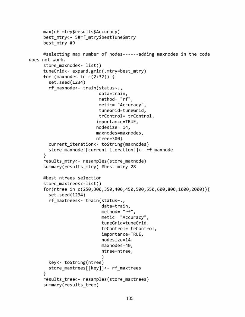
135

max(rf_mtry$results$Accuracy) best_mtry<- 5#rf_mtry$bestTune$mtry best_mtry #9 #selecting max number of nodes------adding maxnodes in the code

does not work. store_maxnode<- list() tuneGrid<- expand.grid(.mtry=best_mtry) for (maxnodes in c(2:32)) { set.seed(1234) rf_maxnode<- train(status~., data=train, method= "rf", metic= "Accuracy", tuneGrid=tuneGrid, trControl= trControl, importance=TRUE, nodesize= 14, maxnodes=maxnodes, ntree=300) current_iteration<- toString(maxnodes) store_maxnode[[current_iteration]]<- rf_maxnode } results_mtry<- resamples(store_maxnode) summary(results_mtry) #best mtry 28 #best ntrees selection store_maxtrees<-list() for(ntree in c(250,300,350,400,450,500,550,600,800,1000,2000)){ set.seed(1234) rf_maxtrees<- train(status~., data=train, method= "rf", metic= "Accuracy", tuneGrid=tuneGrid, trControl= trControl, importance=TRUE, nodesize=14, maxnodes=40, ntree=ntree, ) key<- toString(ntree) store_maxtrees[[key]]<- rf_maxtrees } results_tree<- resamples(store_maxtrees) summary(results_tree)

136

#fit the RF model using selected parametrs set.seed(1234) fit_rf<-randomForest(status~., data=train, method= "rf", metic= "Accuracy", tuneGrid=tuneGrid, trControl= trControl, importance=TRUE, mtry=5, nodesize=18, maxnodes=40, ntree=450) summary(fit_rf) #predict/evaluate the model, ACCURACY of Test Data prediction<- predict(fit_rf,test) confusionMatrix(prediction,test$status) ######plot significant variables varImpPlot(fit_rf) ##accuracy of train model prediction1<- predict(fit_rf,train) confusionMatrix(prediction1,train$status) ####new model with significant variables set.seed(1234) fit_rf<-randomForest(status~

pcs0+pds0+cu1s0+pu1s0+cu1v0+cu1s20+cu1v30+cds5+cds0+cdv0, data=train, method= "rf", metic= "Accuracy", tuneGrid=tuneGrid, trControl= trControl, importance=TRUE, mtry=10, nodesize=10, maxnodes=10, ntree=250) summary(fit_rf) #predict/evaluate the model, ACCURACY of Test Data prediction<- as.data.frame(predict(fit_rf,test)) confusionMatrix(prediction,test$status) #varImp(fit_rf)

137

varImpPlot(fit_rf) ##accuracy of train model prediction1<- predict(fit_rf,train) confusionMatrix(prediction1,train$status) ########################AUC############ library(pROC) p1<- predict(fit_rf,test,type="prob") pr<-prediction(p1, test$status) plot(rf.roc) auc <- performance(p1, measure = "auc") auc <- auc@y.values[[1]] auc

138

Appendix A.1. 3: R codes of SVM Model

library(ggplot2) library(lattice) library(caret) library(rlang) library(kernlab) library(RColorBrewer) #library(tidyverse) library(readxl) library(e1071) library(plyr) library(dplyr) df <- read_excel("Final Variables Data from 0

Sensor.xlsx",sheet="12") str(df) df[["status"]]=factor(df[["status"]]) #df$status<- ifelse(df$status=="Accident",1,0) df<- select(df,-c("Index")) #to remove the index column sum(is.na(df)) # check for any empty cell df<-na.omit(df) ###removed all the empty cells detach(df) #detach any previously loaded data #########parameter tuning attach(df) ### attach the latest data ##x<- data.frame(subset(df,select=-status)) ##y<- status svm<- ksvm(status~.,data=train, kernel= "rbfdot", C=2,cross=20,

gamma=0.125) ###Tune the rbf model svm_tune<- tune(method="svm",train.x=x,train.y=y, kernel="radial", ranges=list(cost=10^(-

1:3),gamma=2^(-2:2))) svm_tune<- tune( method="svm",train.x=x,train.y=y, kernel="radial",

list(gamma=c(.1,.2,.3,.4,.5,.6,.7,.8,.9,1))) print(svm_tune) #cost 2, gamma.125 svm_tune$performances

139

###Model Development8 set.seed(1234) # to reproduce the results intrain<-createDataPartition(df$status,p=0.80,list=FALSE) ## to

change the split, change p value train<- df[intrain,] ##seperating data for training test<-df[-intrain,] ##seperating data for testing #test<-as.data.frame(test) ################### SVM ########################### svm<- ksvm(status~.,data=train, kernel= "rbfdot", C=100,cross=5,

gamma=1) ## run the model, th e parameters cna be changed print(svm) #shows the output of the model ###prediction and confusion matrix p<-predict(svm,test) ## predict the test data set #p1<-as.data.frame(p) confusionMatrix(as.factor(p), as.factor(test$status)) #shows the

confusion matrix as a contingency table p1<- predict(svm,train) confusionMatrix(as.factor(p1), as.factor(train$status)) ####AUC################# library(ROCR) p1<- predict(svm,test, type="decision") pr<-prediction(p1, test$status) prf<- performance(pr, measure="tpr",x.measure="fpr") plot(prf) lines(x = c(0,1), y = c(0,1),col="blue") auc <- performance(pr, measure = "auc") auc <- auc@y.values[[1]] auc