Machine Learning for Automatic Prediction of theQuality of Electrophysiological RecordingsThomas Nowotny1*, Jean-Pierre Rospars2, Dominique Martinez3, Shereen Elbanna2¤a, Sylvia Anton2¤b

1 Sussex Neuroscience and Centre for Computational Neuroscience and Robotics, University of Sussex, Brighton, United Kingdom, 2 Physiologie de l’Insecte: Signalisation

et Communication, Institut National de la Recherche Agronomique, and Universite Pierre et Marie Curie, Versailles, France, 3 Laboratoire Lorrain de Recherche en

Informatique et ses Applications, Centre National de la Recherche Scientifique, Vandœuvre-les-Nancy, France

Abstract

The quality of electrophysiological recordings varies a lot due to technical and biological variability and neuroscientistsinevitably have to select ‘‘good’’ recordings for further analyses. This procedure is time-consuming and prone to selectionbiases. Here, we investigate replacing human decisions by a machine learning approach. We define 16 features, such asspike height and width, select the most informative ones using a wrapper method and train a classifier to reproduce thejudgement of one of our expert electrophysiologists. Generalisation performance is then assessed on unseen data, classifiedby the same or by another expert. We observe that the learning machine can be equally, if not more, consistent in itsjudgements as individual experts amongst each other. Best performance is achieved for a limited number of informativefeatures; the optimal feature set being different from one data set to another. With 80–90% of correct judgements, theperformance of the system is very promising within the data sets of each expert but judgments are less reliable when it isused across sets of recordings from different experts. We conclude that the proposed approach is relevant to the selectionof electrophysiological recordings, provided parameters are adjusted to different types of experiments and to individualexperimenters.

Citation: Nowotny T, Rospars J-P, Martinez D, Elbanna S, Anton S (2013) Machine Learning for Automatic Prediction of the Quality of ElectrophysiologicalRecordings. PLoS ONE 8(12): e80838. doi:10.1371/journal.pone.0080838

Editor: Johannes Reisert, Monell Chemical Senses Center, United States of America

Received August 13, 2013; Accepted October 15, 2013; Published December 4, 2013

Copyright: � 2013 Nowotny et al. This is an open-access article distributed under the terms of the Creative Commons Attribution License, which permitsunrestricted use, distribution, and reproduction in any medium, provided the original author and source are credited.

Funding: This work was funded by the EPSRC (http://www.epsrc.ac.uk/), grant number EP/J019690/1 ‘‘Green Brain’’, and BBSRC (http://www.bbsrc.ac.uk/), grantnumber BB/F005113/1 ‘‘PheroSys’’, to TN, the state program ‘‘Investissements d’avenir’’ managed by the Agence Nationale de la Recherche (http://www.agence-nationale-recherche.fr/), grant ANR-10-BINF-05 ‘‘Pherotaxis’’ to JPR, DM and SA and grant ANR-12-ADAP-0012-01 ‘‘Pherotox’’ in the programm Bioadapt to SA andJPR. The funders had no role in study design, data collection and analysis, decision to publish, or preparation of the manuscript.

Competing Interests: The authors have declared that no competing interests exist.

* E-mail: t.nowotny@sussex.ac.uk

¤a Current address: Zoology Department, Faculty of Science, Suez Canal University, Ismailia, Egypt¤b Current address: Laboratoire Recepteurs et Canaux Ioniques Membranaires, Institut National de la Recherche Agronomique and Universite d’Angers, Angers,France

Introduction

Electrophysiological recordings are widely used to evaluate how

nervous systems process information. Whereas up to about two

decades ago rather small data sets were acquired which were easy

to analyse manually, a rapid development of data acquisition and

storage techniques now allow to accumulate huge datasets within a

relatively short time and their analysis is often highly automated.

This trend tends to further accelerate with the introduction of

automated electrophysiology in ion channel discovery [1–3].

Nevertheless, an experienced electrophysiologist will typically still

examine recordings by hand, one by one, to evaluate which

recordings in a dataset will be suitable for exploitation by

automated analyses. This practice can be problematic in several

ways. Because it is based upon human judgement on a case-by-

case basis, data selection by manual inspection is liable to selection

or sampling bias; that is, a statistical error due to the selection of a

limited, non-representative, sample of the full neural population.

Although some statistical techniques aim at correcting for the

small number of recordings [4], the reliability of the selected data

remains problematic [5]. Different experimenters may select or

reject different recordings and their decisions can depend on

context, e.g. if a lower quality recording occurs among many very

high quality ones or among other low quality recordings.

A secondary problem with manual data inspection is the sheer

effort that is needed to classify large data sets. With ‘‘easy’’

experimental protocols, a strategy to keep only rapidly recogniz-

able ‘‘good’’ recordings can be used, but with complex experi-

mental protocols it is often time consuming to judge each

recording trace ‘‘by eye’’ and errors in the judgement can lead

either to a loss of recordings (if judged not sufficient although they

might be analysable), errors in results (if judged analysable

although they lack quality and hence lead to errors in the results)

or a waste of time (if judged analysable, but their quality proves

insufficient during analysis).

Many aspects of data analysis have undergone a process of

automation starting from filters [6] to spike detection [7] and

sorting [8–10], and from feature analysis of spike responses

[11,12], and inter-burst interval detection [13] in EEG recordings

to statistical analysis and visualisation [14].

However, the final judgement whether to include a recording

into the analysis or reject it as too low in quality or artefactual is

still reserved to the human researcher. Here, we begin to challenge

this established practice.

PLOS ONE | www.plosone.org 1 December 2013 | Volume 8 | Issue 12 | e80838

To facilitate the choice of electrophysiological recording traces

for further analysis, and remove subjectivity from this process, we

propose an automated evaluation process based on machine

learning algorithms using examples of intracellular recordings

from central olfactory neurons in the insect brain.

In machine learning [15], in contrast to alternative, automated

expert systems [16], there is no rule-based decision for deciding

the class of an input, e.g. the quality of a recording, but the

distinction between classes are derived from examples. Rather

than setting specific limits on features like the spike height, width

and noise amplitude, examples of values of these features are made

available to the machine learning system together with the correct

classification of the recordings and the system extrapolates from

the examples to decide on new inputs. In this work we define 16

characteristics (features) of electrophysiological recordings and

encode a large number of recordings by the value of these 16

features as 16-dimensional feature vectors. The recordings are

classified by an experienced electrophysiologist into three classes of

‘‘good’’ (can be used for analysis), ‘‘intermediate’’ (may be used for

analysis but there are problems) and ‘‘bad’’ (not suitable for further

analysis). A subset of the recordings is then used to train the

machine learning classifier and this classifier can then be used to

predict the classification of the remaining or new recordings.

An important ingredient for successful application of machine

learning methods is feature selection [17,18]. It is well established

that for solving any particular problem, like the classification of

recording quality addressed here, it is important to only use the

features that are most relevant to the specific problem. Including

additional, non-relevant features into the process will degrade the

ability of the classifier to generalize to novel examples. However,

for any given problem, the optimal number and identity of features

are typically unknown. In this paper we use a so-called wrapper

method [19,20] of feature selection to determine the relevant

features: the classifier is trained and tested in cross-validation

[21,22] on all possible choices of features in a brute force

exploration; the best combinations of features is then used in the

final classifier.

Methods

Data SetsWe used two data sets within the numerical analysis in this

work. Data set 1 was acquired by one of the authors (‘‘expert 1’’ in

what follows) and combines recordings from central olfactory

neurons in the antennal lobe of the noctuid moths Spodoptera

littoralis and Agrotis ipsilon. Data set 2 was acquired by another

author (‘‘expert 2’’ in what follows) and contained similar

recordings from A. ipsilon. Data set 1 consists of 183 recordings

and data set 2 of 549 recordings.

All recording traces were obtained with attempted intracellular

recordings with sharp glass electrodes of central olfactory neurons

within the antennal lobe of the two moth species. Each recording

trace was approximately 5 s in duration. A species-specific sex

pheromone stimulus (varying doses for different traces) was applied

1.5 s after the onset of the recording for 0.5 s.

For the purpose of this work on automatic data quality

assessment, the ground truth for the data quality of the used

Figure 1. Illustration of the calculation of spike height, spike width and noise amplitude. A) Spike height and width: The blue tracerepresents the original voltage data with small blue markers indicating the sampling. The red line is the moving average, which is used in spikedetection. The black horizontal line represents the baseline value that is calculated by averaging the membrane potential in windows to the left andthe right of the spike. The spike height is determined as the difference of the maximal voltage value of the spike and the baseline value. The spikewidth is measured as the distance of the two closest measurements below the half-height of the spike. B) Short time scale noise amplitude: Thedifference is taken between the original membrane potential measurement Vm and the filtered membrane potential measurement Vavg (movingaverage, see Figure 1A), and its Euclidean norm (normalised by 2 times the filter length +1) is calculated over two filter lengths,

r tnzNavg

� �~

1

2Navgz1

ffiffiffiffiffiffiffiffiffiffiffiffiffiffiffiffiffiffiffiffiffiffiffiffiffiffiffiffiffiffiffiffiffiffiffiffiffiffiffiffiffiffiffiffiffiffiffiffiffiffiffiffiffiffiffiffiffiffiffiX2Navg

i~0

Vm tnzið Þ{Vavg tnzið Þ� �2

vuut , (1) e.g. the noise level at the arrowhead is calculated from the marked interval of 2 filter

lengths. The areas of 2 maximal spike widths (263 ms) around every detected spike are excluded from this calculation and the local noise level isundefined in these areas around spikes.doi:10.1371/journal.pone.0080838.g001

Automatic Prediction of Recording Quality

PLOS ONE | www.plosone.org 2 December 2013 | Volume 8 | Issue 12 | e80838

recordings was established by visual inspection by two experts.

They classified the recordings in 3 categories: ‘‘bad’’, ‘‘interme-

diate’’ and ‘‘good’’ as defined in the introduction. Expert 19s

classification resulted in 29 bad, 54 intermediate and 100 good

recordings for data set 1 and 90 bad, 130 intermediate and 329

good recordings for data set 2. Expert 29s classification resulted in

20 bad, 39 intermediate, and 124 good recordings in data set 1

and 178 bad, 75 intermediate, and 296 good recordings in data set

2. Exemplary plots of the data are provided in Data S1.

Candidate FeaturesIn order to enable a machine classifier to make decisions about

the quality of recordings it needs access to the relevant properties

of the data. We defined 16 such properties that we call features.

The data are first pre-processed with filters and a rule-based spike

detection algorithm. If recorded with different gain factors during

data acquisition, the recorded membrane potential V(t) was

multiplied by the gain factor to achieve a common scale for all

recordings (e.g. mV). For the purpose of spike detection, V(t) was

then filtered with a moving average of window size 3 ms. Candidate

spike events were detected based on two threshold criteria on the

derivative of the filtered membrane potential. Detecting spikes

based on the derivative will automatically remove any occurring

plateau potentials and possible recording artefacts due to current

injections. In order to qualify as a candidate spike event, 3

consecutive derivatives need to be above the upward threshold hup

and within tspike,max = 3 ms, 3 consecutive derivatives need to be

below the downward threshold hdown. These conditions test for the

sharp rise and fall of the membrane potential around a spike and are

independent of the overall amplitude and baseline values. The

upward and downward derivative thresholds hup and hdown were

chosen as three times the 80th percentile and 3 times the 20th

percentile of all observed values of the derivative, respectively.

Deriving the threshold values from percentiles of observed values of

the derivative helps us to take into account if a sufficient number of

spikes are less steep due to current injections or other prolonged

excitation. Our manual controls of spike detection showed that this

strategy is vey reliable in finding all candidate spike events.

Figure 1 illustrates the characterization of spike features (Fig. 1A)

and local noise (Fig. 1B). The maximum of the candidate spike was

calculated as the maximum of V(t) (‘‘spike max’’ in Fig. 1A)

between the first crossing of the derivative above hup and the last

point where the derivative was below hdown and the time when this

maximum is attained defines the spike time tspike. The local

baseline value around the candidate spike was calculated as the

average membrane potential V(t) in the intervals [tspike –6 ms, tspike

–3 ms] and [tspike +3 ms, tspike +6 ms] (black horizontal line in

Fig. 1A). The spike height is then given by the difference between

the maximum membrane potential and this local baseline.

To eventually be accepted as a spike event, some additional

conditions have to be met: (i) there are points within 3 ms before

and after the spike time where the membrane potential is lower

than the half height of the spike, and (ii) the spike height has more

than half the 95th percentile of all observed spike heights. The first

rule excludes certain artefacts, where there is mainly a step up or

step down of the recorded potential and the second rule excludes

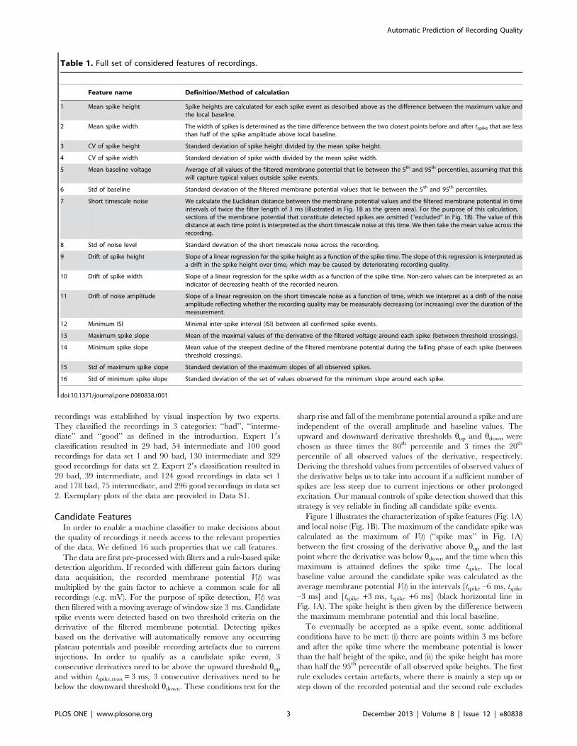
Table 1. Full set of considered features of recordings.

Feature name Definition/Method of calculation

1 Mean spike height Spike heights are calculated for each spike event as described above as the difference between the maximum value andthe local baseline.

2 Mean spike width The width of spikes is determined as the time difference between the two closest points before and after tspike that are lessthan half of the spike amplitude above local baseline.

3 CV of spike height Standard deviation of spike height divided by the mean spike height.

4 CV of spike width Standard deviation of spike width divided by the mean spike width.

5 Mean baseline voltage Average of all values of the filtered membrane potential that lie between the 5th and 95th percentiles, assuming that thiswill capture typical values outside spike events.

6 Std of baseline Standard deviation of the filtered membrane potential values that lie between the 5th and 95th percentiles.

7 Short timescale noise We calculate the Euclidean distance between the membrane potential values and the filtered membrane potential in timeintervals of twice the filter length of 3 ms (illustrated in Fig. 1B as the green area). For the purpose of this calculation,sections of the membrane potential that constitute detected spikes are omitted (‘‘excluded’’ in Fig. 1B). The value of thisdistance at each time point is interpreted as the short timescale noise at this time. We then take the mean value across therecording.

8 Std of noise level Standard deviation of the short timescale noise across the recording.

9 Drift of spike height Slope of a linear regression for the spike height as a function of the spike time. The slope of this regression is interpreted asa drift in the spike height over time, which may be caused by deteriorating recording quality.

10 Drift of spike width Slope of a linear regression for the spike width as a function of the spike time. Non-zero values can be interpreted as anindicator of decreasing health of the recorded neuron.

11 Drift of noise amplitude Slope of a linear regression on the short timescale noise as a function of time, which we interpret as a drift of the noiseamplitude reflecting whether the recording quality may be measurably decreasing (or increasing) over the duration of themeasurement.

12 Minimum ISI Minimal inter-spike interval (ISI) between all confirmed spike events.

13 Maximum spike slope Mean of the maximal values of the derivative of the filtered voltage around each spike (between threshold crossings).

14 Minimum spike slope Mean value of the steepest decline of the filtered membrane potential during the falling phase of each spike (betweenthreshold crossings).

15 Std of maximum spike slope Standard deviation of the maximum slopes of all observed spikes.

16 Std of minimum spike slope Standard deviation of the set of values observed for the minimum slope around each spike.

doi:10.1371/journal.pone.0080838.t001

Automatic Prediction of Recording Quality

PLOS ONE | www.plosone.org 3 December 2013 | Volume 8 | Issue 12 | e80838

small secondary events like secondary spikes from other neurons

(Note, that even though these are intra-cellular recordings, spikes

from other neurons can potentially be present due to either strong

coupling by gap junctions, recording electrodes contacting more

than one cell or the existence of multiple spike initiation zones

[23,24].) or mere EPSPs.

The 16 features of a recording that we consider in the following

are based on the detected spike events as well as on general

properties of the full bandwidth V(t) signal. They are summarized

in table 1 and Figure 1A,B. Automatic feature extraction was

performed with Matlab (Mathworks, Natick, MA) and takes about

21 minutes for the larger of our data sets (549 recordings). The

Matlab tools for automatic feature extraction are provided as

supplementary material (Toolbox S1).

DistributionsThe statistical distributions of feature values are shown as

histograms (20 bins) in a range that includes the 5th to the 95th

percentile of observed values (i.e. excluding extreme outliers if

there are any). Statistically significant differences between distri-

butions were determined by Kolmogorov-Smirnov tests with

Bonferroni correction for multiple pairwise tests at 5% and 1%

significance levels.

Crossvalidation and Classification MethodCrossvalidation is used to assess the success of a classification

method when no separate test set is available. The data set of

interest is split repeatedly into a training and testing portion and

the performance of the classification algorithm is assessed on these

different splits. We use 10-fold crossvalidation, in which the data is

split into a 90% training set and 10% left out samples for testing.

The split is chosen randomly, but such that after 10 repeats, all

samples have been left out once. If not stated otherwise we repeat

the full 10-fold crossvalidation 50 times with independent random

splits.

As classifiers we used linear support vector machines (SVMs)

[25]. SVMs are known to perform competitively in a number of

applications. We decided to employ a linear SVM to avoid

introducing additional meta-parameters such as a kernel degree or

parameters of radial basis functions and, importantly, to limit the

risk of over-fitting, which is higher in non-linear SVMs when the

data is high dimensional. To avoid infinite iterations, which occur

in rare cases with minimal features (which arguably are not even

particularly interesting), we limited the learning iterations of the

SVM algorithm to 104 steps. We checked with unlimited learning

iterations (with a ceiling of 106 iterations in two rare cases where

otherwise apparently infinite iterations occurred) and observed no

discernible differences in the results.

For the cost parameter of the linear SVM we used C = 512.

Repeated runs with C = 8, 32, and 128 gave similar results.

Wrapper Approach to Feature SelectionThe wrapper approach to feature selection is a brute force

method in which all possible choices of features are tested with

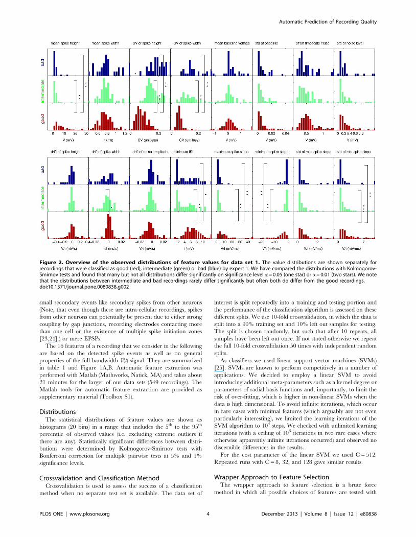
Figure 2. Overview of the observed distributions of feature values for data set 1. The value distributions are shown separately forrecordings that were classified as good (red), intermediate (green) or bad (blue) by expert 1. We have compared the distributions with Kolmogorov-Smirnov tests and found that many but not all distributions differ significantly on significance level a= 0.05 (one star) or a= 0.01 (two stars). We notethat the distributions between intermediate and bad recordings rarely differ significantly but often both do differ from the good recordings.doi:10.1371/journal.pone.0080838.g002

Automatic Prediction of Recording Quality

PLOS ONE | www.plosone.org 4 December 2013 | Volume 8 | Issue 12 | e80838

respect to the performance of classification in crossvalidation based

on each feature choice. Here, there are 16 possible features

allowing 216 – 1 potential choices for the group of used features.

We call a particular choice of features, e.g. features (1, 4, 9, 11) a

feature set and the number of employed features, 4 in this

example, the size of the feature set. Most results will be reported

separately for feature sets of different sizes.

The wrapper features selection was executed on the in-house

computer cluster of the University of Sussex in separate processes

for each feature set size. Computation times varied from 20 s for

feature sets of size 16 to about 3.5 days for feature sets of size 7–9.

The normal wrapper approach of feature selection with

crossvalidation is prone to the following over-fitting effect: we

typically test all possible feature sets in crossvalidation and then

report the best observed performance and identify the feature set

that obtained this performance. If this best-performing feature set

is interpreted as the optimal feature choice for the problem at

hand one is exposed to the selection bias of potentially identifying

Figure 3. Overview of the observed distributions of feature values for data set 2. The conventions are as in Figure 3. We note that for thisdata set the differences of feature value distributions are even more pronounced.doi:10.1371/journal.pone.0080838.g003

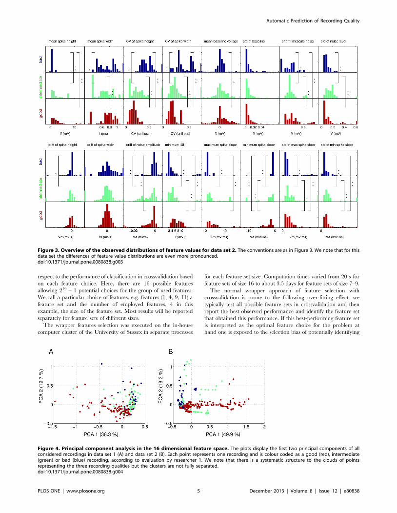
Figure 4. Principal component analysis in the 16 dimensional feature space. The plots display the first two principal components of allconsidered recordings in data set 1 (A) and data set 2 (B). Each point represents one recording and is colour coded as a good (red), intermediate(green) or bad (blue) recording, according to evaluation by researcher 1. We note that there is a systematic structure to the clouds of pointsrepresenting the three recording qualities but the clusters are not fully separated.doi:10.1371/journal.pone.0080838.g004

Automatic Prediction of Recording Quality

PLOS ONE | www.plosone.org 5 December 2013 | Volume 8 | Issue 12 | e80838

a feature set where the crossvalidation procedure (which contains a

random element) worked particularly well by chance. This bias is

particularly strong when a large number of feature sets with very

similar quality are compared. To avoid this bias and, without using

truly novel test data, get a realistic estimate of how well one would

do when using a wrapper method for feature selection, we devised

a two-stage-leave-one-out crossvalidation procedure. In the first

stage, one recording is left out and the remaining training set of

n21 recordings is used for a full wrapper feature selection with

crossvalidation. This involves choosing feature sets and evaluating

them in crossvalidation, i.e. leaving out another recording, training

a classifier on the resulting training set with n22 recordings and

testing it on the left out recording. For full crossvalidation, this

procedure is repeated until all n21 recordings have been left out.

We then use the top10 best feature sets (see below for a definition

of the top10 group) and train corresponding classifiers on the

‘‘full’’ training set of n21 recordings. The resulting classifiers are

then finally used for predicting the class of the originally left out

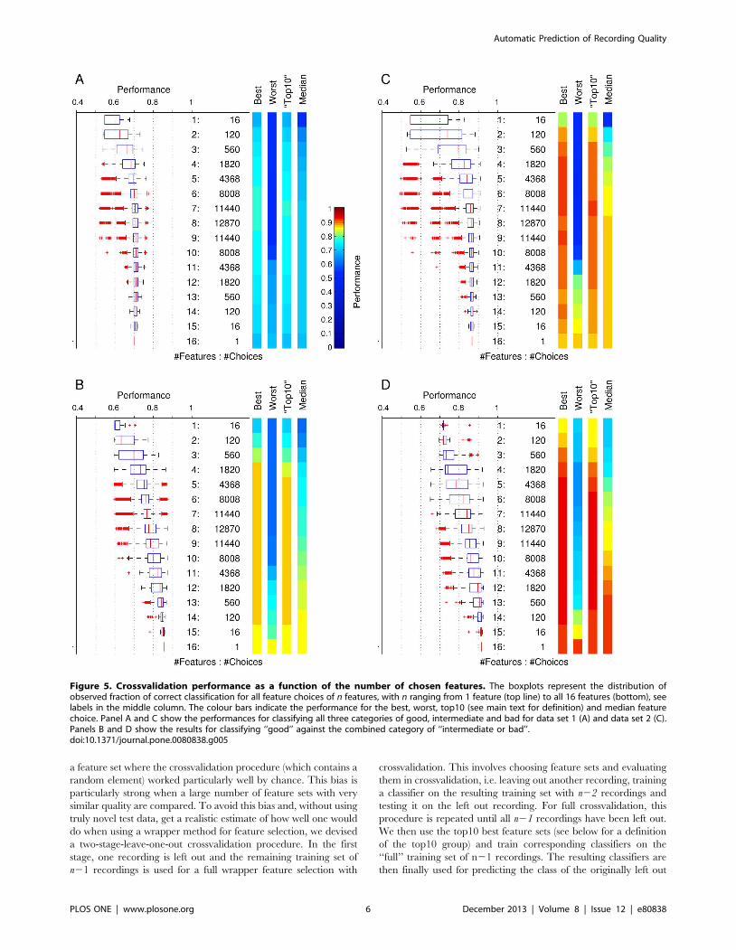
Figure 5. Crossvalidation performance as a function of the number of chosen features. The boxplots represent the distribution ofobserved fraction of correct classification for all feature choices of n features, with n ranging from 1 feature (top line) to all 16 features (bottom), seelabels in the middle column. The colour bars indicate the performance for the best, worst, top10 (see main text for definition) and median featurechoice. Panel A and C show the performances for classifying all three categories of good, intermediate and bad for data set 1 (A) and data set 2 (C).Panels B and D show the results for classifying ‘‘good’’ against the combined category of ‘‘intermediate or bad’’.doi:10.1371/journal.pone.0080838.g005

Automatic Prediction of Recording Quality

PLOS ONE | www.plosone.org 6 December 2013 | Volume 8 | Issue 12 | e80838

recording. This procedure is repeated until all recordings have

been left out once in stage one.

Results and Discussion

Statistical Distributions of Feature Values in the Data SetsWe calculated the values of all 16 features on the two data sets

and plotted the distribution of observed values separately for each

group of bad (blue), intermediate (green) and good (red)

recordings, as judged by expert 1 (Fig. 2, 3). The quantities

plotted are noted in each graph. The plots report relative

occurrence within each group rather than absolute numbers to

take into account the different group sizes (100 good, 54

intermediate, and 29 bad recordings in data set 1 and 329 good,

130 intermediate and 90 bad in data set 2).

The plots reveal noticeable differences between distributions of

feature values for good recordings and intermediate or bad

recordings, e.g. for the mean spike height or the CV of the spike

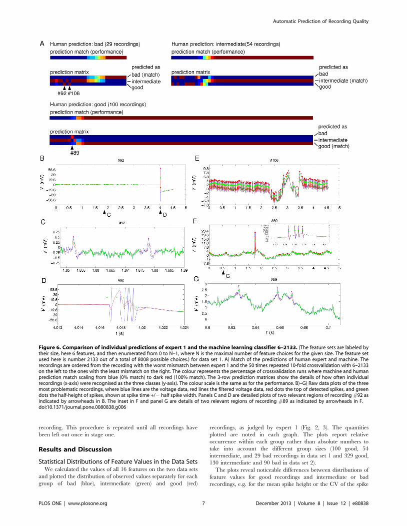
Figure 6. Comparison of individual predictions of expert 1 and the machine learning classifier 6–2133. (The feature sets are labeled bytheir size, here 6 features, and then enumerated from 0 to N–1, where N is the maximal number of feature choices for the given size. The feature setused here is number 2133 out of a total of 8008 possible choices.) for data set 1. A) Match of the predictions of human expert and machine. Therecordings are ordered from the recording with the worst mismatch between expert 1 and the 50 times repeated 10-fold crossvalidation with 6–2133on the left to the ones with the least mismatch on the right. The colour represents the percentage of crossvalidation runs where machine and humanprediction match scaling from blue (0% match) to dark red (100% match). The 3-row prediction matrices show the details of how often individualrecordings (x-axis) were recognised as the three classes (y-axis). The colour scale is the same as for the performance. B)–G) Raw data plots of the threemost problematic recordings, where blue lines are the voltage data, red lines the filtered voltage data, red dots the top of detected spikes, and greendots the half-height of spikes, shown at spike time +/2 half spike width. Panels C and D are detailed plots of two relevant regions of recording #92 asindicated by arrowheads in B. The inset in F and panel G are details of two relevant regions of recording #89 as indicated by arrowheads in F.doi:10.1371/journal.pone.0080838.g006

Automatic Prediction of Recording Quality

PLOS ONE | www.plosone.org 7 December 2013 | Volume 8 | Issue 12 | e80838

height. To test this observation formally, we performed pairwise

Kolmogorov-Smirnov tests with a Bonferroni correction for

multiple statistical tests on a 5% significance level (one star in

Figures 2 and 3) and 1% significance level (two stars in the

Figures). We find that many features show significant differences

between the distributions for good and bad recordings and

between distributions for good and intermediate recordings. The

main features with highly significant differences in both data sets

are spike height, CV of spike height, CV of spike width, minimum

and maximum spike slope, and standard deviations of minimum

and maximum spike slope (see relevant panels in Fig. 2, 3).

The distributions for bad and intermediate recordings rarely

differ significantly but more so in data set 2 than in data set 1. It is

worth noting that the different numbers of recordings for the three

categories imply that the power of the KS test will be different for

the various comparisons and hence in some cases differences

between intermediate and bad recordings are not significant even

though they are visible to the eye (Fig. 2, 3).

To further analyse whether the observed differences in the

distributions of feature values for the three different categories

result in a clear cluster structure in the 16 dimensional feature

space that would be amenable to standard machine learning

algorithms for classifying new recordings of unknown quality, we

performed a principal component analysis. The results are

illustrated in Figure 4. The two first principal components account

for 36.2% and 19.7% of the total variance in data set 1 and 49.9%

and 18.2% for data set 2, indicating that data set 2 has a lower-

dimensional structure in the 16 dimensional feature space that can

be captured more easily in two principal components.

We observe some visible differences between good recordings

and the rest, but clusters are not particularly well defined in either

data set. Especially intermediate and bad recordings seem very

intermingled (Fig. 4). This suggests that building a machine

learning system for automatic detection of recording quality may

not be trivial.

From the statistical analysis we can conclude that most of the

chosen features are informative for distinguishing the quality of

recordings. We would expect that when assessed for their

suitability in a machine learning approach to predicting recording

quality the features that gave rise to the most significant differences

between recordings of differing quality would be the best

candidates. We will re-examine this question in the framework

of a wrapper feature selection method below.

Feature Selection and ClassificationThe problem of not well-separated classes is common in

machine learning and one of the most important elements of a

successful machine learning system is the selection of a subset of

the most relevant features and the omission of the less informative

or misleading ones. Here we used a standard approach to this

problem, a so-called wrapper method. In brief, in a wrapper

approach to feature selection all possible subsets of features are

tested with the employed classifier on the training set, usually in

crossvalidation (see Methods). The feature set with the best

prediction performance in crossvalidation is chosen for the final

classifier, which is then tested on a separate test set.

We performed wrapper feature selection on all possible subsets

of the 16 defined features, a total of 216–1 = 65535 possible

selections. As a classifier we used a linear support vector machine

(SVM). Figure 5 shows the performance for the two data sets.

Performance values are grouped by the size of the employed

feature sets, i.e. size 1 indicates only one feature was used and size

16 means that all features were used. The performance of the

classifier is expressed as the percentage of correct predictions, i.e.,

90% performance would mean that the classifier predicted for

90% of the recordings the true quality value (as provided earlier by

expert 1). We here report the best performance for any of the

feature choices, the worst observed performance, the median of

the observed performance values and the average performance of

the ‘‘top10’’ group of choices (see vertical colour bars in Figure 5).

The top10 group is defined as the 10 best performing choices, or,

for smaller numbers of overall available choices (e.g. when

choosing 15 out of 16 features, etc.), the performance of the best

10% of choices, but always of at least one choice. Using 10-fold

crossvalidation we observed that in data set 1 (Fig. 5A) the best

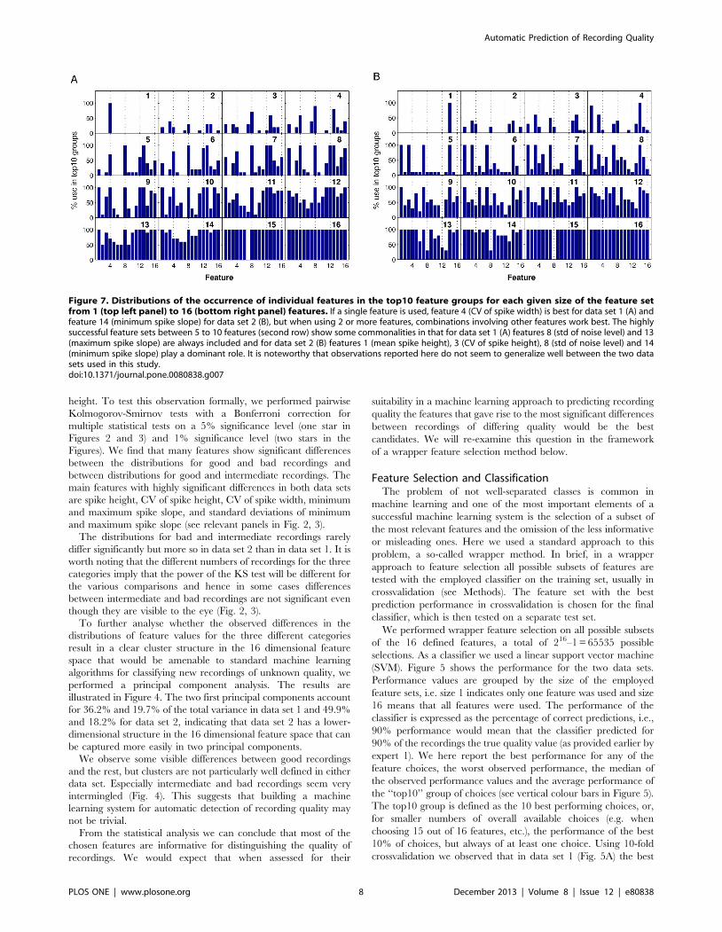
Figure 7. Distributions of the occurrence of individual features in the top10 feature groups for each given size of the feature setfrom 1 (top left panel) to 16 (bottom right panel) features. If a single feature is used, feature 4 (CV of spike width) is best for data set 1 (A) andfeature 14 (minimum spike slope) for data set 2 (B), but when using 2 or more features, combinations involving other features work best. The highlysuccessful feature sets between 5 to 10 features (second row) show some commonalities in that for data set 1 (A) features 8 (std of noise level) and 13(maximum spike slope) are always included and for data set 2 (B) features 1 (mean spike height), 3 (CV of spike height), 8 (std of noise level) and 14(minimum spike slope) play a dominant role. It is noteworthy that observations reported here do not seem to generalize well between the two datasets used in this study.doi:10.1371/journal.pone.0080838.g007

Automatic Prediction of Recording Quality

PLOS ONE | www.plosone.org 8 December 2013 | Volume 8 | Issue 12 | e80838

performance was maximal when using 6 features and led to 77.5%

correct predictions. The maximal average performance of the

‘‘top10’’ groups was 76.8% when using 7 features. In data set 2

(Fig. 5C) we find optimal performance of 87.4% when using 8

features and best average performance of the top10 group of

87.1% when using 10 features. This compares to the following

chance levels: In data set 1, for fully random guesses of equal

probability, the expected performance would be 33.3%, for

guessing proportional to the abundance of the three classes,

41.1% and if guessing that recordings are always of class ‘‘good’’,

55%. In data set 2 the corresponding chance levels are 33.3%

(random), 44.2% (proportional) and 60% (guessing ‘‘good’’).

For data set 1, the set of features that was performing best

consisted of 6 features: (1, 4, 8, 12, 13, 16), and for data set 2 of the

8 features (1, 2, 3, 4, 5, 13, 14, 15). We note that the spike height

(feature 1) and the CV of the spike width (feature 4), as well as, the

maximum spike slope (feature 13) are common to both feature sets.

Comparing to the statistics shown in Figures 2 and 3, the

distributions of feature values for these three features do show

visible and significant differences in both data sets. Conversely, the

standard deviation of the baseline is not a chosen feature in either

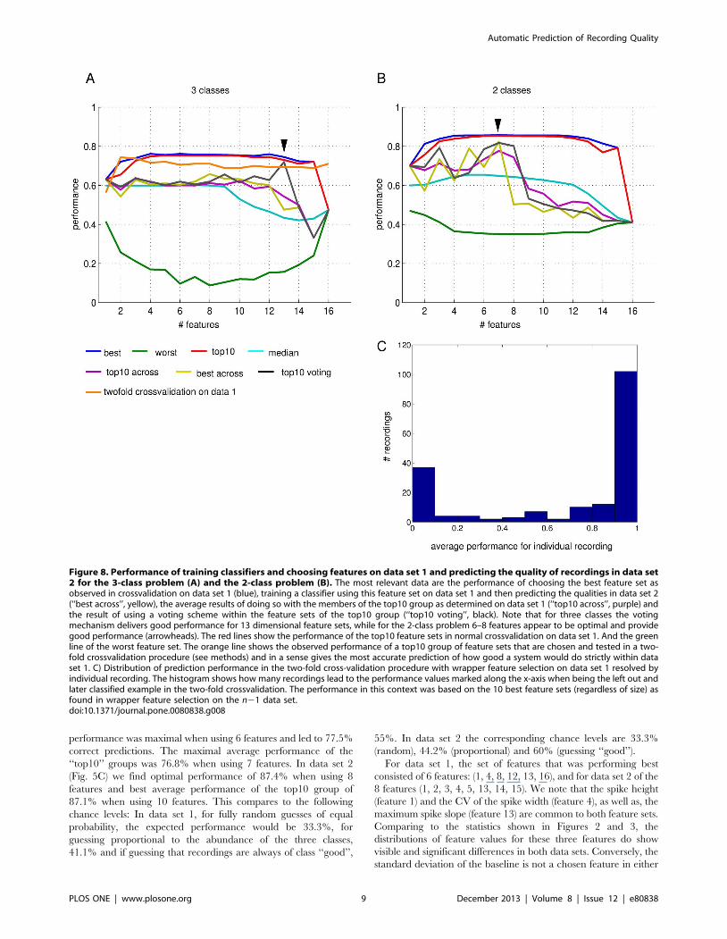
Figure 8. Performance of training classifiers and choosing features on data set 1 and predicting the quality of recordings in data set2 for the 3-class problem (A) and the 2-class problem (B). The most relevant data are the performance of choosing the best feature set asobserved in crossvalidation on data set 1 (blue), training a classifier using this feature set on data set 1 and then predicting the qualities in data set 2(‘‘best across’’, yellow), the average results of doing so with the members of the top10 group as determined on data set 1 (‘‘top10 across’’, purple) andthe result of using a voting scheme within the feature sets of the top10 group (‘‘top10 voting’’, black). Note that for three classes the votingmechanism delivers good performance for 13 dimensional feature sets, while for the 2-class problem 6–8 features appear to be optimal and providegood performance (arrowheads). The red lines show the performance of the top10 feature sets in normal crossvalidation on data set 1. And the greenline of the worst feature set. The orange line shows the observed performance of a top10 group of feature sets that are chosen and tested in a two-fold crossvalidation procedure (see methods) and in a sense gives the most accurate prediction of how good a system would do strictly within dataset 1. C) Distribution of prediction performance in the two-fold cross-validation procedure with wrapper feature selection on data set 1 resolved byindividual recording. The histogram shows how many recordings lead to the performance values marked along the x-axis when being the left out andlater classified example in the two-fold crossvalidation. The performance in this context was based on the 10 best feature sets (regardless of size) asfound in wrapper feature selection on the n21 data set.doi:10.1371/journal.pone.0080838.g008

Automatic Prediction of Recording Quality

PLOS ONE | www.plosone.org 9 December 2013 | Volume 8 | Issue 12 | e80838

case, which appears to correspond with the observation that the

value distributions for this feature are not very different between

classes. Beyond these obvious observations, however, it is hard to

predict by manual inspection of the value distributions which

combination of features may be particularly successful, necessitat-

ing the exhaustive wrapper approach.

To further test the idea that features 1, 4 and 13 are particularly

useful, we inspected the performance of all feature sets that contain

all three of these and compared them to the performance of

feature sets that do not contain them all. We observe that for data

set 1 and feature sets with more than 4 and less than 14 elements,

the average performance of the sets containing the three features is

significantly higher than of the sets not containing all of them (1-

way unbalanced ANOVA, P,1024 or less). For data set 2,

however, we do not see such a significant effect, even though the

performance of the feature sets containing all three features

visually appears higher for most feature set sizes (data not shown).

Finally, on their own, the three features lead to a performance of

68.1% (3 classes), 87.1% (2 classes) in data set 1 and 76.7% (3

classes), 78.3% (2 classes) in data set 2.

When analysing the errors being made by the classifier using the

above best feature choice of size 6 (Fig. 6) we note that there are 3

specific recordings for which predictions are opposite to human

judgement (i.e. predicting ‘‘bad’’ when the ground truth was

‘‘good’’ or predicting ‘‘good’’ when it was ‘‘bad’’) and consistently

so across repeated crossvalidation runs (Fig. 6A, arrowheads). We

inspected these recordings (#89, #92 and #106 in our data set 1)

manually (Fig. 6B–G) and found clear reasons for the discrepancy

that elucidate the remaining limitations of the automated system.

Recording #92 contains a large artefact and no obvious spikes;

it is therefore classified as ‘‘bad’’ by the human expert. The

preprocessing picked up both the artefact and many small, but

very consistent spikes (Fig. 6 C,D). Because of the reliance on

percentiles (aimed at limiting the impact of potential artefacts), the

recording is predicted to be good by the machine based on the

many small spikes.

Recording #106 also contains artefacts, in this case an unstable

baseline voltage that might compromise reliable spike detection

(Figure 6E). It was therefore judged to be ‘‘bad’’ by expert 1.

However, the automatic system detects spikes quite reliably and of

consistent amplitude and because the standard deviation of the

baseline (feature 6) is not included in the feature set employed

here, the automatic system classifies the recording as ‘‘good’’.

The third example, recording #89, contains four clear spikes

(Fig. 6F, inset) and was judged to be good by expert 1. However,

the automatic system detects secondary, very small spikes

(Figure 6G), which are not excluded by the spike eligibility rules

(see Methods) because those are based on percentiles and four

large spikes are not sufficiently many to trigger the exclusion rules

for the spike height. As a result, the calculated features have large

values for the standard deviations of spike height and spike width,

the latter of which is included in our best-performing feature set –

a likely reason for the observed ‘‘bad’’ classification.

Apart from the three discussed examples, all other mistakes are

between good and intermediate or between bad and intermediate,

the latter ones being about twice as frequent. This is consistent

with the observed differences in the statistical distributions of

feature values and suggests that the distinction between interme-

diate and bad recordings is the most difficult. Accordingly, if we

combine intermediate and bad recordings into one class of

unacceptable recordings and ask the same question of classifying

the data quality but now only into the two categories ‘‘good’’ and

‘‘unacceptable’’, we observe much higher classification success

(Fig. 5B,D).

Overall success rates of almost 80% for the three class problem

and over 90% for the two class problem make the automatic

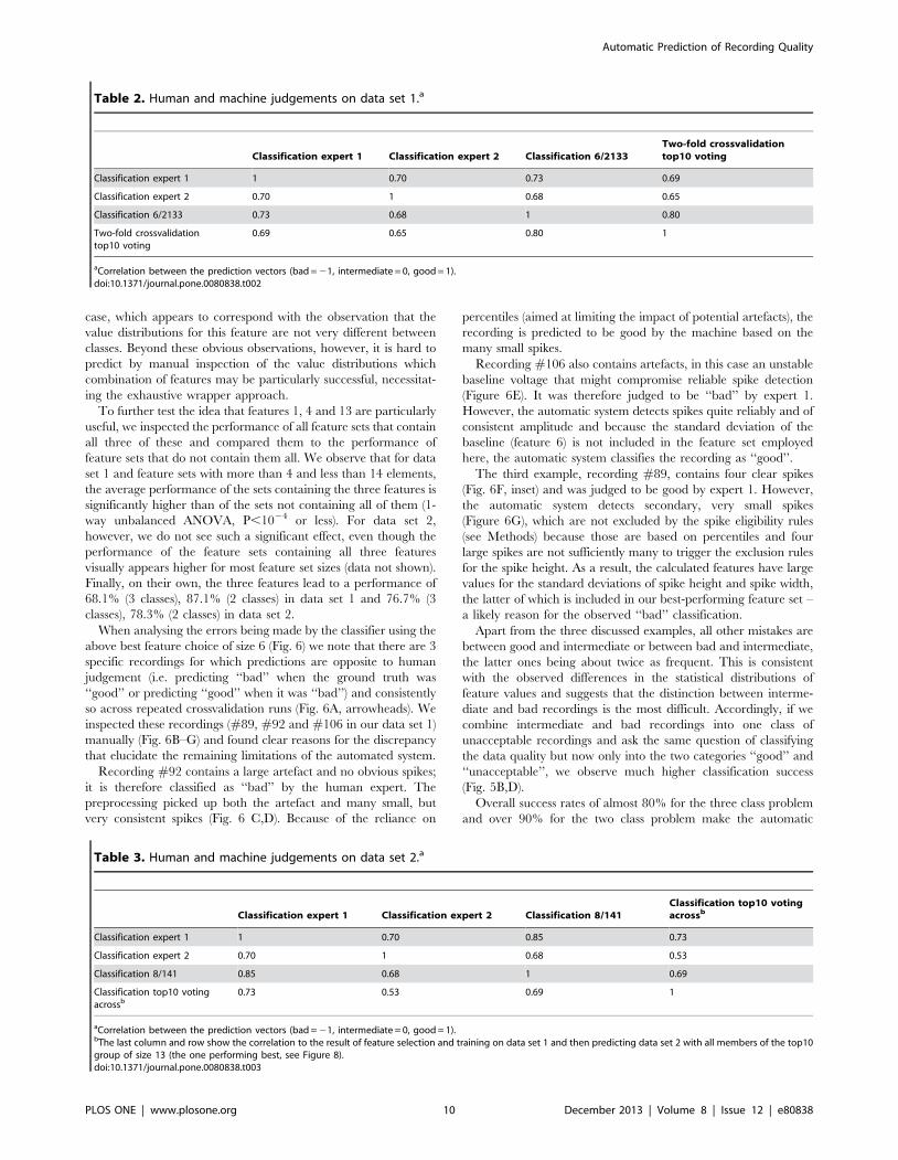
Table 2. Human and machine judgements on data set 1.a

Classification expert 1 Classification expert 2 Classification 6/2133Two-fold crossvalidationtop10 voting

Classification expert 1 1 0.70 0.73 0.69

Classification expert 2 0.70 1 0.68 0.65

Classification 6/2133 0.73 0.68 1 0.80

Two-fold crossvalidationtop10 voting

0.69 0.65 0.80 1

aCorrelation between the prediction vectors (bad = 21, intermediate = 0, good = 1).doi:10.1371/journal.pone.0080838.t002

Table 3. Human and machine judgements on data set 2.a

Classification expert 1 Classification expert 2 Classification 8/141Classification top10 votingacrossb

Classification expert 1 1 0.70 0.85 0.73

Classification expert 2 0.70 1 0.68 0.53

Classification 8/141 0.85 0.68 1 0.69

Classification top10 votingacrossb

0.73 0.53 0.69 1

aCorrelation between the prediction vectors (bad = 21, intermediate = 0, good = 1).bThe last column and row show the correlation to the result of feature selection and training on data set 1 and then predicting data set 2 with all members of the top10group of size 13 (the one performing best, see Figure 8).doi:10.1371/journal.pone.0080838.t003

Automatic Prediction of Recording Quality

PLOS ONE | www.plosone.org 10 December 2013 | Volume 8 | Issue 12 | e80838

system attractive for research areas where high volumes of data

need to be processed. Furthermore, the low error rate between the

extremes of good and bad makes the system fairly safe to use. One

strategy of using it would be to rely on the two class system and

keep all recordings with a ‘‘good’’ rating. Alternatively, one could

additionally use the three class system to identify candidates for

intermediate quality and manually inspect them to maximise the

usable recordings. Optimally one would want to design a system

that is particularly geared towards identifying the distinction

between ‘‘intermediate’’ and ‘‘bad’’; however, the statistics for the

feature values (Fig. 2,3) and our classification results indicate that

this is the hardest part of the problem.

Feature Use StatisticsHaving tried all possible combinations of features we now can

ask which features are the most useful for the classification of

recording quality. We built the distribution of how often particular

features where used in the ‘top10’ groups in the experiments with

data sets 1 and 2. The results are illustrated in Figure 7.

Interestingly, the most successful features differ for the two data

sets, indicating that individual feature selection may be necessary

for different experimenters, and likely also for different types of

experiments (see also ‘testing across data sets’ below). However,

the distributions do have in common that for small feature sets of

2–4 features, there are no clear preferences but many combina-

tions of features seem to work similarly well. This appears to

indicate that several of the defined features are informative for the

quality of the recording and there is no one golden rule deriving

from only one or two central features. For larger feature sets of 5 to

8 features we notice that features (4, 8, 12, 13) seem to (almost)

always be used but with different combinations of other features,

indicating that these features seem to be the most salient for the

task.

Overall the wide spread of features used indicates, however, that

there are less dominant features in this application of machine

learning than in other domains [18]. Furthermore, the difference

in successful features for data set 1 and data set 2 might indicate

that the best features may depend on the experimenter and, to

speculate a bit further, likely on the nature of the preparation and

the experiments. The use of an automatic procedure for both

feature selection (wrapper method) and classification however

alleviates this problem as a data quality system could be fairly

quickly adjusted to novel experiments or preparations, simply by

providing a well-sized set of examples for different quality

recordings and the appropriate class labels based on human

judgement. From there on, the procedure can be fully automated.

Testing Across Data SetsIn a practical application one would choose features and train a

classifier on a reference data set to then automatically recognise

the recording quality in future recordings. To investigate the

performance of our machine learning system with wrapper feature

selection in this situation we choose the best-performing feature

sets in crossvalidation on data set 1, train a classifier for the best

and the top10 feature choices on data set 1 and classify all

recordings in data set 2 using the resulting classifiers.

Figure 8A illustrates our observations in the case of three classes

(bad, intermediate and good). If we use the single best feature set

we observe a classification performance around 60% (barely above

chance) on data set 2 (yellow line in Fig. 8A), where the ground

truth was assumed to be the manual classification of recording

quality by expert 1. This performance is observed for feature sets

of 10 or less features and then rapidly declines to markedly below

chance levels for systems using more features. It compares to

around 75% performance for best and top10 group in cross-

validation on data set 1 only (blue and red lines in Fig. 8A). The

average performance of using top10 group feature sets to train on

set 1 and predict set 2 shows a similar pattern (purple line in

Fig. 8A). We then also used a compound classifier based on a

majority vote of the classifiers trained based on each of the ‘top10’

feature sets (black line in Fig. 8A). This ‘‘voting classifier’’ performs

better than the individual ‘top10’ feature set based classifiers with a

marked best performance for 13 used features, above which

performance drops.

The reduced problem of only 2 classes of recording quality (with

intermediate and bad pooled together) shows a somewhat different

picture (Fig. 8B). Here, some of the classifiers based on the best

feature sets and top10 feature sets and of size 7 or less achieve

more respectable performances of 70 to 80% (yellow, purple and

black lines in Fig. 8B) and rapidly decline in performance for

larger feature sets. The compound voting classifier here performs

best for between 6 and 8 features (black line in Fig. 8B) and with

around 80% well above chance levels of 59%. This seems to

indicate that the simpler 2-class problem is more robustly solved

with less features while the more complex 3-class system needs

more features to distinguish all 3 classes.

In our testing across data sets we have made two separate

advances over the crossvalidation trials with the wrapper feature

selection reported above. We have used a true test set that was not

seen by the machine learning system until after feature selection

and building a classifier with the preferred feature choices has

been completed. We have also used data from one expert to

predict the data quality of recordings of a different expert. Overall,

we see a reduction in prediction accuracy but it is not clear which

of the two changes is mainly to blame. To unravel this potential

confound, we devised a two-fold crossvalidation procedure that

can be run within the data set of a single expert but avoids the

potential over-fitting when using a wrapper feature selection

approach. In the two-fold crossvalidation procedure, one record-

ing is left out from the data set and then the full wrapper feature

selection using crossvalidation (involving more leave-out record-

ings) is performed on the remaining ‘‘n21’’ recordings. We then

choose features and train a classifier on the n21 recordings to

eventually predict the quality of the originally left out recording

(see Methods for more details). We observe that the performance

of voting classifiers based on ‘top10’ feature groups is competitive

(Fig. 8A, orange line). In particular, for very small feature sets of 2

or 3 features, we observe above 73% correct results. When

compared to the 76–77% maximal success rate in the standard

wrapper method (red and blue lines in Fig. 8A), this suggests an

effect of over-fitting. However, when compared to the about 60%

performance seen in classification of data set 2 based on data set 1

(yellow, purple, black lines in Fig. 8A), a similarly strong, if not

stronger, effect of predicting across experts becomes apparent.

From this numerical experiment with twofold leave-one-out

crossvalidation we conclude that in the three class problem, we can

reasonably expect a 73% performance of fully correct predictions

when remaining within the recordings of a single expert.

The observed performances imply that misclassification occurs

in a few cases. It is interesting to ask whether these cases are due to

the classifiers being unreliable, i.e. misclassifying a given recording

occasionally but getting it right as well, or whether the failures are

due to particular recordings (for example the specific examples

discussed above in relationship with classifier 6–2133 in Figure 6)

that are consistently classified incorrectly. To address this question

more systematically we calculated for each individual recording

how often it was classified correctly in the 2-fold wrapper

classification procedure. The results are shown in Figure 8C.

Automatic Prediction of Recording Quality

PLOS ONE | www.plosone.org 11 December 2013 | Volume 8 | Issue 12 | e80838

The histogram indicates clearly that there is a large majority of

recordings that are either always predicted correctly (right hand

side bar) or always predicted incorrectly (left hand side bar),

whereas there are only a few recordings where the repeated use of

the classifier method yields different results from trial to trial (bars

in the middle).

Another aspect of judging the performance of the automated

system is how its consistency of reproducing expert judgement

compares to the consistency of expert judgement between

individual experimenters. To obtain some insight into this problem

we compared the opinions of two experts against each other and

against one of the best machine classifiers. The results are shown

in tables 2 (data set 1) and 3 (data set 2). We observe that on both

data sets, the consistency among human experts and between

humans and machine are comparable. On data set 2 the machine

classifier even seems to be more consistent with expert 1(its trainer)

than is expert 2 with expert 1. When mixing training and

predictions from different data sets, however, the performance

drops measurably (last column in table 3).

Conclusions

We have presented a first attempt at using machine learning

methods for automatically judging the quality of electrophysiolog-

ical recordings. The proposed system is fully automated from data

pre-processing, feature extraction, feature selection, all the way to

a final classification decision so that, even though the employed

wrapper approach needs considerable computation time, there is

no burden on the time of the researcher for using a system like this.

While full automation suggests a degree of objectivity it is worth

keeping in mind that the human judgment on the training

examples plays a decisive role in the performance of the system.

Nevertheless, once features have been collected and a classifier has

been trained, the procedure is fully transparent and reproducible.

Authors using the method would only need to publish the feature

choices and support vectors of their classifier as supplementary

material to their publication to fully document the process of

choosing appropriate recordings.

We observed that the automatic system performs as consistently

compared to its trainer human expert as another human expert.

The success rates for reproducing the ‘‘ground truth’’ human

judgement were on the order of almost 80% for the three class

problem of distinguishing ‘‘bad’’, ‘‘intermediate’’ and ‘‘good’’

recordings and more than 90% for the reduced two class problem

of only distinguishing ‘‘good’’ versus ‘‘not good’’. These success

rates appear high enough to make the system useful for

applications with high data throughput.

Supporting Information

Data S1 PDF collection of example plots of the dataused in our study. The data is displayed in its original

unprocessed form and each plot is labelled with the corresponding

file name of the original data files, which are included in Toolbox

S1.

(PDF)

Toolbox S1 Matlab toolbox and example original datafiles of data used in this study. The installation and use of the

Matlab tools is explained in the included README file.

(ZIP)

Author Contributions

Conceived and designed the experiments: SA SE DM JPR. Performed the

experiments: SA SE. Analyzed the data: TN SA. Contributed reagents/

materials/analysis tools: TN DM JPR. Wrote the paper: TN DM SA JPR.

References

1. Asmild M, Oswald N, Krzywkowski KM, Friis S, Jacobsen RB, et al. (2003)

Upscaling and automation of electrophysiology: toward high throughput

screening in ion channel drug discovery. Receptors Channels 9: 49–58.2. Priest BT, Swensen AM, McManus OB (2007) Automated electrophysiology in

drug discovery. Curr Pharm Des 13: 2325–2337.3. Mathes C (2006) QPatch: the past, present and future of automated patch

clamp. Expert Opin Ther Targets 10: 319–327.4. Panzeri S, Senatore R, Montemurro MA, Petersen RS (2007) Correcting for the

sampling bias problem in spike train information measures. J Neurophysiol 98:

1064–1072.5. Koolen N, GGligorijevich I, Van Huffel S (2012) Reliability of statistical features

describing neural spike trains in the presence of classification errors.International Conference on bio-inspired systems and signal processing

(BIOSIGNALS 2012), Vilamoura, Portugal. 169–173.

6. Wiltschko AB, Gage GJ, Berke JD (2008) Wavelet filtering before spike detectionpreserves waveform shape and enhances single-unit discrimination. J Neurosci

Methods 173: 34–40.7. Wilson SB, Emerson R (2002) Spike detection: a review and comparison of

algorithms. Clin Neurophysiol 113: 1873–1881.8. Lewicki MS (1998) A review of methods for spike sorting: the detection and

classification of neural action potentials. Network 9: R53–78.

9. Franke F, Natora M, Boucsein C, Munk MH, Obermayer K (2010) An onlinespike detection and spike classification algorithm capable of instantaneous

resolution of overlapping spikes. J Comput Neurosci 29: 127–148.10. Takahashi S, Anzai Y, Sakurai Y (2003) Automatic sorting for multi-neuronal

activity recorded with tetrodes in the presence of overlapping spikes.

J Neurophysiol 89: 2245–2258.11. Lei H, Reisenman CE, Wilson CH, Gabbur P, Hildebrand JG (2011) Spiking

patterns and their functional implications in the antennal lobe of the tobaccohornworm Manduca sexta. PLoS One 6: e23382.

12. Ignell R, Hansson B (2005) Insect Olfactory Neuroethology - An Electrophys-iological Perspective. In: Christensen TA, editor. Methods in Insect Sensory

Neuroscience. Boca Raton, FL: CRC Press. 319–347.

13. Matic V, Cherian PJ, Jansen K, Koolen N, Naulaers G, et al. (2012) Automated

EEG inter-burst interval detection in neonates with mild to moderate

postasphyxial encephalopathy. 2012 Annual International Conference of the

Ieee Engineering in Medicine and Biology Society (Embc): 17–20.

14. Friedrich R, Ashery U (2010) From spike to graph – a complete automated

single-spike analysis. J Neurosci Methods 193: 271–280.

15. Mohri M, Rostamizadeh A, Talwalkar A (2012) Foundations Of Machine

Learning. Cambridge, MA: The MIT Press.

16. Jackson P (1998) Introduction to expert systems: Addison Wesley.

17. Saeys Y, Inza I, Larranaga P (2007) A review of feature selection techniques in

bioinformatics. Bioinformatics 23: 2507–2517.

18. Nowotny T, Berna AZ, Binions R, Trowell S (2013) Optimal feature selection

for classifying a large set of chemicals using metal oxide sensors. Sensors and

Actuators B 187: 471–480.

19. John G, Kohavi R, Pfleger K (1994) Irrelevant features and the subset selection

problem. 11th International Conference on Machine Learning. New Brunswick,

NJ: Morgan Kaufmann. 121–129.

20. Kohavi R, John GH (1997) Wrappers for feature subset selection. Artificial

Intelligence 97: 273–324.

21. Olshen L, Breiman JH, Friedman RA, Stone CJ (1984) Classification and

Regression Trees. Belmont, CA: Wadsworth International Group.

22. Weiss SM, Kulikowski CA (1991) Computer Systems that Learn. San Mateo,

CA: Morgan Kaufmann.

23. Galizia CG, Sachse S (2010) Odor coding in insects. In: Menini A, editor. The

neurobiology of olfaction. Boca Raton, FL: CRC Press. 35–70.

24. Galizia CG, Kimmerle B (2004) Physiological and morphological characteriza-

tion of honeybee olfactory neurons combining electrophysiology, calcium

imaging and confocal microscopy. J Comp Physiol. A 190: 21–38.

25. Chang CC, Lin CJ (2011) LIBSVM: A Library for Support Vector Machines.

ACM Transactions on Intelligent Systems and Technology 2.

Automatic Prediction of Recording Quality

PLOS ONE | www.plosone.org 12 December 2013 | Volume 8 | Issue 12 | e80838