Munich Personal RePEc Archive

Estimation and Machine Learning

Prediction of Imports of Goods in

European Countries in the Period

2010-2019

Costantiello, Alberto and Laureti, Lucio and Leogrande,

Angelo

Lum University-Giuseppe Degennaro, Lum University-Giuseppe

Degennaro, Lum University-Giuseppe Degennaro

5 July 2021

Online at https://mpra.ub.uni-muenchen.de/108663/

MPRA Paper No. 108663, posted 08 Jul 2021 11:57 UTC

1

Alberto Costantiello1, Lucio Laureti2, Angelo Leogrande3

Estimation and Machine Learning Prediction of Imports of Goods in European Countries in the Period 2010-2019

Abstract

In this article we estimate the imports of goods in European countries in the period 2010-2019 for 28

countries. We use Panel Data with Fixed Effects, Panel Data with Random Effects, Pooled OLS, WLS.

Our results show that “Imports of Goods” is negatively associated with “Private Consumption

Expenditure at Current Prices”, “Consumption of Fixed Capital”, and “Gross Domestic Product” and

positively associated with “Harmonised consumer price index” and “Gross Operating Surplus: Total

Economy”. Finally, we compare a set of predictive models based on different machine learning

techniques using RapidMiner, and we find that “Gradient Boosted Trees”, “Random Forest”, and

“Decision Tree” are more efficient then “Deep Learning”, “Generalized Linear Model” and “Support

Vector Machine”, in the sense of error minimization, to forecast the degree of “Imports of Goods”.

JEL Code: F00, F01, F02, F14, F17.

Keywords: General Trade, Global Outlook, International Economic Order and Integration, Empirical

Studies of Trade, Trade Forecasting and Simulation.

1. Introduction

In this article we propose an estimation of an econometric model oriented to determine the degree of

“Imports of Goods” in European Countries in the period 2010-2019. We use data from the European

Database Ameco for 28 countries4. Data are analyzed using Panel Data with Fixed Effects, Panel Data

with Random Effects, Pooled OLS and WLS. Finally, we propose the application of different algorithm-

1 Professor of Economics, Lum University-Giuseppe Degennaro, Casamassima, Bari, Puglia, Italy, Eu. 2 Professor of Economics, Lum University-Giuseppe Degennaro, Casamassima, Bari, Puglia, Italy, Eu. 3 Assistant Professor of Economics, Lum University-Giuseppe Degennaro, Casamassima, Bari, Puglia, Italy, Eu. 4 Belgium, Bulgaria, Czechia, Denmark, Germany, Estonia, Ireland, Greece, Spain, France, Croatia, Italy, Cyprus, Latvia, Lithuania, Luxembourg, Hungary, Malta, Netherlands, Austria, Poland, Portugal, Romania, Slovenia, Slovakia, Finland, Sweden.

2

based machine learning techniques to predict the degree of “Imports of Goods” based on the proposed

econometric equation.

In role of imports in the international trade can be considered as a secondary topic since trade theory

seems to be more oriented towards exports rather than imports. But, as we show in the second paragraph,

the role of imports of goods is relevant, especially for low-income countries and developing countries,

since it is a signal of rising GDP, increasing income per capita, and a strengthening of domestic demand.

On the other side the imports of goods in high and middle-income countries have a different dynamic in

respect to low-income countries. In effect in high- and middle-income countries imports of services

overcome the imports of goods. Specifically, as we showed in our econometric results in the third

paragraph, imports of goods in high-income countries are more associated to inputs of firm’s productivity

function. To better introduce the theme, we present a brief synthesis of some of the more relevant theories

on international trade. The idea of absolute advantage in Adam Smith. Adam Smith [1] introduced the idea of absolute

advantage in the context of exports i.e., the idea that countries that have lower costs in producing goods

are more able to sell them to other countries in the international trade. Originally, the absolute advantage

was based on a unique input i.e. labor cost. The countries able to reduce labor cost was also able to win

the competition to export in the context of international trade. Specifically, if a country has no possibility

to reduce the cost of production, i.e., the cost of labor, then that country has more probabilities to become

an importer of that good rather than an exporter. The differences among the presence of absolute

advantages create a classification of countries between importers and exporters.

Ricardian theory of international trade. The economist David Ricardo [2] changed the idea from

absolute advantage to comparative advantage. While Adam Smith focused only on labour, David Ricardo

also considered technology and natural resources as key indicators able to evaluate the competitiveness

in exports goods and services at a country level. But the Ricardian misses the evaluation of socio-

economic, cultural, institutional, and environmental characteristics of the countries that can boost or

reduce the productivity and the export orientation in the context of international trade. In the context of

Ricardian trade theory, the role of labour-value is essential. It is necessary to understand that in the early

stages of economics as a science, economists really were not able to disentangle the question of the

definition of economic value especially in the form of labour-value.

The Heckscher-Ohlin model. Is a model proposed by two Swedish economists i.e., Eli Heckscher and

Bertil Ohlin [3]. The Heckscher-Ohlin model is also referred as H-O model. The H-O model describes

the different positions of countries in the international trade because of factor endowments. Factor

3

endowment is the sum of a series of variables that have a role in promoting manufacturing at a regional

level such as land, labor, capital, entrepreneurship, institutions, culture, language, and political

economies. The differences in factor endowments explain the fact that a country is an importer or an

exporter. Specifically, countries tend to export goods that make large use of factor endowments while

tend to import goods that require factors that are missing at a regional level. The H-O model holds in the

presence of strong assumptions i.e.:

Technology is country-invariant in the long run;

The distribution of labor and capital differs among countries;

Labor and capital flows among sectors;

Consumers have similar preferences among different countries.

The economist Wassily Leontief [4] tested the econometrically the efficacy of Heckscher-Ohlin theorem.

Leontief applied the H-O theorem to the United States. The study showed that U.S. were abundant in

capital and consequently based on H-O theorem U.S. should have been an exporter of capital-intensive

goods. But the study showed that U.S. was net importer of capital-intensive goods. This proposition is

also known as Leontief paradox.

New trade theory. Is a theory that consider the economic advantages that firms have in choosing a

location that is closer to the demand. This effect is also known as home market effect. But the location

in proximity with the demand market can be chosen only if the firm has returns to scales due to reduction

in transportation costs [5] . This theory can sustain the political economies of imports of goods as a driver

for industrialization. In effect firms that export in a country could have some economic convenience in

locating their activity in the country with a significant domestic demand.

The article continues as follow: the second paragraph contains the literature review, the third paragraph

presents the econometric model, the fourth paragraph indicate the predictive model, the fifth paragraph

concludes.

2. Literature Review [1] afford the question of the relationship between the quality of goods imported from German firms and

the geographical distance with countries of origin. A dataset of 3.204.851 observations is analyzed in

2011, with 138.688 firms, 4.986 imported products, 1.938.602 firm-product combination, 175 countries.

Results show the presence of a positive relationship between the quality of goods imported in Germany

and the distance of country of origin. This positive relationship holds even after controlling for goods,

firms, and firm-product.

4

[2] consider the positive relationship among economic growth, trade, imports and exports. Based on this

assumption the authors try to estimate the level of GDP growth rate as a function of the sequent

parameters:

Trade in services;

Exports of goods and services;

Imports of goods and services;

Trade;

Merchandise trade.

To obtain this goal the authors use an Artificial Neural Network-ANN comparing the results of a Back

Propagation learning-BP with the results of Extreme Learning Machine-ELM. Results show that the

accuracy of ELM is more efficient in predicting Gross Domestic Product growth rate.

[3] afford the question of geographical determination of the imports in the Republic of Belarus. The

authors have realized a comparison of imports using statistical methods. Results show that:

Belarus prefers to import goods over services since the percentage of imports of goods on the

total of imports is equal to 88.60% in the period 2012-2018;

Imports in Belarus lack of geographical diversification;

The main part of imports is based on raw material orientation;

Belarus depends on Russia Federation for imports.

These results suggest that Belarus should diversify its imports on a geographical point of view and at the

same time should also promote a deeper economic growth of its economy to improve the percentage of

services in total imports.

[4] afford a complex analysis among various instruments that have a real impact on international trade

using vector error correction model in the period 1981-2015 in Nigeria. The authors analyze the

relationships among the sequent variables:

Foreign Direct Investment;

Domestic Investment;

Exports;

Imports;

Labor Force;

Economic Growth

Results indicate that:

5

There is no relationship among the variables of the model in the long run;

Imports are positively associated with economic growth and domestic investments in the short

run;

In the short run there is a positive relationship labor on one side and exports and Foreign

Direct Investments on the other side;

In the short run there is a positive relationship between labor and Foreign Direct Investments-

FDI.

The authors suggests that politicians should promote economic reform in Nigeria to improve GDP growth

rate.

[5] afford the question of the relationship among exports, imports and economic growth in Panama.

The authors analyze data from the period 1980 ed il 2015 using the Johansen co-integration, the Vector

Auto Regression Model and the Granger Causality test. Results show that:

There is no relationship among exports, imports and economic growth in Panama;

There is a positive relationship between imports and economic growth;

There is a positive relationship between exports and economic growth.

The authors conclude that there is a positive impact of imports and exports on the economic growth of

the economy of Panama.

[6] analyze the relationship between environmental issues and international trade. The authors offer an

historical perspective suggesting that the idea of sustainable development has been introduced in the

1992 Rio de Janeiro Summit. The authors analyze the imports of 34 OECD countries in the period 1996-

2009.The Environmental Kuznets Curve-EKC is used to quantify the environmental impact of air

pollution associated to the imports of environmental goods. Results show that there is a positive

relationship between the increasing of imports of environmental goods and the reduction of air pollution.

[7] consider the role of imports and exports on the economic growth of Somalia during the period 1970-

1991. The authors use a set of econometric methods such as Ordinary Least Squares-OLS, the Granger

Causality, Johansen co-integration tests. Results show that:

There is a positive relationship between export and GDP;

There is biunivocal positive relationship between imports and exports;

The authors conclude that in the case of the economy of Somalia there is a positive relationship between

trade, either in the sense of imports either in the sense of exports, and economic growth.

6

[8] afford the question of the trade relationship between China and India in the period 2002-2016.

Specifically the authors apply a model based on the sequent variables:

Gdp per capita;

Population;

Per capita gross national product;

Import and export.

Results show that:

Either imports either exports between China and India are increased in the period 2002-2016,

The level of Chinese export towards India is greater then the level of Chinese import to India;

Chinese exports in India are driven by Indian GDP per capita;

Chinese imports to India are associated to Chinese GDP growth.

[9] afford the question of the relationship between imports and economic growth in Pakistan. The authors

use Granger causality and simple regression tests. The authors use data from the period 1975-2014.

Results show that:

exist a biunivocal relationship between imports and economic growth in Pakistan;

Pakistan imports essentially capital goods such as machinery groups, chemicals, equipment.

The authors suggest that, in the case of Pakistan, the increase in imports is positively associated to

faster economic growth.

[10] analyze the question of the transmission of knowledge through international trade. The authors

suggest that there are three ways that can promote the international transmission of knowledge that are:

The import of high-technology goods;

The internationalization of R&D business;

Foreign owned patents.

Results confirm the presence of the international spillovers in the case of the developed countries. But

in the case of developing countries the role of import high-technology goods is higher than in the case

of developed countries.

[11] analyze the question of the relationship between capital imports and U.S. economic growth. The

authors apply a neo-classical approach to identify the relationship between imports of goods and

investment-specific productivity. Results show that:

The impact of capital goods imports on U.S. output has been equal to 14 percent since 1975;

7

There is no relationship between capital goods imports and the reduction in equipment

investment;

In the absence of imports of goods the U.S. output per hours should have been lower than 18

percent since 1975 in respect to the present level;

Additional tariffs on capital goods have low effect on the imports in equipment investment.

The authors demonstrate the capital goods import-dependence of the U.S. growth in productivity.

[12] consider the reduction of imports in Spain in the period between 2008-2013. The reduction of

Spanish imports has changed the account balance from a deficit to a surplus in the same period. The

authors sustain that there are two different motivations that can justify the reduction of the imports in

Spain:

The reduction of internal prices;

The long term effect of the 2007-2008 financial crisis.

Results show that the reduction of Spanish imports is a consequence of the compression of GDP growth

that has created a fall in income. The analysis show how the level of imports is positively associated to

economic growth.

[13] consider the question of the relationship between the declining of employment in U.S.

manufacturing and the improvement of imports of cheap products from China and Mexico. Many

political commentators have associated the reduction of employment in manufacturing in U.S. to the

sequent three elements:

North America Free Trade Agreement-NAFTA;

China’s admission to the World Trade Organization-WTO;

The improvement of technology in manufacturing.

To better analyze these propositions the authors have conducted a time series analysis. Results show that:

There is a positive relationship between imports from China and Mexico and US employment in

manufacturing;

There is a negative relationship between the admission of China to WTO and the US employment

in manufacturing.

There is no effect of NAFTA on U.S. employment in manufacturing.

[14] analyze the question of parallel import in China. The practice of parallel import consists in the

imports and selling of goods without the permission of the domestic owner of IP. The author focuses its

attention to the parallel import between China and the United States. China and U.S. have different

8

parallel import policies, but both the countries have subscribed the international IP treaties. While on one

side U.S. tends to reject the practice of parallel imports, on the other side China permits parallel imports

of goods. But the practice of parallel imports in China is associated to increasing legal costs. The authors

propose to reduce the practice of parallel imports in China and to create a deeper convergence between

Chinese and U.S. laws on parallel imports.

[15] consider the impact of high-tech imports in Russia. The author used the classification of OECD high

technological goods with an adjunction of new goods and a classification of goods based on differentiated

levels of technology. A classification of countries based on the degree of high-tech good is proposed.

Results show that China, Germany, Republic of Korea, Switzerland, and Singapore are the leading

countries in exports of high-tech products through a calculation of net exports. The authors also analyze

the Russian competitive index and consider the economic consequences of the imposed sanctions against

Russia. The analysis shows that:

The Russian economy is dependent on imports of medical and electrical equipment, machinery,

and pharmaceutical goods;

The sanctions imposed to Russia have reduced the imports of medical, optical, mechanical

equipment and pharmaceutical goods.

[16] sustain the question of the relationship between political and legal systems of the exporter of meat

and the characteristics of the internal market in China as importer of meat. The authors suggest that more

stringent institutions in the exporting countries could benefit the importer countries either for judicial

questions either for food security. To analyze the relationship between exporting countries and China the

authors perform a gravity model for the period 1990-2013. Results show that:

Institutions in exporting countries have a role in determining Chinese imports of meat;

Countries that have better qualitative institutions exports more in China;

Countries that are geographically closer to China have greater probabilities to exports meat in

China;

The Chinese imports of meat growths with GDP level.

The authors confirm their hypothesis that there is a positive relationship between the quality of

institutions of exporting countries and the degree of meat imports in China-

[17] analyze the impact of imports and exports on economic growth in Tunisia in the period 1977-2012.

The authors use the econometric tool of Granger Causality. Results show that:

Economic growth is positively associated to imports;

9

Exports are positively associated to imports.

The authors conclude that the increasing of imports in Tunisia is the main driver of the economic growth.

[18] analyze the relationship between exports and imports of goods and services in respect to three Indian

macro-economic variables i.e.:

Exchange rate volatility;

Inflation;

Economic output.

The authors use AutoRegressive Distributed Lag in the period 2011-2020. Results show that:

There is a positive relationship between output growth and trade in goods and services in the

long run;

There is a negative relationship between inflation and exports of goods;

There is a negative relationship between volatility and imports of goods in the short run;

There is a positive relationship between volatility and exports of goods in the long run;

There is a positive relationship between inflation and imports of goods in the short run.

The results suggests that either volatility either inflation have a positive impact on imports of goods in

the short run.

[19] scrutinize the existence of a positive relationship between imports and economic growth in Turkey

in the period 1960-2017. Annual data are analyzed with a Times Series approach through the application

of Autoregressive Distributed Lag-ARDL. The analysis is oriented to investigate the relationship

between imports and economic growth either in the short term either in the long term. The authors also

check the relationship through the application of Granger causality. Results show that:

There is a positive relationship between imports and economic growth either in the short term

either in the long term in Turkey;

Economic growth Granger causes imports;

The confirmation of a Granger causation between imports and economic growth is absent.

In the case of Turkey, the increase in GDP augments imports.

3. The model

We estimated the sequent model:

10

= + ( )+ ( ) + ( )+ ( ) + ( )

We use data from AMECO, a dataset from Eurostat [18], and use Panel Data With Fixed Effects, Panel

Data With Random Effects, Pooled OLS, and WLS. We found that the level of imports of goods is

positively associated to:

Consumer Price Index: the level of consumer price index is a proxy of inflation. The increasing

of inflation is positively associated to an increase in imports of goods. The positive impact of

inflation on import of goods can be effectively since consumers in countries with higher inflation

are oriented to pay a good more than in a country with lower inflation.

Operating Surplus Total Economy: is a proxy for total pre-tax profit income. There is a positive

relationship between the total pre-tax and imports of goods. This positive relationship can be

explained because many imports are input factors in the firm productivity function. If firms

increase their income, then they can improve the imports of goods as inputs.

We also found that the level of “Imports of Goods” is negatively associated to:

Private Final Consumption Expenditure: is a measure of expenditures on goods and services of

families and individuals. The increase in expenditure of goods and services is negatively

associated to imports of goods. This negative relationship can be better understood considering

that the main part of imports is input for firm’s productivity function. Countries that are analyzed

in the dataset are not importers of goods for the consumption of individuals and families.

Consumption of Fixed Capital: is the reduction of value of fixed assets of enterprises,

government, and owners of dwellings. The reduction of “Consumption of Fixed Capital” is

negatively associated to the “Imports of Goods”. Since, as showed in the results, “Imports of

Goods” are associated to input of firms’ production function, the reduction of “Consumption of

Fixed Capital” shows the absence of investment in long term asset that are generally imported in

the economies of analyzed countries.

Gross Domestic Product: is the sum of all incomes in a country. There is a negative relationship

between the increasing of “Gross Domestic Product” and the “Imports of Goods”. This negative

relationship can seem counterfactual since the economic literature sustains that there is a positive

11

relationship between “Gross Domestic Product” and imports. The main explanation can be found

considering that the dependent variable i.e., “Imports of Goods” does not consider the imports of

services. Generally high-income and middle-income countries imports more services than goods

since the imports of goods are essentially imports of inputs for the manufacturing sector. High-

and middle-income countries tend to have lower levels of manufacture in respect to low-income

countries and, therefore, also have lower levels of “Imports of Goods”.

Variable Description Label Relations Models Imports of Goods Imports of goods at

current prices (National accounts)

A381

Private Final Consumption Expenditure

Private final consumption expenditure at current prices

A27 Negative Pooled OLS, Fixed Effects, Random Effects, WLS.

Consumer Price Index Harmonised consumer price index (All-items)

A48 Positive Pooled OLS, Fixed Effects, Random Effects, WLS.

Consumption of Fixed Capital

Total economy A92 Negative Pooled OLS, Fixed Effects, Random Effects, WLS.

Gross Domestic Product Gross domestic product at current prices

A214 Negative Pooled OLS, Fixed Effects, Random Effects, WLS.

Operating Surplus, Total Economy

Gross operating surplus: total economy

A301 Positive Pooled OLS, Fixed Effects, Random Effects, WLS.

4. The predictive model

We have also realized a predictive model using RapidMiner. We use the dependent variables of the model

i.e. “Private Consumption Expenditure”, “Consumer Price Index”, “Consumption of Fixed Capital”,

“Gross Domestic Products”, “Operating Surplus of Total Economy” to predict the independent variables

i.e. “Imports of Goods”. We found that in order Random Forest, Gradient Boosted Trees, and Decision

Tree are more efficient in respect to Deep Learning, Generalized Linear Model and Support Vector

Machine, in the sense of error minimization, to forecast the degree of “Imports of Goods”. Specifically,

we analyze different typologies of errors that are: “Root Mean Squared Error”, “Squared Errors”,

“Relative Errors”, “Absolute Errors”. We confront different machine learning techniques and order them

summing up the rank in each of the charts as showed in the following figure.

12

Figure 1. Synthesis of the main results of the predictive model with RapidMiner. Source: Eurostat.

Finally, we create a new chart of the different machine learning techniques based on the minimum rank

and we found the sequent order:

1. Gradient Boosted Trees: is a machine learning technique that generates a prediction model based

on decision trees. Generally, a “Gradient Boosted Tree” outperforms the “Random Forest”. In

our simulation of a predictive model to estimate the degree of “Imports of Goods” based on the

proposed econometric model, we found that the “Gradient Boosted Trees” has the best payoffs

of 7 based on the sum of the different ranking in the charts of error minimization.

2. Random Forest: is a machine learning method that is based on multiple decision tree at a training

time. “Random Forests” are more efficient than “Decision Trees” since “Random Forests”

corrects for the overfitting of the training set. In our predictive model “Random Forest” has the

13

second rank in the sense of the cumulative efficacy in the minimization of different set of errors

with a payoff equal to 8.

3. Decision Tree: is a methodology for decision support that simulate the model of a tree. “Decision

Tree” defines an algorithm that is conditioned based on normative rules. In our application we

use “Decision Tree” as a machine learning technique to predict the degree of “Imports of Goods”

with the variables indicated in the estimated econometric equation. “Decision Tree” is the third

methodology for the efficiency of prediction in the sense of minimization of errors with a payoff

equal to 9.

Figure 2. Ranking of machine learning techniques used to predict the degree of “Imports of Goods” based on the variables of the estimated econometric model.

4. Deep Learning: is a methodology to perform machine learning based on artificial neural

networks. In our case we use “Deep Learning” to predict the degree of “Imports of Goods”. We

found that summing up the rank in the charts of minimization of errors, “Deep Learning” is at the

fourth rank with a payoff equal to 16.

5. Generalized Linear Model: is a generalization of linear regression. In our predictive model,

oriented to estimate the degree of “Imports of Goods”, the Generalized Linear Model is at the

fifth rank in the sense of minimization of multiple errors with a payoff equal to 20.

6. Support Vector Machine: is an algorithm-based machine learning technique to investigate

meaning in data. We use the “Support Vector Machine” to predict the level of “Imports of Goods”

14

based on the variables of the econometric model. We found that the “Support Vector Machine”

is the last model for the predictive efficacy in the sense of error minimization with a total payoff

equal to 24.

Our analysis with RapidMiner show that using the variables of the econometric model estimated in the

third paragraph it is possible to predict the degree of “Imports of Goods” and that “Gradient Boosted

Trees” is the best algorithm to perform the prediction.

7. Conclusion

In this article we have estimated the “Imports of Goods” in 28 European countries in the period 2010-

2019. We present a brief synthesis of the main international trade theory showing that, as indicated in

the new trade theory, the level of imports can work as a driver for the implementation of political

economy oriented to industrial localization. In effect firms that export can have an economic convenience

in locating their plants in countries with sustained domestic demand to reduce transportation costs and

improve the level of increasing return of scales. In the second paragraph we present an analysis of the

economic literature on the macro-economic role of the imports of goods. In the third paragraph we

estimate an econometric model using Panel Data with Fixed Effects, Panel Data with Random Effects,

Pooled OLS, WLS. Our results show that “Imports of Goods” is negatively associated with “Private

Consumption Expenditure at Current Prices”, “Consumption of Fixed Capital”, and “Gross Domestic

Product” and positively associated with “Harmonised consumer price index” and “Gross Operating

Surplus: Total Economy”. Our results show that there are significant differences among medium and

high-level income and low income in the sense of imports of goods. In effect while, on one side, the

imports of goods are positively associated to GDP in low-income countries, as showed in the second

paragraph, on the other side the imports of goods are negatively associated to GDP in medium and high-

income countries, as showed in the econometric estimation in the third paragraph. This can be since

middle- and high-income countries tend to import more services rather than goods. Furthermore,

“Imports of Goods” is positively associated to “Gross Operating Surplus” suggesting that the 28

European countries analyzed tend to import factor of production for their firms. This fact, according to

the new trade theory, could lead to political economies oriented to promote the localization of foreign

firms near the domestic market to reduce the transportation costs and develop a deeper control overo

domestic demand. Finally, in the fourth paragraph we apply a set of predictive models based on different

15

machine learning techniques using RapidMiner, and we find that “Gradient Boosted Trees”, “Random

Forest”, and “Decision Tree” are more efficient then “Deep Learning”, “Generalized Linear Model” and

“Support Vector Machine”, in the sense of error minimization, to forecast the degree of “Imports of

Goods”.

8. Bibliography

[1] A. (. Smith, An inquiry into the nature and causes of the wealth of nations, vol. 1, London: W. Strahan; and T. Cadell, ., 1776.

[2] D. Ricardo, Principles of political economy and taxation, G. Bell and sons, 1891.

[3] G. Heckscher, E. F. Heckscher e B. Ohlin, Heckscher-Ohlin trade theory, Mit Press, 1991.

[4] W. W. Leontief, «Domestic Production and Foreign Trade: The American Capital Position Re-examined,» Proceedings of the American Philosophical Society, vol. 97, p. 332–349, 1953.

[5] P. R. Krugman, «Increasing returns, monopolistic competition, and international trade,» Journal of international Economics, vol. 9, n. 4, pp. 469-479, 1979.

[6] J. Wagner, «Quality of firms' imports and distance to countries of origin: First evidence from Germany,» Economics Bulletin, vol. 36, n. 1, pp. 515-521, 2016.

[7] S. Sokolov-Mladenović, M. Milovančević, I. Mladenović e M. Alizamir, «Economic growth forecasting by artificial neural network with extreme learning machine based on trade, import and export parameters,» Computers in Human Behavior, vol. 20, n. 65, pp. 43-45, 2016.

[8] O. Hrechyshkina e M. Samakhavets, «Evaluation of imports of the republic of Belarus,» The Scientific Journal of Cahul State University “Bogdan Petriceicu Hasdeu” Economic and Engineering Studies, vol. 8, n. 2, pp. 20-25, 2020.

[9] S. Bakari, M. Mabroukib e A. Othmani, «The Six Linkages between Foreign Direct Investment, Domestic Investment, Exports, Imports, Labor Force and Economic Growth: New Empirical and Policy Analysis from Nigeria,» Journal of Smart Economic Growth, vol. 3, pp. 25-43, 2018.

[10] S. Bakari e M. Mabrouki, «Impact of exports and imports on economic growth: new evidence from Panama,» Journal of Smart Economic Growth, vol. 2, n. 1, pp. 67-79, 2017.

[11] F. D. Gönel, N. T. Terregrossa e O. Akgün, «Air pollution and imports of environmental goods in OECD countries,» 2017.

16

[12] A. Ali, A. Ali e M. Dalmar, «The impact of imports and exports performance on the economic growth of Somalia.,» International journal of economics and Finance, vol. 10, n. 1, pp. 110-119, 2018.

[13] N. Yue, Y. Liu e Y. Duan, «A Research on the Influencing Factors of Goods Trade Between China and India,» 3rd International Symposium on Asian B&R Conference on International Business Cooperation (ISBCD 2018), pp. 335-339, 2018.

[14] M. Y. Khan, S. Akhtar e S. Riaz, «Dynamic Relationship Between Imports and Economic Growth in Pakistan,» 2019.

[15] H. Belitz e F. Mölders, «International knowledge spillovers through high-tech imports and R&D of foreign-owned firms.,» The Journal of International Trade & Economic Development, vol. 25, n. 4, pp. 590-613, 2016.

[16] M. Cavallo e A. Landry, «Capital-goods imports and US growth,» Bank of Canada Staff Working Paper, 2018.

[17] K. Orsini, «The contraction of imports in Spain: a temporary phenomenon?,» ECFIN Country Focus, vol. 12, n. 2, pp. 1-8, 2015.

[18] M. Hassan e R. Nassar, «AN EMPIRICAL INVESTIGATION OF THE EFFECTS OF NAFTA, CHINA'S ADMISSION TO THE WORLD TRADE ORGANIZATION, AND IMPORTS FROM MEXICO AND CHINA ON EMPLOYMENT IN US MANUFACTURING,» Journal of International Business Disciplines, vol. 13, 2018.

[19] D. Zhu, «How to Improve China's Approach to Parallel Imports of Goods Bearing Trademarks,» UIC Rev. Intell. Prop. L., , vol. 125, p. 19, 2019.

[20] A. Gnidchenko, A. Mogilat, O. Mikheeva e V. Salnikov, «Foreign technology transfer: an assessment of Russia’s economic dependence on high-tech imports,» Форсайт, vol. 10, n. 1, 2016.

[21] E. Hasiner e X. +. Yu, «When institutions matter: a gravity model for Chinese meat imports,» International Journal of Emerging Markets, 2019.

[22] A. A. J. Saaed e M. A. Hussain, «Impact of exports and imports on economic growth: Evidence from Tunisia,» Journal of Emerging Trends in Educational Research and Policy Studies, vol. 6, n. 1, pp. 13-21, 2015.

[23] A. Arora e S. Rakhyani, «Investigating the Impact of Exchange Rate Volatility, Inflation and Economic Output on International Trade of India,» The Indian Economic Journal, vol. 68, n. 2, pp. 207-226, 2020.

[24] C. Koyuncu e M. Ünver, «Is there a long-term relationship between imports and economic growth?: The case of Turkey,» VIII. IBANESS Congress Series–Plovdiv, vol. Bulgaria , pp. 341-346, 2018.

[25] Eurostat, «AMECO,» Eurostat, [Online]. Available: https://ec.europa.eu/info/business-economy-euro/indicators-statistics/economic-databases/macro-economic-database-ameco/ameco-database_en. [Consultato il giorno 04 07 2021].

17

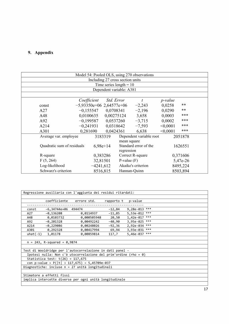
9. Appendix

Model 54: Pooled OLS, using 270 observations Including 27 cross section units

Time series length = 10 Dependent variable: A381

Coefficient Std. Error t p-value

const −5,93350e+06 2,64577e+06 −2,243 0,0258 ** A27 −0,155547 0,0708341 −2,196 0,0290 ** A48 0,0100635 0,00275124 3,658 0,0003 *** A92 −0,199587 0,0537260 −3,715 0,0002 *** A214 −0,241931 0,0318642 −7,593 <0,0001 *** A301 0,281690 0,0424361 6,638 <0,0001 ***

Average var. employee 3183319 Dependent variable root mean square

2051878

Quadratic sum of residuals 6,98e+14 Standard error of the regression

1626551

R-square 0,383286 Correct R-square 0,371606 F (5, 264) 32,81501 P-value (F) 5,47e-26 Log-likelihood −4241,612 Akaike's criterion 8495,224 Schwarz's criterion 8516,815 Hannan-Quinn 8503,894

Regressione ausiliaria con l'aggiunta dei residui ritardati: coefficiente errore std. rapporto t p-value --------------------------------------------------------------- const −6,34744e+06 494474 −12,84 9,28e-013 *** A27 −0,136208 0,0114937 −11,85 5,53e-012 *** A48 0,0103732 0,000505948 20,50 1,42e-017 *** A92 −0,201328 0,00492242 −40,90 3,95e-025 *** A214 −0,229086 0,00248026 −92,36 2,92e-034 *** A301 0,292328 0,00417994 69,94 3,93e-031 *** uhat(-1) 1,01178 0,00859814 117,7 5,46e-037 *** n = 243, R-squared = 0,9874 Test di Wooldridge per l'autocorrelazione in dati panel - Ipotesi nulla: Non c'è utocorrelazione del prim'ordine (rho = 0) Statistica test: t(26) = 117,675 con p-value = P(|t| > 117,675) = 5,45709e-037 Diagnostiche: incluse n = 27 unità longitudinali Stimatore a effetti fissi implica intercette diverse per ogni unità longitudinale

18

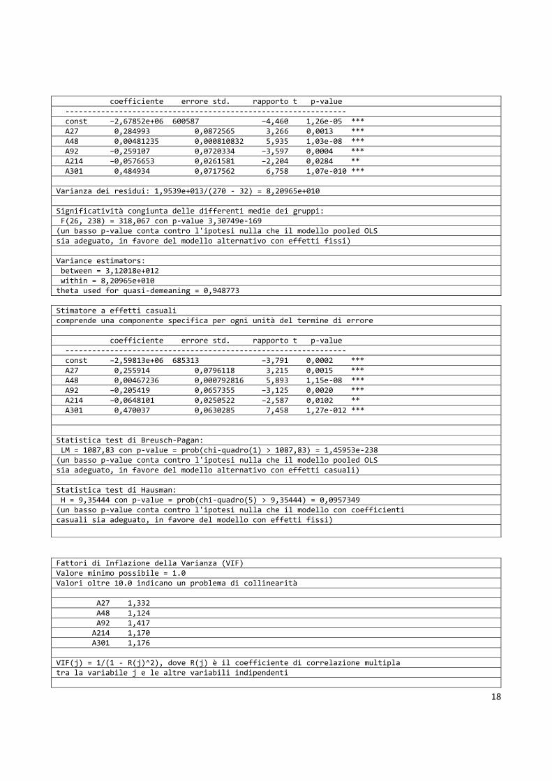
coefficiente errore std. rapporto t p-value --------------------------------------------------------------- const −2,67852e+06 600587 −4,460 1,26e-05 *** A27 0,284993 0,0872565 3,266 0,0013 *** A48 0,00481235 0,000810832 5,935 1,03e-08 *** A92 −0,259107 0,0720334 −3,597 0,0004 *** A214 −0,0576653 0,0261581 −2,204 0,0284 ** A301 0,484934 0,0717562 6,758 1,07e-010 *** Varianza dei residui: 1,9539e+013/(270 - 32) = 8,20965e+010 Significatività congiunta delle differenti medie dei gruppi: F(26, 238) = 318,067 con p-value 3,30749e-169 (un basso p-value conta contro l'ipotesi nulla che il modello pooled OLS sia adeguato, in favore del modello alternativo con effetti fissi) Variance estimators: between = 3,12018e+012 within = 8,20965e+010 theta used for quasi-demeaning = 0,948773

Stimatore a effetti casuali comprende una componente specifica per ogni unità del termine di errore coefficiente errore std. rapporto t p-value --------------------------------------------------------------- const −2,59813e+06 685313 −3,791 0,0002 *** A27 0,255914 0,0796118 3,215 0,0015 *** A48 0,00467236 0,000792816 5,893 1,15e-08 *** A92 −0,205419 0,0657355 −3,125 0,0020 *** A214 −0,0648101 0,0250522 −2,587 0,0102 ** A301 0,470037 0,0630285 7,458 1,27e-012 *** Statistica test di Breusch-Pagan: LM = 1087,83 con p-value = prob(chi-quadro(1) > 1087,83) = 1,45953e-238 (un basso p-value conta contro l'ipotesi nulla che il modello pooled OLS sia adeguato, in favore del modello alternativo con effetti casuali) Statistica test di Hausman: H = 9,35444 con p-value = prob(chi-quadro(5) > 9,35444) = 0,0957349 (un basso p-value conta contro l'ipotesi nulla che il modello con coefficienti casuali sia adeguato, in favore del modello con effetti fissi)

Fattori di Inflazione della Varianza (VIF) Valore minimo possibile = 1.0 Valori oltre 10.0 indicano un problema di collinearità A27 1,332 A48 1,124 A92 1,417 A214 1,170 A301 1,176 VIF(j) = 1/(1 - R(j)^2), dove R(j) è il coefficiente di correlazione multipla tra la variabile j e le altre variabili indipendenti

19

Diagnostiche di collinearità di Besley, Kuh e Welsch: proporzioni della varianza lambda cond const A27 A48 A92 A214 A301 4,577 1,000 0,000 0,009 0,000 0,007 0,011 0,011 0,635 2,684 0,000 0,070 0,000 0,012 0,409 0,113 0,418 3,311 0,000 0,067 0,000 0,253 0,290 0,041 0,299 3,915 0,000 0,400 0,000 0,000 0,011 0,585 0,070 8,080 0,006 0,414 0,005 0,673 0,260 0,241 0,001 82,252 0,994 0,040 0,995 0,056 0,019 0,009 lambda = Autovalori dell'inversa della matrice di covarianza (smallest is 0,000676605) cond = indice di condizione nota: le colonne delle proporzioni di varianza sommano ad uno Secondo BKW, cond >= 30 indica quasi-dipendenza lineare "forte" e cond fra 10 e 30 "moderatamente forte". Stime dei parametri la cui varianza è associata a valori di cond problematici potrebbero essere a loro volta problematiche. Numero dei condtion index >= 30: 1 Proporzioni di varianza >= 0.5 associate a cond >= 30: const A48 0,994 0,995 Numero dei condtion index >= 10: 1

20

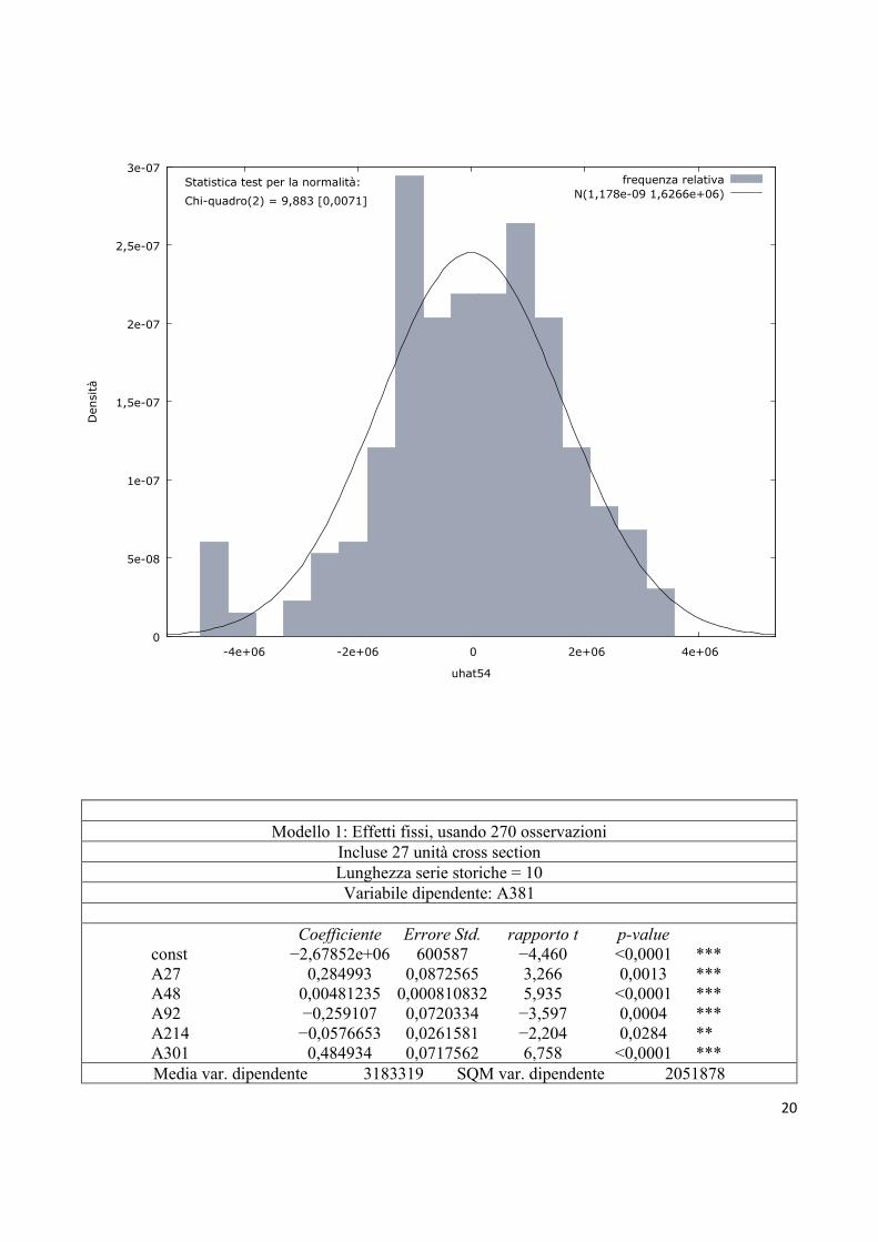
Modello 1: Effetti fissi, usando 270 osservazioni

Incluse 27 unità cross section Lunghezza serie storiche = 10 Variabile dipendente: A381

Coefficiente Errore Std. rapporto t p-value

const −2,67852e+06 600587 −4,460 <0,0001 *** A27 0,284993 0,0872565 3,266 0,0013 *** A48 0,00481235 0,000810832 5,935 <0,0001 *** A92 −0,259107 0,0720334 −3,597 0,0004 *** A214 −0,0576653 0,0261581 −2,204 0,0284 ** A301 0,484934 0,0717562 6,758 <0,0001 ***

Media var. dipendente 3183319 SQM var. dipendente 2051878

0

5e-08

1e-07

1,5e-07

2e-07

2,5e-07

3e-07

-4e+06 -2e+06 0 2e+06 4e+06

Den

sità

uhat54

frequenza relativaN(1,178e-09 1,6266e+06)

Statistica test per la normalità:

Chi-quadro(2) = 9,883 [0,0071]

21

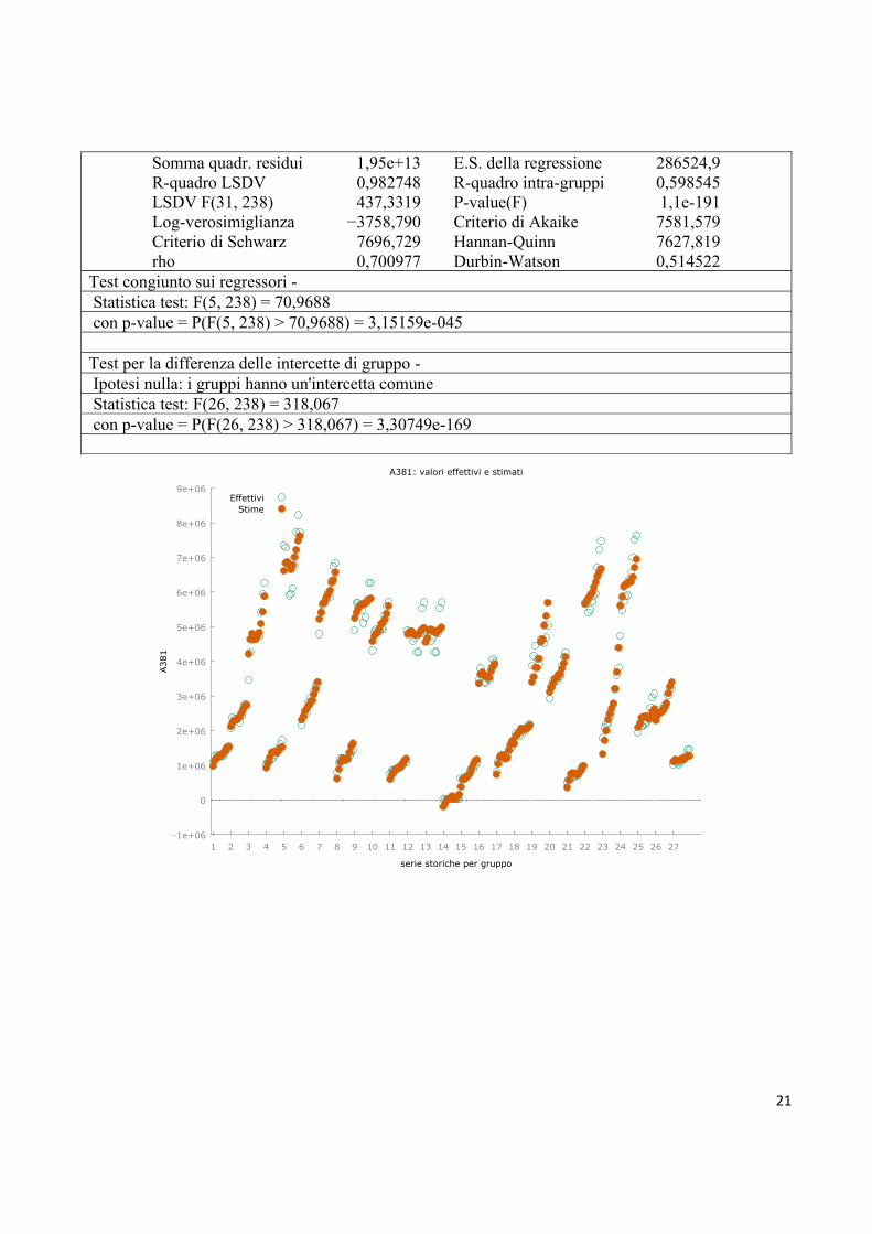
Somma quadr. residui 1,95e+13 E.S. della regressione 286524,9 R-quadro LSDV 0,982748 R-quadro intra-gruppi 0,598545 LSDV F(31, 238) 437,3319 P-value(F) 1,1e-191 Log-verosimiglianza −3758,790 Criterio di Akaike 7581,579 Criterio di Schwarz 7696,729 Hannan-Quinn 7627,819 rho 0,700977 Durbin-Watson 0,514522

Test congiunto sui regressori - Statistica test: F(5, 238) = 70,9688 con p-value = P(F(5, 238) > 70,9688) = 3,15159e-045 Test per la differenza delle intercette di gruppo - Ipotesi nulla: i gruppi hanno un'intercetta comune Statistica test: F(26, 238) = 318,067 con p-value = P(F(26, 238) > 318,067) = 3,30749e-169

-1e+06

0

1e+06

2e+06

3e+06

4e+06

5e+06

6e+06

7e+06

8e+06

9e+06

1 2 3 4 5 6 7 8 9 10 11 12 13 14 15 16 17 18 19 20 21 22 23 24 25 26 27

A38

1

serie storiche per gruppo

A381: valori effettivi e stimati

EffettiviStime

22

Distribuzione di frequenza per uhat1, oss. 1-270 Numero di intervalli = 17, media = -2,36452e-009, scarto quadratico medio = 272050 Intervallo P.med. Frequenza Rel. Cum. < -8,330e+005 -8,854e+005 2 0,74% 0,74% -8,330e+005 - -7,282e+005 -7,806e+005 1 0,37% 1,11% -7,282e+005 - -6,233e+005 -6,757e+005 4 1,48% 2,59% -6,233e+005 - -5,185e+005 -5,709e+005 4 1,48% 4,07% -5,185e+005 - -4,136e+005 -4,661e+005 7 2,59% 6,67% -4,136e+005 - -3,088e+005 -3,612e+005 8 2,96% 9,63% * -3,088e+005 - -2,040e+005 -2,564e+005 11 4,07% 13,70% * -2,040e+005 - -9,912e+004 -1,515e+005 33 12,22% 25,93% **** -9,912e+004 - 5724, -4,670e+004 76 28,15% 54,07% ********** 5724, - 1,106e+005 5,814e+004 58 21,48% 75,56% ******* 1,106e+005 - 2,154e+005 1,630e+005 31 11,48% 87,04% **** 2,154e+005 - 3,202e+005 2,678e+005 8 2,96% 90,00% * 3,202e+005 - 4,251e+005 3,727e+005 6 2,22% 92,22% 4,251e+005 - 5,299e+005 4,775e+005 8 2,96% 95,19% * 5,299e+005 - 6,348e+005 5,824e+005 5 1,85% 97,04% 6,348e+005 - 7,396e+005 6,872e+005 5 1,85% 98,89% >= 7,396e+005 7,920e+005 3 1,11% 100,00% Test per l'ipotesi nulla di distribuzione normale: Chi-quadro(2) = 28,754 con p-value 0,00000

Modello 5: Effetti casuali (GLS), usando 270 osservazioni

0

5e-07

1e-06

1,5e-06

2e-06

2,5e-06

3e-06

-1e+06 -800000 -600000 -400000 -200000 0 200000 400000 600000 800000

Den

sità

uhat1

frequenza relativaN(-2,3645e-09 2,7205e+05)

Statistica test per la normalità:

Chi-quadro(2) = 28,754 [0,0000]

23

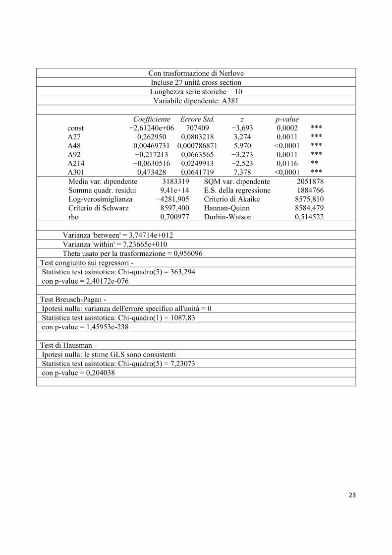
Con trasformazione di Nerlove Incluse 27 unità cross section Lunghezza serie storiche = 10 Variabile dipendente: A381

Coefficiente Errore Std. z p-value

const −2,61240e+06 707409 −3,693 0,0002 *** A27 0,262950 0,0803218 3,274 0,0011 *** A48 0,00469731 0,000786871 5,970 <0,0001 *** A92 −0,217213 0,0663565 −3,273 0,0011 *** A214 −0,0630516 0,0249913 −2,523 0,0116 ** A301 0,473428 0,0641719 7,378 <0,0001 ***

Media var. dipendente 3183319 SQM var. dipendente 2051878 Somma quadr. residui 9,41e+14 E.S. della regressione 1884766 Log-verosimiglianza −4281,905 Criterio di Akaike 8575,810 Criterio di Schwarz 8597,400 Hannan-Quinn 8584,479 rho 0,700977 Durbin-Watson 0,514522

Varianza 'between' = 3,74714e+012 Varianza 'within' = 7,23665e+010 Theta usato per la trasformazione = 0,956096 Test congiunto sui regressori - Statistica test asintotica: Chi-quadro(5) = 363,294 con p-value = 2,40172e-076 Test Breusch-Pagan - Ipotesi nulla: varianza dell'errore specifico all'unità = 0 Statistica test asintotica: Chi-quadro(1) = 1087,83 con p-value = 1,45953e-238 Test di Hausman - Ipotesi nulla: le stime GLS sono consistenti Statistica test asintotica: Chi-quadro(5) = 7,23073 con p-value = 0,204038

24

0

1e+06

2e+06

3e+06

4e+06

5e+06

6e+06

7e+06

8e+06

9e+06

1 2 3 4 5 6 7 8 9 10 11 12 13 14 15 16 17 18 19 20 21 22 23 24 25 26 27

A38

1

serie storiche per gruppo

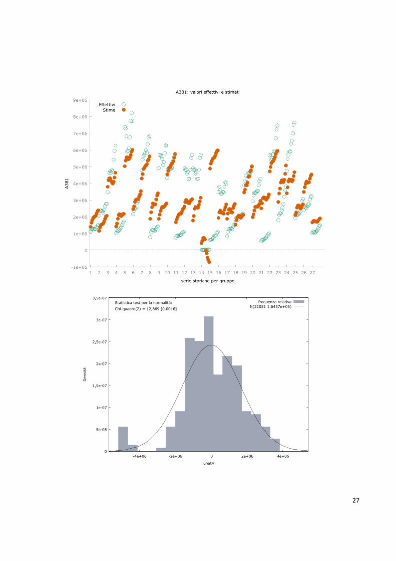
A381: valori effettivi e stimati

EffettiviStime

25

Diagnostiche di collinearità di Besley, Kuh e Welsch: proporzioni della varianza lambda cond const A27 A48 A92 A214 A301 3,437 1,000 0,011 0,019 0,010 0,019 0,020 0,021 0,991 1,863 0,156 0,029 0,018 0,000 0,146 0,042 0,747 2,145 0,006 0,146 0,000 0,010 0,576 0,044 0,499 2,623 0,094 0,005 0,004 0,445 0,118 0,087 0,233 3,838 0,000 0,679 0,005 0,043 0,139 0,804 0,093 6,064 0,733 0,122 0,963 0,482 0,001 0,002 lambda = Autovalori dell'inversa della matrice di covarianza (smallest is 0,0934684) cond = indice di condizione nota: le colonne delle proporzioni di varianza sommano ad uno Secondo BKW, cond >= 30 indica quasi-dipendenza lineare "forte" e cond fra 10 e 30 "moderatamente forte". Stime dei parametri la cui varianza è associata a valori di cond problematici potrebbero essere a loro volta problematiche. Numero dei condtion index >= 30: 0

0

5e-08

1e-07

1,5e-07

2e-07

2,5e-07

3e-07

3,5e-07

4e-07

4,5e-07

-6e+06 -4e+06 -2e+06 0 2e+06 4e+06 6e+06

Den

sità

uhat3

frequenza relativaN(-6,8047e-09 1,8883e+06)

Statistica test per la normalità:

Chi-quadro(2) = 4,003 [0,1351]

26

Numero dei condtion index >= 10: 0 No evidence of excessive collinearity

Prima equazione in differenze (dipendente, d_y): coefficiente errore std. rapporto t p-value ------------------------------------------------------------ d_A27 0,343887 0,134657 2,554 0,0169 ** d_A48 0,00459451 0,00109370 4,201 0,0003 *** d_A92 −0,294263 0,130323 −2,258 0,0326 ** d_A214 −0,0427822 0,0380446 −1,125 0,2711 d_A301 0,486026 0,157961 3,077 0,0049 *** n = 243, R-squared = 0,3718 Autoregressione dei residui (dipendente, uhat): coefficiente errore std. rapporto t p-value ------------------------------------------------------------- uhat(-1) 0,280888 0,0452520 6,207 1,45e-06 *** n = 216, R-squared = 0,0845 Test di Wooldridge per l'autocorrelazione in dati panel - Ipotesi nulla: Non c'è autocorrelazione del prim'ordine (rho = -0.5) Statistica test: F(1, 26) = 297,785 con p-value = P(F(1, 26) > 297,785) = 9,2989e-016

Modello 4: WLS, usando 270 osservazioni Incluse 27 unità cross section Variabile dipendente: A381

Pesi basati sulle varianze degli errori per unità Coefficiente Errore Std. rapporto t p-value

const −5,25720e+06 802465 −6,551 <0,0001 *** A27 −0,129147 0,0337818 −3,823 0,0002 *** A48 0,00886943 0,000912035 9,725 <0,0001 *** A92 −0,190721 0,0156461 −12,19 <0,0001 *** A214 −0,213122 0,0154253 −13,82 <0,0001 *** A301 0,380176 0,0180841 21,02 <0,0001 ***

Statistiche basate sui dati ponderati: Somma quadr. residui 240,3749 E.S. della regressione 0,954207 R-quadro 0,874164 R-quadro corretto 0,871781 F(5, 264) 366,7931 P-value(F) 1,4e-116 Log-verosimiglianza −367,4234 Criterio di Akaike 746,8468 Criterio di Schwarz 768,4374 Hannan-Quinn 755,5166

Statistiche basate sui dati originali: Media var. dipendente 3183319 SQM var. dipendente 2051878 Somma quadr. residui 7,15e+14 E.S. della regressione 1645866

27

-1e+06

0

1e+06

2e+06

3e+06

4e+06

5e+06

6e+06

7e+06

8e+06

9e+06

1 2 3 4 5 6 7 8 9 10 11 12 13 14 15 16 17 18 19 20 21 22 23 24 25 26 27

A38

1

serie storiche per gruppo

A381: valori effettivi e stimati

EffettiviStime

0

5e-08

1e-07

1,5e-07

2e-07

2,5e-07

3e-07

3,5e-07

-4e+06 -2e+06 0 2e+06 4e+06

Den

sità

uhat4

frequenza relativaN(21051 1,6457e+06)

Statistica test per la normalità:

Chi-quadro(2) = 12,869 [0,0016]

28

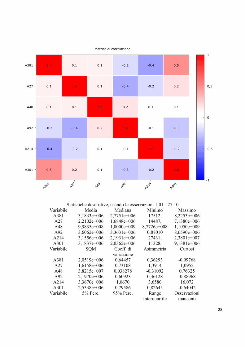
Statistiche descrittive, usando le osservazioni 1:01 - 27:10

Variabile Media Mediana Minimo Massimo A381 3,1833e+006 2,7751e+006 17512, 8,2253e+006 A27 2,2102e+006 1,6848e+006 14487, 7,1380e+006 A48 9,9835e+008 1,0000e+009 8,7726e+008 1,1050e+009 A92 3,6062e+006 3,3631e+006 0,87010 8,6590e+006

A214 3,1556e+006 2,1931e+006 27431, 2,3801e+007 A301 3,1837e+006 2,0365e+006 11328, 9,1381e+006

Variabile SQM Coeff. di variazione

Asimmetria Curtosi

A381 2,0519e+006 0,64457 0,36293 -0,99768 A27 1,6158e+006 0,73108 1,3914 1,0952 A48 3,8215e+007 0,038278 -0,31092 0,76325 A92 2,1970e+006 0,60923 0,36128 -0,88968

A214 3,3670e+006 1,0670 3,6580 16,072 A301 2,5338e+006 0,79586 0,82645 -0,64042

Variabile 5% Perc. 95% Perc. Range interquartile

Osservazioni mancanti

Matrice di correlazione

0.5 0.2 0.1 -0.3 -0.2 1.0

-0.4 -0.2 0.1 -0.1 1.0 -0.2

-0.2 -0.4 0.2 1.0 -0.1 -0.3

0.1 0.1 1.0 0.2 0.1 0.1

0.1 1.0 0.1 -0.4 -0.2 0.2

1.0 0.1 0.1 -0.2 -0.4 0.5

A301

A214

A92

A48

A27

A381

A381 A2

7A4

8A9

2A2

14A3

01-1

-0,5

0

0,5

1

29

A381 6,1295e+005 6,7566e+006 3,5757e+006 0 A27 7,9287e+005 6,1317e+006 1,2935e+006 0 A48 9,2549e+008 1,0611e+009 3,2596e+007 0 A92 8,2049e+005 7,6832e+006 3,8458e+006 0

A214 6,1554e+005 7,2175e+006 2,2038e+006 0 A301 7,4405e+005 8,0727e+006 3,4359e+006 0

Analisi delle componenti principali n = 270 Analisi degli autovalori della matrice di correlazione Componente Autovalore Proporzione Cumulata 1 2,0025 0,3337 0,3337 2 1,2191 0,2032 0,5369 3 1,0704 0,1784 0,7153 4 0,8720 0,1453 0,8607 5 0,5132 0,0855 0,9462 6 0,3228 0,0538 1,0000 Autovettori (pesi della componente) PC1 PC2 PC3 PC4 PC5 PC6 A381 0,540 0,310 -0,088 -0,258 0,554 -0,481 A27 0,393 -0,331 0,365 0,620 -0,213 -0,416 A48 0,059 0,382 0,846 -0,061 0,128 0,338 A92 -0,365 0,679 -0,018 0,147 -0,382 -0,488 A214 -0,384 -0,430 0,377 -0,536 0,002 -0,488 A301 0,519 0,044 -0,015 -0,487 -0,697 0,073

30

A38

1

A27A38

1A48

A38

1

A92

A38

1

A214

A38

1

A301

0

5e+06

1e+07

1,5e+07

2e+07

2,5e+07

1 2 3 4 5 6 7 8 9 10 11 12 13 14 15 16 17 18 19 20 21 22 23 24 25 26 27 8,5e+08

9e+08

9,5e+08

1e+09

1,05e+09

1,1e+09

1,15e+09

serie storiche per gruppo

A381 (sinistra)A27 (sinistra)A48 (destra)

A92 (sinistra)A214 (sinistra)A301 (sinistra)

31

0

1e+06

2e+06

3e+06

4e+06

5e+06

6e+06

7e+06

8e+06

9e+06

1 68 135 202 269

A381

0

1e+06

2e+06

3e+06

4e+06

5e+06

6e+06

7e+06

8e+06

1 68 135 202 269

A27

8,5e+08

9e+08

9,5e+08

1e+09

1,05e+09

1,1e+09

1,15e+09

1 68 135 202 269

A48

0

1e+06

2e+06

3e+06

4e+06

5e+06

6e+06

7e+06

8e+06

9e+06

1 68 135 202 269

A92

0

5e+06

1e+07

1,5e+07

2e+07

2,5e+07

1 68 135 202 269

A214

0

1e+06

2e+06

3e+06

4e+06

5e+06

6e+06

7e+06

8e+06

9e+06

1e+07

1 68 135 202 269

A301

32

33

34

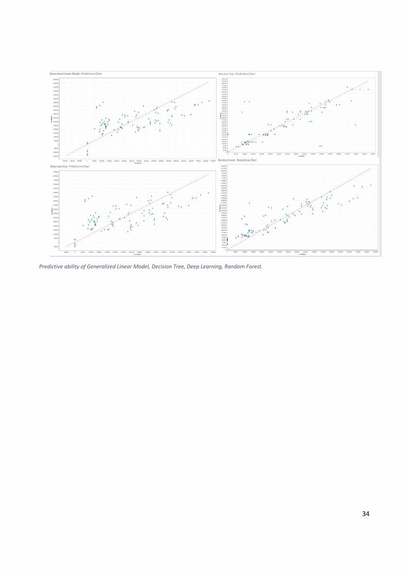
Predictive ability of Generalized Linear Model, Decision Tree, Deep Learning, Random Forest.

35

The predictive ability of Gradient Boosted Trees and Support Vector Machine.