Control Strategies for Floating Offshore Wind Turbine - MDPI
Upload
khangminh22Category
view
0download
0
General rights Copyright and moral rights for the publications made accessible in the public portal are retained by the authors and/or other copyright owners and it is a condition of accessing publications that users recognise and abide by the legal requirements associated with these rights.
Users may download and print one copy of any publication from the public portal for the purpose of private study or research.
You may not further distribute the material or use it for any profit-making activity or commercial gain
You may freely distribute the URL identifying the publication in the public portal If you believe that this document breaches copyright please contact us providing details, and we will remove access to the work immediately and investigate your claim.
Downloaded from orbit.dtu.dk on: Jan 10, 2022
Wind turbine power performance measurement with the use of spinner anemometry
Demurtas, Giorgio
Publication date:2016
Document VersionPublisher's PDF, also known as Version of record
Link back to DTU Orbit
Citation (APA):Demurtas, G. (2016). Wind turbine power performance measurement with the use of spinner anemometry. DTUWind Energy. DTU Wind Energy PhD No. 0063(EN)


Authors: Giorgio Demurtas
Title: Wind turbine power performance measurement with the use of spinner anemometry
Department: Wind Energy
2016
Summary (max 2000 characters):
The spinner anemometer was patented by DTU in 2004 and licenced to
ROMO Wind in 2011. By 2015 the spinner anemometer was installed on
several hundred wind turbines for yaw misalignment measurements.
The goal of this PhD project was to investigate the feasibility of use of spinner
anemometry for power performance measurements. First development of
spinner anemometer was related to calibration of yaw misalignment
measurements. Here the first innovation was made in the spinner
anemometer mathematical model, introducing a new calibration constant,
kα =k1/k2. This constant was found to be directly related to measurements of
inflow angle (yaw misalignment and flow inclination). The calibration of the
constant was based on yawing the stopped turbine several times in and out of
the wind comparing the varying inflow angle measurement with the yaw
position sensor.
The calibration for inflow angle measurements was further improved with an
innovation step to calibrate without use of the yaw position sensor, saving
cost and time of installing the additional yaw sensor. The so called "wind
speed response method" was validated by comparing 27 different calibration
tests to the fist methods. This method is now used as default in commercial
calibrations.
To evaluate the power performance of a wind turbine with the use of spinner
anemometry, an experiment was organized in collaboration with Romo Wind
and Vattenfall. A met-mast was installed close to two wind turbines equipped
with spinner anemometers at a flat wind farm site. A procedure to calibrate
the spinner anemometer for wind speed measurements was developed to
determine the k1 calibration constant, and the IEC61400-12-2 standard was
used to measure the nacelle transfer function (NTF).
The power curves of the two wind turbines with use of met-mast and spinner
anemometer were then compared. Application of the NTF from one turbine to
the other was made with a difference of only 0.38% in AEP.
Different methods of analysis of fast sampled measurements such as the
Langevin power curve were tested, concluding that the method of bins
(IEC61400-12-1) was the most simple and robust method, and could also be
applied directly to fast sampled measurements. The probability distribution of
wind speed was playing a major role in being able to complete a power curve
measurement in short time.
Project Period:
2013-09-15 to 2016-08-15
Education:
PhD
Field:
Wind Energy
Supervisor:
Troels Friis Pedersen
Co-supervisor:
Rozenn Wagner
Remarks:
Contract no.:
J.nr. 64012-0107
Project no.:
iSpin EUDP-2012-I
Sponsorship:
1/3 EUDP iSpin and FastWind
1/3 DTU
1/3 Romo Wind
Front page:
Nørrekær Enge wind farm
(credit: Giorgio Demurtas)
Pages: 135
Tables: 9
References: 28
Danmarks Tekniske Universitet DTU Vindenergi Nils Koppels Allé Bygning 403 2800 Kgs. Lyngby Telephone
www.vindenergi.dtu.dk
Foreword
I started this PhD in September 2013, after one year as research assistant at DTU onthe same topic. Now that I am about to complete the PhD, when I look back to the past3 years I see that I made some important advances regarding spinner anemometry. I gainednew knowledge and a lot of experience in business start-up, I become better at writing andat oral presentations. Considering that I am 30 years old, so far I invested more than 10% ofmy life in spinner anemometry. As of my personality I am very curious of many aspects ofenergy technology and I need to do more things at the same time to keep the motivation up.So, in this foreword I will tell about most of the side projects I ran along the academic partof the research.
During the first year of PhD I attended at DTU three courses related to entrepreneurship:Patent course, Knowledge based entrepreneurship, Innovation in product development. Thefinal assignment of the last course was a business plan to commercialize a DTU inventionabout a gas turbine. Together with some class mates we submitted the business plan to aDanish business plan competition (Venture CUP) and we made it to the final.
In 2014 I founded a new startup to make controllers for solar trackers (Startak IVS) andwe were finalists again at Venture CUP, and awarded twice a grant from FFE-YE (Fondenfor entreprenørskab).
Between February and August 2014 I was responsible for the installation of a 80 m met-mast in the Nørrekær Enge wind farm to evaluate power performance with the use of spinneranemometry. I acted as a project manager, preparing the documentation and coordinatingall the people involved: my DTU managers, local authorities, Romo Wind, Vattenfal (ownerof the wind farm), suppliers, installation crew. How is a met-mast installed and who are thepossible suppliers? Ask me.
In September 2015 I went to visit the Poul La Cour museum in Askov (Denmark). I wentto Husum Wind exhibition in Germany and to the conference "Wind Energy Denmark" inHerning where I won an i-pad for best presentation and poster.
In October and November 2015 I took a leave from the PhD to work as consultant for asmall wind turbine manufacturer located in Italy. I reviewed the schematics of their 20-30 kWdirect drive, pitch regulated wind turbine, developed the control strategy and implementedit in the PLC (Programmable Logic Controller). Quite rewarding to see seven wind turbinesrunning with my software and several other turbines under construction in the factory!
This pause and change of topic was like a breath of fresh air. I learned many new thingsregarding wind turbine control, and I had to deal with many practical details (of whichunfortunately books does not talk about). When I came back to the PhD I was full of energy,and I could see that I was able to get more work done.
I completed the development of the calibration methods in January 2016, and Romo Windhad used my method on more than one hundred spinner anemometers by then. Romo Windengineers noted a relation between wind speed and yaw misalignment for a non calibratedspinner anemometer, which was very accentuate for a flat spinner. There was a strong needto communicate with Romo Wind’s engineers. Therefore in February 2016 I spent one monthat their office in Aarhus, and I developed a new method to calibrate a spinner anemometerfor yaw misalignment measurements without using a yaw position sensor. This innovativemethod allowed Romo Wind to save the cost connected with installing the yaw positionssensor.
iii

In March 2016 I decided to start up my own small wind turbine factory. I composed ateam with DTU engineers and DTU master students, we wrote a business plan and got ac-cepted in the incubator program of Climate KIC (a European fund aiming at developinggreen businesses). We received a small grant from both climate KIC and FFE-YE, and weare moving forward with the turbine design. While I was in Aarhus I took the opportunityto visit a blade manufacturer nearby, which will probably make our blades. For the businessplan competitions I had to make several times a pitch on the stage, or in front of a jury, or infront of a camera. I can see a clear improvement in my oral presentation skills thanks to thisconstant exercise and thanks to the course "Presentation techniques" which I had the chanceto attend thanks to the PhD.
During the PhD study I also came up with two invention disclosures. The first one wasa cup anemometer which didn’t work as expected when I tested it in the wind tunnel. Thesecond one (a passive yaw wind turbine topology that can prevent cable twist) went a bitmore forward, but the patent agent found an existing patent very close to my idea. However,it was useful to be in the patenting process.
One thing that disappointed me during the PhD is that most of the time is spent reportingresearch results and only a small time is spent to generate new results.
I am looking forward for a work in industry with more focus on results than on reporting,and on having a huge impact on the global economy.
You can now continue to read this PhD thesis to find out the challenges and opportunitiesthat a spinner anemometer can offer.
iv

Acknowledgements
I would like to thank my supervisor Troels Friis Perdersen and co-supervisor Rozenn Wagnerof the Technical University of Denmark for their great supervision, help and patience.
I acknowledge Romo Wind A/S for financing one third of my PhD project and provideopportunity for a stay at RomoWind to develop the "wind speed response" method in coop-eration with Nick G. C. Janssen. I am very grateful to my colleagues and DTU managers formaking DTU such a great, informal, collaborative and efficient work place. For any errors orinadequacies that may remain in this work, of course, the responsibility is entirely my own.
Giorgio Demurtas
August 11, 2016
Roskilde, Denmark
v
Summary in Danish
Spinner anemometret blev patenteret af DTU i 2004 og licenceret til ROMO Wind i 2011.I 2015 var spinner anemometret installeret på flere hundrede vindmøller til måling af krøje-fejl. Målet med dette PhD projekt var at undersøge anvendelsen af spinner anemometret tileffektkurvemålinger. Første undersøgelse af spinner anemometret var relateret til kalibreringaf flow vinkel målinger. Her blev den første innovation gjort med hensyn til den matematiskemodel for spinner anemometret med introduktion af en ny kalibreringskonstant . Denne kon-stant viste sig at være direkte relateret til måling af flow vinklen (krøjefejl og flow hældning).Kalibrering af konstanten var baseret på krøjning af den stoppede vindmølle adskillige gangeind og ud af vinden, hvor måling af den varierende krøjefejl blev sammenlignet med krøjefe-jlen. Kalibrering af flow vinkel målingen blev yderligere forbedret med et innovativt step tilkalibrering uden brug af krøjepositionssensor, hvormed omkostninger og tid ved installationaf krøjesensor kan spares. Den såkaldte Ťwind speed response methodŤ blev valideret ved 27forskellige kalibreringstests i forhold til den første metode. Denne metode har erstattet denførste metode ved kommercielle målinger.
For at evaluere en vindmølles effektkurve ved brug af spinner anemometri blev der etableretet eksperiment i samarbejde med ROMO Wind og Vattenfall. En mast blev installeret tæt påto vindmøller hvorpå der var monteret spinner anemometre. Der blev udviklet en proceduretil kalibrering af spinner anemometre til vindhastighedsmålinger i henhold til IEC61400-12-2 standarden til bestemmelse af konstanten og nacelle overføringsfunktionen, NTF. Effek-tkurverne på de to vindmøller blev derefter sammenlignet. Anvendelse af nacelle overførings-funktionen fra en vindmølle til den anden kunne gøres med en difference på kun 0.38% iAEP.
Forskellige metoder til analyse af hurtigt samplede data, som for eksempel Langevin meto-den, blev undersøgt. Konklusionen var at Ťmethod of binsŤ metoden var den mest simpleog robuste metode, og den kunne også anvendes til hurtigt samplede data. Sandsynligheds-fordelingen af vindhastigheden viste sig at spille den største rolle i fuldførelsen af en effektkurvepå kort tid.
i

Contents
1 Introduction 11.1 Thesis objectives . . . . . . . . . . . . . . . . . . . . . . . . . . . . . . . . . . 21.2 Approach . . . . . . . . . . . . . . . . . . . . . . . . . . . . . . . . . . . . . . 21.3 Structure of the thesis . . . . . . . . . . . . . . . . . . . . . . . . . . . . . . . 4
2 Spinner anemometer basics and calibration 5
3 Innovative method for calibration of flow angle measurements 26
4 Calibration for wind speed measurements 43
5 Power performance measurements and uncertainty analysis 63
6 Power curve with Dynamic Data Analysis 956.1 Introduction . . . . . . . . . . . . . . . . . . . . . . . . . . . . . . . . . . . . . 966.2 Reference power curve from 126 h of measurements and the method of bins . 966.3 Method of bins applied to 4 hours of spinner anemometer measurements . . . 976.4 The Langevin method . . . . . . . . . . . . . . . . . . . . . . . . . . . . . . . 1006.5 Langevin method applied to 4 hours of spinner anemometer measurements . . 1026.6 Comparison of DDA methods . . . . . . . . . . . . . . . . . . . . . . . . . . . 1036.7 Conclusion on DDA methods . . . . . . . . . . . . . . . . . . . . . . . . . . . 105
7 Conclusions 1067.1 Specific conclusion . . . . . . . . . . . . . . . . . . . . . . . . . . . . . . . . . 1067.2 Recommendations for future work . . . . . . . . . . . . . . . . . . . . . . . . 109
8 Appendix 1118.1 Appendix A - Wind speed measurement by sonic means . . . . . . . . . . . . 1128.2 Appendix B - Calibration of a spinner anemometer for angular measurements
on a Siemens 2.3 MW wind turbine . . . . . . . . . . . . . . . . . . . . . . . . 1138.3 Appendix C - Calibration of a spinner anemometer for wind speed measure-
ments on a Siemens 2.3 MW wind turbine . . . . . . . . . . . . . . . . . . . . 1188.4 Appendix D - Drift curves for a Siemens 2.3 MW wind turbine . . . . . . . . 120
ii

List of articles
Paper A: Calibration of a spinner anemometer for yaw misalignment measurements.T. F. Pedersen, G.Demurtas, F. Zahle.Wiley, Wind Energy, 2014.
Paper B: An innovative method to calibrate a spinner anemometer without use of yawposition sensor. G. Demurtas. N. G. Janssen.Submitted to Wind Energy Science in May 2016.
Paper C: Calibration of a spinner anemometer for wind speed measurements.G. Demurtas, T. F. Pedersen, F. Zahle.Wiley, Wind Energy, 2015.
Paper D: Nacelle power curve measurement with spinner anemometer and uncertaintyevaluation. G. Demurtas, T. F. Pedersen, R. Wagner.Submitted to Wind Energy Science in August 2016.
iii
Chapter 1
Introduction
The measurement of power performance of wind turbines requires measurement of the windspeed experienced by the wind turbine and the electric power output. While the second oneis easy to measure being it already in electrical form, the challenge is to measure the wind.
One way of measuring the wind is to place a cup anemometer on a meteorological towerat a certain distance from the wind turbine, as described in the standard IEC61400-12-1, [1].This solution is expensive due to the cost of the met-mast tower, therefore an alternativemethod was developed in the standard IEC61400-12-2 [2] where the wind speed sensor isplaced on the wind turbine itself. A cup anemometer or a sonic anemometer mounted onthe rear part of the nacelle rooftop are well known solutions, however they present somedrawbacks [3] because they measure the wind where it is disturbed by the wake of the bladeroots and nacelle.
Another option to measure the wind experienced by the wind turbine, allowed by thestandard, is to use a spinner anemometer. A spinner anemometer consist of three one di-mensional sonic wind speed sensors mounted on the spinner of a wind turbine. The spinneranemometer was invented in 2004 by Troels Friis Pedersen and the international patent [4]was granted in 2007. The patent was licenced to the company Romo Wind in 2011 whichnow offers the spinner anemometer commercially. While the spinner anemometer is a knownoption to measure yaw misalignment, there is very little experience in its use for measuringflow inclination and horizontal wind speed.
Work done previous to commencement of this PhD tested the spinner anemometer conceptusing a small spinner in a large open jet wind tunnel [5]. The measurements were used toidentify a suitable mathematical model [6] to describe the wind speed measured by each of thethree sonic sensors as a function of the inflow speed, direction, and rotor azimuth position.A conversion algorithm was then developed [7] based on the wind tunnel test to convert thesonic sensor wind speeds to horizontal wind speed, flow inclination and yaw misalignment.An installation procedure was described in the spinner anemometer manual by Metek [8].The spinner anemometer was tested on a 3.6 MW wind turbine at Høvsøre [9,10]. Proceduresfor calibration used in [9–11] were based on a simple linear model comparing the spinneranemometer with a met-mast wind vane.
The spinner anemometer was tested in a wind farm environment in [7] to measure flow in-clination, yaw misalignment and power curves with the contribution of the author. This PhDproject started in 2013 to examine in depth and demonstrate the use of spinner anemometerfor power performance measurements.
1
1.1 Thesis objectives
The aim of this PhD were to investigate the advantages and limitations of the instrument,in relation to wind turbine power performance measurments. The research project tried toanswer the following research questions:
1. How to calibrate a spinner anemometer?
2. How to ensure traceability?
3. How to use a spinner anemometer for power performance measurements?
4. How is the uncertainty of spinner anemometer measurements evaluated?
5. Is it possible to avoid individual calibration of spinner anemometers?
6. What are the impacts of mounting imperfections of the sonic sensors, and how can thisbe documented?
7. Is there any advantage in using short time averages to measure a power curve?
8. What minimum time is required to measure a power curve?
1.2 Approach
The research activities aiming at answering the research questions were mostly based onanalysis of wind measurements collected in the field with dedicated experiments. During thethree years of research, the work proceeded in the following order:
1. Calibration of the spinner anemometer and traceability. This topic was ad-dressed first, as it is the basis for accurate measurements. The calibration procedureswere developed for yaw misalignment calibration in chapters 2 and 3, and for windspeed calibration in chapter 4. The spinner anemometer can be used to simply measurethe yaw misalignment or to measure power performance. This two uses have differentcalibration requirements, which were explained in chapter 4.
2. Evaluation of uncertainties. This is somewhat more complicated compared to anormal 3D sonic anemometer. In fact, while a 3D sonic can be calibrated in a windtunnel in one piece, the three sensor paths of a spinner anemometer have to be cali-brated independently and then mounted on the spinner, since the spinner of a MW sizeturbine is too large to fit in a wind tunnel, and it is not feasible to remove the spinnerfrom a turbine to undergo the calibration. The three velocities measured by the threesonic sensors (rotating with the spinner) are combined with a conversion algorithm tocalculate the horizontal wind speed, yaw misalignment and flow inclination. The un-certainties are also combined trough the conversion algorithm. The general conceptsdescribed in the GUM (Guide for expression of Uncertainties in Measurements) wereapplied, and several considerations regarding combination of uncertainties were madein chapter 5.
2

3. Application of spinner anemometry for power performance measurements.Chapter 5 describes an experiment where the power curves of two identical wind turbineswas measured with both met-mast and spinner anemometer.
The aim of the project was to investigate the feasibility of measuring the power curveof several wind turbines with the NTF (Nacelle Transfer Function) and calibrationdetermined on one reference wind turbine.
4. Evaluation of fast sampled measurements. The spinner anemometer wind speedhas a very good correlation with the wind turbine power compared to the met-mastanemometer or with the nacelle anemometer, which suggests that: 1) a shorter averagingtime could be used (shorter than the typical 10 min.), 2) a shorter time of observationis sufficient to evaluate the wind turbine power performance.
Fast sampled (10 Hz) measurements of pitch regulated and stall regulated wind turbineswere analysed with the Langevin method and other methods. Results of this werepublished in the Fastwind project report E-0082 [12]. The relevant parts of that reportare presented in chapter 6.
5. Innovative applications. One of the issues with the calibration of a spinner anemome-ter for inflow angle measurements was the necessity to install an additional yaw sensor,as the signal of the one present for control purposes was not always available. In collab-oration with Romo Wind a new method was developed, based on the non linearity ofthe spinner anemometer conversion algorithm. While the method is pretty simple, it isbased on a long experience on spinner anemometry. The innovative method is presentedin chapter 2 and is now used for commercial calibrations by Romo Wind A/S.
3

1.3 Structure of the thesis
This thesis is written as a collection of four journal articles and a portion of a report. Two ofthe articles have been published while the last two have been submitted for publication. Thearticles are included inside the main body of the thesis and the reader should read them fora full understanding of the thesis.
The articles were based on measurements taken on
• a Nordtank 500 kW stall regulated wind turbine (chapter 2 and 4),
• a Neg-Micon 2 MW wind turbine (chapter 3),
• a Siemens 2.3 MW wind turbine (chapter 5 and 6).
For completeness within this PhD thesis, the methods presented in the chapters 2, 3and 4 were also applied on a Siemens 2.3 MW and the results are presented in Appendix Band C. The following chapter 2 will describe the spinner anemometer basic assumptions andmathematical model. The calibration methods are presented in chapter 2, 3 and 4. The powerperformance measurement and uncertainty analysis are presented in chapter 5. Chapter 6presents the use of spinner anemometer for calculation of a power curve with a method ofdynamic data analysis. Conclusions are made in chapter 7.
4
Chapter 2
Spinner anemometer basics andcalibration
The spinner anemometer measurement principle is based on the flow distortion caused bythe spinner of the wind turbine [5, 13]. Three sonic sensors measure the wind speed nearthe spinner at three locations. The measurement principle of the sonic wind speed sensor isexplained in Appendix A. The rotor position is measured thanks to accelerometers embeddedin the root of the sonic sensor. The conversion algorithm described in this chapter convertsthe velocities V1, V2, V3 measured by the three sonic sensors and the rotor position φ intohorizontal wind speed Uhor, flow inclination angle β and yaw misalignment γ.
Two constants are part of the conversion algorithm to take into account the shape ofthe spinner. k1 mainly related to wind speed measurements, kα entirely related to flowangle measurements. When a spinner anemometer is mounted on a spinner of a new windturbine type the spinner anemometer constants are normally not known. Meanwhile, datacan be acquired with default spinner anemometer constants (for example k1,d = k2,d = 1, oruse of a good guess from a similarly shaped spinner), and later be corrected when calibrationcorrection factors Fα and F1 have been determined. The subscript d refers to values measuredwith default value.
The following article
• describes the coordinate system
• describes the conversion algorithm
• derives the expression of the correction factors
• describe five methods for the calibration of a spinner anemometer for flow angle mea-surements and apply them on a 500 kW stall regulated wind turbine.
5

WIND ENERGYWind Energ. (2014)
Published online in Wiley Online Library (wileyonlinelibrary.com). DOI: 10.1002/we.1798
RESEARCH ARTICLE
Calibration of a spinner anemometer for yawmisalignment measurementsT. F. Pedersen, G. Demurtas and F. ZahleTechnical University of Denmark, Frederiksborgvej 399, PO Box 49, 4000 Roskilde, Denmark
ABSTRACT
The spinner anemometer is an instrument for yaw misalignment measurements without the drawbacks of instrumentsmounted on the nacelle top. The spinner anemometer uses a non-linear conversion algorithm that converts the measuredwind speeds by three sonic sensors on the spinner to horizontal wind speed, yaw misalignment and flow inclination angle.The conversion algorithm utilizes two constants that are specific to the spinner and blade root design and to the mountingpositions of the sonic sensors on the spinner. One constant, k2, mainly affects the measurement of flow angles, while theother constant, k1, mainly affects the measurement of wind speed. The ratio between the two constants, k˛ D k2=k1,however, only affects the measurement of flow angles. The calibration of k˛ is thus a basic calibration of the spinneranemometer.
Theoretical background for the non-linear calibration is derived from the generic spinner anemometer conversion algo-rithm. Five different methods were evaluated for calibration of a spinner anemometer on a 500 kW wind turbine. The firstthree methods used rotor yaw direction as reference angular, while the wind turbine, was yawed in and out of the wind. Thefourth method used a hub height met-mast wind vane as reference. The fifth method used computational fluid dynamicssimulations. Method 1 utilizing yawing of the wind turbine in and out of the wind in stopped condition was the pre-ferred method for calibration of k˛ . The uncertainty of the yaw misalignment calibration was found to be 10%, giving anuncertainty of 1ı at a yaw misalignment of 10ı. © 2014 The Authors. Wind Energy published by John Wiley & Sons, Ltd.
KEYWORDS
anemometer; yaw misalignment; yaw error; flow inclination angle; nacelle anemometer; spinner anemometer; calibration
Correspondence
T. F. Pedersen, Wind Energy Department, DTU, Building 118, Frederiksborgvej 399, PO Box 49, 4000 Roskilde, Denmark.E-mail: [email protected]
This is an open access article under the terms of the Creative Commons Attribution License, which permits use, distribution andreproduction in any medium, provided the original work is properly cited.
Received 14 June 2013; Revised 7 May 2014; Accepted 25 July 2014
LIST OF SYMBOLS
F1 calibration factor converting k1,d to k1F2 calibration factor converting k1,d to k1F˛ calibration factor converting k˛,d to k˛k1 algorithm and calibration constant mainly related to wind speed measurementsk1,d default algorithm constant mainly related to wind speed measurementsk2 algorithm constant mainly related to angular measurementsk2,d default algorithm constant mainly related to angular measurementsk˛ angular measurement calibration constant equal to k2=k1k˛,d default angular measurement calibration constant equal to k2,d=k1,dU wind speed vector modulusUhor horizontal wind speed (calibrated)Uhor,d horizontal wind speed (measured with k1,d and k2,d)Uhor,d,c horizontal wind speed (calibrated with correct k˛ but not correct k1)
© 2014 The Authors. Wind Energy published by John Wiley & Sons, Ltd.
Calibration of a spinner anemometer for yaw error measurements T. F. Pedersen, G. Demurtas and F. Zahle
Ux,n horizontal wind speed component along nacelle x-axisUy,n horizontal wind speed component transversal to shaft axisUz,n vertical wind speed componentV1 wind speed along sonic sensor path 1V2 wind speed along sonic sensor path 2V3 wind speed along sonic sensor path 3Vave average wind speed of sonic sensors˛ wind inflow angle relative to the shaft axisˇ flow inclination angle relative to horizontal (positive when upwards)� yaw misalignment defined as wind direction minus turbine yaw direction�ref reference yaw misalignment (calculated as mast wind direction minus wind turbine yaw direction)ı shaft tilt angle� rotor azimuth position (equal to zero when sonic sensor 1 is at top position, positive clockwise seen from the
front of the wind turbine)� spinner azimuth position of flow stagnation point (relative to sonic sensor 1)�dir wind direction measured at the met mast, referred to geographical north�dir,10 10 min average of �dir�yaw yaw direction of the wind turbine nacelle, measured by the yaw position sensor�yaw,10 10 min average of �yaw.
�dir mean wind direction during the calibration test, referred to the yaw position sensor
1. INTRODUCTION
A challenge in wind turbine design is how to achieve an accurate and cheap measurement of the wind that flows intothe wind turbine rotor. An accurate knowledge of the incoming wind is important in order to regulate yaw and pitch foroptimized power, without being jeopardized by higher rotor loads or noise. Nacelle anemometry is used in wind turbineyaw control to measure wind speed and wind direction by cup anemometers and wind vanes or 2D sonic anemometers,mounted on top of the nacelle. Nacelle-mounted sensors are, however, influenced significantly by flow distortion fromblade root sections and by a range of other sources, see the work of Frandsen et al.1 Computational fluid dynamics (CFD)calculations confirm the sensitivity to flow distortion on the turbine nacelles.2 The flow distortion is normally corrected forin the control systems, often based on a wind speed dependent function. However, mounting and adjustments of the windsensors might introduce large yaw misalignments if not made with high precision in mounting, adjustment and calibration.Variations in the flow inclination angle due to terrain slope or swirl of wakes of other wind turbines may also influence onthe efficiency of nacelle-based wind direction sensors. Inefficient yaw misalignment measurements lead to loss of energy.3
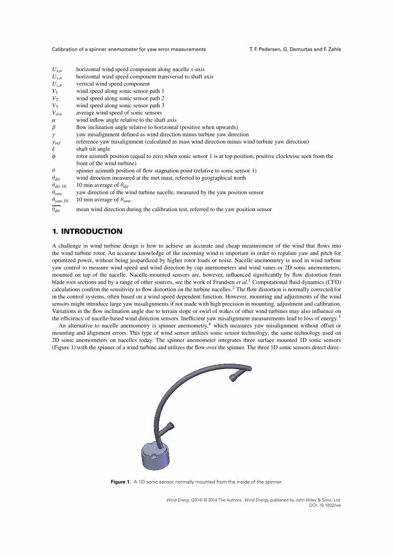
An alternative to nacelle anemometry is spinner anemometry,4 which measures yaw misalignment without offset ormounting and alignment errors. This type of wind sensor utilizes sonic sensor technology; the same technology used on2D sonic anemometers on nacelles today. The spinner anemometer integrates three surface mounted 1D sonic sensors(Figure 1) with the spinner of a wind turbine and utilizes the flow over the spinner. The three 1D sonic sensors detect direc-
Figure 1. A 1D sonic sensor normally mounted from the inside of the spinner.
Wind Energ. (2014) © 2014 The Authors. Wind Energy published by John Wiley & Sons, Ltd.DOI: 10.1002/we
T. F. Pedersen, G. Demurtas and F. Zahle Calibration of a spinner anemometer for yaw error measurements
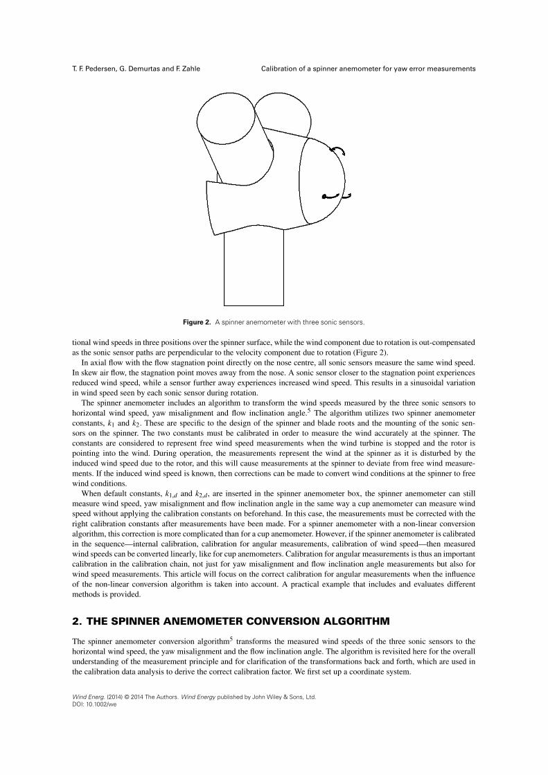
Figure 2. A spinner anemometer with three sonic sensors.
tional wind speeds in three positions over the spinner surface, while the wind component due to rotation is out-compensatedas the sonic sensor paths are perpendicular to the velocity component due to rotation (Figure 2).
In axial flow with the flow stagnation point directly on the nose centre, all sonic sensors measure the same wind speed.In skew air flow, the stagnation point moves away from the nose. A sonic sensor closer to the stagnation point experiencesreduced wind speed, while a sensor further away experiences increased wind speed. This results in a sinusoidal variationin wind speed seen by each sonic sensor during rotation.
The spinner anemometer includes an algorithm to transform the wind speeds measured by the three sonic sensors tohorizontal wind speed, yaw misalignment and flow inclination angle.5 The algorithm utilizes two spinner anemometerconstants, k1 and k2. These are specific to the design of the spinner and blade roots and the mounting of the sonic sen-sors on the spinner. The two constants must be calibrated in order to measure the wind accurately at the spinner. Theconstants are considered to represent free wind speed measurements when the wind turbine is stopped and the rotor ispointing into the wind. During operation, the measurements represent the wind at the spinner as it is disturbed by theinduced wind speed due to the rotor, and this will cause measurements at the spinner to deviate from free wind measure-ments. If the induced wind speed is known, then corrections can be made to convert wind conditions at the spinner to freewind conditions.
When default constants, k1,d and k2,d, are inserted in the spinner anemometer box, the spinner anemometer can stillmeasure wind speed, yaw misalignment and flow inclination angle in the same way a cup anemometer can measure windspeed without applying the calibration constants on beforehand. In this case, the measurements must be corrected with theright calibration constants after measurements have been made. For a spinner anemometer with a non-linear conversionalgorithm, this correction is more complicated than for a cup anemometer. However, if the spinner anemometer is calibratedin the sequence—internal calibration, calibration for angular measurements, calibration of wind speed—then measuredwind speeds can be converted linearly, like for cup anemometers. Calibration for angular measurements is thus an importantcalibration in the calibration chain, not just for yaw misalignment and flow inclination angle measurements but also forwind speed measurements. This article will focus on the correct calibration for angular measurements when the influenceof the non-linear conversion algorithm is taken into account. A practical example that includes and evaluates differentmethods is provided.
2. THE SPINNER ANEMOMETER CONVERSION ALGORITHM
The spinner anemometer conversion algorithm5 transforms the measured wind speeds of the three sonic sensors to thehorizontal wind speed, the yaw misalignment and the flow inclination angle. The algorithm is revisited here for the overallunderstanding of the measurement principle and for clarification of the transformations back and forth, which are used inthe calibration data analysis to derive the correct calibration factor. We first set up a coordinate system.
Wind Energ. (2014) © 2014 The Authors. Wind Energy published by John Wiley & Sons, Ltd.DOI: 10.1002/we
Calibration of a spinner anemometer for yaw error measurements T. F. Pedersen, G. Demurtas and F. Zahle
2.1. Coordinate systems
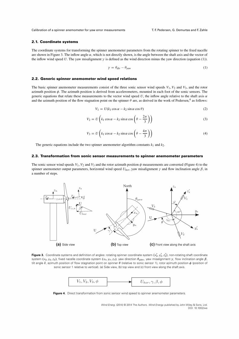
The coordinate systems for transforming the spinner anemometer parameters from the rotating spinner to the fixed nacelleare shown in Figure 3. The inflow angle ˛, which is not directly shown, is the angle between the shaft axis and the vector ofthe inflow wind speed U. The yaw misalignment � is defined as the wind direction minus the yaw direction (equation (1)).
� D �dir � �yaw (1)
2.2. Generic spinner anemometer wind speed relations
The basic spinner anemometer measurements consist of the three sonic sensor wind speeds V1, V2 and V3, and the rotorazimuth position �. The azimuth position is derived from accelerometers, mounted in each foot of the sonic sensors. Thegeneric equations that relate these measurements to the vector wind speed U, the inflow angle relative to the shaft axis ˛and the azimuth position of the flow stagnation point on the spinner � are, as derived in the work of Pedersen,4 as follows:
V1 D U.k1 cos ˛ � k2 sin˛ cos �/ (2)
V2 D U
�k1 cos ˛ � k2 sin˛ cos
�� � 2�
3
��(3)
V3 D U
�k1 cos ˛ � k2 sin˛ cos
�� � 4�
3
��(4)
The generic equations include the two spinner anemometer algorithm constants k1 and k2.
2.3. Transformation from sonic sensor measurements to spinner anemometer parameters
The sonic sensor wind speeds V1, V2 and V3 and the rotor azimuth position � measurements are converted (Figure 4) to thespinner anemometer output parameters, horizontal wind speed Uhor , yaw misalignment � and flow inclination angle ˇ, ina number of steps.
Figure 3. Coordinate systems and definition of angles: rotating spinner coordinate system�x0s, y0s , z0s
�, non-rotating shaft coordinate
system .xs, ys, zs/, fixed nacelle coordinate system .xn, yn, zn/, yaw direction �yaw , yaw misalignment � , flow inclination angle ˇ ,tilt angle ı , azimuth position of flow stagnation point on spinner � (relative to sonic sensor 1), rotor azimuth position � (position of
sonic sensor 1 relative to vertical). (a) Side view, (b) top view and (c) front view along the shaft axis.
Figure 4. Direct transformation from sonic sensor wind speed to spinner anemometer parameters.
Wind Energ. (2014) © 2014 The Authors. Wind Energy published by John Wiley & Sons, Ltd.DOI: 10.1002/we
T. F. Pedersen, G. Demurtas and F. Zahle Calibration of a spinner anemometer for yaw error measurements
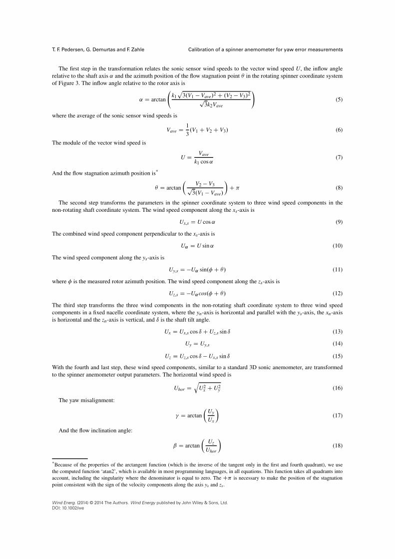
The first step in the transformation relates the sonic sensor wind speeds to the vector wind speed U, the inflow anglerelative to the shaft axis ˛ and the azimuth position of the flow stagnation point � in the rotating spinner coordinate systemof Figure 3. The inflow angle relative to the rotor axis is
˛ D arctan
k1p
3.V1 � Vave/2 C .V2 � V3/2p3k2Vave
!(5)
where the average of the sonic sensor wind speeds is
Vave D 1
3.V1 C V2 C V3/ (6)
The module of the vector wind speed is
U D Vave
k1 cos ˛(7)
And the flow stagnation azimuth position is*
� D arctan�
V2 � V3p3.V1 � Vave/
�C � (8)
The second step transforms the parameters in the spinner coordinate system to three wind speed components in thenon-rotating shaft coordinate system. The wind speed component along the xs-axis is
Ux,s D U cos ˛ (9)
The combined wind speed component perpendicular to the xs-axis is
U˛ D U sin˛ (10)
The wind speed component along the ys-axis is
Uy,s D �U˛ sin.� C �/ (11)
where � is the measured rotor azimuth position. The wind speed component along the zs-axis is
Uz,s D �U˛cos.� C �/ (12)
The third step transforms the three wind components in the non-rotating shaft coordinate system to three wind speedcomponents in a fixed nacelle coordinate system, where the yn-axis is horizontal and parallel with the ys-axis, the xn-axisis horizontal and the zn-axis is vertical, and ı is the shaft tilt angle.
Ux D Ux,s cos ı C Uz,s sin ı (13)
Uy D Uy,s (14)
Uz D Uz,s cos ı � Ux,s sin ı (15)
With the fourth and last step, these wind speed components, similar to a standard 3D sonic anemometer, are transformedto the spinner anemometer output parameters. The horizontal wind speed is
Uhor Dq
U2x C U2
y (16)
The yaw misalignment:
� D arctan
�Uy
Ux
�(17)
And the flow inclination angle:
ˇ D arctan�
Uz
Uhor
�(18)
*Because of the properties of the arctangent function (which is the inverse of the tangent only in the first and fourth quadrant), we usethe computed function ‘atan2’, which is available in most programming languages, in all equations. This function takes all quadrants intoaccount, including the singularity where the denominator is equal to zero. The C� is necessary to make the position of the stagnationpoint consistent with the sign of the velocity components along the axis ys and zs.
Wind Energ. (2014) © 2014 The Authors. Wind Energy published by John Wiley & Sons, Ltd.DOI: 10.1002/we

Calibration of a spinner anemometer for yaw error measurements T. F. Pedersen, G. Demurtas and F. Zahle
2.4. Transformation from spinner anemometer parameters back to sonic sensorwind speeds
In order to correct measured spinner anemometer data with calibrated spinner anemometer constants, it is necessary toreverse the spinner anemometer algorithm. This inverse transformation to the sensor path speeds is presented in Figure 5.A special consideration of the rotor position � has to be given because the rotor position is not an output parameter of thespinner anemometer.
The first step of the inverse transformation transforms the spinner anemometer output parameters Uhor, � and ˇ to thesonic sensor wind speed components Ux, Uy and Uz in the nacelle coordinate system:
Ux D Uhor cos � (19)
Uy D Uhor sin � (20)
Uz D Uhor tanˇ (21)
The second inverse step transforms the wind speed components in the nacelle coordinate system to wind speedcomponents in the shaft coordinate system:
Ux,s D Ux cos ı � Uz sin ı (22)
Uy,s D Uy (23)
Uz,s D Ux sin ı C Uz cos ı (24)
The third inverse step transforms the wind speed components in the shaft coordinate system to wind parameters in thespinner coordinate system. The rotor azimuth position is not important for transformations back and forth and can be setequal to zero. The vector wind speed and the inflow angle to the shaft are:
U Dq
U2x,s C U2
y,s C U2z,s (25)
U˛ Dq
U2y,s C U2
z,s (26)
˛ D arctan�
U˛Ux,s
�(27)
And now, using the rotor azimuth position to find the flow stagnation azimuth position,
� D arctan�
Uy,s
Uz,s
�� � C � (28)
Finally, the fourth inverse step transforms the wind parameters in the spinner coordinate system to the sonic sensor windspeeds:
V1 D U .k1 cos ˛ � k2 sin˛ cos �/ (29)
V2 D U
�k1 cos ˛ � k2 sin˛ cos
�� � 2�
3
��(30)
V3 D U
�k1 cos ˛ � k2 sin˛ cos
�� � 4�
3
��(31)
Figure 5. Inverse transformation, from spinner anemometer parameters to sonic sensors wind speeds.
Wind Energ. (2014) © 2014 The Authors. Wind Energy published by John Wiley & Sons, Ltd.DOI: 10.1002/we
T. F. Pedersen, G. Demurtas and F. Zahle Calibration of a spinner anemometer for yaw error measurements
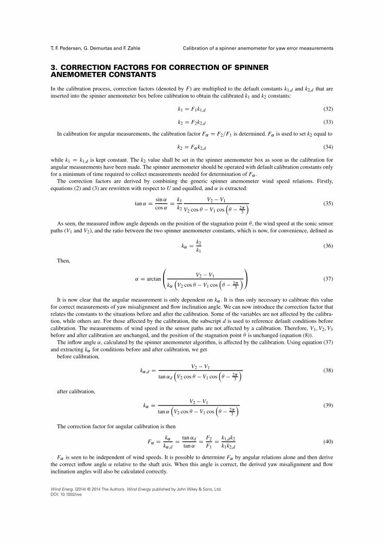
3. CORRECTION FACTORS FOR CORRECTION OF SPINNERANEMOMETER CONSTANTS
In the calibration process, correction factors (denoted by F) are multiplied to the default constants k1,d and k2,d that areinserted into the spinner anemometer box before calibration to obtain the calibrated k1 and k2 constants:
k1 D F1k1,d (32)
k2 D F2k2,d (33)
In calibration for angular measurements, the calibration factor F˛ D F2=F1 is determined. F˛ is used to set k2 equal to
k2 D F˛k2,d (34)
while k1 D k1,d is kept constant. The k2 value shall be set in the spinner anemometer box as soon as the calibration forangular measurements have been made. The spinner anemometer should be operated with default calibration constants onlyfor a minimum of time required to collect measurements needed for determination of F˛ .
The correction factors are derived by combining the generic spinner anemometer wind speed relations. Firstly,equations (2) and (3) are rewritten with respect to U and equalled, and ˛ is extracted:
tan˛ D sin˛
cos ˛D k1
k2
V2 � V1
V2 cos � � V1 cos�� � 2�
3
� (35)
As seen, the measured inflow angle depends on the position of the stagnation point � , the wind speed at the sonic sensorpaths (V1 and V2), and the ratio between the two spinner anemometer constants, which is now, for convenience, defined as
k˛ D k2
k1(36)
Then,
˛ D arctan
0@ V2 � V1
k˛�
V2 cos � � V1 cos�� � 2�
3
�1A (37)
It is now clear that the angular measurement is only dependent on k˛ . It is thus only necessary to calibrate this valuefor correct measurements of yaw misalignment and flow inclination angle. We can now introduce the correction factor thatrelates the constants to the situations before and after the calibration. Some of the variables are not affected by the calibra-tion, while others are. For those affected by the calibration, the subscript d is used to reference default conditions beforecalibration. The measurements of wind speed in the sensor paths are not affected by a calibration. Therefore, V1, V2, V3before and after calibration are unchanged, and the position of the stagnation point � is unchanged (equation (8)).
The inflow angle ˛, calculated by the spinner anemometer algorithm, is affected by the calibration. Using equation (37)and extracting k˛ for conditions before and after calibration, we get
before calibration,
k˛,d D V2 � V1
tan˛d
�V2 cos � � V1 cos
�� � 2�
3
� (38)
after calibration,
k˛ D V2 � V1
tan˛�
V2 cos � � V1 cos�� � 2�
3
� (39)
The correction factor for angular calibration is then
F˛ D k˛k˛,d
D tan˛d
tan˛D F2
F1D k1,dk2
k1k2,d(40)
F˛ is seen to be independent of wind speeds. It is possible to determine F˛ by angular relations alone and then derivethe correct inflow angle ˛ relative to the shaft axis. When this angle is correct, the derived yaw misalignment and flowinclination angles will also be calculated correctly.
Wind Energ. (2014) © 2014 The Authors. Wind Energy published by John Wiley & Sons, Ltd.DOI: 10.1002/we
Calibration of a spinner anemometer for yaw error measurements T. F. Pedersen, G. Demurtas and F. Zahle
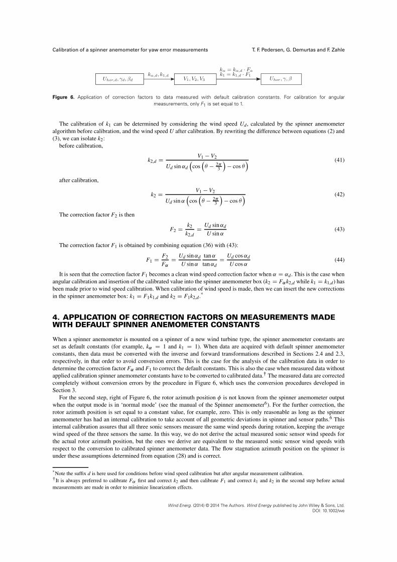
Figure 6. Application of correction factors to data measured with default calibration constants. For calibration for angularmeasurements, only F1 is set equal to 1.
The calibration of k1 can be determined by considering the wind speed Ud , calculated by the spinner anemometeralgorithm before calibration, and the wind speed U after calibration. By rewriting the difference between equations (2) and(3), we can isolate k2:
before calibration,
k2,d D V1 � V2
Ud sin˛d
�cos
�� � 2�
3
�� cos �
� (41)
after calibration,
k2 D V1 � V2
Ud sin˛�
cos�� � 2�
3
�� cos �
� (42)
The correction factor F2 is then
F2 D k2
k2,dD Ud sin˛d
U sin˛(43)
The correction factor F1 is obtained by combining equation (36) with (43):
F1 D F2
F˛D Ud sin˛d
U sin˛
tan˛
tan˛dD Ud cos ˛d
U cos ˛(44)
It is seen that the correction factor F1 becomes a clean wind speed correction factor when ˛ D ˛d . This is the case whenangular calibration and insertion of the calibrated value into the spinner anemometer box (k2 D F˛k2,d while k1 D k1,d) hasbeen made prior to wind speed calibration. When calibration of wind speed is made, then we can insert the new correctionsin the spinner anemometer box: k1 D F1k1,d and k2 D F1k2,d .*
4. APPLICATION OF CORRECTION FACTORS ON MEASUREMENTS MADEWITH DEFAULT SPINNER ANEMOMETER CONSTANTS
When a spinner anemometer is mounted on a spinner of a new wind turbine type, the spinner anemometer constants areset as default constants (for example, k˛ D 1 and k1 D 1). When data are acquired with default spinner anemometerconstants, then data must be converted with the inverse and forward transformations described in Sections 2.4 and 2.3,respectively, in that order to avoid conversion errors. This is the case for the analysis of the calibration data in order todetermine the correction factor F˛ and F1 to correct the default constants. This is also the case when measured data withoutapplied calibration spinner anemometer constants have to be converted to calibrated data.� The measured data are correctedcompletely without conversion errors by the procedure in Figure 6, which uses the conversion procedures developed inSection 3.
For the second step, right of Figure 6, the rotor azimuth position � is not known from the spinner anemometer outputwhen the output mode is in ‘normal mode’ (see the manual of the Spinner anemometer6). For the further correction, therotor azimuth position is set equal to a constant value, for example, zero. This is only reasonable as long as the spinneranemometer has had an internal calibration to take account of all geometric deviations in spinner and sensor paths.6 Thisinternal calibration assures that all three sonic sensors measure the same wind speeds during rotation, keeping the averagewind speed of the three sensors the same. In this way, we do not derive the actual measured sonic sensor wind speeds forthe actual rotor azimuth position, but the ones we derive are equivalent to the measured sonic sensor wind speeds withrespect to the conversion to calibrated spinner anemometer data. The flow stagnation azimuth position on the spinner isunder these assumptions determined from equation (28) and is correct.
*Note the suffix d is here used for conditions before wind speed calibration but after angular measurement calibration.�It is always preferred to calibrate F˛ first and correct k2 and then calibrate F1 and correct k1 and k2 in the second step before actualmeasurements are made in order to minimize linearization effects.
Wind Energ. (2014) © 2014 The Authors. Wind Energy published by John Wiley & Sons, Ltd.DOI: 10.1002/we
T. F. Pedersen, G. Demurtas and F. Zahle Calibration of a spinner anemometer for yaw error measurements
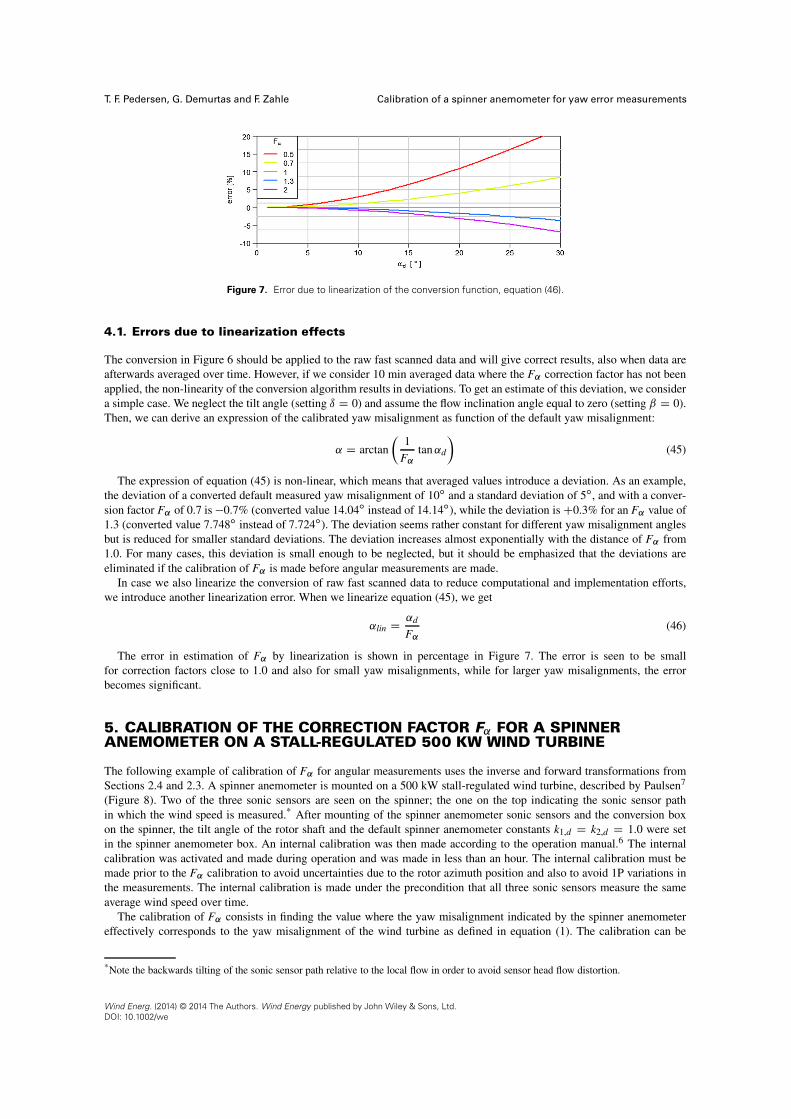
Figure 7. Error due to linearization of the conversion function, equation (46).
4.1. Errors due to linearization effects
The conversion in Figure 6 should be applied to the raw fast scanned data and will give correct results, also when data areafterwards averaged over time. However, if we consider 10 min averaged data where the F˛ correction factor has not beenapplied, the non-linearity of the conversion algorithm results in deviations. To get an estimate of this deviation, we considera simple case. We neglect the tilt angle (setting ı D 0) and assume the flow inclination angle equal to zero (setting ˇ D 0).Then, we can derive an expression of the calibrated yaw misalignment as function of the default yaw misalignment:
˛ D arctan�
1
F˛tan˛d
�(45)
The expression of equation (45) is non-linear, which means that averaged values introduce a deviation. As an example,the deviation of a converted default measured yaw misalignment of 10ı and a standard deviation of 5ı, and with a conver-sion factor F˛ of 0.7 is �0.7% (converted value 14.04ı instead of 14.14ı), while the deviation is C0.3% for an F˛ value of1.3 (converted value 7.748ı instead of 7.724ı). The deviation seems rather constant for different yaw misalignment anglesbut is reduced for smaller standard deviations. The deviation increases almost exponentially with the distance of F˛ from1.0. For many cases, this deviation is small enough to be neglected, but it should be emphasized that the deviations areeliminated if the calibration of F˛ is made before angular measurements are made.
In case we also linearize the conversion of raw fast scanned data to reduce computational and implementation efforts,we introduce another linearization error. When we linearize equation (45), we get
˛lin D ˛d
F˛(46)
The error in estimation of F˛ by linearization is shown in percentage in Figure 7. The error is seen to be smallfor correction factors close to 1.0 and also for small yaw misalignments, while for larger yaw misalignments, the errorbecomes significant.
5. CALIBRATION OF THE CORRECTION FACTOR F˛ FOR A SPINNERANEMOMETER ON A STALL-REGULATED 500 KW WIND TURBINE
The following example of calibration of F˛ for angular measurements uses the inverse and forward transformations fromSections 2.4 and 2.3. A spinner anemometer is mounted on a 500 kW stall-regulated wind turbine, described by Paulsen7
(Figure 8). Two of the three sonic sensors are seen on the spinner; the one on the top indicating the sonic sensor pathin which the wind speed is measured.* After mounting of the spinner anemometer sonic sensors and the conversion boxon the spinner, the tilt angle of the rotor shaft and the default spinner anemometer constants k1,d D k2,d D 1.0 were setin the spinner anemometer box. An internal calibration was then made according to the operation manual.6 The internalcalibration was activated and made during operation and was made in less than an hour. The internal calibration must bemade prior to the F˛ calibration to avoid uncertainties due to the rotor azimuth position and also to avoid 1P variations inthe measurements. The internal calibration is made under the precondition that all three sonic sensors measure the sameaverage wind speed over time.
The calibration of F˛ consists in finding the value where the yaw misalignment indicated by the spinner anemometereffectively corresponds to the yaw misalignment of the wind turbine as defined in equation (1). The calibration can be
*Note the backwards tilting of the sonic sensor path relative to the local flow in order to avoid sensor head flow distortion.
Wind Energ. (2014) © 2014 The Authors. Wind Energy published by John Wiley & Sons, Ltd.DOI: 10.1002/we
Calibration of a spinner anemometer for yaw error measurements T. F. Pedersen, G. Demurtas and F. Zahle
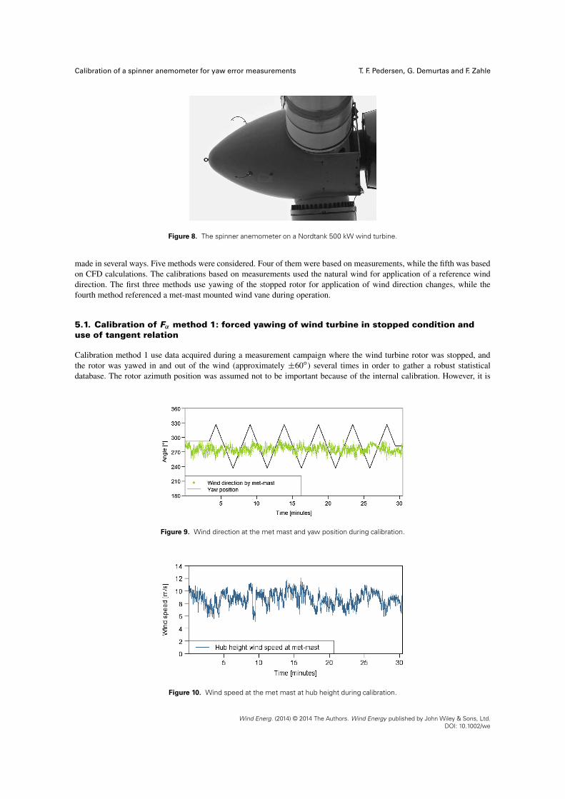
Figure 8. The spinner anemometer on a Nordtank 500 kW wind turbine.
made in several ways. Five methods were considered. Four of them were based on measurements, while the fifth was basedon CFD calculations. The calibrations based on measurements used the natural wind for application of a reference winddirection. The first three methods use yawing of the stopped rotor for application of wind direction changes, while thefourth method referenced a met-mast mounted wind vane during operation.
5.1. Calibration of F˛ method 1: forced yawing of wind turbine in stopped condition anduse of tangent relation
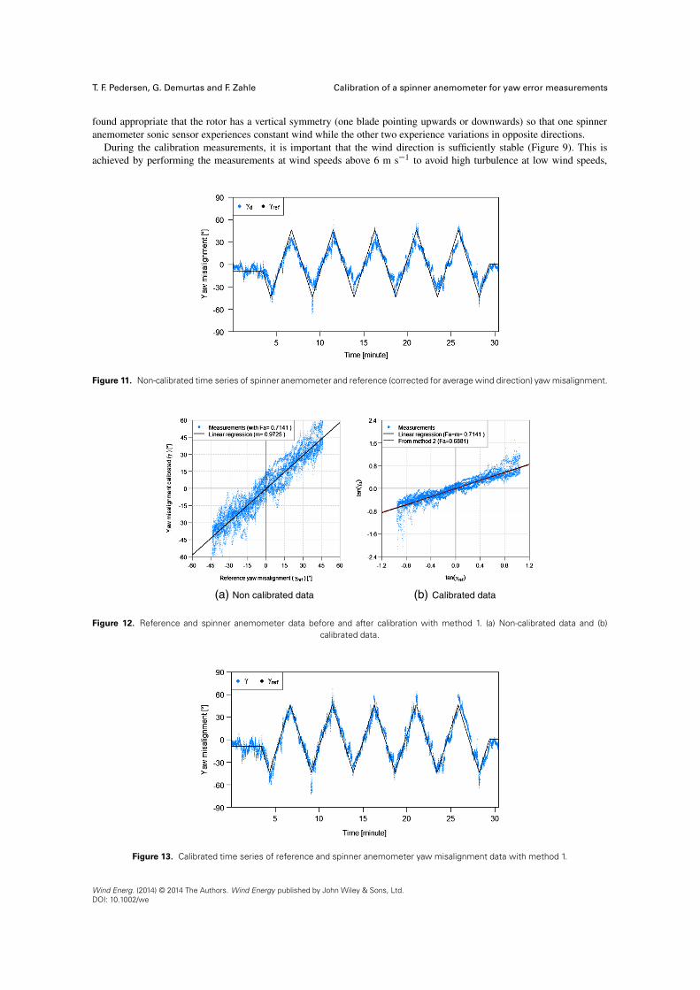
Calibration method 1 use data acquired during a measurement campaign where the wind turbine rotor was stopped, andthe rotor was yawed in and out of the wind (approximately ˙60ı) several times in order to gather a robust statisticaldatabase. The rotor azimuth position was assumed not to be important because of the internal calibration. However, it is
Figure 9. Wind direction at the met mast and yaw position during calibration.
Figure 10. Wind speed at the met mast at hub height during calibration.
Wind Energ. (2014) © 2014 The Authors. Wind Energy published by John Wiley & Sons, Ltd.DOI: 10.1002/we
T. F. Pedersen, G. Demurtas and F. Zahle Calibration of a spinner anemometer for yaw error measurements
found appropriate that the rotor has a vertical symmetry (one blade pointing upwards or downwards) so that one spinneranemometer sonic sensor experiences constant wind while the other two experience variations in opposite directions.
During the calibration measurements, it is important that the wind direction is sufficiently stable (Figure 9). This isachieved by performing the measurements at wind speeds above 6 m s�1 to avoid high turbulence at low wind speeds,
Figure 11. Non-calibrated time series of spinner anemometer and reference (corrected for average wind direction) yaw misalignment.
Figure 12. Reference and spinner anemometer data before and after calibration with method 1. (a) Non-calibrated data and (b)calibrated data.
Figure 13. Calibrated time series of reference and spinner anemometer yaw misalignment data with method 1.
Wind Energ. (2014) © 2014 The Authors. Wind Energy published by John Wiley & Sons, Ltd.DOI: 10.1002/we

Calibration of a spinner anemometer for yaw error measurements T. F. Pedersen, G. Demurtas and F. Zahle
which normally increase the variability of the wind direction. Figure 10 shows the measured wind speed on the met mastduring the calibration. The spinner anemometer data Uhor,d , �d and ˇd , the rotor yaw direction �yaw and the met-mast datawere sampled at 20 Hz during the measurements. The rotor yaw direction is now converted to a reference yaw misalignmentwith reference to the average wind direction: �ref D �dir � �yaw. In Figure 11, the spinner anemometer yaw misalignment�d and the reference yaw misalignment �ref are plotted with time, and in Figure 12, the parameters are plotted againsteach other.
In order to use the tangent relations in equation (40), the reference yaw misalignment from Figure 9 must be offset to zeroyaw misalignment with the averaged wind direction �dir. This was made with a linear regression between reference yawmisalignment data and default yaw misalignment measured by spinner anemometer. The offset was subtracted in Figures 11and 12(a). Now, the tangent relation can be plotted, Figure 12(b), and a linear regression be made to find F˛ D 0.7141.The calibrated yawing is shown in Figure 13.
5.2. Calibration of F˛ method 2: forced yawing of wind turbine in stopped condition anduse of minimization procedure
Calibration method 2 used the same measurement procedure and database as method 1. For a calibrated instrument, whereF˛ has been found, the slope of the linear regressed line for the reference and calibrated yaw misalignments shall be equalto one (Figure 14(b)). This constraint is used to find the value of F˛ with a minimization function f .m/ D jm � 1j, wherem is the slope of the linear regressed line of the reference and back and forth converted measured yaw misalignment data.The minimization routine utilizes a golden section search and successive parabolic interpolation on F˛ . The back and forthconversion follows the procedure in Figure 6. The non-calibrated data are shown in Figure 14(a), while the calibrated dataare shown in Figure 14(b), with F˛ D 0.6881.
5.3. Calibration of F˛ method 3: forced yawing of wind turbine in stopped condition anduse of direct expression
Calibration method 3 uses the same measurement procedure and database as methods 1 and 2. In method 3, F˛ is foundfrom a direct expression of F˛ for each measured dataset with the tangent relation, (equation (40)). The default inflow angleto the rotor shaft axis ˛d is found from the spinner anemometer output values through combination of the transformationequations derived in Section 3, considering also whether the default yaw misalignment �d is positive or negative:
for �d � 0 : tan˛d Dq
sin2 �d C .cos �d sin ı C tanˇdcosı/2
cos �d cos ı � tanˇdsinı
for �d < 0 : tan˛d D �q
sin2 �d C .cos �d sin ı C tanˇdcosı/2
cos �d cos ı � tanˇdsinı
(47)
The reference inflow angles are found from the rotor yaw direction measurements and calculated with equation (48). Thereference yaw misalignment �ref is determined with the inverse transformation (Section 2.4). With a good approximation,one can set the reference flow inclination angle equal to the measured flow inclination angle with the default spinneranemometer constants: ˇref D ˇd:
Figure 14. Reference and spinner anemometer yaw misalignment data before and after calibration with method 2. (a) Non-calibrateddata and (b) calibrated data.
Wind Energ. (2014) © 2014 The Authors. Wind Energy published by John Wiley & Sons, Ltd.DOI: 10.1002/we
T. F. Pedersen, G. Demurtas and F. Zahle Calibration of a spinner anemometer for yaw error measurements
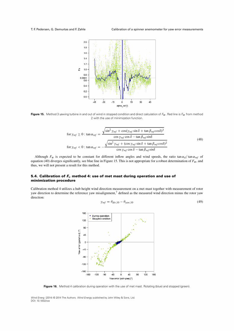
Figure 15. Method 3 yawing turbine in and out of wind in stopped condition and direct calculation of F˛ . Red line is F˛ from method2 with the use of minimization function.
for �ref � 0 : tan˛ref Dq
sin2 �ref C cos.�ref sin ı C tanˇref cosı/2
cos �ref cos ı � tanˇref sinı
for �ref < 0 : tan˛ref D �q
sin2 �ref C .cos �ref sin ı C tanˇref cosı/2
cos �ref cos ı � tanˇref sinı
(48)
Although F˛ is expected to be constant for different inflow angles and wind speeds, the ratio tan˛d= tan˛ref ofequation (40) diverges significantly, see blue line in Figure 15. This is not appropriate for a robust determination of F˛ , andthus, we will not present a result for this method.
5.4. Calibration of F˛ method 4: use of met mast during operation and use ofminimization procedure
Calibration method 4 utilizes a hub height wind direction measurement on a met mast together with measurement of rotoryaw direction to determine the reference yaw misalignment,7 defined as the measured wind direction minus the rotor yawdirection:
�ref D �dir,10 � �yaw,10 (49)
Figure 16. Method 4 calibration during operation with the use of met mast. Rotating (blue) and stopped (green).
Wind Energ. (2014) © 2014 The Authors. Wind Energy published by John Wiley & Sons, Ltd.DOI: 10.1002/we
Calibration of a spinner anemometer for yaw error measurements T. F. Pedersen, G. Demurtas and F. Zahle
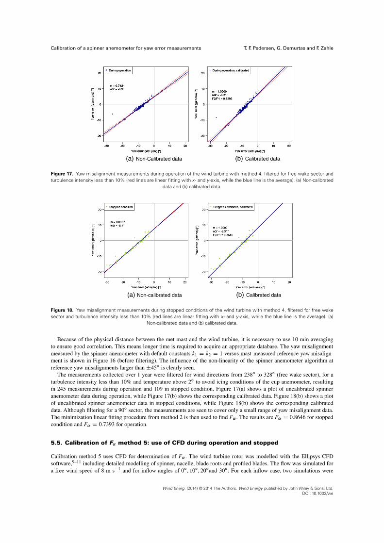
Figure 17. Yaw misalignment measurements during operation of the wind turbine with method 4, filtered for free wake sector andturbulence intensity less than 10% (red lines are linear fitting with x- and y -axis, while the blue line is the average). (a) Non-calibrated
data and (b) calibrated data.
Figure 18. Yaw misalignment measurements during stopped conditions of the wind turbine with method 4, filtered for free wakesector and turbulence intensity less than 10% (red lines are linear fitting with x- and y -axis, while the blue line is the average). (a)
Non-calibrated data and (b) calibrated data.
Because of the physical distance between the met mast and the wind turbine, it is necessary to use 10 min averagingto ensure good correlation. This means longer time is required to acquire an appropriate database. The yaw misalignmentmeasured by the spinner anemometer with default constants k1 D k2 D 1 versus mast-measured reference yaw misalign-ment is shown in Figure 16 (before filtering). The influence of the non-linearity of the spinner anemometer algorithm atreference yaw misalignments larger than ˙45ı is clearly seen.
The measurements collected over 1 year were filtered for wind directions from 238ı to 328ı (free wake sector), for aturbulence intensity less than 10% and temperature above 2ı to avoid icing conditions of the cup anemometer, resultingin 245 measurements during operation and 109 in stopped condition. Figure 17(a) shows a plot of uncalibrated spinneranemometer data during operation, while Figure 17(b) shows the corresponding calibrated data. Figure 18(b) shows a plotof uncalibrated spinner anemometer data in stopped conditions, while Figure 18(b) shows the corresponding calibrateddata. Although filtering for a 90ı sector, the measurements are seen to cover only a small range of yaw misalignment data.The minimization linear fitting procedure from method 2 is then used to find F˛ . The results are F˛ D 0.8646 for stoppedcondition and F˛ D 0.7393 for operation.
5.5. Calibration of F˛ method 5: use of CFD during operation and stopped
Calibration method 5 uses CFD for determination of F˛ . The wind turbine rotor was modelled with the Ellipsys CFDsoftware,9–11 including detailed modelling of spinner, nacelle, blade roots and profiled blades. The flow was simulated fora free wind speed of 8 m s�1 and for inflow angles of 0ı, 10ı, 20ıand 30ı. For each inflow case, two simulations were
Wind Energ. (2014) © 2014 The Authors. Wind Energy published by John Wiley & Sons, Ltd.DOI: 10.1002/we
T. F. Pedersen, G. Demurtas and F. Zahle Calibration of a spinner anemometer for yaw error measurements
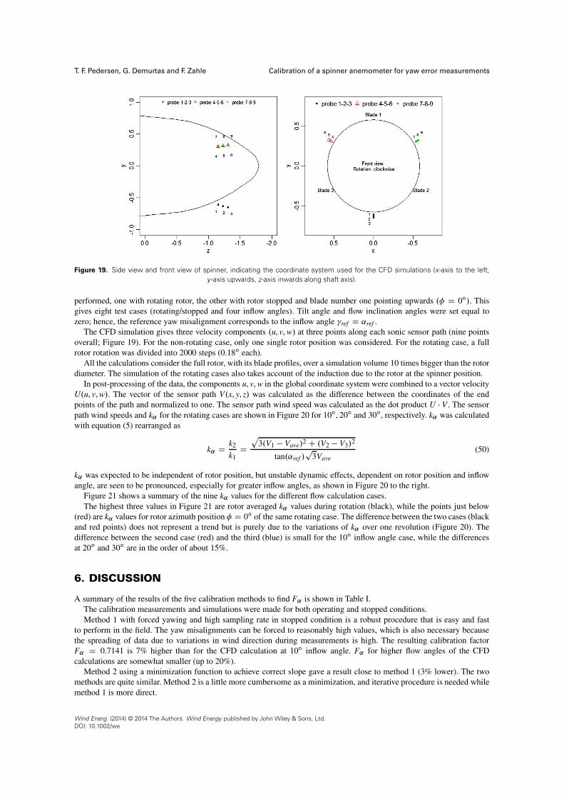
Figure 19. Side view and front view of spinner, indicating the coordinate system used for the CFD simulations (x-axis to the left,y -axis upwards, z-axis inwards along shaft axis).
performed, one with rotating rotor, the other with rotor stopped and blade number one pointing upwards .� D 0ı/. Thisgives eight test cases (rotating/stopped and four inflow angles). Tilt angle and flow inclination angles were set equal tozero; hence, the reference yaw misalignment corresponds to the inflow angle �ref D ˛ref .
The CFD simulation gives three velocity components .u, v, w/ at three points along each sonic sensor path (nine pointsoverall; Figure 19). For the non-rotating case, only one single rotor position was considered. For the rotating case, a fullrotor rotation was divided into 2000 steps (0.18ı each).
All the calculations consider the full rotor, with its blade profiles, over a simulation volume 10 times bigger than the rotordiameter. The simulation of the rotating cases also takes account of the induction due to the rotor at the spinner position.
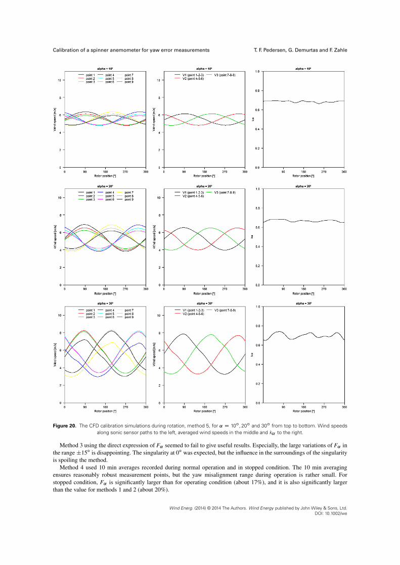
In post-processing of the data, the components u, v, w in the global coordinate system were combined to a vector velocityU.u, v, w/. The vector of the sensor path V.x, y, z/ was calculated as the difference between the coordinates of the endpoints of the path and normalized to one. The sensor path wind speed was calculated as the dot product U � V . The sensorpath wind speeds and k˛ for the rotating cases are shown in Figure 20 for 10ı, 20ı and 30ı, respectively. k˛ was calculatedwith equation (5) rearranged as
k˛ D k2
k1Dp
3.V1 � Vave/2 C .V2 � V3/2
tan.˛ref /p
3Vave(50)
k˛ was expected to be independent of rotor position, but unstable dynamic effects, dependent on rotor position and inflowangle, are seen to be pronounced, especially for greater inflow angles, as shown in Figure 20 to the right.
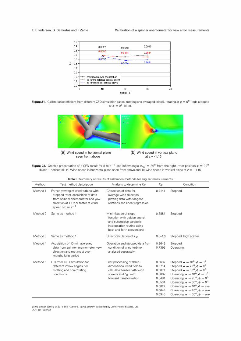
Figure 21 shows a summary of the nine k˛ values for the different flow calculation cases.The highest three values in Figure 21 are rotor averaged k˛ values during rotation (black), while the points just below
(red) are k˛ values for rotor azimuth position � D 0ı of the same rotating case. The difference between the two cases (blackand red points) does not represent a trend but is purely due to the variations of k˛ over one revolution (Figure 20). Thedifference between the second case (red) and the third (blue) is small for the 10ı inflow angle case, while the differencesat 20ı and 30ı are in the order of about 15%.
6. DISCUSSION
A summary of the results of the five calibration methods to find F˛ is shown in Table I.The calibration measurements and simulations were made for both operating and stopped conditions.Method 1 with forced yawing and high sampling rate in stopped condition is a robust procedure that is easy and fast
to perform in the field. The yaw misalignments can be forced to reasonably high values, which is also necessary becausethe spreading of data due to variations in wind direction during measurements is high. The resulting calibration factorF˛ D 0.7141 is 7% higher than for the CFD calculation at 10ı inflow angle. F˛ for higher flow angles of the CFDcalculations are somewhat smaller (up to 20%).
Method 2 using a minimization function to achieve correct slope gave a result close to method 1 (3% lower). The twomethods are quite similar. Method 2 is a little more cumbersome as a minimization, and iterative procedure is needed whilemethod 1 is more direct.
Wind Energ. (2014) © 2014 The Authors. Wind Energy published by John Wiley & Sons, Ltd.DOI: 10.1002/we
Calibration of a spinner anemometer for yaw error measurements T. F. Pedersen, G. Demurtas and F. Zahle
Figure 20. The CFD calibration simulations during rotation, method 5, for ˛ D 10ı, 20ı and 30ı from top to bottom. Wind speedsalong sonic sensor paths to the left, averaged wind speeds in the middle and k˛ to the right.
Method 3 using the direct expression of F˛ seemed to fail to give useful results. Especially, the large variations of F˛ inthe range ˙15ı is disappointing. The singularity at 0ı was expected, but the influence in the surroundings of the singularityis spoiling the method.
Method 4 used 10 min averages recorded during normal operation and in stopped condition. The 10 min averagingensures reasonably robust measurement points, but the yaw misalignment range during operation is rather small. Forstopped condition, F˛ is significantly larger than for operating condition (about 17%), and it is also significantly largerthan the value for methods 1 and 2 (about 20%).
Wind Energ. (2014) © 2014 The Authors. Wind Energy published by John Wiley & Sons, Ltd.DOI: 10.1002/we
T. F. Pedersen, G. Demurtas and F. Zahle Calibration of a spinner anemometer for yaw error measurements
Figure 21. Calibration coefficient from different CFD simulation cases; rotating and averaged (black), rotating at � D 0ı (red), stoppedat � D 0ı (blue).
Figure 22. Graphic presentation of a CFD result for 8 m s�1 and inflow angle ˛ref D 30ı from the right, rotor position � D 90ı
(blade 1 horizontal). (a) Wind speed in horizontal plane seen from above and (b) wind speed in vertical plane at z D �1.15.
Table I. Summary of results of calibration methods for angular measurements.
Method Test method description Analysis to determine F˛ F˛ Condition
Method 1 Forced yawing of wind turbine with Correction of data for 0.7141 Stoppedstopped rotor, acquisition of data average wind direction,from spinner anemometer and yaw plotting data with tangentdirection at 1 Hz or faster at wind relations and linear regressionspeed >6 m s�1
Method 2 Same as method 1 Minimization of slope 0.6881 Stoppedfunction with golden searchand successive parabolicinterpolation routine usingback and forth conversions
Method 3 Same as method 1 Direct calculation of F˛ 0.6–1.0 Stopped, high scatter
Method 4 Acquisition of 10 min averaged Operation and stopped data from 0.8646 Stoppeddata from spinner anemometer, yaw condition of wind turbine 0.7393 Operatingdirection and met mast over analysed separately.months long period
Method 5 Full rotor CFD simulation for Post-processing of three- 0.6637 Stopped, ˛ D 10ı,� D 0ı
different inflow angles, for dimensional wind field to 0.5714 Stopped, ˛ D 20ı,� D 0ı
rotating and non-rotating calculate sensor path wind 0.5871 Stopped, ˛ D 30ı,� D 0ı
conditions speeds and F˛ with 0.6862 Operating, ˛ D 10ı,� D 0ı
forward transformation 0.6481 Operating, ˛ D 20ı,� D 0ı
0.6534 Operating, ˛ D 30ı,� D 0ı
0.6827 Operating, ˛ D 10ı,� D ave0.6648 Operating, ˛ D 20ı,� D ave0.6946 Operating, ˛ D 30ı,� D ave
Wind Energ. (2014) © 2014 The Authors. Wind Energy published by John Wiley & Sons, Ltd.DOI: 10.1002/we
Calibration of a spinner anemometer for yaw error measurements T. F. Pedersen, G. Demurtas and F. Zahle
The difference in F˛ from stopped to operating might be due to induced wind speed from the operating andthrust-generating rotor. The induced wind speed reduces the longitudinal component Ux, while the transversal componentUy is the same. The effect is that the local yaw misalignment at the spinner is larger than in the far field. With a knowninduction function a.U/ D .U1 � U/=U1, the correction of locally measured yaw misalignment to the far field is
�1 D arcsin..1 � a/ sin �/ (51)
For a yaw misalignment measured at the spinner of 10ı and an induction factor of 10%, the yaw misalignment measuredat the far field is 9.0ı (10% lower). When a yaw misalignment at the spinner is higher during operation than when stopped,then the F˛ value for operating condition should be higher than for stopped condition. Method 4 in Table I shows theopposite. This is a controversy. However, the measurements in stopped condition are made during operating periods ofthe wind turbine. Stopped conditions do only occur for very low wind speeds where the wind turbine stops or is idlingbecause of low wind conditions. The measurements for stopped conditions are thus far from the requirements in methods1–3 of wind speeds above 6 m s�1. The stopped condition measurements of method 4 should therefore be considered withreservation. The measurements during operation comply well with the measurements in stopped condition of methods 1and 2 considering a calculated induction factor in the range 2.5% to 7.4%, using equation (51). This level of the inductionfactor is, however, lower than what should be expected. A reason for an increased uncertainty in use of method 4 is thequite small yaw misalignment range during operation.
Method 5 with CFD simulations results in quite some variety. Figure 20 shows increasing variability of k˛ over arotation with increasing inflow angle. The variability pattern is without a 3P similarity. This indicates fluctuations in theaerodynamic flow over the spinner or unsteadiness in the CFD calculations. The wind speed flow pattern in Figure 22(b)indicates flow separation at the spinner nose at 30ı inflow angle. At lower inflow angles, Figure 20 right, the variabilityis reduced. The most trustworthy calibration values with CFD for angular measurements must therefore be found in the10ı inflow angle simulations, as this is the area where actual yaw misalignment measurements are expected. For stoppedcondition, k˛ is significantly higher for 10ı inflow angle than for 20ı or 30ı. For operating condition, k˛ is 3.4% higherfor 10ı, while it is 11–13% for 20ı to 30ı.
Overall, methods 1 and 3, with quite comparable results, are in good agreement with method 4 for operating conditions,with a calculated increase in k˛ of 3.5% for operating conditions due to induction. This is equivalent to CFD simulationsfor 10ı inflow angle with an increase of 3.5% due to induction. The CFD simulations just give k˛ values about 8% lowervalues than field calibrations, as seen in Table I. The reason for the lower k˛ values from CFD simulations might be due tocalculation uncertainties connected with flow separation on the spinner nose because of the pointed spinner. This might bea disadvantage specifically on this type of spinner and might not be found on more rounded spinners.
6.1. Uncertainty of yaw misalignment measurements
Angular measurements with the spinner anemometer has some uncertainties connected to calibration as well as some otherrelations. The influence of induced wind speeds raises the question whether the measured yaw misalignment is defined asa local inflow angle at the spinner or a far field inflow angle. We find it most appropriate to define the yaw misalignmentas a local inflow angle, as well as we find it most appropriate to define the measured wind speed as a local wind speed.The induction function, as mentioned earlier, should be used to correct the measurements to the far field. The inductionfunction should be found as part of the calibration of F1. This could be made according to the International ElectrotechnicalCommission standard,8 as a determination of the nacelle transfer function. Defining the yaw misalignment as a localmeasurement reduces the uncertainty because of a clear definition of the measurand. Calibration methods 1 and 2 aretherefore also the preferred methods.
The sonic sensors must always be zero wind calibrated, as they are from factory. A traceable wind tunnel calibrationcould be made if required, but this should normally not be necessary for angular measurements because the uncertainty isrelatively low. The internal calibration must be made prior to calibration for angular measurements to smooth out variationsduring each rotation, so that the rotor azimuth position during calibration yawing does not influence on the calibration.The uncertainty related to the calibration factor F˛ with methods 1 and 2, where we have taken the non-linearity of thespinner anemometer algorithm into account, is estimated at ˙2%, for use of either of the two methods and a linearizationuncertainty with a standard deviation of 10%. The uncertainty of the yaw direction sensor is estimated at ˙2ı. However,the uncertainty on the linearity is estimated to be close to zero, so we do not need to take this into account. If we assumerectangular uncertainty distributions for use of methods 1 or 2 and linearization, and combine the uncertainty components,we get a standard uncertainty of 10% of F˛ .
The uncertainty of F˛ , and thus k˛ , provides an uncertainty of ˛ of the same order. The yaw misalignment and flowinclination angles are directly derived from ˛ and have the same uncertainty connected to them. A spinner anemometerthat measures for example 10ı yaw misalignment, and where the standard uncertainty of F˛ is 10%, will have a standarduncertainty on the yaw misalignment of 1ı.
Wind Energ. (2014) © 2014 The Authors. Wind Energy published by John Wiley & Sons, Ltd.DOI: 10.1002/we
T. F. Pedersen, G. Demurtas and F. Zahle Calibration of a spinner anemometer for yaw error measurements
7. CONCLUSIONS
In the first part, the spinner anemometer conversion algorithm that converts the measured wind speeds by the sonic sensorsto horizontal wind speed, yaw misalignment and flow inclination angle is described. The inverse conversion is derived inorder to use earlier measured wind data (measured with default constants k1 and k2) to find the calibration factor F˛ . F˛ isused to correct the default spinner anemometer ratio k˛,d D k2,d=k1,d to the calibrated ratio k˛ D k2=k1 by k˛ D F˛k˛,d .It was found that F˛ was the only single calibration factor that angular measurements depend on. It was further found thatcalibration for angular measurements should be made after internal calibration of the spinner anemometer and before windspeed calibration.
Five different methods for calibration of a spinner anemometer for yaw misalignment measurements were presented fora stall-regulated 500 kW wind turbine with a spinner anemometer mounted on a pointed spinner. The first three calibrationmethods 1–3 consist of stopping the turbine in a steady and low turbulent wind (>6 m s�1) and yawing the turbine severaltimes in and out of the wind. These methods used fast-sampled measurements (20 Hz,>1 Hz). Time required was about halfan hour. Method 1 used a tangent relation with a linear regression to find F˛ D 0.7141 and was the highest recommendedmethod with method 2 using a minimization function and an iterative process with back and forth conversion algorithms tofind F˛ D 0.6881, following very close. Method 3 failed to give a satisfactory result.
Method 4 used 10 min average data during normal operation and standstill of the wind turbine, combined with winddirection measurements from a met-mast upwind of the wind turbine. Data for stopped condition were found to be madeat too low wind speeds. For operation condition, we found F˛ D 0.7393. The higher value than for methods 1 and 2 wasassumed to be due to rotor induction.
Method 5 used CFD to calculate the flow over the spinner for axial and skew airflow during operating and stoppedconditions. F˛ was found directly from the calculations. The calculations for 10ı inflow angle were considered to be themost trustworthy, deriving F˛ values approximately 8% lower than for field calibrations. The differences were consideredto be due to separation on the pointed spinner.
The influence of rotor induction increases the yaw misalignment measurements locally at the spinner compared with thefar field. We define the yaw misalignment measurements to be a local measurement; therefore recommending calibrationsby yawing the wind turbine in and out of the wind in stopped conditions and eventually using an induction function forcorrection to the far field. The uncertainty connected with the calibration was found to be approximately 10%, resulting inan uncertainty of 1ı for a 10ı yaw misalignment measurement.
ACKNOWLEDGEMENTS
This work was performed as part of an EUDP project funded by the Danish Energy Agency and by Vattenfall, Metek andVestas. (J.nr 64009-0273). The authors would like to thank the people from Metek, Vattenfall and ROMO Wind for thehelp with technical support and for their good collaboration in the project.
REFERENCES
1. Frandsen S, Sørensen N, Mikkelsen R, Pedersen TF, Antoniou I, Hansen K. The generics of wind turbine nacelleanemometry. EWEC 2009, Bruxelles, 2009.
2. Zahle F, Sørensen NN. Characterization of the unsteady flow in the nacelle region of a modern wind turbine. WindEnergy 2011; 14: 271–283.
3. Højstrup J, Nielsen D, Hansen K, Lauritzen L. Maximise energy production by minimizing yaw misalignment. Largescale field deployment of spinner anemometer. Poster 0162, EWEC 2013, Vienna, 2013.
4. Pedersen TF. Spinner anemometer—an innovative wind measurement concept. EWEC 2007, Milan, 2007.5. Pedersen TF, Sørensen N, Evevoldsen P. Aerodynamics and characteristics of a spinner anemometer. Journal of
Physics: Conference Series 75 012018 2007.6. Spinner anemometer user manual version 9.27-3. Metek Meteorologische Messtechnik GmBH, Germany, 2012.7. Paulsen US, Vindmølleafprvning Nordtank NTK 500/41, Måling af Effektkurve, Technical Report Risø-I-889 DA, Risø
National Laboratory, Roskilde, Denmark, November 1995.8. IEC 61400-12-2 Wind turbines - part 12-2: Power performance of electricity producing wind turbines based on nacelle
anemometry, Edition 1.0, 2013-03.9. Michelsenl JA, Basis3D–a platform for development of multiblock PDE solvers. Technical Report AFM 92-05,
Technical University of Denmark, 1992.
Wind Energ. (2014) © 2014 The Authors. Wind Energy published by John Wiley & Sons, Ltd.DOI: 10.1002/we

Calibration of a spinner anemometer for yaw error measurements T. F. Pedersen, G. Demurtas and F. Zahle
10. Michelsen JA, Block structured multigrid solution of 2D and 3D elliptic PDEs. Technical Report AFM 94-06, TechnicalUniversity of Denmark, 1994.
11. Sørensen NN, General purpose flow solver applied to flow over hills. Technical Report Risø-R-827(EN), Risø NationalLaboratory, 1995.
Wind Energ. (2014) © 2014 The Authors. Wind Energy published by John Wiley & Sons, Ltd.DOI: 10.1002/we
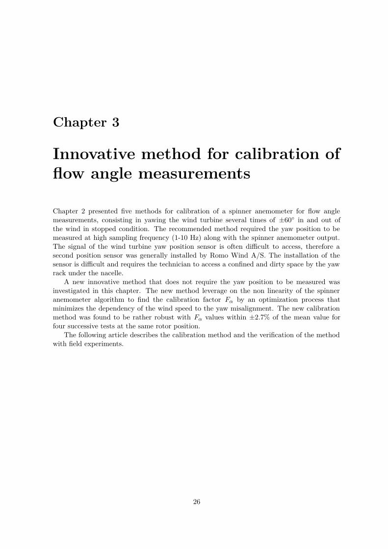
Chapter 3
Innovative method for calibration offlow angle measurements
Chapter 2 presented five methods for calibration of a spinner anemometer for flow anglemeasurements, consisting in yawing the wind turbine several times of ±60◦ in and out ofthe wind in stopped condition. The recommended method required the yaw position to bemeasured at high sampling frequency (1-10 Hz) along with the spinner anemometer output.The signal of the wind turbine yaw position sensor is often difficult to access, therefore asecond position sensor was generally installed by Romo Wind A/S. The installation of thesensor is difficult and requires the technician to access a confined and dirty space by the yawrack under the nacelle.
A new innovative method that does not require the yaw position to be measured wasinvestigated in this chapter. The new method leverage on the non linearity of the spinneranemometer algorithm to find the calibration factor Fα by an optimization process thatminimizes the dependency of the wind speed to the yaw misalignment. The new calibrationmethod was found to be rather robust with Fα values within ±2.7% of the mean value forfour successive tests at the same rotor position.
The following article describes the calibration method and the verification of the methodwith field experiments.
26
An innovative method to calibrate a spinner anemometer withoutuse of yaw position sensorGiorgio Demurtas1 and Nick Gerardus Cornelis Janssen2
1DTU Wind Energy, Frederiksborvej 399, 4000 Roskilde, Denmark.2Romo Wind A/S, Olof Palmes Alle 47, 8200 Aarhus N, Denmark.
Correspondence to:Giorgio Demurtas ([email protected])
Abstract. A spinner anemometer can be used to measure the yaw misalignment and flow inclination experienced by a wind
turbine. Previous calibration methods used to calibrate a spinner anemometer for flow angle measurements were based on
measurements of a spinner anemometer with default settings (arbitrary values, generallyk1,d = 1 andk2,d = 1) and a reference
yaw misalignment signal measured with a yaw position sensor. The yaw position sensor is normally present in wind turbines for
control purposes, however, such a signal is not always available for a spinner anemometer calibration. Therefore, an additional5
yaw position sensor was installed prior to the spinner anemometer calibration. An innovative method to calibrate the spinner
anemometer without a yaw positions sensor was then developed. It was noted that a non calibrated spinner anemometer that
overestimate (underestimate) the inflow angle will also overestimate (underestimate) the wind speed when there is a yaw
misalignment. The new method leverage on the non linearity of the spinner anemometer algorithm to find the calibration factor
Fα by an optimization process that minimizes the dependency of the wind speed to the yaw misalignment. The new calibration10
method was found to be rather robust withFα values within±2.7% of the mean value for four successive tests at the same
rotor position.
Nomenclature
V1 Speed along the sensor path of probe 1. α Inflow angle respect to the shaft axis.
V2 Speed along the sensor path of probe 2. δ Shaft tilt angle.
V3 Speed along the sensor path of probe 3. β Flow inclination angle.
Vave Mean value betweenV1, V2, V3. γ Yaw misalignment.
U Wind speed vector modulus. γref Reference yaw misalignment.
Uhor Horizontal wind speed component. φ Rotor position
Uhor,d Horizontal wind speed (noncalibrated). Uhor Mean horizontal wind speed.
Uhor,d,c Horizontal wind speed component (calibrated
with correctkα but not yetk1).
θ Azimuth position of flow stagnation point on spin-
ner (relative to sonic sensor 1).
1

k1 Calibration constant mainly related to wind
speed calibration.
F1 Calibration correction factor mainly re-
lated to wind speed calibration.
kα Calibration constant mainly related to an-
gle calibration.
Fα Calibration correction factor mainly re-
lated to angle calibration.
k2 Calibration constant (equal tokα ∙ k1). F2 Calibration correction factor (Fα ∙F1).
RMSE Root Mean Square Error TI Turbulence Intensity.
QSC Quality Score WSR Wind Speed Response method
GGref Gamma-Gamma reference method TanTan Tangent-Tangent method
1 Introduction
The spinner anemometer (Pedersen et al.(2007)) measures the horizontal wind speedUhor, yaw misalignmentγ and flow
inclinationβ experienced by a wind turbine by measuring the flow on the spinner by using three 1D sonic sensors. The three
1D sonic sensors are mounted on the spinner and connected to a so called "conversion box". Each sonic sensor arm also5
contains a 1D accelerometer which measurements are used in the conversion box to calculate the rotor position. The main
purpose of the conversion box is to execute the conversion algorithm that transform the 1D sonic sensors readings which
are in a rotating coordinate reference system (Fig.1) to the fixed nacelle coordinate reference system asUhor, γ andβ. The
conversion algorithm takes into consideration the wind turbine tilt angleδ which is set in the conversion box as a constant.
The shape of the spinner is accounted for by two calibration coefficients,k1 andk2. The first coefficient mainly relates to10
wind speed measurements, while the ratio of the two coefficientskα = k2/k1 mainly relates to flow angle measurements. The
relations between the wind speedU , flow angleα and azimuth position of the stagnation pointθ producingV1, V2 andV3
measured by the three 1D sonic sensors are:
V1 = U (k1 cos(α)− k2 sin(α)cos(θ)) = U ∙ k1 (cos(α)− kα sin(α)cos(θ)) (1)
V2 = U
(
k1 cos(α)− k2 sin(α)cos
(
θ−2π
3
))
= U ∙ k1
(
cos(α)− kα sin(α)cos
(
θ−2π
3
))
(2)15
V3 = U
(
k1 cos(α)− k2 sin(α)cos
(
θ−4π
3
))
= U ∙ k1
(
cos(α)− kα sin(α)cos
(
θ−4π
3
))
(3)
2
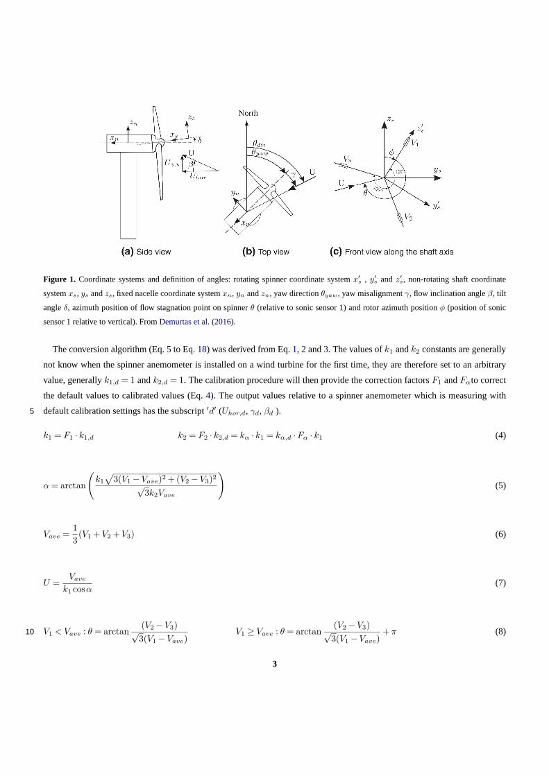
Figure 1. Coordinate systems and definition of angles: rotating spinner coordinate systemx′s , y′
s andz′s, non-rotating shaft coordinate
systemxs, ys andzs, fixed nacelle coordinate systemxn, yn andzn, yaw directionθyaw, yaw misalignmentγ, flow inclination angleβ, tilt
angleδ, azimuth position of flow stagnation point on spinnerθ (relative to sonic sensor 1) and rotor azimuth positionφ (position of sonic
sensor 1 relative to vertical). FromDemurtas et al.(2016).
The conversion algorithm (Eq.5 to Eq.18) was derived from Eq.1, 2 and3. The values ofk1 andk2 constants are generally
not know when the spinner anemometer is installed on a wind turbine for the first time, they are therefore set to an arbitrary
value, generallyk1,d = 1 andk2,d = 1. The calibration procedure will then provide the correction factorsF1 andFαto correct
the default values to calibrated values (Eq.4). The output values relative to a spinner anemometer which is measuring with
default calibration settings has the subscript′d′ (Uhor,d, γd, βd ).5
k1 = F1 ∙ k1,d k2 = F2 ∙ k2,d = kα ∙ k1 = kα,d ∙Fα ∙ k1 (4)
α = arctan
(k1
√3(V1 −Vave)2 +(V2 −V3)2√
3k2Vave
)
(5)
Vave =13(V1 + V2 + V3) (6)
U =Vave
k1 cosα(7)
V1 < Vave : θ = arctan(V2 −V3)√3(V1 −Vave)
V1 ≥ Vave : θ = arctan(V2 −V3)√3(V1 −Vave)
+ π (8)10
3
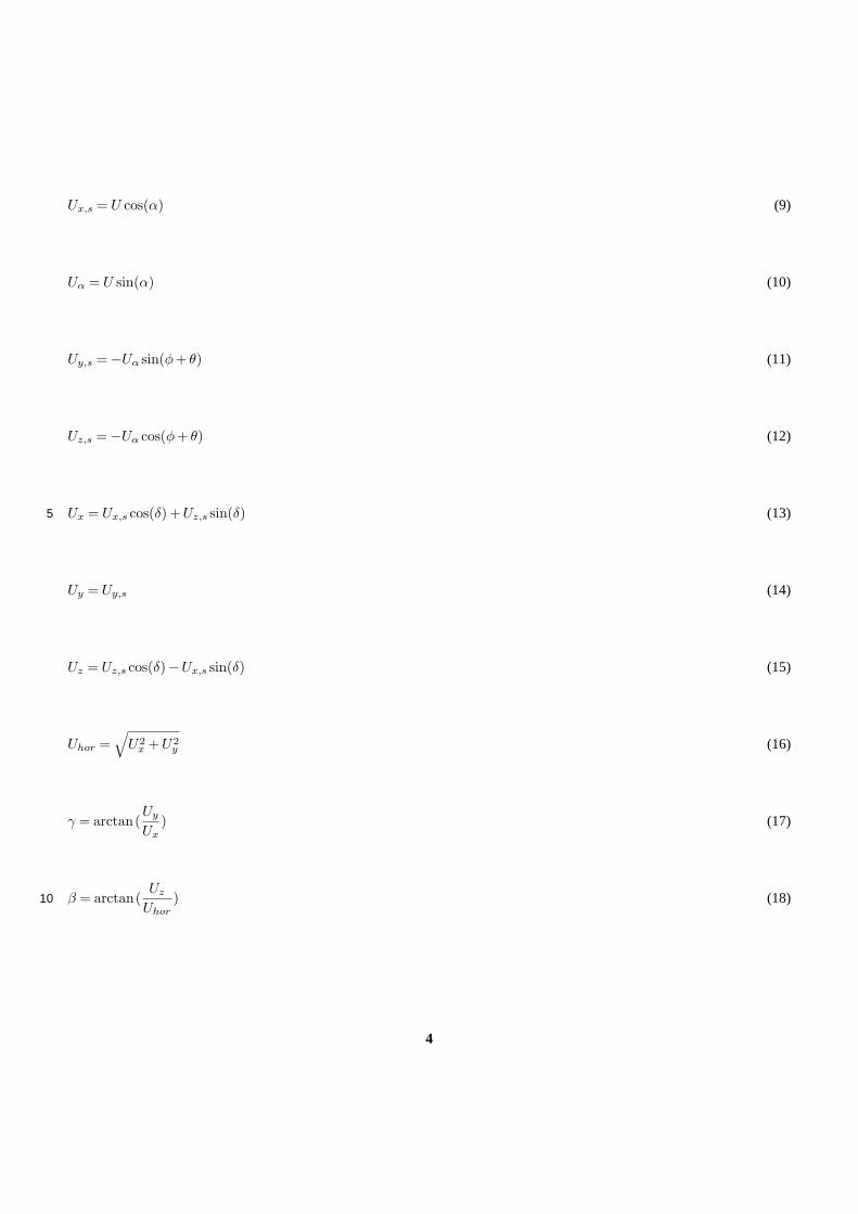
Ux,s = U cos(α) (9)
Uα = U sin(α) (10)
Uy,s = −Uα sin(φ + θ) (11)
Uz,s = −Uα cos(φ + θ) (12)
Ux = Ux,s cos(δ)+ Uz,s sin(δ) (13)5
Uy = Uy,s (14)
Uz = Uz,s cos(δ)−Ux,s sin(δ) (15)
Uhor =√
U2x + U2
y (16)
γ = arctan(Uy
Ux) (17)
β = arctan(Uz
Uhor) (18)10
4
1.1 Existing calibration methods for flow angle measurements
Two methods based on measurements to calibrate a spinner anemometer for flow angle measurements proposed inPedersen
and Demurtas (2014) consist in yawing the wind turbine of± 60◦ several times under manual control (as indicated by the
turbine yaw position sensor, with respect to the mean wind direction). During this test, the output parameters of the spinner
anemometer (Uhor, γ, β) are recorded at high sampling frequency (10 Hz). The analysis of the measurements provide the5
correction factorFα that multiplied by the defaultkα,d gives the correctkα calibration value.
The methods are based on the assumption that the wind direction is constant during the test. Due to this requirement,
Pedersen and Demurtas(2014) recommended to do the test at wind speeds above 6 m/s. Both methods need the yaw position
to be measured in order to calculate the reference yaw misalignmentγref , defined as the mean wind direction minus the
instantaneous yaw position during test (seePedersen and Demurtas(2014) for details). In the first method (abbreviated as10
GGref)Fα was calculated by calibrating the measurements iteratively, until the linear fit ofγ as a function ofγref was giving
a line of slope equal to 1.
In the second method (abbreviated as TanTan), only one linear fitting was made totan(γ) as a function oftan(γref ). In this
case, the slope coefficient of the fit was exactlyFα. The two calibration methods were found to be sensitive to the width of the
yawing span. In fact, differentFα values were obtained sub-setting the data-set to a variable span ofγref .15
A new method to find theFα value, that does not require a yaw position measurement, and use the non linearity of the
spinner anemometer conversion algorithm is proposed.
2 The wind speed response method
The method (abbreviated WSR) is based on the assumption that the wind speed is constant during the test. The turbulence of
the real wind will add some scatter in the measurements which will reduce the repeatability of the result. While in principle a20
single yawing movement is sufficient, in practice the wind speed fluctuations needs to be averaged by yawing the wind turbine
several times. The spinner anemometer is able to measure inflow angles (yaw misalignmentγ and flow inclinationβ) and wind
speedU . A wrong kα value will result in a wrong value of the angleγ, which will turn into a wrong value of the horizontal
wind speedUhor. In other words, a wrongkα makes the wind speed measurement dependent on the yaw misalignment. This
property of the spinner anemometer model (Eq.1, 2 and3) was verified with a data-set consisting of constant wind speedUhor25
and 13 values of yaw misalignment going from -60◦ to 60◦ in steps of 10◦. The tilt angle and the flow inclination were set to
arbitrary values (equal to zero for Fig.2). In the real world the tilt angle of the wind turbine is typically between 3◦ and 6◦
while the flow inclination varies within approximately±10◦. The conversion algorithm takes into consideration both the tilt
angleδ and the measured flow inclinationβd when calculating the yaw misalignmentγd, therefore they have no influence on
the result of this method.V1, V2 andV3 were calculated with Eq.1, 2 and3 with kα = 1 andk2 = 1.30
Eq.5 to Eq.18 (which are the direct conversion algorithm presented inPedersen and Demurtas(2014)) were used with new
values of kα equal to 0.5, 1 and 2, with the calculatedV1, V2 andV3 to calculateUhor,d andαd. k1 was kept equal to one.
5
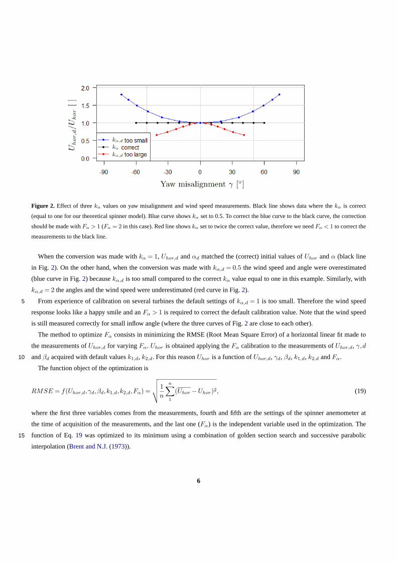
Figure 2. Effect of threekα values on yaw misalignment and wind speed measurements. Black line shows data where thekα is correct
(equal to one for our theoretical spinner model). Blue curve showskα set to 0.5. To correct the blue curve to the black curve, the correction
should be made withFα > 1 (Fα = 2 in this case). Red line showskα set to twice the correct value, therefore we needFα < 1 to correct the
measurements to the black line.
When the conversion was made withkα = 1, Uhor,d andαd matched the (correct) initial values ofUhor andα (black line
in Fig. 2). On the other hand, when the conversion was made withkα,d = 0.5 the wind speed and angle were overestimated
(blue curve in Fig.2) becausekα,d is too small compared to the correctkα value equal to one in this example. Similarly, with
kα,d = 2 the angles and the wind speed were underestimated (red curve in Fig.2).
From experience of calibration on several turbines the default settings ofkα,d = 1 is too small. Therefore the wind speed5
response looks like a happy smile and anFα > 1 is required to correct the default calibration value. Note that the wind speed
is still measured correctly for small inflow angle (where the three curves of Fig.2 are close to each other).
The method to optimizeFα consists in minimizing the RMSE (Root Mean Square Error) of a horizontal linear fit made to
the measurements ofUhor,d for varyingFα. Uhor is obtained applying theFα calibration to the measurements ofUhor,d, γ,d
andβd acquired with default valuesk1,d, k2,d. For this reasonUhor is a function ofUhor,d, γd, βd, k1,d, k2,d andFα.10
The function object of the optimization is
RMSE = f(Uhor,d,γd,βd,k1,d,k2,d,Fα) =
√√√√ 1
n
n∑
1
(Uhor −Uhor)2, (19)
where the first three variables comes from the measurements, fourth and fifth are the settings of the spinner anemometer at
the time of acquisition of the measurements, and the last one (Fα) is the independent variable used in the optimization. The
function of Eq.19 was optimized to its minimum using a combination of golden section search and successive parabolic15
interpolation (Brent and N.J.(1973)).
6
3 Application of the method
The measurements were acquired in February 2016 on a Neg-Micon 2 MW wind turbine installed in Denmark. The wind
turbine was yawed in and out of the wind several times with the rotor stopped with one blade pointing downwards. Figures3
and4 show the 10 Hz data recorded during the calibration procedure. Figure3A, B and C show non calibrated measurements,
while Fig.4A, B and C show calibrated measurements. In both Fig.3 and4 the sub-figure A shows the time series of the yaw5
misalignment and yaw misalignment reference (measured with a yaw position sensor). Sub-figure B shows the time series of
the wind speed. Sub-figure C shows the wind speed response as a function of yaw misalignment.
Figure3D shows the value ofFα calculated with the three different methods (GGref and TanTan fromPedersen and Demurtas
(2014) and the present method, WSR), for varying range of yawing the wind turbine out of the wind (data were filtered
according toγref in steps of 5◦ span per side). The Fα value was calculated with the WSR method only if there were at least10
30 seconds of measurements in the outmost 5◦ of the considered range (which justifies the fact that the scatter plot of Fig.4C
appears wider than the maximum range shown in Fig.3D by the green line).
7

Figure 3. Before calibration, test 6. A: Time series of yaw misalignment as measured by the spinner anemometer and by the yaw position
sensor. B: wind speed time series as measured by the spinner anemometer before F1 calibration. C: Wind speed as a function of yaw
misalignment both measured by spinner anemometer. D: Calibration correction factorFα calculated in three different methods, as a function
of yawing span ranging from±10◦ to±90◦ in steps of±5◦.
8
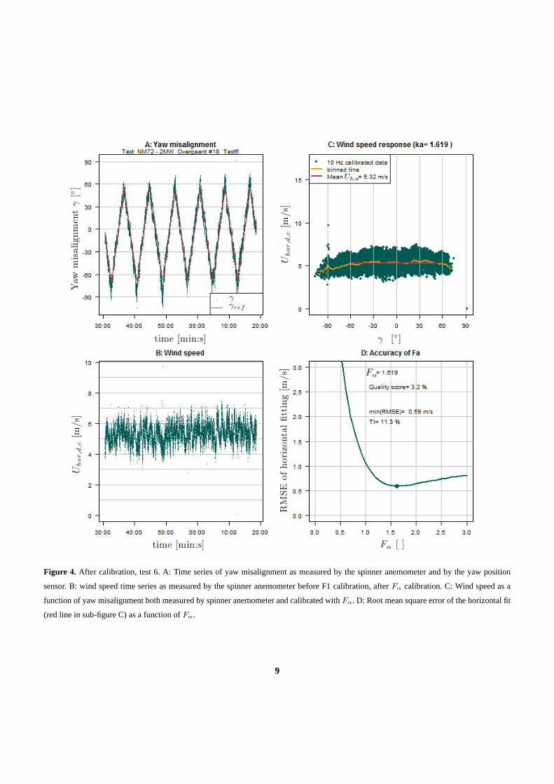
Figure 4. After calibration, test 6. A: Time series of yaw misalignment as measured by the spinner anemometer and by the yaw position
sensor. B: wind speed time series as measured by the spinner anemometer before F1 calibration, afterFα calibration. C: Wind speed as a
function of yaw misalignment both measured by spinner anemometer and calibrated withFα. D: Root mean square error of the horizontal fit
(red line in sub-figure C) as a function ofFα.
9
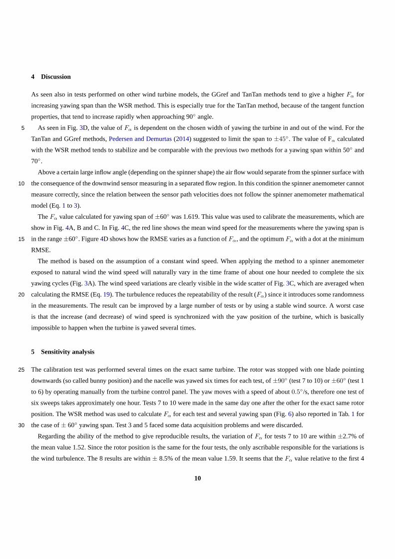
4 Discussion
As seen also in tests performed on other wind turbine models, the GGref and TanTan methods tend to give a higherFα for
increasing yawing span than the WSR method. This is especially true for the TanTan method, because of the tangent function
properties, that tend to increase rapidly when approaching 90◦ angle.
As seen in Fig.3D, the value ofFα is dependent on the chosen width of yawing the turbine in and out of the wind. For the5
TanTan and GGref methods,Pedersen and Demurtas(2014) suggested to limit the span to±45◦. The value of Fα calculated
with the WSR method tends to stabilize and be comparable with the previous two methods for a yawing span within 50◦ and
70◦.
Above a certain large inflow angle (depending on the spinner shape) the air flow would separate from the spinner surface with
the consequence of the downwind sensor measuring in a separated flow region. In this condition the spinner anemometer cannot10
measure correctly, since the relation between the sensor path velocities does not follow the spinner anemometer mathematical
model (Eq.1 to 3).
TheFα value calculated for yawing span of±60◦ was 1.619. This value was used to calibrate the measurements, which are
show in Fig.4A, B and C. In Fig.4C, the red line shows the mean wind speed for the measurements where the yawing span is
in the range±60◦. Figure4D shows how the RMSE varies as a function ofFα, and the optimumFα with a dot at the minimum15
RMSE.
The method is based on the assumption of a constant wind speed. When applying the method to a spinner anemometer
exposed to natural wind the wind speed will naturally vary in the time frame of about one hour needed to complete the six
yawing cycles (Fig.3A). The wind speed variations are clearly visible in the wide scatter of Fig.3C, which are averaged when
calculating the RMSE (Eq.19). The turbulence reduces the repeatability of the result (Fα) since it introduces some randomness20
in the measurements. The result can be improved by a large number of tests or by using a stable wind source. A worst case
is that the increase (and decrease) of wind speed is synchronized with the yaw position of the turbine, which is basically
impossible to happen when the turbine is yawed several times.
5 Sensitivity analysis
The calibration test was performed several times on the exact same turbine. The rotor was stopped with one blade pointing25
downwards (so called bunny position) and the nacelle was yawed six times for each test, of±90◦ (test 7 to 10) or±60◦ (test 1
to 6) by operating manually from the turbine control panel. The yaw moves with a speed of about0.5◦/s, therefore one test of
six sweeps takes approximately one hour. Tests 7 to 10 were made in the same day one after the other for the exact same rotor
position. The WSR method was used to calculateFα for each test and several yawing span (Fig.6) also reported in Tab.1 for
the case of± 60◦ yawing span. Test 3 and 5 faced some data acquisition problems and were discarded.30
Regarding the ability of the method to give reproducible results, the variation ofFα for tests 7 to 10 are within±2.7% of
the mean value 1.52. Since the rotor position is the same for the four tests, the only ascribable responsible for the variations is
the wind turbulence. The 8 results are within± 8.5% of the mean value 1.59. It seems that theFα value relative to the first 4
10
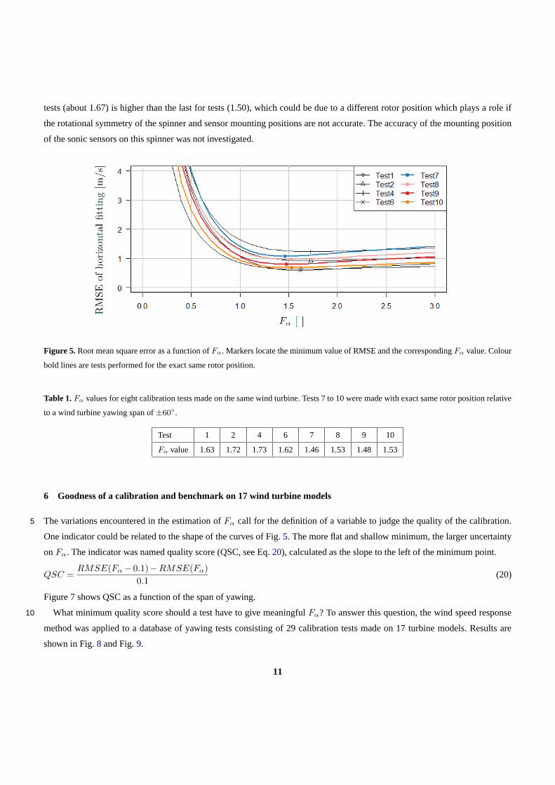
tests (about 1.67) is higher than the last for tests (1.50), which could be due to a different rotor position which plays a role if
the rotational symmetry of the spinner and sensor mounting positions are not accurate. The accuracy of the mounting position
of the sonic sensors on this spinner was not investigated.
Figure 5. Root mean square error as a function ofFα. Markers locate the minimum value of RMSE and the correspondingFα value. Colour
bold lines are tests performed for the exact same rotor position.
Table 1.Fα values for eight calibration tests made on the same wind turbine. Tests 7 to 10 were made with exact same rotor position relative
to a wind turbine yawing span of±60◦.
Test 1 2 4 6 7 8 9 10
Fα value 1.63 1.72 1.73 1.62 1.46 1.53 1.48 1.53
6 Goodness of a calibration and benchmark on 17 wind turbine models
The variations encountered in the estimation ofFα call for the definition of a variable to judge the quality of the calibration.5
One indicator could be related to the shape of the curves of Fig.5. The more flat and shallow minimum, the larger uncertainty
onFα. The indicator was named quality score (QSC, see Eq.20), calculated as the slope to the left of the minimum point.
QSC =RMSE(Fα − 0.1)−RMSE(Fα)
0.1(20)
Figure7 shows QSC as a function of the span of yawing.
What minimum quality score should a test have to give meaningfulFα? To answer this question, the wind speed response10
method was applied to a database of yawing tests consisting of 29 calibration tests made on 17 turbine models. Results are
shown in Fig.8 and Fig.9.
11
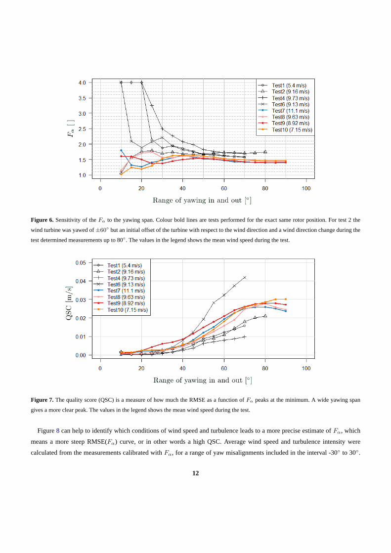
Figure 6. Sensitivity of theFα to the yawing span. Colour bold lines are tests performed for the exact same rotor position. For test 2 the
wind turbine was yawed of±60◦ but an initial offset of the turbine with respect to the wind direction and a wind direction change during the
test determined measurements up to 80◦. The values in the legend shows the mean wind speed during the test.
Figure 7. The quality score (QSC) is a measure of how much the RMSE as a function ofFα peaks at the minimum. A wide yawing span
gives a more clear peak. The values in the legend shows the mean wind speed during the test.
Figure8 can help to identify which conditions of wind speed and turbulence leads to a more precise estimate ofFα, which
means a more steep RMSE(Fα) curve, or in other words a high QSC. Average wind speed and turbulence intensity were
calculated from the measurements calibrated withFα, for a range of yaw misalignments included in the interval -30◦ to 30◦.
12
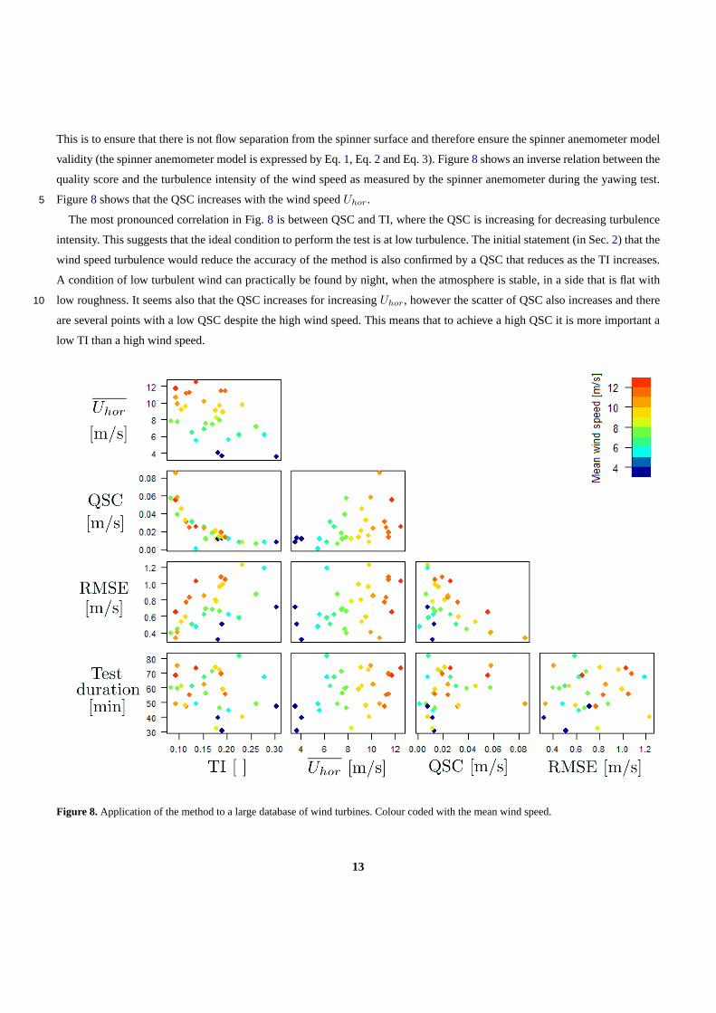
This is to ensure that there is not flow separation from the spinner surface and therefore ensure the spinner anemometer model
validity (the spinner anemometer model is expressed by Eq.1, Eq.2 and Eq.3). Figure8 shows an inverse relation between the
quality score and the turbulence intensity of the wind speed as measured by the spinner anemometer during the yawing test.
Figure8 shows that the QSC increases with the wind speedUhor.5
The most pronounced correlation in Fig.8 is between QSC and TI, where the QSC is increasing for decreasing turbulence
intensity. This suggests that the ideal condition to perform the test is at low turbulence. The initial statement (in Sec.2) that the
wind speed turbulence would reduce the accuracy of the method is also confirmed by a QSC that reduces as the TI increases.
A condition of low turbulent wind can practically be found by night, when the atmosphere is stable, in a side that is flat with
low roughness. It seems also that the QSC increases for increasingUhor, however the scatter of QSC also increases and there10
are several points with a low QSC despite the high wind speed. This means that to achieve a high QSC it is more important a
low TI than a high wind speed.
Figure 8. Application of the method to a large database of wind turbines. Colour coded with the mean wind speed.
13
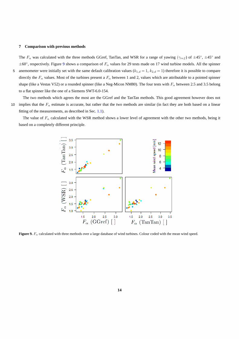
7 Comparison with previous methods
The Fα was calculated with the three methods GGref, TanTan, and WSR for a range of yawing(γref ) of ±45◦, ±45◦ and
±60◦, respectively. Figure9 shows a comparison ofFα values for 29 tests made on 17 wind turbine models. All the spinner
anemometer were initially set with the same default calibration values (k1,d = 1, k2,d = 1) therefore it is possible to compare5
directly theFα values. Most of the turbines present aFα between 1 and 2, values which are attributable to a pointed spinner
shape (like a Vestas V52) or a rounded spinner (like a Neg-Micon NM80). The four tests withFα between 2.5 and 3.5 belong
to a flat spinner like the one of a Siemens SWT-6.0-154.
The two methods which agrees the most are the GGref and the TanTan methods. This good agreement however does not
implies that theFα estimate is accurate, but rather that the two methods are similar (in fact they are both based on a linear10
fitting of the measurements, as described in Sec.1.1).
The value ofFα calculated with the WSR method shows a lower level of agreement with the other two methods, being it
based on a completely different principle.
Figure 9. Fα calculated with three methods over a large database of wind turbines. Colour coded with the mean wind speed.
14
8 Conclusions
The article presented a new method to calibrate spinner anemometer flow angle measurements (yaw misalignment). The ad-
vantage of the method is that it does not need the yaw position of the nacelle to be measured.
The robustness of the method was investigated by repeating the calibration test on the same turbine several times, with the5
rotor locked in the exact same rotor position to avoid sensor mounting deviations to play a role. TheFα values found for 4 tests
for the exact same rotor position were within±2.7% of the mean value.
The quality score parameter (QSC) was introduced to quantify goodness of theFα estimate. The QSC was found inversely
dependent on the turbulence intensity. To have a sharp estimate ofFα it is therefore better to perform the test in low turbulence
wind conditions. The relation found between the QSC and the width of yawing suggests to yaw the turbine further than±60◦,10
up to±80◦ (this values might be different for other spinner shapes). Another issue to consider is that the test could start with
an offset, and end up being -90◦ to 70◦ instead of -80◦ to 80◦. This is easily avoidable yawing the wind turbine a bit further
than the desired yawing span.
The sensitivity of the method to the width of yawing the turbine in and out of the wind was investigated by applying the
calibration method to a subset of the original database. The subset was obtained filtering forγref ∈ [−s,s], wheres was15
the span ranging from 10◦ to 90◦ in steps of 5◦. Significant variations of theFα value were found for yawing spans below
approximately 60◦.
The Fα calculated with the wind speed response method was compared with theFα calculated with previous methods
(GGref, TanTan) using 29 calibration tests performed by Romo Wind A/S on 17 wind turbine models. The sensitivity to span
of yawing showed that the WSR method tends to stabilize to same values as GGref for yawing span larger than approximately20
50◦. Both the GGref and TanTan methods gave similar values up to±40◦, then the TanTan method gave higherFα and diverged
for a yawing span larger than 70◦.
A recommended yawing span to use to calculateFα seems to be±60◦ for the WSR method and±40◦ for the TanTan and
GGref methods, however the turbine shall be yawed further than this angle (±90◦ recommended) to compensate for initial
offset error in the yaw position and wind speed direction change during the test.25
It is best to perform the test at the lowest possible turbulence intensity, which might be found in stable atmospheric condition
(typically by night) in a flat site with low roughness.
It is recommended to verify the variation ofFα as a function of span of yawing (using the calibrated yaw misalignment if
the yaw sensor is not available), since substantially different spinner shapes might give a stableFα at different yawing span.
Acknowledgements.Romo wind A/S for financing one third of the PhD project this article is part of.
15

References
Brent, R. and N.J., E. C.: Algorithms for Minimization without Derivatives., Prentice-Hall, 1973.
Demurtas, G., Pedersen, T. F., and Zahle, F.: Calibration of a spinner anemometer for wind speed measurements, Wind Energy, 2016.
Pedersen, T., Madsen, H., M, R., Courtney, M., S, N., Enevoldsen, P., and Egedal, P.: Spinner Anemometry - An Innovative Wind Measure-5
ment Concept, 2007.
Pedersen, T. F. and Demurtas, G.: Calibration of a spinner anemometer for flow angle measurements, Wind Energy, 2014.
16
Chapter 4
Calibration for wind speedmeasurements
What has been presented in chapter 2 and 3 closes the topic of the calibration for flowinclination and yaw misalignment measurements. This chapter will address the topic ofcalibration for wind speed measurements.
The calibration of a wind sensor to be used for power performance measurements is alwaysneeded to ensure traceability to reference wind speed sensors such as the Pitot tube of a windtunnel. The large size of a spinner anemometer does not allow to place it directly into a windtunnel, therefore each sonic sensor is first calibrated in the wind tunnel in order to measurethe wind speed correctly at the sonic sensor positions, and then (once mounted on the spinner)internally calibrated and kα calibrated [14, 15]. It is then calibrated with k1 as described inthis chapter. k1 is calibrated as the ratio between spinner anemometer horizontal wind speedand met-mast wind speed in a zero induction condition.
When the turbine is in operation the calibrated spinner anemometer wind speed will becorrected again to the free wind speed by the NTF (Nacelle Transfer Function) to compensatefor the rotor induction.
One could in principle neglect the calibration of the k1 constant and correct everything(spinner shape, sensor mounting position and rotor induction) with the NTF alone, but therewere found good reasons to keep the two corrections independent. The following articleexplains why.
43
WIND ENERGYWind Energ. (2016)
Published online in Wiley Online Library (wileyonlinelibrary.com). DOI: 10.1002/we.1965
RESEARCH ARTICLE
Calibration of a spinner anemometer for windspeed measurementsGiorgio Demurtas, Troels Friis Pedersen and Frederik ZahleTechnical University of Denmark, Frederiksborgvej 399, PO Box 49, 4000 Roskilde, Denmark
ABSTRACT
The power curve of a wind turbine can be measured, according to IEC 61400-12-2 with a nacelle-mounted anemometer.Typically, a sonic anemometer or a cup anemometer and a wind vane are mounted on the back of the nacelle roof. Anotheroption is to use a spinner anemometer.
The measurement principle of the spinner anemometer is based on the flow distortion caused by the wind turbine spinner.The flow on the spinner surface is measured by means of three 1D sonic sensors mounted on the spinner and a conversionalgorithm to convert the wind velocity components measured by the three sonic sensors to horizontal wind speed, yawmisalignment and flow inclination angle. The algorithm utilizes two calibration constants that are specific to the spinnershape, blade root design and to the mounting positions of the sonic sensors on the spinner.
The present analysis describes methods to determine the calibration constant related to wind speed measurements.The first and preferred method is based on the definition of the calibration constant and uses wind speed measurementsduring the stopped condition of the wind turbine. Two alternative methods that did not require the turbine to be stoppedwere investigated: one used relatively high wind speed measurements during normal operation of the wind turbine, whilethe other one used a CFD simulation of the flow over the spinner. The method that entails stopping the turbine in goodwind conditions showed the best results and is recommended. The evaluation of uncertainty was not included in the presentanalysis. Copyright © 2016 The Authors Wind Energy Published by John Wiley & Sons Ltd.
KEYWORDS
anemometer; spinner anemometer; spinner anemometer calibration; iSpin; nacelle anemometry; calibration; wind speed
Correspondence
Giorgio Demurtas, Technical University of Denmark, Frederiksborgvej 399, 4000 Roskilde, Denmark.E-mail: [email protected]
reproduction in any medium, provided the original work is properly cited.
Received 15 April 2015; Revised 10 December 2015; Accepted 22 December 2015
LIST OF SYMBOLS
V1 velocity component of the wind speed along sensor path 1V2 velocity component of the wind speed along sensor path 2V3 velocity component of the wind speed along sensor path 3
Vave average of V1, V2, V3Ud wind speed vector modulus measured by the spinner anemometer prior to calibrationU wind speed vector modulus at the spinner anemometer (reference value to calibrate Ud , equal to the free wind
speed vector modulus in stopped conditions or conditions of null rotor induction)Uhor horizontal wind speed component measured with the spinner anemometer (calibrated value)
Uhor,d horizontal wind speed component measured with the spinner anemometer (non-calibrated value)Uhor,d,c horizontal wind speed component measured with the spinner anemometer (corrected with F˛ but not F1)
U˛ wind velocity component in the plane perpendicular to the shaft axis xs
Ux wind velocity component along xUy wind velocity component along yUz wind velocity component along z
Copyright © 2016 The Authors Wind Energy Published by John Wiley & Sons Ltd.
This is an open access article under the terms of the Creative Commons Attribution License, which permits use, distribution and

Calibration of a spinner anemometer for wind speed measurements G. Demurtas, T. F. Pedersen and F. Zahle
Ux,n wind velocity component along xn
Uy,n wind velocity component along yn
Uz,n vertical wind velocity component, along zn
Ux,s wind velocity component along xs
Uy,s wind velocity component along ys
Uz,s wind velocity component along zs
ı shaft tilt angleˇ flow inclination angle (positive when upwards)� yaw misalignment˛ inflow angle with respect to the shaft axis˛d inflow angle with respect to the shaft axis measured by the spinner anemometer prior to calibration� rotor position (equal to zero when sonic sensor one is at top position, positive clockwise)� azimuth position of flow stagnation point on spinner (relative to sonic sensor 1)
�yaw yaw direction referred to geographical coordinate system�dir wind direction referred to geographical coordinate system
k1 calibration constant mainly related to wind speed calibrationk˛ calibration constant related to angle calibrationk2 calibration constant mainly related to angle calibration (equal to k˛ � k1)F1 calibration correction factor mainly related to wind speed calibrationF˛ calibration correction factor related to angle calibrationF2 calibration correction factor mainly related to angle calibration (equal to F˛ � F1)� standard deviationN number of measurementsI rotor induction, calculated as I D .Umm � Uhor/=Umm
Umm horizontal wind speed component (free wind speed measured with the met-mast)Ufree horizontal wind speed component measured with the spinner anemometer and corrected with the nacelle transfer
function to free wind speedUN,i nacelle wind speed average value in bin i of the nacelle transfer functionUF,i free wind speed average value in bin i of the nacelle transfer function
LIST OF ABBREVIATIONS
s.a. spinner anemometerNTF nacelle transfer functionIEC International Electrotechnical Commission
CFD Computational Fluid Dynamics
1. INTRODUCTION
The spinner anemometer1 can be used to measure the inflow wind speed to a wind turbine and to measure its power per-formance. For this last purpose, spinner anemometers need to be calibrated similarly to nacelle cup anemometers. Previousresearch2, 3 described problems related to cup anemometers and wind vanes, or 2D sonic anemometers, mounted on topof the nacelle. The flow distortion caused by the blade roots and nacelle affects even state-of-the-art nacelle anemometryinstruments. This flow distortion is normally corrected for in the wind turbine control system. However, corrections in thecontroller might not take all situations into account, for example, when the wake swirl from upstream wind turbines intro-duces upwards and downwards flow on the nacelle.4 Such corrections are not required for a spinner anemometer, which isnot affected by blade wakes since it measures the wind upstream of the rotor (Figure 1). The measurement principle usedby the spinner anemometer is actually based on the flow distortion created by the spinner. Because of the size of a modernwind turbine spinner and imperfections of the spinner shape, such as poor rotational symmetry, it is challenging to mountthe sensors equally distant from the spinner center and spaced 120ı. These challenges in the spinner anemometer mount-ing could be easily solved in the future by integrating the sensor mounting holes in the spinner mold and by improving thespinner quality control during manufacture of the spinner.
The calibration of a spinner anemometer accounts for the shape of the spinner, mounting position of the sonic sensorsand characteristics of the sensors, while the rotor induction is accounted for with the nacelle transfer function (NTF) asdefined in IEC 61400-12-2.6 It is important to keep the wind speed calibration separate from the NTF, so that changes dueto the spinner anemometer (mounting position of the sonic sensors, spinner geometry) can be accounted for with a newcalibration only, whereas changes in the wind turbine control system or blades can be accounted with a new NTF only.
Wind Energ. (2016) © 2016 The Authors Wind Energy Published by John Wiley & Sons Ltd.DOI: 10.1002/we
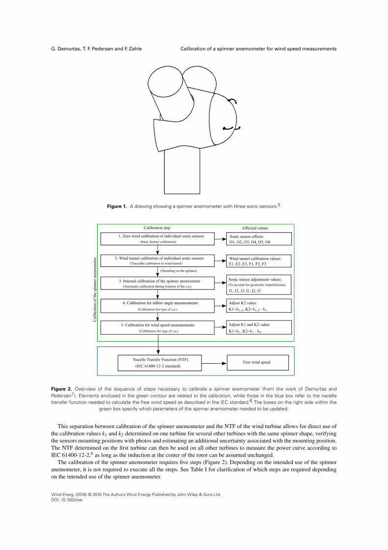
G. Demurtas, T. F. Pedersen and F. Zahle Calibration of a spinner anemometer for wind speed measurements
Figure 1. A drawing showing a spinner anemometer with three sonic sensors.5
Figure 2. Overview of the sequence of steps necessary to calibrate a spinner anemometer (from the work of Demurtas andPedersen7). Elements enclosed in the green contour are related to the calibration, while those in the blue box refer to the nacelletransfer function needed to calculate the free wind speed as described in the IEC standard.6 The boxes on the right side within the
green box specify which parameters of the spinner anemometer needed to be updated.
This separation between calibration of the spinner anemometer and the NTF of the wind turbine allows for direct use ofthe calibration values k1 and k2 determined on one turbine for several other turbines with the same spinner shape, verifyingthe sensors mounting positions with photos and estimating an additional uncertainty associated with the mounting position.The NTF determined on the first turbine can then be used on all other turbines to measure the power curve according toIEC 61400-12-2,6 as long as the induction at the center of the rotor can be assumed unchanged.
The calibration of the spinner anemometer requires five steps (Figure 2). Depending on the intended use of the spinneranemometer, it is not required to execute all the steps. See Table I for clarification of which steps are required dependingon the intended use of the spinner anemometer.
Wind Energ. (2016) © 2016 The Authors Wind Energy Published by John Wiley & Sons Ltd.DOI: 10.1002/we
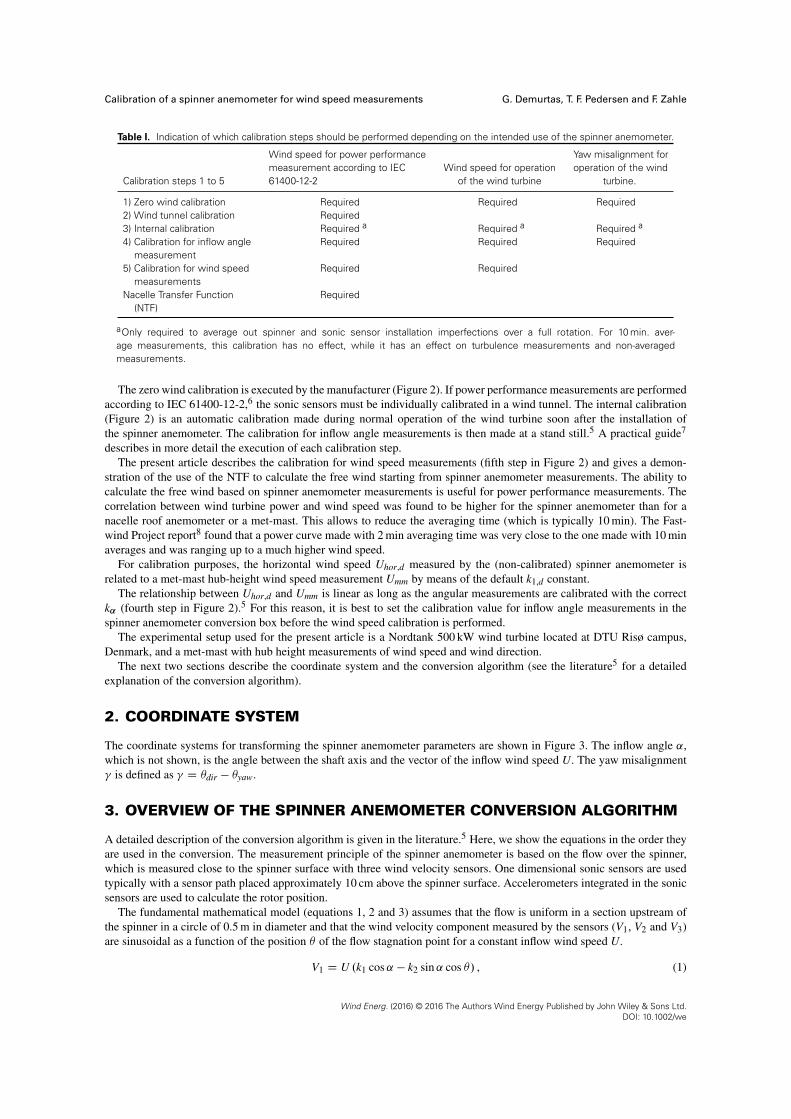
Calibration of a spinner anemometer for wind speed measurements G. Demurtas, T. F. Pedersen and F. Zahle
Table I. Indication of which calibration steps should be performed depending on the intended use of the spinner anemometer.
Wind speed for power performance Yaw misalignment formeasurement according to IEC Wind speed for operation operation of the wind
Calibration steps 1 to 5 61400-12-2 of the wind turbine turbine.
1) Zero wind calibration Required Required Required2) Wind tunnel calibration Required3) Internal calibration Required a Required a Required a
4) Calibration for inflow angle Required Required Requiredmeasurement
5) Calibration for wind speed Required Requiredmeasurements
Nacelle Transfer Function Required(NTF)
aOnly required to average out spinner and sonic sensor installation imperfections over a full rotation. For 10 min. aver-age measurements, this calibration has no effect, while it has an effect on turbulence measurements and non-averagedmeasurements.
The zero wind calibration is executed by the manufacturer (Figure 2). If power performance measurements are performedaccording to IEC 61400-12-2,6 the sonic sensors must be individually calibrated in a wind tunnel. The internal calibration(Figure 2) is an automatic calibration made during normal operation of the wind turbine soon after the installation ofthe spinner anemometer. The calibration for inflow angle measurements is then made at a stand still.5 A practical guide7
describes in more detail the execution of each calibration step.The present article describes the calibration for wind speed measurements (fifth step in Figure 2) and gives a demon-
stration of the use of the NTF to calculate the free wind starting from spinner anemometer measurements. The ability tocalculate the free wind based on spinner anemometer measurements is useful for power performance measurements. Thecorrelation between wind turbine power and wind speed was found to be higher for the spinner anemometer than for anacelle roof anemometer or a met-mast. This allows to reduce the averaging time (which is typically 10 min). The Fast-wind Project report8 found that a power curve made with 2 min averaging time was very close to the one made with 10 minaverages and was ranging up to a much higher wind speed.
For calibration purposes, the horizontal wind speed Uhor,d measured by the (non-calibrated) spinner anemometer isrelated to a met-mast hub-height wind speed measurement Umm by means of the default k1,d constant.
The relationship between Uhor,d and Umm is linear as long as the angular measurements are calibrated with the correctk˛ (fourth step in Figure 2).5 For this reason, it is best to set the calibration value for inflow angle measurements in thespinner anemometer conversion box before the wind speed calibration is performed.
The experimental setup used for the present article is a Nordtank 500 kW wind turbine located at DTU Risø campus,Denmark, and a met-mast with hub height measurements of wind speed and wind direction.
The next two sections describe the coordinate system and the conversion algorithm (see the literature5 for a detailedexplanation of the conversion algorithm).
2. COORDINATE SYSTEM
The coordinate systems for transforming the spinner anemometer parameters are shown in Figure 3. The inflow angle ˛,which is not shown, is the angle between the shaft axis and the vector of the inflow wind speed U. The yaw misalignment� is defined as � D �dir � �yaw.
3. OVERVIEW OF THE SPINNER ANEMOMETER CONVERSION ALGORITHM
A detailed description of the conversion algorithm is given in the literature.5 Here, we show the equations in the order theyare used in the conversion. The measurement principle of the spinner anemometer is based on the flow over the spinner,which is measured close to the spinner surface with three wind velocity sensors. One dimensional sonic sensors are usedtypically with a sensor path placed approximately 10 cm above the spinner surface. Accelerometers integrated in the sonicsensors are used to calculate the rotor position.
The fundamental mathematical model (equations 1, 2 and 3) assumes that the flow is uniform in a section upstream ofthe spinner in a circle of 0.5 m in diameter and that the wind velocity component measured by the sensors (V1, V2 and V3)are sinusoidal as a function of the position � of the flow stagnation point for a constant inflow wind speed U.
V1 D U .k1 cos˛ � k2 sin˛ cos �/ , (1)
Wind Energ. (2016) © 2016 The Authors Wind Energy Published by John Wiley & Sons Ltd.DOI: 10.1002/we
G. Demurtas, T. F. Pedersen and F. Zahle Calibration of a spinner anemometer for wind speed measurements
(a) Side view (b) Top view (c) Front view along the shaft axis
Figure 3. Coordinate systems and definition of angles: rotating spinner coordinate system .x0s, y0s and z0s/, non-rotating shaft coordi-nate system .xs, ys and zs/, fixed nacelle coordinate system .xn, yn and zn/, yaw direction yaw,yaw error � , flow inclination angle ˇ ,tilt angle ı, azimuth position of flow stagnation point on spinner � (relative to sonic sensor 1) and rotor azimuth position � (position
of sonic sensor 1 relative to vertical).
Figure 4. Direct transformation from sonic sensor wind speeds to spinner anemometer parameters.
V2 D U
�k1 cos˛ � k2 sin˛ cos
�� �
2�
3
��, (2)
V3 D U
�k1 cos˛ � k2 sin˛ cos
�� �
4�
3
��. (3)
The spinner anemometer conversion algorithm transforms the sonic sensor wind velocity components V1, V2 and V3and the rotor azimuth position � measurements into the spinner anemometer output parameters: horizontal wind speedUhor, yaw misalignment � and flow inclination angle ˇ. This transformation (Section 3.1 and Figure 4) is called directtransformation and runs inside the spinner anemometer conversion box.
The inverse transformation (Section 3.2) transforms the output of the spinner anemometer into the input values V1, V2and V3. This is needed to post-calibrate measurements that were acquired with certain (default) calibration constant to newcalibration constants, as described in Section 3.3.
3.1. Direct transformation
The mathematical expressions of the conversion algorithm implemented in the spinner anemometer are as follows:
˛ D arctan
k1p
3.V1 � Vave/2 C .V2 � V3/2p
3k2Vave
!(4)
Vave D1
3.V1 C V2 C V3/ (5)
U DVave
k1 cos˛(6)
V1 < Vave : � D arctan.V2 � V3/p
3.V1 � Vave/(7)
V1 � Vave : � D arctan.V2 � V3/p
3.V1 � Vave/C � (8)
Wind Energ. (2016) © 2016 The Authors Wind Energy Published by John Wiley & Sons Ltd.DOI: 10.1002/we

Calibration of a spinner anemometer for wind speed measurements G. Demurtas, T. F. Pedersen and F. Zahle
Ux,s D U cos.˛/ (9)
U˛ D U sin.˛/ (10)
Uy,s D �U˛ sin.� C �/ (11)
Uz,s D �U˛ cos.� C �/ (12)
Ux D Ux,s cos.ı/C Uz,s sin.ı/ (13)
Uy D Uy,s (14)
Uz D Uz,s cos.ı/ � Ux,s sin.ı/ (15)
Uhor Dq
U2x C U2
y (16)
� D arctan
�Uy
Ux
�(17)
ˇ D arctan
�Uz
Uhor
�(18)
3.2. Inverse transformation
The mathematical expressions of the inverse transformation are as follows:
Ux D Uhorcos.�/ (19)
Uy D Uhor sin.�/ (20)
Uz D Uhor tan.ˇ/ (21)
Ux,s D Ux cos.ı/ � Uz sin.ı/ (22)
Uy,s D Uy (23)
Uz,s D Ux sin.ı/C Uz cos.ı/ (24)
U Dq
U2x,s C U2
y,s C U2z,s (25)
U˛ Dq
U2y,s C U2
z,s (26)
˛ D arctan
�U˛Ux,s
�(27)
Uz,s > 0 : � D arctan
�Uy,s
Uz,s
�� � (28)
Uz,s � 0 : � D arctan
�Uy,s
Uz,s
�� � C � (29)
V1 D U.k1 cos.˛/ � k2 sin.˛/ cos.�// (30)
V2 D U
�k1 cos.˛/ � k2 sin.˛/ cos
�� �
2�
3
��(31)
V3 D U
�k1 cos.˛/ � k2 sin.˛/ cos
�� �
4�
3
��(32)
Wind Energ. (2016) © 2016 The Authors Wind Energy Published by John Wiley & Sons Ltd.DOI: 10.1002/we
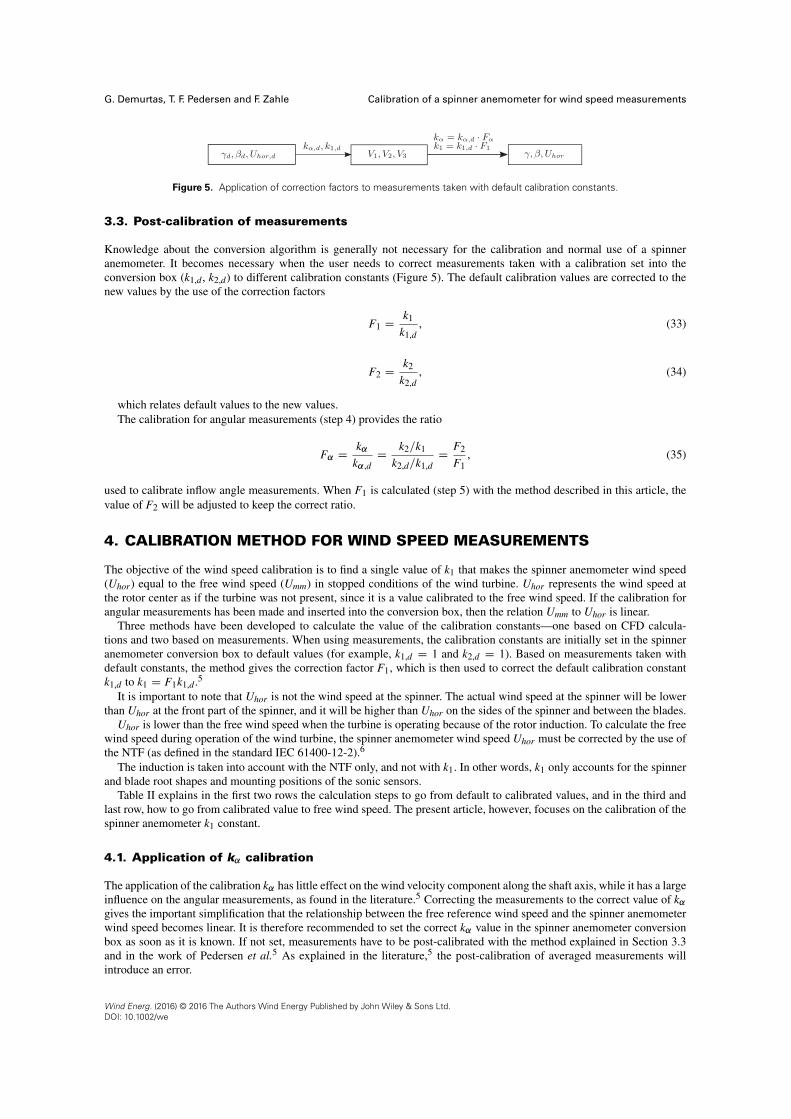
G. Demurtas, T. F. Pedersen and F. Zahle Calibration of a spinner anemometer for wind speed measurements
Figure 5. Application of correction factors to measurements taken with default calibration constants.
3.3. Post-calibration of measurements
Knowledge about the conversion algorithm is generally not necessary for the calibration and normal use of a spinneranemometer. It becomes necessary when the user needs to correct measurements taken with a calibration set into theconversion box (k1,d , k2,d) to different calibration constants (Figure 5). The default calibration values are corrected to thenew values by the use of the correction factors
F1 Dk1
k1,d, (33)
F2 Dk2
k2,d, (34)
which relates default values to the new values.The calibration for angular measurements (step 4) provides the ratio
F˛ Dk˛
k˛,dD
k2=k1
k2,d=k1,dD
F2
F1, (35)
used to calibrate inflow angle measurements. When F1 is calculated (step 5) with the method described in this article, thevalue of F2 will be adjusted to keep the correct ratio.
4. CALIBRATION METHOD FOR WIND SPEED MEASUREMENTS
The objective of the wind speed calibration is to find a single value of k1 that makes the spinner anemometer wind speed(Uhor) equal to the free wind speed (Umm) in stopped conditions of the wind turbine. Uhor represents the wind speed atthe rotor center as if the turbine was not present, since it is a value calibrated to the free wind speed. If the calibration forangular measurements has been made and inserted into the conversion box, then the relation Umm to Uhor is linear.
Three methods have been developed to calculate the value of the calibration constants—one based on CFD calcula-tions and two based on measurements. When using measurements, the calibration constants are initially set in the spinneranemometer conversion box to default values (for example, k1,d D 1 and k2,d D 1). Based on measurements taken withdefault constants, the method gives the correction factor F1, which is then used to correct the default calibration constantk1,d to k1 D F1k1,d .5
It is important to note that Uhor is not the wind speed at the spinner. The actual wind speed at the spinner will be lowerthan Uhor at the front part of the spinner, and it will be higher than Uhor on the sides of the spinner and between the blades.
Uhor is lower than the free wind speed when the turbine is operating because of the rotor induction. To calculate the freewind speed during operation of the wind turbine, the spinner anemometer wind speed Uhor must be corrected by the use ofthe NTF (as defined in the standard IEC 61400-12-2).6
The induction is taken into account with the NTF only, and not with k1. In other words, k1 only accounts for the spinnerand blade root shapes and mounting positions of the sonic sensors.
Table II explains in the first two rows the calculation steps to go from default to calibrated values, and in the third andlast row, how to go from calibrated value to free wind speed. The present article, however, focuses on the calibration of thespinner anemometer k1 constant.
4.1. Application of k˛ calibration
The application of the calibration k˛ has little effect on the wind velocity component along the shaft axis, while it has a largeinfluence on the angular measurements, as found in the literature.5 Correcting the measurements to the correct value of k˛gives the important simplification that the relationship between the free reference wind speed and the spinner anemometerwind speed becomes linear. It is therefore recommended to set the correct k˛ value in the spinner anemometer conversionbox as soon as it is known. If not set, measurements have to be post-calibrated with the method explained in Section 3.3and in the work of Pedersen et al.5 As explained in the literature,5 the post-calibration of averaged measurements willintroduce an error.
Wind Energ. (2016) © 2016 The Authors Wind Energy Published by John Wiley & Sons Ltd.DOI: 10.1002/we

Calibration of a spinner anemometer for wind speed measurements G. Demurtas, T. F. Pedersen and F. Zahle
Table II. Calculation steps to convert default values to calibrated values and finally tofree wind speed.
From Action To
Uhor,d Application of F˛ (determined in5) Uhor,d,cUhor,d,c Determination and application of F1 (chapters 5.4, 5.5 and 5.6) UhorUhor Determination and application of the NTF (IEC 61400-12-2 )6 Uhor,free
4.2. Calculation of the calibration correction factor F1
As derived in the work of Pedersenet al.5 and summarized in Section 3, the calibration factor F1 is defined as
F1 Dk1
k1,dD
Ud
U
cos.˛d/
cos.˛/, (36)
where Ud is the magnitude of the wind velocity measured by the non-calibrated spinner anemometer and U is the magnitudeof the wind velocity used as a reference for the calibration.
When the measurements of the spinner anemometer have been corrected with F˛ , we can neglect the cosine ratio, since˛ D ˛d (the value of the measured inflow angle is correct). This is also the case when the correct k˛ D k2=k1 was set inthe conversion box at the time when the measurements were acquired, or the measurements have been corrected with theprocedure schematized in Figure 5.
The calibration test is performed using the natural wind. The reference wind speed U shall be measured at hub heightat a distance upstream of the wind turbine according to IEC 61400-12-1.9 U can be measured with a 3D sonic anemome-ter or with a specifically designed cup anemometer that measures the vector wind speed rather than the horizontal velocitycomponent. Most of the cup anemometers available on the market are however designed to measure the horizontal com-ponent of U. Therefore, under the assumption that the flow inclination at the spinner is equal to the flow inclination at themet-mast, we can turn equation 36 into
F1 DUhor,d,c
Umm, (37)
so that we compare the horizontal components, instead of the modulus of the wind vectors.
5. APPLICATION OF THE CALIBRATION METHOD ON A SPECIFICWIND TURBINE SPINNER ANEMOMETER
A spinner anemometer was mounted on a Nordtank 500 kW wind turbine located at DTU Risø Campus test site,approximately 6 km north of Roskilde, Denmark. The wind turbine has been used for many years for research and edu-cational purposes and is very well instrumented (see description of the site and of the instrumentation in the work ofPaulsen and Wagner10).
Three methods to calibrate the k1 constants are presented here: for Method 1 the wind turbine is stopped, for Method 2the wind turbine is in operation, while Method 3 is based on CFD simulation of the stopped rotor.
According to the definition of k1 (equal to the ratio between the spinner anemometer horizontal wind speed and the freehorizontal wind speed in a condition of zero induction), the correct method to determine k1 is Method 1, which uses astopped turbine. The drawback of this method is that it requires the wind turbine to be stopped for several hours in goodwind conditions, which is generally not acceptable by the wind turbine owner. Therefore, we investigated the possibilityof determining the calibration constant using measurements during operation of the wind turbine (Method 2) and CFDsimulation of the stopped turbine (Method 3). The following subsections describe the instrument setup, data selection, aswell as present an analysis of the three methods.
5.1. Spinner anemometer mounting evaluation
Figure 6 shows the spinner of the Nordtank turbine and two of its sonic sensors. Figure 6 is an overlay of three photostaken from ground level during rotation of the rotor in a way that each photo shows one of the three sensors when it isclearly visible on the side of the spinner. The sides of the spinner were used as reference to align the photos. Due to theheight of the wind turbine, in order to obtain a good resolution of the photo, it was necessary to use a digital camera witha 300 mm zoom optic (12 Megapixel, 18�24 mm CCD sensor). The camera was standing on a tripod at ground level underthe spinner, 1.8 m from the tower.
Wind Energ. (2016) © 2016 The Authors Wind Energy Published by John Wiley & Sons Ltd.DOI: 10.1002/we
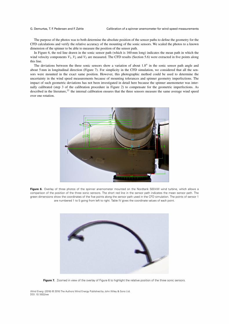
G. Demurtas, T. F. Pedersen and F. Zahle Calibration of a spinner anemometer for wind speed measurements
The purpose of the photos was to both determine the absolute position of the sensor paths to define the geometry for theCFD calculations and verify the relative accuracy of the mounting of the sonic sensors. We scaled the photos to a knowndimension of the spinner to be able to measure the position of the sensor path.
In Figure 6, the red line drawn in the sonic sensor path (which is 160 mm long) indicates the mean path in which thewind velocity components V1, V2 and V3 are measured. The CFD results (Section 5.6) were extracted in five points alongthis line.
The deviations between the three sonic sensors show a variation of about 1.8ı in the sonic sensor path angle andabout 5 mm in longitudinal direction (Figure 7). For simplicity in the CFD simulation, we considered that all the sen-sors were mounted in the exact same position. However, this photographic method could be used to determine theuncertainty in the wind speed measurements because of mounting tolerances and spinner geometry imperfections. Theimpact of such geometric deviations has not been investigated in detail here because the spinner anemometer was inter-nally calibrated (step 3 of the calibration procedure in Figure 2) to compensate for the geometric imperfections. Asdescribed in the literature,11 the internal calibration ensures that the three sensors measure the same average wind speedover one rotation.
Figure 6. Overlay of three photos of the spinner anemometer mounted on the Nordtank 500 kW wind turbine, which allows acomparison of the position of the three sonic sensors. The short red line in the sensor path indicates the mean sensor path. Thegreen dimensions show the coordinates of the five points along the sensor path used in the CFD simulation. The points of sensor 1
are numbered 1 to 5 going from left to right. Table IV gives the coordinate values of each point.
Figure 7. Zoomed in view of the overlay of Figure 6 to highlight the relative position of the three sonic sensors.
Wind Energ. (2016) © 2016 The Authors Wind Energy Published by John Wiley & Sons Ltd.DOI: 10.1002/we
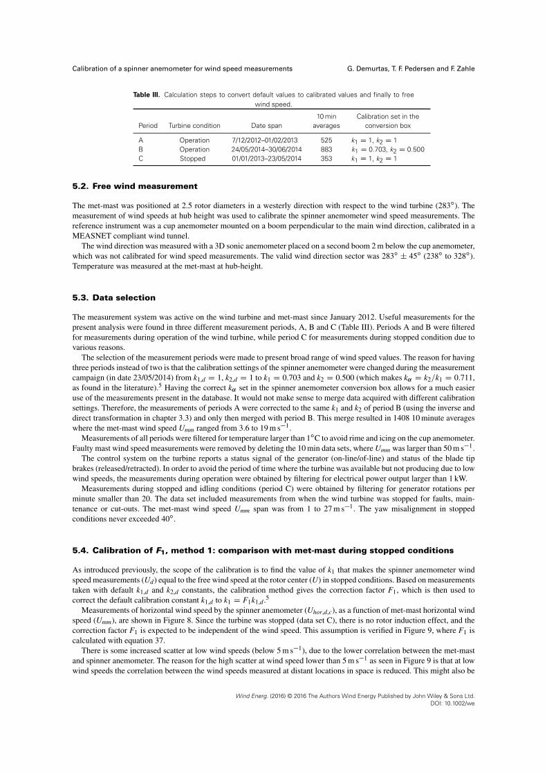
Calibration of a spinner anemometer for wind speed measurements G. Demurtas, T. F. Pedersen and F. Zahle
Table III. Calculation steps to convert default values to calibrated values and finally to freewind speed.
10 min Calibration set in thePeriod Turbine condition Date span averages conversion box
A Operation 7/12/2012–01/02/2013 525 k1 D 1, k2 D 1B Operation 24/05/2014–30/06/2014 883 k1 D 0.703, k2 D 0.500C Stopped 01/01/2013–23/05/2014 353 k1 D 1, k2 D 1
5.2. Free wind measurement
The met-mast was positioned at 2.5 rotor diameters in a westerly direction with respect to the wind turbine (283ı). Themeasurement of wind speeds at hub height was used to calibrate the spinner anemometer wind speed measurements. Thereference instrument was a cup anemometer mounted on a boom perpendicular to the main wind direction, calibrated in aMEASNET compliant wind tunnel.
The wind direction was measured with a 3D sonic anemometer placed on a second boom 2 m below the cup anemometer,which was not calibrated for wind speed measurements. The valid wind direction sector was 283ı ˙ 45ı (238ı to 328ı).Temperature was measured at the met-mast at hub-height.
5.3. Data selection
The measurement system was active on the wind turbine and met-mast since January 2012. Useful measurements for thepresent analysis were found in three different measurement periods, A, B and C (Table III). Periods A and B were filteredfor measurements during operation of the wind turbine, while period C for measurements during stopped condition due tovarious reasons.
The selection of the measurement periods were made to present broad range of wind speed values. The reason for havingthree periods instead of two is that the calibration settings of the spinner anemometer were changed during the measurementcampaign (in date 23/05/2014) from k1,d D 1, k2,d D 1 to k1 D 0.703 and k2 D 0.500 (which makes k˛ D k2=k1 D 0.711,as found in the literature).5 Having the correct k˛ set in the spinner anemometer conversion box allows for a much easieruse of the measurements present in the database. It would not make sense to merge data acquired with different calibrationsettings. Therefore, the measurements of periods A were corrected to the same k1 and k2 of period B (using the inverse anddirect transformation in chapter 3.3) and only then merged with period B. This merge resulted in 1408 10 minute averageswhere the met-mast wind speed Umm ranged from 3.6 to 19 m s�1.
Measurements of all periods were filtered for temperature larger than 1ıC to avoid rime and icing on the cup anemometer.Faulty mast wind speed measurements were removed by deleting the 10 min data sets, where Umm was larger than 50 m s�1.
The control system on the turbine reports a status signal of the generator (on-line/of-line) and status of the blade tipbrakes (released/retracted). In order to avoid the period of time where the turbine was available but not producing due to lowwind speeds, the measurements during operation were obtained by filtering for electrical power output larger than 1 kW.
Measurements during stopped and idling conditions (period C) were obtained by filtering for generator rotations perminute smaller than 20. The data set included measurements from when the wind turbine was stopped for faults, main-tenance or cut-outs. The met-mast wind speed Umm span was from 1 to 27 m s�1. The yaw misalignment in stoppedconditions never exceeded 40ı.
5.4. Calibration of F1, method 1: comparison with met-mast during stopped conditions
As introduced previously, the scope of the calibration is to find the value of k1 that makes the spinner anemometer windspeed measurements (Ud) equal to the free wind speed at the rotor center (U) in stopped conditions. Based on measurementstaken with default k1,d and k2,d constants, the calibration method gives the correction factor F1, which is then used tocorrect the default calibration constant k1,d to k1 D F1k1,d .5
Measurements of horizontal wind speed by the spinner anemometer (Uhor,d,c), as a function of met-mast horizontal windspeed (Umm), are shown in Figure 8. Since the turbine was stopped (data set C), there is no rotor induction effect, and thecorrection factor F1 is expected to be independent of the wind speed. This assumption is verified in Figure 9, where F1 iscalculated with equation 37.
There is some increased scatter at low wind speeds (below 5 m s�1), due to the lower correlation between the met-mastand spinner anemometer. The reason for the high scatter at wind speed lower than 5 m s�1 as seen in Figure 9 is that at lowwind speeds the correlation between the wind speeds measured at distant locations in space is reduced. This might also be
Wind Energ. (2016) © 2016 The Authors Wind Energy Published by John Wiley & Sons Ltd.DOI: 10.1002/we
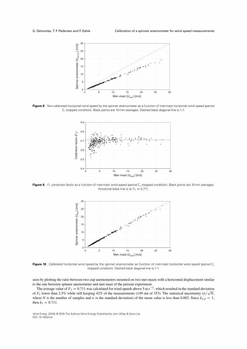
G. Demurtas, T. F. Pedersen and F. Zahle Calibration of a spinner anemometer for wind speed measurements
Figure 8. Non-calibrated horizontal wind speed by the spinner anemometer as a function of met-mast horizontal wind speed (periodC, stopped condition). Black points are 10-min averages. Dashed black diagonal line is 1:1.
Figure 9. F1 correction factor as a function of met-mast wind speed (period C, stopped condition). Black points are 10 min averages.Horizontal black line is at F1 D 0.711.
Figure 10. Calibrated horizontal wind speed by the spinner anemometer as function of met-mast horizontal wind speed (period C,stopped condition). Dashed black diagonal line is 1:1.
seen by plotting the ratio between two cup anemometers mounted on two met-masts with a horizontal displacement similarto the one between spinner anemometer and met-mast of the present experiment.
The average value of F1 D 0.711 was calculated for wind speeds above 5 m s�1, which resulted in the standard deviationof F1 lower than 2.5% while still keeping 42% of the measurements (149 out of 353). The statistical uncertainty (�=
pN,
where N is the number of samples and � is the standard deviation) of the mean value is less than 0.002. Since k1,d D 1,then k1 D 0.711.
Wind Energ. (2016) © 2016 The Authors Wind Energy Published by John Wiley & Sons Ltd.DOI: 10.1002/we

Calibration of a spinner anemometer for wind speed measurements G. Demurtas, T. F. Pedersen and F. Zahle
The measurements during stopped conditions calibrated with F˛ D 0.714 and F1 D 0.711 (F2 D F˛F1 D 0.508)are shown in Figure 10. In the same figure, the 1:1 relationship between spinner anemometer measurements and met-mastmeasurements confirms a correct calibration of F1 and absence of rotor induction.
5.5. Calibration of F1, method 2: comparison with met-mast at high wind speeds
This second method to determine F1 uses measurements during operation of the wind turbine (Figure 11).During operation, however, the rotor induction reduces the wind speed at the rotor plane with respect to the free wind
speed, introducing a significant error in the calculation of F1. This slow down is small when the turbine is operating at highwind speeds, with a low power coefficient, as seen in the works of Pedersen et al.,4, 11 where the induction was found to besmaller than 1% above 17 m s�1, for a pitch-regulated Vestas V80* wind turbine.
A set of F1 values was determined from the measurements with equation 37 and plotted as a function of wind speed(Figure 12).
The red line is a bin average with 1 m s�1 bin size, centered at integer wind speeds. The horizontal black line shows thevalue of F1 found for stopped conditions (Section 5.4). As expected, the red line tends asymptotically to the value of F1calculated for the stopped rotor (method 1) shown with a horizontal black line. There were unfortunately no measurementsbetween 18 and 25 m s�1. It is not possible to determine a value of F1 for an induction free condition during operation forthe measured data (the red line does not seem to reach an asymptotic value and increases with the wind speed as a result ofthe induction decreasing).
The measurements of the period during operation calibrated with F˛ D 0.714 (found in the literature5) and F1 D 0.711(found in Section 5.4 for a stopped rotor) are shown in Figure 13 as a function of the met-mast wind speed.
Figure 11. Non-calibrated horizontal wind speed by the spinner anemometer as a function of met-mast horizontal wind speed (mergeof periods A and B, during operation). Dashed black diagonal line is 1:1.
Figure 12. F1 correction factor as a function of met-mast wind speed, disturbed by the rotor induction during operation of the windturbine (data sets A and B). The black horizontal line at F1 D 0.711 shows the calibration result obtained with method 1 (stopped
condition). Black points are 10 min averages. Red line is 1 m s�1 bin average.
*Vestas Wind Systems A/S, Hedeager 42, 8200 Aarhus N, Denmark.
Wind Energ. (2016) © 2016 The Authors Wind Energy Published by John Wiley & Sons Ltd.DOI: 10.1002/we
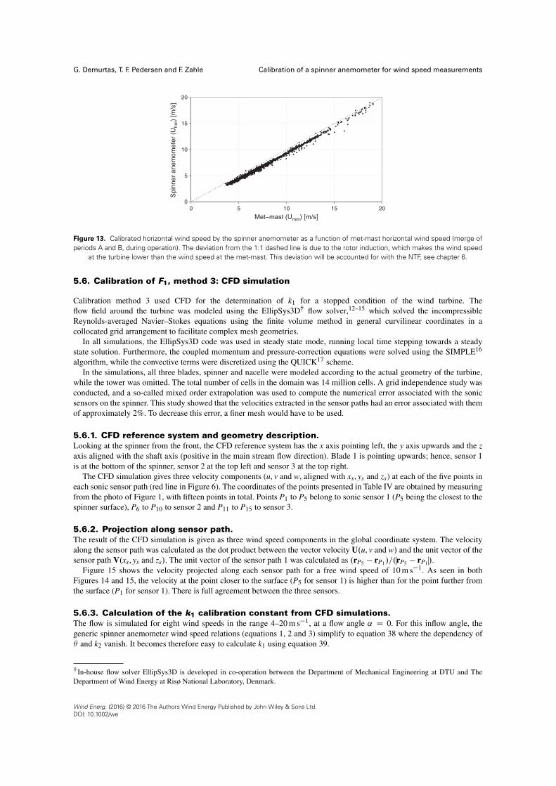
G. Demurtas, T. F. Pedersen and F. Zahle Calibration of a spinner anemometer for wind speed measurements
Figure 13. Calibrated horizontal wind speed by the spinner anemometer as a function of met-mast horizontal wind speed (merge ofperiods A and B, during operation). The deviation from the 1:1 dashed line is due to the rotor induction, which makes the wind speed
at the turbine lower than the wind speed at the met-mast. This deviation will be accounted for with the NTF, see chapter 6.
5.6. Calibration of F1, method 3: CFD simulation
Calibration method 3 used CFD for the determination of k1 for a stopped condition of the wind turbine. Theflow field around the turbine was modeled using the EllipSys3D� flow solver,12–15 which solved the incompressibleReynolds-averaged Navier–Stokes equations using the finite volume method in general curvilinear coordinates in acollocated grid arrangement to facilitate complex mesh geometries.
In all simulations, the EllipSys3D code was used in steady state mode, running local time stepping towards a steadystate solution. Furthermore, the coupled momentum and pressure-correction equations were solved using the SIMPLE16
algorithm, while the convective terms were discretized using the QUICK17 scheme.In the simulations, all three blades, spinner and nacelle were modeled according to the actual geometry of the turbine,
while the tower was omitted. The total number of cells in the domain was 14 million cells. A grid independence study wasconducted, and a so-called mixed order extrapolation was used to compute the numerical error associated with the sonicsensors on the spinner. This study showed that the velocities extracted in the sensor paths had an error associated with themof approximately 2%. To decrease this error, a finer mesh would have to be used.
5.6.1. CFD reference system and geometry description.Looking at the spinner from the front, the CFD reference system has the x axis pointing left, the y axis upwards and the zaxis aligned with the shaft axis (positive in the main stream flow direction). Blade 1 is pointing upwards; hence, sensor 1is at the bottom of the spinner, sensor 2 at the top left and sensor 3 at the top right.
The CFD simulation gives three velocity components (u, v and w, aligned with xs, ys and zs) at each of the five points ineach sonic sensor path (red line in Figure 6). The coordinates of the points presented in Table IV are obtained by measuringfrom the photo of Figure 1, with fifteen points in total. Points P1 to P5 belong to sonic sensor 1 (P5 being the closest to thespinner surface), P6 to P10 to sensor 2 and P11 to P15 to sensor 3.
5.6.2. Projection along sensor path.The result of the CFD simulation is given as three wind speed components in the global coordinate system. The velocityalong the sensor path was calculated as the dot product between the vector velocity U.u, v and w/ and the unit vector of thesensor path V.xs, ys and zs/. The unit vector of the sensor path 1 was calculated as .rP5 � rP1/=.rP5 � rP1 /.
Figure 15 shows the velocity projected along each sensor path for a free wind speed of 10 m s�1. As seen in bothFigures 14 and 15, the velocity at the point closer to the surface (P5 for sensor 1) is higher than for the point further fromthe surface (P1 for sensor 1). There is full agreement between the three sensors.
5.6.3. Calculation of the k1 calibration constant from CFD simulations.The flow is simulated for eight wind speeds in the range 4–20 m s�1, at a flow angle ˛ D 0. For this inflow angle, thegeneric spinner anemometer wind speed relations (equations 1, 2 and 3) simplify to equation 38 where the dependency of� and k2 vanish. It becomes therefore easy to calculate k1 using equation 39.
�In-house flow solver EllipSys3D is developed in co-operation between the Department of Mechanical Engineering at DTU and TheDepartment of Wind Energy at Risø National Laboratory, Denmark.
Wind Energ. (2016) © 2016 The Authors Wind Energy Published by John Wiley & Sons Ltd.DOI: 10.1002/we
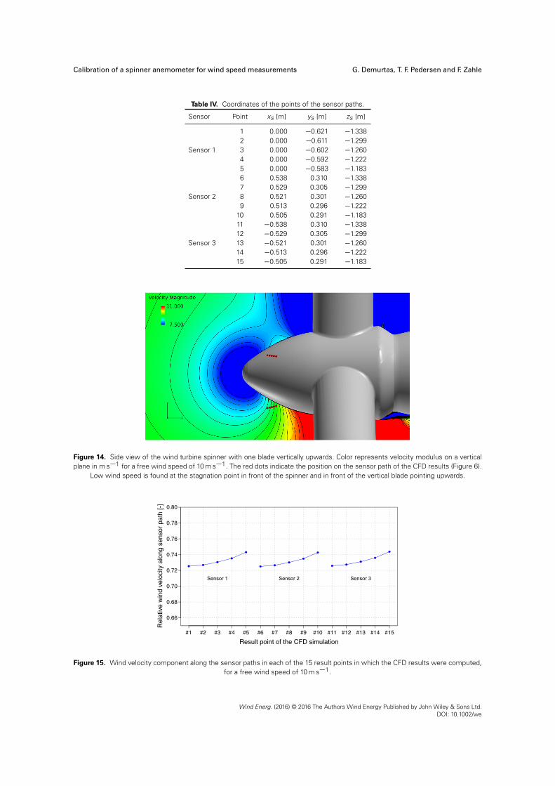
Calibration of a spinner anemometer for wind speed measurements G. Demurtas, T. F. Pedersen and F. Zahle
Table IV. Coordinates of the points of the sensor paths.
Sensor Point xs [m] ys [m] zs [m]
1 0.000 �0.621 �1.3382 0.000 �0.611 �1.299
Sensor 1 3 0.000 �0.602 �1.2604 0.000 �0.592 �1.2225 0.000 �0.583 �1.1836 0.538 0.310 �1.3387 0.529 0.305 �1.299
Sensor 2 8 0.521 0.301 �1.2609 0.513 0.296 �1.222
10 0.505 0.291 �1.18311 �0.538 0.310 �1.33812 �0.529 0.305 �1.299
Sensor 3 13 �0.521 0.301 �1.26014 �0.513 0.296 �1.22215 �0.505 0.291 �1.183
Figure 14. Side view of the wind turbine spinner with one blade vertically upwards. Color represents velocity modulus on a verticalplane in m s�1 for a free wind speed of 10 m s�1. The red dots indicate the position on the sensor path of the CFD results (Figure 6).
Low wind speed is found at the stagnation point in front of the spinner and in front of the vertical blade pointing upwards.
Figure 15. Wind velocity component along the sensor paths in each of the 15 result points in which the CFD results were computed,for a free wind speed of 10 m s�1.
Wind Energ. (2016) © 2016 The Authors Wind Energy Published by John Wiley & Sons Ltd.DOI: 10.1002/we
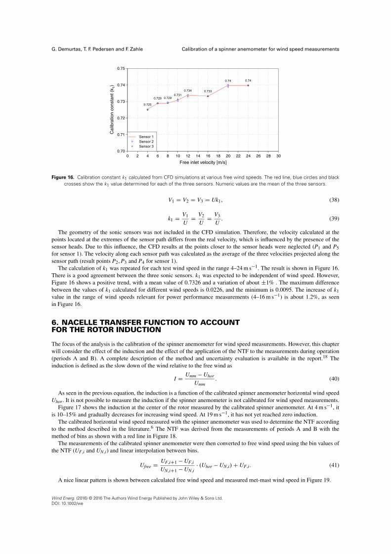
G. Demurtas, T. F. Pedersen and F. Zahle Calibration of a spinner anemometer for wind speed measurements
Figure 16. Calibration constant k1 calculated from CFD simulations at various free wind speeds. The red line, blue circles and blackcrosses show the k1 value determined for each of the three sensors. Numeric values are the mean of the three sensors.
V1 D V2 D V3 D Uk1, (38)
k1 DV1
UD
V2
UD
V3
U. (39)
The geometry of the sonic sensors was not included in the CFD simulation. Therefore, the velocity calculated at thepoints located at the extremes of the sensor path differs from the real velocity, which is influenced by the presence of thesensor heads. Due to this influence, the CFD results at the points closer to the sensor heads were neglected (P1 and P5for sensor 1). The velocity along each sensor path was calculated as the average of the three velocities projected along thesensor path (result points P2, P3 and P4 for sensor 1).
The calculation of k1 was repeated for each test wind speed in the range 4–24 m s�1. The result is shown in Figure 16.There is a good agreement between the three sonic sensors. k1 was expected to be independent of wind speed. However,Figure 16 shows a positive trend, with a mean value of 0.7326 and a variation of about ˙1% . The maximum differencebetween the values of k1 calculated for different wind speeds is 0.0226, and the minimum is 0.0095. The increase of k1value in the range of wind speeds relevant for power performance measurements (4–16 m s�1) is about 1.2%, as seenin Figure 16.
6. NACELLE TRANSFER FUNCTION TO ACCOUNTFOR THE ROTOR INDUCTION
The focus of the analysis is the calibration of the spinner anemometer for wind speed measurements. However, this chapterwill consider the effect of the induction and the effect of the application of the NTF to the measurements during operation(periods A and B). A complete description of the method and uncertainty evaluation is available in the report.18 Theinduction is defined as the slow down of the wind relative to the free wind as
I DUmm � Uhor
Umm. (40)
As seen in the previous equation, the induction is a function of the calibrated spinner anemometer horizontal wind speedUhor. It is not possible to measure the induction if the spinner anemometer is not calibrated for wind speed measurements.
Figure 17 shows the induction at the center of the rotor measured by the calibrated spinner anemometer. At 4 m s�1, itis 10–15% and gradually decreases for increasing wind speed. At 19 m s�1, it has not yet reached zero induction.
The calibrated horizontal wind speed measured with the spinner anemometer was used to determine the NTF accordingto the method described in the literature.6 The NTF was derived from the measurements of periods A and B with themethod of bins as shown with a red line in Figure 18.
The measurements of the calibrated spinner anemometer were then converted to free wind speed using the bin values ofthe NTF (UF,i and UN,i) and linear interpolation between bins.
Ufree DUF,iC1 � UF,i
UN,iC1 � UN,i� .Uhor � UN,i/C UF,i. (41)
A nice linear pattern is shown between calculated free wind speed and measured met-mast wind speed in Figure 19.
Wind Energ. (2016) © 2016 The Authors Wind Energy Published by John Wiley & Sons Ltd.DOI: 10.1002/we
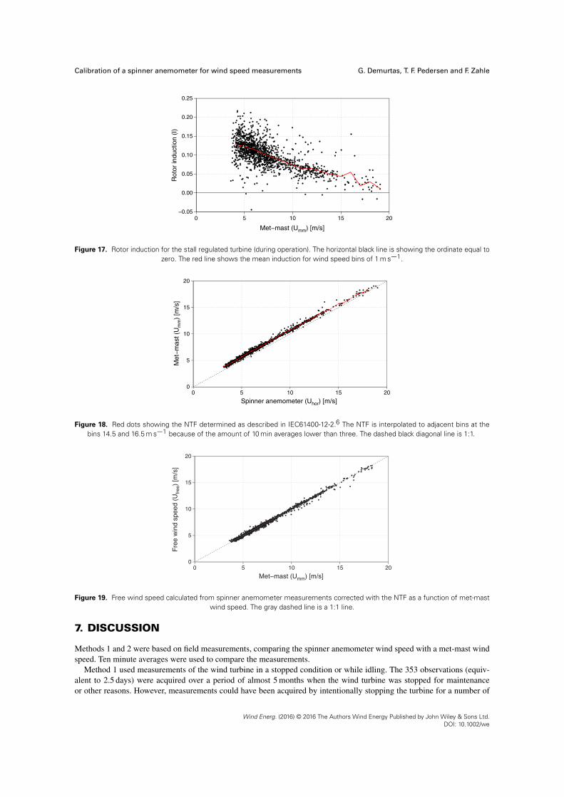
Calibration of a spinner anemometer for wind speed measurements G. Demurtas, T. F. Pedersen and F. Zahle
Figure 17. Rotor induction for the stall regulated turbine (during operation). The horizontal black line is showing the ordinate equal tozero. The red line shows the mean induction for wind speed bins of 1 m s�1.
Figure 18. Red dots showing the NTF determined as described in IEC61400-12-2.6 The NTF is interpolated to adjacent bins at thebins 14.5 and 16.5 m s�1 because of the amount of 10 min averages lower than three. The dashed black diagonal line is 1:1.
Figure 19. Free wind speed calculated from spinner anemometer measurements corrected with the NTF as a function of met-mastwind speed. The gray dashed line is a 1:1 line.
7. DISCUSSION
Methods 1 and 2 were based on field measurements, comparing the spinner anemometer wind speed with a met-mast windspeed. Ten minute averages were used to compare the measurements.
Method 1 used measurements of the wind turbine in a stopped condition or while idling. The 353 observations (equiv-alent to 2.5 days) were acquired over a period of almost 5 months when the wind turbine was stopped for maintenanceor other reasons. However, measurements could have been acquired by intentionally stopping the turbine for a number of
Wind Energ. (2016) © 2016 The Authors Wind Energy Published by John Wiley & Sons Ltd.DOI: 10.1002/we
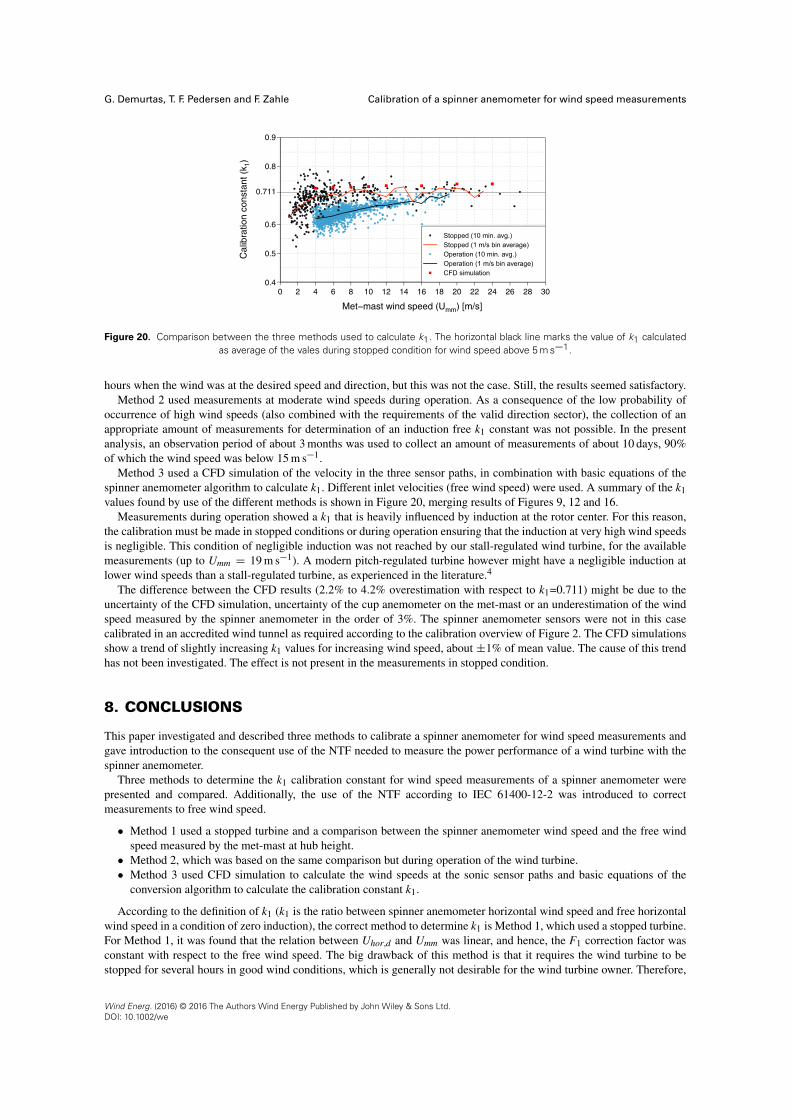
G. Demurtas, T. F. Pedersen and F. Zahle Calibration of a spinner anemometer for wind speed measurements
Figure 20. Comparison between the three methods used to calculate k1. The horizontal black line marks the value of k1 calculatedas average of the vales during stopped condition for wind speed above 5 m s�1.
hours when the wind was at the desired speed and direction, but this was not the case. Still, the results seemed satisfactory.Method 2 used measurements at moderate wind speeds during operation. As a consequence of the low probability of
occurrence of high wind speeds (also combined with the requirements of the valid direction sector), the collection of anappropriate amount of measurements for determination of an induction free k1 constant was not possible. In the presentanalysis, an observation period of about 3 months was used to collect an amount of measurements of about 10 days, 90%of which the wind speed was below 15 m s�1.
Method 3 used a CFD simulation of the velocity in the three sensor paths, in combination with basic equations of thespinner anemometer algorithm to calculate k1. Different inlet velocities (free wind speed) were used. A summary of the k1values found by use of the different methods is shown in Figure 20, merging results of Figures 9, 12 and 16.
Measurements during operation showed a k1 that is heavily influenced by induction at the rotor center. For this reason,the calibration must be made in stopped conditions or during operation ensuring that the induction at very high wind speedsis negligible. This condition of negligible induction was not reached by our stall-regulated wind turbine, for the availablemeasurements (up to Umm D 19 m s�1). A modern pitch-regulated turbine however might have a negligible induction atlower wind speeds than a stall-regulated turbine, as experienced in the literature.4
The difference between the CFD results (2.2% to 4.2% overestimation with respect to k1=0.711) might be due to theuncertainty of the CFD simulation, uncertainty of the cup anemometer on the met-mast or an underestimation of the windspeed measured by the spinner anemometer in the order of 3%. The spinner anemometer sensors were not in this casecalibrated in an accredited wind tunnel as required according to the calibration overview of Figure 2. The CFD simulationsshow a trend of slightly increasing k1 values for increasing wind speed, about˙1% of mean value. The cause of this trendhas not been investigated. The effect is not present in the measurements in stopped condition.
8. CONCLUSIONS
This paper investigated and described three methods to calibrate a spinner anemometer for wind speed measurements andgave introduction to the consequent use of the NTF needed to measure the power performance of a wind turbine with thespinner anemometer.
Three methods to determine the k1 calibration constant for wind speed measurements of a spinner anemometer werepresented and compared. Additionally, the use of the NTF according to IEC 61400-12-2 was introduced to correctmeasurements to free wind speed.
� Method 1 used a stopped turbine and a comparison between the spinner anemometer wind speed and the free windspeed measured by the met-mast at hub height.
� Method 2, which was based on the same comparison but during operation of the wind turbine.� Method 3 used CFD simulation to calculate the wind speeds at the sonic sensor paths and basic equations of the
conversion algorithm to calculate the calibration constant k1.
According to the definition of k1 (k1 is the ratio between spinner anemometer horizontal wind speed and free horizontalwind speed in a condition of zero induction), the correct method to determine k1 is Method 1, which used a stopped turbine.For Method 1, it was found that the relation between Uhor,d and Umm was linear, and hence, the F1 correction factor wasconstant with respect to the free wind speed. The big drawback of this method is that it requires the wind turbine to bestopped for several hours in good wind conditions, which is generally not desirable for the wind turbine owner. Therefore,
Wind Energ. (2016) © 2016 The Authors Wind Energy Published by John Wiley & Sons Ltd.DOI: 10.1002/we
Calibration of a spinner anemometer for wind speed measurements G. Demurtas, T. F. Pedersen and F. Zahle
we investigated the possibility of calculating the calibration constant using measurements during operation of the windturbine (Method 2) and CFD simulation of the stopped turbine (Method 3).
Method 2 was notably influenced by the rotor induction. We tried to identify a range of high wind speeds in which F1was stabilizing to an asymptotic value. However, this condition was not met for our stall-regulated turbine at wind speedsup to 19 m s�1. Method 2 seems to be more applicable on a pitch regulated turbine, where induction decreases more thanfor a stall-regulated turbine because of the pitching of the blades. This will make the F1 values approach an asymptote.
Method 3, CFD simulation of the stopped turbine, has the obvious advantage of not requiring wind measurementsto determine k1. The method showed a low dependency of k1 on the wind speed (about 1.2% linear increase from 4to 16 m s�1) and 2.2% to 4.2% difference from the value obtained with method 1. In the absence of a free wind speedmeasurement, this method is appropriate to determine an initial value of the calibration coefficients.
The analysis shows the important simplification of the equations used to calculate k1 arising from having set the correctk˛ value in the spinner anemometer conversion box. Failing to do so means that the full conversion algorithm of sampleddata has to be used to calculate back to sonic sensor wind speeds and forth to spinner anemometer wind speed for differentk1 and k2 values. This was needed in this analysis because data was gathered with k1 and k2 values not representing acalibrated k˛ value. It is recommended to follow the order of the five steps calibration procedure described in the work ofDemurtas and Pedersen.7
The calibration of k1 in addition to determination of the NTF is needed to measure the nacelle power curve of a windturbine, ensuring separation between the instrument characteristics and the slow down of the wind due to the rotor induction.It is important to keep the calibration of the spinner anemometer separated from the NTF because the calibration of thespinner anemometer is invariant to control system settings and blade design.
Since the physics of extracting power from the wind is similar between different wind turbines, future research willinvestigate the possibility of defining a general NTF as a standard correction of the rotor induction. The specificity ofthe spinner shape and sonic sensors mounting will be accounted by the calibration of the spinner anemometer alone,on each turbine.
ACKNOWLEDGEMENTS
This work was performed as part of an EUDP project iSpin funded by the Danish Energy Agency (J.nr 64012-0107). Theauthors would like to thank all the people from Vattenfall, Metek and ROMO Wind for their good collaboration. This workwas performed under the EUDP-2012-I project: iSpin (J.nr 64012-0107).
REFERENCES
1. Cuerva A, Pedersen TF, Sánchez Luengo S, Alamillo Pastor JD, SanzAndrs A, Franchini SA. Theoretical model onspinner anemometry based on ultrasonic paths. Proceedings of EWEC 2008, Brussels, 2008.
2. Frandsen S. Nacelle anemometry. Proceedings of EWEA 2006, Bruxelles, 2006.3. Zahle F, Srensen NN. Characterization of the unsteady flow in the nacelle region of a modern wind turbine. Wind
Energy 2011; 14: 271–283.4. Pedersen TF, Demurtas G, Sommer A, Hjstrup J. Measurement of rotor centre flow direction and turbulence in wind
farm environment. Torque 2014, Journal of Physics, Denmark, June 2014.5. Pedersen TF, Demurtas G, Zahle F. Calibration of a spinner anemometer for yaw misalignment measurements. Wind
Energy 2014.6. IEC 61400-12-2: Power Performance of Electricity Producing Wind Turbines Based on Nacelle Anemometry. Edition
1. International Electrotechnical Commission: Geneva, Switzerland, 2012.7. Demurtas G, Pedersen TF. Summary of the steps involved in the calibration of a spinner anemometer. DTU Wind
Energy Report I-0364, Roskilde, 2014.8. Pedersen TF, Wagner R, Demurtas G. Wind turbine performance measurements by means of dynamic data analysis.
DTU Wind Energy Report, Roskilde, 2015.9. 61400-12-1 IEC. Power Performance Measurements of Electricity Producing Wind Turbines. Edition 3. International
Electrotechnical Commission: Geneva, Switzerland, 2005.10. Paulsen US, Wagner R. IMPER Characterization of the wind field over a large wind turbine rotor—final report.
(Chapter 4: Description of the experimental facility). DTU Wind Energy report E-0002, Roskilde, 2012.11. Pedersen TF, Demurtas G, Gottschall J, Hjstrup J, Nielsen JD, Christiansen W, Weich G, Sommer A, Kristoffersen
JR. Improvement of wind farm performance by means of spinner anemometry. Section 2.3: Development of internalcalibration method. DTU Wind Energy report E-0040, 2013.
Wind Energ. (2016) © 2016 The Authors Wind Energy Published by John Wiley & Sons Ltd.DOI: 10.1002/we

G. Demurtas, T. F. Pedersen and F. Zahle Calibration of a spinner anemometer for wind speed measurements
12. Michelsen JA, Basis3D—a platform for development of multiblock PDE solvers, Technical Report AFM 92-05,Technical University of Denmark, 1992.
13. Michelsen JA, Block structured multigrid solution of 2D and 3D elliptic PDEs, Technical Report AFM 94-06, TechnicalUniversity of Denmark, 1994.
14. Sørensen NN, General purpose flow solver applied to flow over hills, Technical Report Ris-R-827(EN), Risø NationalLaboratory, 1995.
15. Ivanell S, Mikkelsen R, Srensen JN, Henningson D, Validation of methods using EllipSys3D, Technical Report, KTHTRITA-MEK, 2008.
16. Patankar SV, Spalding DB. A calculation procedure for heat, mass and momentum transfer in three-dimensionalparabolic flows. International Journal of Heat and Mass Transfer 1972; 15: 1787–1972.
17. Leonard PB. A stable and accurate convective modelling procedure based on quadratic upstream interpolation.Computer Methods in Applied Mechanics and Engineering 1979; 19: 59–98.
18. Demurtas G. Power curve measurement with spinner anemometer according to IEC 61400-12-2. DTU Wind EnergyReport I-0440 2015; 9: 22–31.
Wind Energ. (2016) © 2016 The Authors Wind Energy Published by John Wiley & Sons Ltd.DOI: 10.1002/we
Chapter 5
Power performance measurementsand uncertainty analysis
Chapter 4 explained how to accurately measure the wind speed with a spinner anemometerand how to correct it to free wind speed by use of the NTF.
Measuring the performance of a wind turbine means establish the relation between electricpower output and wind speed input. While the measurement of the electric power is straightforward, the challenge is to measure the wind speed. The IEC61400-12-1 standard describesthe instrumentation requirements and the calculation procedures to determine the powercurve with the method of bins, measuring the wind at hub height upstream of the windturbine with a cup anemometer installed on a meteorological mast. Such structure is costly,therefore the IEC61400-12-2 standard was developed to define requirements and proceduresto measure the wind on the wind turbine nacelle and on the spinner.
An experiment was set-up in the Nørrekær Enge wind farm, in the north of Denmark, nearLøgstør. The wind farm consists of 13 Siemens 2.3 MW wind turbines (90 m diameter and 80m hub height) aligned in a single row, almost east to west, in an open flat area. A met-mastwas erected in a position suitable to measure the power curve of two adjacent wind turbines,the 4th and the 5th counting from west were both equipped with a spinner anemometer.
The met-mast was IEC61400-12-1 compliant and instrumented with a cup anemometerat hub height and a wind vane on a boom at 78 m height.
The reason for placing the met-mast in a position suitable to measure the power curve ofboth turbine 4 and 5 was to investigate if the calibration values and NTF determined on thereference turbine 4 could be applied on turbine 5.
The power curve comparison of turbines 4 and 5 presented in the report [16] was notsatisfactory, and the cause was attributed to the excessive mounting tolerance of the sonicsensors on the spinner. The mounting was then improved and the analysis repeated. Theposition of the sonic sensors on each spinner was verified with photos taken from ground level.The power curves compared much better after the mounting improvement. The experimentand the analysis are presented in the following article, including a detailed evaluation ofuncertainties.
63
Nacelle power curve measurement with spinner anemometer anduncertainty evaluationGiorgio Demurtas1, Troels Friis Pedersen1, and Rozenn Wagner1
1DTU Wind Energy, Frederiksborgvej 399, 4000 Roskilde
Correspondence to:Giorgio Demurtas ([email protected])
Abstract. The objective of this investigation was to verify the feasibility of using the spinner anemometer calibration and
nacelle transfer function determined on one reference turbine, to assess the power performance of a second identical turbine.
An experiment was set up with a met-mast in a position suitable to measure the power curve of the two wind turbines, both
equipped with a spinner anemometer. An IEC 61400-12-1 compliant power curve was then measured for both turbines using
the met-mast. The NTF (Nacelle Transfer Function) was measured on the reference turbine and then applied to both turbines5
to calculate the free wind speed. For each of the two wind turbines, the power curve (PC) was measured with the met-mast
and the nacelle power curve (NPC) with the spinner anemometer. Four power curves (two PC and two NPC) were compared
in terms of AEP (Annual Energy Production) for a Rayleigh wind speed probability distribution. For each turbine, the NPC
agreed with the corresponding PC within 0.10% of AEP for the reference turbine and within 0,38% for the second turbine, for
a mean wind speed of 8 m/s.10
Keywords: Nacelle power curve, NPC, spinner anemometer, Nacelle transfer function, NTF
1 Introduction
Measuring the performance of a wind turbine means establishing the relation between wind speed (input) and electric power
(output). While the measurement of the electric power is straight forward (because it is already in electrical form), the challenge15
is to measure the wind speed. The IEC61400-12-1 standard describes the instrumentation requirements and the calculation
procedures to determine the power curve with the method of bins, measuring the wind at hub height upstream of the wind
turbine with a cup anemometer installed on a meteorological mast. A met-mast is costly, therefore the IEC61400-12-2 standard
was developed to define requirements and procedures to measure the wind speed on the wind turbine. While the use of the
nacelle anemometer (mounted on the nacelle roof) for performance measurements is a well established procedure, the spinner20
anemometer is a less experienced option to measure the wind turbine performance. A spinner anemometer (Pedersen(2007))
consist of three one dimensional sonic wind speed sensors mounted on the spinner of the wind turbine. The advantage of a
spinner anemometer over a nacelle anemometer is that it is measuring in front of the rotor rather than behind, where the flow
is influenced by the wake of the blades and other elements present on the nacelle as described byFrandsen et al.(2009).
1

The spinner anemometer must be traceable calibrated using a met-mast in order to measure the wind speed accurately and
to obtain an absolute power curve, according to the standardIEC61400-12-2(2013) and as reported byDemurtas(2014).
Installation of a met-mast for each wind turbine is obviously not viable. Therefore the possibility of using the calibration
found on a first -reference- turbine with a spinner anemometer to another one of same type was investigated in this work.
The objectives of the investigation were to:5
– Install a met-mast to measure the power curve (PC) on two wind turbines next to each other.
– Install spinner anemometer on both wind turbines.
– Calibrate the spinner anemometer on the reference wind turbine.
– Measure the nacelle transfer function (NTF) on the reference wind turbine.
– Compute the NPC and PC for the reference turbine10
– Apply the calibration values and NTF measured on the reference turbine to the second turbine.
– Compute the NPC and PC for the second turbine
– Compare the NPC with PC for both turbines.
– Evaluate the uncertainty related to spinner anemometer measurements
2

2 Site description
The measurements were taken at the Nørrekær Enge wind farm, located in the north of Denmark. This wind farm consist of a
row of 13 Siemens 2.3 MW wind turbines (Fig.1) in a very flat site, 80 m hub height and 93 m in rotor diameter. Every wind
turbine was equipped with a spinner anemometer, but only the data from turbine T4 and T5 were used in this work. For this
experiment, anIEC61400-12-1(2005) compliant met-mast was erected near turbine T4 and T5 (Fig.2).5
Figure 1. Left: Location of the wind farm in Denmark. Right: location of the 13 wind turbines in the wind-farm. The turbines are numbered
1 to 13 from the left to the right.
Figure 2. Relative position between reference turbine T4, met-mast and turbine T5.
3

The met-mast was positioned 2.5 rotor diameters from turbine T4 and 3.35 rotor diameters from turbine T5 (Fig.2). The
met-mast was equipped with a top mounted cup anemometer at 80 m a.g.l. (above ground level) at hub height, a wind vane at
78 m , barometer, thermometer and hygrometer at 78 m a.g.l.
The met-mast used a data-logger for meteorological measurements connected with a 3G modem to a server of DTU Wind
Energy. In each turbine the spinner anemometer was connected to a local data-logger and with a 3G modem to a server of Romo5
Wind A/S. The electric power produced by the wind turbine was measured with additional voltage and current transducers and
the same data logger used for the spinner anemometer (for more details seeDemurtas(2015)).
3 Spinner anemometer calibration
Calibration of spinner anemometer has been analyzed and investigated inPedersen et al.(2015) andDemurtas et al.(2016).
Due to the large size of the spinner of a modern wind turbine it is not feasible to place it directly into a wind tunnel. Therefore10
each sonic sensor was first calibrated in the wind tunnel, and then, once mounted on the spinner, internally calibrated (for
details see the manual of the spinner anemometer byMetek(05-01-2009)). The internal calibration procedure ensures that the
three sensors read the same average wind speed. The spinner anemometer on T4 waskα calibrated to ensure that the inflow
angle is measured correctly, andk1 calibrated to ensure that the output valueUhor equals the free wind speed when the turbine
is stopped and pointed to the wind (seeDemurtas(2014) for details). Thekα and k1 calibration values found for T4 were used15
on both T4 and T5 (which is reasonable as long as the mounting of the sonic sensors and the spinner shapes are equal).
3.1 Sonic sensors wind tunnel calibration
The objective of the calibration of individual sonic sensors is to calibrate the wind speed measurements by the sonic sensors
V1, V2 andV3. Each sensor was calibrated individually in a MEASNET compliant wind tunnel. The sensor was mounted on a
support plate to hold it in the wind tunnel test section, Fig.3. The mounting plate geometry was defined inDemurtas(2014) and20
the procedure described inIECRE(2015)). A calibration certificate was released for each sonic sensor. The values resulting
from the wind tunnel calibration (slopem, offsetq and sensor path angleφs, Tab.1) should be set in the spinner anemometer
conversion box (which convertsV1, V2 , V3 and the rotor position intoUhor, γ andβ) with the method described inDemurtas
(2014). However this was not done, and a correction was applied to the measurements afterwards (see section4). The sensor
path angleφ was not used.25
4
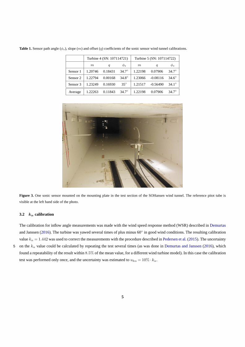
Table 1.Sensor path angle (φs), slope (m) and offset (q) coefficients of the sonic sensor wind tunnel calibrations.
Turbine 4 (SN:107114721) Turbine 5 (SN:107114722)
m q φs m q φs
Sensor1 1.20746 0.18431 34.7◦ 1.22198 0.07906 34.7◦
Sensor2 1.22794 0.00168 34.8◦ 1.23066 -0.08116 34.6◦
Sensor3 1.23249 0.16930 35◦ 1.21517 -0.56490 34.1◦
Average 1.22263 0.11843 34.7◦ 1.22198 0.07906 34.7◦
Figure 3. One sonic sensor mounted on the mounting plate in the test section of the SOHansen wind tunnel. The reference pitot tube is
visible at the left hand side of the photo.
3.2 kα calibration
The calibration for inflow angle measurements was made with the wind speed response method (WSR) described inDemurtas
and Janssen (2016). The turbine was yawed several times of plus minus 60◦ in good wind conditions. The resulting calibration
valuekα = 1.442 was used to correct the measurements with the procedure described inPedersen et al.(2015). The uncertainty
on thekα value could be calculated by repeating the test several times (as was done inDemurtas and Janssen(2016), which5
found a repeatability of the result within8.5% of the mean value, for a different wind turbine model). In this case the calibration
test was performed only once, and the uncertainty was estimated toukα = 10% ∙ kα.
5
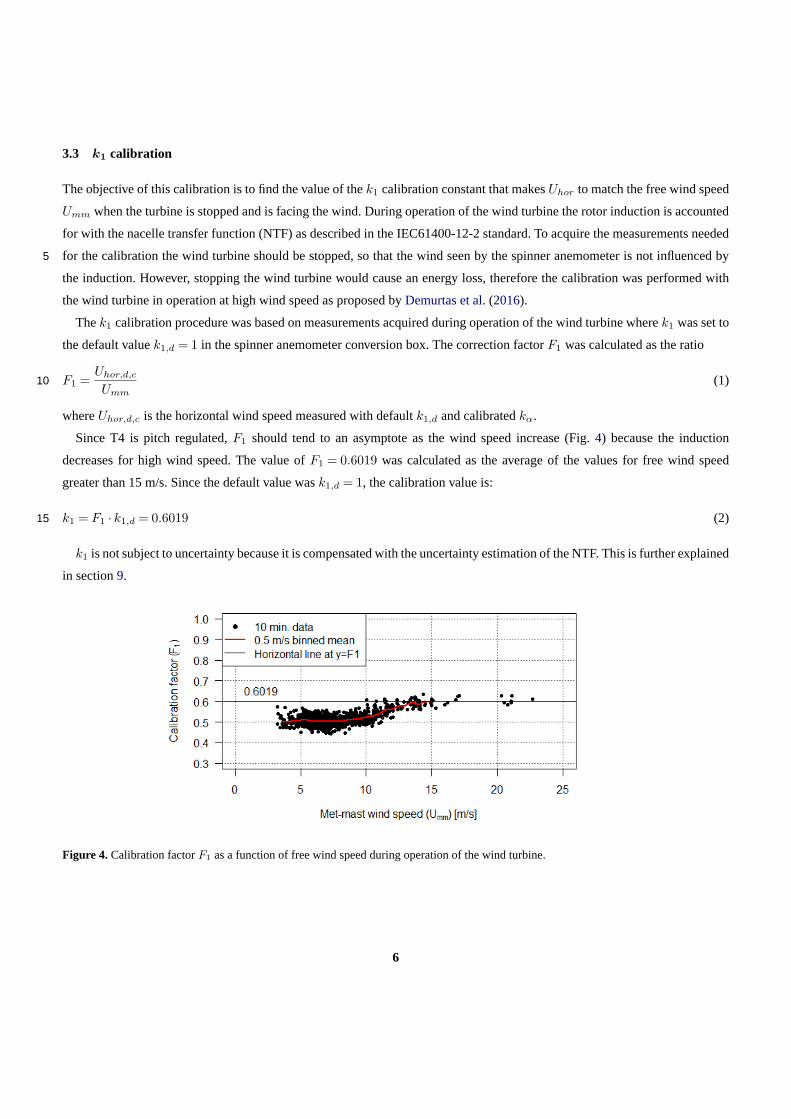
3.3 k1 calibration
The objective of this calibration is to find the value of thek1 calibration constant that makesUhor to match the free wind speed
Umm when the turbine is stopped and is facing the wind. During operation of the wind turbine the rotor induction is accounted
for with the nacelle transfer function (NTF) as described in the IEC61400-12-2 standard. To acquire the measurements needed
for the calibration the wind turbine should be stopped, so that the wind seen by the spinner anemometer is not influenced by5
the induction. However, stopping the wind turbine would cause an energy loss, therefore the calibration was performed with
the wind turbine in operation at high wind speed as proposed byDemurtas et al.(2016).
Thek1 calibration procedure was based on measurements acquired during operation of the wind turbine wherek1 was set to
the default valuek1,d = 1 in the spinner anemometer conversion box. The correction factorF1 was calculated as the ratio
F1 =Uhor,d,c
Umm(1)10
whereUhor,d,c is the horizontal wind speed measured with defaultk1,d and calibratedkα.
Since T4 is pitch regulated,F1 should tend to an asymptote as the wind speed increase (Fig.4) because the induction
decreases for high wind speed. The value ofF1 = 0.6019 was calculated as the average of the values for free wind speed
greater than 15 m/s. Since the default value wask1,d = 1, the calibration value is:
k1 = F1 ∙ k1,d = 0.6019 (2)15
k1 is not subject to uncertainty because it is compensated with the uncertainty estimation of the NTF. This is further explained
in section9.
Figure 4. Calibration factorF1 as a function of free wind speed during operation of the wind turbine.
6
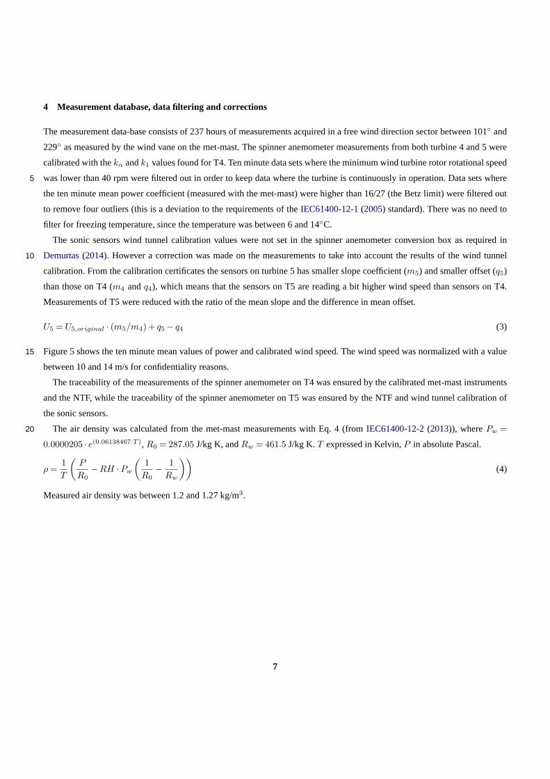
4 Measurement database, data filtering and corrections
The measurement data-base consists of 237 hours of measurements acquired in a free wind direction sector between 101◦ and
229◦ as measured by the wind vane on the met-mast. The spinner anemometer measurements from both turbine 4 and 5 were
calibrated with thekα andk1 values found for T4. Ten minute data sets where the minimum wind turbine rotor rotational speed
was lower than 40 rpm were filtered out in order to keep data where the turbine is continuously in operation. Data sets where5
the ten minute mean power coefficient (measured with the met-mast) were higher than 16/27 (the Betz limit) were filtered out
to remove four outliers (this is a deviation to the requirements of theIEC61400-12-1(2005) standard). There was no need to
filter for freezing temperature, since the temperature was between 6 and 14◦C.
The sonic sensors wind tunnel calibration values were not set in the spinner anemometer conversion box as required in
Demurtas(2014). However a correction was made on the measurements to take into account the results of the wind tunnel10
calibration. From the calibration certificates the sensors on turbine 5 has smaller slope coefficient (m5) and smaller offset (q5)
than those on T4 (m4 andq4), which means that the sensors on T5 are reading a bit higher wind speed than sensors on T4.
Measurements of T5 were reduced with the ratio of the mean slope and the difference in mean offset.
U5 = U5,original ∙ (m5/m4)+ q5 − q4 (3)
Figure5 shows the ten minute mean values of power and calibrated wind speed. The wind speed was normalized with a value15
between 10 and 14 m/s for confidentiality reasons.
The traceability of the measurements of the spinner anemometer on T4 was ensured by the calibrated met-mast instruments
and the NTF, while the traceability of the spinner anemometer on T5 was ensured by the NTF and wind tunnel calibration of
the sonic sensors.
The air density was calculated from the met-mast measurements with Eq.4 (from IEC61400-12-2(2013)), wherePw =20
0.0000205 ∙ e(0.06138467∙T ), R0 = 287.05 J/kg K, andRw = 461.5 J/kg K.T expressed in Kelvin,P in absolute Pascal.
ρ =1T
(P
R0−RH ∙Pw
(1
R0−
1Rw
))
(4)
Measured air density was between 1.2 and 1.27 kg/m3.
7
Figure 5. Scatter plot of power as a function of spinner anemometer normalized wind speed (n.w.s.) and met-mast normalized wind speed
measurements, for turbines T4 and T5, before application of the NTF and before air density correction. Met-mast measurements to the left,
and spinner anemometer measurements to the right. Turbine T4 measurements upper and turbine T5 measurements lower. Data refers to the
same measurement period.
5 Nacelle transfer function measurement
The purpose of the NTF is to correct the spinner anemometer measurements to be representative of the free wind speed.
Umm is the free wind speed measured by the met-mast, andUfree is the free wind speed calculated by correcting the spinner
anemometer measurements (Uhor) with the NTF.
TheIEC61400-12-2(2013) standard defines the NTF as the met-mast wind speed binned as a function of the nacelle wind5
speed.Krishna et al.(2014) investigated the root cause for high deviations in the self consistency check with theIEC61400-
12-2 (2013) method and proposed an improved method, which consist of binning the spinner anemometer wind speed as a
function of the met-mast wind speed. This procedure is used here. If a wind speed bin has less than 3 measurements, the value
8

of the NTF is calculated by linear interpolation from the adjacent bins if they both have at least 3 measurements each. No air
density correction was made for the measurement of the NTF. The measured NTF for the spinner anemometer installed on
turbine T4 is shown in Fig.6 .
As expected the NTF is approximately 1:1 at high wind speed (around 11-15 m/s, thanks to thek1 calibration), and is lower
than 1:1 for the range of wind speeds where the turbine is operating with high Cp (high induction, which makes the wind speed5
by the spinner anemometer lower than the free wind speed).
Figure 6. Nacelle transfer function measured with the spinner anemometer of turbine 4. Red line is the NTF obtained by linear interpolation
between the red dots, which are the NTF binned values.
6 NTF self consistency check
The black line in Fig.7 shows the power difference between the PC and the NPC of turbine 4. The blue and red curves shows
the pass/fail boundaries defined inIEC61400-12-2(2013) for the NTF. Both power curves were interpolated to the center of
the bin with a cubic spline1, so that the power values for the two power curves correspond to the same wind speed.Krishna10
et al. (2014) claimed that a NPC calculated from the same data-set used to measure the NTF (as it is the case for turbine 4)
is identical to the PC (and therefore the self consistency check should return zero power difference for any wind speed bin).
However in the present calculations the power difference was not zero. The PC was binned according to the met-mast wind
speed (Umm), and the NPC was binned according to the corrected nacelle wind speed (Ufree). Krishna et al.(2014) suggested
to bin both PC and NPC according toUmm to keep uniformity in the binning process, but doing so would mean binning the15
exact same measurements for NPC and PC, resulting obviously in the same binned values of power.
1as suggested in the draft of IEC61400-12-1, 88/460/CD, regarding presenting a power curve with values interpolated to the center of the bin.
9
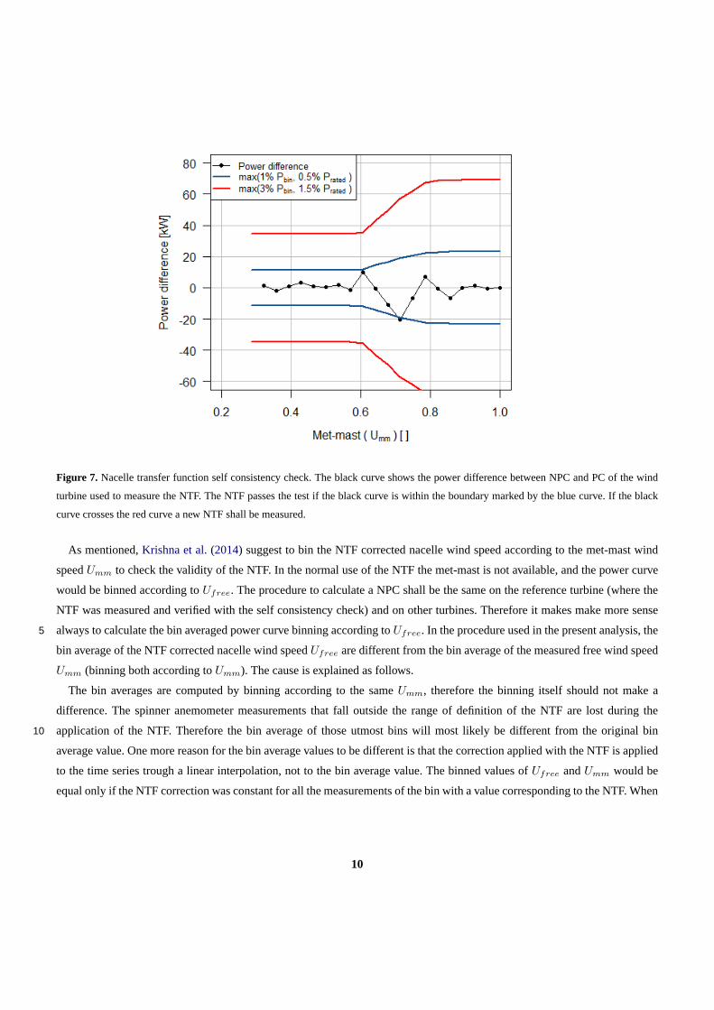
Figure 7. Nacelle transfer function self consistency check. The black curve shows the power difference between NPC and PC of the wind
turbine used to measure the NTF. The NTF passes the test if the black curve is within the boundary marked by the blue curve. If the black
curve crosses the red curve a new NTF shall be measured.
As mentioned,Krishna et al.(2014) suggest to bin the NTF corrected nacelle wind speed according to the met-mast wind
speedUmm to check the validity of the NTF. In the normal use of the NTF the met-mast is not available, and the power curve
would be binned according toUfree. The procedure to calculate a NPC shall be the same on the reference turbine (where the
NTF was measured and verified with the self consistency check) and on other turbines. Therefore it makes make more sense
always to calculate the bin averaged power curve binning according toUfree. In the procedure used in the present analysis, the5
bin average of the NTF corrected nacelle wind speedUfree are different from the bin average of the measured free wind speed
Umm (binning both according toUmm). The cause is explained as follows.
The bin averages are computed by binning according to the sameUmm, therefore the binning itself should not make a
difference. The spinner anemometer measurements that fall outside the range of definition of the NTF are lost during the
application of the NTF. Therefore the bin average of those utmost bins will most likely be different from the original bin10
average value. One more reason for the bin average values to be different is that the correction applied with the NTF is applied
to the time series trough a linear interpolation, not to the bin average value. The binned values ofUfree andUmm would be
equal only if the NTF correction was constant for all the measurements of the bin with a value corresponding to the NTF. When
10
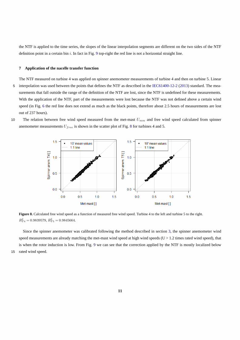
the NTF is applied to the time series, the slopes of the linear interpolation segments are different on the two sides of the NTF
definition point in a certain bini. In fact in Fig.9 top-right the red line is not a horizontal straight line.
7 Application of the nacelle transfer function
The NTF measured on turbine 4 was applied on spinner anemometer measurements of turbine 4 and then on turbine 5. Linear
interpolation was used between the points that defines the NTF as described in theIEC61400-12-2(2013) standard. The mea-5
surements that fall outside the range of the definition of the NTF are lost, since the NTF is undefined for these measurements.
With the application of the NTF, part of the measurements were lost because the NTF was not defined above a certain wind
speed (in Fig.6 the red line does not extend as much as the black points, therefore about 2.5 hours of measurements are lost
out of 237 hours).
The relation between free wind speed measured from the met-mastUmm and free wind speed calculated from spinner10
anemometer measurementsUfree is shown in the scatter plot of Fig.8 for turbines 4 and 5.
Figure 8. Calculated free wind speed as a function of measured free wind speed. Turbine 4 to the left and turbine 5 to the right.
R2T4 = 0.9839579, R2
T5 = 0.9845664.
Since the spinner anemometer was calibrated following the method described in section3, the spinner anemometer wind
speed measurements are already matching the met-mast wind speed at high wind speeds (U > 1.2 times rated wind speed), that
is when the rotor induction is low. From Fig.9 we can see that the correction applied by the NTF is mostly localized below
rated wind speed.15
11

Figure 9. Ratio between calculated free wind speed and measured free wind speed (Ufree/Umm) as a function of measured free wind speed
(Umm).
8 Power curves and AEP
The calculated free wind speed and measured free wind speed were corrected to standard air density of 1.225 kg/m3 with Eq.
5 after the application of the NTF. This is in accordance withIEC61400-12-2(2013) for a pitch regulated turbine.
Ufree,n = Ufree
( ρ
1.225
)1/3
(5)
The met-mast power curve was also corrected to standard air density of 1.225 kg/m3 with Eq.6 in accordance withIEC61400-5
12-1 (2005) for a pitch regulated turbine.
Umm,n = Umm
( ρ
1.225
)1/3
(6)
The power curves of turbines 4 and 5 were obtained by averaging the power in each wind speed bin of 0.5 m/s, see Fig.10.
The value of power was interpolated with a cubic spline to the center of the wind speed bin so that the power values of the four
power curves are comparable (they all refer to the center of the wind speed bins).10
Figure10shows the four power curves, NPC for T4, PC for T4, NPC for T5, PC for T5.
12

Figure 10.Power curves of turbines 4 and 5, measured with met-mast and with spinner anemometer.
A measure of the difference between the curves was evaluated by calculating the annual energy production (AEP) for a
Rayleigh wind speed distribution with annual average wind speed between 4 m/s and 11 m/s. Table2 shows the difference in
AEP estimated for the four power curves. The AEP was calculated for the extrapolated power curve up to 25 m/s.
The nacelle power curve compared with the met-mast power curve within 0.10 % of AEP (at 8 m/s average wind speed) on
the reference turbine, and within 0.38 % on the other turbine (see Tab.2). The NPC is not identical to the PC, as well as the5
binned values ofUfree are not equal to the binned values ofUmm even when binning both according toUmm.
As expected, PC4 with NPC4 compares better than PC5 with NPC5, since the NTF was measured on T4. The uncertainty
on AEP calculated for PC4 in the DTU report I-0440Demurtas(2015) (with the same turbine and same measurement set-up,
but not public for confidentiality of the data presented) was found to be 14.2% forVavg = 4 m/s, 5.7% forVavg = 8 m/s and
4.2% forVavg = 11 m/s. The AEP difference is more than ten times smaller than the AEP uncertainty.10
13

Table 2. Comparison between met-mast power curve (PC) and nacelle (spinner) power curve (NPC) in terms of annual energy production.
The values in the table are calculated as(from/to− 1) ∙ 100. The AEP was calculated with the extrapolated power curve from valid data to
25 m/s.
Vavg From: NPC4 NPC5 PC5 NPC5
to: PC4 PC5 PC4 NPC4
m/s % % % %
4 0.10 -1.35 -1.04 -2.47
5 0.14 -0.95 -0.74 -1.82
6 0.13 -0.69 -0.55 -1.37
7 0.12 -0.51 -0.44 -1.06
8 0.10 -0.38 -0.36 -0.84
9 0.09 -0.30 -0.31 -0.69
10 0.07 -0.24 -0.28 -0.59
11 0.07 -0.19 -0.25 -0.51
9 Uncertainty analysis
This section will describe the evaluation of uncertainty of the free wind speed measured with the met-mast, and free wind speed
calculated with an NTF applied to spinner anemometer measurements. The spinner anemometer measures the wind speed by
means of three sonic sensors and a conversion algorithm. Each sensor was calibrated independently in a MEASNET compliant
wind tunnel. The uncertainty of the three velocities were combined through the spinner anemometer conversion algorithm to5
give the uncertainty of the horizontal wind speed.
The uncertainty of spinner anemometer on T4 due to differences in mounting of the three sonic sensors is zero, since this
spinner anemometer was used to measure the NTF. The mounting of the second spinner anemometer (on T5) was compared
with the mounting of the reference spinner anemometer (on T4) and an additional uncertainty due to mounting differences with
respect to T4 was added to the measurements of the spinner anemometer on T5.10
9.1 Uncertainty related to wind tunnel calibration of sonic sensors
The relation between the wind tunnel speed and the velocity component in the sensor path is:
V1 = Vt ∙ cos(φs) (7)
If the angleφs of the sonic sensor path with respect to the horizontal mounting plate was not measured, one should assume
thatφs is within the manufacturing tolerance,φs = 35◦ ± 1.5◦. The standard uncertainty onφs can therefore be expressed by15
the tolerance divided by the square root of three as:
uφs = (a+ − a−)/(2√
3) = (36.5− 33.5)/(2√
3) = 0.866◦ (8)
14
In this case the angleφs was measured as part of the wind tunnel calibration (see Tab.1). The uncertainty onφs depends on
the accuracy of the protractor (the instrument to measure angles). In this case, a digital protractor with an accuracy of 0.2◦ was
used, and thereforeuφs = 0.2◦ was used instead of0.866◦ .
The uncertainty on the wind tunnel calibration was expressed in the calibration certificates for a coverage factorkc = 2 as a
binned value as a function of wind tunnel speed. While the uncertainty is typically almost constant for a cup anemometer, the5
sonic sensor uncertainty showed increase with wind speed. The standard uncertainty (kc = 1) was calculated by dividing the
value reported in the certificates by two. The calibration standard uncertainty (function of wind speed) was fitted to a line as
shown in Eq.9.
ut = (2.24 ∙Vi +0.855) ∙ 10−3m/s (9)
The uncertainty on the sonic sensor velocityV1 is obtained combining the uncertaintyut with the uncertaintyuφs, using10
the equation for combination of uncertainty of independent variables as expressed in Eq.10 (according to section 5.1.2 of the
GUM, JCGM/WG1(2008)) and also shown inIECRE(2015) clarification sheet.
u2c(y) =
N∑
i=1
(∂f
∂xi
)
u2(xi) (10)
Equation10applied to Eq.7 results in Eq.11:
u21 =
(∂(Vt cosφs)
∂Vt
)2
u2t +
(∂(Vt cosφs)
∂φs
)2
uφ2s = cos2 φs ∙u
2t + V 2
t sin2 φs ∙uφ2s (11)15
With ut (Eq.9) as the uncertainty of the wind tunnel wind speed anduφs as the uncertainty on the sensor path angle (Eq.8 or
uncertainty of the protractor). The combined uncertainty onV1 due to wind tunnel calibration is:
u1 =√
(cosφs)2 ∙u2t +(Vt ∙ sinφs)2 ∙uφ
2s (12)
The same applies to each of the sensors (u2, u3).
9.2 Evaluation of spinner anemometer mounting20
The three sonic sensors should be mounted on the spinner with the best possible rotational symmetry and equal distance from
the spinner center of rotation. A visualization method for documentation of the sonic sensors installations was developed by
Demurtas and Pedersen with the use of photography,Demurtas(2015). The initial mounting of the sensors was used for the
first power curve measurements reported inDemurtas(2015). The accuracy of sensor mounting was then improved and the
power curve measurement repeated and reported in this work. The mounting position was evaluated with photography method25
described in . Due to the challenge of photographing a feature of size in the order of centimeters (the sonic sensor) from a long
distance (80 meters from ground to spinner) we used a 400 mm optic zoom and a high resolution digital camera (24 megapixel).
15
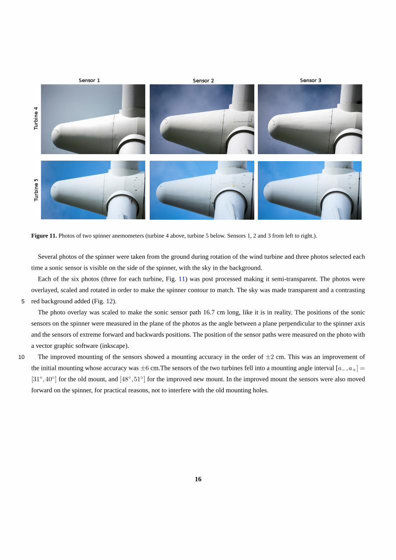
Figure 11.Photos of two spinner anemometers (turbine 4 above, turbine 5 below. Sensors 1, 2 and 3 from left to right.).
Several photos of the spinner were taken from the ground during rotation of the wind turbine and three photos selected each
time a sonic sensor is visible on the side of the spinner, with the sky in the background.
Each of the six photos (three for each turbine, Fig.11) was post processed making it semi-transparent. The photos were
overlayed, scaled and rotated in order to make the spinner contour to match. The sky was made transparent and a contrasting
red background added (Fig.12).5
The photo overlay was scaled to make the sonic sensor path 16.7 cm long, like it is in reality. The positions of the sonic
sensors on the spinner were measured in the plane of the photos as the angle between a plane perpendicular to the spinner axis
and the sensors of extreme forward and backwards positions. The position of the sensor paths were measured on the photo with
a vector graphic software (inkscape).
The improved mounting of the sensors showed a mounting accuracy in the order of±2 cm. This was an improvement of10
the initial mounting whose accuracy was±6 cm.The sensors of the two turbines fell into a mounting angle interval [a−,a+] =
[31◦,40◦] for the old mount, and[48◦,51◦] for the improved new mount. In the improved mount the sensors were also moved
forward on the spinner, for practical reasons, not to interfere with the old mounting holes.
16

Figure 12.Sonic sensors relative mounting position between turbine 4 and turbine 5. Not to scale, dimensions are in centimeters.
Left: original mounting. Right: after improvement of the mounting accuracy. The blue lines connects the center of the spinner sphere with the
extreme mounting position of the sensors. In the figure at the right hand side four blue lines show the position of the original and improved
mounting.
9.3 Uncertainty in wind speed measurements due to mounting imperfections
The uncertainty connected to the error in mounting position of the sonic sensor was investigated approximating the spinner as
a sphere and using potential flow theory to calculate the flow around a sphere. The mean air velocity along the sensor path was
calculated averaging the wind velocity component along the sensor path in three points along the path (points shown with a
black or red dots in Fig.13).5
The flow field was calculated for a mesh of 0.01 inx andy direction. The coordinates of each point were converted from
cartesian coordinates (xp, yp) to polar coordinates (r, θ) with Eq.13and Eq.14. An angle ofπ/2 was added to theθp coordinate
(Eq.14) to rotate the result in order to have the flow coming from the left parallel to thex axis. This also rotated the origin of
the angles to the vertical axis, which is convenient to measure the position of the mounting angles of the sonic sensors.
r =√
(x2p + y2
p) (13)10
θp = arctan(yp/xp)+ π/2 (14)
17

Figure 13. Simulation of the flow around the spinner, which was approximated to a sphere. The flow was calculated with the equations of
the potential flow around a sphere. The sensor positions retrace the position of the sensors found in Fig.12. The sensor paths with the red
dots refer to the old mount (31◦, 40◦), while these with the black dots refer to the improved mounting (48◦, 51◦), where the sensors are more
closely spaced.
The potential flow model is oriented such that the inflow is in axis with the pinner axis of rotation, thereforeU = Uhor = U0.
The flow field was calculated in polar coordinates with Eq.15 (along radius) and Eq.16 (perpendicular to radius) with the
equations byFaith and Morrison(2013).
vr = U0[1− (R/r)3] cos(θp) (15)
5
vt = −U0[1+ 0.5 ∙ (R/r)3] sin(θp) (16)
The modulus of the wind speed was calculated with Eq.17and shown with the color scale in Fig.13.
U =√
(v2r + v2
t ) (17)
The air velocity along the sensor path at the pointp(r,θ) was calculated with Eq.18, where 35◦ is the default angle between
the sensor path and the sensor root (tangent to the spinner surface).10
Up = vr ∙ sin(35 ∙π/180)− vt ∙ cos(35 ∙π/180) (18)
18
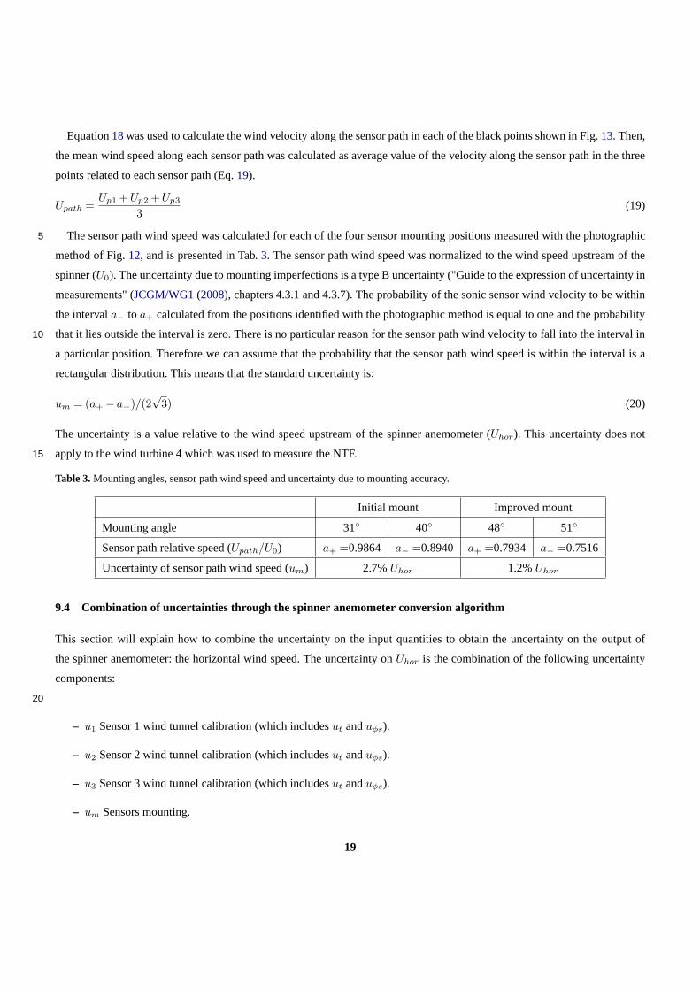
Equation18was used to calculate the wind velocity along the sensor path in each of the black points shown in Fig.13. Then,
the mean wind speed along each sensor path was calculated as average value of the velocity along the sensor path in the three
points related to each sensor path (Eq.19).
Upath =Up1 + Up2 + Up3
3(19)
The sensor path wind speed was calculated for each of the four sensor mounting positions measured with the photographic5
method of Fig.12, and is presented in Tab.3. The sensor path wind speed was normalized to the wind speed upstream of the
spinner (U0). The uncertainty due to mounting imperfections is a type B uncertainty ("Guide to the expression of uncertainty in
measurements" (JCGM/WG1(2008), chapters 4.3.1 and 4.3.7). The probability of the sonic sensor wind velocity to be within
the intervala− to a+ calculated from the positions identified with the photographic method is equal to one and the probability
that it lies outside the interval is zero. There is no particular reason for the sensor path wind velocity to fall into the interval in10
a particular position. Therefore we can assume that the probability that the sensor path wind speed is within the interval is a
rectangular distribution. This means that the standard uncertainty is:
um = (a+ − a−)/(2√
3) (20)
The uncertainty is a value relative to the wind speed upstream of the spinner anemometer (Uhor). This uncertainty does not
apply to the wind turbine 4 which was used to measure the NTF.15
Table 3.Mounting angles, sensor path wind speed and uncertainty due to mounting accuracy.
Initial mount Improvedmount
Mountingangle 31◦ 40◦ 48◦ 51◦
Sensor path relative speed (Upath/U0) a+ =0.9864 a− =0.8940 a+ =0.7934 a− =0.7516
Uncertainty of sensor path wind speed (um) 2.7%Uhor 1.2%Uhor
9.4 Combination of uncertainties through the spinner anemometer conversion algorithm
This section will explain how to combine the uncertainty on the input quantities to obtain the uncertainty on the output of
the spinner anemometer: the horizontal wind speed. The uncertainty onUhor is the combination of the following uncertainty
components:
20
– u1 Sensor 1 wind tunnel calibration (which includesut anduφs).
– u2 Sensor 2 wind tunnel calibration (which includesut anduφs).
– u3 Sensor 3 wind tunnel calibration (which includesut anduφs).
– um Sensors mounting.
19
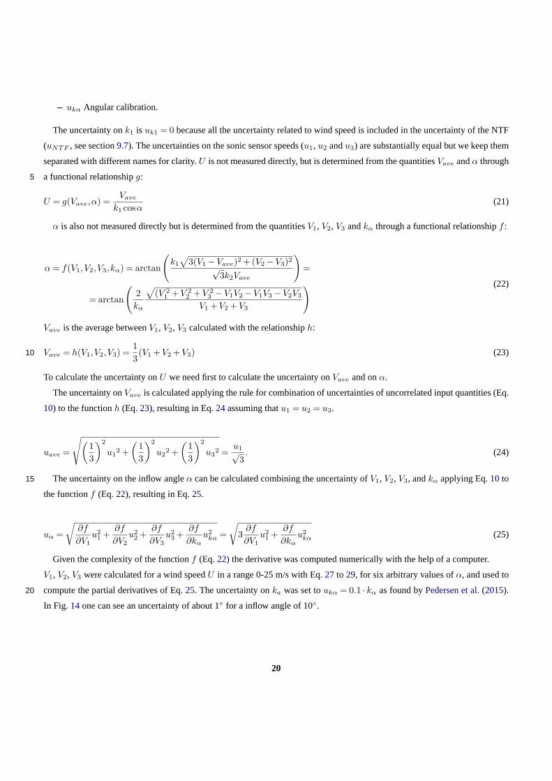
– ukα Angular calibration.
The uncertainty onk1 is uk1 = 0 because all the uncertainty related to wind speed is included in the uncertainty of the NTF
(uNTF , see section9.7). The uncertainties on the sonic sensor speeds (u1, u2 andu3) are substantially equal but we keep them
separated with different names for clarity.U is not measured directly, but is determined from the quantitiesVave andα through
a functional relationshipg:5
U = g(Vave,α) =Vave
k1 cosα(21)
α is also not measured directly but is determined from the quantitiesV1, V2, V3 andkα through a functional relationshipf :
α = f(V1,V2,V3,kα) = arctan
(k1
√3(V1 −Vave)2 + (V2 −V3)2√
3k2Vave
)
=
= arctan
(2kα
√(V 2
1 + V 22 + V 2
3 −V1V2 −V1V3 −V2V3
V1 + V2 + V3
) (22)
Vave is the average betweenV1, V2, V3 calculated with the relationshiph:
Vave = h(V1,V2,V3) =13(V1 + V2 + V3) (23)10
To calculate the uncertainty onU we need first to calculate the uncertainty onVave and onα.
The uncertainty onVave is calculated applying the rule for combination of uncertainties of uncorrelated input quantities (Eq.
10) to the functionh (Eq.23), resulting in Eq.24assuming thatu1 = u2 = u3.
uave =
√(13
)2
u12 +
(13
)2
u22 +
(13
)2
u32 =
u1√3. (24)
The uncertainty on the inflow angleα can be calculated combining the uncertainty ofV1, V2, V3, andkα applying Eq.10 to15
the functionf (Eq.22), resulting in Eq.25.
uα =
öf
∂V1u2
1 +∂f
∂V2u2
2 +∂f
∂V3u2
3 +∂f
∂kαu2
kα =
√
3∂f
∂V1u2
1 +∂f
∂kαu2
kα (25)
Given the complexity of the functionf (Eq.22) the derivative was computed numerically with the help of a computer.
V1, V2, V3 were calculated for a wind speedU in a range 0-25 m/s with Eq.27 to 29, for six arbitrary values ofα, and used to
compute the partial derivatives of Eq.25. The uncertainty onka was set toukα = 0.1 ∙ kα as found byPedersen et al.(2015).20
In Fig. 14one can see an uncertainty of about 1◦ for a inflow angle of 10◦.
20
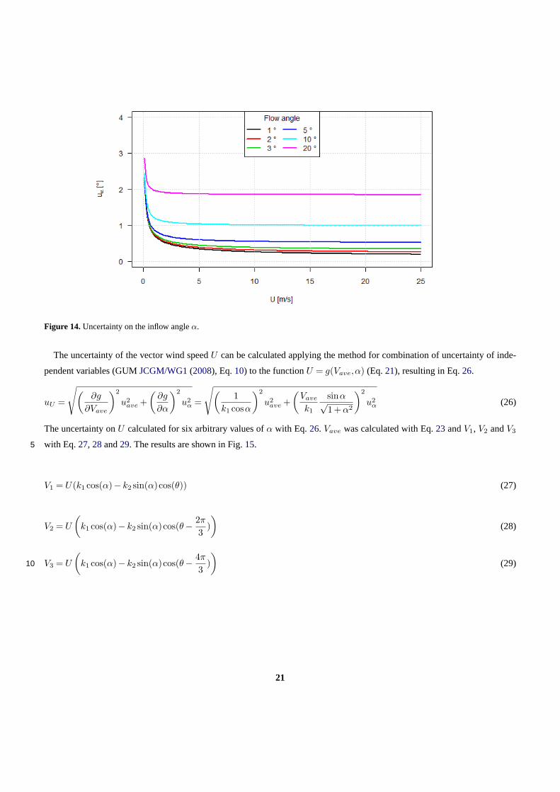
Figure 14.Uncertainty on the inflow angleα.
The uncertainty of the vector wind speedU can be calculated applying the method for combination of uncertainty of inde-
pendent variables (GUMJCGM/WG1(2008), Eq.10) to the functionU = g(Vave,α) (Eq.21), resulting in Eq.26.
uU =
√(∂g
∂Vave
)2
u2ave +
(∂g
∂α
)2
u2α =
√(1
k1 cosα
)2
u2ave +
(Vave
k1
sinα√
1 + α2
)2
u2α (26)
The uncertainty onU calculated for six arbitrary values ofα with Eq.26. Vave was calculated with Eq.23 andV1, V2 andV3
with Eq.27, 28and29. The results are shown in Fig.15.5
V1 = U(k1 cos(α)− k2 sin(α)cos(θ)) (27)
V2 = U
(
k1 cos(α)− k2 sin(α)cos(θ−2π
3)
)
(28)
V3 = U
(
k1 cos(α)− k2 sin(α)cos(θ−4π
3)
)
(29)10
21
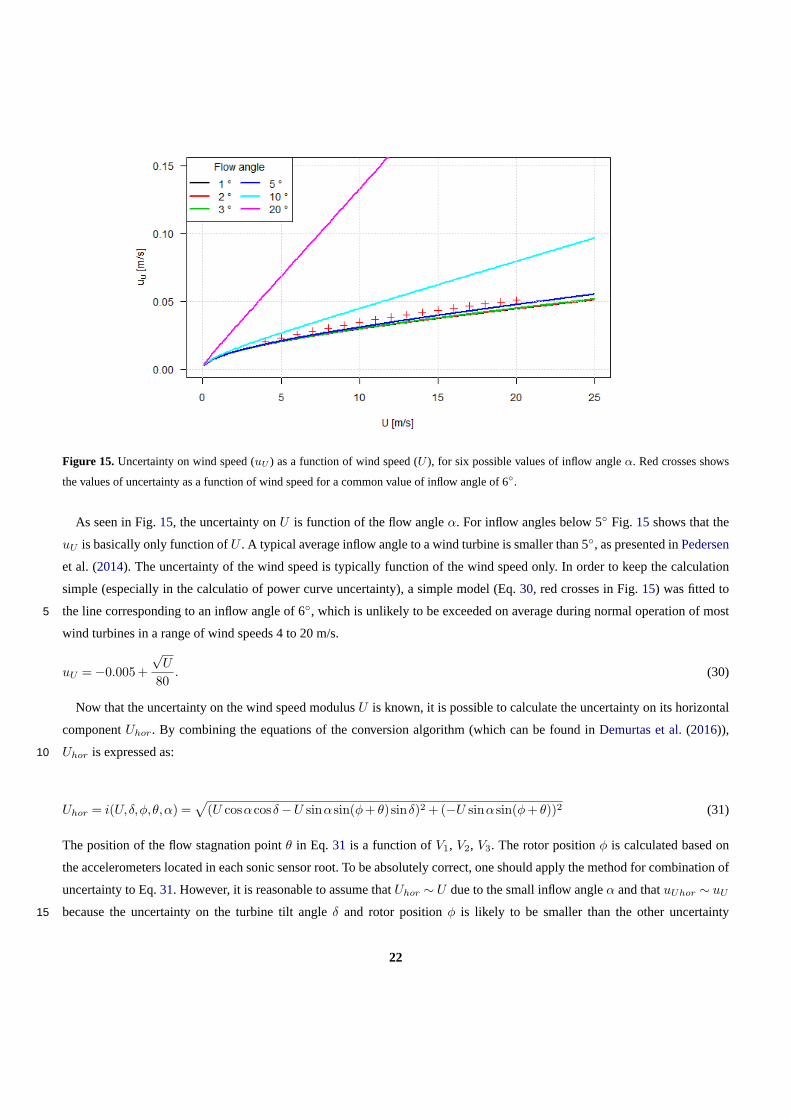
Figure 15. Uncertainty on wind speed (uU ) as a function of wind speed (U ), for six possible values of inflow angleα. Red crosses shows
the values of uncertainty as a function of wind speed for a common value of inflow angle of 6◦.
As seen in Fig.15, the uncertainty onU is function of the flow angleα. For inflow angles below 5◦ Fig. 15 shows that the
uU is basically only function ofU . A typical average inflow angle to a wind turbine is smaller than 5◦, as presented inPedersen
et al. (2014). The uncertainty of the wind speed is typically function of the wind speed only. In order to keep the calculation
simple (especially in the calculatio of power curve uncertainty), a simple model (Eq.30, red crosses in Fig.15) was fitted to
the line corresponding to an inflow angle of 6◦, which is unlikely to be exceeded on average during normal operation of most5
wind turbines in a range of wind speeds 4 to 20 m/s.
uU = −0.005+
√U
80. (30)
Now that the uncertainty on the wind speed modulusU is known, it is possible to calculate the uncertainty on its horizontal
componentUhor. By combining the equations of the conversion algorithm (which can be found inDemurtas et al.(2016)),
Uhor is expressed as:10
Uhor = i(U,δ,φ,θ,α) =√
(U cosαcosδ−U sinαsin(φ + θ)sinδ)2 + (−U sinαsin(φ + θ))2 (31)
The position of the flow stagnation pointθ in Eq. 31 is a function ofV1, V2, V3. The rotor positionφ is calculated based on
the accelerometers located in each sonic sensor root. To be absolutely correct, one should apply the method for combination of
uncertainty to Eq.31. However, it is reasonable to assume thatUhor ∼ U due to the small inflow angleα and thatuUhor ∼ uU
because the uncertainty on the turbine tilt angleδ and rotor positionφ is likely to be smaller than the other uncertainty15
22
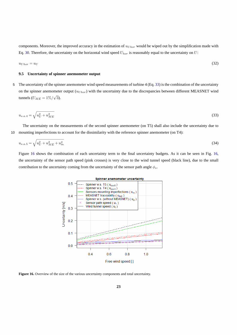
components. Moreover, the improved accuracy in the estimation ofuUhor would be wiped out by the simplification made with
Eq.30. Therefore, the uncertainty on the horizontal wind speedUhor is reasonably equal to the uncertainty onU :
uUhor = uU (32)
9.5 Uncertainty of spinner anemometer output
The uncertainty of the spinner anemometer wind speed measurements of turbine 4 (Eq.33) is the combination of the uncertainty5
on the spinner anemometer output (uUhor) with the uncertainty due to the discrepancies between different MEASNET wind
tunnels (UME = 1%/√
3).
us.a.4 =√
u2U + u2
ME (33)
The uncertainty on the measurements of the second spinner anemometer (on T5) shall also include the uncertainty due to
mounting imperfections to account for the dissimilarity with the reference spinner anemometer (on T4):10
us.a.5 =√
u2U + u2
ME + u2m (34)
Figure 16 shows the combination of each uncertainty term to the final uncertainty budgets. As it can be seen in Fig.16,
the uncertainty of the sensor path speed (pink crosses) is very close to the wind tunnel speed (black line), due to the small
contribution to the uncertainty coming from the uncertainty of the sensor path angleφs.
Figure 16.Overview of the size of the various uncertainty components and total uncertainty.
23
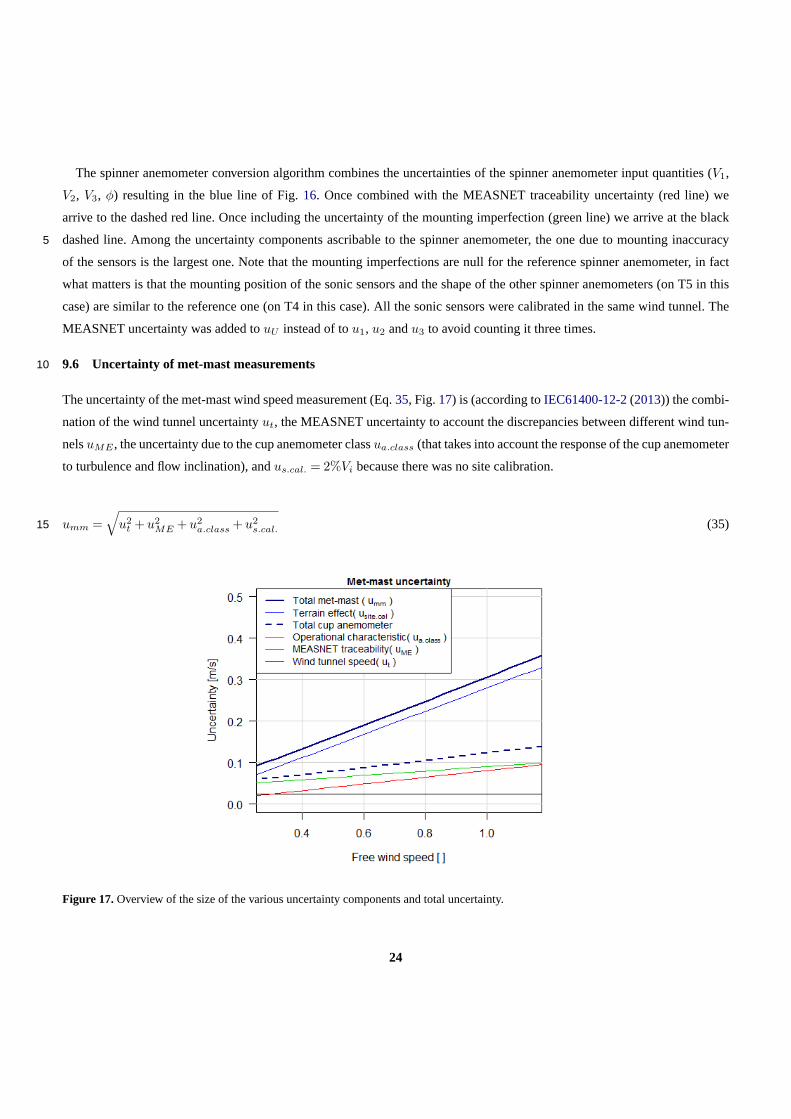
The spinner anemometer conversion algorithm combines the uncertainties of the spinner anemometer input quantities (V1,
V2, V3, φ) resulting in the blue line of Fig.16. Once combined with the MEASNET traceability uncertainty (red line) we
arrive to the dashed red line. Once including the uncertainty of the mounting imperfection (green line) we arrive at the black
dashed line. Among the uncertainty components ascribable to the spinner anemometer, the one due to mounting inaccuracy5
of the sensors is the largest one. Note that the mounting imperfections are null for the reference spinner anemometer, in fact
what matters is that the mounting position of the sonic sensors and the shape of the other spinner anemometers (on T5 in this
case) are similar to the reference one (on T4 in this case). All the sonic sensors were calibrated in the same wind tunnel. The
MEASNET uncertainty was added touU instead of tou1, u2 andu3 to avoid counting it three times.
9.6 Uncertainty of met-mast measurements10
The uncertainty of the met-mast wind speed measurement (Eq.35, Fig.17) is (according toIEC61400-12-2(2013)) the combi-
nation of the wind tunnel uncertaintyut, the MEASNET uncertainty to account the discrepancies between different wind tun-
nelsuME , the uncertainty due to the cup anemometer classua.class (that takes into account the response of the cup anemometer
to turbulence and flow inclination), andus.cal. = 2%Vi because there was no site calibration.
umm =√
u2t + u2
ME + u2a.class + u2
s.cal. (35)15
Figure 17.Overview of the size of the various uncertainty components and total uncertainty.
24

9.7 Uncertainty of NTF
The uncertainty on the NTF (uNTF ) is the combination of the various uncertainty components as:
uNTF =√
u2mm + u2
sa4 + u2M + s2
NTF (36)
where
umm is the uncertainty on the measured free wind speed.5
usa is the uncertainty of the spinner anemometer measurements.
uM is the uncertainty due to the NTF method, considered 2% of the wind speed due to seasonal variations (uM = 0.02Vi) in
the standard IEC61400-12-2.
sNTF is the statistical uncertainty of the captured data-set (sNTF = σNT F√Nj
Usa4). σNTF is dimensionless because it is the
standard deviation of the ratioUfree/Usa4.10
9.8 Uncertainty on calculated free wind speed
To measure the absolute power curve of a wind turbine the spinner anemometer output must be corrected to free wind speed
by use of the nacelle transfer function (NTF). The uncertainty on the free wind speed is therefore a combination ofus.a. with
uNTF .
ufree5 =√
u2sa5 + u2
NTF (37)15
For the case of the reference wind turbine (T4, used to measure the NTF) the uncertainty is calculated differently.uNTF
already contains the uncertainty of the reference spinner anemometer (T4) and the uncertainty of the met-mast measurements.
Therefore the uncertainty of the free wind speed calculated with the NTF is just the uncertainty of the NTF (Eq.38).
ufree4 = uNTF (38)
25

10 Results of uncertainty analysis
The mounting accuracy was investigated by overlaying six photos of the spinner taken from ground level during rotation, each
showing the corresponding sensor when it is at the side of the spinner. The photos unveil deviations in the order of±2 cm
between some of the sensors. It was expected that the mounting imperfections played a major role in the total uncertainty of
the second spinner anemometer. However, the contribution of other uncertainty sources combined (the1/√
3% MEASNET5
traceability of wind tunnel calibrations for cup-anemometer on the met-mast and spinner anemometers sensors, the 2% for
lack of site calibration) was much larger than the uncertainty due to the mounting of the sensors (which was 1.2%).
Figure 18.Uncertainty on wind speed. The met-mast wind speed includes 2% additional uncertainty due to lack of site calibration.
As shown in Fig.18, the uncertainty of the NTF is larger than the met-mast uncertainty, as expected. The met-mast un-
certainty is larger than the spinner anemometer uncertainties (dashed lines) because of the 2% added due to missing site
calibration, which does not apply to the spinner anemometer output (but applies to the NTF later to calculate the free wind10
speed). The turbine T5 has a larger uncertainty than the reference turbine, as expected, due to the mounting imperfections.
Note that the distance between the two dashed lines is due to the mounting imperfections, but the impact of such imperfections
is significantly reduced once the uncertainties on the spinner anemometer output are combined with the NTF uncertainty.
26
11 Discussion
The main goal of this study was to measure the power performance of a wind turbine using a spinner anemometer which was
calibrated with the calibration determined on a “reference” spinner anemometer on an identical wind turbine. The calibration
(kα andk1 values) determined on the reference spinner anemometer can be moved to a second spinner anemometer estimating
an additional uncertainty due to the mounting differences. This is only possible if the two spinners have the same outer shape.5
The mounting differences (and associated uncertainty) could be completely avoided if the positioning of the sonic sensors
was exactly equal between the reference spinner, and another spinner. This geometric perfection could be achieved with the
collaboration of the manufacturer of the spinner, by integrating the sensor mounting fittings in the mould, so that all the spinners
comes out identical.
The spinner anemometer was calibrated for wind speed measurement, so that it reads the wind speed correctly in a condition10
of zero induction (stopped rotor, or operation at high wind speed ). While this step is not essential because this correction can
be included in the NTF, it is convenient to use the NTF to only correct the induction. When the spinner is calibrated for wind
speed measurements, a change in the spinner anemometer configuration (for example move the sensors to another point on the
spinner) can be accounted with a newk1, and the NTF stays unvaried.
Apply the same NTF on another turbine is reasonable only if the wind turbine control strategy and the rotor are identical to15
the reference turbine. This requirement however could be removed if further research can demonstrate that the induction at the
rotor centre (what matters for the spinner anemometer) is unvaried for changing rotor diameter or control strategy.
The uncertainty due to discrepancies between MEASNET wind tunnels (uME = 1%/√
3) was combined with the uncer-
tainty of the spinner anemometer output wind speed (uU ), while a more correct approach would have been to includeuME in
the wind tunnel uncertaintyut. The first approach was used to keep the analysis of propagation of uncertainties (through the20
spinner anemometer conversion algorithm) free from contributions of constant terms (such asuME), which would otherwise
have masked the contribution attributable to the sole spinner anemometer conversion algorithm.
Adding the MEASNET uncertainty to the spinner anemometer output instead of to the input does not lead to a significant
error in the total uncertainty, since the effect of the conversion algorithm on the uncertainties is small (as shown in Fig.16 by
the small distance between the pink crosses and the blue line, which is basically all due to the 10% uncertainty onkα).25
If the spinner anemometer of the reference turbine (T4) is replaced, the uncertainty of the new spinner anemometer should
be added to the NTF uncertainty (ufree4 =√
u2NEWsa4 + u2
NTF ). If the data set used to calculate NPC on T4 is different to
the one used to measure the NTF, the type A uncertainty of the new data set shall be added to the NTF uncertainty (ufree4 =√
u2NTF + s2
NEWsa4).
Each sonic sensor (three for each spinner anemometer) should be calibrated in the wind tunnel and the results of the cali-30
bration set in the spinner anemometer conversion box (the procedure is explained inDemurtas(2014)). If a sensor fails and is
replaced, the new wind tunnel calibration values should be set in the conversion box. If the sensors are not calibrated, a new
(more difficult) calibration ofk1 should be made every time a sonic sensor is replaced.
27
The reference spinner anemometer should be calibrated in flat terrain. The calibration of the spinner anemometer for wind
speed measurements and the measurement of the NTF can, in practice, be done with any free wind speed measurement device
(met-mast, nacelle lidar or ground based lidar). In complex terrain, a spinner anemometer should be assigned the calibration
and NTF measured on a identical wind turbine in a flat terrain. The free wind speed calculated applying the NTF to the spinner
anemometer measurements in complex terrain will provide a free wind equivalent to the one of a flat site, with no need for site5
calibration.
A large flow inclination can also be expected in a wind farm environment. The spinner anemometer is well suited to measure
in the wake of other turbines (turbulent flow with large flow inclination angles). However it has to be kept in mind that the
spinner anemometer is a point measurement, compared to the rotor swept area. If the rotor is partially operating in the wake of
another turbine there will be a reduced power output, but the spinner anemometer measurement (which is not interested by the10
wake) would not be representative of the average wind condition over the swept area.
12 Conclusions
The study investigated the methods to evaluate the power performance of two wind turbines using spinner anemometers.
The power curves of two adjacent wind turbines (T4, T5) were measured by means of a common traceable calibrated met-
mast and spinner anemometers on each turbine. All sonic sensors were calibrated in a traceable wind tunnel. T4 was the15
reference turbine. The reference spinner anemometer installed on T4 was calibrated with respect to angular and wind speed
measurements to take into account the shape of the spinner and the mounting position of the sensors. The spinner anemometer
on T5 instead, was assigned the calibration constants of the reference spinner anemometer. Similarly, the NTF (Nacelle Transfer
Function) was measured on the reference turbine T4 and applied to both turbines. The four power curves of the two turbines
(two met-mast power curves and two spinner anemometer power curves) were compared in terms of AEP (Annual Energy20
Production). The nacelle power curves compared very well with the met-mast power curves for a range of annual average wind
speeds. The uncertainty of the spinner anemometer wind speed measurements was analyzed in detail, taking account of the
propagation of the uncertainty trough the spinner anemometer conversion algorithm. Some small approximations were made.
The sonic sensor mountings were verified with photos taken from the ground and a method for estimation of uncertainty
related to mounting imperfections was proposed. The uncertainty on the free wind speed calculated with the NTF was mostly25
due to the uncertainty of MEASNET traceability and lack of site calibration. In less significant part the uncertainty was due to
the spinner anemometer sensor calibration and mounting imperfections.
In summary, under the condition that the mounting of the sonic sensors are very similar to the reference mounting, power
performance measurements with use of spinner anemometer can be made within 0.38% difference in AEP for an annual average
wind speed of 8 m/s.30
28

Appendix A: List of symbols
α Wind inflow angle relative to the shaft axis.
β Flow inclination.
δ Wind turbine tilt angle.
F1 Calibration factor mainly related to wind speed calibration.5
Fα Calibration factor related to angle calibration.
γ Yaw misalignment.
φ Rotor azimuth position (equal to zero when sonic sensor 1 is at top position, positive clockwise seen from the front of
the wind turbine.
φs Angle of the sensor path respect to the mounting plate.10
k1 Calibration constant mainly related to wind speed calibration.
kα Calibration constant related to angle calibration.
k2 Calibration constant (equal tokα ∙ k1).
m Slope coefficient of the wind tunnel calibration equation (generic).
q Offset of the wind tunnel calibration equation (generic).15
R Radius of the sphere approximating the pinner.
r Radial coordinate in a polar coordinate system.
θ Azimuth position of the flow stagnation point on the spinner measured clockwise from sensor 1.
U Wind speed vector modulus (U =√
U2hor + w2).
Uhor Horizontal wind speed (calibrated).20
Uhor,d Horizontal wind speed (measured with default valuesk1,d andk2,d).
Uhor,d,c Horizontal wind speed (calibrated with correctkα but not correctk1).
Umm Horizontal wind speed measured by the met-mast at hub height.
Umm,n Horizontal wind speed measured by the met-mast at hub height, corrected to standard air density.
29

Ufree4 Free wind speed calculated with the nacelle transfer function from spinner anemometer measurements (turbine 4).
Ufree5 Free wind speed calculated with the nacelle transfer function from spinner anemometer measurements (turbine 5).
U0 Free stream inlet wind speed used in the potential flow analysis.
u1 Uncertainty onV1.
ut Uncertainty onVt.5
um Uncertainty on wind speed due to mounting imperfections.
uM Uncertainty due to the NTF method (seasonal variations equal to 0.02Vi).
uME Uncertainty to account for the discrepancies between different MEASNET wind tunnels.
umm Uncertainty onUmm.
usa4 Uncertainty on wind speed measurements of the spinner anemometer mounted on turbine T4.10
usa5 Uncertainty on wind speed measurements of the spinner anemometer mounted on turbine T5.
V1 is the wind speed in the sensor path 1.
V2 is the wind speed in the sensor path 2.
V3 is the wind speed in the sensor path 3.
Vave Average wind speed of sonic sensors.15
Vavg Annual average wind speed used to calculate the wind speed probability distribution.
Vi Center wind speed of bini.
vr Velocity component along radius in a polar coordinate system.
vt Velocity component perpendicular to radius in a polar coordinate system.
Vt Wind tunnel air speed.20
w Vertical wind component.
30

Appendix B: List of abbreviations
Cp Power coefficient of a wind turbine
IEC International Electrotechnical Commission
NPC Nacelle power curve
NTF Nacelle transfer function5
PC Power curve
s. a. Spinner anemometer
SN Serial Number
T4 Turbine 4
T5 Turbine 510
Acknowledgements.Romo wind A/S is acknowledged for the good collaboration along the project and for the help to provide the spinner
anemometer and power data of the Nørrekær Enge wind farm. Vattenfall A/S is acknowledged for providing access to the wind turbines used
in the test and the help for installation of the met-mast. This work was performed under the EUDP-2012-I project: iSpin (J.nr 64012-0107).
31

Chapter 6
Power curve with Dynamic DataAnalysis
Chapter 5 demonstrated how to measure the power curve of a wind turbine by using thespinner anemometer and the method of bins applied to 10 minute averages. The collectionof a sufficient amount of 10 minute measurements requires typically few weeks of good windconditions. The possibility of the spinner anemometer to sample the wind at high frequency(up to 20 Hz) and the good correlation with the wind turbine power opens the possibility fordetermining the power curve of a wind turbine in a shorter time.
The content of this chapter was developed and written as part of the Fastwind project,which results are available in [12]. The experimental set-up used to collect the measurementswas the same as the one described in chapter 5, with the sole difference that the met-mastwas not used in the analysis and the spinner anemometer was not calibrated for simplicity(as the primary focus of this chapter is on the level of agreement between different methodsof analysis more than the absolute values of the power curve).
A reference power curve was determined with the method of bins applied to 126 hoursof 10 minute averages. Then, three different methods were applied to 4 hours of 10 Hzmeasurements:
1. Method of bins applied to 4 hours of 10 Hz measurements.
2. Method of bins applied to 4 hours of 10 Hz measurements averaged to 1 Hz.
3. Langevin method [17–21] applied to 4 hours of 10 Hz measurements averaged to 1 Hz.
The resulting three power curves were compared to the reference power curve.
95

6.1 Introduction
The wind turbine was part of the same wind farm described in Chapter 5. The turbine underconsideration was the 4th counting from west. The rotor diameter was 90 m and the hub height80 m. The wind turbine was equipped with a spinner anemometer. At a direction of 215degrees from the wind turbine there was an IEC61400-12-1 compliant met-mast instrumentedwith cup anemometer at hub height and wind vane on a boom at 78 m height. The samplingfrequency was 10 Hz for both the spinner anemometer and the electric power output
6.2 Reference power curve from 126 h of measurements andthe method of bins
The wind speed was simultaneously measured by the met-mast and by the spinner anemome-ter installed on the turbine. The selected valid wind direction sector as calculated from theIEC standard was 101-229 degrees. However we only used 120 to 210 degrees (according tothe 10 Hz wind turbine yaw position), which is 90 degrees wide and is centered onto thedirection 165 degrees to have some safety margins to avoid wind turbine wakes. A narrowersector should increase further the correlation between mast wind speed and turbine power.The spinner anemometer was calibrated for yaw misalignment measurements [15], but thewind speed calibration and the nacelle transfer function were not determined. As a conse-quence, the power curve by the spinner anemometer differs significantly from the one by themet-mast (Figure 6.1).
Figure 6.1: Power curve by met-mast (green) and spinner anemometer (red) without a cal-ibration factor. Scatter plot showing 126 hours of simultaneous measurements. The x scalewas suppressed for confidentiality of the measurements.
96
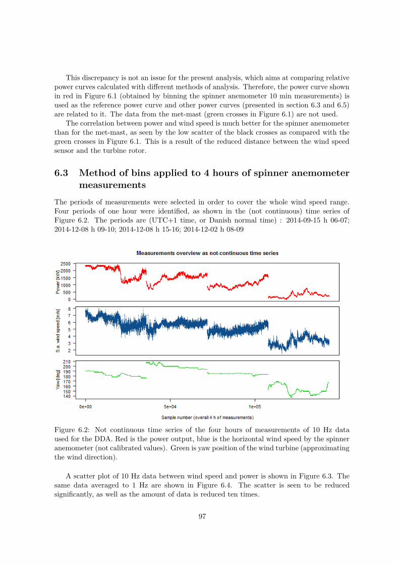
This discrepancy is not an issue for the present analysis, which aims at comparing relativepower curves calculated with different methods of analysis. Therefore, the power curve shownin red in Figure 6.1 (obtained by binning the spinner anemometer 10 min measurements) isused as the reference power curve and other power curves (presented in section 6.3 and 6.5)are related to it. The data from the met-mast (green crosses in Figure 6.1) are not used.
The correlation between power and wind speed is much better for the spinner anemometerthan for the met-mast, as seen by the low scatter of the black crosses as compared with thegreen crosses in Figure 6.1. This is a result of the reduced distance between the wind speedsensor and the turbine rotor.
6.3 Method of bins applied to 4 hours of spinner anemometermeasurements
The periods of measurements were selected in order to cover the whole wind speed range.Four periods of one hour were identified, as shown in the (not continuous) time series ofFigure 6.2. The periods are (UTC+1 time, or Danish normal time) : 2014-09-15 h 06-07;2014-12-08 h 09-10; 2014-12-08 h 15-16; 2014-12-02 h 08-09
Figure 6.2: Not continuous time series of the four hours of measurements of 10 Hz dataused for the DDA. Red is the power output, blue is the horizontal wind speed by the spinneranemometer (not calibrated values). Green is yaw position of the wind turbine (approximatingthe wind direction).
A scatter plot of 10 Hz data between wind speed and power is shown in Figure 6.3. Thesame data averaged to 1 Hz are shown in Figure 6.4. The scatter is seen to be reducedsignificantly, as well as the amount of data is reduced ten times.
97
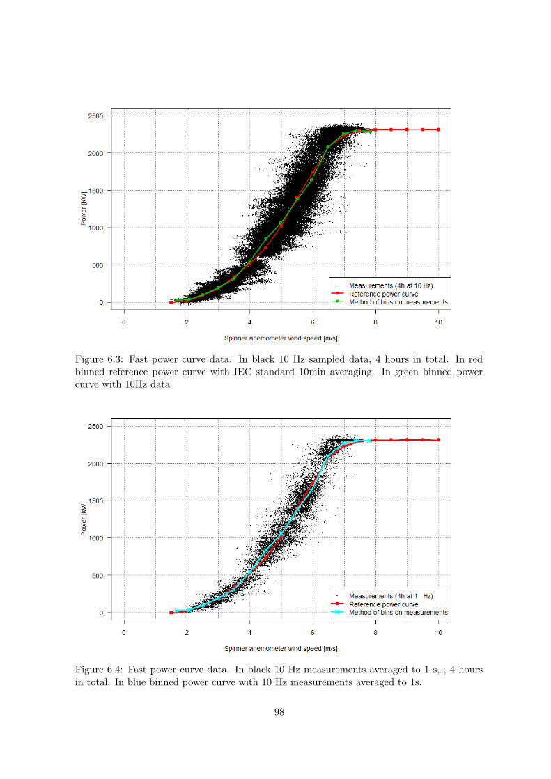
Figure 6.3: Fast power curve data. In black 10 Hz sampled data, 4 hours in total. In redbinned reference power curve with IEC standard 10min averaging. In green binned powercurve with 10Hz data
Figure 6.4: Fast power curve data. In black 10 Hz measurements averaged to 1 s, , 4 hoursin total. In blue binned power curve with 10 Hz measurements averaged to 1s.
98
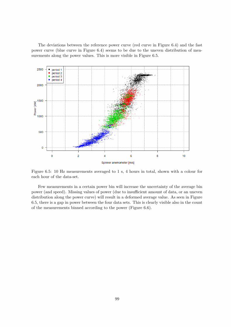
The deviations between the reference power curve (red curve in Figure 6.4) and the fastpower curve (blue curve in Figure 6.4) seems to be due to the uneven distribution of mea-surements along the power values. This is more visible in Figure 6.5.
Figure 6.5: 10 Hz measurements averaged to 1 s, 4 hours in total, shown with a colour foreach hour of the data-set.
Few measurements in a certain power bin will increase the uncertainty of the average binpower (and speed). Missing values of power (due to insufficient amount of data, or an unevendistribution along the power curve) will result in a deformed average value. As seen in Figure6.5, there is a gap in power between the four data sets. This is clearly visible also in the countof the measurements binned according to the power (Figure 6.6).
99
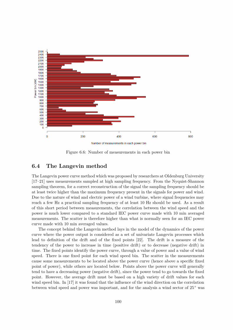
Figure 6.6: Number of measurements in each power bin
6.4 The Langevin method
The Langevin power curve method which was proposed by researchers at Oldenburg University[17–21] uses measurements sampled at high sampling frequency. From the Nyquist-Shannonsampling theorem, for a correct reconstruction of the signal the sampling frequency should beat least twice higher than the maximum frequency present in the signals for power and wind.Due to the nature of wind and electric power of a wind turbine, where signal frequencies mayreach a few Hz a practical sampling frequency of at least 10 Hz should be used. As a resultof this short period between measurements, the correlation between the wind speed and thepower is much lower compared to a standard IEC power curve made with 10 min averagedmeasurements. The scatter is therefore higher than what is normally seen for an IEC powercurve made with 10 min averaged values.
The concept behind the Langevin method lays in the model of the dynamics of the powercurve where the power output is considered as a set of univariate Langevin processes whichlead to definition of the drift and of the fixed points [22]. The drift is a measure of thetendency of the power to increase in time (positive drift) or to decrease (negative drift) intime. The fixed points identify the power curve, through a value of power and a value of windspeed. There is one fixed point for each wind speed bin. The scatter in the measurementscause some measurements to be located above the power curve (hence above a specific fixedpoint of power), while others are located below. Points above the power curve will generallytend to have a decreasing power (negative drift), since the power tend to go towards the fixedpoint. However, the average drift must be based on a high variety of drift values for eachwind speed bin. In [17] it was found that the influence of the wind direction on the correlationbetween wind speed and power was important, and for the analysis a wind sector of 25◦ was
100
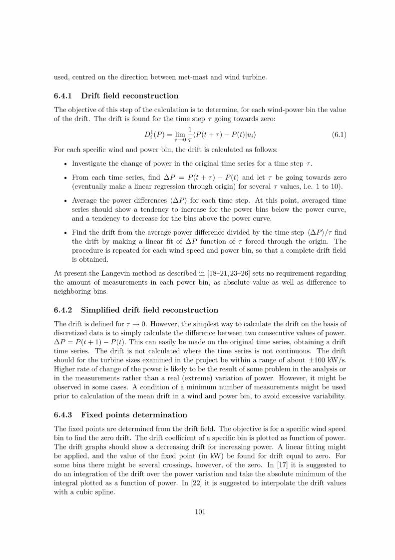
used, centred on the direction between met-mast and wind turbine.
6.4.1 Drift field reconstruction
The objective of this step of the calculation is to determine, for each wind-power bin the valueof the drift. The drift is found for the time step τ going towards zero:
D1i (P ) = lim
τ→0
1τ〈P (t+ τ)− P (t)|ui〉 (6.1)
For each specific wind and power bin, the drift is calculated as follows:
• Investigate the change of power in the original time series for a time step τ .
• From each time series, find ΔP = P (t + τ) − P (t) and let τ be going towards zero(eventually make a linear regression through origin) for several τ values, i.e. 1 to 10).
• Average the power differences 〈ΔP 〉 for each time step. At this point, averaged timeseries should show a tendency to increase for the power bins below the power curve,and a tendency to decrease for the bins above the power curve.
• Find the drift from the average power difference divided by the time step 〈ΔP 〉/τ findthe drift by making a linear fit of ΔP function of τ forced through the origin. Theprocedure is repeated for each wind speed and power bin, so that a complete drift fieldis obtained.
At present the Langevin method as described in [18–21,23–26] sets no requirement regardingthe amount of measurements in each power bin, as absolute value as well as difference toneighboring bins.
6.4.2 Simplified drift field reconstruction
The drift is defined for τ → 0. However, the simplest way to calculate the drift on the basis ofdiscretized data is to simply calculate the difference between two consecutive values of power.ΔP = P (t+ 1)− P (t). This can easily be made on the original time series, obtaining a drifttime series. The drift is not calculated where the time series is not continuous. The driftshould for the turbine sizes examined in the project be within a range of about ±100 kW/s.Higher rate of change of the power is likely to be the result of some problem in the analysis orin the measurements rather than a real (extreme) variation of power. However, it might beobserved in some cases. A condition of a minimum number of measurements might be usedprior to calculation of the mean drift in a wind and power bin, to avoid excessive variability.
6.4.3 Fixed points determination
The fixed points are determined from the drift field. The objective is for a specific wind speedbin to find the zero drift. The drift coefficient of a specific bin is plotted as function of power.The drift graphs should show a decreasing drift for increasing power. A linear fitting mightbe applied, and the value of the fixed point (in kW) be found for drift equal to zero. Forsome bins there might be several crossings, however, of the zero. In [17] it is suggested todo an integration of the drift over the power variation and take the absolute minimum of theintegral plotted as a function of power. In [22] it is suggested to interpolate the drift valueswith a cubic spline.
101
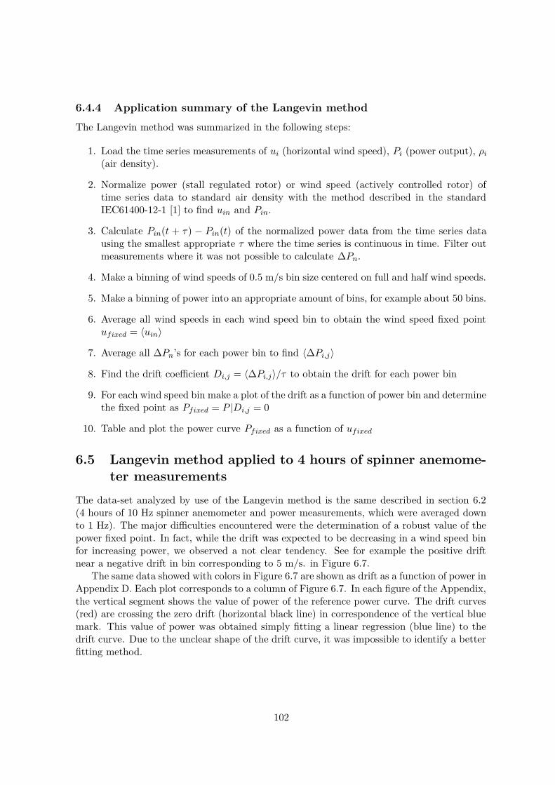
6.4.4 Application summary of the Langevin method
The Langevin method was summarized in the following steps:
1. Load the time series measurements of ui (horizontal wind speed), Pi (power output), ρi(air density).
2. Normalize power (stall regulated rotor) or wind speed (actively controlled rotor) oftime series data to standard air density with the method described in the standardIEC61400-12-1 [1] to find uin and Pin.
3. Calculate Pin(t + τ) − Pin(t) of the normalized power data from the time series datausing the smallest appropriate τ where the time series is continuous in time. Filter outmeasurements where it was not possible to calculate ΔPn.
4. Make a binning of wind speeds of 0.5 m/s bin size centered on full and half wind speeds.
5. Make a binning of power into an appropriate amount of bins, for example about 50 bins.
6. Average all wind speeds in each wind speed bin to obtain the wind speed fixed pointufixed = 〈uin〉
7. Average all ΔPn’s for each power bin to find 〈ΔPi,j〉
8. Find the drift coefficient Di,j = 〈ΔPi,j〉/τ to obtain the drift for each power bin
9. For each wind speed bin make a plot of the drift as a function of power bin and determinethe fixed point as Pfixed = P |Di,j = 0
10. Table and plot the power curve Pfixed as a function of ufixed
6.5 Langevin method applied to 4 hours of spinner anemome-ter measurements
The data-set analyzed by use of the Langevin method is the same described in section 6.2(4 hours of 10 Hz spinner anemometer and power measurements, which were averaged downto 1 Hz). The major difficulties encountered were the determination of a robust value of thepower fixed point. In fact, while the drift was expected to be decreasing in a wind speed binfor increasing power, we observed a not clear tendency. See for example the positive driftnear a negative drift in bin corresponding to 5 m/s. in Figure 6.7.
The same data showed with colors in Figure 6.7 are shown as drift as a function of power inAppendix D. Each plot corresponds to a column of Figure 6.7. In each figure of the Appendix,the vertical segment shows the value of power of the reference power curve. The drift curves(red) are crossing the zero drift (horizontal black line) in correspondence of the vertical bluemark. This value of power was obtained simply fitting a linear regression (blue line) to thedrift curve. Due to the unclear shape of the drift curve, it was impossible to identify a betterfitting method.
102

Figure 6.7: Drift field and Langevin power curve (power bin is 50 kW)
6.6 Comparison of DDA methods
The power curve used as reference for comparing the methods was made on the basis of 126hours of spinner anemometer measurements and the method of bins. The deviations fromthe reference power curve shown in Figure 6.8 are better represented in Figure 6.9, where thevertical scale shows the difference between each of the three methods and the reference powercurve. The deviation between use of the method of bins or use of the Langevin method seemscomparable.
103
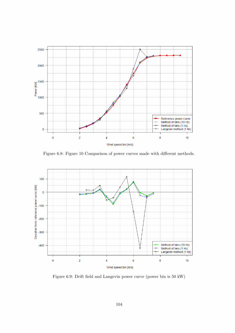
Figure 6.8: Figure 10 Comparison of power curves made with different methods.
Figure 6.9: Drift field and Langevin power curve (power bin is 50 kW)
104
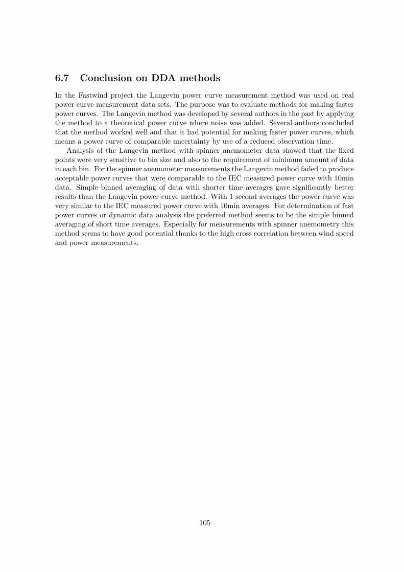
6.7 Conclusion on DDA methods
In the Fastwind project the Langevin power curve measurement method was used on realpower curve measurement data sets. The purpose was to evaluate methods for making fasterpower curves. The Langevin method was developed by several authors in the past by applyingthe method to a theoretical power curve where noise was added. Several authors concludedthat the method worked well and that it had potential for making faster power curves, whichmeans a power curve of comparable uncertainty by use of a reduced observation time.
Analysis of the Langevin method with spinner anemometer data showed that the fixedpoints were very sensitive to bin size and also to the requirement of minimum amount of datain each bin. For the spinner anemometer measurements the Langevin method failed to produceacceptable power curves that were comparable to the IEC measured power curve with 10mindata. Simple binned averaging of data with shorter time averages gave significantly betterresults than the Langevin power curve method. With 1 second averages the power curve wasvery similar to the IEC measured power curve with 10min averages. For determination of fastpower curves or dynamic data analysis the preferred method seems to be the simple binnedaveraging of short time averages. Especially for measurements with spinner anemometry thismethod seems to have good potential thanks to the high cross correlation between wind speedand power measurements.
105
Chapter 7
Conclusions
The main goal of this PhD was to investigate the use of spinner anemometer for powerperformance measurements. Traceability, calibration and uncertainty analysis are centraltopics to evaluate the power performance of a wind turbine in an accurate, and traceableway. The PhD study developed a new method for the calibration of a spinner anemometercompared to the past. Calibration requirements were defined in relation to the specific use ofthe sinner anemometer:
1. Yaw misalignment (and flow inclination) sensor for wind turbine operation.
2. Wind speed sensor for wind turbine operation.
3. Wind speed sensor for power performance measurements according to IE61400-12-2.
The conclusions are here organized by answering one by one the research questions pro-posed in chapter 1.
7.1 Specific conclusion
1. How to calibrate a spinner anemometer?Remove a spinner from an erected wind turbine to place it into a (large) wind tunnel isnot a feasible solution. Therefore the calibration should follow a different approach. Severalmethods were investigated, where the spinner anemometer is calibrated using the naturalwind. Most of the methods investigated are based on postprocessing of non calibrated spinneranemometer measurements. Besides the basic calibrations (zero wind calibration, wind tunnelcalibration of individual sonic sensors, internal calibration of spinner anemometer to accountfor mounting imperfections), the spinner anemometer should undergo two calibrations: thefirst one is for flow angle measurements (yaw misalignment and flow inclination), while thesecond one is for wind speed measurements.
Several methods for calibration of angular measurements were proposed during the PhD.The most recent and robust one is the WSR (wind speed response) method. This methodconsist in yawing the stopped wind turbine several times in and out of the wind while recordingat high sampling frequency (10 Hz) the yaw misalignment and wind speed measured by thespinner anemometer. Once the test is complete, the data are calibrated iteratively to finda value of Fα that minimizes the dependency of wind speed to the yaw misalignment. TheFα values found for 4 tests for the exact same rotor position were within ±2.7% of the mean
106
value. A yawing span of ±60◦ was recommended for the analysis, however the turbine shallbe yawed further than this angle (±90◦ recommended, reading in the wind turbine controllerdisplay) to compensate for initial offset error in the yaw position and wind speed directionchange during the test.
Regarding the calibration for wind measurements, it is important that the spinner anemome-ter is calibrated for flow angle measurements before undertaking the wind speed calibration,as it will notably simplify the equation needed to calculate F1. Several methods were de-veloped, two of which were based on comparison with a met-mast wind speed measurementduring operation or stopped condition of the wind turbine. According to the calibration cor-rection factor F1 (F1 is the ratio between spinner anemometer horizontal wind speed and freehorizontal wind speed in a condition of zero induction), the correct method to determine F1 isby using a stopped turbine. However stopping the wind turbine for a long period is unwanteddue to the consequent energy loss. Therefore the calibration was performed with the windturbine in operation at high wind speed (low rotor induction effect). The calibration cor-rection factor F1 was then the mean ratio between the spinner anemometer horizontal windspeed and free horizontal wind speed. The method was found to be applicable for a pitchregulated turbine. For a calibration on a stall regulated turbine the condition of having F1
to stabilize to an asymptotic value was not et (the wind speed was not high enough and theinduction was still significant and decreasing).
2. How to ensure traceability?The traceability of measurements is ensured trough the individual calibration of 1D sonicsensors in a wind tunnel. The sensor calibration values e are set into the spinner anemometersettings. In this way, if a sensor is replaced, the new values are set into the spinner anemometerconversion box and there is no need to repeat any other calibration.
3. How to use a spinner anemometer for power performance measurements?Once the spinner anemometer is calibrated, it will measure correctly the wind when theturbine is stopped. The NTF will then correct the rotor induction when the turbine is inoperation. The NTF was binned according to the met-mast wind speed (which differs fromIEC61400-12-2 which requires to bin according to the spinner anemometer wind speed). TheNTF self consistency check with this method was still not zero, and the check is still necessary.
The calibration values kα, k1, and the NTF measured in a flat site on a reference turbine(T4, which spinner anemometer was calibrated comparing with a met-mast) were used ona second turbine (T5) of exact same model. Over all, use of the spinner anemometer wasdemonstrated to be able to measure the power performance of both wind turbines very well,within 0.1% of AEP of met-mast measurements on T4 or within 0.38% AEP on T5. Theuncertainty on wind speed measurements due to spinner anemometer mounting imperfectionsand uncertainty on kα was very small compared to the contribution due to NTF, met-mast,site effects, and MEASNET wind tunnel variations. If the spinner anemometer is used forrelative power performance measurements (which compare the turbine performance to itselfor to other identical turbines over time) there is no need for wind speed calibration and NTF,and the total uncertainty may be significantly be reduced.
4. How is the uncertainty of spinner anemometer measurements evaluated?The uncertainty on the spinner anemometer output values (such as yaw misalignment andhorizontal wind speed) is evaluated throw combination of the uncertainty of the input values
107
(the three velocities measured by the 1D sonic sensors). The uncertainty on the input valuescomes form the wind tunnel calibration certificates. There is no uncertainty associated to thek1 calibration because is included in the NTF. The uncertainty on kα was assumed 10% (therepeatability of the result was found within ±8.5% in a series of eight repeated calibrationtests performed on the same turbine). The combination of uncertainty involved an extensiveuse of partial derivatives, which were computed numerically due to their complexity. Theuncertainty was not only depending on the wind speed, but also on the flow angle. Atthe end, the result presented in chapter 5 was simplified to the following expression of theuncertainty on horizontal wind speed in m/s, as a function of horizontal wind speed:
uUhor = −0.005 +
√Uhor80
(7.1)
The equation is valid for spinner anemometers similar to the one used for the uncertaintyanalysis in chapter 5. Specifically, the uncertainty due to mounting and wind tunnel calibra-tion should be equal or lower, and the calibration constants should be similar to kα = 1.4 andk1 = 0.6.
5. Is it possible to avoid individual calibration of spinner anemometers?Yes, as long as the mounting position of the sonic sensors and the spinner outer shape areidentical. An additional uncertainty must be introduced due to the mounting differencesbetween the reference spinner anemometer (on which the calibration values were measured)and the other spinner anemometer. The mounting position of the individual sonic sensorscould be measured by means of photos of the spinner taken from ground level during operationof the wind turbine, as it was presented in chapter 5. The sonic sensors should be calibratedin the wind tunnel, unless the uncertainty of a non calibrated sensor is acceptable.
6. What are the impacts of mounting imperfections of the sonic sensors?The uncertainty for sensor mounting imperfections shall not be considered on the referencewind turbine (the one used for the wind speed calibration and NTF measurement). The otherturbines will have an uncertainty due to the dissimilarity with the reference wind turbine.A geometric difference of 4 cm lead to a wind speed uncertainty of 1.2%, which is a minorcontributor to the total uncertainty of the free wind speed calculated with the NTF. This wasan improvement of an initial mounting whose uncertainty was 2.7% for a tolerance of 12 cm.
The major contributors are the NTF uncertainty, the met-mast uncertainty, the 2% dueto lack of site calibration, and the MEASNET variability 1/
√3%. The uncertainty due to
mounting could be easily reduced further by reducing the mounting tolerances.
7. Is there any advantage in using short time averages to measure a power curve?The spinner anemometer wind speed measurements correlate with the wind turbine power,better than the met-mast (which is at a considerable distance from the turbine) and betterthan a nacelle anemometer (where flow is disturbed by the blade roots and nacelle body).This allows for use of shorter time averages. 10 min. measurements were used to determinea reference power curve with the method of bins. Fast sampled measurements were analyzedwith the Langevin method and with regular binning of 1s averages. The simple binning (as ofIE61400-12-2) gave a power curve close to the reference power curve. The Langevin methodgave a similar result with exception of some bins, which failed completely to estimate thecorrect power. A number of parameters had to be chosen to apply the Langevin method,
108

such as the width of the power bins, and the method to calculate the fixed point from thedrift curve. Because of the better result, the lack of arbitrary parameters and its simplicity,the method of bins is still the most appropriate to analyze fast sampled measurements, withthe advantage of broadening the wind speed distribution.
8. What minimum time is required to measure a power curve?Wind speed is always sampled at high frequency (typically 10-20 Hz for sonic anemometersand 1-5 Hz for cup anemometers) and the measurements averaged to 10 minute averages. Ashorter averaging time (or no averaging) can help to broaden the wind speed range covered bythe measurements.. It was found that the wind speed and power probability distribution playsa major role in providing a good power curve. A power curve was made with 4 hours of highfrequency measurements which were selected to cover as best as possible the power intervalfrom zero to nominal power. The four hours were selected over a period of measurements of2.5 months. So, the answer to this question is related to the wind conditions more than tothe instrumentation or method of analysis.
7.2 Recommendations for future work
The spinner anemometer has proven to be suitable to measure yaw misalignment and powerperformance of wind turbines. However, very few wind turbines in the world are equippedwith this instrument. As of the current state of development, the areas in which there arepossible improvements to do are:
1. Calibration methods. The existing methods for calibration of flow angle measure-ments should be validated in a flow with no turbulence. Practically this could be donein a large wind tunnel.
2. Mounting accuracy. The procedures to mount the sonic sensors on the spinnerof a wind turbine which is already erected shall be improved to reduce the mountingaccuracy. The mold used to cast the spinners shall be modified to mark with absoluteaccuracy the position for sonic sensors, or even embed the sensor fittings in the fiberglassinfusion. This is to ensure the best geometric accuracy and make sure that all the spinneranemometers are identical, for a certain spinner model.
3. Spinner anemometer classification. The evaluation of uncertainties shall be sim-plified further. The uncertainty related to wind tunnel calibration is typically the samefor different 1D (one dimensional) sonic sensors. The uncertainty due to mounting canalso be considered constant if the tolerance of the mounting is constant. An expressionof the uncertainty as a function of wind speed and calibration constants could be devel-oped. The simplification could follow the approach that was used for the classificationof cup anemometers.
4. Yaw control. Up until now the spinner anemometer has been used for correctionof static yaw misalignment, by correcting the mounting offset of the wind directionsensor on the roof of wind turbines. A dedicated collaboration with a wind turbinemanufacturer could integrate the spinner anemometer signals in the wind turbine controlsystem.
109

5. Condition monitoring. Method of data analysis to detect power performance changesof a wind turbine should be developed and tested. For this, it is not necessary tocalibrate the spinner anemometer. Initial recordings must define what is the normalbehaviour of the wind turbine, and some boundaries set at a certain distance wouldtrigger an alarm when exceeded.
6. Generalized NTF, investigation of the rotor center induction. It could be that therotor center induction is very similar among different wind turbine control strategies,or different rotors, or even different wind turbine models. If so, it would be possible todefine a generalized NTF to use with spinner anemometers to calculate free wind speed.
7. New IEC requirements to wind and power database. The DDA (Dynamic DataAnalysis) has shown that the shape of the probability distribution of the power can affectthe shape of the power curve made with binning as a function of wind speed. This wasevident when analysing 4 hours of 1 Hz data, but it would also affect a power curve madewith many hours of measurements (the IEC requirements are 180 h of measurementsand at least 30 minute of measurements in each bin). Would it be more appropriate inthe IEC method to insert a limit on the difference in number of measurements betweenadjacent bins? or, would it be better to have the same amount of measurements in eachbin?
8. NPC in complex terrain. The spinner anemometer could give much better insightof the wind conditions inside a wind farm as well as in complex terrain, that is in allthose situations of turbulent and not horizontal wind. The spinner anemometer shouldbe installed in all the wind turbines of a large offshore wind farm.
9. NPC in wind farm environment. The spinner anemometer can not detect if a partof the rotor disc is operating in the wake of a wind turbine. However, thanks to theability to well measure the flow inclination can detect very well the wake swirl at thesides of the wake. This information could be used to identify the wind direction sectorsto exclude to perform a NPC measurement.
110

Chapter 8
Appendix
111
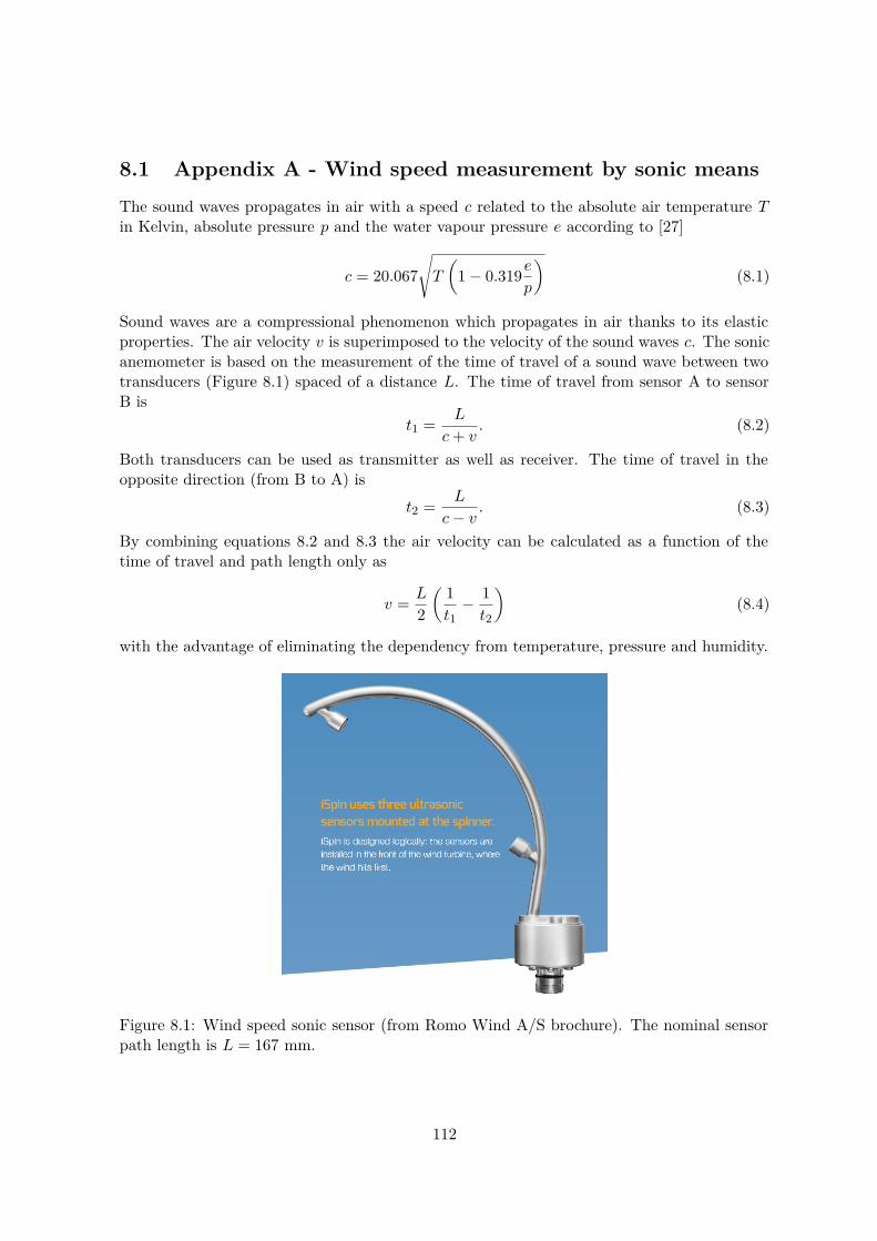
8.1 Appendix A - Wind speed measurement by sonic means
The sound waves propagates in air with a speed c related to the absolute air temperature Tin Kelvin, absolute pressure p and the water vapour pressure e according to [27]
c = 20.067
√
T
(
1− 0.319e
p
)
(8.1)
Sound waves are a compressional phenomenon which propagates in air thanks to its elasticproperties. The air velocity v is superimposed to the velocity of the sound waves c. The sonicanemometer is based on the measurement of the time of travel of a sound wave between twotransducers (Figure 8.1) spaced of a distance L. The time of travel from sensor A to sensorB is
t1 =L
c+ v. (8.2)
Both transducers can be used as transmitter as well as receiver. The time of travel in theopposite direction (from B to A) is
t2 =L
c− v. (8.3)
By combining equations 8.2 and 8.3 the air velocity can be calculated as a function of thetime of travel and path length only as
v =L
2
(1t1−
1t2
)
(8.4)
with the advantage of eliminating the dependency from temperature, pressure and humidity.
Figure 8.1: Wind speed sonic sensor (from Romo Wind A/S brochure). The nominal sensorpath length is L = 167 mm.
112
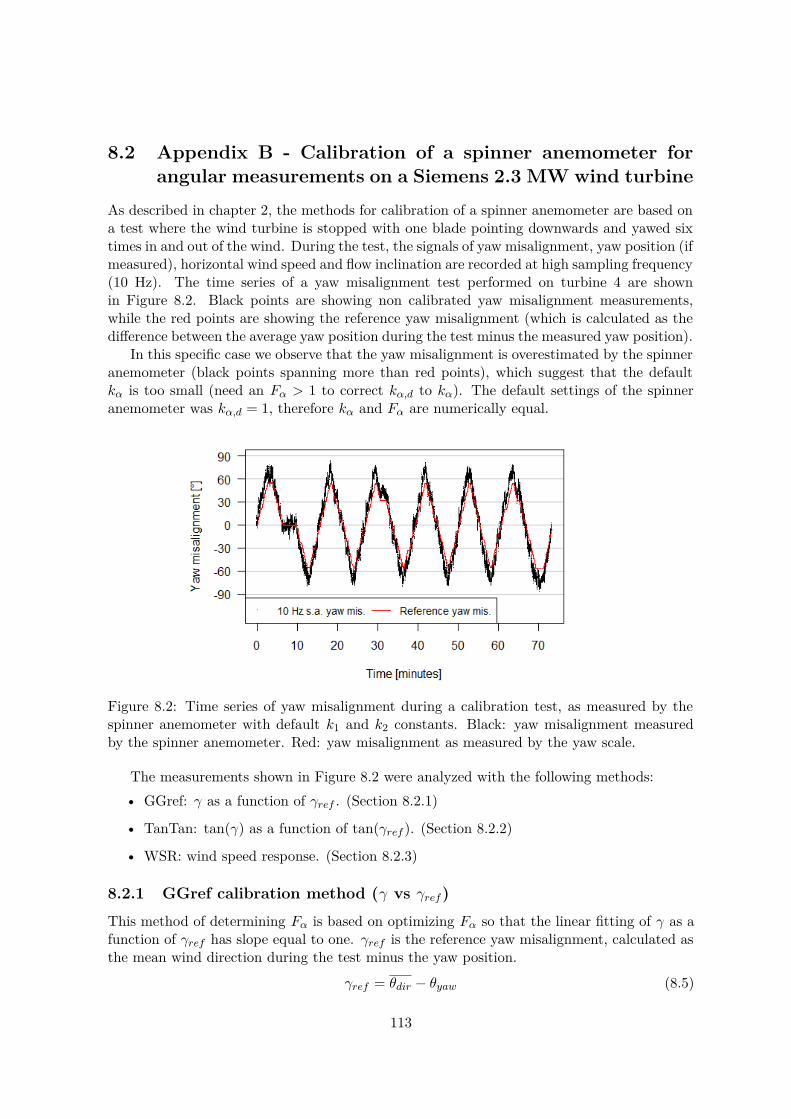
8.2 Appendix B - Calibration of a spinner anemometer forangular measurements on a Siemens 2.3 MW wind turbine
As described in chapter 2, the methods for calibration of a spinner anemometer are based ona test where the wind turbine is stopped with one blade pointing downwards and yawed sixtimes in and out of the wind. During the test, the signals of yaw misalignment, yaw position (ifmeasured), horizontal wind speed and flow inclination are recorded at high sampling frequency(10 Hz). The time series of a yaw misalignment test performed on turbine 4 are shownin Figure 8.2. Black points are showing non calibrated yaw misalignment measurements,while the red points are showing the reference yaw misalignment (which is calculated as thedifference between the average yaw position during the test minus the measured yaw position).
In this specific case we observe that the yaw misalignment is overestimated by the spinneranemometer (black points spanning more than red points), which suggest that the defaultkα is too small (need an Fα > 1 to correct kα,d to kα). The default settings of the spinneranemometer was kα,d = 1, therefore kα and Fα are numerically equal.
Figure 8.2: Time series of yaw misalignment during a calibration test, as measured by thespinner anemometer with default k1 and k2 constants. Black: yaw misalignment measuredby the spinner anemometer. Red: yaw misalignment as measured by the yaw scale.
The measurements shown in Figure 8.2 were analyzed with the following methods:
• GGref: γ as a function of γref . (Section 8.2.1)
• TanTan: tan(γ) as a function of tan(γref ). (Section 8.2.2)
• WSR: wind speed response. (Section 8.2.3)
8.2.1 GGref calibration method (γ vs γref)
This method of determining Fα is based on optimizing Fα so that the linear fitting of γ as afunction of γref has slope equal to one. γref is the reference yaw misalignment, calculated asthe mean wind direction during the test minus the yaw position.
γref = θdir − θyaw (8.5)
113
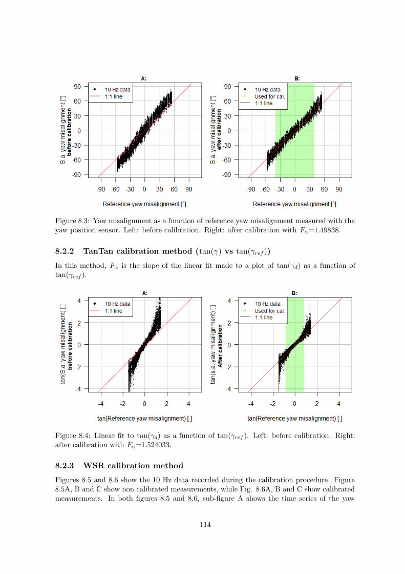
Figure 8.3: Yaw misalignment as a function of reference yaw misalignment measured with theyaw position sensor. Left: before calibration. Right: after calibration with Fα=1.49838.
8.2.2 TanTan calibration method (tan(γ) vs tan(γref ))
In this method, Fα is the slope of the linear fit made to a plot of tan(γd) as a function oftan(γref ).
Figure 8.4: Linear fit to tan(γd) as a function of tan(γref ). Left: before calibration. Right:after calibration with Fα=1.524033.
8.2.3 WSR calibration method
Figures 8.5 and 8.6 show the 10 Hz data recorded during the calibration procedure. Figure8.5A, B and C show non calibrated measurements, while Fig. 8.6A, B and C show calibratedmeasurements. In both figures 8.5 and 8.6, sub-figure A shows the time series of the yaw
114
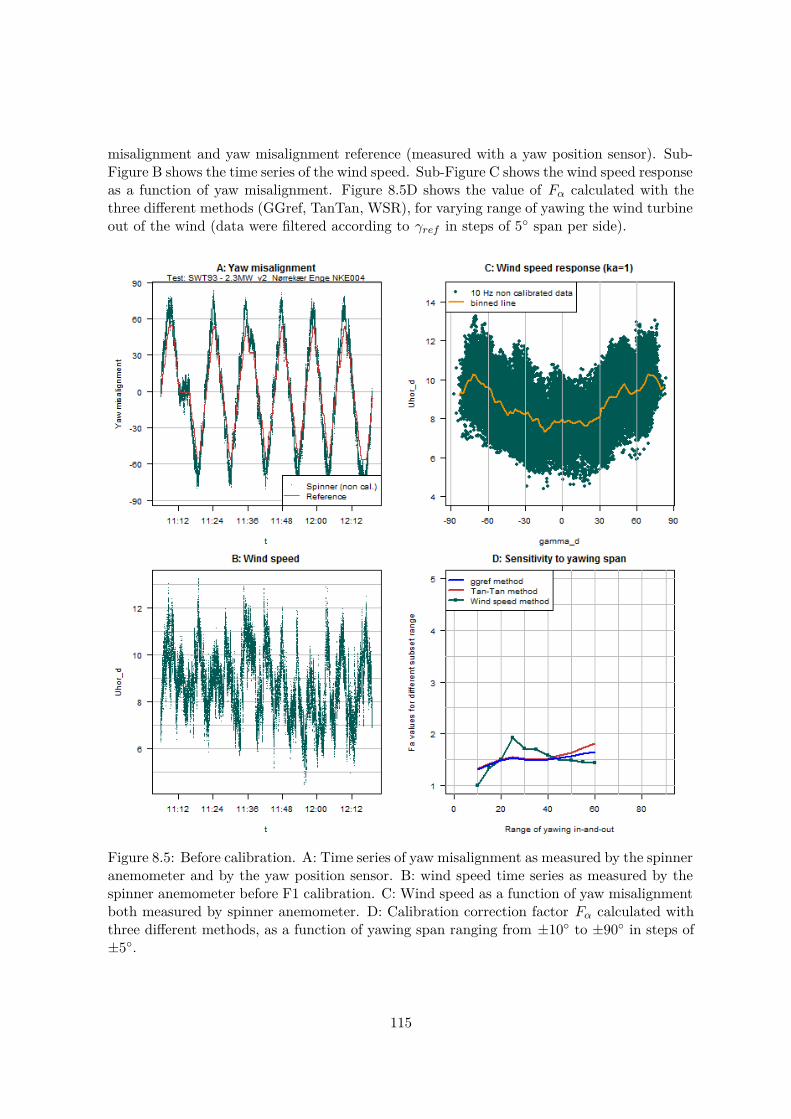
misalignment and yaw misalignment reference (measured with a yaw position sensor). Sub-Figure B shows the time series of the wind speed. Sub-Figure C shows the wind speed responseas a function of yaw misalignment. Figure 8.5D shows the value of Fα calculated with thethree different methods (GGref, TanTan, WSR), for varying range of yawing the wind turbineout of the wind (data were filtered according to γref in steps of 5◦ span per side).
Figure 8.5: Before calibration. A: Time series of yaw misalignment as measured by the spinneranemometer and by the yaw position sensor. B: wind speed time series as measured by thespinner anemometer before F1 calibration. C: Wind speed as a function of yaw misalignmentboth measured by spinner anemometer. D: Calibration correction factor Fα calculated withthree different methods, as a function of yawing span ranging from ±10◦ to ±90◦ in steps of±5◦.
115
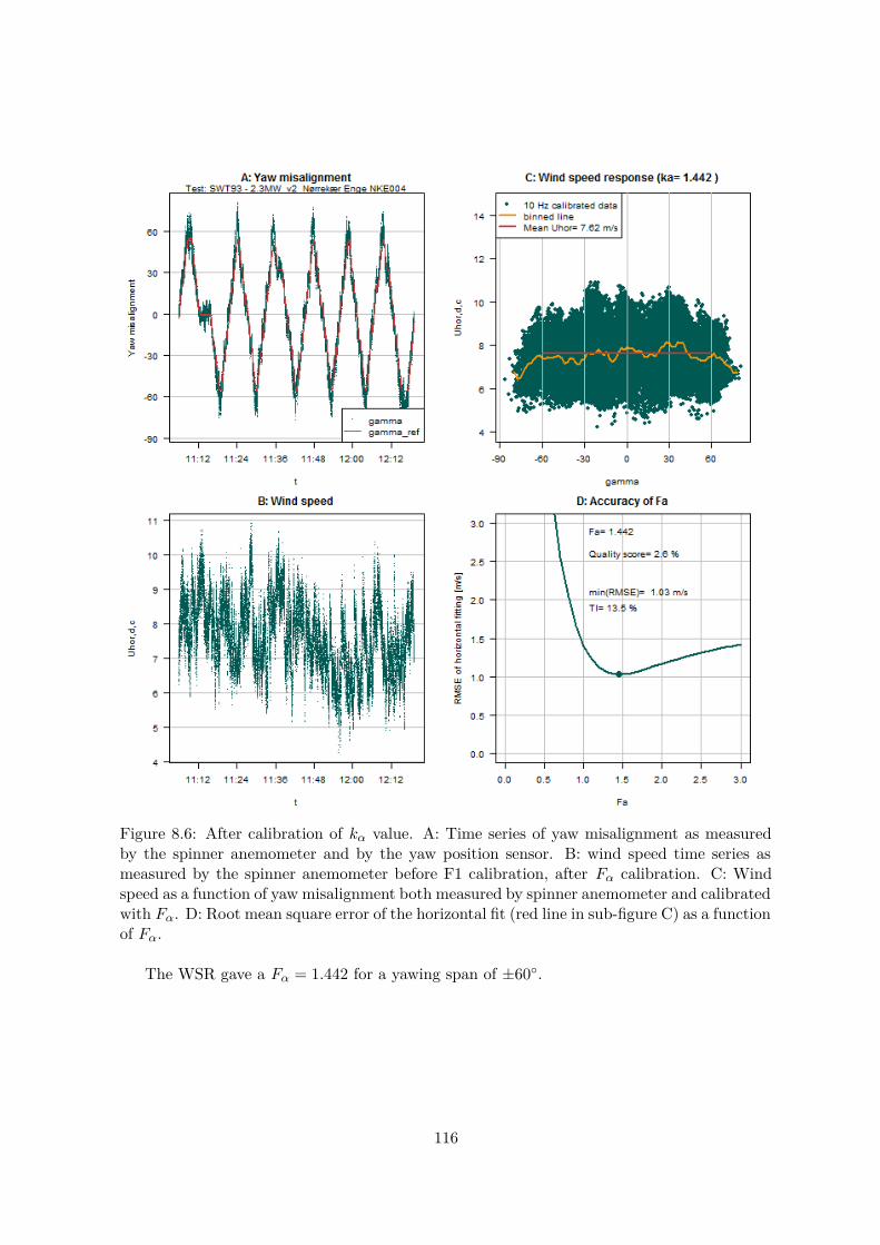
Figure 8.6: After calibration of kα value. A: Time series of yaw misalignment as measuredby the spinner anemometer and by the yaw position sensor. B: wind speed time series asmeasured by the spinner anemometer before F1 calibration, after Fα calibration. C: Windspeed as a function of yaw misalignment both measured by spinner anemometer and calibratedwith Fα. D: Root mean square error of the horizontal fit (red line in sub-figure C) as a functionof Fα.
The WSR gave a Fα = 1.442 for a yawing span of ±60◦.
116
8.2.4 Discussion regarding kα calibration
The three kα calibration methods presented in sections 8.2.1, 8.2.2 and 8.2.3 gave the followingFα values:
Method: GGref TanTan WSRFα: 1.498 1.524 1.442
Table 8.1: Summary of Fα values calculated with three different methods for a Siemens 2.3MW wind turbine.
Note that the calibration examples presented in chapter 2 were based on measurementsmade on wind turbine with different spinner shape (a Nordtank 500 kW or a Neg-MiconNM80 2 MW) therefore the Fα values presented in Table 8.1 shall not be compared with thevalues presented in the article.
A sensitivity analysis to the span of yawing the wind turbine in and out of the windmade in chapter 2 unveiled limitations related to the first two methods. For this reason, thevalue used to calibrate the spinner anemometer measurements of this wind turbine is the onecalculated with the WSR method (Fα=1.442).
117

8.3 Appendix C - Calibration of a spinner anemometer forwind speed measurements on a Siemens 2.3 MW windturbine
The objective of the spinner anemometer calibration for wind speed measurements is to findthe k1 calibration constant that makes Uhor to match the free wind speed Umm when theturbine is stopped and is facing the wind. During operation of the wind turbine the rotorinduction is accounted for with the nacelle transfer function described in the IEC61400-12-2standard. The calibration procedure was based on measurements acquired with a spinneranemometer where k1 was set to default value k1,d. The correction factor F1 was calculatedas the ratio
F1 =Uhor,d,cUmm
(8.6)
where Uhor,d,c is the horizontal wind speed measured with default k1,d and correct kα. Thedata-set used to find the F1 value is show in Figure 8.7.
Figure 8.7: Horizontal wind speed of the spinner anemometer (prior to calibration) as afunction of the met-mast horizontal wind speed. Turbine 4.
To acquire the measurements needed for the calibration the wind turbine shall ideallybe stopped. However, this is not desirable due to power production losses, therefore thecalibration was performed with the wind turbine in operation, as proposed in [28] for a stallregulated turbine. In the case shown in Figure 8.8 the wind turbine is pitch regulated and theF1 as a function of free wind speed shows a clear asymptote as the induction decreases. Thevalue of F1 = 0.7101 was calculated as average of the values for free wind speed greater than15 m/s. Note that the article is based on measurements acquired after the sensor mountingposition on the spinner was improved. The sensors were moved forward in the new mounting,determining a lower F1. In Figure 8.9, the good agreement between met-mast wind speedand spinner anemometer wind speed confirm that the calibration is correct.
118

Figure 8.8: F1 correction factor as a function of met-mast wind speed, disturbed by the rotorinduction during operation of the wind turbine. The horizontal black line shows the valueof F1 chosen to calibrate the measurements. Turbine 4 (initial mounting position of sonicsensors).
Figure 8.9: Horizontal wind speed (calibrated with F1 = 0.7101) of the spinner anemometeras a function of the met-mast horizontal wind speed. Turbine 4.
119
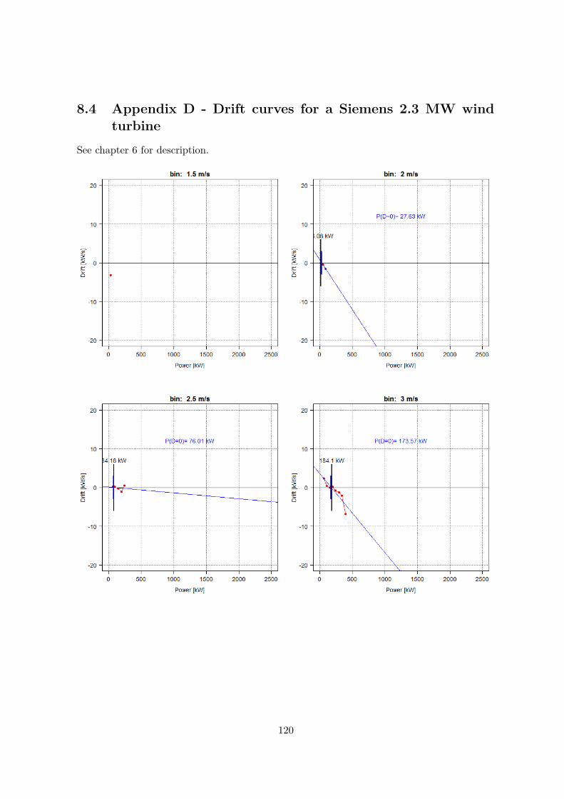
8.4 Appendix D - Drift curves for a Siemens 2.3 MW windturbine
See chapter 6 for description.
120
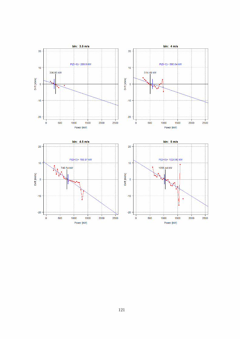
121
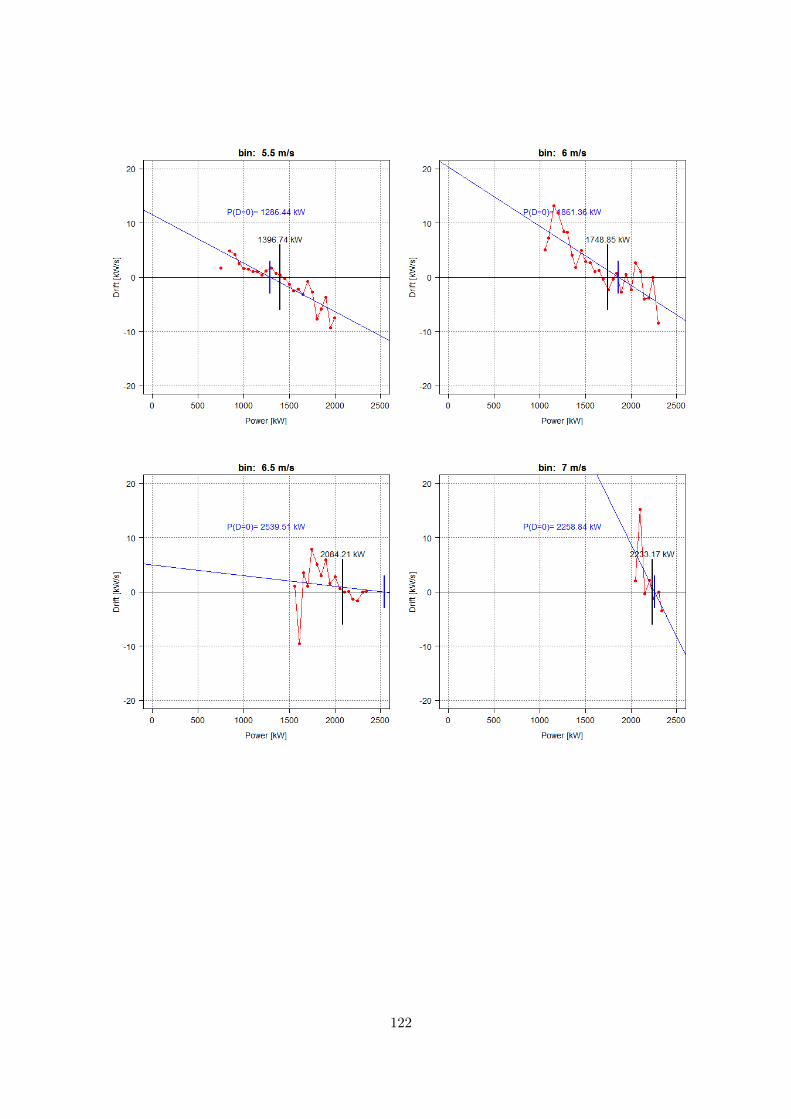
122
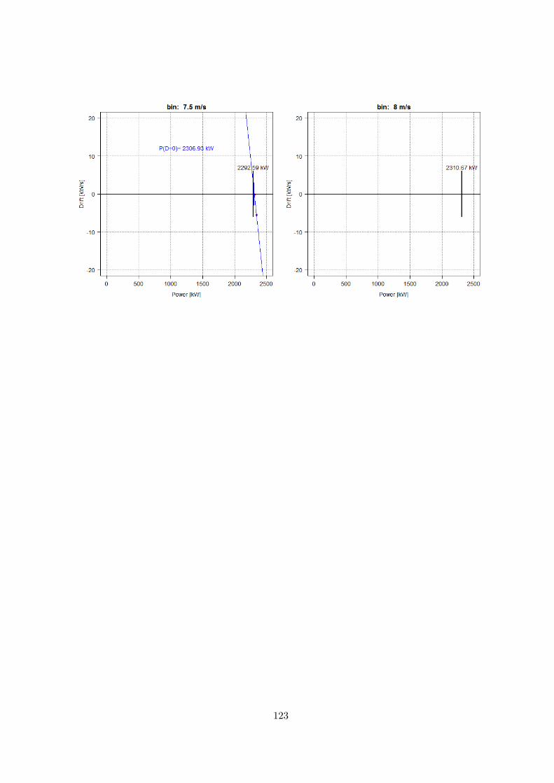
123

Bibliography
[1] “Iec61400-12-1 wind turbines part 12-1: Power performance measurements of electricityproducing wind turbines,” 2008.
[2] “Iec61400-12-2 wind turbines part 12-2: Power performance of electricity producing windturbines based on nacelle anemometry,” 2012.
[3] F. Zahle and N. N. Sørensen, “Characterization of the unsteady flow in the nacelle regionof a modern wind turbine,” Wind Energy, vol. 14, no. 2, pp. 271–283, 2011.
[4] “Apparatus for adjusting the yaw of a wind turbine. WO2013117470A1.”
[5] T. F. Pedersen, N. Sørensen, and P. Enevoldsen, “Aerodynamics and Characteristics of aSpinner Anemometer,” Journal of Physics: Conference Series, vol. 75, p. 012018, 2007.
[6] EWEC 2008 Brussels, Theoretical model of spinner anemometry based on ultrasonicpaths, 2008.
[7] T. F. Pedersen, G. Demurtas, J. Gottschall, J. Højstrup, J. D. Nielsen, G. Weich, A. Som-mer, and R. Kristoffersen, “E-0040 Improvement of Wind Farm Performance by Meansof Spinner Anemometry,” Tech. Rep. E-0040, DTU Wind Energy, December 2013.
[8] Metek, “Spinner anemometer user manual 05-01-2009.”
[9] T. F. Pedersen, U. S. Paulsen, S. M. Pedersen, and P. Enevoldsen, “Operational Ex-perience and Analysis of a Spinner Anemometer on a MW Size Wind Turbine,” WindEnergy, no. 1, pp. 356–356, 2007.
[10] T. F. Pedersen, N. Sørensen, L. Vita, and P. Enevoldsen, “Optimization of Wind TurbineOperation by Use of Spinner Anemometer,” Tech. Rep. R-1654, DTU Wind Energy,August 2008.
[11] P. Troels Friis, “Risø spinner anemometer, prototype 2, installation and calibration andquality of signal output.,” Tech. Rep. Risø-I-2779, DTU Wind Energy, October 2008.
[12] T. F. Pedersen, R. Wagner, and G. Demurtas, “Wind Turbine Performance Measure-ments by Means of Dynamic Data Analysis,” 2015.
[13] EWEC 2007 Milan, Spinner Anemometry - An Innovative Wind Measurement Concept,2007.
[14] G. Demurtas and T. F. Pedersen, “Summary of the steps involved in the calibration ofa spinner anemometer,” Tech. Rep. I-0364, DTU Wind Energy, November 2014.
124
[15] T. F. Pedersen, G. Demurtas, and F. Zahle, “Calibration of a spinner anemometer foryaw misalignment measurements,” Wind Energy Wiley, vol. 18, no. 11, pp. 1933–1952,2015.
[16] G. Demurtas, “Power curve measurement with spinner anemometer according to iec61400-12-2,” Tech. Rep. I-0440, DTU Wind Energy, December 2015.
[17] C. Brown, “Fast Verification of Wind Turbine Power Curves : Summary of ProjectResults (MSc Thesis - Tec. Uni of Denmark),” Thesis, 2012.
[18] J. Gottschall and J. Peinke, “How to improve the estimation of power curves for windturbines,” Environmental Research Letters, 2008.
[19] P. Milan, T. Mücke, A. Morales, M. Wächter, and J. Peinke, “Applications of the langevinpower curve,” in Proceedings of the EWEC 2010, (Warsaw, Poland), EWEA, 2010.
[20] M. Wächter, P. Milan, T. Mücke, and J. Peinke, “Power performance of wind energyconverters characterized as stochastic process: applications of the langevin power curve,”Wind Energy, vol. 14, pp. 711 –717, 2011.
[21] E. Anahua, S. Barth, and J. Peinke, “Markovian power curves for wind turbines,” WindEnergy, vol. 11(3), p. 219Ű232, 2008.
[22] J. Gottshall and M. Courtney, “On the robustness of the fixed points for a dynamicalperformance characteristic Ű or: a closer look at the langevin power curve„” WindEnergy, no. we1718, 2014.
[23] A. Rauh and J. Peinke, “A phenomenological model for the dynamic response of windturbines to turbulent wind,” Journal of Wind Eng. Ind. and Aerody, no. 92, pp. 159–183,2004.
[24] E. Anahua, S. Barth, and J. Peinke, “Characterization of the wind turbine power per-formance curve by,” EWEC, 2006.
[25] J. Gottschall and J. Peinke, “Stochastic modelling of a wind turbineŠs power output withspecial respect to turbulent dynamics,” Journal of Physics: Conference Series, no. 75:012045 (8pp) DOI: 10.1088/1742-6596/75/1/012045, 2007.
[26] J. Gottschall and J. Peinke, “On the definition and handling of different drift and diffusionestimates,” New Journal of Physics, 2008.
[27] R. M. Schotland, “The Measurement of Wind Velocity by Sonic Means,” 1955.
[28] G. Demurtas, T. F. Pedersen, and F. Zahle, “Calibration of a spinner anemometer forwind speed measurements,” Wind Energy, 2016.
125

Curriculum vitae
Giorgio Demurtas was born on 14th March 1986 in Cagliari, Italy.
He received the high school diploma in Electrotechnics and Automation in 2005 from the G.Marconi technical school in Cagliari, Italy. He completed the Bachelor in Electrical Engineer-ing at the University of Cagliari in 2009. Soon after, he funded the company Piccolecentrali,which designed and installed approximately 140 kW of photovoltaic solar plants.
In August 2010 he started the Master of Science in wind Energy at the Technical Universityof Denmark. In August 2012 he completed the Master of Science with a thesis written incollaboration with Alsom Wind in Barcelona.
He then worked in the Test and Measurements section of DTU Wind Energy as researchassistant and later as PhD student. During the second year of PhD he registered the companyStartak IVS, in Denmark, to produce and sell control systems for solar trackers.
In 2015, during a two months leave from the PhD he worked as consultant for AentulaSrl, developing the control system for a 30 kW pitch regulated direct drive wind turbine.
For the future, he wants to free the world from fossil fuels in favour of renewable energies.
126

DTU Wind Energy is a department of the Technical University of Denmark with a unique integration of research, education, innovation and public/private sector consulting in the field of wind energy. Our activities develop new opportunities and technology for the global and Danish exploitation of wind energy. Research focuses on key technical-scientific fields, which are central for the development, innovation and use of wind energy and provides the basis for advanced education at the education. We have more than 240 staff members of which approximately 60 are PhD students. Research is conducted within nine research programmes organized into three main topics: Wind energy systems, Wind turbine technology and Basics for wind energy.
Danmarks Tekniske Universitet DTU Vindenergi Nils Koppels Allé Bygning 403 2800 Kgs. Lyngby Telephone 45 25 25 25 [email protected] www.vindenergi.dtu.dk
Copyright © 2022 FDOKUMEN