WIND TURBINE LINEAR PARAMETER VARYING CONTROL USING FAST CODE

Farzad A. Shirazi ∗

Dept. of Mechanical EngineeringUniversity of HoustonHouston, TX 77204

Email: fashiraz@mail.uh.edu

Karolos M. GrigoriadisDept. of Mechanical Engineering

University of HoustonHouston, TX 77204karolos@uh.edu

Daniel ViassoloVestas Technology R&D Americas Inc.

Houston, TX 77002davia@vestas.com

ABSTRACTLinear parameter varying (LPV) control of a three-bladed

horizontal-axis wind turbine in partial and full load conditionsusing FAST code is presented. The multivariable LPV controlleris designed for a lumped model of the wind turbine with fivedegrees-of-freedom consisting blades, drive-train and the tower.The controller is scheduled in real-time based on the mean windspeed. The objective is to minimize the H∞ performance indexfrom the wind turbulence to the controlled output vector. Theclosed-loop responses of the LPV controller are compared witha traditional PI-scheduled controller in the FAST/Simulink envi-ronment for the NREL 5MW baseline wind turbine. Comparedto the PI-scheduled controller, the LPV design reduced the tran-sient loads in switching between partial to full load regions of theoperation. The fluctuations of the generator speed and torque aredecreased resulting in a smoother power generation. The windturbine structural loads in terms of blade root flap-wise bendingmoments and tower fore-aft bending moment are mitigated indifferent loading conditions.

1 IntroductionWind turbine technology has been advancing rapidly in last

decades while new challenges are appearing for the future growthof the technology. The size of wind turbines has been steadilyincreasing over the past years resulting in larger and heavier de-sign of the subsystems and higher mechanical loads on the tur-bine. In addition, force/moment sensing or accelerometers cannow be installed on blades as well as the nacelle and tower toimprove controllability. Design of novel advanced multivari-able controllers are in need to increase the power capture andreduce fatigue loads on the wind turbine structure. However, in

∗Address all correspondence to this author.

most of the current commercial systems simplistic single-input-single-output (SISO) gain-scheduled proportional-integral (PI)controllers are still being used for control [9,10]. Advanced con-trol techniques that take benefit of the multi-input-multi-output(MIMO) nature of these systems are essential to accommodatecoupling between loops [4, 6]. Optimal controllers based onlinear quadratic Gaussian (LQG) design have been examinedin [12]. Robust MIMO control of blade pitch angles and thegenerator torque has also been studied recently [3, 6]. Gain-Scheduled H∞ control via LMI techniques has been designed andimplemented in [11].

Linear parameter varying (LPV) controllers have been pro-posed to cope with the nonlinear parameter-varying dynamics ofwind turbines in partial and full load conditions [2, 13]. LPVcontrollers have been shown to be very effective in improvingclosed-loop performance in different operating regions, as wellas, addressing robustness [3, 13, 15]. It is common in the liter-ature to design LPV controllers for the linearized model of thewind turbine and then simulate them on the original nonlinearlumped model. However in our approach, for the first time, themultivariable LPV controllers for the full operating region of awind turbine are validated using FAST (Fatigue, Aerodynamics,Structures, and Turbulence) code environment and the closed-loop responses are compared with a conventional PI-scheduledcontroller.

The wind turbine under study is a 5MW onshore three-bladed horizontal axis turbine which its technical information isprovided by the DOE National Renewable Energy Lab (NREL)[9]. The FAST code is a comprehensive aeroelastic simulator ca-pable of predicting both the extreme and fatigue loads of two-and three-bladed horizontal-axis wind turbines (HAWTs) [8].FAST is considered as a standard wind turbine dynamic simu-lation tool in industry and will be used in this work to validate

ASME 2012 5th Annual Dynamic Systems and Control Conference joint with theJSME 2012 11th Motion and Vibration Conference

DSCC2012-MOVIC2012

1 Copyright © 2012 by ASME

DSCC2012-MOVIC2012-8558

October 17-19, 2012, Fort Lauderdale, Florida, USA

Downloaded From: http://proceedings.asmedigitalcollection.asme.org/ on 12/20/2013 Terms of Use: http://asme.org/terms

our open-loop and closed-loop results.The rest of the paper is organized as follows. Section 2

describes an eighth-order lumped model of the horizontal-axiswind turbine, its time and frequency domain validation via de-tailed numerical simulations using FAST, and the LPV modelingof the plant. In Section 3 the LPV controller design for the fulloperating region of a wind turbine is investigated and the closed-loop responses are compared with a traditional PI-scheduled con-troller in FAST/Simulink environment for the NREL 5MW base-line wind turbine. Section 4 will summarize the results of thepaper.

2 Wind Turbine ModelingIn this section, we present a dynamic model of the wind tur-

bine that is suitable for our multivariable control design purpose.Here, we consider a model with five degrees-of-freedom (DOFs)consisting of a static aerodynamic model, a structural model in-cluding the blades, drive-train and tower, a model of the pitchmechanism and a model of the generator. In sequel sections, wepresent the dynamic equations of each subsystem and we derivethe state-space representation of the combined system.

2.1 Aerodynamic ModelThe aerodynamic interaction of the wind and the turbine

blades produces a torque which rotates the rotor, and a thrustforce acting on the turbine nacelle. The generated power of theturbine depends on the wind speed relative to the rotor Ve, theair density ρa, the rotor swept area S and the rotor aerodynamicproperties. Commonly, rotor power, torque and thrust force oneach blade of the wind turbine are expressed in terms of non-dimensional power (CP), torque (CQ) and thrust coefficients (CT )as follows

Pr =12

ρaSCP(λ,β)V 3e (1)

Tr =12

ρaSRCQ(λ,β)V 2e (2)

FT =12

ρaSCT (λ,β)V 2e (3)

where CQ=CP/λ, the tip-speed-ratio (TSR) is defined as λ = RωrVe

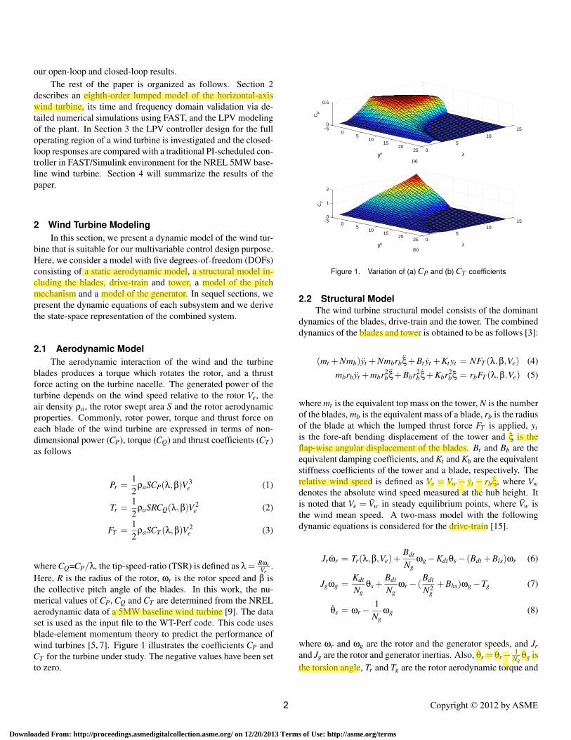
.Here, R is the radius of the rotor, ωr is the rotor speed and β isthe collective pitch angle of the blades. In this work, the nu-merical values of CP, CQ and CT are determined from the NRELaerodynamic data of a 5MW baseline wind turbine [9]. The dataset is used as the input file to the WT-Perf code. This code usesblade-element momentum theory to predict the performance ofwind turbines [5, 7]. Figure 1 illustrates the coefficients CP andCT for the turbine under study. The negative values have been setto zero.

0

5

10

15−50

510

1520

25

0

0.5

λβo

CP

05

1015−5

05

1015

2025

0

1

2

λβo

CT

(a)

(b)

Figure 1. Variation of (a) CP and (b) CT coefficients

2.2 Structural ModelThe wind turbine structural model consists of the dominant

dynamics of the blades, drive-train and the tower. The combineddynamics of the blades and tower is obtained to be as follows [3]:

(mt +Nmb)yt +Nmbrbξ+Bt yt +Ktyt = NFT (λ,β,Ve) (4)mbrbyt +mbr2

bξ+Bbr2bξ+Kbr2

bξ = rbFT (λ,β,Ve) (5)

where mt is the equivalent top mass on the tower, N is the numberof the blades, mb is the equivalent mass of a blade, rb is the radiusof the blade at which the lumped thrust force FT is applied, ytis the fore-aft bending displacement of the tower and ξ is theflap-wise angular displacement of the blades. Bt and Bb are theequivalent damping coefficients, and Kt and Kb are the equivalentstiffness coefficients of the tower and a blade, respectively. Therelative wind speed is defined as Ve = Vw − yt − rbξ, where Vwdenotes the absolute wind speed measured at the hub height. Itis noted that Ve = Vw in steady equilibrium points, where Vw isthe wind mean speed. A two-mass model with the followingdynamic equations is considered for the drive-train [15].

Jrωr = Tr(λ,β,Ve)+Bdt

Ngωg −Kdtθs − (Bdt +Bls)ωr (6)

Jgωg =Kdt

Ngθs +

Bdt

Ngωr − (

Bdt

N2g

+Bhs)ωg −Tg (7)

θs = ωr −1

Ngωg (8)

where ωr and ωg are the rotor and the generator speeds, and Jrand Jg are the rotor and generator inertias. Also, θs = θr− 1

Ngθg is

the torsion angle, Tr and Tg are the rotor aerodynamic torque and

2 Copyright © 2012 by ASME

Downloaded From: http://proceedings.asmedigitalcollection.asme.org/ on 12/20/2013 Terms of Use: http://asme.org/terms

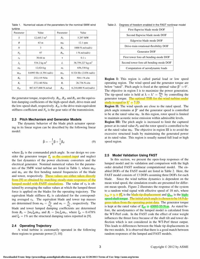
Table 1. Numerical values of the parameters for the nominal 5MW windturbine

Parameter Value Parameter Value

S 12,445.3 m2 PN 5.297 MW

R 63 m ωN 12.1 rpm

N 3 Bls 1000 N.m/(rad/s)

Ng 97 Bhs 1 N.m/(rad/s)

rb 30.64 m τ 0.1 s

Jg 534.2 kg.m2 Jr 38,759,227 kg.m2

mb 12,024 kg mt 656,330 kg

ω1b 0.6993 Hz (4.394 rad/s) ω1t 0.324 Hz (2.036 rad/s)

Kb 232,119 N/m Bb 504.1 N.s/m

Kt 272,140 N/m Bt 26,736 N.s/m

Kdt 867,637,000 N.m/rad Bdt 6,210,000 N.m/(rad/s)

the generator torque, respectively. Bhs, Bdt and Bls are the equiva-lent damping coefficients of the high-speed shaft, drive-train andthe low-speed shaft, respectively. Kdt is the drive-train equivalentstiffness coefficient and Ng is the gear ratio of the transmission.

2.3 Pitch Mechanism and Generator ModelsThe dynamic behavior of the blade pitch actuator operat-

ing in its linear region can be described by the following linearmodel:

β = −1τ

β+1τ

βd (9)

where βd is the commanded pitch angle. In our design we con-sider the generator torque Tg as the control input and neglectthe fast dynamics of the power electronic converters and theelectrical generator. Nominal numerical values for the parame-ters of the 5MW wind turbine are listed in Table 1, where ω1band ω1t are the first bending natural frequencies of the bladeand tower, respectively. These values are either taken directlyfrom [9] or obtained by matching steady-state responses of thelumped model with FAST simulations. The value of rb is ob-tained by averaging the radius values at which the lumped thrustforce is applied on the blades for the operating trajectory. Theequivalent blade stiffness Kb is calculated for the correspond-ing averaged rb. The equivalent blade and tower top massesare determined from mb = Kb

ω21b

and mt = Ktω2

1t, respectively. The

blade and tower lumped damping coefficients are determinedfrom Bb = 2mbξbω1b and Bt = 2mtξtω1t , where ξb = 0.478%and ξt = 1% are the structural damping ratios reported in [9].

2.4 Operating TrajectoryA wind turbine is customarily operated in the following

three regions to generate power [3, 10]:

Table 2. Degrees of freedom enabled in the FAST nonlinear model

First flapwise blade mode DOF

Second flapwise blade mode DOF

Edgewise blade mode DOF

Drive-train rotational-flexibility DOF

Generator DOF

First tower fore-aft bending-mode DOF

Second tower fore-aft bending-mode DOF

Computation of aerodynamic loads

Region I: This region is called partial load or low speedoperating region. The wind speed and the generator torque arebelow “rated”. Pitch angle is fixed at the optimal value β∗ ≃ 0◦.The objective in region I is to maximize the power generation.The tip-speed ratio is held at λ = λ∗ = Rωr

Vwby controlling the

generator torque. The optimal TSR for the wind turbine understudy is equal to λ∗ = 7.55.Region II: The wind speeds are close to the rated speed. Thepitch angle remains at β∗ and the generator speed is controlledto be at the rated value ωN . In this region, rotor speed is limitedto maintain acoustic noise emission within admissible levels.Region III: The pitch angle is increased to limit the capturedpower at its rated value PN and the rotor speed is controlled to beat the rated value ωN . The objective in region III is to avoid theexcessive structural loads by maintaining the generated powerat its rated value. This region is usually named full load or highspeed region.

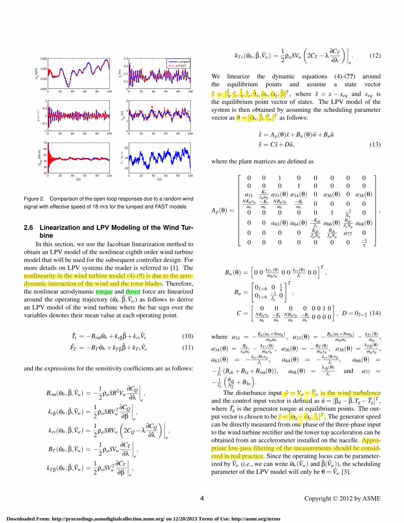
2.5 Model Validation Using FASTIn this section, we present the open-loop responses of the

lumped model and its validation and comparison with the highorder detailed FAST nonlinear computational model. The en-abled DOFs of the FAST model are listed in Table 2. Here, theFAST model consists of 13 DOFs assuming three DOFs for eachblade. Since the wind turbine dynamics is dependent on themean wind speed, the simulation results are presented for differ-ent mean speeds. Figure 2 illustrates the response of the systemto a random wind signal with effective speed of 18 m/s, whereytip = yt +Rξ is the blade tip displacement and Qhss is the high-speed shaft torque. The initial pitch angle is chosen to be 14.9 de-grees taken from the operating point data. The generator torqueis kept at the rated value of TgN = 43093.55 N.m. As stated be-fore, the aerodynamics of the lumped model is calculated fromthe WT-Perf code. In the FAST code the effect of rotor weightinfluences the thrust force because of the shaft tilt and tower de-flection which is not considered in the WT-Perf thrust output.This leads to differences between the blade tip displacements inthe two models. It is observed that there is a good match betweenrandom responses of the lumped and FAST models.

3 Copyright © 2012 by ASME

Downloaded From: http://proceedings.asmedigitalcollection.asme.org/ on 12/20/2013 Terms of Use: http://asme.org/terms

0 20 40 60 80 1001000

1100

1200

1300

ωg (

rpm

)

0 20 40 60 80 1000

0.1

0.2

0.3

0.4

y t (m

)

LumpedFAST

0 20 40 60 80 100−1

−0.5

0

0.5

1

y t(m

/s2

)

1

0 20 40 60 80 1000

1

2

3

y tip (

m)

0 20 40 60 80 10020

30

40

50

60

70

t(s)

Qhs

s (kN

.m)

0 20 40 60 80 100

16

18

20

t(s)

Vw

(m/s)

Figure 2. Comparison of the open-loop responses due to a random windsignal with effective speed of 18 m/s for the lumped and FAST models

2.6 Linearization and LPV Modeling of the Wind Tur-bine

In this section, we use the Jacobian linearization method toobtain an LPV model of the nonlinear eighth order wind turbinemodel that will be used for the subsequent controller design. Formore details on LPV systems the reader is referred to [1]. Thenonlinearity in the wind turbine model (4)-(9) is due to the aero-dynamic interaction of the wind and the rotor blades. Therefore,the nonlinear aerodynamic torque and thrust force are linearizedaround the operating trajectory (ωr, β,Vw) as follows to derivean LPV model of the wind turbine where the bar sign over thevariables denotes their mean value at each operating point.

Tr = −Brωωr + krββ+ krvVe (10)

FT = −BT ωr + kT ββ+ kT vVe (11)

and the expressions for the sensitivity coefficients are as follows:

Brω(ωr, β,Vw) = −12

ρaSR2Vw∂CQ

∂λ

∣∣∣∣e,

krβ(ωr, β,Vw) =12

ρaSRV 2w

∂CQ

∂β

∣∣∣∣e,

krv(ωr, β,Vw) =12

ρaSRVw

(2CQ −λ

∂CQ

∂λ

)∣∣∣∣e,

BT (ωr, β,Vw) = −12

ρaSVw∂CT

∂λ

∣∣∣∣e,

kT β(ωr, β,Vw) =12

ρaSV 2w

∂CT

∂β

∣∣∣∣e,

kT v(ωr, β,Vw) =12

ρaSVw

(2CT −λ

∂CT

∂λ

)∣∣∣∣e. (12)

We linearize the dynamic equations (4)-(??) aroundthe equilibrium points and assume a state vectorx = [ξ, yt ,

˙ξ, ˙yt , θs, ωr, ωg, β]T , where x = x − xeq and xeq isthe equilibrium point vector of states. The LPV model of thesystem is then obtained by assuming the scheduling parametervector as θ = [ωr, β,Vw]T as follows:

˙x = Ap(θ)x+Bw(θ)w+Buu

y = Cx+Du, (13)

where the plant matrices are defined as

Ap(θ) =

0 0 1 0 0 0 0 00 0 0 1 0 0 0 0

a31Kt

rbmta33(θ) a34(θ) 0 a36(θ) 0 a38(θ)

NKbrbmt

−Ktmt

NBbrbmt

−Btmt

0 0 0 00 0 0 0 0 1 −1

Ng0

0 0 a63(θ) a64(θ) −KdtJr

a66(θ) BdtJrNg

a68(θ)

0 0 0 0 KdtJgNg

BdtJgNg

a77 00 0 0 0 0 0 0 −1

τ

,

Bw(θ) =[

0 0 kT v(θ)mbrb

0 0 krv(θ)Jr

0 0]T

,

Bu =

[01×6 0 1

τ01×6

−1Jg

0

]T

,

C =[

0 0 0 0 0 0 1 0NKbrb

mt−Ktmt

NBbrbmt

−Btmt

0 0 0 0

], D = 02×2 (14)

where a31 = −Kb(mt+Nmb)mbmt

, a33(θ) = −Bb(mt+Nmb)mbmt

− kT v(θ)mb

,

a34(θ) = Bbrbmt

− kT v(θ)mbrb

, a36(θ) = −BT (θ)mbrb

, a38(θ) =kT β(θ)mbrb

,

a63(θ) = − krv(θ)rbJr

, a64(θ) = − krv(θ)rbJr

, a66(θ) =

− 1Jr

(Bdt +Bls +Brω(θ)), a68(θ) =krβ(θ)

Jrand a77 =

− 1Jg

(BdtN2

g+Bhs

).

The disturbance input w = Vw − Vw is the wind turbulenceand the control input vector is defined as u = [βd − β,Tg − Tg]T ,where Tg is the generator torque at equilibrium points. The out-put vector is chosen to be y = [ωg−ωg, ¨yt ]T . The generator speedcan be directly measured from one phase of the three-phase inputto the wind turbine rectifier and the tower top acceleration can beobtained from an accelerometer installed on the nacelle. Appro-priate low-pass filtering of the measurements should be consid-ered in real practice. Since the operating locus can be parameter-ized by Vw (i.e., we can write ωr(Vw) and β(Vw)), the schedulingparameter of the LPV model will only be θ = Vw [3].

4 Copyright © 2012 by ASME

Downloaded From: http://proceedings.asmedigitalcollection.asme.org/ on 12/20/2013 Terms of Use: http://asme.org/terms

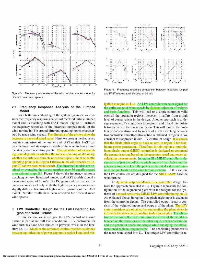
Figure 3. Frequency responses of the wind turbine lumped model fordifferent mean wind speeds

2.7 Frequency Response Analysis of the LumpedModel

For a better understanding of the system dynamics, we con-sider the frequency response analysis of the wind turbine lumpedmodel and its matching with FAST model. Figure 3 illustratesthe frequency responses of the linearized lumped model of thewind turbine in (14) around different operating points character-ized by mean wind speeds. The direction of the arrows show thedecrease in the wind speed value. Here, we present the frequencydomain comparison of the lumped and FAST models. FAST canprovide linearized state-space models of the wind turbine aroundthe steady state operating points. The calculation of an operat-ing point depends on whether the rotor is spinning or stationary,whether the turbine is variable or constant speed, and whether theoperating point is in Region I (below rated wind speed) or Re-gion III (above rated wind speed). The linearized models are ob-tained by averaging the system matrices over 36 equally spacedrotor azimuth steps [8]. Figure 4 shows the frequency responsematching between linearized lumped and FAST models around amean wind speed of 20 m/s. The DC gains and first natural fre-quencies coincide closely while the high frequency responses areslightly different because of higher order dynamics of the FASTmodel. Similar results have been observed for different meanwind speeds.

3 LPV Controller Design for the Full Operating Re-gion of a Wind TurbineIn this section, we investigate the LPV control of a wind

turbine in partial and full loads conditions. LPV controllers forwind turbines have been studied in previous works in the liter-ature [2, 13]. Much of the advanced control research is dividedbetween optimization of power capture in region I and load mit-

Figure 4. Frequency response comparison between linearized lumpedand FAST models at wind speed of 20 m/s

igation in region III [10]. An LPV controller can be designed forthe entire range of wind speeds by delicate selection of weightsand basis functions. This will lead to a single controller validover all the operating regions, however, it suffers from a highlevel of conservatism in the design. Another approach is to de-sign separate LPV controllers for regions I and III and interpolatebetween them in the transition region. This will remove the prob-lem of conservatism, and by means of a soft switching betweentwo controllers smooth control action is obtained in region II. Weconsider this approach in our LPV controller design. It is knownthat the blade pitch angle is fixed at zero in region I for max-imum power generation. Therefore, in this region a multiple-input-single-output (MISO) controller is designed to commandthe generator torque based on the generator speed and tower ac-celeration measurements. In region III a MIMO controller is de-signed to adjust the collective pitch angle of the blades and thegenerator torque to keep the power at the rated value and mini-mize fatigue loads on the wind turbine structure. In this section,the LPV controllers are designed for the NREL 5MW baselinewind turbine.

The dynamic output-feedback LPV controller design fol-lows the approach presented in [1]. Figure 5 represents the con-figuration of the augmented plant with the weights for the syn-thesis of a mixed-sensitivity MIMO LPV controller in region III.As explained above, in region I the pitch angle input is excludedfrom the controller design. The controlled output vector z con-sists of the weighted inputs and outputs of the plant. The LPVsystem matrices are obtained by augmenting the plant states in(13) with the states corresponding to design weights. The objec-tive of the controller is to minimize the effect of the wind tur-bulence on the variations of the pitch angle, tower acceleration,and the generator speed and torque while satisfying the above-mentioned regional requirements. The scheduling parameter isthe mean wind speed θ = Vw. The torque LPV controller in re-

5 Copyright © 2012 by ASME

Downloaded From: http://proceedings.asmedigitalcollection.asme.org/ on 12/20/2013 Terms of Use: http://asme.org/terms

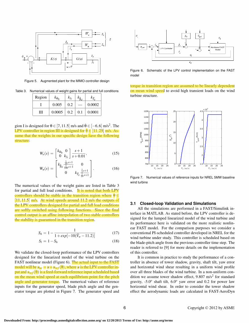
Figure 5. Augmented plant for the MIMO controller design

Table 3. Numerical values of weight gains for partial and full conditions

Region kωg kyt kβdkTg

I 0.005 0.2 — 0.0002

III 0.0005 0.2 0.1 0.0001

gion I is designed for θ ∈ [7,11.5] m/s and θ ∈ [−6,6] m/s2. TheLPV controller in region III is designed for θ ∈ [11,25] m/s. As-sume that the weights in our specific design have the followingstructure:

We(s) =[

kωg 00 kyt

]s+1

s+0.01, (15)

Wu(s) =

kβd

110 s+11

100 s+10

0 kTg

12 s+1120 s+1

. (16)

The numerical values of the weight gains are listed in Table 3for partial and full load conditions. It is noted that both LPVcontrollers should be stable in the transition region where θ ∈[11,11.5] m/s. At wind speeds around 11.2 m/s the outputs ofthe LPV controllers designed for partial and full load conditionsare softly switched using following functions. Since the finalcontrol output is an affine interpolation of two stable controllersthe stability is guaranteed in the transition region.

Sh = 1− 11+ exp[−10(Vw −11.2)]

(17)

Sl = 1−Sh (18)

We validate the closed-loop performance of the LPV controllersdesigned for the linearized model of the wind turbine on theFAST nonlinear model (Figure 6). The actual input to the FASTmodel will be uac = u+ure f (θ), where u is the LPV controller in-put and ure f (θ) is a feed-forward reference input scheduled basedon the mean wind speed at each equilibrium point for the pitchangle and generator torque. The numerical values of referenceinputs for the generator speed, blade pitch angle and the gen-erator torque are plotted in Figure 7. The generator speed and

Figure 6. Schematic of the LPV control implementation on the FASTmodel

torque in transition region are assumed to be linearly dependenton mean wind speed to avoid high transient loads on the windturbine structure.

10 15 20 25750

800

850

900

950

1000

1050

1100

1150

1200

Vw (m/s)

ωg,

ref (

RP

M)

10 15 20 250

5

10

15

20

25

Vw (m/s)β re

f (o )

10 15 20 251.5

2

2.5

3

3.5

4

4.5x 10

4

Vw (m/s)

Tg,

ref (

N.m

)

Figure 7. Numerical values of reference inputs for NREL 5MW baselinewind turbine

3.1 Closed-loop Validation and SimulationsAll the simulations are performed in a FAST/Simulink in-

terface in MATLAB. As stated before, the LPV controller is de-signed for the lumped linearized model of the wind turbine andits performance here is validated on the more realistic nonlin-ear FAST model. For the comparison purposes we consider aconventional PI-scheduled controller developed in NREL for thewind turbine under study. This controller is scheduled based onthe blade-pitch angle from the previous controller time step. Thereader is referred to [9] for more details on the implementationof this controller.

It is common in practice to study the performance of a con-troller in absence of tower shadow, gravity, shaft tilt, yaw errorand horizontal wind shear resulting in a uniform wind profileover all three blades of the wind turbine. In a non-uniform con-dition we assume tower shadow effect, 9.807 m/s2 for standardgravity, -5.0o shaft tilt, 6.0o yaw error and 0.2 for power lawhorizontal wind shear. In order to consider the tower shadoweffect the aerodynamic loads are calculated in FAST-AeroDyn

6 Copyright © 2012 by ASME

Downloaded From: http://proceedings.asmedigitalcollection.asme.org/ on 12/20/2013 Terms of Use: http://asme.org/terms

20 40 60 80

1100

1200

1300

ωg (

rpm

)

20 40 60 80 1003000

4000

5000

6000

Gen

erat

or p

ower

(kW

)

LPVPI−scheduled

20 40 60 800

5

10

β (o )

20 40 60 80

4000

6000

8000

10000

12000

Bla

de r

oot f

alpw

ise

m

omen

t (kN

.m)

20 40 60 802

4

6

8

x 104

Tow

er b

ase

fore

−af

t

m

omen

t (kN

.m)

t(s)20 40 60 80

10

11

12

13

14

Win

d sp

eed

(m/s

)

t(s)

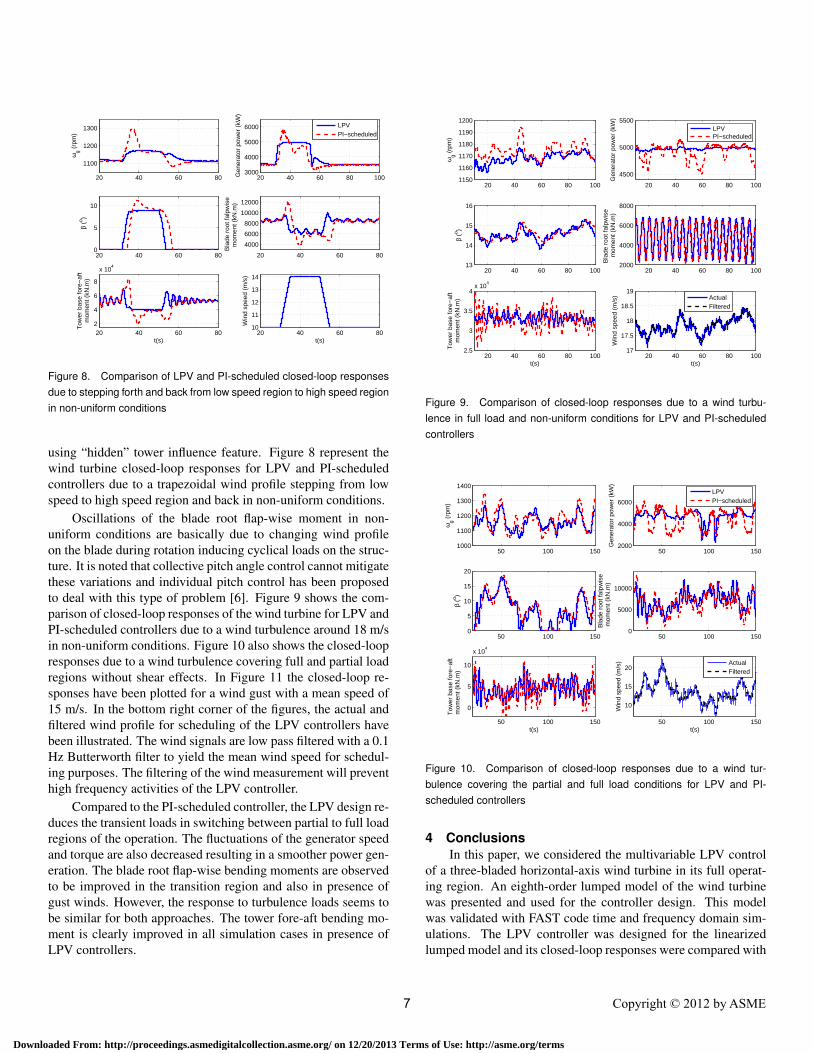
Figure 8. Comparison of LPV and PI-scheduled closed-loop responsesdue to stepping forth and back from low speed region to high speed regionin non-uniform conditions

using “hidden” tower influence feature. Figure 8 represent thewind turbine closed-loop responses for LPV and PI-scheduledcontrollers due to a trapezoidal wind profile stepping from lowspeed to high speed region and back in non-uniform conditions.

Oscillations of the blade root flap-wise moment in non-uniform conditions are basically due to changing wind profileon the blade during rotation inducing cyclical loads on the struc-ture. It is noted that collective pitch angle control cannot mitigatethese variations and individual pitch control has been proposedto deal with this type of problem [6]. Figure 9 shows the com-parison of closed-loop responses of the wind turbine for LPV andPI-scheduled controllers due to a wind turbulence around 18 m/sin non-uniform conditions. Figure 10 also shows the closed-loopresponses due to a wind turbulence covering full and partial loadregions without shear effects. In Figure 11 the closed-loop re-sponses have been plotted for a wind gust with a mean speed of15 m/s. In the bottom right corner of the figures, the actual andfiltered wind profile for scheduling of the LPV controllers havebeen illustrated. The wind signals are low pass filtered with a 0.1Hz Butterworth filter to yield the mean wind speed for schedul-ing purposes. The filtering of the wind measurement will preventhigh frequency activities of the LPV controller.

Compared to the PI-scheduled controller, the LPV design re-duces the transient loads in switching between partial to full loadregions of the operation. The fluctuations of the generator speedand torque are also decreased resulting in a smoother power gen-eration. The blade root flap-wise bending moments are observedto be improved in the transition region and also in presence ofgust winds. However, the response to turbulence loads seems tobe similar for both approaches. The tower fore-aft bending mo-ment is clearly improved in all simulation cases in presence ofLPV controllers.

20 40 60 80 1001150

1160

1170

1180

1190

1200

ωg (

rpm

)

20 40 60 80 100

4500

5000

5500

Gen

erat

or p

ower

(kW

)

LPVPI−scheduled

20 40 60 80 10013

14

15

16

β (o )

20 40 60 80 1002000

4000

6000

8000

Bla

de r

oot f

alpw

ise

mom

ent (

kN.m

)

20 40 60 80 1002.5

3

3.5

4x 10

4

Tow

er b

ase

fore

−af

t m

omen

t (kN

.m)

t(s)20 40 60 80 100

17

17.5

18

18.5

19

Win

d sp

eed

(m/s

)

t(s)

ActualFiltered

Figure 9. Comparison of closed-loop responses due to a wind turbu-lence in full load and non-uniform conditions for LPV and PI-scheduledcontrollers

50 100 1501000

1100

1200

1300

1400

ωg (

rpm

)

50 100 1502000

4000

6000

Gen

erat

or p

ower

(kW

)

50 100 1500

5

10

15

20

β (o )

50 100 1500

5000

10000

Bla

de r

oot f

alpw

ise

mom

ent (

kN.m

)

50 100 150

0

5

10

x 104

Tow

er b

ase

fore

−af

t m

omen

t (kN

.m)

t(s)50 100 150

10

15

20

Win

d sp

eed

(m/s

)

t(s)

ActualFiltered

LPVPI−scheduled

Figure 10. Comparison of closed-loop responses due to a wind tur-bulence covering the partial and full load conditions for LPV and PI-scheduled controllers

4 ConclusionsIn this paper, we considered the multivariable LPV control

of a three-bladed horizontal-axis wind turbine in its full operat-ing region. An eighth-order lumped model of the wind turbinewas presented and used for the controller design. This modelwas validated with FAST code time and frequency domain sim-ulations. The LPV controller was designed for the linearizedlumped model and its closed-loop responses were compared with

7 Copyright © 2012 by ASME

Downloaded From: http://proceedings.asmedigitalcollection.asme.org/ on 12/20/2013 Terms of Use: http://asme.org/terms

0 10 20 30 401000

1100

1200

1300

1400

1500

ωg (

rpm

)

0 10 20 30 402000

4000

6000

8000

Gen

erat

or p

ower

(kW

)

LPVPI−scheduled

0 10 20 30 405

10

15

20

β (o )

0 10 20 30 40

0

5000

10000B

lade

roo

t fal

pwis

e m

omen

t (kN

.m)

0 10 20 30 40−1

−0.5

0

0.5

1

x 105

Tow

er b

ase

fore

−af

t m

omen

t (kN

.m)

t(s)0 10 20 30 40

10

15

20

Win

d sp

eed

(m/s

)

t(s)

ActualFiltered

Figure 11. Comparison of closed-loop responses due to a wind gust witha mean speed of 15 m/s for LPV and PI-scheduled controllers

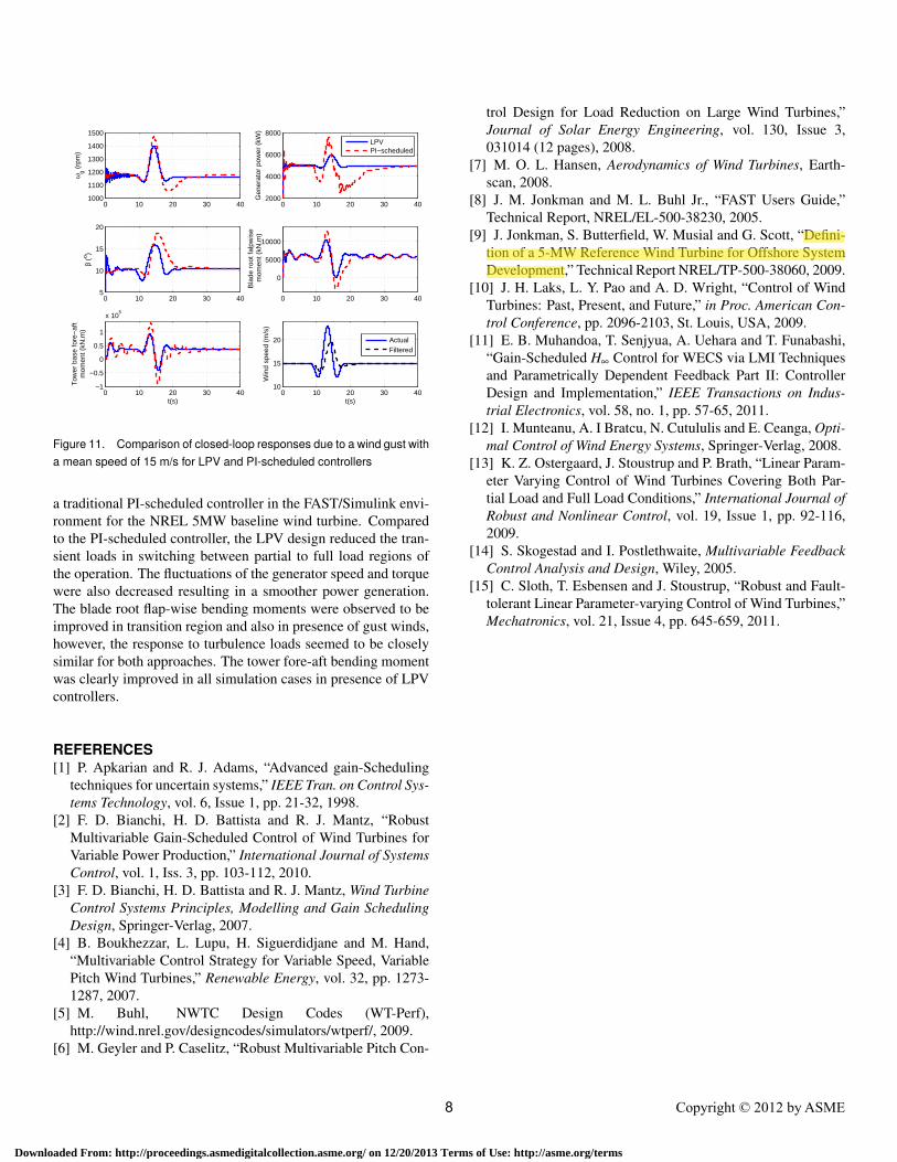
a traditional PI-scheduled controller in the FAST/Simulink envi-ronment for the NREL 5MW baseline wind turbine. Comparedto the PI-scheduled controller, the LPV design reduced the tran-sient loads in switching between partial to full load regions ofthe operation. The fluctuations of the generator speed and torquewere also decreased resulting in a smoother power generation.The blade root flap-wise bending moments were observed to beimproved in transition region and also in presence of gust winds,however, the response to turbulence loads seemed to be closelysimilar for both approaches. The tower fore-aft bending momentwas clearly improved in all simulation cases in presence of LPVcontrollers.

REFERENCES[1] P. Apkarian and R. J. Adams, “Advanced gain-Scheduling

techniques for uncertain systems,” IEEE Tran. on Control Sys-tems Technology, vol. 6, Issue 1, pp. 21-32, 1998.

[2] F. D. Bianchi, H. D. Battista and R. J. Mantz, “RobustMultivariable Gain-Scheduled Control of Wind Turbines forVariable Power Production,” International Journal of SystemsControl, vol. 1, Iss. 3, pp. 103-112, 2010.

[3] F. D. Bianchi, H. D. Battista and R. J. Mantz, Wind TurbineControl Systems Principles, Modelling and Gain SchedulingDesign, Springer-Verlag, 2007.

[4] B. Boukhezzar, L. Lupu, H. Siguerdidjane and M. Hand,“Multivariable Control Strategy for Variable Speed, VariablePitch Wind Turbines,” Renewable Energy, vol. 32, pp. 1273-1287, 2007.

[5] M. Buhl, NWTC Design Codes (WT-Perf),http://wind.nrel.gov/designcodes/simulators/wtperf/, 2009.

[6] M. Geyler and P. Caselitz, “Robust Multivariable Pitch Con-

trol Design for Load Reduction on Large Wind Turbines,”Journal of Solar Energy Engineering, vol. 130, Issue 3,031014 (12 pages), 2008.

[7] M. O. L. Hansen, Aerodynamics of Wind Turbines, Earth-scan, 2008.

[8] J. M. Jonkman and M. L. Buhl Jr., “FAST Users Guide,”Technical Report, NREL/EL-500-38230, 2005.

[9] J. Jonkman, S. Butterfield, W. Musial and G. Scott, “Defini-tion of a 5-MW Reference Wind Turbine for Offshore SystemDevelopment,” Technical Report NREL/TP-500-38060, 2009.

[10] J. H. Laks, L. Y. Pao and A. D. Wright, “Control of WindTurbines: Past, Present, and Future,” in Proc. American Con-trol Conference, pp. 2096-2103, St. Louis, USA, 2009.

[11] E. B. Muhandoa, T. Senjyua, A. Uehara and T. Funabashi,“Gain-Scheduled H∞ Control for WECS via LMI Techniquesand Parametrically Dependent Feedback Part II: ControllerDesign and Implementation,” IEEE Transactions on Indus-trial Electronics, vol. 58, no. 1, pp. 57-65, 2011.

[12] I. Munteanu, A. I Bratcu, N. Cutululis and E. Ceanga, Opti-mal Control of Wind Energy Systems, Springer-Verlag, 2008.

[13] K. Z. Ostergaard, J. Stoustrup and P. Brath, “Linear Param-eter Varying Control of Wind Turbines Covering Both Par-tial Load and Full Load Conditions,” International Journal ofRobust and Nonlinear Control, vol. 19, Issue 1, pp. 92-116,2009.

[14] S. Skogestad and I. Postlethwaite, Multivariable FeedbackControl Analysis and Design, Wiley, 2005.

[15] C. Sloth, T. Esbensen and J. Stoustrup, “Robust and Fault-tolerant Linear Parameter-varying Control of Wind Turbines,”Mechatronics, vol. 21, Issue 4, pp. 645-659, 2011.

8 Copyright © 2012 by ASME

Downloaded From: http://proceedings.asmedigitalcollection.asme.org/ on 12/20/2013 Terms of Use: http://asme.org/terms