copertinaclemente:Layout 1 7-04-2010 16:28 Pagina 1

WIM (WEIGH IN MOTION), LOAD CAPACITY

AND BRIDGE PERFORMANCE

Edited by Paolo Clemente and Alessandro De Stefano 2010 ENEA

Italian National Agency for New Technologies, Energy and Sustainable Economic Development Lungotevere Thaon di Revel, 76 00196 Rome

ISBN 978-88-8286-220-6

WIM (WEIGH IN MOTION),

LOAD CAPACITY AND BRIDGE PERFORMANCE

EDITED BY

PAOLO CLEMENTE AND ALESSANDRO DE STEFANO

5

TABLE OF CONTENTS

Preface

7

Extreme Traffic Load Effects on Medium Span Bridges M. Arroyo, M. Hannachi, D. Sieger, B. Jacob

9

Pedestrian loads and dynamic performances of lively footbridges: an overview on measurement techniques and codes of practice F. Venuti, L. Bruno

15

Bridge-WIM as an efficient tool for optimised bridge assessment A. Žnidarič

27

Experimental characterization of innovative dampers and large scale validation tests of systems for the control of vibrations induced by traffic on bridge decks and railway basements Vito Renda

35

Real-Time Monitoring of Displacement for Health Monitoring of Structures M.Çelebi

45

Development of an integrated structural health monitoring system H.Hao, X.Q. Zhu

53

Identification of dynamic axle loads from bridge responses by means of an extended dynamic programming algorithm E. Lourens, G. Lombaert, G. De Roeck, G. Degrande

59

Recent Advances in the Governing Form of Traffic for Bridge Loading C.C. Caprani, E.J. Obrien

71

The role of low-cost vibration measurement systems in bridge health monitoring applications - example of pedestrian bridges N. Haritos

79

Dynamic Response of a Footbridge to Walking People P. Clemente, G. Ricciardi, F. Saitta

89

Development of fully equipped test beds and an online damage identification system S. Beskhyroun, T. Oshima, Y. Miyamori, S. Mikami, T. Yamazaki

99

Monitoring of Traffic Loads and Bridge Performance using a Bridge Weigh-In-Motion System J. Dowling, A. González, E. J. Obrien

107

Critical considerations and proposals in developing Bridge Weigh in Motion (B-WIM) systems L. Degiovanni, A. De Stefano, A. Iranmanesh, F. Ansari

115

6

Model-free bridge-based vehicle classification G. Rutherford, D. K. McNeill

123

Dynamic assessment of PSC bridge structures under moving vehicular loads H.Hao, X.Q. Zhu

129

Structural Load Rating and Long-Term Rehabilitation Cost Estimate for the El Prieto Bridge F.J. Carrión, J.A. Quintana, M.J. Fabela, J.T. Pérez, P.R. Orozco, M. Martínez, M.A. Barousse

137

New Features in Dynamic Instrumentation of Structures D. Rinaldis, P. Clemente, M. Caponero

141

Determination of Live Load Factors for Reliability-Based Bridge Design and Evaluation Using WIM Data H.-M. Koh, E.-S. Hwang

149

Influence of heavy traffic trend on EC1-2 load models for road bridges S. Caramelli, P. Croce

157

Fatigue evaluation and assessment of a railway bridge C. Pellegrino, A. Pipinato, C. Modena

165

In-Service and Weigh-In-Motion Monitoring of Typical Highway Bridges M. Rakowski, H.W. Shenton III, M.J. Chajes

173

Damage detection algorithm for bridge equipped with anti-seismic devices C. Amaddeo, G. Benzoni, E. D’Amore

179

7

PREFACE The continuous ageing and subsequent structural deterioration of a large number of existing structures make essential the development of efficient SHM systems (Structural Health Monitoring). The state of the health of structures is conditioned by several factors that are manifested in terms of cracks, strain changes or thermal gradients. The knowledge of the relationship correlating such factors is therefore essential in providing an effective and useful damage detection analysis in order to improve maintenance activities and make better use of available resources. Successful Structural Health Monitoring strategies require detection of reliable and accurate measures, captured in strategic points of the structure and with systematic or continuous monitoring. Due to the increasing interest on the safeguard of the infrastructures, the scientific research has been devoted to the development of structural monitoring techniques. Instrumentation of structures and bridges is a very good technique for the evaluation of safety and of structural health in order to plan the maintenance program. On these subjects, under the supervision of ISHMII (International Society for Structural Health Monitoring of Intelligent Infrastructures, http://www.ishmii.org), ENEA (Italian National Agency for New Technologies, Energy and Sustainable Economic Development), Politecnico of Torino, University of Illinois at Chicago, University of Manitoba, GLIS (Base Isolation and other Antiseismic Design Strategies) organized the workshop “Civil Structural Health Monitoring 2”, which was held in Taormina (Italy) between September 28th and October 1st. In this volume a selection of the papers presented is reported. Specifically the main goal of the CSHM2 was to promote international cooperation in the fields of load capacity, bridge performance maintenance and safety, taking into account that bridges are the most vulnerable part of civil transportation system that affects directly the public safety. The organization of the conference arises from the need to focus the attention on the measure of intensity and velocity of moving loads and the evaluation of load carrying capacity of bridges, in order to create a cooperating working group and provide guidelines useful for the future researches in the field. As a matter of fact, a terrific increase of the road traffic happened in the last decades. In the same time also the weight of the vehicle got higher. The acquisition of data about number, type and weight of vehicles is possible by means of WIM (Weigh In Motion) systems, but their use is still scarce. Main topics were:

• Safety of the existing structures • Analysis of the overloading on bridges • Evaluation of the suitability of instrumentation, methods and models • Solutions by means of innovative technologies of structural monitoring and sensors

(WIM sensors, permanent monitoring arrays, etc...). International Scientific Committee

Ansari Fahrad USA Celebi Mehmet USA Clemente Paolo Italy De Stefano Alessandro Italy Jacob Bernard France Mancini Giuseppe Italy Mufti Aftab Canada

8

Organizing Committee

De Stefano Alessandro, Politecnico di Torino (Italy) Clemente Paolo, ENEA (Italy) Ansari Farhad, University of Illinois, Chicago, (USA) Mufti Aftab, University of Manitoba (Canada) Arato Giordano-Bruno, ENEA (Italy) Degiovanni Luisa, Politecnico di Torino (Italy)

Three working groups were organized to prepare short documents as kick-off bases for future guidelines and recommendations related to the workshop topics:

1. Formulate the State-of-the-Art and outlining capabilities and limitations of the WIM sensors

2. W.I.M. and Load Assessment, Load capacity 3. Performance in the context of Risk assessment, Maintenance and Life cost based

design The list of the members of the three groups is shown in the following table.

Group 1 Group 2 Group 3 Brunner Fritz K., Coord. McNeill Dean, Recorder Ansar Farhad Bakht Baidar Degiovanni Luisa Habel Wolfgang Jacob Bernard Mufti Aftab Rinaldis Dario Spindler Thomas Weiss Florian Žnidarič Aleš

Carrion Francisco, Coord. Haritos Nicholas, Recorder Caprani Colin Croce Pietro De Stefano Alessandro Hwang Eui-Seung Newhook John

Wenzel Helmut, Coord. Shenton Tripp, Recorder Beskhyroun Sherif Celebi Mehmet Clemente Paolo Giacosa Luca Marengo Giorgio Oshima Toshiyuki Pastore Giuseppe Salza Barbara

P. Clemente & A. De Stefano (eds.), WIM (Weigh In Motion), Load Capacity and Bridge Performance. ENEA, Roma, 2010

1 INTRODUCTION

Road bridges are designed for service lives over 50,

100, 120 years so that they would withstand the forces that might be expected to impact upon them. Therefore, the extreme traffic load effects

were considered in the calibration studies performed for the load model for Eurocode 1 [4]. In the previous calibration studies, available weigh in motion (WIM) data recorded on heavy trafficked highways were passed over and a large representative selection of influence lines for estimating the probability density function of the load effects. Subsequently, loading events that exceeded a level with a probability of 0.001 in any one year were estimated using different extrapolation methods [6, 5, 7]. Such a low value of probability is related to events generally not observed during the measuring period and the results have been interpreted with caution regarding the quality of the data and the extrapolation methods. The selection of the extreme value distribution is still only based on faith. Furthermore, as extreme value theory rely on asymptotic results based on the assumptions of independent identically distributed of the considered events, these conditions must be fulfilled for estimating the parameters. Generalized extreme value distributions of critical bridge loading events were identified from long run simulation data in accordance with these requirements, i.e. extreme laws of the effects were inferred for categorized loading events [1]. It was also noticed in reference [8]that the parameter identification of the extreme value distribution was very sensitive to the parameter estimation methods (maximum likeli-hood, least squares, moments) and that the Gumbel distribution was a suitable choice for the example considered. In this paper, recent examples of extreme value statistics of traffic loads and effects on a medium span bridge are presented. 1000 years return values extrapolated estimates from different models are

compared and their consistency with realistic traffic loading events are discussed. 2 THEORETICAL BACKGROUND FOR PARAMETER

ESTIMATION 2.1 Derivation from the parent distribu- tion The asymptotic distribution of the block maxima (e.i. daily maxima) drawn from a gaussian tail is a Gumbel law. This theoretical result was used for estimating the extreme distribution of the truck loads from the multi-modal normal distribution of the gross vehicle weight or single and group of axles loads. The Gumbel asymptotic cumulative distribution of the daily max values drawn from a fixed number n = pN of events normally distributed is expressed as

Gn(x)= exp(−exp(−an(x − bn)) with the parameters:

where µ2 and σ2 are the mean and standard deviation of the proportion p of trucks in the heavier mode and N the number of trucks per day. An alternative description of the asymptotic

Extreme Traffic Load Effects on Medium Span Bridges

M. Arroyo University Autonomous of Queretaro, Mexico (on sabbatical year with LCPC)

M. Hannachi , D. Siegert

, B. Jacob

Université Paris-Est, LCPC, 58 boulevard Lefebvre 75732 Paris, France

10

behaviour of the extreme values is given by the thinned Poisson model

Where T = 1 day and Φ is the cumulative normal distribution 2.2 Generalized extreme value distribu- tion and

return levels The GEV distribution which captures the Gumbel, Fr´echet and weibull families is of the form [2]

Where µ, σ and ξ are respectively the location, scale and shape parameters. When ξ = 0, the distribution corresponds to the Gumbel family

The return level xp of the block maxima is associated with the return period

1

p , i.e. the value xp is exceeded in any block with a probability p by the following approximate relationship when p is closed to zero

3 EXTREME GROSS VEHICLE WEIGHT 3.1 Wim data The WIM data considered in this example were recorded in June and September 2007 on the slow lane of A64 highway near Toulouse (Muret). The mean traffic flow intensity during the working days was 1550 trucks per day. The traffic composition with respect to the number of axles of the truck is reported in Figure 1.

Figure 1: Vehicle classification (axle number) and composition. The gross vehicle weight histogram is shown in Figure 2 with the bimodal gaussian fitted distribution

2πσ11 2πσ22 The maximum likelihood estimates of the parameters of the the distribution are reported in table 1.

p µ1 σ1 µ2 σ2

(kN) (kN) (kN) (kN)

0.33 165 70 378 46

Table 1: Fitted bimodal parameters of the GVW The daily measured maximum values of the GVW are plotted in figure 3. They are all above 500 kN and are related to semi-trailer with either 5 or 6 axles with a tridem. The data collected can be considered homogeneous with regard to the silhouette of the vehicles.

11

Figure 2: Gross vehicle weight distribution for trucks over 35 kN.

3.2 RETURN LEVEL ESTIMATES The return level of the GVW were estimated with the asymptotic Gumbel distribution of the daily maxima with parameters either derived from the tail of the bimodal GVW distribution and from the block maxima using the maximun likelihood method. In the latter case, the evd package of R software was used for estimating the parameters of the Gumbel law [9]. The comparison between the different estimates of the return values is plotted in 4. The 1000 years return period of the gross vehicle weight predicted with the gaussian tail is close to 700 kN. This value is significantly below the extrapolated Gumbel estimate from the daily maximum values. 4 EXTREME TRAffiC EffECTS 4.1 Bridge description and measurements The considered structure consists of five prestressed concrete isostatic girders connected by an overall concrete deck and five cross braces as shown in Figure 5. The instrumented span is 33 m long and carries three one way lanes. The bridge is located on a heavy trafficked itinerary in the North of Paris and undergoes a free-flowing traffic. Information on the truck traffic pattern was collected during eight weeks to get statistics on the vehicle speed, the traffic flow per lane and the silhouette composition.

A mean traffic flow of 8500 trucks per day was measured on the site with an amount of 23 % circulating on the second lane and 77 % on the slow lane. The mean speed value was 85 km/h with a coefficient of variation of 10 %. 80 % of the trucks were

Figure 3: Daily maximum gross vehicle weight.

Figure 4: Extreme GVW with respect the return period. classified in the tractor with a semi-trailer on a tridem axle category. The distribution of truck types with respect to the axle number is shown in Figure 6. The maximum strain was measured at mid-span of the girder under the slow lane. The data were collected and processed to eliminate the thermal effects or electrical drift in the

12

Figure 5: View of the girders of Roberval bridge

measurement. The maximum and minimum values of 120 s duration signals were recorded during 256 days and the daily maximum values of the traffic effects were obtained from the variation ranges since it was checked that the minimum values of the signals were only varying with a slowly evolving trend over the whole measurement period

Figure 6: Vehicle classification (axle number) and composition. . In addition, some signals were filtered with a low-pass filter to remove the frequency content above the first resonant frequency of the bridge close to 4 Hz. It was noticed that the dynamic effects of the traffic were negligible for the tested configurations, probably thanks to the use of pneumatic suspension devices in the lorries carrying heavy loads. Figure 7 shows the plots of the daily maximum values of the deformation measured at midspan on the girder between January and June, respectively in

2004 and 2005. The maximum values of the effects measured during the week-end and public holidays must be removed from the analysis because they correspond to events that are not identically distributed when considering the whole population. The observed maximum daily values of the traffic effects ranged from 60 m/m to 100 m/m and the lower bound of the maximum daily values was 70 m/m.

Figure 7: Time series of the measured daily maximum strains. 4.2 Discussion of return level estimates Extrapolated return values of the strain are displayed in Figure 8. The extrapolated estimates from the measured daily maxima are compared with the simple traffic load model derived from considering the load effect related to the meeting events on the bridge involving two heavy trucks circulating on the slow lane and on the second lane. The extreme distribution of the traffic load effect x can be expressed as [3]

with

where N1 and N2 are the traffic intensities in lane 1 and 2, V the speed and L is the interdistance between the tridems considered for calculating the deformation. Here, the latter geometrical parameter was taken equal to 3 m. Φ12 is the cumulative normal distribution of the effects derived from the maximum linear combination of the loads which is assumed constant over the inter-distance L. As it was noticed for the case of the GVW extrapolation,

13

the thinned poisson model lead to extrapolated values significantly lower than with the daily maxima. the return value at 1000 years extrapolated with the Gumbel distribution fitted to the daily max observed is still 50 % below the effect calculated with the Eurocode load model LM1;

Figure 8: Extreme strain with respect to the return period.

The maximum effects of some traffic configurations involving overloaded lorries were calculated. The considered silhouettes were a 16 m long five axles semi-trailer (T2R3) with a gross weight in the range from 400 kN to 540 kN and a 25 m long five axles semi-trailer coupled to a tandem trailer (T2R3R2) with a gross weight in the range from 600 kN to 730 kN. The latter vehicle is currently used in North European countries with a 600 kN gross weight. Eleven loading configurations were calculated, the results are reported in Figure 9. The range of the calculated effects match well the measured maximum effects.

Figure 9: effects of overloaded trucks

5 CONCLUSIONS • Extended weigh-in -motion data are needed for

a better characterization of the tail of the load distribition;

• the return values of the traffic loads and effects predicted from the bimodal model of the gross weight are underestimated;

• the return value at 1000 years extrapolated with the Gumbel distribution fitted to the daily max observed is still 50 % below the effect calculated with the Eurocode load model LM1;

• Difficulties for predicting observed extreme effects could be overcome by simulation meth-ods?

ACKNOWLEDGEMENTS The authors are grateful to D. Stanczyk for providing the WIM traffic data with detailed information concerning the measurements conditions. REFERENCES [1] C.C. Caprani, E.J. OBrien, and G.J. McLachlan. Characteristic traffic load effects from a mixture of loading events on short to medium span bridges. Structural Safety, page doi:10.1016/j.strusafe.2006.11.006, 2008. [2] S. Coles. An Introduction to Statistical Modeling of Extreme Value Theory. Springer Verlag, 2001. [3] O. Ditlevsen and H.O. Madsen. Stochastic vehicle queue load model for large bridges. Journal of Engineering Mechanics, 1994. [4] Eurocode-1. Partie 2, Actions sur les ponts, dues au trafic. NF-EN 1991-2, Paris, 2004. [5] A.R. Flint and B. Jacob. Extreme traffic loads on road bridges and target values of their effects for code calibration. In Proceedings of IABSE Colloquium, pages 469–478, Delft, The Netherlands, 1996. IABSE-AIPC-IVBH. [6] B. Jacob, J.B. Maillard, and J.F. Gorse.

14

Probabilistic traffic load models and extreme loads on a bridge. In ICOSSAR 89 Proceedings, pages 1973–1980, San Francisco, 1989. [7] A.J. O’Connor, B.Jacob, E. O’Brien, and M. Prat. Report of current studies performed on normal load model of ec1-traffic loads on bridges. Revue Fran¸caise du G´enie Civil, Hermes Science Publications, 2001. [8] D. Siegert, M. Estivin, J. Billo, F. Barin, and F. Toutlemonde. Extreme effects of the traffic loads on a prestressed concrete bridge. [9] A. Stephenson. Functions for extreme value distribtions -evd package Vers. 2.2-3. 2008.

P. Clemente & A. De Stefano (eds.), WIM (Weigh In Motion), Load Capacity and Bridge Performance. ENEA, Roma, 2010

1 INTRODUCTION

In the field of bridge performance maintenance and safety, a distinction can be made between road/railway bridges and pedestrian bridges. In fact, the recent increase of the road traffic and of the weight of the vehicles have mainly caused problems of safety and stability in existing bridges. In the case of footbridges, the pedestrian loads did not almost change in the last decades - even though their mod-eling remains a difficult task for engineers - but newly built structures have changed due to the in-creasing strength of construction materials and the aesthetic requests for greater slenderness. It follows that new footbridges are very often lively structures, which means that they are characterized by reduced mass, stiffness and damping and, therefore, they are extremely prone to vibration. The natural frequen-cies of newly built footbridges usually fall in the characteristic ranges of the pedestrian dynamic load-ing, which frequently represents the dominant ac-tion. It should be pointed out that human-induced vibrations normally affect serviceability and not ul-timate performances. Nonetheless, their reduced ser-viceability can involve high costs for the assessment of the dynamic behavior after the construction, therefore serviceability becomes the leading design rule. For this reason, it is now accepted that foot-bridges should not be designed for static loads only,

but the analysis of their dynamic behavior should be considered in a very early design stage. Therefore, it is important to describe and measure the crowd flow characteristics, such as its velocity, density and walking frequency and the structural response of ex-isting structure to define comfort criteria, tune suita-ble and predictive load models and propose practical design rules.

The investigations about pedestrian-induced vi-brations on footbridges begun in the 19th century, when a bridge in Broughton collapsed due to march-ing soldiers. All over the 20th century, the research was mainly directed towards the effects of vertical excitation, except for a few cases of lateral vibra-tions reported in literature in the Seventies and Nine-ties of the 20th century (e.g. Fujino et al. 1993). The closure of the London Millennium Bridge in 2000 focused the attention of researchers towards the problem of lateral vibration due to synchronized pe-destrians (Dallard et al. 2001). This particular event gave rise to an intense research activity devoted to vibration problems in footbridges (Živanović et al. 2005a). This great effort is firstly testified by the or-ganization from 2002 of a specific international con-ference, named Footbridge, which is mainly devoted to this issue; secondly by an intense laboratory and in situ experimental activity; finally by the publica-tion of international design guidelines and the fi-nancing of international research projects related to footbridge dynamic behavior. One of the most recent design guidelines is the fib Bulletin n° 32 (FIB

Pedestrian loads and dynamic performances of lively footbridges: an overview on measurement techniques and codes of practice

F. Venuti & L. Bruno Politecnico di Torino, Department of Structural and Geotechnical Engineering, Italy

ABSTRACT: Modern pedestrian bridges are very often lively structures, due to the increasing strength of ma-terials and the trend towards greater slenderness. Their natural frequencies are usually very close to the cha-racteristic frequencies of the pedestrian dynamic loading, so that they are extremely prone to vibration. Hu-man-induced vibrations reduce the footbridge serviceability and frequently imply high costs for the improvement of the dynamic behavior of the bridge after the construction. Therefore, it is important to define comfort criteria, suitable and predictive load models and practical design rules and to develop monitoring sys-tems to measure the crowd flow and the structural response. The scope of this paper is to provide an overview of the state of the art concerning human induced vibrations on footbridges, through a description of the main features of the pedestrian loading, a review of the different types of experimental tests and measurement de-vices, of comfort criteria and load models provided by codes and guidelines.

16

2006), which is mainly devoted to a review of the existent codes of practice in footbridge design; in the same year, the French organizations Sétra and AFGG published a French guideline (Sétra /AFGC 2006) which provides new load models on the basis of experimental tests and proposes a new design me-thod for the assessment of the footbridge dynamic behaviour under pedestrian loading. In addition, a European project, named Synpex (Butz et al. 2008), with the aim of publishing a European design guide (Heinemeyer & Feldmann 2008, Hivoss 2008).

The scope of this paper is to provide an overview of the state of the art concerning human-induced vi-brations in lively footbridges. Section 2 is devoted to a brief description of the main features of pedestrian loading, with particular attention to human-structure interaction phenomena; Section 3 is devoted to a re-view of the main kinds of tests that have been per-formed in order to measure the intensity of pede-strian forces on rigid or vibrating platforms and the occurrence of synchronization phenomena; Section 4 and 5 illustrate the comfort criteria and load models proposed in standard codes and newly published de-sign guidelines; finally, the conclusions are outlined in Section 6.

2 PHENOMENOLOGICAL ANALYSIS

2.1 Pedestrian behavior on a rigid surface When a pedestrian walks on a rigid surface, he/she exerts a dynamic force which has three components: a vertical component, which has the highest magni-tude; a horizontal component and a longitudinal component. Figure 1 shows the typical shapes of walking forces in the three directions, as measured by Andriacchi et al. (1997). As for the walking fre-quency, Table 1 summarizes the values measured by different authors. Table 1. Typical values of mean walking frequencies and stan-dard deviation (Std). Mean value

(Hz) Std (Hz) Sample

(people)Matsumoto et al. 1978

2.0 0.173 505

Pachi & Ji 2001*

1.83 – 2.0 0.11 – 0.135 800

Kerr & Bishop 2001

1.9 n.a. 40

Sahnaci & Kas-perski 2005

1.82 0.12 251

Živanović et al. 2005b

1.87 0.186 1976

Ricciardelli et al. 2007

1.835 0.172 116

Butz et al. 2008 1.84 0.126 n.a. * the values refer to measurements on footbridges and floors The vertical frequency fv is related to the walking velocity v and step length l by the fundamental law:

lfv v= . Different relations between the walking fre-quency and velocity have been proposed as fitting to experimental measurements. Linear relations have been proposed by Butz et al. (2008) from experi-mental measurements:

f = 0.7868 v + 0.7886, (1) and by Ricciardelli et al. 2007:

f = 0.754v + 0.024, (1) while Venuti & Bruno (2007) proposed a relation based on the data of Bertram & Ruina (2001) (Figure 2):

f = 0.35 v3 – 1.59 v2 + 2.93 v. (2) The horizontal frequency fh has to be intended as the number of times the same foot touches the ground, therefore it is half the vertical frequency. Table 2 shows a classification of frequency ranges for differ-ent activities, that is, walking, running and jumping, and for different velocities, as proposed by Bach-mann (2002). Generally, the main pedestrian dynam-ic loading is related to the walking activity, but de-pending on the location of the footbridge also running or jumping loads should be considered.

Figure 1: Typical shapes of walking force components (after Andriacchi et al. 1997)

17

Figure 2: Examples of f-v relations Table 2. Walking frequency ranges for different activities (af-ter Bachmann 2002). Total range Slow Normal FastWalking 1.4 – 2.4 1.4 – 1.7 1.7 – 2.2 2.2 – 2.4Running 1.9 – 3.3 1.9 – 2.2 2.2 – 2.7 2.7 – 3.3Jumping 1.3 – 3.4 1.3 – 1.9 1.9 – 3.0 3.0 – 3.4

2.2 Pedestrian behavior on a vibrating surface When a pedestrian crosses a lively footbridge, he/she walks on a vibrating surface, therefore hu-man-structure interaction can occur. The interaction takes place in two ways. First of all, the presence of the pedestrians modifies the bridge dynamic proper-ties. A first effect is the change of natural frequen-cies due to the pedestrian added mass, and the change is much higher if the ratio of the dead load to live load is small, that is, if a very light bridge is crossed by a high density crowd. A second effect is a change in damping (Živanović et al. 2005a). This effect is well-known in the case of stationary people, but it is not completely understood in the case of moving people. According to some authors (e.g. Živanović et al. 2005a), walking pedestrians cause an increase in damping in the vertical direction, due to human’s inability to synchronize their pace with surfaces that move in the vertical direction. On the contrary, damping can be reduced by walking pede-strians, when the second interaction effect takes place, that is, the possibility of synchronization be-tween the pedestrians and the structure, when the vi-brations become perceptible. This phenomenon is more likely to occur in the horizontal direction, since pedestrians are more sensible to lateral vibrations which affect their balance during gait. This pheno-menon is called Synchronous Lateral Excitation (SLE) and has come to the world attention after the closure of the London Millennium Bridge. In fact, this problem had already been observed on different kinds of footbridges and even on a road bridge in New Zealand (Dallard et al. 2001). The problem is

not related to a specific structural type, but it can oc-cur on any bridge with a lateral frequency close to the lateral walking frequency and crossed by a suffi-cient number of pedestrians.

The SLE has been the leading research topic in footbridge dynamics in the last decade. The pheno-menon is due to the development of two kinds of synchronization (Ricciardelli 2005, Venuti et al. 2005). The first is the pedestrian-structure synchro-nization, which takes place when the lateral vibra-tions become perceptible and the pedestrian uncons-ciously adapts his/her frequency to that of the bridge in order to maintain balance. This first type of syn-chronization is also known as lock-in, in analogy to the well-known fluid-structure interaction phenome-non. The second kind of synchronization develops between the pedestrians themselves and it depends on the crowd density. As a matter of fact, when the crowd density is very high, each pedestrian cannot move freely and is conditioned by the surrounding people, so he/she tends to walk at the same frequen-cy and in phase with the pedestrians in front. In the SLE these two synchronization effects are strictly re-lated and it is very difficult to separate their contri-bution. Moreover, to the authors’ knowledge, the experiments devoted to the comprehension of the synchronization among pedestrians are very scarce (Butz et al. 2008), therefore further research in this field is required.

The SLE is a self-excited phenomenon, since the lateral force exerted by the pedestrians grows for in-creasing amplitude of the deck lateral motion, as well as the probability of lock-in (Figure 3, Figure 4). On the other hand the phenomenon is also self-limited, in the sense that when the vibrations exceed a certain value, pedestrians can no more maintain balance, so they stop, detune or touch the handrails, causing the vibrations to decay. For this reason the SLE has never caused structural failure, but only problems of comfort for the users. Nevertheless, in the last few years, a great number of footbridges have been closed after the construction in order to install damping devices, therefore it is very impor-tant to avoid the occurrence of this problem by tak-ing it into account in the design stage.

18

Figure 3: Single pedestrian lateral force as a function of the moving platform vibration amplitude (data from Dallard et al. 2001).

Figure 4: Probability of lock-in (after Dallard et al. 2001).

Finally, a few words should be spent about van-dal loading, which is the deliberate movement of pe-destrians in order to magnify the footbridge vibra-tions through knee-bending, skipping or shaking handrails. The data about this kind of loading are scarce and the debate is still open. What is clear is that it deserves greater attention, especially nowa-days when footbridges are very lively and easy to excite.

3 MEASUREMENT TECHNIQUES

3.1 Laboratory tests One of the most common ways to measure

ground reaction forces is by means of a force plate (e.g. Ebrahimpour & Fitts 1996, Ebrahimpour et al. 1996). A force plate is usually provided with four tri-axial force sensors that measure the force acting between the foot and the ground along three axes: transverse, anteroposterior and vertical. Usually the force plate is inserted in a platform on which the pe-destrian walks. The force plate only permits the force produced by one step to be measured. In order to measure the force during gait over a great number of steps, instrumented shoes, with the sole provided with force transducers, can be used. In some cases the force measured with instrumented shoes results lower than the one measured through the force plate, due to the influence of the type of sole. Shoes pro-vided with a pressure sensor can also be used to de-termine the step frequency and the synchronization of the pedestrian with the platform (Butz et al. 2008).

Another way to measure the intensity of pede-strian forces is through a treadmill (e.g. Belli et al. 2001, Masani et al. 2002). After the closure of the Millennium Bridge several tests have been per-formed in the civil engineering field by means of treadmills able to laterally oscillate with different

combinations of frequency and amplitude. These kind of tests were performed, for instance, by Arup at the London Imperial College and the University of Southampton (Dallard et al. 2001), to better un-derstand the relationship between the lateral motion of the platform and the force exerted by the pede-strian and to estimate the probability of lock-in. A extensive study in this direction was also conducted by Pizzimenti & Ricciardelli (2005) at the Universi-ty of Reggio Calabria (Figure 5).

On one hand, treadmill devices permit a steady-state walking behavior to be easily reached; on the other, they only allow the walking behavior of a sin-gle pedestrian to be explored. Moreover, the pede-strian is forced to walk at a given velocity and is conditional on the small treadmill surface. In order to better simulate the conditions that can occur on a footbridge, on which groups of pedestrians walk continuously, Sétra built a 7m-long and 2m-wide vi-brating platform (Figure 6) while a 12 m-long and 3 m-wide test platform able to vibrate both in the ver-tical and horizontal direction was built within the Synpex project (Figure 7). One of the main limits of the vibrating platforms built so far is that their re-duced length does not permit the synchronization phenomena to fully develop in a steady-state regime. On the other hand, they allow experiments to be per-formed in a controlled environment, so that the ef-fect of different factors can be isolated.

Figure 5: Treadmill ergometer device (after Ricciardelli 2005)

19

Figure 6: Platform built by Sétra (after Sétra/AFGC 2006)

Figure 7: Test platform – Synpex project (after Butz et al. 2008)

3.2 Field tests Besides laboratory tests, field tests performed in situ on real footbridges provide useful data on the foot-bridge behavior under pedestrian loading (Cunha et al. 2008). Single pedestrians or groups of pedestrians with different configurations of crowd density walk across the bridge and the deck oscillations are meas-ured.

This kind of tests have been performed on the London Millennium Bridge after its closure, with the aim of determining the triggering threshold for the SLE, in terms of critical number of pedestrians which trigger the lock-in. Nakamura (2003) per-formed field tests on a suspended footbridge in Ja-pan, the M-bridge. In that case, a pedestrian was in-strumented and walked among other pedestrians. In this way, it was possible to measure not only the bridge vibration, but also the lateral movement of the pedestrian, and to identify the tuning and detun-ing of the pedestrian walk with the deck vibration depending on the amplitude of the deck oscillation. Field tests were also performed in 2006 on the Si-mon de Beauvoir footbridge in Paris before the opening and after the installation of tuned mass dampers (Figure 8). Finally, it is worth citing the experimental campaign conducted during the Syn-pex project, when measurements on nine footbridges were performed, in order to characterize the pede-strian perception of footbridge vibrations, to validate pedestrian load models and to identify the most rele-vant footbridge dynamic properties (Butz et al. 2008).

Even though field tests give further information with respect to laboratory tests, it has to be pointed out that in both kind of tests the pedestrians do not walk in a completely natural way, since they are conditioned by several constraints (for example they are asked to tune their pace to the sound of a metro-

nome): this fact should be considered in the interpre-tation of the test results.

Figure 8: Field tests on the Simon de Beauvoir footbridge (after OTUA 2008)

3.3 Crowd quantities measurements Different techniques are nowadays available for the measurement of crowd characteristic quantities, such as density, flow, walking frequency and velocity, during field tests or real crowd events. Most of them are currently employed in the transportation research field (Daamen 2004, Buchmueller & Weidmann 2006). The simplest one consists in counting: for ex-ample the crowd flow can be calculated by counting the number of persons that cross the bridge at a spe-cific cross section and in a certain interval of time; walking speed and frequency can be measured by noting down the number of steps and time taken by randomly selected pedestrians to cross a given length. More sophisticated techniques are the GPS to measure velocity, step frequency and step length or the use of infrared, which allow to count people moving across a line and extract complete pedestrian trajectories.

The observation of videos is also a way of mea-suring crowd density and velocity. For example, the T-bridge in Japan (Fujino et al. 1993, Yoshida et al. 2002), which connects a stadium to a bus terminal, was instrumented with three cameras installed on the stadium roof, synchronized between each other and connected to a computer (Figure 9). Thanks to an ad hoc conceived digital head-tracking system, the mo-tions of 50 pedestrians have been identified and compared with the lateral motion of the deck. This post-processing technique has been very useful to estimate the percentage of pedestrians synchronized to each other. To the authors’ knowledge, this is one of the few attempts, besides the one performed dur-ing the Synpex project, to measure the synchroniza-tion among pedestrians, even if this technique does not provide real-time data, which could be addressed to traffic control under service conditions. More generally, additional efforts are needed to develop suitable techniques to obtain real-time, continuous measurements of the crowd flow and the related

20

synchronization phenomena in everyday traffic con-ditions.

Figure 9: Measurement system with three cameras (after Yo-shida et al. 2002)

4 COMFORT CRITERIA

The definition of comfort criteria is not an easy task, since the reaction of pedestrians to vibrations is very complex and highly subjective: for instance, differ-ent persons can react differently to the same vibra-tion, or the same person can react differently to the same condition occurring on different days; a pede-strian walking in a crowd is less sensitive to vibra-tion than a pedestrian walking alone and pedestrians who expect vibrations have a higher threshold of vi-bration acceptance (Živanović et al. 2005a).

4.1 Comfort criteria in international codes The comfort criteria proposed in standard codes are based on the fulfillment of one of two requirements. The first is that the footbridge natural frequencies should not fall in the typical ranges of walking fre-quencies. Table 3 summarizes the frequency ranges that should be avoided, according to international standards (Eurocode 5 2004, BS EN 1991-2 2003, BS5400 2006). This first requirement is rarely satis-fied in newly built footbridges. In that case a dynam-ic calculation with suitable load models is required, and the second requirement to be satisfied is that the maximum vertical and lateral accelerations do not exceed a limit value. Table 4 summarizes the limit values of vertical and horizontal accelerations re-ported by international standards (ISO 10137 2007, Eurocode 5 2004, BS5400 2006). It should be pointed out that ISO 10137 refers to the root mean

square (rms) values of acceleration, instead of the peak values.

Table 3. Frequency ranges to be avoided. Code Vertical [Hz] Horizontal [Hz]Eurocode 5 < 5 < 2.5UK N.A. to Eurocode 1 < 8* < 1.5**BS 5400 < 5 < 1.5* unloaded bridge ** loaded bridge Table 4. Limits on accelerations. Code Vertical [m/s2] Horizontal [m/s2]ISO 10137* 0.6/f 0.5 1 < f ** < 4

Hz 0.3 4 < f < 8 Hz

0.2

Eurocode 5 0.7 0.2 BS 5400 0.5/f 0.5 - * values referred to walking pedestrians ** f = first natural frequency

4.2 Comfort criteria in international guidelines In comparison to the comfort requirements proposed in standard codes, the new design guidelines (Sétra /AFGC 2006, Hivoss 2008) adopt a different ap-proach. Comfort criteria are not proposed as absolute values but depend on the footbridge class and re-quired comfort level, which can be decided by the footbridge Owner. Since the Sétra /AFGC and the Hivoss guidelines propose a very similar design me-thodology, the common features will be outlined in the following.

Footbridges are classified into traffic classes (4 in Sétra /AFGC, 5 in Hivoss) depending on the traffic level which they undergo. Besides, four comfort le-vels (maximum, average, minimum, discomfort) and related acceleration limits are defined (Table 5). If the occurrence of SLE has to be avoided (maximum comfort), a lateral acceleration of 0.1 m/s2 should not be exceeded. It is worth pointing out that the Sétra /AFGC and Hivoss guidelines consider the triggering of the lock-in in terms of an acceleration threshold. This approach seems to be more appropri-ate than the one proposed by Arup (Dallard et al. 2001), which is based on the calculation of a critical number of pedestrians which trigger the lock-in:

kfMNc

πξ8= ,

where ξ is the damping ratio, M the modal mass and k is a constant (300 Ns/m approximately over the range 0,5-1,0 Hz). In fact, acceleration actually cor-responds to what the pedestrians feel, while a critical number of pedestrians depends on the way in which they are organized and positioned on the footbridge. The Hivoss guideline considers the two approaches as equivalent, therefore it is possible to calculate the triggering number of pedestrians by means of the

21

Arup formula or to verify the lateral acceleration does not exceed 0.1-0.15 m/s2.

Table 5. Comfort classes and related acceleration limits. Comfort level Vertical [m/s2] Horizontal [m/s2]Maximum < 0.5 < 0.1 Average 0.5 - 1 0.1 – 0.3Minimum 1 – 2.5 0.3 – 0.8 Discomfort > 2.5 > 0.8

According to the Hivoss guideline, a dynamic

calculation should be performed if the footbridge vertical frequencies fall in the range 1.25-2.3 Hz and the lateral frequencies in the range 0.5-1.2 Hz. In the case of the Sétra /AFGC guideline, the need for dy-namic calculation and the Load Case (LC) to be ap-plied depend on the footbridge class and on the ranges within which its natural frequencies are si-tuated (Table 6).

Table 6. Acceleration checks according to Sétra /AFGC 2006 Traffic class

Density [ped/m2]

Natural frequency ranges 1* 2** 3***

Few ped. - No check necessarySparse 0.5 LC 1 No check necessaryDense 0.8 LC 1 LC 1 LC 3Very dense 1 LC 2 LC 2 LC 3* vertical: 1.7 – 2.1 / horizontal: 0.5 – 1.1 Hz ** vert.: 1 – 1.7 and 2.1 – 2.6 / hor.: 0.3 – 0.5 and 1.1 – 1.3 Hz *** vertical: 2.6 – 5 / horizontal: 1.3 – 2.5 Hz

Finally, the approach proposed in the draft provi-sions for the UK National Annex to Eurocode 1 - Part2 is briefly reviewed (Barker & Mackenzie 2008). The acceleration limit is defined for vertical vibrations only and is given by:

alimit =1.0 k1 k2 k3 k4 m/s2 (3) where k1 changes the pedestrian sensitivity accord-ing to the site usage; k2 allows for route redundancy; k3 is related to the height of the structure and k4 is an exposure factor to be taken equal to 1. The occur-rence of SLE is avoided by satisfying a stability condition, which consists in the calculation of the pedestrian excitation mass damping parameter:

ξspedestrian

bridge

mm

D = (4)

where mbridge is the mass per unit length of the bridge and mpedestrians is the mass per unit length of pede-strians. Depending on this parameter and on the lat-eral frequency, the designer can enter the diagram reported in Figure 10 and verify the stability. The stability curve for natural frequencies under 0.5 Hz (hidden curve) is based on a theoretical model of re-sponse and is not supported by test measurements, therefore it should be used with caution.

Figure 10: Lateral lock-in stability boundary (after Barker & Mackenzie 2008)

5 LOAD MODELS

In order to calculate the bridge accelerations, suita-ble load models should be defined. The pedestrian load models proposed in literature can be divided in-to two main categories: time domain and frequency domain force models (Živanović et al. 2005a). Time domain force models are based on the assumption that both feet produce exactly the same periodic force: they can be deterministic, when a general model is proposed for each human activity (i.e. walking, running, jumping), or probabilistic, when they take into account the fact that most of the pa-rameters that influence the human force (like body weight or walking frequency) are random variables that should be described in terms of probability den-sity functions. This is the approach used by the new guidelines. Frequency domain force models are based on the more realistic assumption that pede-strian loads are random processes and walking forces are represented by Power Spectral Densities. The first type of models are widely used in codes of practice, while the second still belongs to the re-search field. Therefore, in the following, reference will be made to time domain force models in codes of practice and new guidelines.

5.1 Action of a single pedestrian Usually, the force exerted by a single pedestrian is modeled as a periodic force. Therefore, each force component, vertical, lateral and longitudinal, can be decomposed in a Fourier series:

( )[ ]

( )[ ]

( )[ ]∑

∑

∑

=

=

=

−=

−=

−+=

n

ilongilongilong

n

ilatilatilat

n

ivertivertivert

tifGtF

tifGtF

tifGGtF

1,,

1,,

1,,

2sin)(

sin)(

2sin)(

φπα

φπα

φπα

(5)

22

where G is the pedestrian’s weight (usually taken as 700 N), αi the Dynamic Load Factor (DLF) of the ith harmonic, φi the phase shift of the ith harmonic, i the order number of the harmonic, n a suitable num-ber of harmonics and f the frequency [Hz]. Different authors have tried to measure the DLFs related to the different force components. A complete review is reported by Živanović et al. (2005a); as an example, only the measurements of Bachmann & Ammann (1987) for the vertical and lateral component are re-ported in Table 7.

Table 7. DLFs according to Bachmann & Ammann (1987). Direction α1 α2 α3 α4 α5Vertical 0.37 0.10 0.12 0.04 0.08Lateral 0.039 0.01 0.043 0.012 0.015 One of the loading scenarios recommended by ISO 10137 (2007) is represented by one pedestrian cross-ing the bridge, while another (the receiver) stands at midspan. The vertical and lateral force exerted by one pedestrian should be modeled according to Equ-ation (5). The suggested values of DLFs are summa-rized in Table 8. It should be pointed out that the values of αi,lat do not account for pedestrian-structure synchronization phenomena.

Table 8. DLFs according to ISO 10137. Activity Harmonic

number i Frequency range [Hz]

αi,vert αi,lat

Walking 1 1.2 – 2.4 0.37(f – 1.0) 0.12 2.4 – 4.8 0.1 3 3.6 – 7.2 0.06 4 4.8 – 9.6 0.06 5 6.0 – 12.0 0.06

Running 1 2.0 – 4.0 1.4 0.22 4.0 – 8.0 0.4 3 6.0 – 12.0 0.1

Loading scenarios representing a single pede-

strian as a moving harmonic load are now regarded as obsolete, therefore they are no more considered in the new guidelines.

5.2 Action of groups and crowds The action of a group or stream of pedestrians is generally modeled by multiplying the action of (or the acceleration induced by) a single pedestrian by a multiplication factor, which should account for ran-domness of the loading or for synchronization ef-fects. This general approach can be summarized in the following formula:

)2cos()( 0 tfFkNCtFn π⋅⋅⋅= (6)

where N is the number of pedestrians in the group or stream, C is a synchronization factor, k is a reduction factor, which account for the probability of occur-rence of step frequencies, and F0 is the amplitude of

the force component (Table 9). The multiplication factor is, therefore, given by the product kNC ⋅⋅ .

Table 9. Amplitude F0 [N] in codes and guidelines. Code Vertical Longitudinal Horizontal UK N.A. to Eu-rocode 1

280 (walk)910 (jogging)

- -

Sétra /AFGC 280 140 35 ISO 10137 recommends to consider other loading

scenarios, besides the one of a single pedestrian: the presence of a group of 8 to 15 people; the presence of a stream of pedestrians (more than 15); event traf-fic (if relevant). The action of several pedestrians is accounted for by introducing a “coordination factor” C, equal to NN / . This model recovers the one proposed by Matsumoto et al. (1978), who derived it by summing the responses of pedestrians arriving on the bridge according to the Poisson distribution and walking with the same resonant frequency and ran-dom phases (uncorrelated pedestrians). The coordi-nation factor can be intended as the percentage of people in the crowd who, by chance, walk in step. This model, conceived for footbridges vibrating in the vertical direction, was tested on a laterally vi-brating footbridge by Fujino et al. (1993): the model underestimated the structural response, since it is not able to account for human-structure interaction.

The same approach can also be found in Euro-code 5, but, in this case, the multiplication factor is not applied to the action but to the response induced by a single pedestrian. The synchronization factors for vertical and lateral vibrations are 0.23 and 0.18, respectively. The latter comes from the Arup crite-rion for lateral lock-in (Dallard et al, 2001) for an acceleration amplitude of 0.2 m/s2 (Butz, 2008). In addition, the structural response can be reduced ac-cording to the reduction factors kvert and khor, re-ported in Figure 11.

Figure 11: Reduction factors according to Eurocode 5.

23

The multiplication factor approach is also at the

basis of the new guidelines. With respect to standard codes, which propose deterministic load models, the new guidelines consider the stochastic properties of the pedestrian-induced loading, e.g. body weight, step frequencies, phase shift among pedestrians, etc., by means of probability distributions. The Sétra /AFGC guideline defines an equivalent number of pedestrians, who, equally distributed along the deck and walking in step with the natural frequency, cause the 95% fractile of the peak acceleration due to random pedestrian streams. The equivalent num-ber Neq (which can be seen as the product NC ⋅ in Equation 6) is derived empirically through Monte Carlo simulations by calculating the structural res-ponses of bridges with different length and dynamic properties, crossed by random pedestrian streams of different densities. The following equivalent num-bers of pedestrians have been derived:

2ped/m 8.0for 8.10 ≤= dNNeq ξ (7)

2ped/m 0.1for 85.1 ≥= dNNeq (8)

where d is the crowd density. The expression in Eq-uation (8) is derived assuming that the pedestrians walk with the same frequency (2 Hz) but random phases, while the first expression (7) also assumes the randomness of frequencies (normal distribution with fm = 2 Hz, σf = 0.175 Hz). In such a way, the possibility of interaction among pedestrians is con-sidered when the density is very high (> 1 ped/m2). The risk of resonance is taken into account by means of the reduction factors ψ (Figure 12). The load should be uniformly applied along the bridge length L and the load sign should match the sign of the mode shape φ(x) under consideration, in order to ob-tain the most unfavorable effect. Therefore, the mul-tiplication factor in the classical sense could be ob-tained as

∫L

eq dxxN0

)(φψ , (9)

as observed by Brownjohn et al. (2008).

Figure 12: Reduction factors for vertical and lateral force ac-cording to Sétra /AFGC (2006).

The time domain load models proposed in the

Hivoss guideline (Hivoss 2008) are the same as in the Sétra /AFGC guideline, with a slight difference in the definition of ψ .

Finally, the load models recommended in the UK National Annex to Eurocode 1-Part 2 (BS EN 1991-2: 2003) are briefly reviewed (Barker & Mackenzie, 2008). It should be pointed out that these load mod-els only refer to the vertical action, since the occur-rence of lateral lock-in is checked by means of the stability criterion, reviewed in 4.2 (Equation 4). Ac-cording to the footbridge traffic class, the effects of one pedestrian, groups or crowds should be consi-dered. The action of a group of N pedestrians is modeled as a vertical pulsating load, which is mov-ing across the footbridge span at a constant speed v (= 1.7 m/s for walking, = 3 m/s for jogging). With reference to Equation (6), the multiplication factor is given by:

kN ⋅−+ )1(1 γ (10)

where k is the population factor (Figure 13), which has the same meaning of the reduction factor intro-duced before, while the term under square root represents the equivalent number of pedestrians. The latter is based on the following assumptions: one pe-destrian in the group walks with the same frequency as the mode under consideration, while the other N-1 pedestrians are assumed to walk with frequencies and phases that are randomly chosen from the pede-strian population model. The factor γ is a function of damping and span length and accounts for the un-synchronized combination of actions in the group.

Figure 13: Population factor as a function of the natural vertical frequency, after Barker & Mackenzie, 2008.

As far as the crowd model is concerned, it is represented by a vertical pulsating distributed load [N/m2]. The multiplication factor is given by:

λγ /8.1 Nk ⋅⋅ (11)

24

where λ is a factor that reduces the effective number of pedestrians in proportion to the enclosed area of the mode shape of interest. The distributed load should be applied in order to maximize the structural response, as recommended in the guidelines.

6 CONCLUSIONS

The problem of vibration serviceability of foot-bridges under human-induced excitation has been one of the leading research topic in the last decade, due to the construction of very lively footbridges. Particular attention has been devoted to design and perform in situ load tests with the aim of measuring the actual crowd load and the structural response.

In spite of the intense international debate and the need for reliable design and analysis tools for the dynamic design of footbridges, a supranational Code has so far not been produced. The only attempt in this direction is represented by the UK National An-nex to Eurocode 1-Part 2 and the publication of Guidelines. With respect to standards, the Guide-lines propose a new and improved approach to the problem of vibration serviceability, which consists in considering the stochastic properties of human loading and in the possibility for the Owner to de-fine the comfort requirements on the basis of the footbridge traffic class and required comfort level. The guidelines also specify in which cases the dy-namic calculation is needed and the loading models to be applied. As far as the lateral vibrations are concerned, the loading models proposed so far have proven to be inaccurate, since they take into account only empirically the dynamic synchronization phe-nomena.

Additional effort is needed towards the develop-ment of permanent monitoring systems of pedestrian traffic on footbridges under service conditions. The acquisition of data will allow to explain some com-plex phenomena, such as the synchronization among pedestrians in a crowd, to propose and validate more accurate and predictive load models, which can be implemented in Codes and Guidelines, to conceive traffic and structural response real-time control strategies.

REFERENCES

Andriacchi T. P., Ogle J. A., Galante J. O. 1977. Walking speed as a basis for normal and abnormal gait measure-ments, Journal of Biomechanics 10: 261–268.

Barker C., Mackenzie D. 2008. Calibration of the UK National Annex, Proc. Footbridge 2008, Porto.

Bachmann H., Ammann W. 1987. Vibration in structures in-duced by man and machines, Structural Engineering Doc-uments, vol. 3e, IABSE, Zurich.

Bachmann H. 2002. Lively footbridges - a real challenge, Proc. Footbridge 2002, Paris.

Belli A., Bui P., Berger A., Geyssant A. H., Lacour J. H. 2001. A treadmill ergometer for three-dimensional ground reac-tion forces measurement during walking, Journal of Biome-chanics 34: 105–112.

Bertram J. E., Ruina A. 2001. Multiple walking speed-frequency relations are predicted by constrained optimiza-tion, Journal of Theoretical Biology 209: 445–453.

British Standard BS 5400: 2006. Steel, Concrete and composite bridges – Part 2: Specification for loads, British Standard Institute

British Standard BS EN 1991-2: 2003. UK National Annex to Eurocode 1: Actions on structures – Part 2: Traffic loads on bridges, British Standard Institute

Brownjohn J., Zivanovic S., Pavic A. 2008. Crowd dynamic loading on footbridges, Proc. Footbridge 2008, Porto.

Buchmueller S., Weidmann U. 2006. Parameters of pede-strians, pedestrian traffic and walking facilities, ETH Zürich, Ivt Report no. 132.

Butz C. 2008. Codes of practice for lively footbridges: state of the art and required measures, Proc. Footbridge 2008, Por-to.

Butz C., Feldmann M., Heinemeyer C., Sedlacek G., Chabrolin B., Lemaire A., Lukic M., Martin P. O., Caetano E., Cunha A., Goldack A., Keil A., Schlaich M. 2008. Advanced load models for synchronous pedestrian excitation and optimised design guidelines for steel footbridges (Synpex), Research Fund for Coal and Steel.

Cunha A., Caetano E., Moutinho C., Magalhaes F. 2008. The role of dynamic testing in design, construction and long-term monitoring of lively footbridges, Proc. Footbridge 2008, Porto.

Daamen W. 2004. Modelling passenger flows in public trans-port facilities, PhD thesis, Delft University of technology, Department of transport and planning.

Dallard P., Fitzpatrick T., Flint A., Bourva S. L., Low A., Ridsdill R. M., Willford M. 2001. The London Millennium Footbridge, The Structural Engineer 79 (22): 17–33.

Ebrahimpour A., Fitts L. L. 1996. Measuring coherency of hu-man-induced rhythmic loads using force plates, ASCE Journal of Structural Engineering 122: 829–831.

Ebrahimpour A., Hamam A., Sack R. L., Patten W. N. 1996. Measuring and modelling dynamic loads imposed by mov-ing crowds, ASCE Journal of Structural Engineering 122: 1468–1474.

Eurocode 5, Design of timber structures – Part 2: Bridges, EN 1995-2: 2004. European Committee for Standardization, Brussels, Belgium 2004.

FIB 2005. Guidelines for the design of footbridges. Bulletin n.32, Fédération Internationale du Béton.

Fujino Y., Pacheco B. M., Nakamura S., Warnitchai P. 1993. Synchronization of human walking observed during lateral vibration of a congested pedestrian bridge, Earthquake En-gineering and Structural Dynamics 22: 741–758.

Georgakis C. T., Ingólfsoon E. T. 2008, Vertical footbridge vi-brations: the response spectrum methodology, Proc. Foot-bridge 2008, Porto.

Heinemeyer C., Feldmann M. 2008. European design guide for footbridge vibration, Proc. Footbridge 2008, Porto.

Hivoss. 2008. Design of footbridges:guideline, Research Fund for Coal and Steel.

ISO 10137: 2007. Bases for design of structures - Serviceabili-ty of buildings and pedestrian walkways against vibrations, International Standardization Organization, Geneva

Kerr S.C., Bishop N.W.M. 2001. Human induced loading on flexible staircases. Engineering Structures, 23:37-45.

Masani K., Kouzaki M., Fukunaga T. 2002. Variability of ground reaction forces during treadmill walking, Journal Appl. Physiol. 92: 1885–1890.

25

Matsumoto Y., Nishioka T., Shiojiri H., Matsuzaki K. 1978. Dynamic design of footbridges, IABSE Proceedings P17/78: 1–15.

Nakamura S. 2003. Field measurement of lateral vibration on a pedestrian suspension bridge, The Structural Engineer 81 (22): 22–26.

Oeding D. 1963. Verkehrsbelastung und Dimensionierung von Gehwegen und anderen Anlagen des Fußgängerverkehrs, Straßenbau and Straßenverkehrstechnik 22

OTUA 2008. Ouvrages métallique, Bulletin n. 5, Office Tech-nique pour l’Utilisation de l’Acier.

Pachi A., Ji T. 2005. Frequency and velocity of people walk-ing, The Structural Engineer 83 (3): 36-40.

Pizzimenti A. D., Ricciardelli F. 2005. Experimental evaluation of the dynamic lateral loading of footbridges by walking pedestrians, Proc. 6th International Conference on Struc-tural Dynamics Eurodyn, Paris.

Ricciardelli F. 2005. Lateral loading of footbridges by walkers, Proc. Footbridge 2005, Venezia

Ricciardelli F., Briatico C., Ingolfsson E.T., Georgakis C.T. 2007. Experimental validation and calibration of pedestrian loading models for footbridges. Proc. International Confer-ence on Experimental vibration analysis for civil engineer-ing structures EVACES, Porto.

Sahnaci C., Kasperski M. 2005. Random loads induced by walking. Proc. 6th International Conference on Structural Dynamics Eurodyn, Paris.

Sétra/AFGC 2006, Passerelles piétonnes. Evaluation du com-portement vibratoire sous l’action des piétons.

Venuti F., Bruno L., Bellomo N. 2005 Crow-structure interac-tion: mathematical modelling and computational simulation, Proc. Footbridge 2005, Venezia.

Venuti F., Bruno L., Napoli P. 2007 Pedestrian lateral action on lively footbridges: a new load model, Structural Engi-neering International 17 (3): 236-241.

Venuti F., Bruno L. 2007. An interpretative model of the pede-strian fundamental relation, C.R. Mecanique, 335: 194-200.

Yoshida J., Abe M., Fujino Y., Higashiuwatoko K. 2002. Im-age analysis of human-induced lateral vibration of a pede-strian bridge, Proc. Footbridge 2002, Paris.

Živanović S., Pavic A., Reynolds P. 2005a. Vibration servicea-bility of footbridges under human-induced excitation: a lite-rature review, Journal of Sound and Vibration 279: 1–74.

Živanović S., Pavic A., Reynolds P., Vuiovic P. 2005b. Dy-namic analysis of lively footbridges under everyday pede-strian traffic. Proc. 6th International Conference on Struc-tural Dynamics Eurodyn, Paris.

P. Clemente & A. De Stefano (eds.), WIM (Weigh In Motion), Load Capacity and Bridge Performance. ENEA, Roma, 2010

1 BRIDGE-WIM AND BRIDGE ASSESSMENT

When assessing the existing bridges, either because the traffic has increased compared to the period when they were constructed or because they are de-teriorated and thus their carrying capacity may have been reduced, we are facing many difficulties. This is particularly true, when we are evaluating struc-tural safety of a bridge that has no drawings or other information about how it was designed and built. Yet, it is well known that bridges are designed con-servatively, with hidden mechanism of resistance not accounted for, and therefore there is a good chance that they are safe for the applied present loadings. The project SAMARIS (Sustainable and Advanced Materials for Road Infrastructure) from the Euro-pean Commission 5th Framework Programme among others proposed two new approaches to make the structural analysis quicker, more efficient and cheaper: soft load testing and optimised evaluation of the dynamic amplification factor (DAF). Both are based on B-WIM results and can considerably con-tribute to the more optimised bridge assessment and, consequently, to rationalised spending of financial resources for maintenance of road infrastructure.

2 BRIDGE WIM

Weigh-in-motion systems have been traditionally used to collect freight traffic data to support trans-portation planning and decision making activities. As high axle loads are responsible for road and bridge damage, the aim of any WIM system is to ob-tain accurate axle load and gross weight information. Despite the dynamic interaction between the ve-hicles and the pavement which affects accuracy of WIM results, weighing in motion is well recognized as the only weighing method which can measure the entire population of vehicles on a road section, in-cluding the overloaded vehicles which successfully avoid other modes of weighing. It is therefore the most efficient way to provide unbiased data on heavy freight vehicles. There are two major groups of WIM systems on the market, the ones that weigh with sensors built into the pavement, with numerous varieties and quality of sensors, and bridge WIM systems.

2.1 Bridge weigh-in-motion Bridge weigh-in-motion (B-WIM) systems are ap-plied on existing bridges or culverts from the road network which are transformed into undetectable weighing scales (WAVE 2001). For this purpose the structures are instrumented with the strain measuring

Bridge-WIM as an efficient tool for optimised bridge assessment

A. Žnidarič Slovenian National Building and Civil Engineering Institute, Ljubljana, Slovenia

ABSTRACT: Bridge WIM (B-WIM) method was introduced almost 30 years ago (Moses 1979) but has neverflourished as could have been expected based on its many advantages. It became popular only in Australia (over 150 installations), where B-WIM evolved into a system that replaced bridges with culverts. Based on Moses’ theory two prototype B-WIM systems were developed independently in early 1990’s in Slovenia and in Ireland. Some work has also taken place in some other countries, particularly Japan. B-WIM was exten-sively studied in the late 1990’s in two European projects: the COST 323 action “Weigh-in-Motion of Road Vehicles” and especially in the Work Package 1.2 of the European Commission 4th Framework research pro-ject “WAVE – Weighing of Axles and Vehicles for Europe” (WAVE 2001). This research emerged in a commercially available B-WIM system, called SiWIM, that is constantly being improved.

28

gauges and, when necessary, with the axle detectors. Traditionally, strains are measured on the main lon-gitudinal members of the bridge to provide response records of the structure under the moving vehicle load (Figure 2).

Measurements during the entire vehicle pass over the structure provide redundant data, which facili-tates evaluation of axle loads. This is an advantage over the pavement WIM systems where an axle measurement lasts only a few milliseconds (with the exception of the multi-sensor installations). Bridge WIM is particularly appropriate for: − Short term measurements as it can be easily in-

stalled and detached from the bridge. Unlike other WIM system, its accuracy of results is not affected due to portability of installation.

− Measurements on sites, where cutting into the pavement is not allowed or is not feasible due to the heavy traffic.

− Bridge assessments, as it provides supplementary structural data: the dynamic (impact) factors, the load distribution factor and the strain records.

2.2 FAD measurements B-WIM algorithm requires information about the passing axles to identify vehicle occurrences, veloci-

ties, number of axles per vehicle and axle spacings. This data was traditionally obtained from the axle detectors attached to the surface or built into the pavement. As axle detectors are under direct impact of the traffic, they are prone to damages and are as such the weakest component of a B-WIM system. To overcome this difficulty, FAD (Free-of-Axle De-tector) approach has been developed (WAVE 2001, Žnidarič et. all. 2005) where information from the axle detectors is replaced by signals obtained from additional strain transducers under each lane (Figure 7). FAD sensors are generally installed on the bridge deck, which provide sharp strain responses (peaks) due to the passing wheels.

FAD installations comprised around 70% of all B-WIM installations in Europe in 2007. Some coun-tries, like Sweden, used FAD setups only. More de-tails about the FAD bridge WIM installations and applications can be found for example in Žnidarič et. all (2005).

3 INFLUENCE LINES

Influence lines are the key factor for quality B-WIM measurements. The first generation of B-WIM sys-tems in the 1980’s used theoretical influence lines,

Figure 1. Bridge WIM instrumentation.

Figure 2. Bridge instrumentation with strain transducers.

Figure 3. FAD bridge WIM installation.

Time

5-axle semi-trailer

Van

Car

Figure 4. Clear definition of axles from a strain record of a FAD bridge WIM installation.

29

which was sufficient for calculation of relatively ac-curate gross weights, but it simply could not provide reliable axle loads, especially on shorter spans. Therefore, the latest generations of B-WIM always use influence lines that are directly derived from the measured data on the site. Figure 6 shows a window from the SiWIM software, displaying a measured signal of a 3-axle truck, decomposed to the static and dynamic component, and individual contribu-tions of the three axles, based on the “measured” in-fluence line.

SiWIM has a unique feature among the WIM sys-tems that it stores not only weighing results but also the measured strains. This enables to double-check all suspicious results. If the measured and the calcu-lated static signals of a random vehicle are very close, then reliability of weighing results is very high (Figure 6).

Figure 5 . Influence line calculated from a 3-axle vehicle.

Figure 6. A random 3-axle vehicle calculated from the influ-ence line in figure 5.

4 BRIDGE LIVE LOAD MODELLING

B-WIM data can be very beneficial when modelling traffic loading on bridges, either to calibrate the loading schemes for the bridge design or assessment codes, or to develop a site-specific load model for a specific structure.

Site-specific load modelling in general implies rather sophisticated calculation procedures, such as simulations. Yet, on shorter bridges, where the gov-erning loading event is meeting of 2 vehicles in ad-jacent lanes (bridges with spans below 30 m), simi-lar results can be obtained directly from WIM data using the formula (Moses & Verma, 1987):

gImHWaQ ×××××= 95. (1)

where Q = predicted maximum load effect (mo-ment, shear or axial force), a = deterministic value relating the load effect to a reference loading scheme, W.95 = characteristic vehicle weight, defined as 95th percentile of the vehicle weight probability function, H = headway factor, describing the mul-tiple presence of vehicles on the span structure, m = factor, reflecting the variations of load effects of random heavy vehicles, compared to the standard, reference vehicle, I = coefficient of impact and g = girder distribution factor. All parameters but a are random variables evaluated from the WIM data.

The convolution method, which is used to deter-mine the headway factor, assumes that the maximum load effect is obtained due to two vehicles posi-tioned side by side in the middle of the span. Assum-ing independent traffic in both lanes, probability of such event is expressed as:

∑ ×=×==i

mnY tpPwWPwWPyf )()()()( 21 (2)

where the probability density function of an event, fY(y), is a function of weight wn from the his-togram of Lane 1, P(W1=wn), probability of weight wm from the histogram of Lane 2, P(W2=wm), and probability of specific combination of vehicles of different types, P(tp).

Headway factor, H, is defined as the median val-ue of the corresponding cumulative probability den-sity function, Fy(Y), raised on N:

( )Nyy YFYF )()(max

= (3)

Number of events, N, in certain time period is es-timated from the ADT (Average Daily Traffic) of heavy vehicles and the data, provided by the SiWIM system: headways (distances between vehicles), classification data, average speed and length of ve-hicles. An example of maximum live load prediction by the convolution method, calculated by the Si-WIM system, is presented on Figure 7. In a similar way the software evaluates other parameters from equation 1, to obtain the site-specific loadings.

Figure 7. Expected maximum gross weight of two vehicles.

30

5 STRUCTURAL ASSESSMENT AND B-WIM

The purpose of safety assessment is to verify that a structure has adequate capacity to safely carry or re-sist the loading levels/effects. The methodology is used to identify those structures which probability of exceeding a limit state surpasses the acceptable val-ues, as defined by the structure owner or manager. The process employs site specific modelling of load-ing and material resistance thereby facilitating the development of a structure specific safety rating.

This paper is focusing on two procedures that can improve safety assessment procedures and were pro-posed in the SAMARIS project: − better knowledge about actual carrying capacity

of structures through load testing and − improved dynamic traffic load modelling.

5.1 Load testing When applying standard calculation methods in the safety evaluation of bridges, there are many cases where bridges that seem to carry normal traffic satis-factorily, fail to pass the assessment procedure. One reason for this is because the normal methods for calculating the bridge resistance tend to be conserva-tive and often do not take into account the reserve capacity that comes from additional sources of strength (composite action between slab and girders in bridges designed as non-composite, rigid or semi-rigid connections that were designed as flexible,…). Thus, the objective of load testing is to optimise bridge assessment by finding reserves in its behav-iour and load carrying capacity. Consequently, this can result in considerable savings in less severe re-habilitation measures on deteriorated structures.

However, execution of a load test is costly, not only because a number of loaded trucks or other means for loading the bridge must be available, but also because the bridge under investigation must be closed, which causes interruption for the users. Thus, use of load testing is only recommended when the benefits from the data gathered in the test are higher than the costs of its execution. The bridges that are in general the best candidates for a load test are those for which structural idealisation is particu-larly difficult or they are lacking documentation (drawings, calculations…). In addition to the tradi-tionally known diagnostic and proof load testing, the SAMARIS project proposed a new, soft load testing method.

5.1.1 Diagnostic load tests In this case, the test uses pre-weighed vehicles (Fig-ure 8) and is aimed to supplement and check the as-sumptions and simplifications made in the theoreti-cal assessment. Diagnostic tests serve to verify and adjust the predictions of an analytical model. The bridge is closed to normal traffic and the applied

load is at a level similar to the serviceability condi-tions or normal use of the bridge (up to 70% of the characteristic live load from the design codes). As a consequence, extrapolation of the analytical models to the assessment of bridge performance at the ulti-mate limit states is not feasible.

Normally, diagnostic tests are classified accord-ing to the variation with position/time of the load applied to the bridge. Therefore, they are divided in-to: − static (the load, a vehicle or a weight, is applied at

fixed points), − pseudo-static (a vehicle moves across the bridge

at a crawl speed) and − dynamic (the vehicle moves at different normal

speeds over the bridge). One of the main objectives of this type of test is

to estimate correctly the traffic load distribution be-tween the main load carrying members and the boundary conditions. Countries like Estonia, Slove-nia, Spain, Latvia and others are still obliged to per-form static diagnostic load test on every larger bridge after construction or major rehabilitation.

Figure 8. Diagnostic load test with pre-weighed vehicles, stat-ic (above) and dynamic with one vehicle (below).

5.1.2 Proof load tests Due to the high levels of loading and consequent risks of collapse or of damaging essential elements

31

of the structure, the proof load test are restricted to bridges that have failed to pass the most advanced theoretical assessment and are therefore condemned to be closed to traffic or demolished. In this test, the bridge is loaded with a high percentage of the design loading to prove that its behaviour is in compliance with the design. The load is applied incrementally. Two main issues are of interest: a) the target proof load to introduce in the bridge and b) when the load-ing increase must stop. The way to control the risk is by appropriate monitoring during the test. Proof load tests are used only occasionally.

5.1.3 Soft load testing The novel concept of “soft load testing” was intro-duced in the SAMARIS project through the devel-opment and implementation of the new generation of bridge B-WIM systems.

Using B-WIM systems means no need for pre-weighed vehicles to load the bridge, as during a tra-ditional diagnostic load test. Furthermore, there is no interference for the users during measurements as the bridge is left opened for the traffic. And, due to the lower load levels, there is no risk of damaging the structure, one of the main concerns with other load tests.

Soft load testing can be very efficient in acquiring the realistic influence lines (of bending moments es-pecially), which can, particularly in older shorter bridges, differ considerably from the theoretical ones (for example, due to restricted movements of the ex-pansion joints or because the design details at the time of assessment are not known). Further im-provements of the structural model can be achieved if real dynamic amplification factors (DAF) and load distribution to different structural members are measured and evaluated.

If a diagnostic load test has been carried out on the bridge before its opening, then soft loading tests can be repeated later at different times to check if the structure changes its behaviour.

In addition to its enormous potential and benefits, the SAMARIS also identified the following limita-tion of the soft load testing: − It is not intended to predict the ultimate state be-

haviour of a bridge but rather to optimise its structural model used for safety assessment.

− The validity of bridge assessment is generally short-term (from a single specific event sto a few years or a decade) and so should be the validity of the soft load test.

− If the traffic loading can exceed the one during the soft load test for more than 50%, it is recom-mended to extend the measurements to capture such vehicles or to perform a diagnostic load test.

− At this moment, it has only been tested and used on bridges shorter than 50 m.

− It should be used by experienced bridge engineers who know how bridge might behave under heav-ier loading.

5.1.4 Soft load testing example Figure 9 illustrates the benefits of using soft load testing. The bridge evaluated is a 1950’s slab single-span structure. It has a 7.20 m long span and is 8.5 m wide. Strain transducers were installed at mid-span, 72 cm apart in the later direction. It has no bearings and no expansions joints and is located on a major road with around 800 heavy vehicles per day. The exact capacity and the documentation were missing, thus soft load testing was selected to check if it can carry not only normal traffic, but also some heavy special transports.

Figure 9 demonstrates this typical behaviour in ILG, a linear FE (Finite Element) software devel-oped for this purpose. ILG can generate influence lines for bridges with up to 3 spans. By varying the boundary conditions a close match between the measured and the updated (calibrated) influence lines is obtained. In this case, the real influence line reduced the theoretical mid-span bending moment for 35%. Similar model updating procedure can be used with any other 2-D or 3-D software packages.

Figure 9. Comparison of theoretical (top) and meas-ured/modelled influence lines (bottom).

32

The next soft load testing parameters that are used for model updating are the load distribution factors. These are also obtained from a B-WIM sys-tem directly in a form of mean values of maximum strains recorded under hundreds of vehicle passes. High number of averaged runs is necessary to obtain reliable values of load distribution factors. These are then used to optimise other, typical torsional proper-ties of the structural model. Figure 10 shows the load distribution factors measured on the bridge de-scribed above.

The main benefit of soft load testing is that it can improve structural models at any complexity of structural analysis, from simple 1-D, as illustrated in Figures 9 and 10, to the most sophisticated finite element structural models. The method is being fur-ther studied within some national projects and within the EC 6th Framework project ARCHES on Assess-ment and Rehabilitation of Central European High-way Structures (http://arches.fehrl.org).

Figure 10. Measured load distribution factors obtained with a B-WIM system in both lanes.

6 DYNAMIC AMPLIFICATION UNDER TRAFFIC LOADING

There is considerable variation in dynamic amplifi-cation between runs of given vehicles at specified speeds and even greater variation when speed, ve-hicle etc. are changing. Theoretical studies are often not reliable indicators of dynamic amplification, mainly because all structural and (random) vehicle parameters are very difficult to model. Field mea-surements may be much more reliable indicators of DAF, especially as they incorporate in the results all unknowns and variations that are so difficult to model.

The SAMARIS project has demonstrated, by both theory and field measurements, that there is a ten-dency for dynamic amplification to decrease as static bending moment increases. Thus, extreme loading events, which may include several heavy trucks meeting simultaneously on a bridge, have a lesser dynamic amplification than less significant crossings of single trucks or meetings of two light trucks. If this trend is extrapolated for the 1000-year return pe-

riod, the dynamic amplification is much smaller than typically accounted for in the design load models.

6.1 Experimental results To verify the results of theoretical modelling (Niel-sen et al 1998, SAMARIS 2006), the SAMARIS and ARCHES projects have performed experiments on several bridges in Slovenia and in the Netherlands. The bridge in SAMARIS experiment has 6 simply supported spans of 30.8 m and has exhibited high susceptibility to dynamic load amplifications under traffic. The DAF issue is demonstrated in Figure 11 that displays measured strains at the mid-span of the same 3-axle vehicle when crossing a 31-m bridge span alone (above) and with another heavy vehicle (a multiple truck event). The difference in DAF was 102% vs. 9%.

Figure 11. High DAF of a 3-axle vehicle (above) and the same vehicle in a multiple-vehicle event.

To obtain an overview of the measured DAF of all loading events on this bridge, 2-week measure-ments were conducted in SAMARIS project before and after resurfacing of the pavement. 10 770 load-ing events, 370 of which were multiple presence events with another light and 166 with another heavy vehicle, were recorded (Figure 12) and, using and upgraded version of the SiWIM system, for all of them the DAF factors were calculated.

The most important conclusions were as follows: 1. The DAF did decrease considerably as a func-

tion of increasing weight of the loading events. Diagrams on Figure 13 exhibit the steady de-cline of the average and the standard deviation of the DAF as a function of total loading. For the heaviest loading events the DAF values were as low as 1.04 before resurfacing of the pavement and 1.03 after it.

33

2. Resurfacing of the pavement decreased the av-erage value of DAF factors of all loading events for around 50%.

There was no obvious correlation between the dy-namic amplification factor and velocity of the mul-tiple-vehicle events.

Figure 12. Measured DAF values of loading events after resur-facing of the pavement compared to the values from different bridge design and assessment codes.

1,00

1,02

1,04

1,06

1,08

1,10

1,12

0 5 10 15 20 25

DA

F

Before resurfacing

Af ter resurfacing

0%

2%

4%

6%

8%

10%

12%

0 5 10 15 20 25

CoV

(DA

F)

Before resurfacing

Af ter resurfacing

Figure 13. Decrease of average values of DAF (left) and its coefficients of variation (right) with total traffic load effect, expressed in micro-strains.

The SAMARIS project has demonstrated that there is a tendency for dynamic amplification to de-crease as static bending moment increases. Thus, ex-treme loading events, which may include several heavy trucks meeting simultaneously on a bridge, have a lesser dynamic amplification than less sig-nificant crossings of single trucks or meetings of two light trucks. If this trend is extrapolated to the 1000-year extreme, the dynamic amplification is much smaller than typically accounted for in the design load models.

The available experimental results of measure-ments of DAF compare very well with the recom-mendations of the Guideline for Reliability Based Classification of the Load Carrying Capacity of Ex-isting Bridges (Danish Roads Directorate 2004) for modelling of dynamic effects, especially for the relevant heavier events above the weigh of a fully loaded, 40-ton semi-trailer. The results of thousands of measured loading events demonstrate an inverse proportionality between vehicle weight and dynamic amplification and also a reduction in standard devia-tion with increasing weight.

In the ARCHES project further DAF measure-ments were done on other bridges of different design concepts, but with up to 145 000 vehicles and many multiple-presence events. In all cases similar trends, yielding DAF values close to 1 with increasing total weight of the loading event, were obtained.

7 CONCLUSIONS

In the last decade, bridge weigh-in-motion systems evolved into important players on the WIM market, not only as collectors of traffic data, but also as a tool to support optimised bridge assessment. Their main advantages are full portability, high accuracy due to the large weighing platform and the Free-of-Axle (FAD) technology, which does not require putting any measuring devices on or even in the pavement.

Load testing, especially the diagnostic one, effi-ciently optimises structural models used for assess-ment. Unfortunately, performing a load test is rather expensive and requires closing of the traffic. To avoid these, the soft load testing was proposed as a new and cost-efficient variation of the traditional procedure. With the same objective to gather infor-mation about the real behaviour of the bridge in or-der to optimise the structural model, it uses a B-WIM system to collect necessary information from the normal traffic rather than from the pre-weighed vehicles. Due to the lower level of loading the re-sults are more conservative than those from the tra-ditional diagnostic load test, but can still result in large optimisations of results, the procedure itself is considerably cheaper and does not require closing the lanes to traffic. To this stage it has been applied to shorter span bridges (up to 50 m), but this does include the majority, even over 90% of the entire bridge stock in most of the countries.

The experimental results of measurements of dy-namic amplification factors compared very well with the recommendations of the Guideline for Reliability Based Classification of the Load Carrying Capacity of Existing Bridges (Danish Roads Directorate 2004) for modelling of dynamic effects, especially for the relevant heavier events above the weigh of a fully loaded, 40-ton semi-trailer. The results of thou-

34

sands of measured loading events demonstrate an inverse proportionality between vehicle weight and dynamic amplification and also a reduction in stan-dard deviation with increasing weight. However, re-sults at this stage are limited and it is not entirely clear how much data is needed to determine the cha-racteristic level of DAF that would be exceeded in 10% of cases in a 100 year design life.

Although some further work is needed to fully verify the new assessment methods, the final benefit of such optimised approach is evident: to avoid un-necessary interventions on bridges and thus to spend the financial resources for other, more urgent pur-poses.

8 REFERENCES

Moses, F., Verma, D. 1987. Load Capacity Evaluation of Exist-ing Bridges, National Cooperative Highway Research Pro-gram (NCHRP) Report 301. Washington DC.

SAMARIS report D30 2006. Guidance for the optimal assess-ment of highway structures, Ljubljana, http://samaris.zag.si/.

Danish Roads Directorate 2004. Reliability-Based Classifica-tion of the Load Carrying Capacity of Existing Bridges. Guideline Document. Report 291. Copenhagen.

Moses F. 1979. Weigh-In-Motion system using instrumented bridges. In ASCE Transportation Engineering Journal 1979; 105: 233-249.

Nielsen, S.R.K., Kirkegaard, P.H., Enevoldsen, I. 1998. Dy-namic vehicle impact for safety assessment of bridges. In Structural Reliability Theory Paper No. 173, Aalborg Uni-versity, ISSN 1395-7953-R9810.

WAVE 2001. Bridge WIM. In E.J. O'Brien and A. Žnidarič (eds.), Report of Work Package 1.2, WAVE. University College Dublin and ZAG Ljubljana.

Žnidarič, A., Lavrič, I., Kalin, J. 2002. The next generation of bridge weigh-in-motion systems. In 3rd International Con-ference on Weigh-in-Motion (ICWIM3). Orlando, Florida, USA, pp 219-229.

Žnidarič, A., Lavrič, I. and Kalin, J. 2005. Nothing-on-the-Road axle detection with threshold analysis. In E.J. OBrien, B. Jacob, A. Gonzales, CP. Chou (eds.), 4th International Conference on Weigh-in-Motion (ICWIM4): 95-106. Na-tional Taiwan University, Taipei.

Žnidarič, A., Lavrič, I., Kalin, J. 2008. Measurements of bridge dynamics with a bridge weigh-in-motion system, In B. Jacob, E.J. OBrien, A. OConnor, M. Bouteldja (eds.), 5th International Conference on Weigh-in-Motion (ICWIM5). LCPC Publications, Paris.

1 INTRODUCTION

The mission of the JRC is to provide customer-driven scientific and technical support for the con-ception, development, implementation and monitor-ing of EU policies. To comply with its mission the JRC executes its own institutional research actions and participates as Partner in European projects compliant with the specific lines of the European Framework Programme (FP) for Research.

In this frame the JRC has been Partner of the European project CASCO, which is a follow up of the FP4 European project ACE (Active Control in Civil Engineering) investigating the effectiveness of active hydraulic actuators in damping the vibrations of cable stayed bridges. Both for ACE and CASCO the JRC had the role of executing the experimental campaigns on large scale mock ups integrating all technologies and components in order to verify and validate the whole system.

The project ACE provided strong background on active hydraulic actuators while CASCO investi-gated systems based on both hydraulic and Mag-neto-Rheological (MR) actuators for which the background was to be acquired thus needing pre-liminary characterization tests.

The semi-active devices and systems have been investigated mainly for application to bridges in or-der to reduce vibration due to wind and traffic, while the innovative passive devices and systems, some of them with possibility to adjust the stiffness through oil pressure, have been investigated mainly for ap-plications to support base of the railway tracks, in order to reduce the vibrations caused by the passage of trains in tunnels

2 PRELIMINARY CHARACTERIZATION OF MR DEVICES

A preliminary theoretical and experimental study has been conducted at ELSA in order to acquire knowledge and characterize the magneto-rheological devices for vibrations damping. The study, per-formed on a Single Degree Of Freedom (SDOF) structure, was intended for:

o Evaluating the semi-active implementation of control laws for ground isolation problems;

o Evaluating the Lord Corporation MR damper (commercial device present on the market) as a semi-active damping device.

A ground isolation problem consists in reducing the forces transmitted to the ground by an excited mov-ing mass through a supporting structure. The sup-

Tests on innovative devices and systems for damping bridge decks and railway basements

V. Renda, F. Marazzi, G. Magonette and B. Viaccoz European Laboratory for Structural Assessment (ELSA), TP-480 EC, Joint Research Centre, Via E. Fermi, 21027 Ispra (VA), Italy

ABSTRACT: The Joint Research Centre (JRC) is a Directorate General of the European Commission in charge of the European Laboratory for Structural Assessment (ELSA, Ispra, Varese, Italy), which is a unique facility in Europe for testing full/large scale models of structures under the effects of static and dynamic loads, including severe earthquakes. The laboratory is based on a 21-m long and 16-m high Reaction Wall and performs tests by using the Pseudo-Dynamic (PsD) method. The JRC has been involved in the European project CASCO (Consistent semi-Active System COntrol) funded by the European Commission under the FP5 Specific Programme “Competitive and Sustainable Growth”. The project focused on the control of vibra-tions of transport infrastructures as bridges and railway basements in tunnels and investigated the characteris-tics of both semi-active and passive devices to be used as dampers in vibration control systems. Main role of the JRC was to characterize innovative energy dissipation devices for structural vibration damping and vali-date the innovation systems through an experimental campaign performed on large-scale models representa-tives of the above mentioned civil infrastructures. The tests showed the industrial feasibility of the innovation technologies and the overall effectiveness that can be expected in real applications

P. Clemente & A. De Stefano (eds.), WIM (Weigh In Motion), Load Capacity and Bridge Performance. ENEA, Roma, 2010

porting structure behaves like a suspension, i.e.: o The excitation force is well filtered beyond the

corner frequency of the suspension (the force transmitted to the ground is low);

o At the suspension resonance frequency, the force transmitted to the ground is more or less amplified according to the quality factor of the suspension.

In this experiment, the goal of the semi-active im-plementation of the Integral Force Feedback (IFF) control law is to reduce the amplification at reso-nance while maintaining the original suspension properties beyond the corner frequency.

Even in a very simple case like a SDOF mass-spring-dashpot oscillator, several implementation aspects must be taken into account because they can heavily influence the response of the real system. Play among connections, non-linearity of the springs, torsional movements of the mass are exam-ples of unwanted behaviours to be taken into consid-eration.

The physical model under investigation is sketched in Figure 1. The mass is moving vertically and is connected to the ground with a spring and a dashpot with fixed characteristics plus another vari-able dashpot. The variable dashpot can be adjusted in real time in its characteristic via a control law im-plemented into a computer.

In the practical configuration shown in Figure 2, a heavy squared plate is lifted upon four air-spring bearings at its corners. These special bearings, hav-

ing little damping, have a variable stiffness accord-ingly with the inflation pressure.

A MR device (manufactured by Lord Corpora-tion) is fixed in the middle of the plate. Four circular load cells were added under each air-spring to proper monitor the force flux thought the bearings, while a smaller load cell was added in series with the MR device to measure the force acting on the dissipator.

The tests performed with this simple mock up al-lowed better understanding of the behaviour of the semi-active control systems and the assessment and improvement of the control law showing promising capabilities in the damping of the structural vibra-tions.

3 EXPERIMENTAL CAMPAIGN PERFORMED ON A LARGE SCALE MODEL OF CABLE-STAYED BRIDGE

Cable supported structures, as roofs and bridges, are becoming more and more popular because of the maturity of the cable technology that makes possible to obtain slander and lighter structure, cheaper and more efficient. As modern cable-stayed bridges move toward longer and more flexible design, the problems related to vibrations have become increas-ingly apparent.

Traffic, wind, waves and sometimes earthquakes can induce dangerous oscillations both in the deck and in the cables. Some stays can reach peak ampli-tudes of oscillation of more than five times the stay diameter. During these vibrations, the resulting stresses in the stay are unknown. The state of stresses in the steel elements is critical in the an-chorage region due to bending stresses with effect of fatigue and fretting in this area.

To prevent such vibrations, passive measures like

Figure 1: Semi-active SDOF scheme

Figure 2: SDOF test mock up

36

cross-ties interconnecting the stay cables or dampers installation at the bridge deck have been widely used, but some problems have occurred with these systems. The initial tension of the cross-ties must be selected with care in order to avoid de-tensioning and shock effects in the cable system and viscous dampers located near the cable anchorage at bridge deck have a limited damping effect, in particular in the case of parametric excitation

3.1 Reasons for a large-scale mock-up

Traditional counteract measures are reaching their limit and new technologies to be applied shall be studied and tested. In particular active and semi-active techniques have received increasing attention because their effectiveness and good performances. Since the First World Conference on Structural Con-trol held in Pasadena, California in 1992, researchers devoted their attention to algorithms and techniques for active and semi-active vibration mitigation.

The majority of these studies were conducted on a numerical or theoretical approach, trying to com-pare different strategies and to import ideas from the automatic control field. The effectiveness of the damping control idea has been already confirmed experimentally (Ackire 1997) on a small-scale ca-ble-stayed mock-up. This control technique is based on the control of the displacement of the cable an-chor point and has a strong physical support. This mock-up was in scale 1/100 and used piezoelectric actuators.

The mock-up used for the experimental campaign performed at ELSA is shown in Figure 3 and con-sists of a large scale model (deck of around 30 m long) of cable-stayed bridge especially designed to improve knowledge of the controlled structure dy-namics.

The structural control system consists of a num-ber of important components such as sensors, con-trollers, actuators and power generators that must be part of an integrated system. In particular semi-active hydraulic actuators (shown in the detail of Figure 3) have been mounted in se-ries with the two longer cables (as for the ACE ac-tive actuators) in order to modify dynamically the length of the cables according with the control law thus inducing damping of the vibrations.

A number of implementation aspects must be ad-dressed such as intermittent and fail-safe operations, integrated safety, reliability, maintenance and en-ergy consumption which is also important aspect. These issues require experimental verification under realistic conditions and the validation of the active control system prototype on a large-scale mock-up

will provide better knowledge of the non-linear dy-namic behaviour of the system and of the real loads in the cables and the anchorages.

Finally it must be stressed the importance of vali-dating the active control concepts and verify the overall performances of the system on a realistic structure composed with industrial and commercial elements.

3.2 Objectives of the experimental campaign

As mentioned above, a solid and very important background to the CASCO testing campaign has been the European project ACE (Active control in Civil Engineering), which allowed for the first time in Europe the validation of the active control con-cepts based on laboratory tests performed on a large scale mock-up representative of cable stayed bridges. It was very successful because has clearly demonstrated that an active control strategy can be applied to a structure with an impressive improve-ment of its dynamic behaviour, in particular in in-creasing structural damping. The main drawback was the energy consumption; the active devices needed a constant oil flow at 210 bars that result in high energy consumption and in fatigue effects. The CASCO project addressed this problem with a second generation of actuators, which were com-pletely redesigned following the acquired experience in order to reduce internal friction and using an elec-tric motor to adjust the dynamic pressure thus avoid-ing the need of external pumping systems.

3.2.1 Specific objectives The overall objective of the testing campaign was to perform experimental tests on the cable-stayed mock-up constructed in the ELSA laboratory at the JRC-Ispra. The aims of the testing campaign were:

o To evaluate the behaviour of the actuators both

Figure 3: Cable stayed bridge model at ELSA and detail of the actuator

37

in the static and dynamic domains; o To verify the capability of the semi-active sys-

tem to mitigate the effects of induced vibra-tions;

o To evaluate in details the performances and the reliability of the whole implementation;

o To measure the energy consumption of the semi-active device under all possible function-ing configuration;

o To compare the obtained results with those from the ACE project, both in terms of dis-placements and forces reduction.

The tests have been repeated with different loading conditions to provide the reliable data necessary for assessing the good performance of both the actuators and the control scheme.

3.3 Testing campaign

The experimental campaign consisted in preliminary tests for the calibrations of the devices performed in close collaboration with Bosch-Rexroth followed by quantitative comparisons among different choices of the control gain.

The system has been designed for the most unfa-vourable case of stays oscillating together with the deck. For this reason the first bending and torsional modes of the deck were designed to be close each other and the first mode of the longest cables was approached to the first bending and torsional modes with the addition of lead masses on the cables.

The excitation was induced by a shaker with iner-tial mass of 430 kg piloted in displacement and the adopted control law was based on a direct velocity feedback control strategy because of its well know properties of stability (Premount et al. 2002). Fur-thermore, the same strategy was adopted in the ACE project, allowing a strait comparison among the two different generations of actuators.

3.3.1 Selected results The testing campaign consisted of almost 40 tests with the acquisition of more than 30 channels for each test, thus summing around 1200 signals ac-quired and stored in the ELSA Database. For this reason only few most meaningful results of the last test are presented in the following.

The test was conducted giving to the shaker a ref-erence signal constituted by a bandwidth noise be-tween 0.6 and 1.3 Hz. The actuators were on and driven through the control law. Some most meaning-ful results related to the displacements of the free edge of the bridge, the forces into the stay-cables and the strokes of the two actuators are shown and discussed in the following.

It is very interesting to trace out a very brief com-parison between five tests in which different control gains were used. The first test is the reference one: the actuators are off, so the bridge behaves like a traditional cable-stayed bridge without any supple-mentary damping device or vibration mitigation damper. In this case the deck is subject to large movements (more than 10 cm) and dynamic forces at the cable anchorage are remarkable (more than 13 kN). The energy consumption and the rod strokes of the semi-active devices are obviously zero.

During the second test the actuators were switched on, but no control algorithm was inserted, except from the Bosch-Rexroth positioning control-ler that always try to keep the actuators rods in mid-dle position. In this case the bridge behaves exactly like a passively controlled structure, the damping characteristic of the actuators being constant. In this case the control gain is set to zero: this means that no control action more than the zero positioning re-quest is achieved. Even if displacements are still large (in the order of 7 cm) and the forces are still varying considerably (+/- 7 kN), there is an evident reduction in vibration phenomena.

The following three tests where performed with the actuators control loop algorithm set respectively to the nominal value, to the half of the nominal value and to the double of the nominal value. This study was necessary to assess the robustness of the control algorithm and the validity of the theory used to chose the optimal gain. The algorithm seems to be-have better with high gain values and remain stable, but the performance variation is not so high. Maxi-mum displacements values are close to 3.3 cm, while forces variations are less than 4 kN. Moreover the mean behaviour is smoother than in the previous cases. To increase the gain seems to have a positive effect in reducing the energy associated to the first bending and torsional mode shape of the bridge, but has negative influence on other frequencies.

Higher gains means higher stroke in actuators: this also means higher energy consumption. These tests showed that the optimal gain is a good balance between good performance and low energy con-sumption. On the other side a different value of the control gain in the order of magnitude of the optimal one will lead to less efficient solutions, but the good performance of the overall system will nevertheless be guaranteed. The displacements of the deck, the forces measured in the cable and the strokes of the actuator for the various configurations and gains are shown respectively in Figure 4, Figure 5 and Figure 6 (zoom in time).

38

Figure 4: Displacements of the Deck

Figure 5: Forces measured in the Cable

Figure 6: Strokes of the Actuator

3.4 Comparison with ACE project

The overall comparison with the results obtained from the ACE project highlighted that the CASCO actuators provide excellent results very close to the ACE ones. As regards energy consumption, the CASCO actuators behaved better than the ACE ones because, once the accumulator was pressurised, the ELSA pumping system was no longer needed. The qualitative and quantitative comparison of the CASCO and ACE actuators clearly showed that this second generation of actuators provide significant advantages in terms of hardware simplification and energy consumption and should be considered excel-lent candidate for future applications.

4 EXPERIMENTAL CAMPAIGN PERFORMED ON A LARGE SCALE MODEL OF RAILWAY BASEMENT FOR TUNNELS

4.1 Reasons for the test campaign

Due to their high transport capacity and effective use of energy with lowest damage to the environment, railways are one of the most important means of transportation for the future. In spite of the advan-tages of railways in comparison with other transport systems as for example motorcars, the acceptance of new railway lines is very low especially by potential neighbours.

One of the most important reasons for that is the fear of irritations from noise and vibrations induced by modern high-speed trains. These problems espe-cially occur in densely populated areas as in towns, where railway routes are in tunnels with low over-burden and very close to residential buildings (Geier & Wenzel 2001).

For maintenance reasons permanent railways basements become more and more important, espe-cially for such tunnel lines. With regard to load car-rying capability and long-time stability of the track, these solid roadways show a lot of advantages. Nev-ertheless the most important disadvantages of most kinds of permanent ways are the additional increas-ing noise and vibration emissions caused by using such superstructures. The source of noise and vibration emissions of rail-way lines is the rough contact area of the wheel-rail-system. The roughness causes vibrations that are in-duced into the superstructure and propagate through the soil to buildings in the neighbourhood. In the fol-lowing, vibrations are defined as perceptible low frequency oscillations between 1 Hz and 80 Hz, whereas structure or ground borne noise is due to mechanical vibrations in an audible frequency range between 16 Hz and 20 kHz.

Both kinds of emissions are propagated through the soil by mechanical wave propagation. Noise and vibrations caused by rail traffic can be transmitted through the air (railway lines at ground level) and trough the soil (railway lines at ground level and un-derground).

In adjacent structures the induced vibrations in the frequency range of around 8 Hz to 20 Hz mainly affect timber-ceiling structures or steel girder con-struction. Excitation frequencies of railway induced vibrations between 40 Hz and 80 Hz may cause sig-nificant acoustic phenomena that are called structure borne sound.

For the reduction of vibrations, sufficient results

39

have been obtained so far by application of mass-spring systems, but improvements are still needed, especially in intense populated regions.

4.2 Objectives of the experimental campaign

A mass-spring system basically consists in a large mass (a concrete slab) beard on some special devices called bearings (the springs). A mass connected with springs to the ground can be considered as a simple oscillator, at least considering its vertical vibrations. In this way the concrete slab has its own natural fre-quencies and can be considered as a natural filter (Marazzi & Magonette 2001). Frequencies that are 3 times higher than the natural frequency of the mass-spring system are almost completely cut off. This low pass filter can practically eliminate the high fre-quencies vibrations induced by the train passage.

The aim of the testing campaign was to test the special bearings called “Cup Springs” and the Mag-neto-Rheological (MR) dampers, both developed by Bosch-Rexroth for the CASCO project. A proper evaluation of the newly developed devices perform-ances needs a very precise measure of the commer-cially available solutions. To have an updated state of the art of the current technology available is the first and fundamental step for properly compare dif-ferent solutions.

Several manufacturers of rubber or steel bearings for bridges supply the bearings. Up to now, there was no systematic testing campaign with a compari-son of these devices.

The only available fact sheets are related to chemical and physical properties of the rubbers, but there is only rare information about dynamic behav-iour under pre-compression or stiffness characteris-tic for different level of compression.

4.3 Testing campaign

The testing campaign was very exhaustive because several bearing devices were installed under the con-crete slab and tested. The tests have been executed for the following de-vices:

o Getzner rubber bearings o Gerb rubber bearings o Proceq rubber bearings o Bosch-Rexroth Cup-Springs (various configura-

tions)o Gerb steel springs o Gerb steel springs equipped with viscous fluid o Bosch-Rexroth MR dampers jointly with the

Gerb steel springs For each bearing type almost 5 tests were conducted

using:a) Random signal at low level; b) Random signal at high level; c) Train signal at low level; d) Train signal at high level; e) Without any excitation (ambient vibration).

Excitation was induced with a hydraulic shaker with an inertial mass of 430 kg that can be commanded in displacement. The excitation signals were a random noise and a record of the real excitation due to a train in a tunnel. Random noise is very good for mo-dal analysis, because it excites a wide frequencies spectrum, while the train signal is useful to have an idea of the real behaviour of the mass-spring system under a realistic loading pattern. Sinusoidal excita-tion or sweep sine tests were also performed for the cup-springs elements and the MR devices in order to properly understand their frequency dependence.

4.4 The large scale mock up

The reinforced concrete slab shown in the following represents a real-scale portion of a typical mass-spring system commonly adopted in railways tun-nels. The dimensions of the slab are: 12.8 meters long, 3.8 meters large and 0.6 meters thick. The con-struction technique is usually the following: a thin layer (10 cm thick) of reinforced concrete is placed inside the tunnel on the already disposed bearings.

Figure 7: Design of the mock up for the laboratory

Figure 8: The railway basement model at ELSA 40

The remaining 50 cm of reinforced concrete are then cast upon the thin layer. In this way there is no need for shattering and the construction method results to be very quick and cheap.

Because of the need of measuring the relative displacement with the ground, easily changing the bearings and keeping photos of the experimental ar-rangement, a different construction technique was adopted in the ELSA laboratory in order to keep the bottom side of the concrete slab accessible.

For this reason 6 short piers were constructed, where the six bearings were placed. The slab was cast in one step since this was the cheapest and fast-est way for the construction.

The plant view and dimensions of the slab are shown in Figure 7 and the mock up mounted at the ELSA laboratory is shown in Figure 8.

4.5 Selected results

All the acquired signals were placed in the Internet accessible ELSA experimental Database, along with all photos, pictures, sketches and any other informa-tion regarding the tests. Hereafter the main results for few specific devices are presented to give an idea of the experimental campaign.

4.5.1 Tests with Getzner rubber bearings The first tests series was conducted with rubber bearings manufactured by Getzner. This company is present on the market since several years and offers solutions for the spring elements of mass-spring sys-tems.

The Getzner rubber bearings (40x40x5.4 cm) were placed between the slabs and the piers as shown in Figure 9 on a steel interface that is con-nected to the load cell.

Since the material is very soft, it can compensate

the little misalignment between the two facing plates (the upper one is anchored into the concrete mass and the lower one is fixed on the load cell). Typical results for Displacements and Forces under high level train excitation are shown in Figure 10 and Figure 11.

After these preliminary tests, two additional masses of 20 tons were added to the two extremity of the slab giving a static load comparable to that of a train.

The test campaign on the Getzner rubber bearings has been repeated in this configuration and com-pared with the same sequence of tests performed on

the slab without any bearings.

4.5.2 Tests with cup-springs The testing campaign on the cup-springs bearings was one of the most extensive of the CASCO testing programme. The previous tested devices are com-mercially available, but their study was necessary in order to properly evaluate the improvement of the cup-springs developed devices.

Figure 9: Getzner bearings (violet) placed under the concrete slab

Figure 10: Displ (high level train excitation)

Figure 11: Forces (high level train excitation)

Figure 12: Series of Gerb steel springs under the concrete slab

41

Two tests series where conducted. The first one had the main purpose of calibrating the load acting on each device and to understand if the devices were properly installed. The second and final tests series were performed without and with the insertion of thin rubber layer (1 cm thick) between the device and the steel plate in order to have a better contact and optimized load distribution on the bearings. For each configuration, the devices were tested with the train and the random signal at low and high level with different openings of the valve connecting the cup-spring to the little annexed accumulator. Sweep sine tests between 1 Hz and 80 Hz were also con-ducted to be sure to excite all the natural frequencies of the structure.

The devices, shown in Figure 13, were designed and manufactured by Bosch-Rexroth and the pre-liminary characterisation tests were conducted at Lohr in Germany

Several tests were conducted in order to evaluate the influence of the little accumulator connected with the oil chamber of the cup-spring. The comparison of the displacements obtained at mid span of the slab (between two supports) and those obtained close to at the support itself showed no significant difference as well as for the forces

flowing to the ground remaining almost the same in each situation. The same behaviour has been ob-served also with the high level train excitation.

This may mean that the accumulator has little in-fluence on the device dynamic behaviour. For this reason to develop this device into a semi-active one, i.e. to be able to control the opening and closing of the valve in real time accordingly with a control al-gorithm, is not interesting because no further im-provement is expected. Further investigations are

needed, because the dynamic displacement of the bearings (their strain during tests) was very little, in the order of magnitude of the concrete slab dis-placement (less than +/- 0.2 mm), so probably af-fecting the effectiveness of the cup-springs bearings.

4.5.3 Tests with Gerb steel springs Three Gerb steel springs without damping liquid were inserted at each bearing (18 in total) as shown in Figure 12. As in the cup-springs case, thin steel layers were inserted between the top side of the springs and the concrete slab in order to distribute loads equally among the 6 bearings. This was neces-sary to have each bearing subjected to the same load in order to simulate a continuous slab.

The Gerb bearing devices are made of a heli-coidal steel spring with a steel hat and placed inside a steel cylinder. The cylinder can be filled with a viscous liquid or not. If no liquid is present, the de-vices have very low damping, as in this case. For this reason no sweep sine tests were done: such a low damping cannot avoid very large displacement at the resonance frequency. Springs vertical stiffness is constant over a wide range of strains and lateral one is in the same order of magnitude. The first mode of the mass-spring system is around 4.8 Hz cutting off frequencies above 10-12 Hz that were not transmitted to the ground.

4.5.4 Tests with Gerb steel springs and magneto-rheological damper

The magneto-rheological (MR) damper was placed in the middle of the left half of the slab and tested jointly with the Gerb steel springs. Before imple-menting a control algorithm, some preliminary test sets were performed with constant current in the ex-citation coil. This allowed the evaluation of the de-vice capabilities in modifying the structural re-sponse.

The adopted MR damper, shown in Figure 14, was developed and tested by Bosch-Rexroth and mounted under the concrete slab with ad-hoc devel-oped interfaces. A small load cell (+/- 5000 N) was installed between the dampers and the ground in or-der to monitor the force acting on the device.

The tests showed that no sensible improvement was obtained by the presence of the MR damper, even when the excitation current was at its maxi-mum.

This fact can be easily explained observing that the force generated by the MR damper under grow-ing excitation current, shown in Figure 15, is con-siderably smaller than the total forces flowing to the ground thought the other 6 bearings. This means that

Figure 13: Two cup-springs devices before being put in charge under the concrete slab

42

the MR damper is too small for this specific applica-tion or, better, that more than one damper should be installed to observe significant effects.

4.5.5 Tests with Gerb steel springs filled with vis-cous liquid

The test campaign with Gerb steel springs has been repeated after having filled each device with damp-ing liquid for half of its length. The experimental set up and the tests sequence was exactly the same as before in order to make easier the comparison of the results.

4.6 Comparison of the results

A comparison in the time domain among different solutions clearly showed that some bearings behaved better than others. Looking at the time response of the slab under the train excitation, the best solution seems to be the adoption of the Gerb steel springs filled with the viscous matrix. The reduction in the force response is coupled with a reduction in the dis-placements response both near the central bearing and around the mid-span between two bearings.

The same conclusion came by observing the Power Spectral Density of the signal given by the sum of the forces at the 6 bearings.

The input energy is always the same because the shaker always followed the same command signal given by the generator, so the observed reduction in energy response means that energy has exerted from the system and the resulting signal is quite attenu-ated.

As regards the MR semi-active actuator, the ex-perimental campaign allowed a better understanding of its characteristics and dynamic behaviour but, de-spite the encouraging results, was not sufficient to verify the vibrations damping capability in realistic configuration.

The reason is that, because of manufacturing costs, only one device was provided to ELSA while it would have been necessary to install many devices in parallel to obtain meaningful results to prove the effectiveness of the technology and validate the de-vice for damping systems to be used in real applica-tions.

5 CONCLUSION

The Joint Research Centre, a Directorate General of the EC owning the European Laboratory for Struc-tural Assessment (ELSA), performs tests on full/large scale models of structures under the effects of static and dynamic loads, including severe earth-quakes.The JRC has been Partner of the Consortium execut-ing the European project CASCO (Consistent semi-Active Structural COntrol) and had the role of exe-cuting the experimental campaign on large scale mock ups integrating the new devices based on in-novative technologies developed by other Partners of the Consortium in order to verify and validate the whole system.

The project focused on the control of vibrations induced by the traffic on transport infrastructures such as the bridges, in order to improve the comfort, and the railway basements, in order to reduce the noise in tunnels.

Figure 14: View of the magneto-rheological damper

Figure 15: Forces on the MR device for various current excitations

43

Both innovative passive devices with adjustable stiffness and semi active hydraulic and MR devices have been used for damping large scale mock ups representative of the above mentioned civil infra-structures.

The experimental results showed the industrial feasibility of the tested innovative technologies and provided useful indication on the overall effective-ness that can be expected in the real applications.

ACKNOWLEDGMENT

The CASCO Project has been executed thanks to the financial support of the European Commission, Di-rectorate General for Research and Technological Development (DG-RTD). The European Consortium consisted of Vienna Consulting Engineers (CVE, Austria), Mannesmann Rexroth (MMR, Germany), Institute of Structural Engineering (IKI, Austria), Joint Research Centre (JRC, European Union), Uni-versité Libre de Bruxelles (ULB, Belgium), Austrian Federal Railways (OBB, Austria), Micromega Dy-namics (MIMEG, Belgium).

REFERENCES

Zhang, X.Z., Li, W.H. (2009), “Adaptive tuned dy-namic vibration absorbers working with MR elas-tomers”, Smart Structures and Systems (SSS), Volume 5, Number 5, September.

Jung, H.J., Jang, J.E., Choi, K.M. Lee, H.J. (2008), “MR fluid damper based smart damping systems for long steel stay cable under wind load”, SmartStructures and Systems (SSS), Volume 4, Number 5, September.

Casciati, F., Magonette, G., Marazzi, F. (2006), “Technology of Semiactive Devices and Applica-tions in Vibration Mitigation”, John Wiley & Sons, ISBN-13: 978-0-470-02289-4, February.

Marazzi, F., Magonette, G. (2004), “Cable-Stayed Bridge Control: Strategies and Implementations”,Proceedings of the Third European Conference on Structural Control, 3ECSC, Vienna University of Technology, Vienna, Austria, July 12-15.

Preumont, A., Francois, A., Bossens, F., Abu-Hanieh, A. (2002), “Force feedback versus accel-eration feedback in active vibration isolation”,Journal of Sound and Vibration, Vol 257 No. 4, pp 605-613.

Aupérin, M., Dumoulin, C., Magonette, G., Marazzi, F., Försterling, H., Bonefeld, R., Hooper, A., Jen-ner, A.G. (2001), “Active control in Civil Engi-neering: From Conception to Full Scale Applica-

tions”, Journal of Structural Control, Vol. 8, Number 2, December.

Marazzi, F., Magonette, G. (2001), “Active and Semi-active Control of Structures: a Compari-son”, Proceedings of the European Meeting on Intelligent Structures, Ischia, Italy, September 22-28.

44

P. Clemente & A. De Stefano (eds.), WIM (Weigh In Motion), Load Capacity and Bridge Performance. ENEA, Roma, 2010

1 INRODUCTION

1.1. Background and Rationale Following an earthquake, rapid and accurate as-

sessment of the damage condition or performance of a building is of paramount importance to stake-holders, including owners, leasers, permanent and/or temporary occupants, and city officials and rescue teams that are concerned with safety of those in the building and those that may be af-

fected in nearby buildings and infrastructures. These stakeholders will require answers to key questions such as: (a) is there visible or hidden damage?, (b) if damage occurred, what is the ex-tent?, (c) does the damage threaten other neighbor-ing structures?, (d) can the structure be occupied immediately without compromising life safety or is life safety questionable? As a result, property damage and economic loss due to lack of permit to enter and/or re-occupy a building may be signifi-cant.

Until recently, assessments of damage to build-ings following an earthquake were essentially car-

Real-Time Monitoring of Displacement for Health Monitoring of Structures

M.Çelebi Research Civil Engineer and Manager of Structural Monitoring, USGS, 345 Middlefield Road, Menlo Park, CA., USA [mail: celebi@usgs.gov]

ABSTRACT: In earlier papers, we described how observed data from classical accelerometers (Çelebi and others, 2004) or from differential GPS (with high sampling ratios) deployed at roofs of tall buildings (Çelebi and Sanli, 2002) deployed on structures can be configured to establish seismic health monitoring of structures. The idea is that, in these configurations, relative displacements (between any two floors for buildings or appropriately any two points of a bridge structure) can be used as the main parametric indica-tor of damage condition of a structure or component of a structure. Real-time measurement of displacements are acquired either by double integration of accelerometer time-series data or directly using GPS. Recorded displacement is then related to the performance level of a structure. Performance-based design method stipulates that for a building the amplitude of relative dis-placement of the roof of a building (with respect to its base) indicates its performance. For a bridge, sev-eral critical locations may be defined to define its performance (e.g. relative vertical displacement of the deck center, relative lateral displacement of the deck center, relative displacements of tower structures, if any) For buildings, usually, drift ratio is computed using relative displacement between two consecutive floors. When accelerometers are used, this is possible by strategically deploying them at feasibly select number of pairs of consecutive floors. However, GPS measured relative displacements are acquired only at the roof with respect to its reference base. Thus, computed drift ratio is the average drift ratio for the whole building. Until recently, the validity of measurements using GPS was limited to long-period struc-tures (T>1 s) because GPS systems readily available were limited to 10-20 sps capability. However, re-cently, up to 50 sps differential GPS systems are available on the market and have been successfully used (Panagitou et al, 2006) – thus enabling its future usefulness to all types of structures. For accelerometer-based systems, softwares are used to compute displacements and drift ratios in real-time by double inte-gration of accelerometer data. Several levels of threshold drift ratios are postulated in order to make deci-sions for inspections and/or occupancy. For bridges, the term, “drift ratio” is not generally used; however, relative displacements can be con-strued as such. The process described for buildings can be applied directly for bridges as well. Experience and data acquired with both types of sensor deployments (accelerometers and GPS) indi-cate that they are reliable and provide pragmatic alternatives to alert the owners and other authorized par-ties to make informed decisions and select choices for pre-defined actions following significant events. Furthermore, recent adoption of such methods by financial and industrial enterprises is testimony to their viability.

46

ried out through inspections by city-designated en-gineers following procedures similar to ATC-20 tagging requirements (ATC 1989). Tagging usually involves visual inspection only and is implemented by colored tags indicative of potential hazard to occupants: green indicating the building can be oc-cupied - that is, the building does not pose a threat to life safety; yellow indicates limited occupation - that is, hazardous to life safety but not to prevent limited entrance to retrieve possessions; and red indicating entrance prohibited - that is, hazardous to life. However, one of the impediments to accu-rately assessing the damage level of structures by visual inspection is that some serious damage may not be visible due to the presence of building fi-nishes and fireproofing. In the absence of visible damage to the building frame, most steel or rein-forced concrete moment-frame buildings will be tagged based on visual indications of building de-formation, such as damage to partitions or glazing. Lack of certainty regarding the actual deforma-tions that the building experienced may typically lead an inspector toward a relatively conservative tag. In such cases, expensive and time-consuming intrusive inspections may be recommended to building owners (e.g., it is known that, following the [Mw=6.7] 1994 Northridge, CA earthquake, approximately 300 buildings ranging in height from 1 to 26 stories were subjected to costly intru-sive inspection of connections (FEMA352, SAC 2000)).

This paper describes an alternative to tagging that is now available to owners and their designat-ed engineers by configuring real-time response of a structure instrumented as a health monitoring tool. As Porter and others (2006) state, most new methods do not utilize real-time measurements of deformations of a building for assessments of a building’s performance during an event with the exception outlined by Çelebi and Sanli (2002) and Çelebi and others (2004). In these applications, differential GPS (Çelebi and Sanli, 2002) with high sampling ratios and classical accelerometer deployed structures (Çelebi and others, 2004) are configured to obtain data in real-time and compute drift ratios1 as the main parametric indicator of damage condition of a structure or one or more components of a structure. The rationale here is that a building owner and designated engineers are expected to use the response data acquired by a real-time health monitoring system to justify a re-duced inspection program as compared to that which would otherwise be required by a city gov-ernment for a similar non-instrumented

1 Drift ratio is defined as relative displacement between any two floors divided by the difference in elevation of the two floors. Usually, this ratio is computed for two consecutive floors.

building in the same area2. It is possible, depend-ing on the deformation pattern and associated damage indicators observed in a building, to direct the initial inspections toward specific locations in the building that experienced large and potentially damage-inducing drifts during an earthquake.

Examples of and data from either type of sensor deployment (GPS or accelerometers) indicate that these methods are reliable and provide requisite in-formation for owners and other parties to make in-formed decisions and select choices for pre-defined actions following significant events. Fur-thermore, recent additional adoptions of such me-thods by financial and industrial enterprises vali-date its usefulness.

1.2. Requisites

The most relevant parameter to assess performance is the measurement or computation of actual or av-erage story drift ratios. Specifically, the drift ratios can be related to the performance-based force-deformation curve hypothetically represented in Figure 1 [modified from Figure C2-3 of FEMA-274 (ATC 1997)]. When drift ratios, as computed from relative displacements between consecutive floors, are determined from measured responses of the building, the performance, and as such “dam-age state”, of the building can be estimated as in Figure 1.

Measuring displacements directly is very diffi-cult and, except for tests conducted in a laboratory (e.g., using displacement transducers), has not yet been feasible for a variety of real-life structures. For structures with long-period responses, such as tall buildings, displacement measurements using GPS are measured directly at the roof only; hence, drift ratio then is an average drift ratio for the whole building. Thus, recorded sensor data is re-lated to performance level of a building and hence to performance-based design, which stipulates that for a building the amplitude of relative displace-ment of the roof of a building with respect to its base indicates its performance. For accelerometer-based systems, the accelerometers must be strateg-ically deployed at specific locations on several floors of a building to facilitate real-time mea-surement of the actual structural response, which in turn is used to compute displacements and drift ratios as the indicators of damage. Table 1 shows typical ranges of drift ratios that define threshold stages for steel moment resisting framed buildings. The table is developed from

2 The City of San Francisco, California, has developed a “Building Occupancy Resumption Program” (BORP, 2001) whereby a pre-qualified Occupancy decision-making process, as described in this paper, may be proposed to the City as a reduced inspection program and in lieu of detailed inspections by city engineers following a se-rious earthquake.

47

FEMA 352 (also SAC 2000). For reinforced con-crete framed buildings, the lower figures may be more appropriate to adopt.

Figure 1. Hypothetical displacement time-history as related to performance [modified from Figure C2-3 of FEMA-274 (ATC 1997)].

Table 1. Summary of Suggested Typical Threshold Stages and Ranges of Drift Ratios

Threshold Stage 1 2 3

Suggested Typi-cal Drift Ratios

.2 - .3% .6 - .8% 1.4-2.2%

2 TWO APPROACHES FOR MEASURING

DISPLACEMENTS

2.1. Use of GPS for Direct Measurements of Displace-ments 2.1.1. Early Pioneering Application of GPS Until recently, use of GPS was limited to long-period structures (T>1 s) because differential GPS systems readily available (with the accuracy of 10-20 Hz GPS measurements is ± 1 cm horizontal and ± 2 cm vertical) were limited to 10-20 sps capabili-ty. Recently, up to 50 sps differential GPS systems are available on the market and have been success-fully used (Panagitou et al, 2006, and J. I. Restre-po, personal correspondence, 2007). It is stressed herein that, with GPS deployed on buildings, mea-surement of displacement is possible only at the roof. A schematic and photos of a pioneering applica-tion using GPS to directly measure displacements is shown in Figure 2. In this particular case, two GPS units are used in order to capture both the translational and torsional response of the 34-story building in San Francisco, CA (Çelebi and Sanli, 2002). At the same locations as the GPS antennas, tri-axial accelerometers are deployed in order to compare the displacements measured by GPS with

those obtained by double-integration of the accele-rometer records. Both acceleration and displace-ment data stream into the monitoring system as shown also in Figure 2. To date, strong shaking data from the deployed system has not been recorded. However, ambient data obtained from both accelerometers and GPS units (Figures 3a-d) have been analyzed. Sample cross-spectra (Sxy) and coherency and phase angle plots of pairs of parallel records (N-S component of north deployment [N_N] vs. N-S component of south deployment [S_N], from accelerometers are shown in Figures 3e-f. The same is repeated for the differential displacement records from GPS units (Figures 3g-h). The dominant peak in fre-quency at 0.24-.25 Hz seen in cross-spectra (Sxy) plots from both acceleration and displacement data are compatible with expected fundamental fre-quency for a 34-story building. A second peak in frequency at 0.31 Hz in the acceleration data be-longs to the torsional mode.

Figure 2. (Left)- Schematic of the overall system using GPS and accelerometers (San Francisco, CA.): (Cen-ter)- GPS and radio modem antenna and the recorders connected to PC, (Right)- streaming acceleration and displacement data in real-time.

0 20 40 60-1.5

-1

-.5

0

0.5

1

1.5

x 10-3

TIME (S)

AC

C.[C

M/S

/S]

S_N

0 20 40 601.5

1

0.5

0

0.5

1

1.5x 10

-3

TIME (S)

AC

C.[C

M/S

/S]

N_N

0 0.5 10

1

2

3x 10 5

FREQ (HZ)

Sxy

CROSS -SPECTRUM

ACCELERATION

N_N vs S_N

.25

.31

0 0.5 10

2

4

6

8

10

12

FREQ (HZ)

Sxy

CROSS -SPECTRUM

.24DISPL.

N_N vs S_N

[FROM GPS][FROM ACCELEROMETER]

-150-100

-50

0

50

100

150

0 0.5 10

0.2

0.4

0.6

0.8

1

FREQ(HZ)

CO

HE

RE

NC

E

ACC:N_N vs. S_N

-150

-100

-50

50

100

150

0 0.5 10

0.2

0.4

0.6

0.8

1

FREQ(HZ)

DISPL.(N_N vs. S_N)

PH

AS

E A

NG

.(D

EG

.)

0

DIS

PL

(CM

)D

ISP

L (C

M)

-0.5

0.5

0.5

-0.5

-1.5

-1.5

0

0

-1

-1

N_N COMPONENT

S_N COMPONENT

200

200

0

0 400

400 600

600

800

800

1000

1000

1200

1200

TIME (S)

TIME (S)

[FROM GPS]

[FROM GPS]

[FROM ACCELEROMETER]

[FROM ACCELEROMETER]

[a]

[b]

[c]

[d]

[e]

[f ]

[g]

[h]

Figure 3. [a,b] 60-second windowed accelerations and [c,d] 1200 second windowed GPS displacement data in the north-south orientation and at N (North) and S (South) locations (acceleration data sampled at 200 sps and GPS at 10 sps). Cross-spectra (Sxy) and associated coherency and phase angle plots of horizontal, and pa-rallel accelerations [e,f] and GPS displacements [g,h]. [Note: In the coherency-phase angle plots, solid lines are coherency and dashed lines are phase-angle].

48

At the fundamental frequency at 0.24 Hz, the dis-placement data exhibits a 0o phase angle; howev-er, the coherencies are low (~0.6-0.7). The fact that the fundamental frequency (0.24 Hz) can be identi-fied from the GPS displacement data (amplitudes of which are within the manufacturer specified er-ror range) and that it can be confirmed by the acce-leration data, is an indication of promise of better results when larger displacements can be recorded during strong shaking. 2.2. Displacement via Real-time Double Integration A general flowchart for an alternative strategy based on computing displacements and drift ratios in real-time from signals of accelerometers strateg-ically deployed throughout a building is depicted in Figure 4 and described by Çelebi and others (2004). Although ideal, deploying multiple accele-rometers in every direction on every floor level is not a feasible approach, not only because of the in-stallation cost, but also from the point of view of being able to robustly, and in near real-time, (a) stream accelerations, (b) compute and stream dis-placements and drift ratios after double-integration of accelerations, and (c) visually display threshold exceedences, thus fulfilling the objective of timely assessment of performance level and damage con-ditions. A schematic of a recently deployed health mon-itoring system which utilizes these principles is shown in Figure 5 (Çelebi and others, 2004). The distribution of accelerometers provides data from several pairs of neighboring floors to facilitate drift computations. The system server at the site (a) di-gitizes continuous analog data, (b) pre-processes the 1000 sps digitized data with low-pass, anti-alias filters (c) decimates the data to 200 sps and streams it locally, (d) monitors and applies server triggering threshold criteria and locally records (with a pre-event memory) when prescribed thre-sholds are exceeded, and (e) broadcasts the data continuously to remote users by high-speed inter-net. Data can also be recorded locally on demand to facilitate studies while waiting for strong shak-ing events. A “Client Software” remotely acquires accelera-tion data that can then be used to compute veloci-ty, displacement and drift ratios. Figure 6 shows two PC screen snapshots of the client software display configured to stream acceleration or veloc-ity or displacement or drift ratio time series. The amplitude spectrum for one of the selected chan-nels is periodically recomputed and clearly dis-plays several identifiable and distinct frequency

peaks. In the lower left, time series of drift ratios are shown. Corresponding to each drift ratio, there are 4 stages of colored indicators. When only the “green” color in-dicator is activated, it indicates that the computed drift ratio is below the first of three specific thresholds. The thresholds of drift ratios for selected pairs of data must also be manually entered in the boxes. As drift ratios exceed the designated three thresholds, additional indi-cators are activated, each with a different color (see Figure 4). The drift ratios are calculated using data from any pair of accelerometer channels oriented in the same direction. The

Figure 4. Flow-chart for observation of damage levels based on threshold drift ratios.

Figure 5. Schematic of real-time seismic monitoring of the building.

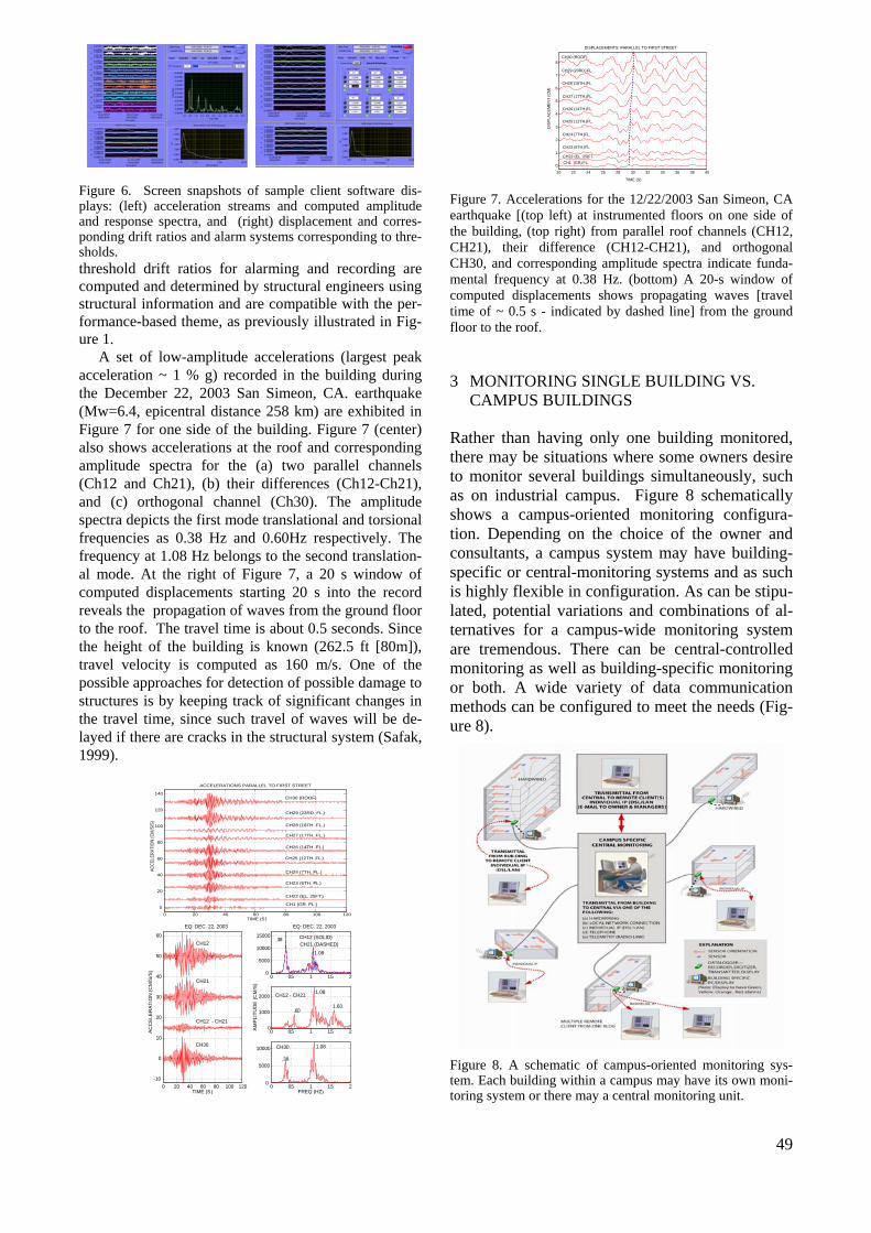
49

Figure 6. Screen snapshots of sample client software dis-plays: (left) acceleration streams and computed amplitude and response spectra, and (right) displacement and corres-ponding drift ratios and alarm systems corresponding to thre-sholds. threshold drift ratios for alarming and recording are computed and determined by structural engineers using structural information and are compatible with the per-formance-based theme, as previously illustrated in Fig-ure 1.

A set of low-amplitude accelerations (largest peak acceleration ~ 1 % g) recorded in the building during the December 22, 2003 San Simeon, CA. earthquake (Mw=6.4, epicentral distance 258 km) are exhibited in Figure 7 for one side of the building. Figure 7 (center) also shows accelerations at the roof and corresponding amplitude spectra for the (a) two parallel channels (Ch12 and Ch21), (b) their differences (Ch12-Ch21), and (c) orthogonal channel (Ch30). The amplitude spectra depicts the first mode translational and torsional frequencies as 0.38 Hz and 0.60Hz respectively. The frequency at 1.08 Hz belongs to the second translation-al mode. At the right of Figure 7, a 20 s window of computed displacements starting 20 s into the record reveals the propagation of waves from the ground floor to the roof. The travel time is about 0.5 seconds. Since the height of the building is known (262.5 ft [80m]), travel velocity is computed as 160 m/s. One of the possible approaches for detection of possible damage to structures is by keeping track of significant changes in the travel time, since such travel of waves will be de-layed if there are cracks in the structural system (Safak, 1999).

0 20 40 60 80 100 120

0

20

40

60

80

100

120

140

TIME (S)

ACC

ELER

ATIO

N (C

M/S

/S)

ACCELERATIONS PARALLEL TO FIRST STREET

CH30 (ROOF)

CH29 (23RD. FL.)

CH28 (18TH. FL.)

CH27 (17TH. FL.)

CH26 (14TH. FL.)

CH25 (12TH. FL.)

CH24 (7TH. FL.)

CH23 (6TH. FL.)

CH22 (EL. 25FT.)

CH1 (GR. FL.)

0 20 40 60 80 100 120

-10

0

10

20

30

40

50

60

EQ: DEC. 22, 2003

TIME (S)

AC

CE

LER

AT

ION

(C

M/S

/S)

CH30

CH12 - CH21

CH21

CH12

0 0.5 1 1.5 20

5000

10000

15000

EQ: DEC. 22, 2003

CH12 (SOLID)CH21 (DASHED)

.38

1.08

0 0.5 1 1.5 20

1000

2000 CH12 - CH21

AM

PLI

TU

DE

(C

M/S

)

.60

1.08

1.60

0 0.5 1 1.5 20

5000

10000 CH30

FREQ (HZ)

.38

1.08

20 22 24 26 28 30 32 34 36 38 40

0

1

2

3

4

5

6

7

8CH30 (ROOF)

CH29 (23RD. FL.)

CH28 (18TH. FL.)

CH27 (17TH. FL.)

CH26 (14TH. FL.)

CH25 (12TH. FL.)

CH24 (7TH. FL.)

CH23 (6TH. FL.)

CH22 (EL. 25 FT.)

CH1 (GR. FL.)

DISPLACEMENTS: PARALLEL TO FIRST STREET

DIS

PLA

CE

ME

NT

(C

M)

TIME (S) Figure 7. Accelerations for the 12/22/2003 San Simeon, CA earthquake [(top left) at instrumented floors on one side of the building, (top right) from parallel roof channels (CH12, CH21), their difference (CH12-CH21), and orthogonal CH30, and corresponding amplitude spectra indicate funda-mental frequency at 0.38 Hz. (bottom) A 20-s window of computed displacements shows propagating waves [travel time of ~ 0.5 s - indicated by dashed line] from the ground floor to the roof.

3 MONITORING SINGLE BUILDING VS. CAMPUS BUILDINGS

Rather than having only one building monitored, there may be situations where some owners desire to monitor several buildings simultaneously, such as on industrial campus. Figure 8 schematically shows a campus-oriented monitoring configura-tion. Depending on the choice of the owner and consultants, a campus system may have building-specific or central-monitoring systems and as such is highly flexible in configuration. As can be stipu-lated, potential variations and combinations of al-ternatives for a campus-wide monitoring system are tremendous. There can be central-controlled monitoring as well as building-specific monitoring or both. A wide variety of data communication methods can be configured to meet the needs (Fig-ure 8).

Figure 8. A schematic of campus-oriented monitoring sys-tem. Each building within a campus may have its own moni-toring system or there may a central monitoring unit.

50

4 CASE FOR BRIDGES

As mentioned before, since the terminology “drift ratio” does not apply for bridges, it is necessary to define and identify their performance-wise critical locations for which relative displacements can be computed from real-time streaming response data. Thresholds can be assessed for measurements of relative vertical or lateral displacements of deck center or relative horizontal displacements at tops of towers of long-span suspension or cable-stayed bridges. As an example, Figure 9 exhibits cable-stayed Cape Girardeau Bridge (Missouri,USA) in-strumented with a monitoring system capable of streaming real-time acceleration response data that can be configured to establish performance indica-tors using the sensor data at the deck center or tops of towers or other locations for which data is readi-ly available.

Figure 9. Example of extensively instrumented cable-stayed Cape Girardeau (Missouri, USA) bridge that has real-time streaming of responses.

5 CONCLUSIONS

Capitalizing on advances in global positioning sys-tems (GPS), in computational capabilities and me-thods, and in data transmission technology, it is now possible to configure and implement a seismic monitoring system for a specific building with the objective of rapidly obtaining and evaluating re-sponse data during a strong shaking event in order to help make informed decisions regarding the health and occupancy of that specific building. Displacements, and in turn, drift ratios, can be ob-tained in real-time or near real-time through use of GPS technology and/or double-integrated accelera-tion. Drift ratios can be related to damage condi-tion of the structural system by using relevant pa-rameters of the type of connections and story structural characteristics including its geometry.

Thus, once observed drift ratios are computed in near real-time, technical assessment of the damage condition of a building can be made by comparing the observed with pre-determined threshold stag-es. Both GPS and double-integrated acceleration applications can be used for performance evalua-tion of structures and can be considered as build-ing health-monitoring applications. Although, to date, these systems were not tested during strong shaking events, analyses of data recorded during smaller events or low-amplitude shaking are prom-ising.

REFERENCES

Applied Technology Council (ATC), 1989. Pro-cedures for Post-Earthquake Safety Evaluation of Buildings, ATC-20, Redwood City, CA.

Applied Technology Council (ATC). 1997.

NEHRP Commentary on the Guidelines for the Seismic Rehabilitation of Buildings, prepared for the Building Seismic Safety Council, pub-lished by the Federal Emergency Management Agency, FEMA 274, Washington, D.C.

Building Occupancy Resumption Program

(BORP). 2001. City and County of San Fran-cisco, Department of Building Inspection, Emergency Operation Plan, (Rev. 2001). [www.seaonc.org/member/committees/des_build.html).

Çelebi, M., and Sanli, A. 2002) GPS in Pioneering

Dynamic Monitoring of Long-Period Struc-tures, Earthquake Spectra, Journal of EERI,. Volume 18, No. 1, pages 47–61, February 2002.

Çelebi, M., Sanli, A., Sinclair, M., Gallant, S., and

Radulescu, D. 2004. Real-Time Seismic Moni-toring Needs of a Building Owner and the solu-tion – A Cooperative Effort, Journal of EERI, Earthquake Spectra, v.19, Issue 1, pp.1-23.

FEMA-352: Recommended Post-earthquake

Evaluation and Repair Criteria for Welded Steel Moment-Frame Buildings (also SAC Joint Ven-ture 2000 prepared for FEMA), Washington, D.C.

Panagitou, M., Restrepo, J.I., Conte, J. P., and En-

glekirk, R. E. 2006. Seismic Response of Rein-

51

forced Concrete Wall Buildings, 8NCEE (pa-per no. 1494), San Francisco, Ca. April 18-22, 2006.

Porter, K., Mitrani-Reiser, J., Beck, J. L., and

Ching, J. 2006. Smarter Structures: Real- time loss estimation for instrumented buildings, 8NCEE (paper no. 1236), San Francisco, Ca. April 18-22, 2006.

Safak, E. 1999. Wave-propagation formulation of

seismic response of multistory buildings, ASCE, Journal of Structural Engineering, vol. 125, no. 4, April 1999, pp. 426-437.

P. Clemente & A. De Stefano (eds.), WIM (Weigh In Motion), Load Capacity and Bridge Performance. ENEA, Roma, 2010

1 INTRODUCTION The load carrying capacity of bridges is an important parameter in bridge management. It will affect the serviceability, traffic safety and transportation costs directly. Unfortunately, the load carrying capacity of a bridge tends to decreasing over years of service owing to physical damage caused by factors such as over loading, accidental impact, or materials deteri-oration. On the other hand, increasing demand of the traffic volume requests higher load carrying capaci-ty. To deal with this dilemma and avoid the huge cost on repair, upgrading or replacement of existing bridges, the accurate assessment of load carrying ca-pacity of bridges is becoming more and more impor-tant.

With the rapid development of computer’s capa-bility and finite element methodology, research on methods that combine the field test and modal analy-sis for bridge load carrying capacity prediction be-comes active during the last two decades. Law et al (1995) derived the best estimation of the moment of inertia of a girder by the closest fitting of the first frequency between the finite element model and the test results. Chajes et al (1997) used diagnostic test-ing results to determine the composite section prop-erties of the girders and support restrain, and then to develop a numerical model of the bridge to estimate the maximum allowable load. By comparing the moment distribution in the longitudinal direction ob-tained from different finite element models with the field test data, Jauregui and Barr (2004) developed an equivalent frame model to calculate the load dis-tribution factor for bridge load rating. Brownjohn and Xia (2000) introduced the sensitive-analysis-based model updating method into the structure con-

dition assessment procedure. Later, this method was applied to real bridge strctures to update the bridge model for condition assessment (Brownjohn et al 2003; Xia and Brownjohn 2004). The method that combines the finite element analysis and model up-dating provides a more precise estimation of bridge load carrying capacity.

Qualitative condition assessment of prestressed concrete bridge structures has been traditionally us-ing proof load test leading to an indication of the load-carrying capacity. Alternative approaches which claim to be more effective to identify the local damages, such as those making use of ultrasonic, magnetic flux, etc., are also costly with the capital cost of the testing equipments and the training of the operator. Dynamics approach is very popular nowa-days to identify local damages, but it does not give any clue on the associated load-carrying capacity of the structure.

In this paper, the field vibration test data on Bridge No. 852 in Western Australia is used to up-date its finite element model developed using the commercial software ABAQUS (ABAQUS Manual, 2003). The updated model is then used to perform nonlinear analysis to predict the bridge’s load carry-ing capacity at present condition. The approach used to model reinforced concrete structure at ultimate load conditions in this finite element model is veri-fied through the comparisons with a bench mark ex-ample available in the literature. The load carrying capacities of the bridge predicted by using the codi-fied method and the finite element model without model updating are also obtained and presented. Comparisons and discussions are made on the results derived from different approaches.

Dynamic assessment of PSC bridge structures under moving vehicular loads

H.Hao & X.Q. Zhu CRC for Integrated Engineering Asset Management School of Civil and Resource Engineering, University of Western Australia, Australia

ABSTRACT: This study presents a novel method to extract the damage information from the response of a bridge induced by operating vehicles. The results also show the operating vehicle loads could be utilized to reduce the number of sensors. It has the potential of detecting damage using vehicle response of highway bridges with small number of sensors and without interrupting traffic flow. Finally, the load carrying capaci-ties of a practical bridge are predicted by using the finite element model updating.

54

2 VEHICLE-BRIDGE INTERACTION ANALYSIS

2.1 Vehicle-bridge system (Ding et al, 2008a)

The equation of motion of the vehicle system with respect to the vertical degrees of freedom

[ ]nyyyy L321=Y derived using Lagrange formulation can be expressed as follows

intvvvv FYKYCYM −=++ &&& (1)

where intvF is the interaction force vector applied to

the vehicle; vM , vC , vK are the mass, damping and stiffness matrices of the vehicle, respectively.

Based on the finite element method, the govern-ing equation of the bridge can be written as

intbbbb FΦ=++ uKuCuM &&& (2)

where Mb, Cb and Kb are the structural mass, damp-ing and stiffness matrices of the bridge; uuu &&&,, de-note nodal displacement, velocity and acceleration vectors respectively. int

bF is the interaction force vector applied to the bridge;

Npl ΦΦΦΦ=Φ ........21 is a 2(N+1)×Np matrix and N is the number of finite element in the bridge.

Eqs. (2) and (3) can be combined together and written in a matrix form as follows

fKuuCuM =++ &&& (3) where M, C and K are the structural mass, damping and stiffness matrices of the vehicle-bridge system.

By introducing the state vector [ ]TTT uuz &= , Eq. (3) can be rewritten as

)()()()()( ttttt rd bbzAz ++=& (4) where

⎥⎦

⎤⎢⎣

⎡−−

= −− CMKMI0

A 11)(t ; drd t fMb =)( ;

rrr t fMb =)( ; ⎥⎦

⎤⎢⎣

⎡= −1M

0M r

Because the inputs df and rf are independent of each other and the system is linear, the responses corresponding to these excitations can be calculated separately. Consider the deterministic excitation due to the vehicle weight, it can be easily solved by the Runge-Kutta method.

The response equation for the random force is )()()()( tttt rrr bzAz +=& (5)

Considering the random component, the particu-lar solution to Eq. (5) is expressed as

ττ dtttt

rr ∫= 0)(),()( bHz (6)

Hence, the covariance matrix of )(trz can be ex-pressed as

ξτξξττ ddtEt

ttE

TTrr

t t

Trr

),()]()([),(

)]()([

0 0

HbbH

zz

∫ ∫= (7)

where the covariance matrix of random excitation is

)()]()([)()()]()([)(

)()]()([)()()]()([)(

)]()([

ξξττξξττ

ξξττξξττ

ξτ

cT

ckT

c

cT

kkT

k

Trr

EE

EE

E

SrrSSrrS

SrrSSrrS

bb

′′+′+

′+=

(8) where

t

Tn

rk

Mt K

I0Φ

MS⎪⎭

⎪⎬

⎫

⎪⎩

⎪⎨

⎧−=)( and

t

Tn

rc

Mt C

I0Φ

MS⎪⎭

⎪⎬

⎫

⎪⎩

⎪⎨

⎧−=)(

2.2 Quarter vehicle model

Figure 1 A quarter car model moving on a simply supported

bridge

To verify the proposed method, a dynamic analy-sis is performed first for a vehicle-bridge system available in the literature (Green and Cebon, 1994) as shown in Figure 1, which is a 1-axle 2-DOF ve-hicle model moving at a constant speed along a simply-supported beam. The parameters of the ve-hicle and beam are given in Table 1.

Table 1. Vehicle and bridge parameters

The road surface roughness is not considered in

the latter study. Therefore, for comparison purpose,

Data of the bridge

Data of the 1-axle vehicle

Data of the 2-axle vehi-cle

L =40 m

bm = 12 000 kg/m EI = 127 500 MN.m2

1m =36 000 kg

2m =4 000 kg

sk =1.8×107 N/m

tk =7.2×107 N/m

sc =14.4 ×104Ns/m

tc =14.4 ×104Ns/m

vm =36 000 kg

1m = 2m =2 000 kg

vI =144×103kgm2

S = 2 m

21 aa = =0.5

1sk = 2sk =0.9×107 N/m

1tk = 2tk =3.6×107 N/m

1sc = 2sc =7.2 ×104Ns/m

1tc = 2tc =7.2 ×104Ns/m

y

x

s1

m1

c

m1

y2

y1

ks

kt

cs

ct

m2

55

in this calculation, the smooth road surface condition is assumed. In Figure 2(a), the time history of the mid-span displacement of the bridge by the proposed algorithm is compared with that from Green and Ce-bon (1994) when the vehicle speed is 25 m/s. It shows that the results agree very well and therefore the proposed method is reliable to analyse the dy-namic response of the coupled vehicle-bridge sys-tem.

(a) Displacement at the mid-span of the bridge

body

(b) Vehicle axle forces

Figure 2 Deterministic response of the vehicle-bridge system (Quarter vehicle model)

Figure 2(a) also shows the time history of the normalized mid-span displacement of the bridge when the vehicle speed is 15 and 35 m/s, in which δ is the mid-span displacement of the bridge and stδ is the maximum static displacement at the mid-span of the bridge under the same vehicle load. From Figure 2(a), the time histories of the bridge displacement corresponding to different vehicle speeds are close to each other. The maximum displacements of the bridge are 1.01, 1.00 and 1.03 times stδ for the three cases. The vehicle speed has no obvious effect on the bridge response for the smooth surface condi-tion. The normalized time histories of axle loads are plotted in Figure2(b). In the figure, the interaction force oscillates around the static axle load axlef or the vehicle weight. The peak-peak value of the oscil-

lation increases with the vehicle speed. It should be noted that although the vehicle speed affects its ver-tical dynamic response, its effect is insignificant as compared to the static vehicle load or the weight of the vehicle on bridge responses.

2.3 Dynamic amplification factor (DAF)

The effect of the road surface roughness, vehicle speed, vehicle and bridge vibration frequencies and vehicle axle spacing on the vehicle-bridge interac-tion, and hence on the dynamic bridge responses are analysed in this section through two commonly used parameters in bridge design, i.e., the Dynamic Am-plification Factor (DAF) and the Dynamic Load Coefficient (DLC). The DLC is used to study the magnitude of the dynamic axle loads, which is de-fined as

st

dyn

PP

=DLC (9)

dynP is the maximum value of the axle load, includ-ing the static axle load and the maximum RMS value of the dynamic axle load; stP is the static axle load. The DAF is defined in terms of the dynamic re-sponse of the bridge, as the ratio of the maximum bridge deflection dynδ to the maximum static deflec-tion stδ under static vehicle load

st

dyn

δδ

=DAF (10)

Figure 3 DAF for different road surface condition

-0.3

0

0.3

0.6

0.9

1.20 0.3 0.6 0.9 1.2

Vehicle position (vt/L)

δ/δs

tatic

v=15 m/sv=25 m/sv=35 m/sv=25 m/s (Green&Cebon)

0.994

0.996

0.998

1

1.002

1.004

1.006

1.008

0 0.3 0.6 0.9 1.2

Vehicle position (vt/L)

p(t)/

f axle

v=15 m/sv=25 m/sv=35 m/s

0.8

1.1

1.4

1.7

2

2.3

2.6

2.9

10 15 20 25 30 35 40

Vehicle speed (m/s)

DA

F

0

2×10-6

8×10-6

32×10-6 (m3/rad)

Very good Good

Average

Poor

0.5×10-6

56

Figure 4 DLC for different road surface conditions

The parameters of the vehicle and bridge models

are listed in Table 1. The half vehicle model is used in the calculation. Five different road surface condi-tions, namely smooth, very good, good, average and poor road surface conditions are used in the calcula-tion to study the effect of the road surface roughness on DAF and DLC. Five different vehicle speeds in the range of 15 to 35 m/s are considered in the anal-ysis. Figures 3 and 4 respectively show the DAF and DLC when the vehicle travels through the bridge of different surface conditions with different speeds. DLC for rear axle has about the same value as the front axle in this example and therefore only the DLC for front axle is plotted in Figure 4. The re-sults show that both of the DAF and DLC are close to unity for a smooth road surface condition. The maximum DAF and DLC are 1.02 and 1.03 when the vehicle speed is 35 m/s, indicating the dynamic effect is small when the bridge surface is smooth. At the same vehicle speed, the DAF and DLC values increase when the road surface condition changes from smooth to poor. When the vehicle speed is 35 m/s, the DAF is 1.02 for smooth surface condition, 1.21, 1.40, 1.78 and 2.56 for very good, good, aver-age and poor surface condition, respectively. These observations indicate the dynamic effects caused by road surface roughness increase the bridge dis-placement by 19%, 38%, 76% and 154% of stδ . Si-milarly, DCL is 1.03 for smooth surface condition, but is 1.21, 1.39, 1.75 and 2.49 for very good, good, average and poor surface condition, when the ve-hicle speed is 35 m/s, indicating the dynamic effects by road surface roughness cause an increase in the vehicle axle loads by 18%, 36%, 72% and 146% of

stP .

3 BRIDGE LOAD CARRYING CAPACITY

3.1 Description of Bridge No. 852

This over 30 years old slab-on-girder bridge com-prises three spans, and 7 girders for each span. Fig-

ure 5 shows the dimensions of the bridge deck. The width of the slab is 9.14 m accommodating two traf-fic lanes. The external span is 17.84 m and the cen-tral span is 18.29 m. The girders are precasted as simple beams and then made continuous by placing enough reinforcements in the cast-in-place concrete slab over the support. The slab and girders are inte-grated by shear connectors as shown Figure 5. The location of the shear connectors in the girders are il-lustrated in Figure 6. The layout of the section in middle of the span is shown in Figure 5. The pre-stressing strands are 7-wire stress-relieved high ten-sile steel strands. They were released at 123 kN per strand for 84.8 kN design prestressing load per strand. The girders are prefabricated, while the run-on RC slab and diaphragms were casted in place to joint the girders. The diaphragms are supported on cap beams measured as 1004×648mm for the abut-ments and 1004×684mm for the middle piers. The thickness of the slab is 140 mm on average. Figure 5 shows the reinforcement of the slab in the middle of span.

Figure 5 Dimension of the bridge deck and the reinforcement in

the middle of span

Figure 6. Loacation of the shear connectors in half girder

CENTER OF

De

Layer 1&2 φ16@203.2

(φ21@203 2

Layer 3&4

20-φ12 7 t d

4

De

0.8

1.1

1.4

1.7

2

2.3

2.6

10 15 20 25 30 35 40

Vehicle speed (m/s)

DLC

0

2×10-6

8×10-6

32×10-6 (m3/rad)

Very good Good

Average

Poor

0.5×10-6

57

3.2 Finite element model

Figure 7 Finite-element model of Bridge No. 852

A three-dimensional finite element model (Figure 7) is built according to the design drawings. The letters A to G indicate the transverse position of the girders and the bearings. The material constitutive models used in the analysis are described in detail by Ding et al (2008b).

3.3 Load action for ultimate load carrying capacity evaluation

This bridge was designed based on the old Australi-an Standards nearly 30 years ago. In order to eva-luate the capacity of bridge No. 852 under the action of modern traffic loads, the new traffic loads stan-dard, AS 5100.2—2004, is applied in this study.

Standard AS 5100.2-2004 provides several road traffic loads including single load like the W80 wheel load and the A160 axle load and group loads like M1600 and S1600. The influence line diagram was used to choose the most critical traffic load combinations and hence to determine the longitudin-al positions of the critical loads on the bridge. Then the M1600 traffic loads are selected (see Figure 8). The M1600 moving traffic load consists of uniform-ly distributed load together with truck wheel loads. The uniformly distributed load component (UDL) is considered as uniformly distributed over the width of a 3.2 m standard design lane (Figure 8). The wheel loads are treated as concentrated load.

Figure 8 M1600 moving traffic load

According to the standard AS 5100.2-2004, the

width of a standard design lane is 3.2m. The width of the deck for this bridge between the curbs is 8.5 m. Consequently, two traffic lanes are loaded. The wheel loads for the first lane are located on the second girder to cause the maximum response in this girder. AS 5100.2 requires the minimum clear width for the vehicular traffic is (lane width+1.2) m. Con-sequently, the second traffic lane is positioned 1.2 m away from the first lane to produce the maximum moment in the second girder.

The live load effects of the nominated vehicle for load rating, RVL is

( )∑=

+=n

i

LiiLRV SWL

11 αγ (11)

n, the number of the design lane, equals 2. Live load factor, Lγ is selected as 1.8 (AS 5100.7-2004). iW is the accompanying lane factor determined in AS 5100.2, which is 1.0 for the first lane and 0.8 for the second lane. The dynamic allowance, α, of 0.3 is considered in the analysis. In this case, the magni-tudes of the traffic loads calculated from equation (11) are nominated for the load carrying capacity analyses. Furthermore, the nominated rating live load value is equal to the traffic load for ultimate limit state design (AS 5100.2-2004).

The traffic loads are placed at different places to get the most adverse positive and negative moment. Finally, the maximum positive moment is achieved as 7568 kN·m when the first and third spans are loaded, and the minimum negative moment is achieved as -8625 kN·m when the first and second spans are loaded. Comparing with the capacity of the bridge calculated from the empirical formula in sec-tion 4.1, the bridge capacity is dominated by the positive moment capacity. This bridge can carry 1.39 of the nominated traffic loads. So the load con-dition to produce the most adverse positive moment is applied in the following finite element analysis. The positions of the traffic loads are shown in Figure 9.

Figure 9 Longitudinal load position for the most adverse posi-

tive moment

3.4 Analysis results

Figure 10 compares the load displacement curves calculated from the updated model with results from the original model. The vertical axis represents the ratio of the applied load to the nominated rating

360 360 6

360 360

Plan

0.

0.

0.2

1.2 1.2 3.75 1.2 varies 6.25m min.

3.2m standard de-

5.0 1.2 1.25 1.2 1.2

0.

2.0

1.2

M1600 moving traffic load

17.838 18.288 5 4 3 7 4 0 5.0

Section A

58

loads. For the original model, the load-displacement curve can be easily divided to three stages, elastic deformation stage, after cracking, and strands yield-ing. And the ultimate load carrying capacity is de-termined by the turning point from increasing to the decreasing of the load. However, for the load-displacement relationship for updated model, the bridge lost it stiffness at 0.87 of the nominated loads with 53 mm displacement. Then the displacement increased enormously with a little increase of the load. So the turning point A is treated as the maxi-mum load to which the structure can be subjected. It happened before yielding of the strands. Figure 10 shows the initial stiffness increased by 16% after model updating. The decrease of stiffness in majori-ty of the slab elements is counteracted by the in-crease of the stiffness in most parts of the girders. For concrete in tension, the plastic strain is defined as the strain minus cracking strain. So the develop-ment of cracking can be seen from the contour plot of the plastic strain (PE). In this case, the complete failure mechanism can’t be explained clearly. But from the contour plot of the plastic strain in girder B-1 (Figure 11) at the moment of the turning point A (in Figure 10), we can find out that the shear cracks near the support cause the failure of the girder before the cracks developed in the middle of the span.

Figure 10 Load-displacement relationship comparison between

original and updated model

Figure 11 The plastic strain of girder B-1

4 CONCLUSIONS

In this paper, the nonlinear finite element analysis and model updating method are applied to calculate the load carrying capacity of the slab-on-girder bridge. The bilinear elastic-plastic model is used to model reinforcements, and the damage plasticity model is applied for concrete. The model is verified

with a bench mark example available in literature. The load-displacement relationship curve shows the approach used in this study capture the main charac-ters of the RC member at ultimate load conditions. The approach is applied to a practical bridge evalua-tion in following part.

5 ACKNOWLEDGEMENT

The work described in this paper was supported from CIEAM through Project ID207.

6 REFERENCES

Australian Standard 2004. Bridge Design Part 2: Design loads (AS5100.2). Sydney: Standards Australia International Ltd.

Australian Standard 2004. Bridge Design Part 7: Rating of ex-isting bridges (AS5100.7). Sydney: Standards Australia In-ternational Ltd.

Brownjohn, J.M.W. & Xia, P.Q. 2000. Dynamic assessment of a curved cable-stayed bridge by model updating. Journal of Structural Engineering ASCE, 126( 2): 252-260.

Brownjohn, J.M.W., Moyo, P., Omenzetter, P. & Lu, Y. 2003. Assessment of highway bridge upgrading by dynamic test-ing and finite-element model updating. Journal of Bridge Engineering ASCE, 8(3): 162-172.

Chajes, M.J., Mertz, D.R. & Commander, B. 1997. Experimen-tal load rating of a posted bridge. Journal of Bridge Engi-neering ASCE, 2(1):1-10.

Ding, L.N., Hao, H. & Zhu, X.Q. 2008a. Evaluation of dynam-ic vehicle axle loads on bridges with different surface con-ditions. Journal of Sound and Vibration (Submitted).

Ding, L.N., Hao, H., Xia Y. & Deeks A. J. 2008b. Highway bridge load carrying capacity evaluation using the finite element method and model updating. Journal of Bridge En-gineering ASCE (Submitted).

Green, M.F. & Cebon, D. 1994 Dynamic response of highway bridges to heavy vehicle loads: Theory and experimental validation. Journal of Sound and Vibration, 170(1): 51-78.

Jauregui, D.U. & Barr, P.J. 200. Nondestructive Evaluation of the I-40 Bridge Over the Rio Grande River. Journal of Per-formance of Constructed Facilities, 18(4): 195-204.

Law, S.S., Ward, H.S., Shi, G.B., Chen, R.Z., Waldron, P. & Taylor, C. 1995. Dynamic assessment of bridge load-carrying capacity. I. Journal of Structural Engineering ASCE, 121(3): 478-487.

Xia, P.Q. & Brownjohn, J.M.W. 2004. Bridge structural condi-tion assessment using systematically validated finite-element model. Journal of Bridge Engineering ASCE, 9(5): 418-423.

Displace-

Load

Original model

Updated model

0

0.2

0.4

0.6

0.8

1

1.2

1.4

1.6

1.8

0 50 100 150 200 250 300

Identification of dynamic axle loads from bridge responses by means of anextended dynamic programming algorithm

E. Lourens & G. Lombaert & G. De Roeck & G. DegrandeK.U. Leuven, Department of Civil Engineering, Kasteelpark Arenberg 40, B-3001, Leuven, Belgium

The reconstruction of dynamic axle loads from vibration responses forms an interesting alternative to the tra-ditional approaches used to obtain these dynamic loads. One of the methods which has been proposed for thesolution of such moving force identification problems, especially because of its efficiency and the flexibility itoffers regarding the type, complexity and order of the model, is that of dynamic programming. In this paper thetheory of dynamic programming is used to derive new recursion formulae for a more general observation equa-tion, thus developing an extended, more versatile dynamic programming algorithm. Compared to the originalalgorithm significant improvements in the quality of the identification is observed when the extended algorithmis employed in conjunction with acceleration measurements. These improvements are attributed to the presenceof a direct transmission term in the new observation equation, which establishes a more direct link between theapplied forces and the data and renders the data more sensitive to the positions of the forces.

1 INTRODUCTIONInformation on vehicle loads on a bridge deck is es-sential to bridge design since they constitute the liveload components in bridge design codes. Equivalentstatic loads can be measured using weigh-in-motion(WIM) systems, where a distinction is made betweenWIM systems installed in the road surface and bridge-WIM systems, where bridges are used as scales andstrains are measured on the main members of thebridge. Since, however, the dynamic wheel loads maysignificantly increase the road surface damage (3),studies on how to obtain these dynamic loads remainof interest. Traditionally, the dynamic loads are ei-ther directly measured using an instrumented vehi-cle - an expensive approach which is prone to bias -or computed with a vehicle-bridge interaction model,where the results then largely depend on the knowl-edge of input parameters. Reconstructing these loadsfrom vibration responses forms an interesting alterna-tive which can be applied under real traffic conditionswithout the need for an instrumented vehicle or theinterruption of traffic.

In recent years moving force identification hasreceived considerable attention with early develop-ments such as the time domain method (12), thefrequency-time domain method (13) and the inter-pretive method (5). Departing from the differentialequation describing the deflection of a simply sup-

ported Euler beam, the time domain method modelsthe forces as step functions in a small time intervaland solves for them in the modal coordinates usingdeconvolution in the time domain. The frequency-time domain method departs from the same differ-ential equation, expressed in modal coordinates, andperforms a Fourier transformation to solve for the un-known forces in the frequency domain. Both thesemethods, as well as the interpretive method, have thedisadvantage of being computationally expensive - alltime components are solved for simultaneously by in-verting large matrices, the effect of which is a practi-cal limit on the number of forces and/or the numberof time steps that can be computed - as well as diffi-cult to apply to more complex structures. The appli-cation of the dynamic programming technique to themoving force identification problem (14) provided ananswer to these shortcomings, but placed a restric-tion on the measurement types (bending moments,strains) that could be used in the inversion. The DPalgorithm departs from a state-space model of the dy-namic system and solves the inverse problem in thetime domain, recursively. Recently a new algorithm,the MOMA ((23),(24)), was developed, in which themoving loads are presented as a combination of ba-sis functions (Legendre polynomials or Fourier series)and identified by solving a system of equations de-veloped with these basis functions. The MOMA also

P. Clemente & A. De Stefano (eds.), WIM (Weigh In Motion), Load Capacity and Bridge Performance. ENEA, Roma, 2010

proved to be considerably more efficient and accuratethan the early methods, although it still has the dis-advantage of being limitedly applicable to more com-plex structures when compared to DP, which is inher-ently flexible because of its departure from a state-space model of the dynamic system.

In this paper the field of moving force identifica-tion is explored further by, based on the theory of dy-namic programming, deriving new recursion formu-lae for a more general observation equation and thusdeveloping an extended, more versatile, dynamic pro-gramming algorithm. The accuracy and effectivenessof the proposed method are studied by means of a se-ries of numerical examples where special attention isgiven to the influence of the measurement type (ac-celeration / displacement / strain), the excitation fre-quency, as well as the number of measurements, onthe quality of the identification.

2 EXTENDED DYNAMIC PROGRAMMINGThe mathematical theory of dynamic programmingis thoroughly discussed and the recursion formulaeneeded for its application derived in Trujillo andBusby (20). What is presented here is firstly the clas-sic recursion formulae, slightly modified to allow fordifferent points of application of the forces during thetime history. Secondly, by applying the same math-ematical theory used to obtain the classic recursionformulae, new recursion formulae are derived by de-parting from a more general observation equationwhich allows the measurements to be not only dis-placements, velocities and strains, but accelerationsas well. Compared to the observation equation used inthe classic formulation, this more general observationequation has a positive effect on the identification, aswill become clear at a later stage.

Since the classic as well as the extended dynamicprogramming algorithm departs from a state-spacemodel of the dynamic system, the formulation of thismodel is presented first.

2.1 State-space model formulationThe continuous-time governing equations of motionfor a mechanical system with nDOF degrees of free-dom are presented:

Mu(t) +Cu(t) +Ku(t) = f(t) = Sp(t)p(t) (1)

where M, C and K denote the mass, damping andstiffness matrix, respectively; u, u and u are vectors ofaccelerations, velocities and displacements of all thefree degrees of freedom of the system and p(t) is theexcitation. The excitation is factorized into a selec-tion matrix Sp(t) ∈ R

nDOF×np specifying the locationsof the forces, and the vector p(t) ∈ R

np , representing

the np force time histories. Introducing the state vec-tor

x(t) =

[u(t)u(t)

]

where x(t) ∈ Rns , ns = 2nDOF, equation (1) can be

rewritten in first order state-space form

x(t) = Acx(t) +Bc(t)p(t) (2)

where Ac ∈ Rns×ns and Bc ∈ R

ns×np are defined as:

Ac =

[0 I

−M−1K −M−1C

],

Bc(t) =

[0

M−1Sp(t)

](3)

and the subscript ‘c’ denotes continuous time. Timediscretization of these continuous-time state-spacematrices and the input based on a zero-order holdassumption leads to the discrete-time counterpart ofequation (2)

xk+1 = Axk +Bkpk (4)where k = 0,1, . . . ,N . This discrete-time state-spacemodel is obtained through the use of the exponentialmatrix

A = eAcΔt, Bk = [A− I]A−1c Bc(tk) (5)

with Bc(tk) calculated using the value of Sp at timetk = kΔt. Given a set of measurements on some ofthe state variables, the problem is to find the unknownforcing terms pk whilst assuming that the various Bk,dependent on the positions of the forces at each timeinstant, are known.

2.2 Original DPLet the set of measurements be denoted by d, whered∈R

nd and nd signifies the number of measurements.The relationship between the state-variables and themeasurements is formulated as follows

dk Qxk. (6)

where the data is represented as any linear combina-tion of the states. Given equation (6), the least squareserror in the presence of a Tikhonov penalty term canbe written as follows

E(c,p1,p2, . . . ,pN) =N∑

k=1

(Qxk − dk,W(Qxk − dk))

+(pk,Hpk)(7)

60

with the notation (., .) indicating the inner product ofa vector: (x, y) =

∑N

i=1xiyi. The vector c represents

the initial conditions x0 and the matrices W and H,assumed symmetric, provide the flexibility of weight-ing the data and the forces, respectively. The mini-mum value of this error function starting at any stagen given any initial state c, where c= xn−1 is now con-sidered arbitrary, and taking the values of the forces attimes k as the free parameters, can be expressed as

fn(c) = minpk

En(c,pn,pn+1, . . . ,pN). (8)

The application of Bellman’s Principle of Optimality(2) to the above minimization leads to the followingrecurrence formula

fn−1(c) = minpn−1

[(Qc− dn−1,W(Qc− dn−1))

+(pn−1,Hpn−1

)+ fn (Ac+Bn−1pn−1)

].

(9)

It can be proven that fn is quadratic in c (20), allowingthe formulation

fn(c) = (c,Rnc) + (c,Sn) + qn (10)

in whichRn ∈Rns×ns is a symmetric matrix, Sn ∈R

ns

a vector, and qn a scalar. This leads to the followingrecurrence formulae

Rn−1 = QTWQ+AT (Rn−HTnDnHn/2

)A (11)

Sn−1 = −2QTWdn−1 +AT (I−HTnDnBT

n−1

)Sn

(12)

whereDn =

(2H+ 2BT

n−1RnBn−1

)−1 (13)

Hn = 2BTn−1Rn. (14)

These equations are solved backwards starting at thelast time step and the quantities needed for the calcu-lation of the optimal forcing terms

poptn−1 = −DnBT

n−1Sn−DnHnAc (15)

at all time steps are saved. The subsequent forwardsweep, given a set of initial conditions x0, consistsof alternately calculating the optimum forces usingequation (15) and advancing the state of the systemusing equation (4). It is mentioned that a recurrenceformula for the scalar value qn of equation (10) is notpresented due to the fact that qn is not needed for thecalculation of the optimum forcing functions.

2.3 Extended DP: derivation of recursion formulaefor a more general observation equation

In the previous section the classic dynamic program-ming recursion formulae were presented. Here weemploy the same strategy used to arrive at the originalrecursion formulae to derive new recursion formulaedeparting from a more general observation equation

d(t) Sau(t) + Svu(t) + Sdu(t) (16)

where d(t) ∈Rnd again signifies the nd measurements

serving as input data to the inverse problem and Sa,Sv and Sd ∈ R

nd×nDOF are selection matrices for ac-celeration, velocity and displacement, respectively, inwhich the locations of the measurements and/or dif-ference relations can be specified. Using equation (1)and the definition of the state vector, it is possible totransform equation (16) into its state-space form

d(t) Gcx(t) + Jc(t)p(t) (17)

where Gc ∈ Rnd×ns and Jc ∈ R

nd×np are referred to asthe output influence matrix and direct throughput ordirect transmission matrix, respectively. They relateto the finite element model matrices as follows

Gc =[Sd − SaM−1K Sv − SaM−1C

],

Jc(t) = SaM−1Sp(t) (18)

and remain unchanged when discretizing

dk Gxk + Jkpk (19)

G = Gc, Jk = Jc(tk). (20)

The presence of the direct transmission term in theobservation equation (17) implies a direct influenceof the forces on the data at any given time step. Whenthe direct transmission matrix is a non-zero matrix,i.e. when accelerations are measured, a stronger de-pendency is thus established between the measureddata and the applied forces compared to the originalalgorithm, in which the forces are only indirectly re-lated to the data by the observation equation (6).

The error function now becomes

E(c,p1,p2, . . . ,pN) =

N∑k=1

(Gxk + Jkpk − dk,W(Gxk + Jkpk − dk))

+ (pk,Hpk) (21)

61

and by applying the Priniciple of Optimality its min-imum value, starting at an arbitrary stage n, can bewritten as

fn−1(c) = minpn−1

[(Gc+ Jn−1pn−1 − dn−1,

W(Gc+ Jn−1pn−1 − dn−1)) +(pn−1,Hpn−1

)

+fn (Ac+ Bn−1pn−1)] . (22)

At the end of the process the optimal function has thevalue

fN(c) =

minpN

[(Gc+ JNpN − dN,W(Gc+ JNpN − dN))

+(pN,HpN)] (23)

which, by choosing pN = 0 and using the quadraticassumption (10), leads to the following initial valuesfor Rn, Sn and qn

RN = GTWG

SN = −2GTWdN

qN = dTNWdN. (24)

Equation (10) is used in equation (22) to obtain

(c,Rn−1c) + (c,Sn−1) + qn−1 = minpn−1

[(Gc +

Jn−1pn−1 − dn−1,W(Gc+ Jn−1pn−1 − dn−1))+

(pn−1,Hpn−1

)+ (Ac+Bn−1pn−1,Rn (Ac +

Bn−1pn−1)) + (Ac+Bn−1pn−1,Sn) + qn] (25)

where it is important to note that Rn is now no longersymmetric as was the case in the original algorithm.The optimal forcing term is obtained by performingthe above minimization

2JTn−1W

(Gc+ Jn−1popt

n−1 − dn−1

)+ 2Hpopt

n−1+

BTn−1RT

nAc+BTn−1Rn

(Ac+ 2Bn−1popt

n−1

)+

BTn−1Sn = 0 (26)

with W and H assumed symmetric. By defining thefollowing matricesLn =

(2JT

n−1WJn−1 + 2H+ 2BTn−1RnBn−1

)−1

Tn = 2JTn−1WG+BT

n−1(RTn +Rn)A

Fn = 2JTn−1Wdn−1 (27)

poptn−1 can be expressed as

poptn−1 = −LnTnc+ LnFn−LnBT

n−1Sn. (28)By substituting equation (28) into equation (25) andequating like powers of c, the new recursion formulaeare obtainedRn−1 = GTW (G− Jn−1LnTn) +

AT (RnA− (Rn +RTn)Bn−1LnTn/2

)(29)

Sn−1 = GTWJn−1Ln

(Fn−BT

n−1Sn

)− 2GTWdn−1

+TTnLT

n

(JT

n−1Wdn−1 −BTn−1Sn/2

)

+AT(Rn +RTn)Bn−1Ln

(Fn/2−BT

n−1Sn/2)

+ATSn (30)with Rn ∈ R

ns×ns and Sn ∈ Rns as before.

The backward sweep now consists of solving theabove equations backwards starting with the initialconditions defined earlier and repeatedly saving thequantities LnTn and LnFn − LnBT

n−1Sn needed forthe calculation of the optimum forcing functions inequation (28). Given a set of initial conditions x0 theoptimum values of the forces at the first time stepcan then be calculated using equation (28), whereastheir values at the subsequent time steps are obtainedby each time advancing the state of the system usingequation (4).

3 NUMERICAL EXAMPLESThe effectiveness and accuracy of the proposedmethod are studied by means of a series of numeri-cal examples in which the dynamic loads on a bridgeduring the passage of a two-axle vehicle are identi-fied. The bridge is considered to be very stiff, imply-ing no vehicle bridge interaction, and is modelled asa simply supported beam characterized by the follow-ing physical parameters

L = 40 m; EI = 7× 1010 Nm2;

ρA = 36000 kg/m; f1 = 1.368 Hz;

f2 = 5.468 Hz; f3 = 12.282 Hz.

62

The beam is discretized into 10 beam elements hav-ing one translational and one rotational degree of free-dom at each node and a length of 4 m. A constantdamping ratio of 2% is assumed for all modes of thestructure.

The 2D 4-DOF dynamic vehicle model presentedin figure 1 is used to represent the moving vehicle.The following values are used for the parameters ofthe vehicle model: mb = 9000 kg, Ib = 35 000 kgm2,ma1 = 600 kg, ma2 = 400 kg, kp1 = 0.61 ×106 N/m,kp2 = 0.32 ×106 N/m, kt1 = 3 ×106 N/m, kt2 = 1.5×106 N/m, cp1 = 16 000 Ns/m, cp2 = 10050 Ns/m,ct1 = ct2 = 0 Ns/m, l1 = 1.49 m and l2 = 3.72 m.

ma1 ma2

v

kt1 ct1 kt2 ct2

kp1 cp1 kp2 cp2

mbIb

z

y

l2l1

Figure 1: 2D 4-DOF model for a vehicle with twoaxles.

Since the positions of the two forces at each timeinstant k are assumed to be known the nodal forces atthe ith and (i + 1)th node, given a force time historyp(t), can be represented as

Vi =

(1−

3x2

l2+

2x3

l3

)p(t)

Vi+1 =

(3x2

l2−

2x3

l3

)p(t)

Mi =

(x−

2x2

l+

x3

l2

)p(t)

Mi+1 =

(x3

l2−

x2

l

)p(t) (31)

where V signifies the vertical nodal forces and M thenodal bending moments, x is the distance between theleft end of the element in question and the point ofapplication of the force, and l the element length.

The aim is to identify the two moving forces, 5.21m apart, traversing the beam at a constant velocity of72 km/h. In order to asses the influence of the exci-tation frequency on the quality of identification thewavelength of the road unevenness λy is varied. The

amplitude of the road unevenness is kept constant at0.01 m.

To generate artificial measurement time historiesthe simulated transmitted forces are applied to thebridge using the equivalent nodal loads presented inequation (31). To represent measurement error whitenoise is added to each of the calculated responses ofthe system

d = d+ γσr (32)

where d and d ∈ RN represent the polluted and un-

polluted data, respectively, γ is the noise level, σ =√∑N

i=1d2

i

Nsignifies the root mean square value of the

calculated response at the location in question, andr ∈ R

N is a vector of random values drawn indepen-dently from a normal distribution with zero mean andunit standard deviation. The noise level γ is chosen tobe 5%. It is important to note that modelling the noiseas in equation (32) implies a dependence of the levelof noise in the frequency domain on the period of thesimulated measurement data. For this reason the pe-riod as well as the sampling frequency F = 1000 Hzis kept constant throughout the investigation.

The regularization matrix H in equations (7) and(21) is set equal to λI, where λ signifies the regular-ization parameter and the use of the identity matrixcorresponds to finding a minimum norm solution. Inall examples an optimal regularization parameter isobtained using the L-curve method (10).

It is mentioned that when no noise is added to thesimulated response and λ is set to zero, the forcesare reconstructed perfectly. This statement holds forall measurement quantities and excitation frequenciesand serves as a validation of the original as well as theextended algorithm.

3.1 Different measurement quantitiesThe effect of using different measurement quantitieson the quality of the identification is investigated. Theforces transmitted to the bridge by the axles for λy =5 m, implying an excitation frequency of 4 Hz, arepresented in figure 2. The time- as well as frequencydomain noise-free displacement, strain and accelera-tion response at midspan are shown in figures 3, 4 and5, respectively. Figures 6, 7 and 8 show a comparisonbetween these forces and their reconstructions whenusing contaminated displacement, strain and acceler-ation measurements, respectively, taken at three loca-tions along the beam: at ± L/4, L/2 and ± 3L/4.

From figures 6, 7 and 8 two observations can bemade. Firstly, when considering the reconstructedforces obtained using displacement and strain mea-surements, one notes an over- and underidentificationof the front and rear axle forces, respectively. This isa direct consequence of solving for a minimum norm

63

0 0.5 1 1.5 2 2.5 30

20

40

60

80

Time [s]

Forc

e [k

N]

Figure 2: Forces transmitted to the bridge by the front(solid line) and rear (dashed line) axle of the vehicle.f = 4 Hz.

0 0.5 1 1.5 2 2.5 3−20

−15

−10

−5

0

5x 10−4

Time [s]

Dis

plac

emen

t [m

]

0 2 4 6 8 100

0.5

1

1.5

2

2.5x 10−3

Frequency [Hz]

[m/H

z]

Figure 3: Noise-free displacement response atmidspan in the time domain (top) and frequency do-main (bottom) for frequencies between 0 and 10 Hz.

solution whilst trying to identify two forces of dif-ferent magnitudes, an effect that would increase werethis difference in magnitude to become larger. Thisunwanted spatial smoothing of the forces cannot beavoided and is a result of having to apply too muchregularization which, in turn, points to a lack of infor-mation in the data. The effect is observed to be muchless when using acceleration measurements whichbrings us to the second observation, namely that thequality of reconstruction is better when using accel-

0 0.5 1 1.5 2 2.5 3−2

0

2

4

6

8

10x 10−5

Time [s]

Stra

in0 2 4 6 8 10

0

0.2

0.4

0.6

0.8

1x 10−4

Frequency [Hz]

[Hz−1

]

Figure 4: Noise-free strain and response at midspan inthe time domain (top) and frequency domain (bottom)for frequencies between 0 and 10 Hz.

0 0.5 1 1.5 2 2.5 3

−0.02

0

0.02

0.04

Time [s]

Acc

eler

atio

n [m

/s2 ]

0 2 4 6 8 100

0.01

0.02

0.03

0.04

0.05

0.06

Frequency [Hz]

[m/s

2 /Hz]

Figure 5: Noise-free acceleration response at midspanin the time domain (top) and frequency domain (bot-tom) for frequencies between 0 and 10 Hz.

64

0 0.5 1 1.5 2 2.5 30

20

40

60

80

Time [s]

Forc

e [k

N]

0 0.5 1 1.5 2 2.5 30

20

40

60

80

Time [s]

Forc

e [k

N]

Figure 6: Applied (solid line) versus reconstructed(dashed line) force of the front (top) and rear (bot-tom) axle using displacement measurements at threelocations. f = 4 Hz.

erations. The direct transmission term in the obser-vation equation (17), which formed the basis for thedevelopment of the extended dynamic programmingequations, establishes a more direct link between theforces and the data. The presence of this term rendersthe acceleration measurements more sensitive to thepositions of the forces and thus makes the data moreinformative compared to displacements or strains.

3.2 Different frequenciesThe frequency of excitation can also be expected tohave an influence on the accuracy of the identifica-tion. It was found that at higher frequencies a dis-cernible deterioration starts to set in, a phenomenonwhich has also been noted by Pinkaew (16). When,for instance, the excitation frequency is increased to20 Hz, corresponding to a wavelength λy of 1 m forthe road unevenness, the forces are reconstructed asshown in figures 10, 11 and 12. The measurement lo-cations were kept the same as before. In figure 9 theapplied forces are plotted separately.

In figures 10, 11 and 12 the quality of the identifica-tion is once again seen to be better when using accel-eration measurements, with the reconstructed forcesmatching the applied forces rather well at the major-ity of time instants. In fact, the superiority of the ac-celeration data in reconstructing the forces gets more

0 0.5 1 1.5 2 2.5 30

20

40

60

80

Time [s]

Forc

e [k

N]

0 0.5 1 1.5 2 2.5 30

20

40

60

80

Time [s]Fo

rce

[kN

]

Figure 7: Applied (solid line) versus reconstructed(dashed line) force of the front (top) and rear (bottom)axle using strain measurements at three locations. f =4 Hz.

0 0.5 1 1.5 2 2.5 30

20

40

60

80

Time [s]

Forc

e [k

N]

0 0.5 1 1.5 2 2.5 30

20

40

60

80

Time [s]

Forc

e [k

N]

Figure 8: Applied (solid line) versus reconstructed(dashed line) force of the front (top) and rear (bot-tom) axle using acceleration measurements at threelocations. f = 4 Hz.

65

0 0.5 1 1.5 2 2.5 30

20

40

60

80

100

120

Time [s]

Forc

e [k

N]

Figure 9: Forces transmitted to the bridge by the front(solid line) and rear (dashed line) axle of the vehicle.f = 20 Hz.

0 0.5 1 1.5 2 2.5 30

20

40

60

80

100

120

Time [s]

Forc

e [k

N]

0 0.5 1 1.5 2 2.5 30

20

40

60

80

100

120

Time [s]

Forc

e [k

N]

Figure 10: Applied (solid line) versus reconstructed(dashed line) force of the front (top) and rear (bot-tom) axle using displacement measurements at threelocations. f = 20 Hz.

pronounced as the excitation frequency increases. Athigher frequencies the acceleration data is capable oflifting the response above the noise since higher orderfrequency components are more amplified than whenusing displacements or strains. This phenomenon isalready observable from figures 3, 4 and 5 where aclear peak is distinguishable in the frequency spec-trum of the acceleration response at the excitation fre-quency of 4 Hz, whereas the strain and even moreso the displacement spectrum lacks such an amplifi-

0 0.5 1 1.5 2 2.5 30

20

40

60

80

100

120

Time [s]

Forc

e [k

N]

0 0.5 1 1.5 2 2.5 30

20

40

60

80

100

120

Time [s]

Forc

e [k

N]

Figure 11: Applied (solid line) versus reconstructed(dashed line) force of the front (top) and rear (bottom)axle using strain measurements at three locations. f =20 Hz.

0 0.5 1 1.5 2 2.5 30

20

40

60

80

100

120

Time [s]

Forc

e [k

N]

0 0.5 1 1.5 2 2.5 30

20

40

60

80

100

120

Time [s]

Forc

e [k

N]

Figure 12: Applied (solid line) versus reconstructed(dashed line) force of the front (top) and rear (bot-tom) axle using acceleration measurements at threelocations. f = 20 Hz.

66

cation. To illustrate this more clearly the frequencyspectra of the various noise-free responses at midspanand the added noise are plotted separately in figures13, 14 and 15. In the figures only frequencies aroundthe excitation frequency f = 20 Hz are considered.The information contained in the signal is seen to becompleted drowned out by the noise in the case ofdisplacements whereas the noise spectrum is hardlyvisible on the acceleration plot.

18 19 20 21 220

2

4

6

8x 10−6

Frequency [Hz]

[m/H

z]

Figure 13: Detail of frequency spectrum of displace-ment response (solid line) and added noise (dashedline) at midspan. f = 20 Hz.

3.3 Number of measurementsAs a last investigation the influence of the number ofmeasurements on the accuracy of the reconstructionis studied. The analysis using 3 acceleration measure-ments taken at± L/4, L/2 and± 3L/4 is supplementedfirst with another 2 acceleration measurements takenat 2L/5 and 3L/5, and subsequently with yet anothertwo, at 3L/10 and 7L/10. A comparison is thus madebetween using 3, 5 and 7 measurements, when the ex-citation frequency f is equal to 4 Hz. The results areplotted in figures 16, 17 and 18. Some improvementis observed when using 5 as opposed to 3 as well as 7as opposed to 5 measurements. The effect of the noise

18 19 20 21 220

1

2

3

4

5

6x 10−6

Frequency [Hz]

[Hz−1

]

Figure 14: Detail of frequency spectrum of strain re-sponse (solid line) and added noise (dashed line) atmidspan. f = 20 Hz.

18 19 20 21 220

0.02

0.04

0.06

0.08

0.1

Frequency [Hz]

[m/s

2 /Hz]

Figure 15: Detail of frequency spectrum of acceler-ation response (solid line) and added noise (dashedline) at midspan. f = 20 Hz.

is seen to decrease with an increase in the number ofmeasurements.

0 0.5 1 1.5 2 2.5 30

20

40

60

80

Time [s]

Forc

e [k

N]

0 0.5 1 1.5 2 2.5 30

20

40

60

80

Time [s]

Forc

e [k

N]

Figure 16: Applied (solid line) versus reconstructed(dashed line) force of the front (top) and rear (bottom)axle using 3 acceleration measurements. f = 4 Hz.

4 CONCLUSIONSApart from its high efficiency the versatility of the dy-namic programming algorithm which lies in its abilityto handle state-space models of any given order andcomplexity, makes it an ideal method for solving thegeneral force identification problem. An extended al-gorithm was developed and shown to be an effectivealternative to the original dynamic programming for-mulation, bringing with it significant gains connected

67

0 0.5 1 1.5 2 2.5 30

20

40

60

80

Time [s]

Forc

e [k

N]

0 0.5 1 1.5 2 2.5 30

20

40

60

80

Time [s]

Forc

e [k

N]

Figure 17: Applied (solid line) versus reconstructed(dashed line) force of the front (top) and rear (bottom)axle using 5 acceleration measurements. f = 4 Hz.

0 0.5 1 1.5 2 2.5 30

20

40

60

80

Time [s]

Forc

e [k

N]

0 0.5 1 1.5 2 2.5 30

20

40

60

80

Time [s]

Forc

e [k

N]

Figure 18: Applied (solid line) versus reconstructed(dashed line) force of the front (top) and rear (bottom)axle using 7 acceleration measurements. f = 4 Hz.

to performing the identification using acceleration asopposed to displacement or strain data. The superi-ority of the acceleration measurements in identifyingthe unknown moving forces can be attributed to thepresence of a direct transmission term in the observa-tion equation, which makes them more sensitive to thepositions of the applied forces, as well as their abilityto lift the response above the noise when exciting athigher frequencies. It is also worth mentioning that ingeneral acceleration can be measured more accuratelythan displacement or strain.

It was found that the quality of the identificationdeteriorates as the excitation frequency increases andimproves, up to a certain threshold, with an increasein the number of measurements.

REFERENCES[1] R. Adams and J.F. Doyle. Multiple force identifica-

tion for complex structures. Experimental Me-chanics, 42(1):25–36, 2002.

[2] R. Bellman. Introduction to the Mathematical Theoryof Control Processes. Academic Press New York,1967.

[3] D. Cebon. Handbook of vehicle-road interaction.Taylor & Francis, 1999.

[4] T.H.T. Chan and D.B. Ashebo. Theoretical studyof moving force identification on continu-ous bridges. Journal of Sound and Vibration,295:870–883, 2006.

[5] T.H.T. Chan, S.S. Law, and T.H. Yung. An inter-pretive method for moving force identification.Journal of Sound and Vibration, 219(3):503–524,1999.

[6] T.H.T. Chan, S.S. Law, and T.H. Yung. Moving forceidentification using an existing prestressed con-crete bridge. Engineering Structures, 22:1261–1270, 2000.

[7] T.H.T. Chan, L. Yu, S.S. Law, and T.H. Yung. Movingforce identification studies, I: Theory. Journal ofSound and Vibration, 247(1):59–76, 2001.

[8] T.H.T. Chan, L. Yu, S.S. Law, and T.H. Yung. Movingforce identification studies, II: Comparative stud-ies. Journal of Sound and Vibration, 247(1):77–95, 2001.

[9] T.H.T. Chan and T.H. Yung. A theoretical studyof force identification using prestressed concretebridges. Engineering Structures, 23:1529–1537,2000.

[10] P.C. Hansen. Analysis of discrete ill-posed prob-lems by means of the L-curve. SIAM Review,34(4):561–580, 1992.

[11] S.S. Law, J.Q. Bu, X.Q. Zhu, and S.L. Chan. Vehi-cle axle loads identification using finite elementmethod. Engineering Structures, 26:1143–1153,2004.

68

[12] S.S. Law and T.H.T. Chan. Moving force identifica-tion: a time domain method. Journal of Soundand Vibration, 201(1):1–22, 1997.

[13] S.S. Law, T.H.T. Chan, and Q.H. Zeng. Moving forceidentification: a frequency and time domain anal-ysis. Journal of dynamic systems, measurementand control, 121:394–401, 1999.

[14] S.S. Law and Y.L. Fang. Moving force identifica-tion: optimal state estimation approach. Journalof Sound and Vibration, 239(2):233–254, 2001.

[15] S.S. Law and Q.X. Zhu. Study on different beammodels in moving force identification. Journal ofSound and Vibration, 234(4):661–679, 2000.

[16] T. Pinkaew. Identification of vehicle axle loadsfrom bridge responses using the updated staticcomponent technique. Engineering Structures,28:1599–1608, 2006.

[17] T. Pinkaew and P. Asnachinda. Experimental studyon the identification of dynamic axle loads ofmoving vehicles from the bending moments ofbridges. Engineering Structures, 29:2282–2293,2007.

[18] T.N. Thanh, M.J. Perry, and C.G. Koh. Moving ForceIdentification: A Time Subdomain Genetic Algo-rithm Approach. In Structural Health Monitoring2007: Quantification, Validation, and Implemen-tation, Stanford, USA, September 2007.

[19] D.M. Trujillo. Application of dynamic programmingto the general inverse problem. Internationaljournal for numerical methods in engineering,12:613–624, 1978.

[20] D.M. Trujillo and H.R. Busby. Practical inverseanalysis in engineering. CRC Press LLC, 1997.

[21] L. Yu and T.H.T. Chan. Moving force identifica-tion based on the frequency-time domain method.Journal of Sound and Vibration, 261:329–349,2003.

[22] L. Yu and T.H.T. Chan. Moving force identificationfrom bridge dynamic responses. Structural Engi-neering and Mechanics, 21(3):369–374, 2005.

[23] L. Yu, T.H.T. Chan, and J. Zhu. A MOM-based al-gorithm for moving force identification: Part I -theory and numerical simulation. Structural En-gineering and Mechanics, 29(2):135–154, 2008.

[24] L. Yu, T.H.T. Chan, and J. Zhu. A MOM-based algo-rithm for moving force identification: Part II - ex-periment and comparative studies. Structural En-gineering and Mechanics, 29(2):155–169, 2008.

[25] X.Q. Zhu and S.S. Law. Practical aspects in movingload identification. Journal of Sound and Vibra-tion, 258(1):123–146, 2002.

69

P. Clemente & A. De Stefano (eds.), WIM (Weigh In Motion), Load Capacity and Bridge Performance. ENEA, Roma, 2010

1 INTRODUCTION

1.1 Background Ageing bridge stocks across the world mean that maintenance costs are an increasing proportion of road infrastructure expenditure. The EU expenditure on the repair, rehabilitation and maintenance of bridge structures is estimated to be €4-6 bn annually (COST 345). As only the 15 member states up to May 2004 are included in this estimate, in the 27-state EU, bridge maintenance expenditure is likely to be significantly more than €6 bn annually.

As a result of the increasingly high maintenance cost, research into the assessment of existing infra-structure has come into focus as significant savings are possible. Such savings can be made through more accurate modelling of both the physical and statistical phenomena associated with the problem. In particular, given that bridge traffic loading is sig-nificantly more variable than bridge capacity, it is in this area that much progress towards reducing main-tenance expenditure may be made.

1.2 Basis of Research Modelling bridge traffic load effect requires the in-put of actual highway traffic data, obtained from suitable installations. Weigh-In-Motion (WIM) technology is frequently used for this purpose. In this work five working days of WIM data was taken

from the A6 Paris to Lyon motorway near Auxerre, France. The site has 4 lanes of traffic (2 in each di-rection) but only the traffic recorded in the slow lanes was used (it is acknowledged that this results in conservative loading for a 2-lane bridge, for ex-ample). Truck traffic characteristics, such as weight and dimensional data, were collected for 17 756 and 18 617 trucks in the north and south slow lanes re-spectively (an average daily truck flow of 6744 trucks). The model used for the distribution of headways is particularly important as described by OBrien & Caprani (2005).

Monte Carlo simulation of traffic streams, based upon the measured traffic characteristics is per-formed (Caprani 2005). The bridge loading induced by such a traffic stream is then obtained by using in-fluence lines (whether theoretical, site-measured, or obtained from finite-element modelling of the bridge) for the load effect of interest. We consider bridges with two opposing lanes of lengths in the range 20 to 50 m. The load effects examined are: − Load Effect 1: Bending moment at the mid-span

of a simply-supported bridge; − Load Effect 2: Bending moment at the central

support of a two-span continuous bridge; − Load Effect 3: Left hand shear in a simply-

supported bridge. Only significant crossing events, defined as mul-

tiple-truck presence events and single truck events where the vehicle’s Gross Vehicle Weight (GVW) is

Recent Advances in the Governing Form of Traffic for Bridge Loading

C.C. Caprani Department of Civil & Structural Engineering, Dublin Institute of Technology, Ireland

E.J. OBrien School of Architecture, Landscape & Civil Engineering, University College Dublin, Ireland

ABSTRACT: The assessment of site-specific bridge traffic loading using WIM data is a critical feature of minimizing the cost of rehabilitation and replacement for bridge stock. For short- to medium-span bridges, it is often assumed that free-flowing traffic, including the dynamic interaction between the vehicles and bridge, governs the extreme load effect. In this paper, some recent advances in statistical techniques applied to bridge load effect extrapolation are presented. A critical review of these new approaches is made and it is shown that extrapolation results are now considerably more reliable and repeatable. It is also shown that there is doubt over the governing form of traffic. Therefore, the authors present some initial results of congested-traffic models in comparison to a free-flowing model. For a range of bridge lengths and load effects, the authors de-termine the dynamic ratio that would be required for free-flowing traffic to govern. The implications of these recent advances and various findings are discussed with reference to the future direction of research into bridge traffic loading

72

in excess of 40 tonnes, were processed to minimize computing requirements. For such events, the com-prising truck(s) are moved in 0.02 second intervals across the bridge and the maximum load effects of interest identified. The set of daily maximum load effect values for each loading event type were de-termined for further statistical analysis.

IN this work traffic growth is not consider and consequently the statistical models applied are sta-tionary. In addition, it is taken that the ‘economic year’ is equivalent to about 50 weeks of weekday traffic and consequently 250 ‘simulation days’ are taken to represent a calendar year.

2 STATIC TRAFFIC LOAD EFFECT

2.1 Statistical Methods in the Literature 2.1.1 Attributes of Good Statistical Modelling The attributes required of a robust statistical extrapo-lation procedure are described by Caprani (2005) and summarized here. The most important property is that a model should not be subjective: different re-sults obtained as a result of the analyst’s decisions should be avoided. Other requirements are: − Choice of Population: The population upon which

the analysis is based must be in keeping with the limitations of the statistical model to be applied. In many cases the stationarity assumption of many statistical models is violated.

− Distribution of Extreme Load Effects: Often deci-sions about which extreme value distribution to use are made in block maxima analyses. This is unnecessary given that the Generalized Extreme Value (GEV) distribution (Coles 2001) incorpo-rates all three Fisher-Tippett familes.

− Estimation: The means by which the model pa-rameter estimation is done is often graphical or least-squares-based when more accurate methods, such as maximum likelihood estimation exist.

− Choice of Thresholds: Many authors make deci-sions regarding the data which is to be kept as a basis for the analysis – the ‘tail’ data problem. This is unnecessary if the correct model is being applied to the correct population using good esti-mation procedures.

2.1.2 Statistical Methods in the Literature In the bridge traffic load effect literature, load ef-fects have been found from various methods, but it is the methods of extrapolating this load effect data that is of interest here.

In the background studies for the development of the Eurocode for bridge loading (EC1.2 2003), Bruls et al. (1996) and Flint & Jacob (1996) consider vari-ous methods of extrapolation, including: − a half-normal curve fitted to the histogram tail; − a Gumbel distribution fit to the histogram tail; − Rice’s formula for a stationary Gaussian process;

Rice’s formula has been used extensively in the literature (Flint & Jacob 1996, Cremona 2001). This method involves the choice of a threshold; Cremona (2001) develops an optimal level at which to set the threshold, based on minimization of the Kolmo-gorov-Smirnov statistic.

In the papers Nowak (1989) and Nowak & Hong (1991), straight lines are fit to the tails of the load ef-fect distributions plotted on normal probability pa-per. Nowak (1994) uses curved lines to extrapolate for the load effects of various return periods whilst Nowak (1993) determines the distribution of maxi-mum load effect by raising the parent distribution of load effect to an appropriate power. In this way he determines the mean and coefficient of variation of the maximum load effect. Fu & Hag-Elsafi (1995) also obtain the distribution of maximum load effect by raising the parent distribution to an appropriate power. Similarly, Ghosn & Moses (1985) use a 2.4 hour maximum as their extreme data which is then fitted and raised to the appropriate power to obtain the 50-year load effect distribution. Cooper (1995, 1997) also raises the distribution of measured load effect to a power to get the 4.5-day distribution of maximum load effect. This is modelled with a Gum-bel distribution, which is used to extrapolate to a 2400-year return period.

Buckland et al. (1980) use a Gumbel distribution to fit 3-monthly maximum load effect which is then used to extrapolate to the return periods of interest. Bailey & Bez (1994 and 1999) determine that the Weibull distribution is most appropriate to model load effect tails and used maximum likelihood esti-mation. In Moyo et al. (2002), daily maximum bridge strain measurements are fit to a Gumbel dis-tribution using least-squares on probability paper.

Lastly, but notably, Crespo-Minguillón & Casas (1997) adopt the peaks-over-threshold approach and use the Generalized Pareto Distribution to model the exceedances of weekly maximum traffic load effect over a threshold. An optimal threshold is selected based on the overall minimum least-squares value, and the distribution corresponding to this threshold is used as the basis for extrapolation.

2.1.3 Conclusions Save for the approach of Crespo-Minguillón & Casas (1997), other means of extrapolation generally fail to meet one or more of the minimum require-ments of a good statistical model. Further, as can be seen, variability of the characteristic load effect is not typically assessed. Extrapolations are carried out to the return period, rather than to find the actual characteristic value, which for the Eurocode (EC1.2 2003) is usually taken as 10% probability of ex-ceedance in 100 years.

73

2.2 Recent Advances 2.2.1 The Nature of Bridge Traffic Load Effect Recent work (Caprani et al. 2008) has concluded that bridge traffic load effect is not a single statisti-cal generating mechanism. As is intuitively reason-able, the distribution of load effects caused by a 2-truck event (two trucks concurrently present on the bridge) differs to that of a 3-truck event. When each loading event-type is isolated, it is found that the GEV distribution is appropriate to model the daily maximum load effects that result (Caprani 2005). Thus a composite distribution of daily maximum load effect is required as a basis for extrapolation. Caprani et al. (2008) show that an appropriate model is the composite distribution statistics (CDS) model, GC(·):

( ) ( )1

N

C ii

G s G s=

=∏ (1)

where Gi(·) is any extreme value distribution. When the block maxima method is used (Coles 2001), the GEV distribution for loading event type i is:

( )1/

exp 1i

ii i

i

sG sξ

μξσ

+

⎧ ⎫⎡ ⎤⎛ ⎞−⎪ ⎪= − −⎢ ⎥⎨ ⎬⎜ ⎟⎢ ⎥⎝ ⎠⎪ ⎪⎣ ⎦⎩ ⎭

(2)

where [h]+ = max(h, 0) and the parameters, μi, σi, ξi, are found by fitting to the load effect data of loading event type i solely. This model has been shown to exhibit greater fidelity in fitting distributions of load effect, and meets minimum requirements for a good extrapolation model (Caprani 2005).

2.2.2 Predicting the Lifetime Load Effect Extrapolations to a return period result in a single value of load effect. Since repeating the process would generally yield a different result, there should be a means of acknowledging both this variability and the variability that arises from the modelling process itself. Since many codes define characteris-tic values as a probability of exceedance in the de-sign life of the structure (for example, the Euro-code’s 10% probability of exceedance in 100 years definition), it is not a distribution of characteristic values that is of interest, but the distribution of life-time load effect. Therefore focus should be centred on the estimation of the lifetime distribution of load effect, from which the characteristic value can then be derived. Of significant further value would be a means by which allowances for modelling uncertain-ties, such as parameter confidence intervals, could be included.

Predictive likelihood is a method for estimation which allows both for sampling and modelling un-certainties. It is based on the maximization of the likelihood of both the data and a predictand (possi-ble prediction value):

( ) ( ) ( )| sup ; ;P y zL z y L y L zθ

θ θ= (3)

where LP(z|y) is the predictive (joint) likelihood of the predictand z, given the data vector, y; Ly(θ;y) is the likelihood of the parameter vector θ given the data y, and; Lz(θ;z) is the likelihood of the parameter vector θ given the predictand z. Since the likelihoods are jointly maximized, LP gives an indication of the relative likelihood of the data giving rise to the pre-dictand. Application of Equation (3) for a range of predictands allows a probability density function of predictands to be determined. See Caprani (2005)for a more detailed explanation.

Caprani & OBrien (2009) have applied this method to the bridge loading problem and showed that the traditional return period approach yields dif-ferent results to the direct estimate of the characteris-tic value from the lifetime distribution of load effect (Caprani & OBrien 2006a). The method has also been shown Caprani & OBrien (2006b) to be effec-tive in predicting extreme vehicle weights.

2.3 Comparison The net effect of the application of the two advances just described, in comparison to a statistical model which represents the best of the models in the litera-ture, is shown in Figure 1 for the three load effects being considered in this work.

From Figure 1 it can be seen that the differences are generally small, with notable exceptions for spans of about 40 m. In particular, Load Effect 2 is sensitive to spans around 40 m due to the shape of its influence line, and the inter-vehicle gaps. That the differences are not excessive, despite the ad-vances in analysis, shows a certain degree of robust-ness amongst the better statistical extrapolation methods.

-10

-2

6

14

20 30 40 50Bridge Length (m)

Diff

eren

ce (%

)

LE 1 LE 2 LE 3

Figure 1. Change in predicted load effect due to recent ad-vances.

74

3 TRAFFIC LOAD EFFECT ALLOWING FOR DYNAMIC INTERACTION

3.1 Allowing for Dynamic Interaction The dynamic amplification factor (DAF) is defined as the ratio of total to static load effect, where total load effect results from the truck and bridge interact-ing dynamically. Allowances for dynamic interac-tion are made in bridge loading codes, based on the notion of the DAF. Usually however, the worst pos-sible DAF is applied to the critical static load effect and this approach does not take into account the re-duced likelihood of these events coinciding. Indeed it is intuitively reasonable that grossly overloaded vehicles are not as dynamically lively as unloaded vehicles, for example. Furthermore, it is also reason-able that critical static loading events, involving many vehicles, will have destructive interference of the dynamic behaviour, resulting in lower levels of dynamic interaction, on the average.

3.2 Dynamic Interaction at the Lifetime Load Effect 3.2.1 Statistical Background Total and static load effects are related through the DAF, which is not constant as all loading events dif-fer both dynamically and statically. However, there remains a degree of correlation between these statis-tical variables. The recent statistical theory of multi-variate extreme values has been applied to this prob-lem to extrapolate these correlated variables to their design lifetime values (Caprani 2005). Their ratio at this level is therefore the level of dynamic interac-tion applicable for the bridge design lifetime. This has been termed the assessment dynamic ratio (ADR) in recognition that it does not arise from any one single loading event.

3.3 Sample Application The Mura River bridge in Slovenia is used to pro-vide a sample application of the statistical analysis for ADR. Monthly maximum mid-span bending stresses were identified from static simulations. These events then modelled to determine the level of dynamic interaction, as explained in Gonzalez et al (2008). The population of total and static load ef-fects were analysed using a Gumbel Bivariate Ex-treme Value Distribution (BEVD). Parametric boot-strapping was then used to determine the lifetime BEVD, from which the relationship between charac-teristic total and characteristic static load effects was determined, the ratio of which is defined as the ADR, shown in Figure 2 (Caprani 2005). As can be seen, the expected level of lifetime dynamic interac-tion, for this site and bridge, is a DAF of about 1.06. This is significantly less than the DAF allowed for in the Eurocode of about 1.13 for such a bridge and load effect.

(a) Bivariate parent and extreme populations;

(b) Lifetime total and static load effect; Figure 2. Bivariate extreme value extrapolation for ADR.

3.4 Implications for the General Bridge Traffic Load Effect Problem

The findings, just outlined, have significant implica-tions for the assessment of lifetime bridge traffic load effect, as well as the direction that future re-search into the area should take. The ADR finding has particular importance given that the majority of bridges are of short- to medium-length since it is currently assumed that the governing loading sce-nario for these bridges is that of free-flowing traffic with associated dynamic effects. The low level of lifetime dynamic allowance found for the Mura River bridge, if found to be general, will alter the governing loading scenario for the vast majority of bridges as summarised in Figure 3.

Total Stress (MPa)

Sta

tic S

tress

(MP

a)

7.5 8.0 8.5 9.0

7.5

8.0

8.5

9.0

ADR = 1.058

Static = Total

( )1 0.9TG−

( )1 0.9SG−

Total Stress (MPa)

Sta

tic S

tress

(MP

a)

6.0 6.5 7.0 7.5 8.0 8.5 9.0

6.0

6.5

7.0

7.5

8.0

8.5

9.0

75

Figure 3. Governing loading scenarios for different bridge lengths and traffic load effect source.

4 THE GOVERNING FORM OF TRAFFIC

4.1 Traffic Modelling To examine the issue of the governing form of traf-fic, several forms of traffic models are considered. For the free-flow models, the measured hourly flow rate of trucks of the Auxerre site are maintained, thereby eliminating truck volume as a variable. Also, the site-measured truck composition is used. A range of car percentages is also considered.

4.1.1 Standard Free-Flow Model (SFFM) Free-flow traffic models have been used for many years to model highway bridge loading (Caprani 2005). Measured parameters such as speed and hourly flow rates can be maintained throughout a simulation. However, there remains the problem area of headway, or distance (in time) from the front of one truck to the front of the subsequent truck. OBrien and Caprani (2005) propose a model that is sympathetic to the measured headway data, accounts for flow, and does not require subjective assess-ments of minimum gap and this model is used here with measured site flow properties to constitute a standard free-flow model (SFFM).

4.1.2 Standard Congestion Model (SCM) Congested traffic modelling for loading on short- to medium-length bridges has not been studied exten-sively. Nowak and Hong (1991) modelled static con-figurations of traffic with assumed gaps of 15 ft (4.57 m) and 30 ft (9.14 m). Vrouwenvelder and Waarts (1993) use two models: for distributed lane loads a gap of 5.5 m is used, whilst for full model-ling a variable gap of 4 to 10 m is used. In the back-ground studies to the Eurocode (EC1.2 (2003)), Bruls et al (1996) and Flint and Jacob (1996) use a 5 m gap between vehicles.

In this study, the gap between vehicles is consid-ered as a stochastic variable. Thus the standard con-gestion model (SCM) is taken to have the 5 m mean and a coefficient of variation of 5%, due to its preva-lence in the literature.

4.1.3 Traffic Microsimulation Model (MS-IDM) Traffic microsimulation is an ideal tool to counter many of the problems associated with previous traf-fic modelling for bridge loading. Microsimulation models the actual driving behaviour of vehicles on the roadway. For this work, the Intelligent Driver Model (IDM) developed by M. Treiber and others (Treiber et al 2000a, Treiber et al 2000b) is used as the microsimulation model. The IDM has a limited number of parameters and an intuitive algorithm. These authors have calibrated the IDM against data obtained for three German highways (Treiber et al 2000b). The IDM parameters used in this study are similar to these values, but are taken to be stochastic variables with small variation. Two relevant parame-ters are given the values: − Desired velocity: taken as normally distributed;

N(110 km/h, 7.0 km/h) for cars and N(90 km/h, 3.6 km/h) for trucks;

− Safe time headway: taken as normally distributed; N(1.2 s, 0.05 s) for cars and N(1.5 s, 0.05 s) for trucks; A 2 km road section was used to simulate the ve-

hicles movement using the IDM. A speed limit of 50 km/h was defined from 500 m to 1500 m. The arri-val times of the vehicles at a virtual loop detector (located at the start of the speed limit region) were output, to give the headway between successive ve-hicles.

4.2 Application to Bridge Traffic Loading Traffic streams were generated using both the SFFM and the SCM for a range of car percentages. Using influence lines and the statistical extrapolations ex-

~ 15 ~ 200+

Free-flowing traffic with dynamics of ~ 20+%

Congested traffic; little dynamic interaction

~ 45

CurrentLiterature

Free-flowing traffic with dynamics of

~ 6%

Congested traffic; little dynamic interaction

Unknown

Based on Recent

Findings

Length

90+% No. of Bridges

Required Research

<10%

76

plained previously, the lifetime load effects for a range of spans and load effects were found for these traffic scenarios. Traffic microsimulation of the SFFM and SCM traffic files was then carried out. These new traffic files were again processed for life-time load effects.

Figure 4 shows the mean change in load effect that occurs by the application of traffic microsimula-tion. Immediately apparent is that load effect in-creases significantly when microsimulation is ap-plied to the free-flow model when the traffic is comprised of 90% cars. This is explained by the large number of vehicles which result in congestion on the microsimulation road, even though the arrival times to the start of the road were generated accord-ing to a free-flow model. The final values of load ef-fect are close to those caused by congested models, as would be expected. Also obvious is the general trend for load effects to reduce for all other traffic models and composition. In fact applying mi-crosimulation to the congestion model reduces load effect significantly suggesting that the congested

models used for bridge load effect estimation are quite conservative. In contrast, except for the in-crease in load effect for 90% cars, the application of microsimulation to free-flow model-generated traffic results in smaller reduction in load effect. This is as may be expected since a free-flow model should closely resemble driving traffic.

4.3 The Governing Form of Traffic To determine for what load effects and bridge lengths the different traffic regimes govern, it is use-ful to consider the value of DAF (or equivalently ADR) which is required in order for free-flowing traffic regimes to govern (Figure 5). Thus, as knowl-edge about lifetime DAF values becomes more available, it is easier to assess the governing form of traffic. As a simplification, we take the average load effect predictions from the three traffic compositions considered. Dividing the congested model results by the free-flow model results gives us this ‘Required DAF’.

-60%

-40%

-20%

0%

20%

40%

60%

10 20 30 40 50 60Bridge Length (m)

Diff

eren

ce

SCM - 0% Cars

SCM - 50% Cars

SCM - 90% Cars

SFFM - 0% Cars

SFFM - 50% Cars

SFFM - 90% Cars

Figure 4. Impact of traffic microsimulation on load effects from standard free-flow and congested traffic models.

0.80

1.00

1.20

1.40

1.60

1.80

10 20 30 40 50 60Bridge Length (m)

DA

F

Req'd DAF - LE 1

Req'd DAF - LE 2Req'd DAF - LE 3

EC1.2 DAFEC1.2 80% DAF

Congestion governs

Free-flowing traffic with dynamics governs

Figure 5. Identification of governing traffic state through required DAF.

77

Figure 5 shows the values of Required DAF for each load effect, along with the Eurocode values DAF for comparison. In this figure, once the re-quired DAF is larger than the design DAF, con-gested traffic governs. Thus, from Figure 5, con-gested traffic governs above lengths of about 52 m, 33 m and 45 m, for Load Effects 1, 2 and 3 respec-tively.

It is also possible to assess the impact of a postu-lated reduction in the dynamic increment of 20%, as shown in Figure 5. For example, the DAF of 1.20 has an increment of 20% which, when reduced by 20% results in a DAF of 1.16 – called EC1.2 80% DAF in the figure. Depending on the slopes of the various lines, this change may have small or signifi-cant impact. Applying this 20% reduction in DAF, results in congestion governing for bridge lengths of about 50 m, 32 m and 38 m, for Load Effects 1, 2 and 3 respectively. Thus the governing traffic load-ing scenario for Load Effect 2 is sensitive to the value of DAF used.

5 SUMMARY & CONCLUSIONS

5.1 Summary In this paper a number of advances in the statistical analysis of bridge traffic loading have been pre-sented. A model that better represents the physical phenomenon has been presented as has a means of establishing the distribution of lifetime load effect, allowing for numerous sources of variability. Also, of significance, is a bivariate extreme value model that yields the dynamic amplification factor at the lifetime level. The cumulative effect of these find-ings is to challenge the idea that congested traffic only governs for spans over about 45 m.

To investigate the governing form of traffic load-ing, standard free-flow and congested traffic models were used to generate traffic streams which were then processed using traffic microsimulation. This has shown that congested traffic models are quite conservative. Further, the idea of a required DAF was introduced to show that different forms of traffic govern at different bridge lengths for different load effects. It was also shown that the length at which congestion begins to govern is sensitive to the codi-fied DAF requirement.

5.2 Conclusions A clear need for further research is evident from the advances presented here. For computing the dy-namic interactions, advances are required so that traffic simulations could incorporate dynamics as the simulations progress, instead of requiring time-consuming post-processing outside the simulation. Also, the statistical methods presented need to be further advanced. For example, a multivariate peaks-

over-threshold approach would avoid the need for decisions as to block and population size. Indeed, if dynamic interaction is subsequently found to play only a small part in bridge lifetime loading, reduc-tions in loading are more likely to come from ad-vancing the statistical analyses applied to the prob-lem. It was also found that traffic microsimulation, while better modelling real traffic, also yields lower traffic load effects in general. The proper calibration and extensive use of this technique could thus yield significant reductions in lifetime load effect.

Due to the critical importance of highway infra-structure and the consequent need for conservatism, many national bridge authorities are reluctant to al-low bridge assessment consultants to operate outside codes of practice. The significant benefits that the ongoing research into the bridge loading problem can bring must therefore be brought to the attention of bridge owners and consultants. Concurrently, codes of practice must be updated, and where possi-ble, provision made for the possibility of using proven state-of-the-art methods. It is only through such measures that the ultimate goal of bridge traffic load estimation will be realized.

REFERENCES

Bailey, S.F. & Bez, R. 1994. A parametric study of traffic load effects in medium span bridges. In Procs. of the Fourth In-ternational Conference on Short and Medium Span Bridges, 503-514. Halifax, Canada.

Bailey, S.F. & Bez, R. 1999. Site specific probability distribu-tion of extreme traffic action effects. Probabilistic Engi-neering Mechanics 14(1): 19-26.

Bruls, A., Croce, P., Sanpaolesi, L. & Sedlacek, G. 1996. ENV1991 – Part 3: Traffic Loads on Bridges; Calibration of Load Models for Road Bridges. In Procs. of IABSE Col-loquium, 439-453. Delft, IABSE-AIPC-IVBH.

Buckland, P.G., Navin, P.D., Zidek, J.M. & McBride, J.P. 1980. Proposed vehicle loading for long span bridges. Journal of Structural Engineering, ASCE, 106(4): 915 - 931.

Caprani, C.C. 2005. Probabilistic Analysis of Highway Bridge Traffic Loading. PhD Thesis, School of Architecture, Land-scape, and Civil Engineering, University College Dublin, Ireland, available at: www.colincaprani.com.

Caprani, C.C., OBrien, E.J. & McLachlan, G.J. 2008. Charac-teristic traffic load effects from a mixture of loading events on short to medium span bridges. Structural Safety 30(5): 394-404.

Caprani, C.C. & OBrien, E.J. 2009. The Use of Predictive Likelihood to Estimate the Distribution of Extreme Bridge Traffic Load Effect. Structural Safety, under review.

Caprani, C.C. & OBrien, E.J. 2006a. Statistical Computation for Extreme Bridge Traffic Load Effects. In B.H.V. Top-ping (ed.), Proc. 8th Int. Conf. on Computational Structures Technology, Civil-Comp Press, Stirling, Scotland, Paper No. 139.

Caprani, C.C. & OBrien, E.J. 2006b. Finding the Distribution of Bridge Lifetime Load Effect by Predictive Likelihood. 3rd International ASRANet Colloquium, University of Glasgow, UK.

Coles, S.G. 2001. An Introduction to Statistical Modeling of Extreme Values. London: Springer-Verlag.

78

Cooper, D.I. 1995. The determination of highway bridge de-sign loading in the United Kingdom from traffic measure-ments. In B. Jacob et al. (eds.), Pre-Proceedings of the First European Conference on Weigh-in-Motion of Road Vehi-cles, 413-421. Zurich: E.T.H.

Cooper, D.I. 1997. Development of short span bridge-specific assessment live loading. In P.C. Das (ed.), Safety of Bridges, 64-89. London: Thomas Telford.

COST 345, 2004. Procedures Required for Assessing Highway Structures. Report of Working Group 1: Report on the Cur-rent Stock of Highway Structures in European Countries, the Cost of their Replacement and the Annual Cost of Main-taining, Repairing and Renewing them, available from http://cost345.zag.si/.

Cremona, C. 2001. Optimal extrapolation of traffic load effects. Structural Safety 23: 31-46.

Crespo-Minguillón, C. & Casas, J.R. 1997. A Comprehensive traffic load model for bridge safety checking. Structural Safety 19: 339-359.

EC1.2. 2003. Eurocode 1: Actions on Structures, Part 2: Traf-fic loads on bridges, European Standard EN 1991-2: Euro-pean Committee for Standardization, Brussels.

Flint, A.R. & Jacob, B.A. 1996. Extreme traffic loads on road bridges and target values for their effects for code calibra-tion. In Procs. of IABSE Colloquium, 469-478. Delft, IABSE-AIPC-IVBH.

Fu, G. & Hag-Elsafi, O. 1995. Bridge Evaluation for Overloads Including Frequency of Appearance. In Favre & Mébarki (eds.) Applications of Statistics and Probability, 687-692. Rotterdam.

Ghosn, M. & Moses, F. 1985. Markov renewal model for maximum bridge loading. Journal of Engineering Mechan-ics, ASCE, 111(9): 1093-1104.

González, A., Rattigan, P.H., OBrien, E.J. & Caprani, C.C. 2008. Determination of bridge lifetime dynamic amplifica-tion factor using finite element analysis of critical loading scenarios. Engineering Structures 30(9): 2330-2337.

Moyo, P., Brownjohn, J.M. & Omenzetter, P. 2002. Highway bridge live loading assessment and load carrying estimation using a health monitoring system. In D. L. Balageas (ed.) Procs. of the First European Workshop on Structural Health Monitoring. Paris: Cachan.

Nowak, A.S. 1989. Probabilistic basis for bridge design codes. In International Conference on Structural Safety and Reli-ability, 2019-2026. San Francisco.

Nowak, A.S. 1993. Live load model for highway bridges. Structural Safety 13: 53-66.

Nowak, A.S. 1994. Load model for bridge design code. Cana-dian Journal of Civil Engineering 21: 36-49.

Nowak, A.S. & Hong, Y.K. 1991. Bridge live load models. Journal of Structural Engineering, ASCE, 117(9): 2757-2767.

OBrien, E.J., & Caprani, C.C. 2005. Headway modelling for traffic load assessment of short-to-medium span bridges. The Structural Engineer, 83(16): 33-36.

Treiber, M., Hennecke, A. & Helbing, D. 2000a. Microscopic Simulation of Congested Traffic. In D. Helbing, H.J. Herrmann, M. Schreckenberg, & D.E. Wolf (eds.), Traffic and Granular Flow ’99, Springer, Berlin, 365-376.

Treiber, M., Hennecke, A. & Helbing, D. 2000b. Congested Traffic States in Empirical Observations and Microscopic Simulations. Physical Review E, 62(2): 1805-1824.

Vrouwenvelder, A.C.W.M. & Waarts, P.H. 1993. Traffic loads on bridges. Structural Engineering International, 3/93: 169-177.

P. Clemente & A. De Stefano (eds.), WIM (Weigh In Motion), Load Capacity and Bridge Performance. ENEA, Roma, 201

1 INTRODUCTION

1.1 MEMS-based accelerometers MEMS-based accelerometers have for some time now been mass produced for the automotive industry (integral part of air-bag technology) and the note-book computer market (detect free-fall to trigger shutdown of hard-disks to prevent a “disk crash”), as well as other mass markets. More recently, these ac-celerometers are increasingly being incorporated in hobbyist application areas, eg home robotics, (Ro-botshop 2008) and in more scientific instrumentation eg for human movement studies, (Burchfield & Ven-katesan 2007), and in more general purpose wireless sensors, (Crossbow 2008). Key manufacturers in-clude Analogue Devices, (Analogue Devices 2008) and Freescale (Freescale 2008).

The iMEMS accelerometer sensor model ADXL330 (Analogue Devices 2008) is a tri-axial “low g” model sensor that is at the heart of several low cost Tilt-meter devices, both USB interfaced and wireless, that are now available in the market-place. A brief description of this product follows:

The ADXL330 is a small, thin, low power, complete 3-axis accelerometer (minimum full-scale range of ±3 g) with signal condi-tioned voltage outputs, all on a single mono-lithic IC. It can measure the static accelera-tion of gravity in tilt-sensing applications, as well as dynamic acceleration resulting from motion, shock, or vibration. The user selects the bandwidth of the accelerometer using the CX, CY, and CZ capacitors at the X/Y/ZOUT pins. Bandwidths can be selected to suit the application, with a range of 0.5 Hz to 1600 Hz for X and Y axes, and a range of 0.5 Hz to 550 Hz for the Z axis. The ADXL330 is available in a small, low profile, 4 mm × 4 mm × 1.45 mm, 16-lead, plastic lead frame chip scale package (LFCSP_LQ)

1.2 USB Accelerometer-based Sensor Devices MEMS-based tri-axial accelerometer devices pack-aged to be readily interfaced to PC and notebook computers are available at low cost from several suppliers, (Robotshop 2008, Sparkfun 2008).

The role of low-cost vibration measurement systems in bridge health monitoring applications - example of pedestrian bridges

N. Haritos The University of Melbourne, Parkville, Victoria, Australia

ABSTRACT: MEMS-based technology has advanced to the point where rather low-cost accelerometer sen-sors may be considered suitable for conducting vibration measurements in Bridge Structural Health Monitor-ing (SHM) applications. These MEMS-based sensors are now available packaged as individual tri-axial acce-lerometer sensors with USB or Serial port interfaces for direct measurement input into notebook computers. However, there are still a number of challenges to be overcome before we see these devices being commonly employed in Bridge SHM applications, (eg improved resolution, simultaneous sampling, etc), but these chal-lenges are progressively being met in time as enhancements and improvements are continuously being rea-lized in this technology. This paper discusses application of MEMS-based accelerometer sensors in two con-figurations: as a single node or pair of nodes via a USB computer data-logging interface and, separately, via being incorporated in a low-cost battery powered stand-alone data-logging system assembled by the author. The systems were trialed on the six pedestrian bridges along the Eastern Freeway in Melbourne, Australia. Despite first mode frequencies for all six bridges being located in the so-called “troublesome range” for foot-fall excitation (1.5 – 3.5 Hz), results obtained from these trial measurements have demonstrated these bridges satisfy code implied acceptability limits for footfall excitation. In addition, preliminary results from multiple pedestrian excitation, suggest that peak response levels do not appear to scale in the manner suggested by cur-rent random response models.

80

Alternatively, breakout boards using MEMS-based accelerometer models are also readily availa-ble for interfacing to controllers or user-supplied da-ta acquisition systems, whether stand-alone or com-puter driven.

The Phidgets ±3g Triple Axis USB Accelerome-ter (Phidgets 2008) is based upon the Analogue De-vices ADXL330 iMEMS chip. The breakout board can be connected directly to the system whose vibra-tions are to be monitored or can alternatively be packaged in a weatherproof housing for applications requiring more robust interfacing.

Figure 1 depicts a view of this accelerometer sys-tem as supplied, together with two “packaged” ex-amples, which have been assembled by the author for pedestrian bridge testing applications.

Communication for control and data logging can be effected via a purpose-written Visual Basic pro-gram operating from within MS-Excel with driver programs and libraries supporting other Phidgets de-vices available for downloading from the Phidgets web-site (Phidgets 2008).

Figure 1 Phidgets ±3g accelerometer: (a) as supplied (b) packaged in housings

1.3 Serial Accelerometer-based Sensor Devices A fully packaged low cost alternative to the Phidgets model above is the SparkFun SerAccel v5 Enclosed. This version interfaces to a 3 axis accelerometer that can be ranged up to +/-6g and is accessed and con-trolled via a simple serial interface.

The v5 development has a number of new im-provements over earlier versions including variable baud rate, a factory reset command, and a complete triple axis measurement system based on the newly released MMA7260Q sensor from Freescale. Power is gained from any RS232 port (including USB-to-RS232 converters as many notebooks and PCs no longer come with serial ports as standard) so no ex-ternal power supply is needed.

The onboard PIC (16LF88) runs at 10MHz and outputs three different types of outputs including calculated, binary, and raw outputs.

The SerAccel v5 has software configurable set-tings to select between 4 sensing ranges (+/- 1.5, 2, 4, and 6g), as well as a software selectable mea-surement frequency (0-590Hz).

Figure 2 depicts this accelerometer and its enclo-sure.

Figure 2 Sparkfun Serial Accelerometer SerAcc v5 highlight-ing enclosure

1.4 Loggers using MEMS-based Accelerometer Breakout Boards

Low cost vibration data logging is achievable by in-terfacing MEMS-based accelerometers, that have conveniently been assembled on breakout boards, to inexpensive data-logging devices, such as the Lo-gomatic V1.0 (SparkFun 2008).

Whilst additional demands are placed on the po-tential user to arrange the required connections and to design and incorporate a suitable power supply in the logging system housing, these are reasonably straight forward tasks for an electronics workshop and pose no real difficulties to the interested user.

Figure 3(a) depicts views of the Sparkfun Logo-matic Logger and the MMA 7260Q accelerometer breakout board whilst Figure 3(b) depicts the system packaged in a weatherproof enclosure complete with regulated power supply, as developed by the author. Control of logging is via a .TXT file on the SD Ram card which can have up to a 1 Gigabyte capacity.

This Mark I design provides approximately 2mg resolution in acceleration measurement on all 3 ac-celeration channels of the MMA7260Q with up to 7 days of continuous vibration measurement in ASCII file mode at a sampling rate of 64 Hz.

Sampling rates of up to 256 Hz in ASCII logging mode over all three acceleration channels (and even higher in binary mode) are possible using this de-vice.

Figure 3 Sparkfun Logomatic datalogger and accelerometer board: (a) as supplied (b) packaged in a weatherproof enclosure with regulated battery power supply

81

2 HUMAN-INDUCED VIBRATION OF PEDESTRIAN BRIDGES

2.1 Human-induced vertical force During walking, pedestrians induce a periodically recurrent dynamic time varying force on the floor structure, which has three orthogonal components: vertical, horizontal-lateral and horizontal-longitudinal. These dynamic forces induced by hu-mans are highly complex in nature, and depend on several parameters such as pacing frequency, walk-ing speed, step length and mass of the pedestrian and so on (Zivanovic et al 2005). It should be noted that before the opening of the London Millennium Bridge, most studies paid attention only to the ver-tical component of the dynamic force because it has the highest magnitude and assumes the greatest sig-nificance in the majority of pedestrian bridge de-signs (Dallard et al 2001).

There are two kinds of pedestrian induced loading conditions on bridges, viz walking and running. Dur-ing walking there is an overlap of ground contact be-tween the left and right foot because both feet are on the ground over short time periods. This means that at least one foot is always in contact with the ground during walking and the force over time graph exhi-bits a sort of “saddle shape”, see Fig. 4, with a do-minant frequency corresponding to the number of paces per second, typically in the range 1.4 to 2.4 Hz for slow to fast walking.

When a person starts to run, however, there is discontinuous footfall contact with the ground, which means that there are some periods when both feet are “in the air” leading to zero vertical force during that period. The force over time graph for running therefore exhibits a semi-sinusoid shape.

Figure 4 Shape of human-induced vertical force trace from walking, (Zivanovic et al. 2005)

2.2 Single pedestrian-induced vertical load modeling

Generally, loading from a pedestrian is considered as a point force exerted on the deck, translated as a function of time and pedestrian position. The load associated with a single pedestrian in motion can be represented as the product of a periodic time compo-nent Fp(t) with a space component δ(x – vt), which may be expressed as (AFGC 2006):

( , ) ( ). ( )pP x t F t x vtδ= − (1)

and x: the pedestrian position in relation to the footbridge centerline

v : the pedestrian moving speed t : the time during the pedestrian excursion

The periodic function Fp(t) is resolved into a

Fourier series by Bachmann et al. (1995) as:

1( ) . .sin(2 )

n

p i p ii

F t G G if tα π φ=

= + −∑ (2)

G : weight of the person (N) αi: Fourier coefficient for the ith harmonic (re-

ferred to as a DLF or dynamic load factor) Fp: activity rate (pedestrian walking frequency

Hz) φ i: phase lag of the ith harmonic relative to the

first harmonic n: number of harmonics taken into account i: number for the ith harmonic In practice, Eq. (2) is often limited to the first

harmonic so that the vertical component for a single-pedestrian load can be expressed as, (AFGC 2006):

( ) 0.4 sin(2 )p pF t G G if tπ= + (3)

Several researchers have suggested a variety of model variants and values for DLF in Eq. (2), eg for αi up to i = 3, see Zivanovic et al. (2005), but these have seldom been used in practice.

2.3 Multiple pedestrian-induced vertical load modeling

In practice, footbridges are subjected to several pe-destrians though single pedestrian excursions are of-ten used as the basis for ascertaining serviceability limits. These pedestrians have their own characteris-tics (weight, pacing frequency, position on bridge) and the initial phase shifts between pedestrians would also be different. All of these factors make the dynamic excitation much more complicated and therefore it becomes very difficult if not impossible to use software to fully simulate the actual action of a crowd on the bridge. Consequently, most research on pedestrian footfall excitation has been conducted on the orthogonal forces induced by a single person. However, the synchronization phenomenon of people walking in groups and crowds has only re-cently been discovered (principally due to the prob-lems associated with crowd induced lateral excita-tion resonance problems experienced with the London Millenium Bridge) so this phenomenon is therefore not as well understood. Here, our interest

82

is in the vertical force induced by pedestrians as a crowd.

It is natural that a first attempt to model loads in-duced by a group of pedestrians is in terms of simply multiplying the load induced by a single pedestrian, Fp(t) , by some suitably determined constant. Mat-sumoto et al (1978) assumed that pedestrian arrival on a bridge followed a Poisson distribution, whereas the phase angle followed a completely random dis-tribution. Based on these assumptions, Matsumoto et al defined a factor m for multiplying the vibration amplitude calculated for a single pedestrian via:

om Tλ= (4)

where λ : the mean arrival rate expressed as the number of pedestrians per second per width of the bridge

To : the time in seconds needed to cross over the bridge

The product n =λTo is equal to the number of pe-destrians on the bridge at any time instant. This means that the dynamic forces for n pedestrians present on the bridge are equivalent to all of m n= pedestrians synchronised to the bridge.

2.4 Acceptability limits

Acceptability limits for bridge response to pedestrian induced footfall excitation that appear in a number of bridge codes and design guidelines are normally expressed in terms of acceleration limits for single pedestrian excursions over the bridge. Table 1 provides a summary of these criteria taken from a selection of bridge codes.

It is clearly observed from Table 1 that at a walk-ing frequency of 2 Hz, BS 5400.2 equates to the Eurocode EN 1990 limit which is some 40% higher than the ISO 10137 “flat” limit of 0.5%g (or 0.5 m/s2) which applies to the 1 to 5 Hz bridge natural frequency range.

In the case of the Australian Bridge Code AS5100.2, the bridge response acceptability criteria are depicted in terms of a deflection versus fre-quency plot, and not an acceleration limit. Figure 5 provides a conversion to an acceleration response limit of this plot and compares against the accelera-tion response limits of a selection of other codes listed in Table 1. Table1. Acceleration response limits for human-induced excita-tion of pedestrian bridges

Design Standard Acceleration Limit, amax ISO 10137 amax < 5%g (1-5Hz) ISO 2631 amax < 5%g (4-8Hz)

logarithmic elsewhere Eurocode EN 1990 amax < 0.7 m/s2, all frequencies

BS 5400-2 amax < 0.5 of m/s2 fo < 5 Hz;

no limit for fo > 5 Hz AS 5100.2 (2004) Deflection curve (see Fig. 5)

0.0

0.5

1.0

1.5

2.0

2.5

1 2 3 4 5 6 7 8 9 10

frequency (Hz)

Acc

eler

atio

n (m

/s2)

AS 5100.2

ISO 10137

ISO 2631EN 1990

Figure 5 Acceleration limits (selected code comparisons)

It is quite clear from Fig. 5 that AS5100.2 allows

more generous acceleration response limits for bridges with first mode frequencies in the walking range of 1.4 to 2.4 Hz than the limits specified by other design codes, which range covers the major portion of the so-called “troublesome range” of 1.5 to 3.5 Hz to which these response limits are applica-ble.

3 PEDESTRIAN BRIDGE INVESTIGATIONS AS5100.2 (2004) Bridge Design - design loads quotes: "For pedestrian bridges with resonant fre-quencies for vertical vibrations inside the range 1.5Hz to 3.5 Hz, the vibration of the superstructure shall be investigated as a serviceability limit state".

The six pedestrian bridges over Melbourne's Eastern Freeway, (most of which were constructed in the early to mid 1990's), are considered to be in relatively good serviceable condition. All six bridges were recently instrumented to measure their vibra-tory response to pedestrian in combination with am-bient excitation (wind and freeway traffic below each bridge) using tri-axial accelerometers posi-tioned near mid-span of each. A number of records of 64 second duration captured at 64Hz were ex-tracted from these measurements so as to investigate the in-service performance of these bridges and as-certain dynamic properties of their primary vibration modes.

83

3.1 Description of bridges The six pedestrian bridges over Melbourne's Eastern freeway are identified in Fig. 6 below and numbered in sequence from the downtown end

Figure 6 The six pedestrian bridges over Melbourne's Eastern freeway

All six bridges were the subject of a pilot study of their dynamic response characteristics performed on 1st April, 2007, using a single Phidget accelerometer temporarily adhered to the deck using dental plaster near centre span of a chosen major span. Four of these bridges (excluding Bridges #3 and #6) became the subject of follow-up more extensive testing in the period mid-September to mid-October, 2007 us-ing a pair of Phidgets accelerometers located at ap-prox. 1/3 span of the chosen major span of the bridge under test (on opposite edges of deck) in tan-dem with the Logomatic datalogging device.

In the case of the Pilot test series (using a single Phidgets tri-axial accelerometer) the initial five or six record sets over all three accelerometer compo-nents were sampled at 64 Hz continuously for 64 seconds to yield 4096 data points (the intended length of record for processing) and to verify func-tionality of the system. This was followed by a 640 second test record (10 contiguous data sets).

Similarly, a 64 Hz sample rate was used for the follow-up test series (for both the pair of Phidgets accelerometers and the Logomatic datalogging sys

tem). Phidget data was set to approx. 960 seconds (number of data points just below the limit of 65386 rows in Excel). Several such series (from 8 to 16) were taken over a typical test day, after a couple of short 64 second records, to verify functionality of the system. One or two of the data series were re-corded under ambient conditions (no pedestrians across the bridge), ie excitation only from the mostly mild wind conditions that applied, and ground vibra-tion from the freeway traffic below the bridge, for comparison purposes.

It should be noted that on the occasions that all pedestrian bridges were tested, there were very few “normal” pedestrians that crossed the bridge under test. Consequently, the author and the research stu-dent associated with the particular test series, them-selves, either individually or in combination, acted as pedestrians for the majority of the test record se-quences in both test series by traversing back and forth over 80% of the centre span.

For Bridge#1, additional visits with differing numbers of active pedestrians (up to 12 student vol-unteers from The University of Melbourne) were

Trenerry Cres. - Abottsford (Bridge#1)

Four span curved beam (slight) on pier Estelle Street - Bulleen (Bridge#2)

Three span curved beam on pier

ngton Ave. - Doncaster (Bridge#3)

Steel frame, timber deck, suspension type Eram Rd. - Doncaster (Bridge#4)

Single span tapered frame

Joseph St. - Blackburn Nth. (Bridge#5)

Arch over, inclined stringers Cabena St. - Donvale (Bridge#6)

Arch under, braced vertical deck support

84

made to record a mixture of pedestrian interaction test cases on the bridge, in the follow-on test series.

3.2 Analysis procedure The procedure adopted for data analysis was to “split” the continuous data records into 64 second long segments of 4096 data points (the limit for per-forming a FFT using the release of Excel current at that time) in the case of the Phidgets data in both tests series. The single continuous record from the Logomatic datalogger was split into a number of 128 second long .TXT files for subsequent ease of han-dling using Excel. Time domain records from the test series could be directly inspected to ascertain re-sponse levels of pedestrian excursions over each bridge and for comparison of these levels to accept-ability criteria.

Acceleration response spectra, Sa(f), were formed from the FFT on 4096 data points (Nyquist fre-quency of 32 Hz – half the sampling rate, and fre-quency resolution of 1/64 Hz). These were ensemble averaged from within each data set (15 - 16 records in each set for the Pilot test series and 30 - 150 re-cords in each set for the follow-on test series, de-pending on the weather/laptop battery charge condi-tions) and as appropriate to the investigation under consideration. The spectra could be investigated to identify modal frequencies (the first mode fre-quency, fo, and damping level, ζ, were of particular interest to this study) using the following curve fit-ting procedure:

4

22 2

.( )

(1 2

a

o o

A fS ff ff f

ζ

=⎛ ⎞⎛ ⎞ ⎛ ⎞⎜ ⎟− +⎜ ⎟ ⎜ ⎟⎜ ⎟⎝ ⎠ ⎝ ⎠⎝ ⎠

(5)

based upon the white-noise input energy at reso-nance assumption, where A is a scaling constant.

For the follow-on test series, the use of a pair of Phidgets tri-axial accelerometers at approximately 1/3 span allowed a crude Experimental Modal Analysis to be performed.

By averaging the sum and the difference in the vertical acceleration recorded from this pair, it be-came conveniently possible to separate the up-down vertical acceleration from the twisting acceleration at this location on the bridges tested thus separating time domain records pertinent to flexural response modes from the torsional modes of vibration for each.

Time domain analyses in the form of a Randec investigation (Cole 1973) were also performed in the follow-up test series. This allowed an alternative ap-proach for estimating natural frequency and damping levels at the fundamental mode of vibration.

Figure 7 depicts one of the most lively 64-sec long single pedestrian induced response records for

vertical acceleration from the pilot series of tests. The offset of 0.99g (nominally 1 g) in this trace is symptomatic of the z-axis (vertical) accelerometer orientation of the MEMS-based instrumentation.

By inspection, it is clear that the response trace satisfies the ± 5%g acceleration acceptability crite-rion within this time period (ie within 64 seconds).

Figure 7 Single pedestrian excursion of Bridge#1 ample trace

3.3 Results from pilot test series Table 2 summarises the results of the study per-formed in the pilot test series in terms of the dy-namic characteristics of the first vibration mode and the peak excursion limits (single pedestrian on the bridge at any one time and a second “stationary”). In all cases, the first mode frequency was observed to be in the so-called troublesome range of 1.5 – 3.5 Hz, and peak response was discernible (though often just barely), to a stationary observer. Damping levels were rather low, estimated to be between 0.6 and 1.5 % critical, depending upon the bridge (see Table 2).

The most dynamically lively bridge was found to be Bridge#3 - the curved cable-stayed bridge near Heyington Ave., Doncaster, (see Fig. 6). The peak response exceeded the ± 5% g limit for just six cy-cles reaching a maximum of 7% g, when a jogger crossed the bridge simultaneously with two pedestri-ans walking at a random quick pace.

Figure 8 depicts a view of the curve-fit of Eq. (5) to the ensemble averaged acceleration spectrum (15 records) for Bridge#1 from which the results for fo (= f1) and ζ presented in Table 2 were obtained, con-sidered typical of this approach on the bridges tested. Table 2 Results from pilot test series Bridge (#) fo (Hz) ζ (% crit.) Acc. Limit (% g) 1 2.18 0.8 4 2 1.95 1.4 2 3 2.84 0.6 5 4 3.05 1.0 2.5 5 2.73* 1.5 3 6 2.75 0.6 3 * later identified to be torsional mode

85

0.01

0.1

1

10

100

1000

1 2 3 4 5

f (Hz)

Pow

er S

pect

rum

(g^2

.sec

) f1 = 2.18 Hz (flexural)

f2 = 3.69 Hz (torsional)

Figure 8 Fitted and observed Sa(f) (Bridge#1)

The observed spectrum shows some minor re-sponse at approximately 3.69 Hz, notionally associ-ated with the first torsional mode of vibration for this bridge, which was subsequently collaborated as such by Finite Element Modelling.

3.4 Results from follow-on test series Table 3 summarises the results of the study per-formed in the follow-on test series in terms of the dynamic characteristics of the first flexural mode and the peak excursion limits (only one pedestrian on the bridge sometimes with and sometimes with-out a second stationary person controlling the data acquisition system) for the four bridges tested in this series. Results from the averaged time traces (verti-cal acceleration only), from the Phidgets acceler-ometer pair and from the Logomatic data-logger are depicted on the same line (separated by a comma) whilst the results from the Randec analysis on the Phidgets accelerometer data are shown in brackets for comparison.

These results are largely in agreement with those from the pilot test series (see Table 2) and between measurement hardware, (Phidgets accelerometer versus Logomatic data-logger) and method of analy-sis, (curve-fitting versus Randec analysis methods), except for Bridge#5. The lowest mode for this bridge is found to be torsional at 2.75 Hz (as in Ta-ble 2), not flexural.

Figure 9 depicts the Randec trace for Bridge#1 using a crossing level of 0.01g and data records for single pedestrian excursions. The exponential decay fit with ζ = 1.4% critical and fo = 2.17 Hz is super-imposed on the Randec trace to indicate that the fit is quite reasonable. As indicated in Table 3, the Randec results were in excellent agreement for fre-quency with the spectral curve-fitting procedure but generally yielded higher values for damping levels than obtained from this latter procedure.

3.5 Results for multiple pedestrians excursions on Bridge#1

Bridge#1 was visited on several occasions in the fol-low-on test series primarily because of its close proximity to the university.

Table 3 Results from follow-on test series (single pedestrian) Bridge (#) fo (Hz) ζ (% crit.) Acc. Limit (% g)1 2.18, 2.18

(2.17)0.8 (1.4)

4.5

2 1.94, 1.94(1.94)

1.2 (1.9)

3

4 3.03, 3.05(unreliable)

1.3 (unreliable)

2

5 4.02, 4.02(4.00)

0.6 (0.7)

2

Figure 9 Randec analysis of vertical acceleration records for single pedestrian on Bridge#1

The first occasion was without the data-logger as it had not been assembled in time. On subsequent occasions, tests were sometimes limited because of either weather not being suitable to extend these to a near full day, or because of the unavailability of suf-ficient volunteer pedestrians to excite the bridge.

Figure 10 depicts an ensemble of portions of re-cord associated with maximum acceleration level excursions produced by single through to multiple pedestrian interactions with Bridge#1. It is clear that going from one to three pedestrians in synchronous close proximity on the bridge increases response levels but there seems to be a “steadying off” in lev-els for 4 to 5 pedestrians then a “drop” to levels as-sociated more closely with just a single pedestrian for 6 to 12 pedestrians.

This “drop” in response level is considered to be a result of a combination of factors – the spreading over the span of the pedestrians as their number in-creases; the inability to synchronise pacing over the bridge as easily with increasing numbers of pedestri-ans and an increase in overall damping level of the bridge due to the pedestrians themselves, amongst others – a situation that certainly cannot be captured by a simple factor on the single pedestrian response as implied by Eq (4).

Figures 11 and 12 investigate the variations in observed damping level and natural frequency with number of pedestrians on the bridge. As intimated above, there appears to be an increase in damping with number of pedestrians, though the relationship

86

does not appear to be straightforward. A simple straight line fit is depicted in Fig. 11 which would model damping increase on a pro-rata basis with number of pedestrians, for comparison purposes. Such a model implies that each pedestrian is consid-ered to be a small damper and there is a cumulative effect on damping with number of pedestrians.

-0.07

-0.05

-0.03

-0.01

0.01

0.03

0.05

0.07

0 60 120 180 240 300 360 420 480

acce

lera

tion

(g)

time clip (secs)

1-ped 2-peds 3-peds 4-peds 5-peds 6-peds 7-peds 12-peds

Figure 10 Ensemble plot of maximum acceleration response level time segments (Bridge#1)

0.8

0.9

1

1.1

1.2

1.3

1.4

1.5

0 2 4 6 8 10 12

N - Number of pedestrians

Dam

ping

(% c

ritic

al)

““ambientambient””

approx. linear fitapprox. linear fit

0.8

0.9

1

1.1

1.2

1.3

1.4

1.5

0 2 4 6 8 10 12

N - Number of pedestrians

Dam

ping

(% c

ritic

al)

““ambientambient””““ambientambient””

approx. linear fitapprox. linear fitapprox. linear fitapprox. linear fit

Figure 11 Damping level vs number of pedestrians

Figure 12 Frequency vs number of pedestrians

Now the natural frequency for a single degree of freedom modelling of a structure would be inversely proportional to the effective mass. Consider individ-ual pedestrians to contribute an effective mass, MP, of 70kg and the effective mass, Mo, of the test span of Bridge#1 to be 55 tonnes, we would predict a mild systematic reduction in natural frequency of the bridge with number of pedestrians on its span as de-picted by the near straight line variation in Fig. 12.

The observed variation in natural frequency of the bridge appears to follow the tendency of the theo-retical inverse square root relationship depicted in Fig. 12, though the agreement suffers from the accu-racy to which observed natural frequency values can be reported using the methods described in this pa-per.

4 CONCLUDING REMARKS

From our field testing experience, it can be con-cluded that, although all six pedestrian bridges over Melbourne’s Eastern Freeway were observed to pos-sess fundamental mode frequencies that were gener-ally in the so-called "troublesome" range, their ob-served peak response accelerations to single pedestrian excursions were below the 5%g threshold limit. This was observed despite the generally rela-tively low damping levels of < 1% critical inferred from the measurement response data.

In addition, the response characteristics of the candidate bridge chosen for investigating multiple pedestrian excursions were found to be rather com-plex. Response levels did not appear to modify ac-cording to the theoretical response factor of Matsu-mato et al depicted in Eq. (4).

Clearly, there is a need for more extensive sys-tematic studies to be performed on the influence of the dynamic response characteristics of pedestrian bridges to varying number of pedestrians with and without synchronised gait.

The role of low-cost MEMS-based accelerome-ters in providing affordable instrumentation for as-sisting with the performance of such studies has been clearly demonstrated by the limited pilot stud-ies reported in this paper.

5 ACKNOWLEDGEMENTS

The author wishes to acknowledge the contribution of Mr Ed Smelt and Ms Yan (Wendy) Chen, the re-search students involved with the data collection and some of the analysis in the pilot and follow-on test series that formed part of their respective research projects. The assistance of a number of graduate stu-dents who volunteered to act as pedestrians, is also acknowledged.

REFERENCES

AFGC. 2006. Association Française de Génie Civil (AFGC) Technical Guide on Footbridges - Assessment of vibrational behaviour of footbridges under pedestrian loading. Oct. Sétra. France

Analogue Devices, 2008. Analogue Devices iMEMS Accele-rometers: http://www.analog.com/en/subCat /0,2879,764%255F800%255F0%255F%255F0%255F,00.html, (accessed 30/03/2008).

AS 5100.2 2004. Bridge Design, Part 2: Design Loads. Stan-dards Australia Int. Ltd.

Bachmann, H. Ammann, W.J. Deischl, F. Eisenmann, J. Flogel, I. Hirsch, G.H. et al. 1995. Appendix G - Dynamic forces from rhythmical human body motions. In Bachmann H., Pretlove AJ, Rainer JH, editors. Vibration Problems in Structures: Practical Guidelines. Basel: Birkhäuser.

87

Burchfield, T. & Venkatesan, S. 2007. Accelerometer-based human abnormal movement detection in wireless sensor networks. Proceedings of the 1st ACM SIGMOBILE inter-national workshop on Systems and networking support for healthcare and assisted living environments, San Juan, Puerto Rico, 67-69.

Cole, H.A. 1976. On-Line failure detection and damping mea-surement of aerospace structures by Random Decrement signatures, NASA Contractor Report (NASA CR-2205), Washington, 75 p.

Crossbow, 2008. Crossbow Wireless Sensor Networks: http://www.xbow.com/Products/product de-tails.aspx?sid=261 , (accessed 30/03/2008).

Dallard, P. Fitzpatrick, T. Flint, A. Low, A. Ridsdill-Smith, R. Willford, M. & Roche, M. 2001. London Millennium Bridge: Pedestrian-Induced Lateral Vibration. Jl of Bridge Eng, 6(6), 412-7.

EN 1990 Eurocode. 2002. Basis of Structural Design. Belgium: European Com. for Stand.

Freescale, 2008. Freescale MEMS-Based Sensor Technology: http://www.freescale.com/webapp/ sps/site/overview.jsp?nodeId=011269yvHrz8vY1818&tid=tsDR, (accessed 30/03/2008).

Matsumoto, Y. Nishioka, T. Shiojiri, H. Matsuzaki, K. 1978. Dynamic design of footbridges. Proc. IABSE, 17(78), 1–15.

Phidgets, 2008. Phidgets: http://www.phidgets.com/products.php?product_id=1059, (accessed 30/03/2008).

Robotshop, 2008. Robotshop accelerometers: http://www.robotshop.ca/home/products/robot-parts/ sensors/accelerometer-gyro-imu/sensors-accelerometers/index.html, (accessed 30/03/2008).

SparkFun (2008) SparkFun accelerometers: http://www.sparkfun.com/commerce/categories.php? cPath=23_80, (accessed 30/03/2008).

Zivanovic, S. Pavic, A. Reynolds, P. 2005. Vibration servicea-bility of footbridges under human-induced excitation: a lite-rature review. Jl of Sound & Vibration. 279:1-74.

P. Clemente & A. De Stefano (eds.), WIM (Weigh In Motion), Load Capacity and Bridge Performance. ENEA, Roma, 2010

1 INTRODUCTION

Dynamics of footbridges under human walking became in recent years a main topic in vibration con-trol. Although the subject do not concern the reli-ability of the structure, it is strictly related to the fright sensation in people who walk on the bridge when vertical and/or horizontal acceleration become too high. Indeed, modern structures are designed more and more slender, thanks to the improvement in material and analysis techniques.

Some papers on footbridge dynamics were pro-posed in the past. An interesting example was pro-posed by Brownjohn (1997), in which the Author reports an experimental and numerical study on a 35 m span suspension footbridge in Singapore, charac-terized by excessive vibration due to walking peo-ple. The pedestrian load is modelled by means of Fourier representation, and the analysis of vertical vibration is carried out using modal analysis on a continuous model of the bridge. The model does not take into account the variation in time of the mass on the bridge, neither the damping added by human be-ings.

The problem came up again in 2000, when the Millennium bridge in London was opened. The

crowd on the bridge implied large amplitude vibra-tions in lateral direction, as was extensively reported in several papers (Dallard et al. 2001, Strogatz et al. 2005). The lack of rules in structural codes for the analysis of this phenomenon was evident. At the opening about 1.3÷1.5 people per square meter were on the bridge in some times. The excessive vibration caused the stop of walkers. Dallard et al. (2001) in-dicates that the footfall frequency is about 2 Hz and the applied vertical load is about 40% of human weight; the lateral frequency is half the footfall fre-quency and the load is 10 times smaller. The reason for the lateral vibration seemed to be related to the synchronization of the human step frequency due to the crowd. In fact, when bridge is very congested the mass of the people must move with a similar for-ward speed, generally slower than the average speed at which free individuals would walk.

After the event of Millennium bridge, several pa-pers where published disclosing a great interest of research in the subject of footbridge vertical or lat-eral vibrations. Blekherman (2005) highlights the possibility of a non linear parametric resonance as the reason for excessive lateral vibration, due to the fact that the first vertical frequency of bridge deck and the lateral one are in the ratio 2:1 in many cases.

Dynamic Response of a Footbridge to Walking People

P. Clemente ENEA, Casaccia Research Centre, Via Anguillarese 301, 00123 Roma, Italy

G. Ricciardi & F. Saitta

Dept. of Civil Engineering, University of Messina, C.da di Dio, Villaggio S. Agata, 98166 Messina, Italy

ABSTRACT: Dynamics of cable-stayed footbridges have had great attention in recent years, after the unex-pected high level vibrations under pedestrian load exhibited by the Millennium footbridge in London, just af-ter its opening. After this event, several papers were published, dealing with crowd-induced vibration of foot-bridges. Analytic models have been proposed for representing human loads and study synchronization phenomena of crowd. The correct evaluation of modal properties is fundamental in the design methodologies to reduce vibrations. It is well known that in some cases Finite Element (FE) method must be used with cau-tion in the evaluation of modal properties. Therefore, modal testing after construction can be an important tool in updating and validating FE models. In this work the modal parameters of a cable-stayed footbridge have been estimated by means of ambient vibration testing. The recorded data have been analysed by Frequency Domain Decomposition (FDD), which is an accurate technique in identifying close modes. A FE model has been set up and updated by making use of experimental results in terms of frequencies and modal shapes. In addition, a numerical simulation has been performed, with the aim of estimating changing in dynamic re-sponse of the bridge when human masses are considered. These, in fact, can be of the same order of dead loads.

90

Using the governing differential equations of a continuous beam, Roberts (2005) proposed a method for predicting the critical number of pedestrians, which is likely to induce synchronized lateral excita-tion. His analysis indicates that theoretical predic-tions are sensitive to a non-uniform distribution of pedestrians along the span and to stochastic varia-tions of the walking frequencies that can be main-tained by a large number of pedestrians over an ex-tended period of time. Nakamura (2006) reported field experiments on two footbridges in Japan, and a numerical analyses for lateral excitation in which the human mass is considered distributed and constant on the bridge deck.

The state of the art was presented in detail in a review paper by Živanović et al. (2005). In this work the Authors gave a review of force modelling, show-ing both models in the time domain and models in frequency domain. The former are divided into de-terministic and stochastic, whereas the latter are in some fashion based on the treatment of human in-duced force as a stochastic stationary process char-acterized by means of a Power Spectral Density (PSD). For time domain models, the stochastic analysis are based on Monte Carlo simulations, tak-ing into account the probabilistic distributions of human weight, human step and so on. While deter-ministic time domain models seems to be more de-tailed, stochastic models are still in definition and, in the knowledge of the writers, no complete stochastic definition of the multivariate process characterizing the load has been proposed up to now. Deterministic time domain models are based on the characteriza-tion of the force, supposed to be periodic, by means of a Fourier series, in which the ratio between the coefficients and the human weight is called Dynamic Load Factor (DLF). The experimental definition of DLFs, which varies with the walking frequency, al-low the evaluation of force induced by human walk-ing. Another interesting aspect to be investigated is that people in crowd sometimes adjust their step ac-cording to the movement of the others, which is the synchronization phenomenon.

An improved stochastic-oriented modelling of the walking excitation has been proposed by Živanović et al. (2007). Step frequency and step length of walking people are defined by means of Gaussian distributions, and the first five DLFs are reported by means of experimentally defined polynomial expres-sions, dependent on walking frequencies. Taking into account that the loading process is not a per-fectly narrow band process and the Fourier spectrum of a real load contains also sub-harmonic compo-nents, these latter are also defined. Thus, the load function is defined for each pedestrian and the mo-dal force is calculated. The model does not consider the variation of structural mass due to human beings on the bridge; in addition, no mention is made about the synchronization phenomenon.

A more complex load model was proposed by Venuti et al. (2007) and Venuti & Bruno (2007a,b). Their model accounts for the human-structure inter-action and is based on a substructure approach. In particular, the structure and the crowd are the two subsystems; crowd flow is defined according to con-tinuous fluid dynamics and human mass on the bridge is updated in time. However, the simulations are based on a single degree of freedom continuous model with mass distribution constant along the span, which is a correct assumption in the case of crowd. As stated by the Authors, the model needs more experimental investigations to validate the pa-rameters appearing in the equations.

In this paper an experimental and numerical analysis on a cable stayed footbridge located in Forchheim (Germany) is presented (Neuner 2004). The dynamic properties of the footbridge have been derived by means of modal testing (Clemente et al. 2003). As well known, dynamic characterization of slender structures, which is the case of many foot-bridges, needs an adequate individuation of modal properties; the most uncertain parameters are bound-ary conditions and modelling of certain non-structural elements (Živanović et al. 2005).

The recorded data have been analysed by means of Frequency Domain Decomposition (FDD) tech-nique (Brincker et al. 2000). A Finite Element (FE) model has been developed and manually updated on the basis of the experimental data and used to per-form a numerical simulation of bridge dynamic re-sponse under human walking. In this perspective, characteristics of human beings are defined by prob-abilistic methods (Živanović et al. 2007); in addi-tion, the arrival times on the bridge are defined by means of a Poisson random process (Ricciardi 1994). The velocities of walkers are mutually inde-pendent at entrance; however, people adjust their ve-locity according to people in front. Differing from other works, the simulation does not adopt a single degree of freedom model and the people mass is fully accounted for in its effective position on the deck. In fact, for the analyzed footbridge such as for many others similar structures, live loads in the case of crowd can be of the same order of dead loads. Then, neglecting human mass can lead to unaccept-able errors in response evaluation as will be shown in this paper. The analysis has been performed in the time domain, with some computational effort. In-deed, the equation of motion is characterized by non constant matrices, because both mass and stiffness matrices have been updated at every time step. A step by step procedure is presented and the results show differences in acceleration, which become large as the people number on the deck increases.

2 EXPERIMENTAL ANALYSIS

91

The Footbridge over the Regnitz River in Forchheim, Germany (Figure 1), is a cable stayed bridge composed of a main span of 88.1 m and one side span of 29.4 m. Two truss beams compose the cross-section. They also compose the parapets and are connected at their intrados by means of a reticu-lar horizontal structure, which supports the wooden deck, about 4.0 m in width.

Figure 1. Forchheim footbridge.

In the main span the girder is suspended to three

couples of fan-shaped stays, starting at the top of a steel tower and connected to the deck by means of transversal beams. Cables are almost regularly spread along the deck. Two anchor cables are con-strained to the abutment, i.e., to an external gravity anchoring.

The girder can be supposed to be hinged to the A-shaped pylon. This is composed by two steel circular pillars (diameter ≈ 900 mm) and has a height of about 31.0 m from the ground. Each pillar is hinged at its base (Clemente et al., 2003). Some time after the experimental measurements the bridge was pro-vided by a tuned mass damper, in order to reduce vertical vibrations (Neuner 2004).

Figure 2. Sismometers.

In order to record experimental data, eight seis-

mometers Kinemetrix SS1 were used (Figure 2), with an HP3566A signal conditioner and a laptop. The signals recorded by the eight seismometers, used in a synchronized way, were collected by the

acquisition system and analysed in real time by HP software in order to have a first glance of the ex-perimental data. Transducers have been temporarily installed in several locations of the structure in three different configurations (Figure 3).

Figure 3. Sensor layout: plan view Several time-histories were recorded for each

configuration, with the purpose to show repeatability of the vibration characteristics and to get average values. The structure was excited by means of ambi-ent vibrations, pedestrian- and bicycle-induced vi-brations. Vibration amplitudes were very high, often out of the allowable range for the used devices. Therefore, only low level recordings, which were in-cluded into seismometers allowable range, has been used for the identification reported in this paper. The spectral analysis shows several peaks, but only four of them, which have been related to the structural modes, have been used with the purpose of identifi-cation; actually, the few measurement points used did not allow a clear identification of higher modes. In particular, the first lateral mode, the first and sec-ond vertical modes have been clearly identified; the first torsional mode can be observed also. The modal identification has been performed by means of the Frequency Domain Decomposition method, which makes use of a Singular Value Decomposition (SVD) of the PSD matrix ( )ωG at every frequency value (Brincker et al. 2000):

( )i i i iω =G U S V (1)

where the matrix iU is a unitary matrix holding the singular vectors, and iS is a diagonal matrix holding the singular values. Near the peak corresponding to a mode in the spectrum, this mode or a possible close mode will be dominating. If only one mode is domi-nating, then the first singular vector of the matrix iU (the first column) is an estimation of the mode, and the corresponding singular value is the power spec-tral density of the corresponding single degree of freedom system. If two orthogonal modes are domi-nating, the first and second singular vectors are an

92

estimation of the two modes. Figure 4 shows the singular value spectra for two recordings, whereas the same plot in logarithmic scale is represented in Figure 5.

a)

b) Figure 4. Singular values of the power spectral density ma-trix, for two recordings

A FE model has been performed by using spatial

frame elements (six degree of freedom per node), for the bridge truss girder and the pylon. Cables have been modelled by means of axially resistant ele-ments, with a reduced elastic modulus of the mate-rial Ec, in order to take into account the sag effect (Clemente & D’Apuzzo 1990, Gimsing 1997):

2 2

3112( / )

cEE

L ET Aγ

=+

(2)

where L is the horizontal distance between cable ends, γ the weight per unit volume of the cable ma-terial, T the cable tension, A the cable cross section, E the elastic modulus of the material.

The FE model has been updated on the basis of the four identified modal shapes (Figure 6-7) and frequencies. The initial model was not suitable to fit the measured values of certain frequencies correctly.

In particular, the numerical frequency relative to the first lateral mode was much higher than the ex-perimental one. Thus, the model has been manually updated, by introducing elastic connections between the pylon and the girder (Figure 8). The stiffness of

these spring elements has been changed in order to obtain a good match between experimental and nu-merical results.

a)

b) Figure 5. Singular values of the power spectral density ma-trix, in logarithmic scale for two recordings In table 1 the measured frequencies are compared

with the numerical ones, finally deduced by standard FE modal analysis performed by means of the com-puter code Matlab.

Table 1. Numerical and experimental frequencies ______________________________________________ Mode Prevalent FE freq. Exp.freq. Error _______ _______ _______ displ. (Hz) (Hz) (%) ______________________________________________ 1 Vertical 1.22 1.22 2.52 2 Lateral 1.24 1.20 3.33 3 Torsional 2.06 2.19 5.93 4 Vertical 2.77 2.76 0.36 _____________________________________________

3 NUMERICAL SIMULATION OF THE EX-CITATION

As reported in the literature, the synchronization phenomenon needs more in deep investigation; in fact, when the bridge is crowded, pedestrians adjust their walking speed on the speed of each other, so determining a synchronization of loads. In addition, the mass of people, which is usually neglected or added as uniformly distributed, becomes very impor-tant when bridge dead loads are similar to travelling loads.

Since some aspects of walking people modelling are still to clarify, in this paper a multi-degree of

93

freedom model of the structure is adopted. The dy-namic response of the bridge, due to human loads, has been numerically evaluated through a simulation based on the updated FE model. Human mass is considered by assuming a time-varying mass-matrix in the equation of motion.

a)

b)

c)

d) Figure 6. FE model: a) Mode 1; b) Mode 2; c) Mode 3; d) Mode 4.

a)

b)

c)

d)

Figure 7. Comparison between analytical and experimental modes: a) Mode 1; b) Mode 2; c) Mode 3; d) Mode 4.

The simulation of walking people is based on the following consideration. For simplicity, it is sup-posed that people move in one direction only. The arrival times are probabilistically defined through a Poisson distribution with parameter λ (Ricciardi, 1994):

( )( , )

!

Nte tp N t

N

λ λ−

= (3)

The human weight has been defined as a random variable with uniform distribution between 500 and 1000 N. According to Živanovic et al. (2007), the step frequency and length have been supposed to be random parameters with Gaussian distribution, whose mean values and standard deviation are, re-spectively:

94

1.87 ; 0.186 ;f fHz Hzμ σ= = (4)

0.71 ; 0.071s sm mμ σ= = (5)

with obvious meaning of the symbols.

Figure 8. Connection girder-pylon.

The step frequency determines the velocity. The

position of the i-th person at time t on the bridge is defined by two coordinates, collected into a vector

( )i tX . Each person moves along a straight line and, if a person moves more slowly than the person be-hind him, the latter changes the velocity, in accor-dance with the person in front; this to account for the synchronization phenomenon in a simplified way, although this aspect would need a more accurate in-vestigation.

After the start of the simulation, the stationary condition is reached when people are distributed on the whole bridge length. The number of people on the bridge in stationary condition depends on the pa-rameter λ of Poisson distribution and gets higher with λ. Figure 9 shows the people number on the bridge versus time, for three values of λ. The human load have been modeled in the time domain by a su-perposition of harmonic and sub-harmonic compo-nents (Živanovic et al. 2007). The dynamic part of the load is:

Figure 9. People number on the bridge

5 5

1 1

( ) ( ) ( )si i

i i

F t F t F t= =

= +∑ ∑ (6)

In Eq. (6) the following quantities are defined:

0.25

0.25

( ) ( )cos(2 ( ))j

i

ii i j j s jf i

F t W DLF DLF f f f t fπ θ+

= −

= −∑0.25

0.75

( ) ( )cos(2 ( ))j

i ss s s s sii i j j s j

f i

F t W DLF DLF f f f t fπ θ−

= −

= −∑ (7a,b) The dynamic loading factors DLF for harmonics and sub-harmonics and the other quantities have been defined according to the suggestions by Živanovic et al. (2007). However, according to person movement, the force has been applied at a correspondent point on the bridge, and has been lumped in the FE sense. In the same way, also human mass has been applied, leading to a modification in the mass matrix of the system, as will be shown later. Only the vertical component of human load has been taken into ac-count. The simulated force on a node located at first stay-cables anchor point, is plotted in Figure 10.

4 NUMERICAL INTEGRATION OF THE EQ-UATION OF MOTION

The equation of motion can be written as follows:

( ) ( ) ( ) ( ) ( ) ( )t t t t t t+ + =&& &M u Cu K u F (8)

M(t) is the time-variable mass matrix, C is the damping matrix, K(t) is the stiffness matrix, u(t) the displacements vector, F(t) the load vector dependent on human walking. The dependence of K(t) on the time is due to cables stiffness (see Eq. (2)).

The damping matrix is determined assuming a modal damping ratio equal to 1% for all modes; this modal damping ratio has been estimated as an aver-aged value by means of the half-power bandwidth method for the identified modes. If Ξ indicates the modal damping matrix, the matrix C is determined by means of the following relation:

Figure 10. Dynamic component of force upon a node at first stay anchor point

0 0T=C M ΦΞΦ M (9)

where M0 is the initial mass matrix and Φ is the modal matrix. The model is composed by means of 912 frame elements, and the total number of degrees

95

of freedom is equal to 1524, after condensation of the rotational degrees of freedom. Considering forces in vertical direction only, an additional sim-plification has been done by condensation of all non-vertical degrees of freedom. The reduced dynamic model possesses 508 degrees of freedom.

Instead of solving the equation of motion by the modal analysis approach, with the aim of consider-ing large variability in the mass matrix a direct time integration approach has been used. On this purpose, the equation of motion is written in first order form:

( ) ( ) ( ) ( )t t t t= +&Y A Y H (10)

The following quantities have been defined:

1 1( )( ) ( ) ( )

tt t t− −

⎧ ⎫⎪ ⎪= ⎨ ⎬− −⎪ ⎪⎩ ⎭

0 IA

M K M C (11)

( )( ) ; ( )

( ) ( )t

t tt t

⎧ ⎫ ⎧ ⎫= =⎨ ⎬ ⎨ ⎬⎩ ⎭ ⎩ ⎭&

u 0Y H

u F (12a,b)

Thus, the dimension of the state-space vector Y(t) is 1016. The Eq. (10) is a linear differential equation with variable coefficients, and the solution can be obtained numerically by means of a step-by-step in-tegration technique:

1 11( ) ( )

1( ) ( ) ( )tk tk

ktk

k

t dt t t dtk k t

t e t e dτ τ τ+ +

+

+ = +∫ ∫∫A A

Y Y H (13)

Assuming ( )tA constant in each time step tΔ : 1

1 1( ) ( ) ( ) ( ) ( )k

k

t

k k k k ktt t t t dτ τ τ+

+ += Δ + −∫Y Θ Y Θ H (14)

where: ( )( ) kt t

k t e ΔΔ = AΘ (15)

This expression differs from the one which can be used for constant A(t) only for the fact that at every time step the matrix Θ has to be redefined. An ex-plicit expression of the solution at time 1kt + can be derived assuming H(t) linear in each time step:

1

0, 1, 1

( ) ( ) ( )( ) ( ) ( ) ( )

k k k

k k k k

t t tt t t t

+

+

= Δ +

+ Δ + Δ

Y Θ Yγ H γ H

(16)

in which:

10,

1( ) ( ) ( ) ( )k k k kt t t tt

−⎡ ⎤Δ = Δ − Δ⎢ ⎥Δ⎣ ⎦γ Θ L A (17)

11,

1( ) ( ) ( )k k kt t tt

−⎡ ⎤Δ = Δ −⎢ ⎥Δ⎣ ⎦γ L I A (18)

[ ] 1( ) ( ) ( )k k kt t t−Δ = Δ −L Θ I A (19)

Time histories of 300 s have been derived, neg-lecting the human-structure interaction. Three values

for λ have been considered: λ =1, λ =2 and λ =3. Thus, the dynamics response for different crowd in-tensity have been obtained. The first value corres-ponds, as soon as stationary conditions have been reached, to a people density of about 0.19 people/m2, the second value to a density of about 0.42 people/m2 and finally the third value to a density of about 0.64 people/m2. It is worth noting that during the opening day, the maximum people density on the Millennium Bridge in London was 1.3÷1.5 people/m2.

a)

b) Figure 11. Vertical acceleration in a node located at first stay location: a) 1λ = and constant mass matrix; b) 1λ = and variable mass matrix

In the integration, the time step tΔ =0.05 s has

been used. Figures 11, 12 and 13 show the time his-tories of response in terms of acceleration in a node of the FE model, located at first stay-cable anchor-age. In particular, for each examined people densi-ties, two analyses have been done: the first is based on constant mass matrix, whereas the second is based on variable mass matrix. Figures 11a,b show that, in the case λ =1, results for constant or variable mass matrix are comparable, i.e. the difference in terms of maximum (minimum) acceleration is low. In the case λ =2 (Figures 12a,b) differences become apparent: the maximum acceleration reaches values of about 0.8 m/s2 in the analysis with variable mass matrix, whereas for constant mass matrix the maxi-mum acceleration value is about 0.4 m/s2. Finally, for λ =3 the maximum acceleration is larger in the case of constant mass matrix (Figure 13a,b). This is

96

obviously due to the fact that according to distribu-tion of human beings on the bridge, the structure changes its dynamic characteristics and this can be favorable or un-favorable, depending on the domi-nant frequencies of the excitation.

a)

b) Figure 12. Vertical acceleration in a node located at first stay location: a) 2λ = and constant mass matrix; b) 2λ = and variable mass matrix

Figures 14-16 show the envelope of maximum

and minimum acceleration along the whole bridge span. The three mentioned λ values with the corres-pondent people density have been considered in the analysis. Also these figures are represented for con-stant or variable mass matrix. It is interesting to ob-serve that Eurocode 5 indicates the value 0.7 m/s2 as limit vertical acceleration value for timber bridges with natural frequencies lower than 5 Hz.

Figures 17a,b show the amplitude Fourier spectra for the case λ =2, with constant or variable mass ma-trix. It can be observed some variation in frequency values and significant differences in amplitude. In particular, the second vertical mode (about 2.76 Hz) possesses a higher amplitude in the case of variable mass.

Finally, Figures 18a,b show the amplitude spec-trum for the acceleration, for the case λ =2 and with constant or variable mass matrix. The differences becomes very large. In fact, even though the peaks are lower, the area under the spectrum becomes larger in the case of variable mass matrix.

a)

b) Figure 13. Vertical acceleration in a node located at first stay location: a) 3λ = and constant mass matrix; b) 3λ = and variable mass matrix

5 CONCLUSIONS

The experimental modal analysis and a numerical investigation relative to the Forchheim cable-stayed footbridge have been proposed in this paper. The dynamic properties of the structure have been identi-fied through FDD method and a refined three di-mensional FE model has been developed and up-dated on the basis of the experimental analysis.

Since the bridge exhibited large amplitude vibra-tion under human loads, a numerical procedure based on the results of existing literature on the sub-ject has been implemented by means of the com-puter code Matlab, in order to evaluate the dynamic response of the structure excited by people who walk on the deck. Differing from other similar analysis, the procedure consider arrival times of people defined through a Poisson distribution; there-fore, each person is considered in its effective posi-tion and the relative mass is applied in the corre-spondent point, lumped in the FE sense. Thus, the equation of motion of the structure becomes a matrix differential equation with variable coefficients, which is solved by means of a step-by-step proce-dure, as presented extensively in the paper.

97

a)

b) Figure 14. Envelope of maxima and minima acceleration along the: a) 1λ = and constant mass matrix; b) 1λ = and variable mass matrix

a)

b) Figure 15. Envelope of maxima and minima acceleration along the: a) 2λ = and constant mass matrix; b) 2λ = and variable mass matrix

a)

b) Figure 16. Envelope of maxima and minima acceleration along the: a) 3λ = and constant mass matrix; b) 3λ = and variable mass matrix

a)

b) Figure 17. Fourier amplitude of displacement in a node at first stay location: a) 2λ = and constant mass matrix; b) 2λ = and variable mass matrix

98

The analysis has been performed for three differ-ent values of the parameter of the Poisson distribu-tion, i.e. three different people density on the bridge deck. Also people characteristics are defined prob-abilistically. Results are presented in terms of verti-cal acceleration for constant and variable mass ma-trix, showing large differences in maximum acceleration values. In particular, for low people density value, results are comparable ( 1λ = ), whereas differences become more and more large when people density increases. Depending on the people density, the maximum acceleration can be larger in the case of variable mass matrix ( 2λ = ) or in the case of constant mass matrix ( 3λ = ). Obtained values of acceleration are higher than the value sug-gested by Eurocode for vertical acceleration in tim-ber bridges.

Therefore, an analysis such as the proposed one can be effective in prediction of the discomfort for people who walks on the bridge deck. A next step could be modelling the human beings as biological oscillators, in order to evaluate the human-structure interaction, which is not considered in this work.

a)

b) Figure 18. Fourier amplitude of acceleration in a node at first stay location: a) 2λ = and constant mass matrix; b) 2λ = and variable mass matrix

6 ACKNOWLEDGEMENTS

The experimental analyses here described are part of SPACE project, funded by the European Commission – Contract EVG1-CT-1999-00016 with Maurer Söhne GmbH & Co. KG (D, Coordinator), Bilfinger Berger AG (D), Thales Underwater

Systems (F), Kungl Tekniska Högskolan (S), ENEL.Hydro–ISMES (I), ENEA (I), CESI (I), University Roma Tre (I), Tun Abdul Razak Research Centre (GB).

7 REFERENCES

Blekherman, A.N. 2005. Swaying of Pedestrian Bridges. Jour-nal of Bridge Engineering 10(2): 142-150.

Brincker, R., Zhang, L., Andersen, P. 2000. Modal identifica-tion from ambient responses using Frequency Domain De-composition. Proc. of the 18th International Modal analysis conference, S. Antonio, Texas, USA, 7-10 February.

Brownjohn J.M.W. 1997. Vibration Characteristics of a Sus-pension Footbridge. Journal of Sound and Vibration 202(1): 29-46.

Clemente P., D’Apuzzo M. 1990. Analisi del modello genera-lizzato di ponte strallato. Fondazione Politecnica per il Mezzogiorno d’Italia, No. 162, Giannini, Napoli (in Ita-lian).

Clemente, P., Rinaldis, D., Paciello, A., Verrubbi, V. 2003. Experimental Dynamic Analysis of the Forchheim Foot-bridge. SPACE Report TR_EN_07_02.

Dallard, P., Fitzpatrick, T., Flint, A., Low A., Smith, R.R., Willford, M., and Roche M. 2001. London Millennium Bridge: Pedestrian-Induced Lateral Vibration. Journal of Bridge Engineering 6(6): 412-417.

Eurocode 5 (1995). Design of timber structures. Part 2: Bridges.

Gimsing, N.J. 1997. Cable supported bridges. Chichester: John Wiley & Sons.

Nakamura, S., Kawasaki, T. 2006. Lateral vibration of foot-bridges by synchronous walking. Journal of Constructional Steel Research 62(11): 1148–1160.

Neuner F. 2004. Geh- und Radwegbrücke über den Main-Donau-Kanal in Forchheim: Entwurf und Ausarbeitung des ausgeführten Sondervorschlags. Stahlbau 73: 14-19. (in German).

Ricciardi G. 1994. Random vibration of beam under moving loads. Journal of Engineering Mechanics 120(11): 2361-2380.

Roberts, T.M. 2005. Lateral Pedestrian Excitation of Foot-bridges. Journal of Bridge Engineering 10(1): 107-112.

Strogatz, S.H., Abrams, D.M., McRobie, A., Eckhardt, B., Ott, E. 2005. Theoretical mechanics: Crowd synchrony on the Millennium Bridge. NATURE Brief Communication 438(3): 43-44.

Venuti, F., Bruno, L., Bellomo, N. 2007. Crowd dynamics on a moving platform: Mathematical modelling and application to lively footbridges. Mathematical and Computer Model-ling 45(3-4): 252–269.

Venuti, F., Bruno, L. 2007a. An interpretative model of the pe-destrian fundamental relation. Mecanique 335: 194–200.

Venuti, F., Bruno, L. 2007b. The synchronous lateral excitation phenomenon: modelling framework and an application. Mecanique 335: 739-745.

Živanović S., Pavić A., Reynolds P. 2005. Vibration service-ability of footbridges under human-induced excitation: a literature review. Journal of Sound and Vibration 279(1): 1-74.

Živanović S., Pavić A., Reynolds P. 2006. Modal testing and FE model tuning of a lively footbridge structure. Engineer-ing Structures 28(6): 857–868.

Živanović S., Pavić A., Reynolds P. 2007. Probability-based prediction of multi-mode vibration response to walking ex-citation, Engineering Structures 29(6): 942–954.

P. Clemente & A. De Stefano (eds.), WIM (Weigh In Motion), Load Capacity and Bridge Performance. ENEA, Roma, 201

1 INTRODUCTION

All load-carrying structures, such as buildings, bridges and offshore platforms continuously accu-mulate damage which is usually caused by degrada-tion and deterioration of structural components and/or connections during their service life. The re-cent bridge accidents in Minneapolis in USA and Kisogawa Bridge in Japan indicate that collapses of infrastructures threaten safety of life even in the most developed countries. Therefore, the need for rapid assessment of the state of critical and conven-tional civil structures such as bridges, control cen-

ters, airports, hospitals among many is essential be-cause undetected damage may lead to structural fail-ure and the loss of human lives.

The most widely used damage detection method relies on visual assessments. However, this common nondestructive evaluation (NDE) method does not always reveal structural anomalies because many portions of the structure are not accessible to visual inspection and damage can propagate to critical le-vels. Localized testing techniques such as eddy cur-rent, ultrasonic, acoustic based sensing, strain moni-toring, and corrosion monitoring are also widely used for damage detection in bridges and civil struc-tures. However, these methods require the possible location of damage to be known prior to the assess-

Development of fully equipped test beds and an online damage identification system

S. Beskhyroun & T. Oshima & Y. Miyamori & S. Mikami & T. Yamazaki Kitami Institute of Technology, Kitami, Japan

ABSTRACT: The occurrence of damage in a structure produces changes in its global dynamic characteristics such as its natural frequencies, mode shapes, modal damping and frequency response functions. In this paper, a newly derived algorithm based on vibration measurement is presented. The algorithm is used to detect dam-age, predict its location and assess the extent of damage in structures. The proposed method is based on only the measured data without the need for any modal identification or numerical models. The method is de-scribed theoretically and applied to the experimental data from a railway steel bridge. Several damage scena-rios were introduced to the members of the test structure. Experimental results show that the proposed ap-proach may be successfully implemented online to detect the damage and to locate regions where damage occurred. This research also aims at establishment of experimental environment to enable the verification of applicability and the effective evaluation of the structural health monitoring (SHM) technology that uses the high performance sensor system in real bridges. Promotion of joint research between Japan and U.S. is anoth-er essential goal of the project. In operation, firstly, Japan constructs the experiment site for accessible ab-olished bridges. Furthermore, database of the abolished railway will be marched and developed and then uti-lized to select the appropriate experiment sites or bridges. Meanwhile, the United States decides the bridges for the experiment by using this database, and prepares for the experiment for verification of applicability and the effective evaluation of the SHM technology that the United States possesses. Finally, the SHM experi-ment is executed as Japan-U.S. cooperate at the stage where the experimental environment is in order, so as the effectiveness of the experiment and the validity of the experimental environment are confirmed. The con-tribution of the outcomes to a worldwide research promotion can be expected by publishing the findings and the experiences obtained by the cooperation of both sides of Japan-U.S. in workshops etc. In addition, the da-tabase and the experiment sites will be disclosed and become available for other researchers. The primary goal of the project is development of test beds that meet wider requests for SHM experiments. The test beds can be utilized by not only researchers of this project but also other researchers. And the final goal of the project is international contribution by means of cooperative utilization of the test beds. Summarized informa-tion of ex-railway will be shown to the general public as a contribution to local community.

100

ment and are, therefore, not convenient for damage identification in complex structures. To overcome these shortcomings, numerous studies have ad-dressed non-destructive damage evaluation via changes in the dynamic modal responses of a struc-ture (Ewins, 1985, Abdo & Hori 2002, Farrar & Jau-regui 1996, Beskhyroun et al. 2005). The basic pre-mise of this technique is that change in structural properties caused by damage affects the dynamic modal parameters of structures, which can be meas-ured experimentally. One of the main advantages of vibration-based methods is that damage can be de-tected in a global sense even when the location of damage is inaccessible. This technique began ap-proximately 30 years ago in mechanical engineering community and has received increasing interest in civil engineering in recent years. Several vibration based damage identification techniques have been proposed in the last two decades (Beskhyroun et al. 2005); however, the ability to detect small damage levels and accurately identify their locations is still a challenging task. The feasibility of using these tech-niques for on-line continuous health monitoring is another challenge. Most of proposed schemes and techniques and their applicability have been ex-amined in laboratory tests. However, limited num-bers of experiments have been performed in real structures because of lack of opportunities. Torch cut and loosening bolts to real bridges, which are in service, are forbidden by authorities although struc-tural deterioration should be monitored in SHM tests.

In this paper, a proposed damage identification algorithm based on strain energy is presented. The technique requires that the excitation forces used for the undamaged and damaged structure must have the same amplitude, location and waveform in order to ensure that the changes in the structure dynamic re-sponse data are mainly due to damage and not due to the change in excitation force characteristics. How-ever, the excitation force does not need to be meas-ured. The algorithm is used to detect damage and lo-cate its position using only the measured data without the need for any modal identification or nu-merical models. The method is applied to the expe-rimental data extracted from a railway steel bridge after inducing some defects to its members. The damage was introduced to the bridge through the re-lease of some bolts from two stiffeners located on the web of the main girder of the bridge. One important issue in SHM is obtaining appropriate structural response data. In most cases, one would typically excite the structure with a hammer or shak-er, and measure the response. However, for many structures, using these tools to induce response for SHM purposes may be infeasible or forbidden. For example, the traffic over the bridge must be inter-rupted in case of using dynamic shakers. Hammers cannot be used for inaccessible members and are

time consuming. Moreover, these tools are not con-venient for continuous on-line SHM. Many research papers have presented ambient excitation (e.g., mi-crotremor, wind, traffic, etc.) as an inexpensive exci-tation force that can be used for continuous health monitoring. However, ambient vibrations are very random in nature and it is extremely difficult to ob-tain two equal excitation forces as many damage identification algorithms require. Additional chal-lenge arise from the fact that damage is typically a local phenomenon and may not significantly influ-ence the lower-frequency global response of struc-tures that is normally measured during vibration tests. In order to overcome these problems, the use of multi-layer piezoelectric actuators as a local exci-tation force for continuous health monitoring of steel bridges is investigated in this paper. Finally, the pa-per explains the applicability of the proposed me-thod, combined with the use of piezoelectric actua-tors, for an automated monitoring system of steel bridges.

2 PRINCIPLE OF THE PROPOSED METHOD

The proposed method for damage detection uses the difference between the strain energy obtained from the operational mode shapes of the undamaged and damaged structures. Firstly, the structure’s response at each measuring channel is converted from the time domain to the frequency domain by using power spectral density (PSD) function (MATLAB 2007 a, b). At each frequency component, the struc-ture’s response at various measuring points repre-sents an operational mode shape. A cubic polyno-mial function is utilized to approximate the readings between measuring locations. The resulting opera-tional mode shapes are then used to compute the strain energy stored in different sections of the monitored structural element. Finally, the difference between the strain energy, stored in each section, be-fore and after damage is estimated to identify the possible damage location, as shown in the following expressions.

Let ᴪf denotes an operational mode shape esti-mated at frequency value f. The strain energy stored in an element can be computed by integrating the mode shape function, ᴪf, along the element length. The absolute difference in the strain energy in any element, i, before and after damage can then be de-fined as:

∫ ∫Ψ−Ψ=Δb

a

b

aff

if dxxdxx )()( * . (1)

where a and b represent the limits of the element and the asterisk denotes the damaged structure. In real

101

cases, mode shape data which are affected by ex-perimental noise should be considered. Therefore, a threshold limit must be defined to distinguish be-tween the changes in strain energy associated with damage from those resulting from noise. In order to deduce the response due to the damage accurately and, thereby facilitate damage detection, proper methods should be selected to reduce the response noise of damaged structure or undamaged structure. In this paper, stationary wavelet transform (SWT) denoising technique which is similar to the applica-tion in image processing (Wang et al. 2003), was chosen. Usually, the SWT de-noising is achieved via thresholding. There are two thresholding methods frequently used: hard thresholding and soft-thresholding functions. The hard-thresholding func-tion is defined as:

⎪⎩

⎪⎨

⎧ >

≤=

thzz

thzht

,

,,0η (2)

where th is the threshold. The general soft-thresholding function is defined by (Wang et al. 2003)

)0,max()( thzzsignst −=η (3) The hard-thresholding and soft-thresholding func-tions are illustrated in Figure 1. In this example, a straight line signal is thresholded using a threshold limit of 0.6. The following threshold function th was used in this paper:

Nth log2σ= (4) where N is the number of elements and σ is the stan-dard deviation of Δf. Denoting Ωi

f the thresohlded change in strain energy of element i estimated from the mode shape at the frequency component f, the damage localization indicator is defined as the sum of Ωi

f over different frequency components and squared to reduce the influence of false positive readings.

22

1 ⎥⎥⎦

⎤

⎢⎢⎣

⎡Ω=Π ∑

f

f

ii f

(5)

3 UTILIZING TUNABLE PIEZOELECTRIC ACTUATORS IN STEEL BRIDGES

Dynamic shakers and impulse hammers have been used extensively as an excitation source for

structural dynamics applications especially in civ-il engineering applications. On the other hand, employing piezoelectric actuators (Oshima et al. 2002) with large civil infrastructures such as bridges or buildings has not been reported in lite-rature because of their small force amplitude. In this research work, we have used piezoelectric ac-tuators as a local excitation source to excite a lo-calized area of the structure (or one member) ra-ther than exciting the structure in a global sense.

-1 -0.8 -0.6 -0.4 -0.2 0 0.2 0.4 0.6 0.8 1-1

-0.8

-0.6

-0.4

-0.2

0

0.2

0.4

0.6

0.8

1Original signal

XY

upper limit

lower limit

-1 -0.8 -0.6 -0.4 -0.2 0 0.2 0.4 0.6 0.8 1-1

-0.8

-0.6

-0.4

-0.2

0

0.2

0.4

0.6

0.8

1Hard thresholded signal

X

Y(h

ard

thre

shol

d)

upper limit

lower limit

-1 -0.8 -0.6 -0.4 -0.2 0 0.2 0.4 0.6 0.8 1-1

-0.8

-0.6

-0.4

-0.2

0

0.2

0.4

0.6

0.8

1Soft thresholded signal

X

Y(s

oft t

hres

hold

)

upper limit

lower limit

Figure 1. (a) Original signal, (b) Hard thresholded signal, (c) Soft thresholded signal

102

Damage locations

Elevation19610

9700

4301300

Accelerometer

700

220360

1200

Actuator

1510

1

1400600

11001200

2 3

Units: mm

1300

54 7

1200600

1100

6

1510 1400

8

360220

430

1200480

1710

1170

1170

570830 630 530 550 750

620

710

780

820

780

710

620

300

Figure 2. The bridge main girder layout and main dimension

The main advantages of using piezoelectric ac-

tuators over conventional excitation methods such as dynamic shakers, hammers or ambient vibra-tion can be summarized as follows:

- The actuator is very small (6x8x10 cm in-cluding a magnetic holder), very light (about 1.0 kg including a magnetic holder) and can be han-dled easily. Consequently, the actuator can be permanently fixed to any structural element and remotely operated for continuous health monitor-ing of the structure.

- Actuators provide local excitation that can be employed to excite only a localized region of the whole system. This employment of the local exci-tation facilitates the extraction of features that are sensitive to local structural responses rather than the global behavior of the structure. As a result, actuators are very efficient in mitigating the envi-ronmental and operation effects, which tend to be global phenomena.

- Piezoelectric actuators can excite the struc-ture at different and high frequencies and, there-fore, activate various and higher modes of the structure.

- In case of monitoring bridges, traffic over the bridge does not need to be interrupted as it would be when using dynamic shakers.

- The ability to generate vibration data from the actuators at any specific time allows undesired vibrations induced from wind, traffic or other sources to be avoided.

- The same excitation force (equal magnitude and the same waveform) can be produced for ex-citing both the undamaged and damaged struc-tures, which is a crucial need for the application of several damage identification techniques. The main procedures of using the actuators as

well as their basic characteristics are explained in this section. A wave function generator is used to adjust the required excitation frequency range, the time in which the actuator reaches the maximum frequency and the excitation wave form. Then, the adjusted wave is transferred to the power supplier which in turn provides the actuator with the adjusted power. The actuator is fixed to the structure by a magnetic holder. This magnetic holder is suitable for fixing the actuator to steel structures; however, a

thin steel plate must be mounted on the surface of concrete structures to attach the magnetic holder. A steel spring is fixed over the actuator to control the excitation force amplitude. The produced force am-plitude is constant but the excitation frequency grad-ually increases over time until it reaches its maxi-mum value after the designated time. It should also be noted that because the actuator is pressed but not glowed to the test structure, the actuator provides pressure force only.

4 RAILWAY STEEL BRIDGE: DESCRIPTION AND EXPERIMENTAL SETUP

The experimental work in this research was per-formed on an out-of-service railway steel bridge. The bridge was used as a turning table for a railway train, as shown in Figure 2. It was removed from its service location several years ago and stored in a dif-ferent place. The bridge consists of two steel plate girders and two steel stringers support the train rails. Loads from the stringers are transferred to the plate girders by floor beams located at various intervals. The bridge dimensions and layout are shown in Fig-ure 2. The owner of the bridge granted us a permis-sion to introduce some damage to the bridge, such as releasing some bolts. However, introducing torch cuts to the bridge was not permitted. All connections of different bridge elements are riveted and no dam-age could be introduced to these connections. Only two angles, which were used to turn the bridge, are bolted to the web of main girder. Therefore, it was decided to remove the bolts one by one from these two angles to introduce damage to the main girder (Fig. 2). Two actuators, located at the upper part on the web of the main girder, were utilized for exciting the web of the main girder in the horizontal direction (Fig. 2). The excitation forces used for the unda-maged and damaged structure were sweep, equal in amplitude and had the same vibration waveform but the excitation force was not measured. The actuator force amplitude was estimated around 200 N by measuring the displacement in the spring that presses the actuator. Although this force amplitude was very small compared to the shaker force or am-bient vibration, it was sufficient to excite the web of

103

the main girder at the farthest accelerometer. The acceleration response in the horizontal direction is collected at eight locations, as shown in Figure 2. One accelerometer was mounted at the geometrical center of gravity of each panel of the main girder, as shown in Figure 2. For this study, 20-second time histories were sampled at a rate of 1600 Hz, produc-ing 32000 time points. A matrix of response data sets was recorded before and after damage. For each damage case, five separate time histories were rec-orded.

5 DAMAGE IDENTIFICATION RESULTS (DIR) USING EXPERIMENTAL DATA

PSD function was employed to convert acceleration response to the frequency domain. A hanning win-dow of size 256 was employed to minimize leakage producing 129 frequency components in the fre-quency range of 1-800 Hz. At each frequency com-ponent in the total measurement range (not only peak components), the structure response magnitude at various measuring channels is estimated to con-struct one operational mode shape. A total of 129 operational modes were employed in the damage identification algorithm. For each operational mode, interpolation between the measured points using cu-bic polynomial function has been made to approx-imate mode shape amplitude between the measured points. Ten points were used between each two mea-suring channels. The influence of increasing the number of interpolation points was investigated but no significant improvement of the results was found. The distance between each two measuring channels was equally divided and consequently the monitored area was divided to eight elements. The strain ener-gy in each element was estimated by integrating the structure’s response as shown in Eq. (1). The differ-ences between the strain energy before and after damage are determined to identify damage locations. The first damage case was introduced to the bridge by removing one bolt from the angle close to chan-nel 5. Figures. 3a and 3b show the obtained results for this case using both hard and soft thresholding, respectively. As can be seen in these figures, dam-age location could be identified accurately at chan-nel 5 using both thresholding techniques. However; some small false positive readings were noticed at channels 4 and 7. When the damage level increased at the same location near channel 5 by removing another bolt, more accurate results were obtained and the values of false positive readings were mini-mized, as shown in Figure 4.

1 2 3 4 5 6 7 80

50

100

150

200

250

300(a) DIR using hard threshold

Channel Number

Dam

age

Indi

cato

r

1 2 3 4 5 6 7 80

1

2

3

4

5

6

7

8(b) DIR using soft threshold

Channel NumberD

amag

e In

dica

tor

Figure 3. Damage identification results after removing one bolt near channel 5 (a) using hard threshold, (b) using soft threshold

1 2 3 4 5 6 7 80

100

200

300

400

500

600

700

800

900(a) DIR using hard threshold

Channel Number

Dam

age

Indi

cato

r

1 2 3 4 5 6 7 80

5

10

15

20

25

30(b) DIR using soft threshold

Channel Number

Dam

age

Indi

cato

r

Figure 4. damage identification results after removing two bolts near channel 5 (a) using hard threshold, (b) using soft threshold

104

1 2 3 4 5 6 7 80

50

100

150

200

250

300

350(a) DIR using hard threshold

Channel Number

Dam

age

Indi

cato

r

1 2 3 4 5 6 7 80

1

2

3

4

5

6

7

8(b) DIR using soft threshold

Channel Number

Dam

age

Indi

cato

r

Figure 5. Damage identification results for the case of multiple damage near channels 3 and 5 using soft threshold (a) integra-tion from mid distances between measuring channels, (b) inte-gration between adjacent points

The case of multiple damage was investigated by removing one bolt from two locations simultaneous-ly; the first location is about 15 cm from channel 5 and the second location is about 85 cm from channel 3. Two damage locations were detected at channels 2 and 3 and a small indication of damage was found at channel 5, as indicated in Figure 5a. The results of this case were improved when the integration of the mode shapes was estimated at every two adjacent points of the interpolation function (Fig. 5b).

6 DEVELOPMENT OF TEST BED STRUCTURES

Many researchers have proposed effective schemes and techniques and their applicability have been ex-amined in laboratory tests. However, limited num-bers of experiments have been performed in real structures because of lack of opportunities. Torch cut and loosening bolts to real bridges, which are in service, are forbidden by authorities although struc-tural deterioration should be monitored in SHM tests. The situation is common in both Japan and U.S.

The Hokkaido Chihoku Highland Railway Com-pany closed “The Furusato Ginga Line (The Home-town Galaxy Line)” on April 2006. It was 140km local railway in eastern Hokkaido, Japan. The rail-way was originally constructed in 1910 and it has

almost 140 bridges. Around 70% of these bridges are steel Table 1. Bridge candidates for on-site experiments No Name (Owner) Length

(m) Year

Removal schedule: Fall 2008 ~ Spring 2009 41 Senbiri River Bridge (Honbetsu) 19.60 1909 43 No. 2 Toshibestu River Bridge (2 spans 105.7 1909 48 Shinsano River Bridge (Ashoro) 15.12 1990 49 No. 3 Toshibestu River Bridge (Ashoro) 76.80 1909 55 No. 4 Toshibestu River Bridge (Ashoro) 105.60 1909 56 No. 5 Toshibestu River Bridge (Ashoro) 57.60 1909 Removal schedule: Fall 2009 ~ Spring 2010 43 No. 2 Toshibestu River Bridge (4 spans 105.7 1909 57 No. 6 Toshibestu River Bridge (Ashoro) 122.10 1909 58 Shiohoro River Bridge (Ashoro) 16.00 1909 59 No. 7 Toshibestu River Bridge (Ashoro) 102.50 1909 61 No. 8 Toshibestu River Bridge (Ashoro) 76.80 1909 Removal schedule: Fall 2010 ~ Spring 2011 33 Honbetsu River Bridge (Honbetsu) 38.4 1908 64 No. 9 Toshibestu River Bridge (Ashoro) 105.60 1909 65 No. 10 Toshibestu River Bridge (Ashoro) 70.40 1909 67 Tofushi River Bridge (Ashoro) 9.80 1909 74 Roji River Bridge (Ashoro) 9.80 1910 76 No. 11 Toshibestu River Bridge (Ashoro) 60.24 1910

Table 2. Bridge candidates for purchase by KIT

No Name (Owner) Span (m) Year

45 Shinano River Bridge (Ashoro) 6.960 1909 50 Iwao River Bridge (Ashoro) 2.438 1909 52 Sakanoshita River Bridge (Ashoro) 2.438 1909 60 Horonai River Bridge (Ashoro) 5.334 190962 Nakagawa River Bridge (Ashoro) 3.048 1909 63 Miyuki River Bridge (Ashoro) 3.810 1909 68 Misawa River Bridge (Ashoro) 2.438 1909 71 Ishimi River Bridge (Ashoro) 3.810 1910 73 Misono River Bridge (Ashoro) 4.450 1910 75 Koroji River Bridge (Ashoro) 2.438 1910 80 Yoshino River Bridge (Ashoro) 3.048 1910 136 Arai River Bridge (Kitami) 6.000 1925 138 Harusame River Bridge (Kitami) 2.220 1911 139 Ikuei River Bridge (Kitami) 6.000 1925 140 Shinbori River Bridge (Kitami) 6.000 1925

bridges. Table 1 shows bridge candidates for on-

site experiments and Table 2 shows bridge candi-dates for purchase by Kitami Institute of Technology (KIT). Standard I beam are implemented for 6m or less span bridges while plate girder are used for bridges with 6m or longer spans, as shown in Fig-ures 6 a and b, respectively. Every asset of the rail-way including bridges will be transferred to local governments after dissolving the company. Many bridges will be left without any maintenance until its removal.

105

The Japanese research team has collected inspec-tion reports and plans of bridges from the railway company. The team has also performed preliminary investigation before 2006. Some of the bridges have suitable features for SHM test-bed. And the team has developed vibration based SHM technique using portable piezoelectric actuators. Long-term remote monitoring of a cable stayed bridge has been per-formed for 3 years by the team.

The U.S. research team has deeply investigated advanced schemes of SHM using advanced sensor system based on multidisciplinary collaborations. Comparing to conservative structural monitoring system to obtain dynamic characteristics of lower modes, SHM system needs dense sensor array with wireless communication and small power resources. The team has much experience and knowledge in such area. In this research project, the Japan team develops SHM test beds at ex-railway including database for assistance of choosing suitable bridges. The U.S. team utilizes the database and prepares on-site expe-riments. On-site experiments are to be performed by both U.S. and Japan teams independently or coope-ratively. The test beds also welcome other researches from around the world and the experiences and knowledge of their tests will be exchanged in work-shops. Therefore, the research teams complement each other and their achievement will provide bene-fits to other researchers and industries by utilizing the test-beds.

7 PROJECT STRUCTURE

7.1 Development of Bridge Database for SHM Test-Bed (Jan 2008 – Apr 2009, Japan Group)

In the first year of the project, from January 2008 to April 2009, a detailed database of the abolished railway will be constructed and a historical archive of this data will be prepared. The database provides the following information: location of the bridge, the accessing ways to the infrastructures, lifeline at test site (electricity, communication, water and so on), structural dimension and history, plan of bridge, record of maintenance and inspection report.

The database will be composed based on docu-ments from the railway company. Furthermore, addi-tional investigation will be carried out to collect de-tailed information of test sites. Some documents will be published for citizens’ life-time education. By us-ing the database, bridge owners may find some bridges which can be transferred to another place for reusing.

7.2 Cooperative Relationship between Bridge Owners (Jan 2008 – Jan 2011, Japan Group)

Continuous communication with bridge owners should be maintained for the success of the project.

The research group requests bridge owners (local governments) to permit experiments including intro-ducing damages to structures. Incidental supports such as lifelines might be asked too. The local gov-ernments and community will accept secondary ben-efits from experiments and stay of researchers.

7.3 Development of Test-Beds (Jan 2008 – Apr 2009, Japan Group and US Group)

In the first stage of the project, a few bridges will be prepared as “a fully equipped station for internation-al cooperation”. The bridge sites will be provided with electricity and a prefab cabin for monitoring equipment. Transformer and other necessary devices may be installed for devices from U.S. and other countries. High speed internet access will be pro-vided for remote communication between overseas laboratories. Some bridge sites have plain container with security lock to save instruments. An equipped room in university campus will be provided to over-seas researchers as an advanced base. Japan and U.S. groups will hold meetings to discuss specification of test beds. U.S. group provide information and sample of monitoring system. Meanwhile, Japan group prepare test-sites for the se-lected bridges.

(a) Bridge candidate for on-site experiment

(b) Bridge candidate for purchase by KIT Figure 6. Examples of bridge candidates for test-beds

(43) No. 2 Toshibestu River Bridge: Deck girder

(45) Shinano River Bridge: Deck girder

106

8 PREPARATION OF TEST-BEDS

8.1 Cooperative Utilization of Test-Beds for SHM (May 2009 – Oct 2010, Japan Group and US Group)

Experiments for SHM are to be performed by Japan and U.S. groups in the period between May 2009 and October 2010. This period has one cold winter in eastern Hokkaido in which the water level in riv-ers become very low. After primary experiments of Japan and U.S. groups, test-beds will be opened in-ternationally. Each experiment will be performed by responsibility of each researcher. The data from ex-periment will probably revert to each researcher (this condition may be changed by international agree-ment). Japan group will provide necessary support to execute experiments such as transport, coordinating accommodations and etc.

8.2 Workshop in Kitami, Hokkaido, Japan (Nov. 2010 – Jan. 2011, Japan Group and US Group)

A workshop will be held for test-bed users in the project to share experience and knowledge of expe-riments. The workshop is scheduled on November 2010 to January 2011.

8.3 The Archives of Railway for People in the Area - K-12 Social Activity (Jan 2008 – Jan. 2011, Japan Group)

General information, which is collected in our re-search, such as photos, bridge name, length, type, location, construction year and present status are edited as the archives of “the hometown galaxy rail-way”. The archives are shown to the public in the area via internet website. It will help elder citizen to teach children. The archives will be prepared in Jap-anese and English languages.

9 CONCLUSIONS This paper presents a novelty detection technique for structural damage diagnosis using strain energy. The proposed method can be utilized to detect damage location based only on the measured data without the need for any modal identification or numerical models. The proposed approach is demonstrated us-ing experimental data obtained from a railway steel bridge. The new method showed high accuracy in predicting damage location. The accuracy of the proposed method is slightly influenced by the type of thresholding technique and the way of estimating the strain energy.

The feasibility of using piezoelectric actuators for exciting large structures such as steel bridges has been demonstrated in this paper. One of the main advantages of the proposed approach is that it can be applied using the structure response without the need for adjusting any parameters. This feature is conve-

nient when the method is to be implemented in an automated structural health monitoring system. The high detection performance, combined with the sim-ple computation structure and the easy implementa-tion could lead to a promising real-time damage de-tection system. This paper discusses a joint research project be-tween Japan and U.S. that aims at the establishment of experimental environment to enable the verifica-tion of applicability and the effective evaluation of SHM technology. The project is scheduled from January 2008 to January 2011 and is funded by Ja-pan Science and Technology (JST) Agency. In this project, two types of test beds will be prepared by Japanese group using steel bridges on an abolished railway in eastern Hokkaido, Japan. Long span bridges will be utilized on site in the first test bed type and a number of short span bridges will be pur-chased by KIT and stored in an experimental site for the second type of test beds. SHM experiments will be carried out using various test beds by Japan and U.S. research teams. Researchers from other coun-tries will be invited to utilize the test beds interna-tionally. Finally, an international workshop will be held in KIT to discuss the outcomes of the experi-ments and recommendations for future improvement of SHM methodologies.

10 PREFERENCES

Ewins, D. J. 1985. Modal Testing: Theory and Practice, (John Wiley, New York).

Abdo, M. A. B., & Hori, M. 2002. A Numerical Study of Struc-tural Damage Detection using Changes in the Rotation of Mode Shapes. Journal of Sound and Vibration, 251(2), 227-239.

Farrar, C. R. & Jauregui, D. A. 1996. Damage Detection Algo-rithms Applied to Experimental and Numerical Model Data from the I-40 Bridge. Los Alamos National Laboratory Re-port, LA-12979-MS.

Beskhyroun, S., Oshima, T., Mikami, S., & Tsubota, Y. 2005. Structural damage identification algorithm based on changes in power spectral density. Journal of Applied Me-chanics, Japan Society of Civil Engineers (JSCE), Vol.8, 73-84.

Oshima T, Yamazaki T, Onishi K, Mikami S. 2002. Study on damage evaluation of joint in steel member by using local vibration excitation, (In Japanese). Journal of Applied Me-chanics JSCE; 5: pp.837-846.

MATLAB. 2007a. Reference Guide, The Math Works, Inc., Natick, MA.

MATLAB. 2007b. User’s Guide, The Math Works, Inc., Na-tick, MA.

X.H. Wang, R.S.H. Istepanian & Y.H. Song. 2003. Microarray image enhancement by denoising using stationary wavelet transform. IEEE Transactions on Nanobioscience 2 (4).

P. Clemente & A. De Stefano (eds.), WIM (Weigh In Motion), Load Capacity and Bridge Performance. ENEA, Roma, 2010

1 INTRODUCTION

1.1 Bridge Weigh-In-Motion Weigh-In-Motion systems have traditionally been used to collect data on the truck fleet at a specific lo-cation. This data could then be used for the design or analysis of new or existing pavements/ structures etc. These pavement based WIM systems consist of weighing detectors embedded into the pavement sur-face and also may include axle detectors used to de-termine velocity and axle-spacing. As an alternative to pavement based WIM systems, Bridge based Weigh-In-Motion (B-WIM) systems were first pro-posed in the late 70’s by Moses (1979). B-WIM sys-tems use bridges as scales to weigh trucks while moving at full highway speeds. Modern systems consist of strain transducers attached to the soffit of the bridge and axle detectors attached to the road surface, or in the case of Free-of-Axle-Detector (FAD) B-WIM systems, extra strain transducers un-der the bridge (WAVE 2001).

1.2 Assessment Dynamic Ratio Many authors report values of Dynamic Amplifica-tion Factor (DAF), (Brady et al. 2006, SAMARIS 2006, Li et al. 2006) to represent the dynamic in-crement of load. DAF is defined as the ratio between the total load effect and the static load effect for a

single event. Bridge lifetime load, for design and as-sessment purposes is oftentimes calculated by de-termining the characteristic static load effect using Monte-carlo simulation, WIM data, extrapolation by extreme value theory and multiplying this by some DAF value to allow for dynamic interaction. There are a large number of unknowns in the vehicle-bridge interaction problem, tire and suspension stiff-nesses and other properties and pavement roughness etc. Due to the level of uncertainty involved in the dynamic response, the magnitude of this DAF value can be difficult to determine. This level of uncer-tainty is the cause for conservative allowances for DAF in bridge design codes. Lifetime loads, for bridge design and assessment purposes, are based on the characteristic load effects. Taking the Eurocode (2003) for new bridge design for example, the char-acteristic load effects are those corresponding to a 1000-year return period. Hence the required ratio is Assessment Dynamic Ratio (ADR), defined here as the ratio of the characteristic total (dynamic + static) load effect to the characteristic static load effect. As a point of interest it is worth noting that in contrast to DAF, these two characteristic load effect values need not be associated with the same vehicle loading event.

1.3 Trends in ADR

Monitoring of Traffic Loads and Bridge Performance using a Bridge Weigh-In-Motion System

J. Dowling, A. González & E. J. OBrien University College Dublin, Dublin, Ireland

ABSTRACT: Traffic loads and bridge response can be simultaneously monitored using a Bridge Weigh-In-Motion (B-WIM) system or alternatively, a pavement-based WIM system in combination with bridge meas-urements. The WIM data collected at the site can be employed for the determination of the characteristic static load effect using Monte-Carlo simulations and extreme value statistics. The value of the characteristic total load effect has a higher degree of uncertainty, and it can be obtained from bridge codes recommenda-tions on dynamic allowance. An alternative way to determine a more realistic dynamic allowance is to meas-ure the bridge response and the Assessment Dynamic Ratio (ADR). ADR is defined here as the ratio of the maximum total load effect to the maximum static load effect for a given return period. Research carried out within the 6th European Framework ARCHES (Assessment and Rehabilitation of Central European Highway Structures, 2006-2009), indicates that after a relatively short period of measurements, it is possible to obtain a good approximation of the dynamic amplification associated to the characteristic total load effect.

108

Recent work (Rattigan 2007, OBrien et al. 2008) has shown a trend in ADR. ADR has relatively large fluctuations for short periods of measurements (i.e., one hour, one day or one week), but it reaches a point when it remains nearly constant or tends to de-crease as the period of the measurement campaign increases. This finding is in agreement with previous field tests that revealed dynamic amplification fac-tors associated to heavy goods vehicles generally decrease as the gross vehicle weight increases. A study was carried out on the Hrastnik Bridge in Slo-venia (SAMARIS 2006), shown in two views in Figure 1. The results of this study are presented in Figure 2. They show that there exists a clear ten-dency for ADR to reduce as GVW or load effect in-crease.

1.4 Implementation in the Field The implications for bridge assessment are clear, i.e., the one-month ADR obtained on site could be used as an estimate of the 1000-year ADR. B-WIM is an ideal system to carry out the task of collecting maximum total load effect, static load effect and ADR for different periods of time. Nevertheless, the maximum static load effect is the result of fitting the B-WIM measurements to some mathematical model that contains some degree of error. Hence, the period of measurement that is necessary for ADR to charac-terise the dynamics associated to the critical loading event is going to depend on the level of vehicle-bridge interaction, the road profile and the accuracy of the bridge WIM static calculations. The results from the simulation of 10 years of trucks crossing both 15m and 25m bridges are presented in the sec-

tions that follow. The ADR’s determined using a B-WIM algorithm are compared to the correct values to analyse the accuracy of the algorithm.

Figure 2. Results of the SAMARIS (2006) study. The reduction in DAF with increasing GVW, and hence load effect. Source: SA-MARIS (2006).

Figure 1. Site of the SAMARIS (2006) study, the Hrastnik Bridge in Slovenia. Top: View of the bridge from above. Bot-tom: Side view of the bridge. Source: SAMARIS (2006).

109

2 MOSES ALGORITHM The algorithm developed by Moses (1979) remains the most popular algorithm used in B-WIM systems. This algorithm is based on the assumption that a moving load will induce stresses within a structure that are proportional to the magnitude of the load and the value of the influence line ordinate for the point of measurement. The point of measurement is generally taken at mid-span, where maximum stresses most often occur. Strains are recorded at regular intervals, defined by the scanning frequency (for example, 200Hz), during the truck crossing for the whole bridge span. This means there will be a lot of measurements to use, compared to pavement based WIM, where the axle is in contact with the sensor for only a few milliseconds. Moses Algo-rithm takes advantage of this fact to remove the dy-namics from the measured (static + dynamic + noise) response. This is achieved by minimizing an error function defined as the sum of the squares of the dif-ferences between the measured response and the theoretical response. In Equation 1, this error func-tion is represented as φ, where S is total number of scans, k is scan number, Mm

k is measured bending moment at scan k and Mth

k is theoretical bending moment at scan k.

2)( thk

MS

k

mkM −=∑ϕ (1)

2.1 Theoretical Bending Moment The theoretical bending moment in Equation 1, Mth

k, is calculated as the product of the individual axle weights and the influence line ordinate for the loca-tion of the truck at each scan. To give an example, if the first axle of a truck with i axles is located at a distance d from the first support, Equation 2 repre-sents the theoretical bending moment for scan num-ber k. Where Wi represents the axle weights and ai, represents the spacing between axle’s i+1 and i.

)1

...1

()...1

(2

)(1 −

−−+−+=i

aadIi

WadIWdIWthk

M (2)

For the theoretical model described in this paper

the theoretical triangular influence line correspond-ing to a beam was used. In reality, however, due to friction at the supports and load dispersion through bridge deck, etc., it is difficult to find an experimen-tal influence line with those characteristics. Recent B-WIM systems use a measured influence line (OBrien et al. 2006). This is due to the fact that the correct influence line lies somewhere between the simply supported and fixed cases (Žnidarič and Baumgärtner 1998).

The separation of the static and total response by a B-WIM system has some degree of inaccuracy that will affect the estimation of ADR. This is due to the equations which Moses Algorithm solves being ill-conditioned (Rowley et al. 2008). So, B-WIM sys-tems are best suited for short span bridges, they are more accurate for gross vehicle weights than for axle weights, and in some cases they cannot distinguish between closely spaced loads like tandems and tridems. COST323 (2002), in their final report, put forth a WIM specification and accuracy classifica-tion system to categorise and compare different types of systems (Jacob et al. 2000). This was a sig-nificant advance in the field of WIM that allows classification of each B-WIM system and bridge site within an accuracy class.

3 DESCRIPTION OF THE MODEL

3.1 Truck and Bridge All simulations described in this paper were imple-mented with MATLAB (2005). The truck model is a 5-axle, articulated truck model with eight independ-ent degrees of freedom. These are bouncing and pitching motion of the tractor centre of gravity, pitching motion of the semitrailer centre of gravity and vertical hop motions of each axle assembly as described by Harris et al. (2006). The truck crosses a simply-supported, 15m or 25m long beam (proper-ties of the 15m beam are as follows: young’s modulus = 3.5 ×1010 N/m2, moment of inertia = 0.537 m4, mass per unit length = 28125 kg/m and first natural frequency = 5.66Hz.) Bending moments are generated for the bridge mid-span location as the truck traverses it. GVW (and individual axle load) and axle spacing were varied for each truck accord-ing to a measured statistical normal distribution at a site (A196) in France as described by Grave (2001). Mean values from this distribution are: GVW = 291 kN (truck mass of ~30 tonnes); first, second, third, fourth and fifth axle loads of 58 kN, 86 kN, 49 kN, 49 kN and 49 kN respectively; axle spacings of 3.63 m, 5.70 m, 1.20 m and 1.20 m between the 1st-2nd, 2nd- 3rd, 3rd-4th and 4th-5th axles respectively. A ve-locity distribution was also used from this site in France, the mean value of which was 23.6m/s (~85 km/hr).

3.2 Road Surface The model incorporates road irregularities in the form of a numerically generated road surface profile. The profile generated was a ‘carpet’ profile, whereby the model randomly picks a slightly differ-ent line through the profile, to correspond to the fact the not all trucks will follow precisely the same line over a bridge. The profile was generated based on the International Standards Organisation’s method of

110

representing road surface roughness with a power spectral density function. The profile used had a roughness parameter of 4.95 × 10-6, which corre-sponds to a class ‘A’ or ‘Very Good’ profile.

4 B-WIM SYSTEM ACCURACY CLASSIFICATION

One hundred trucks with GVW’s & axle spacings randomly selected form the distribution mentioned in Section 3.1 were run in the model in order to clas-sify the system for simulations on the 15m bridge. The results are summarised in Table 1. For 100 trucks there are 200 single axles, i.e., the first and second axles of 100 five axle trucks. The system was classified as ‘B+(7)’, which roughly means that most of individual static axle weights could be predicted within a ±7% of their true values, while axle group weights and GVW could be typically obtained within a ±5% of their true values. Table 1. COST323’s (2002) Accuracy Classification ______________________________________________ Number Class Accepted Class _______ _______ _______ Entity % % ______________________________________________ Single Axle 200 B+(7) Group of Axles 100 A(5) GVW 100 A(5) System B+(7) _____________________________________________

5 ADR AND INFERRED ADR

5.1 Simulations Taking a typical value of 2,000 trucks per day and using the working (5 day) week, simulations were run for ten years (taking the working year to contain

50 weeks). To reduce the computational demand of the numerical simulations, full dynamic calculations were only applied to the truck with the maximum static load per day, i.e. for every day of simulation there are 2,000 static calculations and 1 dynamic calculation. The alternative to this type of simulation with selective dynamic calculations, a simulation with full dynamic calculations, is hugely computa-tional demanding.

5.2 Trends in ADR

Figure 3. ADR, Inferred ADR, Maximum Total Bending Mo-ment and Maximum Static Bending Moment for a 10-year pe-riod. Figure 3 shows the results of the ten-year (2000×5×50×10 = 5,000,000 trucks) simulation on a 25m bridge. The ADR values calculated in this fig-ure are based both on the exact axle weights (the solid black line) and the axle weights inferred by Moses Algorithm, the ‘Inferred ADR’ (broken black line).

Figure 4. ADR, Inferred ADR, Maximum Total Bending Moment and Maximum Static Bending Moment for a 1-year period.

0 0.5 1 1.5 2 2.5 3 3.5 4 4.5 51

1.01

1.02

1.03

1.04

1.05

1.06

1.07

1.08

1.09

1.1

No. of trucks (× 1,000,000)

AD

R

0 500 1000 1500 2000 2500

2.2

2.3

2.4

2.5

2.6

2.7

2.8

2.9

3

3.1

No. of Days

Max

imum

Ben

ding

Mom

ent (

× 10

6 )Exact ADRInferred ADR

Max TotalMax Static

0 0.5 1 1.5 2 2.5 3 3.5 4 4.5 51

1.01

1.02

1.03

1.04

1.05

1.06

1.07

1.08

1.09

1.1

No. of trucks (× 100,000)

AD

R

0 50 100 150 200 250

2.2

2.3

2.4

2.5

2.6

2.7

2.8

2.9

3

3.1

No. of Days

Max

imum

Ben

ding

Mom

ent (

× 10

6 )Exact ADRInferred ADR

Max TotalMax Static

111

Figure 4 shows the same data as Figure 3 but in this case only the first year of the 10-year period is shown for clarity. The maximum total and static bending moment lines, shown is gray, are to provide a visual aid to the concept of ADR. As these lines represent maximums of all the previous data on the graph, they can only gain in magnitude. The ADR line is in the ratio of these two maximum lines, and so changes as each of these lines changes in turn, remembering that the maximum lines can change indepently as they need not be related to the same events, although oftentimes this is the case. The Inferred ADR line is the ratio of the maximum bending moment line and the maximum inferred static bending moment line, which has been omitted so as not to confuse the figure.

Figure 3 and Figure 4 also show a tendency for the ADR values inferred by Moses Algorithm to be less than the exact values. This is a troubling 'non-conservative' tendancy. Moses predictions will be looked at more closely in Section 5.3.

Figure 5 presents the results of ten 1-year simulations, on a 15m bridge, in a single figure. The lighter lines represent the ADR's from each on the ten individual 1-year simulations. The variation in ADR from simulation to simulation can be seen from the scatter present in each of these gray lines. If however, the average of these ADR lines is plotted to produce a mean ADR value for the 1-year period, a clear trend is visible in ADR. This, somewhat convincingly, confirms the downward trend in ADR as GVW, and hence load effect increase.

5.3 Moses Algorithm Results As stated previously Figure 3 and Figure 4 show that there exists a tendancy for the ADR's calculated using the Moses Algorithm predicted axle weights to be less than the exact ADR values. While calculating

GVW relatively accuartely, Moses Algorithm is not so accurate at calculating individual axle weights. In particular it is poor at distinguishing between closely spaced axles like tandems and tridems. As all the trucks in these simulations are 5-axle articulated trucks with a tridem, the tridem axle weights used in thet calculation of the inferred static response were the average of the three tridem axle weights predicted by the Moses Algorithm (which was relatively accurate). Figure 6 shows the total bending moment, static bending moment and the inferred static bending moment of a truck for which the Moses Algorithm prediction was 'good' (from a simulation on a 25m bridge). The gray lines (dotted representing the exact static response and the solid representing the inferred static response) are almost indistinguishable from one another.

Figure 6. Typical Total Bending Moment, Static Bending

Moment and Inferred Static Bending Moment responses for a truck in which the Moses Algorithm prediction was ‘good’.

0 5 10 15 20 25 30 35

0

1

2

3

4

5

6

7

8

9

First Axle Distance (m)

Ben

ding

Mom

ent (

Nm

× 1

05 )

TotalStaticInferred Static

50 100 150 200 2501

1.01

1.02

1.03

1.04

1.05

1.06

1.07

1.08

1.09

No. of Days

AD

R

Figure 5. Ten 1-year ADR’s.

112

Figure 7 shows the total bending moment, static

bending moment and the inferred static bending moment of a truck for which the Moses Algorithm prediction was 'bad' (again, from a simulation on a 25m bridge). Unlike Figure 6, in this figure the gray lines are discernabley different.

Figure 7. Typical Total Bending Moment, Static Bending Moment and Inferred Static Bending Moment responses for a truck in which the Moses Algorithm prediction was ‘bad’.

For clarity, the upper portion of Figure 7 is re-

shown, enlarged as Figure 8. In this case, it can be seen that Moses Algorithm has overestimated the Maximum Static response by ~0.29 × 105, or ~1.6%. This is a considerable overestimation leading to a se-rious error in the predicted ADR value.

A possible explanation for this tendency to over-estimate the static response is an under-estimation of the steering axle weight in the Moses predictions. As the Algorithm is considered to be more accurate for GVW than for individual axle weights, the magni-tude of its errors in predicting axle weights can be higher than the magnitude of the error in the associ-ated predicted GVW, i.e. calculating GVW quite well despite associated predicted axle weights being relatively poor. There is some redistribution of weight between the axles. The tendency to under-weigh steer axles in a Culvert WIM system has been observed in a previous study (Tierney et al. (1996)). The underestimation of the steer axle weight, cou-pled with the redistribution of weight between the axles could explain an overestimation of the second axle weight ,which tends to have the greatest contri-bution to the trucks maximum static response, and hence would explain the tendency to overestimate maximum static response.

Figure 8. Enlarged depiction of the upper portion of Figure

7, reprinted for clarity.

6 CONCLUSIONS

The discovery of a trend in the relationship between ADR and return period, the reduction of ADR as re-turn period increases, represents a significant ad-vance in the field of soft load testing. It means that there exists the potential to determine an reasonable, slightly conservative site specific ADR with a short period of measurement. Its implementation in prac-tice requires considering inaccuracies associated with the calculation of the static component con-tained within the bridge measurements. The results presented in this paper confirm the existence of this trend in ADR.

The accuracy of the Moses Algorithm in use in most modern B-WIM systems has been investigated. By minimising the error function, Moses Algorithm attempts to remove the effect of dynamics. In areas of higher dynamics, this method is less accurate however, and it was shown that there exists a ten-dency for this algorithm to over-estimate the maxi-mum static response. This over-estimation in the static response leads to an under-estimation of ADR that needs to be taken into count.

7 ACKNOWLEDGEMENTS

The authors would like to express their gratitude for the financial support received from the 6th European Framework Project ARCHES (Assessment and Re-habilitation of Central European Highway Struc-tures) towards this investigation.

0 5 10 15 20 25 30 35

-2

0

2

4

6

8

10

12

14

16

18

First Axle Distance (m)

Ben

ding

Mom

ent (

Nm

× 1

05 )

TotalStaticInferred Static

14 16 18 20 22 2415

16

17

18

19

First Axle Distance (m)

Ben

ding

Mom

ent (

Nm

× 1

05 )

TotalStaticInferred Static

113

8 REFERENCES

Brady, S.P., OBrien, E.J. & Žnidarič, A. 2006. The effect of vehicle velocity on the dynamic amplification of a vehicle crossing a simply supported bridge. ASCE Journal of Bridge Engineering 11(2): 241-249.

COST 323. 2002. Weigh-In-Motion of Road Vehicles. Final Report of the COST 323 Action (WIM-LOAD), 1993-1998. Jacob, B., OBrien, E.J. & Jehaes, S. (eds). LCPC, Paris.

European Committee for Standardisation (CEN). 2003. Euro-code 1, Part 2 (EN 1991-2). Actions on Structures; Traffic loads on bridges. Brussels.

Grave, S. 2001. Modeling of Site-Specific Traffic Loading on Short to Medium Span Bridges. Ph.D. Thesis. Dept. of Civil Engineering, Trinity College Dublin, Ireland.

Harris, N.K., OBrien, E.J. & González, A. 2006. Reduction of bridge dynamic amplification through adjustment of vehicle suspension damping. Journal of Sound and Vibration 302(3): 471-485.

Jacob, B., OBrien, E.J. & Newton, W. 2000. Assessment of the accuracy and classification of weigh-in-motion systems: Part 2 European Specification. Heavy Vehicle Systems, A Series of the International Journal of Vehicle Design 7(2/3): 153-168.

Li, Y., OBrien, E.J. & González, A. 2006. The development of a dynamic amplification estimator for bridges with good road profiles. Journal of Sound and Vibration 293: 125-137.

Moses, F. 1979. Weigh-in-motion system using instrumented bridges. ASCE Journal of Transportation Engineering 105(3): 233–249.

OBrien, E.J., Quilligan, M. & Karoumi, R. 2006. Calculating an Influence Line from Direct Measurements. Proceedings of the Institution of Civil Engineers: Bridge Engineering 159(BEI): 31-34.

OBrien, E.J., Rattigan, P.H., González, A. & Dowling, J. 2008. Characteristic Dynamic Traffic Load Effects in Bridges. Engineering Structures, Submitted for publication, 2008.

Rattigan, P.H. 2007. The Assessment of Bridge Traffic Loading Allowing for Vehicle-Bridge Dynamic Interaction. Ph.D. Thesis. School of Architecture, Landscape and Civil Engi-neering, University College Dublin, Ireland.

Rowley, C., González, A., OBrien, E.J. & Žnidarič, A. 2008. Comparison of Conventional and Regularised Bridge Weigh-In-Motion Algorithms. In Jacob, B., OBrien, E.J., OConnor, A. & Bouteldja M. (eds), International Confer-ence on Heavy Vehicles Paris 2008, Weigh-in-Motion (ICWIM5), 271-283. Paris, France.

SAMARIS Programme. 2006. Sustainable and Advanced Ma-terials for Road Infrastructure. Guidance for the optimal as-sessment of highway structures. Deliverable SAM-GE-D30, Author: Žnidarič, A. EU 6th framework.

Tierney, O.F., OBrien, E.J., & Peters, R.J. 1996. The Accuracy of Australian and European Culvert Weigh-In-Motion Sys-tems. In Knoebel, G. (ed.), Proceedings of National Traffic Data Acquisition Conference Vol. II, 647-656. Alliance for Transportation Research.

MATLAB. Version R14 User’s Manual. 2005. The Math-works, Inc., USA.

WAVE. 2001. Weighing-in-motion of Axles and Vehicles for Europe, Report of Work Package 1.2. OBrien, E.J. & Žni-darič, A. (eds). Ljubljana, Slovenia.

Žnidarič, A. & Baumgärtner, W. 1998. Bridge weigh-in-motion systems: an overview. In Jacob, B. & OBrien, E.J. (eds), Pre-Proceedings of 2nd European Conference on Weigh-in-

Motion of Road Vehicles, Lisbon, 139-151. European Commission, Luxembourg.

P. Clemente & A. De Stefano (eds.), WIM (Weigh In Motion), Load Capacity and Bridge Performance. ENEA, Roma, 2010

1 INTRODUCTION

In the recent decades the development of Weigh

in Motion systems has undergone a relevant en-hancement, according to the growing interest in the protection of infrastructures and in the improvement of structural safety. In particular, the problems of ageing and subsequent structural deterioration of bridges make structural engineers and researchers gradually more interested in the diffusion and appli-cation of such systems, which are able to give direct information on the actual loads acting on them.

Weigh in Motion systems allow essentially to es-timate the weight of a vehicle while travelling at highway speed. They have been widely deployed for data collection project, for the assessment of existing pavements and as a pre-screening tool for weight en-forcement and reveal to be a promising tool to un-derstand bridge performances and estimate fatigue life. The reliable knowledge of the density and the amount of heavy loads plays an essential role in con-sidering the real efficiency and the safety limits of a structure.

Italy and European countries host many of the most ancient bridges of the world, monuments of the

cultural heritage that, among others, are particularly vulnerable to the traffic load because of the un-avoidable deterioration experienced throughout the ages. While reducing the resistance, due to damages, environmental and other time dependent effects, the loads can increase, according to the change in the vehicle weight regulation or to transportation and economy needs.

It is evident that the protection and the manage-ment of the public heritage of roads and engineering structures require knowledge of traffic loads in in-creasingly fine detail.

1.1 Bridge Weigh in Motion systems – an overview

Several WIM technologies have been developed, including load cells and bending technology, which are usually embedded in the pavement and measure axles pressure as the vehicle passes over them. Each technology has distinct advantages in terms of costs, accuracy, and maintainability.

From the structural point of view, more interest-ing is the application of WIM systems to bridges, which allows to evaluate the effective condition of the bridge, in calculating the deflection under the ef-fective loadings. The Bridge WIM (B-WIM) concept

Critical considerations and proposals in developing Bridge Weigh in Motion (B-WIM) systems

L. Degiovanni, A. De Stefano Politecnico di Torino, Italy

A. Iranmanesh, F. Ansari University of Illinois at Chicago, USA

ABSTRACT: The work proposed herein reports some critical considerations related to the procedure for the development of Bridge Weigh in Motion (B-WIM) systems and identifies the main points to be taken into account. Traditionally the concept consists in instrumenting bridges and in correlating the effects to the caus-es, respectively the strains to the weight of the vehicles. Sensor configuration and technology, number and position of sensors and necessity of vehicles and axles detectors are discussed in order to suggest efficient so-lution tools. The study of a very simple element and the preliminary tests performed at the University of Illi-nois at Chicago (UIC) are the starting point of a future research on innovative Weigh in Motion systems. The experimental purpose is essentially to verify the basic functioning of the proposed fiber optic sensor, both in static and in dynamic way, by applying controlled loadings. In particular the influences of speed and tire pres-sure changes are analyzed experimentally, by simulating the effect of truck movements on the sensor with the application of ramp loading with a MTS machine.

116

consists in instrumenting the bridges and in correlat-ing the total stress detected by the sensors placed under the bridge’s deck to the load, consequently to the weight of the vehicle, causing the stress.

Such solution allows combining Weigh in Motion sensors and Structural Health Monitoring purposes and measuring the actual response of bridges to the acting loads, often influenced by the interaction be-tween vehicles and road surface and not simple to be evaluated.

However the use of B-WIM systems is not widely used due to the difficulty in achieving a very high accuracy in measurements, to the costs and to the lack in information. The availability of information could enable more frequent assessments and thus re-duce costs for large interventions.

The work proposed herein aims to identify the main points to be considered in developing a B-WIM system, to deal with some problems related to the in situ measurements and to suggest efficient so-lutions. The study of a very simple element and the preliminary tests performed at the University of Illi-nois at Chicago (UIC) are the starting points of a fu-ture research on innovative Bridge Weigh in Motion systems.

2 GENERAL APPROACH AND CRITICAL CONSIDERATONS

The traditional approach, first applied by Moses

in 1979 [7], bases on the principle of the influence lines, which allow easily describing the behavior of the structure under a moving load. Influence lines are defined in fact as a diagram whose ordinates show the magnitude of some functions of a structure (E.g. deflection) as a unit load moves across the structure.

In B-WIM systems it is useful to consider the in-fluence lines as an inverse problem, in order to de-termine the load of the truck, by strictly knowing its effects on the structure through the response of the sensors. However the application of the influence lines is not simple because of the high number of va-riables.

The principal problems to be evaluated, in study-ing B-WIM, derive principally from the sensitivity of the system itself, and from the effects due to brak-ing, jumping (caused by the interaction between ve-hicles and road surface), suspension and tire type, tire pressure, vehicle speed etc. Other uncertainties arise from the presence of other vehicles in both longitudinal and transversal direction: the behavior of the bridge deck is influenced in fact by the num-ber, the weight and the position of all the vehicles driving upon.

The majority of the systems employed nowadays collects data through the application of strain sensors applied on the bottom deck of the bridge and whose

position is established according to the structure configuration, the road features and the specific needs of the case.

Following are discussed some general points of interest in the application and development of WIM systems which have been considered by the authors in this work.

2.1 Long gage deformation sensors

Long-gage deformation sensors, by definition, are sensors with a gage-length longer than the maximal distance between discontinuities. The application of these sensors is warmly recommended in case of in-homogeneous materials (E.g. concrete or wood), since the measurements, obtained by averaging the strain over long measurement basis , are not influ-enced by local material discontinuities and inclu-sions.

The probable opening of cracks on concrete struc-tures in fact makes local strain gages often inappro-priate for the measure of parameters, which should represent a realistic picture of the behavior of the structure. More in general local sensor, if located near cracks, may detect very high or low values, which are not useful because unrealistic.

2.2 Fiber optic technology The application of Fiber Optic technology is pro-

posed in this work as a promising tool in the field of the B-WIM systems.

Fiber Bragg Gratings, written into optical fibers, are widely used to measure each kind of structural parameters, as strains, deformations or accelerations. Such gratings are simple sensing elements, which can be photo-inscribed into a silica fiber and have all the advantages normally attributed to fiber sensors [6]. They are ideal candidates for sensors that meas-ure dynamic strain to a 1 με resolution and operate well in hostile environments, such as high pressure. In addition FBGs have a self-referencing capability and are easily multiplexing in series along the fiber, making possible the realization of quasi-distributed systems.

This choice has been taken also considering the fact that fiber optic sensors offer a large number of advantages over the traditional technologies such as geometry versatility, immunity to magnetic fields, potential for real time transmission of truck loading statistics via fiber optic telephone lines to a central computer and therefore the possibility to act imme-diately, for example for enforcement purpose. Num-ber and position of sensors

The reduction of the number of the sensors to be installed is another important aspect to be taken in account in developing a WIM system. The abate-ment of the cost of the system in fact is determined

117

not only by the purchase of each sensor, but also by the time of its installation. In addition a smaller amount of input data contributes in containing the complexity of architecture of the analysis system and therefore in shortening the times.

Traditionally B-WIM systems measure the strain at the mid-span, since it is in general the most stressed point. However the individuation of the best distribution of sensors could make a difference in terms of cost and efficiency.

2.3 Presence of vehicles and axles detectors The possibility of avoiding the installation of

axles detectors is a point to be exploited while studying and developing B-WIM systems. The idea to obtain information about the vehicles directly with the sensor system was already introduced by Dempsey in 1998, who studied a new Free of Axle Detector (FAD) algorithm for orthotropic bridges [10].

Axles detectors are usually installed before the bridge to obtain information on vehicle’s type and velocity. They recognize the trucks class of the ve-hicle and calculate its speed as ratio between dis-tance and time. The principal troubles are that these devices are prone to deterioration and could deter-mine an increase in costs and time losses, since they need to be installed under the road pavement.

Thus the study of a very simple element, spread on the bridge deck and detecting global information about the behavior of the structure under a moving load, is the starting point of the present work, which is now in development at the University of Illinois at Chicago.

3 CONFIGURATION BASIS

The basic idea is to measure the deflection of the bridge deck through a simple element placed trans-versally to the traffic direction. This model, which proposes the use of at least three FBGs (two local strain sensor and one long gage displacement sen-sor), allows the detection of load intensity, speed and position.

Fig. 1: B-WIM sensor configuration

3.1 Speed and axles distance estimation The presence of two sensors in longitudinal direc-

tion is essential in the determination of the speed and the axles’ distance of a vehicle.

When the truck’s first axle is travelling on the sensor, the detection of the speed is possible by sim-ply knowing the distance between the two sensors and the time interval. Once the speed of the vehicle is known the determination of the axle distance is relative simple when the second axle comes.

The determination of the axle distance is very important in B-WIM problems for the individuation of the truck class which related to axle distance, wheel distance, and load range.

Furthermore the identification of the vehicle type allows recognizing and distinguishing the passage of a truck from the following one.

3.2 Trucks weight and position estimation Once recognized the truck class of the vehicle

travelling on the structure, it is possible to assume a fixed distance between the wheels and to draw for each class the influence line in respect of the meas-ures of the long gage displacement sensor. The in-fluence lines, traced transversally to the traffic direc-tion, typically do not show a monotone behaviour, so that it is important to know the exact position of the load, in order to improve the resolution of the system. This could be achieved by comparing the measures of the two local strain sensors: due to the effects’ overlap principle, the ratio between strains calculated in different places along the sensor is constant when the load increases.

4 EXPERIMENTAL TESTS

The sensing element proposed for the weight as-sessment of the heavy vehicles is an optical fiber sensor. The technology employed for the realization of the sensors applied in the preliminary experiments expects that the FBGs are sandwiched between two thin sheets of polyimide, glued together with bicom-ponent glue, so that such devices are usually called ‘patch sensors’ (Ansari and Bassam [11]).

Fig. 2: Example of FBG patch sensor

Sensor configuration

local strain sensor

displacement sensor

118

The polyimide is a high resistant plastic material, generally used for electronic employs and presents a Young modulus very closed to the steel’s one. By utilizing sheet with thickness around few microns the sensibility of the FBGs and the strain transmis-sion are ensured.

In the long gage displacement sensor proposed in this work the FBG has been let free to move inside the polyimide sandwich and is attached only by the two ends at the distance of 86.4 cm. It reads thus the elongation (or the medium strain) between the end points. In this way the occurrence and the opening of cracks cannot invalidate the detection of the global response of the structure.

The experimental purpose of this work is to verify the basic functioning of the B-WIM system configu-ration, both in static and in dynamic way, by apply-ing controlled loadings with the MTS machine of the UIC (University of Illinois at Chicago) laboratory.

Fig. 3: Test configuration Series of loads at different position are applied on

a simple supported steel beam through 20 cm diame-ter tires and the speed has been simulated by apply-ing loading ramps in longer or shorter time intervals. The beam has been assumed as the simplest model of the bridge deck superstructure and all along its bottom has been glued the patch sensor.

In these experiments each load application has been repeated for different combination of speed and tyre pressure, so that both comparison and detection of the effect could be estimated.

In addition two LVDT devices have been in-stalled, one for the horizontal displacement of the bottom end points of the beam and one for the ver-tical displacement in the middle point, as control element in the static session of the tests.

4.1 Static loading influence lines The static loads are applied with displacement

control by incrementing the load from 0 to 1600 Lb (7.12 kN) in a time interval of five minutes. In this way the dynamic effect can be neglected and the load can be considered static.

The distance between the tires has been assumed fixed and equal to 60 cm and they have been moved from left to right in in five different positions with steps of 6 cm. The air pressure of the tires has been maintained on 60 psi (413 kPa).

In the following graphics are plotted the measures registered by the long gage displacement sensor by varying load intensity and position. It is to consider that the graph represents only the trend of the influ-ence lines, which could be obtained by simply divid-ing the curve by the corresponding load applied.

Fig. 4: Influence lines trend The Figure 4 shows how the small loads are poor

in resolution and the influence line shape is hardly recognizable. Therefore in applying dynamic load-ing only high loads, between 1000 and 1500 Lb (equivalent to 4.45 and 6.67 kN), have been consid-ered.

As mentioned before, the knowledge of the posi-tion of the load is fundamental in order to increase the resolution of the WIM sensor here presented.

In Figure 5 it is presented the ratio between the values detected by the strain sensors. Except than for very low loads (between 100 and 300 Lb, corre-sponding to 0.44 and 1.33 kN), the ratio lines are co-inciding, confirming the curve is independent of the loads applied. Thus by simply entering the diagram with the strain ratio, it is possible to locate exactly the loads.

FBG Horizontal Bottom Displacement

100 Lb

200 Lb

300 Lb

400 Lb

500 Lb

600 Lb

700 Lb

800 Lb

900 Lb

1000 Lb

1100 Lb

1200 Lb

1300 Lb

1400 Lb

1500 Lb

1600 Lb

0

0.001

0.002

0.003

0.004

0.005

0.006

0.007

0.008

0.009

0.01

0.011

0.012

0.013

0.014

0.015

0.016

19 20 21 22 23 24 25 26 27 28 29

Load center position [in]

Dis

plac

emen

t [in

]

119

Fig. 5: Side and middle strain ratio However, due to the configuration of the system,

the function has no monotone behaviour and this makes ambiguous the location detection, since the same ratio value corresponds to two different load positions. The strain sensors position therefore should be studied more carefully in order to obtain a perfectly monotone function.

4.1 Dynamic loading influence lines Due to the impossibility to apply a horizontal

speed in simulating the vehicle transit, loads be-tween 1000 and 1500 Lb (equivalent to 4.45 and 6.67 kN) have been applied in different time inter-vals. The same approach was already developed by Ansari and Wang in previous experiments [2].

The time intervals chosen for the tests and the cor-respondent frequencies are reported in Table 1 and represented in Figure 6. Table 1. Time and frequency values _____________________________

Time Frequency ____________ _____________ s Hz _____________________________ 100 0.01 30 0.03 10 0.10 5 0.20 2 0.50 0.67 1.50 _____________________________

Fig. 6: Dynamic tests - Loading ramps

The purpose of the dynamic loading is to detect the loading speed influence on the WIM sensor de-veloped in this study and eventually to find out the function which correlates different results. For the same system setup (same load at the same position) six frequencies have been applied. In addition for three loads, 1100, 1300 and 1500 Lb (corresponding to 4.89, 5.78 and 6.67 kN), the dynamic test has been repeated, after having changed the air pressure of the tires.

The error introduced by the change in velocity is shown in Figure 7, representing as example, the measures of the fifth position, with the load centre positioned on the beam middle point, by applying 1.5 kips.

FBG HORIZONTAL DISPL (location 5 - 1.5 Kips)

0.01530.015350.0154

0.015450.0155

0.015550.0156

0.015650.0157

0.015750.0158

0.01585

0 0.2 0.4 0.6 0.8 1 1.2 1.4 1.6F [Hz]

DIS

PL [i

n]

Fig. 7: Speed effects (location 5 ‐ 1.5 kips)

The curves show a hyperbolic trend, with a rapid

increase for low frequencies (between 0.01 and 0.2 Hz) and a sensible decrease for higher frequencies.

The complete study of the dynamic behaviour, depending on the speed load application for the fifth location, is represented in Figure 8, in relation with the loading ramp frequency.

Fig. 8: Speed effects (location 5)

Figure 8 shows that the distinction between the

different loads applied is maintained even by chang-ing the loading application speed. The system is not strongly influenced by changes in speeds.

Side and Middle Strain RATIO

100 Lb200 Lb

300 Lb

400 - 1600 Lb

0.6

0.7

0.8

0.9

1

1.1

19 20 21 22 23 24 25 26 27 28 29Load center position [in]

Stra

in R

atio

[-]

FBG HORIZONTAL DISPLACEMENT (location 5)

0.009

0.01

0.011

0.012

0.013

0.014

0.015

0.016

0.017

0 0.5 1 1.5

F [Hz]

DIS

PL[in

]

1K 1.1K 1.2K 1.3K 1.4K 1.5

DYNAMIC LOAD SIMULATION (RAMP LOADINGS 1.5 KIPS LOC 3)

0

0.1

0.2

0.3

0.4

0.5

0.6

0.7

0.8

0.9

1

40 60 80 100 120 140

Time [s]

Mac

hine

dis

plac

emen

t [in

]

T0.66 T2 T5 T10 T30 T100

120

The same experiment procedure exposed above has been applied for the loads 1.1, 1.3 and 1.5 kips, after having change the air pressure in tires from 60 psi to 50 and 40 psi (equivalent respectively to 413. 344 and 275 kPa).

The purpose of this session of experiment is to study the influence of the pressure in detecting the static load of trucks and verify if this parameter can affect the results resolution in a substantial way.

Fig. 9: Dynamic tests – Tire pressure changes

Fig. 10: Tire pressure changes (Middle location)

As Figure 9 and Figure 10 show, the trend of the measures of the long gage displacement sensor doesn’t change essentially, if we consider also the unavoidable errors caused by the experimental setup nature.

The dynamic loading tests have been performed in order to understand if the function displacement-frequency changes, with pressure variation. How-ever probably due to the limited, although high, resolution of the sensor or to the system setup imper-fection, it is not possible. The distribution of the curves by changing load and position is not regular, and therefore the functions can be considered as co-incident.

It can be considered that the tires are acting as dampers of the system, and from the dynamic point of view neglected increases are expected, since the force applied to the system can be consider as an impulse. The impulse has a relative short duration;

therefore the dampers have not a main importance in controlling the maximum response.

Thus due to the complexity of the dynamic sys-tem, that includes also the loading beam, the two wheels and the supports of the wheels, it is not easy to find a credible theory explaining the system be-haviour. A further analytic examination of the whole system should be necessary in order to validate these hypotheses.

5 CONCLUSION The present work presented the study of a very

simple B-WIM system with the use of fiber optic technology.

It should be considered that the experimental setup contributes the increasing of the errors, due to the precision of the MTS machine, the accuracy in positioning the tyres at the exact location and the planarity of the supports. Thus considering also the littleness of the parameters measured, the response of the sensor can be judged satisfactory.

The resolution of the system, by including the dynamic effects of the speed, is around 100 Lb (0.44 kN), but may decrease with a careful study of the curves displacements-frequency shown in Figures 7 and 8. However it is difficult to figure out the actual resolution and behaviour of the sensor, since the sys-tem should be related to a real structure.

Further experiments and verifications should therefore be performed, in order to establish the real applicability and functioning of this sensor in terms of resolution and speed influence. The hypothesis assumed for these experiments that consider the transit of only one vehicle and the presence of only one lane, are not realistic. The deformation of the bridge deck is influenced by the number and the load of the other vehicles and cannot be neglected.

Further tests on bridges will be necessary, in or-der to verify the correct performance of the sensors in situ and approach to the several and fundamental problems not met in this first and simple assessment.

6 REFERENCES [1] F. Ansari, 2005. Sensing Issues in Civil Structural Health

Monitoring, Springer. [2] F. Ansari, Oct. 1995, J. Wang, Rate Sensitivity of High

Birefringent Fiber Optic Sensors Under Large Dynamic Loads, Journal of Lightwave Technology.

[3] Y. Zhao, F. Ansari, Feb. 2002, Embedded fiber optic sen-

sor for characteriazation of interface strains in FRP compo-site, Sensors and Actuators.

[4] F. Ansari, 1997, State of the art in the applications of Fi-

ber Optic Sensors to cementitious composites, Cement and Concrete Composites.

1000 Lb

1100 Lb

1200 Lb

1300 Lb

1400 Lb

1500 Lb

0.009

0.01

0.011

0.012

0.013

0.014

0.015

19 20 21 22 23 24 25 26 27 28 29

Position load center [in]

Dis

pl [i

n]

1000 60 psi

1100 60 psi

1200 60 psi

1300 60 psi

1400 60 psi

1500 60 psi

1000 50 psi

1100 50 psi

1200 50 psi

1300 50 psi

1400 50 psi

1500 50 psi

1000 40 psi

1100 40 psi

1200 40 psi

1300 40 psi

1400 40 psi

1500 40 psi

121

[5] Y. Zhao, F. Ansari, Sept. 2001, Quasi distributed white

light fiber optic strain sensor, Optic Communication. [6] A. Othonos, K. Kalli, Fiber Bragg Gratings, Foundamen-

tals and Applications in Telecommunications and Sensing, Artech House, London.

[7] Moses F., May/June 1979, Weigh-in-Motion System Us-

ing Instrumented Bridges, ASCE Journal of Transportation Engineering 105(3): 233–249.

[8] Udd, E., et al., March, 2001, Fiber Grating Systems for

Traffic Monitoring, The International Society for Optical Engineering (SPIE).

[9] Udd, E., et al., February 1998, Fiber Optic Sensors for In-

frastructure Applications, Report No. FHWA-OR-RD-98-1. [10] COST 323. 2002. Weigh-In-Motion of Road Vehicles.

Final Report of the COST 323 Action (WIM-LOAD), 1993-1998. Jacob, B., OBrien, E.J. & Jehaes, S. (eds). LCPC, Paris.

[11] A. Bassam, F. Ansari, February, 2008, Post-seismic

Structural Health Monitoring of a Column Subjected to Near Source Ground Motions, Journal of Intelligent Ma-terial Systems and Structure.

[12] WAVE. 2001. Weighing-in-motion of Axles and Vehicles

for Europe, Report of Work Package 1.2. OBrien, E.J. & Žnidarič, A. (eds). Ljubljana, Slovenia.

[13] Žnidarič, A. & Baumgärtner, W. 1998. Bridge weigh-in-

motion systems: an overview. In Jacob, B. & OBrien, E.J. (eds), Pre-Proceedings of 2nd European Conference on Weigh-in-Motion of Road Vehicles, Lisbon, 139-151. Euro-pean Commission, Luxembourg.

P. Clemente & A. De Stefano (eds.), WIM (Weigh In Motion), Load Capacity and Bridge Performance. ENEA, Roma, 2010

1 INTRODUCTION

In most structural health monitoring (SHM) projects, sensors are used to measure the changing condition of a structure over time. Many structures are now being built with sensors already incorporated into them, and it is thus useful to consider what other in-formation may be extracted from the data that they will collect apart from the basic health of the struc-ture. One interesting application is the problem of vehicle classification and weighing.

This paper focuses on the development of a sim-ple automated classifier, and a study of the useful-ness of automatic classification to bridge-based weigh-in-motion (WIM) systems.

2 BRIDGE SENSOR SYSTEM AND EVENT DETECTION

The real-world data used in this study was collected from the North Perimeter Highway Red River Bridge in Winnipeg, Manitoba, Canada. The decking on this vehicle bridge was recently replaced and electrical strain gauges were added to the superstruc-ture to monitor its performance. The primary pur-pose of these sensors was to observe the operation of one section of the deck that is constructed using GFRP reinforcement, rather than steel. The instru-mented deck span is 25m in length, and carries two lanes of traffic in the eastbound direction, in addition

to a cantilevered pedestrian walkway. The posted speed limit is 100 km per hour. However, much of the traffic moves at a slower velocity due to an uphill grade and a nearby merging lane.

Data from a total of 27 electrical strain gauges (ESGs) affixed to girders, steel strapping and inter-nal reinforcement within the deck section itself, were available for analysis. The ESGs are sampled continuously at 100 samples per second. Data for this study was collected on a range of dates between July 2007 and February 2008.

2.1 Event localization The first challenge to be addressed is the problem

of distinguishing vehicle events from normal struc-tural loads. Prior work in this area has identified that “normal" output for this type of structure is a rela-tively flat baseline signal (Card 2004). With this in mind, a novelty detection algorithm was developed that attempts to determine how much energy is present in the signal relative to normal deviations.

This algorithm is based on a number of running averages, implemented using digital low-pass infi-nite impulse response (IIR) filters. The first average collected for each of the 27 sensors is the average value of each of those signals, µt. This average is subtracted from all further calculations. The time constant of this average is set to 20 seconds. The va-riance of the signal from this average, st, is then cal-

Model-free bridge-based vehicle classification

G. Rutherford & D. K. McNeill University of Manitoba, Winnipeg, Manitoba, Canada

ABSTRACT: This study investigates the use of a sensor network on a bridge span to estimate vehicle para-meters such as weight and classification. An algorithm is developed to automate the identification of vehicle events on the bridge. These events are then matched against labels obtained through manual classification in order to study the features that distinguish various vehicle classes. A number of features are extracted from both labelled and unlabelled event files, and an attempt is made to estimate the weight of the vehicle from simple features. Perceptron and radial basis function neural networks are trained using manual classification labels and subsequently employed to classify vehicle events based on the extracted features. A search of the parameter and feature space is performed to select suitable network properties. Finally, vehicle weight estimates are improved through the use of the classification networks.

124

culated as an estimate of the instantaneous energy of the signal.

Two running averages of this variance are then collected. One of these, st

long , uses a long time con-stant (5 minutes), and is meant to estimate the nor-mal energy of the signal. In this way, sensors that are normally more sensitive can be given a lower significance, while sensors that usually have very lit-tle variance can be given more weight. The second running average of variance with a time constant of 1 second, st

short, is intended to smooth out the energy

of the signal over the duration of an event, so that the beginning and end of the event can be more easi-ly established.

The instantaneous novelty index Nt,k is then cal-culated for each sensor by taking the ratio of the short and long variance averages. An example of a typical novelty index is given in Figure 1. Finally, the average novelty index of all 27 sensors is com-puted to generate an instantaneous global novelty index for the entire structure.

Once the instantaneous novelty index is found for each sample, it can be used to identify events. Through a trial and error approach, a novelty thre-shold of 1.4 was found to effectively identify the be-ginning of an event and 1.3 to identify the end of that event. These values produced a reasonable trade-off between very few undetected vehicles and too many detections of non-events.

The data from each sensor during the event, along with one second of data before and after the event, was extracted and stored in an event file for further processing. In addition, a low pass filter was applied to the event data, with both the filtered and unfil-tered data being used in analysis.

It was observed that the data contained a number of momentary jumps (discontinuities), thought to be due to a loose electrical connection. In order to filter out these false events, any potential event with a du-ration of more than 10 seconds is discarded.

3 MANUAL EVENT CLASSIFICATION

In addition to the automated detection of vehicle events, a number of events were also observed and categorized manually so as to permit assessment of the automated algorithms and to tune them for im-proved performance. These manual observations oc-curred on four separate dates.

On July 12th, 2007, a pair of vehicles of known weights travelled over the bridge in a series of con-trolled tests. The smaller vehicle in these tests con-sisted of a single trailer and had a total weight of 40340 kg. The larger vehicle consisted of two trai-lers and had a total weight of 63783 kg. These ve-

hicles crossed the bridge at a variety of speeds and in different lane configurations. A total of 11 single vehicle events were captured in the recorded strain history.

On August 22nd, 2007 and February 5th and 6th, 2008, a number of live traffic events were manually classified. For the purposes of this study, four classes of events were observed: Normal trucks tra-velling in the left (passing) lane, normal trucks tra-velling in the right lane, other large vehicles in either lane, and multiple vehicle events.

In the context of this work, normal trucks are de-fined to be semi-trailer trucks with one or more trai-lers. These include both loaded and unloaded ve-hicles, with all varieties of trailer. These classes conform roughly to FHWA Classifications 8 though 13 (US 2001).

The “other” class of observed vehicles are all those which appeared to the observer as having a high likelihood of triggering the novelty detection algorithm. This class contains a huge variety of ve-hicles, including passenger trucks with a trailer, trucks with a non-detachable cargo space, cement trucks, and road-cleaning vehicles. Notable excep-tions, which are not recorded in any class, include passenger cars and trucks, vans, and ordinary semi-trailer trucks without a trailer.

Over 1000 events were manually observed over the course of this study and each was correlated with the results of the novelty detector. Some of these were detected as part of multiple-vehicle events by the novelty detector.

In addition to the labelled data collected on the days indicated, the system collects unlabeled data continuously. In order to draw general conclusions about the bridge, traffic, and system, this data has been collected and analyzed for the period from Au-gust 23rd 2007 to February 4th 2008. A total of 379600 valid events were identified by the novelty detector during this six month period.

Due to the large temperature variations that the structure experiences, the measured data captures not only the response to short-term events, but also its static behaviour over a wide band of tempera-tures. Data from embedded temperature sensors (thermocouples) recorded temperatures over the range of –25 degrees Celsius through +30 degrees Celsius. This large database of measurements in-

Figure 1. Typical novelty index for vehicle event.

125

cludes normal aging, night and day cycles, and a large variety of traffic patterns.

4 FEATURE EXTRACTION AND ANALYSIS

Once the data has been collected, sorted into events, labelled, and filtered, the next step is to extract fea-tures from the signal that may be used for event classification. A number of unique features were in-vestigated for the use of automatic classifiers.

Peak and variance values were extracted from the unfiltered data for a number of ESGs. Also, the cross correlation between sensor signals from ESGs near the left support and ESGs in the middle of the span was calcualted in an attempt to estimate the vehicle speed. The length of an event based on the output from the novelty detector, together with a corres-ponding estimate from the filtered signal were also obtained.

A final pair of features extracted from the filtered data involved the attempted identification of axle groups and their count. Since each axle group would add load as it rolled onto the bridge span, it is be-lieved that there should be a distinguishable peak or increase in recorded strain when this happens. It was noticed that these jumps in strain did appear in the data, but they did not always take the form of a local maximum. Instead, the concavity of the filtered sig-nal was used. The point in the signal where the min-imum of the numerical second derivative occurred, and with a value less than zero, was identified as a location of the axle group. The count of the groups, and the time between groups were extracted as fea-tures.

Interesting features of the data can be observed by plotting event data versus time. A plot of the number of events per hour (Figure 2) confirms some expectations and raises some interesting questions. First of all, as expected, it can be seen that the num-ber of events detected per hour is cyclic over the day, with more events during the day and less at

night. Also, looking at the graph from August to February, it can be seen that the number of events detected stays relatively constant. If the assumption is made that there are no long-term trends in the traf-fic size or frequency, this confirms that the bridge, sensors, and novelty detection algorithm are not be-coming more or less sensitive over time.

However, as a consequence of this analysis there were some interesting and unexpected characteristics observed. It was believed that the bridge would not be strongly affected by small passenger vehicles. Yet, on this graph there is a clear trend towards de-tecting more events during weekends and holidays, rather than fewer. It seems unlikely that shipping and other heavy traffic would be more prevalent dur-ing these days, so it seems possible that the system is also sensitive to smaller vehicles. The bridge does see fairly constant traffic of passenger vehicles, so not every passenger vehicle is triggering the system. One possible conclusion is that some heavier pas-senger vehicles or vans are being identified, or alter-natively that a combination of two passenger ve-hicles on the span at once causes an event to be detected.

A look at the average event intensity over time seems to confirm this conclusion. For the purpose of this analysis, event intensity is defined as the aver-age of the peak measurements of all girder ESG sen-sors during the event. Figure 3 shows event intensity during the month of December. While there is still a clear day to night cycle, average event intensity is clearly much higher on weekdays than on weekends. Also, the event intensity remains low for the entire week between Christmas Day and New Year's Day.

5 KDE VEHICLE WEIGHT ANALYSIS

A final analysis of the unlabeled data is done with kernel density estimation (KDE) (Bishop 1995). For the sake of simplicity, a one dimensional KDE will be performed using the event intensity parameter

Figure 2: Number of events per hour recorded over the five month testing period.

126

discussed in the previous section. Figure 4 shows such a probability estimation using a gaussian kernel with a width parameter of 0.1 microstrain.

It seems reasonable, initially, to assume that the peak sensor activation is linearly related to the gross vehicle weight of an event. The maximum allowed weight for a vehicle in Manitoba is 62500 kg, and this bridge and the surrounding highways have no special weight restrictions (Manitoba 2008). If the small peak around 40 microstrain in Figure 4 is as-sumed to represent multiple-vehicle events, and a margin is allowed to represent over-weight vehicles, a rough approximation can be made with the intensi-ty of a 62500 kg vehicle at around 32 microstrain. Assuming a linear relationship, this translates to about 1953 kg per microstrain.

The vehicle events observed during the controlled tests of July 12th can be used to check this estimate. Taking the average of the trials from that test, the smaller vehicle implies a conversion of 1127 kg per microstrain, and the larger vehicle implies a conver-sion of 1486 kg per microstrain.

These results, however, are not very consistent, with variations of more than 25%, even with the controlled trials. It seems both that there is a large variation of strain readings for the same vehicle, as well as a non-linear relationship of some kind be-tween average strain peaks and vehicle weight.

These problems could also be due to the fact that the sensors may have a different sensitivity to the event depending on factors such as the lane of the truck and the speed of the vehicle.

Since Figure 4 includes every event that exceeded the novelty threshold from the novelty detector, it represents everything of interest that occurs on the bridge. This will include normal semi-trailer trucks, multiple vehicle events, sensor glitches, and quite likely many passenger vehicles. It would also in-clude events with vehicles present in both the left and right lanes. In the next section a method of clas-sifying these events will be investigated.

6 NEURAL NETWORK CLASSIFIERS

In order to classify the vehicle events, both a mul-ti-layer perceptron and a radial basis function net-

work were used to learn a mapping from the feature values to the vehicle classes. In both neural net-works, each vehicle class is represented by a single output corresponding to a vehicle type designation. For training purposes, the desired target output is as-signed a value of one if the output represents the proper class for the current inputs, and zero if it does not. The final classification decision when classify-ing new events is then made by choosing the output with the highest value and assigning the same classi-fication which that output was given during training.

There are a number of adjustable parameters which must be selected for each network. The value of these parameters was chosen by performing a number of tests at various points in the parameter space, and choosing the network that performed best. Also, the choice of features to use as inputs was optimized by starting with one feature, and add-ing the next best feature, one at a time, until no im-provement in classification accuracy was found. All optimization was done on the problem of classifying the February data using the August data as the train-ing set.

For the perceptron, the best results were found with 1000 training cycles, 80 hidden nodes, and an initial learning rate of 0.01. The ideal parameters for the RBF network were chosen to be 3000 training cycles, 80 basis functions, 0.01 initial learning rate, and 0.2 standard deviations for the gaussian width.

The nine features chosen by the perceptron net-work included the event length, four peak measure-ments, two variance measurements, and two esti-mates of the vehicle length. The three features chosen by the perceptron network were the event length, a peak measurement, and an estimate of the vehicle length. The perceptron was able to correctly classify 80.15% of the events, while the RBF was only able to classify 67.65% of the events. There-fore, the perceptron network is used for classifica-tions in the following section.

Figure 3: Event intensity (December only). Figure 4: KDE of event intensity probability function.

127

7 KDE WEIGHT ANALYSIS USING NEURAL NETWORK CLASSIFIERS

It may be possible to refine the previous KDE calcu-lation of vehicle weight by using the perceptron classifier to group the events by vehicle type. By us-ing the classifier to label each event, and forming a separate KDE for each class, a clearer picture can be obtained.

The improved KDEs are shown in Figures 5 and 6. With these, the magnitude of a fully loaded ve-hicle event can be re-estimated. Assuming, once again, that most trucks will be less than 62500 kg, by looking at the graph, a value can be visually cho-sen for each traffic lane that includes the majority of the trucks.

If the assumption is made that a small portion of the vehicles identified are actually overweight, a safe choice for the fully loaded vehicle intensity seems to be about 48 microstrain in the left lane and 40 microstrain in the right lane. Using the maximum vehicle weight of 62500, this gives a conversion of 1302 kg per microstrain for the left lane and 1563 kg per microstrain for the right lane, if linear conver-sion is used.

The weighed vehicles from the July data had an average event intensity of 33.59 microstrain for the smaller truck in the right lane, versus 44.67 micro-strain in the left lane. Similarly, the large truck has average intensities of 36.86 microstrain and 55.02 microstrain for the right and left lanes, respectively. The linear conversions based on the weights of these vehicles are summarized in Table 1.

While these results are not perfect, they are a significant improvement over the results in section 5. It appears that either significant variation in the event intensity with the July data or non-linearities in the conversion prevent further refinement.

Table 1.Event intensity to microstrain conversion.

KDE Estimate (kg/µε)

Small Truck (kg/µε)

Large Truck(kg/µε)

Left Lane 1302 903 1159Right Lane 1563 1201 1730

8 CONCLUSIONS

While this study was unable to infer a consistent conversion between peak bridge strain and vehicle weight, a number of other useful conclusions were reached.

First of all, it seems that an automatic classifier

can be made to be fairly insensitive to changes in a structure due to aging and temperature, with the se-lection of appropriate inputs and parameters.

Secondly, vehicle events can be effectively seg-mented from continuous strain measurements. In ad-dition, these events were found to include events corresponding to some regular passenger vehicles.

Finally, it seems that a linear estimate of vehicle weight from the peak bridge strain can be signifi-cantly improved by first using a classifier to elimi-nate variability due to non-vehicle events and by grouping events based on the lane of travel.

REFERENCES

Bishop, C.M. 1995. Neural Networks for Pattern Recognition. Oxford University Press, 1995.

Card, L. 2004. Unsupervised neural computation for event identification in structural health monitoring systems. M.Sc. thesis, University of Manitoba.

Government of Manitoba. 2008. Infrastructure and Transpor-tation. Truck Weight Limit Map and Information Guide.

U.S. Department of Transportation: Federal Highway Adminis-tration. 2001. Traffic Monitoring Guide.

Figure 5: KDE of trucks in the left lane. Figure 6: KDE of trucks in the right lane.

P. Clemente & A. De Stefano (eds.), WIM (Weigh In Motion), Load Capacity and Bridge Performance. ENEA, Roma, 2010

1 INTRODUCTION

Civil engineering structures are subject to environ-mental, service and accidental actions, which may cause damage to the structures. Regular inspection and condition assessment of engineering structures are necessary to determine their safety and reliabili-ty. Early damage detection and localisation is vital for effective planning of maintenance and repair work. This allows to minimise the annual costs for maintenance and repair (~1.5% of initial value p. a. for bridges) and may help to avoid long out of ser-vice times that is usually associated with higher eco-nomic loss (e.g. traffic delay due to major bridge re-pair).

In recent years, structural health monitoring (SHM) has been increasingly recognized as a viable tool for improving the safety and reliability of struc-tures. Many monitoring techniques have been re-ported in the literature by Doebling et al (1998) and Sohn et al (2003). These methods can be generally classified as either a global or local.

Global approaches are based on relatively low-frequency vibration measurements of the structure. The first few of modes are used to assess the loca-tions and the amount of damage. Vibration based condition monitoring has gained significant interest among researchers in recent decades, and a compre-hensive literature review can be found in Doebling et al (1998) and Brownjohn (2007). Damage changes the dynamic response of structures, which may indi-cate the degradation of structural properties. Damage is local phenomenon (typically), and local response is captured by higher frequency modes whereas low-er frequency modes tend to capture global response. It is even more difficult to identify damage by ex-

amining response-time histories directly, com-pounded by changes in excitation sources and/or en-vironmental conditions. Also a common limitation of these techniques is that they require a high-fidelity model of the structure to start with.

Local approaches are also called non-destructive evaluation (NDT) techniques. Conventional NDT is based on the regular visual inspection or localized methods using acoustic or ultrasonic, magnetic field, radiograph, eddy-current and thermal field prin-ciples. Chang and Liu (2003) present a literature re-view. While this can provide very useful information for decision-makers, these techniques require that the vicinity of the damage is known a priori and that the portion of the structure being inspected is readily accessible. Recently, guided waves have been wide-ly used for SHM and NDT. The guided wave (GW) based methods generate a fairly high frequency pulse to the structure, which make minor damage de-tection become possible. GW can be defined as stress waves forced to follow a path defined by the material boundaries of a structure. Due to its capaci-ty of relatively long propagation range as well as its flexibility in selecting sensitive mode-frequency combinations, GW has been found as an effective and efficient way to detect incipient damages in civ-il, mechanical and aerospace structures recently. Raghavan and Cesnik (2007) presented a literature review for GW based structural health monitoring. The majority of research has focused on damage sources such as delamination, low velocity impact and debond in sandwich and stiffened CFRP struc-tures (Kim et al, 2007). The piezoelectric materials are widely used for exciting and measuring GWs in SHM. With the use of built-in actuators and sensors, the GW based approach is complementary to devel-

Development of an integrated structural health monitoring system

H.Hao & X.Q. Zhu CRC for Integrated Engineering Asset Management School of Civil and Resource Engineering, University of Western Australia, Australia

ABSTRACT: This paper is to present briefly some of the recent research activities in the University of West-ern Australia related to structural health monitoring to develop an integrated structural health monitoring sys-tem. The system includes guided-wave and vibration based structural health monitoring and its implementa-tion in laboratory.

130

opment of integrated systems for continuous on-line monitoring (Lee and Sohn, 2006).

In this paper, the vibration-based global approach is integrated with the guided wave based local tech-nique. The global health monitoring is to check the changes of the global properties and the local NDT is to determine the nature of damage. Some of the recent research activities in the University of West-ern Australia related to SHM to develop an inte-grated structural health monitoring system are pre-sented. The integrated system includes guided-wave and vibration based structural health monitoring and its implementation in laboratory.

2 LOCAL APPROACH: GUIDED WAVE BASED SHM

2.1 Guided wave based SHM system The guided wave based SHM system, shown in Fig-ure 1, includes two parts: a) the actuating part is to provide the excitation or input of the system. It in-cludes the actuator base on piezoelectric strips and the power amplifier that provides the power supply of the actuator. B) The piezo sensing part is to measure the response. This part includes the piezo film element and its charge amplifier.

The actuators were mounted on the surface of the steel reinforcing bar with Araldite Kit K138 and the steel bars were cast into a concrete slab to evaluate the delamination between the steel bars and con-crete. The stripe actuators from APC International, Ltd. are selected as actuators in this study. The actu-ator includes two thin strips of piezoelectric ceramic that bonded together, with the direction of polariza-tion coinciding and are electrically connected in pa-rallel. When electrical input is applied, one ceramic layer expands and the other contracts, causing the actuator to flex. In this study, only one ceramic layer is applied the electrical input so that it will generate the wave. NI USB-6251 is used to provide the short-time Morlet wavelet for actuating the structure by a linear power amplifier. The frequency and the num-ber of waves can be adjusted to optimize the wave propagation along the steel bars.

Scaled Model

Embedded Actuator

Linear Power Amplifier

Embedded sensors:

piezoelectric film elements

Charge Amplifier

Computer System

Excitation Signal

NI USB 6251: D/A

Response Signal

NI 6133: A/D

Figure 1 Guided wave based SHM system scheme

The DT1 series piezo film elements from Mea-surement Specialties, Inc. are selected as the sensors.

The sensors are also glued to the steel bars with Araldite Kit K138. Signals from sensors are col-lected by a data acquisition system based NI PCI-6133. The sampling frequency of the system is up to 2MHz. A program based on Labview is developed to control NI USB-6251 and 2 NI PCI-6133 working simultaneously.

2.2 Debonding detection of RC structures

(a) Actuator and sensor locations

(b) Experimental model

Figure 2 Experimental model

A reinforced concrete slab (1500mm×500mm×100 mm), shown in Figure 2, is constructed for debond tests in the laboratory. The slab is supported at two ends and includes 5 reinforcement bars (round bar with diameter 16mm) with 50mm cover of concrete to reduce the effect of the concrete thickness. The distance between two rebars is about 100mm. The strength of the rebars is 250MPa. The slab was cov-ered in plastic the following day after pouring the concrete and then the formwork was stripped after 14 days in compliance with the code requirement stated in AS36610 clause 19.6.2.5. Cylinders for the slab were tested after 28 days and had an average compressive strength of 40.2MPa. The Young’s modulus of the slab is 3.3×1010 Pa and the density is 2450kg/m3. Different debond sizes between the reinforcement bar and concrete, b=0mm, 21mm, 37mm, 58mm and 99mm, are simulated. The debond is simulated by a plastic tube sealed at two ends so that the concrete can’t enter the tube during the con-struction. One actuator and four piezo film elements with different distances (400mm, 600mm, 800mm

PZT Actuator Piezo Film Elements

Debonding

Bar1

Concrete

1500

250 250200 200200 200 200

50 100 100 100 100 50

100

b

Bar3

Bar4

Bar5

Bar2

131

and 1000mm) are mounted on the surface of the reinforcement bar without debond, and other rebars are with one actuator and two piezo film elements at 400mm and 1000mm, respectively.

Two parameters are changed when the wave propagates along the steel bar in or out of concrete: the wave speed and the response signal’s amplitude. The speed of the wave propagation along the steel bar in concrete are related to the property of the in-terface between steel bars and concrete. Measure-ments of the wave speeds using the embedded pie-zoelectric sensors provide a technique to assess the delamination in the interface. Supposing that the dis-tance between the tip of actuator and the tip of the receiver is L and the time for the wave to travel this distance is t, the average speed of the wave is

tLv /= . If the wave speeds along the steel bar only or in concrete without delamination are sv and cv , respectively, the scalar parameter can be defined as follows

cs

cspeed vv

vv−−

−= 1α (1)

where speedα is a scalar parameter. 0=speedα is cor-respond to the wave propagation along the steel bar only. 1=speedα is for the steel bar in concrete with-out delamination.

The signal’s amplitude is another parameter to be affected by the interface between steel bars and con-crete. When the wave travels though a medium, its intensity diminishes with the distance. Attenuation that includes the combined effect of scattering and absorption is the decay rate of wave as it propagates though material. For a single frequency wave, the amplitude change of a decaying plane wave can be expressed as

xeAA α−= 0 (2) where 0A is the amplitude of the wave at the actuat-ing point and A is the reduced amplitude after the wave was travelled at a distance x from the initial location. α is the attenuation coefficient of the wave travelling in the x-direction.

Similar to the scalar parameter speedα , there is another parameter corresponding to the changes of the signal’s amplitude

cs

camplitude AA

AA−−

−= 1α (3)

where cs AA , are the signal’s amplitudes for wave propagation along the steel bars only or in concrete without delamination, respectively. 0=amplitudeα shows that there is no concrete around the steel bar. Otherwise, the steel bar is in the concrete without delamination in the interface.

Figure 3 shows the values of two scalar parame-ters for the rebars with different debonding lengths. The experimental results show that there are approx-imate linear relationship between the parameters and the debond length. The scalar speed parameter re-

duces with the debond length and the amplitude pa-rameter increases. These two parameters could be good indicators of debonding damage.

α (amplitude) vs Debonding Length

0

0.5

1

1.5

2

2.5

0 20 40 60 80 100 120

Debonding Length (mm)

α(a

mpl

itude

)

(a) Relationship between the amplitude ratio and the debonding

length

α (speed) vs Debonding Length

0

0.2

0.4

0.6

0.8

1

0 20 40 60 80 100 120

Debonding Length (mm)

α (s

peed

)

(b) Relationship between the speed parameter and debond

length Figure 3 Experimental results

2.3 Spectral element model for debonding damage

In order to further study the wave propagation along the rebar in the concrete, a concrete-steel interface spectral element is developed and scalar damage pa-rameters characterizing changes in the interface (de-bonding damage) are incorporated into the formula-tion of the spectral finite element that is used for damage detection of reinforced concrete structures (Wang et al, 2008). Through the bond, concrete and steel can work together. But in reality, concrete will not deform uniformly over the cross section. Only the concrete near the steel bar will have similar de-formation as the steel rebar, and the deformation de-creases along the cross section away from the steel bar towards the concrete surface. Therefore, the axi-al deformation of the concrete beam is not uniform over the cross section. Based on the axial deforma-tion assumption and stress equilibrium, an equiva-lent area cA is then defined, which can be obtained from the wave speed. Since η is very small, the wave speed along the steel rebar in concrete can be represented as follows:

ccss

ccss

AAAEAE

AEAc

ρρρ +−

== (4)

Where Es, Ec denote the Young’s modulus of the steel and concrete. As and Ac are the areas of the cross-sections corresponding to the steel and con-

132

crete; respectively. cs ρρ , are the densities of the steel and concrete. Thus,

scc

ssc A

cEcEA 2

2

ρρ

+−

= (5)

In practice, c can be measured easily. Based on Eq. (5), cA can be obtained, the following equivalent parameters are defined

A

AEAEEE ccsseq

−==

A

AA ccsseq

ρρρρ +==

AAA ccss

eqηηηη +

== (6)

where cseq AAAA +== . cs ηη , are the viscous damping ratios of the steel and concrete, which are used to simulate the material damping.

In the proposed SEM, cA is the variable which can provide some indications of debonding damage. In this study, the debonding damage index and con-ventional damage indices are defined as follows:

c

cb A

A′−=1α

s

ss E

E′−=1α

c

cc E

E′−=1α (7)

where cA′ is the unknown real effective area of con-crete. sc EE ′′, are the damaged elastic moduli for con-crete and steel respectively. When there is no de-bonding nor damage to concrete and steel rebar,

cc AA =′ , cc EE =′ , ss EE =′ and 0=== scb ααα . When full debonding occurs, 0=′cA , or full damage to concrete or steel rebar, 0=′cE , 0=′sE , then

1=== scb ααα . In other cases, 1,,0 << scb ααα . In order to study the feasibility of GW-based

damage identification of debonding damage in RC structures, the effect of different debonding damage on the received wave is studied using the proposed numerical model. The above parameters of the test model are used in the calculation. Three parameters, namely debonding length, location and level, are used to describe the debonding damage. The de-bonding level is defined as a debonding damage in-dex in Eq. (7) by the real effective area of concrete around the steel bar. The debonding damage zone is defined as a damaged element. The debonding length and location correspond to the length and lo-cation of the damage element. Different debonding damage scenarios are simulated by changing the de-

bonding length, location and level. The effect of damage in concrete or steel bar on waveform is also investigated by changing the damage indices sc αα , in the element.

Guided-wave propagation along the steel bar bu-ried in concrete is much complicated. Figure 4 shows a typical wave propagation process from the input signal to the response. There are three waves, namely Wave A, B and C in the figure. Wave A is the main incident wave propagated from the wave source. Wave B and C are additional waves caused by debonding damage. In this study, four parameters are used to describe the changes in the waveform due to the damage. The arrival time of Wave A is defined as the time interval between the input signal and Wave A. This parameter is used to describe the time delay of Wave A, which is related to the wave speed directly. The amplitude of Wave A is the second parameter to describe the attenuation of wave propagation in the material. The time interval be-tween Wave A and B or Wave A and C is used to describe the time delay of Wave B or C. The ampli-tude ratio of Wave A to B or Wave A to C is used to describe the amplitude properties of Wave B or C. In the above, the amplitude of the wave is defined as the absolute peak value. The changes of these para-meters due to the damage and their sensitivity to damage are studied in the following.

0 0.1 0.2 0.3 0.4 0.5 0.6 0.7 0.8-2

-1

0

1

2x 10-4

Inpu

t am

plitu

de

0 0.1 0.2 0.3 0.4 0.5 0.6 0.7 0.8-1

-0.5

0

0.5

1x 10-6

Time (ms)

Sca

led

ampl

itude

of r

ecei

ved

wav

es

Arrival time of wave A

Time intervalbetween wave A and B

Time intervalbetween wave A and C

Wave A

Wave B Wave CAmplitude of wave A

Input impulse

Figure 4 Illustration of received waves and the correspond-

ing parameters Since cA changes with the interface condition, it

can provide some indications of debonding damage. The above parameters of the test model are used in the calculation. Three parameters, namely debonding length, location and level, are used to describe the debonding damage. The 5-spectral element model is used in the calculation. The 3rd element is taken as the damaged element and the debonding damage is assumed as the full debond of the element. Both the debonding length and location are varied in numeri-cal calculations. Figure 5 shows the relationship be-

133

tween the four parameters and the debonding length when the debonding damage occurs at different loca-tions.

a) Arrival time of Wave A

b) Amplitude of Wave A

c) Time interval between Wave A and B

d) Amplitude ratio between Wave A and B

Figure 5 Relationship between the debonding length and the 4 parameters

The results show that the debonding location has

no obvious effect on the arrival time, the amplitude of Wave A, and the time interval and the amplitude

ratio between Wave A and B. But all these parame-ters depend on the debonding length, the analytical relationships between debonding length and these parameters are derived based on the numerical simu-lation results. These relationships can be used as in-dicators to quantify the debonding length.

3 GLOBAL APPROACH: VIBRATION BASED SHM

3.1 Operational modal analysis For some structures, in-operation modal analysis is the only way to obtain an experimental modal model since classical forced-vibration tests are difficult or impossible to conduct. Moreover, the use of artificial excitation devices is considered expensive and un-practical especially in cases where the ambient exci-tation sources cannot be excluded from the mea-surement set-up. The classical operational modal analysis (OMA) techniques are limited to the case when the excitation loads can be assimilated to sta-tionary white-noise inputs (Hermans and Van Der Auweraer, 1999; Peeters and De Roeck, 2001). In practice, structural vibration observed in operation can not always be considered as pure white-noise excitation. For example, offshore structures are vi-brating due to periodic wave excitation in addition to stationary white noise. Due to the presence of peri-odic excitation, the modal identification procedures might lose their robustness and lead to inaccurate identified modal parameters. Three methods, im-proved Hilbert-Huang transform method, correla-tion-based ARMA model (Bao et al, 2008) and blind source separation based modal identification (Li et al, 2009), have been developed for the operational modal analysis.

3.2 Vibration-based SHM Shear connectors are of primary importance in slab-girder bridges to provide composite action. Their damage will decrease the load-carrying capacity of the structure. To test the suitability and efficiency of various vibration-based damage identification me-thods to assess the integrity of the shear connectors, a 1:3 scaled bridge model was constructed in the la-boratory (Xia et al, 2007). Some removable anchors were specially designed and fabricated to link the beams and slab that cast separately. Each anchor consists of a threaded bar that penetrates through the soffit of the beam and ties up into an embedded nut cap to simulate a shear connector in the real bridges. Different damage scenarios were introduced by pull-ing out some connectors. Vibration tests were car-ried out in each damage scenario. Various vibration-based damage detection methods have been applied for comparison.

0.2 0.3 0.4 0.5 0.6 0.7 0.88

10

12

14

16

18

Debonding length (m)

Am

plitu

de ra

tio b

etw

een

WA

and

WB

debonding location: 0.5mdebonding location: 0.6mdebonding locaiton: 0.8mfitted curve

0.2 0.3 0.4 0.5 0.6 0.7 0.80.05

0.1

0.15

0.2

0.25

0.3

0.35

0.4

Debonding length (m)

Tim

e in

terv

al b

etw

een

WA

and

WB

(ms)

debonding location: 0.5mdebonding location: 0.6mdebonding location: 0.8mfitted curve

0 0.2 0.4 0.6 0.8 15

6

7

8

9

10

11x 10-7

Debonding length (m)

Sca

led

ampl

itude

of W

A

debonding location: 0.4mdebonding location: 0.5mdebonding location: 0.8mFitted curve

0 0.2 0.4 0.6 0.8 10.2

0.3

0.4

0.5

Debonding length (m)

Arri

val t

ime

(ms)

debonding location: 0.4mdebonding location: 0.5mdebonding location: 0.8mfitted curve

134

Two damage indicators are used to evaluate the condition of the shear connectors. The first one is the correlation of the vertical frequency response functions (FRFs) (COFRF) of the girder and the cor-responding slab points, in a procedure resembling the COMAC technique:

( ) ( ) ( ) ( ) ( ) ( )22, ωωωω A

iGi

Ai

TGi

Ai

Gi HHHHHHCOFRF ⋅=

(8)

Another indicator is the relative difference of the FRFs (RDFRF) between the girder and the slab, which is defined as

( ) ( ) ( ) ( ) ( ) ωωωω Si

Gi

Si

Gi

Si

Gi HHHHHHRDFRF +−=,

(9) where Hi is the FRF at the ith frequency line, ||⋅|| de-notes the Euclidean norm, and superscripts “G” and “S” represent girder and slab, respectively. A high COFRF and/or a low RDFRF value means a high correlation of the response of the point on the slab with the corresponding point on the girder. On the other hand, a low COFRF and/or a high RDFRF value means a significant difference in the responses at the particular point, which indicates damage in the vicinity.

Figure 6 COFRF and RDFRF between the slab and Girder A

for the damaged state D1 (damage around SA6)

Figure 7 COFRF and RDFRF between the slab and Girder A for the damaged state D2 (damage around SA6 and SA10) Figures 6 and 7 show the results of the two dam-

age indicators calculated for damage states D1~D2. For D1, two anchors around SA6 are removed. For D2, another two anchors around SA10 are also re-moved. In Figure 6, the results show that the damage is detected successfully and no false identification

has occurred. For the multiple damage state D2, the two damage locations (SA6 and SA10) are also clearly identified. Therefore, with this local ap-proach, all the damage has been located successfully without false identification. The results are consis-tent and the method is robust. It must be noted that the two indicators are calculated by comparing the FRFs on the slab and those underneath the girder point by point over the whole frequency range (0~250 Hz here), within the same undamaged or damage state. Consequently the indicators in each state can be evaluated individually and the intact da-ta is not necessary (DIs calculated for the unda-maged state D0 are just presented here for compari-son).

The proposed local method was also compared with some global methods, including optimal model updating technique. Sensitivity region of this local vibration method for damage detection is also inves-tigated.

3.3 Vibration-based SHM in operational conditions

System identification technique is used widely in the damage assessment of engineering structures. It is regarded as the key part of a structural health moni-toring system, which identifies the physical parame-ters from the raw measurement data. The changes in the identified parameters will be used to assess the damage of the structure. Most system identification methods need the input loading and output response information. However, the input excitations, such as wind forces, traffic or earthquake loads are usually unknown or difficult to be accurately measured un-der actual operating conditions. This is particularly true for large civil engineering structures such as buildings, long bridges and offshore structures. Sys-tem identification techniques using measured struc-tural responses only to identify modal or structural parameters invoked great interests in the past few decades. One of the questions that attract significant re-search attention is related to the use of structural re-sponse from operational dynamic loads in the dam-age detection procedures. Previous studies are mainly on the problem of modal testing and analysis of structures under operational loads. Here the bridge condition assessment under traffic conditions is presented as an example (Zhu and Hao, 2007). For a vehicle-bridge system, the equations of motion of the bridge under moving vehicular loads can be writ-ten as follows:

PuKuCuM Φ=++ bbb &&& (10) where Mb, Cb and Kb are the structural mass, damp-ing and stiffness matrices of the bridge; uuu &&&,, de-note nodal displacement, velocity and acceleration

135

vectors respectively. TNp tPtPtP )(,),(),( 21 L=P

are vehicle-bridge interaction forces; Npl ΦΦΦΦ=Φ ........21 is a 2(N+1)×Np matrix and

N is the number of finite element in the bridge struc-ture.

In the inverse problem of damage identification, it is assumed that the stiffness matrix of the whole element decreases uniformly with damage, and the flexural rigidity, EIi, of the ith finite element of the beam becomes ii EIα when there is damage. A posi-tive value of ]1,0[∈iα will indicate a loss in the element stiffness. The ith element is undamaged when 1=iα and the stiffness of the ith element is completely lost when 0=iα . The stiffness matrix of the damaged structure is the assemblage of all the element stiffness matrix

∑=

=N

iibi

Tiib

1

AKAK α (11)

where iA is the extended matrix of element nodal displacement that facilitates automatic assembling of global stiffness matrix from the constituent element stiffness matrix.

From Equation (10), the moving loads can be ob-tained as follows if the restoring forces are known

( ) [ ]uKuCuMΦΦΦP b++=−

&&& bbTT 1 (12)

The moving loads obtained from Equation (12) with a straightforward least-squares solution would be unbounded. A regularization technique can be used to solve the ill-posed problem in the form of minimizing the function

22),( PUBPP λλ +−=J (13) where B=Φ and uKuCuMU b++= &&& bb .λ is the non-negative regularization parameter. And the ele-ment damage index matrix is obtained from Equa-tion (9) after the moving loads are identified from minimizing the following function

2)()( uuα bKFJ −= (14) where uCuMΦPu &&& bbidentify tF −−= )()( ; )(tidentifyP is the identified moving loads from Equation (13).

As the damage index and moving loads are all unknown, the iterative algorithm shown below will be adopted to solve the problem.

1) Calculate the nodal displacements or strains from measurements by Equation (10);

2) Use the orthogonal function expansion to calculate the nodal velocity and accelera-tions. Twenty terms in the expansion has been used in this study;

3) Initially assume there is no damage in the beam: T1,,1,10 L=α ;

4) Identify the moving loads )(tidentifyP from the measured responses using Equation (13). Regularization technique is used to stabilize the solution.

5) Calculate the elastic restoring forces, uCuMΦPu &&& bbidentify tF −−= )()( (15)

6) Identify the damage index using Equations (14);

7) Calculate the error for convergence:

⎪⎪⎩

⎪⎪⎨

⎧

×−

=

×−

=

+

+

%α

αα

%P

PP

1002

1001

1

1

i

ii

i

ii

Error

Error (16)

Convergence is achieved when the sum of these two errors is a minimum.

8) When the computed errors do not converge, repeat Steps 4 to 7.

Ks2, Cs2 Ks1, Cs1

Kt2, Ct2 Kt1, Ct1

m2 m1

a2S a1S

mv, yv

Iv, θv

y1 y2

L

)(ˆ1 tx

)(ˆ2 tx)(1 tP )(2 tP

v

EI(x), Aρ

Figure 8 A vehicle-bridge system

A simple example is presented here to the appli-cation of this method. The bridge/vehicle system is represented by a simply supported bridge subject to a four DOFs system of moving vehicle as shown in Figure 8. The parameters of the bridge are:

2101030.4 NmEI ×= , mKgA /11000=ρ , mL 60= . The first six natural frequencies of the bridge are 5.23, 20.56, 48.16, 85.83, 129.80 and 189.73Hz. The characteristics of the vehicle model are as follows:

25132

131

142

141

162

161

162

16121

21

1047.1,1030.4

,1090.3,1000.4,1000.3

,1060.4,1074.3,1023.4

,1047.2,80.1,481.0,519.0

,27.4,1000,1500,17735

KgmIsNmc

sNmcsNmcsNmc

NmkNmkNmk

NmkmHaa

mSKgmKgmKgm

vt

tss

tts

s

v

×=×=

×=×=×=

×=×=×=

×====

====

−

−−−

−−−

−

The natural frequencies of the vehicle are 1.63, 2.30, 10.35 and 15.10Hz. The weight ratio between the vehicle and bridge is 0.135. All these parameters are within the usual range of long span bridge deck. The damage of the beam is the same as for the last study. 1, 5 and 10 percent noise is added to the cal-culated responses to simulate the polluted measure-ments. The moving loads and damage in the bridge are identified in sequence of iteration from the mea-surements. The number of the measurements is equal to the number of the elements minus one. The time

136

interval is 0.004s in the calculation. Figures 9 and 10 show the identified results with different noise level in the measurements. The moving speed of the ve-hicle is 30m/s. The following observations are made from this study:

0 0.5 1 1.5 2 2.50

5

10

15x 10

4 The first axle force

N

0 0.5 1 1.5 2 2.50

5

10

15x 10

4 The second axle force

N

s

True 1% 5% 10%

True 1% 5% 10%

Figure 9-Identified moving loads

-1.00E-01

0.00E+00

1.00E-01

2.00E-01

3.00E-01

4.00E-01

5.00E-01

1 2 3 4 5 6 7 8 9 10 11 12 13 14 15 16

Element No.

Dam

age

inde

x

TRUE1%5%10%

Figure 10-Identified damage index

1) The identified results are close to the true values indicating that the method is effective and re-liable to identify damage in the bridge structure and the moving loads iteratively from noisy measure-ments.

2) The identified results are insensitive to the noise level up to 10%. This is due to the orthogonal function expansion method used to calculate the ge-neralized responses, and the noise in the response is reduced with this approach.

4 CONCLUSIONS

Some of the recent research activities in the Univer-sity of Western Australia related to structural health monitoring to develop an integrated structural health monitoring system have been presented briefly. The system includes guided-wave and vibration based structural health monitoring and its implementation in laboratory.

5 ACKNOWLEDGEMENT

The work described in this paper was supported from CIEAM through Project ID207.

6 REFERENCES

Bao, C.X., Zhu, X.Q., Hao, H. & Li Z.X. 2008. Operational modal analysis using correlation-based ARMA models. Proceedings of the 10th International Symposium on Struc-tural Engineering for Young Experts, 19-21 October 2008, Changsha, China.

Brownjohn, J.M.W. 2007. Structural health monitoring of civil infrastructure. Philosophical Transactions of the Royal So-ciety A: Mathematical, Physical & Engineering Sciences, 365(1851): 589-622.

Chang, P.C. & Liu, S.C. 2003. Recent research in nondestruc-tive evaluation of civil infrastructures. Journal of Materials in Civil Engineering ASCE, 15(3): 298-304.

Chong, K.P., Carino, N.J. & Washer, G. 2003. Health monitor-ing of civil infrastructures. Smart Materials and Structures, 12: 483-493.

Doebling, S.W., Farrar, C.R., Prime, M.B. & Shevitz, D.W. 1998. A review of damage identification methods that ex-amine changes in dynamic properties. Shock and Vibration Digest, 30(2): 91-105.

Hermans, L. & Van Der Auweraer, H. 1999. Modal testing and analysis of structures under operational conditions: Indus-trial applications. Mechanical Systems and Signal Processing 13(2): 193-216.

Kim, S.D., In, C.W., Cronin, K.E., Sohn, H. & Harries, K. 2007. Reference-free NDT technique for debonding detec-tion in CFRP-strengthened RC structures. Journal of Struc-tural Engineering, ASCE, 133(8): 1080-1091.

Lee, S.J. & Sohn, H. 2006. Active self-sensing scheme devel-opment for structural health monitoring. Smart Materials and Structures, 15: 1734-1746.

Li, Y.H., Fan, K.Q., Zhu, X.Q. & Hao, H. 2009. Operational modal identification of offshore structures using blind source separation. Proceedings of the Annual Subsea Tech-nical Conference, Perth, Western Australia, Australia.

Peeters, B. & De Roeck, G. 2001. Stochastic system identifica-tion for operational modal analysis: a review. Journal of Dynamic Systems, Measurement and Control, 123: 659-667.

Raghavan, A. & Cesnik, C.E.S. 2007. Review of Guided-wave structural health monitoring. The Shock and Vibration Di-gest, 39(2): 91-114.

Sohn, H., Farrar, C.R., Hemez, F.M., Czarnecki, J.J., Shunk, D.D., Stinemates, D.W. & Nadler B.R. 2003. A review of structural health monitoring literature: 1996-2001. Los Alamos National Laboratory Report; LA-13976-MS.

Wang, Y., Zhu, X.Q., Hao, H. & Ou, J.P. 2008. Guided wave propagation and spectral element method for debonding damage assessment in RC structures. Journal of Sound and Vibration (under review).

Xia, Y., Hao, H. & Deeks, A.J. 2007. Dynamic assessment of shear connectors in slab-girder bridges. Engineering Struc-tures, 29: 1475-1486.

Zhu, X.Q. & Hao, H. 2007. Dynamic assessment of highway bridges using operating vehicle loads. Proceedings of The 6th International Workshop on Structural Health Monitor-ing, Stanford, CA, 11-13 September 2007.

P. Clemente & A. De Stefano (eds.), WIM (Weigh In Motion), Load Capacity and Bridge Performance. ENEA, Roma, 2010

1 INTRODUCTION

1.1 General bridge description The “El Prieto” bridge is a metallic structure de-signed and constructed 26 years ago, and it is lo-cated in a corrosion aggressive environment in the Gulf of Mexico, over the Pánuco River at the north of the state of Veracruz in México, close to the Port of Tampico. This structure has a total length of 526.85 m and it is formed by 22 metallic piles and 23 simply supported slabs with lengths from 8.15 m, to 38.2 m, and 11 m wide. Bridge decks are made of reinforced concrete slabs with 4 I non uniform beams with steel frames (Fig. 1). Piles were de-signed using discharged oil pipe. Actual traffic re-ports 3093 vehicles per day (14% heavy trucks, 2% bus and 84% light vehicles) (Barousse, 2007).

This structure is a toll bridge owned and operated by the state of Veracruz and during its life it has re-ported few maintenance activities, due to govern-ment economic limitations. Present alternatives for rehabilitation are considering a private concession for the operation and maintenance; though, a full technical and financial analysis was necessary to de-termine the economical feasibility of a 30 years pe-riod concession.

For a full cost-benefit analysis in a 30 year long term, it was necessary a complete structural assess-ment, that included corrosion damage evaluation, dynamic testing, and the calibration of a simulation FE model to evaluate actual structural condition and

estimate total rehabilitation costs to reach initial conditions (zero condition), and operational and maintenance costs to keep the bridge at this condi-tion. From these data, analysis was done to evaluate the economical feasibility of the concession and to set toll fees according to present and future traffic.

Figure 1. Panoramic view of “El Prieto” Bridge.

Since little design and maintenance information was available, the study included visual inspection, structural evaluation, damage assessment, corrosion evaluation and dynamic testing to calibrate the FE model. From these analyses, service state limits and resistance state limits were calculated for the struc-tural evaluation and rehabilitation cost estimates.

Structural Load Rating and Long-Term Rehabilitation Cost Estimate for the El Prieto Bridge

F.J. Carrión, J.A. Quintana, M.J. Fabela, J.T. Pérez, P.R. Orozco & M. Martínez Instituto Mexicano del Transporte, Sanfandila, Qro., México

M.A. Barousse Grupo Básico Mexicano, S.A. de C.V., México, D. F., México

ABSTRACT: Evaluation for a 30 years scenario of the operational and maintenance costs of a 26 years old bridge has been done to propose different financial strategies for public and private concession. Detailed visu-al and non destructive inspections were used to calibrate a finite element model. Three different design mod-els were assumed to calculate the service and resistance state limits, considering the one used for its design; the current AASTHO model; and a Mexican model considering local conditions. From this analysis, it was found that longest spans (38 m) exceeded their service design limit and the medium size spans (25 m) were close to the maximum value. Considering future expected load conditions and traffic, it was concluded that both spans must be reinforced. Minor maintenance activities were also detected to diminish dead loads and immediate and long term maintenance strategies were defined for the 30 years scenario.

138

State limits considered three different design codes; the AASHTO code used when the bridge was designed 26 years ago (1983), the current AASHTO code (AASHTO, 1994), and a Mexican code project (Rascón, 1999). Analysis included also the wind and seismic loads.

2 FIELD STUDIES

2.1 Nondestructive inspection Direct visual inspection was used to get geometrical and dimensional data from the bridge to build the detailed bridge FE model. An ultrasonic technique was used to measure steel thickness in piles and beams, and to complete the required structural data.

Six different span lengths were identified and classified to 6 separate types of slabs (Table 1). Ac-cording to this information, the most common size was the 25 m long span; the longest was the 38.2 m; and the shortest was the 8.15 m long span. Location of the slabs is referenced to their sequential position traveling from north to south along the bridge.

Table 1. Span length and location identification.

Slab type

Span Length m

Number of spans in the

bridge

Location (from north to south)

1 8.15 3 1, 21, 23 2 12.50 1 17 3 14.00 1 19 4 24.50 1 2 5 25.00 15 3 to 16, 22 6 38.20 2 18, 20

At the same time, visual inspection was used to identify and classify damage in the bridge. The most relevant problems that were identified were: evi-dence of corrosion in the concrete deck near the joints in almost all the bridge (Fig. 2); scarps under the concrete deck (Fig. 3) and damage at 60% of the joints (Fig. 4).

Figure 2. Corrosion evidence at bridge joints. modes.

Figure 3. Scarps under the deck near a joint, due to stress concentration. Figure 4. Damage at a joint on the bridge deck.

2.2 Dynamic testing The sensors configuration included 20 uniaxial and 4 triaxial accelerometers, with a data acquisition sys-tem to measure the dynamic responses of the bridge under traffic loading excitation and for modal analy-sis to identify vibration frequencies and modes. Fig-ure 5 shows the experimental setup for sections 16 to 20, considering that these sections represent 4 dif-ferent types of slabs, assuming that type 4 behaves almost identically to type 5 and slabs type 1 are structurally less critical due to their short span.

Figure 5. Sensor distribution in the instrumented sections, Ci, indicate accelerometer location and triaxial sensors were located at the center of slabs 16 & 18.

139

Experimental conditions considered diverse load-

ing scenarios, including normal operational traffic and controlled traffic with one truck with known load. Results are shown in Table 2. Table 2. Dynamic frequencies and modes for the most critical slabs in the “El Prieto” Bridge

Slab Frequency [Hz] Mode

20

2,30 - 2,33 Longitudinal flexion2,63 - 2,70 Longitudinal flexion4,87 - 5,13 Transverse flexion6,70 - 7,17 Longitudinal flexion7,43 - 7,73 Longitudinal torsion9,47 - 9,77 Longitudinal torsion

19 4,87 - 5,03 Longitudinal torsion

18

2,33 Longitudinal flexion2,50 Transverse flexion

4,87 - 5,13 Transverse flexion7,00 - 7,43 Longitudinal flexion

17 4,87 - 5,03 Longitudinal torsion

16 6,37 - 7,07 Longitudinal flexion7,43 - 7,73 Longitudinal flexion

15 7,43 - 7,73 Longitudinal flexion

2.3 Corrosion evaluation

Different evaluations were made to measure the concrete carbonation and chlorine ion content, the electrochemical corrosion activity, and the effective-ness of the cathodic protection system in the steel piles.

In general, it was found that little carbonation was present and almost null ion content in the con-crete. At the same time, the corrosion activity in the steel structure was controlled by the cathodic protec-tion and only two piles were found without full pro-tection and they required rehabilitation. Some indi-cations of corrosion damage were present within the joints in the bridge deck.

Figure 6. FE model used for calibration and analysis.

3 STRUCTURAL ANALYSIS

3.1 FE model calibration The SAP2000 FE software was used to elaborate the bridge’s model (Fig. 6) and to evaluate its static be-havior and to calculate the modal parameters. From

experimental data, the model was calibrated to with-in 5% difference in the natural frequencies.

3.2 State limit analysis The state limit analysis was done considering dead, live, wind and seismic loads. For live loads three codes criteria were used as to compare initial design specifications, to present operational conditions and using the actual AASHTO design code and a Mex-ican design code.

The live loads conditions according to the AASHTO code used at the time the bridge was de-signed, considered the HS15-44 and HS20-44 tuck types, uniform load of 953.3 kg/m, and concentrated loads of 8172 kg and 11804 kg for maximum mo-ment and shear stresses. For the loading conditions according to the actual AASHTO code, the HL-93 truck model was used with a 948 kg/m uniform. The Mexican code (Rascón, 1999) considers a 67000 kg truck (Fig. 7) and a uniform load of 500 kg/m

Figure 7. Configuration and loads for the Mexican truck type.

A total of 32 loading scenarios were set for the two longest bridge slabs (25 m & 38.2 m), as those were the most critical ones. Loading conditions were set to impose extreme torsional and flexural stress con-ditions. In most cases, from one to three trucks were placed on different lanes configurations and with uniform loads on one or two lanes.

State service limits were calculated according to Table 3; thus, for the 38.2 m slab a maximum flex-ion of 0.0475 m is obtained. For the 25 span length slab, a maximum flexion of 0.03125 is allowed ac-cording to the same criteria.

Table 3. State service limits for steel and concrete bridges.

Load Type Maximum Flexion (m)

General truck loads Span/800Truck loads and/or pedestrians Span/1000Truck loads in cantilever Span/300Truck loads and/or pedestrians in cantilever Span/375

Results for state service limits (SSL) for the 38.2

m long span, are presented in Table 4; clearly, load conditions exceed limits, even for the old AASHTO design code.

Resistance state limits (RSL) were calculated us-ing the load conditions in Table 5. The worst case scenario was obtained with the Strength I condition that simulates a heavy traffic with heavy loads. For a

140

38.2 m span, the calculated RSL was 574 MPa, which is out of the limit given by the typical yield stress of structural steel (245 MPa). At the same time, for the 25 mm span, the RSL is 232 MPa, which is within the limit. In both cases, it was rec-ommended a structural reinforcement to increase RSL to acceptable limits. Table 4. Service state limits (SSL) for a 38.2 m slab

Load Code Model

Displace-ment @ cen-

ter (m)

SSL (m)

Disp/SSL

1.5 DL ---- 0.0337

0.0475

0.71DL +

2 Trucks Old

AASHTO 0.0637 1.34

DL + 2 Trucks + Unif. load

Current AASHTO 0.0780 1.64

Mexican 0.0758 1.59 Table 5. Load conditions used to calculate RSL.

Load distribution Condition1.50 DL Strength-IV1.25 DL +1.75 LL Strength-I1.25 DL + 1.4 WL Strength-III1.25 DL + 1.35 LL + 0.4 WL Strength-V0.90 DL + 1.0 EL Extreme-I1.25 DL + 0.5 LL +1.0 EL Extreme-I

DL: Dead Load; LL: Live Load; WL: Wind Load; El: Seismic Load To compare the three code specifications used in this study, equivalent loading conditions were simulated to calculate resistance state limits (see Table 6). Table 6. Comparison of the code specifications used for RSL.

Load Condition Code Specification

Difference w.r.t. current AASHTO

1.5 DL + 1.75 (UL + 2 CL) Old AASHTO 26%

1.5 DL + 1.75 (2TL+UL)

Current AASHTO 0%

Mexican 9%

DL. Dead Load; UL: Uniform Load; TL: Truck Load; CL: Concentrated Load

4 COST ANALYSIS

From the structural evaluation, it was found that the bridge requirements were a mayor reinforcement for the 25 m and 38.2 m long spans (17 out of 23 sec-tions), minor rehabilitation of the cathodic protection system, full repair of the bridge joints, reduction of dead loads and, a general deck rehabilitation.

According to the technical diagnosis, the rehabili-tation cost to reach the zero condition (Barousse, 2007), were calculated as in Table 7.

Additional $193 000.00 US Dlls were estimated to rehabilitate the toll system and the bridge ap-proaches. Regular maintenance was estimated on $6 890.00 US Dlls per month, including bridge clean up and asphalt surface rehabilitation. Mayor main-

tenance, including full deck rehabilitation, joint maintenance, upholding of the corrosion protection system and concrete cracks repairs, was estimated on $399 560.00 US Dlls for a 12 years period. Table 7. Rehabilitation cost estimate for zero condition

Description Cost (US Dlls)

Reinforcement of 25 and 38.2 m slabs $ 1 558 000Change of lateral protection $ 91 811Joints rehabilitation $ 91 800Rehabilitation cathodic protection system $ 33 455Paint $ 52 296Rehabilitation of concrete bridge deck $ 15 773Bridge lighting system $ 6 818

TOTAL $ 1 849 953

To present costs, the total investment for a 30 years scenario was calculated in $5 320 654.00 US Dlls, including initial rehabilitation cost and regular and mayor maintenance. According to present traffic and if a $1.00 US Dollar toll is assumed, the total income in this same 30 years period is approximate-ly six times the total investment, assuming that dur-ing this period the traffic remains within the same volume and without considering salaries and admin-istration costs.

5 CONCLUSIONS

According to Resistance State Limits, the rehabilita-tion of the bridge is required in a short term, to rein-force the large span slabs and to avoid the possibility of severe damage due to high loading conditions.

Little corrosion damage was present and rehabili-tation of the cathodic protection system is required to a low cost.

With proper reinforcement of the bridge and ade-quate maintenance, the long term operation and eco-nomical feasibility are assured, even with low toll rates. Nonetheless, it is necessary to implement effi-cient operational and administrative systems to achieve low costs.

Comparison of the current AASHTO code with the Mexican code, show some difference within a 9%, and where the AASHTO specifications are more conservative.

6 REFERENCES

AASHTO. 1994. LRFD, Bridge Design Specifications. Ameri-can Association of State Highway and Transportation Offi-cials, Washington DC, USA.

Barousse, M.A. 2007. Private communication, Grupo Promotor Aries, México, D. F.

Rascón, O.A. 1999. Modelo de Cargas Vivas Vehiculares para Diseño Estructural de Puentes en México, Instituto Mexicano del Trsnporte, Technical Publication No. 118, Sanfandila, Qro., México.

SAP2000. 2006. Integrated Software for Structural Analysis & Design, Computers & Structures Inc., Berkeley, CA, USA.

P. Clemente & A. De Stefano (eds.), WIM (Weigh In Motion), Load Capacity and Bridge Performance. ENEA, Roma, 2010

1 INTRODUCTION

Instrumentation of structures to measure their motion under various loading conditions is a widely used practice in engineering, especially for complex structures. The uncertainties in structural modeling, due to the uncertainties in geometrical parameters and mechanical properties, make the results of ana-lytical models somewhat doubtful; besides, the exci-tation is often not known, because it cannot be measured.

Therefore the experimental analysis is a suitable way to understand the actual behavior and to check the validity of the adopted model. Recent develop-ments in technology, such as the availability of fiber optics, digital instrumentation and computer soft-ware, have resulted in more precise and easy-to-use instruments and much faster and cheaper data proc-essing, thus making instrumentation even more at-tractive for engineers.

This paper aimed at analyzing the base concepts to design a monitoring system for structures sub-jected to dynamic loadings, such as bridges and structures in seismic areas. Some relevant cases, the Garigliano cable stayed bridge, the Indiano cable-stayed bridge and the Civita pedestrian bridge are recalled, in which a velocimetric networks has been used. Then the main features of Fiber Bragg Grating are discussed and the recent application on the rail-way bridge at Seiano, Italy, is shown. Finally, a mixed system is suggested and tested in laboratory on the simple case of a cantilever beam.

2 ACCELEROMETRIC AND VELOCIMETRIC ARRAYS

Many strong motion transducers consist in (or are equivalent to) a pendulum that oscillates when its support is subject to an acceleration. Their motion is recorded by detecting a light beam projected onto paper or film (Hudson, 1970), by induction of volt-age in a coil moving in a permanent magnetic field, by recording the current in a coil proportional to the inertial force of the transducer mass, or by measur-ing relative displacement via variable capacitance in the force balance accelerometer (FBA - Amini & Trifunac, 1985). In particular the FBA is a spring-mass device which uses variable capacitance trans-duction (Figure 1). The output is fed back to the par-allel combination of capacitor D and the torque coil, which is an integral part of the mass. From the coil the feedback loop is completed through a resistor R0. This has the effect of stiffening the system, thus in-creasing the natural frequency to 50 Hz. The resistor controls the damping, which normally is adjusted to 70% of the critical value. The acceleration sensitiv-ity is controlled by the gain K of the post-amplifier.

If x&&a is the measured acceleration, x&&R the relative acceleration of the system and x&&r the ground accel-eration, the equations of motion are:

a g rx x x= +&& && &&

0 0r r r g

DKG DKGmx C x K x mxR R

⎛ ⎞ ⎛ ⎞γ+ + + + = −⎜ ⎟ ⎜ ⎟

⎝ ⎠ ⎝ ⎠&& & &&

New Features in Dynamic Instrumentation of Structures

D. Rinaldis, P. Clemente ENEA, Casaccia Research Centre, Via Anguillarese 301, 00123 Roma, Italy

M. Caponero ENEA, Frascati Research Centre, Via Enrico Fermi 45, 00044 Frascati, Italy

ABSTRACT: The paper aimed at analyzing the base concepts to design a monitoring system for structures subjected to dynamic loadings, such as bridges and structures in seismic areas. Traditional sensors, such as velocimeters and accelerometers are first presented and same relevant case studies on bridges are shown. Then Fiber Bragg Grating sensors are introduced, and a recent application in a railway bridge is discussed. Finally, the results obtained in a laboratory experiment on the simple case of cantilever beam are shown, in which a mixed system has been used and the results obtained by means of accelerometric and Fiber Bragg Grating sensors are compared.

142

Figure 1. Force balance accelerometer block diagrame

22r n r n r gx x x x+ ω ζ + ω = −&& & &&

0

2 nC DKGm mR

⎛ ⎞γω ζ = +⎜ ⎟

⎝ ⎠

G being the gain of the generator. It is clear, from previous equations, that the advantages of force-balanced transducers is the broadening of the fre-quency response range, altering the natural frequen-cy of the transducer by changing the electrical con-stants in the feedback loop.

Seismometers are widely recognized as an excel-lent short-period field instruments. SS-1 Ranger Seismometer, in particular, is the terrestrial version of the "lunar seismometer" designed for the Ranger lunar program. The current SS-1 retains the original features of small size, high sensitivity, adjustable natural period and rugged watertight construction. It can be adapted as either a vertical or horizontal seismometer by simple adjustment of the mass cen-tering spring and is frequently used for ambient vi-bration measurements of buildings, bridges, founda-tions and offshore platforms. The SS-1 Ranger Seismometer is a "moving coil" style (velocity) transducer. The coil is stationary, however, while the strong permanent magnet serves as the seismic iner-tial mass. The mass is supported and constrained by annular springs at the top and bottom of the moving magnet. The basic natural period of 0.35 s is ex-tended to 1.0 s or more by means of small rod mag-nets which surround the periphery of the mass, inter-acting with its magnetic field.

2.1 Experimental dynamic analysis by using ve-locimetric array

Several experimental dynamic analyses were car-ried out by the Authors by using velocimnetric array. Among the most interesting cases in the field of bridge structures, it is worth reminding: • The test of two span cable-stayed bridge that

crosses over the Garigliano River, along the coast road between Naples and Rome (Figure 2). The bridge has a length of 180 m, 90 m for each span. The prefabricated pre-stressed concrete

box girder is fully constrained at the centered tower, simply supported at the other ends and suspended to eighteen couples of cables, nine for each span, starting at different sections of the py-lon. The analysis was performed in the frame-work of the final testing before the opening (Clemente et al., 1998).

• The Indiano Cable-Stayed Bridge over the Arno River in Florence, whose main span is 189 m (Figure 3). The height of the pylons is about 55.0 m from the ground. They have steel box cross-section, and are fully constrained at their founda-tions. Three boxes compose the cross-section of the girder, which has a very large torsional stiff-ness (Clemente 2004, Clemente & al. 2004).

• The approach pedestrian bridge to Civita di Bag-noregio (Italy), composed of 14 simply sup-ported spans of about 19.00 m (Figure 4), with girder composed by pre-stressed concrete beams and a concrete slab and piers by 4 circular pil-lars. The analysis was carried out in the frame-work of a rehabilitation intervention. In fact, the structural elements were in bad conditions due to the carbonation of concrete, the phenomenon be-ing favoured by the combined action of rain and wind. Several cracks could be seen in the pillars, where the concrete cover was split and the rein-forcement bars were uncovered (Buffarini & Clemente, 1999).

Figure 2. The Garigliano Bridge

Figure 3. The Indiano Bridge in Florence

143

Figure 4. The approach pedestrian bridge to Civita di Bagnore-gio

In all the cases the measurements were performed

using an experimental set-up based on eight seis-mometers and an acquisition system. In the last two cases (Indiano and Civita bridges) an HP3566A 16 bits dynamics digital recorder and eight Kinemetrics SS1 seismometers driven by a laptop were used. Seismometers were temporarily installed in different locations on the structure and in free field.

The Garigliano bridge, which was not opened at the time of test, was subjected to the impact due to a lorry of about 300 kN, driving over a bar placed on the paving. Three wooden bars of different height (3, 8 and 10 cm) were used. For the Indiano and Civita bridges, both ambient and traffic-induced vibrations were recorded at different time during the day.

For all the recordings, both time and frequency domain analysis have been performed. Peak and ef-fective values of the velocity of all the time-histories and the power spectral density (PSD) functions have been plotted. Then the cross spectral density (CSD) functions, with the corresponding phase factor and coherence function, were moreover computed for se-lected couples of records. In all cases the system identification was carried out by comparing the ex-perimental results with those of a 3-D linear elastic finite element model. These were based on the known information about the geometry and the ma-terial characteristics and then changed in order to fit the experimental data. The finite element analysis was very useful in understanding the experimental dynamic behavior of the bridges.

3 FIBER BRAGG GRATING ARRAY

Fibre Bragg Grating (FBG), widely used in tele-communications as wavelength filters, consist of a periodic modulation of the refractive index of the core of an optical fibre. If a wide-band light propa-gates along the optical fibre, it is diffracted by the FBG and, as a result, narrow-band light is back-reflected along the optical fibre. The wavelength λ of the back-reflected light is a function of the grat-

ing period Λ and of the effective refractive index neff of the fibre at the grating:

2 effnλ = ⋅ ⋅ Λ FBGs can be easily used for strain or temperature

sensing, if a suitable structural or thermal bond is provided between the structure to be monitored and the piece of the optical fibre where FBG is located. Any deformation or temperature variation of the op-tical fibre will affect the value of neff and/or Λ, thus modifying the back-reflected wavelength λ. As a sensing device, FBGs have a very long term stabil-ity, multiplexing read-out capability, electromag-netic field insensitivity, hostile environment endur-ance and mass lightness. According to the actual technology available for both FBG production and FBG signal analysis, resolution for temperature monitoring is about 0.1 K and about 1μstrain for tensile deformation monitoring (Hill & Meltz, 1997).

FBG sensors are optical strain gauges that can of-fer effective advantages in the set-up of instrumenta-tions devoted to monitoring of civil engineering structures. Among the specific features of FBGs it is worth mentioning the easy cabling (many sensors connected in series along one optical fibre), the pas-sive working principle (absence of power supply at the sensing point), the environmental and chemical hardness, but the feature that most candidates such sensors for innovative monitoring systems is their al-ready mentioned unrivalled long term stability, asso-ciated to a dynamic response ranging from 0 up to more than 1 kHz, thus allowing the use of the same sensor for both static and modal structural monitor-ing. Obviously, modal analysis must be worked out by strain time history instead of acceleration time history: it must be kept in mind that best location for FBG sensors is close to operational nodes, whereas best location for accelerometers is far from them.

Many applications concerning structural monitor-ing of civil engineering structures by FBG sensors are reported in literature, and early experimental analyses in such field where carried out by our re-search team, too. In the following a recent applica-tion is presented, where FBG sensors were used to monitor railway technical infrastructures, namely rails and sleepers (Moyo et al., 2005).

3.1 The monitoring of the railway bridge at Seiano

FBG sensors have been installed on railway in-frastructures to test and validate an innovative moni-toring technique aimed to be integrated in a general monitoring system devoted to both early damage de-tection and maintenance planning optimization. The site of the experimental analysis is localized on a bridge of the track line of the Circumvesuviana Railway, at the train station of Seiano (Italy).

144

Stazione 1 Station 1

Station 2

Figure 5. Experimental set-up: six FBG sensors were arranged in two monitoring stations as sketched in the drawings. The picture shows the shield installed to protect the sensor attached on the rail; the shield protecting the sensor attached on the sleeper is hidden by the ballast.

Six FBG sensors were installed, arranged in two

monitoring stations, with three FBG sensors each. In both monitoring stations the FBG sensors were posi-tioned as in Figure 5: one sensor on the right rail and one on the left rail, facing each other; one sensor on a sleeper. The installed monitoring stations allow continuous monitoring of the track, with respect to both environment temperature and mechanical exci-tation at the transit of the trains.

Figure 6 shows the result of the monitoring of the right and left rail at one of the monitoring station, lasted about three hours. The data obtained show the quasi-static deformation due to the environment temperature and the abrupt deformations due to tran-sits of the trains.

Comparison between quasi-static deformation of the right and of the left rail, points out the capability of the system to monitor the occurrence of rail mu-tual disalignement, which is an actual issue in rail-way management.

Figure 7 shows the time-history of the signal rela-tive to the transit of a train, with expanded view of the signal due to the transit of two consecutive trol-leys: the deformation of the two axles of each trolley is clearly recognisable and can be analysed.

Figure 6. Evidence of unequal deformation of the right and left rail. Clusters of peaks correspond to train transits, each peak corresponding to one axle; bias slowly varying deformation is due to environment temperature and sun irradiation.

In the expanded views differences can be ob-

served among the signal of different wheels, proba-bly due to wheel ovalisation or bearing stroke.

4 FBG VERSUS FBA: A COMPARISON In order to compare recordings obtained from

FBA and FBG sensors a laboratory experiment has been set up. In a stainless steel cantilever beam, 100 cm length, 15 cm width and having a thickness of 0.5 cm (Figure 8), 2 FBG sensors and 2 FBA have been installed. Different experimental analyses have been carried out by fixing the beam at different sec-tions, having abscissa equal to 10, 20 and 30 cm, re-spectively. Consequently, the span length L of the beam varied from 90 to 70 cm.

The beam was fully restrained at the mentioned sections to a metallic table by means of iron bolts. All sensors were positioned along the x axis, i.e. along the middle line of the longitudinal size (Figure 9). One FBG sensor was installed exactly at the fully restrained section (x = 10, 20 and 30 cm, respec-tively). The second FBG sensor was installed at the middle of the residual beam length (x = 55, 60 and 65 cm, respectively); the accelerometers were in-

145

stalled always at x = 90 cm, i.e. 10 cm from the free end of the cantilever beam, in the longitudinal direc-tion and in the direction orthogonal to this, which coincide in the horizontal undeformed configuration with x and z axes, respectively.

The beam has been excited by deflecting its free end, and then releasing it. The free vibrations have been studied and the dynamic properties have been extracted.

4.1 Time domain analysis Records from both FBG sensors and the FBA

were analyzed both in time and frequency domain. Figure 9a and 10a show the time-histories obtained in the cases L = 90 and L = 70 cm. Each time-history is normalized to its own peak, in order to properly compare them.

Figures 10b and 11b show the same records in the shorter time interval [2.0, 3.0] s and [0.4, 1.1] s, for L = 90 cm and L = 70 cm respectively, i.e. after re-moving the pre-event time from the accelerometric records and shifting it to maximize acceleration cor-relation (negative) to the FBG measurements.

In both cases it is possible to divide the time in-terval in two parts. For L = 90 cm, in the first part between 2.00 and about 2.75 s, we observe the sen-sors behaviour before reaching the edge indicating the start point for the oscillations; in particular the FBG start to be tensed, increasing linearly the value up to the edge. The same happens in the case L = 70 cm between 0.4 and about 0.9 s.

In order to analyze the accelerometric sensor re-cording in these time intervals, it is worth to better investigate the experimental trend. The acceleromet-ric sensor in the longitudinal direction measures the acceleration impressed (tangentially) along the same longitudinal axis of the beam where FBG are tensed. The FBA sensor in the vertical direction, instead, is affected by the motion of the cantilever beam along the vertical direction. We assume that the accelera-tion is positive if directed from down to up and from West to Est.

Then, as expected and with reference to the case L = 90 cm, the horizontal acceleration time-history follows the FBG trend giving a small negative ac-celeration almost linearly increasing up to 2.72 s and rapidly rising the negative edge.

The vertical acceleration instead apart two small oscillations at 2.30 and 2.72 s respectively, shows an average value near to zero, then rapidly reach the negative edge as the horizontal component.

Actually, the inferred acceleration to the cantile-ver beam has an up-down direction and should be instantaneously decomposed in the longitudinal and orthogonal directions of the beam (Figure 12).

Left Rail

Left Rail

Right Rail

Right Rail

Figure 7. Evidence of the deformation due to the transit of a train restarting after a stop. Peak spacing changes according to train acceleration. Differences among wheel signals can be ac-counted for by wheel ovalisation or bearing stroke.

Figure 8. The tested specimen

0 0.2 0.4 0.6 0.8 1

y

xFBG1 FBG2 FBAh FBAv

Restrain

Figure 9. Scheme of the cantilever beam in the case L = 90 cm, and sensor locations

146

a)

b) Figure 10. L = 90 cm: a) Time-histories in [2, 6] s interval and b) in the [2.0 3.0] s interval

a)

b) Figure 11. L = 70 cm: a) Time-histories in [2, 6] s interval and b) in the [0.4 1.1] s interval

0 0.2 0.4 0.6 0.8 1

α

x

z

Figure 12. Oscillations of the cantilever beam and correspond-ing directions of FBAs

So along the beam axis, which coincides at each

time with the horizontal accelerometric sensor direc-tion, there will be a component of the acceleration impressed in the vertical direction. The amount of that horizontal component will depend of the value of the α(t) angle; then if a(t) is the value of vertical acceleration at time t, the horizontal component measured by the accelerometric sensor is a(t)*sinα(t).

The measured acceleration (FBA) can be easily correlated to the measured strain (FBG), taking into account the mass distribution. Actually, the total mass of the beam was about 0.5 kg, while the mass of the two FBAs, including the cables, was about 2.0 kg. In practice, referring to normalized values, small differences are noticeable between measured strains at the middle and at the restrained end of the canti-lever beam. So it is a good approximation comparing values of measured strains at the middle of the beam and the measured accelerations at the beam end.

4.2 Frequency domain analysis Fourier Amplitude Spectrum (FAS) of recorded

acceleration (FBA) and recorded strain (FBG), both normalized to their own peak, have been computed. Figure 13 show a comparison between the frequency content of the two measurements in the case L = 90 cm. A natural frequency of about 3.5 Hz is apparent in all the records. This value is compatible with the first frequency of a steel cantilever beam, having the mentioned sizes. A second mode at 25 Hz seems to be individualized by the records obtained by the FBAs. If comparison is made between the FAS of acceleration of 90 cm and 70 cm beam length (Fig-ure 14), peaks of the cantilever beam first natural frequency is provided. The second peak at 25 Hz for the 90 cm span is shifted at 40 Hz, when a second mode at 10 Hz is evident in the 70 cm beam spectra. No other differences are noticeable.

4.3 FBG to integrates FBA measurements As already told best location for FBG sensors is

close to operational nodes and then, FBG measure-ments integrates information on the dynamic beha-vior of a structure instrumented by a FBA array.

147

a)

b) Figure 13. L = 90 cm: Fourier Spectral Amplitude a) in the tested range, and b) in the [2.0, 5.0] Hz interval

a)

b) Figure 14. L = 70 cm: Fourier Spectral Amplitude a) in the tested range, and b) in the [4.0, 7.0] Hz interval

Even much more promising seems to be a FBG application to free-field arrays. Since the late 1970s, the dynamic range and resolution of strong motion digital recorders have leaped from 65 to 200 dB, opening new possibilities for advanced data processing and interpretation. One of these new pos-sibilities is the calculation of permanent displace-ment of the ground or of structures, associated with faulting or with non-linear response. Proposals on how permanent displacements could be recovered from recorded strong motion have been published since 1976 (Bogdanov & Graizer, 1976). One of the main problem to solve for measuring permanent dis-placement using FBA sensors is the superposition of rotational and translational motion at very low fre-quencies: in particular, to have a good measurement of the permanent displacement, the contributions from tilting and of angular accelerations to the rec-orded accelerogram should be negligible. Unfortu-nately , as has been recently shown (Trifunac & To-dorowska, 2001) the tilting component of the accelerations, at a very low frequencies, is of the same order of the translational motion.

Having all this in mind, the characteristic of the FBG to be insensitive to the motion of rigid body (then to rigid rotation of the ground and then in the tilting of the FBA), is a feature to be investigated to apply FBG in free-field array to measure permanent displacements.

5 CONCLUSIONS The experimental dynamic analysis is becoming a

powerful tool to interpret the effective behaviour of complex structures. Therefore cheaper sensor are to be designed, which allow a more spread instrumen-tation, and more reliable interpretation of the ex-perimental data. In this optic FBGs seem to be suit-able sensors, like the comparison with traditional sensors has pointed out in this study. FBG sensors are certainly suitable in analyzing the dynamic be-haviour. Obviously the sensor locations should be chosen case by case and the amplitudes of the effects should be analyzed in detail. Furthermore, because of the insensitive of FBG to rigid motion, applica-tions of FBG to free-field seismic array seems to be promising.

ACKNOWLEDGEMENTS

The experimental analysis of the Garigliano bridge was carried out in collaboration with the L. Lecce and S. Marulo of the University Federico II of Naples and of STRAGO s.r.l. of Pozzuoli (Italy). The Indiano bridge analysis was part of a research project also funded by NATO (Research Grant No. CRG 960109). The analysis of the approach pedes-trian bridge to Civita di Bagnoregio was carried out

148

in collaboration with the municipality of Bagnore-gio. The experimentation of the Seiano Railway bridge was carried out within the framework of the SIMMI project, financially supported by a national funded RTD program and under the management of Consorzio TRAIN.

REFERENCES

Amini A, Trifunac MD 1985. Analysis of force balance accel-erometer. Soil Dynamics and Earthquake Eng;4(2):83-90

Amini A, Trifunac MD. Analysis of a feedback transducer. Dept of Civil Eng Rep No. 83-03, University Southern Cali-fornia, Los Angeles, California, 1983

Bogdanov V.E., Graizer V.M. 1976. The determination of the residual displacement of the ground from the seismogram. Reports of the Academy of Sciences of the USSR 1976;229:59-62

Clemente P., Buffarini G. (1999). Dynamic test of a pedestrian bridge as part of safety assessment. IABSE Report “Struc-tures for the Future. The Search for Quality”, Vol. 83, IABSE, Zurich, 540-547

Clemente P., Celebi M., Bongiovanni G., Rinaldis D. 2004. Seismic analysis of the Indiano cable-stayed bridge. Proc., 13th World Conference on Earthquake Engineering (Van-couver, 1-6 August), IAEE & CAEE, Mira Digital Publish-ing, Saint Louis, Paper No. 3296

Clemente P., Marulo S., Lecce L., Bifulco A. (1998). Experi-mental modal analysis of the Garigliano cable-stayed bridge. Int. J. Soil Dynamics and Earthquake Engineering, Elsevier Science Ltd, Vol. 17, No. 7-8, 485-493, Oct-Dec

Hill K.O. & Meltz G., 1997. Fibre Bragg grating technology fundamentals and overview, J. Lightwave Technol 15(8): 1263-1276

Hudson DE, 1970. Ground motion measurements, Chapter 6. In: Wiegel R, editor. Earthquake engineering. Englewood Cliffs, NJ: Prentice-Hall, 107±25

Hudson DE. Dynamic tests of full-scale, 1970. Chapter 7. In: Wiegel R, editor. Earthquake engineering. Englewood Cliffs, NJ: Prentice- Hall, 1970. p. 127-149

Lekidis V., Karakostas C., Christodoulou K., Karamanos S. A., Papadimitriou C., Panetsos P. 2004. Investigation of dy-namic response and model updating of instrumented R/C bridges. Proc., 13th World Conference on Earthquake Engi-neering (Vancouver, 1-6 August), IAEE & CAEE, Mira Digital Publishing, Saint Louis, Paper No. 2591

Moyo P., Brownjohn J.M.W., Suresh R., Tjin S.C. 2005. De-velopment of fiber Bragg grating sensors for monitoring civil infrastructure. Engineering Structures. 27(12): 1828-1834

Trifunac M.D., Todorovska M.I. 2001. A note on the useable dynamic range in accelerographs recording translation. Soil Dynamics and Earthquake Eng, 21:275-286.

P. Clemente & A. De Stefano (eds.), WIM (Weigh In Motion), Load Capacity and Bridge Performance. ENEA, Roma, 2010

1 INTRODUCTION

The live load model used in the bridge design represents the effects of traveling vehicle on the bridge. The current live load model in Korea Bridge Design Code needs to be updated to consider the fast growing truck traffic and weight. Also the reliabili-ty-based code requires statistical data of the load model. In Korea, new load models and load factors have been proposed for the first reliability-based bridge design code. To keep up with new design code and increased number of existing bridges, re-liability-based bridge evaluation is also being devel-oped, which gives more rational and comprehensive tools for evaluation. This paper presents the current development of live load factors for design of new bridges and strength evaluation of existing bridges using data from BWIM(Bridge Weigh-In-Motion) system and portable WIM(Weigh-In-Motion) sys-tem.

Truck weight data are collected on various sites in the area. They include highways, national roads and provincial roads. Procedures for determining the maximum load effects are determined. From the col-lected data, maximum weights are estimated for each truck type and sites using the extreme analysis. Only upper 20% of data are used in the estimation

and assumed as having extreme type distribution. Various factors such as truck types, total weights, headway distances, and correlation of truck types and weights are considered for each lane. The max-imum load effects are evaluated for different span lengths of the bridge. Multiple presence of trucks in one lane (series of trucks) and two or more lanes(side-by-side trucks) are considered. The prob-ability of multiple presences of trucks is determined from the video recording and other studies.

The load effects used in bridge evaluation are dif-ferent from those in bridge design because they must consider local effects, different return-period, specif-ic traffic condition and so on. To consider the differ-ence of return-period between evaluation and design, this study has analyzed truck weights in the period of 5 years for evaluation and 100 years for design. To consider local effects or specific traffic condi-tion, various factors are also taken into account si-multaneously such as weight distribution, number of trucks (ADTT), probabilities of multiple presences and so on. Differences between statistical properties of loads between evaluation and design are also ana-lyzed. The results are compared with the various evaluation load factors from various international codes.

Determination of Live Load Factors for Reliability-Based Bridge Design and Evaluation Using WIM Data

H.-M. Koh Seoul National University, Seoul, Korea

E.-S. Hwang Kyunghee University, Yongin, Korea

ABSTRACT: Current live load model in bridge design was adopted in 1970’s and need to be updated. Relia-bility-based design concept is being introduced in design of various structures. In Korea, new load models and load factors have been proposed for the first reliability-based bridge design code. To keep up with new design code and increased number of existing bridges, reliability-based bridge evaluation is also being developed, which gives more rational and comprehensive tools for evaluation. This paper presents the current develop-ment of live load factors for design of new bridges and strength evaluation of existing bridges. Evaluation load factors are different from design load factors in the fact that they must consider local effects, different re-turn-period, specific traffic condition and so on. In this study, effects of various factors are investigated in-cluding the weight distribution, the number of trucks (ADTT), probability of multiple truck presences, and so on. These are mainly from WIM(Weigh-In-Motion) systems operated in various locations in Korea. Based on 5 year return period of evaluation on existing bridges, the maximum load effects for 5 years are estimated us-ing actual WIM truck weight data. Also, differences between statistical properties of loads between evaluation and design are also analyzed. The results are compared with the various evaluation load factors from various international codes.

150

2 DATA COLLECTION FROM WIM SYSTEM

2.1 WIM system In this study truck weight data are collected using WIM(Weigh-In-Motion) and BWIM(Bridge Weigh-In-Motion) system. The WIM system measured each truck axle weight from piezo sensors attached on the surface of the pavement, as shown in Figure 1. Weight data and other information are stored in the main unit and can be downloaded to computer.

The BWIM system utilizes the bridge as the weight scale. Hardware of the BWIM system is composed of piezo sensors, loop sensors, strain gag-es, signal transforming and acquisition device. A piezo sensor and two loop sensors are embedded in the pavement on each lane just before the bridge as shown in Figure 2. These measure the vehicle veloc-ity, number of axles and axle distances. The electric-al strain gages are attached at the bottom surfaces of the middle of girders to measure the strain when the girders are loaded by traveling vehicles. Weight of the vehicle is calculated by using the strain gage sig-nal.

2.2 Data collection site Data used in modeling the live load model includes data collected in this study and other previous stu-dies such as Koh(1998) and Bae(2001). The sites in these studies are shown in Figure 3. The sites in-clude Highways(HW), National Roads(NR) and Provincial Roads(PR). Figure 4 shows the histogram of total weights of Bibong and Pohang area, which shows the difference of weight characteristics.

3 LIVE LOAD MODELLING

3.1 Maximum Truck Weight The procedure to model the live load is summarized in Figure 5. Data have been collected on various lo-cations as described above. Main truck types and their dimensions are determined from collected data, as shown in Figure 6. Figure 7 shows the plot of to-tal weights of each truck type on Normal Probability Paper (NPP). It shows that total weights are normal-ly distributed and Code 70 and Code 91 are heaviest of all types. To find the maximum total weights, ex-treme value theory(Ang, 1974) is used and it is as-sumed that upper portion of data have extreme type I distribution. Figure 8 shows the plot of upper 10% and 20% of total truck weight data at Pohang on Gumbel Probability Paper (GPP).

Assuming that the bridge lifetime or return period is 100 years, the maximum weight is calculated as in Equation 1.

max lnW Nμ σ= + (1)

where μ = mean of truck weight (kN); σ = standard deviation of truck weight (kN); and N = the number of trucks in specified years. Estimated maximum weights using GPP and NPP are shown in Table 1. Estimated weights from 10% and 20% data are simi-lar and it is determined that upper 20% data on GPP are appropriate. The average of maximum total weights of Code 70 and 91 trucks are determined as 815 kN and 1,182 kN, respectively. In Table 1, data from area D and M are not used due to system fail-ure and data corruption. Also Code 70 truck was not found at S, E and D area.

Figure 1. WIM(Weigh-In-Motion) system

Figure 2. BWIM(Bridge Weigh-In-Motion) system

151

Location ADT ADTT ADTT(L) NoData① NR39 Bibong 48,265 23,352 1,177 11,489② HW15 Dogok 55,346 13,796 1,313 23,221③ NR45 Dongchun 13,359 4,336 84 5,539④ HW1 Maebong 118,232 32,606 4,611 10,561⑤ PR56 Eunhyun 20,405 8,555 1,828 3,564⑥ NR42 Munmak 16,438 5,318 244 10,687⑦ NR20 Pohang 10,425 6,580 3,306 29,394⑧ HW1 Somgpo 46,185 20,988 6,356 94,721 Figure 3. Data collection sites Figure 4. Histogram of total truck weight (Bibong and Pohang) Figure 4. Histogram of total truck weight (Bibong and Pohang)

Figure 5. Procedure for developing live load modeling Figure 6. Typical truck types and dimensions Figure 7. Plot of total truck weights on Normal probability pa-per Figure 8. Plot of upper portion of total truck weights data on Gumbel probability paper

152

Table 1. Estimated maximum weights Code 70

Area 10% 20% GPP NPP GPP NPP

Songpo - - - -

Eunhyun - - - -

Dongchun - - - -

Dogok

Maebong

Pohang 737 815 760 860

Munmak 915 1062 927 1090

Bibong 752 849 759 885

Average 802 909 815 945

C.O.V 0.10 0.12 0.097 0.109 Code 91

Area 10% 20% GPP NPP GPP NPP

Songpo 1134 1445 1081 1393

Eunhyun 1247 1505 1217 1505

Dongchun 1214 1343 1262 1395

Dogok

Maebong

Pohang 1056 1238 1051 1251

Munmak 1337 1572 1341 1706

Bibong 1025 1210 1138 1358

Average 1169 1386 1182 1435

C.O.V 0.093 0.096 0.086 0.099

3.2 One lane loading To determine the one lane loading model, the effect of series of trucks in one lane should be calculated and probability of multiple trucks should be deter-mined. It was impossible to get this information from WIM or BWIM system since the system does not have accurate clock system. To find the proba-bility, videos of actual traffic at Suwon area were recorded as shown in Figure 9. Considering analysis of video records and result of other study (Nowak 1999), the probability of two trucks with uncorrela-tion and fully correlation are determined as 1/50 and 1/250 respectively. The probability of three and four trucks in series uses the same probability. Then weights of one truck, two trucks, three trucks and four trucks are estimated as shown in Table 3. The load effects of each case on midspan moment of simply supported span are calculated using truck

dimensions and axle weight distribution in Figure 6 and shown in Figure 10. In the figure, the vertical axis shows the moment ratio of simulated trucks to design loads in current bridge design code (MOCT, 2005). One truck case governs for spans up to about 30 m. Two trucks with full correlation cases govern for spans from about 30 m to about 75 m. Four trucks with full correlation cases govern for span longer than about 100 m. The envelope of these curves is the basis for the design load model for one lane loading. Figure 10 is based on the headway dis-tance of 5 m. However, this distance is for congested condition and there is no dynamic effect. Figure 11 shows the comparison of headway distance of 5m without dynamic load effect and 15m. Dynamic load effect is assumed as 10% in average.

Consequently the design live load model is based on one truck or multiple trucks with headway dis-tance of 5 m and reduced to 90% and proposed model is in Figure 12. It is the combination of design truck (three concentrated loads) or design tandem and design lane (uniformly distributed) load. The same design truck as one in current design code(MOCT 2005) is selected to avoid the confusion in bridge design. Detailed analysis results are in the reference(Hwang 2006).

For reliability analysis of bridges, statistical properties should be determined. Mean-to-nominal ratio is calculated as 1.0 to 1.1 depending on the span length. The coefficient of variation is affected by various factors. The probability distribution has about 7% COV as shown in Figure 8. From Table 1, COV by bridge location is about 10%. COV of dy-namic load effect and structural analysis is assumed as 10%. Consequently COV of live load effect is calculated as 20%. Based on the statistical properties of the load effect and Equation 2 and 3 used in the calibration process of bridge design code, live load factor for design is proposed as 1.75.

(2)

(3) where, φ = the resistance factor; λR and

iQλ = bias factor of resistance R and load Qi; γi = load factor; μQ = mean of load Q; βT = the target reliability in-dex; σR and σQ = standard deviation of resistance and load; k =function of βT ; and

iQV = coefficient of variation of load.

2 2

R i i

Q T R Q

Qλ γφ

μ β σ σ=

+ +∑

(1 )i ii Q QkVγ λ= +

153

Figure 9. Video recording for calculating probability of mul-tiple presences Table 2. Probability of two trucks in a lane

Area probability

No correlation Full correlation

Suwon(congestion) 1/10 1/100

Suwon(normal) 1/70 1/350

Nowak’s value 1/50 1/500

used in this study 1/50 1/250

Table 3. Weight of multiple trucks in a lane Multiple Trucks Code 70 Code 91

No. Type

1 815 1182

2 N 488 718 576 1010

F 678 678 939 939

3

N-N 488 620 488 576 837 576

N-F 488 580 580 576 767 767

F-F 540 540 540 696 696 696

4 N-N-N 488 522 488 488 576 665 576 576

F-F-F 402 402 402 402 453 453 453 453 N: no correlation, F: full correlation Figure 10. Load effects of series of trucks in one lane

Figure 11. Comparison of headway distance of 5m and 15m

192kN 192kN

48kN

4.2m 4.2m

9.6kN/m

192kN 192kN

48kN

4.2m 4.2m

192kN 192kN

48kN

4.2m 4.2m

9.6kN/m

145kN 145kN

1.2m

9.6kN/m

145kN 145kN

1.2m

145kN 145kN

1.2m

9.6kN/m

Figure 12. Proposed live load model

3.3 Two or more lane loading For multiple lane bridges, two or more lanes can be loaded with heavy vehicles. Probabilities of side-by-side trucks are determined from video recording. Results of Nowak(1999) are considered also. Probabilities consi-dered in this study are shown in Table 4. Based on total weight distribution mentioned above, weights of multiple side-by-side trucks are estimated depending on the traffic volume and truck types. Table 5 shows an example of es-timated truck weights for Code 91 trucks at Pohang area.

There are two ways to consider the effects of side-by-side trucks in the design. One is to use the reduced magnitude of loading in adjacent lanes. Eu-ropean and Japanese code use this system. The other is to introduce so-called multi-lane loading factor with the same magnitude of loading at each lane. US, Canadian and Korean code use this system. In this study, multi-lane loading factors are calculated. To get the values, two bridges with two lanes and five lanes are analyzed. Their sections are shown in Figure 13. Based on the total weights in Table 5, multi-lane loading factors are calculated for each site (probability) and summarized in Table 6. Table 7 shows the statistics and proposed values for multi-lane loading factors.

154

Table 4. Probabilities of side-by-side trucks

Location Probability

Remarks No correla-tion

Full correla-tion

Pohang 1/25 1/2250 Low ADTT

Bibong 1/20 1/1200 High ADTT

Suwon 1/10 1/500 Congested area

Nowak’s study 1/15 1/450 -

Table 5. Total weights of side-by-side trucks

No. Tr. Corr. Probability

Truck weights (kN)

L1 L2 L3 L4 L5 1 1051

2 N(No) 25 959 613

F(Full) 2,250 831 831

3 N-N 625 868 613 868

N-F 56,250 739 739 613 F-F 5,062,500 610 610 610

4

N-N-N 15,625 776 613 776 613

F-N-N 1,406,250 647 647 613 647 F-F-N 126,562,500 613 518 518 518 F-F-F 1.139×1010 390 390 390 390

5 N-N-N-N 390,625 684 613 613 613 613

F-F-F-F 2.563×1013 169 169 169 169 169

Figure 13. Bridge sections for calculations of multi-lane load-ing factors

Table 6 Multi-lane loading factors for each location Loca-tions Girder Case No correla-

tion Full corre-lation

Pohang

Outside

Pohang(Code 70) 0.82 0.81 Bibong(Code 70) 0.74 0.75 Pohang (Code 91) 0.76 0.75 Bibong (Code 91) 0.70 0.71

Inside

Pohang (Code 70) 0.76 0.81 Bibong (Code 70) 0.64 0.75 Pohang (Code 91) 0.68 0.75 Bibong (Code 91) 0.58 0.71

Bibong

Outside

Pohang (Code 70) 0.82 0.83 Bibong (Code 70) 0.74 0.78 Pohang (Code 91) 0.74 0.77 Bibong (Code 91) 0.70 0.74

Inside

Pohang (Code 70) 0.76 0.83 Bibong (Code 70) 0.64 0.78 Pohang (Code 91) 0.67 0.77 Bibong (Code 91) 0.59 0.74

Suwon

Outside

Pohang (Code 70) 0.84 0.91 Bibong (Code 70) 0.76 0.88 Pohang (Code 91) 0.78 0.88 Bibong (Code 91) 0.72 0.86

Inside

Pohang (Code 70) 0.77 0.91 Bibong (Code 70) 0.65 0.88 Pohang (Code 91) 0.69 0.88 Bibong (Code 91) 0.60 0.86

Nowak

Outside

Pohang (Code 70) 0.83 0.85 Bibong (Code 70) 0.75 0.80 Pohang (Code 91) 0.77 0.80 Bibong (Code 91) 0.71 0.77

Inside

Pohang (Code 70) 0.76 0.85 Bibong (Code 70) 0.64 0.80 Pohang (Code 91) 0.69 0.80 Bibong (Code 91) 0.59 0.77

Table 7. Statistics and proposed values for multi-lane loading factors

Loading Lane(s) mean max min St. dev COV Proposed

1 1 - - - - 1.0 2 0.80 0.91 0.60 0.09 0.11 0.9 3 0.70 0.82 0.43 0.08 0.12 0.8 4 0.59 0.75 0.41 0.08 0.13 0.7

5 (or more) 0.51 0.70 0.32 0.20 0.39 0.6

Two lane bridge

Five lane bridge

155

4 EVALUATION LOAD FACTORS

Some important effects on determination of evalua-tion live load factors containing return period effect and specific bridge loading condition.

4.1 Return period In proposed reliability-based bridge design code, bridges are assumed to have service life of 100 years. Therefore, the design load model is also based on 100 years return period, as shown above. Mean-while, the period of 5 years is assumed to evaluate bridges. Therefore, evaluation load factors can be calculated by using ratio of expected maximum truck weight in 5-year return period to that in 100-year return period and multiplied to design load fac-tor of 1.75. Figure 14 illustrates how to extrapolate the expected maximum truck weight in periods of 5 years and 100 years of Pohang area. Similarly, these values of other areas are also estimated and shown in Table 8. Reduction factor by return period difference is calculated by the ratio of 5-year maximum truck weight to that of 100-year interval. So, the obtained reduction factor due to the return period is 0.9.

4.2 Number of multiple presences In describing multiple presences, side-by-side prob-abilities affect to the expected maximum truck weight because they related to the number of trucks in a specified return period. Nowak’s study (Nowak, 1999) assumed the probability of side-by-side (Ps/s) as 1/15 for ADTT of 5,000. Moses (Moses, 2001) use Ps/s = 1/15, 1/100, and 1/1,000 for ADTT = 5000, 1000 and 100, respectively. In this study, vid-eo recording was taken at the various locations and Ps/s is determined, as shown in Table 9 and Figure 15. From the linear extrapolation, following rela-tionship is assumed between Ps/s and ADTT.

ADTTP ss5

/ 1074.0 −×= (4)

Based on Equation 4, maximum truck weight are es-timated and summarized in Table 10.

Table 8. Estimated maximum truck weights (kN) at 6 locations in Korea

Location ADTT Code 70 Code 91100 y 5 y 100 y 5 y

S 9424 - - E 2316 - - D 1266 - - P 3469 760 709 1051 966 M 2978 927 820 1341 1165 B 7506 759 689 1138 1002 Ave. 4493 815 739 1182 1049 COV 0.10 0.08 0.09 0.08

Table 9. Collected probability of side-by-side Location ADTT Ps/s

P 3,469 1/25

B 7,506 1/20

SW 13,589 1/10

Figure 14. Example of estimation of maximum truck weights in Pohang for different return period

Figure 15. Example of estimation of maximum truck weights in Pohang for different return period

Table 10. Estimated maximum truck weights (kN) within Ps/s

ADTT Code S E D P M B Ave.W Ratio

100 70 - - - 584 563 521 556 0.85

91 668 580 933 760 741 674 726 0.80

1,000 70 - - - 624 645 575 615 0.94

91 777 723 1007 826 877 779 831 0.92

5,000 70 - - - 652 702 612 655 1.00

91 839 824 1059 872 971 852 903 1.00

10,000 70 - - - 664 727 629 673 1.03

91 865 867 1081 891 1012 884 934 1.03

15,000 70 - - - 671 742 638 683 1.04

91 881 893 1094 903 1036 902 952 1.05

4.3 Evaluation load factors In the calibration process for reliability-based codes, Equation 2 and 3 are used to determine resistance factors and load factors. Since this paper only focus-es on determination of load factors, the bias factor and coefficient of deviation (COV) from Equation 3 is considered. Bias factors were calculated as 1.0 to

156

1.1 above. The COV of design load effects was cal-culated as 20% above. For evaluation, analysis effect is reduced and local effect should not be included. In this study, analysis effect is assumed as 5% for eval-uation. Therefore, the COV of maximum live load effect is 2 2 20.07 0.1 0.05 0.13COV = + + = and COV of 15 % is proposed for evaluation of concrete bridges in this study. In Equation 3, k of 2 is pro-posed for both design and evaluation.

The live load factor for evaluation is calculated by product of reduction factors of return period, multiple presences, statistical differences and design load factor of 1.75. Based on ADTT of 5,000, the live load factor for evaluation is 1.75×0.9×0.93=1.46. For ADTT of 100, 1000, 5000, 10000 and 15000, load factors are determined and proposed as shown in Table 11.

In AASHTO LRFR (AASHTO 2003), the live load factor for strength evaluation is 1.75 at Invento-ry rating and 1.35 at Operating rating, regardless of the volume of ADTT. For Legal load rating, the load factor varies from 1.40(ADTT≤100) to 1.80(ADTT≥5,000), which give higher values than proposed values in this study. With normal traffic in CSA (CSA 2000), live load factors for evaluation levels 1, 2 and 3 correspond to the target reliability indices as shown in Table 12. It is shown that the calculated live load factors are different from those of Canadian code.

Table 11. Calculated live load factors for evaluation ADTT 100 1,000 5,000 10,000 15,000

γ 1.21 1.36 1.46 1.51 1.54

Table 12. Live load factors (evaluation levels 1,2,3) of CSA Target β 2.50 2.75 3.00 3.25 3.50 3.75 4.00

All spans 1.35 1.42 1.49 1.56 1.63 1.70 1.77

5 CONCLUSIONS

This paper has introduced a procedure to determine live load model and live load factors for the reliabili-ty-based design and evaluation in Korea. By collect-ing the practical data from different areas in Korea, the maximum projected truck weights are calculated including the effects of return period, volume of ADTT and multiple presence. The live load factors are then determined and proposed for new load models in design and evaluation of bridges.

New live load model is proposed as the combina-tion of design truck and design lane load. Design truck load is determined as the same as in the current code (DB24). Multi-lane loading factors are pro-posed based on the probability of side-by-side truck probability. Live load factors for evaluation is dif-

ferent from design due to various factors and they varies from 1.21 to 1.54 depending of the volume of ADTT, compared with the design load factors of 1.75. Further study should be performed to the relia-bility-based evaluation of bridges and other struc-tures.

Weigh-In-Motion data are vital to design and evaluation of bridges. More reliable and long-term data for truck weights and probability of multiple presences should be collected for better estimation of actual effects of truck live loading.

ACKNOWLEDGMENTS

This work is a part of a research project supported by Ko-rea Ministry of Construction & Transportation (MOCT) through Korea Bridge Design & Engineering Research Center at Seoul National University and Infrastructures Assessment Research Center. The authors wish to ex-press their gratitude for the financial support.

REFERENCES

AASHTO 2003. Manual for Condition Evaluation and Load and Resistance Factor Rating (LRFR) of Highway Bridge. American Association of State Highway and Transportation Officials.

Ang, A.H and Tang, W.H. 1984. Probability Concepts in Engi-neering Planning and Design, Volume II-Decision, Risk, and Reliability.

Bae, D. B., Hwang, E. S., Jung, G. S. & Cho, J. B. 1997. Anal-ysis of traffic pattern of heavy vehicles using BWIM sys-tem. Journal of Korean Society of Steel Construction 6(2).

CSA 2000. Highway Bridge Design Code, Section 14 Evalua-tion.

Hwang, E.-S. et al 2006. Annual Report of Korea Bridge De-sign Research Center, KBRC.

Koh, H.-M et al 1998. Development of Live and Fatigue Load Model, Final Report R&D 96-0013 MOCT.

MOCT 2005. Korean Road Bridge Design Code. Ministry of Construction and Transportation.

Moses, F. 2001. NCHRP Report 454 Calibration of Load Factors for LRFR Bridge Evaluation.

Nowak, A. S. 1999. Calibration of LRFD Bridge Design Code. NCHRP Report 368, National Academy Press, Washington D.C.

P. Clemente & A. De Stefano (eds.), WIM (Weigh In Motion), Load Capacity and Bridge Performance. ENEA, Roma, 2010

1 INTRODUCTION

Traffic load models given in Eurocode 1-2 (EN 1991-2 2003) for static and fatigue assessment of road bridges have been derived on the basis of real traffic data recorded in two experimental campaign performed in Europe between 1980 and 1994. In prenormative research phase, critical examination of the available data allowed to identify the traffic re-corded in may 1986 in Auxerre (F) on the motorway Paris- Lyon as the most characteristic European con-tinental traffic, both in terms of composition and ag-gressiveness, so that the static and fatigue load mod-els of EC1-2 were calibrated mainly considering this traffic, that was also judged well representative of the future traffic trends in Europe. On the other hand, these assumptions were confirmed by further studies performed by the Authors some years ago.

In order to improve the organization of the Euro-pean transportation network, the European Commis-sion enacted the 96/53/EC Directive allowing the use of Long and Heavy Vehicles (LHV), weighing up 60 t, instead of usual Heavy Good Vehicles (HGV), weighing up 44 t. Consequently, in the last years some Countries, in particular Sweden, Finland, Netherlands and Germany, experienced a significant increase of the number of LHVs in long distance traffic.

Despite of their effectiveness in terms of decrease of pollutant emissions and cost reduction, LHVs could result too much demanding for existing infra-structures, in particular for bridges, so that their im-pact requires careful examination.

Aim of the paper is to define the impact of LHVs on EC1-2 static and fatigue load models, comparing the effects induced on relevant bridge schemes by the Auxerre traffic with those induced by an updated one, containing a relevant number of LHVs, re-corded with a WIM device at the Moerdijk site in the Netherlands in April 2007, in order to draw some sounder preliminary conclusion.

2 THE BACKGROUND OF EC1-2

2.1 Available traffic data and reference traffics Real traffic measurements used for derivation and calibration of EC models were obtained through WIM devices located on bridges and roads located all around the Europe (O’Brien et al. 1998, O’Connor et al. 1998, Bruls et al. 1996, Croce 2001a,b, Croce & Salvatore 2001, Croce & Sanpao-lesi 2004), referring to daily flows of lorries on the slow lane of the carriageway varying between 1000 and 8000 lorries on motorways, between 600 and 1500 lorries on main roads and drastically reduced to 100-200 lorries on secondary roads.

Statistical analyses of available data in terms of traffic composition, inter-vehicle distances, inter-axles, weight, length and speed of each lorry, dem-onstrated that the most consistent data were those recorded in Italy, France and Germany, while UK data resulted scarcely representative of the continen-tal situation, while Spanish and Dutch data appeared excessively influenced by the peculiarities of the re-spective road networks.

Influence of heavy traffic trend on EC1-2 load models for road bridges

S. Caramelli & P. Croce Department of Structural Engineering, University of Pisa, Pisa, Italy

ABSTRACT: In the last years, according to the EC Directive 96/53/EC, in several European countries Long and Heavy Vehicles (LHV), weighing up 60 t, are adopted instead of usual Heavy Good Vehicles (HGV), weighing up 44 t. Despite of their effectiveness in terms of decrease of pollutant emissions and cost reduction, LHVs could result too much demanding for existing infrastructures, in particular for bridges. In order to evaluate the impact of LHVs on EC1-2 static and fatigue load models, in the paper the effects of the Auxerre (F) traffic, on which the EC1-2 models are based, are compared with those induced by the Moerdijk (NL) traffic, containing a relevant number of LHVs. The obtained results demonstrate that EC1-2 models cover sat-isfactorily also these new traffic trends.

158

Some relevant information concerning long dis-tance motorway traffics recorded in Auxerre (F), Ga-ronor (F), Brohltal (D), Fiano Romano (I), Sasso Marconi (I) and Piacenza (I), is shown in tables 1 and 2, where for each relevant measurement site the daily flow, the mean value, the maximum value and the standard deviation of axle and lorry loads are re-ported, respectively. Table 1. Daily flow and statistical parameters of single axle loads for heavy vehicles Flow Pmean

[kN] σ

[kN] Pmax [kN]

Brohltal (D) 19970 59.0 28.4 165.0

Garonor (F) 1982 8470 57.6 27.6 180.0

Garonor (F) 1984 11593 59.3 30.0 195.0

Auxerre (F) slow lane 10442 82.5 35.2 195.0

Auxerre (F) fast lane 581 73.1 41.2 200.0

Fiano R. (I) 15000 56.8 32.9 142.0

Piacenza (I) 20000 61.8 31.0 135.0

Sasso M. (I) 13000 61.9 30.8 135.0

Table 2. Daily flow and statistical parameters of total load for heavy vehicles Flow Pmean

[kN] σ

[kN] Pmax [kN]

Brohltal (D) 4793 245.8 127.3 650.0

Garonor (F) 1982 2570 189.8 107.5 550.0

Garonor (F) 1984 3686 186.5 118.0 560.0

Auxerre (F) slow lane 2630 326.7 144.9 630.0

Auxerre (F) fast lane 153 277.2 163.6 670.0

Fiano R. (I) 4000 204.5 130.3 590.0

Piacenza (I) 5000 235.2 140.0 630.0

Sasso M. (I) 3500 224.9 149.0 620.0

Main conclusion of the background study was that: − in consequence of industrial choices of the lorry

manufacturers, HGV geometries remained practi-cally unchanged until the introduction of LHVs;

− long distance continental European traffic is ho-mogeneous enough;

− the daily maximum of the axle-loads as well as the daily maximum of total weight of the vehicle largely exceed the values legally admitted;

− the heavy traffic composition evolved in a very straightforward way during the 1980’s: the per-centage of articulated lorries stepped up despite a strong reduction in the less commercially profita-

ble trailer trucks, , in conjunction with a contrac-tion of the number of single lorries, whose use is limited increasingly to local routes; besides, in consequence of a better and more rational man-agement of the lorry fleets, the number of empty lorry passages has been reduced or limited, in case of articulated lorries to the tractor unit only, so raising the mean vehicle loads;

− the long distance traffics are much more aggres-sive than local traffics;

− the traffic recorded in France on the motorway A6 Paris-Lyon, near Auxerre, was judged as the most significant one, as its composition was at the same time very aggressive as well as representa-tive of the of the expected future trends of long distance European traffic;

− mean values of axle-loads as well as total weight of heavy vehicles are strongly dependent on the traffic typology, i.e. on the road classification, and are very scattered;

− statistical distribution of the axle-load is generally unimodal, with the mode of about 60 kN, while the statistical distribution of the total weight is bimodal with the first mode around 150 kN and the second mode around 400 kN;

− on the contrary, daily maximum values are much less sensitive to the traffic typology and they vary between 130 and 210 kN for single axles, be-tween 240 and 340 kN for two axles in tandem, between 220 and 390 kN for three axles in tri-dem, and between 400 and 690 kN for the total weight, as it is evident in figure 1, where the lorry total load relative frequency histogram of the Auxerre traffic is compared with the lorry total load relative frequency histogram recorded in Ireland on the M4 motorway: despite that the Ireland lorry traffic is very light, its tail looks very similar to the Auxerre one;

− some European traffic, like the one recorded in Paris on the Boulevard Périférique, is more ag-gressive than the Auxerre one, but it depends on local situations, and cannot be generalized.

Figure 1. Comparison of the total lorry load relative frequency histograms for Auxerre (F) and M4 (IRL) traffics.

159

2.2 The EC1-2 load models The statistical elaboration and extrapolation of the Auxerre traffic effects on the most significant influ-ence surfaces and spans, accordingly, when relevant, to suitable extreme and multilane traffic scenarios, finally allowed determining the well known static load and fatigue load models of EC1-2, widely dis-cussed in reference papers.

For a better understanding of the following, we recall here only the EC1-2 fatigue load model 4 (equivalent load spectrum), reported in figure 2, where the figure traffic composition is also given, depending on the traffic type.

Figure 2. Fatigue load model 4 (equivalent load spectrum) of EC1-2 and typical traffic composition.

Fatigue load model n. 4 is constituted by a set of lorries, whose axle loads are equivalent to the Aux-erre ones, when damage checks via Palmgren-Miner rule are performed. This model allows performing very precise evaluation of the fatigue life and so-phisticated verifications, provided that the interac-tions amongst vehicles simultaneously crossing the bridge are negligible or opportunely considered.

Besides the normative load models, in EC1-2 is also foreseen the use of a further general purpose fa-tigue model, denominated fatigue model n. 5. This model is constituted by a sequence of consecutive axle loads, directly derived from traffic measure-ments, duly supplemented to take into account ve-hicle interactions, where relevant. Fatigue model n. 5 is aimed to allow accurate fatigue verifications in particular situations, like suspended or cable-stayed bridges, important existing bridges or bridges carry-ing unusual traffics, whose relevance justifies most refined studies and/or ad hoc investigations (Cara-melli & Croce, 2000).

3 LHV TRAFFIC MEASUREMENT

3.1 Moerdijk traffic measurements As said, the introduction of LHVs, permitted by the 96/53/EC Directive, whereas from one hand has opened new prospects for traffic management, on the other hand could determine excessive surcharge of bridges, with disproportionate increase of cost.

At present, the results of a wide campaign of in-situ measurements concerning typical LHV traffic in the Netherlands are available. These measurements has been performed in the first week of April 2007 in Moerdijk (NL), using a state of art WIM device, in the framework of the studies concerning the as-sessment of equivalent fatigue loads for bridge decks (van Bentum, C.A. & Dijkstra, O.D. 2008). In the records vehicles travelling with speed greater than 33 m/s were disregarded, considering that in this case the reliability is not granted.

3.2 Characteristics of Moerdijk traffic

Analysis of Moerdijk traffic allows classifying commercial lorries in the 53 relevant subclasses, characterized by axle number varying between 2 and 9, described in figures 3.a and 3.b. It must be noted that lorries with up to 13 axles appear in the records and that the maximum recorded lorry load was about 1140 kN, pertaining to a ten axle lorry type O13411, 19.5 m long.

Preliminary examination of the records demon-strated that in some cases measurements were inac-curate. In fact the four records summarized in table 3 and relative to two axle lorries appear largely unrea-listic, also due to excessive speed or length. Table 3. Inaccurate data for 2 axle lorries in Moerdijk records

Speed [m/s]

Length[m]

Weight [kN]

1st axleload [kN]

2nd axleload [kN]

30.6 21.02 707 398 309

3.3 13.05 613 208 405

3.3 62.02 684 318 366

27.2 11.32 689 353 336

Disregarding these data, the maximum recorded

axle load is about 292 kN, pertaining to the 3rd axle of a T12O3 lorry, whose total weight is 636 kN, while the maximum uniformly distributed load is about 63 kN/m, pertaining to a T12O21 silhouette weighing 813 kN in total.

Static and fatigue effects of the Moerdijk traffic, amended according to the aforesaid considerations, have been then considered and compared with those induced by the Auxerre traffic, as well as those in-duced by EC1-2 l models, as described in the fol-lowing.

160

Figure 3.a. Lorry subclasses and symbols for Moerdijk (NL) traffic

Figure 3.b. Lorry subclasses and symbols for Moerdijk (NL) traffic

161

4 TRAFFIC COMPOSITION COMPARISON

4.1 Axle and lorry loads Comparison between Auxerre and Moerdijk traffics can be performed from the static assessment point of view in a very simple way considering the distribu-tion of axle and vehicle loads.

In figures 4, 5, 6 and 7 load spectra for single, tandem or tridem axle’s weight and total weight of lorries for the two recorded traffics are reported, re-spectively.

Figure 4. Comparison of the single axle load spectra for Auxerre (F) and Moerdijk (NL) traffics.

Figure 5. Comparison of the tandem axle load spectra for Auxerre (F) and Moerdijk (NL) traffics.

Figure 6. Comparison of the tridem axle load spectra for Auxerre (F) and Moerdijk (NL) traffics.

Figure 7. Comparison of the total lorry weight spectra for Auxerre (F) and Moerdijk (NL) traffics.

4.2 Preliminary conclusions about static loads

The exam of the traffic records and the load spectra comparison discussed above highlight that: − in consequence of the new traffic trend, the aver-

age axle number of the commercial vehicle tends to increase significantly;

− total weight of lorry vehicles LHVs could raise very high level, but usually this level is asso-ciated with axle loads close to the legal limits;

− despite that occasionally axle loads can reach about 300 kN, Moerdijk traffic appears, in gener-al, less severe than the Auxerre traffic;

− it seems, therefore, the EC1-2 load models for static verifications cover also Moerdijk traffic ef-fects, so confirming, at this stage, its effective-ness;

− clearly, to draw more definitive conclusions it is necessary to enlarge the field of investigation, al-so considering various traffic records. It must be stressed, moreover, that Auxerre traffic

data, obtained with less refined WIM devices, prob-ably are affected by a systematic overestimate.

5 FATIGUE DAMAGE

5.1 Reference traffics and equivalent load spectra Besides static assessment, it is necessary to ascertain the aggressiveness of traffic in terms of fatigue dam-age, as described below.

For this purpose four different traffic samples, composed by 10,000 vehicle each, have been taken into account: two real ones, directly derived from Auxerre traffic measurements used for calibration of EC1-2 models and from the new Moerdijk traffic measurements, respectively, and two conventional ones, suitably derived from the fatigue load model n. 4 for long distance traffic, just reported in figure 2.

162

The aforesaid conventional traffic models were obtained considering a yearly flow of 2×106 stan-dard LM4 lorry silhouettes on the slow lane. The models, obtained through a Monte Carlo algorithm, differ on the inter-vehicle distances, that in the for-mer case are as simulated, in order to consider also interaction between vehicles simultaneously present on the bridge, and in the latter case are suitably in-creased in such a way that only isolated lorry can cross the bridge, so avoiding interaction. It must be stressed that EC1-2 states that, as rule, fatigue load models cannot be used directly when vehicle interac-tions become significant, unless adequate additional ad hoc studies are performed.

The choice of these four reference traffics is par-ticularly appropriate, because it allows to compare the fatigue damage induced by the Auxerre traffic not only with the damage induced by Moerdijk one, but also with those induced by the equivalent load spectra of EC1-2.

5.2 Reference influence lines and spans for bridges

Preliminarily, five influence surfaces for simply supported and continuous beams have been selected to perform the fatigue damage assessment. The in-fluence surfaces, illustrated in figures 8 to 12, refer to the bending moment at midspan of a simply sup-ported beam (Mo

), to the bending moment at inter-mediate support (M1) and at section 0.432·L away from the first support (M2) of a two span continuous beam and to the to the bending moment at the third support (M3) and at midspan (M4) of a five span continuous beam.

0 0.5 1

Figure 8. Influence line for bending moment M0 at midspan of a simply supported beam.

0 1 2 Figure 9. Influence line for bending moment M1 at intermediate support of a two span continuous beam.

0.4320 1 2

Figure 10. Influence line for bending moment M2 in section

0.432·L away from the support of a two span continuous beam.

0 1 2 3 4 5

Figure 11. Influence line for bending moment M3 at the third support of a five span continuous beam.

0 1 2 3 4 5

Figure 12. Influence line for bending moment M4 at midspan of a five span continuous beam.

5.3 Fatigue damage comparison

For each influence line 9 different span lengths have been considered, varying between 3 m and 100 m (3 m, 5 m, 10 m, 20 m, 30 m, 50 m, 70 m, 100 m) and the bending moment histories induced in them by each one of the four relevant traffics considered have been determined.

Stress spectra have been derived from the above mentioned oscillograms using the rainflow cycle counting method and finally fatigue damage has been evaluated using the Palmgren Miner rule.

In the damage assessment, consistently with the assumptions made in EC1-2 background studies, simplified single slope S-N curves, without fatigue limit, have been taken into account, assuming, in turn, a slope m=3 and m=5. These statements are ful-ly justified, as they simplify drastically fatigue as-sessments, introducing negligible errors.

The fatigue damage induced by each relevant is then compared with the one induced by the Auxerre traffic, both for m=3 or m=5, and the aggressiveness of each traffic is finally derived in terms of the equi-valence factor Keq,t for the actual traffic, given by

eqAux

teq

Aux

t m

DD

teqKσ

σ

Δ

Δ⎟⎟⎠

⎞⎜⎜⎝

⎛==

1

, (1)

where Dt is the fatigue damage induced by the actual traffic, DAux is the fatigue damage induced by the Auxerre traffic and m is the slope of the S-N curve adopted for the evaluation of Dt and DAux, Δσeq,t is the equivalent values of the stress range for the ac-tual traffic anΔσeq,Aux is the equivalent value of the stress range for the Auxerre traffic. Obviously, high-er values of Keq,t correspond to more aggressive traf-fics.

163

Keq,t is a characteristic traffic parameter and it represents a concise way to compare different traf-fics: in fact, it can be interpreted as an adjustment factor for which the axle load values of Auxerre traf-fic must be multiplied to reproduce the fatigue dam-age induced by the actual traffic.

The Keq,t curves, pertaining to Moerdijk traffic as well as to conventional traffics derived from fatigue LM4 of EC1-2, with and without vehicle interaction, are plotted, in terms of span length, for each relevant influence line in figures 13 to 17 for m=3 and in fig-ures 18 to 22 for m=5. More precisely figures 13 and 18 refer to M0, figures 14 and 19 to M1, figures 15 and 20 to M2, figures 16 and 21 to M3 and figures 17 and 22 to M4.

Figure 13. Keq curves for bending moment M0 (m=3)

Figure 14. Keq curves for bending moment M1 (m=3)

Figure 15. Keq curves for bending moment M2 (m=3)

Figure 16. Keq curves for bending moment M3 (m=3)

Figure 17. Keq curves for bending moment M4 (m=3)

Figure 18. Keq curves for bending moment M0 (m=5)

Figure 19. Keq curves for bending moment M1 (m=5)

Figure 20. Keq curves for bending moment M2 (m=5)

164

Figure 21. Keq curves for bending moment M3 (m=5)

Figure 22. Keq curves for bending moment M4 (m=5)

Critical examination of these Keq,t curves allows concluding that: − LM 4 reproduces very satisfactorily the target fa-

tigue damage induced by the Auxerre traffic and is generally safe-sided;

− despite of EC1-2 statement that establishes that isolated standard lorries cannot be used when ve-hicle interactions are relevant (i.e. when L > 30 m), use of conventional LM4 traffic without inte-raction often leads to a better approximation than the refined one considering interaction, but for bending moment at intermediate supports of con-tinuous beams it results unsafe-sided, where, on the contrary, LM4 based traffic with interaction leads to significant overestimates of fatigue dam-age, with Keq values raising up 1.25;

− the aforesaid phenomena can be explained consi-dering that influence line of intermediate support are characterized by two adjacent zones where the ordinates of the influence line are comparable, so that from one side the stress range induced by iso-lated vehicles, which affect only one zone, is too low, while, from the other side, interacting LM4 vehicles, which affect both adjacent zones, de-termine too high stress range, as their equivalent axle loads values, calibrated considering short and medium span bridges, are similar;

− the Moerdijk traffic is characterized by Keq fac-tors generally ranging between 0.8 and 0.85 ex-cept the cases M1 and M3 for span length L > 50 m and m=5.

6 CONCLUSIONS

The impact of LHVs on design of bridges in terms of static and fatigue assessments has been discussed, comparing the effects induced by the Moerdijk (NL) traffic, characterized by high percentage of LHVs, with those induced by the Auxerre traffic, used as reference traffic in background of EC1-2. The fati-gue assessments have been supplemented as well al-so considering two conventional traffics, deduced by

the fatigue load model 4 of EC1-2, constituted by equivalent lorries.

Results of the study demonstrates thEC1-.2 load models adequately cover the effect induced by the LHVs, as included in Moerdijk measurements. This can be explained considering, on the one hand that overloads of single axles of LHVs are usually not so relevant as for HGVs, on the other hand that Aux-erre data, obtained in 1986 with a less refined WIM device, could be affected by some systematic overes-timate.

Clearly, these results must be intended as abso-lutely preliminary as they concern specific traffic measurement, therefore further studies are necessary enlarging the field of investigation and considering various traffic measurements.

7 REFERENCES

EN1991-2 2003. Eurocode 1: Actions on structures - Part 2: Traffic loads on bridges. Brussels: CEN.

Bruls, A et al. 1996. ENV1991 Part 3: The main model of traf-fic loads on road bridges. Background studies. Proceedings of IABSE Colloquium on Basis of Design and Actions on Structures. Background and Application of Eurocode 1. Delft.

Caramelli, S. & Croce, P. 2000. Messina bridge: testing as-sisted deck fatigue design, International Institute of Weld-ing Conference on Welded Constructions: Achievements and perspectives for the new millennium. Florence.

Croce, P. 2001a. Background to Fatigue Load Models for Eurocode 1: Part 2 Traffic Loads. Progress in Structural Engineering and Materials 1(3:4): 250-263

Croce, P. 2001b. Traffic loads on road bridges. Proceedings of Leonardo Seminar on EN1991 - Actions on structures. Pisa: TEP

Croce, P. & Salvatore, W. 2001. Stochastic model for multilane traffic effects on bridges. Journal of Bridge Engineering, ASCE, 6(2): 136-143

Croce, P. & Sanpaolesi, L. 2004. Design of bridges. Pisa: TEP. O’Brien, E.J. et al. 1998. Bridge applications of weigh-in-

motion. Paris: Laboratoire Central des Ponts et Chaussées. O’Connor, A.J. et al. 1998. Effects of traffic loads on road

bridges – Preliminary studies for the re-assessment of the Eurocode 1, Part 3. Proceedings of the 2nd European Con-ference on Weigh-in- motion of road vehicles. Lisbon.

van Bentum, C.A. & Dijkstra, O.D. 2008. Process description of equivalent fatigue load on bridge decks. TNO report 366 B UK. Delft: TNO.

P. Clemente & A. De Stefano (eds.), WIM (Weigh In Motion), Load Capacity and Bridge Performance. ENEA, Roma, 2010

1 INTRODUCTION

The increase of mobility and traffic on infrastruc-tures, has lead to the consequent increase of cargos and speeds in railway bridges, strategic node of an historical national net in some case at the limit of the traffic capacity. Managing authorities are more and more aware of this relevant consistency of old bridges, and they are interrogating on multiple as-pects, that goes from the appraisal of the residual life, to the possibilities offered by programmed maintenance operations (Pellegrino et al. 2009), un-til the extreme solution of the substitution of the complete structure. In order to answer to these ques-tions, specific scientific competences are required, regarding in particular the materials and the resis-tance to repeated loading cycles. In order to bridge the gap of a minor attention on historical metal bridges, a deep analysis consisting in a numerical study, based on previous experimental investigations (Pipinato et al. 2009a, 2009b), has been carried out at the University of Padova, in collaboration with the railway national authority, RFI-Rete Ferroviaria

Italiana: non-linear Finite Element analyses have been carried out, giving some key issues on the fa-tigue assessment of railway bridges. In particular, according to the experimental findings of Pipinato et al (2009a, 2009b) related to flexural and shear be-haviour of some critical fatigue riveted details, a Fi-nite Element (FE) analysis, taking into account ma-terial non linearities due to plasticization of materials and contact phenomena between the rivets and the plate and the plates themselves, is developed to obtain some indications on the failure mode of the critical fatigue details and accurate stress variations for the estimation of the residual fatigue life.

2 FATIGUE ASSESSMENT The estimation of the remaining fatigue life is an

essential ongoing general procedure particularly im-portant for railway bridge management (Sustainable Bridges 2006, Kuhn et al. 2008). Fatigue behaviour of riveted connections has been overly studied dur-ing these last decades both with experimental and numerical approaches (Al-Emrani 2005, Al-Emrani

Numerical and experimental study on fatigue behaviour of critical details in railway bridges

C. Pellegrino A. Pipinato C. Modena Department of Structural and Transportation Engineering, University of Padova, Italy

ABSTRACT: The abandonment of the construction system of steel bridges with riveted connections, devel-oped in the last century, has led to less attention and less data concerning fatigue strength behaviour for this type of structures, especially if compared to the remarkable amount of study on structures containing fasten-ing elements such as bolts or welds. The behaviour of riveted members is a matter of considerable economic importance to owners and regulatory authorities due to the large number of these structures actually in service particularly in railways. A series of diagnostic tests were performed on one short-span, two-lane, historical railway steel-girder bridge, in service from 1918, in the line Venezia-Trieste, in the north-east of Italy. In a first phase, physical and physicochemical tests were performed to characterize the component material (Pipi-nato et al. 2009a) and real scale static and high-cycle fatigue tests on one half part of the bridge, dismantled, and recovered in the University laboratory, were developed (Pipinato et al. 2009b). In this work strains and stresses were calculated with Finite Element analysis, taking into account material non linearities and contact phenomena between the rivets and the plate, to obtain some indications on the failure mode of the critical fa-tigue details and accurate stress variations for the estimation of the residual fatigue life.

166

and Kliger 2003, DiBattista et al. 1997, 1998, Imam et al. 2007, Kulak 1996, 2000, Matar 2007, Matar and Greiner 2006, Pipinato et al. 2009a, 2009b, Righiniotis et al. 2008).

Some existing studies related to riveted structures indicates that some fatigue failures are related to connected elements, rather than to the rivets them-selves (Kulak 2000). Other authors, such as Bruhwiler et al. (1990), suggested that rivet failures could also be probable in those cases in which riv-eted connections were designed according to the di-mensions of the elements in the connection, rather than designed using allowable stress. With regard to fatigue assessment of riveted historical metal bridges, many factors have found to play an impor-tant role, as documented by several studies (see, among others, Di Battista et al. 1997, Matar and Greiner 2006, Pipinato et al. 2009a, Pipinato et al. 2009b) and an accurate estimation of the stress variation by means of a detailed experimental ap-proach or proper numerical analyses of the critical details is of key importance for a reliable estimation of the remaining fatigue life of the structure.

As shown in Pipinato et al. (2009a), the fatigue life of riveted railway bridges is often governed by particular critical structural details since they un-dergo a much larger number of loading fluctuations and stress variations with respect to other members. In short and medium span riveted bridges, and in particular in twinned beam bridges short diaphragm riveted connections were found to be the governing fatigue details. In relation to this critical detail, com-paring the high-cycle shear fatigue results (Tab. 2 and Pipinato et al. 2009a) with Eurocode predictions (EN 1993-1-9 2005) a fatigue strength of this shear diaphragm detail more extended than that expected was observed.

3 A TYPICAL RAILWAY BRIDGE

The Department of Structural and Transportation

of the University of Padova, collaborates from 2003 with the Italian Railway Authority (RFI), Compart-ment of Venice. In this context, the dismantling of a twinned-beam bridge, built in 1918, of the Venezia-Trieste line, the bridge over river Casaratta, has been the reason to consider the opportunity to analyze the structure with laboratory and FEM analysis. The bridge has been in service near Latisana in the north-eastern part of Italy, until the first half of 2008.

3.1 Geometrical survey The bridge is characterized by one single span of

12.30m, and consisted in two twinned-beams, with independent lane for every direction. Each double composite twinned-beam, has 85cm width, and

95cm height (Figs. 1-2). The thickness of the web is constant along the beam and measure 11mm, whereas the flanges increase throughout the span with 11-22-33mm thicknesses.

Wood beams were located between the coupled beams. Transverse short shear diaphragms riveted with double angles to both webs carried the rails, as illustrated in Figs. 3 and 4. Each twinned beam sup-ported the wood elements of a single rail.

In Fig. 5 and 6 the riveted superior flange and the diaphragm-to-stringer connection are respectively shown.

Fig. 1: Plant of the bridge.

Fig. 2: Lateral view of the bridge. Fig. 3: Cross-section of the bridge.

3.1 Condition survey From a global point of view the existing structure

is not severely damaged by corrosion but there are

167

some parts of the bridge in which the corrosion phe-nomena are evident (see Figs. 5 and 6).

Fig. 4: Twinned beams after dismantling. Fig. 5: Superior flanges. Fig. 6: Diaphragm-to-stringer connection.

Maintenance works have been extended to the

whole bridge, but have not been systematic. Some lower deck members are difficult to reach and con-sequently have not been recently re-painted: these appear black and are still in their original condition.

The design of the bridge pays attention to durabil-ity issues except for some details: for example plates in lower and upper flanges are very sensitive to wa-ter permeability and their condition may have been alerted railway authority in order to replace the ex-isting bridge with a new bridge.

4 PREVIOUS EXPERIMENTAL TESTS

Tests for the physical and chemical characteriza-

tion of the basic material, and tests for the determi-nation of the mechanical properties must be carried out to obtain reliable information regarding the re-sidual life and characterize the global structural be-haviour of the bridge. The experimental results can be used for the calibration of FEM models of this structure.

Tests for the characterization of the material, to-gether with full scale static and high-cycle fatigue tests have been carried out by the authors (Pipinato et al. 2009a) on a railway bridge built in the same year, in the same region of Italy and with structural scheme and dimensions very similar to that de-scribed above. These tests are briefly summed up in Tables 1 and 2.

The details of this experimental investigation can be found in Pipinato et al. (2009a and 2009b) and can be used for the calibration of the numerical analyses of the critical detail of the present bridge described in the following. Table 1. Available experimental tests overview. Mechanical properties and characterization tests. Description Results Mechanical properties

Tensile test (medium value):fy = 264 MPa ft = 353MPa E = 172.000 MPa Charpy test: Rmedia = 10 J

Characterization tests Quantometric test: C (0.025), Mn (0.35), Cr (0.006), N (0.02), Mo (0.001), Co (0.01), P (0.036), S (0.050) Metallografic test: ferritic structure, with evident trace of sulphure

168

Table 2. Available experimental tests overview. Static, cyclic and fatigue bending and shear tests.

Description Results Bending test on not-reinforced web section P = 0 2610 kN (failure)

Out of plane failure of the web. Un-til this failure, the vertical deforma-tion has increased with a linear be-haviour with the load; this failure has been observed only in one of the two beams, and this could be given by a global geometrical de-fect, or due to a local flange defect, or of the web, or of the connection.

Cyclic bending test on reinforced web section - full scale 1 X 0 300 kN 1 X 0 1000 kN 1 X 0 1500 kN 1 X 0 1800 kN 1 X 0 2200 kN 4 X 0 3000 kN

While in the first cycle, there were not any sign of failures of the struc-ture, from 2600 kN has been noted a plastic phase. During the execu-tion of the test, has been recorded deformation on the connection be-tween the web and the angles; the most relevant has been observed in sections near the point of the ap-plied load.

Cyclic bending test on reinforced web section – small scale 1 X 0 1060 kN (failure)

The test has been performed until failure of the local connection of the plate with the angles: the failure had developed with no advise.

Shear high cycle tests on short transversal diaphragm.

High cycle tests has been developed on short diaphragms carrying the rail. Results lead to an assessment of existing SN curve of shear riv-eted details of EN-1993-1-9.

In Fig. 7 the test setup for the characterization of

the shear strength of the rivets in the critical detail is shown.

Fig. 7: Test for the characterization of the shear strength of the rivets in the critical detail.

Concerning these previous experimental tests, once discovered that the critical detail is the short shear diaphragm carrying the rail (Pipinato et al. 2009a), the most relevant part of research has fo-cused on this detail. Performing a 5% fractile regres-sion of real testing results of Pipinato et al. (2009b), Bruhwiler et al. (1990) and Stadelmann (personal communication 1984), assuming a safety coefficient equal to 1.35, a design fatigue category C=117 has been suggested, instead of the category C=100 pro-posed by Eurocode 3 (EN1993-1-9 2005).

5 FINITE ELEMENT ANALYSIS

Finite Element (FE) analysis has been performed

to confirm, with an accurate numerical model, the stress levels considered in the fatigue assessment. The analyses were developed with the Abaqus (2004) in which specific subroutines were used.

The riveted connection considered in this numeri-cal study is shown in Fig. 8a (front view) and 8b (rear view).

(a)

(b)

Fig. 8: Front view (a) and rear view (b) of the critical diaphragm-to-stringer connection considered for this study..

169

Symmetry with respect to the perpendicular plane

passing through the center lines of both the twinned-beams was assumed to reduce the computational ef-fort hence a double pendulum free to move in the vertical direction only has been placed on the sym-metry axis.

The three-dimensional simplified scheme adopted for the FE model for the riveted connection is shown in Fig. 9.

Fig. 9: Three-dimensional scheme of the critical diaphragm-to-stringer connection.

5.1 Description of the model

The model was made of 50.000 solid brick with 8 nodes.

The following assumptions were adopted in the construction of the FE model (Bursi and Jaspart 1997, Van Der Vegte 2004):

-_the nominal dimensions were derived from the technical drawings of the bridge;

-_the rivets were modeled with an initially ‘per-fectly cylindrical’ shape. This was not the case for all the rivets in the actual connections. A wide range of small variation in rivet shape and dimensions was observed, with many rivets having ‘flattened’ and/or eccentrically shaped heads. These imperfections were neglected in the model;

-_tensile tests, previously performed on speci-mens taken from stringer flanges and some rivets in stringer-flange connections of a similar railway bridge (Pipinato et al 2009a), were used to define the stress–strain relations for the steel in the plates and the rivets, respectively;

- contact between the individual parts of the as-sembly (plate-to-plate, rivet head-to-plate and rivet to-hole) was simulated by means of contact surfaces, meshed with linear quadratic rigid elements (R3D4), using the master-slave surface algorithm; a Coulomb friction model with an assumed coefficient of fric-

tion of 0.3 is used in all the contact pairs of the model; the clamping stress in the rivet is modeled using the “pre-tension surface” option of the FE code (Abaqus 2004). In Figs. 10, 11, 12 and 13 the complete three-dimensional mesh, the FE detail of the mesh along a rivet row, the FE mesh near one rivet’s hole and the 3D FE mesh of one rivet are re-spectively shown;

- cyclic loadings are defined by the Dload subrou-tine (Abaqus 2004), with periodical loadings from 100 and 900 kN as obtained by real testing (Pipinato et al. 2009a). The Fourier loading can be represented with the following equations:

for and a = A0 for t < t0. - according to previous experimental tests on a

similar metal bridge (Pipinato et al. 2009a and Del-prete et al. 2007), the basic metal material adopted was characterized by the following basic parameters:

ρ = 7850 kg/m3 (unit weigth), E=207 GPa (Young modulus), ν=0.3 (Poisson ratio), α=15 μm/m/°C (coefficient of thermal expan-sion), Rp(0.2)=322 MPa (stress at 0.2% of strain), Rm=421 MPa (maximum stress), whereas for the rivets the following basic pa-rameters were considered: ρ = 7850 kg/m3 (unit weigth), E = 220 GPa (Young modulus), ν = 0.3 (Poisson ratio), α = 15 μm/m/°C (coefficient of thermal expan-sion), Rp(0.2)=322 MPa (stress at 0.2% of strain), Rm=470 MPa (maximum stress).

Fig. 10: Complete three-dimensional mesh

∑=

−+−+=N

nnn ttnBttnAAa

1000 )](sin)(cos[ ωω

0tt ≥

170

Fig. 11: Detail of the FE mesh along a rivet row.

Fig. 12: Detail of the FE mesh near one rivet’s hole.

Fig. 13: Detail of the FE mesh of one rivet.

5.2 Material constitutive models Metal materials could be described by the theory

of classic plasticity for temperature not exceeding 0.25Tfusion and when load application is fast and does not lead to viscous phenomena.

The total strain can be obtained with a superposi-tion of an elastic component (εe) and a plastic one (εp) as follows:

(1)

In terms of total strain flux it can be expressed as follows: (2) where dεe is the incremental elastic strain dεp is the incremental plastic strain, E and v are the Young modulus and the Poisson ratio respectively, 1 the unit tensor, σ the stress tensor. The incremental plas-tic strain dεp depends on the assumed hardening

model. In this work the hardening model of Chabo-che model (1989) was considered, where the time dependence of the X cinematic factor takes into ac-count the strain history: (3) being dp the incremental accumulated strain and γ a material coefficient.

Plastic behavior of metal materials for cyclic load-ings in which isotropic hardening and non-linear ki-nematic hardening are taken into account (Chaboche 1989) is assumed in this work. In this model, the elastic behavior is described according the isotropic elastic hypothesis, whereas the non-linear kinematic hardening is described by:

- an isotropic hardening which recalculate the yielding point for each loading cycle;

- a non-linear kinematic hardening with the translation of the elastic phase by the calcula-tion of the back stress tensor.

5.3 Analysis and results of the model The criteria adopted to verify the FE model is to

check the ability of the model to correctly simulate the static test consisting in shear testing on short diaphragms (see Fig. 7). The comparison between experimental and numerical results has shown a good ability of the model to estimate the shear fail-ure load of the connection (equal to 1060 kN, see Tab. 2).

Moreover the same crack propagation pattern of the experimental test has been numerically found near failure.

In Fig. 14 the detail of the rivet stress distribution near failure related to the shear static tests is shown.

Fig. 14: Detail of the rivet stress distribution according to the shear static test.

XdpCddX p γε −=32

ppe TrEE

εσνσνεεε +−+

=+= 1)(1

ppe dTrdE

dE

ddd εσνσνεεε +−+

=+= 1))((1

171

A significant stress concentration was obtained in

the upper part of the contact zone between the rivet and the plate. This stress concentration caused the formation of the crack, experimentally observed in the cross-section of the rivet, close to its head, after the conclusion of the laboratory test.

In Fig. 15 the rivets’ heads failed after the ex-perimental tests.

Fig. 15: Rivets’ heads failed during experimental tests (Fig. 7).

According to the numerical analysis the shear load acting on the short diaphragm induces an higher stress level on the central rivets than the external ones (due to the difference regarding the shear sur-faces). In these central rivets, cracks propagate cycle by cycle until the critical dimension, and finally the head of the rivets fail, transferring all the shear load to the external rivets, also failing.

6 CONCLUSIONS

Short diaphragm riveted connections have been a common source of fatigue damage in some typical riveted railway bridges with short span. Hence the fatigue life of riveted railway bridges is often gov-erned by this structural details since they undergo a much larger number of loading fluctuations and stress variations with respect to other members.

For this kind of connection an accurate numerical analysis, taking into account material non linearities due to plasticization of materials and contact phe-nomena between the rivets and the plate and the plates themselves, is developed to obtain some indi-cations on the failure mode of the critical fatigue de-tails and accurate stress variations for the estimation of the residual fatigue life. The numerical results well fit the experimental results in terms of maxi-mum shear load of the connection.

The numerical analysis showed that, for typical this connection, the damage is generated by high stress levels concentrated in central rivets. As a re-sult, rivet failure due to shear stress concentration, together with possible rivet’s loss or diffused corro-sion, was found to be the one of the major mecha-nism related to fatigue cracking for this type of rail-way bridges.

ACKNOWLEDGMENTS

The authors would like to acknowledge the Italian Railway Autority (RFI), which has donated the tested bridge elements, and, in particular Eng. Anto-nio Perrone. The writes wish to thank Bojan Huljev for the contribution developed during the prepara-tion of his degree thesis.

Financial support of Italian Ministry of Education and Scientific Research (Progetto di Ateneo 2008 cod. CPDA081713 and PRIN 2007JHK33Y_003) is gratefully acknowledged. The research conclusions are only the views of the authors.

REFERENCES

ABAQUS (2004). Users' Manual, Hibbert, Karlsson and Sor-rensen Inc., Providence, RI, USA.

Al-Emrani M. (2005). Fatigue Performance of Stringer-to-Floor-Beam Connections in Riveted Railway Bridges. Journal of Bridge Engineering, 10(2), pp.179-185.

Al-Emrani M., Kliger R. (2003). FE analysis of stringer-to-floor-beam connections in riveted railway bridges. Journal of Constructional Steel Research, 59(7), pp. 803-818.

Bruhwiler E., Smith I.F.C., Hirt, M.A. (1990). Fatigue and fracture of riveted bridge members. Journal of Structural Engi-neering, 116(1), pp. 198–214.

Bursi O.S., Jaspart J.P. (1997). Benchmarks for finite element modelling of bolted steel connections. Journal of Construc-tional Steel Research, 43(1–3), pp. 17–42.

Chaboche J.L. (1989). Constitutive equations for cyclic plastic-ity and viscoplasticity. International Journal of Plasticity, 5, pp. 247–302.

Delprete C., Fissore S., Sesana R., Vercelli A. (2007). Con-fronto tra modelli costitutivi plastici per il comportamento ci-clico dei materiali. XXXVI AIAS National Congress, Ischia, Italy (in Italian).

DiBattista J.D., Adamson D.E., Kulak G.L. (1997). Fatigue strength of riveted connections. Journal of Structural Engineer-ing, 124(7), pp. 792-797.

DiBattista J.D., Adamson D.E., Kulak G.L. (1998). Evaluation of remaining fatigue life for riveted truss bridges. Canadian Journal of Civil Engineering, 25, pp. 678-691.

EN 1993-1-9 2005. Eurocode 3: Design of steel structures_part 1_9: Fatigue. CEN, Brussels. 2005.

172

Imam B.M., Righiniotis T.D., Chryssanthopoulos M.K. (2007), Numerical modelling of riveted railway bridge connections for fatigue evaluation. Engineering Structures, 29(11), pp. 3071-3081.

Kühn B., Lukić M., Nussbaumer A., Günther H.-P., Helmerich R., Herion S., Kolstein M.H., Walbridge S., Androic B., Dijkstra O., Bucak Ö. (2008). Assessment of Existing Steel Structures: Recommendations for Estimation of Remaining Fa-tigue Life. Joint Report Prepared under the JRC – ECCS coop-eration agreement for the evolution of Eurocode 3 (programme of CEN/TC 250) - Editors: G. Sedlacek, F. Bijlaard, M. Géradin, A. Pinto and S. Dimora - Background documents in support to the implementation, harmonization and further de-velopment of the Eurocodes First Edition, EUR 23252 EN – 2008.

Kulak G.L. (1996). Fatigue strength of riveted connections. Stalhbau, 11, pp. 445-451.

Kulak G.L. (2000). Fatigue strength of riveted shear splices. Progress in Structural Engineering and Materials, 2(1), pp. 1-10.

Matar E.B. (2007). Evaluation of fatigue category of riveted steel bridge connections. Structural Engineering International, 1, pp. 72-78.

Matar E.B., Greiner R. (2006). Fatigue test for a riveted steel railway bridge in Salzburg. Structural Engineering Interna-tional, 16(3), pp. 252-260.

Pellegrino C., Pipinato A., Modena C. (2009). A simplified management procedure for bridge network maintenance. Struc-ture and Infrastructure Engineering, DOI: 10.1080/15732470802659084.

Pipinato A., Pellegrino C., Bursi O., Modena C (2009a). High-cycle fatigue behavior of riveted connections for railway metal bridges. Journal of Constructional Steel Research DOI:10.1016/j.jcsr.2009.06.019

Pipinato A., Molinari M., Pellegrino C., Bursi O., Modena C. (2009b). Fatigue tests on riveted steel elements taken from a railway bridge. Structure and Infrastructure Engineering, DOI: 10.1080/15732470903099776.

Righiniotis T.D., Imam B.M., Chryssanthopoulos M.K. (2008), Fatigue analysis of riveted railway bridge connections using the theory of critical distances. Engineering Structures, 30(10), pp. 2707-2715.

Sustainable Bridges (2006). Guideline for Load and Resistance Assessment of Existing European Railway Bridges - Advices on the use of advanced methods. European research project un-der the EU 6th framework Programme. Available from: http://www.sustainablebridges.net.

Van Der Vegte G.J. (2004). Numerical simulations of bolted connections: The implicit versus the explicit approach. Proc. of ECCS/AISC workshop: Connections in steel structures V: In-novative steel connections.

P. Clemente & A. De Stefano (eds.), WIM (Weigh In Motion), Load Capacity and Bridge Performance. ENEA, Roma, 2010

1 INTRODUCTION

The deteriorating state of our bridges has generated a great need for developing new and cost effective ways of collecting quantitative data on the perfor-mance of bridges. Visual inspections are done every two years in the United States, but these inspections are very qualitative and inspector dependent. Thus, there is a tremendous need to develop new tools and techniques for quantitatively assessing the actual re-sponse of bridges due to live loads. In recent years, load testing of bridges has become one such tool. Using this technique, the bridge is instrumented to measure strains and in some cases displacements, as a vehicle of known weight travels across the bridge. Load test have been shown to be very beneficial (Chajes and Shenton, 2006); however, they are usually only conducted when a bridge is known to have a problem. There is a need for even simpler techniques that can be used on all bridges in a rou-tine manner, that does not tax the limited funds available for bridge inspection and maintenance.

Presented in this paper are the results to date of an on-going project aimed at developing a new tool/procedure for monitoring the response of typical bridges. Some years ago, the second author devel-oped a simple sensor and data acquisition system for monitoring the response of a bridge due to site spe-cific traffic (Howell and Shenton, 2006). Referred to as the In-Service Bridge Monitoring System (ISBMS), the unit is small, battery operated, and easy to deploy. A single strain transducer is mounted

to mid-span of a key girder. What is unique is that the ISBMS only captures and records the peak strain (stress) of a time history that exceeds a user speci-fied threshold. Thus, the data gathered by the ISBMS is a table of peak strains that are date and time stamped. Provided below is an overview of the project and results to-date.

2 INVENTORY OF MONITORED BRIDGES

A total of 12 bridges in Delaware were monitored as part of this study. To select the bridges, data from the National Bridge Inventory was used. The criteria for choosing the bridges were: (1) bridges were due for their biennial inspection in either 2006 or 2007, (2) only concrete slab-on-steel girder designs, (3) lo-cated on major roads with a high Average Daily Truck Traffic (ADTT), (4) ease of access, and (5) at least a few were on highways and in close proximity to Weigh-In-Motion (WIM) stations. The twelve bridges were selected in 2006; six were monitored in 2006 and the remaining six were monitored in 2007. Presented in Table 1 is a list of the bridges and their key characteristics.

Table 1. List of monitored Delaware bridges

Bridge Year Built ADT %

Trucks # Spans

Span Length (ft)

Girder Monitored /Location

1-791 1966 26955 15 2 35 3 NB/ mid-span 1-149 1989 23750 6 2 80 4 NB / mid-span

In-Service and Weigh-In-Motion Monitoring of Typical Highway Bridges

M. Rakowski Pennoni Asscociates, Wilmington, Delaware, USA

H.W. Shenton III & M.J. Chajes Department of Civil and Environmental Engineering, University of Delaware, Newark, Delaware, USA

ABSTRACT: Presented in the paper are the results of an on-going study to gather in-service strain data from a collection of typical bridges in Delaware, and to demonstrate how this data can be used to more effectively manage and maintain our bridges. A total of 12 bridges have been monitored, each for a nominal period of 14 days. The maximum stresses recorded ranged from a low of 0.98 ksi to a high of 6.96 ksi. A procedure has been developed for calculating a load rating factor based on the in-service data. In-service rating factors are computed and compared to the purely theoretically values. The factors based on the measured data are all higher than the theoretical values, which show the conservative nature of the theoretical calculation. Weigh-In-Motion (WIM) data was also collected from four WIM stations that are located near some of the monitored bridges. The WIM data and the in-service data are shown to be well correlated.

174

1-826 1972 33632 15 3 70 4 NB/ mid-span 1-234 1949 38889 6 4 62 3 SB / mid-span 1-262 1984 28237 5 2 90 3 SB/ mid-span 1-704 1962 38387 15 5 25 7 SB / mid-span 2-918 1992 18920 10 1 65 10 NB/ mid-span 1-911 2003 18669 11 1 70 3 SB/ mid-span 1-781 1967 26955 15 3 31 10 NB / mid-span 1-821 1975 43553 15 4 76 5 NB / mid-span 1-728 1958 6059 13 3 35 3 NB/ mid-span 1-394 1964 5349 11 3 62 3 SB/ mid-span

3 MONITORING PROCEDURE

Setup and deployment of the ISBMS was conducted in tandem with the bridge inspection, which was conducted by inspectors from the Delaware Depart-ment of Transportation (DelDOT). On the day of the inspection the UD team met the DelDOT crew at the bridge in the early morning. At that time the ISBMS was configured and made ready to collect data. The lead inspector from DelDOT worked closely with the UD team during this process and was, in effect, trained on-site in the operation of the system. This form of technology transfer was a key component of the project, as the ultimate goal is to have the inspec-tion team take ownership of the ISBMS and use it on a routine basis on all bridges.

Preparing the ISBMS involves selecting the trig-ger threshold, confirming other data acquisition pa-rameters, installing fully charged batteries, mounting the strain transducer to the girder, balancing the transducer, and completing a shunt calibration. Once this is completed the system was armed to collect data and the monitoring process began. Setup and installation of the system usually takes less than an hour if there is easy access to the girder. The moni-toring period was scheduled for two weeks. In a few instances it was left on a bridge for longer than two weeks.

After two weeks the UD team returned to the bridge and retrieved the ISBMS. Data was down-loaded to a computer on-site and the system was re-turned to the laboratory.

4 SAMPLE RESULTS

Presented in Table 2 is a summary of the data col-lected from the 12 bridges. Listed in the table is the bridge number, date the monitoring commenced, number of days that data was collected, trigger thre-shold in ksi, number of events that were recorded, and the maximum stress (in ksi) captured during the monitoring period.

The shortest monitoring period was 5 days and the longest was 23 days. The data acquisition system has the capacity to store just over 5900 “events” (date, time, peak strain, along with overhead infor-

mation). When the memory is filled the system au-tomatically shuts down and does not collect any more data. Note that in two instances (bridges 1-911 and 1-821) the memory filled and the system shut-down. This is caused by using too low of a trigger threshold for the bridge and traffic conditions. The longer periods occurred because the memory did not fill and the team could not get back out to retrieve the system in the scheduled 14 days.

Table 2. Summary of monitoring results

Bridge Monitor Start Date

# Days Mon

Trigger Level (ksi)

# of Events

Max Event (ksi)

1-791 9/26/2006 14 1.02 2889 3.14 1-149 3/21/2006 14 1.45 1892 4.21 1-826 5/1/2006 15 1.45 4204 4.71 1-234 8/16/2006 13 0.44 62 0.98 1-262 6/6/2006 14 1.45 754 3.47 1-704 8/30/2006 13 1.45 1543 3.02 2-918 10/24/2007 23 1.45 1576 4.32 1-911 6/7/2007 5 1.45 5937 4.84 1-821 7/31/2007 6 1.74 5937 6.96 1-728 12/4/2007 17 0.87 1145 2.66 1-394 8/23/2007 21 1.16 1275 3.19

Consider now the number of events recorded. The

fewest number of events recorded for the 12 bridges was 62 and the greatest was 5937 (the available memory of the system). For the most part the trigger level was fairly constant for all the bridges, at 50 microstrain (1.45 ksi). Selecting the appropriate trigger level so that the maximum number of events possible is recorded during the 14 days and the memory does not fill prematurely requires know-ledge of the bridge, traffic conditions, and expe-rience.

The maximum stress recorded ranged from a low of 0.98 ksi to a high of 6.98 ksi. The average maxi-mum stress was 3.7 ksi.

Presented in Figure 1 is a timeline plot of the data recorded for bridge 1-826. The x-axis is date/time and the y-axis if the stress recorded. A single data point is plotted for each event recorded. One notes a banded structure to the data that is coincident to the days of the week and the weekend. Heavy commer-cial traffic tends to move along the highways in the early morning hours of the day, thus there is a great-er frequency of events in the early hours of the day and fewer later on. Likewise, commercial traffic is lighter on the weekends; therefore, there is a notice-able decrease in the number of events on the week-ends. The weekends can be easily identified from the data sets by the void in the timeline plot. The results shown in Figure 1 are fairly typical of the data rec-orded on all the bridges.

175

Presented in Figure 2 is a histogram of the data

from bridge 1-826. The number of events is greatest at the lower stress levels and decreases as the stress increases. This would be expected and is typical of the load spectra for truck traffic. The most frequent number of events occurred in the stress range 1.7 to 1.9 ksi.

5 APPLICATION OF THE MEASURED DATA

There are a number of different ways in which the measured data can be used to monitor the perfor-mance of a bridge. If the in-service data is collected every two years, in conjunction with the regularly scheduled biennial inspection, it can become part of the inspection record. With each new inspection and ISBMS data set, the new data can be compared to the old data. Changes in the data may be indications of damage in the bridge, deterioration, or changes in the traffic. More research needs to be done to inves-tigate how the in-service data can specifically be used to identify damage in the bridge.

The in-service data can also be used to monitor and record the bridge response due to permit ve-hicles. If a permit vehicle is scheduled to cross a specific bridge on a known date, or within a certain window of time, and there is concern over the load being placed in the bridge or the owner would like to

have, for the record, the peak stress induced in the bridge by the permit vehicle, the ISBMS can be dep-loyed on the bridge to capture the stress due to the load. It is not necessary to know exactly when the permit vehicle will cross the bridge, as the system will automatically trigger to capture it when it does. Note also that this is a form of a controlled load test, since the weight and axle configuration of the load is known, as is how the bridge responded.

Lastly, the in-service data can be used to conduct a load rating of the bridge. This will be referred to as an In-Service Load Rating (ISRF). This has been done and is discussed in more detail in the next sec-tion.

6 LOAD RATING BASED ON IN-SERVICE DATA

Theoretical load ratings tend to be very conservative and may lead to overly restrictive load ratings, and therefore, more load postings. As the best model of the bridge is the bridge itself, using response data measured on the actual bridge is likely to lead to a load rating that is more reflective of the true live load capacity of the bridge (Chajes and Shenton, 2006). A theoretical load rating is calculated based on a 75-year maximum stress event. The ISBMS provides actual response data from the bridge, but for only a limited time period (e.g., two weeks in this study). A procedure is needed, therefore, to project out to longer time intervals, such as 2-, 50-, and 75-years, to be consistent with the AASHTO code intervals. A procedure for doing this using the ISBMS data has been developed and is presented be-low.

The first step to predict the strains is to represent the data in a form that will allow for accurate predic-tions. Histograms usually lack accuracy, especially at extreme values. The method to predict the strain for other return periods is similar to that used by Nowak, et al (1993). In this method, the inverse standard normal of the data set is plotted against the recorded strain values. Strain can then be extrapo-lated for various return periods from a linear fit to the data points.

With the inverse standard normal, a plot of relia-bility index versus strain is created (the reliability index is representative of the probability of exceed-ance and becomes meaningful when it is expressed as a period of time). A linear equation is then fit to the tail of the curve, which can be used to estimate the maximum strain that would be recorded for a specified reliability index, i.e., return period. With the estimated maximum strain, the load rating can be calculated using this value.

1017

1907

622

220 174 136 75 33 6 8 2 1 1 1 0 0 0 10

500

1000

1500

2000

2500

1.5 1.7 1.9 2.1 2.3 2.5 2.7 2.9 3.1 3.3 3.5 3.7 3.9 4.1 4.3 4.5 4.7 More

Stress (ksi)

Freq

uenc

y

Min = 1.45 ksiMax = 4.71 ksiAverage = 1.69 ksiNumber of Events = 4204

Figure 1. Timeline plot of recorded events for bridge 1-826

1.4

1.9

2.4

2.9

3.4

3.9

4.4

4.9

4/30 5/

1

5/2

5/3

5/4

5/5

5/6

5/7

5/8

5/9

5/10

5/11

5/12

5/13

5/14

5/15

5/16

5/17

5/18

Date (2006)

Stre

ss (k

si)

WeekendWeekend

Figure 2. Histogram of recorded events for bridge 1-826

176

Figure 3. Reliability index versus strain for bridge 1-826

Presented in Figure 3 is the reliability index ver-

sus microstrain for bridge 1-826. One can see the complete data set is plotted, with the lower strain values shown in gray and the tail, or higher strain values shown in black. A linear equation was fit to the tail of the data and is shown on the plot; the equ-ation of the line is given in the figure. Presented in Table 3 is a list of the estimated maximum strains for different return periods for bridge 1-826. It ranges from a low of 154με in two years to a high of 260με in 75 years. Table 3. Estimated maximum strain for different return pe-riods for bridge 1-826

Return Period

# of Events

Pe (1/# Events)

Reliability Index (β)

Micro-strain

2 Weeks 4204 2.378E-04 3.4941083 154.321 Year 100896 9.9112E-06 4.2670349 203.872 Years 201792 4.9556E-06 4.4192821 213.6310 Years 1008960 9.9112E-07 4.7554753 235.1850 Years 5044800 1.98224E-07 5.0709775 255.4075 Years 7567200 1.32149E-07 5.1476155 260.32

With the estimated maximum strain, the in-service load rating can now be calculated. The stan-dard rating equation is

LDRRF

L

NDn

γγφ −

= (1)

in which is the resistance factor, is the dead load factor, is the live load factor, is the no-minal resistance, the nominal dead load, and L is the nominal live load including live load impact.

The estimated strain is the live load effect, includ-ing the effect of impact, and therefore represents the term in the denominator of equation (1); the capacity and dead load effects (numerator term) do not change, and the live load factor ( ) is not needed since the strain is based on the measured response of the bridge itself. Therefore, the ISRF is simply the ratio of the theoretical factored live load moment to the estimated live load moment based on the mea-surements, times the theoretical load rating factor.

Presented in Table 4 is a summary of the theoreti-cal (RF) and in-service rating factors (ISRF) for the 12 bridges. The theoretical rating factors range from a low of 0.97 to a high of 2.22. The in-service based rating factors range from a low of 3.69 to a high of 9.18 for the 2-year factor, and 3.03 to 7.51 for the 75-year factor. Note that because the maximum es-timated stress increases with increasing return pe-riod, the rating factor decreases with increasing re-turn period. Thus, the 2-year factors will always be less than the 75-year factors.

In all instances the in-service data has resulted in a higher rating factor relative to the theoretically based factor. While less conservative, the in-service factors are more reflective of the true bridge live load capacity than the purely theoretical calculation, since the former is based on the measured response of the bridge while that later is based on a number of conservative assumptions and engineering judge-ment. In using the ISRF, a bridge owner may not wish to take full advantage of the benefit derived from the results, i.e., we might say that the rating factor to be used for the purpose of permit vehicles and planning lies somewhere between RF and the ISRF value.

Note that some of the theoretical rating factors are very close to 1, and in fact the rating factor for bridge 1-791 is below 1. These are likely to trigger some type of remedial action on the part of the bridge owner (i.e., load posting, repair, etc). Howev-er, using the in-service rating factors one can see that the ratings are actually much higher for these bridges. Clearly, different actions would be triggered if the planning decisions were based on the in-service data as opposed to the purely theoretical val-ues.

Table 4. Summary of theoretical (RF) and in-service (ISRF) rating factors and comparison

Bridge Age RF 2-Year ISRF

Ratio ISRF/RF

75-Year ISRF

Ratio ISRF/RF

1-791 42 0.97 5.36 5.53 4.70 4.85 1-149 19 1.48 5.43 3.67 4.49 3.03 1-826 36 1.02 3.69 3.62 3.03 2.97 1-234 59 1.07 9.18 8.58 7.51 7.02 1-262 24 1.46 7.62 5.22 6.67 4.57 1-704 46 1.05 5.53 5.27 4.77 4.54 2-918 16 2.22 6.82 3.07 6.16 2.77 1-911 5 1.58 6.62 4.19 6.15 3.89 1-781 41 1.29 6.84 5.30 5.76 4.47 1-821 33 1.16 2.61 2.25 2.17 1.87 1-728 50 1.39 7.90 5.68 7.03 5.06 1-394 44 1.68 7.33 4.36 6.66 3.96

7 WIM DATA AND CORRELATION TO ISBMS DATA

WIM stations were in close proximity to 4 out of the 12 bridges monitored. This included bridges 1-826, 2-918, 1-911 and 1-821. The closet station was 0.4

y = 0.0156x + 1.0867R2 = 0.9276

-4

-3

-2

-1

0

1

2

3

4

5

6

0 20 40 60 80 100 120 140 160 180 200 220 240 260 280 300

Microstrain

Rel

iabi

lity

Inde

x (β

)

1-Year

75-Year

2-Year

177

miles from the bridge (1-826) and the farthest was 4 miles from the bridge (2-918). In all instances there were no exits or entrances onto the highway between the bridge and the WIM station; therefore, we are able to assume that the truck traffic recorded at the WIM station is the traffic that crosses or crossed the bridge. Here we also assume that the distribution of vehicles by lanes is the same at the bridge as it was at the WIM station. This assumption may be less va-lid the further the WIM station is from the bridge.

WIM data from the four stations was obtained for the same time periods when the ISBMS was dep-loyed on the bridges. WIM records include axle weights, the lane in which it occurred, and the date and time it passed.

With the WIM data and the ISBMS from the same time periods we are able to study the correla-tion between the load and the response. Presented in Figure 4 is the WIM histogram from lane 2 (the lane over which the girder was instrumented) on bridge 1-826 for the period of time the ISBMS was dep-loyed. A total of 30,118 vehicles were recorded by the WIM in that lane during that time. A total of 4,181 strain events were recorded by the ISBMS. To make the correlation, the heaviest 4,181 WIM records were extracted from the data set (shown by the red line in the Figure 4).

Presented in Figure 5 is a plot of the frequency of events of both the WIM data and the ISBMS for each day for bridge 1-826: there is very good corre-lation between the two.

Figure 4. WIM data from bridge 1-826

Figure 5. Comparison of frequency of WIM and ISBMS events for bridge 1-826

The correlation between the WIM and ISBMS da-

ta is seen in Figure 6. This was created by simply rank ordering the WIM data by weight and the ISBMS data by magnitude of strain and plotting strain versus weight. Using this plot, for any given truck weight one can estimate the maximum ex-pected strain (stress) response in the bridge. This of course can be used to predict the maximum live load moment and therefore a load rating. These results are not included here but will be presented in subse-quent publications.

Figure 6. Maximum strain in bridge versus truck weight

8 SUMMARY AND CONCLUSIONS

Results have been presented of an on-going project to monitor a sample of bridges in Delaware. A total of 12 bridges have been monitored to date. Using the In-Service Bridge Monitoring System, strain in-duced in the bridge due to site specific traffic has been collected. Timeline and histogram plots of the data have been created, which will become part of the permanent bridge inspection recorded. By com-paring these data from different times, changes in the bridge response due to damage or deterioration should be obtained. A procedure for conducting a load rating based on the in-service data has been de-

0

500

1000

1500

2000

2500

3000

3500

2 6 10 14 18 22 26 30 34 38 42 46

Weight (Metric Tons)

Freq

uenc

y

0

100

200

300

400

500

600

5/1 5/2 5/3 5/4 5/5 5/6 5/7 5/8 5/9 5/10 5/11 5/12 5/13

Date (2006)

Freq

uenc

y

WIM ISBMS

y = 5.0865x - 102.81R2 = 0.9172

y = 1.8964x + 21.416R2 = 0.9685

0

20

40

60

80

100

120

140

160

180

0 20 40 60 80 100 120 140 160

Weight (Metric Tons)

Mic

rost

rain

Trend 1 - Under 40 MT Trend 2 - Over 40 MT Outlier

ε = 5.065W - 102.81

ε = 1.8964W + 21.416

178

veloped and discussed. The results presented show that the in-service based rating factors are all higher than the theoretical values. This is not unexpected since the theoretical values are based on conserva-tive models of the bridge and a number of other as-sumptions. The improved rating factors should be of benefit in planning and management of the bridge inventory, where there are limited resources for maintenance and repair. WIM data has also been collected and correlated to the ISBMS data. The cor-relation is very good.

ACKNOWLEDGMENTS

The authors would like to thanks the Delaware De-partment of Transportation for their financial sup-port for the project and their assistance with the field work.

REFERENCES

Chajes, M.J., and Shenton III, H.W., 2006, Using Diagnostic Load Tests for Accurate Load Rating of Typical Bridges, Journal of Bridge Structures, 2(1), 13-23.

Howell, D.A. and Shenton III, H.W., 2006, System for In-Service Strain Monitoring of Ordinary Bridges, ASCE Journal of Bridge Engineering, Vol. 11, No. 6, pp. 673-680.

Nowak, A.S., Nassif, H., and DeFrain, L. 1993, Effect of truck loads on bridges, Journal of Transportation Engineering, Vol. 119, No. 6, 853-86

P. Clemente & A. De Stefano (eds.), WIM (Weigh In Motion), Load Capacity and Bridge Performance. ENEA, Roma, 2010

1 INTRODUCTION

This paper examine the general problem of using change in dynamic modal parameters of structures to non-destructively detect, locate and estimate the se-verity of damage in structures equipped with anti-seismic devices. During the past decade, a signifi-cant amount of research has been conducted in the area of damage detection using the dynamic re-sponse of a structure but without taking into account the existence of energy dissipators. After the appli-cation, in recent years, of different Seismic Re-sponse Modification Devices (SRMDs) on the main bridges of California, the transportation agency in charge is responsible for maintaining the devices in the required service conditions. For this goal the sensor networks existing on several bridges appear as a feasible tool to provide the response data to be interpreted in terms of structural integrity for the traditional structural components as well as for the SRMD devices.

In this work we proposed a new algorithm able to take into account the anti-seismic devices based on the algorithm proposed by Stubbs et al. (1992) and Kim et al (1993). The proposed algorithm validation was performed through an extensive series of test performed on numerical model as well a real bridge structures.

1.1 Problem formulation Identifying the location of the damage in the struc-tures is performed by examining change on the dy-namic response. Identification of the modal parame-ters it is possible through the acceleration measurements of real structures. Due to the fact that we can have different type of records (i.e. ambient registration or earthquake registration) we need to use different system identification methods to extract the modal parameters of the structures, as described in the following section. A description of the solu-tion procedure in provided in the here and summa-rized in Figure 1.

Mode shape

OKID-ERA/DC

Undamaged structure

Damaged structure

Damage index assessment for each element and mode

Interpretation of the damage indicators and localization of damage

SSI-Cov

Acceleration measurements

Figure 1. Schematic diagram of the procedure.

Damage detection algorithm for bridge equipped with anti-seismic devices

C. Amaddeo Mediterranea University of Reggio Calabria, Italy

G. Benzoni University of California, San Diego, USA

E. D’Amore Mediterranea University of Reggio Calabria, Italy

ABSTRACT: The time in service of many anti-seismic devices on bridge structures is approaching a number of years that suggests particular attention to their performance. A research program was initiated at the University of California San Diego to estimate the device performance when in service through the monitoring of the bridge response under vibrations. The proposed methodology is based only on the variation of the dynamic characteristic of the bridge obtained from the recorded response of the struc-ture. The algorithm was adapted and expanded, from an existing damage detection approach in order to take into account the existence of anti-seismic devices. The procedure allows a continuous monitoring of the performance of the structural elements as well as of the anti-seismic devices, based on a realistic number of accelerometers located on the bridge structure. The theory of the damage detection procedure and the results of an extensive validation program are presented.

180

2 IDENTIFICATION OF MODAL PARAMETER

To identify the modal parameter of the structure have been used two different method. The first one is the Observer/Kalman filter IDentification (OKID), initially developed by Juang et al., (1993) and it is used in conjunction with the Eigensystem Realiza-tion Algorithm with Data Correlation (ERA/DC) (Juang et al., 1988) to identify the dynamic characte-ristics of a multi degree of freedom structural system subjected to seismic loading. The OKID filter it is used to obtain the Markov parameters or impulse re-sponse function (IRF), this algorithm introduces an asymptotically stable observer which increases the stability of the system and reduces the computation time, improving the performance even when noise and slight non-linearities are present. The second system identification method is the Covariance-driven Stochastic Subspace Identification method (SSI-Cov), introduced by Van Overschee and de Moor (1996) and Peeters and de Roeck (2001), this method is addressing the problem of identifying a stochastic state-space model from output-only data (i.e. ambient registration). The SSI-Cov method in-stead IRF used in deterministic realization theory to identify the modal parameters such as ERA method, the stochastic realization theory uses the covariance of output-only response in the modal identification

In general the behavior of an N degree of freedom linear structural system can be represented by the second-order vector differential equation as follows:

( ) ( ) ( ) ( )t t t t+ + =M x C x K x Bf&& & (1)

where x, &x and &&x are the vectors of nodal displace-ment, velocity and acceleration response of the sys-tem, respectively and M, C, and K are the mass, damping and stiffness matrices, respectively. B is the load distribution matrix and f(t) is the input vec-tor. Initial conditions are assumed to be x(0)=x0 and &x (0)= &x 0 The second-order differential equation (1) can be transformed into discrete time state-space formulation as

( ) ( ) ( )( ) ( ) ( )

1+ = +

= +

k k k

k k k

x Ax Bu

y Cx Du (2)

where A, B, C, D are the state-space matrices in dis-crete form, x (n×1) is the state vector, u (r×1) is the load function and y (m×1) is the system response at the time t=k(Δt) along the N measured degree of freedom

2.1 Formulation of OKID-ERA/DC method The OKID approach centers on identifying a concise observer state-space model from the recorded data and subsequently obtaining the system Markov pa-rameters from a relatively simple model form. The

results can be assembled into a pulse-response ma-trix Y with dimension m by r as follows

10 1 2

k -k; ; ;= = = =Y D Y CB Y CAB Y CA BL (3)

the constant matrices in the sequence are known as Markov parameters. The following (ms×s) Hankel matrix is formed using the Markov parameters de-fined in Equation (3)

( )

( )

1 1

1 2

1 2 1

1

k k k s

k k k s

k s k s k s

k

+ + −

+ + +

+ − + + −

⎡ ⎤⎢ ⎥⎢ ⎥− = ⎢ ⎥⎢ ⎥⎢ ⎥⎣ ⎦

Y Y YY Y Y

H

Y Y Y

L

L

M M O M

L

(4)

where s is an integer that determines the size of the matrix. To reduce the bias due to noise in the data, an alternative formulation of the ERA the ERA/DC can be used. The ERA/DC combines the minimum order realization approach with insights from the Correlation Fit method, using auto correlations and cross-correlations output data instead of the actual response data.

The ERA process starts with the factorization of the block data matrix, Equation (4), using the singu-lar value decomposition for k=1:

( )0

00

Tn nT

n p Tp p

⎡ ⎤⎡ ⎤⎡ ⎤= = ⎢ ⎥⎢ ⎥⎣ ⎦ ⎢ ⎥⎣ ⎦ ⎣ ⎦

Σ SH RΣS R R

Σ S. (5)

The singular value decomposition is partitioned according to the selected number of n largest singu-lar values; where n represent the order of the system. It is possible to define the matrices H1 and H2 as

1 2 1 21 2andn n n n= =H R Σ H Σ S . (6)

The expression for the left inverse †1H and the

right inverse †2H are given below

† 1 2 † 1 21 2andn n n n

− −= =H Σ R H S Σ (7)

Defining Oi as a null matrix, Ii as an identity ma-trix of order i, [ ]T

m m m m=E I O OL as m being the number of outputs, and [ ]T

r r r r=E I O OL as r being number of inputs. Based on the realization algorithm, the state-space matrices can be obtained as

1 2 1 2 1 21

1 20

−= =

= =

Tn n n n n n rTm n n

, ,

,

A Σ R H S Σ B Σ S E

C E R Σ D Y (8)

The modal parameters such as natural frequencies and damping ratios of the system are identified from the relations

( )( )( )( )

ln

cos angle ln

ω λ

ς λ

= Δ

= −

n n

n n

t (9)

181

where λn is the nth eigenvalues of matrix A and Δt is the sampling rate. The vibration mode shapes of the structures are obtained as

=Φ CΨ (10) where Ψ contains the eigenvectors (column-wise) of matrix.

2.2 Formulation of the SSI-Cov Stochastic components have to be included in equa-tion (2). The discrete-time combined deterministic-stochastic state-space model is obtained as

( ) ( ) ( ) ( )( ) ( ) ( ) ( )

1+ = + +

= + +

k k k w k

k k k v k

x Ax Bu

y Cx Du (11)

where ( ) nk ∈w R is the process noise due to distur-bances and modeling inaccuracies; ( ) lv k ∈R is the measurement noise due to sensor inaccuracy. The SSI-Cov method is based on the construction of the output covariance matrix, defined as

( ) ( )Ti E y k i y k⎡ ⎤= +⎣ ⎦Λ (12)

then we can find

( ) ( )

( ) ( )( ) ( ) ( )( )0

.

⎡ ⎤= =⎣ ⎦⎡ ⎤= + + =⎢ ⎥⎣ ⎦

= +

T

T

x T

E k k

E k v k k v k

Λ y y

Cx Cx

CΣ C R

(13)

The state and output covariance matrix G is de-fined as

( ) ( )

( ) ( )( ) ( ) ( )( ).

⎡ ⎤= =⎣ ⎦⎡ ⎤= + + =⎢ ⎥⎣ ⎦

= +

T

T

x T

E k k

E k w k k v k

G x y

Ax Cx

AΣ C S

(14)

Based on these definitions, the following proper-ties are readily be derived

01

;

; .−

= + = +

= + =

x T x T

x T ii

xΣ AΣ A Q Λ CΣ C R

G AΣ C S Λ CA G (15)

the property 1ii

−=Λ CA G in the above equation in-dicates that the output covariance can be considered as Markov parameters (impulse responses) of a de-terministic linear time invariant system A, G, C, and Λ0. Thus the classical deterministic realization theory can be extended to stochastic systems. In practice, the covariance Λi can be estimated form measurement data

( ) ( ) ( ) ( )1

0

1limN

T Ti

kE k i k k i k

N

−

=

⎡ ⎤= + = +⎣ ⎦ ∑Λ y y y y (16)

where the second equation follows the ergodicity as-sumption.

In order to estimate A, C, and G though decom-position of the covariance matrix, two block Toep-litz matrices T(0) and T(1) are defined

( )

1 1

1 2

2 1 2 2

-1 -2

i-1

0

i i

i ii i

i i i

i i

−

+

− −

⎡ ⎤⎢ ⎥⎢ ⎥= = =⎢ ⎥⎢ ⎥⎣ ⎦

⎡ ⎤⎢ ⎥⎢ ⎥ ⎡ ⎤= ⎣ ⎦⎢ ⎥⎢ ⎥⎣ ⎦

Λ Λ ΛΛ Λ Λ

T O Γ

Λ Λ Λ

CCA

A G A G G

CA

L

L

M M O M

L

LM

(17)

( )

1 2

2 1 3

2 2 1 1

1

i i

i ii i

i i i

+

+ +

− +

⎡ ⎤⎢ ⎥⎢ ⎥= =⎢ ⎥⎢ ⎥⎣ ⎦

Λ Λ ΛΛ Λ Λ

T O AΓ

Λ Λ Λ

L

L

M M O M

L

(18)

where the matrices Oi and Γi are called the extended observability matrix and the reversed extended sto-chastic controllability matrix, respectively. Follow-ing the same procedure as described in the ERA sec-tion, both matrices Oi and Γi can be obtained through the singular value decomposition of the block Toep-litz matrix T(0) . Then the system matrices A and C as well as modal parameters are ready to be identi-fied.

3 DAMAGE DETECTION PROCEDURE

During the past decade a significant amount of re-search has been conducted in the area of damage de-tection using the dynamic response of a structure. Research efforts have been made to detect structural damage directly from dynamic response measure-ments in the time domain, e.g. the random decre-ment technique (Kummer et al., 1981 and Yang et al., 1984), or from frequency response functions (FRF) (Flesh et al., 1988). Many research study as been conducted on the area of non-destructive dam-age detection (NDD) using changes in modal para-meters. The NDD method, originally introduced by Stubbs et al. (1992) and Kim et al. (1993) was adapted to structures equipped with energy dissipa-tion devices. Pre-damage and post-damage configu-rations of the structure are compared in terms of energy content obtained from flexural and axial de-formations.

182

3.1 Updated Algorithm In order to take into account the existence of the energy dissipators the core algorithm of the proce-dure required a new formulation and the solution of several numerical difficulties associated with the original algorithm (Benzoni et al., 2008 and Amad-deo et al., 2008). The energy contribution provided by the dampers is expressed as function of the equivalent stiffness of the damper ( keq )

Edamp = keqs2 (19)

where s is he length variation of the damper in rela-tion to the modal displacements. The equivalent stiffness is obtained as

keq = Fmax x(Fmax ) (20)

where Fmax is the peak force and x(Fmax ) represents the associated displacement. In the Damage Indica-tor definition the energy contributions for the struc-tural elements and for the dampers need to be com-bined as homogeneous quantities. For this reason the stiffness associated to the dampers is normalized to the bending stiffness of the other structural elements

km = keq EI . (21)

The amplitude of the energy dissipated by the dampers could be, in many circumstances, larger than the portion related to the structural elements. Numerically this effect tends to reduce the sensitivi-ty of the approach to the changes experienced in the structural elements when the dampers are mobilized with a significant level of stroke involved. For this reason an additional coefficient ( imt ) is introduced in order to normalize the maximum contribution of energy in the structural elements to the maximum value of energy in the dampers.

( )

2"1...

2

max ( )

max

el

b

j N iaim

m im

x dxt

k s

ψ=⎛ ⎞⎡ ⎤⎜ ⎟⎣ ⎦⎝ ⎠=∫

(22)

where the index i indicates the mode under consider-ation, index m refers to the damper, km is the norma-lized dampers stiffness, and sim is the mth damper length variation for the ith mode. The numerator represents the maximum modal stiffness of each jth element for the ith mode shape. The denominator is the maximum modal stiffness for each mth damper for the ith mode shape. The index m is needed to take into account configurations with dampers of different length, connecting non-symmetric elements and/or with different performance characteristics. For the Damage Indicator the two components, for structural elements and dampers, are obtained re-spectively as

( )

( )

( )

( ) ⎥⎦

⎤⎢⎣

⎡+

⎥⎦

⎤⎢⎣

⎡+

×

×

⎭⎬⎫

⎩⎨⎧

⎥⎦

⎤⎢⎣

⎡++

⎭⎬⎫

⎩⎨⎧

⎥⎦

⎤⎢⎣

⎡++

≅

∑ ∑∫

∑ ∑∫

∑ ∑∫∫

∑ ∑∫∫

= =

= =

= =

= =

el d

el d

el d

el d

N

n

N

mimim

Ln

i

N

n

N

mimim

Ln

i

N

n

N

mimim

Ln

i

b

a i

N

n

N

mimim

Ln

i

b

a i

ij

stdxx

stdxx

stdxxdxx

stdxxdxxDI

1 1

2*2

0

*"

1 1

22

0

"

1 1

22

0

"2"

1 1

2*2

0

*"2*"

)]([

)]([

)]([)]([

)]([)]([

ψ

ψ

ψψ

ψψ

(23)

( ) ( )

( ) ( )

( )

( ) ⎥⎦

⎤⎢⎣

⎡+

⎥⎦

⎤⎢⎣

⎡+

×

×

⎭⎬⎫

⎩⎨⎧

⎥⎦

⎤⎢⎣

⎡++

⎭⎬⎫

⎩⎨⎧

⎥⎦

⎤⎢⎣

⎡++

≅

∑ ∑∫

∑ ∑∫

∑ ∑∫

∑ ∑∫

= =

= =

= =

= =

el d

el d

el d

el d

N

n

N

mimim

Ln

i

N

n

N

mimim

Ln

i

N

n

N

mimim

Ln

iimim

N

n

N

mimim

Ln

iimim

ij

stdxx

stdxx

stdxxst

stdxxstDI

1 1

2*2

0

*"

1 1

22

0

"

1 1

22

0

"2

1 1

2*2

0

*"2*

)]([

)]([

)]([

)]([

ψ

ψ

ψ

ψ

(24)

where Nel is the number of sub-components of the structure. Sub-components are intended as assembly of single portions of the structure, with physical sig-nificance, as columns, beams etc. Nd is the total number of dampers.

A further improvement of the original algorithm consists on the application, to the contribution of each mode, of a coefficient that takes into account the variation of the natural frequencies of the signif-icant modes between un-damaged and damaged con-figuration. The coefficient (ci) represents a reliable indicator of the ‘importance’ of the modal contribu-tion and is obtained as

( )i

ii v

vc

max= (25)

where ( )*i iv abs f f= − , in witch f i

* and f i are the natural frequency of the ith mode for the damaged and undamaged case, respectively. The coefficient ci is multiplied by the damage indicator ijDI to pro-vide the normalized damage indicator Zj, as

1 1

1

NM NM

i ij i iji i

j NM

i iji

c DI c DIZ

c DI

μ

σ

= =

=

⎛ ⎞− ⎜ ⎟

⎝ ⎠=⎛ ⎞⎜ ⎟⎝ ⎠

∑ ∑

∑ (26)

Similarly to the original formulation of the proce-dure the damage severity index jα is obtained as

1 1 1

1 1 1

11 1

el el

el el

n nNM*

ij ij iji j j

j n nNMj* *

ij ij iji j j

K K K

DIK K K

α = = =

= = =

⎛ ⎞+⎜ ⎟

⎝ ⎠= − = −⎛ ⎞

+⎜ ⎟⎝ ⎠

∑ ∑ ∑

∑ ∑ ∑ (27)

183

where ijK and *ijK are the modal stiffness of the

elements in the un-damaged and damaged configura-tion, respectively. The existence of damage is indi-cated by 0α ≤j .

4 NUMERICAL VERIFICATION

The objective here is to evaluate the feasibility of the proposed algorithm to localize and estimate the se-verity of damage from the registered data of a real structure when only data on few modes of vibration are available. The validation of the proposed proce-dure was obtained through the use of several numer-ical models of progressively increasing structural complexity, including the presence of energy dissi-pators with different characteristics.

4.1 Vincent Thomas Bridge Application The main case study presented here consists of the Vincent Thomas suspended Bridge (VTB), con-structed in the early 1960s, is located in the Los An-geles metropolitan area on Route 47. The route is a critical artery for commercial traffic in and out of the Los Angeles Harbor. The bridge was retrofitted in different stages, and lately equipped with 48 viscous dampers. The Vincent Thomas Bridge in 1980 was instrumented with 26 accelerometers as part of a seismic upgrading project. Currently, the sensor network is maintained by the California Division of Mines and Geology (CDMG) through the California Strong Motion Instrumentation Program (CSMIP). Figure 2 shows the layout of the location of all 26 sensors mounted on the bridge (Smyth et al., 2003).

In the present analysis are considered two differ-ent types of data set: ambient registration and earth-quake registration. These data sets represent a unique validation tool because at the time of record-ing the energy dissipators were at a different stage of performance. Specifically, in April 2003 and June 2006 at least one damper indicated degradation in performance due to loss of viscous fluid. A set of four dampers were replaced in 2006 with new devic-es and the records obtained in December 2006 were used, for this application, as bridge responses cor-responding to the “un-damaged” configuration. The set of data from the Chino Hills earthquake (July 2008) are after the substitution of the devices.

The first step of the procedure requires the esti-mate of the modal parameters for both the unda-maged and damaged configuration. The SSI-Cov method was used to extract the modal parameters of the bridge for the ambient vibration data (i.e. April 2003, June 2006 and December 2006). The OKID-ERA/DC was used to extract the modal parameters of the bridge for the earthquake registration (i.e. July 2008).

Figure 2. Accelerometer locations for the instrumental network.

The acceleration records provided by the bridge

sensors were used to extract the natural frequencies and mode shapes for the first three mode of the bridge deck. The frequencies and the coefficients ci , Equation (25), are reported in Tabable 1.

Table 1. Modal frequencies and coefficients of mode importance for each case

Case # Frequencies (Hz) Coefficient ci Mode 1 Mode 2 Mode 3 Mode 1 Mode 2 Mode 3

Dec 2006 0.25 0.39 0.46 - - -

April 2003 0.22 0.37 0.46 1.0 0.40 0.30

June 2006 0.24 0.34 0.54 1.0 0.40 0.30

July 2008 0.32 0.43 0.62 1.0 0.30 0.70

The best-fit curve of the mode shapes was ob-

tained with a polynomial function of a degree ap-propriate to the specific modal response. The appli-cation of the procedure requires, at this stage, the definition of an interpretative scheme of the bridge portion under consideration (see Figure 3). Each structural component (deck, pylons etc.) is discre-tized in an arbitrary number of sub-elements.

It must be noted that the interpretative scheme is implemented as a purely operational tool for the es-timation of the mode shapes as a continuous func-tion, for the computation of curvatures and strain energies associated with each sub-element, as well as for the visualization of results. In this application, the attention was specifically dedicated to the bridge deck conditions and to the response of the installed anti-seismic devices (dampers). The existence of the pylons was taken into account for the estimate of the relative displacements pertinent to the dampers (connected to the deck and the bridge piers) howev-er, due to the limited number of sensors available on the pylons, the damage indexes do not take into ac-count the contribution of these structural elements.

184

78.080.0161.089.0

Midspan East Pier

East Pylon

5(Ch 21)2(Ch 17)1(Ch 15)

95.0

78.0

7(Ch 13)

9(Ch 12)

10(Ch 10)

Damper #1 Damper #2

3 4

8

6

Figure 3. Interpretative scheme of the bridge portion under analysis

The length of each single subdivision of the in-

terpretative scheme is 1 meter. In Figure 4 are re-ported the results of the analysis of April 2003 and December 2006. The x axis indicates the location of the damage from deck mid-span. Two dampers are indicated at the right end of the x axis as D#1 and D#2. With dots are reported the locations of the sen-sors to provide a reference with the real structure.

Figure 4(a) shows the normalized index, calcu-lated as in Eq.(17). The existence of damage in the first set of dampers (D#1) is clearly visible. The se-verity of the this damage is approximately 50% as indicated in Figure 4(b) by a negative value of α . One additional area of possible damage is detected in the deck at 180-250 meters from the mid-span. The additional set of data of June 2006, Figure 5, confirms the previous results. From the last set of data, Figure 6, is clearly visible that the dampers didn’t suffer any damage. The damage is present just in the deck at 80-100 meters and 200-250 meters from the mid-span.

50 100 150 200 250 300 350 400

-1.5

-1

-0.5

0

0.5

1

1.5

2

2.5

3

3.5

Nor

mal

ized

Dam

age

Indi

cato

r Zj

Distance from the midspan (meter)

#2#1 #3 #9 #4 #5 #6

D #2

D #1

(a)

50 100 150 200 250 300 350 400

-1

-0.8

-0.6

-0.4

-0.2

0

0.2

0.4

0.6

0.8

Dam

age

Seve

rity

α

Distance from the midspan (meter)

#2#1 #3 #9 #4 #5 #6

D #2

D #1

(b) Figure 4. Data December 2006- April 2003: (a) Normalized Damage Index Zj, (b) Damage Severity αj

50 100 150 200 250 300 350 400

-1.5

-1

-0.5

0

0.5

1

1.5

2

2.5

3

3.5

Nor

mal

ized

Dam

age

Indi

cato

r Zj

Distance from the midspan (meter)

#2#1 #3 #9 #4 #5 #6

D #2

D #1

(a)

50 100 150 200 250 300 350 400

-1

-0.8

-0.6

-0.4

-0.2

0

0.2

0.4

0.6

0.8

Dam

age

Seve

rity

α

Distance from the midspan (meter)

#2#1 #3 #9 #4 #5 #6

D #2

D #1

(b) Figure 5. Data December 2006- June 2006: (a) Normalized Damage Index Zj, (b) Damage Severity αj

50 100 150 200 250 300 350 400

-1

0

1

2

3

4

5

Nor

mal

ized

Dam

age

Indi

cato

r Zj

Distance from the midspan [m]

#2#1 #3 #9 #4 #5 #6D #2

D #1

(a)

50 100 150 200 250 300 350 400

-1

-0.5

0

0.5

1

1.5

2

Dam

age

Seve

rity

αj

Distance from the midspan [m]

#2#1 #3 #9 #4 #5 #6D #2

D #1

(b) Figure 6. Data December 2006- July 2008: (a) Normalized Damage Index Zj, (b) Damage Severity αj

5 CONCLUSIONS

An existing damage detection algorithm, based on the variation of energy contents of structural ele-ments was modified and improved to take into ac-

185

count the presence of energy dissipators. The proce-dure was validated with data obtained from ambient vibrations of an actual bridge structures equipped with viscous dampers in undamaged and damaged configuration. The obtained results were confirmed with the experimental results of the tests conducted on the dampers installed on the bridge before the substitution.

6 REFERENCES

Amaddeo, C., Benzoni, G., and D’Amore, E., (2008). “Structural health monitoring for a bridge with energy dissipators.” AIP Con-ference Proceedings, Commemorating the 1908 Messina and Reggio Calabria earthquake, Mercea ’08, 1020, pp. 1312-1319.

Benzoni, G., Amaddeo, C., Di Cesare, A., Palermo, G., (2008). “A damage identification procedure for bridge structures with energy dissipation devices.” Report SRMD 2007/08, La Jolla, CA, August 2008.

Flesh, R. G., and Kernichler, K., (1988). “Bridge inspection by dy-namic tests and calculations dynamic investigations of Lavent bridge.” Workshop on Structural Safety Evaluation Based on Sys-tem Identification Approaches (H. G. Natke and J. T. P. Yao, edi-tors), pp. 433-459.

Kim, J.T., Stubbs, N., (2002). “Improved damage identification me-thod based on modal information.” Journal of Sound and Vibra-tion, 252(2), pp. 223-238.

Kummer, E., Chen, J.C., and Dagalakis, N.G., (1981). “Detection of fatigue craks in structural members”. 2nd American Society of Civil Engineering/EMD Specialty Conference, Atlanta, Georgia, 44-460 (1981).

Juang, J.N., Cooper, J.E., and Wright, J.R., (1988). “An Eigensystem realization using data correlation and model reduction.” Control Theory Adv. Technol., 4(1), pp. 5-14.

Juang, J.N., Phan, M., Horta, L.G., and Longman, R.W., (1993). “Identification of observer/Kalman filter Markov parameters: theory and experiments”. J. Guidance Control Dyn., 16(12), pp. 320-329.

Peeters, B., and De Roeck, G., (2001). “Stochastic system identifica-tion for operational modal analysis: A review.” Journal of Dy-namic Systems, Measurement, and Control, 123(4), pp. 659-667.

Smyth, A.W., Pei, J. S., Masri, S.F., (2003). “System Identification of the Vincent Thomas suspension bridge using earthquake records.” Earthquake Engineering and Structural Dynamics, 32, pp. 339-367.

Stubbs, J.T. Kim, K. Topole, (1992). “An efficient and robust Algo-rithm for damage localization in Offshore Platforms.” Proceed-ings ASCE 10th Structures Congress, San Antonio, pp. 543-546.

Yang, J. C. S., Chen, J., and Daglakis, N. G., (1984). “Damage detec-tion in of-shore structures by the random decrement technique.” Journal of Energy Resources Technology.American Society of Mechanical Engineers 106, pp. 38-42.

Van Overschee, P., and De Moor, B. (1996). “Subspace Identification for Linear Systems: Theory-Implementation-Applicatiosn.” Kluw-er Academic Publishers, Norwell, Massachusetts, USA.

Published by ENEA – Communication Unit

Lungotevere Thaon di Revel, 76 – 00196 Rome

www.enea.it

Cover design: Cristina Lanari

Printing: Frascati ENEA Research Centre

Printed in April 2010