Why Poisson's Ratio Isn't 1/2,Usually

Larry L. EricksonNASA Ames Research CenterMoffett Field, CA 94035

Paper No. 21A

International Tire Exhibition and ConferenceSeptember 10-12, 1996

Akron, Ohio

Why Poisson's Ratio Isn't 1/2, Usually

by Larry L. EricksonNASA Ames Research Center

Abstract

For an incompressible solid, which many rubber-like materials closely approximate, thecommonly accepted value for Poisson's ratio is 1/2. The value 1/2 arises when theincompressibility condition is approximated by only the linear terms. Retention of the normallyneglected nonlinear terms leads to the conclusion that the value 1/2 is precisely correct only inthe limiting case of zero strain. This limiting behavior is demonstrated for triaxial and biaxialloading of an isotropic material governed by a Hooke's law like stress-strain law, and for auniaxially stressed rod. In the latter case Poisson's ratio takes on values less than 1/2 fortension, and greater than 1/2 for compression. The uniaxial behavior is used to formulate arevised (bimodular) constitutive equation for the biaxial loading of rubber-like materials.

Primary Symbols

ei strain (!li/ l

i) in principal direction i

ti true stress, in principal direction i

!i = 1 + ei extension ratio, in principal direction i" parameter in the stress-strain equations, that is conventionally

called Poisson's ratio, or transverse contraction ratio

Introduction

Numerous texts (e.g., reference 1) state that Poisson's ratio is 1/2 for an incompressible solid.In this paper, Poisson’s ratio is shown to be 1/2 only in the limit of zero strain. Themotivation for this work is the apparent controversy generated by the variable Poisson's ratiotheory in reference 2, where metal-like stress-strain equations were proposed for rubber-likematerials. In those equations, Young's modulus E was constant, and a second materialparameter

!

" was determined by imposing the exact incompressibility (no volume change)condition. For the case of biaxial (t3=0) stress, the resulting equation for

!

" was

!

"biaxial

=1# ($

1$2)#1

$1+ $

2# ($

1$2)#1#1

=1

2 + (e1+ e

2) #

e1e2

(e1+ e

2) + e

1e2

, (1)

which depends on the principal extension ratios !i, or principal strains ei. Thus thehypothesized stress-strain equations contain a material parameter ! that is variable ratherthan a constant. The parameter ! was called Poisson's ratio since its position in the stress-strain equations is identical to that of Poisson's ratio in the isotropic Hooke's law stress-strain equations for metals.

Equation (1) is a consequence of the exact condition of no volume change, which is

! 1!2! 3 = (1 + e1 ) (1 + e2 )(1+ e3 ) = 1 (2)

or (e1 + e2 + e3 ) + (e1e2 + e1e3 + e2e3 ) + e1e2e3 = 0 (3)

Neglecting all the nonlinear terms in equation (3) produces the linear approximation

e1 + e2 + e3 = 0 (4)

The proof (reference 1) that ! = 1/2 follows from Hooke's law and the approximate equation(4) rather than the exact equations (2) or (3). It is shown herein that for an incompressiblematerial governed by a Hooke's law like stress-strain equation, the pair of conditions e1 + e2+ e3 = 0 and ! = 1/2 cannot be satisfied except when all three principal strains are zerosimultaneously, which means that ! can be 1/2 only at zero strain. Before proving this for thegeneral three-dimensional case, the simpler uniaxially stretched rod is discussed.

An anisotropic bimodular revision to the isotropic, variable Poisson's ratio stress-strainequations of reference 2 is also presented. The bimodular revision eliminates a singularityexhibited by the isotropic formulation for cases of combined biaxial tension andcompression.

Uniaxial Loading

The sketch below shows a unit cube stretched into a rod of extension-ratio length !1 by atensile stress t1, the lateral stresses being zero.

t1

t1

!1 = 1

!1

!2

Sketch 1. - Uniaxially stretched rod.

Poisson's ratio is (by definition) that number which when multiplied by the axial strain, givesthe negative of the lateral strains when the lateral stresses are zero. For an isotropic material,the lateral strains are equal and Poisson's ratio becomes ! = - e2/e1 = - e3/e1. Theincompressibility condition !1 !2 !3 = 1 then gives the lateral extension ratios as!2 = !3 = 1/#!1, hence ! = - (!2 $1)/(!1 $1), or

!

"uniaxial

=1# 1

$1

$1#1

(5)

Equation (5) also appears in reference 3, as equation (44.3), and recasts Poisson's ratio as afunction of extension ratio for uniaxial loading. This equation also results from the moregeneral biaxial equation (1) when !2 is replaced in that equation with 1/#!1.

Figure 1 shows how "uniaxial varies with extension ratio !1. For tensile loads, !1 is greaterthan one and

!

" is less than 1/2. For compressive loads, !1 is less than one and

!

" isgreater than 1/2. It is only at !1 =1 (zero strain) that

!

" equals 1/2.

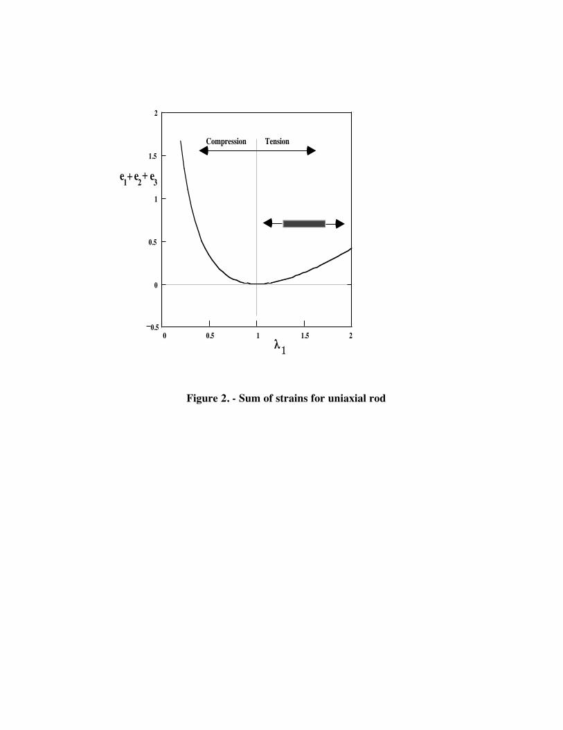
Figure 2 shows how the sum e1 + e2 + e3 varies with !1 when the exact incompressibilitycondition !1 !2 !3 = 1 is imposed. This sum is exactly zero only at zero strain, otherwise itis positive. Consequently, for uniaxial loading, the linear-strain approximation toincompressibility, equation (4), is satisfied only at zero strain.

Since the two conditions e1 + e2 + e3 = 0,

!

" = 1/2, occur only at zero strain for theincompressible uniaxial case, it follows that this may also be true for other incompressibleloading cases. The next section shows that this is the case for a metal-like stress-strain lawgoverning a three-dimensional state of stress.

Three-Dimensional Isotropic Stress-Strain Equations

For the uniaxial case, equation (5) for Poisson's ratio was obtained without any knowledge ofhow the material stress and strain are related. The three-dimensional formulation in reference 2uses the experimental observation that for numerous synthetic rubbers, and natural rubber,uniaxial true stress ti (force per unit deformed area) varies linearly with strain as ti = Eei for

strains of 100 percent and more4. In this equation E is Young's modulus, the constant-slopepart of the experimental, uniaxial stress-strain curve. Reference 2 hypothesized that the linearuniaxial behavior could be extended to three dimensions by writing the following triaxialHooke's-law like relations between principal strains and principal true stresses.

!1 " 1 = e1 =t1

E" #

t2

E" #

t3

E, ! 2 " 1 = e2 = "#

t1

E+t2

E"#

t3

E, ! 3 " 1 = e3 = "#

t1

E"#

t2

E+t3

E (6)

Again, the subscripts indicate the three principal directions. The parameter ! is allowed tovary, which makes equations (6) nonlinear. As in the uniaxial case, ti represents true stress,not engineering stress fi (force per unit original area). For an incompressible material thetrue and engineering stresses are related as ti = !ifi .

In reference 2, t3 was set to zero, the first two of equations (6) were solved for t1 and t2

t1

E=e1+ !e

2

1" !2,

t2

E=e2+ !e

1

1 "! 2 (7)

and then substituted into the third equation, giving a relation among the three strains and ! .The incompressibility condition !1 !2 !3 =1 was then used to eliminate e3, and finally theresulting equation was solved for ! , resulting in equation (1). For the uniaxial case, wheret2 = t3 = 0, equations (6) reduce to e1 = t1/E and e2 = e3 = - ! t1/E = - ! e1. From theseequations the expression ! = - e2/e1 = - e3/e1 is recovered, which is the definition ofPoisson's ratio.

The Triaxial Case (all three principal stresses non zero). - For convenience, equations (6)are cast in matrix form as

1 !" !"

!" 1 !"

!" !" 1

#

$

% % %

&

'

( ( (

t1

t2

t3

)

*

+ + +

,

-

.

.

. = E

e1

e2

e3

)

*

+ + +

,

-

.

.

. , (8)

Using Gaussian elimination, equation (8) is changed to echelon form,

1 !" !"

0 1! " 2 !"(1+ ")

0 0(1 + ")(1! 2")

1! "

#

$

% % % %

&

'

( ( ( (

t1

t 2

t3

)

*

+ + +

,

-

.

. . = E

e1

e2 + "e1

e3 +"

1! "(e1 + e2 )

)

*

+ + + +

,

-

.

.

.

.

(9)

The third of equations (9) gives ! as a quadratic function of t3 and the three strains.Imposing !1 !2 !3 =1 and specifying t3 gives ! in terms of e1 and e2. For the special caseof biaxial loading, t3 = 0, the quadratic equation reduces to equation (1).

When does ! equal 1/2 ? - If ! is assigned the value 1/2, equation (9) becomes

1 !1/ 2 !1/ 2

0 3 / 4 !3 / 4

0 0 0

"

#

$ $ $

%

&

' ' '

t1

t2

t3

(

)

* * *

+

,

- - -

= E

e1

e2 + (1 / 2)e1

e3 + e1 + e3

(

)

* * *

+

,

- - -

(10)

The third row of the square matrix contains all zeros. This means equations (8) aresingular for ! = 1/2, and there is either no solution for the stresses ti, or there are aninfinite number of solutions. To explore these two possibilities the third of equations(10) is examined,

(0 ! t1) + (0 ! t2 ) + (0 ! t3 ) = E(e1 + e2 + e3) (11)

which must be satisfied for ! to have the value 1/2. For E % 0, equation (11) is satisfiedonly if the strains are constrained to satisfy

e1 + e2 + e3 = 0 , or equivalently, !1 + !2 + !3 = 3 (12), (13)

This condition must be satisfied for equations (6) to have a solution (an infinite number ofthem) when ! takes the value 1/2; there are no solutions if the constraint is not satisfied.Surprisingly, this ! = 1/2 solution constraint is identical to the small-strain approximation toincompressibility. This result is important, revealing that ! = 1/2 requires that the sum ofthe principal strains be zero. But, for incompressibility, equation (2) must also be satisfied.Using equation (2) to eliminate !3 from equations (13) and (2) gives

!

"1("

2)2

+ "1("

1# 3)"

2+1= 0 (14)

which must be satisfied for incompressibility and the sum of the strains equaling zero to be truesimultaneously. There are no physically realizable values of !i (real and nonnegative) thatsatisfy equation (14) other than !1=!2=!3=1, i.e., all three strains are zero. Thus, for no volumechange, " = 1/2 requires that e1 + e2 + e3 = 0 be satisfied, and this is not possible except at zero

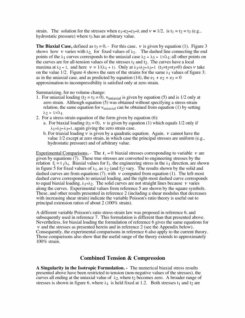
strain. The solution for the stresses when e1=e2=e3=0, and ! = 1/2, is t1 = t2 = t3 (e.g.,hydrostatic pressure) where t3 has an arbitrary value.

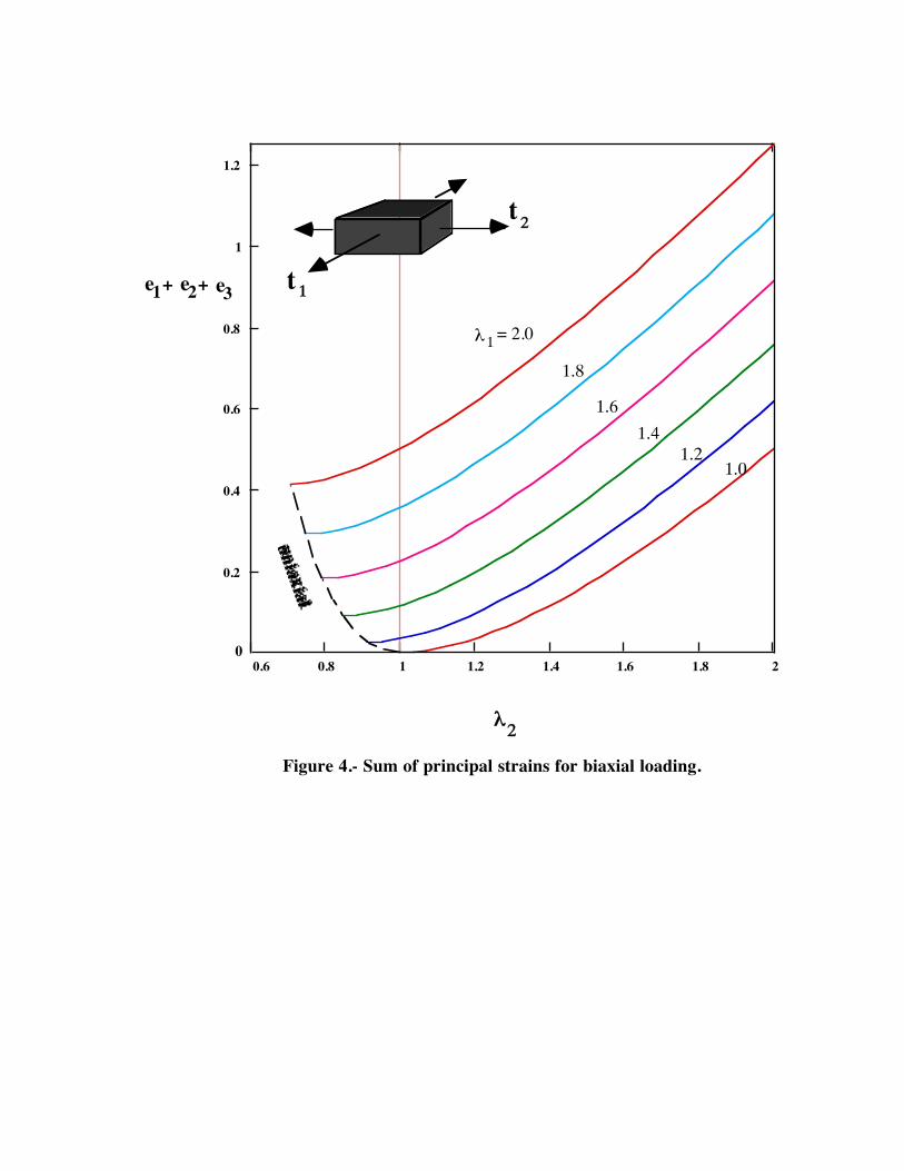
The Biaxial Case, defined as t3 = 0. - For this case, ! is given by equation (1). Figure 3shows how ! varies with !2, for fixed values of !1. The dashed line connecting the endpoints of the !1 curves corresponds to the uniaxial case !2 = !3 = 1/#!1; all other points onthe curves are for all-tension values of the stresses t1 and t2. The curves have a localmaxima at !2 = 1, and here ! = 1/(!1 + 1). Only at !1=!2=!3=1 (t1=t2=t3=0) does ! takeon the value 1/2. Figure 4 shows the sum of the strains for the same !1 values of figure 3;as in the uniaxial case, and as predicted by equation (14), the e1 + e2 + e3 = 0approximation to incompressibility is satisfied only at zero strain.

Summarizing, for no volume change:1. For uniaxial loading (t2 = t3 = 0), "uniaxial is given by equation (5) and is 1/2 only at

zero strain. Although equation (5) was obtained without specifying a stress-strainrelation, the same equation for "uniaxial can be obtained from equation (1) by setting!2 = 1/#!1.

2. For a stress-strain equation of the form given by equation (6):a. For biaxial loading (t3 = 0), ! is given by equation (1) which equals 1/2 only if

!1=!2=!3=1, again giving the zero strain case.b. For triaxial loading ! is given by a quadratic equation. Again, ! cannot have the

value 1/2 except at zero strain, in which case the principal stresses are uniform (e.g., hydrostatic pressure) and of arbitrary value.

Experimental Comparisons. - The

!

t3

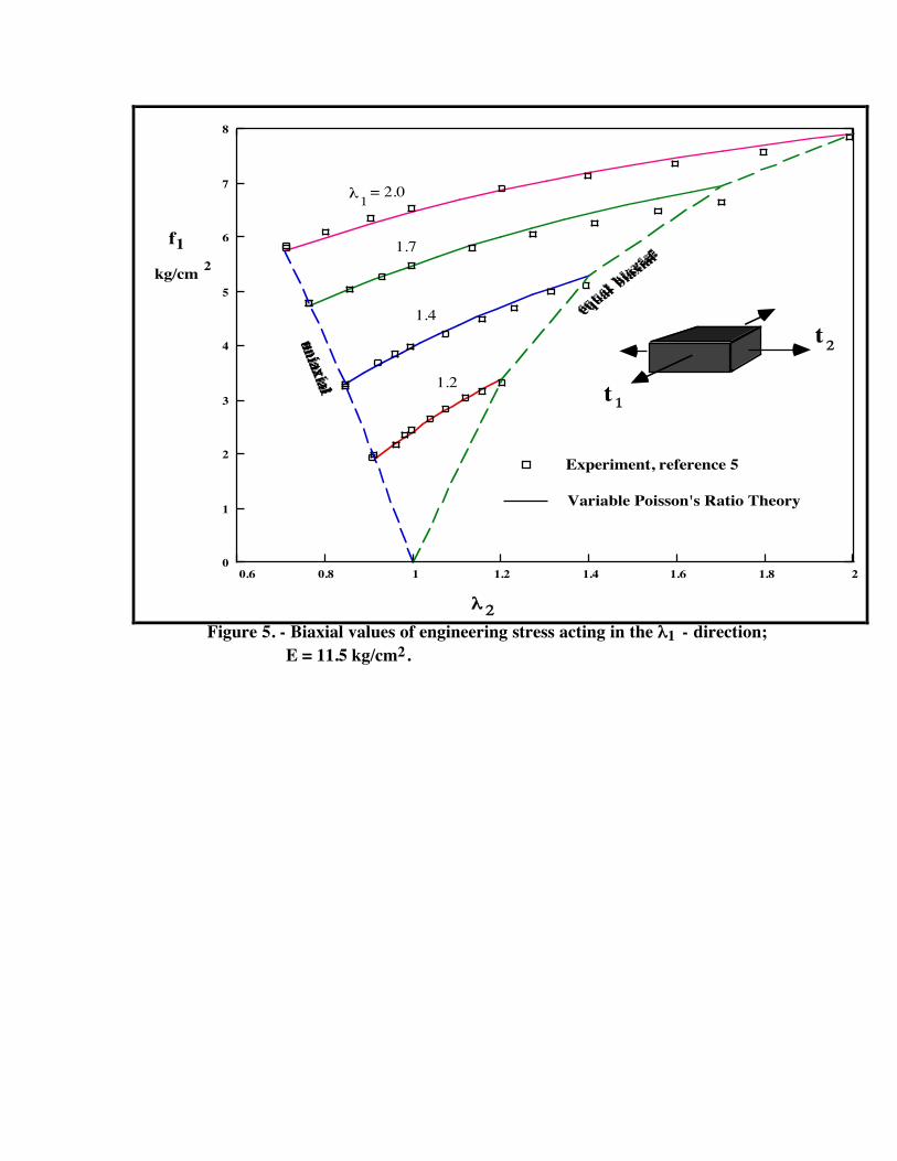
= 0 biaxial stresses corresponding to variable ! aregiven by equations (7). These true stresses are converted to engineering stresses by therelation fi = t i/!i. Biaxial values for f1, the engineering stress in the !1 direction, are shownin figure 5 for fixed values of !1, as !2 (and f2) vary. The results shown by the solid anddashed curves are from equations (7), with ! computed from equation (1). The left-mostdashed curve corresponds to uniaxial loading, and the right-most dashed curve correspondsto equal biaxial loading, !1=!2. The solid curves are not straight lines because ! variesalong the curves. Experimental values from reference 5 are shown by the square symbols.These, and other results presented in reference 2 (including a shear modulus that decreaseswith increasing shear strain) indicate the variable Poisson's ratio theory is useful out toprincipal extension ratios of about 2 (100% strain).

A different variable Poisson's ratio stress-strain law was proposed in reference 6, andsubsequently used in reference 7. This formulation is different than that presented above.Nevertheless, for biaxial loading the formulation of reference 6 gives the same equations for! and the stresses as presented herein and in reference 2 (see the Appendix below).Consequently, the experimental comparisons in reference 6 also apply to the current theory.Those comparisons also show that the useful range of the theory extends to approximately100% strain.

Combined Tension & Compression

A Singularity in the Isotropic Formulation. - The numerical biaxial stress resultspresented above have been restricted to tension (non-negative values of the stresses), thecurves all ending at the uniaxial value of !2, where t2 becomes zero. A broader range ofstresses is shown in figure 6, where !1 is held fixed at 1.2. Both stresses t1 and t2 are

positive (tension) when !2 is greater than the uniaxial value of about .913, indicated by theright-most vertical line. Both stresses are negative (compressive) when !2 is less thanabout .694, indicated by the left-most vertical line. The region between these two verticallines is one of combined tension and compression, wherein t1 is expected to remain positive(tension) and t2 negative (compression). However, the variable Poisson's ratio stress-strainequations have a singularity in this region, exhibited in figure 6 by each stress reversingsigns twice near !2 = 0.82.

This physically unrealistic event is caused by

!

" 's singular behavior in the combined tension& compression region -- see figure 7. As the tension and compression region isapproached from the right,

!

" 's slow decrease becomes more rapid as

!

" drops to zero andchanges sign at !2 = 0.833, and then changes sign again, discontinuously, by "goingthrough" minus and plus infinity at !2 = 0.818. This singular behavior occurs even atinfinitesimal strain, so the problem cannot be attributed to nonlinearities associated withlarge deformations.

Examining the all-tension and all-compression regions of figure 7 yields insight into thesource of the singularity. In the all-tension region

!

" is less than 1/2, and in the all-compression region

!

" is greater than 1/2, similar to the uniaxial case of figure 1. But, inthe combined tension & compression region too much is being asked of the singlePoisson's ratio, viz., to be both less than and greater than 1/2 simultaneously. This resultsuggests the need for two parameters;

!

" 1 associated with say the tension direction, and

!

" 2associated with the compression direction. The two parameters could then take on separatevalues when the stresses are of opposite sign. Such a bimodular anisotropic approach isexamined in the following section.

A Bimodular Formulation. - The proposed stress-strain equations are generalized fromequations (6) by associating a separate

!

" i and Ei with each ti. For t3 = 0 the equationsbecome

! 1 " 1 = e1 = +t1

E1

" #2t2

E2

, ! 2 " 1 = e2 = "#1t1

E1

+t2

E2

, ! 3 " 1 = e3 = "#1t1

E1

" #2t2

E2

(15)

Solving the first two of equations (15) for the stresses gives

!

t1

E1

=e1+ "

2e2

1#"1"2

,t2

E2

=e2

+ "1e1

1#"1"2

(16)

There are now two Poisson's-ratio like parameters to determine. This bimodular approachis being developed, and some initial results are shown below.

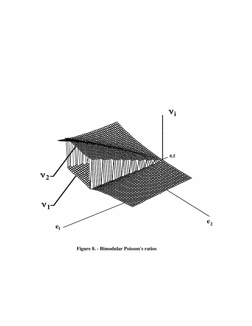
Figure 8 shows qualitatively how

!

" 1 and

!

" 2 vary with biaxial strain. In the relatively flatforeground region of the surface plot,

!

" 1 and

!

" 2 are equal. Here, the corresponding t1and t2 are both tensile stresses. Moving in the negative e2-direction the surface bifurcates atthe uniaxial boundary !2 = !3 = 1/#!1, and

!

" 1 and

!

" 2 take on separate values. In thisbimodular region the state of stress is one of combined tension and compression. Movingfurther in the negative e2-direction another boundary is reached at which the two Poisson'sratios become equal again, corresponding to t1 and t2 both being compressive.

For !1 = 1.2, figure 9 compares the stresses predicted by the bimodular formulation (thickcurves) with the figure 6 isotropic formulation stresses (thin curves). The singular behavior

exhibited by the isotropic formulation is eliminated with the bimodular formulation. Thestresses predicted by the bimodular theory vary smoothly through the singular region ofthe isotropic formulation, and asymptotically approach the isotropic stresses in the all-tension and all-compression regions.

Conclusions

For no volume change, and for triaxial and biaxial loading of a material governed by aHooke's law like stress-strain equation, and also for uniaxial loading (where a stress-strainlaw is not needed), it is shown that Poisson's ratio

!

" varies with strain and equals 1/2 onlyat zero strain. For biaxial tension, experimental stress comparisons show the variablePoisson's ratio theory is useful to about 100 % strain. For biaxial loading of combinedtension and compression, the original isotropic theory of reference 2 produces incorrectsingular stresses, even at small strain. A bimodular formulation presented here, thatinvolves two parameters

!

" 1 and

!

" 2, eliminates the singularity and produces physicallyrealistic stresses for combined tension and compression loading.

Acknowledgments

The author thanks Dr. Robert F. Landel of the California Institute of Technology's JetPropulsion Laboratory, and Mr. Lado Muhlstein, Jr., NASA Ames Research Center, fortheir support and encouragement, and Dr. O. H. Yeoh of GenCorp Research, who broughtreference 6 to my attention.

References

1. R. R., Archer, et. al., An Introduction to the Mechanics of Solids, S. H. Crandall and N.C. Dahl, editors, McGraw-Hill Book Co., Inc., 1954, New York, pages 213 and 229,1959.

2. L. L. Erickson, "A New Constitutive Equation for Elastomers," Rubber & PlasticsNews, March 15, 1993.

3. C. Truesdell and R. Toupin, "Principles of Classical Mechanics and Field Theory,"Encyclopedia of Physics, S. Flugga, ed., Springer-Verlag, Berlin, vol. III, part 1, 1960.

4. T. J. Peng and R. F. Landel, "Stored Energy Function of Rubberlike Materials Derivedfrom Simple Tension Data, " J. Appl. Phys., vol. 43, no. 7, July 1972.

5. S. Kawabata and H. Kawai, "Strain Energy Density Functions of Rubber Vulcanizatesfrom Biaxial Extension," Advances in Polymer Science, Molecular Properties, vol. 24,pp. 89-124, 1977.

6. D. M. Turner and M. Brennan, "The Multiaxial Elastic Behaviour of Rubber," Plasticsand Rubber Processing and Applications, vol. 14, no. 3, pp. 183-188, 1990.

7. D. J. Charlton, and J. Yang, "A Review of Methods to Characterize Rubber ElasticBehavior for Use in Finite Element Analysis," Rubber Chemistry and Technology, vol.67, no. 3, pp. 481-503, 1994.

Appendix - Connection Between Reference 2 & 6 Theories

A different variable Poisson's ratio isotropic formulation is given by equations (8), (9) and (10)of reference 6. In the notation of the present paper, the hypothesized stress-strain law fromreference 6 is given by

1 !" !(1! ")

!" 1 !(1! ")

!" !" 2"

#

$

% % %

&

'

( ( (

t1

t2

t3

)

*

+ + +

,

-

.

. . = E

e1

e2

e3

)

*

+ + +

,

-

.

. . (A1)

or, in echelon form,

1 !" !(1 ! ")

0 1 ! "2 !(1! "2 )

0 0 0

#

$

% % %

&

'

( ( (

t1

t2

t3

)

*

+ + +

,

-

.

. . = E

e1

e2 +"e1

e3 +"

1! "(e1 + e2 )

)

*

+ + + +

,

-

.

.

.

.

(A2)

Although not mentioned in reference 6, the non-symmetric set of equations (A1) is singularfor all values of ! since the third column is a linear combination of the first two columns(minus the sum of columns one and two). Gaussian elimination produces equation (A2).For there to be a solution (an infinite number of them), the third of equations (A2) yieldsthe following constraint equation that must be satisfied.

e3 +!

1" !(e1 + e2 ) = 0 (A3)

This constraint equation happens to be identical to the condition required for t3 to be zero inequation (9). So, again equation (1) is obtained. The first two of equations (A2) give

t1

E=e1+ !e

2

1" !2+t3

E,

t2

E=e2+ !e

1

1" !2+t3

E (A4)

where t3 can be any value. If t3 is specified to be zero, equations (A4) produce equations (7).

Because the biaxial formulas for ! and the stresses are the same in both references 2 and6 it might appear that the formulations in references 2 and 6 are equivalent. This is not so,the differences being:

1. The stress-strain laws given by equations (8) and (A1), or (9) and (A2), are differentexcept when ! =1/2.

2. Equation (8) is not singular except when ! =1/2 (or minus 1), whereas thecorresponding equation (A1) is singular for all values of ! .

3. In the case of equations (8), for general triaxial loading ! is the solution of a quadraticequation -- only if t3 = 0 is ! is given by equation (1). In contrast, for equations (A1) !is always given by equation (1) for all values of t3, and t3 is arbitrary.

For the biaxial case t3 = 0, the reference 2 and 6 formulations happen to give the sameequations for ! and the stresses t1 and t2. The theoretical and experimental resultscomparisons in reference 6 are for t3 = 0, and hence also apply to the present isotropicbiaxial formulation.

0.2 0.4 0.6 0.8 1 1.2 1.4 1.6 1.8 2

0

0.2

0.4

0.6

0.8

1

1.2

1.4

1.6

!uniaxial

"1

Compression Tension

! = 0.5

t1

Figure 1. - Poisson's ratio for uniaxially-stressed rod.

0 0.5 1 1.5 20.5

0

0.5

1

1.5

2

!1

Compression Tension

+ +e1e2e3

Figure 2. - Sum of strains for uniaxial rod

0.6 0.8 1 1.2 1.4 1.6 1.8 2

0.2

0.3

0.4

0.5

1.8

1.6

1.0

1.2

1.4

!

"

uniaxial

2

! 1=2.0t1

2

1t

t

biaxial

Figure 3.- Poisson's ratio for biaxial loading.

0.6 0.8 1 1.2 1.4 1.6 1.8 2

0.2

0.4

0.6

0.8

1

1.2

1.8

1.6

1.4

1.21.0

e1e2 e

3+ +

!2

uniaxial

!1 = 2.0

t1

t2

0

Figure 4.- Sum of principal strains for biaxial loading.

0.6 0.8 1 1.2 1.4 1.6 1.8 20

1

2

3

4

5

6

7

8

un

iaxial

1

1.2

1.7

1.4

! = 2.0

! 2

f1

equal b

iaxia

l

Experiment, reference 5

Variable Poisson's Ratio Theory

kg/cm2

t1

t2

Figure 5. - Biaxial values of engineering stress acting in the !1 - direction;

E = 11.5 kg/cm2.

0.6 0.7 0.8 0.9 10.4

0.2

0

0.2

0.4

<<>

t1

t2

^

^

CombinedTension &CompressionCompression

All

Tension

All

t1/E

t2/E

t

t1

2

! 2

^

<> >

Figure 6. - Nonphysical stresses due to singular "; !1 = 1.2

0.6 0.7 0.8 0.9 1

2

1

0

1

2

Tension

!

Compression

Combined

.5

"2

<>

Tension &Compression

<

>^

^ >^<

t1

t2

AllAll

<>

^

^

>

^

<

Figure 7. - Singularity in "; !1 = 1.2

0.5

!i

2!

!1

e2

e1

Figure 8. - Bimodular Poisson's ratios

0.6 0.7 0.8 0.9 10.4

0.2

0

0.2

0.4

<<>

t1

t2

^

^

CombinedTension &CompressionCompression

All

Tension

All

t

t1

2

! 2

^

<> >

t1/E1

t2/E2

Figure 9. - Bimodular (thick lines), and isotropic (thin lines) formulation stresses, !1 = 1.2.