Why Do Diffusion Data Not Fit the Logistic Model? A Note on Network Discreteness, Heterogeneity &...

Why Do Diffusion Data not Fit the LogisticModel? A Note on Network Discreteness,Heterogeneity & Anisotropy

Dominique Raynaud

Abstract Diffusion of innovations and knowledge is in most cases accounted forby the logistic model. Fieldwork research however constantly report that empiricaldata utterly deviate from this mathematical function. This chapter scrutinizes net-work forcing of diffusion process. The departure of empirical data from the logisticfunction is explained by social network discreteness, heterogeneity and anisotropy.New indices are proposed. Results are illustrated by empirical data from an originalstudy of knowledge diffusion in the medieval academic network.

Introduction

Diffusion of innovations is the process by which an innovation is communicatedthrough certain channels over time among the members of a social system [27, p. 5].Diffusion of knowledge may be defined in the same manner, replacing what shouldbe in the previous definition. Social network analysis is in its early stages of appli-cation to diffusion issues.

Compared with other aspects of diffusion research, there have been relatively few studies ofhow the social or communication structure affects the diffusion and adoption of innovationsin a system [27, p. 25].

So speaks Everett M. Rogers, the outstanding promoter of diffusion studies, aboutthe way they are connected to network analysis. In the 1970’s, according to a contentanalysis of 1,084 empirical publications, diffusion networks represented less thanone percent of diffusion research. Ten years ago, a book especially dedicated tonetwork analysis has the same diagnosis:

Dominique RaynaudPLC, Université de Grenoble, F-38040 Grenoble Cedex 9, and GEMASS, CNRS UMR 8598 /Université Paris Sorbonne, 54 bd Raspail, F-75000 Paris, Francee-mail: [email protected]

81

82 D. Raynaud

Only few material coupling a diffusion study with network analysis is available [8, p. 189].

The authors consequently content themselves with classical studies in the field. Thefact that different authors interested in the diffusion of innovations vs. network anal-ysis have detected the same lack of research, vouches for a promising fieldwork.

1 A Brief Historical Sketch

Despite the fact that the first paper explicitly dedicated to network diffusion waswritten in 1979 by Everett M. Rogers [26], the concern is much more ancient. Forinstance, in the course of his studies on the cholera, in 1884, Etienne-Jules Mareyalready applied network perspective to diffusion data. He had the insight that thetopology of social network determines the form of the diffusion process. Mareysays: “Closed institutions: prisons, boarding schools, convents, asylums, etc., usu-ally escape to cholera; but if it gets into, it takes a terrible toll of victims” [20,p. 670]. Cliques (i.e. closed communities) exhibit atypical behaviour: they are re-sistant to the disease or completely devastated by the epidemic. The “clique effect”was independently rediscovered in 1973 by Mark S. Granovetter [12]: “weak ties”favour diffusion, “strong ties” protect the members from a tentative adoption: eitherthey all adopt, or they all reject.

The first book approaching the diffusion of innovations through network analysiscame out in 1995 by a student of Rogers: Thomas W. Valente [35]. His scope was tocompare three classical datasets: the adoption of tetracycline by 130 physicians ofthe Middle West [6]; the diffusion of innovations among 692 Brazilian farmers [28];the diffusion of family planning in 24 Korean villages [29]. Held with fifteen yearsof hindsight, the book appears a little disapointing for seven chapters out of nine arein fact dedicated to apply thresholds and critical mass models to diffusion issues.Network analysis occupies thirty pages [35, p. 31-61], where classical measures ofdensity, centrality and equivalence are processed out on the three datasets.

In the past decades, diffusion process have been simulated either within deter-ministic or probabilistic models [1, 19, 16, 5, 9, 17]. Researchers have explored afull range of simulations, including Monte Carlo, Ising, Potts, Krause-Hegselmannand Deffuant models [16, 10, 32, 34, 4]. However, more often than not, models pre-suppose the population to be homogeneous. Simulations are implemented on regularbi-dimensional lattices. Modeling rarely assumes the topology in which the diffu-sion occurs, and it is only in the 2000s that sociologists, economists and physicistsaddressed the point [7, 15, 30, 31, 18, 2]. The network-based approach of diffusionis full of consequences, some of which are still developing.

There is consequently little research on the irregularity of diffusion curves. Thestate-of-the-art is the following: 1/ Threshold models have relied the ! curve slopeto higher or lower individual adoption thresholds [13, 14, 36]. 2/ Critical mass mod-els have shown that, the more the early majority members have a high centralityindex, the faster the critical mass is reached, and the higher is the saturation thresh-old [23, 35]. 3/ In a forthcoming paper, we find, with no supplementary details,

Network Discreteness, Heterogeneity and Anisotropy 83

that “important consequences of this large variability [of human behaviour] are theslowing down or speed up of information” [18, p. 6].

Diffusion irregularity is not the main concern of papers in statistical physics thatclosely combine network analysis with diffusion processes. They consider instead:1/ critical points for avalanches [15]; 3/ random walks, qua they provide networktopology characteristics [30]; 4/ modularity-based partitioning of graphs [31]; 5/mean-field theory applications [2]. An overview of the current research would saythat diffusion is basically seen as a means to find network properties. Hence, the lit-erature is still lacking for network-based studies that could answer the long-delayedquestion of diffusion anomalies.

2 The Logistic Function

The choice of the mathematical model accounting for diffusion depends on the em-pirical conditions of spreading. If the empirical process is a step-by-step diffusionthrough interpersonal contacts, it follows the logistic function, which was first dis-covered in 1838 by Pierre-François Verhulst—albeit he never used the term [38]. Inthe recent years, there was a propensity to emancipate from his formalism; see [5].In the following equation, the term e!!t is the most characteristic of the process:

nt =N"

1+ae!!t (1)

nt represents the cumulative number of individuals having adopted at time t; N"

the number of susceptible adopters in the given population; a is a parameter settingthe number of early adopters; ! the slope of the curve at the inflection point (when! # 0, the curve is flat).

The bell-shaped first derivative represents the instant number of adopters at timet. The second derivative is swing-shaped. First and second derivatives respond toequations (2) and (3) respectively:

dndt

=!N"ae!!t

1+ae!!t (2)

d2ndt2 =

!2N"ae!!t(ae!!t !1)(1+ae!!t)3 (3)

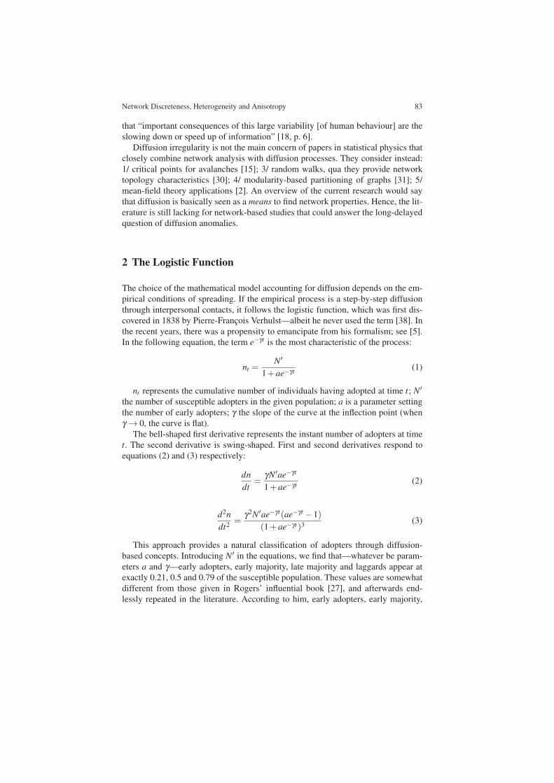
This approach provides a natural classification of adopters through diffusion-based concepts. Introducing N" in the equations, we find that—whatever be param-eters a and !—early adopters, early majority, late majority and laggards appear atexactly 0.21, 0.5 and 0.79 of the susceptible population. These values are somewhatdifferent from those given in Rogers’ influential book [27], and afterwards end-lessly repeated in the literature. According to him, early adopters, early majority,

84 D. Raynaud

Fig. 1: The logistic function and its derivatives

late majority and laggards appear respectively at 0.16, 0.5 and 0.84 of the suscepti-ble population.

The reason for such a disagreement is that the classification of adopters is envis-aged through common statistical concepts. The logistic first derivative is assimilatedto a normal distribution. Rogers’ values are in fact those of the mean µ and µ !!2,µ +!2. Valente is even more explicit:

The logistic function has an inflexion point at 50 % adoption and two second-order inflec-tion points, one each at one standard deviation below and above the mean [35, p. 83].

Standard deviation concept is inappropriate in this context: logistic function is nota Gaussian distribution. There is a simple visual proof for that: respective curvescross several times with each other, as in Fig. 1 (b). As a consequence, the values0.16, 0.5 and 0.84 must be discarded and replaced by 0.21, 0.5 and 0.79.

3 Empirical Data

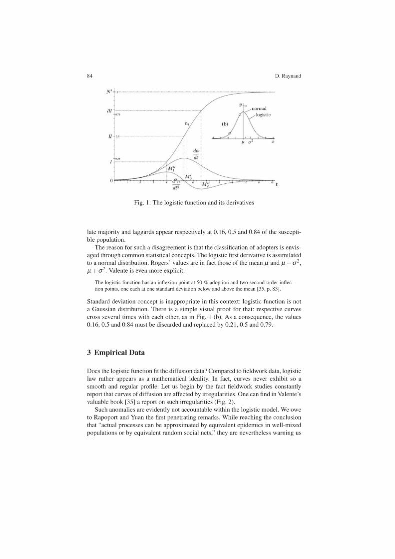
Does the logistic function fit the diffusion data? Compared to fieldwork data, logisticlaw rather appears as a mathematical ideality. In fact, curves never exhibit so asmooth and regular profile. Let us begin by the fact fieldwork studies constantlyreport that curves of diffusion are affected by irregularities. One can find in Valente’svaluable book [35] a report on such irregularities (Fig. 2).

Such anomalies are evidently not accountable within the logistic model. We oweto Rapoport and Yuan the first penetrating remarks. While reaching the conclusionthat “actual processes can be approximated by equivalent epidemics in well-mixedpopulations or by equivalent random social nets,” they are nevertheless warning us


Fig. 2: Diffusion curves irregularity.

that this conjecture “does not apply to highly structured populations” [24, p. 344-345]. The gap between the model and the real world lies in the assumption thatsocieties are “well-mixed populations,” thus assimilating the adoption of innova-tion to a random draw. Social network heterogeneity urges to abandon this assump-tion, which is the basis of all SIR—susceptible/infective/removed—epidemiologicalmodels.

During the 2000s, statistical physicists took part in the debate, by criticizing thelogistic model as “utterly inaccurate” [22]. They have again argued that standardepidemiological models do not take into account that diffusions happen in highlystructured, heterogeneous population, whose topology influences the very form ofthe diffusion [39, 21, 22]. This observation put the answer at hand.

4 Accounting for Anomalies

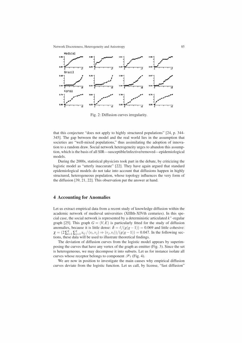
Let us extract empirical data from a recent study of knowledge diffusion within theacademic network of medieval universities (XIIIth-XIVth centuries). In this spe-cial case, the social network is represented by a deterministic articulated k+-regulargraph [25]. This graph G = (V,E) is particularly fitted for the study of diffusionanomalies, because it is little dense: ! = !/(g(g!1)) = 0.069 and little cohesive:" = (2!g

i=1 !gj=1 xi j / (vi,v j)" (v j,vi))/(g(g!1)) = 0.047. In the following sec-

tions, these data will be used to illustrate theoretical findings.The deviation of diffusion curves from the logistic model appears by superim-

posing the curves that have any vertex of the graph as emitter (Fig. 3). Since the setis heterogeneous, we may decompose it into subsets. Let us for instance isolate allcurves whose receptor belongs to component P7 (Fig. 4).

We are now in position to investigate the main causes why empirical diffusioncurves deviate from the logistic function. Let us call, by license, “fast diffusion”

86 D. Raynaud

Fig. 3: Diffusion (any receptor) Fig. 4: Diffusion (receptor ! P7)

any diffusion that converts many vertices in few steps; “slow diffusion” the one thateiher converts few vertices, or requires many steps to convert them all. Analyticalconcepts presented hereinafter are devised to fit diffusion networks that are alwaysdirected graphs and, more often than not, grounded networks—i.e. dependent on theposition of vertices in space.

5 Net Discreteness

Discreteness of social networks results in slowing down/accelerating adoption,hence flattening/straightening the diffusion curve.

The more obvious difference between the logistic function (Fig. 1) and empiricalcurves (Fig. 3 and 4), is that the former is a smooth curve, when the latter is angled.While the logistic function is defined on a continuous (infinite) set, social diffu-sion happens within discrete (finite) structures. The lower the number of susceptibleadopters, the more angled the curve.

There is a simple estimate for network discreteness. Let us call vi the emittervertex of any given diffusion process. The number of diffusion steps will be equalto the lenght of the longest geodesic dik originating in vi. Local discreteness rangesfrom 0 when dik = !, to 1 when dik = 1, hence:

Di =1

max(dik)Di ! [0,1] (4)

If we need a comparative index, we first calculate the mean discreteness DG—where g is the total number of vertices—, then the difference D"

i = Di #DG:

D"i =

1max(dik)

# 1g

g

"j=1

1max(d jk)

D"i ! [#1,+1] (5)


Local discreteness is null if the geodesic on which the vertex stands is as longas the graph mean geodesics. Positive values occur if Di ! DG, when the regionin which the information is going through is less dense than the rest of the graph,thus slowing down the diffusion; negative values otherwise. Discreteness values onthe academic network are given in Appendix (columns Di and D!

i). The data (ROS,0.111, "0.048) are to be read as: “All vertices standing on the longest geodesicattached to ROS, i.e. {ROS, KOL, STR, DIJ, AST, GEN, PIS, SIE, PER, TOD, ROM}have discreteness 0.111 or, equivalently, are 0.048 less discrete than the rest of thegraph.”

6 Net Heterogeneity

Heterogeneity of social networks results in slowing down/accelerating adoption,hence flattening/straightening the diffusion curve.

Let us consider anew all curves of diffusion (Fig. 4). At t = 2, the curves, whichwere hitherto undifferentiated, split into five distinct profiles. The message from DIJis adopted by six new vertices (fast growth); the one from ESZ is adopted by onlytwo new vertices (slow growth). This difference is due to the fact the first messageis diffused within two distinct subsets, when the second message never leaves thestarting subset, composed of few susceptible adopters. The diffusion growth is asfast as the conversion rate. It is only when the message gets into new componentsof the network that it can cause mass adoption. Consequently, slow and fast phasesare sensitive to articulators.

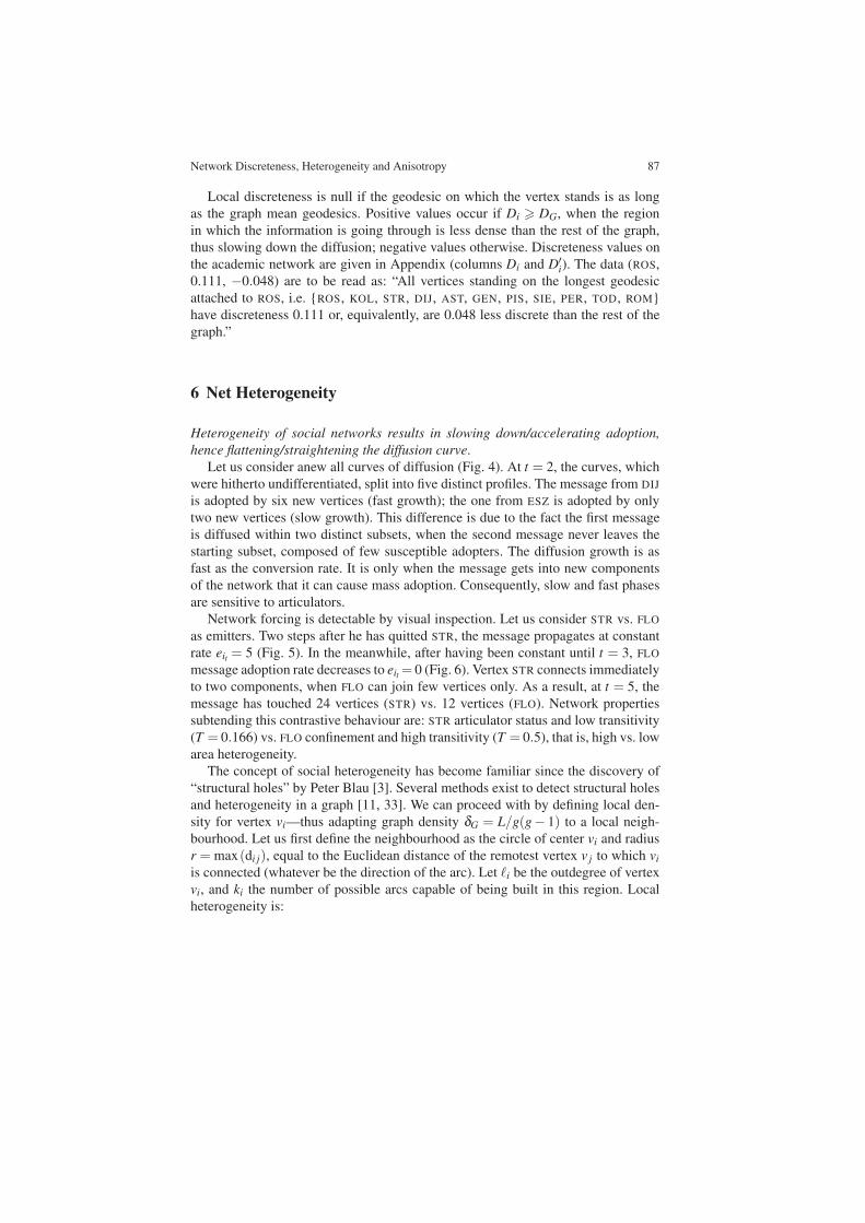
Network forcing is detectable by visual inspection. Let us consider STR vs. FLOas emitters. Two steps after he has quitted STR, the message propagates at constantrate eit = 5 (Fig. 5). In the meanwhile, after having been constant until t = 3, FLOmessage adoption rate decreases to eit = 0 (Fig. 6). Vertex STR connects immediatelyto two components, when FLO can join few vertices only. As a result, at t = 5, themessage has touched 24 vertices (STR) vs. 12 vertices (FLO). Network propertiessubtending this contrastive behaviour are: STR articulator status and low transitivity(T = 0.166) vs. FLO confinement and high transitivity (T = 0.5), that is, high vs. lowarea heterogeneity.

The concept of social heterogeneity has become familiar since the discovery of“structural holes” by Peter Blau [3]. Several methods exist to detect structural holesand heterogeneity in a graph [11, 33]. We can proceed with by defining local den-sity for vertex vi—thus adapting graph density !G = L/g(g" 1) to a local neigh-bourhood. Let us first define the neighbourhood as the circle of center vi and radiusr = max(di j), equal to the Euclidean distance of the remotest vertex v j to which viis connected (whatever be the direction of the arc). Let !i be the outdegree of vertexvi, and ki the number of possible arcs capable of being built in this region. Localheterogeneity is:

88 D. Raynaud

Fig. 5: Fast diffusion from STR Fig. 6: Slow diffusion from FLO

Hi = 1! !i

kiHi " [0,1] (6)

If we prefer a comparative index, we first calculate the mean heterogeneity HGon the graph, then the difference H #

i = Hi !HG:

H #i =

!1! !i

ki

"! 1

g

g

!j=1

!1!

! j

k j

"that is equal to :

H #i =

1g

g

!j=1

!! j

k j

"! !i

kiH #

i " [!1,+1] (7)

This index is null when the region the information is going through is as dense asthe whole graph. Positive values occur when Hi ! HG, that is when the local regionis more heterogeneous than the rest of the graph, thus slowing down the diffusion;negative values otherwise. See Appendix for academic network values (columns Hiand H #

i ). For example, the data (ROS, 0.000, !0.323) are to be read as: “Vertex ROShas null heterogeneity or, equivalently, is 0.323 less heterogeneous than the rest ofthe graph.”

7 Net Anisotropy

Anisotropy of social networks results in slowing down/accelerating adoption, henceflattening/straightening the diffusion curve.


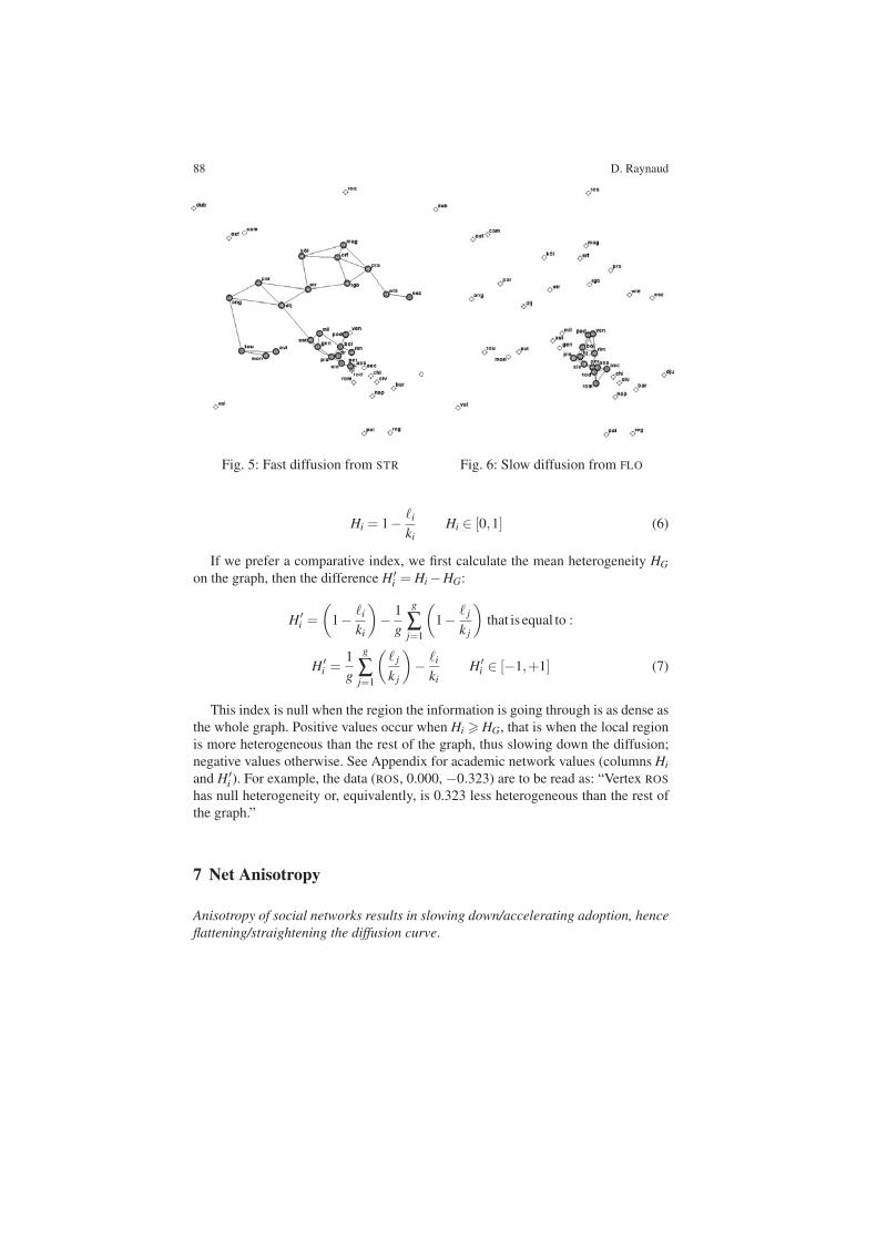
Let us isolate curves originating in DIJ and ESZ, two vertices having the greatestdifference among component P7. A good way to link irregularity of curves withnetwork properties is to represent the message progression within the network byjoining all vertices converted at the same time by “isochrones.” Fast spreading is as-sociated to even isochrones when slow diffusion is coupled with uneven isochrones.As a result, six to nine steps are needed so that DIJ and ESZ information could coverthe same area (Fig. 7 and 8). At any first steps, DIJ can distribute the message allaround (quasi-isotropy), when ESZ can send information to its western neighboursonly (anisotropy). This is a last factor explaining anomalies.

Fig. 7: Fast diffusion from DIJ Fig. 8: Slow diffusion from ESZ

As far as I know, network anisotropy has never been defined in network analysisliterature. This concept could be derived from other fields of physics, as optics,electricity or magnetism, but in the special case of grounded social networks, thereis a more direct method to define the concept of anisotropy. Suppose vertex vi has anoutdegree !i and let !mn be the angle of two adjacent arcs. The isotropic case ariseswhen every angle is equal to 2"/!i. In order to appreciate anisotropy, we define thedeviation of angle !mn from 2"/!i. Vertex local anisotropy will then be the sum ofactual deviations divided by the sum of theoretical maximum deviations:

Ai =

!!!!mn !2"!i

!!!+!!!!no !

2"!i

!!!+ . . .+!!!!sm ! 2"

!i

!!!

2(!i !1)2"!i

Since angles !mn,!no . . . are supplementary, we may simplify:

90 D. Raynaud

Ai =2 max

!!!!mn !2"!i

!!!

2(!i !1)2"!i

!

Ai =!i max

!!!!mn !2"!i

!!!

2"(!i !1)Ai " [0,+1] (8)

The comparative index is obtained as previously, by calculating the mean anisotropyAG on the graph (with g vertices), then the difference A#

i = Ai !AG:

A#i =

12"

"

##$!i max

!!!!mn !2"!i

!!!

(!i !1)! 1

g

g

!j=1

!i max!!!!pq !

2"! j

!!!

(! j !1)

%

&&' A#i " [!1,+1] (9)

Local anisotropy is null when the local region has the same degree of isotropy asthe rest of the graph. Positive values occur in the case Ai " AG, when the region themessage is going through is less isotropic than the rest of the graph, thus slowingdown the diffusion; negative values otherwise. See Appendix for academic networkdata (columns Ai and A#

i). The data (ROS, 0.866, +0.388) are to be read as: “VertexROS has anisotropy 0.866 or, equivalently, is 0.388 more anisotropic than the rest ofthe graph.”

8 A Test of DHA Indices

First of all, the definition of D (discreteness), H (heterogeneity) and A (anisotro-py) enables us to tell the difference between regular and irregular graphs. In a 2Dsquare lattice, all geodesics are infinite, the term 1/dik is null and D = 0. Since allvertices are disposed regularly, and have the same outdegree, the term !i/ki = +1everywhere, thus H = 0. Finally, since angles of all adjacent arcs are equal, anyterm !mn = 2"/!i so that A = 0. We recognize a well known property: a lattice is aperfect infinite, homogeneous and isotropic network.

Social networks utterly differ from this model. Regarding the conditions ofspreading in the same graph, DHA indices make it possible to see the regions wherethe diffusion is speeding up, and where it is slowing down. Let us resume the dis-cussion of the medieval academic network and compare the indices of all vertices(see Appendix). Network mean values are: discreteness DG = 0.159, heterogeneityHG = 0.323, anisotropy AG = 0.478. Because of the problem of sign combination, itis not appropriate to agregate directly DHA indices. General results are nonethelessaccessible.

Maximum discreteness occurs for vertices in the graph innermost component{AST, MIL, PAD, VEN, GEN, BOL, PIS, FIR, SIE, RIM, PER} because several directed


filters impede information to propagate outside the component, thereby reducing thenumber of steps of diffusion. Maximum heterogeneity occurs for vertices situatedon the borders of the central component {AST, PIS, ROM, CHI, CIV} because thosevertices are both in dense regions and in position to be tied to many vertices withwhich they have no actual relation. Maximum anisotropy occurs for the outermostvertices of the graph (DUB, ROS, ESZ, DJU) because they can send information onlyinwards the network.

All vertices are now sorted into eight classes, according to the sign of their indices(see Appendix, last column):

!!! {OXF, CAM, WIE}+!! {MON, AVI, GEN, FIR, PAD}!+! {PRA, ERF, RGB, STR, PAR, VAL, ASC, CHI, CIV}!!+ {LIS, SEV, SAL, TOU, ANG, DUB, ROS, ESZ, DJU, REG, PAL}++! {DIJ, BOL, SIE, PER, ASS, TOD}+!+ {MIL, VEN}!++ {MAG, KOL, BAR, NAP}+++ {AST, PIS, ROM, RIM}

The behaviour of classes (!!!) and (+++) is quite obvious. Other classescan either accelerate or slow down the diffusion.

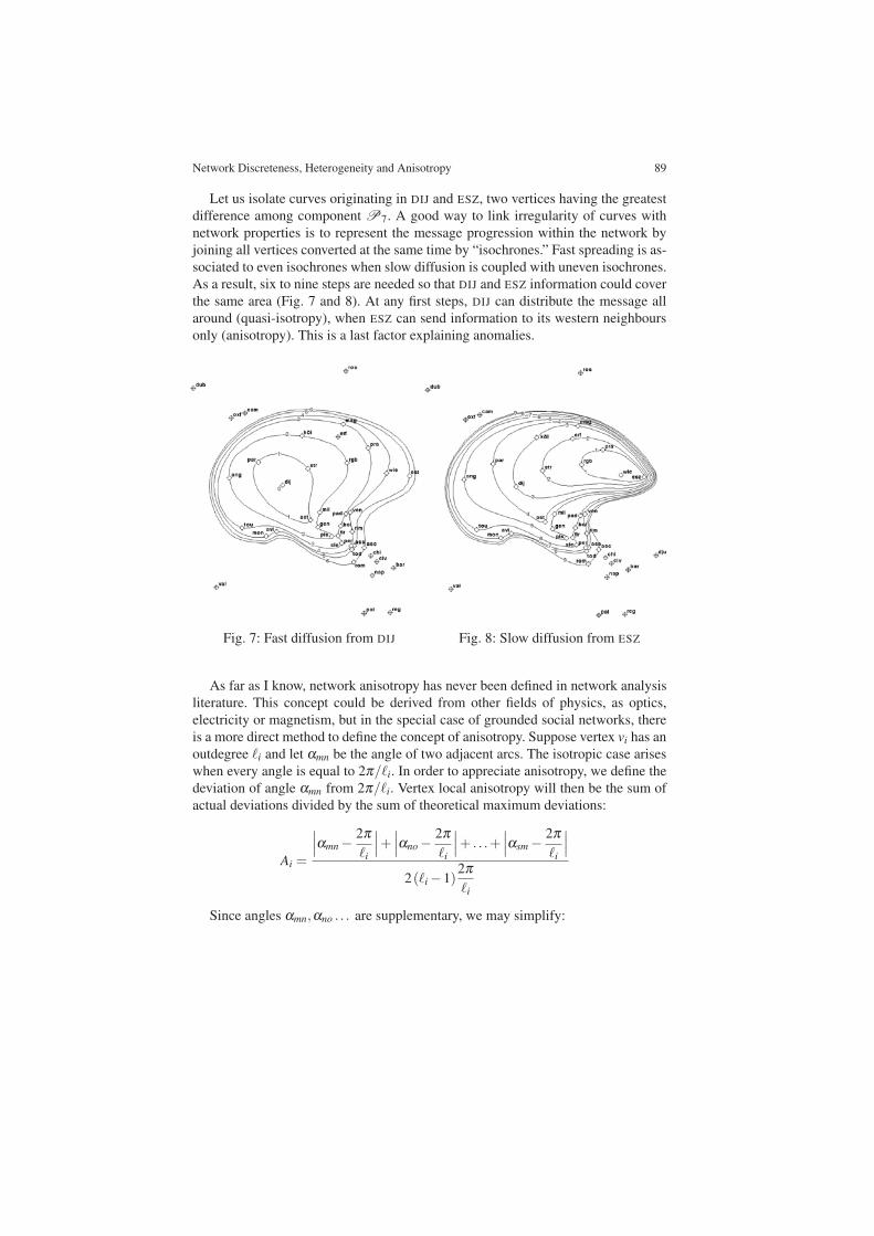
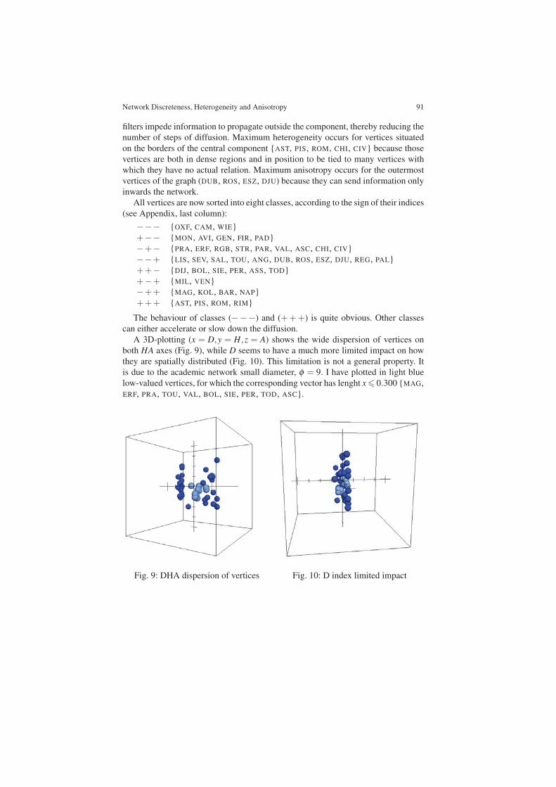
A 3D-plotting (x = D,y = H,z = A) shows the wide dispersion of vertices onboth HA axes (Fig. 9), while D seems to have a much more limited impact on howthey are spatially distributed (Fig. 10). This limitation is not a general property. Itis due to the academic network small diameter, ! = 9. I have plotted in light bluelow-valued vertices, for which the corresponding vector has lenght x! 0.300 {MAG,ERF, PRA, TOU, VAL, BOL, SIE, PER, TOD, ASC}.

Fig. 9: DHA dispersion of vertices Fig. 10: D index limited impact

92 D. Raynaud

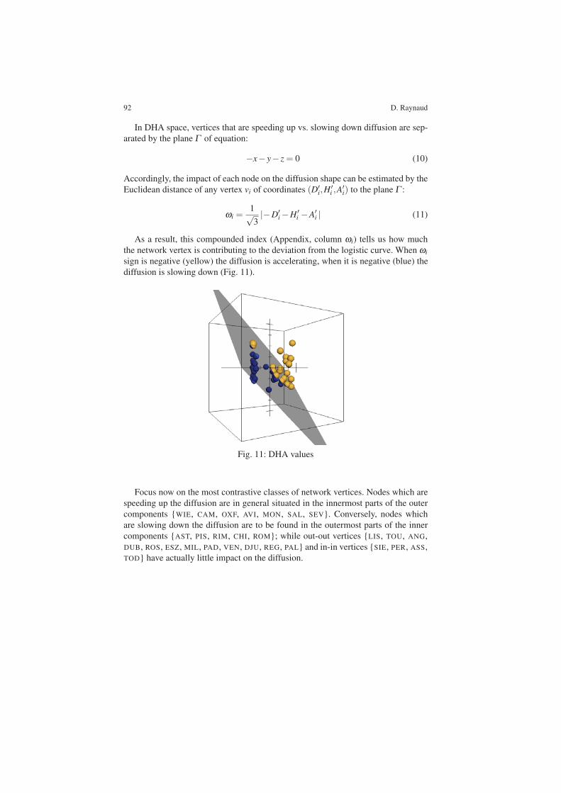
In DHA space, vertices that are speeding up vs. slowing down diffusion are sep-arated by the plane ! of equation:

!x! y! z = 0 (10)

Accordingly, the impact of each node on the diffusion shape can be estimated by theEuclidean distance of any vertex vi of coordinates (D"

i,H"i ,A

"i) to the plane ! :

"i =1#3|!D"

i !H "i !A"

i | (11)

As a result, this compounded index (Appendix, column "i) tells us how muchthe network vertex is contributing to the deviation from the logistic curve. When "isign is negative (yellow) the diffusion is accelerating, when it is negative (blue) thediffusion is slowing down (Fig. 11).

Fig. 11: DHA values

Focus now on the most contrastive classes of network vertices. Nodes which arespeeding up the diffusion are in general situated in the innermost parts of the outercomponents {WIE, CAM, OXF, AVI, MON, SAL, SEV}. Conversely, nodes whichare slowing down the diffusion are to be found in the outermost parts of the innercomponents {AST, PIS, RIM, CHI, ROM}; while out-out vertices {LIS, TOU, ANG,DUB, ROS, ESZ, MIL, PAD, VEN, DJU, REG, PAL} and in-in vertices {SIE, PER, ASS,TOD} have actually little impact on the diffusion.


Conclusion

We are now in position to answer the issue adressed at the beginning of the chap-ter: Diffusion data do not fit the logistic model because social space is discrete,heterogeneous and anisotropic. Social space is thus an inadequate metaphor thatshould be outlawed. Any social spreading of innovations and knowledge is network-dependent. The agenda for future research should plan to: 1/ test DHA indicesrobustness—especially the concept of “net anisotropy” presented in these pages,2/ focus on how DHA indices could predict the precise shape of a diffusion processoccuring in a given social network and, conversely, 3/ deduce, from any empiricaldata on social diffusion, the DHA indices of the social network in which the diffu-sion takes place.

94 D. Raynaud

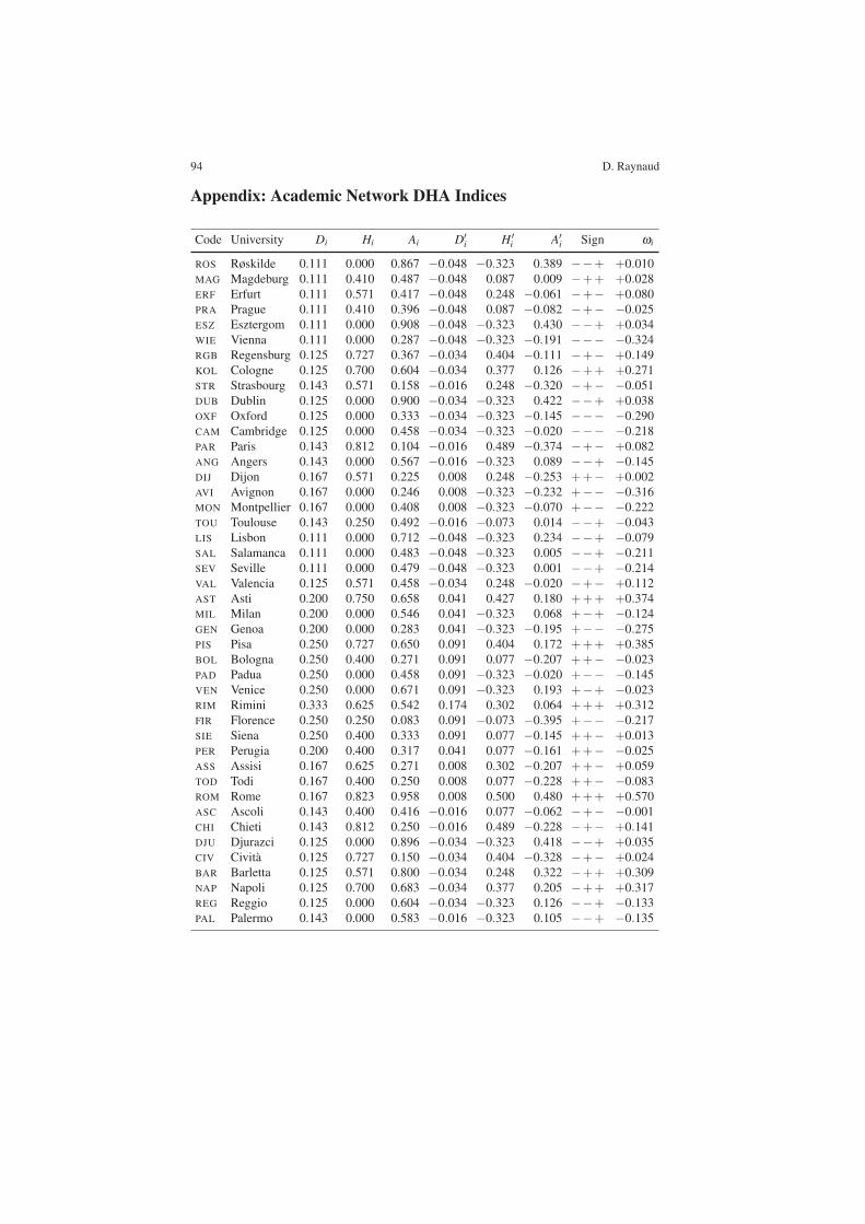
Appendix: Academic Network DHA Indices

Code University Di Hi Ai D!i H !

i A!i Sign !i

ROS Røskilde 0.111 0.000 0.867 "0.048 "0.323 0.389 ""+ +0.010MAG Magdeburg 0.111 0.410 0.487 "0.048 0.087 0.009 "++ +0.028ERF Erfurt 0.111 0.571 0.417 "0.048 0.248 "0.061 "+" +0.080PRA Prague 0.111 0.410 0.396 "0.048 0.087 "0.082 "+" "0.025ESZ Esztergom 0.111 0.000 0.908 "0.048 "0.323 0.430 ""+ +0.034WIE Vienna 0.111 0.000 0.287 "0.048 "0.323 "0.191 """ "0.324RGB Regensburg 0.125 0.727 0.367 "0.034 0.404 "0.111 "+" +0.149KOL Cologne 0.125 0.700 0.604 "0.034 0.377 0.126 "++ +0.271STR Strasbourg 0.143 0.571 0.158 "0.016 0.248 "0.320 "+" "0.051DUB Dublin 0.125 0.000 0.900 "0.034 "0.323 0.422 ""+ +0.038OXF Oxford 0.125 0.000 0.333 "0.034 "0.323 "0.145 """ "0.290CAM Cambridge 0.125 0.000 0.458 "0.034 "0.323 "0.020 """ "0.218PAR Paris 0.143 0.812 0.104 "0.016 0.489 "0.374 "+" +0.082ANG Angers 0.143 0.000 0.567 "0.016 "0.323 0.089 ""+ "0.145DIJ Dijon 0.167 0.571 0.225 0.008 0.248 "0.253 ++" +0.002AVI Avignon 0.167 0.000 0.246 0.008 "0.323 "0.232 +"" "0.316MON Montpellier 0.167 0.000 0.408 0.008 "0.323 "0.070 +"" "0.222TOU Toulouse 0.143 0.250 0.492 "0.016 "0.073 0.014 ""+ "0.043LIS Lisbon 0.111 0.000 0.712 "0.048 "0.323 0.234 ""+ "0.079SAL Salamanca 0.111 0.000 0.483 "0.048 "0.323 0.005 ""+ "0.211SEV Seville 0.111 0.000 0.479 "0.048 "0.323 0.001 ""+ "0.214VAL Valencia 0.125 0.571 0.458 "0.034 0.248 "0.020 "+" +0.112AST Asti 0.200 0.750 0.658 0.041 0.427 0.180 +++ +0.374MIL Milan 0.200 0.000 0.546 0.041 "0.323 0.068 +"+ "0.124GEN Genoa 0.200 0.000 0.283 0.041 "0.323 "0.195 +"" "0.275PIS Pisa 0.250 0.727 0.650 0.091 0.404 0.172 +++ +0.385BOL Bologna 0.250 0.400 0.271 0.091 0.077 "0.207 ++" "0.023PAD Padua 0.250 0.000 0.458 0.091 "0.323 "0.020 +"" "0.145VEN Venice 0.250 0.000 0.671 0.091 "0.323 0.193 +"+ "0.023RIM Rimini 0.333 0.625 0.542 0.174 0.302 0.064 +++ +0.312FIR Florence 0.250 0.250 0.083 0.091 "0.073 "0.395 +"" "0.217SIE Siena 0.250 0.400 0.333 0.091 0.077 "0.145 ++" +0.013PER Perugia 0.200 0.400 0.317 0.041 0.077 "0.161 ++" "0.025ASS Assisi 0.167 0.625 0.271 0.008 0.302 "0.207 ++" +0.059TOD Todi 0.167 0.400 0.250 0.008 0.077 "0.228 ++" "0.083ROM Rome 0.167 0.823 0.958 0.008 0.500 0.480 +++ +0.570ASC Ascoli 0.143 0.400 0.416 "0.016 0.077 "0.062 "+" "0.001CHI Chieti 0.143 0.812 0.250 "0.016 0.489 "0.228 "+" +0.141DJU Djurazci 0.125 0.000 0.896 "0.034 "0.323 0.418 ""+ +0.035CIV Cività 0.125 0.727 0.150 "0.034 0.404 "0.328 "+" +0.024BAR Barletta 0.125 0.571 0.800 "0.034 0.248 0.322 "++ +0.309NAP Napoli 0.125 0.700 0.683 "0.034 0.377 0.205 "++ +0.317REG Reggio 0.125 0.000 0.604 "0.034 "0.323 0.126 ""+ "0.133PAL Palermo 0.143 0.000 0.583 "0.016 "0.323 0.105 ""+ "0.135


References

1. Bailey, N.T.J.: The Mathematical Theory of Epidemics. Charles Griffin, London (1957)2. Baronchelli, A., Pastor-Satorras, R.: Diffusive dynamics on weighted networks. Preprint:

arXiv: 0907.3810v1 (2009) [cond-mat.stat.mech]3. Blau, P.: Inequality and Heterogeneity. The Free Press, New York (1977)4. Castellano, C., Fortunato, S., Loreto, V.: Statistical physics of social dynamics. Rev. Mod.

Phys. 81 591 (2009). Preprint: arXiv:0710.3256v1 [physics.soc-ph]5. Cavalli-Sforza, L.L., Feldman, M.W.: Cultural Transmission and Evolution: A Quantitative

Approach. Princeton University Press, Princeton (1981)6. Coleman, J.S., Katz, E., Menzel, H.: The diffusion of an innovation among physicians. So-

ciometry 20 253–270 (1957)7. Cowan, R., Jonard, N.: Network Structure and the Diffusion of Knowledge. MERIT Technical

report 99028, Maastricht University (1999)8. Degenne, A., Forsé, M.: Introducing Social Networks. Sage Publications, London (1999)9. Doran, J.E. and Gilbert, G.N. (eds.) Simulating Societies: The Computer Simulation of Social

Phenomena. UCL Press, London (1994)10. Doreian, P.: Mapping networks through time. In: Weesie, J. and Flap, H. (eds.) Social Net-

works through Time, pp. 245–264. ISOR/University of Utrecht (1990)11. Fararo, T.J.: Biased networks and social structure theorems. Social Networks 3 137–159

(1981)12. Granovetter, M.S.: The strength of weak ties. Am. Journal Soc. 78 1360–1380 (1973)13. Granovetter, M.S.: Threshold models of collective behavior. Am. Journal Soc. 83 1420–1443

(1978)14. Granovetter, M.S., Soong, R.: Threshold models of diffusion and collective behavior. Journal

Math. Soc. 9 165–179 (1983)15. Guardiola, X., Diaz-Guilera, A., Prez, C.J., Arenas, A., Llas, M.: Modelling diffusion of in-

novations in a social network. Phys. Rev. E 66 0206121 (2002)16. Hägerstrand, T.: A Monte Carlo approach to diffusion. Eur. Journal Soc. 6 43–67 (1965)17. Hegselmann, R., Mueller, U., Troizsch, K.G. (eds.) Modelling and Simulation in the Social

Sciences from the Philosophy of Science Point of View. Kluwer Academic Publishers, Dor-drecht (1996)

18. Iribarren, J.L., Moro, E.: Information diffusion epidemics in social networks. Preprint: arXiv:0706.0641v1 (2008) [physics.soc-ph]

19. Kendall, D.G.: Mathematical Models of the Spread of Infection. Medical Research Council,London (1965)

20. Marey, E.J.: Les eaux contaminées et le choléra. CRAS 99 667–683 (1884)21. Moreno, Y., Pastor-Satorras, R., Vespignani, A.: Epidemic outbreaks in complex heteroge-

neous networks. Eur. Phys. Journal B 26 521–529 (2002)22. Newman, M.E.J.: The spread of epidemic disease on networks. Phys. Rev. E 66 016128 (2002)23. Oliver, P.E., Marwell, G., Teixera, R.: A theory of critical mass, I. Interdependance, group

heterogeneity, and the production of collective action. Am. Journal Soc. 91 522–556 (1985)24. Rapoport, A., Yuan, Y.: Some experimental aspects of epidemies and social nets. In: Kochen,

M. (ed.) The Small World, pp. 327–348. Ablex Publishing Company, Norwood (1989)25. Raynaud, D.: Etudes d’épistémologie et de sociologie des sciences, 2. Pourquoi la perspective

a-t-elle été inventée en Italie centrale? Habilitation à diriger les recherches. Université de ParisSorbonne, Paris (2004)

26. Rogers, E.M.: Network analysis of the diffusion of innovations. In: Holland, P.W. and Lein-hardt, S. (eds.) Perspectives on Social Network Research, pp. 137-164. Academic Press, NewYork (1979)

27. Rogers, E.M.: Diffusion of Innovations [1962]. The Free Press, New York (1995)28. Rogers, E.M., Ascroft, J.R., Röling, N.: Diffusion of Innovation in Brazil, Nigeria, and India.

Unpublished Report. Michigan State University, East Lansing (1970)

96 D. Raynaud

29. Rogers, E.M., Kincaid, D.L.: Communication Networks: Towards a New Paradigm for Re-search. The Free Press, New York (1981)

30. Simonsen, I., Eriksen, K.A., Maslov, S., Sneppen, K.: Diffusion on complex networks: a wayto probe their large-scale topological structures. Physica A 336 163–173 (2004)

31. Simonsen, I.: Diffusion and networks: a powerful combination. Physica A 357 317–330 (2005)32. Skillnäs, N.: Modified innovation diffusion. A way to explain the diffusion of cholera in

Linköping in 1866. A study of methods. Geografiska Annaler B: Human Geography 81 243–260 (1999)

33. Skvoretz, J.: Salience, heterogeneity, and consolidation of parameters: civilizing Blaus primi-tive theory. American Sociological Review 48 360–375 (1983).

34. Stauffer D., Solomon, S.: Physics and mathematics applications in social science. In: Mayers,R.A. (ed): Encyclopedia of Complexity and Systems Science. Springer, New York, pp. 6804-6810 (2009). Preprint: arXiv:0801.01121v1 [physics.soc-ph]

35. Valente, T.W.: Network Models of the Diffusion of Innovations. Hampton Press, Creskill(1995)

36. Valente, T.W.: Social network thresholds in the diffusion of innovations. Social Networks 1869–89 (1996)

37. Valente, T.W.: Network models and methods for studying the diffusion of innovations. In:Carrington, P.T., Scott, J. and Wasserman, S. (eds.) Models and Methods in Social NetworkAnalysis, pp. 98-116. Cambridge University Press, New York (2005)

38. Verhulst, P.F.: Notice sur la loi que la population suit dans son accroissement. Corresp. math.phys. 4 113–121 (1838)

39. Watts, D.J., Strogatz S.H.: Collective dynamics of small word networks. Nature 393 440–442(1998)

Credits

“All figures are property of the author, except fig. 2, reprinted with permission ofHampton Press.”

Why Do Diffusion Data Not Fit the Logistic Model? A Note on Network Discreteness, Heterogeneity &...

Documents

Transcript of Why Do Diffusion Data Not Fit the Logistic Model? A Note on Network Discreteness, Heterogeneity &...