
'What is a Thing?': Topos Theory in the Foundations of Physics
212
arXiv:0803.0417v1 [quant-ph] 4 Mar 2008 ‘What is a Thing?’: Topos Theory in the Foundations of Physics 1 AndreasD¨oring 2 and Chris Isham 3 The Blackett Laboratory Imperial College of Science, Technology & Medicine South Kensington London SW7 2BZ 2 March 2008 Abstract “From the range of the basic questions of metaphysics we shall here ask this one question: “What is a thing?” The question is quite old. What remains ever new about it is merely that it must be asked again and again [36].” Martin Heidegger The goal of this paper is to summarise the first steps in developing a fundamentally new way of constructing theories of physics. The motivation comes from a desire to address certain deep issues that arise when contemplating quantum theories of space and time. In doing so we provide a new answer to Heidegger’s timeless question “What is a thing?”. Our basic contention is that constructing a theory of physics is equivalent to finding a representation in a topos of a certain formal language that is attached to the system. Classical physics uses the topos of sets. Other theories involve a different topos. For the types of theory discussed in this paper, a key goal is to represent any physical quantity A with an arrow ˘ A φ :Σ φ →R φ where Σ φ and R φ are two special objects (the ‘state-object’ and ‘quantity-value object’) in the appropriate topos, τ φ . 1 To appear in New Structures in Physics, ed R. Coecke, Springer (2008). 2 email: [email protected] 3 email: [email protected] 1
-
Upload
independent -
Category
Documents
-
view
1 -
download
0
Transcript of 'What is a Thing?': Topos Theory in the Foundations of Physics
arX
iv:0
803.
0417
v1 [
quan
t-ph
] 4
Mar
200
8
‘What is a Thing?’: Topos Theory in the Foundationsof Physics1
Andreas Doring2
and
Chris Isham3
The Blackett LaboratoryImperial College of Science, Technology & Medicine
South KensingtonLondon SW7 2BZ
2 March 2008
Abstract
“From the range of the basic questions of metaphysicswe shall here ask this one question: “What is a thing?”The question is quite old. What remains ever new about itis merely that it must be asked again and again [36].”
Martin Heidegger
The goal of this paper is to summarise the first steps in developinga fundamentally new way of constructing theories of physics. Themotivation comes from a desire to address certain deep issues thatarise when contemplating quantum theories of space and time. Indoing so we provide a new answer to Heidegger’s timeless question“What is a thing?”.
Our basic contention is that constructing a theory of physics isequivalent to finding a representation in a topos of a certain formallanguage that is attached to the system. Classical physics uses thetopos of sets. Other theories involve a different topos. For the typesof theory discussed in this paper, a key goal is to represent any physicalquantity A with an arrow Aφ : Σφ → Rφ where Σφ and Rφ are twospecial objects (the ‘state-object’ and ‘quantity-value object’) in theappropriate topos, τφ.
1To appear in New Structures in Physics, ed R. Coecke, Springer (2008).2email: [email protected]: [email protected]
1
We discuss two different types of language that can be attached toa system, S. The first, PL(S), is a propositional language; the sec-ond, L(S), is a higher-order, typed language. Both languages providedeductive systems with an intuitionistic logic. With the aid of PL(S)we expand and develop some of the earlier work4 on topos theoryand quantum physics. A key step is a process we term ‘daseinisa-tion’ by which a projection operator is mapped to a sub-object of thespectral presheaf Σ—the topos quantum analogue of a classical statespace. The topos concerned is SetsV(H)op : the category of contravari-ant set-valued functors on the category (partially ordered set) V(H)of commutative sub-algebras of the algebra of bounded operators onthe quantum Hilbert space H.
There are two types of daseinisation, called ‘outer’ and ‘inner’:they involve approximating a projection operator by projectors thatare, respectively, larger and smaller in the lattice of projectors on H.
We then introduce the more sophisticated language L(S) and use itto study ‘truth objects’ and ‘pseudo-states’ in the topos. These objectstopos play the role of states: a necessary development as the spectralpresheaf has no global elements, and hence there are no microstatesin the sense of classical physics.
One of the main mathematical achievements is finding a toposrepresentation for self-adjoint operators. This involves showing that,for any bounded, self-adjoint operator A, there is a correspondingarrow δo(A) : Σ→ R where R is the quantity-value object for thistheory. The construction of δo(A) is an extension of the daseinisationof projection operators.
The object R is a monoid-object only in the topos, τφ = SetsV(H)op ,of the theory, and to enhance the applicability of the formalism wediscuss another candidate, R↔, for the quantity-value object. In thispresheaf, both inner- and outer-daseinisation are used in a symmet-ric way. Another option is to apply to R a topos analogue of theGrothendieck extension of a monoid to a group. The resulting object,k(R), is an abelian group-object in τφ.
Finally we turn to considering a collection of systems: in particu-lar, we are interested in the relation between the topos representationof a composite system, and the representations of its constituents. Ourapproach to these matters is to construct a category of systems andto find coherent topos representations of the entire category.
4By CJI and collaborators.
2
Contents
1 Introduction 8
2 The Conceptual Background of our Scheme 17
2.1 The Problem of Using Real Numbers a Priori . . . . . . . . . 17
2.1.1 Why Are Physical Quantities Assumed to be Real-Valued? . . . . . . . . . . . . . . . . . . . . . . . . . . 17
2.1.2 Why Are Probabilities Required to Lie in the Interval[0, 1]? . . . . . . . . . . . . . . . . . . . . . . . . . . . 19
2.2 The Genesis of Topos Ideas in Physics . . . . . . . . . . . . . 20
2.2.1 Why are Space and Time Modelled with Real Numbers? 20
2.2.2 Another Possible Role for Heyting Algebras . . . . . . 22
2.2.3 Our Main Contention about Topos Theory and Physics 24
3 Propositional Languages and Theories of Physics 26
3.1 Two Opposing Interpretations of Propositions . . . . . . . . . 26
3.2 The Propositional Language PL(S) . . . . . . . . . . . . . . . 28
3.2.1 Intuitionistic Logic and the Definition of PL(S) . . . . 28
3.2.2 Representations of PL(S). . . . . . . . . . . . . . . . . 30
3.2.3 Using Geometric Logic . . . . . . . . . . . . . . . . . . 31
3.2.4 Introducing Time Dependence . . . . . . . . . . . . . . 32
3.2.5 The Representation of PL(S) in Classical Physics . . . 34
3.2.6 The Failure to Represent PL(S) in Standard QuantumTheory. . . . . . . . . . . . . . . . . . . . . . . . . . . 35
4 A Higher-Order, Typed Language for Physics 36
4.1 The Basics of the Language L(S) . . . . . . . . . . . . . . . . 36
4.2 Representing L(S) in a Topos . . . . . . . . . . . . . . . . . . 41
4.2.1 The Local Set Theory of a Topos. . . . . . . . . . . . . 43
4.2.2 Theory Construction as a Translation of Languages . . 43
4.3 Classical Physics in the Local Language L(S) . . . . . . . . . 45
4.4 Adapting the Language L(S) to Other Types of Physical System 46
3
5 Quantum Propositions as Sub-Objects of the Spectral Presheaf 48
5.1 Some Background Remarks . . . . . . . . . . . . . . . . . . . 48
5.1.1 The Kochen-Specker Theorem . . . . . . . . . . . . . . 48
5.1.2 The Introduction of Coarse-Graining . . . . . . . . . . 51
5.1.3 Alternatives to von Neumann Algebras . . . . . . . . . 54
5.2 From Projections to Global Elements of the Outer Presheaf . . 55
5.2.1 The Definition of δ(P )V . . . . . . . . . . . . . . . . . 55
5.2.2 Properties of the Mapping δ : P(H)→ ΓO. . . . . . . . 58
5.2.3 A Logical Structure for ΓO? . . . . . . . . . . . . . . . 59
5.2.4 Hyper-Elements of ΓO. . . . . . . . . . . . . . . . . . . 61
5.3 Daseinisation: Heidegger Encounters Physics . . . . . . . . . . 61
5.3.1 From Global Elements of O to Sub-Objects of Σ. . . . 61
5.3.2 The Definition of Daseinisation . . . . . . . . . . . . . 64
5.4 The Heyting Algebra Structure on Subcl(Σ). . . . . . . . . . . 65
5.5 Daseinisation and the Operations of Quantum Logic. . . . . . 65
5.5.1 The Status of the Possible Axiom ‘Aε∆1 ∧ Aε∆2 ⇔Aε∆1 ∩∆2’ . . . . . . . . . . . . . . . . . . . . . . . . 66
5.5.2 Inner Daseinisation and δ(¬P ). . . . . . . . . . . . . . 67
5.5.3 Using Boolean Algebras as the Base Category . . . . . 69
5.6 The Special Nature of Daseinised Projections . . . . . . . . . . 71
5.6.1 Daseinised Projections as Optimal Sub-Objects . . . . 71
6 Truth Values in Topos Physics 72
6.1 The Mathematical Proposition “x ∈ K” . . . . . . . . . . . . 72
6.2 Truth Objects . . . . . . . . . . . . . . . . . . . . . . . . . . . 75
6.2.1 Linguistic Aspects of Truth Objects. . . . . . . . . . . 75
6.2.2 The Micro-State Option . . . . . . . . . . . . . . . . . 77
6.2.3 The Truth Object Option. . . . . . . . . . . . . . . . . 77
6.2.4 The Example of Classical Physics. . . . . . . . . . . . . 79
6.3 Truth Objects in Quantum Theory . . . . . . . . . . . . . . . 79
6.3.1 Preliminary Remarks . . . . . . . . . . . . . . . . . . . 79
6.3.2 The Truth Objects T |ψ〉. . . . . . . . . . . . . . . . . . 80
4
6.4 The Pseudo-state Option . . . . . . . . . . . . . . . . . . . . . 82
6.4.1 Some Background Remarks . . . . . . . . . . . . . . . 82
6.4.2 Using Pseudo-States in Lieu of Truth Objects . . . . . 83
6.4.3 Linguistic Implications . . . . . . . . . . . . . . . . . . 85
6.4.4 Time-Dependence and the Truth Object. . . . . . . . . 86
6.5 The Presheaf Pcl(Σ). . . . . . . . . . . . . . . . . . . . . . . . 87
6.5.1 The Definition of Pcl(Σ). . . . . . . . . . . . . . . . . . 87
6.5.2 The Monic Arrow From O to Pcl(Σ). . . . . . . . . . . 88
6.6 Yet Another Perspective on the K-S Theorem . . . . . . . . . 89
7 The de Groote Presheaves of Physical Quantities 92
7.1 Background Remarks . . . . . . . . . . . . . . . . . . . . . . . 92
7.2 The Daseinisation of an Arbitrary Self-Adjoint Operator . . . 93
7.2.1 Spectral Families and Spectral Order . . . . . . . . . . 93
7.2.2 Daseinisation of Self-Adjoint Operators. . . . . . . . . 95
7.2.3 Properties of Daseinisation. . . . . . . . . . . . . . . . 96
7.2.4 The de Groote Presheaves . . . . . . . . . . . . . . . . 98
8 The Presheaves sp(A), R and R↔ 101
8.1 Background to the Quantity-Value Presheaf R. . . . . . . . . 101
8.2 Definition of the Presheaves sp(A), R and R↔. . . . . . . . 102
8.3 Inner and Outer Daseinisation from Functions on Filters . . . 107
8.4 A Physical Interpretation of the Arrow δ(A) : Σ→ R↔ . . . . 112
8.5 The value of a physical quantity in a quantum state . . . . . . 115
8.6 Properties of R↔. . . . . . . . . . . . . . . . . . . . . . . . . . 118
8.7 The Representation of Propositions From Inverse Images . . . 119
8.8 The relation between the formal languages L(S) and PL(S) . 121
9 Extending the Quantity-Value Presheaf to an Abelian GroupObject 123
9.1 Preliminary Remarks . . . . . . . . . . . . . . . . . . . . . . . 123
9.2 The relation between R↔ and k(R). . . . . . . . . . . . . . . 125
9.3 Algebraic properties of the potential quantity-value presheaves 126
5
10 The Role of Unitary Operators 129
10.1 The Daseinisation of Unitary Operators . . . . . . . . . . . . . 129
10.2 Unitary Operators and Arrows in SetsV(H)op . . . . . . . . . . . 131
10.2.1 The Definition of ℓU : Ob(V(H))→ Ob(V(H)) . . . . . 131
10.2.2 The Effect of ℓU on Daseinisation . . . . . . . . . . . . 132
10.2.3 The U -twisted Presheaf . . . . . . . . . . . . . . . . . 133
11 The Category of Systems 136
11.1 Background Remarks . . . . . . . . . . . . . . . . . . . . . . . 136
11.2 The Category Sys . . . . . . . . . . . . . . . . . . . . . . . . 137
11.2.1 The Arrows and Translations for the Disjoint Sum S1⊔S2.137
11.2.2 The Arrows and Translations for the Composite Sys-tem S1 ⋄ S2. . . . . . . . . . . . . . . . . . . . . . . . . 140
11.2.3 The Concept of ‘Isomorphic’ Systems. . . . . . . . . . 141
11.2.4 An Axiomatic Formulation of the Category Sys . . . . 142
11.3 Representations of Sys in Topoi . . . . . . . . . . . . . . . . . 146
11.4 Classical Physics in This Form . . . . . . . . . . . . . . . . . . 148
11.4.1 The Rules so Far. . . . . . . . . . . . . . . . . . . . . . 148
11.4.2 Details of the Translation Representation. . . . . . . . 151
12 Theories of Physics in a General Topos 153
12.1 The Pull-Back Operations . . . . . . . . . . . . . . . . . . . . 153
12.1.1 The Pull-Back of Physical Quantities. . . . . . . . . . . 153
12.1.2 The Pull-Back of Propositions. . . . . . . . . . . . . . 155
12.1.3 The Idea of a Geometric Morphism. . . . . . . . . . . . 156
12.2 The Topos Rules for Theories of Physics . . . . . . . . . . . . 157
13 The General Scheme applied to Quantum Theory 162
13.1 Background Remarks . . . . . . . . . . . . . . . . . . . . . . . 162
13.2 The Translation Representation for a Disjoint Sum of Quan-tum Systems . . . . . . . . . . . . . . . . . . . . . . . . . . . . 162
13.3 The Translation Representation for Composite Quantum Sys-tems . . . . . . . . . . . . . . . . . . . . . . . . . . . . . . . . 167
13.3.1 Operator Entanglement and Translations. . . . . . . . 167
6
13.3.2 A Geometrical Morphism and a Possible Translation . 169
14 Characteristic Properties of Σφ, Rφ and T/w 172
14.1 The State Object Σφ . . . . . . . . . . . . . . . . . . . . . . . 172
14.1.1 An Analogue of a Symplectic Structure or CotangentBundle? . . . . . . . . . . . . . . . . . . . . . . . . . . 173
14.1.2 Σφ as a Spectral Object: the Work of Heunen andSpitters . . . . . . . . . . . . . . . . . . . . . . . . . . 174
14.1.3 Using Boolean Algebras as the Base Category . . . . . 175
14.1.4 Application to Other Branches of Algebra . . . . . . . 176
14.1.5 The Partial Existence of Points of Σφ . . . . . . . . . . 177
14.1.6 The Work of Corbett et al . . . . . . . . . . . . . . . . 178
14.2 The Quantity-Value Object Rφ . . . . . . . . . . . . . . . . . 179
14.3 The Truth Objects T, or Pseudo-State Object Wφ . . . . . . . 181
15 Conclusion 181
16 Appendix 1: Some Theorems and Constructions Used in theMain Text 187
16.1 Results on Clopen Subobjects of Σ. . . . . . . . . . . . . . . . 187
16.2 The Grothendieck k-Construction for an Abelian Monoid . . . 190
16.3 Functions of Bounded Variation and ΓR . . . . . . . . . . . . 192
16.4 Taking Squares in k(ΓR) . . . . . . . . . . . . . . . . . . . . 193
16.5 The Object k(R) in the Topos SetsV(H)op . . . . . . . . . . . . 195
16.5.1 The Definition of k(R). . . . . . . . . . . . . . . . . . 195
16.5.2 The Presheaf k(R) as the Quantity-Value Object. . . 196
16.5.3 The square of an arrow [δo(A)]. . . . . . . . . . . . . . 196
17 Appendix 2: A Short Introduction to the Relevant Parts ofTopos Theory 197
17.1 What is a Topos? . . . . . . . . . . . . . . . . . . . . . . . . . 197
17.2 Presheaves on a Poset . . . . . . . . . . . . . . . . . . . . . . 201
17.3 Presheaves on a General Category . . . . . . . . . . . . . . . . 202
7
1 Introduction
Many people who work in quantum gravity would agree that a deep changein our understanding of foundational issues will occur at some point alongthe path. However, opinions differ greatly on whether a radical revision isnecessary at the very beginning of the process, or if it will emerge ‘alongthe way’ from an existing, or future, research programme that is formulatedusing the current paradigms. For example, many (albeit not all) of thecurrent generation of string theorists seem inclined to this view, as do a,perhaps smaller, fraction of those who work in loop quantum gravity.
In this article we take the iconoclastic view that a radical step is neededat the very outset. However, for anyone in this camp the problem is alwaysknowing where to start. It is easy to talk about a ‘radical revision of currentparadigms’—the phrase slips lightly off the tongue—but converting this pioushope into a concrete theoretical structure is a problem of the highest order.
For us, the starting point is quantum theory itself. More precisely, webelieve that this theory needs to be radically revised, or even completelyreplaced, before a satisfactory theory of quantum gravity can be obtained.
In this context, a striking feature of the various current programmes forquantising gravity—including superstring theory and loop quantum gravity—is that, notwithstanding their disparate views on the nature of space andtime, they almost all use more-or-less standard quantum theory. Althoughunderstandable from a pragmatic viewpoint (since all we have is more-or-lessstandard quantum theory) this situation is nevertheless questionable whenviewed from a wider perspective.
For us, one of the most important issues is the use in the standard quan-tum formalism of critical mathematical ingredients that are taken for grantedand yet which, we claim, implicitly assume certain properties of space and/ortime. Such an a priori imposition of spatio-temporal concepts would be amajor category5 error if they turn out to be fundamentally incompatible withwhat is needed for a theory of quantum gravity.
A prime example is the use of the continuum6 by which, in this context,is meant the real and/or complex numbers. These are a central ingredient inall the various mathematical frameworks in which quantum theory is com-monly discussed. For example, this is clearly so with the use of (i) Hilbert
5The philosophy of Kant runs strongly in our veins.6When used in this rather colloquial way, the word ‘continuum’ suggests primarily the
cardinality of the sets concerned, and, secondly, the topology that is conventionally placedon these sets.
8
spaces or C∗-algebras; (ii) geometric quantisation; (iii) probability functionson a non-distributive quantum logic; (iv) deformation quantisation; and (v)formal (i.e., mathematically ill-defined) path integrals and the like. The apriori imposition of such continuum concepts could be radically incompatiblewith a quantum-gravity formalism in which, say, space-time is fundamentallydiscrete: as, for example, in the causal-set programme.
As we shall argue later, this issue is closely connected with the question ofwhat is meant by the ‘value’ of a physical quantity. In so far as the concept ismeaningful at all at the Planck scale, why should the value be a real numberdefined mathematically in the usual way?
Another significant reason for aspiring to change the quantum formalismis the peristalithic problem of deciding how a ‘quantum theory of cosmology’could be interpreted if one was lucky enough to find one. Most people whoworry about foundational issues in quantum gravity would probably placethe quantum-cosmology/closed-system problem at, or near, the top of theirlist of reasons for re-envisioning quantum theory. However, although we aredeeply interested in such conceptual issues, the primary motivation for ourresearch programme is not to find a new interpretation of quantum theory.Rather, our main goal is to find a novel structural framework within whichnew types of theories of physics can be constructed.
However, having said that, in the context of quantum cosmology it is cer-tainly true that the lack of any external ‘observer’ of the universe ‘as a whole’renders inappropriate the standard Copenhagen interpretation with its in-strumentalist use of counterfactual statements about what would happen ifa certain measurement is performed. Indeed, the Copenhagen interpretationis inapplicable for any7 system that is truly ‘closed’ (or ‘self-contained’) andfor which, therefore, there is no ‘external’ domain in which an observer canlurk. This problem has motivated much research over the years and continuesto be of wide interest.
The philosophical questions that arise are profound, and look back to thebirth of Western philosophy in ancient Greece, almost three thousand yearsago. Of course, arguably, the longevity of these issues suggests that thesequestions are ill-posed in the first place, in which case the whole enterpriseis a complete waste of time! This is probably the view of most, if not all, ofour colleagues at Imperial College; but we beg to differ8.
7The existence of the long-range, and all penetrating, gravitational force means that,at a fundamental level, there is only one truly closed system, and that is the universeitself.
8Of course, it is also possible that our colleagues are right.
9
When considering a closed system, the inadequacy of the conventionalinstrumentalist interpretation of quantum theory encourages the search foran interpretation that is more ‘realist’ in some way. For over eighty years,this has been a recurring challenge for those concerned with the conceptualfoundations of modern physics. In rising to this challenge we join our Greekancestors in confronting once more the fundamental question:9
“What is a thing?”
Of course, as written, the question is itself questionable. For manyphilosophers, including Kant, would assert that the correct question is not“What is a thing?” but rather “What is a thing as it appears to us?”However, notwithstanding Kant’s strictures, we seek the thing-in-itself, and,therefore, we persevere with Heidegger’s form of the question.
Nevertheless, having said that, we can hardly ignore the last three thou-sand years of philosophy. In particular, we must defend ourselves against thecharge of being ‘naive realists’.10 At this point it become clear that theoret-ical physicists have a big advantage over professional philosophers. For weare permitted/required to study such issues in the context of specific math-ematical frameworks for addressing the physical world; and one of the greatfascinations of this process is the way in which various philosophical posi-tions are implicit in the ensuing structures. For example, the exact meaningof ‘realist’ is infinitely debatable but, when used by a classical physicist, itinvariably means the following:
1. The idea of ‘a property of the system’ (for example, ‘the value of aphysical quantity at a certain time’) is meaningful, and mathematicallyrepresentable in the theory.
2. Propositions about the system (typically asserting that the system hasthis or that property) are handled using Boolean logic. This require-ment is compelling in so far as we humans are inclined to think in aBoolean way.
9“What is a thing?” is the title of one of the more comprehensible of Heidegger’s works[36]. By this, we mean comprehensible to the authors of the present article. We cannotspeak for our colleagues across the channel: from some of them we may need to distanceourselves.
10If we were professional philosophers this would be a terrible insult. :-)
10
3. There is a space of ‘microstates’ such that specifying a microstate11
leads to unequivocal truth values for all propositions about the system:i.e., a state12 encodes “the way things are”. This is a natural way ofensuring that the first two conditions above are satisfied.
The standard interpretation of classical physics satisfies these requirementsand provides the paradigmatic example of a realist philosophy in science.Heidegger’s answer to his own question adopts a similar position [36]:
“A thing is always something that has such and such properties,always something that is constituted in such and such a way. Thissomething is the bearer of the properties; the something, as itwere, that underlies the qualities.”
In quantum theory, the situation is very different. There, the existenceof any such realist interpretation is foiled by the famous Kochen-Speckertheorem [50]. This asserts that it is impossible to assign values to all physicalquantities at once if this assignment is to satisfy the consistency conditionthat the value of a function of a physical quantity is that function of thevalue. For example, the value of ‘energy squared’ is the square of the valueof energy.
Thus, from a conceptual perspective, the challenge is to find a quantumformalism that is ‘realist enough’ to provide an acceptable alternative tothe Copenhagen interpretation, with its instrumentally-construed intrinsicprobabilities, whilst taking on board the implications of the Kochen-Speckertheorem.
So, in toto what we seek is a formalism that is (i) free of prima facieprejudices about the nature of the values of physical quantities—in particular,there should be no fundamental use of the real or complex numbers; and (ii)‘realist’, in at least the minimal sense that propositions are meaningful, andare assigned ‘truth values’, not just instrumentalist probabilities of whatwould happen if appropriate measurements are made.
However, finding such a formalism is not easy: it is notoriously difficult tomodify the mathematical framework of quantum theory without destroying
11In simple non-relativistic systems, the state is specified at any given moment of time.Relativistic systems (particularly quantum gravity!) require a more sophisticated under-standing of ‘state’, but the general idea is the same.
12We are a little slack in our use of language here and in what follows by frequentlyreferring to a microstate as just a ‘state’. The distinction only becomes important ifone wants to introduce things like mixed states (in quantum theory), or macrostates (inclassical physics) all of which are often just known as ‘states’. Then one must talk aboutmicrostates (pure states) to distinguish them from the other type of state.
11
the entire edifice. In particular, the Hilbert space structure is very rigid andcannot easily be changed; and the formal path-integral techniques do notfare much better.
To seek inspiration let us return briefly to the situation in classical physics.There, the concept of realism (as asserted in the three statements above) isencoded mathematically in the idea of a space of states, S, where specifying aparticular state (or ‘micro-state’), s ∈ S, determines entirely ‘the way thingsare’ for the system. In particular, this suggests that each physical quantity Ashould be associated with a real-valued function A : S → R such that whenthe state of the system is s, the value of A is A(s). Of course, this is indeedprecisely how the formalism of classical physics works.
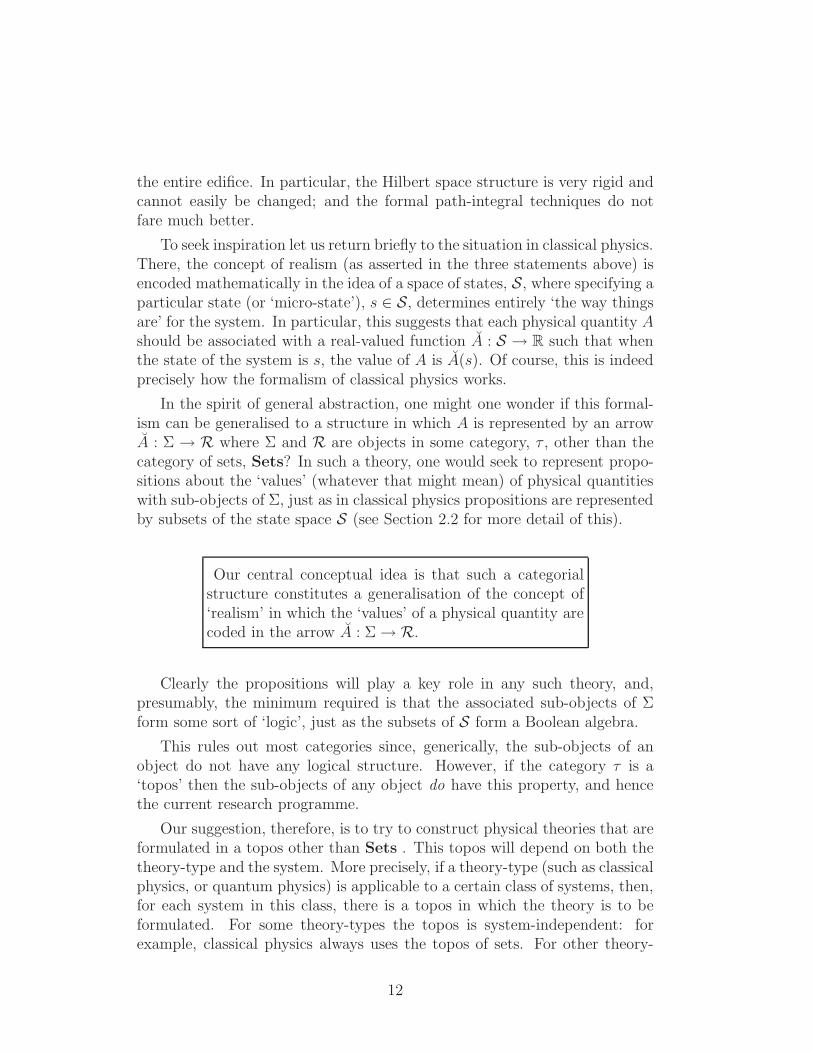
In the spirit of general abstraction, one might one wonder if this formal-ism can be generalised to a structure in which A is represented by an arrowA : Σ → R where Σ and R are objects in some category, τ , other than thecategory of sets, Sets? In such a theory, one would seek to represent propo-sitions about the ‘values’ (whatever that might mean) of physical quantitieswith sub-objects of Σ, just as in classical physics propositions are representedby subsets of the state space S (see Section 2.2 for more detail of this).
Our central conceptual idea is that such a categorialstructure constitutes a generalisation of the concept of‘realism’ in which the ‘values’ of a physical quantity arecoded in the arrow A : Σ→ R.
Clearly the propositions will play a key role in any such theory, and,presumably, the minimum required is that the associated sub-objects of Σform some sort of ‘logic’, just as the subsets of S form a Boolean algebra.
This rules out most categories since, generically, the sub-objects of anobject do not have any logical structure. However, if the category τ is a‘topos’ then the sub-objects of any object do have this property, and hencethe current research programme.
Our suggestion, therefore, is to try to construct physical theories that areformulated in a topos other than Sets . This topos will depend on both thetheory-type and the system. More precisely, if a theory-type (such as classicalphysics, or quantum physics) is applicable to a certain class of systems, then,for each system in this class, there is a topos in which the theory is to beformulated. For some theory-types the topos is system-independent: forexample, classical physics always uses the topos of sets. For other theory-
12
types, the topos varies from system to system: as we shall see, this is thecase in quantum theory.
In somewhat more detail, any particular example of our suggested schemewill have the following ingredients:
1. There are two special objects in the topos τφ: the ‘state-object’13, Σφ
and the ‘quantity-value object’, Rφ. Any physical quantity, A, is rep-resented by an arrow Aφ : Σφ → Rφ in the topos. Whatever meaningcan be ascribed to the concept of the ‘value’ of a physical quantity isencoded in (or derived from) this representation.
2. Propositions about a system are represented by sub-objects of the state-object Σφ. These sub-objects form a Heyting algebra (as indeed do thesub-objects of any object in a topos): a distributive lattice that differsfrom a Boolean algebra only in that the law of excluded middle neednot hold, i.e., α∨¬α 1. A Boolean algebra is a Heyting algebra withstrict equality: α ∨ ¬α = 1.
3. Generally speaking (and unlike in set theory), an object in a toposmay not be determined by its ‘points’. In particular, this may be sofor the state-object, in which case the concept of a microstate is notso useful.14 Nevertheless, truth values can be assigned to propositionswith the aid of a ‘truth object’ (or ‘pseudo-state’). These truth valueslie in another Heyting algebra.
Of course, it is not instantly obvious that quantum theory can be writ-ten in this way. However, as we shall see, there is a topos reformulationof quantum theory, and this has two immediate implications. The first isthat we acquire a new type of ‘realist’ interpretation of standard quantumtheory. The second is that this new approach suggests ways of generalisingquantum theory that make no fundamental reference to Hilbert spaces, pathintegrals, etc. In particular, there is no prima facie reason for introducingstandard continuum quantities. As emphasised above, this is one of our mainmotivations for developing the topos approach. We shall say more about thislater.
From a conceptual perspective, a central feature of our scheme is the‘neo-realist’ structure reflected mathematically in the three statements above.
13The meaning of the subscript ‘φ’ is explained in the main text. It refers to a particulartopos-representation of a formal language attached to the system.
14In quantum theory, the state-object has no points/microstates at all. As we shall see,this statement is equivalent to the Kochen-Specker theorem.
13
This neo-realism is the conceptual fruit of the fact that, from a categorial per-spective, a physical theory expressed in a topos ‘looks’ like classical physicsexpressed in the topos of sets.
The fact that (i) physical quantities are represented by arrows whosedomain is the state-object, Σφ; and (ii) propositions are represented bysub-objects of Σφ, suggests strongly that Σφ can be regarded as the topos-analogue of a classical state space. Indeed, for any classical system the toposis just the category of sets, Sets, and the ideas above reduce to the familiarpicture in which (i) there is a state space (set) S; (ii) any physical quantity,A, is represented by a real-valued functions A : S → R; and (iii) proposi-tions are represented by subsets of S with a logical structure given by theassociated Boolean algebra.
Evidently the suggested mathematical structures could be used in twodifferent ways. The first is that of the ‘conventional’ theoretical physicistwith little interest in conceptual matters. For him/her, what we and ourcolleagues are developing is a new tool-kit with which to construct noveltypes of theoretical model. Whether or not Nature has chosen such modelsremains to be seen, but, at the very least, the use of topoi certainly suggestsnew techniques.
For those physicists who are interested in conceptual issues, the toposframework gives a radically new way of thinking about the world. The neo-realism inherent in the formalism is described mathematically using the in-ternal language that is associated with any topos. This describes how thingslook from ‘within’ the topos: something that should be particularly useful inthe context of quantum cosmology15.
On the other hand, the pragmatic theoretician with no interest in con-ceptual matters can use the ‘external’ description of the topos in which thecategory of sets provides a metalanguage with which to formulate the the-ory. From a mathematical perspective, the interplay between the internaland external languages of a topos is one of the fascinations of the subject.However, much remains to be said about the significance of this interactionfor real theories of physics.
This present article is partly an amalgam of a series of four papers thatwe placed on the ArXiv server16 in March, 2007 [21, 22, 23, 24]. However,we have added a fair amount of new material, and also made a few minor
15In this context see the work of Markopoulou who considers a topos description of theuniverse as seen by different observers who live inside it [58].
16These are due to published in Journal of Mathematical Physics in the Spring of 2008.
14
corrections (mainly typos).17 We have also added some remarks about devel-opments made by researchers other than ourselves since the ArXiv preprintswere written. Of particular importance to our general programme is thework of Heunen and Spitters [38] which adds some powerful ingredients tothe topoi-in-physics toolkit. Finally, we have included some background ma-terial from the earlier papers that formed the starting point for the currentresearch programme [44, 45, 35, 13].
We must emphasise that this is not a review article about the generalapplication of topos theory to physics; this would have made the article fartoo long. For example, there has been a fair amount of study of the use ofsynthetic differential geometry in physics. The reader can find references tomuch of this on the, so-called, ‘Siberian toposes’ web site18. There is alsothe work by Mallios and collaborators on ‘Abstract Differential Geometry’[59, 60, 66, 61]. Of course, as always these days, Google will speedily revealall that we have omitted.
But even less is this paper a review of the use of category theory in generalin physics. For there any many important topics that we do not mention atall. For example, Baez’s advocation of n-categories [5, 6]; ‘categorial quantumtheory’ [2, 73]; Takeuti’s theory19 of ‘quantum sets’ [71]; and Crane’s workon categorial models of space-time [17].
Finally, a word about the style in which this article is written. Wespent much time pondering on this, as we did before writing the four ArXivpreprints. The intended audience is our colleagues who work in theoreti-cal physics, especially those whose interests included foundational issues inquantum gravity and quantum theory. However, topos theory is not an easybranch of mathematics, and this poses the dilemma of how much backgroundmathematics should be assumed of the reader, and how much should be ex-plained as we go along.20 We have approached this problem by includinga short mathematical appendix on topos theory. However, reasons of spaceprecluded a thorough treatment, and we hope that, fairly soon, someone willwrite an introductory review of topos theory in a style that is accessible toa typical theoretical-physicist reader.
17Some of the more technical theorems have been placed in the Appendix with the hopethat this makes the article a little easier to read.
18This is http://users.univer.omsk.su/˜topoi/. See also Cecilia Flori’s website that dealsmore generally with topos theory and physics: http://topos-physics.org/
19Takeuti’s work is not exactly about category theory applied to quantum theory: it ismore about the use of formal logic, but the spirit is similar. For a recent paper in thisgenre see [64].
20The references that we have found most helpful in our research are [55, 29, 52, 8, 56, 48].
15
This article is structured in the following way. We begin with a discussionof some of the conceptual background, in particular the role of the real num-bers in conventional theoretical physics. Then in Section 3 we introduce theidea of attaching a propositional language, PL(S), to each physical systemS. The intent is that each theory of S corresponds to a particular represen-tation of PL(S). In particular, we show how classical physics satisfies thisrequirement in a very natural way.
Propositional languages have limited scope (they lack the quantifiers ‘∀’and ‘∃’), and in Section 4 we propose the use of a higher-order languageL(S). Languages of this type are a central feature of topos theory and it isnatural to consider the idea of representing L(S) in different topoi. Classicalphysics always takes place in the topos, Sets, of sets but our expectation isthat other areas of physics will use a different topos.
This expectation is confirmed in Section 5 where we discuss in detail therepresentation of PL(S) for a quantum system (the representation of L(S) isdiscussed in Section 8). The central idea is to represent propositions as sub-objects of the ‘spectral presheaf’ Σ which belongs to the topos, SetsV(H)op ,of presheaves (set-valued, contravariant functors) on the category, V(H), ofabelian sub-algebras of the algebra B(H) of all bounded operators on H.This representation employs the idea of ‘daseinisation’ in which any givenprojection operator P is represented at each context/stage-of-truth V inV(H) by the ‘closest’ projector to it in V . There are two variants of this:(i) ‘outer’ daseinisation, in which P is approached from above (in the latticeof projectors in V ); and (ii) ‘lower’ daseinisation, in which P is approachedfrom below.
The next key move is to discuss the ‘truth values’ of propositions in aquantum theory. This requires the introduction of some analogue of the mi-crostates of classical physics. We say ‘analogue’ because the spectral presheafΣ—which is the quantum topos equivalent of a classical state space—has noglobal elements, and hence there are no microstates at all: this is equivalentto the Kochen-Specker theorem. The critical idea is that of a ‘truth object’,or ‘pseudo-state’ which, as we show in Section 6, is the closest one can getin quantum theory to a microstate.
In Section 7 we introduce the ‘de Groote’ presheaves and the associatedideas that lead to the concept of daseinising an arbitrary bounded self-adjointoperator, not just a projector. Then, in Section 8, the spectral theorem isused to construct several possible models for the quantity-value presheafin quantum physics. The simplest choice is R, but this uses only outerdaseinisation, and a more balanced choice is R↔ which uses both inner and
16
outer daseinisation. Another possibility is k(R): the Grothendieck toposextension of the monoid object R. A key result is the ‘non-commutativespectral theorem’ which involves showing how each bounded, self-adjointoperator A can be represented by an arrow A : Σ→ R↔.
In Section 10 we discuss the way in which unitary operators act on thequantum topos objects. Then, in Sections 11, 12 and 13 we discuss theproblem of handling ‘all’ possible systems in a single coherent scheme. Thisinvolves introducing a category of systems which, it transpires, has a naturalmonoidal structure. We show in detail how this scheme works in the case ofclassical and quantum theory.
Finally, in Section 14 we discuss/speculate on some properties of the stateobject, quantity-value object, and truth objects that might be present in anytopos representation of a physical system.
To facilitate reading this long article, some of the more technical materialhas been put in Appendix 1. In Appendix 2 there is a short introduction tosome of the relevant parts of topos theory.
2 The Conceptual Background of our Scheme
2.1 The Problem of Using Real Numbers a Priori
As mentioned in the Introduction, one of the main goals of our work is tofind new tools with which to develop theories that are significant extensionsof, or developments from, quantum theory but without being tied a priorito the use of the standard real or complex numbers.
In this context we note that real numbers arise in theories of physics inthree different (but related) ways: (i) as the values of physical quantities; (ii)as the values of probabilities; and (iii) as a fundamental ingredient in modelsof space and time (especially in those based on differential geometry). Allthree are of direct concern vis-a-vis our worries about making unjustified, apriori assumptions in quantum theory. We shall now examine them in detail.
2.1.1 Why Are Physical Quantities Assumed to be Real-Valued?
One reason for assuming physical quantities are real-valued is undoubtedlygrounded in the remark that, traditionally (i.e., in the pre-digital age), theyare measured with rulers and pointers, or they are defined operationally interms of such measurements. However, rulers and pointers are taken to be
17
classical objects that exist in the physical space of classical physics, and thisspace is modelled using the reals. In this sense there is a direct link betweenthe space in which physical quantities take their values (what we call the‘quantity-value space’) and the nature of physical space or space-time [41].
If conceded, this claim means the assumption that physical quantitiesare real-valued is problematic in any theory in which space, or space-time,is not modelled by a smooth manifold. Admittedly, if the theory employsa background space, or space-time—and if this background is a manifold—then the use of real-valued physical quantities is justified in so far as theirvalue-space can be related to this background. Such a stance is particularlyappropriate in situations where the background plays a central role in givingmeaning to concepts like ‘observers’ and ‘measuring devices’, and therebyprovides a basis for an instrumentalist interpretation of the theory.
But even here caution is needed since many theoretical physicists haveclaimed that the notion of a ‘space-time point in a manifold’ is intrinsicallyflawed. One argument (due to Penrose) is based on the observation that anyattempt to localise a ‘thing’ is bound to fail beyond a certain point becauseof the quantum production of pairs of particles from the energy/momentumuncertainty caused by the spatial localisation. Another argument concernsthe artificiality21 of the use of real numbers as coordinates with which toidentify a space-time point. There is also Einstein’s famous ‘hole argument’in general relativity which asserts that the notion of a space-time point (ina manifold) has no physical meaning in a theory that is invariant under thegroup of space-time diffeomorphisms.
Another cautionary caveat concerning the invocation of a background isthat this background structure may arise only in some ‘sector’ of the theory;or it may exist only in some limiting, or approximate, sense. The associatedinstrumentalist interpretation would then be similarly limited in scope. Forthis reason, if no other, a ‘realist’ interpretation is more attractive than aninstrumentalist one.
In fact, in such circumstances, the phrase ‘realist interpretation’ doesnot really do justice to the situation since it tends to imply that there areother interpretations of the theory, particularly instrumentalism, with whichthe realist one can contend on a more-or-less equal footing. But, as wejust argued, the instrumentalist interpretation may be severely limited ascompared to the realist one. To flag this point, we will sometimes refer to a
21The integers, and associated rationals, have a ‘natural’ interpretation from a physicalperspective since we can all count. On the other hand, the Cauchy-sequence and/or theDedekind-cut definitions of the reals are distinctly un-intuitive from a physical perspective.
18
‘realist formalism’, rather than a ‘realist interpretation’.22
2.1.2 Why Are Probabilities Required to Lie in the Interval [0, 1]?
The motivation for using the subset [0, 1] of the real numbers as the valuespace for probabilities comes from the relative-frequency interpretation ofprobability. Thus, in principle, an experiment is to be repeated a largenumber, N , times, and the probability associated with a particular resultis defined to be the ratio Ni/N , where Ni is the number of experiments inwhich that result was obtained. The rational numbers Ni/N necessarily liebetween 0 and 1, and if the limit N → ∞ is taken—as is appropriate fora hypothetical ‘infinite ensemble’—real numbers in the closed interval [0, 1]are obtained.
The relative-frequency interpretation of probability is natural in instru-mentalist theories of physics, but it is not meaningful if there is no classicalspatio-temporal background in which the necessary measurements could bemade; or, if there is a background, it is one to which the relative-frequencyinterpretation cannot be adapted.
In the absence of a relativity-frequency interpretation, the concept of‘probability’ must be understood in a different way. In the physical sciences,one of the most discussed approaches involves the concept of ‘potentiality’,or ‘latency’, as favoured by Heisenberg [37], Margenau [57], and Popper [65](and, for good measure, Aristotle). In this case there is no compelling reasonwhy the probability-value space should necessarily be a subset of the realnumbers. The minimal requirement is that this value-space is an orderedset, so that one proposition can be said to be more or less probable than an-other. However, there is no prima facie reason why this set should be totallyordered: i.e., there may be pairs of propositions whose potentialities cannotbe compared—something that seems eminently plausible in the context ofnon-commensurable quantities in quantum theory.
By invoking the idea of ‘potentiality’, it becomes feasible to imaginea quantum-gravity theory with no spatio-temporal background but whereprobability is still a fundamental concept. However, it could also be thatthe concept of probability plays no fundamental role in such circumstances,and can be given a meaning only in the context of a sector, or limit, of the
22Of course, such discussions are unnecessary in classical physics since, there, if knowl-edge of the value of a physical quantity is gained by making a (ideal) measurement, thereason why we obtain the result that we do, is because the quantity possessed that valueimmediately before the measurement was made. In other words, “epistemology modelsontology”.
19
theory where a background does exist. This background could then sup-port a limited instrumentalist interpretation which would include a (limited)relative-frequency understanding of probability.
In fact, most modern approaches to quantum gravity aspire to a formalismthat is background independent [4, 15, 67, 68]. So, if a background space doesarise, it will be in one of the restricted senses mentioned above. Indeed, it isoften asserted that a proper theory of quantum gravity will not involve anydirect spatio-temporal concepts, and that what we commonly call ‘space’and ‘time’ will ‘emerge’ from the formalism only in some appropriate limit[12]. In this case, any instrumentalist interpretation could only ‘emerge’ inthe same limit, as would the associated relative-frequency interpretation ofprobability.
In a theory of this type, there will be no prima facie link between the val-ues of physical quantities and the nature of space or space-time, although, ofcourse, this cannot be totally ruled out. In any event, part of the fundamen-tal specification of the theory will involve deciding what the ‘quantity-valuespace’ should be.
These considerations suggest that quantum theory must be radicallychanged if one wishes to accommodate situations where there is no back-ground space/space-time, manifold within which an instrumentalist interpre-tation can be formulated. In such a situation, some sort of ‘realist’ formalismis essential.
These reflections also suggest that the quantity-value space employed inan instrumentalist realisation of a theory—or a ‘sector’, or ‘limit’, of thetheory—need not be the same as the quantity-value space in a neo-realistformulation. At first sight this may seem strange but, as is shown in Section8, this is precisely what happens in the topos reformulation of standardquantum theory.
2.2 The Genesis of Topos Ideas in Physics
2.2.1 Why are Space and Time Modelled with Real Numbers?
Even setting aside the more exotic considerations of quantum gravity, one canstill query the use of real numbers to model space and/or time. One mightargue that (i) the use of (triples of) real numbers to model space is based onempirically-based reflections about the nature of ‘distances’ between objects;and (ii) the use of real numbers to model time reflects our experience that‘instants of time’ appear to be totally ordered, and that intervals of time are
20
always divisible23.
However, what does it really mean to say that two particles are separatedby a distance of, for example,
√2cms? From an empirical perspective, it
would be impossible to make a measurement that could unequivocally re-veal precisely that value from among the continuum of real numbers that liearound it. There will always be experimental errors of some sort: if noth-ing else, there are thermodynamical fluctuations in the measuring device;and, ultimately, uncertainties arising from quantum ‘fluctuations’. Similarremarks apply to attempts to measure time.
Thus, from an operational perspective, the use of real numbers to label‘points’ in space and/or time is a theoretical abstraction that can never berealised in practice. But if the notion of a space/time/space-time ‘point’ ina continuum, is an abstraction, why do we use it? Of course it works well intheories used in normal physics, but at a fundamental level it must be seenas questionable.
These operational remarks say nothing about the structure of space (ortime) ‘in itself’, but, even assuming that this concept makes sense, which isdebatable, the use of real numbers is still a metaphysical assumption withno fundamental justification.
Traditionally, we teach our students that measurements of physical quan-tities that are represented theoretically by real numbers, give results thatfall into ‘bins’, construed as being subsets of the real line. This suggeststhat, from an operational perspective, it would be more appropriate to basemathematical models of space or time on a theory of ‘regions’, rather thanthe real numbers themselves.
But then one asks “What is a region?”, and if we answer “A subset oftriples of real numbers for space, and a subset of real numbers for time”, weare thrown back to the real numbers. One way of avoiding this circularity isto focus on relations between these ‘subsets’ and see if they can be axioma-tised in some way. The natural operations to perform on regions are (i) takeintersections, or unions, of pairs of regions; and (ii) take the complement ofa region. If the regions are modelled on Borel subsets of R, then the inter-sections and unions could be extended to countable collections. If they aremodelled on open sets, it would be arbitrary unions and finite intersections.
From a physical perspective, the use of open subsets as models of regionsis attractive as it leaves a certain, arguably desirable, ‘fuzziness’ at the edges,which is absent for closed sets. Thus, following this path, we would axioma-
23These remarks are expressed in the context of the Newtonian view of space and time,but it is easy enough to generalise them to special relativity.
21
tise that a mathematical model of space or time (or space-time) involves analgebra of entities called ‘regions’, and with operations that are the analogueof unions and intersections for subsets of a set. This algebra would allowarbitrary ‘unions’ and finite ‘intersections’, and would distribute24 over theseoperations. In effect, we are axiomatising that an appropriate mathematicalmodel of space-time is an object in the category of locales.
However, a locale is the same thing as a complete Heyting algebra (forthe definition see below), and, as we shall, Heyting algebras are inexorablylinked with topos theory.
2.2.2 Another Possible Role for Heyting Algebras
The use of a Heyting algebra to model space/time/space-time is an attractivepossibility, and was the origin of the interest in topos theory of one of us (CJI)some years ago. However, there is another motivation which is based moreon logic, and the desire to construct a ‘neo-realist’ interpretation of quantumtheory.
To motivate topos theory as the source of neo-realism let us first considerclassical physics, where everything is defined in the category, Sets, of setsand functions between sets. Then (i) any physical quantity, A, is representedby a real-valued function A : S → R, where S is the space of microstates;and (ii) a proposition of the form “Aε∆” (which asserts that the value ofthe physical quantity A lies in the subset ∆ of the real line R)25 is repre-sented by the subset26 A−1(∆) ⊆ S. In fact any proposition P about thesystem is represented by an associated subset, SP , of S: namely, the set ofstates for which P is true. Conversely, every (Borel) subset of S representsa proposition.27
It is easy to see how the logical calculus of propositions arises in thispicture. For let P and Q be propositions, represented by the subsets SP and
24If the distributive law is dropped we could move towards the quantum-set ideas of[71]; or, perhaps, the ideas of non-commutative geometry instigated by Alain Connes [14].
25In the rigorous theory of classical physics, the set S is a symplectic manifold, and ∆is a Borel subset of R. Also, the function A : S → R may be required to be measurable,or continuous, or smooth, depending on the quantity, A, under consideration.
26Throughout this article we will adopt the notation in which A ⊆ B means that A is asubset of B that could equal B; while A ⊂ B means that A is a proper subset of B; i.e.,A does not equal B. Similar remarks apply to other pairs of ordering symbols like ≺,;or ≻,, etc.
27More precisely, every Borel subset of S represents many propositions about the valuesof physical quantities. Two propositions are said to be ‘physically equivalent’ if they arerepresented by the same subset of S.
22
SQ respectively, and consider the proposition “P and Q”. This is true if, andonly if, both P and Q are true, and hence the subset of states that representsthis logical conjunction consists of those states that lie in both SP and SQ—i.e., the set-theoretic intersection SP ∩ SQ. Thus “P and Q” is representedby SP ∩ SQ. Similarly, the proposition “P or Q” is true if either P or Q(or both) are true, and hence this logical disjunction is represented by thosestates that lie in SP plus those states that lie in SQ—i.e., the set-theoreticunion SP ∪ SQ. Finally, the logical negation “not P” is represented by allthose points in S that do not lie in SP—i.e., the set-theoretic complementS/SP .
In this way, a fundamental relation is established between the logicalcalculus of propositions about a physical system, and the Boolean algebraof subsets of the state space. Thus the mathematical structure of classicalphysics is such that, of necessity, it reflects a ‘realist’ philosophy, in the sensein which we are using the word.
One way to escape from the tyranny of Boolean algebras and classicalrealism is via topos theory. Broadly speaking, a topos is a category thatbehaves very much like the category of sets; in particular, the collectionof sub-objects of an object forms a Heyting algebra, just as the collectionof subsets of a set form a Boolean algebra. Our intention, therefore, is toexplore the possibility of associating physical propositions with sub-objectsof some object Σ (the analogue of a classical state space) in some topos.
A Heyting algebra, h, is a distributive lattice with a zero element, 0, anda unit element, 1, and with the property that to each pair α, β ∈ h there isan implication α⇒ β, characterized by
γ (α⇒ β) if and only if γ ∧ α β. (2.1)
The negation is defined as ¬α := (α ⇒ 0) and has the property that thelaw of excluded middle need not hold, i.e., there may exist α ∈ h, such thatα ∨ ¬α ≺ 1 or, equivalently, there may existα ∈ h such that ¬¬α ≻ α. Thisis the characteristic property of an intuitionistic logic.28 A Boolean algebrais the special case of a Heyting algebra in which there is the strict equality:i.e., α ∨ ¬α = 1 for all α. It is known from Stone’s theorem [70] that eachBoolean algebra is isomorphic to an algebra of (clopen, i.e., closed and open)subsets of a suitable (topological) space.
28Here, α ⇒ β is nothing but the category-theoretical exponential βα and γ ∧ α isthe product γ × α. The definition uses the adjunction between the exponential and theproduct, Hom(γ, βα) = Hom(γ×α, β). A slightly easier, albeit ‘less categorical’ definitionis: a Heyting algebra, h, is a distributive lattice such that for any two elements α, β ∈ h,the set γ ∈ h | γ ∧ α ≤ β has a maximal element, denoted by (α⇒ β).
23
The elements of a Heyting algebra can be manipulated in a very similarway to those in a Boolean algebra. One of our claims is that, as far as theoriesof physics are concerned, Heyting logic is a viable29 alternative to Booleanlogic.
To give some idea of the difference between a Boolean algebra and aHeyting algebra, we note that the paradigmatic example of the former is thecollection of all measurable subsets of a measure space X. Here, if α ⊆ Xrepresents a proposition, the logical negation, ¬α, is just the set-theoreticcomplement X\α.
On the other hand, the paradigmatic example of a Heyting algebra is thecollection of all open sets in a topological space X. Here, if α ⊆ X is open,the logical negation ¬α is defined to be the interior of the set-theoreticalcomplement X\α. Therefore, the difference between ¬α in the topologicalspace X, and ¬α in the measurable space generated by the topology of X,is just the ‘thin’ boundary of the closed set X\α.
2.2.3 Our Main Contention about Topos Theory and Physics
We contend that, for a given theory-type (for example, classical physics,or quantum physics), each system S to which the theory is applicable isassociated with a particular topos τφ(S) within whose framework the theory,as applied to S, is to be formulated and interpreted. In this context, the‘φ’-subscript is a label that changes as the theory-type changes. It signifiesthe representation of a system-language in the topos τφ(S): we will come tothis later.
The conceptual interpretation of this formalism is ‘neo-realist’ in the fol-lowing sense:
1. A physical quantity, A, is to be represented by an arrow Aφ,S : Σφ,S →Rφ,S where Σφ,S and Rφ,S are two special objects in the topos τφ(S).These are the analogues of, respectively, (i) the classical state space,S; and (ii) the real numbers, R, in which classical physical quantitiestake their values.
29The main difference between theorems proved using Heyting logic and those usingBoolean logic is that proofs by contradiction cannot be used in the former. In particular,this means that one cannot prove that something exists by arguing that the assumptionthat it does not leads to contradiction; instead it is necessary to provide a constructiveproof of the existence of the entity concerned. Arguably, this does not place any majorrestriction on building theories of physics. Indeed, over the years, various physicists (forexample, Bryce DeWitt) have argued that constructive proofs should always be used inphysics.
24
In what follows, Σφ,S and Rφ,S are called the ‘state object’, and the‘quantity-value object’, respectively.
2. Propositions about the system S are represented by sub-objects of Σφ,S.These sub-objects form a Heyting algebra.
3. Once the topos analogue of a state (a ‘truth object’) has been speci-fied, these propositions are assigned truth values in the Heyting logicassociated with the global elements of the sub-object classifier, Ωτφ(S),in the topos τφ(S).
Thus a theory expressed in this way looks very much like classical physicsexcept that whereas classical physics always employs the topos of sets, othertheories—including quantum theory and, we conjecture, quantum gravity—use a different topos.
One deep result in topos theory is that there is an internal language asso-ciated with each topos. In fact, not only does each topos generate an internallanguage, but, conversely, a language satisfying appropriate conditions gen-erates a topos. Topoi constructed in this way are called ‘linguistic topoi’,and every topos can be regarded as a linguistic topos. In many respects, thisis one of the profoundest ways of understanding what a topos really ‘is’.30.
These results are exploited in Section 4 where we introduce the idea that,for any applicable theory-type, each physical system S is associated witha ‘local’ language, L(S). The application of the theory-type to S is theninvolves finding a representation of L(S) in an appropriate topos; this isequivalent to finding a ‘translation’ of L(S) into the internal language ofthat topos.
Closely related to the existence of this linguistic structure is the strikingfact that a topos can be used as a foundation for mathematics itself, just asset theory is used in the foundations of ‘normal’ (or ‘classical’) mathematics.In this context, the key remark is that the internal language of a topos hasa form that is similar in many ways to the formal language on which normalset theory is based. It is this internal, topos language that is used to interpretthe theory in a ‘neo-realist’ way.
The main difference with classical logic is that the logic of the toposlanguage does not satisfy the principle of excluded middle, and hence proofsby contradiction are not permitted. This has many intriguing consequences.For example, there are topoi in which there exist genuine infinitesimals that
30This aspect of topos theory is discussed at length in the books by Bell [8], and Lambekand Scott [52]
25
can be used to construct a rival to normal calculus. The possibility of suchquantities stems from the fact that the normal proof that they do not existis a proof by contradiction.
Thus each topos carries its own world of mathematics: a world which,generally speaking, is not the same as that of classical mathematics.
Consequently, by postulating that, for a given theory-type, each physicalsystem carries its own topos, we are also saying that to each physical sys-tem plus theory-type there is associated a framework for mathematics itself!Thus classical physics uses classical mathematics; and quantum theory uses‘quantum mathematics’—the mathematics formulated in the topoi of quan-tum theory. To this we might add the conjecture: “Quantum gravity uses‘quantum gravity’ mathematics”!
3 Propositional Languages and Theories of
Physics
3.1 Two Opposing Interpretations of Propositions
Attempts to construct a naıve realist interpretation of quantum theory founderon the Kochen-Specker theorem. However, if, despite this theorem, some de-gree of realism is still sought, there are not that many options.
One approach is to focus on a particular, maximal commuting subset ofphysical quantities and declare by fiat that these are the ones that ‘have’values; essentially, this is what is done in ‘modal’ interpretations of quantumtheory. However, this leaves open the question of why Nature should selectthis particular set, and the reasons proposed vary greatly from one schemeto another.
In our work, we take a completely different approach and try to formulatea scheme which takes into account all these different choices for commutingsets of physical quantities; in particular, equal ontological status is ascribedto all of them. This scheme is grounded in the topos-theoretic approachthat was first proposed in [44, 45, 35, 13]. This uses a technique whose firststep is to construct a category, C, the objects of which can be viewed ascontexts in which the quantum theory can be displayed: in fact, they arejust the commuting sub-algebras of operators in the theory. All this will beexplained in more detail in Section 5.
In this earlier work, it was postulated that the logic for handling quan-
26
tum propositions from this perspective is that associated with the topos ofpresheaves31 (contravariant functors from C to Sets), SetsC
op
. The idea isthat a single presheaf will encode quantum propositions from the perspec-tive of all contexts at once. However, in the original papers, the crucial‘daseinisation’ operation (see Section 5) was not known and, consequently,the discussion became rather convoluted in places. In addition, the general-ity and power of the underlying procedure was not fully appreciated by theauthors.
For this reason, in the present article we return to the basic questionsand reconsider them in the light of the overall topos structure that has nowbecome clear.
We start by considering the way in which propositions arise, and are ma-nipulated, in physics. For simplicity, we will concentrate on systems thatare associated with ‘standard’ physics. Then, to each such system S thereis associated a set of physical quantities—such as energy, momentum, posi-tion, angular momentum etc.32—all of which are real-valued. The associatedpropositions are of the form “Aε∆”, where A is a physical quantity, and ∆is a subset33 of R.
From a conceptual perspective, the proposition “Aε∆” can be read intwo, very different, ways:
(i) The (naıve) realist interpretation: “The physical quantity A hasa value, and that value lies in ∆.”
(ii) The instrumentalist interpretation: “If a measurement is madeof A, the result will be found to lie in ∆.”
The former is the familiar, ‘commonsense’ understanding of propositions inboth classical physics and daily life. The latter underpins the Copenhagen in-terpretation of quantum theory. Of course, the instrumentalist interpretationcan also be applied to classical physics, but it does not lead to anything new.For, in classical physics, what is measured is what is the case: “Epistemologymodels ontology”.
31In quantum theory, the category C is just a partially-ordered set, which simplifiesmany manipulations.
32This set does not have to contain ‘all ’ possible physical quantities: it suffices toconcentrate on a subset that are deemed to be of particular interest. However, at somepoint, questions may arise about the ‘completeness’ of the set.
33As was remarked earlier, for various reasons, the subset ∆ ⊆ R is usually required tobe a Borel subset, and for the most part we will assume this without further comment.
27
We will now study the role of propositions in physics more carefully,particularly in the context of ‘realist’ interpretations.
3.2 The Propositional Language PL(S)
3.2.1 Intuitionistic Logic and the Definition of PL(S)
We are going to construct a formal language, PL(S), with which to expresspropositions about a physical system, S, and to make deductions concerningthem. Our intention is to interpret these propositions in a ‘realist’ way: anendeavour whose mathematical underpinning lies in constructing a represen-tation of PL(S) in a Heyting algebra, H, that is part of the mathematicalframework involved in the application of a particular theory-type to S.
In constructing PL(S) we suppose that we have first identified some set,Q(S), of physical quantities : this plays a fundamental role in our language.In addition, for any system S, we have the set, PBR of (Borel) subsets ofR. We use the sets Q(S) and PBR to construct the ‘primitive propositions’about the system S. These are of the form “Aε∆” where A ∈ Q(S) and∆ ∈ PBR.
We denote the set of all such strings by PL(S)0. Note that what hasbeen here called a ‘physical quantity’ could better (but more clumsily) betermed the ‘name’ of the physical quantity. For example, when we talk aboutthe ‘energy’ of a system, the word ‘energy’ is the same, and functions in thesame way in the formal language, irrespective of the details of the actualHamiltonian of the system.
The primitive propositions “Aε∆” are used to define ‘sentences’. Moreprecisely, a new set of symbols ¬,∧,∨,⇒ is added to the language, andthen a sentence is defined inductively by the following rules (see Ch. 6 in[29]):
1. Each primitive proposition “Aε∆” in PL(S)0 is a sentence.
2. If α is a sentence, then so is ¬α.
3. If α and β are sentences, then so are α ∧ β, α ∨ β, and α⇒ β.
The collection of all sentences, PL(S), is an elementary formal language thatcan be used to express and manipulate propositions about the system S. Notethat, at this stage, the symbols ¬, ∧, ∨, and ⇒ have no explicit meaning,although of course the implicit intention is that they should stand for ‘not’,
28
‘and’, ‘or’ and ‘implies’, respectively. This implicit meaning becomes explicitwhen a representation of PL(S) is constructed as part of the applicationof a theory-type to S (see below). Note also that PL(S) is a propositionallanguage only: it does not contain the quantifiers ‘∀’ or ‘∃’. To include themrequires a higher-order language. We shall return to this in our discussion ofthe language L(S).
The next step arises because PL(S) is not only a vehicle for expressingpropositions about the system S: we also want to reason with it about thesystem. To achieve this, a series of axioms for a deductive logic must beadded to PL(S). This could be either classical logic or intuitionistic logic,but we select the latter since it allows a larger class of representations/models,including representations in topoi in which the law of excluded middle fails.
The axioms for intuitionistic logic consist of a finite collection of sentencesin PL(S) (for example, α∧β ⇒ β∧α), plus a single rule of inference, modusponens (the ‘rule of detachment’) which says that from α and α ⇒ β thesentence β may be derived.
Others axioms might be added to PL(S) to reflect the implicit meaning ofthe primitive proposition “Aε∆”: i.e., (in a realist reading) “A has a value,and that value lies in ∆ ⊆ R”. For example, the sentence “Aε∆1 ∧ Aε∆2”(‘A belongs to ∆1’ and ‘A belongs to ∆2’) might seem to be equivalent to“A belongs to ∆1 ∩ ∆2” i.e., “Aε∆1 ∩ ∆2”. A similar remark applies to“Aε∆1 ∨ Aε∆2”.
Thus, along with the axioms of intuitionistic logic and detachment, wemight be tempted to add the following axioms:
Aε∆1 ∧ Aε∆2 ⇔ Aε∆1 ∩∆2 (3.1)
Aε∆1 ∨ Aε∆2 ⇔ Aε∆1 ∪∆2 (3.2)
These axioms are consistent with the intuitionistic logical structure of PL(S).
We shall see later the extent to which the axioms (3.1–3.2) are compatiblewith the topos representations of classical and quantum physics. However,the other obvious proposition to consider in this way—“It is not the casethat A belongs to ∆”—is clearly problematical.
In classical logic, this proposition34, “¬(Aε∆)”, is equivalent to “A be-longs to R\∆”, where R\∆ denotes the set-theoretic complement of ∆ in R.This might suggest augmenting (3.1–3.2) with a third axiom
¬(Aε∆)⇔ AεR\∆ (3.3)
34The parentheses ( ) are not symbols in the language; they are just a way of groupingletters and sentences.
29
However, applying ‘¬’ to both sides of (3.3) gives
¬¬(Aε∆)⇔ Aε∆ (3.4)
because of the set-theoretic result R\(R\∆) = ∆. But in an intuitionisticlogic we do not have α⇔ ¬¬α but only α⇒ ¬¬α, and so (3.3) could be falsein a Heyting-algebra representation of PL(S) that is not Boolean. Therefore,adding (3.3) as an axiom in PL(S) is not indicated if representations are tobe sought in non-Boolean topoi.
3.2.2 Representations of PL(S).
To use a language PL(S) ‘for real’ for some specific physical system S onemust first decide on the set Q(S) of physical quantities that are to be used indescribing S. This language must then be represented in the concrete math-ematical structure that arises when a theory-type (for example: classicalphysics, quantum physics, DI-physics,. . . ) is applied to S. Such a represen-tation, π, maps each primitive proposition, α, in PL(S)0 to an element, π(α),of some Heyting algebra (which could be Boolean), H, whose specification ispart of the theory of S. For example, in classical mechanics, the propositionsare represented in the Boolean algebra of all (Borel) subsets of the classicalstate space.
The representation of the primitive propositions can be extended recur-sively to all of PL(S) with the aid of the following rules [29]:
(a) π(α ∨ β) := π(α) ∨ π(β) (3.5)
(b) π(α ∧ β) := π(α) ∧ π(β) (3.6)
(c) π(¬α) := ¬π(α) (3.7)
(d) π(α⇒ β) := π(α)⇒ π(β) (3.8)
Note that, on the left hand side of (3.5–3.8), the symbols ¬,∧,∨,⇒ areelements of the language PL(S), whereas on the right hand side they denotethe logical connectives in the Heyting algebra, H, in which the representationtakes place.
This extension of π from PL(S)0 to PL(S) is consistent with the ax-ioms for the intuitionistic, propositional logic of the language PL(S). Moreprecisely, these axioms become tautologies: i.e., they are all represented bythe maximum element, 1, in the Heyting algebra. By construction, the mapπ : PL(S)→ H is then a representation of PL(S) in the Heyting algebra H.A logician would say that π : PL(S) → H is an H-valuation, or H-model, ofthe language PL(S).
30
Note that different systems, S, can have the same language. For example,consider a point-particle moving in one dimension, with a Hamiltonian func-tion H(x, p) = p2
2m+V (x) and state space T ∗R. Different potentials V corre-
spond to different systems (in the sense in which we are using the word ‘sys-tem’), but the physical quantities for these systems—or, more precisely, the‘names’ of these quantities, for example, ‘energy’, ‘position’, ‘momentum’—are the same for them all. Consequently, the language PL(S) is independentof V . However, the representation of, say, the proposition “Eε∆” (where ‘E’is the energy), with a specific subset of the state space will depend on thedetails of the Hamiltonian.
Clearly, a major consideration in using the language PL(S) is choosingthe Heyting algebra in which the representation is to take place. A funda-mental result in topos theory is that the set of all sub-objects of any object ina topos is a Heyting algebra, and these are the Heyting algebras with whichwe will be concerned.
Of course, beyond the language, S, and its representation π, lies thequestion of whether or not a proposition is ‘true’. This requires the con-cept of a ‘state’ which, when specified, yields ‘truth values’ for the primitivepropositions in PL(S). These can then be extended recursively to the rest ofPL(S). In classical physics, the possible truth values are just ‘true’ or ‘false’.However, as we shall see, the situation in topos theory is more complex.
3.2.3 Using Geometric Logic
The inductive definition of PL(S) given above means that sentences caninvolve only a finite number of primitive propositions, and therefore onlya finite number of disjunctions (‘∨’) or conjunctions (‘∧’). An interestingvariant of this structure is the, so-called, ‘propositional geometric logic’. Thisis characterised by modifying the language and logical axioms so that:
1. There are arbitrary disjunctions, including the empty disjunction (‘0’).
2. There are finite conjunctions, including the empty conjunction (‘1’)
3. Conjunction distributes over arbitrary disjunctions; disjunction dis-tributes over finite conjunctions.
This structure does not include negation, implication, or infinite conjunc-tions.
From a conceptual viewpoint, this set of rules is obtained by consideringwhat it means to actually ‘affirm’ the propositions in PL(S). A careful
31
analysis of this concept is given by Vickers [72]; the idea itself goes backto work by Abramsky [1]. The conclusion is that the set of ‘affirmable’propositions should satisfy the rules above.
Clearly such a logic is tailor-made for seeking representations in the opensets of a topological space—the paradigmatic example of a Heyting algebra.The phrase ‘geometric logic’ is normally applied to a first-order logic withthe properties above, and we will return to this in our discussion of the typedlanguage L(S). What we have here is just the propositional part of this logic.
The restriction to geometric logic would be easy to incorporate into ourlanguages PL(S): for example, the axiom (3.2) (if added) could be extendedto read35 ∨
i∈I
(Aε∆i) = Aε⋃
i∈I
∆i (3.9)
for all index sets I.
The move to geometric logic is motivated by a conception of truth thatis grounded in the actions of making real measurements. This resonatesstrongly with the logical positivism that seems still to lurk in the collectiveunconscious of the physics profession, and which, of course, was stronglyaffirmed by Bohr in his analysis of quantum theory. However, our drive to-wards ‘neo-realism’ involves replacing the idea of observation/measurementwith that of ‘the way things are’, albeit in a more sophisticated interpre-tation than that of the ubiquitous cobbler-in-the-market. Consequently, theconceptual reasons for using ‘affirmative’ logic are less compelling. This issuedeserves further thought: at the moment we are open-minded about it.
The use of geometric logic becomes more interesting in the context of thetyped language L(S), and we shall return to this in Section 4.2.2
3.2.4 Introducing Time Dependence
In addition to describing ‘the way things are’ there is also the question ofhow the-way-things-are changes in time. In the form presented above, thelanguage PL(S) may seem geared towards a ‘canonical’ perspective in sofar as the propositions concerned are implicitly taken to be asserted at aparticular moment of time. As such, PL(S) deals with the values of physi-cal quantities at that time. In other words, the underlying spatio-temporal
35Note that the bi-implication⇔ used in, for example, (3.1–3.2), is not available if thereis no implication symbol. Thus we have assumed that we are now working with a logicalstructure in which ‘equality’ is a meaningful concept; hence the introduction of ‘=’ in(3.9).
32
perspective seems thoroughly ‘Newtonian’.
However, this is only partly true since the phrase ‘physical quantity’ canhave meanings other than the canonical one. For example, one could talkabout the ‘time average of momentum’, and call that a physical quantity. Inthis case, the propositions would be about histories of the system, not just‘the way things are’ at a particular moment in time.
In practice, the question of time dependence can be addressed in variousways. One is to attach a (external) time label, t, to the physical quantities,so that the primitive propositions become of the form “At ε ∆”. This canbe interpreted in two ways. The first is to think of Q(S) as including thesymbols At for all physical quantities A and all values of time t ∈ R. Thesecond is to keep Q(S) fixed, but instead let the language itself becomestime-dependent, so that we should write PL(S)t, t ∈ R.
In the former case, PL(S) would naturally include history propositionsof the form
(A1t1 ε∆1) ∧ (A2t2 ε∆2) ∧ · · · ∧ (Antn ε∆n) (3.10)
and other obvious variants of this. Here we assume that t1 ≤ t2 ≤ · · · ≤ tn.
The sequential proposition in (3.10) is to be interpreted (in a realist read-ing) as asserting that “ ‘The physical quantity A1 has a value that lies in ∆1
at time t1’ and ‘the physical quantity A2 has a value that lies in ∆2 at time t2’and · · · and ‘the physical quantity An has a value that lies in ∆n at time tn’”. Clearly what we have here is a type of temporal logic. Thus this would bean appropriate structure with which to discuss the ‘consistent histories’ in-terpretation of quantum theory, particularly in the, so-called, HPO (historyprojection formalism) [39]. In that context, (3.10) represents a, so-called,‘homogeneous’ history.
From a general conceptual perspective, one might prefer to have an in-ternal time object, rather than adding external time labels in the language.Indeed, in our later discussion of the higher-order language L(S) we willstrive to eliminate external entities. However, in the present case, ∆ ⊆ R
is already an ‘external’ (to the language) entity, as indeed is A ∈ Q(S), sothere seems no particular objection to adding a time label too.
In the second approach, where there is only one time label, the represen-tation π will map “At ε∆” to a time-dependent element, π(At ε∆), of theHeyting algebra, H; one could say that this is a type of ‘Heisenberg picture’.
This suggests another option, which is to keep the language free of anytime labels, but allow the representation to be time-dependent. In this case,
33
πt(Aε∆) is a time-dependent member of H.36
A different approach is to ascribe time dependence to the ‘truth objects’in the theory: this corresponds to a type of Schrodinger picture. The conceptof a truth object is discussed in detail in Section 6.
3.2.5 The Representation of PL(S) in Classical Physics
Let us now look at the representation of PL(S) that corresponds to classicalphysics. In this case, the topos involved is just the category, Sets, of setsand functions between sets.
We will denote by πcl the representation of PL(S) that describes theclassical, Hamiltonian mechanics of a system, S, whose state-space is a sym-plectic (or Poisson) manifold S. We denote by A : S → R the real-valuedfunction37 on S that represents the physical quantity A.
Then the representation πcl maps the primitive proposition “Aε∆” tothe subset of S given by
πcl(Aε∆) := s ∈ S | A(s) ∈ ∆= A−1(∆). (3.11)
This representation can be extended to all the sentences in PL(S) with theaid of (3.5–3.8). Note that, since ∆ is a Borel subset of R, A−1(∆) is a Borelsubset of the state-space S. Hence, in this case, H is equal to the Booleanalgebra of all Borel subsets of S.
We note that, for all (Borel) subsets ∆1,∆2 of R we have
A−1(∆1) ∩ A−1(∆2) = A−1(∆1 ∩∆2) (3.12)
A−1(∆1) ∪ A−1(∆2) = A−1(∆1 ∪∆2) (3.13)
¬A−1(∆1) = A−1(R\∆1) (3.14)
and hence, in classical physics, all three conditions (3.1–3.3) that we discussedearlier can be added consistently to the language PL(S).
Consider now the assignment of truth values to the propositions in thistheory. This involves the idea of a ‘microstate’ which, in classical physics, is
36Perhaps we should also consider the possibility that the Heyting algebra is time de-pendent, in which case πt(Aε∆) is a member of Ht.
37In practice, A is required to be measurable, or smooth, depending on the type ofphysical quantity that A is. However, for the most part, these details of classical mechanicsare not relevant to our discussions, and usually we will not characterise A : S → R beyondjust saying that it is a function/map from S to R.
34
simply an element s of the state space S. Each microstate s assigns to eachprimitive proposition “Aε∆”, a truth value, ν
(Aε∆; s
), which lies in the
set false, true (which we identify with 0, 1) and is defined as
ν(Aε∆; s
):=
1 if A(s) ∈ ∆;0 otherwise
(3.15)
for all s ∈ S.
3.2.6 The Failure to Represent PL(S) in Standard Quantum The-ory.
The procedure above that works so easily for classical physics fails completelyif one tries to apply it to standard quantum theory.
In quantum physics, a physical quantity A is represented by a self-adjointoperator A on a Hilbert space H, and the proposition “Aε∆” is representedby the projection operator E[A ∈ ∆] which projects onto the subset ∆ of thespectrum of A; i.e.,
π(Aε∆) := E[A ∈ ∆]. (3.16)
Of course, the set of all projection operators, P(H), inH has a ‘logic’ of itsown—the ‘quantum logic’38 of the Hilbert space H—but this is incompatiblewith the intuitionistic logic of the language PL(S), and the representation(3.16).
Indeed, since the ‘logic’ P(H) is non-distributive, there will exist non-commuting operators A, B, C, and Borel subsets ∆A,∆B,∆C of R such that39
E[A ∈ ∆A] ∧(E[B ∈ ∆B] ∨ E[C ∈ ∆C ]
)6=
(E[A ∈ ∆A] ∧ E[B ∈ ∆B]
)∨
(E[A ∈ ∆A] ∧ E[C ∈ ∆C ]
)(3.17)
while, on the other hand, the logical bi-implication
α ∧ (β ∨ γ)⇔ (α ∧ β) ∨ (α ∧ γ) (3.18)
can be deduced from the axioms of the language PL(S).
38For an excellent survey of quantum logic see [18]. This includes a discussion of afirst-order axiomatisation of quantum logic, and with an associated sequent calculus. It isinteresting to compare our work with what the authors of this paper have done. We hopeto return to this at some time in the future.
39There is a well-known example that uses three rays in R2, so this phenomenon is notparticularly exotic.
35
This failure of distributivity bars any naıve realist interpretation of quan-tum logic. If an instrumentalist interpretation is used instead, the spectralprojectors E[A ∈ ∆] now represent propositions about what would happen ifa measurement is made, not propositions about what is ‘actually the case’.And, of course, when a state is specified, this does not yield actual truthvalues but only the Born-rule probabilities of getting certain results.
4 A Higher-Order, Typed Language for Physics
4.1 The Basics of the Language L(S)
We want now to consider the possibility of representing the physical quanti-ties of a system by arrows in a topos other than Sets.
The physical meaning of such an arrow is not clear, a priori. Nor is iteven clear what it is that is being represented in this way. However, what isclear is that in such a situation it is not correct to assume that the quantity-value object is necessarily the real-number object in the topos (assuming thatthere is one). Rather, the target-object, RS, has to be determined for eachtopos, and is therefore an important part of the ‘representation’.
A powerful technique for allowing the quantity-value object to be system-dependent is to add a symbol ‘R’ to the system language. Developing thisline of thinking suggests that ‘Σ’, too, should be added to the language, asshould a set of symbols of the form ‘A : Σ→R’, to be construed as ‘what itis’ (hopefully a physical quantity) that is represented by arrows in a topos.Similarly, there should be a symbol ‘Ω’, to act as the linguistic precursor tothe sub-object classifier in the topos; in the topos Sets, this is just the set0, 1.
The clean way of doing all this is to construct a ‘local language’ [8]. Ourbasic assumption is that such a language, L(S), can be associated with eachsystem S. A physical theory of S then corresponds to a representation ofL(S) in an appropriate topos.
The symbols of L(S). We first consider the minimal set of symbols neededto handle elementary physics. For more sophisticated theories in physics itwill be necessary to change, or enlarge, this set of ‘ground-type’ symbols.
The symbols for the local language, L(S), are defined recursively as fol-lows:
36
1. (a) The basic type symbols are 1,Ω,Σ,R. The last two, Σ and R, areknown as ground-type symbols. They are the linguistic precursorsof the state object, and quantity-value object, respectively.
If T1, T2, . . . , Tn, n ≥ 1, are type symbols, then so is40 T1 × T2 ×· · · × Tn.
(b) If T is a type symbol, then so is PT .
2. (a) For each type symbol, T , there is associated a countable set ofvariables of type T .
(b) There is a special symbol ∗.
3. (a) To each pair (T1, T2) of type symbols there is associated a set,FL(S)(T1, T2), of function symbols. Such a symbol, A, is said tohave signature T1 → T2; this is indicated by writing A : T1 → T2.
(b) Some of these sets of function symbols may be empty. However, inour case, particular importance is attached to the set, FL(S)(Σ,R),of function symbols A : Σ→R, and we assume this set is non-empty.
The function symbols A : Σ → R represent the ‘physical quantities’ ofthe system, and hence FL(S)(Σ,R) will depend on the system S. In fact,the only parts of the language that are system-dependent are these functionsymbols. The set FL(S)(Σ,R) is the analogue of the set, Q(S), of physicalquantities associated with the propositional language PL(S).
For example, if S1 is a point particle moving in one dimension, theset of physical quantities could be chosen to be FL(S1)(Σ,R) = x, p,Hwhich represent the position, momentum, and energy of the system. Onthe other hand, if S2 is a particle moving in three dimensions, we couldhave FL(S2)(Σ,R) = x, y, z, px, py, pz, H to allow for three-dimensional po-sition and momentum (with respect to some given Euclidean coordinatesystem). Or, we could decide to add angular momentum too, to give theset FL(S2)(Σ,R) = x, y, z, px, py, pz, Jx, Jy, Jz, H. A still further extensionwould be to add the quantities x · n and p ·m for all unit vectors n and m;and so on.
Note that, as with the propositional language PL(S), the fact that a givensystem has a specific Hamiltonian41—expressed as a particular function ofposition and momentum coordinates—is not something that is to be coded
40By definition, if n = 0 then T1 × T2 × · · · × Tn := 1.41It must be emphasised once more that the use of a local language is not restricted to
standard, canonical systems in which the concept of a ‘Hamiltonian’ is meaningful. The
37
into the language: instead, such system dependence arises in the choice ofrepresentation of the language. This means that many different systems canhave the same local language.
Finally, it should be emphasised that this list of symbols is minimal andone will certainly want to add more. One obvious, general, example is a typesymbol N that is to be interpreted as the linguistic analogue of the naturalnumbers. The language could then be augmented with the axioms of Peanoarithmetic.
The terms of L(S). The next step is to enumerate the ‘terms’ in thelanguage, together with their associated types [8, 52]:
1. (a) For each type symbol T , the variables of type T are terms of typeT .
(b) The symbol ∗ is a term of type 1.
(c) A term of type Ω is called a formula; a formula with no freevariables is called a sentence.
2. If A is function symbol with signature T1 → T2, and t is a term of typeT1, then A(t) is term of type T2.
In particular, if A : Σ → R is a physical quantity, and t is a term oftype Σ, then A(t) is a term of type R.
3. (a) If t1, t2, . . . , tn are terms of type T1, T2, . . . , Tn, then 〈t1, t2, . . . , tn〉is a term of type T1 × T2 × · · · × Tn.
(b) If t is a term of type T1×T2×· · ·×Tn, and if 1 ≤ i ≤ n, then (t)iis a term of type Ti.
4. (a) If ω is a term of type Ω, and x is a variable of type T , then x | ωis a term of type PT .
(b) If t1, t2 are terms of the same type, then ‘t1 = t2’ is a term of typeΩ.
(c) If t1, t2 are terms of type T, PT respectively, then t1 ∈ t2 is a termof type Ω.
scope of the linguistic ideas is much wider than that and the canonical systems are onlyan example. Indeed, our long-term interest is in the application of these ideas to quantumgravity where the local language is likely to be very different from that used here. However,we anticipate that the basic ideas will be the same.
38
Note that the logical operations are not included in the set of symbols.Instead, they can all be defined using what is already given. For example,(i) true := (∗ = ∗); and (ii) if α and β are terms of type Ω, then42 α ∧ β :=(〈α, β〉 = 〈true, true〉
). Thus, in terms of the original set of symbols, we have
α ∧ β :=(〈α, β〉 = 〈∗ = ∗, ∗ = ∗〉
)(4.1)
and so on.
Terms of particular interest to us. Let A be a physical quantity in theset FL(S)
(Σ,R
), and therefore a function symbol of signature Σ → R. In
addition, let ∆ be a variable (and therefore a term) of type PR; and let s bea variable (and therefore a term) of type Σ. Then some terms of particularinterest to us are the following:
1. A(s) is a term of type R with a free variable, s, of type Σ.
2. ‘A(s) ∈ ∆’ is a term of type Ω with free variables (i) s of type Σ; and(ii) ∆ of type PR.
3. s | A(s) ∈ ∆ is a term of type PΣ with a free variable ∆ of typePR.
As we shall see, ‘A(s) ∈ ∆’ is an analogue of the primitive propositions“Aε∆” in the propositional language PL(S). However, there is a crucialdifference. In PL(S), the ‘∆’ in “Aε∆” is a specific subset of the external(to the language) real line R. On the other hand, in the local language L(S),the ‘∆’ in ‘A(s) ∈ ∆’ is an internal variable within the language.
Adding axioms to the language. To make the language L(S) into adeductive system we need to add a set of appropriate axioms and rules ofinference. The former are expressed using sequents : defined as expressionsof the form Γ : α where α is a formula (a term of type Ω) and Γ is a set ofsuch formula. The intention is that ‘Γ : α’ is to be read intuitively as “thecollection of formula in Γ ‘imply’ α”. If Γ is empty we just write : α.
The basic axioms include things like ‘α : α’ (tautology), and ‘: t ∈ t |42The parentheses ( ) are not symbols in the language, they are just a way of grouping
letters and sentences. The same remark applies to the inverted commas ‘’.
39
α ⇔ α’ (comprehension) where t is a variable of type T . These axioms43
and the rules of inference (sophisticated analogues of modus ponens) give riseto a deductive system using intuitionistic logic. For the details see [8, 52].
For applications in physics we could, and presumably should, add extraaxioms (in the form of sequents). For example, perhaps the quantity-valueobject should always be an abelian-group object, or at least a semi-group44?This can be coded into the language by adding the axioms for an abeliangroup structure for R. This involves the following steps:
1. Add the following symbols:
(a) A ‘unit’ function symbol 0 : 1 → R; this will be the linguisticanalogue of the unit element in an abelian group.
(b) An ‘addition’ function symbol + : R×R → R.
(c) An ‘inverse’ function symbol − : R→ R
2. Then add axioms like ‘: ∀r(
+ 〈r, 0(∗)〉 = r)’ where r is a variable of
type R, and so on.
For another example, consider a point particle moving in three dimen-sions, with the function symbols FL(S)(Σ,R) = x, y, z, px, py, pz, Jx, Jy, Jz, H.As L(S) stands, there is no way to specify, for example, that ‘Jx = ypz−zpy’.Such relations can only be implemented in a representation of the language.However, if this relation is felt to be ‘universal’ (i.e., if it is expected tohold in all physically-relevant representations) then it could be added to thelanguage with the use of extra axioms.
43The complete set is [8]:
Tautology: α = α
Unity : x1 = ∗ where x1 is a variable of type 1.
Equality: x = y, α(z/x) : α(z/y). Here, α(z/x) is the term α with z replaced
by the term x for each free occurrence of the variable z. The terms
x and y must be of the same type as z.
Products: : (〈x1, . . . , xn〉)i = xi
: x = 〈(x)1, . . . , (x)n〉Comprehension: : t ∈ t | α ⇔ α
44One could go even further and add the axioms for real numbers. However, the exampleof quantum theory suggests that this is inappropriate: in general, the quantity-value objectwill not be the real-number object [23].
40
One of the delicate decisions that has to be made about L(S) is whatextra axioms to add to the base language. Too few, and the language lackscontent; too many, and representations of potential physical significance areexcluded. This is one of the places in the formalism where a degree of physicalinsight is necessary!
4.2 Representing L(S) in a Topos
The construction of a theory of the system S involves choosing a represen-tation45/model, φ, of the language L(S) in a topos46 τφ. The choice of bothtopos and representation depend on the theory-type being used.
For example, consider a system, S, that can be treated using both clas-sical physics and quantum physics, such as a point particle moving in threedimensions. Then, for the application of the theory-type ‘classical physics’,in a representation denoted σ, the topos τσ is Sets, and Σ is representedby the symplectic manifold Σσ := T ∗R3; R is represented by the usual realnumbers R.
On the other hand, as we shall see in Section 5, for the application ofthe theory-type ‘quantum physics’, τφ is the topos, SetsV(H)op , of presheavesover the category47 V(H), where H ≃ L2(R3, d3x) is the Hilbert space of thesystem S. In this case, Σ is represented by Σφ := Σ, where Σ is the spectralpresheaf; this representation is discussed at length in Sections 5. For boththeory types, the details of, for example, the Hamiltonian, are coded in therepresentation.
We now list the τφ-representation of the most significant symbols andterms in our language, L(S) (we have picked out only the parts that areimmediately relevant to our programme: for full details see [8, 52]).
1. (a) The ground type symbols Σ and R are represented by objects Σφ
and Rφ in τφ. These are identified physically as the state object
45The word ‘interpretation’ is often used in the mathematical literature, but we wantto reserve that for use in discussions of interpretations of quantum theory, and the like.
46A more comprehensive notation is τφ(S), which draws attention to the system S underdiscussion; similarly, the state object could be written as Σφ,S, and so on. This extendednotation is used in Section 11 where we are concerned with the relations between differentsystems, and then it is essential to indicate which system is meant. However, in the presentarticle, only one system at a time is being considered, and so the truncated notation isfine.
47We recall that the objects in V(H) are the unital, commutative von Neumann sub-algebras of the algebra, B(H), of all bounded operators on H. We will explain, andmotivate, this later.
41
and quantity-value object, respectively.
(b) The symbol Ω, is represented by Ωφ := Ωτφ , the sub-object classi-fier of the topos τφ.
(c) The symbol 1, is represented by 1φ := 1τφ, the terminal object inτφ.
2. For each type symbol PT , we have (PT )φ := PTφ, the power object ofthe object Tφ in τφ.
In particular, (PΣ)φ = PΣφ and (PR)φ = PRφ.
3. Each function symbol A : Σ → R in FL(S)
(Σ,R
)(i.e., each physical
quantity) is represented by an arrow Aφ : Σφ →Rφ in τφ.
We will generally require the representation to be faithful : i.e., the mapA 7→ Aφ is one-to-one.
4. A term of type Ω of the form ‘A(s) ∈ ∆’ (which has free variables s, ∆of type Σ and PR respectively) is represented by an arrow [[A(s) ∈∆ ]]φ : Σφ × PRφ → Ωτφ . In detail, this arrow is
[[A(s) ∈ ∆ ]]φ = eRφ 〈[[A(s) ]]φ, [[ ∆ ]]φ〉 (4.2)
where eRφ: Rφ × PRφ → Ωτφ is the usual evaluation map; [[A(s) ]]φ :
Σφ → Rφ is the arrow Aφ; and [[ ∆ ]]φ : PRφ → PRφ is the identity.
Thus [[A(s) ∈ ∆ ]]φ is the chain of arrows:
Σφ × PRφ
Aφ×id−→Rφ × PRφ
eRφ−→Ωτφ . (4.3)
We see that the analogue of the ‘∆’ used in the PL(S)-proposition“Aε∆” is played by sub-objects of Rφ (i.e., global elements of PRφ)in the domain of the arrow in (4.3). These objects are, of course,representation-dependent (i.e., they depend on φ).
5. A term of type PΣ of the form s | A(s) ∈ ∆ (which has a freevariable ∆ of type PR) is represented by an arrow [[ s | A(s) ∈ ∆ ]]φ :PRφ → PΣφ. This arrow is the power transpose48of [[A(s) ∈ ∆ ]]φ:
[[ s | A(s) ∈ ∆ ]]φ = p[[A(s) ∈ ∆ ]]φq (4.4)
48One of the basic properties of a topos is that there is a one-to-one correspondencebetween arrows f : A × B → Ω and arrows pfq : B → PA := ΩA. In general, pfq iscalled the power transpose of f . If B ≃ 1 then pfq is known as the name of the arrowf : A→ Ω.
42
6. A term, ω, of type Ω with no free variables is represented by a globalelement [[ω ]]φ : 1τφ → Ωτφ . These will typically act as ‘truth values’ forpropositions about the system.
7. Any axioms that have been added to the language are required to berepresented by the arrow true : 1τφ → Ωτφ .
4.2.1 The Local Set Theory of a Topos.
We should emphasise that the decision to focus on the particular type oflanguage that we have, is not an arbitrary one. Indeed, there is a deepconnection between such languages and topos theory.
In this context, we first note that to any local language, L, there isassociated a ‘local set theory’. This involves defining an ‘L-set’ to be a termX of power type (so that expressions of the form x ∈ X are meaningful)and with no free variables. Analogues of all the usual set operations can bedefined on L-sets. For example, if X, Y are L-sets of type PT , one can defineX ∩ Y := x | x ∈ X ∧ x ∈ Y where x is a variable of type T .
Furthermore, each local language, L, gives rise to an associated topos,C(L), whose objects are equivalence classes of L-sets, where X ≡ Y is definedto mean that the equation X = Y (i.e., a term of type Ω with no freevariables) can be proved using the sequent calculus of the language with itsaxioms. From this perspective, a representation of the system-language L(S)in a topos τ is equivalent to a functor from the topos C(L(S)) to τ .
4.2.2 Theory Construction as a Translation of Languages
Conversely, for each topos τ there is a local language, L(τ), whose ground-type symbols are the objects of τ , and whose function symbols are the arrowsin τ . It then follows that a representation of a local language, L, in τ isequivalent to a ‘translation’ of L in L(τ).
Thus constructing a theory of physics is equivalent tofinding a suitable translation of the system language,L(S), to the language, L(τ), of an appropriate topos τ .
As we will see later, the idea of translating one local language into anotherplays a central role in the discussion of composite systems and sub-systems.
43
In the case of spoken languages, one can translate from, say, (i) Englishto German; or (ii) from English to Greek, and then from Greek to German.However, no matter how good the translators, these two ways of going fromEnglish to German will generally not agree. This is partly because the trans-lation process is not unique, but also because each language possesses certainintrinsic features that simply do not admit of translation.
There is an interesting analogous question for the representation of thelocal languages L(S). Namely, suppose φ1 : L(S)→ L(τφ1) and φ2 : L(S)→L(τφ2) are two different topos theories of the same system S (these couldbe, say, classical physics and quantum physics). The question is if/when willthere be a translation φ12 : L(τφ1)→ L(τφ2) such that
φ2 = φ12 φ1 (4.5)
In terms of the representation functors from the topos C(L(S)) to the topoiτφ1 and τφ2 , the question is if there exists an interpolating functor from τφ1
to τφ2 .
In Section 12.2, we will introduce a certain category, M(Sys), whoseobjects are topoi and whose arrows are geometric morphisms between topoi.It would be natural to require the arrow from τφ1 to τφ2 (if it exists) to bean arrow in this category.
It is at this point that ‘geometric logic’ enters the scene (cf. Section 3.2.3).A formula in L(S) is said to be positive if it does not contain the symbols49
⇒ or ∀. These conditions imply that ¬ is also absent. In fact, a positiveformula uses only ∃,∧ and ∨. A disjunction can have an arbitrary indexset, but a conjunction can have only a finite index set. A sentence of theform ∀x(α ⇒ β) is said to be a geometric implication if both α and β arepositive. Then a geometric logic is one in which only geometric implicationsare present in the language.
The advantage of using just the geometric part of logic is thatgeometric implications are preserved under geometric morphisms.This makes it appropriate to ask for the existence of ‘geometrictranslations’ φ12 : L(τφ1) → L(τφ2), as in (4.5), since these willpreserve the logical structure of the language L(S).
The notion of ‘toinvariance’ introduced recently by Landsmann [53] canbe interpreted within our structures as asserting that the translations φ12 :
49Here, the formula α ⇒ β is defined as α ⇒ β := (α ∧ β) = α; ∀ is defined as∀xα := (x | α = x | true); where true := ∗ = ∗
44
L(τφ1) → L(τφ2) should always exist; or, at least, they should under appro-priate conditions. Of course, the significance of this depends on how muchinformation about the system is reflected in the language L(S) and how muchin the individual representations.
For example, in the case of classical and quantum physics, one might goso far as to include information about the dynamics of the system within thelocal language L(S). If the topoi φ1 and φ2 are those for the classical andquantum physics of S respectively (so that φ1 is Sets and φ2 is SetsV(H)op),then an interpolating translation φ12 : L(Sets)→ L(SetsV(H)op) would be anice realisation of Landsmann’s long-term goal of regarding quantisation assome type of functorial operation.
Of course, introducing dynamics raises interesting questions about thestatus of the concept of ‘time’ (cf the discussion in Section 3.2.4). In par-ticular, is time to be identified as an object in representing topos, or is itan external parameter, like the ‘∆’ quantities in the propositional languagesPL(S)?
4.3 Classical Physics in the Local Language L(S)
The quantum theory representation of L(S) is studied in Section 5. Here wewill look at the concrete form of the expressions above for the example ofclassical physics. In this case, for all systems S, and all classical representa-tions, σ, the topos τσ is Sets. This representation of L(S) has the followingingredients:
1. (a) The ground-type symbol Σ is represented by a symplectic mani-fold, Σσ, that is the state-space for the system S.
(b) The ground-type symbol R is represented by the real line, i.e.,Rσ := R.
(c) The type symbol PΣ is represented by the set, PΣσ, of all50 sub-sets of the state space Σσ.
The type symbol PR is represented by the set, PR, of all subsetsof R.
2. (a) The type symbol Ω, is represented by ΩSets := 0, 1: the sub-object classifier in Sets.
50To be super precise, we really need to use the collection PBorΣσ of all Borel subsetsof Σσ.
45
(b) The type symbol 1, is represented by the singleton set: i.e., 1Sets =∗, the terminal object in Sets.
3. Each function symbol A : Σ→R, and hence each physical quantity, isrepresented by a real-valued function, Aσ : Σσ → R, on the state spaceΣσ.
4. The term ‘A(s) ∈ ∆’ of type Ω (where s and ∆ are free variables oftype Σ and PR respectively) is represented by the function [[A(s) ∈∆ ]]σ : Σσ × PR→ 0, 1 that is defined by (c.f. (4.3))
[[A(s) ∈ ∆ ]]σ(s,∆) =
1 if Aσ(s) ∈ ∆;0 otherwise.
(4.6)
for all (s,∆) ∈ Σσ × PR.
5. The term s | A(s) ∈ ∆ of type PΣ (where ∆ is a free variable of typePR) is represented by the function [[ s | A(s) ∈ ∆ ]]σ : PR → PΣσ
that is defined by
[[ s | A(s) ∈ ∆ ]]σ(∆) := s ∈ Σφ | Aσ(s) ∈ ∆= A−1
σ (∆) (4.7)
for all ∆ ∈ PR.
4.4 Adapting the Language L(S) to Other Types of
Physical System
Our central contention in this work is that (i) each physical system, S, can beequipped with a local language, L(S); and (ii) constructing an explicit theoryof S in a particular theory-type is equivalent to finding a representation ofL(S) in a topos which may well be other than the topos of sets.
There are many situations in which the language is independent of thetheory-type, and then, for a given system S, the different topos representa-tions of L(S) correspond to the application of the different theory-types to thesame system S. We gave an example earlier of a point particle moving in threedimensions: the classical physics representation is in the topos Sets, but thequantum-theory representation is in the presheaf topos SetsV(L2(R3, d3x)) .
However, there are other situations where the relationship between thelanguage and its representations is more complicated than this. In particular,there is the critical question about what features of the theory should go into
46
the language, and what into the representation. The first step in adding newfeatures is to augment the set of ground-type symbols. This is because theserepresent the entities that are going to be of generic interest (such as a stateobject or quantity-value object). In doing this, extra axioms may also beintroduced to encode the properties that the new objects are expected topossess in all representations of physical interest.
For example, suppose we want to use our formalism to discuss space-time physics: where does the information about the space-time go? If thesubject is classical field theory in a curved space-time, then the topos τ isSets, and the space-time manifold is part of the background structure. Thismakes it natural to have the manifold assumed in the representation; i.e., theinformation about the space-time is in the representation.
Alternatively, one can add a new ground type symbol, ‘M ’, to the lan-guage, to serve as the linguistic progenitor of ‘space-time’; thusM would havethe same theoretical status as the symbols Σ and R. In this context, we re-call the brief discussion in Section 2.2.1 about the use of the real numbersin modelling space and/or time, and the motivation this provides for repre-senting space-time as an object in a topos, and whose sub-objects representthe fundamental ‘regions’.
If ‘M ’ is added to the language, a function symbol ψ : M →R is then theprogenitor of a physical field. In a representation, φ, the object Mφ plays therole of ‘space-time’ in the topos τφ, and ψφ : Mφ →Rφ is the representationof the field.
Of course, the language L(S) says nothing about what sort of entityMφ is,except in so far as such information is encoded in extra axioms. For example,if the subject is classical field theory, then τφ = Sets, and Mφ would be astandard differentiable manifold. On the other hand, if the topos τφ admits‘infinitesimals’, then Mφ could be a manifold according to the language ofsynthetic differential geometry [51].
The same type of argument applies to the status of ‘time’ in a canonicaltheory. In particular, it would be possible to add a ground-type symbol,T , so that, in any representation, φ, the object Tφ in the topos τφ is theanalogue of the ‘time-line’ for that theory. For standard physics in Sets wehave Tφ = R, but the form of Tφ in a more general topos, τφ, would be a richsubject for speculation.
The addition of a ‘time-type’ symbol, T , to the language L(S) is a primeexample of a situation where one might want to add extra axioms. Thesecould involve ordering properties, or algebraic properties like those of anabelian group, and so on. In any topos representation, these properties would
47
then be realised as the corresponding type of object in τφ. Thus abelian groupaxioms mean that Tφ is an abelian-group object in the topos τφ; total-orderingaxioms for the time-type T mean that Tφ is a totally-ordered object in τφ,and so on.
As an interesting extension of this idea, one could have a space-timeground type symbol M , but then add the axioms for a partial ordering. Inthat case, Mφ would be a poset-object in τφ, which could be interpretedphysically as the τφ-analogue of a causal set [27].
5 Quantum Propositions as Sub-Objects of
the Spectral Presheaf
5.1 Some Background Remarks
5.1.1 The Kochen-Specker Theorem
The idea of representing quantum theory in a topos of presheaves stemmedoriginally [44] from a desire to acquire a new perspective on the Kochen-Specker theorem [50]. It will be helpful at this stage to review some of thisolder material.
A commonsense belief, and one apparently shared by Heidegger, is thatat any given time any physical quantity must have a value even if we do notknow what it is. In classical physics, this is not problematic since the under-lying mathematical structure is geared precisely to realise it. Specifically, ifS is the state space of some classical system, and if the physical quantity Ais represented by a real-valued function A : S → R, then the value Vs(A) ofA in any state s ∈ S is simply
V s(A) = A(s). (5.1)
Thus all physical quantities possess a value in any state. Furthermore, ifh : R → R is a real-valued function, a new physical quantity h(A) can be
defined by requiring the associated function ˘h(A) to be
˘h(A)(s) := h(A(s)) (5.2)
for all s ∈ S; i.e., ˘h(A) := h A : S → R. Thus the physical quantity h(A)is defined by saying that its value in any state s is the result of applying thefunction h to the value of A; hence, by definition, the values of the physical
48
quantities h(A) and A satisfy the ‘functional composition principle’
V s(h(A)) = h(V s(A)) (5.3)
for all states s ∈ S.
However, standard quantum theory precludes any such naive realist in-terpretation of the relation between formalism and physical world. And thisobstruction comes from the mathematical formalism itself, in the guise ofthe famous Kochen-Specker theorem which asserts the impossibility of as-signing values to all physical quantities whilst, at the same time, preservingthe functional relations between them [50].
In a quantum theory, a physical quantity A is represented by a self-adjointoperator A on the Hilbert space of the system, and the first thing one has todecide is whether to regard a valuation as a function of the physical quantitiesthemselves, or on the operators that represent them. From a mathematicalperspective, the latter strategy is preferable, and we shall therefore definea valuation to be a real-valued function V on the set of all bounded, self-adjoint operators, with the properties that : (i) the value V (A) of the physicalquantity A represented by the operator A belongs to the spectrum of A (theso-called ‘value rule’); and (ii) the functional composition principle (or FUNCfor short) holds:
V (B) = h(V (A)) (5.4)
for any pair of self-adjoint operators A, B such that B = h(A) for some real-valued function h. If they existed, such valuations could be used to embed theset of self-adjoint operators in the commutative ring of real-valued functionson an underlying space of microstates, thereby laying the foundations for ahidden-variable interpretation of quantum theory.
Several important results follow from the definition of a valuation. Forexample, if A1 and A2 commute, it follows from the spectral theorem thatthere exists an operator C and functions h1 and h2 such that A1 = h1(C)and A2 = h2(C). It then follows from FUNC that
V (A1 + A2) = V (A1) + V (A2) (5.5)
andV (A1A2) = V (A1)V (A2). (5.6)
The defining equation (5.4)) for a valuation makes sense whatever thenature of the spectrum sp(A) of the operator A. However, if sp(A) containsa continuous part, one might doubt the physical meaning of assigning oneof its elements as a value. To handle the more general case, we shall view
49
a valuation as primarily giving truth-values to propositions about the valuesof a physical quantity, rather than assigning a specific value to the quantityitself.
As in Section 3, the propositions concerned are of the type “Aε∆”, which(in a realist reading) asserts that the value of the physical quantity A liesin the (Borel) subset ∆ of the spectrum sp(A) of the associated operator A.This proposition is represented by the spectral projector E[A ∈ ∆], whichmotivates studying the general mathematical problem of assigning truth-values to projection operators.
If P is a projection operator, the identity P = P 2 implies that V (P ) =V (P 2) = (V (P ))2 (from (5.6)); and hence, necessarily, V (P ) = 0 or 1. ThusV defines a homomorphism from the Boolean algebra 0, 1, P ,¬P ≡ (1−P )to the ‘false(0)-true(1)’ Boolean algebra 0, 1. More generally, a valuationV induces a homomorphism χV : W → 0, 1 where W is any Booleansub-algebra of the lattice P(H) of projectors on H. In particular,
α β implies χV (α) ≤ χV (β) (5.7)
where ‘α β’ refers to the partial ordering in the lattice P(H), and ‘χV (α) ≤χV (β)’ is the ordering in the Boolean algebra 0, 1.
The Kochen-Specker theorem asserts that no global valuations exist if thedimension of the Hilbert space H is greater than two. The obstructions tothe existence of such valuations typically arise when trying to assign a singlevalue to an operator C that can be written as C = g(A) and as C = h(B)with [A, B] 6= 0.
The various interpretations of quantum theory that aspire to use ‘be-ables’, rather than ‘observables’, are all concerned in one way or anotherwith addressing this issue. Inherent in such schemes is a type of ‘contextual-ity’ in which a value given to a physical quantity C cannot be part of a globalassignment of values but must, instead, depend on some context in which Cis to be considered. In practice, contextuality is endemic in any attempt toascribe properties to quantities in a quantum theory. For example, as em-phasized by Bell [9], in the situation where C = g(A) = h(B), if the valueof C is construed counterfactually as referring to what would be obtained ifa measurement of A or of B is made—and with the value of C then beingdefined by applying to the result of the measurement the relation C = g(A),or C = h(B)—then one can claim that the actual value obtained depends onwhether the value of C is determined by measuring A, or by measuring B.
In the programme to be discussed here, the idea of a contextual valuationwill be developed in a different direction from that of the existing modal
50
interpretations in which ‘reality’ is ascribed to only some commutative subsetof physical quantities. In particular, rather than accepting such a limiteddomain of beables we shall propose a theory of ‘generalised’ valuations thatare defined globally on all propositions about values of physical quantities.However, the price of global existence is that any given proposition mayhave only a ‘generalised ’ truth-value. More precisely, (i) the truth-value of aproposition “Aε∆” belongs to a logical structure that is larger than 0, 1;and (ii) these target-logics, and truth values, are context-dependent.
It is clear that the main task is to formulate mathematically the idea of acontextual, truth-value in such a way that the assignment of generalisedtruth-values is consistent with an appropriate analogue of the functionalcomposition principle FUNC.
5.1.2 The Introduction of Coarse-Graining
In the original paper [44], this task is tackled using a type of ‘coarse-graining’operation. The key idea is that, although in a given situation in quantumtheory it may not be possible to declare a particular proposition “Aε∆” tobe true (or false), nevertheless there may be (Borel) functions f such that theassociated propositions “f(A) ε f(∆)” can be said to be true. This possibilityarises for the following reason.
Let WA denote the spectral algebra of the operator A that represents aphysical quantity A. Thus WA is the Boolean algebra of projectors E[A ∈∆] that project onto the eigenspaces associated with the Borel subsets ∆of the spectrum sp(A) of A; physically speaking, E[Aε∆] represents theproposition “Aε∆”. It follows from the spectral theorem that, for all Borelsubsets J of the spectrum of f(A), the spectral projector E[f(A) ε J ] forthe operator f(A) is equal to the spectral projector E[Aε f−1(J)] for A. Inparticular, if f(∆) is a Borel subset of sp(f(A)) then, since ∆ ⊆ f−1(f(∆)),we have E[Aε∆] E[Aε f−1(f(∆))]; and hence
E[Aε∆] E[f(A) ε f(∆)]. (5.8)
Physically, the inequality in (5.8) reflects the fact that the proposition“f(A) ε f(∆)” is generally weaker than the proposition “Aε∆” in the sensethat the latter implies the former, but not necessarily vice versa. For example,the proposition “f(A) = f(a)” is weaker than the original proposition “A =a” if the function f is many-to-one and such that more than one eigenvalueof A is mapped to the same eigenvalue of f(A). In general, we shall say that“f(A) ε f(∆)” is a coarse-graining of “Aε∆”.
51
Now, if the proposition “Aε∆” is evaluated as ‘true’ then, from (5.7) and(5.8), it follows that the weaker proposition “f(A) ε f(∆)” is also evaluatedas ‘true’.
This remark provokes the following observation. There may be situationsin which, although the proposition “Aε∆” cannot be said to be either trueor false, the weaker proposition “f(A) ε f(∆)” can. In particular, if the lat-ter can be given the value ‘true’, then—by virtue of the remark above—itis natural to suppose that any further coarse-graining to give an operatorg(f(A)) will yield a proposition “g(f(A)) ∈ g(f(∆))” that will also be eval-uated as ‘true’. Note that there may be more than one possible choice forthe ‘initial’ function f , each of which can then be further coarse-grained inthis way. This multi-branched picture of coarse-graining is one of the mainjustifications for our invocation of the topos-theoretic idea of a presheaf.
It transpires that the key remark above is the statement:
If “f(A) ε f(∆)” is true, then so is “g(f(A) ε g(f(∆)”for any function g : R→ R.
This is key because the property thus asserted can be restated by sayingthat the collection of all functions f such that “f(A) ε f(∆)” is ‘true’ is asieve; and sieves are closely associated with global elements of the sub-objectclassifier in a category of presheaves.
To clarify this we start by defining a category O whose objects are thebounded, self-adjoint operators on H. For the sake of simplicity, we willassume for the moment that O consists only of the operators whose spectrumis discrete. Then we say that there is a ‘morphism’ from B to A if there existsa Borel function (more precisely, an equivalence class of Borel functions)f : sp(A)→ R such that B = f(A), where sp(A) is the spectrum of A. Anysuch function on sp(A) is unique (up to the equivalence relation), and hencethere is at most one morphism between any two operators. If B = f(A), thecorresponding morphism in the category O will be denoted fO : B → A. Itthen becomes clear that the statement in the box above is equivalent to thestatement that the collection of all functions f such that “f(A) ε f(∆)” is‘true’, is a sieve51 on the object A in the category O.
This motivates very strongly looking at the topos category, SetsOop
ofcontravariant52, set-valued functors on O. Then, bearing in mind our dis-
51It is a matter of convention whether this is called a sieve or a co-sieve.52Ab initio, we could just as well have looked at covariant functors, but with our defi-
nitions the contravariant ones are more natural.
52
cussion of values of physical quantities, it is rather natural to construct thefollowing object in this topos:
Definition 5.1 The spectral presheaf on O is the contravariant functor Σ :O → Sets defined as follows:
1. On objects: Σ(A) := sp(A).
2. On morphisms: If fO : B → A, so that B = f(A), then Σ(fO) :σ(A)→ σ(B) is defined by Σ(fO)(λ) := f(λ) for all λ ∈ σ(A).
Note that Σ(fO) is well-defined since, if λ ∈ σ(A), then f(λ) is indeed anelement of the spectrum of B; indeed, for these discrete-spectrum operatorswe have σ(f(A)) = f(σ(A)).
The key remark now is the following. If C is any category, a global element ,of a contravariant functor X : C → Sets is defined to be a function γ thatassigns to each object A in the category C an element γA ∈ X(A) in sucha way that if f : B → A then X(f)(γA) = γB (see Appendix 2 for moredetails).
In the case of the spectral functor Σ, a global element is therefore afunction γ that assigns to each (bounded, discrete spectrum) self-adjointoperator A, a real number γA ∈ sp(A) such that if B = f(A) then f(γA) =γB. But this is precisely the condition FUNC in Eq. (5.4) for a valuation!
Thus, the Kochen-Specker theorem is equivalent to thestatement that, if dimH > 2, the spectral presheaf Σhas no global elements.
It was this observation that motivated the original suggestion by one ofus (CJI) and his collaborators that quantum theory should be studied fromthe perspective of topos theory. However, as it stands, the discussion aboveworks only for operators with a discrete spectrum. This is fine for finite-dimensional Hilbert spaces, but in an infinite-dimensional space operatorscan have continuous parts in their spectra, and then things get more com-plicated.
One powerful way of tackling this problem is to replace the categoryof operators with a category, V(H), whose objects are commutative vonNeumann sub-algebras of the algebra B(H) of all bounded operators on H.There is a close link with the category C since each self-adjoint operator
53
generates a commutative von Neumann algebra, but using V(H) rather thanC solves all the problems associated with continuous spectra [35].
Of course, this particular motivation for introducing V(H) is purely math-ematical, but there are also very good physics reasons for this step. As wehave mentioned earlier, one approach to handling the implications of theKochen-Specker theorem is to ‘reify’ only a subset of physical variables, as isdone in the various ‘modal interpretations’. The topos-theoretic extension ofthis idea of ‘partial reification’, first proposed in [44, 45, 35, 13], is to build astructure in which all possible reifiable sets of physical variables are includedon an equal footing. This involves constructing a category, C, whose objectsare collections of quantum observables that can be simultaneously reified be-cause the corresponding self-adjoint operators commute. The application ofthis type of topos scheme to an actual modal interpretation is discussed inthe recent paper by Nakayama [62]
From a physical perspective, the objects in the category C can be viewedas contexts (or ‘world-views’, or ‘windows on reality’, or ‘classical snapshots’)from whose perspectives the quantum theory can be displayed. This is thephysical motivation for using commutative von Neumann algebras.
In the normal, instrumentalist interpretation of quantum theory, a con-text is therefore a collection of physical variables that can be measured si-multaneously. The physical significance of this contextual logic is discussedat length in [44, 45, 35, 13, 46] and [22, 23].
5.1.3 Alternatives to von Neumann Algebras
It should be remarked that V(H) is not the only possible choice for the cate-gory of concepts. Another possibility is to construct a category whose objectsare the Boolean sub-algebras of the non-distributive lattice of projection op-erators on the Hilbert space; more generally we could consider the Booleansub-algebras of any non-distributive lattice. This option was discussed in[44].
Yet another possibility is to consider the abelian C∗-sub-algebras of thealgebra B(H) of all bounded operators on H. More generally, one could con-sider the abelian sub-algebras of any C∗-algebra; this is the option adopted byHeunen and Spitters [38] in their very interesting recent development of ourscheme. One disadvantage of a C∗-algebra is that does not contain projectors,and if one wants to include them it is necessary to move to AW∗-algebras,which are the abstract analogue of the concrete von Neumann algebras thatwe employ. For each of these choices there is a corresponding spectral object,
54
and these different spectral objects are closely related.
It is clear that a similar procedure could be followed for any algebraicquantity A that has an ‘interesting’ collection of commutative sub-algebras.We will return to this remark in Section 14.1.4.
5.2 From Projections to Global Elements of the Outer
Presheaf
5.2.1 The Definition of δ(P )V
The fundamental thesis of our work is that in constructing theories of physicsone should seek representations of a formal language in a topos that may beother than Sets. We want now to study this idea closely in the context ofthe ‘toposification’ of standard quantum theory, with particular emphasis ona topos representation of propositions. Most ‘standard’ quantum systems(for example, one-dimensional motion with a Hamiltonian H = p2
2m+ V (x))
are obtained by ‘quantising’ a classical system, and consequently the formallanguage is the same as it is for the classical system. Our immediate goal isto represent physical propositions with sub-objects of the spectral presheafΣ.
In this Section we concentrate on the propositional language PL(S) in-troduced in Section 3.2. Thus a key task is to find the map πqt : PL(S)0 →Sub(Σ), where the primitive propositions in PL(S)0 are of the form “Aε∆”.As we shall see, this is where the critical concept of daseinisation arises: theprocedure whereby a projector P is transformed to a sub-object, δ(P ), of the
spectral presheaf, Σ, in the topos SetsV(H)op (the precise definition of Σ isgiven in Section 5.3.1).
In standard quantum theory, a physical quantity is represented by a self-adjoint operator A in the algebra, B(H), of all bounded operators on H.If ∆ ⊆ R is a Borel subset, we know from the spectral theorem that theproposition “Aε∆” is represented by53 the projection operator E[A ∈ ∆] inB(H). For typographical simplicity, for the rest of this Section, E[A ∈ ∆]will be denoted by P .
We are going to consider the projection operator P from the perspectiveof the ‘category of contexts’—a keystone of the topos approach to quantumtheory. As we have remarked earlier, there are several possible choices for
53Note, however, that the map from propositions to projections is not injective: twopropositions “Aε∆1” and “Bε∆2” concerning two distinct physical quantities, A and B,can be represented by the same projector: i.e., E[A ∈ ∆1] = E[B ∈ ∆2].
55
this category most of which are considered in detail in the original papers [44,45, 35, 13]. Here we have elected to use the category V(H) of unital, abeliansub-algebras of B(H). This partially-ordered set has a category structure inwhich (i) the objects are the abelian sub-algebras of B(H); and (ii) there isan arrow iV ′V : V ′ → V , where V ′, V ∈ Ob(V(H)),54 if and only if V ′ ⊆ V .By definition, the trivial sub-algebra V0 = |C1 is not included in the objects ofV(H). A context could also be called a ‘world-view’, a ‘classical snap-shot’, a‘window on reality’, or even a Weltanschauung55; mathematicians often referto it as a ‘stage of truth’.
The critical question is what can be said about the projector P ‘from theperspective’ of a particular context V ∈ Ob(V(H))? If P belongs to V thena ‘full’ image of P is obtained from this view-point, and there is nothingmore to say. However, suppose the abelian sub-algebra V does not containP : what then?
We need to ‘approximate’ P from the perspective of V , and an importantingredient in our work is to define this as meaning the ‘smallest’ projectionoperator, δ(P )V , in V that is greater than, or equal to, P :
δ(P )V :=∧
α ∈ P(V ) | α P. (5.9)
where ‘’ is the usual ordering of projection operators, and where P(V )denotes the set of all projection operators in V .
To see what this means, let P and Q represent the propositions “Aε∆”and “Aε∆′” respectively with ∆ ⊆ ∆′, so that P Q. Since we learnless about the value of A from the proposition “Aε∆′” than from “Aε∆”,the former proposition is said to be weaker. Clearly, the weaker proposition“Aε∆′” is implied by the stronger proposition “Aε∆”. The construction ofδ(P )V as the smallest projection in V greater than or equal to P thus givesthe strongest proposition expressible in V that is implied by P (although, ifA /∈ V , the projection δ(P )V cannot usually be interpreted as a propositionabout A).56 Note that if P belongs to V , then δ(P )V = P . The mappingP 7→ δ(P )V was originally introduced by de Groote in [32], who called it the‘V -support’ of P .
54We denote by Ob(C) the collection of all objects in the category C.55‘Weltanschauung’ is a splendid German word. ‘Welt’ means world; ‘schauen’ is a verb
and means to look, to view; ‘anschauen’ is to look at; and ‘-ung’ at the end of a word canmake a noun from a verb. So it’s Welt-an-schau-ung.
56Note that the definition in (5.9) exploits the fact that the lattice P(V ) of projec-tion operators in V is complete. This is the main reason why we chose von Neumannsub-algebras rather than C∗-algebras: the former contain enough projections, and theirprojection lattices are complete.
56
The key idea in this part of our scheme is that rather than thinking of aquantum proposition, “Aε∆”, as being represented by the single projectionoperator E[A ∈ ∆], instead we consider the entire collection δ
(E[A ∈ ∆]
)V|
V ∈ Ob(V(H)) of projection operators, one for each context V . As we willsee, the link with topos theory is that this collection of projectors is a globalelement of a certain presheaf.
This ‘certain’ presheaf is in fact the ‘outer’ presheaf, which is defined asfollows:
Definition 5.2 The outer57 presheaf O is defined over the category V(H)as follows [44, 35]:
(i) On objects V ∈ Ob(V(H)): We have OV := P(V )
(ii) On morphisms iV ′V : V ′ ⊆ V : The mapping O(iV ′V ) : OV → OV ′ isgiven by O(iV ′V )(α) := δ(α)V ′ for all α ∈ P(V ).
With this definition, it is clear that, for each projection operator P , theassignment V 7→ δ(P )V defines a global element of the presheaf O. Indeed,for each context V , we have the projector δ(P )V ∈ P(V ) = OV , and ifiV ′V : V ′ ⊆ V , then
δ(δ(P )V
)V ′ =
∧Q ∈ P(V ′) | Q δ(P )V
= δ(P )V ′ (5.10)
and so the elements δ(P )V , V ∈ Ob(V(H)), are compatible with the structureof the outer presheaf. Thus we have a mapping
δ : P(H) → ΓO
P 7→ δ(P )V | V ∈ Ob(V(H)) (5.11)
from the projectors in P(H) to the global elements, ΓO, of the outer presheaf.58
57In the original papers by CJI and collaborators, this was called the ‘coarse-graining’presheaf, and was denoted G. The reason for the change of nomenclature will becomeapparent later.
58Vis-a-vis our use of the language L(S) a little further on, we should emphasise thatthe outer presheaf has no linguistic precursor, and in this sense, it has no fundamentalstatus in the theory. In fact, we could avoid the outer presheaf altogether and always workdirectly with the spectral presheaf, Σ, which, of course, does have a linguistic precursor.However, it is technically convenient to introduce the outer presheaf as an intermediatetool.
57
5.2.2 Properties of the Mapping δ : P(H)→ ΓO.
Let us now note some properties of the map δ : P(H)→ ΓO that are relevantto our overall scheme.
1. For all contexts V , we have δ(0)V = 0.
The null projector represents all propositions of the form “Aε∆” withthe property that sp(A)∩∆ = ∅. These propositions are trivially false.
2. For all contexts V , we have δ(1)V = 1.
The unit operator 1 represents all propositions of the form “Aε∆” withthe property that sp(A) ∩∆ = sp(A). These propositions are triviallytrue.
3. There exist global elements of O that are not of the form δ(P ) for anyprojector P . This phenomenon will be discussed later. However, ifγ ∈ ΓO is of the form δ(P ) for some P , then
P =∧
V ∈Ob(V(H))
δ(P )V , (5.12)
because δ(P )V P for all V ∈ Ob(V(H)), and δ(P )V = P for any Vthat contains P .
The next result is important as it means that ‘nothing is lost’ in mappinga projection operator P to its associated global element, δ(P ), of the presheafO.
Theorem 5.1 The map δ : P(H)→ ΓO is injective.
This simply follows from (5.12): if δ(P ) = δ(Q) for two projections P , Q,then
P =∧
V ∈Ob(V(H))
δ(P )V =∧
V ∈Ob(V(H))
δ(Q)V = Q. (5.13)
58
5.2.3 A Logical Structure for ΓO?
We have seen that the quantities δ(P ) := δ(P )V | V ∈ Ob(V(H)), P ∈P(H), are elements of ΓO, and if they are to represent quantum propositions,one might expect/hope that (i) these global elements of O form a Heytingalgebra; and (ii) this algebra is related in some way to the Heyting algebraof sub-objects of Σ. Let us see how far we can go in this direction.
Our first remark is that any two global elements γ1, γ2 of O can be com-pared at each stage V in the sense of logical implication. More precisely, letγ1V ∈ P(V ) denote the V ’th ‘component’ of γ1, and ditto for γ2V . Then wehave the following result:
Definition 5.3 A partial ordering on ΓO can be constructed in a ‘local’ way(i.e., ‘local’ with respect to the objects in the category V(H)) by defining
γ1 γ2 if, and only if, ∀V ∈ Ob(V(H)), γ1V γ2V (5.14)
where the ordering on the right hand side of (5.14) is the usual ordering inthe lattice of projectors P(V ).
It is trivial to check that (5.14) defines a partial ordering on ΓO. Thus ΓOis a partially ordered set.
Note that if P , Q are projection operators, then it follows from (5.14)that
δ(P ) δ(Q) if and only if P Q (5.15)
since P Q implies δ(P )V δ(Q)V for all contexts V .59 Thus the mappingδ : P(H)→ ΓO respects the partial order.
The next thing is to see if a logical ‘∨’-operation can be defined on ΓO.Once again, we try a ‘local’ definition:
Theorem 5.2 A ‘∨’-structure on ΓO can be defined locally by
(γ1 ∨ γ2)V := γ1V ∨ γ2V (5.16)
for all γ1, γ2 ∈ ΓO, and for all V ∈ Ob(V(H)).
Proof. It is not instantly clear that (5.16) defines a global element of O.However, a key result in this direction is the following:
59On the other hand, in general, P ≻ Q does not imply δ(P )V ≻ δ(Q)V but onlyδ(P )V δ(Q)V .
59
Lemma 5.3 For each context V , and for all α, β ∈ P(V ), we have
O(iV ′V )(α ∨ β) = O(iV ′V )(α) ∨O(iV ′V )(β) (5.17)
for all contexts V ′ such that V ′ ⊆ V .
The proof is a straightforward consequence of the definition of the presheafO.
One immediate consequence is that (5.16) defines a global element60 ofO. Hence the theorem is proved.
It is also straightforward to show that, for any pair of projectors P , Q ∈P(H), we have δ(P ∨ Q)V = δ(P )V ∨ δ(Q)V , for all contexts V ∈ Ob(V(H)).This means that, as elements of ΓO,
δ(P ∨ Q) = δ(P ) ∨ δ(Q). (5.18)
Thus the mapping δ : P(H)→ ΓO preserves the logical ‘∨’ operation.
However, there is no analogous equation for the logical ‘∧’-operation. Theobvious local definition would be, for each context V ,
(γ1 ∧ γ2)V := γ1V ∧ γ2V (5.19)
but this does not define a global element of O since, unlike (5.17), for the∧-operation we have only
O(iV ′V )(α ∧ β) O(iV ′V )(α) ∧ O(iV ′V )(β) (5.20)
for all V ′ ⊆ V . As a consequence, for all V , we have only the inequality
δ(P ∧ Q)V δ(P )V ∧ δ(Q)V (5.21)
and henceδ(P ∧ Q) δ(P ) ∧ δ(Q). (5.22)
It is easy to find examples where the inequality is strict. For example,let P 6= 0, 1 and Q = 1 − P . Then P ∧ Q = 0 and hence δV (P ∧ Q) = 0,while δ(P )V ∧ δ(Q)V can be strictly larger than 0, since δ(P )V P andδ(Q)V Q.
60The existence of the ∨-operation on ΓO can be extended to O itself. More precisely,there is an arrow ∨ : O × O → O where O × O denotes the product presheaf over V(H),whose objects are (O × O)V := OV × OV . Then the arrow ∨ : O × O → O is defined at
any context V by ∨V (α, β) := α ∨ β for all α, β ∈ OV .
60
5.2.4 Hyper-Elements of ΓO.
We have seen that the global elements of O, i.e., the elements of ΓO, can beequipped with a partial-ordering and a ‘∨’-operation, but attempts to definea ‘∧’-operation in the same way fail because of the inequality in (5.21).
However, the form of (5.20–5.21) suggests the following procedure. Letus define a hyper-element of O to be an association, for each stage V ∈Ob(V(H)), of an element γV ∈ OV with the property that
γV ′ O(iV ′V )(γV ) (5.23)
for all V ′ ⊆ V . Clearly every element of ΓO is a hyper-element, but notconversely.
Now, if γ1 and γ2 are hyper-elements, we can define the operations ‘∨’and ‘∧’ locally as:
(γ1 ∨ γ2)V := γ1V ∨ γ2V (5.24)
(γ1 ∧ γ2)V := γ1V ∧ γ2V (5.25)
Because of (5.20) we have, for all V ′ ⊆ V ,
O(iV ′V )((γ1 ∧ γ2)V
)= O(iV ′V )
(γ1V ∧ γ2V
)(5.26)
O(iV ′V )(γ1V ) ∧O(iV ′V )(γ2V ) (5.27)
γ1V ′ ∧ γ2V ′ (5.28)
= (γ1 ∧ γ2)V ′ (5.29)
so that the hyper-element condition (5.23) is preserved.
The occurrence of a logical ‘∨’ and ∧’ structure is encouraging, but itis not yet what we want. For one thing, there is no mention of a negationoperation; and, anyway, this is not the expected algebra of sub-objects of a‘state space’ object. To proceed further we must study more carefully thesub-objects of the spectral presheaf.
5.3 Daseinisation: Heidegger Encounters Physics
5.3.1 From Global Elements of O to Sub-Objects of Σ.
The spectral presheaf, Σ, played a central role in the earlier discussions ofquantum theory from a topos perspective [44, 45, 35, 13]. Here is the formaldefinition.
61
Definition 5.4 The spectral presheaf, Σ, is defined as the following functorfrom V(H)op to Sets:
1. On objects V : ΣV is the Gel’fand spectrum of the unital, abelian sub-algebra V of B(H); i.e., the set of all multiplicative linear functionalsλ : V → |C such that 〈λ, 1〉 = 1.
2. On morphisms iV ′V : V ′ ⊆ V : Σ(iV ′V ) : ΣV → ΣV ′ is defined byΣ(iV ′V )(λ) := λ|V ′; i.e., the restriction of the functional λ : V → |C tothe sub-algebra V ′ ⊆ V .
One central result of spectral theory is that ΣV has a topology that is compactand Hausdorff, and with respect to which the Gel’fand transforms61 of theelements of V are continuous functions from ΣV to |C. This will be importantin what follows [49].
The spectral presheaf plays a fundamental role in our research programmeas applied to quantum theory. For example, it was shown in the earlier workthat the Kochen-Specker theorem [50] is equivalent to the statement that Σhas no global elements. However, Σ does have sub-objects, and these arecentral to our scheme:
Definition 5.5 A sub-object S of the spectral presheaf Σ is a functor S :V(H)op → Sets such that
1. SV is a subset of ΣV for all V .
2. If V ′ ⊆ V , then S(iV ′V ) : SV → SV ′ is just the restriction λ 7→ λ|V ′
(i.e., the same as for Σ), applied to the elements λ ∈ SV ⊆ ΣV .
This definition of a sub-object is standard. However, for our purposes weneed something slightly different, namely concept of a ‘clopen’ sub-object.This is defined to be a sub-object S of Σ such that, for all V , the set SV is aclopen62 subset of the compact, Hausdorff space ΣV . We denote by Subcl(Σ)the set of all clopen sub-objects of Σ. We will show later (in the Appendix)that, like Sub(Σ), the set Subcl(Σ) is a Heyting algebra. In Section 6.5 weshow that there is an object PclΣ whose global elements are precisely theclopen sub-objects of Σ.
This interest in clopen sets is easy to explain. For, according to theGel’fand spectral theory, a projection operator α ∈ P(V ) corresponds to a
61If A ∈ V , the Gel’fand transform, A : ΣV → |C, of A is defined by A(λ) := 〈λ, A〉 forall λ ∈ ΣV .
62A ‘clopen’ subset of a topological space is one that is both open and closed.
62
unique clopen subset, Sα of the Gel’fand spectrum, ΣV . Furthermore, theGel’fand transform α : ΣV → |C of α takes the values 0, 1 only, since thespectrum of a projection operator is just 0, 1.
It follows that α is the characteristic function of the subset, Sα, of ΣV ,defined by
Sα := λ ∈ ΣV | 〈λ, α〉 = 1. (5.30)
The clopen nature of Sα follows from the fact that, by the spectral theory,the function α : ΣV → 0, 1 is continuous.
In fact, there is a lattice isomorphism between the lattice P(V ) of pro-jectors in V and the lattice CL(ΣV ) of clopen subsets of ΣV ,63 given by
α 7→ Sα := λ ∈ ΣV | 〈λ, α〉 = 1. (5.31)
Conversely, given a clopen subset S ∈ CL(ΣV ), we get the correspondingprojection α as the (inverse Gel’fand transform of the) characteristic functionof S. Hence, each S ∈ CL(ΣV ) is of the form S = Sα for some α ∈ P(V ).
Our claim is the following:
Theorem 5.4 For each projection operator P ∈ P(H), the collection
δ(P ) := Sδ(P )V⊆ ΣV | V ∈ Ob(V(H)) (5.32)
forms a (clopen) sub-object of the spectral presheaf Σ.
Proof. To see this, let λ ∈ Sδ(P )V. Then if V ′ is some abelian sub-algebra
of V , we have δ(P )V ′ =∧
α ∈ P(V ′) | α δ(P )V δ(P )V . Now let
α := δ(P )V ′ − δ(P )V . Then 〈λ, δ(P )V ′〉 = 〈λ, δ(P )V 〉 + 〈λ, α〉 = 1, since〈λ, δ(P )V 〉 = 1 and 〈λ, α〉 ∈ 0, 1. This shows that
λ|V ′ | λ ∈ Sδ(P )V ⊆ Sδ(P )V ′
. (5.33)
However, the left hand side of (5.33) is the subset O(iV ′V )(Sδ(P )V) ⊆ ΣV ′ of
the outer-presheaf restriction of elements in Sδ(P )Vto ΣV ′, and the restricted
elements all lie in Sδ(P )V ′. It follows that the collection of sets
δ(P ) := Sδ(P )V⊆ ΣV | V ∈ Ob(V(H)) (5.34)
63The lattice structure on CL(ΣV ) is defined as follows: if (Ui)i∈I is an arbitrary familyof clopen subsets of ΣV , then the closure
⋃i∈I Ui is the maximum. The closure is necessary
since the union of infinitely many closed sets need not be closed. The interior int⋂i∈I Ui
is the minimum of the family. One must take the interior since⋂i∈I Ui is closed, but not
necessarily open.
63
forms a (clopen) sub-object of the spectral presheaf Σ.
By these means we have constructed a mapping
δ : P(H) −→ Subcl(Σ)
P 7→ δ(P ) := Sδ(P )V| V ∈ Ob(V(H)) (5.35)
which sends projection operators on H to clopen sub-objects of Σ. As amatter of notation, we will denote the clopen subset Sδ(P )V
⊆ ΣV as δ(P )V.
The notation δ(P )V refers to the element (i.e., projection operator) of OV
defined earlier.
5.3.2 The Definition of Daseinisation
As usual, the projection P is regarded as representing a proposition aboutthe quantum system. Thus δ maps propositions about a quantum system to(clopen) sub-objects of the spectral presheaf. This is strikingly analogous tothe situation in classical physics, in which propositions are represented bysubsets of the classical state space.
Definition 5.6 The map δ in (5.35) is a fundamental part of ourconstructions. We call it the daseinisation of P . We shall use thesame word to refer to the operation in (5.9) that relates to the outerpresheaf.
The expression ‘daseinisation’ comes from the German word Dasein, whichplays a central role in Heidegger’s existential philosophy. Dasein translatesto ‘existence’ or, in the very literal sense often stressed by Heidegger, tobeing-there-in-the-world64. Thus daseinisation ‘brings-a-quantum-property-into-existence’65 by hurling it into the collection of all possible classical snap-shots of the world provided by the category of contexts.
We will summarise here some useful properties of daseinisation.
1. The null projection 0 is mapped to the empty sub-object of Σ:
δ(0) = ∅V | V ∈ Ob(V(H)) (5.36)
64The hyphens are very important.65The hyphens are very important.
64
2. The identity projection 1 is mapped to the unit sub-object of Σ:
δ(1) = ΣV | V ∈ Ob(V(H)) = Σ (5.37)
3. Since the daseinisation map δ : P(H) → ΓO is injective (see Section5.2.2), and the mapping ΓO → Γ(PclΣ) is injective (because there is amonic arrow O → PclΣ in SetsV(H)op ; see Section 6.5.2), it follows thatthe daseinisation map δ : P(H)→ Γ(PclΣ) ≃ Subcl(Σ) is also injective.Thus no information about the projector P is lost when it is daseinisedto become δ(P ).
5.4 The Heyting Algebra Structure on Subcl(Σ).
The reason for daseinising projections is that the set, Sub(Σ), of sub-objectsof the spectral presheaf forms a Heyting algebra. Thus the idea is to find amap πqt : PL(S)0 → Sub(Σ) and then extend it to all of PL(S) using thesimple recursion ideas discussed in Section 3.2.2.
In our case, the act of daseinisation gives a map from the projectionoperators to the clopen sub-objects of Sub(Σ), and therefore a map πqt :PL(S)0 → Subcl(Σ) can be defined by
πqt(Aε∆) := δ(E[A ∈ ∆]
)(5.38)
However, to extend this definition to PL(S), it is necessary to show thatthe set of clopen sub-objects, Subcl(Σ), is a Heyting algebra. This is notcompletely obvious from the definition alone. However, it is true, and theproof is given in Theorem 16.1 in the Appendix.
In conclusion: daseinisation can be used to give a representation/modelof the language PL(S) in the Heyting algebra Subcl(Σ).66
5.5 Daseinisation and the Operations of Quantum Logic.
It is interesting to ask to what extent the map δ : P(H)→ Subcl(Σ) respectsthe lattice structure on P(H). Of course, we know that it cannot be com-pletely preserved since the quantum logic P(H) is non-distributive, whereasSubcl(Σ) is a Heyting algebra, and hence distributive.
66Since the clopen subobjects of Σ correspond bijectively to the global sections of theouter presheaf O, it is clear that ΓO too is a Heyting algebra.
65
We saw in Section 5.2.3 that, for the mapping δ : P(H)→ ΓO, we have
δ(P ∨ Q)V = δ(P )V ∨ δ(Q)V , (5.39)
δ(P ∧ Q)V δ(P )V ∧ δ(Q)V (5.40)
for all contexts V in Ob(V(H)).
The clopen subset of ΣV that corresponds to δ(P )V ∨ δ(Q)V is Sδ(P )V∪
Sδ(Q)V. This implies that the daseinisation map δ : P(H) → Subcl(Σ) is a
morphism of ∨-semi-lattices.
On the other hand, δ(P )V∧δ(Q)V corresponds to the subset Sδ(P )V∩Sδ(Q)V
of ΣV . Therefore, since Sδ(P∧Q)V⊆ Sδ(P )V
∩ Sδ(Q)V, daseinisation is not a
morphism of ∧-semi-lattices. In summary, for all projectors P , Q we have
δ(P ∨ Q) = δ(P ) ∨ δ(Q) (5.41)
δ(P ∧ Q) δ(P ) ∧ δ(Q) (5.42)
where the logical connectives on the left hand side lie in the quantum logicP(H), and those on the right hand side lie in the Heyting algebra Subcl(Σ),as do the symbols ‘=’ and ‘’.
As remarked above, it is not surprising that (5.42) is not an equality.Indeed, the quantum logic P(H) is non-distributive, whereas the Heytingalgebra Subcl(Σ) is distributive, and so it would be impossible for both (5.41)and (5.42) to be equalities. The inequality in (5.42) is the price that mustbe paid for liberating the projection operators from the shackles of quantumlogic and transporting them to the existential world of Heyting algebras.
5.5.1 The Status of the Possible Axiom ‘Aε∆1 ∧ Aε∆2 ⇔ Aε∆1 ∩∆2’
We have the representation in (5.38), πqt(Aε∆) := δ(E[A ∈ ∆]
), of the
primitive propositions Aε∆, and, as explained in Section 3.2.2, this can beextended to compound sentences by making the obvious definitions:
(a) πqt(α ∨ β) := πqt(α) ∨ πqt(β) (5.43)
(b) πqt(α ∧ β) := πqt(α) ∧ πqtβ) (5.44)
(c) πqt(¬α) := ¬πqt(α) (5.45)
(d) πqt(α⇒ β) := πqt(α)⇒ πqt(β) (5.46)
As a result, we necessarily get a representation of the full language PL(S)
66
in the Heyting algebra Subcl(Σ). However, we then find that:
πqt(Aε∆1 ∧Aε∆2) := πqt(Aε∆1) ∧ πqt(Aε∆2) (5.47)
= δ(E[A ∈ ∆1]) ∧ δ(E[A ∈ ∆2]) (5.48)
δ(E[A ∈ ∆1] ∧ E[A ∈ ∆2]) (5.49)
= δ(E[A ∈ ∆1 ∩∆2)]) (5.50)
= πqt(Aε∆1 ∩∆2) (5.51)
where, (5.49) comes from (5.42), and in (5.50) we have used the property ofspectral projectors that E[A ∈ ∆1] ∧ E[A ∈ ∆2] = E[A ∈ ∆1 ∩∆2)]. Thus,although by definition, πqt(Aε∆1 ∧ Aε∆2) = πqt(Aε∆1) ∧ πqt(Aε∆2), weonly have the inequality
πqt(Aε∆1 ∩∆2) πqt(Aε∆1 ∧Aε∆2) (5.52)
On the other hand, the same line of argument shows that
πqt(Aε∆1 ∨ Aε∆2) = πqt(Aε∆1 ∪∆2) (5.53)
Thus it would be consistent to add the axiom
Aε∆1 ∨Aε∆2 ⇔ Aε∆1 ∪∆2 (5.54)
to the language PL(S), but not
Aε∆1 ∧Aε∆2 ⇔ Aε∆1 ∩∆2 (5.55)
Of, course, both axioms are consistent with the representation of PL(S) inclassical physics.
It should be emphasised that there is nothing wrong with this result:indeed, as stated above, it is the necessary price to be paid for forcing anon-distributive algebra to have a ‘representation’ in a Heyting algebra.
5.5.2 Inner Daseinisation and δ(¬P ).
In the same spirit, one might ask about “¬(Aε∆)”. By definition, as in (3.8),we have πqt(¬(Aε∆)) := ¬πqt(Aε∆) = ¬δ
(E[A ∈ ∆]
). However, the ques-
tion then is how, if at all, this is related to δ(E[A ∈ R/∆]) = δ(¬E[A ∈ ∆]),bearing in mind the axiom
¬(Aε∆)⇔ AεR\∆ (5.56)
67
that can be added to the classical representation of PL(S). Thus somethingneeds to be said about δ(¬P ), where ¬P = 1− P is the negation operationin the quantum logic P(H).
To proceed further, we need to introduce another operation:
Definition 5.7 The inner daseinisation, δi(P ), of P is defined for each con-text V as
δi(P )V :=∨
β ∈ P(V ) | β P. (5.57)
This should be contrasted with the definition of outer daseinisation in (5.9).
Thus δi(P )V is the best approximation that can be made to P by takingthe ‘largest’ projector in V that implies P .
As with the other daseinisation construction, this operation was first in-troduced by de Groote in [32] where he called it the core of the projectionoperator P . We prefer to use the phrase ‘inner daseinisation’, and then torefer to (5.9) as the ‘outer daseinisation’ operation on P . The existing nota-tion δ(P )V will be replaced with δo(P )V if there is any danger of confusingthe two daseinisation operations.
With the aid of inner daseinisation, a new presheaf, I, can be constructedas an exact analogue of the outer presheaf, O, defined in Section 5.2.1. Specif-ically:
Definition 5.8 The inner presheaf I is defined over the category V(H) asfollows:
(i) On objects V ∈ Ob(V(H)): We have IV := P(V )
(ii) On morphisms iV ′V : V ′ ⊆ V : The mapping I(iV ′V ) : IV → IV ′ isgiven by I(iV ′V )(α) := δi(α)V for all α ∈ P(V ).
It is easy to see that the collection δi(P )V | V ∈ Ob(V(H)) of projectionoperators given by (5.57) is a global element of I.
It is also straightforward to show that
O(iV ′V )(¬α) = ¬ I(iV ′V )(α) (5.58)
for all projectors α in V , and for all V ′ ⊆ V . It follows from (5.58) that
δo(¬P )V = 1− δi(P )V (5.59)
for all projectors P and all contexts V .
68
It is clear from (5.58) that the negation operation on projectors definesa map ¬ : ΓO → ΓI, γ 7→ ¬γ; i.e., for all contexts V , we map γ(V ) 7→¬γ(V ) := 1−γ(V ). Actually, one can go further than this and show that thepresheaves O and I are isomorphic in the category SetsV(H)op . This meansthat, in principle, we can always work with one presheaf only. However, forreasons of symmetry it is sometime useful to invoke both presheaves.
As with outer daseinisation, inner daseinisation can also be used to definea mapping from projection operators to sub-objects of the spectral presheaf.Specifically, if P is a projection, for each V ∈ Ob(V(H)) define
Tδi(P )V:= λ ∈ ΣV | 〈λ, δi(P )V 〉 = 0. (5.60)
It is easy to see that these subsets form a clopen subobject, δi(P ), of Σ. Itfollows from (5.59) that Tδi(P )V
= Sδo(¬P )V.
5.5.3 Using Boolean Algebras as the Base Category
As we have mentioned several times already, the collection, V(H), of allcommutative von Neumann sub-algebras of B(H) is not the only possiblechoice for the base category over which to construct presheaves. In fact,if we are only interested in the propositional language PL(S), a somewhatsimpler choice is the collection, Bl(H) of all Boolean sub-algebras of the non-distributive lattice, P(H), of projection operators on H. More abstractly,for any non-distributive lattice B, one could use the category of Booleansub-algebras of B. This possibility was raised in the original paper [44] buthas not been used much thereafter. However, it does have some interestingfeatures.
The analogue of the (von Neumann algebra) spectral presheaf, Σ, is theso-called dual presheaf, D:
Definition 5.9 The dual presheaf on Bl(H) is the contravariant functorD : Bl(H)→ Sets defined as follows:
1. On objects in Bl(H): D(B) is the dual of B; i.e., the set Hom(B, 0, 1)of all homomorphisms from the Boolean algebra B to the Boolean alge-bra 0, 1.
2. On morphisms in Bl(H): If iB2B1 : B2 ⊆ B1 then D(iB2B1) : D(B1)→D(B2) is defined by D(iB2B1)(χ) := χ|B2, where χ|B2 denotes the re-striction of χ ∈ D(B1) to the sub-algebra B2 ⊆ B1.
69
A global element of the functor D : Bl(H)op → Set is then a function γthat associates to each B ∈ Ob(Bl(H)) an element γB of the dual of B suchthat if iB2B1 : B2 → B1 then γB1 |B2 = γB2; thus, for all α ∈ B2,
γB2(α) = γB1((iB2B1(α)). (5.61)
Since each projection operator, α belongs to at least one Boolean algebra(for example, the algebra 0, 1, α,¬α) it follows that a global element of thepresheaf D associates to each projection operator α a number V (α) which iseither 0 or 1, and is such that, if α ∧ β = 0, then V (α ∨ β) = V (α) + V (β).These types of valuation are often used in the proofs of the Kochen-Speckertheorem that focus on the construction of specific counter-examples. In fact,it is easy to see the following:
The Kochen-Specker theorem is equivalent to the statementthat, if dimH > 2, the dual presheaf D : Bl(H)op → Sets hasno global elements.
It is easy to apply the concept of ‘daseinisation’ to the topos SetsBl(H)op .In the case of von Neumann algebras, the outer daseinisation of a projectionoperator P was defined as (see (5.9))
δ(P )V :=∧
α ∈ P(V ) | α P
(5.62)
where P(V ) denotes the collection of all projection operators in the com-mutative von Neumann algebra V . In this form, δ(P ) appears as a globalelement of the outer presheaf O.
When using the base category, Bl(H), of Boolean sub-algebras of P(H),we define
δ(P )B :=∧
α ∈ B | α P
(5.63)
for each Boolean sub-algebra B of projection operators on H. Clearly, the(outer) daseinisation, δ(P ), is now a global element of the obvious B(H)-analogue of the outer presheaf O. There are parallel remarks for the innerdaseinisation and inner presheaf. The existence of these daseinisation oper-ations means that the propositional language PL(S) can be represented inthe topos SetsBl(H)op in a way that is closely analogous to that used abovefor the topos SetsV(H)op .
Note that (i) each Boolean algebra of projection operators B generates acommutative von Neumann algebra, B′′, (the double commutant); and, con-versely, (ii) to each von Neumann algebra V there is associated the Boolean
70
algebra P(V ) of the projection operators in V . This implies that the opera-tion
φ : Bl(H) → V(H) (5.64)
B 7→ B′′ (5.65)
defines a full and faithful functor between the categories Bl(H) and V(H).This functor can be used to pull-back the spectral presheaf, Σ, in SetsV(H)op
to the object φ∗Σ := Σ φ in SetsBl(H)op . This pull-back is closely related tothe dual presheaf D.
5.6 The Special Nature of Daseinised Projections
5.6.1 Daseinised Projections as Optimal Sub-Objects
We have shown how daseinisation leads to an interpretation/model of thelanguage PL(S) in the Heyting algebra Subcl(Σ). In particular, any primitiveproposition “Aε∆” is represented by the clopen sub-object δ(E[A ∈ ∆]).
We have seen that, in general, the ‘and’, δ(P )∧δ(Q), of the daseinisation
of two projection operators P and Q, is not itself of the form δ(R) for any
projector R. The same applies to the negation ¬δ(P ).
This raises the question of whether the sub-objects of Σ that are of theform δ(P ) can be characterised in a simple way. Rather interestingly, theanswer is ‘yes’, as we will now see.
Let V ′, V ∈ Ob(V(H)) be such that V ′ ⊆ V . As would be expected,there is a close connection between the restriction O(iV ′V ) : OV → OV ′,δ(P )V 7→ δ(P )V ′, of the outer presheaf, and the restriction Σ(iV ′V ) : ΣV →ΣV ′, λ 7→ λ|V ′ , of the spectral presheaf. Indeed, if P ∈ P(H) is a projectionoperator, and Sδ(P )V
⊆ ΣV is defined as in (5.30), we have the followingresult:
SO(iV ′V )(δ(P )V ) = Σ(iV ′V )(Sδ(P )V). (5.66)
The proof is given in Theorem 16.2 in the Appendix
This result shows that the sub-objects δ(P ) = Sδ(P )V| V ∈ Ob(V(H))
of Σ are of a very special kind. Namely, they are such that the restrictions
Σ(iV ′V ) : Sδ(P )V→ Sδ(P )V ′
(5.67)
are surjective mapping of sets.
71
For an arbitrary sub-object K of Σ, this will not be the case and Σ(iV ′V )only maps KV into KV ′ . Indeed, this is essentially the definition of a sub-object of a presheaf. Thus we see that the daseinised projections δ(P ) =Sδ(P )V
| V ∈ Ob(V(H)) are optimal in the following sense. As we go ‘downthe line’ to smaller and smaller sub-algebras of a context V—for example,from V to V ′ ⊆ V , then to V ′′ ⊆ V ′ etc.—then the subsets Sδ(P )V ′
, Sδ(P )V ′′,...
are as small as they can be; i.e., Sδ(P )V ′is the smallest subset of ΣV ′ such
that Σ(iV ′V )(Sδ(P )V) ⊆ Sδ(P )V ′
, likewise Sδ(P )V ′′is the smallest subset of ΣV ′′
such that Σ(iV ′′V ′)(Sδ(P )V ′) ⊆ Sδ(P )V ′′
, and so on.
It is also clear from this result that there are lots of sub-objects of Σ thatare not of the form δ(P ) for any projector P ∈ P(H).
These more general sub-objects of Σ show up explicitly in the represen-tation of the more sophisticated language L(S). This will be discussed thor-oughly in Section 8 when we analyse the representation, φ, of the languageL(S) in the topos SetsV(H)op . This involves constructing the quantity-valueobject Rφ (to be denoted R), and then finding the representation of a func-
tion symbol A : Σ → R in L(S), in the form of a specific arrow A : Σ → Rin the topos. The generic sub-objects of Σ are then of the form A−1(Ξ) forsub-objects Ξ of R. This is an illuminating way of studying the sub-objectsof Σ that do not come from the propositional language PL(S).
6 Truth Values in Topos Physics
6.1 The Mathematical Proposition “x ∈ K”
So far we have concentrated on finding a Heyting-algebra representation ofthe propositions in quantum theory, but of course there is more to physicsthan that. We also want to know if/when a certain proposition is true: aquestion which, in physical theories, is normally answered by specifying a(micro) state of the system, or something that can play an analogous role.
In classical physics, the situation is straightforward (see Section 3.2.5).There, a proposition “Aε∆” is represented by the subset πcl(Aε∆) :=A−1(∆) ⊆ S of the state space S; and then, the proposition is true in astate s if and only if s ∈ A−1(∆); i.e., if and only if the (micro-) state sbelongs to the subset, πcl(Aε∆), of S that represents the proposition.
Thus, each state s assigns to any primitive proposition “Aε∆”, a truthvalue, ν
(Aε∆; s
), which lies in the set false, true (which we identify with
72
0, 1) and is defined as
ν(Aε∆; s
):=
1 if s ∈ πcl(Aε∆) := A−1(∆);0 otherwise.
(6.1)
However, the situation in quantum theory is very different. There, thespectral presheaf Σ—which is the analogue of the classical state space S—has no global elements at all. Our expectation is that this will be true in anytopos-based theory that goes ‘beyond quantum theory’: i.e., ΓΣφ is empty;or, if Σφ does have global elements, there are not enough of them to determineΣφ as an object in the topos. In this circumstance, a new concept is requiredto replace the familiar idea of a ‘state of the system’. As we shall see, thisinvolves the concept of a ‘truth object’, or ‘pseudo-state’.
In physics, the propositions of interest are of the form “Aε∆”, whichrefers to the value of a physical quantity. However, in constructing a theory ofphysics, such physical propositions must first be translated into mathematicalpropositions. The concept of ‘truth’ is then studied in the context of thelatter.
Let us start with set-theory based mathematics, where the most basicproposition is of the form “x ∈ K”, where K is a subset of a set X, andx is an element of X. Then the truth value, denoted ν
(x ∈ K
), of the
proposition “x ∈ K” is
ν(x ∈ K
)=
1 if x belongs to K;0 otherwise.
(6.2)
Thus the proposition “x ∈ K” is true if, and only if, x belongs to K. Inother words, x 7→ ν
(x ∈ K
)is the characteristic function of the subset K
of X; cf. (17.1) in the Appendix.
This remark is the foundation of the assignment of truth values in classicalphysics. Specifically, if the state is s ∈ S, the truth value, ν
(Aε∆; s
),
of the physical proposition “Aε∆” is defined to be the truth value of themathematical proposition “A(s) ∈ ∆”; or, equivalently, of the mathematicalproposition “s ∈ A−1(∆)”. Thus, using (6.2), we get, for all s ∈ S,
ν(Aε∆; s
):=
1 if s belongs to A−1(∆);0 otherwise.
(6.3)
which reproduces (6.1).
We now consider the analogue of the above in a general topos τ . Let Xbe an object in τ , and let K be a sub-object of X. Then K is determined
73
by a characteristic arrow χK : X → Ωτ , where Ωτ is the sub-object classifier;equivalently, we have an arrow pKq : 1τ → PX.
Now suppose that x : 1τ → X is a global element of X; i.e., x ∈ ΓX :=Homτ
(1τ , X
). Then the truth value of the mathematical proposition “x ∈
K” is defined to beν(x ∈ K
):= χK x (6.4)
where χK x : 1τ → Ωτ . Thus ν(x ∈ K
)is an element of ΓΩτ ; i.e., it is a
global element of the sub-object classifier Ωτ .
The connection with the result (6.2) (in the topos Sets) can be seen bynoting that, in (6.2), the characteristic function of the subset K ⊆ X is thefunction χK : X → 0, 1 such that χK(x) = 1 if x ∈ K, and χK(x) = 0otherwise. It follows that (6.2) can be rewritten as
ν(x ∈ K
)= χK(x) (6.5)
= χK x (6.6)
where in (6.6), x denotes the function x : ∗ → X that is defined byx(∗) := x. The link with (6.4) is clear when one remembers that, in thetopos Sets, the terminal object, 1Sets, is just the singleton set ∗.
In quantum theory, the topos is SetsV(H)op , and so the objects are allpresheaves. In particular, at each stage V , the sub-object classifier Ω :=ΩSetsV(H)op is the set of sieves on V . In this case, if K is a sub-object of X,and x ∈ ΓX, the explicit form for (6.6) is the sieve
ν(x ∈ K
)V
:= V ′ ⊆ V | xV ′ ∈ KV ′ (6.7)
at each stage V ∈ Ob(V(H)). In other words, at each stage/context V, thetruth value of the mathematical proposition “x ∈ K” is defined to be allthose stages V ′ ⊆ V ‘down the line’ such that the ‘component’, xV ′ of x atthat stage is an element of the component, KV ′ ⊆ XV ′, of K at that stage.
The definitions (6.4) and (6.7) play a central role in constructing truthvalues in out quantum topos scheme. However, as Σ has no global elements,these truth values cannot be derived from some expression ν
(s ∈ K
)with
s : 1SetsV(H)op → Σ. Therefore, we must proceed differently, as will becomeclear by the end of the following Section.
However, before we do so, let us make one final remark concerning (6.2).Namely, in normal set theory the proposition “x ∈ K” is true if, and only if,
x ⊆ K (6.8)
74
i.e., if an only if the set x is a subset of K. The transition from theproposition “x ∈ K” to the proposition “x ⊆ K” is seemingly trivial, butin a topos other than sets it takes on a new significance. In particular, as weshall see shortly, although the spectral presheaf, Σ, has no global elements,it does have certain ‘minimal’ sub-objects that are as ‘close’ as one can getto a global element, and then the topos analogue of (6.8) is very important.
6.2 Truth Objects
6.2.1 Linguistic Aspects of Truth Objects.
To understand how ‘truth values’ of physical propositions arise we returnagain to our earlier discussion of local languages. In this Section we will em-ploy the local language L(S) rather than the propositional language, PL(S),that was used earlier in this article.
Thus, let L(S) be the local language for a system S. This is a typedlanguage whose minimal set of ground-type symbols is Σ and R. In addition,there is a non-empty set, FL(S)
(Σ,R
), of function symbols A : Σ → R that
correspond to the physical quantities of S.
Now consider a representation, φ, of L(S) in a topos τφ. As discussedearlier, the propositional aspects of the language L(S) are captured in theterm ‘A(s) ∈ ∆’ of type Ω, where s and ∆ are variables of type Σ and PRrespectively [21]. In a topos representation, φ, the representation, [[A(s) ∈∆ ]]φ, of the term ‘A(s) ∈ ∆’ is given by the chain of arrows67[8] (cf (4.3))
Σφ × PRφ
Aφ×id−→Rφ × PRφ
eRφ−→Ωτφ (6.9)
in the topos τφ. Then, if pΞq : 1τφ → PRφ is the name of a sub-object, Ξ, ofthe quantity-value object Rφ, we get the chain
Σφ ≃ Σφ × 1τφid×pΞq−→Σφ × PRφ
Aφ×id−→Rφ × PRφ
eRφ−→Ωτφ . (6.10)
which is the characteristic arrow of the sub-object of Σφ that represents thephysical proposition “AεΞ”.
Equivalently, we can use the term, s | A(s) ∈ ∆, which has a freevariable ∆ of type PR and is of type PΣ. This term is represented by thearrow [[ s | A(s) ∈ ∆ ]]φ : PRφ → PΣφ, which is the power transpose of[[A(s) ∈ ∆ ]]φ (cf (4.4)):
[[ s | A(s) ∈ ∆ ]]φ = p[[A(s) ∈ ∆ ]]φq (6.11)
67In (6.9), eRφ: Rφ × PRφ → Ωτφ
is the evaluation arrow associated with the powerobject PRφ.
75
The proposition “AεΞ” is then represented by the arrow [[ s | A(s) ∈ ∆ ]]φpΞq : 1τφ → PΣφ; this is the name of the sub-object of Σφ that represents“AεΞ”.
We note an important difference from the analogous situation for thelanguage PL(S). In propositions of the type “Aε∆”, the symbol ‘∆’ is aspecific subset of R and is hence external to the language. In particular,it is independent of the representation of PL(S). However, in the case ofL(S), the variable ∆ is internal to the language, and the quantity Ξ in theproposition “AεΞ” is a sub-object of Rφ in a specific topos representation,φ, of L(S).
So, this is how physical propositions are represented mathematically. Buthow are truth values to be assigned to these propositions? In the topos τφa truth value is an element of the Heyting algebra ΓΩτφ . Thus the challengeis to assign a global element of Ωτφ to each proposition associated with the
representation of the term s | A(s) ∈ ∆ of type PΣ; (or, equivalently, therepresentation of the term ‘A(s) ∈ ∆’).
Let us first pose this question at a linguistic level. In a representation φ,an element of ΓΩτφ is associated with a representation of a term of type Ωwith no free variables. Hence the question can be rephrased as asking how aterm, t, in L(S) of type PΣ can be ‘converted’ into a term of type Ω? At thisstage, we are happy to have free variables, in which case the desired term willbe represented by an arrow in τφ whose co-domain is Ωτφ , but whose domainis other than 1τφ . This would be an intermediate stage to obtaining a globalelement of Ωτφ .
In the context of the language L(S) there are three obvious ways of ‘con-verting’ the term t of type PΣ to a term of type Ω:
1. Choose a term, s, of type Σ; then the term ‘s ∈ t’ is of type Ω. We willcall this the ‘micro-state’ option.
2. Choose a term, T, of type PPΣ; then the term ‘t ∈ T’ is of type Ω.We shall refer to this as the ‘truth-object’ option.
3. Choose a term, w, of type PΣ; then the term ‘w ⊆ t’ is of type Ω.68
For reasons that will become clear later we shall refer to this as the‘pseudo-state’ option.
68In general, if t and s are set-like terms (i.e., terms of power type, PX , say), then‘t ⊆ s’ is defined as the term ‘∀x ∈ t(x ∈ s)’; here, x is a variable of type X .
76
6.2.2 The Micro-State Option
In regard to the first option, the simplest example of a term of type Σ is avariable s1 of type Σ. Then, the term ‘s1 ∈ s | A(s) ∈ ∆’ is of type Ωwith the free variables s1 and ∆ of type Σ and PR respectively. However,the axiom of comprehension in L(S) says that
s1 ∈ s | A(s) ∈ ∆ ⇔ A(s1) ∈ ∆ (6.12)
and so we are back with the term ‘A(s) ∈ ∆’, which is of type Ω and withthe free variable s of type Σ.
As stated above, the φ-representation, [[A(s) ∈ ∆ ]]φ, of ‘A(s) ∈ ∆’ is thechain of arrows in (6.9). Now, suppose the representation, φ, is such thatthere exist global elements, s : 1τφ → Σφ, of Σφ. Then each such element canbe regarded as a ‘(micro)-state’ of the system in that topos representation.Furthermore, let pΞq : 1τφ → PRφ be the name of a sub-object, Ξ, ofthe quantity-value object Rφ. Then, by the basic property of the productΣφ × PRφ, there is an arrow 〈s, pΞq〉 : 1τφ → Σφ × PRφ. This can be
combined with the arrow [[A(s) ∈ ∆ ]]φ : Σφ × PRφ → Ωτφ to give the arrow
[[A(s) ∈ ∆ ]]φ 〈s, pΞq〉 : 1τφ −→ Ωτφ (6.13)
This is the desired global element of Ωτφ .
In other words, when the ‘state of the system’ is s ∈ ΓΣφ, the ‘truthvalue’ of the proposition “AεΞ” is the global element of Ωτφ given by the
arrow [[A(s) ∈ ∆ ]]φ 〈s, pΞq〉 : 1τφ → Ωτφ .
This is the procedure that is adopted in classical physics when a truthvalue is assigned to propositions by specifying a micro-state, s ∈ Σσ, whereΣσ is the classical state space in the representation σ of L(S). Specifically,for all s ∈ Σσ, the truth value of the proposition “Aε∆” as given by (6.13)is (c.f. (6.1))
ν(Aε∆; s
)= [[A(s) ∈ ∆ ]]σ(s,∆) =
1 if Aσ(s) ∈ ∆;0 otherwise.
(6.14)
where [[A(s) ∈ ∆ ]]σ : Σσ × PR → Ωτσ ≃ 0, 1. Thus we recover the earlierresult (6.3).
6.2.3 The Truth Object Option.
By hindsight, we know that the option to use global elements of Σφ is notavailable in the quantum case. For there the state object, Σ, is the spectral
77
presheaf, and this has no global elements by virtue of the Kochen-Speckertheorem. The absence of global elements of the state object Σφ could wellbe true in many other topos models of physics (particularly those that go‘beyond quantum theory’), and therefore an alternative general strategy isneeded to that employing micro-states psq : 1τφ → Σφ.
This takes us to the second possibility: namely, to introduce a term, T,of type PPΣ, and then work with the term ‘s | A(s) ∈ ∆ ∈ T’, which is oftype Ω, and has whatever free variables are contained in T, plus the variable∆ of type PR.
The simplest choice is to let the term of type PPΣ be a variable, T, oftype PPΣ, in which case the term ‘s | A(s) ∈ ∆ ∈ T’ has variables ∆ andT of type PR and PPΣ respectively. Therefore, in a topos representation itis represented by an arrow [[ s | A(s) ∈ ∆ ∈ T ]]φ : PRφ × P (PΣφ)→ Ωτφ .In detail (see [8]) we have that
[[ s | A(s) ∈ ∆ ∈ T ]]φ = ePΣφ [[ s | A(s) ∈ ∆ ]]φ × [[ T ]]φ (6.15)
where ePΣφ : PΣφ × P (PΣφ) → Ωτφ is the usual evaluation arrow. In usingthis expression we need the φ-representatives:
[[ s | A(s) ∈ ∆ ]]φ : PRφ → PΣφ (6.16)
[[ T ]]φ : P (PΣφ)id−→ P (PΣφ) (6.17)
Finally, let 〈pΞq, pTq〉 be a pair of global elements in PRφ and P (PΣφ)respectively, so that pΞq : 1τφ → PRφ and pTq : 1τφ → P (PΣφ). Thus, pTqis the name of a ‘truth object’, T, in τφ. Then, for the physical proposition“AεΞ”, we have the truth value
ν(AεΞ; T
)= [[ s | A(s) ∈ ∆ ∈ T ]]φ 〈pΞq, pTq〉 : 1τφ → Ωτφ (6.18)
where 〈pΞq, pTq〉 : 1τφ → PRφ × P (PΣφ).
A small generalisation: Slightly more generally, if J and T are variablesof type PΣ and P (PΣ) respectively, the term of interest is ‘J ∈ T’. Inthe representation, φ, of L(S), this term maps to an arrow [[ J ∈ T ]]φ :PΣφ × P (PΣφ) → Ωτφ . Here, [[ J ∈ T ]]φ = ePΣφ [[ J ]]φ × [[ T ]]φ where
[[ J ]]φ : PΣφid→ PΣφ and [[ T ]]φ : P (PΣφ)
id−→ P (PΣφ). Let pJq, pTq beglobal elements of PΣφ and P (PΣφ) respectively, so that pJq : 1τφ → PΣφ
and pTq : 1τφ → P (PΣφ). Then the truth of the (mathematical) proposition
78
“J ∈ T” is
ν(J ∈ T
)= [[ J ∈ T ]]φ 〈pJq, pTq〉= ePΣφ 〈pJq, pTq〉 : 1τφ → Ωτφ (6.19)
6.2.4 The Example of Classical Physics.
If classical physics is studied this way, the general formalism simplifies, andthe term ‘s | A(s) ∈ ∆ ∈ T’ is represented by the function ν
(Aε∆; T
):=
[[ s | A(s) ∈ ∆ ∈ T ]]σ : PR× P (PΣσ)→ ΩSets ≃ 0, 1 defined by
ν(Aε∆; T
):= [[ s | A(s) ∈ ∆ ∈ T ]]σ(∆,T) =
1 if s ∈ Σσ | Aσ(s) ∈ ∆ ∈ T;0 otherwise
=
1 if A−1
σ (∆) ∈ T;0 otherwise
(6.20)
for all T ∈ P (PΣσ). We can clearly see the sense in which the truth object T
is playing the role of a state. Note that the result (6.20) of classical physicsis a special case of (6.18).
To recover the usual truth values given in (6.14), an appropriate truthobject, Ts, must be associated with each micro-state s ∈ Σσ. The correctchoice is
Ts := J ⊆ Σσ | s ∈ J (6.21)
for each s ∈ Σσ. It is clear that s ∈ A−1σ (∆) (or, equivalently, Aσ(s) ∈ ∆) if,
and only if, A−1σ (∆) ∈ Ts. Hence (6.20) can be rewritten as
ν(Aε∆; Ts
)=
1 if s ∈ A−1
σ (∆);0 otherwise.
(6.22)
which reproduces (6.14) once ν(Aε∆; s
)is identified with ν
(Aε∆; Ts
).
6.3 Truth Objects in Quantum Theory
6.3.1 Preliminary Remarks
We can now start to discuss the application of these ideas to quantum theory.In order to use (6.18) (or (6.19)) we need to construct concrete truth objects,T, in the topos τφ := SetsV(H)op . Thus the presheaf T is a sub-object of PΣ;equivalently, pTq : 1τφ → P (PΣ).
79
However, we have to keep in mind the need to restrict to clopen sub-objects of Σ. In particular, we must show that there is a well-defined presheafPclΣ such that
Subcl(Σ) ≃ Γ(PclΣ) (6.23)
We will prove this in Section 6.5. Given (6.23) and J ∈ Subcl(Σ), it is thenclear that a truth object, T, actually has to be a sub-object of PclΣ in orderthat the valuation ν
(J ∈ T
)in (6.19) is meaningful.
This truth value, ν(J ∈ T
), is a global element of Ω, and in the topos of
presheaves, SetsV(H)op , we have (see (6.7))
ν(J ∈ T
)V
:= V ′ ⊆ V | JV ′ ∈ TV ′ (6.24)
for each context V .
There are various examples of the presheaf J that are of interest to us. Inparticular, let J = δ(P ) for some projector P . Then, using the propositionallanguage PL(S) introduced earlier, the ‘truth’ of the proposition representedby P (for example, “Aε∆”) is
ν(δ(P ) ∈ T
)V
= V ′ ⊆ V | δ(P )V ′∈ TV ′ (6.25)
for all stages V .
When using the local language L(S), an important class of examples ofthe sub-object J of Σ are of the form A−1
φ (Ξ), for some sub-object Ξ of R.
This will yield the truth value, ν(AεΞ; T
), in (6.18). However, to discuss
this further requires the representation of function symbols A : Σ → R inthe topos SetsV(H)op , and this is deferred until Section 7.
6.3.2 The Truth Objects T |ψ〉.
The definition of truth objects in quantum theory was studied in the originalpapers [44, 45, 35, 13]. It was shown there that to each quantum state|ψ〉 ∈ H, there corresponds a truth object, T |ψ〉, which was defined as thefollowing sub-object of the outer presheaf, O:
T|ψ〉V := α ∈ OV | Prob(α; |ψ〉) = 1
= α ∈ OV | 〈ψ| α |ψ〉 = 1 (6.26)
for all stages V ∈ Ob(V(H)). Here, Prob(α; |ψ〉) is the usual expression forthe probability that the proposition represented by the projector α is true,given that the quantum state is the (normalised) vector |ψ〉.
80
It is easy to see that (6.26) defines a genuine sub-object T |ψ〉 = T |ψ〉V |
V ∈ Ob(V(H)) of O. Indeed, if β α, then 〈ψ| β |ψ〉 ≥ 〈ψ| α |ψ〉, andtherefore, if V ′ ⊆ V and α ∈ OV , then 〈ψ|O(iV ′V )(α) |ψ〉 ≥ 〈ψ| α |ψ〉. Inparticular, if 〈ψ| α |ψ〉 = 1 then 〈ψ|O(iV ′V )(α) |ψ〉 = 1.
The next step is to define the presheaf PclΣ, and show that there is amonic arrow O → PclΣ, so that O is a sub-object of PclΣ. Then, since T |ψ〉
is a sub-object of O, and O is a sub-object of PclΣ, it follows that T |ψ〉 is asub-object of PclΣ, as required. The discussion of the construction of PclΣ isdeferred to Section 6.5 so as not to break the flow of the presentation.
With this definition of T |ψ〉, the truth value, (6.25), for the propositionallanguage PL(S) becomes
ν(δ(P ) ∈ T |ψ〉
)V
= V ′ ⊆ V | 〈ψ| δ(P )V ′ |ψ〉 = 1 (6.27)
It is easy to see that the definition of a truth object in (6.26) can beextended to a mixed state with a density-matrix operator ρ: simply replacethe definition in (6.26) with
TρV := α ∈ OV | Prob(α; ρ) = 1
= α ∈ OV | tr(ρα) = 1 (6.28)
However there is an important difference between the truth object associ-ated with a vector state, |ψ〉, and the one associated with a density matrix,ρ. In the vector case, it is easy to see that the mapping |ψ〉 → T |ψ〉 is one-to-one (up to a phase factor on |ψ〉) so that, in principle, the state |ψ〉 canbe recovered from T |ψ〉 (up to a phase-factor). On the other hand, there aresimple counterexamples which show that, in general, the density matrix, ρcannot be recovered from Tρ.
In a sense, this should not surprise us. The analogue of a density matrixin classical physics is a probability measure µ defined on the classical statespace S. Individual microstates s ∈ S are in one-to-one correspondence withprobability measures of the form µs defined by µs(J) = 1 if s ∈ J , µs(J) = 0if s 6∈ J .
However, one of the main claims of our programme is that any theorycan be made to ‘look like’ classical physics in the appropriate topos. Thissuggests that, in the topos version of quantum theory, a density matrix shouldbe represented by some sort of measure on the state object Σ in the topos τφ;and this should relate in some way to an ‘integral’ of ‘vector truth objects’.The recent work by Heunen and Spitters provides the mathematical basis forsuch a construction [38]. We shall return to some of their ideas later.
81
6.4 The Pseudo-state Option
6.4.1 Some Background Remarks
We turn now to the third way mentioned above whereby a term, t, of typePΣ in L(S) can be ‘converted’ to a term of type Ω. Namely, choose a term,w, of type PΣ and then use ‘w ⊆ t’. As we shall see, this idea is easy toimplement in the case of quantum theory and leads to an alternative way ofthinking about truth objects.
Let us start by considering once more the case of classical physics. There,for each microstate s in the symplectic state manifold Σσ, there is an asso-ciated truth object, Ts, defined by Ts := J ⊆ Σσ | s ∈ J, as in (6.21). Itis clear that the state s can be uniquely recovered from the collection of setsTs as
s =⋂J ⊆ Σσ | s ∈ J (6.29)
Note that (6.29) implies that Ts is an ultrafilter of subsets of Σσ69. As we
shall shortly see, there is an intriguing analogue of this property for thequantum truth objects.
The analogue of (6.29) in the case of quantum theory is rather interesting.Now, of course, there are no microstates, but we do have the truth objectsdefined in (6.26), one for each vector state |ψ〉 ∈ H. To proceed further wenote that 〈ψ| α |ψ〉 = 1 if and only if |ψ〉〈ψ| α. Thus T |ψ〉 can be rewrittenas
T|ψ〉V := α ∈ OV | |ψ〉〈ψ| α (6.30)
for each stage V . Note that, as defined in (6.30), T |ψ〉 is a sub-object of O;i.e., it is defined in terms of projection operators. However, as will be shownin Section 6.5.2, there is a monic arrow O → PclΣ, and by using this arrow,T |ψ〉 can be regarded as a sub-object of PclΣ; hence ΓT |ψ〉 is a collection ofclopen sub-objects of Σ. In this form, the definition of T |ψ〉 involves clopensubsets of the spectral sets ΣV , V ∈ Ob(V(H)).
It is clear from (6.30) that, for each V , T|ψ〉V is a filter of projection
operators in OV ≃ P(V ); equivalently, it is a filter of clopen sub-sets of ΣV .
These ordering properties are associated with the following observation.
69Let L be a lattice with zero element 0. A subset F ⊂ L is a ‘filter base’ if (i) 0 /∈ Fand (ii) for all a, b ∈ F , there is some c ∈ F such that c ≤ a∧b. A subset D ⊂ L is called a‘(proper) dual ideal’ or a ‘filter’ if (i) 0 /∈ D, (ii) for all a, b ∈ D, a∧ b ∈ D and (iii) a ∈ Dand b > a implies b ∈ D. A maximal dual ideal/filter F in a complemented, distributivelattice L is called an ‘ultrafilter’. It has the property that for all a ∈ L, either a ∈ F ora′ ∈ F , where a′ is the complement of a.
82
If |ψ〉 is any vector state, we can collect together all the projection operatorsthat are ‘larger’ or equal to |ψ〉〈ψ| and define:
T |ψ〉 := α ∈ P(H) | |ψ〉〈ψ| α (6.31)
It is clear that, for all stages/contexts V ∈ Ob(V(H)), we have
T|ψ〉V = T |ψ〉 ∩ V (6.32)
Thus the presheaf T |ψ〉 is obtained by ‘localising’ T |ψ〉 at each context V .
The significance of this localisation property is that T |ψ〉 is a maximal(proper) filter in the non-distributive lattice, P(H), of all projection opera-tors on H. Such maximal filters in the projection lattices of von Neumannalgebras were extensively discussed by de Groote [33] who called them ‘quasi-points’. In particular, T |ψ〉 is a, so-called, ‘atomic’ quasi-point in P(H). Ev-ery pure state |ψ〉 gives rise to an atomic quasi-point, T |ψ〉, and vice versa.We will return to these entities in Section 8.4.
6.4.2 Using Pseudo-States in Lieu of Truth Objects
The equation (6.29) from classical physics suggests that, in the quantumcase, we look at the set-valued function on Ob(V(H)) defined by
V 7→∧α ∈ T
|ψ〉V =
∧α ∈ OV | |ψ〉〈ψ| α (6.33)
where we have used (6.30) as the definition of T |ψ〉. It is easy to check thatthis is a global element of O; in fact, the right hand side of (6.33) is nothingbut the outer daseinisation δ( |ψ〉〈ψ| ) of the projection operator |ψ〉〈ψ| !Evidently, the quantity
w |ψ〉 := δ( |ψ〉〈ψ| ) = V 7→∧α ∈ OV | |ψ〉〈ψ| α (6.34)
is of considerable interest. We shall refer to it as a ‘pseudo-state’ for reasonsthat appear below.
Note that w |ψ〉 is defined by (6.34) as an element of ΓO. However, becauseof the monic O → PclΣ we can also regard w |ψ〉 as an element of Γ(PclΣ) ≃Subcl(Σ). The corresponding (clopen) sub-object of Σ will be denoted w |ψ〉 :=δ( |ψ〉〈ψ| ).
We know that the map |ψ〉 7→ T |ψ〉 is injective. What can be said aboutthe map |ψ〉 7→ w |ψ〉? In this context, we note that T |ψ〉 is readily recoverablefrom w |ψ〉 ∈ ΓO as
T|ψ〉V = α ∈ OV | α w
|ψ〉V (6.35)
83
for all contexts V . From these relations it follows that is |ψ〉 7→ w |ψ〉 isinjective.
Note that, (6.35) essentially follows from the fact that, for each V , the
collection, T|ψ〉V of projectors in OV is an upper set (in fact, as remarked
earlier, it is a filter). In this respect, the projectors/clopen subsets T|ψ〉V
behave like the filter of clopen neighbourhoods of a subset in a topologicalspace. This remark translates globally to the relation of the collection, ΓT |ψ〉,of sub-objects of Σ to the specific sub-object w |ψ〉.
It follows that there is a one-to-one correspondence between truth objects,T |ψ〉, and pseudo-states, w |ψ〉. However, the former is (a representation of)a term of type P (PΣ), whereas the latter is of type PΣ. So how is thisreflected in the assignment of generalised truth values?
Note first that, from the definition of w |ψ〉, it follows that if α ∈ T|ψ〉V
then α w|ψ〉V . On the other hand, from (6.35) we have that if α w
|ψ〉V
then α ∈ T|ψ〉V . Thus we have the simple, but important, result:
α ∈ T|ψ〉V if, and only if α w
|ψ〉V (6.36)
In particular, for any projector P we have δ(P )V ∈ T|ψ〉V if, and only if δ(P )V
w|ψ〉V .
In terms of sub-objects of Σ, we have δ(P )V w|ψ〉V if and only if δ(P )
V⊇
w|ψ〉V . Hence, (6.36) can be rewritten as
δ(P )V ∈ T|ψ〉V if, and only if δ(P )
V⊇ wV (6.37)
and so (6.25) can be written as
ν(δ(P ) ∈ T
)V
= V ′ ⊆ V | δ(P )V⊇ w
|ψ〉V (6.38)
However, the right hand side of (6.38) is just the topos truth value,ν(w |ψ〉 ⊆ δ(P )). It follows that
“δ(P ) ∈ T |ψ〉” is equivalent to “w |ψ〉 ⊆ δ(P )” (6.39)
and hence we can use the generalised truth values ν(δ(P ) ∈ T |ψ〉
)or ν
(w |ψ〉 ⊆
δ(P ))
interchangeably.
Thus, if desired, a truth object in quantum theory can be regarded asa sub-object of Σ, rather than a sub-object of PΣ. In a sense, these sub-objects, w |ψ〉, of Σ are the ‘closest’ we can get to global elements of Σ. This
84
is why we call them ‘pseudo-states’. However, note that a pseudo-state is nota minimal element of the Heyting algebra Subcl(Σ) since these will includestalks that are empty sets, something that is not possible for a pseudo-state.70
6.4.3 Linguistic Implications
The result (6.39) is very suggestive for a more general development. In ourexisting treatment, in the formal language L(S) we have concentrated onpropositions of the form “J ∈ T” which, in a representation φ, maps to thearrow [[ J ∈ T ]]φ : PΣφ×P (PΣφ)→ Ωτφ . Here J and T are variables of typePΣ and P (PΣ) respectively.
What is suggested by the discussion above is that we couldequally focus on terms of the form “w ⊆ J”, where both w
and J are variables of type PΣ.
Note that, in general, the φ-representation of such a term is of the form
[[ w ⊆ J ]]φ : PΣφ × PΣφ → Ωτφ (6.40)
where the ‘first slot’ on the right hand side of the pairing in (6.40) is a truth-object (in pseudo-state form), and the second correspond to a propositionrepresented by a sub-object of Σφ.
However, this raises the rather obvious question “What is a pseudo-state?”. More precisely, we would like to know a generic set of characteristicproperties of those sub-objects of Σφ that can be regarded as ‘pseudo-states’.A first step would be to answer this question in the case of quantum theory.In particular, are there any quantum pseudo-states that are not of the formw |ψ〉 for some vector |ψ〉 ∈ H?
In this context the localisation property expressed by (6.31) is rathersuggestive. In the case that H has infinite dimension, de Groote has shownthat there exist quasi-points in P(H) that are not of the form T |ψ〉 for some|ψ〉 ∈ H [33].71 If T is any such quasi-point, (6.31) suggests strongly that we
70Note that the sub-objects w |ψ〉 do not have any global elements since any such wouldgive a global element of Σ and, of course, there are none. Thus if one is seeking examplesof presheaves with no global elements, the collection w |ψ〉, |ψ〉 ∈ H, afford many such.
71However, he has also shown that, in an appropriate topology, the set of all atomicquasi-points is dense in the set of all quasi-points. Of course, none of these intriguing
85
define an associated presheaf, T , by
T V = T ∩ V (6.41)
for all V ∈ Ob(V(H)). This construction seems natural enough from a math-ematical perspective, but we are not yet clear of the physical significance ofthe existence of such ‘quasi truth-objects’. The same applies to the associated‘quasi pseudo-state’, wT , defined by
wTV :=
∧α ∈ T V =
∧α ∈ T ∩ V (6.42)
6.4.4 Time-Dependence and the Truth Object.
As emphasised at the end of Section 3.2, the question of time dependencedepends on the theory-type being considered. The structure of the languageL(S) that has been used so far is such that the time variable lies outsidethe language. In this situation, the time dependence of the system can beimplemented in several ways.
For example, we can make the truth object time dependent, giving a fam-ily of truth objects, t 7→ Tt, t ∈ R. In the case of classical physics, with thetruth objects Ts, s ∈ Σσ, the time evolution comes from the time depen-dence, t 7→ st, of the microstate in accordance with the classical equations ofmotion. This gives the family t 7→ Tst of truth objects.
Something very similar happens in quantum theory, and we acquire a fam-ily, t 7→ T |ψ〉t , of truth objects, where the states |ψ〉t satisfy the usual time-dependent Schrodinger equation. Thus both classical and quantum truthobjects belong to a ‘Schrodinger picture’ of time evolution. Of course, thereis a pseudo-state analogue of this in which we get a one-parameter family,t 7→ w |ψ〉t , of clopen sub-objects of Σ.
It is also possible to construct a ‘Heisenberg picture’ where the truthobject is constant but the physical quantities and associated propositionsare time dependent. We will return to this in Section 10 when we discuss theuse of unitary operators.
structures arise in a finite-dimensional Hilbert space in anything other than a trivial way.So, in that sense, it is unlikely that they will play any fundamental role in explicating thetopos representation of quantum theory.
86
6.5 The Presheaf Pcl(Σ).
6.5.1 The Definition of Pcl(Σ).
We must now show that there really is a presheaf PclΣ.
The easiest way of defining PclΣ is to start with the concrete expressionfor the normal power object PΣ [29]. First, if F is any presheaf over V(H),define the restriction of F to V to be the functor F ↓V from the category72
↓V to Sets that assigns to each V1 ⊆ V , the set F V1, and with the obvious
induced presheaf maps.
Then, at each stage V , PΣV is the set of natural transformations fromΣ↓V to Ω↓V . These are in one-to-one correspondence with families of mapsσ := σV1 : ΣV1
→ ΩV1| V1 ⊆ V , with the following commutative diagram
for all V2 ⊆ V1 ⊆ V : 73
ΣV2ΩV2
-σV2
ΣV1ΩV1
-σV1
?
Σ(iV2V1)
?
Ω(iV2V1)
The presheaf maps are defined by
PΣ(iV1V ) : PΣV → PΣV1(6.43)
σ 7→ σV2 | V2 ⊆ V1 (6.44)
and the evaluation arrow ev : PΣ× Σ→ Ω, has the form, at each stage V :
evV : PΣV × ΣV → ΩV (6.45)
(σ, λ) 7→ σV (λ) (6.46)
Moreover, in general, given a map χ : ΣV → ΩV , the subset of ΣV
associated with the corresponding sub-object is χ−1(1), where 1 is the unit(‘truth’) in the Heyting algebra ΩV .
This suggests strongly that an object, PclΣ, in SetsV(H)op can be definedusing the same definition of PΣ as above, except that the family of maps
72The notation ↓V means the partially-ordered set of all sub-algebras V ′ ⊆ V .73Note that any sub-object, J of Σ, gives rise to such a natural transformation from
Σ↓V to Ω↓V for all stages V . Namely, for all V1 ⊆ V , σV1: ΣV1
→ ΩV1is defined to be
the characteristic arrow χJV1: ΣV1
→ ΩV1of the sub-object J of Σ.
87
σ := σV1 : ΣV1→ ΩV1
| V1 ⊆ V must be such that, for all V1 ⊆ V , σ−1V1
(1)is a clopen subset of the (extremely disconnected) Hausdorff space ΣV1
. Itis straightforward to check that such a restriction is consistent, and thatSubcl(Σ) ≃ Γ(PclΣ) as required.
6.5.2 The Monic Arrow From O to Pcl(Σ).
We define ι : O × Σ → Ω, with the power transpose pιq : O → PclΣ, asfollows. First recall that in any topos, τ there is a bijection Homτ (A,C
B) ≃Homτ (A× B,C), and hence, in particular, (using PΣ = ΩΣ)
HomSetsV(H)op (O,PΣ) ≃ HomSetsV(H)op (O × Σ,Ω). (6.47)
Now let α ∈ P(V ), and let Sα := λ ∈ ΣV | 〈λ, α〉 = 1 be the clopensubset of ΣV that corresponds to the projector α via the spectral theorem;see (5.30). Then we define ι : O × Σ→ Ω at stage V by
ιV (α, λ) := V ′ ⊆ V | Σ(iV ′ V )(λ) ∈ SO(iV ′ V )(α) (6.48)
for all (α, λ) ∈ OV × ΣV .
On the other hand, the basic result relating coarse-graining to subsets ofΣ is
SO(iV ′ V )(δ(α)V ) = Σ(iV ′ V )(Sδ(α)V ) (6.49)
for all V ′ ⊆ V and for all α ∈ OV . It follows that
ιV (α, λ) := V ′ ⊆ V | Σ(iV ′ V )(λ) ∈ Σ(iV ′ V )(Sα) (6.50)
for all (α, λ) ∈ OV × ΣV . In this form is is clear that ιV (α, λ) is indeed asieve on V ; i.e., an element of ΩV .
The next step is to show that the collection of maps ιV : OV ×ΣV → ΩV
defined in (6.48) constitutes a natural transformation from the object O×Σto the object Ω in the topos SetsV(H)op . This involves chasing around afew commutative squares, and we will spare the reader the ordeal. There issome subtlety, since we really want to deal with HomSetsV(H)op (O,PclΣ), notHomSetsV(H)op (O,PΣ); but all works in the end.
To prove that pιq : O → PclΣ is monic, it suffices to show that the mappιqV : OV → PclΣV is injective at all stages V . This is a straightforwardexercise and the details will not be given here.
The conclusion of this exercise is that, since pιq : O → PclΣ is monic, thetruth sub-objects T |ψ〉 of O can also be regarded as sub-objects of PclΣ, andhence the truth value assignment in (6.25) is well-defined.
88
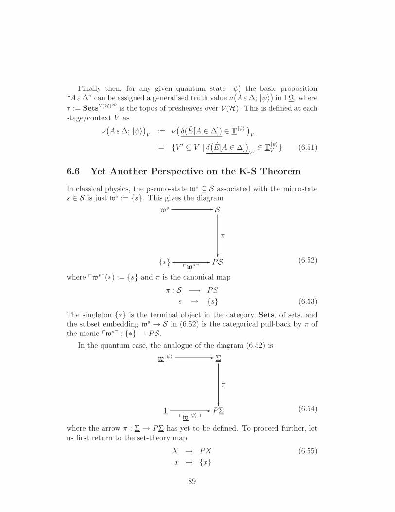
Finally then, for any given quantum state |ψ〉 the basic proposition“Aε∆” can be assigned a generalised truth value ν
(Aε∆; |ψ〉
)in ΓΩ, where
τ := SetsV(H)op is the topos of presheaves over V(H). This is defined at eachstage/context V as
ν(Aε∆; |ψ〉
)V
:= ν(δ(E[A ∈ ∆]) ∈ T |ψ〉
)V
= V ′ ⊆ V | δ(E[A ∈ ∆]
)V ′∈ T
|ψ〉V ′ (6.51)
6.6 Yet Another Perspective on the K-S Theorem
In classical physics, the pseudo-state ws ⊆ S associated with the microstates ∈ S is just ws := s. This gives the diagram
∗ PS-pwsq
ws S-
?
π
(6.52)
where pwsq(∗) := s and π is the canonical map
π : S −→ PS
s 7→ s (6.53)
The singleton ∗ is the terminal object in the category, Sets, of sets, andthe subset embedding ws → S in (6.52) is the categorical pull-back by π ofthe monic pws
q : ∗ → PS.
In the quantum case, the analogue of the diagram (6.52) is
1 PΣ-pw |ψ〉
q
w |ψ〉 Σ-
?
π
(6.54)
where the arrow π : Σ → PΣ has yet to be defined. To proceed further, letus first return to the set-theory map
X → PX (6.55)
x 7→ x
89
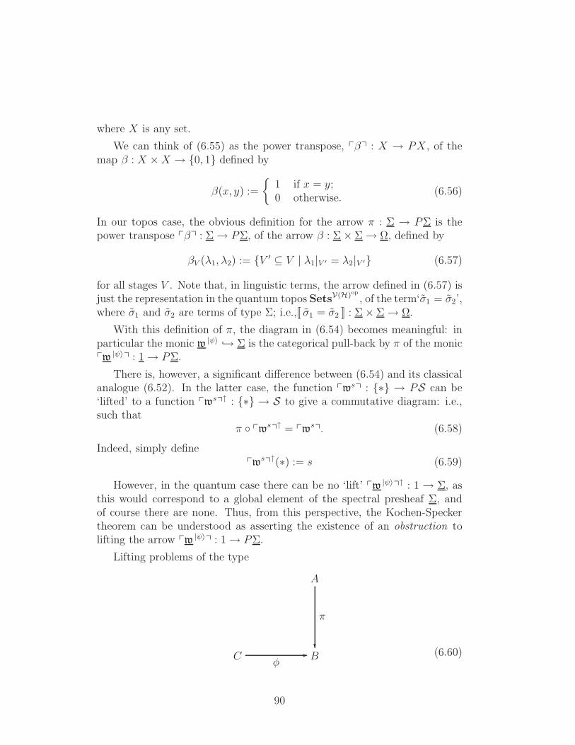
where X is any set.
We can think of (6.55) as the power transpose, pβq : X → PX, of themap β : X ×X → 0, 1 defined by
β(x, y) :=
1 if x = y;0 otherwise.
(6.56)
In our topos case, the obvious definition for the arrow π : Σ → PΣ is thepower transpose pβq : Σ→ PΣ, of the arrow β : Σ× Σ→ Ω, defined by
βV (λ1, λ2) := V ′ ⊆ V | λ1|V ′ = λ2|V ′ (6.57)
for all stages V . Note that, in linguistic terms, the arrow defined in (6.57) isjust the representation in the quantum topos SetsV(H)op , of the term‘σ1 = σ2’,where σ1 and σ2 are terms of type Σ; i.e.,[[ σ1 = σ2 ]] : Σ× Σ→ Ω.
With this definition of π, the diagram in (6.54) becomes meaningful: inparticular the monic w |ψ〉 → Σ is the categorical pull-back by π of the monicpw |ψ〉
q : 1→ PΣ.
There is, however, a significant difference between (6.54) and its classicalanalogue (6.52). In the latter case, the function pws
q : ∗ → PS can be‘lifted’ to a function pws
q↑ : ∗ → S to give a commutative diagram: i.e.,
such thatπ pws
q↑ = pws
q. (6.58)
Indeed, simply definepwsq↑(∗) := s (6.59)
However, in the quantum case there can be no ‘lift’ pw |ψ〉q↑ : 1 → Σ, as
this would correspond to a global element of the spectral presheaf Σ, andof course there are none. Thus, from this perspective, the Kochen-Speckertheorem can be understood as asserting the existence of an obstruction tolifting the arrow pw |ψ〉
q : 1→ PΣ.
Lifting problems of the type
C B-φ
A
?
π
(6.60)
90
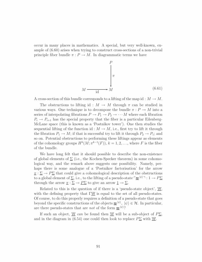
occur in many places in mathematics. A special, but very well-known, ex-ample of (6.60) arises when trying to construct cross-sections of a non-trivialprinciple fiber bundle π : P →M . In diagrammatic terms we have
M M-id
P
?
π
(6.61)
A cross-section of this bundle corresponds to a lifting of the map id : M →M .
The obstructions to lifting id : M → M through π can be studied invarious ways. One technique is to decompose the bundle π : P → M into aseries of interpolating fibrations P → P1 → P2 → · · ·M where each fibrationPi → Pi+1 has the special property that the fiber is a particular Eilenberg-McLane space (this is known as a ‘Postnikov tower’). One then studies thesequential lifting of the function id : M → M , i.e., first try to lift it throughthe fibration P1 → M ; if that is successful try to lift it through P2 → P1; andso on. Potential obstructions to performing these liftings appear as elementsof the cohomology groups Hk(M ; πk−1(F )), k = 1, 2, . . ., where F is the fiberof the bundle.
We have long felt that it should possible to describe the non-existenceof global elements of Σ (i.e., the Kochen-Specker theorem) in some cohomo-logical way, and the remark above suggests one possibility. Namely, per-haps there is some analogue of a ‘Postnikov factorisation’ for the arrowπ : Σ→ PΣ that could give a cohomological description of the obstructionsto a global element of Σ, i.e., to the lifting of a pseudo-state pw |ψ〉
q : 1→ PΣthrough the arrow π : Σ→ PΣ to give an arrow 1→ Σ.
Related to this is the question of if there is a ‘pseudo-state object’, W,with the defining property that ΓW is equal to the set of all pseudo-states.Of course, to do this properly requires a definition of a pseudo-state that goesbeyond the specific constructions of the objects w |ψ〉, |ψ〉 ∈ H. In particular,are there pseudo-states that are not of the form w |ψ〉?
If such an object, W can be found then W will be a sub-object of PΣ,and in the diagram in (6.54) one could then look to replace PΣ with W.
91
7 The de Groote Presheaves of Physical Quan-
tities
7.1 Background Remarks
Our task now is to consider the representation of the local language, L(S), inthe case of quantum theory. We assume that the relevant topos is the sameas that used for the propositional language PL(S), i.e., SetsV(H)op , but theemphasis is very different.
From a physics perspective, the key symbols in L(S) are (i) the ground-type symbols, Σ and R—the linguistic precursors of the state object and thequantity-value object respectively—and (ii) the function symbols A : Σ →R, which are the precursors of physical quantities. In the quantum-theoryrepresentation, φ, of L(S), the representation, Σφ, of Σ is defined to be the
spectral presheaf Σ in the topos SetsV(H)op .
The critical question is to find the object, Rφ (provisionally denoted as a
presheaf R), in SetsV(H)op that represents R, and is hence the quantity-valueobject. One might anticipate that R is just the real-number object in thetopos SetsV(H)op , but that turns out to be quite wrong, and the right answercannot just be guessed. In fact, the correct choice for R is found indirectlyby considering a related question: namely, how to represent each functionsymbol A : Σ→ R, with a concrete arrow Aφ : Σφ → Rφ in SetsV(H)op , i.e.,
with a natural transformation A : Σ→ R between the presheaves Σ and R.
Critical to this task are the daseinisation operations on projection oper-ators that were defined earlier as (5.9) and (5.57), and which are repeatedhere for convenience:
Definition 7.1 If P is a projection operator, and V ∈ Ob(V(H)) is anycontext/stage, we define:
1. The ‘outer daseinisation’ operation is
δo(P )V :=∧
α ∈ P(V ) | P α. (7.1)
where ‘’ denotes the usual ordering of projection operators, and whereP(V ) is the set of all projection operators in V .
2. Similarly, the ‘inner daseinisation’ operation is defined in the contextV as (c.f. (5.57))
δi(P )V :=∨
β ∈ P(V ) | β P. (7.2)
92
Thus δo(P )V is the best approximation to P in V from ‘above’, being thesmallest projection in V that is larger than or equal to P . Similarly, δi(P )Vis the best approximation to P from ‘below’, being the largest projection inV that is smaller than or equal to P .
In Section 6.5, we showed that the outer presheaf is a sub-object of thepower object PclΣ (in the category SetsV(H)op), and hence that the globalelement δo(P ) of O determines a (clopen) sub-object, δo(P ), of the spectralpresheaf Σ. By these means, the quantum logic of the lattice P(H) is mappedinto the Heyting algebra of the set, Subcl(Σ), of clopen sub-objects of Σ.
Our task now is to perform the second stage of the programme: namely(i) identify the quantity-value presheaf, R; and (ii) show that any physicalquantity can be represented by an arrow from Σ to R.
7.2 The Daseinisation of an Arbitrary Self-Adjoint Op-erator
7.2.1 Spectral Families and Spectral Order
We now want to extend the daseinisation operations from projections to arbi-trary (bounded) self-adjoint operators. To this end, consider first a bounded,self-adjoint operator, A, whose spectrum is purely discrete. Then the spec-tral theorem can be used to write A =
∑∞i=1 aiPi where a1, a2, . . . are the
eigenvalues of A, and P1, P2, . . . are the spectral projection operators ontothe corresponding eigenspaces.
A construction that comes immediately to mind is to use the daseinisationoperation on projections to define
δo(A)V :=∞∑
i=1
ai δo(Pi)V (7.3)
for each stage V . However, this procedure is rather unnatural. For one thing,the projections, Pi, i = 1, 2, . . . form a complete orthonormal set:
∞∑
i=1
Pi = 1, (7.4)
PiPj = δijPi, (7.5)
whereas, in general, the collection of daseinised projections, δo(Pi)V , 1 =1, 2, . . . will not satisfy either of these conditions. In addition, it is hard
93
to see how the expression δo(A)V :=∑∞
i=1 ai δo(Pi)V can be generalised to
operators, A, with a continuous spectrum.
The answer to this conundrum lies in the work of de Groote. He realisedthat although it is not useful to daseinise the spectral projections of anoperator A, it is possible to daseinise the spectral family of A [32].
Spectral families. We first recall that a spectral family is a family ofprojection operators Eλ, λ ∈ R, with the following properties:
1. If λ2 ≤ λ1 then Eλ2 Eλ1 .
2. The net λ 7→ Eλ of projection operators in the lattice P(H) is boundedabove by 1, and below by 0. In fact,
limλ→∞
Eλ = 1, (7.6)
limλ→−∞
Eλ = 0. (7.7)
3. The map λ 7→ Eλ is right-continuous:74
∧
ǫ↓0
Eλ+ǫ = Eλ (7.8)
for all λ ∈ R.
The spectral theorem asserts that for any self-adjoint operator A, there existsa spectral family, λ 7→ EA
λ , such that
A =
∫
R
λ dEAλ (7.9)
We are only concerned with bounded operators, and so the (weak Stieljes)integral in (7.9) is really over the bounded spectrum of A which, of course, is acompact subset of R. Conversely, given a bounded spectral family Eλλ∈R,75
there is a bounded self-adjoint operator A such that A =∫
Rλ dEλ.
74It is a matter of convention whether one chooses right-continuous or left-continuous.75I.e., there are a, b ∈ R such that Eλ = 0 for all λ ≤ a and Eλ = 1 for all λ ≥ b.
94
The spectral order. A key element for our work is the so-called spectralorder that was introduced in [63].76 It is defined as follows. Let A andB be (bounded) self-adjoint operators with spectral families EA
λ λ∈R andEB
λ λ∈R, respectively. Then define:
A s B if and only if EBλ EA
λ for all λ ∈ R. (7.10)
It is easy to see that (7.10) defines a genuine partial ordering on B(H)sa (theself-adjoint operators in B(H)). In fact, B(H)sa is a ‘boundedly complete’lattice with respect to the spectral order, i.e., each bounded set S of self-adjoint operators has a minimum
∧S ∈ B(H)sa and a maximum
∨S ∈
B(H)sa with respect to this order.
If P , Q are projections, then
P s Q if and only if P Q, (7.11)
so the spectral order coincides with the usual partial order on P(H). Toensure this, the ‘reverse’ relation in (7.10) is necessary, since the spectralfamily of a projection P is given by
EPλ =
0 if λ < 0
1− P if 0 ≤ λ < 1
1 if λ ≥ 1.
(7.12)
If A, B are self-adjoint operators such that (i) either A or B is a projection,or (ii) [A, B] = 0, then A s B if and only if A B. Here ‘’ denotes theusual ordering on B(H)sa.
77
Moreover, if A, B are arbitrary self-adjoint operators, then A s B im-plies A B, but not vice versa in general. Thus the spectral order is apartial order on B(H)sa that is coarser than the usual one.
7.2.2 Daseinisation of Self-Adjoint Operators.
De Groote’s crucial observation was the following. Let λ 7→ Eλ be a spectralfamily in P(H) (or, equivalently, a self-adjoint operator A). Then, for eachstage V , the following maps:
λ 7→∧
µ>λ
δo(Eµ)V (7.13)
λ 7→ δi(Eλ)V (7.14)
76The spectral order was later reinvented by de Groote, see [31].77The ‘usual’ ordering is A B if 〈ψ| A |ψ〉 ≤ 〈ψ| B |ψ〉 for all vectors |ψ〉 ∈ H.
95
also define spectral families.78 These spectral families lie in P(V ) and hence,by the spectral theorem, define self-adjoint operators in V . This leads to thedefinition of the two daseinisations of an arbitrary self-adjoint operator:
Definition 7.2 Let A be an arbitrary self-adjoint operator. Then the outerand inner daseinisations of A are defined at each stage V as:
δo(A)V :=
∫
R
λ d(δiV (EA
λ )), (7.15)
δi(A)V :=
∫
R
λ d( ∧
µ>λ
δoV (EAµ )
), (7.16)
respectively.
Note that for all λ ∈ R, and for all stages V , we have
δi(Eλ)V ∧
µ>λ
δo(Eµ)V (7.17)
and hence, for all V ,δi(A)V s δo(A)V . (7.18)
This explains why the ‘i’ and ‘o’ superscripts in (7.15–7.16) are defined theway round that they are.
Both outer daseinisation (7.15) and inner daseinisation (7.16) can be usedto ‘adapt’ a self-adjoint operator A to contexts V ∈ Ob(V(H)) that do notcontain A. (On the other hand, if A ∈ V , then δo(A)V = δi(A)V = A.)
7.2.3 Properties of Daseinisation.
We will now list some useful properties of daseinisation.
1. It is clear that the outer, and inner, daseinisation operations can beextended to situations where the self-adjoint operator A does not belongto B(H)sa, or where V is not an abelian sub-algebra of B(H). Specifically,let N be an arbitrary von Neumann algebra, and let S ⊂ N be a propervon Neumann sub-algebra such that 1N = 1S = 1. Then outer and inner
78The reason (7.13) and (7.14) have a different form is that λ 7→ δi(Eλ)V is rightcontinuous whereas λ 7→ δo(Eλ)V is not. On the other hand, the family λ 7→ ∧
µ>λ δo(Eµ)V
is right continuous.
96
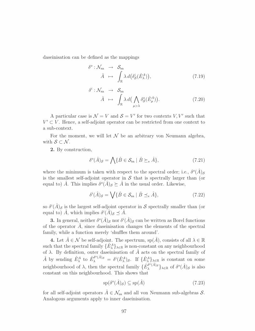
daseinisation can be defined as the mappings
δo : Nsa → Ssa
A 7→∫
R
λ d(δiS(EA
λ )), (7.19)
δi : Nsa → Ssa
A 7→∫
R
λ d( ∧
µ>λ
δoS(EAµ )
). (7.20)
A particular case is N = V and S = V ′ for two contexts V, V ′ such thatV ′ ⊂ V . Hence, a self-adjoint operator can be restricted from one context toa sub-context.
For the moment, we will let N be an arbitrary von Neumann algebra,with S ⊂ N .
2. By construction,
δo(A)S =∧B ∈ Ssa | B s A, (7.21)
where the minimum is taken with respect to the spectral order; i.e., δo(A)Sis the smallest self-adjoint operator in S that is spectrally larger than (orequal to) A. This implies δo(A)S A in the usual order. Likewise,
δi(A)S =∨B ∈ Ssa | B s A, (7.22)
so δi(A)S is the largest self-adjoint operator in S spectrally smaller than (orequal to) A, which implies δi(A)S A.
3. In general, neither δo(A)S nor δi(A)S can be written as Borel functionsof the operator A, since daseinisation changes the elements of the spectralfamily, while a function merely ‘shuffles them around’.
4. Let A ∈ N be self-adjoint. The spectrum, sp(A), consists of all λ ∈ R
such that the spectral family EAλ λ∈R is non-constant on any neighbourhood
of λ. By definition, outer daseinisation of A acts on the spectral family of
A by sending EAλ to E
δo(A)Sλ = δi(EA
λ )S . If EAλ λ∈R is constant on some
neighbourhood of λ, then the spectral family Eδo(A)Sλ λ∈R of δo(A)S is also
constant on this neighbourhood. This shows that
sp(δo(A)S) ⊆ sp(A) (7.23)
for all self-adjoint operators A ∈ Nsa and all von Neumann sub-algebras S.Analogous arguments apply to inner daseinisation.
97
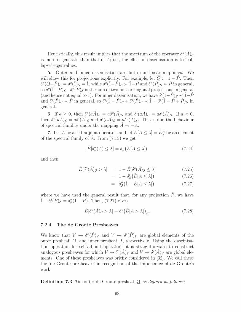
Heuristically, this result implies that the spectrum of the operator δo(A)Sis more degenerate than that of A; i.e., the effect of daseinisation is to ‘col-lapse’ eigenvalues.
5. Outer and inner daseinisation are both non-linear mappings. Wewill show this for projections explicitly. For example, let Q := 1− P . Thenδo(Q+P )S = δo(1)S = 1, while δo(1−P )S ≻ 1−P and δo(P )S ≻ P in general,so δo(1−P )S+δo(P )S is the sum of two non-orthogonal projections in general(and hence not equal to 1). For inner daseinisation, we have δi(1−P )S ≺ 1−Pand δi(P )S ≺ P in general, so δi(1− P )S + δi(P )S ≺ 1 = δi(1− P + P )S ingeneral.
6. If a ≥ 0, then δo(aA)S = aδo(A)S and δi(aA)S = aδi(A)S . If a < 0,then δo(aA)S = aδi(A)S and δi(aA)S = aδo(A)S . This is due the behaviourof spectral families under the mapping A 7→ −A.
7. Let A be a self-adjoint operator, and let E[A ≤ λ] = EAλ be an element
of the spectral family of A. From (7.15) we get
E[δoS(A) ≤ λ] = δiS(E[A ≤ λ]) (7.24)
and then
E[δo(A)S > λ] = 1− E[δo(A)S ≤ λ] (7.25)
= 1− δiS(E[A ≤ λ]
)(7.26)
= δoS(1− E[A ≤ λ]
)(7.27)
where we have used the general result that, for any projection P , we have1− δi(P )S = δoS(1− P ). Then, (7.27) gives
E[δo(A)S > λ] = δo(E[A > λ]
)S. (7.28)
7.2.4 The de Groote Presheaves
We know that V 7→ δo(P )V and V 7→ δi(P )V are global elements of theouter presheaf, O, and inner presheaf, I, respectively. Using the daseinisa-tion operation for self-adjoint operators, it is straightforward to constructanalogous presheaves for which V 7→ δo(A)V and V 7→ δi(A)V are global ele-ments. One of these presheaves was briefly considered in [32]. We call thesethe ‘de Groote presheaves’ in recognition of the importance of de Groote’swork.
Definition 7.3 The outer de Groote presheaf, |O, is defined as follows:
98
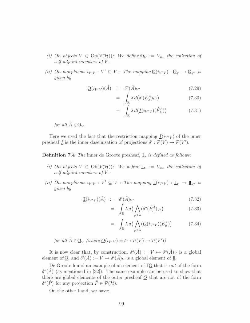
(i) On objects V ∈ Ob(V(H)): We define |OV := Vsa, the collection ofself-adjoint members of V .
(ii) On morphisms iV ′V : V ′ ⊆ V : The mapping |O(iV ′ V ) : |OV → |OV ′ isgiven by
|O(iV ′ V )(A) := δo(A)V ′ (7.29)
=
∫
R
λ d(δi(EA
λ )V ′
)(7.30)
=
∫
R
λ d(I(iV ′ V )(EA
λ ))
(7.31)
for all A ∈ |OV .
Here we used the fact that the restriction mapping I(iV ′ V ) of the innerpresheaf I is the inner daseinisation of projections δi : P(V )→ P(V ′).
Definition 7.4 The inner de Groote presheaf, II, is defined as follows:
(i) On objects V ∈ Ob(V(H)): We define IIV := Vsa, the collection ofself-adjoint members of V .
(ii) On morphisms iV ′V : V ′ ⊆ V : The mapping II(iV ′ V ) : IIV → IIV ′ isgiven by
II(iV ′ V )(A) := δi(A)V ′ (7.32)
=
∫
R
λ d( ∧
µ>λ
(δo(EAµ )V ′
)(7.33)
=
∫
R
λ d( ∧
µ>λ
(O(iV ′ V )(EAµ )
)(7.34)
for all A ∈ |OV (where O(iV ′ V ) = δo : P(V )→ P(V ′)).
It is now clear that, by construction, δo(A) := V 7→ δo(A)V is a globalelement of |O, and δi(A) := V 7→ δi(A)V is a global element of II.
De Groote found an example of an element of Γ |O that is not of the formδo(A) (as mentioned in [32]). The same example can be used to show thatthere are global elements of the outer presheaf O that are not of the formδo(P ) for any projection P ∈ P(H).
On the other hand, we have:
99
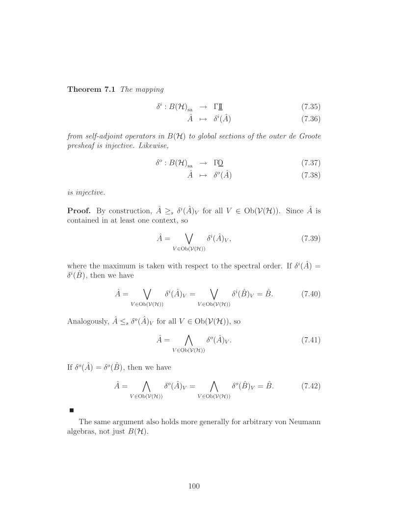
Theorem 7.1 The mapping
δi : B(H)sa → ΓII (7.35)
A 7→ δi(A) (7.36)
from self-adjoint operators in B(H) to global sections of the outer de Grootepresheaf is injective. Likewise,
δo : B(H)sa → Γ |O (7.37)
A 7→ δo(A) (7.38)
is injective.
Proof. By construction, A ≥s δi(A)V for all V ∈ Ob(V(H)). Since A iscontained in at least one context, so
A =∨
V ∈Ob(V(H))
δi(A)V , (7.39)
where the maximum is taken with respect to the spectral order. If δi(A) =δi(B), then we have
A =∨
V ∈Ob(V(H))
δi(A)V =∨
V ∈Ob(V(H))
δi(B)V = B. (7.40)
Analogously, A ≤s δo(A)V for all V ∈ Ob(V(H)), so
A =∧
V ∈Ob(V(H))
δo(A)V . (7.41)
If δo(A) = δo(B), then we have
A =∧
V ∈Ob(V(H))
δo(A)V =∧
V ∈Ob(V(H))
δo(B)V = B. (7.42)
The same argument also holds more generally for arbitrary von Neumannalgebras, not just B(H).
100
8 The Presheaves sp(A), R and R↔
8.1 Background to the Quantity-Value Presheaf R.
Our goal now is to construct a ‘quantity-value’ presheaf R with the propertythat inner and/or outer daseinisation of an self-adjoint operator A can beused to define an arrow, i.e., a natural transformation, from Σ to R.79
The arrow corresponding to a self-adjoint operator A ∈ B(H) is denotedfor now by A : Σ→R. At each stage V , we need a mapping
AV : ΣV → RV (8.1)
λ 7→ AV (λ), (8.2)
and we make the basic assumption that this mapping is given by evaluation.More precisely, λ ∈ ΣV is a spectral element80 of V and hence can be evalu-ated on operators lying in V . And, while A will generally not lie in V , boththe inner daseinisation δi(A)V and the outer daseinisation δo(A)V do.
Let us start by considering the operators δo(A)V , V ∈ Ob(V(H)). Eachof these is a self-adjoint operator in the commutative von Neumann algebraV , and hence, by the spectral theorem, can be represented by a function,
(the Gel’fand transform81) δo(A)V : ΣV → sp(δo(A)V ), with values in thespectrum sp(δo(A)V ) of the self-adjoint operator δo(A)V . Since the spectrum
of a self-adjoint operator is a subset of R, we can also write δo(A)V : ΣV → R.
The question now is whether the collection of maps δo(A)V : ΣV → R,V ∈ Ob(V(H)), can be regarded as an arrow from Σ to some presheaf R.
To answer this we need to see how these operators behave as we go ‘downa chain’ of sub-algebras V ′ ⊆ V . The first remark is that if V ′ ⊆ V thenδo(A)V ′ δo(A)V . When applied to the Gel’fand transforms, this leads tothe equation
δo(A)V ′(λ|V ′) ≥ δo(A)V (λ) (8.3)
for all λ ∈ ΣV , where λ|V ′ denotes the restriction of the spectral elementλ ∈ ΣV to the sub-algebra V ′ ⊆ V . However, the definition of the spectral
79In fact, we will define several closely related presheaves that can serve as a quantity-value object.
80A ‘spectral element’, λ ∈ ΣV of V , is a multiplicative, linear functional λ : V → |Cwith 〈λ, 1〉 = 1, see also Def. 5.4.
81This use of the ‘overline’ symbol for the Gel’fand transform should not be confusedwith our later use of the same symbol to indicate a co-presheaf.
101
presheaf is such that λ|V ′ = Σ(iV ′ V )(λ), and hence (8.3) can be rewritten as
δo(A)V ′
(Σ(iV ′ V )(λ)
)≥ δo(A)V (λ) (8.4)
for all λ ∈ ΣV .
It is a standard result that the Dedekind real number object, R, in apresheaf topos SetsC
op
is the constant functor from Cop to R [56]. It follows
that the family of Gel’fand transforms, δo(A)V , V ∈ Ob(V(H)), of the da-seinised operators δo(A)V , V ∈ Ob(V(H)), does not define an arrow from Σto R, as this would require an equality in (8.4), which is not true. Thus thequantity-value presheaf, R, in the topos SetsV(H)op is not the real-numberobject R, although clearly R has something to do with the real numbers. Wemust take into account the growth of these real numbers as we go from V tosmaller sub-algebras V ′. Similarly, if we consider inner daseinisation, we geta series of falling real numbers.
The presheaf, R, that we will choose, and which will be denoted by R↔,incorporates both aspects (growing and falling real numbers).
8.2 Definition of the Presheaves sp(A), R and R↔.
The inapplicability of the real-number object R may seem strange at first,82
but actually it is not that surprising. Because of the Kochen-Specker theo-rem, we do not expect to be able to assign (constant) real numbers as valuesof physical quantities, at least not globally. Instead, we draw on some recentresults of M. Jackson [47], obtained as part of his extensive study of mea-sure theory on a topos of presheaves. Here, we use a single construction inJackson’s thesis: the presheaf of ‘order-preserving functions’ over a partiallyordered set—in our case, V(H). In fact, we will need both order-reversingand order-preserving functions.
Definition 8.1 Let (Q,) and (P,) be partially ordered sets. A function
µ : Q → P (8.5)
is order-preserving if q1 q2 implies µ(q1) µ(q2) for all q1, q2 ∈ Q. It isorder-reversing if q1 q2 implies µ(q1) µ(q2). We denote by OP(Q,P)the set of order-preserving functions µ : Q → P, and by OR(Q,P) the setof order-reversing functions.
82Indeed, it puzzled us for a while!
102
We note that if µ is order-preserving, then −µ is order-reversing, and viceversa.
Adapting Jackson’s definitions slightly, if P is any partially-ordered set,we have the following.
Definition 8.2 The P-valued presheaf, P, of order-reversing functionsover V(H) is defined as follows:
(i) On objects V ∈ Ob(V(H)):
PV := µ :↓V → P | µ ∈ OR(↓V,P) (8.6)
where ↓V ⊂ Ob(V(H)) is the set of all von Neumann sub-algebras ofV .
(ii) On morphisms iV ′V : V ′ ⊆ V : The mapping P(iV ′ V ) : PV → P
V ′ isgiven by
P(iV ′ V )(µ) := µ|V ′ (8.7)
where µ|V ′ denotes the restriction of the function µ to ↓V ′ ⊆↓V .
Jackson uses order-preserving functions with P := [0,∞) (the non-negativereals), with the usual order ≤.
Clearly, there is an analogous definition of the P-valued presheaf, P, oforder-preserving functions from ↓V to P. It can be shown that P and P
are isomorphic objects in SetsV(H)op .
Let us first consider P. For us, the key examples for the partially orderedset P are (i) R, the real numbers with the usual order ≤, and (ii) sp(A) ⊂ R,the spectrum of some bounded self-adjoint operator A, with the order ≤inherited from R. Clearly, the associated presheaf sp(A) is a sub-object of
the presheaf R.
Now let A ∈ B(H)sa, and let V ∈ Ob(V(H)). Then to each λ ∈ ΣV thereis associated the function
δo(A)V (λ) :↓V → sp(A), (8.8)
given by(δo(A)V (λ)
)(V ′) := δo(A)V ′(Σ(iV ′V )(λ)) (8.9)
= δo(A)V ′(λ|V ′) (8.10)
= 〈λ|V ′, δo(A)V ′〉 (8.11)
= 〈λ, δo(A)V ′〉 (8.12)
103
for all V ′ ⊆ V . We note that as V ′ becomes smaller, δo(A)V ′ becomes larger(or stays the same) in the spectral order, and hence in the usual order onoperators. Therefore, δo(A)V (λ) :↓V → sp(A) is an order-reversing function,for each λ ∈ ΣV .
It is worth noting that daseinisation of A, i.e., the approximation ofthe self-adjoint operator A in the spectral order, allows to define a func-tion δo(A)V (λ) (for each λ ∈ ΣV ) with values in the spectrum of A, sincewe have sp(δo(A)V ) ⊆ sp(A), see (7.23). If we had chosen an approximationin the usual linear order on B(H)sa, then the approximated operators would
not have a spectrum that is contained in sp(A) in general.
Let
δo(A)V : ΣV → sp(A)V
(8.13)
λ 7→ δo(A)V (λ) (8.14)
denote the set of order-reversing functions from ↓V to sp(A) obtained in thisway. We then have the following, fundamental, result which can be regardedas a type of ‘non-commutative’ spectral theorem in which each bounded,self-adjoint operator A is mapped to an arrow from Σ to R:
Theorem 8.1 The mappings δo(A)V , V ∈ Ob(V(H)), are the componentsof a natural transformation/arrow δo(A) : Σ→ sp(A).
Proof. We only have to prove that, whenever V ′ ⊂ V , the diagram
ΣV ′ sp(A)V ′
-δo(A)V ′
ΣV sp(A)V
-δo(A)V
? ?
commutes. Here, the vertical arrows are the restrictions of the relevantpresheaves from the stage V to V ′ ⊆ V .
In fact, the commutativity of the diagram follows directly from the defi-nitions. For each λ ∈ ΣV , the composition of the upper arrow and the rightvertical arrow gives
(δo(A)V (λ))|V ′ = δo(A)V ′(λ|V ′), (8.15)
104
which is the same function that we get by first restricting λ from ΣV to ΣV ′
and then applying δo(A)V ′.
In this way, to each physical quantity A in quantum theory there is as-signed a natural transformation δo(A) from the state object Σ to the presheafsp(A). Since sp(A) is a sub-object of R for each A, δo(A) can also be
seen as a natural transformation/arrow from Σ to R. Hence the presheafR in the topos SetsV(H)op is one candidate for the quantity-value object ofquantum theory. Note that it follows from Theorem 7.1 that the mapping
θ : B(H)sa → HomSetsV(H)op (Σ,R) (8.16)
A 7→ δo(A) (8.17)
is injective. 83
If S denotes our quantum system, then, on the level of the formal languageL(S), we expect the mapping A → A to be injective, where A is a functionsymbol of signature Σ → R. It follows that we have obtained a a faithfulrepresentation of these function symbols by arrows δo(A) : Σ → R in thetopos SetsV(H)op .
Similarly, there is an order-preserving function
δi(A)V (λ) : ↓V → sp(A), (8.18)
that is defined for all V ′ ⊆ V by(δi(A)V (λ)
)(V ′) = δi(A)V ′(Σ(iV ′V )(λ)) (8.19)
= 〈λ, δi(A)V ′〉. (8.20)
Since δi(A)V ′ becomes smaller (or stays the same) as V ′ gets smaller, δi(A)V (λ)indeed is an order-preserving function from ↓V to sp(A) for each λ ∈ ΣV .Again, approximation in the spectral order (in this case from below) allowsus to define a function with values in sp(A), which would not be possiblewhen using the linear order.
Clearly, we can use the functions δi(A)V (λ), λ ∈ ΣV , to define a naturaltransformation δi(A) : Σ→ R from the spectral presheaf, Σ, to the presheaf
83Interestingly, these results all carry over to an arbitrary von Neumann algebra N ⊆B(H). In this way, the formalism is flexible enough to adapt to situations where we havesymmetries (which can described mathematically by a von Neumann algebra N that hasa non-trivial commutant) and super-selection rules (which corresponds to N having anon-trivial centre).
105
R of real-valued, order-preserving functions on ↓V . The components ofδi(A) are
δi(A)V : ΣV → sp(A)V
(8.21)
λ 7→ δi(A)V (λ). (8.22)
It follows from Theorem 7.1 that the mapping from self-adjoint operators tonatural transformations δi(A) is injective.
The functions obtained from inner and outer daseinisation can be com-bined to give yet another presheaf, and one that will be particularly usefulfor the physical interpretation of these constructions. The general definitionis the following.
Definition 8.3 Let P be a partially-ordered set. The P-valued presheaf,P↔, of order-preserving and order-reversing functions on V(H) is defined asfollows:
(i) On objects V ∈ Ob(V(H)):
P↔V := (µ, ν) | µ ∈ OP(↓V,P), ν ∈ OR(↓V,P), µ ≤ ν (8.23)
where ↓V ⊂ Ob(V(H)) is the set of all sub-algebras V ′ of V . Note that weintroduce the condition µ ≤ ν, i.e., for all V ′ ∈↓V we demand µ(V ′) ≤ ν(V ′).
(ii) On morphisms iV ′V : V ′ ⊆ V :
P↔(iV ′V ) : P↔V −→ P↔
V ′ (8.24)
(µ, ν) 7−→ (µ|V ′ , ν|V ′), (8.25)
where µ|V ′ denotes the restriction of µ to ↓V ′ ⊆↓V , and analogously for ν|V ′.
Note that since we have the condition µ ≤ ν in (i), the presheaf P↔ is notsimply the product of the presheaves P and P.
As we will discuss shortly, the presheaf, R↔, of order-preserving andorder-reversing, real-valued functions is closely related to the ‘k-extension’ ofthe presheaf R (see the Appendix for details of the k-extension procedure).
Now let
δ(A)V :=(δi(A)V (·), δo(A)V (·)
): ΣV → R↔
V (8.26)
denote the set of all pairs of order-preserving and order-reversing functionsfrom ↓V to R that can be obtained from inner and outer daseinisation. It iseasy to see that we have the following result:
106
Theorem 8.2 The mappings δ(A)V , V ∈ Ob(V(H)), are the components ofa natural transformation δ(A) : Σ→ R↔.
Again from Theorem 7.1, the mapping from self-adjoint operators to naturaltransformations, A→ δ(A), is injective.
Since δi(A)V (λ) ≤ δo(A)V (λ) for all λ ∈ ΣV , we can interpret each pair(δi(A)V (λ), δo(A)V (λ)) of values as an interval, which gives a first hint at thephysical interpretation.
8.3 Inner and Outer Daseinisation from Functions onFilters
There is a close relationship between inner and outer daseinisation, and cer-tain functions on the filters in the projection lattice P(H) of B(H). We givea summary of these results here: details can be found in de Groote’s work[32, 34], the article [20], and a forthcoming paper [26]. This subsection servesas a preparation for the physical interpretation of the arrows δ(A) : Σ→ R↔.
Filter bases, filters and ultrafilters. We first need some basic defini-tions. Let L be a lattice with zero element 0. A subset f of L is called a filterbase if (i) 0 6= f and (ii) for all a, b ∈ f , there is a c ∈ f such that c ≤ a ∧ b.
A subset F of a lattice L with zero element 0 is a (proper) filter (or dualideal) if (i) 0 /∈ F , (ii) a, b ∈ F implies a ∧ b ∈ F and (iii) a ∈ F and b ≥ aimply b ∈ F . In other words, a filter is an upper set in the lattice L that isclosed under finite minima.
By Zorn’s lemma, every filter is contained in a maximal filter. Obviously,such a maximal filter is also a maximal filter base.
Let L′ be a sublattice of L (with common 0), and let F ′ be a filter in L′.Then F ′, seen as a subset of L, is a filter base in L. The smallest filter in L
that contains F ′ is the cone over F ′ in L:
CL(F ′) := b ∈ L | ∃a ∈ F ′ : a ≤ b. (8.27)
This is nothing but the upper set ↑F ′ of F ′ in L.
In our applications, L typically is the lattice P(H) of projections in B(H),and L′ is the lattice P(V ) of projections in an abelian sub-algebra V .
If L is a Boolean lattice, i.e., if it is a distributive lattice with minimalelement 0 and maximal element 1, and a complement (negation) ¬ : L→ L
107
such that a ∨ ¬a = 1 for all a ∈ L, then we define an ultrafilter F to bea maximal filter in L. An ultrafilter F is characterised by the followingproperty: for all a ∈ L, either a ∈ F or ¬a ∈ F . This can easily be seen:we have a∨¬a = 1 by definition. Let us assume that F is an ultrafilter anda /∈ F . This means that there is some b ∈ F such that b ∧ a = 0. Usingdistributivity of the lattice L, we get
b = b ∧ (a ∨ ¬a) = (b ∧ a) ∨ (b ∧ ¬a) = b ∧ ¬a, (8.28)
so b ≤ ¬a. Since b ∈ F and F is a filter, this implies ¬a ∈ F . Conversely, if¬a /∈ F , we obtain a ∈ F .
The projection lattice P(V ) of an abelian von Neumann algebra V is aBoolean lattice. The maximal element is the identity operator 1 and, as wesaw earlier, the complement of a projection is given as ¬α = 1 − α. Eachultrafilter F in P(V ) hence contains either α or 1− α for all α ∈ P(V ).
Spectral elements and ultrafilters. Let V ∈ Ob(V(H)), and let λ ∈ ΣV
be a spectral element of the von Neumann algebra V . This means that λ isa multiplicative state of V . For all projections α ∈ P(V ), we have
〈λ, α〉 = 〈λ, α2〉 = 〈λ, α〉〈λ, α〉, (8.29)
and so 〈λ, α〉 ∈ 0, 1. Moreover, 〈λ, 0〉 = 0, 〈λ, 1〉 = 1, and if 〈λ, α〉 = 0,then 〈λ, 1 − α〉 = 1 (since 〈λ, α〉 + 〈λ, 1 − α〉 = 〈λ, 1〉). Hence, for eachα ∈ P(V ) we have either 〈λ, α〉 = 1 or 〈λ, 1− α〉 = 1. This shows that thefamily
Fλ := α ∈ P(V ) | 〈λ, α〉 = 1 (8.30)
of projections is an ultrafilter in P(V ). Conversely, each λ ∈ ΣV is uniquelydetermined by the set 〈λ, α〉 | α ∈ P(V ) and hence by an ultrafilter inP(V ). This shows that there is a bijection between the setQ(V ) of ultrafiltersin P(V ) and the Gel’fand spectrum ΣV .
Observable and antonymous functions. Let N be a von Neumannalgebra, and let F(N ) be the set of filters in the projection lattice P(N ) ofN . De Groote has shown [34] that to each self-adjoint operator A ∈ N , therecorresponds a, so-called, ‘observable function’ fA : F(N ) → sp(A). If N is
abelian, N = V , then fA|Q(V ) is just the Gel’fand transform of A. However,it is striking that fA can be defined even if N is non-abelian; for us, theimportant example is N = B(H).
108
If EAµ µ∈R is the spectral family of A, then fA is defined as
fA : F(N ) → sp(A)
F 7→ infµ ∈ R | EAµ ∈ F. (8.31)
Conversely, given a bounded function f : D(H)→ R with certain properties,one can find a unique self-adjoint operator A ∈ B(H) such that f = fA.
It can be shown that each observable function is completely determinedby its restriction to the space of maximal filters [34]. Let Q(N ) denote thespace of maximal filters in P(N ). The sets
QP (N ) := F ∈ Q(N ) | P ∈ F, P ∈ P(N ), (8.32)
form the base of a totally disconnected topology on Q(N ). Following deGroote, this space is called the Stone spectrum of N . If N is abelian, N = V ,then, upon the identification of maximal filters (which are ultrafilters) inP(V ) and spectral elements in ΣV , the Stone spectrum Q(V ) is the Gel’fandspectrum ΣV of V .
This shows that for an arbitrary von Neumann algebra N , the StonespectrumQ(N ) is a generalisation of the Gel’fand spectrum (the latter is onlydefined for abelian algebras). The observable function fA is a generalisation
of the Gel’fand transform of A.
We want to show that the observable function fδo(V )Aof the outer da-
seinisation of A to V can be expressed by the observable function fA of Adirectly. Since this works for all V ∈ Ob(V(H)), we obtain a nice encodingof all the functions fδo(A)V
and hence of the self-adjoint operators δo(A)V .The result (already shown in [32]) is that, for all stages V ∈ Ob(V(H)) andall filters F in F(V ),
fδo(A)V(F ) = fA(CB(H)(F )). (8.33)
We want to give an elementary proof of this. We need
Lemma 8.3 Let N be a von Neumann algebra, S a von Neumann sub-algebra of N , and let δiS : P(N ) → P(S) be the inner daseinisation mapon projections. Then, for all filters F ∈ F(S),
(δiS)−1(F ) = CN (F ). (8.34)
Proof. If Q ∈ F ⊂ P(S), then (δiS)−1(Q) = P ∈ P(N ) | δi(P )S = Q.Let P ∈ P(N ) be such that there is a Q ∈ F with Q ≤ P , i.e., P ∈ CN (F ).
109
Then δi(P )S ≥ Q, which implies δi(P )S ∈ F , since F is a filter in P(S).This shows that CN (F ) ⊆ (δiS)−1(F ). Now let P ∈ P(N ) be such that thereis no Q ∈ F with Q ≤ P . Since δi(P )S ≤ P , there also is no Q ∈ F withQ ≤ δi(P )S , so P /∈ (δiS)−1(F ). This shows that (δiS)−1(F ) ⊆ CN (F ).
We now can prove
Theorem 8.4 Let A ∈ Nsa. For all von Neumann sub-algebras S ⊆ N andall filters F ∈ F(S), we have
fδo(A)S(F ) = fA(CN (F )). (8.35)
Proof. We have
fδo(A)S(F ) = infλ ∈ R | Eδo(A)Sλ ∈ F
= infλ ∈ R | δi(EAλ )S ∈ F
= infλ ∈ R | EAλ ∈ (δiS)−1(F )
= infλ ∈ R | EAλ ∈ CN (F )
= fA(CN (F )).
The second equality is the definition of outer daseinisation (on the level ofspectral projections, see (7.14)). In the penultimate step, we used Lemma8.3.
This clearly implies (8.33). We saw above that to each λ ∈ ΣV there cor-responds a unique ultrafilter Fλ ∈ Q(V ). Since δo(A)V ∈ Vsa, the observablefunction fδo(A)V
is the Gel’fand transform of δo(A)V , and so, upon identifyingthe ultrafilter Fλ with the spectral element λ, we have
fδo(A)V(Fλ) = δo(A)V (λ) = 〈λ, δo(A)V 〉. (8.36)
From (8.33) we have
〈λ, δo(A)V 〉 = fδo(A)V(Fλ) = fA(CB(H)(Fλ)) (8.37)
for all V ∈ Ob(V(H)) and for all λ ∈ ΣV . In this sense, the observablefunction fA encodes all the outer daseinisations δo(A)V , V ∈ Ob(V(H)), of
A.
110
There is also a function, gA, on the filters in P(H) that encodes all the
inner daseinisations δi(A)V , V ∈ Ob(V(H)). This function is given for anarbitrary von Neumann algebra N by
gA : F(N ) → sp(A) (8.38)
F 7→ supλ ∈ R | 1− EAλ ∈ F (8.39)
and is called the antonymous function of A [20]. If N is abelian, then gA|Q(V )
is the Gel’fand transform of A and coincides with fA on the space Q(V ) ofmaximal filters, i.e., ultrafilters in P(V ). As functions on F(V ), fA and gAare different also in the abelian case. For an arbitrary von Neumann algebraN , the antonymous function gA is another generalisation of the Gel’fand
transform of A.
There is a close relationship between observable and antonymous func-tions [34, 20]: for all von Neumann algebras N and all self-adjoint operatorsA ∈ Nsa, it holds that
−fA = g−A. (8.40)
There is a relation analogous to (8.33) for antonymous functions: for allV ∈ Ob(V(H)) and all filters F in F(V ),
gδi(A)V(F ) = gA(CB(H)(F )). (8.41)
This follows from
Theorem 8.5 Let A ∈ Nsa. For all von Neumann sub-algebras S ⊆ N andall filters F ∈ F(S), we have
gδi(A)S(F ) = gA(CN (F )). (8.42)
Proof. We have
gδi(A)S(F ) = supλ ∈ R | 1− Eδi(A)S
λ ∈ F= supλ ∈ R | 1−
∧
µ>λ
δo(EAµ )S ∈ F
= supλ ∈ R | 1− δo(EAλ )S ∈ F
= supλ ∈ R | δi(1− EAλ )S ∈ F
= supλ ∈ R | 1− EAλ ∈ (δiS)−1(F )
= supλ ∈ R | 1− EAλ ∈ CN (F )
=gA(CN (F )),
111
where in the penultimate step we used Lemma 8.3.
Let λ ∈ ΣV , and let Fλ ∈ Q(V ) be the corresponding ultrafilter. Sinceδi(A)V ∈ V , the antonymous function gδi(A)V
is the Gel’fand transform of
δi(A)V , and we have
gδi(A)V(Fλ) = δi(A)V (λ) = 〈λ, δi(A)V 〉. (8.43)
From (8.41), we get
〈λ, δi(A)V 〉 = gδi(A)V(Fλ) = gA(CB(H)(Fλ)) (8.44)
for all V ∈ Ob(V(H)) and all λ ∈ ΣV . Thus the antonymous function gAencodes all the inner daseinisations δi(A)V , V ∈ Ob(V(H)), of A.
8.4 A Physical Interpretation of the Arrow δ(A) : Σ→R↔
Let |ψ〉 ∈ H be a unit vector in the Hilbert space of the quantum system.The expectation value of a self-adjoint operator A ∈ B(H) in the state |ψ〉is given by
〈ψ| A |ψ〉 =
∫ ||A||
−||A||
λ d〈ψ| EAλ |ψ〉. (8.45)
In the discussion of truth objects in section 6, we introduced the maximalfilter T |ψ〉 in P(H),84 given by (cf. (6.31))
T |ψ〉 := α ∈ P(H) | α |ψ〉〈ψ| , (8.46)
where |ψ〉〈ψ| is the projection onto the one-dimensional subspace of H gen-erated by |ψ〉. As shown in [20], the expectation value 〈ψ| A |ψ〉 can bewritten as
〈ψ| A |ψ〉 =
∫ fA
(T |ψ〉)
gA
(T |ψ〉)
λ d〈ψ| EAλ |ψ〉. (8.47)
In an instrumentalist interpretation,85 one would interpret gA(T |ψ〉), resp.fA(T |ψ〉), as the smallest, resp. largest, possible result of a measurement of
84Since P(H) is not distributive, T |ψ〉 is not an ultrafilter; i.e., there are projectionsP ∈ P(H) such that neither P ∈ T |ψ〉 nor 1− P ∈ T |ψ〉.
85Which we avoid in general, of course!
112
the physical quantity A when the state is |ψ〉. If |ψ〉 is an eigenstate ofA, then 〈ψ| A |ψ〉 is an eigenvalue of A, and in this case, 〈ψ| A |ψ〉 ∈ sp(A);moreover,
〈ψ| A |ψ〉 = gA(T |ψ〉) = fA(T |ψ〉). (8.48)
If |ψ〉 is not an eigenstate of A, then
gA(T |ψ〉) < 〈ψ| A |ψ〉 < fA(T |ψ〉). (8.49)
For details, see [20].
Let V be an abelian sub-algebra of B(H) such that ΣV contains thespectral element, λ |ψ〉, associated with |ψ〉.86 The corresponding ultrafilterin P(V ) consists of those projections α ∈ P(V ) such that α |ψ〉〈ψ| . This
is just the evaluation, T|ψ〉V , at stage V of our truth object, T |ψ〉; see (6.30).
Hence the cone C(T |ψ〉V ) := CB(H)(T
|ψ〉V ) consists of all projections R ∈
P(H) such that R |ψ〉〈ψ| ; and so, for all stages V such that |ψ〉〈ψ| ∈P(V ) we have
C(T |ψ〉V ) = T |ψ〉. (8.50)
This allows us to write the expectation value as
〈ψ| A |ψ〉 =
∫ fA
(C(T|ψ〉V
)
gA
(C(T|ψ〉V
)
λ d〈ψ| EAλ |ψ〉 (8.51)
=
∫ fδo(A)V
(T|ψ〉V
)
gδi(A)V
(T|ψ〉V
)
λ d〈ψ| EAλ |ψ〉 (8.52)
for these stages V .
Equations (8.36) and (8.43) show that fδo(A)V(T
|ψ〉V ) = 〈ψ| δo(A)V |ψ〉
and gδi(A)V(T
|ψ〉V ) = 〈ψ| δi(A)V |ψ〉. In the language of instrumentalism, for
stages V for which λ |ψ〉 ∈ ΣV , the value 〈ψ| δi(A)V |ψ〉 ∈ sp(A) is thesmallest possible measurement result for A in the quantum state |ψ〉; and〈ψ| δo(A)V |ψ〉 ∈ sp(A) is the largest possible result.
These results depend on the fact that we use (inner and outer) daseini-sation, i.e., approximations in the spectral, not the linear order.
If λ ∈ ΣV is not of the form λ = λ |ψ〉, for some |ψ〉 ∈ H, then the coneC(Fλ) over the ultrafilter Fλ corresponding to λ cannot be identified with a
86This is the element defined by λ |ψ〉(A) := 〈ψ| A |ψ〉 for all A ∈ V . It is characterised bythe fact that λ |ψ〉( |ψ〉〈ψ| ) = 1 and λ |ψ〉(Q) = 0 for all Q ∈ P(V ) such that Q |ψ〉〈ψ| = 0.We have λ |ψ〉 ∈ ΣV if and only if |ψ〉〈ψ| ∈ P(V ).
113
vector in H. Nevertheless, the quantity C(Fλ) is well-defined, and (8.33) and(8.41) hold. If we go from V to a sub-algebra V ′ ⊆ V , then δi(A)V ′ δi(A)Vand δo(A)V ′ δo(A)V , hence
〈λ, δi(A)V ′〉 ≤ 〈λ, δi(A)V 〉, (8.53)
〈λ, δo(A)V ′〉 ≥ 〈λ, δo(A)V 〉 (8.54)
for all λ ∈ ΣV .
We can interpret the function
δ(A)V : ΣV → R↔V (8.55)
λ 7→ δ(A)V (λ) =(δi(A)V (λ), δo(A)V (λ)
)(8.56)
as giving the ‘spread’ or ‘range’ of the physical quantity A at stages V ′ ⊆ V .Each element λ ∈ ΣV gives its own ‘spread’ δ(A)V (λ) :↓V → sp(A)× sp(A).The intuitive idea is that at stage V , given a point λ ∈ ΣV , the physicalquantity A ‘spreads over’ the subset of the spectrum, sp(A), of A given bythe closed interval of sp(A) ⊂ R defined by
[δi(A)V (λ)(V ), δo(A)V (λ)(V )] ∩ sp(A) = [〈λ, δi(A)V 〉, 〈λ, δo(A))V 〉] ∩ sp(A),(8.57)
For a proper sub-algebra V ′ ⊂ V , the spreading is over the (potentiallylarger) subset
[δi(A)V (λ)(V ′), δo(A)V (λ)(V ′)] ∩ sp(A) = [〈λ, δi(A)V ′〉, 〈λ, δo(A)V ′〉] ∩ sp(A).(8.58)
All this is local in the sense that these expressions are defined at a stage Vand for sub-algebras, V ′, of V , where λ ∈ ΣV . No similar global constructionor interpretation is possible, since the spectral presheaf Σ has no globalelements, i.e., no points (while the set ΣV does have points).
As we go down to smaller sub-algebras V ′ ⊆ V , the spread gets larger.This comes from the fact that A has to be adapted more and more as we goto smaller sub-algebras V ′. More precisely, A is approximated from belowby δi(A)V ′ ∈ V ′ and from above by δo(A)V ′ ∈ V ′. This approximation getscoarser as V ′ gets smaller, which basically means that V ′ contains less andless projections.
It should be remarked that δ(A) does not assign actual values to thephysical quantity A, but rather the possible range of such values; and theseare independent of any state |ψ〉. This is analogous to the classical casewhere physical quantities are represented by real-valued functions on statespace. The range of possible values is state-independent, but the actual valuepossessed by a physical quantity does depend on the state of the system.
114
The quantity-value presheaf R↔ as the interval domain. Spittersand Heunen observed [38] that the presheaf R↔ is the interval domain inout topos. This object has mainly been considered in theoretical computerscience [28] and can be used to systematically encode situations where realnumbers are only known—or can only be defined—up to a certain degree ofaccuracy. Approximation processes can be well described using the math-ematics of domain theory. Clearly, this has close relations to our physicalsituation, where the real numbers are spectral values of self-adjoint opera-tors and coarse-graining (or rather the inverse process of fine-graining) canbe understood as a process of approximation.
8.5 The value of a physical quantity in a quantum state
We now want to discuss how physical quantities, represented by naturaltransformations δ(A), acquire ‘values’ in a given quantum state. Of course,this is not as straightforward as in the classical case, since from the Kochen-Specker theorem, we know that physical quantities do not have real numbersas their values. As we saw, this is related to the fact that there are nomicrostates, i.e., the spectral presheaf has no global elements.
In classical physics, a physical quantity A is represented by a functionA : S → R from the state space S to the real numbers. A point s ∈ S is amicrostate, and the physical quantity A has the value A(s) in this state.
We want to mimic this as closely as possible in the quantum case. Inorder to do so, we take a pseudo-state
w |ψ〉 := δ( |ψ〉〈ψ| ) = V 7→∧α ∈ OV | |ψ〉〈ψ| α (8.59)
(see (6.34)) and consider it as a sub-object of Σ. This means that at eachstage V ∈ Ob(V(H)), we consider the set
w|ψ〉V := λ ∈ ΣV | 〈λ, δo( |ψ〉〈ψ| )V 〉 = 1 ⊆ ΣV . (8.60)
Of course, the sub-object of Σ that we get simply is δo( |ψ〉〈ψ| ). Sub-objectsof this kind are as close to microstates as we can get, see the discussion insection 6.3 and [25]. We can then form the composition
w |ψ〉 → Σδ(A)−→ R↔, (8.61)
which is also denoted by δ(A)(w |ψ〉). One can think of this arrow as beingthe ‘value’ of the physical quantity A in the state described by w |ψ〉.
115
The first question is if we actually obtain a sub-object of R↔ in this way.Let V, V ′ ∈ Ob(V(H)), V ′ ⊆ V . We have to show that
R↔(iV ′V )(δ(A)V (w|ψ〉V )) ⊆ δ(A)V ′(w
|ψ〉V ′ ). (8.62)
Let λ ∈ w|ψ〉V , then
R↔(iV ′V )(δ(A)V (λ)) = (δ(A)V (λ))|V ′ = δ(A)V ′(λ|V ′). (8.63)
By definition, we have
w|ψ〉V ′ = Σ(iV ′V )(w
|ψ〉V ) = λ|V ′ | λ ∈ w
|ψ〉V , (8.64)
that is, every λ′ ∈ w|ψ〉V ′ is given as the restriction of some λ ∈ w
|ψ〉V . This
implies that we even obtain the equality
R↔(iV ′V )(δ(A)V (w|ψ〉V )) = δ(A)V ′(w
|ψ〉V ′ ), (8.65)
so δ(A)(w |ψ〉) is indeed a sub-object of R↔.
Values as pairs of functions and eigenvalues. At each stage V ∈Ob(V(H)), we have pairs of order-preserving and order-reversing functions
δ(A)(λ), one function for each λ ∈ w|ψ〉V . If |ψ〉 is an eigenstate of A and
V is an abelian sub-algebra that contains A, then δi(A)V = δo(A)V = A.
Moreover, w|ψ〉V contains the single element λ |ψ〉〈ψ| ∈ ΣV , which is the pure
state that assigns 1 to |ψ〉〈ψ| and 0 to all projections in P(V ) orthogonalto |ψ〉〈ψ| .
Evaluating δ(A)(w |ψ〉) at V hence gives a pair, consisting of an order-preserving function δi(A)V (λ |ψ〉〈ψ| ) :↓ V → sp(A) and an order-reversing
function δo(A)V (λ |ψ〉〈ψ| ) :↓V → sp(A):
δ(A)V (w|ψ〉V ) = (δi(A)V (λ |ψ〉〈ψ| ), δ
o(A)V (λ |ψ〉〈ψ| )). (8.66)
The value of both functions at stage V is A(λ |ψ〉〈ψ| ) = 〈λ |ψ〉〈ψ| , A〉, which is
the eigenvalue of A in the state |ψ〉. In this sense, we get back the ordinaryeigenvalue of A when the system is in the eigenstate ψ.
A simple example. We consider the value of the self-adjoint projectionoperator |ψ〉〈ψ| , seen as (the representative of) a physical quantity, in the(pseudo-)state w |ψ〉. We remark that sp( |ψ〉〈ψ| ) = 0, 1. By definition,
δ( |ψ〉〈ψ| )V (λ) = (δi( |ψ〉〈ψ| )V (λ), δo( |ψ〉〈ψ| )V (λ)) (8.67)
116
for all V ∈ Ob(V(H)) and all λ ∈ ΣV . In particular, the function
δo( |ψ〉〈ψ| )V (λ) :↓V → 0, 1 (8.68)
is given as (see (8.12), for all V ′ ⊆ V ,
δo( |ψ〉〈ψ| )V (λ)(V ′) = 〈λ, δo( |ψ〉〈ψ| )V ′〉. (8.69)
If λ ∈ w|ψ〉V , then 〈λ, δo( |ψ〉〈ψ| )V 〉 = 1, see (8.60). Hence, for all λ ∈ w
|ψ〉V ,
we obtain, for all V ′ ⊆ V ,
δo( |ψ〉〈ψ| )V (λ)(V ′) = 〈λ, δo( |ψ〉〈ψ| )V ′〉 = 1. (8.70)
If we denote the constant function on ↓V with value 1 as 1↓V , then we canwrite
δ( |ψ〉〈ψ| )V (λ) = (δi( |ψ〉〈ψ| )V (λ), 1↓V ) (8.71)
for all V and all λ ∈ w|ψ〉V . The constant function 1↓V trivially is an order-
reversing function from ↓V to sp( |ψ〉〈ψ| ). We now consider the function
δi( |ψ〉〈ψ| )V (λ) :↓V → 0, 1. (8.72)
It is given as (see (8.20), for all V ′ ⊆ V ,
δi( |ψ〉〈ψ| )V (λ)(V ′) = 〈λ, δi( |ψ〉〈ψ| )V ′〉. (8.73)
If |ψ〉〈ψ| ∈ P(V ′), then, for all λ ∈ w|ψ〉V ′ , we have 〈λ, δi( |ψ〉〈ψ| )V ′〉 =
〈λ, |ψ〉〈ψ| 〉 = 1. If |ψ〉〈ψ| /∈ P(V ′), then δi( |ψ〉〈ψ| )V ′ = 0, since δi( |ψ〉〈ψ| )V |ψ〉〈ψ| and |ψ〉〈ψ| is a projection onto a one-dimensional subspace, so δi( |ψ〉〈ψ| )V ′
must project onto the zero-dimensional subspace.
Thus we get, for all V , for all λ ∈ w|ψ〉V and all V ′ ⊆ V :
δi( |ψ〉〈ψ| )V (λ)(V ′) =
1 if |ψ〉〈ψ| ∈ V ′
0 if |ψ〉〈ψ| /∈ V ′ (8.74)
Summing up, we have completely described the ‘value’ δ( |ψ〉〈ψ| )(w |ψ〉) ofthe physical quantity described by |ψ〉〈ψ| in the pseudo-state given by w |ψ〉.
There is an immediate generalisation of one part of this result: Consideran arbitrary non-zero projection P ∈ V(H),87 the corresponding sub-objectδo(P ) of Σ obtained from outer daseinisaion, and the sub-object δ(P )(δo(P ))
87Of course, if P is not a projection onto a one-dimensional subspace, then it cannot beidentified with a state.
117
of R↔. For all V ∈ Ob(V(H)) and all λ ∈ δo(P )V, a completely analogous
argument to the one given above shows that for the order-reversing functionsδo(P )V (λ) :↓V → 0, 1, we always obtain the constant function 1↓V .
The behaviour of the order-preserving functions δi(P )V (λ) :↓V → 0, 1is more complicated than in the case that P projects onto a one-dimensionalsubspace. In general, P /∈ V ′ does not imply δi(P )V ′(λ)(V ′) = 0 for λ ∈δo(P )
V, so the analogue of (8.74) does not hold in general.
8.6 Properties of R↔.
From the perspective of our overall programme, Theorem 8.2 is a key resultand shows that R↔ is a possible choice for the quantity-value object forquantum theory. To explore this further, we start by noting some elementaryproperties of the presheaf R↔. Analogous arguments apply to the presheavesR and R.
1. The presheaf R↔ has global elements: namely, pairs of order-preservingand order-reversing functions on the partially-ordered set Ob(V(H)) ofobjects in the category V(H); i.e., pairs of functions (µ, ν) : Ob(V(H))→R such that:
∀V1, V2 ∈ Ob(V(H)), V2 ⊆ V1 : µ(V2) ≤ µ(V1), ν(V2) ≥ ν(V1). (8.75)
2. (a) Elements of ΓR↔ can be added: i.e., if (µ1, ν1), (µ2, ν2) ∈ ΓR↔,define (µ1, ν1) + (µ2, ν2) at each stage V by
((µ1, ν1) + (µ2, ν2))(V′) := (µ1(V
′) + µ2(V′), ν1(V
′) + ν2(V′))
(8.76)for all V ′ ⊆ V . Note that if V2 ⊆ V1 ⊆ V , then µ1(V2) ≤ µ1(V1)and µ2(V2) ≤ µ2(V1), and so µ1(V2) + µ2(V2) ≤ µ1(V1) + µ(V1).Likewise, ν1(V2) + ν2(V2) ≥ ν1(V1) + ν2(V1). Thus the definitionof (µ1, ν1) + (µ2, ν2) in (8.76) makes sense. Obviously, addition iscommutative and associative.
(b) However, it is not possible to define ‘(µ1, ν1) − (µ2, ν2)’ in thisway since the difference between two order-preserving functionsmay not be order-preserving, nor need the difference of two order-reversing functions be order-reversing. This problem is addressedin Section 9.
(c) A zero/unit element can be defined for the additive structure onΓR↔ as 0(V ) := (0, 0) for all V ∈ Ob(V(H)), where (0, 0) de-
118
notes a pair of two copies of the function that is constantly 0 onOb(V(H)).
It follows from (a) and (c) that ΓR↔ is a commutative monoid(i.e., a semi-group with a unit).
The commutative monoid structure for ΓR↔ is a reflection of the strongerfact that R↔ is a commutative-monoid object in the topos SetsV(H)op .Specifically, there is an arrow
+ : R↔ × R↔ → R↔, (8.77)
+V ((µ1, ν1), (µ2, ν2)) := (µ1 + µ2, ν1 + ν2) (8.78)
for all (µ1, ν1), (µ2, ν2) ∈ R↔V , and for all stages V ∈ Ob(V(H)). Here,
(µ1 + µ2, ν1 + ν2) denotes the real-valued function on ↓V defined by
(µ1 + µ2, ν1 + ν2)(V′) := (µ1(V
′) + µ2(V′), ν1(V
′) + ν2(V′)) (8.79)
for all V ′ ⊆ V .
3. The real numbers, R, form a ring, and so it is natural to see if amultiplicative structure can be put on ΓR↔. The obvious ‘definition’would be, for all V ,
(µ1, ν1)(µ2, ν2)(V ) := (µ1(V )µ2(V ), ν1(V )ν2(V )) (8.80)
for (µ1, ν1), (µ2, ν2) ∈ ΓR↔. However, this fails because the right handside of (8.80) may not be a pair consisting of an order-preserving andan order-reversing function. This problem arises, for example, if ν1(V )and ν2(V ) become negative: then, as V gets smaller, the productν1(V )ν2(V ) gets larger and thus defines an order-preserving function.
8.7 The Representation of Propositions From InverseImages
In Section 3.2, we introduced a simple propositional language, PL(S), foreach system S, and discussed its representations for the case of classicalphysics. Then, in Section 5 we analysed the, far more complicated, quantum-theoretical representation of this language in the set of clopen subsets of thespectral presheaf, Σ, in the topos SetsV(H)op . This gives a representation ofthe primitive propositions “Aε∆” as sub-objects of Σ:
πqt(Aε∆) := δo(E[A ∈ ∆]
)(8.81)
119
where ‘δo’ is the (outer) daseinisation operation, and E[A ∈ ∆] is the spectralprojection corresponding to the subset ∆∩ sp(A) of the spectrum, sp(A), ofthe self-adjoint operator A.
We now want to remark briefly on the nature, and representation, ofpropositions using the ‘local’ language L(S).
In any classical representation, σ, of L(S) in Sets, the representation, Rσ,of the quantity-value symbol R is always just the real numbers R. There-fore, it is simple to take a subset ∆ ⊆ R of R, and construct the propositions“Aε∆”. In fact, if Aσ : Σσ → R is the representation of the function symbolA with signature Σ→R, then A−1
σ (∆) is a subset of the symplectic manifoldΣσ (the representation of the ground type Σ). This subset, A−1
σ (∆) ⊆ Σσ,represents the proposition “Aε∆” in the Boolean algebra of all (Borel) sub-sets of Σσ.
We should consider the analogue of these steps in the representation, φ,of the same language, L(S), in the topos τφ := SetsV(H)op . In fact, the issuesto be discussed apply to a representation in any topos.
We first note that if Ξ is a sub-object of Rφ, and if Aφ : Σφ → Rφ,then there is an associated sub-object of Σφ, denoted A−1
φ (Ξ). Specifically, if
χΞ : Rφ → Ωτφ is the characteristic arrow of the sub-object Ξ, then A−1φ (Ξ)
is defined to be the sub-object of Σφ whose characteristic arrow is χΞ Aφ :Σφ → Ωτφ . These sub-objects are analogues of the subsets, A−1
σ (∆), ofthe classical state space Σσ: as such, they can represent propositions. Inthis spirit, we could denote by “AεΞ” the proposition which the sub-objectA−1φ (Ξ) represents, although, of course, it would be a mistake to interpret
“AεΞ” as asserting that the value of something lies in something else: in ageneral topos, there are no such values.
In the case of quantum theory, the arrows Aφ : Σφ → Rφ are of the form
δ(A) : Σ → R↔ where Rφ := R↔. It follows that the propositions in our
L(S)-theory are represented by the sub-objects δ(A)−1(Ξ) of Σ, where Ξ isa sub-object of R↔.
To interpret such propositions, note first that in the PL(S)-propositions“Aε∆”, the range ‘∆’ belongs to the world that is external to the language.Consequently, the meaning of ∆ is given independently of PL(S). This‘externally interpreted’ ∆ is then inserted into the quantum representationof PL(S) via the daseinisation of propositions discussed in Section 5.
However, the situation is very different for the L(S)-propositions “AεΞ”.Here, the quantity ‘Ξ’ belongs to the particular topos τφ, and hence it isrepresentation dependent. The implication is that the ‘meaning’ of “AεΞ”
120
can only be discussed from ‘within the topos’ using the internal languagethat is associated with τφ, which, we recall, carries the translation of L(S)given by the topos-representation φ.
From a conceptual perspective, this situation is ‘relational’, with themeanings of the various propositions being determined by their relationsto each other as formulated in the internal language of the topos. Concomi-tantly, the meaning of ‘truth’ cannot be understood using the correspondencetheory (much favoured by instrumentalists) for there is nothing external towhich a proposition can ‘correspond’. Instead, what is needed is more like acoherence theory of truth in which a whole body of propositions is consideredtogether [30]. This is a fascinating subject, but further discussion must bedeferred to later work.
8.8 The relation between the formal languages L(S)
and PL(S)
In the propositional language PL(S), we have symbols “Aε∆” representingprimitive propositions. In the quantum case, such a primitive proposition isrepresented by the outer daseinisation δo(P ) of the projection correspondingto the proposition. (The spectral theorem gives the link between propositionsand projections.)
We now want to show that the sub-objects of Σ of the form δo(P ) for
P ∈ P(H) also are part of the language L(S). More precisely, we will showthat δo(P ) can be obtained as the inverse image of a certain sub-object ofR↔.
The sub-object of R↔ that we consider is δ(P )(δo(P )). We take the
inverse image of this sub-object under the natural transformation δ(P ) :Σ → R↔. This means that we assume that the language L(S) contains afunction symbol P : Σ→R that is represented by the natural transformationδ(P ).
One more remark: although it may look as if we put in from the startthe sub-object δo(P ) that we want to construct, this is not the case: we cantake the inverse of an arbitrary sub-object of R↔, and we happen to chooseδ(P )(δo(P )). Forming the inverse image of a sub-object of R↔ under the
natural transformation δ(P ) is analogous to taking the inverse image f−1rof some real value r under some real-valued function f . The real value rcan be given as the value r = f(x) of the function at some element x of itsdomain. This does not imply that f−1r = x: the inverse image may
121
contain more elements than just x. Likewise, we have to discuss whetherthe inverse image δ(P )−1(δ(P )(δo(P ))) equals δo(P ) or is some larger sub-object of Σ.
We start with the case that P = |ψ〉〈ψ| , i.e., P is the projection onto aone-dimensional subspace.
Theorem 8.6 The inverse image δ( |ψ〉〈ψ| )−1(δ( |ψ〉〈ψ| )(w |ψ〉)) is w |ψ〉.
Proof. Let S := δ( |ψ〉〈ψ| )−1(δ( |ψ〉〈ψ| )(w |ψ〉)). In any case, we have
S ⊇ w |ψ〉. (8.82)
Let us assume that the inclusion is proper. Then there exists some V ∈Ob(V(H)) such that
S(V ) ⊃ w|ψ〉V = λ ∈ ΣV | 〈λ, δo( |ψ〉〈ψ| )V 〉 = 1, (8.83)
which is equivalent to the existence of some λ0 ∈ SV such that
〈λ0, δo( |ψ〉〈ψ| )V 〉 = 0. (8.84)
By definition, we have S(V ) = λ ∈ ΣV | δ( |ψ〉〈ψ| )V (λ) ∈ δ( |ψ〉〈ψ| )V (w |ψ〉).For all λ ∈ w
|ψ〉V , it holds that
〈λ, δo( |ψ〉〈ψ| )V 〉 = 1, (8.85)
see (8.70). This implies that for all λ ∈ S(V ), we must have 〈λ, δo( |ψ〉〈ψ| )V 〉 =1, which contradicts (8.84). Hence there cannot be a proper inclusion S ⊃w |ψ〉, and we rather have equality
S(V ) = w|ψ〉V (8.86)
for all V ∈ Ob(V(H)).
The proof is based on the fact that the order-reversing functions of theform δo( |ψ〉〈ψ| )V (λ) : ↓V → 0, 1, where V ∈ Ob(V(H)) and λ ∈ w
|ψ〉V , are
constant functions 1↓V . The remark at the end of Section 8.5 shows that this
holds more generally for arbitrary non-zero projections P . Hence we obtain:
Corollary 8.7 The inverse image δ(P )−1(δ(P )(δo(P ))) is δo(P ).
122
9 Extending the Quantity-Value Presheaf to
an Abelian Group Object
9.1 Preliminary Remarks
We have shown how each self-adjoint operator, A, on the Hilbert space Hgives rise to an arrow δ(A) : Σ → R↔ in the topos SetsV(H)op . Thus, inthe topos representation, φ, of L(S) for the theory-type ‘quantum theory’,the arrow δ(A) : Σ → R↔ is one possible choice88 for the representation,Aφ : Σφ → Rφ, of the function symbol, A : Σ→R.
This implies that the quantity-value object, Rφ, is the presheaf, R↔.However, although such an identification is possible, it does impose certainrestrictions on the formalism. These stem from the fact that R↔ is onlya monoid -object in SetsV(H)op , and ΓR↔ is only a monoid, whereas thereal numbers of standard physics are an abelian group; indeed, they area commutative ring.
In standard classical physics, HomSets
(Σσ,R
)is the set of real-valued
functions on the manifold Σσ; as such, it possesses the structure of a commu-tative ring. On the other hand, the set of arrows HomSetsV(H)op
(Σ,R↔
)has
only the structure of an additive monoid. This additive structure is definedlocally in the following way. Let α, β ∈ HomSetsV(H)op
(Σ,R↔
). At each stage
V ∈ Ob(V(H)), αV is a pair (µ1,V , ν1,V ), consisting of a function µ1,V fromΣV to R
V , and a function ν1,V from ΣV to RV . For each λ ∈ ΣV , one
has an order-preserving function µ1,V (λ) :↓V → R, and an order-reversingfunction ν1,V (λ) :↓V → R. We use the notation αV (λ) := (µ1,V (λ), ν1,V (λ)).
Similarly, β is given at each stage V by a pair of functions (µ2,V , ν2,V ),and for all λ ∈ ΣV , we write βV (λ) := (µ2,V (λ), ν2,V (λ))
We define, for all V ∈ Ob(V(H)), and all λ ∈ ΣV , (c.f. (8.79))
(α+ β)V (λ) = ((µ1,V (λ), ν1,V (λ)) + (µ2,V (λ), ν2,V (λ))) (9.1)
:= (µ1,V (λ) + µ2,V (λ), ν1,V (λ) + ν2,V (λ)) (9.2)
= αV (λ) + βV (λ), (9.3)
It is clear that (α + β)V (λ) is a pair consisting of an order-preserving andan order-reversing function for all V and all λ ∈ ΣV , so that α + β is welldefined.89
88Another choice is to use the presheaf R as the quantity-value object, or the isomor-phic presheaf R.
89To avoid confusion we should emphasise that, in general, the sum δ(A) + δ(B) is notequal to δ(A+ B).
123
Arguably, the fact that HomSetsV(H)op
(Σ,R↔
)is only a monoid90 is a
weakness in so far as we are trying to make quantum theory ‘look’ as muchlike classical physics as possible. Of course, in more obscure applications suchas Planck-length quantum gravity, the nature of the quantity-value object isvery much open for debate. But when applied to regular physics, we mightlike our formalism to look more like classical physics than the monoid-onlystructure of HomSetsV(H)op
(Σ,R↔
).
The need for a subtraction, i.e. some sort of abelian group structureon R↔, brings to mind the well-known Grothendieck k-construction that ismuch used in algebraic topology and other branches of pure mathematics.This gives a way of ‘extending’ an abelian semi-group to become an abeliangroup, and this technique can be adapted to the present situation. Thegoal is to construct a ‘Grothendieck completion’, k(R↔), of R↔ that is anabelian-group object in the topos SetsV(H)op .91
Of course, we can apply the k-construction also to the presheaf R (or R,if we like). This comes with an extra advantage: it is then possible to definethe square of an arrow δo(A) : Σ→ R, as is shown in the Appendix. Hence,
given arrows δo(A) and δo(A2), we can define an ‘intrinsic dispersion’:92
∇(A) := δo(A2)− δo(A)2. (9.4)
Since the whole k-construction is quite complicated and is not used in thispaper beyond the present section, we have decided to put all the relevantdefinitions into the Appendix where it can be read at leisure by anyone whois interested.
Interestingly, there is a close relation between R↔ and k(R), as shownin the next subsection.
90An internal version of this result would show that the exponential object R↔ Σ is amonoid object in the topos SetsV(H)op . This could well be true, but we have not studiedit in detail.
91Ideally, we might like k(R) or k(R↔) to be a commutative-ring object, but this isnot true.
92The notation used here is potentially a little misleading. We have not given anymeaning to ‘A2’ in the language L(S); i.e., in its current form, the language does not give
meaning to the square of a function symbol. Therefore, when we write δo(A2) this mustbe understood as being the Gel’fand transform of the outer daseinisation of the operatorA2.
124
9.2 The relation between R↔ and k(R).
In Section 8.2, we considered the presheaf R↔ of order-preserving and order-reversing functions as a possible quantity-value object. The advantage of thispresheaf is the symmetric utilisation of inner and outer daseinisation, andthe associated physical interpretation of arrows from Σ to R↔.
It transpires that R↔ is closely related to k(R). Namely, for each V , wecan define an equivalence relation ≡ on R↔
V by
(µ1, ν1) ≡ (µ2, ν2) iff µ1 + ν1 = µ2 + ν2. (9.5)
Then R↔/ ≡ is isomorphic to k(R) under the mapping
[µ, ν] 7→ [ν,−µ] ∈ k(R)V (9.6)
for all V and all [µ, ν] ∈ (R↔/ ≡)V .93
However, there is a difference between the arrows that represent physicalquantities. The arrow [δo(A)] : Σ → k(R) is given by first sending A ∈B(H)sa to δo(A) and then taking k-equivalence classes—a construction thatonly involves outer daseinisation. On the other hand, there is an arrow[δ(A)] : Σ → R↔/ ≡, given by first sending A to δ(A) and then takingthe equivalence classes defined in (9.5). This involves both inner and outerdaseinisation.
We can show that [δo(A)] uniquely determines A as follows: Let
[δo(A)] : Σ→ k(R) (9.7)
denote the natural transformation from the spectral presheaf to the abeliangroup-object k(R), given by first sending A to δo(A) and then taking thek-equivalence classes at each stage V . The monoid R is embedded intok(R) by sending ν ∈ R
V to [ν, 0] ∈ k(R)V for all V , which implies thatA is also uniquely determined by [δo(A)].94 We note that, currently, it is anopen question if [δ(A)] also fixes A uniquely.
We now have constructed several presheaves that are abelian group ob-jects within SetsV(H)op , namely k(R↔), k(R) and R↔/ ≡. The latter twoare isomorphic presheaves, as we have shown. All three presheaves can serve
93This identification also explains formula (9.5), which may look odd at first sight.Recall that [µ, ν] ∈ (R↔/ ≡)V means that µ is order-preserving and ν is order-reversing.
94In an analogous manner, one can show that the arrows δi(A) : Σ→ R and [δi(A)] :
Σ → k(R) uniquely determine A, and that the arrow δ(A) : Σ → R↔ also uniquelydetermines A.
125
as the quantity-value presheaf if one wants to have an abelian-group objectfor this purpose. Intuitively, if the quantity-value object is only an abelian-monoid object like R↔, then the ‘values’ can only be added, while in the caseof an abelian-group object, they can be added and subtracted.
9.3 Algebraic properties of the potential quantity-valuepresheaves
As matters stand, we have several possible choices for the quantity-valuepresheaf, which is the representation for quantum theory of the symbol Rof the formal language L(S) that describes our physical system. In thissub-section, we want to compare the algebraic properties of these variouspresheaves. In particular, we will consider the presheaves R, k(R), R↔
and k(R↔).95
Global elements. We first note that all these presheaves have global el-ements. For example, a global element of R is given by an order-reversingfunction ν : V(H) → R. As remarked in the Appendix, we have Γk(R) ≃k(ΓR). Global elements of R↔ are pairs (µ, ν) consisting of an order-preserving function µ : V(H) → R and an order-reversing function ν :V(H)→ R. Finally, it is easy to show that Γk(R↔) ≃ k(ΓR↔).
The real number object as a sub-object. In a presheaf topos SetsCop
,the Dedekind real number object R is the constant functor from Cop to R.The presheaf R is an internal field object (see e.g. [48]).
The presheaf R contains the constant presheaf R as a sub-object: letV ∈ Ob(V(H)) and r ∈ RV ≃ R. Then the function cr,V :↓V → R thathas the constant value r is an element of R
V since it is an order-reversingfunction. Moreover, the global sections of R are given by constant functionsr : V(H)→ R, and such functions are also global sections of R.
The presheaf R can be seen as a sub-object of k(R): let V ∈ V(H)and ν ∈ R
V , then [ν, 0] ∈ k(R)V . Thus the real number object R is also asub-object of k(R).
A real number r ∈ RV defines the pair (cr,V , cr,V ) consisting of two copiesof the constant function cr,V :↓V → R. Since cr,V is both order-preservingand order-reversing, (cr,V , cr,V ) is an element of R↔
V and hence R is a sub-
95The presheaf R is isomorphic to R and hence will not be considered separately.
126
object of R↔. Since R↔ is a sub-object of k(R↔), the latter presheaf alsocontains the real number object R as a sub-object.
Multiplying with real numbers and vector space structure. Letcr ∈ ΓR be the constant function on V(H) with value r. The global elementcr of R defines locally, at each V ∈ V(H), a constant function cr,V : ↓V → R.We want to consider if, and how, multiplication with these constant functionsis defined in the various presheaves. We will call this ‘multiplying with a realnumber’.
Let µ ∈ RV . For all V ′ ∈↓V , we define the product
(cr,V µ)(V ′) := cr,V (V ′)µ(V ′) = rµ(V ′). (9.8)
If r ≥ 0, then rµ :↓V → R is an order-reversing function again. However,if r < 0, then rµ is order-preserving and hence not an element of R
V .This shows that for the presheaf R only multiplication by non-negative realnumbers is well-defined.
However, if we consider k(R) then multiplication with an arbitrary realnumber is well-defined. For simplicity, we first consider r = −1, i.e., negation.Let [ν, κ] ∈ R
V , then, for all V ′ ∈↓V ,
(c−1,V [ν, κ])(V ′) := c−1,V (V ′)[ν(V ′), κ(V ′)] (9.9)
= −[ν(V ′), κ(V ′)] (9.10)
= [κ(V ′), ν(V ′)], (9.11)
so we havec−1,V [ν, κ] = −[ν, κ] = [κ, ν]. (9.12)
This multiplication with the real number −1 is, of course, defined in such away that it fits in with the additive group structure on k(R).
It follows that multiplying an element [ν, κ] of k(R)V with an arbitraryreal number r can be defined as
cr,V [ν, κ] :=
[cr,V ν, cr,V κ] = [rν, rκ] if r ≥ 0−[c−r,V ν, c−r,V κ] = [−rκ,−rν] if r < 0.
(9.13)
Remark 9.1 In this way, the group object k(R) in SetsV(H)op becomes avector space object, with the field object R as the scalars.
Interestingly, one can define multiplication with arbitrary real numbersalso for R↔, although this presheaf is not a group object in SetsV(H)op . Let
127
(µ, ν) ∈ R↔V , so that µ :↓ V → R is an order-preserving function and
ν :↓V → R is order-reversing. Let r be an arbitrary real number. We define
cr,V (µ, ν) :=
(cr,V µ, cr,V ν) = (rµ, rν) if r ≥ 0(cr,V ν, cr,V µ) = (rν, rµ) if r < 0.
(9.14)
This is well-defined since if µ is order-preserving, then −µ is order-reversing,and if ν is order-reversing, then −ν is order-preserving. For r = −1, weobtain
c−1,V (µ, ν) = −(µ, ν) = (−ν,−µ). (9.15)
But this does not mean that −(µ, ν) is an additive inverse of (µ, ν). Suchinverses do not exist in R↔, since it is not a group object. Rather, we get
(µ, ν) + (−(µ, ν)) = (µ, ν) + (−ν,−µ) = (µ− ν, ν − µ). (9.16)
If, for all V ′ ∈↓V , we interpret the absolute value |(µ− ν)(V ′)| as a measureof uncertainty as given by the pair (µ, ν) at stage V ′, then we see from (9.16)that adding (µ, ν) and (−ν,−µ) gives a pair (µ−ν, ν−µ) ∈ R↔
V concentratedaround (0, 0), but with an uncertainty twice as large (for all stages V ′). Wecall −(µ, ν) = (−ν,−µ) the pseudo-inverse of (µ, ν) ∈ R↔.
More generally, we can define a second monoid structure (besides addi-tion) on R↔, called pseudo-subtraction and given by
(µ1, ν1)− (µ2, ν2) := (µ1, ν1) + (−ν2,−µ2) = (µ1 − ν2, ν1 − µ2). (9.17)
This operation has a neutral element, namely (c0,V , c0,V ), for all stages V ∈V(H), which of course is also the neutral element for addition. In this sense,R↔ is close to being a group object. Taking equivalence classes as describedin (9.5) makes R↔ into a group object, R↔/ ≡, isomorphic to k(R).
Since multiplication with arbitrary real numbers is well-defined, the presheafR↔ is ‘almost a vector space object’ over R.
Elements of k(R↔)V are of the form [(µ1, ν1), (µ2, ν2)]. Multiplicationwith an arbitrary real number r is defined in the following way:
cr,V [(µ1, ν1), (µ2, ν2)] :=
[(rµ1, rν1), (rµ2, rν2)] if r ≥ 0[(−rµ2,−rν2), (−rµ1,−rν1)] if r < 0.
(9.18)
The additive group structure on k(R↔) implies
−[(µ1, ν1), (µ2, ν2)] = [(µ2, ν2), (µ1, ν1)], (9.19)
so the multiplication with the real number −1 fits in with the group structure.On the other hand, this negation is completely different from the negation onR↔ (where −(µ, ν) = (−ν,−µ) for all (µ, ν) ∈ R↔
V and all V ∈ Ob(V(H))).
128
Remark 9.2 The presheaf k(R↔) is a vector space object in SetsV(H)op , withR as the scalars.
10 The Role of Unitary Operators
10.1 The Daseinisation of Unitary Operators
Unitary operators play an important role in the formulation of quantum the-ory, and we need to understand the analogue of this in our topos formalism.
Unitary operators arise in the context of both ‘covariance’ and ‘invari-ance’. In elementary quantum theory, the ‘covariance’ aspect comes the factthat if we have made the associations
Physical state 7→ state vector |ψ〉 ∈ HPhysical observable A 7→ self-adjoint operator A acting on H
then the same physical predictions will be obtained if the following associa-tions are used instead
Physical state 7→ state vector U |ψ〉 ∈ H (10.1)
Physical observable A 7→ self-adjoint operator UAU−1 acting on H
for any unitary operator U . Thus the mathematical representatives of phys-ical quantities are defined only up to arbitrary transformations of the typeabove. In non-relativistic quantum theory, this leads to the canonical com-mutation relations; the angular-momentum commutator algebra; and theunitary time displacement operator. Similar considerations in relativisticquantum theory involve the Poincare group.
The ‘invariance’ aspect of unitary operators arises when the operatorcommutes with the Hamiltonian, giving rise to conserved quantities.
Daseinisation of unitary operators. As a side remark, we first considerthe question if daseinisation can be applied to a unitary operator U . Theanswer is clearly ‘yes’, via the spectral representation:
U =
∫
R
eiλdEUλ (10.2)
where λ 7→ EUλ is the spectral family for U . Then, in analogy with (7.15–7.16)
we have the following:
129
Definition 10.1 The outer daseinisation, δo(U), resp. the inner daseinisa-tion, δi(U), of a unitary operator U are defined as follows:
δo(U)V :=
∫
R
eiλ d(δiV (EU
λ )), (10.3)
δi(U)V :=
∫
R
eiλ d( ∧
µ>λ
δoV (EUµ )
), (10.4)
at each stage V .
To interpret these entities96 we need to introduce a new presheaf definedas follows.
Definition 10.2 The outer, unitary de Groote presheaf, |U, is defined by:
(i) On objects V ∈ Ob(V(H)): |UV := Vun, the collection of unitary opera-tors in V .
(ii) On morphisms iV ′V : V ′ ⊆ V : The mapping |U(iV ′ V ) : |UV → |UV ′ isgiven by
|U(iV ′ V )(α) := δo(α)V ′ (10.5)
=
∫
R
eiλ d(δi(Eα
λ )V ′
)(10.6)
=
∫
R
eiλ d(I(iV ′ V )(Eα
λ ))
(10.7)
for all α ∈ |UV .
Clearly, (i) there is an analogous definition of an ‘inner’, unitary de Grootepresheaf; and (ii) the map V 7→ δo(U)V defines a global element of |U.
This definition has the interesting consequence that, at each stage V ,
δo(eiA)V = eiδo(A)V (10.8)
A particular example of this construction is the one-parameter family ofunitary operators, t 7→ eitH , where H is the Hamiltonian of the system.
Of course, in our case everything commutes. Thus suppose g 7→ Ug is arepresentation of a Lie group G on the Hilbert spaceH. Then these operators
96It would be possible to ‘complexify’ the presheaf k(R) in order to represent uni-tary operators as arrows from Σ to |Ck(R). Similar remarks apply to the presheaf R↔.However, there is no obvious physical use for this procedure.
130
can be daseinised to give the map g 7→ δo(Ug), but generally this is not arepresentation of G (or of its Lie algebra) since, at each stage V we have
δo(Ug1)V δo(Ug2)V = δo(Ug2)V δ
o(Ug1)V (10.9)
for all g1, g2 ∈ G. Clearly, there is an analogous result for inner daseinisation.
10.2 Unitary Operators and Arrows in SetsV(H)op.
10.2.1 The Definition of ℓU : Ob(V(H))→ Ob(V(H))
In classical physics, the analogue of unitary operators are ‘canonical trans-formations’; i.e., symplectic diffeomorphisms from the state space S to itself.This suggests that should try to associate arrows in SetsV(H)op with eachunitary operator U .
Thus we want to see if unitary operators can act on the objects inSetsV(H)op . In fact, if U(H) denotes the group of all unitary operators inH, we would like to find a realisation of U(H) in the topos SetsV(H)op .
As a first step, if U ∈ U(H) and V ∈ Ob(V(H)) is an abelian vonNeumann sub-algebra of B(H), let us define
ℓU(V ) := UAU−1 | A ∈ V . (10.10)
It is clear that ℓU(V ) is a unital, abelian algebra of operators, and that self-adjoint operators are mapped into self-adjoint operators. Furthermore, themap A 7→ U AU−1 is continuous in the weak-operator topology, and hence, ifAii∈I is a weakly-convergent net of operators in V , then UAiU−1i∈I is aweakly-convergent net of operators in ℓU(V ), and vice versa.
It follows that ℓU(V ) is an abelian von Neumann algebra (i.e., it is weaklyclosed), and hence ℓU can be viewed as a map ℓU : Ob(V(H))→ Ob(V(H)).We note the following:
1. Clearly, for all U1, U2 ∈ U(H),
ℓU1 ℓU2
= ℓU1U2(10.11)
Thus U 7→ ℓU is a realisation of the group U(H) as a group of trans-formations of Ob(V(H)).
2. For all U ∈ U(H), V and ℓU(V ) are isomorphic sub-algebras of B(H),and ℓ−1
U= ℓU−1 .
131
3. If V ′ ⊆ V , then, for all U ∈ U(H),
ℓU(V ′) ⊆ ℓU(V ). (10.12)
Hence, each transformation ℓU preserves the partial-ordering of theposet category V(H).
From this it follows that each ℓU : Ob(V(H))→ Ob(V(H)) is a functorfrom the category V(H) to itself.
4. One consequence of the order-preserving property of ℓU is as follows.Let S be a sieve of arrows on V , i.e., a collection of sub-algebras of Vwith the property that if V ′ ∈ S, then, for all V ′′ ⊆ V ′ we have V ′′ ∈ S.Then
ℓU(S) := ℓU(V ′) | V ′ ∈ S (10.13)
is a sieve of arrows on ℓU(V ).97
10.2.2 The Effect of ℓU on Daseinisation
We recall that if P is any projection, then the (outer) daseinisation, δo(P )V ,of P at stage V is ((5.9))
δo(P )V :=∧
Q ∈ P(V ) | Q P
(10.14)
where we have resorted once more to using the propositional language PL(S).Thus
Uδo(P )V U−1 = U
∧ Q ∈ P(V ) | Q P
U−1
=∧
UQU−1 ∈ P(ℓU(V )) | Q P
=∧
UQU−1 ∈ P(ℓU(V )) | UQU−1 U P U−1
= δo(U P U−1)ℓU
(V ) (10.15)
where we used the fact that the map Q 7→ UQU−1 is weakly continuous.
Thus we have the important result
Uδo(P )V U−1 = δo(U P U−1)ℓ
U(V ) (10.16)
for all unitary operators U , and for all stages V . There is an analogous resultfor inner daseinisation.
97In the partially ordered set V(H), an arrow from V ′ to V can be identified with thesub-algebra V ′ ⊆ V , since there is exactly one arrow from V ′ to V .
132
Equation (10.16) can be applied to the de Groote presheaf |O to give
Uδo(A)V U−1 = δo(UAU−1)ℓ
U(V ) (10.17)
for unitary operators U , and all stages V .
We recall that the truth sub-object, T |ψ〉, of the outer presheaf, O, isdefined at each stage V by (cf (5.57))
T|ψ〉V := α ∈ OV | Prob(α; |ψ〉) = 1
= α ∈ OV | 〈ψ| α |ψ〉 = 1 (10.18)
The neo-realist, physical interpretation of T |ψ〉 is that the ‘truth’ of the propo-sition represented by P is
ν(δo(P ) ∈ T |ψ〉
)V
:= V ′ ⊆ V | δo(P )V ′ ∈ T|ψ〉V ′ (10.19)
= V ′ ⊆ V | 〈ψ| δo(P )V ′ |ψ〉 = 1 (10.20)
for all stages V . We then get
ℓU(ν(δo(P ) ∈ T |ψ〉
)V
= ℓUV ′ ⊆ V | 〈ψ| δo(P )V ′ |ψ〉 = 1 (10.21)
= ℓU(V ′) ⊆ ℓU(V ) | 〈ψ| δo(P )V ′ |ψ〉 = 1 (10.22)
= ℓU(V ′) ⊆ ℓU(V ) | 〈ψ| U−1Uδo(P )V ′U−1U |ψ〉 = 1 (10.23)
= ℓU(V ′) ⊆ ℓU(V ) | 〈ψ| U−1δo(U P U−1)ℓU
(V )U |ψ〉 = 1 (10.24)
= ν(δo(U P U−1) ∈ TU |ψ〉
)ℓU
(V ).(10.25)
Thus we get the important result
ν(δo(U P U−1) ∈ TU |ψ〉
)ℓU
(V )= ℓU
(ν(δo(P ) ∈ T |ψ〉
)V
). (10.26)
This can be viewed as the topos analogue of the statement in (10.1) aboutthe invariance of the results of quantum theory under the transformations|ψ〉 7→ U |ψ〉, A 7→ U AU−1. Of course, there is a pseudo-state analogue of allthese expressions involving the sub-objects w |ψ〉, |ψ〉 ∈ H.
10.2.3 The U-twisted Presheaf
Let us return once more to the definition (10.10) of the functor ℓU : V(H)→V(H). As we shall see later, any such functor induces a ‘geometric morphism’
133
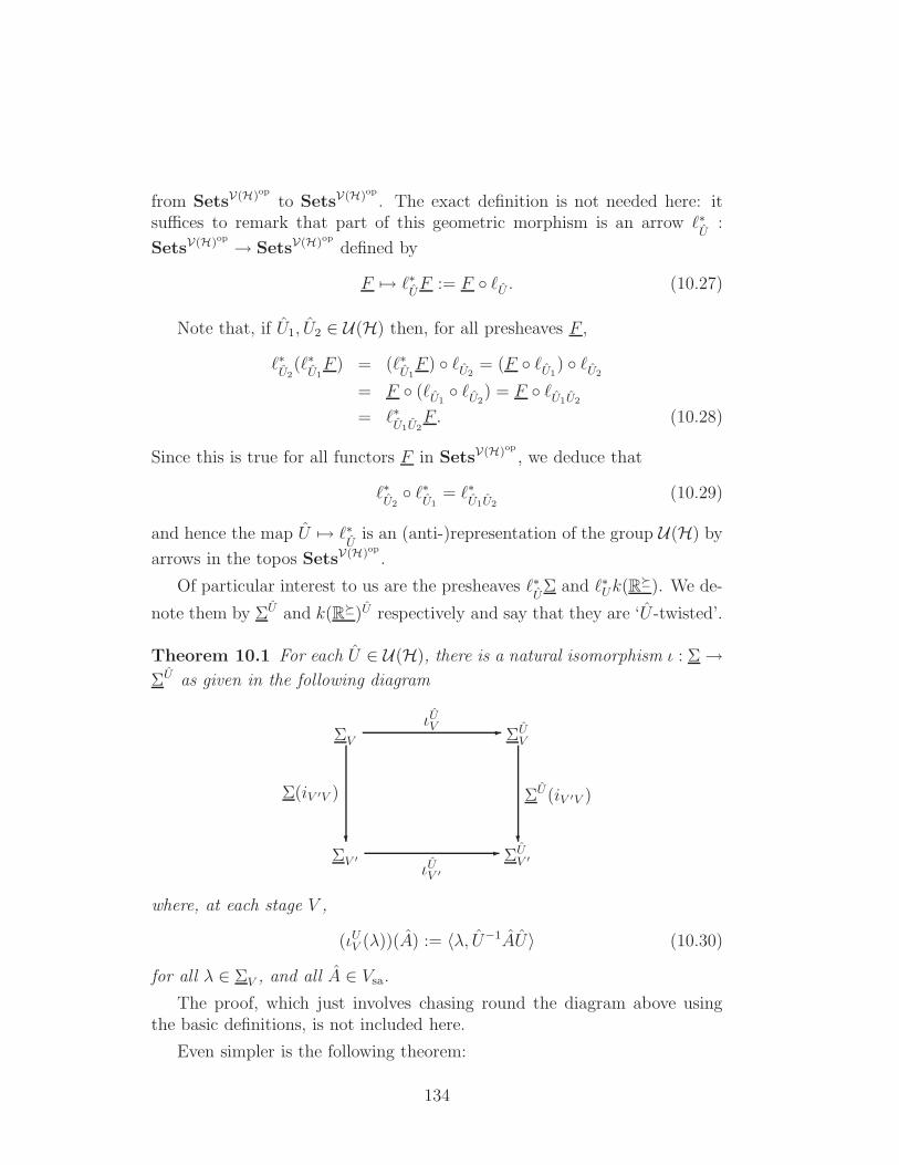
from SetsV(H)op to SetsV(H)op . The exact definition is not needed here: itsuffices to remark that part of this geometric morphism is an arrow ℓ∗
U:
SetsV(H)op → SetsV(H)op defined by
F 7→ ℓ∗UF := F ℓU . (10.27)
Note that, if U1, U2 ∈ U(H) then, for all presheaves F ,
ℓ∗U2
(ℓ∗U1F ) = (ℓ∗
U1F ) ℓU2
= (F ℓU1) ℓU2
= F (ℓU1 ℓU2
) = F ℓU1U2
= ℓ∗U1U2
F. (10.28)
Since this is true for all functors F in SetsV(H)op , we deduce that
ℓ∗U2 ℓ∗
U1= ℓ∗
U1U2(10.29)
and hence the map U 7→ ℓ∗U
is an (anti-)representation of the group U(H) by
arrows in the topos SetsV(H)op .
Of particular interest to us are the presheaves ℓ∗UΣ and ℓ∗Uk(R
). We de-
note them by ΣU and k(R)U respectively and say that they are ‘U -twisted’.
Theorem 10.1 For each U ∈ U(H), there is a natural isomorphism ι : Σ→ΣU as given in the following diagram
ΣV ′ ΣUV ′
-ιUV ′
ΣV ΣUV
-ιUV
?
Σ(iV ′V )
?
ΣU(iV ′V )
where, at each stage V ,
(ιUV (λ))(A) := 〈λ, U−1AU〉 (10.30)
for all λ ∈ ΣV , and all A ∈ Vsa.
The proof, which just involves chasing round the diagram above usingthe basic definitions, is not included here.
Even simpler is the following theorem:
134
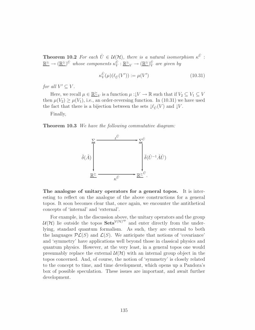
Theorem 10.2 For each U ∈ U(H), there is a natural isomorphism κU :
R → (R)U whose components κUV : RV → (R)UV are given by
κUV (µ)(ℓU(V ′)) := µ(V ′) (10.31)
for all V ′ ⊆ V .
Here, we recall µ ∈ RV is a function µ :↓V → R such that if V2 ⊆ V1 ⊆ V
then µ(V2) ≥ µ(V1), i.e., an order-reversing function. In (10.31) we have usedthe fact that there is a bijection between the sets ↓ℓU(V ) and ↓V .
Finally,
Theorem 10.3 We have the following commutative diagram:
R RU .-κU
Σ ΣU-ιU
?
δ(A)
?
δ(U−1AU)
The analogue of unitary operators for a general topos. It is inter-esting to reflect on the analogue of the above constructions for a generaltopos. It soon becomes clear that, once again, we encounter the antitheticalconcepts of ‘internal’ and ‘external’.
For example, in the discussion above, the unitary operators and the groupU(H) lie outside the topos SetsV(H)op and enter directly from the under-lying, standard quantum formalism. As such, they are external to boththe languages PL(S) and L(S). We anticipate that notions of ‘covariance’and ‘symmetry’ have applications well beyond those in classical physics andquantum physics. However, at the very least, in a general topos one wouldpresumably replace the external U(H) with an internal group object in thetopos concerned. And, of course, the notion of ‘symmetry’ is closely relatedto the concept to time, and time development, which opens up a Pandora’sbox of possible speculation. These issues are important, and await furtherdevelopment.
135
11 The Category of Systems
11.1 Background Remarks
We now return to the more general aspects of our theory, and study itsapplication to a collection of systems, each one of which may be associatedwith a different topos. For example, if S1, S2 is a pair of systems, withassociated topoi τ(S1) and τ(S2), and if S1 is a sub-system of S2, then wewish to consider how τ(S1) is related to τ(S2). Similarly, if a compositesystem is formed from a pair of systems S1, S2, what relations are therebetween the topos of the composite system and the topoi of the constituentparts?
Of course, in one sense, there is only one true ‘system’, and that is theuniverse as a whole. Concomitantly, there is just one local language, andone topos. However, in practice, the science community divides the universeconceptually into portions that are sufficiently simple to be amenable totheoretical and/or empirical discussion. Of course, this division is not unique,but it must be such that the coupling between portions is weak enough that,to a good approximation, their theoretical models can be studied in isolationfrom each other. Such an essentially isolated98 portion of the universe is calleda ‘sub-system’. By an abuse of language, sub-systems of the universe areusually called ‘systems’ (so that the universe as a whole is one super-system),and then we can talk about ‘sub-systems’ of these systems; or ‘composites’of them; or sub-systems of the composite systems, and so on.
In practice, references by physicists to systems and sub-systems99 do notgenerally signify actual sub-systems of the real universe but rather idealisa-tions of possible systems. This is what a physics lecturer means when heor she starts a lecture by saying “Consider a point particle moving in threedimensions.....”.
To develop these ideas further we need mathematical control over thesystems of interest, and their interrelations. To this end, we start by focussingon some collection, Sys, of physical systems to which a particular theory-typeis deemed to be applicable. For example, we could consider a collection ofsystems that are to be discussed using the methodology of classical physics;
98The ideal monad has no windows.99The word ‘sub-system’ does not only mean a collection of objects that is spatially
localised. One could also consider sub-systems of field systems by focussing on a justa few modes of the fields as is done, for example, in the Robertson-Walker model forcosmology. Another possibility would be to use fields localised in some fixed space, orspace-time region provided that this is consistent with the dynamics.
136
or systems to be discussed using standard quantum theory; or whatever. Forcompleteness, we require that every sub-system of a system in Sys is itself amember of Sys, as is every composite of members of Sys.
We shall assume that the systems in Sys are all associated with locallanguages of the type discussed earlier, and that they all have the same setof ground symbols which, for the purposes of the present discussion, we taketo be just Σ and R. It follows that the languages L(S), S ∈ Sys, differ fromeach other only in the set of function symbols FL(S)
(Σ,R
); i.e., the set of
physical quantities.
As a simple example of the system-dependence of the set of functionsymbols let system S1 be a point particle moving in one dimension, andlet the set of physical quantities be FL(S1)
(Σ,R
)= x, p,H. In the lan-
guage L(S1), these function-symbols represent the position, momentum, andenergy of the system respectively. On the other hand, if S2 is a parti-cle moving in three dimensions, then in the language L(S2) we could haveFL(S2)
(Σ,R
)= x, y, z, px, py, pz, H to allow for three-dimensional position
and momentum. Or, we could decide to add angular momentum as well, togive the set FL(S2)
(Σ,R
)= x, y, z, px, py, pz, Jx, Jy, Jz, H.
11.2 The Category Sys
11.2.1 The Arrows and Translations for the Disjoint Sum S1 ⊔ S2.
The use of local languages is central to our overall topos scheme, and thereforewe need to understand, in particular, (i) the relation between the languagesL(S1) and L(S2) if S1 is a sub-system of S2; and (ii) the relation betweenL(S1), L(S2) and L(S1 ⋄ S2), where S1 ⋄S2 denotes the composite of systemsS1 and S2.
These discussions can be made more precise by regarding Sys as a cate-gory whose objects are the systems.100 The arrows in Sys need to cover twobasic types of relation: (i) that between S1 and S2 if S1 is a ‘sub-system’ ofS2; and (ii) that between a composite system, S1 ⋄ S2, and its constituentsystems, S1 and S2.
This may seem straightforward but, in fact, care is needed since althoughthe idea of a ‘sub-system’ seems intuitively clear, it is hard to give a physicallyacceptable definition that is universal. However, some insight into this ideacan be gained by considering its meaning in classical physics. This is very
100To control the size of Sys we assume that the collection of objects/systems is a setrather than a more general class.
137
relevant for the general scheme since one of our main goals is to make alltheories ‘look’ like classical physics in the appropriate topos.
To this end, let S1 and S2 be classical systems whose state spaces arethe symplectic manifolds S1 and S2 respectively. If S1 is deemed to be asub-system of S2, it is natural to require that S1 is a sub-manifold of S2,i.e., S1 ⊆ S2. However, this condition cannot be used as a definition of a‘sub-system’ since the converse may not be true: i.e., if S1 ⊆ S2, this doesnot necessarily mean that, from a physical perspective, S1 could, or would,be said to be a sub-system of S2.
101
On the other hand, there are situations where being a sub-manifold clearlydoes imply being a physical sub-system. For example, suppose the statespace S of a system S is a disconnected manifold with two components S1
and S2, so that S is the disjoint union, S1
∐S2, of the sub-manifolds S1 andS2. Then it seems physically appropriate to say that the system S itself isdisconnected, and to write S = S1 ⊔ S2 where the symplectic manifolds thatrepresent the sub-systems S1 and S2 are S1 and S2 respectively.
One reason why it is reasonable to call S1 and S2 ‘sub-systems’ in thisparticular situation is that any continuous dynamical evolution of a statepoint in S ≃ S1⊔S2 will always lie in either one component or the other. Thissuggests that perhaps, in general, a necessary condition for a sub-manifoldS1 ⊆ S2 to represent a physical sub-system is that the dynamics of thesystem S2 must be such that S1 is mapped into itself under the dynamicalevolution on S2; in other words, S1 is a dynamically-invariant sub-manifoldof S2. This correlates with the idea mentioned earlier that sub-systems areweakly-coupled with each other.
However, such a dynamical restriction is not something that should becoded into the languages, L(S1) and L(S2): rather, the dynamics is to be as-sociated with the representation of these languages in the appropriate topoi.
Still, this caveat does not apply to the disjoint sum S1 ⊔ S2 of two sys-tems S1, S2, and we will assume that, in general, (i.e., not just in classi-cal physics) it is legitimate to think of S1 and S2 as being sub-systems ofS1 ⊔ S2; something that we indicate by defining arrows i1 : S1 → S1 ⊔ S2,and i2 : S2 → S1 ⊔ S2 in Sys.
To proceed further it is important to understand the connection betweenthe putative arrows in the category Sys, and the ‘translations’ of the as-
101For example, consider the diagonal sub-manifold ∆(S) ⊂ S × S of the symplecticmanifold S×S that represents the composite S ⋄S of two copies of a system S. Evidently,the states in ∆(S) correspond to the situation in which both copies of S ‘march together’.It is doubtful if this would be recognised physically as a sub-system.
138
sociated languages. The first step is to consider what can be said aboutthe relation between L(S1 ⊔ S2), and L(S1) and L(S2). All three languagesshare the same ground-type symbols, and so what we are concerned withis the relation between the function symbols of signature Σ → R in theselanguages.
By considering what is meant intuitively by the disjoint sum, it seemsplausible that each physical quantity for the system S1⊔S2 produces a phys-ical quantity for S1, and another one for S2. Conversely, specifying a pair ofphysical quantities—one for S1 and one for S2—gives a physical quantity forS1 ⊔ S2. In other words,
FL(S1⊔S2)
(Σ,R
)≃ FL(S1)
(Σ,R
)× FL(S2)
(Σ,R
)(11.1)
However, it is important not to be too dogmatic about statements of this typesince in non-classical theories new possibilities can arise that are counter tointuition.
Associated with (11.1) are the maps L(i1) : FL(S1⊔S2)
(Σ,R
)→ FL(S1)
(Σ,R
)
and L(i2) : FL(S1⊔S2)
(Σ,R
)→ FL(S2)
(Σ,R
), defined as the projection maps
of the product. In the theory of local languages, these transformations are es-sentially translations [8] of L(S1 ⊔ S2) in L(S1) and L(S2) respectively; a sit-uation that we denote L(i1) : L(S1 ⊔ S2)→ L(S1), and L(i2) : L(S1 ⊔ S2)→L(S2).
To be more precise, these operations are translations if, taking L(i1) asthe explanatory example, the map L(i1) : FL(S1⊔S2)
(Σ,R
)→ FL(S1)
(Σ,R
)is
supplemented with the following map from the ground symbols of L(S1 ⊔ S2)to those of L(S1):
L(i1)(Σ) := Σ, (11.2)
L(i1)(R) := R, (11.3)
L(i1)(1) := 1, (11.4)
L(i1)(Ω) := Ω. (11.5)
Such a translation map is then extended to all type symbols using the defi-nitions
L(i1)(T1 × T2 × · · · × Tn) = L(i1)(T1)× L(i1)(T2)× · · · × L(i1)(Tn),(11.6)
L(i1)(PT ) = P [L(i1)(T )] (11.7)
for all finite n and all type symbols T, T1, T2, . . . , Tn. This, in turn, can beextended inductively to all terms in the language. Thus, in our case, thetranslations act trivially on all the type symbols.
139
Arrows in Sys are translations. Motivated by this argument we nowturn everything around and, in general, define an arrow j : S1 → S inthe category Sys to mean that there is some physically meaningful way oftransforming the physical quantities in S to physical quantities in S1. If, forany pair of systems S1, S there is more than one such transformation, thenthere will be more than one arrow from S1 to S.
To make this more precise, let Loc denote the collection of all (small102)local languages. This is a category whose objects are the local languages, andwhose arrows are translations between languages. Then our basic assumptionis that the association S 7→ L(S) is a covariant functor from Sys to Locop,which we denote as L : Sys→ Locop.
Note that the combination of a pair of arrows in Sys exists in so far asthe associated translations can be combined.
11.2.2 The Arrows and Translations for the Composite SystemS1 ⋄ S2.
Let us now consider the composition S1 ⋄S2 of a pair of systems. In the caseof classical physics, if S1 and S2 are the symplectic manifolds that representthe systems S1 and S2 respectively, then the manifold that represents thecomposite system is the cartesian product S1 × S2. This is distinguishedby the existence of the two projection functions pr1 : S1 × S2 → S1 andpr2 : S1 × S2 → S2.
It seems reasonable to impose the same type of structure on Sys: i.e., torequire there to be arrows p1 : S1 ⋄ S2 → S1 and p2 : S1 ⋄ S2 → S2 in Sys.However, bearing in mind the definition above, these arrows p1, p2 exist if,and only if, there are corresponding translations L(p1) : L(S1)→ L(S1 ⋄ S2),and L(p2) : L(S2)→ L(S1 ⋄ S2). But there are such translations: for if A1 isa physical quantity for system S1, then L(p1)(A1) can be defined as that samephysical quantity, but now regarded as pertaining to the combined systemS1 ⋄ S2; and analogously for system S2.
103 We shall denote this translatedquantity, L(p1)(A1), by A1 ⋄ 1.
Note that we do not postulate any simple relation between FL(S1⋄S2)
(Σ,R
)
and FL(S1)
(Σ,R
)and FL(S2)
(Σ,R
); i.e., there is no analogue of (11.1) for
102This means that the collection of symbols is a set, not a more general class.103For example, if A is the energy of particle 1, then we can talk about this energy in the
combination of a pair of particles. Of course, in—for example—classical physics there isno reason why the energy of particle 1 should be conserved in the composite system, butthat, dynamical, question is a different matter.
140
combinations of systems.
The definitions above of the basic arrows suggest that we might also wantto impose the following conditions:
1. The arrows i1 : S1 → S1 ⊔ S2, and i2 : S2 → S1 ⊔ S2 are monic in Sys.
2. The arrows p1 : S1 ⋄ S2 → S1 and p2 : S1 ⋄ S2 → S2 are epic arrows inSys.
However, we do not require that S1 ∪ S2 and S1 ⋄ S2 are the co-product andproduct, respectively, of S1 and S2 in the category Sys.
11.2.3 The Concept of ‘Isomorphic’ Systems.
We also need to decide what it means to say that two systems S1 and S2
are isomorphic, to be denoted S1 ≃ S2. As with the concept of sub-system,the notion of isomorphism is to some extent a matter of definition ratherthan obvious physical structure, albeit with the expectation that isomorphicsystems in Sys will correspond to isomorphic local languages, and be repre-sented by isomorphic mathematical objects in any concrete realisation of theaxioms: for example, by isomorphic symplectic manifolds in classical physics.
To a considerable extent, the physical meaning of ‘isomorphism’ dependson whether one is dealing with actual physical systems, or idealisations ofthem. For example, an electron confined in a box in Cambridge is presumablyisomorphic to one confined in the same type of box in London, although theyare not the same physical system. On the other hand, when a lecturer says“Consider an electron trapped in a box....”, he/she is referring to an idealisedsystem.
One could, perhaps, say that an idealised system is an equivalence class(under isomorphisms) of real systems, but even working only with idealisa-tions does not entirely remove the need for the concept of isomorphism.
For example, in classical mechanics, consider the (idealised) system S ofa point particle moving in a box, and let 1 denote the ‘trivial system’ thatconsists of just a single point with no internal or external degrees of freedom.Now consider the system S ⋄ 1. In classical mechanics this is represented bythe symplectic manifold S × ∗, where ∗ is a single point, regarded as azero-dimensional manifold. However, S × ∗ is isomorphic to the manifoldS, and it is clear physically that the system S ⋄1 is isomorphic to the systemS. On the other hand, one cannot say that S ⋄ 1 is literally equal to S, sothe concept of ‘isomorphism’ needs to be maintained.
141
One thing that is clear is that if S1 ≃ S2 then FL(S1)
(Σ,R
)≃ FL(S2)
(Σ,R
),
and if any other non-empty sets of function symbols are present, then theytoo must be isomorphic.
Note that when introducing a trivial system, 1, it necessary to specify itslocal language, L(1). The set of function symbols FL(1)
(Σ,R
)is not com-
pletely empty since, in classical physics, one does have a preferred physicalquantity, which is just the number 1. If one asks what is meant in general bythe ‘number 1’ the answer is not trivial since, in the reals R, the number 1 isthe multiplicative identity. It would be possible to add the existence of sucha unit to the axioms forR but this would involve introducing a multiplicativestructure and we do not know if there might be physically interesting toposrepresentations that do not have this feature.
For the moment then, we will say that the trivial system has just a singlephysical quantity, which in classical physics translates to the number 1. Moregenerally, for the language L(1) we specify that FL(1)
(Σ,R
):= I, i.e.,
FL(1)
(Σ,R
)has just a single element, I, say. Furthermore, we add the axiom
: ∀s1∀s2, I(s1) = I(s2), (11.8)
where s1 and s2 are variables of type Σ. In fact, it seems natural to add sucha trivial quantity to the language L(S) for any system S, and from now onwe will assume that this has been done.
A related issue is that, in classical physics, if A is a physical quantity,then so is rA for any r ∈ R. This is because the set of classical quantitiesAσ : Σσ → Rσ ≃ R forms a ring whose structure derives from the ringstructure of R. It would be possible to add ring axioms for R to the languageL(S), but this is too strong, not least because, as shown earlier, it fails inquantum theory. Clearly, the general question of axioms for R needs morethought: a task for later work.
If desired, an ‘empty ’ system, 0, can be added too, with FL(0)
(Σ,R
):= ∅.
This, so called, ‘pure language’, L(0), is an initial object in the category Loc.
11.2.4 An Axiomatic Formulation of the Category Sys
Let us now summarise, and clarify, our list of axioms for a category Sys:
1. The collection Sys is a small category whose objects are the systems ofinterest (or, if desired, isomorphism classes of such systems) and whosearrows are defined as above.
Thus the fundamental property of an arrow j : S1 → S in Sys is thatit induces, and is essentially defined by, a translation L(j) : L(S) →
142
L(S1). Physically, this corresponds to the physical quantities for systemS being ‘pulled-back’ to give physical quantities for system S1.
Arrows of particular interest are those associated with ‘sub-systems’and ‘composite systems’, as discussed above.
2. The axioms for a category are satisfied because:
(a) Physically, the ability to form composites of arrows follows fromthe concept of ‘pulling-back’ physical quantities. From a math-ematical perspective, if j : S1 → S2 and k : S2 → S3, then thetranslations give functions L(j) : FL(S2)
(Σ,R
)→ FL(S1)
(Σ,R
)
and L(k) : FL(S3)
(Σ,R
)→ FL(S2)
(Σ,R
). Then clearly L(j)
L(k) : FL(S3)
(Σ,R
)→ FL(S1)
(Σ,R
), and this can thought of as
the translation corresponding to the arrow k j : S1 → S3.
The associativity of the law of arrow combination can be provedin a similar way.
(b) We add by hand a special arrow idS : S → S which is defined tocorrespond to the translation L(idS) that is given by the identitymap on FL(S)
(Σ,R
). Clearly, idS : S → S acts an an identity
morphism should.
3. For any pair of systems S1, S2, there is a disjoint sum, denoted S1⊔S2.The disjoint sum has the following properties:
(a) For all systems S1, S2, S3 in Sys:
(S1 ⊔ S2) ⊔ S3 ≃ S1 ⊔ (S2 ⊔ S3). (11.9)
(b) For all systems S1, S2 in Sys:
S1 ⊔ S2 ≃ S2 ⊔ S1. (11.10)
(c) There are arrows in Sys:
i1 : S1 → S1 ⊔ S2 and i2 : S2 → S1 ⊔ S2 (11.11)
that are associated with translations in the sense discussed in Sec-tion 11.2.1. These are associated with the decomposition
FL(S1⊔S2)
(Σ,R
)≃ FL(S1)
(Σ,R
)× FL(S2)
(Σ,R
). (11.12)
We assume that if S1, S2 belong to Sys, then Sys also contains S1⊔S2.
143
4. For any given pair of systems S1, S2, there is a composite system inSys, denoted104 S1 ⋄ S2, with the following properties:
(a) For all systems S1, S2, S3 in Sys:
(S1 ⋄ S2) ⋄ S3 ≃ S1 ⋄ (S2 ⋄ S3). (11.13)
(b) For all systems S1, S2 in Sys:
S1 ⋄ S2 ≃ S2 ⋄ S1. (11.14)
(c) There are arrows in Sys:
p1 : S1 ⋄ S2 → S1 and p2 : S1 ⋄ S2 → S2 (11.15)
that are associated with translations in the sense discussed in Sec-tion 11.2.2.
We assume that if S1, S2 belong to Sys, then Sys also contains thecomposite system S1 ⋄ S2.
5. It seems physically reasonable to add the axiom
(S1 ⊔ S2) ⋄ S ≃ (S1 ⋄ S) ⊔ (S2 ⋄ S) (11.16)
for all systems S1, S2, S. However, physical intuition can be a dangerousthing, and so, as with most of these axioms, we are not dogmatic, andfeel free to change them as new insights emerge.
6. There is a trivial system, 1, such that for all systems S, we have
S ⋄ 1 ≃ S ≃ 1 ⋄ S (11.17)
7. It may be convenient to postulate an ‘empty system’, 0, with the prop-erties
S ⋄ 0 ≃ 0 ⋄ S ≃ 0 (11.18)
S ⊔ 0 ≃ 0 ⊔ S ≃ S (11.19)
for all systems S.
Within the meaning given to arrows in Sys, 0 is a terminal object inSys. This is because the empty set of function symbols of signatureΣ→ R is a subset of any other set of function symbols of this signature.
104The product operation in a monoidal category is often written ‘⊗’. However, a differentsymbol has been used here to avoid confusion with existing usages in physics of the tensorproduct sign ‘⊗’.
144
It might seem tempting to postulate that composition laws are well-behaved with respect to arrows. Namely, if j : S1 → S2, then, for anyS, there is an arrow S1 ⋄ S → S2 ⋄ S and an arrow S1 ⊔ S → S2 ⊔ S.105
In the case of the disjoint sum, such an arrow can be easily constructed us-ing (11.12). First split the function symbols in FL(S1⊔S)
(Σ,R
)into FL(S1)
(Σ,R
)×
FL(S)
(Σ,R
)and the function symbols in FL(S2⊔S)
(Σ,R
)into FL(S2)
(Σ,R
)×
FL(S)
(Σ,R
). Since there is an arrow j : S1 → S2, there is a transla-
tion L(j) : L(S2) → L(S1), given by a mapping L(j) : FL(S2)
(Σ,R
)→
FL(S1)
(Σ,R
). Of course, then there is also a mapping L(j) × L(idS) :
FL(S2)
(Σ,R
)× FL(S)
(Σ,R
)→ FL(S1)
(Σ,R
)× FL(S)
(Σ,R
), i.e., a transla-
tion between L(S2 ⊔ S) and L(S1 ⊔ S). Since we assume that there is anarrow in Sys whenever there is a translation (in the opposite direction),there is indeed an arrow S1 ⊔ S → S2 ⊔ S.
In the case of the composition, however, this would require a translationL(S2 ⋄ S)→ L(S1 ⋄ S), and this cannot be done in general since we have noprima facie information about the set of function symbols FL(S2⋄S)
(Σ,R
).
However, if we restrict the arrows in Sys to be those associated with sub-systems, combination of systems, and compositions of such arrows, then itis easy to see that the required translations exist (the proof of this makesessential use of (11.16)).
If we make this restriction of arrows, then the axioms (11.14), (11.17–11.20), mean that, essentially, Sys has the structure of a symmetric monoidal106
category in which the monoidal product operation is ‘⋄’, and the left andright unit object is 1. There is also a monoidal structure associated with thedisjoint sum ‘⊔’, with 0 as the unit object.
We say ‘essentially’ because in order to comply with all the axioms of amonoidal category, Sys must satisfy certain additional, so-called, ‘coherence’axioms. However, from a physical perspective these are very plausible state-ments about (i) how the unit object 1 intertwines with the ⋄-operation; howthe null object intertwines with the ⊔-operation; and (iii) certain propertiesof quadruple products (and disjoint sums) of systems.
105A more accurate way of capturing this idea is to say that the operation Sys×Sys→Sys in which
〈S1, S2〉 7→ S1 ⋄ S2 (11.20)
is a bi-functor from Sys×Sys to Sys. Ditto for the operation in which 〈S1, S2〉 7→ S1⊔S2.106In the actual definition of a monoidal category the two isomorphisms in (11.17) are
separated from each other, whereas we have identified them. Further more, these iso-morphism are required to be natural. This seems a correct thing to require in our case,too.
145
A simple example of a category Sys. It might be helpful at this pointto give a simple example of a category Sys. To that end, let S denote apoint particle that moves in three dimensions, and let us suppose that S hasno sub-systems other than the trivial system 1. Then S ⋄ S is defined to bea pair of particles moving in three dimensions, and so on. Thus the objectsin our category are 1, S, S ⋄ S, . . ., S ⋄ S ⋄ · · ·S . . . where the ‘⋄’ operationis formed any finite number of times.
At this stage, the only arrows are those that are associated with theconstituents of a composite system. However, we could contemplate addingto the systems the disjoint sum S ⊔ (S ⋄ S) which is a system that is eitherone particle or two particles (but, of course, not both at the same time).And, clearly, we could extend this to S ⊔ (S ⋄ S) ⊔ (S ⋄ S ⋄ S), and so on.Each of these disjoint sums comes with its own arrows, as explained above.
Note that this particular category of systems has the property that it canbe treated using either classical physics or quantum theory.
11.3 Representations of Sys in Topoi
We assume that all the systems in Sys are to be treated with the same theorytype. We also assume that systems in Sys with the same language are to berepresented in the same topos. Then we define:107
Definition 11.1 A topos realisation of Sys is an association, φ, to eachsystem S in Sys, of a triple φ(S) = 〈ρφ,S,L(S), τφ(S)〉 where:
(i) τφ(S) is the topos in which the theory-type applied to system S is to berealised.
(ii) L(S) is the local language in Loc that is associated with S. This is notdependent on the realisation φ.
(iii) ρφ,S is a representation of the local language L(S) in the topos τφ(S).As a more descriptive piece of notation we write ρφ,S : L(S) τφ(S).The key part of this representation is the map
ρφ,S : FL(S)
(Σ,R
)→ Homτφ(S)
(Σφ,S,Rφ,S
)(11.21)
107As emphasised already, the association S 7→ L(S) is generally not one-to-one: i.e.,many systems may share the same language. Thus, when we come discuss the represen-tation of the language L(S) in a topos, the extra information about the system S is usedin fixing the representation.
146
where Σφ,S and Rφ,S are the state object and quantity-value object, re-spectively, of the representation φ in the topos τφ(S). As a convenientpiece of notation we write Aφ,S := ρφ,S(A) for all A ∈ FL(S)
(Σ,R
).
This definition is only partial; the possibility of extending it will be discussedshortly.
Now, if j : S1 → S is an arrow in Sys, then there is a translationarrow L(j) : L(S)→ L(S1). Thus we have the beginnings of a commutativediagram
S 〈ρφ,S,L(S), τφ(S)〉-φ
S1 〈ρφ,S1,L(S1), τφ(S1)〉-φ
?
j
6
?× L(j)×?
(11.22)
However, to be useful, the arrow on the right hand side of this diagramshould refer to some relation between (i) the topoi τφ(S1) and τφ(S); and (ii)the realisations ρφ,S1 : L(S1) τφ(S1) and ρφ,S : L(S) τφ(S): this is thesignificance of the two ‘?’ symbols in the arrow written ‘?× L(j)×?’.
Indeed, as things stand, Definition 11.1 says nothing about relations be-tween the topoi representations of different systems in Sys. We are particu-larly interested in the situation where there are two different systems S1 andS with an arrow j : S1 → S in Sys.
We know that the arrow j is associated with a translation L(j) : L(S)→L(S1), and an attractive possibility, therefore, would be to seek, or postulate,a ‘covering’ map φ(L(j)) : Homτφ(S)
(Σφ,S,Rφ,S
)→ Homτφ(S1)
(Σφ,S1,Rφ,S1
)
to be construed as a topos representation of the translation L(j) : L(S) →L(S1), and hence of the arrow j : S1 → S in Sys.
This raises the questions of what properties these ‘translation representa-tions’ should possess in order to justify saying that they ‘cover’ the transla-tions. A minimal requirement is that if k : S2 → S1 and j : S1 → S, then themap φ(L(j k)) : Homτφ(S)
(Σφ,S,Rφ,S
)→ Homτφ(S2)
(Σφ,S2 ,Rφ,S2
)factorises
asφ(L(j k)) = φ(L(k)) φ(L(j)). (11.23)
We also require that
φ(L(idS)) = id : Homτφ(S)
(Σφ,S,Rφ,S
)→ Homτφ(S)
(Σφ,S,Rφ,S
)(11.24)
147
for all systems S.
The conditions (11.23) and (11.24) seem eminently plausible, and theyare not particularly strong. A far more restrictive axiom would be to requirethe following diagram to commute:
FL(S1)
(Σ,R
)Homτφ(S1)
(Σφ,S1 ,Rφ,S1
)-
ρφ,S1
FL(S)
(Σ,R
)Homτφ(S)
(Σφ,S,Rφ,S
)-ρφ,S
?
L(j)
?
φ(L(j))
(11.25)
At first sight, this requirement seems very appealing. However, caution isneeded when postulating ‘axioms’ for a theoretical structure in physics. Itis easy to get captivated by the underlying mathematics and to assume,erroneously, that what is mathematically elegant is necessarily true in thephysical theory.
The translation φ(L(j)) maps an arrow from Σφ,S to Rφ,S to an arrowfrom Σφ,S1 to Rφ,S1 . Intuitively, if Σφ,S1 is a ‘much larger’ object than Σφ,S
(although since they lie in different topoi, no direct comparison is available),the translation can only be ‘faithful’ on some part of Σφ,S1 that can be iden-tified with (the ‘image’ of) Σφ,S. A concrete example of this will show up inthe treatment of composite quantum systems, see Subsection 13.3. As onemight expect, a form of entanglement plays a role here.
11.4 Classical Physics in This Form
11.4.1 The Rules so Far.
Constructing maps φ(L(j)) : Homτφ(S)
(Σφ,S,Rφ,S
)→ Homτφ(S1)
(Σφ,S1 ,Rφ,S1
)
is likely to be complicated when τφ(S) and τφ(S1) are different topoi, and sowe begin with the example of classical physics, where the topos is alwaysSets.
In general, we are interested in the relation(s) between the representationsρφ,S1 : L(S1) τφ(S1) and ρφ,S : L(S) τφ(S) that is associated with anarrow j : S1 → S in Sys. In classical physics, we only have to study therelation between the representations ρσ,S1 : L(S1) Sets and ρσ,S : L(S) Sets.
148
Let us summarise what we have said so far (with σ denoting the Sets-realisation of classical physics):
1. For any system S in Sys, a representation ρσ,S : L(S) Sets consistsof the following ingredients.
(a) The ground symbol Σ is represented by a symplectic manifold,Σσ,S := ρσ,S(Σ), that serves as the classical state space.
(b) For all systems S, the ground symbol R is represented by the realnumbers R, i.e., Rσ,S = R, where Rσ,S := ρσ,S(R).
(c) Each function symbol A : Σ → R in FL(S)
(Σ,R
)is represented
by a function Aσ,S = ρσ,S(A) : Σσ,S → R in the set of functions108
C(Σσ,S,R).
2. The trivial system is mapped to a singleton set ∗ (viewed as a zero-dimensional symplectic manifold):
Σσ,1 := ∗. (11.26)
The empty system is represented by the empty set:
Σσ,0 := ∅. (11.27)
3. Propositions about the system S are represented by (Borel) subsets ofthe state space Σσ,S .
4. The composite system S1 ⋄ S2 is represented by the Cartesian productΣσ,S1 × Σσ,S2 ; i.e.,
Σσ, S1⋄S2 ≃ Σσ,S1 × Σσ,S2 . (11.28)
The disjoint sum S1⊔S2 is represented by the disjoint union Σσ,S1
∐Σσ,S2 ;i.e.,
Σσ,S1⊔S2 ≃ Σσ,S1
∐Σσ,S2 . (11.29)
5. Let j : S1 → S be an arrow in Sys. Then
(a) There is a translation map L(j) : FL(S)
(Σ,R
)→ FL(S1)
(Σ,R
).
(b) There is a symplectic function σ(j) : Σσ,S1 → Σσ,S from the sym-plectic manifold Σσ,S1 to the symplectic manifold Σσ,S.
108In practice, these functions are required to be measurable with respect to the Borelstructures on the symplectic manifold Σσ and R. Many of the functions will also besmooth, but we will not go into such details here.
149
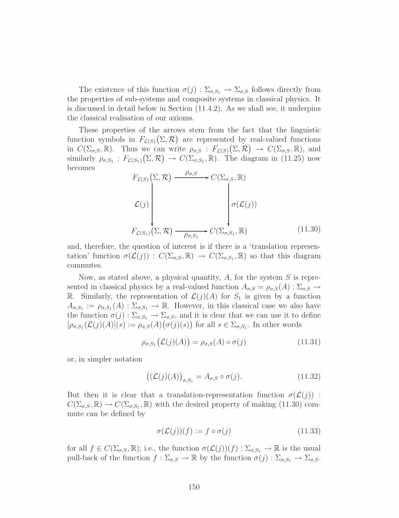
The existence of this function σ(j) : Σσ,S1 → Σσ,S follows directly fromthe properties of sub-systems and composite systems in classical physics. Itis discussed in detail below in Section (11.4.2). As we shall see, it underpinsthe classical realisation of our axioms.
These properties of the arrows stem from the fact that the linguisticfunction symbols in FL(S)
(Σ,R
)are represented by real-valued functions
in C(Σσ,S,R). Thus we can write ρσ,S : FL(S)
(Σ,R
)→ C(Σσ,S ,R), and
similarly ρσ,S1 : FL(S1)
(Σ,R
)→ C(Σσ,S1 ,R). The diagram in (11.25) now
becomes
FL(S1)
(Σ,R
)C(Σσ,S1 ,R)-
ρσ,S1
FL(S)
(Σ,R
)C(Σσ,S,R)-ρσ,S
?
L(j)
?
σ(L(j))
(11.30)
and, therefore, the question of interest is if there is a ‘translation represen-tation’ function σ(L(j)) : C(Σσ,S ,R) → C(Σσ,S1 ,R) so that this diagramcommutes.
Now, as stated above, a physical quantity, A, for the system S is repre-sented in classical physics by a real-valued function Aσ,S = ρσ,S(A) : Σσ,S →R. Similarly, the representation of L(j)(A) for S1 is given by a functionAσ,S1 := ρσ,S1(A) : Σσ,S1 → R. However, in this classical case we also havethe function σ(j) : Σσ,S1 → Σσ,S, and it is clear that we can use it to define[ρσ,S1(L(j)(A)](s) := ρσ,S(A)
(σ(j)(s)
)for all s ∈ Σσ,S1 . In other words
ρσ,S1
(L(j)(A)
)= ρσ,S(A) σ(j) (11.31)
or, in simpler notation
((L(j)(A)
)σ,S1
= Aσ,S σ(j). (11.32)
But then it is clear that a translation-representation function σ(L(j)) :C(Σσ,S ,R)→ C(Σσ,S1 ,R) with the desired property of making (11.30) com-mute can be defined by
σ(L(j))(f) := f σ(j) (11.33)
for all f ∈ C(Σσ,S ,R); i.e., the function σ(L(j))(f) : Σσ,S1 → R is the usualpull-back of the function f : Σσ,S → R by the function σ(j) : Σσ,S1 → Σσ,S.
150
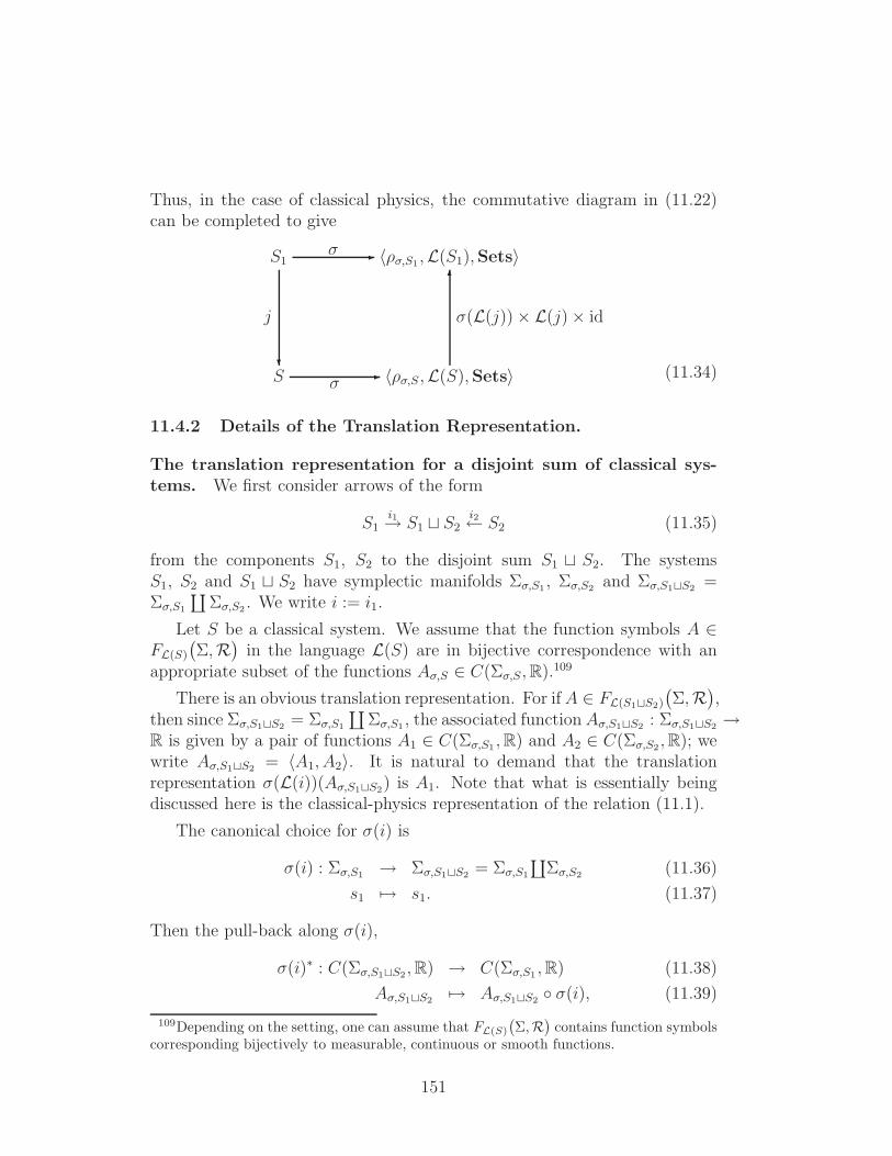
Thus, in the case of classical physics, the commutative diagram in (11.22)can be completed to give
S 〈ρσ,S ,L(S),Sets〉-σ
S1 〈ρσ,S1 ,L(S1),Sets〉-σ
?
j
6
σ(L(j))× L(j)× id
(11.34)
11.4.2 Details of the Translation Representation.
The translation representation for a disjoint sum of classical sys-tems. We first consider arrows of the form
S1i1→ S1 ⊔ S2
i2← S2 (11.35)
from the components S1, S2 to the disjoint sum S1 ⊔ S2. The systemsS1, S2 and S1 ⊔ S2 have symplectic manifolds Σσ,S1 , Σσ,S2 and Σσ,S1⊔S2 =Σσ,S1
∐Σσ,S2 . We write i := i1.
Let S be a classical system. We assume that the function symbols A ∈FL(S)
(Σ,R
)in the language L(S) are in bijective correspondence with an
appropriate subset of the functions Aσ,S ∈ C(Σσ,S,R).109
There is an obvious translation representation. For ifA ∈ FL(S1⊔S2)
(Σ,R
),
then since Σσ,S1⊔S2 = Σσ,S1
∐Σσ,S1 , the associated functionAσ,S1⊔S2 : Σσ,S1⊔S2 →
R is given by a pair of functions A1 ∈ C(Σσ,S1 ,R) and A2 ∈ C(Σσ,S2 ,R); wewrite Aσ,S1⊔S2 = 〈A1, A2〉. It is natural to demand that the translationrepresentation σ(L(i))(Aσ,S1⊔S2) is A1. Note that what is essentially beingdiscussed here is the classical-physics representation of the relation (11.1).
The canonical choice for σ(i) is
σ(i) : Σσ,S1 → Σσ,S1⊔S2 = Σσ,S1
∐Σσ,S2 (11.36)
s1 7→ s1. (11.37)
Then the pull-back along σ(i),
σ(i)∗ : C(Σσ,S1⊔S2 ,R) → C(Σσ,S1 ,R) (11.38)
Aσ,S1⊔S2 7→ Aσ,S1⊔S2 σ(i), (11.39)
109Depending on the setting, one can assume that FL(S)
(Σ,R
)contains function symbols
corresponding bijectively to measurable, continuous or smooth functions.
151
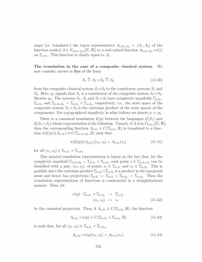
maps (or ‘translates’) the topos representative Aσ,S1⊔S2 = 〈A1, A2〉 of thefunction symbol A ∈ FL(S1⊔S2)
(Σ,R
)to a real-valued function Aσ,S1⊔S2 σ(i)
on Σσ,S1 . This function is clearly equal to A1.
The translation in the case of a composite classical system. Wenow consider arrows in Sys of the form
S1p1← S1 ⋄ S2
p2→ S2 (11.40)
from the composite classical system S1⋄S2 to the constituent systems S1 andS2. Here, p1 signals that S1 is a constituent of the composite system S1 ⋄ S2,likewise p2. The systems S1, S2 and S1 ⋄ S2 have symplectic manifolds Σσ,S1 ,Σσ,S2 and Σσ,S1⋄S2 = Σσ,S1 × Σσ,S2 , respectively; i.e., the state space of thecomposite system S1 ⋄ S2 is the cartesian product of the state spaces of thecomponents. For typographical simplicity in what follows we denote p := p1.
There is a canonical translation L(p) between the languages L(S1) andL(S1 ⋄ S2) whose representation is the following. Namely, ifA is in FL(S1)
(Σ,R
),
then the corresponding function Aσ,S1 ∈ C(Σσ,S1 ,R) is translated to a func-tion σ(L(p))(Aσ,S1) ∈ C(Σσ,S1⋄S2 ,R) such that
σ(L(p))(Aσ,S1)(s1, s2) = Aσ,S1(s1) (11.41)
for all (s1, s2) ∈ Σσ,S1 × Σσ,S2 .
This natural translation representation is based on the fact that, for thesymplectic manifold Σσ,S1⋄S2 = Σσ,S1 × Σσ,S2 , each point s ∈ Σσ,S1⋄S2 can beidentified with a pair, (s1, s2), of points s1 ∈ Σσ,S1 and s2 ∈ Σσ,S2 . This ispossible since the cartesian product Σσ,S1×Σσ,S2 is a product in the categorialsense and hence has projections Σσ,S1 ← Σσ,S1 × Σσ,S2 → Σσ,S2 . Then thetranslation representation of functions is constructed in a straightforwardmanner. Thus, let
σ(p) : Σσ,S1 × Σσ,S2 → Σσ,S1
(s1, s2) 7→ s1 (11.42)
be the canonical projection. Then, if Aσ,S1 ∈ C(Σσ,S1 ,R), the function
Aσ,S1 σ(p) ∈ C(Σσ,S1 × Σσ,S2 ,R) (11.43)
is such that, for all (s1, s2) ∈ Σσ,S1 × Σσ,S2 ,
Aσ,S1 σ(p)(s1, s2) = Aσ,S1(s1). (11.44)
152
Thus we can define
σ(L(p))(Aσ,S1) := Aσ,S1 σ(p). (11.45)
Clearly, σ(L(p))(Aσ,S1) can be seen as the representation of the functionsymbol A ⋄ 1 ∈ FL(S1⋄S2)
(Σ,R
).
12 Theories of Physics in a General Topos
12.1 The Pull-Back Operations
12.1.1 The Pull-Back of Physical Quantities.
Motivated by the above, let us try now to see what can be said about thescheme in general. Basically, what is involved is the topos representation oftranslations of languages. To be more precise, let j : S1 → S be an arrow inSys, so that there is a translation L(j) : L(S)→ L(S1) defined by the trans-lation function L(j) : FL(S)
(Σ,R
)→ FL(S1)
(Σ,R
). Now suppose that the
systems S and S1 are represented in the topoi τφ(S) and τφ(S1) respectively.Then, in these representations, the function symbols of signature Σ → Rin L(S) and L(S1) are represented by elements of Homτφ(S)
(Σφ,S,Rφ,S
)and
Homτφ(S1)
(Σφ,S1 ,Rφ,S1
)respectively.
Our task is to find a function
φ(L(j)) : Homτφ(S)
(Σφ,S,Rφ,S
)→ Homτφ(S1)
(Σφ,S1 ,Rφ,S1
)(12.1)
that can be construed as the topos representation of the translation L(j) :L(S)→ L(S1), and hence of the arrow j : S1 → S in Sys. We are particularlyinterested in seeing if φ(L(j)) can be chosen so that the following diagram,(see (11.25)) commutes:
FL(S1)
(Σ,R
)Homτφ(S1)
(Σφ,S1 ,Rφ,S1
)-
ρφ,S1
FL(S)
(Σ,R
)Homτφ(S)
(Σφ,S,Rφ,S
)-ρφ,S
?
L(j)
?
φ(L(j))
(12.2)
However, as has been emphasised already, it is not clear that one should ex-pect to find a function φ(L(j)) : Homτφ(S)
(Σφ,S,Rφ,S
)→ Homτφ(S1)
(Σφ,S1 ,Rφ,S1
)
153
with this property. The existence and/or properties of such a function willbe dependent on the theory-type, and it seems unlikely that much can besaid in general about the diagram (12.2). Nevertheless, let us see how far wecan get in discussing the existence of such a function in general.
Thus, if µ ∈ Homτφ(S)
(Σφ,S,Rφ,S
), the critical question is if there is some
‘natural’ way whereby this arrow can be ‘pulled-back’ to give an elementφ(L(j))(µ) ∈ Homτφ(S1)
(Σφ,S1,Rφ,S1
).
The first pertinent remark is that µ is an arrow in the topos τφ(S), whereasthe sought-for pull-back will be an arrow in the topos τφ(S1), and so we needa mechanism for getting from one topos to the other (this problem, of course,does not arise in classical physics since the topos of every representation isalways Sets).
The obvious way of implementing this change of topos is via some functor,τφ(j) from τφ(S) to τφ(S1). Indeed, given such a functor, an arrow µ : Σφ,S →Rφ,S in τφ(S) is transformed to the arrow
τφ(j)(µ) : τφ(j)(Σφ,S)→ τφ(j)(Rφ,S) (12.3)
in τφ(S1).
To convert this to an arrow from Σφ,S1 to Rφ,S1, we need to supplement(12.3) with a pair of arrows φ(j), βφ(j) in τφ(S1) to get the diagram:
Σφ,S1 Rφ,S1
τφ(j)(Σφ,S) τφ(j)(Rφ,S)-τφ(j)(µ)
6φ(j)
?
βφ(j)
(12.4)
The pull-back, φ(L(j))(µ) ∈ Homτφ(S1)
(Σφ,S1 ,Rφ,S1
), with respect to these
choices can then be defined as
φ(L(j))(µ) := βφ(j) τφ(j)(µ) φ(j). (12.5)
It follows that a key part of the construction of a topos representation, φ, ofSys will be to specify the functor τφ(j) from τφ(S) to τφ(S1), and the arrowsφ(j) : Σφ,S1 → τφ(j)(Σφ,S) and βφ(j) : τφ(j)(Rφ,S) → Rφ,S1 in the toposτφ(S1). These need to be defined in such a way as to be consistent with achain of arrows S2 → S1 → S.
When applied to the representative Aφ,S : Σφ,S → Rφ,S of a physicalquantity A ∈ FL(S)
(Σ,R
), the diagram (12.4) becomes (augmented with the
154
upper half)
Σφ,S1 Rφ,S1-
φ(L(j))(Aφ,S)
τφ(j)(Σφ,S) τφ(j)(Rφ,S)-
6φ(j)
?
βφ(j)
τφ(j)(Aφ,S)
Σφ,S Rφ,S-Aφ,S
?
τφ(j)
?
τφ(j)
(12.6)
The commutativity of (12.2) would then require
φ(L(j))(Aφ,S) = (L(j)A)φ,S1 (12.7)
or, in a more expanded notation,
φ(L(j)) ρφ,S = ρφ,S1 L(j), (12.8)
where both the left hand side and the right hand side of (12.8) are mappingsfrom FL(S)
(Σ,R
)to Homτφ(S1)
(Σφ,S1,Rφ,S1
).
Note that the analogous diagram in classical physics is simply
Σσ,S1 R-σ(L(j))(Aσ,S)
Σσ,S R-Aσ,S
6σ(j)
?id
(12.9)
and the commutativity/pull-back condition (12.7) becomes
σ(L(j))(Aσ,S) = (L(j)A)φ,S1 (12.10)
which is satisfied by virtue of (11.33).
It is clear from the above that the arrow φ(j) : Σφ,S1 → τφ(j)(Σφ,S) canbe viewed as the topos analogue of the map σ(j) : Σσ,S1 → Σσ,S that arisesin classical physics whenever there is an arrow j : S1 → S.
12.1.2 The Pull-Back of Propositions.
More insight can be gained into the nature of the triple 〈τφ(j), φ(j), βφ(j)〉by considering the analogous operation for propositions. First, consider an
155
arrow j : S1 → S in Sys in classical physics. Associated with this there is (i)a translation L(j) : L(S) → L(S1); (ii) an associated translation mappingL(j) : FL(S)
(Σ,R
)→ FL(S1)
(Σ,R
); and (iii) a symplectic function σ(j) :
Σσ,S1 → Σσ,S.
Let K be a (Borel) subset of the state space, Σσ,S ; hence K representsa proposition about the system S. Then σ(j)∗(K) := σ(j)−1(K) is a subsetof Σσ,S1 and, as such, represents a proposition about the system S1. Wesay that σ(j)∗(K) is the pull-back to Σσ,S1 of the S-proposition representedby K. The existence of such pull-backs is part of the consistency of therepresentation of propositions in classical mechanics, and it is important tounderstand what the analogue of this is in our topos scheme.
Consider the general case with the two systems S1, S as above. Then letK be a proposition, represented as a sub-object of Σφ,S, with a monic arrowiK : K → Σφ,S. The question now is if the triple 〈τφ(j), φ(j), βφ(j)〉 can beused to pull K back to give a proposition in τ(S1), i.e., a sub-object of Σφ,S1?
The first requirement is that the functor τφ(j) : τφ(S) → τφ(S1) shouldpreserve monics. In this case, the monic arrow iK : K → Σφ,S in τφ(S) istransformed to the monic arrow
τφ(j)(iK) : τφ(j)(K) → τφ(j)(Σφ,S) (12.11)
in τφ(S1); thus τφ(j)(K) is a sub-object of τφ(j)(Σφ,S) in τφ(S1). It is aproperty of a topos that the pull-back of a monic arrow is monic ; i.e., ifM → Y is monic, and if ψ : X → Y , then ψ−1(M) is a sub-object of X.Therefore, in the case of interest, the monic arrow τφ(j)(iK) : τφ(j)(K) →τφ(j)(Σφ,S) can be pulled back along φ(j) : Σφ,S1 → τφ(j)(Σφ,S) (see diagram(12.6)) to give the monic φ(j)−1(τφ(j)(K)) ⊆ Σφ,S1 . This is a candidate forthe pull-back of the proposition represented by the sub-object K ⊆ Σφ,S.
In conclusion, propositions can be pulled-back provided that the functorτφ(j) : τφ(S) → τφ(S1) preserves monics. A sufficient way of satisfying thisrequirement is for τφ(j) to be left-exact. However, this raises the question of“where do left-exact functors come from?”.
12.1.3 The Idea of a Geometric Morphism.
It transpires that there is a natural source of left-exact functors, via theidea of a geometric morphism. This fundamental concept in topos theory isdefined as follows [56].
Definition 12.1 A geometric morphism φ : F → E between topoi F and Eis a pair of functors φ∗ : E → F and φ∗ : F → E such that
156
(i) φ∗ ⊣ φ∗, i.e., φ∗ is left adjoint to φ∗;
(ii) φ∗ is left exact, i.e., it preserves all finite limits.
The morphism φ∗ : E → F is called the inverse image part of the geometricmorphism ϕ; φ∗ : F → E is called the direct image part.
Geometric morphisms are very important because they are the toposequivalent of continuous functions. More precisely, if X and Y are topolog-ical spaces, then any continuous function f : X → Y induces a geometricmorphism between the topoi Sh(X) and Sh(Y ) of sheaves on X and Y re-spectively. In practice, just as the arrows in the category of topologicalspaces are continuous functions, so in any category whose objects are topoi,the arrows are normally defined to be geometric morphisms. In our case,as we shall shortly see, all the examples of left-exact functors that arise inthe quantum case do, in fact, come from geometric morphisms. For thesereasons, from now on we will postulate that any arrows between our topoiarise from geometric morphisms.
One central property of a geometric morphism is that it preserves expres-sions written in terms of geometric logic. This greatly enhances the attrac-tiveness of assuming from the outset that the internal logic of the systemlanguages, L(S), is restricted to the sub-logic afforded by geometric logic.
En passant, another key result for us is the following theorem ([56] p359):
Theorem 12.1 If ϕ : C → D is a functor between categories C and D, thenit induces a geometric morphism (also denoted ϕ)
ϕ : SetsCop → SetsD
op
(12.12)
for which the functor ϕ∗ : SetsDop → SetsC
op
takes a functor F : D → Setsto the functor
ϕ∗(F ) := F ϕop (12.13)
from C to Sets.
In addition, ϕ∗ has a left adjoint ϕ!; i.e., ϕ! ⊣ ϕ∗.
We will use this important theorem in several crucial places.
12.2 The Topos Rules for Theories of Physics
We will now present our general rules for using topos theory in the mathe-matical representation of physical systems and their theories.
157
Definition 12.2 The category M(Sys) is the following:
1. The objects ofM(Sys) are the topoi that are to be used in representingthe systems in Sys.
2. The arrows from τ1 to τ2 are defined to be the geometric morphismsfrom τ2 to τ1. Thus the inverse part, ϕ∗, of an arrow ϕ∗ : τ1 → τ2 is aleft-exact functor from τ1 to τ2.
Definition 12.3 The rules for using topos theory are as follows:
1. A topos realisation, φ, of Sys in M(Sys) is an assignment, to eachsystem S in Sys, of a triple φ(S) = 〈ρφ,S,L(S), τφ(S)〉 where:
(a) τφ(S) is the topos in M(Sys) in which the physical theory ofsystem S is to be realised.
(b) L(S) is the local language that is associated with S. This is inde-pendent of the realisation, φ, of Sys inM(Sys).
(c) ρφ,S : L(S) τφ(S) is a representation of the local language L(S)in the topos τφ(S).
(d) In addition, for each arrow j : S1 → S in Sys there is a triple〈τφ(j),φ(j), βφ(j)〉 that interpolates between ρφ,S : L(S) τφ(S)and ρφ,S1 : L(S1) τφ(S1); for details see below.
2. (a) The representations, ρφ,S(Σ) and ρφ,S(R), of the ground symbols Σand R in L(S) are denoted Σφ,S and Rφ,S, respectively. They areknown as the ‘state object’ and ‘quantity-value object’ in τφ(S).
(b) The representation by ρφ,S of each function symbol A : Σ→R ofthe system S is an arrow, ρφ,S(A) : Σφ,S →Rφ,S in τφ(S); we willusually denote this arrow as Aφ,S : Σφ,S →Rφ,S.
(c) Propositions about the system S are represented by sub-objectsof Σφ,S. These will typically be of the form A−1
φ,S(Ξ), where Ξ is asub-object of Rφ,S.
110
3. Generally, there are no ‘microstates’ for the system S; i.e., no globalelements (arrows 1 → Σφ,S) of the state object Σφ,S; or, if there areany, they may not be enough to determine Σφ,S as an object in τφ(S).
110Here, A−1φ,S(Ξ) denotes the sub-object of Σφ,S whose characteristic arrow is χΞ Aφ,S :
Σφ,S → Ωτφ(S), where χΞ : Rφ,S → Ωτφ(S) is the characteristic arrow of the sub-object Ξ.
158
Instead, the role of a state is played by a ‘truth sub-object’ T ofPΣφ,S.
111 If J ∈ Sub(Σφ,S) ≃ Γ(PΣφ,S), the ‘truth of the proposi-tion represented by J ’ is defined to be
ν(J ∈ T
)= [[ J ∈ T ]]φ 〈pJq, pTq〉 (12.14)
See Section 6.2 for full information on the idea of a ‘truth object’.Alternatively, one may use pseudo-states rather than truth objects, inwhich case the relevant truth values are of the form ν(w ⊆ J).
4. There is a ‘unit object’ 1M(Sys) in M(Sys) such that if 1Sys denotesthe trivial system in Sys then, for all topos realisations φ,
τφ(1Sys) = 1M(Sys). (12.15)
Motivated by the results for quantum theory (see Section 13.2), wepostulate that the unit object 1M(Sys) in M(Sys) is the category ofsets:
1M(Sys) = Sets. (12.16)
5. To each arrow j : S1 → S in Sys, we have the following:
(a) There is a translation L(j) : L(S) → L(S1). This is speci-fied by a map between function symbols: L(j) : FL(S)
(Σ,R
)→
FL(S1)
(Σ,R
).
(b) With the translation L(j) : FL(S)
(Σ,R
)→ FL(S1)
(Σ,R
)there is
associated a corresponding function
φ(L(j)) : Homτφ(S)
(Σφ,S,Rφ,S
)→ Homτφ(S1)
(Σφ,S1 ,Rφ,S1
).
(12.17)These may, or may not, fit together in the commutative diagram:
FL(S1)
(Σ,R
)Homτφ(S1)
(Σφ,S1 ,Rφ,S1
)-
ρφ,S1
FL(S)
(Σ,R
)Homτφ(S)
(Σφ,S,Rφ,S
)-ρφ,S
?
L(j)
?
φ(L(j))
(12.18)
111In classical physics, the truth object corresponding to a micro-state s is the collectionof all propositions that are true in the state s.
159
(c) The function φ(L(j)) : Homτφ(S)
(Σφ,S,Rφ,S
)→ Homτφ(S1)
(Σφ,S1 ,Rφ,S1
)
is built from the following ingredients. For each topos realisationφ, there is a triple 〈νφ(j), φ(j), βφ(j)〉 where:
(i) νφ(j) : τφ(S1)→ τφ(S) is a geometric morphism; i.e., an arrowin the category M(Sys) (thus νφ(j)
∗ : τφ(S) → τφ(S1) is leftexact).
N.B. To simplify the notation a little we will denote νφ(j)∗
by τφ(j). This is sensible in so far as, for the most part, onlythe inverse part of νφ(j) will be used in our constructions.
(ii) φ(j) : Σφ,S1 → τφ(j)(Σφ,S
)is an arrow in the topos τφ(S1).
(iii) βφ(j) : τφ(j)(Rφ,S
)→Rφ,S1 is an arrow in the topos τφ(S1).
These fit together in the diagram
Σφ,S1 Rφ,S1-
φ(L(j))(Aφ,S)
τφ(j)(Σφ,S) τφ(j)(Rφ,S)-
6φ(j)
?
βφ(j)
τφ(j)(Aφ,S)
Σφ,S Rφ,S-Aφ,S
?
τφ(j)
?
τφ(j)
(12.19)
The arrows φ(j) and βφ(j) should behave appropriately undercomposition of arrows in Sys.
The commutativity of the diagram (12.18) is equivalent to therelation
φ(L(j))(Aφ,S) = [L(j)(A)]φ,S1 (12.20)
for allA ∈ FL(φ,S)
(Σ,R
). As we keep emphasising, the satisfaction
or otherwise of this relation will depend on the theory-type and,possibly, the representation φ.
(d) If a proposition in τφ(S) is represented by the monic arrow, K →Σφ,S, the ‘pull-back’ of this proposition to τφ(S1) is defined to beφ(j)−1
(τφ(j)(K)
)⊆ Σφ,S1 .
6. (a) If S1 is a sub-system of S, with an associated arrow i : S1 → Sin Sys then, in the diagram in (12.19), the arrow φ(j) : Σφ,S1 →τφ(j)(Σφ,S) is a monic arrow in τφ(S1).
160
In other words, Σφ,S1 is a sub-object of τφ(j)(Σφ,S), which is de-noted
Σφ,S1 ⊆ τφ(j)(Σφ,S). (12.21)
We may also want to conjecture
Rφ,S1 ≃ τφ(j)(Rφ,S
). (12.22)
(b) Another possible conjecture is the following: if j : S1 → S isan epic arrow in Sys, then, in the diagram in (12.19), the arrowφ(j) : Σφ,S1 → τφ(j)(Σφ,S) is an epic arrow in τφ(S1).
In particular, for the epic arrow p1 : S1⋄S2 → S1, the arrow φ(p1) :Σφ,S1⋄S2 → τφ
(Σφ,S1
)is an epic arrow in the topos τφ(S1 ⋄ S2).
One should not read Rule 2. above as implying that the choice of thestate object and quantity-value object are unique for any given system S.These objects would at best be selected only up to isomorphism in the toposτ(S). Such morphisms in the τ(S)112 can be expected to play a key rolein developing the topos analogue of the important idea of a symmetry, orcovariance transformation of the theory.
In the example of classical physics, for all systems we have τ(S) = Setsand Σσ,S is a symplectic manifold, and the collection of all symplectic man-ifolds is a category. It would be elegant if we could assert that, in general,for a given theory-type the possible state objects in a given topos τ formthe objects of an internal category in τ . However, to make such a statementwould require a general theory of state-objects and, at the moment, we donot have such a thing.
From a more conceptual viewpoint we note that the ‘similarity’ of ouraxioms to those of standard classical physics is reflected in the fact that(i) physical quantities are represented by arrows Aφ,S : Σφ,S → Rφ,S; (ii)propositions are represented by sub-objects of Σφ,S; and (iii) propositionsare assigned truth values. Thus any theory satisfying these axioms ‘looks’like classical physics, and has an associated neo-realist interpretation.
112Care is needed not to confuse morphisms in the topos τ(S) with morphisms in thecategoryM(Sys) of topoi. An arrow from the object τ(S) to itself in the categoryM(Sys)is a geometric morphism in the topos τ(S). However, not every arrow in τ(S) need arise inthis way, and an important role can be expected to be played by arrows of this second type.A good example is when τ(S) is the category of sets, Sets. Typically, τφ(j) : Sets→ Sets
is the identity, but there are many morphisms from an object O in Sets to itself: they arejust the functions from O to O.
161
13 The General Scheme applied to Quantum
Theory
13.1 Background Remarks
We now want to study the extent to which our ‘rules’ apply to the toposrepresentation of quantum theory.
For a quantum system with (separable) Hilbert space H, the appropriatetopos (what we earlier called τφ(S)) is SetsV(H)op : the category of presheavesover the category (actually, partially-ordered set) V(H) of unital, abelian vonNeumann sub-algebras of the algebra, B(H), of bounded operators on H.
A particularly important object in SetsV(H)op is the spectral presheaf Σ,where, for each V , ΣV is defined to be the Gel’fand spectrum of the abelianalgebra V . The sub-objects of Σ can be identified as the topos representationsof propositions, just as the subsets of S represent propositions in classicalphysics.
In Sections 8 and 9, several closely related choices for a quantity-valueobject Rφ in SetsV(H)op were discussed. In order to keep the notation sim-pler, we concentrate here on the presheaf R of real-valued, order-reversingfunctions. All results hold analogously if the presheaf R↔ (which we actuallyprefer for giving a better physical interpretation) is used.113
Hence, physical quantities A : Σ → R, which correspond to self-adjointoperators A, are represented by natural transformations/arrows δo(A) : Σ→R. The mapping A 7→ δo(A) is injective. For brevity, we write δ(A) :=δo(A).114
13.2 The Translation Representation for a Disjoint Sumof Quantum Systems
Let Sys be a category whose objects are systems that can be treated usingquantum theory. Let L(S) be the local language of a system S in Sys whosequantum Hilbert space is denoted HS. We assume that to each functionsymbol, A : Σ → R, in L(S) there is associated a self-adjoint operator
113Since the construction of the arrows δ(A) : Σ → R↔ involves both inner and outerdaseinisation, we would have double work with the notation, which we avoid here.
114Note that this is not the same as the convention used earlier, where δ(A) denoted adifferent natural transformation!
162
A ∈ B(HS),115 and that the map
FL(S)
(Σ,R
)→ B(H)sa (13.1)
A 7→ A (13.2)
is injective (but not necessarily surjective, as we will see in the case of adisjoint sum of quantum systems).
We consider first arrows of the form
S1i1→ S1 ⊔ S2
i2← S2 (13.3)
from the components S1, S2 to a disjoint sum S1 ⊔ S2; for convenience wewrite i := i1. The systems S1, S2 and S1 ⊔ S2 have the Hilbert spaces H1,H2 and H1 ⊕H2, respectively.
As always, the translation L(i) goes in the opposite direction to the arrowi, so
L(i) : FL(S1⊔S2)
(Σ,R
)→ FL(S1)
(Σ,R
). (13.4)
Then our first step is find an ‘operator translation’ from the relevant self-adjoint operators in H1 ⊕H2 to those in H1,
To do this, let A be a function symbol in FL(S1⊔S2)
(Σ,R
). In Section
11.2.1, we argued that FL(S1⊔S2)
(Σ,R
)≃ FL(S1)
(Σ,R
)× FL(S2)
(Σ,R
)(as
in (11.1)), and hence we introduce the notation A = 〈A1, A2〉, where A1 ∈FL(S1)
(Σ,R
)and A2 ∈ FL(S2)
(Σ,R
). It is then natural to assume that
the quantisation scheme is such that the operator, A, on H1 ⊕ H2 can bedecomposed as A = A1 ⊕ A2, where the operators A1 and A2 are definedon H1 and H2 respectively, and correspond to the function symbols A1 andA2.
116 Then the obvious operator translation is A 7→ A1 ∈ B(H1)sa.
We now consider the general rules in the Definition 12.2 and see to whatextent they apply in the example of quantum theory.
1. As we have stated several times, the topos τφ(S) associated with aquantum system S is
τφ(S) = SetsV(HS)op . (13.5)
Thus (i) the objects of the categoryM(Sys) are topoi of the form SetsV(HS)op,S ∈ Ob(Sys); and (ii) the arrows between two topoi are defined to be ge-ometric morphisms. In particular, to each arrow j : S1 → S in Sys there
115More specifically, one could postulate that the elements of FL(S)
(Σ,R
)are associated
with self-adjoint operators in some unital von Neumann sub-algebra of B(HS).116It should be noted that our scheme does not use all the self-adjoint operators on the
direct sum H1 ⊕H2: only the ‘block diagonal’ operators of the form A = A1 ⊕ A2 arise.
163
must correspond a geometric morphism νφ(j) : τφ(S1) → τφ(S) with asso-ciated left-exact functor τφ(j) := νφ(j)
∗ : τφ(S) → τφ(S1). Of course, theexistence of these functors in the quantum case has yet to be shown.
2. The realisation ρφ,S : L(S) τφ(S) of the language L(S) in the toposτφ(S) is given as follows. First, we define the state object Σφ,S to be thespectral presheaf, ΣV(HS), over V(HS), the context category of B(HS). To
keep the notation brief, we will denote117 ΣV(HS) as ΣHS .
Furthermore, we define the quantity-value object, Rφ,S, to be the presheafR HS that was defined in Section 8 . Finally, we define
Aφ,S := δ(A), (13.6)
for all A ∈ FL(S)
(Σ,R
). Here δ(A) : ΣHS → RHS is constructed using the
Gel’fand transforms of the (outer) daseinisation of A, for details see later.
3. The truth object T |ψ〉 corresponding to a pure state |ψ〉 was discussedin Section 6.3. Alternatively, we have the pseudo-state w |ψ〉.
4. Let H = |C be the one-dimensional Hilbert space, corresponding tothe trivial quantum system 1. There is exactly one abelian sub-algebra ofB( |C) ≃ |C, namely |C itself. This leads to
τφ(1Sys) = Sets∗ ≃ Sets = 1M(Sys). (13.7)
5. Let A ∈ FL(S1⊔S2)
(Σ,R
)be a function symbol for the system S1 ⊔ S2.
Then, as discussed above, A is of the form A = 〈A1, A2〉 (compare equation(11.1)), which corresponds to a self-adjoint operator A1⊕A2 ∈ B(H1⊕H2)sa.
The topos representation of A is the natural transformation δ(〈A1, A2〉) :ΣH1⊕H2 → R H1⊕H2 , which is defined at each stage V ∈ Ob(V(H1 ⊕H2)) as
δ(〈A1, A2〉)V : ΣH1⊕H2V → R H1⊕H2
V
λ 7→ V ′ 7→ 〈λ|V ′ , δ(A1 ⊕ A2)V ′〉 | V ′ ⊆ V (13.8)
where the right hand side (13.8) denotes an order-reversing function.
We will need the following:
Lemma 13.1 Let A1⊕A2 ∈ B(H1⊕H2)sa, and let V = V1⊕V2 ∈ Ob(V(H1 ⊕H2))such that V1 ∈ Ob(V(H1)) and V2 ∈ Ob(V(H2)). Then
δ(A1 ⊕ A2)V = δ(A1)V1 ⊕ δ(A2)V2 . (13.9)
117Presheaves are always denoted by symbols that are underlined.
164
Proof. Every projection Q ∈ V is of the form Q = Q1 ⊕ Q2 for uniqueprojections Q1 ∈ P(H1) and Q2 ∈ P(H2). Let P ∈ P(H) be of the form
P = P1 ⊕ P2 such that P1 ∈ P(H1) and P2 ∈ P(H1). The largest projection
in V smaller than or equal to P , i.e., the inner daseinisation of P to V , is
δi(P )V = Q1 ⊕ Q2, (13.10)
where Q1 ∈ P(V1) is the largest projection in V1 smaller than or equal to P1,and Q2 ∈ P(V2) is the largest projection in V2 smaller than or equal to P2,so
δi(P )V = δ(P1)V1 ⊕ δ(P2)V2. (13.11)
This implies δ(A ⊕ B)V = δ(A)V1 ⊕ δ(B)V2, since (outer) daseinisation of aself-adjoint operator just means inner daseinisation of the projections in itsspectral family, and all the projections in the spectral family of A⊕ B are ofthe form P = P1 ⊕ P2.
As discussed in Section 12, in order to mimic the construction that wehave in the classical case, we need to pull back the arrow/natural transfor-mation δ(〈A1, A2〉) : ΣH1⊕H2 → R H1⊕H2 to obtain an arrow from ΣH1 toR H1 . Since we decided that the translation on the level of operators sendsA1 ⊕ A2 to A1, we expect that this arrow from ΣH1 to R H1 is δ(A1). Wewill now show how this works.
The presheaves ΣH1⊕H2 and ΣH1 lie in different topoi, and in order to‘transform’ between them we need we need a (left-exact) functor from thetopos SetsV(H1⊕H2)opto the topos SetsV(H1)op : this is the functor τφ(j) :τφ(S) → τφ(S1) in (12.19). One natural place to look for such a functoris as the inverse-image part of a geometric morphism from SetsV(H1)op toSetsV(H1⊕H2)op . According to Theorem 12.1, one source of such a geometricmorphism, µ, is a functor
m : V(H1)→ V(H1 ⊕H2), (13.12)
and the obvious choice for this is
m(V ) := V ⊕ |C1H2 (13.13)
for all V ∈ Ob(V(H1)). This function from Ob(V(H1)) to Ob(V(H1 ⊕H2))is clearly order preserving, and hence m is a genuine functor.
Let µ : SetsV(H1)op → SetsV(H1⊕H2)op denote the geometric morphisminduced by m. The inverse-image functor of µ is given by
µ∗ : SetsV(H1⊕H2)op → SetsV(H1)op (13.14)
F 7→ F mop. (13.15)
165
This means that, for all V ∈ Ob(V(H1)), we have
(µ∗FH1⊕H2)V = FH1⊕H2
m(V ) = FH1⊕H2
V⊕|C1H2
. (13.16)
For example, for the spectral presheaf we get
(µ∗ΣH1⊕H2)V = ΣH1⊕H2
m(V ) = ΣH1⊕H2
V⊕|C1H2
. (13.17)
This is the functor that is denoted τφ(j) : τφ(S1)→ τφ(S) in (12.19).
We next need to find an arrow φ(i) : ΣH1 → µ∗ΣH1⊕H2 that is the ana-logue of the arrow φ(j) : Σφ,S1 → τφ(j)(3Σφ,S) in (12.19).
For each V , the set (µ∗ΣH1⊕H2)V = ΣH1⊕H2
V⊕|C1H2
contains two types of spec-
tral elements λ: the first type are those λ such that 〈λ, 0H1⊕ 1H2〉 = 0. Then,clearly, there is some λ ∈ ΣH1
V such that 〈λ, A〉 = 〈λ, A⊕ 0H2〉 = 〈λ, A⊕ 1H2〉for all A ∈ Vsa. The second type of spectral elements λ ∈ ΣH1⊕H2
V⊕|C1H2
are such
that 〈λ, 0H1 ⊕ 1H2〉 = 1. In fact, there is exactly one such λ, and we denoteit by λ0. This shows that ΣH1⊕H2
V⊕|C1H2
≃ ΣH1V ∪ λ0. Accordingly, at each stage
V , the mapping φ(i) sends each λ ∈ ΣH1V to the corresponding λ ∈ ΣH1⊕H2
V⊕|C1H2
.
The presheaf R H1⊕H2 is given at each stage W ∈ Ob(V(H1 ⊕H2)) asthe order-reversing functions ν :↓W → R, where ↓W denotes the set of unital,abelian von Neumann sub-algebras of W . Let W = V ⊕ |C1H2 . Clearly, thereis a bijection between the sets ↓W ⊂ Ob(V(H1 ⊕H2)) and ↓V ⊂ Ob(V(H)).We can thus identify
(µ∗R H1⊕H2)V = R H1⊕H2
V⊕|C1H2
≃ RH1
V (13.18)
for all V ∈ Ob(V(H)). This gives an isomorphism βφ(i) : µ∗R H1⊕H2 →R H1 , which corresponds to the arrow βφ(j) : τφ(j)(Rφ,S) → Rφ,S1 in(12.19).
Now consider the arrow δ(〈A1, A2〉) : ΣH1⊕H2 → R H1⊕H2 . This is theanalogue of the arrow Aφ,S : Σφ,S → Rφ,S in (12.19). At each stage W ∈Ob(V(H1 ⊕H2)), this arrow is given by the (outer) daseinisation δ(A1 ⊕A2)W ′ for all W ′ ∈↓W . According to Lemma 13.1, we have
δ(A1⊕A2)V⊕|C1H2= δ(A1)V⊕δ(A2)|C1H2
= δ(A1)V⊕max(sp(A2))1H2 (13.19)
for all V ⊕ |C1H2 ∈ Ob(V(H1 ⊕H2)). This makes clear how the arrow
µ∗(δ(〈A1, A2〉)) : µ∗ΣH1⊕H2 → µ∗R H1⊕H2 (13.20)
166
is defined. Our conjectured pull-back/translation representation is
φ(L(i))(δ(〈A1, A2〉)
):= βφ(i)µ∗(δ(〈A1, A2〉))φ(i) : ΣH1 → R H1 . (13.21)
Using the definitions of φ(i) and βφ(i), it becomes clear that
βφ(i) µ∗(δ(〈A1, A2〉)) φ(i) = δ(A1). (13.22)
Hence, the commutativity condition in (12.20) is satisfied for arrows in Sysof the form i1,2 : S1,2 → S1 ⊔ S2.
13.3 The Translation Representation for Composite Quan-
tum Systems
We now consider arrows in Sys of the form
S1p1← S1 ⋄ S2
p2→ S1, (13.23)
where the quantum systems S1, S2 and S1 ⋄ S2 have the Hilbert spaces H1,H2 and H1 ⊗H2, respectively.118
The canonical translation119 L(p1) between the languages L(S1) and L(S1 ⋄ S2)(see Section 11.2.2) is such that if A1 is a function symbol in FL(S1)
(Σ,R
),
then the corresponding operator A1 ∈ B(H1)sa will be ‘translated’ to the
operator A1 ⊗ 1H2 ∈ B(H1 ⊗ H2). By assumption, this corresponds to thefunction symbol A1 ⋄ 1 in FL(S1⋄S2)
(Σ,R
).
13.3.1 Operator Entanglement and Translations.
We should be cautious about what to expect from this translation whenwe represent a physical quantity A : Σ → R in FL(S1)
(Σ,R
)by an arrow
between presheaves, since there are no canonical projections
H1 ←H1 ⊗H2 →H2, (13.24)
and hence no canonical projections
ΣH1 ← ΣH1⊗H2 → ΣH2 (13.25)
118As usual, the composite system S1 ⋄ S2 has as its Hilbert space the tensor product ofthe Hilbert spaces of the components.
119As discussed in Section 11.2.2, this translation, L(p1), transforms a physical quantityA1 of system S1 into a physical quantity A1 ⋄ 1, which is the ‘same’ physical quantity butnow seen as a part of the composite system S1 ⋄ S2. The symbol 1 is the trivial physicalquantity: it is represented by the operator 1H2
.
167
from the spectral presheaf of the composite system to the spectral presheavesof the components.120
This is the point where a form of entanglement enters the picture. Thespectral presheaf ΣH1⊗H2 is a presheaf over the context category V(H1⊗H2)of H1 ⊗ H2. Clearly, the context category V(H1) can be embedded intoV(H1 ⊗ H2) by the mapping V1 7→ V1 ⊗ |C1H2, and likewise V(H2) can beembedded into V(H1 ⊗H2). But not every W ∈ Ob(V(H1 ⊗H2)) is of theform V1 ⊗ V2.
This comes from the fact that not all vectors in H1 ⊗H2 are of the formψ1 ⊗ ψ2, hence not all projections in P(H1 ⊗H2) are of the form Pψ1 ⊗ Pψ2 ,which in turn implies that not all W ∈ V(H1 ⊗H2) are of the form V1 ⊗ V2.There are more contexts, or world-views, available in V(H1⊗H2) than thosecoming from V(H1) and V(H2). We call this ‘operator entanglement’.
The topos representative of A1 is δ(A1) : ΣH1 → R H1 , and the repre-sentative of A1 ⊗ 1H2 is δ(A1 ⋄ 1) : ΣH1⊗H2 → R H1⊗H2 . At sub-algebrasW ∈ Ob(V(H1 ⊗H2)) which are not of the form W = V1 ⊗ V2 for any V1 ∈Ob(V(H1)) and V2 ∈ Ob(V(H2)), the daseinised operator δ(A1W⊗1H2) ∈Wsa
will not be of the form δ(A1)V1 ⊗ δ(A1)V2.121 On the other hand, it is easy to
see that δ(A1 ⊗ 1H2)W = δ(A1)V1 ⊗ 1H2 if W = V1 ⊗ |C1H2 .
Given a physical quantity A1, represented by the arrow δ(A1) : ΣH1 →RH1 , we can (at best) expect that the translation of this arrow into an arrow
from ΣH1⊗H2 to RH1⊗H2 coincides with the arrow δ( ˆA1 ⋄ 1) on the ‘image’of ΣH1 in ΣH1⊗H2 . This image will be constructed below using a certaingeometric morphism. As one might expect, the image of ΣH1 is a presheaf Pon V(H1⊗H2) such that P V1⊗|C1H2
≃ ΣH1V1
for all V1 ∈ V(H1), i.e., the presheaf
P can be identified with ΣH1 exactly on the image of V(H1) in V(H1 ⊗H2)under the embedding V1 7→ V1 ⊗ |C1H2 . At these stages, the translation ofδ(A1) will coincide with δ( ˆA1 ⋄ 1). At other stages W ∈ V(H1 ⊗ H2), thetranslation cannot be expected to be the same natural transformation asδ( ˆA ⋄ 1) in general.
120On the other hand, in the classical case, there are canonical projections
Σσ,S1← Σσ,S1⋄S2
→ Σσ,S2(13.26)
because the symplectic manifold Σσ,S1⋄S2that represents the composite system is the
cartesian product Σσ,S1⋄S2= Σσ,S1
×Σσ,S2, which is a product in the categorial sense and
hence comes with canonical projections.121Currently, it is even an open question if δ(A1W ⊗ 1H2
) = δ(A1)V1⊗ 1H2
if W = V1⊗V2
for a non-trivial algebra V2.
168
13.3.2 A Geometrical Morphism and a Possible Translation
The most natural approach to a translation is the following. Let W ∈Ob(V(H1 ⊗H2)), and define VW ∈ Ob(V(H1)) to be the largest sub-algebraof B(H1) such that VW ⊗ |C1H2 is a sub-algebra of W . Depending on W , VWmay, or may not, be the trivial sub-algebra |C1H1 . We note that if W ′ ⊆ W ,then
VW ′ ⊆ VW , (13.27)
but W′ ⊂W only implies VW ′ ⊆ VW .
The trivial algebra |C1H1 is not an object in the category V(H1). This iswhy we introduce the ‘augmented context category’ V(H1)∗, whose objectsare those of V(H1) united with |C1H1 , and with the obvious morphisms ( |C1H1
is a sub-algebra of all V ∈ V(H1)).
Then there is a functor n : V(H1 ⊗H2) → V(H1)∗, defined as follows.On objects,
n : Ob(V(H1 ⊗H2)) → Ob(V(H1)∗)
W 7→ VW , (13.28)
and if iW ′W : W ′ → W is an arrow in V(H1 ⊗ H2), we define n(iW ′W ) :=iVW ′VW (an arrow in V(H1)∗); if VW ′ = VW , then iVW ′VW is the identity arrowidVW .
Now letν : SetsV(H1⊗H2)op → Sets(V(H1)∗)op (13.29)
denote the geometric morphism induced by π. Then the (left-exact) inverse-image functor
ν∗ : Sets(V(H1)∗)op → SetsV(H1⊗H2)op (13.30)
acts on a presheaf F ∈ Sets(V(H1)∗)op in the following way. For all W ∈Ob(V(H1 ⊗H2)), we have
(ν∗F )W = F nop(W ) = F VW(13.31)
and(ν∗F )(iW ′W ) = F (iVW ′VW ) (13.32)
for all arrows iW ′W in the category V(H1 ⊗H2).122
122We remark, although will not prove it here, that the inverse-image presheaf ν∗F coin-cides with the direct image presheaf φ∗F of F constructed from the geometric morphism
169
In particular, for all W ∈ V(H1 ⊗H2), we have
(ν∗ΣH1)W = ΣH1VW, (13.34)
(ν∗R H1)W = R H1VW. (13.35)
Since VW can be |C1H1, we have to extend the definition of the spectral
presheaf ΣH1 and the quantity-value presheaf RH1 such that they becomepresheaves over V(H1)∗ (and not just V(H1)). This can be done in a straight-forward way: the Gel’fand spectrum Σ|C1H1
of |C1H1 consists of the single spec-
tral element λ1 such that 〈λ1, 1H1〉 = 1. Moreover, |C1H1 has no sub-algebras,so the order-reversing functions on this algebra correspond bijectively to thereal numbers R.
Using these equations, we see that the arrow δ(A1) : ΣH1 → R H1 thatcorresponds to the self-adjoint operator A1 ∈ B(H1)sa gives rise to the arrow
ν∗(δ(A1)) : ν∗ΣH1 → ν∗R H1 . (13.36)
In terms of our earlier notation, the functor τφ(p1) : SetsV(H1)op → SetsV(H1⊗H2)op
is ν∗, and the arrow in (13.36) is the arrow τφ(j)(Aφ,S) : τφ(j)(Σφ,S) →τφ(j)(Rφ,S) in (12.19) with j : S1 → S being replaced by p : S1 ⋄ S2 → S1,which is the arrow in Sys whose translation representation we are trying toconstruct.
The next arrow we need is the one denoted βφ(j) : τφ(j)(Rφ,S) → Rφ,S1
in (12.19). In the present case, we define βφ(p) : ν∗R H1 → R H1⊗H2 asfollows. Let α ∈ (ν∗R H1)W ≃ R H1
VWbe an order-reversing real-valued
function on ↓VW . Then we define an order-reversing function βφ(p)(α) ∈R H1⊗H2
W as follows. For all W ′ ⊆W , let
[βφ(p)(α)](W ′) := α(VW ′) (13.37)
which, by virtue of (13.27), is an order-reversing function and hence a memberof R H1⊗H2
W .
We also need an arrow in SetsV(H1⊗H2)op from ΣH1⊗H2 to ν∗ΣH1 , whereν∗ΣH1 is defined in (13.34). This is the arrow denoted φ(j) : Σφ,S1 →τφ(j)(Σφ,S) in (12.19).
φ induced by the functor
κ : V(H1) → V(H1 ⊗H2)
V 7→ V ⊗ |C1H2. (13.33)
Of course, the inverse image presheaf β∗F is much easier to construct.
170
The obvious choice is to restrict λ ∈ ΣH1⊗H2W to the sub-algebra VW ⊗
|C1H2 ⊆ W , and to identify VW ⊗ |C1H1 ≃ VW ⊗ 1H1 ≃ VW as von Neumannalgebras, which gives ΣH1⊗H2
VW⊗|C1H2
≃ ΣH1VW
. Let
φ(p)W : ΣH1⊗H2W → ΣH1
VW
λ 7→ λ|VW (13.38)
denote this arrow at stage W . Then
βφ(p) ν∗(δ(A1)) φ(p) : ΣH1⊗H2 → R H1⊗H2 (13.39)
is a natural transformation which is defined for all W ∈ Ob(V(H1 ⊗H2))and all λ ∈W by(βφ(p) ν∗(δ(A1)) φ(p)
)
W(λ) = ν∗(δ(A))(λ|VW ) (13.40)
= V ′ 7→ 〈λ|V ′, δ(A)V ′〉 | V ′ ⊆ VW(13.41)
This is clearly an order-reversing real-valued function on the set ↓W of sub-algebras of W , i.e., it is an element of R H1⊗H2
W . We define βφ(p)ν∗(δ(A1))φ(p) to be the translation representation, φ(L(p))(δ(A1)) of δ(A1) for thecomposite system.
Note that, by construction, for each W , the arrow (βφ(p) ν∗(δ(A1)) φ(p))W corresponds to the self-adjoint operator δ(A1)VW ⊗ 1H2 ∈Wsa, since
〈λ|VW , δ(A1)VW 〉 = 〈λ, δ(A1)VW ⊗ 1H2〉 (13.42)
for all λ ∈ ΣH1⊗H2W .
Comments on these results. This is about as far as we can get with thearrows associated with the composite of two quantum systems. The resultsabove can be summarised in the equation
φ(L(p))(δ(A1))W = δ(A1)VW ⊗ 1H2 (13.43)
for all contexts W ∈ Ob(V(H1 ⊗H2)). If W ∈ Ob(V(H1 ⊗H2)) is of theform W = V1 ⊗ |C1H2 , i.e., if W is in the image of the embedding of V(H1)into V(H1 ⊗H2), then VW = V1 and the translation formula gives just whatone expects: the arrow δ(A1) is translated into the arrow δ( ˆA1 ⋄ 1) at thesestages, since δ(A1 ⊗ 1H2)V1⊗|C1H2
= δ(A1)V1 ⊗ 1H2.123
123To be precise, both the translation φ(L(p))(δ(A1))W , given by (13.43), and δ( ˆA ⋄ 1)W
are mappings from ΣH1⊗H2
W to RH1⊗H2
W . Each λ ∈ ΣH1⊗H2
W is mapped to an order-
reversing function on ↓W . The mappings φ(L(p))(δ(A1))W and δ( ˆA ⋄ 1)W coincide at allW ′ ∈↓W that are of the form W ′ = V ′ ⊗ |C1H2
.
171
If W ∈ Ob(V(H1 ⊗H2)) is not of the form W = V1 ⊗ |C1H2, then it isrelatively easy to show that
δ(A1 ⊗ 1H2)W 6= δ(A1)VW ⊗ 1H2 (13.44)
in general. Henceφ(L(p))(δ(A1)) 6= δ(A1 ⋄ 1), (13.45)
whereas, intuitively, one might have expected equality. Thus the ‘commuta-tivity’ condition (12.7) is not satisfied.
In fact, there appears to be no operator B ∈ B(H1 ⊗ H2) such that
φ(L(p))(δ(A1)) = δ(B). Thus the quantity, βφ(p)ν∗(δ(A1))φ(p), that is ourconjectured pull-back, is an arrow in HomSetsV(H1⊗H2)op
(ΣH1⊗H2 ,R H1⊗H2
)
that is not of the form Aφ,S1⋄S2 for any physical quantity A ∈ FL(S1⋄S2)
(Σ,R
).
Our current understanding is that this translation is ‘as good as possible’:the arrow δ(A1) : ΣH1 → RH1 is translated into an arrow from ΣH1⊗H2 to
RH1⊗H2 that coincides with δ(A1) on those part of ΣH1⊗H2 that can beidentified with ΣH1 . But ΣH1⊗H2 is much larger, and it is not simply aproduct of ΣH1 and ΣH2 . The context category V(H1 ⊗ H2) underlyingΣH1⊗H2 is much richer than a simple product of V(H1) and V(H2). This isdue to a kind of operator entanglement. A translation can at best give afaithful picture of an arrow, but it cannot possibly ‘know’ about the morecomplicated contextual structure of the larger category.
Clearly, both technical and interpretational work remain to be done.
14 Characteristic Properties of Σφ, Rφ and
T/w
14.1 The State Object Σφ
A major motivation for our work is the desire to find mathematical structureswith whose aid genuinely new types of theory can be constructed. Conse-quently, however fascinating the ‘toposification’ of quantum theory may be,this particular theory should not be allowed to divert us too much from themain goal. However, it is also important to see if any general lessons canbe learnt from what has been done so far. This is likely to be crucial in theconstruction of new theories.
In developing the topos version of quantum theory we have constructedconcrete objects in the topos to function as the state object and quantity-
172
value object. We have also seen how each quantum vector state gives aprecise truth object, or ‘pseudo-state’.
The challenging question now is what, if anything, can be said in generalabout these key ingredients in our scheme. Thus, ideally, we would be ableto specify characteristic properties for Σφ, Rφ, and the truth objects/pseudo-states. A related problem is to understand if there is an object, Wφ, of alltruth objects/pseudo-states, and, if so, what are its defining properties. Anysuch universal properties could be coded into the structure of the language,L(S), of the system, hence ensuing that they are present in all topos repre-sentations of S. In particular, should a symbol W be added to L(S) as thelinguistic precursor of an object of pseudo-states?
So far, we only know of two explicit examples of physically-relevant toposrepresentations of a system language, L(S): (i) the representation of classicalphysics in Sets; and (ii) the representation of quantum physics in topoiof the form SetsV(H)op . This does provide much to go on when it comesto speculating on characteristic properties of the key objects Σφ and Rφ.From this perspective, it would be helpful if there is an alternative way offinding the quantum objects Σ and R↔ in addition to the one provided by theapproach that we have adopted. Fortunately, this has been done recently byHeunen and Spitters [38]; as we shall see in Section 14.1.2, this does providemore insight into a possible generic structure for Σφ.
14.1.1 An Analogue of a Symplectic Structure or Cotangent Bun-dle?
Let us start with the state object Σφ. In classical physics, this is a symplec-tic manifold; in quantum theory it is the spectral presheaf Σ in the toposSetsV(H)op . Does this suggest any properties for Σφ in general?
One possibility is that the state-object, Σφ, has some sort of ‘symplec-tic structure’. If taken literally, this phrase suggests synthetic differentialgeometry (SDG): a theory that is based on the existence in certain topoi(not Sets) of genuine ‘infinitesimals’. However, this seems unlikely for thequantum topoi SetsV(H)op and we would probably need to extend these topoiconsiderably in order to incorporate SDG. Thus when we say “. . . some sortof symplectic structure”, the phrase ‘some sort’ has to be construed ratherbroadly.
We suspect that, with this caveat, the state object Σ may have such astructure, particularly for those quantum systems that come from quantisinga given classical system. However, at the moment this is still a conjecture.
173
We are currently studying systems whose classical state space is the cotan-gent bundle, T ∗Q, of a configuration space Q. We think that the quantumanalogue of this space is a certain presheaf, MQ, that is associated with
the maximal commutative sub-algebra, MQ ∈ Ob(V(H)), generated by thesmooth, real-valued functions on Q. This is currently work in progress.
But even if the quantum state-object does have a remnant ‘symplecticstructure’, it is debatable if this should be axiomatised in general. Symplec-tic structures arise in classical physics because the underlying equations ofmotion are second-order in the ‘configuration’ variables q, and hence first-order in the pair (q, p), where p are the ‘momentum variables’.
However if, say, Newton’s equations of gravity had been third-order in q,this would lead to triples (q, p, a) (a are ‘acceleration’ variables) and sym-plectic structure would not be appropriate.
14.1.2 Σφ as a Spectral Object: the Work of Heunen and Spitters
Another way of understanding the state object Σφ is suggested by the recentwork of Heunen and Spitters [38]. They start with a non-commutative C∗-algebra, A, of observables in some ‘ambient topos’, S—in our case, this isSets—and then proceed with the following steps:
1. Construct the poset category124 V(A) of commutative sub-algebras ofA.
2. Construct the topos, SV(A) of covariant functors (i.e., co-presheaves)on the category/poset V(A). 125
3. Construct the ‘tautological’ co-presheaf A in which A(V ) := V foreach commutative sub-algebra, V , of A. Then if iV1V2 : V1 ⊆ V2, theassociated arrow A(iV1V2) : A(V1)→ A(V2) is just the inclusion map ofA(V1) in A(V2).
4. They show that A has the structure of a commutative (pre126) C∗-algebra inside the topos
124This notation has been chosen to suggest more clearly the analogues with our toposconstructions that use the base category V(H). It is not that used by Heunen and Spitters.
125They affirm that the operation A 7→ SV(A) defines a functor from the category ofC∗-algebras in S to the category of elementary topoi and geometric morphisms.
126The ‘pre’ refers to the fact that the algebra is defined using only the co-presheaf, Q,of complexified rationals. This co-presheaf is constructed from the natural-number object,N, only. This restriction is necessary because it is not possible to define the norm of aC∗-algebra in purely constructive terms.
174
5. Using a recent, very important, result of Banacheswski and Mulvey [7],Heunen and Spitters show that the spectrum, Σ, of the commutativealgebra A can be computed internally, and that it has the structure ofan internal locale in SV(A).
6. They then show that, in the case of quantum theory, Σ is essentiallyour spectral object, Σ, but viewed as a co-presheaf of locales, ratherthan as a presheaf of topological spaces.
Thus Heunen and Spitters differ from us in that (i) they work in a gen-eral ambient topos S, whereas we use Sets; (ii) they use C∗-algebras ratherthan von Neumann algebras127; and (iii) they use covariant rather than con-travariant functors.
The fact that they recover what is (essentially) our spectral presheaf isstriking. Amongst other things, it suggests a possible axiomatisation of thestate object, Σφ. Namely, we could require that in any topos representation,φ, the state object is (i) the spectrum of some internal, commutative (pre)C∗-algebra; and (ii) the spectrum has the structure of an internal locale inthe topos τφ.
It is not currently clear whether or not it makes physical sense to alwaysrequire Σφ to be the spectrum of an internal algebra. However, even inthe contrary case it still makes sense to explore the possibility that Σφ hasthe ‘topological’ property of being an internal locale. This opens up manypossibilities, including that of constructing the (internal) topos, Sh(Σφ), ofsheaves over Σφ.
14.1.3 Using Boolean Algebras as the Base Category
As remarked earlier, there are several possible choices for the base categoryover which the set-valued functors are defined. Most of our work has beenbased on the category, V(H), of commutative von Neumann sub-algebrasof B(H). As indicated above, the Heunen-Spitters constructions use thecategory of commutative C∗-algebras. More abstractly, one can start withany AW ∗-algebra or C∗-algebra.
However, as discussed briefly in Section 5.5.3, another possible choice isthe category, Bl(H), of all Boolean sub-algebras of the lattice of projection
127One problem with C∗-algebras is that they very often do not contain enough projec-tors; and, of course, these are the entities that represent propositions. This obliges Heunenand Spitters to move from a C∗-algebra to a AW ∗-algebra, which is just an abstract versionof a von Neumann algebra.
175
operators on H. The ensuing topos, SetsBl(H)op , or SetsBl(H), is interestingin its own right, but particularly so when combined with the ideas of Heunenand Spitters. As applied to the category Bl(H), their work suggests that wefirst construct the tautological co-presheaf Bl(H) which associates to eachB ∈ Ob(Bl(H)), the Boolean algebra B. Viewed internally in the toposSetsBl(H), this co-presheaf is a Boolean-algebra object. We conjecture thatthe spectrum of Bl(H) can be obtained in a constructive way using theinternal logic of SetsBl(H). If so, it seems clear that, after using the localetrick of [38], this spectrum will essentially be the same as our dual presheafD.
Thus, in this approach, the state object is the spectrum of an internalBoolean-algebra, and daseinisation maps the projection operators in H intoelements of this algebra. This reinforces still further our claim that quantumtheory looks like classical physics in an appropriate topos. This raises somefascinating possibilities. For example, we make the following:
Conjecture: The subject of quantum computation isequivalent to the study of ‘classical’ computation in thequantum topos SetsV(H)op .
14.1.4 Application to Other Branches of Algebra
It is clear that the scheme discussed above could fruitfully be extended tovarious branches of algebra. Thus, if A is any algebraic structure128, we canconsider the category V(A) whose objects are the commutative sub-algebrasof A, and whose arrows are algebra embeddings (or, slightly more generally,monomorphisms). One can then consider the topos, SetsV(A)op , of all set-valued, contravariant functors on V(A); alternatively, one might look at thetopos, SetsV(A), of covariant functors.
For this structure to be mathematically interesting it is necessary that theabelian sub-objects of A have a well-defined spectral structure. For example,let A be any locally-compact topological group. Then the spectrum of anycommutative (locally-compact) subgroup A is just the Pontryagin dual of A,which is itself a locally-compact, commutative group. The spectral presheafof A can then be defined as the object, ΣA, in SetsV(A)op that is constructedin the obvious way (i.e., analogous to the way in which Σ was constructed)from this collection of Pontryagin duals.
128We are assuming that the ambient topos is Sets, but other choices could be considered.
176
We conjecture that a careful analysis would show that, for at least somestructures of this type:
1. There is a ‘tautological’ object, A, in the topos SetsV(A) that is asso-ciated with the category V(A).
2. Viewed internally, this tautological object is a commutative algebra.
3. This object has a spectrum that can be constructed internally, and isessentially the spectral presheaf, ΣA, of A.
It seems clear that, in general, the spectral presheaf, ΣA, is a potentialcandidate as the basis for non-commutative spectral theory.
14.1.5 The Partial Existence of Points of Σφ
One of the many intriguing features of topos theory is that it makes senseto talk about entities that only ‘partially exist’. One can only speculate onwhat would have been Heidegger’s reaction had he been told that the answerto “What is a thing?” is “Something that partially exists”. However, in therealm of topos theory the notion of ‘partial existence’ lies easily with theconcept of propositions that are only ‘partly true’.
A particularly interesting example is the existence, or otherwise, of ‘points’(i.e., global elements) of the state object Σφ. If Σφ has no global elements(as is the case for the quantum spectral presheaf, Σ) it may still have ‘partialelements’. A partial element is defined to be an arrow ξ : U → Σφ wherethe object U in the topos τφ is a sub-object of the terminal object 1τφ . Thusthere is a monic U → 1τφ with the property that the arrow ξ : U → Σφ
cannot be extended to an arrow 1τφ → Σφ. Studying the obstruction to suchextensions could be another route to finding a cohomological expression ofthe Kochen-Specker theorem.
Pedagogically, it is attractive to say that the non-existence of a globalelement of Σ is analogous to the non-existence of a cross-section of the fa-miliar ‘double-circle’, helical covering of a single circle, S1. This principalZ2-bundle over S1 is non-trivial, and hence has no cross-sections.
However, local cross-sections do exist, these being defined as sections ofthe bundle restricted to any open subset of the base space S1. In fact, thisbundle is locally trivial ; i.e., each point s ∈ S1 has a neighbourhood Us suchthat the restriction of the bundle to Us is trivial, and hence sections of thebundle restricted to Us exist.
177
There is an analogue of local triviality in the topos quantum theory whereτφ = SetsV(H)op . Thus, let V be any object in V(H) and define ↓V := V1 ∈Ob(V(H)) | V1 ⊆ V . Then ↓V is like a ‘neighbourhood’ of V ; indeed, thatis precisely what it is if the poset Ob(V(H)) is equipped with the topologygenerated by the lower sets. Furthermore, given any presheaf F in τφ, therestriction, F ↓V , to V , can be defined as in Section 6.5. It is easy to seethat, for all stages V , the presheaf F ↓V does have global elements. In thissense, every presheaf in SetsV(H)op is ‘locally trivial’. Furthermore, to eachV there is associated a sub-object UV of 1 such that each global element ofF ↓V corresponds to a partial element of F .
Thus, for the topos SetsV(H)op , there is a precise sense in which the spec-tral presheaf has ‘local elements’, or ‘points that partially exist’. However,it is not clear to what extent such an assertion can, or should, be made fora general topos τφ. Certainly, for any presheaf topos, SetsC
op
, one can talkabout ‘localising’ with respect to the objects in the base category C, but thesituation for a more general topos is less clear.
14.1.6 The Work of Corbett et al
Another interesting question is whether these different ways of seeing thestate-object relate at all to the work of Corbett and his collaborators [3, 16].
For some time Corbett has been studying what he calls ‘quantum’ realnumbers, or ‘qr-numbers’, as another way of a obtaining a ‘realist’ interpre-tation of quantum theory. The first step is to take the space of states, ES,of a quantum system (where a state is viewed as a positive linear functionalon an appropriate C∗-algebra, A) and equip it with the weakest topologysuch that the functions A 7→ tr(Aρ) are continuous for all states ρ ∈ ES.Then a ‘qr-number’ is defined as a global element of the sheaf of germs ofcontinuous real-valued functions on ES. Put another way, a qr-number isa (Dedekind) real number in the topos, Sh(ES), of sheaves over ES. Thefundamental physical postulate is then:
1. The ‘numerical values’ of a physical quantity, A, are given by the qr-numbers aQ(U) := tr(Aρ)ρ∈U where U is an open subset of ES.
2. Every physical quantity has a qr-number value at all times.
3. Every physical quantity has an open subset of ES associated with itat all times. This is the extent to which the quantity can be said to‘exist’.
178
Evidently this theory also is ‘contextual’, with the contexts now being iden-tified with the open sets of ES.
There seems a possible link between these ideas and the work of Heunenand Spitter. The latter construct the (internal in the topos SetsV(H)) topos,Sh(Σ), of sheaves over the locale Σ and then show that each bounded self-adjoint operator in H is represented by an analogue of an ‘interval domain129’in this topos. This is their analogue of our non-commutative spectral theoryin which A is represented by an arrow δo(A) : Σ→ R (or an arrow from Σto R↔, if one prefers that choice of quantity-value object).
It would be interesting to see if there is any relation between the realnumbers in the Corbett presheaf, Sh(ES) and the interval domains in theHeunen-Spitters presheaf Sh(Σ). Roughly speaking, we can say that Corbettet al assign exact values to physical quantities by making the state ‘fuzzy’,whereas we (and Heunen & Spitter) keep the state sharp, but ascribe ‘fuzzy’values to physical quantities. Clearly, there are some interesting questionshere for further research.
14.2 The Quantity-Value Object Rφ
Let us turn now to the quantity-value object Rφ. This plays a key role inthe representation of any physical quantity, A, by an arrow Aφ : Σφ → Rφ.In so far as a ‘thing’ is a bundle of properties, these properties refer tovalues of physical quantities, and so the nature of these ‘values’ is of centralimportance.
We anticipate that Rφ has many global elements 1τφ → Rφ, and thesecan be interpreted as the possible ‘values’ for physical quantities. If Σφ alsohas global elements/microstates s : 1τφ → Σφ, then these combine with anyarrow Aφ : Σφ → Rφ to give global elements of Rφ. It seems reasonableto refer to the element, Aφ s : 1τφ → Rφ as the ‘value’ of A when themicrostate is s. However, our expectation is that, in general, Σφ may wellhave no global elements, in which case the interpretation of Aφ : Σφ → Rφ
in terms of values is somewhat subtler. This has to be done internally usingthe language L(τφ) associated with the topos τφ: the overall logical structureis a nice example of a ‘coherence’ theory of truth [30].
As far as axiomatic properties of Rφ are concerned, the minimal require-ment is presumably that it should have some ordering property that arises inall topos representations of the system S. This universal property could becoded into the internal language, L(S), of S. This implements our intuitive
129This is rather like a Dedekind real number except that the overlap axiom is missing.
179
feeling that, in so far as the concept of ‘value’ has any meaning, it must bepossible to say that the value of one quantity is ‘larger’ (or ‘smaller’) thanthat of another. It seems reasonable to expect this relation to be transitive,but that is about all. In particular, we see no reason to suppose that thisrelation will always correspond to a total ordering: perhaps there are pairs ofphysical quantities whose ‘values’ simply cannot be compared at all. Thus,tentatively, we can augment L(S) with the axioms for a poset structure onR.
Beyond this simple ordering property, it becomes less clear what to as-sume about the quantity-value object. The example of quantum theory showsthat it is wrong to automatically equate Rφ with the real-number object Rφ
in the topos τφ. Indeed, we believe that is almost always the case.
However, this makes it harder to know what to assume of Rφ. The quan-tum case shows that Rφ may have considerably fewer algebraic propertiesthan the real-number object Rφ. On a more ‘topological’ front it is attrac-tive to assume that Rφ is an internal locale in the topos τφ. However, oneshould be cautious when conjecturing about Rφ since our discussion of var-ious possible quantity-value objects in quantum theory depended closely onthe specific details of the spectral structure in this topos.
A more general perspective is given by the work of Heunen and Spitters[38]. We recall that their starting point is a (non-commutative) C∗-algebra,A in an ambient topos S. Then they construct the topos of co-presheaves,SV(A), and show that A is an internal, pre C∗-algebra in this topos. Finally,they construct the spectrum, Σ, of A and show that it is an internal locale.
Having shown that Σ has the structure of a locale, it is rather natural toconsider the (internal) topos of sheaves, Sh(Σ), over Σ, and then constructthe ‘interval-domain’ object in this topos130. In the case of quantum theory,they show that this is related to what we have called R↔.
This approach might be a useful tool when looking for ways of axioma-tising Rφ. Thus, if in any topos representation φ, we assume that the stateobject Σφ is an internal local in τφ, we can construct the internal topos Sh(Σφ)and consider its interval-domain number object. It remains to be seen if thishas any generic use in practice.
130If X is any topological space it is well-known that the real numbers in the topos Sh(X)are in one-to-one correspondence with elements of the space, C(X,R), of continuous, real-valued functions on X
180
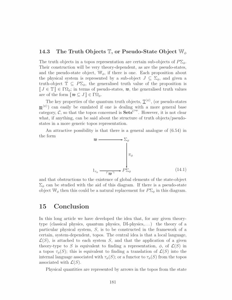
14.3 The Truth Objects T, or Pseudo-State Object Wφ
The truth objects in a topos representation are certain sub-objects of PΣφ.Their construction will be very theory-dependent, as are the pseudo-states,and the pseudo-state object, Wφ, if there is one. Each proposition aboutthe physical system is represented by a sub-object J ⊆ Σφ, and given atruth-object T ⊆ PΣφ, the generalised truth value of the proposition is[[ J ∈ T ]] ∈ ΓΩφ; in terms of pseudo-states, w, the generalised truth valuesare of the form [[ w ⊆ J ]] ∈ ΓΩφ.
The key properties of the quantum truth objects, T |ψ〉, (or pseudo-statesw |ψ〉) can easily be emulated if one is dealing with a more general basecategory, C, so that the topos concerned is SetsC
op
. However, it is not clearwhat, if anything, can be said about the structure of truth objects/pseudo-states in a more generic topos representation.
An attractive possibility is that there is a general analogue of (6.54) inthe form
1τφ PΣφ-
pwq
w Σφ-
?
πφ
(14.1)
and that obstructions to the existence of global elements of the state-objectΣφ can be studied with the aid of this diagram. If there is a pseudo-stateobject Wφ then this could be a natural replacement for PΣφ in this diagram.
15 Conclusion
In this long article we have developed the idea that, for any given theory-type (classical physics, quantum physics, DI-physics,. . . ) the theory of aparticular physical system, S, is to be constructed in the framework of acertain, system-dependent, topos. The central idea is that a local language,L(S), is attached to each system S, and that the application of a giventheory-type to S is equivalent to finding a representation, φ, of L(S) ina topos τφ(S); this is equivalent to finding a translation of L(S) into theinternal language associated with τφ(S); or a functor to τφ(S) from the toposassociated with L(S).
Physical quantities are represented by arrows in the topos from the state
181
object Σφ,S to the quantity-value object Rφ,S, and propositions are repre-sented by sub-objects of the state object. The idea of a ‘truth sub-object’of PΣφ,S (or a ‘pseudo-state’ sub-object of Σφ,S) then leads to a neo-realistinterpretation of propositions in which each proposition is assigned a truthvalue that is a global element of the sub-object classifier Ωτφ(S). In general,neo-realist statements about the world/system S are to be expressed in theinternal language of the topos τφ(S). Underlying this is the intuitionistic,deductive logic provided by the local language L(S).
These axioms are based on ideas from the topos representation of quan-tum theory, which we have discussed in depth. Here, the topos involved isSetsV(H)op : the topos of presheaves over the base category V(H) of com-mutative, von Neumann sub-algebras of the algebra, B(H), of all boundedoperators on the quantum Hilbert space, H. Each such sub-algebra canbe viewed as a context in which the theory can be viewed from a classi-cal perspective. Thus a context can be described as a ‘classical snap-shot’,or ‘window on reality’, or ‘world-view’/weltanschauung. Mathematically, acontext is a ‘stage of truth’: a concept that goes back to Kripke’s use of apresheaf topos as a model of his intuitionistic view of time and process.
We have shown how the process of ‘daseinisation’ maps projection oper-ators (and hence equivalent classes of propositions) into sub-objects of thestate-object Σ. We have also shown how this can be extended to an arbitrary,bounded self-adjoint operator, A. This produces an arrow A : Σ→ R wherethe minimal choice for the quantity-value object, R, is the object R. Wehave also argued that, from a physical perspective, it is more attractive tochoose R↔ as the quantity-value presheaf. The significance of these resultsis enhanced considerably by the alternative, Heunen & Spitters derivation ofΣ as the spectrum of an internal, commutative algebra. These, and related,results all encourage the idea that quantum theory can be viewed as classicaltheory but in a topos other than the topos of sets, Sets.
Every classical system uses the same topos, Sets. However, in general,the topos will be system dependent as, for example, is the case with thequantum topoi of the form SetsV(H)op , where H is the Hilbert space of thesystem. This leads to the problem of understanding how the topoi for a classof systems behave under the action of taking a sub-system, or combininga pair of systems to give a single composite system. We have presented aset of axioms that capture the general ideas we are trying to develop. Ofcourse, these axioms are not cast in stone, and are still partly ‘experimental’in nature. However, we have shown that classical physics exactly fits our sug-gested scheme, and that quantum physics ‘almost’ does: ‘almost’ because ofthe issues concerning the translation representation of the arrows associated
182
with compositions of systems that were discussed in Section 13.3.
An important challenge for future work is to show that our general toposscheme can be used to develop genuinely new theories of physics, not just torewrite old ones in a new language. Of particular interest is the problem withwhich we motivated the scheme in the first place: namely, to find tools forconstructing theories that go beyond quantum theory and which do not useHilbert spaces, path integrals, or any of the other familiar entities in whichthe continuum real and/or complex numbers play a fundamental role.
As we have discussed, the topoi for quantum systems are of the formSetsV(H)op , and hence embody contextual logic in a fundamental way. Oneway of going ‘beyond’ quantum theory, while escaping the a priori impositionof continuum concepts, is to use presheaves over a more general ‘category ofcontexts’, C, i.e., develop the theory in the topos SetsC
op
. Such a structureembodies contextual, multi-valued logic in an intrinsic way, and in that sensemight be said to encapsulate one of the fundamental insights of quantumtheory. However, and unlike in quantum theory, there is no obligation to usethe real or complex numbers in the construction of the category C.
Indeed, early on in this work we noted that real numbers arise in theoriesof physics in three different (but related) ways: (i) as the values of physi-cal quantities; (ii) as the values of probabilities; and (iii) as a fundamentalingredient in models of space and time. The first of these is now subsumedinto the quantity-value object Rφ, and which now has no a priori relationto the real number object in τφ. The second source of real numbers has gonecompletely since we no longer have probabilities of propositions but rathergeneralised truth values whose values lie in ΓΩτφ . The third source is alsono long binding since models of space and time in a topos could depend onmany things: for example, infinitesimals.
Of course, although true, these remarks do not of themselves give a con-crete example of a theory that is ‘beyond quantum theory’. On the otherhand, these ideas certainly point in a novel direction, and one at which,almost certainly, we would not have arrived if the challenge to ‘go beyondquantum theory’ had been construed only in terms of trying to generaliseHilbert spaces, path integrals, and the like.
From a more general perspective, other types of topoi are possible realmsfor the construction of physical theories. One simple, but mathematically richexample arises from the theory of M-sets. Here, M is a monoid and, like allmonoids, can be viewed as a category with a single object, and whose arrowsare the elements ofM . Thought of as a category, a monoid is ‘complementary’to a partially-ordered set. In a monoid, there is only one object, but plenty of
183
arrows from that object to itself; whereas in a partially-ordered set there areplenty of objects, but at most one arrow between any pair of objects. Thus apartially-ordered set is the most economical category with which to capturethe concept of ‘contextual logic’. On the other hand, the logic associatedwith a monoid is non-contextual as there is only one object in the category.
It is easy to see that a functor from M to Sets is just an ‘M-set’: i.e., aset on which M acts as a monoid of transformations. An arrow between twosuch M-sets is an equivariant map between them. In physicists’ language,one would say that the topos SetsM—usually denoted BM— is the categoryof the ‘non-linear realisations’ of M .
The sub-object classifier, ΩBM , in BM is the collection of left ideals in M ;hence, many of the important constructions in the topos can be handled usingthe language of algebra. The topos BM is one of the simplest to define andwork with and, for that reason, it is a popular source of examples in texts ontopos theory. It would be intriguing to experiment with constructing modeltheories of physics using one of these simple topoi. One possible use of M-sets is discussed in [43] in the context of reduction of the state vector, butthere will surely be others.
Is there ‘un gros topos’? It is clear that there are many other topics forfuture research. A question that is of particular interest is if there is a singletopos within which all systems of a given theory-type can be discussed. Forexample, in the case of quantum theory the relevant topoi are of the formSetsV(H)op , where H is a Hilbert space, and the question is whether all suchtopoi can be gathered together to form a single topos (what Grothendiecktermed ‘un gros topos’) within which all quantum systems can be discussed.
There are well-known examples of such constructions in the mathematicalliterature. For example, the category, Sh(X), of sheaves on a topologicalspace X is a topos, and there are collections T of topological spaces whichform a Grothendieck site, so that the topos Sh(T) can be constructed. Aparticular object in Sh(T) will then be a sheaf over T whose stalk over anyobject X in T will be the topos Sh(X).
For our purposes, the ideal situation would be if the various categoriesof systems, Sys, can be chosen in such a way that M(Sys) is a site. Thenthe topos of sheaves, Sh(M(Sys)), over this site would provide a commontopos in which all systems of this theory type—i.e., the objects of Sys—canbe discussed. We do not know if this is possible, and it is a natural subjectfor future study.
184
Some more speculative lines of future research. At a conceptual level,one motivating desire for the entire research programme was to find a for-malism that would always give some sort of ‘realist’ interpretation, even inthe case of quantum theory which is normally presented in an instrumental-ist way. But this particular example raises an interesting point because theneo-realist interpretation takes place in the topos SetsV(H)op , whereas theinstrumentalist interpretation works in the familiar topos Sets of sets, andone might wonder how universal is the use of a pair of topoi in this way.
Another, related, issue concerns the representation of the PL(S)-propositionsof the form “Aε∆” discussed in Section 5. This serves as a bridge betweenthe ‘external’ world of a background spatial structure, and the internal worldof the topos. This link is not present with the L(S) language whose proposi-tions are purely internal terms of type Ω of the form ‘A(s) ∈ ∆’. In a toposrepresentation, φ, of L(S), these become propositions of the form ‘A ∈ Ξ’,where Ξ is a sub-object of Rφ.
In general, if we have an example of our axioms working neo-realisticallyin a topos τ , one might wonder if there is an ‘instrumentalist’ interpretationof the same theory in a different topos, τi, say? Of course, the word ‘in-strumentalism’ is used metaphorically here, and any serious consideration ofsuch a pair (τ, τi) would require a lot of very careful thought.
However, if a pair (τ, τi) does exist, the question then arises of whetherthere is a categorial way of linking the neo-realist and instrumentalist inter-pretations: for example, via a functor I : τ → τi. If so, is this related tosome analogue of the daseinisation operation that produced the representa-tion of the PL(S)-propositions, “Aε∆” in quantum theory? Care is neededin discussing such issues since informal set theory is used as a meta-languagein constructing a topos, and one has to be careful not to confuse this withthe existence, or otherwise, of an ‘instrumentalist’ interpretation of any givenrepresentation.
If such a functor, I : τ → τi, did exist then one could speculate on thepossibility of finding an ‘interpolating chain’ of functors
τ → τ 1 → τ 2 → · · · → τn → τi (15.1)
which could be interpreted conceptually as corresponding to an interpolationbetween the philosophical views of realism and instrumentalism!
Even more speculatively one might wonder if “one person’s realism isanother person’s instrumentalism”. More precisely, given a pair (τ, τi) in thesense above, could there be cases in which the topos τ carries a neo-realistinterpretation of a theory with respect to an instrumentalist interpretation in
185
τi, whilst being the carrier of an instrumentalist interpretation with respectto the neo-realism of a ‘higher’ topos; and so on? For example, is theresome theory whose ‘instrumentalist manifestation‘ takes place in the toposSetsV(H)op?
On the other hand, one might want to say that ‘instrumentalist’ interpre-tations always take place in the world of classical set theory, so that τi shouldalways be chosen to be Sets. In any event, it would be interesting to studythe quantum case more closely to see if there are any categorial relations be-tween the formulation in SetsV(H)op and the instrumentalism interpretationin Sets. It can be anticipated that the action of daseinisation will play animportant role here.
All this is, perhaps131, rather speculative but there is a more obvioussituation in which a double-topos structure will be necessary, irrespective ofphilosophical musings on instrumentalism. This is if one wants to discussthe ‘classical limit’ of some topos theory. In this case this limit will exist inthe topos, Sets, and this must be used in addition to the topos of the basictheory. A good example of this, of course, is the topos of quantum theorydiscussed in this article. If, pace Landsmann, one thinks of ‘quantisation’as a functor from Sets to SetsV(H)op , then the classical limit will perhapsinvolve a functor going in the opposite direction.
Implications for quantum gravity. A serious claim stemming from ourwork is that a successful theory of quantum gravity should be constructedin some topos U—the ‘topos of the universe’—that is not the topos of sets.All entities of physical interest will be represented in this topos, includingmodels for space-time (if there are any at a fundamental level in quantumgravity) and, if relevant, loops, membranes etc. as well as incorporating theanticipated generalisation of quantum theory.
Such a theory of quantum gravity will have a neo-realist interpretation inthe topos U , and hence would be particularly useful in the context of quantumcosmology. However, in practice, physicists divide the world up into smaller,more easily handled, chunks, and each of them would correspond to whatearlier we have called a ‘system’ and, correspondingly, would have its owntopos. Thus U is something like the ‘gros topos’ of the theory, and wouldcombine together the individual ‘sub-systems’ in a categorial way. Of course,it is most unlikely that there is any preferred way of dividing the universe upinto bite-sized chunks, but this is not problematic as the ensuing relativismis naturally incorporated into the idea of a Grothendieck site.
131To be honest, the ‘perhaps’ should really be replaced by ‘highly’.
186
16 Appendix 1: Some Theorems and Con-
structions Used in the Main Text
16.1 Results on Clopen Subobjects of Σ.
Theorem 16.1 The collection, Subcl(Σ), of all clopen sub-objects of Σ is aHeyting algebra.
Proof. First recall how a Heyting algebra structure is placed on the set,Sub(Σ), of all sub-objects of Σ.
The ‘∨’- and ‘∧’-operations. Let S, T be two sub-objects of Σ. Thenthe ‘∨’ and ‘∧’ operations are defined by
(S ∨ T )V := SV ∪ T V (16.1)
(S ∧ T )V := SV ∩ T V (16.2)
for all contexts V . It is easy to see that if S and T are clopen sub-objects ofΣ, then so are S ∨ T and S ∧ T .
The zero and unit elements. The zero element in the Heyting algebraSub(Σ) is the empty sub-object 0 := ∅V | V ∈ Ob(V(H)), where ∅V isthe empty subset of ΣV . The unit element in Sub(Σ) is Σ. It is clear thatboth 0 and Σ are clopen sub-objects of Σ.
The ‘⇒’-operation. The most interesting part is the definition of theimplication S ⇒ T . For all V ∈ Ob(V(H)), it is given by
(S ⇒ T )V := λ ∈ ΣV | ∀V ′ ⊆ V, if
Σ(iV ′V )(λ) ∈ SV ′ then Σ(iV ′V )(λ) ∈ T V ′ (16.3)
= λ ∈ ΣV | ∀V ′ ⊆ V, if
λ|V ′ ∈ SV ′ then λ|V ′ ∈ T V ′. (16.4)
Since ¬S := S ⇒ 0, the expression for negation follows from the aboveas
(¬S)V = λ ∈ ΣV | ∀V ′ ⊆ V, Σ(iV ′V )(λ) /∈ SV ′ (16.5)
= λ ∈ ΣV | ∀V ′ ⊆ V, λ|V ′ /∈ SV ′. (16.6)
187
We rewrite the formula for negation as
(¬S)V =⋂
V ′⊆V
λ ∈ ΣV | λ|V ′ ∈ ScV ′
(16.7)
where SV ′c denotes the complement of SV ′ in ΣV ′ . Clearly, SV ′
c is clopen inΣV ′ since SV ′ is clopen. Since the restriction Σ(iV ′V ) : ΣV → ΣV ′ is continu-ous and surjective132, it is easy to see that the inverse image Σ(iV ′V )−1(SV ′
c)is clopen in ΣV . Clearly,
Σ(iV ′V )−1(SV ′c) =
λ ∈ ΣV | λ|V ′ ∈ SV ′
c
(16.8)
and so, from (16.7) we have
(¬S)V =⋂
V ′⊆V
Σ(iV ′V )−1(SV ′c) (16.9)
The problem is that we want (¬S)V to be a clopen subset of ΣV . Nowthe right hand side of (16.9) is the intersection of a family, parameterised byV ′ | V ′ ⊆ V , of clopen sets. Such an intersection is always closed, but it isonly guaranteed to be open if V ′ | V ′ ⊆ V is a finite set, which of coursemay not be the case.
If V ′′ ⊆ V ′ and λ|V ′′ ∈ SV ′′c, then λ|V ′ ∈ SV ′
c. Indeed, if we had λ|V ′ ∈SV ′, then (λ|V ′)|V ′′ = λ|V ′′ ∈ SV ′′ by the definition of a sub-object, so wewould have a contradiction. This implies Σ(iV ′′V )−1(SV ′′
c) ⊆ Σ(iV ′V )−1(SV ′c),
and hence the right hand side of (16.9) is a decreasing net of clopen subsetsof ΣV which converges to something, which we take as the subset of ΣV thatis to be (¬S)V .
Here we have used the fact that the set of clopen subsets of ΣV is acomplete lattice, where the minimum of a family (Ui)i∈I of clopen subsets isdefined as the interior of
⋂i∈I Ui. This leads us to define
(¬S)V := int⋂
V ′⊆V
Σ(iV ′V )−1(SV ′c) (16.10)
= int⋂
V ′⊆V
λ ∈ ΣV | λ|V ′ ∈ (SV ′
c)
(16.11)
as the negation in Subcl(Σ). This modified definition guarantees that ¬Sis a clopen sub-object. A straightforward extension of this method gives aconsistent definition of S ⇒ T .
132See proof of Theorem 16.2 below.
188
This concludes the proof of the theorem.
The following theorem shows the relation between the restriction map-pings of the outer presheaf O and those of the spectral presheaf Σ. Webasically follow de Groote’s proof of Prop. 3.22 in [33] and show that thisresult, which uses quite a different terminology, actually gives the desiredrelation.
Theorem 16.2 Let V, V ′ ∈ Ob(V(H)) such that V ′ ⊂ V . Then
SO(iV ′V )(δo(P )V ) = Σ(iV ′V )(Sδo(P )V). (16.12)
Proof. First of all, to simplify notation, we can replace δo(P )V by P (whichamounts to the assumption that P ∈ P(V ). This does not play a role forthe current argument). By definition, O(iV ′V )
(P
)= δo(P )V ′ , so we have to
show that Sδo(P )V ′= Σ(iV ′V )(SP ) holds.
If λ ∈ SP , then λ(P ) = 1, which implies λ(Q) = 1 for all Q ≥ P . In
particular, λ(δo(P )V ′) = 1, so Σ(iV ′V )(λ) = λ|V ′ ∈ Sδo(P )V ′. This shows that
Σ(iV ′V )(SP ) ⊆ Sδo(P )V ′.
To show the converse inclusion, let λ′ ∈ Sδo(P )V ′, which means that
λ′(δo(P )V ′) = 1. We have P ∈ O(iV ′V )−1(δo(P )V ′). Let
Fλ′ := Q ∈ P(V ′) | λ′(Q) = 1 = λ′−1(1) ∩ P(V ′). (16.13)
As shown in section 8.3, Fλ′ is an ultrafilter in the projection lattice P(V ′).133
The idea is to show that Fλ′∪ P is a filter base in P(V ) that can be extendedto an ultrafilter, which corresponds to an element of the Gel’fand spectrumof V .
Let us assume that Fλ′ ∪ P is not a filter base in P(V ). Then there existssome Q ∈ Fλ′ such that
Q ∧ P = QP = 0, (16.14)
which implies P ≤ 1− Q, so
O(iV ′V )(P ) = δo(P )V ′ ≤ O(iV ′V )(1− Q) = 1− Q (16.15)
and hence we get the contradiction
1 = λ′(δo(P )V ′) ≤ λ′(1− Q) = 0. (16.16)
133In general, each ultrafilter F in the projection lattice of an abelian von Neumannalgebra V corresponds to a unique element λF of the Gel’fand spectrum of V . Theultrafilter is the collection of all those projections that are mapped to 1 by λ, i.e., F =λ−1F (1) ∩ P(V ).
189
By Zorn’s lemma, the filter base Fλ′∪ P is contained in some (not necessarilyunique) maximal filter base in P(V ). Such a maximal filter base is an ul-trafilter and thus corresponds to an element λ of the Gel’fand spectrum ΣV
of V . Since P is contained in the ultrafilter, we have λ(P ) = 1, so λ ∈ SP .By construction, Σ(iV ′V )(λ) = λ|V ′ = λ′ ∈ Sδo(P )V ′
, the element of ΣV ′ we
started from. This shows that Sδo(P )V ′⊆ Σ(iV ′V )(SP ), and we obtain
Sδo(P )V ′= Σ(iV ′V )(SP ). (16.17)
It is well-known that every state λ′ ∈ ΣV ′ is of the form λ′ = Σ(iV ′V )(λ) =λ|V ′ for some λ ∈ ΣV . This implies
Σ(iV ′V )−1(Sδo(P )V ′) = Sδo(P )V ′
⊆ ΣV . (16.18)
Note that on the right hand side, Sδo(P )V ′(and not SP , which is a smaller set
in general) shows up.
De Groote has shown in [33] that for any unital abelian von Neumannalgebra V , the clopen sets SQ, Q ∈ P(V ), form a base of the Gel’fandtopology on ΣV . Formulas (16.17) and (16.18) hence show that the restrictionmappings
Σ(iV ′V ) : ΣV → ΣV ′
λ 7→ λ|V ′
of the spectral presheaf are open and continuous. Using continuity, it is easyto see that Σ(iV ′V ) is also closed: let C ⊆ ΣV be a closed subset. Since ΣV iscompact, C is compact, and since Σ(iV ′V ) is continuous, Σ(iV ′V )(C) ⊆ ΣV ′
is compact, too. However, ΣV ′ is Hausdorff, and so Σ(iV ′V )(C) is closed inΣV ′.
16.2 The Grothendieck k-Construction for an Abelian
Monoid
Let us briefly review the Grothendieck construction for an abelian monoidM .
Definition 16.1 A group completion of M is an abelian group k(M) to-gether with a monoid map θ : M → k(M) that is universal. Namely, givenany monoid morphism φ : M → G, where G is an abelian group, there existsa unique group morphism φ′ : k(M) → G such that φ factors through φ′;i.e., we have the commutative diagram
190
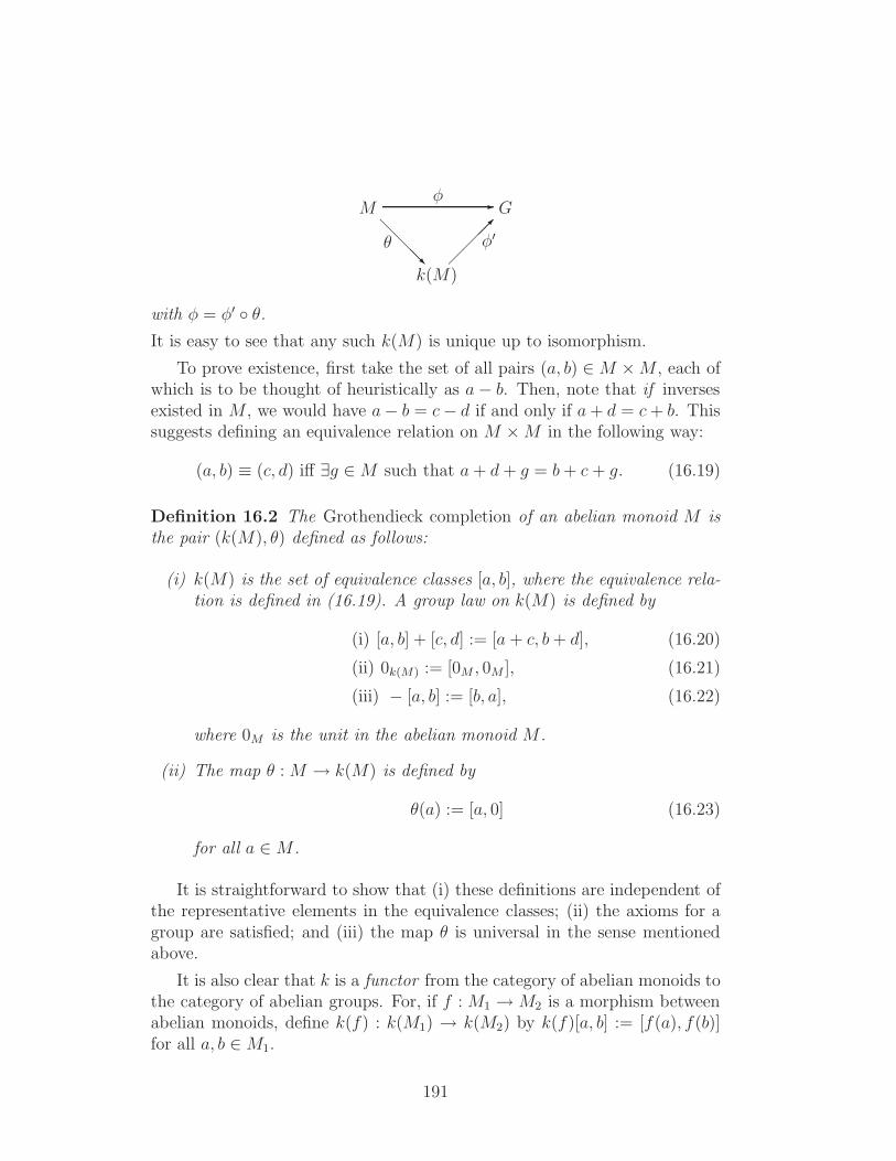
M G-φ
k(M)
θ@
@@@R
φ′
with φ = φ′ θ.It is easy to see that any such k(M) is unique up to isomorphism.
To prove existence, first take the set of all pairs (a, b) ∈M ×M , each ofwhich is to be thought of heuristically as a− b. Then, note that if inversesexisted in M , we would have a− b = c− d if and only if a+ d = c+ b. Thissuggests defining an equivalence relation on M ×M in the following way:
(a, b) ≡ (c, d) iff ∃g ∈M such that a+ d+ g = b+ c + g. (16.19)
Definition 16.2 The Grothendieck completion of an abelian monoid M isthe pair (k(M), θ) defined as follows:
(i) k(M) is the set of equivalence classes [a, b], where the equivalence rela-tion is defined in (16.19). A group law on k(M) is defined by
(i) [a, b] + [c, d] := [a + c, b+ d], (16.20)
(ii) 0k(M) := [0M , 0M ], (16.21)
(iii) − [a, b] := [b, a], (16.22)
where 0M is the unit in the abelian monoid M .
(ii) The map θ : M → k(M) is defined by
θ(a) := [a, 0] (16.23)
for all a ∈M .
It is straightforward to show that (i) these definitions are independent ofthe representative elements in the equivalence classes; (ii) the axioms for agroup are satisfied; and (iii) the map θ is universal in the sense mentionedabove.
It is also clear that k is a functor from the category of abelian monoids tothe category of abelian groups. For, if f : M1 → M2 is a morphism betweenabelian monoids, define k(f) : k(M1) → k(M2) by k(f)[a, b] := [f(a), f(b)]for all a, b ∈M1.
191
16.3 Functions of Bounded Variation and ΓR
These techniques will now be applied to the set, ΓR, of global elementsof R. We could equally well consider ΓR↔ and its k-extension, but thiswould just make the notation more complex, so in this and the followingsubsections, we will mainly concentrate on ΓR (resp. R). The results caneasily be extended to ΓR↔ (resp. R↔).
It was discussed in Section 8.2 how global elements of R↔ are in one-to-one correspondence with pairs (µ, ν) consisting of an order-preserving andan order-reversing function on the category V(H); i.e., with functions µ :Ob(V(H)) → R such that, for all V1, V2 ∈ Ob(V(H)), if V2 ⊆ V1 thenµ(V2) ≤ µ(V1) and ν : Ob(V(H))→ R such that, for all V1, V2 ∈ Ob(V(H)),if V2 ⊆ V1 then ν(V2) ≥ ν(V1); see (8.75). The monoid law on ΓR↔ is givenby (8.79).
Clearly, global elements of R are given by order-reversing functions ν :V(H) → R, and ΓR is an abelian monoid in the obvious way. Hence theGrothendieck construction can be applied to give an abelian group k(ΓR).This is defined to be the set of equivalence classes [ν, κ] where ν, κ ∈ ΓR,and where (ν1, κ1) ≡ (ν2, κ2) if, and only if, there exists α ∈ ΓR, such that
ν1 + κ2 + α = κ1 + ν2 + α (16.24)
Since ΓR has a cancellation law, we have (ν1, κ1) ≡ (ν2, κ2) if, and only if,
ν1 + κ2 = κ1 + ν2. (16.25)
Intuitively, we can think of [ν, κ] as being ‘ν−κ’, and embed ΓR in k(ΓR)by ν 7→ [ν, 0]. However, ν, κ are R-valued functions on Ob(V(H)) and hence,in this case, the expression ‘ν − κ’ also has a literal meaning: i.e., as thefunction (ν − κ)(V ) := ν(V )− κ(V ) for all V ∈ Ob(V(H)).
This is not just a coincidence of notation. Indeed, let F(Ob(V(H)),R
)
denote the set of all real-valued functions on Ob(V(H)). Then we can con-struct the map,
j : k(ΓR) → F(Ob(V(H)),R
)(16.26)
[ν, κ] 7→ ν − κ
which is well-defined on equivalence classes.
It is easy to see that the map in (16.26) is injective. This raises thequestion of the image in F
(Ob(V(H)),R
)of the map j: i.e., what types of
real-valued function on Ob(V(H)) can be written as the difference betweentwo order-reversing functions?
192
For functions f : R → R, it is a standard result that a function can bewritten as the difference between two monotonic functions if, and only if, ithas bounded variation. The natural conjecture is that a similar result applieshere. To show this, we proceed as follows.
Let f : Ob(V(H))→ R be a real-valued function on the set of objects inthe category V(H). At each V ∈ Ob(V(H)), consider a finite chain
C := V0, V1, V2, . . . , Vn−1, V | V0 ⊂ V1 ⊂ V2 ⊂ · · · ⊂ Vn−1 ⊂ V (16.27)
of proper subsets, and define the variation of f on this chain to be
Vf(C) :=n∑
j=1
|f(Vj)− f(Vj−1)| (16.28)
where we set Vn := V . Now take the supremum of Vf (C) for all such chainsC. If this is finite, we say that f has a bounded variation and define
If (V ) := supC
Vf(C) (16.29)
Then it is clear that (i) V 7→ If (V ) is an order-preserving function onOb(V(H)); (ii) f − If is an order-reversing function on Ob(V(H)); and (iii)−If is an order-reversing function on Ob(V(H)). Thus, any function, f , ofbounded variation can be written as
f ≡ (f − If )− (−If ) (16.30)
which is the difference of two order-reversing functions; i.e., f can be ex-pressed as the difference of two elements of ΓR.
Conversely, it is a straightforward modification of the proof for functionsf : R→ R, to show that if f : Ob(V(H))→ R is the difference of two order-reversing functions, then f is of bounded variation. The conclusion is thatk(ΓR) is in bijective correspondence with the set, BV(Ob(V(H)),R), offunctions f : Ob(V(H))→ R of bounded variation.
16.4 Taking Squares in k(ΓR)
We can now think of k(ΓR) in two ways: (i) as the set of equivalenceclasses [ν, κ], of elements ν, κ ∈ ΓR; and (ii) as the set, BV(Ob(V(H)),R),of differences ν − κ of such elements.
193
As expected, BV(Ob(V(H)),R) is an abelian group. Indeed: supposeα = ν1 − κ1 and β = ν2 − κ2 with ν1, ν2, κ1, κ2 ∈ ΓR, then
α + β = (ν1 + ν2)− (κ1 + κ2) (16.31)
Hence α + β belongs to BV(Ob(V(H)),R) since ν1 + ν2 and κ1 + κ2 belongto ΓR.
The definition of [ν, 0]2. We will now show how to take the square ofelements of k(ΓR) that are of the form [ν, 0]. Clearly, ν2 is well-defined asa function on Ob(V(H)), but it may not belong to ΓR. Indeed, if ν(V ) < 0for any V , then the function V 7→ ν2(V ) can get smaller as V gets smaller,so it is order-preserving instead of order-reversing.
This suggests the following strategy. First, define functions ν+ and ν− by
ν+(V ) :=
ν(V ) if ν(V ) ≥ 0
0 if ν(V ) < 0(16.32)
and
ν−(V ) :=
0 if ν(V ) ≥ 0
ν(V ) if ν(V ) < 0.(16.33)
Clearly, ν(V ) = ν+(V ) + ν−(V ) for all V ∈ Ob(V(H)). Also, for all V ,ν+(V )ν−(V ) = 0, and hence
ν(V )2 = ν+(V )2 + ν−(V )2 (16.34)
However, (i) the function V 7→ ν+(V )2 is order-reversing; and (ii) the functionV 7→ ν−(V )2 is order-preserving. But then V 7→ −ν−(V )2 is order-reversing.Hence, by rewriting (16.34) as
ν(V )2 = ν+(V )2 − (−ν−(V )2) (16.35)
we see that the function V 7→ ν2(V ) := ν(V )2 is an element of BV(Ob(V(H)),R).
In terms of k(ΓR), we can define
[ν, 0]2 := [ν2+,−ν2
−] (16.36)
which belongs to k(ΓR). Hence, although there exist ν ∈ ΓR that haveno square in ΓR, such global elements of R do have squares in the k-completion, k(ΓR). On the level of functions of bounded variation, we haveshown that the square of a monotonic (order-reversing) function is a functionof bounded variation.
194
On the other hand, we cannot take the square of an arbitrary element[ν, κ] ∈ ΓR, since the square of a function of bounded variation need not bea function of bounded variation.134
16.5 The Object k(R) in the Topos SetsV(H)op
.
16.5.1 The Definition of k(R).
The next step is to translate these results about the set k(ΓR) into theconstruction of an object k(R) in the topos SetsV(H)op . We anticipate that,if this can be done, then k(ΓR) ≃ Γk(R).
As was discussed in Section (8.2), the presheaf R is defined at each stageV by
RV := ν :↓V → R | ν ∈ OR(↓V,R). (16.37)
If iV ′V : V ′ ⊆ V , then the presheaf map from RV to R
V ′ is just therestriction of the order-reversing functions from ↓V to ↓V ′.
The first step in constructing k(R) is to define an equivalence relationon pairs of functions, ν, κ ∈ R
V , for each stage V , by saying that (ν1, κ1) ≡(ν2, κ2) if, and only, there exists α ∈ R
V such that
ν1(V′) + κ2(V
′) + α(V ′) = κ1(V′) + ν2(V
′) + α(V ′) (16.38)
for all V ′ ⊆ V .
Definition 16.3 The presheaf k(R) is defined over the category V(H) inthe following way.
(i) On objects V ∈ Ob(V(H)):
k(R)V := [ν, κ] | ν, κ ∈ OR(↓V,R), (16.39)
where [ν, κ] denotes the k-equivalence class of (ν, κ).
(ii) On morphisms iV ′V : V ′ ⊆ V : The arrow k(R)(iV ′V ) : k(R)V →k(R)V ′ is given by
(k(R)(iV ′V )
)([ν, κ]) := [ν|V ′, κ|V ′] for all [ν, κ] ∈
k(R)V .
134We have to consider functions like (ν+ +ν−−(κ+ +κ−))2, which contains terms of theform ν+κ− and ν−κ+: in general, these are neither order-preserving nor order-reversing.
195
It is straightforward to show that k(R) is an abelian group-object in thetopos SetsV(H)op . In particular, an arrow + : k(R) × k(R) → k(R) isdefined at each stage V by
+V
([ν1, κ1], [ν2, κ2]
):= [ν1 + ν2, κ1 + κ2] (16.40)
for all([ν1, κ1], [ν2, κ2]
)∈ k(R)V × k(R)V . It is easy to see that (i)
Γk(R) ≃ k(ΓR); and (ii) R is a sub-object of k(R) in the topos SetsV(H)op .
16.5.2 The Presheaf k(R) as the Quantity-Value Object.
We can now identify k(R) as a possible quantity-value object in SetsV(H)op .To each bounded, self-adjoint operator A, there is an arrow [δo(A)] : Σ →k(R), given by first sending A ∈ B(H)sa to δo(A) and then taking k-equivalence classes. More precisely, one takes the monic ι : R → k(R)and then constructs ι δo(A) : Σ→ k(R).
Since, for each stage V , the elements in the image of [δo(A)]V = (ι δo(A))V are of the form [ν, 0], ν ∈ R
V , their square is well-defined. From aphysical perspective, the use of k(R) rather than R renders possible the
definition of things like the ‘intrinsic dispersion’, ∇(A) := δo(A2) − δo(A)2;see (9.4).
16.5.3 The square of an arrow [δo(A)].
An arrow [δo(A)] : Σ → k(R) is constructed by first forming the outerdaseinisation δo(A) of A, which is an arrow from Σ to R, and then composingwith the monic arrow from R to k(R). Since only outer daseinisation isused, for each V ∈ V(H) and each λ ∈ ΣV one obtains an element of k(R)Vof the form [δo(A)V (λ), 0]. We saw how to take the square of these functions,and applying this to all λ ∈ ΣV and all V ∈ V(H), we get the square [δo(A)]2
of the arrow [δo(A)].
If we consider an arrow of the form δ(A) : Σ→ R↔, then the constructioninvolves both inner and outer daseinisation, see Theorem 8.2. For each Vand each λ ∈ ΣV , we obtain a pair of functions (δi(A)V (λ), δo(A)V (λ)), whichare both not constantly 0 in general. There is no canonical way to take thesquare of these in R↔
V . Going to the k-extension k(R↔) of R↔ does notimprove the situation, so we cannot define the square of an arrow δ(A) (or[δ(A)] in general.
196
17 Appendix 2: A Short Introduction to the
Relevant Parts of Topos Theory
17.1 What is a Topos?
It is impossible to give here more than the briefest of introductions to topostheory. At the danger of being highly imprecise, we restrict ourselves tomentioning some aspects of this well-developed mathematical theory andgive a number of pointers to the literature. The aim merely is to give a veryrough idea of the structure and internal logic of a topos.
There are a number of excellent textbooks on topos theory, and the readershould consult at least one of them. We found the following books useful:[54, 29, 56, 48, 8, 52].
Topos theory is a remarkably rich branch of mathematics which can beapproached from a variety of different viewpoints. The basic area of mathe-matics is category theory; where, we recall, a category consists of a collectionof objects and a collection of morphisms (or arrows).
In the special case of the category of sets, the objects are sets, and amorphism is a function between a pair of sets. In general, each morphism fin a category is associated with a pair of objects135, known as its ‘domain’and ‘codomain’, and is written as f : B → A where B and A are the domainand codomain respectively. Note that this arrow notation is used even iff is not a function in the normal set-theoretic sense. A key ingredient inthe definition of a category is that if f : B → A and g : C → B (i.e., thecodomain of g is equal to the domain of f) then f and g can be ‘composed’to give an arrow f g : C → A; in the case of the category of sets, this isjust the usual composition of functions.
A simple example of a category is given by any partially-ordered set(‘poset’) C: (i) the objects are defined to be the elements of C; and (ii) ifp, q ∈ C, a morphism from p to q is defined to exist if, and only if, p q inthe poset structure. Thus, in a poset regarded as a category, there is at mostone morphism between any pair of objects p, q ∈ C; if it exists, we shall writethis morphism as ipq : p→ q. This example is important for us in form of the‘category of contexts’, V(H), in quantum theory. The objects in V(H) arethe commutative, unital136 von Neumann sub-algebras of the algebra, B(H),
135The collection of all objects in category, C, is denoted Ob(C). The collection of arrowsfrom B to A is denoted HomC
(B,A
). We will only be interested in ‘small’ categories in
which both these collections are sets (rather than the, more general, classes.)136‘Unital’ means that all these algebras contain the identity operator 1 ∈ B(H).
197
of all bounded operators on the Hilbert space H.
Topoi as mathematical universes. Every (elementary) topos τ can beseen as a mathematical universe. As a category, a topos τ possesses a numberof structures that generalise constructions that are possible in the category,Sets, of sets and functions.137 Namely, in Sets, we can construct new setsfrom given ones in several ways. Specifically, let S, T be two sets, then wecan form the cartesian product S × T , the disjoint union S ∐ T and theexponential ST—the set of all functions from T to S.
These constructions turn out to be fundamental, and they can all bephrased in an abstract, categorical manner, where they are called the ‘prod-uct’, ‘co-product’ and ‘exponential’, respectively. By definition, in a toposτ , these operations always exist. The first and second of these properties arecalled ‘finite completeness’ and ‘finite co-completeness’, respectively.
One consequence of the existence of finite limits is that each topos, τ , hasa terminal object, denoted by 1τ . This is characterised by the property thatfor any object A in the topos τ , there exists exactly one arrow from A to 1τ .In Sets, any one-element set 1 = ∗ is terminal.138
Of course, Sets is a topos, too, and it is precisely the topos which usuallyplays the role of our mathematical universe, since we construct our mathe-matical objects starting from sets and functions between them. As a slogan,we have: a topos τ is a category with ‘certain crucial’ properties that aresimilar to those in Sets. A very nice and gentle introduction to these aspectsof topos theory is the book [54]. Other good sources are [29, 55].
In order to ‘do mathematics’, one must also have a logic, including adeductive system. Each topos comes equipped with an internal logic, which isof intuitionistic type. We will now very briefly sketch the main characteristicsof intuitionistic logic and the mathematical structures in a topos that realisethis logic.
The sub-object classifier. Let X be a set, and let P (X) be the power setof X; i.e., the set of subsets of X. Given a subset K ∈ P (X), one can ask foreach point x ∈ X whether or not it lies in K. Thus there is the characteristic
137More precisely, small sets and functions between them. Small means that we do nothave proper classes. One must take care in these foundational issues to avoid problemslike Russell’s paradox.
138Like many categorical constructions, the terminal object is fixed only up to isomor-phism: all one-element sets are isomorphic to each other, and any of them can serve as aterminal object. Nonetheless, one speaks of the terminal object.
198
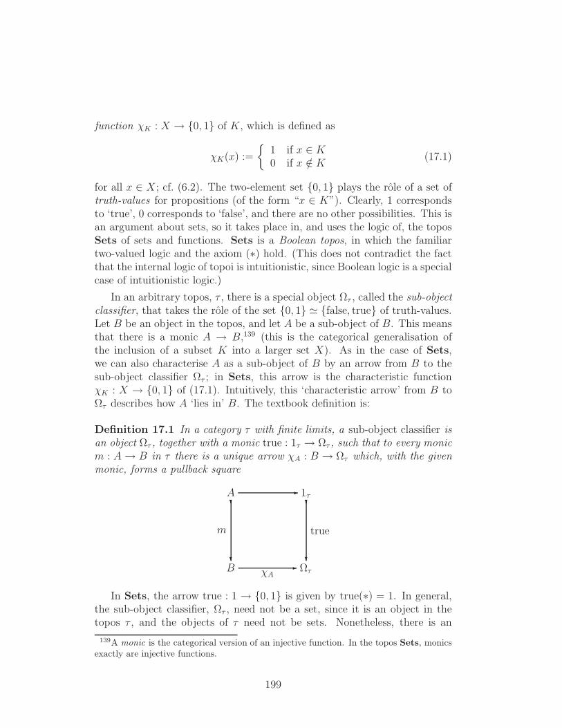
function χK : X → 0, 1 of K, which is defined as
χK(x) :=
1 if x ∈ K0 if x /∈ K (17.1)
for all x ∈ X; cf. (6.2). The two-element set 0, 1 plays the role of a set oftruth-values for propositions (of the form “x ∈ K”). Clearly, 1 correspondsto ‘true’, 0 corresponds to ‘false’, and there are no other possibilities. This isan argument about sets, so it takes place in, and uses the logic of, the toposSets of sets and functions. Sets is a Boolean topos, in which the familiartwo-valued logic and the axiom (∗) hold. (This does not contradict the factthat the internal logic of topoi is intuitionistic, since Boolean logic is a specialcase of intuitionistic logic.)
In an arbitrary topos, τ , there is a special object Ωτ , called the sub-objectclassifier, that takes the role of the set 0, 1 ≃ false, true of truth-values.Let B be an object in the topos, and let A be a sub-object of B. This meansthat there is a monic A → B,139 (this is the categorical generalisation ofthe inclusion of a subset K into a larger set X). As in the case of Sets,we can also characterise A as a sub-object of B by an arrow from B to thesub-object classifier Ωτ ; in Sets, this arrow is the characteristic functionχK : X → 0, 1 of (17.1). Intuitively, this ‘characteristic arrow’ from B toΩτ describes how A ‘lies in’ B. The textbook definition is:
Definition 17.1 In a category τ with finite limits, a sub-object classifier isan object Ωτ , together with a monic true : 1τ → Ωτ , such that to every monicm : A→ B in τ there is a unique arrow χA : B → Ωτ which, with the givenmonic, forms a pullback square
B Ωτ-
χA
A 1τ-
?
?
m
?
?
true
In Sets, the arrow true : 1 → 0, 1 is given by true(∗) = 1. In general,the sub-object classifier, Ωτ , need not be a set, since it is an object in thetopos τ , and the objects of τ need not be sets. Nonetheless, there is an
139A monic is the categorical version of an injective function. In the topos Sets, monicsexactly are injective functions.
199
abstract notion of elements (or points) in category theory that we can use.Then the elements of Ωτ are the truth-values available in the internal logicof our topos τ , just like ‘false’ and ‘true’, the elements of false, true, arethe truth-values available in the topos Sets.
To understand the abstract notion of elements, let us consider sets for amoment. Let 1 = ∗ be a one-element set, the terminal object in Sets. LetS be a set and consider an arrow e from 1 to S. Clearly, (i) e(∗) ∈ S is anelement of S; and (ii) the set of all functions from 1 to S corresponds exactlyto the set of all elements of S.
This idea can be generalised to any category that has a terminal object 1.More precisely, an element of an object A is defined to be an arrow from 1 toA in the category. For example, in the definition of the sub-object classifierthe arrow ‘true : 1τ → Ωτ ’ is an element of Ωτ . It may happen that anobject A has no elements, i.e., there are no arrows 1τ → A. It is common toconsider arrows from subobjects U of A to A as generalised elements.
As mentioned above, the elements of the sub-object classifier, understoodas the arrows 1τ → Ωτ , are the truth-values. Moreover, the set of thesearrows forms a Heyting algebra (see, for example, section 8.3 in [29]). Thisis how (the algebraic representation of) intuitionistic logic manifests itself ina topos. Another, closely related fact is that the set, Sub(A), of sub-objectsof any object A in a topos forms a Heyting algebra.
The definition of a topos. Let us pull together these various remarksand list the most important properties of a topos, τ , for our purposes:
1. There is a terminal object 1τ in τ . Thus, given any object A in thetopos, there is a unique arrow A→ 1τ .
For any object A in the topos, an arrow 1τ → A is called a globalelement of A. The set of all global elements of A is denoted ΓA.
Given A,B ∈ Ob(τ), there is a product A × B in τ . In fact, a toposalways has pull-backs, and the product is just a special case of this.140
2. There is an initial object 0τ in τ . This means that given any object Ain the topos, there is a unique arrow 0τ → A.
Given A,B ∈ Ob(τ), there is a co-product A ⊔ B in τ . In fact, atopos always has push-outs, and the co-product is just a special case ofthis.141
140The conditions in 1. above are equivalent to saying that τ is finitely complete.141The conditions in 2. above are equivalent to saying that τ is finitely co-complete.
200
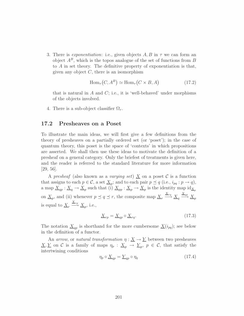
3. There is exponentiation: i.e., given objects A,B in τ we can form anobject AB, which is the topos analogue of the set of functions from Bto A in set theory. The definitive property of exponentiation is that,given any object C, there is an isomorphism
Homτ
(C,AB
)≃ Homτ
(C × B,A
)(17.2)
that is natural in A and C; i.e., it is ‘well-behaved’ under morphismsof the objects involved.
4. There is a sub-object classifier Ωτ .
17.2 Presheaves on a Poset
To illustrate the main ideas, we will first give a few definitions from thetheory of presheaves on a partially ordered set (or ‘poset’); in the case ofquantum theory, this poset is the space of ‘contexts’ in which propositionsare asserted. We shall then use these ideas to motivate the definition of apresheaf on a general category. Only the briefest of treatments is given here,and the reader is referred to the standard literature for more information[29, 56].
A presheaf (also known as a varying set) X on a poset C is a functionthat assigns to each p ∈ C, a set Xp; and to each pair p q (i.e., ipq : p→ q),a map Xqp : Xq → Xp such that (i) Xpp : Xp → Xp is the identity map idXp
on Xp, and (ii) whenever p q r, the composite map Xr
Xrq−→ Xq
Xqp−→ Xp
is equal to Xr
Xrp−→ Xp, i.e.,
Xrp = Xqp Xrq. (17.3)
The notation Xqp is shorthand for the more cumbersome X(ipq); see belowin the definition of a functor.
An arrow, or natural transformation η : X → Y between two presheavesX, Y on C is a family of maps ηp : Xp → Y p, p ∈ C, that satisfy theintertwining conditions
ηp Xqp = Y qp ηq (17.4)
201
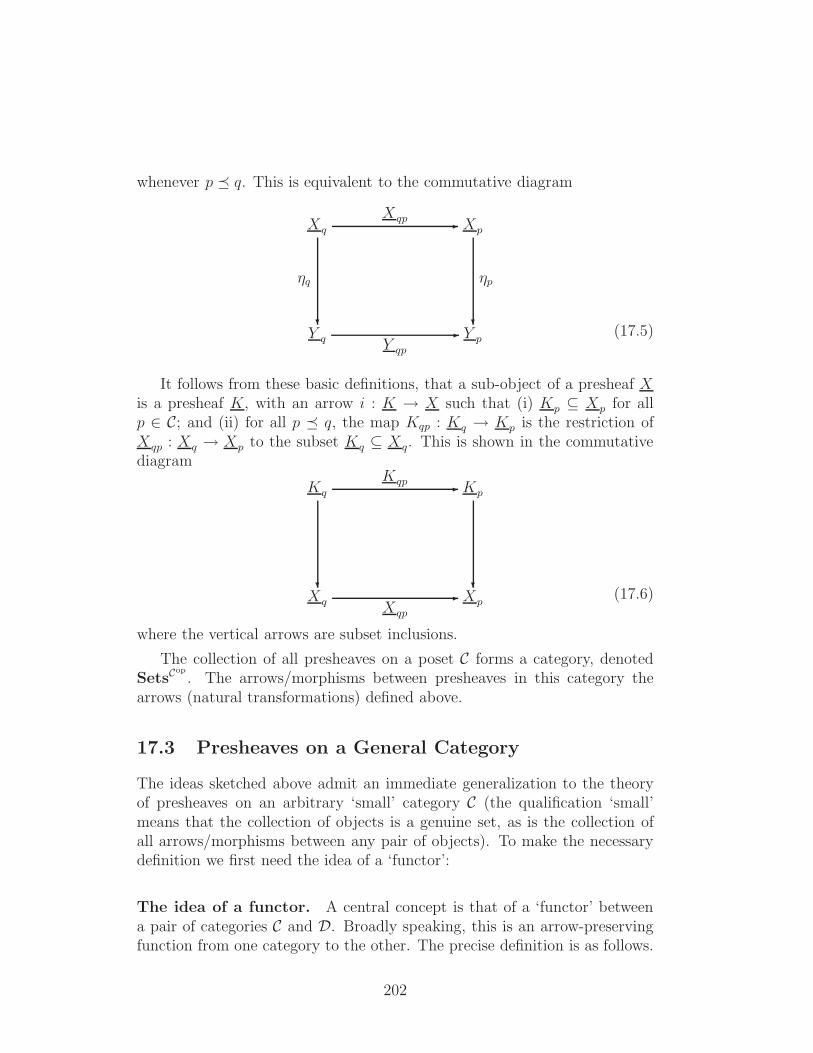
whenever p q. This is equivalent to the commutative diagram
Y q Y p-
Y qp
Xq Xp-
Xqp
?
ηq
?
ηp
(17.5)
It follows from these basic definitions, that a sub-object of a presheaf Xis a presheaf K, with an arrow i : K → X such that (i) Kp ⊆ Xp for allp ∈ C; and (ii) for all p q, the map Kqp : Kq → Kp is the restriction ofXqp : Xq → Xp to the subset Kq ⊆ Xq. This is shown in the commutativediagram
Xq Xp-
Xqp
Kq Kp-
Kqp
? ?(17.6)
where the vertical arrows are subset inclusions.
The collection of all presheaves on a poset C forms a category, denotedSetsC
op
. The arrows/morphisms between presheaves in this category thearrows (natural transformations) defined above.
17.3 Presheaves on a General Category
The ideas sketched above admit an immediate generalization to the theoryof presheaves on an arbitrary ‘small’ category C (the qualification ‘small’means that the collection of objects is a genuine set, as is the collection ofall arrows/morphisms between any pair of objects). To make the necessarydefinition we first need the idea of a ‘functor’:
The idea of a functor. A central concept is that of a ‘functor’ betweena pair of categories C and D. Broadly speaking, this is an arrow-preservingfunction from one category to the other. The precise definition is as follows.
202
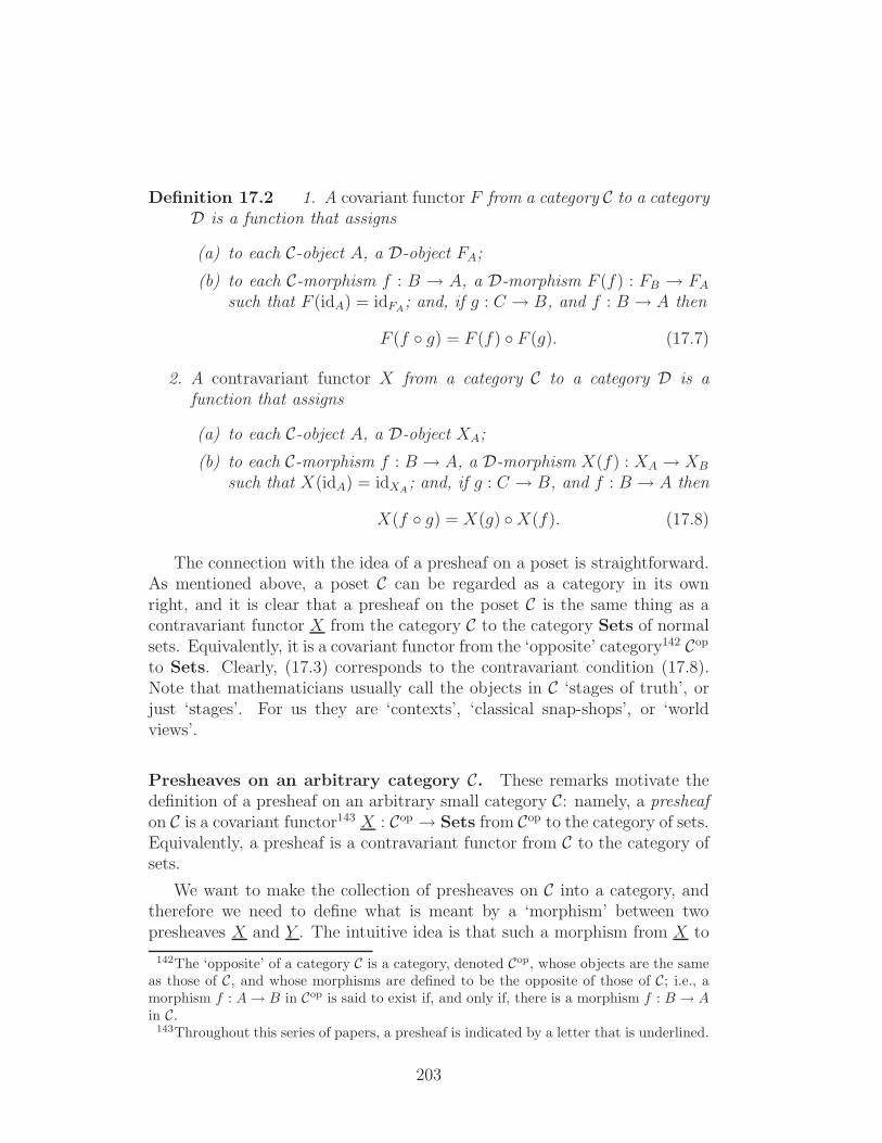
Definition 17.2 1. A covariant functor F from a category C to a categoryD is a function that assigns
(a) to each C-object A, a D-object FA;
(b) to each C-morphism f : B → A, a D-morphism F (f) : FB → FAsuch that F (idA) = idFA; and, if g : C → B, and f : B → A then
F (f g) = F (f) F (g). (17.7)
2. A contravariant functor X from a category C to a category D is afunction that assigns
(a) to each C-object A, a D-object XA;
(b) to each C-morphism f : B → A, a D-morphism X(f) : XA → XB
such that X(idA) = idXA ; and, if g : C → B, and f : B → A then
X(f g) = X(g) X(f). (17.8)
The connection with the idea of a presheaf on a poset is straightforward.As mentioned above, a poset C can be regarded as a category in its ownright, and it is clear that a presheaf on the poset C is the same thing as acontravariant functor X from the category C to the category Sets of normalsets. Equivalently, it is a covariant functor from the ‘opposite’ category142 Cop
to Sets. Clearly, (17.3) corresponds to the contravariant condition (17.8).Note that mathematicians usually call the objects in C ‘stages of truth’, orjust ‘stages’. For us they are ‘contexts’, ‘classical snap-shops’, or ‘worldviews’.
Presheaves on an arbitrary category C. These remarks motivate thedefinition of a presheaf on an arbitrary small category C: namely, a presheafon C is a covariant functor143 X : Cop → Sets from Cop to the category of sets.Equivalently, a presheaf is a contravariant functor from C to the category ofsets.
We want to make the collection of presheaves on C into a category, andtherefore we need to define what is meant by a ‘morphism’ between twopresheaves X and Y . The intuitive idea is that such a morphism from X to
142The ‘opposite’ of a category C is a category, denoted Cop, whose objects are the sameas those of C, and whose morphisms are defined to be the opposite of those of C; i.e., amorphism f : A→ B in Cop is said to exist if, and only if, there is a morphism f : B → Ain C.
143Throughout this series of papers, a presheaf is indicated by a letter that is underlined.
203
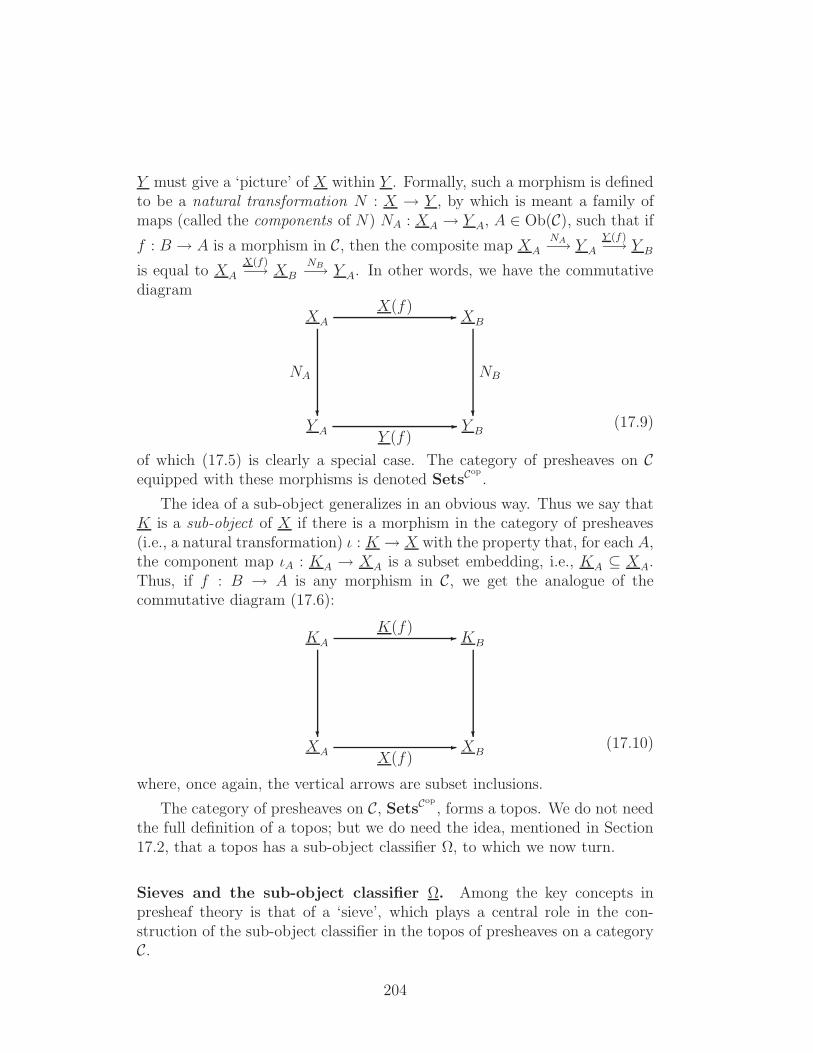
Y must give a ‘picture’ of X within Y . Formally, such a morphism is definedto be a natural transformation N : X → Y , by which is meant a family ofmaps (called the components of N) NA : XA → Y A, A ∈ Ob(C), such that if
f : B → A is a morphism in C, then the composite map XA
NA−→ Y A
Y (f)−→ Y B
is equal to XA
X(f)−→ XB
NB−→ Y A. In other words, we have the commutativediagram
Y A Y B-
Y (f)
XA XB-X(f)
?
NA
?
NB
(17.9)
of which (17.5) is clearly a special case. The category of presheaves on Cequipped with these morphisms is denoted SetsC
op
.
The idea of a sub-object generalizes in an obvious way. Thus we say thatK is a sub-object of X if there is a morphism in the category of presheaves(i.e., a natural transformation) ι : K → X with the property that, for each A,the component map ιA : KA → XA is a subset embedding, i.e., KA ⊆ XA.Thus, if f : B → A is any morphism in C, we get the analogue of thecommutative diagram (17.6):
XA XB-
X(f)
KA KB-K(f)
? ?(17.10)
where, once again, the vertical arrows are subset inclusions.
The category of presheaves on C, SetsCop
, forms a topos. We do not needthe full definition of a topos; but we do need the idea, mentioned in Section17.2, that a topos has a sub-object classifier Ω, to which we now turn.
Sieves and the sub-object classifier Ω. Among the key concepts inpresheaf theory is that of a ‘sieve’, which plays a central role in the con-struction of the sub-object classifier in the topos of presheaves on a categoryC.
204
A sieve on an object A in C is defined to be a collection S of morphismsf : B → A in C with the property that if f : B → A belongs to S, and ifg : C → B is any morphism with co-domain B, then f g : C → A alsobelongs to S. In the simple case where C is a poset, a sieve on p ∈ C is anysubset S of C such that if r ∈ S then (i) r p, and (ii) r′ ∈ S for all r′ r;in other words, a sieve is nothing but a lower set in the poset.
The presheaf Ω : C → Sets is now defined as follows. If A is an object inC, then ΩA is defined to be the set of all sieves on A; and if f : B → A, thenΩ(f) : ΩA → ΩB is defined as
Ω(f)(S) := h : C → B | f h ∈ S (17.11)
for all S ∈ ΩA; the sieve Ω(f)(S) is often written as f ∗(S), and is known asthe pull-back to B of the sieve S on A by the morphism f : B → A.
It should be noted that if S is a sieve on A, and if f : B → A belongs toS, then from the defining property of a sieve we have
f ∗(S) := h : C → B | f h ∈ S = h : C → B =: ↓B (17.12)
where ↓B denotes the principal sieve on B, defined to be the set of allmorphisms in C whose codomain is B.
If C is a poset, the pull-back operation corresponds to a family of mapsΩqp : Ωq → Ωp (where Ωp denotes the set of all sieves/lower sets on p in theposet) defined by Ωqp = Ω(ipq) if ipq : p→ q (i.e., p q). It is straightforwardto check that if S ∈ Ωq, then
Ωqp(S) :=↓p ∩ S (17.13)
where ↓p := r ∈ C | r p.A crucial property of sieves is that the set ΩA of sieves on A has the
structure of a Heyting algebra. Specifically, the unit element 1ΩAin ΩA is
the principal sieve ↓A, and the null element 0ΩAis the empty sieve ∅. The
partial ordering in ΩA is defined by S1 S2 if, and only if, S1 ⊆ S2; and thelogical connectives are defined as:
S1 ∧ S2 := S1 ∩ S2 (17.14)
S1 ∨ S2 := S1 ∪ S2 (17.15)
S1 ⇒ S2 := f : B → A | ∀g : C → B if f g ∈ S1 then f g ∈ S2(17.16)
As in any Heyting algebra, the negation of an element S (called the pseudo-complement of S) is defined as ¬S := S ⇒ 0; so that
¬S := f : B → A | for all g : C → B, f g 6∈ S. (17.17)
205
It can be shown that the presheaf Ω is a sub-object classifier for thetopos SetsC
op
. That is to say, sub-objects of any object X in this topos(i.e., any presheaf on C) are in one-to-one correspondence with morphismsχ : X → Ω. This works as follows. First, let K be a sub-object of X withan associated characteristic arrow χK : X → Ω. Then, at any stage A in C,the ‘components’ of this arrow, χKA : XA → ΩA, are defined as
χKA(x) := f : B → A | X(f)(x) ∈ KB (17.18)
for all x ∈ XA. That the right hand side of (17.18) actually is a sieve on Afollows from the defining properties of a sub-object.
Thus, in each ‘branch’ of the category C going ‘down’ from the stage A,χKA(x) picks out the first member B in that branch for which X(f)(x) lies inthe subset KB, and the commutative diagram (17.10) then guarantees thatX(h f)(x) will lie in KC for all h : C → B. Thus each stage A in C servesas a possible context for an assignment to each x ∈ XA of a generalisedtruth value—a sieve belonging to the Heyting algebra ΩA. This is the sensein which contextual, generalised truth values arise naturally in a topos ofpresheaves.
There is a converse to (17.18): namely, each morphism χ : X → Ω (i.e., anatural transformation between the presheaves X and Ω) defines a sub-objectKχ of X via
KχA := χ−1
A 1ΩA. (17.19)
at each stage A.
Global elements of a presheaf. For the category of presheaves on C, aterminal object 1 : C → Sets can be defined by 1A := ∗ at all stages A inC; if f : B → A is a morphism in C then 1(f) : ∗ → ∗ is defined to be themap ∗ 7→ ∗. This is indeed a terminal object since, for any presheaf X, wecan define a unique natural transformation N : X → 1 whose componentsNA : X(A)→ 1A = ∗ are the constant maps x 7→ ∗ for all x ∈ XA.
As a morphism γ : 1 → X in the topos SetsCop
, a global element corre-sponds to a choice of an element γA ∈ XA for each stage A in C, such that,if f : B → A, the ‘matching condition’
X(f)(γA) = γB (17.20)
is satisfied.
206
Acknowledgements
This research was supported by grant RFP1-06-04 from The FoundationalQuestions Institute (fqxi.org). AD gratefully acknowledges financial supportfrom the DAAD.
This work is also supported in part by the EC Marie Curie Research andTraining Network “ENRAGE” (European Network on Random GEometry)MRTN-CT-2004-005616.
We are both very grateful to Professor Hans de Groote for his detailedand insightful comments on our work.
CJI expresses his gratitude to Jeremy Butterfield for the lengthy, andmost enjoyable, collaboration in which were formulated the early ideas aboutusing topoi to study quantum theory.
References
[1] S. Abramsky. Domain Theory and the Logic of Observable Properties.PhD thesis, Queen Mary College, London University (1987).
[2] S. Abramsky and B. Coecke. A categorical semantics of quantum pro-tocols. In Proceedings of the 19th Annual IEEE Symposium on Logicin Computer Science, 415–425, IEEE Computer Science Press (2004).arXiv:quant-ph/0402130v5.
[3] M. Adelman and J.V. Corbett. A sheaf model for intuitionistic quantummechanics. Applied Categorical Structures 3, 79–104 (1995).
[4] J.C. Baez. An Introduction to Spin Foam Models of Quantum Gravityand BF Theory. Lect. Notes Phys. 543, 25–94 (2000).
[5] J. Baez. Quantum Quandaries: a Category-Theoretic Perspective. InThe Structural Foundations of Quantum Gravity, eds. S. French, D.Rickles and J. Sahatsi. Oxford University Press, Oxford (2006).
[6] J. Baez and U. Schreiber. Higher Gauge Theory. arXiv:math/0511.710v2(2005).
[7] B. Banaschewski and C.J. Mulvey. A globalisation of the Gelfand dualitytheorem. Ann. Pure & Applied Logic 137, 62–103 (2006).
207
[8] J.L. Bell. Toposes and Local Set Theories. Clarendon Press, Oxford(1988).
[9] J.S. Bell. On the problem of hidden variables in quantum mechanics. InSpeakable and Unspeakable in Quantum Mechanics. Cambridge Univer-sity Press, Cambridge, 1–13 (1987).
[10] E. Beltrametti and G. Cassinelli. The Logic of Quantum Mechanics.Addison-Wesley, Massachusetts (1981).
[11] G. Birkhoff and J. von Neumann. The logic of quantum mechanics. Ann.Math. 37, 823–843 (1936).
[12] J. Butterfield and C.J. Isham. Space-time and the philosophical chal-lenge of quantum gravity. In Physics Meets Philosophy at the PlanckScale, eds. C. Callender and N. Huggett, Cambridge University Press,33–89 (2001).
[13] J. Butterfield and C.J. Isham. A topos perspective on the Kochen-Specker theorem: IV. Interval valuations. Int. J. Theor. Phys 41, 613–639 (2002).
[14] A. Connes. Noncommutative Geometry. Academic Press, San Diego(1994). Download from http://www.alainconnes.org/en/
[15] A. Connes, H. Moscovici. Background independent geometry and Hopfcyclic cohomology. math.QA/0505475 (2005).
[16] J.V. Corbett and T. Durt. Collimation processes in quantum mechanicsinterpreted in quantum real numbers. preprint (2007).
[17] L. Crane. What is the Mathematical Structure of Quantum Spacetime?arXiv:0706.4452 (2007).
[18] M.L. Dalla Chiara and R. Giuntini. Quantum logics. In Handbookof Philosophical Logic, vol. VI, G. Gabbay and F. Guenthner (eds.).Kluwer, Dordrecht, 129–228 (2002).
[19] A. Doring. Kochen-Specker theorem for von Neumann algebras. Int.Jour. Theor. Phys. 44, 139–160 (2005).
[20] A. Doring. Observables as functions: Antonymous functions.arXiv:quant-ph/0510.102 (2005).
208
[21] A. Doring, and C.J. Isham. A topos foundation for theories of physics:I. Formal languages for physics, arXiv:quant-ph/0703.060, to appear inJ. Math. Phys (2008).
[22] A. Doring, and C.J. Isham. A topos foundation for theories of physics:II. Daseinisation and the liberation of quantum theory. arXiv:quant-ph/0703.062, to appear in J. Math. Phys (2008).
[23] A. Doring, and C.J. Isham. A topos foundation for theories of physics:III. Quantum theory and the representation of physical quantities witharrows δ(A) : Σ→ R. arXiv:quant-ph/0703.064, to appear in J. Math.Phys (2008).
[24] A. Doring, and C.J. Isham. A topos foundation for theories of physics:IV. Categories of systems. arXiv:quant-ph/0703.066, to appear in J.Math. Phys (2008).
[25] A. Doring. Topos theory and ‘neo-realist’ quantum theory.arXiv:0712.4003 (2007), to appear in Proceedings of workshop RecentDevelopments in Quantum Field Theory (MPI MiS Leipzig, July 2007)
[26] A. Doring. The physical interpretation of daseinisation. In preparation(2008).
[27] F. Dowker. Causal sets and the deep structure of space-time. In 100Years of Relativity—Space-time Structure: Einstein and Beyond, ed.Abhay Ashtekar. World Scientific, Singapore (2005).
[28] M.H. Escard. PCF extended with real numbers: a domain-theoreticapproach to higher-order exact real number computation. PhDthesis. Download from http://www.lfcs.inf.ed.ac.uk/reports/97/ECS-LFCS-97-374/index.html (2007).
[29] R. Goldblatt. Topoi: The Categorial Analysis of Logic. North-Holland,London (1984).
[30] A.C. Grayling. An Introduction to Philosophical Logic. Duckworth Press,London (1990).
[31] H.F. de Groote. On a canonical lattice structure on the effect algebraof a von Neumann algebra. arXiv:math-ph/0410.018v2 (2004).
[32] H.F. de Groote. Observables. arXiv:math-ph/0507.019 (2005).
209
[33] H.F. de Groote. Observables I: Stone spectra. arXiv:math-ph/0509.020(2005).
[34] H.F. de Groote. Observables II: Quantum observables. arXiv:math-ph/0509.075 (2005).
[35] J. Hamilton, J. Butterfield and C.J. Isham. A topos perspective onthe Kochen-Specker theorem: III. Von Neumann algebras as the basecategory. Int. J. Theor. Phys. 39, 1413-1436 (2000).
[36] M. Heidegger. What is a Thing? Regenery/Gateway, Indiana (1967).
[37] W. Heisenberg. Philosophic Problems of Nuclear Science. Pantheon,New York (1952).
[38] C. Heunen and B. Spitters. A topos for algebraic quantum theory.arXiv:0709.4364 (2007).
[39] C.J. Isham. Quantum logic and the histories approach to quantumtheory. J. Math. Phys. 35, 2157–2185 (1994).
[40] C.J. Isham. Topos theory and consistent histories: The internal logic ofthe set of all consistent sets. Int. J. Theor. Phys. 36, 785–814 (1997).
[41] C.J. Isham. Some reflections on the status of conventional quantumtheory when applied to quantum gravity. In Proceedings of the Confer-ence in Honour of Stephen Hawking’s 60’th birthday, ed. G. Gibbons,Cambridge University Press, Cambridge (2003).
[42] C.J. Isham. Is it true; or is it false; or somewhere in between? The logicof quantum theory. Contempory Phys. 46, 207–219 (2005).
[43] C.J. Isham. A Topos Perspective on State-Vector Reduction. Int. J.Theor. Phys. 45, 994–1020 (2006).
[44] C.J. Isham and J. Butterfield. A topos perspective on the Kochen-Specker theorem: I. Quantum states as generalised valuations. Int. J.Theor. Phys. 37, 2669–2733 (1998).
[45] C.J. Isham and J. Butterfield. A topos perspective on the Kochen-Specker theorem: II. Conceptual aspects, and classical analogues. Int.J. Theor. Phys. 38, 827–859 (1999).
[46] C.J. Isham and J. Butterfield. Some possible roles for topos theoryin quantum theory and quantum gravity. Found. Phys. 30, 1707–1735(2000).
210
[47] M. Jackson. A sheaf theoretic approach to measure theory. PhD thesis,University of Pittsburgh (2006).
[48] P.T. Johnstone. Sketches of an Elephant: A Topos Theory CompendiumI, II. Oxford Science Publications, Oxford (2002/03).
[49] R.V. Kadison and J.R. Ringrose. Fundamentals of the Theory of Op-erator Algebras, Volume 1: Elementary Theory. Academic Press, NewYork (1983).
[50] S. Kochen and E.P. Specker. The problem of hidden variables in quan-tum mechanics. Journal of Mathematics and Mechanics 17, 59–87(1967).
[51] A. Kock. Synthetic Differential Geometry (LMS lecture note series: 51).Cambridge University Press, Cambridge (1981).
[52] J. Lambek and P.J. Scott. Introduction to higher order categorical logic.Cambridge University Press, Cambridge (1986).
[53] K. Landsmann. Lecture given at the conference Deep Beauty: Math-ematical Innovation and the Search for an Underlying Intelligibility ofthe Mathematical World. Princeton (2007).
[54] F.W. Lawvere and R. Rosebrugh. Sets for Mathematics. CambridgeUniversity Press, Cambridge (2003).
[55] S. MacLane. Categories for the Working Mathematician. Springer, NewYork, Berlin, Heidelberg (1971).
[56] S. MacLane and I. Moerdijk. Sheaves in Geometry and Logic: A FirstIntroduction to Topos Theory. Springer, New York, Berlin, Heidelberg(1992).
[57] H. Margenau. Reality in quantum mechanics. Phil. Science 16, 287–302(1949).
[58] F. Markopoulou. The internal description of a causal set: What theuniverse looks like from the inside. Comm. Math. Phys. 211, 559–583(2002).
[59] A. Mallios. Modern Differential Geometry in Gauge Theories, vol 1:Maxwell Fields. Birkhauser, Boston (2006).
211
[60] A. Mallios. Modern Differential Geometry in Gauge Theories, vol 2:Yang-Mills Fields. Birkhauser, Boston (2006).
[61] A. Mallios and E. Zafiris Topos-theoretic relativization of physical rep-resentability and quantum gravity. arXiv:gr-qc/0610.113 (2007).
[62] K. Nakayama. Topos-theoretic extension of a modal interpretation ofquantum mechanics. arXiv:0711.2200 (2007).
[63] M.P. Olson. The Selfadjoint Operators of a von Neumann Algebra form aConditionally Complete Lattice. Proc. of the AMS 28, 537–544 (1971).
[64] M. Ozawa. Transfer principle in quantum set theory. J. Symbolic Logic72 (2007), 625–648. arXiv:math/0604.349v2.
[65] K. Popper. Quantum Theory and the Schism in Physics. Hutchinson,London (1982).
[66] I. Raptis. Categorical quantum gravity. Int. Jour. Theor. Phys. 45,1495-1523 (2006).
[67] L. Smolin. The case for background independence. In The StructuralFoundations of Quantum Gravity, eds. S. French, D. Rickles and J. Sa-hatsi. Oxford University Press, Oxford (2006).
[68] L. Smolin. Generic predictions of quantum theories of gravity.arXiv:hep-th/0605.052, to appear in Approaches to Quantum Gravity—Toward a New Understanding of Space, Time, and Matter, ed. D. Oriti.Cambridge University Press, Cambridge (2006).
[69] R. D. Sorkin. Causal Sets: Discrete Gravity (Notes for the Valdivia Sum-mer School). In Lectures on Quantum Gravity, eds. Andres Gomberoffand Don Marolf. Plenum (2005).
[70] M.H. Stone. The Theory of Representations for Boolean algebras. Trans.Amer. Math. Soc. 40, 37–111 (1936).
[71] G. Takeuti. Quantum set theory. In Current Issues in Quantum Logic,E.G. Beltrametti and B.C. van Fraasen (eds.). Plenum, New York, 303–322 (1981).
[72] S. Vickers. Topology via Logic. Cambridge University Press, Cambridge(1982).
[73] J. Vicary. The quantum harmonic oscillator as an adjunction.arXiv:0706.0711 (2007), to appear in Int. J. Theor. Phys.
212