What happened to real earnings in Egypt, 2008 to 2009?
38
ORIGINAL ARTICLE Open Access What happened to real earnings in Egypt, 2008 to 2009? Paul Cichello 1* , Hala Abou-Ali 2 and Daniela Marotta 3 * Correspondence: [email protected] 1 Economics Department, Boston College, 140 Commonwealth Ave, Chestnut Hill, MA 02467, USA Full list of author information is available at the end of the article Abstract: Nominal earnings in Egypt did not respond to the increase in inflation between February 2008 and February 2009, resulting in a 12.3 (9) percent decline in average (median) real earnings among 25 to 60 years old workers. Changes in earnings differ significantly by groups: (i) those with higher initial earnings (reported and predicted) suffered the largest declines in earnings; (ii) men lost more than women but after controlling for initial earnings, women lost considerably more than men; (iii) those who were initially in agriculture also had greater declines despite rising food prices. JEL classification codes: J62; J16; J42; J43; O15; O17 Keywords: Earnings mobility; Egypt; Inflation; Gender; Wage differentials; Segmented labor market 1. Introduction The returns to labor are critical for ensuring household economic well-being in Egypt, as elsewhere. As such, government leaders are concerned if they observe more labor lying dormant when unemployment rates rise or if they see the returns to labor fall when real earnings fall. In trying to better understand the workings and outcomes of the labor market and the returns to labor a multitude of studies have analyzed the Egyptian labor market. A number of these studies have examined earnings changes using cross-sectional data, illuminating important features of the Egyptian labor mar- ket (Arabsheibani 2000; Belhaj-Hassine 2012; Datt and Olmstead 2004; Said 2009, 2012). However, comparisons of cross-sectional data from two points in time do not allow us to follow the same individual over time when trying to determine who is get- ting ahead and who is falling behind. Recently, panel data has been collected that allows researchers to track the same in- dividual over time. By following individuals over time, we can identify how an individ- ual’ s earnings level in the current year compares to his or her earnings in the previous period. We can also investigate how such earnings mobility experiences vary across in- dividuals. This allows us to map the changes in earnings to the standard covariates, such as gender and education levels, and also to include new covariates such as the poverty level of the individual’ s household and the earnings level of the individual in the initial period. Inclusion of these items can have an important impact on how we interpret the observed changes in the economy and resulting policy implications. © Cichello et al.; licensee Springer. This is an open access article distributed under the terms of the Creative Commons Attribution License (http://creativecommons.org/licenses/by/2.0), which permits unrestricted use, distribution, and reproduction in any medium, provided the original work is properly cited. Cichello et al. IZA Journal of Labor & Development 2013 2013, 2:10 http://www.izajold.com/content/2/1/10
-
Upload
independent -
Category
Documents
-
view
0 -
download
0
Transcript of What happened to real earnings in Egypt, 2008 to 2009?

Cichello et al. IZA Journal of Labor & Development 2013, 2:10http://www.izajold.com/content/2/1/10
ORIGINAL ARTICLE Open Access
What happened to real earnings in Egypt,2008 to 2009?Paul Cichello1*, Hala Abou-Ali2 and Daniela Marotta3
* Correspondence:[email protected] Department, BostonCollege, 140 Commonwealth Ave,Chestnut Hill, MA 02467, USAFull list of author information isavailable at the end of the article
©Am
Abstract: Nominal earnings in Egypt did not respond to the increase in inflationbetween February 2008 and February 2009, resulting in a 12.3 (9) percent decline inaverage (median) real earnings among 25 to 60 years old workers. Changes inearnings differ significantly by groups: (i) those with higher initial earnings (reportedand predicted) suffered the largest declines in earnings; (ii) men lost more thanwomen but after controlling for initial earnings, women lost considerably more thanmen; (iii) those who were initially in agriculture also had greater declines despiterising food prices.
JEL classification codes: J62; J16; J42; J43; O15; O17
Keywords: Earnings mobility; Egypt; Inflation; Gender; Wage differentials; Segmentedlabor market
1. IntroductionThe returns to labor are critical for ensuring household economic well-being in Egypt,
as elsewhere. As such, government leaders are concerned if they observe more labor
lying dormant when unemployment rates rise or if they see the returns to labor fall
when real earnings fall. In trying to better understand the workings and outcomes of
the labor market and the returns to labor a multitude of studies have analyzed the
Egyptian labor market. A number of these studies have examined earnings changes
using cross-sectional data, illuminating important features of the Egyptian labor mar-
ket (Arabsheibani 2000; Belhaj-Hassine 2012; Datt and Olmstead 2004; Said 2009,
2012). However, comparisons of cross-sectional data from two points in time do not
allow us to follow the same individual over time when trying to determine who is get-
ting ahead and who is falling behind.
Recently, panel data has been collected that allows researchers to track the same in-
dividual over time. By following individuals over time, we can identify how an individ-
ual’s earnings level in the current year compares to his or her earnings in the previous
period. We can also investigate how such earnings mobility experiences vary across in-
dividuals. This allows us to map the changes in earnings to the standard covariates,
such as gender and education levels, and also to include new covariates such as the
poverty level of the individual’s household and the earnings level of the individual in
the initial period. Inclusion of these items can have an important impact on how we
interpret the observed changes in the economy and resulting policy implications.
Cichello et al.; licensee Springer. This is an open access article distributed under the terms of the Creative Commonsttribution License (http://creativecommons.org/licenses/by/2.0), which permits unrestricted use, distribution, and reproduction in anyedium, provided the original work is properly cited.
2013

Cichello et al. IZA Journal of Labor & Development Page 2 of 382013, 2:10http://www.izajold.com/content/2/1/10
To our knowledge, this study represents the first analysis of earnings mobility in
Egypt to incorporate initial earnings into analysis of earnings changes for both
wage and non-wage workers1. We initially viewed this project as a study designed
to establish baseline statistics for “typical” earnings mobility patterns in the Egyp-
tian labor market.
However, given the significant inflation shock that occurred between interviews, we
recognize that this may be a rather unique period in the labor market and should not
be thought of as “typical”. Therefore we proffer this study as a window into the changes
in the labor market in a time of severe stress on real wages due to an external shock of
rising commodity prices.
Aggregate employment outcomes and nominal earnings or profits among prime-aged
workers are shown to be fairly non-responsive despite the increased prices. Instead, in-
flation severely erodes the real earnings that individuals receive, implying an adjust-
ment process that relies heavily on reduced real earnings. On average, a worker earns
approximately 10 percent less than he or she did in the previous year.
The inability of workers to garner higher wages helped to keep inflation from con-
tinuing on an upward spiral2. The self-employed and employers also experienced de-
clines in real profits suggesting that they either did not try or were not able to raise the
prices of their goods and services in order to keep their real earnings constant or
growing3.
The lack of labor market response to inflation in aggregate employment and nominal
earnings outcomes should not be construed as a signal of rigidity of experiences at the
individual level. As is typical in such studies, there is a large degree of heterogeneity in
the earnings changes experienced by individuals. We identify key determinants associ-
ated with earnings mobility using a variety of descriptive regression techniques.
There is a strong association between initial earnings and subsequent earnings
changes, with those initially earning more experiencing larger declines than their coun-
terparts. As such changes can be caused by temporary fluctuations in earnings and/or
measurement errors; this effect is taken with some caution. Nonetheless, we find these
results generally robust to methods that address measurement error concerns, such as
using predicted earnings in place of actual earnings. Additionally, other determinants
of earnings changes that one would assume would be quite powerful predictors of earn-
ings change—such as workers changing the sector of employment (agriculture, indus-
try, or services)—have a limited ability to predict earnings mobility.
Changes in earnings also differ significantly by gender. On average, the earnings
changes are far more negative for men than for women. However, this gender effect is
completely reversed if one controls for initial earnings; i.e. for men and women who
have the same initial earnings (and otherwise similar job characteristics), the earnings
changes tend to be less negative for men than for women. In contrast, the average dif-
ference in log earnings is relatively similar across gender, with men having a slight ad-
vantage. This advantage for males is dramatically magnified if one controls for initial
log earnings.
The rest of the paper is organized as follows. Section 2 first describes the context of
our study, and explains the context of the Egyptian economy during this time, includ-
ing a review of the rise in inflation. Section 3 depicts the panel data used in this study.
Section 4 portrays the empirical approach. Section 5 introduces the results. Section 6

Cichello et al. IZA Journal of Labor & Development Page 3 of 382013, 2:10http://www.izajold.com/content/2/1/10
provides a discussion of these results and presents the relevance to policy and future
research.
2. Background discussion of the Egyptian economyThe World Bank study, “Poverty in Egypt 2008–2009: Withstanding the global eco-
nomic crisis,” includes a substantive review of the Egyptian economy leading up to
2008 (World Bank 2011). In this section, we review some of its critical findings relevant
to our study.
From 2004 to mid-2008, Egypt experienced a period of steady economic growth with
an average real GDP annual growth of 6.4 percent. This growth period was followed by
a series of economic shocks starting in the second half of 2008 and continuing for most
of 2009, namely:
(i) the slowdown in economic growth, which followed the global downturn in the
world economy;
(ii)a simultaneous and related fall in remittances; and
(iii)a sudden acceleration in prices, mostly driven by exogenous factors such as the
commodities price shock.
The economic developments over the period 2004–2009 are summarized in Figure 1.
Note that the table begins in the last quarter of 2004 using the calendar year (second
quarter of the fiscal year). For reference, the panel data analyzed in this study were col-
lected in the first quarter of 2008 and the first quarter of 2009. They are denoted by
the vertical strips at the third quarter of fiscal year 2008 and 2009, respectively.
25
45
65
85
105
125
145
165
185
205
225
0%
1%
2%
3%
4%
5%
6%
7%
8%
Rem
itta
nce
s, L
E/q
uar
ter/
per
cap
ita
CP
I an
d G
DP
per
cap
ita q
/o/q
ind
ices
HIECS Panel CPI GDP per capita Remittances, const. 2002 LE
Figure 1 Quarterly GDP growth, inflation rate and remittances in Egypt, 2004–2009. Reprinted fromThe World Bank (2011). Data from CAPMAS and Ministry of Economic Development. Note: The quarterlyGDP per capita data were annualized before determining the percent increase or decrease in thequarter-on-quarter index. CPI data were not annualized.

Cichello et al. IZA Journal of Labor & Development Page 4 of 382013, 2:10http://www.izajold.com/content/2/1/10
At first glance, Egypt weathered the global crisis relatively well. Despite an abrupt
economic slowdown, from seven percent growth in 2008 to 4.7 percent in 2009, growth
remained positive. However, employment growth stalled in absolute terms (employ-
ment was flat during 2008 and the first quarter of 2009), and unemployment started to
rise again (to 9.4 percent in the first quarter of 2009). According to the Labor Force
Sample Survey (LFSS) conducted by the Central Agency for Public Mobilization and
Statistics (CAPMAS), there was a seven percent reduction in employment in manufac-
turing in the first quarter of 2009 (compared to the first quarter of 2008), and a 15 per-
cent drop in the restaurants and hotel sectors. Meaning that, both sectors are most
exposed to global trends and thus more susceptible to global shocks.
These changes came during a period of accelerating inflation, which peaked at 20
percent (annual average) in the summer of 2008. After peaking to an unprecedented
level in August 2008 (23.7 percent), inflation remained exceptionally high for two quar-
ters, only to stabilize at 9.9 percent between May and July-09. Inflation was almost
completely imported, as a result of the sharp acceleration in global commodities prices
(mostly fuel and food, including fruits and vegetables). Some components of the infla-
tion basket, such as food and non-alcoholic beverages, remained high (up by 13.4 per-
cent y-to-y in July-09) even after and despite the steep fall in international prices since
mid-2008.
By the last quarter of 2009, the Egyptian economy showed signs of rebounding, and
since then has been growing at five percent and higher each quarter. The employment
losses were soon recovered (at least in absolute figures). Thus, our earnings mobility
analysis may overestimate some of the long term decline in earnings that individuals
faced from this period.
3. DataThe data used in this analysis come from the Household Income, Expenditure and
Consumption Panel Survey (HIECPS), which is a subcomponent of the Household In-
come, Expenditure and Consumption Survey (HIECS). This is a nationally representa-
tive panel survey. However, as there were relatively few observations from the frontier
governorates, we exclude the border region from our analysis.
Households were interviewed in February 2008 and those same households were
interviewed again in February 2009. Information gathered included individual labor
market outcomes, wages and profits from enterprises run by household members, as
well as standard demographic information such as age, gender, and education level of
all household members.
Earnings were constructed at the individual level. Earnings from household enter-
prises were split among all household members engaged in the enterprise, including
those typically referred to as “unpaid workers4”. Unless clearly denoted as nominal
earnings, all earnings are deflated over both time and space and represent the purchas-
ing power of the 2005 Egyptian pound (EGP) spent in the metropolitan area.
The analysis is limited to those who were 25 to 58 years old in 2008, unless explicitly
stated. We are most interested in the changes in earnings of those actively engaged in
the labor market and do not want large earnings changes by those retiring or moving
to part time jobs in a pseudo-retirement phase to cloud our analysis. Additionally, large

Cichello et al. IZA Journal of Labor & Development Page 5 of 382013, 2:10http://www.izajold.com/content/2/1/10
gains from recent entrants (or entrants into full time work) can disrupt our analysis.
This is not to say that we are not interested in the important issues of youth (15–
24 years) unemployment or earnings. We simply feel they should be analyzed separ-
ately. We will discuss how the inclusion of these younger workers affects some of our
key results below.
Additionally, we limit earnings mobility analysis to those who are employed in both
periods5. We use 3,481 observations of dual employed individuals with valid data.
One concern of such panel studies is that not every person interviewed in 2008 can
be found again (or is willing to be re-interviewed) in 2009. This can have a particularly
pernicious effect on our analysis if those who were not re-interviewed tend to have (ex-
tremely) positive or (extremely) negative earnings changes compared to those who are
similar to them but were re-interviewed. There is some empirical evidence that such
movers, particularly those that move farther away, tend to have more positive earnings
changes than those left behind (Beegle et al. 2011). However, the existing evidence is
quite limited and not from Egypt. Additionally, there are some common sense theoret-
ical arguments that suggest that such missing individuals could be worse off. This ques-
tion remains open as we do not have enough evidence to answer it in one direction or
the other.
The fact that attrition rates in this panel are relatively low (just three percent of 2008
households are not re-interviewed in 2009) is therefore reassuring. As is typical in such
studies, the individual attrition rate, 9.1 percent, is higher than the household attrition
rate. Among 25 to 58 year olds, the individual attrition rate is 8.7 percent.
Overall, attrition appears to be driven more by who a person is and general life-cycle
effects than by an individual’s productive characteristics or outcomes. The first column
of Table 1 shows the results of a linear probability model (LPM) predicting individual
attrition. The dependent variable is 1 if the individual is not re-interviewed and 0 if the
individual is re-interviewed. Those who were not married, were either very young or
very old, were male and lived in the Metropolitan region were more likely to be missing
at the 2009 interview. Meanwhile, joint significance tests on education level, initial sec-
tor of work, and relationship with employer categories were not found to have a signifi-
cant effect at the ten percent level. An exception to this general trend is the fact that
those who had higher initial earnings were found to be more likely to attrite. This was
statistically significant at the five percent level, with change of one standard deviation
in real earnings in 2008 resulting in a change in the predicted probability of attrition of
0.009 percentage points, ceteris paribus. A probit model was also run (see rightmost
column of Table 1). The results of the probit model generally corroborate the LPM
findings. One potential exception is that individuals working in the manufacturing and
construction and trades and services sectors are less likely to attrite than those working
in agriculture6.
4. Empirical approachWe identify the typical change in earnings experienced by different types of Egyptian
workers using empirical approaches that are common in the earnings and income mo-
bility literature. We start by reporting mean and median earnings changes and move
on to control for an increasing set of covariates. Techniques are similar to some of

Table 1 Determinants of attrition
Dep. Var. (Attrition = 1)
Linear Probit
Prob. Model dF/dx
Metropolitan (omitted)
Lower Urban −0.061*** −0.039***
Lower Rural −0.056*** −0.043***
Upper Urban −0.045** −0.029**
Upper Rural −0.063*** −0.046***
Male 0.041*** 0.030***
Working Housewife −0.024 −0.029*
Married −0.091*** −0.059***
Age −0.022*** −0.017***
Age-squared 0.000*** 0.0001***
Illiterate/no formal schooling (omitted)
Basic education/literacy 0.008 0.010
Completed Primary 0.004 0.006
Secondary education −0.005 −0.003
University degree 0.025 0.022
wage worker public (omitted)
wage worker private 0.018 0.015
employer −0.019 −0.015
self employed −0.002 −0.001
unpaid worker 0.007 0.002
Agriculture (omitted)
Manu/Const −0.032* −0.025**
Trade/Services −0.021 −0.022*
Log per capita consumption 0.008 0.009
Earnings in 2008 −0.000** 0.000
Constant 0.635***
n 4160 4160
R-squared / Pseudo R-squared 0.076 0.112
Notes: legend: * p < 0.10; ** p < 0.05; *** p < 0.01. Probit dF/dx evaluated at the mean of all other variables. Dummyvariables show difference from 0 to 1.Source: HIECPS, Feb 2008 to Feb 2009 (CAPMAS 2009).
Cichello et al. IZA Journal of Labor & Development Page 6 of 382013, 2:10http://www.izajold.com/content/2/1/10
those used in Cichello et al. (2005), Fields et al. (2003a/2003b), and Fields and Sanchez-
Puerta (2010). Fields (2008) provides a literature review of such micro-mobility studies
and provides a description of methods. There is a particular emphasis on controlling
for initial earnings.
The goal of this empirical approach is to identify who has experienced the most se-
vere declines in earnings, who has been able to avoid such severe declines in earnings,
and which variables are consistently associated with the changes in earnings experi-
enced by Egyptian workers. While all of the analysis, even the multivariate regression
analysis, is descriptive rather than causal, one can confidently identify which groups of
workers have been most or least adversely affected7. One can also piece together strong
circumstantial evidence regarding some of the major drivers of earnings change.

Cichello et al. IZA Journal of Labor & Development Page 7 of 382013, 2:10http://www.izajold.com/content/2/1/10
Theories of what caused the changes in earnings should, at a minimum, be consistent
with these descriptive results.
Our analysis will use both the change in earnings and the change in log earnings as
the outcome variables of interest. The former is self-explanatory while the latter con-
forms roughly to the percentage change in earnings. Given that utility functions are
concave, determining that earnings have fallen more on average for those who started
with higher earnings may not necessarily suggest a lower welfare loss8. Also, in the con-
text of an inflation shock, one may not be overly surprised if those with higher initial
earnings have greater earnings declines. However, if the log earnings falls more for
those with higher initial earnings, this goes beyond just the changes due to inflation.
We assess the change in earnings across a variety of characteristics. These include
demographic variables (gender, age, marital status), location/region (urban and rural),
and education level. We take these variables as exogenous variables that individuals
bring to the labor market9. We also include a number of 2008 outcomes which may
well be co-determined with the earnings change process. These include an individual’s
sector of employment (agriculture, industry or construction, trade or services); relation-
ship with employer (public wage worker, private wage worker, employer, self-employed,
unpaid worker); and formal or informal worker status, with formal workers defined as
those covered by the social insurance system. We also include whether one lives in a
poor household, defined as having consumption levels below the household specific
poverty line10. In our multivariate analysis, these variables will be right hand side deter-
minants of the change in log earnings.
Additionally, the relationship between the change in earnings and initial earnings is
explored using flexible estimation approaches. The non-parametric lowess estimator es-
timates a smoothed change in log earnings value, yis, for each observation by running n
observation specific regressions of the change in log earnings (yi) on initial log earnings
(xi) and calculating the predicted value of yi. Weights for each observation in the re-
gression are determined based on the distance from the xi value of the current observa-
tion. More emphasis is placed on observations that are close to the current
observation, even going so far as to give a zero weight to observations outside the
bandwidth. The lowess estimator in STATA uses the tri-cube weight of Cleveland
(1979) and we apply a bandwidth of 0.8 throughout these figures11.
Measurement error can be particularly problematic when determining the change in
earnings to initial earnings. For example, assume the relationship between these vari-
ables is linear and we would like to run a simple regression of change in reported earn-
ings Δyri , on initial reported earnings yr08,i.
Δyr i ¼ β0 þ β1yr08;i þ εi; ð1Þ
This can be re-written incorporating the potential for measurement error, signified
by μ. We use yk to represent the true level of earnings in year k.
Δyi þ μ09;i–μ08;i� � ¼ β0 þ β1 y08;i þ μ08;i
� �þ εi; ð2Þ
Even if measurement error is assumed to be mean zero, independent across individ-
uals, independent across time for a given individual and independent of an individual’s
earnings level, the problems are more than the standard attenuation concerns that
Cichello et al. IZA Journal of Labor & Development Page 8 of 382013, 2:10http://www.izajold.com/content/2/1/10
typically accompany a classical measurement error. The realized measurement error in
year 2008 turns up on both the left hand and right hand sides of this equation causing
a spurious negative correlation. To the extent that the measurement error is not per-
fectly auto-correlated, this can lead to a problem identical in nature to Galton’s Fallacy.
A negative relationship between initial earnings and the change in earnings might sim-
ply be due to random reporting errors.
Running the above regression will not give us the desired regression coefficient,
β̂� ¼ Cov Δy; y08ð ÞVar y08ð Þ ð3Þ
Instead, as shown in a more general form in Fields et al. (2003a), we obtain:
β̂ ¼ β̂ � Var y08ð ÞVar y08ð Þ þ Var μ08ð Þ−
Var μ08ð ÞVar y08ð Þ þ Var μ08ð Þ ð4Þ
The first term identifies the standard attenuation bias issue while the second term ac-
counts for the spurious negative correlation caused by the measurement error being on
both the right and left side of the equation.
A simple example will illustrate why addressing this issue is of fundamental import-
ance to our analysis. Suppose β̂� ¼ 0:50 , implying that for each additional pound of
earnings in 2008, on average, the individuals experiences a change in earnings that is a
half a pound more (i.e. less negative). Also, suppose that the variance in measurement
error is exactly equal to the variance in initial earnings. In this case, the attenuation
bias would shrink the estimate from 0.5 to 0.25 and the second term would take away
another 0.50. In other words, we would observe a coefficient of −0.25 in our analysis.
Our story would be one of converging earnings, but the reality would be significant di-
vergence of earnings in this sample. This example, while extreme, shows how powerful
the impact of these biases can be on our results. It also highlights that the extent of the
problem is driven in part by our assumption of how large the variance of the measure-
ment error is relative to the variance of the initial earnings. For example, if we assumed
the variance of μ was ten percent of the variance of initial earnings, the coefficient
would observe would be 0.35 rather than 0.5012.
In order to assess the robustness of our results given this potential problem, two ap-
proaches will be applied. First, initial earnings will be substituted by predicted initial
earnings on the right hand side of equation (1) in the simple regression above (as well
as in other methods). This process, i.e., the use of predicted values of initial values,
should rid the right hand side of equation (1) of the spurious measurement error13. Of
course, if our ability to predict initial earnings is weak, we may lose more than we gain
from this approach. It should be noted that the key variables used to predict initial
earnings are gender, age, education, place of residence, relationship with employer, sec-
tor of work, and log per capita consumption in the household.
The prediction regression results are shown in Table 2. When predicting initial earn-
ings, the R-squared is 0.32. When predicting initial log earnings, the R-squared is .612.
Thus, there is a relatively strong ability to predict initial earnings in levels and logs.
The coefficient estimates are entirely reasonable; they are what we would expect in
Egypt. Ceteris paribus, men have a strong initial advantage, earnings are concave with
respect to age (turning point at roughly 45 years of age), those with higher education

Table 2 Regressions used to predict 2008 earnings and log earnings
2008 earnings 2008 log earnings
Male 4517*** 0.580***
Age 723*** 0.090***
Age-squared −8*** −0.001***
Working Housewife 603 −0.207***
Married 2873*** 0.366***
Illiterate/no formal schooling (omitted)
Basic education/literacy 414 0.094***
Completed Primary 1700*** 0.155***
Secondary education 636* 0.115***
University degree 1406*** 0.194***
Metropolitan (omitted)
Lower Urban −1035** −0.007
Lower Rural −1495*** −0.049*
Upper Urban −563 0.033
Upper Rural −439 −0.021
wage worker public (omitted)
wage worker private −356 −0.032
employer 3724*** 0.388***
self employed 152 −0.114***
unpaid worker −882 −0.509***
Agriculture (omitted)
Manu/Const 1021** 0.148***
Trade/Services 775* 0.126***
log per capita consumption (08) 5748*** 0.520***
Constant −60681*** 1.682***
n 3481 3481
R-squared 0.32 0.612
Notes: legend: * p < 0.10; ** p < 0.05; *** p < 0.01.Source: HIECPS, Feb 2008 to Feb 2009 (CAPMAS 2009).
Cichello et al. IZA Journal of Labor & Development Page 9 of 382013, 2:10http://www.izajold.com/content/2/1/10
are earning considerably more than those with less education, wage workers outper-
form the self-employed and unpaid workers, but not employers, and agricultural
workers earn less than others.
We will also assess whether such a classical measurement error can explain the re-
sults we observe in this dataset using a second approach. We assess the amount of
measurement error that must be present, defined in terms of the variance, for measure-
ment error to explain our observed regression coefficient if the true β coefficient is
positive; i.e. if those higher initial earners experienced greater earnings gains. This is
similar to a subset of simulations found in Fields et al. (Fields et al. 2003a). Addition-
ally, in the annex, we use a simple simulation to demonstrate what our lowess graphs
would look like given certain assumed levels of classical measurement error.
Under these assumptions, we consider it implausible that the negative coefficient on
initial earnings from the simple regression was driven solely by classical measurement
error. In order for this to be true, the variance of measurement error must be at least
1.56 times the variance of the true earnings level.

Cichello et al. IZA Journal of Labor & Development Page 10 of 382013, 2:10http://www.izajold.com/content/2/1/10
5. Findings5.1 Transitions into and out of employment
Employment participation held steady and even increased slightly (68.2 to 69.6 per-
cent), between February 2008 and February 2009 among panel members who were 25
to 58 years old in 2008. Thus, this is not a period where job losses were a dominant
feature in the labor market for prime-aged workers14.
Table 3 reveals that the aggregate participation rate masks strikingly different partici-
pation rates by gender, 94.5 percent for men versus 44.4 percent for women in 2008.
The difference is largely due to many more women remaining outside the labor force.
Given the decline in real earnings between 2008 and 2009 (which is discussed in
much more detail below), one might expect households to offset the erosion of real
earnings by increasing the number of earners in the households. Since most men are
already participating, this would require an influx of women into the labor market.
The “added worker effect” is discussed in the labor literature primarily with regard to
married women entering the labor market in response to unemployment of the male
(Lundberg 1985; Serneels 2002). The empirical evidence has been relatively weak for
any large scale effects on employment rates in other countries, and often weak for even
desiring more employment (Serneels 2002). Our situation differs from the often cited
situation in that the male is not unemployed and therefore not necessarily “freely”
available to substitute for the wife in the production of goods and services at the home.
Additionally, the wife’s real wage has also been reduced. Thus, we are not necessarily
expecting a large change in female participation in response to the reduced earnings
power of the male.
We find that the employment participation rates increase slightly for both males and
females in 2009, to 94.9 percent and 46.7 percent respectively. These numbers do not
suggest that households are adding workers as a major strategy for coping with infla-
tion. Nor does the data suggest that firms fired large numbers of workers as a result of
inflation15. These finding are consistent with findings of Roushdy and Gadallah (2011)
which finds relatively little change in employment outcomes despite the economic
downturn and large real earnings declines in 2009.
Table 4 takes advantage of the longitudinal nature of the data to allow us to see the
flows into and out of each labor market status. The tables show the percentage of men
(women) in each transition possibility, with the sum of all cells equaling 100 percent.
Most interesting is the large flow of women moving into and out of employment
from the ‘out of the labor force’ category. Approximately one in six of women employed
in 2008 are classified as out of the labor force in 2009, with roughly similar percentages
of those out of the labor force in 2008 moving into employment in 2009. It is possible
Table 3 Labor force status of 25 to 58 year olds in 2008 and 2009, by gender
All Male Female
2008 2009 2008 2009 2008 2009
Employed 68.2 69.6 94.5 94.9 44.4 46.7
Unemployed 1.9 1.6 1.7 1.5 2.1 1.7
Out of Labor Force 29.9 28.8 3.8 3.6 53.6 51.6
Notes: n = 5702.Source: HIECPS, Feb 2008 to Feb 2009 (CAPMAS 2009).

Table 4 Labor force transitions of 25 to 58 year olds in 2008 and 2009, by gender
Male
2009
Status in 2008 Employed Unemp OLF
Employed 92.4 0.6 1.5
Unemployed 1.0 0.5 0.2
Out of Labor Force 1.6 0.3 1.9
Female
2009
Status in 2008 Employed Unemp OLF
Employed 36.2 0.4 7.8
Unemployed 0.4 0.7 1.0
Out of Labor Force 10.1 0.7 42.7
Notes: n = 2702 and 2995, respectively.Source: HIECPS, Feb 2008 to Feb 2009 (CAPMAS 2009).
Cichello et al. IZA Journal of Labor & Development Page 11 of 382013, 2:10http://www.izajold.com/content/2/1/10
that some of this apparent flow is due to mis-measurement as women may not be de-
clared employed in one period. However, it suggests that there are a large number of
women who are capable of entering the labor force, at least for some time, if the house-
hold desires additional earnings. The story is similar if the data is restricted to only
married women (not shown). Thus, there appears to be some scope culturally for many
houses to add women workers to the labor force if needed. Finally, there is actually a
slight decline in the unemployment rate for women, from 4.5 percent in 2008 to 3.5
percent in 2009.
While the bulk of men are employed in both periods, there is some evidence that the
limited set of men who are unemployed may remain unemployed for some time. Thirty
percent of those men who were unemployed in 2008 were unemployed again when
interviewed in 2009 (as compared to just 0.7 percent who were employed at the time of
the interview in 2008). The unemployment issue is similar for females as 31 percent of
females who were unemployed in 2008 were unemployed again in 2009. However, in
Egypt, unemployment is generally considered a luxury, where highly educated workers
wait for a high paying job. For example, 85 percent of those unemployed in 2008 have
secondary or university education, as compared to 45 percent of the entire prime-age
working population.
5.2 A period of declining real earnings
Restricting our attention to the dual employed, the mean earnings change was a loss of
950 EGP, with the median change being a loss of 446 EGP. As will be detailed below,
this decline in mean and median earnings was experienced by almost every type of
worker. This is consistent with the erosion in real pay found by Said using the quarterly
Egypt Labor Force Survey (ELFS) from 2007–2009 (Said 2012). The decline in real
earnings is the dominant story of the labor market during this time period.
This decline in real earnings appears directly related to the increase in inflation. The
mean (median) change in nominal earnings is just 107(330) EGP compared to a mean
(median) of 9,858 (7,890) EGP in 2008 nominal earnings. Alternatively, if we apply the
2009 deflators to the 2008 nominal earnings, we project the average earnings fall from

Cichello et al. IZA Journal of Labor & Development Page 12 of 382013, 2:10http://www.izajold.com/content/2/1/10
7,755 EGP in 2008 to 6,727 EGP in 2009. In fact, the average real earnings in 2009 are
6,804 suggesting that workers earnings basically stagnated while inflation took away its
buying power.
The improvement when comparing the median earnings level in each year is consid-
erably better. The 6,237 EGP median earnings in 2008 would equate to 5,424 EGP
using the 2009 deflators while the real median earnings in 2009 was 5,832EGP. Thus,
comparing median earnings levels across distributions, workers were able to get back
approximately 50 percent of the loss in earnings due to inflation. However, this seems
to be an unusual point in the distribution of earnings. Corresponding values at the 25th
and 75th percentiles are 16 percent and 23 percent. Figure 2 depicts the percentage of
earnings lost to inflation that earners were able to recover due to increased nominal
earnings for each percentile. At the top and bottom of the distributions, earnings ap-
pear to fall even in nominal terms. Overall, nominal earnings don’t seem to increase
much in response to the rapid rise in inflation, resulting in a significant loss of earnings
power.
This result is in keeping with other findings from the Egyptian labor market. For ex-
ample, Datt and Olmsted suggest that the rise and fall of real wages in Egypt between
the mid-1970s and the early 1990s “masks a complex dynamic process by which nom-
inal wages adjust in response to changes in food prices” (Datt and Olmsted 2004). The
authors show a slow adjustment of nominal wages, with “a significant negative initial
impact of rising food prices on real wages, though wages do catch up in the long run”
(ibid).
Figure 3 depicts the real earnings changes using a density function of the change in
log earnings for all but the top and bottom 2.5 percent of changes. The distribution is
-100
-50
050
Per
cent
of l
ost e
arni
ngs
rega
ined
0 20 40 60 80 100
Percentile of earnings in 2008 and in 2009
Figure 2 Percent of real earnings lost to inflation that was regained due to increased nominal pay,Egypt 2008 to 2009. Source: Authors’ compilation from HIECPS (Feb 2008 to Feb 2009 (CAPMAS 2009)).Notes: This figure shows the change in nominal earnings for a given percentile in the earnings distributionas a percentage of the loss in real earnings that would have been experienced due to increased inflation ifnominal earnings were the same in 2008 and 2009. The first percentile value (−161) has not been shown asit distorts the scale. Negative percentages imply that nominal earnings have declined between 2008 and2009 for that percentile of the earnings distribution.

0.2
.4.6
.81
Den
sity
-1.5 -1 -.5 0 .5 1Change in real ln earnings 2008 to 2009
kernel = epanechnikov, bandwidth = 0.0378
Figure 3 Changes in log earnings in Egypt, 2008 to 2009. Source: HIECPS (Feb 2008 to Feb 2009(CAPMAS 2009)). Notes: Density function excludes top and bottom 2.5 percent of changes. The vertical linedepicts the median change in log earnings.
Cichello et al. IZA Journal of Labor & Development Page 13 of 382013, 2:10http://www.izajold.com/content/2/1/10
centered below zero, with a median change in log earnings of negative 0.09 and a mean
of negative 0.123.
Despite the substantial decline in earnings for measures of central tendency, the pic-
ture is indeed more complex than one where every individual earns 12 percent less
than the year before: 41 percent of individuals experienced a gain in earnings over the
time period; many individuals experienced positive and negative changes that were
quite sizeable relative to their initial earnings; 31 percent of the changes in the density
function above are greater than 0.5 or less than −0.5. While we would expect some dif-
ferential across years due solely to the measurement error, we would expect that differ-
entials of 50 percent in reported earnings would be extremely rare if an individual had
the same earnings in both years16.
As this is the first earnings mobility study in Egypt, we cannot say if this is more or
less volatility in earnings than is the norm. What is clear is the following: while the ag-
gregate employment numbers suggest a stagnant situation overall—with little change in
employment status and average and median nominal wages—individuals are experien-
cing substantial fluctuations in their earnings. The rest of this paper seeks to explore
which characteristics are associated with changes in earnings at the individual level.
5.3 The influence of initial earnings
There is a strong negative relationship between initial earnings and the ensuing earn-
ings change. Using simple regression, Table 5 shows a statistically significant relation-
ship. The coefficient estimate implies that the predicted earnings change is 0.61 EGP
less for every additional Egyptian pound of reported initial earnings.
Table 5 shows that the negative relationship between earnings change and initial
earnings holds up even if one replaces reported initial earnings with predicted initial
earnings, although the coefficient falls to −0.29. Predicted initial earnings should not be

Table 5 Simple regression of change in earnings on initial earnings
Regression Coeff. st. error p-value
Δy on y −0.61 0.097 0.000
Δy on predicted y −0.29 0.052 0.000
Δln(y) on ln(y) −0.23 0.017 0.000
Δln(y) on predicted ln(y) −0.04 0.026 0.131
Notes: Standard errors account for strata and clusters in sample survey design. Standard errors are bootstrapped whenusing predicted earnings or predicted log earnings.Source: HIECPS, Feb 2008 to Feb 2009 (CAPMAS 2009).
Cichello et al. IZA Journal of Labor & Development Page 14 of 382013, 2:10http://www.izajold.com/content/2/1/10
correlated with the measurement error term under standard classical measurement
error assumptions, although the random error in the predicted value of initial earnings
may result in attenuation bias.
We consider it implausible that the negative coefficient on initial reported earnings
from the simple regression was driven solely by classical measurement error. In order
for this to be true, under the assumptions outlined above and the resulting equation
(4), the variance of measurement error must be at least 1.54 times the variance of the
true earnings level.
The analysis is repeated using log earnings. For every one percent increase in initial
earnings, the predicted change in earnings decreases by approximately 0.23 percent.
This result is statistically significant at the 1 percent level. In this case, again using
equation (4), the variance of measurement error need only be 30 percent of the vari-
ance of the true earnings level for it to entirely explain the observed negative coeffi-
cient17. Additionally, we find that the predicted change in earnings decreases by 0.04
percent for every 1 percent increase in predicted initial log earnings. However, the p-
value for this coefficient lies slightly outside the ten percent range for statistical signifi-
cance. Thus, we are not confident that the true coefficient is negative.
This analysis assumes a linear relationship between initial earnings and earnings
change. Next we allow more flexible approaches of establishing this relationship. Table 6
presents the mean and median change in earnings for each quintile of initial earnings.
Table 6 Change in earnings by initial earnings quintile
Initial reported earnings quintile Change in earnings Change in log earnings
Mean Median % positive Mean Median % positive
1st (Lowest) 567 122 56% 0.086 0.071 56%
2nd 502 142 54% −0.045 0.035 54%
3rd 119 −245 45% −0.080 −0.040 45%
4th −914 −1,148 31% −0.200 −0.143 31%
5th −5,026 −3,825 19% −0.375 −0.294 19%
Initial Predicted (Log) Earnings Quintile
Mean Median % positive Mean Median % positive
1st (Lowest) 20 −45 48% −0.124 −0.073 45%
2nd −290 −295 44% −0.103 −0.039 47%
3rd −417 −306 45% −0.062 −0.055 45%
4th −867 −939 36% −0.133 −0.111 37%
5th −3,199 −1,880 32% −0.193 −0.161 32%
TOTAL −950 −446 41% −0.123 −0.090 41%

Cichello et al. IZA Journal of Labor & Development Page 15 of 382013, 2:10http://www.izajold.com/content/2/1/10
It also documents the percent of individuals in each group that experienced positive
changes in earnings.
The results clearly demonstrate a downward trend in the change in earnings as initial
earnings quintile increases each step. The change between the first and second quintiles
is rather limited, but other changes are quite large. This result is fairly consistent when
comparing the change in earnings across predicted earnings quintiles. There is a clear
downward trend in mean, median and percent positive earnings change across initial
predicted earning quintile, except some bunching or minor reversal at the second and
third quintiles.
When comparing the change in log earnings across initial log earnings quintiles, the
results demonstrate a clear downward trend by initial earnings quintile. When compar-
ing the change in log earnings across initial predicted log earnings, however, the data
shows some potential for an inverted U shape, where those in the middle earnings cat-
egory were able to buffer their losses (in percentage terms) as compared to those in the
lowest earnings quintiles. Overall, however, the typical decline is far worse for those at
the highest earnings levels as compared to those initially at the lowest earnings levels.
The severe decline in earnings experienced by those in the highest quintile is consist-
ent across all four models. Just 19 percent of those in the highest initial earnings cat-
egory experienced positive earnings changes. The mean decline in earnings for this
group was 5,026 EGP as compared to the average of 950 EGP across the full sample.
The median decline in earnings was 3,825 EGP and the median difference in log earn-
ings was −0.29.Figure 4 presents a more flexible method for assessing the relation between changes
in log earnings and initial log earnings using a locally weighted regression. The vertical
lines denote the different quintiles of initial log earnings. These results confirm the
-1-.
50
.51
Sm
ooth
ed c
hang
e in
log
earn
ings
6 7 8 9 10 11Log real earnings, 2008
Figure 4 Change in log earnings based on initial log earnings, Egypt 2008–2009. Source: HIECPS (Feb2008 to Feb 2009 (CAPMAS 2009)). Notes: Locally weighted regression was used to determine the predictedchange in log earnings based on log real earnings in 2008. The top and bottom one percent of changes inlog earnings are excluded. Vertical lines denote the 20th, 40th, 60th and 80th percentiles for 2008 logreal earnings.

Cichello et al. IZA Journal of Labor & Development Page 16 of 382013, 2:10http://www.izajold.com/content/2/1/10
downward sloping relationship between the change in log earnings and initial log earn-
ings, with bunching at the second and third quintile.
This result is consistent with previous examinations of real earnings that show de-
clining inequality in periods when real earnings are falling in Egypt (Said 2009).
5.4 The role of characteristics besides initial earnings
Table 7 presents the mean and median earnings change and the percent of positive
earnings changes for a series of additional characteristics that may be useful for either
understanding more about the underlying process that drove the earnings changes dur-
ing this time period and/or for understanding who was most adversely affected for the
purpose of targeting assistance. This information is presented in columns (3) through
(5), respectively. Columns (6) and (7) present the mean and median change in log earn-
ings. Columns (1) and (2) are provided solely to assist the reader in understanding the
composition of the labor force and relative earnings standings of each type of worker in
the initial period.
Men had larger mean and median declines in real earnings than women, with an
average decline of 1,189 EGP versus 391 EGP, respectively. This is not entirely unex-
pected in a period of rising inflation as men were initially earning more. Column (6)
and (7) show a cloudier picture when it comes to differences across gender in terms of
the average change in log earnings, or the percentage change in earnings. Men had a
slightly larger median decline, but a slightly lower average decline. Thus, the story is
less clear when it comes to the difference in log earnings.
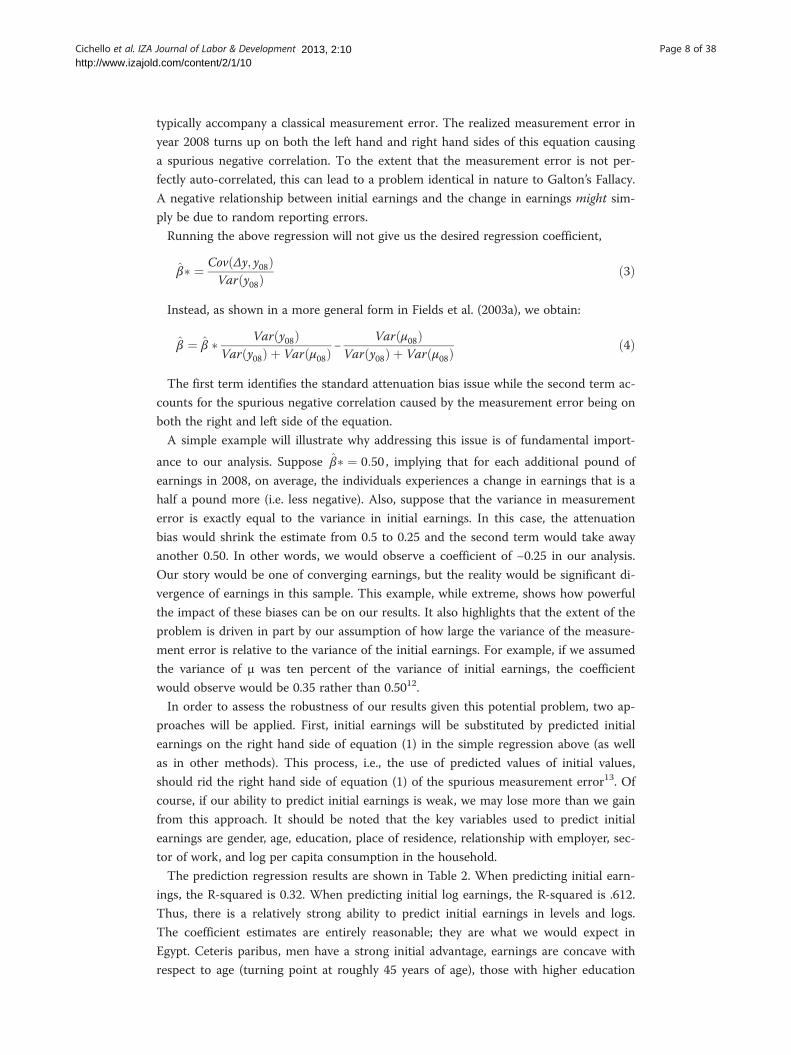
Column (1) of Table 8 provides a simple regression of earnings change on each vari-
able alone. This allows an easy way to identify the difference between groups relative to
the omitted category (denoted by a 0) and whether this differential is statistically sig-
nificant. The 798 EGP difference between average earnings for men and women is sta-
tistically significant.
Before reading too much into these average changes, one should consider controlling
for initial earnings. Column (2) of Table 8 presents the regression results with initial
earnings included as the sole additional right hand side variable. Compared to a female
with the same initial earnings, a male is expected to have an earnings change that is
2,751 EGP better than his female counterpart. Thus, whether one considers this period
a particularly bad period for male or female earners depends on whether we choose to
consider male and female earners who are alike in their initial labor market outcomes
or simply compare typical outcomes for each gender irrespective of their initial starting
point. Similar analysis of the change in log earnings is presented in column (3), which
has the average difference from the omitted group, and column (4) which includes log
initial earnings on the right hand side. The minimal advantage that men had relative to
women in the average change in log earnings expands dramatically (from 6 percent to
36 percent) once we control for initial log earnings.
Reviewing the results of Table 7 and columns (1) and (2) of Table 8, earnings declines
were often larger for those groups who started with higher initial earnings, just as they
were for men versus women. Examples include older workers, those in urban areas and
the Metropolitan region, those who were employers in 2008, those who weren’t unpaid
workers in 2008, and those who lived in poor households in 2008. Consistent with this,

Table 7 Change in earnings and log earnings by individual characteristics, Egypt 2008 to2009
2008 Change in earningsChange in lnearnings
(1) (2) (3) (4) (5) (6) (7)
Percent of panelworkers
Medianearnings
Individualcharacteristics Mean Median
Percentpositive Mean Median
TOTAL
100% 6,237 -950 -446 41% -0.12 -0.09
Gender
30% 2,964 Female -391 -206 44% -0.16 -0.08
70% 7,627 Male -1,189 -628 40% -0.11 -0.10
Age
31% 4,648 25-34 -459 -317 43% -0.09 -0.08
34% 6,778 35-44 -803 -421 42% -0.10 -0.07
35% 7,478 45-58 -1,518 -639 38% -0.18 -0.12
Education
30% 4,047Illiterate/no formalschooling -781 -471 39% -0.19 -0.14
12% 7,010Basic education/literacy -1,534 -815 34% -0.17 -0.16
10% 7,072 Completed Primary -2,070 -699 41% -0.14 -0.10
32% 6,503 Secondary education -610 -287 43% -0.07 -0.06
16% 8,490 University degree -850 -349 46% -0.04 -0.05
Urban
62% 5,316 Rural -648 -404 41% -0.14 -0.10
38% 7,783 Urban -1,437 -516 42% -0.10 -0.08
Region
17% 8,272 Metropolitan -2,318 -817 39% -0.13 -0.14
11% 8,481 Lower Urban -413 -214 46% -0.03 -0.03
38% 5,421 Lower Rural -534 -287 43% -0.11 -0.08
10% 6,859 Upper Urban -1,053 -620 42% -0.14 -0.08
24% 5,068 Upper Rural -827 -522 37% -0.18 -0.14
Type of worker
33% 7,400 wage worker public -633 -117 47% -0.03 -0.02
25% 5,914 wage worker private -628 -504 41% -0.10 -0.10
15% 9,324 employer -2,809 -1,803 28% -0.30 -0.21
16% 4,054 self employed -1,077 -522 38% -0.25 -0.16
10% 1,925 unpaid worker 214 -70 47% -0.01 -0.04
Informal worker
53% 4,603 Informal -838 -471 40% -0.16 -0.13
47% 7,827 Formal -1,074 -395 42% -0.08 -0.06
Industry
31% 3,411 Agriculture -829 -427 39% -0.20 -0.17
19% 7,010 Manu/Const -1,200 -645 37% -0.12 -0.10
51% 7,151 Trade/Services -931 -361 44% -0.08 -0.06
Cichello et al. IZA Journal of Labor & Development Page 17 of 382013, 2:10http://www.izajold.com/content/2/1/10

Table 7 Change in earnings and log earnings by individual characteristics, Egypt 2008 to2009 (Continued)
Poor household in2008
84% 6,893 Non-poor -1,171 -601 39% -0.15 -0.11
16% 3,924 Poor 214 28 52% 0.00 0.01
Source: HIECPS, Feb 2008 to Feb 2009 (CAPMAS 2009).
Cichello et al. IZA Journal of Labor & Development Page 18 of 382013, 2:10http://www.izajold.com/content/2/1/10
but to a lesser degree, those who were formal workers and those who started outside of
agriculture also had smaller mean and median changes. Working against this general
trend, those with university education experienced smaller average losses than those
with some primary schooling or complete primary schooling and those in the lower
urban area seemed to withstand large losses relative to others despite high initial earn-
ings. Yet, this relationship generally flips once one controls for initial earnings (or ex-
pands further in favor of the initially favored).
Columns (3) and (4) of Table 8 re-affirm this relationship with log earnings. The main
difference is that the initial comparison between the favored and less favored groups is
not as consistent. Besides the mixed results by gender, there are some notable excep-
tions where the log earnings changes of those who have low initial earnings are higher
—such as for agricultural workers, informal workers, and those in rural regions. Results
for age, education, employer relationship, and poor/non-poor household in 2008 gener-
ally conform to our previous analysis. Yet in almost all these cases, the initially favored
group has much better average earnings changes once we control for initial log earn-
ings is controlled.
With this in mind, we return to the flexible estimation approach of locally weighted
regressions, mapping the relationship between earnings changes and initial earnings for
particular groups of individuals.
Figure 5 shows that men consistently have better earnings change experiences than
women who started at the same initial earnings18. The reason men had worse average and
median earnings overall is because they started at higher initial earnings in 2008. This is
clear through the fact that the area of support is pushed further to the right for men as
compared to women. Thus, although men had larger declines on average, one might sus-
pect that they actually had an advantage in responding to the surge in inflation.
Figure 6 assesses the change in log earnings based on the initial sector of work. Again,
the negative relationship between log earnings change and initial log earnings is relatively
consistent across all groups. In this case, the relationship in Table 7 is not overturned
when controlling for initial earnings. Those who started out working in agriculture have
consistently worse earnings changes than those working in other sectors.
Figure 7 suggests that there is no consistent differential for those who were in poor
households in 2008 compared to those in non-poor households once one controls for
initial earnings. There may be some gap at the lower and upper initial earnings, but
those in poor households have a slight advantage in the middle range of shared initial
earnings. Thus, the earnings mobility disadvantages that some individuals face do not
appear rooted in initial year poverty status.
Column (7) in Table 7 shows the regression coefficient from bivariate regressions of
earnings change on the category of interest, controlling for initial earnings. By looking
across columns (6) and (7), we can see that there are multiple cases where our
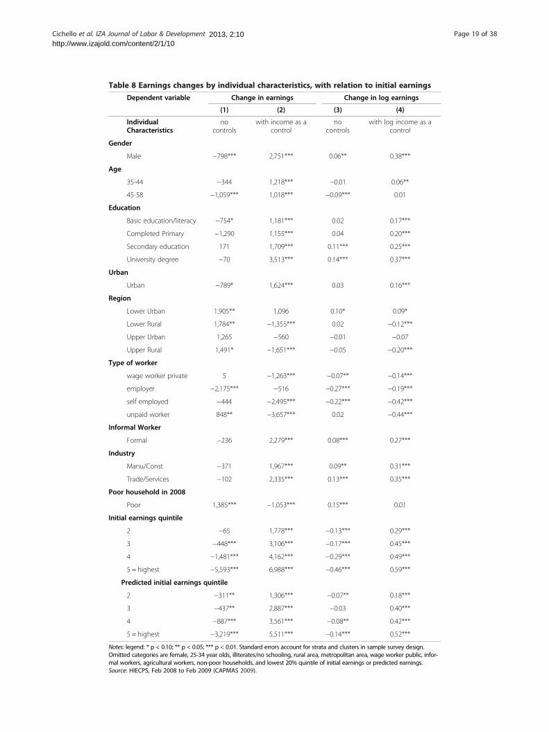
Table 8 Earnings changes by individual characteristics, with relation to initial earnings
Dependent variable Change in earnings Change in log earnings
(1) (2) (3) (4)
IndividualCharacteristics
nocontrols
with income as acontrol
nocontrols
with log income as acontrol
Gender
Male −798*** 2,751*** 0.06** 0.38***
Age
35-44 −344 1,218*** −0.01 0.06**
45-58 −1,059*** 1,018*** −0.09*** 0.01
Education
Basic education/literacy −754* 1,181*** 0.02 0.17***
Completed Primary −1,290 1,155*** 0.04 0.20***
Secondary education 171 1,709*** 0.11*** 0.25***
University degree −70 3,513*** 0.14*** 0.37***
Urban
Urban −789* 1,624*** 0.03 0.16***
Region
Lower Urban 1,905** 1,096 0.10* 0.09*
Lower Rural 1,784** −1,355*** 0.02 −0.12***
Upper Urban 1,265 −560 −0.01 −0.07
Upper Rural 1,491* −1,651*** −0.05 −0.20***
Type of worker
wage worker private 5 −1,263*** −0.07** −0.14***
employer −2,175*** −516 −0.27*** −0.19***
self employed −444 −2,495*** −0.22*** −0.42***
unpaid worker 848** −3,657*** 0.02 −0.44***
Informal Worker
Formal −236 2,279*** 0.08*** 0.27***
Industry
Manu/Const −371 1,967*** 0.09** 0.31***
Trade/Services −102 2,335*** 0.13*** 0.35***
Poor household in 2008
Poor 1,385*** −1,053*** 0.15*** 0.01
Initial earnings quintile
2 −65 1,778*** −0.13*** 0.29***
3 −448*** 3,106*** −0.17*** 0.45***
4 −1,481*** 4,162*** −0.29*** 0.49***
5 = highest −5,593*** 6,988*** −0.46*** 0.59***
Predicted initial earnings quintile
2 −311** 1,306*** −0.07** 0.18***
3 −437** 2,887*** −0.03 0.40***
4 −887*** 3,561*** −0.08** 0.42***
5 = highest −3,219*** 5,511*** −0.14*** 0.52***
Notes: legend: * p < 0.10; ** p < 0.05; *** p < 0.01. Standard errors account for strata and clusters in sample survey design.Omitted categories are female, 25-34 year olds, illiterates/no schooling, rural area, metropolitan area, wage worker public, infor-mal workers, agricultural workers, non-poor households, and lowest 20% quintile of initial earnings or predicted earnings.Source: HIECPS, Feb 2008 to Feb 2009 (CAPMAS 2009).
Cichello et al. IZA Journal of Labor & Development Page 19 of 382013, 2:10http://www.izajold.com/content/2/1/10

-2-1
01
2
Sm
ooth
ed c
hang
e in
log
earn
ings
6 8 10 12Log real earnings, 2008
Male Female
Figure 5 Change in log earnings based on initial log earnings by gender, Egypt 2008–2009. Source:HIECPS (Feb 2008 to Feb 2009 (CAPMAS 2009)). Notes: Locally weighted regression was used to determinethe predicted change in log earnings based on log real earnings in 2008. Analysis was done separately bygender and then plotted on the same graph.
Cichello et al. IZA Journal of Labor & Development Page 20 of 382013, 2:10http://www.izajold.com/content/2/1/10
impression of whether a group (such as males) has had better average outcomes than
another (women), is overturned when we compare the two groups conditional on the
same initial earnings. This overturning effect generally holds for females, younger
workers, those living in rural areas, or in regions with lower initial earnings, unpaid
workers, informal workers, those working in agriculture and those living in poor house-
holds. While mean and median earnings changes for these groups were better than
those of their counterparts, they performed worse on average than their counterparts
who had similar initial earnings.
-2-1
01
2
Sm
ooth
ed c
hang
e in
log
earn
ings
6 8 10 12Log real earnings, 2008
Agriculture Manu/ConstructionTrade/Services
Figure 6 Change in log earnings based on initial log earnings by industry in 2008, Egypt 2008–2009. Source: HIECPS (Feb 2008 to Feb 2009 (CAPMAS 2009)). Notes: Locally weighted regression was usedto determine the predicted change in log earnings based on log real earnings in 2008. Analysis was doneseparately by industry and then plotted on the same graph.

-2-1
01
2
Sm
ooth
ed c
hang
e in
log
earn
ings
6 8 10 12Log real earnings, 2008
Poor in 2008 Non-poor in 2008
Figure 7 Change in log earnings based on initial log earnings by 2008 poverty status, Egypt 2008–2009. Source: HIECPS (Feb 2008 to Feb 2009 (CAPMAS 2009)). Notes: Locally weighted regression was usedto determine the predicted change in log earnings based on log real earnings in 2008. Analysis was doneseparately by 2008 poverty status and then plotted on the same graph.
Cichello et al. IZA Journal of Labor & Development Page 21 of 382013, 2:10http://www.izajold.com/content/2/1/10
In short, it is very important to consider the impact of initial earnings when evaluat-
ing how certain types of individuals were able to succeed and advance during the
period. This type of evaluation generally requires panel data.
5.5 The role of transitions across types of work
Next we examine the systematic earnings changes associated with moving to a different
sector of employment or to a job with a different employer relationship. First, we assess
how often these transitions take place.
Table 9a shows that just more than half (51 percent) of all panel workers are
employed in trade and services in 2008. Ninety-two percent of these workers are
employed there again in 2009, while five percent are in manufacturing or construction
and three percent are in agriculture. Agriculture also retains the vast majority (88 per-
cent) of its workers in 2009 while manufacturing and construction work appears a bit
less stable, with the sector retaining just 78 percent of 2008 workers in 2009. Overall
the flows result in a slight loss of employment in agriculture and manufacturing/con-
struction and movements into trade and services, which now employ 53 percent of
workers. Overall, 12 percent of panel members were in a different sector in 2009 than
in 2008.
Table 9b demonstrates the strength of tie to public wage employment. Ninety-five
percent of public wage workers in the panel remained in public wage employment in
2009 as compared to just 66 percent of those in private wage work, 69 percent of em-
ployers, 55 percent of the self-employed and 75 percent of the unpaid workers. Flows
from private to public wage work were particularly plentiful, helping to explain the
three percent increase in public wage employment and the corresponding three percent
loss in private wage employment in 2009, even though flows into public employment
came from all other types of employment.
Table 9 Employment transitions by type of work or worker, Egypt 2008 to 2009
a: Sector of work
Sector in 2009
Sector in 2008 Agriculture Ind/Const Trade/Services
Agriculture (31%) 87.8% 3.8% 8.4%
Industry/Construction (19%) 5.0% 78.2% 16.7%
Trade/Services (51%) 2.7% 5.0% 92.3%
Total 29% 18% 53%
b: Employer Relationship
Employer Relationship in 2009
Employer Relationship in 2008 Public Wage Private Wage Employer Self-employed Unpaid
Public Wage (33%) 94.9% 3.6% 0.8% 0.5% 0.1%
Private Wage (25%) 15.4% 66.0% 8.3% 8.1% 2.1%
Employer (15%) 2.8% 11.8% 69.3% 12.5% 3.5%
Self-employed (16%) 2.5% 11.4% 16.1% 55.3% 14.6%
Unpaid (10%) 2.2% 5.8% 3.5% 13.9% 74.7%
Total 36% 22% 16% 15% 11%
c: Formality
Status in 2009
Status in 2008 Informal Formal
Informal (53%) 88.2% 11.8%
Formal (47%) 14.8% 85.2%
Total 53% 47%
Source: HIECPS, Feb 2008 to Feb 2009 (CAPMAS 2009).
Cichello et al. IZA Journal of Labor & Development Page 22 of 382013, 2:10http://www.izajold.com/content/2/1/10
The transient nature of self-employment is also apparent as just 55 percent of 2008
workers were self-employed in 2009. More than ten percent of these individuals ended
up as private wage employees (11 percent), as employers (16 percent), and as unpaid
workers (15 percent). While moving to employer status might be thought of as a suc-
cessful outcome for a self-employed individual, other outcomes may be less certain.
Movement to private wage employment may often occur by choice and may often be
the result of business failure. Movement to unpaid worker status might result from
more family members working in a successful household enterprise or it might be a re-
sult of failure of the business that the individual was running and falling back into an-
other household enterprise. The earnings mobility outcomes may help us form
opinions on these.
Tables 10a-b and 11 should be interpreted bearing in mind the mean (−950) and me-
dian (−446) earnings losses for the population of workers as a whole.
Those who left agricultural work were generally better able to stem the earnings
losses. The median change and the percent experiencing positive earnings gains were
higher for those who switched sectors, though the average decline in earnings for those
who moved to trade/services was actually larger than those who stayed in agriculture.
Meanwhile, those who moved into agricultural work were experiencing larger than
average earnings losses. This evidence is consistent with what one might expect if there
is significant labor market segmentation, with agriculture representing the least pre-
ferred free entry sector and the differential pay being offered to the same individual

Table 10 Mean and median earnings change by employment transition, Egypt 2008 to2009
a: Sector of work
Sector in 2009
Sector in 2008 Agriculture Ind/Const Trade/Services
Agriculture Mean −852 −97 −921
Median −456 −115 −222
% positive 38% 48% 45%
n obs 1,002 38 92
Industry/Construction Mean −1,342 −1,411 −154
Median −963 −641 −258
% positive 32% 37% 42%
n obs 37 507 104
Trade/Services Mean −3,878 −966 −842
Median −1,148 −947 −349
% positive 39% 42% 44%
n obs 54 87 1,559
b: Employer Relationship
Employer Relationship in 2009
Relationship in 2008 Public Wage Private Wage Employer Self-employed Unpaid
Public Wage Mean −614 −116
Median −109 210
% positive 47% 51%
n obs 1,053 39
Private Wage Mean −640 −846 984 −178 −1,815
Median −188 −641 808 −235 −1,661
% positive 47% 37% 61% 46% 12%
n obs 124 566 78 71 20
Employer Mean −2,956 −2,481 −3,441
Median −2,364 −1,482 −1,744
% positive 15% 32% 23%
n obs 61 390 68
Self-employed Mean −3,388 19 −953 −1,116
Median −1,719 −205 −471 −603
% positive 22% 47% 38% 33%
n obs 65 93 331 95
Unpaid Mean 2,047 305 −277
Median 1,644 245 −230
% positive 93% 59% 39%
n obs 20 47 274
Notes: Cells with less than 20 observations not shown.Source: HIECPS, Feb 2008 to Feb 2009 (CAPMAS 2009).
Cichello et al. IZA Journal of Labor & Development Page 23 of 382013, 2:10http://www.izajold.com/content/2/1/10
working in different sectors. However, a much more detailed analysis would be needed
to assess this hypothesis more fully.
The earnings decline for those remaining in the industry/construction sector was
large. Combined with the previous information of workers flowing out of this sector, a

Table 11 Formality
Status in 2009
Status in 2008 Informal Formal
Informal Mean −865 −640
Median −479 −222
% positive 39% 46%
n obs 1,690 212
Formal Mean −2,848 −765
Median −1,160 −267
% positive 29% 45%
n obs 239 1,340
Source: HIECPS, Feb 2008 to Feb 2009 (CAPMAS 2009).
Cichello et al. IZA Journal of Labor & Development Page 24 of 382013, 2:10http://www.izajold.com/content/2/1/10
consistent picture emerges that this sector was under stress during the 2008 to 2009
period. The only group of individuals that started in industry/construction and ended
with less than average earnings losses was the group that moved to trade/services. Cor-
respondingly, those who started in trade/services suffered high median losses if they
moved to industry/construction, but the mean earnings loss for this group and the per-
cent experiencing positive gains were basically the same as the overall average. Thus,
the data is less clearly consistent with what we would expect if there was segmentation
across industry/construction and trade/services sectors. It does appear that the indus-
try/construction sector was under strain. It is a bit surprising that those who transi-
tioned from industry/construction to trade/services had such relatively positive
earnings changes. This seems to be driven by those coming from construction or elec-
trical utilities rather than manufacturing sectors, but the estimates are too variable to
find the differences to be statistically significant.
Public wage workers who stayed on in public wage employment did better than aver-
age in stemming the loss in real earnings. This is surprising given their high initial
earnings levels and our earlier results regarding high initial earnings. Those who moved
from public to private wage employment did even better. This suggests that such
moves were likely voluntary moves.
In fact, with the exception of movements into unpaid worker status, wage workers
who moved to new work categories consistently had better earnings changes than those
who stayed within their same worker category. Thus, a generalization might be to as-
sume that most observed changes of wage workers were voluntary, while those moving
to unpaid worker status were involuntary. It does not appear that this was a period of
substantial labor shedding of wage workers, public or private. Instead, workers
absorbed losses in their real wage.
In contrast to this, the employed and self-employed who moved to private wage ex-
perienced even worse mean and median changes than those who stayed in their re-
spective categories, consistent with a notion of being involuntarily pushed out of
business rather than finding a better job.
Those who started as employers took large losses whether they moved sectors or
tried to ride out the storm remaining as an employer. The self-employed also had rela-
tively large losses. This might seem to be surprising given that such individuals have
the opportunity to immediately change their product prices in response to inflation
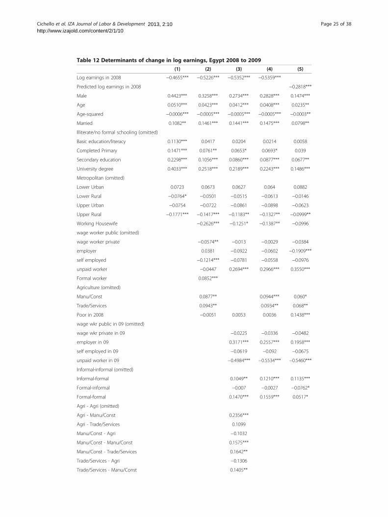
Table 12 Determinants of change in log earnings, Egypt 2008 to 2009
(1) (2) (3) (4) (5)
Log earnings in 2008 −0.4655*** −0.5226*** −0.5352*** −0.5359***
Predicted log earnings in 2008 −0.2818***
Male 0.4423*** 0.3258*** 0.2734*** 0.2828*** 0.1474***
Age 0.0510*** 0.0423*** 0.0412*** 0.0408*** 0.0235**
Age-squared −0.0006*** −0.0005*** −0.0005*** −0.0005*** −0.0003**
Married 0.1082** 0.1461*** 0.1441*** 0.1475*** 0.0798**
Illiterate/no formal schooling (omitted)
Basic education/literacy 0.1130*** 0.0417 0.0204 0.0214 0.0058
Completed Primary 0.1471*** 0.0761** 0.0653* 0.0693* 0.039
Secondary education 0.2298*** 0.1056*** 0.0860*** 0.0877*** 0.0677**
University degree 0.4033*** 0.2518*** 0.2189*** 0.2243*** 0.1486***
Metropolitan (omitted)
Lower Urban 0.0723 0.0673 0.0627 0.064 0.0882
Lower Rural −0.0764* −0.0501 −0.0515 −0.0613 −0.0146
Upper Urban −0.0754 −0.0722 −0.0861 −0.0898 −0.0623
Upper Rural −0.1771*** −0.1417*** −0.1183** −0.1327** −0.0999**
Working Housewife −0.2626*** −0.1251* −0.1387** −0.0996
wage worker public (omitted)
wage worker private −0.0574** −0.013 −0.0029 −0.0384
employer 0.0381 −0.0922 −0.0602 −0.1909***
self employed −0.1214*** −0.0781 −0.0558 −0.0976
unpaid worker −0.0447 0.2694*** 0.2966*** 0.3550***
Formal worker 0.0852***
Agriculture (omitted)
Manu/Const 0.0877** 0.0944*** 0.060*
Trade/Services 0.0943** 0.0934** 0.068**
Poor in 2008 −0.0051 0.0053 0.0036 0.1438***
wage wkr public in 09 (omitted)
wage wkr private in 09 −0.0225 −0.0336 −0.0482
employer in 09 0.3171*** 0.2557*** 0.1958***
self employed in 09 −0.0619 −0.092 −0.0675
unpaid worker in 09 −0.4984*** −0.5534*** −0.5460***
Informal-informal (omitted)
Informal-formal 0.1049** 0.1210*** 0.1135***
Formal-informal −0.007 −0.0027 −0.0762*
Formal-formal 0.1470*** 0.1559*** 0.0517*
Agri - Agri (omitted)
Agri - Manu/Const 0.2356***
Agri - Trade/Services 0.1099
Manu/Const - Agri −0.1032
Manu/Const - Manu/Const 0.1575***
Manu/Const - Trade/Services 0.1642**
Trade/Services - Agri −0.1306
Trade/Services - Manu/Const 0.1405**
Cichello et al. IZA Journal of Labor & Development Page 25 of 382013, 2:10http://www.izajold.com/content/2/1/10

Table 12 Determinants of change in log earnings, Egypt 2008 to 2009 (Continued)
Trade/Services - Trade/Services 0.1548***
Constant 2.3032*** 3.0926*** 3.1953*** 3.2530*** 1.6737***
n 3481 3481 3480 3481 3481
R-squared 0.2358 0.2728 0.3471 0.3411 0.1297
Notes: legend: * p < 0.10; ** p < 0.05; *** p < 0.01. Standard errors account for strata and clusters in sample survey design.Column (5) uses bootstrapped standard errors.Source: HIECPS, Feb 2008 to Feb 2009 (CAPMAS 2009).
Cichello et al. IZA Journal of Labor & Development Page 26 of 382013, 2:10http://www.izajold.com/content/2/1/10
(and have their earnings rise) whereas workers may be locked into longer term con-
tracts. This will be discussed more fully in Section 6.
Movements from formal to informal employment tended to result in very large
losses. They were also quite numerous. This could signal labor shedding, where individ-
uals are being forced to change jobs and losing out on pay. However, there was an in-
flow from informal to formal employment that was similar in size as the above outflow.
This inflow did not result in earnings gains on par with the losses noted above. There-
fore, it was not simply a case of individuals changing positions with similar earnings.
An alternative explanation could be that employers under duress are opting out of the
social pension system (and simultaneously giving workers reduced earnings). One
might expect a certain flow from both of these causes in any time period. Without a
baseline to know the typical flows and earnings changes from such transitions in Egypt,
it is difficult to pinpoint an explanation.
Interestingly, those who moved from informal to formal sectors had earnings changes
that were significantly but not so dramatically better than those who stayed informal.
The changes were similar to those experienced by those who started and remained in
the formal sector.
5.6 Multivariate analysis
We turn to multivariate analysis to better understand the determinants of earnings mo-
bility. Table 12 presents a series of regressions that have the change in log earnings as
the dependent variable. Results are presented using only exogenous base year charac-
teristics and initial earnings (column 1) and then adding endogenous variables from the
base year (column 2)19. Columns (3) and (4) include employment transition variables,
with column (4) being the preferred specification (discussed below). In column (5), we
replace initial log earnings with predicted initial log earnings and include all previous
variables. In this specification, the effect of predicted initial log earnings is identified by
fluctuations in log per capita consumption in the household in the base period.
Initial earnings are a powerful predictor of earnings change across all specifications.
The coefficients imply that the predicted change in log earnings decreases by between
0.47 and 0.54 for each additional unit in reported log income. When using predicted
initial log income, the coefficient drops to −0.28, which is still highly significant from
an economic perspective. The coefficient is statistically significant at the one percent
level for all specifications.
Another characteristic exhibiting a consistently important influence on predictions is
gender. Males experience approximately 27 percent to 44 percent higher earnings
changes than females, ceteris paribus, in columns (1)-(4)20. When using predicted

Cichello et al. IZA Journal of Labor & Development Page 27 of 382013, 2:10http://www.izajold.com/content/2/1/10
initial earnings, this falls to about 15 percent higher, ceteris paribus, but remains both
statistically significant and important in terms of economic loss. In contrast, re-running
column (4) without including initial earnings, leads to a negative though statistically in-
significant gender effect (see Table 13).
Higher education levels also seem to be associated with higher earnings changes
when controlling for initial earnings. Focusing on column (4), those with secondary
education and university education had statistically significant differences in earnings
changes compared to those who were illiterate/had no schooling, with gains of approxi-
mately 8.8, and 22.4 percent respectively. If one does not control for initial earnings,
the estimated differences by education level are neither individually nor jointly statisti-
cally significant.
Age is also statistically significant, with earnings changes increasing and then de-
creasing with age. In column (4) the turning point is 43 years of age, while in column
(5) it is 39 years of age (not shown in the table). Being married raises predicted earn-
ings change by approximately 15 percent in the preferred specification, although, in
column (5), the point estimate is less than half the size and it is only statistically signifi-
cant at the ten percent significance level. These effects were also considerably different
when running regression analysis without initial earnings21.
Using the preferred specification, the upper rural region had statistically lower earn-
ings changes, ceteris paribus, than the Metropolitan region. Returning to Table 7, one
may notice that the highest median pay in 2008 was in the Lower Urban region,
followed by the Metropolitan region and the lowest pay was in Upper Rural region.
Looking at the employment transition variables, there are some surprising results.
First, after controlling for other characteristics and initial earnings, the variables identi-
fying transitions across industry in column (3) are not jointly statistically significant.
The data did not reject the null hypothesis that only the initial sector of employment
was needed for predicting earnings changes. This is surprising, but does allow a simpler
form to be used as our preferred specification in column (4).
Using just initial industry characteristics we determine that those who started in agri-
culture experienced approximately nine percent lower earnings changes than others.
The results are statistically significant. This result might seem surprising since the infla-
tion was driven in part by rising food prices. One might assume that food producers
would be able to increase their prices at least at the rate of inflation.
There are some potential explanations behind this unexpected result. We begin with
some explanations that justify why farmers’ gains from rising food prices might be less
than expected for those unfamiliar with the Egyptian setting. First, for most of the small
farmers, the agricultural production makes up only up to 40 percent of their incomes,
and they simultaneously sell their labor to other farmers/enterprises. Since higher food
prices only benefit farmers on the share they sell, and agricultural wages may be slow
to adjust, particularly if the food price shocks come too late to adjust the production
size, the overall gains may be less than expected. Second, many farmers in Egypt are
net consumers of food. Egypt is a very large importer of grains (mostly wheat), oil, and
sugar—three main items in the consumption basket. Meat production relies heavily on
imported grains as well. Therefore, it's possible that the prices for the main consump-
tion items and input costs were going up substantially faster than the production items.
Finally, even assuming that farmers could benefit from higher prices, it did not seem

Table 13 Determinants of change in log earnings, with and without initial earnings
(1) (2)
with initial earnings without initial earnings
Log earnings in 2008 −0.5359***
Male 0.2828*** −0.0076
Age 0.0408*** 0.0022
Age-squared −0.0005*** −0.0001
Married 0.1475*** 0.0001
Illiterate/no formal schooling (omitted)
Basic education/literacy 0.0214 −0.0308
Completed Primary 0.0693* −0.0126
Secondary education 0.0877*** 0.0203
University degree 0.2243*** 0.0326
Metropolitan (omitted)
Lower Urban 0.064 0.1136*
Lower Rural −0.0613 0.0461
Upper Urban −0.0898 −0.0238
Upper Rural −0.1327** −0.0368
Working Housewife −0.1387** −0.0457
wage worker public (omitted)
wage worker private −0.0029 −0.033
employer −0.0602 −0.3161***
self employed −0.0558 −0.0734
unpaid worker 0.2966*** 0.4930***
wage wkr public in 09 (omitted)
wage wkr private in 09 −0.0336 −0.0455
employer in 09 0.2557*** 0.1889***
self employed in 09 −0.092 −0.0678
unpaid worker in 09 −0.5534*** −0.5493***
Informal-informal (omitted)
Informal-formal 0.1210*** 0.1174**
Formal-informal −0.0027 −0.0812**
Formal-formal 0.1559*** 0.0414
Agriculture (omitted)
Manu/Const 0.0944*** 0.0117
Trade/Services 0.0934** 0.0277
Poor in 2008 0.0036 0.2309***
Constant 3.2530*** −0.0816
n 3481 3481
R-squared 0.3411 0.1228
Notes: legend: * p < 0.10; ** p < 0.05; *** p < 0.01. Standard errors account for strata and clusters in sample survey design.Source: HIECPS, Feb 2008 to Feb 2009 (CAPMAS 2009).
Cichello et al. IZA Journal of Labor & Development Page 28 of 382013, 2:10http://www.izajold.com/content/2/1/10
the case for most of the domestic prices on food items, which increase in a very differ-
ent way from international prices, as shown in Figure 8.
These explanations are admittedly lacking. While they offer ideas on why the
relative gains for those engaged in agriculture may be weaker than expected, they
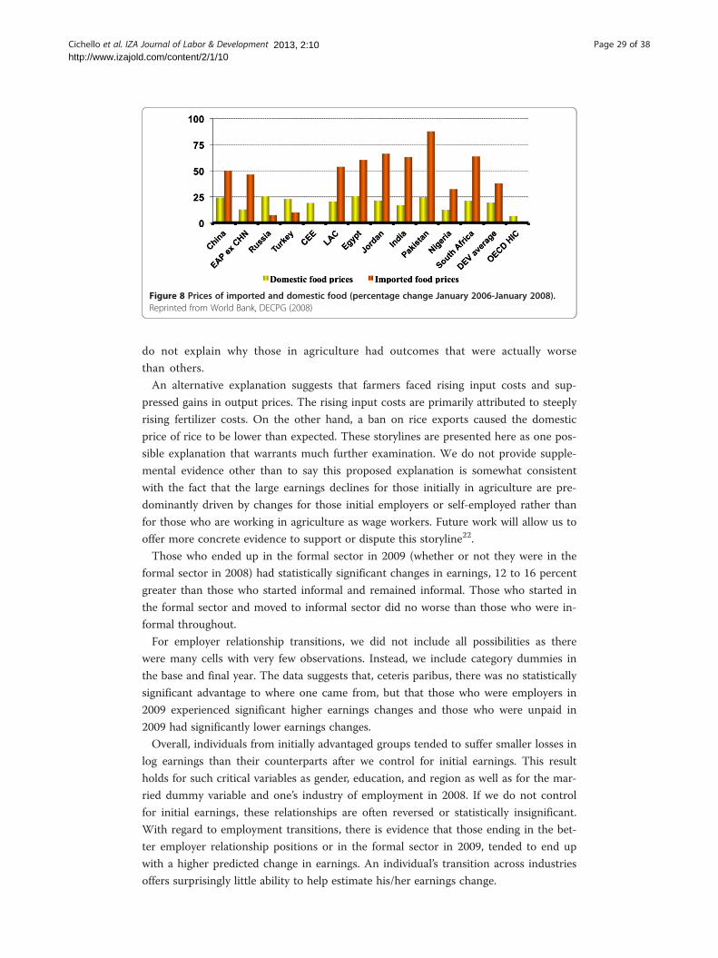
Figure 8 Prices of imported and domestic food (percentage change January 2006-January 2008).Reprinted from World Bank, DECPG (2008)
Cichello et al. IZA Journal of Labor & Development Page 29 of 382013, 2:10http://www.izajold.com/content/2/1/10
do not explain why those in agriculture had outcomes that were actually worse
than others.
An alternative explanation suggests that farmers faced rising input costs and sup-
pressed gains in output prices. The rising input costs are primarily attributed to steeply
rising fertilizer costs. On the other hand, a ban on rice exports caused the domestic
price of rice to be lower than expected. These storylines are presented here as one pos-
sible explanation that warrants much further examination. We do not provide supple-
mental evidence other than to say this proposed explanation is somewhat consistent
with the fact that the large earnings declines for those initially in agriculture are pre-
dominantly driven by changes for those initial employers or self-employed rather than
for those who are working in agriculture as wage workers. Future work will allow us to
offer more concrete evidence to support or dispute this storyline22.
Those who ended up in the formal sector in 2009 (whether or not they were in the
formal sector in 2008) had statistically significant changes in earnings, 12 to 16 percent
greater than those who started informal and remained informal. Those who started in
the formal sector and moved to informal sector did no worse than those who were in-
formal throughout.
For employer relationship transitions, we did not include all possibilities as there
were many cells with very few observations. Instead, we include category dummies in
the base and final year. The data suggests that, ceteris paribus, there was no statistically
significant advantage to where one came from, but that those who were employers in
2009 experienced significant higher earnings changes and those who were unpaid in
2009 had significantly lower earnings changes.
Overall, individuals from initially advantaged groups tended to suffer smaller losses in
log earnings than their counterparts after we control for initial earnings. This result
holds for such critical variables as gender, education, and region as well as for the mar-
ried dummy variable and one’s industry of employment in 2008. If we do not control
for initial earnings, these relationships are often reversed or statistically insignificant.
With regard to employment transitions, there is evidence that those ending in the bet-
ter employer relationship positions or in the formal sector in 2009, tended to end up
with a higher predicted change in earnings. An individual’s transition across industries
offers surprisingly little ability to help estimate his/her earnings change.

Cichello et al. IZA Journal of Labor & Development Page 30 of 382013, 2:10http://www.izajold.com/content/2/1/10
5.7 A review of changes by initial poverty status
Individuals from initially poor households fared as well or better than others. They do not
appear to be more vulnerable to earnings declines during this period. Those initially from
poor households had substantially better average and median earnings changes than those
from non-poor households. While this relationship was reversed when conditioning on ini-
tial earnings alone, non-parametric analysis showed limited differences for individuals from
poor rather than non-poor households (see Figure 7). More importantly, the initially poor
variable showed no statistical significance in the multivariate analysis (see Table 12), except
for the positive coefficient in the specification using predicted earnings (column 5). This
was significant at the one percent level and suggested a 14 percent advantage in earnings
changes for those from poor households, ceteris paribus.
5.8 A more detailed examination by gender
Table 14 offers separate regression analysis by gender. Some interesting differences
emerge. First, while the importance of initial earnings is apparent for all three groups,
Table 14 Determinants of change in log earnings, by gender
Male Female
Log earnings in 2008 −0.4879*** −0.6533***
Age 0.0354*** 0.0351
Age-squared −0.0004*** −0.0004
Married 0.2429*** −0.1033*
Illiterate/no formal schooling (omitted)
Basic education/literacy 0.0192 0.0206
Completed Primary 0.0515 0.1422
Secondary education 0.0747** 0.1005
University degree 0.2301*** 0.2564***
Metropolitan (omitted)
Lower Urban 0.0744 0.0793
Lower Rural −0.0448 −0.0411
Upper Urban −0.0384 −0.1535
Upper Rural −0.1243** −0.1631*
wage worker public (omitted)
wage worker private −0.0403 −0.1930*
employer 0.0024 −0.0382
self employed −0.0206 −0.3898**
unpaid worker −0.0503 −0.2502
Formal worker 0.0703** 0.2116**
Agriculture (omitted)
Manu/Const 0.0337 0.1795
Trade/Services 0.0260 0.2113**
Poor in 2008 −0.0160 −0.0198
Constant 3.2490*** 4.4566***
n 2439 1042
R-squared 0.2672 0.3311
Notes: legend: * p < 0.10; ** p < 0.05; *** p < 0.01. Standard errors account for strata and clusters in sample survey design.Source: HIECPS, Feb 2008 to Feb 2009 (CAPMAS 2009).

Cichello et al. IZA Journal of Labor & Development Page 31 of 382013, 2:10http://www.izajold.com/content/2/1/10
the impact is greater for women as compared to men. This could be due to a variety of
reasons. For example, women may have a higher degree of transitory income as a gen-
eral norm. Or, it could result from period-specific changes. Suppose, for example, suc-
cessful women had a disproportionate decline in earnings because households had to
spend more on food and had less left to spend on stock for the female run enterprises.
Simultaneously, women with low earnings may have had disproportionate gains in
earnings as they worked more aggressively in the labor market in an attempt to make
up for inflation reducing the buying power associated with the male breadwinner’s take
home pay. We do not examine these points fully here, but leave them as open
questions.
Additional differences exist between males and females. For example, while married
men had 24 percent higher earnings gains than an otherwise similar non-married men,
married women had 10 percent lower earnings than an otherwise similar non-married
woman. However, the effect for females was not statistically significant. Additionally, fe-
males saw much greater differentials in earnings change experiences based on formal
work status in 2008; employment type in 2008, specifically in comparison to public
wage workers; and sector of employment in 2008, specifically non-agricultural versus
agricultural workers.
While these differences are present, other aspects of the earnings change experience
are quite similar across gender. Both groups were estimated to have earnings changes
that increase and then decrease with age, with nearly identical turning points (at
43 years). Additionally, there were nearly identical gains for those with a University de-
gree compared to those with no education. Other results across education levels were
quite similar for males and females or were statistically insignificant. Results were also
similar across gender when looking at changes experienced in different regions of Egypt.
6. Conclusions and areas of further researchUsing panel data from February 2008 to February 2009, we observe changes in earnings
experienced by workers in Egypt during a period of high inflation. In aggregate, the
data shows that the labor market reacted to this rapid inflation by inducing a rapid de-
cline in real earnings. There was no major reduction in employment levels, at least not
for prime-aged workers. Average nominal earnings remained relatively unchanged. The
mean and median changes in real earnings were almost universally negative across a
wide spectrum of individual and regional characteristics.
At the individual level, however, the earnings change experience exhibited substantial
heterogeneity, with 27 percent of the workers with employment in both periods report-
ing pay at least fifty percent higher or fifty percent lower than their reported 2008 earn-
ings. Additionally, many individuals transitioned to new sectors of work or employer
relationships during this period. Thus, for many individuals, this was a period of con-
siderable fluidity and complexity compared to the rather simple aggregate story. As this
is the first panel dataset in Egypt that captures such movements, we cannot determine
the extent to which these earnings changes and employment transitions differ from
what is typically found in a more stable economic period.
However, using this panel data and a descriptive regression approach, we are able to
identify key covariates that have a significant association with earnings change. The de-
scriptive regression approach cannot give us causal interpretations, but it does provide

Cichello et al. IZA Journal of Labor & Development Page 32 of 382013, 2:10http://www.izajold.com/content/2/1/10
statistical determinants of earnings change. It gives circumstantial evidence that favors
particular items as driving forces. It also leaves us with many new questions to explore
in the future.
We found that initial earnings had a powerful negative association with earnings
change. Those with higher earnings in 2008 had a greater average (and median) decline
in earnings. This might be expected in a time period where inflation is driving the
change in real earnings. Yet, the data also shows that those with higher reported log
earnings in 2008 had a greater average decline in reported log earnings as well.
Such results may be driven by a spurious correlation resulting from classical meas-
urement error. Thus, we re-computed the analysis using predicted earnings in place of
initial earnings. The levels result was robust to this approach. The log result was not
robust, although the coefficient was still negative. Thus, the data suggests that those
with lower initial earnings experienced percentage declines that were, at worst, similar
to those with higher initial earnings and there is some evidence that the percentage de-
clines were lower for those with lower initial earnings.
The importance of controlling for initial earnings was evident when examining the
relationship between earnings change and gender. On average, men experienced a
much larger average decline in earnings than women. However, for men and women
with the same initial earnings, women had a greater average fall in earnings.
For a number of other covariates, the story was similar. The disadvantaged
groups—such as young workers, those living in rural areas or those living in low-
earning regions—experienced smaller average declines in earnings than their
advantaged counterparts. However, if individuals started with the same initial
earnings, it was members of the disadvantaged group that experienced greater
average declines. One exception to this was that those from poor households did
not generally show themselves to be more vulnerable to earnings declines even
after conditioning on initial earnings.
When controlling for a larger host of covariates, higher initial earnings remained
negatively related to earnings change. This association is statistically significant and has
large economic significance as well whether controlling for reported or predicted initial
log earnings.
The inevitable question is, why? What is it about having high initial earnings in 2008
that causes individuals to fall further relative to similar individuals with lower initial
earnings? Did these individuals possess some unobservable characteristics that are no
longer being rewarded as well as before? Is it capturing a dynamic adjustment process
where individuals with positive or negative shocks gradually return to their conditional
mean? To begin to address these questions, we would need panel data with more than
two periods. Thus, it remains an open question for future work.
One consequence of this negative relationship between earnings change and initial
earnings is that individuals are often changing position in the earnings distribution.
Thus, when assessing income inequality over time using cross-sectional data, one
should recognize that there are likely different people in different earnings positions
over time (see Fields and Sanchez-Puerta (2010) for a clear graphical example).
There is also more work to be done in understanding why women had worse earnings
change experiences than men who started at the same initial earnings level. This result was
robust to excluding women who were listed as working housewives. Yet, it is worth

Cichello et al. IZA Journal of Labor & Development Page 33 of 382013, 2:10http://www.izajold.com/content/2/1/10
investigating whether these changes were brought on by lower investment in female busi-
nesses, firms offering lower pay or holding pay fixed for women or other possible reasons.
Additionally, understanding why earnings changes were more responsive to initial earnings
for women than men may help us better understand how initial earnings impact earnings
change.
This influence of initial earnings leads to a situation where various groups might see
themselves as disproportionately affected by the inflation shock and ensuing decline in
earnings. For example, men might recognize the absolute value and even percentage
value of their losses were greater than that of females. On the other hand, women
might notice that their losses and percentage losses were far greater than men who
started with the same initial earnings (and had otherwise similar characteristics as
them). It is an open question whether such settings give rise to more social discontent
than settings where aggregate differences and differences conditioning on those like
oneself allows only one group to claim relative disadvantage. The absolute decline in
earnings experienced by so many different types of individuals was undoubtedly a
source of widespread social discontent in this period. But a hypothesis worth consider-
ing is that such discontent becomes even greater in situations where all groups could
also consider themselves relatively worse off depending on whether they focus on ag-
gregate effects or effects conditional on personal characteristics.
Finally, earnings changes for those initially engaged in agriculture were unexpected,
given that the changes in inflation were driven in part by rising food prices. Those who
started in agriculture had the biggest average decline in earnings, holding all else con-
stant. A number of possible explanations have been raised. In our view the most plaus-
ible revolve around rising fertilizer costs with relatively stagnant farm-gate prices for at
least some crops. A more complete explanation would require a detailed examination
of the agricultural sector and is left for future work.
Endnotes1Concurrent analysis of earnings mobility using this data has been undertaken by Silva as
part of the World Bank investigation into informality. Earlier, Assad and Roushdy (2007)
also used the panel data from the Egyptian labor market conditions surveys (ELMPS) con-
ducted in 1998 and 2006 together with the 2005 HIECS to provide very detailed informa-
tion on employment status, earnings, and poverty. The work was descriptive using
transition matrices and focused on wage workers. Their results reveal that between 1998
and 2006 there was a notable improvement in labor-market conditions in Egypt. New jobs
were created at a faster rate than the growth of the labor force, leading to a reduction in the
unemployment rate. They also found an uneven increase in earnings where only few of the
poor had benefited from these gains. However, both studies did not take into account the
relationship between the initial earnings and earnings changes that is central to this paper.2This statement is not meant to be a central thesis for what kept inflation from con-
tinuing to increase. The lack of adjustment of wages, itself, was likely driven by many
underlying factors.3An alternative hypothesis would be that they did raise prices but that demand for
their product fell as buyers had less of their constant nominal earnings to spend on do-
mestic services and products due to increased prices of the imported goods that they
were buying.

Cichello et al. IZA Journal of Labor & Development Page 34 of 382013, 2:10http://www.izajold.com/content/2/1/10
4This process divides enterprise gains solely among residents engaged in a home en-
terprise. Such a division can lead to measurement error. Fortunately, more than half of
those engaged in household enterprise work are the only ones in the household en-
gaged in such activity (and thus do not need to split profit). In multiple person enter-
prises (often two person activities), there may be some concern in this regard.5We also discard 9 observations in 2008 and 12 observations in 2009 that had zero
earnings despite being listed as employed. These were primarily unpaid workers and we
believe the values to be erroneous.6We can reject the hypothesis that each dummy variable equals zero when testing
them separately. Surprisingly, using a ten percent significance level, we cannot reject
the joint hypothesis test that both of these dummy variables simultaneously equal zero.7Such descriptive regressions do not attempt to eliminate or fix endogenous right hand side
variables that can conflate causal interpretations of regression coefficients. This approach is
useful in predicting who was affected by a given change, without explaining why. In other
words, we may be able to say that individuals who transitioned from sector A to sector B ex-
perienced higher average earnings changes than those of similar age, education level, etc.
who stayed in sector A. We cannot say that they earn more because they switched sectors or
that anyone else who had made a similar switch would have enjoyed the same gain.8Here, we ignore the fact that there is not a direct correspondence between earnings
and consumption per capita.9There may be some concern about marital status being considered exogenous. This
will be discussed in the results section.10The construction of the poverty lines is explained in The World Bank (2011).11Cameron and Trivedi (2005) also offer a useful discussion of the lowess esti-
mator. However, the previous paragraph paraphrases from the STATA manual,
which also includes the basic formula for the tri-cube weighting scheme: wj = and
Δ = 1.0001*max(xi+ - xi, xi – xi-) where xi+ and xi- are edges of the usable observa-
tions. As our bandwidth is 0.8, this is limited to be no more than 40% of the ob-
servations above and no more than 40% of the observations below the current
observation when observations are lined up according to value of x. Put another
way, an observation at the median level of x would use the middle 80% of the
sample in its regression, while an observation at the upper extreme of x would
use just the observations with the highest 40% of values of x. In our case x is ini-
tial earnings level. One negative feature of this approach is that it does not in-
corporate the probability weights in the underlying sample.12In the case where we start with a negative coefficient, the attenuation bias will help
mitigate the overall bias. For example, if the actual value is −0.50 rather than 0.50, we
would find −0.55.13Note: The measurement error, μ08, will no longer be present in the predicted earn-
ings from 2008, thus eliminating the spurious correlation. The new equation will be:
Δyi + (μ09,i – μ08,i) = β0 + β1(yhat08,i) + εi. As the long as the measurement error in 2008,
μ08,i is not correlated with any of the variables used to predict initial earnings, which is
a standard assumption of classical measurement error, it will not be present in our pre-
dicted earnings for 2008, here denoted by yhat08,i.14Employment participation rates were also increasing from 48% to 53% among those
18 to 24 year olds in 2008 and the rate for those 18 to 24 years old in 2009 was also
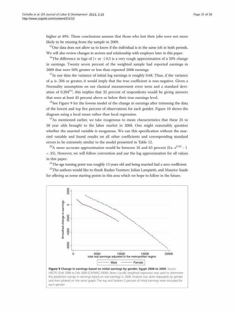
Cichello et al. IZA Journal of Labor & Development Page 35 of 382013, 2:10http://www.izajold.com/content/2/1/10
higher at 49%. These conclusions assume that those who lost their jobs were not more
likely to be missing from the sample in 2009.15Our data does not allow us to know if the individual is in the same job in both periods.
We will also review changes in sectors and relationship with employer later in this paper.16The difference in logs of (+ or -) 0.5 is a very rough approximation of a 50% change
in earnings. Twenty seven percent of the weighted sample had reported earnings in
2009 that were 50% greater or less than reported 2008 earnings.17In our data the variance of initial log earnings is roughly 0.68. Thus, if the variance
of μ is .204 or greater, it would imply that the true coefficient is non-negative. Given a
Normality assumption on our classical measurement error term and a standard devi-
ation of 0.2040.5, this implies that 32 percent of respondents would be giving answers
that were at least 45 percent above or below their true earnings level.18See Figure 9 for the lowess model of the change in earnings after trimming the data
of the lowest and top five percent of observations for each gender. Figure 10 shows the
diagram using a local mean rather than local regression.19As mentioned earlier, we take exogenous to mean characteristics that these 25 to
58 year olds brought to the labor market in 2008. One might reasonably question
whether the married variable is exogenous. We ran this specification without the mar-
ried variable and found results on all other coefficients and corresponding standard
errors to be extremely similar to the model presented in Table 12.20A more accurate approximation would be between 35 and 63 percent (Ex. e0.30 - 1
= .35). However, we will follow convention and use the log approximation for all values
in this paper.21The age turning point was roughly 13 years old and being married had a zero coefficient.22The authors would like to thank Ruslan Yemtsov, Julian Lampietti, and Maurice Saade
for offering us some starting points in this area which we hope to follow in the future.
0006-0004-
0002-0
2000
Sm
ooth
ed c
hang
e in
ear
ning
s
0 5000 10000 15000 20000total real earnings adjusted to the metropolitan region
Male Female
Figure 9 Change in earnings based on initial earnings by gender, Egypt 2008 to 2009. Source:HIECPS (Feb 2008 to Feb 2009 (CAPMAS 2009)). Notes: Locally weighted regression was used to determinethe predicted change in earnings based on real earnings in 2008. Analysis was done separately by genderand then plotted on the same graph. The top and bottom 5 percent of initial earnings were excluded foreach gender.

000 3-00 02-
000 1-0
1000
Sm
ooth
ed c
hang
e in
ear
ning
s
0 5000 10000 15000 20000total real earnings adjusted to the metropolitan region
Male Female
Figure 10 Change in earnings based on initial earnings, by gender, Egypt 2008 to 2009. Source:HIECPS (Feb 2008 to Feb 2009 (CAPMAS 2009)). Notes: Local mean constructed using tri-cube weight usinglowess command with mean option. Top and bottom 5 percent of initial earnings are excluded foreach gender.
Cichello et al. IZA Journal of Labor & Development Page 36 of 382013, 2:10http://www.izajold.com/content/2/1/10
Annex 1: measurement error simulation
In order to demonstrate how our lowess simulations are affected by classical measure-
ment error, we conducted a simulation. For simplicity we treat the observed values of
log 2008 earnings as true values. In order to create our simulated values of log 2008 re-
ported earnings, we add a simulated measurement error realization to each
-.4
-.2
0.2
.4
Sim
ulat
ed e
arni
ngs
chan
ge w
ith m
easu
rem
ent e
rror
, s.d
.=.3
6 8 10 12gridx
sim_mean sim_uppersim_lower
Figure 11 Simulated change in log earnings based on initial log earnings, Egypt 2008 to 2009.Source: Authors’ compilation from HIECPS (Feb 2008 to Feb 2009 (CAPMAS 2009)). Notes: Simulated earningsvalues for 2008 and 2009 were both based on reported log 2008 earnings plus some random measurementerror, which was drawn from a Normal distribution with mean zero and variance of 0.3. A change inearnings was then constructed directly from these simulated values. Finally, locally weighted regression wasused to determine the predicted change in log earnings based on log real earnings in 2008. Upper andlower confidence intervals are shown as well.

Cichello et al. IZA Journal of Labor & Development Page 37 of 382013, 2:10http://www.izajold.com/content/2/1/10
observation. These realizations are drawn randomly from a Normal distribution with a
mean of zero and a standard deviation of 0.3. This standard deviation is admittedly ar-
bitrary, but we feel it offers a significant amount of measurement error. Under this dis-
tribution, 32 percent of the sample would receive a random measurement error term
with a magnitude greater than approximately 30 percent of the value of their ‘true’
earnings level. Five percent of the sample would receive measurement error that was
more than approximately 60 percent of their ‘true’ earnings level.
We then constructed a second set of values in the exact same manner and called
them log 2009 reported earnings. We take the difference and run a lowess regression of
the simulated difference on the simulated 2008 data. This simulation thus represents
what the lowess graph would look like if individuals had no real change in earnings but
a fairly significant amount of measurement error. The result, shown in Figure 11 below,
is initially disturbing as it shares many feature with our observed lowess results of the
change in earnings on initial earnings. It is distinctly downward sloping.
However, this level of measurement error definitely cannot explain the results ob-
served in our data. Figure 12 graphs the simulation again, this time also graphing the
lowess graph using the change in log reported earnings and log initial reported earn-
ings observed in our dataset. The simulation was downward sloping but the magni-
tude of the changes is tiny compared to the magnitude using our observed data.
Thus, we are reassured that our lowess results are not driven solely by classical
measurement error. Others may not feel as confident in this conclusion if they feel
measurement error has a much larger variance or is otherwise different from our
maintained assumptions. In this sense, this validation approach is similar to the
approach of Fields et al. (Fields et al. 2003a).
-2-1
01
2
6 8 10 12gridx
sim_mean sim_uppersim_lower Smoothed change in log earnings
Figure 12 Simulated and reported change in log earnings based on initial log earnings, Egypt 2008to 2009. Source: Authors’ compilation from HIECPS (Feb 2008 to Feb 2009 (CAPMAS 2009)). Note: Simulatedearnings values for 2008 and 2009 were both based on reported log 2008 earnings plus some randommeasurement error, which was drawn from a Normal distribution with mean zero and variance of 0.3. Achange in earnings was then constructed directly from these simulated values. Finally, locally weightedregression was used to determine the predicted change in log earnings based on log real earnings in 2008.Upper and lower confidence intervals are shown as well.

Cichello et al. IZA Journal of Labor & Development Page 38 of 382013, 2:10http://www.izajold.com/content/2/1/10
AbbreviationsCAPMAS: Central Agency for Public Mobilization and Statistics; EGP: Egyptian Pound; HIECPS: Household Income,Expenditure and Consumption Panel Survey; HIECS: Household Income, Expenditure and Consumption Survey;LFSS: Labor Force Sample Survey; LPM: Linear Probability Model.
Competing interestsThe IZA Journal of Labor & Development is committed to the IZA Guiding Principles of Research Integrity. The authorsdeclare that they have observed these principles.
AcknowledgementsThe authors would like to thank Rania Rouchdy, Ruslan Yemtsov, Joanna Silva, Julian Lampietti, Maurice Saade, HebaEl-Laithy, Sherine El-Shawarbi, the Editor and an anonymous referee for their comments. We would also like to thankNicholas Diebel, Mallimalika Gupta, Choon-Sung Lim, and Caleb Pomeroy for research assistant work related to thispaper. Ideas expressed in this paper are those of the authors and do not reflect policies of their respective organiza-tions. The usual disclaimers apply.Responsible editor: David Lam
Author details1Economics Department, Boston College, 140 Commonwealth Ave, Chestnut Hill, MA 02467, USA. 2Faculty ofEconomics and Political Science, Cairo University, Cairo, Egypt. 3World Bank, 1818 H Street NW, Washington, D.C 20433,USA.
Received: 25 June 2013 Accepted: 24 October 2013Published:
References
25 Nov 2013
Arabsheibani R (2000) Male–female Earnings Differentials in an Islamic Country: The Case of Highly Educated Egyptians.Educ Econ 8(2):129–138
Assaad R, Roushdy R (2007) Labor market trends and living standards in Egypt. In: Arab Republic of Egypt – PovertyAssessment Update, vol 1. The World Bank, Arab Republic of Egypt, pp 69–91
Beegle K, De Weerd J, Dercon S (2011) Migration and Economic Mobility in Tanzania: Evidence from a Tracking Survey.Rev Econ Stat 93(3):1010–1033
Belhaj-Hassine N (2012) Inequality of opportunity in Egypt. World Bank Econ Rev 26(2):265–295Cameron AC, Trivedi PK (2005) Microeconometrics: Methods and applications. Cambridge University Press, CambridgeCAPMAS (Central Agency for Public Mobilization and Statistics) (2009) Various issues. HIECS (Household Income,
Expenditure and Consumption Surveys). CAPMAS, Cairo, EgyptCichello PL, Fields GS, Leibbrandt M (2005) Earnings and employment dynamics for Africans in post-apartheid South Af-
rica: A panel study of KwaZulu-Natal. J Afr Econ 14(2):143–190Cleveland WS (1979) Robust locally weighted regression and smoothing scatter plots. J Am Stat Assoc 74:829–836Datt G, Olmsted J (2004) Induced wage effects of changes in food prices in Egypt. J Dev Stud 40(4):137–166Fields GS (2008) A brief review of the literature on earnings mobility in developing countries. : , Working Papers n. 101,
ILR School, Cornell University. http://digitalcommons.ilr.cornell.edu/workingpapers/101 (retrieved 07/05/2011)Fields GS, Sanchez Puerta ML (2010) Earnings mobility in times of growth and decline: Argentina from 1996 to 2003.
World Dev 38(6):870–880Fields GS, Cichello PL, Freije S, Menéndez M, Newhouse D (2003a) For richer or for poorer? Evidence from Indonesia,
South Africa, Spain, and Venezuela. J Econ Inequal 1(1):67–99Fields GS, Cichello PL, Freije S, Menéndez M, Newhouse D (2003b) Household income dynamics: A four country story. J
Dev Stud 40(2):30–54Lundberg S (1985) The added worker effect. J Labor Econ 3(1):11–37Roushdy R, Gadallah M (2011) Labor Market Adjustment to the World Financial Crisis: Evidence from Egypt. ERF Annual
Conference paper, ERF17AC_054., http://www.erf.org.eg/cms.php?id=publication_details&publication_id=1363Said M (2009) The Fall and Rise of Earnings and Inequality in Egypt: New Evidence from the Egypt Labor Market Panel
Survey 2006. Ch. 2. In: Assaad R (ed) The Egyptian Labor Market Revisited. American University in Cairo Press, NewYork and Cairo, pp 53–81
Said M (2012) Wage Differentials during Economic Reform and Crisis: Evidence from Egypt and Jordan. Comp EconStud 54:65–101
Serneels P (2002) The added worker effect and intra household aspects of unemployment. CSAE Working Paper Series2002–14. Centre for the Study of African Economies, University of Oxford
World Bank (2011) Poverty in Egypt 2008–2009: Withstanding the global economic crisis. The World Bank, EgyptWorld Bank, DECPG (2008) Commodity Markets Review, Development Prospects Group. The World Bank, Washington,
DC
Cite this article as: Cichello et al.: What happened to real earnings in Egypt, 2008 to 2009? IZA Journal ofLabor & Development
10.1186/2193-9020-2-10
2013, 2:10