What Difference Do Unions Make? Their Impact on Productivity and Wages in Latin America
256
What Difference Do Unions Make? Their Impact on Productivity and Wages in Latin America Peter Kuhn and Gustavo Márquez Editors Inter-American Development Bank Washington, D.C. 2005
-
Upload
independent -
Category
Documents
-
view
3 -
download
0
Transcript of What Difference Do Unions Make? Their Impact on Productivity and Wages in Latin America

What Difference Do Unions Make? Their Impact on
Productivity and Wages in Latin America
Peter Kuhn and Gustavo Márquez
Editors
Inter-American Development BankWashington, D.C.
2005

Latin American Research Network
Inter-American Development Bank
The Inter-American Development Bank created the Latin American Research
Network in 1991 in order to strengthen policy formulation and contribute to the
development policy agenda in Latin America. Through a competitive bidding
process, the Network provides grant funding to leading Latin American research
centers to conduct studies on economic and social issues selected by the Bank
in consultation with the region’s development community. Most of the studies
are comparative, which allows the Bank to build its knowledge base and draw on
lessons from experiences in macroeconomic and financial policy, modernization
of the state, regulation, poverty and income distribution, social services, and
employment. Individual country studies are available as working papers and are
also available in PDF format on the Internet at http://www.iadb.org/res.
©2005 Inter-American Development Bank
1300 New York Avenue, N.W.
Washington, DC 20577
Cataloging-in-Publication data provided by the
Inter-American Development Bank
Felipe Herrera Library
What difference do unions make? : their impact on productivity and wages in
Latin America / Peter Kuhn and Gustavo Márquez, editors.
p. cm.
Includes bibliographical references.
ISBN: 1931003963
1. Labor unions—Latin America. 2. Industrial productivity—Effect of Labor
unions on—Latin America. 3. Wages—Effect of Labor unions on—Latin America.
I. Kühn, Peter. II. Márquez, Gustavo. III. Inter-American Development Bank.
Research Dept.
331.88 W452--------dc22

TABLE OF CONTENTS
Chapter 1.
The Economic Effects of Unions in Latin America . . . . . . . . . . . . . . . . . . . . . . . . . 1
Peter Kuhn and Gustavo Márquez
Chapter 2.
An Empirical Examination of Union Density in Six Countries:
Canada, Ecuador, Mexico, Nicaragua, the United States, and Venezuela . . . . . . . 13
Susan Johnson
Chapter 3.
Union Density Changes and Union Effects on Firm Performance in Peru . . . . . 33
Jaime Saavedra and Máximo Torero
Chapter 4.
Unions and the Economic Performance of Brazilian Establishments . . . . . . . . . 77
Naercio Menezes-Filho, Helio Zylberstajn, Jose Paulo Chahad and Elaine Pazello
Chapter 5.
The Economic Effects of Unions in Latin America: Their Impact
on Wages and the Economic Performance of Firms in Uruguay . . . . . . . . . . . . 101
Adriana Cassoni, Gaston J. Labadie and Gabriela Fachola
Chapter 6.
The Effects of Unions on Productivity: Evidence from Large Coffee
Producers in Guatemala . . . . . . . . . . . . . . . . . . . . . . . . . . . . . . . . . . . . . . . . . . . . . 143
Carmen Urízar H. and Sigfrido Lée
Chapter 7.
Teacher Unionization and the Quality of Education in Peru:
An Empirical Evaluation Using Survey Data . . . . . . . . . . . . . . . . . . . . . . . . . . . . 173
Eduardo Zegarra and Renato Ravina

Chapter 8.
The Economic Effects of Unions in Latin America:
Teachers’ Unions and Education in Argentina . . . . . . . . . . . . . . . . . . . . . . . . . . . 197
M. Victoria Murillo, Mariano Tommasi, Lucas Ronconi and Juan Sanguinetti
Bibliography . . . . . . . . . . . . . . . . . . . . . . . . . . . . . . . . . . . . . . . . . . . . . . . . . . . . . . 233

ACKNOWLEDGMENTS
The studies in this volume were made possible through the efforts of many
individuals, not all of whom are named here. Particular thanks, though, are
extended to Luis Enrique González for his valuable time and assistance, and for
sharing his knowledge of the coffee sector in Guatemala. The authors additionally
wish to thank María Isabel Bonilla, Carlos Castejón, Karina Lée, Jorge Lavarreda
and Hugo Maul for their research, and Dardo Curti for estimating survival
models.
Various assistant researchers also made invaluable contributions. They
include Emmanuel Abuelafia, Gabriela Cordourier, Virgilio Galdo, Juan Manuel
García, Gerardo Ponciano, Oscar Portillo, Alejandro Retamoso and Michelle
Viau.
Finally, the completion of this volume would not have been possible without
the expertise of several members of the IDB Research Department. Thanks are
particularly extended to Norelis Betancourt and Raquel Gómez for their managerial
and administrative efforts throughout the life of this project, and to Rita Funaro
and John Dunn Smith for their editorial expertise.


CHAPTER ONE
The Economic Effects of Unions in Latin America
Peter Kuhn Gustavo Márquez1
Ever since the classic analysis of union relative wages by H.G. Lewis (1963),
the economic effects of trade unions have been a vibrant field of study in the
United States. The empirical analysis of union effects has expanded to encompass
outcomes other than wages—including profits, productivity, and employment—
and to consider unionism in other countries, particularly the United Kingdom
and Canada. A recent review of this literature is provided by Kuhn (1998).
Perhaps surprisingly, the empirical study of union effects has not spread
far beyond these three industrialized, Anglo-Saxon countries in the four decades
since 1963.2 What Difference Do Unions Make? takes a major step towards filling
the research gap by examining unionism in five Latin American economies, as well
as comparing union density in North America and a sample of Latin American
countries. At this point, very little is known about unions as economic actors in
Latin America. The literature that does exist on Latin American unions instead
tends to focus on the history of the various union movements and the constitutional
and legal bases of unionism in the various countries of the region.3 In addition
to providing information to scholars and policymakers with an interest in Latin
America, the studies in this volume thus constitute an important addition to the
economic analysis of unionism, since they are among the first to extend empirical
analysis into several institutional frameworks of collective bargaining that are very
different from the Anglo-Saxon norm.
1 Peter Kuhn is Professor of Economics at the University of California, Santa Barbara, and Gustavo Márquez is Lead Research Economist at the Research Department of the Inter-American Development Bank.2 Most of the European research remains theoretical, though recently a few empirical studies have emerged (e.g., Holden, 1998).3 See, for example, Ojeda and Ermida (1993), Garza Toledo (2001), and O’Connell (1999).

2 THE ECONOMIC EFFECTS OF UNIONS IN LATIN AMERICA
To accomplish this goal a group of authors was selected to focus on three sets
of questions. First, what factors influence the tendency of individual workers to
belong to unions in Latin America? Are these factors the same as in North America
(that is, the United States and Canada)? And what factors explain cross-national
differences in unionization rates, both within Latin America and between Latin
American and North American countries? Chapter 2 explores these questions.
Second, what are the effects of private sector unions in Latin America on outcomes
such as productivity, wages, investment and profits? How—if at all—do these
effects differ from their estimated effects in other regions of the world? Chapters
3-6, which focus in turn on Peru, Brazil, Uruguay and Guatemala, examine these
topics. Third, what are the effects of public sector unions in Latin America? To
address this question, Chapters 7 and 8 analyze the effects of teachers’ unions
in Peru and Argentina on various dimensions of teacher performance, working
conditions and student outcomes. Teachers’ unions have become a much-studied
institution in the United States because of high unionization rates among those
professionals and because of teachers’ central role in training the labor force of the
future. The same considerations motivate this study of Latin America.
What Makes People Join Unions?
To investigate the determinants of union density (the share of workers belonging
to labor unions), in Chapter 2 Susan Johnson uses comparable 1998 micro data
surveys from six countries: Canada, Ecuador, Mexico, Nicaragua, the United States
and Venezuela. Of these countries, Canada has the highest union density, at 29
percent of the labor force, and is therefore used as a convenient reference point for
comparison with the remaining countries. Thus, Johnson asks what differences
between Canada and the other countries might explain their lower rates of
unionization, which are as follows: 22 percent in Venezuela, 16 percent in Mexico,
14 percent in the United States, 9 percent in Ecuador and 5 percent in Nicaragua.
Given the nature of her data, Johnson focuses exclusively on “structural”
explanations of international differences in union density. Structural explanations
are based on the premise that certain kinds of workers and/or jobs lend themselves
more readily to unionization than others. For example, teenage workers may be
hard to unionize because of low attachment rates to their jobs, and jobs in small,
private sector firms may not provide adequate incentives for unionization because
few economic rents are available to be transferred to workers. As a result, if some

WHAT DIFFERENCE DO UNIONS MAKE? 3
Latin American countries have disproportionate shares of workers or jobs in hard-
to-unionize categories, this may help explain their low levels of unionization.
Of course, many “non-structural” factors such as historical, legal and political
developments also affect union density levels across countries; these will appear in
the “unexplained” portions of Johnson’s gaps.
Johnson’s first key finding is that, for the most part, the same personal and
job characteristics are associated with a higher likelihood of union membership
in all six countries studied. In particular, in both North America and Latin
America, the following types of workers tend to be highly unionized: those in
manufacturing, utility and transportation industries; those in professional,
administrative, or manual occupations; those aged 45-54; workers in large firms;
and public sector workers.4 In all six countries, agricultural workers and workers
under 34 or over 64 years of age tend to have low unionization rates. Johnson’s
findings in this regard are supported by Saavedra and Torero’s finding in Chapter
3 that union membership is associated with having a permanent contract, working
in a large firm and working in the public sector. In Chapter 5, Cassoni, Labadie
and Fachola also find that union density is higher in Uruguay’s public sector
than in its private sector. The uniformity of these patterns of unionization, in the
face of large differences in politics and institutions across the countries studied,
strongly supports the idea that structural factors play a role in union density and
are consequently worth exploring in a cross-national context.
Johnson’s second key finding is that structural factors play a substantial role
in explaining cross-national differences in unionization among the six countries
she examines. Considering the gap between Canada and the four Latin American
countries studied, she finds that international differences in the gender, age,
industry, occupation, education and part-time/full-time mix of the labor force
can account for as little as 36 percent of the gap, in the case of Mexico, and as
much as 81 percent of it, in the case of Venezuela. Of these factors, the largest
role is played by industry mix: even when self-employed and unpaid workers are
removed from the analysis (as they are throughout the chapter), the much larger
agricultural sectors in Latin American countries are a critical factor in explaining
their low union density. Other factors playing a significant role in the Canada-
Latin America union density gap are occupation mix and age, since the very young
labor force in Latin America hinders unionization there. Accounting for the effects
4 According to Johnson’s probit estimates, women are less likely to be unionized than men in five of the six countries, but this gender differential is statistically significant in only two of the six cases.

4 THE ECONOMIC EFFECTS OF UNIONS IN LATIN AMERICA
of public sector employment on union density differentials, however, presents
some intriguing puzzles.5 For example, according to the data, Venezuela (partly,
no doubt, as a result of oil revenues) has a larger public sector and a greater share
of employment in large firms than Canada. While this helps explain Venezuela’s
high unionization rate relative to other Latin American countries, it complicates
the question of why Venezuela is less unionized than Canada. Such comparisons
underscore the need to consider political and legal factors as well as structural
ones.
Several other lessons can be drawn from Johnson’s analysis. First, low
unionization rates among paid workers in certain Latin American countries
(for example, Ecuador and Nicaragua) are not necessarily a consequence of the
political and legal features of those countries. Their labor forces are characterized
by a high percentage of younger workers and a high percentage of employment
in small agricultural enterprises—circumstances that would make unionization
difficult in almost any institutional environment. Second, most determinants
of unionization are the same in all the countries studied, with one interesting
exception: unionization is concentrated among less-educated workers in North
America, but among better-educated workers in Latin America. Thus the nature
of the union movement, at least in its current form, and its likely effects on overall
wage inequality are different in Latin America. Third, while demonstrating the
importance of structural factors, Johnson’s analysis also shows that other factors
must play a role. In addition to the case of Venezuela noted above, the clearest
example of this is provided by a comparison of Canada and the United States.
Structurally, the measured differences between these two highly developed
economies are minimal, especially compared to differences between North and
South America. At the same time, union density in the United States was less than
half of Canada’s in 1998 and even less than the level in Mexico. A number of authors
(such as Weiler, 1983) have therefore attributed most of the Canada-United States
union density gap to legal factors affecting the representation process.
Other evidence of the effects of legal factors on union density emerges from
Saavedra and Torero’s study of Peruvian manufacturing in Chapter 3. According
to the authors, union density in metropolitan Lima fell from about 40 percent in
the late 1980s to 10 percent by 1998. An acceleration in the rate of decline was
associated with important changes in the Collective Bargaining Law of 1993; since
this decline occurred within narrowly defined labor market segments it cannot
5 This issue is discussed in further detail in the Data Appendix of Johnson (2004), the paper on which Chapter 2 is based.

WHAT DIFFERENCE DO UNIONS MAKE? 5
be readily explained by structural factors. Sizable within-country changes in
union density that accompany changes in collective bargaining legislation, such as
occurred in Peru in the early 1990s, provide very suggestive evidence that, despite
structural constraints, legislation can have a major impact on unionization in
Latin America. Whether legislation could have an equally powerful effect in rural
areas, however, remains an open question. Another obvious illustration of the
importance of legal factors is the emergence of unions after the prohibition on
collective bargaining in Uruguay was lifted in 1984.
Finally, taken together, Chapters 3-5 of this volume provide evidence of a
crucial determinant of private sector union density that is neither legal, political,
nor usually considered a “structural” factor: the degree of competition in product
markets.6 It is noteworthy that each of the three countries examined in these
chapters—Peru, Brazil and Uruguay—underwent a dramatic episode of trade
liberalization during the 1990s and a considerable decline in union density. Clearly,
one main reason why workers join unions is that unions transfer economic rents
from the firm’s owners and consumers to workers; if competition reduces the size
of those rents, union membership is less beneficial. The inescapable conclusion
is that the continued reduction of trade barriers and deregulation of product
markets is likely to be detrimental to the union movement in Latin America.
Private Sector Labor Unions and Economic Performance
What are the effects of labor unions on the economic performance of private-
sector firms in Latin America? Chapters 3, 4 and 5 look at the manufacturing
sectors of Peru, Brazil and Uruguay, respectively, using panel data on individual
firms. Manufacturing is the “traditional” environment in which union effects on
firm performance have been studied in the past (for example, Clark, 1984). By
examining firms in this sector, the three chapters benefit from relatively reliable
measures of output and productivity, as well as comparability with existing
research. In all three of these countries, there is considerable heterogeneity across
firms and over time in the prevalence of unions, and the authors exploit this
heterogeneity in order to identify union effects. Notably, this is the case even in
Brazil, where wage bargaining was highly centralized and union-bargained wage
rates were automatically extended to non-union workers. In the Brazilian case,
6 Nickell (1999) provides a recent review of the literature on the important but often underemphasized link between product markets and unionization in the labor market.

6 THE ECONOMIC EFFECTS OF UNIONS IN LATIN AMERICA
issues such as working conditions, employment and the introduction of new
technologies are bargained over at the plant level, and the authors measure these
effects in their analysis. Finally, Chapter 6 offers insights into the role of unions in
a very different environment: Guatemala’s agricultural sector.
Taking a closer look at each of these four studies in turn, Chapter 3 analyzes
the effects of unions on profits in Peru. Using a panel of manufacturing firms from
1994 to 1996, Saavedra and Torero find that unions reduce profits, even when
firm fixed effects are held constant—a highly desirable specification to use when
feasible. They also find that unions appear to reduce productivity, but this result is
not robust to firm fixed effects.
Chapter 4 examines union effects in Brazil, where Menezes-Filho et al. study
a panel of Brazilian manufacturing firms from 1988 to 1998. During this period,
Brazilian firms faced a massive increase in exposure to foreign competition and
union density declined, perhaps in response. Like Saavedra and Torero, the authors
of Chapter 4, using a firm random effects model with year and industry dummies,
find that an increase in union density or influence at the firm level tends to reduce
profitability. In contrast, union density seems to have an inverted U-shaped effect
on productivity and employment, both reaching a maximum at about 50 percent
unionization. On the other hand, the authors find no significant union effect on
investment. Since the majority of the firms in their sample were less than 25 percent
unionized, the effect of union density in a typical Brazilian manufacturing firm
is to raise productivity and employment. Probing the robustness of their results
to permanent, firm-specific effects using a long-difference specification, the only
result that remains statistically significant is that unions raise employment.
Turning to Uruguay, in Chapter 5 Cassoni, Labadie and Fachola base their
analysis on a panel of establishments from 1988 to 1995. As in Brazil and Peru, this
was a period of considerable trade liberalization in Uruguay. Another important
trend during this period was a move away from centralized wage negotiations
toward enterprise-level bargaining. The authors argue that this change should
increase unions’ likelihood of bargaining over employment as well as wages. In
this panel, the authors find that unionization increases wages, reduces profits,
increases employment and promotes investment, mainly by encouraging firms to
substitute capital for labor. In agreement with the Brazilian results, but in contrast
with the Peruvian results, Cassoni, Labadie and Fachola find that unionization
raises productivity. Although the authors find an increased union emphasis on
employment in the latter part of the period analyzed, this result is not statistically
significant.

WHAT DIFFERENCE DO UNIONS MAKE? 7
Chapter 6, which addresses union effects in Guatemala, departs from the
preceding three chapters to look at the role of unions in a very different setting.
Here, Urízar and Lée break ground in considering the effects of unions on
large Guatemalan coffee plantations. Aside from being the only study of union
productivity effects in the agricultural sector of which the editors are aware, this
study also has the advantage of employing a better measure of output—and hence
a better measure of productivity—than most other studies. Since all plantations
produce the same product—coffee—their productivity can be measured in
physical units. This circumvents a serious problem in much of the literature
on union-productivity effects, namely that value-based measures of output are
influenced by union effects on output prices as well as quantities.
Urízar and Lée’s sample for analysis, based on their own survey, consists of
37 plantations, each of which provided complete data for four consecutive years
between 1992 and 2000. Their focus in this chapter is only on the productivity
effects of unions, not on other outcomes such as wages, profits or employment.
Incorporating controls for the types of workers employed (temporary, permanent
or administrative), land quantity and quality, a variety of detailed capital and
technology measures, and region fixed effects, they find in a pooled generalized
least squares (GLS) specification that unions—which are relatively uncommon on
Guatemalan coffee plantations—appear to reduce productivity. This is perhaps not
surprising given the very detailed work rules sometimes observed in plantation-
level union agreements, even including restrictions on the number and size of
holes to be dug per day.
Restricting their attention to the very small number of firms that changed
union status, however, Urízar and Lée cannot confirm their productivity results
in a fixed-effects specification. It is nonetheless interesting that their fixed-effects
model shows a large productivity disadvantage in substituting permanent for
temporary workers, a policy pursued by many unions in Guatemala.
When the results of all four studies of unions and firm performance in this
volume are considered, what conclusions can be drawn? Mirroring the existing
literature outside Latin America (see Kuhn, 1998, pp. 1046-1048), estimated
effects of unionization on productivity differ across studies, with both positive
and negative effects observed. Although this could reflect differences in definitions
and techniques across studies, it more likely reflects true heterogeneity in union
effects, as a number of authors (such as Clark, 1984) have argued. Theoretically,
union productivity effects can be positive, because of employee “voice” effects, or
negative, because of work rules and increased conflict, including strikes. Which
8 THE ECONOMIC EFFECTS OF UNIONS IN LATIN AMERICA
of these effects dominates can vary by industry, country, and time period, and
it appears that Latin America is no exception in this regard. Neither blanket
opposition to, nor unqualified support of, unions on productivity grounds is
warranted by the studies in this volume. In all cases careful attention to details of
industry, industrial relations, and production methods is required to assess union
effects on productive efficiency.
This volume presents much more robust findings, however, about two other
union effects. The first is the effect on profits. Given the fact that unions raise wages,
the robust findings in this volume that unions reduce profits is both unsurprising
and consistent with virtually all previous research.7 Of course, this raises concerns
about the likely effects of unions on firms’ incentives to make new investments
in plant, research and development, and equipment, but to date results on these
questions have been much harder to characterize. A second union effect—that of
raising employment levels—is also seen in all studies that address the issue in this
volume. At first glance, this may seem paradoxical given that unions raise the price
of labor to firms, but it is in fact consistent with the well-known “efficient contracts”
model of unionism (for example, Brown and Ashenfelter, 1986): if unions care
about employment as well as wages, Pareto-efficient contracts between unions and
firms may stipulate higher employment levels than in competitive firms. This is
especially the case in declining firms and industries in which unions have a special
interest in preserving the jobs of their existing members.
It is also worth noting that all of the positive employment effects estimated
in these chapters come from a period of deregulation, declining unionization,
and increased exposure to competition. Thus, the data may be capturing
employment cutbacks that occur in conjunction with both de-unionization and
increased product competition, similar to what Brown and Ryan (1998) recently
observed in a sample of deregulated British firms. Given the limitations of the
data, the effects of unionism and product market competition may be partially
confounded in these estimates, but it is clear that in Latin America, as elsewhere
(see, for instance, Boal and Pencavel, 1994), when negotiations occur at the plant
or firm level, unions do what they can to increase their members’ employment
or preserve their members’ jobs. De-unionization, not unionization, is associated
with employment cutbacks in Latin American as well as other data. While such
cuts may eliminate inefficiencies, it is important to note that the short-term costs
of reducing union power appear to include job losses at firms where union power
7 See, for example, Ruback and Zimmerman (1984), Abowd (1989), Bronars and Deere (1990) and Machin and Stewart (1996).

WHAT DIFFERENCE DO UNIONS MAKE? 9
is reduced. Although this is a perfectly sensible and plausible result, it is not what
one would have predicted from a simple labor demand model.
Public Sector Labor Unions and Economic Performance
The final two chapters in this volume consider the effects of Latin American
unions in the public sector. Mirroring considerable recent interest in the effects
of teachers’ unions in the United States and taking advantage of the relative
abundance of data (compared to other public sector workers) on teachers’ salaries,
working conditions, and productivity (as measured by student outcomes), both
chapters look at public school teachers.
Zegarra and Ravina’s study of Peruvian teachers in Chapter 7 draws most of
its data from a sample of schools where both teacher and student performance were
observed as part of a national study to improve educational quality. In addition,
some supplemental evidence is drawn from a group of about 500 teachers selected
from a 1999 national household survey. Peruvian teachers’ wages are negotiated
centrally by a single national union, and these wage agreements apply to union and
non-union teachers. As a consequence, any difference in outcomes between union
and non-union teachers (or their students) must result from differences between
individuals who voluntarily choose to belong to a union and those who do not, or
from differences in the resources or students assigned to union teachers. Thus, one
question posed by these authors is whether unionized teachers command better
classroom and school resources than other teachers in Peru.8
Zegarra and Ravina find that in large schools, unionized teachers do not
command better resources, while in small schools they do. The authors then look
at direct measures of teacher performance (or “effort,” in their terminology) based
on classroom observation. These measures include indicators of effective time use
during class, good control of the classroom and students’ opinions about their
teacher. Unlike some influential recent American studies (such as Hoxby, 1996),
Zegarra and Ravina do not find that unionized teachers are less or more effective;
nor are their students’ standardized test scores any different. This result might,
of course, be driven by their very small sample size (a group of 50 teachers, all of
8 Another important distinction in Peru is between tenured teachers and those hired on temporary contracts, which were introduced in 1993. Unfortunately, Zegarra and Ravina cannot estimate the effect of tenure on teacher performance, since their data on student outcomes contain only tenured teachers.

10 THE ECONOMIC EFFECTS OF UNIONS IN LATIN AMERICA
whom are on permanent, tenured contracts). Alternatively, it could be related to
the structure of collective bargaining, in which both union and non-union teachers
are covered by the same agreement, and union membership decisions may reflect
personal political decisions without having detectable economic consequences at
the individual level. Finally, Zegarra and Ravina present some evidence consistent
with the expected, and intuitive, notion that unions attempt to increase their
members’ job security: union teachers are much more likely to be tenured than
non-union teachers.9
In Chapter 8, Murillo et al. attempt to isolate some effects of teachers’ unions
in Argentina. In doing so, the authors face an institutional problem similar to that
confronted by Zegarra and Ravina: in Argentina, teachers’ salaries, education
budgets, working conditions and regulations affecting teachers are all bargained
at the provincial level between teachers’ unions and the provincial government.
Agreements apply to all teachers, regardless of union membership status. Therefore
the appropriate measure of teacher union strength in Argentina is at the provincial
level.
Looking across Argentina’s 24 provinces in the late 1990s, the authors make
several observations. First, strikes are more frequent in provinces with higher
teacher union density, where teachers’ unions are fragmented, and where their
political relations with the governor (measured by criteria other than strikes,
such as party affiliation) are adversarial. In addition, there is weak evidence that
stronger unions reduce class size. Finally, again looking across 24 provinces and
including a small number of control variables for provincial characteristics, strong
teachers’ unions do not seem to affect the size of the education budget. They do,
however, seem to increase the share of the education budget devoted to salaries.
From a different dataset of 1,534 individual teachers nationwide, the chapter also
finds that unionized teachers express much lower job satisfaction than their non-
unionized counterparts, mirroring a well-known result in other countries (for
instance, Borjas, 1979).
If unions do indeed have the above effects in Argentina, how would this
affect students? Clearly, on the basis of prior experience and studies in other
countries, one would expect an increase in strikes (therefore, fewer class days)
and teacher job dissatisfaction to compromise students’ educational outcomes.
Some supporting evidence for this contention is available from Argentina as well:
9 Of course, this correlation could also be explained by a greater willingness of already-tenured teachers to join unions. In the case of Peruvian teachers, however, Zegarra and Ravina maintain that most union membership decisions are relatively permanent and made fairly early in teachers’ careers.

WHAT DIFFERENCE DO UNIONS MAKE? 11
as the authors discuss, math scores are positively correlated with class days and
teacher job satisfaction in a national sample of seventh-grade students between
1997 and 1999. In combination with the result that teachers’ unions do not seem
to raise education budgets, this suggests that teachers’ unions have an adverse
overall effect on student performance in Argentina, though clearly no direct
link has been drawn. In sum, Argentine teachers’ unions appear to increase their
members’ job security (as they do in Peru). In addition, teachers’ unions increase
industrial conflict and reduce teacher job satisfaction, perhaps harming students
as a consequence. There is no evidence that these unions are successful in lobbying
provincial governments for larger educational budgets—only a larger share of the
budget for teacher salaries.
Pulling It All Together
Overall, what have the studies in this volume taught us about unions in Latin
America? Certainly, one important lesson is methodological: given that bargaining
institutions are often very different in Latin America from those in countries
where the empirical study of unions originated, simplistic adaptation of empirical
techniques developed in the latter environment and applied to the former will
not always yield useful insights. The clearest examples of this difference involve
the analyses of teachers’ unions: in an environment where many aspects of
compensation are bargained nationally and extended automatically to non-union
as well as union workers, cross-sectional comparisons of compensation, working
conditions and productivity of union members versus non-members are not very
informative about union effects on these outcomes.
This methodological caution duly noted, however, perhaps the most surprising
finding in this volume is a substantive one: despite the fact that institutions, laws
and cultures differ so greatly both among Latin American countries and between
Latin America and the rest of the world, it is striking how much unions in all these
countries have in common. With one exception—worker education levels—Latin
American unions are found in the same sectors of the labor market as in other parts
of the world. As elsewhere, there is evidence that they are severely (and negatively)
affected by increases in product market competition. Latin American unions fight
(in most cases effectively) for the same things—higher wages, job security and
increased employment—as unions elsewhere, and in all cases unions appear to
reduce firms’ profits in the process. As regards union effects on perhaps the most

12 THE ECONOMIC EFFECTS OF UNIONS IN LATIN AMERICA
interesting and controversial outcome, productivity, these results also mirror those
in the United Kingdom and the United States: both positive and negative effects
are observed, in different industries and at different times. A blanket case, either
for or against unions, cannot be made on productivity grounds on the basis of
the evidence presented in this volume. As elsewhere, careful attention to industry
conditions, the structure of bargaining, and the nature of industrial relations is
required to assess the effects of unions on the productivity of Latin American
firms.

CHAPTER TWO
An Empirical Examination of Union Density in Six Countries: Canada, Ecuador,
Mexico, Nicaragua, the United States and Venezuela
Susan Johnson1
Unions shape labor market outcomes, influence the broader economy and
additionally affect non-economic aspects of a society. Unions directly affect the
wages, benefits and working conditions of their own members and indirectly
affect those of non-members. By providing workers with a “voice,” unions create
an alternative to “exit” when workers are dissatisfied and can therefore reduce
job turnover. A union’s involvement in the employment relationship affects the
profitability and productivity of the firm, and unions can influence the overall
distribution of wages and level of employment. Moreover, a strong union
movement often plays a role in the political arena by upholding labor’s rights and
interests. While the importance of unions in these dimensions cannot be perfectly
quantified, the usual measure of union influence and strength is union density, or
the proportion of workers who belong to a union in a given economy.
This chapter examines and compares union density in six countries: Canada,
Ecuador, Mexico, Nicaragua, the United States and Venezuela. Two determinants
of union density are examined: (i) the structure of the paid labor force; and (ii)
the probability that a worker with given labor force characteristics is a union
member. The union density gap between Canada, the country with the highest
union density, and each of the other countries is decomposed in order to explore
the contribution of each determinant to the gap.
1 Susan Johnson is Professor of Economics at Wilfrid Laurier University.

14 AN EMPIRICAL EXAMINATION OF UNION DENSITY IN SIX COUNTRIES
Union Density
Union density, the proportion of paid workers who are union members, is a
commonly used indicator of the strength and potential influence of the labor
movement in a country. This chapter analyzes household survey data, from which
comparable information from all six countries is available for 1998. The sample
for each country is the civilian population, over 15 years of age, employed in the
private or public sector with positive working hours in the reference week. Self-
employed workers (incorporated or unincorporated) and those who perform
unpaid work are excluded from the analysis. Observations with missing values for
any variable are also excluded.
Union membership is used throughout the analysis because data on
union coverage are not available for all countries.2 As variables included in the
decomposition analysis must be available and comparable across all six countries,
the variables used in this chapter are limited to the following: gender, worker status
(part-time/full-time job), age, education, occupation and industry. Data on the size
of the public and private sectors and data on establishment size are not available
for all countries, and consequently those variables are not included.3 Table 2.1
presents data on union density for each country in 1998 and for other years where
data are available. These data provide an overview of the size and vitality of the
union movement in each country and permit a comparison across countries. In
1998 there is substantial variation in the degree of unionization across countries.
Canada is the most highly unionized country, with a union density of 29 percent,
followed by Venezuela (22 percent), Mexico (16 percent), the United States (14
percent), Ecuador (9 percent) and Nicaragua, the least unionized country (5
percent). The limited data available on union density over time suggest the union
movement is stagnant or in decline in Canada, Mexico, the United States, Ecuador
and Venezuela.
2 Union membership is different from union coverage. The provisions of a collective agreement can cover workers even though they are not union members. For this reason, coverage is often the preferred measure for capturing the degree of union influence in an economy. Unfortunately, data on union coverage are not available for all countries, and union membership is thus used.3 Johnson (2004) examines the role of the public sector and establishment size in countries where these data are available.

WHAT DIFFERENCE DO UNIONS MAKE? 15
The Determinants of Union Density
Why is union density different across these countries? Differences in union density
among the countries in the sample can be traced to: (i) differences in the proportion
of the workforce with particular characteristics, and (ii) differences in the impact
that each particular characteristic has on the probability of unionization.
Table 2.2 shows the proportion of paid workers by characteristic in 1998
for each country. The table shows there are substantial differences in the structure
of the paid workforces across countries and that many of these differences are
statistically significant. It should be noted, however, that the structures of the
Canadian and American paid workforces are more similar than the structures of
the Canadian and Latin American paid work forces. In Canada and the United
States, for instance, women make up almost half of the paid labor force, while in
Latin American countries women make up only about one third of the paid labor
Table 2.1. Union Density by Country(Standard errors in parentheses)
1984 1989 1992 1993 1994 1995 1996 1997 1998
Canada*0.30
(0.003)
0.29
(0.003)
Ecuador0.11
(0.005)
0.09
(0.005)
Mexico0.24
(0.009)
0.22
(0.006)
0.21
(0.006)
0.18
(0.005)
0.16
(0.004)
0.16
(0.005)
Nicaragua0.05
(0.005)
United
States
0.19
(0.004)
0.16
(0.004)
0.16
(0.003)
0.16
(0.003)
0.16
(0.004)
0.15
(0.003)
0.14
(0.003)
0.14
(0.003)
0.14
(0.003)
Venezuela0.23
(0.004)
0.21
(0.004)
0.22
(0.004)
*Data on union membership are not available from the Labour Force Survey for earlier years in Canada. However aggregate data on union membership are available from the Workplace Information Directorate (Human Resources Canada). Johnson (2002) examines union density in Canada from 1980 to 1998 using data from the Workplace Information Directorate and finds that Canadian union density remained relatively stable from 1980 to 1991 but declined from 1992 to 1998.

16 AN EMPIRICAL EXAMINATION OF UNION DENSITY IN SIX COUNTRIES
force. The proportion of part-time workers varies across countries, from a low of
0.10 in Venezuela to a high of 0.30 in Canada. There are substantial differences
across countries in the size of the service and agricultural sectors, and within Latin
American countries there is substantial variation in the size of the agricultural
sector. The educational structure of the workforce is also very different across
countries. In the United States and Canada the proportion of the workforce with
at least a high school education is greater than 0.80, while in the Latin American
countries it is less than 0.35. The United States and Canada have older workforces
than do the Latin American countries. The proportion of workers age 15-34 is
about 0.4 in both the United States and Canada, while it reaches approximately
0.6 in Latin America. The size and importance of these differences suggest that
structural factors likely account for some of the differences in union density across
countries.
Table 2.3 presents the proportion of paid workers with a particular
characteristic who are union members. This measures the unconditional
probability that a worker with a particular characteristic is unionized and as such
does not take into account interactions with other characteristics. As the table
makes clear, there is substantial variation across countries in the likelihood that
a worker with a given characteristic is unionized. It is also obvious that, not
surprisingly, countries with higher union densities tend to be those with a higher
probability of unionization for any given characteristic. Females are less likely to
be unionized than males in Canada and the United States but more likely to be
unionized in Latin American countries. Part-time workers are less likely to be
unionized than full-time workers in Canada and the United States, but they are
more likely to be unionized in Mexico and Venezuela. In all countries workers in
the utility industry are more likely to be unionized, and workers in agriculture
and trade are less likely to be unionized. The probability that farm and sales
workers are unionized is quite low in all countries. There is a high probability that
professionals and administrators are union members. In all countries those with
“less than high school” are less likely to be unionized and, in most countries, those
with “more than high school” are more likely to be unionized. Younger workers
(15-19, 20-24) and, in most countries, older workers (55-64 and over 64) are less
likely to be unionized than prime-aged workers (35-44, 45-54).
It is interesting to compare these results to those of Blanchflower and
Freeman (1992) who calculated similar probabilities for a selected group of

WHAT DIFFERENCE DO UNIONS MAKE? 17
Table 2.2. Proportion of the Paid Labor Force with Each Characteristic, 1998 (Standard errors in parentheses)
Canada Ecuador Mexico Nicaragua USA Venezuela
Female0.47
(00.003)
0.32
(00.008)
0.33
(0.006)
0.33
(00.010)
0.48
(00.005)
0.35
(0.004)
Part-time0.30
(0.003)
0.21
(0.007)
0.15
(0.005)
0.21
(0.009)
0.24
(0.004)
0.10
(0.003)
Industry
Agriculture0.01
(0.0005)
0.20
(0.006)
0.12
(0.004)
0.27
(0.010)
0.01
(0.001)
0.07
(0.002)
Mining0.02
(0.001)
0.01
(0.001)
0.01
(0.001)
0.006
(0.001)
0.004
(0.001)
0.01
(0.001)
Manufacturing0.18
(0.002)
0.13
(0.005)
0.22
(0.005)
0.13
(0.008)
0.18
(0.004)
0.17
(0.004)
Utilities0.01
(0.001)
0.01
(0.001)
0.01
(0.001)
0.01
(0.002)
0.03
(0.002)
0.01
(0.001)
Construction0.04
(0.001)
0.09
(0.007)
0.07
(0.003)
0.06
(0.005)
0.05
(0.002)
0.09
(0.003)
Trade0.16
(0.002)
0.21
(0.008)
0.14
(0.004)
0.14
(0.007)
0.23
(0.004)
0.19
(0.004)
Transportation0.05
(0.001)
0.05
(0.004)
0.05
(0.003)
0.04
(0.005)
0.05
(0.002)
0.05
(0.002)
Finance0.06
(0.002)
0.05
(0.003)
0.02
(0.001)
0.01
(0.002)
0.13
(0.003)
0.06
(0.002)
Service 0.47
(0.003)
0.25
(0.007)
0.37
(0.006)
0.33
(0.010)
0.32
(0.005)
0.34
(0.004)
Occupation
Professionals0.22
(0.003)
0.13
(0.005)
0.13
(0.004)
0.04
(0.004)
0.18
(0.004)
0.15
(0.003)
Managers0.09
(0.002)
0.02
(0.002)
0.02
(0.002)
0.03
(0.003)
0.13
(0.003)
0.03
(0.002)
Administrators0.17
(0.002)
0.09
(0.005)
0.13
(0.004)
0.14
(0.007)
0.16
(0.004)
0.15
(0.003)
Sales0.10
(0.002)
0.07
(0.004)
0.10
(0.004)
0.05
(0.004)
0.11
(0.003)
0.10
(0.003)
Continued

18 AN EMPIRICAL EXAMINATION OF UNION DENSITY IN SIX COUNTRIES
Table 2.2. Proportion of the Paid Labor Force with Different Characteristics, 1998 (continued)
Canada Ecuador Mexico Nicaragua USA Venezuela
Services0.17
(0.002)
0.21
(0.008)
0.13
(0.004)
0.22
(0.009)
0.14
(0.003)
0.19
(0.004)
Farm0.02
(0.001)
0.19
(0.006)
0.11
(0.004)
0.24
(0.010)
0.01
(0.001)
0.07
(0.002)
Manual0.23
(0.003)
0.29
(0.008)
0.38
(0.006)
0.27
(0.010)
0.25
(0.004)
0.30
(0.004)
Education
Less than
High School
0.17
(0.002)
0.66
(0.008)
0.76
(0.005)
0.79
(0.009)
0.13
(0.003)
0.66
(0.004)
High School0.21
(0.002)
0.14
(0.006)
0.09
(0.004)
0.08
(0.006)
0.33
(0.005)
0.19
(0.004)
More than
High School
0.62
(0.003)
0.20
(0.006)
0.15
(0.005)
0.13
(0.007)
0.54
(0.005)
0.14
(0.003)
Age (years)
15-190.05
(0.001)
0.15
(0.006)
0.12
(0.004)
0.15
(0.007)
0.05
(0.002)
0.09
(0.002)
20-240.11
(0.002)
0.18
(0.008)
0.17
(0.005)
0.18
(0.008)
0.10
(0.003)
0.17
(0.003)
25-340.27
(0.003)
0.29
(0.008)
0.31
(0.006)
0.30
(0.010)
0.25
(0.004)
0.32
(0.004)
35-440.29
(0.003)
0.21
(0.008)
0.22
(0.005)
0.20
(0.008)
0.27
(0.004)
0.23
(0.004)
45-540.20
(0.002)
0.10
(0.005)
0.12
(0.004)
0.10
(0.007)
0.20
(0.004)
0.13
(0.003)
55-640.07
(0.002)
0.05
(0.003)
0.05
(0.003)
0.05
(0.005)
0.09
(0.003)
0.04
(0.002)
Over 640.006
(0.0005)
0.02
(0.003)
0.02
(0.002)
0.02
(0.003)
0.02
(0.001)
0.01
(0.001)
*Proportions within categories may not sum to one because of rounding.

WHAT DIFFERENCE DO UNIONS MAKE? 19
Table 2.3. The Proportion of People with Each Characteristic Who Are Union Members in 1998(Standard errors in parentheses)
Canada Ecuador Mexico Nicaragua USA Venezuela
Gender
Female0.27
(0.004)
0.11
(0.008)
0.19
(0.008)
0.07
(0.008)
0.11
(0.004)
0.28
(0.007)
Male0.30
(0.004)
0.09
(0.005)
0.14
(0.006)
0.05
(0.006)
0.17
(0.005)
0.20
(0.005)
Work Status
Part-time0.24
(0.005)
0.09
(0.009)
0.25
(0.014)
0.06
(0.011)
0.09
(0.006)
0.26
(0.012)
Full-time0.31
(0.003)
0.10
(0.005)
0.14
(0.005)
0.05
(0.005)
0.16
(0.004)
0.22
(0.004)
Industry
Agriculture0.04
(0.010)
0.004
(0.002)
0.002
(0.001)
0.008
(0.003)
0.004
(0.004)
0.02
(0.004)
Mining0.26
(0.015)
0.04
(0.031)
0.42
(0.068)
0.16
(0.085)
0.06
(0.027)
0.54
(0.036)
Manufacturing0.31
(0.007)
0.05
(0.009)
0.18
(0.011)
0.06
(0.018)
0.16
(0.008)
0.22
(0.010)
Utilities0.61
(0.031)
0.54
(0.084)
0.51
(0.066)
0.23
(0.071)
0.32
(0.027)
0.50
(0.042)
Construction0.28
(0.014)
0.02
(0.007)
0.02
(0.005)
0.002
(0.002)
0.19
(0.018)
0.13
(0.010)
Trade0.12
(0.005)
0.02
(0.005)
0.06
(0.008)
0.01
(0.006)
0.06
(0.005)
0.03
(0.004)
Transportation0.44
(0.014)
0.05
(0.015)
0.17
(0.022)
0.05
(0.021)
0.36
(0.022)
0.17
(0.016)
Finance0.07
(0.007)
0.15
(0.024)
0.13
(0.034)
0.18
(0.089)
0.03
(0.005)
0.17
(0.014)
Service 0.35
(0.004)
0.25
(0.014)
0.24
(0.009)
0.10
(0.010)
0.18
(0.006)
0.40
(0.008)
Occupation
Professionals0.40
(0.006)
0.31
(0.020)
0.41
(0.018)
0.08
(0.024)
0.16
(0.008)
0.47
(0.012)
Continued

20 AN EMPIRICAL EXAMINATION OF UNION DENSITY IN SIX COUNTRIES
Table 2.3. The Proportion of People with Each Characteristic Who Are Union Members in 1998 (continued)
(Standard errors in parentheses)
Canada Ecuador Mexico Nicaragua USA Venezuela
Managers0.10
(0.006)
0.23
(0.040)
0.15
(0.031)
0.08
(0.032)
0.06
(0.006)
0.22
(0.020)
Administrators0.26
(0.006)
0.21
(0.022)
0.24
(0.015)
0.14
(0.018)
0.12
(0.008)
0.30
(0.011)
Sales0.10
(0.006)
0.02
(0.009)
0.05
(0.008)
0.013
(0.007)
0.04
(0.006)
0.03
(0.006)
Service 0.24
(0.006)
0.06
(0.009)
0.10
(0.011)
0.05
(0.012)
0.14
(0.009)
0.21
(0.008)
Farm0.16
(0.015)
0.003
(0.002)
0.001
(0.0004)
0.007
(0.003)
0.05
(0.018)
0.03
(0.005)
Manual0.39
(0.006)
0.05
(0.006)
0.14
(0.007)
0.05
(0.008)
0.22
(0.008)
0.18
(0.006)
Education
Less than
High School
0.26
(0.006)
0.04
(0.004)
0.12
(0.005)
0.04
(0.005)
0.09
(0.008)
0.18
(0.004)
High School0.27
(0.006)
0.13
(0.014)
0.28
(0.019)
0.08
(0.019)
0.15
(0.006)
0.29
(0.009)
More than
High School
0.30
(0.004)
0.25
(0.015)
0.28
(0.015)
0.13
(0.019)
0.14
(0.005)
0.36
(0.012)
Age
15-190.06
(0.006)
0.01
(0.003)
0.04
(0.007)
0.01
(0.005)
0.02
(0.006)
0.03
(0.005)
20-240.14
(0.007)
0.02
(0.005)
0.09
(0.009)
0.02
(0.007)
0.05
(0.007)
0.10
(0.007)
25-340.24
(0.005)
0.08
(0.008)
0.16
(0.008)
0.05
(0.008)
0.11
(0.006)
0.21
(0.007)
35-440.34
(0.005)
0.17
(0.013)
0.25
(0.012)
0.09
(0.015)
0.17
(0.007)
0.32
(0.009)
45-540.40
(0.006)
0.19
(0.019)
0.23
(0.015)
0.10
(0.019)
0.21
(0.009)
0.37
(0.012)
55-640.35
(0.011)
0.19
(0.028)
0.19
(0.025)
0.04
(0.017)
0.17
(0.012)
0.32
(0.020)
Over 640.10
(0.023)
0.05
(0.019)
0.04
(0.018)
0.000
(0.000)
0.09
(0.018)
0.16
(0.030)

WHAT DIFFERENCE DO UNIONS MAKE? 21
OECD countries in the mid 1980s.4 In that study, the probability of unionization
associated with any given characteristic is higher than in this chapter, possibly
because the union densities of the countries they study are all substantially
higher than the union densities of the countries included here.5 There are also
differences when the probability of unionization is compared within different
worker characteristic categories. For all countries in their sample, Blanchflower
and Freeman (1992) find that females are less likely to be unionized than males
and part-time workers are less likely to be unionized than full-time workers. These
same relationships exist for Canada and the United States in this study, but do
not exist for the Latin American countries. They find only moderate differences
between highly educated and less educated workers. In contrast, this chapter finds
that workers with less than a high school education have lower unionization rates
than those with higher levels of education. These differences are more pronounced
for the Latin American countries than for Canada and the United States. Like this
chapter, Blanchflower and Freeman (1992) find that younger workers are less likely
to be unionized than older workers.
In order to examine how differences in the probability of unionization across
characteristics and countries affect differences in union densities, a clearer picture
is needed of how each characteristic affects the probability of unionization. This
requires a more sophisticated approach that models the determination of union
status. Such a model isolates the marginal influence of each characteristic on the
likelihood of unionization, controlling for the effects of other characteristics.
Other researchers have used the following reduced form model to describe
union membership status.6 In this model, union membership is determined by
decisions made by the worker, employer, union leaders and union organizers so
that
unioni,c
= 1 f y
i,c > 0
= 0 f yi,c
≤ 0
⎧⎨⎩
⎫⎬⎭
yi,c
= Xi,c
βc + ε
i,c (1)
4 Blanchflower and Freeman (1992) use data from the International Social Survey Program to examine unionization in Australia, Austria, West Germany, the United Kingdom, the United States and Switzerland.5 This is also true for the United States, which is the only country included in both studies.6 See Riddell (1993), Doiron and Riddell (1993), Even and Macpherson (1990,1993), and Riddell and Riddell (2001).

22 AN EMPIRICAL EXAMINATION OF UNION DENSITY IN SIX COUNTRIES
where i is the individual worker and c is the country. y i c
is an unobserved variable
that reflects the net benefit of union membership to the worker and includes the
influence of the employer and union. Xic are variables that capture individual
characteristics that influence the union membership decision, β is the parameter
vector and εic is a random error that is assumed to be normally distributed.
Equation (1) is a reduced form that views union membership status as the result of
both supply and demand factors.7 This probit model is estimated for each country
in 1998.
Table 2.4 presents the change in the predicted probability of unionization if
the variable changes from zero to one and all other variables are held constant at
their means.8 The results indicate that work status, industry, occupation, education,
and age generally affect unionization in ways similar to those of the unconditional
probabilities presented in Table 2.3. Once other factors that affect the probability
of unionization are taken into account, however, the impact of gender (being
female) on the probability of unionization is not statistically significant from
zero for Canada, Mexico, Nicaragua and Venezuela, and has a negative, significant
impact on the probability of unionization in Ecuador and the United States.9 Table
2.4 shows that working in the manufacturing, utility, transportation or service
industries (compared to working in the trade sector), having a professional,
administrative or manual job (compared to working in sales), and being age 45-54
(compared to being age 35-44) are all factors that increase the probability that a
worker is unionized in all six countries.10
Other workforce characteristics decrease the probability that a worker
is unionized in all six countries. These characteristics include: working in the
agricultural sector (compared to being in the trade sector), or being age 15-19, age
20-24, age 25-34 or over 64 (compared to being age 35-44). 11
7 See Ashenfelter and Pencavel (1969) and Farber (1983). 8 Table 2.2 presents descriptive statistics for the variables used to estimate the model for each country. The results of the probit equation estimation are presented in Table 4 of Johnson (2004).9 When the public sector variable is included in the regressions the impact of gender (being female) on the probability of unionization is negative and significant for the United States and is not significantly different from zero for the other countries. (The coefficients on administration and service industries are smaller and no longer statistically significant when public sector is included in the regression).10 When establishment size and public sector are included in the regressions, the size of the coefficients on manufacturing, utilities, transportation, service industries, professional, administrative and manual are smaller; while some remain statistically significant, others are no longer significantly different from zero (though most remain positive). The coefficients on age 45-54 are not much different when public sector and establishment size are included in the regressions.11 When public sector and establishment size are included in the regressions, the coefficients on agriculture and the age dummies are not substantially affected.

WHAT DIFFERENCE DO UNIONS MAKE? 23
Table 2.4. Change in the Predicted Probability of Unionization if the Variable Changes from Zero to One and All Other Variables are Held Constant at their Mean for the Probit Estimates for Each Country, 1998*
Canada Ecuador Mexico Nicaragua USA Venezuela
Female -0.01 -0.02 0.001 -0.005 -0.03 -0.01
Part-time -0.01 -0.01 0.03 -0.002 -0.03 -0.01
Agriculture -0.18 -0.01 -0.05 -0.005 -0.10 -0.01
Mining 0.04 0.002 0.36 0.14 -0.06 0.57
Manufacturing 0.08 0.03 0.10 0.05 0.04 0.29
Utilities 0.37 0.36 0.33 0.19 0.24 0.55
Construction 0.05 -0.01 -0.07 -0.02 0.06 0.17
Transportation 0.23 0.01 0.05 0.03 0.26 0.20
Finance -0.12 0.07 0.02 0.13 -0.04 0.19
Service ind. 0.18 0.13 0.08 0.06 0.14 0.34
Professionals 0.17 0.02 0.25 0.001 0.02 0.24
Managers -0.12 0.01 0.05 0.01 -0.06 0.08
Administrators 0.08 0.04 0.14 0.05 0.02 0.18
Service occ. 0.05 -0.02 0.003 0.01 0.06 0.07
Farm 0.13 -0.03 -0.09 0.01 0.14 0.01
Manual 0.22 0.003 0.06 0.04 0.13 0.09
Less than
High School-0.02 -0.04 0.01 -0.02 -0.04 -0.01
High School 0.001 -0.002 0.06 -0.01 -0.01 0.04
15-19 -0.21 -0. 04 -0.08 -0.03 -0.08 -0.17
20-24 -0.16 -0.04 -0.07 -0.02 -0.08 -0.12
25-34 -0.09 -0.02 -0.04 -0.02 -0.04 -0.06
45-54 0.05 0.01 0.0003 0.01 0.03 0.03
55-64 0.02 0.04 -0.005 -0.01 0.01 0.03
Over 64 -0.19 -0.01 -0.06 n.a. -0.04 -0.06
* The STATA program that produces these results is available in Long and Freese (2001).Notes: (1) Omitted variables are; male, full-time, trade, sales, more than high school and age 35-44.(2) There is no coefficient estimate for those over 64 in Nicaragua. This variable was dropped because it predicts failure perfectly.

24 AN EMPIRICAL EXAMINATION OF UNION DENSITY IN SIX COUNTRIES
Some characteristics have mixed effects on the probability of unionization,
increasing it in some countries and reducing it in others. Workers in the finance
sector in Canada and the United States are less likely to be unionized than their
counterparts in Latin America (compared to workers in the trade sector). In
the United States and Canada, the banking industry is very decentralized and is
difficult to organize. In Latin America the banking industry is highly centralized
and bargaining occurs at the industry level.12 Managers in Canada and the
United States are also less likely to be unionized than those in the Latin American
countries (compared to those in sales occupations). In part this is because in
the Latin American countries being a manager is positively correlated with large
establishments and with being in the public sector, whereas this is not the case for
North America.13
The impact of part-time status on union membership is not significantly
different from zero for Nicaragua and Venezuela and is negative and significant for
Canada, Ecuador and the United States. Nonetheless, part-time status continues
to have a positive, significant impact on unionization for Mexico. The fact that
Mexico has a much higher proportion of part-time workers in service industries
and professional occupations, both highly unionized groups, may explain why
a higher proportion of part-time workers in Mexico are unionized. Once these
variables have been controlled for in the regression, however, the coefficient on
the part-time variable remains positive and significant.14 Institutional or other
unobserved factors may explain the positive impact of part-time status on
unionization in Mexico.
Decomposition
Differences in union density across countries may arise from either structural
differences in their workforces (Xic) or from differences in the probability that a
worker with a given set of characteristics is a union member (βc ). Table 2.2 shows
that the structures of the countries’ paid workforces differ substantially, while Table
12 This difference between the Latin American countries and the North American countries continues to hold true once controls for public sector and establishment size are introduced. See Johnson (2004) for details. 13 When these variables are included in the country regressions, the coefficients on manager are no longer significant for the Latin American countries, while these coefficients continue to be negative and significant for the United States and Canada.14 When public sector and establishment size are included in the Mexican regression, the coefficient on the part-time dummy continues to be positive and significant. See Johnson (2004) for details.

WHAT DIFFERENCE DO UNIONS MAKE? 25
2.3 shows that the probability that a worker with a given set of characteristics is a
union member differs across countries.15 It is possible to decompose the difference
in union density across countries into a portion attributed to differences in the
structure of their paid workforces and a portion attributed to differences in the
probability that a worker with a given set of characteristics is unionized. The
decomposition is analogous to a Oaxaca decomposition (1973) used for Ordinary
Least Squares but is somewhat more complex because it takes into account the
non-linear nature of probit analysis.
Two different approaches have been used to perform this type of
decomposition.16 Doiron and Riddell (1993) and Riddell (1993) use a method
based on a first-order Taylor Series approximation of the probability of
unionization. An alternative method used by Even and Macpherson (1990, 1993)
is based on the predicted probabilities of unionization and provides an exact linear
decomposition of the structural portion of the gap. In practice these approaches
yield very similar results.17 This chapter adopts the approach used by Even and
Macpherson (1990).
Consider comparing union density in one country a to a base country b.
Using estimates βc for each country, an unbiased predictor of the union density
in each country is
Pc =
1—n
⎛⎝
⎞⎠
nc
Σi=1
Φ(Xic β
^
c) (2)
where nc is the size of the sample in country c; Φ is the standard normal
cumulative density function; Xi,c
is a row vector of workforce characteristics for
individual i in country c; and βc is a column vector of coefficients from the probit
estimation in country c. Predicted union density is the mean of the predicted
probability of unionization for all the individuals in the sample.18 The predicted
total difference in unionization (TOTAL) between the base country b and the
other country a is:
TOTAL = Pb – P
a (3)
The total difference can be attributed either to differences in the structure of the
workforce (Xi,c
) or to differences in the coefficients (βc) across the economies. To
decompose the total difference into these two components define P0:
15 Table 5 in Johnson (2004) shows that these differences are frequently statistically significant.16 Doiron and Riddell (1993) provide an excellent description and critique of each method.17 See Riddell (1993) and Doiron and Riddell (1993).18 The results presented in this paper use the probability weights for the sample to calculate the mean of the predicted probability of unionization.

26 AN EMPIRICAL EXAMINATION OF UNION DENSITY IN SIX COUNTRIES
P0 =
1—n
a
⎛⎝
⎞⎠
nc
Σi=1
Φ(Xia β
^
b) (4)
This is the average predicted probability if each individual in country a retains his
or her union determining characteristics, but the impact of these characteristics on
the probability of union membership are those estimated for the base country b.
Now it is possible to write an expression that decomposes the difference in union
density between base country b and the other country a as
TOTAL = (Pb – P
0) + (P
0 – P
a) = STRUCT + PROB (5)
The first term on the right-hand side of this expression is the part of the total
difference in unionization due to the different structures of the paid labor forces
(STRUCT). The second term captures the part of the total difference in unionization
due to differences in the impact of the various workforce characteristics on the
probability of being a union member in each country (PROB). To isolate the
contribution of each specific workforce characteristic, Xk, to the structural part of
the total difference in unionization, STRUCTk, following Even and Macpherson
(1990, 1993), this chapter uses
STRUCTK = (Pb – P
0)
(Xkb – Xk
a)βk
b
–––––––––––j
Σk=1
(Xkb – Xk
a)βk
b
⎡ ⎪ ⎪ ⎪ ⎣
⎤ ⎪ ⎪ ⎪ ⎦
(6)
where Xkc is the average value of characteristic k in either the base country, b, or the
other country, a. βkb
is the parameter estimate of the effect of characteristic k on
the probability of unionization in the base country. This method is an exact linear
decomposition that attributes the portion of the total difference in unionization
due to structural differences across countries due to the share of characteristic k in
the total net impact on unionization.19
Table 2.5 presents the results of the decomposition, using Canada as the base
country because it has the highest union density of the six countries.20 These results
19 It would seem desirable to use an analogous methodology to examine the contribution of each characteristic to the PROB portion of the gap. Jones (1983), however, has shown such a decomposition is not useful. 20 The choice of Canada as the “base” country is arbitrary. The gap could also be decomposed using each of the other countries as the “base” country b and Canada as the “other” country a. This results in a different value of P
0 and therefore affects the decomposition. Johnson (2004) presents decompositions
in which other countries are the “base” country. Although there are some differences, none of the substantive conclusions of this chapter is influenced by the choice of base country.

WHAT DIFFERENCE DO UNIONS MAKE? 27
show there are substantial differences in the size of the union density gap across
the countries. The decomposition reveals that both structural differences in paid
workforces (STRUCT) and differences in probabilities that a worker with given
characteristics is a union member (PROB) contribute positively to the density gap
for all countries. Structural differences explain a larger part of the density gap
between Canada and the Latin American countries than between Canada and the
United States.
Structural differences between Canada and the Latin American countries
account for at least 36 percent of the gap (Mexico) and as much as 81 percent of
the gap (Venezuela). However, structural differences account for only 20 percent
of the gap between Canada and the United States. Eighty percent of the density
gap between Canada and the United States is explained by the fact that a similar
worker in the United States has a much lower probability of being a union member
than in Canada.21
It is interesting that the decomposition of the gap between Canada and the
United States is so different from the decomposition of the gap between Canada
21 This result is very close to that of Riddell (1993) who found that in 1984, 15 percent of the Canada-United States density gap stemmed from to differences in the structure of the workforces and 85 percent from differences in the parameters affecting the probability of unionization. This study examined union coverage and used a different data source for Canada (the Survey of Union Membership).
Table 2.5. Decomposition of the Union Density Gap in 1998, with Canada as Base Country, Following Even and Macpherson (1990) Methodology
Canada-
Ecuador
Canada-
Mexico
Canada-
Nicaragua
Canada-USA Canada-
Venezuela
Decomposition
-parameters
(PROB)
0.101
(520.5%)
0.081 (64%) 0.138 (59%) 0.117 (80%) 0.011 (18%)
-structural
(STRUCT)
0.091
(470.5%)
0.046 (36%) 0.095 (41%) 0.029 (20%) 0.050 (82%)
Predicted Gap
(TOTAL)
0.192 0.127 0.233 0.146 0.061
Actual Gap 0.192 0.127 0.233 0.146 0.061
% is the percent of the total gap explained by each determinant.

28 AN EMPIRICAL EXAMINATION OF UNION DENSITY IN SIX COUNTRIES
and the Latin American countries, given that the gap is of comparable magnitude.
Nevertheless, it is important to note that while structural differences explain a
larger portion of the gap between Canada and the Latin American countries, the
difference in the probability that a worker with similar characteristics is unionized is
also important and accounts for at least 19 percent of the gap (between Canada and
Venezuela) and as much as 64 percent of the gap (between Canada and Mexico).22
The portion of the gap due to differences in the characteristics of the
workforces across countries is decomposed further in order to examine the
contribution of each characteristic. The results are shown in Table 2.6. Gender and
work status tend to slightly narrow the union density gap between Canada and
the Latin American countries, and these results are robust to the incorporation
of public sector and establishment size controls. These countries have lower
proportions of women and part-time workers than Canada, and these groups are
less likely to be union members. Gender has no impact on the gap between Canada
and the United States, and work status slightly narrows the gap.
Differences in education across workforces moderately widen the gap
between Canada and the Latin American countries. The wider gap can be
explained by the higher proportion of workers with “less than high school” in
Latin American countries compared to Canada and the fact that such workers are
less likely to be unionized. Canada and the United States have similar proportions
of workers with each level of educational attainment, and therefore this factor
does not make a substantial contribution to the gap. 23
For all countries, differences in the industrial composition of workforces
account for a large part of the structural portion of the gap and tend to widen
it. The contribution of industrial structure to the gap can be traced mainly to
differences in the proportion of workers in agriculture and service industries in
these countries. All of the Latin American countries have a larger agricultural
sector than Canada, a circumstance that widens the union density gap, since this
sector is less likely to be unionized. There is little difference in the proportion
22 When public sector and establishment size are included in the decompositions the results for Ecuador, Mexico, Nicaragua and the United States confirm that structural factors contribute positively to the gap and explain approximately 50 percent of the density gap between Canada and Ecuador, Mexico and Nicaragua, and 25 percent of the gap between Canada and the United States. The decomposition for Venezuela is sensitive to the inclusion of the public sector and establishment size variables. Structural differences between Canada and Venezuela narrow the gap by 43 percent. 23 Since Latin American countries have a much higher proportion of workers with less than high school education compared to Canada, when public sector and establishment size are included in the analysis, education narrows the structural density gap between Canada and these countries.

WHAT DIFFERENCE DO UNIONS MAKE? 29
Table 2.6. Detailed Decomposition of the Structural Portion of the Union Density Gap
Canada-
Ecuador
Canada-
Mexico
Canada-
Nicaragua
Canada-
USA
Canada-
Venezuela
STRUCT 0.091 0.046 0.095 0.029 0.050
Gender -0.001 (-1%) -0.001(-2%) -0.001(-1%) 0.000(0%) -0.001(-2%)
Part-time -0.001(-1%) -0.002(-4%) -0.001(-1%) -0.001(-3%) -0.002(-4%)
Education
LTHS 0.008 0.011 0.010 -0.001 0.009
HS 0.000 0.000 0.000 0.000 0.000
Total 0.008 (9%) 0.011(24%) 0.010(10%) -0.001(-3%) 0.009(18%)
Industry
Agriculture 0.034 0.021 0.045 0.000 0.012
Mining 0.000 0.000 0.000 0.000 0.000
Manufacturing 0.002 -0.002 0.002 0.000 0.000
Utilities 0.001 0.000 -0.001 -0.005 0.000
Construction -0.002 -0.001 -0.001 0.000 -0.002
Transportation 0.000 0.000 0.002 0.001 0.000
Finance -0.001 -0.005 -0.005 0.006 0.000
Service 0.028 0.014 0.017 0.019 0.019
Total 0.062 (68%) 0.027(59%) 0.059(62%) 0.022(76%) 0.030(60%)
Occupation
Professionals 0.011 0.012 0.021 0.005 0.009
Managers -0.007 -0.007 -0.006 0.004 -0.006
Administrators 0.005 0.002 0.001 0.001 0.001
Service -0.002 0.001 - 0.002 0.001 -0.001
Farm -0.015 -0.009 -0.018 0.000 -0.005
Manual -0.009 -0.024 -0.006 -0.004 -0.012
Total -0.017(-19%) -0.023(-50%) -0.011(-12%) 0.007(24%) -0.014(-28%)
Age
15-19 0.021 0.015 0.021 0.001 0.009
20-24 0.010 0.011 0.010 -0.001 0.010
25-34 0.001 0.003 0.002 -0.001 0.004
45-54 0.004 0.003 0.003 0.000 0.003
55-64 0.000 0.000 0.000 0.000 0.000
Over 64 0.003 0.002 0.002 0.003 0.001
Total 0.040(44%) 0.035(76%) 0.039(41%) 0.001(3%) 0.028(56%)
*Categories may not add up due to rounding.**% is the percent of the structural gap accounted for by the work force category.

30 AN EMPIRICAL EXAMINATION OF UNION DENSITY IN SIX COUNTRIES
of workers involved in agriculture between Canada and the United States, thus
this factor does not contribute to the gap between these two countries. The much
lower proportion of workers in service industries in all countries relative to Canada
widens the gap substantially because workers in service industries are more likely
to be unionized.24
Differences in the occupational composition of the workforces influence the
gap but do not appear to be as important as differences in industrial composition
for understanding the density gap. Occupational composition narrows the
density gap between the Latin American countries and Canada, but contributes
to a widening of the union density gap between Canada and the United States.
Though the higher proportion of manual workers in the United States narrows
the gap because this group is more likely to be unionized, the higher proportion
of managers and the lower proportion of professionals in that country widens the
gap and this effect dominates.25
Differences in the age composition of the workforces play a very substantial
role in understanding the structural portion of the gap between Canada and the
Latin American countries. The age structure of the Latin American countries
widens the density gap. The Latin American countries have a much higher
proportion of younger workers (ages 15-34) who are less likely to be unionized
and a lower proportion of prime-age workers (35-54) who are more likely to be
unionized. The age composition of the Canadian and United States workforces is
very similar, and this factor therefore has only a very small impact on the gap.
Summary and Conclusions
There is considerable variation in union density across Canada, Ecuador, Mexico,
Nicaragua, the United States and Venezuela in 1998. Differences in the structure
of the paid workforces and differences in the probability that a worker with
given characteristics is a union member explain differences in union density
across countries. Canada’s paid workforce is more similar to that of the United
States than to those of the Latin American countries. Taken together, the North
American workforces are older, more highly educated and less likely to work in the
agricultural sector than are the Latin American countries’ workforces.
24 The inclusion of public sector and establishment size in the analysis reduces the contribution of “industry” to the gap. 25 These results are robust to the introduction of controls for public sector and establishment size.

WHAT DIFFERENCE DO UNIONS MAKE? 31
The empirical evidence shows that, across all countries, some workforce
characteristics increase the probability that a worker is a union member.
These characteristics are the following: working in the manufacturing, utility,
transportation or service industry (compared to the trade sector), working
in a professional, administrative or manual job (compared to being in a sales
occupation), and being age 45-54 (compared to being 35-44). Other workforce
characteristics decrease the probability across all countries that a worker is a union
member. These characteristics are working in agriculture (compared to the trade
sector), and being age 15-19, age 20-24, age 25-34 or over 64 (compared to being
age 35-44). Given the diversity of the countries studied, this is a surprising level
of consistency and suggests that workers with these particular characteristics are
systematically more or less likely to be unionized irrespective of the economic,
political or institutional environment.
Structural differences and differences in the probability that a worker
with given characteristics is a union member influence union density in each
country. How important is each of these factors in explaining the difference in
union density between Canada and each of these countries? The decomposition,
based on Even and Macpherson’s (1990) methodology, reveals that both factors
contribute to the gap in all countries. However, differences in the structures of the
labor forces explain a larger portion of the gap between the Canadian and Latin
American union densities than between the Canadian and United States densities.
It is interesting, if not surprising, that the decomposition of the gap is different
between Canada and the Latin American countries and Canada and the United
States, given that the gap itself is of comparable magnitude.
Structural differences in Latin American countries that are important in
explaining the union density gap with Canada include the following: a higher
proportion of workers with lower educational attainment; a younger workforce;
a higher proportion of workers in the agricultural sector; and a lower proportion
of workers in the service sector. A substantial portion of the gap between union
density in Canada and that in the Latin American countries cannot be explained
by structural differences. At least 19 percent (Venezuela) and as much as 64
percent (Mexico) of the gap can be attributed to differences in the probability that
a worker with given characteristics is less likely to be unionized in Latin America
than in Canada. Other factors that influence the difference in the probability that
a worker with given characteristics is unionized could include dissimilarities in
legislation covering unionization or the employment relationship, variations in

32 AN EMPIRICAL EXAMINATION OF UNION DENSITY IN SIX COUNTRIES
the way the legislation is enforced, divergences in public attitudes toward unions,
differences in employer opposition to unions, and disparities in what unions have
to offer workers. Many of these factors are amenable to policy intervention.

CHAPTER THREE
Union Density Changes and Union Effects on Firm Performance in Peru
Jaime Saavedra Máximo Torero1
Until the end of the 1980s, unions were a major player on the political and
economic stage in Peru. The Peruvian Labor Code was one of the most restrictive,
protectionist and cumbersome in Latin America. During the period 1971-1991,
formal workers received absolute job security after a short probationary period.
This meant that if a firm could not prove “just cause” for termination in labor
courts, the worker could choose between being reinstated in a job or receiving
a severance payment. From the employer’s perspective, a worker was effectively
“owner of his post.” Unions played an important role in this setting, as they
supported their members in the event of conflict with employers.
The nature of unions’ activities in Peru, and in several Latin American
countries, is crucial to understanding their potential effect on wages, productivity
and investment. In a highly restrictive labor market, unions played the role of both
protecting their members’ jobs and negotiating for higher salaries, fringe benefits
and working conditions. During the import-substitution period, when many labor
institutions were developed, large economic rents in modern sectors of the economy
were generated; the increase in social benefits for unionized workers, together with
explicit profit-sharing schemes imposed by labor legislation, forced businesses
to share those rents with workers. Pro-labor governments created complex labor
legislation that allowed for the increase in non-wage benefits for workers in several
non-tradable sectors, such as the banking sector, which also enjoyed economic rents
because of oligopolistic structures.2 Moreover, workers in soft budget constraint
sectors (public administration and, in particular, state-owned enterprises) received
salaries and benefits that in most cases were disproportionate to their productivity.
1 The authors are research economists affiliated with the Grupo de Análisis para el Desarrollo (GRADE) in Lima, Peru.2 In other sectors, the associated increase in labor costs triggered a rise in informal sector employ-ment.

34 UNION DENSITY CHANGES AND UNION EFFECTS ON FIRM PERFORMANCE
In the 1990s those rents fell in the context of a more competitive environment,
as a consequence of fast trade liberalization begun in 1991, the elimination of all
price controls and a downsizing of the public sector through privatizations and
layoffs. In 1991, the Employment Promotion Law started the deregulation of the
Peruvian labor market. In 1992, a new Collective Bargaining Law was enacted.
As a result of these changes in labor legislation (including fewer restrictions on
organizing unions in small firms, decentralization of the collective bargaining
process, reduction in red tape in the use of temporary contracts, and elimination
of job stability, among others) union bargaining power diminished sharply. These
changes also facilitated the continuation of a downward trend in union density
that started at the end of the 1980s, when Peru was in the midst of its most severe
economic crisis in recent history.
There has been very little rigorous quantitative analysis of the likelihood of
unionization, the reasons for and the magnitude of the dramatic changes in union
density, and the economic effects of unionization in Peru. This chapter describes
the evolution of unionization and reveals a significant decline in union density and
union membership. The chapter further analyzes how different variables, which
before the reforms increased the likelihood of unionization, became much less
important during the 1990s. Being a blue-collar worker, male, having a permanent
contract and being long-tenured, were all factors that increased unionization
likelihood until 1992; thereafter, their effects remained in many cases significant
but were much smaller. After the Collective Bargaining Law, the only factor that
remained important as a determinant of unionization was working in a large
firm.
On the other hand, the literature has shown that unions affect the rules
and procedures governing the employer-employee relationship in organized
establishments, and that those rules and procedures have an effect on firm
performance. This raises several questions, particularly in a country like Peru, with
traditional management practices, even in large firms, and an aversion to worker
participation in management. First, do unions have disparate effects on the level of
productivity? Do unions reduce profits in Peru as they do in other countries? Will
this effect on profits be correlated with the level of unionization within the firm?
This chapter presents evidence showing that unions in Peru have a negative effect
on profits and also a negative albeit less marked impact on labor productivity.
There is some evidence that the negative effect on profits diminishes over time, as
the rate of unionization in the overall urban economy decreases.

WHAT DIFFERENCE DO UNIONS MAKE? 35
Conceptual Issues
Two conceptual issues must be considered in the analysis. The first is the
unionization decision—that is, whether to work in a union or non-union firm.
The second is the effect of unions on firm performance.
The Unionization Decision
In Peru, a worker faces the decision of accepting a job in a firm that has a union
or in a firm that does not. This decision is constrained by the availability of jobs
with certain characteristics and by the institutional framework. The ith worker
will choose to remain in that job if the utility derived from it is higher than in a
non-union firm—that is, if Uiu– U
in>0.
At the individual level, there are two decisions: to work in a unionized firm
and to be affiliated with the union. In both cases, the decision is not entirely based
on individual characteristics and tastes. Working in a firm with a union will depend
on individual characteristics and also on firm characteristics, which determine the
likelihood of a good employer-employee match. Firms with a union may have
different organizational procedures and therefore different hiring standards.
These firms may, for instance, raise education or experience requirements, or
invest more in selecting workers so that higher productivity has to pay for higher
labor costs. Alternatively, union firms may prefer younger workers who are less
likely to become union members. Larger firms are more likely to have a union,
both because of legal requirements and as a function of size.
In turn, when there is a union in the firm, the membership decision
depends on individual characteristics and preferences for the goods and services
that unions provide. If the worker values union benefits (such as job security
and fringe benefits) more than costs, then the worker will join. Membership also
allows access to certain benefits and gives the worker a reputation derived from
complying with the group norm (Booth, 1985). It is possible that in the short run
there are no pecuniary returns to membership, but there are long-term returns,
as unionized workers are likely to have greater job stability. The cost faced by the
worker is the payment of union dues, and in certain cases a different attitude
toward the worker on the part of the firm. In this sense, membership may be less
attractive for workers who hold or aspire to hold managerial positions.
Free-riding complicates the modeling of the membership decision. Some
goods and services, such as access to fair grievance procedures, more benefits and

36 UNION DENSITY CHANGES AND UNION EFFECTS ON FIRM PERFORMANCE
better pay, can only be consumed if the worker is affiliated with a union. Even
though union membership is optional under Peruvian law, collective bargaining
agreements apply to all workers whether they are unionized or not. This was
particularly true before 1992, when collective bargaining was carried out at the
industry level.
Several individual characteristics may affect the probability of working in a
unionized firm and/or of becoming a union member. In the literature, women are
less likely to unionize, as they are more likely to interrupt their careers. Moreover,
time in the firm is expected to be positively related to affiliation. As the 1992
Collective Bargaining Law introduced the requirement that workers had to have
a tenure of at least one year in order to become a member of a union, the effect
of tenure is expected to be positive. Labor market experience and age should
also be positively related to working in a union firm and union membership, as
older workers value job stability more, and this may be easier to secure under the
protection of a union. Younger workers may value union-provided benefits less
and may prefer to be seen by the management as unrelated to the union. Married
workers may be more likely to work in a unionized firm or become a member,
since they place a higher value on job stability and fringe benefits.
Effects of Unions on Firm Performance
It is commonly argued that unions reduce competitiveness by raising prices above
the competitive level. A study of unions and competitiveness conducted by Mishel
and Voos (1992) concludes that, at the economy-wide level, collective bargaining
and unionization have had “few if any” adverse effects on competitiveness, even
though unions increase wages and benefits. Mishel and Voos (1992) further
hypothesize that competition involves quality as well as price, and quality is more
likely to be maintained and improved by highly participative systems in which
workers are unionized. Moreover, the authors argue that, because most studies
show unionized firms to be more productive than non-union firms, higher union
wages are offset in part by higher productivity and in part by the reduction of
oligopolistic profits.
Findings on profits leave less room for interpretation. Evidence for North
America shows that unions have a negative effect on profits and on shareholder
wealth (Addison and Hirsch, 1989, and Machin and Stewart, 1996). Menezes-Filho
(1997) finds similar results for the United Kingdom.

WHAT DIFFERENCE DO UNIONS MAKE? 37
The evidence on productivity and economic performance, on the other
hand, is mixed. Eaton and Voos (1992), among others, have shown that union
firms are more likely than their non-union counterparts to be involved in
workplace innovation, especially cooperative arrangements such as teamwork and
production gain sharing, which yield higher productivity. Non-union firms are
more apt to concentrate on profit-sharing plans that have little direct impact on
productivity. Kelley and Harrison (1992), in a study of 1,015 metal and machinery
companies in the United States, find that unionized firms were as much as 31
percent more productive than non-union firms. In fact, even unionized branches
of large companies were more productive than non-union branches of those
companies using the same technology, paying similar wages, and making the same
products.
On the other hand, the literature includes several examples of negative union
effects on productivity and economic performance. In Japan during the 1950s,
and in Germany and other countries during the 1960s, evidence suggests that
poor labor-management relations contributed to weak economic performance
(Marshall, 1987). Unions may further reduce productivity by several other means:
promoting compensation practices that reduce rewards to effort (Kuhn, 1998),
promoting job stability and thus reducing effort, as workers do not feel threatened
by a layoff, and reducing flexibility in terms of hours, job description and workplace
practices. However, Kuhn (1998) states that industry studies suggest that the effect
of unions on productivity tends to be positive, and negative effects are restricted
to periods and cases of contentious union-management relations.
In fact, there is evidence that the industrial relations climate influences
economic performance. Belman (1992, pp. 45-46), for example, notes on the basis
of an extensive review:
The structure of bargaining, the history of labor management
relations, the environment in which firms and employees operate,
and the consequent attitudes of labor and management affect firm
performance. In plants and firms in which there is little trust between
employers and employees, in which production workers are largely
excluded from decisions affecting them, and in which there is ongoing
conflict over the boundary between subjects of bargaining and those
under unilateral managerial control, there will be little incentive for
workers and managers to share information, workers will only produce
under compulsion, and the rules of the work site—originating from
conflict—will be used to assert or limit control rather than improve

38 UNION DENSITY CHANGES AND UNION EFFECTS ON FIRM PERFORMANCE
output. In contrast, in environments in which there is high trust,
where employees and their unions are integrated into the decision
process, and in which the parties accept the legitimacy of one another’s
goals, productivity gains and cost reductions can be realized through
creative bargaining, cooperation in development of better production
techniques, and a reduction in the use of restrictive work practices
and monitoring.
Likewise, Freeman and Rogers (1993) have reviewed many studies that show
the critical role of effective labor relations in economic performance and the
dependence of effective labor relations on worker representation.
A final observation about unions and firm performance is that the
institutional viability of unions depends heavily on their ability to transform
themselves into high-performance organizations that protect and promote their
members’ interests while improving productivity and quality. Industrial unions
that have developed attitudes, policies, and procedures that strengthen adversarial
relationships and minimize cooperation appear to achieve better results in this
regard. As noted above, although adversarial relations are inevitable and can be
functional, they can become dysfunctional if the parties involved ignore their
common interests. High-performance unions will therefore give greater weight to
cooperation and allow for flexibility, and will not merely stress stability through
contracts, rules, and regulations. Like the oligopolies and regulated monopolies
with which they initially bargained, unions were established to “take labor out
of competition” through rules and regulations. In a competitive global economy,
however, it is difficult, if not impossible, to remove labor from competition by
traditional means. As is the case for uncompetitive companies, unions’ best option
is to stress competition though productivity and quality, though minimum labor
standards remain an important part of national economic strategies geared to
high productivity. Peruvian unions, however, like many other labor organizations
in Latin America, have not been considered high-performance organizations. In
general, Peruvian unions have maintained a belligerent position toward firms,
on the assumption that profits were a “pie” that should be shared between firms’
owners and workers as part of a political bargaining process. Owners, on the other
hand, were not able to develop a less adversarial relationship, so it is likely that the
presence of unions in Peru has reduced labor productivity and profits.

WHAT DIFFERENCE DO UNIONS MAKE? 39
The Data
The main source of data for this chapter is the Metropolitan Lima Household
Survey from the Ministry of Labor, which is available annually for the period
1986-1998.3 It is a rich dataset that includes all relevant labor market variables,
including the presence of a union in the firm where the individual works (in which
case the worker is considered “unionized”), and whether the worker belongs to the
union (in which case the worker is considered “affiliated” or a “union member”).4
To build the dataset for the firm level analysis, three sources of information
are used. The first is the 1994-1997 Payroll Data Summary Sheets (Hojas de
Resumen de Plantillas) from the Ministry of Labor. The second is the 1994-1997
Yearly Economic Survey of the Manufacturing Sector from the National Institute
of Statistics and Data Processing (known by its Spanish acronym INEI) and the
Ministry of Tourism, Industry and International Trade (known by the Spanish
acronym MITINCI). Finally, information is collected from the Ministry of Labor
on the number of unions in each sector, as well as start and end dates of unions
within the specific firms.
The Payroll Summary Data Sheets are payroll forms that all private, formal
firms with ten or more workers are legally required to present annually to the
Ministry of Labor.5 They contain information on the number of workers (blue-
collar and white-collar workers), the total wage bill, and the number of workers
(blue-collar and white-collar) affiliated with a union.6 The Manufacturing Sector
Survey (Yearly Economic Survey) contains detailed information on the production,
sales, profits and investment of formal manufacturing firms with five or more
workers. These surveys, which consist of three forms, are carried out each year
in all the manufacturing companies of the country by MITINCI. Companies are
required by law to answer this survey, although compliance is far from complete.
The first form is applied to companies with a maximum of four employees, the
second to companies with five to nineteen employees, and the third to companies
with twenty or more. The surveys differ in length according to company size:
3 Except for 1988, when the survey was not conducted.4 Table A.1 in the Annex of Saavedra and Torero (2002) shows the number of observations of salaried workers and how many are unionized workers from each year available. This allows for the construc-tion of a repeated cross-section dataset pooling all years.5 The degree of compliance is high among large firms, and the probability of compliance increases with size.6 One drawback of this source of information is that it is “official” information used to calculate taxes and contributions. Hence some companies may under-report the number of workers and salaries paid in order to reduce the firms’ taxable base.

40 UNION DENSITY CHANGES AND UNION EFFECTS ON FIRM PERFORMANCE
the survey applied to companies with a maximum of four people includes nine
chapters, while that applied to companies with twenty or more workers includes
seventeen chapters. Specifically, in the case of companies with 20 or more workers,
the chapters essentially include the following information:
i. working staff during the year;
ii. remunerations and other establishment staff expenditures during the
year;
iii. establishment expenditure on electric energy;
iv. expenditure in raw material and auxiliary materials used by the
establishment during the year;
v. expenditure on fuels and lubricants used during the year;
vi. annual establishment production;
vii. summary of the movement of the establishment’s fix assets;
viii. maximum and effective production during the year by main
production lines; and
ix. establishment net sales and miscellaneous income during the year.
The first dataset was built by merging firm-level information from the Yearly
Economic Survey with information on the number of workers and wages from
the Ministry of Labor dataset, then constructing a balanced panel of all formal
manufacturing firms that report data. This dataset covers the 1994-1997 period,
which will make it possible to measure the impact of the reduction of unionization
since the labor reforms.7
Empirical Analysis
The empirical analysis encompasses several possible effects. They include changes
in the following areas: union density, the characteristics of union and non-union
members, the impact of unions on firm performance, labor productivity and
profits.
7 Table A.2 of Saavedra and Torero (2002) provides some summary statistics on the balanced panel data set.
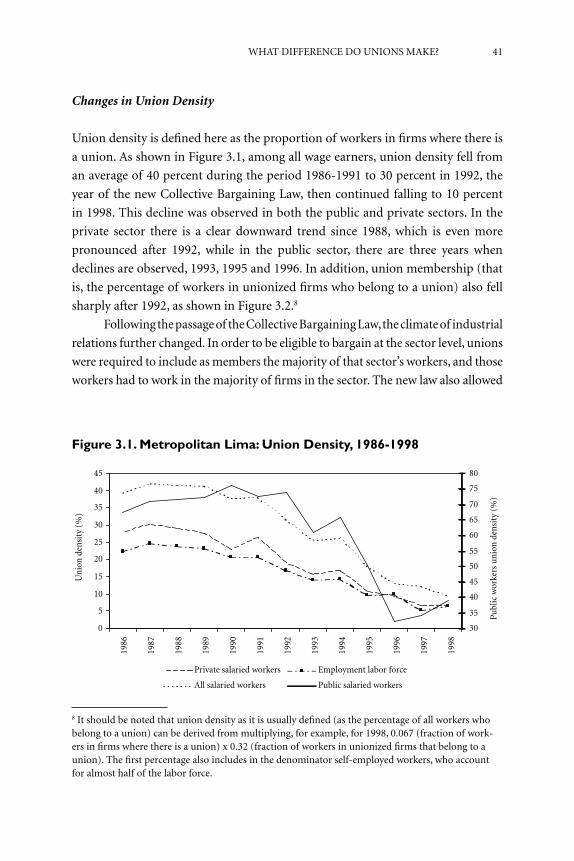
WHAT DIFFERENCE DO UNIONS MAKE? 41
Changes in Union Density
Union density is defined here as the proportion of workers in firms where there is
a union. As shown in Figure 3.1, among all wage earners, union density fell from
an average of 40 percent during the period 1986-1991 to 30 percent in 1992, the
year of the new Collective Bargaining Law, then continued falling to 10 percent
in 1998. This decline was observed in both the public and private sectors. In the
private sector there is a clear downward trend since 1988, which is even more
pronounced after 1992, while in the public sector, there are three years when
declines are observed, 1993, 1995 and 1996. In addition, union membership (that
is, the percentage of workers in unionized firms who belong to a union) also fell
sharply after 1992, as shown in Figure 3.2.8
Following the passage of the Collective Bargaining Law, the climate of industrial
relations further changed. In order to be eligible to bargain at the sector level, unions
were required to include as members the majority of that sector’s workers, and those
workers had to work in the majority of firms in the sector. The new law also allowed
8 It should be noted that union density as it is usually defined (as the percentage of all workers who belong to a union) can be derived from multiplying, for example, for 1998, 0.067 (fraction of work-ers in firms where there is a union) x 0.32 (fraction of workers in unionized firms that belong to a union). The first percentage also includes in the denominator self-employed workers, who account for almost half of the labor force.
�
�
��
��
��
��
��
��
��
��
��
��
��
��
��
��
��
��
��
��
��
������������������������ ����������������������
�������������������� �����������������������
��
���
����
����
���
�
����
����
����
����
���
���
����
����
��
����
����
����
����
����
����
����
����
����
����
����
����
����
Figure 3.1. Metropolitan Lima: Union Density, 1986-1998

42 UNION DENSITY CHANGES AND UNION EFFECTS ON FIRM PERFORMANCE
for the creation of more than one union within a firm and increased to 20 the
minimum number of workers required to form a union. In smaller firms, workers
could designate delegates, but the administrative procedures required for the
authorization in the ministry were cumbersome. Additional restrictions prohibited
workers on probation and in management from belonging to a union, and workers
could not belong to more than one union. Another important change that greatly
undermined unions’ ability to exert pressure was that strike days remained unpaid
and that strikes could be called only after direct bargaining had failed.
Using a probit estimation for a pool of 13 household surveys for Metropolitan
Lima, it is found that the likelihood of unionization among salaried workers
underwent no statistically significant change between 1986 and 1991, as shown in
Figure 3.3.9 In 1993, however, this likelihood is 14 points smaller, while in 1997 it
is 30 points smaller; these differences are statistically significant at the 95-percent
level.10 This suggests a breakpoint in union density immediately after the adoption
of the Collective Bargaining Law.
��
��
��
��
��
��
��
���� ���� ���� ���� ���� ���� ���� ���� ���� ����
Figure 3.2. Metropolitan Lima: Union Membership 1989-1998*
*Shows the percentage of workers in unionized firms who belong to a unionSource: Household Survey, Ministry of Labor-INEI.
9 The next section describes the data in detail.10 The figure reports marginal effects of year dummies, calculated as differences in the predicted probabilities, with all other variables evaluated at sample means. Variables included in the equations were controls for education, experience, industry, occupation, firm size and type of contract, and a dummy for public sector.

WHAT DIFFERENCE DO UNIONS MAKE? 43
In fact, several authors (such as Bernedo, 1994; and Gárate, 1993) have
reported a reduction in union density since the mid-1980s. As shown in Figure
3.4, the number of strikes fell from 780 in 1982 to 613 in 1990 and to only 36 in
1999, suggesting that unions’ ability to exert effective political pressure diminished
sharply during the 1990s. The reduction in union activity is also reflected in a
decline in the number of pliegos de reclamos (“lists of demands”) presented to
the labor authorities from 1,164 in 1990 to only 179 in 1999. Perhaps the most
telling examples of waning union influence occurred in 1990 and 1992. In 1990,
the Confederación General de Trabajadores de Perú (CGTP), probably the most
influential union during the 1980s, called upon its members to strike following the
most drastic economic stabilization program in recent Latin American history; this
call met with no success. The CGTP’s call for another strike in 1992, in response to
the passage of the Collective Bargaining Law, was also a failure.
In spite of the magnitude of the decline in union density, this change is not
related to a sector composition effect. As shown in Table 3.1, most of the changes
in unionization rates are within industries and other classifications (marital
status, gender, white/blue collar, educational status, firm size, public or private
status and type of contract). In the period before the Collective Bargaining Law,
�����
�����
�����
����
����
����
���� ���� ���� ���� ���� ���� ���� ���� ���� ���� ���� ���� ����
Figure 3.3. Metropolitan Lima: Unionization Probabilities
The vertical lines show confidence intervals at 95 percent significance.Note: Marginal effects take as base year 1993.Excludes 1996 because of problems with data for type of worker.

44 UNION DENSITY CHANGES AND UNION EFFECTS ON FIRM PERFORMANCE
�
���
���
���
���
���
���
���
���
���
�����
�
�������
�������
�������
�������
���������
���������
���������
���������
������� �������
����
����
����
����
����
����
����
����
����
����
����
����
����
����
����
����
����
����
����
����
����
����
����
����
����
����
����
����
����
Figure 3.4. Evolution of Strikes and Workers Involved, 1970-1998
Table 3.1. Decomposition of Changes in Unionization Rate (%)
1986-1992 1998-1993
Between
Effect
Within
EffectInteraction
Between
Effect
Within
EffectInteraction
Marital Status 1.15 99.08 -0.24 2.72 100.09 -2.80
Gender 0.00 100.02 -0.02 -1.34 101.08 0.26
Blue/White Collar 2.82 93.08 4.10 1.15 98.48 0.37
Public/Private
Sector27.69 61.25 11.06 14.33 89.61 -3.94
Education -2.44 107.56 -5.11 -0.23 101.05 -0.83
Firm Size 28.62 69.26 2.12 3.82 99.01 -2.82
Contract 35.92 57.60 6.48 35.66 72.98 -8.64
Full/Part Time 0.94 100.59 -1.53 3.33 95.78 0.89
Industry 28.90 74.09 -2.99 12.45 92.73 -5.19
Absolute Change in
Unionization Rate
(points)
-7.29 -13.26

WHAT DIFFERENCE DO UNIONS MAKE? 45
74 percent of the reduction was due to within-industry reductions, and only one
fourth was related to changes in the composition of employment by industry. In
all cases, within-category reductions in unionization rates are more important. In
particular, when employment is divided between the public and private sectors,
it is apparent that the reduction in public employment (a high union density
sector) represented almost one third of the total reduction in density. Moreover,
the increase in temporary employment and in employment among smaller firms,
both low-density categories, independently contributed almost a third to the
overall reduction. In the period 1993-1998, only the further increase in temporary
employment had a role in explaining the further reduction in union density. Aside
from that, all reductions in the post-Collective Bargaining Law years occurred
within categories.
Who Is (and Was) Unionized
Table 3.2 shows sample means for different categories of workers using the datasets
for Metropolitan Lima and Urban Peru. Unionized workers are more likely to be
more educated, older, and with significantly longer tenures than non-unionized
workers. They are also more likely to work in a large firm and to have a permanent
contract. When union members are compared with non-members (among those
who work in a unionized firm), the pattern is similar; members, however, are
more likely to be blue-collar workers. In addition, raw earnings are higher for
non-members after the labor reforms.
It is assumed that the difference in utility between working in a unionized
firm and in a non-union firm varies with individual characteristics, preferences,
firm characteristics and institutional arrangements that affect the costs and benefits
of each alternative. The probability that an individual works in a unionized job is
represented by
ui = X
1iπ
1 + X
2iπ
2 + ε
i
where u is the reduced form of the unobserved utility gain from working in a
unionized firm or belonging to a union for worker i, X1 is a vector of individual
characteristics and X2 is a vector of firm characteristics. In terms of individual
characteristics, it should be noted that there is a prior decision to participate as
a wage-earning worker in the labor market rather than being self-employed. In
order to take into account the bias in the coefficient that may arise from non-
random selection into a salaried job, first-stage probit regressions are estimated

46 UNION DENSITY CHANGES AND UNION EFFECTS ON FIRM PERFORMANCE
1986
-198
719
89-1
992
1993
-199
8
Tota
l
sala
ried
Firm
s
with
out
unio
n
Firm
s
with
unio
n
Tota
l
sala
ried
Firm
s
with
out
unio
n
Firm
s w
ith u
nion
Tota
l
sala
ried
Firm
s
with
out
unio
n
Firm
s w
ith u
nion
Tota
lN
on
mem
bers
Mem
bers
Tota
lN
on
mem
bers
Rea
l wag
e (s
oles
of
1994
)
836.
45
(908
.2)
698.
88
(811
.64)
1038
.33
(100
0.01)
404.
98
(618
.3)
374.
18
(660
.63)
456.
82
(535
.64)
499.
02
(641
.9)
499.
02
(419
.37)
592.
70
(838
.35)
557.
08
(821
.75)
737.
47
(888
.12)
777.2
9
(103
1.45)
Mar
ried
0.54
0.46
0.66
0.54
0.48
0.65
0.56
0.56
0.49
0.47
0.61
0.51
(0.4
9)(0
.49)
(0.4
7)(0
.49)
(0.4
9)(0
.47)
(0.4
9)(0
.44)
(0.4
9)(0
.49)
(0.4
8)(0
.49)
Mal
e0.
690.
680.
700.
690.
680.
710.
680.
680.
680.
690.
660.
65
(0.4
6)(0
.46)
(0.4
5)(0
.46)
(0.4
6)(0
.45)
(0.4
6)(0
.44)
(0.4
6)(0
.46)
(0.4
7)(0
.47)
Blu
e co
llar
wo
rker
0.31
0.33
0.28
0.32
0.37
0.25
0.21
0.21
0.34
0.36
0.26
0.24
(0.4
6)(0
.46)
(0.4
4)(0
.46)
(0.4
8)(0
.43)
(0.4
)(0
.45)
(0.4
7)(0
.48)
(0.4
3)(0
.42)
Pub
lic s
ecto
r0.
290.
150.
490.
270.
110.
530.
450.
450.
180.
110.
500.
46
(0.4
5)(0
.35)
(0.4
9)(0
.44)
(0.3
1)(0
.49)
(0.4
9)(0
.48)
(0.3
8)(0
.3)
(0.4
9)(0
.49)
Sec
ond
ary
educ
atio
n0.
540.
600.
460.
510.
560.
410.
410.
410.
510.
550.
360.
36
(0.4
9)(0
.48)
(0.4
9)(0
.49)
(0.4
9)(0
.49)
(0.4
9)(0
.49)
(0.4
9)(0
.49)
(0.4
7)(0
.47)
Hig
her
educ
atio
n0.
310.
250.
390.
380.
320.
480.
520.
520.
390.
360.
540.
57
(0.4
6)(0
.43)
(0.4
8)(0
.48)
(0.4
6)(0
.49)
(0.4
9)(0
.49)
(0.4
8)(0
.47)
(0.4
9)(0
.49)
Tabl
e 3.
2. M
etro
polit
an L
ima:
Mea
ns a
nd D
evia
tio
ns o
f Var
iabl
es b
y U
nio
n an
d U
nio
n M
embe
rshi
p 19
86-1
998
Con
tinue
d

WHAT DIFFERENCE DO UNIONS MAKE? 47
1986
-198
719
89-1
992
1993
-199
8
Tota
l
sala
ried
Firm
s
with
out
unio
n
Firm
s
with
unio
n
Tota
l
sala
ried
Firm
s
with
out
unio
n
Firm
s w
ith u
nion
Tota
l
sala
ried
Firm
s
with
out
unio
n
Firm
s w
ith u
nion
Tota
lN
on-
mem
bers
Mem
bers
Tota
lN
on-
mem
bers
Med
ium
firm
0.07
0.07
0.07
0.08
0.09
0.06
0.06
0.06
0.07
0.07
0.07
0.07
(0.2
5)(0
.26)
(0.2
5)(0
.26)
(0.2
8)(0
.23)
(0.2
4)(0
.22)
(0.2
5)(0
.26)
(0.2
4)(0
.24)
Lar
ge fi
rm0.
490.
260.
830.
480.
240.
870.
850.
850.
400.
280.
860.
84
(0.4
9)(0
.43)
(0.3
7)(0
.49)
(0.4
2)(0
.33)
(0.3
5)(0
.32)
(0.4
8)(0
.45)
(0.3
5)(0
.36)
Perm
anen
t co
ntra
ct0.
610.
450.
840.
580.
430.
830.
690.
690.
430.
350.
750.
63
(0.4
8)(0
.49)
(0.3
6)(0
.49)
(0.4
9)(0
.37)
(0.4
6)(0
.2)
(0.4
9)(0
.47)
(0.4
3)(0
.48)
Tem
pora
ry c
ont
ract
0.09
0.09
0.09
0.10
0.10
0.10
0.15
0.15
0.19
0.19
0.17
0.25
(0.2
8)(0
.28)
(0.2
8)(0
.29)
(0.3
)(0
.29)
(0.3
6)(0
.2)
(0.3
8)(0
.39)
(0.3
7)(0
.43)
Par
t ti
me
0.15
0.16
0.14
0.14
0.14
0.15
0.15
0.15
0.19
0.17
0.25
0.23
(0.3
5)(0
.36)
(0.3
4)(0
.35)
(0.3
5)(0
.35)
(0.3
5)(0
.35)
(0.3
8)(0
.37)
(0.4
3)(0
.42)
Tenu
re7.
014.
6210
.55
7.00
4.81
10.6
87.
047.
045.
214.
149.
596.
36
(8.2
3)(6
.46)
(9.2
3)(8
.17)
(6.4
6)(9
.34)
(8.0
4)(9
.23)
(7.1
7)(6
.21)
(8.9
5)(7
.59)
Pote
ntia
l exp
erie
nce
16.7
314
.59
19.8
916
.18
14.3
719
.21
15.4
715
.47
15.1
314
.16
19.1
016
.12
(13.
08)
(12.
63)
(13.
08)
(12.
68)
(12.
24)
(12.
83)
(11.
84)
(12.
77)
(12.
24)
(12.
01)
(12.
34)
(12.
14)
Tabl
e 3.
2. M
etro
polit
an L
ima:
Mea
ns a
nd D
evia
tio
ns o
f Var
iabl
es b
y U
nio
n an
d U
nio
n M
embe
rshi
p 19
86-1
998
(con
tinue
d)
48 UNION DENSITY CHANGES AND UNION EFFECTS ON FIRM PERFORMANCE
for the decision to work as a salaried worker. They are then used to correct for
self-selection in the unionization probits.
Probit estimations were carried out for three sub-periods, 1986-1987,
1989-1992 and 1993-1998, pooling yearly cross sections in each case. The first is
a short period of fast economic growth, the second is a period of sharp economic
recession, both before the change in labor legislation and the launching of other
structural reforms, and the third is a period of growth after structural reforms;
the results are shown in Table 3.3. Blue-collar workers and public sector workers
are more likely to work in a unionized firm, although the size of the effect falls
sharply after 1993. Those with higher education are more likely to belong to a
union, although the effect is significant only during the post-reform period. As
expected, moreover, workers with more experience and those with longer tenures
in a firm also have a higher likelihood of working in a unionized firm. Again, the
effect is much smaller after the reforms.
Working in a large or medium-sized firm also increases the likelihood of
unionization, but this effect also falls clearly after 1993. Having a permanent or
temporary job—both formal worker categories—increases the likelihood for
workers who do not have a contract (the likelihood being slightly higher for
temporary workers). In the wake of the 1992 labor legislation reform, however,
temporary workers have a clearly lower probability of working in a unionized
firm. During the 1990s the deregulation of the labor market facilitated the use of
these contracts, and it was thus easier for employers to deter temporary workers
from joining or forming a union. Even if these workers have the legal right to
organize, the employer retains the option of simply not renewing the contract of
a worker who joins a union. In light of these circumstances, the use of temporary
fixed-term contracts increased sharply in Peru during the 1990s.
The previous results were replicated using similar regressions estimated on
an annual basis. The two panels in Figure 3.5 show the estimated marginal effects of
different variables over time. The similarity of the results of these yearly estimations
indicates that the results are not an artifact of pooling the data in sub-periods.
For the sake of clarity, it should be reiterated that not all workers in
unionized firms are in fact union members. As mentioned above, membership
may give workers certain benefits, such as protection of their rights, better working
conditions and more benefits, as well as a reputation derived from complying with
the group norm. Membership is nonetheless voluntary, and collective bargaining
agreements apply to all workers independently of whether they are unionized.
Table 3.4 shows the result of a probit estimation analyzing the characteristics

WHAT DIFFERENCE DO UNIONS MAKE? 49
1986
-198
719
89-1
992
1993
-199
8
Co
effs
.M
arg.
effe
cts
Co
effs
.M
arg.
effe
cts
Co
effs
.M
arg.
effe
cts
Co
effs
.M
arg.
effe
cts
Co
effs
.M
arg.
effe
cts
Co
effs
.M
arg.
effe
cts
Mar
ried
0.12
2
(2.4
9)**
0. 0
480.
057
(0.9
2)0.
016
0.08
4
(2.1
9)**
0.03
4-
0.00
2
(0.0
4)0.
000
- 0.
082
(2.0
9)**
- 0.
009
- 0.
116
(2.4
8)**
- 0.
005
Mal
e-
0.18
4
(2.5
8)**
*-
0.07
3-
0.00
3
(0.0
5)-
0.00
1-
0.06
4
(0.8
5 )
- 0.
025
0.19
8
(3.0
3)**
*0.
034
0.14
7
(4.1
4)**
*0.
017
0.28
2
(6.3
9)**
*0.
010
Blu
e-co
llar
wo
rker
0.37
5
(6.0
7)**
*0.
146
0.61
2
(7.7
1)**
*0.
194
0.25
2
(5.2
4)**
*0.
100
0.46
9
(7.1
6)**
*0.
099
0.29
2
(6.7
7)**
*0.
039
0.33
4
(5.2
4)**
*0.
016
Pub
lic s
ecto
r0.
879
(9.4
0)**
*0.
320
0.57
1
(6.2
4)**
*0.
181
1.15
7
(10.
50)*
**0.
410
0.89
7
(11.
77)*
**0.
226
0.98
6
(13.
80)*
**0.
199
0.79
3
(8.4
7)**
*0.
062
Sec
ond
ary
educ
atio
n
0.00
7
(0.0
7)0.
003
- 0.
201
(1.8
2)*
- 0.
048
- 0.
083
(0.9
3)-
0.02
5-
0.28
1 (2
.97)
***
- 0.
047
0.22
4
(3.4
6)**
*0.
008
0.11
5
(1.4
0)0.
003
Hig
her
educ
atio
n
0.23
8
(1.3
4)0.
094
- 0.
009
(0.0
6)-
0.00
20.
078
(0.4
3)0.
025
- 0.
198
(1.4
9)-
0.03
50.
709
(10.
33)*
**0.
043
0.39
2
(4.2
3)**
*0.
013
Pote
ntia
l
expe
rien
ce
0.04
2
(7.2
7)**
*0.
013
0.00
3
(0.4
2)0.
001
0.03
4
(7.8
9)**
*0.
011
- 0.
002
(0.4
0)0.
000
0.02
7
(5.8
0)**
*0.
001
0.00
7
(1.3
0)0.
000
Pote
ntia
l
expe
rien
ce
squa
red
- 0.
042
(4.0
6)**
*-
0.01
6-
0.00
2
(0.1
1)0.
000
- 0.
028
(3.5
5)**
*-
0.01
1-
0.00
1
(0.1
2 )
0.00
0-
0.03
9
(4.6
5)**
*-
0.00
6-
0.01
7
(1.6
0)-
0.00
1
Tabl
e 3.
3. M
etro
polit
an L
ima:
Pro
babi
lity
of W
ork
ing
in a
Uni
oni
zed
Fir
m, P
robi
t C
oef
fici
ents
and
Mar
gina
l E
ffec
ts
Con
tinue
d

50 UNION DENSITY CHANGES AND UNION EFFECTS ON FIRM PERFORMANCE
1986
-198
719
89-1
992
1993
-199
8
Co
effs
.M
arg.
effe
cts
Co
effs
.M
arg.
effe
cts
Co
effs
.M
arg.
effe
cts
Co
effs
.M
arg.
effe
cts
Co
effs
.M
arg.
effe
cts
Co
effs
.M
arg.
effe
cts
Fir
m o
f 20
to 4
9
wo
rker
s
0.53
8
(5.3
7)**
*0.
170
0.67
7
(8.0
0)**
*0.
176
0.53
7
(5.9
4)**
*0.
032
Med
ium
siz
e
firm
1.01
1
(9.7
8)**
*0.
355
1.16
3
(13.
27)*
**0.
357
0.86
0
(9.7
7)**
*0.
071
Lar
ge fi
rm1.
721
(20.
18)*
**0.
609
1.98
4
(27.
69)*
**0.
661
1.37
0
(17.
82)*
**0.
179
Perm
anen
t
cont
ract
0.44
7
(5.4
2)**
*0.
108
0.55
0
(8.1
1)**
*0.
077
0.40
5
(5.8
9)**
*0.
013
Tem
pora
ry
cont
ract
0.57
1
(5.1
6)**
*0.
146
0.57
0
(6.6
2)**
*0.
081
0.24
9
(3.5
4)**
*0.
007
Par
t ti
me
0.20
4
(2.6
1)**
*0.
059
0.15
7
(2.4
0)**
0.02
90.
242
(4.8
6)**
*0.
011
Tenu
re0.
030
(7.0
6)**
*0.
007
0.02
7
(7.5
6)**
*0.
004
0.01
1
(3.7
0)**
*0.
000
Co
ntro
ls fo
r
occ
upat
ion
and
indu
stry
NO
NO
YES
YES
NO
NO
YES
YES
NO
NO
YES
YES
Tabl
e 3.
3. M
etro
polit
an L
ima:
Pro
babi
lity
of W
ork
ing
in a
Uni
oni
zed
Fir
m, P
robi
t C
oef
fici
ents
and
Mar
gina
l E
ffec
ts (c
ontin
ued)
Con
tinue
d

WHAT DIFFERENCE DO UNIONS MAKE? 51
1986
-198
719
89-1
992
1993
-199
8
Co
effs
.M
arg.
effe
cts
Co
effs
.M
arg.
effe
cts
Co
effs
.M
arg.
effe
cts
Co
effs
.M
arg.
effe
cts
Co
effs
.M
arg.
effe
cts
Co
effs
.M
arg.
effe
cts
Uni
oni
zati
on
and
empl
oym
ent
(sal
arie
d/
self-
empl
oyed
)
- 0.
698
- 0.
1911
- 0.
618
0.02
60.
868
0.83
31
stat
us e
rro
r
corr
elat
ion
(sta
ndar
d er
ror)
(0.1
59)*
*(0
.142
)(0
.195
)**
(0.1
6)(0
.118
)***
(0.0
42)*
**
Unc
enso
red
obs
erva
tio
ns38
1138
1167
2467
2480
8 9
8089
Wal
d C
hi2
522.
3 (9
)11
04
(30)
1084
.2
(11)
2213
(32
)87
0 (1
2)93
57 (
33)
Tabl
e 3.
3. M
etro
polit
an L
ima:
Pro
babi
lity
of W
ork
ing
in a
Uni
oni
zed
Fir
m, P
robi
t C
oef
fici
ents
and
Mar
gina
l E
ffec
ts (c
ontin
ued)

52 UNION DENSITY CHANGES AND UNION EFFECTS ON FIRM PERFORMANCE
that drive union affiliation, conditional on working in a unionized firm. Again,
blue-collar workers are more likely to be affiliated. Education, however, seems
to have a clear negative effect on the likelihood of union membership. Among
these workers, everyone has some type of contract because unionized firms are all
formal firms, but the likelihood of affiliation is higher for those with permanent
contracts.11 Workers with more experience and longer tenure are also more likely
to be affiliated with a union.
�
���
���
���
���
���
���
���
���
���
���� ���� ���� ���� ���� ���� ���� ���� ���� ���� ����
���������������� ���������� ������������������ ������������������
�
���
���
���
���
���
���
���
���� ���� ���� ���� ���� ���� ���� ���� ���� ���� ����
�������������������� ������������������ �������������
Figure 3.5. Metropolitan Lima: Probability of Working in a Unionized Firm (marginal effects)
11 Strictly speaking, however, there is informality even in firms where there is a union, as there is some degree of informal employment in medium-sized firms and marginally in large firms (Saavedra and Maruyama, 1999).

WHAT DIFFERENCE DO UNIONS MAKE? 53
1989
-199
219
93-1
998
Mar
ried
0.05
3 (2
.03)
*0.
040
(1.5
1)0.
041
(1.5
4)0.
094
(2.7
0)**
0.07
6 (2
.11)
*0.
073
(1.9
6)
Mal
e 0.
031
(1.2
3)0.
035
(1.3
9)0.
041
(1.5
3)0.
011
(0.3
1)0.
054
(1.4
9)0.
087
(2.2
9)*
Blu
e-co
llar
wo
rker
0.
227
(7.2
5)**
0.25
6 (7
.96)
**0.
214
(5.4
2)**
0.17
7 (3
.59)
** 0
.237
(4.
50)*
*0.
163
(2.4
1)*
Pub
lic s
ecto
r 0.
206
(7.
82)*
*0.
174
(6.0
1)**
0.05
4 (1
.45)
0.16
6 (4
.42)
**0.
108
(2.4
8)*
-0.0
49 (
0.83
)
Sec
ond
ary
educ
atio
n -0
.080
(1.
75)
-0.1
55 (
3.16
)**
-0.1
15 (
2.21
)*-0
.034
(0.
54)
-0.1
03 (
1.58
)-0
.048
(0.
69)
Hig
her
educ
atio
n -0
.114
(2.
34)*
-0
.234
(4.
47)*
*-0
.133
(2.
26)*
-0.0
21 (
0.30
)-0
.155
(2.
15)*
-0.0
88 (
1.08
)
Fir
m o
f 20
to 4
9 w
ork
ers
-0.1
29 (
1.25
)-0
.055
(0.
52)
0.14
5 (1
.05)
0.19
7 (1
.34)
Med
ium
firm
-0
.186
(1.
87)
-0.1
28 (
1.23
) 0
.099
(0.
74)
0.1
91 (
1.35
)
Lar
ge fi
rm -
0.15
9 (1
.93)
-0.
105
(1.1
9)0.
084
(0.7
2)0.
192
(1.5
9)
Perm
anen
t co
ntra
ct
0.24
3 (5
.05)
**0.
293
(5.4
4)**
0.15
8 (2
.71)
**0.
234
(3.3
8)**
Par
t ti
me
0.04
5 (1
.40)
0.
053
(1.5
9)0.
137
(3.3
8)**
0.
096
(2.2
1)*
Tenu
re
0.01
8 (9
.39)
**0.
019
(9.4
4)**
0.02
0 (8
.04)
**0.
021
(8.0
2)**
Pote
ntia
l exp
erie
nce
0.01
8 (1
.56)
0.00
5 (1
.56)
0.00
7 (2
.05)
*0.
033
(7.4
7)**
0.01
8 (3
.73)
**0.
016
(3.0
3)**
Pote
ntia
l exp
erie
nce
squa
red
-0.0
24 (
4.03
)**
-0.0
20 (
3.16
)**
-0.0
23 (
3.56
)**
-0.0
47 (
5.51
)**
-0.0
38 (
4.24
)**
-0.0
31 (
3.28
)**
Co
ntro
ls fo
r o
ccup
atio
n an
d in
dust
ry
NO
N
O
YES
N
O
NO
Y
ES
Obs
erva
tio
ns
2325
23
25
2325
14
59
1459
14
59
Wal
d C
hi2
187.
24 (
9)
322.
51 (
15)
335
(29)
92
(10
) 20
4.04
(16
) 24
5.98
(30
)
Rob
ust
z st
atis
tics
in p
aren
thes
es. *
Sig
nific
ant
at 1
0%; *
* si
gnifi
cant
at
5%; *
** s
igni
fican
t at
1%
Num
ber
of d
egre
es o
f fre
edom
of W
ald-
chi2
in p
aren
thes
is In
clud
es y
ear
effe
cts
with
in
each
poo
led
sam
ple
Tabl
e 3.
4. M
etro
polit
an L
ima:
Pro
babi
lity
of U
nio
n M
embe
rshi
p fo
r W
ork
ers
in U
nio
nize
d F
irm
s

54 UNION DENSITY CHANGES AND UNION EFFECTS ON FIRM PERFORMANCE
In sum, the reduction in union bargaining power and the increase in the
requirements imposed by the 1992 law in order to form a union reduced the
availability of jobs in unionized firms for most types of workers.
Impact of Unions on Firm Performance
Following Clark (1980), Machin and Wadhani (1991) and Black and Lynch (1997),
this chapter measures the effects of unions on economic performance. In general,
the presence of unions in a firm leads to a different structure of incentives for
management and hence to changes in both managerial behavior and company
performance. The analysis to be conducted here mainly seeks to determine
whether unionization will negatively affect a firm’s performance. Based on a group
of performance measures, the empirical approach comprises two stages. The first
stage consists of a simple statistical analysis to study performance changes in firms
with and without unions. The second stage involves a regression analysis that
controls for the differences between firms, the sectors to which they belong and
the competition structure that they face.
The statistical analysis, following Boubakri and Cosset (1998), consists
first of computing the performance variables for each company for the years for
which information is available. Firms are then divided into those with unions and
those without, and means are computed for each performance variable for the
unionized and the non-unionized firms. Once means are calculated, differences
between unionized and non-unionized firms are calculated:
ΔP = [Punionized – Pnonunionized] (1)
In the simplest possible model to capture the effect on performance with
no regressors, performance in firm i during period t depends only on the union
dummy,
Pi,t
= α + γUnioni,t
+ ui,t
E(ui,t
/ Unioni,t
) = 0 (2)
Coefficients in this specification are likely to be biased for two reasons. First,
the two types of firms may have different characteristics and therefore different
performances unrelated to their union status. Second, differences between
unionized and non-unionized firms may simply be capturing differences in
performance across time. In a more complete specification, regressors are added
to the model that will control for observable characteristics at the firm level,
and sectoral and macroeconomic variables are also included that will attempt to

WHAT DIFFERENCE DO UNIONS MAKE? 55
capture these shocks. Further included is a variable to measure the intensity of
unionization (percentage of workers) as a way of capturing the impact of within-
firm density on performance. In the regression analysis for each of the performance
indicators, different specifications are used based on:
Pi,t
= f(Xit,
, Unionit , S
jt , Y
t ,D
i ) (3)
where Pi,t
are the different performance measures for firm i in period t. Specifically
analyzed are the effects of a union on labor productivity and the rate of return on
sales. Xit are firm characteristics, such as firm size (approximated by the number
of employees), firm sector, number of blue collar and white collar workers, the
percentage of the firm’s output that is exported, age of the firm in years, capital
labor ratio, the wage bill and advertising as a proportion of sales. Unionit is the
union dummy, which could change over time, and Sjt consists of four digit-level
Standard Industrial Classification industry-level variables. Sjt includes the degree
of concentration of the industry, and the proportion of imports with respect to
total domestic consumption. Di are sector or firm fixed effects, depending on the
specifications, which makes it possible to control for unobserved time-invariant
characteristics, and Yt are year effects. An alternative specification uses
Pi,t
= f(Xit,
, Union Densityit , S
j t ,Y
t ,D
i) (4)
where Union Density is the percentage of firm workers who are union members,
a figure that may vary over time.12 Equations (3) and (4) are estimated using
Ordinary Least Squares (OLS) on the 1994-1996 panel of manufacturing firms
described in the data section. The empirical results are presented below.
Table 3.5 shows raw means for performance indicators and other firm-level
variables. It suggests that non-union firms are clearly more profitable, and the
gap between the two types of firms and its significance increases with firm size.
Medium and large union firms have a statistically significant advantage in labor
productivity (gross value of production per worker). These first differences await
econometric analysis, but they may reflect the observed differences in capital
intensity per employee and value of physical assets per unit of value added,
indicators that are clearly higher among union firms, irrespective of size. These
firms consistently consume more electricity per worker and also have a higher
use of installed capacity. Finally, raw differences in wages show that salaries are
12 It should be noted that for the period 1995-1997 industry-level bargaining was not possible, so membership was limited to unions established at the firm level.

56 UNION DENSITY CHANGES AND UNION EFFECTS ON FIRM PERFORMANCE
Firm Size L <= 99 < L
<= 49
49 < L
<= 99L >99
Value of physical assets
per unit of value added
Non-Union1.155
(- 3.456)
1.238
(2.476)
1.567
(2.385)
1.476
(1.590)
Union1.339
(1.465)
2.078
(2.878)
2.074
(2.233)
t - test 4.79 ** 11.6 0** 23.33 **
Capital labor index
Non-Union0.853
(1.628)
0.909
(2.016)
1.479
(2.245)
1.178
(1.450)
Union0.986
(1.455)
2.163
(2.906)
1.909
(3.543)
t - test 4.42 ** 15.94 ** 19.62 **
Electricity expenditure
per worker
Non-Union1121
(1635)
1263
(2408)
1309
(1760)
1184
(1191)
Union1514
(2366)
1877
(1919)
2564
(4334)
t - test 11.35 ** 18.09 ** 31.39 **
Usage of installed
capacity
Non-Union0.588
(0.223)
0.555
(0.255)
0.493
(0.289)
0 .509
(0.239)
Union0.586
(0.260)
0.561
(0.280)
0.561
(0.216)
t - test 11.05 ** 11.51 ** 14.69 **
Return over assets
Non-Union0.020
(1651)
0.097
(0.292)
0.082
(0.383)
0.123
(0.295)
Union0.071
(0.363)
- 0.071
(0.480)
0.002
(0.342)
t - test - 8.68 ** - 19.99 ** - 27.34 **
Gross value of
production by worker
(S/. of 1994)
Non-Union95608
(118458)
102659
(220543)
101878
(118731)
104516
(98833)
Union87541
(135968)
124351
(111421)
149301
(172247)
t - test -6.96 ** 10.68 ** 21.88 **
Table 3.5. Differences in Means between Firm Performance Indicators of Unionized and Non-Unionized Firms
Continued

WHAT DIFFERENCE DO UNIONS MAKE? 57
Firm Size L <= 99 < L
<= 49
49 < L
<= 99L >99
Average blue-collar
wages
Non-Union150.362
(170.77)
28 9.432
(268.63)
386.755
(319.22)
468.384
(376.384)
Union405.201
(293.60)
579.124
(419.45)
790.172
(882.36)
t - test 48.58 ** 30.88 ** 34.97 **
Average white-collar
wages
Non-Union449.746
(403.84)
858.131
(833.62)
1339.56
(1357.44)
1518.508
(1016.8 5)
Union1083.681
(868.05)
1606.186
(1149.44)
2656.139
(4796.15)
t - test 30.80 ** 12.23 ** 23.78 **
Table 3.5. Differences in Means between Firm Performance Indicators of Unionized and Non-Unionized Firms (continued)
Notes:- Significance level: * 5%, ** 1%- t-statistic for Ho: Difference of means
significantly higher in union firms, differences that appear to increase with firm
size. A more detailed analysis of two performance variables, labor productivity
and the rate of return on sales, is presented below.
Effects on Labor Productivity
As mentioned above, the first-difference analysis shows that labor productivity
is higher among larger union firms. Figure 3.6 further explores this issue, using
the within-firm unionization rate in order to capture the possible effect of
heterogeneity in union intensity.13 The size of the circles represents the proportion
of companies in each bracket of unionization rate. Panel A shows that labor
productivity is larger in firms with higher union densities, although the difference
13 Within-firm rates of unionization (or union intensity) go from 1 to 5 and correspond to union densities of ]0-20],]20,30],]30-40],]40-50] and 50 percent or more of employees unionized, respec-tively. Only firms with a union are included in this analysis.
(x1 – x2) (x1 – x2)–––––––– = –––––––––––––––––––––––––––––––––Sx1 – Sx2 (n1 – 1)s2
1 + (n2 – 1)s22 1 1
–––––––––––––––––– * ––– + ––– (n1 + n2 – 2) n1 n2√ √

58 UNION DENSITY CHANGES AND UNION EFFECTS ON FIRM PERFORMANCE
seems to be only between firms with a density smaller than 20 percent and the
rest. Dividing the sample by firm size, it is found that among firms with fewer
than 49 employees (Panel B), there is a negative effect on labor productivity as
the rate of unionization increases. Moreover, the negative effect is clearly greater
at the highest rate of unionization. In the case of medium-size firms the effect
is not clear. However, among large firms (Panel D) there is a clear positive effect
on labor productivity as the rate of unionization increases. In the last two cases,
there is a homogeneous distribution of companies among the different rates of
unionization. This is different from what happens in small firms, since most of
them have high unionization rates.
Table 3.6 estimates specification (3) using OLS to validate the impact of
unions on labor productivity, controlling for firm characteristics and the market
structure of the sector in which firms operate. As shown, the impact of the union
dummy is negative in basic specifications, but disappears as certain firm-specific
variables and sector variables are included. In addition, the interaction of the union
dummy with firm size, which could have confirmed the relationship between the
union productivity effect and size, also loses significance as more firm and sector
controls are included.
Table 3.7 shows the results of using specification (4), including the within-
firm unionization rate instead of a union dummy. As in the previous specification,
the interaction effect of unions and firm size disappears as firm and sector-specific
controls are included. However, the average effect across time retains its significance
in all of the six models presented. There is a negative relationship between union
intensity and labor productivity, which is robust to the introduction of firm-level
observables and also sector-level fixed effects, but it is absorbed once firm-level
fixed effects are included.14
There are two other interesting results. First, the four-firm concentration
index, as a proxy of the competitive environment, always has a positive and
significant sign. A possible explanation is that, in oligopolistic sectors, competition
drives the permanent introduction of better production techniques, which in turn
increase labor productivity; alternatively, this result could be reflecting the effect of
concentration on product prices, which increases dollar output measures. Second,
the capital labor index is positive and significant in all specifications, confirming
a positive relationship between capital intensity and labor productivity. Capital
14 On the other hand, it is clear that input ratios will have different effects on productivity in each sec-tor, so that the estimated union effect may also depend on parameter differences and the level of the input ratios at which the union/non-union comparison takes place.

WHAT DIFFERENCE DO UNIONS MAKE? 59
�����
������������
������
������
�����
�����
������
������
������
� � � � � �
���������������������
�����
����
����
���
����
���
����
��Figure 3.6. Impact of Unions on Value of Gross Production per Worker *
Panel A
Panel B Small Firms with Union
Continued
������
������
�����
�����
�����
�����
�����
�����
�����
�����
������
� � � � � �
���������������������
��
����
���
����
��
�����

60 UNION DENSITY CHANGES AND UNION EFFECTS ON FIRM PERFORMANCE
Panel D Big Firms with Union
Figure 3.6. Impact of Unions on Value of Gross Production per Worker * (continued)
Panel C Medium Firms with Union
�����
�����
������
������
������
� � � � � �
���������������������
��
����
���
����
��
������������������
������
������
�����
�����
������
������
������
� � � � � �
���������������������
��
����
���
����
��
������
�����
������
������
������

WHAT DIFFERENCE DO UNIONS MAKE? 61
mo
del 1
mo
del 2
m
ode
l 3
mo
del 4
m
ode
l 5
mo
del 6
m
ode
l 7
Uni
on
(Ye
s=1,
No
=0)
-27.
6027
(1.9
23)
-28.
4019
*
(2.0
70)
-38.
2798
**
(2.8
19)
-23.
4725
(1.9
20)
-14.
6469
(1.1
99)
-16.
5799
(1.3
72)
12.5
524
(0.5
9)
Uni
on*
Siz
e2
43.4
929
*
(2.4
64)
42.8
481
*
(2.4
50)
38.8
574
*
(2.2
09)
1.10
99 (
0.06
2)-3
.590
0 (0
.206
)-1
.463
2 (0
.085
)-3
0.08
72
(-1.
39)
Uni
on
* S
ize3
70
.555
2 **
(3.8
31)
65.4
049
**
(3.6
82)
58.6
774
**
(3.2
77)
7.84
46 (
0.42
2)0.
1644
(0.
009)
-1.5
464
(0.0
85)
-30.
8378
(-1.
17)
Year
199
5 14
.159
0
(1.1
33)
20.0
657
(1.6
12)
19.4
899
(1.5
71)
24.5
273
*
(2.0
89)
18.4
540
(1.5
71)
18.5
541
(1.5
80)
14.2
064
**
(2.7
7)
Year
199
6 6.
4075
(0.
530)
14.0
054
(1.1
63)
12.7
019
(1.0
51)
14.3
964
(1.2
77)
9.34
53 (
0.83
2)9.
3175
(0.
830)
Indu
stry
co
ncen
trat
ion
inde
x
1.16
23 *
*
(5.5
27)
1.12
43 *
*
(5.4
37)
0.97
66 *
*
(4.9
30)
1.07
18 *
*
(5.5
31)
.227
3 **
(5.8
25)
0.38
35 (
1.59
)
Age
of t
he fi
rm (
year
s)
0.99
39 *
*
(3.0
82)
0.56
58 (
1.67
7)0.
3344
(1.
000)
0.42
90 (
1.23
1)1.
0133
(0.
31)
Cap
ital
labo
r ra
tio
20
.692
3 **
(6.1
83)
20.5
274
**
(6.1
47)
20.1
666
**
(6.0
30)
9.87
92 *
*
(3.6
1)
Whi
te c
olla
r w
age
bill
(10-3
)
13.1
650
(1.8
46)
12.0
389
(1.8
03)
11.7
461
(1.7
64)
-4.2
742
**
(-2.
90)
Exp
ort
s / o
utpu
t 15
6.03
32 *
*
(3.2
74)
162.
9561
**
(3.4
14)
159.
1394
**
(3.3
14)
-36.
1010
(-0.
81)
Tabl
e 3.
6. U
nio
niza
tio
n an
d F
irm
Per
form
ance
, Dep
ende
nt V
aria
ble:
Pro
duct
ion
by T
ota
l Em
ploy
men
t(t-
stat
istics
in p
aren
thes
es)
Con
tinue
d

62 UNION DENSITY CHANGES AND UNION EFFECTS ON FIRM PERFORMANCE
Tabl
e 3.
6. U
nio
niza
tio
n an
d F
irm
Per
form
ance
, Dep
ende
nt V
aria
ble:
Pro
duct
ion
by T
ota
l Em
ploy
men
t(t-
stat
istics
in p
aren
thes
es) (
cont
inue
d) mo
del 1
mo
del 2
m
ode
l 3
mo
del 4
m
ode
l 5
mo
del 6
m
ode
l 7
Impo
rts
in t
he fi
rm’s
4-
digi
t S
IC in
dust
ry (
%)
1369
.965
9 **
(2.7
19)
1537
.351
6 **
(2.8
49)
1574
.373
0 **
(2.9
2)
Adv
erti
sing
as
perc
enta
ge o
f to
tal s
ales
472.
9611
**
(3.3
16)
451.
4623
**
(3.1
17)
-330
.103
3 *
(-2.
12)
Sec
tor
fixe
d ef
fect
s Y
ES
Fir
m fi
xed
effe
cts
YES
Co
nsta
nt
104.
0862
**
(10.
631)
48.5
995
**(3
.610
)
28.9
413
(1.9
05)
-5.5
618
(0.3
91)
-18.
2522
(1.3
53)
67.2
138
(1.7
19)
55.6
982
(0.6
2)
Obs
erva
tio
ns
1030
10
30
1030
10
06
1004
10
04
1004
F
3.20
0 9.
100
8.96
0 27
.370
25
.150
18
.490
4.
370
Pro
b >
F0.
007
0.00
0 0.
000
0.00
0 0.
000
0.00
0 0.
000
Rho
0.
8036
F t
est
that
all
u i =
0 7.
90
Pro
b >
F
R-s
quar
ed
0.01
54
0.05
06
0.05
8 0.
216
0.23
4 0.
242
0.04
6
Not
es:
- Whi
te t
est
was
app
lied
to c
heck
for
hete
rosk
edas
ticity
. -
In m
odel
s 4,
5, a
nd 6
New
ey-W
est
stan
dard
err
ors
are
repo
rted
.-
Size
1 L
< 9
(co
ntro
l cat
egor
y);
Size
2 9
< L
< 4
9; S
ize
3 L
> 4
9

WHAT DIFFERENCE DO UNIONS MAKE? 63
mo
del 1
mo
del 2
mo
del 3
mo
del 4
mo
del 5
mo
del 6
mo
del 7
Wit
hin-
firm
uni
on
dens
ity
-53
.627
9**
-56
.385
1**
-66
.423
0**
-41
.622
6**
-29
.029
1* -
30.0
998*
50.
8911
(3.3
72)
(3.
613)
(4.
112)
(3.
321)
(2.
345)
(2.
398)
(1.
45)
Perc
enta
ge u
nio
nize
d* S
ize
2 8
3.50
06**
88.
7422
** 7
2.88
00*
1.2
599
2.2
565
2.7
024
-3.
8937
(2.6
11)
(2.
693)
(2.
156)
(0.
037)
(0.
070)
(0.
085)
(-0
.08)
Perc
enta
ge u
nio
nize
d* S
ize
3 1
76.8
531*
* 1
61.0
282*
* 1
39.6
397*
* 3
6.74
03 3
1.39
61 2
6.19
15 6
1.85
92
(4.3
07)
(3.
982)
(3.
348)
(1.
011)
(0.
880)
(0.
740)
(1.
30)
Year
199
5 1
4.06
95 1
9.78
56 1
9.22
08 2
4.44
63*
18.
4412
18.
5117
13.
1916
**
(1.1
34)
(1.
599)
(1.
557)
(2.
082)
(1.
568)
(1.
573)
(2.
58)
Year
199
6 8
.377
5 1
5.51
43 1
3.93
27 1
4.51
97 9
.605
4 9
.508
1
(0.7
02)
(1.
305)
(1.
167)
(1.
297)
(0.
861)
(0.
853)
Indu
stry
co
ncen
trat
ion
inde
x 1
.141
2**
1.1
095*
* 0
.970
1**
1.0
656*
* 1
.220
3**
0.3
857
(5.4
47)
(5.
382)
(4.
898)
(5.
509)
(5.
803)
(1.
60)
Age
of fi
rm (
year
s) 0
.881
4**
0.4
299
0.1
856
0.2
705
-33
.145
3
(2.6
96)
(1.
282)
(0.
559)
(0.
781)
(-0
.75)
Cap
ital
labo
r ra
tio
20.
5505
** 2
0.28
31**
19.
9601
** 9
.354
5**
(6.1
66)
(6.
111)
(6.
003)
(3.
40)
Whi
te-c
olla
r w
age
bill
(10
-3)
12.
8300
11.
6477
11.
3264
-4.
0798
**
(1.8
41)
(1.
795)
(1.
753)
(-2
.78)
Tabl
e 3.
7. U
nio
niza
tio
n an
d F
irm
Per
form
ance
, Dep
ende
nt V
aria
ble:
Pro
duct
ion
by T
ota
l Em
ploy
men
t(t-
stat
istics
in p
aren
thes
es)
Con
tinue
d

64 UNION DENSITY CHANGES AND UNION EFFECTS ON FIRM PERFORMANCE
Tabl
e 3.
7. U
nio
niza
tio
n an
d F
irm
Per
form
ance
, Dep
ende
nt V
aria
ble:
Pro
duct
ion
by T
ota
l Em
ploy
men
t (c
ontin
ued)
(t-st
atist
ics in
par
enth
eses
)
mo
del 1
mo
del 2
mo
del 3
mo
del 4
mo
del 5
mo
del 6
mo
del 7
Exp
ort
s / o
utpu
t 5
2.09
77**
58.
9002
** 5
4.65
62**
-33
.145
3
(3.2
58)
(3.
399)
(3.
287)
(-0
.75)
Impo
rts
in t
he fi
rm’s
4-d
igit
SIC
indu
stry
(%
)13
85.3
154*
*15
55.1
054*
*15
16.4
570*
*
(2.7
46)
(2.
884)
(2.
82)
Adv
erti
sing
as
perc
enta
ge o
f to
tal s
ales
463
.438
2**
439
.545
3**
-32
5.89
20**
(3.2
00)
(2.
970)
(-2
.10)
Sec
tor
fixe
d ef
fect
s
YES
Fir
m fi
xed
effe
cts
Y
ES
Co
nsta
nt 1
03.2
841*
* 4
9.00
48**
30.
8234
* -
3.40
72 -
15.9
255
61.
4497
-0.
4083
(10.
921)
(3.
751)
(2.
031)
(0.
242)
(1.
199)
(1.
445)
(0.
00)
Obs
erva
tio
ns 1
030
103
0 1
030
100
6 1
004
100
4 1
004
F 4
.570
10.
050
9.5
60 2
7.32
0 2
5.09
0 1
8.40
0 4
.860
Pro
b >
F 0
.000
0.0
00 0
.000
0.0
00 0
.000
0.0
00 0
.000
Rho
0.8
121
F t
est
that
all
u i =
0 7
.99
Pro
b >
F 0
.000
R-s
quar
ed 0
.022
0.0
56 0
.062
0.2
15 0
.233
0.2
41 0
.047
Not
es:
Whi
te t
est
was
app
lied
to c
heck
for
hete
rosk
edas
ticity
. In
mod
els
4, 5
, and
6 N
ewey
-Wes
t st
anda
rd e
rror
s ar
e re
port
ed.
Size
1 L
< 9
(co
ntro
l cat
egor
y);
Size
2 9
< L
< 4
9; S
ize
3 L
> 4
9

WHAT DIFFERENCE DO UNIONS MAKE? 65
�����
����������
�����
�����
����
����
����
����
����
����
����
� � � � � �
��������������������
���
����
����
����
����
Figure 3.7. Impact of Unions on Capital-Labor Ratio*
Panel A All Firms
Panel B Small Firms with Union
Continued
� � � � � �
��������������������
���
����
����
����
����
�
���
�
���
�
�����
�����
�����
�����
�����

66 UNION DENSITY CHANGES AND UNION EFFECTS ON FIRM PERFORMANCE
Figure 3.7. Impact of Unions on Capital-Labor Ratio* (continued)
Panel C Medium Firms with Union
Panel D Large Firms with Union
* The within-firm rates of unionization (or union intensity) go from 1 to 5 and are respectively ]0-20], ]20,30], ]30-40], ]40-50] and 50 percent or more of employees unionized. Only firms with a union are included in this analysis.
� � � � � �
��������������������
���
����
����
����
����
�
�
�
�
�
����
����
����
�
����
����
����
� � � � � �
��������������������
���
����
����
����
����
�
���
�
���
�
���
�
���
�
���
�
��������
����
����

WHAT DIFFERENCE DO UNIONS MAKE? 67
intensity might also be endogenous, as firms with higher union densities may
choose more capital-intensive techniques. In fact, as shown in Table 3.5, two
indicators of capital intensity (capital labor ratio and electricity expenditure per
worker) show a significantly higher value in unionized firms with respect to non-
unionized firms. Moreover, Figure 3.7 shows a clear positive relation between
union intensity and capital intensity, irrespective of the size of the firm. Within
firm sizes, however, the effect tends to be non-linear.
Effects on Profits (Rate of Return over Sales)
One of the most important findings of research in the United States has been that
unionization is associated with markedly lower profitability (see Belman, 1992,
for a summary of 11 American studies). A similar pattern has been found for the
United Kingdom. The main explanation for this result is that the effect of unions
on wages exceeds the possible positive effect of unions on productivity. Morishima
(1991), however, finds contrary results for Japanese firms.
As previously mentioned, a simple first-difference analysis (see Table 3.5)
suggests a negative impact of unions on profits. Figure 3.8 analyzes differences
in average profit within unionized firms. Within all firm sizes, group profits
are lower the higher the union density in the firm. Tables 3.8 and 3.9 present
alternative specifications of equations (3) and (4), first using a dummy variable
for the presence of unions and then using the within-firm union density variable.
In both cases, there is a negative and significant effect of unions on profits across
all specifications, an effect that is robust to the introduction of both sector and
firm fixed effects.
In general, the evidence points to a sizeable negative effect of unionization
on profits. When using a union dummy, Table 3.8 suggests that the return on sales
is, on average, 19 percent lower in unionized firms, an effect that is reduced by
approximately four percentage points when firm and sector control variables are
included. In the estimation where firm-level fixed effects are included, the negative
effect on profits is 17.5 percent. Moreover, the results suggest that during the
three years of the sample the impact of unions on profits diminishes, although
it is still significant. This can be explained as a consequence of the changes in the
unionization legislation, which reduced union power and therefore its impact on
profits. In the specification where firm-fixed effects are introduced, however, the
year dummies lose their significance.

68 UNION DENSITY CHANGES AND UNION EFFECTS ON FIRM PERFORMANCE
Figure 3.8. Impact of Unions on Return on Sales
Panel A All Firms
Panel B Small Firms with Union
Continued
�����
�����
������
�����
������
������
������
������
�����
�����
�����
�����
�����
�����
�����
�����
� � � � � � �
��������������������
��
�
� � � � � �
��������������������
��
�
�����
����
����
����
����
�����
����
�����
�����
����������

WHAT DIFFERENCE DO UNIONS MAKE? 69
Figure 3.8. Impact of Unions on Return on Sales (continued)
Panel C Medium Firms with Union
Panel D Large Firms with Union
* The within-firm rates of unionization (or union intensity) go from 1 to 5 and are respectively ]0-20], ]20,30], ]30-40], ]40-50] and 50 percent or more of employees unionized. Only firms with a union are included in this analysis.
�����
�����
�����
�����
�����
����
����
����
����
����
� � � � � � �
��������������������
��
�
������
������������
������
�����
�����
�����
�����
����
����
����
����
����
� � � � � �
��������������������
��
�
������
����������
�����
�����

70 UNION DENSITY CHANGES AND UNION EFFECTS ON FIRM PERFORMANCE
Tabl
e 3.
8 U
nio
niza
tio
n an
d F
irm
Per
form
ance
, Dep
ende
nt V
aria
ble:
Ret
urn
on
Sal
es (
RO
S)
(t-st
atist
ics in
par
enth
eses
)
mo
del 1
mo
del 2
mo
del 3
mo
del 4
mo
del 5
mo
del 6
mo
del 7
mo
del 8
Uni
on
(Yes
=1, N
o=0
)-0
.190
4**
-0.1
896*
*-0
.186
5**
-0.1
737*
*-0
.163
3**
-0.1
642*
*-0
.155
1**
-0.1
747*
(4.8
84)
(4.8
84)
(4.6
66)
(4.3
32)
(4.1
48)
(4.1
87)
(3.9
75)
(2.5
08)
Uni
on
* S
ize
20.
1294
*0.
1259
*0.
1266
*0.
1274
*0.
1216
*0.
1272
*0.
1276
*0.
0246
(2.4
26)
(2.3
70)
(2.3
80)
(2.4
03)
(2.3
48)
(2.4
67)
(2.4
94)
(0.6
87)
Uni
on
* S
ize
30.
1056
*0.
0969
0.09
750.
1014
0.10
72*
0.10
97*
0.10
37*
0.07
17
(1.9
64)
(1.8
07)
(1.8
16)
(1.8
94)
(2.0
46)
(2.1
02)
(2.0
02)
(1.6
28)
Year
199
5-0
.144
9**
-0.1
364*
*-0
.136
4**
-0.1
362*
*-0
.141
2**
-0.1
452*
*-0
.146
7**
(4.6
69)
(4.4
23)
(4.4
23)
(4.4
28)
(4.6
67)
(4.7
78)
(4.8
66)
Year
199
6-0
.150
7**
-0.1
393*
*-0
.139
1**
-0.1
378*
*-0
.136
1**
-0.1
404*
*-0
.139
5**
(4.9
65)
(4.5
75)
(4.5
65)
(4.5
37)
(4.5
45)
(4.6
69)
(4.6
78)
Indu
stry
co
ncen
trat
ion
inde
x (C
I 4)
0.00
13**
0.00
13**
0.00
12**
0.00
13**
0.00
13**
0.00
13**
0.00
08
(3.1
68)
(3.1
83)
(2.9
67)
(3.3
75)
(3.3
05)
(3.2
76)
(1.1
13)
Age
of fi
rm (
year
s)-0
.002
0.00
00.
0006
0.00
040.
0005
-0.0
573*
*
(0.3
33)
(0.0
22)
(0.8
49)
(0.5
43)
(0.7
26)
(4.3
09)
Tota
l em
ploy
men
t (1
02 )-0
.162
**-0
.018
6**
-0.0
196*
*-0
.019
7**
-0.0
031
(2.8
07)
(3.1
34)
(3.3
19)
(3.3
48)
(0.2
28)
Cap
ital
labo
r ra
tio
-0.0
409*
*-0
.039
9**
-0.0
394*
*-0
.045
0**
(9.1
99)
(9.0
03)
(8.9
44)
(4.6
81)
Con
tinue
d

WHAT DIFFERENCE DO UNIONS MAKE? 71
mo
del 1
mo
del 2
mo
del 3
mo
del 4
mo
del 5
mo
del 6
mo
del 7
mo
del 8
Whi
te c
olla
r w
age
bill
(10-3
)0.
0140
**0.
0133
**0.
1320
**-0
.001
8
(3.1
76)
(2.9
83)
(2.9
91)
(0.3
48)
Exp
ort
s/o
utpu
t0.
0727
0.08
820.
0897
0.18
28
(1.2
93)
(1.5
72)
(1.6
09)
(1.3
56)
Impo
rts
in t
he fi
rm’s
4-d
igit
SIC
indu
stry
(%)
-0.2
53-0
.041
9-1
.477
5
(0.2
85)
(0.0
46)
(0.8
20)
Adv
erti
sing
as
a pe
rcen
tage
of t
ota
l sal
es1.
1545
**0.
8917
**-0
.508
8
(3.5
55)
(2.6
97)
(1.0
04)
Sec
tor
fixe
d ef
fect
sY
ES
Fir
m fi
xed
effe
cts
YES
Co
nsta
nt0.
2091
**0.
1469
**0.
1518
**0.
1597
**0.
1635
**0.
1621
**-0
.413
6*1.
6975
**
(9.1
93)
(4.8
99)
(4.5
47)
(4.7
82)
4.87
6)(4
.791
)(2
.213
)(4
.672
)
Obs
erva
tio
ns11
0811
0811
0811
0811
0811
0811
0811
08
F11
.01
10.9
29.
379.
2405
.41
14.2
311
.18
5.38
Pro
b> F
0.00
00.
000
0.00
00.
000
0.00
00.
000
0.00
00.
000
Rho
0.93
6
F t
est
that
all
u=0
2.78
0
Pro
b> F
0.00
0
R-s
quar
ed0.
050
0.05
60.
.056
0.06
30.
137
0.14
80.
167
0.08
3
Tabl
e 3.
8 U
nio
niza
tio
n an
d F
irm
Per
form
ance
, Dep
ende
nt V
aria
ble:
Ret
urn
on
Sal
es (c
ontin
ued)
(t-st
atist
ics in
par
enth
eses
)
Not
es: W
hite
tes
t w
as a
pplie
d to
che
ck fo
r he
tero
sked
astic
ity. S
ize
1 L
< 9
(co
ntro
l cat
egor
y). S
ize
2 9
≤ L
≤ 49
. Siz
e 3
L ≥
49.

72 UNION DENSITY CHANGES AND UNION EFFECTS ON FIRM PERFORMANCE
Tabl
e 3.
9 U
nio
niza
tio
n an
d F
irm
Per
form
ance
, Dep
ende
nt V
aria
ble:
Ret
urn
on
Sal
es (
RO
S)
(t-st
atist
ics in
par
enth
eses
)
mo
del 1
mo
del 2
mo
del 3
mo
del 4
mo
del 5
mo
del 6
mo
del 7
mo
del 8
Wit
hin
firm
uni
on
dens
ity
-0.3
562*
*-0
.356
1**
-0.3
480*
*-0
.333
6**
-0.2
850*
*-0
.281
8**
-0.2
905*
*-0
.272
9*
(4.8
18)
(4.8
37)
(4.6
19)
(4.4
38)
(3.8
75)
(3.8
45)
(3.9
93)
(2.3
36)
Perc
enta
ge U
nio
nize
d *
Siz
e 2
0.23
58*
0.22
50*
0.22
67*
0.22
66*
0.19
91*
0.21
18*
0.21
62*
0.03
13
(2.2
76)
(2.1
79)
(2.1
94)
(2.2
02)
(1.9
84)
(2.1
19)
(2.1
85)
(0.4
35)
Perc
enta
ge U
nio
nize
d *
Siz
e 3
0.13
420.
1233
0.12
460.
1239
0.12
410.
1329
0.13
530.
0388
(1.2
48)
(1.1
51)
(1.1
63)
(1.1
62)
(1.1
92)
(1.2
80)
(1.3
16)
(0.4
41)
Year
199
5-0
.137
7**
-0.1
287*
*-0
.128
7**
-0.1
281*
*-0
.130
4**
-0.1
343*
*-0
.136
5**
(4.6
70)
(4.3
61)
(4.3
60)
(4.3
58)
(4.5
07)
(4.6
15)
(4.7
37)
Year
199
6-0
.139
2**
-0.1
290*
*-0
.128
5**
-0.1
259*
*-0
.121
3**
-0.1
256*
*-0
.127
7**
(4.7
98)
(4.4
38)
(4.4
17)
(4.3
46)
(4.2
43)
(4.3
69)
(4.8
48)
Indu
stry
co
ncen
trat
ion
inde
x (C
I 4)
0.00
13**
0.00
13**
0.00
12**
0.00
13**
0.00
13**
0.00
14**
0.00
08
(3.2
05)
(3.2
34)
(3.0
00)
(3.4
12)
(3.3
33)
(3.3
38)
(1.1
08)
Age
of fi
rm (
year
s)-0
.000
40.
0001
0.00
060.
0003
0.00
06-0
.048
5*
(0.5
11)
(0.0
93)
(0.8
02)
(0.4
58)
(0.8
38)
(3.8
05)
Tota
l em
ploy
men
t (1
02 )-0
.182
**-0
.020
1**
-0.0
211*
*-0
.020
9**
-0.0
097
(3.2
19)
(3.4
23)
(3.6
08)
(3.5
96)
(0.7
02)
Cap
ital
labo
r ra
tio
-0.0
401*
*-0
.039
3**
-0.0
386*
*-0
.041
9**
(9.0
10)
(8.8
31)
(8.7
49)
(4.3
39)
Con
tinue
d

WHAT DIFFERENCE DO UNIONS MAKE? 73
mo
del 1
mo
del 2
mo
del 3
mo
del 4
mo
del 5
mo
del 6
mo
del 7
mo
del 8
Whi
te c
olla
r w
age
bill
(10-3
)0.
0133
**0.
0126
**0.
0126
**-0
.002
3
(3.0
16)
(2.8
30)
(2.8
67)
(0.4
43)
Exp
ort
s/o
utpu
t0.
0622
0.07
780.
0784
0.16
92
(1.1
05)
(1.3
83)
(1.4
07)
(1.2
54)
Impo
rts
in t
he fi
rm’s
4-d
igit
SIC
indu
stry
(%)
-0.2
654
-0.0
524
-1.7
903
(0.2
99)
(0.0
58)
(0.9
94)
Adv
erti
sing
as
a pe
rcen
tage
of t
ota
l sal
es1.
1092
**0.
8277
**-0
.496
6
(3.4
05)
(2.4
99)
(0.9
79)
Sec
tor
fixe
d ef
fect
sY
ES
Fir
m fi
xed
effe
cts
YES
Co
nsta
nt0.
1992
**0.
1366
**0.
1441
**0.
1519
**0.
1544
**0.
1536
**-0
.478
3*1.
4545
**
(9.1
84)
(4.6
90)
(4.4
12)
(4.6
58)
4.70
8)(4
.633
)(2
.574
)(4
.188
)
Obs
erva
tio
ns10
8010
8010
8010
8010
8010
8010
8010
80
F11
.450
11.3
309.
740
9.89
015
.440
14.1
4011
.340
5.21
0
Pro
b> F
0.00
00.
000
0.00
00.
000
0.00
00.
000
0.00
00.
000
Rho
0.91
6
F t
est
that
all
u=0
2.76
0
Pro
b> F
0.00
0
R-s
quar
ed0.
0494
0.05
820.
0584
0.06
720.
1370
0.14
710.
1689
0.08
10
Tabl
e 3.
9 U
nio
niza
tio
n an
d F
irm
Per
form
ance
, Dep
ende
nt V
aria
ble:
Ret
urn
on
Sal
es (c
ontin
ued)
(t-s
tatis
tics
in p
aren
thes
es)
Not
es: W
hite
tes
t w
as a
pplie
d to
che
ck fo
r he
tero
sked
astic
ity. S
ize
1 L
< 9
(co
ntro
l cat
egor
y). S
ize
2 9
≤ L
≤ 49
. Siz
e 3
L ≥
49.

74 UNION DENSITY CHANGES AND UNION EFFECTS ON FIRM PERFORMANCE
The impact of unions on profits is also negative and significant when within-
firm union intensity is used instead of a dummy variable (see Table 3.9). The
magnitude of the effect falls as controls are introduced, but the effect is still large.
In this case only the 1995 interaction is significant, and again, time effects cannot
be identified in the firm-level fixed effects specification. As with the finding for
labor productivity, the impact of industry concentration is positive and significant
in explaining the rate of return over sales. Capital intensity, however, has a negative
effect. It is therefore clear from the evidence presented here that unionized firms
earn substantially lower returns than their non-union counterparts. The results
also show a negative, albeit less robust, impact on labor productivity, and there is
also evidence that unionized firms are more capital-intensive.
Summary and Final Comments
There is evidence of a clear reduction in union density immediately after the
passage of the Collective Bargaining Law in 1992. Holding constant worker and
firm observable characteristics, unionization diminished sharply after 1993. Being
a blue-collar worker, male, in a permanent contract and long tenured, increased
unionization likelihood until 1992; thereafter, the effects of these characteristics
were in many cases significant but much smaller. The only factor that remained
important as a determinant of union status was working in a large firm. When the
reduction in union density is decomposed, it is found that most of the reduction
is observed within categories, and the reduction in union density is not related to
a sector composition effect. However, before the change in collective bargaining
legislation, reductions in public employment, a high union density sector,
contributed almost one third to the total reduction in density. The increase in
temporary employment and in employment in small firms, both low union density
sectors, also contributed to the overall reduction. But in the period 1993-1998,
after the labor market reforms, only the further increase in temporary employment
played a small role in explaining the further reduction in union density, and most
of the changes were observed within categories and economic sectors.
With respect to the impact of unions on firm performance, a simple first-
difference analysis finds that unions have a negative impact on profits for all firm
sizes. Within unionized firms, profits are lower the higher the union density in the
firm. The econometric analysis finds a robust negative effect of 17.5 percent, even
after controlling for firm and sector characteristics and firm fixed effects. There is

WHAT DIFFERENCE DO UNIONS MAKE? 75
some evidence that this effect diminishes over time, which is consistent with the
fact that unionization sharply declined and unions saw their power diminished,
partially as a consequence of the Collective Bargaining Law of 1992. The decline
in the negative union effect, however, could not be confirmed in all specifications.
The impact of unions on profits is also negative and significant when within-firm
union intensity is used instead of a union dummy. The magnitude of the effect
falls as controls are introduced, but the effect is still large. Overall, there is clear
evidence that unionized firms earn substantially lower returns than their non-
union counterparts.
As far as other measures of performance are concerned, labor productivity
is negatively related to the presence of a union in the firm, although the negative
effect disappears once firm characteristics, particularly capital intensity, are
controlled for. Capital intensity is clearly higher among unionized firms and is
also higher among firms with higher within-firm union density. A negative effect
on productivity may be related to the history of contentious labor management
relations, as management and unions were in many cases suspicious of each other’s
goals and strategies. The high degree of unions’ politicization, and the infiltration
of terrorist groups into many large unions in the manufacturing sector during the
1980s, led to circumstances in which there was very little trust and no incentive to
work cooperatively so as to improve working conditions or enhance production
techniques.
Summarizing, the evidence derived from the analysis is consistent with a
bargaining model of union-firm interaction in which the union clearly affects
profits negatively and has a negative, albeit not statistically significant, effect on
labor productivity. The negative effect on profits, with a small or nil effect on
productivity, explains the strong opposition of firms in Peru to the revival of a
union movement. Clearly, the possibility of unions’ having a positive effect on
productivity, which could in turn lead to higher rates of investment and productivity
growth, implies a fundamental change in labor-management relations in Peru.


CHAPTER FOUR
Unions and the Economic Performance of Brazilian Establishments
Naercio Menezes-FilhoHelio Zylberstajn
Jose Paulo ChahadElaine Pazello1
Numerous studies have investigated the economic impact of unions, examining
the effects of union presence and density on economic performance and efficiency
variables at the plant, firm or industry level. The outcomes examined reflect either
static performance, such as profitability and productivity, or dynamic efficiency,
such as physical capital and research and development (R&D) investments.
In the United States, for example, Mishel and Voos (1992) and Hirsch (1991)
provide comprehensive surveys of the economic impact of unions, with the general
finding that unions adversely affect economic performance. Menezes-Filho (1997)
uses panel data to find that unions have a negative impact on profitability in the
United Kingdom, but that this effect declined over the 1980s, a period of harsh anti-
union legislation. Moreover, Menezes-Filho, Ulph and Van Reenen (1998) find a
negative correlation between unions and R&D spending in the United Kingdom,
but this correlation basically disappears when they control for cohort dummies
and technological opportunities. Gregg, Machi and Metcalf (1993) find that
unionized firms experienced faster productivity growth in the United Kingdom
in the late 1980s. Finally, Fallick and Hasset (1999) find that union certification
significantly reduces a firm’s investment, whereas Black and Lynch (1997) find
that unionized establishments that have adopted new industrial relations practices
have higher productivity than otherwise similar non-union plants.
In Latin America, however, there are very few econometric studies of the
economic effect of unions. This is very surprising, given unions’ well-known
1 The authors are economists at the Fundação Instituto de Pesquisas Econômicas of the Universidade de São Paulo.

78 UNIONS AND THE ECONOMIC PERFORMANCE OF BRAZILIAN ESTABLISHMENTS
role in shaping economic and political outcomes in the region. When studies
have been conducted, as in the case of union effects on wages, the results have
proven interesting. Arbache (1999), for instance, finds that unions increase wage
dispersion in Brazil, an effect contrary to that found in almost all studies in the
developed world. Such findings highlight the need for research on the effect of
unions on firms’ economic performance in Latin America, so that the role of
unions can be better understood and economic policies devised to improve the
relationship between workers and managers.
Regional integration and globalization have made the need for research even
more pressing. Like other Latin American countries, Brazil has recently undergone
a dramatic trade liberalization process, with tariffs declining from an average
of 57.5 percent in 1988 to about 15.6 percent in 1998. The literature on unions
and international trade shows that increasing imports and the removal of trade
barriers may have a negative impact on union wages (see Driffill and Van der Poeg,
1995, and Gaston and Tefler, 1995). One important research and policy question
that can also be addressed with this research is what happened to the union impact
on firms’ economic performance after the rapid trade liberalization process, which
brought more competition to the market.
In an attempt to arrive at a sound empirical basis for policy, this chapter
presents work indicating that unions seem to affect the economic performance
of Brazilian establishments, especially in terms of profitability, employment
and productivity. The results using the pooled sample indicate that unions
tend to reduce profitability, whereas the relationship between union density
and productivity, employment and average wages seems to be concave. These
performance indicators first rise with union density up to a certain level, usually
about 50 percent, and then start to decline. The results suggest that some unionism
may be good for the plants’ economic performance, although too much unionism
may begin to have negative effects.
A Brief History of Union Activity in Brazil
The main hypothesis that this chapter will investigate is whether trade unions have
had a negative impact on the economic performance of Brazilian firms, measured
in terms of profitability, productivity and capital investment. The chapter also
seeks to examine the conjecture that changes in Brazilian trade policy in the early

WHAT DIFFERENCE DO UNIONS MAKE? 79
1990s, which increased competition in the product market, altered unions’ ability
to affect these outcomes.
The data available seem adequate to test these hypotheses, since information
was collected on many economic variables at the establishment level over time,
and establishments were surveyed in terms of unionization and other industrial
relations policies throughout the 1990s. It was therefore possible to summarize the
main changes that occurred in the industrial relations policies of the firms in the
sample and relate those changes in the competitive environment to the division of
rents within each firm.
The legal environment in which Brazilian unions operate makes for a
particularly interesting history, since Brazil is one of the few countries that have
not signed International Labour Organization (ILO) Convention 87, which
guarantees workers’ freedom to organize. According to the Convention, workers
are entitled to decide on matters of union organization and structure without
any interference from other actors. In particular, under the principle of freedom
to organize, workers are entitled to decide whether labor should be represented
by a single union or multiple unions. In Brazil, where workers’ representation is
regulated by the law and the Constitution, workers do not have the freedom to
organize unions of their own. In order for Brazil to become a signatory of ILO
Convention 87, the country’s Constitution would have to be changed.
Until 1988, the Labor Code greatly restricted union activity in Brazil. Unions
were subject to interference and even takeover by the government, and the law
limited the size of union boards of directors to 25 members. In order to be legally
recognized, moreover, unions needed a formal authorization from the Labor
Secretary, known as the “Union Letter” (Carta Sindical), and unions could only
organize workers belonging to categories defined in the Labor Code; workers
outside of those categories consequently had no access to representation. Brazil’s
Labor Code has the further peculiarity of not recognizing unions’ right to organize
and to represent workers at the plant level. The smallest unit represented is the city,
and, consequently, the smallest bargaining unit is supposed to be the city as well.
These restrictions on unions, however, were to some extent offset by the
concession of certain rights to the unions. The most important is exclusive
jurisdiction; once a union is recognized by the government, it becomes the sole
representative of workers. In addition, the law created the “Union Tax,” a compulsory
fee deducted from the pay of all workers belonging to the corresponding category,
even non-members. The Union Tax corresponds to the value of one day’s work
and is deducted annually, in March. The revenue is distributed in the following

80 UNIONS AND THE ECONOMIC PERFORMANCE OF BRAZILIAN ESTABLISHMENTS
proportions: 60 percent to the local (city) union, 15 percent to the state federation,
5 percent to the national confederation, and 20 percent to the Labor Department.
Brazilian labor law additionally complemented union regulation by
offering personal opportunities to union officers. For instance, within the Labor
Department, some positions were reserved for labor union officers; the Labor
Court system similarly set aside hundreds of positions for union officials. These
politically motivated appointments were used by successive governments to co-
opt labor leaders, and this legal apparatus has enabled the government to control
the labor movement since the 1930s; the resulting combination of repression and
co-optation allowed the country to industrialize with minimal industrial conflict.
In this sense, the model may be considered a success.
The 1988 Constitution changed some of the old provisions and created a
situation similar to that prevailing in the United States and Canada by eliminating
all forms of government interference in union affairs. On the other hand, the new
Constitution retained the single union principle. It also kept the “Union Tax”
and created a second compulsory contribution, whose value is to be decided by a
“workers’ assembly” organized by each union.
The changes of 1988, however, did not address the longstanding problem
of legitimacy. The old system was repressive but consistent, combining elements
of restrictions with compensating privileges, while the system that has emerged
from the new Constitution is very ambiguous. Unions have won more freedom
but, rather than assuming the risks and responsibilities that should come with
freedom, they have managed to keep the old privileges. As a result, Brazilian
unions currently enjoy both a legal guarantee of monopolistic representation and
the right to collect compulsory fees. They are free to define categories of workers
but do not represent them at the plant level.
The new environment for organized labor has produced very curious results.
Because of the maintenance of both the Union Tax and the union monopoly, there
are many incentives to create new unions; Brazilian Labor Department figures
indicate that there are about 18,000 unions in the country. At the same time,
however, union officers are still relatively insulated from rank-and-file pressures to
represent workers’ interests. Nonetheless, it cannot be said that all unions are led
by non-representative, illegitimate officers. In fact, many members of the Central
Unica dos Trabalhadores, Brazil’s labor union congress, advocate the signing of
ILO Convention 87, and some Brazilian unions return the Union Tax contribution
to workers. Some unions additionally work to establish formal representation at

WHAT DIFFERENCE DO UNIONS MAKE? 81
the plant level through Workers’ Councils, and to establish direct negotiations
with management.
What these arrangements mean in practical terms is that all Brazilian workers
in formally organized firms are represented by a trade union, and unions engage in
collective bargaining at least once a year. Bargaining outcomes are automatically
extended to all workers in the industry, irrespective of the membership status of
individual workers. This means, for instance, that wage increases negotiated at
the bargaining table apply to all workers in the industry, even to non-members.
Moreover, all workers in a firm are entitled to the wage increase, even if there are
no union members within the firm’s labor force.
Trade unions do negotiate, however, on a firm-by-firm and even plant-by-
plant basis, on working conditions and practices, employment levels, shifts and
introduction of new machinery, among other issues. Hence this chapter tests the
hypothesis that the wages and practices defined at the industry level act as a floor
(outside option) for workers’ demands within a firm, and that a second-round
bargaining process takes place within each establishment, which will affect various
performance measures, depending on the relative bargaining power of its workers.
This bargaining power depends on the presence of unionized workers and of a
workers’ council in the firm, and also on whether the firm recognizes the union
for bargaining purposes.
The period covered by the data used in this study is 1990-2000. As mentioned
above, the legal framework for union activity in Brazil was reformed in the 1988
Constitution and has not changed during the period. Consequently, variations
in union effects cannot be attributed to changes in the legal and institutional
framework, but should be related to other structural changes, especially the
economic reforms initiated in the Collor administration, since 1990.
In the 1990s, during the administrations of Presidents Itamar Franco and
Fernando Henrique Cardoso, Brazil started a process of opening its domestic
markets, restructured many industries, privatized state-owned enterprises,
deregulated some industries, and transferred to the private sector many services
that had previously been performed by the state.2 Thus, in the period under study,
there were a number of important changes in the Brazilian markets of goods and
services. These reforms have affected the labor market and very probably have
changed the elasticity of demand of labor. Changes in union effects should be
attributed to those changes, rather than to regulation of union activity.
2 For an overall view of the privatization process that took place in Brazil, see Annex 2 of Menezes-Filho, Zylberstajn, Chahad and Pazello (2002).

82 UNIONS AND THE ECONOMIC PERFORMANCE OF BRAZILIAN ESTABLISHMENTS
In sum, trade unions have played a very important role in Brazilian society,
especially in recent times, since the democratization process that took place in
the early 1980s. Despite unions’ significance, however, no econometric study has
attempted to assess the impact of unions on static and dynamic efficiency. This
chapter aims to fill that gap.
Theory and Econometric Methodology
Models of union-firm bargaining are generally applications of a class of game
theoretical models first described by Nash (1953). Bargaining models can be either
static and axiomatic (as formulated by Nash, 1953) or dynamic and strategic (first
analyzed by Rubinstein, 1982). Binmore (1982) describes the conditions under
which the two types of models generate identical solutions. The differences and
correspondences between the two types were also examined in detail by Binmore,
Rubinstein and Wolinsky (1986).
In order to describe a game, one needs to specify its form, the players’
preferences and strategies, and the status quo points. In the games to be examined
in this chapter, the bargaining process takes place over time, consisting of a
sequence of bargaining periods. At each point in time, one of the players suggests
an agreement, and the other can either accept or reject it. If the other player
accepts the proposal, the game ends. If the proposal is rejected, the game goes
on to the next bargaining period, and it is now the other player’s turn to propose
an agreement. The players’ strategies are sequences of rules that will govern the
behavior of each player at each stage of the game, and that may or may not depend
on the entire history of the game.
In order to fully describe the bargaining process, one has to specify the
firm and union’s utility functions, the disagreement pay-offs of both parties
and the scope of the bargaining. Bargaining can be over wages only (right-to-
manage model), over wages and employment (efficient bargaining: see McDonald
and Solow, 1981) or over wages, employment and investment (see Grout, 1984).
The division of rents and the equilibrium level of investment will depend on the
union’s relative bargaining power and the disagreement pay-offs.
Some studies introduce competition into the product market, assuming
that there are two firms and that each firm bargains over wages, with the union
representing its workers in the first stage. In the second stage, each firm sets its
output and employment to maximize profits for a given wage level (the right-to-

WHAT DIFFERENCE DO UNIONS MAKE? 83
manage model). The product market competition (second stage) takes place only
between the two firms (both produce a homogeneous product) and takes the form
of a Cournot-Nash model.3
On the basis of the theoretical ideas and the data availability described above,
the goal here is to estimate simple panel data econometric models such as:
Yt = α
i + βUnion
it + θCompetition
it + γX
it + δ
t +ε
it (1)
where i indicates a firm observed in year t, Y is the dependent variable of interest
(profitability, productivity, investment or wages), αi is the unobserved firm fixed
effect, Union is a proxy for union power (that is, union density), Competition
proxies for local and foreign product market competition, and the vector X
represents econometric controls potentially correlated with unionization and with
performance indicators, such as market share.
If the coefficient on unionism is found to affect wages, investment,
productivity and/or profitability, this would give empirical support to the
proposition, described above, that the division of rents and the equilibrium level
of investment of a firm will depend on the union’s relative bargaining power.
As panel data are available, there are many possible estimation strategies.
First, the data will be pooled and simple Ordinary Least Squares (OLS) models will
be estimated. The aim is to have an idea of the size of the union impact on different
indicators of economic performance in Brazil, and compare them with available
estimates in developed and developing countries. The sample will then be split
and separate regressions run for the periods before and after trade liberalization,
in order to determine whether the coefficient on union density is stable over time.
Finally, it would be very interesting to interact the union variable with product
market competition in order to determine whether the union impact varies with
the degree of monopoly power enjoyed by the firm (see Stewart, 1993).
In a second stage, time-varying (retrospective) information on union
density, together with the firm-level performance variables, will be used to
estimate equation (1) in first differences, so as to eliminate the unobserved firm-
level heterogeneity that is constant over time. This is intended to check whether
the union impact estimated using the pooled sample is biased because of omitted
variables that are constant over time. It is also desirable to run separate first-
differences equations for the beginning and end of the decade to test for temporal
parameter stability.
3 See Dowrick (1989), Davidson (1988), Dobson (1994) and Menezes-Filho (1997).

84 UNIONS AND THE ECONOMIC PERFORMANCE OF BRAZILIAN ESTABLISHMENTS
Finally, information on new industrial relations practices, also gathered by
the survey, will be used to determine whether the introduction of these practices
has improved efficiency, and whether their effect on performance differed
according to union status.
The Data
The data used in this chapter come from two different sources. The first source is
a firm-level survey, the Annual Industrial Survey (Pesquisa Industrial Anual, PIA),
conducted almost every year from 1988 to 1998 by the Brazilian Census Bureau.4
The survey covers a sample of firms operating in the manufacturing sector. An
average number of 10,000 firms is surveyed annually: (i) all firms with more
than 1,000 employees; and (ii) a random sample of firms with fewer than 1,000
employees.
The variables to be used from the surveys are: payroll, fringe benefits, sales
revenue, cost of raw materials and energy, value added, investments in machines,
plants and buildings, number of employees and capital stock. With these variables
the following performance indicators were constructed:
• Profitability = ((Sales Revenue – Wages and Salaries – Fringe Benefits
– Raw Materials)/Sales Revenue).
• Productivity = log (Value Added (Sales Revenue – Cost of Raw
Materials – Capital Depreciation – Energy and other inputs)/
Employment (Number of Employees)).
• Investment Rate = (Investments in Machines/Capital Stock).
• Employment Level = log (Number of Employees).
• Average Wages = log (Amount paid in Annual Wages)/Total Number
of Employees).
Unfortunately, there is no information on unionism in the Industrial
Surveys. Thus, as in Menezes-Filho (1997) and Menezes-Filho, Ulph and Van
Reenen (1998), a retrospective survey was conducted among manufacturing firms
in order to acquire information about the present and past union status of the
workforce, as well as proxies for the strength of unions’ bargaining power and the
effects of new industrial relations policies. Firms were also asked about the degree
of competition that they face, both domestic and international, now and during
the trade liberalization process.
4 For budgetary reasons no survey was conducted in 1991.

WHAT DIFFERENCE DO UNIONS MAKE? 85
About 1,100 manufacturing plants from different regions were surveyed,
most with a medium to large number of employees. The interviews were conducted
by telephone, which led to the extremely high response rate of 95 percent, or
946 establishments. Of those plants, 650 appeared in the Industrial Surveys.
Unfortunately, when the sample is restricted to those establishments with valid
information on the main variables for at least four consecutive years, the total
dropped to 285 establishments, the sample size for the rest of this chapter. Moreover,
a change in PIA methodology between the 1995 and 1996 surveys resulted in the
dropping of many firms surveyed before 1996, as well as the inclusion of new
firms. In order to maximize the information on the time dimension, the sample
was restricted to those firms that were observed before and after this change. Some
robustness tests using the whole sample were conducted, however, and the results
will be reported where pertinent.
Table 4.1a. presents the number of establishments surveyed every year,
and Table 4.1b. shows the balance of the panel. It is apparent that the number of
establishments is reasonably constant over time, and most plants are followed for
9 or 10 years, which represents almost the whole period.
Table 4.2 describes the main variables to be used in the empirical exercises.
The data in the sample accord well with the stylized facts of the Brazilian
economy in the 1980s and 1990s. Employment fell drastically between 1990 and
1992, although it is still a matter of debate whether this was because of the trade
liberalization process or the deep recession in 1991 and 1992. The further fall
between 1996 and 1998 could stem from sample selection, since many firms were
Table 4.1a. Sample Size
Years 88 89 89 92 93 94 95 96 97 98 Total
Establish-
ments232 227 234 262 263 279 268 276 221 275 2,537
Table 4.1b. Balance of the Panel
Years 4 5 6 7 8 9 10 Total
Establishments 13 13 10 23 11 69 149 288

86 UNIONS AND THE ECONOMIC PERFORMANCE OF BRAZILIAN ESTABLISHMENTS
dropped from the survey due to the changes noted above. Real wages were largely
stable between 1988 and 1994, rising continuously afterwards, and productivity
rose abruptly between 1990 and 1992, remaining somewhat constant between
1992 and 1998. The fact that labor productivity falls in most typical recessions
suggests that the rise in productivity between 1990 and 1992 was driven by trade
liberalization.5 Investment fluctuated a great deal over the period, whereas mark-
ups rose conspicuously between 1990 and 1992, but then declined after 1994. The
figures in italics refer to the balanced panel, and these figures are not qualitatively
different, so they are not driven by changes in the sample composition.
Table 4.3 gives the results of the survey in terms of union presence and
importance over the sample period. In about half of the establishments, less than
25 percent of the workforce is unionized; the other half is roughly equally divided
among the other quartiles of union density. There is consequently enough variation
in union density to attempt to identify its effects on economic performance.
Union density varied over time as well as among firms; during the period
considered, 10 percent of firms reported an increase in union density between 1995
and 2000, 58 percent reported stability and 32 percent reported a reduction. The
figures for 1990 and 1995 are approximately the same, which raises suspicions of
measurement errors in the answers for this period. In terms of union recognition,
about 81 percent of establishments recognized unions for bargaining purposes in
2000, and this percentage was roughly constant over time. Finally, only about 24
percent of plants reported the presence of union representatives in their workforce,
and this percentage varies only slightly over time. As plants did not report many
changes in union recognition or the presence of a workers’ council over time,
identification of the long-differences specification will have to rely on changes in
union density.
Table 4.4 compares the means of the economic variables described above
in more and less unionized establishments. As shown in the table, there is a
non-linear (concave) relationship between employment, average wages and
capital investment and the percentage of unionized workers in 2000.6 All of
these variables rise with unionization up to certain level, decreasing afterwards.
With respect to productivity and profitability, there is a continuous decline with
unionization. In terms of union recognition, all performance measures, except for
capital investments, are lower in establishments that explicitly bargain with trade
5 The authors thank Peter Kuhn for pointing out this relationship. 6 It should be noted that this level of unionization is an end-of-period measure and that the level of unionization has changed over the sample period, as Table 4.2 makes clear.

WHAT DIFFERENCE DO UNIONS MAKE? 87
Table 4.2. Descriptive Statistics
YearsEmploy-
ment
Real Wage
(R$ 1998)
Productivity
(R$ 1998)
Investment
(1,000,000 R$
1998)
Profitability
(% Revenue)
1988 1,184 669 47,106 7.84 0.29
1,127 696 48,671 7.36 0.29
1989 1,104 737 48,023 10.38 0.32
1,181 789 51,650 11.84 0.33
1990 1,093 636 41,225 5.27 0.29
1,066 656 43,114 5.34 0.29
1992 871 715 63,876 3,67 0.41
964 746 67,969 4.24 0.45
1993 845 780 67,972 3.96 0.40
918 788 70,415 4.69 0.45
1994 951 750 66,865 3.67 0.42
967 761 58,787 4.10 0.43
1995 912 867 51,331 4.44 0.26
888 915 46,750 4.78 0.27
1996 634 1,017 59,107 4.41 0.32
670 1033 54,112 4.76 0.32
1997 600 1,043 64,660 5.19 0.32
634 1040 60,871 5.95 0.32
1998 577 1,068 63,879 5.82 0.31
606 1120 60,723 7.58 0.30
88-98 870 832 57,813 5.35 0.34
902 854 56,406 6.07 0.34
Source: Pesquisa Industrial Anual, Instituto Brasileiro de Geografia e Estatística (PIA-IBGE).Notes: For definitions of the variables, see text. Total number of observations is 2,437. Numbers in italics are for the balanced panel, which includes 1,410 observations.

88 UNIONS AND THE ECONOMIC PERFORMANCE OF BRAZILIAN ESTABLISHMENTS
Table 4.3. Description of Union Variables
Plant Union Density
Density – 2000
Den<=25% 50%Changes in Union Density over time
25%<Den<=50% 23%
50%<Den<=75% 13% ↑ 90-95 = 90-95 ↓ 90-95 ↑ 95-00 = 95-00 ↓ 95-00
Den > 75% 14% 11% 61% 28% 10% 58% 32%
Union Recognition
Level – 2000 Changes in Union Recognition over Time
NO YES ↑ 90-95 = 90-95 ↓ 90-95 ↑ 95-00 = 95-00 ↓ 95-00
19% 81% 1% 98% 1% 1% 98% 1%
Workers’ Council
Level – 2000 Change in the Presence of a Workers’ Council over Time
NO YES ↑ 90-95 = 90-95 ↓ 90-95 ↑ 95-00 = 95-00 ↓ 95-00
76% 24% 3% 96% 1% 4% 94% 2%
Note: Number of firms = 288.
Table 4.4. Average Performance by Union Status
VariableEmploy-
mentWages
Produc-
tivity
Invest-
ment
Profit-
abilityN
Density
Den ≤ 25% 608 783 63,844 3.37 0.36 1,254
25%>Den≤50% 1,236 991 57,005 8.48 0.34 581
50%>Den<=75% 1,169 886 49,337 8.29 0.31 338
Den>75% 911 696 46,193 3.23 0.29 364
Recognition
No 871 978 66,741 5.32 0.38 487
Yes 870 797 55,692 5.36 0.33 2,050
Workers’ Council
No 747 820 59,832 4.56 0.34 1,913
Yes 1,246 869 51,621 7.79 0.34 624
Source: PIA-IBGE.

WHAT DIFFERENCE DO UNIONS MAKE? 89
unions. The presence of a workers’ council, on the other hand, is associated with
higher employment, wages and capital investments, but with lower mark-up and
productivity.
Results
The findings can be divided into several categories, as follows: pooled sample
results, union effects over time, the results of long-differences equations and the
effects of the introduction of profit-sharing.
Pooled Sample
Table 4.5 presents the results of the levels regressions, using the 1988-1998 pooled
data.7 All estimates were arrived at using a random effects model that takes into
account the presence of serial correlation induced by persistent firm-specific
effects.8 In the first column, the results of using profitability or mark-up as the
dependent variable are set forth. First, it seems that union density is negatively
associated with profitability, even after controls are allowed for market share,
market concentration, employment, capital intensity and 22 sector dummies.9 The
estimated coefficient implies an elasticity, at mean profitability and density, of about
-0.06. It is interesting to note that both market share and market concentration
positively affect profitability, suggesting the importance of efficiency and market
power in Brazilian industry.
In terms of employment, a positive and significant coefficient is reported in
column (2), which implies an elasticity of 0.13. This suggests that unionized plants
employ more people, even when industry in which they operate, market share,
concentration and capital intensity are considered. It appears from the results in
column (3) that unions do not affect the plants’ investment decisions. The only
impact that was precisely measured in the investment equation was a negative
market concentration, which suggests that market power is not very good for
growth.
7 The results of these regressions should perhaps be better interpreted as conditional correlations, since no controls are allowed for firm fixed effects or other endogeneity issues. The industry-fixed effect is nonetheless included. 8 Long-differences specifications that control for fixed effects are discussed below.9 The concentration measure used is based on the authors’ survey, in which managers were asked whether they faced more or fewer than five competitors in their market.

90 UNIONS AND THE ECONOMIC PERFORMANCE OF BRAZILIAN ESTABLISHMENTS
In terms of value added, the results indicate that more unionized plants have
lower output, with the same levels of employment and capital, than less unionized
ones. At mean density the elasticity is -0.11, a significant figure. It is interesting
that market share has a positive and substantial impact on productivity, but that
concentration does not, implying a cost-based interpretation for the market share
effect. In terms of average wages, the impact of union density is positive but not
significant at conventional levels. It is also interesting, however, that both market
share and employment have positive and significant estimated coefficients in the
wage equations. This provides evidence of a non-competitive wage determination
process, in particular of rent sharing.
The models have so far imposed the restriction that the relationship between
unionization and performance is linear (or log-linear), but both the descriptive
statistics presented in Table 4.4 and the results of Menezes-Filho, Ulph and Van
Reenen (1998) suggest a non-linear relationship between union density and the
Table 4.5. Levels Regressions, 1988-1998
ControlsProfitabil-
ity
Employ-
mentInvestment
Value
AddedWages
Union Density-0.063*
(0.032)
0.392**
(0.141)
-0.020
(0.042)
-0.315**
(0.138)
0.120
(0.082)
Market Share0.812**
(0.247)
8.068*
(0.810)
0.067
(0.439)
8.093**
(0.986)
3.370**
(0.406)
Concentration0.037*
(0.019)
0.037
(0.087)
-0.054**
(0.026)
0.045
(0.085)
0.035
(0.051)
Capital/Sales-0.013**
(0.002)
-0.047**
(0.004)-
-0.011
(0.003)
Ln (employ-
ment)
-0.010
(0.008)-
-0.008
(0.015)
0.779**
(0.034)
0.881**
(0.013)
Ln (capital) - - -0.110**
(0.024)-
Mark-Up - -0.061**
(0.014)- -
Source: PIA-IBGE.Note: Random effects regression, standard errors in parentheses. Based on 2,529 observations and 288 groups. Industry and time dummies included. * Significant at 10 percent.** Significant at 5 percent.

WHAT DIFFERENCE DO UNIONS MAKE? 91
performance indicators. Table 4.6 therefore includes union density squared as an
additional explanatory variable in all the models estimated in Table 4.5.10
The results of the random effects specifications show that, in general, the
linear restriction does not seem to fit well with the data. The exception to this rule
is the profitability equation, where the inclusion of density squared inflated the
standard errors, because of multicollinearity, without adding more information to
the specification. It therefore seems that more unionized plants tend to have lower
profits under all conditions.
10 It is important to note that two indicators of change in union density were included in all columns.
Table 4.6. Levels Regressions, Non-Linear Density, 1988-1998
Controls ProfitabilityEmploy-
mentInvestment
Value
AddedWages
Density-0.032 1.889** -0.021 0.836* 1.262**
(0.110) (0.485) (0.147) (0.437) (0.288)
Density
Squared
-0.013 -1.580** -0.005 -1.200** -1.253**
(0.115) (0.510) (0.154) (0.501) (0.302)
Share0.824** 7.997** 0.043 7.956** 3.289**
(0.246) (0.609) (0.440) (0.986) (0.405)
Concentration0.037 0.001 -0.052** 0.038 0.015
(0.019) (0.085) (0.026) (0.085) (0.050)
Capital/Sales-0.013 -0.046** - - -0.011
(0.002) (0.004) (0.003)
Controls Profitability Employment Investment Value Added Wages
Ln (employ-
ment)
-0.011 - -0.006 0.775** 0.876**
(0.008) (0.015) (0.034) (0.013)
Ln (capital)- - - 0.107** -
(0.024)
Mark-up- - 0.060 - -
(0.047)
Source: PIA-IBGE. Notes: Random effects GLS regression. Standard errors in parentheses. Based on 2,529 observations and 288 groups. Industry and time dummies included. All columns include indicators of change in union density between 1988 and1998. * Significant at 10 percent.** Significant at 5 percent.

92 UNIONS AND THE ECONOMIC PERFORMANCE OF BRAZILIAN ESTABLISHMENTS
Union effects on employment, however, are mixed. Table 4.6 clearly shows
that employment grows only up to a certain level of unionization, thereafter
declining. Employment reaches a maximum at a union density of 60 percent;
about 24 percent of plants have higher densities. In terms of investment, the results
remain the same as in the linear case, with no union effects on growth. The results
using value added as a dependent variable, however, are quite significant. The
relation seems to be concave, with the marginal impact reaching its maximum at
mean union density (34 percent). In establishments where more than 80 percent
of the workers belong to a trade union, productivity is actually lower than in non-
unionized ones. A similar phenomenon occurs with average wages, but the impact
reaches its maximum when half of the plant’s workforce is unionized, and it never
leads to lower wages than in non-unionized settings.
The results as a whole imply that unionism always reduces profitability,
defined as the share of total sales that goes to shareholders or is reinvested. Some
unionism, however, is actually good for plants’ performance in terms of value
added, additionally leading to increases in wages and employment. When union
density reaches about 35 percent of the plant’s workforce, the impact in terms of
productivity starts to reverse and, after 50 percent of employees are unionized,
further increases in unionism lead to lower employment and wages. If wages and
employment depend on the plant’s performance, the presence of trade unions may
facilitate communication between workers and managers, increasing efficiency
and productivity, which translate into higher pay and job security. When unions
have too much power, however, they seem to impede progress and lead to the
deterioration of all performance indicators.
Union Effects over Time
In a period of significant changes in the economic environment, as described
above, it is important to test for the time stability of the estimated coefficients.
To this end the data were grouped by periods. Table 4.7 reports the estimated
coefficients of the union density variable in OLS regressions using the various
performance indicators as dependent variables. It must be emphasized that union
density as reported by managers in 2000 is used as the main independent variable
in the regressions, but that controls are included for the plants whose managers
report changes in density between 1990 and 2000.
The grouping was chosen according to changes in the Brazilian economy.
The period between 1988 and 1990 was a period of high inflation and slow growth.

WHAT DIFFERENCE DO UNIONS MAKE? 93
Moreover, trade liberalization, with a large reduction in trade tariffs, began in
1988. Between 1992 and 1994 inflation reached its peak and the trade liberalization
process was completed, and in 1994 the Real stabilization plan was implemented.
Between 1995 and 1998, inflation was quite low and stable, a program of mass
privatization was implemented and the economy was growing.
Column (1) reports the results of the profitability regressions, which show
that the estimated parameters behave differently across periods, especially before
and after the 1994 stabilization plan. Before then, increases in union density led
to lower profitability, but this relationship was reversed when around half the
workers in the establishments were unionized. After stabilization, the situation was
turned around, with unionization first increasing, then decreasing plants’ mark-
ups. One possible explanation for these findings is that in periods of very high and
Table 4.7. The Union Effect Over Time
1988-90 ProfitabilityEmploy-
mentInvestment
Value
AddedWages
Density-0.310** 1.676** -0.152 0.209 1.224**
(0.138) (0.336) (0.560) (0.367) (0.237)
Density
Squared
0.279** -1.598** 0.101 -0.668* -1.190**
(0.136) (0.350) (0.443) (0.392) (0.232)
1992-1994
Density-0.232** 1.242** 0.001 -0.187 1.253**
(0.113) (0.346) (0.050) (0.302) (0.194)
Density
Squared
0.180* -1.017** -0.005 -0.070 -1.256**
(0.113) (0.376) (0.053) (0.317) (0.197)
1995-98
Density0.269** 2.224** -0.027 1.329** 0.802**
(0.086) (0.272) (0.053) (0.475) (0.187)
Density
Squared
-0.323** -2.045** 0.011 -1.790** -0.819**
(0.091) (0.294) (0.055) (0.480) (0.199)
Source: PIA-IBGE.Note: Standard Errors (robust to heteroskedasticity) in parentheses. Industry and time dummies included. All controls in Tables 4.5 to 4.9 are included in the regressions. * Significant at 10 percent.** Significant at 5 percent.

94 UNIONS AND THE ECONOMIC PERFORMANCE OF BRAZILIAN ESTABLISHMENTS
growing inflation, the concept of relative prices lost most of its meaning and the
distributive conflict between unions and managers could always be solved through
price increases (see Amadeo and Pero, 2000). After 1994, profitability followed the
behavior of other indicators, rising and then declining with unionization, as will
be discussed below.
The behavior of the relationship between employment and unionization
is quite stable over time, as column (2) shows. The intensity of this relationship
varies somewhat, with the biggest effects after stabilization. In terms of investment,
no effect was found in any of the sub-periods. With respect to value added, a
negative relationship with union density is noticeable before 1994, whereas after
stabilization the non-linear pattern is evident. Finally, the concave relationship
between density and wages is apparent in all periods, although slightly less intense
in the final period.
Long-Differences Equations
Tables 4.8 and 4.9 report the results of regressions that use the change in union
density as an explanatory variable for changes in the performance measures over
the same period.11 The aim of these exercises is to test the robustness of the results
after the elimination of plant-specific effects.12 The results of the profitability
regressions for the 1995-1998 period (Table 4.8, first column) indicate that a decline
in union density tends to raise mark-ups, though the effect is imprecisely estimated.
In terms of employment, the result of the levels’ specification is reproduced, with a
decline in density leading to a decline in employment. This is an important result,
since it confirms that trade unions tend to increase employment in Brazil.13
In terms of investment, once again no significant results were obtained, but
declines in union density tend to increase productivity, and significantly so, as the
results in the fifth column reveal. The relationship between wages and unionization
all but vanishes in the long-differences specifications, which indicate that plant
fixed effects might be contaminating the levels results. With respect to the other
controls, it is noticeable that the positive (and significant) market share and
11 As reported by the managers who answered the survey. The omitted variable is “constant union density” throughout.12 It must be said that unions effects are notoriously difficult to capture in first-differences specifications (see Hirsch, 1991; and Bronars and Deere, 1990).13 Interactions between rise in density and density were performed to capture non-linearities in the long-differences specifications, but they provided no significant results.

WHAT DIFFERENCE DO UNIONS MAKE? 95
Table 4.8. Long Differences: 1998-1995
Δ Profit-
ability
Δ Employ-
ment
Δ Invest-
ments
Δ Value
AddedΔ Wages
Rise in Density-0.004 0.094 0.027 0.321 0.002
(0.054) (0.133) (0.039) (0.282) (0.073)
Decrease in
Density
0.056 -0.202** 0.008 0.526** -0.002
(0.040) (0.093) (0.024) (0.234) (0.054)
Rise in Local
Competition
0.045 -0.021 -0.023 0.205 0.077
(0.075) (0.223) (0.044) (0.208) (0.093)
Constant Local
Competition
0.048 -0.003 -0.020 0.204 0.074
(0.078) (0.231) (0.048) (0.229) (0.097)
Rise in Foreign
Competition
0.187** 0.043 0.014 0.249 0.021
(0.062) (0.139) (0.036) (0.227) (0.095)
Constant
Foreign
Competition
0.156** 0.117 0.020 0.387 0.071
(0.058) (0.145) (0.039) (0.231) (0.093)
Δ Market Share0.233 6.836** 0.642 2.865 1.719*
(0.847) (2.378) (0.634) (2.195) (0.939)
Δ Employment0.024 - 0.019 0.997** 0.838**
(0.030) (0.018) (0.110) (0.056)
Δ Capital/Sales-0.016 -0.078** - - -0.027
(0.004) (0.018) (0.008)
Δ Capital- - - -0.084 -
(0.146)
Δ Profitability- - -0.006 - -
(0.035)
N 255 255 255 255 255
Source: PIA-IBGE.Note: Standard errors (robust to heteroskedasticity) in parentheses. * Significant at 10 percent.** Significant at 5 percent.

96 UNIONS AND THE ECONOMIC PERFORMANCE OF BRAZILIAN ESTABLISHMENTS
Table 4.9. Long Differences: 1995-1990
Δ Profit-
ability
Δ Employ-
ment
Δ Invest-
ments
Δ Value
AddedΔ Wages
Rise in Density-0.112 0.053 0.022 -0.033 0.086
(0.071) (0.086) (0.050) (0.217) (0.074)
Decrease in
Density
-0.019 -0.051 -0.023 -0.045 0.122**
(0.056) (0.067) (0.057) (0.153) (0.063)
Rise in Local
Competition
0.011 0.282 -0.024 -0.131 -0.078
(0.071) (0.191) (0.049) (0.198) (0.151)
Constant Local
Competition
0.088 0.221 0.056 -0.012 -0.112
(0.072) (0.187) (0.047) (0.201) (0.152)
Rise in Foreign
Competition
-0.084 0.298** -0.071 -0.394 -0.295**
(0.119) (0.089) (0.061) (0.325) (0.105)
Constant For-
eign Competi-
tion
-0.064 0.368** -0.145** -0.424 -0.326**
(0.118) (0.111) (0.066) (0.312) (0.110)
Δ Market Share1.236 2.728** 1.236 7.153** 3.253**
(1.320) (0.958) (1.064) (2.758) (0.758)
Δ Employment-0.002 - -0.042 0.276** 0.647**
(0.058) (0.076) (0.135) (0.088)
Δ Capital/Sales0.004 0.048** - - 0.000
(0.012) (0.016) (0.017)
Δ Capital- - - 0.089 -
(0.071)
Δ Profitability- - -0.438 - -
(0.357)
N 221 221 221 221 221
Source: PIA-IBGE.Note: Standard errors (robust to heteroskedasticity) in parentheses.* Significant at 10 percent.** Significant at 5 percent.

WHAT DIFFERENCE DO UNIONS MAKE? 97
employment coefficients in the wage equations indicate that these relationships
are robust to fixed effects.
The findings for the 1990-1995 period are much less significant. This may
stem from major changes in the macroeconomic environment measurement
errors in managers’ answers on conditions further in the past.
The Introduction of Profit-Sharing
The managers of the establishments were also asked about the introduction of other
industrial relation policies to improve the relationship between employees and
managers so that productivity can rise. The indicators used were the introduction
of profit-sharing, a program of “quality and productivity” and giving employees’
a greater say. For reasons of space the only results presented here are for profit-
sharing, the variable for which the results look most interesting.
The results from Table 4.10 indicate that the introduction of profit-sharing
is associated with a rise in all performance indicators, with significant effects on
profitability and value added, and imprecisely estimated impacts on employment
and average wages. The results must be interpreted with caution, however, since
attributing a causal interpretation to this relationship requires a relatively strong
assumption about the correlation between the introduction of profit-sharing and
the structure of the error term.
Table 4.10. Profit-Sharing: Long Differences, 1998-1995
Δ Profit-
ability
Δ Employ-
ment
Δ Invest-
ment
Δ Value
AddedΔ Wages
Introduc-
tion of
Profit
Sharing
0.123** 0.117 0.032 0.732** 0.086
(0.036) (0.102) (0.026) (0.225) (0.056)
N 255 255 255 255 255
Source: PIA-IBGE.Note: Standard errors (robust to heteroskedasticity) in parentheses; all controls from Table 4.9 are included.* Significant at 10 percent.** Significant at 5 percent.

98 UNIONS AND THE ECONOMIC PERFORMANCE OF BRAZILIAN ESTABLISHMENTS
The results in Table 4.11 indicate that the effects of the introduction of
profit-sharing may depend on the degree of unionization in the establishment
(Black and Lynch, 1997). Columns (1) and (4) show that more unionized firms
had lower profitability and productivity on average than less unionized ones, but
this was offset by the introduction of profit-sharing, although interactive terms
were not precisely estimated. One possible interpretation of the results is that
profit-sharing was introduced as a way to successfully counteract the decline in
economic performance that took place in more unionized establishment in the
late 1990s.
Conclusions
The results of this chapter indicate that unions seem to affect the economic
performance of Brazilian establishments, especially in terms of profitability,
employment and productivity. The findings from the pooled sample indicate
that unions tend to reduce profitability, whereas the relationship between union
density and productivity, employment and average wages seems to be concave.
These performance indicators first rise with union density up to a certain level,
Table 4.11. Profit Sharing and Unionization, Long Differences: 1998-1995
Δ Profit-
ability
Δ Employ-
ment
Δ Invest-
ment
Δ Value
AddedΔ Wages
Union Density
(2000)
-0.070 0.071 -0.048 -0.785 0.002
(0.086) (0.246) (0.047) (0.846) (0.134)
Introduction of
Profit Sharing
0.066 0.105 0.026 0.550** 0.071
(0.050) (0.126) (0.028) (0.187) (0.071)
Profit Sharing *
Union Density
0.166 0.029 0.019 0.564 0.041
(0.122) (0.306) (0.066) (0.739) (0.170)
N 255 255 255 255 255
Source: PIA-IBGE.Note: Standard errors (robust to heteroskedasticity) in parentheses; all controls from Table 4.9 are included.** Significant at 5 percent.

WHAT DIFFERENCE DO UNIONS MAKE? 99
usually about 50 percent, and then start to decline. Hence some unionism may be
good for plants’ economic performance, although too much unionism may begin
to have negative effects.
The profitability effect varies greatly over time, especially before and after the
hyperinflation period, but union effects on wages, employment and productivity
are quite robust over time. Moreover, these effects are also captured in long-
differences specifications, which use changes in unionization as explanatory
variables to control for establishment-fixed effects, with the exception of the union
effect on wages.
There is also evidence that the introduction of profit-sharing schemes was
associated with an improvement in performance, both in terms of productivity
and profitability. Moreover, it seems that this effect was somewhat stronger in
more unionized establishments than in their less unionized counterparts. This
may indicate that unions, by improving communication between managers
and employees, make the introduction of profit-sharing more efficient. Finally,
unionized establishments that did not introduce new industrial relation policies
experienced a downward trend in performance in the 1990s.


CHAPTER FIVE
The Economic Effects of Unions in Latin America: Their Impact on Wages and
the Economic Performance of Firms in Uruguay
Adriana CassoniGaston J. LabadieGabriela Fachola1
This chapter examines the impact of unionization and the level of bargaining on
wages and on the economic performance of firms in Uruguay’s manufacturing
industries. Previous work on the impact of labor market institutions (Cassoni,
Labadie and Allen, 1995) has shown the significance of unionization in
understanding employment determination, labor mobility and the performance of
the Uruguayan labor market. The response of wages to macroeconomic conditions
was also examined, leading to the conclusion that the observed compression and
lower response are the consequences of the resumption of collective bargaining
(Cassoni, Allen and Labadie, 1996). This same conclusion was also found in a
comparison of the evolution of wages and employment before and after re-
unionization (Cassoni, Allen and Labadie, 2000a). However, that same study also
found evidence indicating a decrease in the wage gap generated by unions in the
mid 1990s. These changes could be linked to the fact that firms and unions started
bargaining at a more decentralized level, as well as to a change in the issues over
which negotiations took place, including employment and working conditions.
Evidence was also found of reduced turnover in unionized industries.
In light of these findings, a new study was carried out in order to further
explore these effects. Its conclusions showed that, starting in 1992, unions have
1 Adriana Cassoni and Gabriela Fachola are Professors of Economics at the Universidad de Uruguay. Gaston J. Labadie is a research economist at the Grupo de Estudios de Economía, Organización y Políticas Sociales and Professor of Economics at the Universidad ORT-Uruguay.

102 ECONOMIC EFFECTS OF UNIONS IN LATIN AMERICA: THEIR IMPACT
had a positive impact on employment, while their effect on wages has declined
(Cassoni and Labadie, 2001). Trade unions are also found to buffer the effects of
fluctuations in product demand and of external shocks on employment; the extent
of firm-level bargaining has also buffered those effects. Finally, it was also shown
that unions affect the distribution of employment between production and non-
production workers. Given the relative wages of these categories, unions reduce
the proportion of production workers. Nevertheless, since they also buffer the
impact of external shocks on the employment mix, the direction of the total effect
depends on the degree of import penetration and the share of exports in the total
sales of each manufacturing industry.
It is therefore clear that unions introduced rigidities into the labor market
in the 1980s, especially by raising the wage above its market clearing level. The fact
that unions did not bargain over employment caused lower rates of hiring, while
the fear of strikes generated labor hoarding. Firms used hours of work in order to
adjust their labor input to fluctuations in product demand. At the beginning of
the 1990s, however, workers started worrying about job instability, while the rules
of bargaining changed, mainly with the elimination of the previous mandatory
extension of collective agreements. This in turn promoted the inclusion of work
conditions as a bargaining issue and led to the gradual upsurge of decentralized
bargaining at the firm level.
What effects did these phenomena have on firm performance? Two different
scenarios can be imagined. First, the rigidities introduced by union action in the
mid 1980s, mainly high wages, could have become an incentive for firms to move
toward more capital-intensive technologies. They would have thus increased the
level of investment to achieve productivity gains and higher rates of profit, which
should have implied a further reduction in the level of employment. It should
be noted, however, that the same outcome could have also been secured under a
bargaining model in which job stability was an issue, so that cooperation between
labor and management would have eased the introduction of new technology
while the effects on labor demand were not necessarily negative. Another
possible scenario is that unions kept bargaining over wage levels and preventing
firms from adjusting the employment level, thus reducing productivity. In a
context of increased competition, profitability should also be reduced. Further,
underinvestment should be expected, since unions would also have tried to obtain
extra rents from capital.
The three indicators mentioned—the investment rate, profitability and
productivity—are generally seen as good indicators of firm performance. Hence,

WHAT DIFFERENCE DO UNIONS MAKE? 103
determining the effects of trade unions on these variables will help to explain the
real mechanisms at work. In order to do so, these effects are estimated using data
from 1988 to 1995 at the establishment level. The dataset includes not only surviving
establishments but also new ones and those that closed during the period. The
methodology makes it possible to overcome some of the problems arising from
the use of aggregate data as discussed in the literature, as well as some of the biases
resulting from mortality selection in a balanced panel (Hamermesh, 1993).
Stylized Facts about the Uruguayan Economy in the 1980s and 1990s2
Uruguay began to implement a series of policies geared to opening its economy
in the mid 1970s. It was not until the early 1990s, however, that the effects were
felt at the micro level, both in terms of production and the allocation of local
firms’ resources. This was partly because of initially high tariff levels, and partly
because of non-tariff barriers. At the same time, the reciprocal tariff reductions
with Argentina, Brazil and Paraguay brought about by the Mercosur agreements
introduced strong competitive pressure into an economy that was heavily
dependent on the region in terms of its exports and imports, and yet also heavily
threatened by regional competitors.
By 1988, Uruguay had successfully overcome the 1982-1984 economic
recession, during which GNP declined by 15 percent, and favorable external
conditions allowed the country to grow until 1990. However, the historical
significance of external regional shocks was once again felt in 1991, when Argentina
implemented the Convertibility Plan, which effectively pegged the Argentine peso
to the US dollar. This measure changed the relative prices of tradables and non-
tradables, with positive product and employment impacts on Uruguay’s service
and non-tradable industries. Exports to Argentina increased 130 percent in
1991 and 74 percent in 1992, moving Brazil to second place as a destination for
Uruguayan exports. These circumstances led to growth, but with a change in the
share of the tradable and non-tradable sectors, as shown in Figure 5.1. Uruguay’s
stabilization plan, in turn, although more gradual and less comprehensive than
Argentina’s, also began to have positive effects in 1991 and 1992. Inflation, which
had peaked at 129 percent in 1990, declined to 30 percent in 1996. As a result,
imports into Uruguay increased greatly between 1990 and 1995, partly because of
2 This section is largely based on de Brun and Labadie (1997).

104 ECONOMIC EFFECTS OF UNIONS IN LATIN AMERICA: THEIR IMPACT
tariff reduction and trade preferences granted through Mercosur, and also because
of exchange rate appreciation and an increase in domestic spending. At the same
time, exports to Brazil and Argentina also increased significantly, especially in
terms of their relative share.
The macro changes described above were particularly felt by firms in the
manufacturing sector in Uruguay. Manufacturing accounted for 27 percent of
GDP in 1987 but steadily declined to 18 percent in 1999. The sector’s composition
also changed. In 1985-1987, 21 percent of total sales were exports, while in 1999
that figure rose to 30 percent. There is additionally great variance within the
manufacturing sector. Industries like textiles and leather, which already had export
levels of around 40 percent in 1985, were exporting nearly 80 percent of their sales
in 1995; industries like paper and printing, or metal products, have never exported
more than 20 percent of sales. Still, all industries significantly increased their export
levels during the 1990s. At the same time, as shown in Figure 5.3, the share of
exports going to Mercosur increased, enhancing the importance of the region and
the vulnerability of local industries to regional shocks and regional competitors.
Figure 5.1. Total and Sector GNP (average index 1983=100)
Source: Central Bank of Uruguay.
�
���
����
����
����
����
����
����
����
����
����
����
����� ����� ����� ����� ����� ����� ����� ����� ����� �����
�������
�������� �
������

WHAT DIFFERENCE DO UNIONS MAKE? 105
Figure 5.2. Regional Imports/Total Imports (percentage)
������
������
������
������
������
������
������
���� ���� ���� ���� ���� ���� ���� ����
Figure 5.3. Regional Exports/Total Exports (percentage)
Source: Central Bank of Uruguay.
������
������
������
������
������
������
������
���� ���� ���� ���� ���� ���� ���� ����

106 ECONOMIC EFFECTS OF UNIONS IN LATIN AMERICA: THEIR IMPACT
One of the effects of Mercosur on Uruguayan manufacturing was thus
to promote changes in the source of imports and the destination of exports.
Countries in the region have become a more convenient market for Uruguayan
manufacturing goods while, with a lower common external tariff, imports from
the rest of the world have increased sharply, although only after 1994.
The manufacturing sector shrank in the 1990s, and the level of manufacturing
employment decreased even more. In 1990, some 168,000 workers were employed
in manufacturing, representing 15 percent of total employment, but by 1999 that
number had declined to 96,000, or just 8 percent of total employment. Accordingly,
wage increases started to decelerate, and a decline began in 1994, as shown in
Figures 5.4 and 5.5.
Starting in 1993 there was a significant increase in the previously declining
average productivity of the sector, due in part to the restructuring of many
manufacturing firms but also to cuts in staff. The manufacturing sector apparently
chose to lower the level of employment in order to reduce its wage costs in the
context of unfavorable relative prices and increasing competitiveness. Granted,
Figure 5.4. Employment in Manufacturing Industry (number of workers)
Source: National Institute of Statistics.
�
�����
������
������
������
���� ���� ���� ���� ���� ���� ���� ����

WHAT DIFFERENCE DO UNIONS MAKE? 107
��
��
���
���
���
���
���
���
����
���
����
���
����
���
����
���
����
���
����
���
����
���
����
���
����
���
����
���
����
���
the actual employment numbers only partially take into account the different
outsourcing strategies that the sector also developed. The available information
on outsourcing refers to 1994-1996 and indicates that, in total, the manufacturing
sector outsourced activities that involved 2.2 percent of its staff; larger firms
outsourced lower proportions of their personnel.3 Nonetheless, staff cuts were
particularly high among exporting firms, defined as those that export 75 percent
or more of their production, but relatively lower among the sub-sample of firms
that export to Mercosur. More interesting is the result that non-unionized firms
outsourced areas with higher proportions of personnel in the period 1994-1996
than unionized firms, suggesting that unions bargained on employment in that
period. Further, the reduction of employees through outsourcing was higher
among those firms that had collective agreements only at the industry level than
among those with firm-level agreements (5.4 percent versus 2.4 percent). It is
Figure 5.5. Real Wage Costs in Manufacturing Industry (1986.1=100)
Source: National Institute of Statistics, Central Bank of Uruguay.
3 These calculations were performed using a special-purpose survey on firm performance that was carried out by the Department of Economics at the Social Sciences Faculty of the University of Uruguay.

108 ECONOMIC EFFECTS OF UNIONS IN LATIN AMERICA: THEIR IMPACT
apparent—and theoretically consistent—that those firms bargaining at a more
decentralized level negotiated over employment more than those that did not.
Labor Unions and Labor Relations in Uruguay and its Manufacturing Sector
Uruguayan unions date from the beginning of the twentieth century, but it was only
in the early 1940s that they started playing an active role in setting wages, through
negotiations in “wage councils.” A distinctive characteristic of the Uruguayan
wage councils was their tripartite composition, which included representatives of
workers, firms and the government. Although the councils’ main objective was
to set the minimum wage by sector and occupation, they also ensured that their
resolutions were effectively followed, and they served as mediators in conflicts.
Whatever was settled at the wage council was enforced on all firms within the
sector, whether they were at the bargaining table or not.
The first national union, the National Convention of Workers (CNT), was
created in 1964. Only two years later, representatives of all workers in the economy
were part of the central union, and the union’s strong appeal legitimized it as an
important social actor. With the advent of the military government in 1973, however,
unions and all activities related to them were declared illegal; unionization was
completely banned. Only at the beginning of the 1980s did the government, still
under military control, authorize the formation of worker associations at the firm
level, which smoothed the path towards re-unionization. In 1984, a year before
democratic elections were held, the union movement was informally reorganized
under the name of PIT-CNT.4 Wage councils were reinstated in 1985, playing a
role very similar to that they performed before the military coup.
Employers’ associations, as well as some firms, actually set wages above the
minimum level negotiated. Hence the most active opponent to unions’ claims
at the bargaining table in the 1980s was ultimately the government, which was
pursuing an inflation-stabilization policy. The main instrument in this endeavor
was the use of governmental approval to extend the result of negotiations to all
firms in the sector, regardless of whether they were effectively represented in the
council. Given the wage, firms were free to determine the level of employment.
Although bargaining took place at the sector level, the central union generally
succeeded in securing consensus among different unions in establishing a common
4 PIT is the Spanish acronym for the Workers’ Inter-Union Plenary.

WHAT DIFFERENCE DO UNIONS MAKE? 109
percentage of wage increases during the 1985-1992 period. Bargaining could be
thus considered quite synchronized during this period. However, since some firms
ended up raising wages above the level set in the agreement, the positive effects of
coordination finally vanished (Calmfors and Driffill, 1988).
In 1991 the new government publicly announced its intention to abandon
the bargaining table in all sectors except construction, health care services and
some activities linked to transportation services. It effectively did so in 1992,
and by 1993 all collective agreements that had been signed under the previous
regime expired. The new institutional setting had two major consequences. On
one hand, it acted as an incentive for both firms and workers to negotiate at more
decentralized levels, particularly at the firm level. On the other, it meant collective
agreements no longer applied to all firms in a sector. As a result, membership in
the central union has declined dramatically since then. This, however, does not
mean unionization per se diminished at that rate, but that the synchronization,
coordination and political bargaining power of the central union deteriorated.
The Nature and Structure of Bargaining
In the early 1990s there were more than 300 trade unions in Uruguay. They
represented workers from specific economic activities but sometimes only included
those employees belonging to a single firm. These unions were further organized
in federations that in turn constituted the central union, and negotiations were
largely undertaken by federations or groups of unions in the same economic sector.
The role of the central union, apart from its political weight, has been generally
one of coordinating the claims of all unions and federations. Employers, for their
part, organized in associations in order to bargain with unions.
A distinctive characteristic of Uruguayan trade unions is the lack of any
regulation regarding their constitution, the bargaining process itself and the
possible channels through which conflicts may be solved. As a consequence, no
legal rules refer to any aspect of the agreements, such as length of the contracts,
issues over which to negotiate, or schedules for future negotiations. However,
bargaining over minimum wages by occupation has always been undertaken at
the wage councils. They have generally set which practice will be followed to raise
wages, as well as the level of wage increases. In the 1980s, and at the beginning of
the 1990s, the indexation of wages to the inflation rate was carried out through a
combination of the past and anticipated (according to the government’s forecast)

110 ECONOMIC EFFECTS OF UNIONS IN LATIN AMERICA: THEIR IMPACT
inflation rate.5 Coordination and synchronization of the negotiations helped keep
wage differentials by economic sectors quite stable in the period. Afterwards,
as enforceability vanished and bargaining at the firm level became a common
practice, negotiated wage increases followed a wide variety of rules, depending on
the degree of competition firms and sectors faced and on the evolution of their
relative prices, as well as on the bargaining power of the particular trade union.
Analysis of all contracts signed up to 1992 shows that other issues have also
been part of the bargaining agenda.6 Rules related to working conditions, such as
length of the working week, paid holidays, job stability, or annual extra premia,
were generally found in collective agreements. Some unions also set hourly wages
for overtime work higher than the legally stipulated rates. Other clauses that were
sometimes included relate to the position at the firm of union leaders and the
means of solving conflicts. These clauses, however, do not directly determine the
level of employment. Most of them may further be translated into non-wage labor
costs. Moreover, although strikes have historically served to discourage employers
from firing workers, there are no collective contracts in which the parties explicitly
reached an agreement on the number of jobs.
In the mid-1990s, contracts began to include two new types of conditions:
those regulating the introduction of new technology—essentially, how to put into
practice training programs and mechanisms to reduce the workforce—and those
determining premia linked to productivity gains. These clauses reflected two facts.
The first was that firms faced increasing foreign competition, which required more
capital and skill-intensive technologies. Second, workers were once more concerned
about job security. It is therefore not surprising that firm-level negotiations began
to include bargaining over employment.7 Contracts signed at the firm level were
often a complement to collective agreements governing the whole sector. That is,
they could either modify some clauses of the general agreement or add others,
especially those related to employment stability.
Union Membership and Union Density
Once unions were again legally recognized in 1985, membership was around
26 percent for the economy as a whole, with variations by economic sector.
5 Anticipated inflation rates were based on government forecasts. For a discussion of the type of contracts signed in the period 1985-1991 and their macroeconomic effects, see Forteza (1992). 6 See Cassoni, Allen and Labadie (2000b), Ermida, Cedrola, Raso et al. (1998), and Rodríguez, Cozzano, Mazzuchi et al. (1998).7 See Rodríguez, Cozzano, Mazzuchi et al. (1998).

WHAT DIFFERENCE DO UNIONS MAKE? 111
Traditionally, public workers have had higher membership rates than private
workers, and this remained so in the 1980s and 1990s. Among private activities,
those related to the manufacturing and construction industries have shown the
highest union density, as shown in Table 5.1.
The evolution of membership rates over time shows the previously
mentioned decline of membership in the central union. Membership, as reported
at annual congresses, has systematically fallen, so that in the last national congress
the number of central union members was only 165,000 (around 15 percent of
employment), compared to 250,000 in 1985.8 Although membership in the central
union has steadily declined, unionized workers have by no means vanished. Many
unions have simply stopped participating in the national confederation, while
continuing to represent workers in an economic sub-sector or even at the firm
level.9
Table 5.1. Union Membership 1985-1997 (percentages)
Union Density 1985 1987 1990 1993 1997
Agriculture and fisheries 18.3 14.3 13.7 6.4 3.9
Manufacturing 32.9 27.3 23.0 25.3 16.6
Electricity, gas and water 79.0 85.4 91.1 91.6 93.7
Construction 28.9 16.4 17.1 10.0 5.2
Commerce 6.5 6.1 4.7 3.1 2.6
Transport and communications 32.3 35.4 32.9 19.9 19.7
Banking and services to firms 26.0 32.4 28.9 20.3 20.1
Social and personal services 20.9 22.3 21.7 20.9 19.1
Private sector 19.4 16.7 14.2 10.0 7.2
Public sector 48.4 42.0 42.3 48.5 47.3
Total 25.8 22.6 20.4 17.3 14.7
Note: Membership is obtained from the National Congresses held in each of the reported years. Union density is defined as the ratio of membership to total employment in each sector.Sources: Various newspapers, according to data reported by the Central Union (PIT-CNT); Household Surveys, National Institute of Statistics.
8 The figures reported in 1985 cannot be taken as exact measures of membership because various unions’ representation at the national congress was linked to the reported number of members. This provided an incentive to overestimate the figure reported. 9 Workers in the frozen meat industry and those at the major beer producer are examples of these two cases, respectively.

112 ECONOMIC EFFECTS OF UNIONS IN LATIN AMERICA: THEIR IMPACT
While union membership has declined substantially in the private sector,
this is not the case in the public sector. Among the former, workers in primary
sectors, as well as those in the manufacturing and construction industries,
have registered the highest de-unionization rates. A possible explanation for
the evolution of membership in the primary and manufacturing sector is that
commercial liberalization and increased competitiveness have set a limit on wage
increases, since employment stability has been at stake. These factors have further
led to a huge restructuring of many firms, and even of whole industries. Jobs have
consequently been lost, and workers have found bargaining at a decentralized
level more profitable for achieving their goals. This might also be the case for
the construction industry, although this may also reflect an increased degree of
informality in that industry.
There have been agreements at the firm or plant level since 1985, but their
number was negligible until the 1990s. During the period 1985-1989, 94 percent
of all contracts were signed at the industry level; this had fallen to 34 percent by
1997. Two percent of contracts, although signed between the trade union and the
employers’ association, and no longer enforceable, covered only those firms and
workers effectively represented at the bargaining table. Thus, while membership
fell dramatically, the new structure of bargaining meant an even larger decline
in the coverage of collective agreements: coverage in 1997 was only 23 percent,
compared to almost 90 percent in 1990, as shown in Table 5.2.10 Membership and
coverage have therefore become very similar concepts since 1997.
10 The percentages were calculated analyzing contracts that were registered at the Ministry of Labor. As the parties were not obliged by law to register these contracts, the figures cannot be considered definitive. This issue is further discussed in Rodríguez, Cozzano, Mazzuchi et al. (1998).
Table 5.2. Membership and Coverage, 1990 and 1997 (percentages)
Membership Coverage
1990 1997 1990 1997
Manufacturing 23 17 83 17
Commerce 5 2.5 91 6
Services 26 21 91 25
Total 20 15 88 23
Source: Rodríguez, Cozzano, Mazzuchi et al. (1998).

WHAT DIFFERENCE DO UNIONS MAKE? 113
Unions in Uruguay’s Manufacturing Sector
As Table 5.3 indicates, union density has always varied among the different
manufacturing industries under study. There are industries, such as textiles and
leather or metal products, in which union density fell from very high levels in
1985 (60 percent) to less than 15 percent in 1996. On the other hand, the decline
has been less severe in the paper and printing industry, and even less so in oil and
chemicals. The latter is an exceptional case, given that it includes a large publicly
owned firm, and the decrease in unionization in the public sector has not been as
sharp as in the private sector.
The most significant decline started in the 1990s, when the government
stopped participating in negotiations and agreements ceased to be enforceable.
After the change in the rules of the game, there was an increase in the number of
Table 5.3. Union Density by Manufacturing Industry (percentages)
Food,
Bever. &
Tobacco
Textiles &
Leather
Paper &
Printing
Oil &
Chemicals
Non-
Metallic
Minerals
Metal
Products
1985 45.13 65.86 46.87 67.22 35.08 68.17
1986 42.71 59.54 43.25 62.45 32.59 59.69
1987 44.35 45.06 36.91 60.52 20.29 33.50
1988 42.72 43.86 34.10 57.32 17.33 26.56
1989 41.74 42.82 34.58 57.44 17.67 27.37
1990 39.70 33.08 27.36 57.36 9.01 28.77
1991 41.00 35.19 29.53 63.24 8.76 29.32
1992 44.02 39.21 29.89 68.33 8.77 31.88
1993 25.75 21.72 27.64 51.18 7.33 25.24
1994 26.26 24.93 32.08 55.98 7.94 28.37
1995 28.03 29.58 33.70 55.86 9.43 30.41
1996 21.48 13.42 24.91 50.22 7.31 9.75
1997 21.50 13.05 27.17 51.69 7.78 9.64
1998 22.06 14.09 28.28 53.41 8.18 10.17
1999 23.48 17.17 29.96 58.95 11.04 10.57
Sources: Various newspapers, according to data reported by the Central Union (PIT-CNT), Household Surveys, National Institute of Statistics.

114 ECONOMIC EFFECTS OF UNIONS IN LATIN AMERICA: THEIR IMPACT
collective agreements signed at the plant or firm level. This change is illustrated
in Table 5.4.
Consistent with the observed decline in unionization, the analysis of the
data stemming from the 1996 special purpose survey indicates that half of the
manufacturing firms were not bound by any collective agreement in 1996. The
percentage, however, decreases with firm size, but rises again for the largest firms
(more than 100 workers). That is, de-unionization has left uncovered by collective
agreements mostly those workers in small firms, as shown in Table 5.5. The result
must be linked to the fact that firm-level agreements are more often found in large
than in small firms.
Small firms, with fewer than 30 workers, tend to have agreements at the
industry level. This is particularly true in paper and printing, non-metallic minerals
and metal products, and it represents a significant trend in firms that export
Table 5.4. Firm-Level Agreements by Industry (Number of ongoing agreements
and percentage workers covered)
Food,
Bever. &
Tobacco
Textiles &
Leather
Paper &
Printing
Oil &
Chemicals
Non-
Metallic
Minerals
Metal
Products
Year FLA %L FLA %L FLA %L FLA %L FLA %L FLA %L
1985 1 0.4 0 0.0 0 0.0 0 0.0 0 0.0 0 0.0
1986 1 0.4 0 0.0 0 0.0 0 0.0 0 0.0 0 0.0
1987 2 0.5 0 0.0 0 0.0 0 0.0 0 0.0 0 0.0
1988 3 0.5 0 0.0 0 0.0 1 1.4 1 0.5 0 0.0
1989 3 0.5 0 0.0 0 0.0 1 1.5 2 2.6 0 0.0
1990 3 0.5 0 0.0 0 0.0 1 1.7 2 2.6 0 0.0
1991 4 0.6 2 1.2 1 7.1 1 1.9 2 2.4 0 0.0
1992 6 0.6 3 1.3 2 14.1 1 2.0 2 2.3 0 0.0
1993 8 2.3 4 1.5 2 13.7 1 2.0 2 2.2 2 0.0
1994 15 2.4 4 1.7 2 15.0 1 1.9 2 2.5 2 0.0
1995 15 2.5 4 2.1 2 15.6 1 1.8 2 2.8 2 0.0
1996 22 6.3 6 6.2 4 19.3 2 2.2 2 2.9 4 0.4
Note: FLA is the number of firm-level agreements in the industry; %L is the percentage of workers covered by those agreements. Source: Database on collective agreements, Industrial Survey, National Institute of Statistics.

WHAT DIFFERENCE DO UNIONS MAKE? 115
between 26 percent and 60 percent of their production. This is not necessarily
true, however, in firms that export more than 60 percent. Only 40 percent of the
40 firms that export 75 percent or more of their production report having some
kind of collective agreement, while 67 percent of the 88 firms that export less than
25 percent report having collective agreements. This proportion is higher (85.7
percent) for those that export between 26 and 50 percent of their output. Hence,
together with the trend of collective agreements at the industry or firm level for
those that export between a quarter and two-thirds of their production, there is
a trend towards not having collective agreements among those that export most
of their production. With slight differences, the situation is similar when only the
level of exports to Mercosur is considered.
Finally, employment clauses are more frequently found among agreements
signed by firms with 10-30 employees, and among those that export 25-50 percent
of their production. This is also the case when only exports to Mercosur are
considered.
Theoretical and Empirical Models
The literature has used two models to approximate union behavior. The first is
the union monopoly union model, which assumes that unions have the power
to impose their preferred wage target on the firm, which then determines
employment from its labor demand curve (see Pencavel, 1991). A second approach
Table 5.5. Distribution of Firms by Type of Collective Agreement and Size, 1996 (percentages)
Number of
workers
No agreement Firm-level
agreement
Industry-level
agreement
Both levels
<10 74.1 1.7 24.1 0
10-29 61.7 10.2 25.8 2.3
30-49 56.0 13.3 24.0 6.7
50-99 35.9 17.5 38.8 7.8
100+ 45.0 22.9 19.3 12.9
Total 52.4 14.7 26.2 6.7
Source: Firm Strategies and Employment Policy Survey, Department of Economics, University of Uruguay.

116 ECONOMIC EFFECTS OF UNIONS IN LATIN AMERICA: THEIR IMPACT
is the bargaining model. The conceptual issues that bargaining models raise are
related to what parties bargain over (wages, employment, other issues), unions’
preferences and objective function, whether bargaining takes place sequentially
(that is, first on wages and then on employment), or whether there is “efficient
bargaining” over wages and employment at the same time.
When the level of employment is set by the firm once wages have been
bargained over, a right-to-manage model must be specified. This model is particularly
appealing when negotiations over wages take place at the industry level, since it is
obvious that employment cannot be bargained at that level (at least at the same
time); this model fits the Uruguayan case for the period until 1993. On the other
hand, when bargaining takes place at the firm level, and unions’ objective functions
seem to be changing, sequential models (of which the “efficient bargaining model”
is a particular case), could be more suitable.11 This could be the case for Uruguay
by the mid-1990s, when bargaining ceased to involve all workers simultaneously,
while employment emerged as a possible additional target of negotiations. Hence,
from a theoretical viewpoint, one could translate the above changes into specifying
two different bargaining models depending on the time period.
The dataset includes only four years of observations from each sub-period.
Hence, and in spite of the importance of employment, it is preferable to assume that
only wages are the result of bargaining, while the determination of employment,
investment, productivity and profitability are determined afterwards according to
different models and subject to the negotiated wage. However, to avoid ruling out
any possible direct effect of unions on these variables, proxies for union power are
included in the models, following a methodology similar to that outlined in Boal
and Pencavel (1994).
The Model for Wages and Employment
The model presented implies that, in a first stage, employers and workers bargain
over the wage at the industry level. Once the wage is set, the firm sets a wage
level that might differ from that which is bargained, depending on its specific
characteristics.12 Afterwards, the firm sets the level of employment according to its
labor demand function.
11 Efficient contracts are a particular case of sequential models, for example, when unions have the same amount of bargaining power in relation to both employment and wages (Manning, 1987).12 Before 1992, they were able to set a wage higher than or equal to that negotiated, since government enforced the agreed wage on all firms in the sector. After that date, smaller wage increases relative to negotiated increases were also possible.

WHAT DIFFERENCE DO UNIONS MAKE? 117
The utility function of unions is derived from a median voter framework,
assuming that they maximize a surplus over an alternative income wa, and that
union members care about the real wage in terms of the consumer price index.
The alternative income is linked to average earnings in the informal sector, average
unemployment benefits and wages in other industries in the previous time
period.13 Let the utility functions of the parties be as follows:
Unions: Γ(wt, wa
t, cp
t, cp
t-1, L
t) = [(w/cp)
t - (wa/cp)
t-1]*L
tφ
Employers: Π(Qt, L
t, K
t, p
t, w
t, p
ct) = p
tQ
t - w
tL
t - p
ctK
t
where w/cp is the real wage; wa/cp is the alternative income in terms of the price of
consumption goods; L is employment; p is the product price; Q is production; pc
is the price of capital services and K is the capital level.
Hence, the generalized Nash bargaining problem implies the maximization
of the weighted product of the utility function of the players, minus their respective
fallback positions. These are assumed to be zero, while the weights are given by the
bargaining power of the parties.14 The resulting expression is as follows:
Max Υ = (Γ-Γ0)β (Π-Π
0)1-β
Subject to the assumption that the capital level is given, once bargaining over
wages occurs, the solution to the Nash bargain yields an equation for the wage at
the industry level as follows
(w/pp)j,t = η(φ,β)*f[(wa/cp)
j, t -1, (pp/cp)
j,t]
where j indexes industries, t indexes the year, η(φ,β) is the mark-up over the
alternative income and the functional form for f depends on the production
function assumed.15 Since unions care about the real wage in terms of consumption
goods, while firms are interested in the cost of labor relative to the price of their
products, the wedge between those two prices also enters the wage equation. The
bargaining power of the union cannot be observed. Thus, it is here assumed that it
is a function of union density (U) and the structure of bargaining (%FLB). Market
conditions, on the other hand, may set a limit to union action. Hence, other
13 The relevant measure for the alternative wage refers to the time period prior to bargaining. Thus it has to be deflated by the consumer price index of that same period (cp
t-1).
14 See Binmore, Rubinstein and Wolinsky (1986). In the event of no agreement there would be a strike. Then the firm will have no operating profits and union members will have zero earnings, as there are no legal provisions assuring income to strikers in Uruguay. 15 See Pencavel (1991, p. 120) and Booth (1995, p. 154).

118 ECONOMIC EFFECTS OF UNIONS IN LATIN AMERICA: THEIR IMPACT
variables (X) are also considered as determining union power, such as the degree
of exposure to competition, the occurrence of external shocks, or the degree of
international trade in the industry. The solution of the maximization problem
results in a negotiated wage level for each industry j as given by:
(w/pp)j,t = η(X
j,t, %FLB
j,t, U
j,t)*f[(wa/cp)
j ,t-1, (pp/cp)
j,t] (1)
If it is further considered that each firm i can set a wage in each time
period t that differs from the bargained wage level depending on its individual
characteristics, its relative size or market power, and its exposure to foreign
competition, the equation for wages at the establishment level can be written as:
(wi,j/pp
j)
t = η(X
j,t, %FLB
j,t, U
j,t)*f[(wa/cp)
j ,t-1, (pp/cp)
j,t] + d(Y
i,j,t, X
j,t, Z
t) (2)
where d(.,.,.) refers to the establishment wage differential, a function of its own
specific characteristics (Yi,j,t
), as well as of industry (Xj,t) and macroeconomic
(Zt) variables. Unobservable characteristics of the establishments are taken into
account using individual fixed effects.
Establishments are assumed to use a technology with two inputs, capital
and labor. Maximization of profits thus yields a two-equation system of derived
demands, given the price of inputs. Employment at the firm level is thus
determined according to a standard labor demand equation, so that it is a function
of the wage set, the level of capital and market conditions. Further included in the
equation, however, are variables accounting for union density and the structure of
bargaining in order to allow for the possibility that negotiations on employment
may also take place. The inclusion of these variables is tested for only the last three
years, once the bargaining regime changed. The estimated model is thus:
Li,j,t
= f[wi,j,t
/ppj,t
, Ki,j,t
, %FLBj,t
, Uj,t
, Yi,j,t
, Xj,t
, Zt) (3)
The Model for Investment
It is assumed that firms make their investment decisions prior to setting wage and
employment levels, either with or without negotiating with unions. Therefore, the
firm has to consider that the union will try to capture quasi-rents from capital as
well, depending on its bargaining power. This has been generally seen as an effective
increase in the price of capital, as if unions were able to tax investment. The known
result of under-investment stemming from the fact that a cooperative bargaining

WHAT DIFFERENCE DO UNIONS MAKE? 119
output is unlikely, given the length of contracts in relation to the life of capital
(Grout, 1984; Dow, 1993), is not, however, the only possible outcome (Hirsch and
Prasad, 1995). Actually, the factor mix in a unionized firm may be identical to that
in a non-union setting, as both labor and capital prices can be distorted. As in the
case of labor, no definite empirical test can be performed to decide on the correct
bargaining model, as both sequential and efficient models are compatible with
the same results. Under these circumstances only union variables are included in
the specification and the statistical significance of their estimated coefficients is
tested for. In order to obtain a simple estimable model for the investment level,
a Cobb-Douglas production function is assumed. Given the model for wages
and employment determination, and assuming there are adjustment costs, it is
possible to specify a model for the level of investment, as in Machin and Wadhani
(1991a), of the form:
Ii,j,t
= f(dqi,j,t
, %FLBj,t
, Uj,t
, pcj,t
/wi,j,t
, Yi,j,t
Xj,t
, Zt) (4)
where for year t, Ii,j,t
is the level of investment of the firm; dqi,j,t
denotes product
growth at the firm level; %FLBj,t refers to the extent of firm-level bargaining in
the industry; Uj,t is a measure of union power at the industry level; and p
cj/w
i,j,t is
the price of capital services relative to the firm’s labor costs. Yi,j,t
refers to variables
accounting for firm-specific characteristics; Xj,t denotes industry-specific variables;
and Zt is a vector of macroeconomic variables.16
As the level of investment is generally related to absolute size of the plant
and/or the existence of capital, the same equation is also estimated, but instead
using the rate of investment as dependent variable:
Ii,j,t
/Ki,t-1
= f(dqi,j,t
, %FLBj,t
, Uj,t
, pcj,t
/wi,j,t
, Yi,j,t
, Xj,t, Z
t) (4')
The Model for Productivity
Unions are generally viewed as rent-seeking agents, but the firm may be willing
to accept sharing extraordinary profits in exchange for increasing productivity.
Unions can thus also be seen as productivity-enhancing agents. This view can be
derived from assuming that the advent of unionism forces management to increase
efficiency, or from the notion that unions promote higher morale and cooperation
16 Adjustment costs are a function of unionization, investment and specific characteristics of the establishment.

120 ECONOMIC EFFECTS OF UNIONS IN LATIN AMERICA: THEIR IMPACT
among the working teams (Freeman and Medoff, 1979). These opposite views
make the empirical analysis of the effects of unions on productivity even more
necessary. Other possible effects are related to the decrease in the turnover rate and
hence in associated costs for the firm, and also to all productivity gains derived
from increased effort at the workplace.
In order to study how unions affect productivity, an equation of productivity
determination is derived from the production function. Assuming a Cobb-Douglas
methodology:
ln(Qi,j,t
/Li,j,t
) = ci,j + αln(K
i,j,t/L
i,j,t) + βln(M
i,j,t/L
i,j,t) + δY
i,j,t + γX
j,t + λZ
t (5)
where cij are firm-specific effects; K
i,j,t refers to the capital stock; L
i,j,t is employment;
and Mi,j,t
are raw materials. Variables in Yi,j,t
refer to firm-specific characteristics;
those in Xj,t account for industry-specific characteristics, including union
density and the structure of bargaining; and those in Zt capture macroeconomic
performance affecting productivity.
Several econometric problems are associated with this model.17 First,
omission of other unobservable variables that affect labor productivity, and that
are in turn correlated with the union variable, would bias the estimated effect of
unions. This could be avoided by estimating the effects of unions on productivity
growth. Unobservable individual characteristics would be considered, but they
would disappear in the dynamic version of equation (5). Another strategy is to
estimate the model in levels, but transforming all variables to deviations from
the sample mean. Second, endogeneity bias could arise from the fact that unions
might tend to organize in those establishments where monopoly power is greater
and hence extra profits are more likely to be obtained. To account for this effect,
variables reflecting monopoly power and the international exposure of the
industries are included. Finally, estimates might be subject to simultaneity bias
if bargained wages alter the level of inputs in the right-hand side of the equation.
This issue can be addressed by estimating the productivity equation as a system
including wage and employment equations. Alternatively, variables can be properly
instrumented, which is the strategy followed here.
Also estimated are the possible effects of union density on the rate of
productivity growth, using an equation analogous to that of the productivity level.
If unions originally concentrate in sectors or establishments with the highest rate
of profits, which in turn can be the consequence of being the most productive
17 Booth (1995) provides a list.

WHAT DIFFERENCE DO UNIONS MAKE? 121
ones, then it might be the case that they are positively correlated with the level of
productivity but negatively correlated with its rate of growth. The model analogous
to equation (5) is (5'):
ln(Qi,j,t
/Li,j,t
) - ln(Qi,j,t
-1/Li,j,t-1
) = cij + α[ln(K
i,j,t/L
i,j,t) - ln(K
i,j,t-1/L
i,j,t-1)] +
β[ln(Mi,j,t
/Li,j,t
) - ln(Mi,j,t-1
/Li,j,t-1
)] + δYi,j,t
+ γXj,t
+ λZt (5')
The Model for Profitability
Given their rent-seeking activity, unions are expected to reduce the profitability
of firms. However, the structure of the product market in which firms operate
is the main determinant of the existence of any profit. When there is bargaining,
whatever the level of supernormal rents, the extent to which owners of the firm
or the union can appropriate these rents will depend on their bargaining power.
A further determinant of the existence of extra surplus is related to the amount
of innovation. Although it is sometimes argued that this surplus is just a normal
return to investment in research and development, unions need not share this
view. Some authors also argue that unions’ share of innovation is captured by
higher wages (Van Reenen, 1995), so that it is necessary to estimate the wage
equation together with the model for profits. On the other hand, if the effects of
unions on productivity are positive, then they might be increasing profitability.
The proposed analysis of these issues is carried out by estimating the direct effect
of unions on some indicator of profits, taking into account the structure of the
market in which the firm operates, the extent to which the firm is subject to
binding foreign competition, union density, and the degree of decentralization of
bargaining. Adequate instruments for the wage are also included in order to avoid
simultaneity biases, since wages and profits are jointly determined. The estimable
equation is:
Profiti,j,t
= g(wi,j,t
/pj,t, %FLB
j,t, U
j,t ,Y
i,j,t, X
j,t, Z
t) (6)
As noted in the case of productivity above, the sectors with the highest union
density might be found in those establishments or sectors with the highest level of
profits. Following the same strategy as before, also estimated is an equation for the
rate of growth of profitability, which is specified analogously to equation (6):
Profiti,j,t
- Profiti,j,t-1
= g[(wi,j,t
/pj,t)-(w
i,j,t-1/p
j,t-1)], %FLB
j,t, U
j,t ,Y
i,j,t, X
j,t, Z
t} (6')

122 ECONOMIC EFFECTS OF UNIONS IN LATIN AMERICA: THEIR IMPACT
Data and Methodology
In order to answer the questions addressed above, it was necessary to select the
data and variables to be used. It was also necessary to specify appropriate models
in light of the strengths and limitations of the dataset.
The Sample
The units of observation are the manufacturing establishments surveyed by
the National Institute of Statistics on an annual basis during the period 1988-
1995. There were 842 establishments in 1988, the base year. Many of them closed
permanently during those years, while others, after remaining closed for a year
or two, re-opened with another owner. Some firms were created during the
period, although many of these establishments did not survive. Consequently,
the total number of establishments surveyed in 1995 is 646. Table 5.6 describes
the distribution of the establishments in the sample according to their status.18
Establishments that survived without any change in ownership during the
period under analysis represented only 50 percent of the sample. Unsuccessful
establishments, that is, those that eventually closed regardless of their original
status, account for 27 percent of the sample.
Establishments in the sample belong to 37 different industries at the
International Standard Industrial Classification (ISIC) three-digit level, except
for food, beverage and tobacco, which is addressed at the four-digit level because
of the heterogeneity of its sub-markets. The observations are not expanded, so
that the results obtained with the dataset cannot be taken as representative of all
establishments in the industry. However, all establishments with more than 50
employees are included in the sample, so that the results must be viewed with
particular caution in regard to small establishments.
The Variables
Data on all variables referring to establishment characteristics are obtained from
the Annual Industrial Survey, conducted by the National Institute of Statistics.
These variables include value added, gross output, value of sales, employment,
18 Annex 1 of Cassoni, Allen and Labadie (2000a) reports descriptive statistics for the whole sample, both yearly and according to this classification.

WHAT DIFFERENCE DO UNIONS MAKE? 123
wages, taxes, exports, value of raw materials, investment, depreciation, and profits.
Variables are measured in pesos and are therefore deflated by the appropriate price
index when necessary. Product prices, capital prices and export prices are not
reported at the establishment level, so that industry-level prices are used instead.
Wages paid are not the relevant variable for firm decision-making, since
other costs linked to labor input are also considered. Hence, a cost of labor variable
is used instead of wages, adding all non-wage costs to the wage. These costs refer
to social security and health insurance contributions, payroll taxes and annual
extra payments. The legal cost of labor is further multiplied by a bargained non-
wage costs index, stemming from the manufacturing collective agreements signed
between 1988 and 1995 following the methodology described in Cassoni, Allen
and Labadie (2000).
Time-series data on capital are not available. However, the 1988 Industrial
Census did request information on capital stock. There have been various
unsuccessful attempts to calculate a time series using the 1988 stock together with
annual depreciation, investment and assets sold. The reasons for this are probably
linked to firms’ accounting policies. Overestimation of the amount of depreciation
is avoided by calculating an average depreciation rate by type of asset—building,
machinery and others—by industrial sector and by year. The resulting depreciation
rate is then used for all firms within each sector annually. Further excluded is the
Table 5.6. Distribution of Establishments According to Survival Status, 1988 -1995
Number of
Observations
Number of
EstablishmentsPercentage
Alive during the whole period 3,832 479 50.0
Born in the period and
surviving216 49 5.1
Born in the period and dead 11 5 0.5
Dead in the period 1,058 234 24.4
Alive, dead, rebirth and
surviving700 169 17.6
Alive, dead, rebirth and dead 60 22 2.3
Total 5877 958 100.0
Source: Industrial Survey, National Institute of Statistics.

124 ECONOMIC EFFECTS OF UNIONS IN LATIN AMERICA: THEIR IMPACT
value of assets sold in the measure of capital, assuming assets have been totally
depreciated when sold.19 The equations for estimating the capital stock in 1988-
1995 are thus:
Kci,j,t
= Kci,j,t-1
+ Ici,j,t
- δcj,t*Kc
i,j,t-1 (7)
where c represents machinery, buildings, and other assets, i indexes the firm, j is
the industrial sector, t is the year; and
δcj,t = ∑
i Dc
i,j,t /∑
i Kc
i,j,t-1 (8)
where K is the capital stock; I refers to the amount of investment; δ is the
depreciation rate; and D is the amount of depreciation.
Union density is defined as the industry’s membership rate at the ISIC three-
digit level. The time series is built by taking the membership figures reported by
the central union in each congress and dividing this figure by total employment.
It is important to note that, given the data available, measured here are the effects
of unionization at the industry level on the performance of establishments in that
industry. Nevertheless, since wage bargaining was carried out at the industry level
during most of the period, the use of union density at the same level is adequate for
the purposes of this chapter. Union effects on the performance of establishments,
however, must not be thought of as relative to non-union establishments but as
relative to establishments in non-union industries.
The bargaining models to be used assume that unions negotiate a mark-
up over an alternative wage. This alternative wage can also be thought of as
the opportunity cost of working, or reservation wage, if no bargaining model
is assumed. The alternative income for a worker in industry j is defined as the
weighted average of what he would earn if hired by a firm in the manufacturing
sector; the income the worker would receive if he became unemployed and
collected unemployment benefits (50 percent of the last wage received); and the
average income of self-employed individuals, under the assumption that if the
worker cannot find a job in the formal sector, he would prefer an informal job to
remaining unemployed. At the establishment level, however, the exact calculation
is not possible, and thus the variables directly defining the reservation wage are
included. The weights are a function of the unemployment rate and the average
duration of the unemployment spell. Consequently, the variables that have to be
included are income in the informal sector and its product with the unemployment
19 This methodology is close to that used in Black and Lynch (1997).

WHAT DIFFERENCE DO UNIONS MAKE? 125
rate, as well as duration of unemployment. The relevant measure to be considered
when bargaining takes place is not the current alternative income, which is not
known at the time of negotiation, but that prevailing in the previous time period.
Using the variables defined above, other indicators are constructed:
1. Investment rate: level of investment in year t divided by capital at the
beginning of the year.
2. Productivity: gross output divided by number of workers.
3. Profitability: profits divided by sales.
4. Export share in total sales.
5. Capital per worker: capital in machinery divided by number of
workers.
6. Relative size of establishment: gross product of establishment divided
by the industry gross product. The indicator can also be taken as a
measure of relative monopoly power of the plant.
Market conditions are also considered. First, the degree of concentration
of the industry (C4), calculated as the ratio of total sales of the four largest
establishments to total sales of the industry. Second, measures of the relative
exposure of the industry to foreign competition, both locally and internationally.
Five time series are thus constructed to account for trade liberalization:
1. The ratio of imports to total consumption (GDP - exports + imports)
in 1988 prices, as an index of import penetration at the industry level,
which accounts for sectoral external shocks.
2. The share of exports in total sales in 1988 prices at the industry level,
also to proxy for sectoral shocks.
3. The share of regional exports in total exports and the share of
regional imports over total imports in order to account for the relative
importance in trade of those countries in the region.
4. Relative prices, defined as the local relative price for each sector
(producer price index of the industry divided by the price index for
non-tradables) divided by international prices.
Finally, the degree of openness of the economy as a whole, which should be
a fundamental factor affecting firm performance in the Uruguayan case, is also
considered. A variety of indicators have been proxied for openness in the literature.

126 ECONOMIC EFFECTS OF UNIONS IN LATIN AMERICA: THEIR IMPACT
In general, these can be classified into two groups: those accounting for the effects
of trade liberalization on the amount of production subject to trade; and those
reflecting the level of price distortion. Among the former group, one criticism that
must be addressed is that quantities are not measured in constant prices, since the
variations in the relative price of tradables and non-tradables would distort the real
index (Low, Olarreaga and Suárez, 1999). Second, the relative size of the tradable
sector will also generate biases. Among the indicators of degree of openness based
on price distortions, the real exchange rate is one of the most popular. Its use has
been extensively criticized, however, because it reflects other phenomena at the
same time.20 Berlinski (1999) proposed an alternative measure based on relative
prices between export and import-substitutive sectors in an economy. These in
turn depend on the international price and the exchange rate, as well as on local
trade policy. Hence, all sources of distortion are included in the indicator. Vaillant
(2001) has calculated the time series for Uruguay and shown that its evolution is
very similar to the analogous time series based on quantities.21
Model Specification and Estimation Methods
All the models described in this section are specified allowing for dynamics, using
only one lag of the dependent variable. Given the nature of the dataset used,
individual effects (establishment-specific) are also included. In order to avoid the
possibility of correlation with predetermined variables, the models are estimated
in orthogonal deviations instead of in levels, so that these effects are eliminated
from the equations.22,23
Many of the predetermined variables included in the models cannot be
considered strictly exogenous. Thus, instrumental variables methods have to be
used to avoid endogeneity bias. Further, given that there are eight time periods in
the panel and lagged endogenous variables, it is also necessary to estimate taking
into account the specific form of the variance-covariance matrix. Hence, in order
20 See Rodrik and Rodríguez (1999).21 Since relative prices in t (rp
t) are defined as (pT/pNT)
t/(p*T/p*NT)
t, which represents the ratio of local
tradable to non-tradables prices divided by international relative prices. This in turn equals the tariff in the base year (τ
0) divided by the tariff in t. The “equivalent” tariff τ
t is equal to [(1+τ
0)/rp
t ]-1 .
22 The correlation between individual effects and predetermined variables is expected. As an example, consider the implausibility of having independence between management skills and relative size of the establishment, or export share. 23 Orthogonal deviations of x
i,t are proposed in Arellano (1988) as deviations from average future
observations, according to:
x*i,t
= [xi,t
– (1/T-t)(xi,t+1
–....+ xi,T
)][/(T-t)/(T-t-1)]1/2 for t=1,...T-1

WHAT DIFFERENCE DO UNIONS MAKE? 127
to achieve consistency and asymptotic efficiency, the estimation method used is
the Generalized Method of Moments (GMM), which has been shown to provide
the optimal set of instruments.24 Following Arellano and Bond (1998), the software
used is the Dynamic Panel Data package.
Although endogeneity bias can be considerable, also reported is the output
of estimation by Generalized Least Squares (GLS), with fixed effects by industry
and a time trend. The exercise is intended to further validate the output of the
GMM estimation, since it is known that the results when using instrumental
variables methods are quite sensitive to the set of instruments chosen. Instruments
for the wage are nevertheless retained in those equations where it appears as an
independent variable, in order to be consistent with the theoretical models proposed.
The estimated effect of unions on the different indicators of firm performance is
of the same sign when estimating the models in levels, except for the employment
equation. Statistical significance, however, is not always found. Regarding the
estimation in orthogonal deviations, effects go in the same direction for the models
explaining wages, productivity, productivity growth, and profitability. The opposite
is found in the models for investment, employment and profitability growth, but in
no case are statistically significant coefficients obtained. The conclusion is thus that
the results obtained using the GMM methodology are sufficiently robust.25
Since the estimation period is 1988-1995, different bargaining models were
not estimated for the sub-periods resulting from the change in the institutional
framework that took place in 1992, as temporal observations in the dataset are not
enough. Dummy variables were included, however, allowing for a change in the
impact of union density and coverage of firm-level agreements on the different
dependent variables from 1993 onwards.26 Recent work at the aggregate level,
which has shown the existence of different effects of unions on diverse variables
in the 1980s and 1990s, indicates that 1993 is the year in which the institutional
changes had an observable effect (Cassoni and Labadie, 2000a).
Apart from the variables entering each equation, observable establishment-
specific and industry-specific characteristics were included in the equations for
wages, employment, investment, productivity and profitability. The establishment-
level variables used are the share of exports in total sales (xsales); and the relative
size of the establishment (size). Industry-specific variables include export share
24 See, for example, Arellano and Bover (1990) or Arellano and Bond (1991).25 The output of the GLS regressions is reported in Annex 2 of Cassoni, Allen and Labadie (2000a).26 Cassoni, Allen and Labadie (2000a) have shown that, according to the available data, 1993 is the first year in which institutional changes are reflected in the evolution of wages and employment.

128 ECONOMIC EFFECTS OF UNIONS IN LATIN AMERICA: THEIR IMPACT
(xsalesI); import penetration (maconsI); the share of regional exports in total
exports (%regxI); the share of regional imports in total imports (%regmI); a
concentration index (C4); the union affiliation rate (%unionI); and the percentage
of workers in the industry that are covered by firm/establishment agreements
(%flbI). Finally, the previously defined price indicator of the overall degree of
openness in the economy is also included (etariff).
The set of instruments used for the control variables at the economy,
industry or establishment level is the same for all equations. These are the ratio
of domestic to international sectoral prices (xpriceI), serving as an instrument
for establishment and industry export share, as well as for industry import
penetration. The equivalent tariff is considered exogenous and thus included as
an instrument. Instruments used for the relative size of the establishment, for the
degree of concentration of the market, union density, and the extent of coverage of
firm-level agreements are all possible lags of the same variables. When the model
includes the lagged dependent variable, all lags starting with the second lag are
included as instruments as well. Regarding the variables that are specific to each
model, they are all considered endogenous, so that all lags starting with the first
are used as instruments in each equation.
Results
Estimated results are summarized in Table 5.7. In the wage equation, the effects of
the average income in the informal sector and its product with the duration of the
unemployment spell and the unemployment rate have the expected signs, which
are positive for the former and negative for the latter two. The wage elasticity of
the wedge between production and consumption prices is -0.63, reflecting the fact
that product wages fall whenever this wedge increases, as unions bargain over real
wages in terms of consumption goods. Larger establishments pay higher wages
relative to the rest. Workers in establishments of exporting industries and in those
that operate in more concentrated markets also receive higher pay than others,
while the reverse holds true in import-substituting industries. If imports come
from the region, however, the negative effect on wages vanishes. Interestingly, the
more open the economy (the lower the equivalent tariff) the higher the wage level.
This result has also been found in other research (see Cassoni and Labadie, 2001)
and is linked to the fact that growth in the Uruguayan case is highly dependent on
the evolution of exports, so that overall growth and openness are currently almost

WHAT DIFFERENCE DO UNIONS MAKE? 129
synonymous. On the other hand, the level of establishment exports and the share
of regional exports in total sales at the industry level have no impact on wages.
Finally, union density is positively correlated with wages, so that full unionization
in the period would have meant an additional real wage increase of 4.8 percent
ceteris paribus, evaluated at the mean value of union density (0.365). The extent of
coverage of firm-level agreements has no statistically significant effect, and neither
do the variables accounting for institutional changes in the 1990s. However, the
estimated coefficients have the expected signs: positive in the case of firm-level
coverage and negative in the case of those multiplying union density and firm-
level coverage since 1993. That is, before 1993, if unions further bargained at the
firm level, they could only add to terms agreed upon at the Wage Council. After
that date, the union effect on wages diminished to half of its previous estimated
level, while firm-level bargaining further reduced wage increases, possibly because
of the inclusion of employment in negotiations.
Labor demand depends on the price of labor relative to the product price and
on the level of capital in machinery and equipment. Wage and capital elasticities
are -0.85 and 0.10, respectively. A more open economy favors employment
through growth, while external sectoral shocks, as measured by export share and
import penetration, are not statistically significant. Regional exports as a share
of total exports are found to have a negative impact on employment levels, while
those establishments that increase their share of exports in total sales also increase
employment. Larger establishments, as well as those operating in more competitive
markets, hire more workers than others. As in the case of wages, the extent of firm-
level bargaining has no effect on employment, while no statistically significant
change in the estimated coefficients in 1993 is found. The direct effect of unions on
labor demand is to increase employment (by 0.1 percent for each 1 percent increase
in union density). Given the indirect effect through wages, full unionization in the
period would have meant a 14 percent increase in employment.
Investment is modeled according to equations (4) and (4'), taking into
account the total amount of investment—that is, investment in machinery and
equipment, in buildings and in other assets. The price of capital relative to the
wage has the expected negative coefficient in both models while that of output
growth is positive (the output elasticity is 0.2 in both models and the price
elasticity is -0.9 in the model for investment levels and -0.7 in that for the rate
of investment). While establishments with a bigger relative size invest less than
the rest, when analyzing the impact in terms of the rate of investment, the effect
vanishes. Establishments operating in markets that are more competitive have a

130 ECONOMIC EFFECTS OF UNIONS IN LATIN AMERICA: THEIR IMPACT
Tabl
e 5.
7. E
stim
ated
Co
effi
cien
ts fo
r th
e D
iffer
ent
Mo
dels
Est
imat
ed
Est
ablis
hmen
t Var
iabl
esW
age
Em
ploy
men
t In
vest
men
tP
rodu
ctiv
ity
Pro
fita
bilit
y R
ate
Leve
lR
ate
Lev
elG
row
th
Leve
lG
row
th
Wed
ge-0
.523
(0.0
56)
Wag
e in
form
al s
ecto
r 0
.349
(0.0
60)
Wag
e in
form
al s
ecto
r
* U
nem
ploy
men
t
dura
tio
n
-0.1
25
(0.0
15)
Wag
e in
form
al s
ecto
r *
Une
mpl
oym
ent
rate
-0.0
94
(0.0
15)
Wag
e-0
.264
(0.0
38)
-0.1
23
(0.0
54)
Cap
ital
0.0
32
(0.0
17)
Pri
ce o
f cap
ital
/ w
age
-0.6
92 (
0.42
5)-0
.515
(0.1
64)
Out
put
rate
of g
row
th0.
141
(0.0
29)
0.18
6
(0.0
34)
Cap
ital
/ em
ploy
men
t0.
237
(0.0
27)
Raw
mat
eria
ls /
empl
oym
ent
0.65
0
(0.0
35)
Con
tinue
d

WHAT DIFFERENCE DO UNIONS MAKE? 131
Est
ablis
hmen
t Var
iabl
esW
age
Em
ploy
men
t In
vest
men
tP
rodu
ctiv
ity
Pro
fita
bilit
y R
ate
Leve
lR
ate
Leve
lG
row
thLe
vel
Gro
wth
Cap
ital
/ em
ploy
men
t
rate
of g
row
th
0.1
13
(0.0
41)
Raw
mat
eria
ls /
empl
oym
ent
rate
of
grow
th
0.5
15
(0.0
50)
Pri
ce o
f cap
ital
-0.1
69
(0.0
87)
Wag
e ra
te o
f gro
wth
-0.0
83
(0.0
47)
Pri
ce o
f cap
ital
rat
e o
f
grow
th
-0.2
27
(0.1
38)
Lag
ged
depe
nden
t
vari
able
0.17
4 (0
.032
)0.
695
(0.0
45)
0.2
22
(0.0
24)
0.2
27
(0.0
20)
0.0
22
(0.0
10)
--
----
--
----
--
----
Exp
ort
s/sa
les
0.0
30
(0.1
87)
0.7
04 (
0.27
1) 0
.038
(1.8
48)
1.4
86
(1.6
87)
-0.0
05
(0.2
45)
0.2
44
(0.2
90)
0.0
71
(0.2
92)
-0.6
75
(0.5
83)
Siz
e 0
.833
(0.2
75)
2.2
02 (
0.64
1)-6
.504
(3.9
71)
-2.5
86
(3.6
41)
5.0
20
(0.9
66)
1.5
79
(0.8
18)
-0.5
68
(0.6
08)
1.7
93
(1.2
69)
Indu
stry
Var
iabl
es
Uni
on
dens
ity
0.0
62
(0.0
24)
0.0
89 (
0.03
6) 0
.596
(0.3
49)
0.7
43
(0.3
65)
0.0
57
(0.0
42)
0.1
47
(0.0
43)
0.0
91
(0.0
45)
-0.0
90
(0.0
63)
Tabl
e 5.
7. E
stim
ated
Co
effi
cien
ts fo
r th
e D
iffer
ent
Mo
dels
Est
imat
ed (c
ontin
ued)
Con
tinue
d

132 ECONOMIC EFFECTS OF UNIONS IN LATIN AMERICA: THEIR IMPACT
Est
ablis
hmen
t Var
iabl
esW
age
Em
ploy
men
t In
vest
men
tP
rodu
ctiv
ity
Pro
fita
bilit
y R
ate
Leve
lR
ate
Leve
lG
row
thLe
vel
Gro
wth
Uni
on
dens
ity
*dum
my9
3
-0.0
31
(0.0
27)
0.0
44 (
0.03
7) 0
.122
(0.3
36)
-0.0
33
(0.3
31)
-0.0
13
(0.0
56)
-0.0
19
(0.0
43)
0.1
09
(0.0
41)
0.0
62
(0.0
65)
% w
ork
ers
cove
red
by
firm
-lev
el a
gree
men
ts
0.2
68
(0.2
21)
0.1
33 (
0.31
1)-5
.566
(2.7
75)
-4.9
29
(2.8
14)
1.72
7
(0.5
05)
-0.5
81
(0.4
31)
1.0
34
(0.4
79)
0.3
04
(0.6
56)
% w
ork
ers
cove
red
by fi
rm-l
evel
agre
emen
ts*d
umm
y93
-0.1
53
(0.1
31)
-0.0
06 (
0.16
6) 1
.182
(1.5
45)
1.0
50
(1.6
99)
0.0
32
(0.2
79)
0.1
38
(0.1
99)
-0.5
00
(0.2
29)
-1.3
19
(0.7
44)
C4
0.29
5 (0
.103
)-0
.324
(0.
159)
-3.4
64
(1.4
34)
-4.7
86
(1.4
29)
-0.0
36
(0.1
67)
-0.2
86
(0.1
12)
0.2
79
(0.2
05)
0.2
99
(0.3
65)
Exp
ort
s/sa
les
0.1
69
(0.1
09)
-0.2
22 (
0.16
2)-4
.881
1.2
98-4
.398
(1.3
41)
0.2
32
(0.1
72)
0.5
06
(0.2
07)
-0.3
02
(0.1
67)
0.1
70
(0.2
95)
% r
egio
nal e
xpo
rts
0.01
0 (0
.035
)-0
.129
(0.
053)
0.8
60
(0.5
09)
0.8
10
(0.5
10)
0.0
16
(0.0
71)
-0.0
34
(0.0
73)
0.0
43
(0.0
63)
0.2
23
(0.1
18)
Impo
rts/
Co
nsum
ptio
n-0
.053
(0.0
25)
-0.0
15 (
0.03
1)-0
.423
(0.2
82)
-0.4
50
(0.2
91)
0.0
07
(0.0
46)
-0.0
53
(0.0
59)
-0.0
29
(0.0
36)
-0.0
33
(0.0
57)
% r
egio
nal I
mpo
rts
0.09
1 (0
.048
)-0
.031
(0.
068)
0.4
63
(0.6
41)
0.5
02
(0.6
50)
0.0
14
(0.0
85)
0.1
10
(0.0
86)
-0.1
19
(0.0
76)
0.2
04
(0.1
62)
Equ
ival
ent
tari
ff
(ref
ers
to t
he w
hole
eco
nom
y)
-0.1
66
(0.0
29)
-0.1
26 (
0.03
4) 0
.416
(0.3
66)
0.4
51
(0.3
66)
-0.1
35
(0.0
37)
-0.1
55
(0.0
54)
0.0
82
(0.0
71)
0.1
76
(0.0
86)
Tabl
e 5.
7. E
stim
ated
Co
effi
cien
ts fo
r th
e D
iffer
ent
Mo
dels
Est
imat
ed (c
ontin
ued)
Con
tinue
d

WHAT DIFFERENCE DO UNIONS MAKE? 133
Est
ablis
hmen
t Var
iabl
esW
age
Em
ploy
men
t In
vest
men
tP
rodu
ctiv
ity
Pro
fita
bilit
y R
ate
Leve
lR
ate
Leve
lG
row
thLe
vel
Gro
wth
Sar
gan
test
0.
044
0.01
50.
014
0.02
30.
017
0.31
80.
320
0.62
9
1st
ord
er
auto
corr
elat
ion
0.00
00.
000
0.00
00.
000
0.00
10.
001
0.22
80.
191
2nd
ord
er
auto
corr
elat
ion
0.20
70.
731
0.16
90.
183
0.58
90.
012
0.64
00.
229
Nº
of o
bser
vati
ons
4849
4849
4849
4849
4849
3073
4849
3073
Not
es:
Sarg
an t
est
is t
hat
of o
ver-
iden
tifyi
ng r
estr
ictio
ns. F
igur
es r
epor
ted
for
all t
ests
are
p-v
alue
s.
Tabl
e 5.
7. E
stim
ated
Co
effi
cien
ts fo
r th
e D
iffer
ent
Mo
dels
Est
imat
ed (c
ontin
ued)

134 ECONOMIC EFFECTS OF UNIONS IN LATIN AMERICA: THEIR IMPACT
higher rate and level of investment. However, increases in export share and import
penetration generate a decline in both the level and rate of investment. This could
mean that firms respond to foreign competition through the use of more labor-
intensive technologies. The effect is as expected in the case of imports, since they
came mainly from the region until 1994, so that imported goods were intensive
in unskilled labor. The destination of exports, on the other hand, changed at the
beginning of the 1990s, from the rest of the world to the region, so it might be that
those firms already had a high level of capital and thus needed to invest less than
others in relative terms. If exporting to the region, the effect is thus smoother. No
statistically significant effect of the overall degree of openness is found.
Variables accounting for union effects are found to be statistically significant
in both models—for the level and rate of investment—although no change in the
estimated coefficients is found in 1993. Establishments in industries with higher
union density and fewer workers covered by firm-level collective agreements are
found to invest more than those in other industries. The estimated elasticities are
0.3 and -0.1, respectively, the total effect of unions being further increased if the
positive and indirect effect through wages is also considered, as shown in Table 5.8.
That is, since unions increase wages and this promotes substitution between capital
and labor, the positive direct effect of unions on investment at the establishment
level is reinforced. If bargaining at the firm level, however, the effect is smaller.
The result is consistent with the structure of bargaining described in previous
sections. Previous work has shown that one of the observed effects of unions has
been to promote substitution between blue- and white-collar workers.27 Hence,
the positive effect of unions on the level and rate of investment can be thought
of as the result of firms moving to more capital-intensive technologies in order to
avoid possible extra costs of union action. If negotiating occurs at the firm level,
however, bargaining over employment is also observed, and it is thus likely that the
parties would agree to slow down this process.
The estimated equations for productivity and productivity growth also
suggest there are positive direct effects of unionization at the industry level. No
change in the estimated parameter is found in 1993. The statistical significance
of the union variable in the levels equation is weak, while firm level bargaining is
highly significant. The positive direct effect of unionism on productivity becomes
negative when adding the estimated indirect effects through employment, as shown
in Table 5.8. Regarding productivity growth, the estimated impact of unionism is
27 See Cassoni and Labadie (2001).
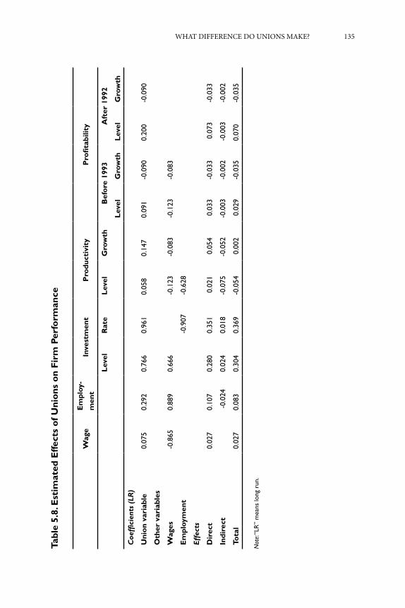
WHAT DIFFERENCE DO UNIONS MAKE? 135
Tabl
e 5.
8. E
stim
ated
Eff
ects
of U
nio
ns o
n F
irm
Per
form
ance
Wag
eE
mpl
oy-
men
tIn
vest
men
tP
rodu
ctiv
ity
Pro
fita
bilit
y
Lev
elR
ate
Lev
elG
row
thB
efo
re 1
993
Aft
er 1
992
Lev
elG
row
thL
evel
Gro
wth
Coe
ffici
ents
(LR
)
Uni
on
vari
able
0.07
50.
292
0.76
60.
961
0.05
80.
147
0.09
1-0
.090
0.20
0-0
.090
Oth
er v
aria
bles
Wag
es-0
.865
0.88
90.
666
-0.1
23-0
.083
-0.1
23-0
.083
Em
ploy
men
t-0
.907
-0.6
28
Eff
ects
Dir
ect
0.02
70.
107
0.28
00.
351
0.0
21 0
.054
0.0
33-0
.033
0.0
73-0
.033
Indi
rect
-
0.02
40.
024
0.01
8-0
.075
-0.0
52-0
.003
-0.0
02-0
.003
-0.0
02
Tota
l 0.
027
0.08
30.
304
0.36
9-0
.054
0.0
02 0
.029
-0.0
350.
070
-0.0
35
Not
e: “L
R”
mea
ns lo
ng r
un.

136 ECONOMIC EFFECTS OF UNIONS IN LATIN AMERICA: THEIR IMPACT
such that a 10 percent increase in membership, evaluated at the mean value of
union density, implies a 0.6 percent rise in the rate of growth of labor productivity.
Full unionization thus would have meant an increase of 9 percent in the rate of
growth. If the indirect impact through employment is included, however, the total
effect is nil.
There are many theoretical explanations for a positive link between unionism
and productivity related to increased cooperation and higher morale, as discussed
above. Some authors, such as Black and Lynch (1997), have also tried to measure
the typical unobservable characteristics by using special surveys. In the Uruguayan
case, however, the result could also be linked to the decrease in turnover that takes
place in unionized sectors (Cassoni, Allen and Labadie, 2000a). Further, if unions
induce substitution of labor by capital and new technologies are more efficient
than their predecessors, then labor productivity can be increased. Regarding
the effect of firm-level bargaining, the positive direct effect further supports the
previous argument; in other words, if bargaining over employment takes place,
one should expect that increased job stability would raise productivity.
Other variables explain the firms’ productivity performances. The relative
size of the establishment and the degree of openness of the economy are variables
that have a positive effect both on the level and the rate of growth of labor
productivity. Belonging to industries facing more competitive pressure through
import penetration lowers productivity, while competing in foreign markets
through exports raises productivity growth. The result, again, can be understood if
the origin of imports and the destination of exports are taken into account. During
most of this period imported goods came mainly from Mercosur countries. Given
the common external tariff established by regional agreements, and considering
the type of goods imported, it could well be that the regional agreements operated
as a subsidy within the region. Hence, products coming from neighboring
countries belonged to industries that were not competitive with the rest of the
world but that were competitive with local industries, at least until 1994. At the
same time those firms that imported the most actually transformed a great deal
of their production into distribution, precisely because they were not competitive.
Exporting industries, instead, were forced to increase their levels of productivity so
as to export to the region. The effect was further reinforced if they were exporting
to the rest of the world. Finally, as expected, the more concentrated the market in
which the establishment operates, the lower the rate of growth of productivity,
while no significant effect is found on the level of labor productivity.

WHAT DIFFERENCE DO UNIONS MAKE? 137
The final equations describing the determinants of the rate of profits and
profit growth are econometrically unsatisfactory, and further work needs to
be done in this area.28 Nonetheless, two results are worth discussing. Plants in
industries with higher union density and a larger percentage of workers covered by
firm-level agreements have higher rates of profits, holding wages constant (direct
effect) and also once the indirect effects through wages are considered. However,
the direct effect of unionization on the rate of growth of profitability is negative,
and firm-level bargaining has no impact on this indicator of firm performance,
while the indirect effects through wages are negligible, as Table 5.8 illustrates. This
could signal that unions organize in those sectors in which there are more rents to
be shared and subsequently prevent further increases in profitability.
The second result worth mentioning is that, starting in 1993, the union
direct effect on the level of profitability increases, while that of firm-level
bargaining falls. The explanation for the results can again be linked to changes in
the structure of bargaining. Surviving unions are still in sectors with the highest
level of supernormal rents. If workers and negotiate over employment at the
firm level, however, then job stability might be gained and wage inflation and
profitability sacrificed in order to face the new economic framework in the 1990s.
As a consequence, the negative effect of unions on the rate of profitability growth
remains negative, although firm-level bargaining reduces that effect.
Table 5.8 summarizes unions’ direct and indirect effects on different
dimensions of firm performance. It must be stressed that the table analyzes the
effects of industry-level unionization on the performance of the firm. Thus gaps
between unionized and non-unionized firms are not calculated, but rather the
effects of the extent and structure of bargaining on indicators of firm performance.
In other words, in comparison to less unionized industries, firms in unionized
sectors pay relatively higher wages, employ more workers, invest more, are relatively
more productive, and obtain higher total profits, but at a lower rate, than those in
less unionized industries.
Given the theoretically feasible but somewhat surprising positive direct
effects of unions on the variables studied, except for profitability growth, and since
these results are robust across different estimation techniques, further explored
are possible biases in the estimation procedure. These biases could be the result
of unobserved variables (such as management quality and practices), the result of
28 While first order autocorrelation is not present, as would be expected given the transformation undertaken, this set of instruments is still inadequate for the purposes described.

138 ECONOMIC EFFECTS OF UNIONS IN LATIN AMERICA: THEIR IMPACT
some exogenous processes taking place that could account for union organization,
or even improperly modeled sample biases. In order to shed light on the possible
existence of biases, further explored was whether unions had organized in
sectors with particularly high productivity, for example, and studied the rank
correlations for 1984, the year when unions re-organized after the military regime.
Unfortunately no data on investments, concentration or profits are available for
that year. With respect to wages, employment and productivity, no significant
high-rank correlation was found (the highest Spearman was 0.33).29 Also used
were the 1988 rankings for investments and concentration as proxies for those in
1984, assuming that neither the levels of investment nor of concentration could
drastically change between those years. Again, no significant rank correlation
could be found using the 37 industries under study. Cross-tabulations for the
levels of unionization were also performed, and some relationship was found
among concentration, effective rates of protection, and union density in 1985
(based on data from Sapelli, 1986). The relation, however, is not systematic across
the different categories defined.30 These results suggest that these sectors could
have been more profitable, and that union density could have increased in such
sectors, eventually preventing further increases in profitability in those industries
that, nonetheless, were the most exposed to competition by trade liberalization
policies.
Biases in the results may also result from the survival, birth and death of
firms in the unbalanced panel under consideration, and unions could have an
effect on their survival and mortality odds. That is, if unions actually hindered
firm performance, they would increase the mortality rate in the industry. In that
scenario, those firms that would actually survive “despite” high union levels in
their industry would be those that excelled on some other unobservable dimension
(such as high-quality management) but not precisely because of the effect of
union behavior. In order to explore the issue, a proportional hazard model was
calculated using Kaplan-Meier hazard estimates.31 These models analyze the
relative probability of survival for a firm, controlling for the relevant variables (the
same used in the models described earlier in this study). The difference between
techniques refers to the former assuming a particular density function for the
29 Basically, industries are rank-ordered along the different variables, and the cancellation between these variables and unionization is calculated.30 For example, although the most concentrated industries are also the most unionized, the relationship cannot be extended to all the other strata, defined according to the degree of concentration. 31 The results are presented in Annex 3 of Cassoni, Allen and Labadie (2001a).

WHAT DIFFERENCE DO UNIONS MAKE? 139
odds of surviving (Cox), while no distribution is assumed in the latter case. The
variables used to explain the survival rates include the degree of unionization of
the industry the firm belonged to and the structure of bargaining in that sector.
The results indicate that unions have no effect on firm mortality, while firm-
level bargaining has a positive significant and effect on firm survival, as expected.
Therefore, it is concluded that there is no significant bias in the sample indirectly
related to unionization.
As is also true for other models, the survival analysis does not make it
possible to control for unobservable variables such as quality of management or
current management practices. It is certainly possible that those firms belonging
to industries with higher levels of unionization could have better quality of
management, particularly given the bias towards large firms in the panel. Despite
this fact, it is clear that, given the variables included in the models, the results are
not biased, except for the apparent capability of unions to organize in industries
with higher levels of profits, and in more concentrated and relatively more
protected sectors.
Conclusions
This chapter reaches several main findings on unions. First, unions increase
both wages and employment. Second, unions promote investment as firms
substitute labor for capital; this occurs as unions organize in plants with higher
rates of profits, promoting increases in productivity and preventing profitability
increases. The mechanism at work seems to be that, given that the result of union
action is wage inflation and labor hoarding, firms have moved to more capital-
intensive technologies, hence increasing the rate of growth of labor productivity
and reducing that of profitability. The hypothesis is consistent with the notion
that unions reduce the share of non-production workers in total employment, as
found in Cassoni and Labadie (2001).
Negotiating at the firm level meant different things in different periods.
Before 1993, given the mandatory extension of collective agreements, it is possible
that bargaining at the firm level further reinforced the previous effects on wages
and hence the indirect effects on the other variables. However, no statistically
significant effects are found. The change in the structure of bargaining at the
beginning of the 1990s, however, introduced another effect of unions that is linked
to bargaining at a decentralized level. It can be presumed that, if unions started

140 ECONOMIC EFFECTS OF UNIONS IN LATIN AMERICA: THEIR IMPACT
caring more about job instability than in the past, then they would be willing to
negotiate over employment in exchange for smaller wage increases, and this largely
appears to be the case in Uruguay in light of the collective agreements registered
at the Ministry of Labor during the period under consideration. Although
statistically significant coefficients cannot be found with the dataset used, the signs
are the expected ones and other research points in the same direction (Cassoni
and Labadie, 2001).32 Nonetheless, it is found that firm-level bargaining reduces
levels and rates of investment, increases productivity and profitability, and has
no effect on the rate of growth of profits. Moreover, after 1993, the more workers
covered by decentralized bargaining, the lower the increase in profitability. The
evidence points to negotiations taking into account the interests of both parties,
so that enhanced productivity and probably survival are achieved together with
lower rates of substitution of labor by capital and/or lower profits.
Union action is associated with increases in the level of investment. The result
can be linked to the decline in the relative price of capital that unions generate
when increasing the wages of those workers in unionized firms. It should also be
related to firms’ interest in overcoming rigidities and transaction costs introduced
by union action. As firm-level bargaining becomes more frequent, the positive
effect is reduced. No doubt it is easier to bargain over the introduction of new
technology at the establishment level, so that union resistance diminishes and, at
the same time, union-management cooperation becomes more feasible.
Unions increase productivity and productivity growth, while increased
coverage of firm-level agreements further reinforces the effect. This may support
arguments derived from the industrial relations literature, such as that unions
promote cooperation and high morale among groups of workers. Given the
Uruguayan general economic framework, however, especially at the beginning
of the 1990s, the fact that unions decrease labor turnover may also have been a
cause.
The above results are consistent with unions generating higher rates of
profits. If they promoted investment in new technology, they generated increased
productivity and productivity growth. So, in spite of rising wage levels, they could
consistently allow the firm to obtain higher profits. However, given their negative
effect on the rate of growth of profitability, the result also reflects the fact that
unions tended to organize and to be stronger in those sectors in which extra rents
were higher because of monopoly power.
32 This might be the consequence of the small number of years included in the analysis, particularly for the second period.

WHAT DIFFERENCE DO UNIONS MAKE? 141
As a final comment, the results here summarized should be seen in light of
the de-unionization process that has been taking place in the country. First, there
is no doubt that the affiliation rate diminished in the 1990s, mostly because of the
non-enforceability of collective agreements. However, the decline reported in the
aggregate statistics overestimates the real magnitude, as it refers to the evolution
of membership in industry-level unions that, in turn, belong to the central union.
Thus workers organized in unions at the firm and establishment levels are not
included. Second, the results suggest that bargaining at the firm level has promoted
easier ways of introducing new technology, increases in productivity, higher job
stability, more moderate wage inflation and lower increases of profitability. It is
therefore sensible to think that cooperation between workers and managers acted
as a means of facing the new economic environment. If this is so, then policymakers
should evaluate the benefits of supporting bargaining so that the smallest firms
can also enjoy the positive effects of unions. The policy, however, need to be well
balanced; while setting general rules to protect the parties is necessary, special care
has to be taken in order not to introduce rigidities that prevent the process from
incorporating the specific characteristics of each unit.
The results indicate that the capital/labor ratio is neutral with respect to
the mortality of firms (significant but not different than 1); the size of the firm
has a positive effect (lower than 1 and significant), and market concentration
(C4) increases the probability of survival (lower than 1 and significant). Tariff
protection also has a positive effect on the odds of surviving; a higher implicit
tariff, or a lower degree of openness, increases an establishment’s probability of
survival.
Among the union variables, union density at the industry level has a positive
effect, but it is not statistically significant, so there are no union effects on survival
odds. The change that took place in 1993—here modeled including a dummy
variable multiplying union density—has no significant effect using this dataset
covering the period up to 1995. If it were to be considered, however, it would lower
the probability of survival relative to the previous period but the overall effect
(adding the coefficients of union density and union density times dummy 1993)
would still be lower than 1, the result thus being that unionization increases the
probability of survival. The only significant result is that of firm-level bargaining,
which increases the probability of survival even more than does a variable such as
size.


CHAPTER SIX
The Effects of Unions on Productivity: Evidence from Large Coffee Producers in
Guatemala
Carmen Urízar H.Sigfrido Lée1
The standard view of trade unions is that their purpose is to improve the material
welfare of their members, principally by raising wages above the competitive
level. There is an enormous body of literature documenting the impact of
unionism on wages, and there is also a smaller body of literature examining
the impact of unionism on other variables, such as wage dispersion (Freeman,
1986a), productivity (Clark, 1980), investment (Machin and Wadhani, 1991a) and
employment (Boal and Pencavel, 1994).
According to several large coffee producers in Guatemala, the general belief
is that unions have a negative effect on productivity, and in several cases unions
have even been blamed for the bankruptcy of firms. This perception explains the
negative attitude of the private sector towards unions. It is nonetheless interesting
to point out that, even though this has long been the general assumption, no
studies so far seem to have tried to quantify this effect. Until now only several
descriptive documents have been published, which present an inconclusive
exchange of opinions. Some of those documents mention the pro-union bias of
labor legislation and its possible economic effects, but they do not present hard
evidence (CIEN, 1999).
This chapter provides an econometric analysis of the impact of unions on a
sample of large coffee plantations, specifically the impact of unions on productivity,
measured as coffee production per worker. First, an equation is estimated using
as independent variables a capital proxy, the proportion of administrative and
1 The authors are research economists at the Centro de Investigaciones Económicas Nacionales (CIEN) in Guatemala City.

144 THE EFFECTS OF UNIONS ON PRODUCTIVITY: EVIDENCE
permanent workers, land per worker, total workers, farm elevation above sea
level and a union dummy. From this equation it is concluded that unions have a
negative effect on productivity.
A similar equation is then estimated, one that includes interaction terms
between the regular variables and the union dummy. The union coefficient in
this equation, when significant, is positive. When a union is present, however, the
effect on productivity of the land and height variables is reduced significantly.
Furthermore, the effect of capital on unionized firms’ productivity is larger than
on the productivity of non-unionized firms. There is also strong evidence that
diseconomies of scale are present in large coffee plantations.
Also tested was whether the overall effect of unions was negative in the
previous equation. The coefficients of these regressions were used to calculate the
predicted level of productivity at the means of all the control variables, and for
two alternative values of the union dummy (zero and one). These values are always
lower when a union is present.
Historical and Labor Market Background
The role of unions must be considered in light of the historically significant role
of coffee in Guatemala’s economy, which is in turn part of a very large agricultural
sector with extensive informality.
Importance of Coffee Production
Coffee began to be cultivated intensively in Guatemala during the second half of
the nineteenth century. Since then, production has expanded continuously, and
coffee has become one of the main products of the country’s economy. Guatemala’s
climate, volcanic soil and mountainous terrain, with a wide range of altitudes
and microclimates, make the country suitable not only for coffee production in
general but also for the development of many varieties, each with a different flavor
and aroma (ANACAFE, 1997).
Currently, the coffee sector represents about 7 percent of GDP, and 2.5 percent
of the national territory is used for coffee cultivation. The close correlation between
general economic growth and the level of international coffee prices illustrates its
importance. The economy generally is booming when international coffee prices
are high, and growth slackens when prices are low (ANACAFE, 1997).

WHAT DIFFERENCE DO UNIONS MAKE? 145
During the last decade coffee represented between 25 percent and 35 percent
of total exports. In 1999 coffee export volume was 268,306,000 kilos, and in 2000
export volume reached 290,384,000 kilos. This represented export earnings of
US$561 million in 1999 and US$574 million in 2000. It is important to note
that, although export volume increased by 8.2 percent between 1999 and 2000,
earnings increased by only 2.2 percent for the same period. This is mainly because
international coffee prices declined during this period (BANGUAT, several years).
Another indicator of the importance of the coffee sector in the Guatemalan
economy is the amount of manual labor it absorbs. Agriculture as a whole employs
40 percent of the economically active population, of which the coffee sector
absorbs approximately 40 percent. This means that about 1.7 million people work
in the coffee sector (ANACAFE, 1997). A national survey, however, only accounts
for 600,000 persons working in this sector (INE, 2000).2
There are almost 7,000 coffee producers in Guatemala, organized through
a national association called ANACAFE. This association classifies producers into
four main groups: (i) large producers: farms producing more than 2,000 one-
hundred pound bags per year; (ii) midsize producers: farms producing 1,000-
2,000 one-hundred pound bags per year; (iii) small producers: farms producing
100-1,000 one-hundred pound bags per year; and (iv) cooperatives of very small
producers: farms that produce fewer than 100 one-hundred pound bags per year.
About 300 farms are registered as large producers, and this category accounts
for almost 80 percent of total coffee production in Guatemala (González, 2001).
Labor Market
Table 6.1 presents some information for the Guatemalan labor market in 1999,
taken from the National Survey on Family Income and Expenses 1998-1999,
compiled by the National Institute of Statistics (INE), and from the 1999 Bulletin of
Labor Statistics of the Labor Ministry, the latest employment statistics available.
According to the Labor Ministry and INE, the unemployment rate for 1999
was less than 2 percent, which is low compared to levels in developed countries. The
main reason is probably the absence of unemployment insurance (public or private)
2 The discrepancies can be attributed to survey procedures. ANACAFE might count the same workers several times, since many of them travel from farm to farm depending on the labor demand. As for INE, the low number might be that on the date when the census was made there was a low demand for workers because of seasonal variations. In addition, many farms harvest several agricultural products rather than coffee alone, a situation that could be biasing both sources. This explanation, however, is only the authors’ opinion.

146 THE EFFECTS OF UNIONS ON PRODUCTIVITY: EVIDENCE
in Guatemala. Another reason is that labor market participation in itself is low (50.5
percent of the total population). Additionally, a large proportion of the population
is employed in the agricultural sector, which is characterized by a high degree of
informality. About 30 percent of the economically active population contributes to
the social security system, but in the agriculture sector this proportion is less than
10 percent. One reason might be that work in this sector is mostly seasonal, so its
contribution is not measured in the formal labor sector.
Table 6.1. General Employment Statistics for Guatemala (1999)
Total population
• Urban population
• Rural population
10.5 million
39.7%
60.3%
Total population of working age (7 years or older) 79.0%
Total economically active population *
• Male
• Female
• Urban
• Rural
50.5%
66.8%
35.2%
52.7%
48.8%
Total inactive working population 49.5%
Annual growth rate of formal employment (1990-98) ** 1.5%
Employment by economic activity
• Agriculture
• Commerce
• Manufacturing industry
39.8%
19.8%
16.6%
Participation of economic activity as percentage of GDP
• Agriculture
• Commerce
• Manufacturing industry
23.0%
24.5%
13.4%
Wages
• Average monthly wage (nominal)
• Minimum wage per working day, non-agricultural activities
• Minimum wage per working day, agricultural activities
US$ 212.15
US$ 3.74
US$ 3.39
Sources: INE (1999), Labor Ministry (1999).*Includes males and females age 7 or older who are working, engaged in productive activities or searching for a job. ** Measured by affiliates of the Instituto Guatemalteco de Seguridad Social (IGSS).

WHAT DIFFERENCE DO UNIONS MAKE? 147
In Guatemala the labor market is characterized by a high degree of
informality, which is even higher in agriculture. The agriculture sector employs
more than a third of the economically active population but pays lower average
wages because it attracts workers with very poor schooling and literacy levels.
Unions in Guatemala
The environment in which Guatemala’s unions operate is determined by the
overall framework of labor legislation, as well as legislation specifically addressing
organized labor. The role of unions is also affected by their overall size and
importance.
General Labor Legal Framework
The Political Constitution of the Republic, the Labor Code (Decree 1441), the Civil
Service Law, and the international agreements and treaties to which Guatemala is
party regulate the country’s labor market. Guatemalan labor legislation is inspired
by the principle that legal protection must favor workers and therefore grants a
minimum and an inalienable set of rights. These principles are established first in
the Political Constitution of the Republic and enforced by general norms such as
the Labor Code and the Civil Service Law. In addition, workers’ rights cannot be
diminished, only expanded.
Foremost among the rights guaranteed in this legal framework is the right
of private sector workers to a minimum wage that must cover the “material, moral
and cultural needs” of the worker and his family. Other minimum rights include a
pre-established number of working days per week; maximum working hours per
day and month; wage levels depending on when hours are worked (for example,
regular weekdays, weekends, after-hours and so on); labor benefits; payment of
lost wages for damages caused by dismissal; and freedom to unionize and strike. 3
The hiring of agricultural workers (laborers, day laborers, cattle drivers, and
others) is additionally regulated by the Labor Ministry according to Labor Code
3 Benefits include vacations (4.11 percent of the total annual wage), severance payments, thirteenth and fourteenth monthly salary (16.66 percent of the total annual wage), productivity bonuses; and payments to the Guatemalan Social Security Institute (13 percent of the total annual wage), the Workers Recreation Institute and the National Institute of Technology and Qualification (2 percent of the total annual wage).

148 THE EFFECTS OF UNIONS ON PRODUCTIVITY: EVIDENCE
Articles 138 to 145. The Labor Code allows the improvement of the minimum
benefits established in the labor legislation, depending on what other employers
usually offer and according to employers’ economic capacity. It is important to
note that the legislation indicates that the minimum guarantees may only be
improved if the employer is (economically) able.
Wages may be paid on the basis of units of time (per month, two weeks,
week, day or hour), on unit of work (per piece, task, raised price or piecework) or
as a share of sales; the worker does not, however, assume the risks of losses that
the employer faces (Articles 88 to 96 of the Labor Code). Generally, the employer
initially determines the wage level, and thereafter it may be negotiated with the
worker.
The minimum wage is set annually by the National Wage Commission,
which is affiliated with the Labor Ministry. The Parity Commission is composed of
two employers and two unionized workers, and a Labor Ministry inspector advises
this commission. If the National Wage Commission cannot reach an agreement on
the minimum wage, the President of the Republic makes a final decision.
Wages can only be paid in legal currency, and it is expressly prohibited to
make payment in whole or part in merchandise, bonds, cards, coupons or any
other form that may replace currency. However, workers in agricultural activities
or cattle-raising activities may obtain a maximum of 30 percent of their total
wage payment in food and other articles used for their own immediate personal
consumption or for that of their dependent relatives; this payment is to be provided
at or below cost by employers.
Legal Framework of Unions
The freedom to organize is a basic right of workers in Guatemala, as guaranteed
by Article 34 of the Political Constitution of the Republic (1985) and International
Labour Organization (ILO) Convention 87; the right of private-sector workers
to organize is further detailed in the Labor Code and its modifications.4 The
enforcement of this right was also an important issue during the peace negotiations
between the Guatemalan government and the guerrilla movement in 1996.5
4 In July 2001 the Labor Code underwent a major reform that strengthened the position of unions. These changes, however, are not included in this chapter.5 Guatemala’s civil war began in the mid-1960s. The war officially ended in 1996 when the government and the guerrillas signed the peace agreements that, besides ending the war, included an extensive program to improve the social and economic conditions of the population.

WHAT DIFFERENCE DO UNIONS MAKE? 149
According to the Labor Code, union associations require the enrollment of
at least 20 workers and are classified as:
a. Agricultural unions: constituted by agricultural workers or employees
of agricultural or cattle-raising companies, or self-employed workers
in cattle-raising or agriculture.
b. Urban unions: all those not included within the activities of agricultural
unions.
Unions can also be classified as:
a. Guild unions: those formed by workers of the same profession or
those of the same economic activity.
b. Company unions: formed by workers of different professions
that provide services to the same company or two or more equal
companies.
Legal principles that apply to all unions include respect for the will of the
majority, secret ballots and one vote per person.
Since freedom of association and the right to unionize are legally recognized,
workers cannot be dismissed for participating in the formation of a union or for
belonging to one. Under the Labor Code workers enjoy the right of non-dismissal
from the moment they notify the General Labor Directorate of the Labor Ministry
that they are forming a union, and they enjoy this protection up to 60 days after
the official publication of an announcement. However, if during this period the
worker commits an act that is defined in the Labor Code as a cause for dismissal,
the employer is allowed to initiate, in the labor courts, a procedure to cancel the
labor contract and authorize dismissal. The right of non-dismissal extends to
union officials as long as they remain in office and until one year after they leave
their position in the union leadership.
Unions are the only labor organizations recognized by law, and only unions
can negotiate collective agreements and call for strikes. Collective bargaining is
carried out only at the establishment level, and collective agreements apply to
all workers, unionized and non-unionized. Although all workers benefit from a
collective agreement, only unionized workers pay membership fees; these fees,
which vary from union to union, are usually a percentage of salary. When a legal
strike is held, the employer must continue paying his employees for as long as the

150 THE EFFECTS OF UNIONS ON PRODUCTIVITY: EVIDENCE
strike lasts, and the employer is not allowed to hire additional workers to replace
them. Employers assume indefinitely all costs of a strike, as long as it is legal and
fair. For a strike to be declared legal it must comply with all the legal requirements,
and for it to be declared fair a labor court must declare that the union is justified
in its demands.6 The only other restriction on the right to strike occurs in the
agricultural sector, where a union cannot call a strike during harvest time.
Although unionization is a right guaranteed by the constitution, employers
may engage in different strategies to discourage union formation. Many of these
are not forbidden by the current legislation, but others can be considered to be
outside the legal framework. As the Labor Ministry does not collect statistics on
illegal actions by employers against unions, information on these practices comes
from interviews with lawyers and union officials. Some of these strategies include
the following:
a. Firing workers. It is illegal to dismiss anyone trying to form a union
once a formal request is presented at the Labor Ministry. Some
employers anticipate this stage and fire union promoters before the
official request is made.
b. Non-compliance with union requirements. Employers can look for any
violation in the formation of a union. If the procedure is not fully
complied with, the Labor Ministry is forced to dissolve the union.
c. Promote alternative associations. Although unions are the only labor
organization recognized by law, employers can promote other types of
associations. Such is the case of a “solidarismo,” a non-profit association
of employers and employees. The advantage of this association is the
perceived goodwill among its members, contrary to the perceived
aggressiveness of unions by employers. Moreover, there are no legal
prohibitions on the coexistence of a union and other organizations in
the same company. This may dilute the power of a union within the
company.
d. Hiring rules and human resources management. Employers can hire
personnel with the specific purpose of informing management
of problems within the workforce or plans of forming a union.
Companies may also develop a policy of not contracting anyone who
6 A fair strike occurs when the reasons that motivated it are caused by the employer, because of non-compliance with individual contracts or collective agreements, or because the employer unjustly denied the workers a raise or any other benefit when able to grant it (Labor Code, Article 242).

WHAT DIFFERENCE DO UNIONS MAKE? 151
has been a union member or has worked in a company that has or had
a union. Another strategy is to hire only temporary personnel.
e. Other strategies. Employers can engage in actions that, although not
necessarily illegal, might be considered unethical. One such practice
involves bribing workers with money or promotions to prevent
them from unionizing. Another is to fragment the establishment so
that there are not enough employees in each firm to form a union.
Some union members have reported illegal actions such as threats
and physical harm, but it is difficult to confirm the veracity of these
claims, since most cases never reach the judicial system. Most of these
conflicts are resolved privately between the interested parties, often
because of the high costs of resolving them in the courts.
Generally, employers will try to stop unions from forming, because unions
are viewed as having a strong negative effect on productivity. For example, a union
has the legal power to force the employer to accept a collective agreement, which
he cannot refuse. Moreover, if the employer still refuses to accept the agreement,
unions have the right to call strikes, but they do not bear any of the costs if the
strike is declared legal and fair.
Additionally, since the law does not restrict what may be included in
collective agreements, union officials tend to make demands that often do not take
into account the reality of the firm. Those demands may include additional wages
and benefits that are not linked in any way to productivity. Collective agreements
may further include restrictions on the contracting of workers and on working
practices.7 In the case of collective agreements on coffee plantations, employees’
duties are covered by detailed restrictions. Sometimes they go as far as limiting the
number and size of holes for new plants that an employee can dig on a working
day. Some agreements also establish how many plants and to what height the
employees can prune them during the working day.
These restrictions have several effects. First, they usually keep employee
productivity under its optimal level. It is observed that similar workers on the same
farm, but hired under agreements that do not impose these restrictions, achieve
higher yields. As a result, employers may be forced to hire additional workers
to complete tasks on time.8 These agreements may also reduce productivity by
7 See Fernández Molina (1996), González (2001) and Contreras (2001).8 See González (2001).

152 THE EFFECTS OF UNIONS ON PRODUCTIVITY: EVIDENCE
delaying technological improvements. Because of the degree of detail in which
the contracts are written, employers introducing technological changes can be
brought before labor courts on charges of violating an agreement. Employers are
usually unwilling to initiate new negotiations simply to change a few working
practices, however, because a new agreement usually implies more benefits for
workers. Moreover, employers already face the prospect of frequent negotiations.
By law, collective agreements are valid for only one year, although they are renewed
automatically for an additional year if neither party chooses to renegotiate.
As can be seen, once a union is created it might be very harmful to a firm.
Nonetheless, employers have available many effective ways of stopping unions
before they form. Moreover, unions have a limited scope for influence: they can
only negotiate a collective agreement for workers in a single firm, rather than an
industry or an economic sector. This might help explain the low density of unions
in the labor force.
Size and Importance of Unions
In 1999 Guatemala had a population of 10.5 million, of which 50.5 percent constituted
the economically active population (EAP). According to Labor Ministry estimates,
in May 1999 there were 1,389 union organizations in Guatemala; slightly over a
third (35.56 percent) were considered to be active organizations (with their own
legal personality and renewal of the executive committees). The average number
of workers per union was 68, and the country’s unions had 94,878 members, or
1.7 percent of the EAP. Although 1997 Labor Ministry estimates indicate that 76.5
percent of unions operated in the private sector, union membership amounted to
Table 6.2. Enrolled Unions, Number of Members by Sector (1999)
Concept Total Public Sector Private Sector
Organizations 1,389 401 988
Affiliated workers 94,878 34,929 59,949
Source: Ministerio de Trabajo, Boletín Estadístico 1999.

WHAT DIFFERENCE DO UNIONS MAKE? 153
only 2 percent of private sector workers, and most unions are concentrated in the
central and southwestern regions of the country.9
Unions are usually associated with national organizations or federations,
which in turn belong to larger associations called confederations, as shown in Table
6.3. Besides the fees that affiliated unions pay to federations and confederations,
these larger associations usually receive additional support from foreign labor
organizations. It is common for unions to change frequently from one federation
to another, and it is also common, because of the low density of unionization,
for other social organizations such as peasant groups to belong to federations.
In general, unions are very rare, especially in the private sector, and they are very
decentralized.
In 1997, 50.6 percent of unions were concentrated in the agricultural sector,
21.8 percent in personal services and 13 percent in industrial activity. The largest
unions, based on the average number of affiliates, were those in electricity, gas and
water (565 members); followed by transport, storage and communications (157
members). The unions with the smallest number of affiliates were those in com-
merce, restaurants and hotels (44 members) and agriculture (50 members). Several
problems limit the organization and operation of unions. These problems include
low levels of motivation and awareness of unions, as well as a loss of credibility in
the leadership of several unions. Actions taken by employers to avert the formation
of unions also limit participation (Morales Modenesi and de León, 1995).
9 The central and southwestern regions consist of the departments of Guatemala, Solola, Totonicapan, Quetzaltenango, Retalhuleu, Suchitepequez and San Marcos. In any event, figures on unionization must be used with care. As Morales Modenesi and de León (1995) observe: “it is difficult to establish with certainty how many organizations are active and how many workers are unionized. Very often not even union leaders, independently of the organization size, have this information on hand.”
Table 6.3. Enrolled Unions, Federations and Confederations (1943 to 1997)
Legal status Total enrollments Public Sector Private Sector
Unions 1,222 293 929
Federations 48 6 42
Confederations 5 0 5
Totals 1,275 299 976
Source: Labor Ministry, Boletín Estadístico 1997.

154 THE EFFECTS OF UNIONS ON PRODUCTIVITY: EVIDENCE
The average number of workers per union in agriculture is low compared
to other productive sectors. This is because agricultural activities are mainly
seasonal, and the temporary workers who make up the majority of the agricultural
workforce do not have the same freedom to organize as permanent employees. It
can thus be concluded that union associations in rural areas do not have the same
presence as those in urban areas.10
In the coffee sector, official information on unions is scant and unreliable.
According to the Labor Ministry, between 1947 and 2000, 19 agricultural unions
have been authorized, of which five were in the coffee sector. Until March 2001,
only two of these unions were legally recognized, and only one had a collective
bargaining agreement on working conditions (Rolando, 2001). Members of
ANACAFE, however, estimate that the employees are unionized on about 10
percent of the large farms (more than 30 farms), but there are no official or private
statistics to support this information.
Table 6.4. Number of Unions by Economic Activity (1943 to 1997)
Number of affiliated workers
Economic activity
Total
enrollments
by activity
Total Females Males
Totals 1,275 97,523 9,274 88,249
Agriculture 646 32,315 1,492 30,823
Operation of mines
and quarries4 228 0 228
Manufacture industry 167 13,335 1,783 11,552
Electricity, gas and
water 6 3,389 104 3,285
Construction 20 2,395 103 2,292
Commerce,
restaurants and hotels 38 1,673 622 1,051
Financial activities 30 3,152 689 2,463
Personal services 278 32,568 4,214 28,354
Not specified 40 1,246 103 1,143
Source: Labor Ministry, Boletín Estadístico 1997.
10 More detailed data about the size and importance of unions in Guatemala can be found in Annex 1 of Urízar H. and Lée (2003).

WHAT DIFFERENCE DO UNIONS MAKE? 155
Data
Given the paucity of other sources, the data used for this chapter’s analysis of coffee
production were collected directly through a survey of 100 coffee producers.11 The
response rate to the survey was 65 percent. Since it was necessary to remove from
the sample those producers that did not provide data for four consecutive years
between 1992 and 2000, the chapter uses data for 37 producers. Table 6.5 shows
the number of firms per year used in this chapter.
Output
This variable was measured in 100-pound bags of pergamino coffee per year.12
Measurement of output in physical units avoids the problem mentioned by Booth
(1995) and Clark (1980) when production is measured in value added. In that case
observed differences in productivity may result from high prices, overestimating
the true productivity differential due to the existence of a union.13
Table 6.5. Unbalanced Panel Data Description
Year Number of Firms
1992 34
1993 34
1994 34
1995 36
1996 36
1997 37
1998 37
1999 37
2000 31
Total Observations 316
11 For further details, see Annex 4 of Urízar H. and Lée (2003).12 Pergamino coffee is obtained after the process of seeding (eliminating the fruit and obtaining only the seed). 13 Although coffee prices are set internationally, it is sold with premiums or discounts because of the quality of the bean, which is established, among other things, by the height of the farm and the variety of the plant.

156 THE EFFECTS OF UNIONS ON PRODUCTIVITY: EVIDENCE
Employment
This variable measures the number of workers, which are divided into:
a. Temporary workers or jornaleros: workers involved in fieldwork, such
as coffee harvesting and plant maintenance. These workers do not live
on the plantations and are hired solely for specific activities. According
to current legislation, the average duration of these contracts must be
less than 90 days for a worker to be considered temporary; afterwards
the relationship is considered permanent.
b. Permanent workers or colonos: workers who perform the same activities
as the temporary workers but generally live on the plantation premises
permanently. This generates additional costs for the producer. These
types of workers tend to unionize, since they have a long-term labor
relationship with the employer.
c. Administrative workers: the administrators of the farm and personnel
(engineers or agronomists), workers in charge of the payroll or planilleros,
teachers and nurses (the latter two when the plantation provides
primary education and health care to its permanent employees).
It should be noted that there may be a significant bias in the employment
measurement. The economic literature generally considers the labor unit as one
employee, but in the case of Guatemala this is not always the case, especially in
agriculture. While the employer negotiates a labor contract with an employee, the
employee’s whole family, including spouse and children, performs agricultural
work. This practice is even recognized in Article 139 of the Labor Code.
Land Input
Land is an indispensable input for all agricultural products, and in this case land
is measured by the area planted with coffee on each farm. It is important to note
that there were several farms that harvested other products, such as sugarcane,
rubber and lumber. The unit of measurement was manzanas, a local measurement
equivalent to 0.6988 hectares.
Another relevant feature of the land input is the elevation of the farm. This
has a distinguishing impact on the life cycle of the plant and the quality of the
coffee bean. At higher altitudes, a better coffee quality is expected. This variable

WHAT DIFFERENCE DO UNIONS MAKE? 157
was measured in feet above sea level. Since portions of the same farm may lie at
different heights, a simple average of the highest and lowest altitude on each farm
is used in the estimations.
Capital
Because of the special characteristics of coffee production, capital investment is
not measured by the traditional variables (cost of equipment or machinery), but
by planting and maintenance of coffee plants.14 These activities were measured by
the following proxies:
a. whether a tree nursery is used or not;
b. whether plants are grafted or not;
c. number of plants seeded per hole;
d. number of times plants are fertilized;
e. distance between plants; and
f. use of traditional or higher technological methods of fieldwork and
harvesting.
These variables represent a very broad definition of capital. Holding land
and employment constant, an attempt was made to determine what other variables
would yield higher productivity when they increased as well. For the estimations,
only statistically significant variables were used: if a tree nursery was used, the
number of plants per hole and whether traditional or highly technological
methods were used.
Regions
The location of the farms is a variable that makes it possible to identify differences
in technology, socio-demographic and cultural characteristics, quality of land and
climate. The farms were divided according to their location into five regions.
1. East: departments of Zacapa, El Progreso, Jalapa, Chiquimula, Jutiapa
and Santa Rosa.
2. South coast: departments of Escuintla, Suchitepequez, Retalhuleu,
San Marcos and Quetzaltenango.
14 See Annex 3 of Urízar H. and Lée (2003) for a more detailed explanation of these characteristics.

158 THE EFFECTS OF UNIONS ON PRODUCTIVITY: EVIDENCE
3. North (Coban): departments of Alta Verapaz, Baja Verapaz, Izabal and
Petén.
4. Central Valley: departments of Guatemala, Chimaltenango and
Sacatepequez.
5. Highlands: departments of Huehuetenango, Quiché, Totonicapán and
Sololá.
Union Presence
Data on the presence of unions on coffee plantations were obtained directly from
the survey, and a dummy variable was constructed to capture this information.
Also of interest was information on any previous unionization efforts on the
plantations. This is important in determining the percentage of plantations that
have previously experienced attempts at union formation, as well in identifying
the means producers used to prevent the formation of a union.
A total of eight unionized firms were interviewed. Of these, four had a union
throughout the full sample of nine years; one firm had a union from 1993 to 2000;
two had a union for only five years (one from 1993 to 1997 and the other from
1992 to 1996); and the last had a union for only two years, from 1999 to 2000.
Seven of these firms are located in region two, and the other is in region four.
Theoretical Framework
The coffee data provides measures of output (Q) and four inputs: capital (K), land
(L), work days of permanent workers (Np), work days of temporary workers (N
j)
and work days of administrative workers (Na). This information can be summarized
and used to estimate the difference in productivity with and without a union,
using the standard analysis of a production function (Chiang, 1984). Therefore, it
is assumed that the coffee production function is written in the following way:
Q = AQ(N, L, K) (1)
where Q denotes output, N is the effective labor input, L is land and K represents
capital. It is assumed that there are two types of workers: union workers, denoted
by Nu, and non-union workers, N
n. N
n workers include permanent, temporary

WHAT DIFFERENCE DO UNIONS MAKE? 159
and administrative workers, while Nu can only include permanent workers.15
Furthermore, it is assumed that productivity differs between unionized and non-
unionized farms. To control for this possibility, and thus to identify the union/non-
union differences that arise from cultural, geographical and idiosyncratic factors,
a Cobb-Douglas production function is specified. Equation (1) can therefore be
rewritten as the following explicit function of labor and capital:
Q = A • Lα • Kβ (Np + σ • N
a)γ (2)
where p stands for permanent workers and a for administrative workers.
Following Clark (1980) and Booth (1995), the production functions for
unionized and non-unionized firms, respectively, can be written as:
and
where u and n indicates union and non-union, respectively. The assumption that
the production function has constant returns of scale (CRS) is given by:
1 = α + β + γ (5)
where γ is the elasticity of output with respect to labor.
Equations (3) and (4) control for union/non-union differences in the
production parameters, but within the two sectors technology and productivity
may vary because of regional effects. Dummy variables have been constructed to
control for this effect. Still, input ratios might have different effects on productivity
in the unionized and non-unionized firms, so that the estimated union effect
may depend on parameter differences and the level of the input ratios at which
the union/non-union comparison takes place. Because of the limited number of
ln
Q—N
⎛⎝
⎞⎠
u
= ln(Au) + α
u ln
L—N
⎛⎝
⎞⎠
u
+ βu ln
K—N
⎛⎝
⎞⎠
u
+ γu ln
Np + σ • N
a—————N
⎛⎝
⎞⎠
u
–
(1 – α – β – γ)ln(N)u (3)
ln
Q—N
⎛⎝
⎞⎠
n
= ln(An) + α
n ln
L—N
⎛⎝
⎞⎠
n
+ βn ln
K—N
⎛⎝
⎞⎠
n
+ γn ln
Np + σ • N
a—————N
⎛⎝
⎞⎠
n
–
(1 – α – β – γ)ln(N)n (4)
15 The legislation recognizes administrative workers as management employees who cannot be part of a union. Temporary workers cannot unionize since they do not have a long-term relationship with their employer, which is also required by union legislation.

160 THE EFFECTS OF UNIONS ON PRODUCTIVITY: EVIDENCE
observations, the union and non-union parameters will be estimated jointly using
interaction terms between the independent variables and the union dummy to
obtain a more efficient estimation.16
The coefficients on the interaction terms provide estimates of the difference
between union and non-union parameters, while the non-union parameters are
given by the coefficients on the regular independent variables.
Empirical Results
In order to evaluate the effects of unions, industry productivity equations are
estimated without union interaction terms and then with them. The results are
finally estimated with fixed effects.
Results of the Industry Productivity Equations without Union Interaction Terms
As mentioned in the data description, for the industry productivity analysis, an
unbalanced panel with data for 37 companies was constructed, consisting of
nine years from 1992 to 2000. A regression analysis was used to estimate a labor
productivity function, for which the results are shown in Table 6.8. These regressions
are the estimation of equation (6) above, but without the union interaction terms.17
ln
Q—N
⎛⎝
⎞⎠
i
= ln An + bU + (α
u – α
n)ln
L—N
⎛⎝
⎞⎠
i
U + (βu – β
n)ln
K—N
⎛⎝
⎞⎠ U +
(γʹu – γʹ
n)ln
Na—
N
⎛⎝
⎞⎠ U + (γʺ
u – γʺ
n)ln
Np—
N
⎛⎝
⎞⎠
i
+ (θu – θ
n)
iln N
iU + α
n ln
K—N
⎛⎝
⎞⎠
i
+
βn ln
K—N
⎛⎝
⎞⎠ +γʹ
n ln
Na—
N
⎛⎝
⎞⎠ + γʺ
n ln
Np—
N
⎛⎝
⎞⎠ + (θ
n – 1)lnN
i +
r
Σk
(πu – π
n)
k
REGkU +
r
Σk
πnk
REGk
(6)
16 In the empirical results, this equation is estimated according to the methodology presented in Clark (1980). Nonetheless, because of the length of the time series in the panel data, when every variable is interacted with unionism the efficiency gains relative to estimating separate regressions for union and nonunion firms are likely to be minor; the only constraint used to improve efficiency is equal error variance in the two equations. Consequently, in the empirical section an equation is first estimated without the union interaction terms.17 This was performed in light of the amount of data available, with a view to securing a better understanding of unions’ direct and overall effects on the productivity of coffee farms, before complicating the estimation by incorporating the union interaction terms.

WHAT DIFFERENCE DO UNIONS MAKE? 161
Table 6.6. Description of Variables Used
Variable
(symbol)
Measurement
issues
Characteristics of the data set used Variable used in
regressions
Q Measuring
output
Production is measured in 100-pound
bags. To measure the productivity per
worker, an additional variable was
constructed: total output divided by total
workers.
Output Output/
Worker
N Labor input Labor is divided into:
1) Jornaleros or temporary workers.
2) Colonos or permanent workers.
3) Administrative workers.
4) Total workers.
1) Temp Workers
2) Perm Workers
3) Adm Workers
4) Total Workers
L Land input Land is measured by cultivated area
(manzanas). Average height of each farm.
Land Height
K Capital input Capital is measure by seedtime, renova-
tion and maintenance of coffee plants,
through:
1) Number of plants seeded per hole.
2) Number of times plants are fertilized.
3) Use of traditional or highly technical
methods of fieldwork and harvesting.
4) Capital investment. 1
1) Plants per hole
2) Fertilizer
3) Hi-tech methods
4) Capital
A Vector to con-
trol for regional
differences
Farms were divided into five regions,
depending on location, defined as follows:
I. Eastern Region
II. Southern Coast
III. Northern Region (Cobán)
IV. Central Valley
V. Highlands
REGi; i=index region
U Unionization A dummy variable that is 1 if a firm is
unionized and 0 if it is not.
Union
1 This variable is a linear aggregation of the number of plants seeded per hole, the number of times plants are fertilized each year and whether the farmer uses traditional or highly technical methods of field work and harvest-ing. For estimation purposes, this variable was used in this form and not on a per-worker basis, since the variable measures only fixed effects (for example, if a farm is considered to be more capital-intensive than another). Dividing this figure by worker would only have been useful if there had also been a better measurement that also indicated changes in slope.

162 THE EFFECTS OF UNIONS ON PRODUCTIVITY: EVIDENCE
The main interest is to estimate the effects of unions on the productivity of coffee
farms. The dependent variable is the logarithm of coffee production or output per
worker, and the values in parenthesis under the coefficients are the corresponding
standard errors.
The estimation method used for the first regression in Table 6.8 was pooled
ordinary least squares (OLS). This equation was estimated using data only
from Region 2, where most of the unionized firms are located. The purpose of
estimating this equation was to establish a benchmark to which results for the
whole country could be compared. This group of farms is very similar in elevation,
Table 6.7. Variable Means and Standard Deviations*
All Farms Non-Unionized farms Unionized Farms
Variable MeanStandard
DeviationMean
Standard
DeviationMean
Standard
Deviation
Output 4,494.2 3845.8 4,288.6 3,846.5 6,063.6 3,778.6
Output/
worker35.8 40.1 41.5 42.6 16.3 13.4
Temp.
workers213.2 307.1 146.8 206.9 420.0 461.8
Perm.
workers65.7 76.1 48.7 67.0 150.7 69.2
Adm.
workers6.9 7.2 5.5 6.0 13.9 9.3
Total
workers287.1 345.4 201.1 245.2 584.5 447.2
Land 666.4 2043.0 289.3 229.4 2,098.6 4,084.3
Height 3,733.2 1191.6 3,915.0 1,114.2 3,381.2 1,282.2
Plants per
hole1.6 0.5 1.7 0.5 1.4 0.5
Fertilizer 2.5 0.6 2.6 0.5 2.1 0.6
Hi-tech
methods0.6 0.5 0.6 0.5 0.6 0.5
Capital 4.6 1.1 4.8 1.1 4.1 0.9
Union 0.2 0.4
* 1992-2000.

WHAT DIFFERENCE DO UNIONS MAKE? 163
Table 6.8. Results of Industry Production Equations (without union interaction
terms)
Dependent variable:
Log(Output/ Total
Workers)
1 2 3 4 5 6
OLS OLS OLS GLS OLS GLS
Constant-0.217 0.020 -1.289 -1.735 -0.014 -0.014
(0.868) (0.054) (0.842) (0.565)* (0.023) (0.006)*
Log (Capital) 1.178 1.719 0.690 0.702 0.608 0.943
(0.281)* (0.325)* (0.188)* (0.090)* (0.184)* (0.107)*
Log (Adm Workers/
Total Workers)
7.638 6.233 0.813 0.881 0.612 0.901
(1.506)* (1.970)* (0.901) (0.425)* (1.060) (0.586)
Log (Perm Workers/
Total Workers)
-0.244 -0.323 0.008 0.053 0.388 0.246
(0.422) (0.451) (0.186)* (0.095) (0.219)** (0.101)*
Log(Land/ Total
Workers)
0.328 0.249 0.398 0.479 0.296 0.556
(0.058)* (0.058)* (0.047)* (0.042)* (0.052)* (0.039)*
Log(Total Workers)-0.180 -0.198 -0.256 -0.248 -0.353 -0.235
(0.082)* (0.069)* (0.048)* (0.021)* (0.044)* (0.032)*
Log(Height)0.250 0.129 0.481 0.511 0.376 0.242
(0.139)** (0.103) (0.101)* (0.069)* (0.048)* (0.025)*
Union -0.459 -0.198 -0.387 -0.235 -0.202 -0.107
(0.114)* (0.095)** (0.099)* (0.072)* (0.068)* (0.062)**
Region20.535 0.614 0.699 0.559
(0.109)* (0.059)* (0.120)* (0.069)*
Region30.359 0.443 0.567 0.401
(0.139)* (0.063)* (0.139)* (0.073)*
Region40.844 0.866 0.888 0.878
(0.128)* (0.077)* (0.138)* (0.080)*
R-squared 0.716 0.888 0.715 0.980 0.950 0.948
F-statistic 47.185 76.147 76.535 148.204 581.186 553.315
Prob(F-statistic) 0.000 0.000 0.000 0.000 0.000 0.000
Durbin-Watson stat. 1.136 0.701 1.005
Total panel
observations 139 139 316 316 316 315
** Denotes significant at 10 percent.* Denotes significant at 5 percent.Values in parentheses are standard errors.

164 THE EFFECTS OF UNIONS ON PRODUCTIVITY: EVIDENCE
coffee variety planted, weather, landscape and socio-demographic characteristics.
Although these differences were controlled for using regional dummy variables in
further estimations, it was unclear whether they would be sufficient to capture the
information related to all of these differences.
The results show that the union dummy has a negative and significant effect
on the productivity of coffee farms. As for the capital variable, the proportion of
administrative workers to total workers, the amount of land to total workers and
the elevation of the farm have a positive and significant effect on productivity. The
total workers variable is negative and significant at the 5 percent level. This could
indicate the presence of some diseconomies of scale.
An exploratory analysis of the results of equation (1) shows that some of
the firms are affected by autocorrelation. Equation (2) basically estimated again
the first equation, except that it corrected for this autocorrelation problem.
It was corrected with generalized differences using an estimated value of the
autocorrelation coefficient of each firm.18 The results are not significantly different
from the previous equation, except that the union coefficient is only significant at
the 10 percent level and the elevation variable is no longer significant.
Equation (3) has the same specification as equation (2), except that the
sample is expanded to include farms from all over the country. Therefore, dummy
variables for each region are also included. The estimation procedure is pooled
OLS and the standard errors are White heteroskedasticity-consistent. Equation
(4) has the same specification but is estimated using pooled generalized least
squares (GLS). Equations (5) and (6) are essentially the same as (3) and (4), but
they are corrected for autocorrelation using the generalized differences procedure
explained above.
The results do not vary greatly between the first two equations: unionization
always has a negative and significant effect on productivity. As for the other
variables, capital and farm elevation are positive and significant at the 5 percent
level. In equations (3), (5) and (6) the coefficient of permanent workers was
positive and significant, while the proportion of administrative workers was no
longer significant. Moreover, in all the equations there were diseconomies of scale.
The dummy regional variables are also significant at the 5 percent level in all cases.
The strongest regional effect on productivity was that of Region 4, which includes
the Central Valley.
18 Each correlation coefficient, ρ, was obtained from the corresponding Durbin-Watson estimator: DW=2*(1-ρ).

WHAT DIFFERENCE DO UNIONS MAKE? 165
Results of the Industry Productivity Equations with Union Interaction Terms
The results of the full estimation of equation (6) above, including the interaction
terms between the union dummy and the other variables, are shown in Table
6.9. The estimation method used in each equation is the same as those shown in
Table 6.8. The first and second column only include data for Region 2, equation
(1) is estimated using pooled OLS, and equation (2) uses the same methodology,
but correcting for autocorrelation. The equations are divided into two parts: the
first are the results of the coefficients of the regular variables, which explain the
changes in productivity in the non-union farms, and the second set are the same
coefficients, but interacting with the union dummy variable. The coefficients on
the interaction terms provide estimates of the difference between union and non-
union parameters.
The union variable is not significant in equation (1). The interaction terms,
however, show some interesting results: administrative workers are more relevant
in explaining productivity; unions reduce the productivity of the land factor; and
some diseconomies of scale may be present as well.19 Of the regular variables, only
administrative workers, land to total workers and total workers are significant, and
the signs of the coefficients are similar to those of equation (1) in Table 6.8.
In equation (2) of Table 6.9 the union coefficient has a highly positive and
significant effect on productivity. The interaction terms nonetheless show that the
effect of permanent workers, land and elevation is negative in unionized farms,
contrary to what is seen in farms where there is no union present. The interaction
term with capital is significantly larger than in non-unionized firms, indicating
that capital investment has a larger effect on unionized farms’ productivity.20 The
interaction term with total workers indicates diseconomies of scale in unionized
firms.
Equations (3) and (4) in Table 6.9 are very similar to equation (1), except that
they include data for all regions, and regional dummies are included to control for
this difference. The estimation method of equation (4) is pooled GLS. Equations
(5) and (6) are similar to the previous two, except that they are also corrected for
autocorrelation.
19 To estimate the economies of scale in unionized firms the coefficient of the interaction term of total workers with the union variable was added to the regular coefficient of total workers, and then added one. If this value was less than one, then diseconomies of scale were present.20 Nonetheless, the causality of the capital variable is not quite clear. According to interviews with coffee producers, union promoters specifically directed the unionization efforts toward those farms that already had high levels of technology and capital investment.

166 THE EFFECTS OF UNIONS ON PRODUCTIVITY: EVIDENCE
Table 6.9. Results of Industry Production Equations
Dependent variable:
Log(Output/ Total
Workers)
1 2 3 4 5 6
OLS OLS OLS GLS OLS GLS
Constant2.941 -0.060 -2.736 -3.597 -0.024 -0.036
(1.464)* (0.087) (1.091)* (0.569)* (0.033) (0.011)*
Log (Capital) 0.248 1.524 0.904 0.887 0.905 0.823
(0.367) (0.555)* (0.183)* (0.088)* (0.181)* (0.109)*
Log (Adm Workers/
Total Workers)
4.867 -2.520 -0.568 -0.457 -1.190 -0.033
(2.810)** (6.955) (0.695) (0.348) (0.707)** (0.517)
Log (Perm Workers/
Total Workers)
0.122 -0.475 -0.396 -0.153 0.113 0.018
(0.543) (1.229) (0.197)* (0.082)** (0.244) (0.114)
Log(Land/ Total
Workers)
0.545 0.995 0.720 0.765 0.660 0.709
(0.118)* (0.166)* (0.056)* (0.028)* (0.056)* (0.036)*
Log(Total Workers)-0.342 0.424 -0.191 -0.173 -0.272 -0.179
(0.094)* (0.106)* (0.048)* (0.023)* (0.042)* (0.033)*
Log(Height)0.142 -0.190 0.579 0.671 0.302 0.254
(0.179) (0.146) (0.125)* (0.067)* (0.036)* (0.025)*
Union 7.232 45.604 17.579 30.051 9.808 23.310
(9.615) (7.907)* (15.141) (10.637)* (6.273) (8.747)*
Log (Capital)*Union 6.763 18.391 6.181 9.179 4.379 7.935
(3.449) (2.802)* (4.495) (3.332)* (1.830)* (2.774)*
Log (Adm
Workers/ Total
Workers)*Union
3.362 3.429 7.591 1.558 6.384 -0.675
(5.243)** (9.707) (3.497)* (1.580) (4.193) (1.539)
Log (Perm
Workers/ Total
Workers)*Union
-1.751 -7.111 -1.203 -2.627 -1.043 -2.580
(1.416) (1.714)* (1.724) (1.148)* (0.810) (0.885)*
Log(Land/ Total
Workers)*Union
-0.487 -1.525 -0.692 -0.969 -0.607 -0.888
(0.251)* (0.276)* (0.242)* (0.157)* (0.150)* (0.139)*
Log(Total
Workers)*Union
0.492 -0.801 0.28 -0.136 0.197 -0.339
(0.227)* (0.426)** (0.196) (0.123) (0.259) (0.118)*
Log(Height)*Union-2.479 -8.139 -2.985 -4.432 -1.796 -3.342
(1.649) (1.313)* (2.147) (1.616)* (0.860)* (1.348)*
Region2*Union-4.365 -6.050 -3.021 -5.004
(2.906) (2.234)* (1.177)* (1.866)*

WHAT DIFFERENCE DO UNIONS MAKE? 167
The union variable is only significant at the 5 percent level in equations (4)
and (6). Contrary to what was expected, the result has a positive sign, although the
interaction terms show that, when a union is present, the productivity of land per
worker and elevation diminishes in comparison to non-unionized firms. The land
and height coefficients are always significant and positive in non-unionized firms.
Therefore, the more land per worker and the higher the elevation of the farm,
the higher the productivity. The presence of a union, though, cancels the positive
effect of these inputs.
Among the interaction terms, the capital estimation is almost always
significant at the 5 percent level, and it is positive. In addition, its value is
significantly higher than that of the regular variable. This implies that unionized
firms rely relatively more on capital for productivity than do non-unionized firms.
Hence it can be expected that unionized firms might choose more capital-intensive
technologies to raise their productivity.
Table 6.9. Results of Industry Production Equations (continued)
Dependent variable:
Log(Output/ Total
Workers)
1 2 3 4 5 6
OLS OLS OLS GLS OLS GLS
Region20.572 0.482 0.483 0.442
(0.106)* (0.064)* (0.126)* (0.072)*
Region30.158 0.212 0.106 0.269
(0.140) (0.075)* (0.168) (0.077)*
Region40.835 0.735 0.759 0.750
(0.120)* (0.079)* (0.134)* (0.083)*
R-squared 0.762 0.788 0.775 0.765 0.943 0.938
F-statistic 30.885 35.845 60.242 57.227 291.006 265.12
Prob(F-statistic) 0 0 0 0 0 0
Durbin-Watson stat 1.278 0.901 0.849
Total panel
observations 139 139 316 316 316 316
** Denotes significant at 10 percent.* Denotes significant at 5 percent.Values in parentheses are standard errors.

168 THE EFFECTS OF UNIONS ON PRODUCTIVITY: EVIDENCE
When the proportion of permanent workers is significant, the effect is
negative in both unionized and non-unionized firms. In both types of firms,
permanent workers cause a reduction in productivity. This may explain the general
trend in the coffee sector of replacing permanent with temporary workers; hired
on the basis of productivity, they also allow for greater flexibility in hiring.21 The
results for administrative workers, on the other hand, are much less clear. They
are rarely significant, and in the case of non-unionized firms the sign is not stable;
when this coefficient is significant, it has a positive sign for unionized firms. This
result might be capturing the importance of administrative workers in managing
and complying with the collective agreement with the union. As for the value of the
coefficient of total workers, it is negative for both unionized and non-unionized
firms, indicating that diseconomies of scale may be present.22
Of the regional dummies, Region 4 still has the largest positive effect on
productivity, followed by Region 2. As for Region 3, when the effect is positive it has
a smaller effect on productivity than Region 2. It is interesting to note, however, that
the value of the regular coefficient of Region 2 changed from positive to negative
when interacted with the union variable. Although this is a very productive coffee
region, the regional effect becomes highly negative when a union is present.
21 Permanent workers are those hired through a long-term contract. They usually live on the same farm, and sometimes the same family has lived on the farm for several generations. By law, they have a right to additional benefits and severance payments. 22 An additional explanation of why the coefficient of permanent workers is so negative is that they usually help to solve a coordination problem within the firm, since they are the real experts in coffee harvesting. In other words, they act as field managers for the landlord. When a union is present they do not contribute to solving this problem, since they have tenure as friends of the union leaders. This could explain why administrative workers are more important in unionized firms. The absence of this explanation for non-unionized firms may result from the need to control for administrative practices, for which information is not available.
Table 6.10. Estimated Value of Productivity at the Means of All Control Variables
Dependent variable:
Log(Output/ Total
Workers)
1 2 3 4 5 6
OLS OLS OLS GLS OLS GLS
A) UNION =0 2.888 3.212 3.131 3.128 3.158 3.184
B) UNION =1 2.337 2.237 2.747 2.815 2.762 2.780

WHAT DIFFERENCE DO UNIONS MAKE? 169
To further understand the effect of unions on the productivity of coffee
farms the productivity level (output per worker) was estimated at the means of
the control variables, for the alternative values of the union dummy (zero for non-
unionized firms and one for unionized firms). The coefficients shown in Table
6.9 were multiplied by the corresponding observed means (Table 6.7), for firms
with and without unions. Line A) of Table 6.10 shows the estimated value for
productivity when the union dummy variable is zero and line B) when the union
dummy variable is one. The values of these estimations when the union variable is
zero are always higher than those when it is one. In other words, when a union is
present, overall productivity is lower. This reinforces the results seen in Table 6.8,
where the effect of unions is negative.
Results of the Industry Productivity Equations with Fixed Effects
Although there is some evidence that unionized establishments are less productive
than non-unionized establishments, this conclusion rests on an important
assumption, namely, that the union coefficient is the measure of the productivity
effect of unionization, assuming the absence of individual firm effects that are
independent of union status and other determinants. Without better information,
when other determinants of productivity are allowed for, it is difficult to separate
whether this is an effect of unions or of selection into union status of the less-
productive firms. It was therefore necessary to estimate another regression, holding
constant firm-specific effects for those firms where a union was present, as shown
in equation (1) of Table 6.11.
In equation (1) of Table 6.9, GLS with fixed effects are used to estimate the
effect of unions on a panel data of eight unionized firms during nine years (1992-
2000); five of those firms changed union status during this period. The estimation
method of equations (2) and (3) is the same as for equation (1), and the difference
in equation two is that all firms (union or non-union) in Region 2 are included,
and in equation three all firms (union or non-union) of all regions are included.
The results show that the union coefficient is not significant in all three
equations. Compared to the previous equations, however, it must be noted that
the specification of this equation includes other changes besides controlling for
fixed effects. It is possible only to establish a relationship between productivity and
labor (administrative and permanent workers), land per worker and total number
of workers. Other production factors such as capital investment, height or regional
dummies cannot be included, because they are constant over time, and including

170 THE EFFECTS OF UNIONS ON PRODUCTIVITY: EVIDENCE
them would have perfect collinearity with the constant terms. Still, the sign of the
proportion of permanent workers coefficient is consistent with that of Table 6.9.
When an attempt is made to estimate the effect of unionization on
productivity using fixed effects, the same conclusions as before cannot be obtained.
This suggests that there might be additional effects that are not being taken into
account in the analysis, such as administrative practices. Still, the specification of
the equation is not the same.
Conclusions
Although several previous studies have analyzed the effects of unions on the
Guatemalan economy, they are mainly descriptive in nature. This chapter
represents a first attempt to quantify the effect of unions on a specific industry,
namely coffee production. Because of the lack of public information on coffee
Table 6.11. Results of Industry Production Equations
Dependent variable: Log(Output/ Total
Workers)
1 2 3
GLS-FE GLS-FE GLS-FE
Union0.035 0.025 0.034
(0.108) (0.091) (0.090)
Log (Adm Workers/ Total Workers)-1.565 -0.265 0.693
(0.715)* (0.080)* (0.608)
Log (Perm Workers/ Total Workers)-4.112 -0.735 -0.466
(0.227)* (0.166)* (0.259)**
Log (Land/ Total Workers)-5.822 -0.714
(9.502) (8.427)
Log (Total Workers)-6.644 -1.579
(9.507) (8.432)
R-squared 0.792 0.881 0.888
Durbin-Watson stat. 2.292 2.411 1.759
Total panel observations 63 139 316
** Significant at 10 percent.* Significant at 5 percent.Values in parentheses are standard errors.

WHAT DIFFERENCE DO UNIONS MAKE? 171
production, the data for this chapter were obtained only for large coffee producers.
Some of the conclusions may therefore apply only to this type of business.
The empirical analysis provides strong evidence that unions have a negative
effect on the productivity of large coffee plantations. First a productivity function
was calculated, using as independent variables a capital proxy, the proportion
of administrative and permanent workers, land per worker, total workers,
farm elevation above sea level and a union dummy. Using different estimation
methodologies, the union variable had a consistently negative effect on productivity.
As for the other variables, when significant, they had a positive effect. The only
exception was total workers, which may indicate some diseconomies of scale.
A second estimation included interaction terms between the regular
independent variables with the union dummy. As for the coefficients of the regular
variables, the signs did not change significantly from the previous estimations
except now that, when significant, the union coefficient was positive. Nonetheless,
the productivity of variables such as land and elevation is reduced significantly
when there is presence of a union within the firm. Also, capital has a greater effect
on productivity per worker in unionized firms than in non-unionized firms.
The effect of permanent workers on productivity, when significant, was
negative in both unionized and non-unionized firms. This appears to result from
a legal framework that does not take into account productivity considerations; this
finding largely explains the trend of replacing permanent workers with temporary
workers hired on the basis of productivity. Although some firms have retained
a largely permanent workforce longer than others, this may reflect the high cost
of severance payments, which can consume firms’ capital. Additional evidence
indicates that there are increasing returns to scale in large, non-unionized coffee
plantations, but there is not enough evidence to say the same about unionized
firms.
The coefficients of these regressions were also used to calculate the predicted
level of productivity at the means of all the control variables, and for two alternative
values of the union dummy (zero and one). The results of these calculations when
the union variable is absent are always higher than those when a union is present.


CHAPTER SEVEN
Teacher Unionization and the Quality of Education in Peru: An Empirical
Evaluation Using Survey Data
Eduardo Zegarra Renato Ravina1
Peruvian public education is characterized by high coverage, at levels comparable
to those of developed countries, but extremely low expenditures per student.
This raises serious concerns about the quality of the educational services that
Peruvian children are receiving. Recent efforts by the government of Peru to
address this problem have been geared to increasing public spending on education
infrastructure, inputs and teacher training, especially through a program focused
on increasing the quality of education called Mejoramiento de la Calidad de la
Educación Peruana (MECEP). The program has increased inputs and training to
teachers, although without significant changes in the institutional context of the
educational system, and there are concerns that the effectiveness of this policy may
be limited because of adverse institutional factors.
One such important institutional factor is the presence of an important
teachers’ union, the Sindicato Unico de Trabajadores de la Educacion del Perú
(SUTEP) in Peru’s public education sector. The union might play a role in the
provision of educational services if it affects the allocation of public resources to
education and/or members’ incentives to provide services. This chapter attempts
to evaluate empirically whether teacher unionism plays such a role in Peru.
Surprisingly, given that SUTEP is the country’s only teachers’ union, no
previous work has considered the effects of the teachers’ union on education in
Peru. Founded in the 1970s, SUTEP has had an important role in the last three
decades because of the mobilization of teachers, especially during the 1970s and
1980s. Its political clout and economic importance declined during the 1990s, but
since 2000 the union has regained some influence by responding to the Ministry
1 The authors conducted this study on behalf of the Instituto APOYO in Lima, Peru.

174 TEACHER UNIONOIZATION AND THE QUALITY OF EDUCATION IN PERU
of Education’s controversial practice of appointing temporary teachers. Since the
union is still one of the largest in Peru’s public sector, questions about its effect
on the quantity and quality of educational services clearly remain important for
policymakers and researchers.
In particular, this chapter addresses four questions: (i) how has the rate of
teacher unionization evolved during the last three decades? (ii) is the profile of
unionized teachers different from that of non-unionized teachers? (iii) is there
empirical evidence that teachers affiliated with SUTEP have better access to
educational resources than non-unionized teachers? and (iv) is there empirical
evidence that unionized teachers perform differently, either better or worse, in the
provision of public educational services?
Recent program evaluations and case studies have made available data that
allow for an empirical treatment of these issues. A growing body of evaluations
and studies has created a critical mass of information permitting a more rigorous
exploration of which institutional and economic factors may affect the quality
and provision of education services to Peruvian children (Instituto APOYO 1999a,
1999b and 2000). In particular, this study uses data taken from a recent evaluation
of the MECEP Program (Instituto APOYO, 1999b) and from a national household
survey (ENAHO, 1999) in which there is a large sub-sample of teachers.
Unionization and the Peruvian Education System
In contrast with the United States and other Latin American countries (Hoxby,
1996), the public education system in Peru is fairly centralized, and most if not
all allocation decisions are made by a central authority, the Ministry of Education
(MOE). Likewise, the teachers’ union, SUTEP, is a consolidated and centralized
body that seeks to influence general policies as well as sector-level decisions.
Founded in 1973 through a merger of four autonomous unions, SUTEP has since
been the sole teacher’s union in Peru, currently representing about 145,000 of the
country’s 265,000 public teachers.
Most analysts agree that the union’s influence on policy and wage bargaining
reached its peak in the mid 1970s; in 1975-1977 the union organized one of the
longest strikes against the military government. After 1977 about 10,000 teachers
(especially those involved in union leadership) were laid off by the military
government, seriously weakening the union’s power. In those years the leftist party

WHAT DIFFERENCE DO UNIONS MAKE? 175
Patria Roja gained control over the union leadership and has since then remained
in control.
During the 1980s SUTEP concentrated on organizing national strikes, which
were less and less effective as the country’s economic conditions deteriorated. In
1984, however, the union was finally recognized by the Belaúnde government
(1980-1985) after several years of union pressure and mobilization.
Individuals interviewed for this chapter noted that unionization in SUTEP’s
early years, the 1970s and early 1980s, was essentially related to the political
convictions of university students. In those years, students in teacher training
programs were easily attracted to the ideology of Patria Roja, and after graduation
they became union members as an expected next step. Also worth considering is
the proposition that Patria Roja pursued a strategy of recruiting union members
who would work in rural areas in order to gain and maintain control of the union.
Since representation in the union leadership is related to the number of political
districts rather than to the number of students in schools, which is higher in urban
areas, the countryside remains important for party advocates and union work.
This remains true in spite of the growing trend, discussed below, of placing non-
union teachers on temporary contracts in rural schools.
Each year SUTEP approves a document called the “Pliego de Reclamos”
listing all its demands to the government in terms of working conditions, wage
increases and educational goals, among other general political issues. Although
the document has lost importance over the years, it remains one of the main tools
that SUTEP leaders use in their union activities.
Another very important tool of union operation is the DERRAMA fund,
which is managed by the SUTEP Executive Committee and used to provide
some services (including loans) to union members.2 The fund was started with
teacher salaries confiscated during the 1977 strike, and is maintained by monthly
contributions from members. A further significant change in the institutional
context of the Peruvian educational system was the approval in 1990, at the end
of the Alan García administration, of the Ley del Profesorado. This law stated
that only those persons who have studied to be a teacher can be hired to teach
in the public sector. According to the law, teachers in the public sector are public
servants with full duties and privileges. A teacher who is tenured (who occupies
a formal position in the public cadre of personnel, or CAP) has job security and
receives social security benefits upon retiring. The Ley del Profesorado is generally
considered one of SUTEP’s most important achievements. 2 Perhaps not coincidentally, the fund’s acronym is a form of a Spanish verb meaning “to pour.”

176 TEACHER UNIONOIZATION AND THE QUALITY OF EDUCATION IN PERU
Since the impact of any salary adjustment for teachers on the public budget
is generally very large, the last three governments (1980-1985, 1985-1990, 1990-
2000) have been totally opposed to any significant increase in teachers’ wages in
real terms. After the severe economic crisis of 1990, in which inflation reached
four digits, the new Fujimori government froze the size of the educational CAP
in order to avoid increasing pressure on the budget from nearly 40,000 retired
teachers. Nonetheless, the demand for teachers remained high in a country where
most children attend public schools. Thus, after 1993, the authorities allowed
the hiring of “temporary” teachers, and it is currently estimated that about 25
percent of teachers have non-tenured status in the public sector.3 This dual
structure for teachers is not linked to any significant wage differences, since wages
are equally low for all teachers. There is, however, an important distinction: non-
tenured teachers do not enjoy job security and can be fired at any time without
compensation. In addition, they do not receive any pension benefits, since they are
hired under a contract in which they figure as service providers without any of the
considerations of a stable labor relationship. Clearly this option was used to avoid
increasing pressure for social benefits among teachers while accommodating the
demand for an greater number of teachers.
In the 1990s, SUTEP did not play a direct role in wage bargaining or even
policy decisions. After the collapse of wages at the beginning of the 1990s, teachers’
real wages did not recover during the whole decade under Fujimori’s rule, and at
the end of the decade they were a mere 70 percent of real wages in 1990 (Figure
7.1).
With teacher salaries at low levels, the Fujimori government increased
public spending on other aspects of education, and since 1996 the Peruvian
education system has enjoyed higher levels of investment in inputs, training and
infrastructure.4 Although SUTEP was not significant in these decisions, at least
at the central level, it may have influenced the impacts on educational outputs.
Because of the massive coverage and network structure of the union, SUTEP may
play a role in the efficiency of resource allocation.
3 The Toledo administration has recently begun to grant tenure to temporary teachers on the basis of an evaluation, a process still contested by SUTEP. This process may ultimately lead to unexpected changes in SUTEP’s role in the education sector, however, as tenured teachers are more likely to enroll in the union. 4 This occurred basically through the MECEP program and other government investments in school infrastructure.

WHAT DIFFERENCE DO UNIONS MAKE? 177
Another important avenue through which the union may influence
educational output is in the process of teacher allocation between rural and
urban areas, or among different types of schools. In general, according to experts
interviewed for this chapter, allocation is not linked to performance or training,
and teachers are assigned to rural and urban areas without major planning,
evaluation or incentives by the MOE. In recent years, temporary teachers have
been much more likely to be assigned to less favorably located schools in rural
areas. It is thus plausible that SUTEP may have ways to influence this allocation
process in order to place unionized teachers in more desirable urban locations,
thereby affecting the final output of the education process. This circumstance
might have policy implications if unionized teachers are really different in the
provision of educational services.
Unionization, Teacher Profile and Access to Educational Infrastructure
Several aspects of the institutional and social environment must be taken into
account when analyzing the role of teachers’ unions. These features include the
����
��������
�
��
���
���
����
�
�����������������������������������������������
������
����
��
���
���
����
��
���
���
����
��
���
���
����
��
���
���
����
��
���
���
����
��
���
���
����
��
���
���
����
��
���
���
����
��
���
���
����
��
���
���
����
��
Figure 7.1. Index of Teachers’ Real Salaries (July 1990 = 100)

178 TEACHER UNIONOIZATION AND THE QUALITY OF EDUCATION IN PERU
unionization rate of public school teachers, the characteristics of unionized and
non-unionized teachers, and teachers’ differential access to educational resources.
Unionization of Teachers in Public Schools
This chapter uses two sources of data on teacher unionization: (i) the 1999
ENAHO survey, which is a representative sample of all Peruvian households in
which there is a sub-sample of 574 teachers; and (ii) the 2000 MECEP evaluation
survey, which is based on a stratified sample of 700 schools nationwide, with about
1,400 teachers surveyed.
Table 7.1 relates teachers’ experience to current unionization status in the 1999
ENAHO survey. The rate of unionization among surveyed teachers is 45 percent,
and teachers with more experience are more likely to be unionized. The data are also
compatible with a declining rate of unionization in the last three decades. For the
purpose of relating these figures to rates of unionization, however, it is necessary to
accept the assumption that exit rates and changes in union status among teachers
do not have a significant impact on the average rate of unionization.
If it is accepted that the rate of unionization in the public education system
has been dropping in the last three decades, the data suggest that this phenomenon
was more dramatic in the 1990s, essentially associated with the entry of non-
tenured teachers who are less likely to be unionized.
It should be mentioned that the ENAHO sample is not necessarily
representative of teachers. Nonetheless, given the importance of teachers in the
total number of households (about 12 percent of households include a teacher), it
may be a good approximation.
Table 7.1. Experience and Unionization
No Teachers Unionized
Year became teacher
less 1980 40 28 70%
1980-85 103 61 59%
1986-90 171 99 58%
1991-99 260 72 28%
Total 574 260 45%
Source: ENAHO 1999.

WHAT DIFFERENCE DO UNIONS MAKE? 179
Figure 7.2 shows the total number of teachers in the ENAHO sample by
four categories in terms of unionization and labor contract. The horizontal axis
displays the year in which teachers in the sample began teaching.
The figure supports the idea that lower unionization in the 1990s could be
associated with the increasing importance of non-tenured teachers in that decade,
especially after 1995. If temporary teachers are excluded from the sample, the
proportion of unionization is 57 percent instead of 45 percent. Thus, the average
rate of SUTEP affiliation may be about 60 percent among tenured teachers.
As shown in Figure 7.2, the sample of teachers from the MECEP evaluation
shows the same pattern observed in Table 7.1. Union membership is much more
prevalent among teachers with more than 10 years of experience than teachers who
have recently entered the profession. The presence of temporarily hired teachers in
recent years is clearly one of the reasons for this difference.
Teacher Profile and Union Status
Table 7.2 presents the distribution of teachers taken from the ENAHO sample of
teachers at the national level by type of location. As can be seen, unionization is
�
��
���
���
���
���
�����
���
����
����
����
����
����
����
�
����
����
����
����
����
����
����
����
����
����
����
����
����
����
����
����
Source: ENAHO 1999.
Figure 7.2. Teachers Classified by Unionization and Type of Contract

180 TEACHER UNIONOIZATION AND THE QUALITY OF EDUCATION IN PERU
greater in rural areas (49 percent) than in urban areas (44 percent), a difference
that is statistically significant at the 95 percent confidence level. This result is
consistent with interviews with SUTEP members, who state that the union has a
strong presence in rural areas.
Table 7.3 displays a similar breakdown for teachers’ tenure status. As can
be seen, non-tenured teachers are more likely to be assigned to rural areas than
Figure 7.3. Number of Union Affiliations per Year (in the sample)
�
�
��
��
��
��
��
��
��
���� ���� ���� ���� ���� ���� ���� ���� ���� ���� ���� ���� ���� ���� ����
Source: MECEP evaluation survey, MOE and Instituto APOYO.
Table 7.2. Unionization of Teachers and Location
Non Unionized Unionized Rate of Union
Capital cities 81 52 39%
Big cities 58 68 54%
With more than 2,000 inh. 88 57 39%
Total urban 227 177 44%
500-2000 inhabitants 35 43 55%
Disperse 52 40 43%
Total rural 87 83 49%
Total 314 260 45%
Source: ENAHO 1999.

WHAT DIFFERENCE DO UNIONS MAKE? 181
tenured teachers, which reflects the increasing presence of temporary teachers in
rural areas. This factor may negatively affect the rate of unionization in rural areas,
as temporary teachers are less likely to join, although it still does not have the effect
of making unionization less prevalent in rural than in urban areas. In general, as
mentioned before, temporary teachers are currently being assigned to the poorest
schools, which are generally in the countryside.
Table 7.4 presents the proportion of teachers who have a secondary activity
besides teaching, ordered by location. It can be seen that unionized teachers are
more likely to have a secondary activity, but this may be the case because teachers
with secondary activities join the union in order to have some extra protection
from being fired. Unionized and tenured teachers have a slightly higher presence
of secondary activities than non-unionized, but the difference is not significant in
statistical terms.
Looking at other characteristics of teachers and their union status in the
ENAHO sample of teachers, a probit estimation was made of the probability of
being unionized in relation to several other characteristics. As shown in Table
7.3, both rural location (although at a 10 percent level of significance) and tenure
status (a tenured teacher is 32 percent more likely to be unionized than a non-
tenured teacher) are clearly related to union status, confirming the statistical
validity of the previous analysis of differences. In terms of the other features in
the regression, years of experience as a teacher is an important variable associated
with unionization. Even when tenured status and location are controlled for, the
Table 7.3. Tenure Status of Teachers and Location
Non-Tenured Tenured Rate of Tenure
Capital cities 26 107 80%
Big cities 36 90 71%
With more than 2,000 inh. 46 99 68%
Total urban 108 296 73%
500-2000 inhabitants 22 56 72%
Disperse 33 59 64%
Total rural 55 115 68%
Total 163 411 72%
Source: ENAHO 1999.

182 TEACHER UNIONOIZATION AND THE QUALITY OF EDUCATION IN PERU
experience variable appears significant, implying that unionization is more likely
among teachers with more experience. Another important result is that male
teachers are much more likely (13 percent) to be unionized than female teachers.
Marital status and age appear as non-significant at the 10 percent level.
The data from the MECEP evaluation survey provides similar results in
terms of the variables analyzed with the ENAHO survey. However, the MECEP
data provide somewhat more information about teachers. For instance, Table 7.5
presents the level of education and the institution from which teachers graduated.
It can be seen that hired (non-tenured) teachers are more likely to come from an
institute than from a university. They are also more likely than tenured teachers to
come from a private institute.
This sample shows that 9 percent of teachers lack a degree, a proportion
that is greater among unionized teachers (10 percent versus 6 percent among the
non-unionized). In the non-unionized group, teachers without a degree are found
exclusively among temporarily hired teachers, whereas in the unionized group the
non-degreed percentage is the same for hired and tenured teachers.
Table 7.4. Secondary Activity by Teachers
Non-Unionized Unionized
Non-
TenureTenure Total
Non-
Tenure Tenure Total
Have secondary
activity (%)
Capital cities 38% 40% 40% 80% 40% 44%
Big cities 35% 52% 43% 80% 33% 37%
With more than
2,000 inh.41% 39% 40% 57% 58% 58%
Rural 500-2000
inhabitants53% 39% 46% 60% 55% 56%
Rural disperse 52% 65% 58% 25% 61% 57%
Total 43% 45% 44% 62% 48% 49%
Source: ENAHO 1999.

WHAT DIFFERENCE DO UNIONS MAKE? 183
Table 7.5. Teachers’ Levels of Education
Non-SUTEP SUTEP
Hired Tenure Total Hired Tenure Total TOTAL
Level of
education
Only secondary 0 0 0 0 1 1 1
Institute 88 291 379 12 238 250 629
University 18 93 111 3 80 83 194
Other 2 35 37 1 18 19 56
Institution
Public Institute 71 301 372 11 237 248 620
Private Institute 15 15 30 1 10 11 41
Public University 16 78 94 1 72 73 167
Private
University2 12 14 1 11 12 26
Other 4 13 17 2 5 7 24
Total 108 419 527 16 335 351 878
Percentages by column
Non-SUTEP SUTEP
Hired Tenure Total Hired Tenure Total TOTAL
Level of
education
Only secondary 0.0 0.0 0.0 0.0 0.3 0.3 0.1
Institute 81.5 69.5 71.9 75.0 71.0 71.2 71.6
University 16.7 22.2 21.1 18.8 23.9 23.6 22.1
Other 1.3 8.4 7.0 6.3 5.4 5. 6.4
Institution
Public Institute 65.7 71.8 70.6 68.8 70.7 70.7 70.6
Private Institute 13.9 3.6 5.8 6.3 3.0 6.1 4.7
Public University 14.8 18.6 17.8 6.3 21.5 20.8 19.0
Private
University1.9 2.9 2.7 6.3 3.3 3.4 3.0
Other 3.7 3.1 3.2 12.5 1.5 2.0 2.7
Source: MECEP Evaluation Survey, MOE, Instituto APOYO.
184 TEACHER UNIONOIZATION AND THE QUALITY OF EDUCATION IN PERU
Access to Educational Resources
Teachers may have differentiated access to educational resources according to
different characteristics and the decisions made by the MOE. This sub-section
therefore analyzes teachers access to various educational resources using data from
the MECEP evaluation study.
Table 7.6 presents data related to educational infrastructure by teachers
according to their tenure and unionization status. As can be seen, tenured teachers
are more likely to be located at bigger and better schools (polidocentes) than non-
tenured teachers. In other words, non-tenured teachers are more likely to be
present in unidocente (that is, rural) schools.
This pattern clearly affects access to educational and local infrastructure.
Polidocente schools are more likely to have electricity and drinkable water. They
are more common in urban areas and thus have better local services. This analysis
suggests that, in comparing access to educational resources by unionized or non-
unionized teachers, it is necessary to control for type of school. The table shows
that when the surveyed teacher is affiliated with SUTEP the principal of the school
is also more likely to be a member of the union. This seems to be related to the fact
that in multigrado and unidocente schools the interviewed teacher is generally the
principal of the school as well.
In order to make the analysis easier and to incorporate other variables
associated with teachers, an index of access to educational infrastructure was
constructed in which school features have a weight of 75 percent and local services
25 percent.5 This index gives a good idea of differences in school quality—that is,
in teachers’ access to educational infrastructure.
Two regressions were run, one for polidocente schools and the other for
multigrado schools, in order to see whether there are some differences in teachers’
access to educational resources controlling by type of school (problems were
encountered with teachers’ data for unidocente schools). The results are presented
in Table 7.7. As the table shows, in the case of polidocente schools union and tenure
status do not seem to play a role in differential access. However, all other variables
are significant at 10 percent, implying that female and older teachers have better
5 The index was built as follows. There were 17 items of access to infrastructure, 11 for local services and 6 for school services, so there are two vectors with 11 and 6 components, respectively. The ratio of existing services was taken in each vector (a value between 0 and 1). Local services were weighted by 0.25, and school services by 0.75, thus obtaining the total index for infrastructure.

WHAT DIFFERENCE DO UNIONS MAKE? 185
Table 7.6. Infrastructure and Teachers’ Union and Tenure Status
Non-Union Union
Non-
TenureTenure
Non-
tenureTenure Total
Teachers 188 419 46 454 1107
School features
Polidocente 22% 57% 17% 62% 52%
Multigrado 37% 43% 20% 36% 38%
Unidocente 42% 0% 63% 2% 11%
Drinkable water 52% 73% 50% 78% 71%
Electricity 23% 54% 22% 61% 50%
Sewerage 17% 44% 11% 53% 42%
Director in Sutep 20% 28% 93% 43% 36%
Local features
Drinkable water 58% 73% 59% 81% 73%
Electricity 28% 56% 26% 64% 54%
Sewerage 16% 42% 9% 52% 40%
Health center 33% 66% 33% 69% 60%
Hospital 4% 18% 2% 20% 16%
Telephone 18% 45% 11% 54% 42%
Paved road 29% 48% 20% 64% 50%
Bank 3% 17% 2% 25% 17%
Police station 10% 29% 11% 38% 29%
Secondary school 18% 49% 17% 60% 47%
Spanish 61% 79% 76% 84% 78%
Source: MECEP Evaluation Survey, MOE, Instituto APOYO.
access. As expected, moreover, the number of classrooms (school size) is clearly
associated with the quality of infrastructure.
In the case of multigrado schools, which are smaller than polidocentes and
much more likely to be in rural areas (in the MECEP evaluation , defined rural-
urban location was not available), union status seems to play a role in improving
access to infrastructure. This is also true for the number of classrooms or school
size (in this case the variation is only within the multigrado schools). Tenure, age
and gender do not have statistically significant coefficients in the regression.

186 TEACHER UNIONOIZATION AND THE QUALITY OF EDUCATION IN PERU
Table 7.7. Effects of Unionization on Access to Infrastructure
Regression of Infrastructure index on teacher features
Polidocente schools
Number of obs 482.0
F(5,476) 53.2
Prob > f 0.00
R-squared 0.36
Adj R-squared 0.35
Root MSE 0.19
Coef. Std. Err. t P>t [95% conf. Interval]
Union 0.011 0.018 0.603 0.547 -0.025 0.046
Tenured 0.049 0.031 1.583 0.114 -0.012 0.109
Number
classrooms0.022 0.001 15.289 0.000 0.019 0.024
Male -0.038 0.018 -2.043 0.042 -0.074 -0.001
Age (years) 0.022 0.013 1.734 0.084 -0.003 0.046
Constant 0.200 0.039 5.182 0.000 0.124 0.276
Regression of Infrastructure index on teacher features
Multigrade schools
Number of obs 382
F(5,476) 8.28
Prob > f 0.00
R-squared 0.10
Adj R-squared 0.09
Root MSE 0.21
Coef. Std. Err. t P>t [95% conf. Interval]
Union 0.049 0.023 2.135 0.033 0.004 0.094
Tenured 0.001 0.028 0.052 0.959 -0.053 0.056
Number
classrooms0.043 0.007 5.913 0.000 0.029 0.058
Male -0.001 0.001 0.537 0.592 -0.004 0.002
Age (years) -0.001 0.001 -1.001 0.317 -0.003 0.001
Constant 0.084 0.035 2.377 0.018 0.015 0.154

WHAT DIFFERENCE DO UNIONS MAKE? 187
These regression assume causality from unionization to access, an
assumption that can be challenged, because teachers with better access may have
greater incentives to become unionized. The use of panel data (with teachers
changing union status through time) or finding a good instrumental variable
linked to unionization but not to access may help to solve this problem, but
those types of data were not available. In this case the only conclusion that can
be drawn is that there is a positive correlation between unionization and access to
infrastructure, but only for multigrado schools, which are smaller and more rural.
This relationship, however, requires further investigation using more appropriate
data.
A Production Function Model for Assessing the Impact of Unionization
In order to consider the potential impact of unionization on the quality of
educational services, a production function approach like that of Hoxby (1996)
will be used to analyze the impact of teacher unionization on educational services
in the United States. The “classroom” will be used as the unit of analysis for the
specification. Furthermore, each classroom is mainly associated with one teacher,
since the focus is on primary education.
A generic production function for educational services in a given classroom
is defined as:
y = f(e, r; h) (1)
where f(.) is a well defined function; y is a measure of student achievement; e
represents the effort level supplied by the classroom’s teacher; r represents
physical inputs used by the teacher and students (books, instructional materials,
and so on); and h is a vector representing other geographic, school, teacher and
student characteristics. As usual, it is assumed that f ’e>0; f ’’
e<0; f ’
r>0; f ’’
r<0; f ’
er>0.
Thus e and r are inputs with decreasing returns given any fixed input and are
complementary in the production of educational services.
Departing from Hoxby’s model for the United States (where teachers have
influence on budget decisions and input allocation), a model is here specified in
which the only variable that teachers control is effort level:
e = g(w;u, t, v) (2)

188 TEACHER UNIONOIZATION AND THE QUALITY OF EDUCATION IN PERU
where w is the implicit cost or disutility of effort for the teacher, u is union status,
t is tenure status, and v represents specific teacher characteristics.
Equations (1) and (2) take the form of a production function in which
effort enters as an input in the production equation, and in which effort depends
on prices and institutional variables. Since effort generally cannot be directly
measured, most studies estimate a reduced form, plugging (2) into (1).
In the present case, however, alternative direct measures of effort will be
used in the estimation of equation (1). The output measure is taken from math
and language tests applied to a sample of students in the MECEP evaluation.
This MECEP evaluation includes in-class observation data, from which
three variables have been taken to approximate teachers’ effort: (i) use of time
in class, (ii) good control of the classroom and (iii) students’ opinions about the
teacher. 6 Students’ opinions of their teachers’ ability and behavior are drawn from
the student survey. The mean of these variables for unionized and non-unionized
teachers are shown in Table 7.8.7
The means among the two groups (unionized and non-unionized) are
statistically different for most variables. However, there are some variables in which
differences are not significant, mostly in students’ opinions about their teachers.
The use of time appears to differ somewhat between the two groups. The
duration of daily sessions seems to be smaller for unionized teachers, who have
a total of 203 minutes per day against 213 minutes per day for non-unionized
teachers. On average, the sessions amount to 79 percent of the total required time,
but unionized teachers use only 77 percent of the required time compared to 82
percent for non-unionized. This may imply that unionized teachers devote less
time to teaching.
Despite the absolute time devoted to daily sessions, it is important to
consider the use of that time. According to what trained observers report, teachers
use about one hour daily for teacher activity as such (lecturing and talking with
students). The use of that time is different by unionization status: unionized
teachers spend less time lecturing and more time talking with students than non-
unionized teachers. It is not clear whether these differences may be important in
terms of the quality of teaching, although it seems that unionized teachers seem to
involve students more in class activity.
6 See Annex 1 of Zegarra and Ravina (2003) for a brief description of the MECEP evaluation dataset.7 There were no non-tenured teachers in the sub-sample of 90 classes used for in-class observation, so the tenure variable cannot be used in the analysis.

WHAT DIFFERENCE DO UNIONS MAKE? 189
Table 7.8. Teacher Behavior in Class
Non-Union Union Total
Use of time in class (minutes)
Time required 261 266 263**
Time observed 213 203 208**
Lecturing 38 29 33**
Dialog 27 34 31**
Students reading 16 25 21**
Students writing 66 69 68*
Individual work 52 50 51
Group work 47 54 51**
No attention 23 21 22**
Good control of class
Good Knowledge (1 to 4) 3.12 3.20 3.16**
Clarity (1 to 4) 3.06 3.18 3.12**
Conduct control (1 to 4) 2.80 3.11 2.96**
Students’ opinion about the teacher
Answers my questions 90% 90% 90%
Is concerned about my learning 91% 87% 89%
He/she hits me when I misbehave 51% 40% 45%
Does not show up in class often 15% 15% 15%
Is late often 21% 18% 19%*
Is good explaining 91% 935 92%
Asks for questions in class 86% 85% 86%
Asks us to use books from the library 77% 76% 76%
Source: In-class observation and student survey, MECEP Evaluation Survey, sample size: 90 classrooms. ** Means are different at 95 percent; * Means are different at 90 percent.
In terms of the second variable, good class control, observers rate teachers’
behavior on a scale from 1 to 4 in terms of knowledge of the matter taught; clarity
of explanations and conduct control in class. In all areas unionized teachers
demonstrated better class management.
Students do not express major differences in their opinions of unionized
and non-unionized teachers, with the notable exception of teachers’ tendency to
hit students in class. Among children surveyed, 45 percent stated that teachers

190 TEACHER UNIONOIZATION AND THE QUALITY OF EDUCATION IN PERU
sometimes hit them in class, a percentage that is greater for non-unionized
teachers (51 percent compared to 40 percent). This is consistent with observers’
reports of better class control by unionized teachers. In all other areas, students do
not perceive significant differences.
This information suggests that the variables associated with class management
are a possible measure of teacher effort in class. The use of this variable as a proxy
for effort has two limitations. First, it is possible that some specific factors related
to the children in the classrooms, such as a small number of disruptive children,
may affect and distort the measure; there might be a low level of control despite
a high level of teacher effort. Second, observation of teachers in class can in some
way alter teacher behavior. Even considering these two limitations, this variable
appears to be the best alternative available from the MECEP evaluation. The
observation distortion, also, should not affect the variation between unionized
and non-unionized teachers, which is the variation needed for this estimation. In
the empirical analysis that follows, the sum of the three class control variables will
be used as a proxy for teacher effort in class.
Production Function Analysis
The dataset used for the estimation consists of 90 classrooms in which math and
language test scores were applied to students, and in which teacher practices and
their use of inputs were observed during three days by specialized observers. This
dataset has most of the variables used in equation (1) from the model.
This dataset, however, has some limitations given its relatively small size.
Moreover, evaluators asked about unionization in only 65 classrooms. Within this
sample, 15 teachers did not respond to this question, which leaves a total of only
50 classrooms for analysis with the union variable.
An additional feature of the data was that all the teachers in the 90 classrooms
sampled were tenured. This is useful for purposes of estimation, as it prevents
confusing union and tenure status effects. Moreover, using a dataset in which all
teachers are tenured makes it possible to check for pure union impacts. Another
important feature of this dataset is that it did not include unidocente (mostly rural)
schools, so that dimension is excluded from the analysis.
Still, as complete information is available for 90 classrooms and teachers
when the union variable is not considered, the estimation process will begin by
abstracting for a moment from the union variable. The union question will be

WHAT DIFFERENCE DO UNIONS MAKE? 191
introduced after estimating the production function for the whole 90-classroom
dataset.
Production Function without Union Status
Based on equation (1) of the model the following equation is estimated:
Y = α + β1N + β
2C + β
3T + β
4r + β
5e + u (3)
where Y is the log of average student achievement or result (standardized
test scores) for the classroom, N and C are vectors of student and community
characteristics, T represents teacher characteristics (gender, experience) r is input
use by teacher (textbooks), and e is effort in teaching measured as the sum of the
three class control variables of class control described above.
Because the sampling scheme used for the MECEP evaluation implies
that what are selected are classrooms, the standard errors of the estimation are
corrected for by using the software package Stata© Version 5.0 with an option for
sample design in running regressions (the routine is called svyreg). This provides
estimations with standard errors that consider the fact that students are clustered
in the 90 classrooms. The regression results are presented in Table 7.9.
As can be seen, most variables are statistically significant and have the
expected sign. In particular, teachers’ effort, measured as the sum of the three class
control variables, has a positive coefficient at the 8.2 percent significance level
for the math test, and at the 2.4 percent significance level for the language test,
implying that what teachers do in class has a clear impact on student achievement.
Textbook use appears to be positive for student achievement in math, but negative
for the language test; according to these estimations, it therefore seems that the
math textbook is having a better impact on students than the language textbooks.
Among other variables, the fact that a student works has a negative impact
on student achievement, both in math and language, whereas the index of school
quality favors student achievement in both cases. Teacher experience appears with
a coefficient not significantly different from zero, whereas male teachers display
lower performance in math and language tests.
Production Function with Union Analysis
First estimated is a regression of effort on union status and other teacher and school
characteristics, corrected for clustering. Table 7.10 presents the results, indicating

192 TEACHER UNIONOIZATION AND THE QUALITY OF EDUCATION IN PERU
Table 7.9. Production Function RegressionMath test
Number of obs 2270
Number of strata 1
Number of PSUs 88
Population size 2270
F(8,80) 10.58
Prob > F 0
R-squared 0.1636
Coef. Std. Err. t P>t [95% Conf. Interval]
Effort 0.0772 0.0439 1.7590 0.0520 -0.0100 0.1644
Use of text 0.0344 0.0190 1.8080 0.0740 -0.0034 0.0722
Urban area 0.0394 0.0296 1.3320 0.1860 -0.0194 0.0981
Student works -0.0522 0.0118 -4.4250 0.0000 -0.0757 -0.0288
School index 0.1967 0.0621 3.1690 0.0020 0.0733 0.3200
Sixth grade 0.0022 0.0201 0.1070 0.9150 -0.0378 0.0422
Experience -0.0096 0.0103 -0.9340 0.3530 -0.0300 0.0108
Teacher male -0.0517 0.0256 -2.0200 0.0460 -0.1026 -0.0008
Constant 5.4073 0.1007 53.6820 0.0000 5.2071 5.6075
Language test
Number of obs 2309
Number of strata 1
Number of PSUs 88
Population size 2309
F(8,80) 17.09
Prob > F 0
R-squared 0.186
Coef. Std. Err. t P>t [95% Conf. Interval]
Effort 0.0901 0.0391 2.3020 0.0240 0.0123 0.1678
Use of text -0.0653 0.0303 -2.1540 0.0340 -0.1256 -0.0050
Urban 0.0973 0.0291 3.3400 0.0010 0.0394 0.1552
Student works -0.0456 0.0165 -2.7550 0.0070 -0.0785 -0.0127
School index 0.1360 0.0484 2.8100 0.0060 0.0398 0.2323
Sixth grade 0.0117 0.0197 0.5940 0.5540 -0.0275 0.0509
Experience 0.0000 0.0111 -0.0020 0.9980 -0.0220 0.0220
Teacher male -0.0488 0.0225 -2.1650 0.0330 -0.0936 -0.0040
Constant 5.3629 0.0874 61.353 0.0000 5.1892 5.5366

WHAT DIFFERENCE DO UNIONS MAKE? 193
that union status does not play a role in the effort made by teachers. School quality
and experience appear as variables with a positive impact on effort.
For testing the direct role of unionization on student achievement, a
regression was run on test scores, including union as an independent variable but
excluding effort. As can be seen in Table 7.11, for both math and language, the
unionization coefficient does not appear statistically different from zero at the 10
percent significance level. In the case of math scores, the coefficient is positive and
significant at 13.2 percent, whereas for language scores the coefficient is negative.
The other coefficients display similar behavior to that found in the larger dataset
of 90 classrooms, suggesting that the production function specification was not
altered by the smaller sample taken (of 50 classrooms).
Conclusions
This chapter has combined two sources of quantitative information in order to
answer questions about the extent, profile and role of teachers’ unionization on
the quality of public education in Peru. An analysis of the cross-section data taken
Table 7.10. Regression of Unionization on Effort
Number of obs 1329
Number of strata 1
Number of PSUs 50
Population size 1329
F(5,45) 2.18
Prob > F 0.0734
R-squared 0.1697
Coef. Std. Err. t P>t [95% Conf. Interval]
Union 0.0428 0.0461 0.9280 0.3580 -0.0499 0.1354
Urban -0.0389 0.0596 -0.6530 0.5170 -0.1587 0.0809
School index 0.2661 0.1394 1.9090 0.0620 -0.0141 0.5462
Experience 0.0725 0.0352 2.0630 0.0440 0.0019 0.1432
Male 0.0272 0.0470 0.5780 0.5660 -0.0673 0.1216
Constant 1.8673 0.1124 16.6170 0.0000 1.6414 2.0931

194 TEACHER UNIONOIZATION AND THE QUALITY OF EDUCATION IN PERU
Table 7.11. Production Function Regression with Union VariableMath test
Number of obs 1283
Number of strata 1
Number of PSUs 50
Population size 1283
F(8,42) 5.53
Prob > F 0.0001
R-squared 0.1487
Coef. Std. Err. t P>t [95% Conf. Interval]
Union 0.0352 0.0230 1.5330 0.1320 -0.0109 0.0814
Use of text 0.0488 0.240 2.0340 0.0470 0.0006 0.0970
Urban 0.0266 0.0485 0.5480 0.5860 -0.0709 0.1241
Student works -0.0458 0.0169 -2.7130 0.0090 -0.0798 -0.0119
School index 0.1778 0.0907 1.9600 0.0560 -0.0045 0.3601
Sixth grade 0.0188 0.0296 0.6310 0.5310 -0.0411 0.0787
Experience 0.0024 0.0141 0.1700 0.8660 -0.0259 0.0307
Teacher male -0.0728 0.0338 -2.1530 0.0360 -0.1407 -0.0049
Constant 5.5539 0.0588 94.4060 0.0000 5.4356 5.6721
Language test
Number of obs 1292
Number of strata 1
Number of PSUs 50
Population size 1292
F(8,42) 6.6
Prob > F 0
R-squared 0.1714
Coef. Std. Err. t P>t [95% Conf. Interval]
Union -0.0029 0.0306 -0.0860 0.9320 -0.0641 0.0589
Use of text -0.0959 0.0418 -2.2930 0.0260 -0.1799 -0.0188
Urban 0.0819 0.0521 1.5710 0.1230 -0.0229 0.1867
Student works -0.0305 0.0236 -1.2890 0.2030 -0.0780 0.0170
School index 0.2167 0.0750 2.8880 0.0060 0.0659 0.3674
Sixth grade 0.0306 0.0312 0.9820 0.3310 -0.0321 0.0934
Experience 0.0179 0.0165 1.0610 0.2940 -0.0157 0.508
Teacher male -0.0724 0.0315 -2.3000 0.0260 -0.1356 -0.0091
Constant 5.4752 0.0717 76.3560 0.0000 5.3311 5.6193

WHAT DIFFERENCE DO UNIONS MAKE? 195
from ENAHO 1999 and the MECEP evaluation study finds evidence compatible
with the hypothesis that unionization has been declining in the last three decades,
especially during the 1990s, because of the hiring of temporary teachers. From
rates of 70 percent to 80 percent for teachers who started working in the 1970s, the
rate of unionization currently is less than half the teacher population. It is not clear
if this trend will continue in the near future, as the current government has begun
a process of eliminating temporary teaching positions from public education.
In general, unionized teachers tend to be older and more experienced, and
they are more likely to be male. Most unionized teachers are tenured, although
there is a small set of non-tenured teachers who are members of the union. The
presence of the union in rural areas is still important, and is related to the electoral
mechanisms for union representation.
In term of access to educational infrastructure, the MECEP evaluation data
indicate that unionized teachers do not enjoy access to better infrastructure at the
polidocente schools, but that they have better access to multigrado schools (which
are an intermediate between polidocente and unidocente or rural schools). This
may imply that unionized teachers are more successful in improving their position
at this intermediate level, but with no ability to do so at larger schools.
This chapter has identified variables directly linked to teacher effort,
facilitating the estimation of a reduced form of the traditional production function.
The estimation of the production function for a sample of 90 classrooms without
a union indicates that the effort variable works well and that, despite the dataset’s
small size, the expected signs are found for most of the independent variables.
Using the smaller dataset with the union variable, the analysis indicates that
unionization does not play a role either in the supply of effort by teachers or in
math and language test scores. Thus, in the Peruvian case, this preliminary evidence
suggests that unionization may not affect the provision of public education in a
definite way.


CHAPTER EIGHT
The Economic Effects of Unions in Latin America: Teachers’ Unions and
Education in Argentina
M. Victoria MurilloMariano Tommasi
Lucas RonconiJuan Sanguinetti1
Education is one of the main instruments for fostering human capabilities and
overall freedoms so that individuals can lead worthwhile and satisfying lives.
Education is also essential in building democratic values, improving human
development and contributing to economic growth (Sen, 1999). When an
education system is not performing well, therefore, the consequences are dire.
In the case of Argentina, several studies have pointed out that education
reinforces rather than reduces inequalities due to deficits in the Argentine education
system (IDB, 1996; Fiszbein, 1999). Low-income people do not have access to
high-quality education, and they generally fail to complete secondary education.
Furthermore, educational achievement in Argentina is poor compared to other
countries that invest similar amounts in education. Consequently, although
Argentina’s net enrollment ratios for primary and lower secondary education are
high, there is a perception of poor quality.
There is a consensus in Latin America that good teaching is key to improving
education. As a result, more attention is being paid to teachers’ incentives and their
impact on performance. In particular, there is a great deal of interest in career
regulations and mechanisms for the recruitment, selection and promotion of
teachers.2 Reforms in these areas, however, have been hard to undertake. Among
1 M. Victoria Murillo is Assistant Professor of Political Science at Yale University. Juan Sanguinetti is affiliated with the Centro de Estudios para el Desarrollo Institucional (CEDI) in Buenos Aires, Argentina. Mariano Tommasi and Lucas Ronconi are affiliated with CEDI and the Universidad de San Andrés.2 For more details see the series of Inter-American Development Bank (IDB) studies in the project “Teachers in Latin America: Careers and Incentives,” which can be downloaded at www.iadb.org/res.

198 THE ECONOMIC EFFECTS OF UNIONS IN LATIN AMERICA: TEACHERS’ UNIONS
other reasons, this is because of the opposition of teachers’ unions to policies
perceived as harmful to their members’ interests.3
The aim of this chapter is to provide empirical evidence of the effects of
teachers’ unions on the quality of education in Argentina. Of particular interest are
“education production functions” and the impact of teachers’ unions on variables
that influence the learning experience of elementary students: days of class,
teachers’ tenure status, class size, budget allocations, and teachers’ satisfaction.4
Also considered are other factors, such as the special laws and rules that regulate
teachers’ careers and work environment, and their possible connection to the
(political) role of unions.
This chapter provides new descriptive statistics on teachers’ unions in
Argentina and presents several empirical findings on the link between unions
and student performance. First, higher union density combined with union
fragmentation and adversarial political alignments tends to decrease the effective
number of class days, with an indirect negative effect on student performance.
Second, there is a negative relation between union membership and job satisfaction,
and students who have a more satisfied teacher perform better. Third, teacher
tenure, a persistent union demand, has a positive effect on student performance.
Fourth, unions have a positive effect on employment and thus a negative effect on
class size. Finally, education budgets and teachers’ wages are mainly determined by
fiscal variables; provincial unions are basically irrelevant except that they increase
the share of salaries in the education budget. These empirical findings provide
mixed conclusions regarding the effect of unions on educational outcomes, but
they provide a first picture of union influence in the learning process.
Background Information
Argentina has relatively high schooling rates. Although enrollment in secondary
education stands only 67 percent, the enrollment rate in primary education is 97
3 Corrales (1998) notes that “The magnetism and high levels of organization of teachers’ unions, together with a union leadership that has a long-term horizon, no alternative career plan, no aversion to conflict, and a discriminating weapon against the government, explain why teachers’ unions are to be expected to be intensely active in resisting reforms.” See Murillo (1997) and Murillo and Maceira (2000) for further discussion of the political economy of reform in the social sectors and the role of unions.4 This paper uses “tenure status” (henceforth tenure), to refer to whether the teacher has a permanent assignment to that position, as opposed to a “temporary” assignment. (In Spanish, titular as opposed to suplente.)

WHAT DIFFERENCE DO UNIONS MAKE? 199
percent, and literacy is 96 percent. The system has a total of 9.7 million students
(70 percent in primary education), 650,000 teachers (540,000 teaching positions)
and 52,177 schools. Some 76 percent of the total roll attends public institutions.
Average spending per student is around $900 ($740 in the case of primary
education), although there are large variations across provinces.
Table 8.1. Public Expenditure on Education, 1997
ProvinceMillions of
US$
% of total
expenditure
US$ per
student
Personnel
expenditure/
total
expenditure
City of Buenos Aires 924 29.4% 1,391 72.7%
Buenos Aires 3,230 30.7% 881 78.7%
Catamarca 135 28.2% 1,435 92.5%
Córdoba 739 26.1% 969 73.3%
Corrientes 209 23.0% 752 93.8%
Chaco 251 22.8% 912 90.3%
Chubut 145 20.9% 1,202 88.9%
Entre Rios 297 21.4% 947 83.4%
Formosa 135 16.6% 875 91.4%
Jujuy 166 30.9% 869 92.2%
La Pampa 113 22.5% 1,575 81.6%
La Rioja 110 25.5% 1,312 92.8%
Mendoza 362 30.0% 894 83.7%
Misiones 193 19.9% 672 97.8%
Neuquen 250 25.5% 1,687 86.3%
Rio Negro 182 25.9% 1,061 86.3%
Salta 202 23.1% 629 92.0%
San Juan 160 23.6% 1,001 88.1%
San Luis 95 25.5% 1,014 76.2%
Santa Cruz 141 20.4% 2,341 86.5%
Santa Fe 771 29.1% 961 74.9%
Sgo. del Estero 204 31.5% 962 98.5%
Tierra del Fuego 79 21.4% 2,566 78.4%
Tucumán 277 29.9% 829 86.4%
Total 9,370 27.2% 966 81.6%

200 THE ECONOMIC EFFECTS OF UNIONS IN LATIN AMERICA: TEACHERS’ UNIONS
Over 80 percent of spending is devoted to teachers’ salaries but there is
substantial inter-provincial variation, and this level is high relative to other
countries, as shown in Table 8.2. This high percentage could result from unions’
ability to defend the salary share of the education budget in a context of fiscal
restraint. This view is supported by the priority given to wage demands, as shown
by an analysis of the demands of the main teachers’ union in Argentina.5
Responsibility for primary and secondary education has been decentralized
at the provincial level (primary since 1978 and secondary in 1993). Indeed, even
at the peak of centralization in 1952, only 43 percent of elementary schools, as
opposed to 75 percent of secondary schools and 83 percent of vocational schools,
were national. Federal Education Law No. 24,049 of 1993 regulates the distribution
of responsibilities between the nation and the provinces, and the provinces now
play the leading role in financial, pedagogical and administrative matters, as
well as in labor relations and teachers’ career paths. The national government
5 Low salaries and payment delay account for almost half of the concerns expressed by teachers’ unions. See Table 8.7.
Table 8.2. Expenditure on Education: International Comparison (1997)
Country
Public
expenditure
on education
(as % of GNP)
Expenditure on
teachers wages as
a % of total current
education expenditure
Student /
Teacher ratio Duration
Argentina 3.5 84.1 17 10
Australia 5.4 54.2 12 10
Brazil 5.1 - 23 8
Canada 6.9 62 16 10
Chile 3.6 - 30 8
Colombia 4.1 81.9 25 5
South Korea 3.7 - 31 9
Mexico 4.9 - 28 6
Peru 2.9 40.1 28 6
Uruguay 3.3 41.5 20 6
Source: World Development Indicators, World Bank.

WHAT DIFFERENCE DO UNIONS MAKE? 201
sets the national curriculum, evaluates the system, implements compensatory
programs and promotes, along with the provinces, teacher education programs.6
The involvement of the province in the administration of Argentina’s education
system—as opposed to the school, municipality or central government—is high in
international terms. The crucial role of the provincial level, as well as very limited
school autonomy, is illustrated by the international comparison in Figure 8.1.
Because almost all schools depend on the provincial government, public
education budgets, teachers’ salaries, and working conditions and regulations
(Estatutos Docentes and Convenios Colectivos) are mainly decided in the subnational
arena. Hence, because educational administration is concentrated at the provincial
level, and most unions are organized at the provincial level as well, the province
affords the most appropriate level of analysis for the political and the labor-
relations effects of unions.7
The Influence of Unions on Education: A Sketch of the Empirical Strategy
Several institutional features of the education system and of teachers’ unions in
Argentina differentiate it from the American system in ways that make it virtually
impossible to replicate the groundbreaking study by Hoxby (1996).8 Education
is “decentralized” at the provincial level, and most unions are organized at the
provincial level as well. Budgets, teachers’ salaries, working conditions and
regulations (Estatutos Docentes and Convenios Colectivos) are negotiated between
the provincial government and teachers’ unions and apply to all teachers and
schools irrespective of their union membership status, or their participation in the
negotiation process or election of union leaders. Consequently, all schools located
in the same province are affected by teachers’ unions, even those whose teachers
6 There is, however still an important element of centralization of political conflict over teachers’ wages. The main federation CTERA has called several national strikes and mobilizations. The most salient recent episode was the so-called “carpa blanca,” a tent with teachers hunger-striking in front of the National Congress, which led to the approval of a special national tax on automobiles to finance wage increases for teachers throughout the country (the so-called incentivo docente or “teaching incentive”).7 As described below, a micro-level relationship can also be traced between unions and teachers’ job satisfaction, which can have a direct impact on the learning process of individual students.8 One additional feature not emphasized in the text is that both unions’ rules and the law, particularly the Ley de Asociaciones Sindicales, do not require unions to operate under democratic rules. Under such circumstances it might be inappropriate to assume that the union’s objective function represents the preference of the “median” member.

202 THE ECONOMIC EFFECTS OF UNIONS IN LATIN AMERICA: TEACHERS’ UNIONS
are not unionized. This institutional feature complicates the possibility of school-
level cross-sectional analysis.9 Hence, in order to look for the potential effect of
unions on education, the most disaggregated level possible is that of the province
in both the provincial political and labor-relations arena.10
Of ultimate interest, however, are education outcomes such as student
learning. This depends not only on variables that are decided at the provincial
level, but also on the socioeconomic characteristics of the student’s family, as well
as on school and classroom factors. Hence the analysis requires different levels of
aggregation. The analytical and empirical strategy undertaken in relation to these
levels can best be understood by reference to Figure 8.2.
Within this approach, this chapter uses a dataset that contains seventh-grade
test scores in mathematics and language from a number of schools throughout the
country. These can be matched to student questionnaires, teacher questionnaires
and school-principal questionnaires to provide useful information about “inputs”
to the education production function. In a simplified manner, it can be postulated
(as in the right side of Figure 8.2) that student achievement is a function:
Yij = f ( X
j ; e
j ; Z
i ) (1)
where Yij is the score of student i in school/classroom j; X
j is a vector of school/
classroom variables (inputs), ej is a vector of (possibly unmeasured) “teacher”
variables (such as effort, or “quality of the match”) that are supposed to affect
student learning, and Zi is a vector of socioeconomic characteristics of the student’s
family. Presumably unions can affect some of the components of X or e, and hence,
indirectly, educational outcomes.
Moving towards the left in Figure 8.2, it can be seen that unions operate
mostly at the political level and to some extent at the labor-relations level, and
hence they can directly affect some provincial-level variables which themselves
are either some of the Xs, or determinants of some Xs or es. For instance, they
9 That is, even if information were available on whether particular teachers in a particular school are unionized, it is not clear whether that should be expected to have any impact on the relevant variables (such as student learning). Even if the empirical analysis showed an impact it is unclear, given the institutional features of the Argentine case, whether that should be attributed to “union effects” or to personal characteristics of the teacher that are correlated with the decision as to whether to join a union. This caveat thus qualifies the analysis of the unionization-job satisfaction link with the micro-level data mentioned in footnote 7 above.10 Of course, it is also quite likely that in the Argentine case one of the most important channels of union influence is in the national political arena, a hypothesis that will be addressed more indirectly because of obvious empirical limitations.

WHAT DIFFERENCE DO UNIONS MAKE? 203
�
���
���
���
���
���
���
���
���
���
�
����� ���� ����� ����� ������ ���� ���� ������
������
�����
��������
�������
Figure 8.1. Level of Decision-Making in Education
Source: OECD, 1998.
���������
���������
�����
������������������������������������������������������������������������������������������������������������������������������������
����������������������������������������
������
��������������������������������������������������������������������������������������������������������������������
�������������������
�
�
�
�
����������
�������� ���������� ������ �������
Figure 8.2. Empirical Strategy Framework

204 THE ECONOMIC EFFECTS OF UNIONS IN LATIN AMERICA: TEACHERS’ UNIONS
can have an impact on provincial education budgets, on budget composition, on
teachers’ wages, on teacher/student ratios, on the quality of the match between
teacher and school, on the number of hours of instruction, on the number of days
of class, on strikes (and hence days of class lost, low morale and so forth) and on
whether wages to public teachers are paid on time.11
There are several possible mechanisms whereby unions can affect those
“intermediate” variables, although these mechanisms are somewhat different
from those usually assumed in the “standard” empirical literature on unions. One
important difference is that, in most provinces, collective bargaining has not been
a practice in the education sector because of legal limitations on public sector
collective bargaining, which lasted until 1990. As a result, unions have sometimes
chosen a political strategy of taking part in the discussion of legislation and
administrative rules affecting teachers, including rules on working conditions
or representation in governance institutions, such as qualification boards, which
affect promotion and tenure.12 Indeed, in addition to strikes, unions also use
expressive protests to make their demands more effective. The political character
of labor relations in the education sector is further reinforced by the attitudes of
the employers (provincial governments) and the fiscal considerations emerging
from the complicated relationship between provincial and national governments
in a federal country. In particular, the interactions between presidents, governors,
and unions, which are sometimes of different political affiliation and have different
incentives regarding budget allocation and political unrest, complicate the context
in which the educational process is taking place. Hence some are codetermined by
more general political and even fiscal variables, as shown on the left side of Figure
8.2. For example, days of class are affected by strikes, which in turn may sometimes
come as a response to delays in wage payments, and whether that delay occurs and
whether it leads to strikes will depend on the provincial fiscal situation, as well as
on the nature of the relationship between the provincial government and teachers’
unions. More generally, the nature of the relationship between political authorities
11 Occasionally, provincial sector employees, including teachers, are paid several months late. This has been one important source of labor conflict in the education sector.12 The decisions on the professional career of teachers are handled by the teaching profession through Qualification Boards (Juntas de Calificaciones). These boards use a system of points in which diplomas, tenure and courses constitute the main factors. Those applicants with the highest scores have the first right to select among open positions, and school authorities and parents have no voice in the selection process. Teachers’ unions presumably play an important role in some of the Juntas.

WHAT DIFFERENCE DO UNIONS MAKE? 205
and unions can explain some of the rigidities in teacher labor laws (such as the
Estatutos Docentes).13
It can be postulated that the “intermediate variables” are a function of:
Xjp = g (U
p ; W
p) (2)
where Xjp are those inputs that affect student performance and are presumably
affected by the union’s behavior. (For example Xjp could be the number of class
days in school j located in province p). Up is a vector of provincial teacher union
characteristics, and Wp is a vector of control variables (for instance, the provincial
fiscal situation).
In order to explore the effect that teachers’ unions have on students’
performance given the data constraints, two steps were taken. The first was to
estimate the education production function from equation (1) with individual and
school-level microdata. The second was to run separate cross-province regressions
for each X presumably affected by teacher unions.14 This approach does not make
it possible to claim a conclusive result on the overall impact that unions have on
education, but it provides evidence of the effect that unions have on some specific
variables that affect student performance (class days, teacher’s job satisfaction,
tenure and class size). In view of the characteristics of the data available, this is the
most informative approach.15
13 See Spiller and Tommasi (2000) for a framework that explains overregulation as the outcome of the inability to strike efficient intertemporal political transactions.14 The system of equations (1) and (2) is recursive. Thus, as long as the error terms in the two equations are independent, each can be estimated separately. 15 There are at least two other approaches to computing the impact that unions have on students’ performance. The first is to estimate the reduced form of equations (1) and (2). While this strategy has the advantage of providing an estimate of the full effect of unions on education outcomes, it also has several disadvantages. First, all heterogeneity is lost across families, and to some extent across schools, since means within provinces must be used. Second, it is not possible to identify the partial effects of unions. From a theoretical perspective, unions affect education through several channels. For example, unions call for strikes and hence students have fewer class days and presumably perform worse; on the other hand, unions could also pressure the government for a higher education budget, leading to better performance. Lastly, another disadvantage of the reduced form estimation is the omitted variables problem. Since information is not available on provincial variables that might have important (direct or indirect) influence on student performance, this might induce biases in the coefficients of the union variables. The second approach consists of two steps. The first is to estimate the education production function including provincial dummies. The second is to regress provincial dummies’ coefficients on the union variables and controls. This approach has disadvantages similar to those of the first approach, but it also reduces significantly the number of observations (in the second regression only 24 observations are used).

206 THE ECONOMIC EFFECTS OF UNIONS IN LATIN AMERICA: TEACHERS’ UNIONS
Education Production Function Estimation
Most economic studies of school effectiveness follow the Educational Production
Function (EPF) approach, asking which policy inputs can increase outputs.
Personal, family and other factors are treated as inputs, and student performance
as the output of this EPF.16 EPF studies classify the factors that influence students’
performance as:
a) personal factors such as sex, race and so on;
b) family factors such as socioeconomic level, family size and parents’
education;
c) factors related to place of residence; and
d) school and teacher factors, such as school structure, number of school
days, teacher experience and teacher dedication.
In order to analyze school production it is essential to use adequate measures
of outcomes. This is not an easy task, since education has multiple objectives and
many of them are hard to measure. A majority of studies in the EPF tradition
measure output by standardized achievement test scores, although others have
employed measures such as student attitudes, school attendance rate, and high
school retention or dropout rates. This chapter uses test scores.17
The problem in statistical terms is to describe the relationships between test
scores, school and teacher processes and characteristics of the pupil intake. The
econometric model that is estimated assumes a linear relationship between test
scores and the factors included in the regression.
Since 1993, the Ministry of Education has implemented a National Evaluation
System in order to quantify students’ knowledge in a variety of subjects and reveal
complementary information to analyze its determinants. The observational units
are the student, the student’s family, the student’s teachers and the school. Different
grades have been tested in different years, as shown below.
Only data corresponding to seventh-grade students attending public schools
in 1997 and 1999 are used in this chapter. These years were chosen because there
are reliable data on union variables for the period 1997-1999 (see next section). All
16 There are several critiques of this approach. An excellent survey is Scheerens (1999).17 It is worth pointing out that an overall reading of the use of EPF throughout the world provides an ambiguous picture, where results are sometime inconsistent and not very robust (Hanushek, 1986, Hanushek, Kain and Rivkin, 1998, and Scheerens, 1999). This is particularly the case when the dependent variables are test scores. Still, the findings are constrained by data availability.

WHAT DIFFERENCE DO UNIONS MAKE? 207
private school observations are dropped because there is only one national private
teachers’ union, which makes it virtually impossible to explore how private teacher
unionism affects outcomes through a cross-province analysis.
The regression includes student and family factors such as parents’
education, kindergarten attendance and family wealth; classroom factors such as
class size, peer effects and classroom structure; and teacher factors such as teacher
experience, education, tenure, dedication, and job satisfaction. Finally considered
are school factors such as class days, principal’s tenure and experience.
Among the variables listed above, four factors deserve special consideration
since they are potentially affected by teacher union behavior. These are class days,
class size, teacher tenure and job satisfaction. The relation between class days and
students’ scores is straightforward; it is expected that more class days improve
student performance. More complex are the relations between performance and
class size, teachers’ tenure, and teachers’ job satisfaction. One might expect a
negative relation between class size and student learning. This is a well-studied
relationship, however, and to date there is no conclusive evidence.18
The provincial teachers’ labor codes (Estatutos Docentes) are very complex
and protectionist, particularly for tenured teachers. Firing tenured teachers is
extremely difficult and absence regulations are very lenient.19 Thus it could be
argued that tenured teachers do not have the incentive to dedicate much effort
to their work. It is also possible, nonetheless, that the restrictions specified in
the Estatutos prevent political discretion and provide a feeling of security to the
tenured teacher, leading to better teaching quality.
Finally, it is reasonable to expect that more satisfied teachers devote more
effort to their duties, improving teaching quality.20 Nevertheless, because job
18 For example, see Hanushek, Kain and Rivkin (1998). In addition, many econometric studies show an insignificant effect. Also, as Hanushek observes (as cited by Bracey, 1998) “Japanese class sizes are much larger than US class sizes. Japanese students’ performance is, on average, much better than US students’ performance.” On the other hand, in the United States a series of experiments undertaken in recent years have proven quite the contrary (such as the California initiative and the Tennessee experiment). Some of these approximations state that the effects differ by level of the class size variable, and therefore equal effects should not be expected for class sizes of 20 students and class sizes of 15 or fewer (Nye, Hedges and Konstantopoulos, 1999). Additionally, Gursky (1998) indicates that reducing class size can improve student achievement, particularly in earlier grades and low-achieving and low-income students.19 There are jurisdictions, such as the City of Buenos Aires or the province of Chaco, where tenured teachers can take, on average, more than one hundred days of absence in one year.20 Hammermesh (1999) argues that a more satisfied worker is more likely to invest in firm-specific human capital and increase his commitment. Locke (1976) suggests that job satisfaction could be used as a proxy to capture aspects of the workplace, such as mode of supervision, physical working conditions and so forth that are not generally measured on data files, and that could have an impact on outcomes such as workers’ productivity. He also suggests that job satisfaction could affect workers’ mental health and hence affect their productivity.
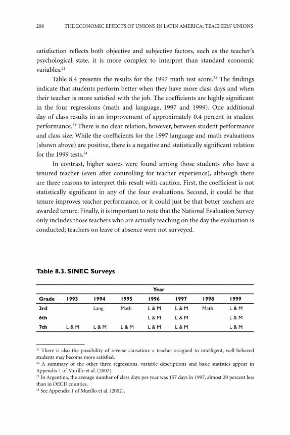
208 THE ECONOMIC EFFECTS OF UNIONS IN LATIN AMERICA: TEACHERS’ UNIONS
satisfaction reflects both objective and subjective factors, such as the teacher’s
psychological state, it is more complex to interpret than standard economic
variables.21
Table 8.4 presents the results for the 1997 math test score.22 The findings
indicate that students perform better when they have more class days and when
their teacher is more satisfied with the job. The coefficients are highly significant
in the four regressions (math and language, 1997 and 1999). One additional
day of class results in an improvement of approximately 0.4 percent in student
performance.23 There is no clear relation, however, between student performance
and class size. While the coefficients for the 1997 language and math evaluations
(shown above) are positive, there is a negative and statistically significant relation
for the 1999 tests.24
In contrast, higher scores were found among those students who have a
tenured teacher (even after controlling for teacher experience), although there
are three reasons to interpret this result with caution. First, the coefficient is not
statistically significant in any of the four evaluations. Second, it could be that
tenure improves teacher performance, or it could just be that better teachers are
awarded tenure. Finally, it is important to note that the National Evaluation Survey
only includes those teachers who are actually teaching on the day the evaluation is
conducted; teachers on leave of absence were not surveyed.
21 There is also the possibility of reverse causation: a teacher assigned to intelligent, well-behaved students may become more satisfied.22 A summary of the other three regressions, variable descriptions and basic statistics appear in Appendix 1 of Murillo et al. (2002).23 In Argentina, the average number of class days per year was 157 days in 1997, almost 20 percent less than in OECD counties. 24 See Appendix 1 of Murillo et al. (2002).
Table 8.3. SINEC Surveys
Year
Grade 1993 1994 1995 1996 1997 1998 1999
3rd Lang. Math L & M L & M Math L & M
6th L & M L & M L & M
7th L & M L & M L & M L & M L & M L & M

WHAT DIFFERENCE DO UNIONS MAKE? 209
Additionally, the sample might have a severe bias. The analysis of the Estatutos
Docentes shows that tenured teachers have an impressive number of leave days
they can take during the year compared to teachers hired on a “temporary” basis.
Thus it can be presumed that being tenured increases a teacher’s likelihood of
being on leave.25 Consequently, while there is evidence that students who have an
active tenured teacher perform better than those who have an active non-tenured
Table 8.4. Regression ResultDependent Variable: log of 1997 mathematics test score (OLS clustered by school)
Variable Coefficient t-value
School
Factors
Class Days 0.004 4.076
Principal tenure (yes=1, no=0) 0.029 1.076
Principal experience 0.012 0.849
Teacher’s
Factors
Job Satisfaction 0.041 2.246
Tenure (yes=1, no=0) 0.018 0.761
Teacher dedication 0.020 0.919
Teacher experience 0.013 1.776
Teacher education 0.011 0.831
Student
and Family
Gender (female=1) -0.019 2.051
Father education -0.002 0.076
Mother education 0.012 3.400
Kindergarten 0.043 2.871
Family size -0.012 2.708
Repeated grade -0.158 12.714
Wealth 0.00002 2.700
Classroom
Factors
Students/Teacher 0.004 1.859
Positive peer effect 0.046 6.211
Negative peer effect (-) -0.015 1.256
Classroom structure 0.008 1.816
Observations 11791
R2 0.14
25 Regrettably, it is impossible to compare the ratio (active tenure teachers / total active teachers) relative to (tenured teachers/total teachers) using census data. The last national survey, conducted in 1994, shows that 57 percent of teachers are tenured. The 1997 and 1999 samples of active teachers show that 61 percent and 53 percent, respectively, of active teachers are tenured.

210 THE ECONOMIC EFFECTS OF UNIONS IN LATIN AMERICA: TEACHERS’ UNIONS
teacher, it cannot be claimed with a high level of confidence that “tenuring”
teachers is an appropriate policy for improving education quality.
Teachers’ Unions
The analysis of the impact of teachers’ unions in Argentina is based on an
understanding of several factors. These include the historical background of
teachers’ unions, the data used, and methods of estimating union influence on the
educational process.
Background
Argentine teachers’ unions, organized mainly at the provincial level, have taken a
very militant stance toward educational administration. Approximately 350,000
teachers are unionized, or 55 percent, representing one of the highest occupational
unionization rates in the country.26 Additionally, teachers’ unions have not only
been active in the development of the education system, but have also organized
more demonstrations and strikes than most other sectors.27
The origins of teachers’ unions can be traced to the end of the nineteenth
century. In 1892 the Liga de Maestros, Argentina’s first teachers’ association, was
established in the province of San Juan. Other provincial teacher associations
followed in Buenos Aires, Córdoba, Tucumán, Mendoza, Corrientes, Santiago del
Estero, Misiones, Entre Rios, Catarmarca and Río Negro; these provincial groups
failed several times to organize a national federation. The first national organization,
the Union of the Argentine Teacher, was created in 1950 under the influence of the
Peronist government and later became the UDA (Union of Argentine Teachers).28
Hence most teachers’ organizations created thereafter emerged in a decentralized
fashion with some exceptions, such as UDA and AMET (Association of Teachers
of Technical Schools), which affiliate teachers under national jurisdiction and had
26 The unionization rate for the whole workforce has been estimated in 28 percent. 27 Among them, the marcha blanca and the carpa blanca had a significant impact. The marcha blanca took place in 1988, and was the major historical teachers mobilization. The carpa blanca was set up by teachers in front of Congress in 1997 to demand a higher public education budget. The carpa blanca influenced political discourse and finally enabled the teachers’ union to participate in the design and congressional approval of an extremely controversial financial law aimed at increasing teachers’ salaries. For a detailed analysis see Behrend (1999).28 See Vásquez and Balduzzi (2000).

WHAT DIFFERENCE DO UNIONS MAKE? 211
a national coverage from the start. A group of 147 provincial unions was founded
in 1973, the Confederation CTERA (Central de Trabajadores de la Educación de
la República Argentina). CTERA is the largest teacher organization in Argentina,
with 200,000 members nationwide. Because CTERA was founded in an attempt to
reduce the fragmentation of the sector, successive mergers reduced the component
unions to a single union per province. This confederation of provincial unions,
which often had different partisan sympathies, opposed the education policies of
both Menem administrations and the Federal Education Law.29 Additionally, the
national leadership has sought collective centralization of demands to negotiate
with the central government and further attempted to implement national
collective bargaining after the approval of new labor relations regulations for the
public sector in 1990.
Table 8.5. Sectoral Union Participation in Total Conflicts
Sector 1996-97 Sector 1990 Sector 1988
Civil Service 25% Teachers 29% Civil Service 26%
Teachers 23% Civil Service 14% Teachers 15%
Transport
workers7% Steelworkers 6% Physicians 4%
Municipal
employees5% Mechanics 4%
Municipal
employees4%
Energy 5%Railway
carmen4%
Railway
carmen3%
Steelworkers 4% Banking 3% Banking 3%
Aeronautics 3% Physicians 3% Health 2%
Banking 3%Paper mill
workers2% Oil workers 2%
Oil workers 3% Port workers 1% Postmen 2%
Mechanics 3% Meat-cutters 1% Port workers 2%
Source: Centro de Estudios para la Nueva Mayoría.
29 CTERA joined the Peronist CGT (General Confederation of Labor) in the mid 1980s after Mary Sánchez, a Peronist leader, won the national elections of the union. However, in 1989, after President Menem abandoned his populist campaign promises, CTERA first joined the anti-government CGT Azopardo and later founded, with other public sector unions, the Congress of Argentine Workers (CTA) with a clear opposition stance. Mary Sánchez left the Peronists and joined a new opposition party.

212 THE ECONOMIC EFFECTS OF UNIONS IN LATIN AMERICA: TEACHERS’ UNIONS
CTERA, however, competes with other unions in almost every province.
Rival provincial unions, together with SADOP (the private teacher’s union), UDA
and AMET have opposed some of CTERA’s strategies. The fragmentation of the
sector was therefore not remedied by CTERA and, at the provincial level, there
are currently more than 150 unions operating in primary and public education.
In addition to political diversity, teachers’ unions present significant differences
across provinces in their density, legal recognition, and political ideology. Table 8.6
presents information on teachers’ unions in the provinces.
Data
This section reviews the principal data sources used in this study to analyze the
impact of teachers’ unions on education in Argentina.30 Of particular interest is
that, despite the limitations of the data, this is the first database of its kind for the
empirical study of teachers’ unions in Argentina. Two sources have been used.
The first is the official record of unions and affiliates provided by the Ministry
of Labor, and the second is the Encuesta de Desarrollo Social, administered by the
Ministry of Social Development.
In the Ministry of Labor’s dataset, the unit of analysis is the union. The
information includes the number of union members, the union’s legal status,
and its jurisdictional coverage. The dataset also provides some information about
how these variables have changed during the last decade. The Ministry of Social
Development’s dataset is drawn from the Encuesta de Desarrollo Social. In this
1997 national household survey, which included more than 70,000 observations,
approximately 1,600 people reported that their occupation was teaching. This
survey makes it possible to determine several characteristics of teachers, including
labor union participation and province of residence. These two datasets, along with
interview-derived information, are used to construct indexes of the characteristics
of teacher unionism in each province.
In order to know teachers’ unions’ objectives and demands, two sources
are used. The first is a review of the corresponding literature on public sector
unionism. The second consists of interviews and unions’ internal documents in
which demands and goals are reported. From those documents it is evident that
their main concern is wages. Low salaries and delays in payment are the most
important issues for teachers’ unions. All of the 15 provincial unions surveyed are
30 Appendix 2 of Murillo et al. (2002) contains additional details.

WHAT DIFFERENCE DO UNIONS MAKE? 213
Table 8.6. Teachers’ Unions (Primary and Public Education, 1999)
Number of
unions
Unions with
personería
gremial
Affiliates*Jurisdictional
coverage
Buenos Aires 96 14 100,965 (P, L)
Catamarca 2 0 2540 (P)
Chaco 9 1 13,856 (P, L)
Chubut 1 1 4,178 P
City of Buenos
Aires8 1 21,299 P
Córdoba 5 2 27,874 (P,L)
Corrientes 4 1 9,075 (P,L)
Entre Rios 1 1 17,651 P
Formosa 6 0 1,718 (P,L)
Jujuy 1 1 3,478 P
La Pampa 1 0 2,785 P
La Rioja 1 0 3,735 P
Mendoza 1 1 11,835 P
Misiones 1 1 6,370 P
Neuquen 1 1 7,492 P
Rio Negro 1 1 8,214 P
Salta 3 1 15,025 P
San Juan 1 1 5,621 P
San Luis 1 0 1,510 P
Santa Cruz 1 1 3,535 P
Santa Fe 1 1 29,344 P
Santiago del
Estero4 1 4,646 P
Tierra del
Fuego1 0 790 P
Tucumán 1 1 8,988 P
Note: P for the province and L for local. (*See note 30 regarding affiliates).Source: Authors’ calculations based on data from Dirección Nacional de Asociaciones Sindicales.

214 THE ECONOMIC EFFECTS OF UNIONS IN LATIN AMERICA: TEACHERS’ UNIONS
concerned about salaries, which represent almost half of total demands reported
by unions. Tenure and job security are also important issues.
Estimating Union Influence
As explained above, a number of institutional features of the education system and
of teacher unionization in Argentina prevent the type of analysis disaggregated at
the level of, say, school or school district, such as has been provided in the United
States. For that reason most of the analysis of the impact of unions is performed
at the provincial level.
The “intermediate variables” that this paper attempts to relate to (provincial
level) union characteristics are variables that: (a) are significant predictors (or possible
determinants of significant predictors) of educational outcomes in the education
production function estimation; and (b) could be related to the theories on union
effects. These include days of class, teacher’s tenure status, class size, and budget
size and composition. Additionally, there is one variable found to be significant in
the education production function, which is teacher satisfaction, for which a more
disaggregated analysis is provided, using a complementary data set.31
Table 8.7. Reported Concerns of Union Members
DemandPercentage of provincial
unions demanding
Percentage of total
demands reported
Salaries 100 % 41 %
Tenuring-absence days 47 % 21 %
Job security 33 % 11 %
Employment 33 % 9 %
Health insurance 20 % 7 %
Unions participation* 33 % 7 %
Teacher training 13 % 5 %
Source: Authors’ calculations based on CTERA (2000), Informe de la Situación en todas las Provincias, which covers 15 provinces.* Includes demands for a higher union participation in the education system, such as collective bargaining and Juntas de Clasificación.
31 There are other channels for union effects such as the Estatutos Docentes and of Juntas de Clasificaciones. Estatutos Docentes are the by-laws ruling labor relations, which define job stability, leaves of absence and so on. These rules are believed to have a large impact on teachers’ incentives, and teachers’ unions report concern about them. The Junta de Calificaciones, where unions have representatives, are the boards in charge of teachers’ evaluation and promotion. These issues are left for further work.

WHAT DIFFERENCE DO UNIONS MAKE? 215
Union Variables
Most of the “intermediate” variables under consideration (days lost, tenure, budget
allocation) are linked to the interaction between unions and their employers—in
the Argentine case, provincial governments. Hence these variables are affected by
characteristics of the unions and by their political relationship to the provincial
government. This chapter considers the impact of union strength, coordination,
legal recognition and political alignment on the (intermediate) dependent
variables under study.
Strength. Measures of both union density (percentage of union members in the
occupational workforce) and of union participation (responses indicating that
teachers have union membership) are considered. Membership or density is a
traditional measure of union strength, which increases not only the effect of work
stoppages but also provides financial resources for the organization (Golden, 1997;
Olson, 1971).
The relationship between union strength and the propensity to strike is not
obvious. Following the Hicks paradox on the impossibility of explaining strikes
when there is complete information, strikes are usually explained as a result of
asymmetric information (Kennan, 1986). In that case, strikes can result from the
search for information by one of two parties. For instance, the union wants to
know how much the employer would give or the employer wants to know the
concession threshold of the union (Hayes, 1984). Tsebelis and Lange (1995) thus
model strikes as “bluffing” from unions that try to secure better conditions from
employers than their real strength would allow. This interpretation also follows
Hicks’s view that the striking union may be trying to maintain a “reputation for
toughness” (Kennan, 1986). In this case, strikes occur when employers try to probe
the union’s real strength. This argument also predicts that the propensity for
strikes should be lower for strong unions, which do not need to bluff, or for weak
unions, which cannot bluff, but higher for those in between. In particular, those
unions whose density is decreasing and whose strength is unclear, but which still
have a reputation for toughness, should be more prone to strike. The alternative
view of strikes is that union strength facilitates collective action and increases the
propensity of the union to strike by increasing its ability to secure concessions by
striking (Franzosi, 1995).
As regards the other dependent variables, the relation between union density
and union demands (such as tenure, budget allocation, and employment) is more

216 THE ECONOMIC EFFECTS OF UNIONS IN LATIN AMERICA: TEACHERS’ UNIONS
straightforward; these are traditional goals of unions. Stronger unions are in a
better position to bargain with the government over these issues, controlling for
other fiscal and legal factors (Freeman and Medoff, 1986).
Fragmentation/Coordination. It can be assumed that coordination is more
complicated when more than a single union has to bargain with the provincial
government. Coordination problems tend to increase the propensity to strike
because they make bargaining more difficult, especially if at least one of the unions
is belligerent (Golden, 1993; Murillo and Maceira, 2000). In this case, although
each union is weak, they are more likely to go on strike because of difficulties
in coordinating negotiations and because they have incentives to appear as more
effective than their rivals in a sector where employees are discontented with
salaries and working conditions. The presence of several unions thus makes
coordination more difficult and weakens their bargaining power. Hence, other
things being equal (such as density, sector, laws), a monopolistic union is stronger
than multiple competing unions in the same sector. For that reason, the demands
of monopolistic unions on tenure, budget allocation, employment and even policy
preferences are more likely to be met. However, their demands or policy preference
can be the result of coordination problems that, combined with different political
alignments, can radicalize the positions of teachers’ unions on policy issues and
make bargaining more difficult.32
Recognition. Also considered is the legal status of the union (if the union is
inscripta or if it has personería gremial). In Argentina, those unions with personería
gremial have several exclusive rights, such as representing all workers in collective
negotiations, enforcing labor legislation and social security regulations, and
cooperating with the government in dealing with problems that affect workers.33
It is therefore presumed that in those provinces where the main teacher union has
personería gremial, the union is more likely to see its demands met.
Political Alignment. The political alignment of teachers’ unions can induce a
propensity to strike by providing national coverage; according to Golden (1997),
32 In the case of very large provinces, unions are discarded that include less than 10 percent of affiliated teachers, because those unions are assumed to be either too small or specialized to guide a coordinated action against the provincial government. 33 Unions that are only inscriptas do not have any of the rights mentioned. They are, however, also allowed to call for strikes and collect contributions from their members.

WHAT DIFFERENCE DO UNIONS MAKE? 217
this makes unions more “strike-prone.” Alternatively, it can influence the union
attitude towards provincial government, on the basis of provincial and national
political dynamics, because of channels of communication and trust based on a
long-term relationship in which previous iterations were beneficial for both parties
(Murillo and Maceira, 2000). This second argument follows the literature on “power
resources” (Korpi, 1978) and the “political exchange” (Pizzorno, 1978)—that is,
the idea that when unions lack political access to an allied government they are
more likely to use measures such as strikes. Hence it can be expected that a positive
political alignment with the government increases trust and communication
between the teachers’ union and the government, facilitating bargaining rather
than striking. It can also influence the attitudes of union leaders and the formation
of preferences regarding policies of uncertain effect, on the basis of the politically
created trust. The opposite is true for the lack of positive political alignments.
In Argentina, membership of CTERA (which rejected President Menem’s
policies at the national level) interacting with a Peronist or conservative government
should increase a union’s propensity to strike. Also explored will be the combination
of political alignment and union fragmentation, following the argument that
when political alignment facilitates trust between the provincial government and
the union, union monopoly induces restraint and negotiation. However, union
fragmentation helps increase conflict even when some of the unions have a good
relationship with the provincial government, because they are afraid of being
labeled as “sell-outs” by rival unions in the eyes of teachers (Murillo and Maceira,
2000). Additionally, the construction of the index of political alignment considered
the diversity in partisan affiliations in CTERA unions across provinces, as well as
the presence of alternative unions and their own political alignments.
Operationalizing the Variables
To summarize, four key features describe the characteristics of teacher unionism
in each province: the number of members, the number of unions, their legal status
and their political relation with the government. Table 8.8 provides a description
of the variables used in the empirical estimation.
Lost Days. The section on EPF estimation describes the impact of class days on
student performance. The relationship between union influence and lost days
is relatively straightforward, as the number of effective class days is affected by
strikes. Although unions organize strikes, they must have a reason to do so. Hence

218 THE ECONOMIC EFFECTS OF UNIONS IN LATIN AMERICA: TEACHERS’ UNIONS
the employer, in this case provincial governments, also has an impact on the
emergence of conflicts in the education sector. For instance, delay in the payment of
salaries provoked the reaction of public sector workers and teachers in many cases,
following the argument that it is not low salaries, but rather the absence of income
that is a source of mobilization (Scott, 1976). Hence the loss of class days results
from the interaction between provincial governments and teachers’ unions; this
effect will be controlled for with variables such as delay in payments. Additionally,
Table 8.8. Union Variables Description
Variable Description Source
ParticipationPercentage of teachers who report
participation in a labor union.Encuesta Desarrollo Social
Membership* Affiliates/Teachers ratio Ministry of Labor
FragmentationNumber of unions per province with
more than 10% of affiliated teachers.Ministry of Labor
Fragmentation II Unions per 10,000 teachers. Ministry of Labor
Recognition
Legal status. Is a dummy variable,
where 1 means that the union has
legal monopoly (personería gremial).
Ministry of Labor
Political
Alignment**
Political alignment between the main
union and the governor. Values range
from to 0 to 1, where 0 means a
highly contentious relationship.
Interviews with union lead-
ers and experts, and press
information
See Appendix 2 of Murillo et al. (2002) for more details.Note: For all the variables the province is the unit of analysis.* One natural measure of union density would have been the members/teachers ratio (membership). However, the official record of members provided by the Ministry of Labor presents several problems: For some unions there is no information about membership; there are also some cases where a single provincial union lists a number of members higher than the total number of provincial teachers. Thus, “participation” is used as a proxy of union den-sity instead of “membership” in the regressions.** In most provinces, there is only one teachers’ union. In those where there are more than one, only the most important union (determined by density and legal status) is considered. Finally, in those provinces where any union could be defined as the main one (such as in Buenos Aires, where two unions have almost equal membership), “Po-litical Alignment” is computed by taking the average political relationship between the governor and the unions.
A value of 1 is assigned to those provinces where the main union is affiliated with CTERA (a founding member of the left wing FREPASO party) and the governor is Peronist or right wing, with the exception of provinces where the union leaders were politically close to the local Peronist party. Conversely, those cases where the governor’s party is center-left (UCR or ALIANZA) and the union is affiliated with CTERA, were assigned lower values ranging from 0.33 to 0.66, depending on how specialists have characterized union leaders local strategy. Finally, a value of 0 is as-signed to those provinces where the main union is not affiliated with CTERA and has a historically close relationship with the ruling local party. Teacher union experts confirmed the coding.

WHAT DIFFERENCE DO UNIONS MAKE? 219
other variables affect the cost of striking and thus the capacity of unions to call for
work stoppages. In particular, attendance bonuses have an impact on the cost for
individual teachers and will be used as control variables.34
Teacher Tenure. According to the results of the EPF, teachers’ tenure has a positive
effect on student performance. Unions generally demand tenure for teachers and,
in fact, “titularización” or “tenuring” is, after wages, the demand most mentioned
by CTERA.35 Unions demand tenure for their members because temporary
employees’ rights are more precarious and there is a difference in the risks they are
willing to run in collective action. Tenure not only benefits temporary teachers;
it also increases homogeneity among union members and reduces the risks of
striking, because it is usually associated with job stability, thus making collective
action easier for unions.
Class Size. Public sector unions have a preference for a larger workforce. Growth
in employment entails a larger constituency to be represented, which can increase
the strength of the union. This is particularly true in a sector characterized by
job stability where salaries are defined in fiscal and political terms rather than
according to productivity, as they are for tradable sectors. Additionally, teachers’
unions have traditionally demanded a low student-teacher ratio to improve the
working conditions of their affiliates. Of present concern is the impact of their
demand for enlarging employment in the education sector, and whether larger
employment results in a smaller student-teacher ratio. That is, if they demand
greater employment but also secure easier conditions for leave or new employment
(which leads to an expansion of administrative positions), the student-teacher
ratio may remains unchanged. The effect of unions on the student-teacher ratio
is therefore tested.
Education Budget. It is not possible to derive a direct effect from the budget
allocation to the education function defined above. The education budget, however,
34 There are significant differences among provinces in this regard. For instance, the attendance bonus in Santa Cruz represents one third of the basic salary, but in Neuquen the bonus does not exist.35 For example, SUTEBA (one of the main teacher’s union in Buenos Aires) claims: “The Ley de Titularización was finally approved. We obtain job security for more than 40,000 teachers in Buenos Aires. It is a triumph for SUTEBA, thanks to the unity and organization of our union. To pass the law we had to confront the government and the provincial legislature, but also the Federación Sarmiento [the other main teacher union in Buenos Aires] who were against the interests of the teachers.” (Authors’ translation from SUTEBA’s web page, www.suteba.org.ar)

220 THE ECONOMIC EFFECTS OF UNIONS IN LATIN AMERICA: TEACHERS’ UNIONS
should have an indirect effect on the learning process. Hoxby (1996) argues that
whether unions perform a rent-seeking role or a collective voice role, they are
always expected to increase the overall budget. Teachers’ unions also affect the
budget composition, pressing for higher wages. Thus, strong unions should lead to
higher education budgets and salaries, or at least to a higher allocation of salaries
in the education budget. Of particular interest is the effect of the present measures
of union characteristics on the expenditures per student in each province, with a
view to assessing their indirect impact on student performance.
Job Satisfaction. According to the results of the education production function,
teachers’ satisfaction has a positive effect on student performance. But what is the
impact of unions on job satisfaction? Unions are supposed to improve the working
conditions of the workers covered, who should therefore express greater satisfaction
with their jobs than do otherwise comparable non-union workers. However, most
empirical studies have found a negative relation between unionized workers and
job satisfaction.36 There might be several reasons for this result. It is important
to note that job satisfaction is a subjective variable, so it is not necessarily related
to the “objective” conditions of each employee relative to others (such as lower
wages or poorer working conditions).37 Freeman and Medoff (1986) argue that
unions galvanize worker discontent in order to make a strong case in negotiations
with management. It is also possible, however, that unionized workers report less
satisfaction because they are truly worse off. As mentioned earlier, these measures of
“unionization” at the individual level might be capturing personal characteristics of
the worker. For instance, teachers who are more prone to conflict and dissatisfaction
may also be more likely to join an organization such as a union.
Expected Results
• More strikes (and fewer class days) are expected in the cases in which
union density is high, in combination with legal recognition and the
36 Freeman (1977), Freeman and Medoff (1986). 37 According to Locke (1976), job satisfaction depends not only on the objective circumstances in which an individual finds himself but also on his psychological state and thus on aspirations, willingness to voice discontent, the hypothetical alternatives to which the current job is compared, and so forth. Kalleberg (1977) provides a similar definition from the sociological perspective. He argues that job satisfaction depends on the personality of the worker and on the nature of the job he performs (which includes wages, fringe benefits, hours of work, degree of control, promotional opportunities and so forth).

WHAT DIFFERENCE DO UNIONS MAKE? 221
lack of political alignment between teachers’ union and the provincial
governor. More strikes are also expected in those provinces where
unionism is fragmented. Membership provides unions with the ability
to call strikes (Franzosi, 1995), whereas union fragmentation and the
lack of political alignment increase incentives for conflict because of
the lack of trust and coordination problems that make negotiation
more difficult.
• As teachers’ unions demand tenure, it is expected that stronger unions
(in terms of density, union monopoly and legal recognition) will be
more effective in achieving tenure for their members.
• Stronger unions are expected to be more able to increase employment
and therefore to reduce class size.
• It is expected that stronger unions in terms of density, union monopoly
and legal recognition have the ability to obtain higher allocations
of the education budget for salaries and higher education budgets.
Positive political alignments should enhance the bargaining power
of monopolistic unions. In contrast, union fragmentation and lower
density are expected to result in lower education budgets and wages.
• There is no particular expectation of the relationship between
union membership and job satisfaction. While unions are supposed
to improve teachers’ working conditions and hence improve their
satisfaction, there are several reasons to expect a negative correlation.
Empirical Results
As discussed above, students’ scores are higher when they have more class days,
when teachers are satisfied with their job, and when teachers have tenure. This
section attempts to provide some new evidence on the relation between teacher
union characteristics and these intermediate outcomes.
Unfortunately there is no dataset containing information on both students’
performance and teachers’ unions in Argentina, but there are also certain
characteristics in the labor relations in education that require a more aggregate
analysis. Therefore an indirect approach, as explained above, is the most appropriate
methodology for exploring the relationship between student performance and
unionism.

222 THE ECONOMIC EFFECTS OF UNIONS IN LATIN AMERICA: TEACHERS’ UNIONS
In addition, factors such as education budgets and teachers’ salaries merit
analysis. These are among the most reported concerns of union members, and it is
presumed that they could have an impact on student performance.38
Lost Days and Strikes
More strikes (and thus fewer class days) are expected in those provinces where
teacher unions are fragmented, and where unions have legal recognition, higher
density, and a contentious relationship with the provincial government. In
addition, attendance bonuses are expected to have a negative effect on strikes, and
payment delays are expected to have a positive effect.
Complete information about teacher strikes in Argentina was not available
before the work for this chapter was begun. On the basis of searching and merging
different sources of information, however, the variable STRIKES was constructed
for the period 1997-1999.39 STRIKESit measures the number of lost days by
province, and by year, as a result of strikes. The variable exhibits high variation
across provinces; in the province of Neuquen, for example, an average of 20 days
per year were lost because of strikes, while in Santa Cruz there were almost no
strikes. Variation over time of provincial averages is lower: the average number of
class days lost as a result of strikes per province was 5.0 during 1997, 4.7 in 1998
and 8.7 in 1999.
Table 8.9 groups the provinces according to the annual average number
of class days lost because of strikes during the period 1997-1999. Higher union
density and a more hostile political relationship with the government is observed
in those provinces with more class days lost.
While the previous table illustrates the potential link between teacher’s
union characteristics and strikes, it is necessary to control the results for other,
presumably important factors such as attendance bonus and payment delays
(Delays).40 Table 8.10 reports the results of pooled provincial regressions.41
38 The last link is an issue that needs further work. Intuitively, it seems obvious that higher expenditure per pupil should improve performance, but if the quality of education is inadequate, increasing expenditures should not necessarily improve performance (IDB, 1996). In Argentina, it is also not obvious that higher wages would improve teachers’ effort and productivity, since there are several barriers that restrict the selection of teachers. 39 For more details, see Appendix 2 of Murillo et al. (2002).40 Regrettably, there are no data on wage payment delays for public sector teachers. On the basis of discussions with union leaders and public officials, the number of provincial civil service strikes is used as a proxy for payment delays.41 Panel data specifications are discarded since most of the explanatory variables do not change over time.

WHAT DIFFERENCE DO UNIONS MAKE? 223
There is evidence suggesting that higher density, union fragmentation and
a hostile political relation with the government result in more strikes.42 A 10
percentage-point increase in union density results in a reduction of 4 class days.
In those provinces where there are two unions, students have 1.2 fewer class days
compared to those provinces with only one union. Finally, in those provinces
where there is a highly hostile political relationship between the governor and
teachers’ unions, there are 4.1 fewer class days than in those provinces with no
conflict.
Table 8.9. Class Days Lost from Strikes
Provinces grouped
by number of
class days lost
from strikes
Average
number of
days lost
Teachers
participation
rate
Union
fragmentation
Political
alignment
Less than 3 days 1.2 3.1 1.3 0.44
Between 3 and 10 4.8 4.3 1.6 0.39
More than 10 days 17.6 7.2 1.4 0.18
Source: CEDI.
Table 8.10. Regression ResultDependent variable: STRIKES. OLS robust
Variable Coefficient t-value
Participation 0.40 2.53
Union Fragmentation 1.24 2.79
Recognition 0.54 0.45
Political alignment -4.12 -2.96
Delay 0.77 8.92
Attendance bonus -0.22 -3.58
Constant -1.74 -0.99
R-adjusted 0.90
Observations 24
42 The coefficient for “recognition” is positive but not significant.

224 THE ECONOMIC EFFECTS OF UNIONS IN LATIN AMERICA: TEACHERS’ UNIONS
Taking into account the positive effect that class days have on student
performance, there is reason to criticize the role unions play. Union leaders
nonetheless argue that strikes are an instrument for improving teachers’ working
conditions and increasing the education budget, and consequently could lead to a
better education system. While the validity of this claim could not be determined,
the results show that the means unions use to obtain their demands have negative
effects on students learning.
There is also evidence that attendance bonus and payment delays are
significant factors in explaining strikes. The variable “Delay” is clearly the most
important explanatory variable in the regression, since most of the variation in
strikes across provinces is explained by payment delays.43 Thus the government
could reduce the number of class days lost by paying wages on time.
Tenure44
Unions report an important concern with “tenuring” and therefore a higher
proportion of tenured teachers (compared to suplentes and interinos) is
expected in those provinces where unionism is “stronger” (higher density, lower
fragmentation and legal recognition). As to the link between tenure and union
political alignment, governors who have a more contentious political relationship
with unions are considered to be less likely to accept unions’ demands, leading to
a lower number of tenured teachers.
Regrettably, reliable data on teacher tenure is available only for 1994, so strong
evidence cannot be provided on the relation between union characteristics and
43 When “delay” is taken out of the regression, the R-adjusted reduces to 0.54.44 In Argentina, teacher’s tenuring is regulated by the Estatutos Docentes and undertaken on an individual basis. The procedure is quite similar across provinces. Only those teachers who satisfy certain conditions, such as age, education, and training courses—and in some cases only those who pass an examination—can be tenured. In some provinces, the Junta de Calificaciones (where unions have representatives) are the boards in charge of the evaluation. However, this mechanism is usually delayed as a consequence of bureaucratic procedures or political convenience. As a matter of fact, a significant proportion of teachers have been tenured through a different mechanism: Leyes de Titularización (“Tenuring Laws”). These laws apply to hundreds or even thousands of teachers at the same time and do not require teachers to fulfill any condition (such as age or education) in order to be tenured. Tenuring laws are usually a consequence of the pressure exercised by teacher unions on the provincial government (see note 33). It is presumed that those teachers who have been awarded tenure through the first mechanism might be the best teachers, but that might not be the case for those teachers who have been tenured through the “tenuring laws.” In order to analyze the impact that unions have on the “tenuring” process, it is necessary to consider their effect on both the Juntas de Clasificación and the legislative process (Tenuring Laws). This issue is left for further work.

WHAT DIFFERENCE DO UNIONS MAKE? 225
tenure.45 Table 8.11 correlates the variable TENURE with different characteristics
of unions.46
The results are neither robust nor clear. Political Alignment and Legal
Recognition are positively associated with TENURE as expected, but only the
last coefficient is clearly different from zero. Union fragmentation and density
are negatively or positively correlated with TENURE depending upon the proxy
used.
Class Size
Teacher unions bargain for higher employment and therefore a lower number
of students per teacher is expected in those provinces where unions have higher
density and lower fragmentation. These expectations seem to be borne out by the
data, as shown in Table 8.12. Teacher union characteristics are probably important
in explaining the student-teacher ratio but other variables should be considered,
such as the provincial fiscal situation or regional per capita GDP.
With respect to the econometric specification, the same methodology is
applied as that used in the STRIKES regression (pooling the original panel across
provinces). All the coefficients have the expected sign, but none of the union
variables is significant at a 90 percent level of confidence. In fact, only union
fragmentation is significant at an 85 percent level of confidence: provinces where
45 See Table 21 in Appendix 2 of Murillo, Tommasi, Ronconi and Sanguinetti (2002).46 TENURE is defined as the percentage of tenured teachers over the total number of teachers in each province.
Table 8.11. Tenure and Unions CharacteristicsCorrelation Coefficient
Unions Characteristics TENURE
Membership 0.11
Participation -0.26
Fragmentation 0.15
Fragmentation II -0.45
Recognition 0.49
Political alignment 0.07

226 THE ECONOMIC EFFECTS OF UNIONS IN LATIN AMERICA: TEACHERS’ UNIONS
there is only one union have a lower number of students per teacher. Most of the
variation across provinces is explained by GDP per capita: richer provinces have
more teachers per student.
In brief, there is only weak evidence to support the proposition that those
provinces where teacher unions are “stronger” also tend to have a lower number
of students per teacher. Since a previous section explored the relation between
class size and student performance and did not find any clear pattern, no effect of
unions on performance through this channel can be claimed.
Budget, Composition and Wages
It is expected that stronger unions in terms of density, legal recognition and
monopoly have the ability to secure higher education budgets and a higher
allocation of the budget to salaries. Provincial education budgets also depend on
local revenues, but as Sanguinetti, Sanguinetti and Nicolini (2000) argue, national
transfers to the provinces are also important, since the federal co-participation
regime is highly redistributive.
Three regressions are run in order to explore these issues. In the first, the
dependent variable is the log of public expenditure on education per student.
The second looks at the share of public education spent on wages, and the third
explores variation in teachers’ wages (relative to the average provincial income)
across provinces. The first and third regressions use means from panel data for
the period 1997-1999. The second regression is based on information for a single
year (1997).
Table 8.12. Class Size and Unions Characteristics
Provinces grouped
according to the students
per teacher ratio
Average number
of students per
teacher
Union Density
(participation)
Union
Fragmentation
Less than 15 students per
teacher13.4 6.5% 1.2
Between 15 and 18 16.6 3.2% 1.1
More than 18 19.4 3.7% 1.9
Note: Provinces are grouped according to the average number of students per teacher during the period 1997-1999.Source: CEDI.

WHAT DIFFERENCE DO UNIONS MAKE? 227
Table 8.13. Regression Results Dependent Variable: Students/Teachers. OLS robust*
Variable Coefficient t-value
Participation -0.08 -0.62
Fragmentation 0.89 1.52
Recognition -0.06 -0.06
Political alignment 1.46 0.95
GDP per capita -0.001 -4.47
Public Expenditure p/c -322.5 -0.32
Constant 20.3 8.15
R2 0.42
Observations 24
*Variables description and basic statistics are in Appendix 2 of Murillo et al. (2002).
Table 8.14. Regression ResultsDependent Variable: Educational Expenditure and Wages. OLS Robust (t-statistics in parentheses)
Variable
Public expenditure
on education per
student
Share of public
education spent on
wages
Teachers’ Wages
(relative to average
income)
Participation-0.001 0.003 -0.484
(-0.18) (1.07) (-0.46)
Fragmentation0.038 0.014 2.296
(0.71) (0.85) (0.25)
Recognition-0.185 0.058 21.74
(-1.68) (1.89) (1.22)
Political
Alignment
-0.071 0.011 -2.448
(-0.45) (0.28) (-0.84)
Local
Revenues
0.417 -0.052 3.600
(8.38) (-4.33) (0.56)
National
Transfers
0.193 0.070 43.13
(1.92) (2.84) (3.06)
Constant3.603 0.618 -194.8
(4.28) (2.82) (-1.49)
R2 0.85 0.61 0.45
Observations 24 24 24

228 THE ECONOMIC EFFECTS OF UNIONS IN LATIN AMERICA: TEACHERS’ UNIONS
The findings show that public education expenditure per student is higher
in those provinces where local revenues and national transfers are higher. None of
the teachers’ unions variables is statistically significant, and they have the opposite
sign of those expected. As expected, however, those provinces where teacher unions
have higher density and legal recognition have a higher share of the education
budget allocated to wages; only “Recognition” is significant at a 90 percent level.
Regarding the fiscal variables, national transfers have a positive and significant
coefficient, but local revenues have a negative effect.
Finally, there is no statistically significant relation between teachers’
unions and teacher wages (relative to the average provincial income). The only
significant factor is national transfers, which have a positive effect. This leads to
the following interpretation. Provinces that are more fiscally responsible (collect
more taxes) tend to have higher expenditures per student, and a smaller share of
that money goes to salaries. Provinces that are more generously treated by the
federal government have higher expenditure per student, but more of this money
goes to salaries, as those provinces have higher teacher wages. Provincial teacher
unions are basically irrelevant, except that they increase the share of salaries in the
education budget.47
Job Satisfaction
The results of the education production function estimation indicate that
the more satisfied the teacher is, the better students perform. There is also the
presumption that teachers’ job satisfaction and union membership are related, so
it could be argued that unions affect students performance through their impact
on teachers’ job satisfaction. From a theoretical perspective, however, the relation
between unions and satisfaction is unclear. Since the aim of this study is to provide
new evidence of the relation between unions and student performance, empirical
analysis rather than theoretical discussion will be emphasized.
The Encuesta de Desarrollo Social (EDS) provides a useful micro dataset
to explore these issues. It contains information for 1,534 teachers spread across
all the provinces. The data include whether a teacher participates in a labor
union, whether the teacher is satisfied with his or her job, and other important
characteristics such as gender, age, income and education. As shown in Table 8.15,
47 This does not mean that teachers’ unions have no impact. Actually, they exert strong pressure for higher wages and budgets, but they have done so in a centralized fashion.

WHAT DIFFERENCE DO UNIONS MAKE? 229
job satisfaction and union participation appear to be negatively correlated. While
12.7 percent of the “dissatisfied” teachers participate in a labor union, only 7.6
percent of the satisfied teachers are union members.
Regrettably, there is not enough information available to determine the
temporal relation between job satisfaction and participation. In other words, it
could not be discerned whether job dissatisfaction was a consequence of union
participation or whether dissatisfaction preceded the decision to participate in
a union. Consequently, the data are not well suited to analyze what this negative
correlation means. As mentioned, there are at least three possible explanations
for this pattern. The first is the “voice” argument provided by Freeman and
Medoff (1986). The second is that unions worsen teachers’ working conditions.
The third possibility is that a negative relation between job satisfaction and union
participation might be capturing unobserved personal characteristics of the
teacher. For instance, teachers who are more prone to conflict and dissatisfaction
may also be more likely to join an organization such as a labor union.
From the evidence available, it seems that that the second hypothesis
should be discarded (as shown, unions seem to increase teachers’ wages and
Table 8.15. Job Satisfaction and Union Participation
Are you satisfied with your job?
YES (JS=1) NO (JS=0)
Union Member 7.6 % 12.7 %
Non-Member 93.4 % 87.3 %
Source: EDS.
Table 8.16. Job Satisfaction and Participation in Ecological or Human Rights Groups
Are you satisfied with your job?
YES (JS=1) NO (JS=0)
Participates 2.1 % 1.4 %
Does not participate 97.9 % 98.6 %
Source: EDS.

230 THE ECONOMIC EFFECTS OF UNIONS IN LATIN AMERICA: TEACHERS’ UNIONS
employment).48 The validity of the third hypothesis is explored by analyzing
the relation between union participation and satisfaction, controlling for
participation in other organizations such as ecological or human rights groups.49
A very low rate of participation in these organizations is found, with a slightly
higher rate among satisfied teachers. Hence the third hypothesis might not be
an appropriate explanation for the negative relation found between satisfaction
and union participation. Since it is not possible to solve the endogeneity problem
between “participation” and job satisfaction (JS), the partial correlation between
JS and union participation is examined, “controlling” for age, gender, the teacher’s
education, income and participation in ecological or human rights groups.
There is a negative and significant relation between job satisfaction and
union participation. It is also observed that the negative relation found in column
1 does not disappear after controlling for participation in ecological or human
rights groups (column 2). This result is interpreted as evidence against the third
hypothesis. As a very first approximation, therefore, it is concluded that the “voice”
Table 8.17. Partial Correlation Coefficients of Job Satisfaction
Column 1 Column 2
Variables Correlation Significance Correlation Significance
Union Participation -0.05 0.04 -0.05 0.03
Participation in
ecological or human
rights groups
0.02 0.54
Age 0.07 0.01 0.07 0.01
Gender (female=0) -0.02 0.54 -0.02 0.53
Teacher’s Education 0.01 0.95 0.01 0.97
Teacher’s Income 0.07 0.00 0.07 0.00
Nº Observations 1,517 1517
Source: Authors’ calculations.
48 Although that might possibly come at the expense of dissatisfaction along other dimensions; alternatively, unions might raise expectations and demand levels, widening the gap between expectations and actual working conditions.49 Perhaps a better control would be how happy the person is overall, or outside of work. Regrettably, this information is not available. People who join organizations such as ecological or human rights groups, however, may also be more prone to express discontent, and this could provide a good control to explore the validity of the third hypothesis.

WHAT DIFFERENCE DO UNIONS MAKE? 231
hypothesis presented by Freeman is possibly the best argument to explain the
negative relation found between job satisfaction and union membership.
Conclusion
This paper constitutes a first look at the effects of trade unions on the education
sector in Argentina, providing new information and preliminary results on some
of the channels of union influence on the performance of this crucial sector.50 The
next few paragraphs highlight some of these main channels.
First, union characteristics have an important effect on days of class lost to
strikes. Days lost are also related to fiscal problems and delayed payment of wages
by provincial authorities. Furthermore, the nature of the political relationship
between unions and provincial authorities is a factor influencing strike activity. As
the number of class days is one of the stronger explanatory variables for student
learning, there is reason to criticize unions in this regard. However, union leaders
argue that strikes are an instrument for improving teachers’ working conditions,
increasing education budgets and consequently improving education outcomes.
While the present results do not confirm or refute this claim, they show that the
means unions use to ensure their demands are met have strong and negative effects
on student learning.
It is also found that unions report a great deal of concern with tenuring
teachers, since student learning improves when the teacher in front of the class
is tenured. Since tenuring also seems to increase absenteeism, however, it might
reduce the actual number of tenured teachers in front of the class, with an uncertain
net effect on student learning. As to public expenditure on education and teachers’
salaries, there is not a strong union effect, except that they increase the share of
salaries in the education budget. Budgets and salaries are mainly determined by
fiscal variables. Finally, there is evidence that union strength is positively correlated
with lower student-teacher ratios, and that union participation and job satisfaction
are negatively correlated.
In summary, the impact of unions on students’ performance depends on
the channel and kind of political market in which unions operate, but not on the
presence of unions per se. There are, however, some limitations to this analysis.
50 It is worth noting at this point that there appear to be broader “political” factors not considered in this analysis, which might have a bigger impact than union activity on the quality of education in Argentina.
232 THE ECONOMIC EFFECTS OF UNIONS IN LATIN AMERICA: TEACHERS’ UNIONS
Only the effect of cross-provincial union characteristics on education outcomes
has been considered, and this may understate the total effects of teachers’ unions,
since much of their activity operates at the national level, by influencing national
legislation, overall budgets and other outcomes. Additionally, there is an “intercept”
of union influence in the weakest-union province, which is not estimated; only the
marginal effect of additional union strength in cross-provincial comparisons is
considered. This “lower bound” in turn is also related to national level factors. For
example, legislation such as the Estatutos Docentes (which is uniformly supported
by teacher unions throughout the country) has its historical origin in national
legislation and is believed to have strong negative incentive effects. Exploration of
these issues is left for future work.

BIBLIOGRAPHY
Abowd, J.M. 1989. “The Effect of Wage Bargains on the Stock Market Value of the
Firm.” American Economic Review 79(4): 774-809.
Abowd, J.M., and L. Allain. 1996. “Compensation Structure and Product Market
Competition.” NBER Working Paper 5493. Cambridge, United States:
National Bureau of Economic Research.
Abowd, J.M., and T. Lemieux. 1991. “The Effects of International Competition on
Collective Bargaining Outcomes: A Comparison of the United States and
Canada.” In: J.M. Abowd and R. B. Freeman, editors. Immigration, Trade,
and the Labor Market. Chicago, United States: University of Chicago Press.
Addison, J., and B. Hirsch. 1989. “Union Effects on Productivity, Profits and
Growth: Has the Long Run Arrived?” Journal of Labor Economics 7: 72-
105.
Albizures, M.A. 2001. Personal interview, Guatemala City, March 8.
Amadeo, E.J., and V. Pero. 2000. “Adjustment, Stabilization and the Structure of
Employment in Brazil.” Journal of Development Studies 36(4): 120-148.
Arbache, J. 1999. “Do Unions Always Decrease Wage Dispersion? The Case of
Brazilian Manufacturing.” Journal of Labor Research 20(3): 425-36.
Arellano, M. 1988. “An Alternative Transformation for Fixed Effects Models with
Predetermined Variables.” Oxford University Applied Economics Discussion
Paper 57. Oxford, United Kingdom: Oxford University.
Arellano, M., and C. Alonso-Borrego. 1999. “Symmetrical Normalized Instrumental
Variables Estimation Using Panel Data.” Journal of Business and Economic
Statistics 17(1).
Arellano, M., and S. Bond. 1991. “Some Tests of Specification for Panel Data: Monte
Carlo Evidence and an Application to Employment Equations.” Review of
Economic Studies 58: 277-297.
----. 1998. “Dynamic Panel Data Estimation Using DPD98 for Gauss.” London,
United Kingdom: Institute for Fiscal Studies. ftp://ftp.cemfi.es/pdf/papers/
ma/dpd98.pdf
Arellano, M., and O. Bover. 1990. “Panel Data Econometrics.” Investigaciones
económicas, Segunda época, 14(1): 3-45.
Ashenfelter, O., and G.E. Johnson. 1969. “Bargaining Theory, Trade Unions and
Industrial Strike Activity.” American Economic Review 59(4): 35-49.

234 BIBLIOGRAPHY
Ashenfelter, O., and J. Pencavel. 1969. “American Trade Union Growth: 1900-1960.”
Quarterly Journal of Economics 83(3): 434-48.
Asociación Nacional del Café (ANACAFE). 1997. Los Cafés de Guatemala: Tradición,
Desarrollo e Identidad. Guatemala City, Guatemala: ANACAFE.
Balbi, C. 1996. “Sindicalismo y flexibilización en el mercado de trabajo en el Perú.”
Debates en Sociología 19.
Banco de Guatemala (BANGUAT). Various years. Statistical Bulletins. Guatemala
City, Guatemala: BANGUAT.
Banco Interamericano de Desarrollo (BID). 1996. Cómo Organizar con Éxito los
Servicios Sociales. Informe de Progreso Económico y Social en América Latina.
Washington, DC, United States: BID.
Banco Mundial. 1999. “Estudio Sectorial sobre Financiamiento Educativo y
Educación Rural en el Perú.” Washington, DC, United States: Banco Mundial.
Draft document.
Barillas, E. 1997. El Problema del Indio durante la Época Liberal. Guatemala City,
Guatemala: Universidad de San Carlos de Guatemala, Escuela de Historia,
Instituto de Investigaciones Históricas, Antropológicas y Arqueológicas.
Batres García, A.R.C. 1980. “Importancia del Café en la Economía de Guatemala.”
Guatemala City, Guatemala: Universidad de San Carlos de Guatemala,
Facultad de Economía. Thesis.
Behrend, J. 1999. “The Carpa Blanca, Civil Society and Democratic Process: A
Study of Teachers’ Protests and Political Response in Argentina, 1997-1999.”
Oxford, United Kingdom: Oxford University, St. Anthony’s College. M.Phil
thesis.
Belman, D. 1992. “Unions, the Quality of Labor Relations and Firm Performance.”
In: L. Mishel and P. Voos, editors. Unions and Economic Competitiveness.
Armonk, United States: M.E. Sharpe.
Berlinski, J. 2000. “International Trade and Commercial Policies of Argentina:
An Overview of Selected Evidence and Issues of the 20th Century.” Buenos
Aires, Argentina: Universidad Torcuato di Tella. Mimeographed document.
Bernedo, J. 1994. “Sindicatos: Razones para el optimismo.” Cuadernos Laborales
(Lima) 100.
----. 1998. “La difícil encrucijada laboral peruana.” Análisis Laboral (Lima) No.
255.
Binmore, K. 1982. “Perfect Equilibria in Bargaining Models.” London, United
Kingdom: London School of Economics. Mimeographed document.

WHAT DIFFERENCE DO UNIONS MAKE? 235
Binmore, K., A. Rubinsten and A. Wolinsky. 1986. “The Nash Bargaining Solution
in Economic Modelling.” Rand Journal of Economics 17(2): 176-88.
Black, S., and L. Lynch. 1997. “How to Compete: The Impact of Workplace Practices
and Information Technology on Productivity.” NBER Working Paper 6120.
Cambridge, United States: National Bureau of Economic Research.
----. 2000. “What’s Driving the New Economy: The Benefits of Workplace
Innovation.” NBER Working Paper 7479. Cambridge, United States:
National Bureau of Economic Research.
Blanchflower, D. and R.B. Freeman. 1992. “Unionism in the United States and
Other Advanced OECD Countries.” Industrial Relations 31(1): 56-79.
Blundell, R., and A. Bond. 1998. “Initial Conditions and Moment Restrictions in
Dynamic Panel Data Models.” Journal of Econometrics 87: 115-43.
Boal, W.M. and J.H. Pencavel. 1994. “The Effects of Labor Unions on Employment,
Wages and Days of Operation: Coal Mining in West Virginia.” Quarterly
Journal of Economics 109(1): 267-98.
Booth, A.L. 1985. “Estimating the Probability of Trade Union Membership: A
Study of Men and Women in Britain.” Economica 53: 41-61.
----. 1995. The Economics of the Trade Union. New York, United States: Cambridge
University Press.
Borjas, G. J. 1979. “Job Satisfaction, Wages, and Unions.” Journal of Human
Resources 14(1): 21-40.
Boubakri, N., and J-C. Cosset. 1998. “The Financial and Operating Performance
of Newly Privatized Firms: Evidence From Developing Countries.” Journal
of Finance 53: 1081-1110.
Boza, G., and M. Canessa. 2000. “Relaciones colectivas de trabajo: Entre la
flexibilidad y el intervencionismo estatal.” In: ETM Países Andinos. Estudios
sobre la flexibilidad en el Perú. Lima, Peru: Organización Internacional del
Trabajo.
Bracey, G. 1998. “The Eighth Bracey Report on the Condition of Public Education.”
Phi Delta Kappan 80(2): 121-131.
Bronars, S.G., and D.R. Deere. 1990. “Union Representation Elections and Firm
Profitability.” Industrial Relations 29(1): 15-37.
Brown, C., and J. Medoff. 1978. “Trade Unions in the Production Process.” Journal
of Political Economy 86(3): 355-78.
Brown, J., and O. Ashenfelter. 1986. “Testing the Efficiency of Employment
Contracts.” Journal of Political Economy 94(3/Part 2, Special Issue): S40–
S87.

236 BIBLIOGRAPHY
Brown, W., and P. Ryan. 1998. “Decentralized Pay Setting and Productivity:
Issues and Evidence.” Cambridge, United Kingdom: Cambridge University.
Mimeographed document.
Budd, J., and I-G. Na. 2000. “The Union Membership Wage Premium for Employees
Covered by Collective Bargaining Agreements.” Journal of Labor Economics
18(4): 783-807.
Calmfors, L., and E.J. Driffill. 1988. “Bargaining Structure, Corporatism and
Macroeconomic Performance.” Economic Policy 6: 13-62.
Carruth, A., and A.J. Oswald, 1987. “On Union Preferences and Labour Market
Models: Insiders and Outsiders.” Economic Journal 97: 431-45.
Casacuberta, C. 1994. “Insiders, Unions and Market Power in Wage Setting in
Uruguay.” London, United Kingdom: London School of Economics. M.Sc.
dissertation.
Cassoni, A., S. Allen and G. Labadie. 1996. “Wages and Employment after
Reunionization in Uruguay.” Cuadernos de Economía 99: 277-294.
----. 2000a. “Unions and Employment in Uruguay.” Research Network Working
Paper R-392. Washington, DC, United States: Inter-American Development
Bank, Research Department.
----. 2000b. “The Effects of Unions on Employment: Evidence from an Unnatural
Experiment in Uruguay.” NBER Working Paper 7501. Cambridge, United
States: NBER.
Cassoni, A., and G.J. Labadie. 2001. “The Outcome of Different Bargaining Models:
Its Effects on Wages, Employment and the Employment Mix.” Montevideo,
Uruguay: Universidad de Uruguay and Grupo de Estudios de Economía,
Organización y Políticas Sociales. Mimeographed document.
Cassoni, A., G.J. Labadie and S. Allen. 1995. “Uruguay.” In: G. Márquez, editor.
Reforming the Labor Market in a Liberalized Economy. Washington, DC,
United States: Inter-American Development Bank, Centers for Research in
Applied Economics.
Cassoni, A., G. J. Labadie, and G. Fachola. 2002. “The Economic Effects of Unions
in Latin America: Their Impact on Wages and the Economic Performance
of Firms in Uruguay.” Latin American Research Network Working Paper R-
466. Washington, DC, United States: Inter-American Development Bank,
Research Department.
Cassoni, A., and Z. Ferre. 1997. “Non-Wage Costs in the Uruguayan Labor
Market.” Working Paper 8/97. Montevideo, Uruguay: University of Uruguay,
Department of Economics.

WHAT DIFFERENCE DO UNIONS MAKE? 237
Centro de Investigaciones Económicas Nacionales (CIEN). 1999. Líneamientos
de Política Económica y Social para Guatemala, 2000-2003. Guatemala City,
Guatemala: CIEN.
----. 2000. “Reformas Laborales.” Carta Económica (213). Guatemala City,
Guatemala: CIEN.
Ceto, P. 2001. Personal interview, Guatemala City, Guatemala, March 15.
Chiang, A.C. 1984. Fundamental Methods of Mathematical Economics. New York,
United States: McGraw-Hill/Irwin.
Clark, K.B. 1980. “Unionization and Productivity: Microeconometric Evidence.”
Quarterly Journal of Economics 95: 613-39.
----. 1984. “Unionization and Firm Performance: The Impact on Profits, Growth,
and Productivity.” American Economic Review 74(5): 893-919.
Cochrane, D., and G.H. Orcutt. 1949. “Application of Least-Squares Regressions
to Relationships Containing Autocorrelated Error Terms.” Journal of the
American Statistical Association 44: 32-61.
Código de Trabajo, Decreto 1441 del Congreso de la República y sus reformas,
Guatemala, 1961
Comisión para el Esclarecimiento Histórico. 1999. “Guatemala, Memoria del
Silencio.” Guatemala City, Guatemala: Oficina de Servicios para Proyectos
de las Naciones Unidas (UNOPS).
Confederación de Trabajadores de la Educación de la República Argentina
(CTERA). 2000. “Informe de la Situación en todas las provincias.” Buenos
Aires, Argentina: CTERA. Mimeographed document.
Consejo Nacional de Planificación Económica, Secretaría General. 1984.
Agricultura de Exportación, Población y Empleo en la Costa Sur. Guatemala
City, Guatemala: Jefatura de Estado.
Contreras, C. 2001. Personal interview, Guatemala City, Guatemala, March.
Corrales, J. 1998. “The Politics of Education Reform Implementation: Bolstering
the Supply and Demand, Overcoming Institutional Blocs.” Amherst, United
States: Amherst College. Mimeographed document.
Cossa, R. 2000. “Determinants of Schooling Attainment in Argentina: An Empirical
Analysis with Extensions to Policy Evaluation.” Chicago, United States:
University of Chicago. Mimeographed document.
Davidson, C. 1988. “Multi-Unit Bargaining in Oligopolistic Industries.” Journal of
Labor Economics 6: 397-422.

238 BIBLIOGRAPHY
De Brun, J., and G.J. Labadie. 1997. “Mercado Laboral, Apertura y Recesión:
La Experiencia Uruguaya de los Noventa.” In: Centro Interdisciplinario
de Estudios sobre el Desarrollo Latinoamericano (CIEDLA). Mercados
Laborales en los ’90: Cinco Ejemplos de América Latina. Buenos Aires,
Argentina: CIEDLA.
De León, J.C. 1989. La Dinámica del Movimiento Sindical Guatemalteco. Guatemala
City, Guatemala: Asociación de Investigación y Estudios Sociales (ASIES)/
Editorial Piedra Santa.
Díaz, H., and J. Saavedra. 2000. “La Carrera de Maestro: Factores Institucionales,
Incentivos Económicos y Desempeño.” Research Network Working Paper
R-410. Washington, DC, United States: Inter-American Development Bank,
Research Department.
Dobson, P. 1994. “Multi-Firm Unions and the Incentive to Adopt Pattern
Bargaining in Oligopoly.” European Economic Review 38(1): 87-100.
Doiron, D., and W.C. Riddell. 1993. “The Impact of Unionization on Male-Female
Earnings Differences in Canada.” Journal of Human Resources 29(2): 505-
534.
Dow, G.K. 1993. “Why Capital Hires Labor: A Bargaining Perspective.” American
Economic Review 83: 118-134.
Dowrick, S. 1989. “Union-Oligopoly Bargaining.” Economic Journal 99(127): 1123-
42.
Driffill, J., and F. van der Poeg. 1995. “Trade Liberalization with Imperfect
Competition in Goods and Labor Markets.” Scandinavian Journal of
Economics 97: 223-243.
Duncan, G. 1985. “The Endogeneity of Union Status: An Empirical Test.” Journal
of Labor Economics 3(3): 385-402.
Eaton, A., and P. Voos. 1992. “Unions and Contemporary Innovations in Work
Organization, Compensation, and Employee Participation.” In: L. Mishel
and P. Voos, editors. Unions and Economic Competitiveness. Armonk, United
States: M.E. Sharpe.
Ellwood, D. 1987. “The Impact of Right-to-Work Laws on Union Organizing.”
Journal of Political Economy 95(2): 250-73.
Ermida, O., G. Cedrola, J. Raso et al. 1998. “Estructura y Contenido de la
Negociación Colectiva en Uruguay.” Lima, Peru: Organización International
de Trabajo. Mimeographed document.

WHAT DIFFERENCE DO UNIONS MAKE? 239
Eskeland, G., and D. Filmer. 2000. “Does Decentralization Improve Learning?
Autonomy and Parental Participation in Argentine Schools.” Washington,
DC, United States: World Bank. Mimeographed document.
Even, W.E., and D.A. Macpherson. 1993. “The Decline of Private-Sector Unionism
and the Gender Wage Gap.” Journal of Human Resources 28(2): 281-296.
----. 1991. “Plant Size and the Decline of Unionism.” Economics Letters 32: 393-
398.
Fallick, B., and K. Hassett. 1999. “Investment and Union Certification.” Journal of
Labor Economics 17(3): 570-82.
Farber, H. 1983. “The Determination of the Union Status of Workers.” Econometrica
51: 1417-1437.
----. 1984. “Right-to-Work Laws and the Extent of Unionization.” Journal of Labor
Economics 2(3): 319-52.
Fernández Molina, L. 1996. Derecho Laboral Guatemalteco. Guatemala City,
Guatemala: Editorial Oscar de León Palacios.
Fiszbein, A. 1999. “Institutions, Service Delivery and Social Exclusion: A case Study
of the Education Sector in Buenos Aires.” Documento de Trabajo 35. Buenos
Aires: Argentina: CEDI, Fundación Gobierno y Sociedad.
Flanagan, R. 1993. “Can Political Models Predict Union Behavior?” In: R.
Flanagan, K.O. Moene and M. Wallerstein, editors. Trade Union Behavior,
Pay Bargaining and Economic Performance. Cambridge, United Kingdom:
Clarendon Press.
Forteza, A. 1992. “Los convenios salariales de 1990 y la inflación.” SUMA 7(12):
7-36.
Franzosi, R. 1995. The Puzzle of Strikes: Class and State Strategies in Postwar Italy.
Cambridge, United Kingdom: Cambridge University Press.
Freeman, R. 1977. “Job Satisfaction as an Economic Variable.” NBER Working Paper
225. Cambridge, United States: National Bureau of Economic Research.
----. 1986. “The Effects of the Union Wage Differential on Management Opposition
and Union Organization Success.” American Economic Review 76: 92-96.
Freeman, R.B., and J.L. Medoff. 1979. “The Two Faces of Unionism.” Public Interest
57: 69-93.
----. 1984. What Do Unions Do? New York, United States: Basic Books.
----. 1994. “American Exceptionalism in the Labor Market: Union-Non-Union
Differentials in the U.S. and Other Countries.” In: C. Kerr and Paul Staudohar,
editors. Labor Economics and Industrial Relations, Markets and Institutions.
Cambridge, United States: Harvard University Press.

240 BIBLIOGRAPHY
Freeman, R.B., and J. Rogers. 1993. “Who Speaks for Us? Employee Relations
in a Non-Union Market.” Employee Representation: Alternatives and
Future Directions. Madison, United States: Industrial Relations Research
Association (IRRA).
Galbraith, J. 1969. The Affluent Society. Boston, United States: Houghton Mifflin.
Gárate, W. 1993. El sindicalismo a inicios de los noventa: Una aproximación
cuantitativa. Lima, Peru: ADEC-ATC
Garza Toledo, E., compiler. 2001. Reestructuración productiva, mercado de
trabajo y sindicatos en América Latina. Buenos Aires, Argentina: Consejo
Latinoamericano de Ciencias Sociales.
Gaston, N., and D. Tefler. 1995. “Union Wage Sensitivity to Trade and Protection:
Theory and Evidence.” Journal of International Economics 39: 1-25.
Gibbons, R. 1992. Un Primer Curso de Teoría de Juegos. Madrid, España: Antoni
Bosch.
Golden, M. 1993. “The Dynamics of Trade Unionism and National Economic
Performance.” American Political Science Review 87(2): 439-455.
----. 1997. Heroic Defeats: The Politics of Job Loss. New York, United States:
Cambridge University Press.
González, L.E. 2001. Several personal interviews, Guatemala City.
Greene, W.H. 1993. Econometric Analysis. New York, United States: Macmillan
Publishing Company.
Gregg, P., S. Machi and D. Metcalf. 1993. “Signals and Cycles? Productivity Growth
and Changes in Union Status in British Companies 1984-89.” Economic
Journal 103: 894-907.
Griliches, Z., and J.A. Hausman. 1986. “Errors in Variables in Panel Data.” Journal
of Econometrics 31: 93-118.
Grout, P.A., 1984. “Investment and Wages in the Absence of Binding Contracts: A
Nash Bargaining Approach.” Econometrica 52(2): 449-460.
Gursky, D. 1998. “Class Size Counts: The Research Shows Us Why.” American
Teacher 82.
Hamermesh, D.S. 1986. “The Demand for Labor in the Long Run.” In: O.
Ashenfelter and R. Layard, eds., Handbook of Labor Economics. Volume 1.
Amsterdam, The Netherlands: Elsevier Science Publishers.
----. 1993. Labor Demand. Princeton, United States: Princeton University Press.
----. 1999. “The Changing Distribution of Job Satisfaction.” NBER Working Paper
7332. Cambridge, United States: National Bureau of Economic Research.

WHAT DIFFERENCE DO UNIONS MAKE? 241
Hanushek, E. 1971. “Teacher Characteristics and Gains in Student Achievement:
Estimation Using Micro Data.” American Economic Review 61(2): 280-288.
----. 1986. “The Economic of Schooling: Production and Efficiency in Public
Schools.” Journal of Economic Literature 24(3): 1141-1177.
Hanushek, E., J. Kain and S. Rivkin. 1998. “Teachers, Schools, and Academic
Achievement.” NBER Working Paper 6691. Cambridge, United States:
National Bureau of Economic Research.
Hayes, B. 1984. “Mirrors and Strikes of Asymmetric Information.” Journal of Labor
Economics 2: 57-83.
Hirsch, B. 1991. Labor Unions and the Economic Performance of US Firms. Kalamazoo,
United States: W.E. Upjohn Institute for Employment Research.
Hirsch, B. and K. Prasad, 1995. “Wage-Employment Determination and a Union
Tax on Capital: Can Theory and Evidence be Reconciled?” Economics Letters
48: 61-71.
Holden, S. 1998. “Wage Drift and the Relevance of Centralised Wage Setting.”
Scandinavian Journal of Economics 100(4): 711–731.
Hoxby, C.M. 1996. “How Teachers Unions Affect Education Production.” Quarterly
Journal of Economics 111: 671-717.
----. 1999. “The Productivity of Schools and Other Local Public Goods Producers.”
Journal of Public Economics 74: 1-30.
Instituto Americano para el Desarrollo del Sindicalismo Libre (IADSL). 1973.
Historia del Movimiento Obrero Mundial. Buenos Aires, Argentina:
IADSL.
Instituto APOYO. 1999a. “Estudio de Evaluación del Programa de Capacitación
Docente PLANCAD: Evaluación de resultados del Programa de Capacitación
sobre el desempeño del docente en el aula y sobre el aprendizaje de los
alumnos.” Lima, Peru: Instituto APOYO.
----. 1999b. “Evaluación de Impacto del Programa MECEP (Primer Avance,
Ministerio de Educación, Plan Institucional 1999, San Borja 1999).” Lima,
Peru: Instituto APOYO.
----. 2000a. “Estudio sobre Alternativas para la Optimización del Sistema de
Bonificaciones a plazas docentes rurales y otras condiciones Especiales.”
Lima, Peru: Instituto APOYO.
Inter-American Development Bank (IDB). 1996. Making Social Services Work.
Economic and Social Progress Report 1996. Washington, DC, United States:
IDB.

242 BIBLIOGRAPHY
----. 1998. “Los Maestros en Latinoamérica: Carreras e Incentivos.” Washington, DC,
United States: Inter-American Development Bank, Research Department.
Call for proposals.
Instituto Nacional de Estadística (INE). 2000. Encuesta Nacional de Ingresos y
Gastos Familiares: Guatemala, 1999-2000. Guatemala City, Guatemala:
INE.
Insituto Nacional de Estadística e Informática (INEI). 1999. Encuesta Nacional de
Hogares (ENAHO). Lima, Peru: INEI.
Johnson, S. 2002. “Canadian Union Density 1980-1998 and Prospects for the
Future: An Empirical Analysis.” Canadian Public Policy 38(3): 333-351.
----. 2004. “An Empirical Examination of Union Density in Six Countries:
Canada, Ecuador, Mexico, Nicaragua, the United States and Venezuela.”
Latin American Research Network Working Paper R-487. Washington, DC,
United States: Inter-American Development Bank, Research Department.
Jones, F.L. 1983. “On Decomposing the Wage Gap: A Critical Comment on
Blinder’s Method.” Journal of Human Resources 18(1): 26-30.
Kalleberg, A. 1977. “Work Values and Job Rewards: A Theory of Job Satisfaction.”
American Sociological Review 42: 124-143
Kelley, M., and B. Harrison. 1992. “Unions, Technology, and Labor Management
Cooperation.” In: L. Mishel and P. Voos, editors. Unions and Economic
Competitiveness. Armonk, United States: M.E. Sharpe.
Kennan, J. 1986. “The Economics of Strikes.” In: O. Ashenfelter and R. Layard,
editors. Handbook of Labor Economics. Volume 2. Amsterdam, The
Netherlands: North Holland.
Korpi, W. 1978. The Working Class in Welfare Capitalism. London, United Kingdom:
Routledge and Kegan Paul.
Kritz, E. 1991. Relaciones laborales y segmentación del mercado de trabajo. Lima,
Peru: Organización Internacional del Trabajo.
Kuhn, P. 1998. “Unions and the Economy: What We Know, What We Should
Know.” Canadian Journal of Economics 31(5): 1033-1056.
Lewis, H. G. 1963. Unionism and Relative Wages in the United States. Chicago,
United States: University of Chicago Press.
----. 1986. Union Relative Wage Effects. Chicago, United States: University of
Chicago Press.
Llach, J.J., S. Montoya, and F. Roldán, F. 1999. Educación para Todos. Buenos Aires,
Argentina: Ediciones IERAL

WHAT DIFFERENCE DO UNIONS MAKE? 243
Locke, E. 1976. “The Nature and Causes of Job Satisfaction.” In: M. Dunnette,
editor. Handbook of Industrial and Organizational Psychology. Skokie, United
States: Rand McNally.
Long, J.S., and J. Freese. 2001. Regression Models for Categorical Dependent Variables
Using STATA. College Station, Texas, United States: Stata Press.
López Larrave, M. 1979. Breve Historia del Movimiento Sindical Guatemalteco.
Guatemala City, Guatemala: Editorial Universitaria.
Low, P., M. Olarreaga and J. Suárez. “Globalization, Regional Integration
and Development.” Geneva, Switzerland: World Trade Organization.
Mimeographed document.
MacDonald, I., and R. Solow. 1981. “Wage Bargaining and Employment.” American
Economic Review 71: 896-908.
Machin, S., and M. Stewart. 1996. “Trade Unions and Financial Performance.”
Oxford Economic Papers 48: 213-41.
Machin, S., and S. Wadhani. 1991. “The Effect of Unions on Investment and
Innovation: Evidence from WIRS.” Economic Journal 101: 324-30.
Mancilla, C. 2001. Personal interview, Guatemala City, March 5.
Manning, A. 1987. “An Integration of Trade Union Models in a Sequential
Bargaining Framework.” Economic Journal 97(1): 121-139.
Marshall, R. 1987. Unheard Voices: Labor and Economic Policy in a Competitive
World. New York, United States: Basic Books.
Martínez, D., and V. Tokman. 1999. Flexibilización en el Margen. Lima: Organización
Internacional del Trabajo.
McCreery, D.J. 1987. “Café y Clases Sociales: La Estructura del Desarrollo
en la Guatemala Liberal.” Translation. Seminario de Integración Social
Guatemalteca, CENALTEX, Guatemala City, Guatemala.
McDonald, I.M., and R.M. Solow. 1981. “Wage Bargaining and Employment.”
American Economic Review 71: 896-908.
McSweeny, J.F. 1988. “El Subsector Café de Guatemala: Una Evaluación, 1988.”
Guatemala City, Guatemala: Agencia para el Desarrollo Internacional
(AID).
Menezes-Filho, N. 1997. “Unions and Profitability Over the 1980s: Some Evidence
on Union-Firm Bargaining in the United Kingdom.” Economic Journal
107(442): 651-670.
Menezes-Filho, N., D. Ulph and J. Van Reenen. 1998. “R&D and Unionism:
Comparative Evidence from British Companies and Establishments.”
Industrial and Labor Relations Review 52(1): 45-63.

244 BIBLIOGRAPHY
Menezes-Filho, N., H. Zylberstajn, J. P. Chahad, and E. Pazello. 2002. “Unions and
the Economic Performance of Brazilian Establishments.” Latin American
Research Network Working Paper R-464. Washington, DC, United States:
Inter-American Development Bank, Research Department.
Milgrom, P., and J. Roberts 1993. Economics, Organization and Management.
Upper Saddle River, United States: Prentice Hall.
Ministerio de Trabajo y Previsión Social, Guatemala. 1990-1999. Boletines de
Estadísticas del Trabajo. Guatemala City, Guatemala: Ministerio de Trabajo
y Previsión Social.
Mishel, L., and P. Voos. 1992. “Unions and American Competitiveness.” In: L.
Mishel and P. Voos, editors. Unions and Economic Competitiveness. Armonk,
United States: M.E. Sharpe.
Morales Modenesi, L.E., and Julio Celso De León. 1995. El Movimiento
Sindical Guatemalteco en 1995. Guatemala City, Guatemala: Instituto de
Investigación y Autoformación Política (INIAP) and Fundación Friedrich
Ebert, Guatemala.
Morduchowicz, A., A. Marcón, G. Iglesias et al. 1999. “La Educación Privada en
la Argentina: Historia, Regulaciones y Asignación de Recursos Públicos.”
Documento de Trabajo 38. Buenos Aires, Argentina: CEDI-Fundación
Gobierno y Sociedad.
Morishima, M. 1991. “Information Sharing and Collective Bargaining in Japan:
Effects on Wage Negotiation.” Industrial and Labor Relations Review 44(3):
469-485.
Murillo, V. 1994. “Latin American Unions and the Reform of Social Service
Delivery Systems: Institutional Constraints and Policy Choice.” Research
Department Working Paper 332. Washington, DC, United States: Inter-
American Development Bank, Research Department.
----. 1997. “Recovering Political Dynamics: Teachers’ Unions and the
Decentralization of Education in Argentina and Mexico.” Journal of
Interamerican Studies and World Affairs 41(1): 31-58.
----. 1999. “Sindicalismo Docente y Reforma Educativa en América Latina: Estado
del Arte.” Buenos Aires, Argentina: CEDI. Mimeographed document.
Murillo, V., and D. Maceira. 2000. “Social Sectors Reform in Latin America and
the Role of Unions.” Buenos, Aires, Argentina: CEDI. Mimeographed
document.

WHAT DIFFERENCE DO UNIONS MAKE? 245
Murillo, V., M. Tommasi, L. Ronconi, and J. Sanguinetti. 2002. “The Economic
Effects of Unions in Latin America: Teachers’ Unions and Education in
Argentina.” Latin American Research Network Working Paper R-463.
Washington, DC, United States: Inter-American Development Bank,
Research Department.
Nash, J. 1953. “Two-Person Cooperative Games.” Econometrica 21: 128-140.
Navarro, J.C., M. Carnoy and C. Castro. 1999. “Education Reform in Latin
America: A Review of Issues, Components and Tools.” Paper presented at
the conference “Institutional Reforms, Growth and Human Development
in Latin America,” New Haven, United States: Yale Center for International
and Area Studies.
Navarro, J.C., and R. de la Cruz. 1997. “La Organización Industrial de Servicios
de Educación en Venezuela.” Research Department Working Paper R-
303. Washington, DC, United States: Inter-American Development Bank,
Research Department.
Nickell, S.J. 1982. “A Bargaining Model of the Phillips Curve.” Centre for Labour
Economics Discussion Paper. London, United Kingdom: London School of
Economics.
----. 1999. “Product Markets and Labour Markets.” Labour Economics 6(1): 1-20.
Nores, M. 1999. “Teachers’ Unions in Argentina.” Buenos Aires, Argentina: CEDI-
Fundación Gobierno y Sociedad. Buenos Aires, Argentina. Mimeographed
document.
Nunura, J. 1993. Salarios y negociación colectiva: 1960-1992. Lima, Peru: ADEC-
ATC.
Nye, B., L.V. Hedges, and S. Konstantopoulos. 1999. “The Long-Term Effects of
Small Classes: A Five-Year Follow-Up of the Tennessee Class Size Experiment.”
Educational Evaluation and Policy Analysis 1(2): 127-142.
Oaxaca, R. 1973. “Male-Female Wage Differentials in Urban Labor Markets.”
International Economic Review 14: 693-709.
O’Connell, L. 1999. “Collective Bargaining Systems in Six Latin American
Countries: Degrees of Autonomy and Decentralization: Argentina, Brazil,
Chile, Mexico, Peru, and Uruguay.” Research Department Working Paper
399. Washington, DC, United States: Inter-American Development Bank,
Research Department.
Ojeda Avilés, A., and O. Ermida Uriarte, editors. 1993. La negociación colectiva
en América Latina. Madrid, Spain: Instituto Europeo de Relaciones
Industriales.

246 BIBLIOGRAPHY
Olson, M. 1971. The Logic of Collective Action: Public Goods and the Theory of
Groups. Cambridge, United States: Harvard University Press.
Oswald, A.J. 1993. “Efficient Contracts Are on the Labour Demand Curve: Theory
and Facts.” Labour Economics 1: 85-113.
Palokangas, T. 2000. Labour Unions, Public Policy and Economic Growth. Cambridge,
United Kingdom: Cambridge University Press.
Pencavel, J. 1991. Labor Markets under Trade Unionism: Employment, Wages and
Hours. London, United Kingdom: Basil Blackwell, Ltd.
Picardo, S., C. Daude and Z. Ferre. 1997. “Index of the cost of labor: 1982-
1995.” Working Paper 1/97. Montevideo, Uruguay: University of Uruguay,
Department of Economics.
Pindyck, R.S., and D.L. Rubinfeld. 1991. Econometric Models and Economic
Forecasts. Third edition. New York, United States: McGraw-Hill.
Pizzorno, A. 1978. “Political Exchange and Collective Identity.” In: C. Crouch and
A. Pizzorno, editors. The Resurgence of Class Conflict in Western Europe Since
1968. Volume II. New York, United States: Holmes and Meier Publishers,
Inc.
Polachek, S., and S. Siebert. 1993. The Economics of Earnings. Cambridge, United
Kingdom: Cambridge University Press.
Pritchett, L., and D. Filmer. 1997. “What Education Production Functions Really
Show: A Positive Theory of Education Expenditures.” World Bank Working
Paper 1795. Washington, DC, United States: World Bank.
Rama, M., 1994. “Bargaining Structure and Economic Performance in the Open
Economy.” European Economic Review 38(1): 403-415.
Riddell, C., and W.C. Riddell. 2001. “Changing Patterns of Unionization: The
North American Experience, 1984-1998.” UBC Department of Economics
Discussion Paper 01-23. Vancouver, Canada: University of British
Columbia.
Riddell, W.C. 1993. “Unionization in Canada and the United States: A Tale of
Two Countries.” In: D. Card and R. Freeman, editors. Small Differences that
Matter. Chicago, United States: University of Chicago Press.
Robinson, C. 1989. “Union Endogeneity and Self-Selection.” Journal of Labor
Economics 7: 106-12.
Rodríguez, J.M., B. Cozzano, G. Mazzuchi et al. 1998. ¿Hacia un nuevo modelo de
relaciones laborales? Montevideo, Uruguay: Trilce-Universidad Católica.
WHAT DIFFERENCE DO UNIONS MAKE? 247
Rodrik, D., and F. Rodríguez. 1999. “Trade Policy and Economic Growth: A
Skeptic’s Guide to Cross-National Evidence.” NBER Working Paper 7081.
Cambridge, United States: National Bureau of Economic Research.
Rolando, O. 2001. Personal interview, Guatemala City, March.
Rose, N.L. 1987. “Labor Rent Sharing and Regulation: Evidence from the Trucking
Industry.” Journal of Political Economy 95(6): 1146-78.
Ruback, R.S., and M.B. Zimmerman. 1984. “Unionization and Profitability:
Evidence from the Capital Market.” Journal of Political Economy 92(6): 1134-
1157.
Rubinstein, A. 1982. “Perfect Equilibrium in a Bargaining Model.” Econometrica
50(1): 97-109.
Saavedra, J., and J.J. Díaz. 1997. “Changes in Labor Earnings Dispersion in Peru:
The Roles of Skills And Institutions.” Lima, Peru: Grupo de Análisis para el
Desarrollo (GRADE). Mimeographed document.
Saavedra, J., and E. Maruyama. 1999. “Empleo y ajuste estructural.” Lima, Peru:
Grupo de Análisis para el Desarrollo (GRADE). Mimeographed document.
Saavedra, J., and M. Torero. 2000. “Labor Market Reforms and Their Impact
on Formal Labor Demand and Job Market Turnover: The Case of Peru.”
Research Network Working Paper R-394. Washington, DC, United States:
Inter-American Development Bank, Research Department.
----. 2002. “Union Density Changes and Union Effects on Firm Performance
in Peru.” Latin American Research Network Working Paper R-465.
Washington, DC, United States: Inter-American Development Bank,
Research Department.
Salanie, B. 1998. The Economics of Contracts. Cambridge, United States: MIT
Press.
Sánchez, M.R. 1968. Historia del Cultivo del Café en Guatemala. Guatemala City,
Guatemala: ANACAFE.
Sanguinetti, P., J. Sanguinetti and J.P. Nicolini. 2000. “Análisis de alternatives
de financiamento de la educación básica en Argentina en el marco de las
instituciones fiscales federales.” Buenos Aires, Argentina: Universidad
Torcuato di Tella. Mimeographed Document.
Sapelli, C. 1986. “Protección Efectiva y Sindicalización en la Industria Manufacturera
Uruguaya.” Montevideo, Uruguay. Mimeographed document.
Scheerens, J. 1999. “School Effectiveness in Developed and Developed Countries,
a Review of the Research Evidence.” Washington, DC, United States: World
Bank. Mimeographed document.

248 BIBLIOGRAPHY
Schneider, P., H. Maul and L. Membreño. 1989. El Mito de la Reforma Agraria: 40
años de experimentación en Guatemala. Guatemala City, Guatemala: CIEN.
Scott, J.C. 1976. The Moral Economy of the Peasant: Rebellion and Subsistence in
Southeast Asia. New Haven, United States: Yale University Press.
Sen, A. 1999. Development as Freedom. New York, United States: Knopf.
Spiller, P., and M. Tommasi. 2000. “The Institutional Determinants of Public Policy:
A Transactions Approach.” Buenos Aires, Argentina: CEDI, Fundación
Gobierno y Sociedad. Mimeographed document.
Stewart, M. 1990. “Union Wage Differentials, Product Market Influences and the
Division of Rents.” Economic Journal 100(403): 1122-37.
TECNICAFE Asociados de Costa Rica, S.A. 1995. “Manejo de Plantaciones de
Café.” San Jose, Costa Rica: TECNICAFE. Video.
Tiramonti, G. 2001 “Sindicalismo Docente y Reforma Educativa en América
Latina de los 90.” Documento de Trabajo 19. Santiago, Chile: El Programa
de Promoción de la Reforma Educativa en América Latina y el Caribe
(PREAL).
Tsebelis, G., and P. Lange. 1995. “Strikes around the World: A Game Theoretic
Approach.” In: S. Jacoby, editor. The Workers of Nations: Industrial Relations
in a Global Economy. Oxford, United Kingdom: Oxford University Press.
Urízar, C., and S. Lée. 2003. “The Effects of Unions on Productivity: Evidence from
Large Coffee Producers in Guatemala.” Latin American Research Network
Working Paper R-473. Washington, DC, United States: Inter-American
Development Bank, Research Department.
Vaillant, M., 2001. “Medidas alternativas de la apertura comercial: Un análisis
país, Uruguay 1976-1999.” Montevideo, Uruguay: Universidad de Uruguay,
Departamento de Economía.
Van Reenen, J. 1995. “The Creation and Capture of Rents: Wages and Innovation
in a Panel of U.K. Companies.” Discussion Paper 1017 (revised version).
London, United Kingdom, University College London, Centre for Economic
Policy Research.
Vásquez, D., Coor. Organización, and Irene Barrientos, Coor. Relaciones
Internacionales. Unidad Sindical de Trabajadores de Guatemala
(UNSITRAGUA). 2001. Personal interview, Guatemala City, March 1.
Vázquez, S., and J. Balduzzi. 2000. De Apóstoles a Trabajadores: Historia de CTERA
I. Buenos Aires, Argentina: Instituto de Investigaciones Pedagógicas Marina
Viltes, Confederación de Trabajadores de la Educación de la República
Argentina.

WHAT DIFFERENCE DO UNIONS MAKE? 249
Vélez, E., E. Schiefelbein and J. Valenzuela. 1993. “Factors Affecting Achievement
in Primary Education: A Review of the Literature for Latin America and the
Caribbean.” Washington, DC, United States: World Bank. Mimeographed
document.
Verdera, F. 1991. “Peru: Temporary and Part-time employment in Metropolitan
Lima, 1984-1989. In: A. Marshall, editor. Circumventing Labour Protection:
Non-Standard Employment in Argentina and Peru. Geneva, Switzerland:
International Labour Organization.
Weiler, P. 1983. “Promises to Keep: Securing Workers’ Rights to Self-Organization
under the NLRA.” Harvard Law Review 96(8): 1769-1827.
White, H. 1980. “A Heteroskedasticity-Consistent Covariance Matrix and a Direct
Test for Heteroskedasticity.” Econometrica 48: 817-838.
Zapata, A., Director of the Unión Revolucionaria Nacional Guatemalteca (URNG).
2001. Personal interview, Guatemala City, March 14.
Zegarra, E. and R. Ravina. 2003. “Teacher Unionization and the Quality of
Education in Peru: An Empirical Evaluation Using Survey Data.” Latin
American Research Network Working Paper R-474. Washington, DC, United
States: Inter-American Development Bank, Research Department.
Zellner, A. 1962. “An Efficient Method of Estimating Seemingly Unrelated
Regressions and Tests of Aggregation Bias.” Journal of the American Statistical
Association 57: 500-509.
Zubillaga, C., and J. Balbi. 1992. Historia del movimiento sindical uruguayo. Vol. 4:
Cuestión social y debate ideológico. Montevideo, Uruguay: Banda Oriental.