What determines financial stability in EU: The effect of banking competition and Eurozone membership...

What determines financial stability in EU: The effect of banking

competition and Eurozone membership on non-performing loans.

by

Panagiotis Asimakopoulos

In partial completion of the requirements for the

MPA in Public and Economic Policy

London School of Economics and Political Science

3

Table of Contents

Acknowledgements . . . . . . . . . . . . . . . . . . . . . . . . . . . . . . . . . . . . . . . . . . . . . . . . . . . . . . . . . . . 5

Abstract . . . . . . . . . . . . . . . . . . . . . . . . . . . . . . . . . . . . . . . . . . . . . . . . . . . . . . . . . . . . . . . . . . . . 7

1. Introduction . . . . . . . . . . . . . . . . . . . . . . . . . . . . . . . . . . . . . . . . . . . . . . . . . . . . . . . . . . . . . . . .9

2. Literature Review. . . . . . . . . . . . . . . . . . . . . . . . . . . . . . . . . . . . . . . . . . . . . . . . . . . . . . . . . . . 11

3. Theoretical Background . . . . . . . . . . . . . . . . . . . . . . . . . . . . . . . . . . . . . . . . . . . . . . . . . . . . . .15

3.1 Financial Stability . . . . . . . . . . . . . . . . . . . . . . . . . . . . . . . . . . . . . . . . . . . . . . . . . . . .15

3.2 Banking Competition . . . . . . . . . . . . . . . . . . . . . . . . . . . . . . . . . . . . . . . . . . . . . . . . . 16

3.3 Eurozone Membership . . . . . . . . . . . . . . . . . . . . . . . . . . . . . . . . . . . . . . . . . . . . . . . .18

3.4 Macroeconomic determinants . . . . . . . . . . . . . . . . . . . . . . . . . . . . . . . . . . . . . . . . . . 19

3.5 Banking sector-specific determinants . . . . . . . . . . . . . . . . . . . . . . . . . . . . . . . . . . . . 20

3.6 Regulatory and Institutional determinants . . . . . . . . . . . . . . . . . . . . . . . . . . . . . . . . . 21

4. Data Analysis and Empirical Strategy . . . . . . . . . . . . . . . . . . . . . . . . . . . . . . . . . . . . . . . . . . . 23

4.1 Data Source and Sample Statistics . . . . . . . . . . . . . . . . . . . . . . . . . . . . . . . . . . . . . 23

4.2 Empirical Strategy . . . . . . . . . . . . . . . . . . . . . . . . . . . . . . . . . . . . . . . . . . . . . . . . . . . 27

5. Empirical Results . . . . . . . . . . . . . . . . . . . . . . . . . . . . . . . . . . . . . . . . . . . . . . . . . . . . . . . . . . . 33

5.1 Main Results . . . . . . . . . . . . . . . . . . . . . . . . . . . . . . . . . .. . . . .. . . . .. . . . . . .. . . . . . 33

5.2 Robustness . . . . . . . . . . . . . . . . . . . . . . . . . . . . . . . . . . . . . . . . . . . . . . . . . . . . . . . . .39

6. Discussion . . . . . . . . . . . . . . . . . . . . . . . . . . . . . . . . . . . . . . . . . . . . . . . . . . . . . . . . . . . . . . . . 42

7. Conclusion . . . . . . . . . . . . . . . . . . . . . . . . . . . . . . . . . . . . . . . . . . . . . . . . . . . . . . . . . . . . . . . . 44

8. References . . . . . . . . . . . . . . . . . . . . . . . . . . . . . . . . . . . . . . . . . . . . . . . . . . . . . . . . . . . . . . . .45

Appendix A . . . . . . . . . . . . . . . . . . . . . . . . . . . . . . . . . . . . . . . . . . . . . . . . . . . . . . . . . . . . . . . . .50

Appendix B . . . . . . . . . . . . . . . . . . . . . . . . . . . . . . . . . . . . . . . . . . . . . . . . . . . . . . . . . . . . . . . . . .51

5

Acknowledgements

I would like to express my gratitude to my family and my friend Nefeli for their support and

valuable advice during the implementation of this project.

7

Abstract

Recent developments, the 2008-banking crisis, showed that when a country’s banking sector

faces a significant increase in the amount of non-performing loans, financial stability is

threatened. This study investigates the impact of banking competition and Eurozone membership

on non-performing loans. By using an up to date panel dataset for the period 1998-2011 and

focusing exclusively on the 28 European Union countries, this study facilitates the design of

macro-prudential policies in the context of the upcoming EU banking union. It adopts a macro-

oriented cross-country approach rather than bank-level or country specific approach and

combines macroeconomic, banking-sector specific, institutional and regulatory variables from a

large number of studies. A new World Bank series, the 2013 Global Financial Development

Database is used as the major source for the main measure of banking competition, the Lerner

index and also for alternative measures of competition and banking sector-specific determinants.

In order to assess the effect of Eurozone on financial stability, contrary to other studies, this study

adopts a difference-in-differences approach.

By using OLS fixed effects and Arellano-Bond GMM estimation methods, we find that a lower

level of banking competition as measured by the Lerner Index, is associated with a lower level of

non-performing loans in EU countries. The use of the Boone Indicator instead of the Lerner Index

appears to confirm these findings, whereas five-bank asset concentration is insignificant. Apart

from banking competition, macroeconomic and institutional determinants are found to be

associated with non-performing loans in EU. More specifically, higher levels of corruption and

unemployment are found to be associated with higher levels of NPLs in EU countries. On the

other hand, higher levels of economic growth, greater depth of credit information available to

financial institutions and a higher percentage of registered individuals in private credit bureaus

are associated with a lower level of NPLs in EU countries. The results of the difference-in-

differences approach show that Eurozone countries appear to have lower levels of non-

performing loans than non-Eurozone EU countries.

9

1. Introduction

Currently, in Europe, the amount of non-performing loans1 is over 1 trillion euros (CNBC, 2013).



threatened. More specifically, a large volume of non-performing loans in a bank’s balance sheet

may lead to lack of confidence from investors. Bank’s solvency is questioned and therefore,

access to funding becomes difficult. When the above holds for a large bank or a number of

banks in a country’s banking sector, financial stability is threatened.

The crisis stimulated changes in the European Union (EU) edifice, leading to further integration in

certain areas. More specifically, recent developments in EU suggest that the banking sectors of

EU countries move towards a union. Following the recent formal adoption of the Single

Supervisory Mechanism (SSM) in October 2013, the European Parliament and the Council have

agreed on Commission’s proposal regarding the adoption of the Single Resolution Mechanism

(SRM). (European Commission, 2014).

Extensive literature investigates the determinants of non-performing loans. However, most

studies focus on one country using bank-level data (Jimenez et al, 2007a; Louizis, 2012). There

are also studies, which consider non-performing loans as a proxy for financial stability and

investigate mostly the effect of banking competition on non-performing loans. However, these

studies focus on a small number of countries, more precisely in transition economies (Agoraki et

al, 2011; Klein, 2013). Studies focusing specifically on EU countries use other proxies for

financial stability such as z-scores and focus either on a small time period with bank-level data

(Andrier and Capraru, 2012) or a small time period with a backdated cross-country aggregated

bank-level dataset, using banking concentration as a proxy for competition (Uhde and Heimeshoff

,2009).

Since the Banking Union and more specifically, the integration of supervision and resolution

mechanisms appears to be inevitable, it becomes significant to investigate which factors affect

financial stability in EU. According to Anginer et al (2012), when a research aims to assess

systemic risk rather than individual bank risk, it is better to use country-level data instead of bank-

level data. Moreover, a cross-country analysis is the best approach to address macro-prudential

policy issues and facilitate in measuring the impact of institutional and regulatory environment. 1 A loan is characterized as non-performing when the borrower has not paid the scheduled amounts for a certain period of time and the loan is close to default or in default. http://lexicon.ft.com/Term?term=non_performing-loan--NPL

10

Considering all the above, this study adopts a macro-oriented cross-country approach rather than

bank-level or country specific approach.

The contribution of this study to the existing literature is multifaceted. First of all, this thesis

contributes to the existing literature that investigates the impact of banking competition on

financial stability by combining the Lerner Index and non-performing loans as measures of

banking competition and financial stability respectively. Secondly, it focuses specifically on the 28

European Union countries and uses an up to date panel dataset for the period 1998-2011,

facilitating in the development of macro-prudential policies in the context of the EU banking union.

Thirdly, it combines a large number of macroeconomic, banking sector-specific, institutional and

regulatory determinants from various studies. Fourthly, a new World Bank series, the 2013 Global

Financial Development Database is used as the major source for the main measure of banking

competition, the Lerner index and also for alternative measures of competition, such as the

Boone Indicator and five-bank asset concentration ratio, and banking sector-specific

determinants. Last but not least, contrary to other studies, which use a dummy variable to assess

the effect of Eurozone on financial stability, this study adopts a difference-in-differences approach

in order to capture any differences at the level of non-performing loans between Eurozone

countries and non-Eurozone countries.

This study is organized as follows. In section 2, existing literature is discussed. Section 3

presents the theoretical background. Section 4 includes the data analysis and describes empirical

strategies. Section 5 presents the main results and robustness checks. In section 6 we discuss

the results and present limitations. Section 7 concludes.

11

2. Literature Review

Extensive theoretical and empirical literature exists investigating the impact of banking

concentration and banking competition on financial stability. Beck (2008) conducts an extensive

literature review on both theoretical and empirical studies around the topic. Regarding theoretical

literature, Beck (2008) makes a distinction between two central theories. On one hand, several

studies argue that banking systems with a high level of concentration and therefore, lower level of

competition may be more stable. On the other hand, others argue that less competitive and more

concentrated systems lead to a lower level of banking system stability. Both arguments are based

on several theories explaining possible links between banking competition and financial stability.

We elaborate further on these theories in the next section. Regarding empirical studies,

researchers mainly use z-scores as a proxy for financial stability, which measures banks’ default

risk. Another proxy is the non-performing loans (NPLs) ratio, which measures credit risk and bank

risk-taking. A major criticism is that neither of the abovementioned proxies considers actual

failure of banks. As for competition, several studies use measures of market structure such as

concentration ratios and Herfindahl-Hirschman indices (HHI). Other studies use measures of

competition and market power such as H-Statistics and Lerner indices. Finally, regulatory

measures such as entry requirements and barriers to entry are considered alternative proxies.

Beck (2008) concludes that bank-level empirical studies do not provide clear evidence for either a

negative or a positive relationship between competition, concentration and banking stability.

However, a conclusion from bank-level studies is that higher concentration is not necessarily

associated with a lower level of competition. A majority of cross-country studies find that

competition has a positive impact on stability, whereas the effect of concentration on stability is

ambiguous. Therefore, concentration ratios are less prominent measures of competition than

other proxies.

Anginer et al (2012) investigate the link between competition and risk-taking behavior of banks.

They obtain a sample of publicly traded banks from 63 countries for the period 1997-2009. They

focus on systemic risk rather than individual bank risk, in order to address macro-prudential policy

issues. Hence, they do not use bank-level data. Instead of z-scores, an alternative measure is

used to address potential spurious correlation between the Lerner Index and z-scores, since both

are calculated using profitability measures. They use R-squared which is found by “ regressing

the changes in bank default risks on changes in average default risk of all banks in a given

country”. Bank-level and macroeconomic determinants are used as controls. GDP per capita is

used to control for economic development, GDP growth for economic stability, population for

country size, and finally, stock market capitalization and private credit to control for financial

development and structure. The results presented show that higher competition leads banks to a

12

higher level of risk diversification and hence, to greater stability. Furthermore, systemic stability is

found to be negatively associated with weak supervision, government ownership of banks. For

robustness checks, they present the correlation of bank asset concentration and Lerner Index,

which is found high and positive.

Uhde and Heimeshoff (2009) aggregate balance sheet data from banks across EU-25 to

investigate the effect of banking concentration on financial stability for the period 1997-2005. It is

the first study investigating this relationship using panel data analysis for EU countries. Z-scores

are the proxy for financial stability. Random effects estimation is conducted as they argue that

Eastern countries differ in their historical transition periods. Macroeconomic determinants are

included such as GDP per capita, GDP growth and interest rates. As for bank-level control

variables, net interest margin is used to control for profitability, loan loss provisions for credit risk

and loan quality, deposit insurance system index for moral hazard and cost-to-income ratio for

efficiency. In addition, the study takes into the regulatory framework by including variables such

as capital regulatory index. Government ownership is considered, as government owned banks

might take up excessive risk because of moral hazard associated with bailouts. Finally, two

instrumental variables for competition are included to address potential endogeneity. The first is

based on the idea that if parties in a country support Keynesian demand-oriented policies, it

indicates preferences for less competitive markets and therefore, higher concentration. The

second is that countries with parties against EU integration are against competition and desire

higher concentration. Their results show a negative relationship between concentration and

stability. Banking sectors with more government owned banks are less stable. Additionally,

capital regulations, credit growth and GDP per capita are found positively correlated with stability,

while there is no evidence for moral hazard effects.

Jiménez et. al (2007a) examine the effect of banking competition on bank risk-taking in Spain for

the period 1988-2003. As a measure of bank risk-taking and financial stability, they use NPLs.

Lerner index is estimated using interest rates. Macroeconomic variables are included and also

bank-level controls for profitability, bank size and market share of each bank. Results show that

measures of market concentration such as the HHI, do not affect NPLs. Contrary to previous

studies, Lerner index is negatively related to bank risk, implying that greater market power is

associated with lower level of NPLs. NPLs are also negatively linked with GDP growth.

Agoraki et al (2011) investigate whether the effect of regulations on bank risk-taking is direct or is

associated with market power. A panel dataset is used for 546 banks in 13 transition countries.

They use a panel of banks because some countries suffer from missing data. However, they also

conducted country-level analysis and results were similar. As a proxy for risk-taking they use both

13

NPLs and z-scores. As for competition they use bank-level Lerner index after estimating marginal

costs. Regulatory indices are constructed and include capital stringency, power of supervisory

agencies and restrictions in activities. The study controls for bank size and efficiency by including

total assets and cost to income ratio. Moreover, GDP growth and interest rates are included to

control for economic and monetary environment. Finally, foreign ownership and public ownership

are considered. GMM Instrumental variable approach is used as countries experienced increases

in regulations due to credit risk. Results show a negative significant relationship between market

power and NPLs. When capital requirements are combined with market power, risk-taking is

lower. Official supervisory power is the only mechanism to reduce directly risk. Activity restrictions

combined with greater market power may reduce credit risk and probability of default.

Regulations and restrictions alone cannot reduce credit risk.

Louzis et al (2012) investigate determinants of NPLs in Greece. Macroeconomic and banking-

specific determinants are examined using quarterly panel data set for the 9 largest Greek banks

for the period 2003-2009. A dynamic panel data method is applied to measure time persistence in

NPLs structure including lagged NPLs. GDP, unemployment, interest rates and public debt are

the macroeconomic factors considered. Return on equity is added to test bad management,

capital-to-assets to assess moral hazard effects and expenses-to-income to check for bad

management and skimping. To control for size and diversification, they include total assets of

each bank and non-interest income to total income. Results show that NPLs in Greece are

explained mainly by macroeconomic factors. Lower economic growth leads to higher NPLs ratio.

A higher level of unemployment is associated with a higher inability to repay debts and therefore,

higher level of NPLs. Lending rates have a positive effect on NPLs. Debt-to-GDP has a positive

effect on NPLs. Bank-specific variables such as performance and efficiency are found to explain

NPLs and confirming bad management hypothesis.

Klein (2013) investigates determinants of NPLs in Central-Eastern and South-Eastern European

countries from 1998 to 2011. A panel data of individual banks’ balance sheets of the ten largest

banks in 16 countries is used. As bank-specific variables the author includes equity-to-assets to

measure moral hazard, return on equity to control for profitability and better management, loan-

to-assets ratio and loans growth rate as measures of excessive risk-taking. Country-specific

variables are inflation, exchange rates and unemployment rates. Eurozone’s growth and global

risk aversion are also included as control variables. Dynamic panel data analysis is conducted,

including lagged NPLs as an explanatory variable. Results suggest that NPLs increase when

unemployment increases, exchange rate depreciates and inflation increases. As for bank-

specific, higher quality of management is associated with lower NPLs. Moreover, when equity-to-

assets ratio is higher, NPLs decrease. Klein (2013) checks the robustness of results and the

14

2008 financial crisis effect by splitting the dataset to pre and post crisis and finds that bank-

specific variables are significant in both periods. Inflation and unemployment effect is higher

before the crisis. This study does not include West, Central and southern European countries.

Goel and Hasan (2011) conduct an OLS estimation using country-level data for the year 2007 for

100 countries to assess the impact of economy-wide corruption on NPLs. In the banking sector,

corruption can serve as a proxy for exogenous effects such as institutional quality, riskiness and

economic uncertainty. Main measure of corruption is a corruption-perception index. Goel and

Hasan(2011) argue that financial performance can also be affected by economic growth and

lending rates. Banking sector specific institutions such as central bank autonomy, Eurozone

membership, bank-based economy, and underdevelopment of financial sector may also affect

NPLs. Results suggest that a higher corruption is associated with higher NPLs ratio. Furthermore,

higher growth and lending rates are associated with lower NPLs. Last but not least, results show

that NPLs are lower in countries members of the Eurozone, whereas Central bank autonomy and

banking sector-specific institutional variables do not affect NPLs.

15

3. Theoretical Background

3.1 Financial Stability

When a country’s banking sector faces a significant increase in the amount of non-performing

loans, financial stability is threatened. More specifically, a large volume of NPLs in a bank’s

balance sheet may lead to lack of confidence from investors. Bank’s solvency is questioned and

therefore, access to funding becomes difficult. When the above holds for a large bank or a

number of banks in a country’s banking sector, financial stability is threatened. Several studies

consider NPLs as a measure of risk-taking and financial stability (Jimenez et al, 2007a ; Agoraki

et al, 2011; Klein, 2013; Goel and Hasan, 2011).

The ratio of NPLs measures credit risk (Beck, 2008). It is basically the ratio of defaulting loans of

a country’s banking system to the total value of loan portfolio of a country’s banking system:

𝑁𝑃𝐿 =𝑁𝑃𝐿𝑠𝑇𝐺𝐿

(1)

Where NPLs is non-performing loans and TGL is total gross loans

There is extensive theoretical and empirical literature on the topic providing us with a variety of

possible variables affecting non-performing loans (BIS Papers, 2001). In the following

subsections we present the factors that are considered as determinants of NPLs and therefore,

financial stability and the theories supporting this link.

16

3.2 Banking Competition

According to Beck (2008), the effect of banking competition on financial stability is ambiguous

and two main theories exist. The first one is that more banking competition and less market

concentration leads to a less stable banking system. This is based on several arguments. First of

all, higher profits “provide incentives against excessive risk-taking”. Moreover, under a

competitive environment, it is more likely that banks “earn fewer information rents from their

relationship with borrowers”, implying fewer incentives for bankers to screen borrowers correctly

and hence, NPLs may increase. Additionally, high levels of competition may prevent banks to

provide credit to another bank that suffers from temporary illiquidity. At the same time studies

show that a small number of banks may cooperate and facilitate such bank. Another argument is

that a more concentrated banking sector has larger banks and therefore, banks can better

diversify risk and take advantage economies of scale. Anginer et al (2012) present results that

higher competition leads banks to a higher level of risk diversification and hence, more systemic

stability. Last but not least, more concentrated banking sectors imply smaller number of banks,

which in turn leads to easier supervision by authorities and hence, financial stability. (Beck, 2008)

The second theory is that a less competitive and more concentrated banking system leads to

instability and this is based on the following. First of all, a more concentrated banking system

leads to greater market power, which may incentivize banks to charge firms higher interest rates.

As a result, firms take up more risk, increasing the likelihood that their loans become non-

performing. Therefore, financial stability is threatened (Boyd and De Nicolo, 2005). Secondly,

more concentration implies smaller number of banks and hence, regulators are more concerned

about bank bankruptcy. As a result, regulators provide larger subsidies to banks as they are

afraid that banks are “too-big to fail”, incentivizing them to take excess risks and therefore,

increase the probability of a financial distress. Finally, more concentrated banking sectors with

large banks may increase the risk of contagion. (Beck, 2008).

Lerner Index

The difficulty in measuring competition and especially, marginal costs, led to a variety of proxies.

Several studies use measurements of market structure such as concentration ratios, the number

of banks and HHI. However, these proxies measure market shares without considering the

competitive behavior of banks. The Lerner Index considers the competitive behavior of banks

(Beck, 2008). The Lerner Index is a measure of market power. Higher values of Lerner Index

17

indicate greater market power and hence, lower level of market competition. The Lerner Index is

given by the following formula (Lerner, 1935) :

𝐿𝑒𝑟𝑛𝑒𝑟 𝐼𝑛𝑑𝑒𝑥 =𝑃 −𝑀𝐶

𝑃 (2)

where P is the price and MC the marginal cost

In the banking sector prices are measured as the total bank revenue over assets. Marginal costs

are found by estimating the translog cost function with respect to output.

𝐿𝑒𝑟𝑛𝑒𝑟 𝐼𝑛𝑑𝑒𝑥 =𝑇𝐵𝑅𝑇𝐴 −𝑀𝐶𝑇𝐵𝑅𝑇𝐴

(3)

Where TBR is total bank revenue; TA is total assets and MC is marginal cost. Higher Lerner

Index implies greater market power and hence less competition in the banking system. The

database we use in this study, calculates Lerner Index from bank-level data and then it

aggregates on the country level to reflect the market power in a country’s banking sector. (The

World Bank, 2013).

Other proxies for banking competition

The Boone indicator measures the degree of competition in banking sectors. It is calculated by

estimating elasticity of profits and dividing it by marginal costs. Elasticity of profits is estimated by

regressing log of return-on-assets on the log of marginal costs. Boone Indicator is based on the

theory that more efficient banks enjoy higher profits. This implies that a more negative Boone

Indicator indicates a higher degree of competition because reallocation of profits effect is greater.

5- bank asset concentration is a measure of concentration in the banking system. It is defined as

the assets of five largest banks of a banking system divided by the total assets of a country’s

18

banking system. A higher asset concentration may be associated with a lower degree of

competition. (The World Bank, 2013)

3.3 Eurozone membership

One of the proxies, Goel and Hasan (2011) use for banking-sector institutions, financial

development and stability is a country’s membership in Eurozone. They use a dummy variable to

capture differences between Eurozone countries and other countries. Results suggest that NPLs

are lower in Eurozone countries. A concern that one can rise regarding these results is that the

comparison is conducted between Eurozone countries and significantly less developed countries,

without capturing the differences in NPLs before the introduction of Eurozone.

Back in 1999, it was expected that in countries of the euro area, credit risk would decrease and

financial stability would be strengthened, especially through the positive macroeconomic effects

of the Eurozone (European Central Bank, 1999). However, throughout the years, many

researchers argued that the prolonged period of a monetary policy of low interest rates might

have led banks to soften their lending standards and take up excessive credit risk. On the other

hand, it was also argued that at the same time, low interest rates might reduce the risk of

outstanding credit. (Jimenez et al, 2007b)

Considering all the above, it appears that Eurozone countries might have as well experienced an

increase in NPLs in the years after the introduction of Eurozone, compared to non-Eurozone

countries. Notwithstanding the aforementioned, with the introduction of the euro, interest rates

were significantly decreased, inter-bank lending became cheaper and easier, financial transaction

costs and exchange rate risks decreased. As a result, due to easier access to funding and

elimination of other risks, banks may have had an incentive to take up excessive risk in other

operations such as the loan market, by increasing provision of loans to less credible individuals

and companies. To sum up, Eurozone membership may have had either a positive effect or a

negative effect on NPLs. This study attempts to capture any differences in non-performing loans

between Eurozone countries and non-Eurozone EU countries.

19

3.4 Macroeconomic Determinants

Existing literature provides us with macroeconomic variables that may affect NPLs. First of all,

GDP growth is used to control for economic environment and stability (Agoraki et al, 2011;

Anginer et al, 2012). GDP growth controls for business cycles, as NPLs tend to change along

cycles (Jimenez et al, 2008). In times of economic growth, debtors are able to pay back their

loans and at the same time, countries with higher growth may have better mechanisms to screen

loan applications and recover loan payments (Goel and Hasan, 2011). Moreover, under higher

growth rates, banks may increase their capital precautionary against upcoming recessions. (Uhde

and Heimeshoff, 2009).

In many studies interest-rates are included to control for monetary environment (Agoraki et al,

2011). A higher interest rate increases deposit rates, which may increase banks’ costs. An

increase in lending rates may increase profitability, but at the same time makes it difficult for

debtors to repay loans and therefore, NPLs may increase (Uhde and Heimeshoff, 2009). On the

other hand, higher interest-rates discourage potential defaulters to request credit. Moreover,

already existing debtors in long-term loans with lower interest rates may be incentivized to pay

their debts on time (Goel and Hasan, 2011).

Other macro-determinants are inflation, unemployment and GDP per capita. Regarding inflation,

banks usually consider current and expected inflation in several decisions. Moreover, interest-

rates rise when inflation is higher and hence, profitability may be realized as higher by banks

(Uhde and Heimeshoff, 2009). As for unemployment, a higher level is associated with higher

inability to repay debts and therefore, higher level of NPLs (Louizis et al, 2012). Finally, GDP per

capita is used to control for economic development, more developed countries should present

greater stability (Anginer et al, 2012).

NPLs may be also affected by government debt. A sovereign debt crisis may lead to a banking

crisis and the reverse may hold. A sovereign debt crisis might lead to a banking crisis for two

reasons. Firstly, in a debt crisis, markets tend to be extremely conservative when evaluating the

credibility of banks, putting banks under pressure for liquidity. As a result, banks cut lending and

consequently, debtors may not be able to refinance their debts. Secondly, high debt levels might

lead to cuts in government spending and more specifically, in social expenditure and wages.

Hence, people might not be able to repay their loans. To sum up, higher public debt may be

associated with a higher level of NPLs. (Louzis et al, 2012)

20

3.5 Banking sector-specific Determinants

Most studies include measures to control for profitability, loan quality, moral hazard and efficiency

of the banking sector. Studies either include net interest margin (Uhde and Heimeshoff, 2009) or

return on equity (Louzis et al, 2012; Klein, 2013) as measures of profitability. In both studies

higher profitability is associated with better management, whereas lower profitability may imply

bad management and hence, higher level of NPLs. In other words, higher quality of management

is associated with lower NPLs. (Louzis et al, 2012; Klein, 2013).

To control for efficiency, cost-to-income ratio is used. Higher efficiency should lead to lower level

of NPLs and hence, more stability (Uhde and Heimeshoff, 2009). More specifically, lower

efficiency is associated with bad management, which implies “poor skills in credit scoring,

appraisal of pledged collaterals and monitoring borrowers” (Louzis et al, 2012). On the other

hand, higher levels of efficiency i.e. lower cost-to-income ratio may increase NPLs. The intuition

is that banks that allocate fewer resources in issuing and monitoring loans will present lower

costs and therefore, will be more efficient. However, at the same time the level of NPLs may be

higher (Louzis et al, 2012).

Capital-to-assets is included in many studies as a proxy for moral hazard (Louizis et al, 2012;

Klein, 2013). When capital-to-assets ratio is lower, NPLs increase (Klein, 2013). The theory

underlying this is that the managers of banks with lower capital may have moral hazard

incentives “to increase the riskiness of their loan portfolio” (Louzis et al, 2012). Louzis et al (2012)

include noninterest income to total income to control for diversification opportunities. This

measure shows the sources of banks’ income other than lending rates. Therefore, it reflects the

level of banks’ diversification; the extent to which a bank takes up risks in order to make profits in

other areas other than loans. Researchers have also included stock market capitalisation and

private credit as a percentage of GDP in order to control for financial development and structure

(Anginer et al, 2012).

21

3.6 Institutional and Regulatory Determinants

There is limited literature for the effect of corruption in the banking sector. As a result, Goel and

Hasan (2011) base their model on general theory of the effect of corruption on institutions. They

argue that lending practices in banking sectors are affected by institutions. A corrupt banking

sector may accept bribes to approve loans with excessive risk. Moreover, if high levels of

corruption characterize a country, law enforcement agents are more likely to be corrupt,

encouraging corruption in the banking sector. Additionally, in countries with greater corruption,

borrowers closer to default might offer bribes to reduce punishments and therefore, probability of

loan default is increased.

As for regulations, Beck et al (2008) concludes from theoretical studies that a minimum capital

requirement for banks reduces incentives for excessive risk taking. Capital regulatory index is

used in Uhde and Heimeshoff (2009) to control for the regulatory framework. In the same

manner, Agoraki et al (2011) construct regulatory indices, which include measures of capital

stringency and power of supervisory agencies. It is argued that capital requirements may reduce

risk directly and they also find that supervisory power directly reduces credit risk. Indeed, it is also

a basic argument in other studies (Uhde and Heimeshoff, 2009) that strength and quality of

institutions have great impact on financial stability. Finally, Uhde and Heimeshoff (2009) control

for origins of judicial systems and argue that different judicial systems have different level of

protection for creditors and this impacts financial development.

In line with existing literature, this study considers the effect of institutions and regulations. First of

all, we include a measure of corruption and a measure of control of corruption, which reflects both

“the extent to which public power is exercised for private gain” and “the capture of the state by

elites and private interests.” Secondly, a measure of regulatory quality is included to control for

quality of institutions. Thirdly, a measure of bank regulatory capital is included. As mentioned

above, a higher level of regulatory capital is expected to reduce risk-taking. Fourthly, two

measures are included to control for the level of availability and depth of credit information used

by financial institutions to make lending decisions. We expect that greater availability and depth

of information may lead to a lower level of NPLs. Finally, a measurement of strength of legal

rights of a country’s creditors and debtors is included to control for the level of protection of

creditors and borrowers. In countries with greater strength of legal rights, access to credit

becomes easier (World Bank, 2014). Therefore, we expect that greater strength of legal rights

may increase NPLs.

22

22

legal rights, access to credit becomes easier (World Bank). Therefore, we expect that greater

strength of legal rights may increase NPLs.

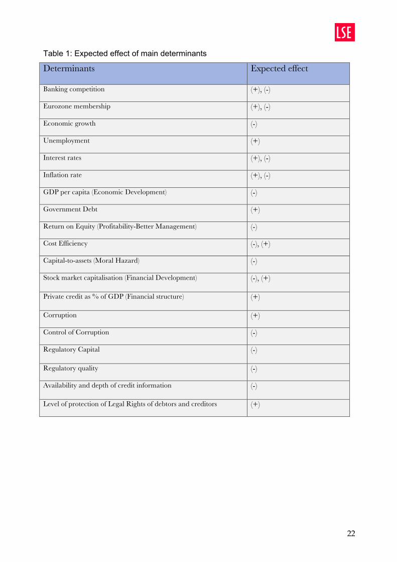
Table 1: Expected effect of main determinants

Determinants

Expected effect

Banking competition

(+), (-)

Eurozone membership

(+), (-)

Economic growth

(-)

Unemployment

(+)

Interest rates

(+), (-)

Inflation rate

(+), (-)

GDP per capita (Economic Development)

(-)

Government Debt

(+)

Return on Equity (Profitability-Better Management)

(-)

Cost Efficiency

(-), (+)

Capital-to-assets (Moral Hazard)

(-)

Stock market capitalisation (Financial Development) (-), (+)

Private credit as % of GDP (Financial structure)

(+)

Corruption

(+)

Control of Corruption

(-)

Regulatory Capital

(-)

Regulatory quality

(-)

Availability and depth of credit information

(-)

Level of protection of Legal Rights of debtors and creditors

(+)

4. Data Analysis and Empirical Strategy

23

4. Data Analysis and Empirical Strategy

In this section we first present the sources of data and sample statistics followed by the empirical

strategy.

4.1 Data Sources and Sample statistics

We use a panel dataset for the 28 EU countries for the period 1998-2011. Our main source is a

new World Bank 2013 series, the Global Financial Development Database2. Other sources are

the OECD3, European Commission’s AMECO database4, World Bank5, World Bank’s Worldwide

Governance Indicators (WGI)6 and Transparency International7

Our dependent variable, NPLs, is measured as the ratio of non-performing loans to total assets

and data are available at the GFDD for EU countries for the period 1998-2011. Regarding

measures of competition, most studies conduct their estimations using a variety of proxies. We

construct our dataset using GFDD. There are 5 indicators available associated with banking

competition. The estimated Lerner index is used as the main proxy for each country’s banking

sector competition for the period 1998-2011. Five-bank asset concentration and the Boone

indicator are used as alternative proxies for banking competition. In GFDD, five-bank asset

concentration is defined as the assets of five largest banks of a banking system divided by total

assets of a country’s banking system.8

In line with existing literature on the topic, we include measures of unemployment, inflation, GDP

growth, GDP per capita and short-term interest rates. Unemployment rates, short-term interest

rates and GDP per capita are found in the European Commission AMECO database. Inflation-

rates are calculated using the GDP deflator available at the AMECO Database. We use real GDP

growth and real short-term interest-rates. Since real short-term interest rates for Luxembourg are

not available in the AMECO database, we calculate them using nominal short-term interest-rates

from the OECD database and the calculated inflation rates. Finally, real GDP growth rate is

calculated using a measure of real GDP available at the World Bank Database9

2Available at: http://econ.worldbank.org/WBSITE/EXTERNAL/EXTDEC/EXTGLOBALFINREPORT/0,,contentMDK:23269602~pagePK:64168182~piPK:64168060~theSitePK:8816097,00.html 3 http://www.oecd.org/statistics/ 4 http://ec.europa.eu/economy_finance/ameco/user/serie/SelectSerie.cfm 5 http://data.worldbank.org 6 http://info.worldbank.org/governance/wgi/index.aspx#home 7 http://www.transparency.org/research/cpi/overview 8 Please be referred to GFDD for details regarding calculation methodology for each variable 9 GDP constant at 2005 prices ($) available at: http://data.worldbank.org/indicator/NY.GDP.MKTP.KD/countries/1W?display=default

24

As for banking sector-specific variables, we include return-on-equity as a proxy for profitability,

stock market capitalization for financial development, private credit as a percentage of GDP for

financial structure, capital-to-assets ratio for moral hazard, non-interest income to total income for

diversification, cost-to-income for efficiency and provisions to non-performing loans. All the above

are available at the GFDD. In GFDD, all variables are aggregated to the country level to reflect

the characteristics of a country’s banking sector. We use the before tax return on equity, which is

measured as banks’ income divided by yearly averaged equity. Cost-to-income ratio is the

operating expenses of a bank, as a share of the sum of net-interest revenue and other operating

income. Non-interest income is banks’ income from noninterest related activities such as trading,

derivatives, other securities, fees and commissions divided by banks’ total income, which is the

sum of net interest income and non-interest income. Capital-to-assets ratio is the shares,

common stocks, other reserves and regulatory capital of a banking sector divided by total

financial and non-financial assets. Finally, stock market capitalization is the total value of all listed

shares in a stock market, as a percentage of GDP, whereas, private credit is the credit provided

by banks to individuals, governments and companies as a percentage of GDP.

As a measure of regulatory capital we consider the bank total regulatory capital as a percentage

of risk-weighted assets, available at GFDD. It measures capital adequacy of banks. It is the total

regulatory capital divided by assets held weighted according to their risk. Regulatory quality is

measured using a perception index from WB’s Worldwide Governance Indicators (WGI), which “

reflects the capacity of governments to formulate and implement sound policies and regulations

that permit and promote private sector development”. It takes values between -2.5 and 2.5 with

lower values indicating weak governance and low regulatory quality.

World Bank database is the source for institutional variables related to availability and depth of

credit information and legal rights of creditors and borrowers. These measures are the private

credit bureau coverage, credit depth of information and strength of legal rights. Credit depth of

information is a measure of rules that determine the scope, accessibility and quality of credit

information available through public or private credit registries. It measures the depth of

information available from public or private bureaus to financial institutions in order to facilitate

lending decisions. It takes values between 0 and 6. Higher values imply that more credit

information is available to facilitate lending decisions (World bank,2014) As for strength of legal

rights, it measures the degree to which rights of debtors and creditors are protected by collateral

and bankruptcy laws. A higher degree of legal protection facilitates lending. The index takes

values from 0 to 10 and higher values reflect that laws are “better designed to expand access to

credit” Finally, private bureau coverage measures the number of individual and firms as a

25

percentage of total population, for which information on repayment history, unpaid debts, credit

outstanding is registered in a private credit bureau. Higher percentage of registered individuals

and companies implies greater availability of credit information.

In order to test the impact of corruption on banking stability, we use two variables. For levels of

corruption in each country, we construct a dataset for EU countries for the period 1998-2011

using the Transparency International Corruption Perception Index. As an alternative measure we

included an indicator described as “control of corruption” available at Worldwide Governance

Indicators. It reflects both “the extent to which public power is exercised for private gain” and “the

capture of the state by elites and private interests.” It takes values from -2.5 to 2.5 with higher

values implying strong governance performance and lower values weak governance

performance.

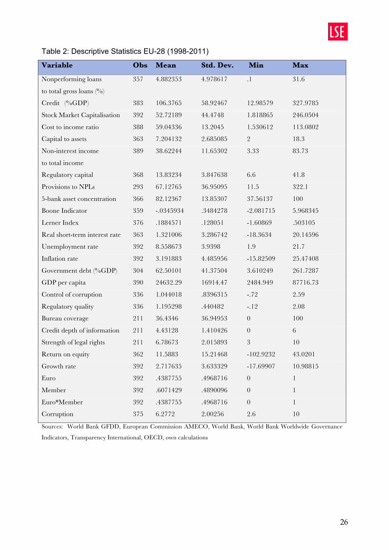
Table 2 presents the descriptive statistics of our dataset. It shows the number of observations

(obs), the mean, the standard deviation (Std.Dev.) and finally, the minimum (min) and maximum

(max) values for each variable. Furthermore, Figure 2 and 3 in Appendix A present the evolution

of nonperforming loans and Lerner index in EU-28 banking sectors.

26

26

Table 2: Descriptive Statistics EU-28 (1998-2011)

Variable Obs Mean Std. Dev. Min Max

Nonperforming loans 357 4.882353 4.978617 .1 31.6

to total gross loans (%)

Credit (%GDP ) 383 106.3765 58.92467 12.98579 327.9785

Stock Market Capitalisation 392 52.72189 44.4748 1.818865 246.0504

Cost to income ratio 388 59.04336 13.2045 1.530612 113.0802

Capital to assets 363 7.204132 2.685085 2 18.3

Non-interest income 389 38.62244 11.65302 3.33 83.73

to total income

Regulatory capital 368 13.83234 3.847638 6.6 41.8

Provisions to NPLs 293 67.12765 36.95095 11.5 322.1

5-bank asset concentration 366 82.12367 13.85307 37.56137 100

Boone Indicator 359 -.0345934 .3484278 -2.081715 5.968345 Lerner Index 376 .1884571 .128051 -1.60869 .503105

Real short-term interest rate 363 1.321006 3.286742 -18.3634 20.14596

Unemployment rate 392 8.558673 3.9398 1.9 21.7

Inflation rate 392 3.191883 4.485956 -15.82509 25.47408 Government debt (%GDP) 304 62.50101 41.37504 3.610249 261.7287

GDP per capita 390 24632.29 16914.47 2484.949 87716.73

Control of corruption 336 1.044018 .8396315 -.72 2.59

Regulatory quality 336 1.195298 .440482 -.12 2.08

Bureau coverage 211 36.4346 36.94953 0 100 Credit depth of information 211 4.43128 1.410426 0 6

Strength of legal rights 211 6.78673 2.015893 3 10

Return on equity 362 11.5883 15.21468 -102.9232 43.0201

Growth rate 392 2.717635 3.633329 -17.69907 10.98815

Euro 392 .4387755 .4968716 0 1

Member 392 .6071429 .4890096 0 1

Euro*Member 392 .4387755 .4968716 0 1

Corruption 375 6.2772 2.00256 2.6 10

Sources: World Bank GFDD, European Commission AMECO, World Bank, World Bank Worldwide Governance

Indicators, Transparency International, OECD, own calculations

27

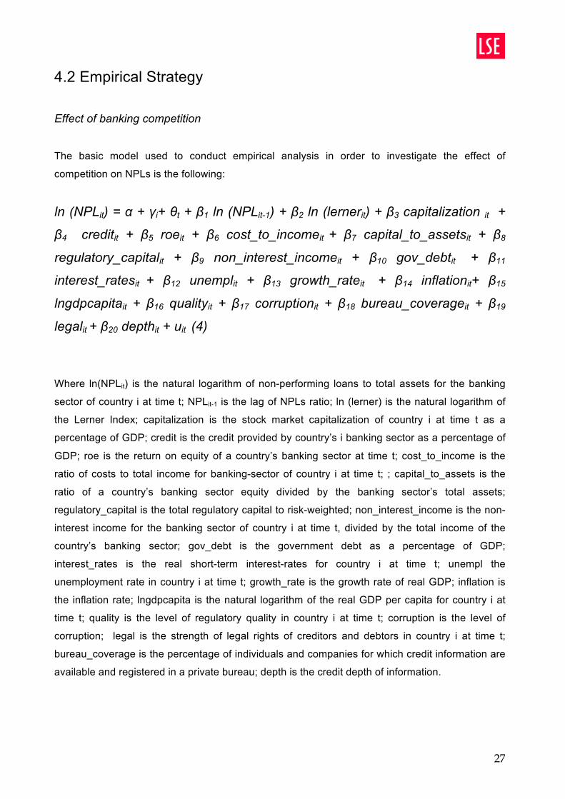
4.2 Empirical Strategy

Effect of banking competition

The basic model used to conduct empirical analysis in order to investigate the effect of

competition on NPLs is the following:

ln (NPLit) = α + γi+ θt + β1 ln (NPLit-1) + β2 ln (lernerit) + β3 capitalization it +

β4 creditit + β5 roeit + β6 cost_to_incomeit + β7 capital_to_assetsit + β8

regulatory_capitalit + β9 non_interest_incomeit + β10 gov_debtit + β11

interest_ratesit + β12 unemplit + β13 growth_rateit + β14 inflationit+ β15

lngdpcapitait + β16 qualityit + β17 corruptionit + β18 bureau_coverageit + β19

legalit + β20 depthit + uit (4)

Where ln(NPLit) is the natural logarithm of non-performing loans to total assets for the banking

sector of country i at time t; NPLit-1 is the lag of NPLs ratio; ln (lerner) is the natural logarithm of

the Lerner Index; capitalization is the stock market capitalization of country i at time t as a

percentage of GDP; credit is the credit provided by country’s i banking sector as a percentage of

GDP; roe is the return on equity of a country’s banking sector at time t; cost_to_income is the

ratio of costs to total income for banking-sector of country i at time t; ; capital_to_assets is the

ratio of a country’s banking sector equity divided by the banking sector’s total assets;

regulatory_capital is the total regulatory capital to risk-weighted; non_interest_income is the non-

interest income for the banking sector of country i at time t, divided by the total income of the

country’s banking sector; gov_debt is the government debt as a percentage of GDP;

interest_rates is the real short-term interest-rates for country i at time t; unempl the

unemployment rate in country i at time t; growth_rate is the growth rate of real GDP; inflation is

the inflation rate; lngdpcapita is the natural logarithm of the real GDP per capita for country i at

time t; quality is the level of regulatory quality in country i at time t; corruption is the level of

corruption; legal is the strength of legal rights of creditors and debtors in country i at time t;

bureau_coverage is the percentage of individuals and companies for which credit information are

available and registered in a private bureau; depth is the credit depth of information.

28

We consider two approaches to estimate the above model. To begin with, after conducting a

Hausman test on whether to choose fixed effects or random effects estimation, we find that the

most appropriate approach is the fixed effects model. The fixed effects model allows controlling

for unobserved time invariant country characteristics and therefore, addresses potential omitted

variable bias. As a result, we first estimate our model with an OLS panel data approach including

country and time fixed effects to control for both time and country invariant unobserved

characteristics. After estimating the model, we conduct a Wooldridge test for autocorrelation and

we find that autocorrelation is present. In order to address autocorrelation and heteroskedasticity

we estimate the model with robust standard errors.

Since previous levels of NPLs may affect current levels of NPLs, we include a lagged dependent

variable as an additional explanatory variable (Louzis et al, 2012; Klein, 2013). However,

estimating the model with OLS fixed effects may result to biased estimations due to possible

endogeneity of the lagged dependent variable and the fixed effects in the error term (Klein, 2013).

More specifically, the lagged dependent variable is correlated with the error terms. Another issue

we identify in our model is reverse causality. More specifically, NPLs may affect several

explanatory variables and more specifically, Lerner Index and banking-sector specific

determinants. Moreover, several explanatory variables may be correlated with the error term and

also with fixed effects. Due to the abovementioned reasons, estimations may suffer from

endogeneity and therefore, an OLS fixed effects approach may lead to inconsistent and biased

estimates.

Given the abovementioned, we apply a dynamic panel data approach using the Arellano-Bond

difference GMM estimator in order to address the abovementioned problems (Arellano and Bond,

1991). The Arellano-Bond difference GMM estimator takes the differences of the variables in the

model and as a result, eliminates any unobserved country heterogeneity (Arellano and Bond,

1991; Roodman, 2009a). Furthermore, it allows addressing endogeneity of variables by using

lagged levels of explanatory variables as instruments (Roodman, 2009a). In order to give

consistent estimates the Arellano-Bond GMM approach requires the errors not to be second

order autocorrelated (Louzis et al, 2012). It is important to note that we instrument

macroeconomic and institutional determinants in IV-style and banking competition and banking

sector-specific measures in GMM-style10.

10 For more information please be referred to Roodman (2009a) and Arellano and Bond (1991).

29

Effect of Eurozone Membership

In order to assess the effect of Eurozone on NPLs, we apply a difference-in-differences

approach. Table 2 shows which countries are allocated to the treatment and control group. The

control group is EU countries non-members of the Eurozone and the treatment group is Eurozone

members. Due to the fact that some countries entered the Eurozone in different time periods, we

have different treatment periods for each country. Table 3 lists Eurozone countries and the year

of entry in Eurozone. As post treatment periods we consider the years after each country of the

treatment group entered the Eurozone. For example, for countries that entered the Eurozone in

1999 such as Germany, France, Netherlands e.t.c the post-treatment period starts from the year

1999 and the pre-treatment period is the year 1998. For countries that entered the Eurozone in

later years such as Greece, Cyprus, Malta, Slovenia e.t.c, the post-treatment period is considered

the year of entry and the years that follow until 2011. A key assumption of the difference-in-

differences estimation is that in the absence of the treatment, treatment and control group would

follow the same path. Table 4 presents the countries of the treatment group and the years in

which the treatment was introduced in each country.

30

29

countries are allocated to the treatment and control group. The control group is EU countries non-

members of the Eurozone and the treatment group is Eurozone members. Due to the fact that

some countries entered the Eurozone in different time periods, we have different treatment

periods for each country. Table 3 lists Eurozone countries and the year of entry in Eurozone. As

post treatment periods we consider the years after each country of the treatment group entered

the Eurozone. For example, for countries that entered the Eurozone in 1999 such as Germany,

France, Netherlands e.t.c the post-treatment period starts from the year 1999 and the pre-

treatment period is the year 1998. For countries that entered the Eurozone in later years such as

Greece, Cyprus, Malta, Slovenia e.t.c , the post-treatment period is considered the year of entry

and the years that follow until 2011. A key assumption of the difference-in-differences estimation

is that in the absence of the treatment, the treatment and the control group would follow the same

path.

Table 3: Treatment and Control Group

Treatment Group: Eurozone Countries

(1998-2011)

Control Group: Non Eurozone Countries

(1998-2011)

30

Austria

Belgium

Cyprus*

Estonia

Finland

France

Germany

Greece

Ireland

Italy

Luxembourg

Malta

The Netherlands

Portugal

Slovenia

Slovakia

Spain

Bulgaria

Croatia

Czech Republic

Denmark

Hungary

Latvia

Lithuania

Poland

Romania

Sweden

United Kingdom

Source: http://www.ecb.europa.eu/euro/intro/html/map.en.html

* excluded from the dataset as data for non-performing loans before Cyprus’ entry in Eurozone are not available.

Table 4: Eurozone Countries and year of entry in Eurozone

Countries Year of Entry (Treatment)

31

Equation (5) specifies a simplification of the difference-in-differences model. We create a dummy

variable denoted as “euro” that is equal to 1 when an observation is from the period after the

introduction of the euro in country i and 0 otherwise. Another dummy variable is created, denoted

as “member” which takes the value of 1 when a country is a Eurozone member and zero

otherwise. In order to apply the difference in differences estimator, we construct the interaction of

these two dummy variables, which is the variable we use to capture the treatment effect and we

denote it as “euromember”.

30

Austria

Belgium

Cyprus*

Estonia

Finland

France

Germany

Greece

Ireland

Italy

Luxembourg

Malta

The Netherlands

Portugal

Slovenia

Slovakia

Spain

Bulgaria

Croatia

Czech Republic

Denmark

Hungary

Latvia

Lithuania

Poland

Romania

Sweden

United Kingdom


* excluded from the dataset as data for non-performing loans before Cyprus’ entry in Eurozone are not available.

Table 4: Eurozone Countries and year of entry in Eurozone

Countries Year of Entry (Treatment)

31

Austria

Belgium

Cyprus

Estonia

Finland

France

Germany

Greece

Ireland

Italy

Luxembourg

Malta

The Netherlands

Portugal

Slovenia

Slovakia

Spain

1999

1999

2008

2011

1999

1999

1999

2001

1999

1999

1999

2008

1999

1999

2007

2009

1999


Equation (6) specifies a simplification of the difference-in-differences model. We create a dummy

variable denoted as “euro” that is equal to 1 when an observation is from the period after the

introduction of the euro in country i and 0 otherwise. Another dummy variable is created, denoted

as member which takes the value of 1 when a country is a Eurozone member and zero

otherwise. In order to apply the difference in differences estimator, we construct the interaction of

these two dummy variables, which is the variable we use to capture the treatment effect and we

denote it as euromember.

ln (NPLit) = α+ eurot + memberi + βDD euromemberit+ uit (5)

Where ln (NPLit): natural logarithm of nonperforming loans in country i at time t.

eurot: dummy variable = 1 if post-treatment period, 0 otherwise

memberi: dummy variable = 1 if country i is member of Eurozone, 0 otherwise

In order to assess the impact of Eurozone membership on non-performing loans, we estimate

equation (6) with two methods; the OLS fixed effects and the Arellano-Bond GMM estimation. We

choose these two methods for the same reasons described in 4.2.1. Equation (6) includes

several additional explanatory variables. We include the Lerner Index and we control for certain

32

ln (NPLit) = α+ eurot + memberi + βDD euromemberit+ uit (5)

Where ln (NPLit): natural logarithm of nonperforming loans in country i at time t.

eurot: dummy variable = 1 if post-treatment period, 0 otherwise

memberi: dummy variable = 1 if country i is member of Eurozone, 0 otherwise

In order to assess the impact of Eurozone on non-performing loans, we estimate equation (6)

with two methods; OLS fixed effects and Arellano-Bond GMM. We choose these two methods for

the same reasons described above. Equation (6) includes several additional explanatory

variables in order to capture any other differences between observations that may affect NPLs in

treatment and control group, supporting the parallel trends assumption and making our estimates

more precise. We control for macroeconomic, regulatory, institutional and banking-specific

determinants. 11 As we also control for time-invariant and country invariant unobserved

characteristics, we only add the treatment variable “euromember” and not the dummies “member”

and “euro” to avoid collinearity with θt and γi.

ln (NPLit) = α + γi + θt + β1 NPLit-1 + β2 euromemberit + β3 ln (lernerit) +β4

capitalizationit + β5 creditit + β6 roeit + β7 cost_to_incomeit + β8

capital_to_assetsit + β9 regulatory_capitalit + β10 non_interest_incomeit + β11

unemplit + β12 growth_rateit + β13 lngdpcapitait + β14 qualityit + β15 corruptionit

+ uit (6)

11 For full description of the variables in Equation (6), please be referred to the previous section

33

5. Empirical Results

5.1. Main results

Effect of banking competition

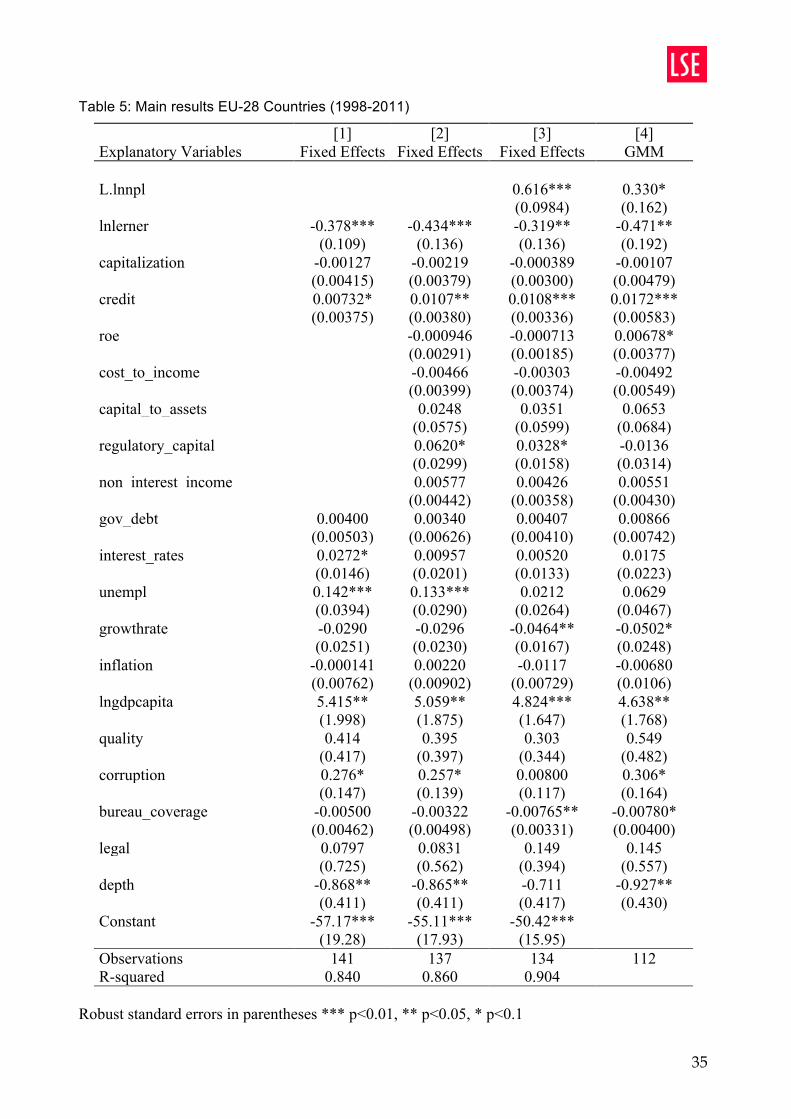
Table 5 presents the main results after estimating equation (5). In all estimations we include year

dummy variables. Due to space constraints we do not include the coefficients of the year

dummies in Table 5. The complete table can be viewed in Appendix B.

Column [1] presents the OLS fixed effects estimations and does not include banking sector-

specific determinants. The Lerner index is negative and statistically significant with a p-value

smaller than 0.01. Therefore, higher market power is associated with a lower level of NPLs.

Credit provided by banks is statistically significant at the 10% level. As for macroeconomic

determinants, interest rates are statistically significant at the 10% level, indicating that a higher

interest rate is linked with a higher NPLs ratio. The coefficient for unemployment is statistically

significant and presents a positive sign. It confirms the theoretical expectation, that a higher

unemployment rate is associated with a higher level of NPLs. The coefficient for growth rate is

negative as expected but it is insignificant. GDP per capita presents a positive significant

coefficient, which contradicts theoretical expectations. Moreover, the coefficient for corruption is

statistically significant with a p-value smaller than 0.1 implying that a higher level of corruption is

associated with a higher level of nonperforming loans. Last but not least, the coefficient for credit

depth of information is statistically significant indicating that when there is greater depth of

information available a lower level of NPLs ratio is observed.

When we include banking-specific determinants (Column [2]), the levels of significance and the

signs of the coefficients discussed above do not change. The changes we observe are at the

coefficient for interest rates, which becomes insignificant, and at the coefficient for domestic

credit, which becomes significant at the 5% level. The coefficient for Lerner Index increases while

it remains highly significant. Furthermore, it appears that neither of the banking-sector specific

determinants is significant. Only regulatory capital is significant with a p-value smaller than 0.1,

implying that a higher regulatory capital to risk-weighted assets is associated with a higher level

of NPLs. This is inconsistent with the expected effect discussed in section 3. In the estimation

presented in column [3], we include lag NPLs ratio, which enters with a positive sign and the

34

coefficient is highly significant. Coefficient for unemployment becomes insignificant, while growth

rate becomes significant and is negatively related with NPLs, as expected. Moreover, corruption

and credit depth of information become insignificant. At the same time, bureau coverage

becomes significant with a p-value smaller than 0.05, implying that a higher percentage of

individuals and companies for which credit information are registered in private credit bureaus is

associated with a lower NPLs ratio.

As mentioned in the previous section, in order to address endogeneity, we apply the Arelano

Bond difference GMM estimation method. The results are presented in column [4]. It is important

to note that the tests we run, reported no second order autocorrelation and the probability of the

Hansen test was sufficiently high (p-value of 1.0) to accept the null hypothesis that the

instruments used are exogenous. The results presented in column [4] are the outcome of using

up to four lags as instruments. We attempt to keep the number of instruments as low as possible

by using the collapsed instruments technique suggested by Roodman (2009b), as a large number

of instruments may lead to biased estimates. 12 As we can observe the coefficient for Lerner

Index remains strongly significant. The sign is negative, which implies that higher market power

and therefore, lower level of market competition, is associated with a lower NPLs ratio. Credit

provided by banks remains strongly significant. Interestingly, our measure for profitability, return

on equity, becomes significant with a p-value smaller than 0.1. The coefficient is weak but

positive, contradicting theoretical expectations that better management i.e higher profitability of

the banking sector, leads to lower NPLs ratio. The coefficient for growth rate remains significant

with a p-value smaller than 0.1. It also remains negative, which is in line with our expectations

and implies that a prosperous economic environment is related with a lower level of NPLs.

Furthermore, GDP per capita remains significant and indicates that the more developed the

economy is, the higher is the level of NPLs. Last but not least, the coefficients of corruption,

private bureau coverage and credit depth of information are significant and maintain the signs

observed in the previously discussed estimations, which are in line with the theory presented in

section 3.

12 For more information please be referred to Roodman (2009)

35

35

Table 5: Main results EU-28 Countries (1998-2011)

[1] [2] [3] [4] Explanatory Variables Fixed Effects Fixed Effects Fixed Effects GMM L.lnnpl 0.616*** 0.330* (0.0984) (0.162) lnlerner -0.378*** -0.434*** -0.319** -0.471** (0.109) (0.136) (0.136) (0.192) capitalization -0.00127 -0.00219 -0.000389 -0.00107 (0.00415) (0.00379) (0.00300) (0.00479) credit 0.00732* 0.0107** 0.0108*** 0.0172*** (0.00375) (0.00380) (0.00336) (0.00583) roe -0.000946 -0.000713 0.00678* (0.00291) (0.00185) (0.00377) cost_to_income -0.00466 -0.00303 -0.00492 (0.00399) (0.00374) (0.00549) capital_to_assets 0.0248 0.0351 0.0653 (0.0575) (0.0599) (0.0684) regulatory_capital 0.0620* 0.0328* -0.0136 (0.0299) (0.0158) (0.0314) non_interest_income 0.00577 0.00426 0.00551 (0.00442) (0.00358) (0.00430) gov_debt 0.00400 0.00340 0.00407 0.00866 (0.00503) (0.00626) (0.00410) (0.00742) interest_rates 0.0272* 0.00957 0.00520 0.0175 (0.0146) (0.0201) (0.0133) (0.0223) unempl 0.142*** 0.133*** 0.0212 0.0629 (0.0394) (0.0290) (0.0264) (0.0467) growthrate -0.0290 -0.0296 -0.0464** -0.0502* (0.0251) (0.0230) (0.0167) (0.0248) inflation -0.000141 0.00220 -0.0117 -0.00680 (0.00762) (0.00902) (0.00729) (0.0106) lngdpcapita 5.415** 5.059** 4.824*** 4.638** (1.998) (1.875) (1.647) (1.768) quality 0.414 0.395 0.303 0.549 (0.417) (0.397) (0.344) (0.482) corruption 0.276* 0.257* 0.00800 0.306* (0.147) (0.139) (0.117) (0.164) bureau_coverage -0.00500 -0.00322 -0.00765** -0.00780* (0.00462) (0.00498) (0.00331) (0.00400) legal 0.0797 0.0831 0.149 0.145 (0.725) (0.562) (0.394) (0.557) depth -0.868** -0.865** -0.711 -0.927** (0.411) (0.411) (0.417) (0.430) Constant -57.17*** -55.11*** -50.42*** (19.28) (17.93) (15.95) Observations 141 137 134 112 R-squared 0.840 0.860 0.904

Robust standard errors in parentheses *** p<0.01, ** p<0.05, * p<0.1

36

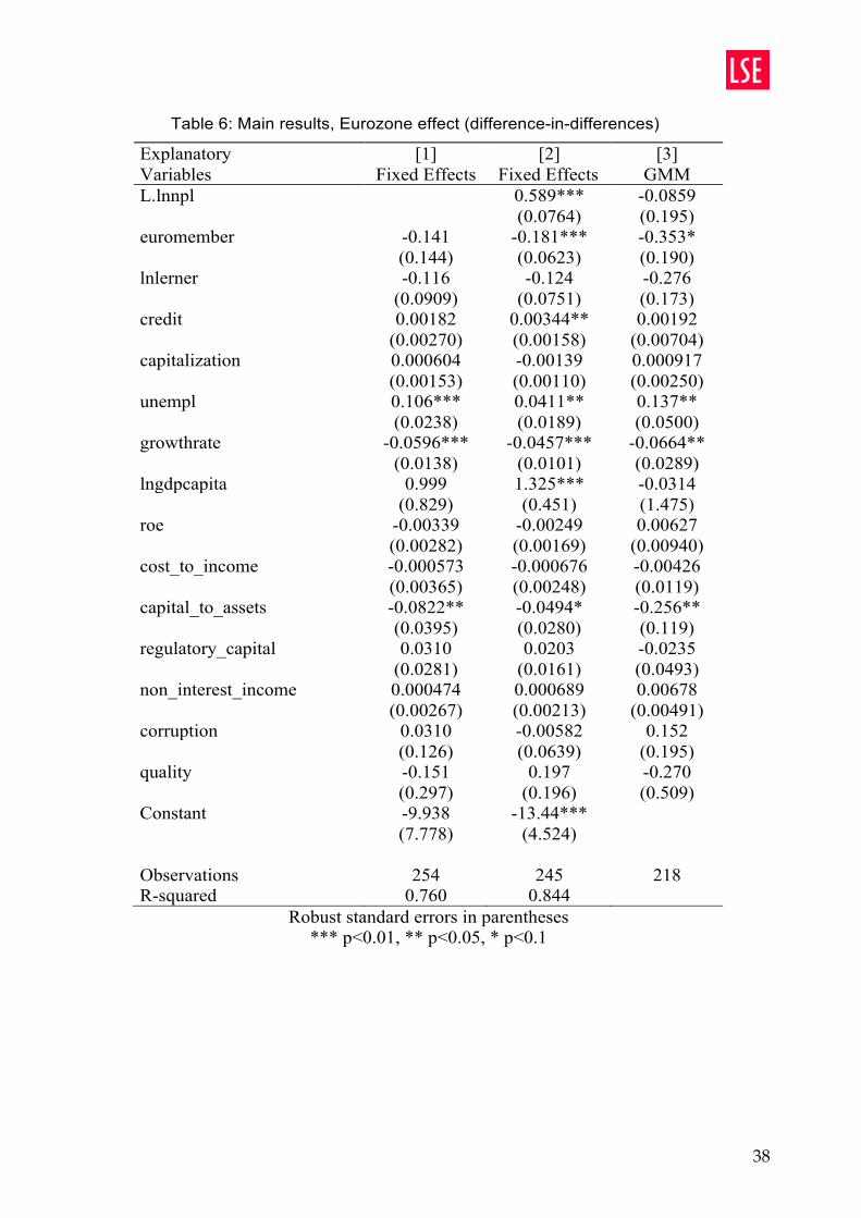
Effect of Eurozone membership

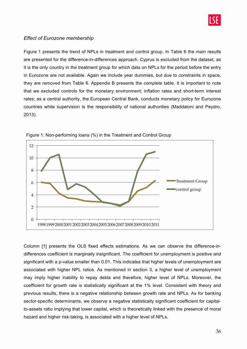
Figure 1 presents the trend of NPLs in treatment and control group. In Table 6 the main results

are presented for the difference-in-differences approach. Cyprus is excluded from the dataset, as

it is the only country in the treatment group for which data on NPLs for the period before the entry

in Eurozone are not available. Again we include year dummies, but due to constraints in space,

they are removed from Table 6. Appendix B presents the complete table. It is important to note

that we excluded controls for the monetary environment; inflation rates and short-term interest

rates; as a central authority, the European Central Bank, conducts monetary policy for Eurozone

countries while supervision is the responsibility of national authorities (Maddaloni and Peydro,

2013).

Column [1] presents the OLS fixed effects estimations. As we can observe the difference-in-

differences coefficient is marginally insignificant. The coefficient for unemployment is positive and

significant with a p-value smaller than 0.01. This indicates that higher levels of unemployment are

associated with higher NPL ratios. As mentioned in section 3, a higher level of unemployment

may imply higher inability to repay debts and therefore, higher level of NPLs. Moreover, the

coefficient for growth rate is statistically significant at the 1% level. Consistent with theory and

previous results, there is a negative relationship between growth rate and NPLs. As for banking

sector-specific determinants, we observe a negative statistically significant coefficient for capital-

to-assets ratio implying that lower capital, which is theoretically linked with the presence of moral

hazard and higher risk-taking, is associated with a higher level of NPLs.

36

Effect of Eurozone membership

In Table 6 the main results are presented for the difference-in-differences approach. We exclude

Cyprus from our estimations, as it is the only country in the treatment group for which data on

non-performing loans for the period before the entry in Eurozone are not available. Again we

include year dummies, but due to constraints in space, they are removed from Table 6. Appendix

B presents full results. It is important to note that we excluded controls for the monetary

environment; inflation rates and short-term interest rates; as a central authority, the European

Central Bank, conducts monetary policy for Eurozone countries. Figure 1 presents the evolution

of non-performing loans for the treatment and control group during the time period 1998-2011.

Figure 1: Non-performing loans (%) in the Treatment and Control Group

Column [1] presents the OLS fixed effects estimations. As we can observe the difference-in-

differences coefficient is marginally insignificant. The coefficient of unemployment rate is positive

and significant with a p-value smaller than 0.01. This indicates that higher levels of

unemployment are associated with higher NPL ratios. Moreover, the coefficient of growth rate is

statistically significant at the 1% level. Consistent with theory and previous results, there is a

negative relationship between growth rate and NPLs. As for banking sector-specific determinants

we observe a significant negative coefficient for the capital to assets ratio implying that lower

capital, which is theoretically associated with the presence of moral hazard and higher risk-taking,

is associated with a higher level of NPLs.

0

2

4

6

8

10

12

1998 1999 2000 2001 2002 2003 2004 2005 2006 2007 2008 2009 2010 2011

Treatment Group

control group

37

In the estimation presented in Column [2], the lag of NPLs ratio is included and enters the

regression with a strongly significant positive coefficient. The difference-in-differences coefficient

becomes significant with a p-value smaller than 0.01 indicating that the level of NPLs is lower in

Eurozone countries. Another coefficient that becomes significant is that of credit provided by

banks, which presents a positive sign. Last but not least; with the inclusion of the lag NPLs ratio,

GDP per capita becomes strongly significant and positive implying that when levels of economic

development are higher, NPLs are higher. As far as unemployment is concerned, the coefficient

is reduced and the p-value is now between 0.01 and 0.05. The value of the coefficient of capital

to assets ratio is significantly reduced and the significance level approximates 10%.

Column [3] presents the Arellano-Bond difference GMM estimations. We use up to two lags as

instruments for endogenous variables. The total number of instruments is 33. There is no second

order autocorrelation since the probability of the test for AR(2) is 0.518. Moreover, the probability

of the Hansen Test is 0.985, which permits us to accept the null hypothesis that the instruments

used are exogenous. Results show that the magnitude of the difference-in-differences coefficient

significantly increased and it is significant at the 10%. This indicates that the NPLs ratio is 35.3%

lower in Eurozone countries than the countries in the control group. If the parallel trends

assumption holds this suggests that the effect of the introduction of the Eurozone on NPLs is

negative. The coefficients for unemployment rate, growth rate and capital-to-assets ratio are

significantly increased and they are statistically significant with p-values smaller than 0.05. The

signs of these coefficients remain the same with the estimations presented in columns [1] and [2]

and are in line with expectations in section 3.

38

38

Table 6: Main results, Eurozone effect (difference-in-differences)

Explanatory Variables

[1] Fixed Effects

[2] Fixed Effects

[3] GMM

L.lnnpl 0.589*** -0.0859 (0.0764) (0.195) euromember -0.141 -0.181*** -0.353* (0.144) (0.0623) (0.190) lnlerner -0.116 -0.124 -0.276 (0.0909) (0.0751) (0.173) credit 0.00182 0.00344** 0.00192 (0.00270) (0.00158) (0.00704) capitalization 0.000604 -0.00139 0.000917 (0.00153) (0.00110) (0.00250) unempl 0.106*** 0.0411** 0.137** (0.0238) (0.0189) (0.0500) growthrate -0.0596*** -0.0457*** -0.0664** (0.0138) (0.0101) (0.0289) lngdpcapita 0.999 1.325*** -0.0314 (0.829) (0.451) (1.475) roe -0.00339 -0.00249 0.00627 (0.00282) (0.00169) (0.00940) cost_to_income -0.000573 -0.000676 -0.00426 (0.00365) (0.00248) (0.0119) capital_to_assets -0.0822** -0.0494* -0.256** (0.0395) (0.0280) (0.119) regulatory_capital 0.0310 0.0203 -0.0235 (0.0281) (0.0161) (0.0493) non_interest_income 0.000474 0.000689 0.00678 (0.00267) (0.00213) (0.00491) corruption 0.0310 -0.00582 0.152 (0.126) (0.0639) (0.195) quality -0.151 0.197 -0.270 (0.297) (0.196) (0.509) Constant -9.938 -13.44*** (7.778) (4.524) Observations 254 245 218 R-squared 0.760 0.844


39

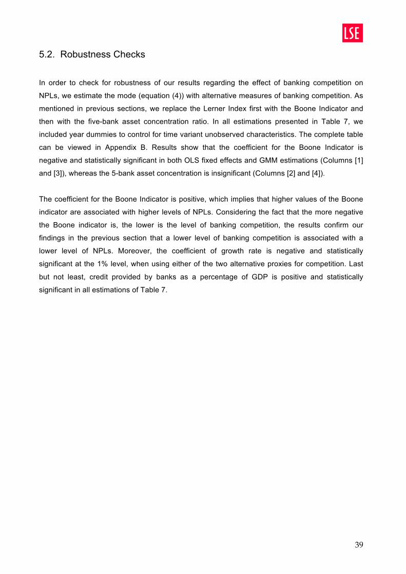
5.2. Robustness Checks

In order to check for robustness of our results regarding the effect of banking competition on

NPLs, we estimate the mode (equation (4)) with alternative measures of banking competition. As

mentioned in previous sections, we replace the Lerner Index first with the Boone Indicator and

then with the five-bank asset concentration ratio. In all estimations presented in Table 7, we

included year dummies to control for time variant unobserved characteristics. The complete table

can be viewed in Appendix B. Results show that the coefficient for the Boone Indicator is

negative and statistically significant in both OLS fixed effects and GMM estimations (Columns [1]

and [3]), whereas the 5-bank asset concentration is insignificant (Columns [2] and [4]).

The coefficient for the Boone Indicator is positive, which implies that higher values of the Boone

indicator are associated with higher levels of NPLs. Considering the fact that the more negative

the Boone indicator is, the lower is the level of banking competition, the results confirm our

findings in the previous section that a lower level of banking competition is associated with a

lower level of NPLs. Moreover, the coefficient of growth rate is negative and statistically

significant at the 1% level, when using either of the two alternative proxies for competition. Last

but not least, credit provided by banks as a percentage of GDP is positive and statistically

significant in all estimations of Table 7.

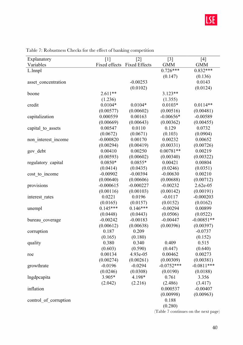
40

40

Table 7: Robustness Checks for the effect of banking competition

Explanatory [1] [2] [3] [4] Variables Fixed effects Fixed Effects GMM GMM L.lnnpl 0.726*** 0.832*** (0.147) (0.136) asset_concentration -0.00253 0.0143 (0.0102) (0.0124) boone 2.611** 3.123** (1.236) (1.355) credit 0.0104* 0.0104* 0.0103* 0.0114** (0.00577) (0.00602) (0.00516) (0.00481) capitalization 0.000559 0.00163 -0.00656* -0.00589 (0.00669) (0.00643) (0.00362) (0.00455) capital_to_assets 0.00547 0.0110 0.129 0.0732 (0.0672) (0.0671) (0.103) (0.0904) non_interest_income -0.000820 0.00170 0.00232 0.00652 (0.00294) (0.00419) (0.00331) (0.00726) gov_debt 0.00410 0.00250 0.00781** 0.00219 (0.00593) (0.00602) (0.00340) (0.00322) regulatory_capital 0.0850* 0.0855* 0.00421 0.00804 (0.0414) (0.0435) (0.0246) (0.0351) cost_to_income -0.00902 -0.00394 -0.00630 0.00210 (0.00640) (0.00606) (0.00688) (0.00712) provisions -0.000615 -0.000227 -0.00232 2.62e-05 (0.00116) (0.00103) (0.00142) (0.00191) interest_rates 0.0221 0.0196 -0.0117 -0.000203 (0.0165) (0.0157) (0.0152) (0.0162) unempl 0.145*** 0.146*** -0.00294 0.00899 (0.0448) (0.0443) (0.0506) (0.0522) bureau_coverage -0.00242 -0.00183 -0.00447 -0.00851** (0.00612) (0.00638) (0.00396) (0.00397) corruption 0.187 0.209 -0.0737 (0.165) (0.180) (0.152) quality 0.380 0.340 0.409 0.515 (0.603) (0.590) (0.447) (0.640) roe 0.00134 4.93e-05 0.00462 0.00273 (0.00274) (0.00261) (0.00309) (0.00381) growthrate -0.0196 -0.0294 -0.0752*** -0.0811*** (0.0246) (0.0308) (0.0190) (0.0188) lngdpcapita 3.905* 4.198* 0.761 3.356 (2.042) (2.216) (2.486) (3.417) inflation 0.000537 -0.00407 (0.00998) (0.00963) control_of_corruption 0.188 (0.280)

(Table 7 continues on the next page)

41

41

Table 7: Robustness Checks for the effect of banking competition (Continued)

Explanatory [1] [2] [3] [4] Variables Fixed effects Fixed Effects GMM GMM

legal 0.749 0.746 0.589 0.206 (1.218) (1.200) (0.957) (0.859) depth -0.662 -0.572 -0.515 -0.288 (0.574) (0.615) (0.528) (0.535) Constant -43.42** -47.23** (19.70) (21.49) Observations 124 121 100 98 R-squared 0.868 0.852


6. Discussion

This study uses a large panel dataset for the period 1998-2011. It combines a large number of

explanatory variables from various studies and focuses on European Union countries. By

including a large number of relevant explanatory variables and controlling for time invariant and

country invariant unobserved characteristics, it manages to reduce omitted variable bias and

hence, potential endogeneity problems. Furthermore, by using clustered standard errors this

study aims to address autocorrelation and heteroskedasticity. To address reverse causality and

endogeneity of explanatory variables, it applies a dynamic panel data Arellano-Bond difference

GMM estimation method using as instruments, lag values of explanatory variables.

Regarding the impact of banking competition on financial stability, we combine non-performing

loans, which we use as a proxy for financial stability with the Lerner Index and the Boone

Indicator, which we consider as proxies for banking-sector competition. Compared to existing

literature we focus specifically in EU countries. We find that greater market power i.e. lower level

of competition in the banking sector is associated with a higher non-performing loans ratio.

Moreover, when growth rate, which is linked with the ability of debtors to pay back their loans and

the availability of mechanisms to screen loan applications and recover loan payments, is higher,

the level of NPLs is lower. We also find evidence that higher levels of corruption are associated

with higher NPLs ratio. Economic development as measured by GDP per capita is also linked

with higher levels of NPLs, which contradicts our expectations. Furthermore, we provide evidence

that the greater the depth of credit information available to financial institutions is, the lower is the

42

6. Discussion

This study uses a large panel dataset for the period 1998-2011 and focuses exclusively on

European Union countries. It combines a large number of explanatory variables from various

studies. By including a large number of relevant explanatory variables and controlling for time

invariant and country invariant unobserved characteristics, it manages to reduce omitted variable

bias and hence, potential endogeneity problems. Furthermore, by using clustered standard errors

this study aims to address autocorrelation and heteroskedasticity. To address reverse causality

and endogeneity of explanatory variables, it applies a dynamic panel data Arellano-Bond

difference GMM method using as instruments, lag values of explanatory variables. Our

estimations pass the test for no second order autocorrelation required for consistency of the

GMM estimator and the Hansen tests required for exogeneity of our instruments.

Regarding the impact of banking competition on financial stability, we combine non-performing

loans, which we use as a proxy for financial stability, with the Lerner Index, which we consider as

the main proxy for banking-sector competition. Compared to existing literature we focus

specifically in EU-28 countries. We find that greater market power i.e. lower level of competition

in the banking sector is associated with a higher non-performing loans ratio. Moreover, higher

growth rate, which is theoretically linked with the ability of debtors to pay back their loans and the

availability of mechanisms to screen loan applications and recover loan payments, is associated

with a lower level of NPLs is lower. This confirms theoretical expectations and findings of

previous studies. Moreover, we present evidence that higher levels of corruption are associated

with higher NPLs ratio, which confirms the theory presented in section 3. Economic development

as measured by GDP per capita is also linked with higher levels of NPLs, which contradicts the

theoretical background that more developed countries should present lower levels of NPLs.

Moreover, higher unemployment, which reflects higher inability to repay debts, is linked with a

higher NPLs ratio, in line with expectations in section 3. Furthermore, we provide evidence that

the a greater depth of credit information available to financial institutions is associated with lower

levels of NPLs. Last but not least, a higher percentage of registered individuals and firms in

private credit bureaus is associated with a lower NPLs ratio. Overall, our findings confirm the

results of previous studies on the topic of competition and financial stability, which find a negative

relationship between competition and financial stability i.e less competition is associated with

higher stability (Jimenez et al, 2007).

43

As for investigating the effect of Eurozone on financial stability, we find that NPLs tend to be

lower in Eurozone countries than in non-Eurozone EU countries. As for banking sector-specific

determinants, we observe a negative statistically significant coefficient for capital-to-assets ratio

implying that lower capital is associated with higher level of NPLs. This finding is consistent with

the theory suggesting that the managers of banks with lower capital may have moral hazard

incentives “to increase the riskiness of their loan portfolio”. Moreover, in line with theory, higher

growth rate is associated with lower level of NPLs, while higher unemployment is linked with a

higher NPLs ratio. In contrast with the theory that more developed countries should experience

lower level of NPLs ratio, GDP per capita is associated with a higher level of NPLs. It is important

to note here, that the Lerner index is marginally insignificant in all regressions when we apply

difference-in-differences approach to investigate the effect of Eurozone. However, this may be

due to the fact that part of the effect of banking competition may be captured by the Eurozone

coefficient as the introduction of the Eurozone led to an increase in banking competition.

Limitations

This study is subject to certain limitations. First of all, despite the fact that there is no missing data

for most countries and variables, data for a significantly small number of years are not available.

It is important to note that the only variables that suffer from a large number of missing data are

the following: credit depth of information, private bureau coverage and strength of legal rights. In

all three, the number of observations is limited to 211. Furthermore, as we mentioned in previous

sections, data for non-performing loans for Cyprus are available only from 2008 to 2011.

Secondly, as noted in the GFDD and highlighted in Klein (2013), the classification of non-

performing loans in each country may be different due to differences in national accounting,

taxation and supervisory regimes and therefore, data may not be strictly comparable across

countries. However, the use of fixed effects may address this problem up to a certain degree.

Regarding the Arellano-Bond GMM estimation method, as noted by Roodman(2009b), as the

number of instruments approaches the number of observations, results reported using the

Arellano-Bond GMM estimation may be biased towards OLS. We attempted to keep the number

of instruments as low as possible with various techniques proposed by Roodman(2009b)

However, it would be difficult to argue with certainty that we managed to address the problem of

endogenous regressors completely.

Fourthly, in the context of the difference-in-differences approach, a strong limitation that this

study faces is that for countries that entered the Eurozone in 1999, the pre-treatment period is

44

only one year, which poses constrains in any attempts to support the parallel trends assumptions

by increasing the pre-treatment period. Unfortunately, data for NPLs for all EU countries are

available only from 1998 and onwards. We were also unable to construct another control group,

which could potentially be valid, with the data available. The limited capacity to support the

parallel trends assumption threatens the internal validity of the results presented in Table 6.

Therefore, results presented in Table 6 should be treated with caution in regards to any causal

interpretations.

7. Conclusion



threatened. This study investigates the impact of banking competition on financial stability in the

28 European Union countries, using non-performing loans as a proxy for financial stability.

Moreover, it applies a difference-in-differences approach to assess the impact of Eurozone

membership on non-performing loans. By using an up to date panel dataset for the period 1998-

2011 and focusing exclusively on the 28 European Union countries, this study facilitates the

design of macro-prudential policies in the context of the upcoming EU banking union. This study

finds that a lower level of banking competition as measured by the Lerner Index, is associated

with a lower level of non-performing loans in EU countries. The use of the Boone Indicator

instead of the Lerner Index appears to confirm these findings, whereas five-bank asset

concentration is insignificant. Apart from banking competition, also macroeconomic and

institutional determinants are found to be associated with non-performing loans in EU. More

specifically, higher levels of corruption, unemployment are found to be associated with higher

levels of NPLs in EU countries. On the other hand, higher levels of economic growth, greater

depth of credit information available to financial institutions and a higher percentage of registered

individuals in private credit bureaus are associated with a lower level of NPLs in EU countries.

The results of the difference-in-differences approach should be treated with caution. Results

show that Eurozone countries appear to have lower levels of non-performing loans than non-

Eurozone EU countries. Moreover, higher levels of unemployment are found to be associated

with higher levels of NPL, while higher capital-to-assets ratio and higher levels of economic

growth, are associated with a lower level of NPLs.

45

8. References

Agoraki, M-E.K. Delis, M.D and Pasiouras, F. 2011. Regulations, competitions and bank risk-

taking in transition countries. Journal of financial stability 7, pp. 38-48

Andries, A. Căpraru, B. S. 2012. How Does EU Banking Competition Impact Financial Stability?

in LESSONS LEARNED FROM THE FINANCIAL CRISIS Proceedings of 13th International

Conference on Finance and Banking, 2012

Available at: http://www.opf.slu.cz/kfi/icfb/proc2011/pdf/01_Andries.pdf

Anginer, D. Demirgur-Kunt, A. and Zhu, M. 2012. How does bank competition affect systemic

stability. The World Bank development research group. Finance and private sector development

team. Policy Research Working Paper WPS5981

Arellano, M. Bond, S.1991. Some tests of specification for panel data: Monte Carlo evidence and

an application to employment equations. Review of Economic Studies 58, pp: 277–297.

Arellano, M. Bover, O.1995. Another look at the instrumental variable estimation

of error-component models. Journal of Econometrics 68, pp: 29–51.

Barnato, K. 2013. “Bad loans at European banks hit $1.7 trillion” [Online] Available at:

http://www.cnbc.com/id/101148313

[Accessed: 10/04/2014]

Beck, T. 2008. Bank completion and financial stability: Friends or Foes? The World Bank

development research group. Finance and private sector development team. Pocily Research

Working Paper WPS4656

BIS Papers. 2001. Marrying the macro- and micro prudential dimensions of financial stability.

Bank for international settlements

Blundell, R., Bond, S., 1998. Initial conditions and moment conditions in dynamic panel data

models. Journal of Econometrics 87, 115–143.

46

Boyd, J.H and De Nicoló G. 2005. The theory of bank risk taking and competition revisited. The

journal of finance LX(3), pp. 1329 – 1343

Clerides, S. Delis, M.D and Kokas, S. 2013. A new data set on bank competition in national

banking markets. University of Cyprus, Department of Economics Working paper 08-2013

European Commission, 2014. Banking union: restoring financial stability in the Eurozone [Online]

Available at:

http://ec.europa.eu/internal_market/finances/banking-union/index_en.htm

[Accessed: 10/04/2014]

European Commission, Economic and Financial Affairs, AMECO, 25 February 2014 [Online]

Available at: http://ec.europa.eu/economy_finance/ameco/user/serie/SelectSerie.cfm

[Accessed: 10/04/2014]

European Central Bank, 1999. Possible effects of EMU on the EU banking systems in the

medium to long term [Online]

Available at: https://www.ecb.europa.eu/pub/pdf/other/emubnken.pdf

[Accessed: 10/04/2014]

European Central Bank. Euro area 1999 – 2014 [Online] Available at:

http://www.ecb.europa.eu/euro/intro/html/map.en.html

[Accessed: 10/04/2014]

Financial Times Lexicon. Definition of non-performing loan NPL [Online] Available at:

http://lexicon.ft.com/Term?term=non_performing-loan--NPL

[Accessed: 10/04/2014]

Goel, R.K. and Hasan, I. 2011. Economy-wide corruption and bad loans in banking: international

evidence. Applied financial Economics 21, pp. 455-461

Ioannidou, V. Ongena, S. and Peydró, J.S. 2008. Monetary policy, risk-taking and pricing:

evidence from quasi-natural experiment. European Banking Center Discussion, Paper No. 2009–

04S

Jiménez, G. Lopez, J.A. and Saurina, J. 2007a. How does competition impact bank risk-taking.

Federal reserve bank of San Francisco Working paper series 2007-23

47

Jiménez, G. Ongena, S. Peydró, J.S. and Saurina, J. 2007b. Hazardous times for monetary

policy: what do twenty-three million bank loans say about the effects of monetary policy on credit

risk? Center Discussion Paper, No 2007-75

Klein, N. 2013. Non-performing loans in CESEE: Determinants and impact on macroeconomic

performance. IMF Working Paper WP/13/72

Lerner, AP. 1935. The Concept of Monopoly and the Measurement of Monopoly Power. The

Review of Economic Studies 1(3), pp: 157-175

Louzis, D.P. Vouldis, A.T. and Metaxas, V.L. 2012. Macroeconomic and bank-specific

determinants of non performing loans in Greece: A comparative study of mortgages, business

and consumer loan portfolios. Journal of banking and finance 36, pp. 1012-1027

Maddaloni, A. And Peydró, J.S. 2013. Monetary policy, macroprudential policy and banking

stability. European Central Bank, Working Paper Series, No 1560

Murphy, N.B. European Union financial developments: The single market, the single currency

and Banking. European Union Financial Developments [Online] Available at:

http://www.fdic.gov/bank/analytical/banking/2000may/2_13n1.pdf

[Accessed: 10/04/2014]

OECD 2011. Bank competition and financial stability [Online] Available at:

http://www.oecd.org/finance/financial-markets/48501035.pdf

[Accessed: 10/04/2014]

OECD, Statistics [Online] Available at: http://www.oecd.org/statistics/

[Accessed: 10/04/2014]

Rinaldi, L. and Sanchis-Arellano, A. 2006. Household debt sustainability: what explains

household non-performing loans? An empirical analysis. European Central Bank Working paper

series, No. 570

Roodman, D. 2009a. How to do xtabond2: An introduction to difference and system GMM in

stata. The Stata Journal 9(1), pp: 86-136

48

Roodman, D. 2009b. Practitioners’ Corner – A note on the theme of too many instruments.

Oxford Bulletin of Economics and Statistics 71(1), pp: 135-158

The World Bank. Data 2014 [Online] Available at: http://data.worldbank.org

[Accessed: 10/04/2014]

The World Bank. Global Financial Development Database (GFDD) 2013 [Online] Available at:

http://econ.worldbank.org/WBSITE/EXTERNAL/EXTDEC/EXTGLOBALFINREPORT/0,,contentM

DK:23269602~pagePK:64168182~piPK:64168060~theSitePK:8816097,00.html

[Accessed: 10/04/2014]

Transparency International, 2014. Corruption Perceptions Index [Online] Available at:

http://www.transparency.org/research/cpi/overview

[Accessed: 10/04/2014]

The World Bank Group. 2013. Worldwide Governance Indicators. [Online] Available at:

http://info.worldbank.org/governance/wgi/index.aspx#home

[Accessed 10/04/2014]

Uhde, A. and Heimeshoff, U. 2009. Consolidation in banking and financial stability in Europe:

Empirical evidence. Journal of banking and finance 33, pp. 1299-1311

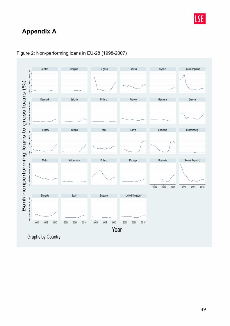
49

Appendix A

Figure 2: Non-performing loans in EU-28 (1998-2007)

0.0

01

0.0

020

.003

0.0

00

.00

10

.002

0.0

030

.00

0.0

01

0.0

020

.003

0.0

00

.00

10

.002

0.0

030

.00

0.0

01

0.0

020

.003

0.0

0

2000 2005 2010 2000 2005 2010

2000 2005 2010 2000 2005 2010 2000 2005 2010 2000 2005 2010

Austria Belgium Bulgaria Croatia Cyprus Czech Republic

Denmark Estonia Finland France Germany Greece

Hungary Ireland Italy Latvia Lithuania Luxembourg

Malta Netherlands Poland Portugal Romania Slovak Republic

Slovenia Spain Sweden United Kingdom

Ba

nk

no

np

erf

orm

ing

loa

ns

to g

ross

loa

ns

(%)

YearGraphs by Country

50

Figure 3: Market power in EU-28 (1998-2011)

-1.5

-1-.

50

.5-1

.5-1

-.5

0.5

-1.5

-1-.

50

.5-1

.5-1

-.5

0.5

-1.5

-1-.

50

.5

2000 2005 2010 2000 2005 2010

2000 2005 2010 2000 2005 2010 2000 2005 2010 2000 2005 2010

Austria Belgium Bulgaria Croatia Cyprus Czech Republic

Denmark Estonia Finland France Germany Greece

Hungary Ireland Italy Latvia Lithuania Luxembourg

Malta Netherlands Poland Portugal Romania Slovak Republic

Slovenia Spain Sweden United Kingdom

Lern

er in

dex

YearGraphs by Country

51

Appendix B

Main Results: Effect of banking competition (Complete Table)

Explanatory (1) (2) (3) (4) Variables Fixed Effects Fixed Effects Fixed Effects GMM L.lnnpl 0.616*** 0.330* (0.0984) (0.162) lnlerner -0.378*** -0.434*** -0.319** -0.471** (0.109) (0.136) (0.136) (0.192) capitalization -0.00127 -0.00219 -0.000389 -0.00107 (0.00415) (0.00379) (0.00300) (0.00479) credit 0.00732* 0.0107** 0.0108*** 0.0172*** (0.00375) (0.00380) (0.00336) (0.00583) roe -0.000946 -0.000713 0.00678* (0.00291) (0.00185) (0.00377) cost_to_income -0.00466 -0.00303 -0.00492 (0.00399) (0.00374) (0.00549) capital_to_assets 0.0248 0.0351 0.0653 (0.0575) (0.0599) (0.0684) regulatory_capital 0.0620* 0.0328* -0.0136 (0.0299) (0.0158) (0.0314) non_interest_income 0.00577 0.00426 0.00551 (0.00442) (0.00358) (0.00430) gov_debt 0.00400 0.00340 0.00407 0.00866 (0.00503) (0.00626) (0.00410) (0.00742) interest_rates 0.0272* 0.00957 0.00520 0.0175 (0.0146) (0.0201) (0.0133) (0.0223) unempl 0.142*** 0.133*** 0.0212 0.0629 (0.0394) (0.0290) (0.0264) (0.0467) growthrate -0.0290 -0.0296 -0.0464** -0.0502* (0.0251) (0.0230) (0.0167) (0.0248) inflation -0.000141 0.00220 -0.0117 -0.00680 (0.00762) (0.00902) (0.00729) (0.0106) lngdpcapita 5.415** 5.059** 4.824*** 4.638** (1.998) (1.875) (1.647) (1.768) quality 0.414 0.395 0.303 0.549 (0.417) (0.397) (0.344) (0.482) corruption 0.276* 0.257* 0.00800 0.306* (0.147) (0.139) (0.117) (0.164) bureau_coverage -0.00500 -0.00322 -0.00765** -0.00780* (0.00462) (0.00498) (0.00331) (0.00400) legal 0.0797 0.0831 0.149 0.145 (0.725) (0.562) (0.394) (0.557) depth -0.868** -0.865** -0.711 -0.927** (0.411) (0.411) (0.417) (0.430) yr7 -0.0769 0.284 0.412* 0.281 (0.288) (0.274) (0.212) (0.315)

Continues to next page

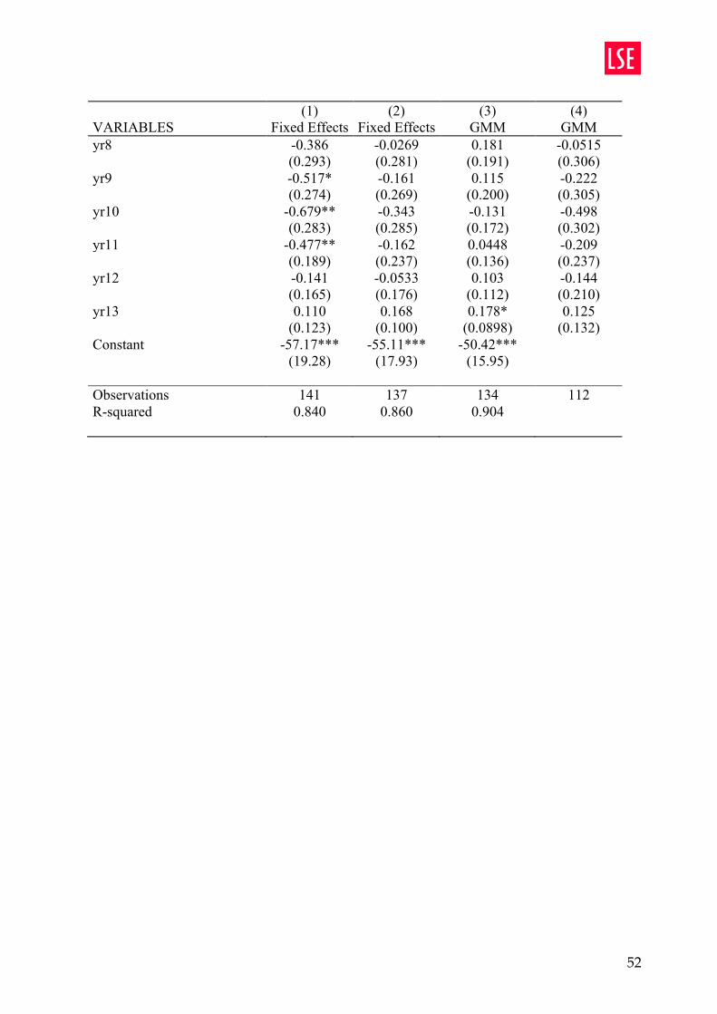
52

(1) (2) (3) (4) VARIABLES Fixed Effects Fixed Effects GMM GMM yr8 -0.386 -0.0269 0.181 -0.0515 (0.293) (0.281) (0.191) (0.306) yr9 -0.517* -0.161 0.115 -0.222 (0.274) (0.269) (0.200) (0.305) yr10 -0.679** -0.343 -0.131 -0.498 (0.283) (0.285) (0.172) (0.302) yr11 -0.477** -0.162 0.0448 -0.209 (0.189) (0.237) (0.136) (0.237) yr12 -0.141 -0.0533 0.103 -0.144 (0.165) (0.176) (0.112) (0.210) yr13 0.110 0.168 0.178* 0.125 (0.123) (0.100) (0.0898) (0.132) Constant -57.17*** -55.11*** -50.42*** (19.28) (17.93) (15.95) Observations 141 137 134 112 R-squared 0.840 0.860 0.904

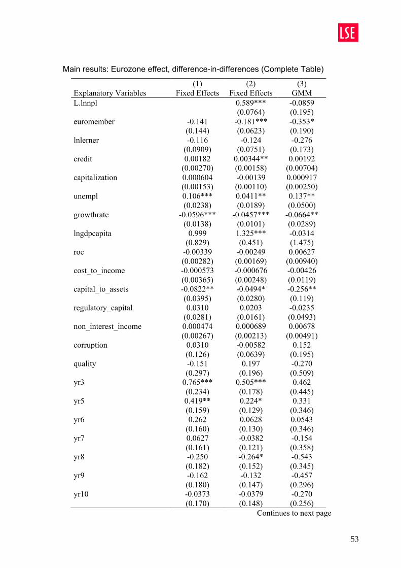
53

Main results: Eurozone effect, difference-in-differences (Complete Table)

(1) (2) (3) Explanatory Variables Fixed Effects Fixed Effects GMM L.lnnpl 0.589*** -0.0859 (0.0764) (0.195) euromember -0.141 -0.181*** -0.353* (0.144) (0.0623) (0.190) lnlerner -0.116 -0.124 -0.276 (0.0909) (0.0751) (0.173) credit 0.00182 0.00344** 0.00192 (0.00270) (0.00158) (0.00704) capitalization 0.000604 -0.00139 0.000917 (0.00153) (0.00110) (0.00250) unempl 0.106*** 0.0411** 0.137** (0.0238) (0.0189) (0.0500) growthrate -0.0596*** -0.0457*** -0.0664** (0.0138) (0.0101) (0.0289) lngdpcapita 0.999 1.325*** -0.0314 (0.829) (0.451) (1.475) roe -0.00339 -0.00249 0.00627 (0.00282) (0.00169) (0.00940) cost_to_income -0.000573 -0.000676 -0.00426 (0.00365) (0.00248) (0.0119) capital_to_assets -0.0822** -0.0494* -0.256** (0.0395) (0.0280) (0.119) regulatory_capital 0.0310 0.0203 -0.0235 (0.0281) (0.0161) (0.0493) non_interest_income 0.000474 0.000689 0.00678 (0.00267) (0.00213) (0.00491) corruption 0.0310 -0.00582 0.152 (0.126) (0.0639) (0.195) quality -0.151 0.197 -0.270 (0.297) (0.196) (0.509) yr3 0.765*** 0.505*** 0.462 (0.234) (0.178) (0.445) yr5 0.419** 0.224* 0.331 (0.159) (0.129) (0.346) yr6 0.262 0.0628 0.0543 (0.160) (0.130) (0.346) yr7 0.0627 -0.0382 -0.154 (0.161) (0.121) (0.358) yr8 -0.250 -0.264* -0.543 (0.182) (0.152) (0.345) yr9 -0.162 -0.132 -0.457 (0.180) (0.147) (0.296) yr10 -0.0373 -0.0379 -0.270 (0.170) (0.148) (0.256)


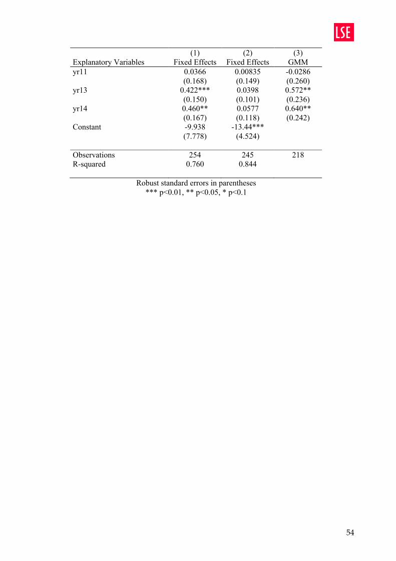
54

(1) (2) (3) Explanatory Variables Fixed Effects Fixed Effects GMM yr11 0.0366 0.00835 -0.0286 (0.168) (0.149) (0.260) yr13 0.422*** 0.0398 0.572** (0.150) (0.101) (0.236) yr14 0.460** 0.0577 0.640** (0.167) (0.118) (0.242) Constant -9.938 -13.44*** (7.778) (4.524) Observations 254 245 218 R-squared 0.760 0.844


55

Robustness checks: effect of banking competition, Boone Indicator and 5-bank asset concentration (Complete Table)

Explanatory Variables (1) (2) (3) (4) OLS fixed

effects OLS fixed

effects GMM GMM

L.lnnpl 0.726*** 0.832*** (0.147) (0.136) asset_concentration -0.00253 0.0143 (0.0102) (0.0124) boone 2.611** 3.123** (1.236) (1.355) credit 0.0104* 0.0104* 0.0103* 0.0114** (0.00577) (0.00602) (0.00516) (0.00481) capitalization 0.000559 0.00163 -0.00656* -0.00589 (0.00669) (0.00643) (0.00362) (0.00455) capital_to_assets 0.00547 0.0110 0.129 0.0732 (0.0672) (0.0671) (0.103) (0.0904) non_interest_income -0.000820 0.00170 0.00232 0.00652 (0.00294) (0.00419) (0.00331) (0.00726) gov_debt 0.00410 0.00250 0.00781** 0.00219 (0.00593) (0.00602) (0.00340) (0.00322) regulatory_capital 0.0850* 0.0855* 0.00421 0.00804 (0.0414) (0.0435) (0.0246) (0.0351) cost_to_income -0.00902 -0.00394 -0.00630 0.00210 (0.00640) (0.00606) (0.00688) (0.00712) provisions -0.000615 -0.000227 -0.00232 2.62e-05 (0.00116) (0.00103) (0.00142) (0.00191) interest_rates 0.0221 0.0196 -0.0117 -0.000203 (0.0165) (0.0157) (0.0152) (0.0162) unempl 0.145*** 0.146*** -0.00294 0.00899 (0.0448) (0.0443) (0.0506) (0.0522) bureau_coverage -0.00242 -0.00183 -0.00447 -0.00851** (0.00612) (0.00638) (0.00396) (0.00397) corruption 0.187 0.209 -0.0737 (0.165) (0.180) (0.152) quality 0.380 0.340 0.409 0.515 (0.603) (0.590) (0.447) (0.640) roe 0.00134 4.93e-05 0.00462 0.00273 (0.00274) (0.00261) (0.00309) (0.00381) growthrate -0.0196 -0.0294 -0.0752*** -0.0811*** (0.0246) (0.0308) (0.0190) (0.0188) lngdpcapita 3.905* 4.198* 0.761 3.356 (2.042) (2.216) (2.486) (3.417) inflation 0.000537 -0.00407 (0.00998) (0.00963) control_of_corruption 0.188 (0.280) legal 0.749 0.746 0.589 0.206 (1.218) (1.200) (0.957) (0.859)


56

Explanatory Variables (1) (2) (3) (4) OLS fixed

effects OLS fixed

effects GMM GMM

depth -0.662 -0.572 -0.515 -0.288 (0.574) (0.615) (0.528) (0.535) yr7 0.343 0.665* 0.109 0.231 (0.292) (0.348) (0.339) (0.350) yr8 -0.0820 0.219 -0.0970 0.0906 (0.307) (0.204) (0.203) (0.189) yr9 -0.135 0.128 0.148 0.277 (0.300) (0.136) (0.170) (0.177) yr10 -0.231 (0.351) yr11 0.0226 0.283 0.0979 0.0778 (0.242) (0.189) (0.122) (0.139) yr13 0.0167 0.396 -0.263 -0.0515 (0.136) (0.405) (0.250) (0.246) yr14 0.0960 0.439 -0.254 -0.0638 (0.167) (0.470) (0.260) (0.222) yr12 0.299 -0.385 -0.165 (0.403) (0.233) (0.185) Constant -43.42** -47.23** (19.70) (21.49) Observations 124 121 100 98 R-squared 0.868 0.852


What determines financial stability in EU: The effect of banking competition and Eurozone membership...

Documents

Transcript of What determines financial stability in EU: The effect of banking competition and Eurozone membership...