What can the Mus musculus musculus/M. m. domesticus hybrid zone tell us about speciation?

14

What can the Mus musculus musculus/M. m.domesticus hybrid zone tell us aboutspeciation?

STUART J. E. BAIRD AND MILOŠ MACHOLAN

Introduction

One of the crucial tasks in the study of speciation is to explain the genetic

basis of reproductive barriers between diverged taxa. Despite the best endeavours of

generations of evolutionary biologists since Darwin andWallace, our understand-

ing of the genetics of speciation has lagged behind other fields of evolutionary

biology. The reason may be simply that the greater the reproductive isolation, the

less cross progeny we have to work with, butmore probably it is because the genetic

factors involved are numerous, with complex interactions. Indeed, it appears that

except for a few cases (Coyne and Orr, 2004) reproductive isolation arises in many

small steps rather than a few strongly selected mutations, in agreement with

theoretical predictions (Walsh, 1982; Barton and Charlesworth, 1984). Obviously,

the more genes with small effect that are involved in reproductive isolation, the

more difficult will be their identification, making traditional laboratory hybrid-

ization experiments and association studies challenging.

It seems only common sense, therefore, to search for alternative approaches.

One promising alternative is to study naturally occurring hybrid zones. The seeds

for progress were sown by Barton and Hewitt (1985, 1989), who suggested the

majority of hybrid zones were ‘tension zones’ (Box 14.1). While initially received

with scepticism in some quarters, the tension zone paradigm now dominates the

hybrid zone literature and is arguably the main justification for the view that

hybrid zones are ‘natural laboratories’ (Hewitt, 1988) and ‘windows on evolu-

tionary process’ (Harrison, 1990). The reason this paradigm is so important is

that it unifies hybrid zone process over a diversity of species, geographic scales,

and histories of contact into a single analytically tractable framework (Box 14.2)

with intuitive, testable results and predictions that have been borne out repeatedly

over the subsequent decades. Tension zones are measured relative to the scale of

Evolution of the House Mouse, ed. Miloš Macholán, Stuart J. E. Baird, Pavel Munclinger, and Jaroslav Piálek.

Published by Cambridge University Press. © Cambridge University Press 2012.

dispersal of the organism involved, and on this metric the stronger the selection

against admixture the more abrupt are the changes between the taxa (clines) we

see as we cross the hybrid zone. This simple contrast (strong selection = narrow

cline; weak selection = wide cline) holds even when comparing snail hybrid zones

to bird hybrid zones – as long as we measure width relative to their respective

dispersal scales – but comparisons across clines at loci within the same genome are

evenmore robust. The approach of plotting cline width for a number of loci along

a linkage group to see where clines are narrow, and therefore to map genes

responsible for reproductive barriers seems obvious given current technology,

Box 14.1 Hybrid zones and the tension zone paradigm

In this chapter we use a consensus definition of hybrid zones as areas where genet-ically distinct groups of individuals meet, mate, and leave at least some offspring ofmixed ancestry (Barton and Hewitt, 1985, 1989; Harrison, 1990). An advantage of thisrather broad notion is its independence of our knowledge of the history or geographyof hybrid zones and the evolutionary forces affecting their dynamics. Hybrid zonescan be maintained by various kinds of selection – for example, by balancing selectionfavouring hybrids within a narrow region of intermediate habitat (‘bounded hybridsuperiority’; Moore, 1977). In this case, a trait at equilibrium may vary gradually fromplace to place, independent of dispersal. However, as pointed out by Barton and Gale(1993), dispersal has a negligible effect only when character gradients (clines) aremuch wider than the characteristic scale of selection (i.e. the distance over whichselection changes allele frequencies), l ¼ �ffiffi

sp , where σ is the rate of dispersal, defined as

the standard deviation of the distance between parent and offspring measured along alinear axis, and s is the magnitude of selection (Slatkin, 1973; Barton and Hewitt,1989). In fact, clines are usually much narrower than potential environmental gra-dients and dispersal-independent zones are thus rare. Moreover, most hybrid zonesconsist of a cluster of coincident clines even for characters with no obvious functionalrelationship (Barton and Hewitt, 1985, 1989) and with similar width and shape acrossdifferent portions of the zone, patterns that are unlikely for clines maintained directlyby the external environment. Thus it appears that most hybrid zones are maintained bya balance between dispersal and selection. This selection can be exogenous (so thatalleles are selected against when appearing in foreign habitat) or endogenous (so thatalleles are counter-selected when appearing on foreign genetic background). If differ-ent alleles are favoured in different habitats, the hybrid zone will be located at aparticular environmental gradient, whereas if selection acts against hybrids, the zoneis free to move and will stop when trapped by a geographic barrier or in an area of lowpopulation density (a ‘density trough’; Hewitt, 1975, 1989; Barton, 1979; Barton andHewitt, 1985). These zones, maintained by a balance between dispersal from each sideand central endogenous selection, are called ‘tension zones’ because, like the surface ofa bubble, they minimize their extent while balancing pressure on either side (Key,1968; Barton, 1979; Barton and Hewitt, 1985) (Fig. 14.1).

What can the hybrid zone tell us about speciation? 335

but in the 1990s when this was first discussed, multi-locus studies focused on a

few unlinked loci, and it took more than a decade to bring the idea to fruition.

One of the ground-breaking studies was done on the house mouse hybrid zone

(HMHZ) in Europe (Payseur et al., 2004), which suggested a reproductive

barrier region on the central X chromosome. In the same year laboratory crosses

mapped sterility genes to the same chromosomal region (Oka et al., 2004;

Storchová et al., 2004; see Forejt et al., Chapter 19 in this volume, for review).

These results demonstrate the efficacy of hybrid zones as tools for speciation

studies, complementary to laboratory crosses and positional cloning approaches,

as well as the paramount role the house mouse can play in this research.

Despite this positive outlook we suggest caution in hybrid zone speciation

research. The intuitive nature of the idea to use narrow clines to locate barriers to

gene flow has led to overconfidence in its application. Just because hybrids are

sampled in the field, rather than bred in the laboratory, does not mean strict

Figure 14.1 When we blow a soap bubble its shape wobbles, then settles into a

sphere which balances the internal and external air pressure while minimizing the

extent of the soap boundary (the sphere is the shape with minimum surface area for

the enclosed volume). Tension zones have similar behaviour: wobbling over the

landscape they settle where the pressure of gene flow is equal from either side and

the extent of the zone isminimized, smoothing thepathof the zone centre towards a

straight line (the shortest distance between two points). See the plate section for a

colour version of this figure.

336 Stuart J. E. Baird and Miloš Macholan

rigour is unnecessary. In fact, more rigour is needed if we hope to distinguish

signals in the data from stochastic noise; laboratory-based research minimizes

this noise by controlling conditions, but when sampling from nature we cannot

control conditions and so wemust be particularly vigilant to sources of noise (Boxes

14.3, 14.4). Ignoring such sources of uncertainty leads to overconfident inference,

and overconfident inference could discredit hybrid zone speciation research before

it has shown its full potential. Under these circumstances our chapter title might

also have been ‘What can the HMHZ not tell us about speciation?’. Knowing the

limits of what we can infer is central to the scientific endeavour. The better our

understanding of (1) the circumstances from which we are sampling in nature;

(2) the assumptions underlying our models of those circumstances; and (3) the

stochastic effects introduced by sampling and the limitations of our analytical

techniques, the better we will be able tomodulate and communicate our confidence

in the results. Here we review each of these issues in turn with respect to inference

about speciation from theHMHZ in an attempt to set a solid foundation for future

research. We finish by suggesting promising future directions.

The house mouse hybrid zone in Europe

There is wide agreement that no extant house mice occupied western

Eurasia before the end of the last glaciation (Thaler, 1986; Auffray et al., 1990;

Auffray and Britton-Davidian, 1992; Cucchi et al., Chapter 3 in this volume; but

see Sage et al., 1990 for a different view). The mouse expansion into western

Eurasia followed two colonization routes consistent with human historical patterns

(Kratochvíl, 1986; Thaler, 1986; Auffray et al., 1990; Cucchi et al., 2005; Bonhomme

et al., 2011). Mus musculus domesticus arrived from Asia Minor, along the

Mediterranean Basin, and now occurs in southern and western Europe; M. m.

musculus followed a pathway north of the Black Sea and today occupies northern

and eastern parts of the continent. Where their ranges abut, a narrow hybrid zone is

created, running across the central part of the Jutland Peninsula (approximately from

Vejle Fjord westwards) and from the Baltic coast ca. 25 km east of Kiel Fjord (East

Holstein, northern Germany) through central Europe and the Balkan Peninsula to

the Black Sea coast (Sage et al., 1993; Macholán et al., 2003; Fig. 14.2). Recently, a

new portion of the zone has been localized in Norway (Jones et al., 2010).

Following the pioneering works of Degerbøl (1949), Zimmermann (1949), and

Ursin (1952), this zone has been studied in Denmark (Selander et al., 1969; Hunt

and Selander, 1973; Schnell and Selander, 1981; Ferris et al., 1983; Vanlerberghe

et al., 1986, 1988b; Nancé et al., 1990; Dod et al., 1993, 2005; Fel-Clair et al., 1996,

1998; Lanneluc et al., 2004; Raufaste et al., 2005); northern Germany (van

Zegeren and van Oortmerssen, 1981; Prager et al., 1993); Saxony, eastern


Germany (Teeter et al., 2010); southern Bavaria (south-eastern Germany) and

northwestern Austria (Sage et al., 1986b; Tucker et al., 1992; Payseur et al., 2004;

Payseur and Nachman, 2005; Teeter et al., 2008, 2010; Dufková et al., 2011);

northeastern Bavaria and the western part of the Czech Republic (Munclinger

et al., 2002; Božíková et al., 2005; Macholán et al., 2007, 2008, 2011); and eastern

Bulgaria (Vanlerberghe et al., 1986, 1988a).

Despite the common belief that the musculus/domesticus zone has resulted

from the secondary contact of the two taxa in the Holocene, the history of initial

contact, including exact dating, is unclear. Almost certainly first contact was in

Figure 14.2 The course of the M. m. musculus/M. m. domesticus hybrid zone in Europe

(bold line). In Norway, its position is only tentative (dashed bold line). Shaded rectangles

depict studied transects: A: Denmark; B: East Holstein (Germany); C: Saxony, Saxony-

Anhalt, and Thuringia (Germany); D: west Bohemia (Czech Republic) and northeast

Bavaria (Germany); E: southeast Bavaria (Germany and northwest Austria); F: east

Bulgaria. The dotted line indicates where the eastern humid continental climate zone

meets any of four other climate zones: anticlockwise from top these are subarctic

(northern Scandinavia); humid oceanic (west); humid and dry subtropical (south); and

semi arid (in the east, north of the Black Sea). For clarity the boundary between the

western and southern zones is omitted, likewise the highland climate zone of the Alps

(simplified from http://printable-maps.blogspot.com/2008/09/map-of-climate-zones-

in-europe.html).


Box 14.2 Tension zone models

Sigmoid clines

The simplest model of a tension zone was proposed by Bazykin (1969). It assumes ahomogeneous environment, heterozygote fitness to be (1 – s) relative to both homo-zygotes, weak selection acting on each locus independently (no cross-locus associa-tions, i.e. linkage disequilibrium), and gene flow approximated by diffusion. Theallele frequency is then p = 1 / (1 + exp[–(x – c) / l]), where (x – c) is the distance of a sitefrom the cline centre and l is the scale of selection defined in Box 14.1 (Slatkin, 1973;Barton and Hewitt, 1989) (Fig. 14.3a, solid line). The width of a cline in trait z isusually defined as w =Δz / (∂z / ∂x): this is the inverse of the maximum slope ∂z/∂xscaled by the total trait change Δz. This definition applies equally to clines in thefrequency of diagnostic alleles from 0 to 1 (Δz = 1), clines in allele frequency atinformative loci (0 <Δz < 1), and clines in quantitative traits where Δz depends onlyon what is measured. It also allows explicit theoretical predictions impossible withother ad hoc width definitions such as the distance over which z changes from 20% to80% (Endler, 1977; Barton and Hewitt, 1989). The cline width (w) depends on theselection acting: for example, when selection acts against heterozygotes it is

ffiffiffiffiffiffiffiffiffi8�2s

p(Bazykin, 1969; Barton and Hewitt, 1989), whereas when selection favours differentalleles on different sides of the hybrid zone the width equals

ffiffiffiffiffiffiffiffiffi3�2s

p(Haldane, 1948; if

we assume no dominance the cline is slightly wider: w ¼ 1:782ffiffiffiffiffiffiffi�2s

p; Barton and

Gale, 1993).There are several ways of expressing the shape of the single locus clines described

by Bazykin (1969), and this has led to some confusion. Bazykin chose to use thehyperbolic tangent function (Tanh), giving a smooth sigmoid curve (or a straight lineif plotted on a logit scale). The Tanh cline is sigmoid in the sense that it is equivalentto a logistic (sigmoid) curve [(tanh(x) + 1) / 2 = logistic (2x)], and this is also why it is astraight line if plotted on a logit scale – the inverse of the logistic function is the logitfunction. The type of selection has little effect on cline shape, so this model can beused for clines caused by heterozygote disadvantage, extrinsic selection favouringdifferent alleles in different places, or selection acting on quantitative traits (Haldane,1948; Fisher, 1950; Bazykin, 1969; Slatkin, 1973, 1975; Nagylaki, 1975, 1976; Endler,1977). If selection is weak the model also approximates clines in structured popula-tions described by the stepping-stone model (Nagylaki, 1975). However, Bazykin’smodel is a single locus model, while selection acting in a hybrid zone typically affectsseveral or many loci.

Stepped clines

Influx of parental gene combinations into a tension zone causes strong associationsbetween the loci or linkage disequilibrium, D (Li and Nei, 1974; Slatkin, 1975). SinceD is proportional to the gradient of allele frequencies, across-locus associations areweak at the edges of the zone, and selection affects each locus separately. However, aswe move towards the zone centre, the gradient steepens, causing stronger disequi-libria. As associations across loci become stronger, selection no longer affects eachlocus independently. Selection is strengthened by a ‘hitch-hiking’ effect: stronger


Box 14.2 (cont.) Tension zone models

A

1 2x

0.2

0.4

0.6

0.8

1.0p

B

−2 −1

−2 −1

1 2

0.2

0.4

0.6

0.8

1.0

Figure 14.3 (a) Solid: sigmoid cline; dashed: stepped cline with the same centre and

width, but more shallow tails of introgression. (b) Progress over time from steep clines

at initial contact (light grey) to quasi-equilibrium width (dark grey).

selection generates stronger associations which, in turn, cause yet stronger selection. Theresult of these associations is a barrier to the (independent) flow of genes across the zonecentre, and is manifested as a sharp step at the centre of each cline (Barton, 1983; Bartonand Bengtsson, 1986; Barton and Gale, 1993). Barton (1986) models clines with a centralbarrier to gene flow as tripartite: allele frequencies in the central portion follow thesigmoid model, but on either side (away from the influence of central associations) the


southern regions, progressing to central and northern Europe, like a zipper

being pulled up through the continent. Therefore, the northern portion of the

hybrid zone may be much younger than the southern parts. According to

Boursot et al. (1993), while mice arrived in the western Mediterranean and

Box 14.2 (cont.) Tension zone models

cline decays exponentially as p / exp 4xffiffiffi�

p=w

� �, where θ is the rate of decay on the

right and left side, respectively (Fig. 14.3a, dashed line). Parameter θ can be expressed interms of the ratio between the selection acting on an individual locus itself (se) and theeffective selection pressure on the locus at the centre, which is primarily due to associationwith other loci (s*): θ= se / s

* (Szymura and Barton, 1986). A stepped cline pattern suggestsa zonewith a central barrier to gene flow, regardless of whether this is caused by a physicalobstacle or by associations with other loci. The strength of the barrier is defined asB=Δp/p0, where Δp is the height of the central step and p0 = ∂p / ∂x is the gradient ofallele frequency on either side of this step. B can be estimated separately for the left andright side of the cline (Nagylaki, 1976) so the asymmetrical stepped model comprises sixparameters: w, c, θL, BL, θL, BL, where subscripts L and R denote left and right side,respectively. The barrier strength has units of distance, and can be thought of as thedistance over which unimpeded gene flow would lead to the same change in allelefrequencies. Barrier strength may be different in each direction, leading to asymmetricclines that will have a tendency to move.

Another way of assessing the magnitude of the barrier is to calculate the number ofgenerations that an allele is delayed when crossing the zone. For a neutral allele, thisdelay can be substantial, from hundreds to tens of thousands of generations (T≈ (B / σ)2;Barton and Hewitt, 1985, 1989; Barton and Gale, 1993). In contrast, even slightlyadvantageous alleles can cross the zone quite rapidly, at T≈ log[(B / σ)2πsa / 2] / 2sagenerations if sa≫ (B / σ)-2, where sa is the selective advantage (Barton and Hewitt,1985, 1989; Barton and Bengtsson, 1986; Barton and Gale, 1993).

Because the central barrier in a tension zone depends so crucially on the associationbetween loci, estimation of D can be used, along with cline shape parameters, forsubsequent estimation of the scale of dispersal, effective selection on marker loci,selection on selected loci, the total number of genes under selection, and the meanfitness of hybrids (see Appendix).

Dynamics of secondary contact

The models above are for clines that have reached a quasi-equilibrium balance betweendispersal of individuals into the centre of the zone and selection against admixture.However, at the beginning of secondary contact, clines are step-like transitions: it takessome generations for them to settle into their equilibrium shape (Fig. 14.3). At thegenomic level progression towards equilibrium depends on the ratio of selection torecombination (or segregation for loci on different chromosomes), and may be very slowleaving intact blocks of the genome of each taxon long after secondary contact, asignature that can be used to date this contact (Baird, 1995, 2006).


central Europe during the Bronze Age (4000–2800 bp; Auffray et al., 1990;

Vigne, 1992; Auffray, 1993), northwestern and northern Europe were colonized

during the Iron Age (ca. 2800 bp; Lepiksaar, 1980; Auffray et al., 1990;

O’Connor, 1992; Auffray, 1993). Sage et al. (1993) supposed 6000 bp for south-

ern Europe and Gyllensten and Wilson (1987) 5000–6000 bp for central

Europe. Estimates of the time of colonization of Scandinavia are even more

variable: Prager et al. (1993) assumed spread of mice following human demic

diffusion 4000–5000 bp (Sokal et al., 1991), whereas Gyllensten and Wilson

(1987) concurred with Clark (1975), who dated the advent of agriculture to 3500–

4500 bp. On the other hand, a recent careful revision of zooarchaeological data

Box 14.3 Spatial sampling noise

When we calculate the likelihood of a set of parameters describing cline shape andmake inferences about selection affecting individual loci, several sources of errorshould be taken into account. These are perhaps especially strong for the housemouse, which has an aggregated spatial distribution and usually lives in small anddefended demes in which most offspring are sired by a dominant male. The lifespanof these demes is rather short, adding a further source of stochasticity to thedistribution of allele frequencies across localities. Calculating the effective samplesize (Phillips et al., 2004; Raufaste et al., 2005; Macholán et al., 2008) takes intoaccount the sampling noise introduced by small samples with deviations from HardyWeinberg equilibrium within each sampling locality and differences in relatednessacross localities, but does not take into account the noise introduced by how thesampled localities fall in relation to the zone centre. This noise is particularly strongwhen a one-dimensional (1D) transect is used to sample a 2D hybrid zone (Fig. 14.4).

One component of spatial sampling error has recently been more rigorouslyassessed for the Czech–Bavarian portion of the HMHZ. The underlying orientationof this zone has been estimated with good support (Macholán et al., 2008, 2011). Forthis known orientation Dufková et al. (2011) used a jackknife-based procedure inwhich one locality at a time was removed from the dataset and cline estimates re-computed for each locus. They showed that exclusion of a single locality can result inincrease of cline width estimates across loci up to 84-fold, considerably higher thanthe 50-fold inter-locus span found in the 39 SNP dataset from 1D sampling insouthern Germany (Teeter et al., 2008).When clines are stepped, exclusion of centrallocalities has a more severe impact on cline width estimates than omitting sites farfrom the centre, whereas for sigmoid clines the impact on the cline width is greater iflocalities further from the centre are deleted. Dense sampling of central localities istherefore vital for reliable estimates of introgression patterns and inferences ofgenomic regions important in speciation (Barton and Gale, 1993; Macholán et al.,2007; Dufková et al., 2011). When sampling from the central segment of the zone issparse relative to cline width, only upper bounds can be placed on the width estimates(Macholán et al., 2007).


2 1 0 1 2

2

1

0

1

2

1.0 0.5 0.5 1.0 1.5 2.0

0.2

0.4

0.6

0.8

1.0

Figure 14.4 Spatial sampling noise. One hundred sampling localities are distributed at random

across a hybrid zone of unknown orientation. (a) Assuming effective sample sizes are Poisson

distributed with mean 10, pies show binomial allele frequency samples from an underlying cline

(shades of grey). Pies close to a horizontal transect line are shaded in orange and cyan (see colour plate

of this figure). (b) The shape of the underlying cline is compared to allele frequency estimates from

the 14 locality samples close to the horizontal transect line: cline estimation would either displace the

centre to the left, or overestimate the steepness of the cline. Without sampling noise there would be

no displacement, and an underestimation of the cline steepness (because the horizontal transect is

oblique to the path of the zone). See plate section for a colour version of this figure.

has suggested that western and northern Europe had not been colonized by

mice before 1000 bc–ad 300 (Cucchi et al., 2005, see also Cucchi et al.,

Chapter 3). The most extreme of recent estimates are given by Sage et al.

(1993), assuming an arrival of mice in Denmark 250 years ago, and Hunt and

Selander (1973), who pointed out that stable mouse populations in western

Jutland could not have been established before the beginning of the programme

of reclamation of marshlands in 1850.

Why is the age of the hybrid zone so important? A hybrid zone will get wider

over time unless some force acts to maintain the distinction between taxa, in

which case the zone will settle into quasi-equilibrium (Box 14.2). Assuming cline

widths ~10–20 km and a scale of dispersal ~1 kmgen–1/2 (see below), a neutral

allele will cross the zone after 16–32 generations. Because the zone, at all points, is

thought to be much older than this, we can assume it has settled into quasi-

equilibrium all along its length. Current estimates suggest the width of the

HMHZ is very similar in Jutland and some 700 km to the south in the Czech

Republic (Macholán et al., 2007). This similarity in the width of the hybrid zone

despite different times of contact, and diverse locations, argues for a similar

Box 14.4 Model choice in hybrid zone analysis

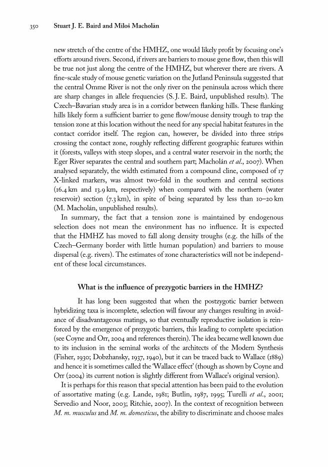
Supposewe choose to analyse hybrid zone samples using a two-parameter sigmoid clinemodel (Box 14.2), but we later find out that the hybrid zone is a multi-locus tensionzone with stepped clines (Box 14.2) due to an asymmetric central barrier to gene flow.What are the consequences of having fitted the wrong model? In particular, what arethe consequences of fitting a symmetric sigmoid curve model to an asymmetric cline(Figure 14.6a)? As the likelihood fitting algorithm tries to match the asymmetric datawith the symmetric model it shifts the model to one side. The more asymmetric thedata, the more the cline centre estimate diverges from the real position of the cline centre(Fig. 14.6b). This is not a bug in the likelihood approach. Rather, it is exactly what weexpect to happen if the inappropriate model is chosen for analysis. The consequencesfor inference are grave. In the data we fully expect clines at different loci to havedifferent degrees of asymmetry. Analyses of these with symmetric models will shift thecentre estimates of each to a different degree, giving the impression that the zone hasnon-coincident cline centres. We might then mis-infer the very nature of the zonebecause ‘coincident cline centres’ is one of the most fundamental expectations of a zonewith a central barrier to gene flow. It is for such reasons that we have repeatedly stressedthe importance of the model-choice stage of cline analysis (Macholán et al., 2007, 2008;Vošlajerová Bímová et al., 2011). Model choice is an automatic feature of, for example,phylogenetic sequence analyses, and it is a matter of some frustration that the issue isstill often ignored in the hybrid zone literature.


mechanismmaintaining taxon separation whenever and whereverM.m. musculus

and M. m. domesticus meet.

Is the zone maintained by exogenous or endogenous factors?

The European HMHZ is a ~20-km wide complex gradation of late-

generation hybrids and backcrosses with F1hybrids missing or extremely rare; for

most markers the zone structure is unimodal with intermediate genotypes in the

centre (Raufaste et al., 2005; Macholán et al., 2007). There has been some debate

regarding the origins of the factors that maintain the zone. A seeming coinci-

dence of its position and the boundary between oceanic and continental climate

zones led several authors to conclude that the contact of these subspecies is

regulated primarily by climatic factors (Zimmermann, 1949; Serafiński, 1965;Hunt and Selander, 1973; Thaler et al., 1981; Boursot et al., 1984; Klein et al.,

1987). However, recalling the concept of the characteristic scale of selection

(Box 14.2), the scale of this climatic gradient is too wide to maintain such a

narrow hybrid zone (Boursot et al., 1993). Further, as human commensals, mice

mostly live in artificial habitats buffered from climate influences, and there is an

obvious discrepancy between the position of the hybrid zone and the climatic

transition, a fact pointed out by Kraft (1985). As shown in Fig. 14.2, the HMHZ

does not match the climate transition closely anywhere in Europe, suggesting

climate is not an important factor in either its position or width.

Barton and Hewitt’s (1985) suggestion that the HMHZ is a tension zone,

maintained by a balance between dispersal and endogenous selection against

hybrids, has received increasing support from genetic studies over geographi-

cally independent transects (e.g. Payseur et al., 2004; Raufaste et al., 2005;

Macholán et al., 2007). Stepped clines (Box. 14.2) with stronger linkage dis-

equilibria in the centre have been demonstrated in Denmark (Dod et al., 2005;

Raufaste et al., 2005), southern Germany (Payseur et al., 2004), and the Czech–

Bavarian portion of the zone (Macholán et al., 2007, 2008). Leaving aside other

potential causes of the stepped pattern of the molecular clines, such as geo-

graphic barriers or epistasis (see Macholán et al., 2007 for discussion), the

stepped shape can be produced either by strong selection acting on a small

number of loci or weak selection affecting a moderate to large number of loci

(cf. Porter et al., 1997; see Walsh, 1982 and Barton and Charlesworth, 1984 for

theoretical arguments in favour of the latter possibility). A stepped cline pattern

has been confirmed for allozyme markers in the Danish transect, where the

number of loci under selection was estimated at 46–120, with effective selection

pressure maintaining the cline s*≈ 3–7% and fitness of hybrids ~45% (Raufaste

et al., 2005); and in the Czech–Bavarian transect, with 56–99 selected loci,


s*≈ 6–9%, and fitness of hybrids 25–60% (Macholán et al., 2007). An analysis of

five X chromosome markers revealed substantially stronger selection (s*≈ 25%)

and a larger reduction in fitness of hybrids than selection affecting autosomal

loci (≈ 23–35%; Macholán et al., 2007, 2008). Estimates of the number of

selected X-linked loci were rather incongruent: while the original study of

Macholán et al. (2007) yielded 380 loci, a later analysis of 17 X chromosome

markers resulted in a much lower estimate (eight selected loci; M. Macholán,

unpublished results). As the first estimate exceeds all estimates of the total

number of selected loci in the genome, we favour the second of these calcu-

lations. It should be noted, however, that all these calculations assume that

epistatic interactions between loci can be neglected. As suggested by several

studies, such interactions may occur between X-linked genes (Oka et al., 2004;

Storchová et al., 2004) and between these genes and autosomal loci (Forejt,

1981, 1996; Montagutelli et al., 1996; Britton-Davidian et al., 2005; Payseur and

Hoekstra, 2005). In addition, the estimates of selection parameters are highly

derived: they are calculated using values which themselves are estimates, and so

should be treated with appropriate caution.

In summary, accumulation of data and better understanding of hybrid zones

mean exogenous hypotheses for maintenance of the HMHZ are now seen as

unlikely. At the same time, this accumulating data consistently matches tension

zone predictions suggesting the zone is maintained by selection against hybrid-

ization, with causes intrinsic to the mice in contact.

What is the nature of endogenous selection against hybrids?

The genetic analyses of different transects consistently imply that hybrid

mice are selectively disadvantaged. But what is the nature of this selection?

Strikingly, our knowledge of this issue is still extremely limited. However, in

theory we expect sterility selection to be more important than viability selection

(Coyne and Orr, 2004), and the results so far are consistent with this idea.

Two potential sources of viability selection against hybrids have been investi-

gated by multiple teams: susceptibility to parasites and developmental instability.

Sage et al. (1986a), Moulia et al. (1991), and Moulia and Joly (2009) suggest

increased parasite load is one of the only indications of less fit hybrids, but a

much larger recent study (Baird et al., 2012; see also Goüy de Bellocq et al.,

Chapter 18) not only indicates that this pattern is inconsistent across transects,

but also shows strong evidence of reduced load in hybrids, consistent with heterosis.

Second, decreased fluctuating asymmetry (FA) in natural hybrids captured along

the Danish transect, as well as in laboratory-produced hybrids (Alibert et al., 1994,

1997; Debat et al., 2000; Alibert and Auffray, 2003), has been taken as evidence of


heterosis. A study of mandible shape in the Czech–Bavarian zone also showed

decreased asymmetry in hybrids (Mikula et al., 2010). However, an analysis of FA

in the shape of the ventral side of the skull of these mice showed the opposite trend,

i.e. higher FA in hybrid populations (Mikula and Macholán, 2008). Thus, the

impact of hybridization on FA appears to be trait-specific (Mikula et al., 2010).

Forejt and Iványi (1974) set out to examine sterility, rather than decreased

viability, in mice. In their experiment, a wild-derived M. m. musculus inbred

strain was crossed with the ‘classic’ laboratory strain C57BL/10 carrying predom-

inantly M. m. domesticus alleles, yielding sterile male F1hybrids, in agreement

with Haldane’s rule (Forejt and Iványi, 1974). Moreover, backcross data sug-

gested epistatic interactions with at least two other loci (Forejt, 1981, 1996). This

gene, named Hybrid sterility 1 (Hst1), was mapped to chromosome 17 (Forejt

et al., 1991; Trachtulec et al., 1994; Gregorová et al., 1996), close to the location of

the t-haplotype (see Herrmann and Bauer, Chapter 12) but not involved with its

function. Subsequent analyses led to identification of Hst1 with the Prdm9 geneencoding meiotic histone H3 lysine 4-methyltransferase (Mihola et al., 2009).

Another one or two sterility genes have been mapped to the M. m. musculus X

chromosome (Hstx1, possibly Hstx2; see Forejt et al., Chapter 19 for a review).

However, sterility studies of wild or wild-derived inbred mice have revealed a

rather complicated picture (Forejt and Iványi, 1974; Britton-Davidian et al., 2005;

Vyskočilová et al., 2005, 2009; Good et al., 2008b), suggesting the basis of

reproductive isolation in the house mouse is likely to be more complex than

can be revealed by the progeny of pairs of laboratory strains.

In summary, given evidence consistent with heterosis (or at least no unequivocal

evidence to the contrary) for viability traits, it seems likely that selection against

hybridization takes the form of sterility/fertility selection rather than viability

selection. Recent studies of sperm morphology and motility and histology of

seminiferous tubules across the Czech–Bavarian region of the HMHZ, showing

reduced motility of sperm from hybrid males (Albrechtová et al., submitted) and

slightly decreased number of round spermatids relative to primary spermatocytes

(G. Pražanová andM.Macholán, unpublished data), are consistent with this view.

What is the scale of dispersal and population density of mice?

Since tension zones are maintained by a balance between selection and

gene flow, reliable estimates of the scale of dispersal are critical in calculations of

absolute (as opposed to relative) zone measures such as effective selection or

number of genes implicated (see Appendix). Assuming standardized linkage

equilibrium at the zone centre Rij≈ 0.058 and a harmonic mean recombination

rate�r≈ 0.4 (Macholán et al., 2007), we get a point estimate of the scale of dispersal


for the Czech–Bavarian transect σ≈ 1.24 kmgen–1/2. This is somewhat higher

than the point estimate reported by Raufaste et al. (2005) for Denmark

(σ≈ 0.7 kmgen–1/2), but given the large degree of uncertainty we must associate

with such point estimates, they are in fact reassuringly close, and consistent with a

dispersal scale of around 1 kmgen–1/2. This seems to be at odds with direct

observations of mouse movement to the order of several tens of metres (Pocock

et al., 2005). However, direct estimates of dispersal will tend to miss long-

distance dispersal events that can, along with frequent extinctions and recoloni-

zations, greatly increase effective dispersal (Barton and Hewitt, 1985). Mouse

dispersal events exceeding 1000m have been reported by several authors (see

Sage, 1981 for a review) and thus direct estimates of mouse dispersal are likely to

be underestimates of the effective dispersal. As with the difference between

census population size and effective population size, it is the effective dispersal

scale that is the more relevant for understanding the evolutionary process, and it

is this we estimate from cline widths. Typically, σ is estimated by contrasting the

centre and tails of a consensus stepped multi-locus cline based on genotype data

combined from several loci. Displacement of one or more loci relative to the

others will result in an overestimate of cline width. Likewise, overestimated width

can result from incorrect orientation of transect direction across the zone

(Box 14.3). Conversely, if the central step is not just due to associations across

loci, but is reinforced by a physical barrier, dispersal will be underestimated.

In terms of evolutionary process, the effective scale of dispersal is inextricably

bound up with the effective population density, their product dictating Wright’s

(1943) neighbourhood size N = 4πρσ2, where ρ is the effective population density.

This is the inverse of the probability that two individuals sampled from a locality

had the same ancestor in the previous generation, assuming Gaussian dispersal,

and is a factor that repeatedly appears in spatial genetic analysis (Barton and

Wilson, 1995; Barton et al., 2002; Baird and Santos, 2010). Neighbourhood size

should have a central place in our understanding of tension zones because whenNis small drift is strong, and this can affect the width of clines (Polechová and

Barton, 2011). When we say tension zones will move towards density troughs or

barriers to gene flow, it might be simpler to say they move towards regions of low

neighbourhood size (or high drift). It is startling therefore to realize that we have

very little information about the effective density of house mouse populations.

While Macholán et al. (2007) estimated census mouse density at ~1.69/km2,

sampling effort has rarely been recorded in mouse surveys, and so, regarding

further direct estimates, all we can say is that there are no data suggesting

reduction of mouse population densities at the centre of the HMHZ. The

neighbourhood size–drift relationship can, however, be used to give an indirect

estimate of house mouse effective density. Applying the Rousset approach for


isolation by distance (Rousset, 1997, 2000) to microsatellite data from localities in

the centre of the Czech–Bavarian zone yields estimates of ρ between 0.69/km2

(for FST data) and 0.89/km2 (for Rousset’s coefficient ).

In summary, as human commensals, house mice have a clustered distribution

in space, being concentrated predominantly in places providing shelter and food.

While tension zone analyses can provide us with estimates of the effective scale of

dispersal and effective density sufficiently reliable to justify calculation of point

estimates for absolute measures regarding the zone, these point estimates should

always be associated with a large degree of uncertainty. Further, the path of the

tension zone across Europe and its width from place to place will be influenced by

local details of mouse distribution and barriers to movement.

What are the influences of local geography?

Theory predicts that tension zones should follow straight lines through

homogeneous environments (Box 14.1). Neither Europe nor the habitats pre-

ferred by house mice are homogeneous. The Jutland Peninsula is by its nature a

narrow corridor oriented north–south. We might assume any transect across the

hybrid zone should follow the same axis. However, as shown by Hunt and

Selander (1973), the Danish zone centre line is rotated clockwise and the zone

is wider in the western part of the Jutland Peninsula than on the eastern side.

Thus, either the peninsula is not a narrow corridor from the point of view of

mouse dispersal or there is another process affecting the local zone orientation.

Either way, extrapolating the local orientation of the zone from the global

geography of the Jutland Peninsula would have introduced an error from the

real orientation of between 10° and 20°. It is not difficult to show that this error

would result in biased estimates of cline position and shape (Box 14.3). Similar

biases will result from guessing the contact zone path anywhere else in Europe,

and thus a correct course of a zone centre in the 2D field space should be precisely

inferred prior to any cline analyses.

The centre of the HMHZ in Jutland coincides with a river (the Omme; Ursin,

1952; S. J. E. Baird, unpublished results). In southern Germany most of the change

in gene frequencies occurs across the floodplain of the Isar River (Sage et al., 1986b).

In northernGermany this is true of the Elbe (Zimmermann, 1949), and in Bulgaria

the Kamchiya River (Vanlerberghe et al., 1988a). These observations could be

coincidental, or a product of the human mind’s tendency to see patterns where

there are none. We therefore grade possible implications, starting with the most

cautious. First, mice are small and warm blooded, and so they may avoid crossing

water, a good conductor of heat. Therefore, it seems a reasonable working hypoth-

esis that rivers act as barriers to gene flow formice, so if onewas setting out tomap a


new stretch of the centre of the HMHZ, one would likely profit by focusing one’s

efforts around rivers. Second, if rivers are barriers to mouse gene flow, then this will

be true not just along the centre of the HMHZ, but wherever there are rivers. A

fine-scale study of mouse genetic variation on the Jutland Peninsula suggested that

the central Omme River is not the only river on the peninsula across which there

are sharp changes in allele frequencies (S. J. E. Baird, unpublished results). The

Czech–Bavarian study area is in a corridor between flanking hills. These flanking

hills likely form a sufficient barrier to gene flow/mouse density trough to trap the

tension zone at this location without the need for any special habitat features in the

contact corridor itself. The region can, however, be divided into three strips

crossing the contact zone, roughly reflecting different geographic features within

it (forests, valleys with steep slopes, and a central water reservoir in the north; the

Eger River separates the central and southern part; Macholán et al., 2007). When

analysed separately, the width estimated from a compound cline, composed of 17

X-linked markers, was almost two-fold in the southern and central sections

(16.4 km and 13.9 km, respectively) when compared with the northern (water

reservoir) section (7.3 km), in spite of being separated by less than 10–20 km

(M. Macholán, unpublished results).

In summary, the fact that a tension zone is maintained by endogenous

selection does not mean the environment has no influence. It is expected

that the HMHZ has moved to fall along density troughs (e.g. the hills of the

Czech–Germany border with little human population) and barriers to mouse

dispersal (e.g. rivers). The estimates of zone characteristics will not be independ-

ent of these local circumstances.

What is the influence of prezygotic barriers in the HMHZ?

It has long been suggested that when the postzygotic barrier between

hybridizing taxa is incomplete, selection will favour any changes resulting in avoid-

ance of disadvantageous matings, so that eventually reproductive isolation is rein-

forced by the emergence of prezygotic barriers, this leading to complete speciation

(see Coyne andOrr, 2004 and references therein). The idea became well known due

to its inclusion in the seminal works of the architects of the Modern Synthesis

(Fisher, 1930; Dobzhansky, 1937, 1940), but it can be traced back to Wallace (1889)

and hence it is sometimes called the ‘Wallace effect’ (though as shown byCoyne and

Orr (2004) its current notion is slightly different fromWallace’s original version).

It is perhaps for this reason that special attention has been paid to the evolution

of assortative mating (e.g. Lande, 1981; Butlin, 1987, 1995; Turelli et al., 2001;

Servedio and Noor, 2003; Ritchie, 2007). In the context of recognition between

M.m. musculus andM.m. domesticus, the ability to discriminate and choose males


or females of the same subspecies has been demonstrated using several types of

olfactory stimuli (see Bímová et al., 2009 and references therein). One of the

specific mate recognition systems proposed to play an important role in behav-

ioural premating isolation is based on urinary cues (Smadja and Ganem, 2002,

2005; Smadja et al., 2004; Ganem et al., 2008; Bímová et al., 2009; VošlajerováBímová et al., 2011). These studies have consistently shown consubspecific

preferences in M. m. musculus while M. m. domesticus displayed no preference,

in agreement with experiments using either bedding (Christophe and Baudoin,

1998; Munclinger and Frynta, 2000; Bímová et al., 2009; Smadja and Ganem,

2002) or individuals of the other sex as signal sources (Smadja andGanem, 2002).

Moreover, Smadja and Ganem (2005) found stronger preferences inside the

HMHZ than in allopatric populations (see Ganem, Chapter 15 for a review).

Another proposed specific recognition system is based on salivary signals coded

for by genes of the androgen binding protein (Abp) family (see Laukaitis and Karn,

Chapter 7 for a review). One of these genes, Abpa27, was found to possess a

different allele fixed in each of the three M. musculus subspecies (Abpa27a in

M. m. domesticus, Abpa27b in M. m. musculus, and Abpa27c in M. m. castaneus;

Karn and Dlouhy, 1991; Laukaitis et al., 2008), which can be viewed as a minimum

requirement for the gene to be involved in premating isolation. However, the

transition of the Abpa27 gene across the Danish and Czech–Bavarian hybrid zone

does not differ from most allozyme loci assumed to be neutral or nearly neutral

(Dod et al., 2005; Vošlajerová Bímová et al., 2011), bringing into question its

importance for maintaining the HMHZ.

In order to test explicitly for potential reinforcement of postzygotic barriers by

behavioural isolation in the mouse hybrid zone, a model of the transition of

quantitative traits under reinforcement selection was developed (VošlajerováBímová et al., 2011). If the two subspecies prefer cues originating from their

own rather than the other taxon, then we can expect reinforcement to modify a

simple sigmoid or stepped cline in preference: preference for the same taxon

should be amplified close to the centre. This phenomenon is called reproductive

character displacement (Butlin, 1995; Lemmon et al., 2004). A reinforced cline

then displays ‘pulses’ of higher consubspecific preferences at the zone edges, and

has a shape similar to self-reinforcing solitary waves, or solitons, known from

physics (Bullough and Caudrey, 1980; Lakshmanan, 1988; Barton and Hewitt,

1989; Fig. 14.5). For the Czech–Bavarian transect, reinforcement was strongly

supported over all scenarios considered (i.e. symmetric vs asymmetric preferen-

ces; clines coincident vs shifted relative to the molecular consensus centre; same

vs different levels of reinforcement) (Vošlajerová Bímová et al., 2011).

In summary, it appears that there is some evidence for reinforcement selection

acting on the HMHZ, mate preferences being modified in a direction consistent


with avoiding the production of unfit hybrids. Whether such reinforcement

selection could ever lead to complete speciation is an entirely different (and

unaddressed) question. The signs of reinforcement selection are yet another

indirect indication that there is a postzygotic barrier to gene flow.

Use of the tension zone paradigm to infer genomic locationsof barriers to gene flow in the HMHZ

The idea that if we score a sufficiently large set of molecular markers with

a known position in the genome we can estimate width of their clines and hence

detect genomic regions under strong selection (Payseur et al., 2004; Carling and

Brumfield, 2009; Payseur, 2010), is intuitively appealing. However, great rigour is

necessary if we hope to distinguish signals in the data from stochastic noise.

Recent studies (Dod et al., 2005; Raufaste et al., 2005; Macholán et al., 2007,

2008, 2011; Dufková et al., 2011) have shown the HMHZ is a multi-locus tension

zone with stepped clines and asymmetric tails, but we have also seen that its shape is

likely to be perturbed from place to place, with variation inmouse neighbourhood

size. Estimates of the number of genes involved in the central barrier to gene

flow, in the order of 50–100, are consistent with theoretical expectations that

−2 −1 1 2x

−1.0

−0.5

0.5

1.0p

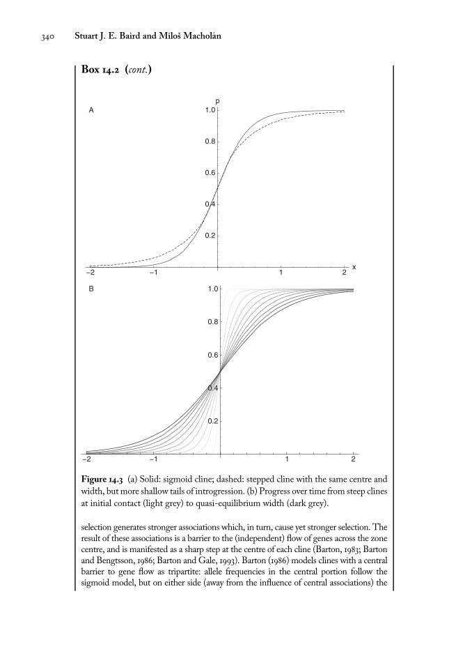
Figure 14.5 An olfactory preference cline modelled as a simple sigmoid curve (solid line).

If the two hybridizing taxa prefer cues originating from their own rather than the other

taxon, preference is amplified close to the zone centre. A reinforced cline (dashed line)

then shows ‘pulses’ similar to self-reinforcing solitary waves called ‘topological solitons’

(Barton and Hewitt, 1989).


reproductive isolation is more likely to arise in many small steps than a few

strongly selected mutations (Walsh, 1982; Barton and Charlesworth, 1984).Many

genes of small effect means there will be a low signal-to-noise ratio for any

particular gene, making the distinction between signal and stochastic effects a

particularly important focus in HMHZ studies.

Sampling the hybrid zone and estimating cline parameters

Barton not only developed much of the model framework for under-

standing hybrid zones, he also provided the tools for researchers to estimate cline

parameters using data collected in the field (Analyse: Barton and Baird, 1995).

The explicit models of tension zones (Box 14.2) allow the likelihood of a dataset

to be calculated for different values of cline parameters. The most likely param-

eters can be found using computational searches, and these point estimates of the

parameters are made meaningful with the addition of a measure of belief in the

estimate, the support interval (a point estimate with no measure of belief is no

better than a guess). The efficacy of likelihood estimation has led all the geo-

graphic cline fitting software that followed Barton’s work also to use likelihood

inference (ClineFit: Porter et al., 1997; CFit: Gay et al., 2008). Given this

consistency of inference framework across hybrid zone studies it might seem

unnecessary for us to discuss estimation of cline parameters, but increasingly this

uniform inference framework seems also to have led to a thoughtlessness in

inference about hybrid zones, which we will illustrate here with reference to the

centre and width of a zone.

It is crucial that researchers distinguish between the centre and width of a hybrid

zone and estimates of these parameters. To illustrate the importance of this dis-

tinction we use a reference scenario of a multi-locus tension zone with an

asymmetric central barrier to gene flow such that in reality clines in many traits

have coincident central steps with steep change on one side and more gradual

change on the other side. What inference could we hope to make about this

reference scenario? It will depend greatly on our spatial sampling of the zone

(Box 14.3) and the cline model we use for analysis (Box 14.4). Let us first assume

spatial sampling. If we sample localities in a line that is oblique to the path of the

zone through the field area, we introduce an upward bias in our estimate of the

zone width (Macholán et al., 2008). The stochastic nature of locality samples near

the zone centre means such biases in width and centre estimates can be surpris-

ingly large and erratic (Dufková et al., 2011). Both of these issues can be resolved

by sampling localities across a 2D area, estimating the course of the hybrid zone

through that region, and then using all the locality samples in relation to their

orthogonal distance from the zone centre (MacCallum, 1994; Bridle et al., 2001).


Taking the path of the zone centre into account minimizes the upward bias in

width estimates, and because the set of localities near the centre of the zone is not

limited to one on either side (the case for linear sampling), the erratic stochas-

ticity of centre and width estimates is greatly reduced.

Turning to the second issue, model choice, suppose we choose to analyse field

samples from the reference scenario using the two-parameter sigmoid cline

model described in Box 14.2. What are the consequences of fitting this model

to asymmetric stepped clines? Since the former is by definition symmetric, the

resulting fitted cline is shifted to one side to try to match the asymmetry in the

data: the more asymmetric the data, the more the cline centre estimate diverges

from the real position of the cline centre (see Fig. 14.6). The consequences for

inference are grave. Since the two-parameter analysis will give the impression

that the zone has non-coincident cline centres, we might mis-infer the very

nature of the zone because ‘coincident cline centres’ is one of the most funda-

mental expectations of a zone with a central barrier to gene flow.

Non-geographic alternatives

An alternative approach to spatial cline analysis, first proposed by

Szymura and Barton (1986, 1991), and now called Barton’s concordance

(Macholán et al., 2011), minimizes both of these issues of spatial sampling and

model selection to some extent. When the geographic pattern of hybridization

within a contact zone is complex it may be rational to disregard information on

geography and fit clines against the hybrid index rather than against geographic

distance. This approach can be especially useful in cases where conventional

geographic cline models are not suitable for describing the spatial pattern, such as

in mosaic hybrid zones or when the introgression pattern of some loci strongly

deviates from that of other markers (Harrison and Rand, 1989; Arntzen and

Wallis, 1991; Bridle et al., 2001; Bierne et al., 2003; Macholán et al., 2008, 2011).

A similar approach of fitting clines against the hybrid index rather than against

geographic distance was taken by Gompert and Buerkle (2009, 2011), who called

the resulting plots ‘genomic clines’. The methods are compared in Macholán

et al. (2011), who note that while these non-spatial analyses may be convenient,

they do not entirely escape the issues of sampling and model choice.

Studies on the X chromosome in the HMHZ

When choosing where to start a search for genetic factors causing

barriers to gene flow, researchers can take as guidance two strong empirical

patterns, also known as the ‘two rules of speciation’ (Coyne and Orr, 1989).


The first is Haldane’s rule, stating that when hybrids of one sex suffer from

reduced viability or fertility, it is usually the heterogametic sex (Haldane, 1922;

Orr, 1997). The second is that genes contributing to reproductive isolation often

map to the X chromosome, the phenomenon known as the large X-effect

(Charlesworth et al., 1987; Coyne and Orr, 1989; Coyne, 1992), recently dubbed

‘Coyne’s rule’ (Turelli and Moyle, 2007). Indeed, it has been shown that sex

chromosomes harbour more genes causing disruption of fertility and/or viability

in hybrids than autosomes and hence will be under stronger selection (see Coyne

A

−2 −1 1 2x

0.2

0.4

0.6

0.8

1.0p

B

14.5 15.0 15.5 16.0 16.5%c

72

74

76

78

80

82

84%w

Figure 14.6 Assuming a hybrid zone scenario in which every sampled locus has a stepped

asymmetric cline with parameters {c, w, BL, θL, BR, θR} = {0, 1, 0.1, 1, 0.2, θR}, such that all

clines have identical centre and width, but vary in their asymmetry as θ1changes in the

interval 0.25 < θR <0.74. (a) Solid curves show the cline shapes at the extremes of this

interval. The dashed lines are the correspondingMLE cline estimates fromdata on 100 large

locality samples spaced evenly across the zone and analysed using a two-parameter {c, w}

sigmoid model. (b) The centre and width estimates from this inappropriate model exceed

the true centre location and width. The errors are expressed as percentages of the true value.


and Orr, 2004 and references therein; for evidence in the mouse, see Oka et al.,

2004; Storchová et al., 2004; Harr, 2006; Good et al., 2008a).

To date, three surveys of X chromosome introgression heterogeneity across

the European HMHZ have been carried out. Working from a 1D transect of

samples that straddle this zone in Bavaria, to the south of the Czech–Bavarian

portion (Fig. 14.2), Payseur et al. (2004) fitted geographic stepped clines to data

for 13 loci, identifying a central-X region of reduced introgression, and also

proposing the X inactivation locus Xist as marking an adaptive introgression

into musculus territory. Teeter et al. (2010), working with the same Bavarian

dataset, and an additional 1D transect sampling across the zone in Saxony (to

the north of the Czech–Bavarian zone, Fig. 14.2), found the resulting likelihood

surfaces for the six-parameter geographic cline model impracticably complex,

so instead chose to fit sigmoid clines to 41 SNPs (but only three X markers, a

subset of Payseur et al. (2004): Emd, Pola1, and Xist) drawn from both datasets.

However, in recognition of the difficulty introduced by geographic complexity,

the authors also used the non-geographic genome clines approach of Gompert

and Buerkle (2009). They concluded that ‘the differences between transects

raise the possibility that there may not be a single genetic architecture of

isolation between these species’ (Teeter et al., 2010: 10), though two out of

the three X markers did not show any difference between transects, but noted

that ‘it is possible that stochastic variation, differences in sampling between

transects, or a combination, could have contributed to these differences’ (Teeter

et al., 2010: 10).

The third study (Macholán et al., 2011) was of a 24-locus superset of the Payseur

et al. (2004) study, on a sample of more than 2870 mice from a geographically

intensively sampled 145× 50 km 2D (rectangular) section of the Czech–Bavarian

portion of the HMHZ. In order to distinguish geographic stochastic effects from

deterministic introgression patterns they compared both non-geographic clines

analysis approaches (Barton’s concordance and genomic clines) to analysis using a

spatially explicit Bayesian model-based clustering algorithm (Geneland 3.1.4;

Guillot et al., 2005). Analysis of the Czech–Bavarian zone (lying between the two

focal transects of theTeeter study) found the same central-X-reduced introgression

region as Payseur et al. (2004) found for one of their transects, and concluded that

there is some evidence of common architecture of reproductive isolation over the

transect studied, and no reliable evidence to the contrary.We suggest that once it is

taken into account that 1D sampling across a 2D zone (Box 14.3) and that fitting a

sigmoidmodel to an asymmetric hybrid zone (Box 14.4) can introduce large sources

of stochastic error, the differences between transect estimates in the Teeter et al.

(2010) study does not justify the suggestion of multiple genetic architectures

maintaining the HMHZ.


Two other interesting findings arose from the Macholán et al. (2011) X

chromosome study. In the Geneland analysis, several loci showed the geo-

graphic pattern known as ‘footprints of a moving hybrid zone’ (Arntzen and

Wallis, 1991), indicating a history of movement of the zone from east to west.

More recently, a study of linkage disequilibrium across 1401 loci came to the same

conclusion regarding zone movement in Bavaria (Wang et al., 2011; see Tucker

et al., Chapter 20). A tendency for M. m. musculus to gain territory from

M. m. domesticus could explain a number of disparate characteristics of the

HMHZ. (1) The geographic asymmetry of the zone across multiple transects –

the long tails of introgression on the musculus side being the result of many small

domesticus ‘footprints’ left behind the zone front. (2) The Jutland musculus

‘colony’, which persists despite being essentially a closed system faced by hybrid-

ization with a comparatively infinite domesticus range. (3) The eight-fold greater

incidence of tapeworms in domesticus – parasites capable of disrupting reproduc-

tion in rodents (see Goüy de Bellocq et al., Chapter 18). The second interesting

finding from Macholán et al. (2011) is evidence of a proximal-X, male-biased

westward introgression, despite the central X barrier to gene flow between the

taxa. This proximal X introgression was in fact predicted by Macholán et al.

(2008) in their study of the Y chromosome invasion across this section of the

HMHZ (see below), and an accompanying mtDNA introgression.

Future perspectives

Much as theoretical expectations and empirical evidence for the large

X-effect made the X chromosome the natural candidate for the studies summar-

ized above, we should let our current understanding of speciation direct future

efforts as we expand the search for genes involved in reproductive barriers across

the rest of the genome.

A model independently proposed by Bateson (1909) and later by Dobzhansky

(1936) and Muller (1940, 1942) is now widely accepted as a framework for

understanding the genetic basis of postzygotic isolation. The Dobzhansky–

Muller (DM) model solves Darwin’s paradox that postzygotic incompatibilities

arising within a population should be counter-selected, making their fixation

unlikely. According to the DM model this problem can be circumvented if

hybrid sterility is brought about through interaction of loci accumulating differ-

ent mutations in allopatry that are only revealed to be incompatible at secondary

contact. Thus, speciation can occur even if the allopatric populations have not

passed through an adaptive valley. (For the sake of completeness it should be

noted that the model can also be derived for a single locus.)


Although the DM model has become a cornerstone of the genetics of speci-

ation (Orr, 1996; Coyne and Orr, 2004), it does not address the following

questions: (1) What kind of genes might produce such epistatic interactions

between alleles? (2) Do these genes drift to fixation in allopatry, or is their fixation

driven by natural selection? (3) To what degree is their evolution within the

diverging subpopulations influenced by intragenomic processes such as genetic

conflict? For example, there is growing empirical evidence that genes implicated

in postzygotic isolation are also associated with meiotic drive, suggesting their

fixation in allopatry could have been through selection at the level of the gene

rather than through Darwinian adaptation of individuals to the external environ-

ment or by random drift (Tao et al., 2003; Orr and Irving, 2005; Orr et al., 2007;

Phadnis and Orr, 2009; Presgraves, 2010). Twenty years ago genetic conflict was

suggested as an explanation for Haldane’s rule of speciation (Frank, 1991; Hurst

and Pomiankowski, 1991), but the idea fell into disfavour, with models invoking

faster substitution on the sex chromosomes being preferred (Charlesworth et al.,

1993). The recent evidence associating genetic conflict with speciation genes

(Presgraves, 2010) therefore adds new interest to an old debate.

Here, in the context of the HMHZ hybrid zone, we are prompted to ask: what

is the expected outcome when a genetic conflict system is split into independent

isolates, and subsequently comes into secondary contact? In natural hybrid zones

we may observe outcomes of many generations of recombination, numbers

entirely impractical in the laboratory. Such natural experiments can therefore

give high-resolution estimates of the number and locations of genes or genomic

regions causing reproductive isolation (‘speciation’ genes), but also allow us to

spot the converse pattern: genes that appear to preferentially cross and break

down the taxon boundary (‘anti-speciation’ genes), even when the two types of gene

are neighbours on the same chromosome – the central X barrier to introgression and

the proximal X invasion, respectively (Macholán et al., 2011).

Introgression of the Y chromosome

In accordance with the idea that introgression of sex chromosomes in a

hybrid zone should be severely impeded, virtually no introgression of the mouse

Y chromosome has been found in Denmark (Vanlerberghe et al., 1986; Dod et al.,

2005), Bulgaria (Vanlerberghe et al., 1988a), or northern Germany (Prager et al.,

1997). This picture, seemingly consistent along 2500 km of the zone of secondary

contact, began to crumble during a survey of the distribution of several autosomal

and sex-linked markers across the Czech and Slovak Republics, which revealed

an unexpectedly gradual introgression of the Y chromosome, substantially higher

and shifted to the domesticus territory compared to the diagnostic autosomal and


X-linked loci analysed (Munclinger et al., 2002). This pattern was later corrobo-

rated and quantified using a larger dataset from the Czech–Bavarian transect

(Macholán et al., 2008) and is possibly also the case in Saxony (K.C. Teeter and

P.K. Tucker, personal communication).

Macholán et al. (2008) showed that the most likely direction of change of the

Y chromosome is rotated about 45° clockwise relative to other loci. When

estimated along this axis, the width of the Y transition was not significantly

different from an X chromosome locus (Btk), while using the consensus

direction based on seven autosomal and one X-linked loci resulted in consid-

erably broader cline and significantly worse fit. Inspection of the spatial intro-

gression pattern showed themusculus Y chromosome has spread across the zone

up to 22 km into the domesticus range, covering – at minimum – a triangular area

approximately 330 km2. This introgression is accompanied by differences in the

census sex ratio: while this ratio is significantly female-biased in the musculus

territory (0.45, p = 0.0005) and in domesticus localities without the introgressed

musculus Y (0.44, p = 0.0065), in the domesticus area with the introgressed

musculus Y it is not different from parity (0.51, p = 0.2037) and significantly

different from the former two areas (Macholán et al., 2008). Reconciling the Y

chromosome introgression and sex ratio distribution led to a hypothesis that a

genetic conflict between the Y and X (and possibly some autosomal) elements is

the underlying cause of both the invasion and sex ratio distortion patterns.

According to this hypothesis, the musculus Y is successful on the naïve domes-

ticus background. As a consequence, the former spreads across the zone at the

expense of the latter. The recent results of Jones et al. (2010), who found the

musculus Y in Norway far behind the zone in domesticus territory, seem con-

sistent with this hypothesis.

What does the mouse hybrid zone tell us about speciation?

The first evidence arising from the HMHZ of genes causing barriers to

gene flow came from the X chromosome. But this was the first place we looked.

With the accelerating accumulation of large genomic datasets, such as SNPmaps

now available for the mouse (Lindblad-Toh et al., 2000; Wade et al., 2002; Abe

et al., 2004; Pletcher et al., 2004; Shifman et al., 2006; Frazer et al., 2007; Yang

et al., 2009), applying similar methods as for the X chromosome wemay expect to

find more and more such factors. While this work will gradually build up a

detailed picture of which genes are involved in the species barrier between two

subspecies of house mouse, perhaps the more exciting results concern the speci-

ation process in general. If hybridizing genomes involve complex mixtures of

DM incompatibility genes intermingled with universally advantaged and/or


invasive conflict elements, as suggested by the contrasting patterns of central and

proximal X chromosome variation (Macholán et al., 2011) in association with the

Y chromosome invasion (Macholán et al., 2008), then the latter may counter the

action of the former. That is: conflict genes may act as anti-speciation genes.

While laboratory-based speciation research has focused onDM incompatibilities

and the circumstances that favour them, perhaps the most important thing

hybrid zone speciation research has shown us is that to understand speciation it

is also necessary to consider what might counter the action of DM incompatibil-

ities, and what circumstances might disfavour their accumulation (Baird et al.,

2012; Goüy de Bellocq et al., Chapter 18).

REFERENCES

Abe, K., Noguchi, H., Tagawa, K., et al. (2004). Contribution of Asianmouse subspeciesMus

musculus molossinus to genomic constitution of strain C57BL/6J, as defined by BAC-end

sequence-SKIP analysis. Genome Research, 14, 2439–47.

Albrechtová, J., Albrecht, T., Baird, S. J. E., et al. (Submitted). Differential sperm perform-

ance in hybrids coincides with Y chromosome invasion across the house mouse hybrid

zone. Current Biology.

Alibert, P. and Auffray, J. -C. (2003). Genomic coadaptation, outbreeding depression, and

developmental instability. In Developmental Instability: Causes and Consequences, ed.

M. Polak. Oxford: Oxford University Press, pp. 116–34.

Alibert, P., Fel-Clair, F., Manolakou, K., Britton-Davidian, J., and Auffray, J. -C. (1997).

Developmental stability, fitness, and trait size in laboratory hybrids between European

subspecies of the house mouse. Evolution, 51, 1284–95.

Alibert, P., Renaud, S., Dod, B., Bonhomme, F., and Auffray, J. -C. (1994). Fluctuating

asymmetry in the Mus musculus hybrid zone: a heterotic effect in disrupted co-adapted

genomes. Proceedings of the Royal Society of London B: Biological Sciences, 258, 53–9.

Arntzen, J.W. and Wallis, G. P. (1991). Restricted gene flow in a moving hybrid zone of

the newts Triturus cristatus and T. Marmoratus in western France. Evolution, 45,

805–26.

Auffray, J. -C. (1993). Chromosomal evolution in the house mouse in the light of palae-

ontology: a colonization-related event? Quaternary International, 19, 21–5.

Auffray, J. -C. and Britton-Davidian, J. (1992). When did the house mouse colonize Europe?

Biological Journal of the Linnean Society, 45, 187–90.

Auffray, J. -C., Vanlerberghe, F., and Britton-Davidian, J. (1990). The house mouse pro-

gression in Eurasia: a palaeontological and archaeozoological approach. Biological Journal

of the Linnean Society, 41, 13–25.

Baird, S. J. E. (1995). A simulation study of multilocus clines. Evolution, 49, 1038–45.

Baird, S. J. E. (2006). Phylogenetics: Fisher’s markers of admixture. Heredity, 97, 81–3.


Baird, S. J. E., Ribas, A., Macholán, M., et al. (2012). Where are the wormy mice? A

re-examination of hybrid parasitism in the European house mouse hybrid zone.

Evolution. doi: 10.1111/j.1558-5646.2012.01633.x.

Baird, S. J. E. and Santos, F. (2010). Monte Carlo integration over stepping stone models for

spatial genetic inference using approximate Bayesian computation. Molecular Ecology

Resources, 10, 873–85.

Barton, N.H. (1979). Gene flow past a cline. Heredity, 43, 333–9.

Barton, N.H. (1983). Multilocus clines. Evolution, 37, 454–71.

Barton, N.H. (1986). The effects of linkage and density-dependent regulation on gene flow.

Heredity, 57, 415–26.

Barton, N.H. and Baird, S. J. E. (1995). Analyse: An Application for Analyzing Hybrid Zones.

Freeware, Edinburgh, UK. Available at http://helios.bto.ed.ac.uk/evolgen/Mac/

Analyse.

Barton, N.H. and Bengtsson, B.O. (1986). The barrier to genetic exchange between hybrid-

ising populations. Heredity, 56, 357–76.

Barton, N.H. and Charlesworth, B. (1984). Genetic revolutions, founder effects, and speci-

ation. Annual Review of Ecology and Systematics, 15, 133–64.

Barton, N.H., Depaulis, F., and Etheridge, A.M. (2002). Neutral evolution in spatially

continuous populations. Theoretical Population Biology, 61, 31–48.

Barton, N.H. and Gale, K. S. (1993). Genetic analysis of hybrid zones. In Hybrid Zones and

the Evolutionary Process, ed. R.G. Harrison. Oxford: Oxford University Press, pp. 13–45.

Barton, N.H. and Hewitt, G.M. (1985). Analysis of hybrid zones. Annual Review of Ecology

and Systematics, 16, 113–48.

Barton, N.H. and Hewitt, G.M. (1989). Adaptation, speciation and hybrid zones. Nature,

341, 497–503.

Barton, N.H. and Shpak, M. (2000). The effect of epistasis on the structure of hybrid zones.

Genetical Research, 75, 179–98.

Barton, N.H. andWilson, I. (1995). Genealogies and geography. Philosophical Transactions of

the Royal Society of London Series B: Biological Sciences, 349, 49–59.

Bateson, W. (1909). Heredity and variation in modern lights. InDarwin and Modern Science,

ed. A.C. Seward. Cambridge: Cambridge University Press, pp. 85–101.

Bazykin, A.D. (1969). Hypothetical mechanism of speciation. Evolution, 23, 685–7.

Bierne, N., Daguin, C., Bonhomme, F., David, P., and Borsa, P. (2003). Direct selection on

allozymes is not required to explain heterogeneity among marker loci across a Mytilus

hybrid zone. Molecular Ecology, 12, 2505–10.

Bímová, B., Albrecht, T., Macholán, M., and Piálek, J. (2009). Signalling components of

mate recognition system in the house mouse. Behavioural Processes, 80, 20–7.

Bonhomme, F., Orth, A., Cucchi, T., et al. (2011). Genetic differentiation of the house mouse

around the Mediterranean basin: matrilineal footprints of early and late colonization.

Proceedings of the Royal Society B: Biological Sciences, 278, 1034–43.

Boursot, P., Auffray, J. -C., Britton-Davidian, J., and Bonhomme F. (1993). The evolution of

house mice. Annual Review of Ecology and Systematics, 24, 119–52.


Boursot, P., Bonhomme, F., Britton-Davidian, J., et al. (1984). Differential introgression of

the nuclear and mitochondrial genomes between 2 semi-species of European mice.

Comptes Rendus de l’Academie des Sciences III – Sciences de la Vie – Life Sciences, 299,

365–70.

Božíková, E., Munclinger, P., Teeter, K. C., et al. (2005). Mitochondrial DNA in the hybrid

zone between Mus musculus musculus and Mus musculus domesticus: a comparison of two

transects. Biological Journal of the Linnean Society, 84, 363–78.

Bridle, J. R., Baird, S. J. E., and Butlin, R. K. (2001). Spatial structure and habitat variation in

a grasshopper hybrid zone. Evolution, 55, 1832–43.

Britton-Davidian, J., Fel-Clair, F., Lopez, J., Alibert, P., and Boursot, P. (2005). Postzygotic

isolation between the two European subspecies of the house mouse: estimates from

fertility patterns in wild and laboratory-bred hybrids. Biological Journal of the Linnean

Society, 84, 379–93.

Bullough, R. K. and Caudrey, P. J. (eds) (1980) Solitons. Berlin: Springer-Verlag.

Butlin, R. K. (1987). Speciation by reinforcement. Trends in Ecology and Evolution, 2, 8–13.

Butlin, R. K. (1995). Reinforcement: an idea evolving. Trends in Ecology and Evolution, 10,

432–4.

Carling, M.D. and Brumfield, R. T. (2009). Speciation in Passerina buntings: introgression

patterns of sex-linked loci identify a candidate gene region for reproductive isolation.

Molecular Ecology, 18, 834–47.

Charlesworth, B., Coyne, J. A., and Barton, N.H. (1987). The relative rates of evolution of sex

chromosomes and autosomes. The American Naturalist, 130, 113–46.

Charlesworth, B., Coyne, J. A., and Orr, H.A. (1993). Meiotic drive and unisexual hybrid

sterility: a comment. Genetics, 133, 421–4.

Christophe, N. and Baudoin, C. (1998). Olfactory preferences in two subspecies of miceMus

musculus musculus and Mus musculus domesticus and their hybrids. Animal Behaviour, 56,

365–9.

Clark, G. (1975). The Earlier Stone Age Settlements of Scandinavia. Cambridge: Cambridge

University Press.

Coyne, J. A. (1992). Genetics and speciation. Nature, 355, 511–15.

Coyne, J. A. and Orr, H.A. (1989). Two rules of speciation. In Speciation and Its Consequences,

ed. D. Otte and J. Endler. Sunderland, MA: Sinauer Associates, pp. 180–207.

Coyne, J. A. and Orr, H.A. (2004). Speciation. Sunderland, MA: Sinauer Associates.

Cucchi, T., Vigne, J. -D., and Auffray, J. -C. (2005). First occurrence of the house mouse

(Mus musculus domesticus Schwarz & Schwarz, 1943) in the western Mediterranean: a

zooarchaeological revision of subfossil occurrences. Biological Journal of the Linnean

Society, 84, 429–45.

Debat, V., Alibert, P., David, P., Paradis, E., and Auffray, J. -C. (2000). Independence

between developmental stability and canalization in the skull of the house mouse.

Proceedings of the Royal Society of London B: Biological Sciences, 267, 423–30.

Degerbøl, M. (1949). Gnavere, vol. 1. Copenhagen: Vort Lands Dyreliv.

Dobzhansky, T. (1936). Studies on hybrid sterility: II. Localization of sterility factors in

Drosophila pseudoobscura hybrids. Genetics, 21, 113–35.


Dobzhansky, T. (1937). Genetics and the Origin of Species. New York: Columbia University

Press.

Dobzhansky, T. (1940). Speciation as a stage in evolutionary divergence. The American

Naturalist, 74, 312–21.

Dod, B., Jermiin, L. S., Boursot, P., et al. (1993). Counterselection on sex chromosomes in the

Mus musculus European hybrid zone. Journal of Evolutionary Biology, 6, 529–46.

Dod, B., Smadja, C., Karn, R. C., and Boursot, P. (2005). Testing for selection on the

androgen-binding protein in the Danish mouse hybrid zone. Biological Journal of the

Linnean Society, 84, 447–59.

Dufková, P., Macholán, M., and Piálek, J. (2011). Inference of selection and stochastic effects

in the house mouse hybrid zone. Evolution, 65, 993–1010.

Endler, J. A. (1977). Geographic Variation, Speciation and Clines. Princeton, NJ: Princeton

University Press.

Fel-Clair, F., Catalan, J., Lenormand, T., and Britton-Davidian, J. (1998). Centromeric

incompatibilities in the hybrid zone between house mouse subspecies from Denmark:

evidence from patterns of NOR activity. Evolution, 52, 592–603.

Fel-Clair, F., Lenormand, T., Catalan, J., et al. (1996). Genomic incompatibilities in the

hybrid zone between house mice in Denmark: evidence from steep and non-coincident

chromosomal clines for Robertsonian fusions. Genetical Research, 67, 123–34.

Ferris, S.D., Sage, R.D., Huang, C. -M., et al. (1983). Flow of mitochondrial DNA across a

species boundary. Proceedings of the National Academy of Sciences of the United States of

America, 80, 2290–4.

Fisher, R.A. (1930). The Genetical Theory of Natural Selection. Oxford: Oxford University Press.

Fisher, R.A. (1950). Gene frequencies in a cline determined by selection and diffusion.

Biometrics, 6, 353–61.

Forejt, J. (1981). Hybrid sterility gene located in the T/t-H-2 supergene on chromosome 17. In

Current Trends in Histocompatibility: Immunogenetic and Molecular Profiles, ed.

R.A. Reisfeld and S. Ferrone. London: Plenum Press, pp. 103–31.

Forejt, J. (1996). Hybrid sterility in the mouse. Trends in Genetics, 12, 412–17.

Forejt, J. and Iványi, P. (1974). Genetic studies on male sterility of hybrids between laboratory

and wild mice (Mus musculus L.). Genetical Research, 24, 189–206.

Forejt, J., Vincek, V., Klein, J., Lehrach, H., and Loudová-Micková, M. (1991). Genetic

mapping of the t-complex region on mouse chromosome 17 including the Hybrid

sterility-1 gene. Mammalian Genome, 1, 84–91.

Frank, S.H. (1991). Divergence of meiotic drive-suppressors as an explanation for sex-biased

hybrid sterility and inviability. Evolution, 45, 262–7.

Frazer, K. A., Eskin, E., Kang, H.M., et al. (2007). A sequence-based variation map of 8.27

million SNPs in inbred mouse strains. Nature, 448, 1050–3.

Ganem, G., Litel, C., and Lenormand, T. (2008). Variation in mate preference across a house

mouse hybrid zone. Heredity, 100, 594–601.

Gay, L., Crochet, P. -A., Bell, D.A., and Lenormand, T. (2008). Comparing clines on

molecular and phenotypic traits in hybrid zones: a window on tension zone models.

Evolution, 62, 2789–806.


Gompert, Z. and Buerkle, C.A. (2009). A powerful regression-based method for admixture

mapping of isolation across the genome of hybrids. Molecular Ecology, 18, 1207–24.

Gompert, Z. and Buerkle, C.A. (2011). Bayesian estimation of genomic clines. Molecular

Ecology, 20, 2111–27.

Good, J.M., Dean, M.D., and Nachman, M.W. (2008a). A complex genetic basis

to X-linked hybrid male sterility between two species of house mice. Genetics, 179,

2213–28.

Good, J.M., Handel, M.A., and Nachman, M.W. (2008b). Asymmetry and polymorphism

of hybrid male sterility during the early stages of speciation in house mice. Evolution, 62,

50–65.

Gregorová, S., Mňuková-Fajdelová, M., Trachtulec, Z., et al. (1996). Sub-milli-Morgan map

of the proximal part of mouse Chromosome 17 including the hybrid sterility 1 gene.

Mammalian Genome, 7, 107–13.

Guillot, G., Mortier, F., and Estoup, A. (2005). Geneland: a program for landscape genetics.

Molecular Ecology Notes, 5, 712–15.

Gyllensten, U. and Wilson, A.C. (1987). Interspecific mitochondrial DNA transfer and the

colonization of Scandinavia by mice. Genetical Research, 49, 25–9.

Haldane, J. B. S. (1922). Sex ratio and unisexual sterility in animal hybrids. Journal of Genetics,

12, 101–9.

Haldane, J. B. S. (1948). The theory of a cline. Journal of Genetics, 48, 277–84.

Harr, B. (2006). Genomic islands of differentiation between house mouse subspecies.Genome

Research, 16, 730–7.

Harrison, R.G. (1990). Hybrid zones: windows on evolutionary process. Oxford Surveys in

Evolutionary Biology, 7, 69–128.

Harrison, R.G. and Rand, D.M. (1989). Mosaic hybrid zones and the nature of species

boundaries. In Speciation and Its Consequences, ed. D. Otte and J. Endler. Sunderland,

MA: Sinauer Associations, pp. 111–33.

Hewitt, G.M. (1975). A sex-chromosome hybrid zone in the grasshopper Podisma pedestris

(Orthoptera: Acrididae). Heredity, 35, 375–87.

Hewitt, G. (1988). Hybrid zones: natural laboratories for evolution studies. Trends in Ecology

and Evolution, 3, 158–66.

Hewitt, G.M. (1989). The subdivision of species by hybrid zones. In Speciation and Its

Consequences, ed. D. Otte and J. A. Endler. Sunderland, MA: Sinauer Associates,

pp. 85–110.

Hunt, W.G. and Selander, R. K. (1973). Biochemical genetics of hybridisation in European

house mice. Heredity, 31, 11–33.

Hurst, L.D. and Pomiankowski, A. (1991). Causes of sex ratio bias may account for unisexual

sterility in hybrids: a new explanation of Haldane’s rule and related phenomena.Genetics,

128, 841–58.

Jones, E. P., van der Kooij, J., Solheim, R., and Searle, J. B. (2010). Norwegian house mice

(Mus musculus musculus/domesticus): distributions, routes of colonization and patterns of

hybridization. Molecular Ecology, 19, 5252–64.


Karn, R.C. and Dlouhy, S. R. (1991). Salivary androgen-binding protein variation inMus and

other rodents. Journal of Heredity, 82, 453–8.

Key, K.H. (1968). The concept of stasipatric speciation. Systematic Zoology, 17, 14–22.

Klein, J., Tichy, H., and Figueroa, F. (1987). On the origin of mice. Anales de l’Universidad de

Chile, 5, 91–120.

Kraft, R. (1985). Merkmale und Verbreitung der Hausmäuse Mus musculus musculus L., 1758,

und Mus musculus domesticus Rutty, 1772 (Rodentia, Muridae) in Bayern.

Säugetierkundliche Mitteilungen, 31, 1–13.

Kratochvíl, J. (1986). Die intraspezifische Evolution der Art Mus domesticus. Acta scientiarum

naturalium Academiae scientiarum bohemoslovacae – Brno, 20, 1–49.

Lakshmanan, M. (ed.) (1988). Solitons. New York: Springer-Verlag.

Lande, R. (1981).Models of speciation by sexual selection on polygenic traits. Proceedings of the

National Academy of Sciences of the United States of America, 78, 3721–5.

Lanneluc, I., Desmarais, E., Boursot, P., Dod, B., and Bonhomme, F. (2004).

Characterization of a centromeric marker on mouse chromosome 11 and its introgression

in a domesticus/musculus hybrid zone. Mammalian Genome, 15, 924–34.

Laukaitis, C.M., Heger, A., Blakley, T.D., et al. (2008). Rapid bursts of androgen-binding

protein (Abp) gene duplication occurred independently in diverse mammals. BMC


Lemmon, A. R., Smadja, C., and Kirkpatrick, M. (2004). Reproductive character displace-

ment is not the only possible outcome of reinforcement. Journal of Evolutionary Biology,

17, 177–83.

Lepiksaar, J. (1980). Animal remains at Tornör: a study of a Thanatocoenosis (Late Iron Age

to recent times). Striae, 10, 3–41.

Li, W.H. and Nei, M. (1974). Stable linkage disequilibrium without epistasis in subdivided

populations. Theoretical Population Biology, 6, 173–83.

Lindblad-Toh, K., Winchester, E., Daly, M. J., et al. (2000). Large-scale discovery and

genotyping of single-nucleotide polymorphisms in the mouse.Nature Genetics, 24, 381–6.

MacCallum, C. J. (1994). Adaptation and habitat preference in a hybrid zone between Bombina

bombina and Bombina variegata. Unpublished PhD thesis, University of Edinburgh.

Macholán, M., Baird, S. J. E., Dufková, P., et al. (2011). Assessing multilocus introgression

patterns: a case study on the mouse X chromosome in central Europe. Evolution, 65,

1428–46.

Macholán, M., Baird, S. J. E., Munclinger, et al. (2008). Genetic conflict outweighs

heterogametic incompatibility in the mouse hybrid zone? BMC Evolutionary Biology,

8, 271–84.

Macholán, M., Kryštufek, B., and Vohralík, V. (2003). The location of the Mus musculus/M.

domesticus hybrid zone in the Balkans: clues frommorphology.Acta Theriologica, 48, 177–88.

Macholán, M., Munclinger, P., Šugerková, M., et al. (2007). Genetic analysis of autosomal

and X-linked markers across a mouse hybrid zone. Evolution, 61, 746–71.

Mihola, O., Trachtulec, Z., Vlcek, C., Schimenti, J. C., and Forejt, J. (2009). A mouse

speciation gene encodes a meiotic Histone H3 Methyltransferase. Science, 323, 373–5.


Mikula, O., Auffray, J. -C., and Macholán, M. (2010). Fluctuating asymmetry in the central

European transect across the house mouse hybrid zone. Biological Journal of the Linnean

Society, 101, 13–27.

Mikula, O. and Macholán, M. (2008). There is no heterotic effect upon developmental

stability in the ventral side of the skull within the house mouse hybrid zone. Journal of


Montagutelli, X., Turner, R., and Nadeau, J.H. (1996). Epistatic control of non-Mendelian

inheritance in mouse specific crosses. Genetics, 143, 1739–52.

Moore,W. S. (1977). An evaluation of narrow hybrid zones in vertebrates.Quarterly Review of

Biology, 52, 263–78.

Moulia, C., Aussel, J. P., Bonhomme, F., et al. (1991). Wormy mice in a hybrid zone: a

genetic control of susceptibility to parasite infection. Journal of Evolutionary Biology, 4,

679–87.

Moulia, C. and Joly, P. (2009). Parasitism and hybrid zones. In Ecology and Evolution of

Parasitism, ed. F. Thomas, J. F. Guégan, and F. Renaud. New York: Oxford University

Press, pp. 69–82.

Muller, H. J. (1940). Bearing of the Drosophila work on systematics. In The New Systematics,

ed. J. S. Huxley. Oxford: Clarendon Press, pp. 185–268.

Muller, H. J. (1942). Isolating mechanisms, evolution, and temperature. Biological Symposia, 6,

71–125.

Munclinger, P., Božíková, E., Šugerková, M., Piálek, J., and Macholán, M. (2002). Genetic

variation in house mice (Mus, Muridae, Rodentia) from the Czech and Slovak Republics.

Folia Zoologica, 51, 81–92.

Munclinger, P. and Frynta, D. (2000). Social interactions within and between two distant

populations of house mouse. Folia Zoologica, 49, 1–6.

Nagylaki, T. (1975). Conditions for the existence of clines. Genetics, 80, 595–615.

Nagylaki, T. (1976). Clines with variable migration. Genetics, 83, 867–86.

Nancé, V., Vanlerberghe, F., Nielsen, J. T., Bonhomme, F., and Britton-Davidian, J. (1990).

Chromosomal introgression in house mice from the hybrid zone between M. m. domes-

ticus and M. m. musculus. Biological Journal of the Linnean Society, 41, 215–27.

O’Connor, T. P. (1992). Pets and pests in Roman and medieval Britain.Mammal Review, 22

(2), 107–13.

Oka, A., Mita, A., Sakurai-Yamatani, N., et al. (2004). Hybrid breakdown caused by

substitution of the X chromosome between two mouse subspecies. Genetics, 166,

913–24.

Orr, H.A. (1996). Dobzhansky, Bateson, and the genetics of speciation. Genetics, 144, 1331–5.

Orr, H.A. (1997). Haldane’s rule. Annual Review of Ecology and Systematics, 28, 195–218.

Orr, H.A. and Irving, S. (2005). Segregation distortion in hybrids between the Bogota and

USA subspecies of Drosophila pseudoobscura. Genetics, 169, 671–82.

Orr, H.A.,Masly, J. P., and Phadnis, N. (2007). Speciation inDrosophila: from phenotypes to

molecules. Journal of Heredity, 98, 103–10.

Payseur, B.A. (2010). Using differential introgression in hybrid zones to identify genomic

regions involved in speciation. Molecular Ecology Resources, 10, 806–20.


Payseur, B.A. and Hoekstra, H.E. (2005). Signatures of reproductive isolation in patterns of

single nucleotide diversity across inbred strains of mice. Genetics, 171, 1905–16.

Payseur, B.A., Krenz, J. G., and Nachman, M.W. (2004). Differential patterns of intro-

gression across the X chromosome in a hybrid zone between two species of house mice.

Evolution, 58, 2064–78.

Payseur, B.A. and Nachman, M.W. (2005). The genomics of speciation: investigating the

molecular correlates of X chromosome introgression across the hybrid zone betweenMus

domesticus and Mus musculus. Biological Journal of the Linnean Society, 84, 523–34.

Phadnis, N. and Orr, H.A. (2009). A single gene causes both male sterility and segregation

distortion in Drosophila hybrids. Science, 323, 376–9.

Phillips, B. L., Baird, S. J. E., and Moritz, C. (2004). When vicars meet: a narrow contact

zone between morphologically cryptic phylogeographic lineages of the rainforest skink,

Carlia rubrigularis. Evolution, 58, 1536–48.

Pletcher, M.T., McClurg, P., Batalov, S., et al. (2004). Use of a dense single nucleotide

polymorphism map for in silico mapping in the mouse. PLoS Biology, 2, e393.

Pocock, M. J. O., Hauffe, H.C., and Searle, J. B. (2005). Dispersal in house mice. Biological

Journal of the Linnean Society, 84, 565–83.

Polechová, J. and Barton, N.H. (2011). Genetic drift widens the expected cline but narrows

the expected cline width. Genetics, 189, 227–35.

Porter, A.H., Wenger, R., Geiger, H., Scholl, A., and Shapiro, A.M. (1997). The Pontia

daplidice-edusa hybrid zone in northwestern Italy. Evolution, 51, 1561–73.

Prager, E.M., Boursot, P., and Sage, R.D. (1997). New assays for Y chromosome and p53

pseudogene clines among East Holstein house mice. Mammalian Genome, 8, 279–81.

Prager, E.M., Sage, R.D., Gyllensten, U., et al. (1993). Mitochrondrial DNA sequence

diversity and the colonization of Scandinavia by house mice from East Holstein.

Biological Journal of the Linnean Society, 50, 85–122.

Presgraves, D.C. (2010). The molecular evolutionary basis of species formation. Nature

Reviews Genetics, 11, 175–80.

Raufaste, N. (2001). Barrières au flux génique et sélection dans une zone hybride: etude théorique et

expérimentale chez la souris domestique. Unpublished PhD thesis, Université Montpellier

II, Montpellier, France.

Raufaste, N., Orth, A., Belkhir, K., et al. (2005). Inferences of selection and migration in the

Danish house mouse hybrid zone. Biological Journal of the Linnean Society, 84, 593–616.

Ritchie, M.G. (2007). Sexual selection and speciation. Annual Review of Ecology, Evolution,

and Systematics, 38, 79–102.

Rousset, F. (1997). Genetic differentiation and estimation of gene flow from F-statistics under

isolation by distance. Genetics, 145, 1219–28.

Rousset, F. (2000). Genetic differentiation between individuals. Journal of Evolutionary

Biology, 58, 58–62.

Sage, R.D. (1981). Wild mice. In The Mouse in Biomedical Research, vol. 1, ed. H. L. Foster,

J. D. Small, and J. G. Fox. New York: Academic Press, pp. 39–90.

Sage, R.D., Atchley, W.R., and Capanna, E. (1993). House mice as models in systematic

biology. Systematic Biology, 42, 523–61.


Sage, R.D., Heyneman, D., Lim, K. -C., andWilson, A.C. (1986a).Wormymice in a hybrid

zone. Nature, 324, 60–3.

Sage, R.D., Prager, E.M., Tichy, H., and Wilson, A.C. (1990). Mitochondrial DNA

variation in house mice, Mus domesticus (Rutty). Biological Journal of the Linnean

Society, 41, 105–23.

Sage, R.D., Whitney, J. B., III, andWilson, A.C. (1986b). Genetic analysis of a hybrid zone

between domesticus and musculus mice (Mus musculus complex): hemoglobin polymor-

phisms. Current Topics in Microbiology and Immunology, 127, 75–85.

Schnell, M.H. and Selander, R. K. (1981). Environmental and morphological correlates of

genetic variation in mammals. In Mammalian Population Genetics, ed. J. Joule and

M.H. Smith. Athens, GA: University of Georgia Press, pp. 60–99.

Selander, R. K., Hunt, W.G., and Yang, S. Y. (1969). Protein polymorphism and genic

heterozygosity in two European subspecies of the house mouse. Evolution, 23, 379–90.

Serafiński, W. (1965). The subspecific differentiation of the Central European house mouse

(Mus musculus L.) in the light of their ecology and morphology. Ekologia Polska: Seria A,

13, 305–48.

Servedio, M.R. and Noor, M.A. F. (2003). The role of reinforcement in speciation: theory

and data. Annual Review of Ecology and Systematics, 34, 339–64.

Shifman, S., Bell, J. T., Copley, R. R., et al. (2006). A high resolution single nucleotide

polymorphism genetic map of the mouse genome. PLoS Biology, 4, 2227–37.

Slatkin, M. (1973). Gene flow and selection in a cline. Genetics, 75, 733–56.

Slatkin, M. (1975). Gene flow and selection on a two-locus system. Genetics, 81, 787–802.

Smadja, C., Catalan, J., and Ganem, G. (2004). Strong premating divergence in a unimodal

hybrid zone between two subspecies in the house mouse. Journal of Evolutionary Biology,

17, 165–76.

Smadja, C. and Ganem, G. (2002). Subspecies recognition in the house mouse: a study of two

populations from the border of a hybrid zone. Behavioral Ecology, 13, 312–20.

Smadja, C. and Ganem, G. (2005). Asymmetrical reproductive character displacement in the

house mouse. Journal of Evolutionary Biology, 18, 1485–93.

Sokal, R. R., Oden, N. L., and Wilson, A.C. (1991). Genetic evidence for the spread of

agriculture in Europe by demic diffusion. Nature, 351, 143–5.

Storchová, R., Gregorová, S., Buckiová, et al. (2004). Genetic analysis of X-linked hybrid

sterility in the house mouse. Mammalian Genome, 15, 515–24.

Szymura, J.M. and Barton, N.H. (1986). Genetic analysis of a hybrid zone between the fire-

bellied toads, Bombina bombina and B. variegata, near Cracow in southern Poland.

Evolution, 40, 1141–59.

Szymura, J.M. and Barton, N.H. (1991). The genetic structure of the hybrid zone between the

firebellied toads Bombina bombina and B. variegata: comparisons between transects and

between loci. Evolution, 45, 237–61.

Tao, Y., Chen, S., Hartl, D. L., and Laurie, C. C. (2003). Genetic dissection of hybrid

incompatibilities between Drosophila simulans and D. mauritiana: I. Differential

accumulation of hybrid male sterility effects on the X and autosomes. Genetics, 164,

1383–97.


Teeter, C. K., Payseur, B.A., Harris, L.W., et al. (2008). Genome-wide patterns of gene flow

across a house mouse hybrid zone. Genome Research, 18, 67–76.

Teeter, C. K., Thibodeau, L.M., Gompert, Z., et al. (2010). The variable genomic architec-

ture of isolation between hybridizing species of house mice. Evolution, 64, 472–85.

Thaler, L. (1986). Origin and evolution of mice: an appraisal of fossil evidence and morpho-

logical traits. Current Topics in Microbiology and Immunology, 127, 3–11.

Thaler, L., Bonhomme, F., and Britton-Davidian, J. (1981). Processes of speciation and semi-

speciation in the house mouse. In Biology of the House Mouse, ed. R. J. Berry. London:

Academic Press, pp. 27–41.

Trachtulec, Z., Vincek, V., Hamvas, R.M., et al. (1994). Physical map of mouse chromosome

17 in the region relevant for positional cloning of the Hybrid sterility 1 gene.Genomics, 23,

132–7.

Tucker, P., Sage, R.D.,Warner, J., Wilson, A.C., and Eicher, E.M. (1992). Abrupt cline for

sex chromosomes in a hybrid zone between two species of mice. Evolution, 46, 1146–63.

Turelli, M., Barton, N.H., and Coyne, J. A. (2001). Theory and speciation. Trends in Ecology

and Evolution, 16, 330–43.

Turelli, M. and Moyle, L.C. (2007). Asymmetric postmating isolation: Darwin’s corollary to

Haldane’s rule. Genetics, 176, 1059–88.

Ursin, E. (1952). Occurrence of voles, mice and rats (Muridae) in Denmark, with a special note

on a zone of intergradation between two species of the house mouse (Mus musculus L.).

Videnskabelige Meddelelser fra Dansk naturhistorisk Forening i Kobenhavn, 114, 217–44.

Vanlerberghe, F., Boursot, P., Catalan, J., et al. (1988a). Analyse génétique de la zone

d’hybridation entre les deux sous-espèces de souris Mus musculus domesticus et Mus

musculus musculus en Bulgarie. Genome, 30, 427–37.

Vanlerberghe, F., Boursot, P., Nielsen, J. T., and Bonhomme, F. (1988b). A steep cline for

mitochondrial DNA in Danish mice. Genetical Research, 52, 185–93.

Vanlerberghe, F., Dod, B., Boursot, P., Bellis, M., and Bonhomme, F. (1986). Absence of

Y-chromosome introgression across the hybrid zone between Mus musculus domesticus

and Mus musculus musculus. Genetical Research, 48, 191–7.

van Zegeren, K. and van Oortmerssen, G.A. (1981). Frontier disputes between theWest- and

East-European house mouse in Schleswig-Holstein, West Germany. Zeitschrift für

Säugetierkunde, 46, 363–9.

Vigne, J. -D. (1992). Zooarchaeological and biogeographical history of the mammals of

Corsica and Sardinia since the last Ice Age. Mammal Review, 22 (2), 87–96.

Vošlajerová Bímová, B., Macholán,M., Baird, S., et al. (2011). Reinforcement selection acting

on the European house mouse hybrid zone. Molecular Ecology, 20, 2403–24.

Vyskočilová, M., Pražanová, G., and Piálek, J. (2009). Polymorphism in hybrid male sterility

in wild-derived Mus musculus musculus strains on proximal chromosome 17.Mammalian

Genome, 20, 83–91.

Vyskočilová, M., Trachtulec, Z., Forejt, J., and Piálek, J. (2005). Does geography matter in

hybrid sterility in house mice? Biological Journal of the Linnean Society, 64, 663–74.

Wade, C.M., Kulbokas, E. J., Kirby, A.W., et al. (2002). The mosaic structure of variation in

the laboratory mouse genome. Nature, 420, 574–8.


Wallace, A. R. (1889).Darwinism: An Exposition of the Theory of Natural Selection with some of

Its Applications. London: Macmillan.

Walsh, J. B. (1982). Rate of accumulation of reproductive isolation by chromosome rearrange-

ments. The American Naturalist, 120, 510–32.

Wang, L., Luzynski, K., Pool, J., et al. (2011). Measures of linkage disequilibrium among

neighboring SNPs indicate asymmetries across the house mouse hybrid zone. Molecular

Ecology, 20, 2985–3000.

Wright, S. (1943). Isolation by distance. Genetics, 28, 114–38.

Wright, S. (1978).Evolution and the Genetics of Populations, vol 4: Variability within and among

Natural Populations. Chicago, IL: University of Chicago Press.

Yang, H., Ding, Y., Hutchins, L.N., et al. (2009). A customized and versatile high-density

genotyping array for the mouse. Nature Methods, 9, 663–8.

Zimmermann, K. (1949). Zur Kenntnis der mitteleuropäischen Hausmäuse. Zoologische

Jahrbücher, Abteilung für Systematik, Ökologie und Geographie der Tiere, 78, 217–322

Appendix

Linkage disequilibrium can be computed as the product of the ratio between the variance

of the distance parents to offspring (σ2) and recombination rate (r) and the gradients at

loci i and j (∂pi / ∂xi and ∂pj / ∂xj, respectively):

Dij ¼ �2

r

@pi@xi

@pj

@xj; (14:A1)

since at the centre these gradients are the inverse of the cline widths, Dij = σ2 / (rwiwj).

Linkage disequilibria can also be estimated as the covariance between quantitative

traits:

cov zi; zj� � ¼ �2

2r

�ziwi

�zj

wj; (14:A2)

where Δzi and Δzj are differences between populations on either side of the zone for

loci i and j, respectively. These equations are based on the assumption that genetic

variance is additive. On the other hand, different loci are not required to coincide in

strength and direction and alleles need not be fixed on either side. To overcome a

potential problem of varying allele frequencies across loci, which can also cause linkage

disequilibria to vary, the standardized measure, Rij ¼ Dijffiffiffiffiffiffiffiffiffiffiffiffiffiffipiqipjqj

p, should be used

instead of Dij.

The stepped cline model consists of three functions: the central segment is described

by a Tanh (‘sigmoid’) function, whereas the tails of the cline are modelled with

exponential functions. The left tail can be expressed as (Raufaste et al., 2005;

Macholán et al., 2007):


p xið Þ ¼ w

2ffiffiffiffiffi�L

p �u

BLexp

2 xi � cð Þw

ffiffiffiffiffi�L

p� �; (14:A3)

and similarly for the right tail:

p xið Þ ¼ 1� w

2ffiffiffiffiffi�R

p �u

BRexp

x � 2 xi � cð Þw

ffiffiffiffiffi�R

p� �; (14:A4)

where

�u ¼ 2=wð ÞBL

ffiffiffiffiffi�L

pBR

ffiffiffiffiffi�R

p

BL

ffiffiffiffiffi�L

p þ BR

ffiffiffiffiffi�R

p þ 2=wÞBL

ffiffiffiffiffi�L

pBR

ffiffiffiffiffi�R

p� ; (14:A5)

which simplifies to �u ¼ Bffiffiffi�

p �w þ B

ffiffiffi�

p� �when the cline is symmetrical.

If we assume that fitness is not frequency-dependent and linkage disequilibria are weak

(Rij≪ 1) the rate of dispersal can be estimated as

� ¼ w

ffiffiffiffiffiffiffiffiffiffiRij�r

1þ �r

r; (14:A6)

where�r is the harmonic mean recombination rate among loci (Barton and Gale, 1993; see

Szymura and Barton, 1991; Porter et al., 1997; Macholán et al., 2007 for the computation

of �r). Assuming selection acting against heterozygotes, the effective selection pressure

maintaining the cline is given as s* = 8(σ / w)2 (Szymura and Barton, 1986, 1991). If we

further assume that the number of selected loci is large and that linkage disequilibrium is

generated predominantly by dispersal, then the barrier B can be approximated as

B ¼ �ffiffiffiffiffiffiffi2ns

p=�r (Barton and Shpak, 2000) and ns=�r ¼ 2ln B=wð Þ (Barton and

Bengtsson, 1986; Raufaste, 2001), where s is selection at loci responsible for reproductive

barrier and n is the number of these loci. From these equations we can derive formulae for

s and n (Raufaste et al., 2005; Macholán et al., 2007), with the total selection pressure

against hybrids S = ns. Finally, assuming fitnesses are not density-dependent, we may use

estimates of cline width, the strength of the barrier, and the harmonic mean recombi-

nation rate to derive mean fitness of a hybrid population relative to parental populations

(Barton and Bengtsson, 1986): �WH= �WP ¼ w=Bð Þ�r; in the zone centre, where we expect

p = q = 0.5, �WH= �WP can be approximated as � exp �S=2ð Þ (Szymura and Barton, 1991;

Macholán et al., 2007).

To cope with potential non-independence of samples due to relatedness

and deviations from the Hardy–Weinberg equilibrium, we can calculate the effective

number of alleles first introduced by Phillips et al. (2004) and described in full by

Macholán et al. (2008). IfN is the number of diploid individuals sampled at a site, FIS is

the measure of deficit/excess of heterozygosity in an individual relative to a


subpopulation (Wright, 1978), and FST is the measure of relatedness in each subpopu-

lation, then the effective number of alleles is

Ne ¼ 2N

2NFST þ 1� FSTð Þ 1þ FISj jð Þ : (14:A7)

If all sampled individuals are completely related, Ne will be 1, whereas if the individuals

are completely unrelatedNe will range fromN (when FIS = 1) to 2N (when FIS = 0). Thus,

for high FST we are avoiding giving undue weight to large samples. For haploid markers

FIS = 0 and so Eq. (14.A7) simplifies to:

Ne ¼ N

2NFST þ 1� FST: (14:A8)

A slightly more complex formula must be used for the X chromosome, which is diploid

in females and haploid in males. If we denote the number of sampled males and females

as Nm and Nf, respectively, and NISf is the measure of deficit/excess of heterozygotes in

females, then the effective number of alleles is:

Ne ¼2Nf þ Nm 1þ FISf

�� 2Nf FST þ 1� FST 1� Nmð Þ½ � 1þ FISf

�� : (14:A9)

As pointed out by Macholán et al. (2008), in some cases estimation of FIS may lead to

confusing results. For example, if one of the genotype classes equals 0 and the second one

is close to 0, then the maximum likelihood estimate of FIS will be 1 (e.g. when pp = 50,

pq = 0, qq = 1) or −1 (e.g. when pp = 0, pq = 1, qq = 50) irrespective of the ‘true’ value. In these

cases some arbitrary decisions must be taken – for instance, if one of the counts is 0 and

the second lowest count is less than some critical value (say, 3), then we set FIS to 0

(Macholán et al., 2008).


What can the Mus musculus musculus/M. m. domesticus hybrid zone tell us about speciation?

Documents

Transcript of What can the Mus musculus musculus/M. m. domesticus hybrid zone tell us about speciation?