Wet Gas Compressor Transient Operation

Ingeborg Mæland Dolve

Master of Science in Mechanical Engineering

Supervisor: Lars Eirik Bakken, EPTCo-supervisor: Martin Bakken, EPT

Tor Bjørge, EPT

Department of Energy and Process Engineering

Submission date: June 2018

Norwegian University of Science and Technology

Preface

This report is the final result of my master thesis: Wet gas compressortransient operation. The work presented was performed during the springof 2018 as the final part of my Master of Science program at the NorwegianUniversity of Science and Technology.

I would like to thank my supervisor, professor Lars E. Bakken, for excel-lent guidance this semester and for always being available for questions. Aspecial thanks to Erik Langørgen and my co-supervisor Martin Bakken fortheir valuable advice and help in the compressor lab. I also wish to thankmy family for supporting and encouraging me throughout my studies.

Ingeborg Mæland Dolve

Juni 2018, Trondheim

i

ii

Abstract

Over the past years, the oil and gas industry has directed its attention to-wards subsea wet gas compression. Previous research has demonstrated thatthe operation of subsea wet gas compressors represents challenges related totransient response at various inlet conditions. Experimental work has beenconducted to study the effects of wet gas on compressor aerodynamic andmechanical performance, which has presented many challenges in quantify-ing the effect of liquid presence on the compressor performance.

To date, the wet gas research has focused on the compressor and littleattention has been given to the control valves surrounding the compressor.Control valves are an important part of the compression process, increas-ing the operational range and making the operation more flexible. Con-sequently, it is important to consider the effects of wet gas on the controlvalves. This thesis evaluates the performance of a centrifugal compressorand its discharge control valve at both wet and dry condition. The mainobjective of this thesis is to document the control valve performance atdifferent gas mass fractions. Previous research on the wet gas compressoris presented, but the experimental campaign focuses on investigating valvewet gas performance.

No standard performance analysis for wet gas throttling through controlvalves exists. Thus, various methods are used in the industry. The valve per-formance calculation procedure used in this thesis is the Addition method.An experimental campaign was conducted in the NTNU wet gas compres-sion test facility. Two different experimental set-ups were used to documentthe control valve performance. Water was injected either upstream or down-stream of the compressor. The volume flow through the system was variedby altering the control valve opening. The gas mass fraction was variedfrom 1 to 0.8. Dry gas experiments were conducted to compare data fromthe valve manufacturer and the wet gas tests.

The results demonstrated that liquid properties influenced the control valveand compressor performance. A reduced volume flow and an increasedpressure differential were observed for each valve opening when liquid wasintroduced. This indicated an increased throttling effect due to liquid block-age. The valve flow coefficient was reduced and a shift towards a linearvalve characteristic was observed when the gas mass fraction was reduced.Additionally, a shift in operational point and system resistance curve wasobserved when liquid was introduced. The results in this thesis confirm theneed for improved understanding of wet gas control valve throttling.

iii

iv

Sammendrag

Olje- og gassindustrien har de siste arene rettet sin oppmerksomhet motundervannsprosessering, spesielt gasskompresjon. Utviklingen av under-vannskompressorer krever økt kunnskap om kompressorytelse og om hvor-dan endringer i driftsforhold pavirker kompressoren. Bade teoretisk ogeksperimentelt arbeid har blitt utført for a studere virkningen av vatgasspa kompressorens aerodynamiske og mekaniske ytelse. Forskningen harfremhevet mange utfordringer knyttet til a kvantifisere effekten av vatgasspa kompressorens ytelse.

Per dags dato har vatgassforskningen i hovedsak fokusert pa kompressoren.Lite oppmerksomhet har blitt gitt til ventilene som omgir kompressoren.Ventiler er en viktig del av kompresjonsprosessen ettersom de utvider drift-somradet og gjør operasjonen mer fleksibel. Det er derfor viktig a vurdereeffekten av vatgass pa ventilen. Denne oppgaven evaluerer ytelsen til en sen-trifugalkompressor og dens utløpsventil i bade vat og tørr tilstand. Hoved-formalet med denne oppgaven er a dokumentere ventilens ytelse og oppførselved ulike gassmassefraksjoner. Tidligere forskning pa vatgass kompressorenpresenteres, men de eksperimentelle forsøkene fokuserer pa a undersøke ven-tilens ytelse.

I dag eksisterer ingen standard metode for a analysere vatgassventilytelse.Følgelig brukes ulike metoder i industrien. I denne oppgaven ble Addisjons-metoden brukt for a beregne ventilytelsen. Eksperimentelle forsøk ble utførti vatgasskompresjonslaboratoriet ved NTNU. To forskjellige eksperimentelleoppsett ble brukt til a dokumentere vat ventilytelse. Vann ble injisert entenoppstrøms eller nedstrøms for kompressoren. Volumstrømmen gjennom sys-temet ble variert ved a kontrollere apningen til utløpsventilen. Gassmasse-fraksjonen ble variert fra 1 til 0.8. Det ble ogsa utført et tørrgasseksperimentfor a sammenligne data fra ventilprodusenten og vatgassforsøkene.

Resultatene viste at introduksjonen av væske pavirket bade ventilens ogkompressorens ytelse. En redusert volumstrøm og en økt trykkdifferanse bleobservert ettersom gassmassefraksjonen ble redusert. Dette indikerte en øktstrupingseffekt pa grunn av væskeblokkering. Ventilstrømningskoeffisientenble redusert, og en forskyvning mot en lineær ventilkarakteristikk ble ob-servert nar gassmassefraksjonen ble redusert. I tillegg forflyttet kompres-sorens driftspunkt og systemmotstandskurven seg, nar væske ble intro-dusert. Resultatene i denne oppgaven bekrefter behovet for en bedre forstae-lse av vatgass struping gjennom ventiler.

v

vi

Nomenclature

Symbols

C Orifice coefficient of discharge -

Cv Valve flow coefficient in US units gpm

D Internal diameter of piping mm

do Orifice diameter mm

F Pressure recovery bar

f Compressor path correction factor -

Fγ Specific heat ratio factor -

Fd Valve style modifier -

Fl Liquid pressure recovery factor -

Fp Piping geometry factor -

H Head kJ

h Entalphy kJ

Kv Valve flow coefficient in SI-units m3/h

L Pipe length mm

m Mass kg

MW Molar mass kg/kmol

N Compressor speed rpm

n Polytropic exponent -

P Power W

p Pressure bar

PR Valve pressure drop ratio -

Q Volume flow m3/s

R Specific gas constant J/kg K

vii

Ro Universal gas constant J/K mol

s Entropy J/K kg

SG Specific gravity -

T Temperature K

V Volume m3

v Specific volume m3/kg

v Velocity m/s

X Schultz’ compressibility function -

x Pressure ratio differential -

xT Pressure differential ratio factor at choked condition -

Y Expansion factor -

Y Schultz’ compressibility function -

Z Compressibility factor -

α Gas volume fraction -

β Beta ratio -

β Gas mass fraction -

∆ Differential -

m Mass flow rate kg/s

ε Orifice expansibility factor -

η Efficiency -

γ Specific heat ratio -

κ Isentropic exponent -

ρ Density kg/m3

Subscripts

1 Inlet -

viii

2 Outlet -

c Compressor -

g Gas -

l Liquid -

L1 Upstream valve -

L2 Downstream valve -

m Mechanical -

max Maximum -

o Orifice -

p Polytropic -

ref Reference -

rel Relative -

s Isentropic -

T Temperature -

tot Total -

v Valve -

v Volume -

vc Vena contracta -

Abbreviations

DN Diameter nominal mm

DPT Differential pressure transmitter -

EOS Equation of state -

FT Flow transmitter -

FTC Flow to close -

FTO Flow to open -

GMF Gas mass fraction -

ix

GVF Gas volume fraction -

HEM Homogeneous equilibrium model -

HNE Homogeneous non-equilibrium -

HNE-DS Homogeneous non-equilibrium-Diener/Schmidt -

HT Humidity transmitter -

HYSYS Process simulation software -

IEC International electrotechnical commission -

IGV Inlet guide vane -

ISO International Organization for Standardization -

NPS Nominal pipe size inch

NTNU Norwegian University of Science and Technology -

PT Pressure transmitter -

ST Speed transmitter -

TM Torque transmitter -

TT Temperature transmitter -

x

Contents

Preface i

Abstract iii

Sammendrag v

Nomenclature vii

Table of Contents xiii

List of Figures xvii

List of Tables xix

1 Introduction 11.1 Background . . . . . . . . . . . . . . . . . . . . . . . . . . . . 11.2 Thesis Statement . . . . . . . . . . . . . . . . . . . . . . . . . 21.3 Limitations of Scope . . . . . . . . . . . . . . . . . . . . . . . 21.4 Structure of Thesis . . . . . . . . . . . . . . . . . . . . . . . . 3

2 Compressor Fundamentals: From Dry to Wet Condition 52.1 Compressibility . . . . . . . . . . . . . . . . . . . . . . . . . . 52.2 Centrifugal Compression: An Overview . . . . . . . . . . . . 5

2.2.1 Instabilities . . . . . . . . . . . . . . . . . . . . . . . . 72.3 Dry Gas Performance . . . . . . . . . . . . . . . . . . . . . . 8

2.3.1 Characteristics . . . . . . . . . . . . . . . . . . . . . . 92.4 Wet Gas Performance . . . . . . . . . . . . . . . . . . . . . . 10

2.4.1 Wet Gas Effects . . . . . . . . . . . . . . . . . . . . . 112.4.2 Wet Gas Performance Models . . . . . . . . . . . . . . 14

2.5 Summary . . . . . . . . . . . . . . . . . . . . . . . . . . . . . 15

3 Valve Fundamentals 173.1 Control Valves: An Overview . . . . . . . . . . . . . . . . . . 173.2 Flow Through Control Valves . . . . . . . . . . . . . . . . . . 193.3 Valve Characteristics . . . . . . . . . . . . . . . . . . . . . . . 213.4 Flashing and Cavitation . . . . . . . . . . . . . . . . . . . . . 233.5 Single-Phase Valve Performance Prediction Models . . . . . . 24

3.5.1 Incompressible Fluids . . . . . . . . . . . . . . . . . . 253.5.2 Compressible Fluids . . . . . . . . . . . . . . . . . . . 25

3.6 Multi-Phase Valve Performance Prediction Models . . . . . . 273.6.1 Homogeneous Equilibrium Models . . . . . . . . . . . 27

xi

3.6.2 Homogeneous Non-Equilibrium Models . . . . . . . . 283.6.3 Conclusion . . . . . . . . . . . . . . . . . . . . . . . . 29

3.7 Summary . . . . . . . . . . . . . . . . . . . . . . . . . . . . . 30

4 Compressors and System Resistance 314.1 System Resistance Curve . . . . . . . . . . . . . . . . . . . . 314.2 Compressor Discharge Throttling . . . . . . . . . . . . . . . . 314.3 Summary . . . . . . . . . . . . . . . . . . . . . . . . . . . . . 34

5 NTNU Wet Gas Compression Lab 355.1 General Explanation of the Lab . . . . . . . . . . . . . . . . . 355.2 Sensors and Instrumentation . . . . . . . . . . . . . . . . . . 375.3 Equipment Specifications . . . . . . . . . . . . . . . . . . . . 37

5.3.1 Compressor . . . . . . . . . . . . . . . . . . . . . . . . 375.3.2 Discharge Valve . . . . . . . . . . . . . . . . . . . . . . 385.3.3 Flow Measurement Device and Calculations . . . . . . 42

5.4 Summary . . . . . . . . . . . . . . . . . . . . . . . . . . . . . 45

6 Experimental Campaign 476.1 Experimental Set-Ups . . . . . . . . . . . . . . . . . . . . . . 476.2 Purpose of Test . . . . . . . . . . . . . . . . . . . . . . . . . . 496.3 Test Matrix . . . . . . . . . . . . . . . . . . . . . . . . . . . . 496.4 Test Procedure . . . . . . . . . . . . . . . . . . . . . . . . . . 506.5 Results and Discussion . . . . . . . . . . . . . . . . . . . . . . 50

6.5.1 Dry Gas Tests . . . . . . . . . . . . . . . . . . . . . . 516.5.2 Wet Gas Tests . . . . . . . . . . . . . . . . . . . . . . 526.5.3 Operational Point and System Resistance Curve . . . 57

6.6 Summary and Conclusion . . . . . . . . . . . . . . . . . . . . 60

7 HYSYS Dynamics 637.1 General . . . . . . . . . . . . . . . . . . . . . . . . . . . . . . 637.2 Valve Characteristics and Operation . . . . . . . . . . . . . . 647.3 Centrifugal Compressor Characteristic and Operation . . . . 667.4 Summary . . . . . . . . . . . . . . . . . . . . . . . . . . . . . 67

8 Conclusion 69

9 Further Work 71

References 73

Appendix A: Research Plan I

xii

Appendix B: Research Log II

Appendix C: Risk Assessment III

Appendix D: The Schultz Polytropic Analysis of CentrifugalCompressors X

Appendix E: Affinity Laws XII

Appendix F: Inherent NPS 8 V150 Fisher Valve Characteris-tics XIII

Appendix G: Lab Results XIX

Appendix H: Calculated Performance Parameters XXVIII

xiii

xiv

List of Figures

1 Cross section of the centrifugal compressor at the NTNU wetgas compression lab (Ferrara, 2016). . . . . . . . . . . . . . . 6

2 Theoretical characteristic of a centrifugal compressor (Sara-vanamuttoo, 2009, p 181). . . . . . . . . . . . . . . . . . . . . 7

3 Centrifugal compressor characteristic (Saravanamuttoo, 2009,p 184). . . . . . . . . . . . . . . . . . . . . . . . . . . . . . . . 9

4 Annular flow. . . . . . . . . . . . . . . . . . . . . . . . . . . . 115 Compressor temperature ratio for various GMFs at 9000 rpm

(Bakken, 2017b). . . . . . . . . . . . . . . . . . . . . . . . . . 136 Compressor pressure ratio for various GMFs at 9000 rpm

(Bakken, 2017b). . . . . . . . . . . . . . . . . . . . . . . . . . 137 Compressor polytropic head for various GMFs at 9000 rpm

(Bakken, 2017b). . . . . . . . . . . . . . . . . . . . . . . . . . 148 Compressor polytropic efficiency for various GMFs at 9000

rpm (Bakken, 2017b). . . . . . . . . . . . . . . . . . . . . . . 149 Various control valves (Borden and Friedmann, 1998, p 38). . 1810 Simple illustration of (a) linear globe valve and (b) rotary

ball valve. . . . . . . . . . . . . . . . . . . . . . . . . . . . . . 1811 General sketch of flow through a control valve. . . . . . . . . 1912 Typical expansion line for a single-stage valve. The recovery

from the vena contracta is shown as wavy because it is notwell defined. (Borden and Friedmann, 1998, p 7) . . . . . . . 20

13 Inherent control valve characteristics. . . . . . . . . . . . . . . 2114 How the equal percentage characteristic changes from inher-

ent to installed condition for various valve pressure drop ratios. 2215 Cavitation. . . . . . . . . . . . . . . . . . . . . . . . . . . . . 2316 Flashing. . . . . . . . . . . . . . . . . . . . . . . . . . . . . . 2417 System resistance curve. . . . . . . . . . . . . . . . . . . . . . 3118 Simple illustration of discharge throttling. . . . . . . . . . . . 3219 How change in discharge valve opening affects the compressor

performance at constant compressor speed. . . . . . . . . . . 3320 Simple illustration of NTNU wet gas compressor test facility. 3621 Compressor discharge valve at the NTNU wet gas compres-

sion test rig. . . . . . . . . . . . . . . . . . . . . . . . . . . . . 3922 Cv 1820 V150 NPS 8 Fisher inherent valve characteristic for

single-phase water and air. . . . . . . . . . . . . . . . . . . . . 4023 Different valve orientations. . . . . . . . . . . . . . . . . . . . 4024 Accumulation of water in front of valve at the NTNU wet gas

compression lab. . . . . . . . . . . . . . . . . . . . . . . . . . 4125 Appropriate pressure tap locations (IEC, 2015). . . . . . . . . 42

xv

26 Simple illustration of an orifice plate. . . . . . . . . . . . . . . 4327 Illustration of the inlet section at the NTNU wet gas com-

pression lab. . . . . . . . . . . . . . . . . . . . . . . . . . . . . 4428 Experimental set-up 1: Water injection upstream of compres-

sor. . . . . . . . . . . . . . . . . . . . . . . . . . . . . . . . . . 4829 Experimental set-up 2: Water injection downstream of com-

pressor. . . . . . . . . . . . . . . . . . . . . . . . . . . . . . . 4830 Comparison of dry gas flow coefficients (Cv) for various valve

openings at installed and inherent condition. . . . . . . . . . 5131 Comparison of dry gas relative flow coefficients (Cv) for var-

ious valve openings at installed and inherent condition. . . . . 5232 Valve inlet temperature curves for various GMFs in relation

to volume flow (9000 rpm). . . . . . . . . . . . . . . . . . . . 5333 Total valve inlet density curves for various GMFs in relation

to volume flow (9000 rpm). . . . . . . . . . . . . . . . . . . . 5334 Valve inlet volume flow curves for various GMFs in relation

to valve opening (9000 rpm). . . . . . . . . . . . . . . . . . . 5435 Valve differential pressure curves for various GMFs in relation

to valve opening (9000 rpm). . . . . . . . . . . . . . . . . . . 5536 Valve differential pressure curves for various GMFs in relation

to volume flow (9000 rpm). . . . . . . . . . . . . . . . . . . . 5537 Flow coefficient curves for various GMFs (9000 rpm). . . . . . 5638 Relative flow coefficient curves for various GMFs (9000 rpm). 5739 Compressor discharge pressure curves for various GMFs in

relation to volume flow (9000 rpm). . . . . . . . . . . . . . . . 5840 How the compressor operational point is affected by wet gas

at low volume flows (valve opening 40 %, 9000 rpm). . . . . . 5941 How the compressor operational point is affected by wet gas

at high volume flows (valve opening 90 %, 9000 rpm). . . . . 5942 Example of how the system resistance curve and operational

point may change from wet to dry condition. . . . . . . . . . 6643 Valve inlet pressure curves for various GMFs in relation to

volume flow (9000 rpm). . . . . . . . . . . . . . . . . . . . . . XXIII44 Valve inlet pressure curves for various GMFs in relation to

valve opening (9000 rpm). . . . . . . . . . . . . . . . . . . . . XXIII45 Total valve inlet density curves for various GMFs in relation

to valve opening (9000 rpm). . . . . . . . . . . . . . . . . . . XXIV46 Valve inlet temperature curves for various GMFs in relation

to valve opening (9000 rpm). . . . . . . . . . . . . . . . . . . XXIV47 Valve pressure ratio (P2/P1) curves for various GMFs in re-

lation to volume flow (9000 rpm). . . . . . . . . . . . . . . . . XXV

xvi

48 Valve pressure ratio (P2/P1) curves for various GMFs in re-lation to valve opening (9000 rpm). . . . . . . . . . . . . . . . XXV

49 Valve pressure ratio (P1/P2) curves for various GMFs in re-lation to volume flow (9000 rpm). . . . . . . . . . . . . . . . . XXVI

50 Valve pressure ratio (P1/P2) curves for various GMFs in re-lation to valve opening (9000 rpm). . . . . . . . . . . . . . . . XXVI

51 Compressor discharge pressure curves for various GMFs inrelation to valve opening (9000 rpm). . . . . . . . . . . . . . . XXVII

xvii

xviii

List of Tables

1 How valve opening affects valve performance parameters. . . 302 Effects of dry gas discharge throttling at constant compressor

speed (Dolve, 2017). . . . . . . . . . . . . . . . . . . . . . . . 343 NTNU compressor rig configurations. . . . . . . . . . . . . . . 384 NTNU discharge valve rig details. . . . . . . . . . . . . . . . . 385 Test matrix. . . . . . . . . . . . . . . . . . . . . . . . . . . . . 496 Research log. . . . . . . . . . . . . . . . . . . . . . . . . . . . II7 NPS 8 V150 Fisher valve characteristics Cv 1750 (Fisher Con-

trols, 2018). . . . . . . . . . . . . . . . . . . . . . . . . . . . . XVIII8 NPS 8 V150 Fisher valve characteristics Cv 1820 (Fisher Con-

trols, 2018). . . . . . . . . . . . . . . . . . . . . . . . . . . . . XVIII9 Explanation of lab parameters used in Table 10-12. . . . . . . XIX10 Dry gas test results (9000 rpm). . . . . . . . . . . . . . . . . . XX11 Set-up 1 wet gas test results (9000 rpm). . . . . . . . . . . . . XXI12 Set-up 2 wet gas test results (9000 rpm). . . . . . . . . . . . . XXII13 Explanation to the parameters used in Table 14-16. . . . . . . XXVIII14 Dry gas calculated performance parameters, based on Table

10. . . . . . . . . . . . . . . . . . . . . . . . . . . . . . . . . . XXIX15 Set-up 1 wet gas calculated performance parameters, based

on Table 11. . . . . . . . . . . . . . . . . . . . . . . . . . . . . XXX16 Set-up 2 wet gas calculated performance parameters, based

on Table 12. . . . . . . . . . . . . . . . . . . . . . . . . . . . . XXXI

xix

xx

1 Introduction

In this section, the background and the objective of this thesis are intro-duced. Limitations of the scope and the thesis’ structure are displayed.

1.1 Background

It is an increasing focus on energy efficiency and environmental emissiontoday. To reduce operational cost, meet environmental restrictions andoptimise the production capacity, new and improved technology is contin-uously implemented in various processes and industries. The oil and gasindustry is no exception.

Over the past years, the oil and gas industry has directed its attentiontowards subsea processing and gas compression in particular. The subseagas compression will make it possible to develop fields in deep waters andharsh environments, where development would have been impossible before.Today many of the major oil and gas fields on the Norwegian continentalshelf are entering the last phases of their lifetime. Many of these fieldsare heavily pressure depleted and thereby limited when it comes to pro-duction rates and lifting capacity. Consequently, the subsea compressorsare installed to lift out more gas and condensate from the reservoirs andincrease the fields’ lifetime. A major advantage of subsea compression isthat the efficiency and production rates increase the closer the compres-sion process is to the wellhead. Equinor is one of the main driving forcesfor subsea processing. Several compressors have been installed subsea atGullfaks and Asgard, and novel experience from first operating phases havebeen achieved. Various technologies exist for subsea compression. Asgard isa dry gas compression system which means that liquids are separated fromthe gas before compression. Gullfaks, on the other hand, is a subsea wet gascompression facility which does not depend on separation of liquid beforecompression. (Equinor, 2018)

In recent years, researchers have focused on investigating the wet gas perfor-mance of the main subsea compression component: namely the compressor.Experimental work has been conducted to study the effects of wet gas oncompressor aerodynamic and mechanical performance, which has presentedmany challenges in quantifying the effect of liquid presence on the com-pressor performance (Musgrove et al., 2014b). However, a compressor neveroperates alone but is integrated into a bigger process scheme. Consequently,the compressor performance is affected by the surrounding equipment andvice versa. Valves are examples of such equipment that are close coupled to

1

the compressor. Control valves are an important part of the compressionprocess, increasing the operational range and making the operation moreflexible. The correlations between pressure drop and volume flow throughthe valves will affect the performance of the compressor. A process is onlyas strong as its weakest link, consequently it is of great interest making surethat the control valves are not detriment to process optimisation.

Control valves are an increasingly vital component of modern manufacturingall around the world. They are frequently used in the oil and gas industry tocontrol fluid mixtures that comprise both single-phase and two-phase flow.Despite this, control valves are usually oversized and the control range ofthese valves often does not fit the control requirements (Diener and Schmidt,2005). A valve must be of sufficient size to pass the required flow by theprocess under all contingencies. However, an oversized control valve is adetriment to process optimisation (Fisher Controls, 2017). Properly sizedcontrol valves have the potential to increase efficiency, safety, profitability,and ecology in the various processes (Fisher Controls, 2017). There is a sig-nificant knowledge gap in making conclusions about the operation of valveswith liquid and gas (Musgrove et al., 2014a). No standards of multi-phaseflow through valves currently exists. To make accurate models and simu-lations of the complete compression system, investigations on this topic isneeded. Consequently, it is of specific interest to investigate the behaviourof the control valves when exposed to wet gas.

1.2 Thesis Statement

The main objective of this thesis is to document a control valve’s transientresponse to variations in gas mass fraction (GMF). This thesis focuses ondocumenting variations in control valve performance parameters when theGMF is varied. An experimental campaign is conducted investigating wetand dry gas characteristics of a V-ball rotary valve placed downstream ofa centrifugal compressor. Additionally, a discussion concerning valve andcompressor characteristics in HYSYS Dynamics is conducted.

1.3 Limitations of Scope

In consultation with the supervisor, it was decided to focus mainly on con-trol valve performance. The reason for this was that much of the previousresearch had focused on the wet gas compressor. Wet gas control valveperformance on the other hand, was a poorly investigated field of research.Fundamental theory and previous research on compressor performance forboth dry and wet conditions are presented, but the experimental campaign

2

focused on the control valve.

Additionally, it was decided together with the supervisor to not focus onHYSYS Dynamics simulations. This was because the latest version of theHYSYS model of the NTNU test facility was developed in a pilot version ofHYSYS not available for the author of this thesis.

1.4 Structure of Thesis

This thesis is constructed as a scientific report, with fundamental theory, lit-erature review and discussion followed by an experimental campaign, resultsand a final conclusion. The main content of each section is listed below:

Section 1: The background and the objective of the master thesis are intro-duced. Limitations of the scope and the thesis’ structure are displayed.

Section 2: Fundamental theory of centrifugal compression is presented. Em-phasis is put on explaining how the compressor performance changes fromdry to wet condition.

Section 3: The fundamental theory of control valves is presented. Variousperformance calculation procedures are discussed.

Section 4: An explanation of the system resistance curve and how it affectsthe compressor operating point is given.

Section 5: An overview of the NTNU compressor lab and its key featuresare displayed.

Section 6: The experimental campaign with results and discussion is dis-played.

Section 7: A discussion on how to implement wet and dry valve character-istics in HYSYS Dynamics is conducted.

Section 8: Final conclusion.

Section 9: Ideas for further work in relation to this thesis are presented.

3

4

2 Compressor Fundamentals: From Dry to WetCondition

In this section the fundamental theory of centrifugal compression is pre-sented. Emphasis is put on explaining how the compressor performancechanges from dry to wet condition. Focus is not put on the basic thermody-namic theory and dry gas performance models, because these was focused onin the author’s project thesis (Dolve, 2017). However, the concept of com-pressibility is included because it is vital when calculating gas properties inthe NTNU lab and in the procedure described in Appendix D.

2.1 Compressibility

Compressibility is used to indicate the relative volume change of a fluidas a response to changes in pressure. For ideal gases the ideal gas lawapplies, as presented in Equation (1). An equation of state (EOS) is athermodynamic equation which describes the state of a fluid under differentphysical conditions. The ideal gas law is such an equation and gives therelation between pressure (p), volume (V) and temperature (T) for a specificamount of gas (m). There are several EOSs that all fit different purposesand situations.

pV = mRT (1)

For real gases, the ideal gas law falls short. To quantify the real gasesdeviation from the ideal, it is necessary to study the compressibility factor(Z).

Z =pvMW

RoT(2)

The compressibility factor can be found using a generalised compressibilitymap or by using an EOS. Generalised maps should only be used for estima-tion purposes. For real gas performance calculations, a proper EOS shouldbe selected and used. In Equation (2), Ro is the universal gas constant andMW is the molar weight of the gas. The molar weight can be found bysummation of the molar weight of each component multiplied by the molefraction. (Bakken, 2017a)

2.2 Centrifugal Compression: An Overview

The main task of a centrifugal compressor is to increase the pressure of afluid. This is done by first accelerating the flow, and then transformingkinetic energy to potential energy.

5

The centrifugal compressor consists essentially of a stationary casing con-taining an impeller, a diffuser and a volute. The impeller is the rotatingpart, where the fluid is drawn in at high speed. The fluid trapped betweenthe impeller blades is forced to move around with the blades due to cen-trifugal forces. This results in a pressure increase from eye to tip in theimpeller. The diffuser transforms the kinetic energy at the impeller outletinto static pressure. The diffuser can be either vanless or vaned. (Saravana-muttoo, 2009) Generally, the diffuser is followed by a volute. The volute isa spiral-shaped channel of increasing cross-sectional area, whose goal is todeliver the discharge flow from the diffuser to the downstream piping system(Ferrara, 2016). Figure 1 illustrates a centrifugal compressor with its mainparts.

Figure 1: Cross section of the centrifugal compressor at the NTNU wet gascompression lab (Ferrara, 2016).

6

2.2.1 Instabilities

Figure 2 illustrates how the pressure ratio will theoretically vary with massflow for a given compressor speed. Other similar curves for other compressorspeeds could have been plotted, but for simplicity, only one curve is includedin Figure 2. When there is no mass flow through the compressor the pressureratio will be at some value A. When the mass flow increases the pressureratio will increase and reach its maximum in point B, where the efficiencyapproaches its maximum. If the mass flow is further increased the efficiencyand the pressure ratio will begin to decrease. (Saravanamuttoo, 2009)

Figure 2: Theoretical characteristic of a centrifugal compressor (Saravana-muttoo, 2009, p 181).

The effective operating range of a centrifugal compressor is limited by phe-nomena such as surge, stall and choke (Saravanamuttoo, 2009). Surge isdefined as pulsations in flow and pressure. This phenomenon can be de-scribed using Figure 2.

Suppose that the compressor is operating at some point between A andB in Figure 2. Because the slope is positive a reduction in mass flow willbe followed by a decrease in discharge pressure. The pressure ratio will de-crease, and the compressor loses its ability to produce the pressure existingin the discharge pipe. The pressure in the discharge pipe will be higherthan the pressure of the compressor and the fluid will reverse its directiontowards the resulting pressure gradient. Reversal flow will occur in thissituation. The compressor discharge pressure drops and is re-establishedin high frequency cycles resulting in unsteady operation. On the contrary,suppose that the compressor is operating at some point between B and C

7

where the slope is negative. In this case, a reduction in mass flow will beaccompanied with an increase in pressure ratio. In this case there will beno reversal flow because the pressure of the compressor is higher than thepressure of the discharge pipe, hence stable operation is maintained. Thesurging can vary in intensity, but intense surging can cause complete de-struction of compressor parts in seconds and should therefore be avoided.(Hundseid and Bakken, 2006a; Saravanamuttoo, 2009)

Stall is another source of instability and poor performance. Stall may con-tribute to surge but can also exist during stable operation. Rotating stallmay lead to vibrations resulting in fatigue failures in downstream equip-ment. Stall occurs when the fluid is separated from the walls in the chan-nels between diffuser vanes and impeller blades. This separation is usuallycaused by non-uniformity in the channel geometry or in the flow. The sep-aration in one channel may lead to changes in angle of incidence in otherchannels. Stall can propagate from channel to channel, stalling the flow.(Saravanamuttoo, 2009)

A third phenomenon that limits the operating range is called choke. Chokeoccurs somewhere between operating point B and C in Figure 2 at the pointwhere no further increase in mass flow can be obtained. (Saravanamuttoo,2009)

2.3 Dry Gas Performance

An accurate compression calculation is essential for estimating the real gasperformance parameters (Bakken, 2017a). Essentially, there are two ways tomodel a compression process: the isentropic and the polytropic approach.For details about these two models see Dolve (2017) or Bakken (2017a).However, other modified approaches based on the two mentioned methodsexist. The Schultz approach is an example of a modified polytropic analy-sis. Schultz’ procedure accounts for the variations in the polytropic volumeexponent. In the isentropic and polytropic procedure this exponent is as-sumed to be constant along the compression path. Schultz showed that itwould be more convenient to include two compressibility functions in thepolytropic analysis (Schultz, 1962). A major advantage of these compress-ibility functions is that the head and efficiency are determined explicit fromthe performance equations (Bakken, 2017a). This corrected method en-sures more accurate results for real gas compression (Schultz, 1962). BothBakken (2017a) and Hundseid et al. (2008) accentuates the superiority ofSchultz’ method compared to the isentropic and the polytropic approach.Additionally, both the ASME and ISO Standard for power testing of dry

8

gas performance in centrifugal compressors are based on Schultz approach(Hundseid et al., 2008). As a result, the preferred method for dry gasperformance calculations is the Schultz polytropic analysis. Consequently,Schultz’ method is the approach used for performance calculations in thisreport. The Schultz procedure can be found in Appendix D.

2.3.1 Characteristics

Once the geometry of the compressor has been fixed at design point, thenthe compressor characteristic or compressor map can be generated. Thepurpose of generating the characteristic is to determine the performance ofthe compressor at off-design conditions. A typical centrifugal compressorcharacteristic is shown in Figure 3.

(a)

(b)

Figure 3: Centrifugal compressor characteristic (Saravanamuttoo, 2009,p 184).

9

Figure 3(a) illustrates the actual variation in pressure over the entire rangeof volume flow and compressor speed. These curves are equal to the onepresented in Figure 2, only here curves for various speeds are included. Ad-ditionally, the surge line and the choke line have been included. These linesset the limits for stable operation. Figure 3(b) shows how the efficiencyvaries over the entire range of volume flow and compressor speed.

Together these figures represent the characteristic of a given compressor.The characteristic is dependent on physical properties of the working fluid,such as the compressor inlet pressure, temperature and composition. Al-tering the inlet conditions will change the characteristic and generate newpressure curves in Figure 3(a). The correlations in Figure 3(a) and 3(b)can be retrieved using suitable performance calculation methods such asdiscussed in Section 2.3. Even though it is dangerous to operate the com-pressor close to the surge line, it is also highly desirable because of the highefficiency in this area. As the figure above displays, only a limited number ofcharacteristic curves can be included in a compressor map. Consequently, ifan operating point lies outside or between these curves, the affinity laws areused for calculating the head, efficiency and volume flow (Dahlhaug, 2017).These laws are presented in further detail in Appendix E.

2.4 Wet Gas Performance

This far in the thesis, only dry gas performance has been discussed. Inthis subsection wet gas performance is introduced. Research shows that thepresence of liquid affects the performance of the compressor to a high degreeand that the models for dry gas performance are no longer valid (Hundseidet al., 2008). A wet gas compression process follows a compression pathgiven by the efficiency in the same way as for dry gas. Wet gas is definedas a gas containing up to 5 % of liquid on a volume basis (Hundseid et al.,2008). The gas volume fraction (GVF) is defined according to Equation(3), while the gas mass fraction (GMF) is defined by Equation (4) (Bakken,2017a).

α =Qg

Qg +Ql=

βρlβρl + (1 − β)ρg

(3)

β =mg

mg + ml=

αρgαρg + (1 − α)ρl

(4)

The total wet gas density is calculated as a weighted average of the single-phase fluids as demonstrated in Equation (5).

ρtot = αρg + (1 − α)ρl (5)

10

Wet gas flow is usually described as annular flow due to the high velocitiesand relative low liquid content (Hundseid et al., 2008). The liquid transportsas a thin film on the pipe wall while the gas flows in the centre of the pipe.The liquid may also be transported as dense droplets in the core of the gasphase as illustrated in Figure 4.

Figure 4: Annular flow.

2.4.1 Wet Gas Effects

This subsection describes the main effects of introducing two-phase flow inthe compressor. The general trends observed in wet gas compression re-search are documented. Attention is paid to the phenomena that occur andhow they affect the performance of the compressor.

The interactions between the phases contribute to multi-phase effects notpresent in single-phase flow. The dynamics of multi-phase flow involve heat,mass and momentum transfer (Hundseid et al., 2008). Hundseid et al. (2008)demonstrated several effects of wet gas that influences the thermodynam-ics of the compressed fluid and the aerodynamics of the compressor. Forstarters, compression of wet gas may result in an evaporative cooling of thecompressed fluid. This is a phenomenon where the liquid phase evaporatesinto gas phase. Because the gas phase has a lower heat capacity than theliquid phase there will be a difference in compressor discharge temperature.The liquid phase is more resistant towards temperature change and willhave a lower discharge temperature compared to the gas. The temperaturedifference causes heat and mass transfer between the phases resulting in anincrease in entropy of the compressed fluid.

Under wet conditions there is also a possibility of liquid entrainment anddeposition. Liquid atomisation and droplet deposition are associated withlosses. When the entrained liquid is accelerated, kinetic energy from the

11

high-velocity gas is reduced. Additionally, the total kinetic energy is re-duced when droplets deposit on the liquid film. The velocity differencebetween the phases is often called slip. Hundseid et al. (2008) also pin-pointed the effect of liquid film formation on the impeller surface. Thefilm increases the surface roughness and results in increased blockage. Thephysical blockage reduces the flow area and is also associate with increasedfrictional losses. This results in less volume flow through the compressor.

Musgrove et al. (2014b) documented the general trends in wet gas compres-sion. The study showed that the compressor temperature ratio decreaseswhen liquid is introduced due to evaporative cooling. Additionally, thepressure ratio normally increases due to the increased density and molecu-lar weight. Musgrove et al. (2014b) also pin-pointed that the volume flowthrough the compressor decreases when liquid is introduced. Both Mus-grove et al. (2014b) and Hundseid and Bakken (2015) stated that liquiddroplet size is not an important parameter in wet gas compression if theliquid injection occurs far enough upstream the compressor.

Brenne et al. (2005) and Hundseid et al. (2008) demonstrated a signifi-cant reduction in specific polytropic head with increasing liquid content,because the mass fraction of liquid is increased due to larger internal lossesin the compressor. The increasing density difference leads to a considerableincrease in the mass fraction entering the compressor. In wet condition, areduction in suction pressure reduces the specific polytropic head even fur-ther. An increase in total polytropic head is also observed due to the changein pressure ratio (Hundseid et al., 2008). Brenne et al. (2005) showed thatthe efficiency drops when the amount of liquid is increased due to increasedpower consumption. The effect is more pronounced at lower pressures dueto the increasing density difference between the phases when the suctionpressure is reduced while holding the GMF constant.

Ferrara and Bakken (2015) investigated the wet gas flow behaviour at theimpeller eye during surge. Their experiments revealed a liquid “doughnut”formation upstream the inlet area. This phenomenon transpires because themain flow fails to transport the high-density particles into the impeller dueto the increased fluid density. Consequently, wet gas conditions increase therisk of liquid accumulation and blockage in front of the impeller eye.

The figures below display the same observations as discussed above. Fig-ures 5-8 are experimental results obtained at the NTNU wet gas test facility(Bakken, 2017b). See Section 5 for details about the test facility. Figure5 demonstrates that the temperature ratio decreases when the GMF is re-

12

duced. Figure 6 shows that the pressure ratio increases when the GMF isreduced. The figure also demonstrates that the increase is more pronouncedat low volume flows. Figure 7 shows that the polytropic head decreaseswhen the GMF is reduced. Figure 8 shows that the polytropic efficiencyalso decreases as the GMF is reduced.

Figure 5: Compressor temperature ratio for various GMFs at 9000 rpm(Bakken, 2017b).

Figure 6: Compressor pressure ratio for various GMFs at 9000 rpm (Bakken,2017b).

13

Figure 7: Compressor polytropic head for various GMFs at 9000 rpm(Bakken, 2017b).

Figure 8: Compressor polytropic efficiency for various GMFs at 9000 rpm(Bakken, 2017b).

2.4.2 Wet Gas Performance Models

Hundseid et al. (2008) clarified that the standard parameters based on drygas theory are not applicable for estimating wet performance, especiallybecause of sensitivity to temperature variation. The effects due to densitychanges, phase interactions and compressibility variations make the stan-dard calculations inadequate, so new methods to estimate performance are

14

fundamental (Ferrara, 2016). Various wet gas performance models exist.Bakken (2017a) mentioned the two-fluid model and the total fluid model.The two-phase model approach assumes that the fluid phases do not in-teract with each other. The total head is the sum of the gas and liquidhead, adjusted according to the GVF like a weighted average. This ap-proach is mainly used for multi-phase pumps at low GVFs. On the otherhand, the total fluid model includes fluid and thermodynamic properties ofall components. Also, Hundseid et al. (2008) proposed a corrected formulato calculate the polytropic head and efficiency, using Wood’s model thatallows for a direct comparison of dry and wet gas performance.

Hundseid and Bakken (2006b) and Bakken (2017a) suggested a direct in-tegration method that utilises the real gas properties along the polytropiccompression path. This method divides the compression process into manysub-compressions and considers any phase change through the compression.Hundseid and Bakken (2006b) pin-pointed the importance of estimating thevolume flow along the compressor path. However, this polytropic direct inte-gration procedure is currently based on phase and thermal equilibrium. Wetgas tests have reviled non-equilibrium conditions (Bakken, 2017a). Thus,Bakken (2017a) accentuated the need for precise performance models thatinclude non-thermal and non-equilibrium behaviour through the compres-sor.

2.5 Summary

In this section, an introduction of centrifugal compression is given. Com-pressor wet gas performance was presented and the effects of introducingliquid were discussed. Previous research showed how the pressure ratio in-creased and the temperature ratio decreased along the entire curve whenthe GMF was reduced. Additionally, the polytropic head and efficiency de-creased along the entire curve when the GMF was reduced. Some of themost important discoveries from this section are listed below.

Multi-phase phenomena include:

• Evaporative cooling.

• Liquid entrainment and deposition.

• Heat and mass transfer between phases.

• Liquid film formation.

• Liquid “doughnut” formation during surge.

15

• Velocity variations between phases.

Multi-phase effects on compressor performance parameters include:

• Decreased temperature ratio.

• Increased pressure ratio, especially at low flows.

• Increased fluid density.

• Decreased specific polytropic head.

• Increased power consumption.

• Decreased efficiency.

16

3 Valve Fundamentals

In this section, the fundamental theory of control valves is introduced. Em-phasis is put on explaining the valve characteristic and various performancecalculation procedures.

3.1 Control Valves: An Overview

Valves are mechanical devices commonly used in pipelines and pipe networksfor industrial applications, including the oil and gas industry. A valve cancontrol the flow rate, pressure and temperature of a fluid. Borden andFriedmann (1998) defines a control valve in the following way:

A control valve is a power operated device which modifies thefluid flow rate on a process control system. It consists of a valveconnected to an actuator mechanism that is capable of changingthe position of a flow controlling element in the valve in responseto a signal from the controlling system. (Borden and Friedmann,1998, p. 1)

A control valve essentially consists of a body, closure member, flow controlorifice and stem. The body is the part of the valve that provides the fluidflow passage and connects the valve to the surrounding piping. The closuremember is the movable part of the valve which is placed in the flow pathto modify the flow rate through the valve. The flow control orifice is thepart of the flow passageway that works together with the closure member tomodify the flow rate through the valve. The stem is the shaft that connectsthe actuator to the closure member. These parts can be designed differentlyand some control valve types are listed in Figure 9.

Usually, control valves are classified based on what motion moves the clo-sure member. This motion can either be linear or rotary. The flow area ina linear valve is dictated by the position of the closure member relative toits flow control orifice, while the flow area in a rotary valve depends on theangular position of a disc (Thomas, 1999). Figure 10(a) illustrates a linearcontrol valve, while Figure 10(b) shows a rotary control valve.

17

Figure 9: Various control valves (Borden and Friedmann, 1998, p 38).

(a) (b)

Figure 10: Simple illustration of (a) linear globe valve and (b) rotary ballvalve.

Valves are also classified by which direction the flow travels: Flow to open(FTO) or flow to close (FTC). Figure 10(a) illustrates a classic FTO valve.

18

The fluid pushes on the closure member trying to open it, like the water ina garden hose. Imagine that the flow direction in Figure 10(a) is reversed.Then the fluid would push on the closure member trying to close it, likethe water on a bathtub plug. In this scenario, the valve would be a FTCvalve. Sometimes FTO is called forward flow and FTC is called reversedflow. (Liptak, 1995)

The mechanism for opening and closing a valve is called an actuator. Man-ually operated valves require someone in attendance to adjust them usinga direct or geared mechanism attached to the valve stem. Power-operatedactuators allow the valve to be operated remotely. These actuators uses gaspressure, hydraulic pressure or electricity to supply force and motion to theclosure member. (Borden and Friedmann, 1998, p 37)

3.2 Flow Through Control Valves

Fluid flowing through a valve obeys the basic laws of conservation of energyand mass. Figure 11 is a simple illustration of the pressure and velocityprofile through a valve.

Figure 11: General sketch of flow through a control valve.

The valve is illustrated as a simple convergent-divergent section. In real-ity, the flow path will be much more complex and vary according to valve

19

type and design. The relationship between pressure and velocity can beobtained by Bernoulli’s equation. The valve acts as a restriction in the flowstream, limiting the flow area. As the fluid approaches the valve, its ve-locity increases for the full flow to pass through the restriction. Energy forthis increase in velocity comes from a corresponding decrease in pressure.(Bahadori, 2014)

The enthalpy of the fluid does not change through the valve, but the processis irreversible with an accompanying increase in entropy, indicating that theenergy has become less useful (Borden and Friedmann, 1998, p 7). Someof the kinetic energy of the fluid is converted to heat and lost as the fluidtravels through the valve. Exactly what portion of the kinetic energy thatis lost, largely depends on the valve type and construction. The throttlingprocess of a control valve is illustrated in an enthalpy-entropy diagram inFigure 12.

Figure 12: Typical expansion line for a single-stage valve. The recoveryfrom the vena contracta is shown as wavy because it is not well defined.(Borden and Friedmann, 1998, p 7)

The vena contracta is the location where the cross-sectional area of the flowis at a minimum. Consequently, it is also the location where the fluid veloc-ity is at a maximum and the pressure is at a minimum. The vena contractanormally occurs just downstream of the actual physical restriction in a con-trol valve. (Borden and Friedmann, 1998, p 219)

Pressure recovery is the increase in pressure that occurs when the fluidmoves from the vena contracta to the valve’s outlet and downstream piping(Borden and Friedmann, 1998, p 165). Exactly how large the pressure re-

20

covery is, depends on valve type. The pressure recovery is illustrated by Fin Figure 11.

As mentioned, the valve opening and thus the valve performance parame-ters can be controlled by varying the position of the closure member. Whenthe valve opening is reduced, the flow area is reduced resulting in increasedvelocity at the vena contracta. The increase in velocity is followed by a sim-ilar decrease in pressure. Thus, the valve differential pressure will increaseacross the valve and the valve inlet pressure increases. On the contrary, ifthe valve opening is increased the valve will experience the opposite effects.

3.3 Valve Characteristics

The valve characteristic is defined as the relationship between the valveopening position and the flow through the valve. It is common to distinguishbetween inherent and installed characteristic. Inherent flow characteristic isdefined as the relationship between valve opening position and the relativeflow through the valve at constant pressure differential. These characteris-tics are normally supplied by the valve manufacturer and the most commonare sketched in Figure 13.

Figure 13: Inherent control valve characteristics.

In the linear case in Figure 13, the flow is directly proportional to the valveopening position. For the quick opening characteristic, the high flows are

21

achieved for low valve openings and as the valve opens further the flowincreases at a slower rate. Contrary, the equal percentage characteristicinitially obtains very low flows at low valve openings, but the flow will in-creases more rapidly as the valve opens to its full position. (Borden andFriedmann, 1998, p 4)

When a valve is installed with other process equipment, such as compres-sors or pumps, the pressure drop across the valve will vary depending onthe complete process scheme and changes in the system. Consequently, theinherent characteristic does not reflect the actual performance of the valve.The installed characteristic is defined as the relationship between the rela-tive flow and valve opening under the system’s actual operating conditions.In this case, the pressure difference is not constant and the characteristicwill be unique for each specific installed system or process. Kinetic pressuredrop in the piping and equipment in series with the valve make the installedcharacteristic decidedly different from the inherent characteristics. (Bordenand Friedmann, 1998, p 4)

Figure 14 illustrates the change in an equal percentage characteristic asit moves from inherent condition to installed condition.

Figure 14: How the equal percentage characteristic changes from inherentto installed condition for various valve pressure drop ratios.

22

The equal percentage inherent valve characteristic moves towards an linearinstalled characteristic as the valve pressure drop ratio decreases (Bordenand Friedmann, 1998, p 5). The valve pressure drop ratio is found by Equa-tion (6). The denominator is the sum of the differential pressure upstream,downstream and across the valve.

PR =∆pv

∆pv + ∆pL1 + ∆pL2(6)

3.4 Flashing and Cavitation

Cavitation occurs in liquid systems when local pressure fluctuations near theliquid’s vapour pressure result in the sudden growth and collapse of vapourbubbles (cavities) within the liquid. The vena contracta area is vulnerableto this phenomenon because cavitation occurs in regions with low pressures.As illustrated in Figure 15, cavities start to form when the static pressureis at or below the fluid’s vapour pressure. The vapour pressure of a fluid isthe pressure where both liquid and gas phase exists in equilibrium. Afterthe vena contracta the static pressure rises above the vapour pressure andthe cavities collapse. The cavity collapse produces localised shock wavesand liquid microjets. If the collapse occurs close to a solid surface it maycause significant damage to the body of the valve. (Borden and Friedmann,1998, p 164-167)

Figure 15: Cavitation.

23

Flashing is a vaporising process similar to cavitation. However, flashing dif-fers from cavitation in that the vapour phase persists and continues down-stream of the valve. For this to happen, the static pressure after the pressurerecovery region must be at or below the vapour pressure as illustrated inFigure 16. (Borden and Friedmann, 1998, p 211-212).

Figure 16: Flashing.

3.5 Single-Phase Valve Performance Prediction Models

The concept of Cv was developed years ago by valve manufacturers. Cv isa flow coefficient which relates to the geometry of a given valve for a givenvalve opening position. Cv is numerically equal to the number of U.S. gal-lons of water at 60◦F that will flow through the valve in one minute when thepressure differential across the valve is one pound per square inch (FisherControls, 2017, p 16). This is not a normal situation in practice, but itprovides a systematic way of comparing one valve characteristic to another.The size of a control valve is dependent on the maximum flow through thevalve (Diener and Schmidt, 2005). Consequently, the flow coefficient playsan important role when selecting and purchasing valves.

The flow coefficient varies with both size and style of the valve but pro-vides an index for comparing capacities of different valves under a standardset of conditions. The general flow coefficient equation is given by Equation(7). However, the equation needs modifications depending on the fluid andflow properties. It should be noted that the equations in this subsection are

24

only valid for single-phase flow.

Q = Cv

√∆p

SG(7)

The specific gravity (SG) is the ratio of density between a substance anda reference substance and is defined by Equation (8). For liquids, the ref-erence is almost always water at its densest (4◦C). For gases, the referencesubstance is almost always air at room temperature (25◦C).

SG =ρ

ρref(8)

Kv is an alternative SI system flow coefficient. The relationship betweenthese two coefficients are shown in Equation (9).

Kv = 0.865Cv (9)

The numerical constants in the equations below allow the input parametersto be specified in SI units (m3/h, bar, K, kg), but still the equations yieldthe flow coefficient in the unit which it is defined .

3.5.1 Incompressible Fluids

The IEC 60534-2-1 Standard (IEC, 2011) presents flow capacity equationsfor incompressible fluids, such as liquids. When a fluid is incompressiblethe density is assumed constant. Equation (10) determines the flow rateof a liquid through a valve under turbulent, non-vaporising flow conditions.The equation assumes no cavitation or flashing through the valve. The IECstandard also specifies that the equations for incompressible flow are not tobe applied for non-Newtonian fluids, fluid mixtures, multi-phase mixtures,slurries or for liquid-solid systems.

Cv =Q

0.865Fp

√SGl

p1 − p2(10)

The piping geometry factor (Fp) is equal to 1 when the valve size and theadjoining pipe sizes are identical. SGl represents the specific gravity of theliquid.

3.5.2 Compressible Fluids

The IEC standard (IEC, 2011) also presents sizing equations for compress-ible fluids in the turbulent flow regime. Equation (11) establishes the re-lationship between the flow rate, flow coefficient, fluid properties, installed

25

factors and conditions for control valves handling a gas or vapour. Equation(11) is derived using the gas law (Equation (2)) and the fundamental modelfor compressible fluids in the turbulent flow regime (IEC, 2011).

Cv =Q

417Fpp1Y

√SGgT1Z

x(11)

SGg is the specific gravity of the gas. The parameter Fp represents thepiping geometry factor as explained in Section 3.5.1. The ratio of pressuredifferential to inlet pressure is defined by Equation (12).

x =p1 − p2p1

(12)

The expansion factor (Y) accounts for the change in density of the fluid asit transports from the valve inlet to the vena contracta. It also accounts forthe change in area of the vena contracta as the pressure drop is varied. Theexpansion factor is defined in Equation (13).

Y = 1 − x

3FγxT(13)

In theory the expansion factor is affected by the following parameters:

1. Ratio of the flow control orifice area to body inlet area.

2. Internal geometry of the valve.

3. Pressure drop ratio (x).

4. Reynolds number.

5. Ratio of specific heats (γ).

The factor Fγ accounts for the effect of the ratio of specific heats for com-pressible fluids. Fγ has the value of 1 for air at moderate temperatures andpressures.

Fγ =γ

1.4(14)

The pressure differential ratio factor (xT ) accounts for parameters 1-3 andcan be found by Equation (15). All parameters in Equation (15) are atchoked condition. (IEC, 2015)

xT =

[Qmax

0.667Cv2250p1

]2 [MWT1Z

Fγ

](15)

26

3.6 Multi-Phase Valve Performance Prediction Models

The IEC 60534-2-1 Standard is primarily applied to calculate the perfor-mance of single-phase flow in the form of liquid or gas as described in Sec-tion 3.5.1 and 3.5.2. Any limitations in mass flow capacity attributed tocavitation and flashing of liquid are considered by empirically developedcorrection factors. If two-phase mixtures are to be considered at the inletof the valve these standards are no longer applicable (Diener and Schmidt,2005; Diener et al., 2005; Darby et al., 2001). In these cases, plant operatorsand manufacturers use various methods for predicting the flow through thevalve according to own experience. Consequently, this leads to different, in-comparable results depending on fluid properties and operating conditions.(Diener et al., 2005).

The most common valve prediction model for two-phase flow in the in-dustry is the Addition model. It is a simple model that deals with eachphase separately using the equations in the IEC 60534-2-1 Standard. Theflow coefficient for single-phase gas and single-phase liquid are added as aweighted average leaving an overall flow coefficient (Diener and Schmidt,2005). No heat, momentum or mass transfer is considered in this model.Therefore, this method may lead to highly over- or underestimations (Di-ener and Schmidt, 2005). The Addition method is presented in Equation(16).

Cv = αQ

417Fpp1Y

√SGgT1Z

x+ (1 − α)

Q

0.865Fp

√SGl

p1 − p2(16)

Sheldon and Schuder (1965) proposed a correction factor to correct for theover- or underestimations. The factor was based on the volume fraction ofthe phases at the valve inlet. Nevertheless, the model still gives inaccurateresults for boiling liquids and mixtures of flashing liquids and vapours.

Two main types of prediction models exist: The Homogeneous Equilib-rium Model (HEM) and the Homogeneous Non-Equilibrium model (HNE).Both models assume that the two-phase flow is homogeneously mixed andthat the fluid can be described as a ”pseudo-single phase” fluid obeying thelaws of single-phase flow with properties that are weighted averages of eachphase (Darby et al., 2001).

3.6.1 Homogeneous Equilibrium Models

The homogeneous equilibrium model is the simplest method for analysingtwo-phase flow. This model assumes that the phases are in both thermody-

27

namic and mechanical equilibrium, i.e. they have equal pressures, tempera-tures and velocities. Any phase change occurs under equilibrium conditionsat saturation pressure and the phases are assumed uniformly distributedover the flow cross-section. These conditions are only true for spray orwet vapour having only small droplets of liquid in the vapour (Diener andSchmidt, 2005). The advantage of the HEM is that the compressibility coef-ficient is only dependent on inlet property data which is generally availablein the industry (Schmidt and Egan, 2009). Various models are based onthe HEM, amongst them is the most common “omega-model” developed byLeung (1986). In the omega-model, the density is represented as a linearfunction of the pressure and the thermal/physical properties of the fluidat stagnation state (Darby et al., 2001). The model is primarily used formixtures with low gas fractions. However, Diener and Schmidt (2005) ar-gued that the model provides acceptable results for higher fractions becauseacceleration in the valve mixes the phases thoroughly and the flow can beseen on as largely homogeneously distributed. Diener and Schmidt (2005)accentuated the uncertainties of the omega-model when mixtures of steamand boiling water are passed through control valves. However, Darby et al.(2001) argued that the HEM is adequate in most cases for two-phase flowthrough long nozzles and pipes, for both non-flashing and flashing flow.

3.6.2 Homogeneous Non-Equilibrium Models

In contrast, the homogeneous non-equilibrium models consider both ther-modynamic and mechanical non-equilibrium of the flow. Mechanical non-equilibrium or slip occurs as a result of an expansion of gas. It is a phe-nomenon where the gas accelerates relative to the liquid, resulting in avelocity difference and a corresponding drag force between the phases. Slipis expected to be most pronounced when the pressure gradient is large, suchas in the entrance section of a nozzle or valve. (Darby et al., 2001)

Diener et al. (2005) developed a model that considers these non-equilibriumeffects of the flow. The Homogeneous Non-Equilibrium-Diener/Schmidt(HNE-DS) model considers how the mixture density flowing through thevalve affects the flow capacity. The model is an extension of the HNEmodel including a boiling delay coefficient to account for the delayed boil-ing of the liquid in the valve (Diener and Schmidt, 2005). The most difficultphysical situation to account for in the models is when the fluid entering thevalve is either saturated liquid, liquid just above the saturation pressure ora two-phase saturated mixture with low gas content (Darby et al., 2001). Inthese cases, extensive flashing is likely to occur. The formation of cavitiesis usually a fast process, but the high velocity experienced in the valve may

28

result in significant fluid travel before the flashing is complete. This sce-nario is called delayed boiling. Diener and Schmidt (2005) pin-pointed thatthe HNE-DS method can be applied equally to various throttling devicesincluding orifices, control valves and safety relief valves. Diener et al. (2005)showed that for mixtures of steam and boiling water the HNE-DS methodis more accurate than the previous mentioned methods.

Other more complex models based on more accurate physical assumptionsexist. These depend on extended property data including densities, en-thalpies and entropies which are rarely available in the industry. Addition-ally, iterative solutions of the mathematical equations are necessary. (Dieneret al., 2005) Consequently, such models are not discussed in this thesis.

3.6.3 Conclusion

To sum up, various models for predicting the flow through valves exist.To limit the scope, only a selection is presented in this subsection. Eachmodel has a set of assumptions making the model valid for certain specificconditions and less accurate for other conditions. Consequently, there is no”best” method, each case must be evaluated individually to choose the rightmethod. If there are reasons to suspect flashing or boiling liquid through thevalve, models such as the HNE-DS or omega-model should be used. In theNTNU test facility the pressure differentials are low and the working fluidis a mixture of air and water at high gas fractions. For these reasons, therisk of cavitation and flashing is considered minimal. Additionally, thereis not much probability of boiling. Consequently, the valve performancecalculation procedure used in this thesis is the Addition model.

29

3.7 Summary

In this section the fundamental theory of control valves was introduced.Various methods for calculating valve performance was discussed. It wasconcluded to use the Addition method for valve performance calculations inthis thesis. Table 1 summarises how valve opening affects valve performance.

Table 1: How valve opening affects valve performance parameters.

Cause Effect on valve

Decreased valve opening Increased velocity at vena contractaDecreased pressure at vena contracta

Increased inlet pressureIncreased pressure differential

Increased valve opening Decreased velocity at vena contractaIncreased pressure at vena contracta

Decreased inlet pressureDecreased pressure differential

30

4 Compressors and System Resistance

A compressor or valve seldom operate alone but are integrated into a biggersystem or process. Consequently, it is important to have knowledge ofhow the various components affect each other. This section explains whata system resistance curve is and how it affects the compressor operatingpoint with emphasis on compressor discharge throttling. This section onlyincludes dry gas effects.

4.1 System Resistance Curve

The system resistance curve is based on losses in the system the compressoris a part of (Forsthoffer, 2006). These losses are associated with pressuredrop due to friction, bends and large piping lengths in e.g. piping, valvesor other equipment surrounding the compressor (Forsthoffer, 2006). Figure17 illustrates a compressor map with an additional system resistance curve.The compressor operating point is determined by the intersection betweenthe compressor characteristic curve and the system resistance curve. Thisis because the compressor and the system resistance interact to drive theflow to a point of equilibrium (Forsthoffer, 2006).

Figure 17: System resistance curve.

4.2 Compressor Discharge Throttling

There are various methods for controlling the compressor’s operational point.Several of these methods were discussed in the author’s project thesis (Dolve,

31

2017). In this thesis, only one of them will be discussed in detail, namely;discharge throttling.

Compressor discharge throttling is a control method where a valve is placeddownstream the compressor as illustrated in Figure 18. To explain the con-cept of discharge throttling and to disclose how the discharge valve can affectthe compressor performance, one must combine the theory of compressors(Section 2) and control valves (Section 3).

Figure 18: Simple illustration of discharge throttling.

Suppose that the compressor operates at point A in Figure 19. At this pointthe valve has a given opening. When the compressor operates at a constantspeed, the operational point must follow the constant speed curve. If thevalve opening is reduced the valve inlet pressure will increase and thus thecompressor discharge pressure will increase. The volume flow through boththe compressor and the valve will decrease. Consequently, the operatingpoint will move to the left towards e.g. point C and a new system resis-tance curve is generated. A new curve is generated because the change invalve opening alters the pressure drop in the system. If the compressor inletpressure is kept relatively constant the decreased valve opening will result inan increased compressor polytropic head. This can be seen using Equation(30) from Appendix D.

Likewise, if the valve opening is increased the operating point will moveto the right towards e.g. point B and a different system curve is generated.This is the result of a decrease in valve inlet pressure and thus a decreasein compressor discharge pressure. Subsequently, the compressor polytropichead will decrease. HYSYS simulations from the author’s project thesis alsoconfirm these effects of varying the valve opening (Dolve, 2017).

32

Figure 19: How change in discharge valve opening affects the compressorperformance at constant compressor speed.

Other factors may also affect and alter the system resistance curve andconsequently the compressor’s operational point. Slight changes in inletparameters contribute to changes in density which alter the friction drop inthe surrounding equipment (Forsthoffer, 2006). A given system resistancecurve will change when composition, pressure, temperature and/or velocitychange (Forsthoffer, 2006). Changes in inlet conditions will also alter thedischarge pressure along the entire curve. Together with supervisor it wasdecided to not discuss this further as discharge throttling is the focus ofthis thesis. However, the impact of wet gas on discharge throttling will bediscussed later in the thesis.

33

4.3 Summary

This section explained how the discharge valve can be used to alter the com-pressor’s operational point for dry gas. The effects of discharge throttlingare summarised in Table 2.

Table 2: Effects of dry gas discharge throttling at constant compressor speed(Dolve, 2017).

Cause Effect

Reduced valve opening Decreased volume flowIncreased valve inlet pressureIncreased valve differential pressureIncreased compressor differential pressureIncreased compressor discharge pressureIncreased compressor polytropic head

Increased valve opening Increased volume flowDecreased valve inlet pressureDecreased valve differential pressureDecreased compressor differential pressureDecreased compressor discharge pressureDecreased compressor polytropic head

34

5 NTNU Wet Gas Compression Lab

In this section, a presentation of the NTNU compressor test facility is given.All experiments done in relation to this thesis were conducted in this facility.First, a general explanation of the facility is given. Then, the instrumenta-tion and equipment considered most essential for this thesis are presentedin detail.

5.1 General Explanation of the Lab

The lab was developed to identify the fundamental mechanisms related towet gas compression and was installed in 2006 at NTNU (Hundseid andBakken, 2015). Since then, modifications have been made, resulting ina module-based lab with the possibility of testing various designs for thevarious components. The facility is used both for academic purposes andindustry related research. Figure 20 is a simplified overview of the open-loop installation.

The working mediums are water and air and the suction condition is at-mospheric. Water and air can either be mixed upstream the compressorthrough the injection module or downstream the compressor through thepulse valve. The water injection module consists of 16 nozzles distributedaround the pipe wall. The nozzle size can be varied to give different dropletsizes. (Hundseid and Bakken, 2015)

The lab is equipped with both a suction and a discharge valve. The valvesare coupled to a hydraulic actuator system making it possible for the valvesto respond fast and with high accuracy. Observation slots have been in-stalled at the impeller and diffuser section. These slots can give valuableinsight into the fundamentals of wet gas compression. The slots are il-lustrated with the ”plexiglas” module in Figure 20. Downstream of thedischarge valve, water and air are separated. (Hundseid and Bakken, 2015)

35

Figure 20: Simple illustration of NTNU wet gas compressor test facility.

36

5.2 Sensors and Instrumentation

The lab is instrumented with various transmitters as shown in Figure 20.There are seven different transmitters:

• Differential pressure transmitter (DPT)

• Flow transmitter (FT)

• Humidity transmitter (HT)

• Pressure transmitter (PT)

• Speed transmitter (ST)

• Torque transmitter (TM)

• Temperature transmitter (TT)

These transmitters allow for pressure, temperature and flow to be measuredseveral places in the system. Likewise, the torque and speed are measuredat the compressor shaft. The measured parameters are all sampled by thecontrol system, facilitating accurate measurements of performance param-eters. The acquisition system for the lab is the National Instruments PXIsolution, which permits synchronous sampling up to 20kHz (Hundseid andBakken, 2015). Figure 20 only displays the most essential transmitters usedfor this thesis’ performance calculations. Overall piping lengths and diame-ters are included, but exact sensor locations are displayed later in the thesisin appropriate sections. See Appendix G Table 9 for explanation of thevarious sensors’ names.

5.3 Equipment Specifications

The instrumentation is in accordance with ASME PTC-10 Standard forcompressors and exhausters. (Hundseid and Bakken, 2015)

5.3.1 Compressor

The lab is equipped with a full-scale low-pressure ratio single-stage cen-trifugal compressor including a vaneless diffuser and a symmetric circularvolute that delivers the flow to the discharge pipe. The compressor sectionis module-based, which allows for testing of different impeller and diffusordesigns. The compressor is driven by a high-speed electrical motor witha maximum speed of 11000 rpm. The motor is connected to an advancedcontrolling system which makes it possible to monitor the performance of

37

the compressor. The variable speed drive is delivered by ABB. The com-pressor inlet and outlet pipe diameter is respectively 250 mm and 200 mm.(Hundseid and Bakken, 2015) The experiments conducted in relation to thisthesis used the compressor rig configurations described in Table 3.

Table 3: NTNU compressor rig configurations.

Component Specification

Impeller NWIDiffuser -3Inducer Long

5.3.2 Discharge Valve

The compressor discharge valve is a Fisher V-ball V150 valve, which is atype of rotary valve where the closure member is a segment of a sphere.The segment is V-shaped and has a travel course of 90 degrees. All detailsof the discharge valve are given in Table 4. The valve and the actuator aredisplayed in Figure 21.

Table 4: NTNU discharge valve rig details.

Manufacturer EmersonValve size NPS 8 inchesValve size DN 200 mmCharacteristic Equal percentage

Cv 1820Type Fisher V150

Travel Course 90 degreesFlow Forward (FTO)

38

Figure 21: Compressor discharge valve at the NTNU wet gas compressiontest rig.

Valve CharacteristicsAs seen from Table 4 the valve is classified with an equal percentage char-acteristic and a maximum flow coefficient of 1820. It was desirable to havethe entire inherent valve characteristic as a baseline to compare with resultsfrom the test campaign. Consequently, contact was made with the valvemanufacturer: Emerson. Emerson provided the characteristics for V150Fisher valve for two flow coefficients: 1820 and 1750. The data receivedfrom Emerson can be found in Appendix F. Emerson contributed with adetailed valve sizing calculation for single-phase water and air for the flowcoefficient 1750. These calculations reviled that single-phase air and waterhave the same characteristic. However, the valve in the lab has a flow coef-ficient of 1820 and the correct inherent characteristic is given in Table 8 inAppendix F. These are the parameters used further in this thesis. Figure22 demonstrates the inherent flow coefficient characteristic of the valve inthe lab.

39

Figure 22: Cv 1820 V150 NPS 8 Fisher inherent valve characteristic forsingle-phase water and air.

Valve OrientationIt is possible to change the orientation of the valves in the lab. The originalorientation of the discharge valve is shown in Figure 23(a). Due to wateraccumulation in front of the discharge valve it was proposed to rotate thevalve 90 degrees, as shown in Figure 23(b). The segmented part of the valvewas facing downwards inhibiting water accumulation. This orientation wasused in all the experiments conducted in relation to this thesis. Figure 24shows how the water accumulated in front of the valve before the rotation.

(a) (b)

Figure 23: Different valve orientations.

40

Figure 24: Accumulation of water in front of valve at the NTNU wet gascompression lab.

Differential Pressure MeasurementBoth dry and wet gas tests were performed already in February 2018 as seenfrom the research log in Appendix B. However, the measured pressure differ-entials across the discharge valve were highly fluctuating. The in-percentagepressure deviations where high, especially for high valve openings wherethe deviations in some cases came above 100 %. Due to the unstable testresults, an investigation of appropriate pressure tap locations for the dif-ferential pressure measurement device was conducted. The investigationrevealed that the pressure taps were not in accordance with the IEC 60534-2-3 Standard for test procedures for industrial process control valves (IEC,2015). The original pressure taps were located to close to the valve inletand outlet, leaving the taps vulnerable to turbulent flow. As explained inSection 3.2 increased velocity is followed by reduced pressure. Hence, thelocation of the pressure taps should be a specific number of straight pipediameters upstream and downstream of the valve (IEC, 2015). This is toassure a stable flow through the taps reducing the risk of large pressurefluctuations.

The IEC 60534-2-3 Standard proposed that the upstream pressure tapshould be located 2 pipe diameters upstream of the valve inlet and that thedownstream pressure tap should be located 6 pipe diameters downstream ofthe valve outlet. The standard also pin-pointed the importance of straightpipe diameters. Bends may also contribute to turbulence, consequently the

41

downstream pressure tap should be located 6 pipe diameters downstreamof the bend. Figure 25 illustrates the appropriate pressure tap locationsaccording to the IEC 60534-2-3 Standard.

Figure 25: Appropriate pressure tap locations (IEC, 2015).

As a part of this thesis, modifications were done to approach the set-upin Figure 25. Together with supervisor it was decided that the upstreampressure tap should be kept. This was because there was already a pressuresensor installed further upstream the valve (See Figure 20) that could beused as a substitute. The downstream pressure tap was moved 1320 mmdownstream of the bend. The new pressure tap location was not exactly inaccordance with the IEC 60534-2-3 Standard, but together with the super-visor the location was assumed to be good enough for more stable results.Comparison of tests conducted before and after the modification confirmedthis assumption.

5.3.3 Flow Measurement Device and Calculations

The air inlet flow was measured with an orifice plate 1875 mm downstreamthe air intake. The orifice is a circular metal plate having a pointed hole atthe centre, such that the sharp edge of the hole faces upstream. A simpleillustration of an orifice is given in Figure 26.

42

Figure 26: Simple illustration of an orifice plate.

The change in cross section is abrupt and consequently the pressure dropssuddenly. The orifice acts similar to a valve and so the pressure-velocityrelationship is the same as discussed in Section 3.2. The vena contractais formed a little distance away from the orifice. Two pressure taps areinstalled to measure the differential pressure across the valve. Orifices areclassified by the beta ratio. The value is defined as the diameter of the orificehole divided by the pipe’s internal diameter. (Kaleem, 2015)

β =doD

(17)

A large beta ratio represents an orifice with a large hole, and consequently asmaller pressure drop. Likewise, a small beta ratio means a larger pressuredrop. The beta ratio of the plate in the lab is 0.64.

Figure 27 is a simple illustration of the air inlet section of the NTNU com-pression lab. Based on the orifice differential pressure (PT-3.1), inlet tem-perature (TT-5.1) and inlet pressure (PT-3.3) the flow can be calculated.The orifice inlet density is also calculated based on the same parametersusing Equation (2). The air mass flow rate is determined using Equation(18) which is in accordance with the ISO 5167-2 Standard for fluid flowmeasurements through orifice plates (ISO, 2003).

m =C√

1 − β4επ

4do

2√

2∆poρ1,o (18)

43

Figure 27: Illustration of the inlet section at the NTNU wet gas compressionlab.

C is the coefficient of discharge which is dependent of the Reynolds numberand the mass flow itself. Consequently, the discharge coefficient should,according to the ISO Standard, be determined by iteration to get the mostaccurate results. (ISO, 2003) However, such iterations are time demandingand the results without such iterations are considered accurate enough.As a result, the lab engineers have implemented a simplified calculationprocedure in the NTNU lab’s virtual workbench (LabVIEW). The methodused for calculating the coefficient of discharge is given by Equation (19).

C = 0.5959 + 0.0312β2.1 − 0.184β8 (19)

The expansibility or expansion factor is an adjustment factor that considersthe compressibility of the fluid. Equation (20) is used in the NTNU lab.

ε = 1 −(0.351 + 0.256β4

) ∆poκp1,o

(20)

Baker (2016) pin-pointed new discoveries that showed errors in Equation(19) and (20). Additionally, the ISO 5167-2 Standard recommends a dif-ferent calculation procedure for calculating the coefficient of discharge andthe expansibility factor. Thus, there may be some inaccuracy in the calcu-lations of the air inlet mass flow. The author suggests an upgrade of theorifice calculation procedure at the NTNU lab in accordance with the ISOStandard. However, no further investigation or modifications were done, asthis is beyond the scope of this thesis.

44

When the mass flow and the density at the orifice are calculated, the volumeflow can be determined using the relationship in Equation (21).

Q =m

ρ(21)

Volume flow varies with pressure, temperature and compressibility (Forsthof-fer, 2006, p. 104). Equation (21) was used to calculate the volume flowthrough the lab. The mass flow through the test facility was assumed con-stant. The density was recalculated for the various pressures and tempera-tures at desired locations in the lab.

5.4 Summary

In this section, an overview of the NTNU test facility was given. Detailsabout the compressor, discharge valve and flow measurement device werediscussed. The inherent characteristic of the discharge valve received fromthe valve manufacturer was presented. Additionally, a new differential pres-sure measurement device was installed across the discharge valve as a partof this thesis.

45

46

6 Experimental Campaign

This section reports the results obtained from an experimental test cam-paign conducted in the NTNU wet gas compression lab. A description ofthe test procedure and results are presented. The objective of this sectionis divided into 3 parts:

1. Comparison of dry gas valve performance data collected in the NTNUlab with data from the valve manufacturer.

2. Investigation of the difference between injecting water upstream anddownstream of the compressor.

3. Comparison of valve performance parameters for dry and wet condi-tion.

6.1 Experimental Set-Ups

Two experimental set-ups were used in the test campaign. Figure 28 illus-trates the experimental set-up for injecting water upstream of the compres-sor. This set-up will be called set-up 1 through the thesis. Water and airwere mixed in the injection module before entering the compressor. Theinjection module was placed 6970 mm upstream of the compressor. Figure29 illustrates the experimental set-up for injecting water downstream of thecompressor. This set-up will be called set-up 2 through the thesis. In set-up2, water and compressed air were mixed in the pipe downstream of the com-pressor. Only air travelled through the compressor. The water was injectedthrough a valve already installed in the lab, with the original purpose ofgenerating pulses. The water injection occurred 660 mm upstream of thedischarge valve.

The main difference between the two set-ups was obviously the placementof the water injection device. Additionally, the injection methods were dif-ferent. In set-up 1 the injection module consisted of a set of nozzles thatallowed for uniformly spraying of liquid droplets in the same direction as theairflow. However, Section 2.4.1 explained that the injection method doesnot affect the compressor performance and consequently not the valve inletconditions. In set-up 2 water was injected as a single spray through the pulsevalve. Because of the placement of the pulse valve the water was sprayedin the opposite direction of the air flow. This may have led to a blockageof liquid affecting the flow through the valve. No further investigation ofthe flow regime was done in relation to this thesis. However, if further workis to be conducted, an investigation of the flow behaviour downstream the

47

compressor is suggested. A proposal is to install observation slots and ex-plore how various water injection methods and flow regimes affect the valveperformance.

Figure 28: Experimental set-up 1: Water injection upstream of compressor.

Figure 29: Experimental set-up 2: Water injection downstream of compres-sor.

48

The reason for testing two experimental set-ups was to document how sen-sitive the valve performance parameters, especially the flow coefficient, wereto changes in inlet conditions. A comparison of the results from the twoset-ups may provide valuable insight into how the upstream compressionaffects the valve performance. Additionally, in real process systems, variouspipelines containing various fluids often unite at some point in the process.The fluids intertwining can be at different temperatures and pressures, sim-ilarly as the fluids in set-up 2. Consequently, set-up 2 is a realistic scenariobecause a process valve is at risk of facing various fluids with various inletconditions.

6.2 Purpose of Test

There were 4 main purposes of conducting the experimental campaign:

1. Establish dry gas baseline curves and compare them with data fromvalve manufacturer to document the transition from inherent to in-stalled condition.

2. Compare dry gas baseline performance curves with wet gas curves.

3. Investigate the effect of injecting water upstream and downstream ofthe compressor on valve performance parameters.

4. Document potential changes in system resistance curve and compres-sor operational point when liquid is introduced.

6.3 Test Matrix

The test matrix for the experiments is shown in Table 5. The compressorspeed was kept constant in all the tests. A speed of 9000 rpm was chosenbecause this is the compressor’s design speed. The GMF was varied from 1to 0.8 in order to see potential trends when decreasing the GMF. For eachGMF, the valve opening was varied from 100 % to 30 %. To avoid enteringthe surge region, it was decided that 30 % was the minimum valve opening.

Table 5: Test matrix.

Speed GMF Valve opening Set-up

9000 rpm 1 100%-30% 19000 rpm 0.95 100%-30% 1,29000 rpm 0.8 100%-30% 1,2

49

6.4 Test Procedure

1. Change to experimental set-up 1.

2. Follow the start-up procedure.

3. Accelerate to 9000 rpm.

4. At GMF 1, incrementally decrease the valve opening from 100 % to30 %. (8 increments)

5. At GMF 0.95, incrementally decrease the valve opening from 100 %to 30 %. (8 increments)

6. At GMF 0.8, incrementally decrease the valve opening from 100 % to30 %. (8 increments)

7. Change to experimental set-up 2.

8. Follow the start-up procedure.

9. Accelerate to 9000 rpm.

10. At GMF 0.95, incrementally decrease the valve opening from 100 %to 30 %. (8 increments)

11. At GMF 0.8, incrementally decrease the valve opening from 100 % to30 %. (8 increments)

6.5 Results and Discussion

The test results from the lab experiments are presented tabulated in Ap-pendix G. Calculated parameters based on the experiments are presentedtabulated in Appendix H. The calculation procedure for the flow throughthe orifice was as discussed in Section 5.3.3. The Addition method wasused to calculate the flow coefficient as discussed in Section 3.6. Due tolimitations in the lab, the compressor was not able to deliver enough flowto measure the choked flow through the discharge valve. Consequently, thepressure differential ratio factor (xT ) was assumed to be equal to the in-herent data from Emerson in Table 8 in Appendix F. A complete researchlog is presented in Appendix B. A risk assessment in relation to the exper-iments was also conducted and is displayed in Appendix C. The modifiedpressure differential measurement set-up (See Section 5.3.2), gave more sta-ble results with a maximum in-percentage deviation of 20 % for both dryand wet condition. The volume flow used in the figures below is the totalvolume flow.

50

6.5.1 Dry Gas Tests

A dry gas baseline flow coefficient performance curve was established tocompare with the inherent characteristic from Emerson. Figure 30 displaysthe flow coefficients obtained from the experiment at the NTNU lab and theinherent coefficients collected from Emerson. A considerable increase in flowcoefficients were observed when going from inherent to installed condition.The exception was at 100 % valve opening where the installed flow coef-ficient was lower than the inherent. Generally, the installed curve shiftedupwards in relation to the inherent curve. For instance, at a valve openingof 70 % the coefficient increased with 21 % when going from inherent toinstalled condition. The most significant deviations were observed betweenthe valve openings 80 % to 90 %. The results were consistent with the the-ory from Section 3.3 stating that the installed and inherent characteristicswill deviate.

Figure 30: Comparison of dry gas flow coefficients (Cv) for various valveopenings at installed and inherent condition.

Figure 31 shows the characteristics of the relative flow coefficient for bothinstalled and inherent condition. The installed curve had a valve pressuredrop ratio (PR) of 0.5. Section 3.3 explained how the installed curve shiftstowards a linear characteristic when the pressure drop ratio is reduced. Thetest results were in compliance with this theory as Figure 31 demonstrates.The installed characteristic lay above the inherent curve. The results clearlyconfirmed a shift towards a linear valve characteristic when comparing in-stalled and inherent characteristics.

51

Figure 31: Comparison of dry gas relative flow coefficients (Cv) for variousvalve openings at installed and inherent condition.

6.5.2 Wet Gas Tests

Curves marked with (1) represent results from set-up 1 and curves markedwith (2) represents results from set-up 2. The dry gas baseline curves areincluded in the figures for comparison.

Figure 32 displays the temperature of the flow entering the discharge valvefor various GMFs. A decrease in temperature was observed when liquidwas introduced for both set-ups. The figure also demonstrates that thetemperature was considerably lower for set-up 1 compared with set-up 2.This observation can be explained by a certain degree of liquid evaporationas the liquid passed through the compressor in set-up 1. A certain cool-ing effect was observed for set-up 2 as well because the hot compressed airwas mixed with colder water. It should be mentioned that the tempera-ture sensor was installed 1600 mm upstream of the pulse valve, as seen inFigure 29. Thus, the temperature may not be completely representative ofthe actual valve inlet temperature in set-up 2. It is possible that the valveinlet temperature was lower due to water cooling further downstream of thetemperature sensor. Temperature changes could have an extended effect onother performance parameters. Thus, this should be investigated furtherfor future work.

52

Figure 32: Valve inlet temperature curves for various GMFs in relation tovolume flow (9000 rpm).

Figure 33 demonstrates how the total valve inlet density (ρtot) varied withvolume flow for various GMFs. The figure shows that the density increasedwhen liquid was introduced. This was a result of decreased valve inlettemperature and increased molecular weight caused by the liquid presence.The densities from set-up 1 were clearly higher compared to set-up 2. Thiscan be explained by the higher valve inlet temperature for set-up 2 resultingin a lower density.

Figure 33: Total valve inlet density curves for various GMFs in relation tovolume flow (9000 rpm).

53

A reduction in volume flow was observed when liquid was introduced. Figure34 displays how the volume flow varied for the various GMFs. Section 2.4.1explained how the presence of liquid could lead to increased blockage andconsequently decreased volume flow through the compressor. The sameprinciple can be used to explain the reduced flow through the valve. Thevolume flow for set-up 2 was lower compared to set-up 1. This appliedto both GMF 0.95 and GMF 0.8. This can be explained by leakage orliquid evaporation through the compressor, resulting in less liquid blockagethrough the valve for set-up 1.

Figure 34: Valve inlet volume flow curves for various GMFs in relation tovalve opening (9000 rpm).

Figure 35 demonstrates how the valve differential pressure changed in rela-tion to valve opening for various GMFs. An increase in differential pressurewas observed for each valve opening when liquid was introduced. For exam-ple, at a valve opening of 70 % the pressure differential increased with 14.2 %for set-up 2 when going from GMF 1 to 0.8. As mentioned, the introductionof liquid decreased the flow area through the valve due to liquid blockage.This will increase the throttling effect at each valve opening, resulting inan increased valve pressure differential. The increase in differential pressurewas more pronounced at high valve openings.

54

Figure 35: Valve differential pressure curves for various GMFs in relationto valve opening (9000 rpm).

Figure 36 shows how the valve differential pressure varied with volume flowfor various GMFs. The figure displays that the differential pressure curveshifted to the left when the GMF was reduced. This can be explained bythe reduction in volume flow discussed above. Figure 36 demonstrates thatthe shift was more pronounced at high volume flows.

Figure 36: Valve differential pressure curves for various GMFs in relationto volume flow (9000 rpm).

Figure 37 demonstrates how the flow coefficient varied with valve opening

55

for various GMFs. The figure clearly shows a decrease in flow coefficientas the GMF was decreased. The wet gas curves for set-up 1 and set-up 2were approximately identical, especially at low valve openings. Based onFigure 37, there is a reason to believe that the choice of set-up had an in-significant effect on the flow coefficient when using the Addition method.This was observed despite the temperature difference between set-up 1 and2, which indicates that the temperature had a minor impact on the flowcoefficient. Equation (16) shows that the changes in density and tempera-ture equalises each other. Thus, it was likely the reduction in volume flowand the increase in pressure differential that resulted in the reduced flowcoefficient. For instance, with set-up 1 and at the valve opening 70 %, thein-percentage deviation of the flow coefficient was 29.4 % when going fromGMF 1 to GMF 0.8. By comparison, at the same conditions the volumeflow was reduced with 9 % and the differential pressure increased with 8.7 %.

Additionally, the deviations from the dry gas baseline were significantlyhigher at high valve openings. This can be explained by the more pro-nounced increase in differential pressure for high valve openings. It shouldbe mentioned that due to the low water content on a volume basis, thesingle-phase water flow coefficient generally contributed to approximately 1% of the total flow coefficient.

Figure 37: Flow coefficient curves for various GMFs (9000 rpm).

Figure 38 displays the variation in the relative flow coefficient for variousGMFs. An increased relative flow coefficient was observed as the GMFwas reduced. The figure shows that the characteristic shifted towards alinear characteristic when liquid was introduced. The valve pressure drop

56

ratio did not change when going from dry to wet condition for low valveopenings. However, for high valve openings it varied between 0.42 to 0.5 inwet condition, as seen in Appendix H.

Figure 38: Relative flow coefficient curves for various GMFs (9000 rpm).

As mentioned in Section 3.5 and 3.6, various valve performance calcula-tion procedures exist. Consequently, the author suggests comparing andexploring various valve performance calculation methods to see potentialvariations in flow coefficient and to evaluate the sensitivity of choice of cal-culation procedure. It is also possible to explore new correction proceduresto account for wet gas effects. However, the accuracy of the addition methodwill not be discussed further in this thesis but should be considered if furtherwork is to be conducted.

6.5.3 Operational Point and System Resistance Curve

As explained in Section 4 the system resistance curve change when the pro-cess conditions change. Section 4 did not discuss how the system resistancecurve and operational point reacts to variations in GMF. Consequently, theresults from the experimental campaign will be used to explain this.

Figure 39 displays the compressor discharge pressure curves for variousGMFs. The dots represent the operational points at constant valve open-ings. The figure shows that the operational point shifts differently for highand low volume flows. Consequently, it was decided to “zoom-in” on theoperational points at 40 % and 90 % valve opening to disclose any differ-ences. For simplicity, the compressor discharge pressure curve from set-up

57

2 with GMF 0.8 is used to explain how the operational point shifts.

Figure 39: Compressor discharge pressure curves for various GMFs in rela-tion to volume flow (9000 rpm).

Figure 40 demonstrates how the operational point shifted from dry to wetcondition at low volume flows. The operational point shifted from pointA (dry) to point B (wet). The valve opening was kept constant at 40 %.When moving from point A to B the compressor discharge pressure wasreduced with 0.009 bar which was a 0.75 % deviation from dry condition.The volume flow was reduced with 9.4 % compared to dry condition.

Figure 41 demonstrates how the operational point shifted from dry to wetcondition at high volume flows. The operational point shifted from pointA (dry) to point B (wet). The valve opening was kept constant at 90 %.When moving from point A to B the compressor discharge pressure wasincreased with 0.005 bar which was a 0.5 % deviation from dry condition.The volume flow was reduced with 5 % compared to dry condition.

The reduction in volume flow and compressor discharge pressure were gen-erally more significant for low volume flows. When the volume flow in-creased the difference in compressor discharge pressure became less. Forthe intermediate valve opening of 60 % the discharge pressure was constantwhen going from dry to wet condition. For the highest valve openings, thecompressor discharge pressure was increased when going from dry to wetcondition. Consequently, the results show that the introduction of liquiddoes change the compressor operational point.

58

Figure 40: How the compressor operational point is affected by wet gas atlow volume flows (valve opening 40 %, 9000 rpm).

Figure 41: How the compressor operational point is affected by wet gas athigh volume flows (valve opening 90 %, 9000 rpm).

The system resistance curves are not plotted in the figures in this subsection.To plot the system resistance curves several new experimental tests wouldhave to be carried out. The compressor speed would have to be varied fromminimum speed to maximum speed while keeping the GMF and the valveopening constant. This would have to be done for each GMF and all thevalve openings. Together with supervisor it was decided to not focus onthis. However, the results in this section demonstrate that the pressure in

59

the equipment and piping changes for the various GMF. Thus, the systemresistance curve will change when liquid is present. Additionally, Figure39 demonstrates that the operational point shifts, making it impossible forthe operational point to follow the dry gas system resistance curve. This isespecially clear for the intermediate flows when the wet operational pointis aligned with the dry operational point. Thus, there is reason to believethat the system resistance curve will shift to the left when going from dryto wet condition.

6.6 Summary and Conclusion

In this section, the results from dry and wet gas experiments were presentedand discussed. A comparison of the installed dry gas valve characteristicsand inherent characteristics from the valve manufacturer was made. Theinstalled characteristics shifted towards a linear characteristic which followsfundamental valve theory. The dry gas flow coefficients obtained in the labwas somewhat higher compared to the manufacturer’s coefficients.

Two different experimental set-ups were tested. The deviations from thedry gas baselines were generally more pronounced for set-up 1, but thesame trends were observed for both set-ups. Reduction in volume flow andincreased differential pressure indicated a more pronounced throttling effectwhen liquid was introduced. The results from both set-ups showed that theintroduction of liquid reduced the flow coefficient along the entire curve.The results indicated that the flow coefficient was independent of whetherexperimental set-up 1 or 2 were used. When analysing the relative flowcoefficient, a shift towards a linear characteristic was observed as the GMFwas reduced.

A shift in compressor operational point and system resistance curve wasalso observed when going from dry to wet condition. Based on the resultsfrom this section one can conclude that the presence of liquid does affectthe valve performance and characteristic.

A list of general trends observed from the experimental campaign is givenbelow. When the GMF was decreased the following was observed:

• Valve inlet temperature decreased.

• Valve pressure differential increased.

• Valve inlet volume flow decreased.

• Valve inlet density increased.

60

• Flow coefficient decreased.

• Relative flow coefficient increased.

• Compressor operational point changed.

61

62

7 HYSYS Dynamics

The objective of this section is to explain how to implement wet and dryvalve characteristics in HYSYS Dynamics. Also, emphasis is put on thecompressor operation and how wet gas possibly affects the HYSYS Dynam-ics simulations. The information in this section is mainly retrieved fromAspen Technology (2016).

7.1 General

Aspen HYSYS Dynamics, delivered by Aspentech, is a dynamic processsimulation software that has been integrated into Aspen HYSYS. The soft-ware makes it possible to convert steady-state process models into dynamicprocess simulation models to study time-dependent oil and gas processes.

An HYSYS model of the NTNU wet gas facility, introduced in Section5, has been developed. The model has progressed over a course of yearsby master students, PhD candidates and employees at the Department ofEnergy and Process Engineering. The latest version of the model is devel-oped in a pilot version of HYSYS not available for the author of this thesis.Consequently, it was decided together with supervisor to not conduct anysimulations in HYSYS Dynamics. However, a brief explanation of today’sprocedure for implementing valve and compressor characteristics in HYSYSis given. Additionally, a discussion regarding the implementation of wet gascharacteristics is conducted.

Physical operations in HYSYS are governed by thermodynamics and massand energy balances together with operation specific relations. An opera-tion can e.g. be a compressor, valve, pipe or other equipment. The dynamicmodels simulate the thermal, equilibrium and reactive behaviour of a chem-ical system in a similar manner as the steady-state models. However, thedynamic model uses a different set of conservation equations which accountfor changes occurring over time. The equations for material, energy, andcomposition balances include an additional accumulation term which is dif-ferentiated with respect to time. Numerical integration is used to determinethe process behaviour at distinct time steps.

Additionally, HYSYS Dynamics uses lumped models for all of the oper-ations. In reality, most chemical engineering systems have thermal or com-ponent concentration gradients in three dimensions as well as in time. Alumped model considers all physical properties to be equal in space. Onlythe time gradients are considered in such analysis’. Besides, HYSYS uses

63

a ”Degrees of Freedom” approach when modelling the various operations.For most operations, the user must provide specific information to begin asimulation. Based on the implemented parameters, HYSYS calculates anyunknowns.

7.2 Valve Characteristics and Operation

To date, HYSYS allows the user to specify details primarily relating to theinherent valve parameters. The default sizing method is the ANSI/ISAS75.01 Standard which is equivalent to the IEC 60534-2 Standard describedin Section 3.5. For two-phase flow, HYSYS practices the addition model de-scribed in Section 3.6. However, this does not happen automatically. Theuser must choose the ”handle multi-phase flows rigorously”-option. HYSYScalculates the valve pressure drop as a function of valve opening and thevalve characteristic implemented by the user. The user must specify thevariables: Cv, Fl, Fp and xT for the maximum inherent flow coefficient. Forthe discharge valve in the NTNU lab, these values would be the ones speci-fied in Table 8 for the maximum valve opening. Additionally, it is essentialthat the user selects the valve operating characteristics most appropriate.The options are the following:

1. Linear

%Cv = %V alveOpening (22)

2. Quick opening

%Cv100

=

√%V alveOpening

100(23)

3. Equal percentage

%Cv100

=

(%V alveOpening

100

)3

(24)

4. User table

These characteristics are explained in detail in Section 3.3. If any of options1-3 are chosen, the theoretical characteristic is used as shown in the asso-ciating equations. The option “User Table” allows the user to implementa distinct and customised characteristic. Two columns must be specified:the valve opening (%) and the corresponding relative flow coefficient. Thesetwo columns are plotted against each other, creating the distinctive valvecharacteristic curve. The author suggests choosing “User Table” because it

64

allows for the installed characteristics to be implemented creating a moreaccurate simulation of the valve performance. Based on the theory and ex-perimental results in this thesis, the installed and theoretical characteristicwill deviate and thus option 4 is likely to be the better choice.

The user can manually change the characteristic curve to document thesystem’s steady-state response to variations in the GMF and hence char-acteristic. This can be done by altering the “User Table” for the variouscharacteristics. In practice, this would e.g. mean implementing the vari-ous curves in Figure 38 depending on the GMF chosen for the simulation.It should be noted that this can be somewhat time demanding and cum-bersome. On contrary, analysing transient responses to variations in valvecharacteristics is not possible in today’s HYSYS. To the author’s knowledge,there is no way to vary the characteristic during a dynamic simulation. Indynamic mode, the user can analyse the valve opening’s impact on the sys-tem response with a constant valve characteristic. Additionally, it is possibleto use a HYSYS spreadsheet to set a correlation between GMF and maxi-mum flow coefficient. If such a spreadsheet is made, valve performance willchange when the maximum flow coefficient is decreased or increased. Thismakes it possible to analyse the maximum flow coefficient’s impact on thesystem response in dynamic mode. But, the characteristic will still be thesame, unable to correct for wet gas effects.

The experimental results in Section 6.5 clearly show that the valve char-acteristic is affected by liquid introduction. The characteristic establishesthe relationship between pressure, flow and valve opening. Alterations inthe characteristic would affect not only the valve discharge parameters, butpossibly the entire system’s response. Consequently, the ability to imple-ment both dry and wet characteristic in HYSYS is much needed. Such animplementation would open for the possibility of dynamically analysing dif-ferent valve characteristics and GMFs impact on the system’s response.

The author suggests adding a feature that allows for the implementationof plural characteristic curves for various GMFs. When the GMF is altered,this feature will automatically change to the corresponding valve character-istic. Such a feature would simplify the steady-state simulations and makewet gas dynamic valve simulations possible. However, such a feature wouldrequire a standard procedure for calculating the wet gas valve characteris-tics. Otherwise, there is a risk of incomparable and inconclusive simulationresults.

65

7.3 Centrifugal Compressor Characteristic and Operation

In HYSYS the operating mode of the compressor and the calculation pro-cedure are specified by the user. In relation to this thesis, the proper choicewould be respectively centrifugal compression and Schultz polytropic pro-cedure. Also, the user must specify the distinctive characteristic curves ofthe desired compressor. This involves implementing a set of polytropic headand efficiency curves into the model. The specified curves allow for accuratesimulations and recreations of in-field compressors. In contrast to the valve,the compressor has a feature that permits the implementation of variouscompressor curves in HYSYS. The ”Multiple IGV Curve” selections allowsfor insertion of compressor curves for various GMFs. This feature allowsfor dynamic simulations of the system’s response to variations in GMF. Tosimulate the compressor at the NTNU lab, the curves in Figure 7 and 8would be implemented. Based on the inlet flow rate, inlet pressure, com-pressor speed and characteristic HYSYS calculates the compressor dischargeparameters. The affinity laws are used if the operational point lies outsidethe implemented set of curves.

Figure 42 is an example of how the system resistance curve and compressoroperational point may change from dry to wet condition based on the resultsfrom Section 6.5.3.

Figure 42: Example of how the system resistance curve and operationalpoint may change from wet to dry condition.

The experiments showed that the compressor’s operational point will shift.However, any changes in wet gas effects are not taken into consideration

66

when using the affinity laws in HYSYS. Additionally, the valve charac-teristic will not change when going from dry to wet condition in HYSYSDynamics. Consequently, the operating point will shift from point A to Bin HYSYS, following the dry gas system resistance curve. But in reality,the operational point actually shifts from point A to C. Thus, there willbe some inaccuracy in the wet gas compressor simulations that potentiallycould affect the entire process’ response. Hence, there is a need for compar-ing the experimental results from this thesis with simulations in HYSYS tovalidate this hypothesis.

7.4 Summary

This section explains how to implement valve and compressor characteris-tics in HYSYS. The results from this thesis can be directly implementedin HYSYS Dynamics. Based on the experimental results, this section con-cludes that there is a need for a feature that allows for the implementationof plural valve characteristic curves in HYSYS Dynamics to document theprocess’s response to variations in GMF. This would require a standard wetgas valve performance calculation procedure. Comparison of the experimen-tal results from this thesis and simulations in HYSYS Dynamics is necessaryto validate potential deviations.

67

68

8 Conclusion

The work presented in this thesis has focused on an experimental test cam-paign with a centrifugal compressor and a rotary V-ball discharge valve.The goal of the thesis was to document compressor and control valve wetgas performance. Because previous wet gas research has focused on thecompressor, it was decided to mainly focus on the wet gas valve behaviourin the experimental campaign. However, previous research in wet gas com-pression was documented.

A dry gas baseline characteristic was experimentally obtained to comparewith wet gas results and the inherent characteristic from the valve manu-facturer. The dry gas flow coefficients obtained in the lab was somewhathigher compared to the manufacturer’s coefficients. The installed dry gasvalve characteristic shifted towards a linear characteristic compared to theinherent. This is in compliance with fundamental valve theory.

Based on the results of the experimental campaign it can be concluded thatthe presence of liquid does affect the valve performance and characteristic.The presence of liquid increased the throttling effect through the valve. Adecrease in volume flow was observed along with an increase in valve dif-ferential pressure. Additionally, the valve inlet temperature decreased andthe valve inlet density increased when liquid was introduced.

Two experimental set-ups were tested. In both set-ups, the flow coefficientwas reduced when the GMF was reduced. The results also indicated thatthe flow coefficient was independent of which set-up was used. When theGMF decreased the installed characteristic shifted towards a linear char-acteristic. A shift in compressor operational point and system resistancecurve was also observed when going from dry to wet condition.

Additionally, this thesis emphasises the need for a standardised wet gas con-trol valve performance calculation procedure. Especially if dynamic simula-tions on wet gas valve performance are to be conducted. This thesis confirmsthe need for further investigation of wet gas control valve performance.

69

70

9 Further Work

Throughout the work of this thesis, several interesting areas for further ex-amination have emerged. Among them is further investigation of the flowregime downstream of the compressor, at the discharge valve inlet. A studyof how the wet gas valve performance is affected by the flow regime can givevaluable insight. A suggestion is to install visualisation slots downstreamof the compressor. The author also proposes to investigate the placementof the valve inlet temperature sensor.

Additionally, wet gas valve simulations should be made using the HYSYSmodel of the NTNU test facility. After implementing the valve characteris-tics from this thesis, simulations should be made to analyse and documentdifferent valve characteristic impact on the system response. Comparisonsof the simulations and the experiments conducted in this thesis should beperformed. Additionally, the initiation of a collaboration with AspentechHYSYS Dynamics should be considered to allow for the implementation ofplural valve characteristic curves for various GMFs.

Work related to documenting potential variations in valve characteristicswhen altering the compressor speed, valve orientation and other parame-ters will also be of interest. Experimental investigations of slugs in relationto valve performance is also an area for further study. It is also of specificinterest to compare various valve performance predictions methods and doc-ument any variations in valve performance parameters. The developmentof a standard for two-phase flow through control valves is also needed. Thevarious subjects for further work are summarised below:

• Compare results using various performance models and develop a stan-dard wet gas control valve performance calculation procedure.

• Visualisation and documentation of flow at discharge valve inlet.

• Investigate the placement of the valve inlet temperature sensor.

• Document the impact of slugs, speed variations and change in valveorientation on valve performance.

• Implement, analyse and document different valve characteristics im-pact on the system response in HYSYS Dynamics.

• Collaboration with HYSYS Dynamics to allow for dynamic simula-tions of valves’ response to variations in GMF and thus characteristic.

71

72

References

Aspen Technology, 2016. Aspen HYSYS V9 User Manual. Version: 9. Ac-cessed: Spring 2018.

Bahadori, A., 2014. Sizing of valve and control valve. In: Natural Gas Pro-cessing. Elsevier Inc., Ch. 8, pp. 371–439.

Baker, R. C., 2016. Flow measurement handbook : industrial designs, oper-ating principles, performance, and applications, second edition. Edition.Ch. 5, pp. 116–162.

Bakken, L. E., 2017a. Thermodynamic compression and expansion. In:TEP04 Gas Turbines and Compressors. NTNU.

Bakken, M., 2017b. Compressor wet gas test data at 9000 rpm. Trondheim,NTNU.

Borden, G., Friedmann, P., 1998. Control Valves. Practical guides for mea-surement and control. Instrument Society of America, Research TrianglePark, N.C.

Brenne, L., Bjørge, T., Gilarranz, J. L., Koch, J. M., Miller, H. F., 2005. Per-formance evaluation of a centrifugal compressor operating under wet gasconditions. Proceedings of the 34th Turbomachinery Symposium, 111–120.

Dahlhaug, O. G., 2017. Fundamental similarity considerations. In: TEP4195Turbo Machinery. NTNU. Accessed: 13.07.17.URL https://ntnu.itslearning.com

Darby, R., Meiller, P., Stockton, J., 2001. Select the best model for two-phase relief sizing. Chemical Engineering Progress 97, 56–64.

Diener, R., Kiesbauer, J., Schmidt, J., March 2005. Improved control valvesizing for multiphase flow. Hydrocarbon Processing 84, 59–65.

Diener, R., Schmidt, J., March 2005. Sizing of throttling device forgas/liquid two-phase flow part 2: Control valves, orifices, and nozzles.Process Safety Progress 24 (1), 29–37.URL http://search.proquest.com/docview/28725208/

Dolve, I. M., 2017. Energy optimization - compressor control. Project thesis.NTNU: Department of Energy and Process Engineering.

73

Equinor, 2018. Asgard subsea gas compression. Accessed: 24.10.2017.URL https://www.equinor.com/en/where-we-are/norway/asgard-

subsea-gas-compression.html

Ferrara, V., 2016. Wet gas compressors - stability and range. Doctoral thesis.NTNU: Department of Energy and Process Engineering.

Ferrara, V., Bakken, L. E., 2015. Wet gas compressor surge stability. Pro-ceedings of ASME Turbo Expo: Turbine Technical Conference and Ex-position 9.

Fisher Controls, 2017. Control Valve Handbook, 4th Edition. Emerson Pro-cess Management, Marshalltown, Iowa, Ch. 1–2.

Fisher Controls, 2018. Catalog 12. Emerson Process Managemet.URL http://www.documentation.emersonprocess.com/groups/

public/documents/catalog/d103182x012.pdf?_ga=2.224074717.

735188938.1524121714-896667971.1520874298

Forsthoffer, W. E., January 2006. Operation of a compressor in a system.In: Forsthoffer’s Rotating Equipment Handbooks. Vol. 3. ElsevierScience, Ch. 4, pp. 43–51.URL https://www.sciencedirect.com/science/article/pii/

B9781856174725500095

Hundseid, Ø., Bakken, L. E., 2006a. Wet gas performance analysis.Proceedings of ASME Turbo Expo: Power for Land, Sea, and Air 5,625–632.URL http://proceedings.asmedigitalcollection.asme.org/

proceeding.aspx?articleid=1590750

Hundseid, Ø., Bakken, L. E., 2006b. Wet gas performance analysis. Proceed-ings of ASME Turbo Expo: Power for Land, Sea, and Air 5, 625–632.URL http://dx.doi.org/10.1115/GT2006-91035

Hundseid, Ø., Bakken, L. E., 2015. Integrated wet gas compressor test fa-cility. Proceedings of ASME Turbo Expo: Turbine Technical Conferenceand Exposition 9.URL http://proceedings.asmedigitalcollection.asme.org/

proceeding.aspx?articleid=2428737

Hundseid, Ø., Bakken, L. E., Gruner, T. G., Brenne, L., Bjørge, T.,2008. Wet gas performance of a single stage centrifugal compressor.Proceedings of ASME Turbo Expo: Power for Land, Sea and Air 7,661–670.

74

URL http://proceedings.asmedigitalcollection.asme.org/

proceeding.aspx?articleid=1626036

IEC, 2011. Industrial-process control valves - part 2-1: Flow capacity - sizingequations for fluid flow under installed conditions. Standard IEC 60534-2-1:2011.URL https://www.standard.no

IEC, 2015. Industrial process control valves - part 2-3: Flow capacity - testprocedures. Standard IEC 60534-2-3:2015.URL https://www.standard.no

ISO, 2003. Measurement of fluid flow by means of pressure differential de-vices inserted in circular cross-section conduits running full - part 2: Ori-fice plates. Standard ISO 5167-2:2003.URL https://www.standard.no

Kaleem, K. M., 2015. Pipe flow. In: Fluid Mechanics and Machinery.Oxford University Press, p. 300.URL http://app.knovel.com/hotlink/pdf/rcid:kpFMM00004/id:

kt00UPLRTA/fluid-mechanics-machinery/pipe-flow?kpromoter=

Summon

Leung, J. C., 1986. A generalized correlation for one-component ho-mogeneous equilibrium flashing choked flow. AIChE Journal 32 (10),1743–1746.URL https://onlinelibrary.wiley.com/doi/abs/10.1002/aic.

690321019

Liptak, B. G., 1995. Instrument Engineers’ Handbook : Process Control,3rd Edition. Butterworth-Heinemann, Oxford, p. 533.

Musgrove, G. O., Poerner, M. A., Beck, G., Kurz, R., Bourn, G., 2014a. Per-spectives and experience with wet gas compression. Turbo Expo: Powerfor Land, Sea, and Air 9.URL http://dx.doi.org/10.1115/GT2016-56159

Musgrove, G. O., Poerner, M. A., Cirri, M., Bertoneri, M., 2014b. Overviewof important considerations in wet gas compression testing and analysis.Turbomachinery and Pump Symposia.URL https://doi.org/10.21423/R1VD1J

Saravanamuttoo, H. I. H., 2009. Gas Turbine Theory, 6th Edition. PearsonPrentice Hall, Ch. 4, pp. 157–186.

75

Schmidt, J., Egan, S., 2009. Case studies of sizing pressure relief valves fortwo-phase flow. Chemical Engineering and Technology 32 (2), 263–272.

Schultz, J. M., 1962. The polytropic analysis of centrifugal compressors.ASME Journal of Engineering for Power 84, 69–82.URL http://gasturbinespower.asmedigitalcollection.asme.org/

article.aspx?articleid=1416225

Sheldon, C. W., Schuder, C. B., January 1965. Sizing control valves forliquid-gas-mixtures. Instruments Control Systems 38.

Thomas, P., 1999. Control valve liquid flow. In: Simulation of IndustrialProcesses for Control Engineers. Butterworth-Heinemann, Oxford, pp.60 – 67.URL https://www.sciencedirect.com/science/article/pii/

B9780750641616500080

76

Appendix A: Research Plan

2018

jan

feb

mar

apr

may

jun

Pro

ject

sta

rt

1/15

/201

8

Fin

ish

lab

tes

ts5/

1/20

18

Fin

ish

lite

ratu

re

revi

ew3/

4/20

18F

inal

d

eliv

ery

6/11

/201

8

Req

uire

dat

a fr

om v

alve

m

anu

fact

ure

r3/

23/2

018

Com

plet

e a

draf

t5/

18/2

018

1/15

/201

8 -

3/4/

2018

Lit

erat

ure

rev

iew

•D

ocu

men

t co

mp

ress

or d

ry/w

et g

as p

erfo

rman

ce•

Doc

um

ent

valv

e d

ry/w

et g

as

per

form

ance

•In

vest

igat

e va

lve

stan

dar

ds fo

r te

stin

g an

d c

alcu

lati

ons

1/29

/201

8 -

5/1/

2018

Lab

tes

ts•

Pre

pare

•E

xecu

te•

Ana

lyse

4/2/

2018

-5/

16/2

018

HY

SY

S•

Exp

lore

how

to

imp

lem

ent

valv

e ch

arac

teri

stic

s

5/18

/201

8 -

6/11

/201

8

Com

ple

te t

he

rep

ort

•F

inal

isat

ion

•Im

prov

emen

ts•

App

eara

nce

1/15

/201

8 -

6/11

/201

8D

ocu

men

t an

d

wri

te

I

Appendix B: Research Log

Table 6: Research log.

Week Activity

8 Wet gas test10 Dry gas test11 Contacted Emerson for inherent data12 Contacted Emerson and repeated request for data12 New differential pressure sensor installed in lab15 Contacted Emerson and repeated request for data16 Received inherent data from Emerson16 Dry gas retest17 Wet gas retest

II

Appendix C: Risk Assessment

III

IV

NT

NU

Ris

k as

sess

men

t

Pre

pare

d by

N

umbe

r D

ate

HS

E s

ectio

n H

MS

RV

2603

E

04.0

2.20

11

App

rove

d by

Rep

lace

s

HS

E/K

S

The

Rec

tor

01

.12.

2006

4.

Hig

h 5.

V

ery

high

D

. C

ritic

al

E.

Ver

y cr

itica

l P

ote

nti

al u

nd

esir

able

inci

den

t/st

rain

Id

entif

y po

ssib

le in

cide

nts

and

cond

ition

s th

at m

ay le

ad t

o si

tuat

ions

tha

t pos

e a

haza

rd t

o pe

ople

, th

e en

viro

nmen

t an

d an

y m

ater

iel/e

quip

men

t in

volv

ed.

Cri

teri

a fo

r th

e as

sess

men

t o

f lik

elih

oo

d a

nd

co

nse

qu

ence

in

rel

atio

n t

o f

ield

wo

rk

Eac

h ac

tivity

is a

sses

sed

acco

rdin

g to

a w

orst

-cas

e sc

enar

io.

Like

lihoo

d an

d co

nseq

uenc

e ar

e to

be

asse

ssed

sep

arat

ely

for

each

pot

entia

l un

desi

rabl

e in

cide

nt. B

efor

e st

artin

g on

the

qua

ntifi

catio

n, t

he p

artic

ipan

ts s

houl

d ag

ree

wha

t th

ey u

nder

stan

d by

the

ass

essm

ent c

rite

ria:

L

ikel

iho

od

Min

imal

1

L

ow

2

M

ediu

m

3

Hig

h

4

Ver

y h

igh

5

O

nce

ever

y 50

yea

rs o

r le

ss

Onc

e e

very

10

yea

rs o

r le

ss

Onc

e a

year

or

less

O

nce

a m

onth

or

less

O

nce

a w

eek

Co

nse

qu

ence

G

rad

ing

Hu

man

E

nvi

ron

men

t F

inan

cial

/mat

eria

l

E

Ver

y c

riti

cal

Ma

y pr

odu

ce fa

talit

y/ie

s V

ery

pro

long

ed, n

on-r

ever

sibl

e da

mag

e S

hutd

own

of w

ork

>1

year

.

D

Cri

tica

l P

erm

anen

t inj

ury,

may

pro

duce

se

riou

s se

rious

hea

lth

dam

age

/sic

knes

s

Pro

long

ed d

amag

e. L

ong

re

cove

ry ti

me.

S

hutd

own

of w

ork

0.5

-1 y

ear.

C

Dan

ger

ou

s S

erio

us p

erso

nal i

njur

y M

ino

r da

mag

e. L

ong

rec

over

y tim

e S

hutd

own

of w

ork

< 1

mon

th

B

R

elat

ivel

y sa

fe

Inju

ry t

hat r

equi

res

med

ical

tr

eatm

ent

Min

or d

am

age.

Sh

ort r

ecov

ery

time

Shu

tdow

n of

wor

k <

1w

eek

A

Saf

e In

jury

tha

t req

uire

s fir

st a

id

Insi

gnifi

cant

dam

age

. Sho

rt

reco

very

tim

e S

hutd

own

of w

ork

< 1

day

The

uni

t mak

es it

s ow

n de

cisi

on a

s to

whe

ther

opt

ing

to f

ill in

or

not c

onse

quen

ces

for

econ

omy/

mat

erie

l, fo

r ex

ampl

e if

the

unit

is g

oing

to u

se

part

icul

arly

val

uabl

e eq

uipm

ent.

It is

up

to t

he in

divi

dua

l uni

t to

choo

se th

e as

sess

men

t cri

teri

a fo

r th

is c

olum

n.

Ris

k =

Lik

elih

oo

d x

Co

nse

qu

ence

P

leas

e ca

lcul

ate

the

risk

val

ue f

or “

Hum

an”,

“E

nvir

onm

ent”

and

, if

chos

en, “

Eco

nom

y/m

ater

iel”,

sep

arat

ely.

Ab

ou

t th

e co

lum

n ”

Co

mm

ents

/sta

tus,

su

gg

este

d p

reve

nta

tive

an

d c

orr

ecti

ve m

easu

res”

: M

easu

res

can

impa

ct o

n bo

th li

kelih

ood

and

cons

eque

nces

. P

rior

itise

mea

sure

s th

at c

an p

reve

nt th

e in

cide

nt fr

om o

ccur

ring;

in o

ther

wor

ds,

likel

ihoo

d-re

duci

ng m

easu

res

are

to b

e pr

iorit

ised

abo

ve g

reat

er e

mer

genc

y pr

epar

edne

ss,

i.e.

cons

eque

nce-

redu

cing

mea

sure

s.

V

NT

NU

Ris

k m

atri

x pr

epar

ed b

y N

umbe

r D

ate

HS

E S

ectio

n H

MS

RV

2604

8

Mar

ch 2

010

appr

oved

by

Pag

e R

epla

ces

H

SE

/KS

R

ecto

r 4

of 4

9 F

ebru

ary

2010

MA

TR

IX F

OR

RIS

K A

SSES

SMEN

TS

at N

TN

U

CONSEQUENCE

Ext

rem

ely

seri

ous

E1

E2

E3

E4

E5

Seri

ous

D1

D2

D3

D4

D5

Mod

erat

e C

1 C

2 C

3 C

4 C

5

Min

or

B1

B2

B3

B4

B5

Not

si

gnif

ican

t

A1

A2

A3

A4

A5

Ver

y lo

w

Low

M

ediu

m

Hig

h V

ery

high

LIK

EL

IHO

OD

Pr

inci

ple

for a

ccep

tanc

e cr

iteria

. Exp

lana

tion

of th

e co

lour

s us

ed in

the

risk

mat

rix.

Col

our

Des

crip

tion

Red

Una

ccep

tabl

e ri

sk. M

easu

res

mus

t be

take

n to

red

uce

the

risk

.

Yel

low

Ass

essm

ent r

ange

. Mea

sure

s m

ust b

e co

nsid

ered

. G

reen

Acc

epta

ble

risk

Mea

sure

s ca

n be

con

side

red

base

d on

oth

er c

onsi

dera

tions

.

VI

SAFE JOB ANALYSIS

SJA name: Discharge Valve Transient Behaviour (Water injection downstream compressor) Date: 15.02.17 Location: Wet gas compressor test facility in cellar at

the thermal energy department at NTNU. Mark for completed checklist:

Participators: Ingeborg Mæland Dolve Erik Langørgen

SJA-responsible: Erik Langørgen

Specification of work (What and how?): The main purpose is to investigate the discharge valve characteristic under transient behaviour. A change in the lab set-up has been done (See Section 6.1 for set-up details). Water is in this experiment injected downstream the compressor through the pulse valve. Variations in GMF will be investigated.

Risks associated with the work: Ignorant control of valves may lead to parts detaching entering the compressor.

Should avoid high compressor speeds together with closed vale. Entering the surge area may lead to noise and vibrations. Should not throttle the

compressor into surge area. Listen for vibrations and inspect the characteristic under operation. A rule of thumb is to only close the valve to 30 % and not further.

Accumulation of water in front of the discharge valve. Can happen if: 1. Valve orientation changes, 2. Water is injected at high rates while the compressor operates at low speeds or 3. The valve is closed while the water keeps being injected.

Risk of reversal flow and water in compressor. The compressor risks mechanical failure if operated with high levels of water,

especially at high speeds. Water tube detaches from pulse valve. Risk of uncontrolled water/air spray.

Safeguards: (plan for actions, see next page): Keep the compressor away from the surge area. Only operate with valve openings between 30%-100%. All experiments will be conducted together with authorized operators and there will

always be two persons in the lab during tests. Make sure water tube is protected and properly attached. Wear protection for eyes and ears. Visual inspection of pulse valve and tubes.

VII

Conclusions/comments: When evaluating the consequences concerning human and material endangerment for this experiment is concluded that the risks are acceptable, and the experiment can be conducted following the safeguards.

Recommended/approved Date/Signature: Recommended/approved Date/Signature:

SJA-responsible: HSE responsible:

Responsible for work: Other, (position):

HSE aspect Yes No NA Comments / actions Resp. Documentation, experience, qualifications Known operation or work? x Knowledge of experiences / incidents from similar operations?

x The compressor lab has been operated for years

Necessary personnel? x Experiments will be done together with approved lab operators

Communication and coordinating Potential conflicts with other operations? x Handling of an eventually incident (alarm, evacuation)?

x

Need for extra assistance / watch? x Will always be two persons or more in the lab.

Working area Unusual working position x Work in tanks, manhole? x Work in ditch, shaft or pit? x Clean and tidy? x Protective equipment beyond the personal? x Ear and eye protection Weather, wind, visibility, lighting, ventilation?

x

Usage of scaffolding/lifts/belts/ straps, anti-falling device?

x

Work at hights? x Ionizing radiation? x Influence of escape routes? x Chemical hazards Usage of hazardous/toxic/corrosive chemicals?

x

Usage of flammable or explosive chemicals? x Risk assessment of usage? x Done according to

department’s procedures

Biological materials/substances? x

VIII

Dust/asbestos/dust from insulation? x Mechanical hazards Stability/strength/tension? x Crush/clamp/cut/hit? x Dust/pressure/temperature? x Working with wet/dry gas

compression

Handling of waste disposal? x Need of special tools? x Water is injected through

pulse valve

Electrical hazards Current/Voltage/over 1000V? x Current surge, short circuit? x Loss of current supply? x Area Need for inspection? x See Procedure for Running

Experiments

Marking/system of signs/rope off? x Environmental consequences? x Key physical security systems Work on or demounting of safety systems? x Other x

IX

Appendix D: The Schultz Polytropic Analysis ofCentrifugal Compressors

In operation of compressors, real gas behaviour has to be accounted for inorder to get proper performance calculations. Schultz proposed a new modelfor performance calculations in 1962. It should be noted that this methodis developed with special regards to the centrifugal compressor. Schultz’procedure accounts for the variations in the polytropic volume exponent.

In Schultz’ model the polytropic volume exponent is defined by Equation(25).

nv =1 +X

Y

[1κ

(1ηp

+X

)−

(1ηp

− 1

)] (25)

Schultz supplemented the known compressibility factor Z with two addi-tional compressibility functions: X and Y.

X =T

V

(∂V

∂T

)p

− 1 (26)

Y = − p

V

(∂V

∂p

)T

(27)

To account for the variations in the polytropic volume exponent, Schultzintroduced a compressor path correction factor f. This correction factor,defined in Equation (28), is the same for both polytropic and isentropicanalysis.

f = fs =h2s − h1

κvκv−1 [p2v2 − p1v1]

(28)

Using Schultz’ volume exponent the pressure-temperature relation becomes:

T2T1

=p2p1

nT−1

nT (29)

The polytropic head is then calculated based on the corrected parametersas shown in Equation (30).

Hp = fnv

nv − 1

Z1RoT1MW

[p2p1

nv−1nv − 1

](30)

X

When the polytropic head is determined, the polytropic efficiency can becalculated as the relationship between the polytropic head and the actualhead. The polytropic efficiency is defined by Equation (31).

ηp =Hp

H(31)

Power Calculations

When the head of the process is known, it is possible to calculate the powerconsumption for the given compression process. Energy consumption for acompression process is given by Equation (32).

P =mH

ηm=mHp

ηmηp(32)

ηm is the mechanical efficiency and represents the losses in the machine thatis not accounted for in neither the polytropic nor the isentropic analysis.

XI

Appendix E: Affinity Laws

As explained in Section 2.3.1 the compressor characteristics is often givenby a set of curves for pressure and efficiency plotted against volume flow ormass flow. Only a limited number of rotational speeds, between the lowestand the highest, are included in the characteristic. So, if an operating pointlies outside or between these curves, the affinity laws are used for calculatingthe head, efficiency and volume flow. The affinity laws provide a methodfor scaling the compressor from one operating point to another. The affinitylaws are shown in Equation (33) and (34). (Dahlhaug, 2017)

Q

Q∗ =N

N∗ (33)

Hp

Hp∗ =

[N

N∗

]2(34)

The parameters that are unknown are marked with *, while the parametersthat are known from the given characteristic have no index. The affinitylaws assume constant efficiency between the calculated and known values.

XII

Appendix F: Inherent NPS 8 V150 Fisher ValveCharacteristics

The information in this appendix was retrieved through mail correspondencewith Kjell Skoe (FSE Valves, Flow Control) from Emerson Automationand Jostein Bergstrom (Inside Sales Engineer, Fisher Valves) from EmersonProcess Management in April 2018.

XIII

9DOYH�5HJXODWRU�6L]LQJ�&DOFXODWLRQ.XQGH�� (PHUVRQ�3URFHVV�0DQDJHPHQW�1RUZD\.RQWDNW�� .RQWDNW��-RVWHLQ�%HUJVWURP&XVWRPHU�5HIHUHQFH�� 6DOHV�2IILFH�5HIHUHQFH��-7%�)<���&DOF� /HDG�7LPH��'D\�V�3RV����� 5HY�� $QWDOO��� 5HY��17187DJ�QU��:DWHU 'DWH�/DVW�0RGLILHG������������%HWHJQHOVH��136���9���6HUYLFH�'HVFULSWLRQ��

6L]LQJ�7\SH��:DWHU )ORZ�LV�7XUEXOHQW 6ROYLQJ�IRU��4 1RLVH�LV�+\GURG\QDPLF )ORZ�LV�0DVV9DULDEOH�1DPH 8QLWV 0LQLPXP 1RUPDO 0D[LPXP6(59,&(��6,=,1*,QOHW�7HPSHUDWXUH��7�� GHJ�& ������� ������� �������,QOHW�3UHVVXUH��3�� EDU�J� �������� �������� ��������3UHVVXUH�&KDQJH��G3� EDU ������� ������� �������0DVV�)ORZ�5DWH�/LTXLG��ZO� NJ�K ��������� ����������� ������������3UHVVXUH�5HFRYHU\�)DFWRU��)O� ����� ����� �����9DOYH�VW\OH�PRGLILHU��)G� ����� ����� �����&DYLWDWLRQ�FRHIILFLHQW��.F� ����� ����� �����$WPRVSKHULF�3UHVVXUH SVL ����� ����� �����

6SHFLILF�*UDYLW\��6*� ����� ����� �����.LQHPDWLF�9LVFRVLW\��1X� 668 ����� ����� �����&ULWLFDO�3UHVVXUH��3F� EDU�J� ��������� ��������� ���������9DSRU�3UHVVXUH��3Y� EDU�J� �������� �������� ��������,QOHW�IOXLG�GHQVLW\��5KR�� NJ�P� ������ ������ ������

3LSH�6L]H�8S PP ��� ��� ���3LSH�6FKHGXOH�8S 67' 67' 67'3LSH�6L]H�'RZQ PP ��� ��� ���3LSH�6FKHGXOH�'RZQ 67' 67' 67'1RPLQDO�9DOYH�'LDPHWHU��GY� PP ������ ������ ������

6L]LQJ�&RHIILFLHQW��&Y� ����� ������� ����������2SHQ �� �� ��$SSOLFDWLRQ�5DWLR��$U� ����� ����� �����G3�&KRNHG EDU ������� ������� �������G3�&DYLWDWLRQ EDU ������� ������� �������)S ���� ���� ����

12,6(�&$/&8/$7,21+\GURG\QDPLF�7ULP 6WDQGDUG�7ULP 6WDQGDUG�7ULP 6WDQGDUG�7ULP9DOYH�/SD��/S$H�P� G%�$� ���� �� ��

9(/2&,7<�28738769��3LSH P�V ������ ������ �������9��3LSH P�V ������ ������ �������,WHP�1RWHV�

XIV

)ORZ�&RHIILFLHQW�*UDSK.XQGH�� (PHUVRQ�3URFHVV�0DQDJHPHQW�1RUZD\.RQWDNW�� .RQWDNW��-RVWHLQ�%HUJVWURP&XVWRPHU�5HIHUHQFH�� 6DOHV�2IILFH�5HIHUHQFH��-7%�)<���&DOF� /HDG�7LPH��

'D\�V�3RV����� 5HY�� $QWDOO���

7DJ�QU��:DWHU 'DWH�/DVW�0RGLILHG������������%HWHJQHOVH��136���9���

6HUYLFH�'HVFULSWLRQ��

3URGXFW��9�����������9DOYH�6L]H 136����������)ORZ )RUZDUG��������&KDUDFWHULVWLF 0RGLILHG�(TXDO�3HUFHQW��������%DOO�6HDO &RPS��������%DOO�0DWHULDO &)�0�667�&53/��������9DOYH�7\SH 9�����������$WWHQXDWRU 1R

XV

9DOYH�5HJXODWRU�6L]LQJ�&DOFXODWLRQ.XQGH�� (PHUVRQ�3URFHVV�0DQDJHPHQW�1RUZD\.RQWDNW�� .RQWDNW��-RVWHLQ�%HUJVWURP&XVWRPHU�5HIHUHQFH�� 6DOHV�2IILFH�5HIHUHQFH��-7%�)<���&DOF� /HDG�7LPH��'D\�V�3RV����� 5HY�� $QWDOO��� 5HY��17187DJ�QU��$LU 'DWH�/DVW�0RGLILHG������������%HWHJQHOVH��136���9���6HUYLFH�'HVFULSWLRQ��

6L]LQJ�7\SH��*DV )ORZ�LV�7XUEXOHQW 6ROYLQJ�IRU��4 1RLVH�LV�,(&$HURG\QDPLF )ORZ�LV�0DVV9DULDEOH�1DPH 8QLWV 0LQLPXP 1RUPDO 0D[LPXP6(59,&(��6,=,1**DV $,5 $,5 $,5,QOHW�3UHVVXUH��3�� EDU�J� �������� �������� ��������3UHVVXUH�&KDQJH��G3� EDU ������� ������� �������,QOHW�7HPSHUDWXUH��7�� GHJ�& ������� ������� �������9ROXPHWULF�)ORZ�5DWH�*DV��4J� 1P��K ��������� ����������� ������������3UHVVXUH�GURS�UDWLR�IDFWRU��;W� ����� ����� �����3UHVVXUH�5HFRYHU\�)DFWRU��)O� ����� ����� �����9DOYH�VW\OH�PRGLILHU��)G� ����� ����� �����$WPRVSKHULF�3UHVVXUH SVL ����� ����� �����.LQHPDWLF�9LVFRVLW\��1X� 668 ������� ������� �������6SHFLILF�KHDWV�UDWLR��JDPPD� ����� ����� �����0ROHFXODU�:HLJKW�6SHFLILF�*UDYLW\ 0 ������ ������ ������,QOHW�&RPSUHVVLELOLW\�)DFWRU��=�� ����� ����� �����

3LSH�6L]H�8S PP ��� ��� ���3LSH�6FKHGXOH�8S 67' 67' 67'3LSH�6L]H�'RZQ PP ��� ��� ���3LSH�6FKHGXOH�'RZQ 67' 67' 67'1RPLQDO�9DOYH�'LDPHWHU��GY� PP ������ ������ ������$HURG\QDPLF�'LVWDQFH��5Q� P ����� ����� �����

6L]LQJ�&RHIILFLHQW��&Y� ����� ������� ����������2SHQ �� �� ��G3�&KRNHG EDU ������� ������� �������G3�3��9DOYH ����� ����� �����)S ���� ���� ����

12,6(�&$/&8/$7,219DOYH�7ULP 6HJPHQWHG�%DOO 6HJPHQWHG�%DOO 6HJPHQWHG�%DOO/S$H7ULP�P G%�$� �� �� ��/S$H2XWOHW�P G%�$� ���� ���� ��9DOYH�/SD��/S$H�P� G%�$� �� �� ��9DOYH�/SD��/S$H5Q� G%�$� �� �� ��

9(/2&,7<�28738769DOYH�2XWOHW�$UHD�$R� PP� ������� ������� �������0��3LSH 0DFK ����� ����� �����0R�9DOYH 0DFK ����� ����� �����0��3LSH 0DFK ����� ����� �����9��3LSH P�V ������ ������� �������9R�9DOYH P�V ������ ������� ��������9��3LSH P�V ������ ������� ��������&��3LSH P�V �������� �������� ��������&R�9DOYH P�V �������� �������� ��������&��3LSH P�V �������� �������� ��������,WHP�1RWHV�

XVI

)ORZ�&RHIILFLHQW�*UDSK.XQGH�� (PHUVRQ�3URFHVV�0DQDJHPHQW�1RUZD\.RQWDNW�� .RQWDNW��-RVWHLQ�%HUJVWURP&XVWRPHU�5HIHUHQFH�� 6DOHV�2IILFH�5HIHUHQFH��-7%�)<���&DOF� /HDG�7LPH��

'D\�V�3RV����� 5HY�� $QWDOO���

7DJ�QU��$LU 'DWH�/DVW�0RGLILHG������������%HWHJQHOVH��136���9���

6HUYLFH�'HVFULSWLRQ��

3URGXFW��9�����������9DOYH�6L]H 136����������)ORZ )RUZDUG��������&KDUDFWHULVWLF 0RGLILHG�(TXDO�3HUFHQW��������%DOO�6HDO &RPS��������%DOO�0DWHULDO &)�0�667�&53/��������9DOYH�7\SH 9�����������$WWHQXDWRU 1R

XVII

Table 7: NPS 8 V150 Fisher valve characteristics Cv 1750 (Fisher Controls,2018).

Valve opening Valve opening Cv Kv Fd Fl xt(degrees) (%)

10 11,11 6,27 5,42 0,51 0,93 0,70320 22,22 44 38,1 0,62 0,94 0,79530 33,33 111 96 0,73 0,93 0,74540 44,44 200 173 0,81 0,9 0,67850 55,56 319 276 0,86 0,86 0,61560 66,67 466 403 0,91 0,83 0,55570 77,78 649 561 0,95 0,79 0,48180 88,89 924 799 0,97 0,74 0,37890 100 1750 1514 0,99 0,51 0,156

Table 8: NPS 8 V150 Fisher valve characteristics Cv 1820 (Fisher Controls,2018).

Valve opening Valve opening Cv Kv Fd Fl xt(degrees) (%)

10 11,11 6,99 6,05 0,51 0,89 0,52620 22,22 50,9 44 0,62 0,9 0,73130 33,33 122 106 0,73 0,9 0,73540 44,44 225 195 0,81 0,88 0,6450 55,56 353 305 0,86 0,87 0,59760 66,67 518 448 0,91 0,82 0,53770 77,78 714 618 0,95 0,78 0,48780 88,89 1030 891 0,97 0,71 0,3690 100,00 1820 1574 0,99 0,54 0,176

XVIII

Appendix G: Lab Results

Table 9: Explanation of lab parameters used in Table 10-12.

Lab parameter Explanation

XT-3.1P Ambient air pressurePT-3.3 Static inlet pressure orificeTT-5.1 Inlet temperature orificePT-3.1 Differential pressure orificePT-3.4 Static inlet pressure compressor

Inlet Temp Averaged inlet temperature compressorPT-3.5 Static inlet pressure discharge valve

Outlet Temp Averaged inlet temperature discharge valvePDT-1.1 Differential pressure discharge valveST-1.1 Shaft speed

OV Set point discharge valve openingml Liquid mass flow

XIX

Tab

le10

:D

ryga

ste

stre

sult

s(9

000

rpm

).

GM

FO

VX

T-3

,1P

PT

-3.3

TT

-5.1

PT

-3.4

Inle

tT

emp

PT

-3.5

Ou

tlet

Tem

pml

PT

-3.1

PD

T-1

.1

-%

bar

bar

◦ Cb

ar◦ C

bar

◦ Ckg/

sb

arb

ar

0,9996

30

1,0

083

1,00

7528

,014

70,

9979

27,8

102

1,23

4851

,094

90,

0002

0,10

810,

2315

0,9997

40

1,0

083

1,00

6928

,287

60,

9890

27,8

184

1,22

0149

,425

00,

0002

0,20

870,

2169

0,9998

50

1,0

084

1,00

5828

,591

40,

9747

28,0

023

1,18

7347

,607

00,

0002

0,37

650,

1846

0,9998

60

1,0

084

1,00

4928

,551

90,

9610

27,8

890

1,14

7745

,776

60,

0002

0,53

380,

1462

0,9998

70

1,0

085

1,00

4228

,508

20,

9498

27,8

937

1,11

3544

,326

00,

0002

0,66

440,

1116

0,9998

80

1,0

085

1,00

3428

,815

50,

9386

27,9

515

1,07

7243

,091

20,

0002

0,79

570,

0742

0,9998

90

1,0

085

1,00

2728

,780

30,

9276

27,9

457

1,04

1841

,481

80,

0002

0,92

510,

0357

0,9998

100

1,0

086

1,00

2527

,991

50,

9242

27,5

036

1,03

1240

,506

60,

0002

0,96

440,

0236

XX

Tab

le11

:S

et-u

p1

wet

gas

test

resu

lts

(900

0rp

m).

GM

FO

VX

T-3

,1P

PT

-3.3

TT

-5.1

PT

-3.4

Inle

tT

emp

PT

-3.5

Ou

tlet

Tem

pml

PT

-3.1

PD

T-1

.1

-%

bar

bar

◦ Cb

ar◦ C

bar

◦ Ckg/

sb

arb

ar

0,9483

30

0,9

944

0,99

4523

,617

50,

9841

18,0

697

1,22

3828

,754

00,

0357

0,10

380,

2330

0,9506

40

0,9

944

0,99

3922

,914

90,

9751

17,1

513

1,21

6727

,279

40,

0477

0,20

470,

2234

0,9475

50

0,9

912

0,98

9225

,726

10,

9589

20,5

033

1,17

7929

,111

90,

0664

0,35

720,

1894

0,9489

60

0,9

911

0,98

8125

,600

80,

9451

20,3

625

1,13

8628

,211

30,

0766

0,50

850,

1500

0,9497

70

0,9

911

0,98

7325

,587

70,

9332

20,1

711

1,10

4227

,241

80,

0847

0,64

770,

1151

0,9534

80

0,9

911

0,98

6425

,069

90,

9212

20,1

428

1,06

6426

,660

90,

0855

0,78

240,

0761

0,9482

90

0,9

911

0,98

5725

,424

10,

9103

19,7

870

1,03

1125

,782

80,

1023

0,90

370,

0378

0,9495

100

0,9

911

0,98

5525

,217

40,

9071

19,3

780

1,02

0625

,423

20,

1016

0,94

080,

0257

0,8003

30

0,9

910

0,99

1024

,816

00,

9815

20,1

595

1,21

9528

,222

30,

1559

0,09

530,

2296

0,8064

40

0,9

910

0,99

0324

,501

00,

9735

19,7

584

1,20

9028

,060

50,

2087

0,18

520,

2188

0,7975

50

0,9

911

0,98

9324

,698

10,

9605

18,9

480

1,18

1327

,289

00,

2949

0,33

400,

1909

0,7973

60

0,9

911

0,98

8524

,131

00,

9477

18,5

609

1,14

7226

,489

70,

3520

0,47

800,

1556

0,8039

70

0,9

911

0,98

7624

,256

40,

9363

18,1

151

1,11

4025

,835

10,

3755

0,59

590,

1213

0,8017

80

0,9

911

0,98

6824

,431

50,

9236

17,7

444

1,07

6025

,001

10,

4212

0,73

640,

0825

0,8032

90

0,9

911

0,98

6224

,955

00,

9125

16,5

477

1,04

1723

,627

40,

4458

0,84

770,

0467

0,8066

100

0,9

910

0,98

6024

,014

50,

9097

16,7

657

1,03

2123

,647

70,

4443

0,87

790,

0352

XXI

Tab

le12

:S

et-u

p2

wet

gas

test

resu

lts

(900

0rp

m).

GM

FO

VX

T-3

,1P

PT

-3.3

TT

-5.1

PT

-3.4

Inle

tT

emp

PT

-3.5

Ou

tlet

Tem

pml

PT

-3.1

PD

T-1

.1

-%

bar

bar

◦ Cb

ar◦ C

bar

◦ Ckg/

sb

arb

ar

0,9487

30

0,9

947

0,99

4525

,498

70,

9847

25,2

670

1,21

9449

,085

90,

0349

0,01

020,

2291

0,9502

40

0,9

946

0,99

3825

,505

10,

9762

25,1

928

1,20

6347

,396

60,

0470

0,01

980,

2160

0,9506

50

0,9

947

0,99

2725

,390

60,

9626

25,1

154

1,17

7945

,139

20,

0620

0,03

640,

1870

0,9500

60

0,9

946

0,99

1725

,355

70,

9492

25,0

140

1,13

8343

,279

80,

0747

0,05

100,

1487

0,9497

70

0,9

946

0,99

0925

,209

50,

9387

24,8

969

1,10

7741

,709

00,

0832

0,06

340,

1174

0,9504

80

0,9

946

0,99

0125

,066

20,

9273

24,6

851

1,07

0940

,166

10,

0898

0,07

640,

0782

0,9510

90

0,9

946

0,98

9324

,999

70,

9153

24,6

190

1,03

3338

,360

50,

0961

0,09

050,

0378

0,9479

100

0,9

946

0,98

9124

,540

60,

9125

24,2

498

1,02

5337

,351

70,

1042

0,09

350,

0282

0,7934

30

0,9

947

0,99

4625

,646

70,

9860

25,2

593

1,21

9149

,551

70,

1554

0,00

880,

2278

0,8005

40

0,9

947

0,99

4125

,506

10,

9787

25,2

624

1,21

1048

,847

70,

2082

0,01

730,

2199

0,8018

50

0,9

947

0,99

3125

,278

60,

9660

25,1

506

1,18

5846

,998

00,

2787

0,03

190,

1932

0,7999

60

0,9

947

0,99

2125

,215

10,

9535

25,0

038

1,14

9945

,425

30,

3385

0,04

650,

1574

0,8025

70

0,9

947

0,99

1325

,529

40,

9437

25,4

875

1,12

0844

,381

60,

3689

0,05

700,

1275

0,8004

80

0,9

948

0,99

0425

,244

90,

9313

25,1

487

1,08

1242

,681

90,

4177

0,07

190,

0853

0,8015

90

0,9

948

0,98

9625

,594

20,

9206

25,3

521

1,04

7141

,441

70,

4465

0,08

420,

0464

0,7985

100

0,9

949

0,98

9624

,604

40,

9175

24,6

893

1,03

7840

,387

20,

4650

0,08

790,

0357

XXII

Figure 43: Valve inlet pressure curves for various GMFs in relation to vol-ume flow (9000 rpm).

Figure 44: Valve inlet pressure curves for various GMFs in relation to valveopening (9000 rpm).

XXIII

Figure 45: Total valve inlet density curves for various GMFs in relation tovalve opening (9000 rpm).

Figure 46: Valve inlet temperature curves for various GMFs in relation tovalve opening (9000 rpm).

XXIV

Figure 47: Valve pressure ratio (P2/P1) curves for various GMFs in relationto volume flow (9000 rpm).

Figure 48: Valve pressure ratio (P2/P1) curves for various GMFs in relationto valve opening (9000 rpm).

XXV

Figure 49: Valve pressure ratio (P1/P2) curves for various GMFs in relationto volume flow (9000 rpm).

Figure 50: Valve pressure ratio (P1/P2) curves for various GMFs in relationto valve opening (9000 rpm).

XXVI

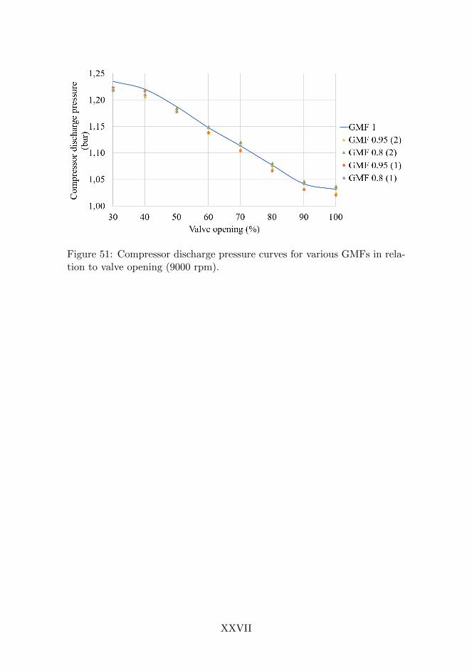
Figure 51: Compressor discharge pressure curves for various GMFs in rela-tion to valve opening (9000 rpm).

XXVII

Appendix H: Calculated Performance Parameters

In this appendix, some of the main calculated performance parameters arepresented tabulated.

Table 13: Explanation to the parameters used in Table 14-16.

Parameter Explanation

OV Set point discharge valve openingmg Gas mass flow at orificeQc Total compressor inlet volume flowQv Total valve inlet volume flowρtot Total valve inlet densityx Pressure ratio differentialY Expansion factorCV Flow coefficient

Cv, rel Relative flow coefficientPR Valve pressure drop ratio

XXVIII

Tab

le14

:D

ryga

sca

lcu

late

dp

erfo

rman

cepar

amet

ers,

bas

edon

Tab

le10

.

GM

FO

Vmg

Qc

Qv

ρtot

xY

Cv

Cv,rel

PR

-%

kg/s

m3/s

m3/s

kg/m

3-

--

--

0,99

97

300,

6638

0,57

540,

5006

1,32

750,

1874

0,91

5616

8,24

419,

9270

0,50

000,

9998

400,

9205

0,80

650,

6996

1,31

830,

1778

0,91

2824

3,61

4414

,374

10,

5000

0,99

98

501,

2267

1,09

210,

9530

1,29

000,

1555

0,91

6435

8,35

8121

,144

40,

5000

0,99

98

601,

4505

1,30

981,

1594

1,25

410,

1274

0,92

6848

4,39

3628

,581

00,

5000

0,99

99

701,

6145

1,47

471,

3238

1,22

230,

1002

0,93

5862

7,11

4337

,002

00,

5000

0,99

99

801,

7557

1,62

571,

4836

1,18

700,

0688

0,95

0784

8,64

5850

,073

20,

5000

0,99

99

901,

8848

1,76

561,

6382

1,15

390,

0343

0,96

6413

28,6

113

78,3

929

0,50

000,

9999

100

1,92

351,

8017

1,68

181,

1458

0,02

290,

9567

1694

,810

510

00,

5000

XXIX

Tab

le15:

Set

-up

1w

etga

sca

lcu

late

dp

erfo

rman

cep

aram

eter

s,b

ased

onT

able

11.

GM

FO

Vmg

Qc

Qv

ρtot

xY

Cv

Cv,rel

PR

-%

kg/s

m3/s

m3/s

kg/m

3-

--

--

0,94

81

300,

6528

0,57

580,

4710

1,48

820,

1904

0,91

4214

9,88

0810

,042

40,

5000

0,95

03

400,

9123

0,81

080,

6594

1,48

340,

1836

0,91

0021

5,79

7914

,459

10,

5000

0,94

72

501,

1897

1,08

320,

8918

1,43

220,

1608

0,91

3631

4,68

2221

,084

60,

5000

0,94

87

601,

4159

1,30

751,

0948

1,38

640,

1318

0,92

4342

9,65

6528

,788

20,

5000

0,94

93

701,

5846

1,48

281,

2601

1,34

790,

1042

0,93

3255

9,69

4337

,501

10,

5000

0,95

31

801,

7376

1,64

171,

4257

1,29

930,

0714

0,94

8876

8,67

1451

,503

10,

5000

0,94

78

901,

8582

1,78

301,

5760

1,26

670,

0367

0,96

4111

80,4

335

79,0

923

0,47

300,

9491

100

1,89

271,

8225

1,62

101,

2536

0,02

520,

9523

1492

,475

610

00,

4364

0,80

02

300,

6244

0,55

280,

4500

1,75

610,

1882

0,91

5212

1,85

3211

,500

10,

5000

0,80

57

400,

8654

0,77

180,

6290

1,72

990,

1810

0,91

1317

6,37

8516

,646

00,

5000

0,79

61

501,

1512

1,04

510,

8571

1,71

370,

1616

0,91

3125

3,80

1723

,953

00,

5000

0,79

58

601,

3715

1,25

861,

0481

1,66

950,

1357

0,92

2034

0,20

7732

,107

70,

4985

0,80

31

701,

5312

1,42

581,

2047

1,60

960,

1089

0,93

0244

3,03

5141

,812

20,

4934

0,80

03

801,

6883

1,59

741,

3740

1,56

370,

0767

0,94

5060

1,03

0556

,723

30,

4861

0,80

23

901,

8087

1,74

561,

5222

1,51

560,

0449

0,95

6087

6,57

4782

,728

30,

4612

0,80

54

100

1,83

861,

7673

1,55

581,

4969

0,03

410,

9355

1059

,582

710

00,

4277

XXX

Tab

le16:

Set

-up

2w

etga

sca

lcu

late

dp

erfo

rman

cep

aram

eter

s,b

ased

onT

able

12.

GM

FO

Vmg

Qc

Qv

ρtot

xY

Cv

Cv,rel

PR

-%

kg/s

m3/s

m3/s

kg/m

3-

--

--

0,94

87

300,

6462

0,56

210,

4901

1,38

980,

1879

0,91

5415

7,16

9110

,827

50,

5000

0,95

02

400,

8986

0,78

820,

6852

1,37

990,

1791

0,91

2222

7,45

6215

,669

60,

5000

0,95

06

501,

1926

1,06

050,

9248

1,35

650,

1587

0,91

4732

9,23

0222

,680

90,

5000

0,95

00

601,

4192

1,27

951,

1322

1,31

940,

1306

0,92

4944

6,61

3430

,767

50,

5000

0,94

97

701,

5717

1,43

221,

2821

1,29

060,

1060

0,93

2156

4,74

3638

,905

60,

5000

0,95

04

801,

7229

1,58

821,

4467

1,25

300,

0730

0,94

7676

8,43

9252

,938

30,

5000

0,95

10

901,

8641

1,74

051,

6127

1,21

540,

0366

0,96

4112

11,7

856

83,4

808

0,48

790,

9479

100

1,89

511,

7728

1,64

711,

2138

0,02

760,

9478

1451

,574

010

00,

4606

0,79

34

300,

5969

0,51

860,

4535

1,65

850,

1868

0,91

5812

2,18

4011

,411

60,

5000

0,80

05

400,

8352

0,73

110,

6373

1,63

660,

1816

0,91

1017

7,23

7516

,553

40,

5000

0,80

18

501,

1277

0,99

970,

8738

1,60

910,

1630

0,91

2425

9,22

7724

,211

00,

5000

0,79

99

601,

3533

1,21

471,

0760

1,57

180,

1369

0,92

1334

9,40

5732

,633

30,

5000

0,80

25

701,

4991

1,36

181,

2189

1,53

210,

1137

0,92

7143

8,50

5440

,954

90,

5000

0,80

04

801,

6744

1,53

961,

4037

1,48

990,

0789

0,94

3460

5,03

8956

,508

50,

4937

0,80

15

901,

8026

1,67

781,

5543

1,44

660,

0443

0,95

6689

7,56

8483

,829

70,

4436

0,79

85

100

1,84

211,

7166

1,59

721,

4441

0,03

440,

9348

1070

,704

210

00,

4161

XXXI