Ž .Global and Planetary Change 31 2001 297–319www.elsevier.comrlocatergloplacha

Weichselian stratigraphy and glaciotectonic deformation along thelower Pechora River, Arctic Russia

Mona Henriksena,), Jan Mangeruda, Olga Maslenikovab, Alexei Matiouchkovc,Jan Tverangerd

a Department of Geology, UniÕersity of Bergen, Allegaten 41, N-5007 Bergen, Norway´b Geological Faculty, St. Petersburg UniÕersity, UniÕersitetskaya 7r9, St. Petersburg 199034, Russian Federation

c ( )VSEGEI National Geological Institute , Sredny pr. 74, St. Petersburg 199026, Russian Federationd Norsk Hydro, OsebergrTune, UMOE bygget, Sandsliasen 46, N-5254 Sandsli, Norway˚

Received 25 January 2000; accepted 23 May 2001

Abstract

A large section near the village of Hongurei on the Pechora River, ca. 100 km inland from the Barents Sea coast, revealsthe following stratigraphic record of the last glaciation: The lowest units are lacustrine silt overlain by fluvial sand. Thesetwo units are repeated by glaciotectonic upthrusting from the NW. On top of this stacked succession is a till where fabricmeasurements reflect ice movement from the NE. Above the till is a partly laminated glaciolacustrine clay, probablydeposited during the deglaciation of the site. We interpret the two ice flow directions to reflect a single ice advance.

The Hongurei site is situated on the eastern rim of a marginal lobe of the Markhida moraine complex. Upthrusting fromthe NW is interpreted as lateral thrusting along the eastern flank of the NE–SW-oriented lobe, whereas the NE till fabricshows flow direction of the same glacier moving across the site. A maximum age for the last ice advance is given by optical

Ž .stimulated luminescence OSL dates of the fluvial sand below the till, dated to 85 ka at this site, but about 60 ka at othersites along the lower Pechora area.q2001 Elsevier Science B.V. All rights reserved.

Keywords: northern Russia; Weichselian; stratigraphy; glaciation; Kara ice sheet

1. Introduction

The Pechora lowland is a large sedimentary basinsituated in the northeastern part of European Russia,between the Ural Mountains, the Timan Ridge and

Ž .the Barents Sea Fig. 1 . The number, extent and age

) Corresponding author. Tel.:q47-5558-3503; fax:q47-5558-9416.

E-mail addresses: Mona.Henriksen@geol.uib.noŽ . Ž .M. Henriksen , Jan.Mangerud@geol.uib.no J. Mangerud ,

Ž .vniikam@mail.wplus.net O. Maslenikova ,Ž .vniikam@mail.wplus.net A. Matiouchkov ,Ž .Jan.Tveranger@hydro.com J. Tveranger .

of ice advances of the Barents–Kara ice sheet reach-ing the Pechora lowland during the last glacial pe-

Žriod have been greatly debated Grosswald, 1980,1998; Guslitser et al., 1985; Arslanov et al., 1987;Faustova and Velichko 1992; Tveranger et al., 1995;

.Astakhov et al., 1999 . Recent investigations haveshown that the Weichselian ice sheets reached theirmaximum extent during the Early or Middle Weich-

Žselian Astakhov et al., 1999; Mangerud et al., 1999,.2001 and that no ice sheet reached the mainland

during the Late Weichselian; at that time the glacierŽlimit was in the Pechora Sea Svendsen et al., 1999;

.Polyak et al., 2000; Gautaullin et al., 2001 .

0921-8181r01r$ - see front matterq2001 Elsevier Science B.V. All rights reserved.Ž .PII: S0921-8181 01 00126-6

( )M. Henriksen et al.rGlobal and Planetary Change 31 2001 297–319298

Ž . Ž . Ž .Fig. 1. a Key map of northern Europe and adjacent areas. b Map of the Pechora Basin. The Markhida and Harbei moraines stippled lineŽ . Ž . Ž .are plotted according to Astakhov et al. 1999 . Note that Mangerud et al. 2001 assume that the Harbei moraine is older 90 ka than the

Ž .Markhida moraine 60 ka , and therefore that the correlation of the two moraines is probably not correct. VK: Vastiansky Kon; M:Ž .Markhida; UV: Urdyuzhskaya Viska; S21: Sula site 21; S22: Sula site 22. c Morainic ridges and ice flow directions in the vicinity of the

Hongurei site. The upthrusting of silt A and sand B from NW, and the deposition of till C from NE are believed to belong to the same iceŽ . Ž .advance. The upthrusting occurred along the left flank of an advancing ice lobe small arrows . Later, the glacier large arrow overrode the

site from NE and deposited the till, when advancing to the Markhida moraine.

A number of end moraines are mapped in thePechora lowland. The Markhida moraine is found

Ž .near the Pechora River. Astakhov et al. 1999 and

Ž .Mangerud et al. 1999 correlated the Markhidamoraine towards west with the Indiga and Varshmoraines, and towards east with the Harbei, Halmer

( )M. Henriksen et al.rGlobal and Planetary Change 31 2001 297–319 299

and Sopkay moraines. They therefore also collec-tively named this morainic belt across the entirePechora lowland for the Markhida Line, assumingthat it represented a synchronous ice sheet limit.However, subsequently, it was shown that parts ofthis correlation were in conflict with OSL datesŽ .Mangerud et al., 2001 . The latter authors thereforeproposed a new hypothesis where they consideredthe Markhida Line as an ice marginal complex formedduring two separate advances, about 90 and 60 ka,respectively. The eastern moraines were postulatedto be of the same age as the huge ice-dammed LakeKomi, about 90 ka, and the Markhida moraine withits western extension to the Indiga–Varsh moraineswere assumed to be of an age about 60 ka. If thathypothesis is correct, the name Markhida Line ismisleading. Therefore, in this paper we use the nameMarkhida moraine only for the moraine close to thePechora River, i.e. the type locality.

We will use observations presented in this paperto test the new hypothesis of two ice advances.However, these uncertainties also demonstrate thatfurther studies of stratigraphic sequences from awider area of the Pechora lowland are needed inorder to solve the glacial history.

Near the village Hongurei is a large bluff situatedon the left bank of the lower Pechora River, ca. 100km from its mouth. The aim of this study was toinvestigate the stratigraphy and map the main sedi-mentary units, and to reconstruct the environmentalhistory of that section. Located 50 km down stream

Žof the Markhida type locality i.e. proximal to the.moraine , the section provides an opportunity to

study and date this last ice advance in the Pechoravalley. Dating of fluvial sand below the Markhida tillat Hongurei and the neighbouring sections provides amean to obtain a maximum date of the last iceadvance. Glacial ridges, glaciotectonic structures andclast fabric are used to determine ice flow directions.

In this work, the stratigraphic nomenclature ofwestern Europe is used, where Eemian correspondsto the Russian Mikulinian interglacial and Weich-selian to the Valdaian glacial period.

2. Methods

Distances along the bluff were measured with a50-m rope at river level from a fixed navigation

Ž .point Fig. 2 . A yardstick and clinometer were usedto measure altitudes above the late summer riverlevel. Considering the uncertainty of the height mea-

Ž .surements, the river level approximately 0.5 m a.s.l.is set to be the same as the sea level. Lithology,boundaries, sedimentary and deformation structureswere measured and described from several clearedsections and traced along the bluff.

Clast fabric analyses were made on 100 prolateŽclasts in matrix-supported diamictons except for one

.on 54 clasts . The fabric data were statistically treatedŽ .by the eigenvalue method Mark, 1973 , and plotted,

as well as the poles to deformed structures, in lowerhemisphere Schmidt equal-area projection. TheeigenvectorV identifies the direction of maximum1

clustering andS the strength of clustering around1Ž .V . One fabric analysis Fig. 14a was corrected for1

Žtectonic tilt of the diamictic lens Collinson and.Thompson, 1989 .

3. Stratigraphy

The sedimentary succession in the Hongurei sec-tion is divided into four units based on lithology: siltA, sand B, diamicton C, and clay D. The twolowermost units, silt A and sand B, are stratigraphi-

Ž .cally repeated along most of the bluff Fig. 2 due toglaciotectonic upthrusting. The units interpreted asbeing in primary position, are designated A and B .1 1

The same units are designated A and B in the2 2

upthrust position. The entire section is covered byŽ .diamicton C, which is overlain by clay D Fig. 2 .

Lenses of diamicton are also found a few placesalong the thrust plane between sand B and silt A .1 2

4. Large-scale thrusting and deformation

The lower boundary of silt A is a thrust fault2Ž .dipping NW Fig. 3 that can be traced along the

entire bluff. At 0–50 and 1000–1100 m the faultŽ .separates sand B and B Fig. 2 with only a few1 2

small lenses of silt A along these parts of the fault.2

Silt A is probably missing because it was smeared2

out during thrusting. Along most of the bluff, thismain fault zone consists of one or several sharp

Ž .thrust plane s with accompanying deformation ofŽ .underlying sediments described in unit B .

()

M.H

enriksenet

al.rG

lobalandP

lanetaryC

hange31

2001297

–319

300

Ž .Fig. 2. Drawing of the Hongurei section. Vertical scale exaggerated 2:1. The section is at almost right angle to the thrust direction from NW out of the paper . Below is aslightly oblique photo of the ca. 50-m high Hongurei section seen from SE. The part between 400 and 800 m of the drawing is seen. The units and boundaries are indicated. Aschematic diagram of the units and facies is shown to the lower right.

( )M. Henriksen et al.rGlobal and Planetary Change 31 2001 297–319 301

Fig. 3. Lower hemisphere stereoplot of poles to main thrust faultrepresenting 62 measurements taken along the Hongurei section.The mean dip direction is 3308. The arrow marks the thrustdirection.

The thrust direction is best seen in the gully at830 m, where the sedimentary structures in sand B1

are cut, displaced and dragged up along three almostparallel fault planes giving it a step-like appearanceŽ .Fig. 4 . Here the thrust is also traced into silt A1

indicating that silt A is really an upthrusted part of2

silt A . The dip of the thrust is ca. 408 but decreases1

and flattens out upwards, indicating an overall rampŽ .and flat thrust geometry Park, 1989 .

Between 940 and 1000 m, a thrust fault withmovement from the NE, possibly representing a split

Ž .fault McClay, 1992 , is observed below the mainthrust fault. In the sand between the two faults is alarge drag fold with an upper limb continuing up toand along the main thrust fault, implying a move-

Ž .ment from N Fig. 5 . Most of the minor reversefaults along the bluff have the same dip direction asthe main thrust fault, i.e. towards NW, but threefaults show displacements of 1–2 m the opposite

Ž . Ž .direction i.e. towards SE Fig. 6 . These are inter-Ž .preted as back thrusts Park, 1989 of the more

dominant fault system from NW.The main thrust fault shows considerable com-

pression from the NW by the stacking of units A andŽ .B. The thrust sheet is 20 m thick silt Aqsand B2 2

and is mapped for more than 1.1 km along the

section, i.e. almost at a right angle to the thrustingdirection. The thrusting distance cannot be measureddirectly, but according to our interpretation, it isestimated to be at least 50 m, but less than 1 km. Theminimum estimate is derived from inferred continua-tion of the thrust fault in the gully at 640 m, whilethe maximum estimate comes from the distance to alow NE–SW-oriented ridge west of Hongurei sectionŽ .Fig. 1c . The style and scale of the thrust indicatethat it was formed in either a proglacial or subglacialposition, where the movement and weight of theglacier caused an external stress on the sedimentsŽ .Hart and Boulton, 1991 . A subglacial position ismost likely due to lenses of diamicton in the defor-

Fig. 4. Sketch of the thrust fault in the gully at 830 m. Silt A is2

upthrusted from silt A along three almost parallel thrust faults.1

The faults level out to near horizontal upward. Below the thrustplanes are drag folds and many small shear planes in sand B .1

Ž .Most shear planes open circles are either parallel or oppositelyŽ .directed to the main thrust faults filled circles .

( )M. Henriksen et al.rGlobal and Planetary Change 31 2001 297–319302

Ž .Fig. 5. A large drag fold between the two thrust faults at 950 m. The fold shows stress direction from N 0108 , a direction in between theŽ . Ž .upper main thrust fault 3368 and the lower split fault 0308 .

Ž .mation zone below the main thrust fault Fig. 7 . Thedecollement was along the incompetent silt A, which´

Ž .is typical for such thrusts Hart, 1990 . Alternatively,

Fig. 6. A thrust fault at 530 m, interpreted as a back thrustuplifting silt A and sand B from the SE. The displacement is2 2

Žmore than 2 m along the thrust plane. Smaller shear planes open.circles cluster in two groups, one group with similar and one with

Ž .opposite dips to the back thrust filled circles .

the decollement could be at the lower border of the´Ž .permafrost layer Berthelsen, 1979 .

5. Unit A—silt

Silt A is found at two stratigraphic levels A and1Ž .A Fig. 2 where the upper silt A is considered2 2

upthrust as discussed above. The base of silt A is1

not exposed. Silt A is more than 10 m thick andconsists of well-consolidated bluish or dark grey silt.The silt is partly massive and partly laminated, andcontains numerous 1–40-cm-thick layers of fine sand,

Ž .irregularly spaced in the vertical succession Fig. 8 .The sand layers are massive or laminated, and usu-ally have sharp lower boundaries and are normallygraded. Some of the silt laminae and sand layers aredeformed by soft-sediment deformation as loading

Ž .and water escape structures Fig. 8 . Occasionally,there are current ripples reflecting northward flow.Some layers in silt A are continuous for more than1

10 m, and dip 10–208 towards NNE.The massive and laminated silt is interpreted to be

deposited from suspension in quiet water or by low-

( )M. Henriksen et al.rGlobal and Planetary Change 31 2001 297–319 303

Fig. 7. Sketch at 610 m. The lower boundary of silt A is the main thrust fault. The movements have been oblique out of the paper to the2

left. Below is an up to 2.7 m thick ductile deformation zone. The thin lines below the main thrust fault are mainly tectonic structures,whereas in the lower part of the section most represent remnants of primary sedimentary structures. Folds, boudins and fluidised structures

Ž . Žcharacterise the deformed sand, which also contains some lenses of silt and clay deformed floodplain sediment? and of diamicton facies. Ž .c3 . Cryoturbation structures dropsoils can be seen to the left.

density turbidity currents, and the sand layers byhigh-density turbidity currents or possible sandy de-

Ž .bris flows Stow et al., 1996 . The soft-sedimentdeformation suggests a rapid sedimentation, support-ing deposition by turbidity currents.

In large parts of silt A, the laminae are folded,Ž .overturned, and cut by small shear planes Fig. 8 .

Blocks of sand and silt of various shapes and sizesŽ . Ž .up to 1 m float in the silt matrix Fig. 9a . Unde-formed layers are interbedded with deformed se-quences, which shows that the structures were formedsynsedimentary. These deformation structures are in-

Ž .terpreted as the result of mass movement slumpthat have not moved far enough to homogenize the

Ž .sediment Walker, 1992 .Rare individuals or fragments of robust species of

foraminifera and diatoms were found, also includingŽsome extinct species M.S. Seidenkrantz, pers.

.comm., 1998 . In general, the fossils are not wellpreserved. Even though the microfossils mainly con-

Žsist of open marine taxa e.g.NeogloboquadrinaŽ . .pachyderma sin. and Paralia sulcata , the small

number compared to the abundant foraminifera and

diatoms found in marine mud at other localitiesŽalong the lower Pechora River e.g. Tveranger et al.,

.1998; Mangerud et al., 1999 , suggests that silt A isa non-marine sediment, and the microfossils aretherefore interpreted as redeposited. However, thelow amount of fossils can also be caused by highsedimentation rate. Redeposited pieces of wood,small brown coal fragments, and peat clasts are alsofound scattered in silt A.

We conclude that silt A was deposited on a slopein a lacustrine basin by suspension and turbidity

Žcurrents in a quiet offshore environment Reading.and Collinson, 1996 . Occasionally, instability on the

slope caused slumping with deformation and resedi-mentation. The dip of the more continuous layersand the paleocurrent directions indicate a lake bot-tom sloping towards NNE with a sediment sourcefrom SSW.

6. Unit B—sand

Sand B is up to 16.3 m thick and consists of wellsorted fine and medium sand with a pale yellow or

( )M. Henriksen et al.rGlobal and Planetary Change 31 2001 297–319304

whitish colour, but frequently stained red and orangedue to oxidation. The lower boundary is erosional onsilt A. At 650 m, there is a 60-cm-deep and 2-cm-wide frost crack in the underlying silt filled withsand, implying subaerial exposure of silt A. Thelower sand B has the main thrust fault as its upper1

boundary at 14–31 m a.s.l., whereas the upthrustsand B is overlain unconformably by diamicton C2Ž .Figs. 2 and 10 . Through the entire sequence, thepaleocurrent has northerly directions. Both sand B1

Žand B are divided into three facies, b1 to b3 Fig.2.10 .Facies b1 consists of cross-bedded and planar

Ž .stratified fine and medium sand Fig. 9b with anerosional lower boundary. The facies is interpreted

Ž .as a fluvial channel deposit Collinson, 1996 . Thethickness of cosets is up to 7.5 m and the sets varybetween 0.2 and 2.5 m, indicating a relatively strong

Ž .current in a more than 7.5-m-deep channel Fig. 11 .Facies b1 is widespread and is commonly found in

Ž .the lowermost part of sand B Fig. 10 . It containsscattered pebbles, wood and plant detritus, and, whereit overlies silt A, silt clasts. Ripple cross laminationfound between some beds was probably formed dur-ing calmer periods with a lower water level.

Facies b2 is up to 5 m thick and dominated byripple cross-laminated beds of silty sand to mediumsand interbedded with few cross-stratified and planarlaminated beds. Some scattered pebbles occur in thesand. The ripple beds are from 2–3 to 1.0 m thick,

Ž .with sharp lower boundaries Fig. 9b . Facies b2 isŽcommonly found on top of facies b1 Figs. 10 and

.11 , and is interpreted as deposited at shallowerwater depth and under calmer current conditions thanfacies b1.

Facies b3 is distinguished from facies b2 by itshigher content of silt, clay and organic detritus,which is found interbedded with fine and medium

Ž .sand Fig. 9c . The silt and clay layers are up to 15cm thick, massive or laminated, and in some placesrich in organic detritus. Silt often forms thin drapings

Fig. 8. Sketch of the structures in silt A at 830 m, the sand layers1

and laminae are marked with dots, silt is white. Undisturbed anddeformed sequences are interbedded showing synsedimentary de-

Žformation caused by loading load casts, load balls and flame. Ž .structures and by slumping shear planes and folds .

( )M. Henriksen et al.rGlobal and Planetary Change 31 2001 297–319 305

Ž .Fig. 9. a Balls of interbedded sand and silt floating in a silt matrix in silt A, interpreted to original to be load cast later deformed by slump.Ž . Ž . Ž .b The lower 40 cm shows cross-bedded fine and medium sand facies b1 overlain by ripple laminated fine sand facies b2 in sand B .1

Ž . Ž .The bedding of the ripples is interpreted to be originally sub-horizontal, now tilted towards NW right , due to the upthrusting. cŽ .Horizontally bedded silt and fine sand in sand B interpreted as floodplain deposit facies b3 of ca. 2 m thickness. The parallel-laminated1

fine-grained sediment is interbedded and overlain by ripple laminated sand. The tilting of the beds are caused by the upthrusting ofŽ .overlying sediments. d Ductile deformed sand with some silt lenses. In the upper right corner, the upthrusted silt A can be seen with a2Ž . Ž .thin lens of diamicton facies c3 just below. A 1-m stick to the right. Photo is marked on Fig. 7. e Brecciated sand with the primary

lamination preserved. Between the sand blocks are fluidised silty clay.

( )M. Henriksen et al.rGlobal and Planetary Change 31 2001 297–319306

Fig. 10. Conceptual drawing showing the interrelation of the described facies in sand B. The main sedimentary structure in each facies isindicated. The line with triangles represents the main thrust fault. Sand B and sand B is 6–16 m thick.1 2

or flaser laminae. Layers up to 10 cm thick, consist-ing of laminated organic detritus and pieces of woodare interbedded with sand. The sand layers in faciesb3 are massive, ripple or planar laminated. Somebeds are graded from ripple-laminated sand to siltand clay. Facies b3 is interpreted as floodplain oroverbank sediment, the sand layers representing floodepisodes. The layers of organic detritus were proba-bly deposited in a quiet, boggy part of the floodplain.Some of the well-sorted massive sand beds might be

Ž .of eolian origin Collinson and Thompson, 1989 .In the upper part of sand B at 610 m, there is a1

5–6-m-long and 40-cm-wide ice wedge cast filledŽ .vertically by stained sand Fig. 12a . Several shear

planes belonging to the main thrust fault systemsubsequently bisected the wedge cast. Close to theupper part of the wedge is an irregular shaped cry-

Ž . Ž .oturbation dropsoil Fig. 7 Vandenberghe, 1988 .Sands B and B are more or less deformed with1 2

an upward increasing degree of deformation into a0.1–5-m-thick deformation zone just below the main

Ž .thrust fault and diamicton C Figs. 10 and 11 . Inthis zone, primary structures are completely de-stroyed or difficult to recognise. There are denselyspaced shear planes in the uppermost ca. 10 cm and

evidence for both ductile and brittle deformationlower in the zone. The ductile-deformed sedimentsexhibit boudins, folds, catchments, shear planes, flu-idisation and water-escape structures, and include

Žstreamlined lenses and layers of diamicton Figs. 7.and 9d . The brecciated sediments consist of lenses

of sand up to 80 cm long, commonly with theprimary lamination preserved. Ductile deformed orfluidised silty clay follows shear planes and joints

Ž .dissecting the sand lenses Fig. 9e . Contrasts inpermeability, strength or different freezing pointcaused the difference between the brittle deformationin the sand and the ductile deformation in the clayŽ .Benn and Evans, 1996 . The deformation zone isinterpreted to be a result of glaciotectonical deforma-tion.

Shear planes and faults cut through the whole ofsand B, most of them connected either with theupthrusting from NW or with the glacier overridingfrom NE. Most of the larger water escape structuresin sand B continue up to the deformation zone or arefolded into glaciotectonic faults cut by diamicton CŽ .Fig. 11 . These structures are therefore consideredto have been generated by the overburden of anoverlying ice sheet.

( )M. Henriksen et al.rGlobal and Planetary Change 31 2001 297–319 307

6.1. The geological deÕelopment

The lower boundary of sand B shows fluvialerosion of silt A after subaerial exposure. The sedi-mentary structures reflect waning current conditions

Ž .from cross-stratified channel sand facies b1 to rip-Ž .ple laminated shallower water sand facies b2 . Then

follows floodplain sediments with sand interbeddedŽ .with silt, clay, or organic detritus facies b3 . Chan-

nel infilling or migration caused this succession. Insome places along the bluff, facies b2 is missing,whereas elsewhere facies b1 and b2 are interbedded

Ž .several times Fig. 10 , indicating vertically aggrad-ing channels. Sand B is interpreted to have beendeposited in a sandy braided river due to its ratheruniform paleocurrent direction and domination of

Ž .cross-beds facies b1 with a few fining-upward suc-Ž .cessions Boggs, 1995; Collinson, 1996 . Consider-

ing that the site is close to the coast, the thickness ofsand B and the aggrading channels indicate a highand rising relative base level.

After deposition, the upper part of sand B hasbeen deformed by cryoturbation and ice wedge for-mation, indicating subaerial exposure with per-mafrost. Some eolian sedimentation might have oc-curred. The permafrost subsequently melted, creatingan ice-wedge cast before sand B was glaciotectoni-cally deformed by an overriding glacier. Whereasthere is much organic matter in the lower part ofsand B, there is little in the upper cryoturbated part,possibly indicating a transition from interglacialrin-terstadial conditions to a colder climate. The meltingof permafrost can either have been caused by warmerclimate or submergence of the landscape by a lake,although lacustrine sediment have not been found atthis stratigraphic level.

7. Unit C—diamicton, and ice movement direc-tions

Unit C is an up-to-10 m thick, well-consolidated,matrix-supported clayey diamicton. The lowerboundary to sand B is undulating with a general dip2

Ž .towards NE Fig. 2 . Two facies c1 and c2 areidentified, and both can be traced all along the bluff.A lens of typical facies c2 sediments is also foundbelow the main thrust fault at 40 m.

Facies c1 is 0.2–3.7 m thick and consists ofdiscontinuous layers of sand, silt, clay and clayey

Ž .diamicton Fig. 12b . The lower boundary is ero-sional and is defined by the first appearance of adiamicton layer. There are numerous shear planes,boudins, and foliations. The layers in facies c1 aresubhorizontal and vary from a few mm to 3-cm-thickclay and 15–20-cm-thick sand layers. Facies c1shows a transition from predominantly sand in thelower part to an increasing content of diamicton inthe upper. The sand is similar to the underlying sandB. At some places, low-angle sandy shear planes insand B continue into facies c1. An inclined, asym-metric fold around a boulder at 650 m shows move-

Ž .ment from the NW Fig. 13 . Facies c1 is interpretedas a subglacial shear zone where pseudolamination isgenerated by high extensional shear between subpar-

Žallel walls Boulton, 1987; Hart and Boulton, 1991;.van der Wateren, 1995 .

Facies c2 overlies facies c1 with a sharp or grad-ual lower boundary. Facies c2 is a clayey, matrix-supported diamicton with scattered shell fragmentsŽMacoma calcarea, Portlandia arctica and Hiatella

.arctica , pebbles and boulders up to 60 cm in diame-ter. The upper 1 m is sandier. The facies is 2.2–9 m

Ž .thick Fig. 12c , and has a dark brownish greycolour. Some of the boulders have striations, and

Žpebbles show a preferred orientation NE–SW Fig..14b–d . A boulder at the transition between facies c1

and c2 at 520 m has an associated plough markŽ .showing movement from 0808 E .

Sandy layers in facies c2 are mainly subhorizontaland are from a few mm to 20–30 cm thick, beingcontinuous for 30 cm to more than 5 m. They arefound along shear planes or as small lenses. At 650m, the layers dip towards the NW overlying a fold in

Ž .facies c1 Fig. 13 , whereas they are almost verticaland folded from the NNW at 790 m. The number ofvisible shear planes and sandy layers decreases up-wards in facies c2. The structures are interpreted tobe formed subglacially.

Facies c2 is interpreted as a subglacial tillŽGoldthwaith, 1971; Dreimanis, 1992; Ehlers, 1996;

.Johnson and Menzies, 1996 , with facies c1 as adeforming bed till. The folds and vertical layersshow that facies c2 is not a homogenized deforma-tion till, and clast ploughing suggests deposition by

Ž .lodgement Clark and Hansel, 1989 , possible also

( )M. Henriksen et al.rGlobal and Planetary Change 31 2001 297–319308

Fig. 11. Sedimentological and structural logs from 200, 520, 610, 650, 790–830, 890, and 1050 m along the Hongurei section.

( )M. Henriksen et al.rGlobal and Planetary Change 31 2001 297–319 309

Ž .Fig. 11 continued .

( )M. Henriksen et al.rGlobal and Planetary Change 31 2001 297–319310

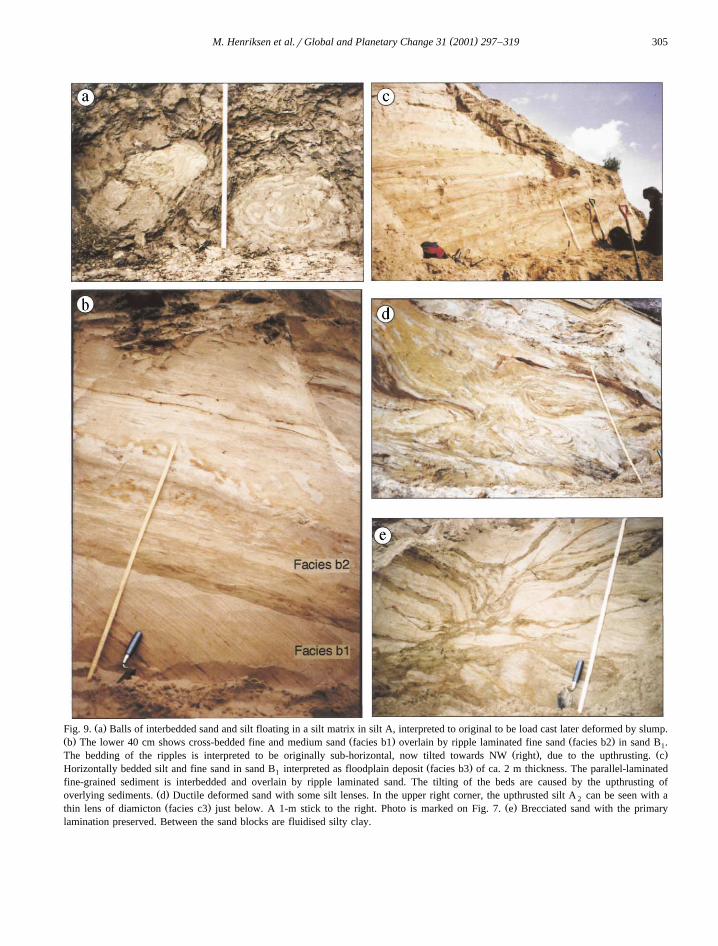
Žby melt-out processes Dreimanis, 1992; Ehlers,.1996; Menzies and Shilts, 1996 . The content of clay

and marine shell fragments indicates that a large partof the till originates from glacial erosion of marinesediments.

7.1. Lenses of diamicton along the main thrust faultbetween unit B and A1 2

Lenses of a diamicton, which we, for simplicity,include in unit C, and designate facies c3, are foundin the ductile deformation zone under the main thrust

Ž .plane at 40, 610, 650, and 700 m Figs. 2c and 7 .Facies c3 appears as 15–65-cm-thick deformed lensesor as discontinuous beds parallel with the thrustfault.

Facies c3 is a brown diamicton with a matrix ofsandy, silty clay with scattered pebbles and sandlaminae along smaller shear planes. Both lower andupper boundaries are glaciotectonic thrusts. Theboundaries are uneven and are cut by smaller shearplanes. The facies differs from facies c1 and c2 bythe brownish colour, being sandier, and lacking boul-ders and shell fragments. At 40 m below the mainthrust fault, a lens of facies c2, the basal till, directlyoverlies a lens of facies c3.

Not found in situ, facies c3 is difficult to inter-pret. Mixing and homogenization of the pre-existingsediments during the upthrusting might possible haveformed facies c3. Alternatively, it may be a sub-glacially formed diamiction.

7.2. Ice moÕement directions

Three fabric measurements of elongated pebblesŽ .in the lower 1–2 m of the basal till facies c2 , taken

Ž .at 520, 790, and 890 m Fig. 14b–d , indicate an icemovement from NE. Fabric analysis of the till lens

below the main thrust shows a NW–SE orientationŽ .Fig. 14a , parallel with the thrust direction.

The main thrust fault between unit B and A , as1 2

well as all the large structures and shear planes,dipping sand layers and folds in units A and B and infacies c1 indicate movement from the NW. Only afew structures have been found in facies c2, andthese indicate generally a northerly direction. Oneexception is at 650 m where sand layers in facies c2

Ž .dip towards NW Fig. 13 . An easy explanationwould be that the clast fabric display a transverseorientation. However, end moraine lobes 20–30 kmsouth of Hongurei, as well as ridges to the north,

Žhave a horseshoe form, opening towards NE Fig..1c , indicating ice movement from that direction

Ž .Astakhov et al., 1999 . On aerial photos parallellineations along the ridges indicate they consist ofupthrust nappes, with a strike NE–SW along thelateral branches.

The disparity of the ice movement indicators maybe caused by two ice advances, first one from theNW, then from the NE. A simpler interpretation isthat the two ice movements identified in the sectionbelong to the same advance. The thrusting took placeat least partly subglacially along the left side of aglacial lobe moving from NE, causing an ice move-

Ž .ment towards the flank from NW , thrusting anddeforming the underlying sediments. Subsequently,the glacier overrode the section and deposited most

Ž . Ž .of the till unit C with NE-fabrics Fig. 16 , orpossibly reoriented the clasts from a NW to a NEdirection.

7.3. Subglacial temperatures

Glacial deformation may take place in non-frozenas well as frozen sediments. In the latter, the degreeof deformation is a magnitude less than during non-

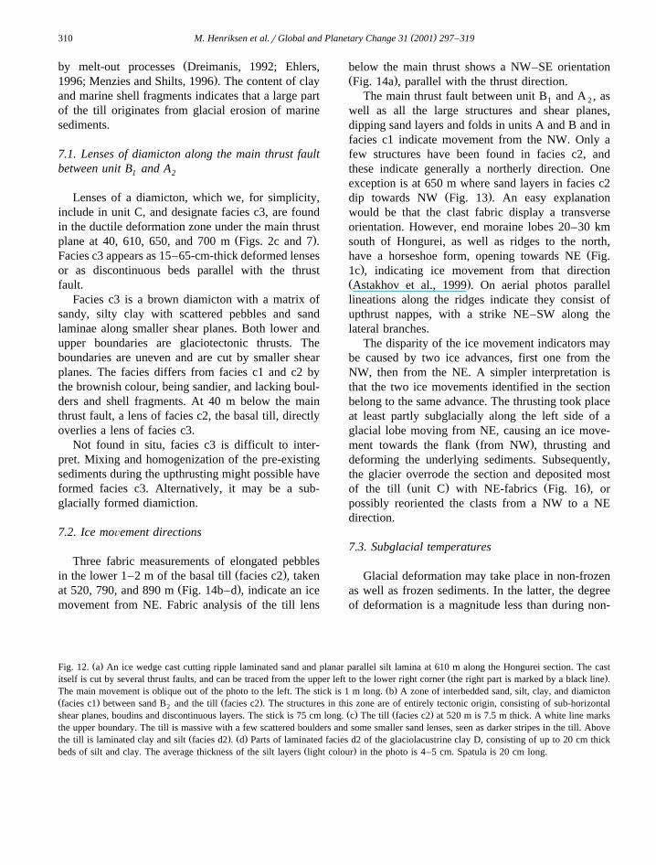
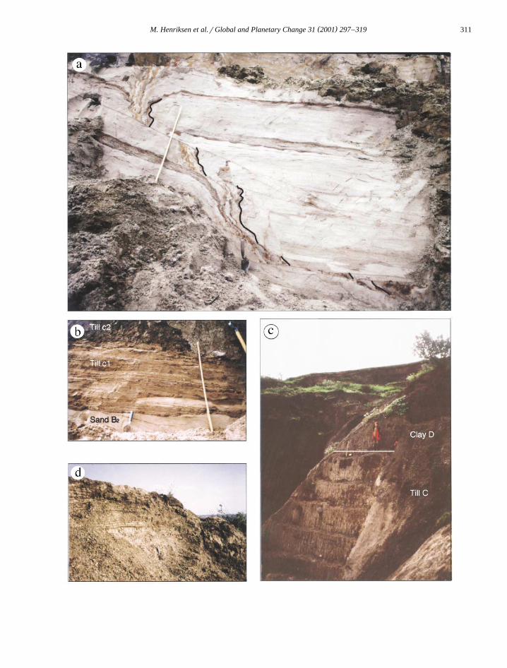
Ž .Fig. 12. a An ice wedge cast cutting ripple laminated sand and planar parallel silt lamina at 610 m along the Hongurei section. The castŽ .itself is cut by several thrust faults, and can be traced from the upper left to the lower right corner the right part is marked by a black line .

Ž .The main movement is oblique out of the photo to the left. The stick is 1 m long. b A zone of interbedded sand, silt, clay, and diamictonŽ . Ž .facies c1 between sand B and the till facies c2 . The structures in this zone are of entirely tectonic origin, consisting of sub-horizontal2

Ž . Ž .shear planes, boudins and discontinuous layers. The stick is 75 cm long. c The till facies c2 at 520 m is 7.5 m thick. A white line marksthe upper boundary. The till is massive with a few scattered boulders and some smaller sand lenses, seen as darker stripes in the till. Above

Ž . Ž .the till is laminated clay and silt facies d2 . d Parts of laminated facies d2 of the glaciolacustrine clay D, consisting of up to 20 cm thickŽ .beds of silt and clay. The average thickness of the silt layers light colour in the photo is 4–5 cm. Spatula is 20 cm long.

( )M. Henriksen et al.rGlobal and Planetary Change 31 2001 297–319 311

( )M. Henriksen et al.rGlobal and Planetary Change 31 2001 297–319312

Fig. 13. Sketch of fold in facies c1 and dipping sandy layers infacies c2 at 650 m. Diamicton C erodes a water escape structure inthe underlying sand B . Stereoplot of poles to bedding in the fold2Ž .facies c1 shown with filled circles and to bedding in the tillŽ .facies c2 with open circles. The arrow marks the direction of themovement, being from NW.

Žfrozen conditions Echelmeyer and Wang, 1987; Hart.and Boulton, 1991 . Water-escape structures and the

thick ductile deformation zone in sand B indicatenon-frozen conditions during thrusting and glacialadvance. Deposition of the thick till certainly showthat the basal ice was at the pressure–melting point.

8. Unit D—clay

The uppermost unit, clay D, consists of 11–12 mŽ .of partly laminated and partly massive clay Fig. 2 .

Three facies d1, d2, and d3 occur in stratigraphicsuccession; d1 at the base and d3 at the top.

Facies d1 is a 50-cm-thick fining-upward succes-sion of sandy clay and pebbly sand with a sharplower boundary to diamicton C. This facies is only

found in a small depression at 620 m, and is inter-preted as a glaciolacustrine sediment deposited fromsuspension and by gravity flows. The coarse materialindicates proximity to the sediment source, probablyan unstable sediment slope.

Facies d2 consists of 7.5 m of horizontal, rhyth-mic couplets of a lower silt and an upper clay laminaŽ .Fig. 12d . The lower boundary of each couplet, andcommonly also the lower boundary of each lamina issharp. The dark clay laminae are 0.5–1 cm thick andthe lighter silt laminae 0.3–20 cm thick. The siltlayers are generally coarser in the lower part of the

Ž .unit Fig. 11 .Facies d2 is interpreted as a glaciolacustrine de-

Ž .posit O’Sullivan, 1983 , where the clay is depositedŽ .from suspension Miller, 1996 . Some silt layers are

laminated, indicating that the silt was partly de-posited from density flows. This indicates that thelower part was deposited closer to the sedimentsource. The pebbles are considered to be ice rafted.

Fig. 14. Contoured stereoplots of clast fabric in the lower 1–2 mŽ . Ž .of till C facies c2 plots b, c, and d , and from an upthrusted till

Ž . Ž .lens facies c2 corrected for tilt plot a . The number measuredŽ . Ž . Ž .N , the eigenvalueS , and the eigenvectorV of each fabric1 1

Ž . Ž . Ž .analysis is given. a From 40 m. b From 520 m. c From 790Ž .m. d From 890 m.

( )M. Henriksen et al.rGlobal and Planetary Change 31 2001 297–319 313

The sediment sources may have been sediments onthe glacial ice, unstable sediments near or in thelake, or melt water rivers. The couplets in facies d2may be varves, characterised by the regular rhyth-mite sequence of fine and course laminae with sharp

Ž .boundaries Sturm, 1979 . We estimated about 600–800 couplets, and, if they are annual layers thesedimentation rate was 0.5–4.6 cmryear.

Facies d3 is a 4-m-thick massive clay. There is agradual transition from facies d2 to d3. The claycontains a few sandier parts and also scattered peb-bles. A sample was investigated for diatoms, butonly three whole individuals of the robust marinespeciesP. sulcata were found. Some shell fragmentswere also found. These are interpreted as rede-posited. Based on the gradual transition from faciesd2 and the nearly total lack of fossils, facies d3 isinterpreted as a massive glaciolacustrine clay. Depo-sition may have taken place in a non-stratified lake,

Žabove the stratification in the water column Ashley,.1975; Talbot and Allen, 1996 , or in the deeper,

distal parts related to low sediment influx in anŽArctic lake with a perennial ice cover Coakley and

.Rust, 1968; Lemmen et al., 1988; Doran, 1993 .Ž .The massive clay facies d3 is similar to clay

described at sites 21 and 22 along Sula river andŽ . Ž .Urdyuzhskaya Viska Fig. 1 Mangerud et al., 1999 .

Possibly, the clay at these localities can be corre-lated, all having been deposited in the same ice-dammed lake.

9. Dating of the units

Three samples from the lower part of sand B and1Ž .B facies b3 were dated by the radiocarbon method2

Ž . ŽTable 1 . All dates except for one at 38.9 ka sam-.ple 96-1156 gave non-finite ages. Arslanov et al.

Ž . Ž .1987 reported an age of 45 ka LU-1492 fromplant remains from sand B. Both finite ages wereprobably caused by a small amount of contamina-tion. Three OSL dates from sand B yielded ages

Žaround 80 ka and a fourth date of 98 ka Table 2;. Ž .Fig. 15 . Sample 96-1189 98 ka was taken laterally

Ž .to sample 96-1187 79 ka , and the apparent agedifference is therefore not real. The mean of all OSLdates is 85 ka. Sand B is interpreted as the product ofan Early Weichselian fluvial event ca. 85 ka BP.

We tried to date clay D with the fine-grained TLmethod. Only maximum ages were obtained, the

Ž .youngest being more than 107 ka Table 3 . Consid-ering the OSL dates of 85 ka from the underlyingsand B, the fine-grained TL dates are considered tobe too old. This is probably due to incomplete

Ž .bleaching zeroing of the sediments prior to deposi-Ž .tion Wintle, 1991 .

10. Discussion and correlation

Several sections along the lower Pechora Riverhave a similar stratigraphy to that at Hongurei, with

Ž . Žfluvial sand below the surface till Fig. 15 Arslanovet al., 1987; Tveranger et al., 1995, 1998; Mangerud

.et al., 1999 . The till occurs as a 1–10-m-thick tillsheet in the Markhida type of hummocky morainiclandscape, with its southern limit along the Markhida

Ž . Ž .moraine Fig. 1b Astakhov et al., 1999 . Thus, tillC at Hongurei is correlated with unit F at Vastiansky

Ž .Kon Tveranger et al., 1998; Mangerud et al., 1999Žand the basal till unit B at Markhida Tveranger et

.al., 1995; Mangerud et al., 1999 .

Table 1Uncalibrated radiocarbon dates of handpicked macrofossils of terrestrial plants from Hongurei section

Unit Field sample no. Lab. no. Age EC-13 Material dated Sediment, stratigraphy. Comments

B 96-1156 TUa-1745 38,790 y23.1 Handpicked Organic detritus interbedded with sand2Ž . Ž .q4740,y2960 terr. moss facies b3 , 2.8 m above main thrust fault.

B 96-1068 TUa-1927 )32,295 y27.3 Twig Organic detritus on top of laminated sand2Ž .facies b3 , ca. 1 m above silt A .2

B 96-1020A TUa-1743 )43,955 y23.5 Handpicked Organic detritus interbedded with sand1Ž .terr. moss facies b3 , ca. 0.5 m above silt A .1

Ž .The samples are prepared at the Trondheim Radiocarbon Laboratory, Norway and measured at the accelerator mass spectrometry AMSlaboratory at Uppsala University, Sweden.

( )M. Henriksen et al.rGlobal and Planetary Change 31 2001 297–319314

Table 2Ž .Optical stimulated luminescence OSL dates on fluvial sediments below the Markhida till at sites along the lower Pechora

Ž .Locality Field sample Lab. no., Dose rate, Paleo-dose, No. of est. wc, % Age, ka Sediment, stratigraphy.Ž . Ž .Risø Gyrka Gy Comments

Hongurei 96-1189 982504 1.31 117 12 27 98"7 Alluvial sand unit B1

below till, planar laminatedfine sand, 21.0 m a.s.l.

Hongurei 96-1187 982503 1.64 130 12 27 79"8 Alluvial sand unit B1

below till, ripple laminatedfine sand, 20.8 m a.s.l.

Hongurei 96-1175 982502 1.45 120 14 27 83"11 Alluvial sand unit B1below till, planar laminatedfine-med. sand, 14.8 m a.s.l.

Hongurei 96-1174 982501 1.30 102 13 27 79"7 Alluvial sand unit B1

below till, ripple laminatedfine-med. sand, 13.2 m a.s.l.

Markhida 93-1Ar7 942501 0.83 53 4 27 67"5 Alluvial sand below tillŽTveranger et al., 1995;

.Mangerud et al., 1999 .Markhida 93-1Br6 942502 1.30 79 3 27 64"6 Alluvial sand below till

ŽTveranger et al., 1995;.Mangerud et al., 1999 .

Markhida 93-1Cr1 942503 1.96 114 4 27 63"7 Alluvial sand below tillŽTveranger et al., 1995;

.Mangerud et al., 1999 .Markhida 96-2117 992522 1.23 69.7 15 27 56"4 Alluvial sand below till.Markhida 96-2118 992523 1.12 65.4 15 27 58"4 Alluvial sand below till.Vastiansky Kon 95-6509 962519 1.70 128 3 27 81"13 Alluvial sand unit D,

Section 3, 57 m a.s.l.Ž .Tveranger et al., 1998 .

Vastiansky Kon 95-6510 962520 1.42 104 3 27 78"5 Alluvial sand unit D,Section 3, 57 m a.s.l.Ž .Tveranger et al., 1998 .

Vastiansky Kon 95-6507 962518 1.45 96 3 27 71"6 Alluvial sand unit D,Section 3, 46 m a.s.l.Ž .Tveranger et al., 1998 .

Vastiansky Kon 95-6506 962517 1.52 87 4 27 61"6 Alluvial sand unit A,Section 3, 39.5 m a.s.l.Ž .Tveranger et al., 1998 .

Vastiansky Kon 95-6505 962516 1.68 101 4 27 64"8 Alluvial sand unit A,Section 3, 38 m a.s.l.Ž .Tveranger et al., 1998 .

Vastiansky Kon 95-6504 962515 1.06 82 2 27 82"10 Alluvial sand unit A,Section 3, 23 m a.s.l.Ž .Tveranger et al., 1998 .

Vastiansky Kon 95-6503 962514 1.29 69 2 27 57"6 Alluvial sand unit A,Section 3, 22 m a.s.l.Ž .Tveranger et al., 1998 .

Ž .Quarts in the fine sand grain fraction is used. Earlier published results are recalculated with a water content wc of 27%. All dates areŽ .performed at the Nordic Laboratory for Luminescence Dating, Risø, with method described in Mangerud et al. 2001 .

Large-scale folding and upthrusting in the Vas-tiansky Kon section was probably caused by thesame ice-advance which deposited the upper till in

Ž .that section Tveranger et al., 1998 . The thrustingand fabric measurements indicate an ice advancefrom the NE. Both the Vastiansky Kon and Hongurei

( )M. Henriksen et al.rGlobal and Planetary Change 31 2001 297–319 315

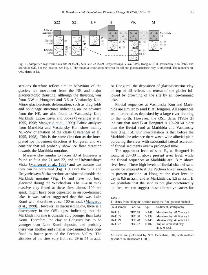
Ž . Ž . Ž . Ž . Ž .Fig. 15. Simplified logs from Sula site 21 S21 , Sula site 22 S22 , Urdyuzhskaya Viska UV , Hongurei H , Vastiansky Kon VK , andŽ .Markhida M . For the location, see Fig. 1. The tentative correlation between the till and glaciolacustrine clay is indicated. The numbers are

OSL dates in ka.

sections therefore reflect similar behaviour of theglacier; ice movement from the NE and majorglaciotectonic thrusting, although the thrusting wasfrom NW at Hongurei and NE at Vastiansky Kon.Minor glaciotectonic deformation, such as drag foldsand boudinage structures indicating an ice advancefrom the NE, are also found at Vastiansky Kon,

ŽMarkhida, Upper Kuya, and Sopka Tveranger et al.,.1995, 1998; Mangerud et al., 1999 . Fabric analyses

from Markhida and Vastiansky Kon show mainlyŽNE–SW orientation of the clasts Tveranger et al.,

.1995, 1998 . This is the same direction as the inter-preted ice movement direction at Hongurei, and weconsider that all probably show ice flow directiontowards the Markhida moraine.

Massive clay similar to facies d3 at Hongurei isfound at Sula site 21 and 22, and at Urdyuzhskaya

Ž .Viska Mangerud et al., 1999 and we assume thatŽ .they can be correlated Fig. 15 . Both the Sula and

Urdyuzhskaya Viska sections are situated outside theŽ .Markhida moraine Fig. 1 , and have not been

glaciated during the Weichselian. The 1–4 m thickmassive clay found at these sites, almost 100 kmapart, might have been deposited in an ice-dammedlake. It was earlier suggested that this was Lake

ŽKomi with shorelines at ca. 100 m a.s.l. Mangerud.et al., 1999 . However, as discussed below, there is a

discrepancy in the OSL ages, indicating that theMarkhida moraine is considerably younger than LakeKomi. Therefore, the clay at Hongurei has to beyounger than Lake Komi deposits, and probablythere was another and smaller ice-dammed lake con-fined to lower parts of the Pechora Valley. Thealtitudes of the sites vary from ca. 29 to 54 m a.s.l.

At Hongurei, the deposition of glaciolacustrine clayon top of till reflects the retreat of the glacier fol-lowed by drowning of the site by an ice-dammedlake.

Fluvial sequences at Vastiansky Kon and Mark-hida are similar to sand B at Hongurei. All sequencesare interpreted as deposited by a large river draining

Ž .to the north. However, the OSL dates Table 2indicate that sand B at Hongurei is 10–20 ka olderthan the fluvial sand at Markhida and Vastiansky

Ž .Kon Fig. 15 . Our interpretation is that before theMarkhida ice advance there was a wide alluvial plainbordering the river with substantial lateral accretionof fluvial sediments over a prolonged time.

The uppermost level of sand B at Hongurei is1

found at 20–30 m above present river level, whilethe fluvial sequences at Markhida are 13 m aboveriver level. These high levels of fluvial channel sandwould be impossible if the Pechora River mouth hadits present position; at Hongurei the river level today is 0.5 m a.s.l. and at Markhida ca. 1.5 m a.s.l. Ifwe postulate that the sand is not glaciotectonicallyuplifted, we can suggest these alternative causes for

Table 3TL dates from Hongurei section using the fine-grained method

Field sample Lab. no. Age Sediment, stratigraphy

96-1181 PEC 29 )148 Massive clay, 47.7 m a.s.l.96-1185 PEC 30 )132 Massive clay, 47.0 m a.s.l.96-1179 PEC 28 )145 Massive clay, 46.4 m a.s.l.96-1177 PEC 27 )107 Top of laminated clay,

45.6 m a.s.l.

All dates are performed by N.C. Debenham, UK, with methodŽ .described in Debenham 1985 .

( )M. Henriksen et al.rGlobal and Planetary Change 31 2001 297–319316

Ž .the high fluvial levels. 1 The river mouth was farout in the Pechora Sea, but still relatively high. Weconsider this unlikely because it would imply a wide

Ž .river plain in the Pechora Sea. 2 The area wasglaciotectonically lowered by an expansion of Bar-ents–Kara ice sheet so that relative sea level washigher than today. This is feasible, in fact the datesfrom Hongurei would fit with the end of the glacia-

Ž .tion damming Lake Komi see below , and the datesat Markhida would date the isostatic reflection of theMarkhida advance, and thus date it to about 60 ka.Ž .3 The base level of the Pechora River could beraised if the Barents–Kara ice sheet dammed a lake.This could be an alternative explanation for theMarkhida site, but with the same conclusion: Theadvance was around 60 ka.

11. Age of the Markhida moraine

Altogether, 16 samples of fluvial sand below theŽ .Markhida till at Hongurei this paper , Vastiansky

Ž .Kon Tveranger et al., 1998; Mangerud et al., 1999Žand the Markhida type site Tveranger et al., 1995;

.Mangerud et al., 1999 along the lower PechoraŽRiver are dated by the OSL method Table 2, Fig.

.15 . These dates therefore provide maximum ages ofthe Markhida moraine. All dates are in the range56"4 to 83"11 ka, with one outlier at 98"7 ka.Taking into account the statistical uncertainties ofindividual dates and the accuracy of OSL dates,

especially the tendency for too young dates for theŽ .Eemian sand Fig. 16 , we conclude that the

Markhida moraine is younger than 60–65 ka.We argued above that the glaciolacustrine clay at

Sula and Urdyuzhskaya Viska probably could beŽ .correlated with the Markhida moraine Fig. 15 . OSL

dates on fluvial sand below the clay are indeedŽ .compatible with that conclusion Fig. 16 .

The oldest ages obtained from sediments abovethe Markhida till are from the Timan BeachŽ .Mangerud et al., 1999 , where radiocarbon datesyielded non-finite ages and OSL dates yielded ages

Ž .of 32, 47 and 52 ka Mangerud et al., 1999 . Surfacesediments on the Yamal Peninsula also post-dateMarkhida, because the ice-flow was from the KaraSea. At Yamal many14C dates in the range 25.1–33.4ka and fine-grained OSL-dates in the range 30–44 ka

Ž .have been obtained Forman et al., 1999 . In thePechora Sea,14C dates from marine mud overlying a

Žtill, yielded ages of 23.6–39.4 ka Polyak et al.,.2000 . The conclusion is that the dates provide a

minimum age of 45–50 ka for the Markhida moraine.The conclusion from these dates is that the

Markhida moraine was formed in the time intervalbetween the minimum ages of 45–50 ka and the

Ž .maximum ages of 60–65 ka. Tveranger et al. 1999argue that the Markhida till is a result of fast-mov-ing, wet-based ice sliding over a deformable bed.The glacier is thought to have been less than 250–350m thick in the Pechora valley with a low gradient,indicating a glaciation of short duration. Apparently,

Fig. 16. OSL dates from three different formations in the Pechora Basin. In the right hand panel are OSL dates from fluvial sand below theŽMarkhida till. In the same diagram are plotted dates from sand below massive glaciolacustrine clay correlated with the Markhida till Fig.

.15 . All these dates should represent a maximum age for the Markhida till, and a possible age zone for the Markhida till is shaded. In theŽ .middle panel are plotted OSL dates from beach sediments from Lake Komi Mangerud et al., 2001 . The mean age 80–100 ka is shaded. In

Ž .the left panel are plotted OSL dates of shallow marine Eemian sand from Mangerud et al. 1999 , but here calculated with a water content ofŽ .27%. As seen, the dates are generally younger than the postulated age of the Eemian 130–117 ka, shaded .

( )M. Henriksen et al.rGlobal and Planetary Change 31 2001 297–319 317

this advance also dammed a short-lived lake. Weconclude that the ice-advance that formed theMarkhida moraine was very short-lived. Mangerud et

Ž .al. 2001 propose that it dates to about 60 ka, i.e.late isotope stage 4, an age compatible with the datesgiven here.

The ice sheet forming the Markhida moraine wasearlier believed to have formed the huge ice-dammed

ŽLake Komi Astakhov et al., 1999; Mangerud et al.,.1999 . However, the shorelines of Lake Komi are

now dated by means of OSL dates to about 90 kaŽ . Ž .Fig. 16 Mangerud et al., 2001 . The latter authorstherefore proposed a new hypothesis, suggesting thatthe Lake Komi was dammed by an older ice-advance

Žabout 90 ka which formed the Harbei–Halmer.moraines , and the Markhida moraine and its western

extension was formed about 60 ka.This hypothesis can to some extent be tested by

the observations given here. Fluvial sediments couldnot be deposited in the lower reaches of the PechoraValley when Lake Komi occupied the valley. There-fore, the age of the fluvial sediments has to be eitherolder or younger than Lake Komi. If there has beenonly one ice advance, then all sub-till fluvial sedi-ments should pre-date Lake Komi. However, as dis-cussed above, nearly all OSL dates of fluvial sedi-

Ž .ments post-date the Lake Komi OSL-age Fig. 16 .In fact, if we consider the large standard deviation ofeach individual OSL date, the dates of Lake Komiand of sub-till fluvial sediments roughly exhibit twoGaussian distributions where only the tails of the two

Ž .populations and some outliers overlap. We use thispattern as an argument that the OSL dates of thesesediments indeed are reliable and reasonably accu-rate. In turn, the results then demonstrate that the

Žice-advance damming Lake Komi and forming the.Harbei–Halmer moraines and the advance forming

the Markhida moraine were separated in time by aperiod with normal fluvial drainage down the Pe-chora Valley.

12. Conclusions

Ž .a The till on top of the section at Hongurei iscorrelated with the Markhida moraine.

Ž .b OSL dates on fluvial sand below till atHongurei and other sections indicate that the age ofthe Markhida moraine is about 60 ka, or slightly

Ž .younger Middle Weichselian .Ž .c The new chronology supports the hypothesis

Ž .of Mangerud et al. 2001 that Lake Komi wasŽ .dammed by an older ice advance about 90 ka than

Markhida.Ž . Ž .d The lower stratigraphic units A and B at

Hongurei show a change from lacustrine and fluvialsediments with organic detritus in the lower part, tosterile and cryoturbated fluvial sediments in the up-per part, indicating a cooling.

Ž .e Two different ice movement directions mea-sured at Hongurei are interpreted to represent onlyone glaciation. An ice lobe of the Kara Sea ice sheetcaused large-scale upthrusting from the NW at theleft side of the lobe, before overriding the site fromthe NE.

Ž .f Clay on top of the till at Hongurei was proba-bly deposited in an ice-dammed lake during thedeglaciation.

Acknowledgements

Marit-Solveig Seidenkrantz, Stein-Kjetil Helle andNjal Fodnes analysed micropaleontological fossils˚and Hilary H. Birks fossils for AMS dating. ElseLier and Jane Ellingsen helped with the figures.Michael Talbot corrected the English language. Thejournals reviewers Michael Houmark-Nielsen and ananonymous referee, as well editor Christian Hjortgave valuable comments. This paper is a contributionto the Russian–Norwegian interdisciplinary projectPaleo Environment and Climate History of the Rus-

Ž .sian Arctic PECHORA funded by the ResearchCouncil of Norway, and to the project Ice Sheets andClimate in the Eurasian Arctic at the Last Glacial

ŽMaximum Eurasian Ice Sheets, Contract no. ENV4-.CT97-0563 of the EC Environment and Climate

Research Program. Both projects are coordinated bythe European Science Foundation research program:Quaternary Environments of the Eurasian NorthŽ .QUEEN . To all these persons we give our sincerethanks.

( )M. Henriksen et al.rGlobal and Planetary Change 31 2001 297–319318

References

Arslanov, K.A., Lavrov, A.S., Potapenko, L.M., Tertychanaya,T.V., Chernov, S.B., 1987. New data on geochronology andpaleogeography of the Late Pleistocene and Early Holocene ofthe northern Pechora lowland. Novye Dannye Po Geokhrono-logii Chetvertichnogo Perioda. Nauka, Moscow, pp. 101–111Ž .in Russian .

Ashley, G.M., 1975. Rhythmic sedimentation in glacial LakeHitchcock, Massachusetts–Connecticut. In: Jopling, A.V., Mc-

Ž .Donald, B.C. Eds. , Glaciofluvial and Glaciolacustrine Sedi-mentation. Society of Economic Paleontologists and Mineralo-gists, Special Publication, vol. 23, pp. 304–320.

Astakhov, V.I., Svendsen, J.I., Matiouchkov, A., Mangerud, J.,Maslenikova, O., Tveranger, J., 1999. Marginal formations ofthe last Kara and Barents ice sheets in northern EuropeanRussia. Boreas 28, 23–45.

Benn, D.I., Evans, D.J.A., 1996. Quaternary Science Reviews 15,23–52.

Berthelsen, A., 1979. Recumbent folds and boudinage structuresformed by subglacial shear: an example of gravity tectonics.Geologie en Mijnbouw 58, 253–260.

Boggs, S., 1995. Principles of Sedimentology and Stratigraphy.Prentice-Hall, New Jersey, 774 pp.

Boulton, G.S., 1987. A theory of drumlin formation by subglacialŽ .sediment deformation. In: Menzies, J., Rose, J. Eds. , Drum-

lin Symposium. A.A. Balkema, Rotterdam, pp. 25–80.Clark, P.U., Hansel, A.K., 1989. Clast ploughing, lodgement and

glacier sliding over a soft glacier bed. Boreas 18, 201–207.Coakley, J.P., Rust, B.R., 1968. Sedimentation in an arctic lake.

Journal of Sedimentary Petrology 38, 1290–1300.Collinson, J.D., 1996. Alluvial sediments. In: Reading, H.G.

Ž .Ed. , Sedimentary Environments: Processes, Facies andStratigraphy. Blackwell, Oxford, pp. 37–82.

Collinson, J.D., Thompson, D.B., 1989. Sedimentary Structures.Chapman & Hall, London, 207 pp.

Debenham, N.C., 1985. Use of UV emissions in TL dating ofsediments. Nuclear Tracks and Radiation Measurements 10,717–724.

Doran, P.T., 1993. Sedimentology of Colour Lake, a nonglacialhigh arctic lake, Axel Heiberg Island, N.W.T., Canada. Arcticand Alpine Research 25, 353–367.

Dreimanis, A., 1992. Downward injected till wedges and upwardinjected till dikes. Sveriges Geologiska Undersokning 81, 91–¨96.

Echelmeyer, K., Wang, Z., 1987. Direct observation of basalsliding and deformation of basal drift at sub-freezing tempera-tures. Journal of Glaciology 33, 83–98.

Ehlers, J., 1996. Quaternary and Glacial Geology. Wiley, Chich-ester, 578 pp.

Faustova, M.A., Velichko, A.A., 1992. Dynamics of the lastglaciation in northern Eurasia. Sveriges Geologiska Undersok-¨ning, Serie Ca 81, 113–118.

Forman, S.L., Ingolfsson, O., Gataullin, V., Manley, W.F.,Lokrantz, H., 1999. Late Quaternary stratigraphy of westernYamal Peninsula, Russia: new constraints on the configurationof the Eurasian ice sheet. Geology 27, 807–810.

Gataullin, V., Mangerud, J., Svendsen, J.I., 2001. The extent ofthe Late Weichselian ice sheet in the southeastern Barents Sea.Global and Planetary Change 31, 453–474.

Goldthwaith, R.P., 1971. Introduction to tills today. In: Goldth-Ž .waith, R.P. Ed. , Till: A Symposium. Ohio State Univ. Press,

pp. 3–26.Grosswald, M.G., 1980. Late Weichselian Ice Sheets of Northern

Eurasia. Quaternary Research 13, 1–32.Grosswald, M.G., 1998. Late-Weichselian ice sheets in Arctic and

Pacific Siberia. Quaternary International 45r46, 3–18.Guslitser, B.I., Duragina, D.A., Kochev, V.A., 1985. The age of

the topography-forming tills in the lower Pechora basin andthe limit of the last ice sheet. Trudy Institute of Geology,Komi Branch of the Academy of Sciences USSR, vol. 54, pp.

Ž .97–107 in Russian .Hart, J.K., 1990. Proglacial glaciotectonic deformation and the

origin of the Cromer Ridge push moraine complex, NorthNorfolk, England. Boreas 19, 165–180.

Hart, J.K., Boulton, G.S., 1991. The interrelation of glaciotectonicand glaciodepositional processes within the glacial environ-ment. Quaternary Science Reviews 10, 335–350.

Johnson, W.H., Menzies, J., 1996. Pleistocene supraglacial andŽ .ice-marginal deposits and landforms. In: Menzies, J. Ed. ,

Past Glacial Environments. Sediments, Forms and Techniques.Glacial Environments, vol. 2. Butterworth-Heinemann, Ox-ford, pp. 137–160.

Lemmen, D.S., Gilbert, R., Smol, J.P., Hall, R.I., 1988. Holocenesedimentation in glacial Tasikutaaq Lake, Baffin Island. Cana-dian Journal Earth Sciences 25, 810–823.

Mangerud, J., Svendsen, J.I., Astakhov, V.I., 1999. Age andextent of the Barents and Kara ice sheets in Northern Russia.Boreas 28, 46–80.

Mangerud, J., Astakhov, V.I., Murray, A., Svendsen, J.I., 2001.Lake Komi, an Early Weichselian ice-dammed lake in North-ern Russia. Global and Planetary Change 31, 321–336.

Mark, D.M., 1973. Analysis of axial orientation data, including tillfabrics. Bulletin of the Geological Society of America 84,1367–1374.

McClay, K.R., 1992. Glossary of thrust tectonics terms. In: Mc-Ž .Clay, K.R. Ed. , Thrust Tectonics. Chapman & Hall, London,

pp. 419–433.Menzies, J., Shilts, W.W., 1996. Subglacial environments. In:

Ž .Menzies, J. Ed. , Past Glacial Environments. Sediments,Forms and Techniques. Glacial Environments, vol. 2. Butter-worth-Heinemann, Oxford, pp. 15–136.

Ž .Miller, J.M.G., 1996. Glacial sediments. In: Reading, H.G. Ed. ,Sedimentary Environments: Processes, Facies and Stratigra-phy. Blackwell, Oxford, pp. 454–484.

O’Sullivan, P.E., 1983. Annually-laminated lake sediments andthe study of Quaternary environmental changes—a review.Quaternary Science Reviews 1, 245–313.

Park, R.G., 1989. Foundations of Structural Geology. Blackie &Son, London, 149 pp.

Polyak, L., Gataullin, V., Okuneva, O., Stelle, V., 2000. Newconstraints on the limits of the Barents–Kara ice sheet duringthe Last Glacial Maximum based on borehole stratigraphyfrom the Pechora Sea. Geology 28, 611–614.

( )M. Henriksen et al.rGlobal and Planetary Change 31 2001 297–319 319

Reading, H.G., Collinson, J.D., 1996. Clastic coasts. In: Reading,Ž .H.G. Ed. , Sedimentary Environments: Processes, Facies and

Stratigraphy. Blackwell, Oxford, pp. 154–231.Stow, D.A.V., Reading, H.G., Collinson, J.D., 1996. Deep seas.

Ž .In: Reading, H.G. Ed. , Sedimentary Environments: Pro-cesses, Facies and Stratigraphy. Blackwell, Oxford, pp. 395–453.

Sturm, M., 1979. Origin and composition of clastic varves. In:Ž .Schluchter, C. Ed. , Moraines and Varves. Origin, Genesis,¨

Classification. A.A. Balkema, Rotterdam, pp. 281–285.Svendsen, J.I., Astakhov, V.I., Bolshiyanov, D.Yu., Demidov, I.,

Dowdeswell, J.A., Gataullin, V., Hjort, C., Hubberten, H.W.,Larsen, E., Mangerud, J., Melles, M., Moller, P., Saarnisto,¨M., Siegert, M.J., 1999. Maximum extent of the Eurasian icesheets in the Barents and Kara sea region during the Weich-selian. Boreas 28, 234–242.

Ž .Talbot, M.R., Allen, P.A., 1996. Lakes. In: Reading, H.G. Ed. ,Sedimentary Environments: Processes, Facies and Stratigra-phy. Blackwell, Oxford, pp. 83–124.

Tveranger, J., Astakhov, V., Mangerud, J., 1995. The Margin ofthe last Barents–Kara Ice Sheet at Markhida, Northern Russia.Quaternary Research 44, 328–340.

Tveranger, J., Astakhov, V., Mangerud, J., Svendsen, J.I., 1998.Signature of the last shelf-centered glaciation at a key sectionin the Pechora Basin, Arctic Russia. Journal of QuaternaryScience 13, 189–203.

Tveranger, J., Astakhov, V.I., Mangerud, J., Svendsen, J.I., 1999.Surface form of the south-western sector of the last Kara SeaIce-Sheet. Boreas 28, 81–91.

Ž .Vandenberghe, J., 1988. Cryoturbations. In: Clark, M.J. Ed. ,Advances in Periglacial Geomorphology. Wiley, Chichester,pp. 180–198.

van der Wateren, F.M., 1995. Process of glaciotectonism. In:Ž .Menzies, J. Ed. , Modern Glacial Environments: Processes,

Dynamics and Sediments. Glacial Environments, vol. 1. But-terworth-Heinemenn, Oxford, pp. 309–335.

Walker, R.G., 1992. Turbidites and submarine fans. In: Walker,Ž .R.G., James, N.P. Eds. , Facies Models: Response to Sea

Level Change. Geological Association of Canada, pp. 239–263.

Wintle, A.G., 1991. Luminescence dating. In: Smart, P.L., Frances,Ž .P.D. Eds. , Quaternary Dating Methods: A User’s Guide.

Quaternary Research Association, London, pp. 108–127.