Week 3. 2D Two quantitative features CONTENTS
33
Week 3. 2D Two quantitative features CONTENTS 1. Scatterplot 2. Linear regression 3. Correlation and determinacy coefficients: properties and meaning 4. Correlation and regression: Case studies 1 CODA Week 3
-
Upload
abomeycalavi -
Category
Documents
-
view
3 -
download
0
Transcript of Week 3. 2D Two quantitative features CONTENTS
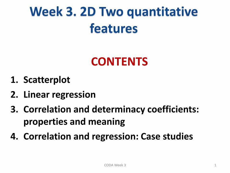
Week 3. 2D Two quantitative features
CONTENTS
1. Scatterplot
2. Linear regression
3. Correlation and determinacy coefficients: properties and meaning
4. Correlation and regression: Case studies
1 CODA Week 3
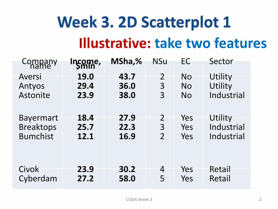
Week 3. 2D Scatterplot 1 Illustrative: take two features
Company name
Income, $mln MSha,% NSu EC Sector
Aversi Antyos Astonite
19.0 29.4 23.9
43.7 36.0 38.0
2 3 3
No No No
Utility Utility Industrial
Bayermart Breaktops Bumchist
18.4 25.7 12.1
27.9 22.3 16.9
2 3 2
Yes Yes Yes
Utility Industrial Industrial
Civok Cyberdam 23.9 27.2
30.2 58.0 4 5
Yes Yes Retail Retail
2 CODA Week 3
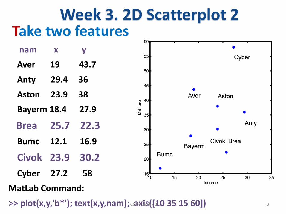
Week 3. 2D Scatterplot 2 Take two features nam x y
Aver 19 43.7
Anty 29.4 36
Aston 23.9 38
Bayerm 18.4 27.9
Brea 25.7 22.3
Bumc 12.1 16.9
Civok 23.9 30.2
Cyber 27.2 58
MatLab Command:
>> plot(x,y,'b*'); text(x,y,nam); axis([10 35 15 60]) 3 CODA Week 3
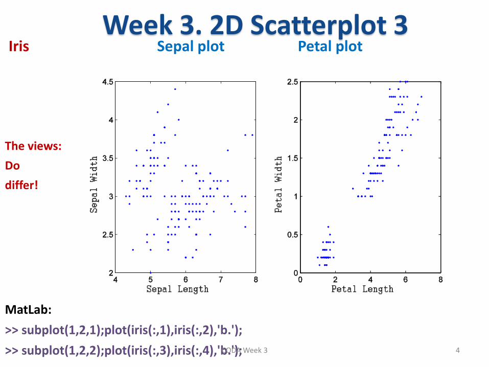
Week 3. 2D Scatterplot 3 Iris Sepal plot Petal plot
The views:
Do
differ!
MatLab:
>> subplot(1,2,1);plot(iris(:,1),iris(:,2),'b.');
>> subplot(1,2,2);plot(iris(:,3),iris(:,4),'b.'); 4 CODA Week 3

End of Part 1 in Week 3
CODA Week 3 5
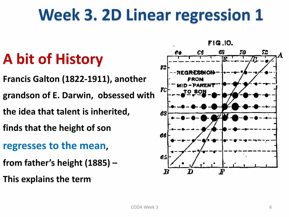
Week 3. 2D Linear regression 1
A bit of History Francis Galton (1822-1911), another
grandson of E. Darwin, obsessed with
the idea that talent is inherited,
finds that the height of son
regresses to the mean,
from father’s height (1885) –
This explains the term
6 CODA Week 3
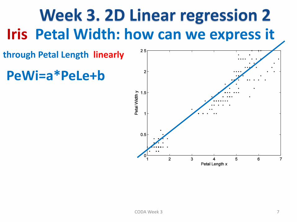
Week 3. 2D Linear regression 2 Iris Petal Width: how can we express it through Petal Length linearly
PeWi=a*PeLe+b
7 CODA Week 3
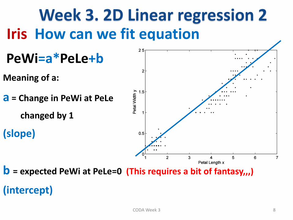
Week 3. 2D Linear regression 2 Iris How can we fit equation
PeWi=a*PeLe+b Meaning of a:
a = Change in PeWi at PeLe
changed by 1
(slope)
b = expected PeWi at PeLe=0 (This requires a bit of fantasy,,,)
(intercept)
8 CODA Week 3
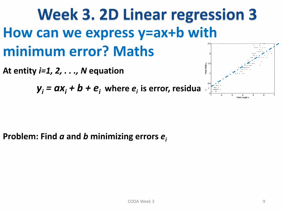
Week 3. 2D Linear regression 3 How can we express y=ax+b with minimum error? Maths At entity i=1, 2, . . ., N equation
yi = axi + b + ei where ei is error, residual
Problem: Find a and b minimizing errors ei
9 CODA Week 3
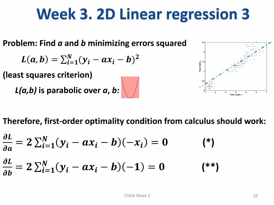
Week 3. 2D Linear regression 3
Problem: Find a and b minimizing errors squared
𝑳 𝒂, 𝒃 = (𝒚𝒊 − 𝒂𝒙𝒊 − 𝒃)𝟐𝑵
𝒊=𝟏
(least squares criterion)
L(a,b) is parabolic over a, b:
Therefore, first-order optimality condition from calculus should work:
𝝏𝑳
𝝏𝒂= 𝟐 𝒚𝒊 − 𝒂𝒙𝒊 − 𝒃 −𝒙𝒊 = 𝟎
𝑵𝒊=𝟏 (*)
𝝏𝑳
𝝏𝒃= 𝟐 𝒚𝒊 − 𝒂𝒙𝒊 − 𝒃 −𝟏 = 𝟎
𝑵𝒊=𝟏 (**)
10 CODA Week 3
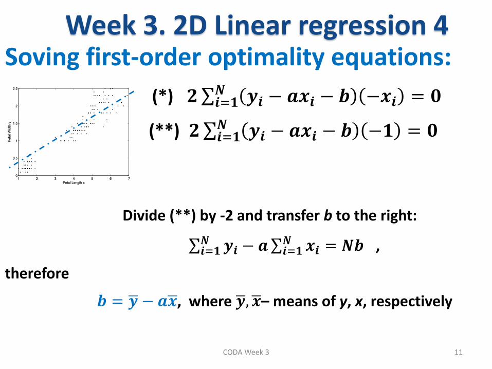
Week 3. 2D Linear regression 4 Soving first-order optimality equations:
(*) 𝟐 𝒚𝒊 − 𝒂𝒙𝒊 − 𝒃 −𝒙𝒊 = 𝟎𝑵𝒊=𝟏
(**) 𝟐 𝒚𝒊 − 𝒂𝒙𝒊 − 𝒃 −𝟏 = 𝟎𝑵𝒊=𝟏
Divide (**) by -2 and transfer b to the right:
𝒚𝒊 − 𝒂 𝒙𝒊𝑵𝒊=𝟏 = 𝑵𝒃
𝑵𝒊=𝟏 ,
therefore
𝒃 = 𝒚 − 𝒂𝒙 , where 𝒚 , 𝒙 – means of y, x, respectively
11 CODA Week 3
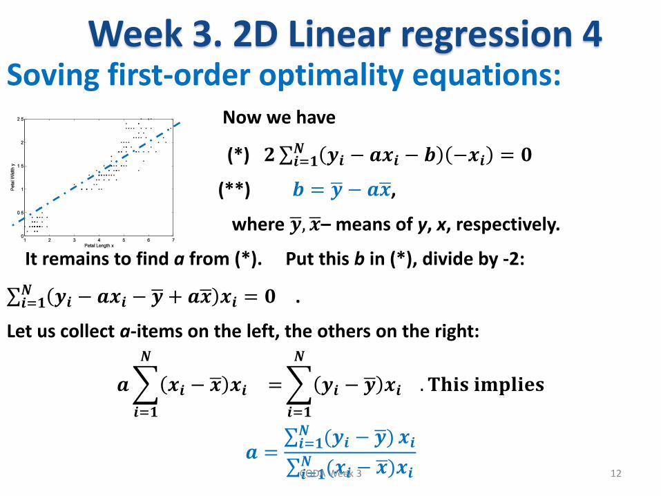
Week 3. 2D Linear regression 4 Soving first-order optimality equations: Now we have
(*) 𝟐 𝒚𝒊 − 𝒂𝒙𝒊 − 𝒃 −𝒙𝒊 = 𝟎𝑵𝒊=𝟏
(**) 𝒃 = 𝒚 − 𝒂𝒙 ,
where 𝒚 , 𝒙 – means of y, x, respectively.
It remains to find a from (*). Put this b in (*), divide by -2:
𝒚𝒊 − 𝒂𝒙𝒊 − 𝒚 + 𝒂𝒙 𝒙𝒊 = 𝟎𝑵𝒊=𝟏 .
Let us collect a-items on the left, the others on the right:
𝒂 𝒙𝒊 − 𝒙 𝒙𝒊 =
𝑵
𝒊=𝟏
𝒚𝒊 − 𝒚 𝒙𝒊
𝑵
𝒊=𝟏
. 𝐓𝐡𝐢𝐬 𝐢𝐦𝐩𝐥𝐢𝐞𝐬
𝒂 = (𝒚𝒊 − 𝒚 )𝑵𝒊=𝟏 𝒙𝒊
(𝒙𝒊 − 𝒙 𝑵𝒊=𝟏 )𝒙𝒊
12 CODA Week 3
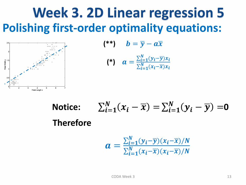
Week 3. 2D Linear regression 5 Polishing first-order optimality equations: (**) 𝒃 = 𝒚 − 𝒂𝒙
(*) 𝒂 = (𝒚𝒊−𝒚 )𝑵𝒊=𝟏 𝒙𝒊
(𝒙𝒊−𝒙 𝑵𝒊=𝟏 )𝒙𝒊
Notice: 𝒙𝒊 − 𝒙 =𝑵𝒊=𝟏 𝒚𝒊 − 𝒚 =
𝑵𝒊=𝟏 0
Therefore
𝒂 = (𝒚𝒊−𝒚 )𝑵𝒊=𝟏 (𝒙𝒊−𝒙 )/𝑵
(𝒙𝒊−𝒙 𝑵𝒊=𝟏 )(𝒙𝒊−𝒙 )/𝑵
13 CODA Week 3
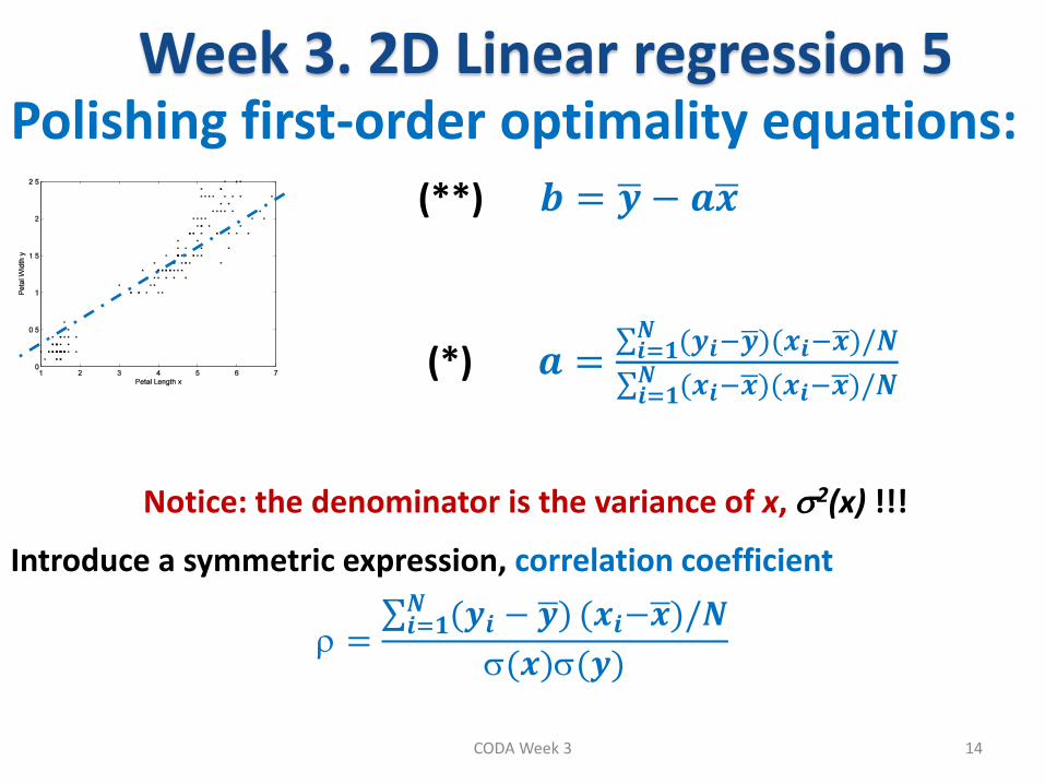
Week 3. 2D Linear regression 5 Polishing first-order optimality equations: (**) 𝒃 = 𝒚 − 𝒂𝒙
(*) 𝒂 = (𝒚𝒊−𝒚 )𝑵𝒊=𝟏 (𝒙𝒊−𝒙 )/𝑵
(𝒙𝒊−𝒙 𝑵𝒊=𝟏 )(𝒙𝒊−𝒙 )/𝑵
Notice: the denominator is the variance of x, 2(x) !!!
Introduce a symmetric expression, correlation coefficient
= (𝒚𝒊 − 𝒚 )𝑵𝒊=𝟏 (𝒙𝒊−𝒙 )/𝑵
(𝒙)(𝒚)
14 CODA Week 3
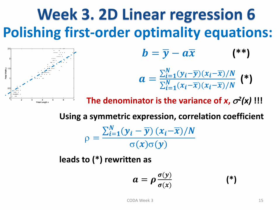
Week 3. 2D Linear regression 6 Polishing first-order optimality equations: 𝒃 = 𝒚 − 𝒂𝒙 (**)
𝒂 = (𝒚𝒊−𝒚 )𝑵𝒊=𝟏 (𝒙𝒊−𝒙 )/𝑵
(𝒙𝒊−𝒙 𝑵𝒊=𝟏 )(𝒙𝒊−𝒙 )/𝑵
(*)
The denominator is the variance of x, 2(x) !!!
Using a symmetric expression, correlation coefficient
= (𝒚𝒊 − 𝒚 )𝑵𝒊=𝟏 (𝒙𝒊−𝒙 )/𝑵
(𝒙)(𝒚)
leads to (*) rewritten as
𝒂 = 𝝆𝝈(𝒚)
𝝈(𝒙) (*)
15 CODA Week 3
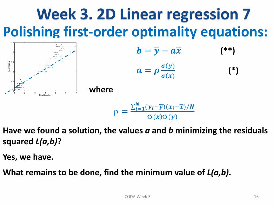
Week 3. 2D Linear regression 7 Polishing first-order optimality equations: 𝒃 = 𝒚 − 𝒂𝒙 (**)
𝒂 = 𝝆𝝈(𝒚)
𝝈(𝒙) (*)
where
= (𝒚𝒊−𝒚 )𝑵𝒊=𝟏 (𝒙𝒊−𝒙 )/𝑵
(𝒙)(𝒚)
Have we found a solution, the values a and b minimizing the residuals squared L(a,b)?
Yes, we have.
What remains to be done, find the minimum value of L(a,b).
16 CODA Week 3
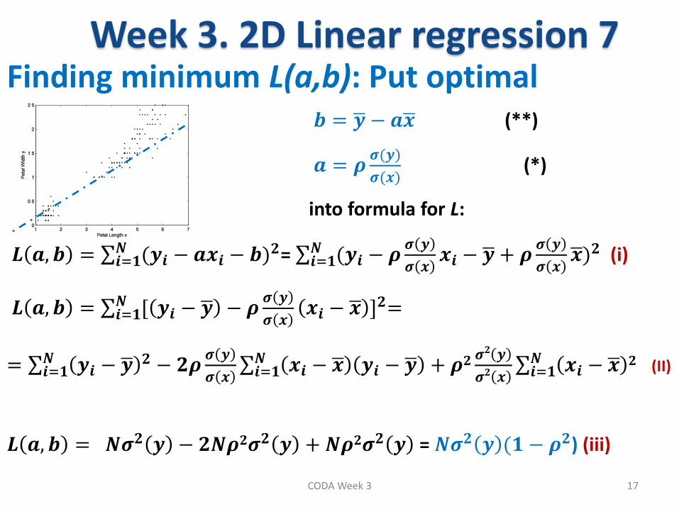
Week 3. 2D Linear regression 7 Finding minimum L(a,b): Put optimal 𝒃 = 𝒚 − 𝒂𝒙 (**)
𝒂 = 𝝆𝝈(𝒚)
𝝈(𝒙) (*)
into formula for L:
𝑳 𝒂, 𝒃 = (𝒚𝒊 − 𝒂𝒙𝒊 − 𝒃)𝟐𝑵
𝒊=𝟏 = (𝒚𝒊 − 𝝆𝝈 𝒚
𝝈 𝒙𝒙𝒊 − 𝒚 + 𝝆
𝝈 𝒚
𝝈 𝒙𝒙 )𝟐𝑵
𝒊=𝟏 (i)
𝑳 𝒂, 𝒃 = [ 𝒚𝒊 − 𝒚 − 𝝆𝝈 𝒚
𝝈 𝒙𝒙𝒊 − 𝒙 ]
𝟐=𝑵𝒊=𝟏
= 𝒚𝒊 − 𝒚 𝟐 − 𝟐𝝆
𝝈 𝒚
𝝈 𝒙 𝒙𝒊 − 𝒙 𝒚𝒊 − 𝒚 𝑵𝒊=𝟏 + 𝝆𝟐
𝝈𝟐 𝒚
𝝈𝟐 𝒙 𝒙𝒊 − 𝒙
𝟐𝑵𝒊=𝟏
𝑵𝒊=𝟏 (II)
𝑳 𝒂, 𝒃 = 𝑵𝝈𝟐 𝒚 − 𝟐𝑵𝝆𝟐𝝈𝟐 𝒚 + 𝑵𝝆𝟐𝝈𝟐 𝒚 = 𝑵𝝈𝟐 𝒚 (𝟏 − 𝝆𝟐) (iii)
17 CODA Week 3
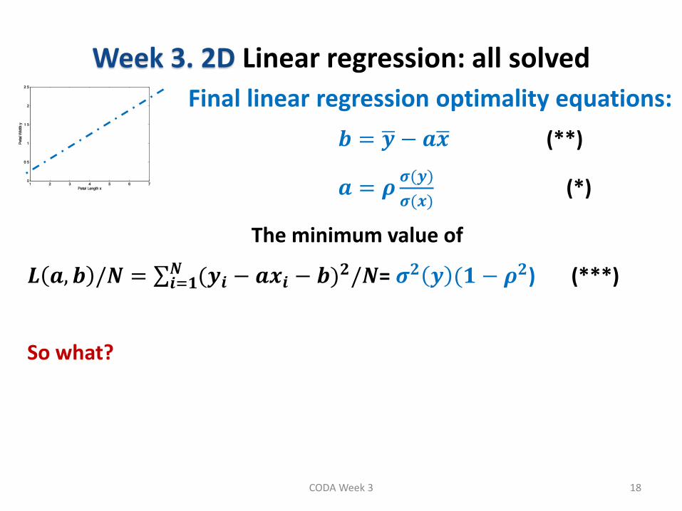
Week 3. 2D Linear regression: all solved
Final linear regression optimality equations:
𝒃 = 𝒚 − 𝒂𝒙 (**)
𝒂 = 𝝆𝝈(𝒚)
𝝈(𝒙) (*)
The minimum value of
𝑳 𝒂, 𝒃 /𝑵 = (𝒚𝒊 − 𝒂𝒙𝒊 − 𝒃)𝟐/𝑵𝑵
𝒊=𝟏 = 𝝈𝟐 𝒚 (𝟏 − 𝝆𝟐) (***)
So what?
18 CODA Week 3

End of Part 2 in Week 3
CODA Week 3 19
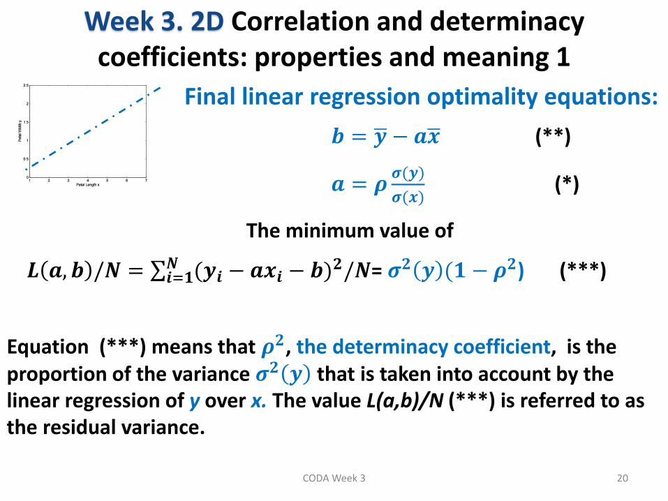
Week 3. 2D Correlation and determinacy
coefficients: properties and meaning 1 Final linear regression optimality equations:
𝒃 = 𝒚 − 𝒂𝒙 (**)
𝒂 = 𝝆𝝈(𝒚)
𝝈(𝒙) (*)
The minimum value of
𝑳 𝒂, 𝒃 /𝑵 = (𝒚𝒊 − 𝒂𝒙𝒊 − 𝒃)𝟐/𝑵𝑵
𝒊=𝟏 = 𝝈𝟐 𝒚 (𝟏 − 𝝆𝟐) (***)
Equation (***) means that 𝝆𝟐, the determinacy coefficient, is the proportion of the variance 𝝈𝟐 𝒚 that is taken into account by the linear regression of y over x. The value L(a,b)/N (***) is referred to as the residual variance.
20 CODA Week 3
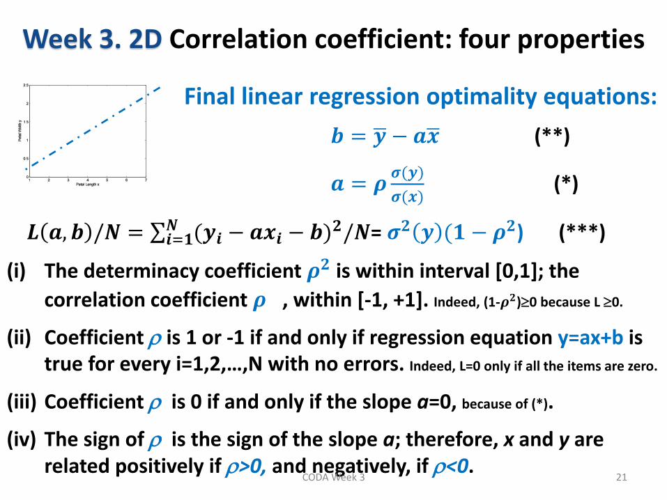
Week 3. 2D Correlation coefficient: four properties
Final linear regression optimality equations:
𝒃 = 𝒚 − 𝒂𝒙 (**)
𝒂 = 𝝆𝝈(𝒚)
𝝈(𝒙) (*)
𝑳 𝒂, 𝒃 /𝑵 = (𝒚𝒊 − 𝒂𝒙𝒊 − 𝒃)𝟐/𝑵𝑵
𝒊=𝟏 = 𝝈𝟐 𝒚 (𝟏 − 𝝆𝟐) (***)
(i) The determinacy coefficient 𝝆𝟐 is within interval [0,1]; the
correlation coefficient 𝝆 , within [-1, +1]. Indeed, (1-𝝆𝟐)0 because L 0.
(ii) Coefficient is 1 or -1 if and only if regression equation y=ax+b is true for every i=1,2,…,N with no errors. Indeed, L=0 only if all the items are zero.
(iii) Coefficient is 0 if and only if the slope a=0, because of (*).
(iv) The sign of is the sign of the slope a; therefore, x and y are related positively if >0, and negatively, if <0.
21 CODA Week 3
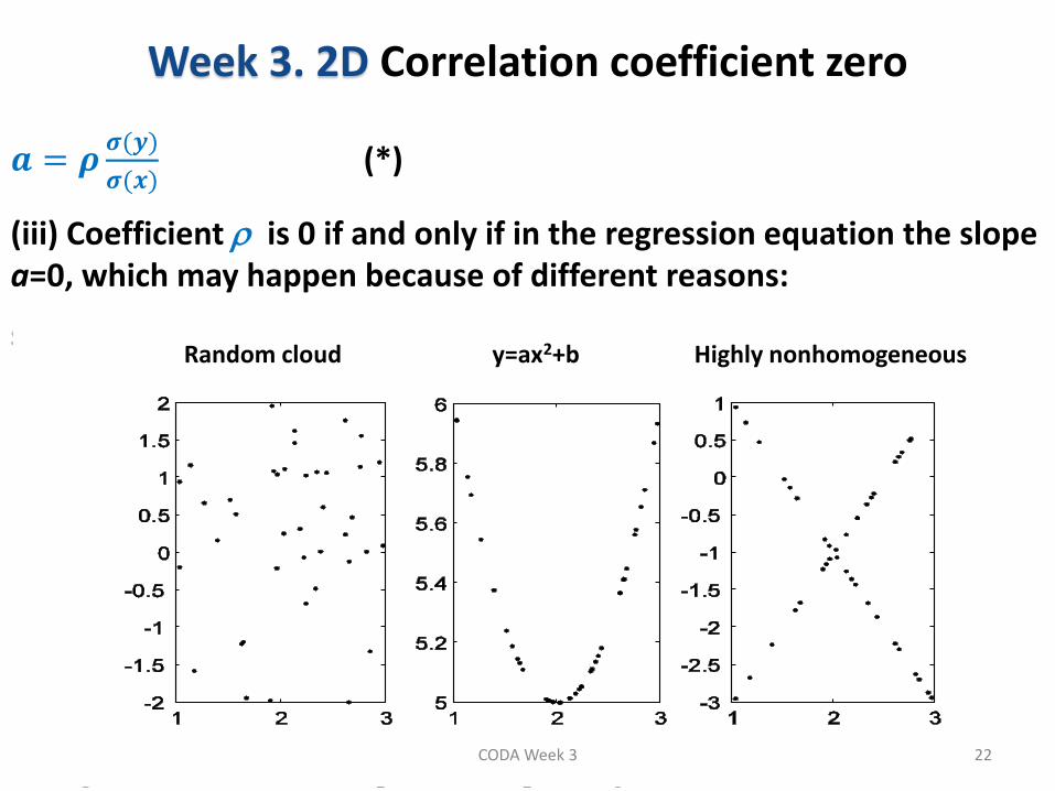
Week 3. 2D Correlation coefficient zero
𝒂 = 𝝆
𝝈(𝒚)
𝝈(𝒙) (*)
(iii) Coefficient is 0 if and only if in the regression equation the slope a=0, which may happen because of different reasons:
so that regression is y=b.
Figure 2.2. Three scatter-plots corresponding to zero or almost zero correlati
Random cloud y=ax2+b Highly nonhomogeneous
22 CODA Week 3
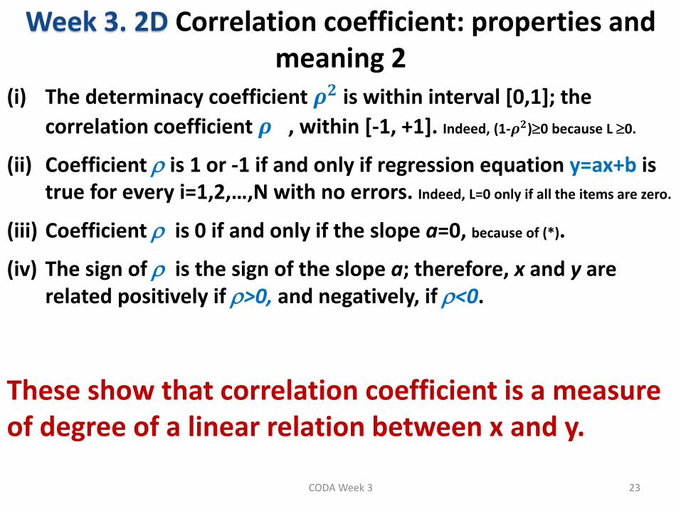
Week 3. 2D Correlation coefficient: properties and
meaning 2 (i) The determinacy coefficient 𝝆𝟐 is within interval [0,1]; the
correlation coefficient 𝝆 , within [-1, +1]. Indeed, (1-𝝆𝟐)0 because L 0.
(ii) Coefficient is 1 or -1 if and only if regression equation y=ax+b is true for every i=1,2,…,N with no errors. Indeed, L=0 only if all the items are zero.
(iii) Coefficient is 0 if and only if the slope a=0, because of (*).
(iv) The sign of is the sign of the slope a; therefore, x and y are related positively if >0, and negatively, if <0.
These show that correlation coefficient is a measure of degree of a linear relation between x and y.
23 CODA Week 3
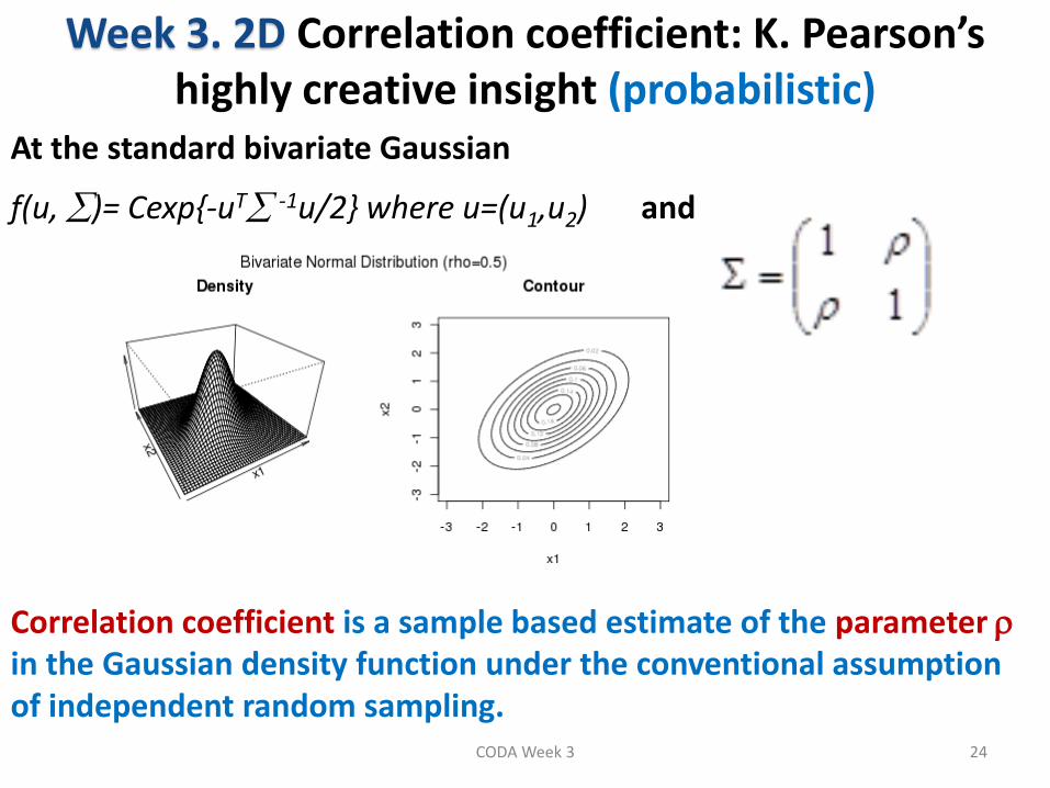
Week 3. 2D Correlation coefficient: K. Pearson’s
highly creative insight (probabilistic) At the standard bivariate Gaussian
f(u, )= Cexp{-uT -1u/2} where u=(u1,u2) and
Correlation coefficient is a sample based estimate of the parameter in the Gaussian density function under the conventional assumption of independent random sampling.
24 CODA Week 3

End of Part 3 in Week 3
CODA Week 3 25
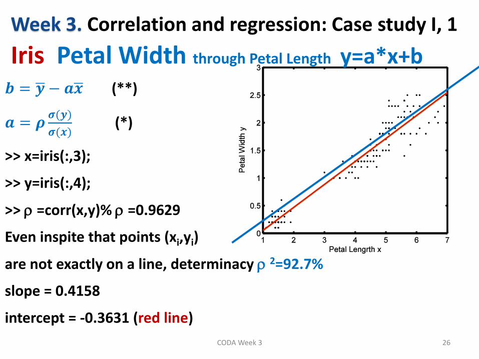
Week 3. Correlation and regression: Case study I, 1
Iris Petal Width through Petal Length y=a*x+b 𝒃 = 𝒚 − 𝒂𝒙 (**)
𝒂 = 𝝆𝝈(𝒚)
𝝈(𝒙) (*)
>> x=iris(:,3);
>> y=iris(:,4);
>> =corr(x,y)% =0.9629
Even inspite that points (xi,yi)
are not exactly on a line, determinacy 2=92.7%
slope = 0.4158
intercept = -0.3631 (red line)
26 CODA Week 3
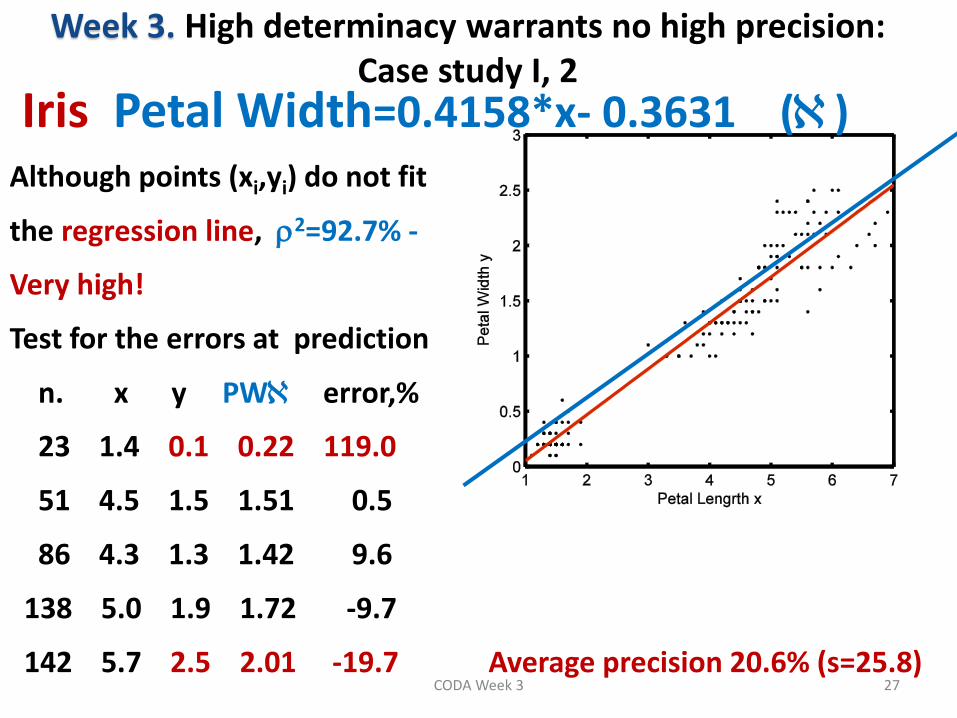
Week 3. High determinacy warrants no high precision: Case study I, 2
Iris Petal Width=0.4158*x- 0.3631 () Although points (xi,yi) do not fit
the regression line, 2=92.7% -
Very high!
Test for the errors at prediction
n. x y PW error,%
23 1.4 0.1 0.22 119.0
51 4.5 1.5 1.51 0.5
86 4.3 1.3 1.42 9.6
138 5.0 1.9 1.72 -9.7
142 5.7 2.5 2.01 -19.7 Average precision 20.6% (s=25.8)
27 CODA Week 3
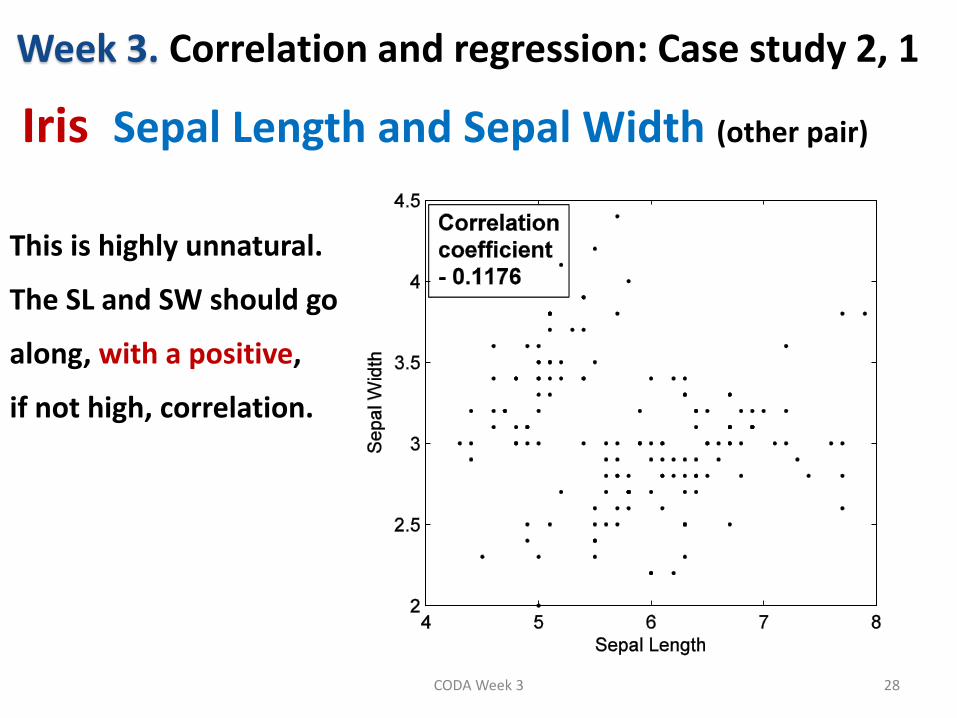
Week 3. Correlation and regression: Case study 2, 1
Iris Sepal Length and Sepal Width (other pair)
This is highly unnatural.
The SL and SW should go
along, with a positive,
if not high, correlation.
28 CODA Week 3
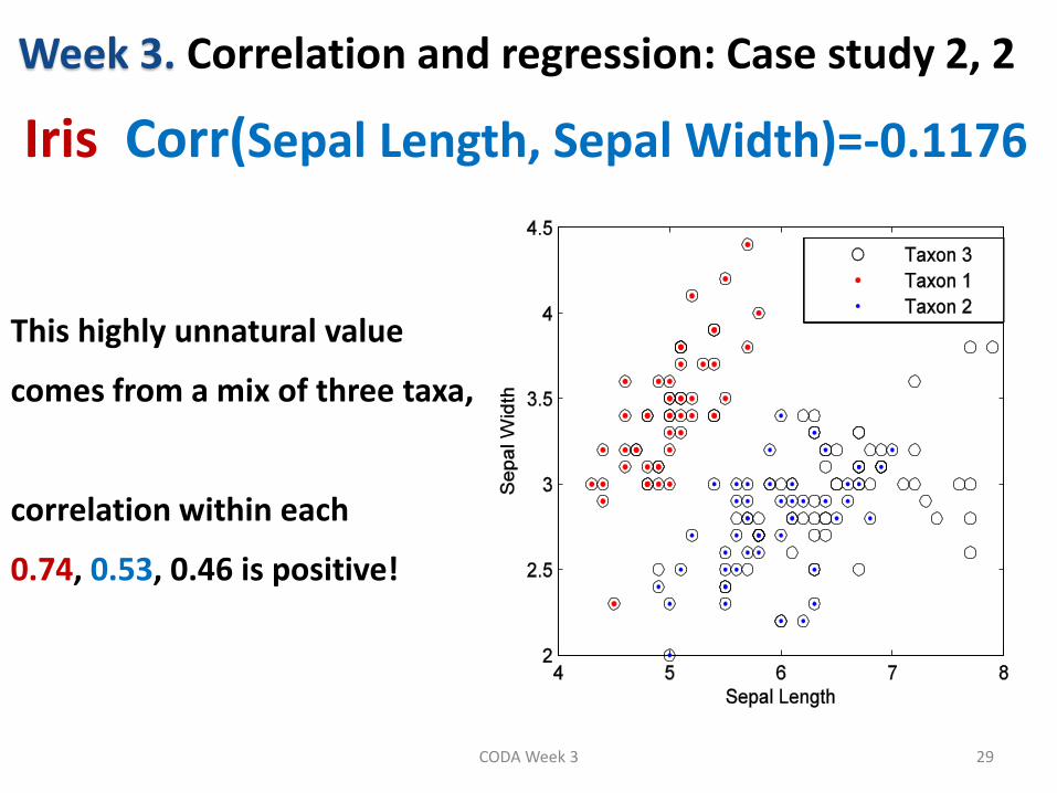
Week 3. Correlation and regression: Case study 2, 2
Iris Corr(Sepal Length, Sepal Width)=-0.1176
This highly unnatural value
comes from a mix of three taxa,
correlation within each
0.74, 0.53, 0.46 is positive!
29 CODA Week 3
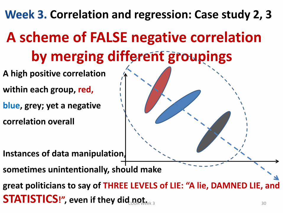
Week 3. Correlation and regression: Case study 2, 3
A scheme of FALSE negative correlation by merging different groupings A high positive correlation
within each group, red,
blue, grey; yet a negative
correlation overall
Instances of data manipulation,
sometimes unintentionally, should make
great politicians to say of THREE LEVELS of LIE: “A lie, DAMNED LIE, and
STATISTICS!”, even if they did not. 30 CODA Week 3
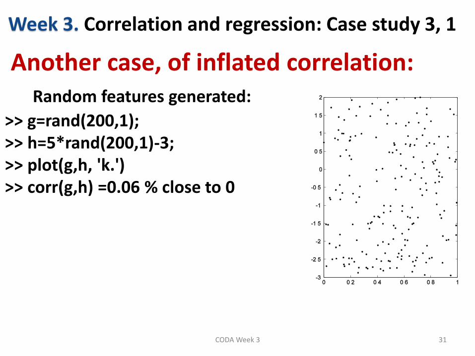
Week 3. Correlation and regression: Case study 3, 1
Another case, of inflated correlation: Random features generated:
>> g=rand(200,1); >> h=5*rand(200,1)-3; >> plot(g,h, 'k.') >> corr(g,h) =0.06 % close to 0
31 CODA Week 3
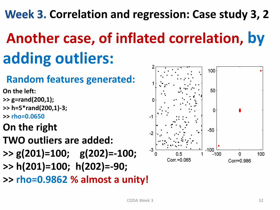
Week 3. Correlation and regression: Case study 3, 2
Another case, of inflated correlation, by adding outliers: Random features generated: On the left: >> g=rand(200,1); >> h=5*rand(200,1)-3; >> rho=0.0650
On the right TWO outliers are added: >> g(201)=100; g(202)=-100; >> h(201)=100; h(202)=-90; >> rho=0.9862 % almost a unity!
32 CODA Week 3
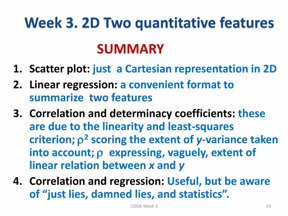
Week 3. 2D Two quantitative features
SUMMARY
1. Scatter plot: just a Cartesian representation in 2D
2. Linear regression: a convenient format to summarize two features
3. Correlation and determinacy coefficients: these are due to the linearity and least-squares criterion; 2 scoring the extent of y-variance taken into account; expressing, vaguely, extent of linear relation between x and y
4. Correlation and regression: Useful, but be aware of “just lies, damned lies, and statistics”.
33 CODA Week 3