re

sear

ch re

port

Committee on Specif ications

for the Design of Cold-Formed

Steel Structural Members

American Iron and Steel Institute

AISI Sponsored ReseaReports

rch

R E S E A R C H R E P O R T R P 0 1 - 1 2 0 0 1 R E V I S I O N 2 0 0 6

eb Crippling of Cold ormed Steel Multi -Web eck Sections Subjected tond One-Flange Loading

E S E A R C H R E P O R T R P 0 3 - 1

WFD E

R M A Y 2 0 0 3 R E V I S I O N 2 0 0 6

The material contained herein has been developed by researchers based on their research findings. The material has also been reviewed by the American Iron and Steel Institute Committee on Specifications for the Design of Cold-Formed Steel Structural Members. The Committee acknowledges and is grateful for the contributions of such researchers.

The material herein is for general information only. The information in it should not be used without first securing competent advice with respect to its suitability for any given application. The publication of the information is not intended as a representation or warranty on the part of the American Iron and Steel Institute, or of any other person named herein, that the information is suitable for any general or particular use or of freedom from infringement of any patent or patents. Anyone making use of the information assumes all liability arising from such use.

Copyright 2003 American Iron and Steel Institute Revised Edition Copyright 2006 American Iron and Steel Institute

Web Crippling of Cold Formed Steel Multi-Web Deck Sections Subjected to

End One-Flange Loading

FINAL REPORT

by

James A. Wallace Research Assistant

Professor R. M. Schuster

Project Director

Canadian Cold Formed Steel Research Group Department of Civil Engineering

University of Waterloo Waterloo, Ontario, Canada

May 2003

ii

Acknowledgements

The authors wish to thank the Canadian Sheet Steel Building Institute and the Steel Deck Institute for their financial support of this project. Further, we would also like to thank the following companies for having supplied the test specimens: Canam-manac, VICWEST, Roll Form Group, Wheeling, United Steel Deck, and Epic Metals.

iii

Abstract

The “North American Specification for the Design of Cold Formed Steel Structural Members” (2001a) (herein referred to as NAS), established in 2001, governs the design of cold formed steel structural members in North America. Given in the specification are equations to predict the various failure modes of cold formed steel members in compression, tension, shear, and bending. The concern of this study was the failure mode called web crippling, which is the deformation of the web elements under concentrated compression loads.

It is difficult (if not impossible) to develop an analytical design method for web crippling of cold formed steel members because of the large deformations, plasticity, variety of section geometries, and loading patterns involved with this failure mode. To simplify the design process, an empirical equation for predicting web crippling capacity is presented in the NAS. The NAS contains tables of coefficients to be used in conjunction with the design equation that account for the different section geometries, load cases, and support conditions

Investigated in this study was the web crippling capacity of multi-web deck sections subjected to End One-Flange loading. There was limited data available in the published literature to support the current coefficients for multi-web decks under End One-Flange loading. Consequently, this study was initiated to derive values that are more accurate. A total of 148 tests were carried out on a range of deck profiles, bearing widths, and fastening conditions. In addition, test data from previous web crippling studies of multi-web deck sections were also considered. It was found that not all specimens from previous studies were tested in a fashion that produced acceptable results. New resistance factors and factors of safety were also developed. New coefficients were established using the data from this study and any appropriate data from previous work.

Also investigated in this study was the web crippling capacity of partially-fastened deck sections and re-entrant deck sections under the same loading conditions. Partially-fastened decks sections are sections that are fastened to supports in a manner that does not meet industry standards. Re-entrant deck sections are multi-web deck sections with a web inclination greater than 90º. 77 partially-fastened multi-web decks and 36 re-entrant decks were tested in this study. It was found that partially-fastened deck sections, unfastened re-entrant deck sections, and fastened re-entrant deck sections all behave similarly to fully-fastened multi-web deck sections and can use the same coefficients, resistance factors, and factors of safety for design purposes.

The ranges of the test specimen parameters were: 299 MPa (43.4 ksi) < Fy < 674 MPa (97.8 ksi); 1.41 < R/t < 19.9; 20.0 < N/t < 110; 20.8 < h/t < 211; and 71º< θ < 108º. These parameters are defined in Section 2.10 (page 15).

iv

Table of Contents Acknowledgements ................................................................................................................................ii Abstract .................................................................................................................................................iii Table of Contents .................................................................................................................................. iv List of Figures ......................................................................................................................................vii List of Tables......................................................................................................................................... ix Chapter 1 Introduction............................................................................................................................ 1

1.1 General ......................................................................................................................................... 1 1.2 Cold Formed Steel........................................................................................................................ 1 1.3 Web Crippling .............................................................................................................................. 2

1.3.1 Load Cases ............................................................................................................................ 2 1.3.2 Section Geometry and Web Crippling Coefficients .............................................................. 3 1.3.3 Support Conditions................................................................................................................ 4 1.3.4 Cross Section Parameters ...................................................................................................... 4

1.4 Objectives of Study ...................................................................................................................... 5 1.5 Scope of Study.............................................................................................................................. 6 1.6 Organization of Thesis ................................................................................................................. 6

Chapter 2 Literature Review .................................................................................................................. 8 2.1 General ......................................................................................................................................... 8 2.2 Winter and Pian (1946) ................................................................................................................ 8 2.3 Baehre (1975) ............................................................................................................................... 9 2.4 Hetrakul and Yu (1978).............................................................................................................. 10 2.5 Wing (1981) ............................................................................................................................... 11 2.6 Yu (1981) ................................................................................................................................... 12 2.7 Studnička (1989) ........................................................................................................................ 13 2.8 Bakker (1992)............................................................................................................................. 14 2.9 Bhakta et al. (1992) .................................................................................................................... 14 2.10 Prabakaran (1993) .................................................................................................................... 15 2.11 Gerges (1997) ........................................................................................................................... 15 2.12 Wu et al. (1997)........................................................................................................................ 16 2.13 Beshara (1999) ......................................................................................................................... 16 2.14 Avci and Easterling (2002)....................................................................................................... 17

Chapter 3 Experimental Investigation .................................................................................................. 18 3.1 General ....................................................................................................................................... 18

v

3.2 Test Specimens........................................................................................................................... 18 3.2.1 Specimen Selection ............................................................................................................. 18 3.2.2 Fastening Patterns................................................................................................................ 19 3.2.3 Specimen Notation .............................................................................................................. 20 3.2.4 Mechanical Properties ......................................................................................................... 22

3.3 Test Set-Up................................................................................................................................. 22 3.4 Interpreting Test Data................................................................................................................. 25

3.4.1 Determining Maximum Applied Load from Load-Stroke Curves ...................................... 25 3.4.2 Converting Applied Load to End Load ............................................................................... 28

3.5 Test Results ................................................................................................................................ 28 Chapter 4 Methods of Analysis and Calibrations................................................................................. 29

4.1 General ....................................................................................................................................... 29 4.2 Developing the Model ................................................................................................................ 29

4.2.1 Method of Least Squares ..................................................................................................... 29 4.2.2 The Mathematical Model .................................................................................................... 30

4.3 Optimization Methods ................................................................................................................ 31 4.3.1 Optimizing using the Genetic Algorithm ............................................................................ 31 4.3.2 Optimizing using Microsoft Excel Solver (Gradient Method) ............................................ 33 4.3.3 Results of Optimization....................................................................................................... 35

4.4 Calibration .................................................................................................................................. 35 Chapter 5 Test Results and Comparisons ............................................................................................. 38

5.1 General ....................................................................................................................................... 38 5.2 Web Crippling Coefficients for Multi-Web Deck Sections ....................................................... 38 5.3 Partially-fastened Support Condition ......................................................................................... 41 5.4 Re-entrant Multi-Web Deck Sections.........................................................................................43 5.5 Discussion and Recommendations .............................................................................................45

References ............................................................................................................................................ 47 Appendix A Material Properties of Specimens .................................................................................... 50 Appendix B Geometric Properties of Specimens ................................................................................. 51

5.6 ...................................................................................................................................................... 51 Appendix C Test Variables and Load Data .......................................................................................... 60

5.7 ..................................................................................................................................................... 60 Appendix D Nominal Resistance of Specimens................................................................................... 67

5.8 ....................................................................................................................................................... 67

vi

Appendix E Experimentally Recorded Load........................................................................................ 77 Appendix F Genetic Algorithm Used to Verify Analysis .................................................................... 93

F.1 General ....................................................................................................................................... 93 F.2 DNA Strings............................................................................................................................... 93 F.3 Gene Splicing and Mutation....................................................................................................... 94 F.4 Fitness Test and Penalty Functions ............................................................................................ 95 F.5 Convergence............................................................................................................................... 96 F.6 Source Code ............................................................................................................................... 96

vii

List of Figures Figure 1.2-1: Common Cold Formed Steel Section Geometries............................................................ 1 Figure 1.2-2: Cold Formed Steel Roof Decking..................................................................................... 1 Figure 1.3-1: Typical Web Crippling Failure for Multi-Web Deck Sections......................................... 2 Figure 1.3-2: Web Crippling Load Cases............................................................................................... 3 Figure 1.3-3: Web Buckling and Flange Rotation.................................................................................. 4 Figure 1.3-4: Cross Section Parameters ................................................................................................. 5 Figure 1.4-1: Examples of Multi-Web Deck Sections ........................................................................... 6 Figure 2.2-1: Examples of Sections Tested by Winter and Pian ............................................................ 8 Figure 2.4-1: C-sections with Stiffened Flanges (left) and Unstiffened Flanges (right) ...................... 11 Figure 2.12-1: Clamps at Midspan of Wu Specimen ........................................................................... 16 Figure 3.2-1: Profiles of Specimens Used in the Study........................................................................ 20 Figure 3.3-1: Specimen Reinforced to Achieve EOF Loading............................................................. 23 Figure 3.3-2: Diagram of Test Set-up................................................................................................... 23 Figure 3.3-3: Photograph Showing Test Set-up. ..................................................................................24 Figure 3.4-1: Yield Arc Mechanism..................................................................................................... 26 Figure 3.4-2: Rolling Mechanism......................................................................................................... 26 Figure 3.4-3: Typical Load-Stroke Curve of Yield Arc Mechanism.................................................... 27 Figure 3.4-4: Typical Load-Deflection Curve of Rolling Mechanism. ................................................ 27 Figure 3.4-5: Test Specimen Layout .................................................................................................... 28 Figure 4.2-1: Graphical Representation of Method of Least Squares .................................................. 30 Figure 4.3-1: Example of Local and True Minima and Maxima with Variable Constraints................ 34 Figure 5.2-1: Spreading of Unfastened Deck ....................................................................................... 40 Figure 5.2-2: Spreading of a 4 Web Deck Section ............................................................................... 40 Figure 5.3-1: Rotation of Inside and Outside Flanges.......................................................................... 42 Figure 5.3-2: Photograph Showing Larger Deformation in Outside Flanges and Webs...................... 43 Figure 5.4-1: Failure of Re-entrant Deck Section ................................................................................ 44 Figure E-1: Load-Stroke Plot, Test Series: T1 ..................................................................................... 77 Figure E-2: Load-Stroke Plot, Test Series: T2 ..................................................................................... 78 Figure E-3: Load-Stroke Plot, Test Series: T3 ..................................................................................... 78 Figure E-4: Load-Stroke Plot, Test Series: C2 ..................................................................................... 79 Figure E-5: Load-Stroke Plot, Test Series: C3 ..................................................................................... 79 Figure E-6: Load-Stroke Plot, Test Series: C1 ..................................................................................... 80 Figure E-7: Load-Stroke Plot, Test Series: R1 ..................................................................................... 80

viii

Figure E-8: Load-Stroke Plot, Test Series: R2 ..................................................................................... 81 Figure E-9: Load-Stroke Plot, Test Series: R3 ..................................................................................... 81 Figure E-10: Load-Stroke Plot, Test Series: U4................................................................................... 82 Figure E-11: Load-Stroke Plot, Test Series: U5................................................................................... 82 Figure E-12: Load-Stroke Plot, Test Series: U6................................................................................... 83 Figure E-13: Load-Stroke Plot, Test Series: U3................................................................................... 83 Figure E-14: Load-Stroke Plot, Test Series: U2................................................................................... 84 Figure E-15: Load-Stroke Plot, Test Series: U1................................................................................... 84 Figure E-16: Load-Stroke Plot, Test Series: U9................................................................................... 85 Figure E-17: Load-Stroke Plot, Test Series: U8................................................................................... 85 Figure E-18: Load-Stroke Plot, Test Series: U7................................................................................... 86 Figure E-19: Load-Stroke Plot, Test Series: V1................................................................................... 86 Figure E-20: Load-Stroke Plot, Test Series: V2................................................................................... 87 Figure E-21: Load-Stroke Plot, Test Series: V4................................................................................... 87 Figure E-22: Load-Stroke Plot, Test Series: V3................................................................................... 88 Figure E-23: Load-Stroke Plot, Test Series: V5................................................................................... 88 Figure E-24: Load-Stroke Plot, Test Series: W1.................................................................................. 89 Figure E-25: Load-Stroke Plot, Test Series: W2.................................................................................. 89 Figure E-26: Load-Stroke Plot, Test Series: E1 ................................................................................... 90 Figure E-27: Load-Stroke Plot, Test Series: E2 ................................................................................... 90 Figure E-28: Load-Stroke Plot, Test Series: E3 ................................................................................... 91 Figure E-29: Load-Stroke Plot, Test Series: E4 ................................................................................... 91 Figure E-30: Load-Stroke Plot, Test Series: E5 ................................................................................... 92

ix

List of Tables Table 3.2-1: Deck Profiles used in Study............................................................................................. 19 Table 3.2-2: Fastener Combinations for each Section Profile Tested. ................................................. 20 Table 3.2-3: Fabricator Code for Specimen Notation .......................................................................... 21 Table 3.2-4: Fastening Pattern Notation............................................................................................... 22 Table 4.3-1: Range of Results From Genetic Algorithm...................................................................... 35 Table 5.2-1: Web Crippling Coefficients for EOF Loading of Multi-Web Deck Sections.................. 38 Table 5.2-2: Comparison of NAS (2001a) and Proposed Coefficients ................................................ 39 Table 5.2-3: Factors of Safety and Resistance Factors for EOF Loading of Multi-Web Decks .......... 40 Table 5.2-4: Comparison of Test Data by Yu (1981) and Avci (2002)................................................ 41 Table 5.3-1: Comparison of Partially-Fastened Test Results ............................................................... 42 Table 5.4-1: Results of Re-entrant Decks Using Multi-Web Coefficients ........................................... 43 Table 5.4-2: Resistance Factors and Factors of Safety for Re-entrant Decks ...................................... 44 Table 5.4-3: Comparison of Coefficients When Re-entrant Data is Incorporated ............................... 45 Table A-1: Mechanical Properties of Specimens ................................................................................. 50 Table B-1: Geometric Properties of Unfastened Specimens ................................................................ 51 Table B-2: Geometric Properties of Fastened Specimens .................................................................... 53 Table B-3: Geometric Properties of Partially-Fastened Specimens ..................................................... 55 Table B-4: Geometric Properties of Unfastened Data by Yu (1981) ................................................... 57 Table B-5: Geometric Properties of Unfastened Data by Wu (1997) .................................................. 57 Table B-6: Geometric Properties of Unfastened Data by Avci and Easterling (2002)......................... 58 Table B-7: Geometric Properties of Unfastened Data by Bhakta et al. (1992) .................................... 58 Table B-8: Geometric Properties of Fastened Data by Avci and Easterling (2002)............................. 59 Table B-9: Geometric Properties of Fastened Data by Bhakta et al. (1992) ........................................ 59 Table C-1: Load Data from Unfastened Specimens............................................................................. 60 Table C-2: Load Data from Fastened Specimens................................................................................. 62 Table C-3: Load Data from Partially-Fastened Specimens .................................................................. 64 Table D-1: Nominal Strength of Unfastened Specimens ..................................................................... 67 Table D-2: Nominal Strength of Fastened Specimens ......................................................................... 69 Table D-3: Nominal Strength of Partially-Fastened Specimens........................................................... 71 Table D-4: Nominal Strength of Unfastened Data by Yu (1981)......................................................... 73 Table D-5: Nominal Strength of Unfastened Data by Bhakta et al. (1992) ......................................... 73 Table D-6: Nominal Strength of Unfastened Data by Avci and Easterling (2002).............................. 74 Table D-7: Nominal Strength of Fastened Data by Avci and Easterling (2002).................................. 75

x

Table D-8: Nominal Strength of Unfastened Data by Wu (1997)........................................................ 76 Table D-9: Nominal Strength of Fastened Data by Bhatka et al. (1992) ............................................. 76 Table F-1: Example Decoding of a DNA String. ................................................................................. 93 Table F-2: Encoding Key for the DNA String ..................................................................................... 94

1

Chapter 1 Introduction

1.1 General

Presented in this chapter are; a brief description of cold formed steel as a construction material, a review of the current design theory regarding web crippling of cold formed steel members, the objectives, and the scope of this study.

1.2 Cold Formed Steel

Cold formed steel refers to structural members formed from thin sheets of steel at room temperature without annealing. Cold formed steel is a widely used construction material for fabricating structural members such as joists, girts and purlins, and for fabricating cladding elements such as roof deck. Presented in the “North American Specification for the Design of Cold Formed Steel Structural Members” (NAS, 2001a) are design rules for cold formed steel members.

Cold formed steel has many advantages over other building materials. It has a high strength-to-weight ratio, which reduces the material weight of the structure. Cold formed steel is a versatile material; one can form almost any section geometry imaginable using cold formed steel. Shown in Figure 1.2-1 are some common section geometries. Shown in Figure 1.2-2 is an example of cold formed steel roof decking used in construction.

Figure 1.2-1: Common Cold Formed Steel Section Geometries

Figure 1.2-2: Cold Formed Steel Roof Decking

2

1.3 Web Crippling

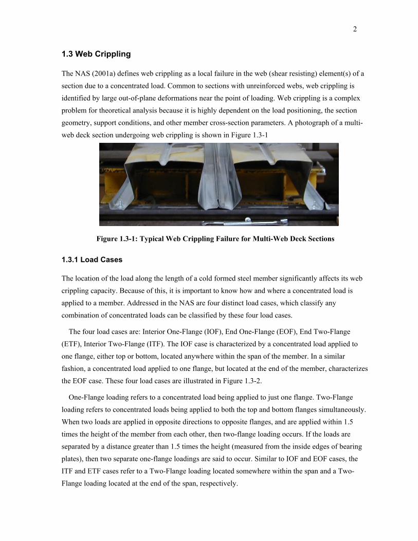
The NAS (2001a) defines web crippling as a local failure in the web (shear resisting) element(s) of a section due to a concentrated load. Common to sections with unreinforced webs, web crippling is identified by large out-of-plane deformations near the point of loading. Web crippling is a complex problem for theoretical analysis because it is highly dependent on the load positioning, the section geometry, support conditions, and other member cross-section parameters. A photograph of a multi-web deck section undergoing web crippling is shown in Figure 1.3-1

Figure 1.3-1: Typical Web Crippling Failure for Multi-Web Deck Sections

1.3.1 Load Cases

The location of the load along the length of a cold formed steel member significantly affects its web crippling capacity. Because of this, it is important to know how and where a concentrated load is applied to a member. Addressed in the NAS are four distinct load cases, which classify any combination of concentrated loads can be classified by these four load cases.

The four load cases are: Interior One-Flange (IOF), End One-Flange (EOF), End Two-Flange (ETF), Interior Two-Flange (ITF). The IOF case is characterized by a concentrated load applied to one flange, either top or bottom, located anywhere within the span of the member. In a similar fashion, a concentrated load applied to one flange, but located at the end of the member, characterizes the EOF case. These four load cases are illustrated in Figure 1.3-2.

One-Flange loading refers to a concentrated load being applied to just one flange. Two-Flange loading refers to concentrated loads being applied to both the top and bottom flanges simultaneously. When two loads are applied in opposite directions to opposite flanges, and are applied within 1.5 times the height of the member from each other, then two-flange loading occurs. If the loads are separated by a distance greater than 1.5 times the height (measured from the inside edges of bearing plates), then two separate one-flange loadings are said to occur. Similar to IOF and EOF cases, the ITF and ETF cases refer to a Two-Flange loading located somewhere within the span and a Two-Flange loading located at the end of the span, respectively.

3

>1.5hh >1.5h h

Interior One - Flange (IOF)

Interior Two-Flange (ITF) End Two - Flange (ETF)

End One-Flange (EOF)

Figure 1.3-2: Web Crippling Load Cases

1.3.2 Section Geometry and Web Crippling Coefficients

The nature of cold formed steel allows a large variety of section geometries that can be fabricated with relative ease and economy.

The Finite Element Method and the Finite Strip Method are two methods of analysis that are capable of dealing with such a large variety of different geometric sections. Unfortunately, both methods require many calculations and are better suited to computer applications than hand calculations.

The NAS (2001a) offers a simplified method involving a single equation using regression coefficients determined on the basis of section geometry, load case, and fastening condition. This simplification makes the analysis manageable, but at the expense of limiting the web crippling equation to sections with known coefficients.

The NAS contains web crippling coefficients for five section geometries: built-up sections (I-sections made from back-to-back channel sections), single web channel sections, single web Z-sections, hat sections, and multi-web deck sections. The coefficients are given in Tables C3.4.1-1 to C3.4.1-5 of the NAS (2001a).

4

1.3.3 Support Conditions

It has been recognized that support conditions have an influence on the web crippling capacity. Web crippling causes deformation in the web elements of the section. As the web element(s) deform, deformation also occurs in the flange elements (see Figure 1.3-3). If the flanges are restrained against deformation, this restraint will also provide some resistance against web deformation. This allows the section to resist higher loads before web crippling can occur.

Figure 1.3-3: Web Buckling and Flange Rotation

The NAS lists coefficients for both fastened and unfastened support conditions. In this study, a fastened support condition has been defined as flanges being bolted to the bearing surface, with a bolt spacing not greater than 450 mm (18 in.). An unfastened support condition occurs when the flanges are not bolted to the bearing surface. The partially-fastened condition, were the flanges are bolted to the bearing surface, but at a spacing greater than 450 mm, is usually overlooked. Deck sections subjected to partially-fastened conditions are considered unfastened. This is in agreement with recommended practices by the Canadian Sheet Steel Building Institute (CSSBI) and the Steel Deck Institute (SDI).

1.3.4 Cross Section Parameters

Important cross section parameters for web crippling include the inside bend radius (R), the section height, (h), the web thickness, and the web inclination, (θ). These parameters are shown graphically in Figure 1.3-4. While not a cross section parameter, the bearing length, (N), and the yield strength, (Fy), of the steel are also important.

5

h

R

θ

t

Figure 1.3-4: Cross Section Parameters

1.4 Objectives of Study

The web crippling coefficients, C, CR, CN, and Ch, listed in the NAS (2001a) were determined by Beshara (1999). In his study, Beshara used existing data from previous work to determine the coefficients; however, he did not find many tests that considered fastened multi-web specimens subjected to End One-Flange loading. He was obliged to combine the data for fastened and unfastened conditions and determine one set of coefficients for both conditions. For this reason, the coefficients for multi-web sections under EOF loading must be reinvestigated.

The primary objective of this study was to determine by experimental means the proper web crippling coefficients for multi-web deck sections subject to EOF loading. To accomplish this, tests on both fastened and unfastened conditions were carried out.

There is some debate over the need to consider support conditions when analyzing web crippling. Only recently has it been accepted that fastening to the support increases the web crippling capacity sufficiently to justify having coefficients for both fastened and unfastened cases. Another objective of this study was to demonstrate the significance that fastening to the bearing surface has on the web crippling capacity of a multi-web section. This was investigated by testing the specimens under unfastened, partially-fastened, and fully-fastened support conditions. None of the partially-fastened data was used in determining the web crippling coefficients.

As a final objective, re-entrant deck sections were tested and their web crippling capacity compared to common multi-web deck sections. The coefficients for multi-web deck sections are intended for sections with web inclinations between 45º and 90º. Re-entrant deck sections have web inclinations greater than 90º. Shown in Figure 1.4-1 are examples of an open multi-web deck section and a re-entrant (closed) deck section. None of the data from testing the re-entrant deck sections were used in determining the web crippling coefficients.

6

Common Deck:

Re-entrant Deck:

Figure 1.4-1: Examples of Multi-Web Deck Sections

1.5 Scope of Study

The scope of this study was primarily experimental in addition to carrying out computations to establish the web crippling coefficients. Testing was limited to common multi-web deck sections subject to End One-Flange (EOF) loading. Some less common deck sections, such as deep sections (more than 100 mm or 4 inches deep) and sections with high yield stresses (greater than 350 MPa or 50 ksi), were tested in an effort to ensure that the full range of specimens available were represented when determining the web crippling coefficients. Some re-entrant (closed) deck specimens were tested, but not used in the determination of the web crippling coefficients.

Any test specimen that showed signs of Interior One-Flange web crippling or bending failure was removed from the data to ensure that only End One-Flange web crippling failures were considered in the analysis. Deck sections that were thought to be susceptible to bending failure were reinforced at midspan to prevent such a failure.

In determining the new web crippling coefficients, data from sources other than this study were considered, but were often ignored. This was necessary because many of the tests from previous studies employed a form of strapping to prevent the deck section from spreading. In many cases, this strapping interfered with the flange deformation and influenced the failure mode.

1.6 Organization of Thesis

This thesis has been organized into five chapters and six appendices. The first chapter is used to introduce the topic of web crippling in cold formed steel design, to explain the objectives of the study, and the process of investigation.

Past work in the field of study is reviewed the second chapter. An effort was made to emphasize work specific to web crippling of multi-web deck sections, although past work in web crippling and other topics of cold formed steel are also discussed.

7

Presented in Chapter 3 is a description of the experimental investigation. Specimen selection and fastening patterns are discussed as well as the test set-up, the determination of mechanical properties, the interpretation of load-stroke curves, and the calculation of load at failure.

Discussed in Chapter 4 are the various methods of analysis used in this study to determine the web crippling coefficients. The analysis can be broken into four parts: curve fitting, optimization using gradient methods, optimization using genetic algorithms, and data calibration. The optimization process was the most difficult, and as such, two different methods were used in the study to lend credibility to the results.

Presented in Chapter 5 are the results of the analysis. There are three main parts to this chapter: the determination of web crippling coefficients, an investigation of the partially-fastened support condition, and an investigation of re-entrant deck sections. At the end of the chapter, discussion and recommendations for future study are given.

This document contains six appendices. Listed in the first appendix are all of the mechanical properties for the test specimens. Contained in the second appendix are geometric properties of the specimens, including specimen data from selected past studies. Listed in the third appendix are load data and test variables, such as span lengths and reaction loads. Contained in the fourth appendix are comparisons of theoretical and actual web crippling capacities, using both the coefficients currently listed in the NAS (2001a) and the new coefficients produced by this study. Data from this study and from selected previous studies are also listed in this appendix. Presented in the fifth appendix are all of the load-stroke curves produced during testing. Finally, given in the sixth appendix is a discussion of the implementation of the genetic algorithm used in this study, including source code.

8

Chapter 2 Literature Review

2.1 General

Much research was carried out in the past 60 years with the goal of establishing an accurate method of predicting web crippling failures. Presented in this chapter are some of the studies and a brief description of how this work advanced the understanding of web crippling.

2.2 Winter and Pian (1946)

Winter and Pian (1946) at Cornell University conducted a series of experimental studies investigating web crippling in cold formed steel sections. The investigators were among the first to identify the four load cases defined in Section 1.3.1. They conducted 136 tests on I-sections built by combining C-sections. Later, Winter performed tests on single web sections, including 128 tests on hat sections and 26 tests on U-sections (Cornell, 1952 and Cornell, 1953).

Location offastener

Figure 2.2-1: Examples of Sections Tested by Winter and Pian

Based on their tests, Winter and Pian found that the web crippling strength of unreinforced webs depend primarily on the yield strength of the steel and on the ratios: N/t, h/t, and R/t (defined on the next page). Current web crippling equations still incorporate these ratios.

From their work, Winter and Pian recommended the following equations for design;

a) I-sections subject to End One-Flange loading

+= t

NtFP yult 25.1102 (2.2-1)

b) I-sections subject to Interior One-Flange loading

+= t

NtFP yult 25.3152 (2.2-2)

9

c) Hat sections and C-sections subject to End One-Flange loading

( )th

th

tN

tNFFt

P yyult 60212355450

33330331

1000

2

.... −−+

−= (2.2-3)

Where Pult is multiplied by the term (1.15 - 0.015R/t) when 1 < R/t ≤ 4.

d) Hat sections and C-sections subject to Interior One-Flange loading

( )th

th

tN

tNFFt

P yyult 305.012517000

3322.022.1

1000

2

−−+

−= (2.2-4)

Where Pult is multiplied by the term (1.06 - 0.06R/t) when 1 < R/t ≤ 4.

Where:

Pult = Ultimate web crippling strength (resistance) per web Fy = Yield strength (ksi) h = Clear distance between flanges measured in the plane of the web (in.) N = Bearing length (in.) t = Web thickness (in.) R = Inside bend radius (in.)

It is important to note that Equations 2.2-1 to 2.2-4 are limited to U.S. Customary units. The range of parameters in these tests was: 30 < h/t < 175, 7 < N/t < 77, and 30 ksi < Fy < 39 ksi.

2.3 Baehre (1975)

Baehre (1975) completed a study of multi-web sections subjected to Interior One-Flange loading. His test specimens were hat sections with web inclinations ranging from 50º to 90º. Based on his tests, Baehre recommended that Equation 2.3-1 be used to predict the web crippling capacity of hat sections subjected to Interior One-Flange loading. For End One-Flange loading, Baehre recommended that only 50% of the load predicted by Equation 2.3-1 be used, although no tests were carried out to confirm this.

( ) ( )( )22

904.201.011.018.08.28.1 θ++

−−= t

Nt

RktFP yult (2.3-1)

Where:

Pult = Ultimate web crippling strength (resistance) per web Fy = Yield strength (ksi) h = Clear distance between flanges measured in the plane of the web (in.) k = Fy/49.3 N = Bearing length (in.)

10

t = Web thickness (in.) R = Inside bend radius (in.) θ = Web inclination, measured as the angle between the web and the bearing surface

Equation 2.3-1 is limited to U.S. Customary units and the following parameters: h/t ≤ 170, R/t ≤ 10, and 50º ≤ θ ≤ 90º.

2.4 Hetrakul and Yu (1978)

Hetrakul and Yu (1978) at the University of Missourri-Rolla completed a study of cold formed steel sections having single unreinforced webs. They tested 140 specimens, most of which were not fastened to the end supports. From this data, and from previously existing data involving hat sections (Cornell, 1952 and Cornell, 1953), they derived design expressions for single web sections for all four load cases (see Section 1.3.1). Because hat sections were involved, these equations were to be used for the design of multi-web deck sections. The expressions are as follows:

a) For Interior One-Flange loading (both stiffened and unstiffened flanges)

( )( )tN

thCC

tFP y

ult 0069.0152.22163171000 21

2

+−= (2.4-1)

If N/t > 60 then the term (1+0.0069N/t) may be replaced with (0.748+0.0111N/t)

b) For End One-Flange loading with stiffened flanges

( )( )tN

thCC

tFP y

ult 0102.0124.18100181000 43

2

+−= (2.4-2)

If N/t > 60 then the term (1+0.0102N/t) may be replaced with (0.922+0.0115N/t) For End One-Flange loading with unstiffened flanges

( )( )tN

thCC

tFP y

ult 0099.0151.865701000 43

2

+−= (2.4-3)

If N/t > 60 then the term (1+0.0099N/t) may be replaced with (0.706+0.0148N/t)

c) For Interior Two-Flange loading (both stiffened and unstiffened flanges)

( )( )tN

thCC

tFP y

ult 0013.0164.68233561000 21

2

+−= (2.4-4)

d) For End Two-Flange loading (both stiffened and unstiffened flanges)

( )( )tN

thCC

tFP y

ult 0099.0128.1774111000 43

2

+−= (2.4-5)

Where:

Pult = Ultimate web crippling strength (resistance) per web C1 = (1.22 - 0.22 Fy /33)

11

C2 = (1.06 - 0.06 R /t) C3 = (1.33 – 0.33 Fy /33) C4 = (1.15 – 0.15 R /t) Fy = Yield strength (ksi) h = Clear distance between flanges measured in the plane of the web (in.) N = Bearing length (in.) t = Web thickness (in.) R = Inside bend radius (in.)

Equations 2.4-1 to 2.4-5 are limited to U.S. Customary units and to the following test parameters: 45 ≤ h/t ≤ 258, 11 ≤ N/t ≤ 140, 1 ≤ R/t ≤ 3, 33 ≤ Fy ≤ 54 ksi, and a web inclination, θ, of 90º.

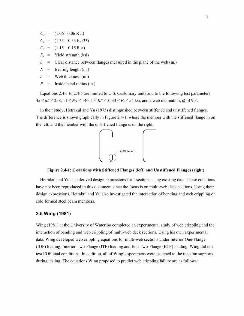
In their study, Hetrakul and Yu (1975) distinguished between stiffened and unstiffened flanges. The difference is shown graphically in Figure 2.4-1, where the member with the stiffened flange in on the left, and the member with the unstiffened flange is on the right.

Lip Stiffener

Figure 2.4-1: C-sections with Stiffened Flanges (left) and Unstiffened Flanges (right)

Hetrakul and Yu also derived design expressions for I-sections using existing data. These equations have not been reproduced in this document since the focus is on multi-web deck sections. Using their design expressions, Hetrakul and Yu also investigated the interaction of bending and web crippling on cold formed steel beam members.

2.5 Wing (1981)

Wing (1981) at the University of Waterloo completed an experimental study of web crippling and the interaction of bending and web crippling of multi-web deck sections. Using his own experimental data, Wing developed web crippling equations for multi-web sections under Interior One-Flange (IOF) loading, Interior Two-Flange (ITF) loading and End Two-Flange (ETF) loading. Wing did not test EOF load conditions. In addition, all of Wing’s specimens were fastened to the reaction supports during testing. The equations Wing proposed to predict web crippling failure are as follows:

12

a) For Interior One-Flange (IOF) loading

( )

+

−

−−=

tN

th

tRkFtP yn 00526.01000985.01074.01107.01sin6.16 2 θ (2.5-1)

b) For Interior Two-Flange (ITF) loading

( )

+

−

−−=

tN

th

tRkFtP yn 00948.0100139.010306.0122.01sin18 2 θ (2.5-2)

c) For End Two flange (ETF) loading

( )

+

−

−−=

tN

th

tRkFtP yn 00887.0100206.01111.010777.01sin9.10 2 θ (2.5-3)

Where:

Pn = Nominal web crippling strength (resistance) Fy = Yield strength (ksi) h = Flat dimension of web measured in plane of web (in.) N = Bearing length (in.) R = Inside bend radius (in.) t = Web thickness (in.) θ = Angle between plane of web and plane of bearing surface, 45° < θ ≤ 90° k = Fy/33

Equations 2.5-1, 2.5-2, and 2.5-3 are limited to U.S. Customary units and to the following parameters: h/t ≤ 200, N/t ≤ 210, and R/t ≤ 3.

Later, Wing and Schuster (1982) performed a more detailed investigation into the web crippling of multi-web deck sections subjected to Two-Flange loading.

2.6 Yu (1981)

At the University of Missouri-Rolla, Yu (1981) completed an extensive study of multi-web deck sections subjected to End One-Flange and Interior One-Flange loading. His goal was to establish experimentally a set of data with which to validate the design equations in the 1980 edition of the AISI Specification (AISI, 1980). He also investigated the interaction of bending and web crippling of multi-web deck sections. Many of Yu’s test specimens were composite deck sections, which have perforations and/or embossments in the web element designed to strengthen the bond between the steel deck and a concrete topping. Due to the potential influence of the embossments on the webs, composite deck sections cannot be included with common multi-web deck sections when establishing design equations.

13

None of Yu’s specimens were fastened to the supports. To prevent spreading, Yu affixed a 1/8” x 3/4” metal strap to the underside of the deck, at a distance of 1.5 times the section depth from the bearing plates. This is different from how multi-web deck sections are used in practice, where the deck sections are attached using discreet fasteners (such as puddle welds) at the point of bearing only. The metal strap restricted the rotation of the outside flanges, which increased the web crippling capacity of the deck section.

It was attempted to incorporate the data from Yu’s study in the current study. However, the data was found to be different, no doubt due to the metal strapping. For this reason, none of the data from Yu’s study was used in the current study.

2.7 Studnička (1989)

Studnička (1989) at the Czech Technical University completed an experimental study to determine the web crippling load resistance of multi-web deck sections subjected to end and interior reaction loads. Studnička proposed using the following equation, modeled from the equations in the 1984 edition of the Canadian standard (CAN/CSA-S136, 1984), for predicting the web crippling capacity of both End One-Flange and End Two-Flange loading;

( ) ( )( )( )tN

hk

th

tRFtP yn 00501151500110110110 2 ...sin ++−

−−= κθ (2.7-1)

Where:

Pn = Nominal web crippling strength (resistance) Fy = Yield strength (MPa) h = Clear distance between the flats of flanges measured in the plane of the web (mm) k = Distance between end of deck and end of bearing plate (mm) N = Bearing length (mm) R = Inside bend radius (mm) t = Web thickness (mm) θ = Angle between plane of web and plane of bearing surface, 45° < θ ≤ 90° κ = Fy/230

Studnička indicated that Equation 2.7-1 is limited S.I. units and to sections with ratios of h/t ≤ 200, N/t ≤ 210, R/t ≤ 3, and k ≤ 3h.

The data produced by Studnička was not used in this study because he fixed a bar to the end of his specimens to simulate the effect of fasteners. This bar and the small length of specimen to which it was attached extended beyond the bearing supports. This violates the definition of EOF loading

14

which requires the edge of the specimen to be in contact with the bearing plate. Studnička’s data should be classified as IOF loading, by definition.

2.8 Bakker (1992)

Bakker (1992) at Eindhoven University of Technology in the Netherlands used yield line theory to create a numerical model to simulate web crippling of a cold formed steel hat section. Her goal was to demonstrate that the statistical deviation between experimental data and theoretical load capacity could be reduced by using a numerical model instead of design equations derived from experimental tests. Her reasoning was that design equations would always be limited to the range of parameters of the test specimens. Yield line theory is a numerical method similar to finite element analysis, but with many simplifications that greatly reduce the amount of computational effort required to find a solution. Due to recent advances in computer technology, finite element analysis is now the preferred numerical method for such modelling.

A web crippling failure occurs by one of two mechanisms: the yield arc mechanism or the rolling mechanism. Bakker was not the first to distinguish between these two mechanisms, however she was one of the first to recognize the importance these mechanisms play in web crippling. Bakker found that she could not use existing test data to verify her model because few researchers record the failure mechanism. This obligated her to create her own experimental database.

The yield arc mechanism and the rolling mechanism are both discussed in more detail in Section 3.4.1. The mechanisms play a small role in interpreting the failure load from load-deflection curves. Bakker observed that the failure mechanism is significantly influenced by the inside bend radius, and that the rolling mechanism is more common to sections with large radii.

The model Bakker developed is that of a simple hat section deforming due to the rolling mechanism while subjected Interior One-Flange loading. Her model was a better predictor of web crippling capacity than the current design equations of the time, however the computational effort required to determine the web crippling capacity rendered this method impractical for design needs.

2.9 Bhakta et al. (1992)

Bhakta, LaBoube, and Yu (1992) at the University of Missouri-Rolla experimentally investigated the influence of flange restraint on the web crippling capacity of beam web elements. Bhakta tested many different section profiles, including multi-web deck sections. One of the conclusions of the study was that deck sections subject to EOF loading experience an increase of 37% in web crippling capacity when the flanges are fastened to the support.

15

Bhakta’s data involving End One-Flange loading of multi-web deck sections have been included in this study.

2.10 Prabakaran (1993)

Prabakaran (Prabakaran, 1993 and Prabakaran and Schuster, 1998) at the University of Waterloo completed an extensive statistical study of the web crippling capacity of cold formed steel sections using experimental data found in the literature. The primary goal of his study was to develop a simplified non-dimensional equation for predicting the web crippling capacity of any cold formed steel section. From the results of his study, Prabakaran recommended Equation 2.10-1, which was adopted for use by the Canadian Standard for Cold Formed Steel Structural Members (CAN/CSA-S136, 1994b) and by the NAS (2001a). Prabakaran was the first to correct a number of problems found in previous web crippling equations, including a problem where using high-strength steels incorrectly resulted in a decrease in web crippling capacity.

−

+

−= t

hCtNCt

RCFCtP hNRyn 111sin2 θ (2.10-1)

Where:

Pn = Nominal web crippling strength Fy = Yield strength C = Coefficient Ch = Web slenderness coefficient CN = Bearing length coefficient CR = Inside bend radius coefficient h = Flat dimension of web measured in plane of web N = Bearing length R = Inside bend radius t = Web thickness θ = Angle between plane of web and plane of bearing surface, 45° < θ ≤ 90°

2.11 Gerges (1997)

Gerges (Gerges, 1997 and Gerges and Schuster, 1998) at the University of Waterloo completed a study of single web members subjected to End One-Flange loading. Particular attention was placed on specimens with inside bend radius to thickness ratios between 5 and 10. In his study, Gerges tested 72 C-sections where 5 < R/t < 10. This data was combined with previous data and new web crippling coefficients were derived for this geometry and loading case.

16

2.12 Wu et al. (1997)

Wu, Yu, and LaBoube (1997) at the University of Missouri-Rolla, completed a study investigating the web crippling capacity of high strength cold formed steel sections. The yield strength of the specimens ranged from 716 MPa (103.9 ksi) to 776 MPa (112.5 ksi). The tests were limited to hat sections and multi-web deck sections, which were tested for all four load cases. None of the test specimens were fastened to the supports during testing.

From the results of their testing, Wu proposed modified kC1 and kC3 factors for use in Equations 2.4-1 to 2.4-5. The terms C1 and C3 are defined in Section 2.4 of this document. The variable, k, is equal to Fy/33, where Fy is in units of ksi. He concluded that the value of 1.691 could be used for kC1 when Fy exceeds 630 MPa (91.5 ksi) and the value of 1.34 could be used for kC3 when Fy exceeds 460 MPa (66.5 ksi).

When testing the End One-Flange load case, Wu clamped the bottom flanges of the specimen to a steel plate. However, these clamps were placed at the midspan of the specimen and do not appear to have restricted the rotation of the flanges at the location of failure, as can be seen in Figure 2.12-1, which was taken from Wu’s research report. Wu’s data was included in this study.

Figure 2.12-1: Clamps at Midspan of Wu Specimen

2.13 Beshara (1999)

Beshara (Beshare, 1999 and Beshara and Schuster, 2000) at the University of Waterloo completed a study with the goal to produce better web crippling coefficients for use with Equation 2.10-1 proposed by Prabakaran (1993). Combining experimental data found in the literature with his own

17

test data, Beshara classified the data by section type (e.g. C-section, Z-section, multi-web, etc), by load configuration (e.g. End One-Flange, Interior One-Flange, etc), and by support conditions (fastened or unfastened). The web crippling coefficients recommended by Beshara were adopted for use in the NAS (2001a).

Beshara also recommended that future research into multi-web sections subjected to EOF loading be conducted due to the relatively few test specimens he was able to find in the literature. This was especially true of multi-web deck sections with fastened support conditions.

2.14 Avci and Easterling (2002)

Avci and Easterling (2002) at Virginia Polytechnic Institute and State University completed an experimental study of multi-web deck sections subjected to EOF loading. The goal of the study was to investigate the relative accuracy of the web crippling equation presenting in the NAS (2001a) compared to the previous web crippling equation used in the American Iron and Steel Institute’s 1996 Edition of the Specification for Cold Formed Steel (AISI, 1996a). Avci and Easterling tested both fastened and unfastened conditions, and they allowed certain geometric parameters to exceed the restrictions imposed by the NAS.

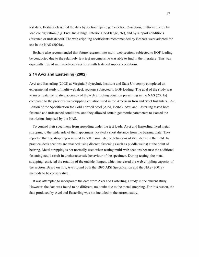
To control their specimens from spreading under the test loads, Avci and Easterling fixed metal strapping to the underside of their specimens, located a short distance from the bearing plate. They reported that the strapping was used to better simulate the behaviour of steel decks in the field. In practice, deck sections are attached using discreet fastening (such as puddle welds) at the point of bearing. Metal strapping is not normally used when testing multi-web sections because the additional fastening could result in uncharacteristic behaviour of the specimen. During testing, the metal strapping restricted the rotation of the outside flanges, which increased the web crippling capacity of the section. Based on this, Avci found both the 1996 AISI Specification and the NAS (2001a) methods to be conservative.

It was attempted to incorporate the data from Avci and Easterling’s study in the current study. However, the data was found to be different, no doubt due to the metal strapping. For this reason, the data produced by Avci and Easterling was not included in the current study.

18

Chapter 3 Experimental Investigation

3.1 General

The experimental component of this study is discussed in detail in this chapter. More specifically, specimen selection is explained, followed by mechanical properties, specimen notation, test procedure, and interpretation of test results.

3.2 Test Specimens

The test specimens used in this study were selected in an effort to represent a wide range of multi-web deck sections currently available in North American. Within the eleven deck profiles used, a range of section depths, yield strengths, web inclinations, and number of webs per specimen are represented. In addition, Canadian and American manufacturers are equally represented.

3.2.1 Specimen Selection

An attempt was made to represent the full range of geometric parameters of deck sections available from three Canadian and three American fabricators. Each selected profile was tested in three different thicknesses: 22 gauge (0.76 mm, 0.030 in.), 20 gauge (0.91 mm, 0.036 in.), and 18 gauge (1.21 mm, 0.048). The exception to this was United Steel Deck decks H6 and H7.5, which were tested at 20 gauge (0.91 mm, 0.036 in.), 18 gauge (1.21 mm, 0.048), and 16 gauge (1.52 mm, 0.060 in.). Listed in Table 3.2-1 are all of the deck profiles used in this study and deck section properties as published by the manufacturer.

To constitute a multi-web deck section, all specimens required a minimum of four webs. In the case where the deck section was rolled with only two webs, two deck sections were attached together and tested as one unit with four webs. The specimens were crimped at both ends and at midspan of the specimen. This resulted in a spacing of approximately 600 mm (24 in.) between points of crimping, which meets the spacing requirements of 900 mm (36 in.) recommended by CSSBI and SDI.

19

Table 3.2-1: Deck Profiles used in Study

Profile Depth, mm (in.) Pitch, mm (in.) Number of WebsUnited Steel Deck J4.5* 114 (4.5) 306 (12) 4 United Steel Deck H6* 152 (6) 306 (12) 4

United Steel Deck H7.5* 190 (7.5) 306 (12) 4 Wheeling DeepRib 114 (4.5) 306 (12) 4

Canam P-3615 38 (1.5) 153 (6) 12 Canam P-2432 76 (3) 306 (12) 4

VicWest RD306 76 (3) 153 (6) 8 VicWest HB30V** 76 (3) 406 (16) 4

Epic ER2R 50 (2) 154 (6 1/16) 8 Epic ER3.5 102 (4) 206 (8 1/8) 6

CMRM S-30-8 76 (3) 203 (8) 6 * Two deck sections were joined together to create a four-web section. ** This section normally has web embossments. It was rolled without web embossments for this study.

3.2.2 Fastening Patterns

Specimens were tested under a variety of fastening patterns ranging from no fastening, to only being fastened at the ends, to being fastened at every flute. A specimen with a pitch less than or equal to 200 mm (8 in.) was considered to be fully-fastened when every second flute was attached. Specimens were fastened to the supports using 11 mm (7/16 in.) bolts with a washer being placed under the bolt head only. The bolt head was always under the bearing plate, so that the washers were never in contact with the specimens.

Common practice in industry is to consider the deck section to be fastened when fasteners are spaced at intervals not greater than 450 mm (18 in.). When the fastener spacing exceeds 450 mm (18 in.), the assumed support condition is unfastened. In this study, a partially-fastened support condition was defined as a deck section that was fastened, but the fasteners were spaced at intervals greater than 450 mm. By this definition, it is not possible for a deck section to be partially-fastened if the width of the section is less than 450 mm (18 in.). In this study, an investigation of partially-fastened support conditions was done to determine if treating this support condition as part of the unfastened support condition is the correct approach for design.

Shown in Figure 3.2-1 are all of the deck profiles of the various specimens used in this study. Listed in Table 3.2-2 are the different fastening patterns used in this study. The fastener locations listed in Table 3.2-2 are in reference to the lowercase letters shown below the deck profiles in Figure 3.2-1 and indicate the location of a fastener.

20

a b c

a b c e d

a b c d

d a b c e g f

A)

B )

C )

D )

E) a b c ed

Figure 3.2-1: Profiles of Specimens Used in the Study.

Table 3.2-2: Fastener Combinations for each Section Profile Tested.

Deck Section Profile Fastener Location Combinations

Number of Combinations

A 0

a-c a-b-c

3

B 0

a-d a-b-d

3

C 0

a-e a-c-e

3

D

0 a-g

a-d-g a-c-e-g

4

E 0

a-e a-c-e

3

3.2.3 Specimen Notation

The notation system used herein identifies each specimen and contains information regarding the specimen geometry and test parameters. There are two parts to the specimen notation.

The first part of the notation is the test series name, which is a two-digit identification code (one letter followed by a number) that links specimens made from the same coil of steel. Because they

21

were fabricated from the same coil, it was assumed that all specimens within a test series will have the same mechanical properties. These properties are listed in Appendix A. Only the size of the bearing plate and the fastening pattern were varied between specimens with the same test series name.

The second part of the notation is the test specimen name, which is divided into four parts: the fabricator code, the number of webs, the bearing plate width, and the fastening pattern. The fabricator code notation and the fastening pattern notation are listed in Tables 3.2-3 and 3.2-4, respectively. For more detail on fastening patterns, refer to Table 3.2-2 and Figure 3.2-1 of the previous section.

Three different sizes of bearing plate were used in testing. The bearing plates are identified as 1, 2, and 3, where 1 is 24 mm (0.94 in.) wide, 2 is 50 mm (1.97 in.) wide, and 3 is 75 mm (2.95 in.) wide.

Example:

C1-CAN30-4-1-NONE

Where

C1 = Test series (see Appendix A) CAN30 = Fabricator and product (See Table 3.2-3) 4 = Number of webs 1 = Bearing plate NONE = Fastening pattern (See Table 3.2-4)

From this example, one can see that C1-CAN30-4-1-NONE is a Canam P-2432 multi-web deck with a steel thickness of 1.16 mm (0.046 in.), a yield strength of 340 MPa (49.3 ksi), 4 webs, a bearing plate width of 24 mm (approximately 1 in.), and an unfastened support condition.

Table 3.2-3: Fabricator Code for Specimen Notation

Fabricator Code Fabricator Product Nominal Depth, mm (in.) CAN15 Canam-Manac P-3615 38 (1.5) CAN30 Canam-Manac P-2432 76 (3.0)

CMRM30 Roll Form Group S-30-8 76 (3.0) EPIC20 Epic Steel ER2R 46 (1.8) EPIC40 Epic Steel ER3.5 89 (3.5) USD45 United Steel Deck J4.5 114 (4.5) USD60 United Steel Deck H6 152 (6.0) USD75 United Steel Deck H7.5 190 (7.5) VIC3a VICWEST RD306 76 (3.0) VIC3b VICWEST HB30V 76 (3.0)

WHE45 Wheeling DeepRib 114 (4.5)

22

Table 3.2-4: Fastening Pattern Notation

Pattern Name 4 webs 6 webs 8 webs 12 webs NONE 0 0 0 0 ENDS a-c a-d a-e a-g 3RDS N.A. N.A. N.A. a-d-g 2NDS N.A. N.A. N.A. a-c-e-g ALL a-b-c a-b-d a-c-e N.A.

3.2.4 Mechanical Properties

The assumption was made that all specimens of the same profile, thickness, and manufacturer were fabricated from the same coil of steel, and as such would have similar mechanical properties. With this in mind, three coupon specimens were cut from the webs of one of the tested deck specimens per profile per thickness, chosen at random. These coupons were carefully measured and tested in accordance with ASTM A370 (2002) and Section A7.1 of the Commentary on the North American Specification for the Design of Cold Formed Steel Structural Members (2001b). The yield strength from each of the three coupons were averaged and recorded as the representative value. This yield strength was then applied to all other specimens of the same profile, thickness, and manufacturer. A complete listing of the mechanical properties of all of the specimens is given in Appendix A.

Contained in Section A2.3.1 of the NAS (2001a) are requirements for ductility. Specifically, the section states that steel used for structural member design have an ultimate-to-yield (Fu/Fy) ratio greater than 1.08 and an elongation greater than 10%. Test series W1 and W2 do not meet these requirements. However, as the intent of Section A2.3.1 is to make the specification more conservative when dealing with high strength steels and as there were no adverse effects from incorporating the data from these two test series in the analysis portion of this study, it was deemed acceptable to include this data.

3.3 Test Set-Up

All specimens were tested under a simply supported condition, subjected to a single line loading with the location of the applied load and the supports chosen to ensure failure at the end supports. To minimize the chance of failure due to bending, the span length was kept as short as possible. In some cases, it was necessary to reinforce the section to prevent bending at the point of load application. The reinforcing was achieved by screw-fastening a piece of the same deck section to the test specimen, while ensuring that a distance of 1.5 times the section depth, measured from the inside of the ‘near’ bearing plate, was not reinforced. A photograph of a reinforced specimen is shown in Figure 3.3-1.

23

Figure 3.3-1: Specimen Reinforced to Achieve EOF Loading

For clarity, the ends of the specimen were designated as ‘near’ and ‘far,’ as shown in Figure 3.3-2. The ‘near’ end was the end at which failure was desirable.

The applied load was positioned a small distance away from the centre of the span so as to cause one support to have a higher load than the other, causing failure at the ‘near’ end of the specimen. Different sized bearing plates were also used for the same reason. At the ‘near’ end, the bearing width varied from 24 mm (1 in.) to 75 mm (3 in.), whereas at the ‘far’ end and at the point of loading the bearing width was 150 mm (6 in.). A schematic layout of the test set-up is shown in Figure 3.3-2 and a photograph of the test set-up is shown in Figure 3.3-3.

PTest

RTest

Load Span Length

Span Length

NearFar

FasteningPattern

BearingLength

> 1.5 h

150 mm

Figure 3.3-2: Diagram of Test Set-up.

24

Figure 3.3-3: Photograph Showing Test Set-up.

The minimum span length for each test (listed in Tables C-1 to C-3 of Appendix C) was 267 mm (10.5 in.) plus three times the height of the specimen, measured from the center of the near bearing plate to the center of the ‘far’ bearing plate. This length was imposed by the size of the bearing plates and the required distance of 1.5 times the section depth between bearing plates (needed on both sides of the applied loading) for One-Flange loading. In testing, the minimum span length was always exceeded, often by 50 mm (2 in.) or more. Exceeding the minimum span length allowed the applied load to be positioned a small distance away from center, towards the ‘near’ end of the specimen. Positioning the applied load as such caused the reaction load at the ‘near’ support to be larger than the reaction at the ‘far’ support, thereby ensuring failure at the ‘near’ end of the specimen.

At the ‘near’ end, the specimens were tested using one of three different bearing lengths: 24 mm (1 in.), 50 mm (2 in.), or 75 mm (3 in.). For some tests, the ‘near’ end of the specimen was fastened to the bearing plate using bolts. The ‘near’ bearing plates were slotted to accommodate the variety of geometries between the different test specimens. Neither the bearing plate under the load nor the ‘far’ bearing plate were slotted. For the few tests where the lack of fasteners at the ‘far’ end of the specimen influenced the specimen’s behaviour, clamps were used in place of bolts.

A hydraulic actuator applied the load at a constant rate of displacement. An electronic load cell positioned between the actuator head and the specimen measured the load, which was recorded by a computer data acquisition system. The load was applied under constant displacement of the actuator head. The computer was able to detect any failure as a sudden drop in load. Deflection of the

25

specimen was not recorded during testing. However, the stroke, or displacement, of the actuator was recorded for plotting the load-stroke curves. The load-stroke curves are given in Appendix E. Note that the magnitude of the stroke has been intentionally omitted from these curves to eliminate any possible confusion between the stroke (which is measured at point of applied loading, near midspan) and member deformation at the point of failure.

For each section geometry and steel thickness, one specimen was tested as per Figure 3.3-2 for each bearing plate width and fastening condition, for a total of nine tests per geometry and thickness (twelve tests for specimens with ten or more webs). Summarized in Tables C-1 to C-3 of Appendix C are the span length and the load span factor for each test specimen. Summarized in Tables B-1 to B-3 of Appendix B are the cross-section parameters for each test specimen.

3.4 Interpreting Test Data

Discussed in the following section is the determination of web crippling capacity of a specimen from the experimental data. Discussed first is the interpretation of the data from the load-stroke curves, followed by the calculation of the end load from the free body diagram and the applied load of the specimen.

3.4.1 Determining Maximum Applied Load from Load-Stroke Curves

There exist two different mechanisms under which web crippling can occur. The first is the yield arc mechanism, which is characterized by out-of-plane deformation within the web element. The second is the rolling mechanism, where the deformation occurs at the radii between the web elements and the flange elements. The radii ‘rolls,’ transferring material from the web elements and redistributing it to the flange elements. The rolling mechanism is more common in shallow sections and sections with large bend radii. Bakker (1992) states that the rolling mechanism occurs in sections with large R/t ratios, whereas the yield arc mechanism occurs in sections with small R/t ratios. Unfortunately, she does not indicate what constitutes a large R/t ratio. These two mechanisms are illustrated by means of diagrams in Figures 3.4-1 and 3.4-2.

26

OriginalShape

Deformed Shape

Location of InitialDeformation

Figure 3.4-1: Yield Arc Mechanism

OriginalShape

Deformed Shape

Location of InitialDeformation

Figure 3.4-2: Rolling Mechanism

The yield arc mechanism and the rolling mechanism have different characteristic load-stroke curves. Illustrated in Figure 3.4-3 is a typical load-stroke curve for a specimen that has experienced the yield arc mechanism. This curve shows an initial increase in load until failure at the first peak. At this point, the web has begun to arc and the ability of the specimen to resist load is diminished. As the web continues to deform, one half of the web will be pushed downward until it becomes part of the flange element. The remaining web element is shorter, and therefore has an increased ability to resist load. This causes a second increase in web crippling resistance that is greater than the initial resistance. One can assume that the specimen has a higher web crippling capacity in the post-buckled state. However, as the specimen is permanently deformed, failure is considered to have occurred at the first peak load. Often during testing, the load from the actuator was released once the first peak load became obvious and any increased post-buckled web crippling capacity was not recorded. The failure load was recorded in this manner for all specimens that failed by the yield arc mechanism.

27

P Applied Web Crippling Failure

Initial Loading Zone

Deformed shapehas higher web crippling capacity.

Stroke

Figure 3.4-3: Typical Load-Stroke Curve of Yield Arc Mechanism

The identification of a peak failure load is not as simple with the rolling mechanism. Illustrated in Figure 3.4-4 is a typical load-stroke curve for a specimen failing due to the rolling mechanism. As can be seen from the curve, the rolling mechanism does not have the abrupt loss of load resistance characteristic to the yield arc mechanism. It is a subtle failure, where once the failure load is reached, deformation occurs gradually. Web crippling is a form of buckling, which is dependent on web depth. As the depth of the web element is gradually decreasing in this mechanism, similarly, the load resistance will also gradually increase. This makes identification of a failure load less straightforward.

P Applied Web Crippling Failure takenat Point of Inflection.

Initial Loading Zone

Deformed shapehas higher web crippling capacity

Stroke, x

Point of Inflection defined as any point along the curve where:

Papplied = 0 d2

dx2

Figure 3.4-4: Typical Load-Deflection Curve of Rolling Mechanism.

The failure load of a rolling mechanism was taken as the load at the point of inflection on the load-stroke curve. The point of inflection, by definition, is any point along a function where the second derivative is equal to zero. In this study, for any specimen that failed due to rolling mechanism, the data from the test was fitted to a sixth order polynomial. The second derivative of the polynomial was determined and solved for zero to determine the failure load. The smallest inflection point within the

28

range of the data was usually taken to be the failure load, although some judgement was used in the decision. Also of note is the initial low stiffness of both curves. The low stiffness of the initial loading zone is caused by a small amount of camber in the bearing plates, which must first be flattened before any significant load can be developed in the webs. It is this straightening that results in a lower initial stiffness of the specimen.

The applied load at failure is referred to as Ptest in this document, which is different from the failure load experienced at the ‘near’ end of the specimen, which is defined as Rtest.

3.4.2 Converting Applied Load to End Load

Discussed in the previous section was how the applied load at failure was determined from the load-stroke curve. However, this curve is the load and stroke near the midspan of the deck section, where the load was applied from the test frame. Failure occurs at the ‘near’ end of the span and an equivalent end load must be determined.

During testing, the span length and the distance between the near end of the span and the point of loading were recorded. Equation 5.2-1 determines the critical end load, Rtest.

( )α−⋅= 1testtest PR (3.4-1)

In Equation 3.4-1, Ptest is the recorded applied load at failure of the test and α is the ratio of the distance between the applied load and the ‘near’ end support to the span length. The ‘near’ end support is the end support at which web crippling occured. The graphical meaning of Rtest, Ptest, and α are shown in Figure 3.4-5.

Ptest

Rtest

α L L

Figure 3.4-5: Test Specimen Layout

3.5 Test Results

The test results can be found in the appendices. More specifically, the load-stroke curves are given in Figures E-1 to E-30 of Appendix E and the specimen failure loads, Rtest, are listed in Tables C-1 to C-3 of Appendix C. Comparisons of the actual failure loads to the theoretical failure loads are given in Tables D-1 to D-3 of Appendix D.

29

Chapter 4 Methods of Analysis and Calibrations

4.1 General

This chapter contains detailed descriptions of the various methods and techniques employed in the analysis of the data produced by this study and the data found in the literature. Specifically discussed are the method of least squares, gradient-based optimization, optimization by genetic algorithms, and calibrations (method to determine resistance factors). The method of least squares was used to ‘fit’ a mathematical function to a given data set; however powerful optimization techniques are required to find this function. To lend credibility to the study, two completely different optimization techniques were employed. The first technique is a gradient-based method found in an established commercial software package. The second technique, a genetic algorithm, was written specifically for this study. The method for determining the resistance factors was taken from Section A5 of the Commentary to the 2001 Edition of the North American Specification for the Design of Cold Formed Steel Structural Members (2001b).

The intent of this chapter is to discuss the methods of analysis. A detailed discussion of the results of the analysis is given in the next chapter.

4.2 Developing the Model

Discussed in this section is the development of the mathematical model used to describe the data. The optimization of the model is discussed in the next section.

4.2.1 Method of Least Squares

Also referred to as regression or curve fitting, the Method of Least Squares (MLS) is a common technique for fitting a mathematical function to a set of known data. MLS is useful because it is a formalized, unbiased method of curve fitting. All statistical tools, from scientific calculations to powerful computer applications, make use of MLS in some form.

MLS works by minimizing the error between a data set and the function describing the data (herein referred to as the trend line). To begin, one must assume a general equation that can describe the data. The data may have to be plotted before any trend can be recognized. Equations like y = a x + b (linear), y = a x2 + b x + c (quadratic), or y = ax (exponential) are commonly used, but any equation

30

can be used, so long as when plotted it has a shape similar to the data set. It is possible to use equations with more than one independent variable.

The next step is to find the exact form of the trend line. To do this, one must determine the value of the coefficients in the trend line for which the sum of the square of the error between the trend line and each data point is a minimum. In mathematical terms, one must minimize Equation 4.2-1, where Pt is a data point and Pc is the corresponding trend line value.

( )∑=

−n

iciti PP

1

2 (4.2-1)

It is important that the error be squared to eliminate any negative error values, otherwise the method would only work for data that fell on one side of the trend line. For many single-variable equations there are methods established for determining the coefficients that correspond to the minimal sum. For most multi-variable equations, there is no such established method. A graphical example showing how MLS works is shown in Figure 4.2-1.

P ci Pti

Pti - Pci

Abscissa

Ord

inat

e

Figure 4.2-1: Graphical Representation of Method of Least Squares

For a more in-depth look at the method of least squares and how it applies to multi-variable nonlinear problems, the reader can to refer to a text such as “Miller & Freund’s Probablility & Statistics for Engineers” by Richard Johnson (1994).

4.2.2 The Mathematical Model

The model used in this study is a non-linear equation with four independent variables. The model is an optimization problem, where the minimum value of Equation 4.2-2 must be found. It is a complex

31

model that cannot be solved easily by hand methods. The optimization techniques used to solve the model are discussed in the next section.

∑=

−

+

−⋅⋅⋅−

n

i ii

hi

iN

ii

Riyiiti thCt

NCtRCFtCR

1

2 111θsin (4.2-2)

Where:

Rti = Sequence of web crippling capacities determined by experiment Fyi = Sequence of measured yield strengths hi = Sequence of web depths (measured in plane of web) Ni = Sequence of bearing lengths Ri = Sequence of inside bend radius ti = Sequence of web thicknesses θι = Sequence of web inclinations C = Coefficient Ch = Web slenderness coefficient CN = Bearing length coefficient CR = Inside bend radius coefficient

The model is subject to the following constraints: C is an integer greater than zero; Ch, CN, and CR are real numbers greater than zero.

4.3 Optimization Methods

Discussed in this section are the methods that were employed to solve the model given in the previous section. Two different methods are discussed and the result of the each method is briefly reviewed. Refer to the next chapter for detailed results and conclusions of this study.

4.3.1 Optimizing using the Genetic Algorithm

Genetic Algorithms (GA) are a topic in the field of optimization. GA’s are simple, easy to understand, and easy to implement in computer applications. GA’s are also capable of solving complex problems.

The concept for GA’s originate with the theory of evolution. The algorithm works by creating a large population of random solutions that is tested, mixed, and spliced until an optimal solution is found. While the basic concepts are easy to follow and understand, the actual implementation of the algorithm requires the user to keep track of a large amount of data and to perform many iterations. As such, GA’s are better suited to computer applications than to hand calculations.

32

Before a GA can be implemented, a scheme must first be devised to describe a solution using binary numbers. As an example, such a scheme might use a five-bit binary number to describe the size of steel reinforcing bar used in a concrete beam. A five-bit binary number can define any integer number between 0 and 31, which could represent the diameter of rebar in millimetres. In GA terminology, a binary solution is referred to as a chromosome or a DNA string.

To initialize a GA, it must be provided with a population of randomly created DNA strings. Each DNA string represents a different possible solution. The likelihood that any one of the DNA strings in the initial population is the optimal solution is small, however, the likelihood that parts of some of the DNA strings match the optimal solution is high. The challenge is to find which parts of which DNA strings once assembled will give the optimal solution.

A method of judging the fitness of a DNA string is needed. Using this fitness test, it will be possible to determine which DNA strings are closer to the final solution, and therefore, better suited to parenting the next generation of solutions.

Often, penalty functions are included in the fitness test. Penalty functions penalize solutions that are too fit. To show why penalty functions are necessary, take the example the problem where a GA is employed to maximize the moment capacity of a concrete beam. If the DNA string describes the amount of reinforcing steel in the beam, and the fitness test is based on the moment capacity, then it follows that the GA will simply increase the amount of reinforcing steel maximum value. The penalty function would penalize a solution that results in an over-reinforced beam. This would cause the over-reinforced beam to appear less fit and prevent the GA from converging on an impractical solution.

Armed with a fitness test and a population of possible solutions, the GA can begin its first iteration by choosing DNA strings to act as parent DNA for the next generation. The parent DNA strings are chosen pseudo-randomly, that is, the DNA strings are selected randomly, but with a bias towards the DNA strings that scored better on the fitness test. In this way, a larger proportion of information from the more-fit DNA strings will be passed to the next generation than from the less fit DNA strings. It should be noted that DNA strings could be selected more than once to act as parents.

Once the parent DNA strings are chosen, the next generation is created. This is done by taking two parent DNA strings and swapping sections of the two DNA strings at random locations. This will result in two children DNA strings, each one being unique but with some traits from each of the parent DNA strings. The children DNA strings will form a new population. The GA will do this for several iterations, while continuously checking for convergence. With each repetition, the less-fit DNA strings are slowly eliminated from the population and the more-fit DNA strings begin to dominate. Once the convergence criteria are met, the algorithm reports its final solution.

33

The last task is to identify the optimized solution, which defines the convergence criteria. One common approach is to count the number of repeated DNA strings. Initially, there should be very few repeated strings, but with each iteration the less-fit DNA strings are eliminated and the remaining DNA strings will become increasingly similar. Once a certain number of DNA strings are identical, that string may be declared as the optimal solution. Another method is to remember the fitness of the most-fit DNA string in each generation. If that same fitness value is repeated in three or more consecutive iterations, it may be declared as the most fit or optimal solution. One may also declare the optimal solution to be the most-fit solution after a set number of iterations.

It is often difficult to ascertain if a final solution truly is the optimal solution. GA’s sometimes converge prematurely on an incorrect solution. Often, parameters within the algorithm must be ‘tweaked’ before the algorithm will give correct results. GA’s must be executed many times to ensure that the optimal solution has been found.

In determining the web crippling coefficients, the GA was used as a secondary means of analysis. Genetic algorithms are not fooled by local minima and maxima in the same way as gradient-based methods, and as such are the perfect compliment to gradient-based optimization techniques. However, genetic algorithms do not reliably produce exact solutions. As such, genetic algorithms are well suited as a means of confirming the results from a gradient-based algorithm as well as being an excellent method of determining appropriate initial values to avoid local minima/maxima when using a gradient-based method of optimization.

A more detailed discussion of the GA used in this study, including an explanation of the DNA strings, string splicing, fitness testing, and convergence criteria have been included with the source code in Appendix F.

4.3.2 Optimizing using Microsoft Excel Solver (Gradient Method)

Solver is an add-on program for Microsoft Excel designed to optimize mathematical functions with constraints. Solver uses the Generalized Reduced Gradient (GRG2) algorithm to optimize nonlinear multivariable problems (The Simplex algorithm is used for linear problems). GRG2 was designed by Lasdon and Waren of the University of Texas at Austin and Cleveland State University, respectively (XL, 2000a and XL, 2000b).

Gradient-based algorithms use partial derivatives to direct a search for an optimal solution. The process begins with a set of variables at some initial value and one or more functions for which to optimize. The goal of the algorithm is to find the value of these variables for which the functions are maximized. To do this, the algorithm determines the value of the partial derivatives of each function for the variables given. When a partial derivative has a numerical value, it is referred to as a gradient

34

(it is also called the ‘slope’ in single variable problems). A positive value gradient indicates that the variable should be increased; a negative value gradient indicates that the value should be decreased.

The algorithm will adjust the variables by some increment based on the value of the gradients. It will continue to adjust the variables until all of the gradients approximately equal zero. At this point, the functions are maximized and the corresponding values of the dependent variables are known. A similar process is used to minimize a set of functions; one must simply change the algorithm so that the value of the variables increases with negative gradients and decreases with positive gradients.

The GRG2 algorithm uses a technique called finite differencing to approximate the partial derivatives numerically. Finite differencing works by adjusting each variable a small amount and observing the rate of change. GRG2 is capable of both forward differencing and central differencing. In forward differencing, the variable is adjusted in just one direction to estimate the gradient. In central differencing, the variable is adjusted in both directions. Central differencing requires more computational effort, but is more accurate for gradients that change rapidly.

The GRG2 algorithm has one weakness: local minima and maxima. In many problems, there exist local maxima and minima that are not the true maximum or minimum for the entire system. In single variable problems, this appears as peaks and valleys in the plot (see Figure 4.3-1). The true maximum is the highest peak and the true minimum is the lowest valley. GRG2 is unable to detect multiple local maxima and minima; it will declare the first maxima or minima it finds as the true maximum or minimum for the system. To compensate for this, one must execute the algorithm several times using different initial values.

Local MaximaTrue Maximum

Local Minima

x

f(x)

True Minimum

Variable Constraints

Figure 4.3-1: Example of Local and True Minima and Maxima with Variable Constraints.

For instructions on how to use Solver, refer to the on-line help system within Excel. Microsoft has provided a complete on-line help system for Excel that provides detailed instructions on how to use Solver to optimize both linear and nonlinear problems.

35

4.3.3 Results of Optimization

Unfortunately, the results determined from a genetic algorithm are very sensitive to the fitness tests, the population size, and the convergence criteria used by the algorithm. In order to get repeatable results, these three parts of the algorithm may need to be revised several times.

It is clear from the results that the genetic algorithm used in this study is not yet perfect. The genetic algorithm did not yield repeatable results. However, the results were always from a small range of possible results. This would suggest that the correct result, being the values of C, Ch, CR, and CN for which Equation 4.2-2 is a minimum, lies somewhere within the range of results produced by the genetic algorithm. For fastened support conditions, the range of results produced by the genetic algorithm is given in Table 4.3-1. When the values of the coefficients as determined by the genetic algorithm were used in Equation 4.2-2, the summation value was always less than 550.

Table 4.3-1: Range of Results From Genetic Algorithm

C CR CN Ch

Upper Limit 4 0.09 0.30 0.015

Lower Limit 3 0.03 0.18 0.031

After many trials using MS Excel Solver, Equation 4.2-2 was found to be a minimum using the fastened support condition data when the coefficients are: C = 4, CR = 0.039572, CN = 0.250063, and Ch = 0.024935. These values are within the range of values suggested by the genetic algorithm, and yield a summation value of 382.7, which is lower than any of the summation values calculated using the coefficients determined by the genetic algorithm, suggesting that the true minimum has been found.

Although it is reassuring to have two methods that are in close agreement, MS Excel Solver is the better method for optimizing Equation 4.2-2. The range of results that was yielded does not justify the additional time required to write a genetic algorithm. It is recommended that future researchers use only MS Excel Solver, although they must be cautioned that numerous trials using different starting values will be necessary.

A detailed discussion of the results of this study, including results for unfastened data and partially-fastened data, is given in Chapter 5.

4.4 Calibration

Resistance factors, φ, are used with the LSD design method in Canada and with the LRFD design method in the US and Mexico. The resistance factors are determined in conformance with each

36

country’s respective load factors, dead to live load ratios, and target reliability index, β. For members the target reliability index is 2.5 for the US and Mexico and 3.0 for Canada (NAS, 2001a).

A satisfactory design can be obtained by equating the factored resistance to the factored loads, as follows:

nLnDn LDR ααφ += (4.5-1)

Where Rn is the nominal resistance, Dn is the nominal dead load intensity, Ln is the nominal live load intensity, and αD and αL are the dead and live load factors, respectively, such that the load combinations are 1.2D + 1.6L for the US and Mexico and 1.25D + 1.5L for Canada. The dead to live load ratios, Dn/Ln, are 1/5 for the US and Mexico and 1/3 for Canada (NAS, 2001a).

Considering Equation 4.5-1, it can be shown that the resistance factors, φ, can be determined as follows.

For U.S. and Mexico:

( )2222

5211QPFMo VVVV

mmm

e

PFM+++

⋅=

βφ

. (4.5-2)

For Canada:

( )2222

4201QPFMo VVVV

mmm

e

PFM+++

⋅=

βφ

. (4.5-3)

Where:

( ) ( )0.105.1

05.1 222

+

+=

nn

LDnnQ LD

VVLDV

(4.5-4)

Mm = Mean value of the material factor, M, given as 1.10 Fm = Mean value of the fabrication factor, F, given as 1.00 Pm = Mean value of the professional factor, P, for the tested component βo = Target reliability index, equal to 2.5 for structural members in the U.S. and Mexico and 3.0

for structural members in Canada VD = Factor of variation of the dead load intensities VL = Factor of variation of the live load intensities VM = Coefficient of variation of the material factor, given as 0.10 VF = Coefficient of variation of the fabrication factor, given as 0.05 VP = Coefficient of variation of the test results, but not less than 6.5%

37

The values of Mm = 1.10, VM = 0.10, Fm = 1.00, and VF = 0.05 were taken from Table F1 – Statistical Data for the Determination of Resistance Factors in the Commentary on the 2001 Edition of the North American Specification for the Design of Cold-Formed Steel Structural Members (2001b).

By knowing the resistance factor, φ, the corresponding factor of safety, Ω, can be computed as follows:

For the US and Mexico

φ

+

+=Ω

1

6.12.1

n

n

n

n

LD

LD

= 1.533 / φ (4.5-5)

The results of calibration analysis are given in Chapter 5.

38

Chapter 5 Test Results and Comparisons

5.1 General

This chapter is divided into four main sections: the web crippling coefficients for the fastened and unfastened support conditions, the investigation of the partially-fastened condition, the investigation of re-entrant decks, and a general discussion of the conclusions of the study. The resistance factors and factors of safety are also discussed.

5.2 Web Crippling Coefficients for Multi-Web Deck Sections

The ultimate goal of this study is to determine appropriate values for the web coefficients, , C, CR, CN, and Ch, to be used so that the web crippling expression given as Equation 5.2-1 can be applied to multi-web deck sections.

−

+

−= t

hCtNCt

RCFCtP hNRyn 111sin2 θ (5.2-1)

Using the methods of analysis described in Chapter 4 and all suitable available data (comprising the new test data from this study, and previous data from Bhakta (1992) and Wu (1997)) the web crippling coefficients were determined to be as shown in Table 5.2-1. In the case where the specimen was fastened to the support, only data pertaining to specimens that were fully-fastened, that is, specimens meeting the fastening requirements of the Steel Deck Institute (SDI) and the Canadian Sheet Steel Building Institute (CSSBI), were considered in determining the coefficients. Specimens not meeting these fastening requirements were called ‘partially-fastened’ and were not used in any calculations of the web crippling coefficients.

The ranges of the test specimen parameters were: 299 MPa (43.4 ksi) < Fy < 674 MPa (97.8 ksi); 1.41 < R/t < 19.9; 20.0 < N/t < 110; 20.8 < h/t < 211; and 71º< θ < 108º. These ranges apply to fully-fastened, partially-fastened, and unfastened support conditions

Table 5.2-1: Web Crippling Coefficients for EOF Loading of Multi-Web Deck Sections

Support Condition C CR CN Ch

Unfastened 3 0.04 0.29 0.028

Fastened 4 0.04 0.25 0.025

39

Reviewing the coefficients listed in Table 5.2-1, one can observe that except for the coefficient, C, the coefficients are similar between the unfastened and fastened end conditions. The value of C increases by 33% from the unfastened to the fastened condition, suggesting that one can expect a 33% increase in web crippling capacity when multi-web deck sections are fastened to their supports. This is in close agreement with a previous study by Bhakta (1992) that found an increase of 37% in web crippling capacity when fasteners were used.

The coefficients listed in Table 5.2-1 are different from the coefficients of C = 3, CR = 0.08, CN = 0.70, Ch = 0.055, as given in the NAS (2001a). These coefficients are based on previous studies that did not distinguish between the fastened and the unfastened end conditions. Hence, the same values are listed for both conditions. One can compare the effectiveness of the new coefficients to the coefficients listed in the NAS (2001a) by comparing the ratios of Rtest-to-Rcalc. Rtest is the recorded test load on the deck section at the failure end. Rcalc is the theoretical load capacity using Equation 2.10-1 with the appropriate web crippling coefficients. Given in Table 5.2-2 is a summary of this comparison.

Table 5.2-2: Comparison of NAS (2001a) and Proposed Coefficients

Coefficients Used

Support Condition

Number of Tests

Mean Rtest/Rcalc

Coefficient of Variation of Rtest/Rcalc

Unfastened 92 0.977 0.484 NAS (2001a)

Fastened 77 1.273 0.306

Unfastened 92 1.006 0.318 Proposed

Fastened 77 1.059 0.129 From Table 5.2-2, one can observe the current NAS design procedure that uses the same

coefficients for both conditions is overly conservative for the fastened support condition. One can also observe that in comparing just the unfastened support condition data shows a small improvement in the average test-to-calculated value, however the improvement in the coefficient of variation is more significant. This indicates that the new web crippling coefficients result in more consistent results than the NAS coefficients.

One can observe from Table 5.2-2 that in general the coefficient of variation is much larger for the unfastened condition than for the fastened condition. This is due to the large scatter in the unfastened data caused by the tendency of many unfastened deck sections to ‘spread’ before web crippling occurs, resulting in a lower failure load. This tendency to spread is difficult to predict in unfastened deck sections, but is more common to sections with web inclinations less than 75º. Section depth, width of the bearing plate, and coefficient of friction between the zinc coating of the specimen and

40

the metal surface of the bearing plate also influenced the specimens tendency to spread. The coefficient of friction was not measured because the possibility of specimens spreading had not been considered at the outset of this study.

Shown in Figure 5.2-1 is a diagram illustrating how multi-web deck sections can spread. Shown in Figure 5.2-2 is a photograph of an unfastened multi-web deck section spreading as indicated in Figure 5.2-1.

Original Deck Profile

Figure 5.2-1: Spreading of Unfastened Deck

Figure 5.2-2: Spreading of a 4 Web Deck Section

The resistance factors and factors of safety (U.S. and Mexico only) have been determined in accordance with Section A5 of the Commentary to the 2001 Edition of the North American Specification of Cold Formed Steel Structural Members (2001b). The method outlined in Section A5 is discussed in Section 4.5 of this document. The resistance factors and factors of safety are given in Table 5.2-3.

Table 5.2-3: Factors of Safety and Resistance Factors for EOF Loading of Multi-Web Decks

U.S. and Mexico Canada Support Condition φ Ω φ

Unfastened 0.626 2.45 0.494

Fastened 0.905 1.69 0.773 There exists data from previous work that was not considered in this analysis. Yu (1981) and Avci

(2002) have undertaken studies involving multi-web deck sections. During testing, both Yu and Avci used a metal strap attached to the lower flanges to try and control spreading under unfastened conditions. It is believed that this strap would also restrict any potential rotation that would occur in

41

the outer flanges (This rotation mechanism is discussed more thoroughly in the next section). Because of this, the web crippling capacity of the specimens tested by Yu and by Avci is greater and does not agree with the test results of this and other studies. It should be noted that Wu (1997), whose data was included in this study, clamped a steel bar to the lower flanges of his specimens at the load point location to control spreading of the deck sections. However, he placed his clamps far enough away from the ends of the specimen that they did not interfere with the flange rotation.

Listed in Table 5.2-4 are the mean and coefficient of variation of the test-to-calculated ratios using Yu’s data (non-embossed sections only), Avci’s data, and the proposed coefficients. As expected, the mean values show that the proposed web crippling coefficients under-predict the capacity of these specimens, which is due to the increased stiffness of the outer webs from the metal strapping. Also, the magnitude of the mean values clearly shows that Yu’s data and Avci’s data are different from other test data and therefore cannot be included in the analysis portion of this study.

Table 5.2-4: Comparison of Test Data by Yu (1981) and Avci (2002)

Data Source Support Condition

Number of Tests

Mean Rtest/Rcalc

Coefficient of Variation of Rtest/Rcalc

Yu* Unfastened 18 1.586 0.185

Unfastened 39 1.458 0.202 Avci

Fastened 39 1.440 0.260 *Only non-embossed specimens were considered.

Surprisingly, the mean values in Table 5.2-4 concerning Avci’s data show that the metal strapping increased the web crippling capacity of both the fastened and the unfastened support conditions by 45%. The strapping was not expected to increase the capacity of the fastened data to the same degree as with the unfastened data. This suggests that the metal strapping has a greater ability to restrain flange rotation, and thus a greater influence on web crippling capacity, than do the fasteners.

5.3 Partially-fastened Support Condition

Also investigated in this study was End One-Flange loading of deck sections under partially-fastened support conditions. The deck sections were considered to be partially-fastened to the supports whenever fasteners were used, but the fastener spacing did not meet requirements of SDI and CSSBI. This includes fastener spacing greater than 450 mm (18 in.), undersized puddle welds, undersized fillet welds, or undersized screws. Only the fastener spacing requirement was considered in this study.

Contained in Table 5.3-1 are the summary values of the partially-fastened deck sections. The data was examined using both unfastened and fastened end condition coefficients to see which set of coefficients best represents the data. It was decided not to determine new coefficients for the

42

partially-fastened conditions. Because partially-fastened support conditions do not meet SDI and CSSBI requirements, web crippling coefficients for this case would not be useful to many designers, and therefore introducing a third support condition would only complicate the process of determining web crippling capacity without adding any significant value.

Table 5.3-1: Comparison of Partially-Fastened Test Results

Coefficients Used

Number of Tests

Mean Rtest/Rcalc

Coefficient of Variation of Rtest/Rcalc

Unfastened 78 1.271 0.137

Fastened 78 1.009 0.132

While one might reason that it would be best to be conservative and use the coefficients for unfastened support conditions, one can see from Table 5.3-1 that this would be overly conservative. Based on using the fastened coefficients to determine the web crippling capacity of partially-fastened test specimens, the resistance values are 0.733 and 0.859 for Canada and the U.S., respectively, and the factor of safety for ASD is 1.78. These values are similar to the resistance values and factor of safety for the fastened test specimens (see Table 5.2-3).

Partially-fastened deck sections were always fastened at the outside flanges. It is reasonable to assume that fasteners have a greater influence on the web crippling capacity if placed at the outside flanges which, being connected on only one side by a web, are normally less restrained against deformation than the inside flanges. This idea is illustrated by means of a diagram in Figure 5.3-1. A photograph showing the deformed shape of an unfastened multi-web deck is shown in Figure 5.3-2 in which one can observe that the outside flanges experience greater deformation than the inside flanges.

Less restraint on theoutside flanges causeslarger deflections andlower web cripplingcapacities in theoutside webs.

Inside flanges are restrained against deformation by webs on two sides.

Figure 5.3-1: Rotation of Inside and Outside Flanges

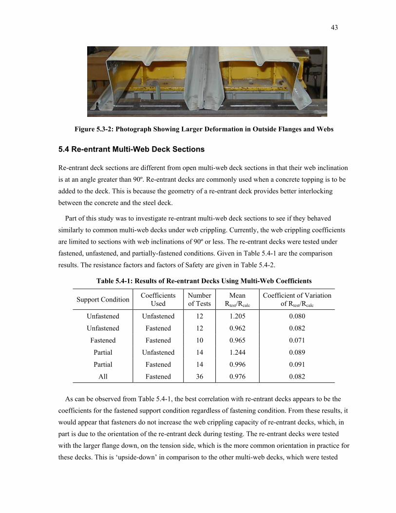
43

Figure 5.3-2: Photograph Showing Larger Deformation in Outside Flanges and Webs

5.4 Re-entrant Multi-Web Deck Sections

Re-entrant deck sections are different from open multi-web deck sections in that their web inclination is at an angle greater than 90º. Re-entrant decks are commonly used when a concrete topping is to be added to the deck. This is because the geometry of a re-entrant deck provides better interlocking between the concrete and the steel deck.

Part of this study was to investigate re-entrant multi-web deck sections to see if they behaved similarly to common multi-web decks under web crippling. Currently, the web crippling coefficients are limited to sections with web inclinations of 90º or less. The re-entrant decks were tested under fastened, unfastened, and partially-fastened conditions. Given in Table 5.4-1 are the comparison results. The resistance factors and factors of Safety are given in Table 5.4-2.

Table 5.4-1: Results of Re-entrant Decks Using Multi-Web Coefficients

Support Condition Coefficients Used

Number of Tests

Mean Rtest/Rcalc

Coefficient of Variation of Rtest/Rcalc

Unfastened Unfastened 12 1.205 0.080

Unfastened Fastened 12 0.962 0.082

Fastened Fastened 10 0.965 0.071

Partial Unfastened 14 1.244 0.089

Partial Fastened 14 0.996 0.091

All Fastened 36 0.976 0.082 As can be observed from Table 5.4-1, the best correlation with re-entrant decks appears to be the

coefficients for the fastened support condition regardless of fastening condition. From these results, it would appear that fasteners do not increase the web crippling capacity of re-entrant decks, which, in part is due to the orientation of the re-entrant deck during testing. The re-entrant decks were tested with the larger flange down, on the tension side, which is the more common orientation in practice for these decks. This is ‘upside-down’ in comparison to the other multi-web decks, which were tested

44

with the larger flange up, on the compression side. This orientation causes the outside web elements to be as equally restrained as the inside web elements at the surface of the bearing plate. Therefore, the mechanism described in Figure 5.4-1 cannot occur and the difference in load capacity between fastened and unfastened re-entrant deck sections will be small.

Figure 5.4-1: Failure of Re-entrant Deck Section

In addition, the coefficient of variation is much lower for re-entrant decks than it was for regular multi-web decks. The most likely explanation for the improved coefficient of variation is that the geometry of the re-entrant deck does not permit the deck to spread. If it were to spread, the flanges would move towards each other and the adjacent webs would meet. Because the coefficient of variation is changed, resistance factors and factor of safety were calculated for re-entrant decks and given in Table 5.4-2.

Table 5.4-2: Resistance Factors and Factors of Safety for Re-entrant Decks

U.S. and Mexico Canada Support Condition

φ Ω φ

Unfastened* 0.863 1.78 0.747

Fastened 0.873 1.76 0.757

All Re-entrant Data* 0.875 1.75 0.758 *Using coefficients for fastened conditions

Again, the resistance factors and factors of safety for re-entrant decks, regardless of support condition, are similar to the resistance factors and factors of safety for regular decks under fully-fastened support conditions. One would expect that the improved coefficient of variation for re-

45

entrant decks would give resistance factors and factors of safety closer to one, but the less conservative mean Rtest-to-Rcalc ratio appears to have negated any such effect.

Regardless of support conditions, the web crippling capacity of re-entrant deck sections can be determined by using the coefficients of regular multi-web deck sections with fixed support conditions. This also suggests that the re-entrant data can be incorporated into the data set for the determination of web crippling coefficients for the fastened support condition.

Including the re-entrant data does not change the coefficients significantly. The values of the modified coefficients, considering fastened support conditions only, are: C = 4, CR = 0.03, CN = 0.24, and Ch = 0.025. Presented in Table 5.4-3 is the statistical comparison of the modified coefficients including the re-entrant data and the coefficients from Table 5.2-1. One can observe upon reviewing the data of Table 5.4-3 that the modified coefficients do not represent a significant change in effectiveness. In fact, the data would suggest that the coefficients proposed in Table 5.2-1 are still a better predictor of the web crippling capacity even though the re-entrant data was not included in their determination.

Table 5.4-3: Comparison of Coefficients When Re-entrant Data is Incorporated

Data Coefficients Used

Number of Tests

Mean Rtest/Rcalc

Coefficient of Variation of Rtest/Rcalc

Fastened Re-entrant and Fastened Multi-web Fastened 86 1.047 0.128

All Re-entrant and Fastened Multi-web Fastened 112 1.031 0.123

Fastened Re-entrant and Fastened Multi-web Modified 86 1.048 0.128

All Re-entrant and Fastened Multi-web Modified 112 1.034 0.123

5.5 Discussion and Recommendations

As was demonstrated by the results shown in Table 5.2-2, improved web crippling coefficients for the case of End One-Flange loading of multi-web sections were developed in this study. While the average test-to-calculated load ratio did not improve significantly, the coefficient of variation did improve, indicating that the new coefficients are more reliable than the previous coefficients.

Considering the coefficients, it is interesting that only the coefficient, C, changes significantly between the fastened and unfastened conditions. This does follow some logic; i.e., since the geometric parameters do not change with the different support conditions, it would follow that the

46

coefficients, CR, CN, and Ch, all of which correspond to different geometric parameters, also would not change. The value of the coefficient, C, increased by 33% between the fastened and unfastened conditions. This is similar to findings by Bhakta (1992) where the web crippling capacity of deck sections increase by 37% when the decks were fastened to their supports.

It was found that partially-fastened deck sections can use the same coefficients as fully-fastened deck sections. Looking at the load-stroke curves, one can observe that the failure loads for partially-fastened specimens are generally lower than for fully-fastened specimens, although they are higher than the failure loads of the unfastened specimens. There is enough scatter in the data that the fully-fastened and partially-fastened specimens appear statistically to be approximately the same.

However, it is not recommended that the NAS (2001a) be amended to allow partially-fastened decks to be treated as fully-fastened, or that the fastening requirements of multi-web decks be lessened. There are other reasons for the fastening requirements of a fully-fastened deck that must also be considered (e.g. wind uplift).

It was found that re-entrant deck sections behave similarly to fastened multi-web deck sections, regardless of their support condition. It is therefore recommended that the NAS be amended so that re-entrant deck sections are included as multi-web deck sections by eliminating the restriction that the web inclination must be less than or equal to 90º.

Since there are two different failure mechanisms that can result with EOF loading of multi-web deck section web crippling, perhaps there should be two different equations for predicting web crippling. It would be worth investigating to see if separate equations would be warranted to predict the web arc yielding capacity and the web rolling capacity of a web element might better predict the web crippling capacity of multi-web deck sections subjected to EOF loading. This would be similar to the equations for web crippling and yielding of hot rolled wide flange beams in clause 15.9 of CAN/CSA-S16-94 (1994a), where the smaller result of two equations is taken to be the web crippling capacity. During testing, it was observed that the horizontal length of the deformation in the web was proportional to the bearing length. As this was beyond the original scope of study, the size of the web deformation was not recorded and further study would be necessary to confirm this observation. If such a link were to be proven, it might enhance the theory regarding the influence of bearing length on web crippling, and possibly further refine the predictability of the web crippling capacity.

It is therefore recommended that further research, involving a theoretical study and experimentation, be undertaken to examine the possibility of there being two equations, one that would predict the web rolling mechanism and one that would predict the web arc mechanism.

47

References

American Iron and Steel Institute (1980), Specification for the Design of Cold-Formed Steel

Structural Members, 1980 Edition, Washington, D.C., U.S.A., 1980.

American Iron and Steel Institute (1999), Specification for the Design of Cold-Formed Steel

Structural Members with Commentary, 1996 Edition, Supplement No.1, Washington, D.C.,

U.S.A., 1999.

American Iron and Steel Institute (2001a), North American Specification for the Design of Cold

Formed Steel Structural Members, 2001 Edition, Washington, DC, U.S.A., 2001.

American Iron and Steel Institute, (2001b) Commentary on the 2001 Edition of the North American

Specification for the Design of Cold Formed Steel Structural Members, 2001 Edition,

Washington, DC, U.S.A., 2001.

American Society for Testing Materials (2002), “Standard Test Methods and Definitions for

Mechanical Testing of Steel Products,” ASTM 370, 2002.

Avci, O. and W.S. Easterling (2002), “Web Crippling Strength of Multi-Web Steel Deck Sections

Subjected to End One-Flange Loading,” Virginia Polytechnic Institute and State University,

Blacksburg, VA, U.S.A., 2002.

Baehre, R. (1975), “Sheet Metal Panels for Use in Building Construction – Recent Research Projects

in Sweden,” Proceeding of the Third International Specialty Conference on Cold Formed Steel

Structures, University of Missouri-Rolla, Rolla, MO, U.S.A., November 1975.

Bakker, M.C.M. (1992), “Web Crippling of Cold-formed Steel Members,” Thesis, Eindhoven

University of Technology, Eindhoven, Holland, 1992.

Beshara, B. (1999), “Web Crippling of Cold-Formed Steel Members,” M.A.Sc. Thesis, University of

Waterloo, Waterloo, ON, Canada, 1999.

Beshara, B. and R.M. Schuster (2000), “Web Crippling Data and Calibrations of Cold-Formed Steel

Members,” Final Report, University of Waterloo, Waterloo, Canada, 2000.

Bhakta, B.H., R.A. LaBoube, and W.W. Yu (1992), “The Effect of Flange Restraint on Web

Crippling Strength,” Final Report, Civil Engineering Study 92-1, University of Missouri-Rolla,

Rolla, MO, U.S.A., March 1992.

Canadian Standards Association (1994a), Limit States Design of Steel Structures,

CAN/CSA-S16.1-94, Rexdale, ON, Canada, 1994.

48

Canadian Standards Association (1984), Cold Formed Steel Structural Members,

CAN/CSA-S136-84, Rexdale, ON, Canada, 1984.

Canadian Standards Association (1994b), Cold Formed Steel Structural Members,

CAN/CSA-S136-94, Rexdale, ON, Canada, 1994.

Cornell (1952), “65th Progress Reports on Light Gage Steel Beams of Cold Formed Steel,” Cornell

University, New York, NY, U.S.A., September 1952 (unpublished).

Cornell (1953), “66th Progress Reports on Light Gage Steel Beams of Cold Formed Steel,” Cornell

University, New York, NY, U.S.A., January 1953 (unpublished).

Gerges, R. R., (1997) “Web Crippling of Single Web Cold Formed Steel Members Subjected to End

One-Flange Loading.” M.A.Sc. Thesis, University of Waterloo, Waterloo, ON, Canada, 1997.

Gerges, R.R., and R.M. Schuster (1998), “Web Crippling of Members Using High-Strength Steels,”

Proceedings of the Fourteenth International Specialty Conference on Cold-Formed Steel

Structures, University of Missouri-Rolla, Rolla, MO, U.S.A., October 1998.

Johnson, R. A. (1994), Miller and Freund’s Probability and Statistics for Engineers, Prentice-Hall,

Inc., Englewood Cliffs, NJ, U.S.A., 1994.

Hetrakul, N. and W.W. Yu (1978), “Structural Behaviour of Beam Webs Subjected to Web Crippling

and a Combination of Web Crippling and Bending,” Final Report, Civil Engineering Study

78-4, University of Missouri-Rolla, Rolla, MO, USA, June 1978.

Microsoft Developer Network (2000), “XL: Solver Uses Generalized Reduced Gradient Algorithm.”

MSDN Library, CD-ROM, Microsoft Press, March 2000.

Microsoft Developer Network (2000), “XL: How to Find Resources on Microsoft Excel Solver.”

MSDN Library, CD-ROM, Microsoft Press, March 2000.

Prabakaran, K. (1993), “Web Crippling of Cold Formed Steel Sections,” M.A.Sc. Thesis, University

of Waterloo, Waterloo, Ontario, Canada, 1993.

Prabakaran, K and R.M. Schuster (1998), “Web Crippling of Cold-Formed Steel Sections,”

Proceedings of the Fourteenth International Specialty Conference on Cold Formed Steel

Structures, University of Missouri-Rolla, Rolla, MO, U.S.A., October 1998.

Studnička, J. (1989), “Web Crippling of Multi-Web Deck Sections,” Czech Technical University,

Prague, Czech Republic, 1989.

49

Wing, B.A. (1981), “Web Crippling and the Interaction of Bending and Web Crippling of

Unreinforced Multi-Web Cold-Formed Steel Sections.” M.A.Sc. Thesis, University of

Waterloo, Waterloo, ON, Canada, 1981.

Wing, B.A. and R.M. Schuster (1982), “Web Crippling for Decks Subjected to Two-Flange

Loading,” Proceedings of the Sixth International Specialty Conference on Cold Formed Steel

Structures, University of Missouri-Rolla, Rolla, MO, U.S.A., November 1982.

Winter, G. and R.H.J. Pian (1946), “Crushing Strength of Thin Steel Webs,” Cornell Bulletin 35,

pt. 1, Cornell University, NY, U.S.A., April 1946.

Wu, S., W.W. Yu and R.A. LaBoube (1997), “Strength of Flexural Members Using Structural Grade

80 of A653 Steel (Web Crippling Tests),” Third Progress Report, Civil Engineering Study 97-

3, University of Missouri-Rolla, Rolla, MO, U.S.A., February 1997.

Yu, W.W. (1981), “Web Crippling and Combined Web Crippling and Bending of Steel Decks,” Civil

Engineering Study 81-2, University of Missouri-Rolla, Rolla, MO, U.S.A., April 1981

(unpublished).

50

Appendix A Material Properties of Specimens

Table A-1: Mechanical Properties of Specimens

Test Series ID Base Steel

Thickness*, mm (in.)

Yield Strength*, Fy,MPa (ksi)

Ultimate Strength* Fu, MPa (ksi)

Percent Elongation** (%)

C1 1.16 (0.046) 340 (49.3) 423 (61.4) 35.2 C2 0.85 (0.033) 310 (45.0) 372 (54.0) 37.2 C3 0.86 (0.034) 304 (44.1) 365 (52.9) 37.6 E1 0.73 (0.029) 345 (50.0) 421 (61.1) 33.9 E2 0.90 (0.035) 326 (47.3) 376 (54.5) 35.8 E3 1.18 (0.044) 314 (45.5) 461 (66.9) 31.9 E4 1.13 (0.044) 309 (44.8) 389 (56.4) 32.7 E5 0.88 (0.035) 375 (54.4) 415 (60.2) 34.1 R1 0.72 (0.028) 310 (45.0) 400 (58.0) 30.6 R2 0.87 (0.034) 327 (47.4) 411 (59.6) 30.2 R3 1.18 (0.046) 341 (49.5) 381 (55.3) 36.9 T1 0.72 (0.028) 335 (48.6) 410 (59.5) 29.7 T2 0.88 (0.035) 349 (50.6) 421 (61.1) 29.3 T3 1.13 (0.044) 329 (47.7) 391 (56.7) 33.7 U1 1.11 (0.044) 299 (43.4) 386 (56.0) 36.2 U2 0.87 (0.034) 337 (48.9) 418 (60.6) 32.7 U3 0.68 (0.027) 329 (47.7) 417 (60.5) 31.5 U4 0.88 (0.035) 319 (46.3) 395 (57.3) 35.0 U5 0.89 (0.035) 347 (50.3) 400 (58.0) 36.3 U6 1.15 (0.045) 300 (43.5) 380 (55.1) 38.3 U7 1.43 (0.056) 306 (44.4) 380 (55.1) 37.7 U8 1.16 (0.046) 344 (49.9) 413 (59.9) 33.3 U9 0.88 (0.035) 326 (47.3) 401 (58.2) 34.6 V1 0.72 (0.028) 321 (46.6) 384 (55.7) 36.9 V2 1.19 (0.047) 322 (46.7) 374 (54.2) 38.9 V3 0.86 (0.034) 328 (47.6) 395 (57.3) 36.6 V4 0.72 (0.028) 335 (48.6) 380 (55.1) 37.4 V5 1.19 (0.047) 311 (45.1) 367 (53.2) 36.8 W1 0.91 (0.036) 663 (96.2) 668 (96.9) 4.59 W2 1.20 (0.047) 674 (97.8) 683 (99.1) 9.67

*Properties are based on the average of three coupon tests **Elongation over 50 mm gauge length, based on the average of three coupon tests

51

Appendix B Geometric Properties of Specimens

5.6 Table B-1: Geometric Properties of Unfastened Specimens

Test Series Specimen # of Webs θ (º) t, mm (in.) R/t N/t h/t CAN30-4-1-NONE 4 77 1.16 (0.046) 2.76 20.7 59.4 C1 CAN30-4-2-NONE 4 77 1.16 (0.046) 2.76 43.1 59.4 CAN30-4-1-NONE 4 77 0.85 (0.033) 4.71 28.2 79.6 CAN30-4-2-NONE 4 77 0.85 (0.033) 4.71 58.8 79.6 CAN30-4-2-NONE 4 77 0.85 (0.033) 4.71 58.8 79.6

C2

CAN30-4-3-NONE 4 77 0.85 (0.033) 4.71 88.2 79.6 CAN30-4-1-NONE 4 77 0.86 (0.034) 4.65 27.9 78.6

C3 CAN30-4-2-NONE 4 77 0.86 (0.034) 4.65 58.1 78.6 CAN30-4-3-NONE 4 77 0.86 (0.034) 4.65 87.2 78.6 WHE45-4-1-NONE 4 84 0.91 (0.036) 6.15 26.4 113

W1 WHE45-4-2-NONE 4 84 0.91 (0.036) 6.15 54.9 113 WHE45-4-3-NONE 4 84 0.91 (0.036) 6.15 82.4 113 WHE45-4-1-NONE 4 84 1.20 (0.047) 4.67 20.0 85.2

W2 WHE45-4-2-NONE 4 84 1.20 (0.047) 4.67 41.7 85.2 WHE45-4-3-NONE 4 84 1.20 (0.047) 4.67 62.5 85.2 VIC30-4-1-NONE 4 71 0.72 (0.028) 6.61 33.3 96.0

V1 VIC30-4-2-NONE 4 71 0.72 (0.028) 6.61 69.4 96.0 VIC30-4-3-NONE 4 71 0.72 (0.028) 6.61 104 96.0 VIC30-4-2-NONE 4 74 1.19 (0.047) 4.00 42.0 56.7

V2 VIC30-4-1-NONE 4 74 1.19 (0.047) 4.00 20.2 56.7 VIC30-4-3-NONE 4 74 1.19 (0.047) 4.00 63.0 56.7 VIC30-8-1-NONE 8 85 0.86 (0.034) 5.08 27.9 78.3

V3 VIC30-8-2-NONE 8 85 0.86 (0.034) 5.08 58.1 78.3 VIC30-8-3-NONE 8 86 0.86 (0.034) 5.08 87.2 78.2 VIC30-8-1-NONE 8 86 0.72 (0.028) 6.07 33.3 93.6

V4 VIC30-8-2-NONE 8 85 0.72 (0.028) 6.07 69.4 93.8 VIC30-8-3-NONE 8 85 0.72 (0.028) 6.07 104 93.8 VIC30-8-3-NONE 8 85 1.19 (0.047) 3.67 63.0 56.3

V5 VIC30-8-2-NONE 8 85 1.19 (0.047) 3.67 42.0 56.3 VIC30-8-1-NONE 8 85 1.19 (0.047) 3.67 20.2 56.3 CMRM30-6-3-NONE 6 82 0.72 (0.028) 19.9 104.2 68.2

R1 CMRM30-6-2-NONE 6 82 0.72 (0.028) 19.9 69.4 68.2 CMRM30-6-1-NONE 6 82 0.72 (0.028) 19.9 33.3 68.2 CMRM30-6-3-NONE 6 82 0.87 (0.034) 16.4 86.2 56.3

R2 CMRM30-6-2-NONE 6 82 0.87 (0.034) 16.4 57.5 56.3 CMRM30-6-1-NONE 6 82 0.87 (0.034) 16.4 27.6 56.3 CMRM30-6-3-NONE 6 81 1.18 (0.046) 12.1 63.6 41.4

R3 CMRM30-6-2-NONE 6 81 1.18 (0.046) 12.1 42.4 41.4 CMRM30-6-1-NONE 6 81 1.18 (0.046) 12.1 20.3 41.4

CAN15-12-1-NONE 12 71 0.88 (0.035) 8.11 27.3 26.9 T2 CAN15-12-3-NONE 12 71 0.88 (0.035) 8.11 85.2 26.9

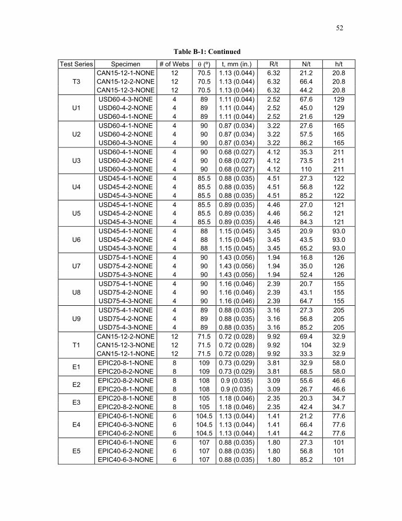
52

Table B-1: Continued

Test Series Specimen # of Webs θ (º) t, mm (in.) R/t N/t h/t CAN15-12-1-NONE 12 70.5 1.13 (0.044) 6.32 21.2 20.8

T3 CAN15-12-2-NONE 12 70.5 1.13 (0.044) 6.32 66.4 20.8 CAN15-12-3-NONE 12 70.5 1.13 (0.044) 6.32 44.2 20.8 USD60-4-3-NONE 4 89 1.11 (0.044) 2.52 67.6 129

U1 USD60-4-2-NONE 4 89 1.11 (0.044) 2.52 45.0 129 USD60-4-1-NONE 4 89 1.11 (0.044) 2.52 21.6 129 USD60-4-1-NONE 4 90 0.87 (0.034) 3.22 27.6 165

U2 USD60-4-2-NONE 4 90 0.87 (0.034) 3.22 57.5 165 USD60-4-3-NONE 4 90 0.87 (0.034) 3.22 86.2 165 USD60-4-1-NONE 4 90 0.68 (0.027) 4.12 35.3 211

U3 USD60-4-2-NONE 4 90 0.68 (0.027) 4.12 73.5 211 USD60-4-3-NONE 4 90 0.68 (0.027) 4.12 110 211 USD45-4-1-NONE 4 85.5 0.88 (0.035) 4.51 27.3 122

U4 USD45-4-2-NONE 4 85.5 0.88 (0.035) 4.51 56.8 122 USD45-4-3-NONE 4 85.5 0.88 (0.035) 4.51 85.2 122 USD45-4-1-NONE 4 85.5 0.89 (0.035) 4.46 27.0 121

U5 USD45-4-2-NONE 4 85.5 0.89 (0.035) 4.46 56.2 121 USD45-4-3-NONE 4 85.5 0.89 (0.035) 4.46 84.3 121 USD45-4-1-NONE 4 88 1.15 (0.045) 3.45 20.9 93.0

U6 USD45-4-2-NONE 4 88 1.15 (0.045) 3.45 43.5 93.0 USD45-4-3-NONE 4 88 1.15 (0.045) 3.45 65.2 93.0 USD75-4-1-NONE 4 90 1.43 (0.056) 1.94 16.8 126

U7 USD75-4-2-NONE 4 90 1.43 (0.056) 1.94 35.0 126 USD75-4-3-NONE 4 90 1.43 (0.056) 1.94 52.4 126 USD75-4-1-NONE 4 90 1.16 (0.046) 2.39 20.7 155

U8 USD75-4-2-NONE 4 90 1.16 (0.046) 2.39 43.1 155 USD75-4-3-NONE 4 90 1.16 (0.046) 2.39 64.7 155 USD75-4-1-NONE 4 89 0.88 (0.035) 3.16 27.3 205

U9 USD75-4-2-NONE 4 89 0.88 (0.035) 3.16 56.8 205 USD75-4-3-NONE 4 89 0.88 (0.035) 3.16 85.2 205 CAN15-12-2-NONE 12 71.5 0.72 (0.028) 9.92 69.4 32.9

T1 CAN15-12-3-NONE 12 71.5 0.72 (0.028) 9.92 104 32.9 CAN15-12-1-NONE 12 71.5 0.72 (0.028) 9.92 33.3 32.9

EPIC20-8-1-NONE 8 109 0.73 (0.029) 3.81 32.9 58.0 E1 EPIC20-8-2-NONE 8 109 0.73 (0.029) 3.81 68.5 58.0 EPIC20-8-2-NONE 8 108 0.9 (0.035) 3.09 55.6 46.6 E2 EPIC20-8-1-NONE 8 108 0.9 (0.035) 3.09 26.7 46.6 EPIC20-8-1-NONE 8 105 1.18 (0.046) 2.35 20.3 34.7 E3 EPIC20-8-2-NONE 8 105 1.18 (0.046) 2.35 42.4 34.7

EPIC40-6-1-NONE 6 104.5 1.13 (0.044) 1.41 21.2 77.6 E4 EPIC40-6-3-NONE 6 104.5 1.13 (0.044) 1.41 66.4 77.6

EPIC40-6-2-NONE 6 104.5 1.13 (0.044) 1.41 44.2 77.6 EPIC40-6-1-NONE 6 107 0.88 (0.035) 1.80 27.3 101

E5 EPIC40-6-2-NONE 6 107 0.88 (0.035) 1.80 56.8 101 EPIC40-6-3-NONE 6 107 0.88 (0.035) 1.80 85.2 101

53

Table B-2: Geometric Properties of Fastened Specimens

Test Series Specimen # of Webs θ (º) t, mm (in.) R/t N/t h/t CAN30-4-1-ALL 4 77 1.16 (0.046) 2.76 20.7 59.4

C1 CAN30-4-2-ALL 4 77 1.16 (0.046) 2.76 43.1 59.4 CAN30-4-1-ALL 4 77 1.16 (0.046) 2.76 20.7 59.4 CAN30-4-1-ALL 4 77 0.85 (0.033) 4.71 28.2 79.6

C2 CAN30-4-2-ALL 4 77 0.85 (0.033) 4.71 58.8 79.6 CAN30-4-3-ALL 4 77 0.85 (0.033) 4.71 88.2 79.6 CAN30-4-1-ALL 4 77 0.86 (0.034) 4.65 27.9 78.6

C3 CAN30-4-2-ALL 4 77 0.86 (0.034) 4.65 58.1 78.6 CAN30-4-3-ALL 4 77 0.86 (0.034) 4.65 87.2 78.6

WHE45-4-1-ALL 4 84 0.91 (0.036) 6.15 26.4 113 WHE45-4-2-ALL 4 84 0.91 (0.036) 6.15 54.9 113 WHE45-4-3-ALL 4 84 0.91 (0.036) 6.15 82.4 113

W1

WHE45-4-3-ALL 4 84 0.91 (0.036) 6.15 82.4 113 WHE45-4-1-ALL 4 84 1.20 (0.047) 4.67 20.0 85.2

W2 WHE45-4-2-ALL 4 84 1.20 (0.047) 4.67 41.7 85.2 WHE45-4-3-ALL 4 84 1.20 (0.047) 4.67 62.5 85.2

VIC30-4-1-ALL 4 71 0.72 (0.028) 6.61 33.3 96.0 VIC30-4-1-ALL 4 71 0.72 (0.028) 6.61 33.3 96.0 VIC30-4-2-ALL 4 71 0.72 (0.028) 6.61 69.4 96.0

V1

VIC30-4-3-ALL 4 71 0.72 (0.028) 6.61 104 96.0 VIC30-4-2-ALL 4 74 1.19 (0.047) 4.00 42.0 56.7

V2 VIC30-4-1-ALL 4 74 1.19 (0.047) 4.00 20.2 56.7 VIC30-4-3-ALL 4 74 1.19 (0.047) 4.00 63.0 56.7 VIC30-8-1-ALL 8 85 0.86 (0.034) 5.08 27.9 78.3

V3 VIC30-8-3-ALL 8 85 0.86 (0.034) 5.08 87.2 78.3 VIC30-8-2-ALL 8 86 0.86 (0.034) 5.08 58.1 78.2 VIC30-8-1-ALL 8 86 0.72 (0.028) 6.07 33.3 93.6

V4 VIC30-8-2-ALL 8 85 0.72 (0.028) 6.07 69.4 93.8 VIC30-8-3-ALL 8 85 0.72 (0.028) 6.07 104 93.8

VIC30-8-2-ALL 8 85 1.19 (0.047) 3.67 42.0 56.3 V5 VIC30-8-1-ALL 8 85 1.19 (0.047) 3.67 20.2 56.3

CMRM30-6-3-ALL 6 82 0.72 (0.028) 19.9 104 68.2 R1 CMRM30-6-2-ALL 6 82 0.72 (0.028) 19.9 69.4 68.2

CMRM30-6-1-ALL 6 82 0.72 (0.028) 19.9 33.3 68.2 CMRM30-6-3-ALL 6 82 0.87 (0.034) 16.4 86.2 56.3 R2 CMRM30-6-1-ALL 6 82 0.87 (0.034) 16.4 27.6 56.3

CMRM30-6-3-ALL 6 81 1.18 (0.046) 12.1 63.6 41.4 R3 CMRM30-6-2-ALL 6 81 1.18 (0.046) 12.1 42.4 41.4

CMRM30-6-1-ALL 6 81 1.18 (0.046) 12.1 20.3 41.4 CAN15-12-1-2NDS 12 71 0.88 (0.035) 8.11 27.3 26.9

T2 CAN15-12-2-2NDS 12 71 0.88 (0.035) 8.11 56.8 26.9 CAN15-12-3-2NDS 12 71 0.88 (0.035) 8.11 85.2 26.9 CAN15-12-1-2NDS 12 70.5 1.13 (0.044) 6.32 21.2 20.8

T3 CAN15-12-2-2NDS 12 70.5 1.13 (0.044) 6.32 66.4 20.8 CAN15-12-3-2NDS 12 70.5 1.13 (0.044) 6.32 44.2 20.8

54

Table B-2: Continued

Test Series Specimen # of Webs θ (º) t, mm (in.) R/t N/t h/t USD60-4-3-ALL 4 89 1.11 (0.044) 2.52 67.6 129

U1 USD60-4-2-ALL 4 89 1.11 (0.044) 2.52 45.0 129 USD60-4-1-ALL 4 89 1.11 (0.044) 2.52 21.6 129 USD60-4-1-ALL 4 90 0.87 (0.034) 3.22 27.6 165

U2 USD60-4-2-ALL 4 90 0.87 (0.034) 3.22 57.5 165 USD60-4-3-ALL 4 90 0.87 (0.034) 3.22 86.2 165 USD60-4-1-ALL 4 90 0.68 (0.027) 4.12 35.3 211

U3 USD60-4-2-ALL 4 90 0.68 (0.027) 4.12 73.5 211 USD60-4-3-ALL 4 90 0.68 (0.027) 4.12 110 211 USD45-4-1-ALL 4 85.5 0.88 (0.035) 4.51 27.3 122

U4 USD45-4-2-ALL 4 85.5 0.88 (0.035) 4.51 56.8 122 USD45-4-3-ALL 4 85.5 0.88 (0.035) 4.51 85.2 122 USD45-4-1-ALL 4 85.5 0.89 (0.035) 4.46 27.0 121

U5 USD45-4-2-ALL 4 85.5 0.89 (0.035) 4.46 56.2 121 USD45-4-3-ALL 4 85.5 0.89 (0.035) 4.46 84.3 121 USD45-4-1-ALL 4 88 1.15 (0.045) 3.45 20.9 93.0

U6 USD45-4-2-ALL 4 88 1.15 (0.045) 3.45 43.5 93.0 USD45-4-3-ALL 4 88 1.15 (0.045) 3.45 65.2 93.0 USD75-4-1-ALL 4 90 1.43 (0.056) 1.94 16.8 126

U7 USD75-4-2-ALL 4 90 1.43 (0.056) 1.94 35.0 126 USD75-4-3-ALL 4 90 1.43 (0.056) 1.94 52.4 126 USD75-4-1-ALL 4 90 1.16 (0.046) 2.39 20.7 155

U8 USD75-4-2-ALL 4 90 1.16 (0.046) 2.39 43.1 155 USD75-4-3-ALL 4 90 1.16 (0.046) 2.39 64.7 155 USD75-4-1-ALL 4 89 0.88 (0.035) 3.16 27.3 205

U9 USD75-4-2-ALL 4 89 0.88 (0.035) 3.16 56.8 205 USD75-4-3-ALL 4 89 0.88 (0.035) 3.16 85.2 205 CAN15-12-2-2NDS 12 71.5 0.72 (0.028) 9.92 69.4 32.9

T1 CAN15-12-3-2NDS 12 71.5 0.72 (0.028) 9.92 104 32.9 CAN15-12-1-2NDS 12 71.5 0.72 (0.028) 9.92 33.3 32.9

EPIC20-8-1-ALL 8 109 0.73 (0.029) 3.81 32.9 58.0 E1 EPIC20-8-2-ALL 8 109 0.73 (0.029) 3.81 68.5 58.0 EPIC20-8-2-ALL 8 108 0.9 (0.035) 3.09 55.6 46.6 E2 EPIC20-8-1-ALL 8 108 0.9 (0.035) 3.09 26.7 46.6

E3 EPIC20-8-1-ALL 8 105 1.18 (0.046) 2.35 20.3 34.7 EPIC40-6-1-ALL 6 104 1.13 (0.044) 1.41 21.2 77.6 E4 EPIC40-6-2-ALL 6 104 1.13 (0.044) 1.41 44.2 77.6

EPIC40-6-1-ALL 6 107 0.88 (0.035) 1.80 27.3 101 E5 EPIC40-6-2-ALL 6 107 0.88 (0.035) 1.80 56.8 101

EPIC40-6-3-ALL 6 107 0.88 (0.035) 1.80 85.2 101

55

Table B-3: Geometric Properties of Partially-Fastened Specimens

Test Series Specimen # of Webs θ (º) t, mm (in.) R/t N/t h/t CAN30-4-1-ENDS 4 77 1.16 (0.046) 2.76 20.7 59.4 C1 CAN30-4-2-ENDS 4 77 1.16 (0.046) 2.76 43.1 59.4

CAN30-4-1-ENDS 4 77 0.85 (0.033) 4.71 28.2 79.6 C2 CAN30-4-2-ENDS 4 77 0.85 (0.033) 4.71 58.8 79.6

CAN30-4-3-ENDS 4 77 0.85 (0.033) 4.71 88.2 79.6 CAN30-4-1-ENDS 4 77 0.86 (0.034) 4.65 27.9 78.6

C3 CAN30-4-2-ENDS 4 77 0.86 (0.034) 4.65 58.1 78.6 CAN30-4-3-ENDS 4 77 0.86 (0.034) 4.65 87.2 78.6 WHE45-4-1-ENDS 4 84 0.91 (0.036) 6.15 26.4 113

W1 WHE45-4-2-ENDS 4 84 0.91 (0.036) 6.15 54.9 113 WHE45-4-3-ENDS 4 84 0.91 (0.036) 6.15 82.4 113 WHE45-4-1-ENDS 4 84 1.20 (0.047) 4.67 20.0 85.2

W2 WHE45-4-2-ENDS 4 84 1.20 (0.047) 4.67 41.7 85.2 WHE45-4-3-ENDS 4 84 1.20 (0.047) 4.67 62.5 85.2 VIC30-4-1-ENDS 4 71 0.72 (0.028) 6.61 33.3 96.0

V1 VIC30-4-2-ENDS 4 71 0.72 (0.028) 6.61 69.4 96.0 VIC30-4-3-ENDS 4 71 0.72 (0.028) 6.61 104 96.0 VIC30-4-2-ENDS 4 74 1.19 (0.047) 4.00 42.0 56.7

V2 VIC30-4-1-ENDS 4 74 1.19 (0.047) 4.00 20.2 56.7 VIC30-4-3-ENDS 4 74 1.19 (0.047) 4.00 63.0 56.7 VIC30-8-1-ENDS 8 85 0.86 (0.034) 5.08 27.9 78.3

V3 VIC30-8-3-ENDS 8 85 0.86 (0.034) 5.08 87.2 78.3 VIC30-8-2-ENDS 8 86 0.86 (0.034) 5.08 58.1 78.2 VIC30-8-1-ENDS 8 86 0.72 (0.028) 6.07 33.3 93.6

V4 VIC30-8-2-ENDS 8 85 0.72 (0.028) 6.07 69.4 93.8 VIC30-8-3-ENDS 8 85 0.72 (0.028) 6.07 104 93.8 VIC30-8-3-ENDS 8 85 1.19 (0.047) 3.67 63.0 56.3

V5 VIC30-8-2-ENDS 8 85 1.19 (0.047) 3.67 42.0 56.3 VIC30-8-1-ENDS 8 85 1.19 (0.047) 3.67 20.2 56.3 CMRM30-6-3-ENDS 6 82 0.72 (0.028) 19.9 104.2 68.2

R1 CMRM30-6-2-ENDS 6 82 0.72 (0.028) 19.9 69.4 68.2 CMRM30-6-1-ENDS 6 82 0.72 (0.028) 19.9 33.3 68.2 CMRM30-6-3-ENDS 6 82 0.87 (0.034) 16.4 86.2 56.3

R2 CMRM30-6-2-ENDS 6 82 0.87 (0.034) 16.4 57.5 56.3 CMRM30-6-1-ENDS 6 82 0.87 (0.034) 16.4 27.6 56.3 CMRM30-6-3-ENDS 6 81 1.18 (0.046) 12.1 63.6 41.4

R3 CMRM30-6-2-ENDS 6 81 1.18 (0.046) 12.1 42.4 41.4 CMRM30-6-1-ENDS 6 81 1.18 (0.046) 12.1 20.3 41.4 CAN15-12-1-ENDS 12 71 0.88 (0.035) 8.11 27.3 26.9 CAN15-12-1-3RDS 12 71 0.88 (0.035) 8.11 27.3 26.9

CAN15-12-2-ENDS 12 71 0.88 (0.035) 8.11 56.8 26.9 T2 CAN15-12-2-3RDS 12 71 0.88 (0.035) 8.11 56.8 26.9 CAN15-12-3-ENDS 12 71 0.88 (0.035) 8.11 85.2 26.9 CAN15-12-3-3RDS 12 71 0.88 (0.035) 8.11 85.2 26.9

56

Table B-3: Continued

Test Series Specimen # of Webs θ (º) t, mm (in.) R/t N/t h/t CAN15-12-1-ENDS 12 70.5 1.13 (0.044) 6.32 21.2 20.8 CAN15-12-1-3RDS 12 70.5 1.13 (0.044) 6.32 21.2 20.8 CAN15-12-2-ENDS 12 70.5 1.13 (0.044) 6.32 66.4 20.8 CAN15-12-2-3RDS 12 70.5 1.13 (0.044) 6.32 66.4 20.8 CAN15-12-3-ENDS 12 70.5 1.13 (0.044) 6.32 44.2 20.8

T3

CAN15-12-3-3RDS 12 70.5 1.13 (0.044) 6.32 44.2 20.8 USD60-4-3-ENDS 4 89 1.11 (0.044) 2.52 67.6 129

U1 USD60-4-2-ENDS 4 89 1.11 (0.044) 2.52 45.0 129 USD60-4-1-ENDS 4 89 1.11 (0.044) 2.52 21.6 129 USD60-4-1-ENDS 4 90 0.87 (0.034) 3.22 27.6 165

U2 USD60-4-2-ENDS 4 90 0.87 (0.034) 3.22 57.5 165 USD60-4-3-ENDS 4 90 0.87 (0.034) 3.22 86.2 165 USD60-4-1-ENDS 4 90 0.68 (0.027) 4.12 35.3 211

U3 USD60-4-2-ENDS 4 90 0.68 (0.027) 4.12 73.5 211 USD60-4-3-ENDS 4 90 0.68 (0.027) 4.12 110 211 USD45-4-1-ENDS 4 85.5 0.88 (0.035) 4.51 27.3 122

U4 USD45-4-2-ENDS 4 85.5 0.88 (0.035) 4.51 56.8 122 USD45-4-3-ENDS 4 85.5 0.88 (0.035) 4.51 85.2 122 USD45-4-1-ENDS 4 85.5 0.89 (0.035) 4.46 27.0 121

U5 USD45-4-2-ENDS 4 85.5 0.89 (0.035) 4.46 56.2 121 USD45-4-3-ENDS 4 85.5 0.89 (0.035) 4.46 84.3 121 USD45-4-1-ENDS 4 88 1.15 (0.045) 3.45 20.9 93.0

U6 USD45-4-2-ENDS 4 88 1.15 (0.045) 3.45 43.5 93.0 USD45-4-3-ENDS 4 88 1.15 (0.045) 3.45 65.2 93.0 USD75-4-1-ENDS 4 90 1.43 (0.056) 1.94 16.8 126

U7 USD75-4-2-ENDS 4 90 1.43 (0.056) 1.94 35.0 126 USD75-4-3-ENDS 4 90 1.43 (0.056) 1.94 52.4 126 USD75-4-1-ENDS 4 90 1.16 (0.046) 2.39 20.7 155

U8 USD75-4-2-ENDS 4 90 1.16 (0.046) 2.39 43.1 155 USD75-4-3-ENDS 4 90 1.16 (0.046) 2.39 64.7 155 USD75-4-1-ENDS 4 89 0.88 (0.035) 3.16 27.3 205

U9 USD75-4-2-ENDS 4 89 0.88 (0.035) 3.16 56.8 205 USD75-4-3-ENDS 4 89 0.88 (0.035) 3.16 85.2 205 EPIC20-8-1-ENDS 8 109 0.73 (0.029) 3.81 32.9 58.0

E1 EPIC20-8-2-ENDS 8 109 0.73 (0.029) 3.81 68.5 58.0 EPIC20-8-3-ENDS 8 109 0.73 (0.029) 3.81 103 58.0 EPIC20-8-3-ENDS 8 108 0.9 (0.035) 3.09 83.3 46.6

E2 EPIC20-8-2-ENDS 8 108 0.9 (0.035) 3.09 55.6 46.6 EPIC20-8-1-ENDS 8 108 0.9 (0.035) 3.09 26.7 46.6

EPIC20-8-1-ENDS 8 105 1.18 (0.046) 2.35 20.3 34.7 E3 EPIC20-8-2-ENDS 8 105 1.18 (0.046) 2.35 42.4 34.7

EPIC40-6-1-ENDS 6 104 1.13 (0.044) 1.41 21.2 77.6 E4 EPIC40-6-3-ENDS 6 104 1.13 (0.044) 1.41 66.4 77.6

EPIC40-6-2-ENDS 6 104 1.13 (0.044) 1.41 44.2 77.6

57

Table B-3: Continued

Test Series Specimen # of Webs θ (º) t, mm (in.) R/t N/t h/t EPIC40-6-1-ENDS 6 107 0.88 (0.035) 1.80 27.3 101

E5 EPIC40-6-2-ENDS 6 107 0.88 (0.035) 1.80 56.8 101 EPIC40-6-3-ENDS 6 107 0.88 (0.035) 1.80 85.2 101

Table B-4: Geometric Properties of Unfastened Data by Yu (1981)

Specimen # of Webs θ (º) t, mm (in.) R/t N/t h/t Fy (ksi) EOF-1A 4 62.4 0.74 (0.029) 6.85 102 70.7 43.3 EOF-1B 4 61.6 0.74 (0.029) 6.83 102 70.6 43.3 EOF-2A 4 62.1 0.76 (0.030) 6.98 197 67.3 43.3 EOF-2B 4 62.7 0.75 (0.030) 7.09 200 68.8 43.3 EOF-3A 4 63.7 1.12 (0.044) 4.52 67.4 44.9 42.9 EOF-3B 4 63.0 1.14 (0.045) 4.47 66.7 44.7 42.9 EOF-4A 4 64.4 1.20 (0.047) 4.45 126 42.3 42.9 EOF-4B 4 64.5 1.20 (0.047) 4.46 126 42.1 42.9 EOF-5A 4 69.5 0.79 (0.031) 6.43 95.8 94.7 48.1 EOF-5B 4 70.0 0.81 (0.032) 6.31 94.0 93.0 48.1 EOF-6A 4 70.5 0.74 (0.029) 6.83 202 97.8 48.1 EOF-6B 4 70.0 0.75 (0.029) 6.80 202 99.5 48.1 EOF-7A 4 71.3 1.24 (0.049) 3.89 61.1 58.8 41.2 EOF-7B 4 72.2 1.22 (0.048) 3.97 62.2 60.1 41.2 EOF-8A 4 71.3 1.17 (0.046) 4.57 129 61.3 41.2 EOF-8B 4 71.3 1.22 (0.048) 4.38 124 57.8 41.2 EOF-19A 10 75.9 0.73 (0.029) 4.86 103 59.4 41.2 EOF-19B 10 75.1 0.73 (0.029) 4.88 104 58.4 41.2

Table B-5: Geometric Properties of Unfastened Data by Wu (1997)

Specimen # of Webs θ (º) t, mm (in.) R/t N/t h/t Fy (ksi) t26h0.75R3/32*60 4 61.0 0.43 (0.017) 5.47 58.8 45.3 112 t26h0.75R3/64*60 4 61.0 0.43 (0.017) 2.76 58.8 45.3 112 t26h1.5R3/32*60 4 61.0 0.43 (0.017) 5.47 58.8 90.0 112 t26h1.5R3/64*60 4 60.1 0.43 (0.017) 2.76 58.8 88.8 112 t22h0.75R5/64*60 4 60.4 0.74 (0.029) 2.69 34.5 27.9 104 t22h0.75R1/16*60 4 60.6 0.74 (0.029) 2.17 34.5 25.9 104 t22h1.5R5/64*60 4 59.8 0.74 (0.029) 2.69 34.5 53.4 104 t22h1.5R1/16*60 4 60.0 0.74 (0.029) 2.17 34.5 52.1 104 t22h2R5/64*60 4 61.0 0.74 (0.029) 2.69 34.5 70.7 104 t22h2R1/16*60 4 59.9 0.74 (0.029) 2.17 34.5 69.0 104 t22h3R5/64*60 2 60.4 0.74 (0.029) 2.69 34.5 106 104 t22h3R1/16*60 2 60.5 0.74 (0.029) 2.17 34.5 103 104

t22h4.5R5/64*60 2 61.6 0.74 (0.029) 2.69 34.5 157 104 t22h4.5R1/16*60 2 61.0 0.74 (0.029) 2.17 34.5 156 104 t22h6R5/64*60 2 62.8 0.74 (0.029) 2.69 34.5 208 104 t22h6R1/16*60 2 61.0 0.74 (0.029) 2.17 34.5 207 104

58

Table B-6: Geometric Properties of Unfastened Data by Avci and Easterling (2002)

Specimen # of Webs θ (º) t, mm (in.) R/t N/t h/t Fy (ksi) U-P1-22-1 6 70.0 0.75 (0.030) 6.9 50.8 42.7 45.8 U-P1-22-2 6 70.0 0.75 (0.030) 6.9 50.8 42.7 45.8 U-P1-22-3 6 70.0 0.75 (0.030) 6.9 50.8 42.7 45.8 U-P2-26-1 6 58.0 0.46 (0.018) 14.6 82.4 42.8 95.4 U-P2-26-2 6 58.0 0.46 (0.018) 14.6 82.4 42.8 95.4 U-P2-26-3 6 58.0 0.46 (0.018) 14.6 82.4 42.8 95.4 U-P3-26-1 6 50.0 0.46 (0.018) 17.1 82.0 75.9 104 U-P3-26-2 6 50.0 0.46 (0.018) 17.1 82.0 75.9 104 U-P3-26-3 6 50.0 0.46 (0.018) 17.1 82.0 75.9 104 U-P4-22-1 6 75.5 0.76 (0.030) 6.8 50.0 56.6 48.0 U-P4-22-2 6 75.5 0.76 (0.030) 6.8 50.0 56.6 48.0 U-P4-22-3 6 75.5 0.76 (0.030) 6.8 50.0 56.6 48.0 U-P5-28-1 6 58.0 0.39 (0.015) 11.2 98.0 29.2 105 U-P5-28-2 6 58.0 0.39 (0.015) 11.2 98.0 29.2 105 U-P5-28-3 6 58.0 0.39 (0.015) 11.2 98.0 29.2 105 U-C1-16-1 6 63.0 1.52 (0.060) 3.1 25.1 31.8 46.5 U-C1-16-2 6 63.0 1.52 (0.060) 3.1 25.1 31.8 46.5 U-C1-16-3 6 63.0 1.52 (0.060) 3.1 25.1 31.8 46.5 U-C1-18-1 6 63.0 1.20 (0.047) 4.0 31.6 40.6 49.5 U-C1-18-2 6 63.0 1.20 (0.047) 4.0 31.6 40.6 49.5 U-C1-18-3 6 63.0 1.20 (0.047) 4.0 31.6 40.6 49.5 U-C1-20-1 6 63.0 0.91 (0.036) 5.2 41.9 54.3 52.0 U-C1-20-2 6 63.0 0.91 (0.036) 5.2 41.9 54.3 52.0 U-C1-20-3 6 63.0 0.91 (0.036) 5.2 41.9 54.3 52.0 U-C1-22-1 6 63.0 0.75 (0.030) 6.4 50.8 66.2 54.0 U-C1-22-2 6 63.0 0.75 (0.030) 6.4 50.8 66.2 54.0 U-C1-22-3 6 63.0 0.75 (0.030) 6.4 50.8 66.2 54.0 U-C2-16-1 6 67.0 1.52 (0.060) 3.1 25.1 48.4 35.0 U-C2-16-2 6 67.0 1.52 (0.060) 3.1 25.1 48.4 35.0 U-C2-16-3 6 67.0 1.52 (0.060) 3.1 25.1 48.4 35.0 U-C2-18-1 6 67.0 1.20 (0.047) 4.0 31.6 61.5 48.0 U-C2-18-2 6 67.0 1.20 (0.047) 4.0 31.6 61.5 48.0 U-C2-18-3 6 67.0 1.20 (0.047) 4.0 31.6 61.5 48.0 U-C2-20-1 6 67.0 0.91 (0.036) 5.2 41.9 82.1 53.5 U-C2-20-2 6 67.0 0.91 (0.036) 5.2 41.9 82.1 53.5 U-C2-20-3 6 67.0 0.91 (0.036) 5.2 41.9 82.1 53.5 U-C2-22-1 6 67.0 0.75 (0.030) 6.4 50.8 100.0 52.5 U-C2-22-2 6 67.0 0.75 (0.030) 6.4 50.8 100.0 52.5 U-C2-22-3 6 67.0 0.75 (0.030) 6.4 50.8 100.0 52.5

Table B-7: Geometric Properties of Unfastened Data by Bhakta et al. (1992)

Specimen # of Webs θ (º) t, mm (in.) R/t N/t h/t Fy (ksi) FD1 6 71 0.66 (0.026) 6.62 101 103 57.5 FD2 6 71 0.66 (0.026) 6.62 101 103 57.5

59

Table B-8: Geometric Properties of Fastened Data by Avci and Easterling (2002)

Specimen # of Webs θ (º) t, mm (in.) R/t N/t h/t Fy (ksi) R-P1-22-1 6 70.0 0.75 (0.030) 6.9 50.8 42.7 45.8 R-P1-22-2 6 70.0 0.75 (0.030) 6.9 50.8 42.7 45.8 R-P1-22-3 6 70.0 0.75 (0.030) 6.9 50.8 42.7 45.8 R-P2-26-1 6 58.0 0.46 (0.018) 14.6 82.4 42.8 95.4 R-P2-26-2 6 58.0 0.46 (0.018) 14.6 82.4 42.8 95.4 R-P2-26-3 6 58.0 0.46 (0.018) 14.6 82.4 42.8 95.4 R-P3-26-1 6 50.0 0.46 (0.018) 17.1 82.0 75.9 104 R-P3-26-2 6 50.0 0.46 (0.018) 17.1 82.0 75.9 104 R-P3-26-3 6 50.0 0.46 (0.018) 17.1 82.0 75.9 104 R-P4-22-1 6 75.5 0.76 (0.030) 6.8 50.0 56.6 48.0 R-P4-22-2 6 75.5 0.76 (0.030) 6.8 50.0 56.6 48.0 R-P4-22-3 6 75.5 0.76 (0.030) 6.8 50.0 56.6 48.0 R-P5-28-1 6 58.0 0.39 (0.015) 11.2 98.0 29.2 105 R-P5-28-2 6 58.0 0.39 (0.015) 11.2 98.0 29.2 105 R-P5-28-3 6 58.0 0.39 (0.015) 11.2 98.0 29.2 105 R-C1-16-1 6 63.0 1.52 (0.060) 3.1 25.1 31.8 46.5 R-C1-16-2 6 63.0 1.52 (0.060) 3.1 25.1 31.8 46.5 R-C1-16-3 6 63.0 1.52 (0.060) 3.1 25.1 31.8 46.5 R-C1-18-1 6 63.0 1.20 (0.047) 4.0 31.6 40.6 49.5 R-C1-18-2 6 63.0 1.20 (0.047) 4.0 31.6 40.6 49.5 R-C1-18-3 6 63.0 1.20 (0.047) 4.0 31.6 40.6 49.5 R-C1-20-1 6 63.0 0.91 (0.036) 5.2 41.9 54.3 52.0 R-C1-20-2 6 63.0 0.91 (0.036) 5.2 41.9 54.3 52.0 R-C1-20-3 6 63.0 0.91 (0.036) 5.2 41.9 54.3 52.0 R-C1-22-1 6 63.0 0.75 (0.030) 6.4 50.8 66.2 54.0 R-C1-22-2 6 63.0 0.75 (0.030) 6.4 50.8 66.2 54.0 R-C1-22-3 6 63.0 0.75 (0.030) 6.4 50.8 66.2 54.0 R-C2-16-1 6 67.0 1.52 (0.060) 3.1 25.1 48.4 35.0 R-C2-16-2 6 67.0 1.52 (0.060) 3.1 25.1 48.4 35.0 R-C2-16-3 6 67.0 1.52 (0.060) 3.1 25.1 48.4 35.0 R-C2-18-1 6 67.0 1.20 (0.047) 4.0 31.6 61.5 48.0 R-C2-18-2 6 67.0 1.20 (0.047) 4.0 31.6 61.5 48.0 R-C2-18-3 6 67.0 1.20 (0.047) 4.0 31.6 61.5 48.0 R-C2-20-1 6 67.0 0.91 (0.036) 5.2 41.9 82.1 53.5 R-C2-20-2 6 67.0 0.91 (0.036) 5.2 41.9 82.1 53.5 R-C2-20-3 6 67.0 0.91 (0.036) 5.2 41.9 82.1 53.5 R-C2-22-1 6 67.0 0.75 (0.030) 6.4 50.8 100.0 52.5 R-C2-22-2 6 67.0 0.75 (0.030) 6.4 50.8 100.0 52.5 R-C2-22-3 6 67.0 0.75 (0.030) 6.4 50.8 100.0 52.5

Table B-9: Geometric Properties of Fastened Data by Bhakta et al. (1992)

Specimen # of Webs θ (º) t, mm (in.) R/t N/t h/t Fy (ksi) FD3-F 6 71 0.66 (0.026) 6.62 101 103 57.5 FD4-F 6 71 0.66 (0.026) 6.62 101 103 57.5

60

Appendix C Test Variables and Load Data

5.7 Ptest

Rtest

α L L

Table C-1: Load Data from Unfastened Specimens

Test Series Specimen L, mm (in.) α Fy, MPa (ksi) Ptest, kN (kip) Rtest, kN (kip)CAN30-4-1-NONE 521 (20.5) 0.41 340 (49.3) 12.8 (2.88) 7.50 (1.69) C1 CAN30-4-2-NONE 508 (20.0) 0.43 340 (49.3) 12.6 (2.83) 7.24 (1.63) CAN30-4-1-NONE 521 (20.5) 0.41 310 (45.0) 5.80 (1.29) 3.37 (0.76) CAN30-4-2-NONE 521 (20.5) 0.41 310 (45.0) 5.40 (1.21) 3.16 (0.71) CAN30-4-2-NONE 521 (20.5) 0.41 310 (45.0) 6.60 (1.49) 3.88 (0.87)

C2

CAN30-4-3-NONE 533 (21.0) 0.43 310 (45.0) 7.60 (1.7) 4.33 (0.97) CAN30-4-1-NONE 521 (20.5) 0.41 304 (44.1) 6.40 (1.43) 3.72 (0.84)

C3 CAN30-4-2-NONE 533 (21.0) 0.40 304 (44.1) 5.70 (1.28) 3.38 (0.76) CAN30-4-3-NONE 533 (21.0) 0.43 304 (44.1) 6.00 (1.34) 3.41 (0.77) WHE45-4-1-NONE 622 (24.5) 0.43 663 (96.2) 9.40 (2.11) 5.36 (1.20)

W1 WHE45-4-2-NONE 635 (25.0) 0.44 663 (96.2) 15.1 (3.40) 8.47 (1.90) WHE45-4-3-NONE 648 (25.5) 0.45 663 (96.2) 14.3 (3.20) 7.82 (1.76) WHE45-4-1-NONE 622 (24.5) 0.43 674 (97.8) 14.6 (3.28) 8.35 (1.88)

W2 WHE45-4-2-NONE 635 (25.0) 0.44 674 (97.8) 27.8 (6.25) 15.5 (3.50) WHE45-4-3-NONE 648 (25.5) 0.45 674 (97.8) 26.1 (5.86) 14.3 (3.22) VIC30-4-1-NONE 572 (22.5) 0.40 321 (46.6) 2.07 (0.47) 1.24 (0.28)

V1 VIC30-4-2-NONE 584 (23.0) 0.39 321 (46.6) 1.86 (0.42) 1.13 (0.25) VIC30-4-3-NONE 584 (23.0) 0.39 321 (46.6) 2.38 (0.54) 1.45 (0.33) VIC30-4-2-NONE 610 (24.0) 0.38 322 (46.7) 8.55 (1.92) 5.34 (1.20)

V2 VIC30-4-1-NONE 610 (24.0) 0.38 322 (46.7) 8.26 (1.86) 5.16 (1.16) VIC30-4-3-NONE 610 (24.0) 0.38 322 (46.7) 9.02 (2.03) 5.64 (1.27) VIC30-8-1-NONE 610 (24.0) 0.38 328 (47.6) 17.2 (3.87) 10.8 (2.42)

V3 VIC30-8-2-NONE 610 (24.0) 0.38 328 (47.6) 23.6 (5.31) 14.8 (3.32) VIC30-8-3-NONE 610 (24.0) 0.38 328 (47.6) 27.7 (6.23) 17.3 (3.89) VIC30-8-1-NONE 610 (24.0) 0.38 335 (48.6) 12.7 (2.86) 7.94 (1.78)

V4 VIC30-8-2-NONE 610 (24.0) 0.38 335 (48.6) 14.6 (3.29) 9.14 (2.06) VIC30-8-3-NONE 610 (24.0) 0.38 335 (48.6) 18.5 (4.15) 11.6 (2.60) VIC30-8-3-NONE 610 (24.0) 0.38 311 (45.1) 53.7 (12.1) 33.5 (7.54)

V5 VIC30-8-2-NONE 610 (24.0) 0.38 311 (45.1) 41.3 (9.29) 25.8 (5.81) VIC30-8-1-NONE 610 (24.0) 0.38 311 (45.1) 31.4 (7.05) 19.6 (4.40)

61

Table C-1: Continued

Test Series Specimen L, mm (in.) α Fy, MPa (ksi) Ptest, kN (kip) Rtest, kN (kip) CMRM30-6-3-NONE 597 (23.5) 0.38 310 (45.0) 15.0 (3.37) 9.26 (2.08)

R1 CMRM30-6-2-NONE 597 (23.5) 0.38 310 (45.0) 12.9 (2.90) 7.97 (1.79) CMRM30-6-1-NONE 597 (23.5) 0.38 310 (45.0) 10.5 (2.36) 6.48 (1.46) CMRM30-6-3-NONE 597 (23.5) 0.38 327 (47.4) 20.2 (4.54) 12.5 (2.80)

R2 CMRM30-6-2-NONE 597 (23.5) 0.38 327 (47.4) 20.0 (4.49) 12.3 (2.77) CMRM30-6-1-NONE 597 (23.5) 0.38 327 (47.4) 14.3 (3.21) 8.80 (1.98) CMRM30-6-3-NONE 597 (23.5) 0.38 341 (49.5) 35.5 (7.98) 21.9 (4.92)

R3 CMRM30-6-2-NONE 597 (23.5) 0.38 341 (49.5) 33.1 (7.45) 20.4 (4.60) CMRM30-6-1-NONE 597 (23.5) 0.38 341 (49.5) 24.5 (5.51) 15.1 (3.40)

CAN15-12-1-NONE 521 (20.5) 0.39 349 (50.6) 31.5 (7.08) 19.2 (4.32) T2 CAN15-12-3-NONE 508 (20.0) 0.43 349 (50.6) 44.1 (9.91) 25.3 (5.70)

CAN15-12-1-NONE 508 (20.0) 0.43 329 (47.7) 45.4 (10.2) 26.1 (5.86) T3 CAN15-12-2-NONE 508 (20.0) 0.43 329 (47.7) 70.6 (15.9) 40.6 (9.13)

CAN15-12-3-NONE 508 (20.0) 0.43 329 (47.7) 58.0 (13.0) 33.4 (7.50) USD60-4-3-NONE 800 (31.5) 0.46 299 (43.4) 24.4 (5.49) 13.2 (2.96)

U1 USD60-4-2-NONE 800 (31.5) 0.46 299 (43.4) 22.0 (4.95) 11.9 (2.67) USD60-4-1-NONE 800 (31.5) 0.46 299 (43.4) 19.4 (4.35) 10.5 (2.35) USD60-4-1-NONE 800 (31.5) 0.46 337 (48.9) 11.6 (2.62) 6.28 (1.41)

U2 USD60-4-2-NONE 800 (31.5) 0.46 337 (48.9) 12.9 (2.89) 6.93 (1.56) USD60-4-3-NONE 800 (31.5) 0.46 337 (48.9) 14.1 (3.17) 7.60 (1.71) USD60-4-1-NONE 800 (31.5) 0.46 329 (47.7) 7.75 (1.74) 4.18 (0.940)

U3 USD60-4-2-NONE 800 (31.5) 0.46 329 (47.7) 8.33 (1.87) 4.50 (1.01) USD60-4-3-NONE 800 (31.5) 0.46 329 (47.7) 7.98 (1.79) 4.31 (0.97) USD45-4-1-NONE 762 (30.0) 0.42 319 (46.3) 11.9 (2.68) 6.94 (1.56)

U4 USD45-4-2-NONE 762 (30.0) 0.42 319 (46.3) 13.5 (3.04) 7.90 (1.78) USD45-4-3-NONE 762 (30.0) 0.42 319 (46.3) 12.9 (2.89) 7.51 (1.69) USD45-4-1-NONE 762 (30.0) 0.42 347 (50.3) 11.4 (2.57) 6.67 (1.50)

U5 USD45-4-2-NONE 762 (30.0) 0.42 347 (50.3) 13.5 (3.04) 7.88 (1.77) USD45-4-3-NONE 762 (30.0) 0.42 347 (50.3) 11.0 (2.47) 6.42 (1.44) USD45-4-1-NONE 762 (30.0) 0.42 300 (43.5) 18.6 (4.18) 10.9 (2.44)

U6 USD45-4-2-NONE 762 (30.0) 0.42 300 (43.5) 22.6 (5.07) 13.2 (2.96) USD45-4-3-NONE 762 (30.0) 0.42 300 (43.5) 25.7 (5.78) 15.0 (3.37) USD75-4-1-NONE 851 (33.5) 0.47 306 (44.4) 30.3 (6.82) 16.1 (3.61)

U7 USD75-4-2-NONE 851 (33.5) 0.47 306 (44.4) 33.0 (7.43) 17.5 (3.94) USD75-4-3-NONE 851 (33.5) 0.47 306 (44.4) 35.0 (7.87) 18.5 (4.17) USD75-4-1-NONE 851 (33.5) 0.47 344 (49.9) 23.4 (5.25) 12.4 (2.78)

U8 USD75-4-2-NONE 851 (33.5) 0.47 344 (49.9) 25.1 (5.64) 13.3 (2.99) USD75-4-3-NONE 851 (33.5) 0.47 344 (49.9) 26.9 (6.04) 14.2 (3.20) USD75-4-1-NONE 851 (33.5) 0.47 326 (47.3) 11.4 (2.55) 6.01 (1.35)

U9 USD75-4-2-NONE 851 (33.5) 0.47 326 (47.3) 11.8 (2.65) 6.24 (1.4) USD75-4-3-NONE 851 (33.5) 0.47 326 (47.3) 13.7 (3.08) 7.27 (1.63) CAN15-12-2-NONE 508 (20.0) 0.43 335 (48.6) 23.3 (5.25) 13.4 (3.02)

T1 CAN15-12-3-NONE 508 (20.0) 0.43 335 (48.6) 28.1 (6.31) 16.1 (3.63) CAN15-12-1-NONE 508 (20.0) 0.43 335 (48.6) 17.2 (3.86) 9.86 (2.22)

62

Table C-1: Continued

Test Series Specimen L, mm (in.) α Fy, MPa (ksi) Ptest, kN (kip) Rtest, kN (kip)EPIC20-8-1-NONE 521 (20.5) 0.41 345 (50.0) 15.1 (3.39) 8.82 (1.98) E1 EPIC20-8-2-NONE 521 (20.5) 0.41 345 (50.0) 23.3 (5.23) 13.6 (3.06) EPIC20-8-2-NONE 521 (20.5) 0.41 326 (47.3) 30.7 (6.89) 18.0 (4.04) E2 EPIC20-8-1-NONE 521 (20.5) 0.41 326 (47.3) 22.6 (5.08) 13.2 (2.98) EPIC20-8-1-NONE 521 (20.5) 0.41 314 (45.5) 41.1 (9.25) 24.1 (5.41) E3 EPIC20-8-2-NONE 521 (20.5) 0.41 314 (45.5) 50.0 (11.2) 29.3 (6.58)

EPIC40-6-1-NONE 572 (22.5) 0.47 314 (45.5) 28.8 (6.48) 15.4 (3.46) E4 EPIC40-6-3-NONE 572 (22.5) 0.47 314 (45.5) 37.9 (8.53) 20.2 (4.55)

EPIC40-6-2-NONE 572 (22.5) 0.47 309 (44.8) 30.6 (6.88) 16.3 (3.67) EPIC40-6-1-NONE 572 (22.5) 0.47 309 (44.8) 19.3 (4.34) 10.3 (2.32)

E5 EPIC40-6-2-NONE 572 (22.5) 0.47 309 (44.8) 21.6 (4.86) 11.5 (2.59) EPIC40-6-3-NONE 572 (22.5) 0.47 375 (54.4) 25.3 (5.69) 13.5 (3.03)

Table C-2: Load Data from Fastened Specimens

Test Series Specimen L, mm (in.) α Fy, MPa (ksi) Ptest, kN (kip) Rtest, kN (kip) CAN30-4-1-ALL 521 (20.5) 0.41 340 (49.3) 23.3 (5.25) 13.7 (3.07)

C1 CAN30-4-2-ALL 521 (20.5) 0.43 340 (49.3) 28.2 (6.33) 16.1 (3.63) CAN30-4-1-ALL 521 (20.5) 0.41 340 (49.3) 19.6 (4.40) 11.5 (2.58) CAN30-4-1-ALL 521 (20.5) 0.41 310 (45.0) 10.0 (2.24) 5.84 (1.31)

C2 CAN30-4-2-ALL 521 (20.5) 0.41 310 (45.0) 13.9 (3.12) 8.11 (1.82) CAN30-4-3-ALL 533 (21.0) 0.43 310 (45.0) 16.7 (3.76) 9.55 (2.15) CAN30-4-1-ALL 521 (20.5) 0.41 304 (44.1) 13.3 (2.99) 7.78 (1.75)

C3 CAN30-4-2-ALL 533 (21.0) 0.40 304 (44.1) 12.9 (2.90) 7.68 (1.73) CAN30-4-3-ALL 533 (21.0) 0.43 304 (44.1) 16.5 (3.71) 9.43 (2.12)

WHE45-4-1-ALL 622 (24.5) 0.43 663 (96.2) 17.6 (3.96) 10.1 (2.26) WHE45-4-2-ALL 635 (25.0) 0.44 663 (96.2) 22.2 (4.98) 12.4 (2.79) WHE45-4-3-ALL 648 (25.5) 0.45 663 (96.2) 25.4 (5.71) 14.0 (3.14)

W1

WHE45-4-3-ALL 648 (25.5) 0.45 663 (96.2) 43.5 (9.77) 23.9 (5.36) WHE45-4-1-ALL 622 (24.5) 0.43 674 (97.8) 35.4 (7.95) 20.2 (4.54)

W2 WHE45-4-2-ALL 635 (25.0) 0.44 674 (97.8) 37.0 (8.31) 20.7 (4.65) WHE45-4-3-ALL 648 (25.5) 0.45 674 (97.8) 44.1 (9.90) 24.2 (5.44)

VIC30-4-1-ALL 572 (22.5) 0.40 321 (46.6) 7.70 (1.73) 4.62 (1.04) VIC30-4-1-ALL 572 (22.5) 0.40 321 (46.6) 7.39 (1.66) 4.43 (1.00) VIC30-4-2-ALL 584 (23.0) 0.39 321 (46.6) 9.86 (2.22) 6.00 (1.35)

V1

VIC30-4-3-ALL 584 (23.0) 0.39 321 (46.6) 12.8 (2.88) 7.79 (1.75) VIC30-4-2-ALL 610 (24.0) 0.38 322 (46.7) 26.9 (6.05) 16.8 (3.78)

V2 VIC30-4-1-ALL 610 (24.0) 0.38 322 (46.7) 19.9 (4.48) 12.5 (2.80) VIC30-4-3-ALL 610 (24.0) 0.38 322 (46.7) 26.1 (5.87) 16.3 (3.67)

V3 VIC30-8-1-ALL 610 (24.0) 0.38 328 (47.6) 20.0 (4.50) 12.5 (2.81) VIC30-8-3-ALL 610 (24.0) 0.38 328 (47.6) 31.3 (7.03) 19.5 (4.39) VIC30-8-2-ALL 610 (24.0) 0.38 328 (47.6) 25.9 (5.82) 16.2 (3.64) VIC30-8-1-ALL 610 (24.0) 0.38 335 (48.6) 12.4 (2.79) 7.76 (1.74)

V4 VIC30-8-2-ALL 610 (24.0) 0.38 335 (48.6) 17.5 (3.93) 10.9 (2.46) VIC30-8-3-ALL 610 (24.0) 0.38 335 (48.6) 21.6 (4.85) 13.5 (3.03)

63

Table C-2: Continued

Test Series Specimen L, mm (in.) α Fy, MPa (ksi) Ptest, kN (kip) Rtest, kN (kip)VIC30-8-2-ALL 610 (24.0) 0.38 311 (45.1) 47.1 (10.6) 29.4 (6.62) V5 VIC30-8-1-ALL 610 (24.0) 0.38 311 (45.1) 36.1 (8.12) 22.6 (5.08)

CMRM30-6-3-ALL 597 (23.5) 0.38 310 (45.0) 16.0 (3.60) 9.87 (2.22) R1 CMRM30-6-2-ALL 597 (23.5) 0.38 310 (45.0) 13.3 (2.99) 8.21 (1.84)

CMRM30-6-1-ALL 597 (23.5) 0.38 310 (45.0) 10.8 (2.42) 6.63 (1.49) CMRM30-6-3-ALL 597 (23.5) 0.38 327 (47.4) 24.8 (5.57) 15.3 (3.43) R2 CMRM30-6-1-ALL 597 (23.5) 0.38 327 (47.4) 17.3 (3.89) 10.7 (2.40)

CMRM30-6-3-ALL 597 (23.5) 0.38 341 (49.5) 48.0 (10.8) 29.6 (6.66) R3 CMRM30-6-2-ALL 597 (23.5) 0.38 341 (49.5) 38.6 (8.69) 23.8 (5.36)

CMRM30-6-1-ALL 597 (23.5) 0.38 341 (49.5) 29.9 (6.72) 18.4 (4.15) CAN15-12-1-2NDS 508 (20.0) 0.43 349 (50.6) 32.1 (7.21) 18.4 (4.15)

T2 CAN15-12-2-2NDS 508 (20.0) 0.43 349 (50.6) 47.2 (10.6) 27.1 (6.10) CAN15-12-3-2NDS 508 (20.0) 0.43 349 (50.6) 58.9 (13.2) 33.9 (7.61) CAN15-12-1-2NDS 508 (20.0) 0.43 329 (47.7) 53.6 (12.0) 30.8 (6.92)

T3 CAN15-12-2-2NDS 508 (20.0) 0.43 329 (47.7) 81.9 (18.4) 47.1 (10.6) CAN15-12-3-2NDS 508 (20.0) 0.43 329 (47.7) 69.0 (15.5) 39.7 (8.92) USD60-4-3-ALL 800 (31.5) 0.46 299 (43.4) 25.4 (5.71) 13.7 (3.08)

U1 USD60-4-2-ALL 800 (31.5) 0.46 299 (43.4) 22.9 (5.15) 12.4 (2.78) USD60-4-1-ALL 800 (31.5) 0.46 299 (43.4) 19.2 (4.32) 10.4 (2.33) USD60-4-1-ALL 800 (31.5) 0.46 337 (48.9) 13.0 (2.91) 6.99 (1.57)

U2 USD60-4-2-ALL 800 (31.5) 0.46 337 (48.9) 14.6 (3.29) 7.89 (1.77) USD60-4-3-ALL 800 (31.5) 0.46 337 (48.9) 16.4 (3.69) 8.87 (1.99) USD60-4-1-ALL 800 (31.5) 0.46 329 (47.7) 7.78 (1.75) 4.20 (0.944)

U3 USD60-4-2-ALL 800 (31.5) 0.46 329 (47.7) 8.95 (2.01) 4.83 (1.09) USD60-4-3-ALL 800 (31.5) 0.46 329 (47.7) 9.93 (2.23) 5.36 (1.20) USD45-4-1-ALL 762 (30.0) 0.42 319 (46.3) 11.3 (2.54) 6.58 (1.48)

U4 USD45-4-2-ALL 762 (30.0) 0.42 319 (46.3) 13.1 (2.94) 7.64 (1.72) USD45-4-3-ALL 762 (30.0) 0.42 319 (46.3) 14.8 (3.32) 8.62 (1.94) USD45-4-1-ALL 762 (30.0) 0.42 347 (50.3) 12.3 (2.77) 7.19 (1.62)

U5 USD45-4-2-ALL 762 (30.0) 0.42 347 (50.3) 13.9 (3.12) 8.09 (1.82) USD45-4-3-ALL 762 (30.0) 0.42 347 (50.3) 17.2 (3.87) 10.0 (2.26) USD45-4-1-ALL 762 (30.0) 0.42 300 (43.5) 19.9 (4.47) 11.6 (2.61)

U6 USD45-4-2-ALL 762 (30.0) 0.42 300 (43.5) 23.5 (5.28) 13.7 (3.08) USD45-4-3-ALL 762 (30.0) 0.42 300 (43.5) 26.1 (5.87) 15.2 (3.42) USD75-4-1-ALL 851 (33.5) 0.47 306 (44.4) 30.7 (6.90) 16.3 (3.65)

U7 USD75-4-2-ALL 851 (33.5) 0.47 306 (44.4) 36.6 (8.23) 19.4 (4.36) USD75-4-3-ALL 851 (33.5) 0.47 306 (44.4) 40.9 (9.20) 21.7 (4.87) USD75-4-1-ALL 851 (33.5) 0.47 344 (49.9) 24.6 (5.54) 13.1 (2.93)

U8 USD75-4-2-ALL 851 (33.5) 0.47 344 (49.9) 28.1 (6.31) 14.9 (3.34) USD75-4-3-ALL 851 (33.5) 0.47 344 (49.9) 28.3 (6.36) 15.0 (3.37) USD75-4-1-ALL 851 (33.5) 0.47 326 (47.3) 12.7 (2.85) 6.72 (1.51)

U9 USD75-4-2-ALL 851 (33.5) 0.47 326 (47.3) 12.4 (2.78) 6.55 (1.47) USD75-4-3-ALL 851 (33.5) 0.47 326 (47.3) 12.5 (2.81) 6.62 (1.49)

64

Table C-2: Continued

Test Series Specimen L, mm (in.) α Fy, MPa (ksi) Ptest, kN (kip) Rtest, kN (kip) CAN15-12-2-2NDS 508 (20.0) 0.43 335 (48.6) 28.3 (6.36) 16.3 (3.66)

T1 CAN15-12-3-2NDS 508 (20.0) 0.43 335 (48.6) 34.9 (7.84) 20.1 (4.51) CAN15-12-1-2NDS 508 (20.0) 0.43 335 (48.6) 20.2 (4.54) 11.6 (2.61)

EPIC20-8-1-ALL 521 (20.5) 0.41 345 (50.0) 17.0 (3.83) 9.96 (2.24) E1 EPIC20-8-2-ALL 521 (20.5) 0.41 345 (50.0) 23.3 (5.25) 13.7 (3.07) EPIC20-8-2-ALL 521 (20.5) 0.41 326 (47.3) 30.8 (6.93) 18.0 (4.06) E2 EPIC20-8-1-ALL 521 (20.5) 0.41 326 (47.3) 23.1 (5.20) 13.5 (3.04)

E3 EPIC20-8-1-ALL 521 (20.5) 0.41 314 (45.5) 41.1 (9.25) 24.1 (5.41) EPIC40-6-1-ALL 572 (22.5) 0.47 314 (45.5) 26.6 (5.97) 14.2 (3.18) E4 EPIC40-6-2-ALL 572 (22.5) 0.47 309 (44.8) 32.6 (7.32) 17.4 (3.90)

EPIC40-6-1-ALL 572 (22.5) 0.47 309 (44.8) 18.2 (4.09) 9.71 (2.18) E5 EPIC40-6-2-ALL 572 (22.5) 0.47 375 (54.4) 21.6 (4.86) 11.5 (2.59)

EPIC40-6-3-ALL 572 (22.5) 0.47 375 (54.4) 26.8 (6.02) 14.3 (3.21)

Table C-3: Load Data from Partially-Fastened Specimens

Test Series Specimen L, mm (in.) α Fy, MPa (ksi) Ptest, kN (kip) Rtest, kN (kip)C1 CAN30-4-1-ENDS 521 (20.5) 0.41 340 (49.3) 20.8 (4.68) 12.2 (2.74)

CAN30-4-2-ENDS 521 (20.5) 0.43 340 (49.3) 25.9 (5.83) 14.9 (3.34) CAN30-4-1-ENDS 521 (20.5) 0.41 310 (45.0) 9.40 (2.12) 5.51 (1.24)

C2 CAN30-4-2-ENDS 521 (20.5) 0.41 310 (45.0) 12.7 (2.85) 7.42 (1.67) CAN30-4-3-ENDS 533 (21.0) 0.43 310 (45.0) 13.8 (3.1) 7.87 (1.77) CAN30-4-1-ENDS 521 (20.5) 0.41 304 (44.1) 10.4 (2.35) 6.11 (1.37)

C3 CAN30-4-2-ENDS 533 (21.0) 0.40 304 (44.1) 12.4 (2.79) 7.39 (1.66) CAN30-4-3-ENDS 533 (21.0) 0.43 304 (44.1) 14.8 (3.32) 8.45 (1.90) WHE45-4-1-ENDS 622 (24.5) 0.43 663 (96.2) 16.9 (3.79) 9.63 (2.16)

W1 WHE45-4-2-ENDS 635 (25.0) 0.44 663 (96.2) 20.5 (4.61) 11.5 (2.58) WHE45-4-3-ENDS 648 (25.5) 0.45 663 (96.2) 25.0 (5.62) 13.7 (3.09) WHE45-4-1-ENDS 622 (24.5) 0.43 674 (97.8) 27.7 (6.23) 15.8 (3.56)

W2 WHE45-4-2-ENDS 635 (25.0) 0.44 674 (97.8) 35.4 (7.96) 19.8 (4.46) WHE45-4-3-ENDS 648 (25.5) 0.45 674 (97.8) 38.5 (8.66) 21.1 (4.75) VIC30-4-1-ENDS 572 (22.5) 0.40 321 (46.6) 7.64 (1.72) 4.58 (1.03)

V1 VIC30-4-2-ENDS 584 (23.0) 0.39 321 (46.6) 9.80 (2.20) 5.97 (1.34) VIC30-4-3-ENDS 584 (23.0) 0.39 321 (46.6) 11.9 (2.68) 7.25 (1.63) VIC30-4-2-ENDS 610 (24.0) 0.38 322 (46.7) 24.1 (5.43) 15.1 (3.39)

V2 VIC30-4-1-ENDS 610 (24.0) 0.38 322 (46.7) 17.4 (3.92) 10.9 (2.45) VIC30-4-3-ENDS 610 (24.0) 0.38 322 (46.7) 29.5 (6.64) 18.5 (4.15) VIC30-8-1-ENDS 610 (24.0) 0.38 328 (47.6) 18.3 (4.11) 11.4 (2.57)

V3 VIC30-8-3-ENDS 610 (24.0) 0.38 328 (47.6) 30.9 (6.94) 19.3 (4.34) VIC30-8-2-ENDS 610 (24.0) 0.38 328 (47.6) 25.5 (5.74) 16.0 (3.59) VIC30-8-1-ENDS 610 (24.0) 0.38 335 (48.6) 13.6 (3.06) 8.51 (1.91)

V4 VIC30-8-2-ENDS 610 (24.0) 0.38 335 (48.6) 16.7 (3.75) 10.4 (2.35) VIC30-8-3-ENDS 610 (24.0) 0.38 335 (48.6) 20.6 (4.63) 12.9 (2.89)

65

Table C-3: Continued

Test Series Specimen L, mm (in.) α Fy, MPa (ksi) Ptest, kN (kip) Rtest, kN (kip) VIC30-8-3-ENDS 610 (24.0) 0.38 311 (45.1) 56.8 (12.8) 35.5 (7.98)

V5 VIC30-8-2-ENDS 610 (24.0) 0.38 311 (45.1) 47.2 (10.6) 29.5 (6.63) VIC30-8-1-ENDS 610 (24.0) 0.38 311 (45.1) 33.5 (7.52) 20.9 (4.70) CMRM30-6-3-ENDS 597 (23.5) 0.38 310 (45.0) 16.0 (3.59) 9.86 (2.22)

R1 CMRM30-6-2-ENDS 597 (23.5) 0.38 310 (45.0) 12.8 (2.88) 7.92 (1.78) CMRM30-6-1-ENDS 597 (23.5) 0.38 310 (45.0) 10.6 (2.39) 6.57 (1.48) CMRM30-6-3-ENDS 597 (23.5) 0.38 327 (47.4) 24.8 (5.58) 15.3 (3.44)

R2 CMRM30-6-2-ENDS 597 (23.5) 0.38 327 (47.4) 20.9 (4.70) 12.9 (2.90) CMRM30-6-1-ENDS 597 (23.5) 0.38 327 (47.4) 16.3 (3.67) 10.1 (2.27) CMRM30-6-3-ENDS 597 (23.5) 0.38 341 (49.5) 47.4 (10.6) 29.2 (6.57)

R3 CMRM30-6-2-ENDS 597 (23.5) 0.38 341 (49.5) 38.7 (8.70) 23.9 (5.37) CMRM30-6-1-ENDS 597 (23.5) 0.38 341 (49.5) 29.5 (6.63) 18.2 (4.09)

CAN15-12-1-ENDS 508 (20.0) 0.43 349 (50.6) 34.1 (7.66) 19.6 (4.41) CAN15-12-1-3RDS 508 (20.0) 0.43 349 (50.6) 32.8 (7.36) 18.8 (4.23) CAN15-12-2-ENDS 508 (20.0) 0.43 349 (50.6) 38.4 (8.63) 22.1 (4.96) CAN15-12-2-3RDS 508 (20.0) 0.43 349 (50.6) 41.5 (9.33) 23.9 (5.36) CAN15-12-3-ENDS 508 (20.0) 0.43 349 (50.6) 51.5 (11.6) 29.6 (6.66)

T2

CAN15-12-3-3RDS 508 (20.0) 0.43 349 (50.6) 53.9 (12.1) 31.0 (6.97) CAN15-12-1-ENDS 508 (20.0) 0.43 329 (47.7) 53.3 (12.0) 30.7 (6.89) CAN15-12-1-3RDS 508 (20.0) 0.43 329 (47.7) 45.4 (10.2) 26.1 (5.87) CAN15-12-2-ENDS 508 (20.0) 0.43 329 (47.7) 73.3 (16.5) 42.2 (9.48) CAN15-12-2-3RDS 508 (20.0) 0.43 329 (47.7) 78.1 (17.6) 44.9 (10.1) CAN15-12-3-ENDS 508 (20.0) 0.43 329 (47.7) 62.2 (14.0) 35.8 (8.04)

T3

CAN15-12-3-3RDS 508 (20.0) 0.43 329 (47.7) 67.3 (15.1) 38.7 (8.70) USD60-4-3-ENDS 800 (31.5) 0.46 299 (43.4) 22.7 (5.10) 12.3 (2.75)

U1 USD60-4-2-ENDS 800 (31.5) 0.46 299 (43.4) 22.7 (5.10) 12.3 (2.75) USD60-4-1-ENDS 800 (31.5) 0.46 299 (43.4) 18.9 (4.24) 10.2 (2.29) USD60-4-1-ENDS 800 (31.5) 0.46 337 (48.9) 12.7 (2.86) 6.86 (1.54)

U2 USD60-4-2-ENDS 800 (31.5) 0.46 337 (48.9) 14.7 (3.30) 7.92 (1.78) USD60-4-3-ENDS 800 (31.5) 0.46 337 (48.9) 15.5 (3.49) 8.39 (1.89) USD60-4-1-ENDS 800 (31.5) 0.46 329 (47.7) 7.96 (1.79) 4.30 (0.966)

U3 USD60-4-2-ENDS 800 (31.5) 0.46 329 (47.7) 8.83 (1.99) 4.77 (1.07) USD60-4-3-ENDS 800 (31.5) 0.46 329 (47.7) 9.46 (2.13) 5.11 (1.15) USD45-4-1-ENDS 762 (30.0) 0.42 319 (46.3) 11.0 (2.48) 6.43 (1.45)

U4 USD45-4-2-ENDS 762 (30.0) 0.42 319 (46.3) 12.7 (2.86) 7.41 (1.67) USD45-4-3-ENDS 762 (30.0) 0.42 319 (46.3) 13.5 (3.04) 7.88 (1.77) USD45-4-1-ENDS 762 (30.0) 0.42 347 (50.3) 11.1 (2.50) 6.49 (1.46)

U5 USD45-4-2-ENDS 762 (30.0) 0.42 347 (50.3) 13.9 (3.12) 8.10 (1.82) USD45-4-3-ENDS 762 (30.0) 0.42 347 (50.3) 15.7 (3.52) 9.14 (2.05) USD45-4-1-ENDS 762 (30.0) 0.42 300 (43.5) 18.8 (4.23) 11.0 (2.47)

U6 USD45-4-2-ENDS 762 (30.0) 0.42 300 (43.5) 23.6 (5.31) 13.8 (3.10) USD45-4-3-ENDS 762 (30.0) 0.42 300 (43.5) 26.2 (5.89) 15.3 (3.43) USD75-4-1-ENDS 851 (33.5) 0.47 306 (44.4) 28.6 (6.44) 15.2 (3.41)

U7 USD75-4-2-ENDS 851 (33.5) 0.47 306 (44.4) 34.7 (7.79) 18.4 (4.13) USD75-4-3-ENDS 851 (33.5) 0.47 306 (44.4) 38.8 (8.73) 20.6 (4.63)

66

Table C-3: Continued

Test Series Specimen L, mm (in.) α Fy, MPa (ksi) Ptest, kN (kip) Rtest, kN (kip) USD75-4-1-ENDS 851 (33.5) 0.47 344 (49.9) 24.4 (5.49) 12.9 (2.91)

U8 USD75-4-2-ENDS 851 (33.5) 0.47 344 (49.9) 26.2 (5.88) 13.9 (3.11) USD75-4-3-ENDS 851 (33.5) 0.47 344 (49.9) 26.2 (5.89) 13.9 (3.12) USD75-4-1-ENDS 851 (33.5) 0.47 326 (47.3) 12.5 (2.81) 6.61 (1.49)

U9 USD75-4-2-ENDS 851 (33.5) 0.47 326 (47.3) 13.8 (3.10) 7.30 (1.64) USD75-4-3-ENDS 851 (33.5) 0.47 326 (47.3) 14.6 (3.28) 7.72 (1.74) EPIC20-8-1-ENDS 521 (20.5) 0.41 345 (50.0) 17.6 (3.95) 10.3 (2.31)

E1 EPIC20-8-2-ENDS 521 (20.5) 0.41 345 (50.0) 24.6 (5.52) 14.4 (3.23) EPIC20-8-3-ENDS 521 (20.5) 0.41 345 (50.0) 25.9 (5.81) 15.1 (3.40) EPIC20-8-3-ENDS 521 (20.5) 0.41 326 (47.3) 32.8 (7.36) 19.2 (4.31)

E2 EPIC20-8-2-ENDS 521 (20.5) 0.41 326 (47.3) 32.7 (7.36) 19.2 (4.31) EPIC20-8-1-ENDS 521 (20.5) 0.41 326 (47.3) 23.1 (5.19) 13.5 (3.04)

EPIC20-8-1-ENDS 521 (20.5) 0.41 314 (45.5) 41.4 (9.31) 24.2 (5.45) E3 EPIC20-8-2-ENDS 521 (20.5) 0.41 314 (45.5) 50.0 (11.2) 29.3 (6.58)

EPIC40-6-1-ENDS 572 (22.5) 0.47 314 (45.5) 30.2 (6.79) 16.1 (3.62) E4 EPIC40-6-3-ENDS 572 (22.5) 0.47 314 (45.5) 40.1 (9.01) 21.4 (4.81)

EPIC40-6-2-ENDS 572 (22.5) 0.47 309 (44.8) 33.8 (7.59) 18.0 (4.05) EPIC40-6-1-ENDS 572 (22.5) 0.47 309 (44.8) 18.3 (4.10) 9.73 (2.19)

E5 EPIC40-6-2-ENDS 572 (22.5) 0.47 309 (44.8) 22.7 (5.10) 12.1 (2.72) EPIC40-6-3-ENDS 572 (22.5) 0.47 375 (54.4) 23.4 (5.26) 12.5 (2.81)

67

Appendix D Nominal Resistance of Specimens

5.8

Table D-1: Nominal Strength of Unfastened Specimens

Series ID Specimen # of Webs Rtest / web (kN) Rcalc

1 (kN) Rtest/Rcalc1 Rcalc

2 (kN) Rtest/Rcalc2

CAN30-4-1-NONE 4 1.88 2.79 0.67 2.27 0.83 C1 CAN30-4-2-NONE 4 1.81 3.74 0.48 2.84 0.64 CAN30-4-1-NONE 4 0.84 1.30 0.65 1.14 0.74 CAN30-4-2-NONE 4 0.79 1.76 0.45 1.45 0.55 CAN30-4-2-NONE 4 0.97 1.76 0.55 1.45 0.67

C2

CAN30-4-3-NONE 4 1.08 2.09 0.52 1.67 0.65 CAN30-4-1-NONE 4 0.93 1.31 0.71 1.14 0.81

C3 CAN30-4-2-NONE 4 0.85 1.77 0.48 1.45 0.58 CAN30-4-3-NONE 4 0.85 2.10 0.41 1.67 0.51 WHE45-4-1-NONE 4 1.34 2.51 0.53 2.58 0.52

W1 WHE45-4-2-NONE 4 1.34 3.38 0.40 3.27 0.41 WHE45-4-3-NONE 4 3.89 4.02 0.97 3.77 1.03 WHE45-4-1-NONE 4 2.87 4.87 0.59 4.51 0.64

W2 WHE45-4-2-NONE 4 5.29 6.51 0.81 5.63 0.94 WHE45-4-3-NONE 4 3.43 7.71 0.45 6.46 0.53 VIC30-4-1-NONE 4 0.31 0.87 0.36 0.82 0.38

V1 VIC30-4-2-NONE 4 0.28 1.18 0.24 1.05 0.27 VIC30-4-3-NONE 4 0.36 1.41 0.26 1.22 0.30 VIC30-4-2-NONE 4 1.34 3.58 0.37 2.75 0.49

V2 VIC30-4-1-NONE 4 1.29 2.68 0.48 2.19 0.59 VIC30-4-3-NONE 4 1.41 4.24 0.33 3.15 0.45 VIC30-8-1-NONE 8 1.35 1.43 0.94 1.26 1.07

V3 VIC30-8-2-NONE 8 1.85 1.93 0.96 1.59 1.16 VIC30-8-3-NONE 8 2.16 2.30 0.94 1.84 1.17 VIC30-8-1-NONE 8 0.99 0.98 1.01 0.91 1.09

V4 VIC30-8-2-NONE 8 1.14 1.33 0.86 1.17 0.98 VIC30-8-3-NONE 8 1.44 1.59 0.91 1.35 1.07 VIC30-8-3-NONE 8 4.19 4.29 0.98 3.17 1.32

V5 VIC30-8-2-NONE 8 3.23 3.62 0.89 2.76 1.17 VIC30-8-1-NONE 8 2.45 2.71 0.90 2.21 1.11 CMRM30-6-3-NONE 6 1.54 1.37 1.13 1.19 1.29

R1 CMRM30-6-2-NONE 6 1.33 1.15 1.16 1.03 1.29 CMRM30-6-1-NONE 6 1.08 0.85 1.28 0.81 1.34 CMRM30-6-3-NONE 6 2.08 2.19 0.95 1.80 1.16

R2 CMRM30-6-2-NONE 6 2.05 1.84 1.12 1.56 1.32 CMRM30-6-1-NONE 6 1.47 1.36 1.08 1.23 1.20 CMRM30-6-3-NONE 6 3.65 4.32 0.85 3.29 1.11

R3 CMRM30-6-2-NONE 6 3.41 3.64 0.93 2.87 1.19 CMRM30-6-1-NONE 6 2.52 2.73 0.92 2.29 1.10

68

Table D-1: Continued

Series ID Specimen # of Webs Rtest / web (kN) Rcalc

1 (kN) Rtest/Rcalc1 Rcalc

2 (kN) Rtest/Rcalc2

CAN15-12-1-NONE 12 1.60 1.97 0.81 1.46 1.10 T2 CAN15-12-3-NONE 12 2.11 3.16 0.67 2.14 0.99

CAN15-12-1-NONE 12 2.17 3.00 0.72 2.18 1.00 T3 CAN15-12-2-NONE 12 3.38 4.76 0.71 3.13 1.08

CAN15-12-3-NONE 12 2.78 4.02 0.69 2.73 1.02 USD60-4-3-NONE 4 3.29 2.44 1.35 2.39 1.38

U1 USD60-4-2-NONE 4 2.97 2.06 1.44 2.08 1.43 USD60-4-1-NONE 4 2.61 1.54 1.70 1.66 1.58 USD60-4-1-NONE 4 1.57 0.90 1.75 1.15 1.37

U2 USD60-4-2-NONE 4 1.73 1.21 1.43 1.45 1.19 USD60-4-3-NONE 4 1.90 1.44 1.32 1.68 1.13 USD60-4-1-NONE 4 1.05 0.40 2.65 0.68 1.54

U3 USD60-4-2-NONE 4 1.12 0.54 2.09 0.87 1.30 USD60-4-3-NONE 4 1.08 0.64 1.68 1.01 1.07 USD45-4-1-NONE 4 1.74 1.12 1.55 1.17 1.48

U4 USD45-4-2-NONE 4 1.97 1.51 1.31 1.49 1.33 USD45-4-3-NONE 4 1.88 1.79 1.05 1.72 1.09 USD45-4-1-NONE 4 1.67 1.25 1.33 1.31 1.28

U5 USD45-4-2-NONE 4 1.97 1.69 1.17 1.65 1.19 USD45-4-3-NONE 4 1.60 2.01 0.80 1.91 0.84 USD45-4-1-NONE 4 2.71 2.00 1.36 1.87 1.45

U6 USD45-4-2-NONE 4 3.29 2.67 1.23 2.34 1.41 USD45-4-3-NONE 4 3.75 3.16 1.19 2.69 1.40

U7 USD75-4-1-NONE 4 4.02 2.48 1.62 2.66 1.51 USD75-4-2-NONE 4 4.38 3.29 1.33 3.30 1.33 USD75-4-3-NONE 4 4.64 3.88 1.19 3.77 1.23 USD75-4-1-NONE 4 3.09 1.61 1.93 1.97 1.57

U8 USD75-4-2-NONE 4 3.33 2.15 1.55 2.46 1.35 USD75-4-3-NONE 4 3.56 2.54 1.40 2.83 1.26 USD75-4-1-NONE 4 1.50 0.64 2.33 1.06 1.42

U9 USD75-4-2-NONE 4 1.56 0.87 1.79 1.34 1.16 USD75-4-3-NONE 4 1.82 1.03 1.76 1.55 1.17 CAN15-12-2-NONE 12 1.12 1.73 0.65 1.24 0.90

T1 CAN15-12-3-NONE 12 1.35 2.06 0.65 1.44 0.94 CAN15-12-1-NONE 12 0.82 1.28 0.64 0.97 0.85

EPIC20-8-1-NONE 8 1.10 1.28 0.86 1.01 1.09 E1 EPIC20-8-2-NONE 8 1.70 1.74 0.98 1.29 1.32 EPIC20-8-2-NONE 8 2.24 2.52 0.89 1.79 1.25 E2 EPIC20-8-1-NONE 8 1.65 1.87 0.89 1.42 1.17 EPIC20-8-1-NONE 8 3.01 3.12 0.96 2.29 1.31 E3 EPIC20-8-2-NONE 8 3.66 4.18 0.88 2.87 1.28

EPIC40-6-1-NONE 6 2.56 2.26 1.13 1.92 1.33 E4 EPIC40-6-3-NONE 6 3.37 3.58 0.94 2.77 1.22

EPIC40-6-2-NONE 6 2.72 3.03 0.90 2.41 1.13

69

Table D-1: Continued

Series ID Specimen # of Webs Rtest / web (kN) Rcalc

1 (kN) Rtest/Rcalc1 Rcalc

2 (kN) Rtest/Rcalc2

EPIC40-6-1-NONE 6 1.72 1.54 1.11 1.42 1.21 E5 EPIC40-6-2-NONE 6 1.92 2.08 0.92 1.80 1.07

EPIC40-6-3-NONE 6 2.25 2.47 0.91 2.08 1.08 1Using coefficients from NAS (2001a); 2Using proposed coefficients

Table D-2: Nominal Strength of Fastened Specimens

Series ID Specimen # of Webs Rtest / web (kN) Rcalc

1 (kN) Rtest/Rcalc1 Rcalc

2 (kN) Rtest/Rcalc2

CAN30-4-1-ALL 4 3.42 2.79 1.22 2.87 1.19 C1 CAN30-4-2-ALL 4 4.04 3.74 1.08 3.55 1.14

CAN30-4-1-ALL 4 2.87 2.79 1.03 2.87 1.00 CAN30-4-1-ALL 4 1.46 1.30 1.12 1.44 1.01

C2 CAN30-4-2-ALL 4 2.03 1.76 1.16 1.81 1.12 CAN30-4-3-ALL 4 2.39 2.09 1.14 2.07 1.15 CAN30-4-1-ALL 4 1.94 1.31 1.49 1.45 1.34

C3 CAN30-4-2-ALL 4 1.92 1.77 1.09 1.81 1.06 CAN30-4-3-ALL 4 2.36 2.10 1.12 2.08 1.13 WHE45-4-1-ALL 4 5.05 2.51 2.01 3.30 1.53

WHE45-4-2-ALL 4 2.52 3.38 0.74 4.12 0.61 W1 WHE45-4-3-ALL 4 5.17 4.02 1.29 4.73 1.09 WHE45-4-3-ALL 4 2.12 4.02 0.53 4.73 0.45 WHE45-4-1-ALL 4 3.58 4.87 0.73 5.75 0.62

W2 WHE45-4-2-ALL 4 1.96 6.51 0.30 7.09 0.28 WHE45-4-3-ALL 4 5.96 7.71 0.77 8.08 0.74

VIC30-4-1-ALL 4 1.16 0.87 1.33 1.04 1.11 VIC30-4-1-ALL 4 1.11 0.87 1.27 1.04 1.06 VIC30-4-2-ALL 4 1.50 1.18 1.27 1.31 1.14

V1

VIC30-4-3-ALL 4 1.95 1.41 1.38 1.51 1.29 VIC30-4-2-ALL 4 4.20 3.58 1.17 3.43 1.23

V2 VIC30-4-1-ALL 4 3.11 2.68 1.16 2.78 1.12 VIC30-4-3-ALL 4 4.08 4.24 0.96 3.90 1.05 VIC30-8-1-ALL 8 1.56 1.43 1.09 1.59 0.98

V3 VIC30-8-3-ALL 8 2.44 2.30 1.06 2.28 1.07 VIC30-8-2-ALL 8 2.02 1.94 1.05 1.99 1.02 VIC30-8-1-ALL 8 0.97 0.98 0.99 1.16 0.84

V4 VIC30-8-2-ALL 8 1.37 1.33 1.03 1.46 0.94 VIC30-8-3-ALL 8 1.69 1.59 1.06 1.68 1.00

VIC30-8-2-ALL 8 3.68 3.62 1.02 3.45 1.07 V5 VIC30-8-1-ALL 8 2.82 2.71 1.04 2.79 1.01

CMRM30-6-3-ALL 6 1.65 1.37 1.21 1.47 1.12 R1 CMRM30-6-2-ALL 6 1.37 1.15 1.19 1.28 1.07

CMRM30-6-1-ALL 6 1.11 0.85 1.31 1.01 1.09 CMRM30-6-3-ALL 6 2.55 2.19 1.16 2.22 1.15 R2 CMRM30-6-1-ALL 6 1.78 1.36 1.31 1.54 1.15

70

Table D-2: Continued

Series ID Specimen # of Webs Rtest / web (kN) Rcalc

1 (kN) Rtest/Rcalc1 Rcalc

2 (kN) Rtest/Rcalc2

CMRM30-6-3-ALL 6 4.94 4.32 1.14 4.06 1.22 R3 CMRM30-6-2-ALL 6 3.97 3.64 1.09 3.56 1.12

CMRM30-6-1-ALL 6 3.07 2.73 1.13 2.88 1.07 CAN15-12-1-2NDS 12 1.54 1.97 0.78 1.82 0.85

T2 CAN15-12-2-2NDS 12 2.26 2.66 0.85 2.27 0.99 CAN15-12-3-2NDS 12 2.82 3.16 0.89 2.61 1.08 CAN15-12-1-2NDS 12 2.57 3.00 0.85 2.72 0.95

T3 CAN15-12-2-2NDS 12 3.92 4.76 0.82 3.83 1.02 CAN15-12-3-2NDS 12 3.31 4.02 0.82 3.36 0.98 USD60-4-3-ALL 4 3.43 2.44 1.40 3.02 1.14

U1 USD60-4-2-ALL 4 3.09 2.06 1.50 2.65 1.17 USD60-4-1-ALL 4 2.59 1.54 1.69 2.14 1.21 USD60-4-1-ALL 4 1.75 0.90 1.94 1.49 1.18

U2 USD60-4-2-ALL 4 1.97 1.21 1.63 1.86 1.06 USD60-4-3-ALL 4 2.22 1.44 1.54 2.14 1.04 USD60-4-1-ALL 4 1.05 0.40 2.66 0.88 1.19

U3 USD60-4-2-ALL 4 1.21 0.54 2.25 1.12 1.08 USD60-4-3-ALL 4 1.34 0.64 2.09 1.29 1.04 USD45-4-1-ALL 4 1.65 1.12 1.47 1.50 1.09

U4 USD45-4-2-ALL 4 1.91 1.51 1.27 1.88 1.01 USD45-4-3-ALL 4 2.16 1.79 1.20 2.16 1.00 USD45-4-1-ALL 4 1.80 1.25 1.43 1.67 1.07

U5 USD45-4-2-ALL 4 2.02 1.69 1.20 2.09 0.97 USD45-4-3-ALL 4 2.51 2.01 1.25 2.40 1.05 USD45-4-1-ALL 4 2.90 2.00 1.45 2.39 1.21

U6 USD45-4-2-ALL 4 3.43 2.67 1.28 2.95 1.16 USD45-4-3-ALL 4 3.81 3.16 1.20 3.36 1.13 USD75-4-1-ALL 4 4.06 2.48 1.64 3.44 1.18

U7 USD75-4-2-ALL 4 4.85 3.29 1.47 4.22 1.15 USD75-4-3-ALL 4 5.42 3.88 1.40 4.78 1.13 USD75-4-1-ALL 4 3.26 1.61 2.03 2.56 1.28

U8 USD75-4-2-ALL 4 3.72 2.15 1.73 3.16 1.18 USD75-4-3-ALL 4 3.75 2.54 1.47 3.60 1.04 USD75-4-1-ALL 4 1.68 0.64 2.61 1.39 1.21

U9 USD75-4-2-ALL 4 1.64 0.87 1.89 1.74 0.94 USD75-4-3-ALL 4 1.66 1.03 1.60 1.99 0.83 CAN15-12-2-2NDS 12 1.36 1.73 0.78 1.52 0.89

T1 CAN15-12-3-2NDS 12 1.67 2.06 0.81 1.75 0.95 CAN15-12-1-2NDS 12 0.97 1.28 0.76 1.21 0.80

EPIC20-8-1-ALL 8 1.25 1.28 0.97 1.26 0.98 E1 EPIC20-8-2-ALL 8 1.71 1.74 0.98 1.60 1.07 EPIC20-8-2-ALL 8 2.26 2.52 0.90 2.22 1.02 E2 EPIC20-8-1-ALL 8 1.69 1.87 0.90 1.78 0.95

E3 EPIC20-8-1-ALL 8 3.01 3.12 0.96 2.88 1.05

71

Table D-2: Continued

Series ID Specimen # of Webs Rtest / web (kN) Rcalc

1 (kN) Rtest/Rcalc1 Rcalc

2 (kN) Rtest/Rcalc2

E4 EPIC40-6-1-ALL 6 2.36 2.26 1.04 2.44 0.97 EPIC40-6-2-ALL 6 2.89 3.03 0.96 3.02 0.96 EPIC40-6-1-ALL 6 1.62 1.54 1.05 1.81 0.89

E5 EPIC40-6-2-ALL 6 1.92 2.08 0.92 2.27 0.85 EPIC40-6-3-ALL 6 2.38 2.47 0.96 2.60 0.92

1Using coefficients from NAS (2001a); 2Using proposed coefficients

Table D-3: Nominal Strength of Partially-Fastened Specimens

Series ID Specimen # of Webs Rtest / web (kN) Rcalc

1 (kN) Rtest/Rcalc1 Rcalc

2 (kN) Rtest/Rcalc2

CAN30-4-1-ENDS 4 3.05 2.79 1.09 2.87 1.06 C1 CAN30-4-2-ENDS 4 3.72 3.74 0.99 3.55 1.05

CAN30-4-1-ENDS 4 1.38 1.30 1.06 1.44 0.95 C2 CAN30-4-2-ENDS 4 1.85 1.76 1.06 1.81 1.03

CAN30-4-3-ENDS 4 1.97 2.09 0.94 2.07 0.95 CAN30-4-1-ENDS 4 1.53 1.31 1.17 1.45 1.06

C3 CAN30-4-2-ENDS 4 1.85 1.77 1.05 1.81 1.02 CAN30-4-3-ENDS 4 2.11 2.10 1.01 2.08 1.02 WHE45-4-1-ENDS 4 3.96 2.51 1.58 3.30 1.20

W1 WHE45-4-2-ENDS 4 2.41 3.38 0.71 4.12 0.58 WHE45-4-3-ENDS 4 4.96 4.02 1.23 4.73 1.05 WHE45-4-1-ENDS 4 3.10 4.87 0.64 5.75 0.54

W2 WHE45-4-2-ENDS 4 6.05 6.51 0.93 7.09 0.85 WHE45-4-3-ENDS 4 3.49 7.71 0.45 8.08 0.43 VIC30-4-1-ENDS 4 1.15 0.87 1.31 1.04 1.10

V1 VIC30-4-2-ENDS 4 1.49 1.18 1.26 1.31 1.13 VIC30-4-3-ENDS 4 1.81 1.41 1.29 1.51 1.20 VIC30-4-2-ENDS 4 3.77 3.58 1.05 3.43 1.10

V2 VIC30-4-1-ENDS 4 2.72 2.68 1.02 2.78 0.98 VIC30-4-3-ENDS 4 4.61 4.24 1.09 3.90 1.18 VIC30-8-1-ENDS 8 1.43 1.43 1.00 1.59 0.90

V3 VIC30-8-3-ENDS 8 2.41 2.30 1.05 2.28 1.06 VIC30-8-2-ENDS 8 1.99 1.94 1.03 1.99 1.00 VIC30-8-1-ENDS 8 1.06 0.98 1.08 1.16 0.92

V4 VIC30-8-2-ENDS 8 1.30 1.33 0.98 1.46 0.89 VIC30-8-3-ENDS 8 1.61 1.59 1.01 1.68 0.96 VIC30-8-3-ENDS 8 4.44 4.29 1.03 3.93 1.13

V5 VIC30-8-2-ENDS 8 3.69 3.62 1.02 3.45 1.07 VIC30-8-1-ENDS 8 2.61 2.71 0.96 2.79 0.94 CMRM30-6-3-ENDS 6 1.64 1.37 1.20 1.47 1.11

R1 CMRM30-6-2-ENDS 6 1.32 1.15 1.15 1.28 1.03 CMRM30-6-1-ENDS 6 1.09 0.85 1.29 1.01 1.08

72

Table D-3: Continued

Series ID Specimen # of Webs Rtest / web (kN) Rcalc

1 (kN) Rtest/Rcalc1 Rcalc

2 (kN) Rtest/Rcalc2

CMRM30-6-3-ENDS 6 2.55 2.19 1.17 2.22 1.15 R2 CMRM30-6-2-ENDS 6 2.15 1.84 1.17 1.93 1.11

CMRM30-6-1-ENDS 6 1.68 1.36 1.23 1.54 1.09 CMRM30-6-3-ENDS 6 4.87 4.32 1.13 4.06 1.20

R3 CMRM30-6-2-ENDS 6 3.98 3.64 1.09 3.56 1.12 CMRM30-6-1-ENDS 6 3.03 2.73 1.11 2.88 1.05 CAN15-12-1-ENDS 12 1.63 1.97 0.83 1.82 0.90

CAN15-12-1-3RDS 12 1.57 1.97 0.80 1.82 0.86 CAN15-12-2-ENDS 12 1.84 2.66 0.69 2.27 0.81 CAN15-12-2-3RDS 12 1.99 2.66 0.75 2.27 0.87 T2

CAN15-12-3-ENDS 12 2.47 3.16 0.78 2.61 0.95 CAN15-12-3-3RDS 12 2.58 3.16 0.82 2.61 0.99 CAN15-12-1-ENDS 12 2.55 3.00 0.85 2.72 0.94 CAN15-12-1-3RDS 12 2.17 3.00 0.72 2.72 0.80

CAN15-12-2-ENDS 12 3.51 4.76 0.74 3.83 0.92 T3 CAN15-12-2-3RDS 12 3.74 4.76 0.79 3.83 0.98 CAN15-12-3-ENDS 12 2.98 4.02 0.74 3.36 0.89 CAN15-12-3-3RDS 12 3.22 4.02 0.80 3.36 0.96 USD60-4-3-ENDS 4 3.06 2.44 1.25 3.02 1.01

U1 USD60-4-2-ENDS 4 3.06 2.06 1.49 3.02 1.09 USD60-4-1-ENDS 4 2.55 1.54 1.65 2.65 1.12 USD60-4-1-ENDS 4 1.71 0.90 1.91 1.49 1.15

U2 USD60-4-2-ENDS 4 1.98 1.21 1.63 1.86 1.06 USD60-4-3-ENDS 4 2.10 1.44 1.45 2.14 0.98 USD60-4-1-ENDS 4 1.07 0.40 2.72 0.88 1.21

U3 USD60-4-2-ENDS 4 1.19 0.54 2.22 1.12 1.06 USD60-4-3-ENDS 4 1.28 0.64 1.99 1.29 0.99 USD45-4-1-ENDS 4 1.61 1.12 1.44 1.50 1.07

U4 USD45-4-2-ENDS 4 1.85 1.51 1.23 1.88 0.98 USD45-4-3-ENDS 4 1.97 1.79 1.10 2.16 0.91 USD45-4-1-ENDS 4 1.62 1.25 1.30 1.67 0.97

U5 USD45-4-2-ENDS 4 2.03 1.69 1.20 2.09 0.97 USD45-4-3-ENDS 4 2.29 2.01 1.14 2.40 0.95 USD45-4-1-ENDS 4 2.74 2.00 1.37 2.39 1.15

U6 USD45-4-2-ENDS 4 3.44 2.67 1.29 2.95 1.17 USD45-4-3-ENDS 4 3.82 3.16 1.21 3.36 1.13 USD75-4-1-ENDS 4 3.79 2.48 1.53 3.44 1.10

U7 USD75-4-2-ENDS 4 4.59 3.29 1.40 4.22 1.09 USD75-4-3-ENDS 4 5.14 3.88 1.32 4.78 1.08 USD75-4-1-ENDS 4 3.23 1.61 2.02 2.56 1.27

U8 USD75-4-2-ENDS 4 3.46 2.15 1.61 3.16 1.10 USD75-4-3-ENDS 4 3.47 2.54 1.36 3.60 0.96 USD75-4-1-ENDS 4 1.65 0.64 2.56 1.39 1.19

U9 USD75-4-2-ENDS 4 1.83 0.87 2.10 1.74 1.05 USD75-4-3-ENDS 4 1.93 1.03 1.87 1.99 0.97

73

Table D-3: Continued

Series ID Specimen Numberof Webs

Rtest / web (kN) Rcalc

1 (kN) Rtest/Rcalc1 Rcalc

2 (kN) Rtest/Rcalc2

EPIC20-8-1-ENDS 8 1.28 1.28 1.00 1.26 1.02 E1 EPIC20-8-2-ENDS 8 1.80 1.74 1.03 1.60 1.13

EPIC20-8-3-ENDS 8 1.89 2.07 0.91 1.84 1.03 EPIC20-8-3-ENDS 8 2.40 2.99 0.80 2.55 0.94

E2 EPIC20-8-2-ENDS 8 2.39 2.52 0.95 2.22 1.08 EPIC20-8-1-ENDS 8 1.69 1.87 0.90 1.78 0.95

EPIC20-8-1-ENDS 8 3.03 3.12 0.97 2.88 1.05 E3 EPIC20-8-2-ENDS 8 3.66 4.18 0.88 3.55 1.03

EPIC40-6-1-ENDS 6 2.68 2.26 1.19 2.44 1.10 E4 EPIC40-6-3-ENDS 6 3.56 3.58 0.99 3.45 1.03

EPIC40-6-2-ENDS 6 3.00 3.03 0.99 3.02 0.99 EPIC40-6-1-ENDS 6 1.62 1.54 1.05 1.81 0.90

E5 EPIC40-6-2-ENDS 6 2.02 2.08 0.97 2.27 0.89 EPIC40-6-3-ENDS 6 2.08 2.47 0.84 2.60 0.80

1Using coefficients from NAS (2001a); 2Using proposed coefficients

Table D-4: Nominal Strength of Unfastened Data by Yu (1981)

Specimen Numberof Webs

Rtest / web (kN) Rcalc

1 (kN) Rtest/Rcalc1 Rcalc

2 (kN) Rtest/Rcalc2

EOF-1A 4 0.476 0.337 1.41 0.267 1.78 EOF-1B 4 0.481 0.336 1.43 0.267 1.80 EOF-2A 4 0.588 0.487 1.21 0.365 1.61 EOF-2B 4 0.578 0.472 1.22 0.356 1.62 EOF-3A 4 1.19 0.797 1.49 0.566 2.10 EOF-3B 4 1.20 0.808 1.49 0.573 2.09 EOF-4A 4 1.24 1.22 1.02 0.817 1.52 EOF-4B 4 1.22 1.22 1.00 0.815 1.50 EOF-5A 4 0.398 0.380 1.05 0.336 1.18 EOF-5B 4 0.408 0.398 1.02 0.349 1.17 EOF-6A 4 0.603 0.462 1.31 0.396 1.52 EOF-6B 4 0.606 0.458 1.32 0.396 1.53 EOF-7A 4 1.00 0.878 1.14 0.664 1.51 EOF-7B 4 1.00 0.849 1.18 0.645 1.55 EOF-8A 4 1.43 1.05 1.37 0.762 1.88 EOF-8B 4 1.41 1.15 1.23 0.823 1.71

EOF-19A 10 0.329 0.383 0.858 0.282 1.17 EOF-19B 10 0.303 0.382 0.793 0.280 1.08

1Using coefficients from NAS (2001a); 2Using proposed coefficients

Table D-5: Nominal Strength of Unfastened Data by Bhakta et al. (1992)

Specimen Numberof Webs

Rtest / web (kN) Rcalc

1 (kN) Rtest/Rcalc1 Rcalc

2 (kN) Rtest/Rcalc2

FD1 6 0.340 0.331 1.09 0.282 1.19 FD2 6 0.333 0.331 1.07 0.280 1.17

1Using coefficients from NAS (2001a); 2Using proposed coefficients

74

Table D-6: Nominal Strength of Unfastened Data by Avci and Easterling (2002)

Specimen Numberof Webs

Rtest / web (kN) Rcalc

1 (kN) Rtest/Rcalc1 Rcalc

2 (kN) Rtest/Rcalc2

U-P1-22-1 6 0.344 0.341 1.01 0.250 1.38 U-P1-22-2 6 0.341 0.341 1.00 0.250 1.36 U-P1-22-3 6 0.346 0.341 1.01 0.250 1.38 U-P2-26-1 6 0.181 0.263 0.689 0.200 0.910 U-P2-26-2 6 0.188 0.263 0.716 0.200 0.942 U-P2-26-3 6 0.183 0.263 0.697 0.200 0.917 U-P3-26-1 6 0.161 0.205 0.787 0.184 0.876 U-P3-26-2 6 0.158 0.205 0.772 0.184 0.859 U-P3-26-3 6 0.168 0.205 0.821 0.184 0.914 U-P4-22-1 6 0.386 0.347 1.11 0.270 1.43 U-P4-22-2 6 0.392 0.347 1.13 0.270 1.45 U-P4-22-3 6 0.393 0.347 1.13 0.270 1.45 U-P5-28-1 6 0.203 0.256 0.794 0.175 1.16 U-P5-28-2 6 0.203 0.256 0.794 0.175 1.16 U-P5-28-3 6 0.200 0.256 0.782 0.175 1.14 U-C1-16-1 6 1.374 1.19 1.16 0.846 1.62 U-C1-16-2 6 1.322 1.19 1.12 0.846 1.56 U-C1-16-3 6 1.390 1.19 1.17 0.846 1.64 U-C1-18-1 6 1.000 0.802 1.25 0.588 1.70 U-C1-18-2 6 0.956 0.802 1.19 0.588 1.62 U-C1-18-3 6 1.011 0.802 1.26 0.588 1.72 U-C1-20-1 6 0.629 0.479 1.31 0.369 1.70 U-C1-20-2 6 0.611 0.479 1.28 0.369 1.66 U-C1-20-3 6 0.584 0.479 1.22 0.369 1.58 U-C1-22-1 6 0.417 0.332 1.26 0.269 1.55 U-C1-22-2 6 0.456 0.332 1.37 0.269 1.70 U-C1-22-3 6 0.444 0.332 1.34 0.269 1.66 U-C2-16-1 6 1.100 0.825 1.33 0.635 1.73 U-C2-16-2 6 1.121 0.825 1.36 0.635 1.77 U-C2-16-3 6 1.025 0.825 1.24 0.635 1.62 U-C2-18-1 6 0.983 0.703 1.40 0.566 1.74 U-C2-18-2 6 0.957 0.703 1.36 0.566 1.69 U-C2-18-3 6 0.967 0.703 1.38 0.566 1.71 U-C2-20-1 6 0.650 0.429 1.51 0.374 1.74 U-C2-20-2 6 0.630 0.429 1.47 0.374 1.68 U-C2-20-3 6 0.634 0.429 1.48 0.374 1.70 U-C2-22-1 6 0.390 0.272 1.44 0.256 1.53 U-C2-22-2 6 0.364 0.272 1.34 0.256 1.43 U-C2-22-3 6 0.378 0.272 1.39 0.256 1.48

1Using coefficients from NAS (2001a); 2Using proposed coefficients

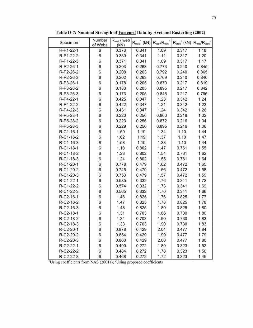
75

Table D-7: Nominal Strength of Fastened Data by Avci and Easterling (2002)

Specimen Numberof Webs

Rtest / web (kN) Rcalc

1 (kN) Rtest/Rcalc1 Rcalc

2 (kN) Rtest/Rcalc2

R-P1-22-1 6 0.373 0.341 1.09 0.317 1.18 R-P1-22-2 6 0.380 0.341 1.11 0.317 1.20 R-P1-22-3 6 0.371 0.341 1.09 0.317 1.17 R-P2-26-1 6 0.203 0.263 0.773 0.240 0.845 R-P2-26-2 6 0.208 0.263 0.792 0.240 0.865 R-P2-26-3 6 0.202 0.263 0.769 0.240 0.840 R-P3-26-1 6 0.178 0.205 0.870 0.217 0.819 R-P3-26-2 6 0.183 0.205 0.895 0.217 0.842 R-P3-26-3 6 0.173 0.205 0.846 0.217 0.796 R-P4-22-1 6 0.425 0.347 1.23 0.342 1.24 R-P4-22-2 6 0.422 0.347 1.21 0.342 1.23 R-P4-22-3 6 0.431 0.347 1.24 0.342 1.26 R-P5-28-1 6 0.220 0.256 0.860 0.216 1.02 R-P5-28-2 6 0.223 0.256 0.872 0.216 1.04 R-P5-28-3 6 0.229 0.256 0.895 0.216 1.06 R-C1-16-1 6 1.59 1.19 1.34 1.10 1.44 R-C1-16-2 6 1.62 1.19 1.37 1.10 1.47 R-C1-16-3 6 1.58 1.19 1.33 1.10 1.44 R-C1-18-1 6 1.18 0.802 1.47 0.761 1.55 R-C1-18-2 6 1.23 0.802 1.54 0.761 1.62 R-C1-18-3 6 1.24 0.802 1.55 0.761 1.64 R-C1-20-1 6 0.778 0.479 1.62 0.472 1.65 R-C1-20-2 6 0.745 0.479 1.56 0.472 1.58 R-C1-20-3 6 0.753 0.479 1.57 0.472 1.59 R-C1-22-1 6 0.585 0.332 1.76 0.341 1.72 R-C1-22-2 6 0.574 0.332 1.73 0.341 1.69 R-C1-22-3 6 0.565 0.332 1.70 0.341 1.66 R-C2-16-1 6 1.46 0.825 1.76 0.825 1.77 R-C2-16-2 6 1.47 0.825 1.78 0.825 1.78 R-C2-16-3 6 1.48 0.825 1.80 0.825 1.80 R-C2-18-1 6 1.31 0.703 1.86 0.730 1.80 R-C2-18-2 6 1.34 0.703 1.90 0.730 1.83 R-C2-18-3 6 1.33 0.703 1.90 0.730 1.83 R-C2-20-1 6 0.878 0.429 2.04 0.477 1.84 R-C2-20-2 6 0.854 0.429 1.99 0.477 1.79 R-C2-20-3 6 0.860 0.429 2.00 0.477 1.80 R-C2-22-1 6 0.490 0.272 1.80 0.323 1.52 R-C2-22-2 6 0.484 0.272 1.78 0.323 1.50 R-C2-22-3 6 0.468 0.272 1.72 0.323 1.45

1Using coefficients from NAS (2001a); 2Using proposed coefficients

76

Table D-8: Nominal Strength of Unfastened Data by Wu (1997)

Specimen Numberof Webs

Rtest / web (kN) Rcalc

1 (kN) Rtest/Rcalc1 Rcalc

2 (kN) Rtest/Rcalc2

t26h0.75R3/32*60 4 0.164 0.278 0.589 0.202 0.809 t26h0.75R3/64*60 4 0.170 0.297 0.573 0.208 0.816 t26h1.5R3/32*60 4 0.110 0.211 0.521 0.188 0.585 t26h1.5R3/64*60 4 0.124 0.225 0.551 0.192 0.645 t22h0.75R5/64*60 4 0.468 0.718 0.652 0.487 0.962 t22h0.75R1/16*60 4 0.486 0.742 0.655 0.493 0.985 t22h1.5R5/64*60 4 0.412 0.601 0.685 0.459 0.897 t22h1.5R1/16*60 4 0.464 0.617 0.752 0.465 0.999 t22h2R5/64*60 4 0.314 0.547 0.573 0.451 0.695 t22h2R1/16*60 4 0.325 0.555 0.586 0.451 0.721 t22h3R5/64*60 2 0.432 0.439 0.983 0.426 1.01 t22h3R1/16*60 2 0.464 0.453 1.024 0.431 1.08

t22h4.5R5/64*60 2 0.337 0.318 1.058 0.404 0.835 t22h4.5R1/16*60 2 0.368 0.325 1.134 0.405 0.909 t22h6R5/64*60 2 0.277 0.214 1.297 0.384 0.721 t22h6R1/16*60 2 0.299 0.216 1.385 0.381 0.784

1Using coefficients from NAS (2001a); 2Using proposed coefficients

Table D-9: Nominal Strength of Fastened Data by Bhatka et al. (1992)

Specimen # of Webs Rtest / web (kN) Rcalc

1 (kN) Rtest/Rcalc1 Rcalc

2 (kN) Rtest/Rcalc2

FD3-F 6 0.402 0.311 1.29 0.349 1.15 FD4-F 6 0.415 0.311 1.33 0.350 1.19

1Using coefficients from NAS (2001a); 2Using proposed coefficients

77

Appendix E Experimentally Recorded Load

5.9

0

5

10

15

20

25

30

35

P tes

t

Bolt Fastening Pattern None Bolts at a, g Bolts at a, d, g Bolts at a, c, e, g

Bearing Length N = 24 mm N = 50 mm N = 75 mm

Deck Profile

a b c d e f g

Figure E-1: Load-Stroke Plot, Test Series: T1

78

0

10

20

30

40

50

60

P tes

t

Bolt Fastening Pattern None Bolts at a, g Bolts at a, d, g Bolts at a, c, e, g

Bearing Length N = 24 mm N = 50 mm N = 75 mm

Deck Profile

a b c d e f g

Figure E-2: Load-Stroke Plot, Test Series: T2

0

10

20

30

40

50

60

70

80

P tes

t

Bolt Fastening Pattern None Bolts at a, g Bolts at a, d, g Bolts at a, c, e, g

Bearing Length N = 24 mm N = 50 mm N = 75 mm

Deck Profile

a b c d e f g

Figure E-3: Load-Stroke Plot, Test Series: T3

79

0

2

4

6

8

10

12

14

16

18

P tes

t

Bolt Fastening Pattern None Bolts at a & c Bolts at a, b, & c

Bearing Length N = 24 mm N = 50 mm N = 75 mm

Deck Profile

a b c

Figure E-4: Load-Stroke Plot, Test Series: C2

0

2

4

6

8

10

12

14

16

18

P tes

t

Bolt Fastening Pattern None Bolts at a & c Bolts at a, b, & c

Bearing Length N = 24 mm N = 50 mm N = 75 mm

Deck Profile

a b c

Figure E-5: Load-Stroke Plot, Test Series: C3

80

0

5

10

15

20

25

30

P tes

t

Bolt Fastening Pattern None Bolts at a & c Bolts at a, b, & c

Bearing Length N = 24 mm N = 50 mm

Deck Profile

a b c

Figure E-6: Load-Stroke Plot, Test Series: C1

0

2

4

6

8

10

12

14

16

18

P tes

t

Bolt Fastening Pattern None Bolts at a & d Bolts at a, b, & d

Bearing Length N = 24 mm N = 50 mm N = 75 mm

Deck Profile

a b c d

Figure E-7: Load-Stroke Plot, Test Series: R1

81

0

5

10

15

20

25

P tes

t

Bolt Fastening Pattern None Bolts at a & d Bolts at a, b, & d

Bearing Length N = 24 mm N = 50 mm N = 75 mm

Deck Profile

a b c d

Figure E-8: Load-Stroke Plot, Test Series: R2

0

5

10

15

20

25

30

35

40

45

50

P tes

t

Bolt Fastening Pattern None Bolts at a & d Bolts at a, b, & d

Bearing Length N = 24 mm N = 50 mm N = 75 mm

Deck Profile

a b c d

Figure E-9: Load-Stroke Plot, Test Series: R3

82

0

2

4

6

8

10

12

14

16

P tes

t

Bolt Fastening Pattern None Bolts at a & c Bolts at a, b, & c

Bearing Length N = 24 mm N = 50 mm N = 75 mm

Deck Profile

a b c

Figure E-10: Load-Stroke Plot, Test Series: U4

0

2

4

6

8

10

12

14

16

18

P tes

t

Bolt Fastening Pattern None Bolts at a & c Bolts at a, b, & c

Bearing Length N = 24 mm N = 50 mm N = 75 mm

Deck Profile

a b c

Figure E-11: Load-Stroke Plot, Test Series: U5

83

0

5

10

15

20

25

30

P tes

t

Bolt Fastening Pattern None Bolts at a & c Bolts at a, b, & c

Bearing Length N = 24 mm N = 50 mm N = 75 mm

Deck Profile

a b c

Figure E-12: Load-Stroke Plot, Test Series: U6

0

1

2

3

4

5

6

7

8

9

10

P tes

t

Bolt Fastening Pattern None Bolts at a & c Bolts at a, b, & c

Bearing Length N = 24 mm N = 50 mm N = 75 mm

Deck Profile

a b c

Figure E-13: Load-Stroke Plot, Test Series: U3

84

0

2

4

6

8

10

12

14

16

18

P tes

t

Bolt Fastening Pattern None Bolts at a & c Bolts at a, b, & c

Bearing Length N = 24 mm N = 50 mm N = 75 mm

Deck Profile

a b c

Figure E-14: Load-Stroke Plot, Test Series: U2

0

5

10

15

20

25

30

P tes

t

Bolt Fastening Pattern None Bolts at a & c Bolts at a, b, & c

Bearing Length N = 24 mm N = 50 mm N = 75 mm

Deck Profile

a b c

Figure E-15: Load-Stroke Plot, Test Series: U1

85

0

2

4

6

8

10

12

14 P t

est

Bolt Fastening Pattern None Bolts at a & c Bolts at a, b, & c

Bearing Length N = 24 mm N = 50 mm N = 75 mm

Deck Profile

a b c

Figure E-16: Load-Stroke Plot, Test Series: U9

0

5

10

15

20

25

30

P tes

t

Bolt Fastening Pattern None Bolts at a & c Bolts at a, b, & c

Bearing Length N = 24 mm N = 50 mm N = 75 mm

Deck Profile

a b c

This drop in load rate was theresult of one of the four webs crippling prematurely.

Figure E-17: Load-Stroke Plot, Test Series: U8

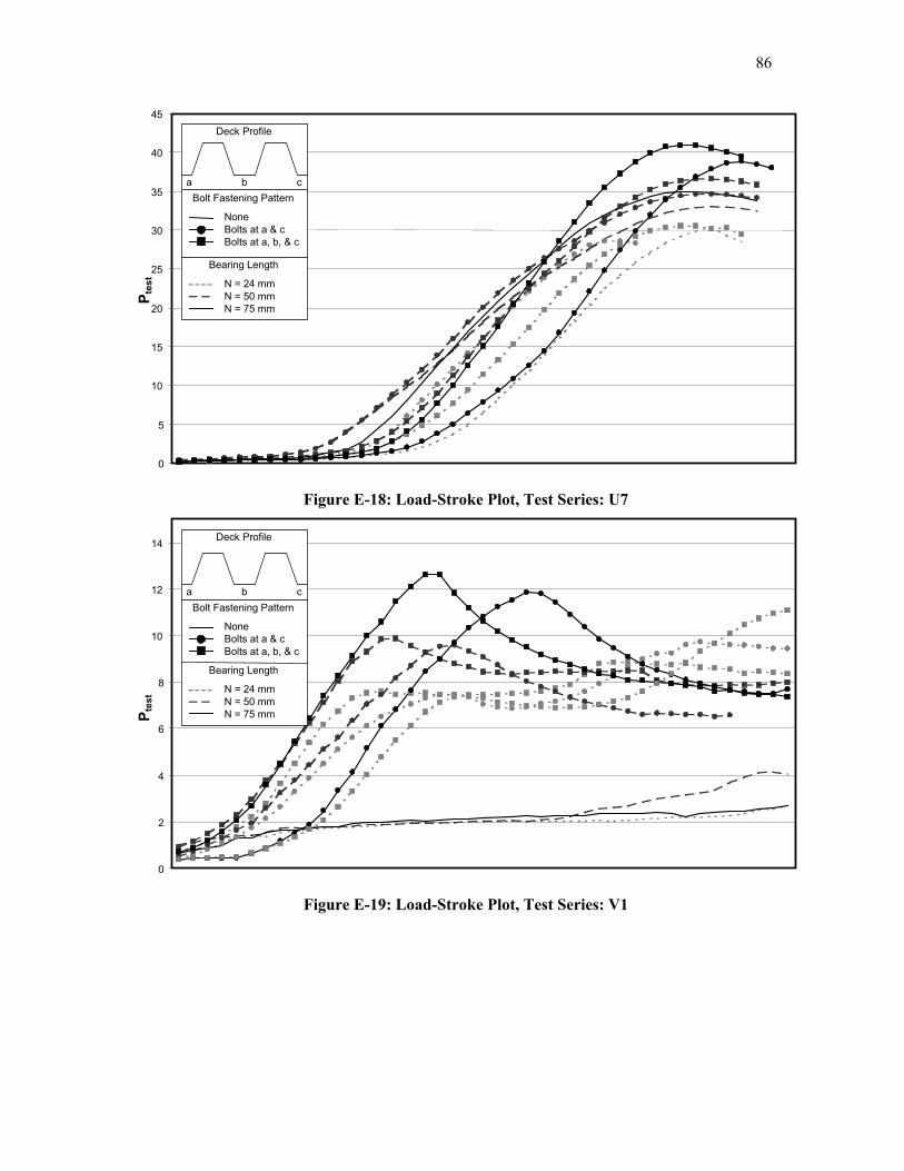
86

0

5

10

15

20

25

30

35

40

45

P tes

t

Bolt Fastening Pattern None Bolts at a & c Bolts at a, b, & c

Bearing Length N = 24 mm N = 50 mm N = 75 mm

Deck Profile

a b c

Figure E-18: Load-Stroke Plot, Test Series: U7

0

2

4

6

8

10

12

14

P tes

t

a b c Bolt Fastening Pattern

None Bolts at a & c Bolts at a, b, & c

Bearing Length N = 24 mm N = 50 mm N = 75 mm

Deck Profile

Figure E-19: Load-Stroke Plot, Test Series: V1

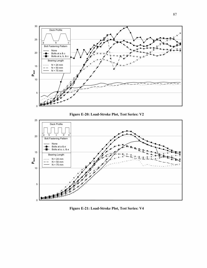
87

0

5

10

15

20

25

30

P tes

t

a b c Bolt Fastening Pattern

None Bolts at a & c Bolts at a, b, & c

Bearing Length N = 24 mm N = 50 mm N = 75 mm

Deck Profile

Figure E-20: Load-Stroke Plot, Test Series: V2

0

5

10

15

20

25

P tes

t

Bolt Fastening Pattern None Bolts at a & e Bolts at a, c, & e

Bearing Length N = 24 mm N = 50 mm N = 75 mm

Deck Profile

a b c d e

Figure E-21: Load-Stroke Plot, Test Series: V4

88

0

5

10

15

20

25

30

35

P tes

t

Bolt Fastening Pattern None Bolts at a & e Bolts at a, c, & e

Bearing Length N = 24 mm N = 50 mm N = 75 mm

Deck Profile

a b c d e

Figure E-22: Load-Stroke Plot, Test Series: V3

0

10

20

30

40

50

60

P tes

t

Bolt Fastening Pattern None Bolts at a & e Bolts at a, c, & e

Bearing Length N = 24 mm N = 50 mm N = 75 mm

Deck Profile

a b c d e

Figure E-23: Load-Stroke Plot, Test Series: V5

89

0

5

10

15

20

25

30

35

40

45

P tes

t

a b c Bolt Fastening Pattern

None Bolts at a & c Bolts at a, b, & c

Bearing Length N = 24 mm N = 50 mm N = 75 mm

Deck Profile

Figure E-24: Load-Stroke Plot, Test Series: W1

0

5

10

15

20

25

30

35

40

45

P tes

t

a b c Bolt Fastening Pattern

None Bolts at a & c Bolts at a, b, & c

Bearing Length N = 24 mm N = 50 mm N = 75 mm

Deck Profile

Figure E-25: Load-Stroke Plot, Test Series: W2

90

0

5

10

15

20

25

30

35

P tes

t

Bolt Fastening Pattern None Bolts at a, d Bolts at a, b, d

Bearing Length N = 24 mm N = 50 mm N = 75 mm

Deck Profile

a b c d

Figure E-26: Load-Stroke Plot, Test Series: E1

0

5

10

15

20

25

30

35

P tes

t

Bolt Fastening Pattern None Bolts at a, d Bolts at a, b, d

Bearing Length N = 24 mm N = 50 mm N = 75 mm

Deck Profile

a b c d

Figure E-27: Load-Stroke Plot, Test Series: E2

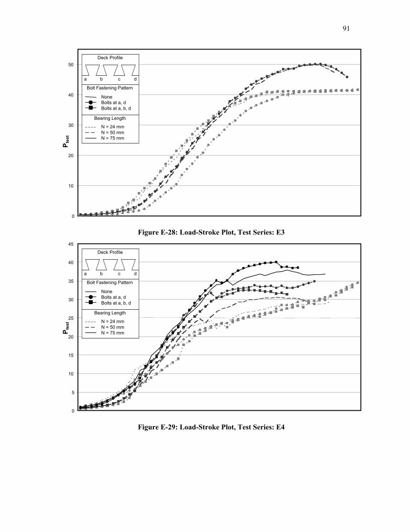
91

0

10

20

30

40

50 P t

est

Bolt Fastening Pattern None Bolts at a, d Bolts at a, b, d

Bearing Length N = 24 mm N = 50 mm N = 75 mm

Deck Profile

a b c d

Figure E-28: Load-Stroke Plot, Test Series: E3

0

5

10

15

20

25

30

35

40

45

P tes

t

Bolt Fastening Pattern None Bolts at a, d Bolts at a, b, d

Bearing Length N = 24 mm N = 50 mm N = 75 mm

Deck Profile

a b c d

Figure E-29: Load-Stroke Plot, Test Series: E4

92

0

5

10

15

20

25

30

P tes

t

Bolt Fastening Pattern None Bolts at a, d Bolts at a, b, d

Bearing Length N = 24 mm N = 50 mm N = 75 mm

Deck Profile

a b c d

Figure E-30: Load-Stroke Plot, Test Series: E5

93

Appendix F Genetic Algorithm Used to Verify Analysis

F.1 General

Discussed in this appendix is the genetic algorithm used in the analysis of this study. Specific information is given explaining the source code, including how the DNA strings are encoded, how the fitness test works, and the convergence criteria. The source code for the algorithm is also given.

F.2 DNA Strings

The full range of possible solutions, describing all four web crippling coefficients, can be represented using a nineteen digit binary number. N.B. that in the interest of reducing memory requirements, binary values do not translate to their decimal equivalent. This section explains how the four coefficients are described using a nineteen-digit binary string.

The first three digits represent the coefficient, C, with 000 indicating a value of 2, 001 indicating a value of 3, and so on to 111 indicating a value of 9.

The next four digits represent the coefficient, CR, with 0000 indicating a value of 0.02, 0001 indicating a value of 0.03, and so on to 1111 indicating a value of 0.17.

The next six digits represent the coefficient, CN, with 000000 indicating a value of 0.10, 000001 indicating a value of 0.11, and so on to 111111 indicating a value of 0.73.

The last six digits represent the coefficient, Ch, with 000000 indicating a value of 0.010, 000001 indicating a value of 0.011, and so on to 111111 indicating a value of 0.073.

As an example, a DNA string of 1000100111001010101 is decoded as shown in Table F-1. The first three digits of the DNA string represent C = 6, the following four digits represent CR = 0.06, the next six digits represent CN = 0.67, and the final six digits represent Ch = 0.031. Contained in Table F-2 is a complete list of all of the possible values represented by the DNA string. This table is very useful for following the source code provided in Appendix F.6.

Table F-1: Example Decoding of a DNA String.

Coefficient Binary Value Actual ValueC 100 6 CR 0100 0.06 CN 111001 0.67 Ch 010101 0.031

94

Table F-2: Encoding Key for the DNA String

Web Crippling Coefficients Coefficients Binary Value C* CR

** CN Ch Binary Value CN Ch

000000 1 0.02 0.1 0.01 100000 0.42 0.042 000001 2 0.03 0.11 0.011 100001 0.43 0.043 000010 3 0.04 0.12 0.012 100010 0.44 0.044 000011 4 0.05 0.13 0.013 100011 0.45 0.045 000100 5 0.06 0.14 0.014 100100 0.46 0.046 000101 6 0.07 0.15 0.015 100101 0.47 0.047 000110 7 0.08 0.16 0.016 100110 0.48 0.048 000111 8 0.09 0.17 0.017 100111 0.49 0.049 001000 0.1 0.18 0.018 101000 0.50 0.050 001001 0.11 0.19 0.019 101001 0.51 0.051 001010 0.12 0.2 0.02 101010 0.52 0.052 001011 0.13 0.21 0.021 101011 0.53 0.053 001100 0.14 0.22 0.022 101100 0.54 0.054 001101 0.15 0.23 0.023 101101 0.55 0.055 001110 0.16 0.24 0.024 101110 0.56 0.056 001111 0.17 0.25 0.025 101111 0.57 0.057 010000 0.26 0.026 110000 0.58 0.058 010001 0.27 0.027 110001 0.59 0.059 010010 0.28 0.028 110010 0.60 0.060 010011 0.29 0.029 110011 0.61 0.061 010100 0.30 0.03 110100 0.62 0.062 010101 0.31 0.031 110101 0.63 0.063 010110 0.32 0.032 110110 0.64 0.064 010111 0.33 0.033 110111 0.65 0.065 011000 0.34 0.034 111000 0.66 0.066 011001 0.35 0.035 111001 0.67 0.067 011010 0.36 0.036 111010 0.68 0.068 011011 0.37 0.037 111011 0.69 0.069 011100 0.38 0.038 111100 0.70 0.070 011101 0.39 0.039 111101 0.71 0.071 011110 0.4 0.04 111110 0.72 0.072 011111 0.41 0.041 111111 0.73 0.073

*The coefficient C is encoded using only the last three digits of the binary value. **The coefficicent CR is encoded using only the last four digits of the binary value.

F.3 Gene Splicing and Mutation

In Genetic algorithm terminology, the term ‘splicing’ is used to describe the process of creating two new ‘child’ DNA strings from two ‘parent’ DNA strings. The term ‘mutation,’ is used to describe the

95

practice of intentionally introducing small errors in the gene splicing process. There is no definite method set out for either splicing or mutation. Splicing only requires that the children DNA are composed entirely of elements from the parent DNA, and that the children are the same size as the parents. Mutation has been found to help the GA to find a solution more quickly, provided that the amount of mutation is kept to a minimal.

In the program created for this project, splicing was done using one splice at a random location along the DNA string. A random number, representing a position in the DNA string, between 1 and 19 is selected, and all elements between the two original DNA strings beyond that position are swapped. For example, if the randomly chosen number is 12, and the original DNA strings were 1111111111111111111 and 0000000000000000000 then the two new DNA strings would be 1111111111110000000 and 0000000000001111111.

The program created for this project uses a mutation rate of 1%. Therefore, for every 100 new DNA strings created, only one should have a mutation. When a mutation occurs one character in the DNA string, chosen at random, is changed. For the example of splicing used above, if a mutation occurred in the first child, it could cause the new DNA strings to become 1111011111110000000 and 0000000000001111111. Note the mutation at the fifth character of the first DNA string.

F.4 Fitness Test and Penalty Functions

As with the splicing and mutation implementations discussed in the previous section, there exists no set method for fitness tests and penalty functions in GA’s. This is because fitness tests and penalty functions are unique to the optimization problem at hand. Fitness tests and penalty functions must be rewritten for each new application.

For this study, it was found that only one fitness test was necessary, and penalty functions were not necessary. Equation F.4-1 summarizes the fitness test, which is a modification of Equation 4.2-1.

( )∑=

−−n

iciti PP

1

23000 Eq. F.4-1

The value, 3 000, was selected because it is larger than the majority of possible values of the summation given the constraints imposed by the range of coefficient values possible within the DNA string. Using Microsoft Excel Solver, the optimized summation was found to be approximately 500, which would result in an optimized fitness value of 2500. A minimum fitness value of 100 was imposed on all DNA strings to ensure than some of the less fit DNA strings survive into the next generation. It is important to ensure that enough diversity continues into each generation to find the optimal solution.

96

F.5 Convergence

Convergence on a final optimal solution was considered to have occurred when the fitness value of the most fit DNA string does not change by more than 1% over five iterations. A maximum of 10 000 iterations has also been imposed.

F.6 Source Code

#include <stdafx.h> #include <iostream.h> #include <fstream.h> #include <iomanip.h> #include <string.h> #include <stdlib.h> #include <time.h> #include <math.h> //Function Headers void CreateDNA (char *, int); void MateDNA (char *, char *, float, float); float TestDNA (char *, float*, float*, float*, float*, float*, float*, float*, int); float getC (char *); float getCr (char *); float getCn (char *); float getCh (char *); int main(int argc, char* argv[]) srand(time(NULL)); //seed the random number generator //Variables const int PopSize = 300; //Population size const int NumIter = 10000; //Maximum number of iterations before convergence float CrossOver = 1; //Probability of Gene splicing (usually 100%) float MutaRate = (float) 0.01; //Probability of mutation (usuall very small) const int DNASize = 20; //Size of DNA String const int total = 74; //total number of data test specimens float t[total], fy[total], sinth[total], R[total], N[total], H[total], P[total]; //specimen variables char choice; //used to cycle between data files char DNA[PopSize][DNASize] = ""; //array of characters used to store DNA population char DNA2[PopSize][DNASize] = ""; //copy of DNA array used to create next generation float FitValue[PopSize]; //array of fitness values from each DNA string float TotalFit=0; //total Fitness of the Population float RandSelect; //used to choose parents float RandTotal; //used to choose parents int counter; //used to choose parents int Parents[PopSize]; //list of DNA strings selected for parenting next generation int Converge=0; //used to indicate convergence float BestFit=0; //used to remember the best fitness value

97

float OldBestFit=0; //used to remember best fit from previous generation int MostFit=0; //used to remember the best fit DNA int Iterate=0; //used to count the number of iterations cout << "Press 1 for unfastened data, anything else for fastened data: "; cin >> choice; if (choice='1') //reads in unfastened data ifstream finu ("unfast.txt", ios::in); if (!finu) //check file was found cerr << "File could not be opened" << endl; for (int a = 0; a<total;a++) finu >> t[a] >> fy[a] >> sinth[a] >> R[a] >> N[a] >> H[a] >> P[a]; else //reads in fastened data ifstream fin ("fast.txt", ios::in); if (!fin) //check file was found cerr << "File could not be opened" << endl; for (int a = 0; a<total;a++) fin >> t[a] >> fy[a] >> sinth[a] >> R[a] >> N[a] >> H[a] >> P[a]; //Create and define DNA sequences. for (int a = 0;a<PopSize;a++) CreateDNA(DNA[a], DNASize); //Program will loop until convergence criteria is met or a max. number of iterations occur. while (Converge < 5 && Iterate < NumIter) TotalFit = 0; //initialize values BestFit=0; Iterate++; for (a = 0; a<PopSize; a++) //Find the fitness of the population FitValue[a]=TestDNA(DNA[a],t, fy, sinth, R, N, H, P, total); TotalFit = TotalFit+FitValue[a]; if (FitValue[a]>BestFit) BestFit = FitValue[a]; MostFit = a; if(BestFit-OldBestFit>=0 && BestFit-OldBestFit<=8) //convergence criteria

98

Converge++; else Converge=0; if (BestFit>OldBestFit) //Record best fit to compare to next generation OldBestFit=BestFit; if(Converge>=5 || Iterate >=NumIter) //If convergence is met, output results. cout <<Iterate << endl << endl << "C:\tCr:\tCn:\tCh:"<< endl

<< getC(DNA[MostFit]) << "\t" << getCr(DNA[MostFit]) << "\t" <<getCn(DNA[MostFit]) << "\t" <<getCh(DNA[MostFit]) << "\t" << endl; else //If convergence is not met, then create next generation for (a=0;a<PopSize;a++) RandTotal=0; counter=0; //Parents are selected by choosing a random number and adding the fitness values until the random //number is exceeded. RandSelect=(float)(rand()%3000)/2999; while (RandTotal<=RandSelect && counter<PopSize) RandTotal=RandTotal+FitValue[counter]/TotalFit; counter++; Parents[a]=counter-1; for (a=0;a<PopSize;a++) //create an array of parent DNA by copying DNA strings from the population strcpy(DNA2[a],DNA[Parents[a]]); for (a=0;a<PopSize/2;a++) //create offspring DNA strings MateDNA(DNA2[a], DNA2[a+PopSize/2],CrossOver, MutaRate); for (a=0;a<PopSize;a++) //copy offspring DNA over the original DNA array for the next iteration. strcpy(DNA[a],DNA2[a]); return 0; //This function randomly generates a binary sequence. It is passed a pointer to a //string array and the length to make the binary sequence. void CreateDNA (char *s1, int size) int dna; for (int a=0;a<size-1;a++) dna = rand()%2; //Returns either 1 or 0 (chosen randomly) as an integer. if (dna == 0) //The DNA sequence is stored as a string. This if statement is strcat(s1,"1"); //used to convert the randomly generated integer to a char.

99

else strcat(s1,"0"); return; //This function determines how two sequences are to be spliced together to generate two new //sequences to be used in the next generation. It is passed the pointers to two string arrays and two //doubling pt numbers. The strings represent the DNA sequece and the doubleing pt numbers are the //Crossover Probability (set to one in this program) and the Mutation Probability (set to 0.05). void MateDNA (char *s1, char *s2, float cross, float mutation) //Assign and create parent DNA char p1[20] = ""; char p2[20] = ""; strcpy (p1,s1); strcpy (p2,s2); //Determine genetic splicing data int Splice = rand() % strlen(s1); int MutationLocation = rand() % strlen(s1); //Splice Genes at a random location. The crossover variable is used to //model the probablity of the genes splicing, in most cases = 100% float Crossover =(float) (rand() % 100); if (Crossover <= cross*100) strncpy(s1,p2,Splice); strncpy(s2,p1,Splice); //Mutate Gene //Consider that first gene may mutate. float Mut = (float) (rand()%100); if (Mut < mutation*100) if (s1[MutationLocation] == '1') //Flip the binary genetic value s1[MutationLocation] = '0'; else s1[MutationLocation] = '1'; //Consider that second gene may mutate. Mut = (float) (rand()%100); if (Mut <= mutation*100) if (s2[MutationLocation] == '1') //Flip the binary genetic value s2[MutationLocation] = '0'; else s2[MutationLocation] = '1';

100

return; //This procedure inputs all of the variables to determine web crippling plus the actual test load and a //DNA string. It will use the DNA string and other procedures to determine the theoretical web //crippling load. Fitness is determined by subtracting the sum of the square from 3000. Any value less //than 2500 is automatically changed to 100. float TestDNA(char *s1, float *t, float *fy, float *sintheta, float *R, float *N, float *H, float *P, int number) float total = 2500; float C, Ch, Cr, Cn; //determine web crippling coeffecients C = getC(s1); Ch = getCh(s1); Cr=getCr(s1); Cn=getCn(s1); for (int a=0; a < number; a++) //determine the sum of the squares total = total - (float)pow(P[a] - C*t[a]*t[a]*fy[a]*sintheta[a]*(1- Cr*sqrt(R[a]))*(1+Cn*sqrt(N[a]))*(1-Ch*sqrt(H[a]))/1000,2); if (total<100) //make all small values equal to 100 total=100; return total; float getC (char *s1) //Decode the C value from a DNA string float x=1; for (int a = 0;a<3;a++) if (s1[a]=='1') x = x+(float)pow(2,a); return x; float getCr (char *s1) //Decode the Cr value from a DNA string float x=(float)0.02; for (int a = 3;a<7;a++) if (s1[a]=='1') x = x+(float)pow(2,a-3)/100; return x; float getCn (char *s1) //Decode the Cn value from a DNA string float x=(float)0.10; for (int a = 7;a<13;a++) if (s1[a]=='1') x = x+(float)pow(2,a-7)/100; return x;

101

float getCh (char *s1) //Decode the Ch value from a DNA string float x=(float)0.010; for (int a = 13;a<19;a++) if (s1[a]=='1') x = x+(float)pow(2,a-13)/1000; return x;

American Iron and Steel Institute

1140 Connecticut Avenue, NW

Suite 705

Washington, DC 20036

www.steel.org

Re

sea

rch

Re

po

rt R

P-0

3-1