Web-based Analytical Tools for the Exploration of Spatial Data

Abstract. This paper deals with the extension of internet-based geographicinformation systems with functionality for exploratory spatial data analysis(ESDA). The specific focus is on methods to identify and visualize outliers inmaps for rates or proportions. Three sets of methods are included: extremevalue maps, smoothed rate maps and the Moran scatterplot. The imple-mentation is carried out by means of a collection of Java classes to extend theGeotools open source mapping software toolkit. The web based spatialanalysis tools are illustrated with applications to the study of homicide ratesand cancer rates in U.S. counties.

Key words: internet GIS, exploratory spatial data analysis, spatial outliers,smoothing, spatial autocorrelation, Geotools

JEL classification: C88, C49, I18

1 Introduction

For close to fifteen years now, there have been substantial efforts to extendGeographic Information Systems with functionality to carry out spatialanalysis in general, and spatial statistical analysis in particular. Early worktended to emphasize objectives for the integration of GIS and spatialanalysis, outline required functionality and describe overall frameworks, asexemplified in, among others, Goodchild (1987), Anselin and Getis (1992),Goodchild et al. (1992), Fotheringham and Rogerson (1993) and Fischer and

* This research was supported in part by a number of grants from the US National Science

Foundation: NSF Grant SBR-9410612, BCS-9978058, to the Center for Spatially Integrated

Social Science (CSISS), and a grant from the National Consortium on Violence Research (NCOVR

is supported under grant SBR-9513040 from the National Science Foundation). In addition,

support was provided by grant RO1 CA 95949-01 from the National Cancer Institute. Special

thanks to Dr. Eugene J. Lengerich of the Pennsylvania State Cancer Institute for providing the

data on colon cancer diagnoses.

J Geograph Syst (2004) 6:197–218

DOI: 10.1007/s10109-004-0132-5

Web-based analytical tools for the explorationof spatial data�

Luc Anselin, Yong Wook Kim and Ibnu Syabri

Spatial Analysis Laboratory, Department of Agricultural and Consumer Economics,

University of Illinois, Urbana-Champaign, Urbana, IL 61801, USA

(e-mail: [email protected], [email protected], [email protected])

Nijkamp (1993). More recently, this has translated into a range of softwareimplementations of linked, embedded and otherwise integrated modulesextending ‘‘traditional’’ GIS functions with data exploration, visualizationand analysis tools.1

The phenomenal growth of the world wide web has resulted in thedevelopment of so-called internet GIS, ranging from the delivery of staticmaps to interactive distributed computing frameworks. Most of the emphasisin internet GIS to date has arguably been on map delivery, cartographicpresentation and providing access to a variety of distributed geographicinformation (see, e.g., Plewe, 1997, Peng, 1999, Kahkonen et al. 1999,Jankowski et al. 2001, Kraak and Brown, 2001, Tsou and Buttenfield, 2002).Increasingly, more specialized spatial analytical capabilities are becoming

implemented in an internet GIS environment as well. Some examples arevirtual reality modeling (Huang and Lin, 1999, 2002), hydrological modeling(Huang and Worboys, 2001), as well as exploratory data analysis (Herzog,1998, Andrienko et al. 1999, Takatsuka and Gahegan, 2001, 2002).Our paper deals with efforts to incorporate methods for exploratory

spatial data analysis in an internet GIS. The original motivation stemmedfrom the need to develop an interactive front end to the Atlas of USHomicides of the National Consortium on Violence Research (Messneret al. 2000), which would include user-friendly ways to carry out a limitedset of spatial data manipulations. The objective was to provide thisfunctionality through a standard web browser, so that the user would notneed to have access to a GIS or specialized spatial data analysis software.Our focus is therefore on techniques to detect and visualize outliers in ratemaps, to smooth these maps to correct for potential spurious inference, andto analyze and visualize patterns of spatial autocorrelation. Such methodsare still largely absent in mainstream statistical and GIS software. A muchmore ambitious effort to provide ESDA and other spatial data analysismethods on the desktop is reflected in CSISS’ GeoDa software project(Anselin, 2003).2

In this paper, we first provide a brief review of the methods included in ourapproach, followed by an outline of the architecture of the softwareimplementation. We illustrate the analytical tools with an application to thestudy of spatial patterns in county homicide rates around St. Louis, MO, andof colon cancer diagnoses in Appalachia. We close with some concludingcomments.

2 Methods

The techniques included in our analytical toolkit are aimed at theexploration of outliers in maps depicting rates or proportions, such ashomicide rates, cancer incidence rates, mortality rates, etc. Three broadclasses of methods are considered: outlier maps, smoothing procedures and

1For some recent reviews of the relevant literature, see, among others, Anselin (2000),

Anselin et al. (2002), Symanzik et al. (2000), Zhang and Griffith, (2000), Haining et al. (2000),

and Gahegan et al. (2002).

2GeoDa can be downloaded from http://sal.agecon.uiuc.edu/geoda_main.php.

198 L. Anselin et al.

spatial autocorrelation analysis. These methods are not new, and moreextensive reviews and background can be found in, among others, Anselin(1994, 1998, 1999), Bailey and Gatrell (1995), Fotheringham et al. (2000),and Lawson et al. (1999). While familiar in the spatial analysis literature,they are typically not part of the standard functionality of a commercialstatistical package or GIS, let alone included in an internet GIS.The most basic set of techniques includes simple enhancements to standard

choropleth maps in order to highlight extreme values. The maps are obtainedby classifying the data in a particular way or by comparing the data to areference value, as implemented in percentile maps, box maps and excess ratemaps. A second set of methods encompasses smoothing procedures, in orderto obtain ‘‘more accurate’’ estimates of the underlying risk than produced bythe raw rate maps. It is well known that when rates are estimated fromunequal populations (such as widely varying county populations), the resultsare inherently unstable. Smoothing techniques address this issue bycorrecting (‘‘shrinking’’) the raw rates while taking into account additionalinformation (such as the indication provided by a reference rate). Twospecific techniques are implemented here, the Empirical Bayes (EB) smootherand a spatial rate smoother. A final set of methods addresses thevisualization of spatial autocorrelation by means of a Moran Scatterplot.A brief review of some technical issues is provided next, for a more in-depthdiscussion we refer to the literature.

2.1 Outlier maps

Underlying any choropleth map is a sorting of the observed values into bins,similar to the classification used to construct a histogram. Each bin thencorresponds to a color and all observations (locations) in the same bin arecolored identically on the map.In order to highlight extreme values in a distribution, and downplay the

values around the median, a percentile map uses six categories for theclassification of ranked observations: 0–1%, 1–10%, 10–50%, 50–90%,90–99% and 99–100%. The lowest and highest percentile are extreme values,although this is only a simple ranking and does not imply that theseobservations are necessarily extreme relative to the rest of the distribution. Inother words, they are candidates to be classified as outliers, but may not beoutliers in a strict sense.A more rigorous assessment of the characteristics of the complete

distribution of the attributes is obtained in a box map (see, e.g., Anselin1998, 1999), a specialized form of a quartile map. Again, there are sixcategories. In addition to four categories corresponding to the four quartiles,an extra category is reserved at both the high and low end for thoseobservations that can be classified as outliers, following the same definition asapplied in the familiar box plot, also known as a box and whisker plot.3

3A box plot shows the ranking of observations by value and classified into four quartiles.

Observations with values that are larger than (less than) the value correspoding to the 75th

percentile (25th percentile) þ (�) 1.5 times the interquartile range are labeled outliers. See also

Cleveland (1993) for an extensive discussion of data visualization issues.

Web-based spatial analysis 199

Consequently, when there are such outliers, the first and last quartile nolonger contain exactly one fourth of the observations. The map shows thelocation of the outliers in the value distribution.These first two types of maps are generic, in the sense that they apply to

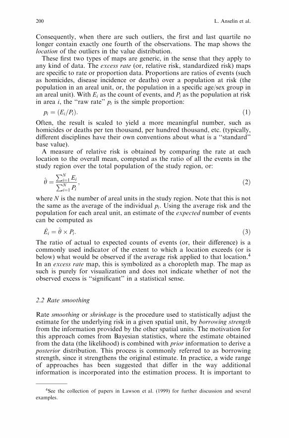
any kind of data. The excess rate (or, relative risk, standardized risk) mapsare specific to rate or proportion data. Proportions are ratios of events (suchas homicides, disease incidence or deaths) over a population at risk (thepopulation in an areal unit, or, the population in a specific age/sex group inan areal unit). With Ei as the count of events, and Pi as the population at riskin area i, the ‘‘raw rate’’ pi is the simple proportion:

pi ¼ ðEi=PiÞ: ð1ÞOften, the result is scaled to yield a more meaningful number, such ashomicides or deaths per ten thousand, per hundred thousand, etc. (typically,different disciplines have their own conventions about what is a ‘‘standard’’base value).A measure of relative risk is obtained by comparing the rate at each

location to the overall mean, computed as the ratio of all the events in thestudy region over the total population of the study region, or:

h ¼PN

i¼1 EiPN

i¼1 Pi; ð2Þ

where N is the number of areal units in the study region. Note that this is notthe same as the average of the individual pi. Using the average risk and thepopulation for each areal unit, an estimate of the expected number of eventscan be computed as

Ei ¼ h� Pi: ð3ÞThe ratio of actual to expected counts of events (or, their difference) is acommonly used indicator of the extent to which a location exceeds (or isbelow) what would be observed if the average risk applied to that location.4

In an excess rate map, this is symbolized as a choropleth map. The map assuch is purely for visualization and does not indicate whether of not theobserved excess is ‘‘significant’’ in a statistical sense.

2.2 Rate smoothing

Rate smoothing or shrinkage is the procedure used to statistically adjust theestimate for the underlying risk in a given spatial unit, by borrowing strengthfrom the information provided by the other spatial units. The motivation forthis approach comes from Bayesian statistics, where the estimate obtainedfrom the data (the likelihood) is combined with prior information to derive aposterior distribution. This process is commonly referred to as borrowingstrength, since it strengthens the original estimate. In practice, a wide rangeof approaches has been suggested that differ in the way additionalinformation is incorporated into the estimation process. It is important to

4See the collection of papers in Lawson et al. (1999) for further discussion and several

examples.


recognize that no method is best, and each will tend to result in (slightly)different adjustments to the raw rate estimate. The motivation for consid-ering different smoothing techniques is to assess the degree of stability of theresults. When two methods yield very different observations as ‘‘outliers,’’additional investigation may be warranted. This contrasts with the situationwhere the same observation is consistently identified as an outlier acrossseveral methods.An Empirical Bayes smoother uses Bayesian principles to guide the

adjustment of the raw rate estimate by taking into account information in therest of the sample. The principle is referred to as shrinkage, in the sense thatthe raw rate is moved (shrunk) towards an overall mean, as an inversefunction of the inherent variance.5

In other words, if a raw rate estimate has a small variance (i.e., is based on alarge population at risk), then it will remain essentially unchanged. Incontrast, if a raw rate has a large variance (i.e., is based on a small populationat risk, as in small area estimation), then it will be ‘‘shrunk’’ towards theoverall mean. From a Bayesian perspective, the overall mean is a prior, whichis conceptualized as a random variable with its own (‘‘prior’’) distribution.Assume this prior distribution is characterized by a mean h and variance /.

The Bayesian estimate for the underlying risk at i then becomes a weightedaverage of the raw rate pi, given in Equation (1), and the ‘‘prior,’’ withweights inversely related to their variance. This can be shown to yield:

pi ¼ wipi þ ð1� wiÞh; ð4Þwith

wi ¼/

/þ ðh=PiÞ: ð5Þ

Note that when the population at risk is large, the second term in thedenominator of (5) becomes near zero, and wi ! 1, giving all the weight in(4) to the raw rate estimate. As Pi gets smaller, more and more weight is givento the second term in (4). The Empirical Bayes approach (EB) consists ofestimating the moments of the prior distribution from the data, rather thantaking them as a ‘‘prior’’ in a pure sense (for technical details, see, e.g.,Marshall 1991).An important practical issue is the choice of the reference set from which

the estimate for h is computed. For example, one could argue that in a studyof homicides in rural Minnesota counties (characterized by very lowhomicide counts, but also by small populations, such that a single homicidemay cause an elevated rate), the proper prior would not necessarily be thenational homicide rate, but rather an average calculated for the Great Plains‘‘region.’’ In any application of smoothing, it is important to consider thesensitivity of the results (in terms of how locations are classified as beingoutliers) to the choice of this reference region. One of the characteristics ofthe tools we implement is to make this straightforward for the user. Again, itis important to realize that there is no best reference region. Rather, in anexploratory exercise, an assessment of sensitivity of the identified ‘‘patterns’’to the choice of technique is an important consideration.

5The original reference is Clayton and Kaldor (1987), details are also given in Bailey and

Gatrell, (1995), pp. 303-308.


A spatial rate smoother (e.g., Kafadar 1996) is based on the notion of aspatial moving average or window average. Instead of computing an estimateas the raw rate for each individual spatial unit, it is computed for that unittogether with a set of ‘‘reference’’ neighbors, Si.

6 This contrasts with the EBtechnique, where the smoothed rate is an average of the raw rate and someseparately computed reference estimate.An important practical consideration in the implementation of a spatial

smoother is the size of the ‘‘window, ’’ or, the selection of the relevantneighbors. As with the EB method, there is no best solution, but rather,interest focuses on the sensitivity of the conclusions to the choice of thewindow. As a general rule, the larger the window (the more neighbors), themore of the original variability will be removed. In the extreme, if the spatialwindow includes all the observations in the data set, the smoothed rate willbe the same everywhere. In practice, neighbors can be defined in similarfashion to the specification of spatial weights in spatial autocorrelationanalysis. In our implementation, we use simple contiguity (common borders)to define the neighbors. The smoothed rate becomes:

pi ¼Ei þ

PJij¼1 Ej

Pi þPJi

j¼1 Pj; ð6Þ

where j 2 Si are the neighbors for i.7 The spatially smoothed rate map is thena choropleth map based on the ranking of the smoothed rate values. Itemphasizes broader regional trends and removes some of the spatial detailfrom the original map.

2.3 Visualizing spatial autocorrelation

The final component in our analytical framework is the visualization ofspatial autocorrelation by means of a Moran Scatterplot (Anselin 1995,1996). This is a specialized scatterplot with the spatially lagged transforma-tion of a variable on the y-axis and the original variable on the x-axis, afterstandardizing the variable such that the mean is zero and variance one. Withsuch a standardized variable as zi, the spatial lag becomes

½Wz�i ¼X

j

wijzj; ð7Þ

where wij are elements of a row-standardized spatial weights matrix.8 For thezi and with a row-standardized spatial weights matrix, Moran’s I coefficientof spatial autocorrelation is:

6A slightly different notion of spatial rate smoother is based on the median rate in the

moving window, as used by Wall and Devine (2000).

7The total number of neighbors for each unit, Ji is not necessarily constant and depends on

the contiguity structure.

8The square spatial weights matrix W has a row/column corresponding to each observation.

For each row (observation) it indicates by a non-zero value those columns (observations) that are

‘‘neighbors.’’ In our implementation, we only consider neighbors defined by simple contiguity.

The weights matrix is row-standardized such that the elements of each row sum to one.


I ¼P

i

Pj ziwijzj

Pi z2i

; ð8Þ

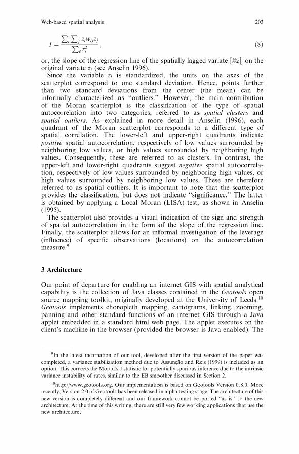
or, the slope of the regression line of the spatially lagged variate ½Wz�i on theoriginal variate zi (see Anselin 1996).Since the variable zi is standardized, the units on the axes of the

scatterplot correspond to one standard deviation. Hence, points furtherthan two standard deviations from the center (the mean) can beinformally characterized as ‘‘outliers.’’ However, the main contributionof the Moran scatterplot is the classification of the type of spatialautocorrelation into two categories, referred to as spatial clusters andspatial outliers. As explained in more detail in Anselin (1996), eachquadrant of the Moran scatterplot corresponds to a different type ofspatial correlation. The lower-left and upper-right quadrants indicatepositive spatial autocorrelation, respectively of low values surrounded byneighboring low values, or high values surrounded by neighboring highvalues. Consequently, these are referred to as clusters. In contrast, theupper-left and lower-right quadrants suggest negative spatial autocorrela-tion, respectively of low values surrounded by neighboring high values, orhigh values surrounded by neighboring low values. These are thereforereferred to as spatial outliers. It is important to note that the scatterplotprovides the classification, but does not indicate ‘‘significance.’’ The latteris obtained by applying a Local Moran (LISA) test, as shown in Anselin(1995).The scatterplot also provides a visual indication of the sign and strength

of spatial autocorrelation in the form of the slope of the regression line.Finally, the scatterplot allows for an informal investigation of the leverage(influence) of specific observations (locations) on the autocorrelationmeasure.9

3 Architecture

Our point of departure for enabling an internet GIS with spatial analyticalcapability is the collection of Java classes contained in the Geotools opensource mapping toolkit, originally developed at the University of Leeds.10

Geotools implements choropleth mapping, cartograms, linking, zooming,panning and other standard functions of an internet GIS through a Javaapplet embedded in a standard html web page. The applet executes on theclient’s machine in the browser (provided the browser is Java-enabled). The

9In the latest incarnation of our tool, developed after the first version of the paper was

completed, a variance stabilization method due to Assuncao and Reis (1999) is included as an

option. This corrects the Moran’s I statistic for potentially spurious inference due to the intrinsic

variance instability of rates, similar to the EB smoother discussed in Section 2.

10http://www.geotools.org. Our implementation is based on Geotools Version 0.8.0. More

recently, Version 2.0 of Geotools has been released in alpha testing stage. The architecture of this

new version is completely different and our framework cannot be ported ‘‘as is’’ to the new

architecture. At the time of this writing, there are still very few working applications that use the

new architecture.


toolkit is open source, which allows for easy customization and completeaccess to all the code.11

3.1 Basic Geotools architecture

In order to put our extensions into proper perspective, Fig. 1 illustrates thebasic logic of the standard Geotools internet mapping implementation. Themain input is a file in ESRI’s shape file format, from which an attribute(variable) is extracted for mapping. The attribute values are stored inGeotools’ so-called GeoData object (data structure), which is essentially a twocolumn matrix, with each row containing the value of a key (matching the IDof a corresponding feature in the shape file) and the attribute value (eithernumeric or character). Both the file name of the shape file as well as the nameof the variable to be mapped are passed as parameters to the Java applet, butonce the main applet is set up, they can no longer be changed.Once the GeoData object is constructed, it is passed to the Classifica-

tionShader class, which can be thought of as a central data dispatch center.The ClassificationShader moves the original data to the appropriateclassification classes, such as Quantile.class, or EqualInterval.class. Theseclasses implement the sorting and classification necessary to group theoriginal data into bins for use in a thematic map. The result of the

Set up fundamental variables

Construct GeoData

Organize outlook

Draw map

Main applet

Classification Shader

PopUp dialog

Distribute GeoData

Distribute classified GeoData

Classification classes

Classify GeoData

Legend draw classes

Original GeoData

Classified GeoData

Fig. 1. Basic Geotools Architecture (original)

11An up to date source tree for the Geotools project is maintained in Sourceforge, at http://

www.sourceforge.net/projects/geotools


classification is passed back to the ClassificationShader, which transfers it tothe main applet for mapping. This is both directly, for the map itself, andindirectly, via the specialized classes required to construct the legend (e.g.,the Key.class and the DiscreteShader.class). The ClassificationShader alsomanages a rudimentary user interface (Popup dialog) to select the type ofclassification for the choropleth map, the number of intervals, start and endcolors for a color ramp, etc. (see Fig. 3).For our purposes, there were several limitations to the standard Geotools

architecture. Foremost among these was the constraint that only a singlevariable could be handled. All manipulations within the Geotools classes(mapping, classification, linking) are limited to this single variable, i.e., thevalues contained in the GeoData object. In our application, the smoothingfunctions require at least two variables, i.e., an event count (numerator) andpopulation at risk (denominator), and also need to allow for the computa-tion of a new variable (the rate). Similarly, spatial correlation statisticsnecessitate that a new variable be calculated (the spatial lag) to provide theinput to the statistic. This was not possible in the ‘‘out of the box’’ Geotoolsrelease we used to implement our web analysis.The original architecture also makes it difficult to implement true

subsetting, as opposed to zooming. In true subsetting, the classification ofthe selected subset of locations is recomputed each time the subset changes,whereas in zooming, the classification is unaffected. Again, the basicGeoData structure does not lend itself to subsetting and recomputation.

Set up fundamental variables

Pass SFR and field name

Organize outlook

Draw map

Draw graph

Main applet

Classification Shader

PopUp dialog

Distribute SFR and field name

Distribute classified simpleGeoData

Classification classes

Construct simpleGeoData

Smooth rates as simpleGeoData

Classify simpleGeoData

Legend draw classes

SFR and field name

Classified SimpleGeoData

Graphics

Moran scatterplot

Calculate spatial weights

Calculate spatial lag

Calculate global Moran's I

Plot location of each record

Fig. 2. Extended Geotools architecture


Finally, there is limited user interaction. For example, it is not possible tospecify a different shape file as input, or to select a different variable fromwhat is hard coded in the original applet.The need for flexible data manipulation, variable selection and subset

computations required us to customize the basic toolkit. This took the formof several extensions to the standard collection of Geotools classes as well asthe development of a number of new classes.

3.2 Geotools class extensions

An overview of the architecture of the extensions required to implement thesmoothing and correlation computations is given in Fig. 2. The maindifference with Fig. 1 is that the GeoData object is no longer constructedin the main applet, but instead only the Shape File Reader (SFR) is passed tothe ClassificationShader. This input is obtained from the user, by extractingthe name of the shape file through an html form embedded in the openingweb page. The ClassificationShader remains the central data dispatch andhandles a slightly more elaborate user interface through which the variablenames and type of classification are selected (see Fig. 4). This is implementedin a new class (Alert.class).In contrast to the original Geotools, where the hard coded variable does

not require any additional computations, the construction of rates and thesmoothing operations must be carried out internally. The main computa-tional work to accomplish this is included in a number of extensions and newclasses.In our implementation, the Classification Classes handle both the

construction of the data to be mapped as well as the customizedclassifications needed for the special outlier maps. The original Quantileclass is extended to incorporate the computation of rates, based on the fieldnames for the numerator (Event) and denominator (Base) passed by the userinterface (Fig. 4). This creates a Geotools SimpleGeoData object, which is

Fig. 3. Geotools interface

Fig. 4. Customized interface


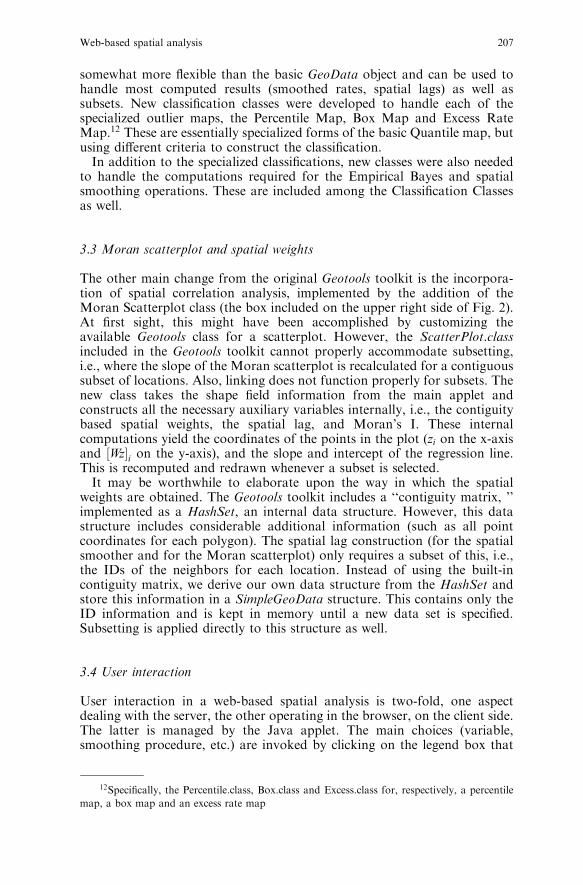
somewhat more flexible than the basic GeoData object and can be used tohandle most computed results (smoothed rates, spatial lags) as well assubsets. New classification classes were developed to handle each of thespecialized outlier maps, the Percentile Map, Box Map and Excess RateMap.12 These are essentially specialized forms of the basic Quantile map, butusing different criteria to construct the classification.In addition to the specialized classifications, new classes were also needed

to handle the computations required for the Empirical Bayes and spatialsmoothing operations. These are included among the Classification Classesas well.

3.3 Moran scatterplot and spatial weights

The other main change from the original Geotools toolkit is the incorpora-tion of spatial correlation analysis, implemented by the addition of theMoran Scatterplot class (the box included on the upper right side of Fig. 2).At first sight, this might have been accomplished by customizing theavailable Geotools class for a scatterplot. However, the ScatterPlot.classincluded in the Geotools toolkit cannot properly accommodate subsetting,i.e., where the slope of the Moran scatterplot is recalculated for a contiguoussubset of locations. Also, linking does not function properly for subsets. Thenew class takes the shape field information from the main applet andconstructs all the necessary auxiliary variables internally, i.e., the contiguitybased spatial weights, the spatial lag, and Moran’s I. These internalcomputations yield the coordinates of the points in the plot (zi on the x-axisand ½Wz�i on the y-axis), and the slope and intercept of the regression line.This is recomputed and redrawn whenever a subset is selected.It may be worthwhile to elaborate upon the way in which the spatial

weights are obtained. The Geotools toolkit includes a ‘‘contiguity matrix, ’’implemented as a HashSet, an internal data structure. However, this datastructure includes considerable additional information (such as all pointcoordinates for each polygon). The spatial lag construction (for the spatialsmoother and for the Moran scatterplot) only requires a subset of this, i.e.,the IDs of the neighbors for each location. Instead of using the built-incontiguity matrix, we derive our own data structure from the HashSet andstore this information in a SimpleGeoData structure. This contains only theID information and is kept in memory until a new data set is specified.Subsetting is applied directly to this structure as well.

3.4 User interaction

User interaction in a web-based spatial analysis is two-fold, one aspectdealing with the server, the other operating in the browser, on the client side.The latter is managed by the Java applet. The main choices (variable,smoothing procedure, etc.) are invoked by clicking on the legend box that

12Specifically, the Percentile.class, Box.class and Excess.class for, respectively, a percentile

map, a box map and an excess rate map


appears when the map is first drawn. Initially, this is a single button, but afterclicking, an interface appears as in Fig. 4. Additionally, selected buttonsappear in the web page to invoke specific methods (see the illustrations inSect. 4).The interaction on the server side ensures that the initialization parameters

are obtained to set the proper configuration for the Java applet. In astandard html page, a ‘‘form’’ is used to record the selections, as illustrated inFig. 5. The form invokes a PHP script (on the server) that generates a webpage corresponding to the selected options. This web page includes one ofthree Java applets, depending on the option selected. After this page isrendered on the client (and the applet downloaded) all further interaction isthrough the Java applet on the client.There are three basic options, as illustrated in Fig. 5.13 First, the screen

resolution can be customized in order to make sure the maps and graphs fiton the user’s screen (assuming the browser window is maximized). Second, aselection can be made from a series of maps/data sets included in a dropdown list. These data sets must be present on the server in a directoryspecified by Geotools. At this point it is not possible for the user to uploadshape files to this directory without proper write permissions. The finaloption pertains to the type of analysis to be carried out. The single mapoption is primarily for visualization and smoothing, but only one map isrendered in the browser. This is the fastest option, with the shortest timerequired to download the applet. In contrast, the two map option rendersboth the smoothed map as well as the original (unsmoothed) map, to allowdirect comparison of outliers and other features of the data. The three mapoption also provides space to draw the Moran Scatterplot for the selectedvariable. These two options take longer to download the applet.

Fig. 5. Welcome screen and general options

13This particular view is for a Safari web browser on a Mac G4 workstation, with the pages

served using the Apache server on a Linux workstation.


Finally, the user can interact directly with the graphics, since all maps andgraphs are linked, such that clicking on a location in one of them highlightsthe matching locations in the others. Also, all three graphics supportzooming, panning and subsetting.

4 Illustration

We provide a brief illustration of the functionality of the spatial analysistools using two sample data sets. One is a subset of the NCOVR USHomicide Atlas, limited to counties surrounding St. Louis, MO (Messneret al. 1999, 2000). The other contains data on colon cancer diagnoses inAppalachian counties.14 Both data sets are for rates, respectively homicidecounts over population (for 1979–84) and colon cancer diagnosis counts overpopulation (1994-98). Using standard practice, the counts are aggregatedover a small number of years to avoid extreme heterogeneity.We start with an Excess Rate map (or relative risk map) for the St. Louis

region homicide rates (Fig. 6). The map is invoked by selecting the countyhomicide count in the period 1979–84 (HC7984) as the ‘‘Event, ’’ and thecounty population in the same period (PO7984) as the ‘‘Base.’’ Also, the propermap type must be clicked in the Legend Interface (see Fig. 4). The buttons atthe top of the map allow zooming, panning and subsetting. For thisparticular map type, the legend is hard coded, showing six intervals for therelative risk.15 Moving the mouse over each county triggers a pop up‘‘tooltip’’ with the ID value for that county (e.g., St. Clair county in Fig. 6).The map illustrates how both St. Louis city and St. Clair county have

homicide rates that far exceed the region-wide average. By contrast, outlyingrural counties have relative risks well below the region-wide average. Thishighlights the dominance of the St. Louis-East St. Louis core when it comesto homicides in the period under consideration.The second example highlights the use of two maps to compare ‘‘raw’’

rates (the simple ratio of events over base) to their smoothed counterparts.The top map in Fig. 7 shows an example for colon cancer rates that havebeen transformed using the Empirical Bayes approach, shrinking the rawrates towards the overall average for the Appalachian region. In thisexample, two Box Maps are shown in the browser, the top map with thesmoothed rates, and the bottom map with the original raw rates. Note howCameron county, identified as a high outlier in the raw rate map (shown as atooltip), does not maintain that position in the smoothed map (on top).16

14Data compiled from individual cancer registry records and aggregated to the county level

by Eugene J. Lengerich, Pennsylvania State Cancer Institute, Pennsylvania State University.

15The colors in the legend can be adjusted individually, but the default is based on

recommendations from ColorBrewer, http://www.colorbrewer.org. The same approach is taken

in all other thematic maps.

16Note that the two county outlines are ‘‘linked’’ in the sense that moving the mouse over

the county in the lower map also highlights the county in the top map. This is near impossible to

see in the Figure shown as hard copy, but an important feature of the user interaction with the

map. The tooltip is only shown for the location that the mouse actually points to. In Fig. 7, this

is Cameron county in the lower map.


Instead, another county on the Eastern edge of Pennsylvania’s Appalachia(Carbon county, not shown as a tooltip) becomes an outlier in the smoothedmap. The smoothing is invoked by clicking on the ‘‘Smooth’’ button in themap window and selecting the specific smoothing method in the drop downlist. Counties that lose their outlier status after smoothing are so-calledspurious outliers, where the extreme rate is likely due to a small population atrisk.In the Empirical Bayes smoothing method, a central role is played by the

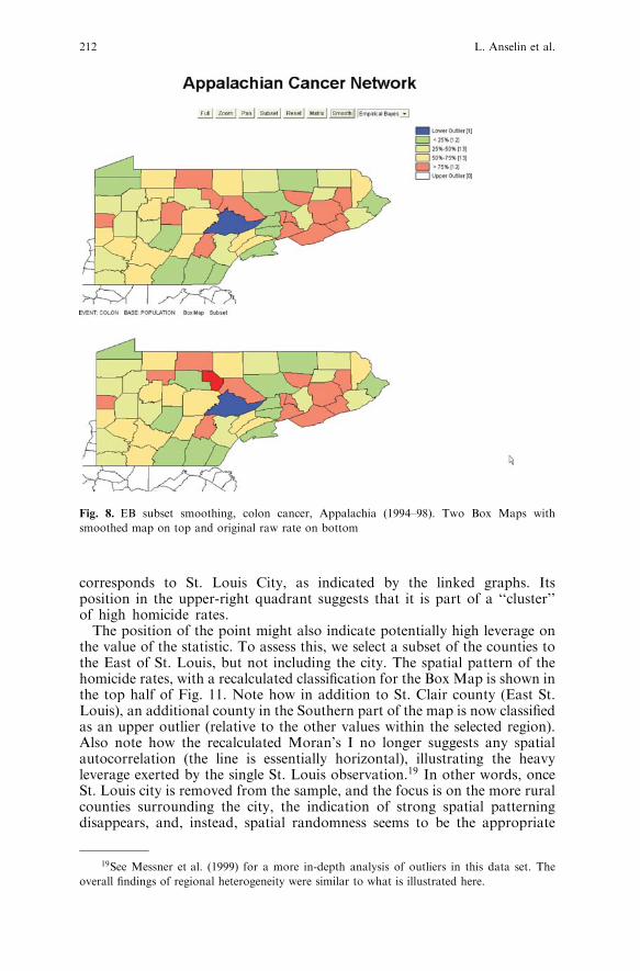
regional average to which the raw rates are shrunk. When the region is highlyheterogeneous, the choice of the overall regional average as the reference ratemay not be appropriate. More precisely, the choice of different subregionswill yield varying subregional averages which affects the smoothing and theresulting indication of outliers. We provide a way to assess the sensitivity ofthe results to this choice by means of the subset command. Clicking on thecorresponding button turns the cursor into a selection rectangle. Theclassification underlying the box map is recalculated for the selected counties,and, as a result, the indication of outlier may change. For example, in Fig. 8,a county appears as a low end outlier, when the subset is reclassified forPennsylvania counties only. In contrast, the overall map (Fig. 7) does notclassify this county as a low end outlier. Again, note how an upper outlier inthe raw rate map disappears in the EB smoothed map. Other changes areminor in this map, likely due to the smoothing of counts over time (the fouryear average used to compute the county rates).Spatial smoothing, shown in Fig. 9, tends to emphasize broad subregional

trends. Note how the patterns are much stronger in the upper map than inthe lower map. The smoothed map highlights a North-South divide in theregion, suggesting spatial heterogeneity (and, possibly, spatial regimes).Again, the indication of outlier changes between the raw rate map and the

Fig. 6. Excess rate map, St Louis Region Homicides (1979–84)


smoothed map, supporting the importance of this type of sensitivity analysisbefore locations are classified as ‘‘extreme.’’The final element in our analytical toolbox pertains to the visualization

of spatial autocorrelation by means of a Moran scatterplot. Figure 10shows the bottom two graphs in the three graph plot generated by theJava applet.17 The illustration is for the same homicide rate in theSt. Louis region as used in Fig. 6. The value of 0.196 is the slope ofthe regression line and suggests strong positive spatial autocorrelation inthe homicide rates.18 The highlighted point in the scatterplot (in red)

Fig. 7. EB Smoothing, Colon Cancer, Appalachia (1994–98). Two Box Maps with smoothed

map on top and original raw rate on bottom

17Since no smoothing is applied in the univariate Moran scatterplot, the smoothed and

original map are identical.

18It is important to note that this does not indicate ‘‘significance’’ of the spatial

autocorrelation statistic, but only shows its magnitude. A formal hypothesis test is not currently

included, but would be required before the value of 0.196 can be characterized as indicating

significant spatial autocorrelation.


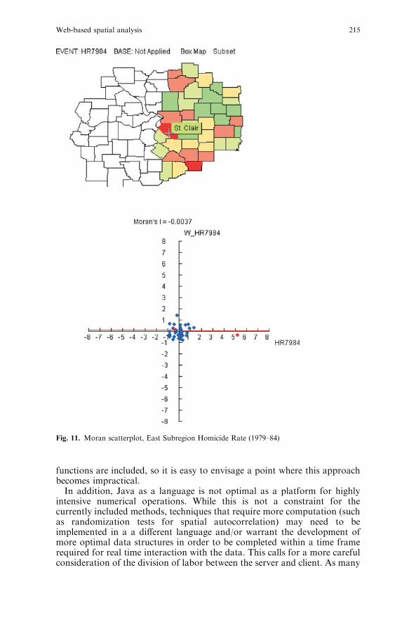
corresponds to St. Louis City, as indicated by the linked graphs. Itsposition in the upper-right quadrant suggests that it is part of a ‘‘cluster’’of high homicide rates.The position of the point might also indicate potentially high leverage on

the value of the statistic. To assess this, we select a subset of the counties tothe East of St. Louis, but not including the city. The spatial pattern of thehomicide rates, with a recalculated classification for the Box Map is shown inthe top half of Fig. 11. Note how in addition to St. Clair county (East St.Louis), an additional county in the Southern part of the map is now classifiedas an upper outlier (relative to the other values within the selected region).Also note how the recalculated Moran’s I no longer suggests any spatialautocorrelation (the line is essentially horizontal), illustrating the heavyleverage exerted by the single St. Louis observation.19 In other words, onceSt. Louis city is removed from the sample, and the focus is on the more ruralcounties surrounding the city, the indication of strong spatial patterningdisappears, and, instead, spatial randomness seems to be the appropriate

Fig. 8. EB subset smoothing, colon cancer, Appalachia (1994–98). Two Box Maps with

smoothed map on top and original raw rate on bottom

19See Messner et al. (1999) for a more in-depth analysis of outliers in this data set. The

overall findings of regional heterogeneity were similar to what is illustrated here.


conclusion. A complete analysis would assess this for other potential highleverage points as well.Finally, note how the point to the utmost right in the Moran scatterplot

of Fig. 11 is more than five standard deviations from the mean. Thisqualifies it as an outlier in the traditional sense of descriptive statistics, asconfirmed by its classification in the box map. Moreover, since it is in thelower-right quadrant of the scatterplot, it also corresponds to a spatialoutlier, a location with a much higher homicide rate than its surroundingneighbors.

5 Conclusion

In this paper, we outlined an initial framework to implement spatial dataanalysis functions in an internet GIS. Our efforts are a ‘‘work in progress’’and part of a much larger and more comprehensive endeavor to develop

Fig. 9. Spatial smoothing, colon cancer, appalachia (1994–98)


spatial analytical software tools as part of the program of the Center forSpatially Integrated Social Science (CSISS).20 While the current tools servetheir purpose, several important issues warrant further scrutiny.The range of spatial analytical methods included in the framework is

clearly limited. In part this is by design, given the specific objective to providean interactive front end to an atlas. However, part of the limitation also hasto do with performance issues encountered for medium size and larger datasets. The download time for the applet increases considerably when more

Fig. 10. Moran scatterplot, St. Louis Region Homicide Rate (1979–84)

20See http://sal.agecon.uiuc.edu/projects_csiss/php.


functions are included, so it is easy to envisage a point where this approachbecomes impractical.In addition, Java as a language is not optimal as a platform for highly

intensive numerical operations. While this is not a constraint for thecurrently included methods, techniques that require more computation (suchas randomization tests for spatial autocorrelation) may need to beimplemented in a a different language and/or warrant the development ofmore optimal data structures in order to be completed within a time framerequired for real time interaction with the data. This calls for a more carefulconsideration of the division of labor between the server and client. As many

Fig. 11. Moran scatterplot, East Subregion Homicide Rate (1979–84)


others have argued, the more computationally intensive operations shouldprobably be carried out on the server, with user interaction and simplecalculations allocated to the client. The exact nature of the tradeoffsassociated with this balancing act merit further attention, and are the subjectof ongoing research.Finally, even given these limitations, the current framework provides some

insight into the complexities of the characterization of spatial outliers and thesensitivity of the ‘‘map’’ to various assumptions made in the process. Thispedagogical objective is reached without requiring the user to have access toadvanced statistical or GIS software, a main advantage of the web-basedapproach. It is hoped that continued work along these lines will furtheradvance the dissemination of spatial analytical techniques to a broaderaudience.21

References

Andrienko G, Andrienko N, Voss H, Carter J (1999) Internet mapping for dissemination of

statistical information. Computers, Environment and Urban Systems, 23:425–441

Anselin L (1994). Exploratory spatial data analysis and geographic information systems.

In: Painho M (ed) New Tools for Spatial Analysis, Eurostat, Luxembourg. pp 45–54

Anselin L (1995) Local indicators of spatial association – LISA. Geographical Analysis, 27:

93–115

Anselin L (1996) The Moran scatterplot as an ESDA tool to assess local instability in spatial

association. In: Fischer M, Scholten H, Unwin D (eds) Spatial Analytical Perspectives on GIS

in Environmental and Socio-Economic Sciences, Taylor and Francis, London. pp 111–125

Anselin L (1998) Exploratory spatial data analysis in a geocomputational environment.

In: Longley P A, Brooks S, Macmillan B, McDonnell R, (eds) Geocomputation: A Primer,

John Wiley, New York, NY. pp 77–94

Anselin L (1999) Interactive techniques and exploratory spatial data analysis. In: Longley PA,

Goodchild MF, Maguire DJ, Rhind DW, (eds) Geographical Information Systems: Principles,

Techniques, Management and Applications, John Wiley, New York, NY. pp 251–264

Anselin L (2000) Computing environments for spatial data analysis. Journal of Geographical

Systems, 2(3):201–220

Anselin L (2003) GeoDa 0.9 User’s Guide. Spatial Analysis Laboratory (SAL). Department of

Agricultural and Consumer Economics, University of Illinois, Urbana-Champaign, IL

Anselin L, Getis A (1992). Spatial statistical analysis and geographic information systems. The

Annals of Regional Science, 26:19–33

Anselin L, Syabri I, Smirnov O (2002) Visualizing multivariate spatial correlation with

dynamically linked windows. In: Anselin L, Rey S (eds) New Tools for Spatial Data Analysis:

Proceedings of the Specialist Meeting. Center for Spatially Integrated Social Science(CSISS),

University of California, Santa Barbara. CD-ROM

Assuncao R, Reis EA (1999) A new proposal to adjust Moran’s I for population density.

Statistics in Medicine, 18:2147–2161

Bailey TC, Gatrell AC (1995) Interactive Spatial Data Analysis. John Wiley and Sons, New

York, NY

Clayton D, Kaldor J (1987) Empirical Bayes estimates of age-standardized relative risks for use

in disease mapping. Biometrics, 43:671–681

Cleveland WS (1993). Visualizing Data. Hobart Press, Summit, NJ

21The web tools described in this paper are available for a sample of six data sets at http://

sal.agecon.uiuc.edu/geotools_main.php.


Fischer M, Nijkamp P (1993) Geographic Information Systems, Spatial Modelling and Policy

Evaluation. Springer-Verlag, Berlin

Fotheringham AS, Brunsdon C, Charlton M (2000) Quantitative Geography. Perspectives on

Spatial Data Analysis. Sage Publications, London

Fotheringham AS, Rogerson P (1993) GIS and spatial analytical problems. International Journal

of Geographical Information Systems, 7:3–19

Gahegan M, Takatsuka M, Wheeler M, Hardisty F (2002) Introducing GeoVISTA Studio: An

integrated suite of visualization and computational methods for exploration and knowledge

construction in geography. Computers, Environment and Urban Systems, 26:267–292

Goodchild MF (1987) A spatial analytical perspective on Geographical Information Systems.

International Journal of Geographical Information Systems, 1:327–334

Goodchild MF, Haining RP, Wise S (1992) Integrating GIS and spatial analysis – problems and

possibilities. International Journal of Geographical Information Systems, 6:407–423

Haining RF, Wise S, Ma J (2000) Designing and implementing software for spatial statistical

analysis in a GIS environment. Journal of Geographical Systems, 2(3):257–286

Herzog A (1998) Dorling Cartogram. http://www.zh.ch/statistik/map/ dorling/dorling.html.

Huang B, Lin H (1999) GeoVR:a web-based tool for virtual reality presentation from 2D GIS

data. Computers and Geosciences, 25:1167–1175

Huang B, Lin H (2002) A Java/CGI approach to developing a geographic virtual reality toolkit

on the internet. Computers and Geosciences, 28:13–19

Huang B, Worboys MF (2001) Dynamic modelling and visualization on the internet.

Transactions in GIS, 5:131–139

Jankowski P, Stasik M, Jankowska MA (2001) A map browser for an internet-based GIS data

repository. Transactions in GIS, 5:5–18

Kafadar K (1996) Smoothing geographical data, particularly rates of disease. Statistics in

Medicine, 15:2539–2560

Kahkonen J, Lehto L, Kiolpelainen T, Sarjakoski T (1999) Interactive visualization of

geographical objects on the internet. International Journal of Geographical Information

Science, 13(4):429–438

Kraak M-J, Brown A (2001) Web Cartography. Taylor & Francis, London

Lawson A, Biggeri A, Bohning D, Lesaffre E, Viel J-F, Bertollini R (1999) Disease Mapping and

Risk Assessment for Public Health. John Wiley, Chichester

Marshall RJ (1991) Mapping disease and mortality rates using Empirical Bayes estimators.

Applied Statistics, 40:283–294

Messner S, Anselin L, Baller R, Hawkins D, Deane G, Tolnay S (1999) The spatial patterning of

county homicide rates:An application of exploratory spatial data analysis. Journal of

Quantitative Criminology, 15(4):423–450

Messner S, Anselin L, Hawkins D, Deane G, Tolnay S, Baller R (2000) An Atlas of the Spatial

Patterning of County-Level Homicide, 1960–1990. National Consortium on Violence Research,

Carnegie-Mellon University, Pittsburgh, PA (CD-ROM)

Peng Z (1999) An assessment framework for the development of internet GIS. Environment and

Planning B, 26:117–132

Plewe B (1997) GIS Online. Information Retrieval, Mapping and the Internet. OnWorld Press,

Santa Fe, NM

Symanzik J, Cook D, Lewin-Koh N, Majure JJ, Megretskaia I (2000) Linking ArcView and

XGobi:Insight behind the front end. Journal of Computational and Graphical Statistics,

9(3):470–490

Takatsuka M, Gahegan M (2001) Sharing exploratory geospatial analysis and decision making

using GeoVISTA studio:From a desktop to the web. Journal of Geographic Information and

Decision Analysis Decision Analysis, 5(2):129–139

Takatsuka M, Gahegan, M (2002) GeoVISTA Studio:A codeless visual programming

environment for geoscientific data analysis and visualization. Computers and Geosciences,

28:1131–1141

Tsou M-H, Buttenfield B (2002) A dynamic architecture for distributing geographic information

services. Transactions in GIS, 6:355–381


Wall P, Devine O (2000) Interactive analysis of the spatial distribution of disease using a

geographic information system. Journal of Geographical Systems, 2(3):243–256

Zhang Z , Griffith D (2000) Integrating GIS components and spatial statistical analysis in

DBMSs. International Journal of Geographical Information Science, 14(6):543–566


Web-based Analytical Tools for the Exploration of Spatial Data

Documents

Transcript of Web-based Analytical Tools for the Exploration of Spatial Data