WEAP-MODFLOW Tutorial - BGR

Management, Protection and Sustainable

Use of Groundwater and Soil Resources in the Arab Region

WEAP-MODFLOW Tutorial

September 2012

WEAP-MODFLOW-Tutorial 2/45

WEAP-MODFLOW Tutorial Version 2

Authors

M. Huber (geo:tools)

M. Al-Sibai (ACSAD)

With participation of

J. Al Mahameed (ACSAD)

A. Abdallah (ACSAD)

O. Al Shihabi (ACSAD)

I. Jnad (ACSAD)

J. Wolfer

J. Maßmann (BGR)

Online available at

http://www.bgr.bund.de/IWRM-DSS

WEAP-MODFLOW-Tutorial 3/45

Content

1 Introduction ........................................................................................................................ 4

2 MODFLOW Model ................................................................................................................ 5

2.1 Model Area – “Main River Basin” ........................................................................................ 5

2.2 Mathematical Model ........................................................................................................... 6

3 Create and link a WEAP-model based on MODFLOW data ..................................................... 8

3.1 Create a new WEAP – Area ................................................................................................. 9

3.2 Start LinkKitchen................................................................................................................ 10

3.3 Set the WEAP Area’s Boundary ......................................................................................... 11

3.4 Add Catchment and Groundwater Nodes to the Schematic ............................................. 13

3.5 Add Rivers to the Schematic.............................................................................................. 16

3.6 Set the Model Runtime in WEAP ....................................................................................... 17

3.7 Define Catchment and Groundwater in the Linkage File .................................................. 18

3.8 Define Rivers in the Linkage File ........................................................................................ 21

3.9 Set the FLOW-STAGE-WIDTH relationship ........................................................................ 25

3.10 Send Linkage File Data to WEAP .................................................................................... 26

3.10.1 Send catchment areas to WEAP .................................................................................... 26

3.10.2 Send groundwater recharge to WEAP ........................................................................... 27

3.11 Link WEAP and MODFLOW ............................................................................................ 28

4 WEAP-hydrology in linked models – Rainfall-Runoff ........................................................... 31

4.1 Add Runoff links to the Schematic .................................................................................... 31

4.2 Assign catchments and Landuse Classes to the Linkage File. ............................................ 32

4.3 Data input in WEAP ........................................................................................................... 34

4.3.1 Enter precipitation ........................................................................................................ 34

4.3.2 Enter ETRef .................................................................................................................... 35

4.3.3 Enter Kc.......................................................................................................................... 35

4.3.4 Enter Runoff- and Infiltration fractions ......................................................................... 35

4.3.5 Run the model and browse the results ......................................................................... 35

5 Common tasks ................................................................................................................... 36

5.1 Abstraction for irrigation ................................................................................................... 36

5.1.1 Add irrigation abstraction by demand site .................................................................... 36

5.1.2 Add irrigation abstraction to a Landuse Class ............................................................... 37

5.2 Changes in Land Use .......................................................................................................... 39

5.2.1 Urbanization .................................................................................................................. 39

5.2.2 Irrigation growth ........................................................................................................... 40

5.3 Domestic water supply from well fields ............................................................................ 41

5.4 Artificial groundwater recharge ........................................................................................ 43

5.5 Climate Change .................................................................................................................. 45

WEAP-MODFLOW-Tutorial 4/45 Introduction

1 Introduction

The present tutorial intends to illustrate the idea of the dynamic link between WEAP and MODFLOW.

The techniques presented are kept as simple as possible in order to make you familiar with the

necessary steps for building up a WEAP model that is linked to MODFLOW and to give you an

introduction to solving common water management problems.

The first part will guide you through building a WEAP model based on the data stored in a MODFLOW

model (“Hard Data approach”). Despite this approach is not recommended in general, as flexibility is

lost and many of WEAP’s powerful modelling options are not available, it might be useful in case

measured data (e.g. precipitation) used to build and calibrate the existing MODFLOW model is

unavailable for whatever reason.

The second part focusses on building and linking a model that makes use of WEAP’s internal

functions to model groundwater recharge and surface runoff.

In the last part, you will learn how to cope with various challenges typical to modellers like

implementing artificial recharge or changes in land use.

Before you start with the tutorial, be advised to have downloaded the associated shape files

(Catchment.shp, Landuse.shp, Wellfields.shp) and the csv-file (InputData.csv).

This tutorial refers to WEAP Version 3.001 (Sep 2012) and LinkKitchen Version 1.00 (Sep 2012).

It is based on the WEAP-MODFLOW-Tutorial by BGR/ACSAD (2009) and includes contributions by M.

Al-Sibai (Chapter 2).

WEAP-MODFLOW-Tutorial 5/45 MODFLOW Model

2 MODFLOWModel

The MODFLOW model used in this tutorial was designed with the intention to make many planning

options possible (dams, irrigation) and to remain easy to understand. It is a modification of the

original GMS-Tutorial model and in the following named “Main River Basin”.

2.1 ModelArea–“MainRiverBasin”

The Main River basin encompasses 783 square kilometres. It is located in a semi-arid climate, with

precipitation only in the winter months. Most of this precipitation is lost by evapotranspiration. The

aquifer consists of fractured crystalline bedrock and alluvial fills in the valleys, its saturated thickness

varies between 35 m in the South to about 53 m in the North.

Groundwater flow is towards the spring, the Main River and its 2 tributaries. The spring represents

the headflow of the Main river, with an average monthly discharge of about 320 000 m³. In the

north, outside the model area the Main River finally drains into a reservoir lake with a constant water

level of 304.8 m a.s.l.

The topography gradually decreases from South (353 m.a.s.l) to North (335 m.a.s.l).

Elevation

demValue

High : 353.331146

Low : 334.447601


2.2 Mathematical Model

GRID: The model consists of one layer (1 unconfined aquifer, 60-80m layer thickness, 35m – 50m

saturated thickness) with 88x70 cells. The cell sizes vary in width and height between 200 m to 1200

m (see figure below)

BOUNDARY CONDITIONS: Specified-Head boundary in the North (Reservoir Lake level). All other

boundaries are No-Flow boundaries (see figure above).

HYDRAULIC CONDUCTIVITY: The 4 hydraulic conductivity zones for the model are shown in the

figure below. The hydraulic conductivity of the aquifer varies between 100 m/day along the river

valley to 40 m/day towards the basin boundary.

0 - 0.0015 m/d

0 - 0.0013 m/d

0 m/d

0-0.003 m/d 0 - 0.0011 m/d


RECHARGE: 5 different recharge zones have been defined. The values in the zones ranging from 0 to

0.0015 m/d (see figure above).

ADDITIONAL PACKAGES: The spring was modelled as 2 DRAIN-cells (pink in the figure above) and the

rivers as RIVER-cells (blue in the figures above).

INITIAL HEAD: The initial head ranges from 306 – 327 m.a.s.l. resulting in a depth to water table of 25

to 36 m (see figures below).

Starting Heads: Depth to groundwater table

The Model has been built and run on transient state in order to cover two years of recharge

variation. It consists of 24 monthly stress periods, which contain 3 equal time steps each. The final

balance (see figure below – units in m³ or m³/d) shows that the model is almost balanced or close to

steady state, with recharge as the main inflow and river leakage as the main outflow fraction.

WEAP-MODFLOW-Tutorial 8/45 Hard-Data-Approach

3 CreateandlinkaWEAP-modelbasedonMODFLOWdata

At the beginning, you will create a new WEAP Area and design the Schematic for it. The necessary

tasks are:

• Create a new WEAP area

• Set the area’s spatial boundaries

• Load background layers

• Digitize 4 rivers

• Add 5 catchment and 5 groundwater nodes

The result will look similar to the image below.


3.1 Create a new WEAP – Area

1. In the Main Menu in WEAP, go to Area → Create Area. In the following dialog, create a new

Area, which is initially blank and give it the name: “DSS-Tutorial”:

2. Click “OK” and ignore the following dialog (“Area boundary”) by clicking on “Cancel”. The

model should look like below:


3.2 Start LinkKitchen

LinkKitchen is a GIS-alike tool designed to assist the setup of the Linkage Shapefile without the need

of further GIS- and Spreadsheet-software. It provides all necessary functionality for producing the

linkage file and for its attribution. Furthermore, it allows direct parameterization of the WEAP-model

based on linkage file’s attributes.

If you are not yet familiar with the use of LinkKitchen, please read its User Manual before you

continue with the tutorial.

Remain WEAP open and start LinkKitchen in parallel.

At start-up, you are prompted to select the one of your WEAP

models which you want to work on. Select DSS-Tutorial and

confirm the dialog by click on OK.

In the following dialog, LinkKitchen prompts for the location of the

MODFLOW model and the Linkage File. Browse for the MODFLOW

model that comes with the Tutorial data and select the Namefile.

As a linkage file does not yet exist, select to create a new Linkage

File.

Once you confirm with OK, all MODFLOW files will be copied to

the WEAP-Area’s standard directory.

LinkKitchen produces the Linkage File as well as two other

shapefiles in the background. Those will be used during the next

steps.


3.3 Set the WEAP Area’s Boundary

Your LinkKitchen User Interface will show an empty grid that represents the geometry of your

MODFLOW model. This is the linkage File.

Switch back to WEAP (don’t close LinkKitchen).

Right-click into the Layer-pane and select Add Vector Layer

from the context menu.

Browse to your WEAP Area directory/SHAPE/ and select

the file MF_Domain_trans_modify_5f_drain.shp. This file

was created at start-up and represents the spatial

boundary of the MODFLOW model. You will use this file to

define the area’s boundaries.

Remove all other layers (Major Rivers, States, Country,

Ocean) except MF_Domain_trans_modify_5f_drain.shp.


Right-click into the Layer-pane and select Set Area

Boundaries from the context menu.

Draw the green rectangle (the area boundary) around the

complete extent of the black rectangle (the MODFLOW

model’s extent) and confirm by click on OK.


3.4 Add Catchment and Groundwater Nodes to the Schematic

It is assumed, that MODFLOW is the only source of information about the model area. Catchments

and Groundwater nodes are thus delineated by zones of equal recharge rate. You will use

LinkKitchen to delineate the Catchment and Groundwater zones in WEAP.

1. Switch to LinkKitchen and browse to the MODFLOW-Layer Recharge SP1 in the MODFLOW

Viewer. Click the Preview-Button to show the recharge zones.

2. Click the Make Snapshot-button to save the preview-image permanently to disc. The

image appears in the List of Layers as a regular Background Layer.

3.

At this stage, the recharge zones are saved as a JPEG-image-file in the WEAP-area directory. The file

doesn’t store any information besides a different colour for each zone.


4. Switch back to WEAP and load the file “Recharge_SP1.jpg” as a background raster layer to

the Schematic.


In the MODFLOW model, five zones of different recharge are defined. You will take these zones as

blueprints for the delineation of WEAP-Catchments and groundwater nodes.

1. Drag and drop one Catchment and one Groundwater node for each recharge zone onto the

schematic.

2. Connect the Groundwater and Catchment nodes by infiltration links.

Catchment node name connection groundwater node name

C_East infiltration link GW_East

C_MainCentral infiltration link GW_MainCentral

C_MainLower infiltration link GW_MainLower

C_MainUpper infiltration link GW_MainUpper

C_West infiltration link GW_West

NOTE: It is good practice to add the prefix “C_” before the catchment’s name and the prefix “GW_”

before groundwater nodes in order to avoid getting confused by identical names of groundwater

nodes, catchments and demand sites.


3.5 Add Rivers to the Schematic

1. Add the file MF_River_trans_modify_5f_drain.shp (located in the folder SHAPE in the area

directory) to the Schematic and give it a solid blue colour.

2. Drag and Drop river nodes onto

the Schematic and digitize each river,

in flow direction, on top of the blue

area. The rivers’ names are Main

River, East River and West River. East

River and West River are tributaries

to Main River.

3. A fourth River needs to be digitized in addition to the three rivers. In

MODFLOW, it is represented by two drain cells upstream of Main River. That

River is named Spring.


3.6 Set the Model Runtime in WEAP

In order to ensure, the WEAP calculation correlates correctly with the MODFLOW model, adjust the

WEAP time steps and the starting month according to the MODFLOW stress periods (here: October

1999 – September 2001).

This is done using the General menu item → Years and Time Steps

Initially you won’t use any WEAP internal model to calculate surface runoff, groundwater recharge

and irrigation demand, therefore choose in

Data View → Demand Sites and Catchments → Advanced


3.7 Define Catchment and Groundwater in the Linkage File

Switch back to LinkKitchen and see how it reflects the changes you made in WEAP. The Nodes you

added to the Schematic are now visible in LinkKitchen’ s Branch Viewer. During the following steps,

you will relate cells of the Linkage File to Catchments, Groundwater Nodes and Rivers.

As you have the recharge zones loaded in the background, you will use these zones as stencils for

selecting cells. Use LinkKitchen’s selection-tools (s. LinkKitchen User Manual) to select cells

corresponding to recharge-zones. The thus selected cells are then attributed with the name of the

catchment as defined in WEAP.

The procedure of attributing groundwater nodes is identical.

1. Select all cells located in the green area (C_Main Upper).


2. Highlight C_MainUpper in the Branch-Viewer and click Add Attribute to Linkage File. This will write

the Branch’s name to the linkage file.

3. Highlight GW_MainUpper and click Add Attribute to Linkage File.

3. Repeat Steps 1 and 2 for the other Catchments

4. Highlight the Parent-Branch Catchments and look at the Linkage File Preview:


3.8 Define Rivers in the Linkage File

In WEAP, a river is defined as a “chain” of reaches, sections between inflow or outflow nodes. Any

river reach requires to have a representation in the Linkage File.

There are two different ways to assign river reaches to the Linkage File. The method to choose

depends on how accurate you digitized the rivers in the WEAP Schematic beforehand. If the WEAP-

rivers are digitized very accurately with no overlaps of the river lines out of the blue river cells, you

should opt for method 2. If the rivers are digitized only roughly around the river cells, choose the first

method. Both methods are described in the following section.

Method 1:

The procedure to assign river reaches to Linkage File cells is similar to the procedure to assign

Catchments except that you start from Information you get from MODFLOW rather than from an

overlay shapefile.

1. In the MODFLOW-Viewer, browse to the Layer IsDrain and click select. The drain cells represent

the river Spring in WEAP.

Accurate → Method 2 Simplistic → Method 1


2. Highlight the River-branch Below Spring Headflow in the Branches-Viewer and click Add Attribute

to Linkage File.

The two drain cells are now linked to the WEAP river reach Below Spring Headflow.

3. Browse to the layer IsRiver in the MODFLOW Viewer to select River cells.

4. Use LinkKitchen’s selection-tools to sub-select those cells corresponding to the WEAP-rivers.

E.g. Click and hold the Alt-Key while drawing a rectangle around West River in order to select from

selected river cells.


5. Highlight the River-branch Below West River Headflow in the Branches-Viewer and click Add

Attribute to Linkage File.

6. Repeat the last two steps for all other river reaches.

The preview of the river-attribution should show an image similar to the image below:

Save the Linkage File to disc by clicking on the Write Linkage File button


Method 2:

You can make WEAP “guess” the river reaches and drains in accordance to your digitizing rivers in the

Schematic. In order to make this procedure work, it is necessary to link WEAP and MODFLOW first.

Continue with the next chapter and once you are about to link with MODFLOW, click the Guess River

Point Linkages and Guess Drain Cell Linkages – Buttons (Chapter 3.11).

Note: it is good practice to save the linkage file frequently in order to not lose your edits. The file is

overwritten every time you save it.


3.9 Set the FLOW-STAGE-WIDTH relationship

In order to allow WEAP to calculate river-related functions correctly, you need to assign a parameter

called “Flow-Stage-Width relationship”. This parameter (or set of parameters) describes the physical

properties of a river and its riverbed and is the basis for WEAP to calculate groundwater-river-

interactions. If you set up a WEAP-model based on the information from a MODFLOW model, it is

likely that the required information about rivers is missing.

LinkKitchen provides a rather pragmatic method to assign the Flow-Stage-Width relationship with

standardized parameters.

1. Switch to LinkKitchen and highlight the River Reach Spring, Below Spring Headflow.

2. Click the - Command to open the Flow-Stage-Width-Dialog. The following Window shows nine

images of rivers of various sizes. Left-click on the top left image (this one should come closest to a

spring).

LinkKitchen will produce a Flow-Stage-Width-curve based on parameters stored with the image (see

the LinkKitchen manual for further details).

3. Click the WEAP-button to send the curve to WEAP and check the result.

Supply and Resources → River → Below Spring Headflow → Reaches → Physical → Flow Stage Width

Note that the curve can be changed in WEAP using the Flow-Stage-Width-Wizard.

Repeat steps 1-3 for all other Rivers.


3.10 Send Linkage File Data to WEAP

In the currently used approach, you use the initial MODFLOW model inputs in WEAP rather than any

of the WEAP built-in models for calculating groundwater recharge. The groundwater recharge

retrieved from MODFLOW will be entered as input in WEAP instead.

Data View → Supply and Resources → Groundwater → Natural Recharge.

As a second obligatory parameter you need to enter catchment areas in WEAP

Data View → Demand Sites and Catchments → Landuse → Area

Both parameters are calculated by LinkKitchen and can be sent automatically to the correct input-

position in WEAP.

3.10.1 Send catchment areas to WEAP

Catchments’ areas are calculated by LinkKitchen and can be sent to WEAP by a single mouse-click:

1. Highlight the Catchments – parent branch and click the WEAP-button on the top toolbar

2. Switch to WEAP and browse to Data View → Demand Sites and Catchments → Landuse → Area

If the area’s units are not yet defined, you need to select

hectares as the area unit in order to make the entries visible.

The area distribution should look similar to the following:


3.10.2 Send groundwater recharge to WEAP

The procedure to send natural recharge to WEAP is similar to sending catchment areas.

1. Highlight the Groundwater – parent branch and click the WEAP-button on the top toolbar

2. Switch to WEAP and browse to

Data View → Supply and Resources → Groundwater → Natural Recharge.

Note: LinkKitchen calculates all recharge-values as million m³ which is the default scale for natural

recharge in WEAP. Check and change the scale if necessary!

General → Units → Groundwater: change the scale to Million m³.

The recharge values should look like:


3.11 Link WEAP and MODFLOW

After having entered the required data in both the Linkage File and WEAP, you are now ready to link

both models. This is done by:

• Loading the linkage shapefile to WEAP

• Set up the linkage in WEAP

Load the linkage shapefile to the WEAP schematic:

Add Vector Layer → select the linkage file (linkage.shp)

From the top menu, select:

Advanced → MODFLOW Link → MODFLOW Name File → MODFLOW/trans_modify_5f_drain.mfn


Choose your linkage shapefile and assign the respective attribute fields for Row and Column,

Groundwater, River Reach and Catchment (this should be correct by default).

If you have not yet assigned river reaches (because you opted for Method 2 in chapter 3.8), you

should now click on Guess River Point Linkages and Guess Drain Cell Linkages.

Click on the results-command and look at the result outputs like the groundwater levels (Supply and

Resources → Groundwater → MODFLOW → Cell Head) etc.

WEAP-MODFLOW-Tutorial 31/45 Rainfall-Runoff-Model

4 WEAP-hydrologyinlinkedmodels–Rainfall-Runoff

In the previous exercise, you entered groundwater recharge directly into WEAP as “Natural

Recharge” and delimited the catchments according to recharge zones in MODFLOW.

In the following exercises, the catchment names remain the same, but they correlate to different

spatial regions (surface water catchments). The Catchments are furthermore subdivided into Landuse

classes in order to reflect various water needs.

In addition, surface-runoff links are assigned to the catchment nodes (from the catchment to the

river).

In this chapter, WEAP will calculate the groundwater recharge based on its internal Rainfall Runoff

(simplified coefficient method) model.

4.1 AddRunofflinkstotheSchematic

In order to let WEAP calculate surface runoff, you need to add runoff-links from catchments to rivers

in the WEAP Schematic. Drag and drop a runoff-link from each Catchment Node to its corresponding

River.

Catchment Runoff link to Headflow yes/no

C_MainUpper Main River No

C_West West River Yes

C_East East River Yes

C_Central Main River No

C_Main Lower Main River No


4.2 Assign catchments and Landuse Classes to the Linkage File.

1. Add Sub-branches to each of the Catchments.

In the Data-View: right-click on the Catchment → Add → type the name of the sub branch as specified

in the table below:

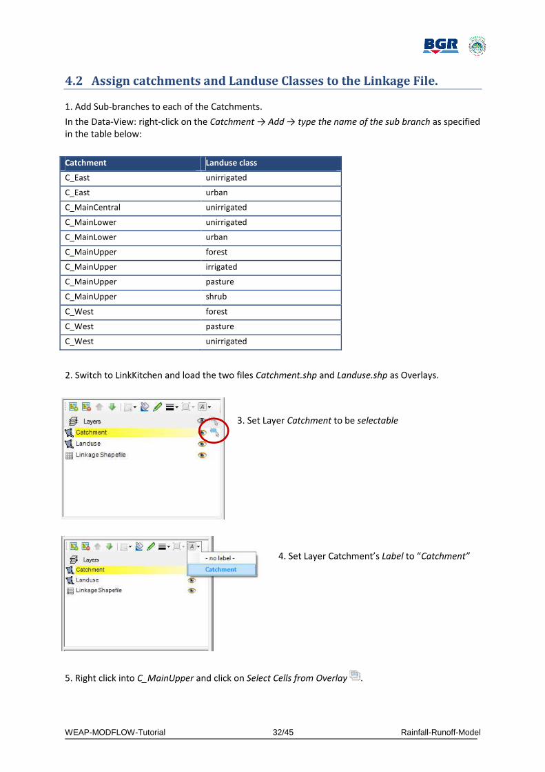
2. Switch to LinkKitchen and load the two files Catchment.shp and Landuse.shp as Overlays.

3. Set Layer Catchment to be selectable

4. Set Layer Catchment’s Label to “Catchment”

5. Right click into C_MainUpper and click on Select Cells from Overlay .

Catchment Landuse class

C_East unirrigated

C_East urban

C_MainCentral unirrigated

C_MainLower unirrigated

C_MainLower urban

C_MainUpper forest

C_MainUpper irrigated

C_MainUpper pasture

C_MainUpper shrub

C_West forest

C_West pasture

C_West unirrigated


6. Highlight C_MainUpper in the Branch Viewer and click Add Attribute to selected Cells.

7. Highlight GW_MainUpper in the Branch Viewer and click Add Attribute to selected Cells.

Repeat steps 5-7 for the other Catchments and Groundwater nodes.

8. Set Layer Landuse selectable and assign Landuse-Classes to the Linkage File. The procedure is

similar to steps 5-7.

9. Send the Area data to WEAP


4.3 Data input in WEAP

Additional inputs at catchment level are precipitation and reference evapotranspiration (ETref). Crop

coefficients (Kc) are entered at Landuse class level. These inputs are read into WEAP using the

ReadFromFile-function. The file from which to read data is named INPUT_DATA.csv. Copy the file into

the TimeSeries-Folder in the WEAP area-directory.

4.3.1 Enter precipitation

1. In the Data View, select C_MainCentral and activate Climate → Precipitation.

2. Click on the arrow besides the data-entry box and select the ReadFromFile Wizard.

3. Open the file \TimeSeries\INPUT_DATA.csv

4. In the lower pane, select the data column Precipitation and click Finish.

5. Repeat steps 2-4 for the other Catchments


4.3.2 Enter ETRef

ETRef is entered the same way as precipitation but with the data column [ET].

4.3.3 Enter Kc

Go to Landuse – Kc and enter Kc values for each Landuse Class the same way as precipitation and

ETRef.

Landuse Classes Irrigated and unirrigated retrieve values from the same data column (unirrigated).

(For details on the Rainfall Runoff (simplified coefficient method)-model, see WEAP-help and FAO

Irrigation and Drainage Paper No. 56 “Crop Evapotranspiration”).

4.3.4 Enter Runoff- and Infiltration fractions

The total runoff volume can be fractioned to surface runoff and groundwater recharge:

Supply and Resources → Runoff and Infiltration → from catchment (C_...) → to …→ Runoff Fraction

Enter a value of 50% for each link.

4.3.5 Run the model and browse the results

The result below shows the calculated recharge- and runoff-flows from C_MainLower.

WEAP-MODFLOW-Tutorial 36/45 Common Tasks

5 Commontasks

The following part of this tutorial will give you some workarounds for dealing with common modeling

challenges. It does make no claim to be complete nor does it pretend to show the one-and-only

solution for any of the problems presented. But you might use some of the shown approaches as the

starting point for your own modeling work.

The descriptions hereafter are reduced to the basic implementations and parameter setting. If you

want to visualize the impacts of each task on the system, you should apply the changes on scenarios

and compare the results with the reference.

5.1 Abstractionforirrigation

There are multiple ways to introduce irrigation abstraction. The two most commonly applied ways

are:

1. Define a Demand Site and enter the abstracted water directly

2. Let WEAP calculate irrigation demand based on climate and crop parameters

For the former, there is no need to care about the climate or what types of crop are grown. This

method is easier to implement but very inflexible when it comes to build scenarios. The later requires

more data to enter but gives better performance for future planning.

The following chapters will show both approaches.

5.1.1 Add irrigation abstraction by demand site

1. Drag and drop a new demand site onto the Schematic View and name it “Irrigation”.

2. Drag and drop a transmission link from groundwater GW_MainUpper to the new demand site

"Irrigation".

3. Enter the water abstraction for irrigation under:

Data→ Demand sites and catchments → irriga@on → water use → Annual water use

The irrigation demand is 30 million m3 per year. As water is needed only during the months of May

and June, the annual irrigation is fractioned with the percentage (40%) in May and (60%) in June. This

is entered at


Data→ Demand sites and catchments → irrigation → water use → Monthly Varia@on

Using the Monthly Time Series Wizard.

4. As WEAP needs to know from which cells to abstract water from, you need to update the Linkage

File with that information. It is assumed, that water is abstracted from wells located all over the

irrigated area.

Switch to LinkKitchen and highlight the Landuse Class C_MainUpper/Irrigated in the Branch Viewer.

5. Click the Select Attributed Cells-Button.

6. Highlight Demand Site Irrigation and click Add Attribute to Linkage File. Now, every cell located

within the Landuse Class “Irrigated” supplies Demand Site Irrigation.

7. Save the Linkage File to disc and go back to WEAP.

8. Re-load the Linkage File if necessary and run WEAP. Browse the results

5.1.2 Add irrigation abstraction to a Landuse Class

Modelling irrigation demand by a WEAP-internal model requires a connection from groundwater to

the catchment. Further specifications, like from which cells to withdraw water and on which cells to

apply water, are defined in the Linkage File.

The water demand is controlled by the crop parameter Kc and by the climate parameters

precipitation and ET. WEAP will calculate water demand, if the plant evapotranspiration is higher

than precipitation.


1. Drag and drop a transmission link from GW_MainUpper to

C_MainUpper

2. Set the demand priority to 1

3. Switch the irrigated Landuse Class to irrigated:

Demand Sites and Catchments→C_MainUpper→Irrigation→Irrigated = 1

4. Run the model and evaluate the results in the results view.

E.g. Land class inflows and

outflows:

You can see irrigation

takeing place during the

months May and June

when ET is high and

precipitation is low.

Although precipitation

remains low during July and

August, there is no need to

irrigate as the crops are

already harvested.


5.2 Changes in Land Use

The purpose of this exercise is to investigate the impact of changes in land use on the groundwater

recharge. In order to emphasize the changes, the total runtime of the model is extruded to 10 years.

General →. Years and @me steps → last year of scenarios = 2009

Land use 2000 Land use 2010

5.2.1 Urbanization

Storyline: Urban areas grow towards extending over the entire catchment areas of C_East and

C_MainLower until 2010. Infiltration vanishes and the entire precipitation runs off the rivers.

1. Let WEAP repeat time-dependant data each year (precipitation, ET, Kc):

Chose “cycle”-

option


to GW_MainLower

to Catchment Inflow Node 5

Runoff Fraction (monthly)

Oct

1999

Feb

2000

Jun

2000

Oct

2000

Feb

2001

Jun

2001

Oct

2001

Feb

2002

Jun

2002

Oct

2002

Feb

2003

Jun

2003

Oct

2003

Feb

2004

Jun

2004

Oct

2004

Feb

2005

Jun

2005

Oct

2005

Feb

2006

Jun

2006

Oct

2006

Feb

2007

Jun

2007

Oct

2007

Feb

2008

Jun

2008

Oct

2008

Feb

2009

Jun

2009

% s

hare

100

95

90

85

80

75

70

65

60

55

50

45

40

35

30

25

20

15

10

5

0

2. Increase the surface runoff fraction from 50% in the year 2000 to 100% in 2009 and reduce the

fraction for groundwater recharge accordingly:

Supply and Resources → Runoff and Infiltra@on → from C_MainLower → Runoff Frac@on

Supply and Resources → Runoff and Infiltration → from C_E ast→ Runoff Frac@on

To interpolate the yearly fractions use the functions Interp(2009, 100) and Remainder(100).

5.2.2 Irrigation growth

Land use class unirrigated is changed to be irrigated from the year 2001 onward.

1. Add transmission links from the groundwater to the catchment for the catchments C_MainUpper,

C_MainCentral and C_West.

2. Within these catchments, set the land use classes unirrigated and irrigated to be irrigated (1)

3. Define an irrigation fraction of 75% (= overirrigation)

4. Run the model and browse the results


5.3 Domestic water supply from well fields

In this chapter, you will introduce two domestic demand sites (City1 & City2), which are supplied by

local well fields. You need to make entries in both WEAP and the Linkage File for this to work.

1. Drag and drop two Demand Sites (City 1 and City 2) onto the Schematic.

2. Add a Transmission link from GW_MainUpper to City 1 and another transmission link from

GW_MainLower to City 2.

3. Set the Annual Water Use Rate for both Cities to 20 Million m³.

4. Set the Consumption to 100%: Demand Sites and Catchments → Water Use →Consump@on

5. Switch to LinkKitchen and load the overlay-layer Wellfields.shp which indicates the location

of the two wellfields.

6. Select all cells of the top wellfields first and assign City 2 to the selected cells. Repeat the step

with the second wellfield. The preview should look like:

7. Save the Linkage File and reload it


into WEAP if necessary.

8. Run WEAP and browse for Cell-Head-results (Map-View)

The result shows a significant cone of depression around the cells you defined as Demand Site

“City2”.


5.4 Artificial groundwater recharge

Modelling artificial recharge (e.g. injection wells) is similar to modelling abstraction. The only

difference is that water is not consumed by the demand site but returned to a groundwater node.

The location of the injection is defined by the demand-attribute in the Linkage File.

1. Add a Demand Site “Artificial Recharge” to the Schematic and set Annual Water Use Rate to

20 Million m³; set Consumption to 0%

2. Add a Transmission link from Main River to the new Demand Site and a Return Flow Link

from the Demand Site to groundwater GW_MainLower

3. Switch to LinkKitchen and link some cells to Demand Site ArtificialRecharge. The preview

should look similar to the image below:

4. Save the Linkage File and go back to WEAP

5. Browse to the Cell-Head-results


Injecting water has a similar effect on the groundwater table as withdrawal but in the opposite

direction. The effects of withdrawal and artificial recharge are visualized in the Map Window and as

3D-chart (s. images below left and bottom). Image below right shows the annual flows as calculated

by WEAP.


5.5 Climate Change

The possible impacts of climate change on surface runoff, groundwater levels and spring flow are (at

a simplistic glance on that complex subject) driven by changes in the parameters precipitation and

evaporation.

In order to visualize the impacts of climate change, create a new scenario “Climate Change” and

change the following parameters for every single catchment:

• ETRef → Growth(3%)

• Precipitation → Growth (-3%)

Run WEAP and browse to the result for groundwater storage.

The comparison of the two scenarios climate change and reference shows the effect of climate

change on groundwater storage over time

WEAP-MODFLOW Tutorial - BGR

Documents

Transcript of WEAP-MODFLOW Tutorial - BGR