PHYSICAL REVIEW E 91, 012711 (2015)

Weak correlation of starch and volume in synchronized photosynthetic cells

M. Michael Rading,1,* Michael Sandmann,2 Martin Steup,3 Davide Chiarugi,1 and Angelo Valleriani1,†1Department of Theory and Bio-Systems, Max Planck Institute of Colloids and Interfaces, 14476 Potsdam, Germany

2innoFSPEC, Institut fur Chemie, Universitat Potsdam, Physikalische Chemie, 14476 Potsdam, Germany3Department of Molecular and Cellular Biology, College of Biological Science, University of Guelph, Guelph, Ontario, Canada N1G 2W1

(Received 22 August 2014; published 28 January 2015)

In cultures of unicellular algae, features of single cells, such as cellular volume and starch content, arethought to be the result of carefully balanced growth and division processes. Single-cell analyses of synchronizedphotoautotrophic cultures of the unicellular alga Chlamydomonas reinhardtii reveal, however, that the cellularvolume and starch content are only weakly correlated. Likewise, other cell parameters, e.g., the chlorophyllcontent per cell, are only weakly correlated with cell size. We derive the cell size distributions at the beginningof each synchronization cycle considering growth, timing of cell division and daughter cell release, and theuneven division of cell volume. Furthermore, we investigate the link between cell volume growth and starchaccumulation. This work presents evidence that, under the experimental conditions of light-dark synchronizedcultures, the weak correlation between both cell features is a result of a cumulative process rather than due toasymmetric partition of biomolecules during cell division. This cumulative process necessarily limits cellularsimilarities within a synchronized cell population.

DOI: 10.1103/PhysRevE.91.012711 PACS number(s): 87.17.Ee, 87.17.Aa, 87.10.Mn

I. INTRODUCTION

For technical reasons, most studies in the Ohmic arearequire the analysis of relatively large cell populations.Essentially, this approach implies that the average valuesobtained from population measurements closely reflect datafrom single cells. However, this assumption is safe only whenthe cells composing a given population are homogeneous withrespect to their physiological state, to their developmentalstates, and to the content of the analytes to be assayed.

For obtaining homogeneous cell populations, experimen-talists rely on various techniques. To maintain both constantefficiency of external conditions and unchanged cell density,continuous cultures are typically used in which the culturemedium is continuously renewed [1]. Under these conditions,the average growth rate can be adjusted to a constant value, i.e.,the so-called steady-state or bound growth. The number of cellsper suspension volume can also be kept constant if the numberof daughter cells released exactly matches the number of cellslost through the outflow of the culture vessel. Uniformity ofthe cellular developmental state is obtained by synchronizationtechniques. These approaches aim at establishing cell culturesthat, temporarily or permanently, will reside in the samephase of the cell cycle. To achieve this goal, various methodsexist [2–4].

Nevertheless, single-cell analyses are providing increasingevidence that a truly homogeneous cell suspension is moredifficult to obtain than expected. Indeed, the single cells com-posing isogenic populations can be largely different from eachother even when they are grown in the same environment [5].The reasons for the heterogeneity at the cellular level have beeninvestigated for several model systems, including prokaryoticand eukaryotic cells, indicating that stochasticity in geneexpression and cell division can play a major role [5–7].

*rading@uni-potsdam.de†angelo.valleriani@mpikg.mpg.de

However, the impact of these sources of stochasticity onsynchronized cell cultures is still not completely understoodand must be carefully taken into consideration. We address thisissue in this paper. In particular, we focus on the unicellulareukaryotic alga Chlamydomonas reinhardtii, which is one ofthe most studied plant model organisms.

When grown photoautotrophically, the vegetative cell cycleof C. reinhardtii depends on the photoperiod. During the lightperiod, photosynthesis drives the growth of cell volume, theDNA replication, and the biosynthesis of all other cellularconstituents. The transition to the dark phase instead marksthe release of daughter cells. These features are typicallyused for continuous synchronization of photoautotrophic cells.Exposing a cell culture of unicellular algae, such as Chlorellaor Chlamydomonas, to a relatively short alternating series oflight-dark phases results into a population that, at the onset ofthe light-dark cycle, consists essentially of young and smalldaughter cells. Photosynthesis-driven growth continues duringillumination, leading to cell division and finally to the releaseof the offspring [8,9]. Readers interested in a comprehensiveoverview of the development of synchronized algal cells canconsult Ref. [10].

Single-cell analyses, however, provide a different view onthe homogeneity of synchronized cell cultures. Indeed, asreported in [11], synchronized cells of C. reinhardtii exhibit arelatively broad distribution of both cell sizes v and the cellularstarch content y as shown by the coefficients of variationof cellular starch density, which ranges between 0.51 and0.63. For the details about this issue, we refer the reader toAppendix A. Moreover, throughout the entire cell cycle, v andy are only weakly correlated [11]. Indeed, the Spearman rankcorrelation coefficient between relative cellular starch contentand cellular volume ranges from 0.08 to 0.30, thus confirmingthat there is no obvious correlation. This finding is surprisingbecause, intuitively, larger cells are expected to contain morestarch than smaller cells. Furthermore, one may ask whetherthis counterintuitive experimental finding holds also for othercellular constituents. Our results will show that the ingredients

1539-3755/2015/91(1)/012711(11) 012711-1 ©2015 American Physical Society

RADING, SANDMANN, STEUP, CHIARUGI, AND VALLERIANI PHYSICAL REVIEW E 91, 012711 (2015)

causing the weak correlation are not specific to starch, thusindicating that this phenomenon is likely to apply to othermetabolites as well.

This weak correlation between volume and other cellularconstituents plays a major role in determining the heterogene-ity of synchronized cultures, together with other peculiaritiesof C. reinhardtii, such as its characteristic cell division process,which consists of a sequence of binary divisions. Accordingto a widely accepted view, the size of the offspring formedby a single cell is determined by the size of the mother cellat the time of cell division [12,13] and the division time isshort compared to other time scales (e.g., the duration offission bursts), at least under the conditions considered in [11].The cellular volume of any eukaryotic unicellular organism isthought to define the onset of cell division [14].

The interplay of all cellular features outlined above pointstowards a higher degree of heterogeneity in synchronized C.reinhardtii cells. In this paper we present a more realisticmodel of a synchronized cell population. The model embedsin a coherent framework the potential sources of variabilityoutlined above. In the following we will build the model insubsequent steps. Starting from a very basic description ofthe cellular volume growth, we progressively include all therelevant sources of heterogeneity in our model.

II. THEORY AND MODEL

In a very general scenario the volume growth rate ofeach cell can be regarded as depending on its age τ andon its volume v [15]. In a synchronized culture, τ coincideswith the observational time, counting from the onset ofeach synchronization period. Thus, the cell volume growthduring the light period is deterministic and can be effectivelydescribed by the growth rate function

dv

dτ= f (v). (1)

In (1) we assume that the impact of an increasing cell densityon the growth process can be ignored given that experimentsare performed in sufficiently diluted cell cultures. The volumegrowth law of algal organisms such as Chlamydomonas canbe modeled after weakly curved functions. Hence, we assumethat the power law

f (v) = fαvα (2)

holds. The curvature of this function is low if α is closeto 1. Values α < 1 imply the concave form of the growthrate function. Although (2) is well supported by empiricaldata collected under the growth conditions used in [11], anapproximate growth law of this kind can be postulated byassuming that cells are approximately spherical and that cellgrowth is determined by the surface of the sphere, which givesα = 2/3. In general, deviations from this growth law should beexpected at very large cell volumes, which have been reportedfor these growth conditions.

The two parameters α and fα are sufficient to determinethe curvature and slope of f (v) for the empirical datapresented in this paper. The power law (2) is particularlysuited for analyzing multiple-cell division as occurring in C.reinhardtii [15]. In various strains of C. reinhardtii values of α

were found to be in the range α ∈ (0.85–0.95) (see also [16]).Presumably, values of α exceed 2/3 as light absorbance by thecellular chlorophyll rather than the uptake of nutrients fromthe medium limits growth. After 12 h light, cells are darkenedand this transfer arrests volume growth. Cell volume remainsessentially constant during the entire dark period.

In synchronization experiments the transition from lightto dark marks the time when daughter cells are released.However, this timing is not precise and does not take placeat exactly one time point (see, e.g., [17]). At the single-celllevel, the release of daughter cells (as well as the preceding celldivision) apparently lacks synchrony. Rather it proceeds overseveral hours and is, to some extent, affected by stochasticity.As revealed by detailed single-cell analyses, this is also truefor the preceding cell division. When cells are grown underconditions of high productivity multiple-cell division occurfrequently. Stochastic elements will be introduced into themodel later. Furthermore, two assumptions are made in themodel presented here. First, the release of daughter cellsimmediately follows the last cell division. Second, both celldivision and the release of daughter cells are affected by thesame stochastic elements.

Figure 1 illustrates possible division times τ1,τ2, . . . ,τn

that all are occurring shortly before the light-dark transition.The times Tlight and Tdark indicate the boundaries of the twosynchronization periods. In the following we suppose thatdivision times τk obey a characteristic distribution densityfunction �(τ ) with well-defined standard deviation στ andaverage value τ . The ratio of both numbers defines thecoefficient of variation Cτ , which indicates how stronglydivision times of individual cells are scattered around theaverage value.

It is also reasonable to assume that asymmetric divisionis a source of noise and consequently increases the cell-to-cell diversity in populations (see, e.g., [18]). In the case ofbinary-cell division the volume of two newly formed daughter

Light

τ1

τ2

τ3

Time t

Tlight Tlight + Tdark

Dark

FIG. 1. Schematic representation of the timing of the cell divisionof C. reinhardtii embedded in the dark-light cycle. For the sake ofreadability, only two subsequent periods of the cycle are considered.The time τk represents the time instant of cell division. The figureillustrates the fate of three different cells. Note that τ1, τ2, and τ3 aredifferent, according to our assumption stating that cell division startsat a random time τk � Tlight. Consequently, a new cell cycle beginsin the vicinity of the light-dark transition, following immediately therelease of daughter cells. However, as reported in the text, the timeintervals Tlight − τk are negligible with respect to the duration of thelight period.

012711-2

WEAK CORRELATION OF STARCH AND VOLUME IN . . . PHYSICAL REVIEW E 91, 012711 (2015)

cells (DCs) is v1 = λvdiv and v2 = (1 − λ)vdiv, where λ isassumed to be a random variable with average λ = 0.5 andcoefficient of variation Cλ = σλ/λ.

Following [19], the growth process of individual cells is castinto a time-discrete model that describes the size distributionat the onset of the growth phase. In this context the indexk numbers the light-dark cycles. We consider f (v) to takethe format displayed in Eq. (2). Moreover, any cell divisionrequires photosynthesis-driven growth, therefore time pointssatisfy τk � Tlight. After division, growth continues until cellshave approached Tlight. However, an effect of synchronizationis to push the beginning of the division time τk very close tothe end of the light period. As a consequence, the time intervalTlight − τk becomes usually small in comparison to τk and thusthis little growth of the daughter cells before the onset of thedark phase will be neglected here. Nevertheless, we will keepconsidering the effects of stochasticity of τ on the variationof the volume and starch content, as we will see. Hence, thebalance of growth and division results in the time-discreteequation

vk+1 ≈ λk

[v1−α

k + fα(1 − α)τk

]1/(1−α), (3)

which relates the volume vk that the mother cell had at birthwith the volume vk+1 that the daughter cell has when released.Equation (3) relates the volumes of mother and daughter cellsalong a single line of the cell division tree. This implies thatthe statistical distribution of the cell ensemble in cycle k

reflects the statistical properties along the time path derivedfrom Eq. (3) over infinite generations k = 1,2, . . . ,∞.

Size plays an important role in the control of the cellcycle [10]. For this reason we presume size-dependent growthof starch content y. The accumulation rate of starch, forinstance, can be directly linked to the cell volume. Hence,the time course of v(τ ) determines the dynamics of y(τ ). Weassume therefore that there is a function h[v(τ )] that capturesthe synthesis rate of starch at each time point τ during the lightperiod. For the moment we leave the function h unspecified,but we will discuss its specific form for starch later. Thisassumption leads to the growth equation

dy

dτ= h[v(τ )]. (4)

Integration of Eq. (4) yields

y(τ ) = y(0) + H [v(τ )] − H [v(0)], (5)

where H (x) is defined as the antiderivative

H [v(τ )] =∫ v(τ )

dxh(x)

f (x). (6)

At the time of division cell content y(τ = τdiv) is distributedamong daughter cells. According to Eq. (3), the mother cellhas reached the size v(τdiv) = vk+1/λk at this point. Noticethat both f (v) and h(v) are strictly positive functions, so bothvariables v and y are monotonically increasing with age τ .

After combining Eq. (4) with degradation and asymmetricpartitioning, we obtain the time-discrete process describing y:

yk+1 = γkmk

(yk + H

[vk+1

λk

]− H [vk]

), (7)

where we assume that partitioning of starch content y isgoverned by the random variable γk ∈ (0,1), which is notnecessarily identical to λk used in Eq. (3) to describe thepartitioning of the cell volume. The parameter mk � 1 in (7)instead takes the possible degradation process into account.The random multiplier mk , which describes the decrease ofy subsequent to cell division, encodes our assumption thatdegradation is a stochastic process. In particular for starch thisterm is biologically meaningful since starch is metabolizedby the cell during the dark period as a source of energy. Aswe will discuss later, the parameter mk is not a determinantof the weak correlation between the cell parameters v and y.Equations (3) and (7) constitute the basic model for analyzingthe distributions of y and v, as well as the correlation betweenthese two cell parameters.

III. CELL SIZE DISTRIBUTION

We denote the probability density of cell volume at the onsetof each synchronization by �(v). The shape of �(v) resultsfrom growth and division of individual cells (see [18]). Onemethod of analyzing the distributions analytically makes useof renewal equations, which describe the population balanceof dividing cells and newly generated daughter cells (see,e.g., [20]). We use the discrete process in Eq. (3) and derivean approximate expression for the size distribution �(v).

A. Asymmetric binary division

Equation (3) is a nonlinear autoregressive equation in whichτk and λk are noisy parameters. Both affect the formation ofthe size distribution at the beginning growth phase. We willuse the notation x to describe the relative deviation x ofparameter x from its average x, that is,

xk ≡ xk − x

x. (8)

Furthermore, we assume that fluctuations around the steadystate are small, which implies Cτ � 1 and Cλ � 1. This canbe experimentally shown for deviations of the average divisiontime of cells of C. reinhardtii (see, e.g., [21]), where thecoefficient of variation takes values Cτ � 0.1.

From Eq. (3) it is possible to derive an equation for vk and

thus obtain a derivation of the coefficient of variation, if onenotices that

C2x = ⟨(

xk

)2⟩k. (9)

In the case that noise terms xk are uncorrelated, the followingrelation for the variation coefficients holds (see Appendix Bfor details of the derivation):

C2v (α) ≈ 1

1 − 22(α−1)

(C2

λ + 1 − 2α−1

1 − αC2

τ

). (10)

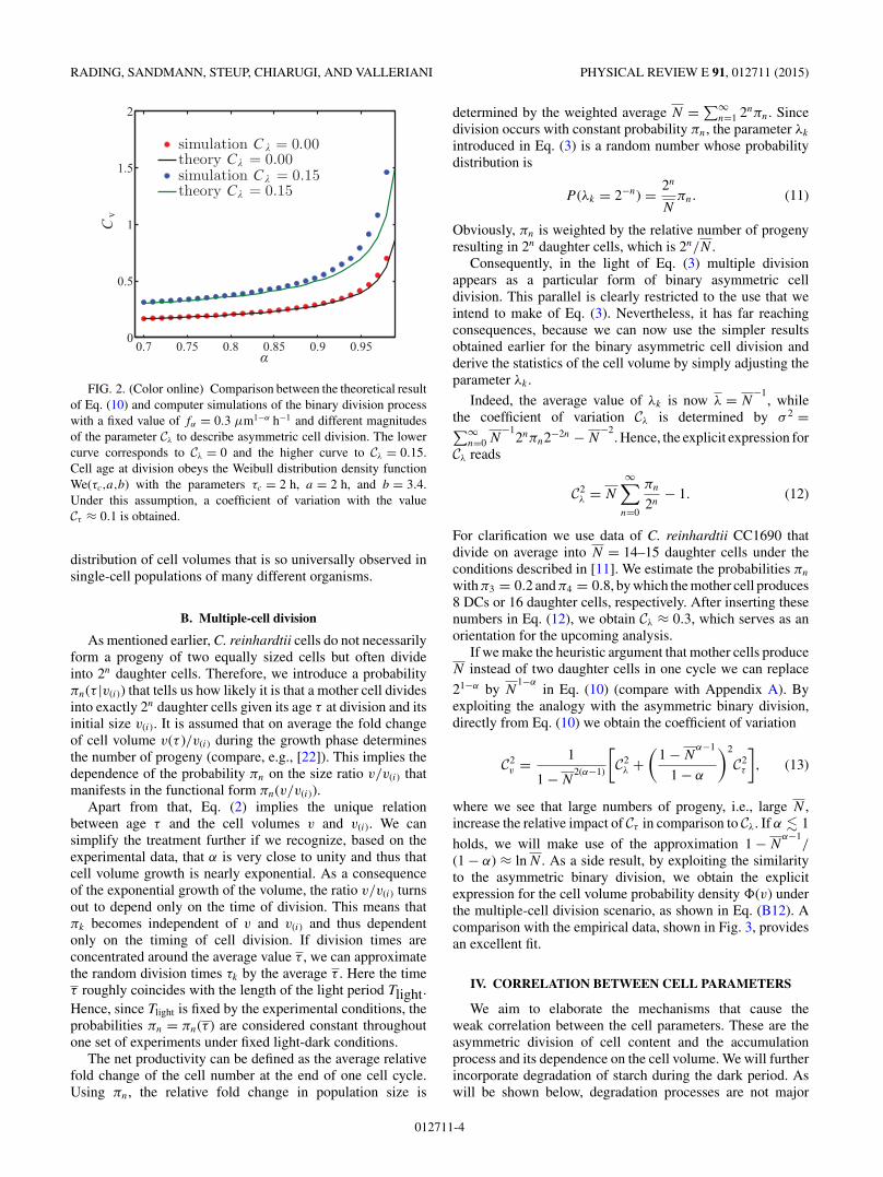
Equation (10) shows to what extent Cτ , Cλ, and the parameterα influence the heterogeneity of cell sizes. A comparison ofthis result with computer simulations is shown in Fig. 2.

If the growth rate function is weakly sloped the parameter1 − α becomes very small and amplifies the variation coeffi-cient Cv . Furthermore, it can be shown (see Appendix B) thatthe underlying process (3) generates naturally the log-normal

012711-3

RADING, SANDMANN, STEUP, CHIARUGI, AND VALLERIANI PHYSICAL REVIEW E 91, 012711 (2015)

0.7 0.75 0.8 0.85 0.9 0.950

0.5

1

1.5

2

α

Cv

simulation C λ = 0.00theory Cλ = 0.00simulation Cλ = 0.15theory Cλ = 0.15

FIG. 2. (Color online) Comparison between the theoretical resultof Eq. (10) and computer simulations of the binary division processwith a fixed value of fα = 0.3 μm1−α h−1 and different magnitudesof the parameter Cλ to describe asymmetric cell division. The lowercurve corresponds to Cλ = 0 and the higher curve to Cλ = 0.15.Cell age at division obeys the Weibull distribution density functionWe(τc,a,b) with the parameters τc = 2 h, a = 2 h, and b = 3.4.Under this assumption, a coefficient of variation with the valueCτ ≈ 0.1 is obtained.

distribution of cell volumes that is so universally observed insingle-cell populations of many different organisms.

B. Multiple-cell division

As mentioned earlier, C. reinhardtii cells do not necessarilyform a progeny of two equally sized cells but often divideinto 2n daughter cells. Therefore, we introduce a probabilityπn(τ |v(i)) that tells us how likely it is that a mother cell dividesinto exactly 2n daughter cells given its age τ at division and itsinitial size v(i). It is assumed that on average the fold changeof cell volume v(τ )/v(i) during the growth phase determinesthe number of progeny (compare, e.g., [22]). This implies thedependence of the probability πn on the size ratio v/v(i) thatmanifests in the functional form πn(v/v(i)).

Apart from that, Eq. (2) implies the unique relationbetween age τ and the cell volumes v and v(i). We cansimplify the treatment further if we recognize, based on theexperimental data, that α is very close to unity and thus thatcell volume growth is nearly exponential. As a consequenceof the exponential growth of the volume, the ratio v/v(i) turnsout to depend only on the time of division. This means thatπk becomes independent of v and v(i) and thus dependentonly on the timing of cell division. If division times areconcentrated around the average value τ , we can approximatethe random division times τk by the average τ . Here the timeτ roughly coincides with the length of the light period Tlight.Hence, since Tlight is fixed by the experimental conditions, theprobabilities πn = πn(τ ) are considered constant throughoutone set of experiments under fixed light-dark conditions.

The net productivity can be defined as the average relativefold change of the cell number at the end of one cell cycle.Using πn, the relative fold change in population size is

determined by the weighted average N = ∑∞n=1 2nπn. Since

division occurs with constant probability πn, the parameter λk

introduced in Eq. (3) is a random number whose probabilitydistribution is

P (λk = 2−n) = 2n

Nπn. (11)

Obviously, πn is weighted by the relative number of progenyresulting in 2n daughter cells, which is 2n/N .

Consequently, in the light of Eq. (3) multiple divisionappears as a particular form of binary asymmetric celldivision. This parallel is clearly restricted to the use that weintend to make of Eq. (3). Nevertheless, it has far reachingconsequences, because we can now use the simpler resultsobtained earlier for the binary asymmetric cell division andderive the statistics of the cell volume by simply adjusting theparameter λk .

Indeed, the average value of λk is now λ = N−1

, whilethe coefficient of variation Cλ is determined by σ 2 =∑∞

n=0 N−1

2nπn2−2n − N−2

. Hence, the explicit expression forCλ reads

C2λ = N

∞∑n=0

πn

2n− 1. (12)

For clarification we use data of C. reinhardtii CC1690 thatdivide on average into N = 14–15 daughter cells under theconditions described in [11]. We estimate the probabilities πn

with π3 = 0.2 and π4 = 0.8, by which the mother cell produces8 DCs or 16 daughter cells, respectively. After inserting thesenumbers in Eq. (12), we obtain Cλ ≈ 0.3, which serves as anorientation for the upcoming analysis.

If we make the heuristic argument that mother cells produceN instead of two daughter cells in one cycle we can replace

21−α by N1−α

in Eq. (10) (compare with Appendix A). Byexploiting the analogy with the asymmetric binary division,directly from Eq. (10) we obtain the coefficient of variation

C2v = 1

1 − N2(α−1)

[C2

λ +(

1 − Nα−1

1 − α

)2

C2τ

], (13)

where we see that large numbers of progeny, i.e., large N ,increase the relative impact of Cτ in comparison to Cλ. If α � 1

holds, we will make use of the approximation 1 − Nα−1

/

(1 − α) ≈ ln N . As a side result, by exploiting the similarityto the asymmetric binary division, we obtain the explicitexpression for the cell volume probability density �(v) underthe multiple-cell division scenario, as shown in Eq. (B12). Acomparison with the empirical data, shown in Fig. 3, providesan excellent fit.

IV. CORRELATION BETWEEN CELL PARAMETERS

We aim to elaborate the mechanisms that cause theweak correlation between the cell parameters. These are theasymmetric division of cell content and the accumulationprocess and its dependence on the cell volume. We will furtherincorporate degradation of starch during the dark period. Aswill be shown below, degradation processes are not major

012711-4

WEAK CORRELATION OF STARCH AND VOLUME IN . . . PHYSICAL REVIEW E 91, 012711 (2015)

0 100 200 300 400 500 6000

0.002

0.004

0.006

0.008

0.010

v (µm3)

Φ(v

) (µ m

−3 )

50 100 200 40010−6

10−4

log v (µm3)lo

gΦ

(v)

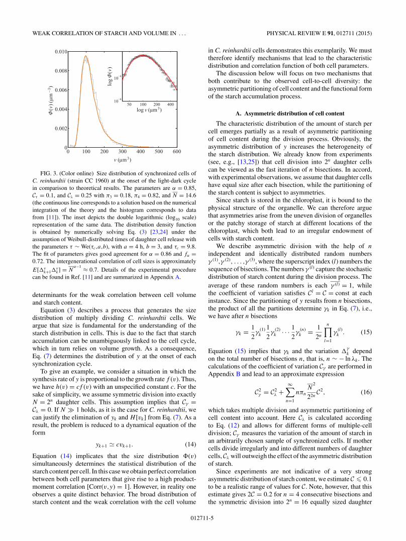
FIG. 3. (Color online) Size distribution of synchronized cells ofC. reinhardtii (strain CC 1960) at the onset of the light-dark cyclein comparison to theoretical results. The parameters are α = 0.85,Cτ = 0.1, and Cλ = 0.25 with π3 = 0.18, π4 = 0.82, and N = 14.6(the continuous line corresponds to a solution based on the numericalintegration of the theory and the histogram corresponds to datafrom [11]). The inset depicts the double logarithmic (log10 scale)representation of the same data. The distribution density functionis obtained by numerically solving Eq. (3) [23,24] under theassumption of Weibull-distributed times of daughter cell release withthe parameters τ ∼ We(τc,a,b), with a = 4 h, b = 3, and τc = 9.8.The fit of parameters gives good agreement for α = 0.86 and fα =0.72. The intergenerational correlation of cell sizes is approximately

E[vk+1

vk] = N

α−1 ≈ 0.7. Details of the experimental procedurecan be found in Ref. [11] and are summarized in Appendix A.

determinants for the weak correlation between cell volumeand starch content.

Equation (3) describes a process that generates the sizedistribution of multiply dividing C. reinhardtii cells. Weargue that size is fundamental for the understanding of thestarch distribution in cells. This is due to the fact that starchaccumulation can be unambiguously linked to the cell cycle,which in turn relies on volume growth. As a consequence,Eq. (7) determines the distribution of y at the onset of eachsynchronization cycle.

To give an example, we consider a situation in which thesynthesis rate of y is proportional to the growth rate f (v). Thus,we have h(v) = cf (v) with an unspecified constant c. For thesake of simplicity, we assume symmetric division into exactlyN = 2n daughter cells. This assumption implies that Cγ =Cλ = 0. If N � 1 holds, as it is the case for C. reinhardtii, wecan justify the elimination of yk and H [vk] from Eq. (7). As aresult, the problem is reduced to a dynamical equation of theform

yk+1 cvk+1. (14)

Equation (14) implicates that the size distribution �(v)simultaneously determines the statistical distribution of thestarch content per cell. In this case we obtain perfect correlationbetween both cell parameters that give rise to a high product-moment correlation [Corr(v,y) = 1]. However, in reality oneobserves a quite distinct behavior. The broad distribution ofstarch content and the weak correlation with the cell volume

in C. reinhardtii cells demonstrates this exemplarily. We musttherefore identify mechanisms that lead to the characteristicdistribution and correlation function of both cell parameters.

The discussion below will focus on two mechanisms thatboth contribute to the observed cell-to-cell diversity: theasymmetric partitioning of cell content and the functional formof the starch accumulation process.

A. Asymmetric distribution of cell content

The characteristic distribution of the amount of starch percell emerges partially as a result of asymmetric partitioningof cell content during the division process. Obviously, theasymmetric distribution of y increases the heterogeneity ofthe starch distribution. We already know from experiments(see, e.g., [13,25]) that cell division into 2n daughter cellscan be viewed as the fast iteration of n bisections. In accord,with experimental observations, we assume that daughter cellshave equal size after each bisection, while the partitioning ofthe starch content is subject to asymmetries.

Since starch is stored in the chloroplast, it is bound to thephysical structure of the organelle. We can therefore arguethat asymmetries arise from the uneven division of organellesor the patchy storage of starch at different locations of thechloroplast, which both lead to an irregular endowment ofcells with starch content.

We describe asymmetric division with the help of n

independent and identically distributed random numbersγ (1),γ (2), . . . ,γ (3), where the superscript index (l) numbers thesequence of bisections. The numbers γ (l) capture the stochasticdistribution of starch content during the division process. Theaverage of these random numbers is each γ (l) = 1, whilethe coefficient of variation satisfies Cl = C = const at eachinstance. Since the partitioning of y results from n bisections,the product of all the partitions determine γk in Eq. (7), i.e.,we have after n bisections

γk = 1

2γ

(1)k

1

2γ

(2)k · · · 1

2γ

(n)k = 1

2n

n∏l=1

γ(l)k . (15)

Equation (15) implies that γk and the variation γ

k dependon the total number of bisections n, that is, n ∼ − ln λk . Thecalculations of the coefficient of variation Cγ are performed inAppendix B and lead to an approximate expression

C2γ = C2

λ +∞∑

n=1

nπn

N2

22nC2, (16)

which takes multiple division and asymmetric partitioning ofcell content into account. Here Cλ is calculated accordingto Eq. (12) and allows for different forms of multiple-celldivision; Cγ measures the variation of the amount of starch inan arbitrarily chosen sample of synchronized cells. If mothercells divide irregularly and into different numbers of daughtercells, Cλ will outweigh the effect of the asymmetric distributionof starch.

Since experiments are not indicative of a very strongasymmetric distribution of starch content, we estimate C � 0.1to be a realistic range of values for C. Note, however, that thisestimate gives 2C = 0.2 for n = 4 consecutive bisections andthe symmetric division into 2n = 16 equally sized daughter

012711-5

RADING, SANDMANN, STEUP, CHIARUGI, AND VALLERIANI PHYSICAL REVIEW E 91, 012711 (2015)

cells [see Eq. (16)]. The value C = 0.1 clearly overestimatesthe impact of asymmetric distribution of starch and wetherefore conclude that C is likely well below this value.

We illustrate a realistic case by choosing the parametersN = 15, π3 = 0.2, π4 = 0.8, Cλ ≈ 0.3, and Cv = 0.5 for a C.reinhardtii CC1690 culture. The value of Cγ is determinedthrough Eq. (16), which yields Cγ ≈ 0.34 for the given setof parameters. Consequently, Cγ keeps relatively close to thevalue of Cλ. In summary, this means that the coefficient ofvariation Cλ related to the division in a random number ofdaughter cells almost completely determines the value of thecoefficient of variation Cγ . The latter instead is related to theasymmetric partitioning of starch content to the daughter cells.Hence, this indicates that the asymmetric partitioning of starchcontent is determined more by the stochasticity in the numberof daughter cells than by the random process that governs theredistribution of cell content. If, however, we had a dominantform of division, we would have observed a pattern of celldivision that produced 2n descendants at each iteration of thesynchronization cycle. In this case, the heterogeneity of thedistribution of starch can originate only from the second termon the right-hand side of Eq. (16) and thus from the asymmetricpartitioning.

B. Starch accumulation

Let vk+1 be the size in the (k + 1)th synchronization cycle.Preliminary considerations led to Eq. (7) and showed thatvk+1 and the initial size vk of the mother cell determine thestarch content yk+1 at the (k + 1)th cycle. Hence, yk+1 becomesalmost proportional to the difference H [Nvk+1] − H [vk]. Forsimplicity, we will further consider an approximation of Eq. (7)

by eliminating the contribution of the term N−1

yk . Thisis possible since N becomes large in the considered case.Given a fixed size vk+1, it is the size vk of the progenitorcell that determines the starch content through the relationyk+1 ∼ H [Nvk+1] − H [vk].

Equation (3) leads to the approximate expectation valueE[vk+1|vk] ≈ vk for parameter choices α � 1. If we reversethe process and use a simple symmetry argument, we can statethe conditional expectation value E[vk|vk+1] ≈ vk+1 for sizesvk of the preceding cycle in order to obtain vk+1 (compare,e.g., Appendix B).

Similarly, we introduce a coefficient of variation Cv thatquantifies the region in the vicinity of E[vk|vk+1] from whereprogenitor cells most likely originate. This simply meansthat the values of vk are spread around their expectationvalue, while the variation v

k around this expectation valueis conditional on the size in the (k + 1)th cycle. For α ≈ 1 andrelatively small variation of the division times Cτ , we use theestimate v

k ≈ vk . In this situation the coefficient of variation

satisfies Cv ≈ Cv . However, it should be noted that parametersα < 1 and large values of Cλ and Cτ considerably complicatethe calculation of Cv but do not result in different qualitativeresults.

We can now discuss the impact of the deviations vk on

the fluctuation of the parameter yk+1. To that end we assumevk+1 to take a fixed value in the (k + 1)th cycle. Hence, themagnitude of the fluctuations of yk+1 around the average yk+1measures how heterogeneously starch is distributed in cells

with the fixed size vk+1. Due to this mechanism, the correlationbetween size and starch content decreases as the outcome ofthe fluctuations of cell sizes in two consecutive cycles.

To show this we evaluate the first-order derivation of H [vk]at the size E[vk|vk+1] ≈ vk+1 and calculate the variation y

of y. The result is a relation between the fluctuations of thestarch content

y

k+1 and the fluctuations of cell sizes, i.e.,

y

k+1(vk+1) ≈ H ′(vk+1)vk+1

H (Nvk+1) − H (vk+1)v

k. (17)

Equation (17) demonstrates that fluctuations of yk+1 around theaverage y(vk+1) depend on the value of vk+1. For this reasonthe factor in front of v measures the strength of fluctuationsas a function of cell size v.

Equation (17) allows us to compare different types ofaccumulation processes. In what follows we assume that h(v)is a monotonically increasing function of size v. In the simplestcase h(v) is proportional to the growth rate f (v), which leadsto the expression H [v] = cv and the unspecified constant c. Ifwe plug h(v) into Eq. (17) and if we further assume N � 1,

we obtain the relation y

k+1 N−1

vk . However, this means

that Cy will be small in comparison to Cv if N becomes large.By this means both parameters, size and starch content, aretightly correlated.

By having a closer look at Eq. (17) we see that it is the ratioof H ′[v]v and H [Nv] − H [v] that determines how strongly y

fluctuates around its mean value. If the absolute value |H [v]|is rapidly decreasing in the vicinity of v, the contribution of|H [Nv]| becomes negligible for very productive forms of celldivision. We want to describe this behavior more clearly andconsider the function

h(v) = A

{1 + [η(v/v)]B}2

(v

v

)B

, (18)

which represents a family of functions that, when embedded inEq. (4), correctly describes the experimental results reportedin [11] and summarized in Fig. 1 therein. In particular,Eq. (18) takes into account the slowing down of the rate ofstarch production when cells become much larger than v. Acomparison of Eq. (18) with the empirical data reported in [11]shows that Eq. (18) is indeed a good model for describing theaccumulation of starch during the light period. A reasonablechoice of parameters for fitting the data mentioned above isη ≈ 0.5–1.0 and B ≈ 2. An analytically tractable case canbe obtained if we integrate Eq. (18) under the assumptionf (v) ≈ f1v and B = 2. With this choice of parameters Eq. (18)still results in a good fit for the experimental data related tocell growth and starch accumulation in

H (v) = − A

1 + η2(v2/v2), (19)

with the unspecified constant A. The model represented inFig. 4 is based on Eq. (19) under the assumption of cell divisioninto strictly N = 24 = 16 daughter cells. It demonstrates how

y

k+1 is affected by the variation of sizes of the progenitorcell, i.e., v

k . According to Eq. (17), the magnitude of the

012711-6

WEAK CORRELATION OF STARCH AND VOLUME IN . . . PHYSICAL REVIEW E 91, 012711 (2015)

0 1 2

0

0.2

0.4

0.6

0.8

1

v/v

yA

Δyk+1

vk+1

Δvk

|H(v)|

|H(Nv)|

E[vk|vk+1]

FIG. 4. (Color online) The behavior of yk+1 can be related tofluctuations of vk+1 in each cycle. The difference of the accumulationfunction H (Nv) − H (v) on average determines the dependence of theparameter y on size v. Cell sizes are distributed around the average v

and obey a log-normal distribution (gray area). The steep decrease of|H (v)| compared to |H (Nv)| for typical cell sizes v ≈ v manifests inthe sensitive response of y(vk+1)k+1 to deviations v

k in each cycle.

fluctuations of y is given through

Cy(v) ≈ 2η2v2

v2 + η2v2Cv. (20)

Equation (20) establishes a relation between Cy on the onehand and v and Cv on the other. Since vk+1 is typically locatedin the vicinity of the average cell size v, we can estimatethe representative value for the coefficient of variation, whichtakes the form

Cy(v) ≈ 2η2

1 + η2Cv. (21)

Here Cy exhibits a magnitude similar to that of Cv for theparameter region η ≈ 1 and as a result the starch contenty shows strong fluctuations around its mean value y(v).The discussed mechanism evidently mitigates the correlationbetween y and v and as the example shows is mainly encodedin the specific form of the function h(v).

V. EXAMPLE

In [11] the authors show that the product moment cor-relation coefficient Corr(�,v) between cell size and starchdensity in the alga C. reinhardtii CC1690 is strictly negative.Similarly, the rank correlation according to Spearman takesvalues in the range CorrS(�,v) = −0.50 to −0.60. At the sametime the correlation coefficient for starch and size takes thevalue CorrS(v,y) ≈ 0.2. In order to explain these experimentalresults, we study the discrete equations (3) and (7) thatdetermine the discrete-time starch concentration �k = yk/vk

in each cycle.The synthesis rate of y is modeled after the concave

function (18). By choosing η = 0.5 and B = 1.93 we obtaina decent description of starch accumulation during the whole

0 5 10 15 20 250.8

1

1.2

1.4

1.6

1.8

2

Time t(h)

Star

chde

nsity

(nor

mal

ized

)

Growth phase Degradation phase

Accumulation ofstarch

Starting degradation of starch

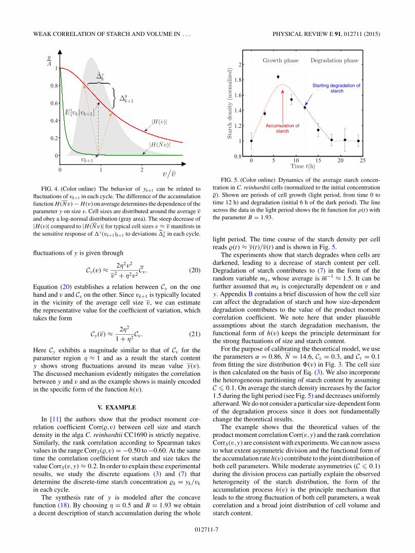
FIG. 5. (Color online) Dynamics of the average starch concen-tration in C. reinhardtii cells (normalized to the initial concentration�). Shown are periods of cell growth (light period, from time 0 totime 12 h) and degradation (initial 6 h of the dark period). The lineacross the data in the light period shows the fit function for ρ(t) withthe parameter B = 1.93.

light period. The time course of the starch density per cellreads �(t) ≈ y(t)/v(t) and is shown in Fig. 5.

The experiments show that starch degrades when cells aredarkened, leading to a decrease of starch content per cell.Degradation of starch contributes to (7) in the form of therandom variable mk , whose average is m−1 ≈ 1.5. It can befurther assumed that mk is conjecturally dependent on v andy. Appendix B contains a brief discussion of how the cell sizecan affect the degradation of starch and how size-dependentdegradation contributes to the value of the product momentcorrelation coefficient. We note here that under plausibleassumptions about the starch degradation mechanism, thefunctional form of h(v) keeps the principle determinant forthe strong fluctuations of size and starch content.

For the purpose of calibrating the theoretical model, we usethe parameters α = 0.86, N = 14.6, Cλ = 0.3, and Cτ = 0.1from fitting the size distribution �(v) in Fig. 3. The cell sizeis then calculated on the basis of Eq. (3). We also incorporatethe heterogeneous partitioning of starch content by assumingC � 0.1. On average the starch density increases by the factor1.5 during the light period (see Fig. 5) and decreases uniformlyafterward. We do not consider a particular size-dependent formof the degradation process since it does not fundamentallychange the theoretical results.

The example shows that the theoretical values of theproduct moment correlation Corr(v,y) and the rank correlationCorrS(v,y) are consistent with experiments. We can now assessto what extent asymmetric division and the functional form ofthe accumulation rate h(v) contribute to the joint distribution ofboth cell parameters. While moderate asymmetries (C � 0.1)during the division process can partially explain the observedheterogeneity of the starch distribution, the form of theaccumulation process h(v) is the principle mechanism thatleads to the strong fluctuation of both cell parameters, a weakcorrelation and a broad joint distribution of cell volume andstarch content.

012711-7

RADING, SANDMANN, STEUP, CHIARUGI, AND VALLERIANI PHYSICAL REVIEW E 91, 012711 (2015)

VI. CONCLUSION

In this paper we reported on a model that explains the originof the multivariate statistics of cell parameters. We provided amechanism that explains the cause of the log-normal-shapedsize distribution of multiply dividing C. reinhardtii cells in awidely used synchronization setup. Nearly exponential growthand variations with respect to the timing of cell division and thegrowth process contribute to the considerable heterogeneityof cell populations. It was demonstrated that multiple-celldivision can be regarded as a form of asymmetric division.The resulting distribution of cell sizes and their characteristicmoments at the onset of each cell cycle are comparable forbinary and multiple division. The theoretically obtained dis-tribution density functions compare well with empirical data.

On the basis of the presumed cell cycle control by size,we elucidated the accumulation of starch per cell. Thecorrelation analysis reveals that a mutual identification of thiscell parameter with the help of cell volume is restricted bythe form of the accumulation process. This has far reachingconsequences. Under certain conditions it is possible to predictthe value y by measuring a more accessible quantity, suchas the cell volume. However, we can demonstrate on thebasis of starch accumulation that for realistic forms of thesize-controlled accumulation process starch content and cellvolume are weakly correlated in each cycle. The heterogeneitymanifests in a considerable variance of the starch content y forany given cell volume v. The potential asymmetric distributionof starch content additionally increases the described effect.

ACKNOWLEDGMENTS

We acknowledge financial support from the GermanFederal Ministry of Education and Research within theprogram Unternehmen Region (Grant No. 03Z2AN12) andGoFORSYS (Grant No. 0313924). A.V. thanks Katja Schulzefor help with the manuscript.

APPENDIX A: SUMMARY OF EXPERIMENTALSETUP AND RESULTS

Materials and methods

Vegetative cells of strain CC1690 from Chlamydomonasreinhardtii were obtained from the Chlamydomonas ResourceCenter, University of Minnesota, St. Paul, Minnesota (USA).Preculture and synchronization of the cells using photoau-totrophic conditions were performed as described in [11].Under standard conditions, synchronized cells were grown ina synthetic medium containing ammonium as nitrogen source,high light intensities (900 to 550 μmol photons m−2 s−1 atthe beginning and the end of the light period, respectively, asmeasured inside of the suspension) and 34 ◦C [11]. Cell volumewas determined using a Beckman Coulter Counter MULTI-SIZER 3 (Beckman Coulter, Krefeld, Germany) as previouslydescribed [11]. Starch content was determined enzymaticallyusing a photometric assay that is based on the conversion ofstarch-derived glucose to glucose 6-phosphate as mediatedby hexokinase and glucose 6-phosphate dehydrogenase. Priorto the photometric assay, cells were broken by sonification in80 vol% ethanol. Starch was solubilized by KOH and converted

TABLE I. Summary of the Spearman correlation coefficient ρ

computed in [11] between the relative starch content and the cellularvolume, measured during the first 6 h of the light period in asynchronized cell culture of C. reinhardtii .

Time (h) ρ starch vs volume

0 0.302 0.124 0.086 0.13

to glucose by amyloglucosidase treatment (Starch Assay Kit,R-Biopharm, Darmstadt, Germany). Tables I and II providea summary of the key results used in this paper. For furtherdetails, see [11].

APPENDIX B: SIZE DISTRIBUTION AND MOMENTS

If perfectly timed, division always occurs at the averagetime point τ . Strictly binary division exhibits the average λ =12 . In order to determine the average cell volume v we expandthe right-hand side of Eq. (3) in powers of τ

k , λk , and v

k andaverage over the contributing noise terms on both sides of theequation.

Equation (3) can be linearized in order to analyze theresponse of the system to noise. To this end we introducethe logarithm of cell size uk = ln v/v, which is a goodapproximation if 1 − α becomes small. Taking the logarithmof v on both sides of Eq. (3) and expanding the expressionaround v, we obtain

uk+1 = λ1−α

uk + λk + 1 − λ

1−α

1 − ατ

k . (B1)

This linear autoregressive process is convergent since

γ = λ1−α

< 1 holds for every choice of α < 1. If noise termsx are small, we can approximate uk by

uk = lnvk

v≈ vk

v. (B2)

We next Taylor expand the right-hand side of Eq. (3) inorders of

xk = xk

x, (B3)

where xk = xk − x denotes the deviation from the averagex. The result of the Taylor expansion of

v(1 + v

k+1

) = λ(1 + λ

k

)[v1−α

(1 + v

k

)1−α

+ · · · + fα(1 − α)τ(1 + τ

k

)]1/(1−α)(B4)

TABLE II. Summary of the mean values and width 2σ of thecellular starch density distribution derived after the log-normal fit,computed in [11]. The errors refer to the 95% confidence intervals.

Time (h) Mean starch density 2σ

0 2.34 ± 0.08 2.98 ± 0.22 4.22 ± 0.32 4.31 ± 0.74 10.23 ± 0.67 10.44 ± 1.56 15.92 ± 0.82 19.72 ± 2.08

012711-8

WEAK CORRELATION OF STARCH AND VOLUME IN . . . PHYSICAL REVIEW E 91, 012711 (2015)

up to second order reads

v(1 + v

k+1

) = λ(1 + λ

k

)[v1−α + fα(1 − α)τ ]1/(1−α)

× [1 + a1(v)v

k + b1(v)τk + c1(v)τ

kvk

+ · · · + a2(v)(v

k

)2 + b2(v)(τ

k

)2 + · · · ].(B5)

In a first step we average this expression, where we assumeE(τ

kvk) = E(τ

kλk ) = 0. This is due to the fact that the

different noise terms show no significant correlation inexperiments. After averaging, we have in the first nonvanishingorder

v = λ[v1−α + fα(1 − α)τ ]1/(1−α)

× . . . × [1 + a2(v)C2

v + b2(v)C2τ

]. (B6)

We square Eq. (B6) and average over the noise terms up tosecond order. This time we obtain

(1 + C2v ) = λ

2(1 + C2

λ)

(1 + fα(1 − α)τ

v1−α

)2/(1−α)

× · · · × {1 + [a2

1(v) + 2a2(v)]C2

v

+ · · · + [b2

1(v) + 2b2(v)]C2

τ }. (B7)

Both Eqs. (B6) and (B7) determine the average size v andthe coefficient of variation Cv as functions of stochasticfluctuations Cτ and Cλ, as well as the system parameters α,fα , τ , and λ.

If we assume Cτ ≈ 0, the coefficients a1 and a2 can be easilydetermined. After a short calculation we arrive at the relations

v = λ[v1−α + fα(1 − α)τ ]1/(1−α)

× · · · ×(

1 − 1

2

αfα(1 − α)τv1−α

[v1−α + fα(1 − α)τ ]2C2

v

)(B8)

and

v2 = λ2 1 + C2

λ

1 + C2v

[v1−α + fα(1 − α)τ ]2/(1−α)

× · · · ×(

1 + v1−α(v1−α − α(1 − α)fατ )

[v1−α + (1 − α)fατ ]2C2

v

). (B9)

By replacing Cv in Eq. (B8) with Eq. (B9), we obtain animplicit relation for v. The first-order approximation of theproblem neglects the impact of Cv in (B8) and thus resultsin Eqs. (B10) and (10). Thus, in lowest order we have thesteady-state solution of Eq. (3),

v =(

fα(1 − α)τ

λ1−α − 1

)1/(1−α)

. (B10)

This equation constitutes a decent approximation if Cτ and Cλ

are sufficiently small.Equation (B1) allows us to assess the functional form

of �(v). By definition, the distribution is centered aroundthe mean value v. The different contributions of the noiseterms broaden the distribution function, where the linearizationaround the steady state results in uk+1 = γ uk + ξ 1

k + ξ 2k , with

ln vk/v = uk . The expectation values of the random numbersξ 1 and ξ 2 are 0. Provided the noise terms ξ 1 and ξ 2 are

Gaussian, the distribution of u itself exhibits the form of aGaussian distribution.

Even if the noise deviates from a normal distribution, wewill likely see convergence according to the central limittheorem. The question is how fast the prefactor γ in an infinitesum declines. If γ is close to 1, which is the case for smallvalues of 1 − α, the sum uk = ξ 1

k + γ ξ 1k−1 + γ 2ξ 1

k−2 + · · ·will eventually converge to a normal distribution. The variationcoefficient of u is approximately given by Eq. (10). Accord-ingly, the standard deviation of the log-normal distribution isdetermined by

σ =√

ln(C2

v + 1). (B11)

After rewriting Eq. (B1) as the infinite sum of randomnumbers with zero mean and decreasing standard deviation,we finally obtain the expression

�(v) ∼ 1

vexp

(− (ln v − ln v + ln

√C2

v + 1)2

2 ln(C2v + 1)

),

to which both random processes contribute via Cv and v.Equation (B12) is utilized for calculations of the conditionalsize distribution in two consecutive cell cycles. This is centralfor Sec. IV B. We encounter two conditional size distributionsP (vk|vk+1) and P (vk+1|vk), where the first tells us about thelikelihood that cells with size vk+1 originate from cells withsize vk . According to the Bayes theorem, we have

P (vk|vk+1) ∼ P (vk+1|vk)�(vk), (B12)

which is used to calculate the conditional average μk|vk+1

of the cell size vk . In Eq. (B12) the conditional probabilityP (vk+1|vk) can be expressed by the help of the hazard functionp(τ ) of the cell division process. Since division is assumed tobe age controlled, we obtain a survival probability �(S)(τ )that is linked to the division rate function by the fundamentalrelation

�(S)(τ ) = p(τ ) exp

(−

∫ τ

0dtp(t)

). (B13)

After replacing τ in Eq. (B13) with vk and Nvk+1 as termsof the growth process (2), we obtain the sought relation forP (vk+1|vk) ∼ �(S)(τ ). Calculations of the conditional meanvalue and standard deviation can now be performed byevaluating

mn|vk+1 ∼∫ ∞

0dx xn−α�(S)

(N

1−αv1−α

k+1 − x1−α

fα(1 − α)

)�(x).

(B14)For α → 1 we obtain the relations of Sec. IV B.

APPENDIX C: CORRELATION BETWEEN SIZE v

AND STARCH CONTENT y

The discrete stochastic process for the deviation from theaverage cell volume is given by

vk+1 = Nα−1v

k + ln Nτk + λ

k

=∞∑l=0

Nl(α−1)(

ln Nτk−l + λ

k−l

). (C1)

012711-9

RADING, SANDMANN, STEUP, CHIARUGI, AND VALLERIANI PHYSICAL REVIEW E 91, 012711 (2015)

The second equation integrates all shock terms λ and τ

in order to determine the current value of vk . We use the

discrete-time equation (7) to evaluate the mean value of yk:

y = 1

MN − 1

(H

[v

λ

]− H [v]

)≈ 1

MN − 1

(H [vN ] + 1

2H ′′[vN ]v2N

2C2v + · · ·

)− 1

MN − 1

(H [v] + 1

2H ′′[v]v2C2

v + · · ·)

. (C2)

In the lowest approximation we have the average

y = 1

MN − 1[H (vN ) − H (v)]. (C3)

Equation (C3) shows that y explicitly depends on M . It canbe estimated as follows. We introduce a rate function dy(v,y)that determines the amount of starch as the solution of a decayprocess that follows

d

dτy(τ ) = dy[v,y(τ )]. (C4)

On average the decrease of starch during the dark period hasto be balanced by faster accumulation of starch during thepreceding light period. This implies that the relative increaseof y exceeds the increase of cell volume v. In other words,the density of starch per cell volume, i.e., the ratio � = y/v,increases by the factor M , as depicted in Fig. 5.

The function dy(v,y) has to be specified on grounds of theunderlying degradation mechanism. If degradation is assumedto be size dependent, we can tentatively cast the probleminto the rate function dy(v,y) = −dyyv, with dy = const. Theargument here is that the depletion of recourses is likely toproceed faster in large cells. On average the factor M satisfiesthe balance condition

1

M= exp(−dyTdegv), (C5)

where Tdeg is the length of the degradation period. Equation(C5) allows us to reformulate dyTdeg in terms of v and M . Theparticular form of the assumed degradation type introduces thedependence on the stochastic variable vk+1, namely,

mk(vk+1) = exp

(− ln M

vk+1

v

). (C6)

Equation (C6) makes clear that we will observe no additionalfluctuations if mk is size independent. In this case mk wouldsimply add a constant factor in front of Eq. (7). If, however,the degradation of starch is dependent on size, we have in thelinear response

mk ≈ − ln Mv

k+1. (C7)

According to Eq. (17), the magnitude of fluctuations decreasesfor large values of vk+1 and the decay in the dark is faster if M

becomes large.

For the linearized equation for the shocks y we can use

y

k+1 = mk +

γ

k + 1

MN

y

k

+ · · · + H ′[Nv]v

Myv

k+1 − H ′[v]v

NMyv

k. (C8)

Equation (C8) together with the linearization of Eq. (3)can be used to determine the variance of y and v. Aftermultiplying Eq. (C8) with v

k+1 and averaging both sidesof the equation, the covariance Cov(v,y) is obtained. Theratio of the covariance and variation coefficients Cv and Cy

defines the product-moment correlation coefficient Corr(v,y)after Pearson:

Corr(v,y) = Cov(v,y)

CyCv

. (C9)

Here Corr(v,y) serves as an orientation for the strength of thecorrelation between size and starch content. In the case thatmk depends on size and γk allows for asymmetric division, wehave

Cov(v,y) = E[m

k vk+1

] + E[

γ

k vk+1

]MN − N

α−1

+ · · · + C2v

MN

MN − 1

MN − Nα−1

× H ′[Nv]Nv − H ′[v]Nα−1

v

H [Nv] − H [v]. (C10)

Averaging of mk v

k+1 results in

E[m

k vk+1

] = − ln MC2v . (C11)

The repeated bisection that produces 2n DCs implies that γk

is a function of 2n = 1/λk . The average of E[γ

k vk+1] =

E[γ

k λk ] is thus dependent on the number of daughter cells.

We can determine E[γkλk] and obtain

E[γkλk] = 1

N2 E

[1 +

γ

k + λk +

γ

k λk

]= 1 + E[γ

k λk ]

N2 . (C12)

Hence, it is possible to determine E[γ

k λk ] by evaluating

E[γkλk]. The n-fold iteration leads to

γk = 1

2γ (1) 1

2γ (2) · · · 1

2γ (n) = 1

2n

n∏l=1

γ (l), (C13)

with γ l = 1 and C = const in each bisection. We find

E[γkλk] =∞∑n

[πn

22n

n∏l=1

γ (l)

]. (C14)

The product can be approximated byn∏

l=1

γ (l) =n∏

l=1

1 + γ (l) ≈ 1 +n∑

l=1

γ (l). (C15)

It is further assumed that the random terms γ (l) describeindependent events. Consequently, averaging yields

012711-10

WEAK CORRELATION OF STARCH AND VOLUME IN . . . PHYSICAL REVIEW E 91, 012711 (2015)

E[γkλk] = ∑∞n

πn

22n and finally

E[

γ

k λk

] = C2λ. (C16)

Similarly, we find for Cγ

E[γkγk] = 1 + C2γ

N2 (C17)

and

E[γkγk] =∞∑n

[πn

22n

n∏l=1

(1 + γ (l))2

]

=∞∑n

[πn

22n(1 + C2)n

]. (C18)

The variation coefficient for y is obtained after squaring andaveraging Eq. (C8). After the adiabatic elimination of

y

k forN � 1 calculations further simplify. For Cλ = 0 and α = 1we find the covariance

Cov(v,y) ≈ C2v

MN

(− ln MMN

MN − 1+ H ′[Nv]Nv − H ′[v]v

H [Nv] − H [v]

)(C19)

and the variation coefficient

C2y ≈ C2

v

(ln M + H ′[Nv]Nv − H ′[v]v

H [Nv] − H [v]

)2

. (C20)

Equation (C19) shows that Cov(v,y) and therefore Corr(v,y)are decreasing functions in M , which can vanish for certain

1 1.5 2 2.5 3 3.5 4−1

−0.5

0

0.5

1

M

Cor

r(v,y)

constant degradation rates

size−dependent degradation rates

Cλ = 0.0 Cλ = 0.3

FIG. 6. (Color online) Correlation coefficient as a function of M .The parameter M describes the difference of the growth processbetween y and v. In the case of constant degradation the correlationbetween the parameters is always close to 1, while size-dependentdegradation of starch decreases the correlation between both parame-ters. The plot shows that the decrease of the correlation depends alsoon the strength of the coefficient of variation (indicated here with C):For Cλ = 0 the decrease of the correlation is slow at small M and andit is stark at intermediate values of M; for Cλ = 0.3 the decrease ofthe correlations is fast at small M and slow at large values of M .

values of the parameters N , v, and M (see Fig. 6). Accordingto Eq. (C19), there is a simple zero that defines the value M ′ forwhich the product-moment correlation vanishes. For example,the case H ≈ cv gives M ′ ≈ 2.71, while a concave functionh(v) entails a smaller value of M ′.

[1] D. Drake and K. Brogden, Polymicrobial Diseases (ASM,Washington, DC, 2002).

[2] D. J. Ferullo, D. L. Cooper, H. R. Moore, and S. T. Lovett,Methods 48, 8 (2009).

[3] E. Bernstein, Science 131, 1528 (1960).[4] T. Cools, A. Iantcheva, S. Maes, H. Van Den Daele, and L. De

Veylder, Plant J. 64, 705 (2010).[5] G. Balazsi, A. Van Oudenaarden, and J. J. Collins, Cell 144, 910

(2011).[6] M. Sturrock, A. Hellander, A. Matzavinos, and M.

A. J. Chaplain, J. R. Soc. Interface 10, 20120988(2013).

[7] M. Thattai and A. Van Oudenaarden, Proc. Natl. Acad. Sci. USA98, 8614 (2001).

[8] B. Alberts, D. Bray, J. Lewis, M. Raff, K. Roberts, and J. D.Watson, Molecular Biology of the Cell, 3rd ed. (Garland Science,New York, 2010).

[9] L. Donnan, E. P. Carvill, T. J. Gilliland, and P. C. L. John,New Phytol. 99, 1 (1985).

[10] K. Bisova and V. Zachleder, J. Exp. Bot. 65, 2585 (2014).[11] A. Garz, M. Sandmann, M. Rading, S. Ramm, R. Menzel, and

M. Steup, Biophys. J. 103, 1078 (2012).

[12] M. McAteer, L. Donnan, and P. C. L. John, New Phytol. 99, 41(1985).

[13] H. Oldenhof, V. Zachleder, and H. van den Ende,Folia Microbiol. 53, 52 (2007).

[14] P. Fantes and P. Nurse, in The Cell Cycle, edited by P. C. L. John(Cambridge University Press, Cambridge, 1981), p. 11.

[15] M. M. Rading, T. A. Engel, R. Lipowsky, and A. Valleriani,J. Stat. Phys. 145, 1 (2011).

[16] K. Matsumura, T. Yagi, and K. Yasuda, Biochem. Biophys. Res.Commun. 306, 1042 (2003).

[17] G. Webb, Math. Biosci. 85, 71 (1987).[18] N. Brenner, K. Farkash, and E. Braun, Phys. Biol. 3, 172 (2006).[19] N. Brenner and Y. Shokef, Phys. Rev. Lett. 99, 138102 (2007).[20] D. Ramkrishna, Math. Biosci. 12, 123 (1969).[21] J. L. Spudich and R. Sager, J. Cell Biol. 85, 136 (1980).[22] M. Kazunori, Y. Toshiki, H. Akihiro, S. Mikhail, and Y. Kenji,

J. Nanobiotechnol. 8, 23 (2010).[23] T. Kuczek, Math. Biosci. 69, 159 (1984).[24] B. H. Shah, J. D. Borwanker, and D. Ramkrishna, Math. Biosci.

31, 1 (1976).[25] E. H. Harris, Annu. Rev. Plant Physiol. Plant Mol. Biol. 52, 363

(2001).

012711-11