We add value to your mining projects. - SAIMM
132
V VOLUME 117 NO. 2 FEBRUARY 2017 Wits Special Edition — Volume II
-
Upload
khangminh22 -
Category
Documents
-
view
2 -
download
0
Transcript of We add value to your mining projects. - SAIMM
VVOLUME 117 NO. 2 FEBRUARY 2017
Wits Special Edition — Volume II

Leading consultants to the mining industry.
Recent projects include:
EIA for oil and gas pipeline in GhanaChrome feasibility study in South AfricaCoal mining consulting in IranTin Resource Audit in RwandaDiamond Due Diligence in CanadaLithium consulting in the DRCCopper and cobalt exploration in central Africa
We add value to your mining projects.

OUR BENEFICIARIES
Our beneficiaries are Witwatersrand
University students from the School of
Mining Engineering who are financially
challenged in completing their studies
towards a mining profession and all our
alumni, locally and internationally.
WUMEA congratulates the School of Mining Engineering
in celebrating 120 years of existence and wishes them a
prosperous future.
OUR MISSION
WUMEA seeks to promote collegiality
amongst Wits mining engineers,
globally, in order to work together
towards building a formidable mining
engineering profession. Its aim is
to provide a vehicle through which
mining engineers can influence the
development of the mining engineering
profession to enhance its contribution to
sustainable development in the African
continent.
ABOUT WUMEA
WUMEA is an alumni body for Wits University graduates in the School of Mining Engineering.
It is non-profit organization which is affiliated to the University of Witwatersrand and
therefore can receive donations and membership fees to carry out its mission. Amongst
its activities, WUMEA provides financial support to deserving students studying towards a
degree in Mining Engineering at Wits University, thus contributing to the sustainability of
the industry in terms of human capital.
To partner with WUMEA, please contact:
Ms PN Neingo | Email: [email protected] | Tel: +27 11 717 7445
COME PARTNER WITH US

�
ii
Mike TekePresident, Chamber of Mines of South Africa
Mosebenzi ZwaneMinister of Mineral Resources, South Africa
Rob DaviesMinister of Trade and Industry, South Africa
Naledi PandorMinister of Science and Technology, South Africa
C. Musingwini
S. Ndlovu
A.S. Macfarlane
M. Mthenjane
R.T. Jones
J. Porter
Z. Botha
V.G. Duke A.G. SmithI.J. Geldenhuys M.H. SolomonM.F. Handley M.R. TlalaW.C. Joughin D. TudorM. Motuku D.J. van NiekerkD.D. Munro A.T. van ZylG. Njowa
N.A. Barcza S.J. RamokgopaR.D. Beck M.H. RogersJ.R. Dixon D.A.J. Ross-WattM. Dworzanowski G.L. SmithH.E. James W.H. van NiekerkG.V.R. Landman R.P.H. WillisJ.C. Ngoma
Botswana L.E. DimbunguDRC S. MalebaJohannesburg J.A. LuckmannNamibia N.M. NamateNorthern Cape C.A. van WykPretoria P. BredellWestern Cape C.G. SweetZambia D. MumaZimbabwe S. MatutuZululand C.W. Mienie
Australia: I.J. Corrans, R.J. Dippenaar, A. Croll, C. Workman-Davies
Austria: H. WagnerBotswana: S.D. WilliamsUnited Kingdom: J.J.L. Cilliers, N.A. BarczaUSA: J-M.M. Rendu, P.C. Pistorius
The Southern African Institute of Mining and Metallurgy
*Deceased
* W. Bettel (1894–1895)* A.F. Crosse (1895–1896)* W.R. Feldtmann (1896–1897)* C. Butters (1897–1898)* J. Loevy (1898–1899)* J.R. Williams (1899–1903)* S.H. Pearce (1903–1904)* W.A. Caldecott (1904–1905)* W. Cullen (1905–1906)* E.H. Johnson (1906–1907)* J. Yates (1907–1908)* R.G. Bevington (1908–1909)* A. McA. Johnston (1909–1910)* J. Moir (1910–1911)* C.B. Saner (1911–1912)* W.R. Dowling (1912–1913)* A. Richardson (1913–1914)* G.H. Stanley (1914–1915)* J.E. Thomas (1915–1916)* J.A. Wilkinson (1916–1917)* G. Hildick-Smith (1917–1918)* H.S. Meyer (1918–1919)* J. Gray (1919–1920)* J. Chilton (1920–1921)* F. Wartenweiler (1921–1922)* G.A. Watermeyer (1922–1923)* F.W. Watson (1923–1924)* C.J. Gray (1924–1925)* H.A. White (1925–1926)* H.R. Adam (1926–1927)* Sir Robert Kotze (1927–1928)* J.A. Woodburn (1928–1929)* H. Pirow (1929–1930)* J. Henderson (1930–1931)* A. King (1931–1932)* V. Nimmo-Dewar (1932–1933)* P.N. Lategan (1933–1934)* E.C. Ranson (1934–1935)* R.A. Flugge-De-Smidt
(1935–1936)* T.K. Prentice (1936–1937)* R.S.G. Stokes (1937–1938)* P.E. Hall (1938–1939)* E.H.A. Joseph (1939–1940)* J.H. Dobson (1940–1941)* Theo Meyer (1941–1942)* John V. Muller (1942–1943)* C. Biccard Jeppe (1943–1944)* P.J. Louis Bok (1944–1945)* J.T. McIntyre (1945–1946)* M. Falcon (1946–1947)* A. Clemens (1947–1948)* F.G. Hill (1948–1949)* O.A.E. Jackson (1949–1950)* W.E. Gooday (1950–1951)* C.J. Irving (1951–1952)* D.D. Stitt (1952–1953)* M.C.G. Meyer (1953–1954)* L.A. Bushell (1954–1955)* H. Britten (1955–1956)* Wm. Bleloch (1956–1957)
* H. Simon (1957–1958)* M. Barcza (1958–1959)* R.J. Adamson (1959–1960)* W.S. Findlay (1960–1961)
D.G. Maxwell (1961–1962)* J. de V. Lambrechts (1962–1963)* J.F. Reid (1963–1964)* D.M. Jamieson (1964–1965)* H.E. Cross (1965–1966)* D. Gordon Jones (1966–1967)* P. Lambooy (1967–1968)* R.C.J. Goode (1968–1969)* J.K.E. Douglas (1969–1970)* V.C. Robinson (1970–1971)* D.D. Howat (1971–1972)
J.P. Hugo (1972–1973)* P.W.J. van Rensburg
(1973–1974)* R.P. Plewman (1974–1975)* R.E. Robinson (1975–1976)* M.D.G. Salamon (1976–1977)* P.A. Von Wielligh (1977–1978)* M.G. Atmore (1978–1979)* D.A. Viljoen (1979–1980)* P.R. Jochens (1980–1981)
G.Y. Nisbet (1981–1982)A.N. Brown (1982–1983)
* R.P. King (1983–1984)J.D. Austin (1984–1985)H.E. James (1985–1986)H. Wagner (1986–1987)
* B.C. Alberts (1987–1988)C.E. Fivaz (1988–1989)O.K.H. Steffen (1989–1990)
* H.G. Mosenthal (1990–1991)R.D. Beck (1991–1992)
* J.P. Hoffman (1992–1993)* H. Scott-Russell (1993–1994)
J.A. Cruise (1994–1995)D.A.J. Ross-Watt (1995–1996)N.A. Barcza (1996–1997)
* R.P. Mohring (1997–1998)J.R. Dixon (1998–1999)M.H. Rogers (1999–2000)L.A. Cramer (2000–2001)
* A.A.B. Douglas (2001–2002)S.J. Ramokgopa (2002-2003)T.R. Stacey (2003–2004)F.M.G. Egerton (2004–2005)W.H. van Niekerk (2005–2006)R.P.H. Willis (2006–2007)R.G.B. Pickering (2007–2008)A.M. Garbers-Craig (2008–2009)J.C. Ngoma (2009–2010)G.V.R. Landman (2010–2011)J.N. van der Merwe (2011–2012)G.L. Smith (2012–2013)M. Dworzanowski (2013–2014)J.L. Porter (2014–2015)R.T. Jones (2015–2016)
Scop Incorporated
Messrs R.H. Kitching
The Southern African Institute of Mining and Metallurgy
Fifth Floor, Chamber of Mines Building
5 Hollard Street, Johannesburg 2001 • P.O. Box 61127, Marshalltown 2107
Telephone (011) 834-1273/7 • Fax (011) 838-5923 or (011) 833-8156
E-mail: [email protected]

�iii
ContentsJournal Comment—Wits Mining Turns 120 Years!by C. Musingwini. . . . . . . . . . . . . . . . . . . . . . . . . . . . . . . . . . . . . . . . . . . . . . . . . . . . . . . . . . . . iv
President’s Corner—The brighter side of career cyclicality in the mining professions in South Africaby C. Musingwini . . . . . . . . . . . . . . . . . . . . . . . . . . . . . . . . . . . . . . . . . . . . . . . . . . . . . . . . . . . v
Wits Postgraduate and Short Courses for 2017 . . . . . . . . . . . . . . . . . . . . . . . . . . . . . . . . . . . 168
A CFD model to evaluate variables of the line brattice ventilation system in an empty headingby T. Feroze and B. Genc . . . . . . . . . . . . . . . . . . . . . . . . . . . . . . . . . . . . . . . . . . . . . . . . . . . . . . 97
Poor sampling, grade distribution, and financial outcomesby R.C.A. Minnitt . . . . . . . . . . . . . . . . . . . . . . . . . . . . . . . . . . . . . . . . . . . . . . . . . . . . . . . . . . . . 109
A version of Gy’s equation for gold-bearing oresby R.C.A. Minnitt . . . . . . . . . . . . . . . . . . . . . . . . . . . . . . . . . . . . . . . . . . . . . . . . . . . . . . . . . . . . 119
Value creation in a mine operating with open stoping mining methodsby P.J. Le Roux and T.R. Stacey . . . . . . . . . . . . . . . . . . . . . . . . . . . . . . . . . . . . . . . . . . . . . . . . . 133
Geostatistical techniques for improved management of brickmaking claysby M.H.M. von Wielligh and R.C.A. Minnitt. . . . . . . . . . . . . . . . . . . . . . . . . . . . . . . . . . . . . . . . 143
Optimization of cut-off grades considering grade uncertainty in narrow, tabular gold depositsby C. Birch . . . . . . . . . . . . . . . . . . . . . . . . . . . . . . . . . . . . . . . . . . . . . . . . . . . . . . . . . . . . . . . . . 149
Analysis of the effect of ducted fan system variables on ventilation in an empty heading using CFDby T. Feroze and B. Genc . . . . . . . . . . . . . . . . . . . . . . . . . . . . . . . . . . . . . . . . . . . . . . . . . . . . . . 157
Reflections on narrow-reef platinum mining pillar design systems as applied to a large platinum exploration feasibility projectby T. Zvarivadza and J.N. van der Merwe . . . . . . . . . . . . . . . . . . . . . . . . . . . . . . . . . . . . . . . . . 169
Using short deflections in evaluating a narrow tabular UG2 Reef platinum group element mineral resourceby J. Witley and R.C.A. Minnitt . . . . . . . . . . . . . . . . . . . . . . . . . . . . . . . . . . . . . . . . . . . . . . . . . 179
3D geological modelling and resource estimation for a gold deposit in Maliby L. Chanderman, C.E. Dohm, and R.C.A. Minnitt . . . . . . . . . . . . . . . . . . . . . . . . . . . . . . . . . . 189
Characterizing a mining production system for decision-making purposes in a platinum mineby T.C. Sebutsoe and C. Musingwini . . . . . . . . . . . . . . . . . . . . . . . . . . . . . . . . . . . . . . . . . . . . . 199
R. Dimitrakopoulos, McGill University, CanadaD. Dreisinger, University of British Columbia, CanadaE. Esterhuizen, NIOSH Research Organization, USAH. Mitri, McGill University, CanadaM.J. Nicol, Murdoch University, AustraliaE. Topal, Curtin University, Australia
VVOLUME 117 N O. 2 FEBRU ARY 2017
Wits Special Edition — Volume II
R.D. BeckJ. Beukes
P. den HoedM. Dworzanowski
B. GencM.F. Handley
R.T. JonesW.C. Joughin
J.A. LuckmannC. Musingwini
S. NdlovuJ.H. PotgieterT.R. StaceyD.R. Vogt
D. Tudor
The Southern African Institute ofMining and MetallurgyP.O. Box 61127Marshalltown 2107Telephone (011) 834-1273/7Fax (011) 838-5923E-mail: [email protected]
Camera Press, Johannesburg
Barbara SpenceAvenue AdvertisingTelephone (011) 463-7940E-mail: [email protected]
The SecretariatThe Southern African Instituteof Mining and Metallurgy
ISSN 2225-6253 (print)ISSN 2411-9717 (online)
THE INSTITUTE, AS A BODY, ISNOT RESPONSIBLE FOR THESTATEMENTS AND OPINIONSADVANCED IN ANY OF ITSPUBLICATIONS.Copyright© 1978 by The Southern AfricanInstitute of Mining and Metallurgy. All rightsreserved. Multiple copying of the contents ofthis publication or parts thereof withoutpermission is in breach of copyright, butpermission is hereby given for the copying oftitles and abstracts of papers and names ofauthors. Permission to copy illustrations andshort extracts from the text of individualcontributions is usually given upon writtenapplication to the Institute, provided that thesource (and where appropriate, the copyright)is acknowledged. Apart from any fair dealingfor the purposes of review or criticism underThe Copyright Act no. 98, 1978, Section 12,of the Republic of South Africa, a single copy ofan article may be supplied by a library for thepurposes of research or private study. No partof this publication may be reproduced, stored ina retrieval system, or transmitted in any form orby any means without the prior permission ofthe publishers. Multiple copying of thecontents of the publication withoutpermission is always illegal.
U.S. Copyright Law applicable to users In theU.S.A.The appearance of the statement of copyrightat the bottom of the first page of an articleappearing in this journal indicates that thecopyright holder consents to the making ofcopies of the article for personal or internaluse. This consent is given on condition that thecopier pays the stated fee for each copy of apaper beyond that permitted by Section 107 or108 of the U.S. Copyright Law. The fee is to bepaid through the Copyright Clearance Center,Inc., Operations Center, P.O. Box 765,Schenectady, New York 12301, U.S.A. Thisconsent does not extend to other kinds ofcopying, such as copying for generaldistribution, for advertising or promotionalpurposes, for creating new collective works, orfor resale.
VVOLUME 117 NO. 2 FEBRUARY 2017
WITS SPECIAL EDITION — VOLUME II
�
iv
From time to time the SAIMM dedicates anedition of its Journal to a special event. Thetwo volumes of which the November 2016
was the first and the February 2017 edition arededicated to the Wits School of MiningEngineering (Wits Mining) in celebrating its 120years of existence, and to providing a platformfor the School to showcase its research efforts.The papers could not fit into a single volume,hence the double edition – ample testimony to theamount of research work that Wits Miningundertakes! A perusal of the papers shows therelevance of the research to both the local andinternational mining industries.
The papers discuss issues in and present newperspectives on mining. A fresh look at thetechnicalities of mining enables a betterunderstanding of how we can undertake ourmining activities more safely, more economically,and more productively. This is particularlyimportant in current times, when the miningindustry is still experiencing depressedcommodity prices that it has suffered from sincethe global financial crisis of mid-2008.
The papers can be categorized into the broadareas of rock engineering and mineral economics,for which Wits Mining is world-renowned;mineral resource management (MRM), in whichWits Mining has a specialization in the Mastersdegree programme; and lastly, mine planning andoptimization, an area of specialization introducedinto the Masters degree programme in 2014.Most of the papers are by multiple authors,reflecting the School’s collaborative approach toresearch.
The rock engineering papers address topicssuch as slope stability, pillar design, androckburst challenges. Some useful proposals aremade. For example, relating a pillar life index(PLI) to the time-dependent factor of safety ofpillars and probability of failure; a strain-basedcriterion for evaluating stope stability; and theuse of sacrificial support as a potential additional
method to prevent rockburst damage. Theoptimization and MRM-related papers presentapproaches to cut-off grade optimization, multi-criteria decision-making (MCDM), a mineral assetmanagement (MAM) framework for maximumvalue extraction for mineral resources, and reef-waste characterization in sampling for improvedseparation of ore from waste during evaluationand extraction. Ultimately, application of theseapproaches should assist the mining industry inrealizing more value from mineral resources.
I believe that readers will find the papers inthese two volumes insightful as they contributetowards the innovative ideas that are required totake our mining industry forward. The papers area foretaste of what one can expect by engagingWits Mining to address respective research needs.It is my hope that we will see similar issues of theJournal in future, with contributions from othermining and metallurgy schools in the country sothat we can showcase our research capabilities toour international and local readership.
C. MusingwiniHead of School of Mining Engineering,
University of the Witwatersrand
Journal CommentWits Mining Turns 120 Years!

�v
The year 2016 has come and gone and is now history. One of the dark reflections on the mining industry inSouth Africa in 2016 is the job losses in the wake of continued low commodity prices. The brighter side isthat commodity prices seem to have bottomed out and some recovery is starting to show. So, are we likely
to witness the industry returning to the high demand for mining professionals as was seen during the boomtimes just prior to the 2008 Global Financial Crisis?
It is undisputable that jobs in the mining industry are cyclical, with the cycles being led by commodity pricecycles. It is estimated that the industry, which contributed around 7% of the country’s GDP in the past decade,directly employed about 500 000 people, making the mining sector a significant employer. The total number ofpeople employed directly by the industry declined in 2016 by an estimated 30 000 to 50 000. Commodity pricerecovery will herald an upswing of employment in the mining industry, and so the cycle repeats itself.
Mining professionals are generally in the fields of mining engineering, mineral processing, metallurgy,geology, and surveying. In order to enter a profession in the mining industry and follow an engineering career,a good mathematics and science education is required when exiting the high school system. It can take close to10 years before one attains a senior position in the industry, during which time commodity prices may becomedepressed. So, given the cyclicality of jobs in the sector, is it worth pursuing an engineering career in themining industry at all?
My opinion is that an engineering career is very rewarding and fulfilling when you consider the excitingand challenging projects and operations one would be exposed to over a lifetime career in mining. It is alsovery exciting to think about the digital era that our industry is entering and how technically fulfilling our jobsare going to be. There are also the economic rewards of an engineering career. Several surveys have been donecomparing the remuneration of engineers in South Africa. Mining jobs top the list. The interesting ones that Ihave come across are the surveys done on 2016 salaries by MyBroadband and CareerJunction. I urge you toengage with their websites and view their survey reports on the average salaries of engineers in South Africa.These reports are produced to guide South African job seekers and the recruitment industry.
The surveys show some interesting patterns and indicate that a career in mining is highly valued. Thereports also note that for anyone seeking to earn a high salary, an engineering degree complemented by aMaster of Business Administration (MBA) or Master of Business Leadership (MBL) is a good option. Amongthe engineering disciplines, the ranking in terms of the average salaries indicates that mining engineers arethe highest paid engineers and chemical engineers the lowest. Average salaries falling in the middle are for theother engineering disciplines such as civil, structural, electrical, electronic, industrial, and mechanicalengineering. Food for thought if you were doubting your wisdom in having chosen a mining profession for acareer! Mining professions have been, are still, and will continue to be a career of choice.
So, although an engineering career in a mining profession may appear risky due to the cyclical nature ofthe mining business, it is technically fulfilling and financially rewarding. As with the principles of risk andreward, commodity price cycles introduce risk but the remuneration levels are a high enough reward for one topursue a career in mining. If you thought an engineering career in mining was not such a good choice, I urgeyou to think again! If you had to advise your child on an engineering career, would you strongly recommend acareer in mining? What are your thoughts on your own engineering career that you are following in themining industry? I urge you to go out and be good ambassadors for the mining professions.
C. MusingwiniPresident, SAIMM
The brighter side of career cyclicality in the mining
professions in South Africa
Presidentʼs
Corner

If you spot a Narina Trogon, consider yourself among a fortunate few. It’s one of Africa’s most elusive birds – a rare breed indeed.
Like graduate professionals. Which is why PPS, with our rare insight into the graduate professional world, acknowledges and rewards the achievement of being one.
As a PPS member, you benefit not only from financial services exclusively available to graduate professionals, but also from our unique PPS Profit-Share Account.
Rare achievements deserve reward. Contact your PPS-accredited financial adviser or visit pps.co.za to see if you qualify.
RARE IS REWARDING
Members with qualifying products share all the profits of PPS PPS offers financial solutions to select graduate professionals with a 4-year degree. PPS is an authorised Financial Services Provider
hava
s145
30/E

Wits Special Edition – Volume IIA CFD model to evaluate variables of the line brattice ventilation system in an empty headingby T. Feroze and B. Genc . . . . . . . . . . . . . . . . . . . . . . . . . . . . . . . . . . . . . . . . . . . . . . . . . . . . . . . . . . . . . . . . . . . . . . . . . . 977
A validated computational fluid dynamics (CFD) model was used to analyse the effect of the line brattice ventilation system variables on the air flow rates close to the face of an empty heading. The outcome is represented in a user-friendly numerical model that can assist ventilation engineers and supervisors to install line brattices correctly and quickly so as to comply with mine regulations and environmental standards.
Poor sampling, grade distribution, and financial outcomesby R.C.A. Minnitt . . . . . . . . . . . . . . . . . . . . . . . . . . . . . . . . . . . . . . . . . . . . . . . . . . . . . . . . . . . . . . . . . . . . . . . . . . . . . . . . 109
This study examines the problems faced by open-pit mine management who are required to make choices about how to direct their materials, either to the waste dump or to the mill. Indications are that the influence of error and bias is not as significant in gold deposits as it is in iron ore and coal deposits, where the introduction of a small amount of error and bias can severely affect the deposit value.
A version of Gy’s equation for gold-bearing oresby R.C.A. Minnitt . . . . . . . . . . . . . . . . . . . . . . . . . . . . . . . . . . . . . . . . . . . . . . . . . . . . . . . . . . . . . . . . . . . . . . . . . . . . . . . . 119
The two methods for calibrating the parameters K and (alpha) for use in Gy’s equation for the Fundamental Sampling Error, Duplicate Sampling Analysis (DSA) and Segregation Free Analysis (SFA), are described in detail. A modified value for is proposed that will greatly simplify the characterization of low-grade gold-bearing ores.
Value creation in a mine operating with open stoping mining methodsby P.J. Le Roux and T.R. Stacey . . . . . . . . . . . . . . . . . . . . . . . . . . . . . . . . . . . . . . . . . . . . . . . . . . . . . . . . . . . . . . . . . . . . . 133
Back analyses of stope instability at Target mine have indicated that conventional rock mass failure criteria are unsuitable for stope design. An alternative strain-based criterion has been developed, and proved to be very successful,allowing the stability of open stopes to be calculated reliably, thus contributing to a reduction in falls of ground with consequently less dilution and equipment damage.
Geostatistical techniques for improved management of brickmaking claysby M.H.M. von Wielligh and R.C.A. Minnitt . . . . . . . . . . . . . . . . . . . . . . . . . . . . . . . . . . . . . . . . . . . . . . . . . . . . . . . . . . . . 143
Consistency in the colour of facebricks depends critically on careful management of the variation in the K2O and Fe2O3 content of the clays. In this paper the authors adopt a geostatistical approach to understanding the distribution of elements in the clay, which then allows for consistency in the construction of the clay stockpiles that feed the brickmaking process.
Optimization of cut-off grades considering grade uncertainty in narrow, tabular gold depositsby C. Birch . . . . . . . . . . . . . . . . . . . . . . . . . . . . . . . . . . . . . . . . . . . . . . . . . . . . . . . . . . . . . . . . . . . . . . . . . . . . . . . . . . . . . 149
This research considers the value of the lost ore and costs of dilution under various degrees of uncertainty in grade values. Simulation and mixed integer linear programming was applied to four Witwatersrand tabular gold deposits and used in a financial optimizer model to maximize either profit or net present value.
These papers will be available on the SAIMM websitehttp://www.saimm.co.za
PAPERS IN THIS EDITIONThese papers have been refereed and edited according to internationally accepted standards and are
accredited for rating purposes by the South African Department of Higher Education and Training

Analysis of the effect of ducted fan system variables on ventilation in an empty heading using CFDby T. Feroze and B. Genc . . . . . . . . . . . . . . . . . . . . . . . . . . . . . . . . . . . . . . . . . . . . . . . . . . . . . . . . . . . . . . . . . . . . . . . . . . 157
Estimation models were developed that can be used to calculate the air flow rate close to the face of an empty heading for different settings of the system variables in forcing and exhausting ducted fan systems. The outcomes will help ventilation engineers in deciding the optimum duct fan system required for sufficient ventilation.
Reflections on narrow-reef platinum mining pillar design systems as applied to a large platinum exploration feasibility projectby T. Zvarivadza and J.N. van der Merwe. . . . . . . . . . . . . . . . . . . . . . . . . . . . . . . . . . . . . . . . . . . . . . . . . . . . . . . . . . . . . . 169
A critical evaluation of the current pillar design systems used in narrow-reef platinum mining was undertaken using practical experience from a large platinum exploration feasibility project and observations from several platinum minesin Zimbabwe. The shortcomings of current design systems are highlighted, and areas proposed for further research toobtain a better understanding of a number of important factors, not previously considered, that have a bearing on pillar system stability.
Using short deflections in evaluating a narrow tabular UG2 Reef platinum group element mineral resourceby J. Witley and R.C.A. Minnitt. . . . . . . . . . . . . . . . . . . . . . . . . . . . . . . . . . . . . . . . . . . . . . . . . . . . . . . . . . . . . . . . . . . . . . 179
A number of techniques and scenarios were employed in order to find the most appropriate way of using short deflection boreholes to estimate grade, thickness, and the nugget effect. A significantly improved level of confidence was gained from using multiple close-spaced intersections rather than a single intersection.
3D geological modelling and resource estimation for a gold deposit in Maliby L. Chanderman, C.E. Dohm, and R.C.A. Minnitt . . . . . . . . . . . . . . . . . . . . . . . . . . . . . . . . . . . . . . . . . . . . . . . . . . . . . . 189
This study describes the identification of additional oxide ore potential at a gold deposit in Mali based on 3D geological modelling and geostatistical evaluation techniques as informed by newly drilled advanced grade-control drill-holes.
Characterizing a mining production system for decision-making purposes in a platinum mineby T.C. Sebutsoe and C. Musingwini . . . . . . . . . . . . . . . . . . . . . . . . . . . . . . . . . . . . . . . . . . . . . . . . . . . . . . . . . . . . . . . . . 199
The empirical relationships between inputs and outputs in a mining production system were investigated in order toassist management in directing efforts at key production drivers. It is shown that for a typical platinum mine, the face advance, face length mined, number of teams, team efficiencies and team size have a statistically significant relationship with the centares (m²) produced.
PAPERS IN THIS EDITIONThese papers have been refereed and edited according to internationally accepted standards and are
accredited for rating purposes by the South African Department of Higher Education and Training
These papers will be available on the SAIMM websitehttp://www.saimm.co.za
Introduction
Ventilation is one of the most importantaspects of underground coal mining. Mineshave been using different techniques forcenturies to provide sufficient air for breathingand to removing harmful contaminants.Initially natural ventilation was used in whichthe flow was created using the difference inmasses of air in the intake and return shaftsdue to differences in temperature and hencedensity. These mines were abandoned oncethe natural ventilation was insufficient for thegrowing size of the mine. The introduction ofsteam-driven fans marked the beginning ofmechanical ventilation. These were supersededby the powerful electrically driven fanscurrently in use. Growing awareness of therequirements for worker health and safety
resulted in the mining industry striving forbetter practices, resulting in an early guidelinefor ventilation design in 1929 (Reed andTaylor, 2007).
The ventilation of underground mines,irrespective of the type of mine and miningmethod, is divided into two broad aspects –primary ventilation and secondary or auxiliaryventilation. The primary ventilation isresponsible for the total volumetric flowthrough the mine and is calculated based onthe pressure, size, complexity, equipmentused, production rate, etc. The auxiliaryventilation is responsible for the ventilation ofthe development ends, production zones, andfacilities disconnected from the main circuit;that is, where there are no through ventilationconnections. Auxiliary ventilation is the mostimportant but also the most difficult to achieve(Bise, 1996). Disruptions to the auxiliaryventilation system are considered to be theprimary cause of methane and coal mine dustexplosions (Creedy, 1996), which haveresulted in a large number of causalities incoalfields around the world (Phillips andBrandt, 1995; Dubinski et al., 2011; Phillips,2015).
A line brattice (LB) ventilation systemforms part of the auxiliary ventilation circuitand is used to ventilate blind headings, bothwhen being mined and when standing, bychannelling the intake air from the lastthrough road (LTR) to the working section andacross the face (Cheremisinoff, 2014). It ismanufactured of plastic sheeting with orwithout fabric reinforcement (Hartman et al.,2012). The design and installation of a LB is afundamental issue for ensuring sufficient airsupply for effective ventilation (Aminossadatiand Hooman, 2008). Various studies havebeen undertaken to understand theperformance of the LB ventilation system and
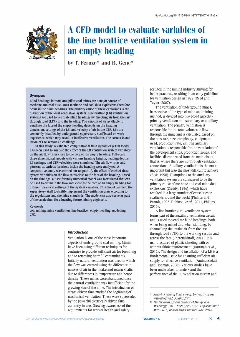
A CFD model to evaluate variables ofthe line brattice ventilation system inan empty headingby T. Feroze* and B. Genc*
Synopsis
Blind headings in room and pillar coal mines are a major source ofmethane and coal dust. Most methane and coal dust explosions thereforeoccur in the blind headings. The primary cause of these explosions is thedisruption of the local ventilation system. Line brattice (LB) ventilationsystems are used to ventilate blind headings by directing air from the lastthrough road (LTR) into the heading. The amount of air available toventilate the face of the empty heading depends on the headingdimension, settings of the LB, and velocity of air in the LTR. LBs arecommonly installed by underground supervisory staff based on workexperience, which may result in ineffective ventilation. The correct instal-lation of LBs remains a challenge.
In this study, a validated computational fluid dynamics (CFD) modelhas been used to analyse the effect of the LB ventilation system variableson the air flow rates close to the face of the empty heading. Full-scalethree-dimensional models with various heading heights, heading depths,LB settings, and LTR velocities were simulated. The air flow rates andpatterns at various locations inside the heading were analysed. Acomparative study was carried out to quantify the effect of each of thesesystem variables on the flow rates close to the face of the heading. Basedon the findings, a user-friendly numerical model was formulated that canbe used to estimate the flow rate close to the face of an empty heading fordifferent practical settings of the system variables. This model can help thesupervisory staff to swiftly implement the ventilation plan according tothe regulations and the mine standards. The model can also serve as partof the curriculum for educating future mining engineers.
Keywords
coal mining, mine ventilation, line brattice , empty heading, modelling,CFD.
* School of Mining Engineering, University of theWitwatersrand, South Africa.
© The Southern African Institute of Mining andMetallurgy, 2017. ISSN 2225-6253. Paper receivedMar. 2016; revised paper received Nov. 2016.
97The Journal of the Southern African Institute of Mining and Metallurgy VOLUME 117 february 2017 s
http://dx.doi.org/10.17159/2411-9717/2017/v117n2a1

A CFD model to evaluate variables of the line brattice ventilation system
ventilation of the working face. The earlier studies revealedthat a LB is essential for the prevention of recirculation andfor the control of respirable dust and methane in the face area(Tien, 1988). It was found that an upstream LB systemincreases the penetration of air by 46% with recirculation ofonly 10% compared to a downstream LB system withpenetration of 16% and recirculation of 50% (Meyer et al.,1991; Meyer, 1993). The use of an air curtain was shown tobe very effective in resolving the problem of dust isolation ata fully mechanized working face (Wang et al., 2011). Acomparison of different auxiliary ventilation systems showedthat the LB is the most suitable system for directing dustparticles away from the face (Candra et al., 2014), and ahybrid brattice system can be effectively used to mitigate dustdispersion from the face and keep the workplace safe for theminers (Candra et al., 2015). Several studies have beenundertaken to ascertain the effect of LB setback distance onthe ventilation of a heading. A reduction in the setbackdistance and increase in the quantity of air at the exit of theLB has been shown to reduce dust and methane levels andimprove ventilation (Lihong et al., 2015; Taylor et al., 2005;Goodman and Pollock, 2004, Thimons et al., 1999). Acombination of brattice-exhausting system has been found toyield the best ventilation performance (Sasmito et al., 2013).arious studies by Wala and Petrov on the effect of setbackdistance and the other system variables on the ventilation ofthe empty headings have shown that 70–80% of the airexiting the LB does not even reach the face of the heading(Wala et al., 2002, 2004; Petrov et al., 2013).
Despite these studies, no models are available to estimatethe effect of all the system variables associated with the LBsystem on ventilation. In the absence of such models, theinstallation is undertaken using past experience. The air flowclose to the face of the heading is increased by increasing thedistance of the LB from the wall and/or increasing the LTRvelocity, or by using an auxiliary fan. This may lead toimproper ventilation, and the correct installation of LBs is stilla challenge. The present study was undertaken to quantifythe effect of heading dimensions (depth and height), LBsettings (LB length in the LTR, LB angle in the LTR, LBlength in the heading, LB to wall distance in the heading),and LTR velocity on the ventilation of an empty headingusing computational fluid dynamics (CFD). Models tocalculate the effect of each of these variables were developedto facilitate the correct and quick installation of the LB. Thisstudy is part of a larger project that was undertaken usingCFD to quantify the effect of various system variables relatedto the ventilation of headings using auxiliary ventilationsystems in different mining scenarios.
Research matrix
Four sets of heading dimensions (W × H × L): 6.6 × 3 × 10 m(group 1, cases 1–24), 6.6 × 3 × 20 m (group 2, cases 25–48), 6.6 × 4 × 10 m (group 3, cases 49–72), and 6.6 × 4 × 20 m (group 4, cases 73–96) were used for this study. Theseheading dimensions were chosen by considering the mostcommon dimensions of headings in South African coalmines, and also to cover a range of scenarios sufficient tocarry out comparative analysis and capture the effect ofheading height and depth. Lower seam heights are currentlybeing investigated, but are not considered in this paper. The
research was organized in such a way that there are 24 basecases in each group. The LB settings shown in Figure 1 werevaried within each group in such a way that sets of casesbecame available within each group and between groups aswell. In order to calculate the precise effect of each systemvariable through comparative analysis, one variable in eachcase of a set was varied while the others were kept constant.The cases of each group were simulated with three LTRvelocities equal to 1 m/s, 1.5 m/s, and 2m/s. The sequence ofcases in all groups was kept the same, as given in Table I forgroup 1. The 24 cases in each group were named using thesyntax: case number - heading width - heading height -heading length - LB length inside heading - LB length in LTR- LB to wall distance in heading - LB angle in LTR. The setsof cases formed in this study to analyse the effect of thesystem variables are given in Table II.
Numerical modelling of the LB ventilation system in
CFD
Model geometry and meshing
ANSYS Design Modeler and Mesher were used to model andmesh the geometries. The length of the LTR modelled on bothsides of the heading was kept constant at 10 m for all thecases as shown in Figure 1. As far as possible a structured,conformal hexahedral mesh aligned with the direction of flowwas created for all the geometries to avoid false diffusion andreduce the number of nodes as compared to a tetrahedralmesh. Inflation layers, where required, were used at theboundaries of the geometries to allow a smooth transitionfrom the laminar flow near the wall to turbulent flow awayfrom the walls. A fine-sized mesh equal to 0.04 m was usedfor geometries of all the cases to resolve the salient featuresof flow and reduce the interpolation errors. The number ofnodes used varied between 8.5 million and 25 million. Thefinal mesh size was selected after undertaking a gridindependence test. This was carried out using mesh sizes of0.1 m, 0.075 m, 0.04 m, and 0.03 m. A mesh size of 0.04 mwas found to be appropriate, with less than 1% deviationwith further reduction in mesh size.
s
98 february 2017 VOLUME 117 The Journal of the Southern African Institute of Mining and Metallurgy
Figure 1—LB and heading parameters varied

Numerical calculations
Velocity inlet and outflow boundary conditions at the inletand outlet, with the wall boundary condition at all theboundaries, was used as shown in Figure 1. Continuity andmomentum equations along with the k-ε realizableturbulence model with enhanced wall treatment were solvedusing ANSYS Fluent. The details of the boundary conditionsand the turbulence model are available in the softwaremanual (ANSYS, 2015). The numerical model used for thisresearch was validated using the study by Feroze and Phillips(2015) as well as the case study in this paper. The solutionwas calculated using a second-order scheme. The iterativeprocess for all the cases was stopped when the desiredconvergence was achieved. Furthermore, the convergence inall the cases was judged by monitoring and ensuring that:
‰ Overall mass conservation was satisfied at the inlet andoutlet of the domain (property conservation)
‰ The residual decreased to 10-5 (convergence criterion) ‰ The surface monitor of the integral of the velocity
magnitude on a vertical plane, defined in the domain asshown in Figure 1, converged properly.
Results and discussion
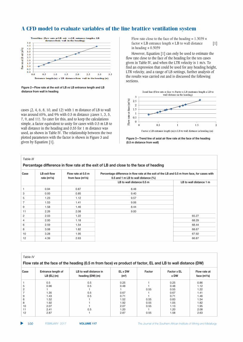
To develop an initial mathematical model for the estimationof air flow rate close to the face of the empty heading (0.5 mfrom face) only the first 12 cases of group 1, simulated with aLTR velocity of 1 m/s, were examined. These cases aretermed the standard cases in this study. This analysis wasthen refined using comparative analysis by considering theeffect of all the system variables on all the cases. The flowrates at the exit of the LB for the standard cases showed adirect proportionality with the product of the entrance lengthand the distance of the LB to the wall of the heading, asshown in Figure 2. Since this product is the same for caseswhere the LB was used with zero angle and the same LB towall distance (same for cases 1 and 3 and 2 and 4), out ofthe first four cases only case 1 and 2 were used.
The flow rates close to the face of the heading for thestandard cases, however, did not show this proportionality.Therefore, a comparison of the flow rates at the exit of the LBand the face of the empty heading was carried out as shownin Table III. The comparison showed that the difference inflow rates at the exit of LB and face of the empty heading for
A CFD model to evaluate variables of the line brattice ventilation system
The Journal of the Southern African Institute of Mining and Metallurgy VOLUME 117 february 2017 99 s
Table I
Numenclature for cases of group 1
Complete names Numerical name Complete names Numerical name
1-6.6-3-10-Half-3-0.5-0 1 13-6.6-3-10-threebyfour-3-0.5-0 132-6.6-3-10-Half-3-1-0 2 14-6.6-3-10-threebyfour-3-1-0 143-6.6-3-10-Half-6-0.5-0 3 15-6.6-3-10-threebyfour-6-0.5-0 154-6.6-3-10-Half-6-1-0 4 16-6.6-3-10-threebyfour-6-1-0 165-6.6-3-10-Half-3-0.5-7.5 5 17-6.6-3-10-threebyfour-3-0.5-7.5 176-6.6-3-10-Half-3-1-7.5 6 18-6.6-3-10-threebyfour-3-1-7.5 187-6.6-3-10-Half-6-0.5-7.5 7 19-6.6-3-10-threebyfour-6-0.5-7.5 198-6.6-3-10-Half-6-1-7.5 8 20-6.6-3-10-threebyfour-6-1-7.5 209-6.6-3-10-Half-3-0.5-15 9 21-6.6-3-10-threebyfour-3-0.5-15 2110-6.6-3-10-Half-3-1-15 10 22-6.6-3-10-threebyfour-3-1-15 2211-6.6-3-10-Half-6-0.5-15 11 23-6.6-3-10-threebyfour-6-0.5-15 2312-6.6-3-10-Half-6-1-15 12 24-6.6-3-10-threebyfour-6-1-15 24
Table II
Set of cases formed in the study
System Set of cases System variables value used
variable Group 1 Group 2 Group 3 Group 4
6.6 x 3 x 10 6.6 x 3 x 20 6.6 x 4 x 10 6.6 x 4 x 20
LB length 1 vs 3, 2 vs 25 vs 37, 26 vs 49 vs 61, 50 vs 73 vs 85, 74 vs LB length in short heading = 5 and in heading 4…12-24 38…36-48 62….60 vs 72 86….84 vs 96 7.5 m and in long heading 10 and 15 mLB to face 1 vs 3,2 vs 25 vs 37, 26 vs 49 vs 61, 50 vs 73 vs 85, 74 vs LB to face distance in short heading = 2.5distance 4….12-24 38….36-48 62….60 vs 72 86….84 vs 96 and 5 m and in long heading 5 and 10 mLB to wall 1 vs 2, 3 vs 4 25 vs 26, 27 vs 49 vs 50, 51 vs 73 vs 74, 75 vs LB to wall distance in distance …..23 vs 24 28….35 vs 36 52….71 vss 72 76….95 vs 96 heading = 0.5 m and 1 mLB length 1 vs 3, 2 vs 4, 25 vs 27, 26 vs 49 vs 51, 52 vs 73 vs 75, 74 vs LB length in LTR = 3 m and 6 min LTR ….22 vs 24 28….34 vs 36 54….70 vs 72 76….94 vs 96LB angle 1 vs 5 vs 9, 2 vs 6 25 vs 29 vs 33, 26 48 vs 53 vs 57,49 73 vs 77 vs 81,74 LB angle in LTR = 0˚,7.5˚, and 15˚in LTR vs 10…16 vs 30 vs 34….40 vs 54 vs 50 …64 vs 78 vs 82….88
vs 20 vs 24 vs 44 vs 48 vs 68 vs 72 vs 92 vs 96LTR air 1 vs 1, 2 vs 25 vs 25, 26 vs 49 vs 49, 50 vs 73 vs 73, 74 vs 1m/s, 1.5 m/s and 2 m/s (each case wasvelocity 2….24 vs 24 26….48 vs 48 50….72 vs 72 74….96 vs 96 run with 3 LTR velocities, creating
3 sets of 2 cases each)Heading 1 vs 49, 2 vs 50…24 vs 48 and 25 vs 73, 26 vs 74,….48 vs 96, group 1 and group 2 were simulated with 3m high heading height and group 3 and 4 are run with 4m high heading
A CFD model to evaluate variables of the line brattice ventilation system
cases (2, 4, 6, 8, 10, and 12) with 1 m distance of LB to wallwas around 65%, and 9% with 0.5 m distance (cases 1, 3, 5,7, 9, and 11). To cater for this, and to keep the calculationssimple, a factor equivalent to unity for cases with 0.5 m LB towall distance in the heading and 0.55 for 1 m distance wasused, as shown in Table IV. The relationship between the twoplotted parameters with the factor is shown in Figure 3 andgiven by Equation [1].
Flow rate close to the face of the heading = 1.3039 ×factor × LB entrance length × LB to wall distance [1]in heading + 0.5059However, Equation [1] can only be used to estimate the
flow rate close to the face of the heading for the ten casesgiven in Table IV, and when the LTR velocity is 1 m/s. Tofind an expression that could be used for any heading height,LTR velocity, and a range of LB settings, further analysis ofthe results was carried out and is discussed the followingsections.
s
100 february 2017 VOLUME 117 The Journal of the Southern African Institute of Mining and Metallurgy
Figure 2—Flow rate at the exit of LB vs LB entrance length and LB
distance from wall in heading
Table III
Percentage difference in flow rate at the exit of LB and close to the face of heading
Case LB exit flow Flow rate at 0.5 m Percentage difference in flow rate at the exit of the LB and 0.5 m from face, for cases with
rate (m3/s) from face (m3/s) 0.5 and 1 m LB to wall distance (%)
LB to wall distance 0.5 m LB to wall distance 1 m
1 0.94 0.87 8.483 0.93 0.85 9.405 1.23 1.12 9.577 1.53 1.41 9.069 1.58 1.46 8.4411 2.26 2.08 9.002 2.03 1.22 65.274 2.00 1.18 68.296 2.59 1.54 68.448 3.08 1.82 68.6710 3.28 1.95 67.9212 4.39 2.63 66.87
Figure 3—Trend line of axial air flow rate at the face of the heading
(0.5 m distance from wall)
Table IV
Flow rate at the face of the heading (0.5 m from face) vs product of factor, EL and LB to wall distance (DW)
Case Entrance length of LB to wall distance in EL x DW Factor Factor x EL Flow rate at
LB (EL) (m) heading (DW) (m) (m2) x DW face (m3/s)
1 0.5 0.5 0.25 1 0.25 0.865 0.96 0.5 0.48 1 0.48 1.122 1 1 1 0.55 0.55 1.227 1.35 0.5 0.67 1 0.67 1.419 1.43 0.5 0.71 1 0.71 1.466 1.52 1 1.52 0.55 0.83 1.548 1.92 1 1.92 0.55 1.05 1.8210 2.07 1 2.07 0.55 1.13 1.9511 2.41 0.5 1.20 1 1.20 2.0812 2.87 1 2.87 0.55 1.58 2.63
Effect of change in LTR velocity
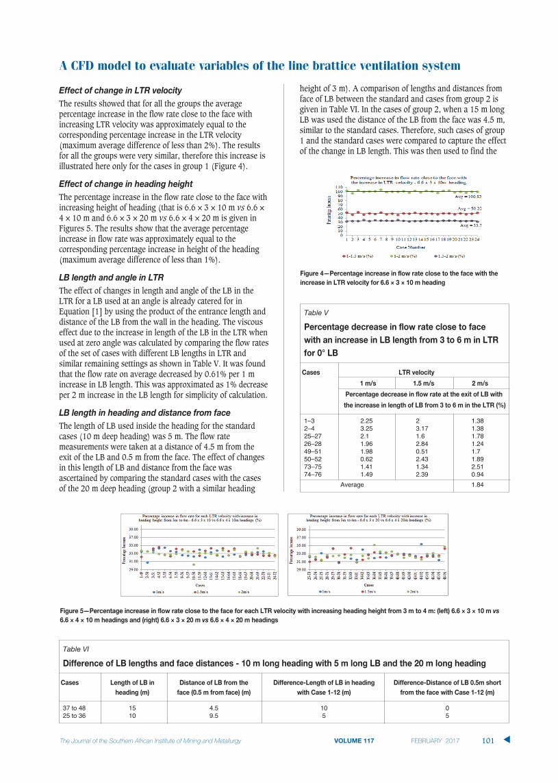
The results showed that for all the groups the averagepercentage increase in the flow rate close to the face withincreasing LTR velocity was approximately equal to thecorresponding percentage increase in the LTR velocity(maximum average difference of less than 2%). The resultsfor all the groups were very similar, therefore this increase isillustrated here only for the cases in group 1 (Figure 4).
Effect of change in heading height
The percentage increase in the flow rate close to the face withincreasing height of heading (that is 6.6 × 3 × 10 m vs 6.6 ×4 × 10 m and 6.6 × 3 × 20 m vs 6.6 × 4 × 20 m is given inFigures 5. The results show that the average percentageincrease in flow rate was approximately equal to thecorresponding percentage increase in height of the heading(maximum average difference of less than 1%).
LB length and angle in LTR
The effect of changes in length and angle of the LB in theLTR for a LB used at an angle is already catered for inEquation [1] by using the product of the entrance length anddistance of the LB from the wall in the heading. The viscouseffect due to the increase in length of the LB in the LTR whenused at zero angle was calculated by comparing the flow ratesof the set of cases with different LB lengths in LTR andsimilar remaining settings as shown in Table V. It was foundthat the flow rate on average decreased by 0.61% per 1 mincrease in LB length. This was approximated as 1% decreaseper 2 m increase in the LB length for simplicity of calculation.
LB length in heading and distance from face
The length of LB used inside the heading for the standardcases (10 m deep heading) was 5 m. The flow ratemeasurements were taken at a distance of 4.5 m from theexit of the LB and 0.5 m from the face. The effect of changesin this length of LB and distance from the face wasascertained by comparing the standard cases with the casesof the 20 m deep heading (group 2 with a similar heading
height of 3 m). A comparison of lengths and distances fromface of LB between the standard and cases from group 2 isgiven in Table VI. In the cases of group 2, when a 15 m longLB was used the distance of the LB from the face was 4.5 m,similar to the standard cases. Therefore, such cases of group1 and the standard cases were compared to capture the effectof the change in LB length. This was then used to find the
A CFD model to evaluate variables of the line brattice ventilation system
The Journal of the Southern African Institute of Mining and Metallurgy VOLUME 117 february 2017 101 s
Table V
Percentage decrease in flow rate close to face
with an increase in LB length from 3 to 6 m in LTR
for 0° LB
Cases LTR velocity
1 m/s 1.5 m/s 2 m/s
Percentage decrease in flow rate at the exit of LB with
the increase in length of LB from 3 to 6 m in the LTR (%)
1–3 2.25 2 1.382–4 3.25 3.17 1.3825–27 2.1 1.6 1.7826–28 1.96 2.84 1.2449–51 1.98 0.51 1.750–52 0.62 2.43 1.8973–75 1.41 1.34 2.5174–76 1.49 2.39 0.94
Average 1.84
Figure 4—Percentage increase in flow rate close to the face with the
increase in LTR velocity for 6.6 × 3 × 10 m heading
Figure 5—Percentage increase in flow rate close to the face for each LTR velocity with increasing heading height from 3 m to 4 m: (left) 6.6 × 3 × 10 m vs
6.6 × 4 × 10 m headings and (right) 6.6 × 3 × 20 m vs 6.6 × 4 × 20 m headings
Table VI
Difference of LB lengths and face distances - 10 m long heading with 5 m long LB and the 20 m long heading
Cases Length of LB in Distance of LB from the Difference-Length of LB in heading Difference-Distance of LB 0.5m short
heading (m) face (0.5 m from face) (m) with Case 1-12 (m) from the face with Case 1-12 (m)
37 to 48 15 4.5 10 025 to 36 10 9.5 5 5

A CFD model to evaluate variables of the line brattice ventilation system
effect of the distance of the LB from the face by comparingthe standard cases with the cases of group 2 where a 10 mlong LB was used.
LB length in the heading
Before discussing this comparison, it is necessary tounderstand how the LB to wall distance and LB length insidethe heading affect the flow of air. The main feature of the airflowing through the channel between the LB and the wall ofheading was the propelling of air due to centrifugal force andflow separation close to the LB and away from the wall at theturn into the heading, as shown in Figure 6. As a result, theair flow at the exit of the LB was not uniform, and the airwas more concentrated close to the LB (due to highervelocity).
It was found that part of the air leaving the LB is divertedtowards the left wall of the heading; air close to the LB turnsfirst and as the air moves farther away from the LB exit theeffect becomes more marked, as shown in Figure 7 (themovement of air in the centre of the heading has beenomitted). This reduces the amount of air actually reaching theface after exiting the LB. Consequently, when the variation inflow rate at the exit of the LB was high, a greater proportionof the air was diverted before reaching the face. Furthermore,the flow of air moving through a narrow channel is higherthan in a wider channel. Hence the reduction in flow rate wasmuch greater with 1 m LB to wall distance (Table III).However, it was found that this reduction decreases withincreasing length of the LB in the heading, as the air becomesuniformly distributed at the exit of LB with this increase inlength (similar to fluid flow in a pipe or channel).
To quantify the effect of the increase in LB length in theheading on this flow rate reduction, cases with LB to walldistances of 0.5 m and 1 m in the long heading (with 15 m
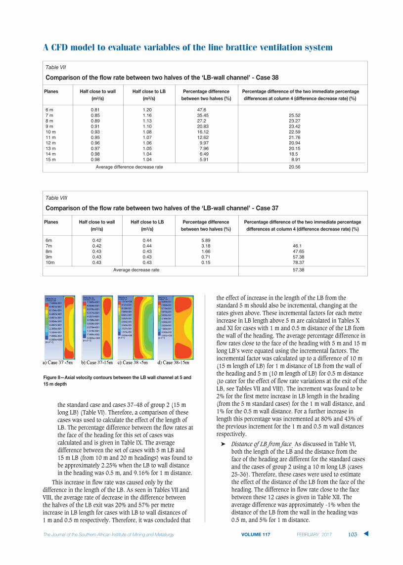
long LB, the maximum for this study) were analysed. Thiswas done by constructing eleven equally-spaced verticalplanes inside the channel between the LB and the wall of theheading. The first plane was constructed at a depth of 5 m.These vertical planes were split into two halves equal to 0.25 m and 0.5 m each for the 0.5 m and 1 m LB to walldistances respectively, and flow rate through these halves ateach depth was calculated. All the cases of each category (0.5 m and 1 m wall distance) showed similar results.Therefore, only one case from each category is presentedhere, i.e. case 37 with 0.5 m LB to wall distance and case 38with 1 m distance. The rest of the configurations are thesame for both the cases. The detailed results are given inTables VII and VIII. The difference in flow rates was found tobe around 50% at 6 m depth, reducing to approximately 5%at the depth of 15 m for case 38 (1 m wall distance). Thedifference in flow rates between the two halves of the planesconstructed for case 37 (0.5 m wall distance) was very low –around 5% even at 6 m depth and close to zero at 10 m depth(LB length of 10 m). To illustrate the impact of length on theair flow variation, the velocity contours at depths of 5 and 15m are shown in Figure 8 for both the cases. It can be seenthat the increase in LB length had a greater effect at a LB towall distance of 1 m (as flow rates were already very uniformwith 0.5 m LB to wall distance).
It was therefore concluded/assumed that for the air flowin the channel between the LB and wall of the heading tobecome uniform (negligible difference in the flow ratesbetween the two halves at LB exit), a minimum length of LBis required. This length was found to vary with the LB to walldistance in the heading, being 15 m and 10 m for the 1m and0.5 m LB to wall distance in heading respectively. Thereforean increase of 0.1 m in the LB wall distance from 0.5 mrequires an additional length of 1 m over the 10 m length ofLB to evenly disperse the air flow at the exit of the LB.
In Tables VII and VIII the percentage decrease rate, i.e.how the difference was decreasing with each metre increasein length of the LB, is also shown (percentage differencebetween the two immediate percentage differences). Theaverage decrease rate for case 38 was approximately 20%,and for case 37 approximately 57%. Although the decreaserate for the case with 0.5 m wall distance was greater, theoverall effect on the difference in magnitude of the flow ratesin the two halves of the planes (constructed in the channelbetween the LB and wall of the heading) was much higher forthe 1 m LB to wall distance.
‰ Factor for length of LB in heading—The distance of theLB from the face of the heading is the same (4.5 m) for
s
102 february 2017 VOLUME 117 The Journal of the Southern African Institute of Mining and Metallurgy
Figure 6—Air diverted away from wall and close to LB due to
centrifugal force and flow separation
Figure 7—Stream lines inside 10 m long heading at LB to wall distances of 0.5 m and 1 m (similar remaining settings)
A CFD model to evaluate variables of the line brattice ventilation system
The Journal of the Southern African Institute of Mining and Metallurgy VOLUME 117 february 2017 103 s
the standard case and cases 37–48 of group 2 (15 mlong LB) (Table VI). Therefore, a comparison of thesecases was used to calculate the effect of the length ofLB. The percentage difference between the flow rates atthe face of the heading for this set of cases wascalculated and is given in Table IX. The averagedifference between the set of cases with 5 m LB and 15 m LB (from 10 m and 20 m headings) was found tobe approximately 2.25% when the LB to wall distancein the heading was 0.5 m, and 9.16% for 1 m distance.
This increase in flow rate was caused only by thedifference in the length of the LB. As seen in Tables VII andVIII, the average rate of decrease in the difference betweenthe halves of the LB exit was 20% and 57% per metreincrease in LB length for cases with LB to wall distances of 1 m and 0.5 m respectively. Therefore, it was concluded that
the effect of increase in the length of the LB from thestandard 5 m should also be incremental, changing at therates given above. These incremental factors for each metreincrease in LB length above 5 m are calculated in Tables Xand XI for cases with 1 m and 0.5 m distance of the LB fromthe wall of the heading. The average percentage difference inflow rates close to the face of the heading with 5 m and 15 mlong LB’s were equated using the incremental factors. Theincremental factor was calculated up to a difference of 10 m(15 m length of LB) for 1 m distance of LB from the wall ofthe heading and 5 m (10 m length of LB) for 0.5 m distance(to cater for the effect of flow rate variations at the exit of theLB, see Tables VII and VIII). The increment was found to be2% for the first metre increase in LB length in the heading(from the 5 m standard cases) for the 1 m wall distance, and1% for the 0.5 m wall distance. For a further increase inlength this percentage was incremented at 80% and 43% ofthe previous increment for the 1 m and 0.5 m wall distancesrespectively.
‰ Distance of LB from face. As discussed in Table VI,both the length of the LB and the distance from theface of the heading are different for the standard casesand the cases of group 2 using a 10 m long LB (cases25-36). Therefore, these cases were used to estimatethe effect of the distance of the LB from the face of theheading. The difference in flow rate close to the facebetween these 12 cases is given in Table XII. Theaverage difference was approximately -1% when thedistance of the LB from the wall in the heading was 0.5 m, and 5% for 1 m distance.
Table VII
Comparison of the flow rate between two halves of the ‘LB-wall channel’ - Case 38
Planes Half close to wall Half close to LB Percentage difference Percentage difference of the two immediate percentage
(m3/s) (m3/s) between two halves (%) differences at column 4 (difference decrease rate) (%)
6 m 0.81 1.20 47.67 m 0.85 1.16 35.45 25.528 m 0.89 1.13 27.2 23.279 m 0.91 1.10 20.83 23.4210 m 0.93 1.08 16.12 22.5911 m 0.95 1.07 12.62 21.7612 m 0.96 1.06 9.97 20.9413 m 0.97 1.05 7.96 20.1514 m 0.98 1.04 6.49 18.515 m 0.98 1.04 5.91 8.91
Average difference decrease rate 20.56
Table VIII
Comparison of the flow rate between two halves of the ‘LB-wall channel’ - Case 37
Planes Half close to wall Half close to LB Percentage difference Percentage difference of the two immediate percentage
(m3/s) (m3/s) between two halves (%) differences at column 4 (difference decrease rate) (%)
6m 0.42 0.44 5.897m 0.42 0.44 3.18 46.18m 0.43 0.43 1.66 47.659m 0.43 0.43 0.71 57.3810m 0.43 0.43 0.15 78.37
Average decrease rate 57.38
Figure 8—Axial velocity contours between the LB wall channel at 5 and
15 m depth

A CFD model to evaluate variables of the line brattice ventilation system
s
104 february 2017 VOLUME 117 The Journal of the Southern African Institute of Mining and Metallurgy
Table IX
Percentage difference in flow rate close to face; 10 m vs 20 m heading with 5 m and 15 m LB in heading for LB
wall distance of 0.5 m and 1 m
Cases Flow rate Cases Flow rate Percentage difference in flow rate close to face: 10 m vs
(0.5 m from face) (m3/s) (0.5 m from face) 20 m heading with 5 and 15 m long LB in heading (%)
(m3/s) (m3/s)
LB to heading wall distance 0.5 m LB to heading wall distance 1 m20 m long heading 10 m long heading
37 0.88 1 0.86 1.2439 0.87 3 0.85 2.3141 1.15 5 1.12 2.843 1.44 7 1.41 2.2745 1.48 9 1.46 1.6947 2.14 11 2.08 3.1638 1.35 2 1.22 9.2740 1.31 4 1.18 9.3542 1.72 6 1.54 10.444 2.00 8 1.82 8.7446 2.18 10 1.95 10.4448 2.82 12 2.63 6.72
Average difference (%) 2.25 9.16
Table X
Incremental percentage increase in flow rate due to the increase in LB length from 5 m (wall distance 1 m)
Case 1–12 vs Cases 37–48 with LB distance of 1 m from wall of heading
Increase in LB Percentage incremental effect for Cumulative percentage increase for corresponding Remarks
length from 5 m each metre increase in length increase in length of LB from 5 m
1 2 22 1.6 3.63 1.28 4.884 1.02 5.905 0.81 6.726 0.65 7.377 0.52 7.908 0.41 8.329 0.33 8.6510 0.26 8.92Total increase 8.92
Note: The average net increase (Table IX) should be around 9%, and the net increase with this approach is around 9%
The effect is decreasing at the rate of 20% from
the previous metre increasein length
Table XI
Incremental percentage increase in flow rate due to the increase in LB length from 5 m (wall distance 0.5 m)
Case 1–12 vs Cases 37–48 with LB distance of 0.5 m from wall of heading
Increase in LB Percentage incremental effect for Cumulative percentage increase for corresponding Remarks
length from 5 m each metre increase in length increase in length of LB from 5 m
1 1 12 0.43 1.433 0.18 1.614 0.07 1.695 0.03 1.72Total increase 1.72
Note: The average net increase (Table IX) should be around 2.25%, and the net increase with this approach is about 1.75%
The effect is decreasing at the rate of 57% from
the previous metre increasein length
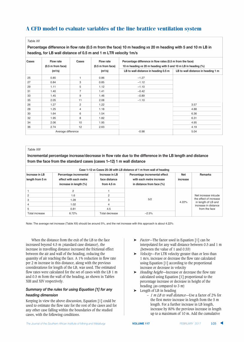
When the distance from the exit of the LB to the faceincreased beyond 4.5 m (standard case distance), theincrease in travelling distance increased the frictional effectbetween the air and wall of the heading, reducing thequantity of air reaching the face. A 1% reduction in flow rateper 2 m increase in this distance, along with the previousconsiderations for length of the LB, was used. The estimatedflow rates were calculated for the set of cases with the LB 1 mand 0.5 m from the wall of the heading, as shown in TablesXIII and XIV respectively.
Summary of the rules for using Equation [1] for any
heading dimension
Keeping in view the above discussion, Equation [1] could beused to estimate the flow rate for the rest of the cases and forany other case falling within the boundaries of the studiedcases, with the following conditions.
‰ Factor—The factor used in Equation [1] can beinterpolated for any wall distance between 0.5 and 1 m(between the value of 1 and 0.55)
‰ Velocity—For LTR velocity greater than or less than 1 m/s, increase or decrease the flow rate calculatedusing Equation [1] according to the proportionalincrease or decrease in velocity
‰ Heading height—Increase or decrease the flow ratecalculated using Equation [1] proportional to thepercentage increase or decrease in height of theheading (as compared to 3 m)
‰ Length of LB in heading – 1 m LB to wall distance—Use a factor of 2% for
the first metre increase in length from the 5 mlength. For a further increase in LB length,increase by 80% the previous increase in lengthup to a maximum of 10 m. Add the cumulative
A CFD model to evaluate variables of the line brattice ventilation system
The Journal of the Southern African Institute of Mining and Metallurgy VOLUME 117 february 2017 105 s
Table XII
Percentage difference in flow rate (0.5 m from the face) 10 m heading vs 20 m heading with 5 and 10 m LB in
heading, for LB wall distance of 0.5 m and 1 m LTR velocity 1m/s
Cases Flow rate Cases Flow rate Percentage difference in flow rates (0.5 m from the face)
(0.5 m from face) (0.5 m from face) 10 m heading vs 20 m heading with 5 and 10 m LB in heading (%)
(m3/s) (m3/s) LB to wall distance in heading 0.5 m LB to wall distance in heading 1 m
25 0.85 1 0.86 –1.2727 0.84 3 0.85 –1.1229 1.11 5 1.12 –1.1031 1.40 7 1.41 –0.4233 1.45 9 1.46 –0.8935 2.05 11 2.08 –1.1026 1.27 2 1.22 3.5728 1.25 4 1.18 4.8830 1.64 6 1.54 6.3632 1.95 8 1.82 6.3134 2.06 10 1.95 4.9536 2.74 12 2.63 4.19
Average difference -0.98 5.04
Table XIII
Incremental percentage increase/decrease in flow rate due to the difference in the LB length and distance
from the face from the standard cases (cases 1–12) 1 m wall distance
Case 1–12 vs Cases 25–36 with LB distance of 1 m from wall of heading
Increase in LB Percentage incremental Increase in LB Percentage incremental effect Net Remarks
length from 5 m effect with each metre face distance with each metre increase increase
increase in length (%) from 4.5 m in distance from face (%)
1 2 12 1.6 23 1.28 34 1.02 45 0.81 4.5Total increase 6.72% Total decrease –2.5%
Net increase inlcudethe effect of increasein length of LB andincrease in distance
from the face
5/24.22%
Note: The average net increase (Table XII) should be around 5%, and the net increase with this approach is about 4.22%

A CFD model to evaluate variables of the line brattice ventilation system
effect and increase the percentage calculatedusing Equation [1]
– 0.5 m LB to wall distance—Use a factor of 1%for the first metre increase in length from the 5m length. For a further increase in LB length,increase 43% of the previous metre increase inlength up to a maximum of 5 m. Add thecumulative effect and increase the percentagecalculated using Equation [1]
– Any other LB to wall distance—Interpolate tofind the percentage for the first metre increase inlength, the reduction factor, and the number ofmetres to calculate the cumulative effect
‰ Distance of the LB from the face: Use a factor of 1% forevery 2 m increase/decrease in distance from the 4.5 mdistance (distance from face). Add the cumulative effectand decrease/increase the same percentage amount offlow as calculated using Equation [1]
‰ Length of LB in the LTR: The effect of the change in thelength of the LB in the LTR for a LB used at an angle isalready catered for in the expression by using theproduct of the entrance length and distance of the LBfrom the wall in the heading. However, for the LB withzero angle in the LTR, the viscous effect for an increasein length of the LB of more than 3 m is estimated at 1%decrease in flow rate per 2 m increase in the length ofthe LB.
Generalized equation
Given the conditions above, a generalized equation toestimate the flow rates at the exit of the LB was developed tosimplify the solution procedure. All the conditions givenabove were incorporated in the formulation of this equation.
Flow rate close to the face of the heading (0.5 m from theface) = [(1.30 × Factor × (X × b)) + 0.51] × [2][1 + (LTR Vel –1) + (HH –3)/3 – (f – 4.5)/(2 × 100) + ((First metre factor) + (∑n
i=2. First metre factor × ReductionFactor (i-1)))/100 – (c - 3)/(2 × 100)]
where
X = LB entrance length First metre factor = 2 (only to be used when LB length is more than 5 m) for 1 m distance of LB from the wall and 1 for 0.5 m distance; for other distances it can be interpolated.
b = LB to wall distance in the heading
c = LB length in LTRd = LB length in headingf = LB distance to face of n = 10 for 1 m distance of LBheading (0.5 m from the face) from the wall and 5 for 0.5 m
distance; for other distances itcan be interpolated
HH = Heading heightLTR Vel = Velocity of air in Reduction factor = 0.8 for 1 mthe LTR distance of LB from the wall
and 0.43 for 0.5 m distance;for other distances it can beinterpolated
First metre factor x reduction Only for LB with zero degreefactor in LTR.
Validation case study
Validation of a numerical model is required to demonstrate itsaccuracy so that it may be used with confidence and that theresults can be considered reliable. The present validationstudy was carried out in the Kriel Colliery, which is situated120 km east of Johannesburg and 50 km southwest ofWitbank. The velocity of air at a number of locations inside aheading ventilated using a LB was measured. A comparisonof the in situ measurements with the numerical resultsshowed that the numerical results are in line with the experi-mental results and the k-ε realizable model is suitable forcarrying out studies related to the ventilation of a headingusing a LB.
The in situ measurements were taken in a headingventilated using a LB; the dimensions of the heading and LBare given in Figure 9. The velocities of air at the entrance ofthe LB, inside the heading, and at the exit of the LB were
s
106 february 2017 VOLUME 117 The Journal of the Southern African Institute of Mining and Metallurgy
Table XIV
Incremental percentage increase/decrease in flow rate due to the difference in the LB length distance from the
face from the standard cases (cases 1–12) 0.5 m wall distance
Case 1–12 vs Cases 25–36 with LB distance of 0.5 m from wall of heading
Increase in LB Percentage incremental Increase in LB Percentage incremental effect Net Remarks
length from 5 m effect with each metre face distance with each metre increase in increase
increase in length (%) from 5 m distance from face (%)
1 1 12 0.43 23 0.18 34 0.07 45 0.03 4.5Total increase 1.72% Total decrease –2.5%
Net increase inlcudesthe effect of increasein length of LB andincrease in distance
from the face
5/2–0.77%
Note: The average net increase (Table XII) should be around –0.99%, and the net increase with this approach is about –0.772%

measured. The air velocities and direction of the air inside theheading were recorded using hot wire and rotating vanedigital anemometers and a smoke tube respectively. Access towithin 4 m of the face was not allowed, therefore flow ratesclose to the face were not taken. The same case wassimulated in ANSYS Fluent, and a comparison of the resultsis given in Table XV and Figure 11.
The flow of air inside the heading is shown using velocityvectors in Figure 10. It can be seen that the air entered the LB- wall channel, ventilated the heading, and returned from thedownstream side. As expected, since the minimum length ofLB required for a LB to wall distance of 1.7 m was not usedand a LB to wall distance of 9.5 m was used, very little airexiting the LB actually reached the face. Therefore, LB to walldistance should always be less than 1 m, unless additionalengineering solutions are also used.
The measured velocities are given in Table XV along withthe coordinates of these points. The bottom right corner ofthe LTR was considered as (0, 0, 0). Positive and negativesigns indicate the direction of air movement. As expected, atthe exit of the LB, air velocities were higher close to the LB.The validation study showed that the ANSYS Fluent k-εrealizable model is suitable for studying the ventilation of aheading connected to the LTR.
Conclusions
To address some of the challenges faced underground bysupervisory staff installing LB systems in coal mines, a model
was developed using CFD. The effect of system variablesrelated to the installation of the LB, LTR velocity, andheading dimensions on the flow rates close to the face of theempty heading (0.5m from the face), were evaluated. Theoutcome was represented in a user-friendly numerical modelto estimate the consolidated effect of all the studied variables,which can be used to estimate the flow rates close to the faceof the heading for different configurations of LB, LTRvelocities, and heading dimensions. The model can assistventilation engineers and the supervisory staff to install LBscorrectly and quickly, so as to comply with environmentalregulations and mine standards. It can also help academia aspart of the curriculum for teaching future mining andventilation engineers how the different variables associatedwith the LB ventilation system affect the ventilation in anempty heading.
A CFD model to evaluate variables of the line brattice ventilation system
The Journal of the Southern African Institute of Mining and Metallurgy VOLUME 117 february 2017 107 s
Table XV
Air velocities measured experimentally and calculated numerically
Point Number Points location Coordinate point (m) Experimental results Numerical results
Velocity (m/s) Velocity (m/s)
1 At LB (7, 0.5, 5.75) 0.96 1.032 inlet (7, 2, 5.75) 0.96 1.033 12.64, 0.5, 9.92 –0.11 –0.124 12.64, 2, 9.92 –0.13 –0.145 Inside 15.28, 0.5, 9.92 –0.51 –0.486 heading 15.28, 2, 9.92 –0.48 –0.507 15.28, 0.5, 14.92 –0.55 –0.588 15.28, 2, 14.92 –0.6 –0.629 10.425, 0.5, 20.4 0.85 0.9110 At LB 10.425, 2, 20.4 0.58 0.6111 exit 11.45, 0.5, 20.4 1.16 1.2612 11.45,2,20.4 1.09 1.12
Figure 10—Velocity vectors of air flow inside the heading
Figure 9—Important dimensions of the heading and LTR
Figure 11—Comparison of the experimental and numerical results

A CFD model to evaluate variables of the line brattice ventilation system
Acknowledgement
The work presented in this paper is part of a PhD researchstudy in the School of Mining Engineering at the Universityof the Witwatersrand. The authors would like to acknowledgethe Wits Mining Institute (WMI), University of theWitwatersrand, for making the Digital Mine facility availablefor the research, and the financial assistance required topurchase the high-performance PC and the CFD software.
References
AMINOSSADATI, S.M. and HOOMAN, K. 2008. Numerical simulation of ventilation
air flow in underground mine workings. Proceedings of the 12th US/North
American Mine Ventilation Symposium, Reno, Nevada, 9-12 June.
Wallace, K.G. Jr. (ed.). Society for Mining, Metallurgy, and Exploration,
Littleton, CO. pp. 253–259.
ANSYS® Academic Research. 2015. Release 15.0, Help System, ANSYS Fluent
Theory Guide. ANSYS, Inc. Chapter 4.
BISE, C.J (ed.). 2013. Modern American Coal Mining: Methods and Applications.
Society for Mining, Metallurgy and Exploration, Englewood, CO.
CANDRA, K.J., SASMITO, A.P., and SADASHIV, M.A. 2014. Dust dispersion and
management in underground mining faces. International Journal of
Mining Science and Technology, vol. 24, no. 1. pp. 39–44.
CANDRA, K.J., SASMITO, A.P., and SADASHIV, M.A. 2015. Introduction and
evaluation of a novel hybrid brattice for improved dust control in
underground mining faces: A computational study. International Journal
of Mining Science and Technology, vol. 24, no. 1. pp. 537–543.
CHEREMISINOFF, N.P. 2014. Dust Explosion and Fire Prevention Handbook: A
Guide to Good Industry Practices. Wiley-Scrivener, Beverly, MA.
CREEDY, D.P. (1996). Methane prediction in collieries. Report COL 303. Safety in
Mines Research Advisory Committee (SIMRAC), Johannesburg, June 1996.
DUBINSKI, J., KRAUSE, E., and SKIBA, J. 2011. Global technical and environmental
problems connected with the coal mine methane. Proceedings of the 22nd
World Mining Congress and Expo 2011, Istanbul, Turkey, 11–16
September.
FEROZE, T. and PHILLIPS, H.W. 2015. An initial investigation of room and pillar
ventilation using CFD to investigate the effects of last through road
velocity. Proceedings of the 24th International Mining Congress and
Exhibition of Turkey (IMCET 15). Antalya, Turkey, 14–17 April. Chamber
of Mining Engineers of Turkey. pp. 970–977.
GOODMAN, G.V.R. and POLLOCK, D.E. 2004. Use of a directional spray system
design to control respirable dust and face gas concentrations around a
continuous mining machine. Journal of Occupational and Environmental
Hygiene, vol. 1, no. 12. pp. 806–815.
HARTMAN, H.L., MUTMANSKY, J.M., RAMANI, R.V., and WANG, Y.J. 2012. Mine
Ventilation and Air Conditioning. 3rd edn. Wiley-Interscience.
LIHONG, Z., CHRISTOPHER, P., and YI, Z. 2015. CFD modeling of methane distri-
bution at a continuous miner face with various curtain setback distances.
International Journal of Mining Science and Technology, vol. 25, no. 4.
pp. 635–640.
MEYER, C.F. 1993. Improving underground ventilation conditions in coal mines.
Final Project Report COL 029a. Safety in Mines Research Advisory
Committee (SIMRAC), Johannesburg. November 1993.
MEYER, J.P., LE GRANGE, L.A., and MEYER, C. 1991. The utilisation of air scoops
for the improvement of ventilation in a coal mine heading. Mining Science
and Technology, vol. 13, no. 1. pp. 17–24.
PETROV, T., WALA, A.M., and HUANG, G. 2013. Parametric study of airflow
separation phenomenon at face area during deep cut continuous mining,
Mining Technology, vol. 122, no. 4. pp. 208–214.
PHILLIPS, H.R. and BRANDT, M.P. 1995. Coal mine explosions - risk and remedy.
Proceedings of SIMRAC Symposium, Johannesburg, 1 September 1995.
Southern African Institute of Mining and Metallurgy, Johannesburg.
PHILLIPS, H.R. 2015. Lessons learnt from mine explosions. Proceedings of the
Australian Mine Ventilation Conference, Sydney, NSW, 31 August - 2
September 2015. Australasian Institute of Mining and Metallurgy,
Melbourne. pp.19–28.
REED, W. AND TAYLOR, C. 2007. Factors affecting the development of mine face
ventilation systems in the 20th century. Proceedings of the Society for
Mining, Metallurgy and Exploration (SME) Annual Meeting and Exhibit,
Denver, Colorado, 25–28 February 2007.
SASMITO, A.P., BIRGERSSON, E.LY.H., and MUJUMDAR, A.S. 2013. Some approaches
to improve ventilation system in underground coal mines environment - A
computational fluid dynamic study. Tunnelling and Underground Space
Technology, vol. 34. pp 82–95.
TAYLOR, C.D., TIMKO, R.J., THIMONS, E. D., and MAL, T. 2005. Using ultrasonic
anemometers to evaluate factors affecting face ventilation effectiveness.
Proceedings of the 2005 Annual Meeting of the Society for Mining,
Metallurgy and Exploration (SME), Salt Lake City, Utah. 28 February–
2 March.
THIMONS, E.D., TAYLOR, C.D., anD ZIMMER, J.A. 1999. Ventilating the box cut of a
two-pass 40ft extended cut. Journal of the Mine Ventilation Society of
South Africa, vol. 59, no. 3. pp. 108–115.
TIEN, J.C. 1988. Face ventilation during cross-cut development in a room and
pillar operation. Proceedings of the 4th US Mine Ventilation Symposium,
Berkeley, CA, 20–22 June. Society for Mining, Metallurgy and Exploration,
Littleton, CO. pp. 202–208.
WALA, A.M., VYTLA, S., TAYLOR, C.D., and HUANG, G. 2007. Mine face ventilation:
a comparison of CFD results against benchmark experiments for the CFD
code validation. Mining Engineering, vol. 59, no. 10. pp. 49–55.
WALA, A.M., VYTLA, S., HUANG, G., and TAYLOR, C.D. 2008. Study on the effects
of scrubber operation on the face ventilation. Proceedings of the 12th
US/North American Mine Ventilation Symposium, Reno, Nevada, 9–11
June. Wallace, K.G. Jr. (ed.). Society for Mining, Metallurgy, and
Exploration, Littleton, CO. pp. 281–286.
WANG, P.F., FENG, T., and RONGHUA, L. 2011. Numerical simulation of dust
distribution at a fully mechanized face under the isolation effect of air
curtain. Mining Science and Technology, vol. 21, no. 1. pp. 65–69. u
s
108 february 2017 VOLUME 117 The Journal of the Southern African Institute of Mining and Metallurgy

THERE’S ONLY ONE
SUBSTITUTE FOR A
WARMAN®

Portable gas detection instruments with “reactive time” communication
up-links.
Fully integrated system that can download gas readings, track people,
assets & vehicles, collect telemetry data, transmit paging messages and
collect SCAS II - Collision Awareness logs.
New generation Caplamps including wireless and digital communication,
worn by the underground worker.
SCAS II Collision Awareness System, providing early perimeter warning
notification that gives vehicle operators and pedestrians a head start in
deciding how to manoeuvre during or before a critical decision making period.
2-way paging& distress call
Portable and Fixed Gas detection
Instrumentation
CollisionAwareness
LocationMonitoring
We innovate to make mines safer and more productive.
011 974-0006 | www.schauenburg.co.za
Schauenburg Systems (Pty) Ltd. A company of the International Group
uppe
mar
keti
ng A
1481
4
The Roxy Self Rescuer is a belt worn breathing apparatus to exit from hazardous
zones. Its intended use is only in the case of emergency escapes in the event of
smoke, toxic gas and oxygen deficiencies.
Roxy 40Self-contained
self-rescuer

Copyright © 2015, Weir Minerals Australia Limited. All rights reserved. WARMAN is a trademark and/or registered trademark of Weir Minerals Australia Ltd and Weir Group African IP Ltd; WBH and AH are trademarks and/or registered trademarks of Weir Minerals Australia Ltd; WEIR and the WEIR Logo are trademarks and/or registered trademarks of Weir Engineering Services Ltd.
ANOTHER WARMAN®
Copyright © 2015, Weir Minerals Australia Limited. All rights reserved. WARMAN is a trademark and/or registered trademark of Weir Minerals Australia Ltd and Weir Group African IP Ltd; WBH and AH are trademarks and/or registered trademarks of Weir Minerals Australia Ltd; WEIR and the WEIR Logo are trademarks and/or registered trademarks of Weir Engineering Services Ltd.
Mineralswww.minerals.weirwww.weirafricastore.com
Warman® pumps work hard. New Warman® pumps work even harder.
Like the Warman® WBH® pump, designed to run even more efficiently
and be even more reliable than the legendary Warman® AH® pump in heavy-duty
process, feed and tailings applications. Which means even greater productivity and
even greater profits.
So whether you’re upgrading, or you just need another pump, your choice is easy, Warman®.For more information contact us on +27 11 9292600
To find out more visit theresonlyonewarman.com

Many SolutionsOne SourceFLSmidth offers you a complete line of equipment and services with proven reliability
and enhancing performance from the leading brand names of ABON, Buffalo, CEntry,
Conveyor Engineering, Dawson Metallurgical Laboratories, Decanter Machine, Dorr-
Oliver, EIMCO, ESSA, FFE, Fuller-Traylor, KOCH, Knelson, Krebs, Ludowici, Maag Gear,
Mayer, Meshcape, MIE, Möller, MVT, PERI, Phillips Kiln Services, Pneumapress, RAHCO,
Raptor, Roymec, Shriver, Summit Valley, Technequip and WEMCO.
FLSmidth is your One Source because:
• We own our technology
• We deliver One Source mineral solutions
• World renowned OEM equipment & brands
• We have operating references across Africa
• We understand Africa’s challenges
• We understand our customer’s operating needs
• We underwrite project funding
For more information contact us
Tel no. +27 (0)10 210 4000 • [email protected] • www.flsmidth.com

The effects of poor sampling and the financialimplications for mining companies, traders inmineral assets, and sellers of metal as dore orcommodities is documented in a number ofstudies, the most notable of which is that byCarasco (2004). He examined the financialimpact of poor sampling practices in theChilean copper industry and found that finaciallosses due to poor sampling amounted tohundreds of millions of dollars over the life ofa mining operation. Holmes (2004) examinedthe effects of correct sampling andmeasurement as the foundations ofmetallurgical balances, and found thatrevenues from the sales of large iron oreshipments may be profoundly affected by poorsampling practices. In South Africa the way inwhich sampling of in situ gold-bearing reefsaffects the mine call factor has been anongoing study since the disparity between the
estimation of gold in the reef and the actualgold bullion produced was noted by earlyinvestigators such as Beringer (1938), Jackson(1946), Sichel (1947), Harrison (1952), and anumber of others.
This study explores the ways in whichmisclassification of ore and waste due to theuncertainty in grade estimation has importanteconomic consequences, particularly if a cut-off grade is superimposed on a metal gradedistribution, as is normally the case. Inaddition, the study demonstrates how thegross value of a mineral deposit can be erodedas a result of poor sampling, taking intoaccount the fact that mineral deposits ofdifferent metals, especially ferrous and non-ferrous metals, are characterized by theskewness of their distributions. Mineralscharacterized by the normal distribution forcertain variables are also considered. Themeans by which the value of primary mineraldeposits is affected as a result of theintroduction of sampling error and samplingbias through poor sampling practise dependssignificantly on the nature of the metal distrib-utions in the deposit.
The effects of poor sampling practise areexamined for specific metals and commoditiesby introducing a 10% sampling error, and 0.9-times to 1.1-times sampling bias intootherwise unsampled mineral deposits. Theerror and bias are introduced on positivelyskewed, negatively skewed, and normal distri-butions for three main commodity types,namely gold, iron ore, and coal deposits.
In most open-pit mining operations the pitsuperintendent is responsible for directing
Poor sampling, grade distribution, andfinancial outcomesby R.C.A. Minnitt*
This study examines the problems faced by open pit mine superintendentswho make choices about how to direct their materials, either to the wastedump or to the mill. The paper explores the effects of introducing a 10%sampling error and a 0.9-times to 1.1-times sampling bias on positivelyskewed distributions for precious and base metals, negatively skeweddistributions in the case of bulk commodities, and normal distributions asis the case for coal deposits. Parent distributions for each commodity werecreated on a 25 x 25 m grid using transformations of gold, iron ore, andcoal data-sets, spatially based on a nonconditional Gaussian simulation.Ordinary kriging of grades for the three commodities into a 10 x 10 m gridprovided the reference case against which the distributions with thesampling error and sampling bias for the commodities were compared.Imposing cut-off grades on the actual-versus-estimated scatterplots of thethree commodities allowed the distributions to be classified intocomponents of waste, dilution, ore, and lost ore. Ordinary kriging of valuesfor each deposit type acted as the reference data-set against which theeffects and influence of 10% sampling error and 0.9-times to 1.1-timessampling bias are measured in each deposit type. Indications are that theinfluence of error and bias is not as significant in gold deposits as it is iniron ore and coal deposits, where the introduction of small amounts oferror and bias can severely affect the deposit value.
sampling error, sampling bias, grade distribution, skewness.
* School of Mining Engineering, University of theWitwatersrand, South Africa.
© The Southern African Institute of Mining andMetallurgy, 2017. ISSN 2225-6253. Paper receivedMar. 2016; revised paper received Jun. 2016.
109VOLUME 117 �
http://dx.doi.org/10.17159/2411-9717/2017/v117n2a2
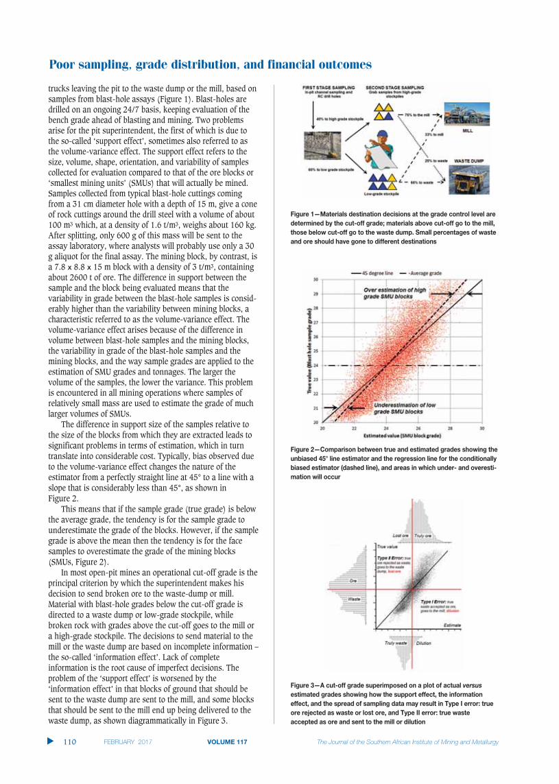
Poor sampling, grade distribution, and financial outcomes
trucks leaving the pit to the waste dump or the mill, based onsamples from blast-hole assays (Figure 1). Blast-holes aredrilled on an ongoing 24/7 basis, keeping evaluation of thebench grade ahead of blasting and mining. Two problemsarise for the pit superintendent, the first of which is due tothe so-called ‘support effect’, sometimes also referred to asthe volume-variance effect. The support effect refers to thesize, volume, shape, orientation, and variability of samplescollected for evaluation compared to that of the ore blocks or‘smallest mining units’ (SMUs) that will actually be mined.Samples collected from typical blast-hole cuttings comingfrom a 31 cm diameter hole with a depth of 15 m, give a coneof rock cuttings around the drill steel with a volume of about100 m3 which, at a density of 1.6 t/m3, weighs about 160 kg.After splitting, only 600 g of this mass will be sent to theassay laboratory, where analysts will probably use only a 30g aliquot for the final assay. The mining block, by contrast, isa 7.8 x 8.8 x 15 m block with a density of 3 t/m3, containingabout 2600 t of ore. The difference in support between thesample and the block being evaluated means that thevariability in grade between the blast-hole samples is consid-erably higher than the variability between mining blocks, acharacteristic referred to as the volume-variance effect. Thevolume-variance effect arises because of the difference involume between blast-hole samples and the mining blocks,the variability in grade of the blast-hole samples and themining blocks, and the way sample grades are applied to theestimation of SMU grades and tonnages. The larger thevolume of the samples, the lower the variance. This problemis encountered in all mining operations where samples ofrelatively small mass are used to estimate the grade of muchlarger volumes of SMUs.
The difference in support size of the samples relative tothe size of the blocks from which they are extracted leads tosignificant problems in terms of estimation, which in turntranslate into considerable cost. Typically, bias observed dueto the volume-variance effect changes the nature of theestimator from a perfectly straight line at 45° to a line with aslope that is considerably less than 45°, as shown in Figure 2.
This means that if the sample grade (true grade) is belowthe average grade, the tendency is for the sample grade tounderestimate the grade of the blocks. However, if the samplegrade is above the mean then the tendency is for the facesamples to overestimate the grade of the mining blocks(SMUs, Figure 2).
In most open-pit mines an operational cut-off grade is theprincipal criterion by which the superintendent makes hisdecision to send broken ore to the waste-dump or mill.Material with blast-hole grades below the cut-off grade isdirected to a waste dump or low-grade stockpile, whilebroken rock with grades above the cut-off goes to the mill ora high-grade stockpile. The decisions to send material to themill or the waste dump are based on incomplete information –the so-called ‘information effect’. Lack of completeinformation is the root cause of imperfect decisions. Theproblem of the ‘support effect’ is worsened by the‘information effect’ in that blocks of ground that should besent to the waste dump are sent to the mill, and some blocksthat should be sent to the mill end up being delivered to thewaste dump, as shown diagrammatically in Figure 3.
�
110 VOLUME 117

The histogram along the y-axis represents the true gradedistribution for the deposit. The histogram along the upper x-axis refers to material that is truly ore; most of it is sent tothe mill, but some of it is sent to the waste dumps as lost ore.The histogram along the lower x-axis refers to material thatis truly waste; most of it is sent to the waste dump, butportion of it is sent to the mill as dilution.
The superintendent’s problem is compounded by the factthat he is required to impose a cut-off grade on the materialsmined, based on assumptions that are not true. Theimposition of the cut-off grade presupposes that firstly, thedecisions are based on the perfect estimator in the form of a45° line in a plot of sample estimates versus block values,and secondly that the cut-off grade perfectly defines whatbroken rock should go to the waste dump and what to themill.
In the day-to-day pressure of mining production, all thesuperintendent can do is base his decision on the estimatedvalue he is given. According to Myers (1997) two errors aremade; the first is an error of estimation because the value ofwaste material is estimated to be above the cut-off grade, andthe second is an error of misclassification because the SMU isincorrectly classified as lying within the domain of revenue-generating ore. Such errors of estimation and misclassifi-cation arise because the decision about how to direct the oreis based on incomplete information. The first is a Type I errormade when rock that is truly ore is rejected and sent to thewaste dump, where it is lost to the value chain. The second isa Type II error made when rock that is truly waste material isaccepted as ore, and is sent to the mill, where it dilutes theore grade. The pit superintendent only has a 2D plan of thepit floor with blocks marked either above or below the cut-offgrade. There are no blocks marked ‘Ore, but actually waste’,or ‘Waste, but actually ore’. He must make a decision at thepoint where the cut-off grade is imposed; either ore or waste.
The category of ‘lost ore’ arises because truly economicore is sent to the waste dump, where it is then ‘lost’ to themining operation. The amount of lost ore is never knownbecause it never adds value to the operation, it never appearson the balance sheet, there is no direct means of accountingfor it, and it contributes to a low mine call factor. The onlyopportunity it may ever have of contributing to the mineralrents is at the end of the life of mine when the plant superin-tendent, desperate to fill the plant with material, resorts tousing material off the low-grade stockpile. At one time SouthAfrica’s largest gold producer recovered 280 kg of gold permonth from treating waste dumps (Brokken, personalcommunication, 2012).
The category referred to as ‘dilution’ arises because trulyuneconomic rock is sent to the mill where it is processed asore. Again, the amount of diluting rock is unknown, but itfirstly appears indirectly on the balance sheet as acombination of higher milling and processing costs, andsecondly it contributes to a lower mine call factor. Its overallcontribution to the cash flow is negative. Quantifying thecosts of dilution is difficult because the additional milling andprocessing costs are evenly spread across the entire stream ofmaterial arriving at the mill. This problem is amplified whenmilling capacity is constrained. The old adage ‘a low-gradetonne should never keep a high-grade tonne out of the mill’should be kept in mind.
The question that this research attempts to answer iswhether these losses and additions to the mine revenuestream can be quantified in terms of sampling error andsampling bias, in terms of tons and grade, and in terms ofdollars. This study aims to show that such quantification ofthe effects of sampling errors and sampling bias is indeedpossible.
Grade distributions in a 1500 x 1500 m domain for threecommodities gold (g/t), iron ore (%Fe), and coal (calorificvalue, MJ/kg) were created from parent distributions for eachcommodity, the histograms of which are shown in Figure 4.
The sampling distribution for each of the mineral deposittypes examined here, gold, coal, and iron ore, are radicallydifferent and represent positvely skewed lognormal, normal,and negatively skewed distributions respectively. It isprecisely the problem of sampling skewed distributions andthe superimposition of error and bias on such distributionsthat this paper aims to investigate. The skewness of thedistributions seriously affects sampling programmes and theoverall estimation of the average grade of a mineral deposit.Even if we could eliminate all sampling errors and biases, thevery nature of the distribution would mean that limitednumbers of samples collected from positively skewedlognormal distributions, typical of precious and base metaldeposits, will generally underestimate the average grade. Fornegatively skewed distributions, typical of bulk commoditiessuch as iron ore, manganese, vanadium, and chromite, alimited number of samples will overestimate the mean, but inthe case of mineral deposits with normally distributedvariables, such as coal qualities and alumina, the mean gradeof samples taken from these materials will generally bestatistically correct.
Poor sampling, grade distribution, and financial outcomes
VOLUME 117 111 �
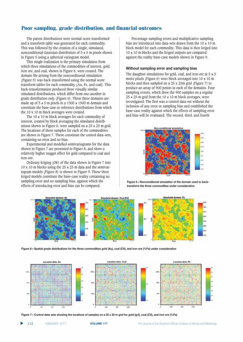
Poor sampling, grade distribution, and financial outcomes
The parent distributions were normal-score transformedand a transform table was generated for each commodity.This was followed by the creation of a single, simulated,nonconditional Gaussian distribution of 5 x 5 m pixels shownin Figure 5 using a spherical variogram model.
This single realization is the primary simulation fromwhich three simulations of the commodities of interest, gold,iron ore, and coal, shown in Figure 6, were created. Thedomain file arising from the nonconditional simulation(Figure 5) was back-transformed using the normal scoretransform tables for each commodity (Au, Fe, and coal). Thisback-transformation produced three visually similarsimulated distributions, which differ from one-another ingrade distribution only (Figure 6). These three domains aremade up of 5 x 5 m pixels in a 1500 x 1500 m domain andconstitute the base case or reference distributions from whichthe 10 x 10 m block averages were created.
The 10 x 10 m block averages for each commodity ofinterest, created by block averaging the simulated distrib-utions shown in Figure 6, were sampled on a 25 x 25 m grid.The locations of these samples for each of the commoditiesare shown in Figure 7. These constitute the control data-sets,containing no error and no bias.
Experimental and modelled semivariograms for the datashown in Figure 7 are presented in Figure 8, and show arelatively higher nugget effect for gold compared to coal andiron ore.
Ordinary kriging (OK) of the data shown in Figure 7 into10 x 10 m blocks using the 25 x 25 m data and the semivar-iogram models (Figure 8) is shown in Figure 9. These threekriged models constitute the base-case reality containing nosampling error and no sampling bias, against which theeffects of introducing error and bias can be compared.
Percentage sampling errors and multiplicative samplingbias are introduced into data-sets drawn from the 10 x 10 mblock model for each commodity. This data is then kriged into10 x 10 m blocks and the kriged outputs are comparedagainst the reality base-case models shown in Figure 9.
The daughter simulations for gold, coal, and iron ore at 5 x 5metre pixels (Figure 6) were block-averaged into 10 x 10 mblocks and then sampled on a 25 x 25m grid (Figure 7) toproduce an array of 900 points in each of the domains. Foursampling events, which drew the 900 samples on a regular25 x 25 m grid from the 10 x 10 m block averages, wereinvestigated. The first was a control data-set without theinclusion of any error or sampling bias and established thebase-case reality against which the effects of sampling errorand bias will be evaluated. The second, third, and fourth
�
112 VOLUME 117

Poor sampling, grade distribution, and financial outcomes
VOLUME 117 113 �
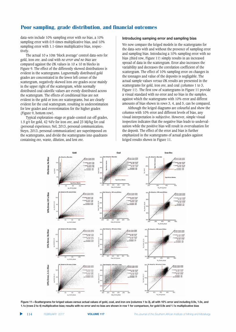
Poor sampling, grade distribution, and financial outcomes
data-sets include 10% sampling error with no bias, a 10%sampling error with 0.9-times multiplicative bias, and 10%sampling error with 1.1-times multiplicative bias, respec-tively.
The actual 10 x 10m ‘block average’ control data-sets forgold, iron ore. and coal with no error and no bias arecompared against the OK values in 10 x 10 m blocks inFigure 9. The effect of the differently skewed distributions isevident in the scattergrams. Lognormally distributed goldgrades are concentrated in the lower left corner of thescattergram, negatively skewed iron ore grades occur mainlyin the upper right of the scattergram, while normallydistributed coal calorific values are evenly distributed acrossthe scattergram. The effects of conditional bias are notevident in the gold or iron ore scattergrams, but are clearlyevident for the coal scattergram, resulting in underestimationfor low grades and overestimation for the higher grades(Figure 9, bottom row).
Typical exploration-stage or grade-control cut-off grades,1.5 g/t for gold, 42 %Fe for iron ore, and 23 MJ/kg for coal(personal experience; Nel, 2013, personal communication;Steyn, 2013, personal communication) are superimposed onthe scattergrams, and divide the scattergrams into quadrantscontaining ore, waste, dilution, and lost ore.
We now compare the kriged models in the scattergrams forthe data-sets with and without the presence of sampling errorand sampling bias. Introducing a 10% sampling error with nobias (third row, Figure 11) simply results in an increasedspread of data in the scattergram. Error also increases thevariability and decreases the correlation coefficient of thescattergram. The effect of 10% sampling error on changes inthe tonnages and value of the deposits is negligable. Theactual sample values versus OK results are presented in thescattergrams for gold, iron ore, and coal (columns 1 to 3,Figure 11). The first row of scattergrams in Figure 11 providea visual standard with no error and no bias in the samples,against which the scattergrams with 10% error and differntamounts of bias shown in rows 3, 4, and 5, can be compared.
Although the kriged diagrams are colourful and show thecolumns with 10% error and different levels of bias, anyvisual interpretation is subjective. However, simple visualinspection indicates that the negative bias leads to underval-uation while the positive bias will result in overvaluation forthe deposit. The effect of the error and bias is furtheremphasized in the scattergrams of actual grades againstkriged results shown in Figure 11.
�
114 VOLUME 117

Poor sampling, grade distribution, and financial outcomes
VOLUME 117 115 �
The effects of poor sampling are better seen in thescatterplots of the control data when compared against thedata including error and bias. It is difficult to see the effectson the gold estimates, but the coal and iron ore estimates areclearly shifted in their positions on the scattergram. Theeffect of 10% error is simply to enlarge the distribution of theestimated points, while the negative bias shifts the pointsbelow the 45° line and the positive bias shifts the pointsabove the 45° line. Again, these shifts are noteworthy, but ofrelatively little importance until we superimpose the cut-offvalues on the scattergrams.
Scattergrams in Figure 11 illustrate the difficulty that thepit superintendent faces, because the decisions he makes insending broken rock to the mill or the waste dump canseriously affect the financial outcomes and profitability of themining operation. The effects of bias on tonnage and depositvalue are more obvious and severe than those of error. Thesampling bias imposed on the already-introduced samplingerror is multiplicative at 0.9 times and 1.1 times, 0.5 timesand 1.5 times for gold. Bias shifts the cloud of points aboveor below the 45 degree line of unbiassed correlation.Inspection of Figure 11 indicates the points are shifteddownwards for a 0.9x bias causing a significant increase indilution, but a decrease in lost ore. In the same way a 1.1xbias causes a significant increase in lost ore, but a decreasein dilution, especially for iron ore and coal.
The value associated with mining waste, dilution, ore, andlost ore can be estimated through a profit/loss function. Thisprovides a framework in which to evaluate the changingvalue of the four categories of mined materials affected byerror and bias. Srivastava (1990) applied the loss functionframework to evaluate the benefits of pumping solvent intoan oil reservoir in order to improve recovery. He noted thatany time an estimate involving over- or underestimation,rather than perfect information, is used to a make a decision,sub-optimality in the form of a loss will be incurred. He alsonoted that very often the error-induced loss is asymmetricand that the penalties for overestimation are different tothose for underestimation. The application of profit and lossfunctions was carried further by Glacken (1997) and Verly(2005), who in a study of grade control classification of oreand waste undertook a critical review of estimation- andsimulation-based procedures showing that misclassificationdue to uncertainty in grade estimation had economic
consequences. The profit functions (g(z)) for blocks of waste,dilution, ore, and lost ore are listed in Table I.
The profit/loss function is shown graphically in Figure 12and provides a means of capturing the economic influence ofmining the four classifications of material – waste, dilution,ore, and lost ore – in a single diagram. This allows the effectsof error and bias to be seen in economic terms. The followingmining and processing costs and cut-off grade parametersapply.
The profit/loss functions listed in Table I were applied foreach class of mining material using the parameters listed inTable II in order to account for the characteristics of thematerial, its final destination, and the costs that the companyincurs, or revenues it may lose as a result of a grade controldecision. The curves showing the change in value for the fourclasses of materials – waste, dilution, ore, and lost ore – forgold, iron ore, and coal calculated in this way are shown inFigure 13. The standard reference for these plots is the OKresult, which is shown in red in Figures 13 and 14.
A noteworthy feature of the ‘Value of ore’ shown in rowfour of Figure 13 is that the variability in value for gold isrelatively small compared to that for iron ore and coal. Inaddition, the values for the commodities are concave-up forgold, concave-down for iron ore, and change from concave-down at low cut-offs to concave-up at higher cut-offs forcoal.
The relative effects of 10% error, 10% error plus 0.9x bias,and 10% error plus 1.1x bias on gold grades, iron ore grades,and coal CV values are summarized in Figure 14.
Table I
Waste g(z) = -cm Correct rejection
Dilution g(z) = -cm + (ω1)(prz-cp)False acceptance; ω1 is a coefficient (0< ω1<1) quantifying the opportunity cost of dilution, i.e.
that low grade ore keeps high grade ore out of the mill, (the risk aversion of the company). ω1 = 0.7
Ore g(z) = prz – cm - cp Correct acceptance
Lost ore g(z) = -cm – (ω2)(prz-cp) False rejection; ω2 is a coefficient (0< ω2<1) quantifying the opportunity cost of losing ore. ω1 = 0.7
p = price, r = recovery rate, z = grade, cm = cost of mining, cp = cost of processing
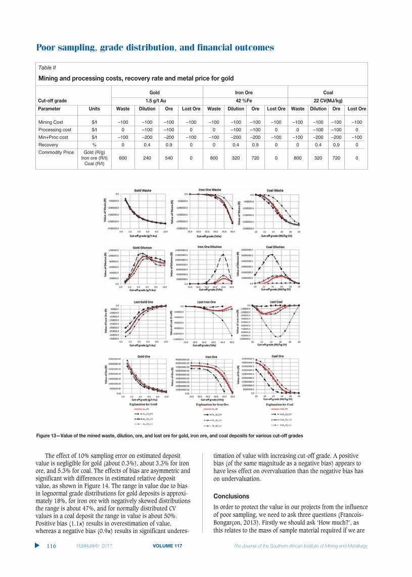
Poor sampling, grade distribution, and financial outcomes
The effect of 10% sampling error on estimated depositvalue is negligible for gold (about 0.3%), about 3.3% for ironore, and 5.3% for coal. The effects of bias are asymmetric andsignificant with differences in estimated relative depositvalue, as shown in Figure 14. The range in value due to biasin lognormal grade distributions for gold deposits is approxi-mately 18%, for iron ore with negatively skewed distributionsthe range is about 47%, and for normally distributed CVvalues in a coal deposit the range in value is about 50%.Positive bias (1.1x) results in overestimation of value,whereas a negative bias (0.9x) results in significant underes-
timation of value with increasing cut-off grade. A positivebias (of the same magnitude as a negative bias) appears to have less effect on overvaluation than the negative bias hason undervaluation.
In order to protect the value in our projects from the influenceof poor sampling, we need to ask three questions (Francois-Bongarçon, 2013). Firstly we should ask ‘How much?’, asthis relates to the mass of sample material required if we are
�
116 VOLUME 117
Table II
Mining Cost $/t –100 –100 –100 –100 –100 –100 –100 –100 –100 –100 –100 –100
Processing cost $/t 0 –100 –100 0 0 –100 –100 0 0 –100 –100 0
Min+Proc cost $/t –100 –200 –200 –100 –100 –200 –200 –100 –100 –200 –200 –100
Recovery % 0 0.4 0.9 0 0 0.4 0.9 0 0 0.4 0.9 0
Commodity Price Gold (R/g)Iron ore (R/t) 600 240 540 0 800 320 720 0 800 320 720 0
Coal (R/t)
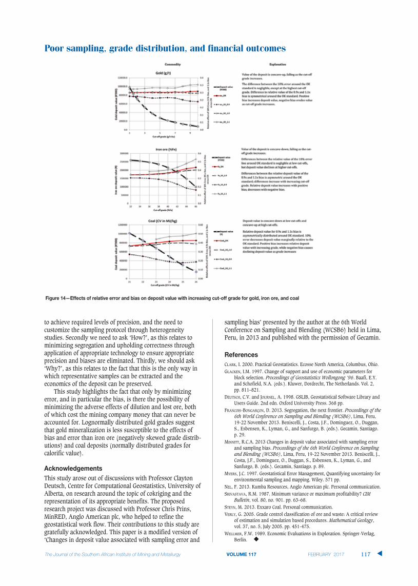
to achieve required levels of precision, and the need tocustomize the sampling protocol through heterogeneitystudies. Secondly we need to ask ‘How?’, as this relates tominimizing segregation and upholding correctness throughapplication of appropriate technology to ensure appropriateprecision and biases are eliminated. Thirdly, we should ask‘Why?’, as this relates to the fact that this is the only way inwhich representative samples can be extracted and theeconomics of the deposit can be preserved.
This study highlights the fact that only by minimizingerror, and in particular the bias, is there the possibility ofminimizing the adverse effects of dilution and lost ore, bothof which cost the mining company money that can never beaccounted for. Lognormally distributed gold grades suggestthat gold mineralization is less susceptible to the effects ofbias and error than iron ore (negatively skewed grade distrib-utions) and coal deposits (normally distributed grades forcalorific value).
This study arose out of discussions with Professor ClaytonDeutsch, Centre for Computational Geostatistics, University ofAlberta, on research around the topic of cokriging and therepresentation of its appropriate benefits. The proposedresearch project was discussed with Professor Chris Prins,MinRED, Anglo American plc, who helped to refine thegeostatistical work flow. Their contributions to this study aregratefully acknowledged. This paper is a modified version of‘Changes in deposit value associated with sampling error and
sampling bias’ presented by the author at the 6th WorldConference on Sampling and Blending (WCSB6) held in Lima,Peru, in 2013 and published with the permission of Gecamin.
CLARK, I. 2000. Practical Geostatistics. Ecosse North America, Columbus, Ohio. GLACKEN, I.M. 1997. Change of support and use of economic parameters for
block selection. Proceedings of Geostatistics Wollongong ’96. Baafi, E.Y.and Schofield, N.A. (eds.). Kluwer, Dordrecht, The Netherlands. Vol. 2, pp. 811–821.
DEUTSCH, C.V. and JOURNEL, A. 1998. GSLIB, Geostatistical Software Library andUsers Guide. 2nd edn. Oxford University Press. 368 pp.
FRANCOIS-BONGARÇON, D. 2013. Segregation, the next frontier. Proceedings of the6th World Conference on Sampling and Blending (WCSB6), Lima, Peru,19-22 November 2013. Beniscelli, J., Costa, J.F., Dominguez, O., Duggan,S., Esbensen, K., Lyman, G., and Sanfurgo, B. (eds.). Gecamin, Santiago.p. 29.
MINNITT, R.C.A. 2013 Changes in deposit value associated with sampling errorand sampling bias. Proceedings of the 6th World Conference on Samplingand Blending (WCSB6), Lima, Peru, 19-22 November 2013. Beniscelli, J.,Costa, J.F., Dominguez, O., Duggan, S., Esbensen, K., Lyman, G., andSanfurgo, B. (eds.). Gecamin, Santiago. p. 89.
MYERS, J.C. 1997. Geostatistical Error Management, Quantifying uncertainty forenvironmental sampling and mapping. Wiley. 571 pp.
NEL, F. 2013. Kumba Resources, Anglo American plc. Personal communication.SRIVASTAVA, R.M. 1987. Minimum variance or maximum profitability? CIM
Bulletin, vol. 80, no. 901. pp. 63–68.STEYN, M. 2013. Exxaro Coal. Personal communication.VERLY, G. 2005. Grade control classification of ore and waste: A critical review
of estimation and simulation based procedures. Mathematical Geology,vol. 37, no. 5, July 2005. pp. 451-475.
WELLMER, F.W. 1989. Economic Evaluations in Exploration. Springer-Verlag,Berlin. �
Poor sampling, grade distribution, and financial outcomes
VOLUME 117 117 �

Gravity Concentrators Africa - CONSEP ACACIA: THE FINEST IN LEACHING TECHNOLOGY
GCA has installed and commissioned three Consep Acacias in Africa, in as many months. The first Acacia found a home at Cata Mine, Tanzania, the second in Liberia and the third was installed in Burkina Faso, with an order for a fourth being placed for Burkina. This brings the total Consep Acacia installations to 24 in Africa and a staggering 138 worldwide.
The reason for this is simple: Consep Acacias are simply the best at what they do.
Gravity leaching has become a standard method of processing high grade gravity concentrates in gold processing plants. The Acacia offers this in the safest, most cost effective and most efficient way possible. It uses an up flow fluidised reactor for the leaching process, to produce the ideal solid-liquid interaction. This allows maximised gold leaching kinetics without mechanical agitation. As a result, Consep Acacias have no moving parts bar common pumps and valves (thus requiring no guarding), making them substantially safer than competitor products. This is just one of the many safety advantages that Acacia have over competitive technologies, as illustrated below:
Consep Acacia Competitor productMinimal moving partsNo guarding requiredCan be vented for indoors applicationsPumps have isolation and rinse pointsSlurry pump doesn’t see cyanideLow energy / static head in the systemLow solution volumesUses LeachAid as the oxidant / catalyst. LeachAid is classed as a low-hazard chemicalShort list of maintenance activities
Rolling drum with pinch points at the rollers and chainDrive parts should be guardedOpen to atmosphere at drum dischargePositive gas pressure resulting in fume generationOpen to atmosphere at pump hopperDifficult to link to a ventilation systemTall solution tank gives high energy / static headOften uses Peroxide - dangerous chemical with a chequered historyLong list of maintenance activities
ADVERTORIAL

In addition to this, over a decade of product refinement has given the Acacia the advantage of robust and reliable leaching chemistry, superior solids handling techniques, compact design and a simple operating philosophy. All of which, allows for the lowest operating costs possible, when compared to other leaching technologies. Furthermore, the compact, packaged plants require minimal client interfacing and therefore greatly reduce installation costs and time.
The Acacia reactor is also able to handle variable concentrate grades, especially very high grades, through maximising the available metallurgical tools. As the design is based around theoretical ideal solid liquid contact data, it allows for easy upscaling - should the need arise. The same cannot be said of other technologies.
Further, LeachAid allows anaerobic dissolution of gold, and thus allows the Consep Acacia to use heated leaching for even faster kinetics and more complete leaching.
In 2011, an independent study conducted in Perth, Australia compared the Consep Acacia to a rival product, operating in a gravity gold circuit. The Acacia replaced the competitor machine, and in addition to drastically increasing gold recovery levels on the plant, it reduced operating costs substantially, thus cutting down the payback period of machinery. Moreover, the Acacia reduced potential safety hazards, significantly reduced the labour required on site, increased security due to no physical contact with gold concentrates, and allowed for better metallurgical accounting.
*Please email [email protected] for a copy of the independent study results.
These are just some of the reasons that GCA is proud to be the official African agent of Consep. Not only is this a privilege in itself, but it allows us to offer our clients access to the best intense cyanide leaching technology in the world, as well as full gravity recovery packages.
Learn more about Consep Acacia reactors on our website www.gca.gold , or get in touch on +27 11 704 6678 / +27 63 699 9109 to make an enquiry.
218 New Market Road,Northriding,2194,South Africa
ADVERTORIAL

ELBROC Mining Products (Pty) Ltd is an original
support manufacturer, with support systems tailored to the needs of underground mines.
Rock support is fundamental to a safe underground mining environment. ELBROC manufactures and distributes a range of mine support products that
durable and backed up with customer support. The company also provides product training, risk assessment and
Quality control at the factory is managed
all products before dispatch. A highly skilled R&D team keep all products up-to-date with technology, ensure that they are easy and safe to use and compliant with mining legal and safety requirements.
underground mining environments.
Design, development, machining,
their patented propriety products is conducted at ELBROC’s ISO 9001 accredited facility in Isando, Johannesburg, South Africa.
which are customised to enable mining companies specialising in diverse
Wilson.
ELBROC’s products are recommended
Coal and Diamond mines.
In coal mines, for instance, both
on longwall moves.
ELBROC produces blast-on support that
events. In several recorded instances this has allowed face crews to walk away unscathed from a face burst during the
Wide product rangenical and Hydraulic Props
Temporary Support with all required accessories.
rout Pumps.
While the delivery of high quality products is central to its business ethos,
For this reason, it constantly keeps in touch with customers worldwide and, with a full range of replacement parts ensures that products are in good
End-user support
address the unique needs of each of its
says Errol. He adds that bearing in mind the mining environment is constantly
improving its products to keep abreast with contemporary demands. Through a dedicated sales team, which includes underground technicians, the company assists clients with their underground support needs.
corners when it comes to safety in mining, that’s why our products adhere to the highest possible standards. We are concerned about safeguarding the lives of employees, a mine’s most invaluable
Growing footprint
widely used in mining in South Africa. The USA remains a major market whilst Russia, Zambia, Zimbabwe and West Africa are regarded as major growth areas currently. The company is going all out to expand its global footprint through forging partnerships with companies involved in underground
to ensure compliance with performance and safety standards required in the harsh mining environment. Their hydraulic press has the following
hydraulic press can perform below or
min.
During a dynamic test the press
for the remainder of the stoke. The onset and period of the dynamic loading is controlled by an operator in the control
room screen during the test while all data is stored so that graphs can be later generated as required.
leading supplier and manufacturer of underground support equipment.
Underground rock support

A number of different methods for determiningthe Fundamental Sampling Error (FSE) havebeen suggested (Carrasco, 2004; Francois-Bongarçon, 1991, 1992a, 1992b, 1993, 1996,1998a, 1998b; Francois-Bongarçon and Gy,2001; Geelhoed, 2005; Gy, 1973, 1979, 1982;Lyman, 1993; Pitard, 1993; Minnitt andAssibey-Bonsu, 2009; Minnitt, Francois-Bongarçon, and Pitard, 2011; Minnitt; 2014).The classic and widely used heterogeneity testfor determining the sampling constants wasproposed by Gy (Pitard, 1993). It has beendescribed by Carrasco (2005) and Magri(2011), and has been championed by Pitard(2015), but this procedure is not described anyfurther in this paper. Francois-Bongarçon(1988a) investigated the changes in thevariance of sample assays due to changes inthe fragment size, and the way in which this
variance can be applied to the determination ofthe constants K and alpha ( ) for use in amodified form of Gy’s formula for the FSEshown in Equation [1]. The samplingparameters are substituted into Equation [1]and a graphic, the sampling nomogram,describing the changes in the FSE for differentstages of crushing and splitting for a specificore type at a given grade is compiled.
[1]
The method described by Francois-Bongarçon (1991), which is generally knownas the Duplicate Sampling Analysis (DSA)method, is widely used in the mining industryand has produced consistently useful results interms of the sampling nomogram that isapplied on mining operations. A secondmethod, referred to as the Segregation FreeMethod (SFA), has also been suggested but iscurrently not widely applied (Minnitt et al.,2011; Minnitt, 2014).
The primary argument against the DSAmethod is that the splitting stage beforesample analysis requires that 10–20 kg ofparticulate material be split into 32 samples.Splitting this material, which includes thecomplete spectrum of fragment sizes from dustto particles up to 19.0 mm in diameter, isthought to introduce grouping and segregationerrors that cannot be eliminated or mitigated.The problem of segregation was avoidedthrough a method proposed by Minnitt et al.(2011) and Minnitt (2014), referred to as theSegregation Free Analysis (SFA) method, forcalibrating the parameters K and . The SFAmethod overcomes the related problems ofsegregation and ambiguity in regard to theexact size of the fragments, but has been
A version of Gy’s equation for gold-bearing oresby R.C.A. Minnitt*
The two methods for calibrating the parameters K and (alpha) for use inGy’s equation for the Fundamental Sampling Error (FSE)–, DuplicateSampling Analysis (DSA) and Segregation Free Analysis (SFA)–, aredescribed in detail. A case study using identical broken reef material froma Witwatersrand-type orebody was calibrated using the DSA and SFAmethods and the results compared. Classically, the form of Gy’s equationfor the FSE raises the nominal size of fragments given by dN to the powerof 3. A later modification of Gy’s formula raises dN to the power (alpha),the latter term being calibrated with the coefficient K in the DSA and SFAmethods. The preferred value of for low-grade gold ores used bysampling practitioners in the mining industry is 1.5. A review ofcalibration experiments for low-grade gold ores using the DSA and SFAmethods has produced values of K that vary between 70 and 170 andvalues of in the range 0.97 to 1.30. The average value for is shown tobe 1, rather than 3 as originally proposed in the classic form of Gy’sequation or the industry-preferred 1.5. It is suggested that for low-gradegold-bearing ores the equation for the FSE should raise dN to a power of 1.Such an equation for the variance of the FSE greatly simplifies the charac-terization of gold ores, now requiring only the calibration of K for a givenmass and established fragment size. The implications of the simplifiedequation for the heterogeneity test are that, provided the fragments havebeen screened to within a narrow size range, any particular size will returna value for K that is acceptable for use in the sampling nomogram.
fundamental sampling error, Gy’s equation, gold ore characterization.
* School of Mining Engineering, University of theWitwatersrand, South Africa.
© The Southern African Institute of Mining andMetallurgy, 2017. ISSN 2225-6253. Paper receivedMar. 2016; revised paper received Oct. 2016.
119VOLUME 117 �
http://dx.doi.org/10.17159/2411-9717/2017/v117n2a3

A version of Gy’s equation for gold-bearing ores
criticized because of its simplicity. Objections raised focus onthe single-stage crushing that the material undergoescompared to the multi-stage crushing associated with theDSA method (Minnitt, 2014). The calibration procedures fordetermining K and by the DSA and the SFA methods aredescribed and compared. Details of the calculation proceduresare almost identical for both methods, but the differences areemphasized.
This paper examines and highlights the differences andsimilarities in the calibration exercises that have been carriedout over the years. As the number of such calibrationexercises has increased, there is also growing empiricalevidence that the exponent of 1.5 for the nominal fragmentsize suggested by Francois-Bongarçon (1991) and Francois-Bongarcon and Gy (2001) should in fact be unity. Thismeans that the sampling variance is actually a function of theproduct of the sampling constant K and the nominal fragmentsize dN, divided by the mass. Lyman (1993) proposed asimilar equation in which the sampling variance is simplyequal to the sampling constant K divided by the sample mass, and has no dependency on the nominal size of thefragments dN.
Four bins, each containing 400 to 600 kg of run-of-minegold-bearing ore from the Target, Tshepong, Joel, andKusasalethu mines, were provided by Harmony Gold MiningCompany Limited. The material from each mining operationwas handled separately and was spread out to dry, at whichstage all fragments larger than 15 cm diameter wereexamined and identified. These larger fragments, whichinvariably consisted of sub-rounded dolerite dyke material orfine-grained, non-mineralized hangingwall quartzite, wereremoved from the lot. A Boyd crusher was used to crush thedried lot to 95% passing 2.50 cm. A total of 333 kg of thebroken ore was divided into two lots, one of 75 kg for theDSA experiment and one of 258 kg for the SFA experiment.The 75 kg of broken ore used for the DSA method was splitinto six series and each of these series was split into 32individual samples using a rotary splitter. The 258 kg ofbroken ore for the SFA experiment was split into 15 seriesand each of these was then split into 32 samples using a rifflesplitter. The author sees no difference between the rotarydivider and riffle splitter methods.
All samples were submitted for fire assay using a 50 galiquot. The choice of aliquot was made to improve theprecision of the analyses, but was permissible only becauseof the very good fluxing and fusion characteristics of theWitwatersrand ores. Reduction of the analytical data toprovide points on the calibration curves for the DSA and theSFA methods was similar, apart from slight changes in thefragment sizes used on the curves.
The principal difference between the DSA and SFA methodsis in the stages and manner of preparation of the crushedparticulate ores for fire assay. The DSA method requires a lotvarying from 40 kg to 80 kg, depending on how many seriesare required. For this particular exercise a series of six sub-
lots split from the run-of-mine ore from Target mine (Table I), with evenly spread top sizes varying from 2.5 cm to0.1 mm as shown in Figure 1, was extracted.
The first step was to crush the material to a nominal topsize of about 95% passing 2.50 cm. This lot was split into sixequal, separate sub-lots, each sub-lot being referred to as aseries as shown in Figure 2. The first sub-lot of about 12 to15 kg may be larger than the following sub-lots simplybecause a greater mass of material is required for largerfragment sizes. This will ensure a better distribution offragments per sample during the rotary splitting procedureand will reduce the variance of the large fragment samplemasses.
The first of the sub-lots, of 15.0 kg at 2.50 cm, wasnamed Series 1. The remaining five sub-lots (65 kg mass)were recombined and homogenized during crushing to asomewhat smaller sieve size having a nominal top size of 95 % passing 1.90 cm. This lot of about 65 kg was then split
�
120 VOLUME 117
Table I
Series 1 95% passing 2.50 cm 15.0 kgSeries 2 95% passing 1.90 cm 13.0 kgSeries 3 95% passing 1.32cm 13.0 kgSeries 4 95% passing 0.945 cm 13.0 kgSeries 5 95% passing 0.435 cm 13.0 kgSeries 6 95% passing 0.2 cm 13.0 kg
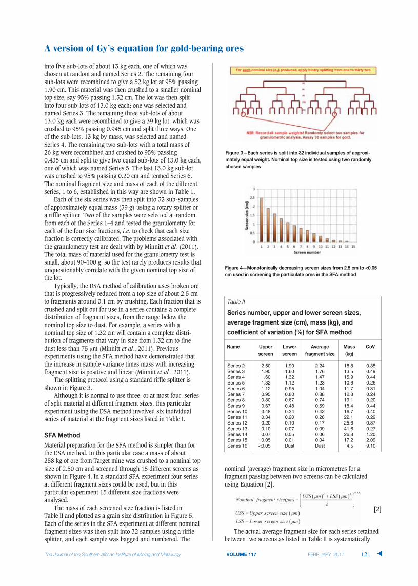
into five sub-lots of about 13 kg each, one of which waschosen at random and named Series 2. The remaining foursub-lots were recombined to give a 52 kg lot at 95% passing1.90 cm. This material was then crushed to a smaller nominaltop size, say 95% passing 1.32 cm. The lot was then splitinto four sub-lots of 13.0 kg each; one was selected andnamed Series 3. The remaining three sub-lots of about 13.0 kg each were recombined to give a 39 kg lot, which wascrushed to 95% passing 0.945 cm and split three ways. Oneof the sub-lots, 13 kg by mass, was selected and namedSeries 4. The remaining two sub-lots with a total mass of 26 kg were recombined and crushed to 95% passing 0.435 cm and split to give two equal sub-lots of 13.0 kg each,one of which was named Series 5. The last 13.0 kg sub-lotwas crushed to 95% passing 0.20 cm and termed Series 6.The nominal fragment size and mass of each of the differentseries, 1 to 6, established in this way are shown in Table 1.
Each of the six series was then split into 32 sub-samplesof approximately equal mass (39 g) using a rotary splitter ora riffle splitter. Two of the samples were selected at randomfrom each of the Series 1–4 and tested the granulometry foreach of the four size fractions, i.e. to check that each sizefraction is correctly calibrated. The problems associated withthe granulometry test are dealt with by Minnitt et al. (2011).The total mass of material used for the granulometry test issmall, about 90–100 g, so the test rarely produces results thatunquestionably correlate with the given nominal top size ofthe lot.
Typically, the DSA method of calibration uses broken orethat is progressively reduced from a top size of about 2.5 cmto fragments around 0.1 cm by crushing. Each fraction that iscrushed and split out for use in a series contains a completedistribution of fragment sizes, from the range below thenominal top size to dust. For example, a series with anominal top size of 1.32 cm will contain a complete distri-bution of fragments that vary in size from 1.32 cm to finedust less than 75 m (Minnitt et al., 2011). Previousexperiments using the SFA method have demonstrated thatthe increase in sample variance times mass with increasingfragment size is positive and linear (Minnitt et al., 2011).
The splitting protocol using a standard riffle splitter isshown in Figure 3.
Although it is normal to use three, or at most four, seriesof split material at different fragment sizes, this particularexperiment using the DSA method involved six individualseries of material at the fragment sizes listed in Table I.
Material preparation for the SFA method is simpler than forthe DSA method. In this particular case a mass of about 258 kg of ore from Target mine was crushed to a nominal topsize of 2.50 cm and screened through 15 different screens asshown in Figure 4. In a standard SFA experiment four seriesat different fragment sizes could be used, but in thisparticular experiment 15 different size fractions wereanalysed.
The mass of each screened size fraction is listed in Table II and plotted as a grain size distribution in Figure 5.Each of the series in the SFA experiment at different nominalfragment sizes was then split into 32 samples using a rifflesplitter, and each sample was bagged and numbered. The
nominal (average) fragment size in micrometres for afragment passing between two screens can be calculatedusing Equation [2].
[2]
The actual average fragment size for each series retainedbetween two screens as listed in Table II is systematically
A version of Gy’s equation for gold-bearing ores
VOLUME 117 121 �
Table II
Series 2 2.50 1.90 2.24 18.8 0.35Series 3 1.90 1.60 1.76 13.5 0.49Series 4 1.60 1.32 1.47 15.9 0.44Series 5 1.32 1.12 1.23 10.6 0.26Series 6 1.12 0.95 1.04 11.7 0.31Series 7 0.95 0.80 0.88 12.8 0.24Series 8 0.80 0.67 0.74 19.1 0.20Series 9 0.67 0.48 0.59 18.4 0.44Series 10 0.48 0.34 0.42 16.7 0.40Series 11 0.34 0.20 0.28 22.1 0.29Series 12 0.20 0.10 0.17 25.6 0.37Series 13 0.10 0.07 0.09 41.6 0.27Series 14 0.07 0.05 0.06 26.8 1.20Series 15 0.05 0.01 0.04 17.2 2.09Series 16 <0.05 Dust Dust 4.5 9.10

A version of Gy’s equation for gold-bearing ores
smaller without any major discontinuities in size. Screeningof the broken ore allows the lot to be separated into 15 statis-tically narrow (clean) size fractions that are then analysed, amethod first proposed by Minnitt et al. (2011).
The grain size distribution of the screened ore fromTarget mine used in this investigation is shown in Figure 5,indicating that about 50% of the material (115.7 kg) is lessthan 1 mm in diameter.
The lognormal distribution of the assay data required that themeans for each series be calculated using a Sichel’s testimate. The summary of the statistics for each series in theDSA and the SFA experiments is shown in Tables III and IV,respectively. The fire assay results for the DSA method aregiven in Appendix 1, and those for the SFA method inAppendix 2.
This data is used in the calibration exercises.
The following derivation of the equation for the slope, , andthe intercept, K, is presented in Minnitt et al. (2011), but isincluded here for completeness. The variance in each of thefifteen size fractions analysed must be represented by thesame formula if correct estimates of the parameters K and are to be derived from the calibration curve. The ratio ofupper and lower screen sizes r, shown in Equation [3], mustbe reasonably consistent across all screen sizes.
[3]
This is indeed the case for most of the larger screen sizesused in this particular SFA experiment, as shown in Figure 6,where r is constrained between 1 and 1.5.
The variance of a sample taken, fragment by fragment,from closely sieved material between dMin and dMax is givenby Equation [4].
�
122 VOLUME 117
Table III
1 2.50 3.84 322 1.90 3.44 323 1.32 3.24 324 0.95 3.06 325 0.42 3.45 326 0.20 3.32 32
DSA average grade 3.09 192 analyses
Standard deviation 0.83
Table IV
1 2.50 3.84 322 1.90 3.44 323 1.32 3.24 324 1.473 6.46 325 1.228 6.18 326 1.042 7.38 327 0.881 5.17 328 0.741 5.08 329 0.635 5.35 3210 0.418 5.37 3211 0.284 4.62 3312 0.165 4.91 3213 0.088 4.93 3214 0.062 4.35 3215 0.040 4.34 3216 0.009 5.77 32
SFA Average grade 5.58 480 Analyses
Standard Deviation 1.66

[4]
where g ' = g '(r) is taken from a curve of the granulometricfactor g ' versus ratio r = dMax/dMin for closely sievedmaterials, shown in Figure 7.
In this experiment the value of r lies between 1 and 1.5,suggesting a g ' value of between 0.6 and 0.7 as acceptablefor this experiment. The liberation factor describes thetransition between the liberated, calculable variance and thenon-liberated one. The term f g 'dMax
3 represents the averagefragment volume in the fraction [dMin, dMax]. The smallestsize fraction of ratio r in which the mineral is liberated has adMax equal to d , so in the case of the sampling within sizefractions of ratio r, the correct liberation factor is:
[5]
where 0 < b' <1, or, if = 3-3b', so:
[6]
The liberation factor is the ratio of the average fragmentvolumes at non-liberation and at liberation to a power 3b' inEquation [5], and fg 'dMax
3 is the average fragment volume inthe fraction [dMin, dMax]. Generally, the mass of the lot is verymuch larger than the mass of the sample so that 1/ML
becomes negligible. Substituting Equation [6] into Equation[4] allows us to rewrite Equation [4] as follows:
[7]
Taking logarithms on both sides of Equation [7], andwith the proviso that ML is much larger than MS, allows theequation to be rearranged as follows:
[8]
[9]
The two variables that are required to compile thecalibration curve are then:
So that the slope of the line is given by , and theintercept is given by:
[10]
On this basis it is now possible to extract values for bothand d by the fitting of a straight line to the graph (Minnitt
et al., 2011).
The method of reduction of the 32 fire assay results for eachof the series in the DSA and SFA experiments is shown inTable V; this particular data is for the DSA Series 3, samples1 to 32, at a fragment size of 1.32 cm. The logarithmic meanand variance are presented in this way because the Sichel’s t-estimate for the mean of a logarithmic distribution was usedto calculate the mean in grams per ton for each of theindividual series. Due to calculating the mean in this way,very few data values are eliminated as outliers. The reductionof analytical data for the SFA method is identical to that forthe DSA method.
The data is further reduced to produce the two variablesln( 2*Mass) and ln(dN) as shown in Table VI.
The final reduced data for the six series of the DSA methodand the fifteen series of the SFA method is compiled in Figure 8.
It is noteworthy that the two curves shown in Figure 7are almost parallel, with slopes of 1.030 for the DSA curve(red) and 1.123 for the SFA curve. The major differencebetween these curves is the value for the intercepts that theyyield: 5.12 for the DSA curve and 7.83 for the SFA curve,which when transformed back from log space gives values of167.42 g/t2 and 2539.1 g/t2 respectively.
The effect of the differences in K and for the DSA and SFAmethods and their impact on the sampling nomogram isshown in Figure 8. A typical 5 Mt/a gold mining operation isconsidered as an example. The mine operates 360 days per
A version of Gy’s equation for gold-bearing ores
VOLUME 117 123 �
Table V
Logarithmic mean (loge g/t) 1.0412Sichel's t factor for the mean 1.1441Logarithmic variance (loge g/t2) 0.4797Mean (g/t) 3.2407Relative std deviation 0.4649Screen size (cm) 1.32Average mass (g) 37.20
*This particular data set is from Series 3 of the DSA method for fragmentsize 95% passing 1.32 cm
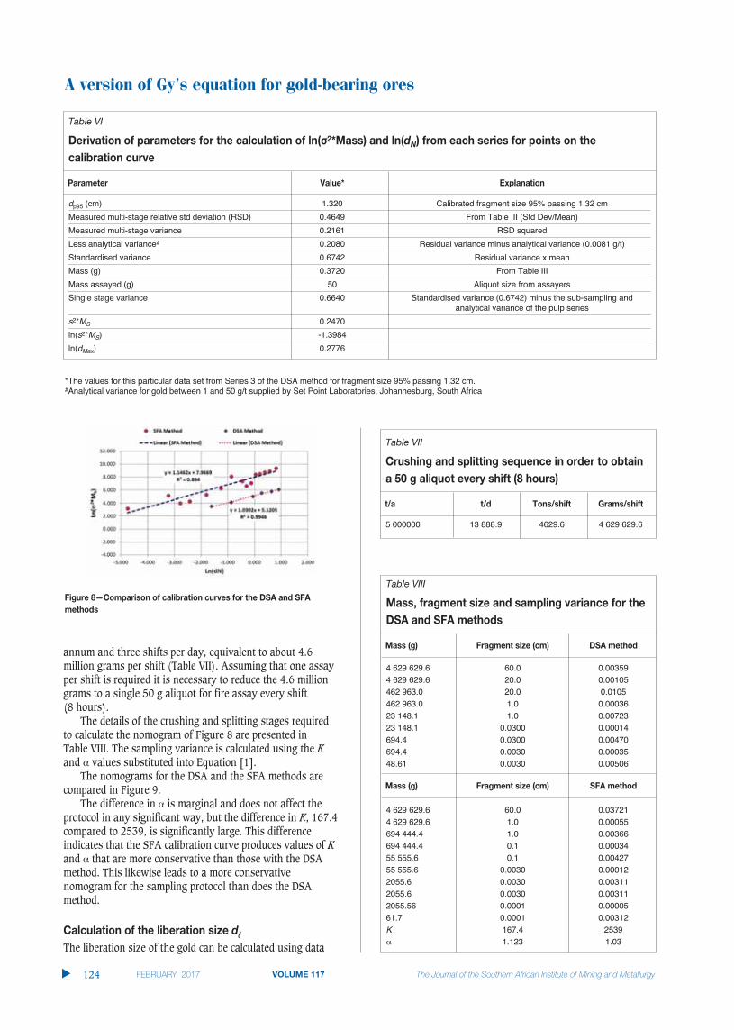
A version of Gy’s equation for gold-bearing ores
annum and three shifts per day, equivalent to about 4.6million grams per shift (Table VII). Assuming that one assayper shift is required it is necessary to reduce the 4.6 milliongrams to a single 50 g aliquot for fire assay every shift (8 hours).
The details of the crushing and splitting stages requiredto calculate the nomogram of Figure 8 are presented in Table VIII. The sampling variance is calculated using the Kand values substituted into Equation [1].
The nomograms for the DSA and the SFA methods arecompared in Figure 9.
The difference in is marginal and does not affect theprotocol in any significant way, but the difference in K, 167.4compared to 2539, is significantly large. This differenceindicates that the SFA calibration curve produces values of Kand that are more conservative than those with the DSAmethod. This likewise leads to a more conservativenomogram for the sampling protocol than does the DSAmethod.
The liberation size of the gold can be calculated using data
�
124 VOLUME 117
Table VIII
4 629 629.6 60.0 0.003594 629 629.6 20.0 0.00105462 963.0 20.0 0.0105462 963.0 1.0 0.0003623 148.1 1.0 0.0072323 148.1 0.0300 0.00014694.4 0.0300 0.00470694.4 0.0030 0.0003548.61 0.0030 0.00506
4 629 629.6 60.0 0.037214 629 629.6 1.0 0.00055694 444.4 1.0 0.00366694 444.4 0.1 0.0003455 555.6 0.1 0.0042755 555.6 0.0030 0.000122055.6 0.0030 0.003112055.6 0.0030 0.003112055.56 0.0001 0.0000561.7 0.0001 0.00312K 167.4 2539
1.123 1.03
Table VII
5 000000 13 888.9 4629.6 4 629 629.6
Table VI
dp95 (cm) 1.320 Calibrated fragment size 95% passing 1.32 cm
Measured multi-stage relative std deviation (RSD) 0.4649 From Table III (Std Dev/Mean)
Measured multi-stage variance 0.2161 RSD squared
Less analytical variance# 0.2080 Residual variance minus analytical variance (0.0081 g/t)
Standardised variance 0.6742 Residual variance x mean
Mass (g) 0.3720 From Table III
Mass assayed (g) 50 Aliquot size from assayers
Single stage variance 0.6640 Standardised variance (0.6742) minus the sub-sampling and analytical variance of the pulp series
s2*MS 0.2470
ln(s2*MS) -1.3984
ln(dMax) 0.2776
*The values for this particular data set from Series 3 of the DSA method for fragment size 95% passing 1.32 cm.#Analytical variance for gold between 1 and 50 g/t supplied by Set Point Laboratories, Johannesburg, South Africa
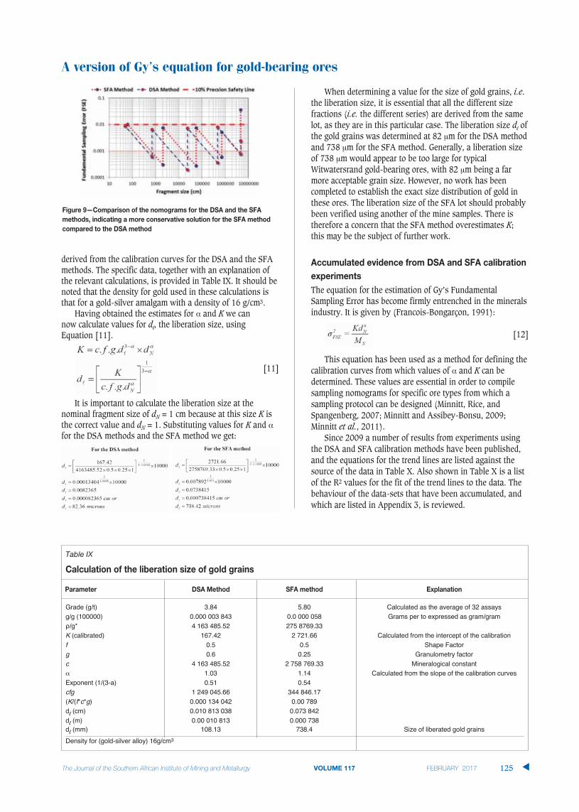
A version of Gy’s equation for gold-bearing ores
VOLUME 117 125 �
derived from the calibration curves for the DSA and the SFAmethods. The specific data, together with an explanation ofthe relevant calculations, is provided in Table IX. It should benoted that the density for gold used in these calculations isthat for a gold-silver amalgam with a density of 16 g/cm3.
Having obtained the estimates for and K we can now calculate values for d , the liberation size, usingEquation [11].
[11]
It is important to calculate the liberation size at thenominal fragment size of dN = 1 cm because at this size K isthe correct value and dN = 1. Substituting values for K and for the DSA methods and the SFA method we get:
When determining a value for the size of gold grains, i.e.the liberation size, it is essential that all the different sizefractions (i.e. the different series) are derived from the samelot, as they are in this particular case. The liberation size d ofthe gold grains was determined at 82 m for the DSA methodand 738 m for the SFA method. Generally, a liberation sizeof 738 m would appear to be too large for typicalWitwatersrand gold-bearing ores, with 82 m being a farmore acceptable grain size. However, no work has beencompleted to establish the exact size distribution of gold inthese ores. The liberation size of the SFA lot should probablybeen verified using another of the mine samples. There istherefore a concern that the SFA method overestimates K;this may be the subject of further work.
The equation for the estimation of Gy’s FundamentalSampling Error has become firmly entrenched in the mineralsindustry. It is given by (Francois-Bongarçon, 1991):
[12]
This equation has been used as a method for defining thecalibration curves from which values of and K can bedetermined. These values are essential in order to compilesampling nomograms for specific ore types from which asampling protocol can be designed (Minnitt, Rice, andSpangenberg, 2007; Minnitt and Assibey-Bonsu, 2009;Minnitt et al., 2011).
Since 2009 a number of results from experiments usingthe DSA and SFA calibration methods have been published,and the equations for the trend lines are listed against thesource of the data in Table X. Also shown in Table X is a listof the R2 values for the fit of the trend lines to the data. Thebehaviour of the data-sets that have been accumulated, andwhich are listed in Appendix 3, is reviewed.
Table IX
Grade (g/t) 3.84 5.80 Calculated as the average of 32 assaysg/g (100000) 0.000 003 843 0.0 000 058 Grams per to expressed as gram/gramρ/g* 4 163 485.52 275 8769.33K (calibrated) 167.42 2 721.66 Calculated from the intercept of the calibrationf 0.5 0.5 Shape Factorg 0.6 0.25 Granulometry factorc 4 163 485.52 2 758 769.33 Mineralogical constant
1.03 1.14 Calculated from the slope of the calibration curvesExponent (1/(3-a) 0.51 0.54cfg 1 249 045.66 344 846.17(K/(f*c*g) 0.000 134 042 0.00 789d (cm) 0.010 813 038 0.073 842d (m) 0.00 010 813 0.000 738d (mm) 108.13 738.4 Size of liberated gold grains
Density for (gold-silver alloy) 16g/cm3
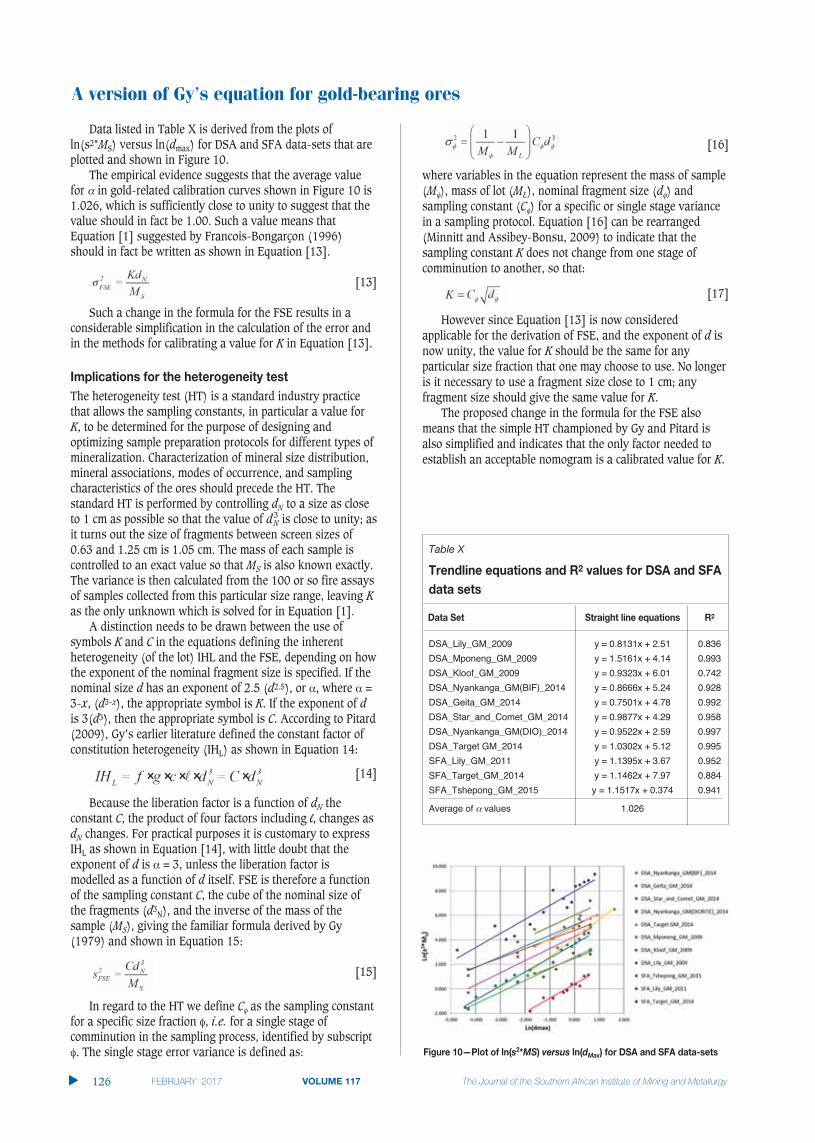
A version of Gy’s equation for gold-bearing ores
Data listed in Table X is derived from the plots ofln(s2*MS) versus ln(dmax) for DSA and SFA data-sets that areplotted and shown in Figure 10.
The empirical evidence suggests that the average valuefor in gold-related calibration curves shown in Figure 10 is1.026, which is sufficiently close to unity to suggest that thevalue should in fact be 1.00. Such a value means thatEquation [1] suggested by Francois-Bongarçon (1996)should in fact be written as shown in Equation [13].
[13]
Such a change in the formula for the FSE results in aconsiderable simplification in the calculation of the error andin the methods for calibrating a value for K in Equation [13].
The heterogeneity test (HT) is a standard industry practicethat allows the sampling constants, in particular a value forK, to be determined for the purpose of designing andoptimizing sample preparation protocols for different types ofmineralization. Characterization of mineral size distribution,mineral associations, modes of occurrence, and samplingcharacteristics of the ores should precede the HT. Thestandard HT is performed by controlling dN to a size as closeto 1 cm as possible so that the value of d 3
N is close to unity; asit turns out the size of fragments between screen sizes of0.63 and 1.25 cm is 1.05 cm. The mass of each sample iscontrolled to an exact value so that MS is also known exactly.The variance is then calculated from the 100 or so fire assaysof samples collected from this particular size range, leaving Kas the only unknown which is solved for in Equation [1].
A distinction needs to be drawn between the use ofsymbols K and C in the equations defining the inherentheterogeneity (of the lot) IHL and the FSE, depending on howthe exponent of the nominal fragment size is specified. If thenominal size d has an exponent of 2.5 (d2.5), or , where =3-x, (d3-x), the appropriate symbol is K. If the exponent of dis 3(d3), then the appropriate symbol is C. According to Pitard(2009), Gy’s earlier literature defined the constant factor ofconstitution heterogeneity (IHL) as shown in Equation 14:
[14]
Because the liberation factor is a function of dN theconstant C, the product of four factors including , changes asdN changes. For practical purposes it is customary to expressIHL as shown in Equation [14], with little doubt that theexponent of d is = 3, unless the liberation factor ismodelled as a function of d itself. FSE is therefore a functionof the sampling constant C, the cube of the nominal size ofthe fragments (d3
N), and the inverse of the mass of thesample (MS), giving the familiar formula derived by Gy(1979) and shown in Equation 15:
[15]
In regard to the HT we define C as the sampling constantfor a specific size fraction , i.e. for a single stage ofcomminution in the sampling process, identified by subscript. The single stage error variance is defined as:
[16]
where variables in the equation represent the mass of sample(M ), mass of lot (ML), nominal fragment size (d ) andsampling constant (C ) for a specific or single stage variancein a sampling protocol. Equation [16] can be rearranged(Minnitt and Assibey-Bonsu, 2009) to indicate that thesampling constant K does not change from one stage ofcomminution to another, so that:
[17]
However since Equation [13] is now consideredapplicable for the derivation of FSE, and the exponent of d isnow unity, the value for K should be the same for anyparticular size fraction that one may choose to use. No longeris it necessary to use a fragment size close to 1 cm; anyfragment size should give the same value for K.
The proposed change in the formula for the FSE alsomeans that the simple HT championed by Gy and Pitard isalso simplified and indicates that the only factor needed toestablish an acceptable nomogram is a calibrated value for K.
�
126 VOLUME 117
Table X
DSA_Lily_GM_2009 y = 0.8131x + 2.51 0.836
DSA_Mponeng_GM_2009 y = 1.5161x + 4.14 0.993
DSA_Kloof_GM_2009 y = 0.9323x + 6.01 0.742
DSA_Nyankanga_GM(BIF)_2014 y = 0.8666x + 5.24 0.928
DSA_Geita_GM_2014 y = 0.7501x + 4.78 0.992
DSA_Star_and_Comet_GM_2014 y = 0.9877x + 4.29 0.958
DSA_Nyankanga_GM(DIO)_2014 y = 0.9522x + 2.59 0.997
DSA_Target GM_2014 y = 1.0302x + 5.12 0.995
SFA_Lily_GM_2011 y = 1.1395x + 3.67 0.952
SFA_Target_GM_2014 y = 1.1462x + 7.97 0.884
SFA_Tshepong_GM_2015 y = 1.1517x + 0.374 0.941
Average of values 1.026

A model for low- (1 to 5 g/t) and high- (6 to 22 g/t) gradeores was simulated to examine the behaviour of values forthe coefficient K and for the exponent . For any givenfragment size, low-grade ores will generally have lowervariance than higher grade ores. The changes in K are largefor changes in grade, whereas there are only minor changesin the exponent for high- and low-grade ores, as shown inFigure 11.
The model shown in Figure 11 indicates that K decreasesfrom about 7 to 2 in low-grade ores, and from about 32 to 2in high-grade ores, as the grade increases from 2 to 22 g/t.Thus the FSE must increase as the grade of the ore increases,meaning that for higher grade ores a sample of larger mass isrequired. Values for the exponent change from 0.96 to1.03, a marginal change around a value of 1.0, in support ofthe empirical evidence that a value of unity should be appliedin heterogeneity studies and in the construction ofnomograms.
Further indications that the value of the exponent in theFrancois-Bongarçon (1992) version of Gy’s formula is unityis provided in Figure 12. Actual data for the exponent froma number of different gold mines where calibration exerciseshad been carried out are plotted against the correspondingmean grade gold grades in Figure 12.
The values are generally between 0.8 and 1.2 and liearound the -high grade and -low grade model lines(dashed) shown in Figure 12. Outliers are present at 0.58and 1.54, but no clear explanation for these values can beoffered. The average value for 83 exponents was 1.009.
This paper compares two different approaches, the DSA andthe SFA, to the calibration of the sampling parameters K and
for use in the formula proposed by Gy (1979) for theestimation of the Fundamental Sampling Error. Theimportance of these comparisons is to demonstrate that whilethey may produce different values for K, the values for theexponent for both methods are almost identical and close tounity, as indicated by an analysis of eleven DSA and SFAtests on twelve different gold-bearing ores.
This conclusion has significant implications for futureheterogeneity tests in that it indicates that provided thefragment size of the material used for the test is closelyscreened, any size ratio should produce the same value forthe sampling constant K. Furthermore, the nomogramsproduced for sampling protocols from constants derived fromthe calibration of K and will be identical.
The author acknowledges the permission of the AustralasianInstitute of Mining and Metallurgy (AusIMM) to publishsome of the material presented in a paper at the Sampling2014 Conference held in Perth. Reviewer’s comments resultedin a minor extension to this paper, for which they arethanked.
CARRASCO, P., CARRASCO, P., and JARA, E. 2004. The economic impact of correct
sampling and analysis practices in the copper mining industry.
Chemometrics and Intelligent Laboratory Systems, vol. 74. pp. 209–214.
FRANCOIS-BONGARÇON, D. 1991. Geostatistical determination of sample variances
in the sampling of broken gold ores. CIM Bulletin, vol. 84, no. 950.
pp. 46–57.
FRANCOIS-BONGARÇON, D. 1992a. The theory of sampling of broken ores,
revisited: An effective geostatistical approach for the determination of
sample variances and minimum sample masses. Proceedings of the XVth
World Mining Congress, Madrid, May 1992.
FRANCOIS-BONGARÇON, D. 1992b. Geostatistical tools for the determination of
fundamental sampling variances and minimum sample masses.
Geostatistics Troia '92. Kluwer Academic, Dordrecht, The Netherlands.
Vol 2, pp. 989–1000.
FRANCOIS-BONGARÇON, D. 1993. The practice of the sampling theory of broken
ores. CIM Bulletin, May 1993.
FRANCOIS-BONGARÇON, D. 1998a. Extensions to the demonstration of Gy’s
formula. Proceedings of the CIM Annual Conference, Montreal, May 1998.
FRANCOIS-BONGARÇON, D. 1998b. Gy's Formula: Conclusion of a New Phase of
Research. MRDI, San Mateo, CA.
A version of Gy’s equation for gold-bearing ores
VOLUME 117 127 �

A version of Gy’s equation for gold-bearing ores
FRANCOIS-BONGARÇON, D. 1996. The theory and practice of sampling. A 5-day
course presented through the Geostatistical Association of South Africa,
Eskom Conference Centre, Midrand, South Africa.
FRANCOIS-BONGARÇON, D. and GY, P. 2001. The most common error in applying
Gy’s Formula in the theory of mineral sampling and the history of the
liberation factor. Mineral Resource and Ore Reserve Estimation, the
AusIMM Guide to Good Practice. Australasian Institute of Mining and
Metallurgy, Melbourne. pp 67–72.
GEELHOED, B. 2005. A generalisation of Gy’s Model for the Fundamental
Sampling Error. Proceedings of the 2nd World Conference on Sampling
and Blending WCSB2, Sunshine Coast, Qld, 10–12 May 2005. Publication
Series no. 4/2005. Australian Institute of Mining and Metallurgy,
Melbourne. pp 19–25.
GY, P.M. 1976. The sampling of broken ores – a general theory. Sampling
Practices in the Mineral Industries Symposium, Melbourne, 16 September
1976. Australasian Institute of Mining and Metallurgy, Melbourne. 17 pp.
GY, P.M. 1979. Sampling of Particulate Materials. Elsevier, Amsterdam.
GY, P.M. 1982. Sampling of Particulate Materials, Theory and Practice. Elsevier.
Amsterdam. p. 431.
LYMAN, G.J. 1993. A critical analysis of sampling variance estimators of
Ingamells and Gy. Geochimica et Cosmochimica Acta, vol. 57.
pp. 3825–3833.
MINNITT, R.C.A. and ASSIBEY-BONSU, W. 2009. A comparison between the
duplicate series analysis and the heterogeneity test as methods for
calculating Gy’s sampling constants, K and . Proceedings of the Fourth
World Conference on Sampling & Blending. Southern African Institute of
Mining and Metallurgy, Johannesburg.
MINNITT, R.C.A., FRANÇOIS-BONGARÇON, D., and PITARD, F.F. 2011. The
Segregation Free Analysis (SFA) for calibrating the constants K and for
use in Gy’s formula. Proceedings of the 5th World Conference on Sampling
and Blending WCSB5. Elfaro, M., Magri, E., and Pitard, F. (eds.). Gecamin
Ltda, Santiago, Chile. pp.133–150.
MINNITT, R.C.A. 2014. A comparison of two methods for calculating the
constants K and in a broken ore. Proceedings of Sampling 2014: Where
it all Begins, Perth, Western Australia, 29–30 July 2014. Australasian
Institute of Mining and Metallurgy, Melbourne. pp. 165-178.
PITARD, F.F. 1993. Pierre Gy’s sampling theory and sampling practice.
Heterogeneity, sampling correctness, and statistical process control. CRC
Press. 488 pp.
PITARD, F.F. 2009. Pierre Gy’s Theory of Sampling and C.O. Ingamells’ Poisson
Process Approach, pathways to representative sampling and appropriate
industry standards. PhD thesis, Aalborg University, Denmark.
PITARD, F.F. 2015. The advantages and pitfalls of conventional heterogeneity
tests and a suggested alternative. Proceedings of WCSB7, the 7th World
Conference on Sampling and Blending, Bordeaux, France, 10–12 June
2005. pp 13–18. �
�
128 VOLUME 117

A version of Gy’s equation for gold-bearing ores
VOLUME 117 129 �

A version of Gy’s equation for gold-bearing ores
�
130 VOLUME 117
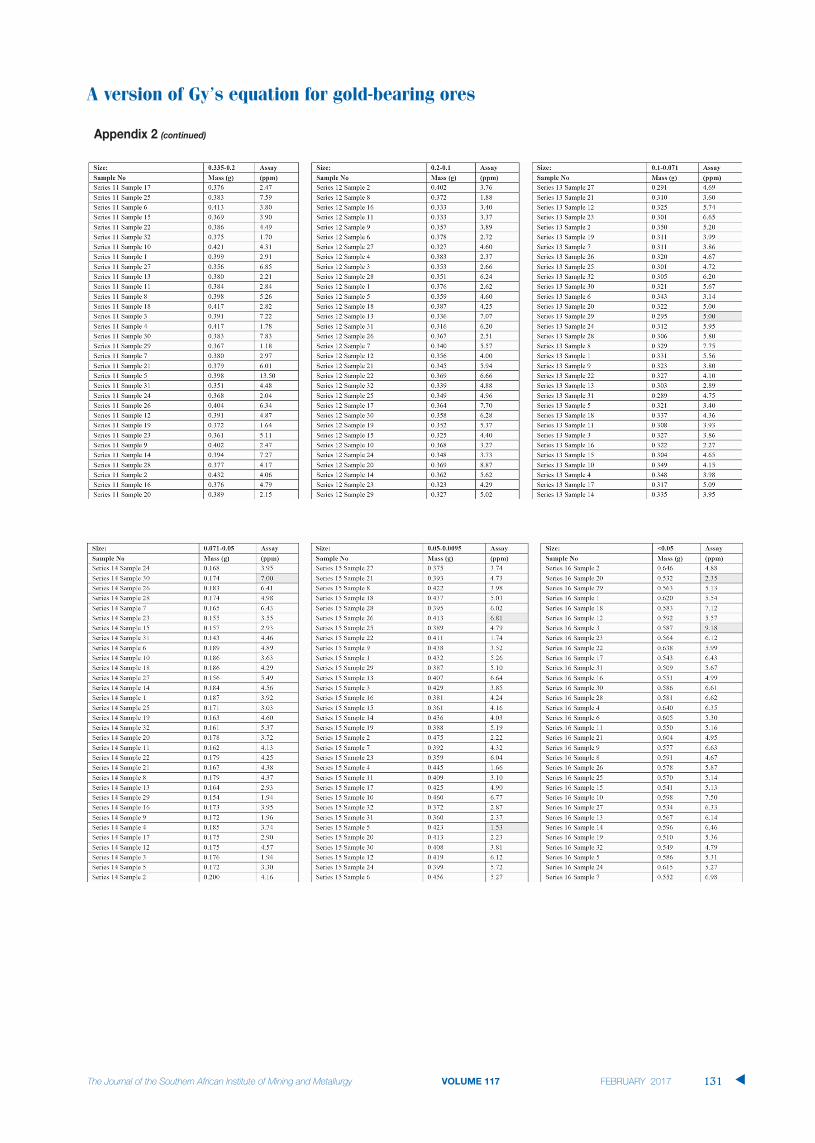
A version of Gy’s equation for gold-bearing ores
VOLUME 117 131 �

A version of Gy’s equation for gold-bearing ores
�
132 VOLUME 117

Mines that make use of an open stopingmining method aim to extract only the ore,leaving the waste behind. Many orebodieshave well-defined boundaries between the oreand the waste rock. In such orebodies, theintroduction of waste into the ore due tooverbreak dilutes the grade. In massivedisseminated orebodies, dilution is lessproblematic. Overblasting, falls of ground, orother causes may result in dilution. A studyundertaken in Canada (Pakalnis et al., 1995)found that approximately 51% of allunderground metal mines utilized openstoping mining methods and, from surveysconducted at these mines, open stopingoperations experienced dilutions of up to 20%,and occasionally more. Dilution of thismagnitude has a significant economic impacton any mining venture. Research carried out inAustralia by Capes (2009) came to the sameconclusion.
Dilution has a significant effect on theviability of South African gold mines that
utilize open stoping mining methods. AtTarget mine the dilution exceeded 10% in anumber of open stopes, which could adverselyimpact the mine’s future. This dilution canresult in the reduction of the recovered gradefrom 5.5 g/t to 4.5 g/t, resulting in a loss ofsome R21 million per month (based on a goldprice of R240 000 per kilogram) at currentproduction levels of 70 000 t/month. Over thelife of mine, the total loss could be in excess ofR3 billion.
Capes (2009) briefly discussed the costs ofdilution. Direct costs are primarily due to theremoval and processing of the additional wastematerial; these costs are for hauling, transport,crushing, hoisting, and milling of the wasterock. Indirect costs are associated with damageto equipment due to falls of ground in openstopes during mucking. Numerous cases ofsuch damage to equipment have occurred atTarget mine.
It is obvious that a reduction in dilutionand equipment damage will be of great benefitto the profitability of a mining operation. Toachieve this requires the accurate prediction ofinstability in open stopes, and hence optimizedstope design. It is not surprising that asignificant amount of research into theprediction of dilution in open stopes has beenundertaken, for example by Potvin (1988),Clark and Pakalnis (1997), Clark (1998),Sutton (1998), Wang (2004), Brady et al.(2005), and Capes (2009). The methodsdescribed in this research could be expected tobe applicable for the design of stable stopes atTarget mine. Their use will be described in thispaper, as well as the development of a newapproach that provided much greater accuracyin stope design and prediction of dilution atTarget mine.
Value creation in a mine operating withopen stoping mining methodsby P.J. Le Roux*† and T.R. Stacey*
Mining companies are under constant pressure to reduce their coststructures to sustain profitability. In mines using an open stoping miningmethod, dilution often has a significant effect on profitability. At Targetmine in South Africa, dilution in some open stopes was found to exceed10%, falls of ground being a major contributor to the problem. Thisdilution can reduce the recovered grade from 5.5 to 4.5 g/t, resulting in apotential loss of about R21 million per month based on a gold price ofR240 000 per kilogram. In addition to the cost of dilution, the cost ofdamage to, or loss of, trackless equipment as a direct result of falls ofground in open stopes is significant. Other associated costs includetransport, hoisting, secondary blasting, milling, and plant treatment ofwaste material. Stable open stopes are essential in order to reduce falls ofground. Back-analyses of stope instability at Target mine have indicatedthat conventional rock mass failure criteria are unsuitable for stopedesign. An alternative strain-based criterion has been developed, and hasproved to be very successful, allowing the stability of open stopes to becalculated reliably. Since its implementation in 2010, dilution andequipment damage have decreased markedly, creating value for the mine.
open stope, stope stability, stope design, dilution stress-strain index.
* University of the Witwatersrand, South Africa.† Brentley, Lucas and Associates, South Africa.© The Southern African Institute of Mining and
Metallurgy, 2017. ISSN 2225-6253. Paper receivedApr. 2016; revised paper received Dec. 2016.
133VOLUME 117 �
http://dx.doi.org/10.17159/2411-9717/2017/v117n2a4

Value creation in a mine operating with open stoping mining methods
Target mine hosts multiple reefs overlying one-another,forming an orebody approximately 180 m in thickness and270 m wide on dip, termed the Eldorado Reefs. The dip of thereefs varies from 10° in the west to 75° in the east. In mostAustralian and Canadian open stoping operations, thehangingwall and footwall consist of waste rock, with theorebody dipping relatively steeply. In contrast, at Target Minethe hangingwall, sidewalls, and footwall generally consist ofreef with different grades. If the stope being mined isadjacent to an existing old stope, one sidewall of this stopewill be backfill. The mining direction of the open stopes isfrom the lowest position of the reef (on the west),progressing up towards the east, as shown in Figure 1.
Owing to the depth of the mine, some 2300 m to 2500 mbelow surface, and resulting high stress levels, a destressing’slot’ is mined to create an artificial shallow miningenvironment in which the maximum stress does not exceed60 MPa. This destressing slot involves narrow-reef mining onthe Dreyerskuil Reef, with an average stoping width of 1.5 m.To extract the massive reefs, open stopes are excavated byblasting to mine selected reef packages within the orebody.These open stopes vary in size between 10 m and 25 m inwidth (span), 10 m and 35 m in height, and 10 m and 100 min length. To establish an open stope, a reef drive isdeveloped on strike at the lowest point where the stope willbe situated, as shown in Figures 1, 2, and 3.
This reef drive is developed to the mining limit of thatspecific open stope. At the end of the open stope slot, cubbiesare developed, cutting across the dip of the strata. In one ofthe cubbies, a drop raise is developed, holing into the topdrive for ventilation. Once developed, the slot is drilled, aswell as the blast rings for the open stope. When completed,the slot is blasted and cleaned using remote loading load,haul, and dump (LHD) mechanized equipment. The openstope is then created by blasting a maximum of four rings ata time, on retreat, and is cleaned using remote-loading LHDs.No personnel may enter these open stopes at any time.
To investigate and document the behaviour of open stopes atTarget mine, and to evaluate alternative open stope designmethods, a comprehensive empirical database wasestablished based on the open stope mining information, rockmass properties, rock mass classification, and cavitymonitoring system (CMS) data. The following information,from 28 case study stopes at Target mine, was included in thedatabase.
� Planned stope volume� Stope volume from CMS survey data� Stope geometry: beam area (stope surface area
analysed), circumference, hydraulic radius� Rock mass properties and rock mass classification
values� Major principal stress at the open stope hangingwall
and sidewall before mining the stope� Modified stability number, N (Potvin, 1988)� Equivalent linear overbreak slough (ELOS) (Clark and
Pakalnis, 1997).
�
134 VOLUME 117
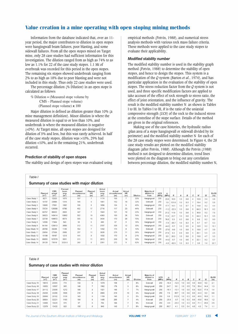
Information from the database indicated that, over an 11-year period, the major contributors to dilution in open stopeswere hangingwall beam failures, poor blasting, and somesidewall failures. From all the open stopes mined on Targetmine, only 28 case studies had sufficient information for thisinvestigation. The dilution ranged from as high as 74% to aslow as 1.1% for 22 of the case study stopes. 1.1 Mt ofoverbreak was recorded for this period in the open stopes.The remaining six stopes showed underbreak ranging from2% to as high as 18% due to poor blasting and were notincluded in this study. Thus only 22 case studies were used.
The percentage dilution (% Dilution) in an open stope iscalculated as follows:
% Dilution = (Measured stope volume by CMS – Planned stope volume)(Planned stope volume) x 100
Major dilution is defined as dilution greater than 10% (amine management definition). Minor dilution is where themeasured dilution is equal to or less than 10%, andunderbreak is where the measured dilution is negative(<0%). At Target mine, all open stopes are designed fordilution of 5% and less, but this was rarely achieved. In halfof the case study stopes, dilution was >10%, 29% haddilution <10%, and in the remaining 21%, underbreakoccurred.
The stability and design of open stopes was evaluated using
empirical methods (Potvin, 1988), and numerical stressanalysis methods with various rock mass failure criteria.These methods were applied to the case study stopes toevaluate their applicability.
The modified stability number is used in the stability graphmethod (Potvin, 1988) to determine the stability of openstopes, and hence to design the stopes. This system is amodification of the Q system (Barton et al., 1974), and hasparticular application in the evaluation of the stability of openstopes. The stress reduction factor from the Q system is notused, and three specific modification factors are applied totake account of the effect of rock strength to stress ratio, theeffect of joint orientation, and the influence of gravity. Theresult is the modified stability number N as shown in TablesI to III. In Tables I to III, R is the ratio of the uniaxialcompressive strength (UCS) of the rock to the induced stressat the centreline of the stope surface. Details of the methodare given in the original references.
Making use of the case histories, the hydraulic radius(plan area of a stope hangingwall or sidewall divided by itsperimeter) and the modified stability number N for each ofthe 28 case study stopes were determined. In Figure 4, the 28case study results are plotted on the modified stabilitydiagram (after Potvin, 1988). Although the Potvin (1988)method is not designed to determine dilution, trend lineswere plotted on the diagram to bring out any correlationbetween percentage dilution, the modified stability number N,
Value creation in a mine operating with open stoping mining methods
VOLUME 117 135 �
Table I
Table II
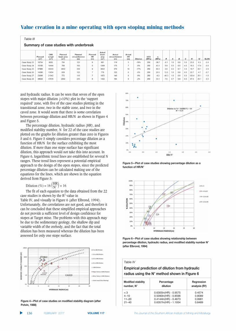
Value creation in a mine operating with open stoping mining methods
and hydraulic radius. It can be seen that seven of the openstopes with major dilution (>10%) plot in the ‘supportrequired’ zone, with five of the case studies plotting in thetransitional zone, two in the stable zone, and two in thecaved zone. It would seem that there is some correlationbetween percentage dilution and HR/N as shown in Figure 4and Figure 5.
The percentage dilution, hydraulic radius (HR), andmodified stability number, N for 22 of the case studies areplotted on the graphs for dilution greater than zero in Figures5 and 6. Figure 5 simply considers percentage dilution as afunction of HR/N for the surface exhibiting the mostdilution. If more than one stope surface has significantdilution, this approach would not take this into account. InFigure 6, logarithmic trend lines are established for several Nranges. These trend lines represent a potential empiricalapproach to the design of the open stopes, since the predictedpercentage dilution can be calculated making use of theequations for the lines, which are shown in the equationderived from Figure 5:
Dilution (%) = 16 (N'HR) + 16
The fit of each equation to the data obtained from the 22case studies is shown by the R2 value in Table IV, and visually in Figure 6 (after Elbrond, 1994).Unfortunately, the correlations are not good, and therefore itcan be concluded that these simplified empirical approachesdo not provide a sufficient level of design confidence forstopes at Target mine. The problems with this approach maybe due to the sedimentary geology, the shallow dip andvariable width of the orebody, and the fact that the totaldilution has been measured whereas the dilution has beenassessed for only one stope surface.
�
136 VOLUME 117
Table III
Table IV
< 3 0.6305ln(HR) - 0.9575 0.45744–10 0.5090ln(HR) - 0.8596 0.808911–20 0.4144ln(HR) - 0.4673 0.998121–40 0.6357ln(HR) - 1.1934 0.8489

The dilution factor is defined as the ELOS predicted from thedilution design graph based on the modified stability numberN and hydraulic radius for an open stope. The 22 casestudies with dilution greater than zero are plotted on themodified stability diagram for ELOS (after Clark andPakalnis, 1997) in Figure 7. The calculated ELOS is from 2.5 m up to 10.4 m for open stopes with major dilution(>10%). A contributing factor could be that the sidewalldilution has not been assessed for ELOS, so the calculatedELOS would be less than the total ELOS recorded. Also, insome cases the significant sidewall dilution greatly increasedthe hydraulic radius of the stope hangingwall, furtherincreasing dilution, which was not predicted from the ELOSapproach. The measured ELOS was based on the differencebetween the planned stope volume and the CMS actual stopevolume, divided by the area of the surface creating themaximum dilution. In cases where significant dilution wasfrom more than one surface, ELOS may be greatly underes-timated. It should be noted that seven of the 14 cases ofmajor dilution had significant dilution from one or twosidewalls as well as the hangingwall.
The modified stability diagram for ELOS (after Clark andPakalnis, 1997) was further modified in an attempt toincorporate the ELOS values obtained on Target mine asshown in Tables I to III. The ELOS values for Target are muchhigher than those obtained by Clark and Pakalnis (1997) andWang (2004), as shown in Figure 7. Due to the limitednumber of case studies, for the ranges of ELOS shown, thetrend lines could not be verified. The maximum ELOSpredicted by Figure 7 is greater than 2 m. The graph does notdelineate the ELOS value if it is greater than 2 m, whichmakes it difficult to apply to many of the case histories.
From the back-analyses on the 22 open stopes wheresufficient data was available, three-dimensional stressanalyses were conducted. MAP3D-SV was the numericalanalysis package used to model the mining of the openstopes. The purpose of the analyses was to determine themedian three principal stresses and the corresponding threeprincipal strains at the centreline of the stope hangingwalland sidewalls for the specific mining configuration. To
achieve this, strings (also known as gridlines) were placed onthe boundaries of the hangingwall and sidewalls in the centreof the open stope hangingwall and sidewalls for each of theopen stopes, and the actual mining extraction sequenceshown in Figure 8 was simulated. It was found that theexpected stresses on the boundaries of the open stope werenot negative or zero due to the accuracy of the model in areaswhere overstoping was conducted. Overstoping is the processby which a narrow reef mining slot is blasted, creating anartificial shallow mining environment in which the openstopes will be mined, as shown in Figure 8.
The rock mass in the numerical model was assumed to behomogeneous and isotropic to simplify modelling (Wiles,2006). The following input parameters were used in theMAP3D-SV analyses:
� Young’s modulus 70 000 MPa� Poisson’s ratio 0.2� Density 2700 kg/m3
� K-ratio 0.5
The Young’s modulus, Poisson’s ratio, and density valueswere determined from laboratory tests conducted at theUniversity of the Witwatersrand by Le Roux (2004). The K-ratio is an estimate based on underground observations andback-analyses.
The principal stresses determined in the analyses weresubstituted into several rock mass failure criteria todetermine whether any of these criteria would be suitable forpredicting instability around open stopes at Target mine. Themost widely accepted failure criteria currently used in rockengineering are the Hoek-Brown failure criterion (Hoek et al.,2002) and the Mohr-Coulomb failure criterion (Labuz andZhang, 2012). These two criteria and the Zhang-Zhu (Zhangand Zhu, 2007), Pan-Hudson (Pan and Hudson, 1988),Priest (Priest, 2009), Simplified Priest (Priest, 2009), andDrucker-Prager criteria (Alejano and Bobet, 2012) were usedin the evaluation.
Only 22 of the case study stopes proved to be appropriatewith regard to the application of these criteria. From thesestudies, it was found that 14 open stopes had undergonehangingwall failure and eight sidewall failure, seven casesbeing a combination of hangingwall and sidewall failure.Major dilution occurred in nine of the 14 stopes withhangingwall failure, and minor dilution in five. For sidewallfailure, it was found that five stopes had major dilution andthree minor dilution. The open stopes with a combination of
Value creation in a mine operating with open stoping mining methods
VOLUME 117 137 �
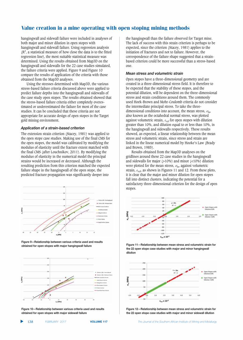
Value creation in a mine operating with open stoping mining methods
hangingwall and sidewall failure were included in analyses ofboth major and minor dilution in open stopes withhangingwall and sidewall failure. Using regression analysis(R2, a statistical measure of how close the data is to the fittedregression line), the most suitable statistical measure wasdetermined. Using the results obtained from Map3D on thehangingwall and sidewalls for the 22 case studies simulated,the failure criteria were applied. Figure 9 and Figure 10compare the results of application of the criteria with thoseobtained from the Map3D analyses.
Using the stresses determined with Map3D, the variousstress-based failure criteria discussed above were applied topredict failure depths into the hangingwall and sidewalls ofthe case study open stopes. The results obtained showed thatthe stress-based failure criteria either completely overes-timated or underestimated the failure for most of the casestudies. It can be concluded that these criteria are notappropriate for accurate design of open stopes in the Targetgold mining environment.
The extension strain criterion (Stacey, 1981) was applied tothe open stope case studies. Making use of the final CMS forthe open stopes, the model was calibrated by modifying themodulus of elasticity until the fracture extent matched withthe final CMS (after Louchnikov, 2011). By modifying themodulus of elasticity in the numerical model the principalstrains would be increased or decreased. Although theresulting prediction from this criterion matched the expectedfailure shape in the hangingwall of the open stope, thepredicted fracture propagation was significantly deeper into
the hangingwall than the failure observed for Target mine.The lack of success with this strain criterion is perhaps to beexpected, since the criterion (Stacey, 1981) applies to theinitiation of fractures and not to failure. However, thecorrespondence of the failure shape suggested that a strain-based criterion could be more successful than a stress-basedone.
Open stopes have a three-dimensional geometry and arecreated in a three-dimensional stress field. It is therefore tobe expected that the stability of these stopes, and thepotential dilution, will be dependent on the three-dimensionalstress and strain conditions around them. The commonlyused Hoek-Brown and Mohr-Coulomb criteria do not considerthe intermediate principal stress. To take the three-dimensional conditions into account, the mean stress, m,also known as the octahedral normal stress, was plottedagainst volumetric strain, vol for open stopes with dilutiongreater than 10%, and dilution equal to or less than 10%, inthe hangingwall and sidewalls respectively. These resultsshowed, as expected, a linear relationship between the meanstress and volumetric strain, since stress and strain arelinked in the linear numerical model by Hooke’s Law (Bradyand Brown, 1985).
Results obtained from the Map3D analyses on thegridlines around these 22 case studies in the hangingwalland sidewalls for major (>10%) and minor (<10%) dilutionwere plotted for the mean stress, m, against volumetricstrain, vol, as shown in Figures 11 and 12. From these plots,it is clear that the major and minor dilution for open stopesfall into distinct clusters, indicating the potential for asatisfactory three-dimensional criterion for the design of openstopes.
�
138 VOLUME 117

Value creation in a mine operating with open stoping mining methods
VOLUME 117 139 �
For the 22 case studies it was found that for open stopeswith >10% dilution due to hangingwall failure, the volumetricstrain and mean stress values were in the very low range,thus placing them in a relaxed or destressed environment.This low-stress environment is found when open stopes aremined very close to the narrow reef destressing or for openstopes with a large hydraulic radius greater than or equal to9. The failure mode in these conditions would include beamfailure and/or keyblock failure. Failure could also occur in thehangingwall and sidewalls where high stress conditions areencountered, such as in pillar areas or high-stress abutmentsat the narrow-reef destressing, resulting in stress fracturing.It should be emphasized that the open stopes with <10%dilution fell within a mean stress range where fracturepropagation is minimal and hangingwall and sidewall dilationis optimal to prevent hangingwall or sidewall failure,suggesting that this method could be used to differentiatebetween stability and failure. The following results wereobtained.
Dilution >10% from hangingwall failure occurred if m >50 MPa; vol > 1.29 × 10⁻³, or m 4.8 MPa; vol < 0,124 × 10-3
as shown in Figure 13. Dilution >10% from sidewall failure occurred if m 85.3
MPa; vol > 2.19 × 10⁻³, or m < 0.5 MPa; vol < 0.013 × 10⁻³
as shown in Figure 14. The data indicated the potential for a strain-based
stability/design criterion for the Target open stopes, whichhas been termed the Dilution Stress-Strain Index (DSSI). Therelation between mean stress m and volumetric strain vol
can be expressed as follows:
[1]
[2]
where q = 39 GPa, which is the slope of the linear trend linesin Figures 11 and 12. The DSSI is the relationship betweenmean stress and volumetric strain, expressed as follows:
[3]
For a factor of safety of 1.0, the DSSI value is 1.0. ADSSI value of greater than 1.0 will indicate failure conditionsin tension. For a set value of mean stress, if the volumetricstrain were less than the threshold as determined by Figures11 and 12, failure would occur due to relaxation. A DSSIvalue of less than 1.0 will indicate failure conditions incompression. This is a new criterion for determining theexpected failure depth in the hangingwall or sidewalls ofexcavations, which does not appear in any literaturereviewed. Although octahedral normal stress forms the basisof this criterion, this is a completely new method ofdetermining failure depth: if the volumetric strain exceeds thecritical value for mean stress, failure will occur. This methodconsiders all three principal stresses and strains, which isappropriate for the three-dimensional environment of openstopes.
A full 3D analysis of the open stopes is required, and stress
and strain magnitudes must be determined on a dense grid ofpoints adjacent to the hangingwall and sidewall surfaces. Thenext step is to determine the statistical median from the 1,
3, m, and vol values for major and minor dilution in openstope hangingwalls and sidewalls. The obtained medianmean stress and volumetric strain values for each case studyare then plotted for major and minor dilution to determine q,which is the slope of the linear trend lines for mean stressand volumetric strain of the open stope case studies, asshown in Figures 11 and 12 for hangingwall and sidewalldilution. The 1 and 3 median results for each case studyfor major and minor dilution in hangingwall and sidewallsare plotted as shown in Figure 13. From these results, thefailure mode (tension or compression) for major and minordilution in open stope hangingwall and sidewalls isdetermined. By making use of the minor dilution data, thefailure envelope cut-off can be determined as shown inFigure 13.
Making use of the median mean stress value m determinedfor each case study, the DSSI can be applied for major failurein open stope hangingwall and sidewalls in Map3D. Now theopen stope CMS can be imported into Map3D as a DXF fileand superimposed on the numerical analysis data to comparethe results, as shown in Figure 14. This is part of thecalibration process. If a good correlation is found between theDSSI prediction and the open stope CMS, the criterion can beused; if not, the model calibration process must be continueduntil a reasonable result is obtained. To calibrate the model,the Young’s modulus (E) and Poisson’s ratio (v) are changeduntil the results match, (after Louchnikov, 2011). When themodel is calibrated, the same values for E and v must beapplied for all case studies being used. The DSSI is appliedfor major failure in open stope hangingwall and sidewalls inMap3D for a planned open stope, and the failure depthdetermined. The DSSI failure lobes indicated in light grey inFigure 14 can also be exported as DXF files and comparedwith the design stope shape to determine the expecteddilution, as shown in Figure 15. Using this information, thestope shape can be amended (reduced in size) so that thefinal shape corresponds with the actual required, plannedshape due to the expected failure depth.
Applying the methodology shown in Figures 11 and 12,the open stope case studies were evaluated. Hangingwall andsidewall failure in open stopes can be predicted by thefollowing equations proposed for Target mine:
[4]
[5]
After the DSSI design criterion had been established forhangingwall failure and sidewall failure on Target mine, theobtained median major principal stress 1 and median minorprincipal stress 3 were plotted for each of the 22 casestudies. Using the obtained results for the 22 case studies,the failure mode for the open stopes with major hangingwallor sidewall dilution (>10%) could be determined. The same
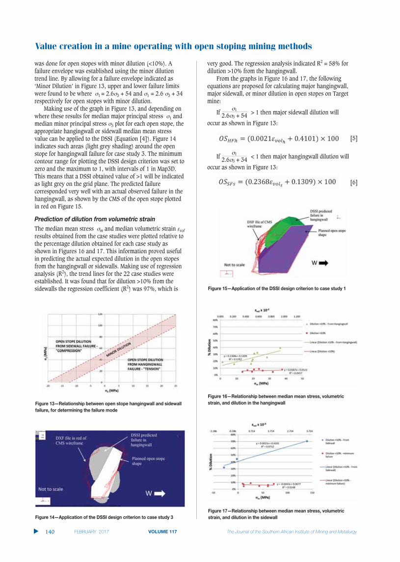
Value creation in a mine operating with open stoping mining methods
was done for open stopes with minor dilution (<10%). Afailure envelope was established using the minor dilutiontrend line. By allowing for a failure envelope indicated as‘Minor Dilution’ in Figure 13, upper and lower failure limitswere found to be where 1 = 2.6 3 + 54 and 1 = 2.6 3 + 34respectively for open stopes with minor dilution.
Making use of the graph in Figure 13, and depending onwhere these results for median major principal stress 1 andmedian minor principal stress 3 plot for each open stope, theappropriate hangingwall or sidewall median mean stressvalue can be applied to the DSSI (Equation [4]). Figure 14indicates such areas (light grey shading) around the openstope for hangingwall failure for case study 3. The minimumcontour range for plotting the DSSI design criterion was set tozero and the maximum to 1, with intervals of 1 in Map3D.This means that a DSSI obtained value of >1 will be indicatedas light grey on the grid plane. The predicted failurecorresponded very well with an actual observed failure in thehangingwall, as shown by the CMS of the open stope plottedin red on Figure 15.
The median mean stress m and median volumetric strain vol
results obtained from the case studies were plotted relative tothe percentage dilution obtained for each case study asshown in Figures 16 and 17. This information proved usefulin predicting the actual expected dilution in the open stopesfrom the hangingwall or sidewalls. Making use of regressionanalysis (R2), the trend lines for the 22 case studies wereestablished. It was found that for dilution >10% from thesidewalls the regression coefficient (R2) was 97%, which is
very good. The regression analysis indicated R2 = 58% fordilution >10% from the hangingwall.
From the graphs in Figure 16 and 17, the followingequations are proposed for calculating major hangingwall,major sidewall, or minor dilution in open stopes on Targetmine:
If 2.6 3 + 541 > 1 then major sidewall dilution will
occur as shown in Figure 13:
[5]
If 2.6 3 + 341 < 1 then major hangingwall dilution will
occur as shown in Figure 13:
[6]
�
140 VOLUME 117

If 2.6 3 + 541 < 1 and 2.6 3 + 34
1 > 1 then minor dilution
will occur as shown in Figure 13:
[7]
[8]
[9]
whereOSHFs is the open stope hangingwall dilution in per cent forfailure in compressionOSSFs is the open stope sidewall dilution in per cent for failurein compressionOSHFh is the open stope hangingwall dilution in per cent forfailure in tensionOSSFh is the open stope sidewall dilution in per cent for failurein tensionOSHFn is the open stope hangingwall dilution in per cent forfailure in normal open stope conditionsOSSFn is the open stope sidewall dilution in per cent for failurein normal open stope conditions.
OSD (open stope dilution) is the maximum value for therespective OS value obtained.
Making use of the graph shown in Figure 11, therelationship between open stope hangingwall and sidewallfailure and ultimately dilution can be determined. This isdone by plotting the obtained 1 and 3 median results foreach separate case study on Figure 13 and reading off thegraph whether there will be expected hangingwall dilution,sidewall dilution, or minor dilution. Thus for sidewalldilution, Equation [5] will be used; for hangingwall dilution,Equation [6] will be used. For minor dilution Equations [7]and [8] will be used. After calculating the expected dilutionusing the relevant equations, only the maximum calculateddilution (OSD) value is used for the open stope beingevaluated.
The results predicted using the DSSI criterion were comparedwith the stope behaviour predicted with the stability numberN’ and hydraulic radius, as calculated for the modifiedstability graph (Potvin, 1988) as shown in Figure 4, and thesite-specific average expected dilution as shown in Figures 5and 6. The OSD method using the DSSI criterion providedreliable estimates of the depth of failure for all the availabledata. The Potvin (1988) modified stability diagram clearlyshows the difference between stable and caving conditionsfor the case studies. The method used by Elbrond (1994)tended to overestimate the amount of dilution expected atTarget mine, probably due to the narrow orebody that themethod was developed from.
Since 2011, when the DSSI design criterion was appliedat Target mine, a significant reduction in dilution has beenrecorded, as shown in Figure 18. With the ability to predictdilution in open stopes, these stopes could be re-designed to‘fail’ to the desired final open stope shape. The DSSI design
criterion has clearly influenced the sustainability andeconomics at Target mine, as shown in Figure 19. Thefinancial benefit has been quantified, and this has proved thevalue of the design approach using the new DSSI criterion.There is no reason why the design approach could not havethe same impact on any other mining operation: it has beenshown to be equally applicable to different mining andgeological environments (Le Roux, 2015).
The objective of the research described in this paper was todevelop an improved method of calculating the expectedfailure depth into the hangingwall and sidewalls of openstopes, and hence determine potential dilution in open stopes.Existing methods of evaluating open stope stability, whichinclude empirical methods and stress analysis methods withstress-based rock mass failure criteria, were assessed. Rockmass properties, rock mass classifications, blast design, blasttechniques, the stress-strain environment, and the hydraulicradius of the stope all have some effect on, or play a part in,the evaluation of dilution. It was found that the stress-strainenvironment also plays a significant role in the behaviour ofopen stopes at depth. Twenty-two case study stopes at Targetmine, which yielded sufficient information for the research,were selected. The results of predictions of the depths offailure into the open stope hangingwall and sidewalls, basedon application of the new DSSI design criterion, allowed openstopes to be redesigned to ‘fail’ up to the required stopeshape, thus reducing dilution.
Value creation in a mine operating with open stoping mining methods
VOLUME 117 141 �

Value creation in a mine operating with open stoping mining methods
This research has contributed to the understanding ofrock behaviour in an open stope environment, and identifieda design methodology to reduce dilution. It also illustratedthat, even with very limited information available (Le Roux,2015) relatively accurate results could be obtained for theopen stope design. This is significant, since when a new mineis designed there is very limited information available, andthe expected dilution usually cannot be determined with anyconfidence. The design approach developed in this researchallows the failure depth into the hangingwall and sidewalls ofopen stopes to be estimated with greater success, and dilutioncan be calculated for use in mine design as shown in Table V.Proof of the value of the new DSSI design criterion is thesignificant impact that it has had on the economics of Targetmine, and that it has ensured the future of mining at thisoperation. It has in fact created substantial value for themine.
The authors would like to thank Harmony Gold MiningCompany Limited for the privilege of presenting this research.The permission to include data and make use of equipment,as well as the assistance received from colleagues at Brentley,Lucas & Associates, Mining Consultants, is greatlyappreciated.
ALEJANO, L.R. and BOBET, A. 2012. Drucker-Prager criterion. Rock Mechanicsand Rock Engineering, vol. 45. pp. 995–999.
BARTON, N., LIEN, I.R., and LUNDE, J. 1974. Engineering classification of rockmasses for design of tunnel support. Rock Mechanics, vol. 6. pp. 186–236.
BRADY, B.H.G. and BROWN, E.T. 1985. Rock Mechanics for Underground Mining.Allen and Unwin, London.
BRADY, T., PAKALNIS, R., and CLARK, L. 2005. Design in weak rock masses,Nevada underground mining operations. Proceedings of the AnnualGeneral Meeting of the SME, Salt Lake City. 9 pp.
CAPES, G.W. 2009. Open stope hangingwall design based on general anddetailed data collection in rock masses with unfavorable hangingwall
conditions. PhD thesis, University of Saskatchewan.CLARK, L. and PAKALNIS, R. 1997. An empirical design approach for estimating
unplanned dilution from open stope hanging walls and footwalls. AnnualGeneral Meeting of the CIM, Calgary, Alberta.
CLARK, L. 1998. Minimizing dilution in open stope mining with a focus on openstope design and narrow vein longhole blasting. MSc thesis, University ofBritish Columbia.
ELBROND, J. 1994. Economic effects of orelosses and rock dilution. CIM Bulletin,vol. 87, no. 978. pp. 131–134.
HOEK, E., CARRANZA-TORRES, C.T., and CORKUM, B. 2002. Hoek–Brown failurecriterion—2002 edition. Proceedings of the Fifth North American RockMechanics Symposium (NARMS-TAC). Hammah, R., Bawden, W., Curran,J., and Telesnicki, M. (eds.). University of Toronto Press, Toronto. pp. 267–273.
LABUZ, J.F. and ZHANG, A. 2012. Mohr-Coulomb failure criterion. RockMechanics and Rock Engineering, vol. 45. pp. 975–979.
LE ROUX, P.J. 2004. Project on rock mass properties for the Free State,mechanical properties of rocks and rock masses. University of theWitwatersrand, South Africa.
LE ROUX, P.J. 2015. Measurement and prediction of dilution in a gold mineoperating with open stoping mining methods. PhD thesis, University ofthe Witwatersrand. 227 pp.
LOUCHNIKOV, V. 2011. Simple Calibration of the Extension Strain Criterion for itsuse in Numerical Modelling. Australian Centre for Geomechanics, Perth.pp. 85-96.
PAKALNIS, R.C., POULIN, R., and HADJIGEORGIOU, J. 1995. Quantifying the cost ofdilution in underground mines. Mining Engineering. pp. 1136–1141.
PAN, X.D and HUDSON, J.A. 1988. A simplified three-dimensional Hoek–Brownyield criterion. Rock Mechanics and Power Plants. Romana, M. (ed.).Balkema, Rotterdam. pp. 95–103.
POTVIN, Y. 1988. Empirical open stope design in Canada. PhD thesis, Universityof British Columbia, Vancouver.
PRIEST, S.D. 2009. Comparisons between selected three-dimensional yieldcriteria applied to rock. Rock Mechanics and Rock Engineering, vol. 43.pp. 379–389.
STACEY, T.R. 1981. A simple extension strain criterion for fracture of brittlerock. International Journal of Rock Mechanics and Mining Sciences &Geomechanics Abstracts, vol. 18. pp. 469–474.
SUTTON, D. 1998. Use of the modified stability graph to predict stope instabilityand dilution at Rabbit Lake Mine, Saskatchewan. Design Project,University of Saskatchewan, Canada.
WANG, J. 2004. Influence of stress, undercutting, blasting, and time on openstope stability and dilution. PhD thesis, University of Saskatchewan.
WILES, T.D. 2006. MAP3D user’s manual. Mine Modelling (Pty) Ltd, MountEliza, Victoria, Australia.
ZHANG, L. and ZHU, H. 2007. Three-dimensional Hoek–Brown strength criterionfor rocks. Journal of Geotechnical and Geoenvironmental Engineering,vol. 133, no. 9. pp. 1128–1135. �
�
142 VOLUME 117
Table V
Most clay in South Africa is used in themanufacturing of tiles, pipes, bricks,whiteware, refractories, and pottery. Bricks aremanufactured from a wide variety of claytypes, the behaviour of which during firingdepends critically on the the clay mineralogyand chemical composition, but thisrelationship not well understood (Stein, 1982).The variety among clay deposits is related tothe different processes of formation (Deer,Howie, and Zussman, 1992). The geochemicalcomposition of the clay can vary betweenlayers and within the same layer in anindividual deposit (Lurie, 1984). Theproperties of clay minerals are determined bytheir structures and the different combinationsof silicate layers, cations, and hydroxyl ions(Kingery, Bowen, and Uhlmann, 1976). SouthAfrican clays can be classified as eitherkaolinite or montmorillonite and are seldomfound in a pure form (Lurie, 1984). Differentclay minerals affect the drying, forming, firingbehaviour, colour, and quality of the brick
product in different ways. Laboratory tests(full physical analysis) can indicate thesuitability of a clay for the manufacture ofceramic products. The minerals most essentialfor the manufacturing of clay brick productsare kaolinite, illite, and quartz (Stein, 1982).
South Africa’s manufacturers of clayfacebricks supply a range of uniquely colouredbricks to the market by blending a variety ofclay materials during the manufacturingprocess. Management of the raw material is akey factor in ensuring that consumer demandsfor a consistent product are met. Thehomogeneity of the raw materials mined fromyear to year is crucial for a reliable supply ofbricks with a consistent colour. Selectivemining of the different clay types from anopencast operation provides the colourvariation in the products that arises fromvariability in the composition of the rawmaterials. These colour variations aremanaged by adjusting either the mixformulation or the process parameters. Thecolour variation of laboratory-fired briquettesfor one of the white clay stockpiles over aperiod of four seasons is shown in Figure 1a.The briquettes show distinct colourdifferences, especially for firing temperaturesbetween 1050°C and 1150°C. Figure 1billustrates the effect of these variables on thecolour of the brick. The colour of the facebrickis controlled by the contents of the K2O fluxingagent and Fe2O3, which are strong colourants.These variables are sensitive the firingtemperature in the kiln, which is strictlycontrolled to maintain year-on-yearconsistency of the colour of the bricks.
Geostatistical techniques for improvedmanagement of brickmaking claysby M.H.M. von Wielligh*† and R.C.A. Minnitt†
Brick manufacturers supply a variety of uniquely coloured facebricks tothe building industry, which requires a high level of colour consistency inthe products. Colour variation in bricks is influenced by the compositionand consistency of the white clay raw material. By blending varieties ofnaturally occurring white clay the manufacturers produce a unique rangeof facebrick products. Homogeneity of the white clay raw materials minedat Lenasia is crucial for producing bricks of consistent colour.Geostatistical investigations of the major element distributions (SiO2,Al2O3, Fe2O3, and K2O) and loss on ignition (LoI) were conducted. Ananalysis of the spatial continuity of these variables followed by ordinarykriging indicated that the upper white clay layer at Lenasia is richer in K2Oand Fe2O3 than the lower layer. Consistency in the colour of facebricksdepends critically on careful management of the variability in the K2O andFe2O3 content of the clays. The geostatistical approach to understandingthe distribution of elements in the clay allows miners to construct claystockpiles of consistent quality for feeding the brick-making process.Geostatistical investigation of the chemical contents in other clay domainswithin the deposit is recommended, and could be extended to all facebrickmanufacturers to assist in improving the colour consistency of theirproducts.
geostatistics, facebrick clay, chemical composition, colour consistency.
* National Ceramic Industries South Africa (Pty)Ltd, Aquarella Investment 389 (Pty) Ltd,Vereeniging,.
† School of Mining Engineering, University of theWitwatersrand, South Africa.
© The Southern African Institute of Mining andMetallurgy, 2017. ISSN 2225-6253. Paper receivedMar. 2016; revised paper received May 2016.
143VOLUME 117 �
http://dx.doi.org/10.17159/2411-9717/2017/v117n2a5
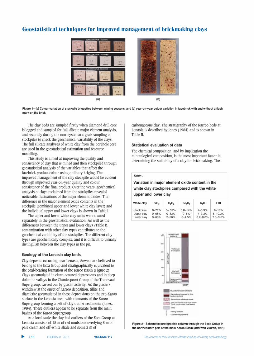
Geostatistical techniques for improved management of brickmaking clays
The clay beds are sampled firstly when diamond drill coreis logged and sampled for full silicate major element analysis,and secondly during the non-systematic grab sampling ofstockpiles to check the geochemical variability of the clays.The full silicate analyses of white clay from the borehole coreare used in the geostatistical estimation and resourcemodelling.
This study is aimed at improving the quality andconsistency of clay that is mined and then stockpiled throughgeostatistical analysis of the variables that affect thefacebrick product colour using ordinary kriging. Theimproved management of the clay stockpile would be evidentthrough improved year-on-year quality and colourconsistency of the final product. Over the years, geochemicalanalysis of clays reclaimed from the stockpiles revealednoticeable fluctuations of the major element oxides. Thedifference in the major element oxide contents in thestockpile (combined upper and lower white clay layer) andthe individual upper and lower clays is shown in Table I.
The upper and lower white clay units were treatedseparately in the geostatistical evaluation. As well as thedifferences between the upper and lower clays (Table I),contamination with other clay types contributes to thegeochemical variability of the stockpiles. The different claytypes are geochemically complex, and it is difficult to visuallydistinguish between the clay types in the pit.
Clay deposits occurring near Lenasia, Soweto are believed tobelong to the Ecca Group and stratigraphically equivalent tothe coal-bearing formation of the Karoo Basin (Figure 2).Clays accumulated in clean-scoured depressions and in deepdolomite valleys in the Chuniespoort Group of the TransvaalSupergroup, carved out by glacial activity. As the glacierswithdrew at the onset of Karroo deposition, tillite anddiamictite accumulated in these depressions on the pre-Karoosurface in the Lenasia area, with remnants of the KarooSupergroup forming a belt of clay outlier sediments (Jones,1984). These outliers appear to be separate from the mainbasins of the Karoo Supergroup.
At a local scale the clay bed outliers of the Ecca Group atLenasia consists of 15 m of red mudstone overlying 8 m ofpale cream and off-white shale and some 2 m of
carbonaceous clay. The stratigraphy of the Karroo beds atLenasia is described by Jones (1984) and is shown in Table II.
The chemical composition, and by implication themineralogical composition, is the most important factor indetermining the suitability of a clay for brickmaking. The
�
144 VOLUME 117
Table I
Stockpiles 6–71% 5– 37% 0.8–14% 2–3.3% 9–18%Upper clay 0–66% 0–33% 9–6% 4–3.3% 8–10.2%Lower clay 0–66% 2–26% 0–4.5% 0.2–0.8% 7.5–9.6%

content of silica (SiO2), alumina (Al2O3), iron (Fe2O3),potassium (K2O), and loss on ignition (LoI) were used in thegeostatistical analysis. The geochemical analyses wereperformed on clay samples gathered from 60 boreholes thatwere drilled into the clay beds in the open pit area (Figure 3).
While it is possible to determine the geochemical distri-bution of elements in the clay using simple contouringtechniques, the more appropriate ordinary kriging techniquewas applied. The aim of this exercise was to estimate thedistribution of elements in the clay beds to assist futurequarry development and planning. Furthermore, thisinformation could provide a means of ensuring thatgeochemically similar clays are extracted and stockpiled,thereby improving the mineralogical consistency of the rawmaterials from which the brickmaking clays are drawn.Planning the extraction of the clay to minimize chemicalvariability will enable value-added decision-making andimprove product quality and consistency.
The location of exploration boreholes relative to theoperating quarry is shown in Figure 3, and is enlarged toshow the stratigraphy of clay types in Figure 4. The core waslogged according to lithology and analysed for chemicalcomposition of some major elements using X-ray diffractionand wet-chemical techniques. The position of boreholesdrilled in the 2009/2010 period are shown as red and greencrosses (Figure 3), and are shown on a 50 m × 40 m grid inFigure 4.
The geological modelling and domaining was based onthe geology revealed in the borehole logs, while geochemicalanalyses were used for geostatistical data analysis,variography, modelling, and estimation. The areal extent ofthe upper white clay domain is larger than that of the lowerwhite clay domain.
Descriptive statistics for the upper and lower white claydomains are given in Table III, with histograms for the majoroxides shown in Figure 5.
The variability of all major oxides in the upper clay bedsis consistently higher than in the lower clay beds, with theupper beds having a higher clay content (lower SiO2/Al2O3
ratio) and higher flux content (Fe2O3 and K2O), as reflected inthe ratios of these oxides. Owing to the paucity of data,definitive statements about the nature of the distributions aresomewhat tenuous, except for the observation that theyappear to be normally distributed.
The lower SiO2/Al2O3 ratio in the white upper clay, at2.14 compared to 2.57 in the lower clay, indicates a greaterclay content. This promotes increased shrinkage during
drying and firing, with the fired brick being less water-absorbent. The difference in the K2O and Fe2O3 contents ofthe upper and lower clay beds is significant. The higher K2O
Geostatistical techniques for improved management of brickmaking clays
VOLUME 117 145 �
Table II
Highly weathered, red mudstones with periodic and alternating chert pebble bands Red kaolin > 25.0Light-cream and off-white coloured kaolinitic shales White clay 8.0Dark-grey, brown and black carbonaceous mudstone Plastic clay 9.5Dark-grey carbonaceous shales Carbonaceous shale 0.0–2.0Grey and off-white coloured grits, siltstones and tillite Dwyka > 3.0
Table III
Mean 57.61 27.17 3.28 1.80 8.50Standard Deviation 3.34 2.70 1.57 1.00 0.95Range 16.10 12.98 5.18 2.77 3.08
Mean 62.27 24.50 2.58 0.57 8.65Standard Deviation 1.97 1.32 1.29 0.18 0.67Range 6.50 4.30 4.14 0.49 2.10

Geostatistical techniques for improved management of brickmaking clays
(3.30%) and Fe2O3 (2.08%) content in the upper clay meansthat bricks manufactured from this clay develop a moreintense colour than those from clay from the lower beds (K2O0.57% and Fe2O3 2.41%). In the presence of K2O, Fe2O3 islikely to develop a dark colour at lower temperatures, and inits absence, a lighter colour (assuming all other propertiesremain constant). The low K2O content in the lower whiteclay should contribute little to the development of the colourintensity in the brick if the Fe2O3 content is low (< 1%);however, the opposite was found for the upper white clay.
Potassium oxide is a strong flux that promotes theformation of a liquid phase from illites and mica minerals athigh temperatures. Data analysis revealed a strong positivecorrelation between K2O and mica content. Iron oxide is astrong colorant that causes an intense red colour in bricks. Avery strong positive correlation was found between Fe2O3 andthe interstratified illite/smectite mineral.
Omnidirectional experimental and model variograms for thefive major elements in both the upper and lower white clayunits were constructed and are shown in Figure 6. Except for
Fe2O3 in the lower clay unit, which has two structures, thevariograms are single structure, spherical with an extremelysmall nugget effect for both the upper and lower clay beds.The geochemical dispersion was naturally found to be morecontinuous along the elongated direction of greatest drillingdensity, but this did not reflect underlying anisotropy norwarrant the use of directional variograms to model thedeposit.
Parameters for the variogram models of elements in theupper and lower clay beds, as shown in Figure 6. are listed inTable IV.
Variogram parameters listed in Table IV are summarizedand compared in Figure 7. The nugget effect and the sill forboth the upper and the lower white clays are low, with thenugget effect and the sill for SiO2 in the upper and lower claybeds being the highest amongst the variables. The longestrange is for Al2O3 in the upper and lower clay beds.
The results of ordinary kriging of the major elementoxides are tabulated in Table V, and are shown graphicallyfor the upper and lower clay beds in Figure 8. The apparentgeochemical continuity in the east–west direction of thedeposit is due to the greater density of drilling in thisdirection rather than a true reflection of geochemical
�
146 VOLUME 117
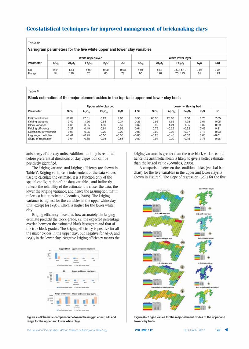
anisotropy of the clay units. Additional drilling is requiredbefore preferential directions of clay deposition can bepositively identified.
The kriging variance and kriging efficiency are shown inTable V. Kriging variance is independent of the data valuesused to calculate the estimate. It is a function only of thespatial configuration of the data variables, and indirectlyreflects the reliability of the estimate; the closer the data, thelower the kriging variance, and hence the assumption that itreflects a better estimate (Coombes, 2008). The krigingvariance is highest for the variables in the upper white clayunit, except for Fe2O3, which is higher for the lower whiteclay.
Kriging efficiency measures how accurately the krigingestimate predicts the block grade, i.e. the expected percentageoverlap between the estimated block histogram and that ofthe true block grades. The kriging efficiency is positive for allthe major oxides in the upper clay, but negative for Al2O3 andFe2O3 in the lower clay. Negative kriging efficiency means the
kriging variance is greater than the true block variance, andhence the arithmetic mean is likely to give a better estimatethan the kriged value (Coombes, 2008).
A comparison between the conditional bias (vertical barchart) for the five variables in the upper and lower clays isshown in Figure 9. The slope of regression (SoR) for the five
Geostatistical techniques for improved management of brickmaking clays
VOLUME 117 147 �
Table IV
Sill 9.81 1.54 1.98 0.90 0.93 4.91 1.55 0.53; 1.13 0.04 0.34Range 54 128 75 65 78 90 128 75; 123 81 123
Table V
Estimated value 56.89 27.61 3.29 2.60 8.56 65.36 23.60 2.00 0.70 7.65Kriging variance 3.40 1.96 0.54 0.27 0.25 0.96 1.56 1.78 0.01 0.05Block variance 4.65 3.85 1.39 0.59 0.62 3.92 1.21 1.35 0.02 0.29Kriging efficiency 0.27 0.49 0.61 0.55 0.61 0.76 –0.29 –0.32 0.45 0.81Coefficient of variation 0.03 0.05 0.22 0.20 0.06 0.02 0.05 0.67 0.15 0.03Lagrange multiplier –1.41 –0.25 –0.06 –0.05 –0.05 –0.23 –0.46 –0.52 0.00 –0.01Slope of regression 0.64 0.85 0.93 0.86 0.89 0.94 0.20 0.15 0.78 0.96

Geostatistical techniques for improved management of brickmaking clays
variables is listed below the bar chart in the figure.Conditional bias indicates the over- and under-estimation ofgrades, with an estimated value of unity being a perfectpredictor (Coombes, 2008). The conditional bias for all themajor oxides in the upper clay was above 0.8, except for SiO2
(0.64), suggesting that in general the variables in the upperclay were better predicted than those in the lower clay. Apartfrom the very low SoR values for Al2O3 and Fe2O3 in thelower clay (0.2 and 0.15, respectively), the SoR suggests thatvariable grades were well predicted. Further investigation intothe nature of the populations was limited by the paucity ofdata for the lower clay unit.
The results of the geochemical and geostatistical investi-gations demonstrate that the upper and lower clay beds aresignificantly different in composition. The average values ofthe elemental oxides in the upper and lower clay beds aresignificantly different from the mean of the poorly blendedclays reclaimed from the stockpile. The assumption that thematerial in the stockpile is geochemically homogeneous istherefore incorrect. Although the upper and lower clay bedscould be blended on a stockpile and fired to produce bricks ofa similar colour, blending inefficiency has led to uncontrolledvariability in the brick products.
The elongated direction of greatest drilling densitymatches the naturally more continuous geochemicaldispersion, but this does not reflect an underlying anisotropyin the deposit. Contour maps indicate a higher major elementoxide variability in the upper clay than in the lower clayunits, making the former a less consistent feed to the kilns.The upper to lower clay volume ratio was 3:1, indicating thatthree times more white clay is recovered from the upper unitthan from the lower unit.
The aim of this study was to provide guidelines forimproving the consistency of blended of raw materials thatare reclaimed from the stockpiles to avoid unnecessaryadjustments in the firing process. Regular sampling ofindividual stockpiles to determine the geochemistry of eachclay type allows for better control of raw material feed andwill prevent contamination between the stockpiles. Providedthe process is controlled, knowledge of the stockpilegeochemistry may be used to minimize variations in productquality and colour. Kriging estimates of elemental variablesprovide valuable information about the quality of the claydeposits and offer insight for improved mine planning andconsistent product quality.
The apparent geochemical continuity in the east–westdirection orientation of the deposit is due to the greaterdensity of drilling in this direction rather than a truereflection of geochemical anisotropy of the clay units. Anyrecommendation to change the mining direction of the
current pit face would be premature. However, any change inmining method that will allow the clay beds to be minedindividually in order to minimize cross-contamination and reduce geochemical variability in the clay stockpiles shouldbe implemented. Current practice is that clay from the upperand lower units is stockpiled together, making it impossibleto discriminate between the clay types at reclamation.Separate stockpiling would allow selective reclaiming of theclay types, enabling the product colour and quality to becontrolled and improved. The capital cost of changing miningmethods or directions must be offset against improvedproduct yields and sales margins.
The value of the geochemical analyses in terms ofaccuracy and precision depends strongly on the quality of thesamples collected during core logging. The chemicalcomposition, and hence the quality, of the clay reclaimedfrom the upper and lower stockpiles can be estimated fromsamples taken from boreholes in the upper and the lower claybeds. With this knowledge, the required volume and ratio ofupper and lower clay could be blended to meet predeterminedproduct specifications. Infill drilling on the lower white claywould provide more detail regarding Al2O3 and Fe2O3geochemistry and thereby improve the estimation anddelineation of the clay beds.
Inconsistency in the product mix could be reduced byblending the upper clay (3.30% Fe2O3 and 2.08% K2O) withclay from a separate lower clay stockpile with a lower Fe2O3(2.41%) and K2O (0.57%) content. Additionally, theproportions of upper and lower white clays are dissimilar andblending them in the current proportions being mined willdeplete the lower clay before the upper clay. Using the lowerclay as a diluting agent should improve the qualityconsistency of the raw material and would extend thelongevity of the lower clay domain. The practice of blendingthese two clays on one stockpile, because they seem similar,exacerbates the quality inconsistency of the raw material. Thereason for this is that the ratio of these two clays mined fromthe deposit is not consistent from one mining season to thenext.
BOHLING, G. 2005. Kriging. Kansas Geological Survey.http://people.ku.edu/~gbohling/cpe940/Kriging.pdf [accessed 10September 2015]
COOMBES, J. 2008. The Art and Science of Resource Estimation. CoombesCapability, Perth, Western Australia.
DEER, W.A., HOWIE, R.A., and ZUSSMAN, J. 1992. An Introduction to the RockForming Minerals. Longman, Harlow, UK.
DOHM, C.E. 2012. Introduction to geostatistical methods in mineral resourceevaluation. Course notes for MINN 7006, May 2012, University of theWitwatersrand, Johannesburg.
JONES, D.H. 1984. Unstable ground conditions associated with Karoo outliers inthe dolomitic environment of the Far West Rand. PhD thesis, University ofPretoria.
JOHNSON, M.R., VAN VUUREN, C.J., VISSER, J.N.J., COLE, D.I., WICKENS, H. DE V.,CHRISTIE, A.D.M., and ROBERTS, D.L. 1997. The foreland Karoo Basin, SouthAfrica. Sedimentary Basins of Africa. Selly, R.C. (ed.). Elsevier,Amsterdam. pp. 269–317.
KINGERY, W.D., BOWEN, H.K., and UHLMANN, D.R. 1976. Introduction to Ceramics.2nd edn. Wiley, New York.
LURIE, J. 1984. South African Geology for Mining, Metallurgical, Hydrologicaland Civil Engeneering. 4th edn. McGraw-Hill, Johannesburg.
STEIN, V. 1982. The raw materials for brick and tile making. Brick and TileMaking. Procedures and Operating Practice in the Heavy Clay Industries.Beider, W. and Handle, F. (eds.). Bauverlag GmbH, Berlin.
VAN VUUREN, C.J. 1981. Depositional models for the Vryheid Formation in thenorth-eastern part of the Karoo Basin – a review. Annals of the GeologicalSurvey of South Africa, vol. 15, pp. 1–11.
VELDE, B. 2010. Origin and Mineralogy of Clays. Springer-Verlag, Berlin,Heidelberg. �
�
148 VOLUME 117

The basics of the cut-off grade theory aredescribed in Hall’s ‘Cut-off Grades andOptimising the Strategic Mine Plan’ (Hall,2014). This book is a comprehensive study ofthe various techniques currently used in themining industry. It includes various measuresof value, including optimizing the discountedcash flow (DCF) and net present value (NPV).Lane (1988) in ‘The Economic Definition ofOre’ describes the economic principles of howcut-off grades are derived and how they can beoptimized at various stages of a mine’s life.Minnitt (2004) looked at how Lane’s cut-offgrade calculations were being adapted to Wits-type gold mines and found that the applicationof the NPV criterion for determining andoptimizing value in mining operations was
limited. He considered NPVs at various pointsin the value chain (mining, processing, andmarketing) to determine a balanced cut-offgrade. Both Lane and Minnitt consider theNPV calculated over the life-of-mine, ratherthan short-term profitability, as the primarymeasure of value. Krige and Assibey-Bonsu(1999) considered how uncertainty affects theoverall tonnage above cut-off grades forvaluation purposes.
One of the commonly applied methodsused by some South African mining companiesis to establish the break-even grade and applythis as the mining cut-off grade. The gradesfor each mining block are estimated fromsampling the deposit and projecting the valuesinto the area to be evaluated. Varioustechniques are used to do this, includingnearest neighbour, inverse distance squared,and kriging. The estimated value is used todetermine if a mining block is classified as oreor waste. There is, however, a degree ofuncertainty regarding the estimated value dueto sample spacing, deposit heterogeneity, andthe method of estimation used. The sizes ofthe mining blocks exceed that of the smallestmining unit and thus the deposit can be minedselectively.
In statistics, accepting a hypothesis whenit should have been rejected is a type I error.The converse error is rejecting a hypothesiswhen it should have been accepted. This iscalled a type II error (Underhill and Bradfield,1994). These two errors can occur due touncertainty in estimation. The type I error iswhere material is classified as ore and mined,although the true value is below the cut-offgrade and thus this is waste material. Thismaterial is dilution. The type II error is wherematerial is estimated to be below the cut-off
Optimization of cut-off gradesconsidering grade uncertainty innarrow, tabular gold depositsby C. Birch*
Mineral reserve statements as well as optimizing mine planning require ablock model with grades for each mining block. A cut-off grade isdetermined by considering the mining costs as well as the expectedrevenue for each block. These grades are estimated using varioustechniques, but in reality there is uncertainty in the grade values. Theseuncertainties result in two types of error. A type I error is where materialis classified as ore and mined, but the true value is below the cut-off gradeand the material is therefore waste. This material constitutes dilution. Thetype II error is where material is estimated to be below the cut-off gradeand is classified as waste, whereas the true grade is actually above thecut-off grade. This material is not mined and the value is lost.
This research considers the value of the lost ore and the costs ofdilution under various degrees of uncertainty. Simulation using @Risk andmixed integer linear programing (Excel Solver) is used in a financialoptimizer model to maximize either profit or net present value. This isapplied to four Witwatersrand tabular gold deposits to investigate theimpact of block grade uncertainty on cut-off grades.
When optimizing for profit, value may be added by adjusting the cut-off grade slightly downwards. When optimizing for NPV, value may beadded by lowering the cut-off grade significantly for the lower discountingrates. At higher discount rates, the lowering of the cut-off grades shouldbe reduced, and in some cases an increase in cut-off grade may berequired. Each mine reacted differently to the optimization and thus thereis no single rule that can be applied across all tabular Witwatersrand golddeposits.
uncertainty, type I error, type II error, cut-off grade, optimization, profit,NPV; simulation, mixed integer linear programing.
* School of Mining Engineering, University of theWitwatersrand, South Africa.
© The Southern African Institute of Mining andMetallurgy, 2017. ISSN 2225-6253. Paper receivedJun. 2016; revised paper received Nov. 2016.
149VOLUME 117 �
http://dx.doi.org/10.17159/2411-9717/2017/v117n2a6
Optimization of cut-off grades considering grade uncertainty
grade and thus it is classified as waste, whereas the truegrade is actually above cut-off grade. This material is notmined and is lost (Minnitt, 2015).
The purpose of this investigation is to determine whatadjustment should be made to the cut-off grade to reduce thefinancial impact of dilution or lost ore in typical narrow,tabular Witwatersrand gold operations. There are threeoptions available:
� Raise the cut-off grade to reduce the dilution – ‘the oldadage that a low-grade ton should never keep a highgrade ton out of the mill’ – (Minnitt, 2015)
� Keep cut-off grades the same considering that the typeI and type II errors would balance each other if there isno bias
� Lower the cut-off grades to ensure all the value fromthe orebody is obtained (thus recovering a higherpercentage of the lost ore).
All three options appear to have their supporters (Tolmay,2016; Minnitt, 2016; Ackerman, 2016). There would appearto be no consensus, and no clear indication of how much thecut-off grade should be adjusted to take into considerationthe uncertainty.
For this study, four South African gold mines were runthrough a simple financial optimizer. Various degrees ofuncertainty for the block grades were considered. Thisuncertainty was introduced using @Risk software. The distri-bution of the uncertainty was assumed to be symmetrical andwithout bias (100% block factor). The databases used for thisexercise were corrected for conditional bias and smoothing(Tolmay, 2014). The dispersion of the uncertainty wascontrolled using the standard deviation to give 5%, 6.7%,10%, and 20% uncertainty.
The SAMREC Code sets out the minimum standardsrequired for public reporting of Exploration Results, MineralResources, and Mineral Reserves in South Africa. Part of thisCode controls the conversion of Mineral Resources to MineralReserves, with the potential for economical extraction beingpart of the requirements for classification as Reserves. Thecut-off grade is therefore fundamental to how investors viewthe potential of an orebody when making their investmentdecisions (SAMREC, 2009).
The mining companies on which the study focused are thoseoperating mines that exploit the narrow, tabular depositswhich characterize the gold mines of South Africa. For thisstudy, four individual mine block listings were selected, alongwith their corresponding ore flow and financial planningfigures.
The highly variable grade distribution for South Africangold mines means that not all the conglomerate targeted aspotential ore resource is economical to mine. Miningcompanies use various approaches to determine what can beconsidered ore and mined, and what is left as waste. One ofthese approaches is to determine the break-even grade andapply this grade as a cut-off grade. This is assumed be a harddecision-making boundary for the purposes of this investi-gation. If a block has an estimated grade above the cut-offgrade, it can be mined. If the grade of the block is below thecut-off grade, then it is left unmined. The break-even grade
takes into account the price of the commodity, the expectedmine recovery factor considering dilution, the unit cost tomine the ore, as well as the fixed costs for the mine. By usingthe planned extraction rate, the variable to break even thenbecomes the in situ grade of the material being sold. As longas the estimated grade is higher than the break-even grade ina particular mining block, the individual block can beconsidered as being profitable to mine and will add tomaximizing profit.
Some mining companies apply the break-even gradeprinciple to individual blocks and determine whether eachindividual block can be mined profitably. Other companiesapply the break-even grade principle to the entire mineralresource or to selected areas of the mine, based on areacosting and considering aspects like geometallurgy that canbe unique for each distinct geozone. When using theseapproaches, the overall grade of the material being minedbecomes the average grade of the blocks above the break-even-derived cut-off grade. An alternative approach is toapply the pay-limit principle, where the overall mining graderequired to break even financially is determined, and then therequired profit margin is determined and added to the break-even grade. The mine planners then control the mining mixto ensure the required grade is achieved.
These approaches, however, fail to consider theinteraction between the mineral resource royalties as well asthe South African gold tax formula, both of which varydepending on the overall profitability of the mine. As part ofa research project into understanding the impact of theMineral and Petroleum Resources Royalty Act of 2008 ongold mines, a revised approach to optimizing the value fromgold mines was required (Birch, 2016). This approachconsiders the full cash flow and optimizes on the overallprofit or NPV for the Measured and Indicated Resourceconsidering the current planned economic and productionprofile for the mine. The financial optimizer uses mixedinteger linear programing (Excel Solver) to maximize eitherprofit or NPV by varying the cut-off grade, which in turnvaries the overall tons and average grade above the cut-offgrade. The approach is simple, robust, and constitutes a toolthat is useful for quickly assessing the impact of gradeuncertainty without requiring extensive information for eachof the mines in the study.
The starting point for the financial model utilized in thisstudy is the block listing. This is created from the geologicalmodel and is a list of all the potential mining areas with theirestimated grades and volumes. Figure 1 shows a grade-tonnage curve for a typical tabular gold deposit based on ablock model (Shaft D), typical of the type used for this study.
From the grade-tonnage curve, the relationship betweenthe volume (tons) available for mining and the cut-off gradeas well as the resultant average grade above the cut-off gradecan be determined. The approach used for this study is toselect various cut-off grades and use the financialoptimization model to determine which combination of tonsand average mining grade is optimal considering either profitor NPV at different discount rates.
In an ideal world, the estimated value for a mining block andthe true value would be the same. There would be no blocks
�
150 VOLUME 117

estimated to be above cut-off grade that are actually belowcut-off grade (type I error or dilution); neither would there beany blocks estimated to be below cut-off grade that areactually above cut-off grade (type II error or lost ore). Thisideal relationship is shown in Figure 2.
This is, however, not reality. The quality and accuracy ofthe sampling and estimation techniques used affect theuncertainty. The effect of low uncertainty (5%) and highuncertainty (20%) are shown in Figures 3 and 4 respectively.There are also limitations related to the cost of sampling, andthe fact that a true grade will ultimately be determinable onlyafter all the material has been mined and milled. Theuncertainty of the estimated grade compared to the true gradehas been generated using a symmetrical distribution aroundthe estimated grade with variable standard deviations tochange the dispersion of uncertainty. For this study, 0%, 5%,6.7%, 10%, and 20% factors have been selected representingincreasing uncertainty in the estimations.
Minnitt (2015) investigated the financial outcomes ofpoor sampling and grade distributions. For gold deposits, he
found that a 10% sampling error has a negligible impact onthe value of the deposit. However, he found positive andnegative bias to have significant impacts on value. Thedatabases from the mines used for this study have beencorrected to reduce conditional bias and smoothing(Ackerman, 2016; Tolmay, 2014). No consideration wasgiven to bias and the model has been set up to result in blockfactors between 99.5% and 100.5%.
Four individual mines have been used for comparisonpurposed. These are named shafts A–D for purposes ofanonymity. The block lists obtained for these mines containgold grades in centimetre-grams per ton (cm.g/t), channelwidth, expected stoping width, and area of the mining blocks.This block area needs to exceed the smallest mining unit sizedetermined by the mine design approach being followed.
Optimization of cut-off grades considering grade uncertainty
VOLUME 117 151 �Estimated vs True Grades
Estimated Value
Estimated vs True Grades
Estimated Value
Estimated vs True Grades
Estimated Value
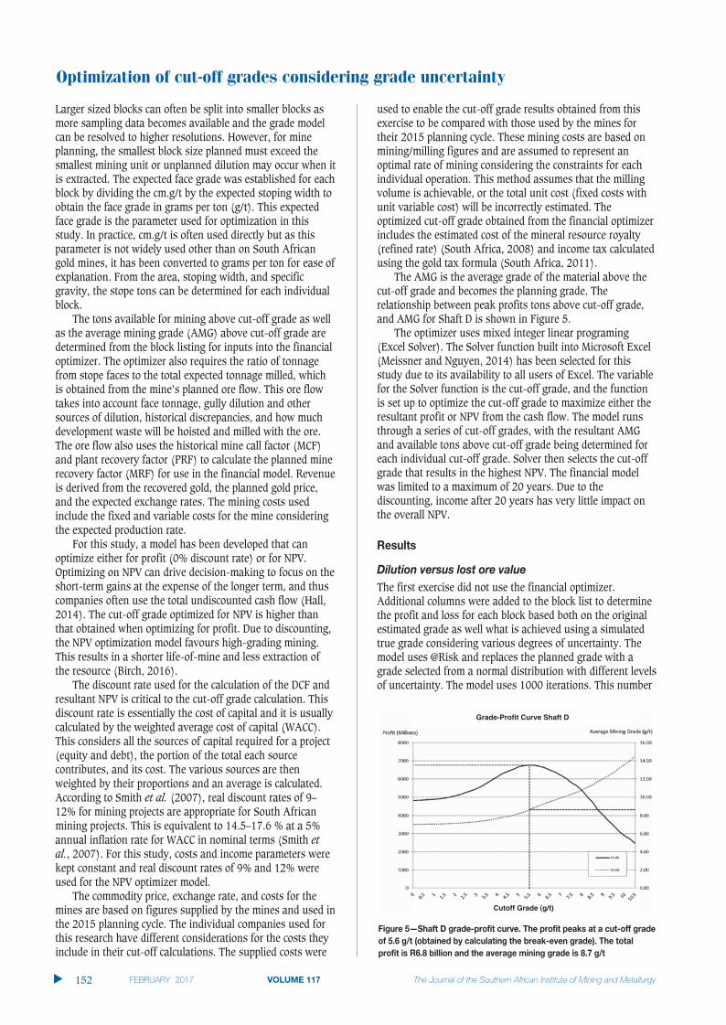
Optimization of cut-off grades considering grade uncertainty
Larger sized blocks can often be split into smaller blocks asmore sampling data becomes available and the grade modelcan be resolved to higher resolutions. However, for mineplanning, the smallest block size planned must exceed thesmallest mining unit or unplanned dilution may occur when itis extracted. The expected face grade was established for eachblock by dividing the cm.g/t by the expected stoping width toobtain the face grade in grams per ton (g/t). This expectedface grade is the parameter used for optimization in thisstudy. In practice, cm.g/t is often used directly but as thisparameter is not widely used other than on South Africangold mines, it has been converted to grams per ton for ease ofexplanation. From the area, stoping width, and specificgravity, the stope tons can be determined for each individualblock.
The tons available for mining above cut-off grade as wellas the average mining grade (AMG) above cut-off grade aredetermined from the block listing for inputs into the financialoptimizer. The optimizer also requires the ratio of tonnagefrom stope faces to the total expected tonnage milled, whichis obtained from the mine’s planned ore flow. This ore flowtakes into account face tonnage, gully dilution and othersources of dilution, historical discrepancies, and how muchdevelopment waste will be hoisted and milled with the ore.The ore flow also uses the historical mine call factor (MCF)and plant recovery factor (PRF) to calculate the planned minerecovery factor (MRF) for use in the financial model. Revenueis derived from the recovered gold, the planned gold price,and the expected exchange rates. The mining costs usedinclude the fixed and variable costs for the mine consideringthe expected production rate.
For this study, a model has been developed that canoptimize either for profit (0% discount rate) or for NPV.Optimizing on NPV can drive decision-making to focus on theshort-term gains at the expense of the longer term, and thuscompanies often use the total undiscounted cash flow (Hall,2014). The cut-off grade optimized for NPV is higher thanthat obtained when optimizing for profit. Due to discounting,the NPV optimization model favours high-grading mining.This results in a shorter life-of-mine and less extraction ofthe resource (Birch, 2016).
The discount rate used for the calculation of the DCF andresultant NPV is critical to the cut-off grade calculation. Thisdiscount rate is essentially the cost of capital and it is usuallycalculated by the weighted average cost of capital (WACC).This considers all the sources of capital required for a project(equity and debt), the portion of the total each sourcecontributes, and its cost. The various sources are thenweighted by their proportions and an average is calculated.According to Smith et al. (2007), real discount rates of 9–12% for mining projects are appropriate for South Africanmining projects. This is equivalent to 14.5–17.6 % at a 5%annual inflation rate for WACC in nominal terms (Smith etal., 2007). For this study, costs and income parameters werekept constant and real discount rates of 9% and 12% wereused for the NPV optimizer model.
The commodity price, exchange rate, and costs for themines are based on figures supplied by the mines and used inthe 2015 planning cycle. The individual companies used forthis research have different considerations for the costs theyinclude in their cut-off calculations. The supplied costs were
used to enable the cut-off grade results obtained from thisexercise to be compared with those used by the mines fortheir 2015 planning cycle. These mining costs are based onmining/milling figures and are assumed to represent anoptimal rate of mining considering the constraints for eachindividual operation. This method assumes that the millingvolume is achievable, or the total unit cost (fixed costs withunit variable cost) will be incorrectly estimated. Theoptimized cut-off grade obtained from the financial optimizerincludes the estimated cost of the mineral resource royalty(refined rate) (South Africa, 2008) and income tax calculatedusing the gold tax formula (South Africa, 2011).
The AMG is the average grade of the material above thecut-off grade and becomes the planning grade. Therelationship between peak profits tons above cut-off grade,and AMG for Shaft D is shown in Figure 5.
The optimizer uses mixed integer linear programing(Excel Solver). The Solver function built into Microsoft Excel(Meissner and Nguyen, 2014) has been selected for thisstudy due to its availability to all users of Excel. The variablefor the Solver function is the cut-off grade, and the functionis set up to optimize the cut-off grade to maximize either theresultant profit or NPV from the cash flow. The model runsthrough a series of cut-off grades, with the resultant AMGand available tons above cut-off grade being determined foreach individual cut-off grade. Solver then selects the cut-offgrade that results in the highest NPV. The financial modelwas limited to a maximum of 20 years. Due to thediscounting, income after 20 years has very little impact onthe overall NPV.
The first exercise did not use the financial optimizer.Additional columns were added to the block list to determinethe profit and loss for each block based both on the originalestimated grade as well what is achieved using a simulatedtrue grade considering various degrees of uncertainty. Themodel uses @Risk and replaces the planned grade with agrade selected from a normal distribution with different levelsof uncertainty. The model uses 1000 iterations. This number
�
152 VOLUME 117
Grade-Profit Curve Shaft D
Cutoff Grade (g/t)

was selected to ensure a representative spread of values andexceeds the number used by @Risk if using the automaticfunction, which runs until a stable output is obtained. Theresults for Shaft B are shown in Tables I–V.
In Table I, there is no uncertainty in the model and thusthe value of the dilution and the lost ore is zero. In Tables IIto V, progressively higher uncertainty is applied and thus theamounts of ore and waste included in the type I and type IIerrors become significantly greater. The cut-off grade usedfor this exercise is 7.09 g/t, which is the cut-off gradeobtained for this mine when optimized for profit (0% NPV),and no uncertainty is considered.
What is immediately apparent from this exercise is thehigh value lost due to type II error. When the uncertainty is5%, this figure is R47 million. When the uncertainty is set to20%, the value lost increases to R574 million. Figure 6 showsthe relationship between the waste and dilution cost and lost
ore for Shaft B with 10% uncertainty at different cut-offgrades (0.5 g/t intervals). The difference line shown in thegraph represents the difference between the waste anddilution cost for a particular cut-off grade and the lost ore.
The difference peaks at 6.5 g/t. This indicates thatlowering the cut-off grade from 7.09 g/t to 6.50 g/t could addvalue. It must be noted, however, that this approachconsiders just the direct mining costs. Similar trends arenoted for shafts A, C, and D.
Mineral resource royalty costs are not included as thesevary with overall profitability and not the profitability of theindividual blocks. Income tax is also not considered in thiscalculation as it is paid only on taxable income (profit) and
Optimization of cut-off grades considering grade uncertainty
VOLUME 117 153 �
Table I
Dilution kilograms 0 0 0Lost kilograms 0 0 0Waste and dilution cost (millions) R0 R0 R0Lost ore value (millions) R0 R0 R0
Table II
Dilution kilograms 520 4 853 10 104Lost kilograms 85 1 037 20 057Waste and dilution cost (millions) –R1 052 –R756 –R454Lost ore value (millions) R1 010 R47 R4
Table III
Dilution kilograms 683 5 204 10 340Lost kilograms 170 2 050 29 600Waste and dilution cost (millions) –R1 126 –R 774 –R 419Lost ore value (millions) R1 467 R90 R6
Table IV
Dilution kilograms 802 5 947 12 036Lost kilograms 441 6 257 37 662Waste and dilution cost (millions) –R1 375 –R825 –R388Lost ore value (millions) R1 739 R253 R18
Table V
Dilution kilograms 2 034 7 747 14 204Lost kilograms 3 161 22 416 66 157Waste and dilution cost (millions) –R2 152 –R1 094 –R520Lost ore value (millions) R2 274 R574 –R401
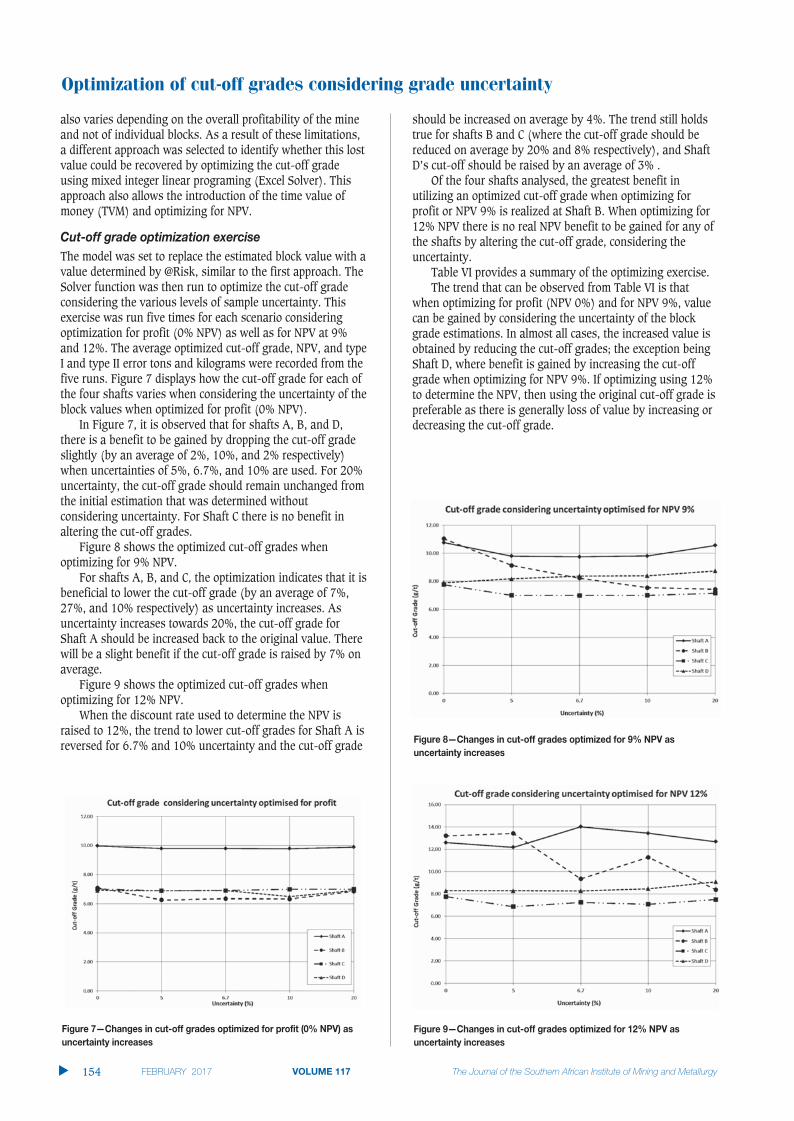
Optimization of cut-off grades considering grade uncertainty
also varies depending on the overall profitability of the mineand not of individual blocks. As a result of these limitations,a different approach was selected to identify whether this lostvalue could be recovered by optimizing the cut-off gradeusing mixed integer linear programing (Excel Solver). Thisapproach also allows the introduction of the time value ofmoney (TVM) and optimizing for NPV.
The model was set to replace the estimated block value with avalue determined by @Risk, similar to the first approach. TheSolver function was then run to optimize the cut-off gradeconsidering the various levels of sample uncertainty. Thisexercise was run five times for each scenario consideringoptimization for profit (0% NPV) as well as for NPV at 9%and 12%. The average optimized cut-off grade, NPV, and typeI and type II error tons and kilograms were recorded from thefive runs. Figure 7 displays how the cut-off grade for each ofthe four shafts varies when considering the uncertainty of theblock values when optimized for profit (0% NPV).
In Figure 7, it is observed that for shafts A, B, and D,there is a benefit to be gained by dropping the cut-off gradeslightly (by an average of 2%, 10%, and 2% respectively)when uncertainties of 5%, 6.7%, and 10% are used. For 20%uncertainty, the cut-off grade should remain unchanged fromthe initial estimation that was determined withoutconsidering uncertainty. For Shaft C there is no benefit inaltering the cut-off grades.
Figure 8 shows the optimized cut-off grades whenoptimizing for 9% NPV.
For shafts A, B, and C, the optimization indicates that it isbeneficial to lower the cut-off grade (by an average of 7%,27%, and 10% respectively) as uncertainty increases. Asuncertainty increases towards 20%, the cut-off grade forShaft A should be increased back to the original value. Therewill be a slight benefit if the cut-off grade is raised by 7% onaverage.
Figure 9 shows the optimized cut-off grades whenoptimizing for 12% NPV.
When the discount rate used to determine the NPV israised to 12%, the trend to lower cut-off grades for Shaft A isreversed for 6.7% and 10% uncertainty and the cut-off grade
should be increased on average by 4%. The trend still holdstrue for shafts B and C (where the cut-off grade should bereduced on average by 20% and 8% respectively), and ShaftD’s cut-off should be raised by an average of 3% .
Of the four shafts analysed, the greatest benefit inutilizing an optimized cut-off grade when optimizing forprofit or NPV 9% is realized at Shaft B. When optimizing for12% NPV there is no real NPV benefit to be gained for any ofthe shafts by altering the cut-off grade, considering theuncertainty.
Table VI provides a summary of the optimizing exercise. The trend that can be observed from Table VI is that
when optimizing for profit (NPV 0%) and for NPV 9%, valuecan be gained by considering the uncertainty of the blockgrade estimations. In almost all cases, the increased value isobtained by reducing the cut-off grades; the exception beingShaft D, where benefit is gained by increasing the cut-offgrade when optimizing for NPV 9%. If optimizing using 12%to determine the NPV, then using the original cut-off grade ispreferable as there is generally loss of value by increasing ordecreasing the cut-off grade.
�
154 VOLUME 117
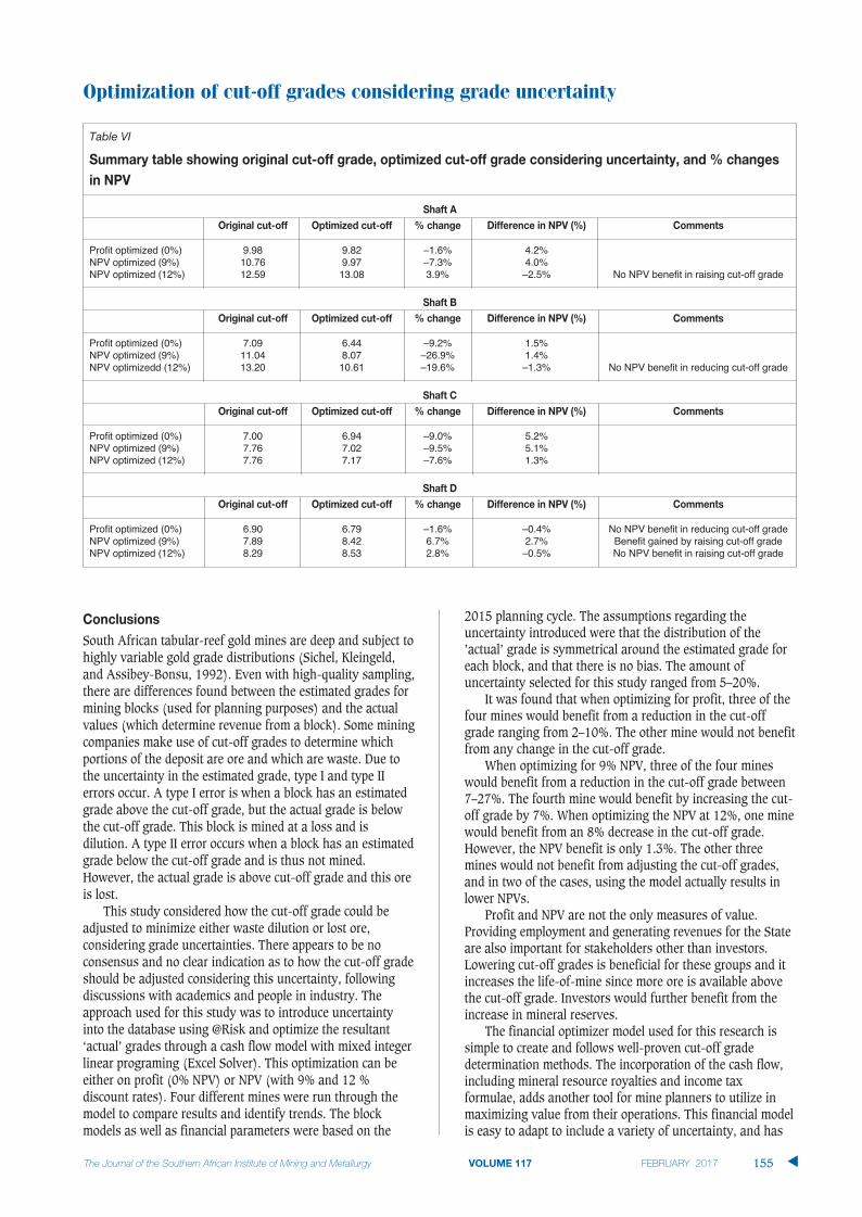
Optimization of cut-off grades considering grade uncertainty
VOLUME 117 155 �
South African tabular-reef gold mines are deep and subject tohighly variable gold grade distributions (Sichel, Kleingeld,and Assibey-Bonsu, 1992). Even with high-quality sampling,there are differences found between the estimated grades formining blocks (used for planning purposes) and the actualvalues (which determine revenue from a block). Some miningcompanies make use of cut-off grades to determine whichportions of the deposit are ore and which are waste. Due tothe uncertainty in the estimated grade, type I and type IIerrors occur. A type I error is when a block has an estimatedgrade above the cut-off grade, but the actual grade is belowthe cut-off grade. This block is mined at a loss and isdilution. A type II error occurs when a block has an estimatedgrade below the cut-off grade and is thus not mined.However, the actual grade is above cut-off grade and this oreis lost.
This study considered how the cut-off grade could beadjusted to minimize either waste dilution or lost ore,considering grade uncertainties. There appears to be noconsensus and no clear indication as to how the cut-off gradeshould be adjusted considering this uncertainty, followingdiscussions with academics and people in industry. Theapproach used for this study was to introduce uncertaintyinto the database using @Risk and optimize the resultant‘actual’ grades through a cash flow model with mixed integerlinear programing (Excel Solver). This optimization can beeither on profit (0% NPV) or NPV (with 9% and 12 %discount rates). Four different mines were run through themodel to compare results and identify trends. The blockmodels as well as financial parameters were based on the
2015 planning cycle. The assumptions regarding theuncertainty introduced were that the distribution of the’actual’ grade is symmetrical around the estimated grade foreach block, and that there is no bias. The amount ofuncertainty selected for this study ranged from 5–20%.
It was found that when optimizing for profit, three of thefour mines would benefit from a reduction in the cut-offgrade ranging from 2–10%. The other mine would not benefitfrom any change in the cut-off grade.
When optimizing for 9% NPV, three of the four mineswould benefit from a reduction in the cut-off grade between7–27%. The fourth mine would benefit by increasing the cut-off grade by 7%. When optimizing the NPV at 12%, one minewould benefit from an 8% decrease in the cut-off grade.However, the NPV benefit is only 1.3%. The other threemines would not benefit from adjusting the cut-off grades,and in two of the cases, using the model actually results inlower NPVs.
Profit and NPV are not the only measures of value.Providing employment and generating revenues for the Stateare also important for stakeholders other than investors.Lowering cut-off grades is beneficial for these groups and itincreases the life-of-mine since more ore is available abovethe cut-off grade. Investors would further benefit from theincrease in mineral reserves.
The financial optimizer model used for this research issimple to create and follows well-proven cut-off gradedetermination methods. The incorporation of the cash flow,including mineral resource royalties and income taxformulae, adds another tool for mine planners to utilize inmaximizing value from their operations. This financial modelis easy to adapt to include a variety of uncertainty, and has
Table VI
Profit optimized (0%) 9.98 9.82 –1.6% 4.2%NPV optimized (9%) 10.76 9.97 –7.3% 4.0%NPV optimized (12%) 12.59 13.08 3.9% –2.5% No NPV benefit in raising cut-off grade
Profit optimized (0%) 7.09 6.44 –9.2% 1.5%NPV optimized (9%) 11.04 8.07 –26.9% 1.4%NPV optimizedd (12%) 13.20 10.61 –19.6% –1.3% No NPV benefit in reducing cut-off grade
Profit optimized (0%) 7.00 6.94 –9.0% 5.2%NPV optimized (9%) 7.76 7.02 –9.5% 5.1%NPV optimized (12%) 7.76 7.17 –7.6% 1.3%
Profit optimized (0%) 6.90 6.79 –1.6% –0.4% No NPV benefit in reducing cut-off gradeNPV optimized (9%) 7.89 8.42 6.7% 2.7% Benefit gained by raising cut-off gradeNPV optimized (12%) 8.29 8.53 2.8% –0.5% No NPV benefit in raising cut-off grade

Optimization of cut-off grades considering grade uncertainty
been used in this example to investigate how block gradeuncertainty can affect cut-off grades. Each mine is unique,and grade uncertainty should be modelled individually todetermine if there is any benefit in adjusting the cut-offgrade. The accuracy of the optimizer model would beincreased by using the actual distribution of uncertainty. Anysampling bias could also be included in the model if it occurson the mine. This would indicate in which direction cut-offgrades should be adjusted to minimize the adverse effects ofdilution or to recover lost ore.
ACKERMAN, J. 2016. Suggested adjustments to cut-off grade consideringuncertainty [Interview] (February 2016).
BIRCH, C. 2016. Impact of discount rates on cut-off grades for narrow, tabulargold deposits. Journal of the Southern African Institute of Mining andMetallurgy, vol. 116, no. 2. pp. 115–122.
BIRCH, C. 2016. Impact of the South African mineral resource royalty on cut-offgrades for narrow, tabular Witwatersrand gold deposits. Journal of theSouthern African Institute of Mining and Metallurgy, vol. 116, no. 3. pp. 237–246.
HALL, B. 2014. Cut-off grades and optimising the strategic mine plan. SpectrumSeries 20. Australasian Institute of Mining and Metallurgy, Carlton,Victoria.
KRIGE, D. and ASSIBEY-BONSU, W. 1999. Use of direct and indirect distributionsof selective mining units for estimation of recoverable resource/reservesfor new mining projects. Colorado School of Mines.
LANE, K.F. 1988. The Economic Definition of Ore. Mining Journal Books,London.
MEISSNER, J. and NGUYEN, T. 2014. Meiss Research Group. An introduction tospreadsheet optimization using Excel Solver. http://www.meiss.com/download/Spreadsheet-Optimization-Solver.pdf [Accessed 2 December2014].
MINNITT, R. 2004. Cut-off grade determination for the maximum value of asmall Wits-type gold mining operation. Journal of the South AfricanInstitute of Mining and Metallurgy, vol. 104, no. 5. pp. 277–283.
MINNITT, R. 2015. Poor sampling, grade distributions, and financial outcomes.Proceedings of Mine Planning and Equipment Selection (MPES) 2015,Sandton, South Africa, 11 November. Southern African Institute of Miningand Metallurgy, Johannesburg. pp. 133–147.
MINNITT, R. 2016. Suggested adjustments to cut-off grade consideringuncertainty. [Interview] (February 2016).
SAMREC. 2009. South African Mineral Resource Committee. The South AfricanCode for Reporting of Exploration Results, Mineral Resources and MineralReserves (the SAMREC Code). 2007 Edition as amended July 2009.http://www.samcode.co.za/downloads/SAMREC2009.pdf [Accessed 4March 2013].
SICHEL, H.S., KLEINGELD, W.J., and ASSIBEY-BONSU, W. 1992. A comparative studyof three frequency-distribution models for use in ore evaluation. Journal ofthe South African Institute of Mining and Metallurgy, vol. 92, no. 4. pp. 91–99.
SMITH, G.L., PEARSON-TAYLOR, J., ANDERSON, D.C., and MARSH, A.M. 2007. Projectvaluation, capital investment and strategic alignment—tools andtechniques at Anglo Platinum. Journal of the Southern African Institute ofMining and Metallurgy, vol. 107. pp. 67–74.
SOUTH AFRICA. 2008. Mineral and Petrolium Resources Royalty Act 2008.http://www.info.gov.za/view/DownloadFileAction?id=92824 [Accessed 4March 2013].
SOUTH AFRICA. 2011. Guide for tax rates/duties/levies (2010/2011 and prioryears). http://www.wvdw.co.za/wvdwcorporate/TaxRatesDutiesLevies201011andprior9November2010[1].pdf [Accessed 4 March 2013].
TOLMAY, L. 2014. On the reduction of algorithmic smoothing of krigedestimates. Journal of the Southern African Institute of Mining andMetallurgy, vol. 114, no. 8. pp. 667–672.
TOLMAY, L. 2016. Suggested adjustments to cut-off grade consideringuncertainty [Interview] (March 2016).
UNDERHILL, L. and BRADFIELD, D. 1994. IntroSTAT. 5th edn. Juta, Cape Town. �
�
156 VOLUME 117
GROWINGwww.harmony.co.zaMining to benefit all stakeholders
Leveraging 60+ years of gold mining experience
1.5Moz within three years – at less than US$950 an ounce
Improving our margins

The ventilation of underground mines,irrespective of the type of mine and miningmethod, is divided into two broad branches,the primary ventilation and secondary orauxiliary ventilation. The primary ventilationis responsible for the total volumetric flowthrough the mine and the auxiliary ventilationis responsible for the ventilation of thedevelopment ends, production areas, andfacilities disconnected from the main circuitwith no through-ventilation connections.Auxiliary ventilation is the more difficult toachieve (Bise, 1996), and the disruption ofthis ventilation system is considered to be oneof the primary factors contributing to methaneand coal dust explosions (Creedy, 1996). Anumber of causalities have been recorded bymany authors due to these explosions (Phillipsand Brandt, 1995; Dubinski et al., 2011;Phillips, 2015). The ventilation of shortheadings, less than 10 m in depth, can becarried out without the use of any auxiliaryequipment (Feroze and Phillips, 2015).However, for headings deeper than 10 m,auxiliary ventilation systems are required.These are generally classified into the three
basic types, namely line brattice (LB)ventilation systems, ducted fan systems, andjet fans (Figures 1 through Figure 3 respec-tively).
Ducted fan systems are also classified intothree types, namely forcing, exhaust, andoverlap. The decision to select a particular typeof ducted fan system depends on the nature ofthe hazard (Pawinski and Roszkowski, 1985;McPherson, 1993). A ducted fan is generallyinstalled on the intake side in the forcingconfiguration and on the return side in theexhaust configuration (Reed and Taylor,2007).
The forcing system of duct and fanconsists of a line of ducting, to which a fan isconnected to force air into the heading. It isusually used in mines with high methanehazards, and can effectively remove themethane hazard through dilution (Taylor etal., 1997). Szlazak et al. (2003) have shownthat the methane concentration measured inheadings is lower with the forcing system thanwith exhaust systems under the sameventilation and methane emission conditions.The high velocity of air helps in mixing themethane with air, which prevents it fromsettling on the roof and provides cooler air atthe face (McPherson, 1993). Studies bySchultz (1993) and Kissell (2003) indicatedthat the proportion of fresh air reaching theface is 39.9% for the forcing system and 10%for the exhaust system. Torano et al. (2009)found these proportions to be 35% and 12%,respectively. The forcing system results in apositive gauge pressure, thus a cheaper andflexible duct can be used (AMC Consultants,2005). In South African coal mines, forcingducted fans generally are used.
Analysis of the effect of ducted fansystem variables on ventilation in anempty heading using CFDby T. Feroze* and B. Genc*
The effect of some of the system variables in forcing and exhaustingducted fan systems on ventilation in an empty heading was investigatedusing computational fluid dynamics(CFD) and comparative analyses. Thediameter of the duct, duct mouth to face distance, and the power of the fan(quantity delivered by the fan) were varied and their effect on ventilationdetermined through a comparative analysis of the flow rates calculatedclose to the face of the heading. Estimation models were developed, whichcan be used to calculate the flow rate close to the face of the emptyheading for different settings of the system variables studied.
The study showed that recirculation for a forcing ducted fan systemcan be reduced by increasing the duct diameter or increasing the ductmouth to face distance. For the exhausting ducted fan system, higher flowrates were achieved by reducing the duct mouth to face distance, andincreasing the fan design flow rate and duct diameter.
The outcomes of this investigation will help ventilation engineers indeciding the optimum duct fan system required for sufficient ventilation.
ducted fan, ventilation, CFD.
* School of Mining Engineering, University of theWitwatersrand, South Africa.
© The Southern African Institute of Mining andMetallurgy, 2017. ISSN 2225-6253. Paper receivedMar. 2016; revised paper received Oct. 2016.
157VOLUME 117 �
http://dx.doi.org/10.17159/2411-9717/2017/v117n2a7
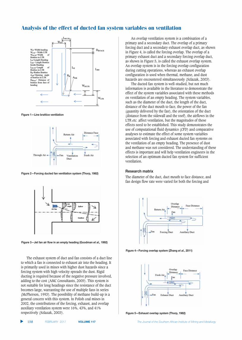
Analysis of the effect of ducted fan system variables on ventilation
The exhaust system of duct and fan consists of a duct lineto which a fan is connected to exhaust air into the heading. Itis primarily used in mines with higher dust hazards since aforcing system with high velocity spreads the dust. Rigidducting is required because of the negative pressure involved,adding to the cost (AMC Consultants, 2005). This system isnot suitable for long headings since the resistance of the ductbecomes large, warranting the use of multiple fans in series(McPherson, 1993). The possibility of methane build-up is ageneral concern with this system. In Polish coal mines in2002, the contributions of the forcing, exhaust, and overlapauxiliary ventilation system were 16%, 43%, and 41%respectively (Szlazak, 2003).
An overlap ventilation system is a combination of aprimary and a secondary duct. The overlap of a primaryforcing duct and a secondary exhaust overlap duct, as shownin Figure 4, is called the forcing overlap. The overlap of aprimary exhaust duct and a secondary forcing overlap duct,as shown in Figure 5, is called the exhaust overlap system.An overlap system is in the forcing overlap configurationduring cutting operations, whereas an exhaust overlapconfiguration is used when thermal, methane, and dusthazards are encountered simultaneously (Szlazak, 2003).
The ducted fan system is well-studied, but not muchinformation is available in the literature to demonstrate theeffect of the system variables associated with these methodson ventilation of an empty heading. The system variables,such as the diameter of the duct, the length of the duct,distance of the duct mouth to face, the power of the fan(quantity delivered by the fan), the orientation of the duct(distance from the sidewall and the roof), the airflows in theLTR etc. affect ventilation, but the magnitudes of theseeffects need to be established. This study demonstrates theuse of computational fluid dynamics (CFD) and comparativeanalyses to estimate the effect of some system variablesassociated with forcing and exhaust ducted fan systems onthe ventilation of an empty heading. The presence of dustand methane was not considered. The understanding of theseeffects is important and will help ventilation engineers in theselection of an optimum ducted fan system for sufficientventilation.
The diameter of the duct, duct mouth to face distance, andfan design flow rate were varied for both the forcing and
�
158 VOLUME 117

exhaust duct systems. The range of values chosen for thesevariables, and the values for those that were kept constant,were based on the most common settings in practice. Thedetails of these variables and their values are given in Table Iand shown in Figure 6 for both the forcing and exhaustducted fan systems. All possible combinations of thesevariables were used to develop scenarios for each fan system.The ducted systems considered were assumed to be leakage-free.
The numerical modelling, comprising the creation of thegeometry, meshing of the geometry, solving the complex setof mathematical equations iteratively, and analysis of theresults, was carried out using the commercially availableANSYS Fluent numerical code. The K- realizable model wasused for this study. This model was used after validating theresults, using experimental studies described later. Theexperimental results showed that the model is suitable forstudying ducted fan systems using CFD. The details of theturbulence model are available in the software manual(ANSYS Fluent Theory Guide, 2015).
The three-dimensional models were generated in the ANSYSdesign modeller software for all the cases. The length of theLTR modelled on both the upstream and downstream side ofthe heading was kept at 10 m for all the cases. As far aspossible, a structured hexahedral mesh with a size of 0.04 mwas created using the ANSYS Mesher. The mesh size wasselected after performing mesh-independence tests. Inflationlayers, where required, were used at the boundaries of the
geometries to allow smooth transition from the laminar flownear the wall to turbulent flow away from the walls.
� At the inlet of the LTR, ‘Velocity inlet’ boundarycondition was used with an air velocity of 2 m/s
� At the outlet of the LTR, ‘Outflow’ boundary conditionwas used
� ‘Fluid fan’ boundary condition was used for both thefans
� At all the walls an enhanced wall function was used inall the simulations.
The variation of the fan design flow rates (maintained at theexit of the duct), diameter, and length of the duct changedthe volumetric flow rates inside the heading at similarlocations. The air flow rates (into the heading) close to theface of the heading were calculated for each case and aretabulated in Table II. These flow rates were calculated usingthe positive axial velocities going into the planes constructedparallel to the face of the heading at distances of 0.5 m, 0.4 m, and 0.3 m from the face. The percentage of fresh air atthese distances was also calculated, using the quantity of airdelivered by the fan and the quantity of air actually presentat these distances (assuming the quantity of air delivered bythe fan is reaching the face of the heading). This enabled thecalculation of the maximum percentage of fresh air reachingthe face and thus the minimum recirculation (100 - % offresh air) near the face of the heading for each case.
The total flow rates and the amount of fresh air close tothe face of the heading, using a forcing ducted fan system,varied as follows.
� Volumetric flow rate close to the face of the heading:– When the diameter of the duct and the duct exit
flow rate were kept constant, the flow rate closeto the face of the heading increased withdecreasing duct mouth to face distance
– When the diameter of the duct and duct mouth toface distance were kept constant, the flow rateclose to the face of the heading increased withincreasing air flow exiting from the duct
– When the duct mouth to face distance and theduct exit flow rate were kept constant, the flowrate close to the face of the heading increasedwith decreasing duct diameter, as expected.
Analysis of the effect of ducted fan system variables on ventilation
VOLUME 117 159 �
Table I
Forcing fan Value 0.57 2.97 8
6.6 x 3 x 200.76 3.713
210
1 0.5Exhaust Value 0.57 2.97 2
fan 0.76 3.713 4
Flow rates were chosen based on the legal requirement of 0.15m3/s/m2 and 25 %
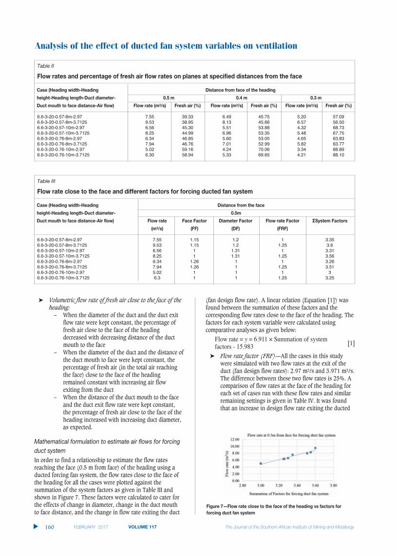
Analysis of the effect of ducted fan system variables on ventilation
� Volumetric flow rate of fresh air close to the face of theheading:
– When the diameter of the duct and the duct exitflow rate were kept constant, the percentage offresh air close to the face of the headingdecreased with decreasing distance of the ductmouth to the face
– When the diameter of the duct and the distance ofthe duct mouth to face were kept constant, thepercentage of fresh air (in the total air reachingthe face) close to the face of the headingremained constant with increasing air flowexiting from the duct
– When the distance of the duct mouth to the faceand the duct exit flow rate were kept constant,the percentage of fresh air close to the face of theheading increased with increasing duct diameter,as expected.
In order to find a relationship to estimate the flow ratesreaching the face (0.5 m from face) of the heading using aducted forcing fan system, the flow rates close to the face ofthe heading for all the cases were plotted against thesummation of the system factors as given in Table III andshown in Figure 7. These factors were calculated to cater forthe effects of change in diameter, change in the duct mouthto face distance, and the change in flow rate exiting the duct
(fan design flow rate). A linear relation (Equation [1]) wasfound between the summation of these factors and thecorresponding flow rates close to the face of the heading. Thefactors for each system variable were calculated usingcomparative analyses as given below:
Flow rate = y = 6.911 × Summation of system [1]factors - 15.983
� Flow rate factor (FRF)—All the cases in this studywere simulated with two flow rates at the exit of theduct (fan design flow rates): 2.97 m3/s and 3.971 m3/s.The difference between these two flow rates is 25%. Acomparison of flow rates at the face of the heading foreach set of cases run with these flow rates and similarremaining settings is given in Table IV. It was foundthat an increase in design flow rate exiting the ducted
�
160 VOLUME 117
Table II
6.6-3-20-0.57-8m-2.97 7.55 39.33 6.49 45.75 5.20 57.096.6-3-20-0.57-8m-3.7125 9.53 38.95 8.13 45.66 6.57 56.506.6-3-20-0.57-10m-2.97 6.56 45.30 5.51 53.88 4.32 68.736.6-3-20-0.57-10m-3.7125 8.25 44.99 6.96 53.35 5.48 67.756.6-3-20-0.76-8m-2.97 6.34 46.85 5.60 53.05 4.65 63.836.6-3-20-0.76-8m-3.7125 7.94 46.76 7.01 52.99 5.82 63.776.6-3-20-0.76-10m-2.97 5.02 59.16 4.24 70.06 3.34 88.896.6-3-20-0.76-10m-3.7125 6.30 58.94 5.33 69.65 4.21 88.10
Table III
6.6-3-20-0.57-8m-2.97 7.55 1.15 1.2 1 3.356.6-3-20-0.57-8m-3.7125 9.53 1.15 1.2 1.25 3.66.6-3-20-0.57-10m-2.97 6.56 1 1.31 1 3.316.6-3-20-0.57-10m-3.7125 8.25 1 1.31 1.25 3.566.6-3-20-0.76-8m-2.97 6.34 1.26 1 1 3.266.6-3-20-0.76-8m-3.7125 7.94 1.26 1 1.25 3.516.6-3-20-0.76-10m-2.97 5.02 1 1 1 36.6-3-20-0.76-10m-3.7125 6.3 1 1 1.25 3.25
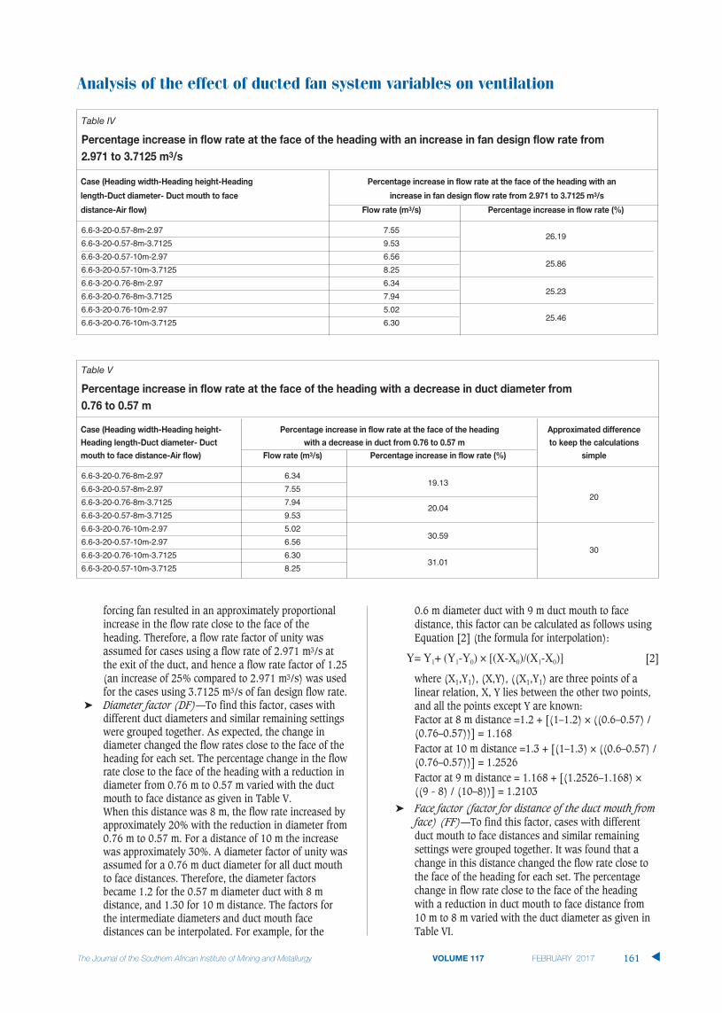
forcing fan resulted in an approximately proportionalincrease in the flow rate close to the face of theheading. Therefore, a flow rate factor of unity wasassumed for cases using a flow rate of 2.971 m3/s atthe exit of the duct, and hence a flow rate factor of 1.25(an increase of 25% compared to 2.971 m3/s) was usedfor the cases using 3.7125 m3/s of fan design flow rate.
� Diameter factor (DF)—To find this factor, cases withdifferent duct diameters and similar remaining settingswere grouped together. As expected, the change indiameter changed the flow rates close to the face of theheading for each set. The percentage change in the flowrate close to the face of the heading with a reduction indiameter from 0.76 m to 0.57 m varied with the ductmouth to face distance as given in Table V. When this distance was 8 m, the flow rate increased byapproximately 20% with the reduction in diameter from 0.76 m to 0.57 m. For a distance of 10 m the increasewas approximately 30%. A diameter factor of unity wasassumed for a 0.76 m duct diameter for all duct mouthto face distances. Therefore, the diameter factorsbecame 1.2 for the 0.57 m diameter duct with 8 mdistance, and 1.30 for 10 m distance. The factors forthe intermediate diameters and duct mouth facedistances can be interpolated. For example, for the
0.6 m diameter duct with 9 m duct mouth to face distance, this factor can be calculated as follows usingEquation [2] (the formula for interpolation):
Y= Y1+ (Y1-Y0) × [(X-X0)/(X1-X0)] [2]
where (X1,Y1), (X,Y), ((X1,Y1) are three points of alinear relation, X, Y lies between the other two points,and all the points except Y are known:Factor at 8 m distance =1.2 + [(1–1.2) × ((0.6–0.57) /(0.76–0.57))] = 1.168Factor at 10 m distance =1.3 + [(1–1.3) × ((0.6–0.57) /(0.76–0.57))] = 1.2526Factor at 9 m distance = 1.168 + [(1.2526–1.168) × ((9 - 8) / (10–8))] = 1.2103
� Face factor (factor for distance of the duct mouth fromface) (FF)—To find this factor, cases with differentduct mouth to face distances and similar remainingsettings were grouped together. It was found that achange in this distance changed the flow rate close tothe face of the heading for each set. The percentagechange in flow rate close to the face of the headingwith a reduction in duct mouth to face distance from 10 m to 8 m varied with the duct diameter as given inTable VI.
Analysis of the effect of ducted fan system variables on ventilation
VOLUME 117 161 �
Table IV
6.6-3-20-0.57-8m-2.97 7.5526.19
6.6-3-20-0.57-8m-3.7125 9.53
6.6-3-20-0.57-10m-2.97 6.5625.86
6.6-3-20-0.57-10m-3.7125 8.25
6.6-3-20-0.76-8m-2.97 6.3425.23
6.6-3-20-0.76-8m-3.7125 7.94
6.6-3-20-0.76-10m-2.97 5.0225.46
6.6-3-20-0.76-10m-3.7125 6.30
Table V
6.6-3-20-0.76-8m-2.97 6.3419.13
206.6-3-20-0.57-8m-2.97 7.55
6.6-3-20-0.76-8m-3.7125 7.9420.04
6.6-3-20-0.57-8m-3.7125 9.53
6.6-3-20-0.76-10m-2.97 5.0230.59
306.6-3-20-0.57-10m-2.97 6.56
6.6-3-20-0.76-10m-3.7125 6.3031.01
6.6-3-20-0.57-10m-3.7125 8.25
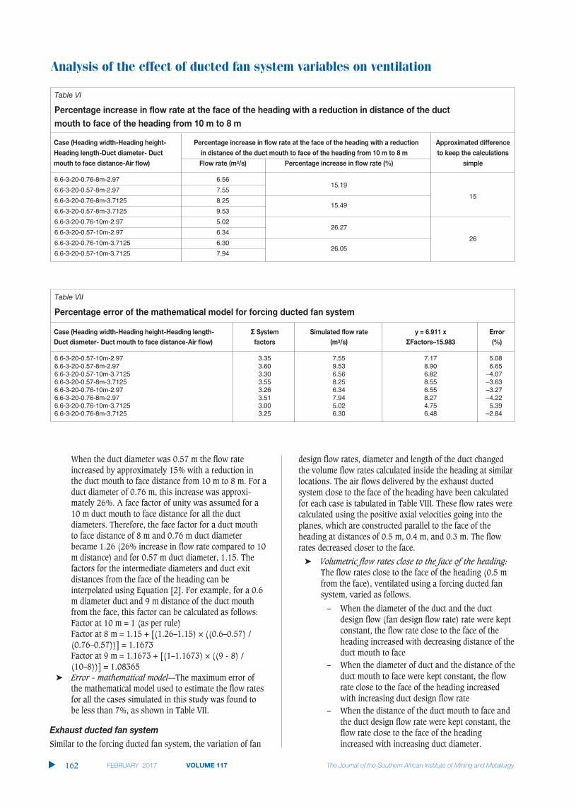
Analysis of the effect of ducted fan system variables on ventilation
When the duct diameter was 0.57 m the flow rateincreased by approximately 15% with a reduction inthe duct mouth to face distance from 10 m to 8 m. For aduct diameter of 0.76 m, this increase was approxi-mately 26%. A face factor of unity was assumed for a10 m duct mouth to face distance for all the ductdiameters. Therefore, the face factor for a duct mouthto face distance of 8 m and 0.76 m duct diameter became 1.26 (26% increase in flow rate compared to 10m distance) and for 0.57 m duct diameter, 1.15. Thefactors for the intermediate diameters and duct exitdistances from the face of the heading can be interpolated using Equation [2]. For example, for a 0.6m diameter duct and 9 m distance of the duct mouthfrom the face, this factor can be calculated as follows:Factor at 10 m = 1 (as per rule)Factor at 8 m = 1.15 + [(1.26–1.15) × ((0.6–0.57) / (0.76–0.57))] = 1.1673Factor at 9 m = 1.1673 + [(1–1.1673) × ((9 - 8) / (10–8))] = 1.08365
� Error - mathematical model—The maximum error ofthe mathematical model used to estimate the flow ratesfor all the cases simulated in this study was found tobe less than 7%, as shown in Table VII.
Similar to the forcing ducted fan system, the variation of fan
design flow rates, diameter and length of the duct changedthe volume flow rates calculated inside the heading at similarlocations. The air flows delivered by the exhaust ductedsystem close to the face of the heading have been calculatedfor each case is tabulated in Table VIII. These flow rates werecalculated using the positive axial velocities going into theplanes, which are constructed parallel to the face of theheading at distances of 0.5 m, 0.4 m, and 0.3 m. The flowrates decreased closer to the face.
� Volumetric flow rates close to the face of the heading:The flow rates close to the face of the heading (0.5 mfrom the face), ventilated using a forcing ducted fansystem, varied as follows.
– When the diameter of the duct and the ductdesign flow (fan design flow rate) rate were keptconstant, the flow rate close to the face of theheading increased with decreasing distance of theduct mouth to face
– When the diameter of duct and the distance of theduct mouth to face were kept constant, the flowrate close to the face of the heading increasedwith increasing duct design flow rate
– When the distance of the duct mouth to face andthe duct design flow rate were kept constant, theflow rate close to the face of the headingincreased with increasing duct diameter.
�
162 VOLUME 117
Table VI
6.6-3-20-0.76-8m-2.97 6.5615.19
156.6-3-20-0.57-8m-2.97 7.55
6.6-3-20-0.76-8m-3.7125 8.2515.49
6.6-3-20-0.57-8m-3.7125 9.53
6.6-3-20-0.76-10m-2.97 5.0226.27
266.6-3-20-0.57-10m-2.97 6.34
6.6-3-20-0.76-10m-3.7125 6.3026.05
6.6-3-20-0.57-10m-3.7125 7.94
Table VII
6.6-3-20-0.57-10m-2.97 3.35 7.55 7.17 5.086.6-3-20-0.57-8m-2.97 3.60 9.53 8.90 6.656.6-3-20-0.57-10m-3.7125 3.30 6.56 6.82 –4.076.6-3-20-0.57-8m-3.7125 3.55 8.25 8.55 –3.636.6-3-20-0.76-10m-2.97 3.26 6.34 6.55 –3.276.6-3-20-0.76-8m-2.97 3.51 7.94 8.27 –4.226.6-3-20-0.76-10m-3.7125 3.00 5.02 4.75 5.396.6-3-20-0.76-8m-3.7125 3.25 6.30 6.48 –2.84
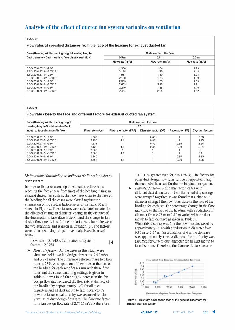
Analysis of the effect of ducted fan system variables on ventilation
VOLUME 117 163 �
In order to find a relationship to estimate the flow ratesreaching the face (0.5 m from face) of the heading, using anexhaust ducted fan system, the flow rates close to the face ofthe heading for all the cases were plotted against thesummation of the system factors as given in Table IX andshown in Figure 8. These factors were calculated to cater forthe effects of change in diameter, change in the distance ofthe duct mouth to face (face factors), and the change in fandesign flow rate. A best fit linear relation was found betweenthe two quantities and is given in Equation [3]. The factorswere calculated using comparative analysis as discussedbelow:
Flow rate = 0.3943 × Summation of system [3]factors + 2.0754
� Flow rate factor—All the cases in this study weresimulated with two fan design flow rates: 2.97 m3/sand 3.971 m3/s. The difference between these two flowrates is 25%. A comparison of flow rates at the face ofthe heading for each set of cases run with these flowrates and the same remaining settings is given in Table X. It was found that a 25% increase in the fandesign flow rate increased the flow rate at the face ofthe heading by approximately 10% for all ductdiameters and all duct mouth to face distances. A flow rate factor equal to unity was assumed for the 2.971 m3/s duct design flow rate. The flow rate factorfor a fan design flow rate of 3.7125 m3/s is therefore
1.10 (10% greater than for 2.971 m3/s). The factors forother duct design flow rates can be interpolated usingthe methods discussed for the forcing duct fan system.
� Diameter factor—To find this factor, cases withdifferent duct diameters and similar remaining settingswere grouped together. It was found that a change indiameter changed the flow rates close to the face of theheading for each set. The percentage change in the flowrate close to the face of the heading with a reduction indiameter from 0.76 m to 0.57 m varied with the ductmouth to face distance as given in Table XI. When this distance was 2 m the flow rate decreased byapproximately 17% with a reduction in diameter from0.76 m to 0.57 m. For a distance of 4 m the decreasewas approximately 14%. A diameter factor of unity wasassumed for 0.76 m duct diameter for all duct mouth toface distances. Therefore, the diameter factors became
Table IX
6.6-3-20-0.57-2m-2.97 1.968 1 0.83 1 2.836.6-3-20-0.57-2m-3.7125 2.155 1.1 0.83 1 2.936.6-3-20-0.57-4m-2.97 1.931 1 0.86 0.98 2.846.6-3-20-0.57-4m-3.7125 2.120 1.1 0.86 0.98 2.946.6-3-20-0.76-2m-2.97 2.365 1 1 1 36.6-3-20-0.76-2m-3.7125 2.603 1.1 1 1 3.16.6-3-20-0.76-4m-2.97 2.240 1 1 0.95 2.956.6-3-20-0.76-4m-3.7125 2.464 1.1 1 0.95 3.05
Table VIII
6.6-3-20-0.57-2m-2.97 1.968 1.64 1.296.6-3-20-0.57-2m-3.7125 2.155 1.79 1.426.6-3-20-0.57-4m-2.97 1.931 1.59 1.246.6-3-20-0.57-4m-3.7125 2.120 1.76 1.396.6-3-20-0.76-2m-2.97 2.365 1.98 1.596.6-3-20-0.76-2m-3.7125 2.603 2.15 1.716.6-3-20-0.76-4m-2.97 2.240 1.88 1.466.6-3-20-0.76-4m-3.7125 2.464 2.04 1.62
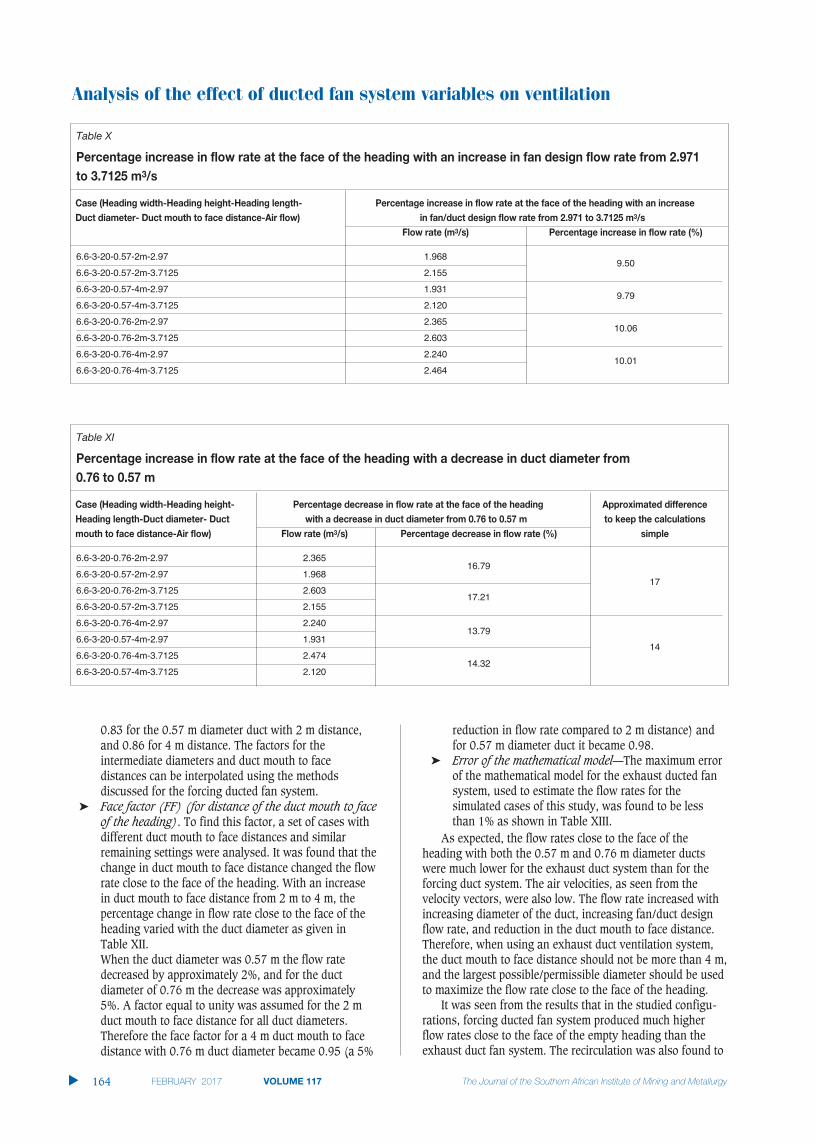
Analysis of the effect of ducted fan system variables on ventilation
0.83 for the 0.57 m diameter duct with 2 m distance,and 0.86 for 4 m distance. The factors for theintermediate diameters and duct mouth to facedistances can be interpolated using the methodsdiscussed for the forcing ducted fan system.
� Face factor (FF) (for distance of the duct mouth to faceof the heading). To find this factor, a set of cases withdifferent duct mouth to face distances and similarremaining settings were analysed. It was found that thechange in duct mouth to face distance changed the flowrate close to the face of the heading. With an increasein duct mouth to face distance from 2 m to 4 m, thepercentage change in flow rate close to the face of theheading varied with the duct diameter as given in Table XII.When the duct diameter was 0.57 m the flow ratedecreased by approximately 2%, and for the ductdiameter of 0.76 m the decrease was approximately5%. A factor equal to unity was assumed for the 2 mduct mouth to face distance for all duct diameters.Therefore the face factor for a 4 m duct mouth to facedistance with 0.76 m duct diameter became 0.95 (a 5%
reduction in flow rate compared to 2 m distance) andfor 0.57 m diameter duct it became 0.98.
� Error of the mathematical model—The maximum errorof the mathematical model for the exhaust ducted fansystem, used to estimate the flow rates for thesimulated cases of this study, was found to be lessthan 1% as shown in Table XIII.
As expected, the flow rates close to the face of theheading with both the 0.57 m and 0.76 m diameter ductswere much lower for the exhaust duct system than for theforcing duct system. The air velocities, as seen from thevelocity vectors, were also low. The flow rate increased withincreasing diameter of the duct, increasing fan/duct designflow rate, and reduction in the duct mouth to face distance.Therefore, when using an exhaust duct ventilation system,the duct mouth to face distance should not be more than 4 m,and the largest possible/permissible diameter should be usedto maximize the flow rate close to the face of the heading.
It was seen from the results that in the studied configu-rations, forcing ducted fan system produced much higherflow rates close to the face of the empty heading than theexhaust duct fan system. The recirculation was also found to
�
164 VOLUME 117
Table X
6.6-3-20-0.57-2m-2.97 1.9689.50
6.6-3-20-0.57-2m-3.7125 2.155
6.6-3-20-0.57-4m-2.97 1.9319.79
6.6-3-20-0.57-4m-3.7125 2.120
6.6-3-20-0.76-2m-2.97 2.36510.06
6.6-3-20-0.76-2m-3.7125 2.603
6.6-3-20-0.76-4m-2.97 2.24010.01
6.6-3-20-0.76-4m-3.7125 2.464
Table XI
6.6-3-20-0.76-2m-2.97 2.36516.79
176.6-3-20-0.57-2m-2.97 1.968
6.6-3-20-0.76-2m-3.7125 2.60317.21
6.6-3-20-0.57-2m-3.7125 2.155
6.6-3-20-0.76-4m-2.97 2.24013.79
146.6-3-20-0.57-4m-2.97 1.931
6.6-3-20-0.76-4m-3.7125 2.47414.32
6.6-3-20-0.57-4m-3.7125 2.120
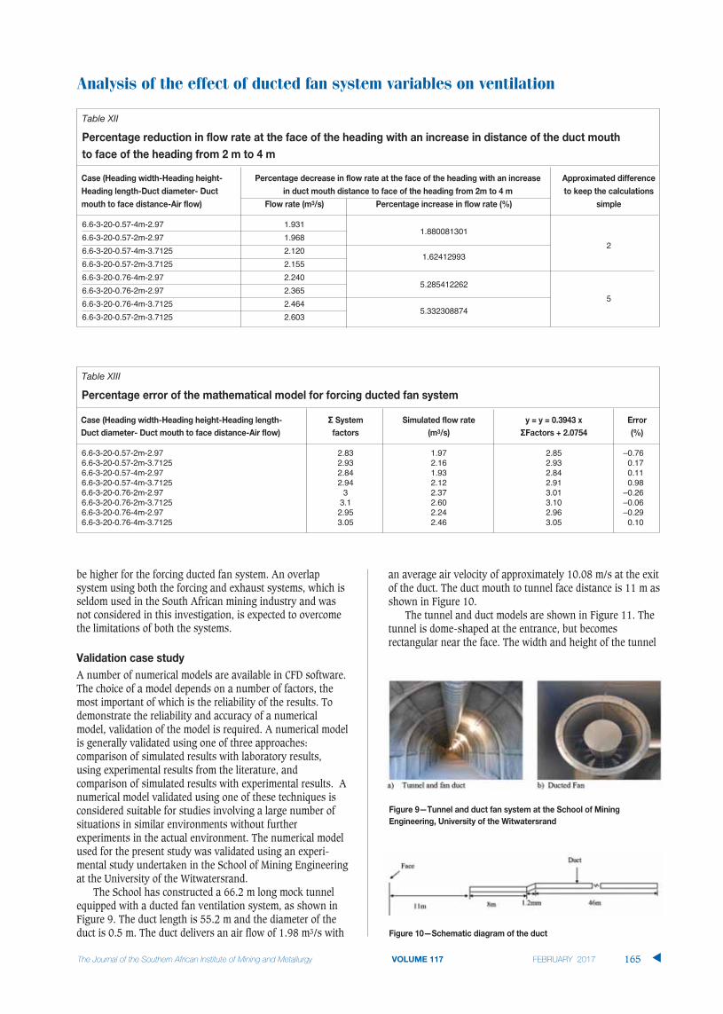
be higher for the forcing ducted fan system. An overlapsystem using both the forcing and exhaust systems, which isseldom used in the South African mining industry and wasnot considered in this investigation, is expected to overcomethe limitations of both the systems.
A number of numerical models are available in CFD software.The choice of a model depends on a number of factors, themost important of which is the reliability of the results. Todemonstrate the reliability and accuracy of a numericalmodel, validation of the model is required. A numerical modelis generally validated using one of three approaches:comparison of simulated results with laboratory results,using experimental results from the literature, andcomparison of simulated results with experimental results. Anumerical model validated using one of these techniques isconsidered suitable for studies involving a large number ofsituations in similar environments without furtherexperiments in the actual environment. The numerical modelused for the present study was validated using an experi-mental study undertaken in the School of Mining Engineeringat the University of the Witwatersrand.
The School has constructed a 66.2 m long mock tunnelequipped with a ducted fan ventilation system, as shown inFigure 9. The duct length is 55.2 m and the diameter of theduct is 0.5 m. The duct delivers an air flow of 1.98 m3/s with
an average air velocity of approximately 10.08 m/s at the exitof the duct. The duct mouth to tunnel face distance is 11 m asshown in Figure 10.
The tunnel and duct models are shown in Figure 11. Thetunnel is dome-shaped at the entrance, but becomesrectangular near the face. The width and height of the tunnel
Analysis of the effect of ducted fan system variables on ventilation
VOLUME 117 165 �
Table XII
6.6-3-20-0.57-4m-2.97 1.9311.880081301
26.6-3-20-0.57-2m-2.97 1.968
6.6-3-20-0.57-4m-3.7125 2.1201.62412993
6.6-3-20-0.57-2m-3.7125 2.155
6.6-3-20-0.76-4m-2.97 2.2405.285412262
56.6-3-20-0.76-2m-2.97 2.365
6.6-3-20-0.76-4m-3.7125 2.4645.332308874
6.6-3-20-0.57-2m-3.7125 2.603
Table XIII
6.6-3-20-0.57-2m-2.97 2.83 1.97 2.85 –0.766.6-3-20-0.57-2m-3.7125 2.93 2.16 2.93 0.176.6-3-20-0.57-4m-2.97 2.84 1.93 2.84 0.116.6-3-20-0.57-4m-3.7125 2.94 2.12 2.91 0.986.6-3-20-0.76-2m-2.97 3 2.37 3.01 –0.266.6-3-20-0.76-2m-3.7125 3.1 2.60 3.10 –0.066.6-3-20-0.76-4m-2.97 2.95 2.24 2.96 –0.296.6-3-20-0.76-4m-3.7125 3.05 2.46 3.05 0.10
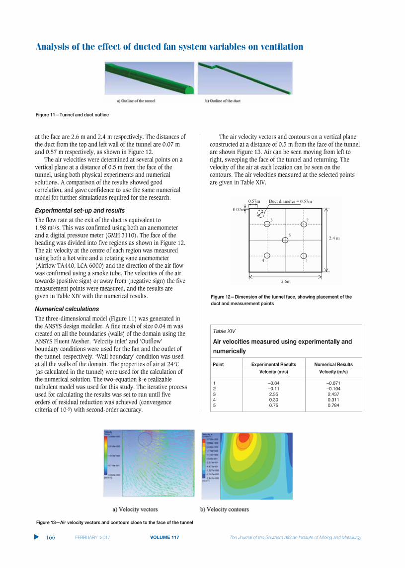
Analysis of the effect of ducted fan system variables on ventilation
at the face are 2.6 m and 2.4 m respectively. The distances ofthe duct from the top and left wall of the tunnel are 0.07 mand 0.57 m respectively, as shown in Figure 12.
The air velocities were determined at several points on avertical plane at a distance of 0.5 m from the face of thetunnel, using both physical experiments and numericalsolutions. A comparison of the results showed goodcorrelation, and gave confidence to use the same numericalmodel for further simulations required for the research.
The flow rate at the exit of the duct is equivalent to 1.98 m3/s. This was confirmed using both an anemometerand a digital pressure meter (GMH 3110). The face of theheading was divided into five regions as shown in Figure 12.The air velocity at the centre of each region was measuredusing both a hot wire and a rotating vane anemometer(Airflow TA440, LCA 6000) and the direction of the air flowwas confirmed using a smoke tube. The velocities of the airtowards (positive sign) or away from (negative sign) the fivemeasurement points were measured, and the results aregiven in Table XIV with the numerical results.
The three-dimensional model (Figure 11) was generated inthe ANSYS design modeller. A fine mesh of size 0.04 m wascreated on all the boundaries (walls) of the domain using theANSYS Fluent Mesher. ‘Velocity inlet’ and ‘Outflow’boundary conditions were used for the fan and the outlet ofthe tunnel, respectively. ‘Wall boundary’ condition was usedat all the walls of the domain. The properties of air at 24°C(as calculated in the tunnel) were used for the calculation ofthe numerical solution. The two-equation k-e realizableturbulent model was used for this study. The iterative processused for calculating the results was set to run until fiveorders of residual reduction was achieved (convergencecriteria of 10-5) with second-order accuracy.
The air velocity vectors and contours on a vertical planeconstructed at a distance of 0.5 m from the face of the tunnelare shown Figure 13. Air can be seen moving from left toright, sweeping the face of the tunnel and returning. Thevelocity of the air at each location can be seen on thecontours. The air velocities measured at the selected pointsare given in Table XIV.
�
166 VOLUME 117
Table XIV
1 –0.84 –0.8712 –0.11 –0.1043 2.35 2.4374 0.30 0.3115 0.75 0.784

A comparison of the numerical results with the experimentalresults is given in Figure 14. It can be seen that thenumerical results are in line with the experimental results.The validation study showed that the ANSYS Fluent k-erealizable model is suitable for studying the ventilation ofempty headings using ducted fan systems.
To understand the effect of the system variables associatedwith ducted fan systems on the ventilation of an emptyheading, mathematical models were developed using CFD,and comparative analysis. The results showed that recircu-lation for a forcing ducted fan system can be reduced byincreasing the duct diameter and by using a duct mouth toface distance of not less than 10 m. Increasing the ductdiameter, from 0.57 m to 0.76 m the and duct mouth to facedistance from 8 m to 10 m reduced recirculation by approxi-mately 20%.
The flow rate delivered by an exhausting ducted fansystem can be increased by reducing the duct mouth to facedistance (for a very small difference of 2–5% per 2 mreduction in distance), increasing the fan design flow rate(10% increase per 25% increase in design flow rate), orincreasing the duct diameter (14–17% increase in flow ratewith an increase in diameter from 0.76 m to 0.57 m).
The outcomes of the study will help ventilation engineersto select the optimum duct fan system required for sufficientventilation.
The work presented in this paper is part of a PhD researchstudy in the School of Mining Engineering at the Universityof the Witwatersrand. The authors would like to acknowledgethe Wits Mining Institute (WMI), University of theWitwatersrand, for making the Digital Mine facility availablefor the research, and the financial assistance required topurchase the high-performance PC and the CFD software.
AMC Consultants Pty Ltd. 2005. Basic Mine Ventilation, Revision 5.http://wenku.baidu.com/view/3a566fb769dc5022aaea00b6.html[Accessed: 2 July 2014].
ANSYS® Academic Research. 2015. Release 15.0, Help System, ANSYS FluentTheory Guide, Chapter 4.
BISE, C.J (ed.). 2013. Modern American Coal Mining: Methods and Applications.Society for Mining, Metallurgy and Exploration, Inc., Englewood,Colorado.
CREEDY, D.P. 1996. Methane prediction in collieries. Report COL 303. Safety inMines Research Advisory Committee (SIMRAC), Johannesburg. June 1996.
DUBINSKI, J., KRAUSE, E., and SKIBA, J. 2011. Global technical and environmentalproblems connected with the coal mine methane. Proceedings of the 22ndWorld Mining Congress and Expo 2011, Istanbul, Turkey, 11–16September.
FEROZE, T. and PHILLIPS, H.W. 2015. An initial investigation of room and pillarventilation using CFD to investigate the effects of last through road
velocity. Proceedings of the 24th International Mining Congress andExhibition of Turkey (IMCET 15), Antalya, Turkey, 14-17 April. Chamberof Mining Engineers of Turkey. pp. 970-977.
GOODMAN, G.V.R., TAYLOR, CD., and THIMONS, E.D. 1992. Jet fan ventilation invery deep cuts - a preliminary analysis. Report of Investigations 9399. USBureau of Mines, US Department of the Interior, Pittsburgh, PA. pp. 1–12.
KISSELL, F.N. 2003. Handbook for Methane Control in Mining. US Departmentof Health and Human Services, National Institute for Occupational Safetyand Health. Pittsburgh Research Laboratory.
MCPHERSON, M.J. 1993. Subsurface Ventilation and Environmental Engineering.Chapman & Hall, New York.
PAWINSKI, J. and ROSZKOWSKI, J. 1985. Emission of methane into mine galleriesdriven in coal by means of combined cutter-loaders. Archives of MiningScience, vol. 30, no. 2. pp. 207–213.
PHILLIPS, H.R. 2015. Lessons learnt from mine explosions. Proceedings of theAustralian Mine Ventilation Conference. Sydney, NSW, 31 August–2September 2015. pp.19-28.
PHILLIPS, H.R., and BRANDT, M.P. 1995. Coal mine explosions - risk and remedy.Proceedings of the SIMRAC Symposium, Johannesburg, 1 September 1995.Southern African Institute of Mining and Metllurgy, Johannesburg. pp. 15.
REED, W. and TAYLOR, C. 2007. Factors affecting the development of mine faceventilation systems in the 20th century. Proceedings of the Society forMining, Metallurgy and Exploration (SME) Annual Meeting and Exhibit,Denver, Colorado, 25-28 February 2007.
SCHULTZ, M.J., BEITER, D.A., WATKINS, T.R., and BARAN, J.N. 1993. Faceventilation investigation: Clark Elkorn Coal Company. Investigative Reportno. P385-V286. Pittsburgh Safety and Health Technology Center,Ventilation Division..
SZLAZAK, N., SZLAZAK, J., TOR, A., OBRACAJ, A., and BOROWSKI, M. 2003.Ventilation systems in dead end headings with coal dust and methanehazard. Proceedings of the 30th International Conference of Safety inMines Research Institutes, Johannesburg, 5–9 October. South AfricanInstitute of Mining and Metallurgy, Johannesburg. pp. 673–688.
TAYLOR, C.D., RIDER, J.P., and THIMONS, E.D. 1997. Impact of unbalanced intakeand scrubber flow on face methane concentrations. Proceedings of the 6thInternational Mine Ventilation Congress. Pittsburgh, Pennsylvania, 17–22May. pp 169–172.
THORP, N. 1982. Auxiliary ventilation practice. Environmental Engineering inSouth African Mines. Burrows, J. (ed.). Cape and Transvaal Printers, CapeTown.
TORANO, J., TORNO, S., MENENDEZ, M., GENT, M., and VELASCO, J. 2009. Models ofmethane behaviour in auxiliary ventilation of underground coal mining.International Journal of Coal Geology, vol. 80, no. 1. pp. 35–43. �
Analysis of the effect of ducted fan system variables on ventilation
VOLUME 117 167 �

School of Chemical and Metallurgical Engineering, University of the Witwatersrand
Pyrometallurgy Programme 2017
Course Presenter Course Code Course Name Attendance Dates Contact E-mail
Prof Serdar Kucukkaragoz /Dr Elias Matinde
CHMT7013 Solid, liquid and gaseous state pyrometallurgical processes 03 – 07 April [email protected]
Prof Eriç Hürman CHMT7016 Selected / Special topics in pyrometallurgy 29 May – 02 June [email protected] Elias Matinde CHMT7060 Coal and carbon in the metallurgical industry 11 – 15 September [email protected] Lesley Cornish CHMT7027 Thermodynamics & Phase Equilibria of Materials September [email protected]
Minerals Processing and Extractive Metallurgy Programme 2017
Prof Vusumuzi Sibanda CHMT7029 02 – 06 October [email protected] Josias van der Merwe/ Prof Herman Potgieter
CHMT7031 Electrometallurgy June [email protected]@wits.ac.za
Prof Geoffrey Simate CHMT7032 Separation Processes in Hydrometallurgy 03 – 07 July [email protected] Tony Paterson CHMT7043 Welding Processes & Equipment 03 – 07 April [email protected]
Welding and Fabrication Engineering Programme 2017
Prof Tony Paterson CHMT7044 Other Welding Processes 24 – 28 April [email protected] Tony Paterson CHMT7045 Advanced Welding Processes 13 – 17 March [email protected] Tony Paterson CHMT7046 Fabrication, applications engineering 11 – 15 September [email protected] Tony Paterson CHMT7047 Non-destructive testing methods & economics 02 – 06 October [email protected] Tony Paterson CHMT7049 Welding Metallurgy of Steels 15 – 19 May [email protected] Tony Paterson CHMT7050 Weldability of alloy steels & stainless steels 05 – 09 June [email protected] Tony Paterson CHMT7051 Weldability of ferrous & non-ferrous materials 26 – 30 June [email protected] Tony Paterson CHMT7052 Case Studies for Welding Engineers 23 – 27 October [email protected] Tony Paterson CHMT7053 Practical Education – Welding Processes 20 – 24 February [email protected] Tony Paterson CHMT7073A Design and Construction of Welded Structures under Static
Loading17 – 21 July [email protected]
Prof Tony Paterson CHMT7074A Design and Construction of Welded Structures under Dynamic Loading
14 – 18 August [email protected]
Coal Science and Technology Programme 2017
Course Presenter Course Code Course Name Attendance Dates Contact E-Mail
Prof Herman Potgieter CHMT7005 Coal Sampling and Quality Assessment 09 – 13 January [email protected] Shehzaad Kauchali CHMT7006 Coal Management and Marketing 30 Oct – 04 Nov [email protected] Samson Bada CHMT7057 Coal Combustion and Power Generation 03 – 08 April [email protected] Murray Bwalya CHMT7058 July [email protected]
Materials Science and Engineering Programme 2017
Ms Nthabiseng Maledi CHMT7018 Materials Characterisation March [email protected] Failure Analysis of Engineering Materials June
Prof Tony Paterson / Dr Josias van der Merwe
CHMT7026 Destructive and Non-Destructive Testing and Evaluation
October [email protected]@wits.ac.za
Prof Lesley Cornish CHMT7027 Thermodynamics & Phase Equilibria of Materials
September [email protected]
Postgraduate and Short Courses for 2017The School of Chemical and Metallurgical Engineering at the University of the Witwatersrand is pleased to announce its 2017 program of postgraduate and short course offerings to support industry skills development and personal development aspirations of attendees over a broad spectrum of specialised programmes. All the advertised postgraduate courses can also simultaneously be followed as a short course. Short courses can be followed on an
Competence. All the postgraduate and short courses are on approved NQF level 9 and the School is in the process to get it accredited for CPD points by the relevant organisations early in 2017. Short course attendance cost R9 500 excluding VAT for 5 days, or a pro-rata portion for shorter periods. The School supports access to all these courses through a combination of recognition of prior learning and suitable postgraduate diplomas in engineering for
For more information, the relevant course coordinators can be contacted, or alternatively Ms Ntokozo Dube, Administration Manager and Postgraduate Coordinator of the School of Chemical and Metallurgical Engineering at Wits on tel: 011 717 7521, e-mail: [email protected], or the Head of School Prof. Herman Potgieter on tel: 011 717 7510 or e-mail: [email protected]. Join us and let us assist you to make your dreams come true!
SCHOOL OF CHEMICAL& METALLURGICAL ENGINEERING

Depend on OUR quality
Distribution and Product Support by:
H/Office: Tel: (011) 306-0700 Fax: (011) 918-7208
e-mail: [email protected]: www.elbequipment.com
Branches and Dealers throughout Southern Africa
Terex® MineralsProcessing SystemsNot just equipment. A complete solution.ELB Equipment, the sub-Sahara Africa distributor of a complete range of Terex® Minerals Processing Systems, understands your business and with Terex® are dedicated to offering cost-effective solutions for your needs.
In today’s competitive environment, you need high quality equipment backed by an outstanding support network locally and inter-nationally. Our sales and after-market teams are trained to provide customers with outstanding crushing and screening process knowledge and service.
As a member of the ELB Group, we have a century of experience in the mining industry that you can depend on. Customer satisfaction is our ultimate goal.

20 April 2017Emperors Palace, Hotel Casino,
Convention Resort Johannesburg
PROXIMITY DETECTION ANDCOLLISION AVOIDANCE SYSTEMS IN MINING COLLOQUIUM 2017
Striving for zero harm from mining mobile machinery
BACKGROUNDConsiderable attention is being focused through the Department of Mineral Resources, the Mine Health and Safety Council, the mining companies and the original equipment manufacturers on the development and implementation of Proximity Detection Systems (PDSs) andCollision Avoidance Systems for underground and surface mobile machinery and underground track bound machinery. These initiatives are allin support of the quest by all stakeholders for reaching “zero harm”.
Systems have been developed and trialled for vehicle to person detection and warning, vehicle to beacon, and vehicle to vehicle detection.Technical challenges have been encountered in terms of the various system reliability and pedestrian/operator acceptance, as well as the
application on diesel powered and electric powered machinery, respectively.Whilst it is the intention to regulate this area in the near future, it is important that the various issues that could be problematic to
implementation be aired and solutions found.
Conference Co-ordinator: Camielah Jardine • SAIMM
Tel: +27 11 834-1273/7 • Fax: +27 11 833-8156 E-mail:[email protected]
Website: http://www.saimm.co.za
Pillars have been used as a means of supportsince the early days of mining. Pillar-supported mining methods such as bord andpillar require a reliable design system for themto be successful. This paper presents anevaluation of the current hard-rock miningpillar design systems as applied to a practicallarge-scale narrow-reef platinum miningfeasibility study. It is vital to have adependable pillar design system for economicand sustainable mining. Using an extensivedatabase collected from the project, the pillarstrength formulae were tested and severaldiscrepancies noted. This necessitates theestablishment of more reliable pillar designsystems. In narrow-reef platinum mining,large compressive stresses accompanied bygeological and geotechnical factors contributeto pillar instability. A well-formulated pillardesign system is required that accounts forsuch factors so as to minimize pillar failures.
A pillar layout design system has toconsider the hangingwall, the pillar material,and the footwall as all these three worktogether for the success of the system. Ozbay,Ryder, and Jager (1995) describe thehangingwall in shallow hard-rock miningsituations as a rock mass containing well-defined discontinuities and subjected todeadweight compression. When thehangingwall is unsupported, it becomessusceptible to backbreaks if critical spans areexceeded (Ozbay, Ryder, and Jager, 1995).
Different pillars are used in narrow-reefplatinum mining, depending on the functionthe pillar is to serve. In hard-rock tabularmining in general, a combination of pillartypes is utilized. Dave (2009) classifies thesetypes as shaft pillars, bracket pillars, boundarypillars, water barrier pillars, barrier pillars,crown pillars, sill pillars, strike-stabilizingpillars, dip-stabilizing pillars, non-yieldingpillars, yielding pillars, and crush pillars.Salamon (1983) classified these pillars intothree main types –support pillars, protectivepillars, and control pillars. He explains thatsupport pillars are usually laid out systemat-ically to offer support to the underminedground. According to this classification,protective pillars protect surface structures andunderground mining excavations or separateone mine from its neighbour, while controlpillars are those laid out systematically and cutin deep-level mines to curb rockbursts byreducing energy release rates.
Current pillar design systems are based onthe empirical determination of pillar designparameters. This approach relies entirely onthe failure of pillars for an empirical pillar
Reflections on narrow-reef platinummining pillar design systems as appliedto a large platinum explorationfeasibility projectby T. Zvarivadza* and J.N. van der Merwe*†
Platinum is a highly valuable resource, its safe and economic extraction isparamount. The success of platinum mining by the bord and pillar methoddepends heavily on a comprehensive and dependable pillar design method.Pillars need to be large enough to safely support the load and smallenough to avoid loss of resources. A critical evaluation of current pillardesign systems used in narrow-reef platinum mining was undertakenusing practical experience from a large feasibility-stage platinumexploration project, supplemented by observations from several platinummines in Zimbabwe. An extensive literature survey was undertaken inorder to determine the current status of design systems. Through thisapproach, the shortcomings of current pillar design systems arehighlighted. Areas are proposed for further research to obtain a betterunderstanding on how additional factors influence pillar system stability.The exploration work highlighted how rock mass classification methodscan be utilized in determining the overall strength of pillars. Current pillardesign systems for narrow-reef platinum mining consider width-to-height-ratio (usually with different exponents for width and height) and thestrength of the pillar material. However, there are many more importantfactors that are not considered and which have a bearing on pillar systemstability. An in-depth study of these parameters with a view to establisheffective narrow- reef platinum mining pillar design systems needs to beundertaken.
pillar design, pre-feasibility, platinum mining, hard rock, comparative
* School of Mining Engineering, University of theWitwatersrand, South Africa.
† Stable Strata Consulting (Pty) Ltd, South Africa.© The Southern African Institute of Mining and
Metallurgy, 2017. ISSN 2225-6253. Paper receivedJan. 2016; revised paper received Nov. 2016.
169VOLUME 117 �
http://dx.doi.org/10.17159/2411-9717/2017/v117n2a8
Reflections on narrow-reef platinum mining pillar design systems
design curve to be calibrated. It cannot be used for minesoutside the empirical range that the pillar design is intendedfor. Several formulae are currently in use to determine pillarstrength. For the calculation of load, the tributary area theory(TAT) which applies to regular mining layouts is used.Coates’ (1981) method is also used to determine pillar loadfor large rectangular pillars like regional pillars. Parameterscurrently accounted for in the design of narrow reef platinummining pillars are strength, load, width-to-height (w/h) ratio,and pillar foundation bearing capacity. The w/h ratio isgenerally used as a first indication of pillar strength. Martinand Maybee (2000) compared extensive data collected fromback-analysis and concluded that most pillars fail at a w/hratio of less than 1.5, while there is a substantial increase inpillar strength at a w/h ratio of more than 2. Stacey and Page(1986) mention that foundation failure, rather than pillarfailure, can be expected at a w/h ratio of more than 7,provided that the pillar and foundation material are the same.Numerical modelling tools are also utilized to aid pillardesign.
Pillar stresses are normally calculated using the tributary areatheory (TAT), which accounts for the full cover load. Thistheory is used in regular mining layouts of large lateralextent (several times greater than the mining depth) andassumes that each pillar in the layout supports an equal loadto the surface. This allocates full cover load to each pillar inthe layout. Pillars of the same size must be used in theregular mining layout for the TAT to be applicable. Thisapproach appears to be operationally convenient as it leads tofixed pillar-design dimensions for any given seam materialand depth. The TAT assumes that a pillar carries the full loadof the overburden above the pillar itself and halfway into thesurrounding roadways (Salamon and Oravecz, 1976;Salamon and Munro, 1967; Hoek and Brown, 1980; Robertset al., 2002).
The average pillar stress (APS) can be expressed as afunction of extraction ratio as follows:
[1]
where v is the vertical component of the virgin stress (MPa),e is the areal extraction ratio, is rock density (kg/m3), g isgravitational acceleration (m/s2), h is depth below groundsurface (m), and v = gh.
Hoek and Brown (1980) present an alternative formulafor calculating APS for square pillars using the TAT. For asquare pillar layout, the formula is:
[2]
where v is the vertical component of the virgin stress, W0 isthe excavation width (bord width), and Wp is the pillar width.
Coates (1981) presented his formula for load calculation afterrealizing that while the TAT can be utilized, it is insufficientsince it does not consider geometrical and rock properties in
its formulation. He went on to consider these parameters inthe derivation of his formula. Coates (1981) admitted that hisformula is only applicable in the centre of the mining areawith undisturbed long rib pillars and in situations where themine span does not exceed half the depth. Coates’ formula(1981), which is applicable for calculating pillar load in deepand long mining zones, is given by:
[3]
where v is the vertical component of the virgin stress (MPa),e is the areal extraction ratio, H is height of the stope (m), h
is the horizontal component of the virgin stress (MPa), isPoisson’s ratio for abutments, p is Poisson’s ratio for pillars,E is Young’s modulus for abutments, Ep is Young’s modulusfor pillars, Bo is room width (m), Bp is pillar width (m), and Lis width of extraction span (m).
It is evident that the formulation of Coates (1981) doesnot consider overburden stiffness and seam stiffness, factorsthat play a pivotal role in determining pillar load.
Note: Coates’ method reduces to the usual TAT when L as shown in the calculation below.
When L , Bp = 0, b = 0 and hs = 0 such that
Coates (1981) mentions that his formula considers thefollowing geometrical (layout) and rock characteristics: thespan of the mining zone with respect to its depth, height ofthe pillars, pillar locations within the mining zone, horizontalstress, and modulus of deformation of the pillar and wall rockmaterials.
There are a number of issues that the current formulae usedto determine hard-rock pillar strength do not address. Most ofthe strength formulae developed for hard-rock pillars have anempirical base. They were proposed after studies fromdifferent mines using failed pillar information. The formulaetake the power form or linear form, but have a commonaspect of considering the w/h ratio of the pillars under study.The forms of the pillar strength formulae are as given inEquations [4] and [5].
[4]
�
170 VOLUME 117
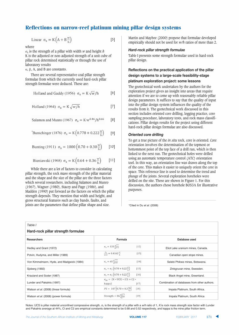
[5]
wheres is the strength of a pillar with width w and height h
K is the adjusted or non-adjusted strength of a unit cube ofpillar rock determined statistically or through the use oflaboratory results
, , A, and B are constants.
There are several representative coal pillar strengthformulae from which the currently used hard-rock pillarstrength formulae were deduced. These are:
[6]
[7]
[8]
[9]
[10]
[11]
While there are a lot of factors to consider in calculatingpillar strength, the rock mass strength of the pillar materialand the shape and the size of the pillar are the three factorswhich several researchers, including Salamon and Munro(1967), Wagner (1980), Stacey and Page (1986), andMadden (1990) put forward as the factors on which the pillarstrength depends. They mention that width and height, andgross structural features such as clay bands, faults, andjoints are the parameters that define pillar shape and size.
Martin and Maybee (2000) propose that formulae developedempirically should not be used for w/h ratios of more than 2.
Table I presents some strength formulae used in hard-rockpillar design.
The geotechnical work undertaken by the authors for theexploration project gives an insight into areas that requireattention if we are to come up with reasonably reliable pillardesign parameters. It suffices to say that the quality of inputinto the pillar design system influences the quality of theresults from it. The geotechnical work discussed in thissection includes oriented core drilling, logging practice, coresampling procedure, laboratory tests, and rock mass classifi-cations. Pillar design results for the project using differenthard-rock pillar design formulae are also discussed.
To get a true picture of the in situ rock, core is oriented. Coreorientation involves the determination of the topmost orbottommost point of the top face of a drill run, which is thenlinked to the next run. The geotechnical holes were drilledusing an automatic temperature control (ATC) orientationtool. In this way, an orientation line was drawn along the topof the core. This makes it easier to uniquely orient the core inspace. This reference line is used to determine the trend andplunge of the joints. Several exploration boreholes weredrilled on the site. These are shown in Figure 1. For thisdiscussion, the authors chose borehole BO53A for illustrativepurposes.
Reflections on narrow-reef platinum mining pillar design systems
VOLUME 117 171 �
*Cited in Du et al. (2008)
Table I
Hedley and Grant (1972) Eliot Lake uranium mines, Canada.
Potvin, Hudyma, and Miller (1989) Canadian open stope mines.
Von Kimmelmann, Hyde, and Madgwick (1984) Selebi Phikwe mines, Botswana.
Sjoberg (1992) Zinkgruvan mine, Sweeden.
Krauland and Soder (1987) Black Angel mine, Greenland.
Lunder and Pakalnis (1997) Combination of databases from other authors.
Watson et al. (2008) (linear formula) Impala Platinum, South Africa.
Watson et al. (2008) (power formula) Impala Platinum, South Africa
Notes: UCS is pillar material unconfined compressive strength, σ1 is the strength of a pillar with a w/h ratio of 1, K is rock mass strength size factor with Lunderand Pakalnis average at 44%, Cl and C2 are empirical constants determined to be 0.68 and 0.52 respectively, and kappa is the mine pillar friction term.
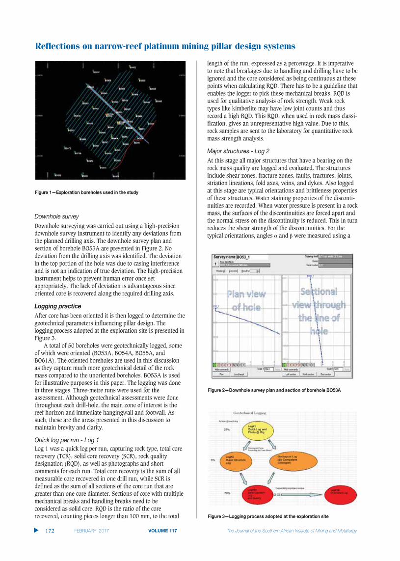
Reflections on narrow-reef platinum mining pillar design systems
Downhole surveying was carried out using a high-precisiondownhole survey instrument to identify any deviations fromthe planned drilling axis. The downhole survey plan andsection of borehole BO53A are presented in Figure 2. Nodeviation from the drilling axis was identified. The deviationin the top portion of the hole was due to casing interferenceand is not an indication of true deviation. The high-precisioninstrument helps to prevent human error once setappropriately. The lack of deviation is advantageous sinceoriented core is recovered along the required drilling axis.
After core has been oriented it is then logged to determine thegeotechnical parameters influencing pillar design. Thelogging process adopted at the exploration site is presented inFigure 3.
A total of 50 boreholes were geotechnically logged, someof which were oriented (BO53A, BO54A, BO55A, andBO61A). The oriented boreholes are used in this discussionas they capture much more geotechnical detail of the rockmass compared to the unoriented boreholes. BO53A is usedfor illustrative purposes in this paper. The logging was donein three stages. Three-metre runs were used for theassessment. Although geotechnical assessments were donethroughout each drill-hole, the main zone of interest is thereef horizon and immediate hangingwall and footwall. Assuch, these are the areas presented in this discussion tomaintain brevity and clarity.
Log 1 was a quick log per run, capturing rock type, total corerecovery (TCR), solid core recovery (SCR), rock qualitydesignation (RQD), as well as photographs and shortcomments for each run. Total core recovery is the sum of allmeasurable core recovered in one drill run, while SCR isdefined as the sum of all sections of the core run that aregreater than one core diameter. Sections of core with multiplemechanical breaks and handling breaks need to beconsidered as solid core. RQD is the ratio of the corerecovered, counting pieces longer than 100 mm, to the total
length of the run, expressed as a percentage. It is imperativeto note that breakages due to handling and drilling have to beignored and the core considered as being continuous at thesepoints when calculating RQD. There has to be a guideline thatenables the logger to pick these mechanical breaks. RQD isused for qualitative analysis of rock strength. Weak rocktypes like kimberlite may have low joint counts and thusrecord a high RQD. This RQD, when used in rock mass classi-fication, gives an unrepresentative high value. Due to this,rock samples are sent to the laboratory for quantitative rockmass strength analysis.
At this stage all major structures that have a bearing on therock mass quality are logged and evaluated. The structuresinclude shear zones, fracture zones, faults, fractures, joints,striation lineations, fold axes, veins, and dykes. Also loggedat this stage are typical orientations and brittleness propertiesof these structures. Water staining properties of the disconti-nuities are recorded. When water pressure is present in a rockmass, the surfaces of the discontinuities are forced apart andthe normal stress on the discontinuity is reduced. This in turnreduces the shear strength of the discontinuities. For thetypical orientations, angles and were measured using a
�
172 VOLUME 117

graduated strip and a carpenter’s angle. The SRKGeotechnical Core Logging Manual (2006) was used as aguide. The alpha angle ( ) is the maximum dip ( ) of thefeature relative to the core axis, as measured by thecarpenter’s angle. For the beta angle ( ), the plastic calibratedstrip is placed with the zero on the orientation line of thesame piece of core and the tape is wrapped clockwise aroundthe core so that the 360º point returns to the orientation line.The angle ( ) is then measured, clockwise, to the bottom ofthe ellipse. In this convention, only the upper part of thefeature is used for the measurement. The measured anglesare as illustrated in Figure 4.
It is often a challenge to determine whether a discontinuityrepresents an open joint or a cemented joint. For this reason,it is rational to consider a cemented joint that is open in thecore as an open joint fracture, since the joint is weak, hence iteasily opens up. Joint infill type has an influence on thestrength of joints, so experience is required to differentiatebetween the various infill types. Joint strength is also affectedby alteration, so knowledge of alteration analysis is critical.Estimation or averaging of joint parameters can also be achallenge since the influence of a joint set on excavationstability depends on the joint set orientation. It follows that itis advisable to assess joint conditions for individual sets asthis permits the use of the most appropriate parameters forthe most influential joint set.
At this stage, an initial estimate of rock strength wasobtained using a geological hammer. Rock strength wasmeasured on a scale of R1 to R6, depending on its responseto a knock by the hammer (SRK Logging Manual, 2006). R1signifies highest strength while R6 is for the weakest rock.The geological hammer results were calibrated by sendingsamples of the rock for laboratory strength tests. The resultsof the laboratory strength tests are shown in Tables II and III.Table IV gives the results of rock specific gravitymeasurements from the laboratory tests.
For more accurate results, the authors observed that it isnecessary to adopt an evaluation scale for weak rock thatquantifies the level of weakness. A scale of S1 to S6 (SRKLogging Manual, 2006) can be used lest detail is lost. It was
also observed that intact rock strength (IRS) is affected byelements such as microdefects, foliation, and schistosity, sofor representative samples sampling has to be done inmultiple orientations. Detailed geotechnical logging was doneon a domain basis so as to pick sections of the core with thesame geotechnical characteristics. The domains were kept toless than 3 m to preserve accuracy by avoiding over-averaging. In addition to IRS, other parameters evaluatedwere fracture frequency, joint conditions, cemented jointcount, and microfractures.
The geotechnical logging should suit the rock mass classifi-cation system to be used. It is imperative for the geotechnicallogging sheet to accommodate all the parameters that will beused in the calculation of pillar strength. The logging sheetand instructions should be presented in a way which is easyto understand to minimize human errors and increaseaccuracy and precision.
Rock mass classification systems were used to estimate thestrength of the rock mass, which is an important parameterfor determining pillar strength. The classification systemsadopted for the project were the Q-system (Barton et al.,1974), Bieniawski’s RMR (Bieniawski, 1989), andLaubscher’s MRMR (Laubscher, 1990).
Reflections on narrow-reef platinum mining pillar design systems
VOLUME 117 173 �
Table II

Reflections on narrow-reef platinum mining pillar design systems
To compare the Bieniawski RMR and the calculated RMR,transformation Equations [20] and [21] were used.
[20]
[21]
It was noted that results obtained using Equation [20]deviated from the Bieniawski RMR, so Equation [21] wasused as it gave a closer correlation. Table IX gives the RMRvalues calculated from Q using Equation [21]. Table V givesthe MRMR classification system results for the project.
For a realistic pillar design criterion, rock mass propertieswere determined using laboratory uniaxial and triaxialcompression tests. The parameters determined were UCS,Poisson’s ratio, Young’s modulus, and specific gravity. Asummary of the tests results is shown in Table VI.
The detailed logging data was processed to give some inputinto the pillar design at the exploration stage. For calculatingstrength, design rock mass strength (DRMS) was usedinstead of the strength of a unit cube of rock. This approachwas adopted since DRMS considers all the parameters that
�
174 VOLUME 117
Table III
Table IV
SG-01 GT 53/1 146.00–146.16 49.29 0.998 17.1 2.870
SG-03 GT 53/3 146.33–146.5 69.89 0.997 24.3 2.864
SG-05 GT 53/5 146.70–146.85 66.33 0.997 23.1 2.864
SG-07 GT 53/7 146.93–147.08 63.99 0.998 22.4 2.851
SG-09 GT 53/9 147.23–147.38 66.75 0.998 23.8 2.803
SG-11 GT 53/11 149.45–149.57 51.01 0.998 16.2 3.141
SG-13 GT 53/13 149.69–149.81 80.09 0.997 25.3 3.160
SG-15 GT 53/15 149.93–150.05 49.37 0.998 15.3 3.225
SG-17 TM 2007 157.49–157.64 37.95 0.998 11.8 3.207
SG-20 TM 2010 157.94–158.09 54.57 0.998 17.3 3.148
SG-23 TM 2013 158.39–158.54 39.51 0.998 12.5 3.160
SG-26 TM 2016 158.84–158.99 49.76 0.998 15.5 3.196
SG-29 TM 2019 159.29–159.44 69.88 0.997 21.8 3.200
Gabbro-Norite
Websterite
Bronzitite
... ...

Reflections on narrow-reef platinum mining pillar design systems
VOLUME 117 175 �
were assessed in the logging programme which have abearing on the pillar strength. In determining DRMS, rockmass strength (RMS) is first calculated using Equation [22](suggested by Laubscher, 1990).
[22]
where: RMR is the total of the rock mass rating and RUCS isthe uniaxial compressive strength rating determined usingBieniawski’s (1989) rock mass rating system table.
To obtain the DRMR needed for calculating pillarstrength, the RMS was adjusted for the effects of blasting,weathering, and joint orientation, which were 95%, 96%, and74% respectively. The Hedley and Grant (1972) powerformula was used for calculating pillar strength; however, thestrength of a unit cube of rock, originally proposed as input,was replaced by DRMR, which is more representative of pillarexperience. The formula used is given in Equation [23].
[23]
where DRMS is the design rock mass strength; We is theeffective pillar width given by 4 × Pillar area/Pillar perimeter,and H is the pillar height.
Since the maximum depth of orebody at the explorationsite is less than 300 m, the mine to be established isconsidered to be shallow so the TAT (Equation [1]) wasapplied. However, the drawbacks of this theory, as discussedearlier, are still valid and further research work need to beundertaken to account for these shortfalls.
A constant safety factor (SF) of 1.6 was used forcomparative analysis of the pillar strength formulae atdifferent depth. A SF of 1.6 was used since it is the commonSF for non-yielding pillars in South Africa. For calculating thesquare pillar width at different depths for a constant SF of1.6, the following values were used in the SF equation (SF =Pillar strength/Pillar load):
Mining height 1.8 mPillar centres 18 mRock density 2 700 kg/m3
UCS of intact pillar rock 152.3 MPaDRMS 48.4 MPa
The resultant square pillar widths at various depths for aconstant SF of 1.6 are given in Table VII.
Note that the same approach was adopted to determinepillar width at different depths for a constant SF of 1.6 fordifferent hard-rock pillar design formulae presented in thispaper as applied to the project database. This was done toillustrate the uncertainty brought about by these formulae inthe pillar design process. The results are as presented inTable X.
The rock mass classification data used for this research ispresented in Tables VIII and IX.
To highlight the current uncertainty in the pillar designprocess, the hard-rock pillar design formulae presented inthis paper were used to determine square pillar sizes atdifferent depth using the platinum exploration data. Aconstant SF of 1.6 was used in the calculations since it is theminimum permitted for the project. The TAT was used todetermine the stresses at different depths since the mininglayout is of large lateral extent, several times greater than themining depth, and regular with same-size pillars. It isimportant to note that the Coates’ method reduces to theusual TAT under these conditions (large width of extractionspan, L) so only the TAT was used for the assessment.
Since there is no straightforward way of calculating pillarwidth from the SF equation, several iterations wereperformed in Excel® to find the pillar width corresponding to
Table V
BO 56 45–53 59 40IBO 01 114–122 74 Weathering 50BO55A 119–127 72 96% 49IBO 02 138–146 69 47BO 54A 142–150 75 51IBO 03 171–179 63 43BO 53A 150–158 70 Induced stress 47IBO 11 182–190 77 100% 52BO 052 143–151 69 47BO 045 158–166 74 50BO 051 115–123 81 55BO 58 100–108 85 Joint orientation 58BO 59 114–122 79 75% 53BO 60 135–143 74 50BO 61A 132–140 70 47BO 62 94–102 72 49BO 66 101–109 72 Blasting 49BO 68 120–128 84 94% 57BO 39 189–197 77 52BO 41 130–138 57 39
Table VI
Triaxial Compressive Strength (TCS) MPa 310.1 198.6Uniaxial Compressive Strength (UCS) MPa 156.4 152.3Density t/m3 2.84 3.18Elastic Modulus GPa 97.6 91.4Poisson’s Ratio 0.31 0.29
Table VII
100 4.53 1.6120 4.88 1.6140 5.19 1.6160 5.47 1.6180 5.73 1.6200 5.98 1.6
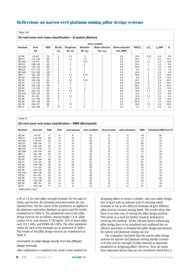
Reflections on narrow-reef platinum mining pillar design systems
a SF of 1.6 for each pillar strength formula. For the sake ofclarity and brevity, the formulae presented earlier are notrepeated here, but the values of the parameters as applied tothe platinum exploration database are given and the resultssummarized in Table X. The parameters used in the pillardesign exercise are as follows: mining height 1.8 m, pillarcentres 18 m, rock density 2 700 kg/m3, UCS of intact pillarrock 152.3 MPa, and DRMS 48.4 MPa. The other parametervalues for each of the formulae are as presented in Table I.The results of the pillar design exercise are summarized inTable X.
After exploration is completed one needs a clear method for
designing pillars to ensure a reliable, safe, and stable design.One is faced with an arduous task of choosing whichformulae to use as the different formulae all give differentpillar sizes at constant mining depth. The results show thatthere is no clear way of solving the pillar design problem.This points to a need for further research dedicated toresolving this problem. All the relevant factors influencingpillar design have to be considered and combined into aneffective procedure or formula that pillar design practitionersfor narrow-reef platinum mining can use.
The evaluation concluded that the current pillar designsystems for narrow-reef platinum mining mainly considerw/h ratio and the strength of pillar material as importantparameters in designing pillars. However, there are manymore important factors that are not considered which have a
�
176 VOLUME 117
Table VIII
BO 56 45–53 76 3 1.5 6 1 2.5 25.3 0.25 0.4 2.5IBO 01 114–122 98 3 1.5 1.5 1 2.5 32.7 1 0.4 13.1BO 55A 119-127 99 4 1 0.75 1 2.5 24.8 1.3 0.4 12.9IBO 02 138–146 89 4 3 3 1 2.5 22.3 1 0.4 8.9BO 54A 142–150 98 4 1 1 1 2.5 24.5 1 0.4 9.8IBO 03 171–179 57 9 3 1 1 2.5 6.3 3 0.4 7.6BO 53A 150–158 100 4 1 1 1 2.5 25.0 1 0.4 6.3IBO 11 182–190 100 2 1.5 0.75 1 2.5 50.0 2 0.4 40.0BO 52 143–151 75 9 3 1 1 2.5 8.3 3 0.4 10.0BO 45 158–166 96 3 1.5 0.75 1 2.5 32.1 2 0.4 25.7BO 51 115–123 99 4 3 1 1 2.5 24.8 3 0.4 29.7BO 58 100–108 100 1 1 1 1 2.5 100.0 1 0.4 40.0BO 59 114–122 95 4 3 2 1 2.5 23.8 1.5 0.4 14.3BO 60 135–143 96 6 1.5 1 1 2.5 16.0 1.5 0.4 9.6BO 61A 132–140 99 6 1 1 1 2.5 16.5 1 0.4 6.6BO 62 94–102 95 9 1.5 1 1 2.5 10.6 1.5 0.4 6.4BO 66 101–109 100 4 1 1 1 2.5 25.0 1 0.4 10.0BO 68 120–128 100 1 1 1 1 2.5 100.0 1 0.4 40.0BO 39 189–197 98 2 1.5 1 1 2.5 49.0 1.5 0.4 29.4BO 41 130–138 77 15 4 4 1 2.5 5.1 1 0.4 2.0
Table IX
BO 56 45–53 17 12 8 12 15 –5 59 65IBO 01 114–122 20 12 10 22 15 –5 74 74BO 55A 119-127 20 12 10 20 15 –5 72 74IBO 02 138–146 17 12 10 20 15 –5 69 72BO 54A 142–150 20 12 15 18 15 –5 75 72IBO 03 171–179 13 12 8 20 15 –5 63 71BO 53A 150–158 20 12 10 18 15 –5 70 70IBO 11 182–190 20 12 15 20 15 –5 77 79BO 52 143–151 17 12 8 22 15 –5 69 72BO 45 158–166 20 12 10 22 15 –5 74 77BO 51 115–123 20 12 15 24 15 –5 81 78BO 58 100–108 20 12 20 23 15 –5 85 79BO 59 114–122 20 12 15 22 15 –5 79 74BO 60 135–143 20 12 10 22 15 –5 74 72BO 61A 132–140 20 12 10 18 15 –5 70 70BO 62 94–102 20 12 10 20 15 –5 72 70BO 66 101–109 20 12 10 20 15 –5 72 69BO 68 120–128 20 12 20 22 15 –5 84 79BO 39 189–197 20 12 15 20 15 –5 77 78BO 41 130–138 17 12 8 10 15 –5 57 64
*RMR=5lnQ + 60.8

bearing on pillar system stability. Some of the unaccounted-for factors that were discovered during the course of thisresearch are contact of the pillar with the roof and floor, roofand floor conditions (Watson, 2010), effects of adverselyoriented joints, spalling and side scaling effects, influence ofpillar loading conditions, blast damage effects, influence ofweak layers and weathering, impact of k-ratio, time-dependent effects, geology, fractured zones, and effects ofdifferent types of discontinuities within the rock strata.
A reliable pillar design system results in a layout with thedesired stability. The main objective of this research was tocritically evaluate the current pillar design systems used innarrow-reef platinum mining using practical experience froma large feasibility-stage platinum exploration project. Theshortcomings of the current pillar design systems werehighlighted. The exploration work also highlighted how rockmass classification methods can be utilized in determining
the overall strength of pillars. Geotechnical parametersimportant for pillar design were collected by means ofgeotechnical logging and laboratory tests. The geotechnicallogging consisted of three stages: quick log per run, majorstructures log, and detailed geotechnical log. Areas thatrequire special attention in each logging stage werehighlighted. It is imperative for the geotechnical logging sheetto accommodate all the parameters that will be used in thecalculation of pillar strength. The logging sheet andinstructions should be presented in a way that is easy tounderstand to minimize human errors and increase accuracy.It suffices to say that the quality of input into the pillardesign system influences the quality of the results obtained.
� Pillar design results using different hard-rock pillardesign formulae were significantly different, showingthe uncertainty introduced by the current pillar designformulae in the pillar design process. These resultsshow that there is currently no clear way of solving thepillar design problem. Further research has to bededicated to resolving this challenge
Reflections on narrow-reef platinum mining pillar design systems
VOLUME 117 177 �
Table X
Hedley and Grant (1972) 149.71 93.43 100 3.06 1.70 1.6Von Kimmelmann, Hyde and Madgwick (1984) 84.20 52.55 100 4.08 2.27 1.6Krauland and Soder (1987) 50.41 31.50 100 5.27 2.93 1.6Potvin, Hudyma and Miller (1989) 120.44 74.79 100 3.4 1.90 1.6DRMS Approach (Laubscher, 1990) 68.27 42.63 100 4.53 2.52 1.6Sjoberg (1992) 92.90 57.81 100 3.89 2.16 1.6Lunder and Pakalnis (1997) 96.75 60.26 100 3.81 2.12 1.6
Hedley and Grant (1972) 155.24 96.98 120 3.29 1.83 1.6Von Kimmelmann, Hyde and Madgwick (1984) 87.18 54.22 120 4.40 2.44 1.6Krauland and Soder (1987) 52.19 32.54 120 5.68 3.16 1.6Potvin, Hudyma and Miller (1989) 127.83 79.67 120 3.63 2.02 1.6DRMS Approach (Laubscher, 1990) 70.85 44.08 120 4.88 2.71 1.6Sjoberg (1992) 95.71 59.51 120 4.20 2.33 1.6Lunder and Pakalnis (1997) 100.01 62.45 120 4.10 2.28 1.6
Hedley and Grant (1972) 160.11 99.98 140 3.50 1.94 1.6Von Kimmelmann, Hyde and Madgwick (1984) 89.69 55.92 140 4.68 2.60 1.6Krauland and Soder (1987) 53.75 33.57 140 6.04 3.36 1.6Potvin, Hudyma and Miller (1989) 134.52 83.93 140 3.82 2.12 1.6DRMS Approach (Laubscher, 1990) 73.07 45.47 140 5.19 2.88 1.6Sjoberg (1992) 98.15 61.29 140 4.47 2.48 1.6Lunder and Pakalnis (1997) 102.60 63.84 140 4.38 2.43 1.6
Hedley and Grant (1972) 164.63 102.24 160 3.70 2.06 1.6Von Kimmelmann, Hyde and Madgwick (1984) 91.95 57.36 160 4.94 2.74 1.6Krauland and Soder (1987) 55.22 34.39 160 6.38 3.54 1.6Potvin, Hudyma and Miller (1989) 140.86 87.48 160 4.00 2.22 1.6DRMS Approach (Laubscher, 1990) 75.02 46.78 160 5.47 3.04 1.6Sjoberg (1992) 100.50 62.56 160 4.73 2.63 1.6Lunder and Pakalnis (1997) 104.88 65.29 160 4.63 2.57 1.6
Hedley and Grant (1972) 168.37 105.14 180 3.87 2.15 1.6Von Kimmelmann, Hyde and Madgwick (1984) 93.98 58.68 180 5.18 2.88 1.6Krauland and Soder (1987) 56.51 35.29 180 6.68 3.71 1.6Potvin, Hudyma and Miller (1989) 146.50 90.99 180 4.16 2.31 1.6DRMS Approach (Laubscher, 1990) 76.78 47.96 180 5.73 3.18 1.6Sjoberg (1992) 102.58 64.01 180 4.96 2.76 1.6Lunder and Pakalnis (1997) 106.75 66.67 180 4.86 2.70 1.6
Hedley and Grant (1972) 172.02 107.20 200 4.04 2.24 1.6Von Kimmelmann, Hyde and Madgwick (1984) 95.87 59.78 200 5.41 3.01 1.6Krauland and Soder (1987) 57.77 36.01 200 6.97 3.87 1.6Potvin, Hudyma and Miller (1989) 151.43 94.62 200 4.30 2.39 1.6DRMS Approach (Laubscher, 1990) 78.43 48.93 200 5.98 3.32 1.6Sjoberg (1992) 104.57 65.20 200 5.18 2.88 1.6Lunder and Pakalnis (1997 108.41 67.53 200 5.09 2.83 1.6

Reflections on narrow-reef platinum mining pillar design systems
� Reliable pillar design systems depend on the accuratedetermination of pillar load and pillar strength. Thereare many factors influencing these two variables thatare unaccounted for in the current pillar designsystems. The current systems consider pillar materialstrength and w/h ratio in determining pillar strength,but the failure of even high safety factor pillars is anindication of the overestimation of pillar strengthbecause other determining factors are omitted, such ascontact of the pillar with the roof and floor, roof andfloor conditions, effects of adversely oriented joints,spalling and side scaling effects, influence of pillarloading condition, blast damage effects, influence ofweak layers and weathering, impact of k-ratio, time-dependent effects, geology, fractured zones, and effectsof different types of discontinuities within the rockstrata
� The tributary area theory works well for shallowmining when the pillar layout is regular. The theoryassumes that each pillar in the system carries an equalamount of load in the layout; however, pillars nearpermanent abutments carry less load. It is imperative tonote that mining potholes and fault losses, often leftout in practical mining, reduce extraction ratios, whichin turn results in a lower APS than what is planned for
� The current pillar design systems for narrow-reefplatinum mining were empirically developed andrequire pillar failure to occur in order to calibrate thepillar design empirical curves. This approach works forthe design of pillars in areas lying within the empiricalrange used to develop the curves. However, somepillars designed this way and which meet the definitionof the empirical database nevertheless fail, showingthat more parameters need to be considered in theempirical database when deriving the formulae.
BARTON, N., LIEN, R., and LUNDE, J. 1974. Engineering classification of rockmasses for the design of tunnel support. International Journal for RockMechanics, vol. 6, no. 4. pp. 189–236.
BUNSCHINGER, J. 1876. Mitteilungen aus dem Mechanisch-TechnishenLaboratorium der K, Technishen Hochschule inMunschen, 6. [Cited in Duet al. (2008)].
BIENIAWSKI, Z.T. 1976. Rock mass classification in rock engineering.Proceedings of the Symposium on Exploration for Rock Engineering,Johannesburg, 1–5 November 1976. Vol. 1, Bieniawski, Z.T. (ed.).Balkema, Cape Town. pp. 97–106.
BIENIAWSKI, Z.T. 1968. The compressive strength of hard rock, Journal of theSouth African Institute of Mining and Metallurg, vol. 8. pp. 163–182.
BIENIAWSKI, Z.T. 1989. Engineering Rock Mass Classifications. Wiley, New York.
BUNTING, D. 1911. Chamber pillars in deep anthracite mines. Transactions of the American Institute of Mining and Metallurgical Engineers (AIME), vol. 42. pp. 236–245.
CHOQUET, P. and GEORGIOUS, J. 1993. Design of support for undergroundexcavations. Comprehensive Rock Engineering. Hudson, J. (ed.),Pergamon, vol. 4. pp. 314–348.
COATES, D. 1981. Rock dynamics. Rock Mechanics Principles. Department ofEnergy, Mines and Resources. Canada. p. 874.
DAVE, S. 2009. Hard rock tabular mining: regional and support pillars. A lecturedelivered to GDE (rock engineering) students class of 2009. University ofthe Witwatersrand, Johannesburg, South Africa.
DU, X., LU, J., MORSY, K., and PENG, S. 2008. Coal pillar design formulae reviewand analysis. Proceedings of the 27th International Conference on Ground
Control in Mining (ICGCM), Morgantown, WV, 29–31 July 2008. pp. 254–261.
HEDLEY, D.G.F. AND GRANT, F. 1972. Stope-and-pillar design for the Elliot Lakeuranium mines. Bulletin of the Canadian Institute of Mining andMetallurgy, vol. 65. pp. 37–44.
HOEK, E. and BROWN, E.T. 1980. Underground Excavations in Rock. Institutionof Mining and Metallurgy, London.
HOLLAND, C.T. and GADDY, F.L. 1956. A study of the ultimate strength of coal asrelated to the absolute size of cubical specimens tested. Bulletin no. 112,Virginia Polytechnic.
HOLLAND, C.T. 1964. The strength of coal in mine pillars. Proceedings of the 6thUS Symposium on Rock Mechanics, University of Rolla. Spokes, E.M. andChristiansen, C.R. (eds.). University of Rolla, Rolla. MO. pp. 450–466.
JAGER, A.J. and RYDER, J.A. 1999. A Handbook on Rock Engineering Practice forTabular Hard Rock Mines. Safety in Mines Research Advisory Committee(SIMRAC), Johannesburg.
KRAULAND, N. and SODER, P.E. 1987. Determining pillar strength from pillarfailure observation. Engineering and Mining Journal, vol. 8. pp. 34–40.
LAUBSCHER, D.H. 1990. A geomechanics classification system for the rating ofrock mass in mine design. Journal of the South African Institure of Miningand Metallurgy, vol. 90, no. 10. pp. 257–273.
LUNDER, P.J. and PAKALNIS, R. 1997. Determination of the strength of hard-rockmine pillars. Bulletin of the Canadian Institute of Mining and Metallurgy,vol. 90, no. 10. pp. 51–55.
MADDEN, B.J. 1990. An investigation into the factors affecting the strength ofpillars in South African coal mines. PhD thesis, School of MiningEngineering, University of the Witwatersrand, Johannesburg, SouthAfrica.
MARTIN, C.D. and MAYBEE, W.G. 2000. The strength of hard-rock pillars.International Journal of Rock Mechanics and Mining Sciences, vol. 37, no. 4. pp. 1239–1246.
OZBAY, M.U., RYDER, J.A., and JAGER, A.J. 1995. The design of pillar systems aspractised in shallow hard-rock tabular mines in South Africa. Journal ofthe South African Institute of Mining and Metalurgy, vol. 84, no. 8. pp. 7–18.
POTVIN, Y., HUDYMA, M.R., and MILLER, H.D.S. 1989. Design guidelines for openstope support. CIM Bulletin, vol. 82. pp. 53–62.
ROBERTS, D.P., VAN DER MERWE, J.N., CANBULAT, I., SELLERS, E.J., and COETZER, S.2002. Development of a method to estimate coal pillar loading. Safety InMines Research Advisory Committee (SIMRAC), Johannesburg, SouthAfrica.
SALAMON, M.D.G. 1983. The role of pillars in mining. Rock Mechanics in MiningPractice. Budavari, S. (ed.). South African Institute of Mining andMetallurgy, Johannesburg. pp. 173–200.
SALMON, M.D.G. and MUNRO, A.H. 1967. A study of the strength of coal pillars.Journal of the South African Institute of Mining and Metalurgy, vol. 68,no. 4. pp. 55–67.
SALAMON, M.D.G. and ORAVECZ, K.I. 1976. Rock mechanics in coal mining. PRDSeries no. 198. Chamber of Mines of South Africa, Johannesburg.
SJOBERGY, J. 1992. Stability and design of stope roofs and sill pillars in cut andfill and open stope mining with application to Zinkgruvan Mines. Liceniatethesis, Lulea University of Technology, Lulea, Sweden.
SRK. 2006. Geotechnical core logging generic internal training manual.Geotechnical Engineering Department, SRK, Johannesburg, South Africa.
STACEY, T.R. and PAGE, C.H. 1986. Practical Handbook for Underground RockMechanics (Series on Rock and Soil Mechanics). Trans Tech Publications.
VON KIMMELMANN, M.R., HYDE, B., and MADGWICK, R.J. 1984. The use of computerapplications at BCL Limited in planning pillar extraction and design ofmining layouts. Proceedings of ISRM Symposium: Design and Performanceof Underground Excavations. Brown, E.T. and Hudson, J.A. (eds.). BritishGeotechnical Society, London. pp. 53–63.
WAGNER, D. 1980. Pillar design in coal mines. Journal of the South AfricanInstitute of Mining and Metallurgy, vol. 80. pp. 37–45.
WATSON, B.P. 2010. Rock behaviour of the Bushveld Merensky Reef and thedesign of crush pillars. PhD thesis, School of Mining Engineering,University of Witwatersrand, Johannesburg, South Africa.
WATSON, B.P., RYDER, J.A., KATAKA, M.O., KUIJPERS, J.S., and LETEANE, F.P. 2008.Merensky pillar strength formulae based on back-analysis of pillar failuresat Impala Platinum. Journal of the Southern African Institute of Miningand Metallurgy, vol. 108, no. 8. pp. 449–461. �
�
178 VOLUME 117
The Upper Group 2 chromitite layer (UG2 orUG2 Reef) is known for its remarkablegeological continuity, being traced almostuninterrupted for tens of kilometres. However,what is often less well emphasized is the highvariability in platinum group element (PGE)grade and thickness (and therefore PGEcontent) and internal reef stratigraphy oververy short distances (several metres or eventens of centimetres).
This paper examines the application ofshort drill-hole deflections in evaluating UG2PGE mineral resources at Marikana in thewestern Bushveld Complex of South Africa.
At Marikana, the UG2 Reef normally comprisesa massive chromitite layer, which is generallybetween 0.9 m and 1.4 m thick. The thicknessand PGE grade gradually change from one areato the next over the 27 km strike length of theproperty.
The hangingwall to the UG2 Reef ispyroxenite, the top contact being sharp andplanar. In contrast, the lower contact with theunderlying pegmatoidal pyroxenite, norite, or
anorthosite is irregular, with the chromiteforming cuspate and even carrot-likeprotrusions into the underlying lithologiesover distances of tens of centimetres (Figure1). Localized areas of internal waste can occur,and the internal waste is necessarily includedin the mineral resource.
The UG2 is disturbed by geologicalconditions such as potholes, faults, intrusivedykes, and iron-rich ultramafic pegmatite(IRUP). Faulted intersections can normally beidentified easily, as can areas of IRUP, whichtend to form geological domains on the scale ofseveral hundred metres to one or twokilometres. Potholes are ubiquitous featuresthat affect the UG2. These are moreproblematic as they occur in a seeminglyrandom fashion and pothole edges can appearas normal UG2 in a single intersection (Figure2). Potholes are in the order of metres tohundreds of metres in scale, although atMarikana approximately 80% are less than2000 m2 (approximately 50 m in diameter;Hoffmann, 2010).
When estimating UG2 mineral resources,intersections affected by local geologicaldisturbances are not used in grade estimationunless they form a distinct domain, such aslarge areas affected by IRUP. A block estimateis often conducted with a small number ofwidely spaced boreholes with the aim ofevaluating a large block of ground (typically500 m by 500 m). The disturbed intersectionsrepresent a small area relative to theestimation block and are removed from theestimation data so that they do not dispropor-tionally impact the estimate. Disturbed areasare not mined and are attributed to geologicallosses that are applied to the model as a factor
Using short deflections in evaluating anarrow tabular UG2 Reef platinumgroup element mineral resourceby J. Witley*† and R.C.A. Minnitt*
Narrow tabular platinum group element deposits in the Bushveld Complexof South Africa are typically evaluated by diamond core drilling fromsurface. Several short deflections are drilled from each mother hole inorder to obtain multiple intersections at a close spacing (less than 1 m).Examination of the intersections from deflection drilling revealed theimportance of these deflections in understanding the representivity of theborehole, obtaining an estimate of the nugget effect, and mitigating theundesirable effect of the high grade variability at the ultra-short rangethat is a characteristic of these deposits. The use of deflections inestimation was investigated by means of a number of techniques andscenarios in order to find the most appropriate way to use them in anestimate. A significantly improved level of confidence was gained fromusing multiple close-spaced intersections rather than a single boreholeintersection.
resource evaluation, deflection drilling, grade variability, nugget effect.
* School of Mining Engineering, University of theWitwatersrand, South Africa.
† The MSA Group, Victory Park, Johannesburg,South Africa.
© The Southern African Institute of Mining andMetallurgy, 2017. ISSN 2225-6253. Paper receivedApr. 2016; revised paper received Jan. 2017.
179VOLUME 117 �
http://dx.doi.org/10.17159/2411-9717/2017/v117n2a9

Using short deflections in evaluating a narrow tabular UG2 Reef
to estimate the quantity of mineral resources. It is importantto identify these disturbances so that an accurate estimate,without using invalid intersections, is made.
The UG2 Reef dips to the north at between 8° and 14°,although it can vary more than this, particularly in thevicinity of geological disturbances.
Diamond drilling of boreholes is conducted predominantlyfrom surface down through the Merensky and UG2 Reefsuntil several tens of metres into the footwall lithologies. Thereef is first drilled through by a BQ-size mother hole usingwireline drilling techniques. The BQ core is of relatively smalldiameter (36.4 mm) and is kept as the reference core for thehole and is not normally sampled. Once the depth of the reefdown the hole has been defined by the mother hole, anumber of TBW-size deflections are drilled through the reefusing conventional drilling techniques. The TBW-size core islarger diameter than BQ; 44.9 mm in diameter.
Deflection intersection drilling is accomplished byinserting a one-degree wedge into the mother hole, whichdeflects the drill bit to one side and provides for additional
reef intersections a short distance away. At Marikana, threedeflections are drilled using wedges inserted first at 5 m,secondly at 10 m, and then thirdly at 15 m above the reefhangingwall position. Once these three deflections have beendrilled, a fourth deflection (stored for destructivemetallurgical or geotechnical test work) is drilled out of thehole formed by the third deflection from 5 m above the reefhangingwall position. Deflection drilling continues byinserting further wedges until four complete and represen-tative cores of the reef intersection are obtained. Reefintersections that are badly broken or suffer core loss throughpoor drilling practice or broken ground are rejected.
The short deflections provide a cluster of intersections ashort distance away from each other. In a normal four-deflection situation, assuming the wedges were positioned asmentioned previously, the maximum distance of the fourthintersection from the mother hole is approximately 0.35 m(Figure 3). Figure 4 shows the relative positions of thedeflection holes to each other as exposed underground. Inthis borehole, the reef was intersected by the deflection holesat distances approximately 6 cm and 35 cm apart.
The cores are marked up for sampling using a standardpattern and layer coding (Figure 5). Cores are cut in halflongitudinally; one half is used for assay and the other keptfor reference or for future check sampling. The samples areweighed in air and water for specific gravity determination atthe core yard and then sent to an independent accreditedlaboratory for PGE analysis as well as for a variety of otherelements.
�
180 VOLUME 117

For convenience, PGE grades are typically combined to 4E(the summation of platinum, palladium, rhodium, and gold)or 6E (4E plus ruthenium and iridium).
The borehole data within the study area consists of data for400 boreholes drilled from surface. Geological disturbances inborehole core can be subtle and difficult to recognize on thebasis of a single deflection. The practice of drilling multipledeflections provides a means to identify boreholes affected bygeological disturbances that might otherwise be missed onthe basis of a single intersection. The validation process is asfollows:
� Samples are composited into a single 4E grade andthickness value for each intersection (Figure 5)
� Lateral composites for each borehole are calculated sothat the grade and thickness of the deflectioncomposite intersections are averaged into a single valuefor the borehole, and the variance is calculated
� The percentage difference between each intersectionand the borehole average is calculated for PGE gradeand intersection true thickness
� Intersections with a large difference from the meanborehole value and boreholes with high between-intersection variance are examined for geologicaldisturbances such as faulting and potholing, as well asfor possible data errors.
Histograms showing percentage difference between thedeflection intersection and the average borehole value forPGE grade and true thickness are positively skewed with along tail (Figure 6). The tail values were examined andgeological disturbances were identified in 30 boreholes,which is equivalent to approximately 7.5% of the boreholedata-set. By examining the boreholes with high variance,seven intersections with data errors were identified. Theerrors were later corrected in the database and included in thestudy data-set. After the invalid intersections were removedthe histograms had shorter tails, the outlier data beingrectified or discarded when found to be invalid (Figure 6).
The lateral composite validation approach is a useful toolin determining whether a borehole intersection is represen-tative. The effects of potholes are often subtle and potholesmay not be easily identifiable during logging. The increasedvariability over short distances apparent in potholed reef isoften identified in multiple deflections by changes in the
Using short deflections in evaluating a narrow tabular UG2 Reef
VOLUME 117 181 �

Using short deflections in evaluating a narrow tabular UG2 Reef
internal stratigraphy, such as the amount of internalpyroxenite or anorthosite, large thickness variations, varyinggrade distribution between deflections, and irregular coreangles.
The use of a single borehole intersection from a widelyspaced grid, rather than a cluster of deflection intersectionsfor each borehole, exposes the estimate to high risk, thesingle intersection not being a good indication of the grade orthickness of a small area (less than 1 m) represented by theborehole deflections. An error is introduced by extending thegrade of the sample (or samples) to that of the area (Krige,1981), which is considerable for the small area of each UG2borehole covered by the deflections. The risk in using onlyone intersection is illustrated by comparing the grades andthicknesses of five valid borehole intersections (Table I). Ineach borehole a single deflection intersection PGE grade isconsiderable different from its neighbours, yet their distanceapart is negligible, thus highlighting the high nugget effectsemivariance and the risk in an estimate should only onedeflection intersection be available. The differences betweenthe grades of intersections in one borehole are as high as thedifferences in grades between the boreholes. The impact isgenerally less severe for true thickness, although in somecases it is considerable. As a result of the high PGE gradevariability between deflection intersections, a high nuggeteffect semivariance may be expected.
A central area of Marikana was selected for the study. TheUG2 stratigraphy in this area is the simplest and there is alarge amount of relatively closely spaced (between 10 m and40 m) channel sample data. The channel samples werecollected by cutting channels in the reef with a diamond sawto produce samples with similar mass per metre to a boreholesample.
The channel samples were composited in the samemanner as the borehole samples (Figure 5). A semivariogramwas calculated and modelled on the channel samplecomposite data.
When calculating the experimental semivariance, thecomposite sample data was set to zero elevation and semivar-iograms were calculated in a two-dimensional plane.Traditional omnidirectional semivariograms were calculated,as no anisotropy was identified. Normalized semivariogramswere used whereby the sill is set to unity relative to theestimated sample variance.
The experimental semivariogram data was modelled withthree spherical structures and a nugget effect for both truethickness and 4E grade (Figure 7). The deflection data wasused to calculate the nugget effect as a proportion of nuggeteffect variance to total variance of the borehole data. Thiswas found to be 56% of the total variance for 4E grade, and17% for true thickness. Only assays using fire assay and leadcollection were considered, as those using other methods(such as nickel sulphide collection) have a different precision,which will impact on the ‘untrue’ nugget effect component.
The nugget effect obtained from deflection intersections ismore correctly the semivariance of a short-range structure.As pointed out by Clark (1979), ‘two samples measured atexactly the same position must have the same value’.Matheron (1971) described the nugget effect as a transitionphenomenon that can have a range of the order ofcentimetres, and emphasized the importance of scale. Krige(1981) pointed out that it can readily be visualized that in theextreme case of a point sample, a minute change in theposition of the point can result in a substantial difference inthe actual grade, due to the presence or absence of minutemetal particles, and he mentioned the additional contributionof sampling and assaying error to the nugget effect. Carrasco
�
182 VOLUME 117
Table I
A D1 4.97 0.94D2 5.76 0.96D3 7.87 1.03
Average A 6.25 0.98
B D1 9.28 1.18D2 7.23 1.09D3 7.04 1.07
Average B 7.89 1.11
C D1 6.27 0.92D2 7.98 0.97D3 6.25 0.91
Average C 6.86 0.93
D D1 6.09 1.04D2 4.99 1.05D3 6.13 1.03
Average D 5.73 1.04
E D1 7.30 0.99D2 5.57 0.98D3 5.34 1.00
Average E 6.07 0.99
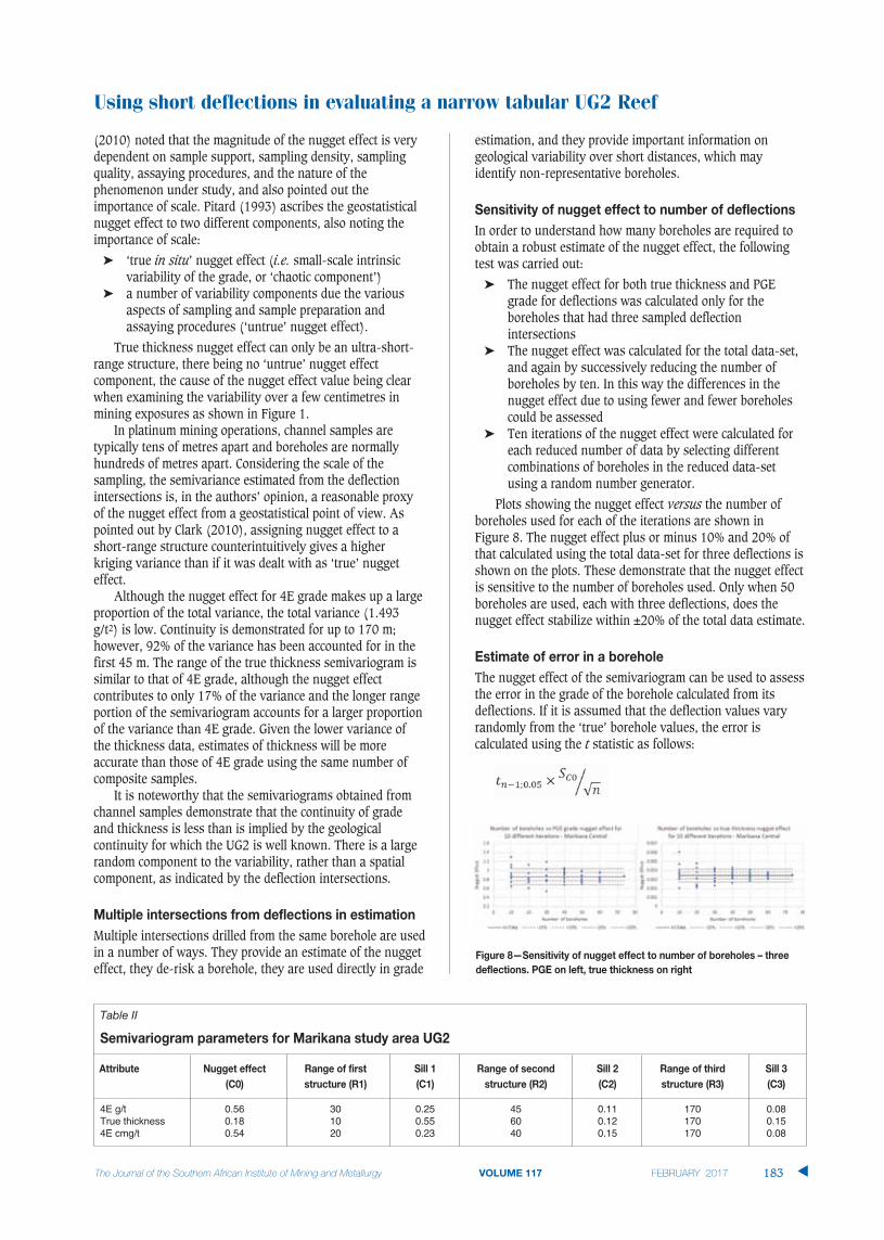
(2010) noted that the magnitude of the nugget effect is verydependent on sample support, sampling density, samplingquality, assaying procedures, and the nature of thephenomenon under study, and also pointed out theimportance of scale. Pitard (1993) ascribes the geostatisticalnugget effect to two different components, also noting theimportance of scale:
� ‘true in situ’ nugget effect (i.e. small-scale intrinsicvariability of the grade, or ‘chaotic component’)
� a number of variability components due the variousaspects of sampling and sample preparation andassaying procedures (‘untrue’ nugget effect).
True thickness nugget effect can only be an ultra-short-range structure, there being no ‘untrue’ nugget effectcomponent, the cause of the nugget effect value being clearwhen examining the variability over a few centimetres inmining exposures as shown in Figure 1.
In platinum mining operations, channel samples aretypically tens of metres apart and boreholes are normallyhundreds of metres apart. Considering the scale of thesampling, the semivariance estimated from the deflectionintersections is, in the authors’ opinion, a reasonable proxyof the nugget effect from a geostatistical point of view. Aspointed out by Clark (2010), assigning nugget effect to ashort-range structure counterintuitively gives a higherkriging variance than if it was dealt with as ‘true’ nuggeteffect.
Although the nugget effect for 4E grade makes up a largeproportion of the total variance, the total variance (1.493g/t2) is low. Continuity is demonstrated for up to 170 m;however, 92% of the variance has been accounted for in thefirst 45 m. The range of the true thickness semivariogram issimilar to that of 4E grade, although the nugget effectcontributes to only 17% of the variance and the longer rangeportion of the semivariogram accounts for a larger proportionof the variance than 4E grade. Given the lower variance ofthe thickness data, estimates of thickness will be moreaccurate than those of 4E grade using the same number ofcomposite samples.
It is noteworthy that the semivariograms obtained fromchannel samples demonstrate that the continuity of gradeand thickness is less than is implied by the geologicalcontinuity for which the UG2 is well known. There is a largerandom component to the variability, rather than a spatialcomponent, as indicated by the deflection intersections.
Multiple intersections drilled from the same borehole are usedin a number of ways. They provide an estimate of the nuggeteffect, they de-risk a borehole, they are used directly in grade
estimation, and they provide important information ongeological variability over short distances, which mayidentify non-representative boreholes.
In order to understand how many boreholes are required toobtain a robust estimate of the nugget effect, the followingtest was carried out:
� The nugget effect for both true thickness and PGEgrade for deflections was calculated only for theboreholes that had three sampled deflectionintersections
� The nugget effect was calculated for the total data-set,and again by successively reducing the number ofboreholes by ten. In this way the differences in thenugget effect due to using fewer and fewer boreholescould be assessed
� Ten iterations of the nugget effect were calculated foreach reduced number of data by selecting differentcombinations of boreholes in the reduced data-setusing a random number generator.
Plots showing the nugget effect versus the number ofboreholes used for each of the iterations are shown in Figure 8. The nugget effect plus or minus 10% and 20% ofthat calculated using the total data-set for three deflections isshown on the plots. These demonstrate that the nugget effectis sensitive to the number of boreholes used. Only when 50boreholes are used, each with three deflections, does thenugget effect stabilize within ±20% of the total data estimate.
The nugget effect of the semivariogram can be used to assessthe error in the grade of the borehole calculated from itsdeflections. If it is assumed that the deflection values varyrandomly from the ‘true’ borehole values, the error iscalculated using the t statistic as follows:
Using short deflections in evaluating a narrow tabular UG2 Reef
VOLUME 117 183 �
Table II
4E g/t 0.56 30 0.25 45 0.11 170 0.08True thickness 0.18 10 0.55 60 0.12 170 0.154E cmg/t 0.54 20 0.23 40 0.15 170 0.08

Using short deflections in evaluating a narrow tabular UG2 Reef
where:tn-1 = the percentage points of the t distribution at various
degrees of freedomSC0 = the nugget effect standard deviationn = the number of intersections in each borehole.
The error was calculated for different numbers ofintersections for PGE grade as well as for true thickness(Figure 9).
A significant decrease in the error is noticeable when thenumber of deflections is increased from two to five. Anincrease in the number of deflections from two to threeresults in the error being more than halved, and a reductionin error of approximately 30% is experienced when thenumber of deflections is increased from three to four. Thetrue thickness error is less than 10 cm (around 10% relativeerror) when three deflections are available, but the PGE gradeerror is over 1 g/t (around 20% relative error). Should fourdeflections be drilled and assayed instead of three, the PGEgrade error would reduce from 1.07 g/t to 0.74 g/t, resultingin a relative error of approximately 15% should the PGEgrade of the borehole be 5 g/t.
In addition to the error calculation, the benefit of eachadditional deflection can be simplistically judged by theweight assigned to the deflection. As the number ofdeflections increases the relative weight assigned to each willnecessarily decrease, as illustrated in Figure 10.
The relative kriging weight of each deflection reducesrapidly as more deflections are used. Once more than fivedeflections are available, little additional benefit to theestimate is gained.
Deflections drilled from mother holes at Marikana result in anumber of reef intersections separated by short distances,from a few centimetres to several tens of centimetres. Thedeflection holes are not surveyed down the hole and thewedges themselves are not inserted in any particular direction(non-directional wedges). When estimating mineral resourcesusing the intersections obtained through deflection drilling,assumptions need to be made about the distance anddirection of the intersections from one another. An alternativeto using individual deflection intersections is using lateralcomposites.
A method of dealing with non-directional deflections is toadd a nominal distance of 20 cm to each deflected intersectionin a clockwise direction, so that the first deflection is 20 cmnorth of the mother hole, the second 20 cm east, the third 20cm south and the fourth 20 cm west, thus forming a cross
arrangement. Should there be more than four deflections then40 cm is added north-east of the mother hole and so on.
The kriging weights for each deflection in the helicalarrangement were examined in order to understand howkriging manages the clustered deflection data. The exercisewas repeated using a number of different deflectionarrangements, including a straight line (Figure 11). Thegrade and thickness estimates were compared so that thesensitivity of the estimate to different arrangements could beassessed:
1 The cross arrangement at 20 cm (the base case)2 The cross arrangement at 500 cm separation3 The cross arrangement at 1 cm4 No separation5 A north-south line separated by 20 cm north, 40 cm
north, and 20 cm south of the mother hole6 An east-west line separated by 20 cm east, 20 cm west,
and 40 cm west of the mother hole.
A 500 m (north) by 500 m (east) block (a standard sizeblock used in areas outside of the channel sampling) wasselected (Figure 12). The block chosen for test estimation hastwo surface boreholes located within it, which are approxi-mately 220 m apart. These two holes are relatively closelyspaced, the remaining boreholes being more typically spacedbetween 400 m and 500 m apart and spread around the testblock. All of the boreholes within the test area intersected theUG2 Reef with three valid assayed deflections. The separationbetween boreholes is greater than the variogram range andtherefore it is expected that the total kriging weight assignedto each borehole outside of the block to be estimated will notvary greatly.
The tests on the different spatial arrangements wereconducted using the semivariogram shown in Figure 7. Table III shows the kriging weights applied in a blockestimate using the standard cross arrangement at a variety ofdeflection separations.
The following observations were made:
�
184 VOLUME 117

Using short deflections in evaluating a narrow tabular UG2 Reef
VOLUME 117 185 �
� Using the standard 20 cm cross arrangement, thekriging weights applied to each deflection are almostthe same. The holes within the block have slightlyhigher weighting on the estimate than those outside ofthe block. Holes outside the block have the sameweight, being further away from the block than the
semivariogram range. Using the 1 cm crossarrangement (or if no separation is used at all), eachdeflection within a hole attracts the exactly the sameweight
� Using the 500 cm cross arrangement, the seconddeflection in each case attracts approximately 8% lowerkriging weight than the first and the third deflectionsfor holes outside of the block. The difference in weightsis likely caused by a principle known as ‘shielding’,whereby a sample in the same line of sight to thediscretized point in the block to be estimated is given alower weight than the other sample close by
� Using a north-south line arrangement introduces aslight shielding effect at 20 cm deflection spacing. Theeast-west arrangement gives the same results
� The average semivariance for each deflection within aborehole is 1.000 for those outside the block (theybeing further away from the block than the semivar-iogram range) and 0.994 and 0.995 for the tworespective boreholes within a block. Insignificantchanges to the total semivariance are seen whetherdeflections are spaced 1 cm, 20 cm, or 500 cm from themother hole, as there is no significant differencebetween 1 cm and 500 cm when related to the range ofinfluence of 170 m
� The estimated PGE grade for the block does not vary bymore than 0.01 g/t 4E with changes in the deflectionarrangement.
The estimation weights assigned to deflections whendifferent numbers of deflections exist for each hole wereexamined using the standard PGE grade semivariogram andthe 20 cm separation cross arrangement for both ordinarykriging and inverse distance squared (Table IV).
Table III
WP018 D1 4.7 4.8 4.7D2 4.7 4.4 4.6 14.1D3 4.7 4.8 4.7
WP023 D1 4.7 4.8 4.7D2 4.7 4.4 4.6 14.1D3 4.7 4.8 4.7
WP017 D1 4.7 4.8 4.7D2 4.7 4.4 4.6 14.1D3 4.7 4.8 4.7
WP024 D1 5.0 5.1 5.0D2 5.0 4.8 4.9 15.0D3 5.0 5.1 5.0
WP016 D1 5.0 5.1 5.0D2 5.0 4.8 5.0 15.0D3 5.0 5.2 5.0
RS137 D1 4.7 4.8 4.7D2 4.7 4.5 4.6 14.1D3 4.7 4.8 4.7
ML048 D1 4.7 4.8 4.7D2 4.7 4.4 4.6 14.1D3 4.7 4.8 4.7
*Refer to Figure 11 for deflection number in the arrangement
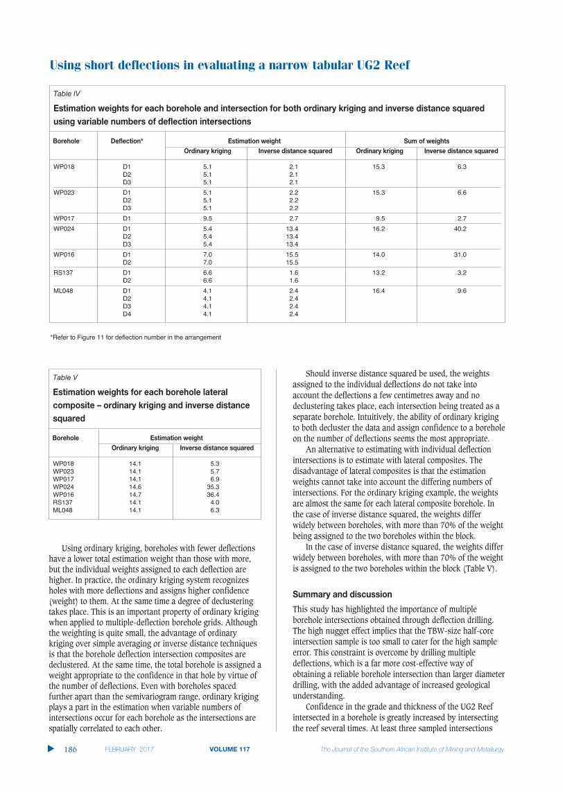
Using short deflections in evaluating a narrow tabular UG2 Reef
Using ordinary kriging, boreholes with fewer deflectionshave a lower total estimation weight than those with more,but the individual weights assigned to each deflection arehigher. In practice, the ordinary kriging system recognizesholes with more deflections and assigns higher confidence(weight) to them. At the same time a degree of declusteringtakes place. This is an important property of ordinary krigingwhen applied to multiple-deflection borehole grids. Althoughthe weighting is quite small, the advantage of ordinarykriging over simple averaging or inverse distance techniquesis that the borehole deflection intersection composites aredeclustered. At the same time, the total borehole is assigned aweight appropriate to the confidence in that hole by virtue ofthe number of deflections. Even with boreholes spacedfurther apart than the semivariogram range, ordinary krigingplays a part in the estimation when variable numbers ofintersections occur for each borehole as the intersections arespatially correlated to each other.
Should inverse distance squared be used, the weightsassigned to the individual deflections do not take intoaccount the deflections a few centimetres away and nodeclustering takes place, each intersection being treated as aseparate borehole. Intuitively, the ability of ordinary krigingto both decluster the data and assign confidence to a boreholeon the number of deflections seems the most appropriate.
An alternative to estimating with individual deflectionintersections is to estimate with lateral composites. Thedisadvantage of lateral composites is that the estimationweights cannot take into account the differing numbers ofintersections. For the ordinary kriging example, the weightsare almost the same for each lateral composite borehole. Inthe case of inverse distance squared, the weights differwidely between boreholes, with more than 70% of the weightbeing assigned to the two boreholes within the block.
In the case of inverse distance squared, the weights differwidely between boreholes, with more than 70% of the weightis assigned to the two boreholes within the block (Table V).
This study has highlighted the importance of multipleborehole intersections obtained through deflection drilling.The high nugget effect implies that the TBW-size half-coreintersection sample is too small to cater for the high sampleerror. This constraint is overcome by drilling multipledeflections, which is a far more cost-effective way ofobtaining a reliable borehole intersection than larger diameterdrilling, with the added advantage of increased geologicalunderstanding.
Confidence in the grade and thickness of the UG2 Reefintersected in a borehole is greatly increased by intersectingthe reef several times. At least three sampled intersections
�
186 VOLUME 117
Table IV
WP018 D1 5.1 2.1 15.3 6.3D2 5.1 2.1D3 5.1 2.1
WP023 D1 5.1 2.2 15.3 6.6D2 5.1 2.2D3 5.1 2.2
WP017 D1 9.5 2.7 9.5 2.7
WP024 D1 5.4 13.4 16.2 40.2D2 5.4 13.4D3 5.4 13.4
WP016 D1 7.0 15.5 14.0 31.0D2 7.0 15.5
RS137 D1 6.6 1.6 13.2 3.2D2 6.6 1.6
ML048 D1 4.1 2.4 16.4 9.6D2 4.1 2.4D3 4.1 2.4D4 4.1 2.4
Table V
WP018 14.1 5.3WP023 14.1 5.7WP017 14.1 6.9WP024 14.6 35.3WP016 14.7 36.4RS137 14.1 4.0ML048 14.1 6.3
*Refer to Figure 11 for deflection number in the arrangement

are required to gain reasonable confidence in the borehole. Atleast 50 boreholes, each with three or more deflections, arerequired to obtain a stable estimate of the nugget effect.
A number of important findings arose from the way inwhich multiple intersections are handled in the estimationprocedure. Most notably:
� The kriged estimate is not sensitive to the spacingapplied between the intersections at very smalldistances (tens of centimetres). The application oflarger distances (several metres) should be avoided asthe shielding effect causes the weights to be differentfor each intersection, when in practice they should beexactly the same for each intersection drilled from thesame hole
� The cross arrangement currently used at Marikana iscorrect as it avoids the shielding effect experienced ifthe intersections are arranged in line. It is not knownexactly what arrangement is actually achieved duringdrilling as the deflections are not surveyed; however,the cross arrangement obtains the most suitable resultwith the (untrue) assumption that deflectionintersections are equally arranged around the motherhole
� Ordinary kriging effectively declusters the clusters ofdeflection intersections while attributing higherconfidence to a borehole with a greater number ofintersections. Intuitively, this is a desired effect
� The use of lateral composites does not take intoaccount the higher confidence that one would wish toassign to a borehole with more intersections. If aninverse distance approach is used then lateralcomposites will avoid over-weighting of boreholes withmany intersections, which would otherwise occur usingindividual deflection intersections. The authorsconsider that inverse distance is not a valid techniquefor high-nugget-effect deposits with clustered data.
Deflection drilling greatly assists in the identification ofboreholes affected by geological disturbances such as faultsand potholes. Techniques that examine the variabilitybetween intersections drilled from the same borehole help toidentify data validation issues and subtle geological distur-bances that might otherwise be overlooked. Multipledeflection drilling greatly reduces the risk associated with aborehole compared with that which would occur if a singleintersection is used.
Lonmin Platinum kindly gave permission to use the data forthis study and for publication of the paper.
CARRASCO, P.C. 2010. Nugget effect, artificial or natural? Journal of the SouthernAfrican Institute of Mining and Metallurgy, vol. 110, no. 6. pp. 299–305.
CLARK, I. 1979. Practical Geostatistics, Elsevier. 129 pp.
CLARK, I. 2010. Statistics or geostatistics? Sampling error or nugget effect?Journal of the Southern African Institute of Mining and Metallurgy, vol. 110, no. 6. pp. 307–312.
HOFFMANN, D. 2010. Statistical size analysis of potholes: an attempt to estimategeological losses ahead of mining at Lonmin’s Marikana mining district.Proceedings of the 4th International Platinum Conference, Platinum inTransition ‘Boom or Bust’, Sun City, South Africa, 11–14 October 2010.Southern African Institute of Mining and Metallurgy, Johannesburg. pp. 97–104.
KRIGE, D.G. 1981. Lognormal–de Wijsian Geostatistics for Ore Evaluation,Monograph Series. South African Institute of Mining and Metallurgy,Johannesburg.
MATHERON, G. 1971. The Theory of Regionalised Variables and its Applications.Cahier no. 5, Centre de Morphologie Mathématique de Fontainebleau. 211pp.
Pitard, F.F. 1993. Exploration of the nugget effect. Geostatistics for the NextCentury. Kluwer, Doordrecht, The Netherlands.
Using short deflections in evaluating a narrow tabular UG2 Reef
VOLUME 117 187 �


This paper describes a methodology that canbe applied when constructing a geologicalmodel of a deposit following a conventionalapproach. An understanding of the geology ofa deposit is fundamental to the MineralResource estimation (MRE) process, sinceestimates are constrained by the geologicalcomplexity captured within the geologicalmodel, usually based on geology, geometry,structural nature, and grade distribution of thedeposit. The risk associated with the geologicalmodel and the choice and suitability ofestimation techniques have an impact onMineral Resource confidence, which isreflected by the resource classification category
associated with the estimate. Each deposit isunique, therefore the MRE process for eachdeposit varies. The workflow adopted in thisstudy is based on a gold deposit containing anoxide zone (oxides) and a deeper sulphidezone (sulphides) comprised of unweathered(fresh rock) material, located in southwesternMali. The mine does not have the plantcapability to treat sulphides due to theindentation hardness, and most of the oxideMineral Reserve on the concession has alreadybeen depleted. Exploring the potential foradditional oxide resources is thus a naturalstep to increase the life of the mine.
Any MRE process is iterative, requiring a goodunderstanding of: the underlying geology,good resource evaluation practice, and relevantknowledge of the literature, including companyreports and maps, to recognize and learn frompast experience. This information provides areference and known a-priori informationabout the deposit to guide both the modellingand estimation processes. The first step in theMRE process is data collation and preparationto serve as the basis for modelling, analysis,and estimation. This data includes collar,survey, alteration, assay, lithology, hardness,and redox information that is validated toensure it is error-free. Light detection andranging (LIDAR) surface topography stringsare another type of data that is validated toensure that the topography is accuratelyrepresented. Once all the data is deemed ofhigh quality and suitable for estimation, thesecond step of the MRE process is 3Dgeological modelling based on the drilling data.During this step, validated data is used togenerate a series of wireframes to representthe extent and current understanding of the
3D geological modelling and resourceestimation for a gold deposit in Maliby L. Chanderman*, C.E. Dohm*, and R.C.A. Minnitt*
Mineral Resource estimation (MRE) and classification are highlydependent on the confidence in the model of the orebody geometry, knownas the geological model, within which the estimates are constrained. Anunderstanding of the geology of a deposit is thus fundamental to theMineral Resource evaluation process. The geological model is a function ofthe structural and depositional complexity of the geology captured bydrilling information, which is limited in the early stages of a project. Theinformation effect has a significant impact in terms of the interpretation ofthe geology as well as the estimation of grade continuity and the resultantrisk associated with the Mineral Resource estimate and classification.
Therefore, as new drilling information becomes available, it isnecessary to update and refine the geological model to appropriatelyconstrain the resource estimates. The grade information is also updated,including statistics and the spatial correlation characteristics. Thisrefinement is based on geological interpretations derived from the drill-hole information that becomes available throughout the life of the mine;orebody knowledge that comes from working experience of the deposit, aswell as familiarity with the software package used for modelling, is alsoimportant.
In updating, the potential to identify new resources in previouslyunknown areas may be realized. The opposite may also occur whereprevious interpretations of ore continuity are refuted. Both scenarios couldresult from a better understanding of the geology of the deposit and thus amore realistic MRE, which reduces geological risk. This paper describeshow newly drilled advanced grade-control holes for a gold deposit in Maliwere used to refine the 3D geological model for the deposit in an attemptto identify the potential for additional oxide ore using conventionalgeostatistical evaluation techniques.
geological modelling, resource estimation, geostatistical evaluation.
* School of Mining Engineering, University of theWitwatersrand, South Africa.
© The Southern African Institute of Mining andMetallurgy, 2017. ISSN 2225-6253. Paper receivedApr. 2016; revised paper received Sep. 2016.
189VOLUME 117 �
http://dx.doi.org/10.17159/2411-9717/2017/v117n2a10
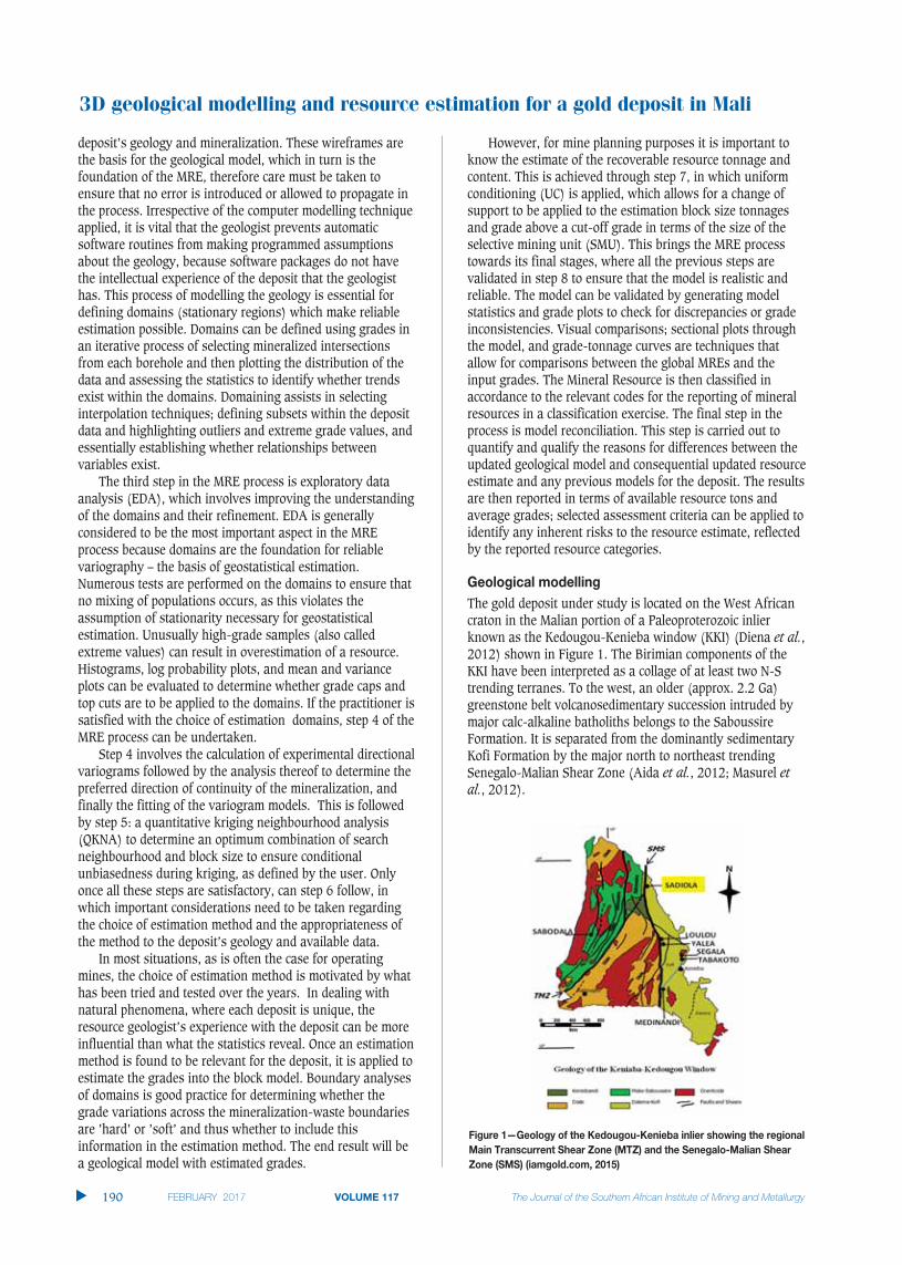
3D geological modelling and resource estimation for a gold deposit in Mali
deposit’s geology and mineralization. These wireframes arethe basis for the geological model, which in turn is thefoundation of the MRE, therefore care must be taken toensure that no error is introduced or allowed to propagate inthe process. Irrespective of the computer modelling techniqueapplied, it is vital that the geologist prevents automaticsoftware routines from making programmed assumptionsabout the geology, because software packages do not havethe intellectual experience of the deposit that the geologisthas. This process of modelling the geology is essential fordefining domains (stationary regions) which make reliableestimation possible. Domains can be defined using grades inan iterative process of selecting mineralized intersectionsfrom each borehole and then plotting the distribution of thedata and assessing the statistics to identify whether trendsexist within the domains. Domaining assists in selectinginterpolation techniques; defining subsets within the depositdata and highlighting outliers and extreme grade values, andessentially establishing whether relationships betweenvariables exist.
The third step in the MRE process is exploratory dataanalysis (EDA), which involves improving the understandingof the domains and their refinement. EDA is generallyconsidered to be the most important aspect in the MREprocess because domains are the foundation for reliablevariography – the basis of geostatistical estimation.Numerous tests are performed on the domains to ensure thatno mixing of populations occurs, as this violates theassumption of stationarity necessary for geostatisticalestimation. Unusually high-grade samples (also calledextreme values) can result in overestimation of a resource.Histograms, log probability plots, and mean and varianceplots can be evaluated to determine whether grade caps andtop cuts are to be applied to the domains. If the practitioner issatisfied with the choice of estimation domains, step 4 of theMRE process can be undertaken.
Step 4 involves the calculation of experimental directionalvariograms followed by the analysis thereof to determine thepreferred direction of continuity of the mineralization, andfinally the fitting of the variogram models. This is followedby step 5: a quantitative kriging neighbourhood analysis(QKNA) to determine an optimum combination of searchneighbourhood and block size to ensure conditionalunbiasedness during kriging, as defined by the user. Onlyonce all these steps are satisfactory, can step 6 follow, inwhich important considerations need to be taken regardingthe choice of estimation method and the appropriateness ofthe method to the deposit’s geology and available data.
In most situations, as is often the case for operatingmines, the choice of estimation method is motivated by whathas been tried and tested over the years. In dealing withnatural phenomena, where each deposit is unique, theresource geologist’s experience with the deposit can be moreinfluential than what the statistics reveal. Once an estimationmethod is found to be relevant for the deposit, it is applied toestimate the grades into the block model. Boundary analysesof domains is good practice for determining whether thegrade variations across the mineralization-waste boundariesare ’hard’ or ’soft’ and thus whether to include thisinformation in the estimation method. The end result will bea geological model with estimated grades.
However, for mine planning purposes it is important toknow the estimate of the recoverable resource tonnage andcontent. This is achieved through step 7, in which uniformconditioning (UC) is applied, which allows for a change ofsupport to be applied to the estimation block size tonnagesand grade above a cut-off grade in terms of the size of theselective mining unit (SMU). This brings the MRE processtowards its final stages, where all the previous steps arevalidated in step 8 to ensure that the model is realistic andreliable. The model can be validated by generating modelstatistics and grade plots to check for discrepancies or gradeinconsistencies. Visual comparisons; sectional plots throughthe model, and grade-tonnage curves are techniques thatallow for comparisons between the global MREs and theinput grades. The Mineral Resource is then classified inaccordance to the relevant codes for the reporting of mineralresources in a classification exercise. The final step in theprocess is model reconciliation. This step is carried out toquantify and qualify the reasons for differences between theupdated geological model and consequential updated resourceestimate and any previous models for the deposit. The resultsare then reported in terms of available resource tons andaverage grades; selected assessment criteria can be applied toidentify any inherent risks to the resource estimate, reflectedby the reported resource categories.
The gold deposit under study is located on the West Africancraton in the Malian portion of a Paleoproterozoic inlierknown as the Kedougou-Kenieba window (KKI) (Diena et al.,2012) shown in Figure 1. The Birimian components of theKKI have been interpreted as a collage of at least two N-Strending terranes. To the west, an older (approx. 2.2 Ga)greenstone belt volcanosedimentary succession intruded bymajor calc-alkaline batholiths belongs to the SaboussireFormation. It is separated from the dominantly sedimentaryKofi Formation by the major north to northeast trendingSenegalo-Malian Shear Zone (Aida et al., 2012; Masurel etal., 2012).
�
190 VOLUME 117
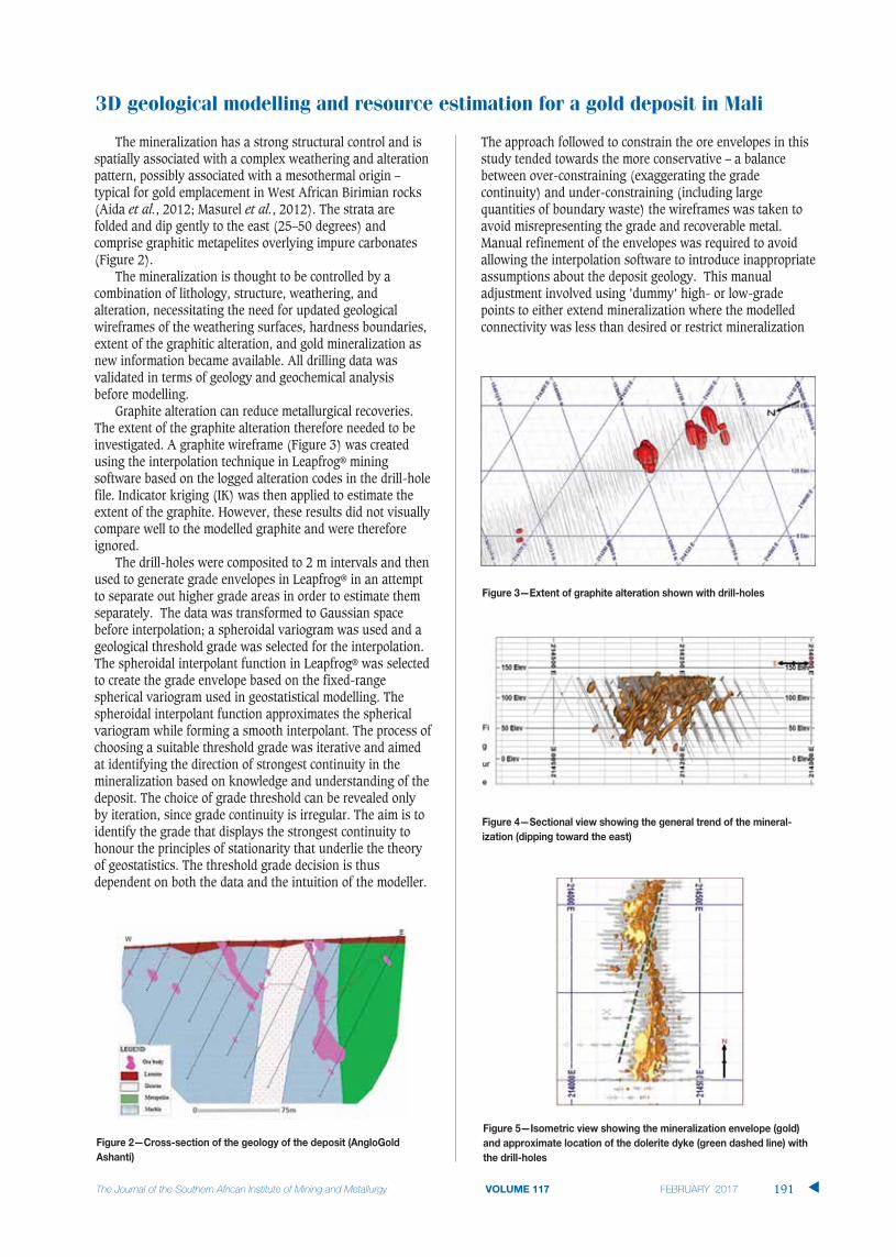
The mineralization has a strong structural control and isspatially associated with a complex weathering and alterationpattern, possibly associated with a mesothermal origin –typical for gold emplacement in West African Birimian rocks(Aida et al., 2012; Masurel et al., 2012). The strata arefolded and dip gently to the east (25–50 degrees) andcomprise graphitic metapelites overlying impure carbonates(Figure 2).
The mineralization is thought to be controlled by acombination of lithology, structure, weathering, andalteration, necessitating the need for updated geologicalwireframes of the weathering surfaces, hardness boundaries,extent of the graphitic alteration, and gold mineralization asnew information became available. All drilling data wasvalidated in terms of geology and geochemical analysisbefore modelling.
Graphite alteration can reduce metallurgical recoveries.The extent of the graphite alteration therefore needed to beinvestigated. A graphite wireframe (Figure 3) was createdusing the interpolation technique in Leapfrog® miningsoftware based on the logged alteration codes in the drill-holefile. Indicator kriging (IK) was then applied to estimate theextent of the graphite. However, these results did not visuallycompare well to the modelled graphite and were thereforeignored.
The drill-holes were composited to 2 m intervals and thenused to generate grade envelopes in Leapfrog® in an attemptto separate out higher grade areas in order to estimate themseparately. The data was transformed to Gaussian spacebefore interpolation; a spheroidal variogram was used and ageological threshold grade was selected for the interpolation.The spheroidal interpolant function in Leapfrog® was selectedto create the grade envelope based on the fixed-rangespherical variogram used in geostatistical modelling. Thespheroidal interpolant function approximates the sphericalvariogram while forming a smooth interpolant. The process ofchoosing a suitable threshold grade was iterative and aimedat identifying the direction of strongest continuity in themineralization based on knowledge and understanding of thedeposit. The choice of grade threshold can be revealed onlyby iteration, since grade continuity is irregular. The aim is toidentify the grade that displays the strongest continuity tohonour the principles of stationarity that underlie the theoryof geostatistics. The threshold grade decision is thusdependent on both the data and the intuition of the modeller.
The approach followed to constrain the ore envelopes in thisstudy tended towards the more conservative – a balancebetween over-constraining (exaggerating the gradecontinuity) and under-constraining (including largequantities of boundary waste) the wireframes was taken toavoid misrepresenting the grade and recoverable metal.Manual refinement of the envelopes was required to avoidallowing the interpolation software to introduce inappropriateassumptions about the deposit geology. This manualadjustment involved using ’dummy’ high- or low-gradepoints to either extend mineralization where the modelledconnectivity was less than desired or restrict mineralization
3D geological modelling and resource estimation for a gold deposit in Mali
VOLUME 117 191 �

3D geological modelling and resource estimation for a gold deposit in Mali
where the modelled connectivity was more than desired (orthere were unreasonable extensions beyond data support –often termed Leapfrog® ’blowouts’).
The resultant interpretation of the mineralization isshown in Figure 4 – it strikes approximately N-S (for 1.1 km)and dips at 50 degrees towards the east. Near its centre, thereis a break in the mineralization where a dolerite dyke hasintruded along a fault that has separated and displaced themineralization (Figure 5). The previous and updated mineral-ization interpretations were carefully assessed and theycompared well in terms of the geological controls governingthe mineralization.
Samples within the mineralized envelope were deemed ‘ore’and those outside, ‘waste’. Domains are defined as zones thatare geologically and statistically homogenous (supported byvariography and statistical analysis) (Duke and Hanna,2001). The domains in the study were defined using gradesin an iterative process of selecting mineralized intersectionsin each borehole using Leapfrog®. Mineralized domains wereidentified on the basis of logged samples and grade
continuity, and were guided by the previously modelledmineralized wireframes. The spatial limits of these domainsare controlled by the 3D geological mesh (Schofield, 2011)and were examined in a boundary analysis exercises. Sixdomains (laterite ore, saprolite ore, hard ore, laterite waste,saprolite waste, and hard waste) were identified. The ‘ore’ (ormineralized) domains (laterite, saprolite, and hard) werecompared to determine whether they should be estimatedtogether or separately.
The statistics and distributions of the hard and saproliteore were compared and found to be fairly similar, but thesaprolite mean ore grade was higher at 1.65 g/t than the hardore mean grade of 1.29 g/t.
In addition, the grade variation along the hard-softcontact was investigated (Figure 8). The results showedslight grade enrichment immediately below the hard-softcontact and that the grade tended to decrease gradually withdepth. It was therefore decided that the saprolite and hard orezones should be estimated separately, applying a hardboundary between them for estimation. Comparison of thelaterite and saprolite mineralization grades (Figure 9) showedcomparable means of 1.59 g/t for laterite and 1.65 g/t forsaprolite. The QQ-plot (Figure 10) also showed that, eventhough the laterite data-set comprised very few samples, thetwo data-sets had similar grade distributions (except at thelower end of the distribution below about 0.5 g/t). The
�
192 VOLUME 117
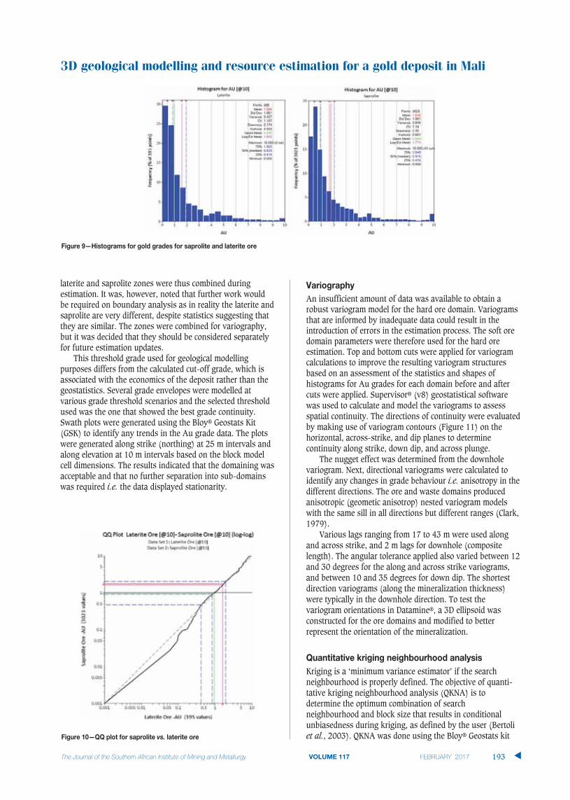
laterite and saprolite zones were thus combined duringestimation. It was, however, noted that further work wouldbe required on boundary analysis as in reality the laterite andsaprolite are very different, despite statistics suggesting thatthey are similar. The zones were combined for variography,but it was decided that they should be considered separatelyfor future estimation updates.
This threshold grade used for geological modellingpurposes differs from the calculated cut-off grade, which isassociated with the economics of the deposit rather than thegeostatistics. Several grade envelopes were modelled atvarious grade threshold scenarios and the selected thresholdused was the one that showed the best grade continuity.Swath plots were generated using the Bloy® Geostats Kit(GSK) to identify any trends in the Au grade data. The plotswere generated along strike (northing) at 25 m intervals andalong elevation at 10 m intervals based on the block modelcell dimensions. The results indicated that the domaining wasacceptable and that no further separation into sub-domainswas required i.e. the data displayed stationarity.
An insufficient amount of data was available to obtain arobust variogram model for the hard ore domain. Variogramsthat are informed by inadequate data could result in theintroduction of errors in the estimation process. The soft oredomain parameters were therefore used for the hard oreestimation. Top and bottom cuts were applied for variogramcalculations to improve the resulting variogram structures based on an assessment of the statistics and shapes ofhistograms for Au grades for each domain before and aftercuts were applied. Supervisor® (v8) geostatistical softwarewas used to calculate and model the variograms to assessspatial continuity. The directions of continuity were evaluatedby making use of variogram contours (Figure 11) on thehorizontal, across-strike, and dip planes to determinecontinuity along strike, down dip, and across plunge.
The nugget effect was determined from the downholevariogram. Next, directional variograms were calculated toidentify any changes in grade behaviour i.e. anisotropy in thedifferent directions. The ore and waste domains producedanisotropic (geometic anisotrop) nested variogram modelswith the same sill in all directions but different ranges (Clark,1979).
Various lags ranging from 17 to 43 m were used alongand across strike, and 2 m lags for downhole (compositelength). The angular tolerance applied also varied between 12and 30 degrees for the along and across strike variograms,and between 10 and 35 degrees for down dip. The shortestdirection variograms (along the mineralization thickness)were typically in the downhole direction. To test thevariogram orientations in Datamine®, a 3D ellipsoid wasconstructed for the ore domains and modified to betterrepresent the orientation of the mineralization.
Kriging is a ‘minimum variance estimator’ if the searchneighbourhood is properly defined. The objective of quanti-tative kriging neighbourhood analysis (QKNA) is todetermine the optimum combination of searchneighbourhood and block size that results in conditionalunbiasedness during kriging, as defined by the user (Bertoliet al., 2003). QKNA was done using the Bloy® Geostats kit
3D geological modelling and resource estimation for a gold deposit in Mali
VOLUME 117 193 �

3D geological modelling and resource estimation for a gold deposit in Mali
(BGK), which involved optimization based on a simulateddrilling grid that approximates the drill spacing of the datainforming the estimate. To optimize the number ofcomposites, the close-spaced theoretical sample spacing of 25 m × 25 m × 7 m was used, together with a discretizationof 5 m × 5 m × 5 m. The maximum and minimum numbers ofsamples were varied and assessed and a minimum numberand maximum number of optimal samples selected for the orezones. For the block size optimization (based on the orevariogram applied for both hard and soft ore estimation) atheoretical sample spacing of 25 m × 25 m × 7 m wasassumed, together with a discretization of 5 m × 5 m × 5 mand a selected minimum and maximum number of samples.Search ellipses were oriented according to the approximateorientation of the mineralization with search distances set toapproximate the variogram ranges. The optimal model blocksize was found to be 25 m × 25 m × 10 m. Smaller blocksizes, although more optimal than larger 25 m × 25 m or 50 m × 50 m blocks, are not useful for uniform conditioningand were therefore ignored. For optimal UC results, largerblock sizes are recommended to ensure a sufficient number of
SMUs in the estimation panel. The search neighbourhoodwas optimized based on a simulated drilling grid that approx-imated the drill spacing where less data was available. Thesearch ranges selected were not limited to the variogramranges. For the search distance optimization, the widerspaced theoretical sample spacing of 25 m (X) × 25 m (Y) ×10 m (Z) was used together with the optimized block size, adiscretization of 5 m (X) × 5 m (Y) × 5 m (Z), and theoptimized minimum and maximum number of samples.
Kriging provides the best estimate since it results in thesmallest standard error, narrowest confidence interval, andmost confidence (lowest risk) (Bertoli et al., 2003). Thedeposit lent itself well to the use of ordinary kriging (OK) asan estimation technique since the method performed well onhistorical models for the deposit. The data did not show anysignificant trends at the scale of modelling and thevariograms were characteristic of local stationarity. The blockmodel grades were estimated using OK in Datamine®
Studio 3.
�
194 VOLUME 117
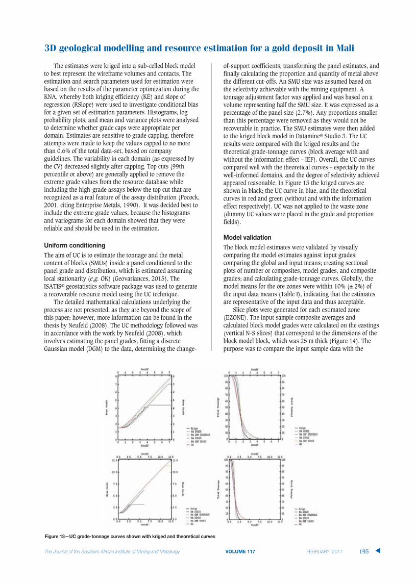
3D geological modelling and resource estimation for a gold deposit in Mali
VOLUME 117 195 �
The estimates were kriged into a sub-celled block modelto best represent the wireframe volumes and contacts. Theestimation and search parameters used for estimation werebased on the results of the parameter optimization during theKNA, whereby both kriging efficiency (KE) and slope ofregression (RSlope) were used to investigate conditional biasfor a given set of estimation parameters. Histograms, logprobability plots, and mean and variance plots were analysedto determine whether grade caps were appropriate perdomain. Estimates are sensitive to grade capping, thereforeattempts were made to keep the values capped to no morethan 0.6% of the total data-set, based on companyguidelines. The variability in each domain (as expressed bythe CV) decreased slightly after capping. Top cuts (99thpercentile or above) are generally applied to remove theextreme grade values from the resource database whileincluding the high-grade assays below the top cut that arerecognized as a real feature of the assay distribution (Pocock,2001, citing Enterprise Metals, 1990). It was decided best toinclude the extreme grade values, because the histogramsand variograms for each domain showed that they werereliable and should be used in the estimation.
The aim of UC is to estimate the tonnage and the metalcontent of blocks (SMUs) inside a panel conditioned to thepanel grade and distribution, which is estimated assuminglocal stationarity (e.g. OK) (Geovariances, 2015). TheISATIS® geostatistics software package was used to generatea recoverable resource model using the UC technique.
The detailed mathematical calculations underlying theprocess are not presented, as they are beyond the scope ofthis paper; however, more information can be found in thethesis by Neufeld (2008). The UC methodology followed wasin accordance with the work by Neufeld (2008), whichinvolves estimating the panel grades, fitting a discreteGaussian model (DGM) to the data, determining the change-
of-support coefficients, transforming the panel estimates, andfinally calculating the proportion and quantity of metal abovethe different cut-offs. An SMU size was assumed based onthe selectivity achievable with the mining equipment. Atonnage adjustment factor was applied and was based on avolume representing half the SMU size. It was expressed as apercentage of the panel size (2.7%). Any proportions smallerthan this percentage were removed as they would not berecoverable in practice. The SMU estimates were then addedto the kriged block model in Datamine® Studio 3. The UCresults were compared with the kriged results and thetheoretical grade-tonnage curves (block average with andwithout the information effect – IEF). Overall, the UC curvescompared well with the theoretical curves – especially in thewell-informed domains, and the degree of selectivity achievedappeared reasonable. In Figure 13 the kriged curves areshown in black; the UC curve in blue, and the theoreticalcurves in red and green (without and with the informationeffect respectively). UC was not applied to the waste zone(dummy UC values were placed in the grade and proportionfields).
The block model estimates were validated by visuallycomparing the model estimates against input grades;comparing the global and input means; creating sectionalplots of number or composites, model grades, and compositegrades; and calculating grade-tonnage curves. Globally, themodel means for the ore zones were within 10% (± 2%) ofthe input data means (Table I), indicating that the estimatesare representative of the input data and thus acceptable.
Slice plots were generated for each estimated zone(EZONE). The input sample composite averages andcalculated block model grades were calculated on the eastings(vertical N-S slices) that correspond to the dimensions of theblock model block, which was 25 m thick (Figure 14). Thepurpose was to compare the input sample data with the
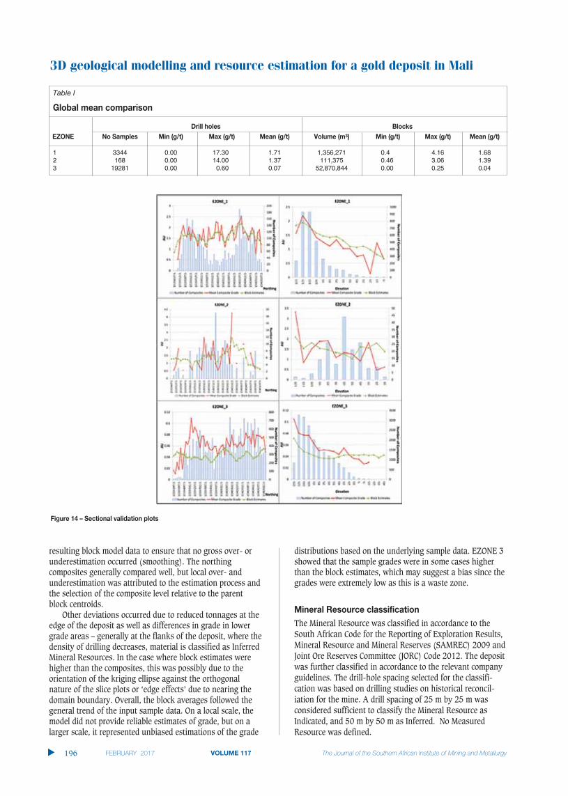
3D geological modelling and resource estimation for a gold deposit in Mali
resulting block model data to ensure that no gross over- orunderestimation occurred (smoothing). The northingcomposites generally compared well, but local over- andunderestimation was attributed to the estimation process andthe selection of the composite level relative to the parentblock centroids.
Other deviations occurred due to reduced tonnages at theedge of the deposit as well as differences in grade in lowergrade areas – generally at the flanks of the deposit, where thedensity of drilling decreases, material is classified as InferredMineral Resources. In the case where block estimates werehigher than the composites, this was possibly due to theorientation of the kriging ellipse against the orthogonalnature of the slice plots or ‘edge effects’ due to nearing thedomain boundary. Overall, the block averages followed thegeneral trend of the input sample data. On a local scale, themodel did not provide reliable estimates of grade, but on a larger scale, it represented unbiased estimations of the grade
distributions based on the underlying sample data. EZONE 3showed that the sample grades were in some cases higherthan the block estimates, which may suggest a bias since thegrades were extremely low as this is a waste zone.
The Mineral Resource was classified in accordance to theSouth African Code for the Reporting of Exploration Results,Mineral Resource and Mineral Reserves (SAMREC) 2009 andJoint Ore Reserves Committee (JORC) Code 2012. The depositwas further classified in accordance to the relevant companyguidelines. The drill-hole spacing selected for the classifi-cation was based on drilling studies on historical reconcil-iation for the mine. A drill spacing of 25 m by 25 m wasconsidered sufficient to classify the Mineral Resource asIndicated, and 50 m by 50 m as Inferred. No MeasuredResource was defined.
�
196 VOLUME 117
Table I
1 3344 0.00 17.30 1.71 1,356,271 0.4 4.16 1.682 168 0.00 14.00 1.37 111,375 0.46 3.06 1.393 19281 0.00 0.60 0.07 52,870,844 0.00 0.25 0.04
The previous Mineral Resource model was compared with theupdated Mineral Resource model within a common volume toquantify the differences as a result of the model update.Grade-tonnage curves for the common volume were alsocalculated. Changes were ascribed mostly to the changes inthe interpretation of the mineralized envelopes, theestimation search parameters, and the general increase in thebulk densities assigned to the various rock types.
The detailed reconciliation study showed that the newMRE identified an additional 7191 ounces of Indicated(oxide) Mineral Resource, 1893 ounces of which waspreviously classified as Inferred. The increase was attributedto the extension of some of the mineralized zones and bettergrade continuity for others based on the updated geologicalmodel.
This study described the identification of additional oxide orepotential at a gold deposit in Mali based on 3D geologicalmodelling and geostatistical evaluation techniques asinformed by newly drilled advanced grade-control holes. Thefindings of the ten-step MRE process adopted revealed thatthe deposit contained an additional oxide Mineral Resource(7191 ounces) identified in the new 3D geological model.Due to the new drilling information, the geologicalunderstanding of the deposit was improved, making itpossible to better constrain the resource estimates within anew geological model. This included improvements in theinterpretation of the mineralized envelope in the areas wherethe drilling campaign provided new information. In someareas the continuity of the modelled mineralization wasextended, and in other areas the envelopes were constrainedto reduce the boundary waste that was previously included.The new data also allowed for the updating of variograms,estimation parameters, and top-capping applied. Potentialrisk to the model could originate from bias identified ingrade-tonnage curves which exists irrespective of theeffectiveness of the estimation process, as well as theinherent risk associated with geological uncertainty as aresult of not being able to completely capture the true natureof the geology. From the context of a conventional approachto 3D geological modelling and MRE, the results wereacceptable. However, to fully characterize the geologicaluncertainty, stochastic approaches to orebody modelling andestimation should be considered.
The authors express their gratitude to AngloGold AshantiLimited for permission to use all data and the relevantsoftware necessary for the project. Special thanks to Mr VasuGovindsammy (Evaluation Manager, AGA) and Miss EmiMaritz (Senior Evaluation Geologist, AGA) for theirassistance and support.
CLARK, I. 1979. Practical Geostatistics. Applied Science Publishers, Barking,
Essex. 129 pp.
DUKE, J.H. and HANNA, P.J. 2001. Geological interpretation for resource
modelling and estimation. Mineral Resource and Ore Reserve Estimation –
The AusIMM Guide to Good Practice. Edwards, A.C. (ed.). Australasian
Institute of Mining and Metallurgy, Melbourne. pp. 147–156.
GEOVARIANCES. 2015. Localized multivariate uniform conditioning.
http://www.geovariances.com/en/IMG/pdf/_GeovMining_LocalizedMultiva
riateUniformConditioning.pdf [Accessed 12 January 2015].
MASUREL, Q., THEBAUD, N., MILLER, J., and ULRICH, S. 2012. Tectonics, magma
generation and gold endowment: a study of the contrasting mineralization
styles in the world-class Sadiola gold camp, Mali, West Africa. Society of
Economic Geologists Conference: Building Exploration Capability for the
21st Century, Keystone, CO, 27-30 September 2014. Society of Economic
Geologists, Littleton, CO.
MASUREL, Q., THEBAUD, N., MILLER, J., STANISLAV, U., and OCKERT, T. 2012. The
world-class Sadiola gold camp, Mali, West Africa: Evidence for contrasting
styles of carbonate-hosted mineralisation within an orogenic gold
province. Proceedings of Gold14@Kalgoorlie, Kalgoorlie, WA, 8-10
October 2014. Australian Institute of Geoscientists.
https://www.google.co.za/url?sa=t&rct=j&q=&esrc=s&source=web&cd=16
&cad=rja&uact=8&ved=0CDEQFjAFOApqFQoTCO6xqJaE_sYCFQwcPgodmi
sD6w&url=http%3A%2F%2Fsjsresource.worldsecuresystems.com%2F_lite
rature_127582%2FBulletin_No_59_(Low_Res)&ei=KpG3Ve70C4y4-
AGa14zYDg&usg=AFQjCNGeInZfYf-
X094WxiMEadhio1tgkg&sig2=Uecf9ejxQuB8zwAKpAJ7Sg&bvm=bv.9871
7601,d.cWw [Accessed 10 June 2015].
NEUFELD, C.T. 2005. Guide to Recoverable Reserves with Uniform conditioning.
Guidebook Series, vol. 4. Centre for Computational Geostatistics (CCG),
Canada.
POCOCK, J.A. 2001. Why feasibility resource estimates under-valued the Peak
ore body. Mineral Resource and Ore Reserve Estimation – The AusIMM
Guide to Good Practice. Edwards, A.C. (ed.). Australasian Institute of
Mining and Metallurgy: Melbourne. pp. 299–314.
SCHOFIELD, N.A. 2011. Geological domaining and resource estimation – a
discussion. Proceedings of the 35th APCOM Symposium, Wollongong,
NSW. Australasian Institute of Mining and Metallurgy, Melbourne.
SAMREC. 2009. South African Mineral Resource Committee. The South African
Code for Reporting of Exploration Results, Mineral Resources and Mineral
Reserves (the SAMREC Code). 2007 Edition as amended July 2009. pp.
11-12. http://www.samcode.co.za/downloads/SAMREC2009.pdf
VANN, J., JACKSON, S., and BERTOLI, O. 2003. Quantitative kriging neighbourhood
analysis for the mining - a description of the method with worked case
examples. Proceedings of the 5th International Mining Geology
Conference, Bendigo, Vic, Australia. Australasian Institute of Mining and
Metallurgy, Melbourne. �
3D geological modelling and resource estimation for a gold deposit in Mali
VOLUME 117 197 �


A mining production system (MPS) is a resultof an iterative process of design, planning, andoptimization of mining input variables anddecision-making variables (DMVs). The MPSexists within the mineral extraction link of thecomplete mining value chain. It represents thestage where mining companies have theopportunity, through production, to startgenerating returns on the investmentsundertaken. Returns on shareholders’investments can be realized at this stage.
More often than not, the actualperformance of the MPS is somewhat differentto that in the optimized MPS plan. Thisbehaviour or characteristic is observed in anensemble of output results of the keyperformance indicators (KPIs). These resultsare sometimes above target, on target, or
below target due to uncertainty associatedwith technical and human factors, resulting inactual output being different to that planned.The first two circumstances are perhaps themost desired. However, in most cases the MPS,especially in the case of mature mines, tends todeliver below target. The variability of the KPIsof interest is influenced by internal variablesor DMVs. The variable units or DMVs can beeither controllable or uncontrollable. It istherefore important to understand and know towhat degree the controllable variables can becontrolled to achieve the desired output and tominimize the effects of the uncontrollablevariables. This paper is part of an MScresearch study at the University of theWitwatersrand, based on a platinum mine MPScase study where actual data was available foranalysis.
Commentary on the mining industry’s produc-tivity has been topical in the last decade due tothe declining productivity trends across severalcommodities. Research, analysis, andpublications from institutions like the Chamberof Mines, Statistics South Africa, Ernest andYoung (EY), McKinsey, DuPont,PricewaterhouseCoopers (PwC), and manyindependent market analysts have highlightedthis trend. All the reports highlight declininglabour productivity versus increasing wagebills, rising input costs due to inflation,decreasing revenues, falling metal prices,declining throughput, and instability of thelabour markets.
Characterizing a mining productionsystem for decision-making purposes ina platinum mineby T.C. Sebutsoe* and C. Musingwini†
The primary objective of any mining business unit is to make profit byextracting, processing, and selling minerals from a particular mineral deposit.It is important to optimize extraction of the mineral resource given time,capital, and space constraints. Mineral extraction is often associated withuncertainty due to variable technical and human factors. Technical factorssuch as grade distribution, ground conditions, and equipment reliabilityinfluence the performance of a mining production system (MPS). Theperformance of the MPS is also impacted by human factors such as employeeskills, health, and attendance. Uncertainty associated with technical andhuman factors often leads to actual output differing from what was planned.Therefore an in-depth analysis of the significant causes of deviations fromthe planned outcomes is relevant.
In this paper we investigate the empirical relationships between inputsand outputs in a MPS in order to assist management in directing efforts atkey production drivers. Once a MPS has been empirically characterized, moreeffort and resources can be focused on the key decision-making variables(DMVs) in order to meet the planned outcomes.
For a typical underground, tabular, narrow-reef conventional drill-and-blast platinum mine the face advance, face length mined, number of teams,team efficiencies, and team size have a statistically significant relationshipwith the centares (m²) produced, which is a key performance indicator (KPI).The production function derived in this study can be used to align thephysical, technical, and human factors together to predict the optimal outputlevel. The most significant production lever of the MPS is the face advance.
mining production system (MPS), productivity, key production drivers,decision-making variables (DMVs), optimization.
* Impala Platinum Mines, Rustenburg Operations,Rustenburg, South Africa.
† School of Mining Engineering, University of theWitwatersrand, South Africa.
© The Southern African Institute of Mining andMetallurgy, 2017. ISSN 2225-6253. Paper receivedJun. 2016; revised paper received Feb. 2017.
199VOLUME 117 �
http://dx.doi.org/10.17159/2411-9717/2017/v117n2a11
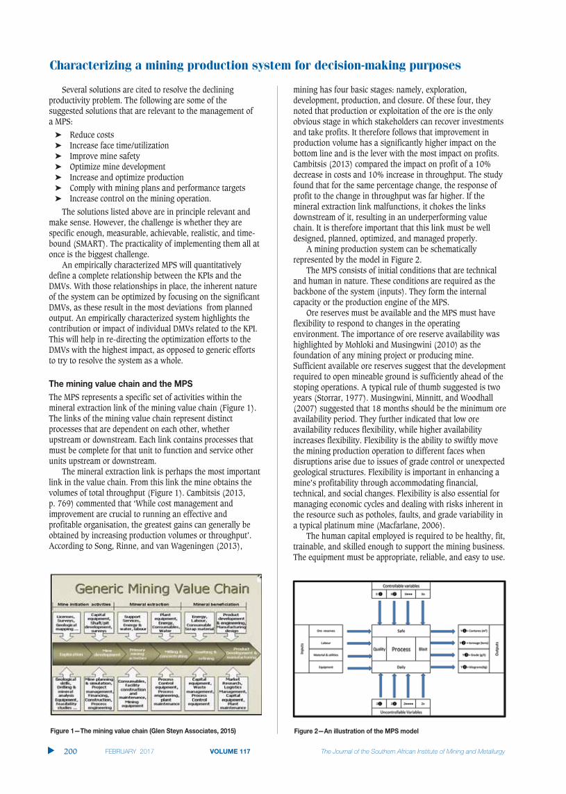
Characterizing a mining production system for decision-making purposes
Several solutions are cited to resolve the decliningproductivity problem. The following are some of thesuggested solutions that are relevant to the management of a MPS:
� Reduce costs� Increase face time/utilization� Improve mine safety� Optimize mine development � Increase and optimize production� Comply with mining plans and performance targets� Increase control on the mining operation.
The solutions listed above are in principle relevant andmake sense. However, the challenge is whether they arespecific enough, measurable, achievable, realistic, and time-bound (SMART). The practicality of implementing them all atonce is the biggest challenge.
An empirically characterized MPS will quantitativelydefine a complete relationship between the KPIs and theDMVs. With those relationships in place, the inherent natureof the system can be optimized by focusing on the significantDMVs, as these result in the most deviations from plannedoutput. An empirically characterized system highlights thecontribution or impact of individual DMVs related to the KPI.This will help in re-directing the optimization efforts to theDMVs with the highest impact, as opposed to generic effortsto try to resolve the system as a whole.
The MPS represents a specific set of activities within themineral extraction link of the mining value chain (Figure 1).The links of the mining value chain represent distinctprocesses that are dependent on each other, whetherupstream or downstream. Each link contains processes thatmust be complete for that unit to function and service otherunits upstream or downstream.
The mineral extraction link is perhaps the most importantlink in the value chain. From this link the mine obtains thevolumes of total throughput (Figure 1). Cambitsis (2013, p. 769) commented that ‘While cost management andimprovement are crucial to running an effective andprofitable organisation, the greatest gains can generally beobtained by increasing production volumes or throughput’.According to Song, Rinne, and van Wageningen (2013),
mining has four basic stages: namely, exploration,development, production, and closure. Of these four, theynoted that production or exploitation of the ore is the onlyobvious stage in which stakeholders can recover investmentsand take profits. It therefore follows that improvement inproduction volume has a significantly higher impact on thebottom line and is the lever with the most impact on profits.Cambitsis (2013) compared the impact on profit of a 10%decrease in costs and 10% increase in throughput. The studyfound that for the same percentage change, the response ofprofit to the change in throughput was far higher. If themineral extraction link malfunctions, it chokes the linksdownstream of it, resulting in an underperforming valuechain. It is therefore important that this link must be welldesigned, planned, optimized, and managed properly.
A mining production system can be schematicallyrepresented by the model in Figure 2.
The MPS consists of initial conditions that are technicaland human in nature. These conditions are required as thebackbone of the system (inputs). They form the internalcapacity or the production engine of the MPS.
Ore reserves must be available and the MPS must haveflexibility to respond to changes in the operatingenvironment. The importance of ore reserve availability washighlighted by Mohloki and Musingwini (2010) as thefoundation of any mining project or producing mine.Sufficient available ore reserves suggest that the developmentrequired to open mineable ground is sufficiently ahead of thestoping operations. A typical rule of thumb suggested is twoyears (Storrar, 1977). Musingwini, Minnitt, and Woodhall(2007) suggested that 18 months should be the minimum oreavailability period. They further indicated that low oreavailability reduces flexibility, while higher availabilityincreases flexibility. Flexibility is the ability to swiftly movethe mining production operation to different faces whendisruptions arise due to issues of grade control or unexpectedgeological structures. Flexibility is important in enhancing amine’s profitability through accommodating financial,technical, and social changes. Flexibility is also essential formanaging economic cycles and dealing with risks inherent inthe resource such as potholes, faults, and grade variability ina typical platinum mine (Macfarlane, 2006).
The human capital employed is required to be healthy, fit,trainable, and skilled enough to support the mining business.The equipment must be appropriate, reliable, and easy to use.
�
200 VOLUME 117
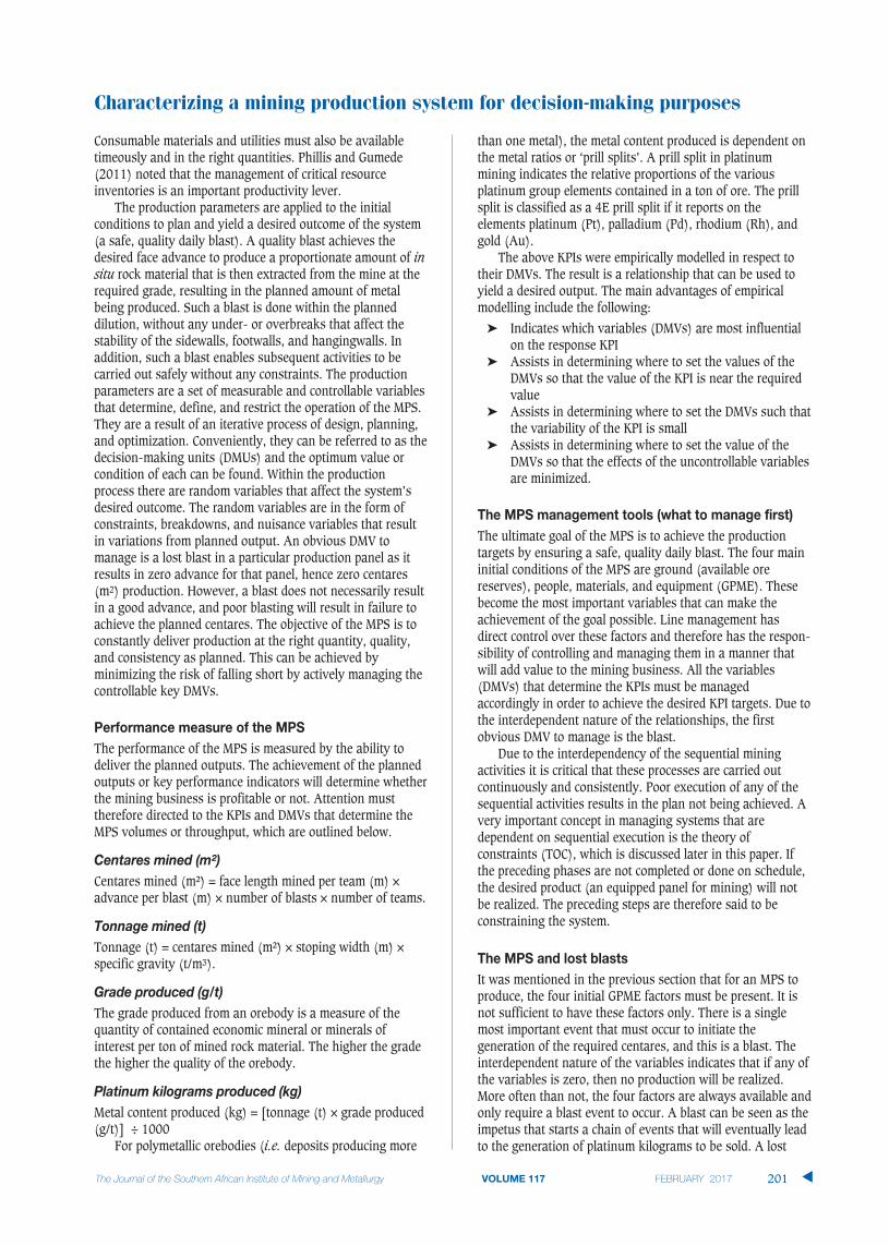
Consumable materials and utilities must also be availabletimeously and in the right quantities. Phillis and Gumede(2011) noted that the management of critical resourceinventories is an important productivity lever.
The production parameters are applied to the initialconditions to plan and yield a desired outcome of the system(a safe, quality daily blast). A quality blast achieves thedesired face advance to produce a proportionate amount of insitu rock material that is then extracted from the mine at therequired grade, resulting in the planned amount of metalbeing produced. Such a blast is done within the planneddilution, without any under- or overbreaks that affect thestability of the sidewalls, footwalls, and hangingwalls. Inaddition, such a blast enables subsequent activities to becarried out safely without any constraints. The productionparameters are a set of measurable and controllable variablesthat determine, define, and restrict the operation of the MPS.They are a result of an iterative process of design, planning,and optimization. Conveniently, they can be referred to as thedecision-making units (DMUs) and the optimum value orcondition of each can be found. Within the productionprocess there are random variables that affect the system’sdesired outcome. The random variables are in the form ofconstraints, breakdowns, and nuisance variables that resultin variations from planned output. An obvious DMV tomanage is a lost blast in a particular production panel as itresults in zero advance for that panel, hence zero centares(m2) production. However, a blast does not necessarily resultin a good advance, and poor blasting will result in failure toachieve the planned centares. The objective of the MPS is toconstantly deliver production at the right quantity, quality,and consistency as planned. This can be achieved byminimizing the risk of falling short by actively managing thecontrollable key DMVs.
The performance of the MPS is measured by the ability todeliver the planned outputs. The achievement of the plannedoutputs or key performance indicators will determine whetherthe mining business is profitable or not. Attention musttherefore directed to the KPIs and DMVs that determine theMPS volumes or throughput, which are outlined below.
Centares mined (m²) = face length mined per team (m) ×advance per blast (m) × number of blasts × number of teams.
Tonnage (t) = centares mined (m²) × stoping width (m) ×specific gravity (t/m3).
The grade produced from an orebody is a measure of thequantity of contained economic mineral or minerals ofinterest per ton of mined rock material. The higher the gradethe higher the quality of the orebody.
Metal content produced (kg) = [tonnage (t) × grade produced(g/t)] ÷ 1000
For polymetallic orebodies (i.e. deposits producing more
than one metal), the metal content produced is dependent onthe metal ratios or ‘prill splits’. A prill split in platinummining indicates the relative proportions of the variousplatinum group elements contained in a ton of ore. The prillsplit is classified as a 4E prill split if it reports on theelements platinum (Pt), palladium (Pd), rhodium (Rh), andgold (Au).
The above KPIs were empirically modelled in respect totheir DMVs. The result is a relationship that can be used toyield a desired output. The main advantages of empiricalmodelling include the following:
� Indicates which variables (DMVs) are most influentialon the response KPI
� Assists in determining where to set the values of theDMVs so that the value of the KPI is near the requiredvalue
� Assists in determining where to set the DMVs such thatthe variability of the KPI is small
� Assists in determining where to set the value of theDMVs so that the effects of the uncontrollable variablesare minimized.
The ultimate goal of the MPS is to achieve the productiontargets by ensuring a safe, quality daily blast. The four maininitial conditions of the MPS are ground (available orereserves), people, materials, and equipment (GPME). Thesebecome the most important variables that can make theachievement of the goal possible. Line management hasdirect control over these factors and therefore has the respon-sibility of controlling and managing them in a manner thatwill add value to the mining business. All the variables(DMVs) that determine the KPIs must be managedaccordingly in order to achieve the desired KPI targets. Due tothe interdependent nature of the relationships, the firstobvious DMV to manage is the blast.
Due to the interdependency of the sequential miningactivities it is critical that these processes are carried outcontinuously and consistently. Poor execution of any of thesequential activities results in the plan not being achieved. Avery important concept in managing systems that aredependent on sequential execution is the theory ofconstraints (TOC), which is discussed later in this paper. Ifthe preceding phases are not completed or done on schedule,the desired product (an equipped panel for mining) will notbe realized. The preceding steps are therefore said to beconstraining the system.
It was mentioned in the previous section that for an MPS toproduce, the four initial GPME factors must be present. It isnot sufficient to have these factors only. There is a singlemost important event that must occur to initiate thegeneration of the required centares, and this is a blast. Theinterdependent nature of the variables indicates that if any ofthe variables is zero, then no production will be realized.More often than not, the four factors are always available andonly require a blast event to occur. A blast can be seen as theimpetus that starts a chain of events that will eventually leadto the generation of platinum kilograms to be sold. A lost
Characterizing a mining production system for decision-making purposes
VOLUME 117 201 �

Characterizing a mining production system for decision-making purposes
blast is an undesired event which results in a planned panelfailing to generate the planned channel tons at the requiredgrade, thus failing to generate the required metal content onthe day. When a lost blast occurs, the labour costs associatedwith that workplace are incurred without any revenueaccruing to the organization. The effect of zero revenuecoupled with the cost of labour obviously has a negativeeffect on the bottom line. In most cases lost blasts occur inthe same workplace, which indicates the failure of linesupervision and line management to eliminate the cause ofthe lost blast.
It is an industry norm in narrow-reef, hard-rock tabularmines to plan for an average of 23 shifts in a productionmonth. The full potential capacity of a team is the ability toproduce on every single planned shift. However, for practicalreasons the business plan (BP) targets are set at an averageof 60% of the full potential. This implies that an allowancehas already been made for lost-blast effects. It is surprisingthat lost blasts exceed the allowed occurrence as per the BP.
The labour factor is the most important input in the aboverelationship. It uses the resources (inputs) (ore reserves,materials, and utilities, and equipment) to generate onesingle primary output of the MPS objective function (centaresmined) by initiating the blast event. The labour in the MPScontrols further down the line the tons mined and qualityachieved (grade). If any of the four variables prevents theMPS from achieving its objective then it becomes a constraintin the system and must be corrected so that it is no longer alimiting factor.
It is not sufficient to only identify a constraint within theMPS. Further analysis is required to establish why theconstraint exists. The root cause of the constraint behaviourmust be identified. A root cause is the highest level of aproblem, and is defined as a factor that causes noncon-formance and should be permanently eliminated throughprocess improvement (ASQ, n.d.). Root cause analysis (RCA)is a technique used to uncover the causes of a problem. RCAhelps to identify not only what and how, but also whysomething happened. For the purpose of this paper, RCA haswas used to analyse constraints as captured by the allowedlost blast reasons booked on a mineral resource management(MRM) system of a platinum mine.
For the purpose of RCA application the four initial conditionswere allocated ID codes (1–4) as follows:
� Ground (ore reserves): 1� People: 2� Materials and services: 3� Equipment: 4.
In the following example, RCA is applied to a roofbolterbreakdown being the reason for lost blasts at four differentworking places. A roofbolter is used to install active roofboltsupport on the immediate face in the hangingwall aspermanent support before a blast. Conventionally, the reasonfor a lost blast is a breakdown of the bolter (equipmentbreakdown, ID code 4). However, by appropriately applyingRCA, the reason then changes to shortage of spares in thestore (shortage of equipment). Further analysis reveals that
someone is responsible for making sure that there is enoughmaterial at the face to achieve a blast and that there isenough buffer at the stores to ensure an uninterruptedmining process. The final RCA indicates that a person(people) (ID code 2) is the underlying constraint. The failureof a supervisor to provide enough material to achieve a blasthas resulted in a lost blast, and hence loss of production forthat day.
Figures 3 and 4 show the distribution of lost blastanalysis for a mine for a month of production. The lost blastsfiltered here are only stoping lost blasts. In total the MPSMRM system has provided for nearly 77 lost blast reasonsgrouped under the following categories:
� Labour (day shift and night shift)� Engineering� Finance� Rock engineering� Geology and ventilation.
The RCA methodology facilitates the grouping of lostblasts into only four categories (GPME), hence minimizingthe ambiguity and therefore directing the controlled action tothe actual root cause. Figure 3 depicts the reasons identifiedfor lost blasts before the application of RCA for the financialyear 2008 (FY08). When RCA was applied to the same datathe causes could be attributed as shown in Figure 4.
�
202 VOLUME 117

The MPS activities are sequential and cyclic in nature. A safe,quality daily blast can be seen as a project delivered on anyparticular day, while the activities that yield a safe qualitydaily blast can be seen as milestones within the blastingproject. The sequential flow of these activities is important tothe achievement of the objective. When the upstreamactivities do not occur, the objective is missed and the systemfails or is constrained. The theory of constraints (TOC) isavailable to understand a system of this nature. TOC is asystems-management philosophy developed by Eliyahu M.Goldratt in the early 1980s (Institute of ManagementAccountants, 1999). It is a tool that assists managers toachieve the bottom line and capacity improvement quickly atlittle or no cost (ApicsAu, 2016). The main objective of TOCis to identify a constraint in the system. In the example of asafe, quality daily blast the production value chain would bedrill–blast–clean–support. If any of the four events does notoccur the cycle cannot be completed or repeated. It thenbecomes necessary to identify where the problem is. The RCAprocess will generally lead to identification of the real causeof the problem. When the problem (constraint) is identified,the TOC methodology suggests a further four critical steps tosolve the problem. There is a five-step focusing process inTOC that helps to manage the change based on the work ofEliyahu Goldratt (McNesse, 2014). The five steps are:
� Identify the bottleneck� Exploit the bottleneck� Subordinate all other elements to the bottleneck� Elevate the bottleneck to get more from it� Repeat the process.
The MPS under study is designed as an undergroundplatinum mine consisting of a vertical shaft system (mainshaft and ventilation shaft) to access the orebody. Theorebody comprises two distinct reef planes, the Merensky andthe UG2 reefs, which dip at about 9 degrees east and strikeroughly north–south. The average platinum group metal(PGM) grade is about 3.71 g/t over a 1.1 m average stopingwidth. The two reef planes are scheduled to be mined concur-rently. Underground mining operations follow traditionalnarrow-reef, tabular mining practices. The orebody is minedon a conventional breast layout grid of 180 m raiselines and300 m back lengths. This layout gives a total of about 18stopes with in-stope grid pillars accounted for. Access to thestopes is by means of off-reef haulages leading to secondarydevelopment to reef. Based on geological and otherconditions, certain portions of ground are left unmined. Astoping team mining about 27 m of available face length hasthe potential to achieve 621 m²/month. For practical reasonsthe BP target is 373 m²/month per stope team, which is 60%of the full potential. This equates to about 13 blasts at anassumed face advance of 1 m per blast.
The production data used for the case study spans aperiod of eight BP years. It is based on direct evidencecollected or reported over the eight-year period. Standardizedstatistical methods were used to enhance the accuracy of theanalysis and to validate empirical conclusions about the data.The data was chosen specifically because it spans the highsand the lows of the MPS in question.
The critical parameters that are assumed to influence orpredict the value of the target KPI (centares) have beenidentified and are briefly described below. The parametersrepresent monthly figures that were used in the regressionanalysis for a total of 84 mining months over the eight yearsas follows:
� Face advance—the distance that the total face lengthmined has been advanced by mining teamsunderground
� Face length mined—the mineable face length perpen-dicular to direction of advance that the teams accessedand worked on
� Achieved blasts—the number of blasts booked(achieved) on the MRM system against all the miningteams
� Teams—the number of mining teams planned to mine� Team efficiency—the average m² that a team achieves� Team size—the number persons at work assigned to a
team per panel� Off-main development—the off-reef main development
done to access the orebody � Re- and predevelopment—the in-stope development
that is done to open a mineable face length� Development to mill—the on-reef secondary
development on the mining main grid layout to openblocks of mineable reserves via raises and winzes.
In statistical terms, the suggestion or inference is that theabove parameters influence or are good predictors of thedependent variable (centares) and must be tested. The choiceof variables is based purely on experience and knowledge ofthe mining environment. The inference is that theindependent variables have some effect or predictive valuewith respect to the future values of the dependent variable(centares).
The variables that are included in the final regressionmodel (run 2) are those variables that have statistical signif-icance in describing or predicting the dependent variable. Apreliminary statistical screening (run 1) was done to identifythe variables that were insignificant so that a refined testing(run 2) could be done with only the variables that really hadsome degree of influence on the dependent variable. In thisway, illogical relationships were eliminated while improvingon the strength of correlation relationships betweensignificant variables.
Table I depicts the correlation coefficients between thevariables selected for the regression run 1. The correlationcoefficient measures the strength of the linear relationshipbetween two variables. The coefficient is measured on arelative scale of -1 to +1. A positive correlation indicates thatthe variables move in the same direction, while a negativecorrelation indicates that the variables move in oppositedirections. Team size in Table I has a negative correlation tothe total m², while all other variables have a positivecorrelation. The variables with the a strong correlation(>50%) after run 1 in descending order are team efficiency,face length mined, face advance, off-main development, anddevelopment to mill.
Characterizing a mining production system for decision-making purposes
VOLUME 117 203 �

Characterizing a mining production system for decision-making purposes
Table II indicates the regression statistics results at run 1.The R² value is 0.998, meaning that 99.8% of the variationwithin the centares analysis is explained.
Table III highlights the significance level test of thevariables used in the regression analysis. A predeterminedconfidence level of 95% was selected for the purpose oftesting. The implication here is that a P-value higher than0.05 for any variable indicates that the variable has littleinfluence in terms of predicting the dependent variable.Therefore teamefficiency, off-main development, re- andpredevelopment, and development to mill were eliminatedand the regression analysis was done as run 2.
The predictive production function derived from Table IIIis shown by Equation [1] :
Total m² = (2488.207 × face advance) + (6.76 × face length mined) + (4.319 × achieved blasts) - (199.5 × teams) + (8.46 × team efficiency) - (617.98 × team size) – [1](1.18 × off main development) - (0.079 × re- and predevelopment) + (1.51 × development to mill)
Tables IV, V, and VI present the results of run 2. Table IVdepicts the correlation coefficients between the variablesselected for the regression run 2. Team size in Table IV has anegative correlation to the total m², while all other variableshave a positive correlation.
Table V indicates the regression statistics results at run 2.The R² value is 0.999, meaning that 99.9% of the variationwithin the centares analysis is explained.
Table VI highlights the significance level test of thevariables used in the regression analysis. A predeterminedconfidence level of 95% was selected for the purpose oftesting. The coefficients of the variables are indicated alongwith the P-value. The P-value indicates that the variables areall significant and relevant in predicting the future values ofthe dependent variable, total m ².
The predictive production function from Table VI isshown by Equation [2]:
Total m² = (2868.47 × face advance) + (7.78 × face length mined) + (4.65 × achieved blasts) – [2](233.87 × teams) - (606.29 × team size)
The results indicate that:� An increase in actual blasts yields only 4.65 m²,
showing that the number of blasts reported on theMRM system does not have a significant influence onthe centares produced. It is the advance per blast that isa good predictor of centares generated
� A 1 m increase in face advance will result in anincrease of 2868 m²
� A 1 m increase in face length mined will result in anincrease of 7.78 m²
�
204 VOLUME 117
Table I
Total m2 1.000Face advance 0.865Face length mined 0.877 0.540 1.000Ach. Blasts 0.419 0.407 0.375 1.000Teams 0.236 0.296 0.194 0.924 1.000Team eff. 0.906 0.741 0.803 0.026 –0.192 1.000Team size –0.238 –0.188 –0.218 –0.637 –0.608 0.045 1.000Off main dev. 0.795 0.708 0.685 0.422 0.258 0.699 –0.224 1.000Re & pre dev. 0.162 0.268 0.089 0.180 0.216 0.073 0.092 0.265 1.000Dev. to mill 0.677 0.674 0.553 0.369 0.312 0.559 –0.140 0.598 0.389 1.000
Table II
Multiple R 0.999R square 0.998Adjusted R square 0.985Standard error 1248.429Observations 84.000
Table III
Intercept 0 #N/A #N/A #N/A #N/A #N/A Face advance 2488.207 322.077 7.726 0.000000000 1846.6 3129.8Face length mines 6.760 0.979 6.907 0.000000001 4.8 8.7Ach. blasts 4.319 1.703 2.537 0.013272915 0.9 7.7Teams –199.499 47.403 –4.209 0.000070517 –293.9 –105.1Team eff. 8.464 10.278 0.823 0.412846203 –12.0 28.9Team size –617.981 75.459 –8.190 0.000000000 –768.3 –467.7Off main dev 1.182 1.268 0.933 0.353923420 –1.3 3.7Re & pre dev. –0.079 0.685 –0.115 0.908900719 –1.4 1.3Dev. to mill 1.509 1.132 1.334 0.186398874 –0.7 3.8
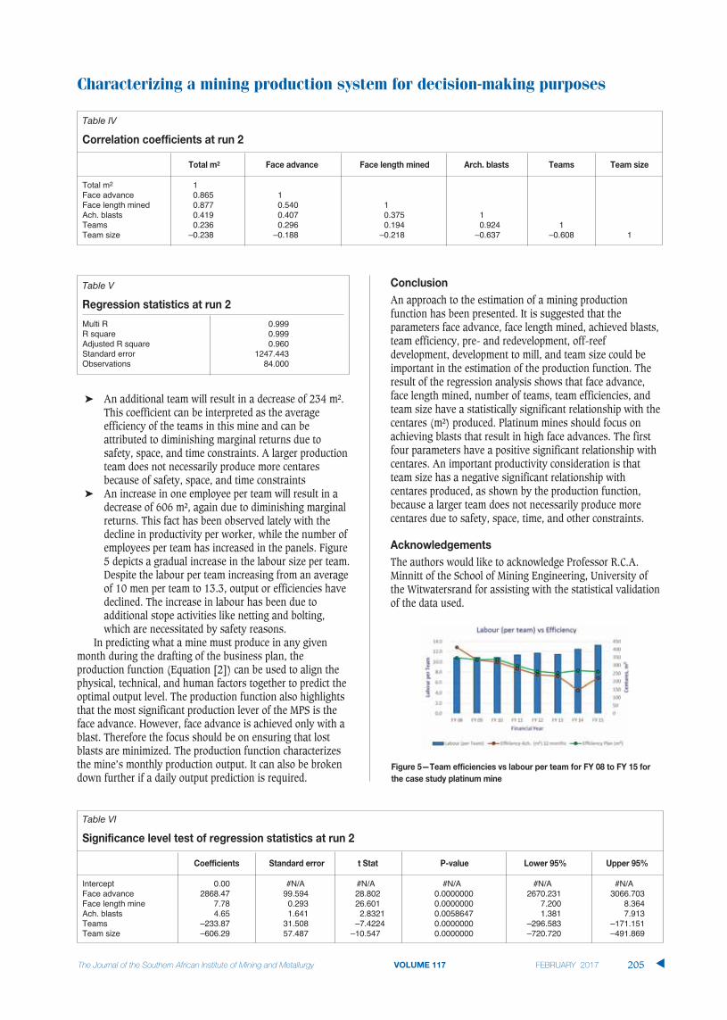
Characterizing a mining production system for decision-making purposes
VOLUME 117 205 �
� An additional team will result in a decrease of 234 m².This coefficient can be interpreted as the averageefficiency of the teams in this mine and can beattributed to diminishing marginal returns due tosafety, space, and time constraints. A larger productionteam does not necessarily produce more centaresbecause of safety, space, and time constraints
� An increase in one employee per team will result in adecrease of 606 m², again due to diminishing marginalreturns. This fact has been observed lately with thedecline in productivity per worker, while the number ofemployees per team has increased in the panels. Figure5 depicts a gradual increase in the labour size per team.Despite the labour per team increasing from an averageof 10 men per team to 13.3, output or efficiencies havedeclined. The increase in labour has been due toadditional stope activities like netting and bolting,which are necessitated by safety reasons.
In predicting what a mine must produce in any givenmonth during the drafting of the business plan, theproduction function (Equation [2]) can be used to align thephysical, technical, and human factors together to predict theoptimal output level. The production function also highlightsthat the most significant production lever of the MPS is theface advance. However, face advance is achieved only with ablast. Therefore the focus should be on ensuring that lostblasts are minimized. The production function characterizesthe mine’s monthly production output. It can also be brokendown further if a daily output prediction is required.
An approach to the estimation of a mining productionfunction has been presented. It is suggested that theparameters face advance, face length mined, achieved blasts,team efficiency, pre- and redevelopment, off-reefdevelopment, development to mill, and team size could beimportant in the estimation of the production function. Theresult of the regression analysis shows that face advance,face length mined, number of teams, team efficiencies, andteam size have a statistically significant relationship with thecentares (m²) produced. Platinum mines should focus onachieving blasts that result in high face advances. The firstfour parameters have a positive significant relationship withcentares. An important productivity consideration is thatteam size has a negative significant relationship withcentares produced, as shown by the production function,because a larger team does not necessarily produce morecentares due to safety, space, time, and other constraints.
The authors would like to acknowledge Professor R.C.A.Minnitt of the School of Mining Engineering, University ofthe Witwatersrand for assisting with the statistical validationof the data used.
Table IV
Total m2 1Face advance 0.865 1Face length mined 0.877 0.540 1Ach. blasts 0.419 0.407 0.375 1Teams 0.236 0.296 0.194 0.924 1Team size –0.238 –0.188 –0.218 –0.637 –0.608 1
Table V
Multi R 0.999R square 0.999Adjusted R square 0.960Standard error 1247.443Observations 84.000
Table VI
Intercept 0.00 #N/A #N/A #N/A #N/A #N/AFace advance 2868.47 99.594 28.802 0.0000000 2670.231 3066.703Face length mine 7.78 0.293 26.601 0.0000000 7.200 8.364Ach. blasts 4.65 1.641 2.8321 0.0058647 1.381 7.913Teams –233.87 31.508 –7.4224 0.0000000 –296.583 –171.151Team size –606.29 57.487 –10.547 0.0000000 –720.720 –491.869

Characterizing a mining production system for decision-making purposes
APICSAU. 2016. Effective management: achieving your goals.
https://www.apicsau.org.au/events/effective-management-achieving-your-goals [Accessed 14 April 2016].
ASQ. Not dated. What is Root Cause Analysis (RCA)?. http://asq.org/learn-about-quality/root-cause-analysis/overview/overview.html [Accessed 14April 2016].
CAMBITSIS, A. 2013. A framework to simplify the management of throughputand constraints. Journal of the Southern African Institute of Mining andMetallurgy, vol. 113, no. 10. pp. 769–773.
GLEN STEYN ASSOCIATES. 2015. Core Competencies. http://www.glensteyn.co.za/page/core-competencies [Accessed 14 February 2015].
INSTITUTE OF MANAGEMENT ACCOUNTANTS. 1999. Theory of constraints (TOC)Mangement system fundamentals. http://www.imanet.org/docs/default-source/thought_leadership/operations-process-management-innovation/theory_of_constraints_(toc_management_systems_fundamentals.pdf?sfvrsn=2 [Accessed 14 April 2016].
MACFARLANE, A. 2006. Establishing a new metric for mineral resourcemanagement. Journal of The South African Institute of Mining andMetallurgy, vol. 106, no. 3. pp. 187–198.
McNesse, D.B. 2014. Theory of Constraints. [http://www.spcforexcel.com/publications/Theory_of_Constraints/13B63E123ED3A6769B6575CE93DA4F2F/Theory%20of%20Constraints.pdf [Accessed 14 April 2016].
MOHLOKI, L. and MUSINGWINI, C. 2010. Sustainable ore reserves generation atvariable stoping rates for a UG2 conventional mining layout. Proceedingsof the 4th International Platinum Conference, Platinum in transition‘Boom or Bust’, Sun City, South Africa, 11–14 October 2010. SouthernAfrican Institute of Mining and Metallurgy, Johannesburg. pp. 309–316.
MUSINGWINI, C., MINNITT, R.C.A., and WOODHALL, M. 2007. Technical operatingflexibility in the analysis of mine layouts and schedules. Journal of theSouth African Institute of Mining and Metallurgy, vol. 107, no. 2. pp. 129–136.
PHILLIS, R. and GUMEDE, H. 2011. Can buffer stores improve productivity.Journal of the Southern African Institute of Mining and Metallurgy, vol. 111, no. 1. pp. 37–43.
SONG, Z., RINNE, M., and VAN WAGENINGEN, A. 2013. A review of real-timeoptimization in underground mining production. Journal of the SouthernAfrican Institute of Mining and Metallurgy, vol. 113, no. 12. pp. 889–897.
STORRAR, C. 1977. South African Mine Valuation. 2nd edn. Chamber of Mines ofSouth Africa, Johannesburg. �
�
206 VOLUME 117
DEVELOPING THE FLOWSHEET
METALLURGICAL LABORATORY
We specialise in commercial mineral processing and metallurgical testwork for process design and the application of Maelgwyn’s proprietary technologies and processes in gold, base metals, PGMs and other commodities.
Successful testwork programmes have included process development on common sulphide minerals, as well as non-sulphide minerals including tin,
Maelgwyn Mineral Services Africa (Pty) LtdTel +27 (0)11 474 0705 Fax +27 (0)11 474 5580 Email [email protected] www.maelgwynafrica.com

�vii
9–10 March 2017 — 3rd Young Professionals ConferenceUnlocking the Future of the African Minerals Industry:Vision2040Innovation Hub, PretoriaContact: Camielah JardineTel: +27 11 834-1273/7, Fax: +27 11 838-5923/833-8156 E-mail: [email protected],Website: http://www.saimm.co.za20 April 2017 — Proximity Detection and Collision AvoidanceSystems in Mining Colloquium 2017Striving for zero harm from mining mobile machineryEmperors Palace, Hotel Casino Convention Resort, JohannesburgContact: Camielah JardineTel: +27 11 834-1273/7, Fax: +27 11 838-5923/833-8156 E-mail: [email protected],Website: http://www.saimm.co.za3–4 May 2017 —The SAMREC and SAMVAL CodesAdvanced Workshop: Can you face your peers?Emperors Palace, Hotel Casino Convention Resort, JohannesburgContact: Raymond van der BergTel: +27 11 834-1273/7, Fax: +27 11 838-5923/833-8156E-mail: [email protected], Website: http://www.saimm.co.za9–12 May 2017 — 6th Sulphur and Sulphuric Acid 2017 ConferenceSouthern Sun Cape Sun, Cape TownContact: Camielah JardineTel: +27 11 834-1273/7, Fax: +27 11 838-5923/833-8156 E-mail: [email protected], Website: http://www.saimm.co.za20–27 May 2017 — ALTA 2017 Nickel-Cobalt-Copper,Uranium-REE and Gold-PM Conference and ExhibitionPan Pacific Perth, AustraliaContact: Allison TaylorTel: +61 (0) 411 692 442 E-mail: [email protected]: http://www.altamet.com.au/conferences/alta-2017/22–23 May 2017 — Entrepreneurship in Mining ForumA Focus on new Business in the Value ChainJohannesburgContact: Raymond van der BergTel: +27 11 834-1273/7, Fax: +27 11 838-5923/833-8156E-mail: [email protected], Website: http://www.saimm.co.za6–7 June 2017 —Mine Planning Colloquium 2017Mintek, RandburgContact: Camielah JardineTel: +27 11 834-1273/7, Fax: +27 11 838-5923/833-8156 E-mail: [email protected], Website: http://www.saimm.co.za7–8 June 2017 —AIMS - Aachen International MiningSymposia Second International Conference: Mining in EuropeAachen, GermanyContact: Iris SchümmerTel: +49-(0) 241-80 95673, Fax: +49-(0) 241-80 92272 E-mail: [email protected]: http://www.aims.rwth-aachen.de19–20 June 2017 —Chrome Colloquium 2017What’s next for Chrome? A debate on the tough questionsMintek, RandburgContact: Camielah JardineTel: +27 11 834-1273/7, Fax: +27 11 838-5923/833-8156 E-mail: [email protected], Website: http://www.saimm.co.za25–28 June 2017 — Emc 2017: European Metallurgical ConferenceLeipzig, GermanyContact: Paul-Ernst-StraßeTel: +49 5323 9379-0, Fax: +49 5323 9379-37E-mail: [email protected], Website: http://emc.gdmb.de
27–29 June 2017 —4th Mineral Project Valuation ColloquiumMine Design Lab, Chamber of Mines Building, The University of the Witwatersrand, JohannesburgContact: Raymond van der BergTel: +27 11 834-1273/7, Fax: +27 11 838-5923/833-8156E-mail: [email protected], Website: http://www.saimm.co.za10–11 July 2017 — Water 2017 ConferenceLifeblood of the Mining IndustryEmperors Palace, Hotel Casino Convention Resort, JohannesburgContact: Raymond van der BergTel: +27 11 834-1273/7, Fax: +27 11 838-5923/833-8156E-mail: [email protected], Website: http://www.saimm.co.za3–4 August 2017 — Building a Robust Mineral IndustryThriving under prolonged low commodity price environmentMandel Training Centre, Marlborough, HarareContact: Raymond van der BergTel: +27 11 834-1273/7, Fax: +27 11 838-5923/833-8156E-mail: [email protected], Website: http://www.saimm.co.za7–9 August 2017 —Rapid Underground Mine & Civil AccessConference 2017Emperors Palace, Hotel Casino Convention Resort, JohannesburgContact: Camielah JardineTel: +27 11 834-1273/7, Fax: +27 11 838-5923/833-8156 E-mail: [email protected], Website: http://www.saimm.co.za22–24 August 2017 — The Southern African Coal ProcessingSociety Conference and Networking OpportunityThe key to profitabilityGraceland Hotel, Casino and Country Club, SecundaContact: Gerda CraddockTel: +27 11 432-8918, E-mail: [email protected] August–1 September 2017 — MINESafe Conference 2017Striving for Zero Harm—Driving Excellence through ComplianceEmperors Palace, Hotel Casino Convention Resort, JohannesburgContact: Raymond van der BergTel: +27 11 834-1273/7, Fax: +27 11 838-5923/833-8156E-mail: [email protected], Website: http://www.saimm.co.za11–15 September 2017 — Uranium 2017 InternationalConference Extraction and Applications of Uranium — Present and FutureSwakopmund Hotel, Swakopmund, NamibiaContact: Raymond van der BergTel: +27 11 834-1273/7, Fax: +27 11 838-5923/833-8156E-mail: [email protected], Website: http://www.saimm.co.za2–7 October 2017 — AfriRock 2017: ISRM InternationalSymposium—Rock Mechanics for AfricaCape Town Convention Centre, Cape TownContact: Raymond van der BergTel: +27 11 834-1273/7, Fax: +27 11 838-5923/833-8156E-mail: [email protected], Website: http://www.saimm.co.za16–20 October 2017 — AMI Precious Metals 2017 The Precious Metals Development Network (PMDN)Protea Hotel Ranch Resort, PolokwaneContact: Raymond van der BergTel: +27 11 834-1273/7, Fax: +27 11 838-5923/833-8156E-mail: [email protected], Website: http://www.saimm.co.za18–20 October 2017 — 7th International Platinum ConferencePlatinum—A Changing IndustryProtea Hotel Ranch Resort, PolokwaneContact: Camielah JardineTel: +27 11 834-1273/7, Fax: +27 11 838-5923/833-8156 E-mail: [email protected], Website: http://www.saimm.co.za
INTERNATIONAL ACTIVITIES
2017

�
viii
Company AffiliatesThe following organizations have been admitted to the Institute as Company Affiliates
3M South Africa (Pty) Limited
AECOM SA (Pty) Ltd
AEL Mining Services Limited
Air Liquide (PTY) Ltd
AMEC Foster Wheeler
AMIRA International Africa (Pty) Ltd
ANDRITZ Delkor (Pty) Ltd
Anglo Operations (Pty) Ltd
Arcus Gibb (Pty) Ltd
Aurecon South Africa (Pty) Ltd
Aveng Engineering
Aveng Mining Shafts and Underground
Axis House Pty Ltd
Bafokeng Rasimone Platinum Mine
Barloworld Equipment -Mining
BASF Holdings SA (Pty) Ltd
BCL Limited
Becker Mining (Pty) Ltd
BedRock Mining Support Pty Ltd
Bell Equipment Limited
Blue Cube Systems (Pty) Ltd
CDM Group
CGG Services SA
Concor Mining
Concor Technicrete
Cornerstone Minerals Pty Ltd
Council for Geoscience Library
Cronimet Mining Processing SA (Pty) Ltd
CSIR Natural Resources and theEnvironment (NRE)
Data Mine SA
Department of Water Affairs and Forestry
Digby Wells and Associates
DRA Mineral Projects (Pty) Ltd
DTP Mining - Bouygues Construction
Duraset
Elbroc Mining Products (Pty) Ltd
eThekwini Municipality
Expectra 2004 (Pty) Ltd
Exxaro Coal (Pty) Ltd
Exxaro Resources Limited
Filtaquip (Pty) Ltd
FLSmidth Minerals (Pty) Ltd
Fluor Daniel SA (Pty) Ltd
Franki Africa (Pty) Ltd-JHB
Fraser Alexander Group
Geobrugg Southern Africa (Pty) Ltd
Glencore
Goba (Pty) Ltd
Hall Core Drilling (Pty) Ltd
Hatch (Pty) Ltd
Herrenknecht AG
HPE Hydro Power Equipment (Pty) Ltd
IMS Engineering (Pty) Ltd
Ivanhoe Mines SA
Joy Global Inc.(Africa)
Kudumane Manganese Resources
Leco Africa (Pty) Limited
Longyear South Africa (Pty) Ltd
Lonmin Plc
Magotteaux (Pty) Ltd
MBE Minerals SA Pty Ltd
MCC Contracts (Pty) Ltd
MD Mineral Technologies SA (Pty) Ltd
MDM Technical Africa (Pty) Ltd
Metalock Engineering RSA (Pty) Ltd
Metorex Limited
Metso Minerals (South Africa) Pty Ltd
MineRP Holding (Pty) Ltd
Mintek
MIP Process Technologies (Pty) Ltd
MSA Group (Pty) Ltd
Multotec (Pty) Ltd
Murray and Roberts Cementation
Nalco Africa (Pty) Ltd
Namakwa Sands (Pty) Ltd
Ncamiso Trading (Pty) Ltd
New Concept Mining (Pty) Limited
Northam Platinum Ltd - Zondereinde
PANalytical (Pty) Ltd
Paterson & Cooke Consulting Engineers(Pty) Ltd
Perkinelmer
Polysius A Division Of ThyssenkruppIndustrial Sol
Precious Metals Refiners
Rand Refinery Limited
Redpath Mining (South Africa) (Pty) Ltd
Rocbolt Technologies
Rosond (Pty) Ltd
Royal Bafokeng Platinum
Roytec Global Pty Ltd
RungePincockMinarco Limited
Rustenburg Platinum Mines Limited
Salene Mining (Pty) Ltd
Sandvik Mining and Construction Delmas(Pty) Ltd
Sandvik Mining and Construction RSA(Pty)Ltd
SANIRE
Schauenburg(Pty) Ltd
SENET (Pty) Ltd
Senmin International (Pty) Ltd
Smec South Africa
SMS group Technical Services South Africa(Pty) Ltd
Sound Mining Solution (Pty) Ltd
South 32
SRK Consulting SA (Pty) Ltd
Technology Innovation Agency
Time Mining and Processing (Pty) Ltd
Tomra (Pty) Ltd
Ukwazi Mining Solutions (Pty) Ltd
Umgeni Water
Webber Wentzel
Weir Minerals Africa
WorleyParsons RSA (Pty) Ltd

2017� CONFERENCE
3rd Young Professionals Conference9–10 March 2017, Innovation Hub, Pretoria
� COLLOQUIUMProximity Detection and Collision Avoidance Systems Colloquium 201720 April 2017, Emperors Palace, Hotel Casino Convention Resort, Johannesburg
� WORKSHOPThe SAMREC and SAMVAL Codes—Advanced Workshop: Can you face your peers?3–4 May 2017, Emperors Palace, Hotel Casino Convention Resort, Johannesburg
� CONFERENCE6th Sulphur and Sulphuric Acid 2017 Conference9–12 May 2017, Southern Sun Cape Sun, Cape Town
� FORUMEntrepreneurship in Mining Forum22–23 May 2017, Johannesburg
� COLLOQUIUMMine Planning Colloquium 20176–7 June 2017, Mintek, Randburg
� COLLOQUIUMChrome Colloquium 201719–20 June 2017, Mintek, Randburg
� COLLOQUIUM4th Mineral Project Valuation Colloquium27–29 June 2017, Mine Design Lab, Chamber of Mines Building, The University of theWitwatersrand, Johannesburg
� CONFERENCEWater 2017: Lifeblood of the Mining Industry Conference 201710–11 July 2017, Emperors Palace, Hotel Casino Convention Resort, Johannesburg
� CONFERENCEBuilding a Robust Mineral Industry3–4 August 2017, Mandel Training Centre, Marlborough, Harare
� CONFERENCERapid Underground Mine & Civil Access 2017 Conference7–9 August 2017, Emperors Palace, Hotel Casino Convention Resort, Johannesburg
� CONFERENCEMINESafe Conference 201730 August–1 September 2017, Emperors Palace, Hotel Casino Convention Resort,Johannesburg
� CONFERENCEUranium 2017 International Conference11–15 September 2017, Swakopmund Hotel, Swakopmund, Namibia
� SYMPOSIUMAfriRock 2017: ISRM International Symposium ‘Rock Mechanics for Africa’2–7 October 2017, Cape Town Convention Centre, Cape Town
� CONFERENCEAMI Precious Metals 2017 ‘The Precious Metals Development Network (PMDN)’17–20 October 2017, Protea Hotel Ranch Resort, Polokwane
� CONFERENCE7th International Platinum Conference18–20 October 2017, Protea Hotel Ranch Resort, Polokwane
SAIMM DIARY
For further information contact:Conferencing, SAIMM
P O Box 61127, Marshalltown 2107Tel: (011) 834-1273/7
Fax: (011) 833-8156 or (011) 838-5923E-mail: [email protected]
For the past 123 years, theSouthern African Institute ofMining and Metallurgy, has
promoted technical excellencein the minerals industry. Westrive to continuously stay at thecutting edge of newdevelopments in the mining andmetallurgy industry. The SAIMMacts as the corporate voice forthe mining and metallurgyindustry in the South Africaneconomy. We activelyencourage contact andnetworking between membersand the strengthening of ties.The SAIMM offers a variety ofconferences that are designedto bring you technicalknowledge and information ofinterest for the good of theindustry. Here is a glimpse ofthe events we have lined up for2017. Visit our website for moreinformation.
EXHIBITS/SPONSORSHIP
Companies wishing to sponsor
and/or exhibit at any of these
events should contact the
conference co-ordinator
as soon as possible

+27 11 494 6000 www.ncm.co.za
Proud supporter of the WITS School of Mining
The New Concept Mining Stope in the Wits Digital Mine