
IN2TRACK - Shift2Rail projects
327
GA H2020 730841 D3.2 Page 1 of 327 IN2TRACK Project Title: Research into enhanced tracks, switches and structures Starting date: 2016-09-01 Duration in months: 30 Call (part) identifier: H2020-S2RJU-2016-01/H2020-S2RJU-CFM-2016-01-01 Grant agreement no: 730841 REPORT Deliverable Title: Enhanced track design solutions through predictive analyses Due date of deliverable: 2019-02-28 Actual submission date: 2019-03-12 Responsible partner Railenium Revision: v.11 Deliverable Nº D3.2 Document Status: Final Dissemination Level: PU This project has received funding from the Shift2Rail Joint Undertaking under the European Union’s Horizon 2020 research and innovation programme under grant agreement No 730841 This document reflects only the author’s view and the JU is not responsible for any use that may be made of the information it contains
-
Upload
khangminh22 -
Category
Documents
-
view
0 -
download
0
Transcript of IN2TRACK - Shift2Rail projects

GA H2020 730841 D3.2 Page 1 of 327
IN2TRACK Project Title: Research into enhanced tracks, switches and structures
Starting date: 2016-09-01
Duration in months: 30
Call (part) identifier: H2020-S2RJU-2016-01/H2020-S2RJU-CFM-2016-01-01
Grant agreement no: 730841
REPORT
Deliverable Title: Enhanced track design solutions through predictive analyses
Due date of deliverable: 2019-02-28
Actual submission date: 2019-03-12
Responsible partner Railenium
Revision: v.11
Deliverable Nº D3.2
Document Status: Final
Dissemination Level: PU
This project has received funding from the Shift2Rail Joint Undertaking under the European Union’s Horizon 2020 research and innovation programme under grant agreement No 730841
This document reflects only the author’s view and the JU is not responsible for any use that may be made of the information it contains

IN2TRACK D3.2 – Enhanced track design solutions through predictive analyses
GA H2020 730841 D3.2 Page 2 of 327
Project information
DISCLAIMER AND ACKNOWLEDGEMENT
This project has received funding from the European Union's Horizon 2020 Programme Research and Innovation action under grant agreement No 730841
This document reflects the views of the author(s) and does not necessarily reflect the views or policy of the European Commission. Whilst efforts have been made to ensure the accuracy and completeness of this document, the IN2TRACK consortium shall not be liable for any errors or omissions, however caused.
IN2TRACK CONSORTIUM
TRAFIKVERKET - TRV (TRV) as coordinator
KOMPETENZZENTRUM - DAS VIRTUELLE FAHRZEUG, FORSCHUNGSGESELLSCHAFT MBH (VIF)
GETZNER WERKSTOFFE GMBH (GEWE), KIRCHDORFER FERTIGTEILHOLDING GMBH (KFTH) PLASSER & THEURER EXPORT VON BAHNBAUMASCHINEN GESELLSCHAFT MBH (P&T)
VOESTALPINE SCHIENEN GMBH (VAS) VOESTALPINE VAE GMBH (VAE) GMBH, FN126714W, WIENER LINIEN GMBH &CO KG (WL) AC2T RESEARCH GMBH (AC2T) MATERIALS CENTER LEOBEN FORSCHUNG GMBH (MCL) ACCIONA INFRAESTRUCTURAS S.A. (ACC) CENTRO DE ESTUDIOS DE MATERIALES Y CONTROL DE OBRA SA (CEM) OBB-INFRASTRUKTUR AG (OBB) NETWORK RAIL INFRASTRUCTURE LIMITED (NR) FONDATION DE COOPERATION SCIENTIFIQUE RAILENIUM (RLM) SNCF RESEAU (SNCF-R) TATA STEEL FRANCE RAIL SA (TATA) new name : BRITISH STEEL France RAIL SAS VOSSLOH COGIFER SA (VCSA) UNIVERSIDAD DEL PAIS VASCO/ EUSKAL HERRIKO UNIBERTSITATEA (UPV/EHU),
INFRAESTRUTURAS DE PORTUGAL SA (IP) SCHWEIZERISCHE BUNDESBAHNEN SBB AG (SBB)
‘beneficiary not receiving JU funding’ TURKIYE CUMHURIYETI DEVLET DEMIR YOLLARI ISLETMESI GENEL MUDURLUGU (TCDD) LIIKENNEVIRASTO (FTA), SLOVENSKE ZELEZNICE DOO (SZ), BLS AG (BLS)
‘beneficiary not receiving JU funding’

IN2TRACK D3.2 – Enhanced track design solutions through predictive analyses
GA H2020 730841 D3.2 Page 3 of 327
Document Information
DOCUMENT DRAFTING
NAME ORGANIZATION SECTION(S)
Deliverable leader
Samir ASSAF Railenium 9.5, 10.2

IN2TRACK D3.2 – Enhanced track design solutions through predictive analyses
GA H2020 730841 D3.2 Page 4 of 327
Author(s) Faiver Botello
Rafael Sánchez Villardón
Markus HEIM
Patrick DELAVALLE
Ernesto GARCIA VADILLO
Javier CANALES
Aimar ORBE
Roque BORINAGA
Frédéric FAU
Charles VOIVRET
Elena KABO
Christof BERNSTEINER
Christof MARTE
Anders EKBERG
Ali ESMAEILI
Johan AHLSTRÖM
Michele MAGLIO
Robin ANDERSSON
Dimitrios NIKAS
Casey JESSOP
Francisco Javier Morales
Canan SISMAN KORKMAZ
Yusuf CATI
Benjamin LEE
Adam BEVAN
Jay JAISWAL
Raphaël MAESTRACCI
Knut Andreas MEYER
Moïse VOUTERS
Carlos HERMOSILLA
Mohamed WEHBI
Acciona
Acciona
GEWE
Vossloh
UPV/EHU
UPV/EHU
UPV/EHU
UPV/EHU
British Steel
SNCF
Trafikverket
VIF
VIF
Trafikverket
Trafikverket
Trafikverket
Trafikverket
Trafikverket
Trafikverket
Trafikverket
Cemosa
TCDD
TCDD
Network Rail
UoH
UoH
Railenium
Trafikverket
Railenium
Acciona
Network Rail
5.1, 5.2
5.1, 5.2, 10.4
5.2
5.3
5.3
5.3
5.3
5.3
6
7, 10.6
8.1, 12.2
8.2, 11.1
8.2, 10.3, 11.1
8.1, 9.1, 11.2, 12.2
9.1
9.1
9.1
9.1
9.1, 10.1
9.1
9.2
9.3
9.3
9.4, 10.5, 11.3
9.4
9.4
9.5
10.1
10.2
10.4
10.5, 11.3

IN2TRACK D3.2 – Enhanced track design solutions through predictive analyses
GA H2020 730841 D3.2 Page 5 of 327
Maria GALLOU
Norbert Frank
Jens NIELSEN
Björn Pålsson
Peter Musgrave
Network Rail
VAS
Trafikverket
Trafikverket
Network Rail
10.5
11.1, 12.1
11.2
11.2
11.3

IN2TRACK D3.2 – Enhanced track design solutions through predictive analyses
GA H2020 730841 D3.2 Page 6 of 327
Publication history
Date Version Description Responsible
2017-03-15 6 Content outlined and responsible partners identified
Anders EKBERG
2018-10-01 10 Intermediate compiled version Samir ASSAF
2018-12-10 11 Compiled version for first review Samir ASSAF
2019-02-25 F1 Final version with mitigated review comments
Samir ASSAF
2019-03-12 F1 Published Sam Berggren

IN2TRACK D3.2 – Enhanced track design solutions through predictive analyses
GA H2020 730841 D3.2 Page 7 of 327
Table of Contents 1 Executive summary 12
2 Terms, acronyms and abbreviations 17
3 Background 20
4 Objective and aim 21
5 Improvements of track structures 24
5.1 Assessment of the different slab track systems 24
5.1.1 Cost analysis 31
5.2 Modular slab track system 33
5.2.1 Modular concept 33
5.2.2 Advantages of the Moulded Multi Modular Block (3MB) slab track 34
5.2.3 Optimized use of elastomer products 35
5.3 Optimised continuously supported modular ballastless track 37
6 New alloys and welding methods 47
6.1 Introduction 47
6.2 Bainite transformation 47
6.3 Carbide free bainitic (CFB) steels 48
6.4 Microstructural characterisation of aluminothermic bainitic welds 50
6.4.1 Characterisation of a B360 aluminothermic weld 50
6.4.2 Characterisation of a B320 aluminothermic weld 52
6.5 Microstructural characterisation of flash butt bainitic welds 55
6.5.1 Micro indentation test: Durascan 55
6.5.2 Optical and SEM images 56
6.5.3 Results 56
6.6 Conclusions 61
7 Optimization of ballasted track 63
7.1 Gluing method 63
7.2 Track tests 64
7.3 Laboratory tests 69
7.3.1 Lateral resistance test conditions 69
7.3.2 Results analysis 71
IN2TRACK D3.2 – Enhanced track design solutions through predictive analyses
GA H2020 730841 D3.2 Page 8 of 327
7.4 Conclusions 83
8 Overcoming limitations of existing predictive methods for rail and track deterioration 85
8.1 Limitations in predictive models of rail crack formation 85
8.1.1 Prediction of squats in rails 85
8.1.2 Formation of anisotropy in rails, and its effect on crack formation and growth 86
8.1.3 Prediction of rail crack formation 86
8.1.4 Prediction of rail crack growth 86
8.1.5 Mechanical performance of wheel and rail materials 87
8.2 Existing predictive methods with respect to wear & rolling contact fatigue 87
8.2.1 Track geometric deterioration and fatigue of components 88
8.2.2 Surface deterioration of the track: Wear and RCF 88
8.2.3 Surface deterioration of the track: Squats 92
9 Improved prediction of rail and track deterioration 95
9.1 Rail and track deterioration under influence of thermal loading 95
9.1.1 Influence of thermal loading in relation to welding 96
9.1.2 Thermal rail stresses and track buckling 96
9.1.3 White Etching Layers (WELs) and consequent surface crack formation and growth 98
9.1.4 Influence of winter conditions on formation of rail head and foot cracks 100
9.2 Statistical data analysis 101
9.2.1 Nowcasting and forecasting 102
9.2.2 Condition indicators 103
9.2.3 Failure modes and degradation mechanisms 106
9.2.4 Mathematical models to describe degradation phenomena 109
9.3 Numerical model of rail corrugation for prediction 112
9.3.1 Introduction 113
9.3.2 Corrugated section 114
9.3.3 Finite element model of wheelset-railway superstructure system 116
9.3.4 The simulation results 119
9.3.5 Conclusions 120

IN2TRACK D3.2 – Enhanced track design solutions through predictive analyses
GA H2020 730841 D3.2 Page 9 of 327
9.4 Designing steel composition and microstructure to better resist degradation during wheel/rail contact 121
9.4.1 Background 121
9.4.2 Designing the microstructure of steel rails 123
9.4.3 Rail degradation mechanisms 125
9.4.4 Loss of rail profile 126
9.4.5 Rolling contact fatigue (RCF) 127
9.4.6 Rail breakage risk 128
9.4.7 Fracture toughness 132
9.4.8 Fatigue crack growth rate 134
9.4.9 Fatigue strength 135
9.4.10 Residual stresses in rail 136
9.4.11 Characterisation of available rail steels 136
9.4.12 Pearlitic rail steels 137
9.4.13 In-service performance of rail steels 138
9.4.14 Establishing contact conditions and damage susceptibility 143
9.4.15 Comparative assessment of degradation susceptibility of rail steels 147
9.4.16 Conclusions 152
9.5 Mechanisms of the head checks resistance of bainitic rails 153
9.5.1 Introduction 153
9.5.2 Literature review 154
9.5.3 Research work 172
9.5.4 Conclusions 194
10 Improve design through simulations 196
10.1 Improved simulation capabilities regarding rail crack formation 196
10.2 Simulation and assessment of the railway track long term dynamic behaviour 197
10.2.1 Introduction 197
10.2.2 Numerical modelling 197
10.2.3 Empirical permanent deformation model 204
10.2.4 Methodology 206
10.2.5 Case study – description 206
10.2.6 Conclusion 220

IN2TRACK D3.2 – Enhanced track design solutions through predictive analyses
GA H2020 730841 D3.2 Page 10 of 327
10.3 Material and component characteristics for whole system modelling of elastomers and concrete products 221
10.3.1 Under sleeper pads 221
10.3.2 Material behaviour of Getzner materials 222
10.4 Track Information Model (TIM) framework 223
10.4.1 BIM (Building Information Modeling) 223
10.4.2 Implementation of BIM in railway sector 228
10.5 Modelling of asphalt track for guideline trackbed design charts 231
10.5.1 Problem statement 231
10.5.2 Aim 231
10.5.3 Methodology 231
10.5.4 The use of asphalt in railway track 232
10.5.5 The use of falling weight deflectometer (FWD) in the trackbed design 238
10.5.6 New guidelines for asphaltic trackbed design 240
10.5.7 Discussion 252
10.5.8 Conclusions 258
10.5.9 Recommendations 259
10.6 Experience from numerical simulations 259
10.6.1 Context and motivations 259
10.6.2 Efficient track scale modelling trough an optimized FEM 260
10.6.3 Precise ballast grain scale modelling trough DEM 260
10.6.4 Best of both worlds through continuous heterogeneous modelling of ballast 261
11 Whole system model framework 265
11.1 Whole system model framework with focus on certification/authorisation of railway components 265
11.1.1 Evaluation and assessment of existing methods and procedures 265
11.1.2 Develop approach for virtual/hybrid authorisation/certification of railway rails 267
11.1.3 Validation 269
11.1.4 Modelling the whole system of track & vehicle Interaction 271
11.2 Possibilities to combine models and methods for holistic analysis of rail crack formation 272
11.2.1 Introduction 272

IN2TRACK D3.2 – Enhanced track design solutions through predictive analyses
GA H2020 730841 D3.2 Page 11 of 327
11.2.2 Wheel–rail contact models 272
11.2.3 Dynamic vehicle–track interaction 275
11.2.4 Rail crack formation in surface initiated RCF 276
11.3 Optimisation of track stiffness 278
11.3.1 Track stiffness definitions 278
11.3.2 Significance of track stiffness 279
11.3.3 Optimisation results 285
11.3.4 Optimum track stiffness in the UK practice 289
11.3.5 Observations and findings 292
12 Quantification of overall track performance 294
12.1 Overall track performance quantification of grooved rail tracks 294
12.1.1 Background 294
12.1.2 Track test setup at Wiener Linien 295
12.1.3 Track test results 296
12.1.4 Interim summary and further work 298
12.2 Quantification status with focus on rail cracks 298
12.2.1 Identification of targets in rail crack monitoring 299
12.2.2 Cost–benefit analysis of rail crack monitoring 299
13 Conclusions and input to demonstrators 301
14 References 307
15 Annexes 327

IN2TRACK D3.2 – Enhanced track design solutions through predictive analyses
GA H2020 730841 D3.2 Page 12 of 327
1 Executive summary Section 5.1: An analysis of the different slab track systems in the market has been carried out, identifying the advantages and drawbacks of every system, with the aim of identifying the requirements that the new modular track system should comply with in order to be competitive in the market.
Section 5.2: The new modular track system is based on the concept of multiple-level modularity and strives to achieve fast and easy maintainability through the use of easily replaceable, precast components.
Section 5.3: A continuously supported precast concrete ballastless slab track, pursuing to have a track receptance in which there is no pinned-pinned resonance, is presented. The slab design includes an optimized geometry in order to save material. An additional objective is to increase the damping properties by adding waste rubber materials within the bonding layer beneath the precast slab.
Section 6: Aluminothermic and flash butt welds of bainitic rails have been examined. The modifications of the metallurgical structure and hardness along the welds have been described. The influence of these modifications on the welds behaviour in track has been explained.
Section 7: Ballasted track reinforcement using ballast gluing is analyzed through two different approaches: monitoring of track geometry evolution, and laboratory lateral resistance measurement tests on a section of track. In the first approach a ballasted track section has been glued superficially and the evolution of data like horizontal and vertical alignments before and after ballast gluing is analyzed. In the laboratory tests the ballast is glued at different locations and depth and the impact on the lateral resistance is quantified in Section 8.1
Section 8.1: The limitations of numerical models in prediction of rail crack formation are mainly based on the applied theories, simplifications and assumptions. The thorough investigation of these (as performed in the current project) and awareness of the limitations in analysis of results gives more physically sound and reliable solutions to predict rail crack initiation and growth. This allows for more cost-efficiency and safe operations.
Section 8.2: Several existing mathematical models focus on the track settlement rate. In contrast, there are few studies dealing with the fatigue of components such as sleepers or railpads. Some of these models and studies, which do not take into account the cost caused by track geometric deterioration and fatigue of components, are summarized in In2Track D2.2. Other approaches (e.g. Oberg and Andersson model and the railway group standard (UK) / UIC formula) create a correlation between both, track geometric deterioration, fatigue of components, and the costs caused by these mechanisms.
There are different models for the assessment of the RCF damage “head-checks”. In addition to simple models (e.g. 𝑇𝛾) that allow a less computational time consuming estimation of the RCF potential, there are more complex models which are able to consider the shear deformation of the near surface layer where cracks are typically initiated, or which are able to estimate the crack length.

IN2TRACK D3.2 – Enhanced track design solutions through predictive analyses
GA H2020 730841 D3.2 Page 13 of 327
The cause for squat initiation and growth in rails is not clarified yet. Because of that, there are no reliable simple approaches for the assessment of a local squat formation potential. Most models are based on finite element methods. A semi-analytical approach (Bernsteiner, 2018) simulates the development of the rail surface geometry and estimates the local crack initiation potential.
Section 9.1.1: Rail welding is necessary both in production of rails, during replacement and in repair operations. Welds are typically prone to fatigue damage, and many rail failures relate to welds. Welding imposes a combination of thermal and mechanical loading, and remaining stresses and variations in strength and ductility make the welds sensitive to fatigue. Chapter 6 in this document explains the metallurgical changes on welding and give indications of strength by its correlation to hardness. A thorough understanding of material responses to welding implemented in predictive tools are essential for successful weld procedure development. Improved FE computational procedures that can be applied to both welding and thermal damage (Section 9.1.3) have been implemented and needs for further development have been identified. Both experimental work and modelling will be continued within In2Track2-3.
Section 9.1.2: Work from In2Rail in developing a methodology to quantify equivalent temperature increase corresponding to decreased resistance to track buckling has been taken further. A structured approach to employ the equivalent temperatures in a decision support system that considers current and stress-free temperatures together with a decreased track resistance (including uncertainties in these) an additional loading has been outlined and will be further elaborated in In2Track2–3.
Section 9.1.3: Short term local friction heating in railway operation might occur when a railway vehicle's wheelset skids along the rail and the consequent temperature elevation might be high enough to result in phase transformations and white etching layers (WEL). To be able to predict the behaviour of railway rail and wheel steels subjected to repeated heating events, an improvement of FE computational procedures considering solid-state phase transformation has been carried out. Procedures are valid for both wheel and rail materials.
Section 9.1.4: Consequences of winter conditions, mainly in the form of track and vehicle deterioration have been investigated and discussed. Root causes and mechanisms for the main phenomena have been discussed. Special focus has been put on the risk of significantly increased levels of (rolling contact) fatigue during winter conditions. A framework for numerical predictions of long crack growth in railhead and rail foot has been further refined and demonstrated for foot cracks. Using this tool, the growth of an existing crack under varying operational conditions (mechanical and thermal load) can be assessed.
In order to investigate the effect of tensile thermal stresses in the rail on repair welds, investigations have been carried out of how the residual state of stress in a repair weld is affected by passing contact loads. A significant decrease in tensile residual stresses at the highest stressed locations is found. This implies that from a tensile stress point of view, repair welds will not have a major detrimental effect once some traffic has passed. The topic of repair welds will be further discussed in In2Track Deliverable D3.3.

IN2TRACK D3.2 – Enhanced track design solutions through predictive analyses
GA H2020 730841 D3.2 Page 14 of 327
Section 9.2: This section is dedicated to perform a complete review of the main statistical data analysis methods, applicable to the railway. For that purpose, a classification based on the approach is proposed. To increase the level of reliability of these methods, a number of key performance indicators are defined along with the degradation models from different methodologies.
Section 9.3: In this section, the prediction of rail corrugation problem is aimed. For this purpose, the recently developed prediction methodology using a finite element method is adopted in order to find rail corrugation frequency (speed/ corrugation wavelength) in a corrugated section on a TCDD line. The simulation results are presented in the section.
Section 9.4: Optimum selection of materials is a key requirement to achieve reductions in the whole life cost of the railway system through increased asset life and reduced maintenance, while realising performance improvements through increased service availability and reliability.
The study carried out includes the comparative laboratory-based assessment of a wide range of steels available for use in plain-line and S&C track. Laboratory assessment is centred around a large diameter twin disc rig capable of replicating a range of contact conditions encountered on mainline railway networks.
The study found that there are areas where established methods of measuring performance and deterioration rates are limited and would benefit from further development.
Section 9.5: Recently, some bainitic rail grade segment tests have been integrated to the network by British Steel. In comparison with conventional pearlitic grade, the results in terms namely of head checks are very good for the bainitic grade. The main objective of this work is to show what characterization techniques can give information to understand the behavior of the bainitic structure under loading. Sampling strategy, analysis tools and investigation methods are exposed to identify key parameters in bainitic steel damage mechanisms in railroad loading conditions.
Section 10.1: The microstructure in the surface layer has a very steep gradient, making it very challenging to understand the properties of this layer. To be able to model the anisotropic behaviour of rail steel, we first need a reliable method of creating anisotropy in the laboratory and then testing the material. A method for artificially creating a similar microstructure, suitable for further testing, is developed. Microstructural investigations and material modeling of this material state is also conducted.
Section 10.2: This section defines a methodology to simulate the long term dynamic behaviour of the railway track due to soil degradation induced by cyclic loads. It is focused on the description of a numerical approach, based on a 2.5D formulation (FEM-PML) to obtain, expeditiously, the displacements but mostly the state stress and stress levels. The soil degradation is studied through the implementation of an empirical model (developed based on laboratory tests) to simulate the permanent deformation of the geomaterials. These types of models are less complex and easy to implement when compared to the elastoplastic constitutive models.

IN2TRACK D3.2 – Enhanced track design solutions through predictive analyses
GA H2020 730841 D3.2 Page 15 of 327
Section 10.3: Generally, under sleeper pads can be used to distribute loads caused by trains over a larger portion of the sleeper foundation and therefore over a large area. Another advantage of the use of under sleeper pads is the reduction of disruptive vibrations. However, to simulate the superstructure with under sleeper pads, models must be capable to consider different non-linear parameters (e.g. load deflection curve).
Section 10.4: The objective of this task is to develop a specific information model framework adapted to the specific needs and peculiarities for an efficient application of BIM (Building Information Modeling) in the railway projects. The ambition is to achieve a living model capable of assimilating incoming data from inspection and monitoring in order to carry out an evaluation process, providing maintenance recommendations scheduled and budgeted accurately.
Section 10.5: The study set out to develop a design charts for track bed design using asphaltic formation for different subgrade modulus (E) using means of FE analysis.
The study found that the comparison between the granular and asphaltic formation demonstrated that the inclusion of an asphalt layer improves dynamic track support stiffness and can be used to reduce depth of construction.
Section 10.6: The section focuses on the lessons learned about numerical modelling of the whole ballasted track. The emphasis is put on the ballast layer modelling approaches and underlying assumptions. Usual approaches are discussed and a new one is introduced as a pertinent way to predict the dynamics of the tracks in the range (0-200Hz).
Section 11.1: Generally, a reduction of the time effort to the authorisation and certification of the components can be achieved by a combination of virtual tests and physical tests. Virtual tests can be used for pre-qualifying of components. The subsequent verification of the results is done by physical tests.
The whole system model framework can be the basis for virtual tests of railway components. In the section, a subsystem of the whole system model framework was used to predict white etching layers on rails. The simulation results were verified by full scale wheel-rail test rig experiments.
Section 11.2: Rail crack formation is a process that involves scales from tens of metres (e.g. track geometry) down to micrometres (material defect sizes). Bearing in mind that detailed models increase computational costs and require more detailed input data, a simulation framework for the mechanical interaction of the whole vehicle–track system needs to be based on modules of different levels of complexity. Possibilities and challenges of modelling at different levels of complexity and detail are investigated. This includes all aspects of dynamic train–track interaction, wheel–rail contact, material response, crack initiation and growth. To provide a compact presentation, the focus in the text of the report is on combining models of wheel–rail contact and dynamic vehicle–track interaction with the prediction of mechanically induced surface initiated RCF. A broader treatment that also includes other damage modes such as subsurface initiated RCF, thermo-mechanical RCF and wear is provided in the scientific paper in Annex 9.

IN2TRACK D3.2 – Enhanced track design solutions through predictive analyses
GA H2020 730841 D3.2 Page 16 of 327
Section 11.3: The aim of this study was to develop a bespoke optimum track stiffness value for the UK railways. This aim was achieved using means of numerical modelling to correlate the total strain energy of the train-track system with the global stiffness of the track system. The work carried out made several conclusions and recommended that further research is required to investigate and test the sensitivity of results found based the assumptions made throughout the analysis.
Section 12.1: Testing of grooved rails was started already at the beginning of the In2Track project aiming to address the special nature of light rail transportation. Two heat treated grooved rail steels are compared in the same curve, with the softer grade as reference. As expected, increasing the rail hardness from approx. 300 to 400 Brinell reduces both wear as well as corrugations significantly. This track test will be continued in In2Track2 to collect sufficient load and degradation as input for the validation of the whole system model at urban conditions.
Section 12.2: Possibilities to monitor rail cracks are discussed. The state-of-the art related to previous work in e.g. Capacity4Rail and in other parts of In2Track are established. A tentative roadmap for rail crack monitoring is presented.

IN2TRACK D3.2 – Enhanced track design solutions through predictive analyses
GA H2020 730841 D3.2 Page 17 of 327
2 Terms, acronyms and abbreviations 3MB Moulded Multi Modular Block slab track system
AM Additive Manufacturing
ANN Artificial Neural Networks
BC Boundary curve
BE Boundary Element
BIM Building Information Modeling
BSE Backscattered electron,
CAD Computer Assisted Design
CAE Computer aided engineering
CAW Changes and Additional Work
CBR California Bearing Ratio
CC Continuous cooling
CCT Continuous cooling temperature
CFPA Cement Filed porous asphalt
DCP Dynamic Cone Penetration
DEM Discrete Element Method
DMRB Design Manual for Roads and Bridges
EBSD Electron backscatter diffraction
ECF Extended Creep Force
EDX Energy Dispersive X-ray
EMGTPA Equivalent Million Gross Tonnes per Annum
FBW Flash butt weld
FCGR fatigue crack growth rate
FE Finite Element
FEA Finite Element Analysis
FEM Finite Element Method
FL Fusion line
FPL Frost protection layer
FRA Federal railway administration
FWD Falling weight deflectometer

IN2TRACK D3.2 – Enhanced track design solutions through predictive analyses
GA H2020 730841 D3.2 Page 18 of 327
GB Great Britain
GIS Geographic Information System
GPR Ground Penetrating Radar
GPS Global Positioning System
GSA General Services Administration
HAZ Heat Affected Zone
HBL Hydraulically bonded layer
HCF High Cycle Fatigue
HMA Hot Mix Asphalt
HPC High Performance Computing
HPT High pressure torsion
IFC Industry Foundation Classes
IM Infrastructure Manager
IPD Integrated Project Delivery
JU Joint undertaking
KENTRACK Computer program to analyze railroad trackbeds (University of Kentucky)
KPI Key Performance Indicator
LCC Life Cycle Cost
LCF Low Cycle Fatigue
LFEM Linear Elastic Fracture Mechanics
MAC Martensite-austenite compound
MGT Million Gross Tons
MTF Mean Time to Failure
NSCD Non Smooth Contact Dynamics
OM Optical micrography
ORE Office of Research and Experiments
PHM Proportional Hazards Modeling
PML Perfect Matched Layers
PRR Pennsylvania Railroad
PSD Power Spectral Density
PYS Primary Yaw Stiffness
RA Retained austenite

IN2TRACK D3.2 – Enhanced track design solutions through predictive analyses
GA H2020 730841 D3.2 Page 19 of 327
RAMS Reliability, availability, maintenance, safety
RCF Rolling Contact Fatigue
REV Representative Elementary Volume
RICT Roughness induced crack termination
RUL Remaining Useful Life
S&C Switches and Crossings
SE Secondary electron
SEM Scanning electron microscope
SFM Structure from Motion
SIF Stress Intensity Factor
SPT Standard Penetration Test
TCDD Turkish State Railways
TD Technology Demonstrator
TEM Transmission Electron Microscopy
TGV Train à Grande Vitesse (high speed train)
TICT Transformation induced crack termination
TQI Track Quality Index
TRIP Transformation Induced plasticity
TRV Track Recording Vehicle
TTS Tribologically transformed surface
TTT Time temperature transformation
Tγ Contact Patch Energy (TGamma)
UBM Under Ballast Mats
UGM Unbound granular materials
UK United Kingdom
USP Under Sleeper Pads
VUC Variable Usage Charges
WEL White Etching Layer
WLRM Whole Life Rail Model
WP Work Package
XFFEM Extended finite element method
XRD X Ray Diffraction

IN2TRACK D3.2 – Enhanced track design solutions through predictive analyses
GA H2020 730841 D3.2 Page 20 of 327
3 Background In In2track task T3.2 innovative design solutions in highly prioritized areas will be investigated. Here possibilities of modular designs, improved mounting and repair methods are important ingredients. To support such an investigation, enhanced analysis/assessment methods are required. These will also be developed within the task. In particular, the holistic evaluation by means of a whole system model framework (which is a consistent theme throughout IN2TRACK) requires methods developed to assess innovative designs to consider the entire track system. This calls for holistic analyses on wide scales of both resolution and technical focus. Further, it requires the analyses to be able to deliver input to asset management and maintenance planning procedures in Shift2Rail's TD3.6–3.8.
The enhanced prediction of operational consequences concerns deterioration including safety issues such as track stability and environmental impact such as noise and vibration, climate proofing. It further investigates the potential for enhanced and new materials. All of these are required to carry out cost and robustness evaluations of the different solutions. Further, the developed models can be employed to improve design by tackling key deterioration and failure mechanisms and thereby improve robustness and cost efficiency.
The investigations in T3.2 will be carried out in close connection to T3.1 in order to match the identified areas of improvement. However due to extensive pre-knowledge, the work can initially set out from known areas of high potential. Naturally the extent to which this can be done in IN2TRACK is restricted by the budgets.
To evaluate the capabilities of these and other innovative track solutions, there is a need for improved prediction methodologies. This will lay the foundation for a virtual testing framework that is a cornerstone in the Shift2Rail strive to drastically streamline the road from innovation to implementation of innovative solutions (referred to as the "feasibility evaluation framework" in the Call).

IN2TRACK D3.2 – Enhanced track design solutions through predictive analyses
GA H2020 730841 D3.2 Page 21 of 327
4 Objective and aim The research in WP3 aims to significantly improve the performance of the track structure. This relates to costs (in a life-cycle sense), robustness (in a RAMS-sense) and performance (e.g. load carrying capacity). To this end, innovative solutions in the form of methods (e.g. whole system technical evaluation framework), products, processes (e.g. track status assessment evaluation for maintenance planning purposes and maintenance execution) and procedures (e.g. establishment of technical requirements) will be required.
To approach the challenges in a structured manner, WP3 invokes three tasks, presented in Figure 1. The current Deliverable relates to Task 2.
Figure 1 Contents of the three Tasks in WP3.
In the Grant Agreement, the following eight sub-tasks are pointed out for task 2:
1. Improvements of continuously supported track structures with focus on modularization, vertical adaptability, and solutions for pertinent transition areas. These solutions also target the risk of lateral track instability.
In the current Deliverable report, section 5.1 provides first an analysis in terms of technical and economic parameters in order to select the most appropriate ballastless track system. Then, section 5.2 presents the main advantages of a new slab track system based on the concept of multiple-level modularity and strives. It gives also requirements to achieve fast and easy maintainability of such modular slab track. Finally, section 5.3 presents a new design of continuously supported precast concrete ballastless slab track. Two main configurations are studied in order to assess the performance of the proposed solution.
2. New alloys and welding methods to reduce the heat affected zones, and also to allow for new materials e.g. bainitic steels. Synergies to the on-going WRIST project will be employed, although the current proposal mainly aims at improving existing methods.
Section 6 analyses the microstructural evolution of the heat affected zones of two bainitic rail grades. These grades were designed to combat head checking defects on the high rails in curves. The effects of Aluminothermic and flash butt welds are presented using different observations techniques. Explanations are given on the modifications of the metallurgical structure and

IN2TRACK D3.2 – Enhanced track design solutions through predictive analyses
GA H2020 730841 D3.2 Page 22 of 327
hardness along the welds. These results will be used to optimize the welding procedures and/or to optimize the chemical composition of bainitic rail steels.
3. Optimization of ballasted track, e.g. by enhancing surface fixation of the ballast bed to decrease maintenance needs and prevent flying ballast and enhance lateral stability.
In section 7, an assessment of track reinforcement performance using ballast gluing through track tests and laboratory tests is conducted. First, the gluing method is described. Then, the impact of ballast gluing on the evolution of the track deformation from track geometry monitoring measures is studied. Finally, the impact on the lateral resistance of the track in different gluing conditions is analyzed using laboratory tests.
4. Rail and track deterioration under different operational conditions and considering different material characteristics. This includes the influence of thermal loads e.g. in relation to welding and to track instability. This work links to the identification of areas where knowledge needs to be increased and predictive capabilities enhanced as identified in T3.1.
Numerical methods and experimental studies have been carried out in section 9 to understand and predict rail and track deteriorations in operational conditions. Improved predictive procedures to understand the material responses under repeated heating events for wheels and rails are developed in Section 9.1 including welding effects, characterization of white etching layers (WEL) and influence of winter conditions on crack growth in rails. Section 9.3 presents a numerical approach based on a finite element method to predict rail corrugation. Sections 9.4 and 9.5 investigate the influence of material properties of different steel grades on the degradation mechanisms in rails. Comparison of a wide range of steels, based on laboratory-based assessment, is carried out in section 9.4 for optimum selection of materials. Several observations techniques have been developed and applied to determine key parameters in bainitic steel damage mechanisms in section 9.5.
5. Limitations of existing predictive methods regarding mechanical loads and resulting deterioration, noise and vibration have in many cases already been charted. Setting out from this pre-knowledge, improvements will be made in increasing understanding and developing refined models in required fields.
In-depth investigation of limitations in prediction of rail crack formation, wear and rolling contact fatigue is carried out in Section 8. The study identifies the limitations related to the simplifications and assumptions of the predictive models and highlights areas where simulation challenges and work progress have to be done. Section 8.1 focuses on predictive models of squat in rails, crack formation due to formation of anisotropy in rail, crack initiation conditions and crack propagation mechanisms. Section 8.2 deals with the relation between track deterioration and fatigue of components, wear and rolling contact fatigue of rails
6. Investigate how simulations and assessment should be used to investigate improved designs (developed in WP3.2) and influences of different operational scenarios (as discussed in WP3.3). This analysis improves upon the outlines derived in In2Rail (and previously INNOTRACK) and forms the basis for the feasibility evaluation framework specifically mentioned in the Call.

IN2TRACK D3.2 – Enhanced track design solutions through predictive analyses
GA H2020 730841 D3.2 Page 23 of 327
Different predictive models of different resolution are investigated in section 10 in order to improve design trough simulations. A method for artificially creating a microstructure similar to the one of the upper part of the rail head is proposed in Section 10.1. Microstructural investigations and material modelling of this material state is also conducted in order to predict rolling contact fatigue cracks. In Section 10.6, an in-depth investigation on the ballast layer modelling approaches and underlying assumptions is carried out. A method coupling a new paradigm for the ballast modelling to an efficient numerical scheme is proposed in order to enhance the model prediction capabilities. In section 10.5, a guideline design chart for track bed design using asphaltic formation for different subgrade elastic modulus is proposed using FE analysis. Section 10.2 Develops a numerical method based on FEM-PML (Perfect Matched Layers) approach to simulate the long-term dynamic behaviour of the railway track due to soil degradation induced by cyclic loads. In order to optimize the performance of railway operations, the potential benefits in using BIM (Building Information Modeling) is investigated in Section 10.4. The main objective is to process efficiently incoming data from inspection and monitoring for use in inspection management, maintenance programming and strategic maintenance planning.
7. Investigating means to combine models and methodologies to a "whole system model framework". This does not imply one monolithic model, but rather a number of models and methods that each tackle specific issues and aspects. One key aim here is to allow these models to cooperate in a holistic analysis that allows for a design optimisation of the entire track systems as well as for pre-qualification and virtual and hybrid homologation of track components for rapid market uptake.
The basic structure of a “whole system model framework”, which is a combination of several models and methods, to perform virtual tests of railway components is proposed in Section 11.1. A subsystem of this whole system model framework has been successfully used to predict squats and white etching layers. Section 11.2 combines models of wheel–rail contact and of dynamic vehicle–track interaction to predict different damage modes as mechanically induced surface initiated RCF, thermo-mechanical RCF (Rolling Contact Fatigue) and wear. Finally, a numerical approach to determine the optimum global track stiffness value in order to support efficient and effective design and maintenance is developed in Section 11.3.
8. Investigate how analysis results can be used to quantify overall track performance (and thereby feed into asset management systems and maintenance planning as carried out in TD4.6).
Two studies have been carried out in Section 12 to investigate how analysis results can be used to quantify overall track performance. In Section 12.1, a track test to assess overall track performance of grooved rail steels in urban transportation is presented. The main objective is to collect sufficient data for the validation of the whole system model at urban conditions. In Section 12.2, an evaluation of the suitable means to quantify the status of the track with respect to the risk of crack formation, crack growth and fracture, is given. A tentative roadmap for monitoring of rail cracks is also discussed based on previous work in Capacity4Rail and in other parts of In2Track.

IN2TRACK D3.2 – Enhanced track design solutions through predictive analyses
GA H2020 730841 D3.2 Page 24 of 327
5 Improvements of track structures Since the beginning of the railway, the ballasted track system has played an important role in the development and operation of the railway infrastructure. For its ease of construction and maintenance as well as its capacity to withstand high stress caused by the passage of the trains, it has been used as a damping element of vibrations and energy absorber.
The fast construction of the ballasted track in addition to the economic aspects of its life cycle have permitted that in many parts of the world the ballasted track is still being built. However, in the last years with the massive introduction of high speed trains, doubts have begun to emerge in the ballasted track about its correct behaviour due to deterioration and flying ballast, which has questioned the suitability of its use for the operation of trains above 300 km per hour. This has led to the development of different slab track systems (concrete slabs made in-situ or precast), explained firstly through the search for a longer track bed lifespans, whereas decreasing the frequency of maintenance.
In this section an analysis of the main parameters has been carried out in order to define the requirements to develop two innovative concepts of slab track systems: modular slab track system and continuously supported ballastless track.
5.1 Assessment of the different slab track systems
In terms of technical and economic criteria that can influence the decision to select the most appropriate ballastless track system, the following parameters should be taken into account: the experience with the system, the speeds it can safely support, the overall height, the noise emissions, the need of track maintenance, the construction costs, the speed of construction and the ease of renewal.
The following analysis differs from the one presented in D3.1 in that generic slab track types or families (instead of specific systems) are addressed, and the fact that each type is characterized by its main advantages and drawbacks (instead of evaluating a fixed set of indicators).
Table 1, Table 2, Table 3, Table 4 and Table 5 describe the main characteristics, advantages, drawbacks of the different kind of slab track systems in the market.
Table 1 Sleepers embedded in concrete
Description:
Sleepers or blocks cast into concrete inside a concrete trough or directly on top of a concrete roadbed.
Examples of the systems:
Rheda, Rheda-Berlin, Rheda 2000, Züblin, Stedef, Sonneville LVT, Heitkamp , SBV, WALO

IN2TRACK D3.2 – Enhanced track design solutions through predictive analyses
GA H2020 730841 D3.2 Page 25 of 327
Figure 2 Rheda 2000. (Mörscher, 1999)
Characteristics:
Top-down track alignment Lateral and longitudinal adjustment through additional devices (alignment portal or
spindles and spreader bars) Durable and optimal bond of sleepers / supporting blocks with the track slab (also
depending on kind of used sleepers / supporting blocks)
Advantages:
It is a flexible system that can be adapted to the specific technical requirements, environmental and structural constraints of each project
Flexible, high performance installation procedures on the basis of simple installation steps reproducible for both manual as well as automated procedures
Easy exchange of wearing parts (rails, elastic elements)
Drawbacks:
Change of the sleepers requires cutting the line for a long time, since being embedded in the concrete it is necessary to break this layer to extract them and then rebuild the section.
Sleeper replacement requires a long term closures due to the curing and hardening procedures of the concrete
Post-adjustment of the vertical track position only possible within the rail fastening elements

IN2TRACK D3.2 – Enhanced track design solutions through predictive analyses
GA H2020 730841 D3.2 Page 26 of 327
Table 2 Sleepers on top of asphalt/concrete layer
Description:
In this type of track system, sleepers are placed on the top of a layer of asphalt-concrete road bed.
Examples of the systems:
ATD, BTD, GETRAC, Walter, SATO, FFYS
Figure 3 Design slab track system ATD. (Mörscher, 1999)
Characteristics:
Bottom-up track alignment No additional devices for adjustment of the mutual rail position (rail inclination, gauge)
required Usually post-adjustment of the track position (due to the bottom-up track alignment)
required, possible within the rail fastening elements or usually by repositioning of sleepers
Advantages:
The system can perform slight plastic adaptations when it is needed Asphalt does not require hardening and can be subjected to loading immediately after
cooling, so high construction productivity can be achieved. Noise and vibrations are less compared to concrete due to the internal damping
properties of asphalt. The asphalt material could be reusable The system allows exchange of sleepers in case of damage by derailments
Drawbacks:
High quality bottom layer required Slower than precast Plastic deformations in the asphalt layer affects track geometry

IN2TRACK D3.2 – Enhanced track design solutions through predictive analyses
GA H2020 730841 D3.2 Page 27 of 327
Table 3 Prefabricated slabs
Description:
Reinforced or pre-stressed precast concrete slabs.
Examples of the systems:
Shinkansen, Bögl, OBB-Porr, IPA, Railtech (floating slab)
Figure 4 Assembly process of the Bögl slab track. (Naranjo, 2008)
Characteristics:
Top-down track alignment The slabs are adjusted on top of concrete or asphalt-concrete roadbed with spindles. No additional devices for adjustment of the mutual rail position (rail inclination, gauge)
required
Advantages:
Higher quality due to the industrial manufacturing process High-level of mechanisation possible Easy exchange of wearing parts (rails, elastic elements) Once installed can be opened to traffic. Easy to replace damaged parts or whole units if needed. The use of prefabricated elements avoid having to process wet concrete during
construction
Drawbacks:
Intricate transport and logistics It is difficult exchange concrete slabs in case of damage The systems have a considerable structural height and high cost Small adaptability to large displacements in the embankment Not many possibilities to do adjustments and repairs after its construction

IN2TRACK D3.2 – Enhanced track design solutions through predictive analyses
GA H2020 730841 D3.2 Page 28 of 327
Table 4 Monolithic in-situ slabs
Description:
In these systems, the rail supporting point is integrated on concrete bearing layer that is established as a monolithic layer made in-situ instead of prefabricated plates.
Examples of the systems:
Lawn track, FFC, Hochtief, BES, BTE-BWG/Hilti, PACT, Vossloh DFF 300
Figure 5 PACT system (Michas, 2012)
Characteristics:
The Construction method is bottom-up It is mainly used in tunnels (wet tunnels) because of its low construction height and low
maintenance needs compared to ballasted track
Advantages:
High performance in the construction Low construction costs High quality geometry
Drawbacks:
The PACT system requires special laying equipment Difficult to do horizontal and vertical adjustments after its construction Higher noise emission The maximum speed in a PACT system nowadays does not exceed the 150 km/h

IN2TRACK D3.2 – Enhanced track design solutions through predictive analyses
GA H2020 730841 D3.2 Page 29 of 327
Table 5 Monolithic in-situ slabs
Description:
In this track type the rail is continuously supported by means of elastic compound such as cork or polyurethane which surrounds almost the entire rail profile except the rail head.
Examples of the systems:
DeckTrack, Infundo-Edilon, BBERS (Balfour Beatty), CDM-CoconTrack, Grooved-ERL (Phoenix), Vanguard, KES, SFF, Saargummi,
Figure 6 Edilon slab track system (Naranjo, 2008)
Characteristics:
Top-down alignment of the rail Additional devices for adjustment of the mutual rail position (rail inclination, gauge)
always required (e.g. gauge bars) An elastic strip provides a continuous rail support Fixation of the rail profile by an elastic poured compound
Advantages:
Low noise emissions The embedded rail construction height on road crossings can be reduced, so that the
system provides a smooth and obstacle free surface for crossing traffic Reduced dynamic forces due to secondary bending between single rail supports
Drawbacks:
No turnout solutions Few references on high-speed and freight traffic. Difficult exchange of wearing parts (rails, elastic elements) Once the elastic compound is poured, adjustment of the rail is not possible Difficult / demanding installation
Figure 7, Figure 8 and Figure 9 based on the research performed in D3.1 on the different slab track systems, show an evaluation of different slab track systems (classified into on-site ballastless track systems, partially prefabricated ballastless track systems and fully prefabricated ballastless track systems) in terms of speed, construction, maintenance and repair.

IN2TRACK D3.2 – Enhanced track design solutions through predictive analyses
GA H2020 730841 D3.2 Page 30 of 327
Figure 7 Analysis of on site ballastless track systems
Figure 8 Analysis of partially prefabricated ballastless track systems
0
1
2
3
EDILON BBERS RASENGLEIS FFC BTE BES STABIRAIL PACT
Valo
ratio
n
On site ballastless track systems
Speed Construction Maintenance Repair
Goo
Norm
Bad
0
1
2
3
RHEDA 2000 STEDEF SATEBA ZÜBLIN LVT BTD SAARGUMMI COCON ATD FFYS SATO GETRAC
Valo
ratio
n
Partially prefabricated ballastless track systems
Speed Construction Maintenance Repair
Good
Normal
Bad

IN2TRACK D3.2 – Enhanced track design solutions through predictive analyses
GA H2020 730841 D3.2 Page 31 of 327
Figure 9 Analysis of fully prefabricated ballastless track systems
5.1.1 Cost analysis Track compendium (Lichtberger 2005) includes costs for ballast track and slab track. The manual quantifies the cost of the superstructure at 350€ by meter of track on ballast and between 750-1100€ by meter for limited slab track lengths, although it mentions the fact that the slab system cost presents scale economies that could, for sufficient lengths, achieve a slab/ballast cost ratio between 1.5 and 2.
According to the INFRACOST (UIC, 2002) the cost of ballasted track (without switches) is 500€ by meter in high speed track, where the cost of a ballastless track is 1.300€ by meter, so a factor 2.6. This last average factor considers much dispersed situations, from a factor of 1.2 announced by the Japanese for the AF slab track in tunnel, until a maximum of 4 announced by the INFRACOST survey.
The deviation of the extra cost factor can be assigned to several reasons:
The distinction to make between the different cases of application (earth works /bridges / tunnels) with the question of the limit between the track and the supporting structures.
Specificities of each project with labour and supply costs that vary according to countries and to the logistical conditions of each working site
The options chosen by the infrastructure owner especially for the replaceable components, the adjustable fastenings option and equipment against noise and vibrations.
Additionally, within “International benchmarking of track cost” (Stalder, 2002)a study the superstructure costs was analyzed in different projects based on the data provided by twelve Western-European countries, five US railway companies (US Class-I) and four East-Asian railways. The study estimates that the superstructure (rail, sleepers, fastening, switches, ballast or slab track without road-bed below ballast or slab) assumes between 10% and 25% of the total
0
1
2
3
BÖGL ÖBB-PORR SHINKANSEN T-TRACK
Valo
ratio
nFully prefabricated ballastless track systems
Speed Construction Maintenance Repair
Normal
Bad

IN2TRACK D3.2 – Enhanced track design solutions through predictive analyses
GA H2020 730841 D3.2 Page 32 of 327
cost of the project, and it provides a cost of 350€/m for a ballast track without switches and 1700€/m for High-speed slab track. These conclusions are obtained from the analysis of a total of 161 projects of which 6 correspond to new construction projects carried out with slab track. In the case of the slab track can be observed the high variations in the costs between 1000€ and 2000€ per meter of track with an average of 1300€ per meter of track.
Figure 10 Project for new track and major track renewal (Stalder, 2002)
Table 6 shows the total cost of the main slab track systems according to Lichtberger (2011).
Table 6 Economic comparison of different slab track designs. (Lichtberger, 2011)
Slab track system Cost (€/m) Ratio Slab vs ballasted track
RHEDA 1198 3,4:1
RHEDA Berlin 630 1,8:1
ZUBLIN 550 1,6:1
ZUBLIN BTE 475 1,4:1
FTR 1750 5:1
ATD 600 1,7:1
GETRAC 625 1,8:1

IN2TRACK D3.2 – Enhanced track design solutions through predictive analyses
GA H2020 730841 D3.2 Page 33 of 327
SATO, FFYS 600 1,7:1
FFC 470 1,3:1
EDILON 470 1,3:1
SHINKANSEN 700 2:1
BALFOUR BEATTY 1275 3,6:1
FLOATING SLAB (RAILTECH)
900 2,6:1
Taking into account the previous assessment, the new slab track concept to be developed in the IN2TRACK project should carry out an analysis in order to increase the advantages of current track systems and overcome or minimize the drawbacks.
5.2 Modular slab track system
5.2.1 Modular concept Modularity is the degree to which system component may be separated and recombined. In construction, it means that modules are a bundle of components that are produced in masse prior to installation. (Capacity 4 Rail, 2014)
Figure 11 Moulded Multi Modular Block Slab Track 3MB (Capacity 4 Rail, 2014)

IN2TRACK D3.2 – Enhanced track design solutions through predictive analyses
GA H2020 730841 D3.2 Page 34 of 327
The 3MB system is based on the concept of multiple-level modularity and strives to achieve fast and easy maintainability through the use of easily replaceable, precast components.
5.2.2 Advantages of the Moulded Multi Modular Block (3MB) slab track This new concept proposed provides different advantages, such as:
High degree of prefabrication and therefore assembly process quality: owing to the use of standardized construction elements. Precast elements provide mass production, high quality and assembly-disassembly time reduction. The assembly may be highly mechanized, increasing the laying speed of track.
Thanks to the top-down alignment process, sub-grade precision tolerance is lowered, simplifying the construction process
Adaptability to changing traffic demands during the service life of the system. Modularity allows the system be upgraded just by plugging in a new improved module.
Excellent noise and vibration behaviour: the modular track offers a solution which integrates vibro-acoustic attenuation elements in different levels of the system, creating an optimal system for urban environments.
In terms of maintenance, the new system should be conceived from a ``plug&play” perspective, allowing a simple, quick and economic restitution with a minimal impact on line operation
The maintenance requirements of the new slab track systems should focus on the following points:
Optimal control of structural damage Optimal track maintenance and innovative track renewal methods
The most easily replaced elements should be designed to act as a “fuse”, guaranteeing that in case of structural damage, it shall be concentrated on these elements.
The modular slab track system aims at achieving fast and easy maintainability through the use of easily replaceable components and the compliance with the following requirements:
Standard easily replaceable elements due to the fact that the design is completely modular
Every single element should be replaced separately Elements designed to act as a fuse should be replaced easily without elevation of the
rail, which would avoid the need for restoring the track geometry. Adaptation to post-construction settlements: system design with shorter slabs allows
adaptation to settlements after construction avoiding bending failures and breakages that are a common problem in other existing slab track systems. In addition, sub-base and base should be designed to adapt better to possible terrain settlements without compromising structural integrity.
Installation process (construction or renewal) should be highly mechanized, which may increase laying speed of track.
Track realignment after a soil settlement episode does not require base slab replacement
Due to the reduced size and weight of the modules. Maintenance and repair operations do not require the use of heavy lifting machinery.
Maintenance costs and track possession time should be drastically reduced.

IN2TRACK D3.2 – Enhanced track design solutions through predictive analyses
GA H2020 730841 D3.2 Page 35 of 327
5.2.3 Optimized use of elastomer products It should be highlighted that modularity is allowed by elastic components between precast concrete elements.
GEWE (Getzner Werkstoffe) as a specialist for elastic rail supports, considering Polyurethane elastomer components like Sylomer and Sylodyn, we offer knowhow for partners (Acciona, SDM, SWIT and others) in the field of optimizing vertical track stiffness, reduction of noise and vibration and the smoothening of transition areas - in this context for continuously supported track structures. Modular designs in improved mounting with new and enhanced materials is possible.
Elastomer products from Getzner were considered for elastic support of concrete rail supporting blocks and the rail fastening system within the Modular Track System. The nonlinear elastomer characteristic is considered in the track design calculations and in the vibration performance prognosis. The following diagram shows a calculated example of the rail deflection of the modular track system due to a boogie with 22.5 to axle load:
Figure 12 Rail deflection of the Modular Track System
In respect of vibration isolation the isolation efficiency can be described by the transfer function, which is defined as a ratio between input and response forces. Following diagram shows an example of the transfer function of the modular track and for a reference a slab track with base plate pads:

IN2TRACK D3.2 – Enhanced track design solutions through predictive analyses
GA H2020 730841 D3.2 Page 36 of 327
Figure 13 Transfer function of the Modular Track System
The frequency-dependent vibration-reducing of elastic elements is quantified by the insertion loss. The insertion loss of a certain mitigation measure indicates how vibrations in the surrounding get changed by inserting a vibration measure into a track system. In other words the insertion loss describes the relative effect of a mitigation measure compared with a reference track (Insertion loss in dB = vibration without measure in dB – vibration with measure in dB).
The vibration mitigation measure in the Modular Track System is the elastic polyurethane layer from Getzner under the modular track.
Following diagram shows for example the insertion loss for the elastic support of the concrete rail supporting blocks within the Modular Track:
Figure 14 Insertion Loss of the Modular Track System

IN2TRACK D3.2 – Enhanced track design solutions through predictive analyses
GA H2020 730841 D3.2 Page 37 of 327
5.3 Optimised continuously supported modular ballastless track
The design of a ballast-less track solution, relies mainly in the use of on-site poured concrete or precast concrete solutions, as previously described in Subsection 7.5 of Deliverable D3.1 and in Subsection 5.2 of the present Deliverable. The loads on the rails are transferred directly or through different kinds of sleepers to the load bearing concrete, the latter in the form of beams, ladders or slabs.
With the data gathered up to date and the varying degrees of adequacy according to the established requirements, behaviour and durability, it is reasonable to affirm that, since long ago, life cycle cost considerations clearly reveal the advantages of ballast-less designs (Esveld 1999). However, concern about certain issues regarding these new systems persists. The main drawbacks encompass the higher construction costs, the higher system stiffness (increasing, among others, noise and vibration issues) and the difficulty for readjusting or replacing the track. The proposed alternative, considers an integrated approach to such issues.
Description of the new slab track system
In contrast to the system shown in Figure 11, the main characteristic of this new proposed ballastless track consists of a continuous support along the length of the rail, discarding the use of any sleeper. A continuous rail pad will act as the upper resilient level between the rail and the concrete bearing layer (see Figure 15).

IN2TRACK D3.2 – Enhanced track design solutions through predictive analyses
GA H2020 730841 D3.2 Page 38 of 327
Figure 15 Continuously supported modular ballastless track.
This concrete bearing layer is designed as a modular precast longitudinal beam. The beams under each rail are connected though transversal stiffeners in order to guarantee a constant gauge. This kind of ladder track has been already used for ballasted tracks, but it makes it difficult to use tamping machines, as stated in Rivas (2011).
Advantages
Besides the general benefits of a ballast-less track system, such as, no ballast pick-up, no tamping necessity nor lateral buckling of the rail, the outlines of the new proposal will cover the following topics.
As mentioned above, the proposed design considers a continuous support for the rail. In comparison to the receptance of a conventional track with discrete supports, whose receptances are as the ones shown in Figure 16, the proposed track pursues having a track receptance in which there is no pinned-pinned resonance. This will avoid the parametric excitation of the track, which has dynamic consequences in terms of rail corrugation, noise and ground-borne vibrations.
Continuos support
HBL
RAIL PAD
RAIL

IN2TRACK D3.2 – Enhanced track design solutions through predictive analyses
GA H2020 730841 D3.2 Page 39 of 327
Figure 16 Track receptance in a ballast-less track with discretely supported rail on booted sleepers: above a sleeper (left) and at midspan (right)
As a design premise, the target receptance for the proposed slab track should match, as much as possible, a receptance similar to the one shown in Figure 17. This receptance has been obtained as described in Oyarzabal et al (2011), after suppressing the pinned-pinned resonance.
Figure 17 Objective track receptance
There are already some other designs in the market implementing a continuous support, but they present some drawbacks regarding vehicle speed limits and slow construction processes. Therefore, a fully precast system will provide a significant increase in track construction speed with a reduced number of construction steps. Another feature of the proposed slab track is its light weight, with a target weight below 3500 kg.
In order to begin with the precast design, two main options are under study. For that purpose, a finite element modelling static analysis is in progress based on the load model 71 defined in EN 16432-1 (2015). The two main options under evaluation are shown in Figure 18. The goal is different for each proposed design. The first one (Figure 18a and c) is based on more traditional dispositions, and its main objective is to improve previous slab track designs (such as Shinkansen, Bögl or OBB Pörr) by adapting them to a continuously supported solution. In contrast to the T-track (see deliverable D3.1), where the cross elements are made out of steel, the precast elements proposed would include concrete cross elements. In this way, the second

IN2TRACK D3.2 – Enhanced track design solutions through predictive analyses
GA H2020 730841 D3.2 Page 40 of 327
proposal (Figure 18b and d) has oblique beams as the main differentiation, seeking for a higher stiffness of the precast slab for the handling during transport and construction. As an additional feature, the slab could have a rhomboid shape (see Figure 18b) in order to avoid the welding of both rails being located in the same cross section of the track.
a)
b)
c)
d)
Figure 18 Preliminary designs
In order to determine the potential of the new slab design combined with a continuous support, the first of the two options proposed has been compared with both Shinkansen and Stedef track systems. For that purpose, three different preliminary models have been developed, as is shown in Figure 19, in which a general view of the model and loads is shown on the left hand side, and a detailed view of each track system is shown on the right hand side. The properties of the Stedef and Shinkansen systems have been taken from Matias (2015) and Xu and Li (2012), respectively. With the aim of easing the comparison of the new slab track system, the material and contact properties of the Shinkansen have also been used for the proposed slab track. Thus, the main difference between the Shinkansen track system studied and the new proposal is on the continuous rail support and on the new slab geometry. All the components present in the Shinkansen system (concrete in the precast slab, cement-asphalt mortar, hydraulically bounded layer, etc.) taken into account have the same properties for the new proposal.

IN2TRACK D3.2 – Enhanced track design solutions through predictive analyses
GA H2020 730841 D3.2 Page 41 of 327
a)
b)
c)
Figure 19 Models used for the comparative analysis: a) Stedef, b) Shinkansen and c) New proposal.

IN2TRACK D3.2 – Enhanced track design solutions through predictive analyses
GA H2020 730841 D3.2 Page 42 of 327
As indicated in the EN 16432-1 (2015) standard, load Model LM71 defined in EN 1991-2 (2003) has been used to compare the model in terms of vertical rail deflection and bending stress at the rail foot. For the Stedef model, the middle point of the four loads is situated at midspan between two consecutive sleepers. For the Shinkansen, the middle point of the four loads is placed at midspan between two fastenings of the slab`s center. Regarding the new proposed slab, the middle point of the four loads placed on the rail, is positioned on the slab’s center, as the rail support is continuous.
Figure 20 shows simulations results in terms of the two parameters used to compare the models: rail deflection and bending stress at the rail foot. These results have been obtained using CivilFem (2018), with linear hexa elements and frictionless support in the boundaries of the whole model. It can be seen that Shinkansen and Stedef systems have a similar behaviour in terms of both rail deflection and longitudinal bending strength. However, the new proposal reduces the maximum values of evaluated parameters and provides a more even distribution of the rail deflection and stresses. This positive effect is mainly caused by the continuous rail support. However, it must be taken into account that (since the mortar is the same as for the Shinkansen), the new proposed slab has less contact surface between the mortar and the HBL. Therefore, higher rail deflection and bending stress would be expected if we had used the same discrete support conditions that the ones used in the other models. This initial disadvantage is clearly compensated for by the continuous rail support, which enables a further slab optimization to reduce as much as possible the weight of the precast element.
a) b)
Figure 20 Results used to compare the models: a) Rail deflection and b) Bending stress at the rail foot.
Obviously, a final grouting stage will ensure that the supporting structure rests correctly in the lower hydraulically bounded layer (HBL). This requirement would be of avail for establishing an additional resilient level. The previously examined solutions have one or more resilient levels, provided by elastomer materials such as rail pads, under sleeper pads or booted sleepers. However, the latter has proved to be problematic in case of water filtration, see Michas (2012). The proposal seeks to merge both elements, the grouting layer and the bottom resilient level. For this purpose, the damping parameters of specimens with different substitutions percentages of rubber powder are being compared to a reference mortar (see Figure 21). As the Shift2Rail
-40
-20
0
20
40
60
0 1 2 3 4 5 6
Bend
ing
stre
ss u
nder
ther
rail
foot
[M
Pa]
Longitudinal distance from the midle point of the four loads [m]
StedefShinkansenNew proposal
-4.5
-4.0
-3.5
-3.0
-2.5
-2.0
-1.5
-1.0
-0.5
0.0
0 1 2 3 4 5 6
Rai
l def
lect
ion
[mm
]
Longitudinal distance from the middle point of the four loads [m]
StedefShinkansen

IN2TRACK D3.2 – Enhanced track design solutions through predictive analyses
GA H2020 730841 D3.2 Page 43 of 327
Multi-annual action plan (2015) establishes as a basis, the objective of decreasing the use of raw materials is achieved with the use of rubber powder obtained from recycled tyres.
Figure 21 Rubber powder and mortar specimen.
According to the Directive 2008/98/EC on waste, end-of-life tyres are to be assigned an end-of-waste status (Uruburu et al. 2013). Within this context, several studies have focused on reusing waste tyres as raw material for a variety of purposes, among which railway tracks can be included due to the elastomer nature of rubber. The RECYTRACK (2011) project developed under ballast mats and isolated blocks for slab tracks with a mixture of end-of-life tyres and resins. Hidalgo et al (2017) have also analysed the vibration behaviour of a mixed sub-ballast with additions of crumbed rubber from end-of-life tyres. All the tests agree in the benefits provided regarding the elastic and damping properties. Moreover, Hernández-Olivares et al. (2002) and Meesit et al. (2017) have recently focused on the advantages of concretes mixed with rubber as replacement of natural raw aggregates, even for railway sleeper applications. Although a strength reduction is reported, damping properties are highly improved. This justifies the exploration addressed in the present project and shown in the following paragraphs.
From a reference mortar with classical in-weight proportions for structural purposes (1:2:6), the sand amount has been reduced while replacing it with rubber powder according to several percentages (10%, 20 % and 30%) in volume. Rubber powder has been selected instead of rubber chips, due to the fineness of the former that is close to the sand grading, which is suitable for mixing within a mortar and filling a reduced space. It must be noticed that the grout layer under the precast concrete rail continuous support would have a limited thickness, around 4 mm. Three specimens with normalized sizes of 40x40x160 mm were cast for each replacement percentage.

IN2TRACK D3.2 – Enhanced track design solutions through predictive analyses
GA H2020 730841 D3.2 Page 44 of 327
Figure 22 Compressive strength reduction.
After their cast and curing period, the mechanical properties of the mortar specimens have been tested. Figure 22 summarizes the normalized strength reduction shown by each of the replacement percentages. It is remarkable the drastic reduction, up to a 50% lower, of the
compressive strength even for the lowest rubber powder amount. It is an expected behaviour, but such a drastic reduction is not suitable for the reliability of the supporting system. Since the aim of the study lies on analysing the damping behaviour of the composite material, the
mortar specimens were subjected to several load cycles at different frequencies.
Figure 23, illustrates the overlapping response of the extensometric gauges in each of the four faces of the prismatic specimen, along with the load cycles. It can be clearly observed that increasing rubber amount, the recorded displacements (i.e. the flexibility) achieve higher values. However, all the measurements are in phase with the loading cycles. Therefore, it may be

IN2TRACK D3.2 – Enhanced track design solutions through predictive analyses
GA H2020 730841 D3.2 Page 45 of 327
concluded that the addition of waste rubber reduces the elastic module of the mortars but shows no positive influence in the damping behaviour. There is not a remarkable increment in the loss factor.
Figure 23 Load cycles for each replacement percentage.
According to the results shown above, Figure 24 summarizes the reduction on the elastic moduli of each of the specimens. As expected, higher sand replacement and, therefore, higher rubber amount, lead to increase the elasticity of the material. The value of the elastic module decreases up to 60% for the highest rubber amount, but the phase shift angle remains constant for all the mixes. There is no evidence of viscoelasticity behaviour due to the rubber addition.
Figure 24 Elastic moduli and phase shift angle.

IN2TRACK D3.2 – Enhanced track design solutions through predictive analyses
GA H2020 730841 D3.2 Page 46 of 327
It is necessary to keep the balance between mechanical and dynamic properties. It has been proved that the inclusion of rubber powder reduces drastically the compression strength of the material, weakening it notoriously. However, there is not any associated dynamic improvement consideration. As stated by Zheng et al (2008), crumbed rubber is more effective in the aim of increasing the damping ratio than rubber powder. But crumbed rubber is too coarse to be mixed within a mortar. Since the mortar may still be subjected to a certain appreciable strength level, it is not considered a suitable approach to affect negatively its mechanical properties. Moreover, the proposed precast concrete modular system focuses one of its remarkable advantages on an easy replacement method that targets on the damage caused to that mortar.
No reasonable benefits have been obtained, so it is convenient to detach the bottom resilient level from the mortar, which already has its important role as resting element for the precast element and its potential replacement. The HBL is a promising candidate to focus on, due to its lower structural responsibility and greater thickness that would allow to add crumbed rubber instead of powder rubber.
Finally, an innovative replacement system is set as a premise. The modularity of the supporting precast elements will allow an easy placement and an equally easy replacement. The longitudinal beams will not be monolithically joined on-site. There are already some other existing systems that present a correct behaviour acting as isolated elements. Ensuring the good performance without the need to connect along the supporting elements will lead to an easy replacement process. This design requirement is addressed in following documents (see Subsection 6.3 of Deliverable D3.3).

IN2TRACK D3.2 – Enhanced track design solutions through predictive analyses
GA H2020 730841 D3.2 Page 47 of 327
6 New alloys and welding methods
6.1 Introduction
Bainitic rails have displayed in track an excellent resistance to head check defects. This has been described in deliverable D3.1, chapter 5.2.4 “Comparison between bainitic and pearlitic rail grades on the initiation of head check defects”.
But in some cases, cracks have initiated in the heat affected zone (HAZ) of welds.
This chapter describes metallurgical examinations of bainitic welds, carried out to understand the metallurgical modifications in the HAZs. The objective of this research is to use these results to optimise the welding procedures and/or to optimise the chemical composition of bainitic rail steels.
6.2 Bainite transformation
Bainite is a microstructural constituent which occurs by decomposition of austenite at a temperature between pearlite and martensite transformation (Bhadeshia, 2001).
Bainite microstructure consisting of bainitic ferrite and a second phase that can be martensite, cementite or retained austenite will confer high strength to the material. There can be two types of bainitic steels as a function of the temperature of transformation: upper and lower bainite (Vi, 2005).
Upper bainite occurs at higher temperatures of transformation than lower bainite, this leads to a bainitic ferrite microstructure free of cementite particles. Lower bainite is produced at lower temperatures at which there is a slow mechanism of carbon diffusion, therefore cementite will precipitate inside the plates and between the plates of bainitic ferrite. Both microstructures are shown in Figure 25. The ellipses represent the ferrite plates; with upper bainite they are free of cementite precipitates; with lower bainite the cementite precipitates are represented by short lines inside the ellipses. The black structures between the ellipses can be martensite, cementite or retained austenite.

IN2TRACK D3.2 – Enhanced track design solutions through predictive analyses
GA H2020 730841 D3.2 Page 48 of 327
Figure 25 Schematic representation of upper and lower bainite
Bainitic ferrite will grow as needles or sheaves, nevertheless, the growth mechanisms of bainitic ferrite is still not entirely clear. Two competing theories try to explain bainitic transformation: displacive and diffusional transformations (Fielding, 2013).
6.3 Carbide free bainitic (CFB) steels
The presence of inter and intralath carbides in the microstructure was believed to deteriorate the performances of the steel. The removal of these carbides in the bainite microstructure was first developed by Bhadeshia (Bhadeshia, 1983).
Bhadeshia studied the addition of large quantities of silicon to low alloy steels (1-2wt%), this can alleviate the presence of deleterious carbides, as it will reduce the solubility in the cementite and growth in the residual austenite. The carbon will enrich the residual austenite, resulting in very thin plates of bainitic ferrite, separated by high carbon austenite regions.
Another advantage of carbide free bainitic steels is that they can achieve high levels of hardness and ductility without the need of any heat treatment or thermomechanical procedure, making the fabrication process cheaper.
Two bainitic rail grades have been designed and produced by British Steel: B320 and B360. These grades are non-heat treated carbide free upper bainite bainitic steels.
These grades were designed to combat head checking defects on the high rails in curves. The main characteristics of these grades are given in Table 7.

IN2TRACK D3.2 – Enhanced track design solutions through predictive analyses
GA H2020 730841 D3.2 Page 49 of 327
Table 7 Main characteristics of B320 and B360 grades
During the cooling of both B320 and B360 rails in the cooling bed, the transformation of the austenitic structure takes place between 500 and 300°C and its cooling rate is of 0.15°C/second, thus, leads to a carbide free upper bainite bainitic microstructure.
A microstructural examination of B320 and B360 rails can be observed in Figure 26. Both microstructures consist in bainitic ferrite laths without any carbides, and retained austenite regions surrounding the bainitic laths.
Figure 26 B320 and B360 microstructural examination
Studying bainitic steels microstructural evolution is much more complicated than with pearlite. Bainite tempers over a wider temperature range than pearlite. This leads to a wider HAZ of welds, high compositional variations and a variety of microstructural constituents during bainitic transformation.
As an example of a B360 weld performance, a comparison between pearlite and bainite HAZs can be observed in Figure 12 in which a pearlitic grade R350HT was welded with a bainitic grade B360 with a conventional Flash Butt Welding (FBW) procedure, with 8 preheats. It can be observed in Figure 12 that the HAZ of bainite is wider than the pearlitic one. When comparing the differences in hardness in both HAZs, higher variations are produced in the B360 grade.
Chemical composition % by mass Minimum tensile
strength
MPa
Minimum elongation
%
Hardness of running
surface HBW
C Si Mn Cr V Mo
B320 0,15 to 0,25
1,00 to 1,50
1,40 to 1,70
0,30 to 0,70
0,10 to 0,20
0,10 to 0,20
1100 14 320 to 360
B360 0,25 to 0,35
1,00 to 1,50
1,40 to 1,70
0,30 to 0,70
- 0,10 to 0,20
1200 13 350 to 390

IN2TRACK D3.2 – Enhanced track design solutions through predictive analyses
GA H2020 730841 D3.2 Page 50 of 327
Figure 27 Flash butt weld R350HT (left) B360 (right)
6.4 Microstructural characterisation of aluminothermic bainitic welds
Rails were aluminothermic welded, leading to two welds under study: a B320-B320 and a B360-B360 aluminothermic weld.
The welds received were cut in a longitudinal-vertical direction with the weld at the centre of the sample.
The microstructure development of bainitic HAZ is very complex. The dissimilar microstructures found on the HAZ are mainly dependent on the thermal cycle during welding, which includes some relevant parameters to take into account such as the heating cycle, peak temperature, carbon diffusion, the time held at temperature and finally the cooling cycle.
For this report, examination of the HAZ of two aluminothermic rails B320 and B360 was made in order to gain a further understanding of its microstructural evolution.
The samples were first cut from the rail head to obtain an appropriate size sample for grinding, polishing and at the same time obtain all the range of microstructures in the HAZ. Grinding papers from 250 to 1200 were used and finally, polishing and Nital 2% etching techniques were utilised to prepare the sample for further analysis. Also, a hardness mapping of a small region of the HAZ was made for both grades, so a relationship between the highest, lowest hardness and the microstructural evolution could be done.
6.4.1 Characterisation of a B360 aluminothermic weld A longitudinal-vertical section of the HAZ was taken with the aim of observing the microstructures found in the HAZ. The microstructural examination was made in the head of the rail.
As the micrographic examination of the HAZ is quite complex, hardness measurements were also made to have a better understanding, as it can be observed in Figure 28.

IN2TRACK D3.2 – Enhanced track design solutions through predictive analyses
GA H2020 730841 D3.2 Page 51 of 327
Figure 28 Hardness measurements of B360 HAZ
Near the fusion line, in the critical HAZ region, the steel has been fully reaustenised during the reheating procedure. The material in the surroundings of the critical HAZ can reach temperatures up to 1400 degrees, at these temperatures austenite grain growth occurs rapidly.
A microstructural examination of the critical HAZ at 2 and 4 mm from the fusion zone leads to an interwoven aggregate of bainitic ferrite and retained austenite laths together with regions of high carbon martensite, as observed in Figure 29 a and b.
Regions with acicular ferrite were found in the microstructure, this might be produced due to the presence of non-metallic inclusions that can be observed in the whole microstructure. These non-metallic inclusions are manganese sulphurs which are added to the material to reduce a higher detrimental effect of hydrogen embrittlement.
As expected, the microstructure appears to get thinner away of the fusion line, because of the fall on peak temperatures. In the intercritical HAZ only partial reversion from bainite to austenite was produced resulting in really fine bainitic microstructures. As observed in figures c and d, which were taken at 22 and 24 mm from the weld centreline, maximum hardness values (~385 HV) correspond with a refined bainitic microstructure together with high amounts of martensite.
In the Sub-critical HAZ, the temperatures achieved during the welding procedure were insufficient to cause reversion of the bainite to austenite, instead of that breakdown of the austenite into carbide and ferrite was taking place, leading to a tempered microstructure which leads to drops in hardness. This can be observed in Figure 29 e, at 32 mm from the weld centre-line.

IN2TRACK D3.2 – Enhanced track design solutions through predictive analyses
GA H2020 730841 D3.2 Page 52 of 327
c 22 mm d 24 mm
Figure 29 Microstructural evolution of B360 HAZ
6.4.2 Characterisation of a B320 aluminothermic weld The same procedure mentioned above was used for an aluminothermic B320 weld. Hardness measurements were made as observed in Figure 30.
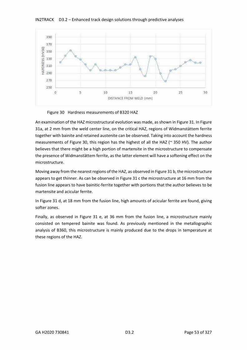
IN2TRACK D3.2 – Enhanced track design solutions through predictive analyses
GA H2020 730841 D3.2 Page 53 of 327
Figure 30 Hardness measurements of B320 HAZ
An examination of the HAZ microstructural evolution was made, as shown in Figure 31. In Figure 31a, at 2 mm from the weld center line, on the critical HAZ, regions of Widmanstättem ferrite together with bainite and retained austenite can be observed. Taking into account the hardness measurements of Figure 30, this region has the highest of all the HAZ (~ 350 HV). The author believes that there might be a high portion of martensite in the microstructure to compensate the presence of Widmanstättem ferrite, as the latter element will have a softening effect on the microstructure.
Moving away from the nearest regions of the HAZ, as observed in Figure 31 b, the microstructure appears to get thinner. As can be observed in Figure 31 c the microstructure at 16 mm from the fusion line appears to have bainitic-ferrite together with portions that the author believes to be martensite and acicular ferrite.
In Figure 31 d, at 18 mm from the fusion line, high amounts of acicular ferrite are found, giving softer zones.
Finally, as observed in Figure 31 e, at 36 mm from the fusion line, a microstructure mainly consisted on tempered bainite was found. As previously mentioned in the metallographic analysis of B360, this microstructure is mainly produced due to the drops in temperature at these regions of the HAZ.

IN2TRACK D3.2 – Enhanced track design solutions through predictive analyses
GA H2020 730841 D3.2 Page 54 of 327
Figure 31 Microstructure evolution of B320 HAZ

IN2TRACK D3.2 – Enhanced track design solutions through predictive analyses
GA H2020 730841 D3.2 Page 55 of 327
6.5 Microstructural characterisation of flash butt bainitic welds
A pearlitic R260 (260HV) rail was welded with a B360 CFB using a standard flash butt weld (FBW) procedure, with 8 preheats cycles, the weld cooled down between 500 and 300°C at 0.8°C/second. This weld can be observed in Figure 32.
Figure 32 B360-R260 flash butt weld
Even a 1mm distance will be enough to produce different microstructures. That is why transversal samples were taken from the top of the rail every 1mm approximately from the fusion line, as can be observed in Figure 33. In addition, two longitudinal-vertical sections of 10 cm each from the head of the rail were cut for metallographic examination and nano-indentation.
Figure 33 Schematic diagram of the regions of the weld for machining
Another sample was cut from the maximum distance of the fusion line, at 24 cm. It was sent for chemical analysis and used for SEM examination.
Both longitudinal sections were manually ground from 600 to 1200 grade with silicon carbide papers and then polished down to 1μm with monocrystalline diamond suspensions until a mirror-like finish was observed.
6.5.1 Micro indentation test: Durascan After grinding and polishing both specimens of the longitudinal section of the weld, indentation tests (HV1) were made every 1 mm of distance with the Durascan machine. Four rows of parallel indentation test were made, each of these from 0 to 200 mm from the fusion line, accounting for a total of 800 indentations.
a

IN2TRACK D3.2 – Enhanced track design solutions through predictive analyses
GA H2020 730841 D3.2 Page 56 of 327
6.5.2 Optical and SEM images Both longitudinal sections were etched with Nital 2%. Later on, microstructural images were taken approximately every 0.36 cm from the fusion line. In total, 66 images were taken.
6.5.3 Results SEM – hardness - macrostructure
Figure 34 shows the microstructure of the B360 parent rail, which consists on upper bainitic ferrite laths together with retained austenite regions.
Figure 34 SEM examination of B360 parent rail
Figure 35 shows the Vickers hardness profile for the B360 region of the FBW. Measurements were made on a polished longitudinal-vertical section at 5 mm below the rail running surface (horizontal axis : distance from the fusion line, from 0 to 200 mm ; vertical axis : hardness, from 280 HV1 to 420 HV1).
Just from an examination of the hardness profile we can observe:
High variations in hardness were found within 140 mm from the Fusion Line (FL). The maximum hardness measurement of 415.5HV1 corresponds at 11 mm from the FL The minimum hardness measurement will be of 282.5HV1 at 21 mm from the FL.
A macrographic examination of the macro-etched region of the HAZ with Nital 2%, can be observed in Figure 36. The width of the visible HAZ is around 2 cm.

IN2TRACK D3.2 – Enhanced track design solutions through predictive analyses
GA H2020 730841 D3.2 Page 57 of 327
Figure 35 Hardness profile of the B360 HAZ
Figure 36 Macro-etched B360 HAZ
Metallographic examination
Four regions are expected in any weld: A coarse-grained, fine-grained, intercritical and subcritical region. These are identified in Figure 37.
Figure 37 Different regions of the B360 HAZ
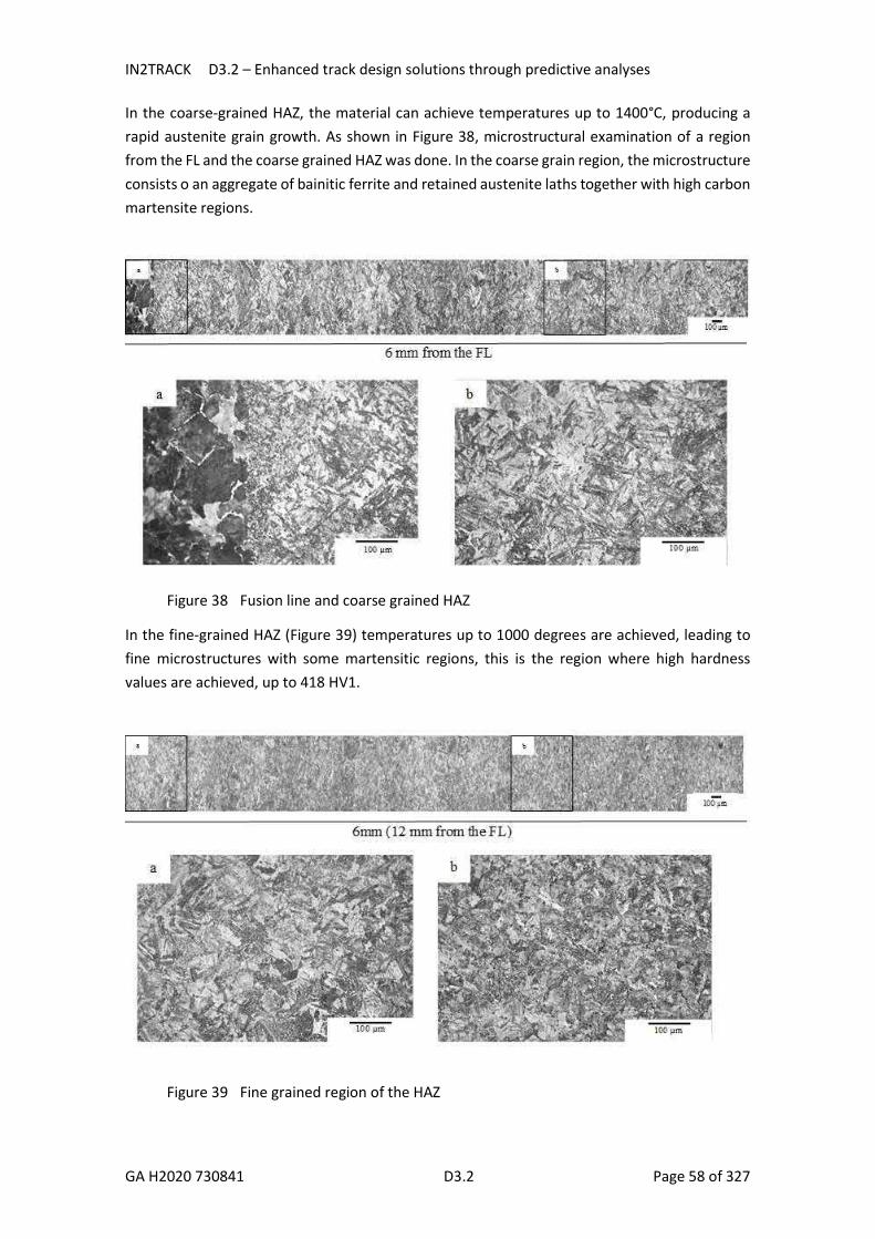
IN2TRACK D3.2 – Enhanced track design solutions through predictive analyses
GA H2020 730841 D3.2 Page 58 of 327
In the coarse-grained HAZ, the material can achieve temperatures up to 1400°C, producing a rapid austenite grain growth. As shown in Figure 38, microstructural examination of a region from the FL and the coarse grained HAZ was done. In the coarse grain region, the microstructure consists o an aggregate of bainitic ferrite and retained austenite laths together with high carbon martensite regions.
Figure 38 Fusion line and coarse grained HAZ
In the fine-grained HAZ (Figure 39) temperatures up to 1000 degrees are achieved, leading to fine microstructures with some martensitic regions, this is the region where high hardness values are achieved, up to 418 HV1.
Figure 39 Fine grained region of the HAZ

IN2TRACK D3.2 – Enhanced track design solutions through predictive analyses
GA H2020 730841 D3.2 Page 59 of 327
In the intercritical region, temperatures up to 900 degrees are achieved, leading to partial re-austenization of the steel. The microstructure shows a coarse aspect, as observed in Figure 40. Acicular ferrite together with blocky ferrite and cementite regions are present in the microstructure, which might be the cause of the drop in hardness.
Figure 40 Intercritical region of the HAZ
Temperatures up to 700°C are achieved in the subcritical HAZ, being insufficient to cause reversion of the bainite to austenite. Instead breakdown of the austenite into carbide and ferrite has taken place. This has led to a tempered microstructure as can be observed in Figure 41. This produces a drop in hardness.
Figure 41 Subcritical region of the HAZ

IN2TRACK D3.2 – Enhanced track design solutions through predictive analyses
GA H2020 730841 D3.2 Page 60 of 327
The return to the parent rail hardness in bainitic steels seems to be produced at greater distances than in pearlitic grades with the same welding procedure. This might be due to the fact that bainite will temper at even lower temperatures than pearlite. As can be observed in Figure 42, at 60 mm from the fusion line, the bainitic microstructure appears tempered.
Figure 42 Bainitic HAZ at 60 mm from the FL
Nano-indentation
Nano-indentation tests were performed to obtain a better understanding of the different regions of the HAZ.
The longitudinal-vertical section was used for this test, which was introduced in the Hysitron Triboindenter during a period of 12 hours.
After a mirror polished sample, nano-indentation tests were performed starting at 400µm from the edge of the sample, every 100 µm, up to 25 mm of distance, making a total of 250 nanoindentations. The load applied was of 5000µN.

IN2TRACK D3.2 – Enhanced track design solutions through predictive analyses
GA H2020 730841 D3.2 Page 61 of 327
Figure 43 Comparison between nano-indentation and micro-indentation results
From Figure 43 we can observe that:
High variations in hardness are produced in the fine and coarse-grain sections of the HAZ, due the coexistence of different phases in the material.
High values of hardness might correspond with high carbon martensite, which seems to be more present in the coarse grain section.
Low values of hardness might correspond to tempered bainitic ferrite. When moving away from the FL, near the intercritical zone, a homogenization of the
properties is produced.
6.6 Conclusions
When analysing the microstructure of the HAZ, hardness and the chemical analysis, a higher understanding of the HAZ properties was achieved.

IN2TRACK D3.2 – Enhanced track design solutions through predictive analyses
GA H2020 730841 D3.2 Page 62 of 327
The presence of hard high carbon martensitic regions can be found in both the coarse and the fine grained regions of the HAZs, being produced due to the cooling rate between 500 and 300°C, which is close to 0.8°C/second.
When moving away to the subcritical zone of the HAZ, lower hardness levels correspond with tempered bainitic microstructures. Bainite tempers over a wide range of temperatures. This is the reason why the HAZ width in carbide free bainite is larger than in pearlitics.
The mechanism of crack initiation at the welds of the B360 rails is believed to be due to the maximum hardness values found in the HAZ, corresponding to high amounts of martensite. This theory states that the wheel will run over the cupped softened region of the HAZ, where tempered bainitic microstructures are produced. It will then hit the martensitic region, resulting in an impact which, later, will initiate a crack.

IN2TRACK D3.2 – Enhanced track design solutions through predictive analyses
GA H2020 730841 D3.2 Page 63 of 327
7 Optimization of ballasted track Initially planned to prevent ballast flying, ballast gluing has the potential of evolving into a method to stabilise and reinforce ballasted tracks. With this aim in mind, preliminary tests have been realised on the French railway network and more are planned in a near future.
Experimental and numerical research works are underway to analyse the reasons of ballast top layers migration in specific conditions, particularly in curves. In parallel of these analyses, different solutions to prevent this track deformation are tested. Ballast gluing is one of them. Glue has hence been applied on a High Speed Line (HSL) track section to prevent ballast creep and maintain the ballast layer profile. Part of this chapter is to report the impact of ballast gluing on the evolution of the track deformation from track geometry monitoring measures.
Ballast gluing offers the possibility to increase the resistance to shear of the ballast layer. This is particularly interesting in the case of tracks with long welded rails (LWR) which are more subject to buckling during large temperature changes. By increasing the shear resistance of the ballast layer, the glue also potentially increases the lateral resistance of the track pushing further constraining LWR limits or simply increasing the safety of these LWR tracks. Another part of this chapter is therefore to report about measure of lateral resistance in different gluing conditions from laboratory tests.
Ballast gluing is hence of primary interest in terms of maintenance and cost as it offers the following possibilities:
Reducing the number of maintenance operations related to track geometry correction by reducing the ballast grains displacements by gluing at the ballast grains contact points,
Maintain the initial elastic properties, drainage and manual or mechanical tamping, Reducing ballast deterioration by reducing tamping operations which are very
aggressive to ballast.
This chapter is divided into the following sections: a description of the gluing method, results of tests on ballasted track geometry deterioration reduction by gluing, results on laboratory test on lateral resistance increase by gluing.
7.1 Gluing method
The glue used in the present tests is named Aquarail and has been developed by the company named INMS (Ingénierie Nouvelle de Mécanique des Sols, France); it is environment friendly (not polluting) and has a low cohesion hence not precluding tamping. It works mainly in tension with no transmission of bending or torsion moment through one contact. 2.5l/m2 of glue were used in each test to glue the top layer of the ballast. Studies are still underway to different combinations of viscosity and volume of glue for optimisation
The glue is sprayed either by small equipment which can be carried in a backpack for small areas, by larger equipment mounted on a trolley including tanks and multiple hoses. Special care has to be taken in order not to spray anything else than the ballast; in particular the rails, switch

IN2TRACK D3.2 – Enhanced track design solutions through predictive analyses
GA H2020 730841 D3.2 Page 64 of 327
equipment, electrical devices should not be sprayed. The glue has to be spread in a dry condition within a reasonable temperature range (10-40°) followed by a non-rainy period of 48h. 100m of track can be treated per hour.
7.2 Track tests
A 1440m HSL track section has been glued in May 2017 following the rules explained in the previous section. In order to be able to determine the impact of the ballast gluing on the evolution of the profile of the track, the data from track geometry monitoring measures were analysed during the period from February 2016 to May 2018. These data correspond to around 60 track geometry measures before gluing and 60 after. The data analysed below include vertical and horizontal alignments of both rails (N1V, N2V, N1H, N2H respectively), the average vertical and lateral rail alignment (NVA, NHA respectively) over a 200m length, the distortion and the cant. In order to filter the data to help visualising the effects of gluing, each measure has been averaged over a 200m long section.
Figure 44 to Figure 48 show the different measures of the spatial evolution of each parameter before gluing (black curves) and after gluing (red curves) for three successive track sections of 1440m each, the middle one (between 2280 and 3720m) being the glued one. It helps comparing the evolution of the glued section with non-glued ones (the preceding and following ones).
The evolution of the vertical alignments N1V and N2V is not significantly impacted by the ballast gluing as both non-glued and glued areas present very similar patterns. Similar comments could be expressed for the lateral alignments of the rails (Figure 45). Figure 46 which shows the evolution of long wave length defects shows closer red curves than black ones for the whole studied section translating into an apparent reduction of this type of defect after the gluing which is slightly more pronounced in the glued middle section. The distortion of the track (Figure 47) does not seem to be impacted by ballast gluing which is consistent with the results on the vertical alignments N1V and N2V. Figure 48 on the other hand shows a clear decreased dispersion of the cant on the overall section and not particularly on the glued one. This prevents any conclusions on the effect of gluing.

IN2TRACK D3.2 – Enhanced track design solutions through predictive analyses
GA H2020 730841 D3.2 Page 65 of 327
Figure 44 Spatial evolution of the vertical alignments N1V and N2V of the analysed track before gluing (black curves) and after gluing (red curves)

IN2TRACK D3.2 – Enhanced track design solutions through predictive analyses
GA H2020 730841 D3.2 Page 66 of 327
Figure 45 Spatial evolution of the lateral alignments N1H and N2H of the analysed track before gluing (black curves) and after gluing (red curves)

IN2TRACK D3.2 – Enhanced track design solutions through predictive analyses
GA H2020 730841 D3.2 Page 67 of 327
Figure 46 Spatial evolution of the average vertical and lateral alignments NVA and NHA of the analysed track before gluing (black curves) and after gluing (red curves)

IN2TRACK D3.2 – Enhanced track design solutions through predictive analyses
GA H2020 730841 D3.2 Page 68 of 327
Figure 47 Spatial evolution of the distortion of the analysed track before gluing (black curves) and after gluing (red curves)
Figure 48 Spatial evolution of the cant of the analysed track before gluing (black curves) and after gluing (red curves)

IN2TRACK D3.2 – Enhanced track design solutions through predictive analyses
GA H2020 730841 D3.2 Page 69 of 327
7.3 Laboratory tests
Laboratory tests were undertaken to analyse the impact of ballast gluing on the lateral resistance of the track. These tests were conducted at the track testing facility of SNCF. Track lateral resistance can be measured in laboratory following a procedure based on German and French method which should soon be added to a European code. The procedure is the following: two sleepers are embedded into a 500mm deep ballast bed confined in a rectangular area by walls on three sides and a free slope on the last one. After applying a cyclic vertical load to assure a stabilisation of the ballast bed similar to track conditions, both sleepers are pulled laterally enabling the establishment of a curve relating the pulling force and the axial displacement of the sleeper.
This test is performed in different configurations by gluing different parts of the shoulder of the track. The results (lateral resistance values) are compared to a reference case without gluing. In each test, the sleeper is pulled four times: once without glue and three times with the same gluing configuration. The conditions of the typical test are described below.
7.3.1 Lateral resistance test conditions The ballast bed is 1.5x4 m and the walls made of wood (Figure 49). All conditions used in this test mimic the HSR (High Speed Rail) conditions. Two M450PI sleepers are loaded through two rail sections. The ballast used was new 31.5/50 ballast of class C2 (French standard), non-washed (for the dust). A 3/2 reinforced shoulder is made in front of the chassis. Marks drawn on the walls allow creating the desired slope. Lateral displacement sensors are set on the ends of each sleeper. Between each replacement of glued ballast, the following steps are performed:
Setting of the ballast bed as described above, Lateral displacement of 5 mm of the sleepers without glue on ballast, Gluing part of the shoulder, Two additional lateral displacements of 5 mm of the sleepers, Final lateral displacement of 10 mm of the sleepers.
The different gluing configurations are presented in Figure 51 for six samples. The depth reached by the glue is checked visually: the glued ballast is removed, and the depth is measured from the mark used to create the slope to the non-glued ballast. The height measurement is realised at several locations and an average is calculated. The gluing method is the same for all the samples. A watering can is filled with the adhesive and weighed. The control of the quantity is made by successive weighing. The watering is equipped with an elongated head including a row of holes reproducing the spreading process used on real track (Figure 50). The desired depth is the height of sleeper (around 16 cm) but the obtained depth average for superficial gluing of cases 1 to 4 were:
sample 1: 23,6 cm sample 2: 18,8 cm sample 3: 16,5 cm sample 4: 13,2 cm

IN2TRACK D3.2 – Enhanced track design solutions through predictive analyses
GA H2020 730841 D3.2 Page 70 of 327
Figure 49 Lateral resistance test configuration
Figure 50 Glue spreading method

IN2TRACK D3.2 – Enhanced track design solutions through predictive analyses
GA H2020 730841 D3.2 Page 71 of 327
Test number Gluing configuration
1
2-3
4-5
6
7
Figure 51 Gluing configurations tested: in blue the glued part of the ballast bed
7.3.2 Results analysis The force-displacement obtained for the different samples are shown in Figure 52 to Figure 58. Each curve present three distinct parts:
A positive slope at the beginning of the test, A plateau-like part which tends toward a limit value F0 at the end of the imposed
displacement A decreasing part corresponding to the unloading of the ballast bed
The transition between the two first parts is more distinct for the first pulling of each sample than for the three next, where the transition is softer. This softening is probably the result of the reorganization of the grains due to the first pulling action: the first pulling creates free spaces, particularly at the front of the sleepers, where particles can later move easier compared to the previous configuration. On some samples as 3 and 4, the first pulling does not seem enough to fully rearrange grains and the 2nd pulling finishes the reorganisation. The first pulling without glue for the different samples presents variability between 15 and 17kN.
When the slope only is glued superficially (sample 2 and 3), the lateral resistance is not significantly improved as the maximum lateral resistance value for a given displacement is barely changed. On the other hand, when the whole shoulder is glued superficially (samples 4 and 5), a 20% gain on lateral resistance is observed. This leads to the hypothesis that gluing superficially only the area next to the sleepers head is beneficial in terms of lateral resistance. Gluing this area to full depth (sample 6) did not improve the lateral resistance showing that gluing at sleeper depth is enough to improve the lateral resistance. Gluing to full depth the whole shoulder
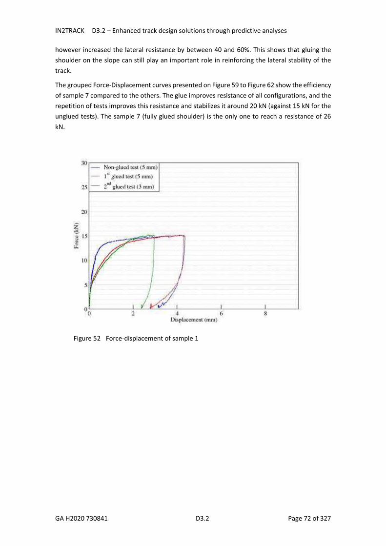
IN2TRACK D3.2 – Enhanced track design solutions through predictive analyses
GA H2020 730841 D3.2 Page 72 of 327
however increased the lateral resistance by between 40 and 60%. This shows that gluing the shoulder on the slope can still play an important role in reinforcing the lateral stability of the track.
The grouped Force-Displacement curves presented on Figure 59 to Figure 62 show the efficiency of sample 7 compared to the others. The glue improves resistance of all configurations, and the repetition of tests improves this resistance and stabilizes it around 20 kN (against 15 kN for the unglued tests). The sample 7 (fully glued shoulder) is the only one to reach a resistance of 26 kN.
Figure 52 Force-displacement of sample 1

IN2TRACK D3.2 – Enhanced track design solutions through predictive analyses
GA H2020 730841 D3.2 Page 73 of 327
Figure 53 Force-displacement of sample 2
Figure 54 Force-displacement of sample 3
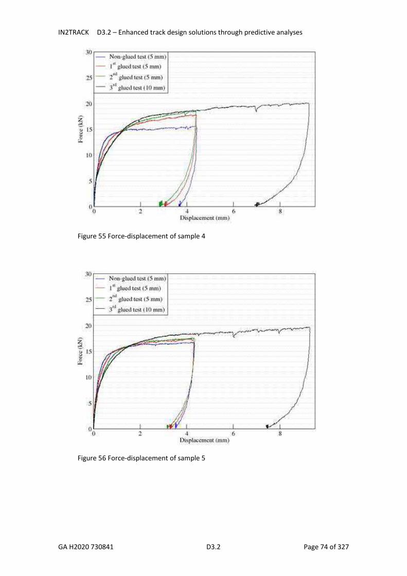
IN2TRACK D3.2 – Enhanced track design solutions through predictive analyses
GA H2020 730841 D3.2 Page 74 of 327
Figure 55 Force-displacement of sample 4
Figure 56 Force-displacement of sample 5

IN2TRACK D3.2 – Enhanced track design solutions through predictive analyses
GA H2020 730841 D3.2 Page 75 of 327
Figure 57 Force-displacement of sample 6
Figure 58 Force-displacement of sample 7
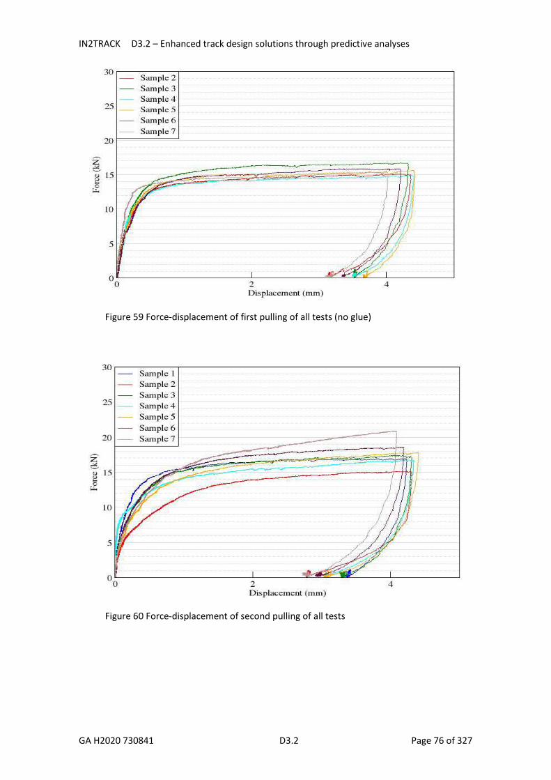
IN2TRACK D3.2 – Enhanced track design solutions through predictive analyses
GA H2020 730841 D3.2 Page 76 of 327
Figure 59 Force-displacement of first pulling of all tests (no glue)
Figure 60 Force-displacement of second pulling of all tests

IN2TRACK D3.2 – Enhanced track design solutions through predictive analyses
GA H2020 730841 D3.2 Page 77 of 327
Figure 61 Force-displacement of third pulling of all tests
Figure 62 Force-displacement of last pulling of all tests
The irreversible displacement, that is the displacement of the sleepers after total release of the pulling force, is taken as a plastic characteristic of the behaviour of the ballast (glued or not) during this test: the higher the irreversible displacement, the poorer the performance of the

IN2TRACK D3.2 – Enhanced track design solutions through predictive analyses
GA H2020 730841 D3.2 Page 78 of 327
ballast/glue system in terms of lateral resistance. The percentage of irreversible displacement of each non-glued test is compared in Figure 63. From a sample to another, this percentage stays in the same order of magnitude, although the particle configurations are different. It shows that the compactions of the different samples are similar or that irreversible displacement is unaffected any inherent variation of compaction.
Figure 63 Percentage of irreversible displacement of each first non-glued test
The evolution of the irreversible displacement percentage is presented in Figure 64. The non-glued sample (sample 1) does not behave like the other and stays at its initial percentage of 80%. Then, for a non-glued ballast bed, the proportion reversible/irreversible displacement is not modified by the repetition of lateral resistance test. Sample 2 is discarded from the graph because of discrepancies.
Sample 7 (totally glued shoulder) has the lowest irreversible displacement percentage: when the ballast is entirely glued, its behaviour seems more elastic than other configurations with less glue. Moreover, sample 3, i.e. the sample with the lowest proportion of glue in the system, presents the higher percentage of irreversible displacement (after the non-glued configuration). In other words this means the more glue in the ballast bed, the more important the reversible part of the displacement. All these observations seem to show that gluing tends to increase the lateral elasticity of the track hence reducing its plastic lateral deformation.

IN2TRACK D3.2 – Enhanced track design solutions through predictive analyses
GA H2020 730841 D3.2 Page 79 of 327
Figure 64 Evolution of percentage of irreversible displacement over consecutive lateral resistance tests
Figure 65 to Figure 68 show the gain of force expressed as the percentage between each lateral resistance test with glue and its corresponding unglued reference test. For all cases except the fully glued shoulder (sample 7), the shape and order of magnitude of curves is similar: the difference with the reference test does not exceed 10% at 4mm displacement. With a fully glued shoulder (Figure 68) the lateral resistance test is almost doubled at 4mm displacement. Even though the other gluing configurations bring an improvement in lateral resistance, they remain less performing than the fully glued one.

IN2TRACK D3.2 – Enhanced track design solutions through predictive analyses
GA H2020 730841 D3.2 Page 80 of 327
Figure 65 Force difference between the glued pulling tests and the non-glued reference one for sample 3 (surface of slope of shoulder glued)

IN2TRACK D3.2 – Enhanced track design solutions through predictive analyses
GA H2020 730841 D3.2 Page 81 of 327
Figure 66 Force difference between the glued pulling tests and the non-glued reference one for samples 4 and 5 (surface of whole shoulder glued)

IN2TRACK D3.2 – Enhanced track design solutions through predictive analyses
GA H2020 730841 D3.2 Page 82 of 327
Figure 67 Force difference between the glued pulling tests and the non-glued reference one for sample 6 (head of sleepers shoulder glued to full depth)
Figure 68 Force difference between the glued pulling tests and the non-glued reference one for sample 7 (head of sleepers shoulder glued to full depth)
In order to describe quantitatively the behaviour of the system ballast/sleeper during the lateral resistance pulling test, the Force-Displacement curve shape observed in Figure 52 to Figure 58 during loading can be fitted using the following equation:

IN2TRACK D3.2 – Enhanced track design solutions through predictive analyses
GA H2020 730841 D3.2 Page 83 of 327
𝐹(𝑢) = 𝐹 (1)
where F(u) and u are the experimental data, and (F₀, u₀) unknown coefficients.
F₀ corresponds to the limit value reached by the curve and gives a way to quantify the lateral resistance of each sample. F0/u0 is the initial slope of the curve. F0 and u0 are hence viewed as characteristic parameters which allow comparing the lateral resistance in different configurations. We define G by the following equation:
𝐺(𝑢) =( )
= 𝑢 + (2)
As G is a linear function of u, it is easier to evaluate F₀ and u₀ for each lateral resistance test using the experimental data (F, u). G(u) is shown in Annex 1 for each sample including a summary of the value of F0, u0, gain of F0 and irreversible displacement. Figure 69 presents the value of F₀ for each test. This figure and the table of Annex 1 show that the repetition of pulling increases F0 whatever the sample. We can see that surface gluing of the slope of the shoulder (samples 2 and 3) increases lateral resistance up to 9% while gluing of the whole surface of the shoulder (samples 4 and 5) increases it up to 22%. Vertical gluing of the sleeper heads (sample 6) gives an augmentation of F0 of the same order (19%). Sample 7 (fully glued shoulder) leads to the highest increase of F0 reaching a 61% gain.
Figure 69 Evolution of F0 for the different samples
7.4 Conclusions
Ballast gluing has been analysed in terms of track reinforcement performance using ballasted tracks surface gluing test and laboratory tests data. The adhesion of the glue is low enough to

IN2TRACK D3.2 – Enhanced track design solutions through predictive analyses
GA H2020 730841 D3.2 Page 84 of 327
allow tamping of the ballast. The on-site gluing data showed that surface gluing of ballast did not have any impact on the evolution of the track geometry, in other words any deformation of the track. The laboratory test, on the other hand, showed that the lateral resistance of the track can be significantly increased up to 61% by gluing the whole shoulder of the track to full depth and up to 22% by gluing only the surface of the whole shoulder. This result is of practical interest when designing tracks with long welded rails prone to buckling during heat waves. Further analysis is underway at SNCF RESEAU to identify precisely the areas and amounts of glue necessary to reinforce significantly the performances of ballasted tracks.

IN2TRACK D3.2 – Enhanced track design solutions through predictive analyses
GA H2020 730841 D3.2 Page 85 of 327
8 Overcoming limitations of existing predictive methods for rail and track deterioration
Limitations of existing predictive methods regarding mechanical loads and resulting deterioration, noise and vibration have in many cases already been charted. Setting out from this pre-knowledge, improvements will be made in increasing understanding and developing refined models in required fields.
8.1 Limitations in predictive models of rail crack formation
Setting out among other studies from In2Rail D3.3, a deeper investigation of limitations in prediction of rail crack formation has been carried out. The investigation relates to dynamic loads, contact stresses, material response, damage formation, crack initiation, growth and final fracture. To be physically sound, a predictive model for RCF crack (e.g. squat or head check) formation and propagation should be able to account for highly compressive and shear loading, large plastic deformations and an anisotropic material response. Furthermore, it should be able to predict crack growth rates and crack growth direction for a three-dimensional crack (crack under multiaxial loading). Finally, it should also be able to predict final fracture. Since there is no such a model today, simplified models with their inherent limitations need to be used.
8.1.1 Prediction of squats in rails A commonly applied approach to assess the loading of cracks is to employ Stress Intensity Factors (SIF). Rolling Contact Fatigue (RCF) loading typically activates all three modes of deformation: opening, characterized by SIF KI, shear in plane (KII) and shear out of plane (KIII). The load cycle typically consists of high compression and shear, and the principal stresses vary out-of-phase, which put special demands on SIF evaluation techniques. An approach to assess SIFs under such conditions has been developed within the current project, see Andersson et al (2018). The overall idea is to construct a displacement ansatz consisting of three superposed parts. The first part expresses the displacement field valid close to the crack tip in terms of the unknown SIFs and is based on (and restricted by) well-known results from Linear Elastic Fracture Mechanics (LEFM) theory. The second and third parts correspond to rigid body motion of the crack tip as well as superposed constant strain fields. The idea is then to fit the displacement ansatz against an approximate (extended finite element method) XFEM/FEM strain field by the method of least squares and in turn obtain the SIFs. For a thorough description, see Andersson et al (2018).
Another common limitation in predictive modelling of rail crack formation related to the lack of material properties under elevated temperatures. This can be exemplified by squat formation close to white etching layers (WELs). Simulation challenges and work progress in this area are further described in section 9.1.3.

IN2TRACK D3.2 – Enhanced track design solutions through predictive analyses
GA H2020 730841 D3.2 Page 86 of 327
8.1.2 Formation of anisotropy in rails, and its effect on crack formation and growth
Deformation induced anisotropy is a well-known phenomenon for sheet metal rolling. The large plastic deformations occurring in the vicinity of the contact zone in rails, is also known to produce an anisotropic material, see e.g. Wetscher et al (2007). There is, to our knowledge, no material model capable of describing the multiaxial, anisotropic ratchetting behaviour associated with repeated rolling to the acceptable accuracy required for accurate fatigue predictions. Much of the work on plastic anisotropy is limited to cases where the anisotropy is present as an initial condition, i.e. from the manufacturing stage (e.g. sheet metals).
Our current work has focused on obtaining a testing methodology that can be used to characterize the material behaviour in the anisotropic surface layer (Meyer et al 2017a). In addition to developing this methodology, we have shown that some standard frameworks (e.g. those built into commercial CAE package such as ABAQUS) are not suitable for simulating the large shear deformations found in the surface layer of rails (Meyer 2017b). Sound material models are a requirement for obtaining correct input to crack initiation and propagation studies. Improvements and progress in research on anisotropy is further described in section 10.1.
8.1.3 Prediction of rail crack formation Crack initiation in rails may take place at the surface or subsurface, depending mainly on the contact conditions at the wheel-rail contact patch. Under dry conditions, large tangential contact stresses are formed at the rail surface. Under the action of those cyclic stresses, large shear deformations accumulate at the surface layer of the rail (ratcheting of the rail material), until the ductile limit in shear of the rail material is exceeded and cracks thereby start to form. In cases of low friction (e.g. under well-lubricated conditions) the point of maximum shear stress shifts into the rail subsurface. Provided that inclusions from manufacturing (or other material/geometric inhomogenities) are embedded in the rail material, subsurface cracks may start to form, and propagate. At such inclusions, the compressive stress may result in a local mode I loading (opening mode) that may be increased by the superposition of global bending of the rail or by residual stresses, e.g. due to welding.
The current state-of-the-art includes predictive methods that relate to ratchetting and low cycle fatigue. These relate the plastic deformation of the surface material to life until crack initiation. Available methods in this field include shakedown maps, equivalent strain approaches, fatigue indices (see Ekberg et al 2002). Alternatively, damage mechanics approaches can be employed. These are essentially a low cycle fatigue criterion and the main challenge is to obtain a relation between the plastic deformation of the material and the crack initiation.
8.1.4 Prediction of rail crack growth Rail crack growth is typically predicted using fracture mechanics approaches (although there are approaches to link it to fatigue damage, see Ekberg et al 2014). The main challenges for fracture mechanics approaches are how to account for load multi-axiality (preferably via a single scalar quantity) and on top of this, how to account for out-of-phase and compressive nature of the

IN2TRACK D3.2 – Enhanced track design solutions through predictive analyses
GA H2020 730841 D3.2 Page 87 of 327
loading. In doing so, the predictive criteria need to be able to predict the direction and rate of growth. These questions are addressed with focus on predicting crack growth directions in the work of Floros (2016), and in In2track D3.1 and D3.3 Deliverables.
The current understanding of mechanisms of crack propagation, including the effect of climatic conditions and material properties, is limited. It is known that friction conditions within the cracks play a significant role in crack propagation and branching, i.e. the climatic conditions will affect crack growth (as well as crack initiation). However, there is a lack of full understanding of this topic.
8.1.5 Mechanical performance of wheel and rail materials Materials used in wheels and rails are exposed to a complex combination of mechanical and thermal loads. One of the most common problems arises from the elevated temperatures that are evolved during braking or sliding of the wheel on the rail. Combined with a fast cooling due to the ambient temperature, this will promote the formation of martensite and also plastic deformation. Due to the high temperatures the predominant pearlitic microstructure degenerates as spheroidisation of the pearlite starts to occur. This change in the material microstructure promotes cracking and consequent crack growth due to the cyclic loading that eventually leads to ultimate material failure.
To provide input for material modelling simulations that will be able to predict the material response more accurately and improve predictive capabilities, fatigue testing has been performed as described in 10.1. Tests include both uniaxial and bi-axial (tension – torsion) experiments of R260 rail steel and other materials. Also, examinations with alternating thermal and mechanical loads (thermomechanical fatigue) have been performed in addition to isothermal tests. Both virgin material and the anisotropic surface layer of used material (or artificially deformed materials) are investigated. Microscopy together with image processing are used to evaluate the influence of high loads and temperatures to the material microstructure with the aim to quantify the effect of pearlite spheroidisation and its role in the material response.
8.2 Existing predictive methods with respect to wear & rolling contact fatigue
Track and rail deterioration is an unavoidable phenomenon for the railway infrastructure subjected to traffic. Accelerating and braking of a vehicle leads to increased wheel-rail contact forces which contribute to rail damage. Furthermore, dynamic contact forces, which are produced in each wheel rail contact while the vehicle is running, are causing certain deterioration in the track.
In principle, the deterioration of the track can be divided into different damage mechanisms:
Vertical or lateral track geometry deterioration. This can happen due to ballast movement, voids, etc.
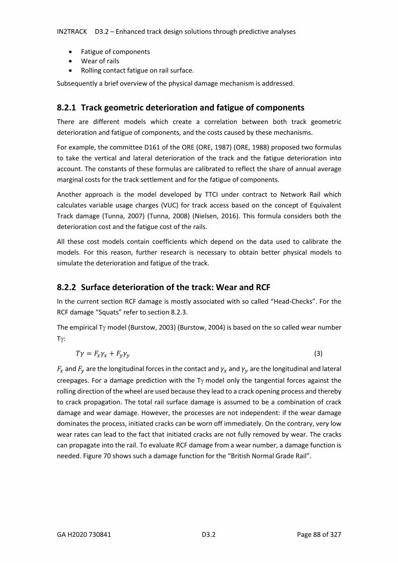
IN2TRACK D3.2 – Enhanced track design solutions through predictive analyses
GA H2020 730841 D3.2 Page 88 of 327
Fatigue of components Wear of rails Rolling contact fatigue on rail surface.
Subsequently a brief overview of the physical damage mechanism is addressed.
8.2.1 Track geometric deterioration and fatigue of components There are different models which create a correlation between both track geometric deterioration and fatigue of components, and the costs caused by these mechanisms.
For example, the committee D161 of the ORE (ORE, 1987) (ORE, 1988) proposed two formulas to take the vertical and lateral deterioration of the track and the fatigue deterioration into account. The constants of these formulas are calibrated to reflect the share of annual average marginal costs for the track settlement and for the fatigue of components.
Another approach is the model developed by TTCI under contract to Network Rail which calculates variable usage charges (VUC) for track access based on the concept of Equivalent Track damage (Tunna, 2007) (Tunna, 2008) (Nielsen, 2016). This formula considers both the deterioration cost and the fatigue cost of the rails.
All these cost models contain coefficients which depend on the data used to calibrate the models. For this reason, further research is necessary to obtain better physical models to simulate the deterioration and fatigue of the track.
8.2.2 Surface deterioration of the track: Wear and RCF In the current section RCF damage is mostly associated with so called “Head-Checks”. For the RCF damage “Squats” refer to section 8.2.3.
The empirical Tmodel (Burstow, 2003) (Burstow, 2004) is based on the so called wear number T:
𝑇𝛾 = 𝐹 𝛾 + 𝐹 𝛾 (3)
𝐹 and 𝐹 are the longitudinal forces in the contact and 𝛾 and 𝛾 are the longitudinal and lateral
creepages. For a damage prediction with the Tmodel only the tangential forces against the rolling direction of the wheel are used because they lead to a crack opening process and thereby to crack propagation. The total rail surface damage is assumed to be a combination of crack damage and wear damage. However, the processes are not independent: if the wear damage dominates the process, initiated cracks can be worn off immediately. On the contrary, very low wear rates can lead to the fact that initiated cracks are not fully removed by wear. The cracks can propagate into the rail. To evaluate RCF damage from a wear number, a damage function is needed. Figure 70 shows such a damage function for the “British Normal Grade Rail”.

IN2TRACK D3.2 – Enhanced track design solutions through predictive analyses
GA H2020 730841 D3.2 Page 89 of 327
Figure 70 RCF damage function (Burstow, 2004)
This RCF-damage function shows four different regions (Burstow, 2004) (Dirks, 2015) (Trummer, 2016):
1. For 0 < Tγ ≤ 15 N, there should be no rail surface damage. 2. For 15 < Tγ ≤ 65 N, RCF damage dominates the process 3. For 65 < Tγ ≤ 175 N, increased wear influence on the RCF damage 4. For Tγ > 175 N, the wear process dominates, so all RCF cracks are worn off
A damage function for heavy haul railways was determined in (Spangenberg, 2015) and the locations of the turning point were determined at: 89 N, 267 N and 890 N.
Ekberg et al (Ekberg, 2002) developed a model for the prediction of RCF and LCF (Low Cycle Fatigue) on railway wheels. Shakedown maps (Figure 71) are used to identify loadings which can lead to ratchetting. The normal load FZ, the contact geometry defined by the Hertzian semiaxes a and b and the yield stress in shear (for work-hardened material) k determine the normalized vertical load ν (vertical axis in Figure 71). Together with the traction coefficient μ, the location of the working point WP is defined in the shakedown map. The material response depends on the location of the WP in the shakedown map. Due to the fact, that the model should only analyse the possibility of surface fatigue, only the region right of the boundary curve (BC) is of interest. The working point is located in this region if the following inequality is fulfilled. (Ekberg, 2002)
𝐹𝐼 = 𝜇 − > 0 (4)

IN2TRACK D3.2 – Enhanced track design solutions through predictive analyses
GA H2020 730841 D3.2 Page 90 of 327
Figure 71Shakedown map. WP is the working point. BC marks the boundary curve for surface plasticity. The surface fatigue index FIsurf is marked with a dashed line. (Ekberg, 2002)
Cracks initiated more than 3 mm below the surface are classified as subsurface cracks. In the model of Ekberg et al (Ekberg, 2002), this cracks belongs to HCF (High Cycle Fatigue) mechanisms (e.g. elastic shakedown). Ekberg et al (Ekberg, 2002) uses a Dang Van based model to estimate subsurface-initiated fatigue (material parameter aDV , hydrostatic stress σh, equivalent fatigue limit σEQ,e)
𝐹𝐼 = (1 − 𝜇 ) + 𝑎 𝜎 , > 𝜎 , (5)
The last criterion of Ekberg et al model (Ekberg, 2002) treats fatigue initiated at deep defects. Typical attributes of such defects are e.g. cracks initiated at defects or voids with a dimension of about 1 mm or fatigue cracks initiated at a depth more than 10 mm below the wheel tread. The fatigue impact at deep defects should be less influenced by the contact geometry (assumption of moderate loads). Based on this assumption, only the normal load FZ is used for the fatigue criterion. The threshold Fth depends on the depth z of the defect below the wheel tread, the size d of the defect and the load history H. (Ekberg, 2002)
𝐹𝐼 = 𝐹 > 𝐹 (𝑧, 𝑑, 𝐻. . ) (6)
In general, fatigue should take place if one or more of these equations are fulfilled (Ekberg, 2002). The main advantage of this model is the low demand on computational effort.
Dirks et al (Dirks, 2015a) (Dirks, 2015b) model combined the so called stress index (SI) and the energy index (EI) model with two material parameters which made it possible to estimate beside the crack initiation potential the actual crack length. The model was calibrated with measurements of crack surface lengths and depths of rails of a Dutch railway and should only be used for small cracks.
The stress index (SI) and the energy index (EI) is calculated by the following formulas. The main difference is that the energy index (EI) takes the creepages into account (Dirks, 2015b).

IN2TRACK D3.2 – Enhanced track design solutions through predictive analyses
GA H2020 730841 D3.2 Page 91 of 327
𝑆𝐼(𝑥, 𝑦) = 𝜏 (𝑥, 𝑦) + 𝜏 (𝑥, 𝑦) − 𝑘, (7)
𝐸𝐼(𝑥, 𝑦) = 𝜏 (𝑥, 𝑦) 𝛾 − (𝜑 ∙ 𝑦) + 𝜏 (𝑥, 𝑦) ∙ 𝛾 + (𝜑 ∙ 𝑥) , (8)
In these equations, τ is the shear stress, k is the yield limit in shear and , 𝛾 , 𝛾 are the
creepages. Generally, damage should occur if the local stress index SI > 0 or EI > 15.
Trummer et al (Trummer, 2016a) (Trummer 2016b) (Trummer, 2014) (Trummer, 2017) developed a model for near-surface crack initiation. This model takes the interaction of wear, shear deformation of the near-surface crack initiation layer and the stress distribution due to contact forces into account.
The model is based on the assumption that cracks are initiated in the near surface layer and prefer a certain orientation of the microstructure of this layer. This shear strain α is estimated by the linear elastic contact stresses and the relative motion between wheel and rail (Trummer, 2016a). Figure 72 shows different orientations of the microstructure of a material. In Figure 73 the shear strain α is illustrated.
Figure 72 Schematic illustration of the orientation of the microstructure: (a) undeformed material; (b) shear strain α is around 60°; (c) shear strain α is around 90°. (Trummer, 2016a)
Figure 73 Dashed line represents an undeformed and the continuous line a deformed unit. The shear strain α is principally measured as shown in this figure. (Trummer, 2016a)
In addition, the model considers the removal of the near surface layer due to wear processes in the wheel-rail contacts (Trummer, 2016a). The wear rate is calculated on the assumptions of Krause and Poll (Krause, 1986).
The assessment of the crack initiation possibility is finally based on the maximum tensile principal stress and the state of the shear deformation of the near surface layer. (Trummer, 2016a)

IN2TRACK D3.2 – Enhanced track design solutions through predictive analyses
GA H2020 730841 D3.2 Page 92 of 327
The model was parametrized by full scale wheel-rail test rig and twin disc experiments. (Trummer, 2016a)
Comments
In order to obtain sensible results, the model must be calibrated tuning the damage model against site data. The calibration will depend on both the site and the type of steel.
8.2.3 Surface deterioration of the track: Squats Defect morphology
Reports of “Squats” have increased in recent years. Because they are hard to detect in an early state and may lead to rail break, they are very important to infrastructure managers nowadays. A further difficulty is that their initiation mechanism is still not fully understood.
Squats are surface initiated RCF defects having three main characteristics:
They show a black spot (indentation) in the shape of two lungs. They form cracks in the shape V, U, W or circular. Due to plastic deformation and/or wear, a widening of the running band is observed.
Other characteristics are a network of subsurface cracks because of the branching of the main crack. Squats can occur isolated or more or less periodically. Especially the isolated occurrence complicates its detection and prediction.
(Grassie, 2012a) reports that cracks develop in the highly sheared surface layer at an angle of about 20° to the surface. Crack growth is associated with fluid entrapment. It is mentioned that the cracks can turn into the rail and can result in a transverse defect (rail break).
It was also reported (RailCorp, 2012) that squats are likely initiated from pre-existing gauge corner checking or Head Checks. The cracks grow laterally and spread towards the crown of the rail head. The occurrence of White Etching Layer (WEL) is possible.
A different mechanism of squat development is described by Li and his colleagues (Li, 2011). They explain the squat development due to any geometrical deviation. An initial defect on the rail surface causes dynamic contact forces. This dynamic contact forces produce the second indentation of the squat. The difference to the squat development mechanism explained previously is, that for this mechanism no pre-existing cracks are needed. Further Li reports that in the Netherlands 72% of the squats are found in the neighbourhood of corrugation and 17% are found at welds. This might indicate that corrugation and welds lead to dynamic contact forces, which in turn result in squats. Furthermore 74% of squats are found near or above sleepers. This might indicate a relation to stiffness changes of the substructure.
Another defect which beset the rails of London underground in the mid-2000s is described in (Grassie, 2012b). This defect appears as squats to the naked eye and ultrasonic signal but due to some differences to squats Grassie named these defects “Studs”. Studs also occur in the centre of the running band and they appear accumulated on the approach to signals where the train is first braking and then accelerating and also on rising outs of the underground where the

IN2TRACK D3.2 – Enhanced track design solutions through predictive analyses
GA H2020 730841 D3.2 Page 93 of 327
train is under high traction. However, they are not reported to occur in tunnels and also no rail break was reported from studs. Studs are reported to grow faster than squats.
As a possible initiation mechanism thermal damage is named. Thermal damage is a result of high creepages which in turn might be caused e.g. by torsional vibrations of the wheelset. Modern traction control systems with higher traction ratios might also lead to higher creepages.
However, a clear distinction between “Studs” and “Squats” is controversial and discussed in the scientific community.
Modelling of squats
There are few reports of technical/physical models in literature. Li set up a transient Finite Element Model where the resulting contact forces, stress and strain levels showed good agreement with field observations (Li, 2008).
Farjoo modelled the crack propagation including entrapped water and elastic foundation with the help of Finite Elements (Farjoo, 2012).
Fletcher used a thermos-mechanical 2D Boundary Element (BE) model to calculate the rail-wheel contact. Cracks formed without evidence of (macroscopic) plastic flow, a WEL lies above a shallow crack.
Bernsteiner et al (Bernsteiner, 2016) calculated the temperature on- and below the surface of a rail in and outside of the wheel rail contact patch. For the calculation of the normal stress distribution a Hertz contact was assumed. The tangential stresses were calculated with the ECF model which estimates the coefficient of friction based on the local normal pressure and temperature (Meierhofer, 2015). The temperature was calculated by the analytical approach of Ertz and Knothe (Ertz, 2002). Temperatures above 700 °C should be possible in the wheel rail contact on- and below the surface in certain circumstances according the simulation results. The comparison of the simulation results with full scale test rig experiments showed a good agreement between the temperatures above 700 °C on- and below the surface and WEL development on rail surfaces. (Bernsteiner, 2016) Other experiments (Bernsteiner, 2017) (Bernsteiner, 2018) revealed that both, cracks in the WEL and base material can be formed under additional loadings of rails with WEL. Furthermore, outbreaks of WEL of the rail surface were found after additional loadings. It should be mentioned, that these rail defects may lead to squats under certain circumstance, but no squat was found on the rails after the experiments!
Furthermore, Bernsteiner developed a new tool for the simulation of squats and other local deviations of the rail surface (Bernsteiner, 2018). This squat model consists of different sub models. The normal stresses are solved for non-Hertzian-contact-patches which occur at squats due to the local deviation of the rail surface. The tangential stresses are calculated with the ECF model (Meierhofer, 2015). The wear rate is estimated by the approach of Krause and Poll (Krause, 1986). Trummer’s model (Trummer, 2016a) (Trummer 2016b) (Trummer, 2014) (Trummer, 2017) is used for the estimation of the local crack initiation potential. This model allows to calculate the formation of a rail surface with initial geometrical deviations and also to estimate the local crack initiation potential. Simulation results showed that initial geometrical deviations remain on the rail due to local variations in the wheel rail contact caused by the

IN2TRACK D3.2 – Enhanced track design solutions through predictive analyses
GA H2020 730841 D3.2 Page 94 of 327
geometrical deviation of the rail surface. Under certain circumstance, the deviations lead to an increased crack initiation potential compared with a rail surface without a geometrical deviation. The article (Bernsteiner, 2018) can be found in Annex 2.

IN2TRACK D3.2 – Enhanced track design solutions through predictive analyses
GA H2020 730841 D3.2 Page 95 of 327
9 Improved prediction of rail and track deterioration This section addresses rail and track deterioration under different operational conditions, considering different material characteristics including the influence of thermal loads e.g. in relation to welding and to track instability. This work links to the identification of areas where knowledge needs to be increased and predictive capabilities enhanced as identified in D3.1.
9.1 Rail and track deterioration under influence of thermal loading
Steel microstructure is recognized for its “temper”. The strong response on different heat treatments gives the possibility to tailor the steel properties to the requirements of the application, and even to introduce beneficial gradients in properties and residual stresses. But as much as this is a benefit during production of steel products, it can be detrimental if heat treatment occurs during product use, the reason for the term “thermal damage”.
Welding and grinding processes induce local heating, and generally are considered damaging the properties of the base material. However, in welding the situation can be improved by introducing fillers or additives to modify the steel chemistry. It can also be improved by controlled heat supply to create new beneficial heat treatments. Short term local friction heating in railway operation might also occur when a railway vehicle’s wheelset skids along the rail (for example in emergency braking, malfunctioning brake systems or varying friction conditions due to climate). The consequent temperature elevation (usually up to 800-1000˚C) in the rail and wheel steels with a pearlitic microstructure leads to phase transformations.
The temperature dependent differences in thermal expansion, density and mechanical properties of phases result in residual stresses and localization of strains upon subsequent rolling contact loading, which can cause crack initiation in rail and wheel surfaces.
New methods for repair welding including additive manufacturing (AM) and surface treatment are developing, that could drastically improve the mechanical performance of the rail running surface. Especially switches and crossings and rails in tight curves could benefit from such new techniques in a life cycle cost (LCC) perspective. However, for new technologies to be developed and successfully implemented in field after rigorous safety assessments, a solid scientific foundation is needed. This is also important for existing welding methods carried out at the track, where the effect of process parameter variations may be large.
There are many parallels between the base material behaviour upon welding and thermal damage from frictional heating, and the two areas benefit from combined studies. The effect of local heating whether induced by welding or friction is a degraded or changed structure, with a gradient in mechanical properties and residual stresses. Accurate prediction of these fields is crucial for judgement of fatigue damage in railway operation. In the following, experiments and models of these phenomena are explained in sections 9.1.1 and 9.1.3, and the activities initiated in In2Track are foreseen to be continued within In2Track2-3.

IN2TRACK D3.2 – Enhanced track design solutions through predictive analyses
GA H2020 730841 D3.2 Page 96 of 327
9.1.1 Influence of thermal loading in relation to welding Understanding thermomechanical phenomena occurring during welding is essential in order to correctly model and predict residual stresses and material behaviour around welds. In the current In2Track project, work has been done to characterize the elevated temperature properties and mechanical behaviour of near pearlitic wheel steels, Annex 3 – “Rail and track deterioration under influence of thermal loading”. The results are transferable also to fully pearlitic rail steels since the main microstructural constituent is pearlite in both cases. Further, work has been done in modelling of thermal damage including cyclic plasticity and phase transformations, as described in 9.1.3. These models are directly applicable also to welding simulation, as soon as the local temperature history is known.
Whole process modelling is useful for characterisation of thermal loadings, basically determining the local temperature history at each point for a given welding sequence. The choice of welding process greatly influences the thermal loadings and the width of the heat affected zone (HAZ). Current specifications are meant to ensure a robust result but attempts to introduce innovative solutions could benefit from prediction capabilities. An example is the attempt to evaluate two alternative welding procedures in the EU project WRIST (2018). A report on repair welding is found in In2Track D3.3, that includes thermal and mechanical simulation of cladding with a simplified constitutive material model.
The remaining needs for welding simulation with more precise modelling of residual stresses and local material constitutive model are dependent on more elaborated experimental data. For example, thermomechanical fatigue tests are necessary to understand how strength varies during the welding process. Also experiments to characterize dilatation and phase transformation strains are necessary. This also needs to be implemented in the computational FE procedures currently used for modelling of thermal damage (Section 9.1.3). Both experimental work and modelling will be continued within In2Track2-3.
9.1.2 Thermal rail stresses and track buckling Track buckling (sun kinking) is a consequence of restricted thermal expansion (usually in combination with longitudinal loading and rail bending due to passing trains). The mechanisms behind track buckling are described in detail in In2Rail D5.1 and D5.3. In short, a continuously welded rail (Young’s modulus E, coefficient of thermal expansion , and cross-sectional area A) with a stress-free temperature of T0, that is subjected to a temperature T will experience an internal longitudinal force F (positive in tension) that can be estimated as
𝐹 = −𝛼𝐸𝐴∆𝑇 (9)
with ∆T = T–T0. where T0 is the stress-free temperature, i.e. the temperature at which the continuously welded rail experiences no thermal forces. Track buckling will occur when a critical value of F is exceeded. This critical value depends on the track resistance to (mainly lateral) deformation. Consequently, the two key parameters here are the stress-free temperature, T0, and the track resistance. In addition, In2Rail included research on how to measure the stress-free temperature. In particular, the studies aimed at developing a method for continuous measurements of stress-free temperature from a rolling train. To this end, numerical

IN2TRACK D3.2 – Enhanced track design solutions through predictive analyses
GA H2020 730841 D3.2 Page 97 of 327
simulations were carried out to establish which accuracy that was required by the measurement system. Further, a measurement system was developed and measurements prepared. These measurements were then carried out in In2Smart and are currently being evaluated.
Regarding track stability, research in In2Rail was carried out to investigate the influence of various parameters on the track resistance. In contrast to theoretical buckling loads, the critical load for track buckling is not well defined. Two reasons are that the unbuckled track contains relatively large geometric irregularities and that the resistance will be a non-linear function of the (lateral) displacement. These effects (and possibly others) will cause the rail to be more gradually deformed than in a classic buckling case. There is thus no clear bifurcation point as in classic buckling theory. The choice of a critical track force therefore becomes fairly arbitrary.
In In2Rail D3.3 and D5.4, these effects were investigated. The need to quantify a critical load was eliminated by adopting the difference (with respect to a reference case) in temperature that corresponds to a lateral deflection of 2.5 mm (∆T2.5) or 5 mm (∆T5), see Figure 74.
Figure 74 Definition of the measures ∆T2.5 and ∆T5 for the load case represented by the red curve. The black curve is the reference case. From In2Rail D3.3.
This innovative approach of quantifying a decrease in track resistance in the form of an equivalent temperature increase allows the influence of altered parameters to be quantified and compared to e.g. a change in the stress-free temperature or the rail temperature. This common quantification greatly simplifies an analysis of the risk of track buckling.
The work in In2Rail continued until April 2018. The work has then continued in In2Track while also awaiting the results from the measurements in In2Smart. The work in In2Track has focused on how to implement the results in a structured framework for estimating track resistance. Such a framework could then be incorporated in a broader and more detailed risk based operational model as outlined in In2Rail D5.3.

IN2TRACK D3.2 – Enhanced track design solutions through predictive analyses
GA H2020 730841 D3.2 Page 98 of 327
This structured framework for estimating track resistance is described in Annex 4 – “Estimating resistance against track buckling”. The framework will be further developed and demonstrated in In2Track2 and In2Track3.
9.1.3 White Etching Layers (WELs) and consequent surface crack formation and growth
Thermal loading that can contribute to rail crack formation is characterised by rapid local heating by frictional work between wheel and rail. Temperature peaks can reach towards 1000°C in a very thin surface layer, which leads to formation of thin white etching layers (WELs) or thicker spots consisting of hardened and embrittled material. The large gradients in strength and residual stress fields arising during WEL formation, provides possible sites with an increased risk for crack initiation during further RCF loadings. Currently there exist hypotheses on crack initiation mechanisms that require further research efforts for clarification and mitigation actions. The first step is to characterise residual stress fields and strength fields around WELs on field samples and try to recreate a similar structure for well-defined testing in laboratory environment.
Test bars with a thermally damaged spot (WEL-like) were tested in axial low cycle fatigue experiments. Cracks were found to initiate in the periphery of the WEL, and fatigue lives were typically reduced, see Annex 5 – “Crack formation on pearlitic rail steel under uniaxial loading effect of initial thermal damage”. Examinations of crack networks, localisation of strains during monotonic deformation, and how residual stresses are affected by the mechanical loadings are under way and will be continued within In2Track2.
The work by Andersson (2018) explained further in Annex 6 – “Squat formation and subsequent crack growth”, investigates crack initiation in the vicinity of WELs in the form of martensite spots using a numerical FE model. To be more specific, the martensite spots are assumed to be of the same size as a contact patch corresponding to a 25 tonne axle load. A maximum thickness of 500 μm on rails and 1000 μm on wheels are considered. To this end, three-dimensional finite element models of wheels and rails are used to simulate temperature driven phase transformation from pearlite into martensite. The martensite spots are then subjected to low and high axle loads (12.5/25 tonnes respectively) as well as a low and high traction coefficient (0/0.4 under full slip condition). The fatigue impact is then assessed by use of the Jiang—Sehitoglu fatigue parameter (see Jiang and Sehitoglu (1999)) on two different evaluation planes: one parallel and one perpendicular to the rolling direction. It is seen that the axle load has a low influence on the results as long as friction is negligible. The traction coefficient, on the other hand, has a large influence on the results. Similar trends are observed independent of the martensite thickness. It is finally observed that occasional eccentric wheel passages (with respect to the center line of the martensite spot) might help explaining crack initiation from the gauge corner side of the rail.

IN2TRACK D3.2 – Enhanced track design solutions through predictive analyses
GA H2020 730841 D3.2 Page 99 of 327
Modelling of cyclic plasticity and phase transformations during repeated local heating events in rail and wheel steels
During braking and traction processes, poor adhesion might result in sliding of the wheel on the rail surface. This can be caused by a defective, frozen or incorrectly tuned brake, as well as a low wheel-rail adhesion caused by environmental conditions (rain, snow, leaves, etc.).
The sliding may develop a localized region of high temperature due to the generation of heat from friction between the wheel and the rail track. The generated friction heat is sometimes enough to form austenite in a thin surface layer. Often, both the rail and the wheel materials (when the wheel unlocks) cool down sufficiently fast to form a martensitic WEL.
As explained in Annex 7 – “Modelling of cyclic plasticity and phase transformations during repeated local heating events in rail and wheel steels”, an FE computational procedure considering solid-state phase transformations is developed based on earlier studies. The main goal of the developments is to enable predictions of the material behaviour of rail and wheel steels in the neighbourhood of WELs that are formed due to repeated short-term local friction heating events. To this end, an accurate description of the kinetics and the constitutive relation for the pearlitic steel is desired. Hence, the description of kinetics of the early model is extended in a way that the strains in each individual phase are calculated separately and the homogenized properties and stress-strain fields of the material are obtained using the Taylor assumption. To capture the dilatation effects on martensite tempering, both untempered and tempered martensitic phases are introduced in the modelling. Furthermore, the current model incorporates nonlinear isotropic and kinematic hardening in the cyclic plasticity model for each phase, to account for the microstructural dependence of the stress strain relation. The parameters of the utilized plasticity model are identified from temperature dependent experimental data for the individual phases. In this context, the identification of the plasticity model parameters is improved as compared to earlier studies by utilizing data from experiments conducted on ferritic and pearlitic phases. Also, the plasticity model is calibrated against the behaviour of untempered and tempered martensitic phases individually.
The developed material model is used in an FE example to analyse the resulting residual stresses close to the wheel-rail contact during repeated heating pulses. To do so, an axisymmetric disc sample is used to model a pearlitic specimen and a (short term) purely thermal loading is applied. It is observed from the FE analyses that the volume expansion due to martensite formation after the first heating pulse gives compressive residual stresses within the brittle martensitic volume, and tensile residual stresses in the un-affected pearlite/ferrite (base material) volume beneath it. If repeated heating occurs in the same spot, the surface layer can either re-austenitise or re-order into a tempered martensite state. Due to volume shrinkage on tempering the martensite, it becomes subjected to high tensile stresses, which increases the risk of fatigue crack initiation.

IN2TRACK D3.2 – Enhanced track design solutions through predictive analyses
GA H2020 730841 D3.2 Page 100 of 327
9.1.4 Influence of winter conditions on formation of rail head and foot cracks
Winter conditions in northern Europe means stiffer track, increased brittleness of the rail steel and superimposed tensile stresses in the rail from restricted thermal contraction, all increasing the risk for crack formation and propagation in both rail head and foot. Operational consequences of winter conditions and their root causes were examined in the European project Capacity4Rail. The study has since been extended and published internationally (Deuce et al, 2018).
Extreme winter conditions may be very costly and devastating for punctuality and robustness. As an example, the Swedish winter 2009–2010 lead to direct costs of some 320 million Euro and more than doubled the delays.
The consequences can be divided into direct and more long-term consequences. Examples of the first kind are ice build-up in switches and crossings and freezing of brake systems. More long-term effects include increased overall track deterioration due to winter conditions.
As for the influence of vehicle loads, winter conditions may affect track stiffness by freezing, although this effect seems to be limited at least in cases where soft rail pads are used. The loading may also be increase due to ice build-up in under-carriages. Further, frozen brake systems may cause wheel out-of-roundness that may lead to increased impact loads.
In addition to the increase in vehicle loads, a low temperature will also generate tensile forces in continuously welded rails. This will add to the loading of rail cracks and thereby shorten the life until fracture.
The cold temperature will also affect the tribology in the wheel–rail interface. Cold temperatures will decrease the absolute humidity and thereby increase friction and wear rates. The increased friction will increase the propensity for rolling contact fatigue crack initiation. This may be balanced by an increase in wear that wears off initiated cracks. However, if snow enters the wheel–rail interface, the friction will be significantly decreased. This will lower the wear rate, but also significantly increase the growth rates of short rolling contact fatigue cracks. The reason is that snow trapped in cracks will melt and thereby lubricate and (possibly) pressurize (part of) the crack faces. The reduced crack face friction will increase the stress intensity factor range in mode II (shearing) and mode III (tearing). The corresponding increase in crack growth rate can be estimated by a Paris law type equation
= 𝐶(∆𝐾) (10)
Due to the mixed mode conditions, magnitudes of the coefficients 𝐶 and 𝑚 are not easily established and the definition of ∆𝐾 is not obvious (cf. In2Track D3.1, section 5.1). What can be said is that the coefficient 𝑚 is on the order of 2–4, which means that even fairly moderate increases in ∆𝐾 will result in large increases in the crack growth rate. This is further exacerbated by the fact that cold temperatures tend to make the rail (and wheel) material more brittle. This generally tends to increase crack growth rates and decrease the fracture toughness. For rail cracks, the tensile force due to the low temperature will further promote crack growth. In addition, the crack will tend towards transverse growth, which increases the risk of rail breaks.

IN2TRACK D3.2 – Enhanced track design solutions through predictive analyses
GA H2020 730841 D3.2 Page 101 of 327
The effect of thermal stresses on long crack growth
Long cracks in rails that propagate transversally grow due to a combination of rail bending and thermal stresses (and for rail head cracks, also the contact stress may give a contribution). Here the bending stress is the “dynamic” stress, whereas the thermal stress is constant during a mechanical load cycle. This will have consequences for the influence of thermal stresses on crack growth and fracture, as discussed in Annex 8 – “Predicting long crack growth in rails – the example of rail foot cracks”. Here the influence of temperature on crack growth and fracture is predicted using beam theory and “standard” fatigue crack growth analysis. It is shown how cold temperature causes a high tensile stress in a continuously welded rail that decreases the critical crack length corresponding to fracture at a fixed mechanical loading. It is further shown how th crack growth rate increases down to a temperature where the thermal stresses cause the crack to be open throughout the load cycle. The examples shown in Annex 8 feature rail foot cracks, however the conclusions are equally valid for rail head cracks. Annex 8 also demonstrates a framework for numerical predictions of rail crack growth that stems back to the European project INNOTRACK. In In2Track it has been further refined and is intended to be demonstrated in In2Track2–3 as a support tool for inspection, maintenance planning and evaluation of consequences of altered operational loads.
The influence of thermal stresses on repair welds
Welds are especially sensitive to tensile forces in the rail since the weld in itself tends to induce tensile residual stresses. This was investigated in In2Rail D3.1 for the case of repair welds. Numerical simulations showed that the temperature evolution would not be likely to cause any martensite formation. Further, it was found that at some locations, especially at the edge of the repair weld where zones of high tensile residual stresses may occur at the surface.
The risk with high tensile residual stresses at the surface is that they may interact with the tensile thermal stresses and form rapidly growing transverse cracks under the influence of passing rolling wheels. It was thus of importance to investigate the influence of passing rolling contact loads on the stress field in weld and its vicinity. To this end, numerical simulations were carried out in In2Track. These analyses are reported in In2Track D3.3. In short, the analyses showed that the rolling contact loading had a beneficial effect in significantly reducing the magnitude of the tensile residual stresses. In addition to investigating the effect at the surface, the study also investigated the risk of subsurface initiated rolling contact fatigue. The study concluded that the remaining residual stresses imposed an increased risk, which called for care to avoid the formation of pores or other material defects in the weld. This was in particular the case for the transition between the weld and the base material. The topic will be further discussed in D3.3.
9.2 Statistical data analysis
Measured data obtained from auscultations conducted periodically in time can give estimates of asset (rail and track) conditions. This information can be used to infer models for assessing

IN2TRACK D3.2 – Enhanced track design solutions through predictive analyses
GA H2020 730841 D3.2 Page 102 of 327
current (nowcast) asset condition and predicting estimates (forecast) with a series of methodologies of Statistical Data Analysis (machine learning and time series analysis).
This type of analysis is extremely linked to the new generation of databases proposed during the deliverable 3.1 in which the information is structured in a way that allow an efficient analysis in terms of time and computational costs.
Moreover, some of the statistical and data processing techniques collected in the following sections comes from In2Rail Project, and are aligned with the developments regarding degradation models and failure analysis achieved in In2Smart project.
Complementary, a new framework of Key Performance Indicators is defined by using the most usual techniques of inspection and testing in railway infrastructure.
9.2.1 Nowcasting and forecasting The prediction of the asset condition can be categorised in two ways: nowcasting and forecasting.
Nowcasting methods are used to identify faults that will lead to failure within a few hours; this is done for safety reasons and also to extend remaining useful life (RUL). Inspection methods are used to identify weak locations.
Forecasting methods are used to assess the condition of the assets for the remaining useful life in the long run. Condition monitoring techniques can find the degradation of the component and extrapolate it to the operating conditions using different types of methods.
Regarding the quantification of the remaining useful life (RUL), there are three types of methods to quantify it: data driven, symbolic and physical models:
Data driven methods: rely purely on the data acquired to train a supervised learning model which can be a regression, classifier or more complex models like Artificial Neural Network (ANN). Clustering techniques can also be used to identify anomalies from predefined normal behaviours. A common problem when using supervised learning is over-fitting data, leading into a loss of predictive power. In order to improve predictions, meta-algorithms are applied, which combine several machine learning techniques into one predictive model in order to decrease the variance (bagging) or bias (boosting)
Symbolic methods: make use of work orders and other empirical records of maintenance activities to identify the condition.
Physical methods: which are based on the physics of failure and allow prediction of system behaviour using either an analytical formulation of system processes based on known principles or an empirically derived relationship. Physics-based models are highly useful for describing the dynamics of time-varying systems, including different operating modes and variability in environmental stressors.
Hybrid methods: are the combination of symbolic, data driven and physical models, and have been demonstrated to be a good solution for nowcasting and forecasting of asset condition.

IN2TRACK D3.2 – Enhanced track design solutions through predictive analyses
GA H2020 730841 D3.2 Page 103 of 327
9.2.2 Condition indicators For effective application of the methods described in the previous section it is essential to be able to measure, monitor and manage the critical condition indicators of the asset from component level or system level. Condition indicators of linear asset evaluate the integrity or health status of the asset by using different parameters that reflect the physical, geometrical or internal properties of the material. It could be an indication of degraded state, degrading state, failed state or other relevant states with respect to the required function.
Table 8 collects features, method for assessing, condition indicators, and KPI associated in order to be able to estimate the condition of the railway elements or subcomponents.
Table 8 Format the Table according to the needs. Mark the Table and chose Insert caption. Select Table and the caption will be automatically numbered.
Features Method Condition Indicators (CI) KPIs
Substructure- Embankment condition
Ballast composition
- Ground penetrating radar (automatic)
- Ballast composition (layered structure)
-
Track stiffness (related to bearing capacity)
- Hydraulic loading (automatic with stops)
- Track deflection/stiffness/ strength
Deduced: Stiffness loss inspection remarks [no. or no./length]
- Deflectographs (continuous)
- Track deflection/stiffness/ strength and deflection speed
Ballast contamination
- Thermographic imaging
- Contamination Deduced: Contaminated ballast and bad drainage inspection remarks [no. or no./length] Moisture
content - Resistivity tomography
- Moisture content (related to drainage)
Substructure- Track geometry
Geometry - Contact axles
- Optical system
- Gyroscope system
- Inertial system
- Gauge
- Cross level
- Cant
- Longitudinal level
- Twist
- TQI (Track quality index), based on standard deviation, commonly for each 200 m.
Deduced:
- Track geometry inspection remarks [no. or no./km]

IN2TRACK D3.2 – Enhanced track design solutions through predictive analyses
GA H2020 730841 D3.2 Page 104 of 327
- Geometry of rails (spatial pos.)
- Alignment
- Wheel rail contact profile
- Failure reporting - Bucklings (or sun kinks) Bucklings [no.]
Substructure- Track surrounding conditions
Clearance and signal visibility
- Video system - Vegetation clearance
- Signal visibility
- Track surroundings inspection remarks [no. or no./km]
Superstructure- Track-Rail condition
Integrity - Continuous monitoring using sensors
- Temperature
- Stress (longitudinal)
Deduced:
- Potential buckling hazards [no. or no./km]
- Potential rail breaks [no. or no./km]
- Bucklings [no. or no./km]
- Rail breaks [no. or no./km]
- Ultrasonic inspection - Discontinuities in central part of head, web, foot and running side
Deduced: Ultrasonic and eddy current inspection remarks [no. or no./km]
- Eddy current inspection
- Discontinuities in the running surface
Rail profile, rail surface and fasteners
- Optical profile and surface sys.
- Differential transformer (LVDT) corrugation sys.
- Axle box accelerometers
- Profile
- Gauge wear
- Running surface wear
- Rail inclination
- Rail type
- Corrugation (amplitude and λ)
Deduced:
- Inspection remarks requiring grinding [no. or no./km]
- Inspection remarks requiring rail replacement [no.]
- Inspection remarks requiring component replacement
- Video system - Rail breaks

IN2TRACK D3.2 – Enhanced track design solutions through predictive analyses
GA H2020 730841 D3.2 Page 105 of 327
- Rail joints
- Burns/patches
- Corrugation
- Fastenings
- Rail breaks [no.]
Superstructure-Switches and crossings (S&C) conditions
Geometry and integrity
- Geometry car - Track deflection at switches Deduced: Switches deflection inspection remarks [no. or no./switches]
- Continuous monitoring using sensors
Switch blade position;
- Contact area of blade and rail
- Switch flangeway (open distance)
- Operational force
- Power and current usage
- Residual stress (retaining force)
- Detector rods position
Deduced: Malfunctions per switch type [no. or %] (in open, in closed, residual stress, detector rods, power or current consumption)
- Impacts on frog (wear) Axis passing [no.]
- Temperature
- Stress (longitudinal)
- Mechatronic system - Gauge Switch total measurements deviation
- Switch blades groove width
- Cross level
- Twist
- Ultrasonic testing - Discontinuities at critical spots
Deduced: Ultrasonic testing remarks [no. or no./switches]

IN2TRACK D3.2 – Enhanced track design solutions through predictive analyses
GA H2020 730841 D3.2 Page 106 of 327
9.2.3 Failure modes and degradation mechanisms Failure modes
A failure mode is the inability of an item to perform a previously required function, or also the set of all events that cause functional failure. The failure modes of a system are often related to its material properties, operation (usage condition), environment, structure, dimension and design feature/defects and other system peculiarities. Human errors caused by operators or maintainers can also be considered as failure modes of a system.
It is essential to identify the possible failure modes in a system in order to know which failure is critical and require condition monitoring. The table 9 shows some failure modes for railway track and S&Cs that are relevant for forecasting.
Table 9 Main failure modes and their effects for railway components
Assembly/
Component Function Failure mode Failure effect on system
Track
Rail Running surface, guidance of train wheel, wheel load transfer to sleeper without deflection
Uneven running surface (corrugations and skid marks)
Increased dynamic effect and vibration, failure of other components, impaired ride comfort
Indentation Reduction of loading capacity, distortion of rail profile, accelerates other failures, discontinuous area
Corrosion Discontinuity, local rail weakness, rail breakage, potential for derailment
Rolling contact fatigue
Rail breakage, potential for derailment,
Out of profile (wear)
Wheel climbing, wheel roll-over, operational effects
Sleeper Receiving and distributing load over supporting ballast, maintaining track gauge & position, restraining lateral,
Cracks Poor distribution of load, damage to other elements,
Concrete damage Poor load distribution, damage of other components

IN2TRACK D3.2 – Enhanced track design solutions through predictive analyses
GA H2020 730841 D3.2 Page 107 of 327
longitudinal and vertical rail movement by anchorage of the superstructure in the ballast
Wooden sleeper twist, decay, ageing, widening of fastening hole
Potential for gauge widening, contribution to poor later track resistance.
Displacement Reduction of loading capacity and potential for derailment
Fastener Elastic fixation of the rail on the rails on the sleeper, take up horizontal forces
Removal, breakage, Loosening.
Gauge change and instability of rail position, possible derailments in case of several breakages
Joint Insulation of rail, provision of expansion possibility
Damage, bond failure, loosening, crushed end posts, delamination of end post, broken joint bars
Isolation and train position problem, risk of train collision, discontinuous area,
Ballast Distribution of load, absorbing shock from dynamic load, anchor the track and drainage function
Contamination Poor water run off, poor track stiffness, bad geometry and load carrying capacity
Breakage and formation of too many fines
Penetration into subgrades Settlement
Lack of consolidation
Poor lateral resistance and potential for buckling
Depletion, displacement
Poor distribution of loads, hanging sleepers, operational effect.
Baseplates Fastening of the rails, distribution of load
Breakage Load increase on nearby plates, gauge change, multiple plate breakage is a potential for derailment

IN2TRACK D3.2 – Enhanced track design solutions through predictive analyses
GA H2020 730841 D3.2 Page 108 of 327
Pads and mats
Reduction of ground & air borne vibration and noise. Improvement of stiffness at transition zones and other critical zones.
Ageing, damage, contamination
Noise, reduction of ride quality and increase in environmental impacts
S&Cs
Switch and stock rail assembly
Enabling vehicles to pass from one track to another by selecting the route.
Stock rail Supporting closed rail and wheel guidance for open blade. Receiving and distributing load over supporting ballast
Cracks, bad rail head profile, cross breakage
Potential for derailment, noise or reduced ride quality
Distance blocks
Horizontal support of switch blade and taking up of forces
Breakage Increase of the switch strain, potential for derailment with other failure modes
Anti-creeping device
Limiting the relative movement between switch and stock rail due to thermal displacement
Element breakage No effect on system besides adjusting problem
Switch rail Guidance to moving wheel, receiving and distributing vertical and horizontal forces
Rail cross breakage in the front or back side
Wheel climbing, potential for derailment, operational effect (speed restriction)
Crossing Enabling smooth passage of wheel. Receiving and distributing track forces
Deformation, cracks, breakage
Discontinuous area, increase in strain, wrong guide function, potential for derailment,
Check rails Prevention of the wheel flange from running against the tip of the crossing. Guiding the wheelsets safely over the crossing gap
Change in profile and size: too small or too large, breakage
Damage of crossing nose, wrong guide function, potential for derailment

IN2TRACK D3.2 – Enhanced track design solutions through predictive analyses
GA H2020 730841 D3.2 Page 109 of 327
Running rails Receiving and transferring loads
Cracks, out of profile (wear), corrugations, rail breakage
Reduction of loading capacity, distortion of rail profile, discontinuous area, possible noise and poor ride quality
Slide plates Fastening of the stock rails, enabling sliding of the switch rail. Distribution of forces
Breakage Change of gauge, adjustment problem, possible interference in operation
Base plate pads
Protection of the track bed, adsorption of vibration and noise, insulation of rail
Ageing, contamination damage
Plate impact with track bed, noise and poor ride quality, potential for train collision due to insulation failure
Fasteners (clip)
Elastic fixation of the rail on the base plates
Loss of contact, breakage
Gauge change and instability of rail position, possible operational interference
Rail pads Stiffness enhancement, Absorption of vibration and noise, insulation
Ageing, damage, contamination
Noise, reduced ride quality and potential for train collision
Sleeper Same as in Track
Ballast Same as in Track
Degradation mechanisms
It is also very important to understand the physical mechanisms that are behind the degradation process leading to critical failure events of the assets. Mathematical models to describe some of these degradation mechanisms are presented.
9.2.4 Mathematical models to describe degradation phenomena The asset condition information, whether it is the current state (nowcasting) or a prediction of future state (forecasting), can be obtained using one or more of the following three modelling approaches: Physics-based, Data-driven, and Knowledge-based.
These three approaches make use of condition data, data-driven being the approach that relies entirely on condition monitoring data. For degradation modelling, the input to models is mainly a time series of geometry data. Segmentation is important in order to establish these time series and to follow the trend over time. Segmentation is also important to integrate condition monitoring time series data with other relevant information such as asset data, maintenance records, and weather information. This is important for the implementation of models.

IN2TRACK D3.2 – Enhanced track design solutions through predictive analyses
GA H2020 730841 D3.2 Page 110 of 327
Physical-based models
Physics-based approaches focus on the load of traffic since a large part of infrastructure degradation depends on the load of every axle passage. When the material is subjected to heavy loads it deforms and the deformation depends on the magnitude of the stresses and/or strains the material is exposed to. The modelling is done at component level, because at system level, it is difficult to determine the resulting deformation (geometry deterioration) even if the load can be determined.
Track degradation, as in fatigue of rail and settlement of track, is largely determined by the force amplitudes excited by a passing wheel set. The loads from a single pair of wheels can be divided into three components:
Static wheel load Quasi static wheel load at curves Dynamic contribution due track or wheel irregularities
The static and quasi-static parts of the load are often relatively easy to derive. For the dynamic contributions various empirical relationships have been developed (ORE, 1988).
Data-driven models
Nowcasting
Nowcasting (current state) of the asset is usually assessed by inspection. Some examples are presented in the following table
Table 10 Nowcasting methods
Infrastructure/ asset
Feature Method/Inspection Output
Railway track Rail profile, gauge, surface defects (RCF, head checks, squats etc.) and corrugations
Ocular inspections, contact based measurement systems and optical systems
Severity level of defects [no. or no./km]
Railway switches and crossings
Switch blade position Continuous monitoring using sensors
Malfunctions per switch type over a short time horizon [no. or %]
Forecasting
The output of a forecasting model should contain two components:
an estimated time to failure, also referred to as remaining useful life (RUL), and an associated confidence limit.

IN2TRACK D3.2 – Enhanced track design solutions through predictive analyses
GA H2020 730841 D3.2 Page 111 of 327
Prognosis is a forecast of the probable course and outcome of a current state. There are different types of prognostic approaches which are listed in the following table:
Table 11 Forecasting methods
Method Advantages Disadvantages Input from Output
Regression-based
Easy to implement. Can be updated as new data comes in. Multiple variables can be included.
Connection to the understanding of the physical process is not always possible.
Condition data Set of model parameters (as defined) and error measures
Reliability Simple and works well with time to failure data
No information about the condition. Can be complex with multi-state systems or for continuous degradation modelling.
Failure data Survival function, Mean Time to Failure (MTF).
Markov models
Well establish approach that can model several failure mode scenarios.
Can only model previously known faults. Assumes single monotonic failure degradation. Large volume of data required for training.
Statistically correlated data of node states (or expert knowledge)
Prior distribution of parameters
Probabilities of next conditions
Covariate hazard
PHM with time-dependent covariates. Covariate information can be combined with a baseline hazard function. The effect of different covariates on the total hazard can
(1) The models mix the casual relationship of different covariates.
(2) When the evolution of covariates is stochastic, another process (mostly a Markov chain) must be used for
Event time, Covariate parameter
Reliability estimation, RUL estimation
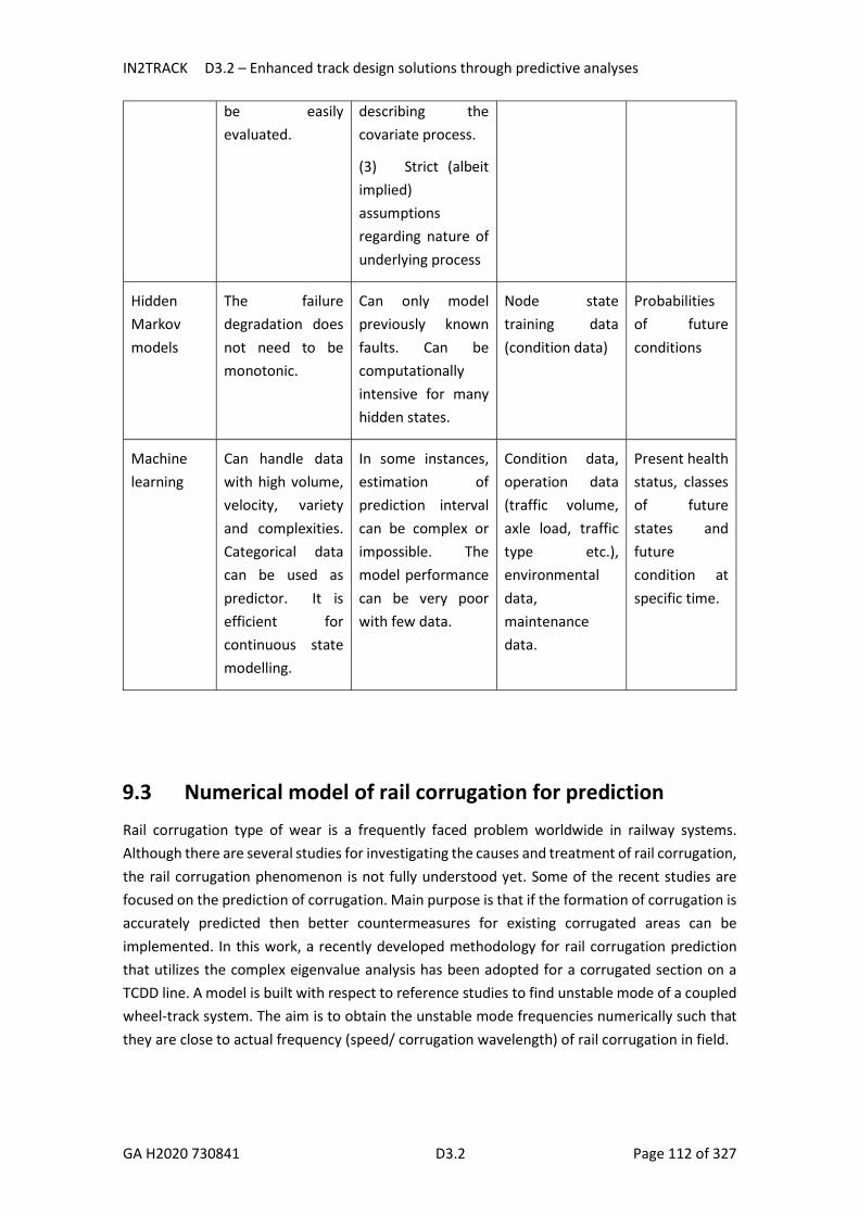
IN2TRACK D3.2 – Enhanced track design solutions through predictive analyses
GA H2020 730841 D3.2 Page 112 of 327
be easily evaluated.
describing the covariate process.
(3) Strict (albeit implied) assumptions regarding nature of underlying process
Hidden Markov models
The failure degradation does not need to be monotonic.
Can only model previously known faults. Can be computationally intensive for many hidden states.
Node state training data (condition data)
Probabilities of future conditions
Machine learning
Can handle data with high volume, velocity, variety and complexities. Categorical data can be used as predictor. It is efficient for continuous state modelling.
In some instances, estimation of prediction interval can be complex or impossible. The model performance can be very poor with few data.
Condition data, operation data (traffic volume, axle load, traffic type etc.), environmental data, maintenance data.
Present health status, classes of future states and future condition at specific time.
9.3 Numerical model of rail corrugation for prediction
Rail corrugation type of wear is a frequently faced problem worldwide in railway systems. Although there are several studies for investigating the causes and treatment of rail corrugation, the rail corrugation phenomenon is not fully understood yet. Some of the recent studies are focused on the prediction of corrugation. Main purpose is that if the formation of corrugation is accurately predicted then better countermeasures for existing corrugated areas can be implemented. In this work, a recently developed methodology for rail corrugation prediction that utilizes the complex eigenvalue analysis has been adopted for a corrugated section on a TCDD line. A model is built with respect to reference studies to find unstable mode of a coupled wheel-track system. The aim is to obtain the unstable mode frequencies numerically such that they are close to actual frequency (speed/ corrugation wavelength) of rail corrugation in field.

IN2TRACK D3.2 – Enhanced track design solutions through predictive analyses
GA H2020 730841 D3.2 Page 113 of 327
9.3.1 Introduction Background of study
Corrugation is one of the costly problems of railway companies in the world. Turkish State Railways (TCDD) has also corrugation problems both on straight and curved sections of its network. Corrugation leads to high maintenance costs for TCDD and delays in revenue operations.
Rail corrugation problems affect the track system and environment in negative ways. For the track system, it gives rise to vibrations that accelerate the degradation of components with respect to fatigue life. Also it may exacerbate RCF failures by inducing high frequency dynamic forces (Grassie (2005)). Environmental effects include the reduction in passenger comfort by corrugated rail induced vibrations in vehicle body and disturbing noise for neighbourhood areas. Rail corrugation is controlled by a costly grinding process. The prediction of corrugation may help to enhance the design and maintenance of track against corrugation formation. In addition, when a prediction approach is applied in existing corrugated section then guidelines for mitigating actions against that corrugation problem can be better obtained.
Literature search
Two opinions exist for rail corrugation formation. One theory is that initially rail running surface has irregularities and when the wheel passes on this surface then rail excitation occurs and this leads to oscillations in wheel–rail contact forces thus undulatory wear starts to grow on the rail head. Several studies investigated the prediction of rail corrugation with numerical models for different types of tracks and speed ranges (Gómez & Vadillo (2003), Johansson & Nielsen(2007), Knothe & Groß-Thebing (2008), Muller (2000), Nielsen (2003), Torstensson et al. (2014)).
Second opinion holds for the friction induced vibration as a cause of corrugation formation. Holders of this opinion is fewer in number than holders of the first opinion. According to this point of view (Brockley & Ko (1988)) creep forces become possibly saturated (Garg & Dukkipati (1984)) due to negative traction-friction behavior during acceleration-braking and that leads to fluctuation on wheel-rail forces so that frictional work increases the periodical wear formation which is the corrugation.
Studies that emerge from the friction induced vibration opinion are carried out by several researchers (Chen (2015); Chen et al. (2016), Cui et al. (2017), Cui, Chen, Zhao, et al. (2017)) . Kurzeck studied the involvement of friction-induced vibrations for light rail vehicles (Bernhard Kurzeck & Hecht (2010)). Also in another study by Kurzeck, they developed 3 degrees of freedom model for the prediction of corrugation as a result of friction induced vibrations (B. Kurzeck (2011)).
Chen and his group developed numerical prediction models that are built with the finite element method. These models are used for complex eigenvalue analysis for the purpose of determination of instable mode of wheel-rail system (Chen et al. (2014)). Unstable modes are determined by their negative damping coefficient, which is used as a parameter to measure the propensity of self-excited vibrations. The results of their studies are promising in terms of predicting rail corrugation frequencies for particular cases. In another study, they carried out

IN2TRACK D3.2 – Enhanced track design solutions through predictive analyses
GA H2020 730841 D3.2 Page 114 of 327
parametric analyses on the model in order to investigate influencing parameters for corrugation formation such as stiffness and damping of rail pad, wheel-rail friction coefficient (Chen et al. (2016)).
Aim and objective of study
In this study, a finite element model is built for adapting the concept developed by Chen et al. (2014) as a prediction method in a corrugated section on TCDD high speed line. In Chen’s study, the model is developed for low rail corrugation formation on a tight curve and the focus of this study is an actual rail corrugation problem in low rail of tight curve in the field. The model of complex eigenvalue analysis includes:
Wheelset Rails Wheel-rail friction Sleepers Rail pad and combined ballast and foundation elements
The numerical model is built with the above-mentioned components with the assumption that friction induced vibration occurs in the low rail curves. The complex eigenvalue analysis is carried out to determine an unstable mode that leads to corrugation formation.
9.3.2 Corrugated section Selection criteria for track section to be investigated are chosen with respect to logistical purposes and time limitations of TCDD. The selection criteria for the track with corrugation are as following:
1- Curved section 2- Corrugated low rail 3- High speed line (having uniform parameters as compared to conventional line)
According to these criteria, a section is chosen in high-speed line next to Ankara main station. This section faces repeated occurrence of corrugation after grinding on low rail. The location of the corrugated section in TCDD map is shown in Figure 75 and the corrugated section is shown in Figure 76. This photo is taken before the grinding process. Wavelength of rail corrugation is approximately 0.1 m and speed of train is 40 Km/h (11.11 m/s) such that the corresponding corrugation frequency is expected to be near 111 Hz.

IN2TRACK D3.2 – Enhanced track design solutions through predictive analyses
GA H2020 730841 D3.2 Page 115 of 327
Figure 75 TCDD Network Map
Figure 76 Corrugated section on TCDD high-speed line in Ankara

IN2TRACK D3.2 – Enhanced track design solutions through predictive analyses
GA H2020 730841 D3.2 Page 116 of 327
9.3.3 Finite element model of wheelset-railway superstructure system Definition and features of finite element model
Patran software for processing and Nastran software as a solver (family of MSC software) are used for finite element modeling. In order to build the model, the required inputs are collected from the vehicle and average velocity of train and track components in the selected zone. These are given below:
Inputs of vehicle type and average velocity in the selected zone are:
High speed train with six wagons (S1002 wheel profile) Average velocity is 40 km/h (acceleration-braking section) (This is for calculating the rail
corrugation frequency in field.)
Inputs of track are:
UIC 60E1 rail B70 concrete sleeper Vossloh HM type fastening system Ballast made of basalt material Curve radius 250 m
Figure 77 Finite element model of rail-wheel couple system
Values for wheelset position on the curve are acquired from a classified track measurement report of the high-speed line. Type of track measurement train is same as the passenger train on the section. These values are:
contact angle for outer wheel is 8.3 contact angle for inner wheel is 2.4
The rail length in Chen’s studies is 36 m that accounts for continuous welded rail. However, in another recent study, it has been shown that the rail length of 11.4 m is sufficient to reach to the resolution of a 36 m model while minimizing the influence of boundaries to local resonance (El Beshbichi (2017)). Therefore, the model length is set as 11.4 m in this study. View of finite element model of coupled wheel-rail-track system is shown in Figure 77 and detail view of left and right wheel-rail couple is shown in Figure 78.

IN2TRACK D3.2 – Enhanced track design solutions through predictive analyses
GA H2020 730841 D3.2 Page 117 of 327
Figure 78 Detail view of finite element presentation of wheels and rails
Geometry of solid components
The dimensions of wheelset (wheels and axle) (S1002 profile), and rail (UIC 60 E1) are obtained from real geometry data. Rail profile is shown in Figure 79, and this geometry is utilized for the finite element model.
Figure 79 UIC60 E1 rail profile (EN 13674-1 (2017))

IN2TRACK D3.2 – Enhanced track design solutions through predictive analyses
GA H2020 730841 D3.2 Page 118 of 327
Sleeper (Tie) model is B70 profile that is the sleeper type used in high-speed track as shown in Figure 80 . In FEM model, the geometry is slightly simplified as compared to real geometry. Holes in sleepers are not considered in FEM model.
Figure 80 B70 sleeper profile (Sadeghi, Kian& Khabbazi (2016))
Material properties
The material properties of modeled structural systems and elastic elements are given in Table 12 and Table 13, respectively. Rail pad and ballast/foundation parameters are taken from the related TCDD departments.
Table 12 Material parameters of wheel, rail and sleepers
Material Young’s modulus (Gpa)
Poisson’s ratio
Density (kg/𝐦𝟑)
Structural damping coefficient
Wheel-rail-axle (steel) 210 0.3 7850 0.004
Sleepers (concrete) 30 0.2 2530 0.1
Table 13 Parameters of elastic elements
Bush Element Stiffness (N/m) Viscous damping (N.s/m)
Rail pad vertical (z) 6e7 9e4
Rail pad lateral (x-y) 2.3e7 4e4
Ballast and foundation vertical (z) 2.94e7 2.9e4
Ballast and foundation lateral (x-y) 1.63e7 1.1e4
Rail pad properties are defined by spring and damper properties in x-y-z directions then they are assigned to rail pad elements on surface between rails and sleepers, see Figure 81. The same

IN2TRACK D3.2 – Enhanced track design solutions through predictive analyses
GA H2020 730841 D3.2 Page 119 of 327
procedure is carried out for the combined ballast/foundation support. The combined ballast/foundation support is defined as a group of spring-damper at the bottom surface of sleepers is also shown in Figure 81.
Element and mesh properties
Model consists of 3-d solid finite element representation of wheels, axle, rail and sleepers. 8 noded brick elements are used for wheel, rail and sleepers and 4-noded tetrahedral elements are used for axle. Elastic elements that the model includes are rail pad, combined ballast and foundation support. Normal eigenvalues analysis is carried out for the convergence studies featuring have different mesh sizes. The comparison of models is made for the first 10 natural frequencies of the coupled system. The converged numerical model consists of 612871 nodes and 389072 elements (unbiased). Size of wheel and rail elements are 10 mm, axle elements are 15 mm, sleeper elements are 30 mm.
Boundary and contact conditions
There are six deformable bodies that are created in Patran. These are outer and inner wheels, axle, outer and inner rails and sleepers.
Wheel/rail is touch contact and wheel/axle contact is glued (tied) contact. Friction coefficient is defined as 0.4 between wheel and rail. All 6 dofs (degrees of freedoms) at the bottom end of combined ballast/foundation
support elements are constrained as shown in Figure 81. Hinged-hinged boundaries are applied for rail ends Gravity in – z direction is defined for all bodies.
Figure 81 Group of spring-damper (yellow bars) and the bottom constrains under spring damper groups
9.3.4 The simulation results The frequency range for the solution is arranged in the interval of 80-130 Hz in order to search for the rail corrugation frequency near 111Hz. The Complex Lanczos extraction method which is

IN2TRACK D3.2 – Enhanced track design solutions through predictive analyses
GA H2020 730841 D3.2 Page 120 of 327
a robust method for eigenvalue extraction (MSC Sofware (2017)) is applied. The simulation yields 12 modes in 80-130 Hz range. Two mode shapes that have negative damping coefficients are shown in Figure 82 and Figure 83.
Figure 82 Mode shape at 98.53 Hz (damping coefficient= -0.0098)
Figure 83 Mode shape at 117.52 Hz (damping coefficient= -0.026)
Low wheel-rail couple in both mode shapes have higher modal deformation when compared to high wheel-rail couple. The differences of the first mode (98.53 Hz) and the second mode (117.52) with respect the analytical corrugation frequency are 11% and 6%, respectively. Considering the approximations in the numerical model and the variations in materials properties, the numerical models provide satisfactorily prediction to determine the corrugation frequency.
9.3.5 Conclusions In this study, a numerical approach developed in literature is adapted to determine the corrugation frequency in tight curve. The modeled railway system has frequent corrugation

IN2TRACK D3.2 – Enhanced track design solutions through predictive analyses
GA H2020 730841 D3.2 Page 121 of 327
problem. Only one type of high-speed train passes on the selected rail section. The materials inputs for the numerical model are acquired from the related TCDD departments. The model is simulated for complex eigenvalue analysis, and the results show that this methodology predicts the actual corrugation frequency in the field satisfactorily in our case.
Increase of model length and different meshing strategy and contact formulations for wheel-rail contact areas can be useful for refinement of model. Afterwards, parametric analysis using the model can be carried out. This analysis can help to find best solutions for mitigation of corrugation formation.
9.4 Designing steel composition and microstructure to better resist degradation during wheel/rail contact
Optimum selection of materials is a key requirement to achieve reductions in the whole life cost of the railway system through increased asset life and reduced maintenance, while realising performance improvements through increased service availability and reliability.
Current research includes the comparative laboratory-based assessment of a wide range of steels available for use in plain-line and S&C track. The laboratory assessment is centred around a large diameter twin disc rig capable of better replicating a range of contact conditions encountered on mainline railway networks. The rate of degradation (in terms of wear and RCF performance) of the different steels will be determined as a function of the operating characteristics. The influence of the wide range of steel compositions and microstructures on degradation through wear and RCF will be used to establish design rules for the development steel grades more resistant to degradation. The investigation focuses primarily on pearlitic steel grades but it is hoped to include two low carbon carbide-free bainitic steel grades to reflect the performance of such grades in Eurotunnel track. Furthermore, time permitting, the large diameter twin disk rig will also be used to assess the wear and RCF resistance of weld metal (aluminothermic and weld repair) and of changes in microstructure and properties across the heat affected zones (HAZ) of rail welds.
Using the outputs from the experimental testing and theoretical analysis; the research will assess (through cost and robustness evaluations) the potential for enhanced materials for a range of track assets. The impact of further changes to steel composition and microstructure on the degradation rates and current maintenance regimes will also be investigated.
9.4.1 Background Rail is a product that demonstrates the infinite capability of steel to adapt to meet the ever-increasing demands of wheel-rail contact since it was first introduced as is apparent from the following.
Although shaped iron rails were a tremendous improvement over the composite wooden and strapped iron tracks when they were introduced in United States in 1845, their inability to cope with heavier and faster vehicles became apparent within the

IN2TRACK D3.2 – Enhanced track design solutions through predictive analyses
GA H2020 730841 D3.2 Page 122 of 327
next couple of decades. The need for frequent replacement and the associated disruption of transportation made them economically unattractive.
The use of steel rails was a result of the improvement of the Bessemer process devised by Robert Mushet (Muschet) leading to the first commercial deployment at a heavily used part of the approach to Derby station in 1857. Iron rails at the same sites were renewed at intervals of just 3-6 months whereas the steel rails remained little affected after 6 years of service and provided an eventual life span of 16 years.
A similar success was apparent in Pennsylvania Rail Road (PRR) that rapidly accelerated its purchase of steel rails despite a price that was double that of iron rails and lead to the comment "Probably no other technological development has done so much to increase the capacity of the railroads and reduce their operating costs as this substitution of steel for iron rails,". Furthermore, the success of the move to steel rails was also apparent from the statistics of use that demonstrated a growth from 29% of the US network utilising steel rails in 1880 to 93% in 1900 while the price of steel rails fell from $140 per ton just $35 per ton between 1872 and 1882 and production grew from 90000 tons to 1.5 million tons (http://explorepahistory.com).
The success of steel as the material for railway rails is apparent from the in-service performance of the first installation at Derby and in the tracks of PRR, USA. The widespread adoption by the industry that followed the pioneering installations is shown in Figure 1 (Carroll). Thus, it is appropriate to consider the first steel rails as the development platform for the compositional and microstructural design of steel for railway rails. It is, therefore, appropriate to note that the Muschet steel rail installed at Derby station contained ≈0.25% C developing a hardness of ≈182HB and a pearlitic microstructure shown in Figure 85.
Figure 84 Transition from iron to steel rails (Carroll)

IN2TRACK D3.2 – Enhanced track design solutions through predictive analyses
GA H2020 730841 D3.2 Page 123 of 327
Figure 85 Microstructure of first steel rail installed in 1857 at Derby Station (Carroll)
9.4.2 Designing the microstructure of steel rails Steel is primarily an alloy of iron and carbon that has proven its capability to meet the challenging properties required for a diverse range of applications. Steel offers a very wide range of tensile strengths from <200 MPa for ultra-low carbon interstitial-free steels to 2800 MPa for Marageing steels and more than 5000 MPa for fine cold drawn wire (Bhadeshia et al, 2017). Such a diverse range of properties are developed through judicious additions of a range of alloying elements combined with precisely controlled manufacturing process parameters to generate the desired microstructure and resulting properties. A schematic illustration of the range of microstructures that can be generated during isothermal transformation of steel is shown in Figure 86 (Bhadeshia et al, 2017) while the influence of the rate of cooling of 0.55%C steel on the hardness developed is shown in Figure 87.
Figure 86 Developed microstructures as a function of transformation temperature

IN2TRACK D3.2 – Enhanced track design solutions through predictive analyses
GA H2020 730841 D3.2 Page 124 of 327
Figure 87 Influence of the rate of cooling on developed hardness (and microstructures) (Clarke et al, 2004)
The influence of alloying elements on the properties of steel has been the subject of extensive research with publications too numerous to list as references but attention is drawn to appropriate text books (Bhadeshia et al (2017), Clarke et al (2004) and Reed-Hill (2009)). However, the primary influence of at least the key elements within the context of pearlitic rail steels is summarised in Table 14 below.
However, although the metallurgical principles that govern the influence of the key alloying elements are relatively well understood, the design of the ideal rail steel needs to take account of:
1. Key rail degradation mechanisms 2. Performance of currently available rail steels
Table 14 Influence of key alloying elements
Alloying Element Primary Influences
Carbon Probably the most important alloying element in both plain carbon and alloy steels that expands the austenite region of the Iron-Carbon equilibrium diagram. It increases hardenability and a maximum hardness of ≈ 65 Rockwell (≈ 740 HB) can be achieved in a steel quenched to form 100% martensite. In non-quenched steels, Carbon content has a dominant influence on parameters such as volume fraction pearlite, resulting interlamellar spacing, and hardness. Requires careful control of casting process to minimise segregation.
Silicon Silicon is a ferrite stabiliser that provides solid solution strengthening, reduces susceptibility to the formation of grain boundary cementite in hypereutectoid steels.

IN2TRACK D3.2 – Enhanced track design solutions through predictive analyses
GA H2020 730841 D3.2 Page 125 of 327
Manganese Austenite stabiliser providing increased hardenability. Combines with Sulphur to form deformable manganese sulphide inclusions that can act as hydrogen sinks which may also trigger subsurface RCF.
Chromium Strong hardenability element and carbide former - it shifts the equilibrium diagram to the right and upwards and thereby lowering he critical cooling rate at which non-pearlitic microstructures can be generated. Susceptible to micro-segregation.
Molybednum Very strong hardenability agent that also shifts the equilibrium diagram to the right. Only small additions to medium and high carbon steels result in martensite in structures even at relatively slow cooling rates
Nickel Ni is an austenite stabiliser and unlike Cr, it lowers the equilibrium transformation temperature and although it also shifts the diagram to the right, the magnitude of the hardenability effect is much lower. In the context of rail steel compositions, a small addition of Ni has little effect on the key properties.
Niobium Strong carbide former with the precipitation of niobium carbides at high temperature with potential of grain refinement and improvement to ductility
Vanadium Strong carbide former with precipitation of vandium carbide occurring at much lower temperatures. When in solution in austenite, Vanadium is a potent hardenability agent leading to lower transformation temperatures and finer interlamellar spacing of resulting pearlite
Copper Probably the most important alloying element in both plain carbon and alloy steels that expands the austenite region of the Iron-Carbon equilibrium
9.4.3 Rail degradation mechanisms The key degradation mechanisms that limit the serviceable life of rail are:
Loss of rail profile o Vertical and side wear o Corrugation o Plastic deformation o Corrosion (in specific aggressive locations)
Rolling Contact Fatigue (RCF) Rail breakage risk

IN2TRACK D3.2 – Enhanced track design solutions through predictive analyses
GA H2020 730841 D3.2 Page 126 of 327
The different degradation mechanisms can be combated by different material properties and consequently a number of rail steel grades with a range of different properties are available to the industry. However, it must be emphasised that rail degradation is the result of the behaviour of the whole system and hence rail metallurgy cannot be addressed independently. Optimisation of other aspects of the systems design and operation need to be taken into consideration in parallel.
9.4.4 Loss of rail profile Rail profiles from three different track locations are shown in Figure 88 (Corus Rail Technologies) and demonstrate how the differences in rail-wheel contact result in different magnitudes of wear and rail profile shapes. The importance of increased wear resistance for longer rail life is further emphasized by the fact that rails have to be taken out of service after a loss of only 20% of their original section weight through wear while the remaining 80% has to be returned to the furnace at scrap value. Hence it is essential to increase wear resistance of rail steels to maximise the life span of this useful 20% of the section.
As shown in Figure 89 and Figure 90, degradation of rail profile is also caused by gross plastic deformation and the formation of corrugation that leads to the loss of rail profile in the longitudinal direction.
Figure 88 A range of rail profiles encountered on railways; 450m radius (a), 960m radius (b), 3000m radius (c)
Figure 89 Other causes of loss of rail profile: gross plastic deformation

IN2TRACK D3.2 – Enhanced track design solutions through predictive analyses
GA H2020 730841 D3.2 Page 127 of 327
Figure 90 Other causes of loss of rail profile: corrugation
The material property parameters relevant to increased resistance to loss of rail profile are:
Proof (yield) strength
Hardness Comparative resistance to abrasive and rolling contact wear
It is interesting to note that the property parameters of proof strength and comparative resistance to wear are not mandated in EN13674-1:2017, although standards from some other railway networks do specify proof strength as a requirement. (Hardness is specified which gives a good indication of expected wear and plastic deformation) Thus, the above parameters need to be included in the design criteria for the rail steels of the future.
9.4.5 Rolling contact fatigue (RCF) Rails are subjected to cyclic loading in service. The stress range and the magnitude of stresses being dependent on a range of variables including the rail and wheel profile, the contact patch position and size, and the dynamic track forces from the vehicle. Consequently, the phenomenon of fatigue is of critical importance to longevity of rails. Although fatigue in rails manifests itself in many ways, the two major classifications of rolling contact fatigue (RCF) are "squats" and "head checks" both of which can be associated with early propagation of surface or near surface initiated rolling contact fatigue cracks. The hive of research and development on RCF prior to and following the Hatfield derailment is a clear indication of the importance of this issue for safety and the longevity of rails.
Figure 91 RCF defects (Corus Rail Technologies): surface initiated RCF defect (2 left images), squat defect (right)

IN2TRACK D3.2 – Enhanced track design solutions through predictive analyses
GA H2020 730841 D3.2 Page 128 of 327
The stages in the life of RCF cracks are:
Crack initiation Shallow angle crack growth Turn down and growth of transverse cracks
As apparent from Figure 92, RCF cracks can also be initiated on sub-surface and hence are not detected by visual inspection but can be detected by ultrasonic inspection once they are of detectable size. Often such defects or breaks can be classified as “Tache Ovale” and attributed to presence of inclusions. Although, modern steelmaking practice has eliminated failures associated with inclusions, sub-surface fatigue cracks can still be initiated because of inappropriate contact conditions giving rise to high sub-surface shear stresses.
Figure 92 Example of a sub-surface initiated RCF crack
The resistance to RCF of rail steels does not feature in any rail steel specification. However, in view of the growing acknowledgement by most railways that RCF is a key cause for rail life curtailment, it is essential to include the following parameters within the design criteria of future rail steels:
Period or cycles to initiation of fatigue cracking Growth rate of cracks during shallow angle stage Growth rate of cracks following turn down
However, there is a need to standardise the methodology for testing to determine these parameters. If a standardised test involved comparative testing in a twin disc facility, then it would be necessary to specify test parameters such as the size of the rail and wheel discs, contact stress, applied lateral force, slippage, use of lubrication, and the duration of the test. Such a test may also offer a means of assessing wear and RCF resistance, particularly the balance required between wear and RCF and the influence of comparative hardness of the two mating components on their relative wear.
9.4.6 Rail breakage risk Historically, a key cause for rail replacement was the occurrence of rail breaks and defectives. In the early days, a primary cause of such breaks was the quality of the steel as was reflected in the breaks shown in the Figure 93. Modern steelmaking practices have significantly reduced the

IN2TRACK D3.2 – Enhanced track design solutions through predictive analyses
GA H2020 730841 D3.2 Page 129 of 327
occurrence of such defects from rails supplied since the introduction of secondary steelmaking and continuous casting. However, some railway networks still contain some very old rails that may contain such defects and the issue is one of inspection capability. Thus, design criteria for rail steels of the future need to continue with the carefully controlled processing requirements of modern rail manufacturing practice.
Figure 93 Example of rail breaks in older rails: Inclusion related fatigue defect (Tache Ovale)(a), Hydrogen related fatigue defect (Tache Ovale) (b), Segregation pipe defect (Vertical Longitudinal Split)(c).
In modern railways, rail breakage risks arise from fatigue initiated, corrosion related foot failures, external mechanical and arc damage, welds, rail joints, fatigue initiated at manual metal arc weld repair defects, or rolling contact fatigue (RCF) defects such as squats. This is well illustrated by the rail breaks data collated over the period of 2013 to 2018 and shown in Figure 94.
Figure 94 Top 15 types of broken rails between 2013 and 2018 – Network Rail
Examples of such defects are shown in Figure 93. Although the metallurgical contribution for the prevention of premature rail replacement caused by corrosion in harsh environments such as coastal track or level crossings comes from the use of barrier or galvanic coatings, it does not appear to be an important design criterion for the design of rail steels unless corrosion resistance was an unintended benefit of the composition designed to resist the other
197
35 32 24 23 19 15 15 15 15 14 14 13 10 100
50
100
150
200
250

IN2TRACK D3.2 – Enhanced track design solutions through predictive analyses
GA H2020 730841 D3.2 Page 130 of 327
degradation mechanisms. Instead, innovative solutions are required to reduce the longitudinal tensile stresses in the foot of the rail to lower the effective outer fibre tensile stresses imposed on the base of the foot of the rail. Alternatively, innovative solutions are required to prevent the formation of corrosion pits near sleeper rail pads that act as stress raisers.
Since discrete rail head defects such as wheel burns and squats occur on even the best maintained railways, availability of an automated process for repair of such defects is considered a more pragmatic solution than the development of rail steels with improved metallurgical properties to resist failures from the head although steels with an improved resistance to squat like defects still presents a significant benefit where rails require frequent replacement for rail damage
Although rail breaks caused by RCF only account for a small proportion (e.g. failure codes 211, 471 and 256 in Figure 94) of the “Top 15” types of broken rails, the important need for resistance of rail steel grades to this degradation mechanism is apparent from Figure 95 and Figure 96. Hence any designing of rail steel composition needs to address the need for increased resistance to RCF in all its manifestations such as: head checks, gauge corner cracking, and squats.
Figure 95 Top 30 plain line defects for the year 2017 – 2018 = 15115, – Network Rail [9]

IN2TRACK D3.2 – Enhanced track design solutions through predictive analyses
GA H2020 730841 D3.2 Page 131 of 327
Figure 96 Top 30 defects for the year 2017 – 2018 (36645 defects), large numbers due to the inclusion of all 053 switch profile defects and 054 crossing defects – Network Rail (Whitney)
As apparent from the data on rail breaks and rail defects, rail breaks can also occur at flash butt or aluminothermic welds and at fish-plated joints. The material properties that are considered relevant are:
Fracture toughness Fatigue strength/limit Fatigue crack growth rate Residual stress in various parts of the rails
Data for the above properties for the range of steels included in EN13674-1:2017 is presented in Table 15 and are discussed briefly in the following sections.
Table 15 Key specified properties of steel grades in EN 13674-1: A1 2017
Steel Grade
Fracture Toughness [MPam1/2]
Max. Fatigue crack growth rate, [m/Gc]
Fatigue strength
Residual stress [MPa]
Hardness [HBW]
Tensile Strength [MPa]
Elongation [%]
Min. single value
Min. mean value
Delta K= 10, [MPam1/
2]
Delta K= 13, [Mpam1/
2]
R200 30 35 Not specified
5X10⁶ <250 200-240 680 14

IN2TRACK D3.2 – Enhanced track design solutions through predictive analyses
GA H2020 730841 D3.2 Page 132 of 327
R220 30 35 17 55 Cycles for total strain amplitude of 0.00135
<250 220-260 770 12
R260 26 29 17 55 <250 260-300 880 10
R260Mn 26 29 17 55 <250 260-300 880 10
R320Cr 24 26 Not specified
<250 320-360 1080 9
R350HT 30 32 17 55 <250 350-390 1175 9
R350LHT 26 29 17 55 <250 350-390 1175 9
R370CrHT 26 29 17 55 <250 370-410 1280 9
R400HT 26 29 17 55 <250 400-440 1280 9
9.4.7 Fracture toughness Fracture toughness (KIc) is often regarded as one of the most important properties of any material for many design applications as it is a property that describes the ability of a material containing a crack to resist fracture. In effect, it is a quantitative assessment of a material's resistance to brittle fracture when a crack is present. Thus, a material possessing high fracture toughness will depict ductile fracture, while brittle fracture is very characteristic of materials with low fracture toughness.
However, as is apparent from Table 15, the mean value of fracture toughness for different rail steels ranges between 26 and 35 MPam1/2 which is neither a wide range nor values that depict highly ductile materials. The expected influence of hardness on the value of fracture toughness is shown in Figure 97 together with the measured values for Grade HP335. It is interesting to note that the specification permits a reduction in the value of fracture toughness with increasing hardness in the as -rolled grades but maintains the values of the heat treated grade at the same level as grade R260 with the exception of grade R350HT which is expected to possess slightly higher level of fracture toughness. However, as shown in Table 16 below, actual measured data indicates that the fracture toughness of heat treated steels is greater than that for grade R260 with the highest value for off-line heat treated 370CrHT grade.

IN2TRACK D3.2 – Enhanced track design solutions through predictive analyses
GA H2020 730841 D3.2 Page 133 of 327
Figure 97 Relationship between mean hardness and fracture toughness (EN13674)
Table 16 Measured fracture toughness of various rail grades (EN13674)
Parameter Fracture Toughness [MPam1/2] – Measured Data
R220 R260 R350HT R350LHT R370CrHT (off-line)
HP335
Mean 41.6 33,7 37.2 33.5 41.3 31 Std. Dev. 6.85 3.94 3.76 1.57 Not available
It is, however, necessary to put the measured levels of fracture toughness into the context of their impact on the safety and integrity of rails in track. This is best assessed with reference to failures emanating from defects in the foot of the rail that experience the highest outer fibre tensile stresses. As is apparent from Figure 98, an improvement in fracture toughness increases the defect size necessary to cause fracture. However, the shape of the relationship also emphasizes the much stronger influence of a reduction in the total stress (applied + laying + residual stress) being experienced by the rail. Therefore, a reduction in the longitudinal residual stress in the foot of the rail is even more desirable.
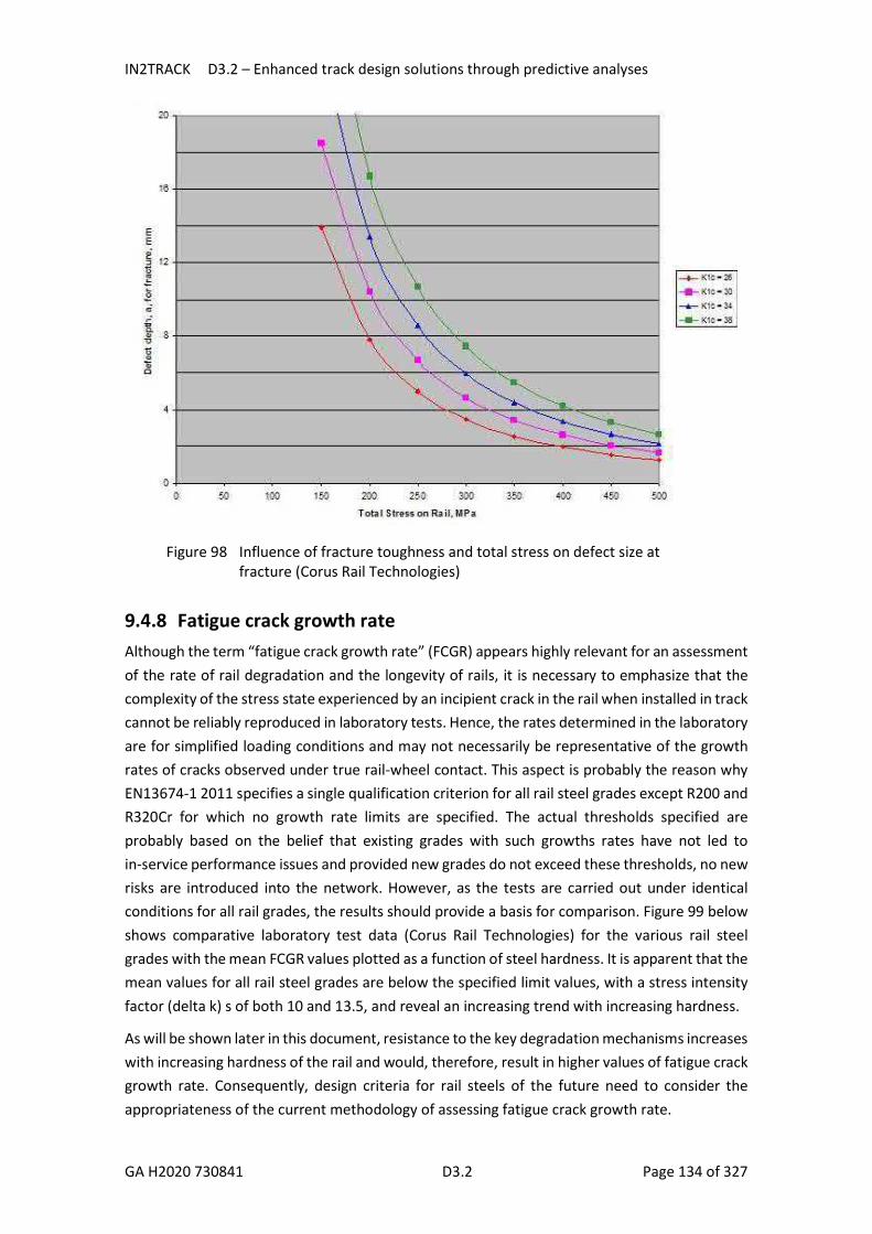
IN2TRACK D3.2 – Enhanced track design solutions through predictive analyses
GA H2020 730841 D3.2 Page 134 of 327
Figure 98 Influence of fracture toughness and total stress on defect size at fracture (Corus Rail Technologies)
9.4.8 Fatigue crack growth rate Although the term “fatigue crack growth rate” (FCGR) appears highly relevant for an assessment of the rate of rail degradation and the longevity of rails, it is necessary to emphasize that the complexity of the stress state experienced by an incipient crack in the rail when installed in track cannot be reliably reproduced in laboratory tests. Hence, the rates determined in the laboratory are for simplified loading conditions and may not necessarily be representative of the growth rates of cracks observed under true rail-wheel contact. This aspect is probably the reason why EN13674-1 2011 specifies a single qualification criterion for all rail steel grades except R200 and R320Cr for which no growth rate limits are specified. The actual thresholds specified are probably based on the belief that existing grades with such growths rates have not led to in-service performance issues and provided new grades do not exceed these thresholds, no new risks are introduced into the network. However, as the tests are carried out under identical conditions for all rail grades, the results should provide a basis for comparison. Figure 99 below shows comparative laboratory test data (Corus Rail Technologies) for the various rail steel grades with the mean FCGR values plotted as a function of steel hardness. It is apparent that the mean values for all rail steel grades are below the specified limit values, with a stress intensity factor (delta k) s of both 10 and 13.5, and reveal an increasing trend with increasing hardness.
As will be shown later in this document, resistance to the key degradation mechanisms increases with increasing hardness of the rail and would, therefore, result in higher values of fatigue crack growth rate. Consequently, design criteria for rail steels of the future need to consider the appropriateness of the current methodology of assessing fatigue crack growth rate.

IN2TRACK D3.2 – Enhanced track design solutions through predictive analyses
GA H2020 730841 D3.2 Page 135 of 327
Figure 99 Fatigue crack growth rate of rail steels in EN13674-1: 2017
9.4.9 Fatigue strength EN13674-1 2017 requires constant amplitude fatigue tests to be undertaken in accordance with ISO 1099. The qualification criteria of each of the three specimens is to achieve a life of >5 × 10⁶ cycles for a total strain amplitude of 0,00135. In such tests, life is defined as the number of cycles up to the complete separation of the specimen. Since this is a pass/fail criterion, it does not permit quantitative comparison of the fatigue strength of the various steels. However, additional data has been obtained that has been generated using the staircase technique of establishing fatigue strength/limit. The results are shown in Figure 100 as a function of rail steel hardness.
Figure 100 Fatigue strength/limit of rail steels defined in EN1674-1:2017
y = 0,0211x + 4,4856R² = 0,7175
y = 0,0931x + 3,2108R² = 0,7802
0
10
20
30
40
50
60
200 220 240 260 280 300 320 340 360
da/
dN
, m/G
cycl
e
Hardness, BHN
Mean FCGR of a Range of Rail Steels
Pearlitic Steels Delta k=10 HPrail Delta k=10 Pearlitic Steels Delta k=13.5
HPrail Delta k=13.5 Specified Limit Delta k=10 Specified Limit Delta k=13.5
y = 1,7003x - 96,581R² = 0,9839
200
250
300
350
400
450
500
550
200 220 240 260 280 300 320 340 360 380
Fa
tig
ue
Str
en
gth
, MP
a
Hardnes, HB
Fatigue Strength as a Function of Hardness
Pearlitic Steels HP335 Minimum Specified Fatigue Strength

IN2TRACK D3.2 – Enhanced track design solutions through predictive analyses
GA H2020 730841 D3.2 Page 136 of 327
Although the loading conditions in the laboratory fatigue tests are not representative of true rail-wheel contact, it is useful to establish the trend of increasing fatigue strength/limit with harder rail steels which are also considered to be more wear resistant.
9.4.10 Residual stresses in rail EN13674-1:2017 requires the determination of the longitudinal stresses in the centreline of the foot of the rail and this property parameter is directly relevant to the susceptibility of the rail to fatigue failure. Although the yield strength of the rail steel is a factor in the development of residual stresses in the foot of the rail, it is largely the effective control of the roller straightening operation that is responsible for the magnitude of residual stresses developed in the full cross section of the rail. In general, residual stresses in rail follow a “C-curve pattern with longitudinal tensile stresses in the head and the foot. Consequently, high longitudinal residual stresses in the head and foot of the rail could affect the nature of crack propagation. However, this attribute is not considered a design criteria for rail steels as it can be influenced by a whole host of manufacturing conditions such as the shape of rails on the cooling banks, the pitch of roller straightener rolls and the magnitude of applied straightening loads.
9.4.11 Characterisation of available rail steels Properties of steels are a reflection of the chemical composition and the rate of cooling through metallurgical transformation. In the context of steels for rail applications, pearlite has been the dominant microstructure and is the focus of current investigations. However, it is appropriate to consider other steel microstructures that have been assessed for rail application.
Low carbon Carbide-free bainitic steels: Although very significant volumes of research has been undertaken into steels with such microstructures (Bhadeshia (1992, 2005), Sawley el (1997), Kristan et al (2003), Kageyama et al (1994), Tata Steel and Clayton et al (1993)), commercial deployment has been restricted to two grades B320 and B360 from British Steel. Grade B320 is a low carbon carbide-free bainitic steel from British Steel France. It is a highly alloyed composition with additions of Si, Mn, Cr, V, and Mo to yield a carbide free microstructure comprising bainite and austenite upon natural cooling following hot rolling. Although wear resistance of the grade is similar to R260, it offers excellent resistance to RCF and has given a long grinding-free life in a 4000 m radius curve in the Eurotunnel, carrying > 100 MGT per year. The grade is known to be weldable using flash butt and aluminothermic processes and the low carbon content should also facilitate development of weld repair techniques. However, there is a need to establish the relevant cost benefit analysis for its deployment in mainline railway networks.
Grade B360 is a slightly higher carbon version (0.25/0.35%) of the B320 grade, also developing a carbide free microstructure comprising bainite and austenite upon natural cooling following hot rolling. The slightly higher hardness provides increased resistance to wear compared to Grade B320, while maintaining the high resistance to RCF. This grade has been approved by SNCF for use in high speed S&C. The higher resistance to RCF has been demonstrated in several trial sites in France, Germany, and Switzerland. However, critical and subcritical HAZ regions of both flash butt and aluminothermic welds made in this grade are susceptible to cracking. This shortcoming has severely restricted the realisation of the benefits of the RCF resistance offered by this steel grade

IN2TRACK D3.2 – Enhanced track design solutions through predictive analyses
GA H2020 730841 D3.2 Page 137 of 327
but modified welding procedures have been developed by rail manufacturers. However, a validated cost-benefit analysis of the deployment of this grade in mainline railway networks is considered desirable and recommended.
Carbide containing bainitic steels: Two steel grades (DOBAIN 380 and DOBAIN 430) were introduced by Voestalpine (Girsch et al (2005 & 2006)). These grades are high carbon (0.80%) steels alloyed with Cr, Ni, Mo, and V and heat treated to develop a conventional lower bainitic structure. This grade is no longer being promoted as track trials on the German network were not as favourable as that of R400HT grade.
Martensitic microstructures: Although the presence of martensite within pearlitic microstructures is considered detrimental to performance, the desire to achieve a very significant increase in the values of fracture toughness led to the development of a low carbon high toughness martensitic rail (Jerath, et al, 1997). This is a low carbon-manganese steel microalloyed with Chromium and Molybdenum that is rapidly cooled using water sprays to a defined core temperature in the rail head to permit controlled tempering to generate high toughness and impact resistance with values of fracture toughness of 100 and 110 MpA/m1/2 compared to typical values for pearlitic rails of 35-40 MPA/m1/2. However, the development did not lead to track trials and hence its in-service performance against wear and RCF has not been established.
9.4.12 Pearlitic rail steels Virtually all rail steels in use since the first installation in 1857 at Derby station belong to the broad family of pearlitic steels but the very diverse range of properties that can be achieved through judicious alloying and cooling through metallurgical transformation is apparent from the very comprehensive range of pearlitic steels on offer from the various leading rail manufacturers. Composition and key property details of the nine steel grades included in EN13674-1:2017 are shown in Table 17 while those compliant with other specifications and offered by leading rail manufacturers are shown in Table 18.
Table 17 Steel grades defined in EN 13674-1: +A1 2017

IN2TRACK D3.2 – Enhanced track design solutions through predictive analyses
GA H2020 730841 D3.2 Page 138 of 327
Table 18 Heat treated steel grades compliant with specifications other than EN13674-1:2017 offered by leading manufacturers
Establishing the design rules for the optimum rail steel with the maximum resistance to the known degradation mechanisms would be greatly facilitated by an understanding of the influence of the key compositional elements in excess of the mid-point for the benchmark grade R260. Furthermore, since the properties of rail steels are a result of the combination of composition and heat treatment, it is necessary to take account of the influence of heat treatment. However, as there are a variety of rail heat treatment systems with bespoke process parameters developed by the manufacturers, it is not possible to make direct comparison between the properties developed from different heat treatment systems. Instead, it will be necessary to establish the dependence of key performance properties on the microstructural parameters such as interlamellar spacing, volume fraction cementite, and lattice strain of the ferrite phase (Marder et all (1976) and Nakada et al (2015)).
9.4.13 In-service performance of rail steels The available rail steels, their specified properties, and the expected in-service rail degradation mechanisms have been detailed in the previous sections. However, the selection of rail steel to maximise rail life in any given stretch of any network requires knowledge of the rate of

IN2TRACK D3.2 – Enhanced track design solutions through predictive analyses
GA H2020 730841 D3.2 Page 139 of 327
degradation as a function of vehicle and track characteristics and the properties of the rail steel grade.
The influence of track characteristics on the rate of wear and RCF growth was examined as part of the Innotrack project (Innotrack, 2009) using degradation monitoring data from a variety of track sites and the key results are shown in Figure 101 to Figure 104.
Figure 101 45 W̊ear of grade 220 rails

IN2TRACK D3.2 – Enhanced track design solutions through predictive analyses
GA H2020 730841 D3.2 Page 140 of 327
Figure 102 Vertical wear of grade 220 rails
Figure 103 Maximum surface crack length growth rate since installation for all rail grades

IN2TRACK D3.2 – Enhanced track design solutions through predictive analyses
GA H2020 730841 D3.2 Page 141 of 327
Figure 104 Period to Initiation of RCF cracks for Grade R220 Rails
The multiplicity of steel grades and track and traffic characteristics make it impractical to undertake controlled assessments to quantify the magnitude of resistance to degradation (wear, RCF, and plastic deformation) of the full range of rail steels grades. This is reflected in the observed spread in the data in the above graphs.
Guidelines on the selection of rail steel grades is also available from UIC and is shown in Figure 106. It is apparent that the guideline is very generic, it recommends the use of harder grades at locations prone to high rates of wear without recognising the availability of several grades covering a hardness range of 350 HB to 440HB.

IN2TRACK D3.2 – Enhanced track design solutions through predictive analyses
GA H2020 730841 D3.2 Page 142 of 327
Figure 105 Recommendation for the use of standard and hard heat treated grades (Innotrack, 2010)
Figure 106 Track radii based rail grade selection (Innotrack, 2010)
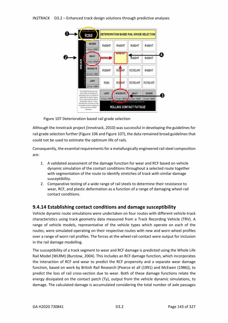
IN2TRACK D3.2 – Enhanced track design solutions through predictive analyses
GA H2020 730841 D3.2 Page 143 of 327
Figure 107 Deterioration based rail grade selection
Although the Innotrack project (Innotrack, 2010) was successful in developing the guidelines for rail grade selection further (Figure 106 and Figure 107), the data remained broad guidelines that could not be used to estimate the optimum life of rails.
Consequently, the essential requirements for a metallurgically engineered rail steel composition are:
1. A validated assessment of the damage function for wear and RCF based on vehicle dynamic simulation of the contact conditions throughout a selected route together with segmentation of the route to identify stretches of track with similar damage susceptibility.
2. Comparative testing of a wide range of rail steels to determine their resistance to wear, RCF, and plastic deformation as a function of a range of damaging wheel-rail contact conditions.
9.4.14 Establishing contact conditions and damage susceptibility Vehicle dynamic route simulations were undertaken on four routes with different vehicle-track characteristics using track geometry data measured from a Track Recording Vehicle (TRV). A range of vehicle models, representative of the vehicle types which operate on each of the routes, were simulated operating on their respective routes with new and worn wheel profiles over a range of worn rail profiles. The forces at the wheel-rail contact were output for inclusion in the rail damage modelling.
The susceptibility of a track segment to wear and RCF damage is predicted using the Whole Life Rail Model (WLRM) (Burstow, 2004). This includes an RCF damage function, which incorporates the interaction of RCF and wear to predict the RCF propensity and a separate wear damage function, based on work by British Rail Research (Pearce et all (1991) and McEwen (1986)), to predict the loss of rail cross-section due to wear. Both of these damage functions relate the energy dissipated on the contact patch (Tγ), output from the vehicle dynamic simulations, to damage. The calculated damage is accumulated considering the total number of axle passages

IN2TRACK D3.2 – Enhanced track design solutions through predictive analyses
GA H2020 730841 D3.2 Page 144 of 327
over a given section of rail for each vehicle type. It also considers the location of the wheel-rail contact patch on the rail and the influence of wear reducing the propensity of RCF cracking.
The mean susceptibility to RCF and wear damage for each track segment was calculated from the accumulated route damage based on the location of each of the track segment. This is plotted against curve radius in Figure 108 below. Similar trends in both the susceptibility to RCF and wear can be seen on all routes, with an increase in RCF damage as curve radius reduces until a curve radius of approximately 800 m, when RCF damage can be seen to decrease as wear increases. Variations in the predicted damage for each curve radius is associated with differences in cant deficiency on each curve.
(a) (b)
Figure 108 Rail damage susceptibility for selected routes – (a) rolling contact fatigue and (b) wear
To illustrate the shape of the damage susceptibility map a generic passenger vehicle model (with two primary yaw stiffnesses (PYS) of 15 and 40 MNm/rad) was simulated on a range of curve radii with two values of cant deficiency. The resulting damage is overlaid on the route damage maps in Figure 109. As expected the poorer curving performance of the higher PYS vehicle and lower cant deficiency results in higher predicted damage. But the shape of the damage map is similar to that generated from the route simulations and illustrates that certain sections of track are more susceptible to degradation and thereby the requirements for optimal rail steel grade selection based on track characteristics and damage susceptibility.

IN2TRACK D3.2 – Enhanced track design solutions through predictive analyses
GA H2020 730841 D3.2 Page 145 of 327
(a) (b)
Figure 109 Rail damage susceptibility for generic vehicle model – (a) rolling contact fatigue and (b) wear
Using the rail damage susceptibility maps presented above it is possible to identify regions of these maps which result in high rates of degradation for the selected routes. These have been divided into regions of high, moderate and low susceptibility to RCF and wear damage as highlighted in Figure 110. The dominant observed degradation mechanisms for each curve radius band are summarised in Table 9.6.6.
(a) (b)
Figure 110 Track sections susceptible to high, moderate and low rail damage – (a) rolling contact fatigue and (b) wear
Hig
h
Mod
era
te
Low
Low
Hig
h
Lo
w
Mod
era
te

IN2TRACK D3.2 – Enhanced track design solutions through predictive analyses
GA H2020 730841 D3.2 Page 146 of 327
Based on the damage susceptibility criteria defined in Table 19 the total number of track segments and track miles in each band for each route was determined. These are presented in
Table 20, along with the assumed values for the entire GB rail network. With the exception of the low damage susceptibility band, mainly associated with tangent track which make up a large proportion of these routes, it can be seen that the high RCF – moderate wear band results in the largest number of track segments and miles.
Table 19 Damage susceptibility criteria
Curve Radius Range (m)
Damage Susceptibility Dominant Degradation Mechanisms
RCF Wear
< 600 Low High High rail – side wear
Low rail – plastic deformation and corrugation
600 – 1500 High Moderate High rail – RCF and side wear
1500 – 2500 Moderate Low High rail – RCF
> 2500 Low Low Vertical wear, squats and corrugation
Table 20 Total number of track segments and miles for each damage susceptibility range
Damage Susceptibility
Route Curve Radius (m)
< 600 600 - 1500 1500 - 2500 > 2500
RCF Low High Moderate Low
Wear High Moderate Low Low
TPE No. segments 3.0 38.0 15.0 74.0
Track miles 0.5 11.7 3.2 25.0
Wessex No. segments 5.0 32.0 18.0 87.0
Track miles 1.1 8.9 6.3 39.9
MML No. segments 0.0 20.0 43.0 111.0
Track miles 0.0 7.5 19.4 69.3
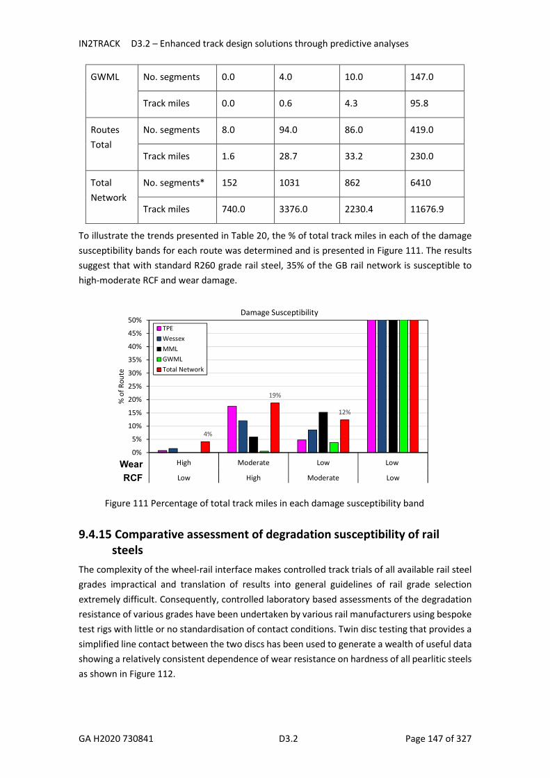
IN2TRACK D3.2 – Enhanced track design solutions through predictive analyses
GA H2020 730841 D3.2 Page 147 of 327
GWML No. segments 0.0 4.0 10.0 147.0
Track miles 0.0 0.6 4.3 95.8
Routes Total
No. segments 8.0 94.0 86.0 419.0
Track miles 1.6 28.7 33.2 230.0
Total Network
No. segments* 152 1031 862 6410
Track miles 740.0 3376.0 2230.4 11676.9
To illustrate the trends presented in Table 20, the % of total track miles in each of the damage susceptibility bands for each route was determined and is presented in Figure 111. The results suggest that with standard R260 grade rail steel, 35% of the GB rail network is susceptible to high-moderate RCF and wear damage.
Figure 111 Percentage of total track miles in each damage susceptibility band
9.4.15 Comparative assessment of degradation susceptibility of rail steels
The complexity of the wheel-rail interface makes controlled track trials of all available rail steel grades impractical and translation of results into general guidelines of rail grade selection extremely difficult. Consequently, controlled laboratory based assessments of the degradation resistance of various grades have been undertaken by various rail manufacturers using bespoke test rigs with little or no standardisation of contact conditions. Twin disc testing that provides a simplified line contact between the two discs has been used to generate a wealth of useful data showing a relatively consistent dependence of wear resistance on hardness of all pearlitic steels as shown in Figure 112.
4%
19%
12%
0%
5%
10%
15%
20%
25%
30%
35%
40%
45%
50%
High Moderate Low Low
Low High Moderate Low
% o
f Rou
te
Damage Susceptibility
TPEWessexMMLGWMLTotal Network
Wear
RCF

IN2TRACK D3.2 – Enhanced track design solutions through predictive analyses
GA H2020 730841 D3.2 Page 148 of 327
Figure 112 Wear and RCF resistance of rail steels as determined under simplified contact
The above relationship between hardness and wear rate clearly demonstrates a dependence on the contact pressure as well as rail hardness. Hence, the need for a multi-dimensional relationship between wear rate, rail hardness, and some measure of contact conditions such as a damage function is apparent. This aspect is addressed in the testing being undertaken as detailed in Figure 113, which illustrates the test loading conditions selected to represent the different damage susceptibility regions. An expected dependence of wear rate as a function of track radii/damage susceptibility parameter and steel grade hardness is shown in Figure 114. It may also be necessary to examine this dependence on other material properties such as yield strength and key microstructural parameters. The analysis of data generated from these tests being undertaken during In2Track2 will examine such dependencies.
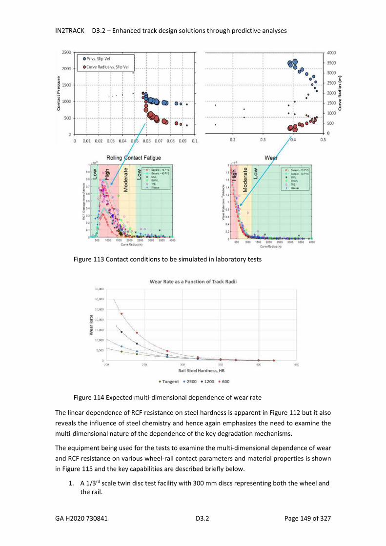
IN2TRACK D3.2 – Enhanced track design solutions through predictive analyses
GA H2020 730841 D3.2 Page 149 of 327
Figure 113 Contact conditions to be simulated in laboratory tests
Figure 114 Expected multi-dimensional dependence of wear rate
The linear dependence of RCF resistance on steel hardness is apparent in Figure 112 but it also reveals the influence of steel chemistry and hence again emphasizes the need to examine the multi-dimensional nature of the dependence of the key degradation mechanisms.
The equipment being used for the tests to examine the multi-dimensional dependence of wear and RCF resistance on various wheel-rail contact parameters and material properties is shown in Figure 115 and the key capabilities are described briefly below.
1. A 1/3rd scale twin disc test facility with 300 mm discs representing both the wheel and the rail.

IN2TRACK D3.2 – Enhanced track design solutions through predictive analyses
GA H2020 730841 D3.2 Page 150 of 327
2. Controllable slippage and angle of attack between the discs. 3. Whole or segmented discs may be used for concurrent testing of multiple samples (up
to 3 samples per 120 ̊segments in a disc). 4. Segmented disc samples cane be machined from a full rail section.
Figure 115 Twin disk testing facility and sample arrangement at IRR (Huddersfield)
The tests being undertaken are summarised in
Table 21 and
Table 22 while the information to be extracted from specific comparative tests is shown in
Table 23 which gives the reasoning for inclusion of the grade within the test matrix. It should be noted that two low carbon bainitic steel grades have been included in the test program.
Table 21 Matrix of tests to determine resistance to wear
Test No. Test Type Loading conditions Segment 1 Segment 2 Segment 3
1 Wear Tangent track R200 R260 R260Mn
2 Wear Tangent track B320 B360 ML330
3 Wear Tangent track R350HT R350LHT HP335
4 Wear Tangent track R370CrHT R400HT HP335HT
5 Wear 2500m radii R200 R260 R260Mn
6 Wear 2500m radii B320 B360 ML330
7 Wear 2500m radii R350HT R350LHT HP335

IN2TRACK D3.2 – Enhanced track design solutions through predictive analyses
GA H2020 730841 D3.2 Page 151 of 327
8 Wear 2500m radii R370CrHT R400HT HP335HT
9 Wear 1200m radii R200 R260 R260Mn
10 Wear 1200m radii B320 B360 ML330
11 Wear 1200m radii R350HT R350LHT HP335
12 Wear 1200m radii R370CrHT R400HT HP335HT
13 Wear 600m radii R200 R260 R260Mn
14 Wear 600m radii B320 B360 ML330
15 Wear 600m radii R350HT R350LHT HP335
16 Wear 600m radii R370CrHT R400HT HP335HT
Table 22 Matrix of tests to determine resistance to rolling contact fatigue
Test No. Test Type Loading conditions
Segment 1 Segment 2 Segment 3
17 RCF 2500m radii R200 R260 R260Mn
18 RCF 2500m radii B320 B360 ML330
19 RCF 2500m radii R350HT R350LHT HP335
20 RCF 2500m radii R370CrHT R400HT HP335HT
21 RCF 1200m radii R200 R260 R260Mn
22 RCF 1200m radii B320 B360 ML330
23 RCF 1200m radii R350HT R350LHT HP335
24 RCF 1200m radii R370CrHT R400HT HP335HT
25 RCF 600m radii R200 R260 R260Mn
26 RCF 600m radii B320 B360 ML330
27 RCF 600m radii R350HT R350LHT HP335
28 RCF 600m radii R370CrHT R400HT HP335HT

IN2TRACK D3.2 – Enhanced track design solutions through predictive analyses
GA H2020 730841 D3.2 Page 152 of 327
Table 23 Reasoning for inclusion of the grade in test matrix
Grade Reasoning for Inclusion in Test Matrix
R200 Does the lower resistance to wear of this grade enhance its resistance to RCF
R260 Benchmark grade against which the performance of other grades will be adjudged
R260Mn Manganese is a key alloying element in rail steels and the comparative tests being undertaken will enable the influence of Manganese to be established
R320Cr This grade is no longer in use in major European networks - so excluded from study
R350HT Benchmark heat treated grade and will permit the assessment of the effect of finer interlamellar spacing
R350LHT Slightly higher Chromium content in this grade is added to increase hardenability and refine interlamellar spacing. Consequently, comparative testing will permit the assessment of the effect of finer interlamellar spacing and the effect of addition of Chromium
R370CrHT A further data point to establish the influence of Chromium additions on interlamellar spacing and resistance to wear and RCF
R400HT Will permit assessment of the effect of hypereutectoid carbon content on hardness, interlamellar spacing, volume fraction cementite, and the key rail degradation mechanisms
HP335 Will permit comparison with performance in Network Rail track and to assess the influence of addition of extra Silicon and Vanadium on the key degradation mechanisms.
HP335HT Will help to establish whether wear and RCF resistance of HP335 could be further improved with accelerated cooling. However, it should be emphasized that heat treated HP335 is currently not commercially available
B320 B320 & B360 are only low carbon carbide free bainitic steels available and have shown very high resistance to RCF.
B360
ML330 This is a grooved rail steel grade but its inclusion is justified because it is a hypoeutectic (lower carbon) version of HP335 and comparative testing of the two grades will permit the effect of carbon to be isolated
9.4.16 Conclusions The key conclusions from the current study are:

IN2TRACK D3.2 – Enhanced track design solutions through predictive analyses
GA H2020 730841 D3.2 Page 153 of 327
EN 13674-1:2017 lists a total of 9 steel grades covering a wide range of hardness levels and tensile properties but their link to known mechanisms of rail degradation is somewhat limited to increasing hardness being desirable for achieving greater resistance to both wear and RCF.
There is little differentiation between the 9 steel grades in terms of the specified metallurgical properties of fracture toughness, fatigue crack growth rate, and fatigue strength. Furthermore, how these properties affect the in-service performance and life span of rails is also not apparent.
Although very significant progress has been made in the understanding of wheel-rail contact conditions, any meaningful prediction of the rate of degradation and residual life of rail requires the determination of the link between material properties and the rate of degradation.
Comparative track trials of selected rail grades have been undertaken in most railway networks but collation of such data within the Innotrack project did not yield any meaningful relationship that could be used to predict rail life.
The two key material properties that are closely linked to the in-service performance of rails are resistance to wear and rolling contact fatigue but a direct measure of these properties is not mandated within EN13674-1:2017. However, railway research academics, rail manufacturers, and some infrastructure managers have developed laboratory tests to assess the resistance of the various steel grades to wear and RCF. However, the simulated wheel-rail contact conditions within such tests is deemed to be relatively simplistic compared to those seen in-service. There is a need to examine the multi-dimensional nature of the dependence of the key degradation mechanisms including key metallurgical attributes of the steel.
A larger diameter (300mm and 1/3rd scale) twin disc test unit has been developed that is capable of simulating the wheel-rail contact conditions representing the various parts of any railway network. Testing of the various steel grades over a range of contact conditions will enable the assessment of the role of composition and microstructure on the key rail degradation mechanisms.
The novel arrangement of test samples also permits the testing of welds made between two rails of the same grade or different grades. The expected differential wear across the weld can be studied to optimise the microstructure and properties of the HAZ and weld metal.
9.5 Mechanisms of the head checks resistance of bainitic rails
9.5.1 Introduction For the last 10 years, British Steel has tested “new” bainitic steel grade in curves highly solicited (curves in Eurotunnel). Compared to conventional pearlitic grade, Bainitic rails exhibit rarely head check defect in curves. The aim of this work is to understand how bainitic rail grades are damaged in order to improve rail metallurgy and thus to extend the life of the rail. The first part of this study is dedicated to the explanation of the railway environment in order to define the loading and principal macroscopic defects. A particular attention is paid to a specific defect named “head check”. Metallurgical elements on steel are reminded and especially about bainitic steels which already presented promising results against head checks. The second part presents the first steps of the characterization of bainitic rails after 10 years work in Eurotunnel. Sampling

IN2TRACK D3.2 – Enhanced track design solutions through predictive analyses
GA H2020 730841 D3.2 Page 154 of 327
strategy, analysis tools and investigation methods are exposed. Then, microstructure of unworn zones of bainitic rails is studied through metallographic observations. Light microscope, scanning and transmission electron microscopes are used and hardness tests, XRD, and EBSD analysis are performed. Finally, the material under the wheel-rail contact is studied and compared to the unworn material to determine clues of the bainitic damaging mechanisms.
9.5.2 Literature review The first part of the literature review focuses on the works on rail loading and on its effect in terms of damage. The second part presents the main used grades: pearlitic and bainitic, their main properties and microstructures. Finally, the third and the forth parts speak about the defects observed on the rails, namely the head checks, on both pearlitic and bainitic grades.
Railway environnement
The railway system is made of a moving element guided by fixed rails. Rails are the top component of the platform. They are fixed on sleepers or attached to the concrete of a bridge or a tunnel and maintained at a defined gauge.Figure 116 shows the structure of railway tracks on bridge or tunnel and on ballast.

IN2TRACK D3.2 – Enhanced track design solutions through predictive analyses
GA H2020 730841 D3.2 Page 155 of 327
Figure 116 Typical track structure. Bridge/tunnel track and ballast track (http://superitn.eu).
We focus in this study on rails. Let us set a coordinate systems (x1,y1,z1) and (x2,y2,z2), see Figure 117, to clarify further images and observations. The horizontal load transmitted from wheel to rail will be positive, the vertical load will be negative and the traffic direction will be positive as presented in Figure 117. A rail is constituted of a base, a web and a head on the top of which there is the running band. It is at the latter location that the wheel-rail contact occurs.
Figure 117 Coordinate system of railway and detailed parts of a rail
The rail-wheel contact can be represented as a zone which is theorically made of 2 parts (see Figure 118). The first part, in the front of the contact zone following the direction of the wheel,

IN2TRACK D3.2 – Enhanced track design solutions through predictive analyses
GA H2020 730841 D3.2 Page 156 of 327
consists in a sticking zone between rail and wheel. The second part, at the tail of the contact, consists in a slipping zone. The slip can be more or less important depending on multiple parameters like load, lubrication, roughness … Actually, Nicollini (2001) showed that the real adhesion exists in multiple microsized zones and that the slip and sticking phenomena occur in parrallel bands along the sliding direction.
Figure 118 Rail-wheel contact characteristics (Simon, 2014).
Different theories are used to simulate the rail-wheel contact e.g. Hertz, Carter and Kalker. The most commonly used algorithm is FASTSIM and the most used software to simulate the rail-wheel contact are VAMPIRE, SIMPACK, VOCO, GENSYS, NEWCAR, MEDYNA, ADAMS, DYMOCAL.
The wheel-rail contact leads to rail damage through two main phenomena: wear and rolling contact fatigue (RCF).
Wear
As a general definition, wear is a loss of material from a surface by means of some mechanical action. Wear mechanisms can be classified in four types : abrasive, adhesive, corrosive and fatigue (Burwell, 1957). In rail damage studies, wear is mainly defined as an abrasive (sometimes combined with adhesive) mechanism. Fatigue mechanism is usually considered as a complementary mechanism and is focused on crack initiation and propagation. Abrasive wear and fatigue depend on multiple parameters given by the traffic condition among other factors such as train speed and axle load. Zhong et al. (2011) have drawn wear and fatigue contribution to rail damage for these two parameters in high-speed and heavy-haul railway (see Figure 119).

IN2TRACK D3.2 – Enhanced track design solutions through predictive analyses
GA H2020 730841 D3.2 Page 157 of 327
Rail wear can be classified into several wear regimes according to the work of Clayton and al. performed on various rail steel grades using a twin-disc laboratory machine (Clayton, 1984) (see Figure 120.a). In this approach, wear rate is given in µg mass loss/m rolled/mm² contact area against creepage percentage: Tγ/A, where T is the tractive force (applied lateral force multiplied by coefficient of friction), γ the slip (percentage difference in surface speeds between the wheel and rail or test specimens) and A the contact area. This graph can be partitioned into 3 parts that Lewis and al. (2004) displayed by taking example on BS11 rail grade wear graph (see Figure 120.b).
In type I wear : mild wear, the wear rate is driven by the magnitude of the tangential load. Flakes creation is almost always linked to the break out of the surface induced by stress concentration generated by inclusions like sulfide manganese.
In type II wear : severe wear, the wear rate depends on both creepage and applied contact pressure. The surface microstructure is highly deformed in bands along the traffic direction. Cracks are rarely associated with inclusions and follow the deformation pattern.
The visible depth of the plastic deformation is constant throughout the specimen, dependent on the applied surface contact and independent of the creepage.
In type III : catastrophic wear, the most damaging regime, the wear rate differs from the type II by the absence of a uniform depth of deformation related to the applied contact pressure, the accentuation of wear debris generation, the roughness amplitude. Cracks propagate across the deformation bands.
Figure 119 Schematic chart representing the competition between wear and fatigue (Zhong, 2011).

IN2TRACK D3.2 – Enhanced track design solutions through predictive analyses
GA H2020 730841 D3.2 Page 158 of 327
Rolling contact fatigue
Fatigue theories have been developed and applied to analyze and design aerospace structures, pressure vessels, welded structures as well as rolling components. Fatigue occurs in steels when it is submitted to a certain stress magnitude for more than a certain number of cycles. The stress causing fatigue damage is lower than for static failure.
In the RCF, the load is multiaxial, local and compressive (Bower, 1989). The load transmitted to the rail is resolved into multiple parts and presented in Figure 121.
a) b)
c)
Figure 120 Wear rate versus relative slip a) after (Clayton, 1984); b) focus on BS11 rail after (Lewis, 2004); c) chemical composition of tested steels.

IN2TRACK D3.2 – Enhanced track design solutions through predictive analyses
GA H2020 730841 D3.2 Page 159 of 327
Figure 121 Rail load in RCF (Dollevoet, 2010)
As described in numerous works (Dollevoet, 2010), (Fouvry , 2001), (Wong, 1997), (Bower, 1991), structure or element may respond to cyclic loading at the macro-scale following four different ways depending on the stress level, see Figure 122 :
A: the stress level is low and the structure deforms in a reversible elastic response. B: the applied stress on the structure exceed the yield stress in the first cycles
generating plastic deformation. After some cycles, the material adapts with geometry change, strain hardening, residual stress and the structure will have an elastic response again commonly called “elastic shakedown” while the maximum loading is under the elastic shakedown limit.
C: above this limit, plastic deformation appears in each cycle. A stabilized and closed cycle of plastic strain is reached in a so called “plastic shakedown”.
D: “Ratchetting” is the situation where, in cycles of stress between prescribed limits, a progressive creep takes place by unidirectional accumulation of plastic strain.
Figure 122 Different types of loading cycles related to fatigue: perfectly elastic (A), elastic shakedown (B), cyclic plasticity (C) and incremental ratcheting (D) (Wong, 1997).
Two major defects caused by the RCF are the head check and the squat. An example of those defects is shown in Figure 123 (see arrows). With regards to the squat, numerous studies focus

IN2TRACK D3.2 – Enhanced track design solutions through predictive analyses
GA H2020 730841 D3.2 Page 160 of 327
on the understanding of its formation. A first stage involves the formation of a tribologically transformed surface (TTS) that has been identified since few decades. It is also called white phase or white etching layer (WEL). In this TTS, the matter differs from the original one by transformation of the microstructure e.g. grain morphology, phase transformation and chemical diffusion.
This special matter induced by RCF also occurs in other fields than wheel-rail contact like rolling bearings and gears (Smejova, 2017). This TTS could be of interest to enlighten some damage mechanisms.
Head check
Squat
Figure 123 Examples of rail degradation due to RCF (Simon, 2014). Defects are indicated by arrows.
Pearlitic and bainitic steel grades
Steel is made of a combination of iron and carbon. It is usually alloyed with other elements to improve the thermomechanical or chemical properties. The microstructure of steel is made of phases characterized by a certain structure and constant atomic arrangement that exist in a defined domain of composition, temperature and pressure. Figure 124 presents the iron-carbide phase diagram.

IN2TRACK D3.2 – Enhanced track design solutions through predictive analyses
GA H2020 730841 D3.2 Page 161 of 327
Figure 124 Iron Carbide phase diagram (Bramfitt, 2001)
Steels contain up to 2,11 wt% carbon (left part of the diagram in Figure 124). This is the maximum amount of carbon that austenite phase γ can dissolve as an interstitial solute. In comparison, ferrite phase α can only dissolves 0,02 wt% carbon. At 727°C and 0,77 wt% carbon is the eutectoid which is the lowest temperature and proportion of elements where a solid phase transforms into 2 solid phases. Below 727°C, the austenite phase γ (face cubic centered crystal lattice) transforms into a ferrite phase α (cubic centered body crystal lattice) and cementite phase Fe3C (orthorhombic).
Alloy elements can influence the different phase formation. For example, body centered cubic structure of α phase can be promoted by Cr, Si, Mo, W, Nb, V, Ta, Al, B and face centered cubic structure of γ phase can be promoted by C, N, Ni, Co, Mn, Zn (Barralis, 2002).
Equilibrium structure
In stable conditions obtained by annealing with low cooling to ambient temperature (around 20°C), microstructure depends on the carbon content:
below 0,008 wt% C, ferrite phase α dissolves all the C, between 0,008 wt% and 0,02 wt% C, there is cementite Fe3C precipitate in ferrite phase
α,
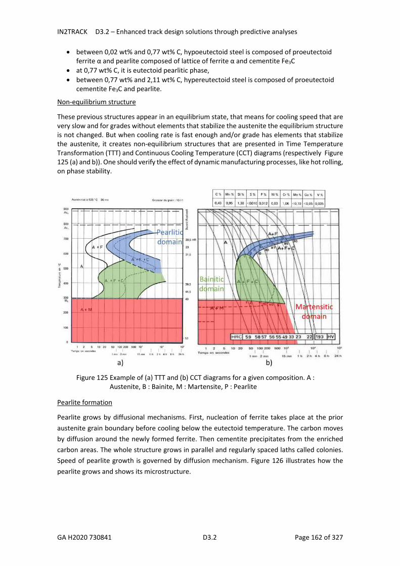
IN2TRACK D3.2 – Enhanced track design solutions through predictive analyses
GA H2020 730841 D3.2 Page 162 of 327
between 0,02 wt% and 0,77 wt% C, hypoeutectoid steel is composed of proeutectoid ferrite α and pearlite composed of lattice of ferrite α and cementite Fe3C
at 0,77 wt% C, it is eutectoid pearlitic phase, between 0,77 wt% and 2,11 wt% C, hypereutectoid steel is composed of proeutectoid
cementite Fe3C and pearlite.
Non-equilibrium structure
These previous structures appear in an equilibrium state, that means for cooling speed that are very slow and for grades without elements that stabilize the austenite the equilibrium structure is not changed. But when cooling rate is fast enough and/or grade has elements that stabilize the austenite, it creates non-equilibrium structures that are presented in Time Temperature Transformation (TTT) and Continuous Cooling Temperature (CCT) diagrams (respectively Figure 125 (a) and b)). One should verify the effect of dynamic manufacturing processes, like hot rolling, on phase stability.
Figure 125 Example of (a) TTT and (b) CCT diagrams for a given composition. A : Austenite, B : Bainite, M : Martensite, P : Pearlite
Pearlite formation
Pearlite grows by diffusional mechanisms. First, nucleation of ferrite takes place at the prior austenite grain boundary before cooling below the eutectoid temperature. The carbon moves by diffusion around the newly formed ferrite. Then cementite precipitates from the enriched carbon areas. The whole structure grows in parallel and regularly spaced laths called colonies. Speed of pearlite growth is governed by diffusion mechanism. Figure 126 illustrates how the pearlite grows and shows its microstructure.
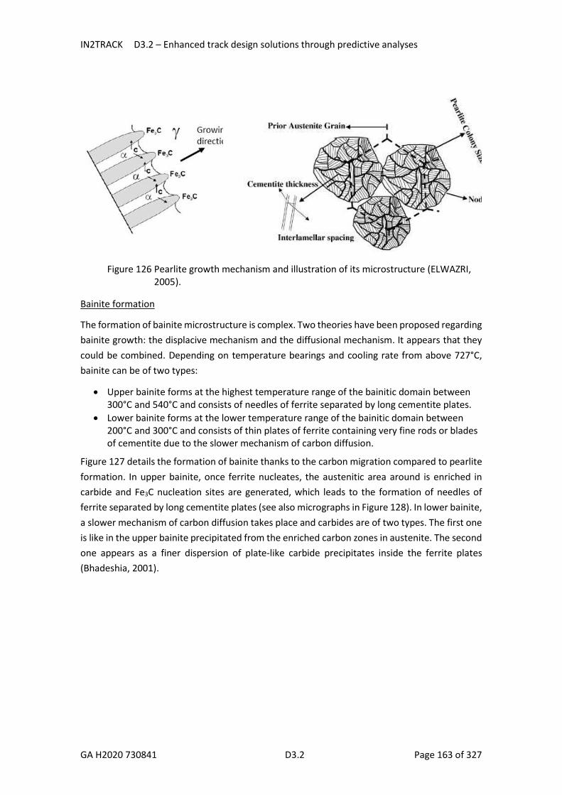
IN2TRACK D3.2 – Enhanced track design solutions through predictive analyses
GA H2020 730841 D3.2 Page 163 of 327
Figure 126 Pearlite growth mechanism and illustration of its microstructure (ELWAZRI, 2005).
Bainite formation
The formation of bainite microstructure is complex. Two theories have been proposed regarding bainite growth: the displacive mechanism and the diffusional mechanism. It appears that they could be combined. Depending on temperature bearings and cooling rate from above 727°C, bainite can be of two types:
Upper bainite forms at the highest temperature range of the bainitic domain between 300°C and 540°C and consists of needles of ferrite separated by long cementite plates.
Lower bainite forms at the lower temperature range of the bainitic domain between 200°C and 300°C and consists of thin plates of ferrite containing very fine rods or blades of cementite due to the slower mechanism of carbon diffusion.
Figure 127 details the formation of bainite thanks to the carbon migration compared to pearlite formation. In upper bainite, once ferrite nucleates, the austenitic area around is enriched in carbide and Fe3C nucleation sites are generated, which leads to the formation of needles of ferrite separated by long cementite plates (see also micrographs in Figure 128). In lower bainite, a slower mechanism of carbon diffusion takes place and carbides are of two types. The first one is like in the upper bainite precipitated from the enriched carbon zones in austenite. The second one appears as a finer dispersion of plate-like carbide precipitates inside the ferrite plates (Bhadeshia, 2001).

IN2TRACK D3.2 – Enhanced track design solutions through predictive analyses
GA H2020 730841 D3.2 Page 164 of 327
Figure 127 Growth of pearlite and bainite (http://practicalmaintenance.net).
Lower and upper bainite can be easily distinguished by classic microscopy analysis and their mechanisms of formation are well known. However, other forms of bainite exist. For instance, granular bainite that, in contrary to classic coarse plate, have a quasi-entirely granular aspect together with retained austenite (RA) and martensite islands (see Figure 127). This particular structure is supposed to be obtained only in continuous cooling and should not be obtained by isothermal transformation.
Figure 128 Micrograph of ferrite and upper bainite mixture (x250) on the left and of martensite and granular bainite (x750) on the right (Barralis, 2002)
Bainite structure depends on the cooling temperature. Therefore, one may distinguish upper bainite (UB), from lower bainite (LB) and low-temperature bainite (LTB) depending on the transformation temperature for a given steel composition (see

IN2TRACK D3.2 – Enhanced track design solutions through predictive analyses
GA H2020 730841 D3.2 Page 165 of 327
Figure 129.a). In carbide-free bainite Long and al. (2014) distinguished upper and lower bainite with misorientation distribution of packets of bainite ferrite plates. In the work of Zajac and al. (2015), upper bainite exhibits a greater number of low-angle lath/grain boundaries (2-15°), while lower bainite exhibits a high proportion of high-angle lath/grain boundaries. Lower temperature results in greater proportion of this high-angle misorientation (
Figure 129.b). Furthermore, a link between these structures and mechanical properties could be observed (
Figure 129.c). Indeed, UB consisting in catenary bainitic ferrite and blocky RA exhibits medium tensile strength and low impact toughness; LB consisting in lath-like bainitic ferrite and flake-like RA exhibits a lower tensile strength and medium impact toughness and LTB consisting in much thinner lath-like bainite ferrite and film-like RA exhibits the best mechanical properties. In addition, the smaller the grain size is, the better these properties are. Finally, strength of the carbide-free steel is proportional to the number of phase interface areas. High-angle misorientation between phase interfaces can prevent crack propagation, thus improving the impact toughness.
Figure 129 a) TTT diagram, b) grain boundary misorientation distribution and c) mechanical characteristics after (Long, 2014). LB: Lower Bainite, UB: Upper Bainite, LTB: Low-Temperature Bainite, TIH: Two-stage Isothermal Holding, CC: Continuous Cooling.
A very rapid cooling rate will not allow a diffusional mechanism, so the microstructure will transform into martensite by displacive mechanism. The CFC austenite lattice will transform into quadratic laths of martensite α’ usually needle shaped. This martensite phase should normally not be a part of the bainitic or pearlitic rail grades. However, as RA could be present after bainitic transformation, one should consider that Transformation Induced Plasticity (TRIP) effect may

IN2TRACK D3.2 – Enhanced track design solutions through predictive analyses
GA H2020 730841 D3.2 Page 166 of 327
occur, leading to its strain-induced transformation to martensite in certain conditions. This is directly linked to the stability of the RA. The following parameters can affect the RA stability (Samek, 2006):
C content of RA: high C content may reduce the Ms (Martensite start) temperature and stabilize the RA.
RA particle size: under 0.01 µm, RA is too stable for strain induced transformation, between 0.01 µm to 1 µm, the RA has an optimum size for TRIP effect, above 1 µm, RA is unstable and transforms at small strains.
Grain morphology and presence of different phases like ferrite matrix or near hard bainite and martensite phases that can influence the C content and the RA stability.
The surrounding matrix strength as the γα’ transformation is accompanied by a volume increase.
Isostatic stress environment can block the transformation because of the previously mentioned volume increase implication of the γα’ transformation.
Temperature that, if high, stabilize the RA by both reducing the driving force for transformation and increasing the intrinsic stacking-fault energy.
Head check on pearlitic steel grades
Recent studies have been performed on the head check defect occurring in pearlitic grades (Popovic, 2015), (Linz, 2015), (Dylewski, 2016), (Zhou, 2017a). In this part, the steps of its creation and propagation are discussed. Special attention is given to the microstructural and mechanical phenomena implied by head check.
Head checks generally appear on the gauge corner of the outer rail in curves where the wheel-rail contact takes place. Figure 130(a) details the surface of the head of a rail with the diverse parts such as the crown, the shoulder, and the gauge parts. In curves, the wheel-rail contact of the outer rail is located on the gauge corner of the rail. The region where RCF damage generally occurs is indicated between dotted lines. Figure 130(b) shows the location of the load transmission through the rail in curve conditions. The picture at the top shows two stressed zones in the outer rail. One on the crown/head and one on the upper gauge corner where the wheel-rail contact is located. The inner rail is only subjected to stress on the top of the crown.
Figure 130 a) Name of the rail profile parts (Dollevoet, 2010), b) Representation of stress transmission from wheel to rail in a curve (Popovic, 2015).
a)
b)

IN2TRACK D3.2 – Enhanced track design solutions through predictive analyses
GA H2020 730841 D3.2 Page 167 of 327
The head check defect is identified by the International Union of Railways under the code 2223 as detailed in Figure 131. Depending on the load conditions, train speed and rail grade material, the distance between cracks ranges between 1 to 7 mm and can reach up to some centimeters. At the crack initiation location, cracks are oriented perpendicular to the shear stress. The β angle between the crack and the transverse direction to the rolling direction ranges from 18° to 30° (Dollevoet, 2010). From the defect depth in the rail it is decided to remove the rail or not. If the defect depth is lower than 5 mm, the defect is kept under control. Above a 20 mm depth defect, the rail must be removed (Popovic, 2015).
Figure 131 The principle of coding for head check rail defect and typical orientation of head check cracks on the rail head (popovic, 2015)
The head check has been studied for decades, especially on pearlitic steels e.g. R260, R350HT… It has been reproduced in laboratory conditions.
Plastic deformation
Plastic deformation occurs in a ratcheting effect each time a wheel rolls on the rail. After running of several trains, the microstructure of the near surface under the wheel-rail contact is oriented long the traffic direction (Figure 132). In pearlitic grades, the lamellae are oriented along the shear direction. Plastic deformation appears under the running band and the gauge corner where the wheel-rail contact is the most frequent (Dylewski, 2015). The plastic deformation decreases from the worn surface (severely deformed) up to 1 mm to 15 mm depth (bulk material) (Bower, 1991). The more loaded the rail is, the more deformed the surface is and deeper the plastic deformation.

IN2TRACK D3.2 – Enhanced track design solutions through predictive analyses
GA H2020 730841 D3.2 Page 168 of 327
Figure 132 Plastic deformation under the R260 rail worn surface and its schematic representation (Dollevoet, 2010), a) as delivered, b) after 100 cycles, c) after 40 000 cycles (Linz, 2015).
Crystallographic behavior
As the plastic deformation occurs, pearlite colonies are fragmented (Dylewski, 2015). In Figure 133, the intense plastic deformation just below the worn surface leads to a grain refinement. At a depth of a few millimeters below the worn surface, pearlite colonies are untransformed and have the same size and morphology as the bulk material.

IN2TRACK D3.2 – Enhanced track design solutions through predictive analyses
GA H2020 730841 D3.2 Page 169 of 327
Figure 133 EBSD orientation image (inverse pole-figure) of a worn R260 rail, a) below the surface, b) 6 mm under the surface (rolling direction from right to left) (Dylewski, 2015).
Crack initiation and propagation
Cracks initiate at the very surface of the rail where the plastic deformation is the most intense. Once the crack is initiated, microstructure plays a key role in crack growth. For pearlitic grades, cracks are generally initiated in shear strained soft proeutectoid ferrite or soft pearlitic ferrite (Dylewski, 2016). Then, they propagate between ferritic grains or pearlitic colonies in which they follow the lamellae direction oriented along the traffic direction because of plastic deformation. Cracks then propagate because of traffic accumulated traffic loading. Their propagation rate can be decreased by coarsening prior grain austenite size, lesser extent the interlamellar spacing (Gray, 1983) and by a poor lamellae alignment.
A simulation of crack propagation is proposed by Zhou and al. after X-Ray computed tomography analysis (Zhou, 2017a). They found out that a head check crack was following a smooth and linear route. First, it propagates faster in lateral direction than in longitudinal direction. Then, with wear rate competition, length-width ratio reduces.
A fine microstructure may reduce crack propagation rate. Koyama and al. (2017) pointed out that the metastable, multi-phase, nanolaminate microstructure of a pearlitic steel implied mechanisms such as the roughness induced crack termination (RICT) and Transformation Induced Crack Termination (TICT). The RICT mechanism can be enhanced when crack crosses grain boundaries and lamellae or when it propagates along it. The RICT and the TICT effects are lowered by higher stress amplitude (Koyama, 2017).
Also, the stress amplitude depends on contact pressure that affects the ratio of wear or RCF in low creepage rolling sliding conditions. If the wear rate is higher than the RCF, fatigue cracks are removed and wear can protect the rail from RCF (Donzella, 2005).

IN2TRACK D3.2 – Enhanced track design solutions through predictive analyses
GA H2020 730841 D3.2 Page 170 of 327
Mechanical properties
In the study of Dylewski and al. the hardness of the near surface rises with the accumulated load from 1,3 MGT (Million Gross Tons) to 234 MGT (Dylewski, 2016). The pearlitic microstructure is work hardened with the accumulated plastic deformation (see Figure 134). In the first millimeters under the contact surface (0-5 mm), one may observe that the more accumulated tonnage rail experiences, the more hardened the near surface of the rail is. The first few micrometers under the surface show a hardness ranging from about 3 GPa after 1.3 MGT to 6 GPa after 234 MGT. Presence of proeutectoid ferrite at the surface is characteristic of decarburizing. This ferrite shows a softening influence on hardness within the first 500 µm under the surface. The hardness is lower than deeper in the rail up to 1 mm under the worn surface and indicates the thickness of this decarburized layer (see green measures after 1.3 MGT).
Figure 134 Hardness under the worn surface at different accumulated traffic tonnage (Dylewski, 2016).
Bainitic rails
Nowadays, railway network tends to increase traffic load and train speed while improving safety. Severe traffic conditions involve rail and wheel damages. In order to extend rail (and wheel) life, to decrease rail maintenance and to prevent rail defect outbreaks, new rail steel grades are required.
Today’s most used materials are steel grades with a pearlitic microstructure e.g. R260, R350HT or MHH. Since a few decades, bainitic grades have emerged and seemed to show a better resistance to contact fatigue and good wear resistance compared to pearlitic grades as Clayton (1996) measured (see Figure 135).
Studies on bainitic steel grades have shown a great potential for these types of microstructures (Clayton, 1987, Zajac, 2006). The bainite present in railway rails is often carbide-free. Bainitic steels can achieve high hardness and offer high wear resistance referring to the Archard law.

IN2TRACK D3.2 – Enhanced track design solutions through predictive analyses
GA H2020 730841 D3.2 Page 171 of 327
However, other studies show that bainite wear could not be predictable due to its microstructure. Even more, bainitic microstructure could have poor wear resistance compared to pearlitic microstructure (Clayton, 1996).
Low C bainitic grade presents better RCF resistance compared to pearlitic grade (Yokoyama, 2002). The initiation time for flaking is systematically longer. In addition, the White Etching Layer (WEL) defect generated by RCF has been shown to be more difficult to obtain. The probable cause may be a high austenitization temperature due to the low C content that is the initial step of the WEL generation with contact heating generation before fast cooling and brittle martensite generation.
Figure 135 : Wear rate vs hardness (Clayton, 1996).
Bainitic damage under rail-wheel service conditions
A study of Clayton and Devanathan showed the better type III wear resistance of a pearlite compared to an upper bainite of the same chemical composition with 0.71 wt.%C (Clayton, 1992). Nevertheless, a more complex microstructure with lower bainite or a mixture of lower and upper bainite exhibits a superior hardness and a better resistance to breaking.
Jin and al. found out the wear resistance of low carbon bainitic steel with a carbon content of 0.023 wt.% C to 0.18 wt.% C can be as good as that of a 0.8 wt.% C pearlitic steel (Jin, 1997). The wear resistance is increased by increasing the carbide-free bainite microstructure proportion and the best microstructure contains also retained austenite and needle-shaped martensite.
In bainitic steels, retained austenite can be beneficial to the RFC performances (Gui, 2016). It can actually slow or blunt the crack by transformation-induced plasticity (TRIP) effect and blocks micro-crack propagation changing the residual stress. RCF performances are improved with a higher content of retained austenite and with a film shape that is more stable than block shape and ensures TRIP effect at large strain. However, Leiro and al. indicate that higher austenite content makes the wear performance of a carbide-free bainitic 60SiCr7 steel decrease (Leiro, 2011). Improving the austenite volume fraction 12.26% to 17.80% made double the wear rate in a rolling-5% sliding test.
Dayot and al. studied the damage under reduced-scale wheel-rail contact simulator (Dayot, 2012). He compared the sensitivity of particle detachment of bainitic grade to pearlitic grade

IN2TRACK D3.2 – Enhanced track design solutions through predictive analyses
GA H2020 730841 D3.2 Page 172 of 327
steel R260 and R350HT. The intensity of particle detachment, hole diameters and plastic deformation increase when the mechanical properties such as Rm and hardness decrease. The behavior of the bainitic grade is between pearlitic grade R260 and heat treated pearlitic grade R350HT as it shows moderate sensitivity to particle detachment and surface plastic deformation.
The rolling-sliding type III wear of a pearlitic eutectoid steel and low to medium carbon content bainitic steels has been tested (Devanathan, 1991). The importance of microstructure on wear properties is highlighted by the banded structure and grain boundary precipitates influence on wear behavior.
Zapata and al. tested pearlitic and bainitic steels in rolling and rolling-sliding condition (Zapata, 2011). The same wear rate was observed due to a low load. Adhesive wear was observed in the test with 2% creepage. Bainitic steels were more affected by work hardening resulting in a larger increase of hardness beneath the surface.
The aim of the study is to understand how bainitic steels have a better resistance to head check defect. Enlighten damage mechanisms in bainitic steel grades should help to answer this question.
9.5.3 Research work Recently, some bainitic rail grade segment tests have been integrated to the network by British Steel. Bainitic rails seem to present enhanced RCF performance and do not exhibit head check defect in curves. Figure 136 presents the rails of this study after test. At left, the B320 bainitic grade does not show head checks whereas at right R260 pearlitic one has. The current work is a preliminary investigation to understand the reason why the bainitic grades resist to the head check default while pearlitic grades cannot. The aim is therefore to identify key parameters in bainitic steel damage mechanisms in railroad loading conditions.
Figure 136 Top view of rail steel grades tested in curve, a) B320 bainitic steel, b) R260 pearlitic steel.
The steel grade used in this study is described as well as the sampling strategy to study the material. Mechanical properties through hardness investigation in a transverse cross section slice of rail is performed to identify the worn affected zone. X Ray Diffraction (XRD) analysis is also performed at a macroscopic scale on the various parts of the slice to find out if phase

IN2TRACK D3.2 – Enhanced track design solutions through predictive analyses
GA H2020 730841 D3.2 Page 173 of 327
transformation occurred. After that, a microstructural investigation on sound parts is settled, dealing with inclusions first and metallographic features then. Finally, main phenomena implied by the wheel-rail contact are presented thanks to OM, SEM and TEM observations and EBSD analysis. Some wear mechanisms are proposed after these analyses.
Steel grades
Two bainitic steel grades are studied in the current work, namely B320 and B360 grades. B320 grade is used on tracks while B360 is used more specifically in switches and crossings. Their chemical composition is presented in Table 24 and their continuous cooling temperature (CCT) diagrams are displayed in Figure 137.
The bainitic rails have been shaped following British Steel process. Initial rectangular bars called blooms are heated up to around 1100°C. They are after hot rolled at around 960°C and finally air cooled in ambient temperature with a cooling rate close to 0.15°C/s.
The rails have been set in track in a curve of the Eurotunnel for about 10 years. They were submitted to 1070 MGT before being removed. While they were in service condition, they have been submitted to operating maintenance and grinding two times.
Table 24 Chemical composition and mechanical properties of bainitic steels compared to commonly used pearlitic steels (British Steel data).

IN2TRACK D3.2 – Enhanced track design solutions through predictive analyses
GA H2020 730841 D3.2 Page 174 of 327
Figure 137 : Continuous Cooling Temperature diagrams of a) B320 and b) B360 bainitic grades (British Steel data).
Sampling, preparation and experimental procedure
15 mm thick lamellae are sampled from the workpiece rail. Each lamella is then cut by water jet into smaller samples splitting the head, the web, left and right parts of the base.
a) B320
b) B360

IN2TRACK D3.2 – Enhanced track design solutions through predictive analyses
GA H2020 730841 D3.2 Page 175 of 327
Figure 138 Original piece of rail and schematic sampling.
Different parameters of the water jet cutting process have been tested in order to get the smoothest surface of the samples. Figure 139(a) shows that a high nozzle speed creates deep scars and the jet is cutting faster at the top compared to the bottom of the sample inducing curved scares. When the nozzle speed decreases, scars are less deep in the workpiece and the cut surface is smoother. The final parameters of water jet cutting process have been fixed as follows:
A pressure of 3.400 bars, An abrasive flow of 340 g/min (diamond powder), A nozzle speed of 12,5 mm/min.
a) b)
Figure 139 Water jet effect on rail cutting. a) Web cut with a decrease of the jet nozzle speed, the white arrows show the water jet direction. b) Head top view with ligth abraded areas.

IN2TRACK D3.2 – Enhanced track design solutions through predictive analyses
GA H2020 730841 D3.2 Page 176 of 327
After cutting, the top of the sample is abraded due to the abrasive diamond powder addition of the water jet that impacts the edge cut. This abraded part is then suppressed at the first preparation step of the sample by a saw cutting. Figure 140 presents the sampling of a rail slice. The base of the latter workpiece is split into 2 parts and the head into 6 parts. The rail-wheel contact zone occurs on sample HA and HB (see Figure 140).
Figure 140 Sampling and identification of the samples. The different parts are referred to by “codes” as mentionned in the present figure.
Prior metallographic analysis, samples are mirror polished using paste with diamond powder of a diameter up to ¼ µm and ethylic alcohol based lubricant.
The duration between the polishing preparation and the observations or analysis must be as short as possible to avoid oxidation of the surface. If it is not possible, or when the sample is needed for different analysis, it is stored in a desiccator.
Equipment used in this study
Optical observations have been carried out with an light microscope Zeiss Axioplan®. Scanning Electron Microscope(SEM) analyses have been performed with a JSM-7800F FEG JEOL SEM® and a Quanta 4000 FEI SEM® in secondary electron (SE) and backscattered electron (BSE) modes. Energy Dispersive X-ray spectroscopy (EDX) has been used for chemical identification at a microscopic scale.
Thin foils for Transmission Electron Microscopy (TEM) are obtained by cutting 150 µm thick slices. Then a mechanical grinding is performed to reach a slice thickness lower than 80 µm.
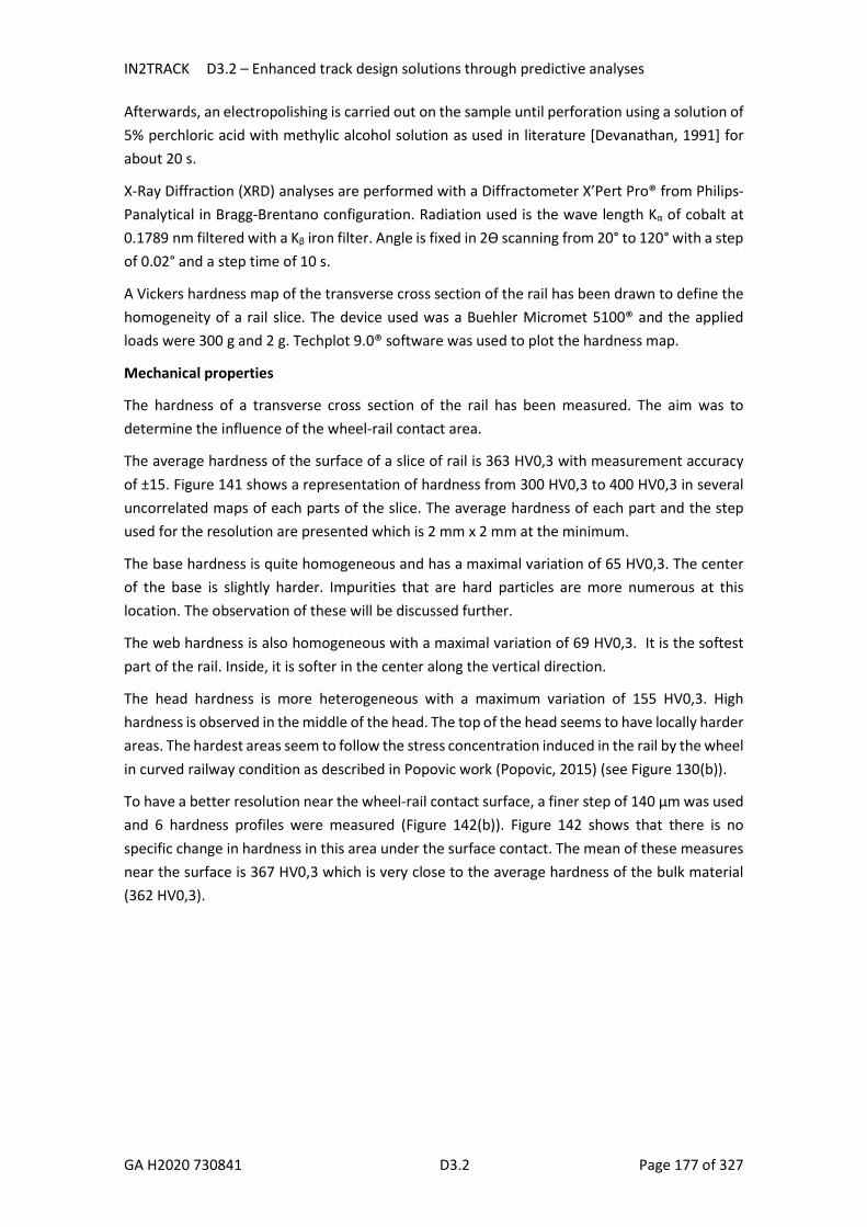
IN2TRACK D3.2 – Enhanced track design solutions through predictive analyses
GA H2020 730841 D3.2 Page 177 of 327
Afterwards, an electropolishing is carried out on the sample until perforation using a solution of 5% perchloric acid with methylic alcohol solution as used in literature [Devanathan, 1991] for about 20 s.
X-Ray Diffraction (XRD) analyses are performed with a Diffractometer X’Pert Pro® from Philips-Panalytical in Bragg-Brentano configuration. Radiation used is the wave length Kα of cobalt at 0.1789 nm filtered with a Kβ iron filter. Angle is fixed in 2Ө scanning from 20° to 120° with a step of 0.02° and a step time of 10 s.
A Vickers hardness map of the transverse cross section of the rail has been drawn to define the homogeneity of a rail slice. The device used was a Buehler Micromet 5100® and the applied loads were 300 g and 2 g. Techplot 9.0® software was used to plot the hardness map.
Mechanical properties
The hardness of a transverse cross section of the rail has been measured. The aim was to determine the influence of the wheel-rail contact area.
The average hardness of the surface of a slice of rail is 363 HV0,3 with measurement accuracy of ±15. Figure 141 shows a representation of hardness from 300 HV0,3 to 400 HV0,3 in several uncorrelated maps of each parts of the slice. The average hardness of each part and the step used for the resolution are presented which is 2 mm x 2 mm at the minimum.
The base hardness is quite homogeneous and has a maximal variation of 65 HV0,3. The center of the base is slightly harder. Impurities that are hard particles are more numerous at this location. The observation of these will be discussed further.
The web hardness is also homogeneous with a maximal variation of 69 HV0,3. It is the softest part of the rail. Inside, it is softer in the center along the vertical direction.
The head hardness is more heterogeneous with a maximum variation of 155 HV0,3. High hardness is observed in the middle of the head. The top of the head seems to have locally harder areas. The hardest areas seem to follow the stress concentration induced in the rail by the wheel in curved railway condition as described in Popovic work (Popovic, 2015) (see Figure 130(b)).
To have a better resolution near the wheel-rail contact surface, a finer step of 140 µm was used and 6 hardness profiles were measured (Figure 142(b)). Figure 142 shows that there is no specific change in hardness in this area under the surface contact. The mean of these measures near the surface is 367 HV0,3 which is very close to the average hardness of the bulk material (362 HV0,3).

IN2TRACK D3.2 – Enhanced track design solutions through predictive analyses
GA H2020 730841 D3.2 Page 178 of 327
Figure 141 Vickers hardness maps of a slice of rail.

IN2TRACK D3.2 – Enhanced track design solutions through predictive analyses
GA H2020 730841 D3.2 Page 179 of 327
Figure 142 a) Vickers hardness profiles under the contact area and b) associated representation of the profiles by colored lines on the surface sample.
Microstructural investigation
Microstructural investigation deals first with inclusion analysis performed with light microscope, SEM views and EDX analysis for chemical validation. Then, the typical microstructure is identified thanks to etchings. The virgin bainitic microstructure will be discussed and compared to the microstructure affected by the wheel-rail contact. Main phenomena induced will be highlighted and will help to propose some wear mechanisms in B320 bainitic rail grade
Inclusion analysis
After sample preparation, cross sections are observed and disclose a smooth surface with some particles from 10 µm to less than 1 µm size. The bainitic microstructure cannot be seen unless the surface is etched. Visible particles are inclusions related to the fabrication process of the steel. When the steel is cooled from liquid to solid state, impurities present in the liquid bath precipitate and create inclusions.
Two main particle types are identified with EDX analysis as disclosed in Figure 143. The first one is manganese sulfide appearing grey with an elongated shape with optical microscope. It is usually oriented along the rolling direction. The second one is titanium carbo-nitride that has angular shape and orange color. Sometimes, black spots which are very likely aluminum oxides can be found inside titanium carbo-nitride.
a) b)

IN2TRACK D3.2 – Enhanced track design solutions through predictive analyses
GA H2020 730841 D3.2 Page 180 of 327
Figure 143 EDX analysis of inclusions spoted by microscope observation of cross section.
B320 steel grade microstructure
To disclose the microstructure (except for the inclusions), etching is required. Different chemical etchants are presented in Table 25. The most common etching on bainitic steels is achieved with Nital. An additional Solution 1 can be used to improve the resolution and reveal potential martensitic structures. Another etching can be done with Solution 2 close to Picral solution.
Table 25 Chemical etching characteristics.
Figure 144 displays the microstructure of the sample after etching with Nital (a) and Solution 2 (b). Irrespective of the etchant, the revealed microstructure is similar. The etched parts (the brightest ones) are probably ferrite and bainitic ferrite. The darkest parts are for the moment not well identified. Some finer investigation with SEM and TEM will help to clarify these phases.

IN2TRACK D3.2 – Enhanced track design solutions through predictive analyses
GA H2020 730841 D3.2 Page 181 of 327
Figure 144 Optical view of transverse cross section of HB sample after 4 s of a) Nital etching, b) Solution 2 etching.
Figure 145 highlights the microstructure by SEM with the BSE mode. The observed contrasts are the same as those depicted with Solution 2 etching by light microscopy. According to Energy Dispersive X-ray (EDX) analysis, there is no significative composition change between the different grey levels revealing a crystallographic orientation contrast.
Figure 145 BSE SEM view of transverse cross section of a rail sample, a) as polished, b) after 4s of solution 2 etching. Indentation imprints are visibles on the right side.
The typical microstructure of bulk B320 rail revealed by solution 2 etching is shown in Figure 147. This microstructure is coarser than the usual one found in the literature. Referring to other works with slightly different bainite composition, one may propose hypotheses, that must be validated through further and finer observations such as TEM analysis, such as:
The positive reliefs are probably bainite ferrite when comparing the microstructure to that reported in Papadimitriou’s work (Papadimitriou, 1997) (see Figure 146).
Thicker parts may be a mixture of several phases by analogy with the microstructures depicted in low carbon carbide free bainitic microstructures seen in the literature (Gu, 2016), (Caballero, 2011): bainitic ferrite that is not etched due to a crystallographic orientation effect, granular bainite (Chao, 2014), carbide for the little white spots. In addition, the blocks may be martensite-austenite compounds (MAC) (Morale, 2015).
a) b)
a) b)

IN2TRACK D3.2 – Enhanced track design solutions through predictive analyses
GA H2020 730841 D3.2 Page 182 of 327
One may find retained austenite in thin film between bainitic ferrite at a lower scale (Zhou,2017b).
Figure 146 SE/SEM transverse cross section view of etched rail (a). Encircled area in micrograph (a) is compared to αub,1 upper bainite plate (b) of Papadimitriou bainite observation (Papadimitriou, 1997).
a) b)

IN2TRACK D3.2 – Enhanced track design solutions through predictive analyses
GA H2020 730841 D3.2 Page 183 of 327
Figure 147 Bulk microstructure of the rail in the head part. SE/SEM transverse cross section view.

IN2TRACK D3.2 – Enhanced track design solutions through predictive analyses
GA H2020 730841 D3.2 Page 184 of 327
Microstructure of the various parts of a rail slice
The microstructure disclosed in Figure 148 is a typical bainitic structure of this kind of rail already observed by SNCF and British Steel teams. On the right side of the sample, at the center of the base, the microstructure is coarser and present an elongated morphology. On the left side of the sample, at the forefront, the microstructure seems finer and the elongated structure is hardly visible. That could correspond to a faster cooling on the surface and the narrowest part of the base at the forefront of the sample compared to the depth of the base at the center of the base. This evolution is visible in Figure 149. The microstructure morphology is coarser from the forefront (1) to the center (6) of the sample.
Figure 148 Optical observation of the microstructure of the transverse cross-section of the base after 4 s of Nital etching.
Figure 149 : Microstructure morphology evolution with the depth of the base of a rail slice. Transverse cross-sectional optical view after 4s of Nital etching.

IN2TRACK D3.2 – Enhanced track design solutions through predictive analyses
GA H2020 730841 D3.2 Page 185 of 327
Looking at the surface of the transversal cross-section of the rail, ferritic-pearlitic areas can be observed (see Figure 150). Ferrite is depicted by light areas and pearlite by dark areas. They appear during the rolling process at high temperature followed by the cooling to room temperature. It can be found in continuous layer under the base or just locally on the top of the base or on the top of HC part of the head which is not in contact with the wheel in curves. These structures are similar to the decarburized areas that can be observed in pearlitic rail steel grades.
Figure 150 Transverse cross section optical view of ferritic-pearlitic areas after Nital etching.
Phase analysis
XRD analysis globally shows the same peaks in the base, the web and the head part where the contact area with the rail is located, as presented in Figure 151. The diagram of the web is slightly shifted in 2Ө due to acquired conditions (positioning of the sample). The main visible peaks correspond to the diffraction of ferrite phase. However, other peaks with a very low intensity correspond to the austenite phase. This should be residual austenite remaining after the rolling process of rail forming.
A quick method described by Bach et al. allows to measure the austenite and ferrite proportion from the area under the peaks and analytic factors (Bach, 1996). It appears that austenite proportion is constant in the different parts of the rail slice with a valor of about 10%.
However, wear phenomena could locally imply a crystallographic mechanism. Leiro and al. described the loss of austenite phase after a wear test due to a phase transformation phenomenon in the case of high carbon content (0,61wt.%) carbide free bainitic steel (Leiro,

IN2TRACK D3.2 – Enhanced track design solutions through predictive analyses
GA H2020 730841 D3.2 Page 186 of 327
2011). Further investigation must be done on finer zones and closer to the wheel-rail contact surface to identify if the previously mentioned phenomenon could occur.
Figure 151 XRD patterns of different parts in a rail slice.
Wear phenomenon under the wheel-rail contact area
The part of the rail that is the most severely worn is the sample HA (Figure 152).
Figure 152 Sampling and identification of the samples.
The focus on the cross section of this part (HA) of the rail reveals clues about the wear phenomenon:
At a macroscopic scale, the geometry of the rail head is not symmetric. After loading and grinding maintenance operation, the top of the left part is missing (HA and HB samples), resulting in an asymmetric transversal cross section of the head of the rail.

IN2TRACK D3.2 – Enhanced track design solutions through predictive analyses
GA H2020 730841 D3.2 Page 187 of 327
At a lower scale, SEM observations reveal a microstructural gradient (see Figure 153). A coarse microstructure is seen in depth in bulk material. Prior austenite grain boundaries are visible. While reaching the surface, these prior austenite grain boundaries are becoming difficult to see. The microstructure is refined and has a less elongated shape than in depth.
Figure 153 SE/SEM transverse cross section view of rail head sample HA and magnified views.
At a higher magnification of the very surface, one may observe a highly deformed area over a distance of between 1 and 10 µm (see Figure 154). Elements of the microstructure are oriented along the surface roughness, elongated along the surface. In addition, they are smaller than these in the bulk material due to an extreme plastic deformation.
Figure 154 SE SEM transverse cross section view of the extreme plastically deformed very surface and magnified views.

IN2TRACK D3.2 – Enhanced track design solutions through predictive analyses
GA H2020 730841 D3.2 Page 188 of 327
The wheel-rail contact surface is rough. One may see hills and valleys. The valleys contain cracks and holes (see Figure 155). Cracks tend to propagate along the surface. Hills are then beheaded causing a smoothing of the surface as a classic wear mechanism.
Figure 155 SE SEM transverse cross section views of areas with cracks (white arrows) and magnified views.
Going down along the wheel rail contact surface, the intense plastic deformation
spotted by the morphology of the microstructure is less and less visible until it disappears (see Figure 156).

IN2TRACK D3.2 – Enhanced track design solutions through predictive analyses
GA H2020 730841 D3.2 Page 189 of 327
Figure 156 SE/SEM transverse cross section views of lower parts in the rail head and magnified views.
Finally, at the bottom of the HA sample, there is a flange below which the geometry of the rail head is the same as originally. A ferritic-perlitic area can be observed which can be considered as a marker of an unworn surface (see Figure 157).
Figure 157 SE/SEM transverse cross section view of a ferritic-pearlitic area in the rail head at the bottom of wheel-rail contact surface.

IN2TRACK D3.2 – Enhanced track design solutions through predictive analyses
GA H2020 730841 D3.2 Page 190 of 327
In the longitudinal cross section (Figure 158), the microstructure is very affected by the plastic deformation caused by the traffic. With SEM high magnification micrographs one can see laths. In Figure 159, some areas seem to be not deformed. A hypothesis is that these blocks are MAC surrounded by very deformed ferrite bainite laths.
Figure 158 SE/SEM longitudinal cross section view of a very deformed area.
Figure 159 SE/SEM longitudinal cross section view of a very deformed area with ferritic bainite laths around blocky compound.
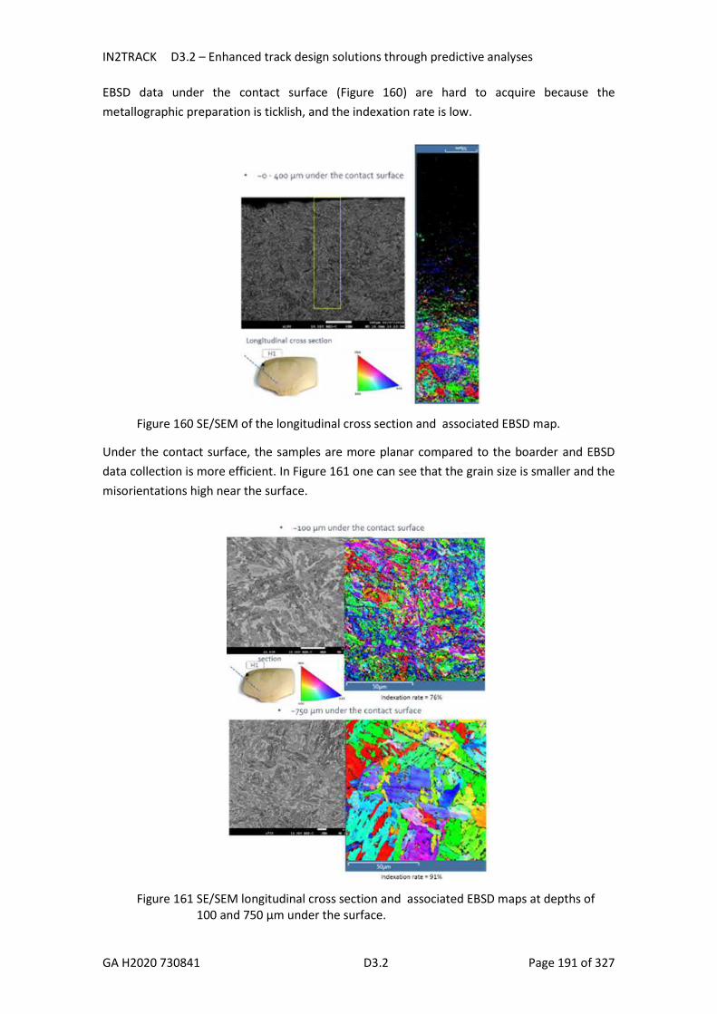
IN2TRACK D3.2 – Enhanced track design solutions through predictive analyses
GA H2020 730841 D3.2 Page 191 of 327
EBSD data under the contact surface (Figure 160) are hard to acquire because the metallographic preparation is ticklish, and the indexation rate is low.
Figure 160 SE/SEM of the longitudinal cross section and associated EBSD map.
Under the contact surface, the samples are more planar compared to the boarder and EBSD data collection is more efficient. In Figure 161 one can see that the grain size is smaller and the misorientations high near the surface.
Figure 161 SE/SEM longitudinal cross section and associated EBSD maps at depths of 100 and 750 µm under the surface.

IN2TRACK D3.2 – Enhanced track design solutions through predictive analyses
GA H2020 730841 D3.2 Page 192 of 327
Micrographs in Figure 162 show that there is a continuous oxide layer at the surface of the rail. Sometimes the oxide is found at the surface and sometimes below the surface.
Figure 162 SE/SEM longitudinal cross section of oxidized surface
On Figure 163, there is iron oxide is surrounding with a CNTi inclusion or a MnS inclusion. A galvanic corrosion probably occurs here between the iron matrix and the inclusion.
Figure 163 SE/SEM and EDS mapping around a titanium carbonitride inclusion
Different types of cracks are observed on the rail (Figure 164). At the top, the steel is mainly crushed by the passage of the train wheels. On the side, the stress is different, with a shear component. On the part on Figure 164, one can see that the cracks are longer on the side, where the shear stress is the greatest. Towards the top, cracks observed are smaller probably because of the high wear rate, which act like a machining of the surface.

IN2TRACK D3.2 – Enhanced track design solutions through predictive analyses
GA H2020 730841 D3.2 Page 193 of 327
Figure 164 Craks in transversal cross section at areas with different sollicitations
Figure 165 shows clearly the crack propagation between two areas with a very different deformation. Near the surface the microstructure is very thin due to high deformation level whereas under the cracks the microstructure is coarser showing a less deformed microstructure.
Figure 165 Cracks on transverse cross section between high and low deformation
Finally, Figure 166 presents a proposal of crack formation mechanism. With the increase of the deformation, cracks appear progressively in the deformation area, parallel to the surface and to the deformation bands. Then they propagate under the surface, preferentially at the interface of areas with high and low deformation levels.
This mechanism can explain the good behavior of the BS bainitic structure considering head check defect. Actually, cracks appear at the surface, in the very deformed zone and propagate between high and low deformation areas, leading to macrocracks parallel to the surface. One

IN2TRACK D3.2 – Enhanced track design solutions through predictive analyses
GA H2020 730841 D3.2 Page 194 of 327
can imagine that the cracked layer is removed by wear that limits the crack propagation and the head check defect formation.
Figure 166 Microstructure modification of the surface under deformation
9.5.4 Conclusions The first aim of this study was to test different techniques of characterization in order to explain why British Steel bainitic structures show a so good behavior in rail applications. A lot of techniques was developed and applied on a used rail: Optical micrography, SEM, TEM, EBSD, XRD, micro hardness tests. The analyses of the microstructure of not worn bainitic steels revealed the presence of:
Inclusion particles of MnS and TiC(N) oriented along hot rolling direction (EDX/SEM) Ferrite and retained austenite (XRD measurements) Bainitic ferrite laths (SEM, TEM) as well as retained austenite with two morphologies
namely “blocky compounds” and “bainitic ferrite inter-laths films”.
A phenomenological approach of the damage mechanisms was revealed:
Plastic deformation spreading gradually from the contact surface 0-20 µm: extremely deformed surface – hard to analyze 20-50 µm: deformed surface starting to rotate along the traffic direction 50-100 µm: transformed area
The oxidation at the surface was shown to be more developed around inclusions.
Microcracks and macrocracks can develop according to the location in the wheel-rail contact area implying higher wear rate or shear stress. A scenario of crack formation is proposed. The cracks appear at the surface and propagate between high and low deformed zones along a plane parallel to the surface. That leads to the removal of the cracked surface area by wear, which limits the propagation of cracks and thus the development of head check type defects.

IN2TRACK D3.2 – Enhanced track design solutions through predictive analyses
GA H2020 730841 D3.2 Page 195 of 327
Although additional observations are still missing in order to confirm the theoretical approach of the proposed mechanism, the main goal of the study is reached. It is proved that the bainitic microstructure developed by British Steel presents particular features at a very fine scale that can explain the good mechanical behavior in use.

IN2TRACK D3.2 – Enhanced track design solutions through predictive analyses
GA H2020 730841 D3.2 Page 196 of 327
10 Improve design through simulations Investigate how simulations and assessment should be used to investigate improved designs (developed in WP3.2) and influences of different operational scenarios (as discussed in WP3.3). This analysis improves upon the outlines derived in In2Rail (and previously INNOTRACK) and forms the basis for the feasibility evaluation framework specifically mentioned in the call.
10.1 Improved simulation capabilities regarding rail crack formation
In general, rail cracks can form in the foot, web and head of the rail. A concise list of different forms of rail cracks can be found in International Union of Railways (2012). In short, foot cracks typically relate to (mechanical or corrosive) induced damage that causes crack propagation and eventually rail break. Web cracks typically relate to welds or drilled holes in the web. Rail head cracks can form at the underside of the head. Such cracks typically grow under the influence of the global stressing (bending/shearing, prevented thermal contraction) of the rail.
The current chapter focuses on cracks that initiate on the upper part of the rail head. Such cracks are primarily driven by the wheel–rail contact stress field and are referred to as rolling contact fatigue cracks. These are very costly since crack formation will require the rails to be ground, milled, or in the worst case replaced.
Deformation induced anisotropy is a well-known phenomenon, well known for sheet metal rolling. The large plastic deformations occurring in the vicinity of the contact zone in rails, is also known to produce an anisotropic material, see e.g. (Wetscher, Stock and Pippan, 2007). (Larijani et al., 2014) found that an anisotropic crack resistance can control if cracks grow downwards and cause crack breakage, or if it only causes spalling. A challenge with characterizing the above is that large gradients of the material behaviour in the near-surface region is present. Suitable mechanical testing is therefore very difficult. To be able to model the anisotropic behaviour of rail steel, we first need a reliable method of creating anisotropy in the laboratory and then testing the material. This is accomplished by pre-deforming cylindrical specimens in an axial-torsion testing machine, through twisting under high axial compressive stress. With this method, we have been able to recreate the strain levels found in used rails, approximately 0.1mm below the running band (Meyer, Ekh and Ahlström, 2018; Meyer, Nikas and Ahlström, 2018; In2track D3.1 Deliverable).
The frameworks that are capable of modelling the large shear strains present in the surface layer of rails, are investigated in Meyer and Ekh (2017), where it is found that two well established frameworks actually coincide when the same energy potential function is used.
To evaluate models available in the literature, a material parameter fitting procedure has been created and used to find the best set of material parameter values for the different models. These are then used to check what features of the pre-deformation process that can be modelled and where the limitations of the different models are. In this investigation, it has been

IN2TRACK D3.2 – Enhanced track design solutions through predictive analyses
GA H2020 730841 D3.2 Page 197 of 327
found that models from the literature can be combined to give very good results for the pre-deformation (Meyer, Ekh and Ahlström, 2018).
10.2 Simulation and assessment of the railway track long term dynamic behaviour
10.2.1 Introduction This work aims to define a methodology to simulate the long term dynamic behaviour of the railway track due to soil degradation induced by cyclic loads. The used 2.5D formulation FEM-PML (Perfect Matched Layers) is less time-consuming since only the invariant cross-section is discretized by finite elements. In the longitudinal direction, the variables time and space are transformed in the frequency and wavenumber domain through the Fourier transform. The numerical methodology of the 2.5 D approach is described, which also includes a numerical explanation about the treatment of the artificial boundaries. With the acquired knowledge about the numerical modelling and the way to obtain the stresses in the elements, a brief description of the empirical permanent deformation model is presented.
A parametric study is conducted in order to compare the quasi-static mechanism and the dynamic mechanism that includes the consideration of the interaction between the vehicle and the track. This study also includes an analysis of the influence of the train’s speed. In the end, the values of the stress levels and permanent deformation induced by the passage of the train are compared.
10.2.2 Numerical modelling The main purpose of this study is to determine and analyse the railway track behaviour due to soil degradation induced by successive passage of the trains. In order to obtain, expeditiously the stress state of the ground, the 2.5 formulation seems to be the most advantageous choice after a rigorous analysis of several numerical tools.
The numerical model of a railway structure can be divided into two main modulus: one includes the track-ground structure (taking into account the tri-dimensional nature of the domain) and the other simulates the dynamic behaviour of the train, which is simulated by a multi-body formulation considering the masses and suspensions of the vehicles (Figure 167). Both models are integrated by a compliance formulation in order to take into account the train-track interaction (Alves Costa et al., 2011).
The dynamic interaction is guaranteed considering the compatibility conditions of the displacements and the equilibrium of forces that there are between the two domains.

IN2TRACK D3.2 – Enhanced track design solutions through predictive analyses
GA H2020 730841 D3.2 Page 198 of 327
Figure 167 Flowchart representative of the sub-structure models - adapted from (Alves Costa, 2011)
Modelling of the train-track interaction by 2.5D models (FEM-PML approach)
The 2.5D models present, clearly, several advantages in the performance of some parametric studies since the method combines the good calculation processing with the consideration of the tridimensional characteristics of this type of problem (Yang and Hung, 2001, Alves Costa, 2011). In this case, the 2.5D formulation is supported by the FEM-PML approach, which means that this numerical procedure performs a coupling between the finite elements and boundary elements in the 2.5D domain. Furthermore, it is assumed that the dynamic problem is linear, which means that the formulation can be developed in the wavenumber-frequency domain considering the application of Fourier expansions for space and for time (only in the track longitudinal direction, as shown in Figure 168).

IN2TRACK D3.2 – Enhanced track design solutions through predictive analyses
GA H2020 730841 D3.2 Page 199 of 327
Figure 168 Infinite and invariant structure in one direction (Lopes et al., 2014)
Hence, the formulation demands a discretization of the cross-section (by finite elements) and implies an important condition: the geometry and loads need to be invariant. This method allows considering the tridimensional characteristics of the model and obtains 3D solutions without being necessary performed a numerical discretization of the space along the direction of the track (Alves Costa et al., 2011).
In this case, the track and also the substructure are modelled by the 2.5D FEM. However, there are some methodologies that allow decomposing the domain simulating the track by the 2.5D FEM and the layered ground through 2.5D BEM.
There are several excitation mechanisms but, usually, a distinction is made between the quasi-static and dynamic excitation mechanisms. The first one is due to the static weight of the vehicle per axles and the second is caused by the train-track interaction that induces vertical acceleration on the rolling-stock. The importance of the quasi-static mechanism increases when the track crosses regions of soft soils and train speed reaches the phase velocity of the system. In these cases, it is possible to identify high amplifications (Auersch, 2008). The dynamic load is due to the dynamic interaction between the train and the track. This subject will be described bellow.
2.5D Approach– modelling of the track
In this study, the ground is modelled by a 2.5D finite element approach. The 3D response of the ground is computed assuming that the structure is invariant along the development direction of the track. As mentioned previously, the track and the embankment are simulated by means of 2.5D finite elements, which allow the inclusion of real geometry of the structure, as well as its mechanical behaviour. The non-linear effects are handled through an equivalent linear analysis (the convergence is obtained element-by-element), which induces a transverse inhomogeneity in the ground due to the fact that the non-linear effects are more pronounced along the railway track than at the far-field.

IN2TRACK D3.2 – Enhanced track design solutions through predictive analyses
GA H2020 730841 D3.2 Page 200 of 327
The “two-and-a-half” dimension concept is a methodology that allows reducing the computational effort using the Fourier transforms with respect to the spatial coordinate along the track. This is the main advantage of the approach but, at the same time, implies the assumption of invariability of geometry and of mechanical properties along that direction, as mentioned previously. One import aspect is the necessity to avoid spurious reflections on artificial boundaries. In order to do so, the Perfect Matched Layers (PML’s) were used.
The application of the 2.D finite elements is adequate in structures which can be assumed to have an infinite development and invariant properties in one direction, as presented in Figure 168. In this case, the structure is 2D but the loading is 3D. Since the response of the structure is linear, the analysis can be carried out on the wavenumber/frequency domain. Thus, all the variables (loads that represent the action and the displacements that represent the response) must be transformed to the transformed domain by means of a double Fourier transform related with the direction along the track (x-direction represented in Figure 168 and with time). Hereafter, that quantities are denoted as functions of the Fourier images of x and t, defined as wavenumber and frequency, are represented by k1 and w, respectively (Alves Costa et al., 2010).
In order to solve the problem, it is necessary to solve the following equilibrium equation that can be derived for any point of a three-dimensional domain:
∫ 𝛿𝜀𝜎𝑑𝑉 + ∫ 𝛿𝑢𝜌( , )
𝑑𝑉 = ∫ 𝛿𝑢𝑝𝑑𝑆 (11)
where is the virtual strain field, represents the stress field, u is the virtual displacement field, u is the displacement field, is the mass density and p represents the applied loads.
After the transformation, the cross-section of the domain remains on the untransformed domain and is discretized into finite elements. This path allows rewriting the previous equation in terms of nodal variables.
In order to apply the concept of virtual work on the transformed domain, some considerations must be attended, namely the Parseval’s theorem:
∫ 𝛿𝑓(𝑥)𝑝(𝑥)𝑑𝑥 = ∫ 𝛿𝑓(−𝑘 )𝑝(𝑘 ) 𝑑𝑘 (12)
The previous equation provides the formulation of the principle of virtual works in the transformed domain. Considering the equation (11), it is possible to obtain the virtual work of the internal stresses and inertial forces in the transformed domain, as shows the followings equation, respectively:
∫ 𝛿𝜀𝜎𝑑𝑉 = ∫ 𝛿𝑢 ( − 𝑘 , 𝑤) ∬ 𝐵
(−𝑘 )𝐷𝐵(𝑘 )𝑑𝑦𝑑𝑧𝑢 (𝑘 , 𝜔)𝑑𝑘 (13)
∫ 𝛿𝑢𝜌( , )
𝑑𝑉 = −𝜔 ∫ 𝛿𝑢 ( − 𝑘 , 𝑤) ∬ 𝑁 𝜌𝑁𝑑𝑦𝑑𝑧
𝑢 (𝑘 , 𝜔)𝑑𝑘 (14)
where B is the matrix with the derivatives of the finite element shape functions, N is the shape function matrix, D is the strain-stress matrix, un is the vector of nodal displacements (in the transformed domain).
The virtual work carried out by the external loads is computed taking into account that the geometry is only discretized on the ZY plane. Thus, considering a coordinate s parallel to the

IN2TRACK D3.2 – Enhanced track design solutions through predictive analyses
GA H2020 730841 D3.2 Page 201 of 327
edge of the element where traction is applied, the virtual work developed by the load system is given by:
𝛿𝑢𝑝𝑑𝑆 =
∫ 𝛿𝑢 (−𝑘 , 𝜔) ∫ 𝑁 𝑝(𝑘 , 𝜔) 𝑑𝑠𝑑𝑘 = ∫ 𝛿𝑢 (−𝑘 )𝑝 (𝑘 , 𝜔)𝑑𝑘 (15)
Replacing the rearranged equations (13) into equation (11), it is possible to obtain the equilibrium of each finite element in the ZY plane through the following expression:
∬ 𝐵
(−𝑘 )𝐷𝐵(𝑘 )𝑑𝑦𝑑𝑧 − 𝜔 ∬ 𝑁 𝜌𝑁𝑑𝑦𝑑𝑧
𝑢 (𝑘 , 𝜔) = 𝑝 (𝑘 , 𝜔) (16)
Through this formulation, the stiffness and mass matrices are defined, respectively, by the following expressions:
[𝐾] = ∬ 𝐵
(−𝑘 )𝐷𝐵(𝑘 )𝑑𝑦𝑑𝑧 (17)
[𝑀] = ∬ 𝑁
𝜌𝑁𝑑𝑦𝑑𝑧 (18)
The matrix [B] is derived from the product of the differential operator matrix [L] (on the transformed domain) with the matrix [N]. It is important to highlight that since in the direction x the variable space is transformed in the wavenumber domain, the derivatives in order to k1 are analytically computed (Alves Costa et al., 2010):
L=
T
ikdy
d
dy
ddy
dik
dy
ddy
d
dy
dik
1000
0100
0001
(19)
In this approach, the damping is introduced by a hysteric damping model, which means that it leads to complex stiffness parameters. The computation effort can be improved by dividing the matrix [K] into sub-matrices, independent of the wavenumber and frequency. In this step, the matrix [B] is considered as the result of the addition of two matrices, where the numerical and analytical derivatives are separated. Thus, the equation (16) can be replaced by:
([𝐾] + 𝑖𝑘 [𝐾] + 𝑘 [𝐾] − 𝜔 [𝑀])𝑢 (𝑘 ) = 𝑝 (𝑘 ) (20)
The global system of equations is defined after the assembly of the individual matrices of each element and the definition of the Newman and Dirichlet boundary conditions. Through solving these equations, the displacements on the transformed domain are obtained. These are mapped the to space/time domain through a double inverse Fourier transform. This method presents several advantages when compared to the 3D modelling since it is possible to solve a smaller system of equations many times (corresponding to a range of wavenumbers) instead of solving a system of equations with a higher DOF (Alves Costa et al., 2010).

IN2TRACK D3.2 – Enhanced track design solutions through predictive analyses
GA H2020 730841 D3.2 Page 202 of 327
Treatment of the boundaries
The treatment of the artificial boundaries can be performed considering the PML approach. This method considers the application of external layers on the domain of and the Dirichlet boundary conditions are applied in the external edge of the special layers. These layers have an important role in the numerical modelling: absorbing the waves that impinge the boundary between the domain described by the 2.5D FEM and by the 2.5D PML, without spurious reflection (Lopes et al., 2014).
This absorbing condition is achieved by stretching coordinates (y and z according to the Figure 168 since the coordinate x is transformed to the wavenumber domain) to a complex domain, which induces an artificial increase of the wave attenuation that propagates along the PML domain (Figure 169). The advantage of the approach is related to the adopted stretching functions since the PML must act not only as an absorbing material but also as a non-reflexive absorbing material. In fact, these two requirements are important to obtain accurate results in the domain of analysis (Lopes et al., 2014).
Figure 169 PML layer - schematic representation of the wave attenuation (Lopes et al., 2014)
For the PML domain, the same procedure of the 2.5D domain can be followed since the PML elements correspond to the 2.5D finite elements affected by the stretching functions that allow the absorption of the wave field. Thus, the y and z coordinates are stretched into the complex domain. The natural and modified coordinates are related by the following relationships:
𝑦 = ∫ 𝜆 (𝑦)𝑑𝑦 (21)
�̃� = ∫ 𝜆 (𝑧)𝑑𝑧 (22)
where y and z are the stretching functions in y and z directions, respectively. Concerning the derivatives, it is also possible to find the following relationships:
=( )
(23)
=( )
(24)

IN2TRACK D3.2 – Enhanced track design solutions through predictive analyses
GA H2020 730841 D3.2 Page 203 of 327
The solution inside the PML domain satisfies the same differential equation as in the domain of interest, which means that a change of the coordinates in equation (16) is enough to create the 2.5D PML approach. The matrices [K*] and [M*] can be derived for the PML region, introducing the Garlekin formalism (equations 21 to 24):
[𝐾∗] = ∬ 𝐵∗
(−𝑘 )𝐷𝐵∗(𝑘 )𝑑𝑦𝑑𝑧 (25)
[𝑀∗] = ∬ 𝑁
𝜌𝑁𝑑𝑦𝑑𝑧 (26)
The B* is derived by the product of the differential operator [L*] (in the transformed and stretched domain) and [N] matrices. In the end, after the assembly of the matrices of the PML layers and of the FE domain, the Dirichlet and Neumann boundary conditions are imposed and the solution (in the frequency-wavenumber domain) is obtained by solving the system of equations. As mentioned previously, the solution in the space-time domain can be obtained by a double inverse Fourier transformation (Lopes et al., 2014).
Modelling of the vehicle
In this analysis, a 2D vehicle model was adopted, which means that only the vertical movement of the train is taken into account (the dynamic loads induced by the movement of the train in any other direction than the vertical are neglected). Thus, in any temporal instant, for any connection points between the train and the track, the following relationship must be verified:
𝑢 , = 𝑢 (𝑥 = 𝑐𝑡 + 𝑎 ) + ∆𝑢 𝑡 + +( ) (27)
where uc,i represents the vertical displacements of the contact point i of the vehicle; ur is the vertical displacements of the rail at the same location; u is the rail unevenness; t is the time; ai is the location of the contact point i at t=0s; c is the vehicle speed; kH is the Hertzian stiffness and Pi is the dynamic interaction load developed at the connection point i.
Thus, the transformation of the irregularity profile of the track into the wavenumber domain is required. The dynamic interactions forces in the frequency domain are determined by the following equations:
𝑁(Ω) = ([𝑘 ] + [𝐴] ) ∆𝑢 (Ω) (28)
where N is the vector of the interaction forces associated to each axle of the train and the irregularity with a certain wavelength (=2c/). The matrices [kv] and [A] represent the dynamic response of train and track due to the dynamic force generated by the irregularity, respectively. These matrices are complex and are explained in the work developed by Zhai and Cai (1997) Sheng et al. (2003), Alves Costa (2011), Alves Costa et al. (2011) and Alves Costa et al. (2012).
Generation of irregularities on the track - modelling of artificial track irregularity profiles
In order to evaluate the train-track interaction and also predict the track degradation, an analytical description of the track geometry is required. In fact, it is very difficult to define track geometry through an analytical expression, which means that is necessary to use a statistical representation. Several inspections carried out by some railway administrators have shown that

IN2TRACK D3.2 – Enhanced track design solutions through predictive analyses
GA H2020 730841 D3.2 Page 204 of 327
the track irregularities can be simulated by a stationary stochastic process. The stationary and stochastic processes may be described by spectral density functions. The power spectral density is used to define the track irregularities, where:
Ω = (29)
where r represents the wavelength of the irregularity.
Depending on the different administrators, the function of the power spectral density (PSD) may be different. Here, the approach developed by FRA railway administrators is presented. FRA is responsible for the Railway administrators of the USA railway lines. This entity carried out several measurements on observed irregularities on the track. The PSD recommended is based on the statistical treatment regarding those measurements. FRA suggests the use of different expressions for PSD function according to the type of irregularity. In this case, we are only interested in the elevation irregularities and not on the cross-level and gauge irregularities. The Power Spectral Density function is given by the following equation:
𝑆 (𝑘 ) =( )
( ) (30)
where A is the parameter dependent on the quality of the track; k2 and k3 are constants and k1 is the wavenumber.
10.2.3 Empirical permanent deformation model The permanent deformation model used in this work is based on laboratory tests (namely the cyclic triaxial tests), where the number of load cycles and stress levels are the most significant factors. The model presented was tested on unbound granular materials (UGMs) that are typically used in the base and sub-base layers of pavements (Hornych and Abd, 2004). These materials present an elastoplastic response and two types of deformation: resilient and irreversible. The irreversible deformation is one that contributes to the permanent deformation and influences the long-term performance of the structure (Paixão et al., 2009, Ling et al., 2017).
The plastic behaviour is, when compared to the resilient behaviour, more complex, time-consuming and depends on many factors such as stress history, number of load cycles, moisture content, fine content, density, aggregate type and principal stress rotation (Lekarp et al., 2000). However, the main factors that influence the permanent deformation are the stress level and the stress path in the p-q space. p is the hydrostatic stress and q is the deviatoric stress:
𝑝 = (31)
𝑞 = ∗ (𝜎 − 𝜎 ) + (𝜎 − 𝜎 ) + (𝜎 − 𝜎 ) (32)
where 1, 2 and 3 are the components of the principal stresses.
In order to study the permanent deformation induced by the passage of trains in the subgrade of the railway structures, an empirical model was tested that is in accordance with the model tested and presented in Correia (2017). This model considers a combination of the number of load cycles (function f1), with stress level (function f2), according to the following equation:
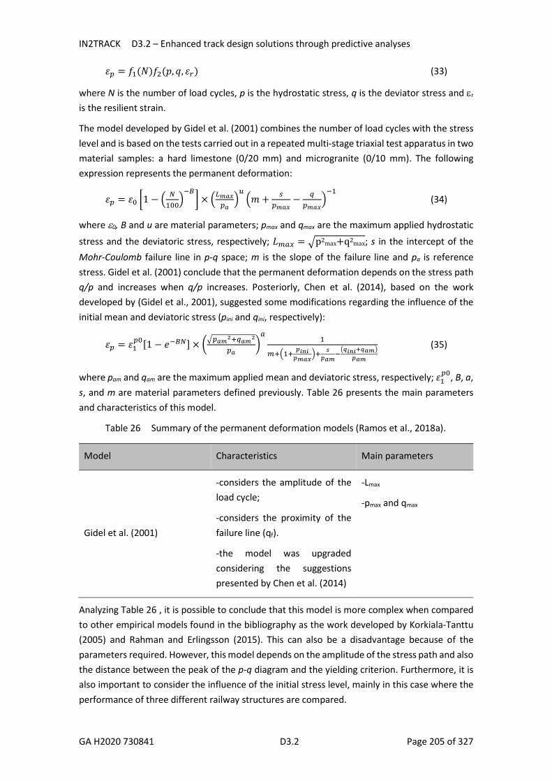
IN2TRACK D3.2 – Enhanced track design solutions through predictive analyses
GA H2020 730841 D3.2 Page 205 of 327
𝜀 = 𝑓 (𝑁)𝑓 (𝑝, 𝑞, 𝜀 ) (33)
where N is the number of load cycles, p is the hydrostatic stress, q is the deviator stress and r is the resilient strain.
The model developed by Gidel et al. (2001) combines the number of load cycles with the stress level and is based on the tests carried out in a repeated multi-stage triaxial test apparatus in two material samples: a hard limestone (0/20 mm) and microgranite (0/10 mm). The following expression represents the permanent deformation:
𝜀 = 𝜀 1 − × 𝑚 + − (34)
where 0, B and u are material parameters; pmax and qmax are the maximum applied hydrostatic
stress and the deviatoric stress, respectively; 𝐿 = p2max+q2
max; s in the intercept of the
Mohr-Coulomb failure line in p-q space; m is the slope of the failure line and pa is reference stress. Gidel et al. (2001) conclude that the permanent deformation depends on the stress path q/p and increases when q/p increases. Posteriorly, Chen et al. (2014), based on the work developed by (Gidel et al., 2001), suggested some modifications regarding the influence of the initial mean and deviatoric stress (pini and qini, respectively):
𝜀 = 𝜀 [1 − 𝑒 ] × (35)
where pam and qam are the maximum applied mean and deviatoric stress, respectively; 𝜀 , B, a, s, and m are material parameters defined previously. Table 26 presents the main parameters and characteristics of this model.
Table 26 Summary of the permanent deformation models (Ramos et al., 2018a).
Model Characteristics Main parameters
Gidel et al. (2001)
-considers the amplitude of the load cycle;
-considers the proximity of the failure line (qf).
-the model was upgraded considering the suggestions presented by Chen et al. (2014)
-Lmax
-pmax and qmax
Analyzing Table 26 , it is possible to conclude that this model is more complex when compared to other empirical models found in the bibliography as the work developed by Korkiala-Tanttu (2005) and Rahman and Erlingsson (2015). This can also be a disadvantage because of the parameters required. However, this model depends on the amplitude of the stress path and also the distance between the peak of the p-q diagram and the yielding criterion. Furthermore, it is also important to consider the influence of the initial stress level, mainly in this case where the performance of three different railway structures are compared.

IN2TRACK D3.2 – Enhanced track design solutions through predictive analyses
GA H2020 730841 D3.2 Page 206 of 327
Throughout this study, values of the material parameters found in the work developed by Salour and Erlingsson (2015) have been used.
10.2.4 Methodology The methodology presented in this work is based on the 2.5D FEM-PML approach and in the implementation of an empirical model. Figure 170 presents a resume of the proposed methodology.
Figure 170 Schematic formulation of the proposed methodology
From the numerical modelling, the principal stresses are obtained, which allows determining the hydrostatic and deviatoric stresses, which are important input parameters to the permanent deformation models.
In this work, in order to obtain the long-term performance of the railway structure and the soil degradation process, we are more interested in the dynamic mechanism, since the track irregularities increase the interaction forces and may cause an increase in acceleration during the track degradation. This is carried out through an introduction of a modification of the regular rail profile geometry in the numerical models.
10.2.5 Case study – description The case study presented in this report follows the previous methodology that includes the numerical modelling and the implementation of the empirical model. This case study establishes a comparison between three railway structures: ballasted track, a slab track (Rheda system) and a special slab track based on the Rheda system constituted only by the concrete slab (the support layers were not considered). This study allows understanding the performance of the different railway structures and identifies the main characteristics and differences, mainly in terms of the long-term performance. The obtained results will help to compare the stress levels and stress paths induced in the subgrade on the ballasted and slab tracks due to the passage of
2.5D formulation(FEM-PML)
Stresses:x,y,x,xy,xz,yz
Principal stresses1,2,3p and q
Inputs: p;q Permanent deformation empirical models
Stress path
Quasi-static mechanism
Dynamic mechanism –> implementation of a track irregularity

IN2TRACK D3.2 – Enhanced track design solutions through predictive analyses
GA H2020 730841 D3.2 Page 207 of 327
a train. The ballasted track is composed of the rail, railpad, sleepers ballast, sub-ballast and the foundation soil. The slab track (Rheda system) is composed of the rail, railpads, concrete slab, support layer designated as hydraulically bonded layer (HBL), frost protection layer (FPL) and foundation soil. This work also studied the Rheda system only constituted by the concrete slab (HBL and FPL were suppressed). In Figure 171 a typical cross-section of a ballasted track and the Rheda system are presented.
Figure 171 Schematic formulation of the proposed methodology
In order to obtain, expeditiously, the stresses and the stress paths, the 2.5D models were used and the values of the permanent deformation were obtained through an empirical model developed by Gidel et al. (2001) and updated by (Chen et al., 2014). In fact, the values of the stress levels obtained from the numerical modelling are important input parameters to the analysis of the permanent deformation.
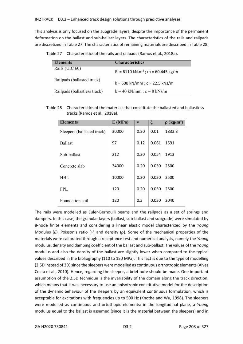
IN2TRACK D3.2 – Enhanced track design solutions through predictive analyses
GA H2020 730841 D3.2 Page 208 of 327
This analysis is only focused on the subgrade layers, despite the importance of the permanent deformation on the ballast and sub-ballast layers. The characteristics of the rails and railpads are discretized in Table 27. The characteristics of remaining materials are described in Table 28.
Table 27 Characteristics of the rails and railpads (Ramos et al., 2018a).
Elements Characteristics Rails (UIC 60)
EI = 6110 kN.m2 ; m = 60.445 kg/m
Railpads (ballasted track) k = 600 kN/mm ; c = 22.5 kNs/m
Railpads (ballastless track) k = 40 kN/mm ; c = 8 kNs/m
Table 28 Characteristics of the materials that constitute the ballasted and ballastless tracks (Ramos et al., 2018a).
Elements E (MPa) kg/m3
Sleepers (ballasted track) 30000 0.20 0.01 1833.3
Ballast 97 0.12 0.061 1591
Sub-ballast 212 0.30 0.054 1913
Concrete slab 34000 0.20 0.030 2500
HBL 10000 0.20 0.030 2500
FPL 120 0.20 0.030 2500
Foundation soil 120 0.3 0.030 2040
The rails were modelled as Euler-Bernoulli beams and the railpads as a set of springs and dampers. In this case, the granular layers (ballast, sub-ballast and subgrade) were simulated by 8-node finite elements and considering a linear elastic model characterized by the Young Modulus (E), Poisson’s ratio () and density (). Some of the mechanical properties of the materials were calibrated through a receptance test and numerical analysis, namely the Young modulus, density and damping coefficient of the ballast and sub-ballast. The values of the Young modulus and also the density of the ballast are slightly lower when compared to the typical values described in the bibliography (110 to 150 MPa). This fact is due to the type of modelling (2.5D instead of 3D) since the sleepers were modelled as continuous orthotropic elements (Alves Costa et al., 2010). Hence, regarding the sleeper, a brief note should be made. One important assumption of the 2.5D technique is the invariability of the domain along the track direction, which means that it was necessary to use an anisotropic constitutive model for the description of the dynamic behaviour of the sleepers by an equivalent continuous formulation, which is acceptable for excitations with frequencies up to 500 Hz (Knothe and Wu, 1998). The sleepers were modelled as continuous and ortothopic elements: in the longitudinal plane, a Young modulus equal to the ballast is assumed (since it is the material between the sleepers) and in
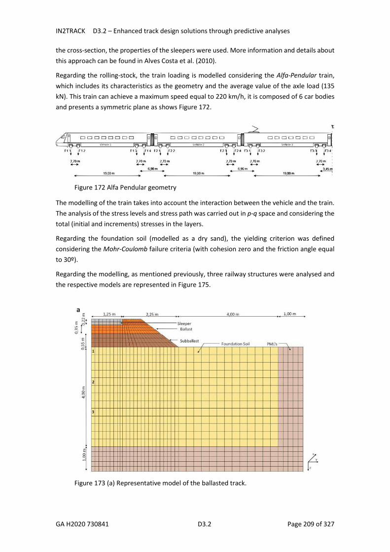
IN2TRACK D3.2 – Enhanced track design solutions through predictive analyses
GA H2020 730841 D3.2 Page 209 of 327
the cross-section, the properties of the sleepers were used. More information and details about this approach can be found in Alves Costa et al. (2010).
Regarding the rolling-stock, the train loading is modelled considering the Alfa-Pendular train, which includes its characteristics as the geometry and the average value of the axle load (135 kN). This train can achieve a maximum speed equal to 220 km/h, it is composed of 6 car bodies and presents a symmetric plane as shows Figure 172.
Figure 172 Alfa Pendular geometry
The modelling of the train takes into account the interaction between the vehicle and the train. The analysis of the stress levels and stress path was carried out in p-q space and considering the total (initial and increments) stresses in the layers.
Regarding the foundation soil (modelled as a dry sand), the yielding criterion was defined considering the Mohr-Coulomb failure criteria (with cohesion zero and the friction angle equal to 30º).
Regarding the modelling, as mentioned previously, three railway structures were analysed and the respective models are represented in Figure 175.
Figure 173 (a) Representative model of the ballasted track.

IN2TRACK D3.2 – Enhanced track design solutions through predictive analyses
GA H2020 730841 D3.2 Page 210 of 327
Figure 174 (b) Representative model of the Rheda system.
Figure 175 (c) Representative model of the ballastless track constituted only by the concrete.

IN2TRACK D3.2 – Enhanced track design solutions through predictive analyses
GA H2020 730841 D3.2 Page 211 of 327
From the numerical models, the quasi-static and dynamic mechanisms were compared. In this analysis, the dynamic mechanism is only due to irregularities on the track (and not on the wheel). This formulation considers that there isn't any loss of contact between the rail and the wheel of the train during the analysis.
According to EN13848-5 (2008), three range of wavelengths were defined:
1<<3; 3<<25 (designated as D1); 25<<70 (designated as D2).
These ranges allow understanding which are the irregularities that most affect the long-term performance of the railway structure. Thus, from this range of wavelengths, the frequencies and also the artificial irregularities profile were defined (Figure 176, Figure 177 and Figure 178). These profiles were generated by the Power Spectral Density (PSD) defined by FRA (equation 30) and considering 40 frequencies. Since the value of the parameter A in equation 30 is limited by the train’s speed (according to the geometric quality of the track), its value was adapted considering the alert limits defined in EN13848-5 (2008) that includes:
Limit of the standard deviation (in mm); Maximum peak value regarding the average of the longitudinal levelling.
The irregularities were defined by the number of harmonic described by a sinusoidal function:
𝑦(𝑖) = 𝑅 𝑒 (36)
where Ri is the amplitude of the irregularity and ki is the wavenumber.
Figure 176 Irregularity profile (3<<25)
Irre
gul
arity
am
plitu
de (
m)

IN2TRACK D3.2 – Enhanced track design solutions through predictive analyses
GA H2020 730841 D3.2 Page 212 of 327
Figure 177 Irregularity profile (1<<3)
Figure 178 Irregularity profile (25<<70)
Results– Stress levels
Considering the irregularity profiles and a train speed equal to 200 km/h, the quasi-static and dynamic mechanism were compared for all the railway structures. For comparison purposes, element 1 of each structure was used (see Figure 175).
Irre
gula
rity
ampl
itude
(m
)Ir
reg
ular
ity a
mpl
itude
(m
)

IN2TRACK D3.2 – Enhanced track design solutions through predictive analyses
GA H2020 730841 D3.2 Page 213 of 327
Figure 179 Stress path (ballasted track) – v=200 km/h
Figure 180 Stress path (ballastless track) – v=200 km/h
Figure 181 Stress path (ballastless track only constituted by the concrete slab) – v=200 km/h

IN2TRACK D3.2 – Enhanced track design solutions through predictive analyses
GA H2020 730841 D3.2 Page 214 of 327
Analyzing Figure 179, Figure 180 and Figure 181 it is possible to conclude that for all the type of structures, the irregularity profiles characterized by wavelengths between 1m and 3m induced higher stress levels. For >3m, the dynamic stresses are almost (3<<25) or even equal (25<<70) to the quasi-static stresses. In fact, the static stresses are overlaid to the dynamic stresses on the case where 25<<70, which means that there isn’t any amplification of the stress levels. These results are supported by Table 29, Table 30 and Table 31 , which present the maximum hydrostatic (dp;máx) and deviatoric (dq;máx) stresses in terms of increments induced by the passage of the trains. Figure 182 presents the comparison of the stress paths for all the structures considering element 1 and the case where the wavelength of the irregularity profile varies between 1m and 3m.
Table 29 Stress in the ballasted track (element 1; v=200 km/h).
Ballasted track dp;máx dq;máx
f=0 Hz Stress (kPa) 7.00 11.50
(1<<3) f=∑ 𝑓 Stress (kPa) 9.50 15.88
Increment (%) 35.71 38.10
(3<<25) f=∑ 𝑓 Stress (kPa) 7.35 12.30
Increment (%) 5.00 7.00
(25<<70) f=∑ 𝑓 Stress (kPa) 7.00 11.50
Increment (%) 0.00 0.00
Table 30 Stress in the ballastless track (element 1; v=200 km/h).
Ballastless track dp;máx dq;máx
f=0 Hz Stress (kPa) 5.70 10.72
(1<<3) f=∑ 𝑓 Stress (kPa) 7.44 12.90
Increment (%) 30.53 20.34
(3<<25) f=∑ 𝑓 Stress (kPa) 5.77 10.87
Increment (%) 1.23 1.40
(25<<70) f=∑ 𝑓 Stress (kPa) 5.70 10.72
Increment (%) 0.00 0.00

IN2TRACK D3.2 – Enhanced track design solutions through predictive analyses
GA H2020 730841 D3.2 Page 215 of 327
Table 31 Stress in the ballastless track only constituted by the concrete slab (element 1; v=200 km/h).
Ballastless track dp;máx dq;máx
f=0 Hz Stress (kPa) 9.07 11.74
(1<<3) f=∑ 𝑓 Stress (kPa) 11.43 14.26
Increment (%) 26.02 21.47
(3<<25) f=∑ 𝑓 Stress (kPa) 9.27 12.12
Increment (%) 2.21 3.24
(25<<70) f=∑ 𝑓 Stress (kPa) 9.07 11.74
Increment (%) 0.00 0.00
Figure 182 Stress path (ballastless track only constituted by the concrete slab) – v=200 km/h
Analysing the previous tables, it is possible to conclude that, according to the results of the stress paths, the dynamic mechanism (namely the irregularity profiles characterized by wavelengths between 1m and 3m) significantly increases the stress magnitudes and the magnitude is higher in the case of the ballasted track. This conclusion is based in the element 1 of each numerical model presented in Figure 175. This element is near to the symmetry plane and close to the surface. As shown in Figure 182, all the railway structures have different initial mean stresses, which have an influence on the permanent deformation results.

IN2TRACK D3.2 – Enhanced track design solutions through predictive analyses
GA H2020 730841 D3.2 Page 216 of 327
The influence of the train speed was also studied considering a comparison between 144 km/h and 200 km/h for all type of structures and irregularity profiles. The influence of this factor is not observable in cases where is higher than 3m. In fact, in these cases, the dynamic stress paths are almost or even equal to the stress path of the quasi-static mechanism. In fact, previous studies show that the influence of the train speed in the case of the quasi-static mechanism is only relevant when the train speed is close to the critical speed. Otherwise, its influence is almost irrelevant and the stress paths are almost overlaid (Ramos et al., 2018b).
The obtained results are presented in Figure 183, Figure 184 and Figure 185. Analysing the figures, it is possible to conclude that, despite the fact that there is a slight difference in the stress paths, the difference is not significant. This fact is relevant when the permanent deformation is analysed since the main input parameters are the maximum value of the hydrostatic and deviatoric stresses and these values are almost equal for both train speeds.
Figure 183 Stress path (ballasted track) – comparison between 144 km/h and 200 km/h (1<<3)
Figure 184 Stress path (ballastless track) – comparison between 144 km/h and 200 km/h (1<<3)

IN2TRACK D3.2 – Enhanced track design solutions through predictive analyses
GA H2020 730841 D3.2 Page 217 of 327
Figure 185 Stress path (ballastless track only constituted by the concrete slab) – comparison between 144 km/h and 200 km/h
Results – Permanent deformation
After the determination of the stress levels on each element of each structure, the purpose of the next stage is to obtain the soil degradation considering a certain number of load cycles that corresponds to the passage of the train. As mentioned previously, an empirical permanent deformation model was used to obtain the permanent deformation of the foundation soil of the railway structures. The analysis was only carried out on this layer since it is the element common to each structure. Implementing the empirical model, it is possible, to obtain the permanent deformation on each structure. In this case, the Mohr-Coulomb yielding criterion (c=0 kPa and =30º) was used.
Figure 186 to Figure 188 show a colour graph regarding the permanent deformation. It is based on the mid-coordinate of each element. Since only the stresses from the case 1<<3 are relevant, the permanent deformation results will be focused on this range.
Figure 186 Permanent deformation of the ballasted track (v=200 km/h)

IN2TRACK D3.2 – Enhanced track design solutions through predictive analyses
GA H2020 730841 D3.2 Page 218 of 327
Figure 187 Permanent deformation of the slab track (v=200 km/h)
Figure 188 Permanent deformation of the slab track only constituted by the concrete slab (v=200 km/h)
In Figure 189, Figure 190 and Figure 191, the cumulative permanent deformation for the first alignment (near the symmetric plane) and for each type of railway structure are presented.

IN2TRACK D3.2 – Enhanced track design solutions through predictive analyses
GA H2020 730841 D3.2 Page 219 of 327
Figure 189 Cumulative permanent deformation of the ballasted track (v=200 km/h) – alignment 1
Figure 190 Cumulative permanent deformation of the ballastless track (v=200 km/h) – alignment 1
Cumulative permanent deformation (mm)-0.24 -0.22 -0.2 -0.18 -0.16 -0.14 -0.12 -0.1 -0.08 -0.06 -0.04 -0.02 0
De
pth
(m
)
-4
-3.5
-3
-2.5
-2
-1.5
-1
-0.5
0
1< <3 (alig.1)3< <25 (alig.1)25< <70 (alig.1)
Cumulative permanent deformation (mm)-0.24 -0.22 -0.2 -0.18 -0.16 -0.14 -0.12 -0.1 -0.08 -0.06 -0.04 -0.02 0
De
pth
(m
)
-4.5
-4
-3.5
-3
-2.5
-2
-1.5
-1
-0.5
0
3< <25 (alig.1)1< <3 (alig.1)25< <70 (alig.1)

IN2TRACK D3.2 – Enhanced track design solutions through predictive analyses
GA H2020 730841 D3.2 Page 220 of 327
Figure 191 Cumulative permanent deformation of the ballastless track (only constituted by the concrete slab) (v=200 km/h) – alignment 1
Analyzing Figure 186-Figure 188, it is possible to conclude that for the ballasted track, the first two rows of the elements near the surface (≈0.7 m) present higher values of permanent deformation. The remaining elements present residual values. In the ballastless track, the first three rows of the elements near the surface (≈1.0 m) present significant values. In the ballastless track constituted only by the concrete slab, the first four rows present significant values in terms of permanent deformation (≈1.40 m). This is due to the omission of the support layers, which implies higher permanent deformation values on the foundation layer. In all the structures, in the first row of the model, in the elements outside the railway structure, we identify higher values of the permanent deformation. This is due to the lack of weight of the structure, which means that the initial mean stress is inferior and the peak value of the p-q diagram is closer to the failure line.
Figure 189-Figure 191 show the importance of the support layer since the ballastless track only constituted by the concrete slab presents higher values of cumulative permanent deformation when compared to the other structures. In the ballasted and ballastless tracks, the values are very similar. When compared to ballastless track only constituted by the concrete slab, the increasing is close to 130%. As expected, the irregularity profiles characterized by the wavenumber between 1m and 3 m present higher stresses and also higher permanent deformation values.
10.2.6 Conclusion In this work, a methodology to evaluate the railway track long term dynamic behaviour due to soil degradation is presented. Firstly, a brief description of the 2.5D models is presented. This numerical approach allows obtaining expeditiously the stresses and strains on the elements of the railway structure. However, this approach implies some disadvantageous as the use of linear elastic models, namely in the case of the granular materials. In order to model the soil degradation, an empirical model was used. This model is based on laboratory tests and is more complex than empirical models found in the literature since it depends on the initial soil stress,
Cumulative permanent deformation (mm)-0.26 -0.24 -0.22 -0.2 -0.18 -0.16 -0.14 -0.12 -0.1 -0.08 -0.06 -0.04 -0.02 0
De
pth
(m
)
-4
-3.5
-3
-2.5
-2
-1.5
-1
-0.5
0
1< <3 (alig.1)
3< <25 (alig.1)
25< <70 (alig.1)

IN2TRACK D3.2 – Enhanced track design solutions through predictive analyses
GA H2020 730841 D3.2 Page 221 of 327
the amplitude in the p-q diagram and the distance between the peak of the p-q diagram and the yield limit. The stress variables obtained in the numerical modelling are used as input parameters to the empirical model as the p and q stresses (determined from the principal stresses).
This study also compares the performance of the ballasted and ballastless tracks. With this analysis, we conclude that the irregularities with small wavelengths (1<<3) present higher amplification of the stresses. These wavelengths are almost equivalent to the discret irregularities on the wheel of the vehicle. The remaining ranges of wavelengths (3<<25 and 25<<70) present stress levels almost or even equal to the quasi-static stresses, which means that there is no dynamic amplification. This conclusion covers any type of railway structure. However, the ballasted track is more susceptible to this effect because of its stiffness.
Regarding the permanent deformation, and considering their mechanical properties and geometries, the ballasted and ballastless tracks present similar cumulative permanent deformation (close to 0.1mm). However, in the case where the ballastless track is only composed of the concrete slab, there is an increase of the cumulative permanent deformation of about 130%. This is due to the omission of the support layer.
10.3 Material and component characteristics for whole system modelling of elastomers and concrete products
10.3.1 Under sleeper pads Sleeper pads preserve the superstructure, improve the quality of the track geometry and reduce disruptive vibrations, both in the open track, in transition zones and within turnouts. Sleeper pads offer the following advantages:
Reduction of maintenance expenses Prolongings of the service life of the track structure Reduction of disruptive vibrations
Sleeper pads offer operators the opportunity to significantly reduce the annual maintenance costs for tracks and switches. Elastic sleeper pads are placed directly beneath the track sleepers and increase the vertical elasticity in the superstructure. With sleeper pads, the load of the rail cars is evenly distributed over the elastic components in the subsoil. Sleeper pads with defined elastic properties significantly reduce wear on the rail line. Highly elastic sleeper pads can also represent an economical alternative to Under Ballast Mats (UBM) as a vibration-isolating measure.
The most common type of superstructure used in the world is ballasted track. Ballast, as the weakest link in the system, is subject to latent dynamic shifting. Loads (ballast compression) lead to wear and breaking up of the rocks. These effects decrease the quality of the track geometry, and the track bed must be tamped.

IN2TRACK D3.2 – Enhanced track design solutions through predictive analyses
GA H2020 730841 D3.2 Page 222 of 327
The effective installation of sleeper pads slows down this process in the following ways:
Distribution of the axle load over a larger number of sleepers The elastic properties of the sleeper pads lengthen the bending line of the rails. The load from the train is distributed over a larger number of sleepers and therefore over a larger area. This reduced average compression also reduces the load on the ballast.
Weakening of the dynamic forces and vibrations in the ballast Sleeper pads reduce the direct dynamic load on the ballast. This reduces shifting of the ballast as well as settling of the track.
Padded sleepers Increase of the contact surface between sleeper and ballast The unique properties of the polyurethane material result in an ideal embedding of the ballast in the surface of the sleeper pads, stabilizing the top-most ballast layer. This yields an increase in the contact surface between sleeper and ballast from about 8 % (without padding) to up to 35 % (with padding).
10.3.2 Material behaviour of Getzner materials To be able to calculate the superstructure with Getzner Under Sleeper Pads (USP) the following information is needed as input e.g. for a FE-Model:
Material bedding non-linearity
As can be seen in the load deflection curve (Figure 192) the material behaviour regarding load – deflection is non-linear and due to its elasto-plasticity and damping the retention of the original shape delayed. A single value is not representative for the material behaviour – the load deflection curve has to be implemented.
Figure 192 Load deflection curve SLB2210 of the 3rd load cycle on ballast plate according to DIN 45673-1. (Getzner Werkstoffe)

IN2TRACK D3.2 – Enhanced track design solutions through predictive analyses
GA H2020 730841 D3.2 Page 223 of 327
Contact area non-linearity
The elasto-plastic material behaviour enables an embedding of the rocks within the USP as mentioned above. This increases the contact area between the sleeper and the ballast and thereby reduces the contact pressure. With an increase of load the ballast rocks will be embedded within the USP and the contact area rises in a non-linear behaviour. (SLB 2210 shows a contact area above 25%).
Reduction of hanging areas
Due to the improved bedding hollow areas underneath sleeper pads will not appear and the distributed forces are well defined. If non bedded track is calculated, hanging sleepers have to be taken into account (without USP complete sleepers can be found hovering several mm above the ballast).
10.4 Track Information Model (TIM) framework
The objective of this task is to develop a specific information model framework adapted to the specific needs and peculiarities for an efficient application of BIM (Building Information Modeling) in the railway projects.
Our ambition is to achieve a living model capable of assimilating incoming data from inspection and monitoring in order to carry out an evaluation process, providing maintenance recommendations scheduled and budgeted accurately.
10.4.1 BIM (Building Information Modeling) The building information modeling (BIM) is an emerging technology providing a comprehensive framework for building of integrated information environment in construction projects. It generally uses 3-D based and object-oriented modeling tools. The interoperability of the model data is also a major concern in the BIM technology. The Industry Foundation Classes (IFC) developed by buildingSMART is becoming a de-jure standard supported by commercial BIM tools.
BIM is used widely in the building sector with success but it has not had the same impact on the civil construction sector, in particular the railway sector.
Regarding the definition of BIM, it could be adopted from (GSA, BIM Guide Overview. (Electronic) PDF-format, 2007), the U.S. General Services Administration:
“Building Information Modeling is the development and use of a multi-faceted computer software data model not only to document a building design, but to simulate the construction and operation of a new capital facility or a recapitalized (modernized) facility. The resulting Building Information Model is a data-rich, object-based, intelligent and parametric digital representation of the facility, from which views appropriate for various users’ needs can be extracted and analyzed to generate feedback and improvement of the facility design.

IN2TRACK D3.2 – Enhanced track design solutions through predictive analyses
GA H2020 730841 D3.2 Page 224 of 327
Figure 193 Life cycle of Building Information Modeling (APROPLAN)
BIM stages
During the pre-BIM stage there is very much dependence on 2D documentation, even though some 3D documentation is generated, it lacks intelligence, and cost-estimates and quantities cannot be generated from the visualization model.
BIM stage 1 is initiated by the use of an object-based 3D parametric software tool, where users generate models within design, construction or operation – the lifecycle phases. Collaborative practices are similar to pre-BIM status and there is no significant model-based collaboration. However, the object-based models allow an earlier increased detail level of design and construction matters which enables faster project life-cycle phases (Succar, 2009).
BIM stage 2 is when players actively collaborate with players from other disciplines. Model-based collaboration may occur within one or between two project lifecycle phases.
BIM stage 3 is when integrated models are created, shared and maintained collaboratively throughout the project lifecycle phases. (Succar, 2009)
The ultimate goal of BIM implementation is to reach integrated project delivery (IPD), which integrates people, systems, business structures and practices into a collaborative process to optimize project results, increase owner value, reduce waste and maximize efficiency through all phases of design, fabrication and construction (Succar, 2009)

IN2TRACK D3.2 – Enhanced track design solutions through predictive analyses
GA H2020 730841 D3.2 Page 225 of 327
Figure 194 The different stages of BIM (Succar, 2009)
BIM tools and parametric modelling
Object-based parametric modeling allows representing objects with fixed geometry and properties by parameters and rules that determine the geometry (it distinguishes modern BIM design applications from earlier CAD applications) The parameters and rules can be used to describe the relation to other objects, which means that objects automatically updates according to changing contexts. This is called the behavior of the object. Complex geometries can be modeled using this technique, customized object libraries could be made for a specific use, add other attributes to the objects depending on their needs.
BIM design applications can carry out specific tasks as a tool, while at the same time providing a platform for data management within a model for different uses. Some have the ability to manage data in different models, also known as a BIM environment (Eastman, 2011).
Interoperability
The idea of interoperability can be explained as a seamless exchange of information between different computer programs.
In terms of data exchange and interoperability, the use of object-based modelling in various areas of the construction industry is improving the value of interoperability. It should meet the following technical needs:
Interchange of information between different roles at a stage in a project. Continued use of information through the different stages of a project To be able to access archived data through the life of facility, it should be accessible
even if the creating software is no longer available.
Benefits from using BIM
BIM aims at maximizing the value and minimizing the waste, to drive the productivity further. This leads to a reduced time and cost for design and construction, an increased complexity of design, a more suitable design and construction and an overall improved building performance (Eastman, 2011).
Regarding the benefits for the owner, they are focused on:
Knowing if a structure of a given size, quality and program requirements can be built within a given cost and time budget.
Increased building performance and quality Improved collaboration using integrated project delivery (IPD)
In terms of benefits for the designer, they aim at:
Earlier and more accurate visualizations of a design

IN2TRACK D3.2 – Enhanced track design solutions through predictive analyses
GA H2020 730841 D3.2 Page 226 of 327
Automatic low-level corrections when changes are made to the design Generation of accurate and consistent 2D drawings at any stage of the design Earlier collaboration of multiple design principles Cost estimates throughout the design phase
Concerning the benefits for the contractor, they are focused on:
Quick reaction to design changes Discovery of design errors and CAWs (Changes and Additional Work) before
construction Synchronization of design and construction planning Better implementation of lean construction techniques Synchronization of procurement with design and construction Machine-guidance. (Digital terrain models, GPS)
In next figure the benefits from using BIM are showed.

IN2TRACK D3.2 – Enhanced track design solutions through predictive analyses
GA H2020 730841 D3.2 Page 227 of 327
Figure 195 Some of the identified benefits from using BIM (Norberg, 2012)

IN2TRACK D3.2 – Enhanced track design solutions through predictive analyses
GA H2020 730841 D3.2 Page 228 of 327
10.4.2 Implementation of BIM in railway sector Owing to BIM has been implemented in the last few years, most of the railway projects have not been carried out by BIM through all the project phases: design, construction and operation. For this reason, the aim of BIM implementation in the railway sector is to define and analyse the minimum necessary amount of data in design and construction phase, to carry out the management properly during the operation phase.
Figure 196 BIM Project phases and the information flow
Track information model framework (BIM)
Regarding the track information model framework, it should be classified into different structural levels, and the minimal data (key information) for every level should be defined, which allow all users (Infrastructure Managers, IMs) to get an insight of the model in order to optimize the performance of the railway operation through BIM model from the IM´s point of view.

IN2TRACK D3.2 – Enhanced track design solutions through predictive analyses
GA H2020 730841 D3.2 Page 229 of 327
Figure 197 BIM track Information model framework
Besides these basic elements of information, the more extra information that can be added to an object, the more clearly and distinguishably the objects can be visualized, categorized and analysed. Different design units should add additional information to the objects in the BIM model, in the railway design, every element of the rail design should be linked to a specific object type of the software’s object library, which would allow for the ballast bed, rails etc. to be clearly visible. This distinction allows even better visualizing and interpreting the different design elements of the railway study.
The object library should cover as much as possible the railway operation. Then additional information is added such as article numbers, material type and coding. This information is placed in a database and its condition should retrieve material lists automatically. The aim is that all the objects should be included in the object library. Using hook-points for insertion and detailed object information placed in a database should solve problems with the level of detail in the objects, as well as how objects should be connected to other objects.
Implementation of BIM in railway maintenance
The Building Information Modeling for railway inspection and maintenance should be a comprehensive inventory management system with the ability to process railway inspection and component information for use in inspection management, maintenance programming, budget development and strategic maintenance planning. The purpose of BIM in railway maintenance management is to capture and reuse information gathered during an inspection to automate the evaluation process in order to provide maintenance recommendations scheduled and budgeted accurately.
It should provide most of the pertinent engineering information required to establish priorities for maintenance and to ensure the identification of deficient components and that the maintenance process is being managed properly.

IN2TRACK D3.2 – Enhanced track design solutions through predictive analyses
GA H2020 730841 D3.2 Page 230 of 327
The application of Building Information Modelling (BIM) in railway maintenance management should comply with the following requirements:
modeling for inspection and evaluation method. (3D models), visualization effect to enhance the overall comprehensiveness with information associated.
retrieval of the last inspection information, including all condition ratings, explanation of condition, maintenance recommendations, and special comments for next inspection.
collection, storage, process, retrieval, and analysis of railway inspection information. the system should increase the database integrity by avoiding redundancy and better
accuracy. provides inspection tasks scheduled, task assignment for inspectors, and inspection
preparation for inspectors. provides maintenance recommendations and estimated repair quantities, which would
be used by railway managers in the decision-making process. And monitoring the status of the maintenance work.
the system should be designed to take advantage of mobile devices with wireless communication capability (real-time access to documentation such as previous inspections, plans), GPS sensor, and photo shooting lens, to assist inspection on-site. Inspection results should be uploaded wirelessly to the remote server
the system should be founded on a Geographic Information System (GIS). Railway components and associated inspection records should be located in maps.
With reference to the future objectives, the application of BIM in the railway maintenance process should be focused on the following guidelines:
maximize the life and serviceability of railway infrastructure by identifying potential problems at an early stage.
prediction of premature failures of railway elements or track geometry degradation using statistical analysis of inspection data, becoming an invaluable data repository for predictive analysis.
evaluation of the effectiveness maintenance process and identification of areas that require revision and/or research
analysis of the track geometry degradation and railway element degradation as a function of time.
schedule and cost estimation of maintenance activities based on statistical information modeling a railway infrastructure and documenting damage information, creating
models in an inventory with emerging technology 3D laser scanning or structure from motion SFM, owing to conventional BIM modeling techniques are economically unfeasible.
the system should be focused on getting a high efficiency of the tamping machines during the available possession time. This process would be based on characteristics of the tamping machines (travelling speed and tamping speed, number of tamping machines) the topology of the railway network (number of switches, side track where the tamping machine must be allocated in order not to disturb normal train operations), duration of tamping interventions during the night service interruptions
the system should be focused on a long term tamping planning strategy, which would be able to solve where tamping should be performed to achieve the best result and how the budget can be spent in the most cost-efficient way. Consequently, a long term tamping planning would make it easier to coordinate with other maintenance operations and would make it optimize the track possession, furthermore this new tool would make tamping planning minimize the costs of corrective tamping.
IN2TRACK D3.2 – Enhanced track design solutions through predictive analyses
GA H2020 730841 D3.2 Page 231 of 327
10.5 Modelling of asphalt track for guideline trackbed design charts
10.5.1 Problem statement Ballasted track is the conventional type of track structure in Europe and around the world. Although it has several benefits, it often requires notable maintenance to ensure adequate operating conditions. Railway track geometry deterioration due to differential settlement of ballast/subgrade is one of the main problems that lead to significant maintenance costs. Also, the high axle loads and operating speeds lead to higher dynamic forces that in combination with high rate of settlement can increase even more the track geometry deterioration. The ongoing railway infrastructure strategies require innovative track design solutions of low maintenance. The track structural design plays a major role in the structural and deformation behaviour of the track, and consequently in the maintenance and availability of the track line (traffic volume, speed limits). This can affect the rail operation and the profitability from the rail service. Apart from slab track that in most cases requires significant investments, an alternative solution that may lead to satisfactory balance of investment and maintenance costs is the use of asphalt in the railway track structure. The asphalt can be used either as a ballast underlayment substituting entirely or partially the subballast granular layer (formation) or as a ballastless asphalt track where the sleepers or slab are placed directly on an asphalt layer that is positioned in a treated base. Using asphalt as formation constitutes a potential of a resilient track structure reducing the need for frequent maintenance and improving whole life cost. This project develops guidelines for an effective track bed design using asphaltic formation instead of conventional granular material. This is performed with the aid of Finite Element Modelling (FEM) to allow evaluation of the deformation performance and sleeper support stiffness.
10.5.2 Aim The aim of the study is to develop design charts for trackbed design using asphaltic formation for different subgrade modulus (E) using means of FEM with minimum total depth of construction (minimum depth of ballast and minimum depth of fill material).
10.5.3 Methodology To achieve the above aim the first step is to undertake a literature review about previous application of asphalt in railway track, advantages and disadvantages of using asphalt formation in the railway track, design criteria of asphalt formation, numerical techniques and critical factors in modelling asphalt in railway track. In a second phase, by considering the critical conclusions of the literature review, the development of a numerical model to mimic the existing UK track bed design approach is required. The function of a Falling Weight Deflectometer (FWD) and its use in the UK trackbed design approach to measure the dynamic sleeper support stiffness is discussed. FEM is then developed to mimic the response of a FWD to measure the FWD sleeper support stiffness. This requires the determination of appropriate material properties; type of analysis and validation of the FEM. FEM analyses are then carried out for multiple

IN2TRACK D3.2 – Enhanced track design solutions through predictive analyses
GA H2020 730841 D3.2 Page 232 of 327
simulation scenarios using asphalt formation for variable asphalt thickness and variable subgrade stiffness. The FEM results are critically assessed and are then used to create the new design charts for trackbed design using asphaltic formation. Different design examples with asphaltic formation are compared to the existing trackbed design with granular formation. Finally, conclusions are discussed, and recommendations are presented.
10.5.4 The use of asphalt in railway track Previous application of asphalt track
Several types of asphalt track have been tested worldwide (Rose & Souleyrette, 2014; Di Mino, Di Liberto, Maggiore, & Noto, 2012). These included mainly hot mix asphalt (HMA) bituminous track bed types that have been constructed and tested in US, Germany, Austria, Italy, France, Japan and Spain. Three different types of asphalt track have been tested;
(a) the asphalt underlayment where the asphalt layer substitutes the subballast granular layer
(b) the asphalt combination that combines asphalt and subballast layer and (c) the ballastless asphalt track that comprises sleepers or slab placed on asphalt layer
positioned in a treated base/subballast.
The typical thickness of asphalt layer used in these cases was 120-200mm. According to Rose and Souleyrette (2014) austrian practice showed that the use of an asphalt layer underneath the ballast bed decreased the annual deterioration rate of the track at 50% in comparison with the conventional granular track whereas french practice showed that asphalt as subballast layer reduced 50% the subgrade pressure readings. Rose and Tucker (2003) described a range of applications of a HMA (hot mix asphalt) layer as underlayment in special locations of the USA track network including tunnel floors and approaches, bridge approaches, crossing diamonds, crossovers and switch turnouts as a way of eliminating the increased maintenance needs of these sites. On the one hand, the use of asphalt track under ballast requires specific design and construction phases such as a well compacted subgrade and a well compacted asphalt layer. On the other hand, it can bring significant maintenance savings; $350,000 maintenance savings over 16 years were raised from the use of asphalt underlayment in a tunnel in Kentucky in 1985.
Advantages of asphaltic formation
The use of an asphalt layer as an underlayment between ballast and subgrade has several benefits. It can improve significantly the load distribution to the subgrade and reduce the subgrade pressures. Additionally, it can eliminate subgrade moisture fluctuations which subsequently improves the behaviour of the subgrade. The stable trackbed can eliminate track surface irregularities, maintain the track geometry and confine ballast and subgrade by providing a more consistent load carrying capacity even for low quality subgrades. Thus, it can provide diminished maintenance costs and a long-term efficient trackbed operation.
Disadvantages of asphaltic formation
Problems that have been related with asphaltic trackbed include cracking of the asphalt layer and development of pore water pressure under the asphaltic layer in cases where the asphaltic layer was built directly on the subgrade where ground water exists (Li, Hyslip, Sussman, &

IN2TRACK D3.2 – Enhanced track design solutions through predictive analyses
GA H2020 730841 D3.2 Page 233 of 327
Chrismer, 2002). For this reason, a granular layer between the asphalt and the subgrade is recommended (Li, Hyslip, Sussman, & Chrismer, 2002). In addition, according to Albalat et al. (2011) the lack of a sub-base granular layer and a well -compacted subgrade beneath the asphaltic layer could reduce the superstructure stability particularly at critical points (S&C, joints, transition zones and areas with high dynamic forces).
Design criteria for asphaltic trackbed design
Design criteria for asphalt in railway track are based in cumulative damage concepts depending on traffic, weather conditions and material properties (Li, Hyslip, Sussman, & Chrismer, 2002).
1. Maximum tensile strain (εt) and stress (σt) at the bottom of the asphalt layer for fatigue cracking
2. Maximum shear stresses on top of the surface of subgrade for permanent deformation
Tensile strain at the base of an asphalt layer increases with an increase in asphalt stiffness, see Figure 198. If this exceeds the ultimate tensile strain of the material, then failure by cracking is likely. Li et al. (2002) indicated that the subgrade stresses with 30cm ballast layer and granular subballast could be up to 144kPa whereas a 15cm HMA layer could reduce the subgrade stresses to 14kPa. Subgrade deformation from repeated loading can be seen as cumulative plastic strain and settlement, for the calculation of which the maximum deviatoric stress resulting from each loading cycle is taken into account.
Figure 198 Influence of asphalt stiffness on tensile stress in the asphalt and shear stress on the subgrade (from Brown, (2013))
The specified thickness for the asphalt layer varies depending on the quality of the support, traffic loadings and type of installation. A 125 to 150 mm of thickness is normally specified for average conditions in pavement engineering (Highways Agency, 2014) (“a minimum hydraulically bound mixture (HBM) base thickness of 150mm is allowed for flexible pavement construction”). Ballast thickness on top of subgrade normally varies from 200 to 300mm (Rose & Tucker, 2003). The soil below the asphalt layer should be well-compacted and well-drained. Asphalt mat is normally placed over 100 mm compacted soil material (Rose & Tucker, 2003). According to DMRB (Highways Agency, 2014) asphalt must be laid over foundations that have a surface stiffness modulus of at least 120MPa at time of construction.

IN2TRACK D3.2 – Enhanced track design solutions through predictive analyses
GA H2020 730841 D3.2 Page 234 of 327
Numerical techniques to model asphalt track and critical factors
Leykauf and Lechner (2001) indicated that the response of an asphalt pavement under dynamic loading within a temperature level below 20oC is nearly an elastic one. Therefore, the tensile stresses caused by the bending of the pavement are decisive (modulus of elasticity of asphalt between 5000 and 10000MPa). Temperature conditions higher than 20oC within the asphalt pavement will increase the amount of plastic deformations at the load contact area. Thus, in addition of the bearing capacity the occurrence of deformation caused by time and temperature dependent visco-elastic behaviour of asphalt must be considered.
Albalat et al. (2011) investigated the use of asphalt layer as substitution of the subballast using Drucker –Prager elasto-plastic constitutive law for soil and granular material where both elastic and visco-elastic model was used for the bituminous layer. The model included 11 sleepers, 9m width and 3m subgrade depth. FEM analyses indicated that a minimum 12cm of asphalt provided the required deformation of the track (deflection 1.6mm). They stated that the fatigue of bottom of asphalt (tensile strain at the bottom) will occur after the fatigue on subgrade. The requirement of subgrade compaction and asphalt compaction is highlighted though a field application in Italy where 30cm of subgrade were compacted and asphalt was compacted to 98% of maximum density.
Esmaelli et al. (2014) developed analytical calculations to investigate the effect of asphaltic formation in the trackbed behaviour. The asphalt layer’s tensile strain and compression stress on top of subgrade layer were determined as a function of load, asphalt thickness and CBR of the subgrade. The exponential equations were obtained by using KENTRACK simulation that use a linear elastic approach for the different railway track components. It was found that the asphalt tensile strain reduces with an increase of the CBR value (stiff soil) whereas the top of subgrade stress increases. The dynamic modulus of elasticity of asphalt is temperature and load frequency dependent and was defined based on Hwang-Witzac (Esmaelli, Amiri, & Jadidi, 2014) equation as follows:
𝐸 = 10 ∗ 10 (37)
where:
𝛽 = 𝛽 + 0.000005 ∗ 𝛽 − 0.00189 ∗ 𝛽 ∗ 𝑓 . (38)
𝛽 = 𝛽 . ∗ 𝛵 (39)
𝛽 = 0.553833 + 0.028829 ∗ 𝑃 ∗ 𝑓 . − 0.03476 ∗ 𝑉 + 0.070377 ∗ 𝜂 +
0.931757 ∗ 𝑓 . (40)
𝛽 = 0.483 ∗ 𝑉 (41)
𝛽 = 1.3 + 0.49825 ∗ log 𝑓 (42)
𝐸 = 10 ∗ 10 (43)
Ea: dynamic modulus of asphalt in psi
f: load frequency in Hz
T: temperature in oF

IN2TRACK D3.2 – Enhanced track design solutions through predictive analyses
GA H2020 730841 D3.2 Page 235 of 327
P200: aggregate passing No200 sieve in %
Vb: volume of bitumen in %
Vv: volume of air voids
η: asphalt viscosity at 70oF (21oC) in 106 poise
Using equations 37 - 43, the dynamic modulus of asphalt can vary from 1182 MPa, 2797 MPa up to 6146 MPa according to temperature range from 30 oC, 21 oC and 12 oC respectively and for typical values of f=1.5 Hz, Vb=13.5%, P200=5.5%, Vv=5.7% and η=2.5x10⁶ poise (Esmaelli, Amiri, & Jadidi, 2014).
Various asphalt moduli of elasticity have been indicated in literature such as 2000-3000MPa (Hakim, Brough , Bonney, & Govan, 2017) 9600MPa (Ramirez Cardona, et al., 2014), 5000-10000 MPa for T<20oC (Leykauf & Lechner, 2001), 2000-5000 MPa (Di Mino, Di Liberto, Maggiore, & Noto, 2012) 4813 MPa (Esmaelli, Amiri, & Jadidi, 2014).
Rose (2008) presented the resilient modulus of hot mix asphalt (HMA) from various field applications of asphalt trackbeds in US for load frequency 1Hz for temperatures 5oC and 25 C. The values depended on the age of the HMA in the track bed (after 1-23 years) and temperature at which they were evaluated. An average value of 3826 MPa for 5oC and 1420 MPa for 25oC was stated for a 14-year-old asphalt trackbed.
Ramirez Cordona et al. (2014) conducted 2D dynamic linear elastic FEM of asphalt track with an asphalt layer of thickness 14cm (E=9600MPa) overlaid (a) on a 20cm subballast layer and 700cm stiff subgrade (E=80MPa) and (b) on a 30cm treated soil (E=10000MPa) and a subgrade of E=50MPa. Sleeper vertical accelerations were validated with field measurements using pressure cells, strain gauges, temperature sensors and accelerometers. Stress on bottom of the capping layer (top of subgrade) was measured experimentally and the first case provided 70% reduction of stress in comparison with the reference non-asphalt case, while FEM showed higher stress level when a very stiff treated soil was used. The maximum tension strain amplitude at the bottom of the asphalt layer was found 2μm/m for the TGV (train à grande vitesse (high speed train)) train passage (320km/h) that was considered low and thus, it cannot lead to asphalt fatigue. However, humidity may affect the asphalt fatigue resistance. The authors supported that the order of magnitude of strain at the bottom of asphalt layer reduces with the speed increase that agrees with road pavement studies. Regarding the vertical stiffness, it was suggested that an increase of the asphalt layer thickness is preferable than the use of a very stiff supporting layer.
Huurman et al. (2002) investigated the behaviour of embedded rail in asphalt using linear elastic FEM. They conducted a parametric analysis for a range of cement filled porous asphalt (CFPA) with various asphalt moduli (950MPa, 12500MPa, 20000MPa) for various Poisson’s ratio (0.48, 0.45 and 0.25 respectively) and varying temperature (40oC, 14oC and -10oC respectively).
Despite the simplifications of theory of elasticity, the mechanical properties of asphalt mixes depend on time or frequency, which is a characteristic of viscoelastic materials. Their stiffness is mainly a function of the temperature and the frequency of the applied load (Ramos-Garcia & Castro, 2017). Their response to temperature depends on the bituminous binder. Low

IN2TRACK D3.2 – Enhanced track design solutions through predictive analyses
GA H2020 730841 D3.2 Page 236 of 327
temperature increases their stiffness while high temperature reduces their stiffness. Some authors indicate that the behaviour of asphalt mixes can be considered linear and elastic at high load application speeds (T=0.1s) and low temperatures (<10oC), while for greater load application periods and higher temperatures, their response is different due to viscosity (Ramos-Garcia & Castro, 2017).
Apart from the linear elastic FEM, other types of FEM have been performed including subroutines of stress dependent constitutive law for the asphalt layer such as viscoelastic (Chupin, Martin, Piau, & Hicher, 2014), elasto-viscoplastic with damage (Collop, Scarpas, Kasbergen, & de Bondt, 2003). Lee et al. (2014) used a 3D FE visco-elasto-plastic model (creep model) using ABAQUS to predict the permanent deformation of a railway ballasted track with asphalt as a subballast layer (E=500-6000MPa, thickness 5cm) and a stiff roadbed underlayment (E=180MPa, thickness 25cm). The creep model was validated against full scale laboratory cyclic tests. The model predicted 6mm of cumulative settlement after 3millions loading cycles. The range of dynamic modulus of asphalt had a small influence on the permanent deformations.
Di Mino et al. (2012) conducted a 2D analytical model of ballasted track with asphaltic subballast layers. They investigated two cases; one with 12cm traditional HMA and one with 30cm dry asphalt rubber mixture. The 2D lumped masses model included four levels of elasticity. The bending behaviour of asphaltic subballast was modelled by visco-elastic continuous beam, for which the stiffness and damping properties were determined after four-point bending tests of prismatic specimens at three different temperatures (10oC, 17oC, 25oC) and at varying loading frequency (0.1-20 Hz). The stiffness range of the HMA was found to be 500-8000MPa and the damping ratio range was found to be 0.05-0.55 (Figure 199). The model predicted up to 3mm deflections, slightly reduced accelerations and 40% pressure reduction in the subgrade layer when asphalt is used as a subballast layer.
Figure 199 Effect of loading frequency and temperature on HMA stiffness and damping ratio (from (Di Mino, Di Liberto, Maggiore, & Noto, 2012))
Lee et al. (2016) conducted full scale tests of directly fastened asphalt track (superstructure laid directly on asphalt layer overlaying reinforced soil layer (E=120MPa). Three different asphalt thicknesses were tested (20cm, 29cm and 35cm) under static loading up to 200kN. Strain at the bottom of the asphalt layer was measured up to 50-80 microstrain, thus the asphalt track was considered sufficient to support train loading without cracking. It was concluded that the required thickness of the asphalt layer should be >29cm to meet the requirements for the

IN2TRACK D3.2 – Enhanced track design solutions through predictive analyses
GA H2020 730841 D3.2 Page 237 of 327
allowable vertical stress on top of subgrade (133kPa, Korean specifications). Both the total displacements and permanent displacements were measured at rail, sleeper and top of subgrade level. It was concluded that 30cm is the most suitable thickness for the asphalt layer providing less than 2mm permanent deformation.
The threshold stress on top of subgrade can be calculated though the equation 44 of Heukelom and Klomp (BSI, 2017):
𝜎,
. ∗
. (44)
Where:
n: the number of loading cycles; unless otherwise specified n=2x10⁶ loading cycles;
Edyn: the dynamic Young’s modulus specified by the customer; if not specified and if Ev2 is applied then Edyn=Ev2 (BSI, 2017) (where Ev2 is the modulus of deformation in N/mm2).
Ballastless design requirements (BSI, 2017) define threshold stress value for top of subgrade to be 50kPa (“unless otherwise specified vertical stresses due to traffic load acting on unbound granular material shall not exceed 0.050 N/mm2”). In addition, EN 16432-2:2017 (BSI, 2017) gives specifications for bituminous (asphalt) layers of ballastless asphalt track (sleepers or slab placed on asphalt layer positioned in a treated base): dynamic Young’s modulus of asphalt E=5000MPa (annual average value) and mean flexural fatigue strength of asphalt 800kPa. Also, it is stated that “contact stresses activated by train loads on top of the asphalt pavement should be uniform and below 0,5N/mm2 (500kPa)”.
Analytical pavement design proposes two approaches to determine threshold stress from the permanent strain readings; defining the threshold as either the deviator stress at which 1% permanent strain was reached or the point of maximum curvature in the curves of permanent strain against deviator stress. The threshold stress of the subgrade material (clay) has been characterised as the 0.5qmax or 50% of the deviator stress at the failure or the undrained shear strength (Cu) of the sample. A more conservative approach defines it to 0.25qmax. If applied subgrade stress is maintained below this level, the permanent deformation sustained should not become unstable and result in rut deformation. An example of the above approaches was described in Frost, Fleming and Rogers (2004)(Figure 200).

IN2TRACK D3.2 – Enhanced track design solutions through predictive analyses
GA H2020 730841 D3.2 Page 238 of 327
Figure 200 Relation between soil shear strength and threshold stress (from Frost, Fleming and Rogers, 2004)
Summary
The dynamic modulus of asphalt can be within the range from 500 to 6000 MPa depending on the temperature and the loading application frequency. A linear elastic FEM can predict the performance of asphalt layer in railway track for temperatures <20oC. For these temperatures, and for frequency range 1-12Hz, the asphalt stiffness can vary between 2000-5000MPa. The damping ratio of asphalt for frequency range 1-12Hz, and for temperature <20oC was found to be 0.35-0.45. When asphalt is used as a ballast underlayment, it is kept less susceptible (compared to highway construction) to oxidation and temperature effects, thus the asphalt embedded layer is expected to have a longer life without weathering and cracking effects. Taking this into account, it would be safe to use one annually averaged stiffness value for asphaltic formation design. Deviator stress on top of subgrade (that include both shear and normal stress components) and tensile strain on bottom of asphalt layer are the basic criteria for the assessment of their performance to avoid fatigue cracking and soil plastic deformation and settlement.
10.5.5 The use of falling weight deflectometer (FWD) in the trackbed design
FWD test
The FWD, initially developed to operate in highways, has been adapted to operate on railway track (Sharpe, 1996). The load is applied to an unclipped sleeper via 1.1 m long beam shaped to distribute the load to both ends of a sleeper. The exact distance (0.55m) of the load application point from the centre of the sleeper is shown in Figure 201. The load can be considered to act in the centre of the sloping part of the sleeper end. The loading history obtained from the FWD is like that applied by a single axle of a train passing at high-speed (Sharpe, 1996). At each location, two adjacent sleepers are unclipped from the rails. The load is measured by a load cell on the centre of the beam. The peak load that falls is 125kN. Geophones are arranged from the FWD apparatus onto the loaded sleeper and ballast at certain distances from the centre of the

IN2TRACK D3.2 – Enhanced track design solutions through predictive analyses
GA H2020 730841 D3.2 Page 239 of 327
beam to record surface velocity. The velocities obtained are integrated to give vertical displacements (deflections) dn, where n is the horizontal distance between the load cell and the geophone. Five deflection values are obtained d0, d300, d1000, d2000 (Figure 201, sleeper deflection d0 is measured in both sleeper ends (d1 and d2) at a distance of 0.37m from the centre of the sleeper) (Burrow, Chan, & Shein, 2007). The FWD loading pulse is assumed to be periodic with a period that can be divided into loading pulse width (Tp), rest period, (Tr). The pulse width is a function of the loading device and the track structure properties, varying from 25 to 60msec for most FWD devices (Sebaaly, Malmouk, & Davies, 1986). The deflection values are then used in the calculation of vertical sleeper support stiffness values.
Figure 201 Typical geophone arrangement (amended from Govan, Sharpe and Brough, (2015)
UK design approach (Trackbed)
An optimum sleeper support stiffness plays significant role in the track quality. Minimum values of dynamic sleeper support stiffness (k) as measured by FWD, are used by NR (NR/L2/TRK/4239) (Network Rail, 2015) as a requirement for different lines to guarantee that the track quality can be maintained to an adequate standard. Specifically, a dynamic sleeper support stiffness (k) of:
30 kN/mm/sleeper end is required for existing lines with line speed <50mph 60 kN/mm/sleeper end is required for existing lines with line speed from 50 to 125mph 60 kN/mm/sleeper end is required for greenfield sites with line speed up to 100mph 100 kN/mm/ sleeper end is required for greenfield sites with line speed >100mph
NR/L2/TRK/4239 (Network Rail, 2015) also specify the requirements for the depth of trackbed construction (bottom of sleeper to top of subgrade) for cohesive soils depending on the undrained shear strength (Cu) of the subgrade. This is described in the design guidelines of granular trackbed layers on cohesive soils, shown in Figure 202. According to this, the depth of granular trackbed (ballast and formation) can be assessed regarding the modulus of elasticity or shear strength of the cohesive subgrade. If the subgrade is not cohesive then no direct measurements of Cu are required, and the equivalent soil stiffness is obtained from Dynamic Cone Penetration (DCP) tests or Standard Penetration Tests (SPT).

IN2TRACK D3.2 – Enhanced track design solutions through predictive analyses
GA H2020 730841 D3.2 Page 240 of 327
Figure 202 Required total depth of granular trackbed layers on cohesive soils (from NR/L2/TRK/4239 Network Rail, 2015)
Summary
The goal of this project is to create design charts for track bed design using asphaltic formation equivalent to the chart illustrated in Figure 202, for different subgrade modulus (E)/shear strength (Cu) using means of FEA (finite element analysis)..
10.5.6 New guidelines for asphaltic trackbed design The research undertaken for the development of new guidelines is described in this section. The description of the FEM, the simulation matrix and the results of the FE analysis are described. The study will use a numerical model that mimics the response of a Falling Weight Deflectometer (FDW) to measure the FWD sleeper support stiffness.
Finite Element Model (FEM)
A 3D dynamic FE model for the FWD test on railway track was developed using ABAQUS software. During an FWD test in -situ, one unclipped sleeper is loaded. For this reason, the model included only one sleeper and trackbed. The load was assumed to act in the position as shown in Figure 203 and the load pulse was idealised by a sinusoidal function for a duration of 40ms with amplitude of 62.5kN (1/2 x 125kN). The model was meshed using 20-node quadratic hexahedral elements. The maximum element size for the meshing of the trackbed was 0.4m. The model included a total number of 11199 nodes and 9708 elements. A linear elastic analysis was carried out. The material properties of the track components used in the analysis are shown in Table 32.

IN2TRACK D3.2 – Enhanced track design solutions through predictive analyses
GA H2020 730841 D3.2 Page 241 of 327
The FE model included the ballast, asphalt, fill and subgrade layer. A fill material (Type 1) is recommended between asphalt and subgrade with minimum thickness 100mm according to the pavement design practice (Highways Agency, 2014). Bonded contact was applied between the sleeper bottom and ballast surface. Fixed support conditions were applied in the bottom of the subgrade layer. The FWD load was applied to the sleeper ends at a distance of 0.55m from the centre of the sleeper (see Figure 201) at a time integration dynamic analysis. The load was applied in a sinusoidal function with frequency 12.5Hz, and amplitude 62.5kN. Deflection-time histories of the sleepers were computed for each scenario. The stiffness per sleeper end was calculated using the following formula:
𝑘 =. ( )
( ) (45)
Where D0 the sleeper deflection at a distance 0.37m from the centre of the sleeper as shown in Figure 205.
During the analysis, the dynamic load generates stress waves that propagate and disperse throughout the fixed foundation volume of the model and upon reaching the fixed support boundary conditions (bottom of subgrade layer), they are reflected into the model. These reflective waves may distort the results of the analysis if they reach the region of interest. To prevent this wave reflection during the period of FWD analysis, the thickness of the subgrade should be large enough. The shear wave velocity of the subgrade can be determined using the equation 46 (Burrow, Chan, & Shein, 2007).
𝑉 =∗( )∗
(46)
Where:
E: the subgrade Young’s modulus
V: the Poisson’s ratio
Ρ: the density of the subgrade material.
For E=5-50MPa, the shear wave velocity will vary between 31.62-100m/s. During the 40ms period of analysis a wave with this velocity will travel 1.26-4m away from the load. Thus, to avoid any reflection during the period of analysis, the boundaries should be at least >4 m away from the load. Here, a volume of 5m x 10m x 10m (depth x width x length) was modelled as shown in Figure 203. A typical example of the deformation of the model due to the FWD load is shown in Figure 204 whereas typical load and deflection time histories of the model are presented in Figure 205.
Table 32 Material properties of the FE model
Component Property Value
Sleeper Young's Modulus E (GPa) 30
Poisson's ratio 0.25

IN2TRACK D3.2 – Enhanced track design solutions through predictive analyses
GA H2020 730841 D3.2 Page 242 of 327
Density (kg/m3) 2400
Dimensions (L x W x H) (m) 2.6 x 0.2 x 0.2
Ballast
Young's Modulus E (MPa) 180
Poisson's ratio 0.25
Density (kg/m3) 1800
Damping ratio 0.05
Asphalt
Young's Modulus E (MPa) 5000
Poisson's ratio 0.35
Density (kg/m3) 2400
Damping ratio 0.3
Type 1
Young's Modulus E (MPa) 100
Poisson's ratio 0.25
Density (kg/m3) 2000
Damping ratio 0.05
Subgrade
Young's Modulus E (MPa) 10-72
Poisson's ratio 0.25
Density (kg/m3) 2000
Damping ratio 0.2

IN2TRACK D3.2 – Enhanced track design solutions through predictive analyses
GA H2020 730841 D3.2 Page 243 of 327
Figure 203 (a) 3D Finite element model, (b) boundary conditions, (c) model idealisation
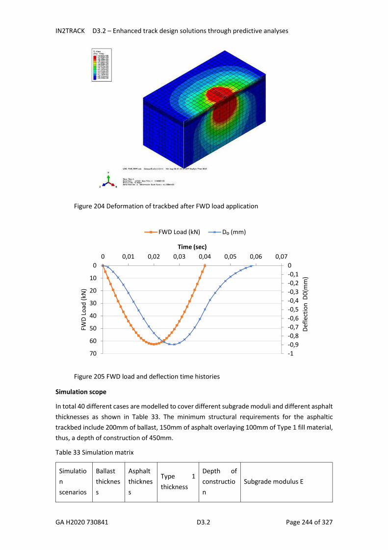
IN2TRACK D3.2 – Enhanced track design solutions through predictive analyses
GA H2020 730841 D3.2 Page 244 of 327
Figure 204 Deformation of trackbed after FWD load application
Figure 205 FWD load and deflection time histories
Simulation scope
In total 40 different cases are modelled to cover different subgrade moduli and different asphalt thicknesses as shown in Table 33. The minimum structural requirements for the asphaltic trackbed include 200mm of ballast, 150mm of asphalt overlaying 100mm of Type 1 fill material, thus, a depth of construction of 450mm.
Table 33 Simulation matrix
Simulation scenarios
Ballast thickness
Asphalt thickness
Type 1 thickness
Depth of construction
Subgrade modulus E
-1-0,9-0,8-0,7-0,6-0,5-0,4-0,3-0,2-0,100
10
20
30
40
50
60
70
0 0,01 0,02 0,03 0,04 0,05 0,06 0,07
Defle
ctio
n D
0(m
m)
FWD
Load
(kN
)
Time (sec)
FWD Load (kN) D₀ (mm)

IN2TRACK D3.2 – Enhanced track design solutions through predictive analyses
GA H2020 730841 D3.2 Page 245 of 327
(mm) (mm) (mm) (mm) (MPa)
S1 - S8 200 150 100 450 10, 20, 25, 31, 40, 45, 52, 72
S9 - S16 200 200 100 500 10, 20, 25, 31, 40, 45, 52, 72
S17 - S24 200 250 100 550 10, 20, 25, 31, 40, 45, 52, 72
S25 - S32 200 300 100 600 10, 20, 25, 31, 40, 45, 52, 72
S33 – S40 200 400 100 700 10, 20, 25, 31, 40, 45, 52, 72
FEM validation
A cross-validation was carried out to evaluate how accurately the FE model is performing for the granular trackbed design. The purpose of this is to create a model that mimics the existing standards (NR/L2/TRK/4239 Network Rail, 2015, Figure 202). In this problem, the model was given the known dataset (depth of construction and trackbed material properties) and was tested against unknown data (deflection, stiffness per sleeper end). The stiffness per sleeper end was evaluated through the FEA results, was cross-validated with the stiffness value provided by the standard chart (NR/L2/TRK/4239 (Network Rail 2015), Figure 202). The goal of cross-validation was to test the model’s ability to simulate new data (new trackbed design context). Multiple rounds of cross validation were performed using different subgrade Young’s modulus (E) (E=10-72MPa, Cu=40-288kPa and varying damping ratio of the subgrade (0.1-0.2). A regression analysis was used to estimate a correction factor to the simulated support stiffness values (ksimulated). The correction factor was applied in the output stiffness set (k) in order any error between the values of stiffness given by the model and by the standard chart to be eliminated (see Figure 206).
Figure 206 Regression analysis for cross-validation of the FWD model
Furthermore, a sensitivity analysis was conducted to assess the effect of damping ratio of asphalt to the deflection results of the FWD model. The comparison was carried out for a very soft subgrade (E=5MPa, Cu=20kPa). The FWD deflection values did not change significantly, as seen in Table 34.

IN2TRACK D3.2 – Enhanced track design solutions through predictive analyses
GA H2020 730841 D3.2 Page 246 of 327
Table 34 Sensitivity analysis for damping ratio of asphalt
0.45m Asphaltic trackbed
Loss factor_ Asphalt
Damping ratio_ Asphalt
Damping coefficient B
Cu Subgrade ESubgrade Ballast Asphalt Type 1 D0
(kPa) (MPa) (mm) (mm) (mm) (mm)
0.6 0.3 6.40E-05 20 5 200 150 100 1.875
0.3 0.15 3.2E-05 20 5 200 150 100 1.873
0.1 0.05 1.1E-05 20 5 200 150 100 1.873
FEA results
The sleeper deflection values and the sleeper support stiffness values were evaluated through the FEA for the different scenarios (see Table 33 and equation 45). The results were reported in Excel and the new design chart was created, shown in Figure 207. The chart gives the dynamic sleeper support stiffness (k) for various values of subgrade shear strength (Cu from 40 to 300 kPa) and for various depths of construction ranging from 0.45m to 0.7m below the sleeper. This include 0.2m of ballast, various asphalt thicknesses from 0.15m to 0.4m and 0.1m of fill material Type 1). It should be noted that the correlation between Cu and Esubgrade was based on the correlation existing on the design chart (NR/L2/TRK/4239 Network Rail, 2015) using the following equation 47:
𝐸 = (47)
The simulated scenarios included E values from 10 to 72MPa that correspond to Cu values from 40 to 288kPa (see Table 35).
Table 35 Correlation between E and Cu according to NR/L2/TRK/4239 (Network Rail 2015)
E (MPa) 10 20 25 31 40 45 52 72
Cu (kPa) 40 80 100 124 160 180 208 288

IN2TRACK D3.2 – Enhanced track design solutions through predictive analyses
GA H2020 730841 D3.2 Page 247 of 327
Figure 207 Required total depth of asphaltic trackbed layers on cohesive soils
It is observed that the simulated scenarios lead to quite high values of stiffness up to 250 kN/mm. Stiffness was found below 60kN/mm only for depth of construction <0.6m for soils with Cu<85kPa. In order to obtain a better understanding of the effect of asphaltic formation in the dynamic sleeper support stiffness a comparison between the design charts of granular and asphaltic trackbed is presented below (Figure 208) by using the same scale on the y axis. It can be concluded that the minimum depth of 0.45m of asphaltic trackbed is required to provide a stiffness value of 30 kN/mm for subgrade with Cu≥55kPa. The same minimum depth of 0.45m of asphaltic trackbed is required to provide a stiffness value of 60 kN/mm for subgrade with Cu≥85kPa. For soils with Cu>100kPa, the minimum depth of 0.45m of asphaltic trackbed will provide a stiffness value of 75 kN/mm whereas a deeper construction above 0.45m will increase the stiffness over 96 kN/mm.
0
50
100
150
200
250
0 50 100 150 200 250 300
Dyn
amic
slee
per s
uppo
rt s
tiffn
ess
k (k
N/m
m)
Subgrade Shear Strength Cu (kPa)
0.7m (0.4m asphalt)
0.6m (0.3m asphalt)
0.55m (0.25m asphalt)
0.5m (0.2m asphalt)
0.45m (0.15m asphalt)

IN2TRACK D3.2 – Enhanced track design solutions through predictive analyses
GA H2020 730841 D3.2 Page 248 of 327
Figure 208 Comparison between granular and asphaltic design charts
0.6m
0.55m
0.5m
0.45m
0
20
40
60
80
100
0 50 100 150 200 250
Dyn
amic
slee
per s
uppo
rt s
tiffn
ess
k (k
N/m
m)
Subgrade Shear Strength Cu (kPa)
Total Thickness of Asphaltic Trackbed Layers

IN2TRACK D3.2 – Enhanced track design solutions through predictive analyses
GA H2020 730841 D3.2 Page 249 of 327
Design examples
N2/L2/TRK/4239 (Network Rail, 2015) defines minimum values of dynamic sleeper support stiffness (k) according to line type and speed to guarantee adequate track quality and reduce maintenance intervention (see Figure 209).
Figure 209 Required dynamic sleeper support stiffness (from N2/L2/TRK/4239, Network Rail 2015)
Depending on the above requirements and taking into account the design chart for granular trackbed (Figure 202) and the new design chart for asphaltic trackbed (Figure 207), a comparison between the two design options was performed for typical cases of line type, speed and subgrade strength. These are presented in Table 36 and Table 37.
From the tables, it can be seen, that high speeds (up to 201 km/h (125mph)) correspond to stiffness requirements of at least 60 kN/mm. For these speed and stiffness requirements and for soft subgrade (≤ 50kPa) using an asphaltic trackbed layer reduces the depth of construction up to 0.2m (up to 25%).. For example, for a subgrade with Cu=40 kPa (see design example 1), a 0.8m granular trackbed is required to provide a stiffness value of 60 kN/mm for speeds up to 125 mph. The equivalent depth of construction by using asphalt is 0.6m (0.2m ballast, 0.3m asphalt, 0.1m well compacted fill material of E=100MPa) to provide the same stiffness.
In the case of stiff subgrade (clay with Cu=100kPa) (see design example 3), a granular layer with depth 0.5m is required to provide a stiffness of 60 kN/mm for high speed line (201km/h (125mph)). The equivalent depth of construction for asphaltic trackbed is 0.45m. This value corresponds to the minimum depth of construction for asphaltic trackbed (0.2m ballast, 0.15m asphalt, 0.1m fill material) and for a subgrade of Cu=100kPa, it provides a stiffness of 74.7kN/mm. Thus, for stiff subgrades Cu≥85kPa and requirements of k=60 N/mm, the depth of construction could be reduced further than 0.45m if the structural requirements allowed a minimum depth of construction for asphaltic trackbed <0.45m.
For stiffness requirements ≤ 30 kN/mm the use of asphalt has a smaller effect in the reduction of construction depth as it can cause 50mm reduction of depth. The design example 4 shows that for speed requirements <80.5km/h (50 mph) in existing lines the stiffness requirement is 30 kN/mm. According to the existing design chart, a granular layer of 0.6m is required whereas

IN2TRACK D3.2 – Enhanced track design solutions through predictive analyses
GA H2020 730841 D3.2 Page 250 of 327
according to the new design chart an asphaltic trackbed of 0.55m is required provide the required stiffness. The minimum depth 0.45m is required for any type of subgrade with Cu≥ 55kPa to provide a stiffness value of 30 kN/mm for speed <80.5km/h (50mph).
Table 36 Design examples
Design Example 1 Design Example 2
Speed 80.5-201 km/h
(50-125 mph)
80.5-201 km/h
(50-125 mph)
Shear strength Cu
40 kPa 50 kPa
Construction type
Existing lines Existing lines
K target 60 kN/mm 60 kN/mm
NR standard design
Asphalt design
% Reduction in construction depth
25% 21%

IN2TRACK D3.2 – Enhanced track design solutions through predictive analyses
GA H2020 730841 D3.2 Page 251 of 327
Table 37 Design examples
Design Example 3 Design Example 4 Design Example 5
Speed 80.5-201 km/h
(50-125 mph)
>161 km/h
(>100 mph)
<80.5 km/h
(<50 mph)
Shear strength Cu
100 kPa 125 kPa 40 kPa
Construction type
Existing lines Greenfield sites Existing lines
K target 60 kN/mm 100 kN/mm 30 kN/mm
NR standard design
Asphalt design
% Reduction in construction depth
10% 29% 8%
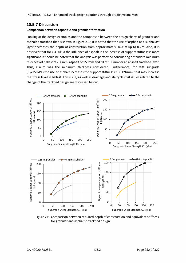
IN2TRACK D3.2 – Enhanced track design solutions through predictive analyses
GA H2020 730841 D3.2 Page 252 of 327
10.5.7 Discussion Comparison between asphaltic and granular formation
Looking at the design examples and the comparison between the design charts of granular and asphaltic trackbed that is shown in Figure 210, it is noted that the use of asphalt as a subballast layer decreases the depth of construction from approximately 0.05m up to 0.2m. Also, it is observed that for Cu>60kPa the influence of asphalt in the increase of support stiffness is more significant. It should be noted that the analysis was performed considering a standard minimum thickness of ballast of 200mm, asphalt of 150mm and fill of 100mm for an apshalt trackbed layer. Thus, 0.45m was the minimum thickness considered. Furthermore, for stiff subgrade (Cu>150kPa) the use of asphalt increases the support stiffness ≥100 kN/mm, that may increase the stress level in ballast. This issue, as well as drainage and life cycle cost issues related to the change of the trackbed design are discussed below.
Figure 210 Comparison between required depth of construction and equivalent stiffness for granular and asphaltic trackbed design.
0
50
100
150
200
0 50 100 150 200 250
Dyna
mic
slee
per s
uppo
rt s
tiffn
ess
k (k
N/m
m)
Subgrade Shear Strength Cu (kPa)
0.45m granular 0.45m asphaltic
0
50
100
150
200
0 50 100 150 200 250
Dyna
mic
slee
per s
uppo
rt s
tiffn
ess
k (k
N/m
m)
Subgrade Shear Strength Cu (kPa)
0.5m granular 0.5m asphaltic
0
50
100
150
200
0 50 100 150 200 250
Dyna
mic
sle
eper
sup
port
stif
fnes
s k
(kN
/mm
)
Subgrade Shear Strength Cu (kPa)
0.55m granular 0.55m asphaltic
0
50
100
150
200
0 50 100 150 200 250
Dyna
mic
sle
eper
sup
port
stif
fnes
s k
(kN
/mm
)
Subgrade Shear Strength Cu (kPa)
0.6m granular 0.6m asphaltic

IN2TRACK D3.2 – Enhanced track design solutions through predictive analyses
GA H2020 730841 D3.2 Page 253 of 327
Comparison with international asphalt trackbed designs
As mentioned in Section 5.4.1, asphalt trackbed designs have been already used by a number of international railway administrations. Table 38 (Sehgal et al. 2018) presents a comparison of the total depth of construction between the proposed design recommendations in this report and other international asphaltic trackbed designs. To ensure comparability, the proposed asphaltic designs are expressed in terms of subgrade modulus (E) instead of subgrade shear strength (Cu) as shown in Figure 211. Figure 212, Figure 213, Figure 214, Figure 215, illustrate the Italian, Spanish, French and Japanese track designs with asphaltic trackbed.
For example, in Italian and Spanish designs shown in Figure 212 and Figure 213, a ballast of 350mm thickness is used with 120mm - 140mm asphalt laid over 300mm-400mm of compacted fill material leading to a depth of construction of 770mm-890mm. France also uses a minimum ballast thickness of 300mm, a 140mm asphaltic layer and an adjustment/fill layer of 200mm over the subgrade leading to a depth of construction of 640mm (Figure 214).
From the comparison in Table 38, it can be concluded that the total depth of construction for asphalt trackbed designs, from worldwide practices, varies between 450mm and 890mm, whereas the proposed design has given depths between 450mm and 700mm. As far as ballast thickness is concerned, a 200mm-350mm has been used in worldwide practices, whereas a 200mm of ballast was used in this study. On the other hand, the asphalt layer thickness, from worldwide practices, varies from 120mm to 150mm whereas a minimum asphalt layer of 150mm was proposed in this study. Furthermore, other worldwide practices use a fill layer, with a thickness of 200mm-600mm, between the asphalt layer and the subgrade; whereas, a fill material with a thickness of 100mm was used in the proposed designs in this study. It should be noted that Table 38 provides a general comparison between different designs of asphaltic trackbed without concentrating on subgrade stiffness, which may impact the total depth of construction.
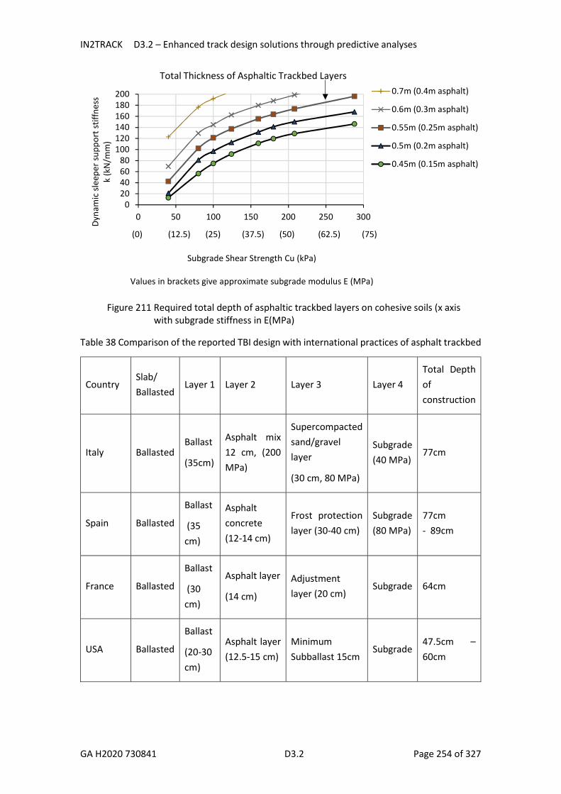
IN2TRACK D3.2 – Enhanced track design solutions through predictive analyses
GA H2020 730841 D3.2 Page 254 of 327
Figure 211 Required total depth of asphaltic trackbed layers on cohesive soils (x axis with subgrade stiffness in E(MPa)
Table 38 Comparison of the reported TBI design with international practices of asphalt trackbed
Country Slab/ Ballasted
Layer 1 Layer 2 Layer 3 Layer 4 Total Depth of construction
Italy Ballasted Ballast
(35cm)
Asphalt mix 12 cm, (200 MPa)
Supercompacted sand/gravel layer
(30 cm, 80 MPa)
Subgrade (40 MPa)
77cm
Spain Ballasted
Ballast
(35 cm)
Asphalt concrete (12-14 cm)
Frost protection layer (30-40 cm)
Subgrade (80 MPa)
77cm - 89cm
France Ballasted
Ballast
(30 cm)
Asphalt layer
(14 cm)
Adjustment layer (20 cm)
Subgrade 64cm
USA Ballasted
Ballast
(20-30 cm)
Asphalt layer (12.5-15 cm)
Minimum Subballast 15cm
Subgrade 47.5cm – 60cm
020406080
100120140160180200
0 50 100 150 200 250 300
Dyn
amic
sle
eper
sup
port
stif
fnes
sk
(kN
/mm
)
Subgrade Shear Strength Cu (kPa)
Values in brackets give approximate subgrade modulus E (MPa)
0.7m (0.4m asphalt)
0.6m (0.3m asphalt)
0.55m (0.25m asphalt)
0.5m (0.2m asphalt)
0.45m (0.15m asphalt)
(0) (12.5) (25) (37.5) (50) (62.5) (75)
Total Thickness of Asphaltic Trackbed Layers

IN2TRACK D3.2 – Enhanced track design solutions through predictive analyses
GA H2020 730841 D3.2 Page 255 of 327
Japan Ballasted
Ballast
(25-30 cm)
Asphalt concrete (5 cm)
Well graded crushed stone (subballast)
(15-60 cm)
Subgrade 45cm - 95 cm
Proposed design
Ballasted Ballast (20cm)
Asphalt layer (15cm – 40cm)
Fill (10cm) Subgrade 45cm – 70cm
Figure 212 Italian design for high speed passenger lines. 35cm ballast, 12cm asphalt, 30cm super compacted layer of sand/gravel E=80MPa. Total depth of construction 77cm. (Adjusted from Rose et al. 2010)
Figure 213 Spain: 35cm ballast, 12-14cm asphalt, 30-40cm form layer. Total depth of construction 77cm-89cm (Adjusted from Rose et al. 2010)

IN2TRACK D3.2 – Enhanced track design solutions through predictive analyses
GA H2020 730841 D3.2 Page 256 of 327
Figure 214 France: designed for high speed 357 mph, ballast 30cm, asphalt 14cm, adjustment layer 20cm.Total depth of construction 64cm. (Adjusted from Rose et al. 2010)
Figure 215 Japanese design: 25-30cm ballast, 5cm asphalt and 15-60cm well graded crushed stone for high speed/regular lines-Total depth of construction 45-95cm. (From Rose et al. 2010)
Crushing effect on ballast
The use of very stiff support conditions below ballast can increase the stress on ballast and this can be critical for the long-term performance of the ballast. A relation between ballast stress and track stiffness was shown in previous publication by Wehbi and Musgrave (2017) (see Figure 216). It was shown that when global track stiffness is less than 73 kN/mm, the stress levels within the ballast appear to decrease with the increasing global track stiffness. On the other hand, when global track stiffness is more than 73 kN/mm, the stress levels within the ballast appear to increase with increased global track stiffness. This is because when the global track stiffness is less than 73 kN/mm, the shear stress governs the deviatoric von Mises stress and the soft subgrade results in the ballast experiencing a punching shear effect from the sleeper (see Figure 217 a). However, when the global track stiffness is more than 73 kN/mm, the deviatoric von Mises stress is governed by the vertical stress component and the ballast starts to be crushed between the stiff subgrade and the sleepers (see Figure 217 b).

IN2TRACK D3.2 – Enhanced track design solutions through predictive analyses
GA H2020 730841 D3.2 Page 257 of 327
Figure 216 Normalised von Mises ballast stress for different global stiffness (from Wehbi and Musgrave, 2017)
Figure 217 Ballast deformation due to (a) shear stress (punching effect) and (b) normal stress (squashing effect) (from Wehbi and Musgrave, 2017)
Drainage of asphaltic trackbed
Drainage goes hand in hand with track performance. Drainage issues may arise if the drainage system is not adapted to the new asphaltic trackbed design. The asphalt layer can have a key benefit of improving drainage due to the impermeable nature of the asphalt. Asphaltic formation can be used effectively with potential elevation of the drainage surface within the track substructure (see Figure 218). Other potential problems arising with the use of asphalt as formation layer, is the possibility of water trapped below the asphalt layer, causing local failure

IN2TRACK D3.2 – Enhanced track design solutions through predictive analyses
GA H2020 730841 D3.2 Page 258 of 327
of the subgrade. The same could happen in case of any crack is developed in the asphalt. In this case, a permeable base layer under the asphalt layer could be used.
Figure 218 Elevation of drainage system to asphalt level from Li et al. (2002)
Life cycle cost
The use of asphalt can reduce tamping and intervention maintenance. FE modelling with train traffic loading to investigate the effect of asphaltic formation on subgrade stress level and the long-term track performance is recommended. It is approximated that Network Rail spend ~ £1million /km for the ballasted track renewal for typical trackbed design (0.3m depth of construction), whereas this cost can be increased (£400,000/km) when an additional sand layer of 100mm is required (0.4m depth of construction). The rate of ballast deterioration (stress on ballast) should be calculated in order to obtain a more reliable conclusion for the life cost of asphaltic formation. A FEM analysis representing the train traffic loading is recommended to be used (rather than a FEM of FWD loading) for the evaluation of ballast/subgrade stresses and track settlement. This would allow the comparison of the annual rate of trackbed settlement between track designs with asphaltic and granular formation.
10.5.8 Conclusions This study develops guideline design charts for track bed design using asphaltic formation for different subgrade modulus (E) using means of FEM. The novelty of this study is that it provides an asphaltic design recommendation with the aim of minimizing the total depth of construction. To this end, the following conclusions can be derived:
The use of asphalt can diminish the depth of construction from 50mm to 200mm. For soils with Cu>60kPa, the use of asphaltic formation instead of granular for the same
depth of construction can increase significantly the sleeper support stiffness. Compared to UK granular trackbed designs, the proposed asphaltic formation designs
can reduce the required depth of construction as follows: o For existing lines with soft subgrade (Cu=40-50 kPa) and speed 80.5-201km/h (50-
125mph) (required k=60 kN/mm/sleeper end), the use of asphaltic formation can reduce the depth of construction up to 25%.

IN2TRACK D3.2 – Enhanced track design solutions through predictive analyses
GA H2020 730841 D3.2 Page 259 of 327
o For existing lines with soft subgrade (Cu=40 kPa) and speed < 80.5km/h (50mph) (required k=30 kN/mm/sleeper end), the use of asphaltic formation can reduce the depth of construction up to 8%
o For newly constructed lines with stiff subgrade (Cu=125 kPa) and speed > 161 km/h (100mph) (required k=100 kN/mm/sleeper end), the use of asphaltic formation can reduce the depth of construction up to 29%.
Compared to other worldwide practices, the proposed asphaltic designs in this study provides generally similar or lower total depth of construction.
There is increased potential for ballast crushing effects if the use of asphalt results in very high sleeper support stiffness values.
The drainage should be adapted for an asphaltic trackbed design (elevation of the drainage surface)
10.5.9 Recommendations Further research is required to investigate the effect of asphalt on the long-term behaviour of railway track. The effect of asphalt on ballast stress, subgrade stresses and trackbed deterioration should be more thoroughly investigated using a train-track model representing more realistic track loading instead of the FWD loading.
10.6 Experience from numerical simulations
10.6.1 Context and motivations Simulation is one of the ways to fulfil the goals of S2R i.e. reduce costs and time to market of new solutions with better performances. Most of the present track are ballasted ones and enhance the performance of those track type through simulation is of major interest. But the ballast is a critical component, both in terms of physical behaviour and in numerical modelling. We will not expand the role of the ballast in track and it’s behaviour but rather discuss here the possible modelling approaches in order to perform mechanical simulations. We then state the problem of interest as follow: find a suitable approach to simulate the dynamical behaviour (up to 200 Hz) of a large multi-layered system including a thin layer of coarse granular media (ballast).
With respect to grain size (between 30 and 50 mm according the EN 13450), the usual thickness (35 cm under sleeper) of the ballast layer is not enough to fully satisfy the Representative Elementary Volume (REV) condition that allow to consider an homogeneous behaviour with respect to the lower scale. The ballast layer can be either seen as a structure of discrete grains or as a complex continuous material. Choosing one of these views is pivotal when developing a numerical approach. In the first case, the suitable approaches fall in the family of Discrete Element Methods (DEM) where the ballast is considered as a set of discrete mechanical bodies in interaction. In the second case, the suitable approaches fall in the family of Finite Element Method (FEM) where the ballast is considered as a continuum associated with a behaviour law that can integrate some of the grain scale mechanism (plasticity, non-linearity, heterogeneity…). Both approaches have been undertaken at SNCF-R and will be described below. The main goal

IN2TRACK D3.2 – Enhanced track design solutions through predictive analyses
GA H2020 730841 D3.2 Page 260 of 327
is to highlight the advantages and limitations of each method and present a new promising approach.
10.6.2 Efficient track scale modelling trough an optimized FEM Numerical simulation of the mechanical behavior of a certain structure often lays on Finite Element Method. Various software (Ansys, Abaqus), have spread this methodology, which is used in many engineering fields during design processes.
Infrastructure can be modelled with FEM, but the size of models is very large. Then, for civil engineering, only static loading is taken into account (using coefficient to consider the dynamic part, as stated in Eurocodes for instance).
This approach is not totally satisfactory to model railway tracks, especially while considering high speed trains. Wave propagation in the structure has to be considered for a realistic mechanical behavior.
To do so, model reduction techniques are well suited. They reduce the size of the model and allow taking into account the dynamic behavior of the structure.
SNCF has developed Dynavoie using a sub-structuring technique following the periocity of the track induced by regular sleeper spacing. The first step of this methodology is to identify the elementary slices of railway track, basically one section of the track, with sleeper spacing width. Then, these elementary slices are meshed using finite element method. Their dynamic behavior is analyzed with finite element method by identifying their dispersion diagram and modal reduction is done. Using a reduction basis identified by this modal analysis on elementary slices, superelement are built, and used to compute a full 3D track. Validation of the representability of these “superelement”, and their ability to reproduce correctly dynamic behavior of the track has been demonstrated in the thesis of Arlaud E. (Arlaud, 2016)
Time computation, and storage capacity required, are then highly reduced using this 3D model instead of a classic 3D FEM model.
One great advantage of this method is to make large parametric studies possible. Different track design, taking into account the whole structure from rail to soil, can be carried on. Transition zones between these different structures can also be designed.
However, limitations have been identified with this approach. In particular, modeling ballast as a homogenous material is a fairly rough approximation. Wave propagation in the ballast layer is totally influenced by granularity of the layer. Moreover, some phenomena that railway companies need to model, such as maintenance operation (tamping, mechanical stabilization…) cannot be reproduced by a continuous model.
10.6.3 Precise ballast grain scale modelling trough DEM Unlike FEM, the software offer proposed by academics and companies to conduct DEM simulation is small. The offer is even smaller when the ability to handle angular particles is

IN2TRACK D3.2 – Enhanced track design solutions through predictive analyses
GA H2020 730841 D3.2 Page 261 of 327
required as one can intuitively think for ballast. This situation can be understood by the fact that each DEM software needs to achieve a satisfactory balance between these interlinked points:
Computational efficiency (mainly time vs number of particles) Modelling complexity (particles shape and interaction laws) Time integration User friendlyness (use case building, graphical user interface…)
Since early 2000’s, SNCF had chosen LMGC90 software (Dubois, 2011) to perform his DEM simulation of the ballast layer. Unlike most of DEM software that consider rigid particles and deformable contacts, LMGC90 is based on the Non Smooth Contact Dynamics (NSCD) approach that considers rigid particles and rigid contact. This particular approach offers a clean and generic framework to compute the behaviour of non-spherical particles as ballast grains.
In our models, the mechanical interactions between bodies (ballast grain, sleeper, soil) are basically represented by a Signorini-Coulomb condition that describe both unilaterality and friction. The main pertinent feature for ballast modelling is the ability to model ballast particles as 3D polyhedra (triangular mesh) of any refinement. Mesh features such as convexity and number of triangles by particles can be taken into account to the price of a significant increase of computational effort. Classically, grains composed of 40 vertices and 60 faces allows for computation one tamping cycle (3 seconds) of systems composed of 22 000 particles to be computed over one week without parallelization. This typical duration is one of the well know drawback of DEM approach but need to be seen with respect to the details that are given by the model: dynamics of each particles and each contact forces. The challenge is then to use this deluge of information to build pertinent quantity of interest, such as solid fraction or stress, and to follow their evolution during the simulation.
DEM approaches are particularly useful to study strongly ballast related problems such as maintenance operation (tamping (Voivret, 2016), artificial stabilization (Ferellec, 2017)), ballast interface (under sleeper pad (Voivret, 2016), soil layer (Taforel, 2015)) and the behaviour of the ballast itself (grain shape effect, wear). These investigation domains are completely out of reach of FEM based approaches and justify the pertinence of DEM approaches to enhance ballasted track performances. However, the computational cost of DEM approaches limits the both the size of the studied system (up to few sleepers plus ballast) and the number of achievable simulation in a parametric study in a limited time. That partly explain the limited use of DEM in railways with respect to FEM.
10.6.4 Best of both worlds through continuous heterogeneous modelling of ballast
Combining the benefits of FEM (rapidity, ability to model all components of the track) and DEM (precise ballast modeling) is very attractive, as there are very complementary approaches. Tentative work has been done to build a direct coupling, but the complexity and the computational cost was too expensive (Taforel, 2015). A fair compromise between both worlds would consist in maintaining the continuous hypothesis for the ballast modelling but taking into account the heterogeneity of the material. With such a model, the predictive capacity of FEM approaches will be enhanced while preserving numerical performance.

IN2TRACK D3.2 – Enhanced track design solutions through predictive analyses
GA H2020 730841 D3.2 Page 262 of 327
To achieve such a challenge, it is necessary to switch to an alternative approach. Lucio de Abreu Corrêa in his PhD thesis (Corrêa, 2017) proposed to consider the ballast layer as a randomly-fluctuating continuous heterogeneous medium. The main purpose of this work is to investigate the dissipation mechanisms inside the ballast layer. One of the main finding is that dissipation occurs, even without damping, due to the heterogeneity. This kind of dissipation cannot be considered with classical homogeneous FEM models.
The heterogeneous ballast is based on a 3D random field for the density and the wave velocities (pressure and shear). A log-normal probability law is chosen, relying on only two parameters: the mean value and the standard deviation. A correlation law is also needed and is parametrized by a correlation length. Then a sample of these random fields is generated, which gives a map of ballast mechanical properties. It is important to note that each sample is fully deterministic because a unique realization of the same stochastic ballast material is used for each simulation. Finally, this heterogeneous medium is included within a track model, where soil and sleepers are homogeneous like in classical FEM approaches (see Figure 219).
Figure 219 Visualisation of the continuous heterogeneous model of the ballast, thanks to iso-surfaces of density
However, the introduction of the heterogeneous field has a serious drawback: the computational cost. First, the mesh of the ballast layer must be very refined (around 2cm) to capture the correlation length (typically 5 cm). Therefore, the number of degrees of freedom rises to millions for a complete track model of 10m long. Secondly, assuring the stability and the precision of the time scheme with huge heterogeneities imposes to reduce drastically the time step (to the microsecond). To achieve such a huge calculation, HPC (High Performance Computing) is required, that is to say efficient parallel calculations done on numerous processors. For this reason, Spectral Element Method (SEM) has been preferred to more usual FEM: in this method, the mass matrix is naturally diagonal, allowing an explicit time scheme, which is more efficiently parallelized on several computing units (Komatitsch, 1999).
This heterogeneous model has been calibrated by two separate identification processes. First, the equivalence between DEM and continuous heterogeneous samples of ballast is investigated. A volume of heterogeneous media is generated and subjected to a nearly-triaxial stress and a

IN2TRACK D3.2 – Enhanced track design solutions through predictive analyses
GA H2020 730841 D3.2 Page 263 of 327
similar system is simulated with DEM. We then compute in each case the vertical stress distribution in the whole sample. A best-fit of correlation law parameters of the continuous model can be found. It appears that such model even represents with accuracy the other components of the stress tensor. Secondly, a track scale model is considered (soil, ballast and sleepers) to calibrate the remaining 6 parameters: mean values and standard deviations of the three random fields (density, pressure and shear velocity). The load of a TGV on this track is taken from measurements on a wheel, processed within a beam model of the rail, and then applied on the sleepers. Thus, a train pass-by can be simulated with a time-based algorithm. The frequency spectra of the vertical acceleration in several points inside the ballast layer are processed and compared with a quadratic norm to the same quantity measured on a high-speed line. Best-fit values are also found, as shown on Figure 220. A snapshot from an example of a simulation is presented on Figure 221.
Figure 220 Identification results for mean wave velocities (m/s). The quadratic norm compares the Fourier transform of vertical acceleration inside the ballast. The global minimum gives the best-fit parameters. Each black dot corresponds to a simulation.
Figure 221 Snapshot of the global displacement magnitude in a pass-by train simulation.
axles SOIL
BALLAST

IN2TRACK D3.2 – Enhanced track design solutions through predictive analyses
GA H2020 730841 D3.2 Page 264 of 327
Even though the results are promising, the computational cost remains an issue: a typical simulation takes more than 30 hours on 300 processors. Such a computational cost is acceptable for research but not for engineering purposes.
For this reason, SNCF Réseau has chosen in 2017 to complete the Dynavoie software with this continuous heterogeneous model of the ballast. The purpose is to maintain the predictivity of the heterogeneous model, while dramatically lowering its computational cost. To achieve this goal, the model reduction developed in Dynavoie has to be extended to heterogeneous domains. This goal will be reached only by studying precisely the influence of the heterogeneity on the spectral response of the track. Moreover, the soil boundary condition will be another point of interest: indeed, classical boundary conditions (clamped, free, elastic…) are not satisfying to represent with accuracy the low frequencies. Finally, resilient components like rail pads will be included to the model. These improvements of the Dynavoie software will be achieved during the PhD of Hadrien Pinault (2017-2020). Afterwards, SNCF Réseau will possess an efficient predictive tool, which can be then used to:
improve the understanding of the behaviour of an actual track thanks to an identification process
optimize the design of a track investigate new designs of a track component enrich monitoring data to build the track numerical twin of the railway track

IN2TRACK D3.2 – Enhanced track design solutions through predictive analyses
GA H2020 730841 D3.2 Page 265 of 327
11 Whole system model framework Investigating means to combine models and methodologies to a "whole system model framework". This does not imply one monolithic model, but rather a number of models and methods that each tackle specific issues and aspects. One key aim here is to allow these models to cooperate in a holistic analysis that allows for a design optimisation of the entire track systems as well as for pre-qualification and virtual and hybrid homologation of track components for rapid market uptake.
11.1 Whole system model framework with focus on certification/authorisation of railway components
11.1.1 Evaluation and assessment of existing methods and procedures Generally, the creation process of a new product up to its utilization is indicated by several time consuming steps. For railway components, this product creation process is schematically illustrated in Figure 222. It can be divided into idea generation, invention and authorisation/certification of the component for operation.
Figure 222 Schematic representation of the different steps of the product creation process and the utilization of track components.
Ideas can be generated by all stakeholders who have a benefit of an innovative product. The development process starts in a laboratory environment and includes the production (in the lab or in the regular production line) and testing of prototypes in laboratory environment.
The authorisation and certification of railway components for operation starts by presenting the benefit of the innovative product to the future user. Since railway components are standardized, any innovation must at least fulfil the requirements of the relevant product standard. Ideally, the new product has superior properties as compared to the best available product. After passing the prototype laboratory testing, the most important test can be started at the place of the later application at real conditions, i.e. in railway operations.
Particularly, the time required for the various physical test steps of railway components is high. As an example, the process for authorization and certification of a new rail steel is sketched in Figure 223.

IN2TRACK D3.2 – Enhanced track design solutions through predictive analyses
GA H2020 730841 D3.2 Page 266 of 327
Figure 223 Schematic representation of the different steps from the idea to the utilization of a new rail steel.
After developing a prototype up to TRL4, the new rail steel must be tested in accordance with EN13674-1. As a minimum requirement, the qualification and acceptance tests must be done and assessed with respect to the specified limits and the values achieved for the best reference rail steel for the planned application. These results may be supported by laboratory tests done at real-space conditions in a wheel-rail test rig setup.
Since rails are used in continuous welded tracks, the next step is to adjust all welding processes for both joining and repair, so that reasonable results are achieved to allow installation of the new rail steel into track for testing. Like for the rail steel itself, European standards for welding of rail are applied to define the minimum testing requirements. Practically, the development of proper welding solutions may take longer than the development of the new rail steel because of the added level of complexity on properties and practical solutions for in-track welding.
For starting track testing in highly stressed tracks, conformity to safety and legal requirements must be proven and documented. Track testing is typically done in two stages in order to limit any risk of failure of the new rail steel. Stage one is one place of installation with special surveillance along the agreed testing time. Stage 2 will follow with more spots at different conditions. Both stages need accumulation of a reasonable tonnage to allow a prognosis on the life extension and reduction of maintenance activities. At European conditions, a minimum collected tonnage of 200 MGTs is considered as representative for assessing the performance of the new rail steel, resulting in testing times of minimum three and typically five years.
As shown in Figure 223, the total time-to-market for a simple product like a rail will take a decade. The key aim of defining and establishing a comprehensive homologation process is to reduce time-to-market by a “hybrid” homologation by combining physical tests, numerical simulation of the product performance (virtual testing) and a shortened real-space test at well-defined track conditions.

IN2TRACK D3.2 – Enhanced track design solutions through predictive analyses
GA H2020 730841 D3.2 Page 267 of 327
11.1.2 Develop approach for virtual/hybrid authorisation/certification of railway rails
A reduction of the time effort to the authorisation and certification of the components can be achieved by hybrid testing methods. Pure physical tests are to be replaced by less time-consuming hybrid testing methods consisting of physical and virtual tests. Virtual test results should be used for pre-qualifying of the components. The subsequent verification of the results is done by physical tests.
Therefore, the whole system model framework will be applied which is capable to predict the behaviour of the track components in operation by virtual tests. Several models, partly connected together, constitute the simulation framework of the whole system model. Each model is able to solve a relevant aspect that can represent an input parameter of another model. Because of that the results of each model have to be reliable.
Figure 224 illustrates the required and desired future development process for such models and the testing process. Results and observations of physical tests are the basis for the development, calibration and verification of models. The better and more reliable these models become, the more significant are the results of these models and their combination into a whole system model within the testing process. At the same time, the significance of the physical tests within the testing process and thus the time required for such tests decreases (see Figure 224). In the future, physical tests e.g. track tests should only be used for verification of the virtual testing results (see Figure 224).
Overall, this hybrid testing method decreases the time required for testing because:
virtual tests are less time-consuming due to their ability of parallelized simulation of different testing scenarios,
of the reduction of number of physical tests resulting in a reduction of needed prototypes and their installation,
components prequalified by virtual tests will probably pass physical tests in the first instance.
Figure 224 Desired future development of physical and virtual testing.

IN2TRACK D3.2 – Enhanced track design solutions through predictive analyses
GA H2020 730841 D3.2 Page 268 of 327
Different physical testing methods are available whose results can be used for the development or improvement of the models of the whole system model framework (see Figure 225).
Small scale tests including e.g. high pressure torsion (HPT), pin on disc, disc on disc, tensile or torsion tests provide basic information about tribological effects, contact mechanics and the behaviour of material loaded by stresses and strains. In contrast to small scale tests are large scale tests more specific to railway conditions. Examples for large scale tests are wheel / rail (wheel / rail smaller sized than in operation) or disc on disc tests. Full scale test rig tests provide test conditions most similar to real railway operation. The contact mechanics and the tribological effects of a full scale wheel / rail test rig test correspond to those of real operation. However, effects caused by e.g. vehicle-track interaction or environmental conditions are at least difficult to be covered by these test rigs. For this reason, track tests are and will be necessary.
Figure 225 Physical testing methods and virtual testing by the whole system model framework.

IN2TRACK D3.2 – Enhanced track design solutions through predictive analyses
GA H2020 730841 D3.2 Page 269 of 327
The whole system model framework (see Figure 225) consists of a vehicle track interaction model and models for the track structure (see Figure 225: ballast settlement model, sleeper model…) and subsystems (see Figure 225: point operating equipment model…). Thereby a modular structure of the whole system model framework is pursued which enables to choose an appropriate model as well as an appropriate combination of models according to the specific requirements of a task. On the one hand, a task can make it necessary, for example, to determine the vehicle-track interaction involving the hunting motion and curving behaviour of a train by a multi body simulation tool and using the results for several track structure models. On the other hand, for some specific tasks it may be sufficient to determine the vertical dynamics of the vehicle track system by a simple spring-mass oscillator system and to assess only the ballast settlement below every sleeper caused by these vertical dynamics.
Basically, the models of the whole system model framework are based on test results. Information about different ballast settlement models, sleeper models, railpad models, rail fastening models, track models as well as vehicle / track interaction models can be found in In2Track (2018). Examples for wear models are the Krause and Poll model (see Krause (1986)) and the Archard model (see Jendel (2002)). For more information on different rail damage models related to RCF and squats, see chapter 8.2.
As an example of a subsystem of the whole system model framework the newly developed squat model should be mentioned. A description of the model can be found in chapter 11.1.4. For a more detailed description as well as for simulation results it should be referred to Bernsteiner (2018). The article (Bernsteiner, 2018) can be found attached to the present report (Annex 15.2).
11.1.3 Validation A subsystem of the whole system model framework can be used for the prediction of white etching layers on rail surfaces (see Bernsteiner, 2016). The subsystem consists of several submodels which are connected together and which are interacting. The local calculations are based on a discretization of the elliptic contact patch according to Hertzian theory. The ECF model (Meierhofer, 2015) is used to solve the tangential contact problem. The ECF model takes into account the normal stress distribution and the temperature dependency of the traction coefficient. The ECF model was parametrized by HPT tests and furthermore validated by the results of twin disc experiments vehicle tests. The temperatures on and below the surface of the wheel and the rail are calculated by the approach of Ertz and Knothe (Ertz, 2002).
In this chapter, one example of the validation results of the subsystem (Hertzian approach, ECF-model, Ertz and Knothe approach) regarding the temperature calculation are shown. For more examples, it is referred to the article Bernsteiner (2016).
In literature it is assumed that white etching layer has partly the material structure of martensite (e.g. see Steenbergen,2013). The presence of martensite indicates a phase transformation from perlite to austenite and subsequently to martensite. The phase transformation process suggests wheel-rail contact temperatures equal to or larger than the austenitisation temperature limit of steel, which is about 700 °C.

IN2TRACK D3.2 – Enhanced track design solutions through predictive analyses
GA H2020 730841 D3.2 Page 270 of 327
For the validation several simulations and experiments at a full scale wheel-rail test rig were done. Due to the fact that the temperatures within the wheel-rail contact cannot currently be measured directly only an indirect validation was possible.
At the test rig, rails were one time cyclic loaded by an increased longitudinal creepage 𝑐 . After that, the rails were investigated for the presence of a WEL. Figure 226 shows a lateral cross section of one tested rail as an example. The WEL has a maximum depth of around 350 𝜇𝑚.
Additional to the experiments, simulations were carried out with the subsystem (Hertzian approach, ECF-model, Ertz and Knothe approach) of the whole system model framework. Figure 227 shows the result of a simulation. The same parameters were chosen for the simulation as for the experiment. The simulation showed temperatures above 700 °C to a depth of about 370 𝜇𝑚, which corresponds approximately to the thickness of the WEL from the experiment (compare Figure 226 and Figure 227).
Figure 226 Lateral cross section of the tested rail. The maximum depth of the WEL is around 350 𝜇𝑚. Experiment parameters: 𝑣 = 0,1 𝑚, 𝑐 = −300 %, 𝐹 =110 𝑘𝑁. Picture from Bernsteiner, (2016).
Figure 227 Simulated temperature distribution on and below the surface in the middle of the contact patch. Simulation parameters: 𝑣 = 0,1 𝑚, 𝑐 = −300 %, 𝐹 = 110 𝑘𝑁. Picture from Bernsteiner, (2016).

IN2TRACK D3.2 – Enhanced track design solutions through predictive analyses
GA H2020 730841 D3.2 Page 271 of 327
11.1.4 Modelling the whole system of track & vehicle Interaction Many different tasks in railway engineering require the modelling of the track and vehicle interaction. Core target is that components of track should be configured and dimensioned not only by field and laboratory test but also based on specific simulations. Generally, the modular structure of the whole system model framework enables to choose an appropriate model as well as an appropriate combination of models according to the specific requirements of a task.
In this chapter, one example of a subset of the whole system model framework, the newly developed squat model, is given. A detailed description of the squat model can be found in Bernsteiner (2018). The article (Bernsteiner, 2018) can be found attached to the present report (Annex 15.2).
In literature initial geometrical deviations of the rail surface are mentioned to cause squats on rails beside other squat initiation mechanisms (Clayton, 1982). A 3D wheel and rail simulation tool (Bernsteiner, 2018) was developed to estimate the geometrical development of different sized geometrical deviations of the rail surface under cyclic loadings. Furthermore, the model is able to assess the local crack initiation potential. In contrast to finite element methods, the model enables the simulation of several thousand cyclic loadings with varying wheel profiles as well as varying lateral positions of the wheelsets within an acceptable time period.
Different submodels are implemented and jointed together to solve the normal and tangential contact problem, to calculate the wear rate and to estimate the crack initiation potential.
The normal contact problem is solved with Kalker’s software CONTACT because of the assumption of non-Hertzian contacts. Non-Hertzian wheel-rail contacts are a consequence of rail surface deviations.
The ECF-model (Meierhofer, 2015) is used to calculate the tangential stresses and the frictional power. This model takes into account the normal pressure and the temperature dependency of the traction coefficient. The temperature on- and below the surface is calculated by the analytical equations of Ertz and Knothe (Ertz, 2002). The model is able to regard the interaction between the temperature and frictional power which depends amongst other things on the traction coefficient.
The calculation of the wear rate is based on the model of Krause and Poll (Krause, 1986). This model distinguishes between two different wear regions, based on the frictional power density: a mild and a severe wear region.
The tendency of crack-initiation (damage potential) is assessed by the wedge model (Trummer, 2016a) which considers the local plastic deformation of the near-surface layer, the amount of wear, and the tensile stresses caused by the wheel-rail-contact stresses.
A simple spring-mass model can be used to estimate the vertical dynamics of the wheel-rail system. Vertical dynamics are caused by geometrical deviations of the rail surface.
As mentioned before, the main advantage of this 3D model is the ability to simulate the evolution of the rail surface geometry of a short rail segment within several thousand cyclic loadings and to estimate the local crack initiation potential. The option of varying the wheel

IN2TRACK D3.2 – Enhanced track design solutions through predictive analyses
GA H2020 730841 D3.2 Page 272 of 327
profiles and the lateral position of the wheelset enable a realistic depiction of typical loading conditions of real railway operation.
11.2 Possibilities to combine models and methods for holistic analysis of rail crack formation
11.2.1 Introduction Considering subsurface initiated rolling contact fatigue (RCF) in a rail as an example, it can be argued that the influence of the distribution of strength of the constituents of the microstructure is smaller than the influence of any material defects. Consequently, reliable statistics on sizes of occurring material defects would provide more useful information than a detailed modelling, and accounting for the spread in strength, of the microstructure constituents. Bearing in mind that detailed models increase computational costs and require more detailed input data, a simulation framework for the mechanical interaction of the whole vehicle–track system needs to be based on modules of different levels of complexity.
Section 11.2 is complemented by the state-of-the-art paper Ekberg and Pålsson (2018), see Annex 9, which has been performed as part of In2Track. In this section, the focus is on combining models of wheel–rail contact and dynamic vehicle–track interaction with the prediction of mechanically induced surface initiated RCF. Other damage modes discussed in the state-of-the-art paper include predictions of subsurface initiated RCF, thermo-mechanical RCF and wear.
11.2.2 Wheel–rail contact models For two contacting elastic bodies large enough to be considered as half-spaces with non-conforming smooth macro- and microgeometry, the contact pressure distribution can be described by Hertzian theory. This is typically the case for nominal contact between wheel tread and top of rail. In this case, the contact between wheel and rail can be represented by a single spring with a stiffness corresponding to the nonlinear relation between force and deflection in the Hertzian contact. The Hertzian spring constant is determined by the wheel and rail radii and the properties of the linearly elastic material. The contact patch is elliptical and the contact pressure distribution has an ellipsoidal shape.
In cases where the range of the dynamic wheel–rail contact force is limited in relation to the static contact force, the contact stiffness can be taken as linear by linearizing the force-deflection relation with respect to the mean value of the contact force (static wheel load). For acoustic roughness excitation (calculation of rolling noise), it has been shown by Wu and Thompson (2000) that the difference between nonlinear and linearised Hertzian contact models is negligible when the root mean square roughness amplitude is less than about 0.35 times the static contact deflection.
Nonlinear wheel–rail contact cannot be neglected in cases where there is an irregularity in the contact conditions, such as at crossings, insulated rail joints and in the case of wheel flats. This

IN2TRACK D3.2 – Enhanced track design solutions through predictive analyses
GA H2020 730841 D3.2 Page 273 of 327
is because of the possibility of loss of (and recovered) wheel–rail contact above a certain vehicle speed and the resulting large range of dynamic contact force. However, the Hertzian spring contact model does not account for the variation in contact stiffness within the contact due to the variation in three-dimensional surface geometry along a wheel/rail irregularity. For wheel flats, it has been shown by Baeza et al (2006) that the use of a Hertzian contact spring model leads to an overestimation of the wheel–rail impact force. To account for this stiffness variation and allowing for cases with non-elliptical contact between two elastic bodies, boundary element (BE) based methods can be employed, see Kalker (1990). For wheel–rail contact in a crossing, Li et al (2017) used an implementation of Kalker’s variational method.
For new and rounded wheel flats, Pieringer et al (2014) studied the influence of contact model on the accuracy of the calculated wheel–rail impact force. Four contact models were compared, where the three-dimensional non-Hertzian contact model based on Kalker’s variational method was used as the reference. The second contact model was a two-dimensional non-Hertzian contact model consisting of a Winkler bedding of independent springs, see Ford and Thompson (2006). Two single non-linear Hertzian contact spring models were also compared, where the relative wheel–rail displacement excitation input was either given as the wheel profile deviation or as the pre-calculated wheel centre trajectory. It was concluded that both the 2D model and the Hertzian spring with the wheel centre trajectory as input give rather similar results to the 3D model, see Figure 228. However, it was found that the Hertzian model with the wheel profile deviation as input can lead to large errors.
Large differences in maximum impact forces are observed in Figure 228 when comparing the new and rounded flats (same depth). From this it can be concluded that the exact geometry of the flat is an important input to the simulation Pieringer et al (2014). Differences in the shape will lead to bigger variations in maximum force than differences in the formulation of the contact. Consequently, predictions of impact forces should rather be based on measured surface geometries than simplified analytical functions.

IN2TRACK D3.2 – Enhanced track design solutions through predictive analyses
GA H2020 730841 D3.2 Page 274 of 327
Figure 228 Maximum wheel–rail impact forces due to a (a) rounded 0.5 mm deep wheel flat; (b) newly formed 0.5 mm deep wheel flat; (c) rounded 0.9 mm deep wheel flat; (d) newly formed 0.9 mm deep wheel flat; (e) rounded 1.75 mm deep wheel flat; (f) newly formed 1.75 mm deep wheel flat. Calculations with different contact models: - 3D; --- 2D; -.- Hertz (wheel centre trajectory); … Hertz (profile deviation). From Pieringer et al (2014).
For the tangential contact, the most straight-forward approach is to assume the frictional stress to be proportional to the contact pressure, see Figure 229. Such an assumption corresponds to a load case of full slip, i.e. the wheel slides on the rail. Under more common frictional conditions, the contact patch can be divided into a stick zone where there is no relative motion between wheel and rail, and a zone where slip occurs (i.e. where q(x) = μ p(x). There exist different methods to analyse the extent of these zones and the frictional stress distribution, see Johnson (1985) and Kalker (1990).
General material models, local dynamic (transient) effects in the wheel–rail contact and arbitrary wheel/rail geometry can be considered when the wheel–rail interaction is modelled by a transient dynamic finite element (FE) model see e.g. Zhao et al (2012), Pletz et al (2012). However, there are significant practical limitations. Firstly, FE contact simulations are computationally expensive, especially in a 3D analysis. One of the reasons is that the discretisation of the contact surface needs to be detailed (i.e. the FE mesh needs to be fine). If rolling contact is studied, this relates to the entire length of the rail and the wheel tread over which contact takes place. To limit this, there are approaches such as Arbitrary Lagrangian–

IN2TRACK D3.2 – Enhanced track design solutions through predictive analyses
GA H2020 730841 D3.2 Page 275 of 327
Eulerian formulations Nackenhorst (2014) that limits the size of the area that requires a very fine discretisation. This simplification comes at the expense of the need to define more complex boundary conditions.
(a) (b)
Figure 229 (a) Three-dimensional view of Hertzian contact pressure and partial slip. (b) Two-dimensional section in the xz-plane of Hertzian contact pressure (solid line) and interfacial shear under the presumption of full (thin dashed line) and partial (thick dashed line) slip conditions. From Ekberg and Pålsson (2018).
11.2.3 Dynamic vehicle–track interaction Dynamic vehicle–track interaction is either simulated in the frequency domain or in the time domain. When interaction is solved in the frequency domain, the model of the vehicle–track system including the wheel-rail rolling contact must be linear. Calculation times in the frequency domain are generally shorter compared to time domain models, and the frequency-dependence of included sub-models can be accounted for. This is for example useful when modelling the dynamic properties of rail pads and ballast/subgrade that exhibit a frequency-dependent behaviour. Time domain models, on the other hand, can readily account for non-linear rolling contact mechanics, state-dependent (nonlinear) vehicle suspensions and randomly distributed track properties.
Dynamic vehicle–track interaction is either solved using commercial software where the focus is on low-frequency (up to about 20 Hz), three-dimensional vehicle dynamics along up to kilometres of track (see e.g. the commercial multibody dynamics software SIMPACK where the analysis is mainly performed in the time domain and the accuracy of the vehicle model is more important than the dynamic features of the track) or using software where the focus is on high-frequency wheel–rail interaction while the motion along the track is of less concern (see e.g. the TWINS software for prediction of rolling noise in the frequency domain). In the latter case, due to the high-frequency interaction, the vehicle model can be reduced to a (rigid or flexible) model

IN2TRACK D3.2 – Enhanced track design solutions through predictive analyses
GA H2020 730841 D3.2 Page 276 of 327
of the wheelset since the primary suspension isolates the bogie and car body, while the various components of the track need to be described in detail, see Knothe and Grassie (1993).
As discussed in the previous section, irregularities on the wheel and/or rail surface will give rise to increased dynamic loads with impact loads from wheel flats and RCF clusters as extreme examples. Loads induced by surface irregularities also tend to have a substantial high-frequency content. An example is rail corrugation where significant load frequencies extend up to kHz Nielsen et al (2005). At high-speed operations, the main effect of a globally deteriorated vertical contact geometry e.g. in the form of corrugation is in generating high contact force magnitudes. At lower speeds, also the influence of the deteriorated contact geometries on higher contact stresses is of importance, Ekberg et al (2007). For isolated defects, the speed mainly affects the normal force magnitude, whereas the stress level seems to be mainly affected by the defect geometry, Andersson et al (2015).
As the contact moves towards the gauge corner of the rail and the flange of the wheel, both the detailed geometry and how the contact is modelled will have significant effects on the resulting contact forces and the predicted dynamic behaviour of the vehicle Burgelman et al (2015). The case is here complicated by the fact that the contact between flange and gauge corner tends towards conformal, especially for worn profiles. This invalidates one of the Hertzian presumptions. However as long as the curvatures of the surfaces in contact are constant, the Hertzian theory provides quite accurate results also for conformal contacts, Alonso and Gimenez (2008). Also, the violation of the elastic half-space assumption in the Hertzian theory has a small influence on the estimation of the contact pressures in conformal contacts with constant curvatures, Wiest et al (2008), Yan and Fischer (2000). The discrepancy between results from Hertzian theory and the actual contact pressure distribution and contact patch shape can however be large when there are significant curvature changes in the contact patch, Shackleton and Iwnicki (2008), Enblom and Berg (2008), Sichani et al (2014).
11.2.4 Rail crack formation in surface initiated RCF Surface initiated RCF typically relates to crack initiation through ratcheting (or in the case of alternating directions of frictional loading, low cycle fatigue). Current models to predict ratcheting induced RCF, generally based on the output from a simulation of dynamic vehicle–track interaction, include the Tγ-model, Burstow (2004) and shakedown approaches Johnson (1989), Ekberg et al (2002). Here, the Tγ-model relates the risk of RCF to the product of the tangential wheel–rail contact force T and the creep γ, i.e.
𝐷 = 𝐹(𝑇𝛾) (48)
where D is the fatigue damage (inverse of the fatigue life) and F is a trilinear material-dependent damage function. Note that both T and γ are global quantities which generally are determined in a simulation of low-frequency, three-dimensional vehicle dynamics. Hence, any influence of contact patch size and/or detailed contact stress distribution is implicitly included in the Tγ-magnitude and/or in the corresponding RCF damage function.
IN2TRACK D3.2 – Enhanced track design solutions through predictive analyses
GA H2020 730841 D3.2 Page 277 of 327
In contrast, the shakedown approach explicitly presumes Hertzian contact and (implicitly) full slip conditions. Further, the contact patch size is explicitly included in the analysis. This is clear if the shakedown analysis is expressed in terms of the FIsurf index, Ekberg et al (2002):
𝐹𝐼 = 𝑓 − (49)
Here f = 𝐹 + 𝐹 /𝐹 = 𝑇/𝐹 is the traction coefficient, a and b the semi-axes of the Hertzian
contact patch, k the yield limit in (cyclic) shear, and Fz the normal contact force. Surface initiated RCF is predicted for FIsurf > 0. As discussed in the previous section, note that loads stemming from surface defects also tend to have a substantial high-frequency content, Nielsen et al (2005). If such defects are accounted for, this may lead to significant FIsurf magnitudes. However, also note that FIsurf presumes Hertzian contact and is not a suitable quantification if the character of the surface defect(s) is such that Hertzian conditions are not plausible, cf the discussion below and in Ekberg and Pålsson (2018), Annex 9.
As discussed above, in wheel–rail contact, the contact stress distribution does not always relate to Hertzian contact and full slip as presumed in the shakedown analysis. To account for cases of partial slip, a “local” approach can be taken where the risk of surface initiated RCF is related to the maximum frictional stress, see Dirks and Enblom (2011), Ekberg et al (2014). A similar approach can be adopted to the Tγ-model, Dirks and Enblom (2011). It would seem that the increased resolution of a local model should allow more precise predictions of surface initiated RCF. This is however not necessarily the case. One reason is that local stresses may be so high that they cause plasticity, which would result in local stress magnitudes that are lower than what is predicted in an elastic analysis. This can be accounted for by an FE analysis of elastoplastic stress. However, also an elastoplastic stress/strain analysis combined with an RCF analysis using a local criterion will overestimate the risk of RCF. The reason is that fatigue is a non-local phenomenon due to statistical and stress gradient effects.
In cases of very localised contact, e.g. in very narrow contact bands or at surface defects, the assumption of Hertzian contact is not plausible. Defining a simple and robust RCF criterion for such conditions is a challenging task. Currently, the best option is probably to make a detailed evaluation of the dynamic loading and resulting stress evolution and then compare load cases qualitatively, cf Andersson et al (2016).
FE analyses can account for an elastoplastic material response. If elastoplastic contact conditions are considered, the analysis is complicated by the fact that the residual stresses will cause the stress/strain response to tend towards elastic as the number of load passages increase. The calibration of a material model then needs to focus either on a correct representation of the first cycles, or on the response at a more stabilised stage after some tens of cycles Ekh et al (2000). This is even further complicated if the loading has a variable magnitude. The vicinity to a (virtually) free edge at the contact interface further complicates the analysis since it is numerically challenging to capture the large plastic deformations, see e.g. Sandström and Ekberg (2009). If elastoplastic stresses and strains are correctly captured the fatigue life can be evaluated, see e.g. Mandal (2014). However, any quantitative prediction relies on a presumed mode of fatigue and on the selection of a “critical volume” (see Ekberg et al (2016)) that needs
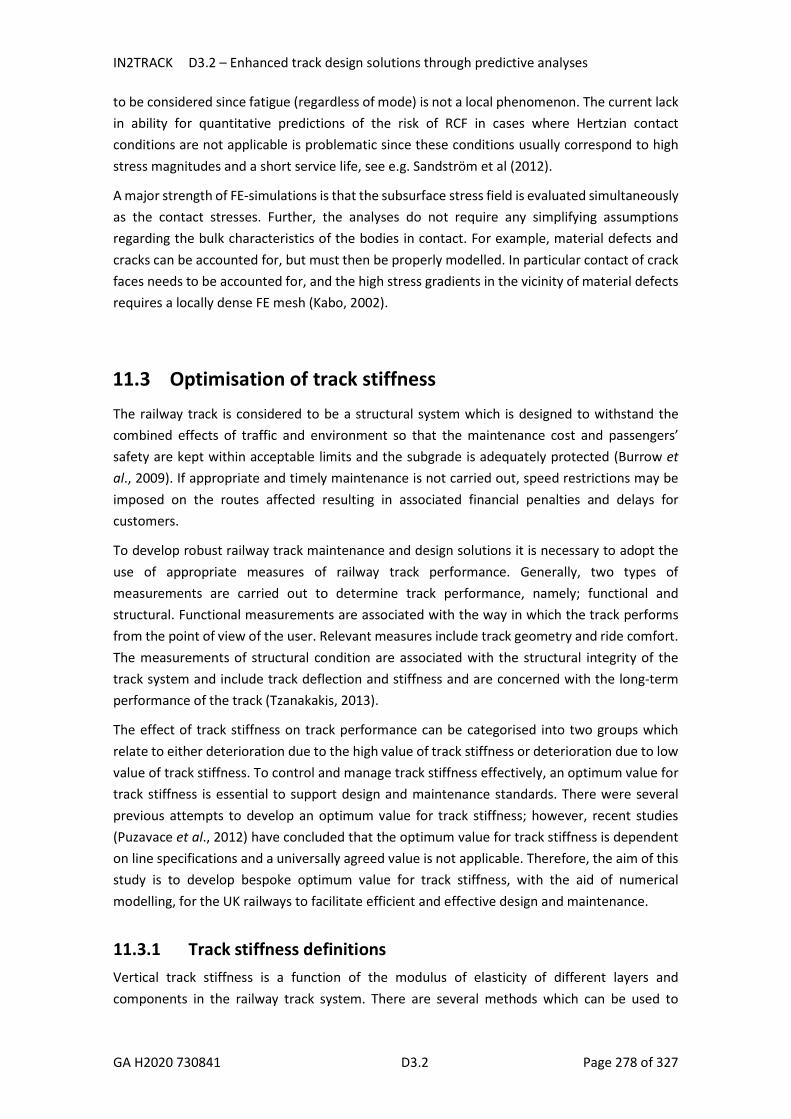
IN2TRACK D3.2 – Enhanced track design solutions through predictive analyses
GA H2020 730841 D3.2 Page 278 of 327
to be considered since fatigue (regardless of mode) is not a local phenomenon. The current lack in ability for quantitative predictions of the risk of RCF in cases where Hertzian contact conditions are not applicable is problematic since these conditions usually correspond to high stress magnitudes and a short service life, see e.g. Sandström et al (2012).
A major strength of FE-simulations is that the subsurface stress field is evaluated simultaneously as the contact stresses. Further, the analyses do not require any simplifying assumptions regarding the bulk characteristics of the bodies in contact. For example, material defects and cracks can be accounted for, but must then be properly modelled. In particular contact of crack faces needs to be accounted for, and the high stress gradients in the vicinity of material defects requires a locally dense FE mesh (Kabo, 2002).
11.3 Optimisation of track stiffness
The railway track is considered to be a structural system which is designed to withstand the combined effects of traffic and environment so that the maintenance cost and passengers’ safety are kept within acceptable limits and the subgrade is adequately protected (Burrow et al., 2009). If appropriate and timely maintenance is not carried out, speed restrictions may be imposed on the routes affected resulting in associated financial penalties and delays for customers.
To develop robust railway track maintenance and design solutions it is necessary to adopt the use of appropriate measures of railway track performance. Generally, two types of measurements are carried out to determine track performance, namely; functional and structural. Functional measurements are associated with the way in which the track performs from the point of view of the user. Relevant measures include track geometry and ride comfort. The measurements of structural condition are associated with the structural integrity of the track system and include track deflection and stiffness and are concerned with the long-term performance of the track (Tzanakakis, 2013).
The effect of track stiffness on track performance can be categorised into two groups which relate to either deterioration due to the high value of track stiffness or deterioration due to low value of track stiffness. To control and manage track stiffness effectively, an optimum value for track stiffness is essential to support design and maintenance standards. There were several previous attempts to develop an optimum value for track stiffness; however, recent studies (Puzavace et al., 2012) have concluded that the optimum value for track stiffness is dependent on line specifications and a universally agreed value is not applicable. Therefore, the aim of this study is to develop bespoke optimum value for track stiffness, with the aid of numerical modelling, for the UK railways to facilitate efficient and effective design and maintenance.
11.3.1 Track stiffness definitions Vertical track stiffness is a function of the modulus of elasticity of different layers and components in the railway track system. There are several methods which can be used to

IN2TRACK D3.2 – Enhanced track design solutions through predictive analyses
GA H2020 730841 D3.2 Page 279 of 327
represent track stiffness mathematically, depending on different factors such as isolating the stiffness of some components, frequency excitations and track stiffness non-linearity. In general, global track stiffness is the ratio of dynamic load applied over top rail deflection; however, it is difficult to determine the applied dynamic loads. Therefore, to overcome this problem, the global track stiffness can also be expressed, in a simplistic approach in terms of: track bed modulus, rail pad modulus and rail flexural bending as shown in equations 50 and 51 (Powrie & Le Pen, 2016).
𝑘 = 2 𝑥 (𝑢 ) . 𝑥 (4𝐸𝐼) . Per unit length (50)
kG : global track stiffness.
us: system track modulus.
EI: rail flexure modulus
= + (51)
upad : rail-pad modulus of stiffness.
ubed: track bed modulus.
11.3.2 Significance of track stiffness The effect of low track stiffness
Low track stiffness leads to high track deflection which in turn generates high bending stresses at the bottom of the rail (Figure 230), rapid rate of geometry deterioration (Figure 231) and high strain on rail clips (Berggren, 2009) (Powrie & Le Pen, 2016). One of the early studies on the effect of track stiffness on track geometry was carried out by British Rail (BR) in 1990 (Jenkins et al, 1990). The BR study analysed a site where approximately 10% of the route had low track stiffness and remainder had high track stiffness. The study concluded that the sections with low track stiffness had 50 % more deterioration compared to stiffer tracks sections. Another study by Ebersohn et al (1993) to determine the effect of low stiffness on the structural and functional condition of the track system used several performance indicators to compare the performance of tracks with low track stiffness against tracks with relatively higher track stiffness. The analysis was normalised in respect to traffic and the results are shown in Table 39.

IN2TRACK D3.2 – Enhanced track design solutions through predictive analyses
GA H2020 730841 D3.2 Page 280 of 327
Figure 230 Rail bending stress for soft and stiff track for typical wheel load travelling at 100mph
Figure 231 Rapid rate of geometry deterioration because of low track stiffness
Table 39 The effect of low track stiffness (after Ebersohn et al, 1993)
Control track Soft track
Global track stiffness (kN/mm) 52 32
Functional performance measures
Settlement (mm) 28 45.6
Ride quality (mm) 2.34 3.78
-40
-20
0
20
40
60
80
100
120
0 4 8 12 16
Rai
l ben
din
g st
ress
(M
Pa)
Rail position (m)
Soft track, k=20kN/mm
Stiff track, k=58kN/mm

IN2TRACK D3.2 – Enhanced track design solutions through predictive analyses
GA H2020 730841 D3.2 Page 281 of 327
Structural performance measures
Ballast fouling index 1.1 4.7
Maintenance input (number of sleepers tamped)
160 452
The effect of high track stiffness
Previous studies by Berggren (2009) and Hunt (2001) have shown that when track stiffness is high, lower displacements and bending stresses will occur. However, the load is distributed over fewer sleepers (Figure 232) which increases the dynamic forces applied on the track resulting in ballast attrition and contact fatigue.
Figure 232 Sleeper/rail seat load for soft and stiff track for typical wheel load (70kN) travelling at 161km/h (100mph)
Track stiffness optimisation
Various studies have been undertaken to determine the optimum global track stiffness value so the track would neither be too stiff to cause contact fatigue and ballast attrition nor too soft to cause rail bending fatigues and ballast settlement. A study by Pita et al (2004) examined the relationship between track stiffness and the total cost (construction and maintenance of tracks) and estimated that the optimum global track stiffness, at which the total asset cost is minimal, is between 70kN/mm and 80kN/mm. However, later studies have concluded that the optimum global track stiffness can vary depending on line specifications (Puzavace et al, 2012). It is also important to note that most of the previous studies have ignored the effect of track stiffness on trains, i.e. wheel damage. Therefore, to develop a bespoke optimum global track stiffness value for the UK railways, the effect on wheel damage should be considered in the optimisation
-40
-35
-30
-25
-20
-15
-10
-5
0
5
0 5 10 15 20
Slee
per/
rail
sea
ting
loa
d (k
N)
Sleeper no.
Soft track, k=20kN/mm
Stiff track, k=58kN/mm

IN2TRACK D3.2 – Enhanced track design solutions through predictive analyses
GA H2020 730841 D3.2 Page 282 of 327
process. One potential approach to achieve this is through examining the total cost, of track construction and maintenance of track and trains, against different global track stiffness’s. Unfortunately, this approach is not feasible to adopt as it is very difficult to estimate the maintenance cost for tracks and trains. An alternative approach to find the optimum global track stiffness would be through the concept of the total elastic strain energy. The elastic strain energy is defined as the energy released when materials are deformed (Gavin, 2015) and it is a function of stress, strain and material volume, as shown in equation 52. Studies suggest that the strain energy generated in the material is highly associated with material damage and fatigue (Ellyin, 1989 and Kujawski, 1989); therefore, examining the effect of track stiffness on the total strain energy in the entire train-track system can serve as a good optimisation function. Minimising the strain energy for the entire train-track system would minimise the overall damage due to stress, hence maximising the lifespan of trains and tracks as a function of global track stiffness (equation 53). To estimate the optimum global track stiffness, Finite Element Modelling (FEM) is used to calculate the total strain energy for the train-track system at different global track stiffness’s and loading conditions. The global track stiffness is varied by changing the subgrade Young’s modulus and explained further in the following subsection.
𝜕 = 𝑉 𝜀 𝜎 (52)
𝜕: elastic strain energy of the material.
𝑉: material volume.
𝜎: material stress.
𝜀: material strain.
𝑚𝑖𝑛( 𝜕 ) = 𝑚𝑖𝑛 𝜕 (𝑘 ) + 𝜕 (𝑘 ) + 𝜕 (𝑘 ) + 𝜕 (𝑘 ) + 𝜕 (𝑘 ) + 𝜕 (𝑘 ) (53)
𝜕 : total elastic strain energy of the system.
𝜕 (𝑘 ): rail strain energy at ith global track stiffness.
𝜕 (𝑘 ): sleeper strain energy at ith global track stiffness.
𝜕 (𝑘 ): ballast strain energy at ith global track stiffness.
Finite element modelling
To find the optimum global track stiffness at which the total strain energy of the train-track system is minimal, a 3D FEM was developed using ABAQUS standard software package and was used to calculate the total strain energy for different global track stiffness’s (generated from changing the stiffness of the subgrade). The model consists of four wheel sets, representing the rear and front of two coaches, interacting with the track through Hertzian contact (Fischer, 1999). Both the wheels and the track are modelled as elastic deformable elements, as illustrated in the idealisation in Figure 233. To simplify the modelling and improve computational efficiency, the wheel load cases for different track qualities are imported from a previous study by Burrow et al (2017) rather than self-generating the dynamic loads and modelling the rail top and vehicle characteristics. As for the track, it consists of two rails fastened to rail pads and sleepers. This assembly is resting on a track bed which consists of different trackbed layers such as the ballast

IN2TRACK D3.2 – Enhanced track design solutions through predictive analyses
GA H2020 730841 D3.2 Page 283 of 327
and natural subgrade supported by non-reflective boundary conditions using infinite elements to avoid stress reflections, Figure 234. The specifications and design of the track are selected to represent a typical UK railway track construction, Table 40. It should be noted that the appropriate mesh size for each component is determined through a convergence analysis.
Figure 233 Model idealisation
Figure 234 Model visualisation

IN2TRACK D3.2 – Enhanced track design solutions through predictive analyses
GA H2020 730841 D3.2 Page 284 of 327
Table 40 model specifications
Train speed (mph) 50-125mph Ballast thickness (mm) 300
Train wheel load (kN) 70* / 125** Ballast density (kg/m3) 1800
Rail type CEN60 Ballast Poisson ratio 0.25
Rail Young’s modulus (MPa)
210,000 Ballast Young’s modulus (MPa)
180
Track quality Good (FRA6) / Poor (FRA5)
Subgrade density (kg/m3) 2200
Rail pads stiffness (kN/mm) 150 Subgrade Poisson ratio 0.3
Sleeper type G44 Subgrade Young’s modulus (MPa)
10-90
Sleeper spacing (m) 0.65 Minimum bogie spacing (m) 5.5
Sleeper Young’s modulus (MPa)
30,000 Minimum axle spacing (m) 2.6
Wheel diameter (m) 0.9 Wheel Young’s modulus (MPa)
210,000
Wheel density (kg/m3) 7650 Wheel Poisson ratio 0.2
*for passenger trains
**for heavy freight trains
Optimisation framework
To achieve the aim of this paper, a parametric study was carried out to determine the total strain energy for the train-track system with different global stiffnesses and loading characteristics. The global track stiffness was varied by changing the subgrade stiffness and the loading characteristics were varied by changing the travel speed and wheel loads (passenger or freight trains). Figure 235 shows a summary of the optimisation scope.

IN2TRACK D3.2 – Enhanced track design solutions through predictive analyses
GA H2020 730841 D3.2 Page 285 of 327
Figure 235 Optimisation scope
11.3.3 Optimisation results Based on the discussed optimisation scope shown in Figure 235, the total strain energy is calculated for the different scenarios. Figure 236 shows the elastic strain energy levels for the entire train-track system for different global track stiffness’s for passenger and freight trains travelling at 161km/h (100mph) on good and poor track quality. It can be noted from the figure that the total strain energy decreases with the increase in global track stiffness and the system would only achieve minimal total strain energy when the graph approaches 160kN/mm; however, it can be argued that this value is uneconomical to be considered as an optimum value for global track stiffness. Alternatively, if Figure 236 is examined more carefully, the decrease in the total strain energy with increase in global track stiffness is non-linear and there is a point, between 35kN/mm and 60kN/mm, at which the rate of decrease in the total strain energy is less significant. From an economical view, this point is a more viable optimum value for global track stiffness. This optimum point (inflection point) can be identified accurately by double differentiating the graphs in Figure 236 and checking where the differentiated graph is intersecting with the x-axis, as shown in Figure 237. From Figure 237, the inflection point is at about 45kN/mm for both passenger and freight trains. This exercise was repeated for different track qualities, line speeds and axle loads which all produced the same optimum value of global track stiffness, 45kN/mm.
Figure 236 Total strain energy for different global track stiffness’s on good and poor track qualities

IN2TRACK D3.2 – Enhanced track design solutions through predictive analyses
GA H2020 730841 D3.2 Page 286 of 327
Figure 237 2nd derivative of strain energy for different global track stiffnesses on good and poor track qualities
To understand the effect and contribution of each individual component on the total strain energy in the train-track system for different global track stiffnesses, the Von Mise stress in each component was investigated as shown in Figure 238. The Von Mise was selected for this exercise because it is the resultant of combining different stresses in different planes and can provide a general understanding of the stress state in the component (equation 54 ) (Kazimi, 2001). It should be noted that the Von Mises outputs for each component is normalised by the Young’s modulus of the component’s material. According to Figure 238, the following observations can be made:
1. Stress in wheel: with the increase of global track stiffness, the stress levels within the wheel seem to increase because of the decrease of the wheel-rail contact area. However, the increase appears to be small and therefore can be considered insignificant for the tested range of global track stiffness’s (Figure 239).
2. Stress in rail: with the increase of global track stiffness, the stress levels within the rail seem to decrease because the rail is experiencing less bending with the decrease in vertical track deflection (Figure 240).
3. Stress in rail pad: with the increase of global track stiffness, the stress levels within the rail pad appear to increase and this is because the rail pad is being compressed, sandwiched, as the track bed stiffness increases.
4. Stress in sleeper: when global track stiffness is less than 50kN/mm, the stress levels within the sleeper appear to decrease with the increase of global track stiffness. On the other hand, when global track stiffness is more than 50kN/mm, the stress levels within the sleeper appear to increase with increased of global track stiffness. This is because when the global track stiffness is less than 50kN/mm, the bending stress within the sleeper is the dominant stress state in the resulting Von Mises stress. However, when the global track stiffness is more than 50kN/mm, the shear stress within the sleeper becomes the more dominant stress state in the resulting Von Mises stress.
5. Stress in ballast: when global track stiffness is less than 73kN/mm, the stress levels within the ballast appear to decrease with the increase of global track stiffness. On the other hand when global track stiffness is more than 73kN/mm, the stress levels within

IN2TRACK D3.2 – Enhanced track design solutions through predictive analyses
GA H2020 730841 D3.2 Page 287 of 327
the ballast appear to increase with increased global track stiffness. This is because when the global track stiffness is less than 73kN/mm, the soft subgrade results in the ballast experiencing a punching shear effect from the sleeper (Figure 241). However, when the global track stiffness is more than 73kN/mm, the ballast starts to be crushed between the stiff subgrade and the sleepers (Figure 242).
6. Stress in subgrade: with the increase of global track stiffness, the normalised stress on the subgrade decreases. This is because of the track ability to dissipate stress on the subgrade surface is higher with higher global track stiffness, hence more protection for the subgrade and lower normalised stress.
𝜎 = √
𝜎 − 𝜎 + 𝜎 − 𝜎 + (𝜎 − 𝜎 ) + 6 𝜏 + 𝜏 + 𝜏.
(54)
𝜎 : Von Mises stress.
𝜎 : normal stress on ith planes.
𝜏 : shear stress on ith planes.
x, y, z: dimension planes.

IN2TRACK D3.2 – Enhanced track design solutions through predictive analyses
GA H2020 730841 D3.2 Page 288 of 327
Figure 238 Normalised Von Mises stress for different components and global stiffnesses (heavy freight travelling at 161km/h on poor track quality)
Figure 239 Wheel stress due to Hertzian contact with the rail

IN2TRACK D3.2 – Enhanced track design solutions through predictive analyses
GA H2020 730841 D3.2 Page 289 of 327
Figure 240 Rail stress and deflection due to wheel load
Figure 241 Ballast deformation due to shear stress (punching effect)
Figure 242 Ballast deformation due to normal stress (squashing effect)
11.3.4 Optimum track stiffness in the UK practice Directly using the proposed optimum global track stiffness value in the UK may be considered difficult as it is a not common practice express and measure track elasticity in terms of global track stiffness. There are two parameters that are used to quantify track elasticity, namely:
1. Track bed sleeper support stiffness, which is measured using the Falling Weight Deflectometer (FWD) (Govan, 2013).
2. Dynamic track deflection, which is measured using sensors attached to the track (Wilk et al, 2015 and Powrie & Priest, 2011).
To facilitate the use of the proposed optimum global track stiffness value in the UK and other countries, it is important to equate it to parameters commonly used in practice.

IN2TRACK D3.2 – Enhanced track design solutions through predictive analyses
GA H2020 730841 D3.2 Page 290 of 327
To translate the optimum global track stiffness value found in the previous subsection (45kN/mm) to FWD track bed sleeper support stiffness, the UK track bed design standard can be utilised (Network Rail, 2016). The 45kN/mm optimum value was generated in the modelling using 300mm ballast and a subgrade with a modulus of 30MPa. If these parameters are used in the standard UK track bed design chart, the resulting track bed sleeper support stiffness would be around 41kN/mm/sleeper end (
Figure 243). It should be noted that this is only valid when using a rail pad with a stiffness of 150kN/mm.
Figure 243 UK track bed design standards (after Network Rail, 2016)
On the other hand, to translate the optimum value of global track stiffness to dynamic rail deflection, the process is more complicated because the dynamic deflection is also a function of static and dynamic load (which varies depending on track quality and speed). Therefore the optimum value of global track stiffness should translate into multiple dynamic deflection values that correspond to different axle loads, track qualities and speeds as shown in Figure 244 and Figure 245. It can be noted from the figures that with the increase of speed and decrease in track quality, the generated rail deflection increases. This is because increasing the speed and worsening track quality will increase the vertical dynamic loading generated from the train (Burrow et al, 2017).
Since it is difficult to determine or measure the dynamic load at a specific point of interest, it would be difficult to choose the appropriate optimum deflection curve (poor or good track quality). Therefore for practicality, it may be better to target the deflection envelope bounded between poor and good track quality as highlighted in green in Figure 244 and Figure 245. It should be noted that depending on the dynamic load casings used for different speeds and track qualities, the generated rail deflection may vary.

IN2TRACK D3.2 – Enhanced track design solutions through predictive analyses
GA H2020 730841 D3.2 Page 291 of 327
Figure 244 Rail deflection based on optimum global stiffness value for a passenger train
Figure 245 Rail deflection based on optimum global stiffness value for a freight train
Since the graphs in Figure 244 and Figure 245 relate to physical measurements, they provide the opportunity to validate the proposed deflection optimum limits by comparing them with deflection measurements from existing sites in the UK. Figure 246 shows rail deflection measurements, due to passenger trains passing on different existing tracks, superimposed on the optimum deflection envelope from Figure 244. The performance for each site is assessed based on several performance criteria such as rate of deterioration of geometry, sleeper voiding and damage to track components.
From Figure 246, it can be observed that the deflection measurements from these sites appear to be in line with the optimum deflection envelope where poorly performing sites are located outside envelope and good performing sites are located inside the envelope. It should be noted that sites with drainage and subgrade erosion problems are excluded from the validation in Figure 246.This is because those problems are not stiffness related although they manifest similar symptoms as stiffness related problems if only stiffness data is examined without looking at other data such as Ground Penetrating Radar (GPR). Including these sites would skew the results with their unpredictable behaviour.
1
1,5
2
2,5
3
50 75 100 125
Rai
l def
lect
ion
(mm
)
Speed (mph)
Good track quality(Lower limit)
Poor track quality(Upper limit)
2
2,5
3
3,5
4
4,5
5
5,5
50 75 100 125
Rai
l def
lect
ion
(mm
)
Speed (mph)
Good track quality(Lower limit)
Poor track quality(Upper limit)
IN2TRACK D3.2 – Enhanced track design solutions through predictive analyses
GA H2020 730841 D3.2 Page 292 of 327
Figure 246 Rail deflection based on optimum global stiffness value for a passenger train (with real deflection measurements)
From a practical point of view, Figure 244 and Figure 245 can be used in three different ways that can benefit the railway administrator, such as the following:
I – Guidance to design: it can help track designers to determine the appropriate combination of track bed layers and rail pad type to achieve the optimum stiffness of the system and maximise asset life by design.
II - Guidance to maintenance: with the aid of track stiffness measurement devices, Figure 244 and Figure 246 can help track maintainers to identify hotspot locations where damage is more likely to happen because of inadequate track stiffness. This will allow maintainers to carry out preventative maintenance rather than corrective maintenance which can reduce the long-term cost for maintenance and minimise disruptions.
III - Assurance to handback speeds: after the construction/renewal of railway lines, handback engineers can use Figure 244 and Figure 245, with the aid of track stiffness measurement devices, to determine the maximum allowable speed for running trains based on track elasticity to ensure the adequate vertical global track stiffness and rail deflection under certain limits.
11.3.5 Observations and findings The aim of this study was to develop a bespoke optimum track stiffness value for the UK railways. This aim was achieved using means of numerical modelling to correlate the total strain energy of the train-track system with the global stiffness of the track system. To this end, the study has found the following:
1. The importance of track stiffness on the train-track system was recognised and it was identified that there is an optimum track stiffness value which is dependent on line specifications.
2. The concept of the total strain energy can be used to determine the optimum track stiffness value.
0
1
2
3
4
5
6
7
50 75 100 125
Rai
l def
lect
ion
(mm
)
Speed (mph)
Good track quality(Lower limit)
Poor track quality(Upper limit)
Good performing sites
Poorly peforming sites(soft)
Poorly peforming sites(stiff)

IN2TRACK D3.2 – Enhanced track design solutions through predictive analyses
GA H2020 730841 D3.2 Page 293 of 327
3. Engineering economy needs to be considered in the optimisation process to produce a feasible optimum value for track stiffness.
4. Depending on the value of the global track stiffness, the failure mode of each component may vary.
5. The effect of global track stiffness, within the tested range, on wheel damage may not be considered significant.
6. The generated rail deflection optimum envelope, which is associated with proposed optimum global track stiffness, correlate with measured field data.
7. Further research is required to investigate and test the sensitivity of results found based the assumptions made throughout the analysis and carry out further validations.

IN2TRACK D3.2 – Enhanced track design solutions through predictive analyses
GA H2020 730841 D3.2 Page 294 of 327
12 Quantification of overall track performance Investigate how analysis results can be used to quantify overall track performance (and thereby feed into asset management systems and maintenance planning as carried out in TD4.6)
12.1 Overall track performance quantification of grooved rail tracks
12.1.1 Background There are numerous track tests of different components cited across all deliverables of In2Track WP3 – Enhanced track. All of them are done in European railway tracks under typical mixed traffic conditions. Some of them will be used to validate a whole system model created in Shift2Rail projects.
To address urban transportation, VAS has started a grooved rail track test together with Wiener Linien in order to support data for further evaluation of the whole system model. The track test was started early because track tests of advanced grooved rail steels do need much time to collect enough accumulated load to show significant difference to any reference rail steel due to the low total annual load of light rail traffic.
The main purpose of grooved rail tracks is to share the space in existing street with the individual traffic. The shape of the grooved rail having a running head and a guiding head is designed for embedded installations so that the top surface is flat out to the surrounding pavement.
Wear and corrugations are the dominant degradation mechanism in tight curves and in stations, resulting in high maintenance costs and limiting the total service life. Rolling contact fatigue is found infrequently due to the low axle loads and soft rail steels that are used. As such, rails with less degradation and higher resistance against wear and corrugations are seen as a possibility to reduce costs and negative environmental effects by increasing intervals between necessary interventions. Two strategies are applied in tram networks to extend the service life especially in tight curves.
The worn area of the rail head is restored by arc welding methods close to the nominal railhead profile shape. This can only be done if the rail metallurgy is suited to any deposit welding process that must not apply high preheating temperatures in order to avoid the formation of brittle phases at the weld-rail interface. Consequently, such a rail must be low on carbon and manganese, which intrinsically leads to a low resistance against abrasive wear at a hardness level of 200 to 240 Brinell. After the first phase of service life, the rail head is more or less a supporting structure for the deposited metal that has a high resistance against abrasive wear. The restoration process is effective to increase the service life, but expensive, leading to high maintenance and total life costs.
The other approach is to use the hardest possible rail material because the wear resistance increases non-linearly with the hardness. This is reached by increasing the alloying content of

IN2TRACK D3.2 – Enhanced track design solutions through predictive analyses
GA H2020 730841 D3.2 Page 295 of 327
the rail steel, combined with a fine-pearlitic heat treatment of both the running and the guiding rail heads. Moving to R260 grade (as used for railway tracks) is not sufficient for tram rails, because the improvement in wear life is too small and it cannot be deposit welded in track. By applying a heat treatment during rail production, the hardness of pearlitic tram steels was raised up to 370 Brinell already around 1995. VAS has adapted the manufacturing process of grooved tram rails, leading to even higher hardness for grooved rails as well.
12.1.2 Track test setup at Wiener Linien A tight curve in double track was chosen for the grooved rail track test. The outer and inner curves are connected by a loop so that the same vehicles pass the test passage in both directions. There are stations before the curve so that the trams accelerate through the curves. Traffic is by both traditional trams with two axle bogies (Type E) as well as low floor trams with independent suspended wheels (ULF). The average axle load is 12,2 to and the annual load is approx. 5,2 MGT.
The inner curve has a radius of 20 m and is equipped with a R290GHT rail steel according to EN14811 of approximately 300 Brinell hardness. The outer curve has a radius of 23 m and is equipped with an advanced grooved rail steel of approximately 400 Brinell hardness. Both rail steels are in-line heat treated. The rails were joined on site by electrode arc, flux core arc and aluminothermic welds.
Figure 247 shows the track test layout indicating the different rail steels, the different welds and the measuring points. Matter of investigation is wear, corrugation and deformation.

IN2TRACK D3.2 – Enhanced track design solutions through predictive analyses
GA H2020 730841 D3.2 Page 296 of 327
Figure 247 Grooved rail test track at Wiener Linien indicating the rail steel grades and the measurement spots.
12.1.3 Track test results The rails were installed in November 2016 and measured twice per year with a Calipri device for wear and different electronic rulers for corrugation.
Figure 248, Figure 249 and Figure 250 show the wear profiles at the measurement point MP5 at 0,8, 1,4 and 2 years of traffic, the latest with approximately 10,5 MGT accumulated load. The outer rails have both vertical as well as gauge wear, while the inner rails show mainly top wear and little material loss at the gauge corner. Both inner and outer rails show lateral wear at the guiding head, indicating that the backside of the wheel has also contact when negotiating the curve radius. All measured profiles demonstrate that the harder rail steel has less wear with an improvement factor of approximately 2 compared to the R290GHT rail steel.

IN2TRACK D3.2 – Enhanced track design solutions through predictive analyses
GA H2020 730841 D3.2 Page 297 of 327
Figure 248 Profile measurements at MP5 (Figure 247) after 10 months at 4,1 MGTs.
Figure 249 Profile measurements at MP5 (Figure 247) after 17 months at 7,3 MGTs.
Figure 250 Profile measurements at MP5 (Figure 247) after 2 years at 10,5 MGTs.
Figure 251 shows longitudinal profiles of the low rails. The softer rail steel R290GHT has corrugations with a peak-to-peak depth of approx. 0,1 mm and a wavelength of approximately 65 mm, while the harder rail steel is smooth without any periodicity.

IN2TRACK D3.2 – Enhanced track design solutions through predictive analyses
GA H2020 730841 D3.2 Page 298 of 327
Figure 251 Longitudinal profiles at MP3 (Figure 247) after 2 years.
12.1.4 Interim summary and further work After two years and approx. 10,5 Mio to accumulated load, this grooved rail track test shows typical degradation of the rails by abrasive wear. The harder rail steel is superior in wear development by a factor of two and shows no corrugation.
The total lateral wear is of the order of 1 to 3 mm, still not high enough to require restoration of the profile by deposit welding or rail replacement. This test will be continued in In2Track2 with the advantage of more than two years of service life in order to reach wear figures closer to the wear limits which would require corrective actions.
12.2 Quantification status with focus on rail cracks
Building on the work in sections 8.1, 10.1, and 11.1.1 an evaluation is made on suitable means to quantify the status of the track with respect to the risk of crack formation, crack growth and fracture. The work also builds on results from European projects INNOTRACK, D-RAIL, In2Rail and relevant work on monitoring possibilities in Capacity4Rail.
The current trends on transportation trigger certain consequences and challenges for track maintenance: higher train speeds give larger effects of track faults and deterioration, heavier trains lead to faster material deterioration, and more trains leave less time for maintenance.
Quantification of track status may be performed by track monitoring. If the monitoring actions are correctly performed and data used efficiently, the monitoring has an enormous potential in dealing with the main challenges for railways in terms of improving safety efficiency, proactively aiding towards higher reliability, ensuring less impact on environment and improving cost efficiency.

IN2TRACK D3.2 – Enhanced track design solutions through predictive analyses
GA H2020 730841 D3.2 Page 299 of 327
In the European project Capacity4Rail (http://capacity4rail.eu/) the suitable monitoring targets and possible cost–benefit analyses of monitoring were investigated and reported in Capacity4Rail (2016) and Capacity4Rail (2017). This project part focuses on monitoring of track related to crack formation in rails.
12.2.1 Identification of targets in rail crack monitoring Crack monitoring is generally carried out using vehicle-based (or hand-held) monitoring and may depend to a great extent on the efficiency of the equipment. Here it is important to be able to localise the crack position along the length and profile of the rail, and also be able to detect crack type, density and size. A good precision in characterisation of cracks in rails may, in addition to safety improvements, aid maintenance and prevention by providing means to identify root causes and to allow for prediction of crack evolution.
Challenges in monitoring may vary from easy-to-monitor parameters to parameters that essentially impossible to measure directly, e.g. stress distribution in the wheel/rail contact. Monitoring strategies often target on indirect measures that are compiled to overview quality indicators.
Existing methods for rail crack detection were presented and discussed in Capacity4Rail (2016). Ideally, both small and long cracks must be detected. Practically, this technology does not exist, and the choice is still between e.g. ultrasonic testing systems that are good at detecting deep cracks and eddy current testing systems that can detect shallow cracks. To overcome these limitations, sometimes more than one technology is employed. A remaining complication for this approach is in detection of deep cracks occurring under shallow ones.
The proper monitoring data aids in establishing status (and trends) of the rail. The translated data may be useful for different predictive models, e.g. safety models, asset management models, and deterioration models, as described in 8.1. It may also help in an analysis of consequences of current operations and prediction of progressive deterioration.
12.2.2 Cost–benefit analysis of rail crack monitoring To be able to compare and find the best monitoring strategies, the benefits and costs of several types of monitoring were evaluated in Capacity4Rail (2017). It was proposed in the evaluation to contrast costs of purchasing, maintenance, potential non-availability, and of potential erroneous measurements to benefits related to improved safety, improved maintenance planning, improved operational control, and improved environmental control. The overall assessment was carried out using so called radar charts, which provide an overview for a typical railway system. An example for monitoring cracks is shown in Figure 252. The environmental benefit here relates e.g. to the increase in noise emission that a rough rail surface (i.e. a rail with head check cracks and/or material fallout) may give, but also to the environmental impact of rail repair/replacement. The example in Figure 252 was derived for a "generic" railway. However, the developed strategy with radar charts may be utilised also for successively refined cost–benefit analyses.

IN2TRACK D3.2 – Enhanced track design solutions through predictive analyses
GA H2020 730841 D3.2 Page 300 of 327
Rail crack monitoring is also important since cracks may grow transversally. They tend to deviate to a more vertical growth, usually some 5 mm below the rail surface (see Ekberg and Kabo, 2014). This will increase reprofiling costs significantly due to the larger grinding/milling depths required. For that reason, it is desirable to detect (and mitigate) cracks before they reach a depth of some 5 mm.
Detection of rail cracks is also crucial to avoid rail breaks (discussed in 11.2). Especially the case of multiple rail breaks over a short rail distance is a major safety aspect.
Figure 252 “Costs” and benefits of monitoring of rail cracks represented in radar charts as proposed in Capacity4Rail (2017).
In addition, knowledge of existing cracks aids in maintenance planning. Track conditions under increasing speeds, axle loads, traffic density, and accelerations/decelerations will sooner or later induce rail cracks. Under such circumstances, rail crack monitoring becomes not only a safety requirement, but will also be useful for maintenance planning.
The inspection frequency generally needs to be decided based on operational characteristics and allowed risk levels. As for type of system to employ, the discussion above on detection of long versus short cracks should be considered. This relates directly to how useful detection data are for maintenance planning, versus the risk of transverse crack growth and subsequent rail breaks.
In In2Track2 and In2Track3, the studies on condition monitoring with focus on rail cracks (and other targets) will be taken further. One aspect that will be investigated is how the use of monitoring data can be increased by coupling to numerical modelling. This relates to the "digital twin" concept where the deterioration of the track system is mirrored in a numerical model through predictive analyses. Another aspect to investigate is the possibility to enhance the precision in defining monitoring targets (i.e. what should be monitored), and the required precision of monitored. The latter relates to uncertainties in risk and LCC/RAMS-analyses.

IN2TRACK D3.2 – Enhanced track design solutions through predictive analyses
GA H2020 730841 D3.2 Page 301 of 327
13 Conclusions and input to demonstrators Section 5.1: An analysis of the different slab track systems in the market has been carried out, identifying the advantages and drawbacks of each system, with the aim of identifying the requirements that the new modular track system should comply with in order to be competitive in the market.
Section 5.2: The new modular track system is based on the concept of multiple-level modularity and strives to achieve fast and easy maintainability through the use of easily replaceable, precast components. The maintenance requirements of the new slab track systems should focus on optimal control of structural damage and on optimal track maintenance and innovative track renewal methods. In terms of elastomer products, they have been considered for elastic support of concrete rail supporting blocks and the rail fastening system within the modular track system. The nonlinear elastomer characteristic has been considered in the track design calculations and in the vibration performance prognosis.
Section 5.3: A new design of continuously supported precast concrete ballastless slab track has been analyzed. The comparison of its static behaviour with other ballastless track systems currently in use, especially for high speed trains, has been satisfactory. Regarding the increase in damping properties, the solutions tested so far on the basis of using waste rubber materials have not shown significant improvements. Therefore, additional alternative products must be considered and tested.
Section 6: The examination of non heat treated carbide free upper bainite bainitic rails welds (flash butt and aluminothermic welds) shows a modification of the metallurgical structure, with tempered bainite, ferritic and martensitic regions. The hardness profile has been correlated with the microstructure. This hardness profile explains the cupping and cracks found in track on some welds. From these observations it will be possible to design an optimised chemical composition and optimised welding conditions in order to reduce the formation of these modified metallurgical structures. These optimisations could be implemented in potential demonstrators (curves in plain tracks) in In2Track2-3, which will confirm the improvement of the behaviour of the welds in track.
Section 7: Surface ballast gluing does not have any impact on the evolution of the track geometry. On the other hand, lateral resistance can be significantly increased by more than 60% by gluing the whole shoulder of the track to full depth and by more than 20% by gluing only the surface of the shoulder. This result is of practical interest to predict lateral resistance to counter long welded rail buckling during heat waves.
Section 8.1: The limitations in predictive capabilities regarding rail crack formation and growth mainly relate to imprecise theories, simplifications and required assumptions. The section provides an overview of how these issues are tackled in the current deliverable report and in the current project. The increased knowledge and awareness of limitations allow for demonstrations targeting both predictions, but also to improve calibration/validation of these predictions. The work on these topics will continue in In2Track2.
IN2TRACK D3.2 – Enhanced track design solutions through predictive analyses
GA H2020 730841 D3.2 Page 302 of 327
Section 8.2: Track deterioration can be related to vertical and lateral geometric deterioration, to fatigue of components, to wear and to rolling contact fatigue of rails. Simple models describing geometric track deterioration take normal load / axle load, speed and unsprung mass into account and empirically relate these quantities to damage and costs. Fatigue of components is included in some of the models. The models reviewed are simple enough to be included in the whole track system model; However, they need to be calibrated to the operating conditions.
Deterioration of the rail surface due to wear and rolling contact fatigue is similar to the mechanisms on the wheel. Thus, it can be expected that models applicable to rails can also be used for wheels. This includes the Tγ-model, which considers both, rail degradation due to rolling contact fatigue, and wear. However, for squats on rails no simple models regarding initiation and growth exist, which makes it difficult to include squat damage explicitly based on key vehicle parameters in a cost model.
Section 9.1.1: Improved FE computational procedures have been implemented, that can be applied to both welding and thermal damage (Section 9.1.3). Needs for further development have been identified. Both experimental work and modelling will be taken further and the predictive capability of the model will be demonstrated within In2Track2-3.
Section 9.1.2: A methodology to quantify the equivalent temperature increase corresponding to a decreased resistance to track buckling was developed in In2Rail. The methodology has been employed for a number of common scenarios of decreased track resistance to quantify their effect. A structured approach to employ the equivalent temperatures in a decision support system that considers current and stress-free temperatures together with a decreased track resistance (including uncertainties in these) has been outlined. The work will be taken further and be demonstrated in In2Track2–3.
Section 9.1.3: An FE model for the simulation of WELs is combined with more advanced material models. The kinetics and the constitutive relations in the FE modelling are improved, with the purpose to increase the accuracy of the predicted residual stress fields that are obtained when the railway rail and wheel steels are subjected to repeated heating events (with potential formation of WELs). The model consists of a cyclic plasticity model incorporating phase transformations from near pearlitic steel to austenite and then to martensite. It is observed from the FE analyses that below the transformed martensite layer (WEL), high tensile residual stresses are generated. Depending on the number and duration of the heating events, the tensile residual stresses are generated within either the (ferritic/pearlitic) base material or the tempered martensite layer. Since the tempered martensite material is rather brittle it is more susceptible to crack initiation.
Section 9.1.4: A framework for numerical predictions of crack growth has been further refined. It is intended to be demonstrated in In2Track2–3 as a support tool for inspection and maintenance planning with respect to crack growth and the risk of rail breaks.
The effect of tensile thermal stresses in the vicinity of repair welds has been investigated. A significant decrease in tensile residual stresses at the highest stressed locations is found after some wheel passages. This implies that from a tensile stress point of view, repair welds will not have a major detrimental effect once some traffic has passed. The topic of repair welds will be

IN2TRACK D3.2 – Enhanced track design solutions through predictive analyses
GA H2020 730841 D3.2 Page 303 of 327
further discussed in In2Track Deliverable D3.3 and could be taken further for additional demonstration (in addition to demonstration made in In2Rail) in In2Track2–3. However, this relies on the interest from industrial partners and infrastructure managers, and on relevant safety approval from regulatory bodies.
Section 9.2: Several methodologies for the data analytics in railways has been identified, and subsequently classified in two different categories: nowcasting and forecasting. Complementary, a set of condition indicators for the main railway components has been defined together with a proposal for key performance indicators (KPI). In this regard, main failures modes for railway components has been associated to these KPIs, for subsequently, applying some mathematical models of degradation models.
Section 9.3: A recent method in the literature for prediction of rail corrugation using complex eigenvalue analysis has been adopted. The model is adopted using the input of wheelset-rail and track parameters from a corrugated section and the results show satisfactory similarity to actual rail corrugation frequency encountered in the chosen section.
Section 9.4: The key conclusions found during the research done in this section are:
EN 13674-1:2017 lists a total of 9 steel grades covering a wide range of hardness levels and tensile properties but their link to known mechanisms of rail degradation is somewhat limited to increasing hardness being desirable for achieving greater resistance to both wear and RCF.
There is little differentiation between the 9 steel grades in terms of the specified metallurgical properties of fracture toughness, fatigue crack growth rate, and fatigue strength. Furthermore, how these properties affect the in-service performance and life span of rails is also not apparent.
Although very significant progress has been made in the understanding of wheel-rail contact conditions, any meaningful prediction of the rate of degradation and residual life of rail requires the determination of the link between material properties and the rate of degradation.
Comparative track trials of selected rail grades have been undertaken in most railway networks but collation of such data within the Innotrack project did not yield any meaningful relationship that could be used to predict rail life.
The two key material properties that are closely linked to the in-service performance of rails are resistance to wear and rolling contact fatigue but a direct measure of these properties is not mandated within EN13674-1:2017. However, railway research academics, rail manufacturers, and some infrastructure managers have developed laboratory tests to assess the resistance of the various steel grades to wear and RCF. However, the simulated wheel-rail contact conditions within such tests is deemed to be relatively simplistic compared to those seen in-service. There is a need to examine the multi-dimensional nature of the dependence of the key degradation mechanisms including key metallurgical attributes of the steel.
Section 9.5: This work is a preliminary investigation to understand the reason why the bainitic grades resist to head check formation better than pearlitic grades. Several techniques have been developed and applied on a used rail: optical micrography, SEM, TEM, EBSD, XRD, micro hardness tests, in order to identify key parameters in bainitic steel damage mechanisms in railroad loading conditions. According to the obtained results, a scenario of crack formation has been proposed. Although additional observations are still missing in order to confirm the

IN2TRACK D3.2 – Enhanced track design solutions through predictive analyses
GA H2020 730841 D3.2 Page 304 of 327
theoretical approach of the proposed mechanism, it was proved that the bainitic microstructure developed by British Steel presents particular features at a very fine scale that can explain the good mechanical behavior in use. In a further work in In2Track2, we propose a comparison of the sound microstructure and the wear affected zone in real parts after different times of use. Thanks to TEM analysis we propose also to verify the hypothesis of phase transformation γα’ under high strain rate.
Section 10.1: The pre-deformation technique presented in this section can be used to evaluate the ability of various rail steels to sustain large deformations under field like loading conditions. Further investigations of the deformed state can lead to an improved understanding of the material behaviour in the highly deformed state. Then these observations can be used in material models to improve the current simulation capabilities on rail crack formation.
Section 10.2: This section develops a methodology to evaluate the railway track long term dynamic behaviour due to soil degradation based on a 2.5D model. This approach reduces significantly the computational effort and has the advantage of using sub-structured models that include the track-ground model and the vehicle model. An empirical approach based on laboratory tests (cyclic triaxial tests) is used to model the soil degradation. The performance of three types of railway structures is analysed (ballasted, ballastless and a special ballastless track only constituted by the concrete slab) considering three irregularity profiles with different amplitudes and frequencies. This parametric study shows the main characteristics and advantages of the proposed methodology.
Section 10.3: Overall, under sleeper pads can preserve the substructure, improve the quality of the track geometry and reduce disruptive vibrations. However, to be able to calculate the superstructure with under sleeper pads, different information (e.g. material bedding non-linearity) is needed which is summarized in this section.
Section 10.4: The track information model framework should be classified into different structural levels, and the minimum data (key information) for every level should be defined, which allow all users (infrastructure managers) to get an insight of the model in order to optimize the performance of the railway operation through BIM model from the infrastructure manager´s point of view.
The building information modeling for railway inspection and maintenance should be a comprehensive inventory management system with the ability to process railway inspection and component information for use in inspection management, maintenance programming, budget development and strategic maintenance planning. The purpose of the BIM in railway maintenance management is to capture and reuse information gathered during an inspection to automate the evaluation process in order to provide maintenance recommendations scheduled and budgeted accurately.
Section 10.5: The study developed a guideline design chart for track bed design using asphaltic formation for different subgrade modulus (E) using means of FEM. As part of that work the following conclusions were derived:
The use of asphalt can decrease the depth of construction with values from 50mm to 200mm.

IN2TRACK D3.2 – Enhanced track design solutions through predictive analyses
GA H2020 730841 D3.2 Page 305 of 327
For soils with Cu>60kPa, the use of asphaltic formation instead of granular for the same depth of construction can increase significantly the sleeper support stiffness.
Compared to UK granular trackbed designs, the proposed asphaltic formation designs can reduce the required depth of construction as follows: o For existing lines with soft subgrade (Cu=40-50 kPa) and speed 50-125m/h (required
k=60 kN/mm/sleeper end), the use of asphaltic formation can reduce the depth of construction up to 25%.
o For existing lines with soft subgrade (Cu=40 kPa) and speed <50mph (required k=30 kN/mm/sleeper end), the use of asphaltic formation can reduce the depth of construction up to 8%
o For newly constructed lines with stiff subgrade (Cu=125 kPa) and speed >100mph (required k=100 kN/mm/sleeper end), the use of asphaltic formation can reduce the depth of construction up to 29%.
Compared to other worldwide practices, the proposed asphaltic designs in this study provides generally similar or lower total depth of construction.
There is increased potential for ballast crushing effects if the use of asphalt results in very high sleeper support stiffness values.
The drainage should be adapted for an asphaltic trackbed design (elevation of the drainage surface)
It is recommended that further research be undertaken to investigate the effect of asphalt on the long-term behaviour of railway track. The effect of asphalt on ballast stress, subgrade stresses and trackbed deterioration should be more thoroughly investigated using a train-track model representing more realistic track loading instead of the FWD loading.
Section 10.6: From SNCF experience, we show that continuous or discrete modelling assumption of the ballast layer has strong consequences on the model predictions capabilities. We are currently developing a new approach coupling a new paradigm for the ballast modelling to an efficient numerical scheme. We are confident that over In2track2, results supported by experimental data will confirm the potential and the performance of this approach.
Section 11.1: The basic structure of the whole system model framework was shown. A subset of the whole system model framework was used for the prediction of squats and for the prediction of white etching layers. The results regarding squats can be found in the article (Bernsteiner, 2018) which is attached as Annex 2. The prediction of white etching layers was based on wheel-rail contact temperature simulations. The simulations showed austenitisation temperature down to a depth approximately the thickness of white etching layers from full scale test rig experiments.
Section 11.2: Possibilities and challenges of analysing rolling contact fatigue crack initiation and growth at different levels of detail and complexity are investigated. This charting provides a solid foundation e.g. for improving simulation-based product validation. The work needs to be continued at different levels: Product assessment focused simulations can adopt more sophisticated simulation approaches for vital features. More research-focused simulations can employ more in-depth simulations to (in combination with tests) enhance the general understanding of the phenomena. However, the main potential for demonstration lies in connecting simulations of different scope and level of detail to each other.

IN2TRACK D3.2 – Enhanced track design solutions through predictive analyses
GA H2020 730841 D3.2 Page 306 of 327
Section 11.3: The aim of this study was to develop a bespoke optimum track stiffness value for the UK railways. This was achieved using means of numerical modelling to correlate the total strain energy of the train-track system with the global stiffness of the track system. To this end, the study drew the following conclusions:
1. Previous work recognised the importance of track stiffness on the train-track system and identified that there is an optimum track stiffness value which is dependent on line specifications.
2. The concept of the total strain energy can be used to determine the optimum track stiffness value.
3. Engineering economy needs to be considered in the optimisation process to produce a feasible optimum value for track stiffness.
4. Depending on the value of the global track stiffness, the failure mode of each component may vary.
5. Within the tested range, the effect of global track stiffness on wheel damage may not be considered significant.
6. The generated rail deflection optimum envelope, which is associated with proposed optimum global track stiffness, correlate with measured field data.
Further research is required to investigate and test the sensitivity of the results found based on the assumptions made throughout the analysis and to carry out further validations.
Section 12.1: The grooved rail track test will be continued in In2Track2 to collect sufficient load and degradation as input for the validation of the whole system model at urban conditions.
Section 12.2: A tentative roadmap for monitoring of rail cracks was discussed based on the current state-of-the art established in e.g. Capacity4Rail and other parts of In2Track. Here use of monitoring data coupled to numerical simulations and investigations into required monitoring precision are two aspects deemed to be of interest.

IN2TRACK D3.2 – Enhanced track design solutions through predictive analyses
GA H2020 730841 D3.2 Page 307 of 327
14 References Albalat, S., Domingo, L., Sanchis, I., Herraiz, J., & Segarra, A. (2011). crumb ruber modified
bitumen for sub-ballast layer. 9th Congress on Railway Research, (pp. 1-9). Lille, France.
Alonso A. and J.G. Gimenez (2008) Wheel–Rail Contact: Roughness, Heat Generation and Conforming Contact Influence, Tribology International, vol. 41, pp. 755–768.
Alves Costa, P. (2011) Vibrações do Sistema Via-maciço Induzidas por Tráfego Ferroviário. Modelação Numérica e Validação Experimental. PhD Thesis, Faculdade de Engenharia da Universidade do Porto, Porto, Portugal.
Alves Costa, P., Calçada, R. & Silva Cardoso, A. (2011) Track-ground vibrations induced by railway traffic: In-situ measurements and validation of a 2.5D FEM-BEM model Soil Dynamics and Earthquake Engineering, 32, 111-128.
Alves Costa, P., Calçada, R. & Silva Cardoso, A. (2012) Influence of train dynamic modelling strategy on the prediction of track-ground vibrations induced by railway traffic. Proceedings of the Institution of Mechanical Engineering, Part F: Journal of Rail and Rapid Transit 226, 434-450.
Alves Costa, P., Calçada, R., Silva Cardoso, A. & Bodare, A. (2010) Influence of soil non-linearity on the dynamic response of high-speed railway tracks. Soil Dynamics and Earthquake Engineering, 30, 221-235.
Andersson R. et al. (2015) The Influence of Rail Surface Irregularities on Contact Forces and Local Stresses, Vehicle System Dynamics, vol. 53, pp. 68–87.
Andersson R. et al. (2016) Integrated Analysis of Dynamic Vehicle–Track Interaction and Plasticity Induced Damage in the Presence of Squat Defects, Wear, vols. 366-367, pp. 139–145.
Andersson R., Ahlström J., Kabo E., Larsson F. and Ekberg A. (2018) Numerical investigation of crack initiation in rails and wheels affected by martensite spots, International Journal of Fatigue, 114, 238-251. https://doi.org/10.1016/j.ijfatigue.2018.05.023
Andersson, R., Larsson, F., Kabo, E. (2018) Evaluation of stress intensity factors under multiaxial and compressive conditions using low order displacement or stress field fitting. Engineering Fracture Mechanics, vol. 189, pp. 204-220.
Arlaud E., Costa d'Aguiar S. and Balmes E. (2016) 'Receptance of railway tracks at low frequency: numerical and experimental approaches', Transportation Geotechnics, 9, p 1-16
Athukorala, A.C., De Pellegrin, D. V. and Kourousis, K.I. (2016) Characterisationofhead-hardenedrailsteelintermsofcyclicplasticityresponseandmicrostructureforimprovedmaterialmodelling, Wear366-367, 416–424.
Auersch, L. (2008) Dynamic interaction of various beams with the underlying soil - finite and infinite, half-space and Winkler models. European Journal of Mechanics A/Solids, 27, 933-958.

IN2TRACK D3.2 – Enhanced track design solutions through predictive analyses
GA H2020 730841 D3.2 Page 308 of 327
Bach, M., Broll, N. and al. (1996) « Diffraction X en traitements thermiques: dosage de l’austénite résiduelle par diffraction des rayons X», Journal de Physique IV, Colloque C4, Supplément au Journal de Physique III, Vol. 6, 887-895.
Baeza L. et al. (2006) Railway Train–Track Dynamics for Wheelflats with Improved Contact Models, Nonlinear Dynamics, vol. 45, pp. 385–397
Barralis J., Maeder G., (2002) Précis de Métallurgie, AFNOR, ed. Nathan
Baumann G., Fecht H.-J., Liebelt S. (1996) « Formation of white-etching layers on rail treads », Wear 191, 133-140.
Berggren, E. (2009). Railway track stiffness, Stockholm: Royal Institute of Technology (KTH).
Bernsteiner C., Meierhofer A., Six K., Künstner D., Dietmaier P. (2017) White Etching Layer und deren Einfluss auf Rissinitiierung an der Schienenoberfläche, 15. Internationale Schienenfahrzeugtagung Dresden, Dresden.
Bernsteiner C., Meierhofer A., Trummer G., Marte C., Scheriau S., Six K., Dietmaier P. (2018) Simulation and experiment based investigations of squat formation mechanisms, Proc. 11th international conference on contact mechanics and wear of rail/wheel systems (CM2018), pp. 56-66, Delft, Netherlands.
Bernsteiner C., Müller G., Meierhofer A., Six K., Künstner D., Dietmaier P. (2016) Development of white etching layers on rails: simulations and experiments, Wear, 366-367:116–122.
Bhadeshia H. (2005), High Performance Bainitic Steels; Materials Science Forum, 500-501, 63-74.
Bhadeshia, H. & Honeycombe, R. (2017), Steels – Microstructure & Properties, ISBN 978-0-08-100270-4, pp. 180.
Bhadeshia, H. (1992), Bainite in Steels; The institute of Materials, London.
Bhadeshia, H. K. D. H. (2001) Bainite in Steels: Transformations, Microstructure and Properties. IOM Communications., pp. 2-9.
Bhadeshia, H. K. D. H., & Edmonds, D. V. (1983) Bainite in silicon steels: new composition–property approach Part 1. Metal Science, 17(9), 411-419.
Bhadeshia, H.K.D.H (2001) Bainite in steels – Transformations, Microstructure and Properties, Second edition first published by IOM Communications Ltd, London.
Bhadeshia, H.K.D.H. and Edmonds, D.V. (1979) The Bainite Transformation in a Silicon Steel, Metallurgical Transactions A, 10A, 885-907.
Bolton, P.J. and Clayton, P. (1984) Rolling-sliding wear damage in rail and tyre steels, Wear 93, 145-165.
Bower A. F. and Johnson, K. L. (1991) « Plastic flow and shakedown of the rail surface in repeated wheel-rail contact, Wear 144, 1- 18.
Bower, A. F. and Johnson, K. L. (1989) « The influence of strain hardening on cumulative plastic deformation in rolling and sliding line contact », J. Mech. Phys. Solids Vol. 37, No 4, pp 471-493.

IN2TRACK D3.2 – Enhanced track design solutions through predictive analyses
GA H2020 730841 D3.2 Page 309 of 327
Bramfitt, B. & Fletcher, F. (2013), A Perspective on the Manufacture of Modern-Day High-Strength Steel Rail, Indianapolis.
Bramfitt, B. L., Wirick, D. P. & Cross, R. L. (1995), Advanced In-Line Head Hardening of Rail, Iron and Steel Society, Proc. International Symposium on Rail Steel for the 21st Century, p. 23 -29.
Bramfitt, B.L. and Benscoter, A.O. (2001) « Metallographer's guide: practice and procedures for irons and steels», Asm International.
Brockley, C. A., & Ko, P. L. (1988), An investigation of rail corrugation using friction-induced vibration theory, Wear.
Brown, S. (2013). An introduction to asphalt pavement design in the UK. ICE, Transport; 166, 189-202.
Brunetière, N. (2016) « Introduction à la tribologie », cours Institut Pprime – Futuroscope, Université de Poitiers.
BSI (2017), BS EN 16432-1:2-17 Railway applications. Ballastless track systems. General requirements. London, UK: British Standards Institute.
Burgelman N. et al. (2015) Influence of Wheel–Rail Contact Modelling on Vehicle Dynamic Simulation, Vehicle System Dynamics, vol. 53, pp. 1190–1203.
Burrow, M., Chan, A. & Shein, A. (2007). Deflectometer-based analysis of ballasted railway tracks. Proceedings of the Institution of Civil Engineers: Geotechnical Engineering, 160(GE3), p. 169–177.
Burrow, M., Shi, J., Wehbi, M. & Ghatoara, G. (2017). Assessing the Damaging Effects of Railway Dynamic Axle Loads. TRB, (2607), 62-73.
Burrow, M., Teixeira, P. & Dahlberg, T. (2009). Track Stiffness Considerations for High Speed Railway Lines. In: N. P. Scott, ed. Railway Transportation: Policies, Technology and Perspectives. UK: Nova Science, pp. 303-354.
Burstow M. C. (2003) Whole Life Rail Model application and development: Development of a rolling contact fatigue damage parameter, Rail Safety & Standards Board (RSSB), Report number AEATR-ES-2003-832.
Burstow M. C. (2004) Whole Life Rail Model Application and Development for RSSB - Continued Development of an RCF Damage Parameter, Rail Safety & Standards Board (RSSB), Report number AEATR-ES-2004-880.
Burstow M.C. (2004) Whole Life Rail Model Application and Development for RSSB – Continued Development of an RCF Damage Parameter, Technical report, Rail Safety & Standards Board, p. 66.
Burwell, J.T. (1957) « Survey of possible wear mechanisms», Wear Vol 1, 119-141.
Caballero, F.G., Bhadeshia, H.K.D.H. and al. (2001) «Design of novel high strength bainitic steels: Part 2», Materials Science and Technology Vol. 17517-522.

IN2TRACK D3.2 – Enhanced track design solutions through predictive analyses
GA H2020 730841 D3.2 Page 310 of 327
Capacity4Rail (2014)
Capacity4Rail (2016) Monitoring based deterioration prediction, Deliverable report D4.1.2, 131 pp
Capacity4Rail (2017) Strategies for data collection and analysis, Deliverable report D4.1.3, 71 pp
Carroll, R., Personal communications.
Chai, G. and Zhou, N. (2013) « Study of crack initiation or damage in very high cycle fatigue using ultrasonic fatigue test and microstructure analysis», Ultrasonics 53, 1406-1411.
Chao, S., Shanwu, Y. and al. (2014) « Evolution of Microstructures of a Low Carbon Bainitic Steel Held at High Service Temperature»,Acta Metallurgica Sinica (English Letters)27(3), 436-443.
Chen, G. (2015), Vibration Engineering and Technology of Machinery
Chen, G. X., Cui, X. L., & Qian, W. J. (2016), Investigation into rail corrugation in high-speed railway tracks from the viewpoint of the frictional self-excited vibration of a wheel–rail system. Journal of Modern Transportation, 24(2), 124–131.
Chen, G. X., Qian, W. J., Cui, X. L., Xiao, X. L., & Mo, J. L. (2014), Understanding the mechanism for the friction modifier suppressing wear-type rail corrugation from the viewpoint of friction-induced vibration. In 5th International Conference on Uncertainty in Structural Dynamics (USD2014) (pp. 1843–1852).
Chen, R., Chena, J., Zhaob, X., Bian, X. & Chen, Y. (2014) Cumulative settlement of track subgrade in high-speed railway under varying water levels. International Journal of Rail Transportation, 2, 205–220.
Chupin, O., Martin, A., Piau, J., & Hicher, P. (2014). Calculation of the dynamic response of a viscoelastic railway structure based on a quasi-stationary approach. international Journal of Solids and Structures, 51 (13), 2297-2307.
CivilFem (2018) “CivilFem Powered by Marc GUI Manual” (www.help.civilfem.com/en/2018/).
Clarke, D. & Varney, W. (2004), Physical Metallurgy for Engineers, D Van Nostrand Company.
Clayton P., Allery M.B. P. (1982) -Metallurgical Aspects of Surface Damage Problems in Rails, The Canadian Journal of Metallurgy and Materials Science 21, 1, pp. 31-46.
Clayton, P. and Devanathan, R. (1992) « Rolling/sliding wear behavior of a chromium-molybdenum rail steel in pearlitic and bainitic conditions », Wear, 156, 121-131.
Clayton, P. and Jin, N. (1996) « Unlubricated sliding and rolling/sliding wear behavior of continuously cooled, low/medium carbon bainitic steels», Wear 200, 74-.82.
Clayton, P. et al (1993), A review of bainitic steels for wheel/rail contact; Rail Quality and Maintenance for Modern Railway Operation, Kluwer, Dordrecht, Netherlands, 44-51.
Collop, A., Scarpas, A., Kasbergen, C., & de Bondt, A. (2003). Development and finite element implementation of stress-dependent elastoviscoplastic constitutive model with damage

IN2TRACK D3.2 – Enhanced track design solutions through predictive analyses
GA H2020 730841 D3.2 Page 311 of 327
for asphalt. Transportation Research Record: Jounral of the Transportation Research Board 1832, 96-104.
Cordova, V. (2003), Rail for the future Seminar; Kansas City.
Corrêa, L. A. et al (2017) 'Randomly-fluctuating heterogeneous continuum model of a granular medium', Computational Mechanics, 60 (5), p 845-861.
Correia, A. G. (2017) First Report - Permanent deformation models for soils. Catalogue of Soil and Subgrade Properties and Models for Numerical Simulation. Shift2Rail - In2Track Project (Railenium - Test & Research Centre): University of Minho - School of Engineering.
Corus Rail Technologies (Various), Project reports on track studies of Rolling Contact Fatigue on Network Rail Track, Rail Break Investigations on a wide range of samples from UK and mainland European Railway Networks & Test Data.
Cui, X., Chen, G., Yang, H., Ouyang, H., & Yan, W. (2017), A case study of rail corrugation phenomenon based on the viewpoint of friction-induced oscillation of a wheelset-track system. Journal of Vibroengineering, 19(6), 4516–4530.
Cui, X., Chen, G., Zhao, J., Yan, W., Ouyang, H., & Zhu, M. (2017), Field investigation and numerical study of the rail corrugation caused by frictional self-excited vibration, Wear, 376–377, 1919–1929.
Dayot, C., Saulot, A. and al. (2012) « Tribological behavior of Pearlitic and Bainitic steel grades under various sliding conditions», Tribology International 46 128-136.
Deiros Quintanilla, I. et al (2016) 'Quantifying Degradation of Railway Ballast Using Numerical Simulations of Micro-deval Test and In-situ Conditions'. Procedia Engineering, 143, p 1016-1023.
Deiros Quintanilla, I. et al (2017) 'Wear of sharp aggregates in a rotating drum', Proceedings of Powders and Grains 2017 - 8th International Conference on Micromechanics on Granular Media, Montpellier, France
Deuce R., A Ekberg A and E Kabo (2018), Mechanical deterioration of wheels and rails under winter conditions – mechanisms and consequences, Wear, in press.
Devanathan, R. and Clayton, P. (1991) « Rolling-sliding wear behavior of three bainitic steels», Wear 151, 255-267.
Di Mino, G., Di Liberto, M., Maggiore, C., & Noto, S. (2012). A dynamic model of ballasted rail track with bituminous sub-ballast layer. Procedia-Social and Behavioral Sciences, 53, 366-378.
Dirks (B. 2015) Simulation and Measurement of Wheel on Rail Fatigue and Wear, PhD Thesis, KTH Royal Institute of Technology, Sweden.
Dirks B. and R. Enblom (2011) Prediction Model for Wheel Profile Wear and Rolling Contact Fatigue, Wear, vol. 271, nos. 1-2, pp. 210–217.

IN2TRACK D3.2 – Enhanced track design solutions through predictive analyses
GA H2020 730841 D3.2 Page 312 of 327
Dirks B., Emblom R., Ekberg A., Berg M. (2015) The development of a crack propagation model for railway wheels and rails, Fatigue & Fracture of Engineering Materials & Structures, 38: 1478-1491.
Dollevoet, R.P.B.J (2010) « Design of an Anti Head Check profile based on stress relief», PhD thesis, University of Twente, Netherlands.
Donzella, G., Faccoli, M. and al. (2005) «The competitive role of wear and RCF in a rail steel», Engineering Fracture Mechanics 72, 287–308.
Dubois, F. et al (2011) 'LMGC90', USB key.
Dylewski, B., Bouvier, S. and al. (2016) « Multiscale characterization of head check initiation on rails under rolling contact fatigue: Mechanical and microstructure analysis», Wear366-367383–391.
Dylewski, B., Risbet, M. and al. (2015) « Experimental characterization of the tridimensional gradient of microstructure induced by RCF in the rolling band of rails», Procedia Engineering 133, 202 – 210.
Eastman (2011), BIM Handbook, a Guide to Building Information Modelling 2nd Ed. Hoboken: John Wiley & Sons, Inc.
Ebersohn, W., Trevizo, M. & Selig, E. (1993). Effect of low track modulus on track performance. China, Fifth international heavy haul railway conference (pp 379-388).
Ekberg A. and B. Pålsson (2018) ‘The Role of Contact Mechanics in Multiscale Modelling of Train–Track Interaction Phenomena’, Proceedings 11th International Conference on Contact mechanics and Wear of Rail/Wheel Systems (CM2018), Delft, The Netherlands.
Ekberg A. and Kabo E., eds. (2014) Surface fatigue initiated transverse defects and broken rails – an International Review, Research report 2014:05, Chalmers Applied Mechanics, ISSN 1652-8549, 22p.
Ekberg A. et al. (2007) Subsurface Initiated Rolling Contact Fatigue of Railway Wheels as Generated by Rail Corrugation, International Journal of Solids and Structures, vol. 44, pp. 7975–7987.
Ekberg A. et al. (2016) Stress Gradient Effects in Surface Initiated Rolling Contact Fatigue of Rails and Wheels, Wear, vols. 366-367, pp. 188–193.
Ekberg A., B. Åkesson B. and E. Kabo (2014) Wheel/Rail Rolling Contact Fatigue – Probe, Predict, Prevent, Wear, vol. 314, pp. 2–12.
Ekberg A., E. Kabo and J.C.O. Nielsen (2009) Alarm limits for wheel–rail impact loads – part 2: analysis of crack growth and fracture. Research report 2009:03, Chalmers Applied Mechanics, Gothenburg, 53 pp
Ekberg A., E. Kabo E. and H. Andersson (2002) An Engineering Model for Prediction of Rolling Contact Fatigue of Railway Wheels, Fatigue & Fracture of Engineering Materials & Structures, vol. 25, no. 10, pp. 899–909.

IN2TRACK D3.2 – Enhanced track design solutions through predictive analyses
GA H2020 730841 D3.2 Page 313 of 327
Ekh M. et al. (2000) Models for Cyclic Ratchetting Plasticity—Integration and Calibration, ASME Journal of Engineering Materials and Technology, vol. 122, pp. 49-55.
El Beshbichi, O. (2017) Complex Eigenvalue Analysis (CEA) and Design of Experiment Analysis (DOE) towards the investigation of the interaction effects of track components on rail corrugation development.
Ellyin F. (1989). Cyclic Strain Energy Density as a Criterion for Multiaxial Fatigue Failure. In: B. M & M. K, eds. Biaxial and Multiaxial Fatigue. London: Mechnical Engineering Publications, pp. 571-583.
Elwazri, A.M. and al. (2005) « The effect of microstructural characteristics of pearlite on the mechanical properties of hypereutectoid steel», Materials Science and Engineering, A 404, 91-98.
EN 13674-1, (2017) Railway applications. Track. Rail. Vignole railway rails 46 kg/m and above.
EN 16432-1 (2015) “Railway applications - Ballastless track systems - Part 1: General requirements”.
EN 1991-2 (2003) “Eurocode 1: Actions on structures - Part 2: Traffic loads on bridges”.
En13848-5 (2008) Railway Applications - Track - Track geometry quality - Part 5: Geometric quality levels. EN13848. European Committee for Standardization (CEN).
Enblom R. and M. Berg (2008) Impact of Non-Elliptic Contact Modelling in Wheel Wear Simulation, Wear, vol. 265, pp. 1532–1541.
Ertz M., Knothe K. (2002) A comparison of analytical and numerical methods for the calculation of temperatures in wheel/rail contact, Wear; 253(10):498-508.
Esmaelli, M., Amiri, S., & Jadidi, K. (2014). An investigation into the use of asphalt layers to control stress and strain levels in railway track foundations. Proceedings of the IMechE, Part F: Journal of Rail and Rapid Transit, 228(2), 182-193.
Esveld, C (1999) “Slab Track: A Competitive Solution” Technical Report. TU Delft.
Farjoo M., Pal S., Daniel W., Meehan P. A. (2012) Stress intensity factors around a 3D squat form crack prediction of crack growth direction considering water entrapment and elastic foundation. Engineering Fracture Mechanics; 94:37-55.
Ferellec, J.-F.et al (2017)., 'Analysis of compaction of railway ballast by different maintenance methods using DEM', Proceedings of Powders and Grains 2017 - 8th International Conference on Micromechanics on Granular Media, Montpellier, France.
Fielding L. C. D. (2013) The Bainite Controversy, Mater. Sci. Technol., vol. 29, no. 4, pp. 383–399.
Fischer-Cripps, A. (1999). The Hertzian contact surface. Journal of Materials Science, 34(1), pp. 129-137.
Floros D. (2016) https://www.sciencedirect.com/science/article/pii/S0142112316301529?via%3Dihub

IN2TRACK D3.2 – Enhanced track design solutions through predictive analyses
GA H2020 730841 D3.2 Page 314 of 327
Ford R.A.J. and D.J. Thompson (2006) Simplified Contact Filters in Wheel/Rail Noise Prediction, Journal of Sound and Vibration, vol. 293, pp. 807–818.
Fouvry, S., Kapsa, P. and al. (2001) « An elastic–plastic shakedown analysis of fretting wear» Wear 247, 41-54.
Frost, M., Fleming, P., & Rogers, C. (2004). Cyclic triaxial tests on clay subgrades for analytical pavement design. Journal of Transportation Engineering, 130(3), 378-386.
Garg, V. ., & Dukkipati, R. (1984), Dynamics of railway vehicle systems, NewYork: Academic Press.
Gavin, H. P. (2015). Strain Energy in Linear Elastic Solids, North Carolina: Department of Civil and Environmental Engineering, Duke University.
Gidel, G., Hornych, P., Chauvin, J.-J., Breysse, D. & Denis, A. (2001) A new approach for investigating the permanent deformation behaviour of unbound granular material using the repeated load triaxial apparatus. Bulletin des Laboratoires des Pont et Chaussées, 233, 5–21.
Girsch, G. & Frank, N. (2005), New rail grades – a technical performance overview; 8th International heavy haul conference; Rio de Janerio.
Girsch, G. & Hyder, R. (2006), Advanced pearlitic and bainitic high strength rails promise to improve rolling contact fatigue resistance, WCRR.
Gómez, I., & Vadillo, E. G. (2003), A linear model to explain short pitch corrugation on rails, Wear.
Govan, C. (2013). The Use of Falling-Weight Deflectometers in Determining Critical Velocity Problems. Paris, Railway Track Science & Engineering Workshop, UIC.
Govan, C., Sharpe, P., & Brough, M. (2015). The Rail Trackform Stiffness Tester-Development and early trials to assess stiffness characterisation of novel trackforms. Railwasy Engineering. Edinburgh.
Grassie et al. (2012b) “Studs”: A squat-type defect in rails. Journal of Rail and Rapid Transit; 226: 243-256.
Grassie S. L. (2012a) Squats and squat- type defects in rails: the understanding to date. Journal of Rail and Rapid Transit; 226:235-242
Grassie, S. L. (2005), Rail corrugation: Advances in measurement, understanding and treatment, Wear, 258(7–8), 1224–1234.
Gray, G.T., Williams J.C. and al. (1983) « Roughness-Induced Crack Closure: An Explanation for Microstructurally Sensitive Fatigue Crack Growth», Metallurgical Transactions A Vol 14A, 421-433.
GSA (2007), BIM Guide Overview. (Electronic) PDF-format http://www.gsa.gov/graphics/pbs/GSA_BIM_Guide_v0_60_Series01_Overview_05_14_07.pdf [2012-02-25]
Gui, X., Wang K. and al. (2016) « Rolling contact fatigue of bainitic rail steels: The significance of microstructure», Materials Science & Engineering A 657 82-85.

IN2TRACK D3.2 – Enhanced track design solutions through predictive analyses
GA H2020 730841 D3.2 Page 315 of 327
Hakim, B., Brough, M., Bonney, C., & Govan, C. (2017). Towards analytical asphalt trackbed design. Proceedings of the 10th International Conference on the Bearing Capacity of Roads, Railways and Airfields (BCRRA 2017). Athens, Greece: CRC Press. Retrieved from https://books.google.co.uk/books?hl=el&lr=&id=csItDwAAQBAJ&oi=fnd&pg=PR32&dq=Hakim,+Brough,+Bonney+,+and+Govan+(+2017).+BCRRA&ots=y6srD-9ie8&sig=G0JTeEWLXdyO23QBwMNLWmd4oT8&redir_esc=y#v=onepage&q=Hakim%2C%20Brough%2C%20Bonney%20%2C%20and%20Govan%20(%2020
Hernández-Olivares, F., Barluenga, G., Bollati, M. Witoszek, B. (2002) ”Static and dynamic behaviour of recycled tyre rubber-filled concrete”. Cement and Concrete Research, 32, 1587 – 1596.
Hidalgo, C., Martínez, P., Medel, E., Insa, R. (2017) ‘Analysis of the vibration alleviation of a new railway sub-ballast layer with waste tyre rubber’. Materials and Structures, 50 (2), 1-13.
Highways Agency. (2014). Design Manual for Roads and Bridges, Volume 7, Pavement Design and Maintenance, Section 2 Pavement design and construction. Part 3. Pavement design. TSO.
Hornych, P. & Abd, A. E. (2004) Selection and evaluation of models for prediction of permanent deformations of unbound granular materials in road pavements. Work Package 5, Performance-based specifications. SAMARIS.
Hunt, G. (2001). EUROBALT II final report to railtrack: optimisation of ballast track, AEATR-TCE-2001-RR-311: European commission.
Huurman, M., Markine, V., & De Man, A. (2002). Design Calculations for Embedded Rail in Asphalt. Transportation Research Record: Journal of the Transpostation Research Board, (1825), 28-37.
In2Rail (2015), Report on parameters influencing concept developments, Deliverable report D5.1, 63 pp (and 5 annexes 6+11+10+4+spreadsheet)
In2Rail (2017), Evaluation of optimised track systems, Deliverable D3.3, 114 pp.
In2Rail (2017), Investigation of repair methods and welding techniques, Deliverable D3.1, 304 pp.
In2Rail (2017), Methodology for thermal stress monitoring, Deliverable report D5.3, 117 pp
In2Rail (2018), Report on technical validation of concepts, Deliverable report D5.4, 148 pp
Innotrack Project (2009), Deliverable D4.2.1 Interim & Final Report – Rail Degradation Algorithms.
Innotrack Project (2010), Deliverable D4.1.5GL – Rail Grade Selection.
Jaiswal. S. (1996), Technical Advancements in Rail Steels, User-Producer Interaction Programme Phase 1, Railway Track Technology, New Delhi.
Jendel, T. (2002) - Prediction of wheel profile wear—comparisons with field measurements, Wear, 253, pp. 89-99.

IN2TRACK D3.2 – Enhanced track design solutions through predictive analyses
GA H2020 730841 D3.2 Page 316 of 327
Jenkins, K. & Wiseman, P. (1990). A statistical investigation of the effect of subgrade stiffness on rate of track, Derby: British Rail.
Jerath, V., Price, D J., & Martin I. W. (1997), Martensitic Rail Steel, US Patent number 5, 645 - 653.
Jiang Y. and Sehitoglu H. (1999) ‘A model for rolling contact failure’, Wear, 224.1, 38-49.
Jin N. and Clayton P. (1997) « Effect of microstructure on rolling/sliding wear of low carbon bainitic steels», Wear 202, 202-207.
Joerg, A. et.al (2015), Hypereutectoid Rail Steels, IHHA, Paper 313.
Johansson, A., & Nielsen, J. C. O. (2007), Rail corrugation growth-Influence of powered wheelsets with wheel tread irregularities, Wear, 262(11–12), 1296–1307.
Johnson K.L. (1985) Contact Mechanics, Cambridge University Press, Cambridge UK.
Johnson K.L. (1989) The Strength of Surfaces in Rolling Contact, Proceedings of the Institution of Mechanical Engineers; Part C; Journal of Mechanical Engineering Science, vol. 203, no. 3, pp. 151–163.
Johnson, K. L. (1987) Contact mechanics, Cambridge University Press, K. L.
Kabo E. (2002) Material Defects in Rolling Contact Fatigue – Influence of Overloads and Defect Clusters, International Journal of Fatigue, vol. 24, no. 8, pp. 887–894.
Kabo E., Ekberg A., Torstensson T., Vernersson T. (2010) Rolling contact fatigue prediction for rails and comparisons with test rig results, Proc. IMechE Part F: Journal of Rail and Rapid Transit, 224, pp. 303-317.
Kageyama, H. & Ueda, M. (1994), Process for manufacturing high-strength bainitic steel rails with excellent rolling-contact fatigue resistance, vyd. Nippon Steel Corporation, Tokio, s. 1-24.
Kalker J.J. (1990) Three-Dimensional Elastic Bodies in Rolling Contact, Springer Science+Business Media.
Kazimi, S. (2001). Solid Mechanics. s.l.: Tata McGraw-Hill Education.
Knothe K. and S.L. Grassie (1993) Modelling of Railway Track and Vehicle/Track Interaction at High Frequencies, Vehicle System Dynamics, vol. 22, pp. 209–262.
Knothe, K. & Wu, Y. (1998) Receptance behaviour of railway track and sub-grade. Archive of Applied Mechanics, 68, 457-470.
Knothe, K., & Groß-Thebing, A. (2008), Short wavelength rail corrugation and non-steady-state contact mechanics, 46(1–2), 41-49–66.
Komatitsch, D., and Tromp, J. (1999) 'Introduction to the spectral element method for three-dimensional seismic wave propagation', Geophysical Journal International 139 (3), p 806-822.

IN2TRACK D3.2 – Enhanced track design solutions through predictive analyses
GA H2020 730841 D3.2 Page 317 of 327
Korkiala-Tanttu, L. (2005) A new material model for permanent deformations in pavements. Proc. of the Seventh Conference on Bearing Capacity of Roads and Airfields, Trondheim, Norway. 10.
Koyama, M., Zhang, Z. and al. (2017) « Bone-like crack resistance in hierarchical metastable nanolaminate steels», Science 355, 1055–1057.
Krause H., Poll G. (1986) Wear of wheel-rail surfaces, Wear, 113:103-122.
Kristan, J., & Sawley, K. (2003), Wear and Rolling Contact Fatigue in Bainitic Steel Microstructures; AREMA Symposium.
Kujawski, D. (1989). Fatigue failure criterion based on strain energy density. Journal of Theoretical and Applied Mechanics, 27(1), 15-22. 1989.
Kurzeck, B. (2011), Combined friction induced oscillations of wheelset and track during the curving of metros and their influence on corrugation, Wear.
Kurzeck, B., & Hecht, M. (2010), Dynamic simulation of friction-induced vibrations in a light railway bogie while curving compared with measurement results, In Vehicle System Dynamics.
Lee, K. M., Polycarpou, A.A. (2005) « Wear of conventional pearlitic and improved bainitic rail steels», Wear 259, 391–399.
Lee, S., Choi, Y., Lee, H., & Park, D. (2016). Performance evaluation of directly fastened asphalt track using a full-scale test. Construction and Building Materials, 113, 404-414.
Lee, S., Lee, J., Lim, Y., Song, G., & Sagong, M. (2014). merical prediction of permanent deformation in asphalt track foundation. Proceedings of the Second International Conference on Railway Technology: Research, Development and Maintenance. Stirlingshire, Scotland: Civil-Comp Press.
Leiro, A., Kankanala, A. and al. (2011) «Tribological behaviour of carbide-free bainitic steel under dry rolling/sliding conditions», Wear 273, 2– 8.
Lekarp, F., Isacsson, U. & Dawson, A. (2000) Permanent Strain Response of Unbound Aggregates. Journal of Transportation Engineering, 126, 76-83.
Lewis, R. and Olofsson, U. (2004) « Mapping rail wear regimes and transitions », Wear 257, 721–729.
Leykauf, G., & Lechner, B. (2001, 04 12). Design of Ballastless Track Structures using sleeper panels fixed on concrete or asphalt pavements. Retrieved from www.sparkrail.org: http://www.sparkrail.org/Lists/Records/DispForm.aspx?ID=11527
Li X., Jin X., Wen Z., Cui D., Zhang W. (2011) A new integrated model to predict wheel profile evolution due to wear, Wear, vol. 271, no. 1–2, pp. 227–237.
Li X., P.T. Torstensson and J.C.O. Nielsen (2017) Simulation of Vertical Dynamic Vehicle–Track Interaction in a Railway Crossing Using Green’s Functions, Journal of Sound and Vibration, vol. 410, pp. 318–329.

IN2TRACK D3.2 – Enhanced track design solutions through predictive analyses
GA H2020 730841 D3.2 Page 318 of 327
Li Z., Dollevoet R., Molodova M., Zhao X. (2011) Squat growth—Some observations and the validation of numerical predictions, Wear, 271:148-157.
Li Z., Zhao X., Esveld C., Dollevoet R., Molodova M. (2008) An investigation into the causes of squats-Correlation analysis and numerical modeling, Wear, 265:1349-1355.
Li, D., Hyslip, J., Sussman, T., & Chrismer, S. (2002). Railway Geotechnics. CRC Press.
Ling, X., Li, P., Zhang, F., Zhao, Y., Li, Y. & An, L. (2017) Permanent Deformation Characteristics of Coarse Grained Subgrade Soils under Train-Induced Repeated Load. Advances in Materials Science and Engineering, 2017 15.
Linz, M., Cihak-Bayr, U. and al. (2015) « EBSD study of early-damaging phenomena in wheel-rail model test», Wear 342-343, 13-21.
Litchberger (2011), Manual de vía
Long, X.Y., Kang, J. and al. (2014) « Carbide-free bainite in medium carbon steel», Materials and Design 64, 237–245.
Lopes, P., Alves Costa, P., Ferraz, M., Calçada, R. & Silva Cardoso, A. (2014) Numerical modeling of vibrations induced by railway traffic in tunnels: From the source to the nearby buildings. Soil Dynamics and Earthquake Engineering, Volumes 61–62, 269–285.
Loy, H., Augustin, A. (2014) PUR pads protect heavy freight corridors (Railway Gazette Int. September 2014)
Loy, H., Augustin, A. (2016) Reduction of vibration emissions and secondary airborne noise with under-sleeper pads, effectiveness and experiences – IWRN (12, September 2016)
Mai, S.H. 2011 « Etude de dégradation des voies ferrées urbaines », thèse de doctorat Université Paris-Est.
Mandal N.K. (2014) On the Low Cycle Fatigue Failure of Insulated Rail Joints (IRJs), Engineering Failure Analysis, vol. 40, pp. 58–74.
Marder, A. R., & Bramfitt, B. L. (1976), Metall. Trans. A, 7A, 365.
Matias, S., (2015) ‘Numerical Modelling and Design of Slab Tracks - Comparison with Ballasted Tracks’. (DOI: 10.13140/RG.2.1.3539.4003), University of Lisbon, Portugal
McEwen, I. & Harvey, R. (1986), Interpretation of wheel/rail wear number, Report Ref: TM VDY004, British Rail Research.
Meesit, R., Kaewunruen, S. (2017) ‘Vibration Characteristics of Micro-Engineered Crumb Rubber Concrete for Railway Sleeper Applications’. Journal of Advanced Concrete Technology, 15, 55-66.
Meierhofer A. (2015) A new Wheel-Rail Creep Force Model based on Elasto-Plastic Third Body Layers, PhD Thesis, Graz University of Technology.
Meyer K.A. and Ekh M. (2017) ’A comparison of two frameworks for kinematic hardening in hyperelasto-plasticity’, XIV International Conference on Computational Plasticity (COMPLAS 2017)

IN2TRACK D3.2 – Enhanced track design solutions through predictive analyses
GA H2020 730841 D3.2 Page 319 of 327
Meyer K.A., Ekh M. and Ahlström J. (2018) ‘Modeling of kinematic hardening at large biaxial deformations in pearlitic rail steel’, International Journal of Solids and Structures, 2017
Meyer K.A., Nikas D. and Ahlström J. (2018) ‘Microstructure and mechanical properties of the running band in a pearlitic rail steel: Comparison between biaxially deformed steel and field samples’, Wear, 396–397, pp.12–21.
Meyer, K. A. (2017) “Modeling and experimental characterization of pearlitic rail steels subjected to large biaxial strains” Licentiate thesis, Chalmers University of Technology
Michas, G. (2012) Slab Track Systems for High-Speed Railways, Master Degree Project, KTH Royal Institute of Technology.
Morales-Rivas, L., Roelofs, H. and al. (2015) « Detailed characterization of complex banding in air-cooled bainitic steels », J. Min. Metall. Sect. B-Metall. 51 (1) B, 25 – 32.
Mörscher (1999), Slab track Roadbeds in Germany- Implementation and Experience
MSC Sofware. (2017), MSC Nastran 2017.1 Dynamic Analysis User’s Guide.
Muller, S. (2000), A linear wheel-rail model to investigate stability and corrugation on straight track, Wear.
Muschet, R., Wikipedia.
Nackenhorst U. (2014) The ALE-Formulation of Bodies in Rolling Contact – Theoretical Foundations and Finite Element Approach, Computer Methods in Applied Mechanics and Engineering, vol. 193, pp. 4299–4322.
Nakada, N. et al., (2015), Strengthening of Pearlitic Steel by Ferrite/Cementite Elastic Misfit Strain; ISIJ International, Vol. 55, No. 9, pp. 2036–2038.
Naranjo (2008), Elementos de ayuda para la toma de decisiones sobre la utilización de vías sin balasto
Network Rail (2016). Formation Treatments standards, London: Network Rail.
Network Rail. (2015). NR/L2/TRK/4239 Trackbed Investigation, Design and Installation. UK: Network Rail.
Newcomb, S.B. and al. (1984) «A transmission election microscopy study of the white etching layer on a rail head», Materials Science and Engineering, 66, 195–204.
Niccolini, E. (2001) « Adhérence roue/rail en traction – Réalité tribologique en conditions de démarrage », Thèse de doctorat, Institut National des Sciences Appliquées de Lyon.
Nielsen D., Cole C., Spiryagin M. (2016), A model to estimate infrastructure damage costs for different train types, Conference on Railway Excellence (C0RE2016), Melbourne Australia.
Nielsen J.C.O. and Ekberg A. (2011) Acceptance criterion for rail roughness level spectrum based on assessment of rolling contact fatigue and rolling noise. Wear 271, 319-327

IN2TRACK D3.2 – Enhanced track design solutions through predictive analyses
GA H2020 730841 D3.2 Page 320 of 327
Nielsen J.C.O., A. Ekberg A. and R. Lundén (2005) Influence of short-pitch wheel/rail corrugation on rolling contact fatigue of railway wheels, Proc IMechE, Part F: Journal of Rail and Rapid Transit, vol. 219, pp. 177–187.
Nielsen, J. C. O. (2003), Numerical prediction of rail roughness growth on tangent railway tracks. Journal of Sound and Vibration, 267(3), 537–548.
Norberg (2012), Implementing Building Information Modeling within the railway sector
Norbert, F. (2003), Recent and Future Developments in Rail Steels; AG 60, Banverket, Borlänge.
ORE (1987) ORE Question D 161.1 (1987), Dynamic effects of 22.5 t axle loads on the track (Report no. 4, 35–42 – 1987)
ORE (1988) Question D161. Dynamic vehicle / track phenomena, from the point of view of track maintenance. Report no. 3, final report.
Ouhbi, N. et al (2017) '3D particle shape modelling and optimization through proper orthogonal decomposition'. Granular Matter, 19(4), p 86.
Oyarzabal, O., Correa, N., Vadillo, E. G., Santamaría, J. & Gómez, J. (2011) “Modelling rail corrugation with specific track parameters focusing on ballasted track and slab track”, Vehicle System Dynamics, 49:11, 1733-1748
Paixão, A., Fortunato, E. & Antunes, M. L. (2009) Emerging trends for high-speed rail track super structures - ballastless track as an alternative to the ballasted track Bearing Capacity of Roads, Railways and Airfields. Unversity of Illinois at Urbana - Champaign, Champaign, Illinois, USA.
Papadimitriou G., Fourlaris, G. (1997) « A TEM Investigation of the Stepped Bainite Reaction in Silicon Steels», Journal de physique IV 7 C5 131-136.
Pearce, T. G., & Sherratt, N. D. (1991), Prediction of wheel profile wear, Wear 144, 343–35.
Pieringer A., W. Kropp W. and J.C.O. Nielsen (2014) The Influence of Contact Modelling on Simulated Wheel/Rail Interaction due to Wheel Flats, Wear, vol. 314, pp. 273–281.
Pita, A., Robust, F. & Teixeira, P (2003). High speed and track deterioration: The role of vertical stiffness of the. Proceedings of the Institution of Mechanical Engineers, Part F: Journal of Rail and Rapid Transit.
Pletz M., W. Davesand H. Ossberger (2012) A Wheel Set/Crossing Model Regarding Impact, Sliding and Deformation – Explicit Finite Element Approach, Wear, vol. 294, pp. 446–456.
Popovic, Z., Lazarevic, L. and al. (2015) « The Importance of Rail Inspections in the Urban Area -Aspect of Head Checking Rail Defects», Procedia Engineering 117, 596 – 608.
Powrie, W. & Le Pen, L. (2016). A Guide to Track Stiffness, Milton Keyns: The Permanent Way Institution.
Powrie, W. & Priest, J. (2011). Behaviour of ballasted track during high speed train passage. London, Railways Day.

IN2TRACK D3.2 – Enhanced track design solutions through predictive analyses
GA H2020 730841 D3.2 Page 321 of 327
Puzavac, L., Popović, Z. & Lazarević, L. (2012). Influence of track stiffness on track behaviour under vertical load. Promet – Traffic&Transportation, 24(5), pp. 405-412.
Quirchmair, M., Loy, H. (2015) Managing track stiffness in transition zones (Railway Gazette Int., August 2015)
Rahman, M. S. & Erlingsson, S. (2015) A model for predicting permanent deformation of unbound granular materials. Road Materials and Pavement Design, 16, 653-673.
RailCorp. Rail defect handbook. June 2012; Version 1.2
Ramirez Cardona, D., Benkahla, J., Costa D'Aguiar, S., Calon, N., Sauzeat, Robinet, A., . . . Sauzeat, C. (2014). High-speed ballasted track behavior with sub-ballast bituminous layer. Retrieved from www.researchgate.net: https://www.researchgate.net/profile/Diego_Ramirez12/publication/280730520_High-speed_ballasted_track_behaviour_with_sub-allast_bituminous_layer/links/570ba70e08aea660813b0b9a/High-speed-ballasted-track-behaviour-with-sub-ballast-bituminous-layer.pdf
Ramos, A. L., Correia, A. G., Calçada, R. & Costa, P. A. (2018) Influence of permanent deformations of substructure on ballasted and ballastless tracks performance. Proceedings of 7th Transport Research Arena TRA 2018, April 16-19, 2018a Vienna, Austria.
Ramos, A. L., Correia, A. G., Calçada, R. & Costa, P. A. (2018b) Stress path evolution in the ground due to railway traffic. Comparison between ballasted and ballastless track systems. 9th European Conference on Numerical Methods in Geotechnical Engineering. Porto.
Ramos-Garcia, J., and Castro, M. (2017). Linear visco-elastic behavior of asphalt pavements: 3D-FE response models. Construction and building materials, 136, 414-425.
RECYTRACK (2011), Elastomeric eco-friendly material based on end-of-life tyres blended with organic bind resin for railway applications. European Union LIFE +2010 (http://life2010-recytrack.com/indexEn.php).
Reed-Hill, R. (2009) Text book, Physical Metallurgy Principles.
Rivas (2011) State of the art review of mitigation measures on track. Deliverable D3.RIVAS Railway Induced Vibration Abatement Solutions Collaborative project.
Rose, J. and Lees, H. (2008). Long-term assessment of asphalt trackbed component materials’ Properties and Performance. Proceedings of the 2008 AREMA Conference (Vol. 41).
Rose, J. and Souleyrette, R. (2014). Hot-Mix Asphalt (Bituminous) Railway Trackbeds: In-Track Tests, Evaluations, and Performances--A Global Perspective. Sustainability, Eco-Efficiency, and Conservation in Transportation Infrastructure Asset Management. CRC Press.
Rose, J. and Tucker, P. (2003). Applications and long-term performances of asphalt underlayment rackbeds at special trackworks. Railway Engineering 2003-6th International Conference & Exhibition. London, UK.

IN2TRACK D3.2 – Enhanced track design solutions through predictive analyses
GA H2020 730841 D3.2 Page 322 of 327
Rose, J. G., Teixeira, P. F., and Ridgway, N. E. (2010). Utilization of asphalt/bituminous layers and coatings in railway trackbeds: a compendium of international applications. 2010 Joint Rail Conference (pp. 239-255). American Society of Mechanical Engineers.
Rose, J. G., Teixeira, P. F., and Veit, P. (2011) International design practices, applications, and performances of asphalt/bituminous railway trackbeds. GEORAIL 2011—International symposium, Paris, France (pp. 19-20).
Sadeghi, J., Tolou Kian, A. R., & Shater Khabbazi, A. (2016), Improvement of Mechanical Properties of Railway Track Concrete Sleepers Using Steel Fibers. Journal of Materials in Civil Engineering.
Salour, F. & Erlingsson, S. (2015) Permanent deformation characteristics of silty sand subgrades from multistage RLT tests. International Journal of Pavement Engineering, 18, 236-246.
Samek, L., De Moor, E. and al. (2006) « Influence of Alloying Elements on the Kinetics of Strain-Induced Martensitic Nucleation in Low-Alloy, Multiphase High-Strength Steels», Metallurgical and materials transactions A, Vol. 37A, 109-123.
Sandström J. and A. Ekberg (2009) Numerical Study of the Mechanical Deterioration of Insulated Rail Joints, Proceedings of the Institution of Mechanical Engineers, Part F: Journal of Rail and Rapid Transit, vol. 223, pp. 265–273.
Sandström J. et al. (2012) ‘Deterioration of Insulated Rail Joints – A Three-Year Field Study’, Proceedings of the 9th International Conference on Contact Mechanics and Wear of Rail/Wheel Systems (CM2012), Chengdu, China, pp. 460–467.
Sawley, K. & Kristan J. (2003), Fatigue Fracture Engineering Materials and Structures, 26, 1019-1029.
Sawley, K., & Sun, J. (1997), Advanced rail steels: investigating the bainitic option, Railway Track Structures, vol. 3, pp. 22-27.
Sebaaly, B., Malmouk, M., & Davies, T. (1986). Dynamic analysis of falling weight deflectometer data. Transportation Research Record, 1070, 6368.
Sehgal, l., Garg, A., and Sehgal, V. Hot mix asphalt in ballasted railway track: International experience and inferences. Retrieved on 21 November 2018 from http://railtec.illinois.edu/articles/Files/Conference%20Proceedings/2017/Sehgal%20et%20al%202016_2c%20IPWE%20(1).pdf
Shackleton P. and S. Iwnicki (2008) Comparison of Wheel–Rail Contact Codes for Railway Vehicle Simulation: An Introduction to the Manchester Contact Benchmark and Initial Results, Vehicle System Dynamics, vol. 46, pp. 129–149.
Sharma, S., Sangal, S. and Mondal, K. (2014) Reciprocating Sliding Wear Behavior of Newly Developed Bainitic Steels », Metallurgical and materials transactions A, 45A, 5451-5468.
Sharpe, P. (1996). Track bed stiffness falling weight deflectometer development. No TR-MSU-2016. Derby, UK: Railway Technical Centre.

IN2TRACK D3.2 – Enhanced track design solutions through predictive analyses
GA H2020 730841 D3.2 Page 323 of 327
Sheng, X., Jones, C. J. C. & Thompson, D. J. A. (2003) Comparison of a theoretical model for quasi-statically and dynamically induced environmental vibration from trains and with measurements Journal of Sound and Vibration, 267, 621-635.
Shift2Rail (2015) Multi-Annual Action Plan.
Sichani M., R. Enblom and M. Berg (2014) A Novel Method to Model Wheel–Rail Normal Contact in Vehicle Dynamics Simulation, Vehicle System Dynamics, vol. 52, pp. 1752–1764.
Simon, S. 2014 « De la dynamique ferroviaire à l’accommodation microstructurale du rail – contribution des TTS à la réponse tribologique des aciers – Cas du défaut squat », Thèse de doctorat, Institut National des Sciences Appliquées de Lyon.
Smejova, V., Schwedt, A., Wang, L. and al. (2017) « Microstructural changes in White Etching Cracks (WECs) and their relationship with those in Dark Etching Region (DER) and White Etching Bands (WEBs) due to Rolling Contact Fatigue (RCF) », International Journal of Fatigue 100, 148–158.
Spangenberg U., Fröhling R. D. (2015) Influence of wheel and rail profile shape on the initiation of rolling contact fatigue cracks at high axle loads, Proceedings of the 24th IAVSD Symposium in Graz.
Stalder (2002), International Benchmarking of Track Cost, UIC
Steenbergen M., Dollevoet R (2013), On the mechanism of squat formation on train rails. International Journal of Fatigue 47 (11):361-372.
Steenbergen, M. and Dollevoet, R. (2013) « On the mechanism of squat formation on train rails – Part II: Growth », International Journal of Fatigue 47, 373–381.
Steger, H., Loy, H. (2015) Sylomer under-sleeper pads on Scandinavian heavy-haul line (ETR Int. 02/2015)
Stock, R. and Pippan, R (2014) « Rail grade dependent damage behaviour – Characteristics and damage formation hypothesis », Wear 314 44–50.
Stock, R. and Pippan, R. (2011) « RCF and wear in theory and practice – the influence of rail grade on wear and RCF », Wear 271 125–133.
Succar (2009), Building information modelling framework: A research and delivery foundation for industry stakeholders. (Electronic) PDF-format. Available: http://www.sciencedirect.com/science/article/pii/S0926580508001568 [2012-04-04]
Taforel, P.et al (2015) 'Finite Element-Discrete Element Coupling Strategies for the Modelling of Ballast-Soil Interaction', International Journal of Railway Technology, 4(2), p73-95.
Tata Steel (now British Steel), Presentations and private communications.
Tazanakakis, K. (2013). The Railway Track and Its Long Term Behaviour: A Handbook for a Railway Track of High Quality. Berlin: Springer Science & Business Media.
IN2TRACK D3.2 – Enhanced track design solutions through predictive analyses
GA H2020 730841 D3.2 Page 324 of 327
Torstensson, P. T., Pieringer, A., & Nielsen, J. C. O. (2014), Simulation of rail roughness growth on small radius curves using a non-Hertzian and non-steady wheel-rail contact model. Wear, 314(1–2), 241–253.
Trummer G. (2016a) Simulation und Prognose von Rollkontaktermüdung im Rad-Schiene-Kontakt, PhD Thesis, Graz University of Technology.
Trummer G., Marte C., Dietmaier P., Sommitsch C., Six K. (2016b) Modeling surface rolling contact fatigue crack initiation taking severe plastic shear deformation into account, Wear, 352-353:136-145.
Trummer G., Six K., Marte C., Dietmaier P., Sommitsch C. (2014) An approximate model to predict near-surface ratcheting of rails under high traction coefficients, Wear, 314:28-35.
Trummer G., Six K., Woelfle A., Huang W., Magel E. (2017) Comparison of rolling contact fatigue crack initiation models under heavy haul conditions, Proceedings of the 11th International Heavy Haul Conference, Advanced Heavy Haul Technologies & Operations in a Changing World, Cape Town, South Africa.
Tunna J. (2007), A Revised Methodology for Variable Usage Charging, Network Rail Report, UK.
Tunna J., Joy R., Shu X., Madrill B. (2008), Methodology to Calculate Variable Usage Charges for Control Period 4, UK NR Report No. 08-002.
Tunna J., Sinclair J., Perez J. (2007) The development of a Wheel Wear and Rolling Contact Fatigue Model, Rail Safety & Standards Board (RSSB), RSSB Report for Task T549.
UIC (2002), Feasibility study ballastless track
Uruburu, Á., Ponce-Cueto, E., Cobo-Benita, J., Ordieres-Meré, J. (2013) ‘The new challenges of end-of-life tyres management systems: A Spanish case study’. Waste Management, 33, 679-688.
Vi, C. & Manuel J. (2005) Transformacion bainıtica en aleaciones Fe-C, pp. 83–96.
Voivret, C., Nhu, V.-H., and Peralès, R. (2016) 'Discrete Element Method Simulation as a Key Tool Towards Performance Design of Ballasted Tracks', International Journal of Railway Technology, 5(1), p 83-98.
Vuorinen, E., Ojala, N., Heino, V. and al. (2016) « Erosive and abrasive wear performance of carbide free bainitic steels – comparison of field and laboratory experiments », Tribology International 98, 108–115.
Wang, K., Tan, Z. and al. (2016) « Ultrahigh strength-toughness combination in Bainitic rail steel: The determining role of austenite stability during tempering », Materials Science & Engineering A 662, 162–168.
Wehbi, M., & Musgrave, P. (2017). Optimisation of track stiffness on the UK railways. The Journal of the Permanent Way Institution 135 (3), 24-31.
Wetscher F., Stock R., Pippan R. (2007) Changes in the mechanical properties of a pearlitic steel due to large shear deformation, Materials Science and Engineering: A (Vol 445-446) 237-243.

IN2TRACK D3.2 – Enhanced track design solutions through predictive analyses
GA H2020 730841 D3.2 Page 325 of 327
Whitney, B., Personal communications – NR Rail Breaks and Defectives Database.
Wiest M. et al. (2008) Assessment of Methods for Calculating Contact Pressure in Wheel–Rail/Switch Contact, Wear, vol. 265, pp. 1439–1445.
Wilk, S., Stark, T. & Rose, J. (2015). Non-Invasive Techniques for Measuring Vertical Transient Track Displacements. TRB, Volume 95.
Wong, S.K., Kapoor, A. and al. (1997) « Shakedown limits on coated and engineered surfaces», Wear 203–204, 162–170.
WRIST (2017) Periodic Reporting for period 1 - WRIST (Innovative Welding Processes for New Rail Infrastructures) https://cordis.europa.eu/result/rcn/196468_en.html
Wu T.X. and D.J. Thompson (2000) ‘Theoretical Investigation of Wheel/Rail Non-linear Interaction due to Roughness Excitation’, Vehicle System Dynamics, vol. 34, pp. 261–282.
Xu Q., Li B., (2012) ‘Study on spatial mechanical characteristic of high-speed railway ballastless slab track on subgrade’. Advanced Materials Research, 503-504, 1010-1015.
Yan W. and F.D. Fischer (2000) Applicability of the Hertz Contact Theory to Rail–Wheel Contact Problems, Archive of Applied Mechanics, vol. 70, pp. 255–268.
Yang, Y. B. & Hung, H. H. 2001. A 2.5D finite/infinite element approach for modelling viscoelastic body subjected to moving loads. International Journal for NumericalMethods in Engineering 51, 1317–1336.
Yokoyama, H., Mitao, S. and al. (2002) « Effect of the angle of attack on flaking behavior in pearlitic and bainitic steel rails», Wear 253, 60–66.
Zajac, S., Komenda, J., Morris, P. “Quantitative structure-property relationships for complex bainitic microstructures”: Final report [Electronic Resource] Directorate-General for Research and Innovation, European Commission
Zapata, D., Jaramillo, J. and Toro, A. (2011) « Rolling contact and adhesive wear of bainitic and pearlitic steels in low load regime», Wear 271, 393–399.
Zhai, W. & Cai, Z. (1997) Dynamic interaction between lumped mass vehicle and a discretely supported continuous rail track Computers & Structures, 63, 987-997.
Zhao X., Z. Li and J. Liu (2012) Wheel–Rail Impact and the Dynamic Forces at Discrete Supports of Rails in the Presence of Singular Rail Surface Defects, Proc IMechE, Part F: Journal of Rail and Rapid Transit, vol. 226, pp. 124–139.
Zheng, L, Huo, X.S., Yuan, Y. (2008) ‘Experimental investigation on dynamic properties of rubberized concrete’ Construction and Building Materials, 22, 939 – 947.
Zhong, W., Hu, J.J, Shen, P., and al. (2011) « Experimental investigation between rolling contact fatigue and wear of high-speed and heavy-haul railway and selection of rail material», Wear 271, 2485– 2493.
Zhou, M., Xu, G. and al. (2017a) «Bainitic Transformation and Properties of Low Carbon Carbide-Free Bainitic Steels with Cr Addition», Metals 7, 263.

IN2TRACK D3.2 – Enhanced track design solutions through predictive analyses
GA H2020 730841 D3.2 Page 326 of 327
Zhou, Y., Zheng X. and al. (2017b) « Modeling of rail head checks by X-ray computed tomography scan technology», International Journal of Fatigue 100, 21–31.

IN2TRACK D3.2 – Enhanced track design solutions through predictive analyses
GA H2020 730841 D3.2 Page 327 of 327
15 Annexes 1. Appendix to Section 7 “Optimization of ballasted track” 2. C. Bernsteiner, A. Meierhofer, G. Trummer, C. Marte, S. Scheriau, K. Six, P. Dietmaier,
Simulation and experiment based investigations of squat formation mechanisms, Proc. 11th international conference on contact mechanics and wear of rail/wheel systems (CM2018), pp. 56-66, Delft, Netherlands, 2018.
3. Nikas, Dimitrios, Rail and track deterioration under influence of thermal loading, Introduction part of PhD Thesis, Chalmers University of Technology, 2018, 49 pages.
4. Ekberg, A., E. Kabo and D. Cedergårdh, Estimating resistance against track buckling, 4 pp, 2018
5. Jessop, C.; J. Ahlström, Crack formation on pearlitic rail steel under uniaxial loading: effect of initial thermal damage in Proceedings of LCF8, Eds T. Beck, E. Charkaluk, DVM Berlin, Germany, 2017, pp 275-280. [also appended to D3.1]
6. Andersson (2018), Squat formation and subsequent crack growth, Introduction part of PhD Thesis, Chalmers University of Technology, 2018, 59 pages. [also appended to D3.1]
7. Esmaeili (2018) Esmaeili, A., Ahlström J., Ekh, M. (2018) “Modelling of cyclic plasticity and phase transformations during repeated local heating events in rail and wheel steels,” Proceedings of the 11th International Conference on Contact Mechanics and Wear of Rail/wheel Systems (CM2018), pp. 245-252, 2018.
8. Ekberg, A., E. Kabo and J.C.O. Nielsen, Predicting long crack growth in rails – the example of rail foot cracks, 7 pp, 2018.
9. Ekberg, A. and B. Pålsson, The role of contact mechanics in multiscale modelling of train--track interaction phenomena, Proceedings of the 11th International Conference on Contact Mechanics and Wear of Rail/Wheel Systems (CM2018), Delft, The Netherlands, 10 pp, 2018 [keynote presentation]