Water Security, Droughts and the Quantification of their Risks to

Agriculture: A Global Picture in Light of Climatic Change

Franziska Gaupp

Linacre College

Environmental Change Institute

University of Oxford

Thesis presented for the degree of Doctor of Philosophy at the University of Oxford

Oxford, 2017

i

Abstract

As a consequence of climatic change, climate variability is expected to increase and climate extremes

to become more frequent. Rising water and food demand are further exacerbating the risks to global

water and food security. The variability but also the spatial inter-connectedness in our globalized

world make our systems more vulnerable to shocks and disasters. To sustain the global water and

food security, more knowledge about risks, especially risks of simultaneous shocks is needed.

This thesis maps and quantifies risks to global water and food security from a water-food-climate

perspective. It starts on a global scale looking at water security in major river basins and then

concentrates on major food producing regions of three important crops.

The thesis explores how storage can buffer inter- and intra-regional hydrological variability. A water

balance model is developed and used to find hotspots of water shortages and to identify river basins

where more investment in infrastructure is needed to improve and sustain water security.

Looking at food security, global wheat, maize and soybean breadbaskets are identified and used to

estimate risks of simultaneous production shocks. Focusing on wheat, I apply different copula

approaches to model joint risks of low yields. It is shown quantitatively that (i) it is important to

include spatial dependencies in risks studies and that (ii) inter-regional risk pooling could decrease

post-disaster liabilities of governments and international organizations.

The last part of the thesis focuses on climate impacts on food production. Relevant climate variables

for crop growth in the breadbaskets are identified and joint climate risks are estimated using regular

vine copulas. It is shown that so far, only wheat has experienced an increase in simultaneous climate

risks. In maize and soybean production regions, positive and negative climate risk changes are

offsetting each other on a global scale. Looking at future projections, however, it is shown that under

a 1.5 and 2 °C global mean warming, simultaneous climate risks increase for all three crops,

especially for maize where the return periods of all five breadbaskets experiencing climate risks

decrease from 16 to every second year.

ii

The findings of this thesis can inform policy makers, businesses and international organizations

about risks to global water and food security resulting from climate variability and extremes. It

indicates where policies and infrastructure investments are needed to maintain water security, it can

assist in building inter-governmental risk pooling schemes and contribute to current climate policy

discussions.

iii

Acknowledgements

I would like to thank my supervisors Dr Simon Dadson and Prof Jim Hall for their support and

mentorship throughout my DPhil. Thanks Simon for navigating me through the many procedural

steps of a DPhil and thanks Jim for always seeing the big picture and for reminding me of the vision

and storyline of my papers.

I am extremely grateful for the opportunities to visit other institutions during my DPhil. Thank you

to Prof Georg Pflug and Dr Stefan Hochrainer-Stigler for hosting me at the International Institute for

Applied Systems Analysis (IIASA) in summer 2015 and for teaching me all about multivariate

copulas. Thank you to the entire Climate Systems Analysis Group (CSAG) for hosting me at the

University of Cape Town during the final period of my DPhil. Special thanks to Dr Olivier Crespo

for being my host and for the many helpful comments on my work. I also want to thank Dr Chris

Jack, Dr Izidine Pinto and Dr Grigory Nikulin (visiting from the Swedish Meteorological &

Hydrological Institute) for the extremely useful discussions around bias correction, model

uncertainty and statistical significance testing. And finally I would like to thank the land-use group

at the Potsdam Institute for Climate Impact Research (PIK), especially Prof Hermann Lotze-

Campen, Dr Susanne Rolinski und Dr Benni Bodirsky for answering all my questions around

agricultural/land-use modelling throughout my DPhil, for welcoming me at PIK whenever I was in

Berlin and for giving me feedback on my work.

Thanks so much to all my friends in and outside of Oxford who have accompanied me during my

DPhil, especially to the DPhil room crew. I loved our lunch discussion, DPhil room yoga and dance

sessions and our picnics in the park!

Thanks to my family for always supporting me and for making me believe that I can achieve

whatever I dream for.

And last but not least I would like to thank the Global Water Partnership (GWP) who funded the

research on hydrological variability as part of the GWP/OECD study on Water Security and

iv

Sustainable Economic Growth, IIASA’s German National Member Organisation (NMO) for funding

my stay at IIASA, and the Economic Modelling for Climate-Energy Policy (ECOCEP) program

funded by the People Programme (Marie Curie Actions) of the European Union’s Seventh

Framework Programme for the travel grant which supported my stay in Cape Town.

v

Publications

Chapter 2-5 are based on the following publications:

1. Gaupp, F., Hall, J., & Dadson, S. (2015). The role of storage capacity in coping with intra-

and inter-annual water variability in large river basins. Environmental Research Letters,

10(12), 125001. (Chapter 2)

2. Gaupp, F., Pflug, G., Hochrainer‐ Stigler, S., Hall, J., & Dadson, S. (2016). Dependency of

Crop Production between Global Breadbaskets: A Copula Approach for the Assessment of

Global and Regional Risk Pools. Risk Analysis. (In press). (Chapter 3)

3. Gaupp, F., Hochrainer‐ Stigler, S. & Hall, J. Changing risks of simultaneous global

breadbasket failure. Under review at Nature Climate Change. (Chapter 4)

4. Gaupp, F., Hall, J., Mitchell, D. & Dadson, S. Increasing risks of multiple breadbasket failure

under 1.5 and 2°C global warming. Submitted to Environmental Research Letters. (Chapter

5)

vi

Contents

Abstract ............................................................................................................................................... i

Acknowledgements ........................................................................................................................... iii

Publications ........................................................................................................................................ v

Contents............................................................................................................................................. vi

List of Figures ................................................................................................................................... ix

List of Tables ..................................................................................................................................... xi

1. Background .................................................................................................................................... 1

1.1 Motivation .......................................................................................................................... 1

1.2 Aims and Objectives .......................................................................................................... 3

1.3 Chapter Outline .................................................................................................................. 4

1.4 Methodological overview ................................................................................................... 6

2. The Role of Storage Capacity in Coping with Intra- and Inter-annual Water Variability in Large

River Basins ....................................................................................................................................... 8

2.1 Introduction ........................................................................................................................ 8

2.2 Methodology .................................................................................................................... 11

2.2.1 Water Balance Model ................................................................................................... 11

2.2.2 Environmental Water Requirements ............................................................................ 14

2.2.3 Sequent Peak Analysis ................................................................................................. 15

2.3 Results .............................................................................................................................. 16

2.3.1 Water Balance Model ................................................................................................... 16

2.3.2 Environmental Water Requirements (EWRs) .............................................................. 22

2.4 Discussion ........................................................................................................................ 25

2.5 Conclusion ........................................................................................................................ 26

3. Dependency of Crop Production between Global Breadbaskets: A Copula Approach for the

Assessment of Global and Regional Risk Pools .............................................................................. 28

3.1 Introduction ...................................................................................................................... 28

3.2 Wheat Yield Data ............................................................................................................. 32

vii

3.3 Statistical Analysis Methodology ..................................................................................... 35

3.3.1 Pairwise Coupling Using a Minimax Structuring Approach ........................................ 36

3.3.2 Vine Copula Approach ................................................................................................. 39

3.3.3 Hierarchical Structuring ............................................................................................... 41

3.4 Results .............................................................................................................................. 42

3.5 Discussion ........................................................................................................................ 50

3.6 Conclusion ........................................................................................................................ 54

Appendix A: Supplementary Materials to Chapter 3 ................................................................... 56

A.1 Generation of a Conditional Gumbel Copula........................................................................ 56

A.2 Wheat Production Curves ..................................................................................................... 57

A.3 Goodness-of-Fit Tests ........................................................................................................... 59

4. Changing Risks of Simultaneous Global Breadbasket Failure ..................................................... 60

4.1 Introduction ...................................................................................................................... 60

4.2 Changing Climatic Risks in Food Producing Regions ..................................................... 61

4.3 Spatial Dependence between Global Breadbaskets .......................................................... 64

4.4 Discussion ........................................................................................................................ 64

Appendix B: Supplementary Materials to Chapter 4 ....................................................................... 66

B.1 Data ....................................................................................................................................... 66

B.2 Supplementary Methods ........................................................................................................ 66

B.2.1 Breadbasket Selection ........................................................................................................ 66

B.2.2 Climate Indicator Selection ................................................................................................ 67

B.2.3 Copulas ............................................................................................................................... 67

B.3 Supplementary Figures and Tables ....................................................................................... 69

5. Increasing Risks of Multiple Breadbasket Failure under 1.5 and 2°C Global Warming ….........82

5.1 Introduction ...................................................................................................................... 82

5.2 Data .................................................................................................................................. 85

5.2.1 HadAM3P Model ......................................................................................................... 85

5.2.2 HAPPI Experiment ....................................................................................................... 85

5.2.3 Historical Crop Yield and Climate Data ...................................................................... 86

viii

5.3 Methods ............................................................................................................................ 87

5.3.1 Climate Indicator Selection .......................................................................................... 87

5.3.2 Bias-correction ............................................................................................................. 90

5.3.3 Regular Vine Copulas .................................................................................................. 91

5.3.4 Impact on Agricultural Production ............................................................................... 92

5.4 Results .............................................................................................................................. 94

5.4.1 Changes in Climate Risks to Agriculture under 1.5 and 2°C Global Warming ........... 94

5.4.2 Increasing Risks of Multiple Breadbasket Failure ....................................................... 98

5.5 Discussion ...................................................................................................................... 101

5.6 Conclusion ...................................................................................................................... 103

Appendix C: Supplementary Materials to Chapter 5.................................................................. 105

C.1 Comparison of Simultaneous Climate Risks with Independent Case ................................. 105

6. Conclusion .................................................................................................................................. 107

6.1 Thesis Summary ............................................................................................................. 107

6.2 Policy Recommendations ............................................................................................... 109

6.3 Future Research .............................................................................................................. 110

Bibliography ................................................................................................................................... 113

ix

List of Figures

Figure 2.1. Index of water scarcity. .................................................................................................. 17

Figure 2.2. Water storage dependency. ............................................................................................ 19

Figure 2.3. Upstream dependency of global BCUs.. ........................................................................ 20

Figure 2.4. Potential for conflicts in transboundary river basins. .................................................... 21

Figure 2.5. Violation of environmental water requirements. ........................................................... 23

Figure 2.6. Storage deficit. Differences of required storage including EWRs and actual storage (in

cm).................................................................................................................................................... 24

Figure 3.1. The global wheat breadbaskets. ..................................................................................... 33

Figure 3.2. Pairwise ordered coupling.............................................................................................. 37

Figure 3.3 a) Five-dimensional C-vine tree b)five-dimensionalR-vine tree ................................... 40

Figure 3.4 Hierarchical structuring. ................................................................................................. 41

Figure 3.5. Gumbel copula for joint modelling of wheat yield deviation in Uttar Pradesh and

Haryana. ........................................................................................................................................... 43

Figure 3.6. Production curves up to the lower 10 percentile of the production distribution for the

Indian breadbasket ........................................................................................................................... 45

Figure 3.7. Production curve for wheat production in five global breadbaskets. ............................. 49

Figure 4.1. Likelihood of simultaneous climate risks.. .................................................................... 62

Figure 5.1. Climate indicators and harvesting periods for the global breadbaskets. ........................ 90

Figure 5.2. Changes in climate threshold exceedance between historical and 1.5 or 2 °C warming

scenarios (in percentage points) using temperature and rainfall based indicators. .......................... 95

Figure 5.3. Risks of multiple breadbasket failure under 1.5 and 2°C warming. ............................ 100

Supplementary Figures

Supplementary Figure SF 3.1.Wheat production curves up to the lower 10 percentile of the

production distribution for the Chinese (a), Argentinian (b), Australian (c) and US (d) breadbaskets.

.......................................................................................................................................................... 58

Supplementary Figure SF4.1. Global breadbaskets. ........................................................................ 69

Supplementary Figure SF 4.2. Definition of a climate indicator threshold. ..................................... 72

x

Supplementary Figure SF 4.3. Risk distributions for period 1 and period 2 for each crop and

breadbasket. ...................................................................................................................................... 75

Supplementary Figure SF 4.4 Climate risk changes in percentage points between 1967-1990 and

1991-2012. ....................................................................................................................................... 75

Supplementary Figure SF 4.5. Comparison with independent breadbaskets and provinces. ........... 79

Supplementary Figure SF 5.1. Simultaneous climate risks in the global breadbaskets – comparison

with independent breadbaskets. Error bars mark the standard error of 1000 simulations. ............. 106

xi

List of Tables

Table 2.1. Population at risk of water restrictions. ........................................................................... 17

Table 2.2. Water scarce BCUs. ........................................................................................................ 23

Table 3.1. Correlations between linearly detrended wheat productions in five global breadbaskets.

.......................................................................................................................................................... 48

Table 3.2. Wheat production in the global breadbaskets. ................................................................ 49

Table 5.1 Pearson correlation coefficient between Princeton re-analysis climatological data and

observed historical subnational crop yield data. .............................................................................. 88

Supplementary Tables

Supplementary Table ST3.1. Vuong and Clarke test results for pair-wise copulas within one

breadbasket. ...................................................................................................................................... 59

Supplementary Table ST4.1. Literature Used for Climate Risk Indicators Selection. ..................... 70

1

1. Background

1.1 Motivation

As we are entering the Anthropocene, a new geological age characterized by the enormous impact

of humans on the Earth System (Crutzen, 2002), we are starting to experience the consequences of

our actions. We are altering the world in unprecedented ways, pushing planetary boundaries

(Rockström et al., 2009). 75% of the planet’s fresh water is controlled by humans; 40% of the

world’s land surface is used to grow food (Vince, 2014). With our actions such as burning fossil

fuels and deforestation we are emitting greenhouse gases that warm our planet leading to

anthropogenic climate and environmental change. As one of the consequences, climate extreme

events such as droughts and floods are expected to become more extreme (Dai et al., 2004) and more

frequent (Field and IPCC, 2012). With a growing population which is expected to reach 9.6 billion

by 2050 (United Nations, 2013) , humans will further impact but also be impacted by the changing

environment.

Demand for water as well as for food is increasing, which already poses a problem and will continue

to threaten global water and food security. The overall costs of water insecurity today were recently

estimated to be 500 billion USD annually.The OECD estimates that by 2050, 3.9 billion people

could suffer from severe water stress (Sadoff et al., 2015). Furthermore, recent research has shown

that hydrologic variability can be as, or more, threatening to water security than average water

availability (Grey et al., 2013; Hall et al., 2014). In order to tackle these challenges, investments in

water infrastructure and in institutions are needed (Grey and Sadoff, 2007).

Concerning food security, population growth is only one factor challenging the current situation

together with degradation of natural resources, the above mentioned increases in extreme events and

spiking food prices in international markets (Ingram and Porter, 2015). According to FAO (2014)

estimates, 805 million people in the world are undernourished today, which means one in ten people.

In a food crisis such as the 2007/08 food price crisis, however, the number of undernourished people

2

increased by 75 million in only four years as international food prices for the major crops had tripled

between 2005 and 2008 (Von Braun, 2008).

The Anthropocene stands for a globalized world with interconnectivities and mutual

interdependencies between economic and ecological systems which increases the vulnerability to

shocks and disasters (Field and IPCC, 2012) as the food price crisis has shown. Globalization, and

specifically global food trade, has helped to compensate for local food scarcity. However, whilst in

normal conditions food trade provides an effective mechanism for hedging the ever-present risks of

agricultural production, when adverse climatic conditions strike in multiple locations at the same

time, the impacts are of global significance. To increase the global food system’s resilience to

weather extremes, the risks of simultaneous droughts and simultaneous production shocks in

different areas have to be understood and quantified (Bailey and Benton, 2015). With more

knowledge about these risks, governments, businesses and international institutions will be able to

mitigate food risks through measures such as early warning systems or increased grain reserves

(Bailey and Benton, 2015). Recently, the term “Multiple breadbasket failure” has gained attention

referring to simultaneous crop failure in major agricultural production areas due to extreme weather

events or pests. Improved probabilistic modelling and scenario development, more data and new

models are needed to better understand the causes, consequences and likelihoods of multiple

breadbasket failures as well as their knock-on effects on other sectors (Janetos et al., 2017; Lunt et

al., 2016; Maynard, 2015).

In this increasingly inter-connected world, it is important not to look at these risks in an isolated way

but to break down the silos and take an inter-disciplinary approach. In recent years, the concept of a

“nexus” has emerged, a powerful way of capturing inter-linkages between different sectors. The

“Water-Food-(Energy)-Climate-Nexus” has caught the attention of major international institutions

such as the World Economic Forum (Waughray, 2012), the UN Food and Agricultural Organisation

(FAO) (Giampietro and FAO, 2013) and of course the scientific community (i.e., Allan et al., 2015;

Beck and Walker, 2013; Ringler et al., 2013). This thesis focuses on water, food and climate and the

inter-linkages between climate and food from a risk perspective. Special attention is put on hydro-

climatic variability which runs as a theme through the whole thesis. The first study analyses how

3

hydrological variability threatens global water security in major river basins and examines how

storage can mitigate water supply variability. Then, I focus on hydro-climatic variability affecting

agricultural production by analysing wheat yield losses in the global breadbaskets. In the final two

studies, climate variability affecting major crop yields is explicitly examined through a risk analysis

of climatic extremes.

1.2 Aims and Objectives

The aim of this dissertation is to map and quantify risks of water scarcity and water scarcity/heat

stress-induced food shortages with a special focus on risks of joint extreme events. I start from a

global scale and then focus on the most important food producing regions, so-called breadbaskets.

The following research questions are addressed:

Which are the most water stressed river basins suffering from inter- and intra-annual

hydrological variability? (Chapter 2)

- Does storage help to improve water security?

- In river basins running through multiple countries, how dependent are downstream

countries on upstream countries?

- Are environmental water requirements met?

What are the risks to food security resulting from simultaneous crop losses in the global

wheat breadbaskets? (Chapter 3)

- Which methodology is best suited to capture dependence structures between and

within the breadbaskets?

- Could risks of simultaneous breadbasket failure be mitigated through inter-regional

risk pooling?

From a climate perspective, what are the risks of simultaneous wheat, maize and soybean

crop losses? (Chapter 4)

- What are the relevant climate variables influencing crops in the global breadbaskets?

4

- How have these climate extremes changed over time (comparison between 1967-

1990 and 1991-2012 periods)?

- How have joint climate risks in multiple breadbaskets changed over time?

- What is the impact of inter- and intra-regional dependence on joint climate risks?

What are the climate risks to global crop production under 1.5 and 2°C mean global

warming? (Chapter 5)

- Does the 0.5°C difference make a difference to crops in the global breadbaskets?

- How are joint climate risks projected to evolve under different warming scenarios?

1.3 Chapter Outline

My exploration of hydroclimatic variability begins with hydrological variability. Both water supply

(through rainfall patterns or snow melt) and water demand (through crop irrigation periods) vary

within and between years. A general solution to varying water supply is building storage capacity.

Chapter 2 of my dissertation examines how storage capacity can improve water security by buffering

inter- and intra-annual water variability. Additionally, it investigates the impact of human water

demand on the ecosystem by comparing environmental water requirements with the actual water

availability after human water needs are satisfied. Results show hotspots of water scarcity in the

Indian subcontinent, Northern China, Spain, Australia, the West of the US and several basins in

Africa. Environmental Water Requirements are violated in most of the basins, at least parts of the

time.

In the second part of my dissertation (chapters 3-5), I focus on water for agriculture. As described

above, risks of simultaneous crop losses due to climate extremes such as droughts in different parts

of the world urgently have to be understood and quantified in order to be able to provide advice for

an adequate policy response to future food crises. Therefore, five major food producing areas, called

breadbaskets, in the US, Argentina, China, India and Australia for wheat and in the US, Argentina,

Brazil, China and India for soybean and maize were defined (as explained in detail in Chapter 3 and

5

4). Dependence structures of both observed historical crop yields and of climate during growing

seasons within and between the breadbaskets are investigated.

In Chapter 3, I focus on joint risks of wheat yield losses in the global breadbaskets and explore the

possibility for risk pooling between different regions to decrease post-disaster liabilities of

international donors and governments. I use the copula methodology to estimate the dependence

structure of global and regional wheat yields and compare three different methodological

approaches. The study finds strong systemic risks within the breadbaskets which make regional risk

pooling and crop insurance ineffective. On a global, inter-breadbasket scale, however, I show

quantitatively that risk pooling is a viable tool to improve food security in case of extreme events.

Chapter 4 concentrates on breadbasket failure due to climatic risks. Using the relationship between

wheat, maize and soybean yields and climate data I identify region and crop specific climate

indicators which influence crop growth as well as threshold whose exceedance indicate crop losses.

The study investigates how these climate risks have evolved between two periods, 1967-1990 and

1991-2012 in each breadbasket and how the joint risks between the breadbaskets on a global scale

have changed. So far, wheat is the only crop that shows increased risks of multiple breadbasket

failure. For soybean and maize, risk increases and decreases between breadbaskets cancel each other

out.

In chapter 5, the climate indicators derived in chapter 4 are used to investigate climate risks under

different future warming scenarios. I examine how a 2°C and 1.5°C mean global warming would

impact climate risks for agricultural production and if the difference between the two increments is

significant for crops in the global breadbasket. Results show a significant difference between the two

warming scenarios with joint risks being higher under a 2°C warming than a 1.5°C warmer world.

Largest increases were found for the global maize breadbaskets, followed by soybean and wheat.

The results provide an important contribution to current climate policy discussion after the Paris

Agreement in 2015 which aims to limit global mean temperature increase to 1.5°C compared to pre-

industrial levels.

Chapter 6 will give a brief summary of the thesis and provide an outlook for future work.

6

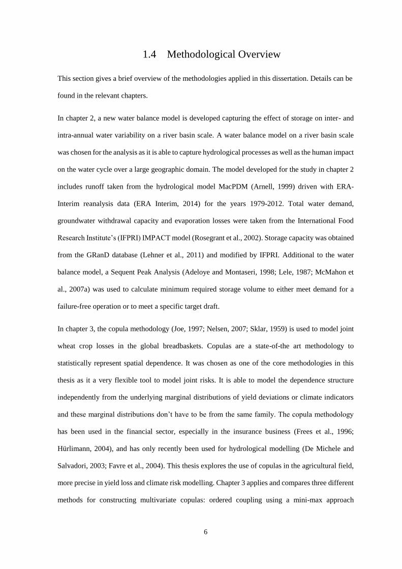
1.4 Methodological Overview

This section gives a brief overview of the methodologies applied in this dissertation. Details can be

found in the relevant chapters.

In chapter 2, a new water balance model is developed capturing the effect of storage on inter- and

intra-annual water variability on a river basin scale. A water balance model on a river basin scale

was chosen for the analysis as it is able to capture hydrological processes as well as the human impact

on the water cycle over a large geographic domain. The model developed for the study in chapter 2

includes runoff taken from the hydrological model MacPDM (Arnell, 1999) driven with ERA-

Interim reanalysis data (ERA Interim, 2014) for the years 1979-2012. Total water demand,

groundwater withdrawal capacity and evaporation losses were taken from the International Food

Research Institute’s (IFPRI) IMPACT model (Rosegrant et al., 2002). Storage capacity was obtained

from the GRanD database (Lehner et al., 2011) and modified by IFPRI. Additional to the water

balance model, a Sequent Peak Analysis (Adeloye and Montaseri, 1998; Lele, 1987; McMahon et

al., 2007a) was used to calculate minimum required storage volume to either meet demand for a

failure-free operation or to meet a specific target draft.

In chapter 3, the copula methodology (Joe, 1997; Nelsen, 2007; Sklar, 1959) is used to model joint

wheat crop losses in the global breadbaskets. Copulas are a state-of-the art methodology to

statistically represent spatial dependence. It was chosen as one of the core methodologies in this

thesis as it a very flexible tool to model joint risks. It is able to model the dependence structure

independently from the underlying marginal distributions of yield deviations or climate indicators

and these marginal distributions don’t have to be from the same family. The copula methodology

has been used in the financial sector, especially in the insurance business (Frees et al., 1996;

Hürlimann, 2004), and has only recently been used for hydrological modelling (De Michele and

Salvadori, 2003; Favre et al., 2004). This thesis explores the use of copulas in the agricultural field,

more precise in yield loss and climate risk modelling. Chapter 3 applies and compares three different

methods for constructing multivariate copulas: ordered coupling using a mini-max approach

7

(Timonina et al., 2015), vine copulas (Aas et al., 2009; Bedford and Cooke, 2002; Kurowicka and

Cooke, 2006) and hierarchical structuring. Wheat ( and later soybean and maize) yield data are taken

from official governmental sources (Australian Bureau of Statistics, 2015; Conab (Companhia

Nacional De Abastecimento) Brazil, 2015; Ministerio de Agricultura, Ganaderia y Pesca de

Argentina, 2015; Ministry of Agriculture and Farmers Welfare, Govt. of India, 2015; National

Bureau of Statistics of China, 2015.; USDA, 2015). For the analysis of joint crop losses, the wheat

data was logistically detrended.

Chapter 4 investigates joint climate risks in the global breadbaskets using regular vines (RVines)

(Dißmann et al., 2013), a flexible class of vine copulas which is specifically well suited to model

dependencies in higher dimensions. Climate indicators, crop- and region-specific temperature and

precipitation data in crop growth sensitive periods, are selected via an extended literature review as

well as a correlation analysis between climate indicators and detrended wheat, maize and soybean

yield data. A climate risk is defined as a climate indicator exceeding a crop- and region-specific

threshold which is the climate value corresponding to the 25 percentile of yield deviations using

linear regression between climate and yield data. Climate data in chapter 4 are monthly temperature

and precipitation Princeton re-analysis data from 1967-2012 (Sheffield et al., 2006).

For chapter 5, RVines are again used to model dependence structures between climate in the global

breadbaskets. Indicators are mostly identical with indicators in chapter 4 except a few examples

which showed different results on the breadbasket scale compared to the province/state scale within

breadbaskets in chapter 4. Climate data projecting a 1.5 and 2°C warmer world are taken from the

atmosphere-only HadAM3P model (Massey et al., 2015) following the “Half a degree Additional

warming, Projections, Prognosis and Impacts” (HAPPI) (Mitchell et al., 2016) experimental set up.

8

2. The Role of Storage Capacity in Coping with

Intra- and Inter-annual Water Variability in Large

River Basins

Abstract

Societies and economies are challenged by variable water supplies. Water storage infrastructure,

on a range of scales, can help to mitigate hydrological variability. This study uses a water balance

model to investigate how storage capacity can improve water security in the world’s 403 most

important river basins, by substituting water from wet months to dry months. We construct a new

water balance model for 676 ‘basin-country units’ (BCUs), which simulates runoff, water use (from

surface and groundwater), evaporation and trans-boundary discharges. When hydrological

variability and net withdrawals are taken into account, along with existing storage capacity, we find

risks of water shortages in the Indian subcontinent, Northern China, Spain, the West of the US,

Australia and several basins in Africa. Dividing basins into basin-country units enabled assessment

of upstream dependency in transboundary rivers. Including Environmental Water Requirements into

the model, we find that in many basins in India, Northern China, South Africa, the US West Coast,

the East of Brazil, Spain and in the Murray basin in Australia human water demand leads to over-

abstraction of water resources important to the ecosystem. Then, a Sequent Peak Analysis is

conducted to estimate how much storage would be needed to satisfy human water demand whilst not

jeopardising environmental flows. The results are consistent with the water balance model in that

basins in India, Northern China, Western Australia, Spain, the US West Coast and several basins in

Africa would need more storage to mitigate water supply variability and to meet water demand.

2.1 Introduction

As recent research has shown, hydrologic variability can be as, or more, important than average

water availability as a threat to water security (Grey et al., 2013; Hall et al., 2014). More extreme

weather conditions (Dai et al., 2004) are likely to increase the risks of floods and droughts

(Hirabayashi and Kanae, 2009; Jongman et al., 2012) with negative impacts on people and on the

environment. According to the World Bank, drought is the largest cause of death due to natural

catastrophes (Dilley, 2005).

9

Water infrastructure, on a range of scales, plays a major role in coping with water supply variability

and enhancing water security. Infrastructure is needed to store, access, move and regulate water

(Grey and Sadoff, 2007) and can consist of small-scale dams, weirs, irrigation systems, rainwater

harvesting cisterns, large multi-purpose dams or inter-basin transfer schemes. Investments in water

infrastructure as well as in institutions are needed to achieve water security which forms the basis

for economic growth, poverty reduction and sustainable development (Grey and Sadoff, 2007).

Inadequate or deteriorating infrastructure, on the other hand, increases vulnerability to water scarcity

(de Fraiture et al., 2010; Garrick and Hall, 2014; Hall et al., 2014) especially under a changing

climate. Nonetheless, storage infrastructure must be interpreted in its broadest sense, from local farm

reservoirs, through to groundwater recharge and larger reservoirs, and is by no means a panacea.

Inappropriate infrastructure investment can have a devastating effect on communities and

ecosystems. Our aim herein, therefore, is to propose methods for appraising sustainable amounts of

storage provision in aggregate. We emphasise the importance of local appraisal, impact assessment

and consultation in the actual implementation of storage schemes.

There are numerous papers defining and measuring water scarcity with a variety of different

methods. We adopt the definition of water scarcity by Loon and Lanen (2013) who define it as a

human effect on the hydrological system when water is overexploited because water demand is

higher than water availability. A review of different water scarcity definitions can be found in Pedro-

Monzonís et al., (2015). Comprehensive reviews of methods measuring water scarcity can be found,

for instance, in Brown and Matlock (2011), Oki and Kanae (2006) and Rijsberman (2006). Recent

studies of water scarcity on a global scale include Alcamo et al. (2003), Hoekstra et al. (2012),

Vorosmarty (2000) and Wada et al. (2011) who use the ratio of water withdrawal, use or demand to

availability as a metric of water scarcity. Most of these studies focus on the average ratio, which

neglects the very significant effects of variability on water security (Hall et al., 2014). By using

monthly data rather than annual totals, Wada and Hoeckstra measured water scarcity resulting from

intra-annual water variability. Yet, they use a 10 year average for each month and thereby cannot

take into account inter-annual variability. Furthermore, they do not include storage. As Biemans et

10

al. (2011) emphasizes, water supply and water stress can be evaluated only when human changes to

the hydrological cycle such as dams and reservoirs are also taken into account. Brown and Lall

(2006) constructed a storage index which highlights countries in need of more storage infrastructure

in order to buffer rainfall variability. However, the analysis on a country scale cannot account for

hydro-climatic differences within a country which is especially important in large countries with

different rainfall pattern across the regions such as China or the US. Moreover, their analysis

included ‘virtual water’ in the water balance. Whilst that is an interesting idea, we believe that it

detracted from the insights gained by studying physical water use from surface and groundwater

sources.

Our study represents an improvement over previous work as it is conducted on a basin-country unit

(BCUs) scale which consists of large global river basins (GRDC, 2007) intersected with country

borders. One country may contain one or more BCUs. River basins that intersect more than one

country are sub-divided into BCUs. In total we analyse 676 BCUs which cover the world’s 403

major river basins. This scale was chosen as many water management decisions are taken on a basin

level as well as at a country level. However, country borders are included in order to incorporate

possible conflicts arising over water allocation within transboundary river basins.

Using a global water balance model, this paper examines the geography of water scarcity. Looking

at past and present, we seek to establish how existing storage capacity helps to buffer intra- and inter-

annual water variability and thereby mitigates resulting water scarcity. First, overall water scarcity

is identified in each BCU considering existing storage and monthly total water use. Variability in

surface water availability is analysed by considering monthly runoff totals from reconstructions for

years 1979 to 2012, averaged over the BCU. Evaporation losses and potential groundwater

withdrawals are included in the water balance. Water scarcity, or shortage, is defined as a situation

when the aggregated current storage in a BCU is less than 20% of capacity. This definition takes

account of dead storage in reservoirs and reflects the conditions under which water restrictions are

typically applied. We go on to refine the analysis and examine dependency on storage in each BCU

as well as upstream dependency in transboundary river basins. Combining upstream dependency

11

with overall water scarcity, areas of potential conflicts over water allocation are detected. Third,

impacts on the ecosystem are included in the analysis. Globally, the area of irrigated land is growing

and the overall water extraction for human use is increasing. This poses a threat to the environment

as these human interventions alter both variability and volume of river flows needed to maintain

freshwater ecosystems such as fish and riparian vegetation (Grafton et al., 2011). Aquatic ecosystems

are adapted to hydrological variability, including droughts. However, when flow variability departs

excessively from natural patterns, there is potential for major ecosystem disturbance. In the definition

of environmental water requirements (EWR) it is therefore important to consider natural flow

variability and the way in which this may be modified by human intervention (Pastor et al., 2013).

In this study we calculate monthly EWRs using the Variable Monthly Flow (VMF) method (Pastor

et al., 2013) and compare them with actual water available after human demand is satisfied. Then,

we conduct a sequent peak analysis (SPA) (Adeloye and Montaseri, 1998; Lele, 1987; McMahon et

al., 2007a) as an alternative methodology to measure water scarcity. In a SPA, hypothetical storage

capacity required to meet water demand is estimated. Comparing required storage with existing

capacity, the need for further infrastructure investments to cope with water variability is identified

on a global scale.

The objective of this study is to inform decision makers about where water supply variability is

causing water shortages in large river basins, given current storage infrastructure, and where it causes

harm to the environment. The results show where policies and infrastructure investments are needed

to sustain and improve global water security.

2.2 Methodology

2.2.1 Water Balance Model

The water balance model is based on the assumption that each BCU with sub-basins and tributaries

can be approximated as one single reservoir with surface runoff and the possibility to withdraw

12

groundwater for water supply. Whilst this is obviously an approximation, Young and Puentes (1969)

found that in a multi-reservoir analysis, unregulated runoff, water demand, and storage can be

aggregated over the study site. It is an assumption that has subsequently been adopted elsewhere

(e.g., Coe (2000)). Average monthly surface runoff per BCU was derived from simulations using the

global hydrological model MacPDM (Arnell, 1999), run at a 1 degree resolution. MacPDM is a

macroscale water balance model simulating streamflow from meteorological input data and

catchment characteristics. MacPDM performs well in reproducing observed runoff, compared with

other global hydrological models as shown in the Water Model Intercomparison Project (WaterMIP)

(Haddeland et al., 2011). In the present study, MacPDM was driven with daily ERA-Interim

reanalysis meteorological data (ERA Interim, 2014) for the period 1979-2012. Groundwater

withdrawal capacity, total water demand and evaporation losses were taken from the IMPACT model

(Rosegrant et al., 2002) provided by the International Food Research Institute (IFPRI). Storage

capacity was taken from the GRanD database (Lehner et al., 2011) and modified by IFPRI who

excluded natural lakes as the storage lakes provide cannot usually be controlled to enhance water

availability for human purposes. Storage thus refers to any kind of surface reservoir whose water can

be managed and used for human activities in the industrial, domestic and agricultural sectors.

Groundwater withdrawal capacity refers to the capacity to pump water. That is not necessarily the

same as actual groundwater withdrawals, but in most regions of the world, groundwater abstractions

are not consistently monitored, so withdrawal capacity is the best approximation of the contribution

to the water balance from groundwater. The groundwater withdrawal that has been assumed may not

be sustainable. Owing to a lack of data, the 2010 figures for groundwater withdrawal capacity were

distributed equally over the 12 months of the year without accounting for possible variation within

a year. Total water use includes consumptive water use from the industrial, domestic and agricultural

sectors. Monthly values were used to describe intra-annual variation of water demand due to

irrigation or hydropower demand.

Including country borders in our study on large global river basins enabled us to analyse the effect

of transboundary flows on water security. This is especially relevant in BCUs such as the Nile in

Egypt where most of the water supply comes from transboundary river flow (Conway, 2005; Zeitoun

13

and Mirumachi, 2008). Comprehensive information on transboundary runoff flows is rarely available

on a global scale. On a country scale, the AQUASTAT database (FAO, 2014b) contains data on

water inflows and outflows. However, transboundary flows depend very much on how borders are

drawn and trying to rescale national AQUASTAT data would not make sense in this case. Therefore,

transboundary flows were calculated specifically for the country-basins used in this study. 305 out

of the 676 country basins considered in this study are transboundary basins. Owing to a lack of global

observed transboundary streamflow data, transboundary runoff was computed by routing from

upstream to downstream BCUs in a basin, using flow accumulation data taken from the global

hydrography HydroSHEDS (Lehner et al., 2008). As a reservoir regulation rule we assumed that

water is released to meet human water demand before recharging the reservoir. When the reservoir

is filled completely, the residual runoff is spilled and flows out to one or several downstream BCUs

or the sea. We assume that groundwater is used directly, so in the case that groundwater withdrawal

capacity is higher than demand, demand is met entirely from groundwater. In BCU j at time t, the

water balance model is therefore as follows:

𝑠𝑗,𝑡 = 𝑠𝑗,𝑡−1 + 𝑞𝑗,𝑡 + 𝑏𝑗,𝑡 − 𝑒𝑗,𝑡 − (𝑢𝑗,𝑡 − 𝑔𝑗)

𝑏𝑗𝑘,𝑡 = 0

{0 ≤ 𝑠𝑗,𝑡−1 + 𝑞𝑗,𝑡 + 𝑏𝑗,𝑡 − 𝑒𝑗,𝑡 − (𝑢𝑗,𝑡 − 𝑔𝑗) ≤ 𝑐𝑗

𝑔𝑗,𝑡 ≤ 𝑢𝑗,𝑡 (2.1)

𝑠𝑗,𝑡 = 𝑠𝑗,𝑡−1 + 𝑞𝑗,𝑡 + 𝑏𝑗,𝑡 − 𝑒𝑗,𝑡

𝑏𝑗𝑘,𝑡 = 0

{0 ≤ 𝑠𝑗,𝑡−1 + 𝑞𝑗,𝑡 + 𝑏𝑗,𝑡 − 𝑒𝑗,𝑡 − (𝑢𝑗,𝑡 − 𝑔𝑗) ≤ 𝑐𝑗

𝑔𝑗,𝑡 > 𝑢𝑗,𝑡 (2.2)

𝑠𝑗,𝑡 = 𝑐𝑗

𝑏𝑗𝑘,𝑡 = 𝑠𝑗,𝑡−1 + 𝑞𝑗,𝑡 + 𝑏𝑗,𝑡 − 𝑒𝑗,𝑡 − (𝑢𝑗,𝑡 − 𝑔𝑗) − 𝑐𝑗

{𝑠𝑗,𝑡−1 + 𝑞𝑗,𝑡 + 𝑏𝑗,𝑡 − 𝑒𝑗,𝑡 − (𝑢𝑗,𝑡 − 𝑔𝑗) > 𝑐𝑗

𝑔𝑗,𝑡 ≤ 𝑢𝑗,𝑡 (2.3)

𝑠𝑗,𝑡 = 𝑐𝑗

𝑏𝑗𝑘,𝑡 = 𝑠𝑗,𝑡−1 + 𝑞𝑗,𝑡 + 𝑏𝑗,𝑡 − 𝑒𝑗,𝑡 − 𝑐𝑗

{𝑠𝑗,𝑡−1 + 𝑞𝑗,𝑡 + 𝑏𝑗,𝑡 − 𝑒𝑗,𝑡 > 𝑐𝑗

𝑔𝑗,𝑡 > 𝑢𝑗,𝑡 (2.4)

with 𝑠𝑗,𝑡 as storage in basin j in month t, 𝑞𝑗,𝑡 as surface runoff, 𝑔𝑗 as groundwater withdrawal (which

is taken as the monthly average and is not time-varying), 𝑢𝑗,𝑡 as total water use, 𝑒𝑗,𝑡 as evaporation

14

losses. 𝑐𝑗 is storage capacity and 𝑠𝑗, 0 = 𝑐𝑗. The transboundary outflow from BCU j to BCU k

downstream basins is written as

𝑏𝑗𝑘,𝑡 = ∑ 𝑏𝑗𝑖,𝑡

𝑘

𝑖=1

(2.5)

and the inflow to BCU j, 𝑏𝑗,𝑡 is computed as the sum from n upstream basins:

𝑏𝑗,𝑡 = ∑ 𝑏𝑖𝑗,𝑡

𝑛

𝑖=1

(2.6)

Owing to a lack of data, institutional arrangements such as water treaties or specific reservoir

management rules could not be included. The reservoir operation rule in this study maximises storage

and does not consider the possibility of multi-purpose use of reservoirs which would include drawing

down reservoir levels in anticipation of floods.

Water shortage in BCU j is defined as the state in which storage is filled to 20% or less, i.e. 𝑠𝑗,𝑡 = ≤

0.2𝑐𝑗, a situation which reflects the dead storage in reservoirs and which is typical of the conditions

under which water restrictions are often applied. The number of months in which the storage water

level is below the 20% threshold during the simulation period is counted and forms, as a percentage

of all 408 months, the index of water scarcity.

2.2.2 Environmental Water Requirements

“Environmental Water Requirements” (EWR) are defined as “quantity, quality and timing of water

flows required to sustain freshwater and estuarine ecosystems and the human livelihoods and

wellbeing that depend on these ecosystems” (The Brisbane Declaration, 2007, p. 1). Including EWRs

in our water balance analysis ensures that ecosystem services such as biodiversity and recreation are

maintained. There are several methods of EWR calculations (Smakhtin et al., 2004; Tennant, 1976;

Tessmann, 1980). This study uses the Variable Monthly Flow (VMF) method introduced by Pastor

et al. (2013) which is based on monthly naturalized flow data and thus can account for intra-annual

15

variability. In contrast to Tessman’s method, VMF allows some water withdrawal in low-flow

seasons which helps the industry and the irrigation sector which need water especially in dry periods.

On the other hand, it allocates at least 30% of the mean monthly flow (MMF) to the environment

throughout the year. The VMF is calculated as follows. During the low-flow season (MMF < 40%

of mean annual flow (MAF)) 60% of MMF is allocated to the environment; during the intermediate-

flow season (MMF 40-80% of MAF) 45% of MMF and during high-flow season (MMF > 80% of

MAF) only 30% are reserved for the environment. In extremely dry conditions (MMF < 1 m3s-1)

there is no environmental flow allocation. EWRs 𝑒𝑤𝑟𝑗, are calculated using naturalized flows. For

each BCU, the EWRs are calculated as described above using average total surface runoff in the ith

month 𝑞 𝑗 ,�� with i = 1, 2,…, 12. Then, the EWRs are compared to monthly outflows in each basin 𝑏𝑗𝑘,.

The number of months in which 𝑏𝑗𝑘, < 𝑒𝑤𝑟𝑗, is counted and forms, as a percentage of all 408 months,

the index of EWR violation.

2.2.3 Sequent Peak Analysis

The Sequent Peak Analysis (SPA) is a method to estimate hypothetical storage capacity required to

meet total water demand. Similar to the Rippl graphical mass curve (Rippl, 1883) and the Extended

Deficit Analysis (Pegram, 2000), SPA calculates the minimum required storage volume to either

meet a specific target draft or to meet demand for a failure-free operation. Using the monthly runoff

data described above, we calculate hypothetical storage capacity needed to satisfy human and

environmental water needs using the following equation:

𝑘𝑗,𝑡 = min[ 0, 𝑘𝑗,𝑡−1 + 𝑢𝑗,𝑡 + 𝑒𝑤𝑟𝑗,𝑡 − 𝑞 𝑗,𝑡 − 𝑏𝑗,𝑡 − 𝑔𝑗] (2.7)

with 𝑘𝑡 as storage in t ( 𝑘0= 0). Then, the required storage capacity is 𝑐𝑗 = max(𝑘𝑗,𝑡). We use the

simple SPA method in which net evaporation losses are ignored. Further discussion of the SPA can

be found in Adeloye and Montaseri, 1998, Lele, 1987 and McMahon et al. (2007a, 2007b).

16

2.3 Results

2.3.1 Water Balance Model

Applying Equation 1 to the 676 BCUs considered in this study, global water scarcity was assessed

using simulated surface runoff for the period 1979-2012. Figure 2.1 shows the results of Equation 1

applied to all BCUs. The shortage scale ranges from 0 (no scarcity) to 1 (very water scarce)

representing the percentages of months in which a BCU is classified as water scarce. Deserts, ice

fields with no runoff and land areas with no large river basins are shaded in grey. Hotspots of water

scarcity are the Indian subcontinent, Northern China, Spain, the West of the US, Australia and

several basins in Africa. In India, the Ganges, the Indus, the Godavari, Krishna or the Penner River

are extremely water scarce. In China, the Yellow River stands out as extremely water scarce. In

Spain, the Guadalquivir, Guadiana and Tejo basins have difficulties to cope with water shortages. In

the West of US, the San Joaquin River, Sacramento River and the Salinas basin show up, whereas

in the South the Bravo, Colorado and Brazos rivers are identified as water scarce. In South America,

most of the BCUs along the West Coast face water limitations: All basins along the coast of Ecuador,

Peru and Northern and Central Chile. In Southern Africa, the Limpopo in South Africa, the Zambezi

in Angola, Malawi and Tanzania show water shortages. The Niger basin has difficulties to supply its

population with water in nearly all basin countries: Algeria, Chad, Guinea, Mali and Benin. In

Australia, the basins in the West were identified as water scarce due to insufficient storage capacity

whereas water scarcity in the Murray basins can be explained by high evaporation losses.

17

Figure 2.1. Index of water scarcity. Percentage of time in which a BCU is water scarce, defined

as 20% storage or less.

Estimating risk involves a combination of probability and consequences. In Table 2.1 we show the

population at risk as an overall indicator of exposure multiplied by our shortage index. Population

data for 2010 is taken from CIESIN (2015).

Table 2.1. Population at risk of water restrictions. Population at risk is the overall BCU population

multiplied with the index of water scarcity. Shown here are global BCUs with population at risk

higher than 1 million.

Drainage Country Population

(millions)

Index

of

water

scarcity

Population at risk

(millions)

INDUS Pakistan 162.97 0.93 151.56

HUANG HE (YELLOW RIVER) China 172.94 0.70 121.06

HUAI HE China 94.90 0.63 59.79

GANGES Bangladesh 62.62 0.34 21.29

GANGES India 483.5 0.05 24.18

GANGES Nepal 29.66 0.44 13.05

18

PENNER RIVER India 11.46 0.95 10.89

ARAL DRAINAGE Uzbekistan 28.35 0.35 9.92

GODAVARI India 71.08 0.13 9.24

ZAMBEZI Malawi 12.40 0.47 5.83

DAMODAR RIVER India 30.25 0.16 4.84

MAHI RIVER India 13.31 0.32 4.26

LIAO HE China 29.46 0.13 3.83

INDUS Afghanistan 10.6 0.35 3.71

LUAN HE China 12.26 0.23 2.82

LIMPOPO South Africa 12.90 0.21 2.71

DALINGHE China 4.3 0.40 1.72

YONGDING HE China 84 0.02 1.68

NILE Rwanda 7.65 0.20 1.53

NILE Burundi 4.87 0.31 1.51

DEAD SEA Jordan 2.5 0.58 1.45

ARAL DRAINAGE Afghanistan 5.6 0.25 1.40

SEBOU Morocco 6.33 0.21 1.33

CONGO Burundi 3.85 0.33 1.27

SACRAMENTO RIVER United States 3.23 0.35 1.13

KRISHNA India 107 0.01 1.07

In Figure 2.2 we quantify how dependent a BCU is on storage by plotting the difference between the

shortage indices with and without storage i.e. with cj = 0 in the latter case.

19

Figure 2.2. Water storage dependency. Difference between months with empty storage and months

in which demand exceeds supply when storage is not included relative to the total time period.

The results show that most basins except the basins in tropical regions show water storage

dependency. Especially India, Northern China, Southern Africa, the entire US, the East of Brazil and

the Murray basin in Australia are dependent on artificial storage capacity to provide reliable flow

over the year. These results coincide with findings of Biemans et al. (2011) who estimated the

contributions of reservoirs to water supply for irrigation for the period 1981 to 2000. They found

that the West Coast of the US as well as basins in China, India and central Asia rely heavily on

reservoir storage.

Figure 2.3 shows upstream dependency independent of storage and reservoir regulation. Therefore,

the frequency with which water demand exceeds water supply when transboundary flows are

excluded is compared with the situation when transboundary runoff is included in the calculations.

Egypt and Sudan in the Nile basin, Syria and Iraq in the Tigris and Euphrates basin, Kazakhstan,

Uzbekistan and Turkmenistan in the Aral Drainage, Niger in the Niger basin, South Africa in the

20

Orange basin and Pakistan in the Indus basin are the most upstream dependant BCUs before storage

is taken into account.

Figure 2.3. Upstream dependency of global BCUs. The index is calculated as follows: Months in

which water demand is exceeding water supply excluding transboundary flows are compared with

a scenario in which transboundary runoff is included and divided through the entire time period.

Our upstream dependence metric quantified the difference between the shortage frequency with and

without transboundary flows. The significance of upstream dependence, however, depends on how

severe the water scarcity is in the BCU itself. Figure 2.4 shows important upstream dependent BCUs

experiencing severe water scarcity despite the possibility to store water. Through the combination of

these two metrics, potential trans-boundary conflicts over water in BCUs are shown, since the

greatest potential for conflicts exists when upstream dependency is combined with water shortage

within the BCU. The Nile in Sudan clearly stands out as highly dependent upon flows from upstream.

However, it is in situations where a combination of upstream dependency and overall water scarcity

occur, such as in the Indus in Pakistan or the Aral Drainage in Kazakhstan and Turkmenistan that

trans-boundary conflicts over water resources might arise. These results, which are based on

hydrological analysis, coincide with findings of other studies on conflict and cooperation in

21

international river basins. A recent study by Bernauer (2014) analysed conflict and cooperation in

global international river basins using International Rivers Conflict and Cooperation event data

(IRCC) which include socio-economic factors such as GDP, population size, existence of democracy

or upstream/downstream power. The following river basins from our study coincide with Bernauer

(2014) results: Indus and the Tigris and Euphrates as basins at risk and Indus, Niger, Nile and Senegal

which were defined as cooperative international basins. A similar study by Yoffe et al. (2003)

highlighted 29 basins at risk from which 24 coincide with our river data set. 17 out of 24 basins

coincided with our upstream dependent basins and 14 out of 24 are basins which resulted to be

upstream dependent as well as water insecure in our study. Among those are the Aral Drainage,

Ganges, Indus, Lake Chad, Limpopo, Nile, Senegal and the Tigris and Euphrates drainage. However,

one has to add that the water balance model used in the present analysis does not include specific

dam operation rules or political aspects such as water treaties. Results have to be interpreted

accordingly.

Figure 2.4. Potential for conflicts in transboundary river basins. The scale reaches from not

upstream dependant or water scarce (0) to very upstream dependant or water scarce (1). Reliance on

trans-boundary flows from upstream is the upstream dependency metric developed for Figure 2.3.

22

2.3.2 Environmental Water Requirements (EWRs)

EWRs are calculated using Pastor et al.'s (2013) VMF method for each month and each BCU using

naturalized surface runoff. Then, the residual outflow of each BCU is compared with EWRs and the

percentage of months in which the EWRs cannot be met is derived. Figure 2.5 shows hotspots of

EWR violation where water requirements for the ecosystem are chronically unmet: India, Northern

China, South Africa, the US, especially the West Coast, the East of Brazil, Spain and the Murray

basin in Australia. This coincides with the findings of numerous papers about the trade-off between

water for agriculture and water for the environment in basins around the globe such as the Indian

river basins (Smakhtin, 2006), in the Yellow river basin in China (Cui et al., 2009; Sun et al., 2008)

and the Murray Basin (e.g., Garrick et al., 2009; Goss, 2003; Grafton et al., 2011; Quiggin, 2001;

Qureshi et al., 2007). Specifically in water-scarce BCUs there is a high prevalence of EWR violations

which is shown in our study through a significant positive correlation between our index of water

restrictions and the frequency of EWR violations (Kendall’s τ= 0.27 with p<0.001). Even more

striking is the correlation between EWR violations and storage dependency (τ= 0.4 with p < 0.001)

which indicates that BCUs whose water security depends on storage are more likely to not meet

EWRs needed for the ecosystem. This emphasizes that dam operation rules and flow dam releases

play a major role in providing the necessary outflow variability to support the downstream

ecosystem.

23

Figure 2.5. Violation of environmental water requirements. Percentage of months in which

EWRs are not met considering the residual outflows after all human water need is met.

Table 2.2 lists all BCUs with a water restriction index higher than 0.5 and other indices developed

in this paper.

Table 2.2. Water scarce BCUs.

Drainage Country Index of water

scarcity

Frequency of

EWR violation

Water storage

dependency

index

Upstream

dependency

Index

CANETE Peru 1.00 0.00 0.01 0.00

DEAD SEA Israel 0.95 0.41 0.11 0.00

PENNER RIVER India 0.95 0.80 0.07 0.00

INDUS Pakistan 0.93 1.00 0.02 0.09

MAJES Peru 0.90 0.15 0.06 0.00

DEAD SEA Egypt 0.90 0.01 0.00 0.00

CHIRA Peru 0.79 0.24 0.12 0.06

TARIM Pakistan 0.77 0.21 0.09 0.00

LOA Chile 0.73 0.02 0.10 0.00

OCONA Peru 0.72 0.12 0.10 0.00

HUASCO Chile 0.72 0.05 0.21 0.00

LOA Bolivia 0.72 0.00 0.11 0.00

HUANG HE

(YELLOW RIVER)

China 0.70 0.69 0.46 0.00

HUAI HE China 0.63 0.83 0.25 0.00

24

ARAL DRAINAGE Kazakhstan 0.61 0.96 0.31 0.01

GEBA Senegal 0.60 0.05 0.00 0.00

SANTA Peru 0.60 0.06 0.11 0.00

DORING South Africa 0.60 0.58 0.36 0.00

DEAD SEA Jordan 0.58 0.18 0.00 0.00

GANGES China 0.51 0.39 0.00 0.00

GAMBIA Senegal 0.51 0.20 0.05 0.10

VOLTA Mali 0.50 0.06 0.26 0.00

Figure 2.6 shows the comparison of existing storage 𝑠𝑗,0 with storage capacity required to meet

current water demand, both for human and environmental need, derived using a SPA. We size the

storage such that the EWR is not violated. Storage deficit is calculated in the following way:

𝑆𝑡𝑜𝑟𝑎𝑔𝑒 𝑑𝑒𝑓𝑖𝑐𝑖𝑡𝑗 = max(𝑘𝑗,𝑡) − 𝑠𝑗,0 (2.8)

Figure 2.6. Storage deficit. Differences of required storage including EWRs and actual storage (in

cm).

According to our analysis, basins which require more storage are the hotspots in India, Northern

China, Western Australia, Spain, the US West Coast and several basins in Africa. Comparing the

25

results of the SPA and the water balance method one can see that both methodologies lead to similar

results. As an overall conclusion one can say that so far, most basins are still water secure.

2.4 Discussion

21.2% of all BCUs show water shortages in at least one month. Although our method is very different

and takes into account variability and storage, the overall percentage is not far off the analysis by

Alcamo et al. (2003) that 24% of all global river basins show “severe water stress” using the ratio of

water withdrawal to availability greater than 0.4 as indicator for water stress. It also coincides with

Hoekstra et al.'s (2012) analysis of global monthly blue water scarcity. Hoekstra identified the basins

in the Indian subcontinent as well as in Northern China, along the US West Coast, in South Africa,

Spain and Australia as most water scarce. Differences are visible in the Murray and Eyre Lake basin

in Australia where Hoekstra measured higher water scarcity than our study. This is due to the fact

that our study accounts for the possibility to store water. Figure 2.2 showed that both basins are

dependent on water storage and therefore can mitigate the impacts of water scarcity. The same

applies to the Mississippi, Colorado and St. Lawrence basins in the US as well as to the Orange basin

in South Africa. In the study by Brown and Lall (2006) several indices were developed indicating

the volume of required storage to meet annual water demand based on the seasonal rainfall cycle as

well as annual water total demand. The 3 countries with highest water deficits identified by Brown

and Lall (2006) are India, Pakistan and China which coincides with our findings. According to our

study most people at risk of water restrictions live in China (196.9 million people), Pakistan (159.7

million) and India (73.4 million), followed by Bangladesh (40.2 million), Nepal (12.2 million) and

Algeria (12.1 million). Desert regions with no major rivers are excluded from the analysis.

This paper highlighted global river basins with water shortages for human use as well as the

environment due to inter- and intra-annual water variability. Using a monthly time scale and BCUs

rather than countries this study represents an improvement over previous work. Furthermore,

possible reasons for the current status of water scarcity, such as dependence on available storage

capacity or on transboundary flows from upstream were identified.

26

The global nature of the analysis means that there are several significant limitations. Storage capacity

includes human made storage and ignores natural storage such as lakes and wetlands. This may lead

to overestimation of the water restriction index in BCUs with large natural lakes such as Lake

Victoria in the Nile basin or Lake Chad in the Chad basin. Groundwater withdrawal data represent

the technological ability to pump up water and does not show how much of it is actually used, nor

the quality of water abstracted. The 2010 annual withdrawal capacity was equally distributed over

the months and therefore does not account for variations within a year. Furthermore, the storage

numbers used in this work do not differentiate between main purposes of reservoirs such as

agriculture, flood protection or hydropower. Although the GRanD database (Lehner et al., 2011)

offers information on main use, most reservoirs are multi-purpose reservoirs and excluding storage

from reservoirs with hydropower as main purpose did not lead to improved results.

2.5 Conclusion

Consideration of water scarcity without proper analysis of hydrological variability, artificial storage

and groundwater withdrawals can give an inaccurate picture of where the global hotspots of water

scarcity are located. In this paper we have implemented a water balance model at the scale of Basin-

Country Units (BCUs) in order to generate a metric of water scarcity. This paper showed in which

BCUs inter- and intra-annual water variability leads to water shortages and highlights where this

situation could be improved through larger storage capacity. However, in basins with a very large

storage deficit (shown in Figure 2.6) greatly exceeding average annual runoff, it may not be possible

to mitigate the problem even with additional storage, which could lead to negative environmental

impacts and higher evaporative losses as pointed out in Brown and Lall (2006). Our results highlight

BCUs in which additional storage capacity can help mitigating the impacts of water variability.

However, this paper should not be seen as a call for more large dams. Storage can be increased

through a plethora of options such as smaller dams, aquifer recharge or rainwater harvesting and our

paper does not recommend one of these options specifically. Our water balance model helps to

explore trade-offs associated with investments in storage, whilst acknowledge the limitations of

27

over-reliance on storage. Furthermore, the model can show trade-offs between water for human use

and water for the environment. While storage is able to buffer water supply variability, the alteration

of natural flows decreases the volume of water flowing downstream and changes the frequency and

timing of high and low flows which are important for downstream river ecosystems (Richter and

Thomas, 2007). It has been shown that dams can be operated to preserve EWRs (e.g., Harman and

Stewardson, 2005; Olden and Naiman, 2010; Richter and Thomas, 2007) but often flow requirements

are still violated as our study has shown. Additionally, more reliable water supply due to increased

storage can lead to increased water demand through a rebound effect which then might have further

negative impact on EWRs.

The analysis is based upon synthetic runoff data derived from a reanalysis dataset. Use of reanalysis

data and simulated runoff has known limitations (Haddeland et al., 2011; Kopp and Lean, 2011), but

was necessary in order to provide global coverage. Additionally, detailed information on reservoir

regulation rules and better groundwater use estimates, e.g. obtained from satellite data, could further

improve the analysis. The same procedure could be applied to future precipitation and runoff series

obtained from climate models, in order to explore the potential effects of climate change on water

scarcity and the sensitivity of infrastructure investments to a changing climate. This will help to

promote storage schemes that are robust to future uncertainties and adaptable in the face of a

changing climate, as well as providing a platform for exploration of other policy responses, including

demand reduction and groundwater resource management.

28

3. Dependency of Crop Production between Global

Breadbaskets: A Copula Approach for the

Assessment of Global and Regional Risk Pools

Abstract

As recent events have shown, simultaneous crop losses in different parts of the world can cause

serious risks to global food security. However, to date, little is known about the spatial dependency

of lower than expected crop yields from global breadbaskets. This is even more so the case for

extreme events, i.e. were one or more breadbaskets are experiencing far below average yields.

Without such information risk management approaches cannot be applied and vulnerability to

extremes may remain high or even increase in the future around the world. We tackle both issues

from an empirical perspective focusing on wheat yield. Interdependencies between historically

observed wheat yield deviations in 5 breadbaskets (USA, Argentina, India, China and Australia) are

estimated via copula approaches that can incorporate increasing tail dependencies. In doing so, we

are able to attach probabilities to inter -regional as well as global yield losses. To address the

robustness of our results we apply three different methods for constructing multivariate copulas:

vine copulas, ordered coupling using a mini - max approach and hierarchical structuring. We found

interdependencies between states within breadbaskets which led us to the conclusion that risk

pooling for extremes are less favourable on the regional level. However, notwithstanding evidence

of global climatic teleconnections that may influence crop production, we also demonstrate

empirically that wheat production losses are independent between global bread baskets which

strengthens the case for inter -regional risk pooling strategies. We argue that through inter -regional

risk pooling, post -disaster liabilities of governments and international donors could be decreased.

3.1 Introduction

The increasing global interconnectivity and mutual interdependence of economic and ecological

systems can amplify vulnerability and risk of disasters (Field and IPCC, 2012). The global food

system demonstrates the effects of increasing interdependence and the possibility of systemic risk.

Owing to the globalization of the grain-market, a food shock due to drought (or other downside risks)

in one or more major food producing areas can lead to a significant increase in the world food prices

and might threaten food security, especially in poorer countries (Gbegbelegbe et al., 2014). For

29

example, between 2005 and 2008, international wheat and maize prices tripled (Von Braun, 2008)

leading to the 2007/2008 food price crisis. Low-income groups in developing countries were

especially affected as they spend 60 – 80% of their income on food (United Nations Conference on

Trade and Development, 2008). Analysing the food price crisis in 2008, several factors were found

to be responsible for the fast increase in grain prices including increased energy prices, shrinking

world grain reserves, a rise in demand through increasing population and wealth, financial

speculation in commodity markets, decline in growth of crop production due to decreased investment

in agricultural R&D and the use of grains for biofuel production (Mittal and others, 2009; Mueller

et al., 2011; Von Braun, 2008). The major cause, however, is considered to be adverse weather

conditions (Lazear, 2008). Especially, the droughts in major crop producing areas including

Australia, the EU, Ukraine and Russia in the years before 2008 had decreased the supply and made

the prices very sensitive to small changes in supply (Mueller et al., 2011). Similar to the 2007/08

crisis, 2010 was another year of severe droughts in different parts of the world. Russia suffered from

the worst drought in a century (Grey et al., 2013), which destroyed more than 13.3 million hectares

of crops, more than 30% of the area cultivated in the affected regions (Wegren, 2011). In August

2010, Russia announced a grain export ban that was meant to curtail price hikes and speculation on

grain products, but which proved to be ineffective. At the same time, 2010 was the driest year on

record in Southwest Australia where crop production is the major driver of the economy. In 2010,

wheat production reached only half of the production in 2011-2012 (Paterson and Wilkinson, 2015).

In south-western China, a drought with the longest period without rain during winter season and the

lowest percentage rainfall anomaly in the past 50 years occurred in 2009-2010 (Yang et al., 2012).

The drought in spring 2010 led to major decline in summer-harvested crops (Zhang et al., 2012). The

confluence of all these weather extreme events in the same year resulted in price shocks: between

June 2010 and January 2011 the global wheat price more than doubled (World Bank, 2011) which

led to a threat to food security in many regions. Some scientists suggest that the increase in food

prices contributed to the unrest that triggered the Arab spring (Grey et al., 2013; Johnstone and Mazo,

2011).

30

The examples given above, together with a projected increase in extreme weather events (Field and

IPCC, 2012) show the need to understand better the consequences of extreme weather events

occurring in more than one location around the world. Moreover, attention needs to be given to how

to manage such risk from a global or regional perspective (Extreme weather and resilience of the

global food system, 2015). Regarding the latter, risk pooling is now seen as one promising way to

manage risk on larger scales(Field and IPCC, 2012) and several applications can be found throughout

the world, including the Caribbean Catastrophe Insurance Facility (CCRIF), the African Risk

Capacity pool (ARC), as well as the European Union Solidarity Fund (EUSF). However, for a risk

pool to work, the risks faced by members of a risk pool should be (statistically) independent, or in

other words, the pool should aggregate highly uncorrelated risks. If independence or low dependence

is ensured, the risk-reduction occurs due to the law of large numbers, which as a consequence, makes

the variance of the aggregated risk less than the variance of the risks taken individually (Embrechts

et al., 1997; Freeman and Scott, 2006). Variance is important as, for a given mean, it determines the

potential loss below some critical threshold. Regarding the global food system and the feasibility of

global and/or regional risk pooling one therefore has to analyse the dependency structure of losses

between and within the regions because different risk instruments, such as structural adaptation or

insurance schemes, need to be applied conditional on the results.

So far, the global food system has kept up with an increasing population and rising food demand but

due to the recent experiences discussed above and under the threat of climate change, understanding

the risks to global food supply together with a functioning system of global food trade becomes

essential for bringing resilience to the system and guaranteeing future food security.

Unfortunately, as recent research has shown, seemingly uncorrelated risk (e.g., for very frequent

events) may become very much more correlated in case of extreme events and therefore this

dependence structure needs to be taken explicitly into account in the analysis (Jongman et al., 2014).

Extreme climate events are often caused by large-scale atmospheric circulations such as El Niño

Southern Oscillation (ENSO) (Ward et al., 2014) or high amplitude quasi-stationary planetary waves

(Petoukhov et al., 2013). Due to climate change, not only the frequency and severity of individual

31

regional climate extremes are projected to increase but also climate phenomena such as ENSO events

and planetary waves might occur more frequently (Cai et al., 2014; Lau and Kim, 2012; Power et

al., 2013) which increases the likelihood of simultaneous climate extremes such as the 2013/14

winter floods in the UK connected with an extreme cold in the US (Huntingford et al., 2014; Rasmijn

et al., 2016) or the 1997/98 extreme El Niño event which had disastrous impacts around the globe

(Cai et al., 2014) .

One emerging method dealing with this issue and now increasingly included in applied research is

the copula method (Embrechts et al., 1997; Jaworski et al., 2010). Copulas are useful for modelling

dependencies between continuous random variables. Using a copula model allows the selection of

marginal distributions separately from the modelling of their interdependence. In other words, while

the marginal distributions contain the information on the separate risks, the copula contains the

information about the structure of the dependency.

Several studies have applied the copula method to analyse yield losses and their implications for

agricultural insurance. Vedenov (2008) used the Gaussian copula to estimate the joint distribution of

corn yields at two aggregation levels, the farm- and the county-level. He found that the dependence

between farm and county yield changed in the lower tail of the distribution. Zhu et al. (2008) applied

the Gaussian and the t-copula to model the dependence structure between crop yield and prices and

found a higher dependency in the distribution tails. Xu et al. (2010) examined the magnitude of

spatial dependence between weather indices used for different regions in Germany. The purpose of

their study was to quantify the likelihood of a crop insurance payoff due to the joint occurrence of

bad weather at different locations. Bokusheva (2011) used the copula method to measure the

dependence between yields and weather indices in Kazakhstan. She first used a regression analysis

to test the sensitivity of crop yields to several weather indices and then applied the copula method to

estimate joint tail dependence between crop yields and weather indices. Okhrin et al. (2013) found

systemic risk in index-based insurance for several regions in China and a decline of the risk premium

with increasing trading area for the insurance. They recommend risk pooling between regions in

order to decrease the required buffer fund and therefore risk premiums. Larsen et al. (2013) found

32

an inverse relationship between geographic conditions and yield dependencies in 380 counties of the

US wheat belt using copulas and Goodwin and Hungerford (2015) used different copula models to

estimate premium rates for revenue insurances, insuring both yield and price losses, for soybean and

corn in four counties in Illinois. In Ahmed and Serra (2015) used the copula methodology to show

for the apple and orange sector, that agricultural revenue insurance reduces premium rates compared

to yield insurance schemes. Compared to the linear correlation approach, copula estimations are

considered to be more reliable as they allow to measure extreme dependence between random

variables (Bokusheva, 2011). Vedenov (2008) recommends using copulas for optimal crop coverage

selection and for crop insurance rating.

Our study contributes to efforts to increase current and future food security by focusing on

production risk and possible ways to decrease such risk explicitly taking spatial dependencies into

account. In doing so we examine the dependence structure of wheat yield losses within and between

five major wheat producing areas, so called breadbaskets, in the US, Argentina, India, China and

Australia. We chose wheat as an exemplary crop as, measured in acreage, it is the most extensively

grown food crop globally. Overall wheat production for human consumption is the second largest

after rice (FAO, 2013).

The paper is organized as follows. Chapter 3.2 introduces the breadbaskets, Chapter 3.3 describes

the copula methodology applied in this study and Chapter 3.4 gives a detailed description of the

results. Afterwards, we base our results within a broader discussion on risk pooling and end with a

summary and outlook to the future in Chapter 3.6.

3.2 Wheat Yield Data

For the selection of global breadbaskets, the Spatial Allocation Model (SPAM)(Harvest Choice,

2014), a crop production data set, was used to identify the major wheat producing regions of the

world. For the analysis, states and provinces were chosen as they provide sufficient accuracy to

examine yield loss correlation structures within a region and, at the same time, there is data available

33

and accessible. SPAM production was aggregated on a state/province scale and the highest crop

producing units in the US, Argentina, China, India and Australia were selected. These results were

compared with suggestions from scientific papers, governmental information and grey literature.

With the premise that the states/provinces of a breadbasket have to be adjacent, global breadbaskets

were defined as shown in Figure 3.1. Production in each breadbasket accounts for at least 60% of its

national wheat production. A sixth very important wheat producer is Russia, but due to limited data

availability, Russia was excluded from the analysis. The five breadbaskets selected for this study

account for 35% of global wheat production in 2011.

Figure 3.1. The global wheat breadbaskets.

In what follows we give a short summary of each of the selected global bread baskets in Argentina,

U.S., China, India and Australia, data sources employed as well as their relation to the global scale.

The Argentinian breadbasket includes Entre Rios, Santa Fe, Buenos Aires and Cordoba. Wheat in

the Argentinian breadbasket accounts for 68% of the national Argentinian wheat production (FAO,

2015). Data were obtained from the agricultural ministry of Argentina (Ministerio de Agricultura,

Ganaderia y Pesca de Argentina, 2015). In 2013, Argentina was the 13th largest wheat producer in

the world and the largest in South America. It is a net exporter of wheat. Wheat in Argentina is

usually planted from May to end of July and harvested between mid-November and mid-January

(USDA/NOAA, 2015).

34

The US breadbasket includes the states Washington, Montana, Idaho, Nebraska, North Dakota,

South Dakota, Minnesota, Kansas, Oklahoma and Texas. Wheat production in these states accounts

for 63% of national production (FAO, 2015) which is the third largest in the world. Behind corn and

soybeans, wheat is the third most important crop produced in the US. The country is the world’s

biggest wheat exporter with half of its production being exported. 70-80% of wheat grown in the US

is winter wheat which is planted between September and end of October and is harvested between

end of May and late August, depending on the region (USDA, 2015). Data used in this study are

taken from the United States Department of Agriculture (2015).

The Chinese breadbasket consists of the provinces Shandong, Hebei, Henan, Jiangsu and Anhui.

Wheat production in this region covers 84% of the entire Chinese wheat production (FAO, 2015).

China is the largest wheat producer in the world but due to its large population, domestic

consumption is very high and therefore, China is also the seventh largest importer of wheat (USDA,

2015). 94% of China’s wheat production consists of winter wheat. Growing season for winter wheat

in China is usually October to May (Li et al., 2010). Agriculture is an important sector in China,

contributing 10% to GDP in 2013. Looking at the provinces relevant to our study, the share of

agriculture of Gross Regional Product (GRP) are 12.4% in Hebei, 6.2% in Jiangsu, 12.3% in Anhui,

8.7% in Shandong and 12.6% in Henan (National Bureau of Statistics of China, 2015). Data were

obtained from the National Bureau of Statistics of China (2015).

The states forming the Indian breadbasket are Uttar Pradesh, Madhya Pradesh, Rajasthan,

Maharashtra, Gujarat, Bihar, Haryana and Punjab. Together, they produce 88% of India’s national

wheat. In 2013, India accounted for 13% of global wheat production and was the second largest

producer after China (FAO, 2015). Same as China, large domestic consumption makes India a net

wheat importer. India grows mostly winter wheat which is planted between October and end of

December and harvested between March and May (USDA/NOAA, 2015). Data for India was taken

from the Ministry of Agriculture and Farmers Welfare, Govt. of India (2015).

The Australian breadbasket includes News South Wales and Southern Australia. Together, they

produce 80% of Australia’s wheat (FAO, 2015). Australia is the 8th largest producer of wheat and an

35

important wheat exporter. Most of its wheat is winter wheat which is planted between May and end

of July and harvested between October and end of December (USDA/NOAA, 2015). Australian

wheat data used in this study was taken from the Australian Bureau of Statistics (2015).

Annual historical wheat yield data on a state or provincial scale from 1967 to 2012 was used. The

wheat yield time series were detrended and the deviations from the trend were taken to estimate the

correlation structure as described in the following section.

3.3 Statistical Analysis Methodology

The copula methodology is based on Sklar’s theorem (Sklar, 1959) which states that the joint

distribution function of any continuous random variables (X,Y) can be written as:

H(x,y) = C[FX(x), FY(y)] x,y ∈ ℝ (3.1)

With FX(x) and FY(y) as marginal probability distributions and C = [0,1]2 → [0,1] as copula. Sklar

(1959) showed that C is uniquely defined if FX and FY are continuous. Assuming that the marginal

distributions are continuous and have probability density functions fX(x) and fY(y), the bivariate joint

probability density function will have the form

fX,Y(x,y) = c(FX(x), FY(y))fX(x)fY(y) (3.2)

with c as the density function of C, defined as

c(u,v) = 𝜕2𝐶(𝑢,𝑣)

𝜕𝑢𝜕𝑣 (3.3)

for 0 ≤ u, v, ≤ 1. The advantage of this approach is that the copula, and thereby the dependence

characteristics between FX and FY, can be chosen independently from the marginal distributions.

There are many different copula families described in literature which can be divided into four

classes: Archimedean, elliptical, extreme value and others (Jaworski et al., 2010). Archimedean

copulas such as the Clayton, Frank, and Gumbel-Hougaard copulas are widely adopted because of

their simple form (Khedun et al., 2011) and for elliptical copulas, the Gaussian copula and the student

36

t-copula are widely adopted examples. However, any multivariate distribution function can generally

be used as the basis for a copula (Aas, 2007).

Usually, four steps have to be taken to build a multivariate copula model. In the first step, an adequate

copula structure has to be chosen. The selection can be based on expert knowledge or is implied by

the structure of the data. A multivariate copula structure can be a hierarchical Archimedean copula

(HAC) (Liu et al., 2011; Okhrin et al., 2013; Savu and Trede, 2010), a vine copula (Aas et al., 2009;

Brechmann and Schepsmeier, 2013; Czado et al., 2013) or a pairwise-coupling process using the

minimax approach (Timonina et al., 2015). For complex datasets no single methodology is

guaranteed to yield robust results. We therefore present and compare three different types of copula

structure selection methods which represent varying degrees of complexity and also implicit

assumptions within the modelling structure (and should shed some light on uncertainty ranges of the

results): For the analysis within the wheat breadbaskets, pairwise-coupling with a minimax approach

using different copulas is shown as well as a regular vine tree structure which can include all types

of copulas. In the end, hierarchical structuring is used to combine all five breadbaskets. In the second

step, appropriate copula families have to be selected which can be done graphically through

scatterplots in the bivariate case or analytically through different goodness-of-fit tests such as the

Kendall (Genest and Rivest, 1993) or the Vuong and Clarke test (Clarke, 2007; Vuong, 1989). Then,

the copula parameters are estimated and in the end, the model has to be evaluated with tests such as

the AIC or BIC criterion. We start with the copula structuring methods applied in our analysis. Our

analysis was conducted using CRAN R including the packages ‘copula’, ‘CDVine’ and

‘VineCopula’.

3.3.1 Pairwise Coupling using a Minimax Structuring Approach

One possibility to order the random variables, in this case yield deviations in the different states or

provinces within one breadbasket, is pairwise ordered coupling. Here, yield deviations are defined

as deviations from a logistic trend. Observations are called yi,t. and we use the following model

37

yi,t= fi (t) + ∆yi,t (3.4)

where fi(t) is a 4-parameter logistic regression function

𝑓𝑖(𝑡) = 𝑎𝑖 +𝑏𝑖

1 + 𝑐𝑖 exp (−𝑑𝑖𝑡)

(3.5)

For pairwise coupling, assume that a breadbasket has 5 states with yield deviations Δyi in each state

i. Let the yield deviation Δy1 in state 1 influence yield deviation Δy2 in state 2. Yield deviation Δy2 in

state 2 then influences yield deviation Δy3 in state 3 which influences yield deviation Δy4 in state 4

and so on. Then, 2-dimensional copula densities c1,2, c2,3, c3,4 and c4,5 are estimated and combined

through conditional copulas in the following way:

𝑐 (𝑢1,𝑢2,𝑢3,𝑢4,𝑢5)= 𝑐1,2 (𝑢2|𝑢1) ∙ 𝑐2,3 (𝑢3|𝑢2) ∙ 𝑐3,4 (𝑢4|𝑢3) ∙ 𝑐4,5 (𝑢5|𝑢4) (3.6)

The tree structure of this copula is shown in Figure 3.2.

Figure 3.2. Pairwise ordered coupling.

In a next step, an ordering technique has to be chosen. In this paper we employ the minimax approach

based on Timonina et al. (2015). First, the metric used for the structuring process has to be chosen.

This can be, e.g., geographical distance between states or the non-parametric correlation coefficient

Kendall’s tau (τ) which was used for this study. Kendall’s τ is calculated for each pair of states

which results in a matrix shown in Equation 3.7.

38

𝚻 = (

1𝜏21

⋮𝜏𝑁1

𝜏12

1⋯

𝜏𝑁2

⋯ ⋯

1⋯

𝜏1𝑁𝜏2𝑁

⋮1

) (3.7)

Columns and rows represent states and Kendall’s τi,j is the non-parametric correlation between state

i and j. Second, the ordering technique minimax is applied by choosing N pairs of states from matrix

T. Therefore, the highest correlation τi,j is chosen and the ordering starts with states i and j. All

correlations with these two states, τi,1, τi,2, …, τi,N and τ1,j, τ2,j, …, τN,j are screened and for each pair

τi,n and τn,j (with n= 1,2,…,N states) the minimum is chosen. Between all minima min[τi,n, τn,j] the

maximum is chosen, max[min[τi,n, τn,j]], which will be k (with k≠i, k≠j). 𝜏𝑖,𝑘 or 𝜏𝑘,𝑗 will be the new

starting point and the selection process for the next basin starts over again. Detailed information

about the minimax technique can be found in Timonina et al. (2015).

After the ordering structure is determined, the copula family for the entire model has to be selected.

Similar to Timonina et al. (2015), we test four types of copulas for the minimax approach, the

Gumbel, Clayton, Gaussian and Frank copula, which possess different characteristics concerning

their tail dependence. We then use the AIC (Akaike, 1973a) and BIC (Schwarz and others, 1978)

goodness-of-fit test for each pair-copula in the structuring process and choose the copula family with

the best overall fit (see supplementary material). As demonstrated in Equation 3.6, conditional

copulas are created to model the dependency between yield deviations in the different states within

one breadbasket. A conditional copula is a partial derivative of the original copula Cθ (u,v) over v:

𝐶𝜃(𝑢|𝑣 = 𝑣0) = 𝜕𝐶𝜃(𝑢,𝑣)

𝜕𝑣|𝑣=𝑣0

(3.8)

Where u and v are placeholders for the cumulative distribution functions F∆yi, and F∆yj of yield

deviations in state i and j. A random number u following the conditional Gaussian copula given v is

given by Equation 3.9.

𝑢 = 𝛷(𝑁(𝜃 𝛷−1(𝑣), 1 − 𝜃2) (3.9)

with 𝛷 as Gaussian distribution and θ as copula parameter which can be calculated using the

relationship to Kendall’s τ: sin(πτ/2) = 𝜃. Unfortunately, the Gumbel copula is not directly invertible

39

as shown in Timonina et al. (2015) and therefore, a numerical iteration has to be used which is

explained in detail in the Appendix A. Gaussian, Clayton and Frank copulas are directly invertible.

By sequentially linking the conditional copulas as in Equation 3.6, a conditional copula with d

dimensions, depending on the number of states in a breadbasket, is calculated. For getting random

joint yields this random generation process is repeated 10 000 times resulting in a 10 000 x d matrix

with dependent yield deviations.

3.3.2 Vine Copula Approach

Another ordering approach for multivariate copula models are vine copulas (Aas et al., 2009;

Bedford and Cooke, 2002; Kurowicka and Cooke, 2006). A vine copula is a flexible graphical model

which uses a cascade of conditional and unconditional bivariate pair-copulas to decompose the

multivariate probability density. The pair-copulas are ordered in so-called tree structures with three

most common ways of ordering being lines trees, called D-vines, star trees, called C-vines, or R-

vines which are most flexible. Figure 3.3a and b show a C-vine and an R-vine respectively for a five-

dimensional copula.

40

Figure 3.3 a) Five-dimensional C-vine tree b) five-dimensional R-vine tree

As each copula pair can be chosen independently an enormous amount of combinations and thereby

dependence structures are possible. For a d-dimensional copula, there are 𝑑(𝑑−1)

2 bivariate copulas

that can be estimated in 𝑑!

2∙ 2( 2

𝑑−2)possible R-vine trees or in d!/2 possible C-vine trees (Czado et

al., 2013). A vine structure has (d-1) trees with nodes Ni and edges Ei-1 joining the nodes. A tree

structure is built considering the proximity condition (Bedford and Cooke, 2002) which states that if

an edge connects two nodes in tree j+1, the corresponding edges in tree j share a node. In order to

select the structure of one tree, there are different selection approaches. Aas et al. (Aas et al., 2009)

choose the variables with the strongest bivariate dependencies, measured with Kendall’s τ, for the

first tree. Other possible edge weights are the p-value of a goodness-of-fit test or directly the copula

parameter θ. This paper selects trees using maximum spanning trees with Kendall’s τ as edge weights

41

(Dißmann et al., 2013). For each tree, the spanning tree which maximizes the sum of absolute

Kendall’s τ’s is selected by solving the following optimization problem:

max ∑ |

𝐸={𝑗,𝑘}𝑖𝑛 𝑠𝑝𝑎𝑛𝑛𝑖𝑛𝑔 𝑡𝑟𝑒𝑒

τ𝑗,𝑘| (3.10)

with τ𝑗,𝑘 as pairwise empirical Kendall’s τ. A spanning tree, i.e. a circle free graph, connects all

nodes.

Compared to the pairwise ordering approach using minimax, the vine copula approach can include

different types of copulas for each bivariate copula. The copulas are selected as described above and

the copula parameters are estimated.

3.3.3 Hierarchical Structuring

The third way of copula structuring discussed in this paper is hierarchical structuring. After

combining the different states in each breadbasket through pairwise coupling using the minimax

approach as shown in Figure 3.2, the copulas themselves are structured in a hierarchical way as

shown in Figure 3.4 for two copulas.

Figure 3.4 Hierarchical structuring.

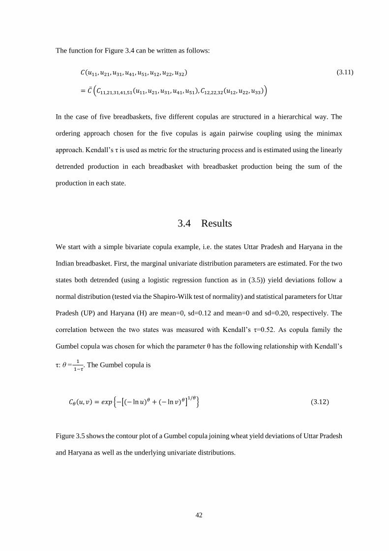
42

The function for Figure 3.4 can be written as follows:

𝐶(𝑢11, 𝑢21, 𝑢31, 𝑢41, 𝑢51, 𝑢12, 𝑢22, 𝑢32)

= �� (𝐶11,21,31,41,51(𝑢11, 𝑢21, 𝑢31, 𝑢41, 𝑢51), 𝐶12,22,32(𝑢12, 𝑢22, 𝑢33))

(3.11)

In the case of five breadbaskets, five different copulas are structured in a hierarchical way. The

ordering approach chosen for the five copulas is again pairwise coupling using the minimax

approach. Kendall’s τ is used as metric for the structuring process and is estimated using the linearly

detrended production in each breadbasket with breadbasket production being the sum of the

production in each state.

3.4 Results

We start with a simple bivariate copula example, i.e. the states Uttar Pradesh and Haryana in the

Indian breadbasket. First, the marginal univariate distribution parameters are estimated. For the two

states both detrended (using a logistic regression function as in (3.5)) yield deviations follow a

normal distribution (tested via the Shapiro-Wilk test of normality) and statistical parameters for Uttar

Pradesh (UP) and Haryana (H) are mean=0, sd=0.12 and mean=0 and sd=0.20, respectively. The

correlation between the two states was measured with Kendall’s τ=0.52. As copula family the

Gumbel copula was chosen for which the parameter θ has the following relationship with Kendall’s

τ: θ =1

1−𝜏. The Gumbel copula is

𝐶𝜃(𝑢, 𝑣) = 𝑒𝑥𝑝 {−[(− ln 𝑢)𝜃 + (− ln 𝑣)𝜃]1/𝜃

} (3.12)

Figure 3.5 shows the contour plot of a Gumbel copula joining wheat yield deviations of Uttar Pradesh

and Haryana as well as the underlying univariate distributions.

43

Figure 3.5. Gumbel copula for joint modelling of wheat yield deviation in Uttar Pradesh and

Haryana.

Using this kind of information one is able to calculate risks of joint yield losses. For example, the

probability that in the same year wheat yields in both states are below the mean by more than one

standard deviation is P(UP ≤ -0.118, H ≤ -0.2)= Cθ [FUP (-0.118), FH (-0.2)] = 0.075. Note, if we

assume independence between the two states, the risk would be underestimated by a factor of three,

e.g., P(UP ≤ -0.118, H ≤ -0.2)= FUP (-0.118)∙ FH (-0.2) = 0.024. The implications of underestimating

this correlated risk are tremendously important for risk pooling and policy makers who have to take

decisions on agricultural policies such as subsidies or post disaster risk finance mechanisms. The

importance of including such dependency structures for risk modelling becomes even more apparent

in the subsequent multivariate models which are discussed next.

To start with, the pairwise coupling was applied to all states within one breadbasket leading to a

Kendall’s τ correlation matrix for all states (which can be interpreted in the same way as discussed

for the bivariate example given above). The copula structure was determined using the minimax

44

approach. Afterwards, the correlation structure for wheat yield deviation was determined and

estimated using Gumbel copulas, and yields were transformed into total production via the formula

pk(t)= ∑(𝑓𝑖(𝑡) + ∆��𝑖,𝑡) ∗ 𝑎𝑖 (3.13)

with i = 1,…., 8 Indian states and t = time. pk is total production in breadbasket k and ai is harvested

area in ha in state i in 2012 which was held constant for each state in order to avoid production

changes due to increased acreage instead of increased yield. ∆𝑦𝑖�� denote random draws from the

estimated joint distribution using the estimated marginals and the estimated copula.

Average yield is time-dependent as yields are increasing over time due to technological

improvements which was captured in the logistic trend function fi(t) (and a linear trend in the

Argentinian breadbasket). Based on the logistic (or linear) trend and the sampled dependent residuals

three production curves were calculated including future production estimates for today, in 10 years

and in 20 years from 2012 onwards. In contrast to ordered pairwise coupling using the minimax

approach, we already indicated that R-vines are more flexible concerning the choice of copula

families, e.g., for each copula pair, a different copula type may be chosen. To find the best fitting

copula family for each pair, the Akaike Information Criterion (AIC) (Akaike, 1973b) was used here.

The R-vines were applied to yield deviations in all breadbaskets and production curves were

produced as described in Equation 3.13. Figure 3.6a shows the results of the analysis of the lower

tail of the distribution of production, using an R-vine compared with results from the previous

approach.

45

a)

b)

Figure 3.6. Production curves up to the lower 10 percentile of the production distribution for

the Indian breadbasket a) comparing the with minimax structured copula using Gaussian copulas

with an R-vine for three time steps. b) comparing the with minimax structured copula using Gaussian

copulas and an R-vine with the independent and fully dependent case with today’s average

production levels.

As we are mainly interested in yield losses, the figure above shows only the lower tail of the

distributions. In more detail, the plot shows production curves for today, for in 10 and for in 20 years.

46

The results between the two structuring methods differ: most importantly the production

distributions for R-vines have fatter tails than the distributions where the minimax approach with

Gaussian copulas was used. In other words production losses are more likely under an R-vine

structure than if the Gaussian copulas are applied. Whilst there is no definitive way to establish which

way of copula structuring fits better, the R-vines structure is more flexible and general so is more

attractive. Figure 3.6b compares the lower tail of wheat production in the Indian breadbasket for

today’s average production levels using minimax with Gaussian copulas, an R-vine, an independent

copula and a copula assuming full dependence between the Indian states. The Gaussian copula using

minimax ordering and the R-vine structure lie between the independent and the fully dependent case.

For example, with a probability of 5% or a 20 year return period, the production in the Indian

breadbaskets will be 76.1 million tons if the breadbaskets were fully dependent, 78.5 million tons

using the R-vine approach, 79.1 million tons applying a structured copula and 80.5 million tons if

we don’t consider correlations between the states. The difference between the R-vine curve and the

independent copula is 2 million tons of wheat which equals 2.2% of the actual wheat production in

the Indian breadbasket in 2012, 91.2 million tons. The difference between the minimax structured

copula and the independent case are 1.4 million tons which equals 1.5% of the actual production.

This shows that, if correlations between wheat yields within the breadbaskets are not considered in

risk analysis, the risk of production losses is underestimated, which is important for crop insurance

schemes and agricultural policy decisions. Using the example above, the risk of a production of 80.5

million tons is more than three times higher assuming all states are independent compared to the R-

vine curve.

As explained above for India, copula models for production risk for all regions have been developed

(see Appendix A.2). In the next step, these copula models were combined through another

multivariate copula, now up to the global level. In that way, dependencies between but also within

the regions can be captured. Pairwise coupling using minimax was chosen to build an ordering

structure for the breadbasket models consisting of multivariate copula distributions as estimated

before. The correlations between linearly detrended production (with production as product of yield

47

and area with area held constant at 2012 levels) in the breadbaskets was used to estimate copulas.

For the copulas within breadbaskets, the results of pairwise coupling with minimax using the

according copula families were again used for all breadbaskets. For the hierarchical structuring,

pairwise ordering with minimax was applied and Gaussian copulas were used to estimate the

conditional multivariate copula model as they proved to be the best fit. The copula density function

for five breadbaskets combined in hierarchical structuring is shown in Equation 3.14:

𝑐 (𝑢𝑈𝑆,𝑢𝐼𝑁,𝑢𝐴𝑅𝐺,𝑢𝐶𝐻,𝑢𝐴𝑈𝑆) = 𝑐��𝑆,𝐴𝑅𝐺 (𝑐𝑈𝑆|𝑐𝐴𝑅𝐺) ∙ 𝑐��𝑁,𝐴𝑅𝐺 (𝑐𝐼𝑁|𝑐𝐴𝑅𝐺) ∙ 𝑐��𝐻,𝐼𝑁 (𝑐𝐶𝐻|𝑐𝐼𝑁)

∙ 𝑐��𝑈𝑆,𝐶𝐻 (𝑐𝐴𝑈𝑆|𝑐𝐶𝐻) (3.14)

with 𝑐𝑈𝑆 = 𝑐𝑈𝑆(𝑢1, 𝑢2, 𝑢3, 𝑢4, 𝑢5, 𝑢5, 𝑢7, 𝑢8, 𝑢9, 𝑢10)

= 𝑐1,2 (𝑢2|𝑢1) ∙ 𝑐2,3 (𝑢3|𝑢2) ∙ 𝑐3,4 (𝑢4|𝑢3) ∙ 𝑐4,5 (𝑢5|𝑢4) ∙ 𝑐5,6 (𝑢6|𝑢5) ∙ 𝑐6,7 (𝑢7|𝑢6)

∙ 𝑐7,8 (𝑢8|𝑢7) ∙ 𝑐8.9 (𝑢9|𝑢8) ∙ 𝑐9,10 (𝑢10|𝑢9)

𝑐𝐴𝑅𝐺 = 𝑐𝐴𝑅𝐺(𝑢11, 𝑢12, 𝑢13, 𝑢14)

= 𝑐11,12 (𝑢12|𝑢11) ∙ 𝑐12,13 (𝑢13|𝑢12) ∙ 𝑐13,14 (𝑢14|𝑢13)

𝑐𝐼𝑁 = 𝑐𝐼𝑁(𝑢15, 𝑢16, 𝑢17, 𝑢18, 𝑢19, 𝑢20, 𝑢21, 𝑢22)

= 𝑐15,16 (𝑢16|𝑢15) ∙ 𝑐16,17 (𝑢17|𝑢16) ∙ 𝑐17,18 (𝑢18|𝑢17) ∙ 𝑐18,19 (𝑢19|𝑢18)

∙ 𝑐19,20 (𝑢20|𝑢19) 𝑐20,21 (𝑢21|𝑢20) ∙ 𝑐21,22 (𝑢22|𝑢21)

𝑐𝐴𝑈𝑆 = 𝑐𝐴𝑈𝑆(𝑢23, 𝑢24)

= 𝑐23,24 (𝑢24|𝑢23)

𝑐𝐶𝐻 = 𝑐𝐶𝐻(𝑢25, 𝑢26, 𝑢27, 𝑢28, 𝑢29)

= 𝑐25,26 (𝑢26|𝑢25) ∙ 𝑐26,27 (𝑢27|𝑢28) ∙ 𝑐27,28 (𝑢28|𝑢27) ∙ 𝑐28,29 (𝑢28|𝑢29)

where i = 1,2,…29 are the 29 states in five breadbaskets used for this analysis.

48

The correlations between detrended wheat productions of the five breadbaskets are shown in Table

3.1. Compared to correlations within the regions, correlations between breadbaskets are found to be

quite low.

Table 3.1. Correlations between linearly detrended wheat productions in five global

breadbaskets. *** for p < .001, ** for p < .01, * for p < .05.

India China USA Argentina Australia

India ------ 0.20* 0.04 -0.17 0.20*

China ------ 0.03 -0.09 0.02

USA ------ 0.23* -0.13

Argentina ------ -0.04

Australia ------

The cumulative production distribution curve for wheat in all five breadbaskets, based on average

production in 2012, can be estimated via the numbers above and is shown in Figure 3.7. Average

production for 2012 in the five breadbaskets is estimated 236 million tons, nearly one third of the

total global wheat production in 2012 (671 million tons according to FAOSTAT (2015)), which

shows that the breadbaskets used in this analysis are a representative selection for global wheat

production. The actual observed production in this area was 244.87 million tons which means that

2012 was a good, above-average year for global wheat production.

49

Figure 3.7. Production curve for wheat production in five global breadbaskets.

As we are interested in occurrences of low production rather than high production, we focus again

on the lower tail of the distribution. Table 3.2 shows quantiles and return periods for low production

based on Figure 3.7.

Table 3.2. Wheat production in the global breadbaskets.

Return

period

5 10 20 50 100 200

Quantiles 0.2 0.1 0.05 0.02 0.01 0.005

Production

in million

tons 231.21 228.75 226.58 224.25 222.66 221.06

50

For example, a one in 50 year event would be a production of 224.25 million tons of wheat which is

a negative deviation from the mean of 11.75million tons which is more than the entire wheat

production in the Argentinian breadbasket (8.5 million tons). We are now able to answer the question

stated at the very beginning of the article, namely if risk pooling is a possible way to reduce

production risk on the global or regional level. The advantage of risk pooling on a global level can

be shown by the following numerical example. We use the 1% Value at Risk (Embrechts et al.,

1997), which can be interpreted here as the wheat production which will be exceeded in 99%, as a

measure for an extremely poor harvest. Alternative ways of estimating extreme yield losses are

described in Ben-Ari et al. (2016). If we calculate the 1%VaR for each breadbasket and define the

difference from the average production as production loss, the overall, aggregated production loss in

all five breadbaskets is 26.59 million tons. However, if we pool risks, the loss from a 1%VaR global

wheat production is only 13.4 million tons. This finding shows that risk aggregation is indeed

feasible on the global level providing that all breadbaskets are aggregated. However, due to the

interdependencies found between states within a breadbasket, risk pooling would be less favourable

on the regional level.

3.5 Discussion

Our results in this study have important implications for risk reduction strategies of wheat production

losses, e.g. through insurance or other pooling arrangements. Results for production within and

between breadbaskets showed that, while production losses between regions are mostly independent,

states within a breadbasket experience systemic production loss risks. A risk is systemic when one

of the main conditions for insurability is not satisfied: stochastically independence of risks across

insured individuals (Miranda and Glauber, 1997).In agriculture, systemic risk of crop failure comes

from geographically extensive weather extremes such as droughts, which impact a large number of

farms across a wide region. Because of systemic risk, crop insurers cannot pool risks across

individuals and therefore, crop insurance markets are not efficient and rely on government subsidies

(Miranda and Glauber, 1997). One solution, suggested by Quiggin (1994), is reinsurance in the

51

international market. However, due to the systemic nature of crop failure risks, the international

private insurance and reinsurance industry is unwilling or unable to offer affordable crop insurance

(Miranda and Glauber, 1997). Even governments, especially from smaller countries, are sometimes

unable to provide post-disaster support (Linnerooth-Bayer and Hochrainer-Stigler, 2014). A possible

solution could be mutual, intergovernmental risk pooling. A recent example is the Caribbean

Catastrophe Risk Insurance Facility (CCRIF) which is a cooperation between Caribbean

governments, international institutions and donors which can provide immediate liquidity in a case

of a hurricane or earthquake (World Bank, 2007). Such a mutual risk financing mechanism could be

applied to crop insurances as well. As this study has shown, systemic risk of crop failure is a problem

within the breadbaskets. Between breadbaskets, however, the independence of yield losses suggests

that insurance schemes could be developed for mutual risk financing between the breadbaskets.

Through inter-regional risk pooling, post-disaster liabilities of governments and international donors

could be decreased. If the global insurance model is well designed, crop insurance might even

become cost-effective and premium rates affordable for farmers.

In this study, future wheat yield projections were obtained by extrapolation of a trend which was

determined from the time series of yield data. However, there is significant uncertainty around the

extrapolation of a statistically determined trend. We consider 20 years to be the limit for credible

extrapolation. The logistic trend accounts for technological change which increases yields and

improves its resilience to heat stress or plant diseases but does not consider climatic change which

has a detrimental impact on wheat yields in many regions of the world (Lobell and Field, 2007).

Other possibilities of projecting a yield trend are using results of crop models such as EPIC (Williams

et al., 1995) or LPJml (Bondeau et al., 2007; Sitch et al., 2003) which base their yield estimations on

plant phenology and future climate scenarios. Especially the consideration of climate impacts on

wheat yield is important as many studies are projecting wheat yield losses due to rising temperatures

as a consequence of climate change in many regions of the world (Lobell and Field, 2007; Tao et al.,

2006; Teixeira et al., 2013).

52

There are limits of interpretation and usefulness of the approach discussed here which need to be

discussed. Firstly, data used for this analysis are historical observed wheat data without a

differentiation between wheat types such as winter or spring wheat or between irrigated and rain-fed

wheat. Owing to limited data availability, this global analysis therefore could not go more into detail

about specific crop types as well as specific technological applications in the different breadbaskets.

However, for countries in which there are data available on irrigated wheat yields versus rain-fed

wheat yields, such as the US, separate analysis of crop loss correlations for rain-fed and irrigated

wheat within a breadbasket could lead to new and interesting conclusions. In China, for instance,

Wang et al. (2009) found a positive economic effect of temperature on irrigated, but negative effect

on rain-fed crop producers. In general, underlying causes of wheat yield losses such as droughts or

pests and their effects on crop yields could be investigated further to be able to give more concrete

policy recommendations. This could be done via explicit global crop modelling approaches which

currently focus on average changes rather than on variability of crop production. This has serious

shortcomings, as without any risk information measures to reduce risk and especially instruments

who will not fail in case of very extreme events cannot be assessed appropriately. Our research can

be seen as one possible step towards the idea of global risk pooling of production risk and the pre-

conditions that need to be satisfied, focusing on dependency issues. The use of copulas within such

kind of extreme risk assessment is emerging and provides promising potential for a more nuanced

approach for decision making using risk-layering frameworks (Mechler et al., 2014). Risk layers

correspond to the probability of events happening (such as losses), e.g. a low risk layer could be

defined as all events which happen very frequently and only cause small losses, e.g. from a 1 to a 20

year return period. In contrast, a high risk layer usually includes events which happen very infrequent

but cause large losses, e.g. it could include events from the 100 till 200 year return period (the actual

range of return periods for each risk layer depends on the decision making context (Linnerooth-

Bayer and Hochrainer-Stigler, 2014)). Three observations are especially relevant for our discussion

and worth to be noted. Firstly, for different risk layers different dependency structures may exist.

For example, within the breadbaskets for the low risk (or frequent event) layer independence can be

assumed (or in other words, during normal times the crop yields within the breadbasket states behave

53

independently), however, for the high risk layer significant differences in losses compared to the

independent assumption were found (see the 1 % Value at Risk example given above). Being able

to distinguish between the risk layers and their differential dependencies is very important, not to the

least to accurately assess and price potential risk financing instruments and therefore improve

accessibility and sustainability of such instruments. Secondly, as our analysis has shown, same risk

layers may have different dependency structures dependent on the scale. For example, on the global

scale, e.g. between the breadbaskets, the high risk layer was showing independence. Hence,

combining copulas with a risk-layer approach seems to be a promising methodology to tackle

complex issues in regards to the assessment and pricing of risk instruments on different scales too

(see Jongman et al. (2014) for the case of flood risk). Thirdly, with a risk-layer approach different

risk management options can be related to the layers. For example, to manage frequent event risk, in

our case small crop losses, risk financing options may be less adequate compared to risk reduction

options, e.g. irrigation canals, water wells, or crop storage. On the other hand, risk reduction options

may be less feasible for the high risk layer (e.g. during drought events groundwater level is low and

irrigation not possible, or stored crops are insufficient to cover the losses), which therefore have to

be dealt with differently, e.g. using insurance or some other kind of pooling arrangements. This was

also indicated through our study, e.g. for the high risk-layer such risk reduction options may not be

feasible within breadbasket states due to the high tail dependencies as indicated by the copula

estimates, however, selected pooling arrangements non-dependent states or across breadbaskets

could be feasible. More research in this area seems very promising.

It should be also mentioned that we could not explicitly include large climate patterns such as the El

Niño Southern Oscillation (ENSO) which affects hydrological processes around the globe and

subsequently has influence for natural hazards including hurricanes and droughts. A recent study by

Ward et al. (2014) showed that climate variability from ENSO can and should be incorporated into

disaster risk assessments and policies. As one possible way forward the use of copula approaches for

determining yield dependencies within ENSO years may be a useful step forward. This may be

especially useful in the light of the predictability of ENSO several seasons in advance, which opens

54

up the opportunity to build and strengthen risk management strategies for these periods.

Additionally, for the future projections of crop production and risks, we implicitly assumed that the

dependency structure stays the same. While this may stay more or less true in the short run, for the

long run this will be not necessarily the case. As was shown in the case of possible future water

shortages in the London water system due to climate change, changes in the dependency structure of

hydrological variables may have as negative effects as changes in distinct water dimensions alone

(Borgomeo et al., 2015). In our example, a possible change in ENSO occurrences (Ashok et al.,

2007; L’Heureux et al., 2013) and a change of its impact on crop yields (Iizumi et al., 2014) might

alter the correlation structures. Last but not least, our focus was on crop production and dependencies

but we did not incorporated in our analysis global trade networks and subsequent risks. A rich

literature on global trade and risks, especially focusing on network effects, now exists (Centeno et

al., 2015) and could shed more light on additional threats due to network disruptions.

3.6 Conclusion

This paper investigated the dependency structure within and between five global wheat breadbaskets

based on historic yield data and an advanced modelling approach via copulas. Results showed high

correlations within but not very significant correlations between the regions. Through the use of the

copula approach it was possible to determine that global risk pooling is feasible even for catastrophe

risks. However, within regions systemic risk to crop losses were found, leading to the conclusion

that risk pooling would not be advisable on that level, at least if disaster risk has to be tackled, too.

Our results open up the possibility to explore risk-pooling mechanisms and mutual risk financing to

mitigate systemic risks within breadbaskets in a more detailed fashion, including a risk based

approach not yet applied on this level.

The paper explored the use of different structuring approaches as well as different copula families.

R-vines were found to be the most accurate structuring and copula estimation approach for this study

as the underlying data did not indicate a clear correlation structure. R-vines offer a large variety of

55

copula families which are chosen separately for each copula pair. In that way, complex correlation

structures can be modelled in an accurate way. For the estimation of a correlation structure between

the five breadbaskets, minimax ordering and the Gaussian copula were chosen. As for pairwise

coupling with minimax, there are no goodness-of-fit tests for the entire model available yet, so the

accuracy of a model can only be assessed for the bivariate copulas within the multivariate model.

Our analysis showed that results are sensitive to the copula structuring approach. Both of the

structures fitted the data well according to existing goodness-of-fit tests. Development of improved

goodness-of-fit tests could help to distinguish between alternative structuring approaches so more

precisely quantify the aggregate risk.

To estimate future production curves, the logistic trend was used for extrapolation of the average

yield in each state. In further research, alternative approaches to estimating future wheat production

in the breadbaskets and their correlation structure can be examined.

The analysis in this paper showed that it is important to include correlation structures in crop yield

risk analysis as otherwise, the risks of production losses are underestimated which can have severe

effects on risk preparedness of governments or crop insurance schemes. The results of this study are

highly relevant for policy makers in the major wheat producing countries. Especially global risk

pooling between the five breadbaskets could decrease the need for government’s post-disaster

liabilities and make crop insurance schemes affordable for farmers.

56

Appendix A: Supplementary Materials to Chapter 3

A. 1 Generation of a Conditional Gumbel copula

The algorithm which generates u conditional on v for the Gumbel copula following Timonina et al. (2015)

includes the following steps:

(1) v is fixed and equals v = v0

(2) r is randomly generated from the interval (0,1)

(3) w = v0 is assigned

(4) an iteration is done in the following way:

𝑤𝑛𝑒𝑤 = 𝑤 −𝑤 (− ln 𝑤) − 𝑟𝑣0 (−ln𝑣0) (

ln 𝑤ln 𝑣0

)𝜃

𝜃 − 1 − ln 𝑤

while |𝑤𝑛𝑒𝑤 − 𝑤| > 10−6

(5) 𝑢 = exp [−[(− ln 𝑤𝑛𝑒𝑤)𝜃 − (− ln 𝑣0)𝜃]1

𝜃]is assigned.

57

A.2 Wheat Production Curves

(a)

(b)

58

(c)

As the Australian breadbasket only has 2 states, the copula is a bivariate Gaussian copula and RVine

cannot be applied. Furthermore, the yield trend has reached a plateau and is not projected to increase

in the future which is why the curves for the next years are identical.

d)

Supplementary Figure SF 3.1.Wheat production curves up to the lower 10 percentile of the

production distribution for the Chinese (a), Argentinian (b), Australian (c) and US (d)

breadbaskets.

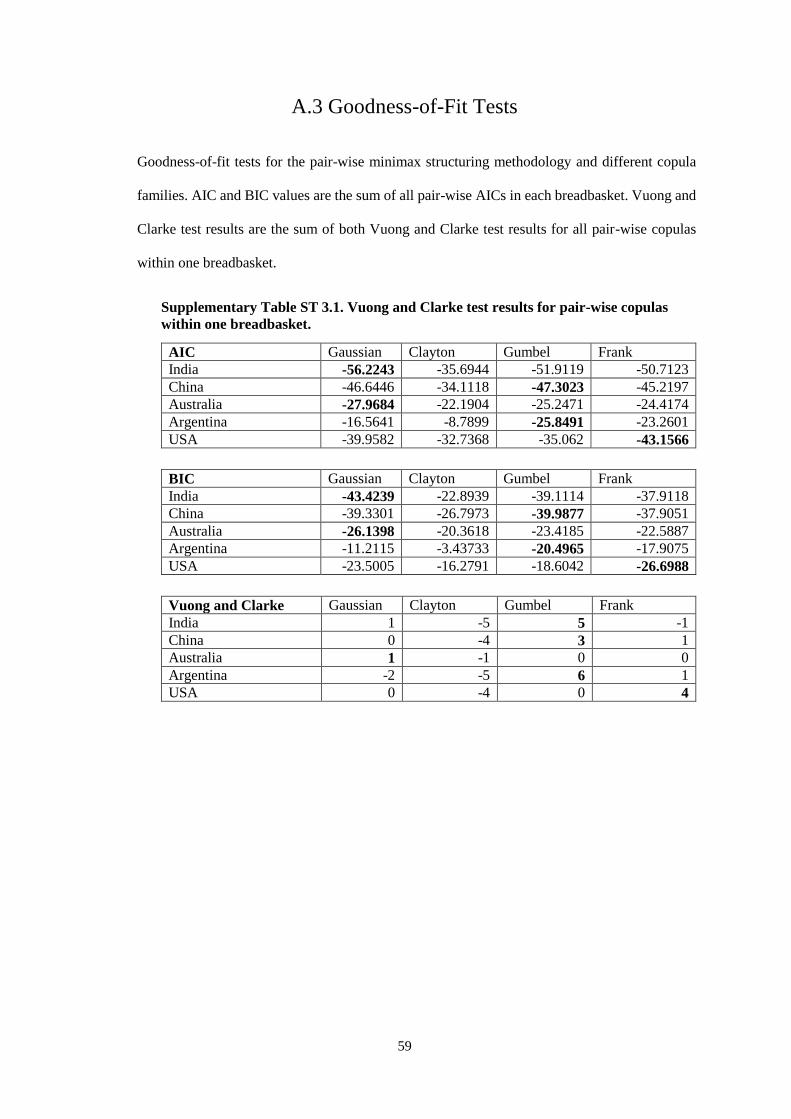
59

A.3 Goodness-of-Fit Tests

Goodness-of-fit tests for the pair-wise minimax structuring methodology and different copula

families. AIC and BIC values are the sum of all pair-wise AICs in each breadbasket. Vuong and

Clarke test results are the sum of both Vuong and Clarke test results for all pair-wise copulas

within one breadbasket.

Supplementary Table ST 3.1. Vuong and Clarke test results for pair-wise copulas

within one breadbasket.

AIC Gaussian Clayton Gumbel Frank

India -56.2243 -35.6944 -51.9119 -50.7123

China -46.6446 -34.1118 -47.3023 -45.2197

Australia -27.9684 -22.1904 -25.2471 -24.4174

Argentina -16.5641 -8.7899 -25.8491 -23.2601

USA -39.9582 -32.7368 -35.062 -43.1566

BIC Gaussian Clayton Gumbel Frank

India -43.4239 -22.8939 -39.1114 -37.9118

China -39.3301 -26.7973 -39.9877 -37.9051

Australia -26.1398 -20.3618 -23.4185 -22.5887

Argentina -11.2115 -3.43733 -20.4965 -17.9075

USA -23.5005 -16.2791 -18.6042 -26.6988

Vuong and Clarke Gaussian Clayton Gumbel Frank

India 1 -5 5 -1

China 0 -4 3 1

Australia 1 -1 0 0

Argentina -2 -5 6 1

USA 0 -4 0 4

60

4. Changing Risks of Simultaneous Global

Breadbasket Failure

Abstract

The risk of extreme climatic conditions leading to unusually low global agricultural production is

exacerbated if more than one global ‘breadbasket’ is subject to climatic extremes at the same time.

Such shocks can pose a risk to the global food system amplifying threats to global food security

(Maxwell and Fitzpatrick, 2012; Von Braun, 2008) and have the potential to trigger other systemic

risks (Johnstone and Mazo, 2011; Von Braun and Tadesse, 2012). So far, while the possibility of

climatic extremes hitting more than one breadbasket has been postulated (Bailey and Benton, 2015;

Schaffnit-Chatterjee et al., 2010) little is known about the actual risk. Here we present quantitative

risk estimates of simultaneous breadbasket failures due to climatic extremes and show how risk has

changed over time. We combine region-specific analysis of agricultural production with spatial

statistics of climatic extremes to quantify the changing risk of low production for the five major food

producing regions (‘breadbaskets’) in the world. We find evidence that there is increasing risk of

simultaneous failure of wheat crops, across the breadbaskets analysed. For maize and soybean,

changing climatic effects cancel each other out, so risk has stayed the same on aggregate. . Thus the

globally distributed character of food production helps to mitigate some but not all of the risks from

climatic extremes. Our analysis can provide the basis for more efficient allocation of resources to

contingency plans and/or strategic crop reserves that would enhance the resilience of the global

food system.

4.1 Introduction

Fluctuations in year-to-year agricultural yield are mostly attributable to climatic variability (Field,

2012). While under ‘normal’ climatic circumstances the global food system can compensate local

crop losses through grain storage and trade (Bren d’Amour et al., 2016), it is doubtful whether the

global food system is resilient to more extreme climatic conditions (Fraser et al., 2013), when export

restrictions (Puma et al., 2015) and low grain stocks may undermine liquidity in agricultural

commodity markets, resulting in price volatility. The food price crisis in 2007/08 has shown that

climatic shocks to agricultural production can lead to food price spikes (Von Braun, 2008) and

famine (Maxwell and Fitzpatrick, 2012), with the potential to trigger other systemic risks including

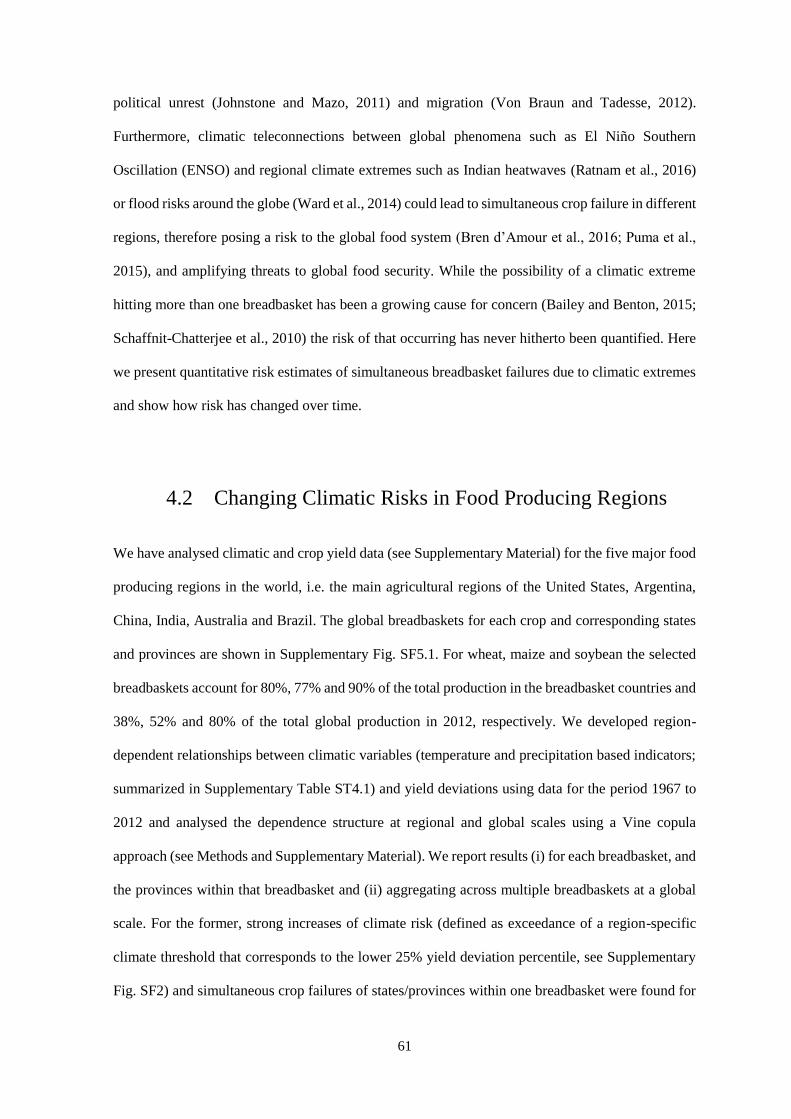
61

political unrest (Johnstone and Mazo, 2011) and migration (Von Braun and Tadesse, 2012).

Furthermore, climatic teleconnections between global phenomena such as El Niño Southern

Oscillation (ENSO) and regional climate extremes such as Indian heatwaves (Ratnam et al., 2016)

or flood risks around the globe (Ward et al., 2014) could lead to simultaneous crop failure in different

regions, therefore posing a risk to the global food system (Bren d’Amour et al., 2016; Puma et al.,

2015), and amplifying threats to global food security. While the possibility of a climatic extreme

hitting more than one breadbasket has been a growing cause for concern (Bailey and Benton, 2015;

Schaffnit-Chatterjee et al., 2010) the risk of that occurring has never hitherto been quantified. Here

we present quantitative risk estimates of simultaneous breadbasket failures due to climatic extremes

and show how risk has changed over time.

4.2 Changing Climatic Risks in Food Producing Regions

We have analysed climatic and crop yield data (see Supplementary Material) for the five major food

producing regions in the world, i.e. the main agricultural regions of the United States, Argentina,

China, India, Australia and Brazil. The global breadbaskets for each crop and corresponding states

and provinces are shown in Supplementary Fig. SF5.1. For wheat, maize and soybean the selected

breadbaskets account for 80%, 77% and 90% of the total production in the breadbasket countries and

38%, 52% and 80% of the total global production in 2012, respectively. We developed region-

dependent relationships between climatic variables (temperature and precipitation based indicators;

summarized in Supplementary Table ST4.1) and yield deviations using data for the period 1967 to

2012 and analysed the dependence structure at regional and global scales using a Vine copula

approach (see Methods and Supplementary Material). We report results (i) for each breadbasket, and

the provinces within that breadbasket and (ii) aggregating across multiple breadbaskets at a global

scale. For the former, strong increases of climate risk (defined as exceedance of a region-specific

climate threshold that corresponds to the lower 25% yield deviation percentile, see Supplementary

Fig. SF2) and simultaneous crop failures of states/provinces within one breadbasket were found for

62

some countries. For example, for soybean in China, the critical climate indicator is the number of

days above 30°C during the growing season. While only 1.8% of extreme hot months occurred

simultaneously in all provinces of the Chinese soybean breadbasket in the period 1961-1990, this

increased to 18.6% for the period 1991-2012 (Fig. 1a).

a

b

c

d

Figure 4.1. Likelihood of simultaneous climate risks. Defined as relevant climate indicators

exceeding the value that corresponds to the to the lower 25% yield deviation percentile. (a)

Simultaneous climate risk in the 9 most important soybean producing provinces in China.

Likelihood of climatic conditions simultaneously threatening crop losses in multiple global (b) wheat

(c) maize and (d) soybean breadbaskets.

On a global scale, there has been a significant increase in probability of multiple global breadbasket

failures for wheat (Figure 4.1b). The likelihood of all breadbaskets suffering from unfavourable

climate for wheat growth increased from 1.2% to 4.1% between the two periods. Climate risks to

wheat yields from both temperature and precipitation effects have increased in all five breadbaskets,

63

except for cumulative precipitation in the USA which has not changed significantly. For all three

crops, the risks of extreme temperature simultaneously hitting yield in multiple breadbaskets have

increased more than risks of unfavourable precipitation.

Simultaneous climate risks for maize (Figure 4.1c) and soybean (Figure 4.1d) have not changed

clearly between the two periods. One reason for this is that in breadbaskets where both temperature

and precipitation are significant influences on low yield (Argentina and India for soybean and

Argentina and China for maize), the effects of temperature and precipitation changes have been

different. For maize, for instance, an increase in spring and summer precipitation in several regions

in Argentina favoured crop productivity (Barros et al., 2015) outweighing the increasing climate risk

in China. Meanwhile risks from extreme temperatures increased more in China than they decreased

in Argentina. Hence, there is no clear overall change of aggregate risk across the breadbaskets while

there are changes in the nature of the climatic risk for individual breadbaskets (see Supplementary

Fig. SF3 and SF4).

For illustrative purposes the global impacts of climatic risks in terms of agricultural production were

compared, based on the total area of crop production in 2012. For soybean, simultaneous climate

risks (as defined above) in all five breadbaskets would lead to at least 9.86 million tons of crop losses,

which exceeds the 7.2 million ton losses in 1988/89, one of the largest historical soybean production

shocks (Bailey and Benton, 2015). Simultaneous maize and wheat climate risks in all of the

breadbaskets considered here would lead to production losses of at least 19.75 and 8.59 million tons

respectively. Global shocks that have occurred in the past (55.9 million tons in 1988 for maize and

36.6 million tons in 2003 for wheat (Bailey and Benton, 2015)) have exceeded our estimated lower

bound on losses for maize and wheat, though we note that our analysis covered only 38% and 52%

of global production of those crops, respectively.

64

4.3 Spatial Dependence between Global Breadbaskets

The aggregate risk of low production at a global scale is influenced by the spatial dependence in

climate variables between breadbaskets, as well as by the climate risk in each breadbasket. There are

positive as well as negative spatial dependencies between the relevant climatic variables, so the

aggregate expected agricultural production losses from simultaneous climate risks in all five

breadbaskets can be both higher and lower than would be the case were this spatial dependence not

to exist. We compared the case of statistical independence between breadbaskets with the observed

climate data, to show the effect of spatial dependence in climate variables (see Supplementary Fig.

SF5). The spatial dependence in climatic variables is shown to increase the aggregate risk of

production losses in some cases e.g. the expected loss for soybean in the first period is 39,440 tons

higher than in the independent case. In other cases, spatial dependence mitigates the aggregate risk

(i.e. the losses are negatively correlated), as is the case for maize in the second period, when expected

losses are 276,500 tons lower than in the independent case, which is about the annual maize

production in Slovenia. However, we found no significant change in the spatial dependence structure

between the two periods. The changes to simultaneous climate risks that are reported above are

attributable to changes in climatic mean and variance only – no significant change was detectable in

the spatial dependence structure.

4.4 Discussion

Analysis of climatic risks to crop production has conventionally used crop models on a global scale.

Whilst crop-models can incorporate complex time-dependent climatic influences on yield, there is

inevitably a mismatch between model predictions and actual yield data. The more direct approach

that we have adopted has incorporated phenological as well as statistical information, with a specific

focus upon the climatic factors that demonstrably influence low agricultural production. Whilst

statistical analysis of global production data does not identify significant inter-regional spatial

65

dependence or climate-related change signals, because of the number of confounding factors, we

have been able to fingerprint the effects of these signals through direct analysis of the relevant

climatic data. We have therefore been able to begin to interpret the risks of climate extremes to crop

production. Climate risks to global wheat production have changed already. Whilst we did not

identify any significant change in climate risks for maize and soybean, climate projections indicate

that risks might increase in the future (Field, 2012). Whilst our empirically based approach has some

attractions compared to global crop modelling, there were inevitable limitations, notably the

omission of Russia (one of the largest wheat producers) due to a lack of historical data availability

on a subnational scale.

Quantifying likelihoods of simultaneous climate risks will help governments, businesses and

international institutions to allocate proportional resources to contingency plans and/or strategic crop

reserves. Importantly, as demonstrated here, while overall risk may stay the same over time, the

likely combinations of conditions that threaten the food system may have changed. For trade

networks, which are built over time, such changes may indeed very important and could increase

risk of food insecurity. Our identification of climatic patterns associated with global crop losses can

help to target the development of early warning systems.

66

Appendix B: Supplementary Materials to Chapter 4

B.1 Data

Subnational yield data from 1967 to 2012 were collected from official governmental data bases

(Australian Bureau of Statistics, 2015; Conab (Companhia Nacional De Abastecimento) Brazil,

2015; Ministerio de Agricultura, Ganaderia y Pesca de Argentina, 2015; Ministry of Agriculture and

Farmers Welfare, Govt. of India, 2015; National Bureau of Statistics of China, 2015; USDA, 2015).

Using a logistic trend, annual detrended yield data was used for the analysis. Climate data come from

Princeton University (Sheffield et al., 2006). The dataset combines reanalysis data with observations

and is disaggregated in space and time. Monthly precipitation, minimum, maximum and mean

temperature as well as daily maximum temperature on a 0.5 degree resolution between 1966 and

2012 were aggregated over the breadbasket states and provinces for each crop.

B.2 Supplementary Methods

B.2.1 Breadbasket Selection

The global breadbaskets were selected using the Spatial Allocation Model (SPAM) (Harvest Choice,

2014), a global crop production data set. For the analysis, the scale of states and provinces was

chosen as they provide sufficient accuracy to examine climate and crop yield correlation structures

within a region and, at the same time, there is data available and accessible. SPAM production was

aggregated on a state/province scale and the highest crop producing units in the US, Argentina,

China, India, Brazil and Australia were selected. The results were then compared with suggestions

from scientific papers, governmental information and grey literature. With the premise that the

states/provinces of a breadbasket have to be adjacent, global breadbaskets were defined.

67

B.2.2 Climate Indicator Selection

A comprehensive literature review was conducted in order to find relevant climate indicators for

each region and crop. Regional case studies were chosen in locations within or very close to the

breadbasket areas used in this study. Selected climate indicators are precipitation and temperature

based and include both measures based on plant phenology such as number of days above 30°C

during the reproductive stage of soybean (Schlenker and Roberts, 2009) as well as statistical

measures such as the Standardized Precipitation Index (McKee et al., 1993) (SPI). In a second step,

the suggested indicators were reproduced on a state/province scale using Princeton re-analysis

climate data (Shepherd, 2014). The best fitting indicator for each breadbasket and crop was selected

through a correlation analysis with the observed, logistically de-trended subnational crop yield data

on state/province level using the Pearson correlation coefficient. As a result, one indicator per crop

and breadbasket was obtained, listed in Supplementary Table ST4.1. In order to analyse changes in

climate risks over time, with climate risk defined as the likelihood of a climate indicator exceeding

a threshold, climate thresholds had to be set. Linear regressions between climate indicators and

observed crop yield deviations in each state/province were used to define a climate threshold which

is related to the lower 25% yield deviation percentile. For a graphical illustration, see Supplementary

Figure SF4.2. Climate risks as likelihood of the indicator exceeding the threshold were compared for

each state/province between two periods, 1967-1990 and 1991-2012 shown in Supplementary Figure

SF4.3. For the analysis of simultaneous climate risks, a breadbasket or state/province was defined as

“under climate risk” if the threshold of the indicator was exceeded. When a breadbasket has two

possible climate indicators, it was defined as “under climate risk” as soon as one of them exceeded

the threshold.

B.2.3. Copulas

In order to model likelihoods of simultaneous climate risks, the copula methodology was used. With

copulas, dependencies between continuous random variables can be modelled. Additionally, the

method allows modelling the marginal distributions of climate indicators separately from modelling

68

the interdependence between climate indicators within or between breadbaskets. The method goes

back to Sklar’s theorem (Sklar, 1959)which states that the joint distribution function of any

continuous random variables (X,Y) can be written as

H(x,y) = C[FX(x), FY(y)] x,y ∈ ℝ (B.1)

with marginal probability distributions FX(x) and FY(y) and C = [0,1]2 → [0,1] as copula. If FX and

FY are continuous, C is uniquely defined. Different copula types describe different dependence

structures. In a multivariate copula model, there are several methods to structure the variables. For

this analysis, we used regular vine tree structures, RVines (Aas et al., 2009; Bedford and Cooke,

2002; Kurowicka and Cooke, 2006), which use different conditional and unconditional bivariate

pair-copulas to decompose the multivariate probability density of the different climate indicators.

RVines are most flexible in modelling complex dependencies in larger dimensions. A d-dimensional

vine structure consists of (d-1) trees with Ni nodes and Ei-1 edges joining the nodes. A tree structure

is built following the proximity condition which states that if an edge connects two nodes in tree j+I,

the corresponding edges in tree j share a node (Bedford and Cooke, 2002). In this paper, we select

trees using a maximum spanning tree algorithm with Kendall’s tau as edge weight (Dißmann et al.,

2013). For each copula-pair, the best-fitting copula family is selected from a list of six families,

namely Gaussian, Student-t, Clayton, Gumbel, Frank and Joe as well as their rotated versions to

capture negative dependencies. These include tail symmetric or asymmetric as well as tail dependent

and not tail dependent copula families. The best fitting copula family is then chosen using the Akaike

information criterion (Akaike, 1973a). The parameters for each bi-variate copula are derived with a

maximum likelihood estimation. Together with fitted and simulated marginal distributions for each

state/province, joint distributions are derived. The analysis was conducted using CRAN R with the

packages ‘copula’, ‘CDVine’ and ‘VineCopula’.

69

B.3 Supplementary Figures and Tables

Supplementary Figure SF4.1. Global breadbaskets.

The global breadbaskets include the following states/provinces:

Wheat:

China: Shandong, Hebei, Henan, Jiangsu, Anhui

USA: Kansas, North Dakota, Idaho, Washington, Montana, Oklahoma, South Dakota, Minnesota,

Nebraska, Texas

Argentina: Buenos Aires, Cordoba, Entre Rios, Santa Fe

Australia: New South Wales, South Australia

India: Uttar Pradesh, Madhya Pradesh, Rajasthan, Maharashtra, Gujarat, Bihar, Haryana, Punjab

Wheat in this study’s breadbaskets covers 80.24% of the breadbasket countries’ production (2012)

and 37.91% of global wheat production. Global coverage is smaller than for the other crops as the

important wheat producer Russia couldn’t be included into the study due to data limitations.

Maize:

China: Shandong, Hebei, Henan, Jilin, Liaoning, Heilongjiang, Inner Mongolia

USA: Kansas, Iowa, Illinois, Indiana, Wisconsin, Missouri, South Dakota, Minnesota, Nebraska,

Ohio

70

Argentina: Buenos Aires, Cordoba, Entre Rios, Santa Fe

Brazil: Goias, Mato Grosso, Parana, Sao Paulo, Minas Gerais

India: Madhya Pradesh, Rajasthan, Uttar Pradesh, Bihar, Maharashtra, Karnataka, Andhra Pradesh

Maize in this study’s breadbaskets covers 76.88% of the breadbasket countries’ production (2012)

and 52.4% of global maize production.

Soybean:

China: Shandong, Hebei, Henan, Jilin, Inner Mongolia, Anhui, Jiangsu, Heilongjiang, Liaoning

USA: Kansas, Iowa, Illinois, Indiana, Missouri, South Dakota, North Dakota, Minnesota, Nebraska,

Ohio, Arkansas

Argentina: Buenos Aires, Cordoba, Entre Rios, Santa Fe

Brazil: Goias, Mato Grosso, Rio Grande do Sul, Parana, Santa Catarina, Sao Paulo, Minas Gerais,

Bahia, Mato Grosso do Sul

India: Madhya Pradesh, Maharashtra, Rajasthan

Soybean in this study’s breadbaskets covers 89.7% of the breadbasket countries’ production (2012)

and 80.32% of global soybean production.

Supplementary Table ST4.1. Literature Used for Climate Risk Indicators Selection.

Crop: Breadbasket:

Indicator:

Literature influencing

climate indicator

choice:

Wheat India

China

Australia

SPI-1 averaged over

June, July, August and

September

Cumulative

precipitation (cp)

between June and

September of the

previous year (rainy

season)

Cp between May and

Nov (growing season)

Maximum temperature

(tmax) between May to

November

Krishna Kumar et al.

(2004)

Subash and Ram Mohan

(2011)

Liu et al. (2007)

Wang et al. (2001)

You et al. (2009)

Potgieter et al. (2002)

Yu et al. (2014)

Innes et al. (2015)

Luo et al. (2005)

Wardlaw and Wrigley

(1994)

71

USA

Argentina

Cp between October

and May (growing

season)

Number of days above

34°C (t34) between

March and May

Minimum temperature

(tmin) between May and

December (growing

season)

Zhang et al. (2015)

Tack et al. (2015)

Magrin et al. ( 2009)

Hernandez et al. (2015)

Maize India

USA

China

Argentina

Brazil

Maximum temperature

(tmax) between June

and October (kharif

season)

Number of days above

29°C between May and

November

(t29)(growing season)

Cp between June and

August

Tmax between May and

September (growing

season)

Cp between November

and January

Tmax between

December and February

Cp between November

and February

Kumar et al. (2011)

Schlenker and Roberts

(2009)

Zhang et al. (2015)

Matsumura et al. ( 2015)

Erec Heimfarth and

Musshoff (2011)

Liu et al. (2012)

Magrin et al. (2005)

Podestá et al. (2009)

Llano and Vargas

(2015)

Llano and Vargas

(2015)

Chen and Da Fonseca

(1980)

Soybean USA

Brazil

Argentina

India

Number of days above

30°C between May and

September

(t30)(growing season)

Cp between November

and March

Cp between November

and March

Tmax between January

and February

(flowering)

Cp between June and

November (growing

season)

T30 between June and

November

Schlenker and Roberts

(2009)

Zhang et al. (2015)

McCarl et al. (2008)

Llano and Vargas

(2015)

Magrin et al. (2005)

Penalba et al. (2007)

Llano and Vargas

(2015)

Lal et al. (1999)

Ramteke et al. (2015)

72

China T30 between May and

September (growing

season)

Zheng et al. (2015)

Yin et al. (2016)

Supplementary Figure SF 4.2. Definition of a climate indicator threshold.

Soybean Soybean

73

Wheat

74

Wheat

Soybean

75

Maize

Supplementary Figure SF 4.3. Risk distributions for period 1 and period 2 for each crop and breadbasket.

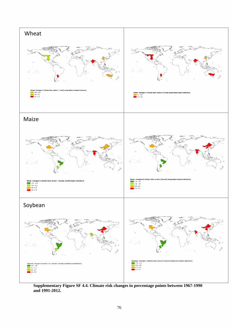
76

Supplementary Figure SF 4.4. Climate risk changes in percentage points between 1967-1990

and 1991-2012.

Maize

Soybean

Wheat

77

Changes between 1967-1990 and 1991-2012 in more detail:

Wheat: Climate risks increased in Argentina due to a strong warming of night-time temperatures

(Barros et al., 2015) which negatively effects wheat growth. Wheat climate risks have increased in

the Southwest of the Indian wheat breadbasket and decreased in the Northwest. Ramteke et al. (2015)

suggest that in the future, wheat as a rabi season crop will become more vulnerable due to large

increase in temperature and higher rainfall uncertainties. In the Chinese breadbasket, climate risk

increased in Anhui, Jiangsu and slightly in Hebei provinces but decreased in Henan and Shandong.

In the US, climate risks have slightly increased in some states and slightly decreased in others. In

Australia, wheat climate risks increased in New South Wales and decreased in South Australia

Maize and Soybean: In Brazil, summer precipitation has a positive correlation with soybean and

maize yields, except for Mato Grosso which is the wettest province in the breadbasket. An increasing

precipitation therefore reduced climate risks for soybean and maize except Mato Grosso province

where excess soil moisture can disturb root growth and thereby nutrient and water uptake (dos Santos

et al., 2015). In the US breadbasket, climate risks for both soybean and maize have mostly declined

in the Northwest and increased toward the Southeast of the breadbasket. This can be explained by

stronger negative correlation between temperature and soybean and maize crops towards the

Southeast compared to the Northwest as well as by an overall decrease in temperature in the centre

of the US’ maize and soybean belts (Lobell et al., 2011; Lobell and Asner, 2003). In China, a clear

positive temperature trend, especially in the Northeast of China’s soybean breadbasket, increased

climate risks to the crop (Yin et al., 2016). Maize, on the other hand, is not negatively influenced by

maximum temperatures in Heilongjiang and Inner Mongolia, which is why climate risks for maize

overall did not increase as strongly in China as for soybean. Precipitation trends are not as clear

which is why the precipitation based climate risks to maize yields in China don’t increase strongly

either. In India, maximum temperatures during maize and soybean growing seasons show an

increasing trend (Arora et al., 2005) which is why climate risks are increasing except for states that

show a positive correlation between high temperatures and yield such as Bihar and Maharashtra for

maize. One possible reason for the positive correlation between maize and hot days in Bihar is the

78

highest irrigation rate within the Indian maize breadbasket. Soybean, on the other hand, is mostly

rain-fed. The precipitation based risk indicator for soybean in India decreases slightly. Although the

overall precipitation stays the same across the two periods, precipitation exceeds the breadbasket’s

climate threshold slightly more often in the first period.

79

a1 Soybean in China a2

b1 Wheat b2

c1 Maize c2

d1 Soybean

d2

Supplementary Figure SF 4.5. Comparison with independent breadbaskets and provinces.

80

Comparison between climate risks to crops when historical dependencies are included and when

independence between the breadbaskets are assumed. Period 1 refers to 1967-2012 and period 2 to

1991-2012.

Results in detail:

a) Soybean in China: There is a significant difference between period 1 and period 2 with

period 2 having a larger mean than period 1 (using the Wilcoxon test). There was no

significant difference in mean between the dependent and independent case. However, there

is a clear and significant difference between the normal and independent case if each

occurrence is examined separately (the likelihood of simultaneous climate risks in 3

provinces differs significantly from the likelihood of simultaneous climate risks in 3

provinces if they are assumed to be independent) using the Poisson test.

b) Soybean: Using the non-parametric Wilcoxon test, period 1 was found to have a significantly

higher mean than period 2. Comparing each likelihood of simultaneous occurrence between

the two periods, there is only a significant difference between the periods for one

simultaneous climate risks and all five simultaneous climate risks.

Comparing dependencies, both periods have significantly smaller means than in the case of

independence between BBs.

c) Maize: Using the Wilcoxon test, period 1 has a significantly smaller mean than period 2.

Looking at the dependencies, maize shows, similar to soybean, for both periods significantly

smaller means than in the case of independence between BBs.. This can be explained through

a considerable number of negative correlation coefficients between BBs in the copula

analysis.

d) Wheat: Period 2 is in average significantly greater than period 1 at 0.001 significance level

for all dependencies when using the Wilcoxon-test. When likelihoods of simultaneous

81

occurrences are compared separately, there are significant differences for all cases between

the two periods as well.

Between the dependencies, there are significant differences of the means in period 2 but not

in period 1.

82

5. Increasing Risks of Multiple Breadbasket Failure

under 1.5 and 2°C Global Warming

Abstract

The increasingly inter-connected global food system is becoming more vulnerable to production

shocks owing to increasing global mean temperatures and more frequent climate extremes. Little is

known, however, about the actual risks of multiple breadbasket failure due to extreme weather

events. Motivated by the Paris Climate Agreement, this paper quantifies spatial risks to global

agriculture in a 1.5 and 2°C warmer world. This paper focuses on climate risks posed to three major

crops - wheat, soybean and maize - in five major global food producing areas. Climate data from

the atmosphere-only HadAM3P model as part of the “Half a degree Additional warming, Prognosis

and Projected Impacts” (HAPPI) experiment are used to analyse the risks of climatic extreme events.

Using the copula methodology, the risks of simultaneous crop failure in multiple breadbaskets are

investigated. Projected losses do not scale linearly with global warming increases between 1.5 and

2°C Global Mean Temperature (GMT). In general, whilst the differences in yield at 1.5 versus 2°C

are significant they are not as large as the difference between 1.5°C and the historical baseline

which corresponds to 0.85°C above pre-industrial GMT. Risks of simultaneous crop failure,

however, do increase disproportionately between 1.5 and 2°C, so surpassing the 1.5°C threshold

will represent a threat to global food security. For maize, risks of multiple breadbasket failures

increase the most, from 6% to 40% at 1.5 to 54% at 2°C warming. In relative terms, the highest

simultaneous climate risk increase between the two warming scenarios was found for wheat (40%),

followed by maize (35%) and soybean (23%). Looking at the impacts on agricultural production, we

show that limiting global warming to 1.5°C would avoid production losses of up to 2 753 million

(161 000, 265 000) tonnes maize (wheat, soybean) in the global breadbaskets and would reduce the

risk of simultaneous crop failure by 26%, 28% and 19% respectively.

5.1 Introduction

The Paris Agreement in 2015, in which 197 countries agreed to limit the increase of mean global

temperature to 1.5°C rather than 2°C above pre-industrial levels (UNFCCC 2015), has received

considerable interest from the scientific community (i.e., Mitchell et al. 2016b; Rogelj and Knutti

2016; Verschuuren 2016; Schleussner et al. 2016; James et al. 2017). However, so far little research

has been done on the impacts of a 1.5°C temperature increase, let alone on the quantification of the

83

differential impacts of 1.5 versus 2°C global warming (James et al 2017). Quantitative impacts

assessments of the relative benefits of limiting global warming to 1.5ºC are required to support such

policies and the scientific community is now encouraged to address research gaps related to a 1.5°C

temperature increase, especially to the different impacts at local and regional scales (Rogelj and

Knutti 2016) and the impacts on other industries.

This paper focuses on the climate change impacts on the agricultural sector. Although agriculture is

not explicitly mentioned in the Paris Climate Agreement, “safeguarding food security” and the

“vulnerabilities of the food production systems to the adverse impacts of climate change” are

recognized (UNFCCC 2015). Agriculture is one of the sectors that will experience the largest

negative impacts from climatic change (Porter et al 2014). Climate trends and specifically climate

variability have already negatively impacted agricultural production in many regions (Lobell et al

2011, Field and IPCC 2012). On the other hand, it has been estimated that by 2050, an increase of

40% of global food production is necessary to meet the growing demand resulting from population

growth and rising calorie intake in developing countries (Verschuuren 2016). Today, (FAO 2014)

estimates that 805 million people are undernourished globally, which is one in nine people. In a crisis

such as the 2007/08 food price crisis, however, the number of undernourished people increased by

75 million in only four years owing to food price spikes for major crops (Von Braun 2008). An

increasingly interconnected global food system (Puma et al 2015) and the projected fragility of the

global food production system due to climatic change (Fraser et al 2013) further exacerbate the

threats to food security. The potential impact of simultaneous climate extremes on global food

security is in particular need of further investigation. Crop losses in a single, main crop producing

area, termed a breadbasket, can be offset through trade with other crop-producing regions (Bren

d’Amour et al 2016). If several breadbaskets suffer from negative climate impacts at the same time,

however, global production losses might lead to price shocks and trigger export restrictions which

amplify the threats to global food security (Puma et al 2015).

84

Research has started to focus on the impacts of multiple, interconnected adverse weather events on

agricultural production and knock-on effects on other industries such as the financial sector

(Maynard 2015, Lunt et al 2016). However, more research and information about climate risk

distributions and the connection of extreme weather events across the world is needed to estimate

the probability of multiple breadbasket failures (Schaffnit-Chatterjee et al 2010, Bailey and Benton

2015). This paper quantifies simultaneous climate risks to agricultural production in the global

breadbaskets under 1.5 and 2°C warming scenarios. Whilst the difference of half a degree might be

considered to be small on an aggregated global level, regional changes can be much larger

(Seneviratne et al 2016). Moreover, changes in extremes events and spatial dependence, which

influence global risks such as multiple breadbasket failures, may expose significant differences

between the two global mean temperature increments.

This paper uses initial results from the “Half a degree Additional warming, Prognosis and Projected

Impacts” (HAPPI) project (Mitchell et al 2016a). HAPPI provides a set of climate data specifically

designed to address the Paris Agreement by simulating scenarios that are 1.5 and 2°C warmer than

pre-industrial worlds. It provides a large enough ensemble of climate model runs to enable a thorough

assessment of extreme weather and climate-related risks. Results will provide an important

contribution to current climate policy discussions about differential impacts at specific global

warming levels.

Our paper is organized as follows. In Section 2 we explain the HAPPI experiment and the HadAM3P

model which was used in this study. In Section 3 we describe the climate indicators that have been

used to assess agricultural risks and how we bias-corrected the data. We introduce the copula

methodology used for the multivariate climate risk analysis in this paper and explain how we

estimate the impact of climate risks on agricultural production. Section 4 shows the results which

will be further discussed in Section 5. The paper ends in Section 6 which summarizes our findings

and gives an outlook to possible future work.

85

5.2 Data

5.2.1 HadAM3P Model

Monthly precipitation and maximum temperature data are taken from the global atmosphere only

model, HadAM3P (Pope et al 2000, Massey et al 2015). HadAM3P was developed by the UK Met

Office Hadley Centre and is based on the atmosphere component of HadCM3, a coupled ocean-

atmosphere model (Gordon et al 2000). It is run at a global resolution of 1.875° longitude and 1.25°

latitude with a 15 minute time step. HadAM3P is run via the climateprediction.net volunteer

distributed computed network (Anderson 2004) and is, owing to its large ensemble size, well suited

to analyse large-scale extreme weather events. Compared to other models from the same modelling

family, HadAM3P has improvements in resolution and model physics (Pope and Stratton 2002).

Results of the HadAM3P distributed computing simulations are comparable to results of state of the

art global climate model (GCM) simulations (Massey et al 2015).

5.2.2 HAPPI Experiment

HadAM3P is one out of several models used for the HAPPI experiment (Mitchell et al 2016a) which

compares the statistics of extreme weather events simulated for a world which is 1.5 and 2 °C warmer

than in pre-industrial (1861-1880) conditions with those of the present day. Driven by several leading

atmosphere-only GCMs, HAPPI uses an experimental design similar to CMIP5 and is able to

produce large simulation ensembles of high resolution global and regional climate data. Compared

to CMIP5 style experiments which use different Representative Concentration Pathways (RCPs) to

reach a certain radiative forcing by 2100 and which contain uncertainty in climate model responses,

HAPPI uses large sets of simulations under steady forcing conditions to calculate risks at certain

warming levels irrespective of the emission pathway. Historical (in this study denoted with HIST)

refers to the 2006-2015 decade (which has already experienced a GMT rise of 0.85°C compared to

pre-industrial levels (Fischer and Knutti 2015)), a time period in which ocean temperatures have

86

been approximately constant but observed Sea Surface Temperatures (SSTs) contain a range of

different patterns including El Nino patterns which were used to force the models. Each of the one-

decade-simulations in the 50 to 100 member ensembles starts with a different initial weather state

which results in 500 to 1000 years of model output. The 1.5°C warming experiment refers to

conditions relevant for the 2106-2115 period and uses anthropogenic radiative forcing conditions

from RCP2.6 (Van Vuuren et al 2011) which coincides with a global average temperature response

of ~1.5°C relative to pre-industrial levels. Natural radiative forcings are used from the 2006-2015

decade. SSTs in the 1.5°C scenario are calculated by adding the mean projected CMIP5 RCP 2.6

SST changes across 23 models averaged over the 2091-2100 period to observed 2006-2015 SSTs.

The 2°C warming scenario refers to 2106-2115 conditions as well and uses a weighted average

between the RCP2.5 and RCP4.6 scenarios to reach a ~2°C global mean temperature response,

exactly 0.5°C warmer than the 1.5°C scenario. Natural forcings again stay at 2006-2015 levels. For

more information on the HAPPI experiment, see (Mitchell et al 2016a).

Using climateprediction.net’s large ensemble modelling system, ~150, ~100 and ~120 ensemble

members for the historical, 1.5 and 2°C scenario respectively were obtained. Owing to the large

number of ensemble members with varied initial conditions, the HAPPI HadAM3P results used in

this study are well suited to the analysis of extreme weather events with an improved representation

of internal climate variability Choosing a one-decade time period allows for assessment of the

impacts of inter-annual climate variability on agricultural production. Note that the number of

ensemble members differs as only ensemble members that were completed on the volunteers’

computers could be included. Reasons for non-completion could be hardware failure or termination

of the experiment by the volunteer ((Massey et al 2015).

5.2.3 Historical Crop Yield and Climate Data

This study focuses on agricultural production risks in major global breadbaskets. Breadbaskets are

important sub-national crop producing regions on a province/state scale in the US, Argentina, China,

India and Australia for wheat and the US, Argentina, Brazil, China and India for maize and soybean

87

(see details in Gaupp et al., in revision). Sub-national, annual crop yield data for all states/provinces

of a breadbasket from 1967 to 2012 were collected from official governmental databases (Australian

Bureau of Statistics 2015, Conab (Companhia Nacional De Abastecimento) Brazil 2015, Ministerio

de Agricultura, Ganaderia y Pesca de Argentina 2015, Ministry of Agriculture and Farmers Welfare,

Govt. of India 2015, National Bureau of Statistics of China 2015, USDA 2015). These and monthly

Princeton re-analysis precipitation and maximum temperature data between 1967 and 2012

(Sheffield et al 2006) were used to find region- and crop-specific relationships between climate and

agricultural production. Princeton re-analysis data is a combination of a number of observation-based

datasets and NCEP/NCAR re-analysis data and provides globally consistent, bias-corrected climate

data.

5.3 Methods

5.3.1 Climate Indicator Selection

We identified climate indicators which significantly impact three important crops - wheat, maize and

soybean - in five breadbaskets around the globe. A climate indicator is a crop and region specific

variable based on either monthly maximum temperature or precipitation data which correlates with

crop yields.

By concentrating on breadbaskets rather than using the national scale, the exact, region-specific

relationship between climate indicator and detrended yield could be determined. This is particularly

relevant in large countries where crop production is concentrated in only a few regions. In order to

find the most robust climate indicators for each crop and breadbasket, an extensive literature review

was carried out (see details in Gaupp et al., in revision). Regional case studies were chosen in

locations within or very close to the breadbasket areas used in this study. Indicators are mainly

average maximum temperature or cumulative precipitation during the crop’s growing season (e.g.

June to November in India’s soybean breadbasket) but also precipitation during the monsoon season

88

(June to September in India’s wheat breadbasket) which is stored in the soil and influences wheat

growth from October to March. Values from the literature were verified through a correlation

analysis between the climate re-analysis data and the observed, logistically de-trended subnational

crop yield data on state/province level using the Pearson correlation coefficient, shown in Table 5.1.

Table 3.1 Pearson correlation coefficient between Princeton re-analysis climatological data

and observed historical subnational crop yield data. ***, ** and * indicate p < 0.01, p < 0.05,

and p < 0.20, respectively. Bold values indicate those properties that have been chosen as climate

indicators in this paper.

Wheat

Maize Soybean

Maximum

temperature

Precipitation Maximum

temperature

Precipitation Maximum

temperature

Precipitation

Argentina -0.493*** -0.140 -0.602*** 0.645*** -0.490*** 0.675***

Australia -0.356** 0.825***

Brazil

-0.023 0.260* 0.041 0.392**

China 0.237 0.147 -0.157 0.335** -0.032 0.137

India -0.406*** -0.195* -0.232* 0.335** -0.334** 0.533***

USA -0.035 0.309** -0.293** 0.420*** -0.208* 0.330**

Depending on the strength and significance of the indicator, one or two indicators per crop and

breadbasket were chosen. In exceptional cases, an indicator was selected when Pearson’s r showed

a non-significant but strong relationship pointing to the same direction as indicated in the literature

if it has been described as significant there. Differences can arise through differences between re-

analysis data and locally observed climate data, different spatial scales or different statistical

methods. Figure 5.1 shows the indicator selection for each crop and breadbasket as well as a global

crop calendar. We kept breadbaskets in the Northern and Southern hemisphere together and started

the crop calendar year for all crops with the Southern hemisphere. For the analysis of climate risks,

with a climate risk defined as a climate indicator exceeding a critical threshold, climate thresholds

were set for each crop, breadbasket and indicator. A simple linear regression between each climate

indicator and observed, detrended crop yield was used to define a temperature or precipitation

threshold related to the lower 25% detrended yield percentile (Gaupp et al., in review). To account

for uncertainties in the sample statistics of the HAPPI data, the data were bootstrapped 1000 times

for the threshold exceedance calculation. Results in Figure 5.2 show the simulation mean. A

89

breadbasket is experiencing a climate risks for a crop as soon as one of the temperature or

precipitation based indicators is exceeding the threshold. The breadbasket-specific relationship

between temperature and precipitation is accounted for through the copula correlation structure

explained in Section 5.3.3.

90

Figure 5.1. Climate indicators and harvesting periods for the global breadbaskets. Argentina

(AR), Australia (AU), Brazil (BR), China (CN), India (IN) and the USA (US). Temperature-based

indicators (continuous line) are monthly maximum temperature averaged over the crop growth

relevant period. Precipitation-based indicators are cumulative precipitation over selected time

periods (dashed line).

5.3.2 Bias-correction

In order to quantify the likelihood of threshold exceedance of different climate indicators, the

HadAM3P model output has to be comparable to the observed historical climate used for setting

these thresholds. Therefore, both historical and future experiment results were calibrated using a

simple bias-correction method (Ho 2010, Hawkins et al 2013) which corrects mean and variability

biases of the climate indicators distributions using the Princeton re-analysis data (Sheffield et al

2006) as calibration dataset:

𝐼𝐵𝐶(𝑡) = 𝑂𝑅𝐸𝐹 +

𝜎𝑂,𝑅𝐸𝐹

𝜎𝐼,𝑅𝐸𝐹 (𝐼𝑅𝐸𝐹 (𝑡) − 𝐼𝑅𝐸𝐹

) (5.1)

𝐼𝐹𝑈𝑇,𝐵𝐶(𝑡) = 𝑂𝑅𝐸𝐹 +

𝜎𝑂,𝑅𝐸𝐹

𝜎𝐼,𝑅𝐸𝐹 (𝐼𝐹𝑈𝑇 (𝑡) − 𝐼𝑅𝐸𝐹

) (5.2)

91

IBC denotes the HAPPI HadAM3P bias-corrected climate indicator, OREF and IREF the observational

Princeton dataset and HAPPI HadAM3P historical raw climate indicators and IFUT represents the 1.5

or 2°C raw climate indicator. This method has the advantage of being simple to calculate and being

independent of the shape of the climate variable distribution (Hawkins et al 2013). It is used widely

in agricultural modelling (Navarro-Racines et al 2016). HadAM3P generally overestimated

temperature compared to the Princeton dataset with HadAM3P maximum temperature being

between 7 and 57% higher than Princeton in all breadbaskets. Precipitation is underestimated in the

maize and soybean breadbaskets by between 2 and 30%. Precipitation for wheat, which has a

different growing season, is both higher and lower than the reference dataset (between 40% lower in

Australia and 37% higher in the US breadbasket).

5.3.3 Regular Vine Copulas

In this study, climate indicators based on historical Princeton re-analysis data were used to estimate

the spatial dependence structure between the five breadbaskets to avoid biases in inter-regional

correlation in the HadAM3P climate model. As the dependence structure of the HAdAM3P climate

indicators in the different breadbaskets did not change between historical and warming scenarios,

we kept the historical dependence structure constant in the 1.5 and 2°C scenario. Changes in

simultaneous climate risks between scenarios occur due to changes in mean and variance of the

underlying marginal distributions of the climate indicators based on HadAM3P data.

In order to estimate risks of multiple breadbasket failure owing to joint climate extremes in major

crop production areas, the spatial dependence structure of the global breadbasket’s climate indicators

was modelled using regular vine (RVine) copulas (Kurowicka and Cooke 2006, Aas et al 2009,

Dißmann et al 2013). RVines are a flexible class of multivariate copulas which are able to model

complex dependencies in larger dimensions. They are based on Sklar’s theorem (Sklar 1959) which

states that any multivariate distribution F can be written as

92

𝐹(𝑥1, … , 𝑥𝑛) = 𝐶[𝐹1(𝑥1), … , 𝐹𝑛(𝑥𝑛)] (5.3)

with marginal probability distributions F1(x1), …, Fn(xn) and C denoting an n-dimensional copula, a

multivariate distribution on the unit hypercube [0,1]2 with uniform marginal distributions. Vine

copulas are constructed using conditional and unconditional bivariate pair-copulas from a set of

copula families with distinct dependence structures (Joe 1997, Aas et al 2009). A set of linked RVine

trees describes the factorisation of the copula’s multivariate density function (Bedford and Cooke

2002). An n-dimensional RVine model consists of (n-1) trees including Ni nodes and Ei-1 edges which

join the nodes. The tree structure is built according to the proximity condition which means that if

an edge connects two nodes in tree j+1, the corresponding edges in tree j share a node (Bedford and

Cooke 2002). The first tree consist of n-1 pairs of variables with directly modelled distributions. The

second tree identifies n-2 variable pairs with a distribution modelled by a pair-copula conditional on

a single variable which is determined in the second tree. Proceeding in this way, the last tree consist

of a single pair of variables with a distribution conditional on all remaining variables, defined by a

last pair-copula (Dißmann et al 2013). The RVine tree structure, the pair-copula families and the

copula parameters are estimated in an automated way starting with the first tree. The tree is selected

using a maximum spanning tree algorithm and Kendall’s tau as edge weights. The best fitting pair-

copula family is chosen using the Akaike Information Criterion (Akaike 1973) and copula

parameters are estimated using Maximum Likelihood Estimation (MLE). In this study we chose from

six different copula families representing different types of tail dependencies to capture the exact

patterns of dependence between the different climate indicators in the crop breadbaskets: Gaussian,

Clayton, Student-t, Gumbel, Joe and Frank copulas (Nelsen 2007).

5.3.4 Impact on Agricultural Production

We analyse events where the climatic conditions in all five breadbaskets are associated with losses

in agricultural yields. We identify a ‘breadbasket failure’ event as being when the climatic conditions

are at least as severe as those conditions associated with the 25 percentile of the logistically

93

detrended yields (with detrended yields as residuals of the non-linear logistic regression with a

residual mean equal to zero). The crop production loss for an event of this severity is the 25 percentile

of the logistically detrended yield multiplied with the 2012 harvested area. Given that we identify

climatic events that are at least as severe as this condition, our estimated loss is the lower bound on

the loss, i.e. the minimum expected loss. Minimum expected losses are then defined as the sum of

crop losses in all five breadbaskets multiplied with the joint probability that climate thresholds are

exceeded in all regions simultaneous as shown in Equation 5.4:

𝑀𝑖𝑛𝑖𝑚𝑢𝑚 𝑒𝑥𝑝𝑒𝑐𝑡𝑒𝑑 𝑙𝑜𝑠𝑠𝑒𝑠 ≥ ∑(| 𝑦25𝑖| ∙ 𝑎𝑟𝑒𝑎𝑖,2012)

𝐵𝐵

𝑖

∙ 𝑝5 (5.4)

with

𝑝5 = 𝑃( 𝐶𝑙𝑖𝑚1 ≷ 𝑡𝐶𝑙𝑖𝑚1, 𝐶𝑙𝑖𝑚2 ≷ 𝑡𝐶𝑙𝑖𝑚2

, 𝐶𝑙𝑖𝑚3 ≷ 𝑡𝐶𝑙𝑖𝑚3, 𝐶𝑙𝑖𝑚4 ≷ 𝑡𝐶𝑙𝑖𝑚4

, 𝐶𝑙𝑖𝑚5 ≷ 𝑡𝐶𝑙𝑖𝑚5)

= 𝐶[𝐹1(𝑡𝑐𝑙𝑖𝑚1 ), 𝐹2(𝑡𝑐𝑙𝑖𝑚2

), 𝐹3(𝑡𝑐𝑙𝑖𝑚3 ), 𝐹4(𝑡𝑐𝑙𝑖𝑚4

), 𝐹5(𝑡𝑐𝑙𝑖𝑚5 )]

with y25i as the 25 percentile of logistically detrended yields in the breadbasket i which was used to

define climate thresholds and which indicates a minimum yield loss , areai,2012 as the 2012 harvested

area in breadbasket i and with p5 as the probability of all five breadbaskets exceeding the climate

thresholds in the same year. Climi denotes the temperature or precipitation based climate indicator,

associated with the 25 percentile of the detrended yields. In case that a breadbasket has two indicators

for a crop, the exceedance of at least one of the climate thresholds 𝑡𝑐𝑙𝑖𝑚𝑖 is counted as threshold

exceedance in the breadbasket. C denotes the copula.

94

5.4 Results

5.4.1 Changes in Climate Risks to Agriculture under 1.5 and 2°C Global

Warming

The change of climate risks to major crops in the global breadbaskets were examined for each region

and crop separately comparing historical risks with risks associated with a 1.5 and 2°C global

warming, shown in Figure 5.2. As expected from an increase of global mean temperature,

temperature based climate risks are increasing, but to different extents depending on the region.

Precipitation signals associated with 1.5 and 2°C warming are less clear. While precipitation based

climate risks in the US and Brazil increase in both scenarios for the summer crops maize and

soybean, precipitation in Argentina does not significantly change. Risks in China and India decrease

due to an increase in monsoon precipitation. For wheat, precipitation-based climate risks only

increase in

monsoon precipitation. For wheat, precipitation-based climate risks only increase in Australia

Australia.

a)

95

Figure 5.2. Changes in climate threshold exceedance between historical and 1.5 or 2 °C

warming scenarios (in percentage points) using temperature and rainfall based indicators. A)

shows the global breadbaskets for wheat, maize and soybean, b) summarizes the risk changes for

the two warming scenarios. The error bar indicates the standard error between the 1000 iterations

of threshold exceedance using resampled climate data. Using the KS test, all differences between

the 1.5°C and 2°C scenarios are significant at a 0.001 significance level.

b)

96

The decrease of precipitation-based climate risks to wheat in the US, China and India, and the

increase in the Australian breadbaskets for both warming scenarios mostly coincide with findings of

a previous study (Gaupp et al., in review) which examined climate risk trends in the past. In India

and China, wheat is indirectly impacted by the summer monsoon rainfall which provides stored soil

moisture for the “rabi” wheat crop. Although precipitation between June and September in the

Chinese breadbasket showed a decrease in the recent past, in a 1.5 and 2°C warmer world

precipitation during monsoon months in the Chinese breadbasket is projected to increase. This

coincides with (Lv et al 2013) who project a decrease in precipitation in China during the wheat

growing season between the 2000s and 2030s and a consistent precipitation increase from the 2030s

to the 2070s. In India, rainfall during summer monsoon months (June to September) showed a

decreasing decadal trend in the recent past (Guhathakurta et al 2015) which was reflected in an

increasing climate risk for wheat in India in the past (Gaupp et al., in review). In the future, however,

monsoon precipitation is projected to increase under all RCP scenarios in CMIP5 projections (Menon

et al 2013, Jayasankar et al 2015) which coincides with decreasing precipitation climate risks to

wheat in the Indian breadbasket found in this study. However, precipitation based risks in India and

China might be underestimated in this study because of the HAPPI experiment structure which has

fixed SSTs driving the model, rather than a fully couple ocean simulation. This often leads to

variability in land-ocean driven cycles not changing much and thereby to an underestimation of

precipitation variability during the monsoon months. CMIP5 models project both increasing and

decreasing standard deviations of monsoon precipitation in India for RCP 2.6 and 4.5. In Australia,

precipitation in the wheat growing season is projected to decrease following different CMIP5 models

under RCP4.5 (Ummenhofer et al 2015) which our study confirms through increased precipitation-

based climate risks. Temperature risks are increasing in all temperature sensitive breadbaskets with

stronger increases in India and Australia than in Argentina.

For soybean, precipitation-based climate risks in South America increase in Brazil but do not change

notably in Argentina. This coincides with findings from other CMIP5 studies (IPCC 2014, Barros et

al 2015). In the US, CMIP5 models show a small, not significant increase in annual precipitation

97

(IPCC 2014)) which can be seen in HadAM3P as well. Precipitation during the soybean growing

season, on the other hand, is projected to decrease in both 1.5 and 2°C scenarios which results in

higher climate risks. In China and India, soybean growing seasons are directly aligned with the

summer monsoon. Hence, precipitation based soybean climate risks decrease due to the above

discussed increase in monsoon precipitation. Temperature based risks, on the other hand, increase

significantly in the US, Argentina and India.

For maize, climate risks show very similar patterns to soybean as the two summer crops have similar

growing seasons and indicators. Additional to the soybean climate indicators, maize in the Chinese

breadbasket is sensitive to temperature.

One of the major concerns in studies of the difference between a 1.5 and 2°C global warming is the

significance of the difference between the temperature increments (James et al 2017). The difference

between climate risks for 1.5 and 2°C in this study was tested with the student two-sample

Kolmogorov-Smirnov (KS) test which tests the null hypothesis that both distributions of resampled

threshold exceedance are drawn from the same distribution. Results showed significant differences

for all indicators and crops at the 0.001 significance level between the two warming levels. The KS

test allows for robust statements about the difference between climate risks under 1.5 and 2°C

warming even if there is an overlap of uncertainty bands (Schleussner et al 2016a). Thanks to the

large ensemble size the power of statistical tests is high. Error bars are small compared to the absolute

change in climate threshold exceedance with the exception of precipitation risks in Argentina for

soybean and maize. Figure 5.2 also compares the difference in changes from historical climate for

both global mean temperature increases. Across all three crops, we found stronger signals for

temperature based risks than for precipitation based risks which show smaller, both positive and

negative signals. Additionally, the difference between the 1.5 and 2°C warming is more pronounced

in temperature based indicators with the largest difference in the Indian soybean breadbasket (26%

points). The difference in precipitation risk changes between the two warming scenarios lies between

0 and 6% points. What stands out is the difference between 1.5 and 2°C for precipitation risks in

98

Brazil. In contrast to other climate indicators, precipitation between December and February and

March in Brazil shows a significantly stronger difference from historical data to 1.5°C than to 2°C.

5.4.2 Increasing Risks of Multiple Breadbasket Failure

Having analysed individual changes of climate risks in the global wheat, soybean and maize

breadbaskets for 1.5 and 2°C enables us to calculate joint climate risks on a global scale. Figure 5.3

shows the largest increase in risks of simultaneous crop failure (resulting from climate exceeding a

crop- and region-specific threshold) in the global breadbaskets for maize, followed by soybean and

wheat. For all three crops the likelihoods that none or just one of the breadbaskets experiences

climate risks decreases to (nearly) zero. For wheat and soybean, the likelihoods of breadbaskets

experiencing detrimental climate change increases significantly from the historical scenario to 1.5°C

and even more assuming 2°C warming. The shape of the distribution stays roughly the same across

warming scenarios with higher probabilities that parts of the breadbaskets exceed the thresholds and

smaller likelihoods in the extremes. While the historical baseline climate still shows the probability

for zero simultaneous climate risks, for higher temperature scenarios these likelihoods disappear.

The mean increases significantly (measured using the KS-test), more for soybean than for wheat.

For maize, likelihoods of simultaneous climate risks increase strongly. Under the 2°C scenario the

likelihood of all five breadbaskets suffering detrimental climate is the highest. For wheat, which

shows the smallest simultaneous climate risks, the return period for all five breadbaskets exceeding

their climate thresholds decreases from 43 years (or 0.023 annual probability under historical

conditions to 21 years (0.047) in a 1.5°C scenario and further down to around 15 years (0.066) under

2°C. Soybean has a return period of simultaneous climate risks in all breadbaskets of around 20 years

(0.049 today which decreases to 9 (0.116) and 7 years (0.143 in a 1.5 and 2°C warmer world

respectively. Maize risks are highest in our study with an initial return period of 16 years (0.061),

decreasing to less than 3 (0.39) and less than 2 years (0.538) under future global warming. In general,

one can say that whilst the differences in yield at 1.5 vs 2°C are significant they are not as large as

the difference between 1.5 and historical. Risk of simultaneous crop failure, however, do increase

99

disproportionately between 1.5 and 2 degrees and this is important because correlated risks lead to

disproportionately high impacts.

a) WHEAT

b) SOYBEAN

100

c) MAIZE

Figure 5.3. Risks of multiple breadbasket failure under 1.5 and 2°C warming. Error bars

reflect the sampling error as well as the copula simulation error which was determined in 1000

iterations.

To illustrate the effects of simultaneous climate risks in a 1.5 and a 2°C warmer world, we estimated

the impacts on agricultural production. Simultaneous crop failure in all breadbaskets, defined as the

25 percentile of detrended yield, would add up to at least 9.86 million tons of soybean losses, 19.75

million tons of maize losses and 8.59 million tons of wheat losses assuming 2012 agricultural area.

Historical examples of global crop production shocks include 7.2 million tons soybean losses in

1988/99 and 55.9 million tons maize losses in 1988 which were mostly caused by low rainfall and

high temperatures during summer growing season in the US (Bailey and Benton 2015). Historical

global wheat production shocks include 36.6 million tons wheat losses in 2003 mostly caused by

heat waves and drought in spring in Europe and Russia but also by reduced acreage due to drought

or winterkill in Europe, India and China (Bailey and Benton 2015). Maize and wheat losses in this

study are lower than in historical cases as our breadbaskets only account for 38% and 52% of global

production respectively. Soybean in this study accounts for 80% of global production. Combining

absolute losses with likelihoods of simultaneous climate risks, we calculated expected crop losses

101

following Equation 4. For all three crops, expected crop losses are significantly higher under the 2°C

than under the 1.5°C scenario. Under a scenario of 2°C mean global warming, expected wheat, maize

and soybean losses are projected to be 161 000, 2 753 000 and 265 000 tonnes higher than if global

temperature increases are limited to 1.5°C. This equals total annual maize production in Uganda, the

world’s 33rd largest maize producer in 2012. The difference of wheat losses is larger than Bolivia’s

annual total production in 2012 (145 000 tonnes) and the increase of expected soybean losses is

comparable to Mexico’s annual production (248 000 tonnes), the world’s 20th biggest soybean

producer (FAO 2015).

To test for the influence of spatial dependence between the climate indicators on the results of this

analysis, we excluded the spatial correlations. We assumed independence between the breadbaskets,

but still accounted for the negative correlation between temperature and precipitation indices within

one breadbasket. Supplementary Figure SF5.1 illustrates the difference between spatial

independence and correlation. Between the three crops, no consistent pattern was found between

dependent and independent cases. The only crop that shows significant differences is soybean with

smaller likelihoods in the extremes when dependence is excluded. This means that the likelihood of

all five soybean breadbaskets experiencing detrimental climate in one year is underestimated if

spatial correlations are not considered in a risk analysis. Expressed in expected production losses,

the losses are up lo 190 000 tonnes higher in the dependent case which is more than what the 22nd

largest soybean producer harvests annually (FAO 2015). For wheat and maize, the difference

between the dependencies was mostly not significant.

5.5 Discussion

Our results illustrate future climate conditions under two warming scenarios in the global

breadbaskets and investigate simultaneous climate risks affecting three major crops. The study

focused explicitly on the climate impact on crop yields. The effects of other factors such as soil

quality, land management or technology were held constant under future warming scenarios.

102

Therefore, our estimates of crop production losses have to be interpreted with care. By not explicitly

including CO2 concentrations, for instance, the CO2 fertilizer effect which increases productivity in

wheat and soybean and to a certain extent in maize (Schleussner et al 2016a) was not taken into

account. The effects of climatic change on plant phenology were not considered. In China, for

instance, the flowering date of wheat is projected to advance owing to increased temperatures and

the gain-filling period will shorten which might further reduce yields (Lv et al 2013). Owing to a

lack of subnational historic time series of irrigated crop yields, irrigation was not specifically taken

into account in setting climate risk thresholds. This was acceptable in this study as, even without

considering irrigation, the correlation coefficients between observed, detrended yields and climate

indicators were mostly significant. A large share of the regions in this study are completely rain-fed.

In other regions such as India or the US, irrigated crops still show correlations with rainfall (Pathak

and Wassmann 2009) or no significant difference to rain-fed crops at all (Zhang et al 2015). Results

of the analysis of simultaneous climate risks may vary depending on the climate indicator selection.

The two-step approach of pre-selecting potential indicators in a literature review and verification

through the correlation analysis with re-analysis climate data and observed historical yield data

represents a robust way of indicator selection. However, including different climate variables such

as number of days above a crop dependent heat threshold (Schlenker and Roberts 2009, Zhang et al

2015, Tack et al 2015) or dry spell length (Hernandez et al 2015, Ramteke et al 2015, Schleussner

et al 2016a) might lead to different results. So far, the HAPPI project only provides monthly data

which limited the climate variable choice. In order to reduce uncertainties, we bootstrapped the

climate indicators and repeatedly simulated the copula models. However, results from 1.5 and 2°C

warming scenarios vary between different GCMs (Schleussner et al 2016a). A comparison with

additional climate models from the HAPPI project will further improve the robustness of the results.

103

5.6 Conclusion

This study found disproportionally increasing future risks of simultaneous crop failure in the global

wheat, maize and soybean breadbaskets in a 1.5 and 2°C warmer world using results of the

HadAM3P atmospheric model as part of the HAPPI experiment. Increases in temperature-based

climate risks were found to be stronger than precipitation-based risks which showed different signals

depending on crop and region. Using the copula methodology, it was possible to capture dependence

structures between regions and to calculate joint climate risks in the major crop producing areas.

Additionally, the copula analysis accounted for the region-specific relationships between

temperature and precipitation. Strongest increases in simultaneous climate risks were found for

maize where return periods of simultaneous crop failure decrease from 16 years in the past to less

than 3 and less than 2 years under 1.5 and 2°C warming. In percentage terms, the largest increase of

simultaneous climate threshold exceedance in all five breadbaskets between the two warming

scenarios was found for wheat (40%), followed by maize (35%) and soybean (23%). Looking at the

impacts on crop production, the study showed that limiting global warming to 1.5°C would avoid

production losses of up to 2 753 million (161 000, 265 000) tonnes maize (wheat, soybean) in the

main production regions.

Our study represents an important first step in the analysis of differential temperature increases of

1.5 and 2°C and their impacts on agricultural production. Compared to climate studies which often

focus on average annual values, this study focused on crop growth periods which may show opposite

signals to annual means – as shown here for soybean in the US - and therefore added valuable

information to existing studies.

Results are based on HadAM3P, the first model in the HAPPI experiment set up. Including outputs

from additional climate models will give more robust information on future climate risks.

Additionally, further analysis of the ability of climate models to accurately model spatial dependence

between regions is needed. This study used historical dependence to avoid biases in spatial

correlation and kept dependence constant under future scenarios. Some literature, however, suggests

104

that teleconnection patterns might change, i.e. owing to changes in El Niño Southern Oscillation

(ENSO) (Power et al 2013, Cai et al 2014), which could then alter the spatial climate dependence

structure in the breadbaskets. Future work (under preparation) will look into climate risks under

different ENSO phases.

This paper provides insights into risks of multiple breadbasket failure under 1.5 and 2°C warming

which can contribute to current climate policy discussions and potentially provides useful

information for the Intergovernmental Panel on Climate Change (IPCC) Special Report on the

impact of 1.5°C global warming commissioned by the UN-FCCC after the Paris Agreement.

105

Appendix C: Supplementary Materials to Chapter 5

C.1 Comparison of Simultaneous Climate Risks with Independent

Case a) Wheat

b) Soybean

106

c) Maize

Supplementary Figure SF 5.1. Simultaneous climate risks in the global breadbaskets –

comparison with independent breadbaskets. Error bars mark the standard error of 1000

simulations.

107

6. Conclusion

6.1 Thesis Summary

The thesis “Water Security, Droughts and the Quantification of their Risks to Agriculture: A Global

Picture in Light of Climatic Change” analysed global risks to water and food security today and in

the future with a focus on joint risks of extreme events.

Chapter 2 identified river basins where inter- and intra-annual water variability lead to water

shortages under current storage capacity. 21.2% of all basin country units (BCUs) experience water

shortages in at least one month. Hotspots are the Indian subcontinent, Northern China, the West of

the US, Spain, Australia and several basins in Africa. Considering environmental water

requirements, over-abstraction of water vital for the ecosystem was found on many basins in India,

Northern China, South Africa, East of Brazil, the US West Coast, Spain and the Murray basin in

Australia.

Moving on to water for agriculture, chapter 3 analysed wheat crop yield deviations from a trend

(which can be attributed to climate influences (Stallings, 1961)) in five global breadbaskets in the

US, Argentina, India, China and Australia. The study found strong systemic risks between the states

and provinces within breadbaskets which make crop insurance schemes ineffective but showed

quantitatively that risk pooling between breadbaskets would be a valuable tool to decrease post-

disaster liabilities of governments and international donor organizations.

Chapter 4 focused on the climate side of the crop-climate relationship by defining region- and crop-

specific climate indicators influencing wheat, maize and soybean yields. Changes of climate risks to

agriculture were analysed comparing two periods, 1967-1990 and 1991-2012. Risks of simultaneous

breadbasket failure were analysed using the copula methodology. Increased joint risks were found

for wheat. For maize and soybean, risks in individual regions changed differently and could therefore

offset each other between the breadbaskets. Again, it was shown that it is important to include spatial

dependence structures in risk analyses. The study compared the case of statistical independence

108

between the breadbaskets with the historic data and found significant differences in joint climate

risks which were both higher and lower depending on the correlation structure between the

breadbaskets. Chapter 5 extended the work in chapter 4 into the future and compared risks of

simultaneous crop failure under 1.5 and 2°C global warming scenarios using climate data from the

HAPPI project. The study found increased temperature based climate risks in all regions but

increases and decreases in precipitation based risks. Looking at joint risks in the global breadbaskets,

the study found the strongest increases in simultaneous climate risks in all five breadbaskets for

maize, followed by soybean and wheat. Comparing the 1.5 and 2°C scenarios, results show that the

return period of simultaneous climate risks decrease from 43 years under current conditions to 21

years under a 1.5°C warming and to 15 years under a 2°C warming. For soybean, return periods

decrease from 20 years to 9 and 7 for 1.5 and 2°C warming respectively. Maize has the shortest

return periods with 16 years under current conditions which decrease to 3 and 2 years under future

global warming.

The thesis started on a global scale to then focus on the global breadbaskets. It explored risks in

different contexts such as water security under hydrological variability or food security under climate

extreme events. The thesis involved different methodological approaches suitable for the different

research questions. It included both process-based and statistical models. Process-based models

include the water balance model in chapter 2 which simulates the hydrological cycle including

human interaction. Chapter 3 uses a purely statistical model based on observed historical wheat yield

data and chapters 4 and 5 are based on data from process-based climate models but use statistical

analysis. The difference between the two approaches is shown, for instance, in the projection of

future risks. In chapter 3, a statistical trend is extrapolated to estimate wheat yield trends in 10 and

20 years. Climate data used in chapter 5, on the other hand, come from climate models which

simulate physical processes. Their future projections are based on Representive Concentration

Pathways (RCPs) (Van Vuuren et al., 2011) which include a range of radiative forcing values and

are based on plausible descriptions of the future under different technological and socio-economic

change, land and energy use and emissions of air pollutants and greenhouse gases. As discussed in

109

a recent paper about projections of weather-yield relationships (Lobell and Asseng, 2017), both

approaches include valuable information. In the future, more attention could be given to the

integration of statistical and process-based approaches when risks to future food security are

investigated.

6.2 Policy Recommendations

This dissertation includes a variety of studies about global risks to present and future water and food

security focussing on variability and extreme events. The outcomes of the studies yield different

recommendations for policy makers and are useful for governments, international organisations or

funding agencies supporting water and food security.

The water balance model developed in chapter 2 informs decision makers about river basins whose

water supply variability causes water shortages given current storage infrastructure and shows where

the environment is harmed. Results indicate where infrastructure investments (on a range of scales,

not only large dams) and policies are needed to keep and improve global water security. The study

helps to promote storage schemes which are robust to future changing climate as well as to explore

policy responses such as water demand reduction or groundwater resource management. The study

in chapter 2 was part of the Global Water Partnership (GWP)/OECD’s “Global Dialogue on Water

Security and Sustainable Growth”. Results were included in the report “Securing Water, Sustaining

Growth”, launched at the World Water Forum in South Korea in 2015 (Sadoff et al., 2015).

The analysis in chapter 3 showed that spatial correlation structures have to be included in crop

production risk analyses as otherwise, risks of joint crop losses within a country are underestimated

which might have severe effects on the risk preparedness of governments or on crop insurance

schemes. The study suggests inter-regional risk pooling to decrease post-disaster liabilities of

governments or international donor organisations. Examples of existing inter-regional risk pools are

the Caribbean Catastrophe Insurance Facility (CCRIF) insuring against hurricanes or earthquakes

(World Bank, 2007) or the African Risk Capacity (ARC) pool which protects agricultural production

110

against natural disasters through diversification of weather risks across Africa. My study shows that

inter-regional risk-pooling for wheat crop losses in the global wheat breadbaskets would be a viable

tool to decrease production risks in those regions.

Findings of chapter 4 which focused on climate risks in the global wheat, maize and soybean

breadbaskets provide information to governments, international institutions and businesses to

efficiently allocate resources to contingency plans and strategic crop reserves to improve the

resilience of the global food system. Climatic patterns associated with crop losses in the breadbaskets

were identified and can help to build early warning systems or to provide information to build

efficient index insurances. Index insurances such as the World Bank led Global Index Insurance

Facility (GIIF) (World Bank, 2017) pay out benefits on the basis of pre-defined indices such as

rainfall levels or temperature thresholds. As they don’t require traditional services of insurance claim

assessors, they provide a quick, simple and affordable insurance to small-scale farmers specifically

in developing countries.

The work in chapter 5 was motivated by the outcomes of the Paris Climate Agreement (UNFCCC,

2015) in which countries agreed to limit the mean global temperature increase to 1.5°C compared to

pre-industrial levels. As scientific studies had mostly concentrated on a 2°C global warming or

higher, little research on the impacts of 1.5°C warming on the agricultural sector exists. Using

climate data from the HAPPI project which is set up specifically to inform policy makers about the

difference between the two warming levels, the study provides useful information about future

climate risks in the global breadbaskets and can contribute to current climate policy discussions.

6.3 Future Research

The work presented in this dissertation can be expanded in different directions.

The water balance model in chapter 2 could be run with precipitation and runoff data from climate

models using different future projections to explore future water security under climate change and

111

to test the sensitivity of current storage to a changing climate. The effect of future demand side

changes such as increased water demand could be analysed.

Research on crop risks could be extended to more crops in more regions. As economic growth,

globalization and urbanization leads in many regions to dietary shifts away from staples to vegetables

and fruits (Pingali, 2007), the extension of the analysis of climate risks to additional crops, pulses or

high-value fruits and vegetables could be useful. This thesis used five breadbaskets covering major

crop producing regions in the world. However, some relevant regions such as Russia for wheat or

the entire African continent could not be included due to a lack of sub-national historical yield data.

In future research, crop and land use model outputs rather than observed data could be used to expand

the number of regions and crops.

Chapter 3 to 5 investigate spatial dependence between regions to estimate joint risks of crop failure

in multiple breadbaskets. An interesting research topic for future work on agricultural risks could be

the correlation structures between different crops in the same region. This could be especially

relevant in regions where double-cropping or inter-cropping is common (Monzon et al., 2014; Qin

et al., 2015). Double-cropping refers to crop rotation where a second crop is sown after the first crop

is harvested. Intercropping refers to two crops being sown simultaneously in the same field. These

intensification strategies help against soil deterioration and economic dependence common in

monoculture. Monzon et al. (2014) found a positive correlation between sole crop yields of soybean

and maize but no correlation if the two crops were inter- or double-cropped in the Argentinean

Pampas.

This thesis concentrated on climate impacts on agricultural production. Risks to agriculture,

however, also include technology (i.e., irrigation systems or fertilizer), political risks (trade policies,

storage, conflicts and wars (see South Sudan at the moment)), infrastructure (roads for food transport

and marketing, dams to store water, flood protection) and biotic stress (pests and diseases). In future

work, additional risk factors could be included in a more complex analysis, especially if land-use

models are used which can include the demand side as well as economic factors such as food prices.

112

The climate risk model in chapter 5 could, as already indicated in the study, use additional climate

model outputs with different future projections in order to make the results more robust.

Another possible research topic that could be included in the climate risk analysis which is already

mentioned in chapters 3 to 5 is the ENSO cycle. In all breadbaskets in this thesis, agriculture is

influenced by ENSO (Cunha, 2001; Iizumi et al., 2014; Podesta et al., 2002; Potgieter et al., 2002;

Tao et al., 2004). The three phases, La Niña, El Niño and Neutral, are characterized by wetter or

drier, cooler or warmer climate than usual, depending on the region, and can improve or decrease

crop yields (Iizumi et al., 2014). The influence of the ENSO phases on the correlation structure and

thereby on the risks of simultaneous crop failure has never been investigated. My next study (under

progress) will look into this.

These are only a few possible directions in which this thesis could be expanded. Future climate

projections show clearly that there are more than enough challenges ahead of us around water

security, droughts and the quantification of their risks to agriculture.

113

Bibliography

Aas, K., 2007. Statistical modelling of financial risk.

Aas, K., Czado, C., Frigessi, A., Bakken, H., 2009. Pair-copula constructions of multiple

dependence. Insur. Math. Econ. 44, 182–198. doi:10.1016/j.insmatheco.2007.02.001

Adeloye, A.J., Montaseri, M., 1998. Adaptation of a single reservoir technique for multiple

reservoir storage–yield–reliability analysis, in: Water: A Looming Crisis, Proceedings of

the International Conference on World Water Resources at the Beginning of the 21st

Century, UNESCO, Paris. pp. 349–355.

Ahmed, O., Serra, T., 2015. Economic analysis of the introduction of agricultural revenue

insurance contracts in Spain using statistical copulas. Agric. Econ. 46, 69–79.

doi:10.1111/agec.12141

Akaike, H., 1973a. Information theory and an extension of the maximum likelihood principle. Á

In: Petran, BN and Csáki, F, in: International Symposium on Information Theory, Second

Edition. Akadémiai Kiadi, Budapest, Hungary, Pp. 267Á281.

Akaike, H., 1973b. XInformation Theory and an Extension of the Likelihood Ratio Principle,’, in:

Proceedings of the Second International Symposium of Information Theory, Edited by BN

Petrov and F. Csaki. p. 281.

Alcamo, J., DÖLL, P., Henrichs, T., Kaspar, F., Lehner, B., RÖSCH, T., Siebert, S., 2003. Global

estimates of water withdrawals and availability under current and future “business-as-

usual” conditions. Hydrol. Sci. J. 48, 339–348.

Allan, T., Keulertz, M., Woertz, E., 2015. The water–food–energy nexus: an introduction to nexus

concepts and some conceptual and operational problems. Int. J. Water Resour. Dev. 31,

301–311. doi:10.1080/07900627.2015.1029118

Anderson, D.P., 2004. Boinc: A system for public-resource computing and storage, in: Grid

Computing, 2004. Proceedings. Fifth IEEE/ACM International Workshop on. IEEE, pp. 4–

10.

Arnell, N.W., 1999. A simple water balance model for the simulation of streamflow over a large

geographic domain. J. Hydrol. 217, 314–335.

Arora, M., Goel, N.K., Singh, P., 2005. Evaluation of temperature trends over India / Evaluation de

tendances de température en Inde. Hydrol. Sci. J. 50. doi:10.1623/hysj.50.1.81.56330

Ashok, K., Behera, S.K., Rao, S.A., Weng, H., Yamagata, T., 2007. El Niño Modoki and its

possible teleconnection. J. Geophys. Res. Oceans 112.

Australian Bureau of Statistics, 2015. Historical Selected Agriculture Commodities.

Bailey, R., Benton, T., 2015. Extreme weather and resilience of the global food system. Final

Project Report from the UK-US Taskforce on Extreme Weather and Global Food System

Resilience, The Global Food Security programme, UK.

Barros, V.R., Boninsegna, J.A., Camilloni, I.A., Chidiak, M., Magrín, G.O., Rusticucci, M., 2015.

Climate change in Argentina: trends, projections, impacts and adaptation: Climate change

in Argentina. Wiley Interdiscip. Rev. Clim. Change 6, 151–169. doi:10.1002/wcc.316

Beck, M.B., Walker, R.V., 2013. On water security, sustainability, and the water-food-energy-

climate nexus. Front. Environ. Sci. Eng. 7, 626–639. doi:10.1007/s11783-013-0548-6

Bedford, T., Cooke, R.M., 2002. Vines: A new graphical model for dependent random variables.

Ann. Stat. 1031–1068.

Ben-Ari, T., Adrian, J., Klein, T., Calanca, P., Van der Velde, M., Makowski, D., 2016. Identifying

indicators for extreme wheat and maize yield losses. Agric. For. Meteorol. 220, 130–140.

Bernauer, T., 2014. Basins at Risk: Predicting International River Basin Conflict and Cooperation.

Glob. Environ. Polit. 14, 116–138. doi:10.1162/GLEP_a_00260

Biemans, H., Haddeland, I., Kabat, P., Ludwig, F., Hutjes, R.W.A., Heinke, J., von Bloh, W.,

Gerten, D., 2011. Impact of reservoirs on river discharge and irrigation water supply

during the 20th century: IMPACT OF RESERVOIRS ON DISCHARGE AND

IRRIGATION. Water Resour. Res. 47, n/a-n/a. doi:10.1029/2009WR008929

114

Bokusheva, R., 2011. Measuring dependence in joint distributions of yield and weather variables.

Agric. Finance Rev. 71, 120–141. doi:10.1108/00021461111128192

Bondeau, A., Smith, P.C., Zaehle, S., Schaphoff, S., Lucht, W., Cramer, W., Gerten, D., LOTZE-

CAMPEN, H., Müller, C., Reichstein, M., others, 2007. Modelling the role of agriculture

for the 20th century global terrestrial carbon balance. Glob. Change Biol. 13, 679–706.

Borgomeo, E., Pflug, G., Hall, J.W., Hochrainer-Stigler, S., 2015. Assessing water resource system

vulnerability to unprecedented hydrological drought using copulas to characterize drought

duration and deficit. Water Resour. Res. 51, 8927–8948.

Brechmann, E.C., Schepsmeier, U., 2013. Modeling dependence with C-and D-vine copulas: The

R-package CDVine. J. Stat. Softw. 52, 1–27.

Bren d’Amour, C., Wenz, L., Kalkuhl, M., Christoph Steckel, J., Creutzig, F., 2016. Teleconnected

food supply shocks. Environ. Res. Lett. 11, 35007. doi:10.1088/1748-9326/11/3/035007

Brown, A., Matlock, M.D., 2011. A review of water scarcity indices and methodologies. Sustain.

Consort. White Pap. 19.

Brown, C., Lall, U., 2006. Water and economic development: The role of variability and a

framework for resilience, in: Natural Resources Forum. Wiley Online Library, pp. 306–

317.

Cai, W., Borlace, S., Lengaigne, M., Van Rensch, P., Collins, M., Vecchi, G., Timmermann, A.,

Santoso, A., McPhaden, M.J., Wu, L., others, 2014. Increasing frequency of extreme El

Niño events due to greenhouse warming. Nat. Clim. Change 4, 111–116.

Centeno, M.A., Nag, M., Patterson, T.S., Shaver, A., Windawi, A.J., 2015. The emergence of

global systemic risk. Annu. Rev. Sociol. 41, 65–85.

Chen, S.C., Da Fonseca, L.B., 1980. Corn yield model for Ribeirão Preto, São Paulo State, Brazil.

Agric. Meteorol. 22, 341–349.

CIESIN, 2015. Gridded Population of the World. Version 3.

Clarke, K.A., 2007. A simple distribution-free test for nonnested model selection. Polit. Anal. 15,

347–363.

Coe, M.T., 2000. Modeling terrestrial hydrological systems at the continental scale: Testing the

accuracy of an atmospheric GCM. J. Clim. 13, 686–704.

Conab (Companhia Nacional De Abastecimento) Brazil, 2015. Séries históricas.

Conway, D., 2005. From headwater tributaries to international river: observing and adapting to

climate variability and change in the Nile basin. Glob. Environ. Change 15, 99–114.

Crutzen, P.J., 2002. Geology of mankind. Nature 415, 23–23.

Cui, B., Tang, N., Zhao, X., Bai, J., 2009. A management-oriented valuation method to determine

ecological water requirement for wetlands in the Yellow River Delta of China. J. Nat.

Conserv. 17, 129–141. doi:10.1016/j.jnc.2009.01.003

Cunha, G.R., 2001. El Niño southern oscillation and climate forecasts applied to crops

management Southern Brazil. Cunha GR Haas JC Berlato MA Appl. Clim. Forecast.

Better Decis.-Mak. Process. Agric. Passo Fundo Embrapa Trigo 181–201.

Czado, C., Brechmann, E.C., Gruber, L., 2013. Selection of vine copulas, in: Copulae in

Mathematical and Quantitative Finance. Springer, pp. 17–37.

Dai, A., Trenberth, K.E., Qian, T., 2004. A global dataset of Palmer Drought Severity Index for

1870-2002: Relationship with soil moisture and effects of surface warming. J.

Hydrometeorol. 5, 1117–1130.

De Fraiture, C., Molden, D., Wichelns, D., 2010. Investing in water for food, ecosystems, and

livelihoods: An overview of the comprehensive assessment of water management in

agriculture. Agric. Water Manag. 97, 495–501. doi:10.1016/j.agwat.2009.08.015

De Michele, C., Salvadori, G., 2003. A generalized Pareto intensity-duration model of storm

rainfall exploiting 2-copulas. J. Geophys. Res. Atmospheres 108.

Dilley, M., 2005. Natural Disaster Hotspots: A Global Risk Analysis. World Bank Publications.

Dißmann, J., Brechmann, E.C., Czado, C., Kurowicka, D., 2013. Selecting and estimating regular

vine copulae and application to financial returns. Comput. Stat. Data Anal. 59, 52–69.

doi:10.1016/j.csda.2012.08.010

115

Dos Santos, H.P., Fontaneli, R.S., Silva, S.R., Santi, A., Verdi, A.C., Vargas, A.M., 2015. Long-

term effects of four tillage systems and weather conditions on soybean yield and

agronomic characteristics in Brazil. Aust. J. Crop Sci. 9, 445.

Embrechts, P., Klüppelberg, C., Mikosch, T., 1997. Modelling extremal events. Springer Science

& Business Media.

ERA Interim, 2014. Daily fields, ECMWF.

Erec Heimfarth, L., Musshoff, O., 2011. Weather index-based insurances for farmers in the North

China plain: An analysis of risk reduction potential and basis risk. Agric. Finance Rev. 71,

218–239.

Extreme weather and resilience of the global food system, 2015. Final Project Report from the UK-

US Taskforce on Extreme Weather and Global Food System Resilience. The Global Food

Security programme, UK.

FAO, 2015. Statistical database.

FAO (Ed.), 2014a. Strengthening the enabling environment for food security and nutrition, The

state of food insecurity in the world. FAO, Rome.

FAO, 2014b. AQUASTAT database, Food and Agriculture Organization of the United Nations

(FAO).

FAO, F., 2013. Statistical Yearbook 2013: World Food and Agriculture. Food Agric. Organ. U. N.

Rome 289.

Favre, A.-C., El Adlouni, S., Perreault, L., Thiémonge, N., Bobée, B., 2004. Multivariate

hydrological frequency analysis using copulas. Water Resour. Res. 40.

Field, C.B., 2012. Managing the risks of extreme events and disasters to advance climate change

adaptation: special report of the intergovernmental panel on climate change. Cambridge

University Press.

Field, C.B., IPCC (Eds.), 2012. Managing the risks of extreme events and disasters to advance

climate change adaption: special report of the Intergovernmental Panel on Climate Change.

Cambridge University Press, New York, NY.

Fischer, E.M., Knutti, R., 2015. Anthropogenic contribution to global occurrence of heavy-

precipitation and high-temperature extremes. Nat. Clim. Change 5, 560–564.

doi:10.1038/nclimate2617

Fraser, E.D.G., Simelton, E., Termansen, M., Gosling, S.N., South, A., 2013. “Vulnerability

hotspots”: Integrating socio-economic and hydrological models to identify where cereal

production may decline in the future due to climate change induced drought. Agric. For.

Meteorol. 170, 195–205. doi:10.1016/j.agrformet.2012.04.008

Freeman, P.K., Scott, K., 2006. Comparative Analysis of Large Scale Catastrophe Compensation

Schemes, in: Policy Issues in Insurance. Organisation for Economic Co-operation and

Development, pp. 187–234.

Frees, E.W., Carriere, J., Valdez, E., 1996. Annuity valuation with dependent mortality. J. Risk

Insur. 229–261.

Garrick, D., Hall, J.W., 2014. Water Security and Society: Risks, Metrics, and Pathways. Annu.

Rev. Environ. Resour. 39, 611–639. doi:10.1146/annurev-environ-013012-093817

Garrick, D., Siebentritt, M.A., Aylward, B., Bauer, C.J., Purkey, A., 2009. Water markets and

freshwater ecosystem services: Policy reform and implementation in the Columbia and

Murray-Darling Basins. Ecol. Econ., Special Section: Analyzing the global human

appropriation of net primary production - processes, trajectories, implications 69, 366–379.

doi:10.1016/j.ecolecon.2009.08.004

Gbegbelegbe, S., Chung, U., Shiferaw, B., Msangi, S., Tesfaye, K., 2014. Quantifying the impact

of weather extremes on global food security: A spatial bio-economic approach. Weather

Clim. Extrem. 4, 96–108. doi:10.1016/j.wace.2014.05.005

Genest, C., Rivest, L.-P., 1993. Statistical inference procedures for bivariate Archimedean copulas.

J. Am. Stat. Assoc. 88, 1034–1043.

Giampietro, M., Food and Agriculture Organization of the United Nations (Eds.), 2013. An

innovative accounting framework for the food-energy-water nexus: application of the

MuSIASEM approach to three case studies, Environment and natural resources

management paper. Food and Agriculture Association of the United Nations, Rome.

116

Goodwin, B.K., Hungerford, A., 2015. Copula-Based Models of Systemic Risk in U.S.

Agriculture: Implications for Crop Insurance and Reinsurance Contracts. Am. J. Agric.

Econ. 97, 879–896. doi:10.1093/ajae/aau086

Gordon, C., Cooper, C., Senior, C.A., Banks, H., Gregory, J.M., Johns, T.C., Mitchell, J.F., Wood,

R.A., 2000. The simulation of SST, sea ice extents and ocean heat transports in a version

of the Hadley Centre coupled model without flux adjustments. Clim. Dyn. 16, 147–168.

Goss, K.F., 2003. Environmental flows, river salinity and biodiversity conservation: managing

trade-offs in the Murray–Darling basin. Aust. J. Bot. 51, 619–625.

Grafton, R.Q., Chu, H.L., Stewardson, M., Kompas, T., 2011. Optimal dynamic water allocation:

Irrigation extractions and environmental tradeoffs in the Murray River, Australia. Water

Resour. Res. 47, W00G08. doi:10.1029/2010WR009786

Grey, D., Garrick, D., Blackmore, D., Kelman, J., Muller, M., Sadoff, C., 2013. Water security in

one blue planet: twenty-first century policy challenges for science. Philos. Trans. R. Soc.

Math. Phys. Eng. Sci. 371, 20120406–20120406. doi:10.1098/rsta.2012.0406

Grey, D., Sadoff, C.W., 2007. Sink or Swim? Water security for growth and development. Water

Policy 9, 545. doi:10.2166/wp.2007.021

Guhathakurta, P., Rajeevan, M., Sikka, D.R., Tyagi, A., 2015. Observed changes in southwest

monsoon rainfall over India during 1901-2011: TREND IN SOUTHWEST MONSOON

RAINFALL OVER INDIA. Int. J. Climatol. 35, 1881–1898. doi:10.1002/joc.4095

Haddeland, I., Clark, D.B., Franssen, W., Ludwig, F., Voß, F., Arnell, N.W., Bertrand, N., Best,

M., Folwell, S., Gerten, D., Gomes, S., Gosling, S.N., Hagemann, S., Hanasaki, N.,

Harding, R., Heinke, J., Kabat, P., Koirala, S., Oki, T., Polcher, J., Stacke, T., Viterbo, P.,

Weedon, G.P., Yeh, P., 2011. Multimodel Estimate of the Global Terrestrial Water

Balance: Setup and First Results. J. Hydrometeorol. 12, 869–884.

doi:10.1175/2011JHM1324.1

Hall, J.W., Grey, D., Garrick, D., Fung, F., Brown, C., Dadson, S.J., Sadoff, C.W., 2014. Coping

with the curse of freshwater variability. Science 346, 429–430.

Harman, C., Stewardson, M., 2005. Optimizing dam release rules to meet environmental flow

targets. River Res. Appl. 21, 113–129. doi:10.1002/rra.836

Harvest Choice, 2014. Crop Production: SPAM.

Hawkins, E., Osborne, T.M., Ho, C.K., Challinor, A.J., 2013. Calibration and bias correction of

climate projections for crop modelling: An idealised case study over Europe. Agric. For.

Meteorol. 170, 19–31. doi:10.1016/j.agrformet.2012.04.007

Hernandez, V., Moron, V., Riglos, F.F., Muzi, E., 2015. Confronting farmers’ perceptions of

climatic vulnerability with observed relationships between yields and climate variability in

Central Argentina. Weather Clim. Soc. 7, 39–59.

Hirabayashi, Y., Kanae, S., 2009. First estimate of the future global population at risk of flooding.

Hydrol. Res. Lett. 3, 6–9. doi:10.3178/hrl.3.6

Ho, C.K., 2010. Projecting extreme heat-related mortality in Europe under climate change.

Hoekstra, A.Y., Mekonnen, M.M., Chapagain, A.K., Mathews, R.E., Richter, B.D., 2012. Global

Monthly Water Scarcity: Blue Water Footprints versus Blue Water Availability. PLoS

ONE 7, e32688. doi:10.1371/journal.pone.0032688

Huntingford, C., Marsh, T., Scaife, A.A., Kendon, E.J., Hannaford, J., Kay, A.L., Lockwood, M.,

Prudhomme, C., Reynard, N.S., Parry, S., others, 2014. Potential influences on the United

Kingdom’s floods of winter 2013/14. Nat. Clim. Change 4, 769–777.

Hürlimann, W., 2004. Fitting bivariate cumulative returns with copulas. Comput. Stat. Data Anal.

45, 355–372.

Iizumi, T., Luo, J.-J., Challinor, A.J., Sakurai, G., Yokozawa, M., Sakuma, H., Brown, M.E.,

Yamagata, T., 2014. Impacts of El Niño Southern Oscillation on the global yields of major

crops. Nat. Commun. 5. doi:10.1038/ncomms4712

Ingram, J.S.I., Porter, J.R., 2015. Plant science and the food security agenda. Nat. Plants 1, 15173.

doi:10.1038/nplants.2015.173

Innes, P.J., Tan, D.K.Y., Van Ogtrop, F., Amthor, J.S., 2015. Effects of high-temperature episodes

on wheat yields in New South Wales, Australia. Agric. For. Meteorol. 208, 95–107.

117

IPCC, 2014. Climate Change 2014–Impacts, Adaptation and Vulnerability: Regional Aspects.

Contribution of Working Group II to the Fifth Assessment Report of the Intergovernmental

Panel on Climate Change. Cambridge University Press, Cambridge, United Kingdom and

New York, NY, USA.

James, R., Washington, R., Schleussner, C.-F., Rogelj, J., Conway, D., 2017. Characterizing half-

a-degree difference: a review of methods for identifying regional climate responses to

global warming targets: Characterizing half-a-degree difference. Wiley Interdiscip. Rev.

Clim. Change e457. doi:10.1002/wcc.457

Janetos, A., Justice, C., Jahn, M., Obersteiner, M., Glauber, J.W., Mulhern, W.S., 2017. The Risks

of Multiple Breadbasket Failures in the 21st Century: A Science Research Agenda. Pardee

Cent. Res. Rep. Boston Univ.

Jaworski, P., Durante, F., Härdle, W.K., Rychlik, T. (Eds.), 2010. Copula Theory and Its

Applications, Lecture Notes in Statistics. Springer Berlin Heidelberg, Berlin, Heidelberg.

Jayasankar, C.B., Surendran, S., Rajendran, K., 2015. Robust signals of future projections of

Indian summer monsoon rainfall by IPCC AR5 climate models: Role of seasonal cycle and

interannual variability: FUTURE PROJECTIONS OF ISMR. Geophys. Res. Lett. 42,

3513–3520. doi:10.1002/2015GL063659

Joe, H., 1997. Multivariate models and multivariate dependence concepts. CRC Press.

Johnstone, S., Mazo, J., 2011. Global warming and the Arab Spring. Survival 53, 11–17.

Jongman, B., Hochrainer-Stigler, S., Feyen, L., Aerts, J.C., Mechler, R., Botzen, W.W., Bouwer,

L.M., Pflug, G., Rojas, R., Ward, P.J., 2014. Increasing stress on disaster-risk finance due

to large floods. Nat. Clim. Change 4, 264–268.

Jongman, B., Ward, P.J., Aerts, J.C.J.H., 2012. Global exposure to river and coastal flooding: Long

term trends and changes. Glob. Environ. Change 22, 823–835.

doi:10.1016/j.gloenvcha.2012.07.004

Khedun, C.P., CHOWDHARY, H., Giardino, J.R., MISHRA, A.K., Singh, V.P., 2011. Analysis of

drought severity and duration based on runoff derived from the Noah land surface model.

Kopp, G., Lean, J.L., 2011. A new, lower value of total solar irradiance: Evidence and climate

significance: FRONTIER. Geophys. Res. Lett. 38, n/a-n/a. doi:10.1029/2010GL045777

Krishna Kumar, K., Rupa Kumar, K., Ashrit, R.G., Deshpande, N.R., Hansen, J.W., 2004. Climate

impacts on Indian agriculture. Int. J. Climatol. 24, 1375–1393. doi:10.1002/joc.1081

Kumar, S., Raju, B.M.K., Rama Rao, C.A., Kareemulla, K., Venkateswarlu, B., 2011. Sensitivity

of yields of major rainfed crops to climate in India. Indian J. Agric. Econ. 66, 340.

Kurowicka, D., Cooke, R.M., 2006. Uncertainty analysis with high dimensional dependence

modelling. John Wiley & Sons.

Lal, M., Singh, K.K., Srinivasan, G., Rathore, L.S., Naidu, D., Tripathi, C.N., 1999. Growth and

yield responses of soybean in Madhya Pradesh, India to climate variability and change.

Agric. For. Meteorol. 93, 53–70.

Larsen, R., W. Mjelde, J., Klinefelter, D., Wolfley, J., 2013. The use of copulas in explaining crop

yield dependence structures for use in geographic diversification. Agric. Finance Rev. 73,

469–492. doi:10.1108/AFR-02-2012-0005

Lau, W.K., Kim, K.-M., 2012. The 2010 Pakistan flood and Russian heat wave: Teleconnection of

hydrometeorological extremes. J. Hydrometeorol. 13, 392–403.

Lazear, E., 2008. Testimony of Edward P. Lazear Chairman, Council of Economic Advisers.

Lehner, B., Liermann, C.R., Revenga, C., Vörösmarty, C., Fekete, B., Crouzet, P., Döll, P.,

Endejan, M., Frenken, K., Magome, J., Nilsson, C., Robertson, J.C., Rödel, R., Sindorf, N.,

Wisser, D., 2011. High-resolution mapping of the world’s reservoirs and dams for

sustainable river-flow management. Front. Ecol. Environ. 9, 494–502. doi:10.1890/100125

Lehner, B., Verdin, K., Jarvis, A., 2008. New global hydrography derived from spaceborne

elevation data. EOS Trans. Am. Geophys. Union 89, 93–94.

Lele, S.M., 1987. Improved algorithms for reservoir capacity calculation incorporating storage-

dependent losses and reliability norm. Water Resour. Res. 23, 1819–1823.

L’Heureux, M.L., Collins, D.C., Hu, Z.-Z., 2013. Linear trends in sea surface temperature of the

tropical Pacific Ocean and implications for the El Niño-Southern Oscillation. Clim. Dyn.

40, 1223–1236. doi:10.1007/s00382-012-1331-2

118

Li, S., Wheeler, T., Challinor, A., Lin, E., Ju, H., Xu, Y., 2010. The observed relationships

between wheat and climate in China. Agric. For. Meteorol. 150, 1412–1419.

doi:10.1016/j.agrformet.2010.07.003

Linnerooth-Bayer, J., Hochrainer-Stigler, S., 2014. Financial instruments for disaster risk

management and climate change adaptation. Clim. Change. doi:10.1007/s10584-013-1035-

6

Liu, J., Wiberg, D., Zehnder, A.J., Yang, H., 2007. Modeling the role of irrigation in winter wheat

yield, crop water productivity, and production in China. Irrig. Sci. 26, 21–33.

Liu, X., Xu, W., Odening, M., 2011. Can crop yield risk be globally diversified?

Liu, Z., Yang, X., Hubbard, K.G., Lin, X., 2012. Maize potential yields and yield gaps in the

changing climate of northeast China. Glob. Change Biol. 18, 3441–3454.

doi:10.1111/j.1365-2486.2012.02774.x

Llano, M.P., Vargas, W., 2015. Climate characteristics and their relationship with soybean and

maize yields in Argentina, Brazil and the United States. Int. J. Climatol.

Lobell, D.B., Asner, G.P., 2003. Climate and management contributions to recent trends in US

agricultural yields. Science 299, 1032–1032.

Lobell, D.B., Asseng, S., 2017. Comparing estimates of climate change impacts from process-

based and statistical crop models. Environ. Res. Lett. 12, 15001.

Lobell, D.B., Field, C.B., 2007. Global scale climate–crop yield relationships and the impacts of

recent warming. Environ. Res. Lett. 2, 14002.

Lobell, D.B., Schlenker, W., Costa-Roberts, J., 2011. Climate trends and global crop production

since 1980. Science 333, 616–620.

Loon, van A., Lanen, van H., 2013. Making the distinction between water scarcity and drought

using an observation-modeling framework. Water Resour. Res. 49, 1483–1502.

Lunt, T., Jones, A.W., Mulhern, W.S., Lezaks, D.P.M., Jahn, M.M., 2016. Vulnerabilities to

agricultural production shocks: An extreme, plausible scenario for assessment of risk for

the insurance sector. Clim. Risk Manag. 13, 1–9. doi:10.1016/j.crm.2016.05.001

Luo, Q., Bellotti, W., Williams, M., Bryan, B., 2005. Potential impact of climate change on wheat

yield in South Australia. Agric. For. Meteorol. 132, 273–285.

doi:10.1016/j.agrformet.2005.08.003

Lv, Z., Liu, X., Cao, W., Zhu, Y., 2013. Climate change impacts on regional winter wheat

production in main wheat production regions of China. Agric. For. Meteorol. 171, 234–

248.

Magrin, G.O., Travasso, M.I., Rodríguez, G.R., 2005. Changes in climate and crop production

during the 20th century in Argentina. Clim. Change 72, 229–249.

Magrin, G.O., Travasso, M.I., Rodriguez, G.R., Solman, S., Nunez, M., 2009. Climate change and

wheat production in Argentina. Int. J. Glob. Warm. 1, 214–226.

Major River Basins of the World / Global Runoff Data Centre., n.d.

Massey, N., Jones, R., Otto, F.E.L., Aina, T., Wilson, S., Murphy, J.M., Hassell, D., Yamazaki,

Y.H., Allen, M.R., 2015. weather@home-development and validation of a very large

ensemble modelling system for probabilistic event attribution: weather@home. Q. J. R.

Meteorol. Soc. 141, 1528–1545. doi:10.1002/qj.2455

Matsumura, K., Gaitan, C.F., Sugimoto, K., Cannon, A.J., Hsieh, W.W., 2015. Maize yield

forecasting by linear regression and artificial neural networks in Jilin, China. J. Agric. Sci.

153, 399–410.

Maxwell, D., Fitzpatrick, M., 2012. The 2011 Somalia famine: Context, causes, and complications.

Glob. Food Secur. 1, 5–12.

Maynard, T., 2015a. Maynard, T., 2015. Food System Shock: The Insurance Impacts of Acute

Disruption to Global Food Supply. Lloyd’s of London.

Maynard, T., 2015b. Food System Shock: The Insurance Impacts of Acute Disruption to Global

Food Supply. Lloyd’s of London., London, UK.

McCarl, B.A., Villavicencio, X., Wu, X., 2008. Climate change and future analysis: is stationarity

dying? Am. J. Agric. Econ. 90, 1241–1247.

119

McKee, T.B., Doesken, N.J., Kleist, J., others, 1993. The relationship of drought frequency and

duration to time scales, in: Proceedings of the 8th Conference on Applied Climatology.

American Meteorological Society Boston, MA, pp. 179–183.

McMahon, T.A., Pegram, G.G.S., Vogel, R.M., Peel, M.C., 2007a. Revisiting reservoir storage–

yield relationships using a global streamflow database. Adv. Water Resour. 30, 1858–

1872. doi:10.1016/j.advwatres.2007.02.003

McMahon, T.A., Vogel, R.M., Pegram, G.G.S., Peel, M.C., Etkin, D., 2007b. Global streamflows –

Part 2: Reservoir storage–yield performance. J. Hydrol. 347, 260–271.

doi:10.1016/j.jhydrol.2007.09.021

Mechler, R., Bouwer, L.M., Linnerooth-Bayer, J., Hochrainer-Stigler, S., Aerts, J.C., Surminski,

S., Williges, K., 2014. Managing unnatural disaster risk from climate extremes. Nat. Clim.

Change 4, 235–237.

Menon, A., Levermann, A., Schewe, J., Lehmann, J., Frieler, K., 2013. Consistent increase in

Indian monsoon rainfall and its variability across CMIP-5 models. Earth Syst. Dyn. 4,

287–300. doi:10.5194/esd-4-287-2013

Ministerio de Agricultura, Ganaderia y Pesca de Argentina, 2015. Statistical database.

Ministry of Agriculture and Farmers Welfare, Govt. of India, 2015. Crop Production Statistics.

Miranda, M.J., Glauber, J.W., 1997. Systemic risk, reinsurance, and the failure of crop insurance

markets. Am. J. Agric. Econ. 79, 206–215.

Mitchell, D., AchutaRao, K., Allen, M., Bethke, I., Forster, P., Fuglestvedt, J., Gillett, N.,

Haustein, K., Iverson, T., Massey, N., Schleussner, C.-F., Scinocca, J., Seland, Ø.,

Shiogama, H., Shuckburgh, E., Sparrow, S., Stone, D., Wallom, D., Wehner, M., Zaaboul,

R., 2016a. Half a degree Additional warming, Projections, Prognosis and Impacts

(HAPPI): Background and Experimental Design. Geosci. Model Dev. Discuss. 1–17.

doi:10.5194/gmd-2016-203

Mitchell, D., James, R., Forster, P.M., Betts, R.A., Shiogama, H., Allen, M., 2016b. Realizing the

impacts of a 1.5 [deg] C warmer world. Nat. Clim. Change.

Mittal, A., others, 2009. The 2008 food price crisis: rethinking food security policies. UN.

Monzon, J.P., Mercau, J.L., Andrade, J.F., Caviglia, O.P., Cerrudo, A.G., Cirilo, A.G., Vega,

C.R.C., Andrade, F.H., Calviño, P.A., 2014. Maize–soybean intensification alternatives for

the Pampas. Field Crops Res. 162, 48–59. doi:10.1016/j.fcr.2014.03.012

Mueller, S.A., Anderson, J.E., Wallington, T.J., 2011. Impact of biofuel production and other

supply and demand factors on food price increases in 2008. Biomass Bioenergy 35, 1623–

1632. doi:10.1016/j.biombioe.2011.01.030

National Bureau of Statistics of China, 2015, Regional data.

Navarro-Racines, C.E., Tarapues-Montenegro, J.E., Ramírez-Villegas, J.A., 2016. BIAS-

CORRECTION IN THE CCAFS-CLIMATE PORTAL: A DESCRIPTION OF

MEHOTODOLOGIES.

Nelsen, R.B., 2007. An introduction to copulas. Springer Science & Business Media.

Okhrin, O., Odening, M., Xu, W., 2013. Systemic Weather Risk and Crop Insurance: The Case of

China. J. Risk Insur. 80, 351–372. doi:10.1111/j.1539-6975.2012.01476.x

Oki, T., Kanae, S., 2006. Global hydrological cycles and world water resources. Science 313,

1068–1072.

Olden, J.D., Naiman, R.J., 2010. Incorporating thermal regimes into environmental flows

assessments: modifying dam operations to restore freshwater ecosystem integrity. Freshw.

Biol. 55, 86–107.

Pastor, A.V., Ludwig, F., Biemans, H., Hoff, H., Kabat, P., 2013. Accounting for environmental

flow requirements in global water assessments. Hydrol. Earth Syst. Sci. Discuss. 10,

14987–15032. doi:10.5194/hessd-10-14987-2013

Paterson, J., Wilkinson, I., 2015. Western Australian wheat industry.

Pathak, H., Wassmann, R., 2009. Quantitative evaluation of climatic variability and risks for wheat

yield in India. Clim. Change 93, 157–175. doi:10.1007/s10584-008-9463-4

Pedro-Monzonís, M., Solera, A., Ferrer, J., Estrela, T., Paredes-Arquiola, J., 2015. A review of

water scarcity and drought indexes in water resources planning and management. J.

Hydrol. 527, 482–493. doi:10.1016/j.jhydrol.2015.05.003

120

Pegram, G.G.S., 2000. Extended deficit analysis of Bloemhof and Vaal Dam inflows during the

period (1920–1994). Rep. Dep. Water Aff. For. Vaal River Contin. Study DWAF Pretoria

South Afr.

Penalba, O.C., Bettolli, M.L., Vargas, W.M., 2007. The impact of climate variability on soybean

yields in Argentina. Multivariate regression. Meteorol. Appl. 14, 3–14. doi:10.1002/met.1

Petoukhov, V., Rahmstorf, S., Petri, S., Schellnhuber, H.J., 2013. Quasiresonant amplification of

planetary waves and recent Northern Hemisphere weather extremes. Proc. Natl. Acad. Sci.

110, 5336–5341.

Pingali, P., 2007. Westernization of Asian diets and the transformation of food systems:

Implications for research and policy. Food Policy 32, 281–298.

Podestá, G., Herrera, N., Veiga, H., Pujol, G., Skansi, M. de los M., Rovere, S., 2009. Towards a

regional drought monitoring and warning system in southern South America: an

assessment of various drought indices for monitoring the 2007-2009 drought in the

Argentine Pampas.

Podesta, G., Letson, D., Messina, C., Royce, F., Ferreyra, R.A., Jones, J., Hansen, J., Llovet, I.,

Grondona, M., O’Brien, J.J., 2002. Use of ENSO-related climate information in

agricultural decision making in Argentina: a pilot experience. Agric. Syst. 74, 371–392.

Pope, V., Stratton, R., 2002. The processes governing horizontal resolution sensitivity in a climate

model. Clim. Dyn. 19, 211–236. doi:10.1007/s00382-001-0222-8

Pope, V.D., Gallani, M.L., Rowntree, P.R., Stratton, R.A., 2000. The impact of new physical

parameterizations in the Hadley Center coupled model without flux adjustments. Clim.

Dyn. 17, 61–81.

Porter, J.R., Xie, L., Challinor, A.J., Cochrane, K., Howden, S.M., Iqbal, M.M., Lobell, D.B.,

Travasso, M.I., 2014. Food security and food production systems. In: Climate Change

2014: Impacts, Adaptation, and Vulnerability. Part A: Global and Sectoral Aspects.

Contribution of Working Group II to the Fifth Assessment Report of the Intergovernmental

Panel on Climate Change [Field, C.B., V.R. Barros, D.J. Dokken, K.J. Mach, M.D.

Mastrandrea, T.E. Bilir, M. Chatterjee, K.L. Ebi, Y.O. Estrada, R.C. Genova, B. Girma,

E.S. Kissel, A.N. Levy, S. MacCracken, P.R. Mastrandrea, and L.L.White (eds.)].

Cambridge University Press, Cambridge, United Kingdom and New York, NY, USA.

Potgieter, A.B., Hammer, G.L., Butler, D., 2002. Spatial and temporal patterns in Australian wheat

yield and their relationship with ENSO. Crop Pasture Sci. 53, 77–89.

Power, S., Delage, F., Chung, C., Kociuba, G., Keay, K., 2013. Robust twenty-first-century

projections of El Nino and related precipitation variability. Nature 502, 541–545.

doi:10.1038/nature12580

Puma, M.J., Bose, S., Chon, S.Y., Cook, B.I., 2015. Assessing the evolving fragility of the global

food system. Environ. Res. Lett. 10, 24007. doi:10.1088/1748-9326/10/2/024007

Qin, W., Wang, D., Guo, X., Yang, T., Oenema, O., 2015. Productivity and sustainability of

rainfed wheat-soybean system in the North China Plain: results from a long-term

experiment and crop modelling. Sci. Rep. 5, 17514. doi:10.1038/srep17514

Quiggin, J., 2001. Environmental economics and the Murray–Darling river system. Aust. J. Agric.

Resour. Econ. 45, 67–94.

Quiggin, J., 1994. The optimal design of crop insurance, in: Economics of Agricultural Crop

Insurance: Theory and Evidence. Springer, pp. 115–134.

Qureshi, M.E., Connor, J., Kirby, M., Mainuddin, M., 2007. Economic assessment of acquiring

water for environmental flows in the Murray Basin*. Aust. J. Agric. Resour. Econ. 51,

283–303. doi:10.1111/j.1467-8489.2007.00383.x

Ramteke, R., Gupta, G.K., Singh, D.V., 2015. Growth and Yield Responses of Soybean to Climate

Change. Agric. Res. 4, 319–323. doi:10.1007/s40003-015-0167-5

Rasmijn, L.M., Schrier, G., Barkmeijer, J., Sterl, A., Hazeleger, W., 2016. Simulating the extreme

2013/2014 winter in a future climate. J. Geophys. Res. Atmospheres.

Ratnam, J.V., Behera, S.K., Ratna, S.B., Rajeevan, M., Yamagata, T., 2016. Anatomy of Indian

heatwaves. Sci. Rep. 6.

Richter, B.D., Thomas, G.A., 2007. Restoring environmental flows by modifying dam operations.

Ecol. Soc. 12, 12.

121

Rijsberman, F.R., 2006. Water scarcity: Fact or fiction? Agric. Water Manag. 80, 5–22.

doi:10.1016/j.agwat.2005.07.001

Ringler, C., Bhaduri, A., Lawford, R., 2013. The nexus across water, energy, land and food

(WELF): potential for improved resource use efficiency? Curr. Opin. Environ. Sustain.,

Aquatic and marine systems 5, 617–624. doi:10.1016/j.cosust.2013.11.002

Rippl, W., 1883. The capacity of storage-reservoirs for water supply., in: Minutes of the

Proceedings. Thomas Telford, pp. 270–278.

Rockström, J., Steffen, W., Noone, K., Persson, \AAsa, Chapin, F.S., Lambin, E.F., Lenton, T.M.,

Scheffer, M., Folke, C., Schellnhuber, H.J., others, 2009. A safe operating space for

humanity. Nature 461, 472–475.

Rogelj, J., Knutti, R., 2016. Geosciences after Paris. Nat. Geosci. 9, 187–189.

Rosegrant, M.W., Meijer, S., Cline, S.A., 2002. International model for policy analysis of

agricultural commodities and trade (IMPACT): Model description. Int. Food Policy Res.

Inst. Wash. DC 28.

Sadoff, C.W., Hall, J.W., Grey, D., Aerts, J.C.J.H., Ait-Kadi, M., Brown, C., Cox, A., Dadson, S.,

Garrick, D., Kelman, J., McCornick, P., Ringler, C., Rosegrant, M.W., Whittington, D.,

Wiberg, D., 2015. Securing Water, Sustaining Growth: Report of the GWP/OECD Task

Force on Water Security and Sustainable Growth.

Savu, C., Trede, M., 2010. Hierarchies of Archimedean copulas. Quant. Finance 10, 295–304.

doi:10.1080/14697680902821733

Schaffnit-Chatterjee, C., Schneider, S., Peter, M., Mayer, T., 2010. Risk management in

agriculture. Dtsch. Bank Reseach Sept.

Schlenker, W., Roberts, M.J., 2009. Nonlinear temperature effects indicate severe damages to US

crop yields under climate change. Proc. Natl. Acad. Sci. 106, 15594–15598.

Schleussner, C.-F., Lissner, T.K., Fischer, E.M., Wohland, J., Perrette, M., Golly, A., Rogelj, J.,

Childers, K., Schewe, J., Frieler, K., Mengel, M., Hare, W., Schaeffer, M., 2016a.

Differential climate impacts for policy-relevant limits to global warming: the case of 1.5

&amp;deg;C and 2 &amp;deg;C. Earth Syst. Dyn. 7, 327–351. doi:10.5194/esd-7-327-

2016

Schleussner, C.-F., Rogelj, J., Schaeffer, M., Lissner, T., Licker, R., Fischer, E.M., Knutti, R.,

Levermann, A., Frieler, K., Hare, W., 2016b. Science and policy characteristics of the

Paris Agreement temperature goal. Nat. Clim. Change 6, 827–835.

doi:10.1038/nclimate3096

Schwarz, G., others, 1978. Estimating the dimension of a model. Ann. Stat. 6, 461–464.

Seneviratne, S.I., Donat, M.G., Pitman, A.J., Knutti, R., Wilby, R.L., 2016. Allowable CO2

emissions based on regional and impact-related climate targets. Nature 529, 477–483.

doi:10.1038/nature16542

Sheffield, J., Goteti, G., Wood, E.F., 2006. Development of a 50-year high-resolution global

dataset of meteorological forcings for land surface modeling. J. Clim. 19, 3088–3111.

Shepherd, T.G., 2014. Atmospheric circulation as a source of uncertainty in climate change

projections. Nat. Geosci. 7, 703–708. doi:10.1038/ngeo2253

Sitch, S., Smith, B., Prentice, I.C., Arneth, A., Bondeau, A., Cramer, W., Kaplan, J.O., Levis, S.,

Lucht, W., Sykes, M.T., others, 2003. Evaluation of ecosystem dynamics, plant geography

and terrestrial carbon cycling in the LPJ dynamic global vegetation model. Glob. Change

Biol. 9, 161–185.

Sklar, M., 1959. Fonctions de répartition à n dimensions et leurs marges. Université Paris 8.

Smakhtin, V., Revenga, C., Döll, P., 2004. A pilot global assessment of environmental water

requirements and scarcity. Water Int. 29, 307–317.

Smakhtin, V.Y., 2006. An Assessment of Environmental Flow Requirements of Indian River

Basins. IWMI.

Stallings, J.L., 1961. A Measure of the Influence of Weather on Crop Production. Am. J. Agric.

Econ. 43, 1153–1160. doi:10.2307/1235564

Subash, N., Ram Mohan, H.S., 2011. Trend detection in rainfall and evaluation of standardized

precipitation index as a drought assessment index for rice–wheat productivity over IGR in

India. Int. J. Climatol. 31, 1694–1709.

122

Sun, T., Yang, Z.F., Cui, B.S., 2008. Critical Environmental Flows to Support Integrated

Ecological Objectives for the Yellow River Estuary, China. Water Resour. Manag. 22,

973–989. doi:10.1007/s11269-007-9205-9

Tack, J., Barkley, A., Nalley, L.L., 2015. Effect of warming temperatures on US wheat yields.

Proc. Natl. Acad. Sci. 112, 6931–6936. doi:10.1073/pnas.1415181112

Tao, F., Yokozawa, M., Xu, Y., Hayashi, Y., Zhang, Z., 2006. Climate changes and trends in

phenology and yields of field crops in China, 1981–2000. Agric. For. Meteorol. 138, 82–

92.

Tao, F.L., Yokozawa, M., Zhang, Z., Hayashi, Y., Graβl, H., Fu, C.B., others, 2004. Variability in

climatology and agricultural production in China in association with the East Asian

summer monsoon and El Niño Southern Oscillation. Clim. Res. 28, 23–30.

Teixeira, E.I., Fischer, G., van Velthuizen, H., Walter, C., Ewert, F., 2013. Global hot-spots of heat

stress on agricultural crops due to climate change. Agric. For. Meteorol. 170, 206–215.

doi:10.1016/j.agrformet.2011.09.002

Tennant, D.L., 1976. Instream flow regimens for fish, wildlife, recreation and related

environmental resources. Fisheries 1, 6–10.

Tessmann, S., 1980. Environmental assessment, Technical appendix E in environmental use sector

reconnaissance elements of the Western Dakotas region of South Dakota study. S. D. State

Univ. BrookingsSouth Dak.

The Brisbane Declaration, 2007. Environmental flows are essential for freshwater ecosystem

health and human well-being. Presented at the 10th International River Symposium,

Brisbane, Australia.

Timonina, A., Hochrainer-Stigler, S., Pflug, G., Jongman, B., Rojas, R., 2015. Structured Coupling

of Probability Loss Distributions: Assessing Joint Flood Risk in Multiple River Basins.

Risk Anal.

Ummenhofer, C.C., Xu, H., Twine, T.E., Girvetz, E.H., McCarthy, H.R., Chhetri, N., Nicholas,

K.A., 2015. How Climate Change Affects Extremes in Maize and Wheat Yield in Two

Cropping Regions. J. Clim. 28, 4653–4687. doi:10.1175/JCLI-D-13-00326.1

UNFCCC, 2015. Adoption of the Paris Agreement. FCCC/ CP/2015/10/Add.1. Paris, France. 1–

32.

United Nations Conference on Trade and Development (Ed.), 2008. Growth, poverty and the terms

of development partnership, The least developed countries report. United Nations, New

York, NY.

United Nations, Department of Economic and Social Affairs, Population Division, 2013. World

Population Prospects: The 2012 Revision, Highlights and Advance Tables.

United States Department of Agriculture, 2015. National Agricultural Statistics Service.

USDA, 2015. Economics, Statistics ad Market Information System.

USDA/NOAA, 2015. Joint agricultural weather facility.

Van Vuuren, D.P., Edmonds, J., Kainuma, M., Riahi, K., Thomson, A., Hibbard, K., Hurtt, G.C.,

Kram, T., Krey, V., Lamarque, J.-F., others, 2011. The representative concentration

pathways: an overview. Clim. Change 109, 5.

Vedenov, D., 2008. Application of copulas to estimation of joint crop yield distributions, in:

American Agricultural Economics Association Annual Meeting, Orlando, FL. pp. 27–29.

Verschuuren, J., 2016. The Paris agreement on climate change: Agriculture and food security. Eur

J Risk Reg 7, 54.

Vince, G., 2014. Adventures in the Anthropocene: A Journey to the Heart of the Planet we Made.

Random House.

Von Braun, J., 2008a. The food crisis isn’t over. Nature 456, 701–701.

Von Braun, J., 2008b. The food crisis isn’t over. Nature 456, 701–701.

Von Braun, J., Tadesse, G., 2012. Global food price volatility and spikes: an overview of costs,

causes, and solutions. ZEF-Discuss. Pap. Dev. Policy.

Vorosmarty, C.J., 2000. Global Water Resources: Vulnerability from Climate Change and

Population Growth. Science 289, 284–288. doi:10.1126/science.289.5477.284

Vuong, Q.H., 1989. Likelihood ratio tests for model selection and non-nested hypotheses. Econom.

J. Econom. Soc. 307–333.

123

Wada, Y., van Beek, L.P.H., Viviroli, D., Dürr, H.H., Weingartner, R., Bierkens, M.F.P., 2011.

Global monthly water stress: 2. Water demand and severity of water stress: GLOBAL

MONTHLY WATER STRESS, 2. Water Resour. Res. 47, n/a-n/a.

doi:10.1029/2010WR009792

Wang, H., Zhang, L., Dawes, W.R., Liu, C., 2001. Improving water use efficiency of irrigated

crops in the North China Plain—measurements and modelling. Agric. Water Manag. 48,

151–167.

Wang, J., Mendelsohn, R., Dinar, A., Huang, J., Rozelle, S., Zhang, L., 2009. The impact of

climate change on China’s agriculture. Agric. Econ. 40, 323–337. doi:10.1111/j.1574-

0862.2009.00379.x

Ward, P.J., Jongman, B., Kummu, M., Dettinger, M.D., Weiland, F.C.S., Winsemius, H.C., 2014.

Strong influence of El Niño Southern Oscillation on flood risk around the world. Proc.

Natl. Acad. Sci. 111, 15659–15664.

Wardlaw, I.F., Wrigley, C.W., 1994. Heat tolerance in temperate cereals: an overview. Funct. Plant

Biol. 21, 695–703.

Waughray, D., 2012. Water security: the water-food-energy-climate nexus. Island Press,

Washington, Covelo, London.

Wegren, S.K., 2011. Food Security and Russia’s 2010 Drought. Eurasian Geogr. Econ. 52, 140–

156. doi:10.2747/1539-7216.52.1.140

Williams, J.R., Singh, V.P., others, 1995. The EPIC model. Comput. Models Watershed Hydrol.

909–1000.

World Bank, 2017. Global Index Insurance Facility.

World Bank, 2011. Food Price Watch.

World Bank, 2007. The Caribbean catastrophe risk insurance initiative; results of preparation work

on the design of a Caribbean catastrophe risk insurance facility. World Bank Wash. DC.

Xu, W., Filler, G., Odening, M., Okhrin, O., 2010. On the systemic nature of weather risk. Agric.

Finance Rev. 70, 267–284. doi:10.1108/00021461011065283

Yang, J., Gong, D., Wang, W., Hu, M., Mao, R., 2012. Extreme drought event of 2009/2010 over

southwestern China. Meteorol. Atmospheric Phys. 115, 173–184.

Yin, X.G., Olesen, J.E., Wang, M., öZtüRk, I., Chen, F., 2016. Climate effects on crop yields in the

Northeast Farming Region of China during 1961–2010. J. Agric. Sci. 154, 1190–1208.

doi:10.1017/S0021859616000149

Yoffe, S., Wolf, A.T., Giordano, M., 2003. Conflict and Cooperation Over International

Freshwater Resources: Indicators of Basins at Risr1. JAWRA J. Am. Water Resour. Assoc.

39, 1109–1126. doi:10.1111/j.1752-1688.2003.tb03696.x

You, L., Rosegrant, M.W., Wood, S., Sun, D., 2009. Impact of growing season temperature on

wheat productivity in China. Agric. For. Meteorol. 149, 1009–1014.

Young, G.K., Puentes, C.D., 1969. Storage yield: Extending the Sequent Peak Algorithm to

multiple reservoirs. Water Resour. Res. 5, 1110–1114. doi:10.1029/WR005i005p01110

Yu, Q., Li, L., Luo, Q., Eamus, D., Xu, S., Chen, C., Wang, E., Liu, J., Nielsen, D.C., 2014. Year

patterns of climate impact on wheat yields. Int. J. Climatol. 34, 518–528.

Zeitoun, M., Mirumachi, N., 2008. Transboundary water interaction I: Reconsidering conflict and

cooperation. Int. Environ. Agreem. Polit. Law Econ. 8, 297–316.

Zhang, L., Xiao, J., Li, J., Wang, K., Lei, L., Guo, H., 2012. The 2010 spring drought reduced

primary productivity in southwestern China. Environ. Res. Lett. 7, 45706.

Zhang, T., Lin, X., Sassenrath, G.F., 2015. Current irrigation practices in the central United States

reduce drought and extreme heat impacts for maize and soybean, but not for wheat. Sci.

Total Environ. 508, 331–342.

Zheng, H.F., Chen, L.D., Yu, X.Y., Zhao, X.F., Ma, Y., Ren, Z.B., 2015. Phosphorus control as an

effective strategy to adapt soybean to drought at the reproductive stage: evidence from

field experiments across northeast China. Soil Use Manag. 31, 19–28.

Zhu, Y., Ghosh, S.K., Goodwin, B.K., 2008. Modeling Dependence in the Design of Whole-Farm

Insurance Contract: A Copula-Based Model Approach, in: Annual Meetings of the

American Agricultural Economics Association, Orlando, FL. pp. 27–29.