
Heterogeneous Background Risks and Portfolio Choice
34
DARIUS PALIA YAXUAN QI YANGRU WU Heterogeneous Background Risks and Portfolio Choice: Evidence from Micro-level Data We construct a set of household-level background risk variables to capture the covariance structure of three nonfinancial assets and two financial as- sets. These risks are in general statistically significant and economically important for a household’s stock market participation and stockholdings. A one-standard-deviation increase in background risks reduces the partic- ipation probability by 11% and the stockholdings-to-wealth ratio by 4%. The volatilities of labor income, housing value, and business income reduce a household’s participation and stockholdings. A household with labor in- come highly correlated with stock (bond) returns is less (more) likely to invest in stock. JEL codes: G11, G12 Keywords: background risks, stock market participation, portfolio choice. We thank Douglas Breeden, Ivan Brick, John Campbell, John Cochrane, Mariano Croce, Stephen Dimmock, Lee Dunham, Esther Eiling, William Greene, Harrison Hong, Ravi Jagannathan, Raymond Kan, Ron Kaniel, Simi Kedia, Hong Liu, Deborah Lucas, Evgeny Lyandres, Imants Paeglis, Ben Sopranzetti, Annette Vissing-Jorgensen, John Wald, Akiko Watanable, Amir Yaron, Motohiro Yogo, Feng Zhao, the Editor (Kenneth West), two anonymous referees, and seminar participants at the Central University of Finance and Economics, Concordia, Northwestern, Rutgers, Texas at San Antonio, Toronto, the FMA conference, the Duke/UNC Asset Pricing Conference, the International Symposium on Financial Engineering and Risk Management, the Singapore International Conference on Finance, the Northern Finance Association conference, and the American Economic Association meetings for helpful comments and discussions. Palia and Wu thank the Whitcomb Financial Services Center for partial financial support. Qi thanks financial support from the Institut de Finance Math´ ematique de Montr´ eal (IFM2) and Fonds de recherche du Qu´ ebec Soci´ et´ e et culture (FQRSC). Part of this work was completed while Wu visited the Central University of Finance and Economics whose hospitality was greatly acknowledged. Palia thanks the Thomas A. Renyi Chair for partial financial support. All errors remain our own responsibility. DARIUS PALIA is the Thomas A. Renyi Chair Professor at the Rutgers Business School, Rutgers Uni- versity (E-mail: [email protected]). YAXUAN QI is an Associate Professor at the Department of Economics and Finance, City University of Hong Kong (E-mail: [email protected]). YANGRU WU is a Professor at the Rutgers Business School, Rutgers University, and a Visiting Professor at the Chinese Academy of Finance and Development, Central University of Finance and Economics (E-mail: [email protected]). Received September 23, 2010; and accepted in revised form October 2, 2013. Journal of Money, Credit and Banking, Vol. 46, No. 8 (December 2014) C 2014 The Ohio State University
-
Upload
khangminh22 -
Category
Documents
-
view
3 -
download
0
Transcript of Heterogeneous Background Risks and Portfolio Choice
DARIUS PALIA
YAXUAN QI
YANGRU WU
Heterogeneous Background Risks and Portfolio
Choice: Evidence from Micro-level Data
We construct a set of household-level background risk variables to capturethe covariance structure of three nonfinancial assets and two financial as-sets. These risks are in general statistically significant and economicallyimportant for a household’s stock market participation and stockholdings.A one-standard-deviation increase in background risks reduces the partic-ipation probability by 11% and the stockholdings-to-wealth ratio by 4%.The volatilities of labor income, housing value, and business income reducea household’s participation and stockholdings. A household with labor in-come highly correlated with stock (bond) returns is less (more) likely toinvest in stock.
JEL codes: G11, G12Keywords: background risks, stock market participation, portfolio choice.
We thank Douglas Breeden, Ivan Brick, John Campbell, John Cochrane, Mariano Croce, StephenDimmock, Lee Dunham, Esther Eiling, William Greene, Harrison Hong, Ravi Jagannathan, RaymondKan, Ron Kaniel, Simi Kedia, Hong Liu, Deborah Lucas, Evgeny Lyandres, Imants Paeglis, BenSopranzetti, Annette Vissing-Jorgensen, John Wald, Akiko Watanable, Amir Yaron, Motohiro Yogo,Feng Zhao, the Editor (Kenneth West), two anonymous referees, and seminar participants at the CentralUniversity of Finance and Economics, Concordia, Northwestern, Rutgers, Texas at San Antonio, Toronto,the FMA conference, the Duke/UNC Asset Pricing Conference, the International Symposium on FinancialEngineering and Risk Management, the Singapore International Conference on Finance, the NorthernFinance Association conference, and the American Economic Association meetings for helpful commentsand discussions. Palia and Wu thank the Whitcomb Financial Services Center for partial financial support.Qi thanks financial support from the Institut de Finance Mathematique de Montreal (IFM2) and Fonds derecherche du Quebec Societe et culture (FQRSC). Part of this work was completed while Wu visited theCentral University of Finance and Economics whose hospitality was greatly acknowledged. Palia thanksthe Thomas A. Renyi Chair for partial financial support. All errors remain our own responsibility.
DARIUS PALIA is the Thomas A. Renyi Chair Professor at the Rutgers Business School, Rutgers Uni-versity (E-mail: [email protected]). YAXUAN QI is an Associate Professor at the Departmentof Economics and Finance, City University of Hong Kong (E-mail: [email protected]). YANGRU
WU is a Professor at the Rutgers Business School, Rutgers University, and a Visiting Professor at theChinese Academy of Finance and Development, Central University of Finance and Economics (E-mail:[email protected]).
Received September 23, 2010; and accepted in revised form October 2, 2013.
Journal of Money, Credit and Banking, Vol. 46, No. 8 (December 2014)C© 2014 The Ohio State University
1688 : MONEY, CREDIT AND BANKING
THIS PAPER EXAMINES HOW risks sourced from nontrad-able/illiquid assets, such as labor, housing, and private business, affect stock marketparticipation and portfolio allocation decisions of a household. Following Heatonand Lucas (2000a), we term these nonfinancial market risks as background risks.Campbell (2006), in his AFA Presidential Address, advocates the importance of theexistence of nontradable assets (human capital) and illiquid assets (owner-occupiedhouse) in determining a household’s asset allocation.1 Standard asset pricing theorysuggests that in complete markets, background risks should have no influence onan investor’s portfolio choice because these risks can be fully insured by tradingfinancial securities. However, when markets are incomplete such that these risksare not entirely spanned by financial assets, a household will alter its portfolioto offset its idiosyncratic background risks (e.g., Constantinides and Duffie 1996,Heaton and Lucas 1996, 2000b, Duffie et al. 1997, Viceira 2001, Cochrane 2008).Consequently, a household’s optimal portfolio is determined by its exposure to back-ground risks. This paper aims to provide some insight on whether and how theheterogeneity of background risks across households can help explain the largefraction of nonstockholders, that is, the limited stock market participation puzzle(Mankiw and Zeldes 1991) and the enormous cross-sectional variation in households’stockholdings.
The importance of background risks on asset allocation has received considerableattention in the financial economics literature. While numerous papers have studiedthis topic, there is still much disagreement on whether the existence of heterogeneousbackground risks can help to explain the observed variation of stock investmentsamong households. Theoretical models and numerical simulation studies are sensitiveto the assumptions on the properties of nonfinancial income/assets (Heaton andLucas 1996, 1997, 2000a, Haliassos and Michaelides 2003, Storesletten, Telmer,and Yaron 2004, Cocco, Gomes, and Maenhout 2005, Benzoni, Collin-Dufresne,and Goldstein 2007, Krueger and Lustig 2010). Research using microlevel data is inpaucity, partly due to the difficulty of estimating background risks at the householdlevel. Prior studies yield mixed results, probably due to the difference of selectedsamples (Haliassos and Bertaut 1995, Heaton and Lucas 2000b, Vissing-Jorgensen2002, Massa and Simonov 2006, Angerer and Lam 2009). This paper uses a long panelof a large sample of U.S. households to study the impact of three nontradable/illiquidassets, namely, labor, housing, and private business, on a household’s stock investmentdecisions. To the best of our knowledge, our paper is the first to comprehensivelyexamine these three backgrounds risks, which are advocated and studied separatelyin the prior literature.
Motivated by the mean-variance analysis (e.g., Davis and Willen 2002, Flavin andYamashita 2002, Cochrane 2008), we characterize the variance–covariance structure
1. Heaton and Lucas (2000a), Campbell (2006), and Cochrane (2006) provide excellent reviews of thisliterature.
DARIUS PALIA, YAXUAN QI, AND YANGRU WU : 1689
generated by the three nonfinancial assets and two financial assets. Specifically, weuse the annual growth rates of labor income, home equity, and business income toproxy returns from human capital, housing, and private business, respectively. Foreach household, we estimate the standard deviations of these growth rates. We furthercalculate the correlations of these growth rates with stock returns and with the risk-freerate. We then use a Logit regression to examine how these background risk variablesimpact a household’s stock market participation, and a Tobit regression to study theireffects on a household’s stockholdings.2 We extend the empirical literature on theimportance of background risks in a household’s portfolio decision in the followingways:
First, by jointly studying the three types of background risks, we are able to quanti-tatively evaluate their relative importance. We show that all three types of backgroundrisks are in general statistically significant and economically important. The existenceof labor income or owner-occupied house encourages stock investment whereas theexistence of private business reduces stock investment. If all the background riskvariables shift one standard deviation from their sample means, the probability ofstock participation decreases by 10.82% and the stock holding proportion to finan-cial wealth drops by 3.69%.3 Given that the sample average of stock participationis 38.8% and the average stock holding proportion to financial wealth is 20.7%, weargue that the economic impact of background risks on the cross-sectional variationof portfolio choice is substantial. In terms of relative importance, labor income isthe most important, followed by housing, while the impact of business income islimited.4
Second, we find strong evidence in support of the hedging motive (e.g., Viceira2001), suggesting that investors alter their portfolios to hedge their labor income risk.The volatility of labor income growth significantly reduces stock market participationand the proportion of wealth invested in stocks, consistent with the notion that riskylabor income reduces investment in risky assets. Moreover, a household with stock-like labor income (i.e., labor income is highly correlated with stock returns) is lesslikely to participate in stock market and allocates a smaller portion of wealth tostocks. In contrast, a household with risk-free-like labor income (i.e., labor income ishighly correlated with the risk-free asset) is more likely to participate in stock marketand invests more wealth in stocks. These findings help to reconcile the contradictingresults provided by prior numerical simulations. For example, Heaton and Lucas
2. As a robustness check, we also employ the Heckman selection model, and OLS regression for asubsample consisting of stockholders.
3. This finding seems to suggest that background risks are more important for stock market participationthan for stockholdings. Further results using the Heckman selection model and OLS regressions ofstockholders confirm this finding.
4. This finding is different from Heaton and Lucas (2000b), who show that business income risk ismore important than labor income risk. The discrepancy could be due to the fact that we use a sample ofordinary households, most of whom do not have a private business while they use the sample of wealthyhouseholds with a private business.
1690 : MONEY, CREDIT AND BANKING
(1996) argue that the inclusion of labor income risks is in general unable to explain theobserved low stock investment by households. Their model assumes a low correlationbetween labor income and stock returns and therefore labor income works like asafe asset that stimulates stock investment. Benzoni, Collin-Dufresne, and Goldstein(2007) assume that labor income and stock dividends are cointegrated, and thuslabor income and stock returns are highly correlated in the long run. Consequently,the stock-like labor income reduces stock investment. In addition, our findings aredifferent from Massa and Simonov (2006), who find that households tend to holdstocks that are geographically and professionally close to them. Their finding isagainst the hedging motive but is in favor of the familiarity and home bias hypothesis.Our findings support the hedging motive and are robust after controlling for industryand state fixed effects.
Third, we examine the impact of owner-occupied housing on stock investment.We find that the volatility of home equity growth significantly reduces stock marketparticipation and stockholdings. Owner-occupied housing functions more like “bond-like” asset. The correlation of home equity growth with the risk-free rate has a positiveimpact on participation and stockholdings, while the correlation of home equity withstock returns has no significant impact. This finding echoes the notion that housinginvestment is a good hedge of inflation risk (Goetzmann and Valaitis 2006). To ourknowledge, this is the first paper that uses household-level data to directly estimate theimpact of correlation between housing value and financial assets on stock investment.Our finding compliments the studies advocating the importance of owner-occupiedhousing on stock investment (Flavin and Yamashita 2002, Cocco 2005, Yao andZhang 2005).
Fourth, we examine the interactive effect of education and background risks onstock participation and stockholdings. Mankiw and Zeldes (1991) and Vissing-Jorgensen (2002), among others, suggest that education is a proxy for transactioncosts and find that education has a significant impact on a household’s portfolio de-cision. We extend this research by finding that the change of background risks hasa more pronounced effect on more highly educated households. Specifically, whenall background risk variables increase by one standard deviation from their samplemeans, a household whose head has a college degree will decrease its likelihood toparticipate in the stock market by 12.53% and reduce its proportion of stockholdingsby 4.24%, whereas a household whose head has no high school education will de-crease its likelihood of participation by only 8.43% and reduce its stockholdings by3.07%.
Overall, we empirically demonstrate the importance of background risks in de-termining a household’s portfolio choice. We document the enormous variation ofbackground risks across households, and argue that this heterogeneity helps to ex-plain the limited stock market participation puzzle and the observed cross-sectionalvariation in stockholdings.
The remainder of this paper is organized as follows. Section 1 reviews the literatureand describes our empirical design. Section 2 details the data with summary statistics.Section 3 presents the empirical results and Section 4 concludes.
DARIUS PALIA, YAXUAN QI, AND YANGRU WU : 1691
1. RELATED LITERATURE AND EMPIRICAL MODEL
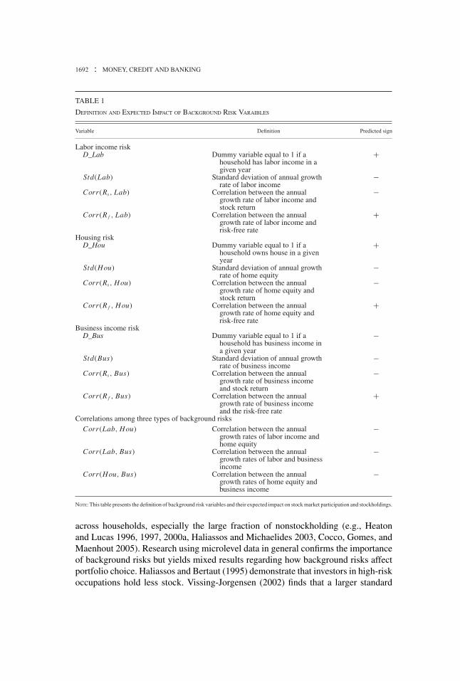
In this section, we first discuss the construction of background risk factors. Basedon theoretical studies in the prior literature, we generate testing hypotheses about thepredicted impacts of background risk factors on portfolio choice. We then specifyour empirical model and discuss econometric issues and measurement errors. Thedefinition of our background risk variables and their predicted (expected) impacts onstock investment are summarized in Table 1.
1.1 Background Risks Measures
We aim to develop an empirical model that allows us to examine how the hetero-geneity of background risk exposures among households affects the cross-sectionalvariation of stock investment. More importantly, we want to jointly consider threetypes of nonfinancial assets—labor, housing, and private business. While each of thesebackground risks has been separately investigated in the literature, to the best of ourknowledge, no study has jointly considered all three types of risks in an optimizingmodel. Developing a theoretical model of optimal portfolio choice in the presence ofthe three types of background risks is beyond the scope of this paper. We thereforeborrow the insights from the prior literature to build a reduced-form empirical modelto test the predicted impacts of these risks on household stock investment. We aim toexamine whether these background risks are quantitatively important to a household’sstock investment. Specifically, we investigate whether the cross-household variationof background risks can help to explain the large fraction of nonstock investment,and the observed enormous cross-sectional variation in households’ stockholdings.
We consider an economy with three types of nonfinancial assets: labor, housing, andprivate business, and two financial assets: risky stock and risk-free bond. Motivatedby the standard mean-variance framework, we argue that the optimal portfolio isdetermined by the variance–covariance structure of returns of these assets. Assumingthat the investor cannot trade nonfinancial assets, optimal portfolio choice involvesselecting a combination of stock and risk-free asset to minimize the overall riskexposure to all risky assets. A household would choose a less risky portfolio if it isexposed to more unfavorable background risks. Assuming that short sale is prohibited,zero stockholding (i.e., nonstock market participation) can yield as an optimal choiceif a household is highly exposed to background risks. Therefore, a household exposedto more unfavorable background risks is expected to allocate less wealth to stocks oris less likely to participate in the stock market.
This hypothesis is motivated by a large body of literature, which provides the-oretical predictions on how background risk affects portfolio choice. For example,Constantinides and Duffie (1996) and Viceira (2001) suggest that investors alter stockinvestment to hedge labor income risk. Cocco (2005), Yao and Zhang (2005), andFlavin and Yamashita (2002) show that the existence of risky housing reduces stockinvestment. Empirical studies based on numerical calibration show that the existenceof background risks cannot fully explain the enormous variation of stockholdings
1692 : MONEY, CREDIT AND BANKING
TABLE 1
DEFINITION AND EXPECTED IMPACT OF BACKGROUND RISK VARAIBLES
Variable Definition Predicted sign
Labor income riskD_Lab Dummy variable equal to 1 if a
household has labor income in agiven year
+
Std(Lab) Standard deviation of annual growthrate of labor income
−Corr (Rs , Lab) Correlation between the annual
growth rate of labor income andstock return
−
Corr (R f , Lab) Correlation between the annualgrowth rate of labor income andrisk-free rate
+
Housing riskD_Hou Dummy variable equal to 1 if a
household owns house in a givenyear
+
Std(Hou) Standard deviation of annual growthrate of home equity
−Corr (Rs , Hou) Correlation between the annual
growth rate of home equity andstock return
−
Corr (R f , Hou) Correlation between the annualgrowth rate of home equity andrisk-free rate
+
Business income riskD_Bus Dummy variable equal to 1 if a
household has business income ina given year
−
Std(Bus) Standard deviation of annual growthrate of business income
−Corr (Rs , Bus) Correlation between the annual
growth rate of business incomeand stock return
−
Corr (R f , Bus) Correlation between the annualgrowth rate of business incomeand the risk-free rate
+
Correlations among three types of background risksCorr (Lab, Hou) Correlation between the annual
growth rates of labor income andhome equity
−
Corr (Lab, Bus) Correlation between the annualgrowth rates of labor and businessincome
−
Corr (Hou, Bus) Correlation between the annualgrowth rates of home equity andbusiness income
−
NOTE: This table presents the definition of background risk variables and their expected impact on stock market participation and stockholdings.
across households, especially the large fraction of nonstockholding (e.g., Heatonand Lucas 1996, 1997, 2000a, Haliassos and Michaelides 2003, Cocco, Gomes, andMaenhout 2005). Research using microlevel data in general confirms the importanceof background risks but yields mixed results regarding how background risks affectportfolio choice. Haliassos and Bertaut (1995) demonstrate that investors in high-riskoccupations hold less stock. Vissing-Jorgensen (2002) finds that a larger standard
DARIUS PALIA, YAXUAN QI, AND YANGRU WU : 1693
deviation of nonfinancial income reduces stock investment, but the covariance of in-come and stock returns has no impact. Heaton and Lucas (2000b) show that investorsinvest less in stocks when they face more volatile business income, but labor incomerisk does not significantly affect stock investment. Angerer and Lam (2009) reportthat a permanent income shock reduces stock investment but a transitory incomeshock does not. Guiso, Jappell, and Terlizzese (1996) and Hochguetel (2002), re-spectively, use data from Italy and the Netherlands to show that households exposedto higher labor income risk hold safer portfolios. Chen, Yao, and Yu (2007) andDimmock (2012) argue that background risks also affect asset allocation of insti-tutional investors. Eiling (2013) uses the industry-level labor income to show thathuman capital affects the cross-sectional stock returns.
Our approach is to construct a set of factors that capture the “unfavorable” back-ground risk exposures. Motivated by the mean-variance framework, we consider thecovariance of returns between financial and nonfinancial assets. One big challenge inthis literature is that returns of these nonfinancial assets are not observable. FollowingJagannathan and Wang (1996), Flavin and Yamashita (2002), and Heaton and Lucas(2000b), we use annual growth rates of labor income, home equity, and businessincome to proxy their respective returns.5 We then estimate the covariance betweenthese annual growth rates and returns of financial assets. Our baseline model consistsof 12 background risk factors, which can be grouped into four categories.
First, we consider the standard deviations of growth rates of labor income, homeequity, and business income, denoted by Std(Lab), Std(Hou), and Std(Bus), respec-tively. Previous research shows that the volatility of additional risky income reducesthe demand for stock (Guiso, Jappell, and Terlizzese 1996, Heaton and Lucas 2000a,2000b, Hochguertel 2002, Vissing-Jorgensen 2002, Angerer and Lam 2009). Hence,we expect each of these variables to have a negative effect on the proportion ofstockholdings and on stock market participation.
Second, we calculate the correlations between the three growth rates andstock returns, denoted by Corr(Rs, Lab), Corr(Rs, Hou), and Corr(Rs, Bus),respectively. The correlation between a background risk shock and stock returnsis potentially important to a household’s portfolio choice (Viceira 2001, Benzoni,Collin-Dufresne, and Goldstein 2007). For example, a positive correlation be-tween labor income and stock returns reduces a household’s willingness to holdstock because labor income substitutes for stock. On the other hand, a negativecorrelation between labor income and stock returns encourages stockholdingsbecause stock can be used as a hedge against labor income risk. We hence expectCorr(Rs, Lab), Corr(Rs, Hou), and Corr(Rs, Bus) to carry negative coefficients.
Third, we include correlations between the three growth rates and the risk-free rate, denoted by Corr(R f , Lab), Corr(R f , Hou), and Corr(R f , Bus), respec-tively. We expect each of these variables to have a positive effect on stockmarket participation and stockholdings. The measure introduced here captures the
5. We consider labor income as dividends of the unobserved human capital, growth of home equity asreturns on housing investment, and business income as dividends of business investment.

1694 : MONEY, CREDIT AND BANKING
comovement of a background risk variable and the real interest rate, which is primar-ily driven by unexpected inflation. This design is to test whether bond-like incomereduces the pressure on precautionary savings, thereby encouraging investment instocks (e.g., Cocco, Gomes, and Maenhout 2005). Intuitively, a household with sta-ble labor income which increases with inflation (e.g., those working in the publicsector) is more likely to invest in risky stocks because its labor income risk is lower.
Fourth, we include the correlations of the returns among the three nonfinancialassets, denoted by Corr(Lab, Hou), Corr(Lab, Bus), and Corr(Hou, Bus). We expectthese variables to have negative coefficients because the positive correlation betweentwo background risks (e.g., labor and housing) exacerbates the overall risk exposureand hence reduces a household’s willingness to bear stock risk.
Overall, our background risk measures consist of 12 variables. We consider a linearregression of stock investment on these variables. We further include three dummyvariables, denoted by D_Lab, D_Hou, and D_Bus that, respectively, indicate if ahousehold has labor income, housing, and business income in a given year to capturethe change of background risks over the life cycle. The empirical model is specifiedas follows:
StockInvti,t = a0 + a1Std(Labit ) + a2Corr(Rst , Labit )
+ a3Corr(R f , Labit )
+ a4Std(Houit ) + a5Corr(Rst , Houit ) + a6Corr(R f t , Houit )
+ a7Std(Busit ) + a8Corr(Rst , Busit ) + a9Corr(R f , Busit )
+ a10Corr(Labit, Houit ) + a11Corr (Labit , Busit )
+ a12Corr(Busit , Houit )
+ a13 D Labit + a14 D Houit + a15 D Busit + δControlsit + εi,t ,
(1)
where subscripts i and t denote household and year, respectively; StockInvt is ei-ther a binary variable of stock market participation or a ratio of stock to wealth;Lab, Hou, and Bus are growth rates of labor income, home equity, and busi-ness income, respectively; Rs and R f are gross return rates of a stock marketportfolio and the risk-free asset, respectively; and Controls is a vector of controlvariables.
1.2 Control Variables
We follow the prior literature to add control variables. Numerous papers documentthat race, income, wealth, and education each has a positive impact on stock marketparticipation (e.g., Mankiw and Zeldes 1991, Vissing-Jorgensen 2002, Hong, Kubik,and Stein 2004, Campbell 2006). The level of education is regarded as a proxy forfixed entry and transaction costs and is found to be positively significantly related to
DARIUS PALIA, YAXUAN QI, AND YANGRU WU : 1695
stock market participation in previous studies. We use two dummy variables, HSchool(equal to 1 if the head of household has a high school education) and College (equalto 1 if the head of household has a college education), to control for educationeffects. We expect Log(Age), the log transformation of the age of the householdhead, to have a positive sign and (Log(Age))2 to have a negative sign to capturethe hump-shaped life-cycle pattern of stockholdings (Jagannathan and Kocherlakota1996).
Flavin and Yamashita (2002) suggest that the house-to-net wealth ratio influ-ences a homeowner’s portfolio composition. We hence include Log(HsValue)—thelog transformation of market value of owner-occupied house. Cocco (2005) arguesthat although housing investment substitutes for stock investment, a mortgage loanserves as a leverage borrowing channel to finance investment in stocks. We includeLog(Mortgage)—the log transformation of unpaid mortgage balance as a controlvariable. Vissing-Jorgensen (2002) documents that the level of nonfinancial incomeis positively related to stock market participation. We use Log(LabIncome)—the logtransformation of labor income as a control variable. To capture the dynamics oflabor income risk, we control for unemployment shock by adding a dummy variableUnemployment, which equals 1 if the head of household lost its job in a given year,and 0 otherwise. We further add a dummy variable that equals 1 if husband and wifework in the same industry, and 0 otherwise.
1.3 Econometric Issues and Measurement Errors
We run regressions that relate stock market participation (DumStk) and theproportion of stock relative to wealth (PtfStk) to a set of explanatory variables.Since DumStk is a discrete-choice variable that equals 1 if a household partici-pates in the stock market, and 0 otherwise, we employ the Logit model specifiedbelow:
Prob(DumStk = 1) = F(β ′ X )
Prob(DumStk = 0) = 1 − F(β ′ X )
where F(β ′ X ) = eβ′ X
1+eβ′ X .
(2)
Given that a large fraction of households hold no stocks, ordinary least squares(OLS) regression is not suitable to study the proportion of stockholdings. Severaltheoretical papers (e.g., Orosel 1998, Haliassos and Michaelides 2003, Guo 2004,Gomes and Michaelides 2005, Ball 2008) have treated stock market nonparticipation(i.e., zero stockholding) as part of a household’s portfolio choice. In this framework,agents maximize their lifetime utility subject to a budget constraint that includes aparticipation cost. Consistent with this line of reasoning and following the empiri-cal methodology employed by Guiso, Jappell, and Terlizzese (1996), Hochoguertel
1696 : MONEY, CREDIT AND BANKING
(2002), and Cocco (2005), we adopt a Tobit model where the lower limit is 0 (ahousehold holds no stock).6 The Tobit model is specified as follows:
PtfStk ={
β ′ X + ε, if PtfStk > 00, if otherwise.
(3)
An alternative method of estimating the determinants of stockholdings is theHeckman selection model. The selection model suggests that households firstmake a decision on whether to participate in the stock market and then, con-ditional on participation, choose the optimal stockholdings related to wealth.7
Vissing-Jorgensen (2002) employs a Heckman model with a fixed participation cost.Therefore, for a robustness check, we consider the Heckman model, as specifiedbelow:
Participation equation: S∗ = β ′ X + υ, DumStk ={
1, if S∗ > 00, otherwise
Stockholding equation: PtfStk = β ′ X + ε, observed if DumStk = 1,
(4)
where S∗ is a latent variable about stock market participation. We only observe abinary variable of DumStk and PtfStk when a household chooses participation inthe stock market. In estimation, we include the lagged stock participation decisionand lagged stockholdings as additional explanatory variables in the participation andstockholding equations, respectively.
We further consider an OLS regression using a truncated sample consisting ofonly stockholders. We include households that hold stock in the current year orever held stocks in previous years. We then run the OLS regression for this sub-sample to shed light on how background risks affect stockholdings conditional onparticipation.
Given a large number of households and a limited number of years in our data,it is hard to estimate the panel regression with household-specific fixed effects.We therefore use year dummy variables to control for time effect, and estimate thestandard errors with clustering by households in order to correct for serial correlations(a household that holds stocks in the previous year is more likely to hold stocks inthe current year).8 Massa and Simonov (2006) argue that households tend to hold
6. We also use a two-sided Tobit model with the lower limit equal to 0 (a household holds no stocks)and the upper limit equal to 1 (a household holds only stocks). The results do not change significantly andare available upon request.
7. One challenge of the Heckman selection model is to find valid instrumental variables that arerelated to stock market participation but not to stockholdings conditional on participation. However, in theempirical tests, we find that total wealth is significantly related to portfolio shares. Furthermore, education,which is regarded as a proxy for fixed cost for stock market participation is also significantly related tostockholdings. Hence, it is hard to identify good instrumental variables. Therefore, we report Tobit as thebaseline model, and provide the Heckman and OLS models for robustness checks.
8. Petersen (2009) shows that given a large number of firms (households in our case) and a smallnumber of years, correct standard errors can be obtained by including time dummies and then estimatingstandard errors with clustering by firms (households).

DARIUS PALIA, YAXUAN QI, AND YANGRU WU : 1697
stocks that are geographically and professionally close to them. We hence controlfor industry and state fixed effects. The industry dummies are based on the majorindustry in which the head of household works.9
In our baseline model, we assume that background risks are time invariant. In re-ality, a household’s background risks may change over the life cycle. As a robustnesscheck, we consider time-varying background risk factors using rolling-over windows(see estimation details in Section 2). Using a rolling-over window increases measure-ment errors because it uses a shorter period rather than the full sample to estimate thestandard deviations and correlations.
We further consider a cross-sectional regression. In particular, we regress thetime average of stockholdings relative to wealth on the time-invariant backgroundrisk factors and the time averages of other control variables. As for stock marketparticipation, we sum the stock participation dummy variable over years and dividethis variable by the number of years when the household appears in the sample. Weclassify a household as a stock market participant if it holds stocks in more than halfof the time in the sample period.
We assume that the background risk variables are predetermined because adjust-ments in labor supply, housing and private business are much harder than adjustmentsin stock investment. In principle, background risk variables can be endogenously de-termined (e.g., Bodie, Merton, and Samuleson 1992, Roussanov 2004) by risk attitudeand investment into human capital. We do not control for risk attitude in our baselinemodel.10 However, we believe that our specification is robust to the existence ofendogeneity as endogeneity would bias our results toward not finding the expectedrelationship between the background risk variables and the investment choice. Forexample, a more risk-averse household would choose to invest in safer assets andselect a safer occupation (with a lower standard deviation of labor income), resultingin a positive relationship between the standard deviation of labor income and stockinvestment. Since our testing hypothesis predicts that the standard deviation of laborincome is negatively related to stockholdings, our regressions provide a conservativeestimate of the impacts of these background risk factors on stock market participationand stockholdings.
2. DATA AND DESCRIPTIVE STATISTICS
Our data are drawn from the Panel Study of Income Dynamics (PSID), which is anannual survey maintained by the University of Michigan. The surveys are conducted
9. The estimation of Logit and Tobit models is sensitive to the distributional assumptions about theerror terms. In unreported robustness check, we also calculate nonparametric t-statistics using bootstrappedstandard errors.
10. The PSID provides data on risk tolerance in the 1996 survey. Adding the risk tolerance variable inour regressions does not change our basic results. This test is not reported but is available upon request.
1698 : MONEY, CREDIT AND BANKING
every year from 1968 to 1997 and every other year after 1997.11 We utilize the PSIDsurveys from 1975 to 2009. The long panel with detailed demographic, income, andhousing data allows us to construct various measures of income and housing risks. Alimitation of the PSID data is that detailed wealth composition such as stockholdingsis provided in the Wealth Supplement Survey, which was conducted once every5 years from 1984 to 1999 and then every other year after 1999. Therefore, thefinancial asset holdings information is available for these 9 years (1984, 1989, 1994,1999, 2001, 2003, 2005, 2007, and 2009). Since questions related to income andwealth in the PSID data are retrospective12 (e.g., those asked in 1994 refer to the1993 calendar year), we refer our sample years as 1983, 1988, 1993, 1998, 2000,2002, 2004, 2006, and 2008. We use the CRSP NYSE/AMEX/NASDAQ value-weighted market index return as a proxy for risky stock return, and the 30-day T-billreturn as a proxy for the risk-free rate. All monetary variables are in constant 1992dollars using the Consumer Price Index obtained from CRSP.
2.1 Stock Values and Stock Participation
In PSID, stock market participation (denoted by DumStk) and the value of stock-holdings are self-reported in the surveys. Unfortunately, PSID changed the definitionof stock in 1999. Up to the 1997 survey, reported stockholdings include stocks helddirectly and held in mutual funds, investment trusts, and pension funds. Since the1999 survey, the value of stockholdings in pension funds is excluded. This changein definition causes an inconsistency in our stock values and stock participation vari-ables over time. We therefore make the following adjustments using questions askedby PSID about pension accounts. The questions are: “Do (you/you or anyone inyour family) have any money in private annuities or Individual Retirement Accounts(IRAs)?” “Are they mostly in stocks, mostly in interest earning assets, split betweenthe two, or what?” and “How much would they be worth?” We assume that all invest-ments in IRAs are stocks if most money in IRAs is invested in stocks. If a householdreports that the money in IRAs is split between stocks and interest-sensitive assets,we assume that half of the value in the IRAs is in stocks and the other half is insavings. We then adjust the post-1999 stock variable by summing the reported stockvalue and the estimated stock value in pension funds.13
Previous studies suggest that the properties of portfolio composition relative todemographic variables are sensitive to the way wealth is measured (see, e.g., Heatonand Lucas 2000a). In computing the proportion of stock value relative to wealth,
11. The original PSID sample consisted of two independently selected samples: a cross-sectionalnational sample (the SRC sample) and a national sample of low-income families (the SEO sample). Weexclude the SEO sample to generate a representative sample of the U.S. population. The PSID is designedto capture demographic and income dynamics of U.S. households over a long period. Households thatwere selected in the 1968 survey have been resurveyed thereafter. The split-off households (householdsestablished by children of the originally selected families) have been added to the sample each year.
12. Most surveys are conducted in the springs and therefore income and wealth data are for the previousyears.
13. Because the post-1999 stockholdings data may not be accurate, we conduct a robustness test usingprior-1999 data and find similar results. These results are not reported but are available upon request.
DARIUS PALIA, YAXUAN QI, AND YANGRU WU : 1699
we consider three definitions of wealth: (i) total family financial wealth—the sumof stock, savings, and bond values; (ii) total family wealth without home equity—the sum of values of financial assets, business, vehicles, and real estate excludingowner-occupied house minus total debts owed; and (iii) total family wealth withhome equity—the sum of value of financial assets, business, vehicles, and real estateincluding home equity of owner-occupied house minus total debts owed. Home eq-uity is the net worth of self-reported market value of house minus unpaid mortgagebalance. These three measures are denoted as PflStk_1, PflStk_2, and PflStk_3, respec-tively. Our main measure is the stockholding relative to financial wealth (PflStk_1). Inrobustness checks, we also consider PflStk_2 and PflStk_3 and obtain similar results.
2.2 Background Risk Measures
Time-invariant background risk measures. To create individual background risk mea-sures, we use the 1976–2009 PSID Family Income Files. We generate the 21-yearconsecutive time series (1976–97) of annual growth rates of labor income, housingvalue, and business income. Unlike the financial assets that are reported only in thePSID Wealth Supplement Survey, the market value of house and unpaid mortgageare provided in the PSID Family Income Survey. For the period 1997–2009, PSIDprovides data every other year. We estimate the annual growth rates by dividingthe 2-year growth rates by two. Overall, we obtain annual growth rates of incomeand housing value for 27 years.14 Since PSID does not provide total family busi-ness income before 1993, we use the head of household business income as a proxyfor total family business income. To make the labor income and business incomemeasures comparable, we also use the head of household labor income as a proxyfor total family labor income. We define the head of household business income asthe sum of business income from assets and business income from labor.15 We usehome equity—the difference between self-reported house value and unpaid mortgagebalance—as our proxy for housing value, because home equity truly reflects a house-hold’s wealth accumulation through housing investment. We also use the growth rateof self-reported market value of owner-occupied house (i.e., ignoring unpaid mort-gage balance) to redo our regressions.16 Using the annual growth rates, we calculatefor each household the standard deviations of labor income, home equity, and busi-ness income, that is, Std(Lab), Std(Hou), and Std(Bus), and the correlations of thesegrowth rates with stock returns, Corr(Rs,.), and with the risk-free rate, Corr(Rf,.).We also calculate the correlations among the three growth rates, Corr(Lab,Hou),Corr(Lab,Bus), and Corr(Bus,Hou).
14. In unreported robustness tests, we construct the background risk variables using data before 1997when we have consecutive annual observations and we obtain similar results.
15. Alternatively, we define the head of household business income as business income from assetsonly, and include business income from labor in the head of household labor income. Under this definition,none of our results change significantly. The results are available upon request.
16. We find that the standard deviation of the growth rate of self-reported market values of owner-occupied house has a negative impact on stock market participation and stockholdings even more sig-nificantly than the standard deviation of the growth rate of home equity, whereas the correlations of thegrowth rate of house value with asset returns do not have a significant impact.
1700 : MONEY, CREDIT AND BANKING
To minimize measurement errors in the data, we apply several filters to the growthrates of labor income, home equity, and business income. Our baseline analysisrequires a household to have at least 3 years of gross growth rates ranging between0.5 and 2 to calculate the standard deviation and correlation statistics.17 That is,we ignore those observations with incomes dropping more than a half or more thandoubling in a year because these figures seem implausible and are more likely subjectto coding or other errors. This filter is denoted by Filter2. To check for robustness,we also require the gross growth rates to lie within the 0.3–3 and 0.2–5 ranges, anddenote these filters by Filter3, and Filter5, respectively.
Note that these filters do not delete households with extraordinary changes of back-ground risks, but they only require a household to have reasonable annual growth ratesfor at least 3 years to be included in our sample. For example, a household may con-tinuously provide labor income but suddenly reports a 0 labor income in year t due tounemployment. This will yield a 0 gross growth rate of labor income in year t, and aninfinite growth rate in year t + 1. We will exclude the observations in years t andt + 1 and use the observations for the rest of the years to estimate its labor incomerisk. We then set the labor income risk variable to 0 for years t and t + 1. We use adummy variable “if head has a job” to control for households without labor incomerisk. These households could be students, retirees, or self-employed people. We usea dummy variable “if head is unemployed” to control for unemployment shock. Forhouseholds that do not have a house or private business, we set the housing risk orbusiness risk to 0. We include dummy variables “if owns a house” and “if owns abusiness” in our regressions.
Rolling-over background risk measures. The above method to calculate standarddeviations and correlations assumes that background risks are time invariant. Inprinciple, these risks can fluctuate with general economic conditions and can changeover the life cycle of a household. Our measures introduced above only capturethe variation of background risks across households, but not the time variation ofbackground risks for a given household over its life cycle. To capture the time-seriesvariation of background risks, we employ two rolling-over methods.
First, we consider a household that makes its portfolio choice based on its currentand past experience of income and housing value fluctuations, so we employ abackward rolling-over measure. These measures are calculated using prior 8-yeardata. For example, risk measures in 1983 are calculated using data from 1976 to1983, and those in 1997 are calculated using data from 1990 to 1997.
Second, rational expectations theory suggests that a household should make itsportfolio choice based on its ex ante expectation of background risks. We thereforeestimate forward rolling-over measures using 5-year posterior data. For example,forward risk measures in 1983 are calculated using data from 1983 to 1987, and thosein 1993 are calculated using data from 1993 to 1997. The shortening in the number
17. To check for robustness, we require a household to have at least 10 years of growth rates to calculatethe standard deviation and correlation statistics and we obtain similar results.
DARIUS PALIA, YAXUAN QI, AND YANGRU WU : 1701
of years used in calculation increases estimation errors. Thus, our main results arebased on the time-invariant measures and we provide a robustness check based onthe two rolling-over measures.
2.3 Descriptive Statistics
Combining the estimated background risk measures with stockholding data fromthe PSID Wealth Supplement Survey, we construct a 9-year unbalanced panel of 4,756households with 22,610 year-household observations. We confirm the well-knownfact of limited stock market participation. The participation rates have significantlyincreased over the past two decades from 28% in 1983 to 44% in 2008. However,more than half of the U.S. households still do not hold any stocks. The average ratio ofstocks to financial wealth generally increases from 43% in 1983 to 51% in 2008, withtwo dips during 2000–02 and in 2008 that reflect, respectively, the Internet bubblecrash and the subprime mortgage crisis.18
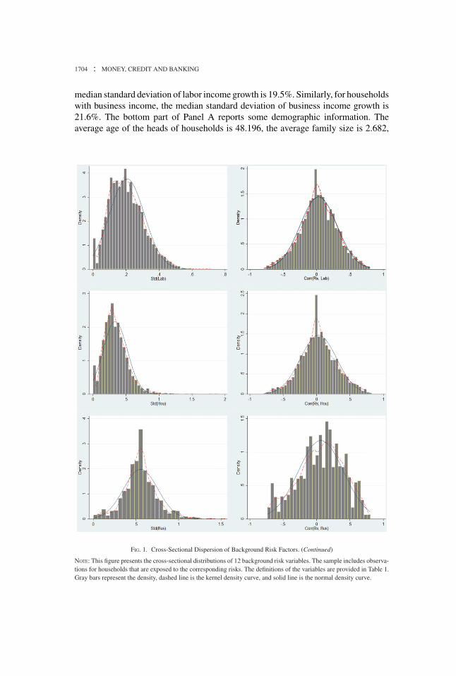
In Figure 1, we present the cross-sectional variation of our 12 background riskvariables. In each panel, we display the estimated density using the sample of house-holds who are exposed to the corresponding risks and the normal density curve forease of comparison. There is a large dispersion for each of these risk factors. Thedistribution of the standard deviation of labor income growth is skewed to the right,indicating that most households are exposed to moderate labor income risk while asmall fraction is subject to large labor risk. A similar pattern is observed for the stan-dard deviation of housing growth. We see a spike around zero in the empirical densityfor the correlations of income growth with stock returns and with the risk-free rate,indicating that there are a substantial number of households whose income growthis unrelated with stocks returns and with the risk-free rate. We find a similar patternfor the correlations of housing growth with financial asset returns. The distributionsof both correlations of housing income with labor income and with business incomeare well dispersed with a spike in zero. On the other hand, for most households,the correlation between labor and business incomes is close to zero. This result isexpected as households owning a private business are mostly self-employed and haveno labor income.
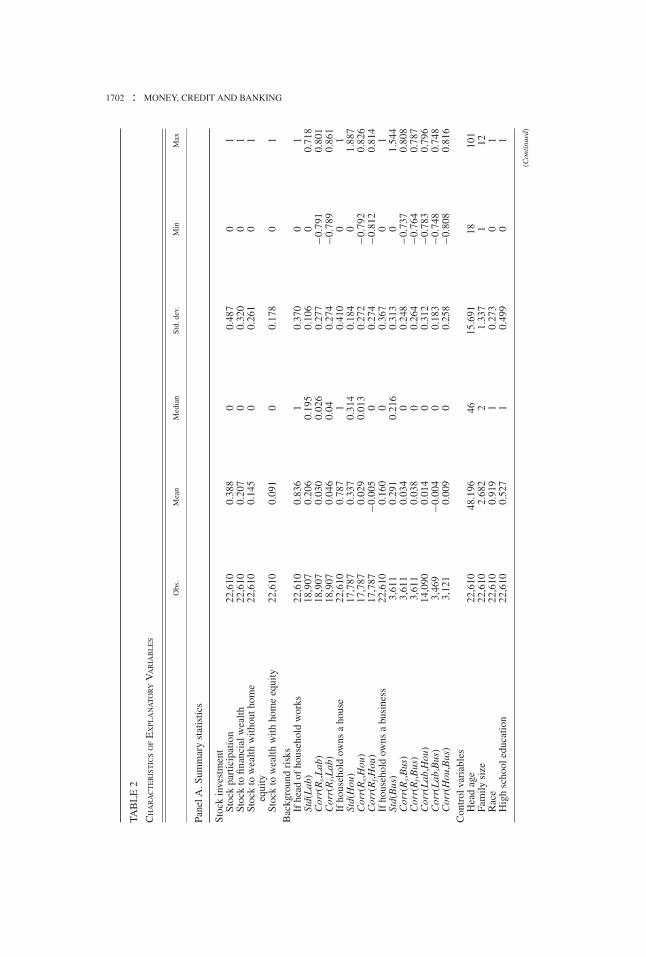
Panel A of Table 2 reports the summary statistics of the variables used in ourregressions. The top part of this table summarizes stock investment. For example,overall 38.8% of households participate in stock market. The middle part in PanelA presents the summary statistics of the background risk variables. We observesubstantial heterogeneity of background risks across households. Overall, 83.6% ofhouseholds have labor income, 78.7% of households own a house, but only 16%have a private business.19 Within the group of households that have labor income, the
18. These results are not tabulated, but are available upon request.19. In the PSID survey, many households that claim owning a private business do not report their
business income. Overall, although 16% of households indicate owning a private business, only 7.54%provide business income information.
1702 : MONEY, CREDIT AND BANKING
TAB
LE
2
CH
AR
AC
TE
RIS
TIC
SO
FE
XPL
AN
AT
OR
YV
AR
IAB
LE
S
Obs
.M
ean
Med
ian
Std.
dev.
Min
Max
Pane
lA.S
umm
ary
stat
istic
s
Stoc
kin
vest
men
tSt
ock
part
icip
atio
n22
,610
0.38
80
0.48
70
1St
ock
tofin
anci
alw
ealth
22,6
100.
207
00.
320
01
Stoc
kto
wea
lthw
ithou
thom
eeq
uity
22,6
100.
145
00.
261
01
Stoc
kto
wea
lthw
ithho
me
equi
ty22
,610
0.09
10
0.17
80
1B
ackg
roun
dri
sks
Ifhe
adof
hous
ehol
dw
orks
22,6
100.
836
10.
370
01
Std(
Lab
)18
,907
0.20
60.
195
0.10
60
0.71
8C
orr(
Rs,L
ab)
18,9
070.
030
0.02
60.
277
−0.7
910.
801
Cor
r(R
f,Lab
)18
,907
0.04
60.
040.
274
−0.7
890.
861
Ifho
useh
old
owns
aho
use
22,6
100.
787
10.
410
01
Std(
Hou
)17
,787
0.33
70.
314
0.18
40
1.88
7C
orr(
Rs,H
ou)
17,7
870.
029
0.01
30.
272
−0.7
920.
826
Cor
r(R
f,Hou
)17
,787
−0.0
050
0.27
4−0
.812
0.81
4If
hous
ehol
dow
nsa
busi
ness
22,6
100.
160
00.
367
01
Std(
Bus
)3,
611
0.29
10.
216
0.31
30
1.54
4C
orr(
Rs,B
us)
3,61
10.
034
00.
248
−0.7
370.
808
Cor
r(R
f,Bus
)3,
611
0.03
80
0.26
4−0
.764
0.78
7C
orr(
Lab
,Hou
)14
,090
0.01
40
0.31
2−0
.783
0.79
6C
orr(
Lab
,Bus
)3,
469
−0.0
040
0.18
3−0
.748
0.74
8C
orr(
Hou
,Bus
)3,
121
0.00
90
0.25
8−0
.808
0.81
6C
ontr
olva
riab
les
Hea
dag
e22
,610
48.1
9646
15.6
9118
101
Fam
ilysi
ze22
,610
2.68
22
1.33
71
12R
ace
22,6
100.
919
10.
273
01
Hig
hsc
hool
educ
atio
n22
,610
0.52
71
0.49
90
1
(Con
tinu
ed)
DARIUS PALIA, YAXUAN QI, AND YANGRU WU : 1703TA
BL
E2
CO
NT
INU
ED
Obs
.M
ean
Med
ian
Std.
dev.
Min
Max
Pane
lA.S
umm
ary
stat
istic
s
Stoc
kin
vest
men
tC
olle
geed
ucat
ion
22,6
100.
309
00.
462
01
Tota
lwea
lthin
clud
ing
hom
eeq
uity
22,6
1017
3,42
882
,674
254,
124
−36,
302
2,09
3,79
3
Tota
lbef
ore-
tax
fam
ilyin
com
e22
,610
52,6
4444
,558
37,8
8239
258,
391
Tota
lhea
dla
bor
inco
me
22,6
1029
,785
25,3
0429
,153
025
3,67
1H
ouse
valu
e22
,610
107,
544
81,5
5211
6,94
80
1,73
1,54
4U
npai
dm
ortg
age
valu
e22
,610
33,7
248,
896
46,4
560
263,
478
Ifhe
adan
dw
ife
insa
me
indu
stry
22,6
100.
063
00.
244
01
Ifhe
adis
inun
empl
oym
ent
22,6
100.
061
00.
240
1
12
34
56
78
910
1112
Pane
lB.C
orre
latio
nm
atri
xof
back
grou
ndri
skfa
ctor
s
1.St
d(L
ab)
1.00
000
34**
0.02
7**−0
.073
**−0
.045
**−0
.032
**0.
094**
−0.0
010.
001
0.01
4*−0
.025
**0.
009
2.C
orr(
Rs,L
ab)
1000
0.43
4**−0
.014
*0.
020**
0.01
0−0
.025
**−0
.003
−0.0
030.
020**
0.01
4*−0
.006
3.C
orr(
Rf,L
ab)
1.00
00.
007
0.01
4*−0
.002
−0.0
38**
−0.0
18**
−0.0
17*
0.02
7**0.
015*
0.00
34.
Std(
Hou
)1.
000
−0.0
15*
−0.0
54**
0.07
2**0.
017*
0.02
8**0.
002
0.00
30.
021**
5.C
orr(
Rs,H
ou)
1.00
00.
492**
−0.0
09−0
.013
−0.0
130.
022**
−0.0
04−0
.008
6.C
orr(
Rf,H
ou)
1.00
0−0
.009
−0.0
05−0
.005
0.05
9**−0
.014
*0.
003
7.St
d(B
us)
1.00
00.
167**
0.21
1**0.
022**
−0.0
26**
0.02
1**
8.C
orr(
Rs,B
us)
1.00
00.
435**
0.01
5*−0
.023
**0.
088**
9.C
orr(
Rf,B
us)
1.00
00.
014*
−0.0
15*
0.01
010
.Cor
r(L
ab,H
ou)
1.00
0−0
.005
−0.0
48**
11.C
orr(
Lab
,Bus
)1.
000
−0.0
49**
12.C
orr(
Hou
,Bus
)1.
000
NO
TE:
Pane
lA
repo
rts
sum
mar
yst
atis
tics
ofth
eex
plan
ator
yva
riab
les
inou
rre
gres
sion
s.Pa
nel
Bre
port
sth
eco
rrel
atio
nm
atri
xof
back
grou
ndri
skva
riab
les.
Std(
X)
isst
anda
rdde
viat
ion
ofva
riab
leX
;C
orr(
X,Y
)is
corr
elat
ion
betw
een
Xan
dY
;Lab
,Hou
,and
Bus
are,
resp
ectiv
ely,
annu
algr
owth
rate
sof
labo
rin
com
e,ho
me
equi
ty,a
ndbu
sine
ssin
com
e;R
sis
annu
algr
oss
retu
rnof
CR
SPva
lue-
wei
ghte
dm
arke
tind
ex;a
ndR
fis
annu
algr
oss
retu
rnof
the
30-d
ayT
-bill
.The
data
are
a9-
year
unba
lanc
edpa
nelf
or4,
756
hous
ehol
dsfo
rth
eye
ars
1984
,198
9,19
94,1
999,
2001
,200
3,20
05,2
007,
and
2009
.*an
d**
deno
test
atis
tical
sign
ifica
nce
atth
e5%
and
1%le
vels
,res
pect
ivel
y.
1704 : MONEY, CREDIT AND BANKING
median standard deviation of labor income growth is 19.5%. Similarly, for householdswith business income, the median standard deviation of business income growth is21.6%. The bottom part of Panel A reports some demographic information. Theaverage age of the heads of households is 48.196, the average family size is 2.682,
FIG. 1. Cross-Sectional Dispersion of Background Risk Factors. (Continued)
NOTE: This figure presents the cross-sectional distributions of 12 background risk variables. The sample includes observa-tions for households that are exposed to the corresponding risks. The definitions of the variables are provided in Table 1.Gray bars represent the density, dashed line is the kernel density curve, and solid line is the normal density curve.

DARIUS PALIA, YAXUAN QI, AND YANGRU WU : 1705
FIG. 1. Continued.
the average family income is $52,644, 30.9% of the heads of households have acollege degree, while 52.7% have only a high school education.
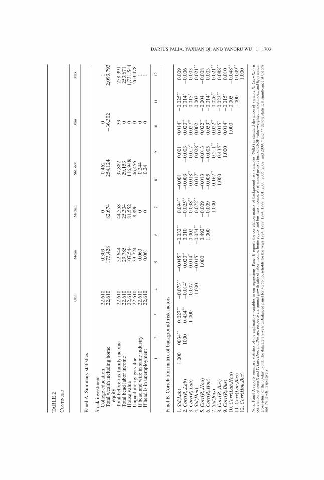
Panel B of Table 2 presents the correlation matrix of the 12 background riskmeasures. The correlation between a background risk measure and stock returns isclosely related to its correlation with the risk-free rate, suggesting some degree ofmulticollinearity. We therefore adjust our baseline model by excluding the correla-tions between the risk-free rate and background risk assets and obtain similar results
1706 : MONEY, CREDIT AND BANKING
as our baseline analysis. The results using these measures are not reported but areavailable upon request.20
3. EMPIRICAL RESULTS
3.1 Statistical Significance
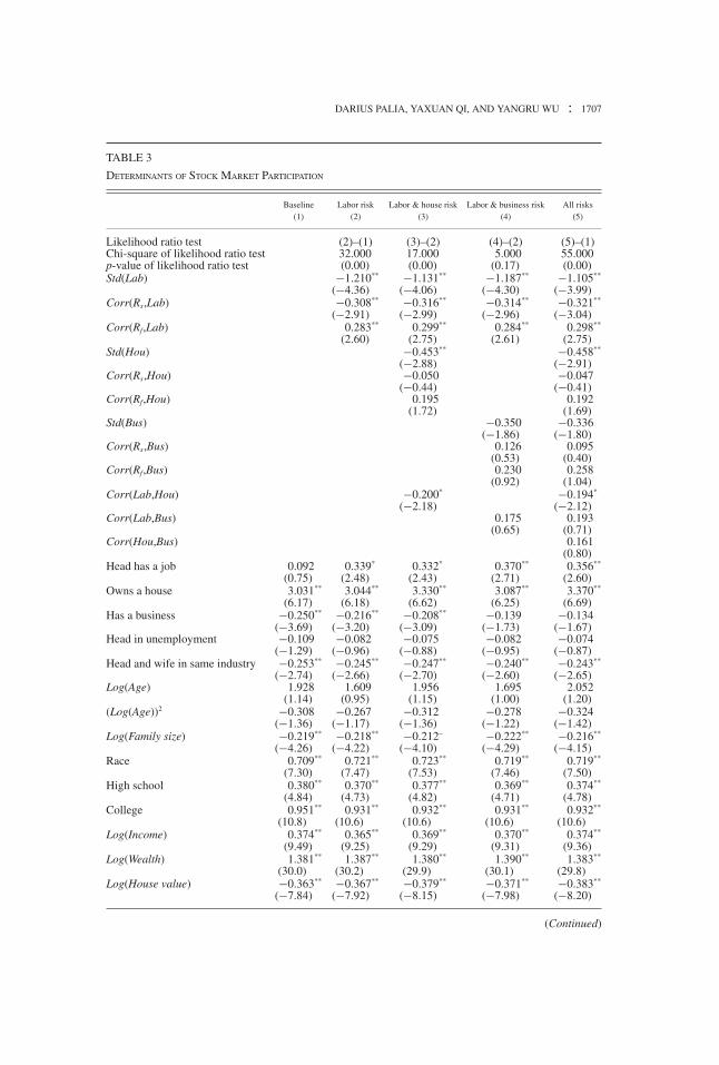
Table 3 presents maximum likelihood estimates of the Logit regressions. Fivespecifications are estimated, each with a different combination of the three types ofbackground risks: (i) no background risk, (ii) with only labor income risk, (iii) withboth labor income and housing risks, (iv) with both labor income and business risks,and (v) with all three types of background risks. The top part reports log likelihoodratio tests for various model comparisons.
Column (1) displays our benchmark model without considering background risks.We find strong explanatory power of education, race, income, and wealth for stockmarket participation, confirming the results of earlier studies. The positive coefficienton Log(Age) and the negative coefficient on (Log(Age))2 confirm the hump-shapepattern of stock market participation with age although these variables are not sta-tistically significant. We find that the “house value” variable carries the expectednegative sign and “unpaid mortgage” has the expected positive coefficient, consistentwith Cocco (2005) and Campbell (2006). These parameters are statistically signifi-cant at the 1% level. These results suggest that although housing investment crowdsout stock investment, mortgage loans can be used as a financing channel to supportstock investment. The “head has a job” variable is positively related to stock marketparticipation, but the effect is not statistically significant. The “owns a house” variablesignificantly increases the likelihood of stock market participation whereas the “has abusiness” variable significantly reduces participation. The “head in unemployment”is negatively related to participation but it is not statistically significant. “Head andwife in same industry” significantly reduces participation.
In column (2), we add the three labor income risk variables to the benchmark model.The coefficients of these three variables are estimated with the expected signs andare statistically significant at the 1% level. They imply that a household is more (less)likely to enter the stock market if its labor income is less (more) uncertain, if its laborincome is less (more) highly correlated with stock return, or if its labor income is more(less) highly correlated with the risk-free rate. Both Corr(Rs, Lab) and Corr(R f , Lab)are statistically significant but with opposite effects on stock investment, suggestingthat labor income risk can affect a household’s stock investment in different ways. Thisresult is consistent with various simulation studies that document that labor incomereduces stockholdings when it is modeled as a risky asset, whereas it encourages
20. We also examine the correlations among time-invariant, forward-looking, and backward-lookingbackground risk measures. We find that the time-invariant measure is more highly correlated with thebackward measure than with the forward measure. The backward and forward measures of standarddeviation variables are highly correlated. In contrast, the backward and forward measures of correlationvariables are not closely associated.
DARIUS PALIA, YAXUAN QI, AND YANGRU WU : 1707
TABLE 3
DETERMINANTS OF STOCK MARKET PARTICIPATION
Baseline Labor risk Labor & house risk Labor & business risk All risks(1) (2) (3) (4) (5)
Likelihood ratio test (2)–(1) (3)–(2) (4)–(2) (5)–(1)Chi-square of likelihood ratio test 32.000 17.000 5.000 55.000p-value of likelihood ratio test (0.00) (0.00) (0.17) (0.00)Std(Lab) −1.210** −1.131** −1.187** −1.105**
(−4.36) (−4.06) (−4.30) (−3.99)Corr(Rs,Lab) −0.308** −0.316** −0.314** −0.321**
(−2.91) (−2.99) (−2.96) (−3.04)Corr(Rf,Lab) 0.283** 0.299** 0.284** 0.298**
(2.60) (2.75) (2.61) (2.75)Std(Hou) −0.453** −0.458**
(−2.88) (−2.91)Corr(Rs,Hou) −0.050 −0.047
(−0.44) (−0.41)Corr(Rf,Hou) 0.195 0.192
(1.72) (1.69)Std(Bus) −0.350 −0.336
(−1.86) (−1.80)Corr(Rs,Bus) 0.126 0.095
(0.53) (0.40)Corr(Rf,Bus) 0.230 0.258
(0.92) (1.04)Corr(Lab,Hou) −0.200* −0.194*
(−2.18) (−2.12)Corr(Lab,Bus) 0.175 0.193
(0.65) (0.71)Corr(Hou,Bus) 0.161
(0.80)Head has a job 0.092 0.339* 0.332* 0.370** 0.356**
(0.75) (2.48) (2.43) (2.71) (2.60)Owns a house 3.031** 3.044** 3.330** 3.087** 3.370**
(6.17) (6.18) (6.62) (6.25) (6.69)Has a business −0.250** −0.216** −0.208** −0.139 −0.134
(−3.69) (−3.20) (−3.09) (−1.73) (−1.67)Head in unemployment −0.109 −0.082 −0.075 −0.082 −0.074
(−1.29) (−0.96) (−0.88) (−0.95) (−0.87)Head and wife in same industry −0.253** −0.245** −0.247** −0.240** −0.243**
(−2.74) (−2.66) (−2.70) (−2.60) (−2.65)Log(Age) 1.928 1.609 1.956 1.695 2.052
(1.14) (0.95) (1.15) (1.00) (1.20)(Log(Age))2 −0.308 −0.267 −0.312 −0.278 −0.324
(−1.36) (−1.17) (−1.36) (−1.22) (−1.42)Log(Family size) −0.219** −0.218** −0.212– −0.222** −0.216**
(−4.26) (−4.22) (−4.10) (−4.29) (−4.15)Race 0.709** 0.721** 0.723** 0.719** 0.719**
(7.30) (7.47) (7.53) (7.46) (7.50)High school 0.380** 0.370** 0.377** 0.369** 0.374**
(4.84) (4.73) (4.82) (4.71) (4.78)College 0.951** 0.931** 0.932** 0.931** 0.932**
(10.8) (10.6) (10.6) (10.6) (10.6)Log(Income) 0.374** 0.365** 0.369** 0.370** 0.374**
(9.49) (9.25) (9.29) (9.31) (9.36)Log(Wealth) 1.381** 1.387** 1.380** 1.390** 1.383**
(30.0) (30.2) (29.9) (30.1) (29.8)Log(House value) −0.363** −0.367** −0.379** −0.371** −0.383**
(−7.84) (−7.92) (−8.15) (−7.98) (−8.20)
(Continued)
1708 : MONEY, CREDIT AND BANKING
TABLE 3
CONTINUED
Baseline Labor risk Labor & house risk Labor & business risk All risks(1) (2) (3) (4) (5)
Log(Unpaid Mortgage) 0.058** 0.057** 0.060** 0.058** 0.060**
(9.12) (9.01) (9.47) (9.06) (9.50)Log(Head Labor Income) −0.012 −0.011 −0.011 −0.015 −0.014
(−1.24) (−1.12) (−1.14) (−1.51) (−1.48)Constant Yes Yes Yes Yes YesIndustry fixed effect Yes Yes Yes Yes YesState fixed effect Yes Yes Yes Yes YesYear fixed effect Yes Yes Yes Yes YesObservations 21,938 21,938 21,938 21,938 21,938Pseudo R2 0.266 0.268 0.269 0.269 0.270
NOTE: This table reports maximum likelihood estimation of Logit regressions. The dependent variable is DumStk, which is a binary-choicevariable equal to 1 if a household participates in stock market, and 0 otherwise. In each panel, coefficient estimates are reported withassociated t-statistics in parentheses. Standard errors are estimated with cluster of households. Log(X) is natural logarithm of variable X;Std(X) is standard deviation of X; Corr(X,Y) is correlation between X and Y; Lab, Hou, and Bus are, respectively, annual growth rates of laborincome, home equity, and business income; Rs is annual gross return of CRSP value-weighted market index; and Rf is annual gross return ofthe 30-day T-bill. * and ** denote statistical significance at the 5% and 1% levels, respectively.
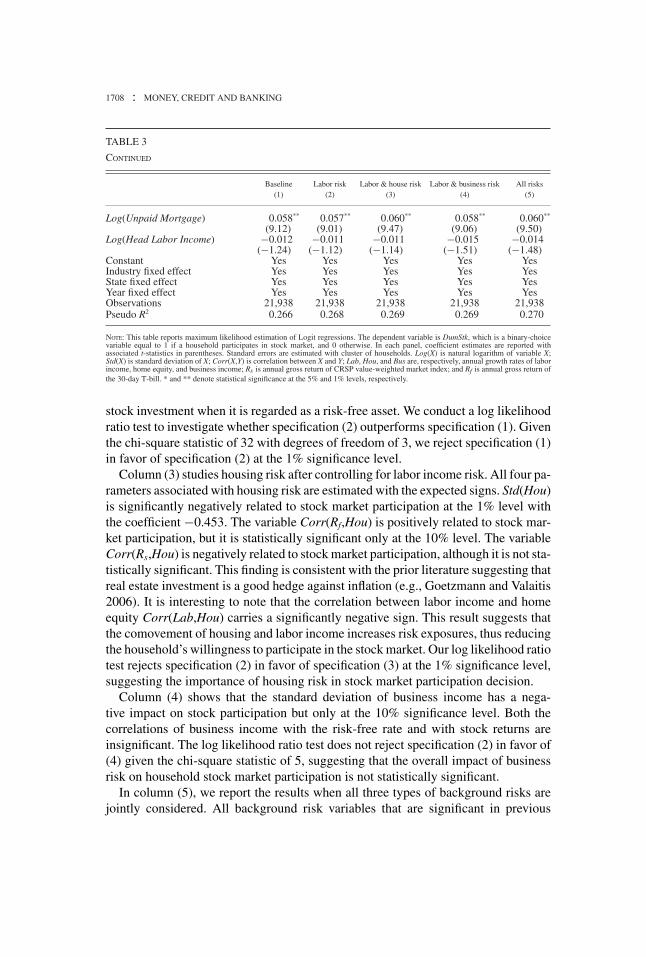
stock investment when it is regarded as a risk-free asset. We conduct a log likelihoodratio test to investigate whether specification (2) outperforms specification (1). Giventhe chi-square statistic of 32 with degrees of freedom of 3, we reject specification (1)in favor of specification (2) at the 1% significance level.
Column (3) studies housing risk after controlling for labor income risk. All four pa-rameters associated with housing risk are estimated with the expected signs. Std(Hou)is significantly negatively related to stock market participation at the 1% level withthe coefficient −0.453. The variable Corr(Rf,Hou) is positively related to stock mar-ket participation, but it is statistically significant only at the 10% level. The variableCorr(Rs,Hou) is negatively related to stock market participation, although it is not sta-tistically significant. This finding is consistent with the prior literature suggesting thatreal estate investment is a good hedge against inflation (e.g., Goetzmann and Valaitis2006). It is interesting to note that the correlation between labor income and homeequity Corr(Lab,Hou) carries a significantly negative sign. This result suggests thatthe comovement of housing and labor income increases risk exposures, thus reducingthe household’s willingness to participate in the stock market. Our log likelihood ratiotest rejects specification (2) in favor of specification (3) at the 1% significance level,suggesting the importance of housing risk in stock market participation decision.
Column (4) shows that the standard deviation of business income has a nega-tive impact on stock participation but only at the 10% significance level. Both thecorrelations of business income with the risk-free rate and with stock returns areinsignificant. The log likelihood ratio test does not reject specification (2) in favor of(4) given the chi-square statistic of 5, suggesting that the overall impact of businessrisk on household stock market participation is not statistically significant.
In column (5), we report the results when all three types of background risks arejointly considered. All background risk variables that are significant in previous
DARIUS PALIA, YAXUAN QI, AND YANGRU WU : 1709
regressions continue to be statistically significant. Furthermore, this modeloutperforms specification (1) at the 1% significance level. Based on the likelihoodratio test, the three types of background risks are important to a household’s decisionto participate in the stock market.
Table 4 studies the potential of background risks to explain the heterogeneity inportfolio compositions among households using Tobit regressions. The dependentvariable, PflStk_1, is the ratio of stock to financial wealth. Compared to the resultsfrom the Logit regressions in explaining market participation, we find that the vari-ables that are used to capture the background risks continue to have the expectedsigns in explaining portfolio choice in the Tobit regressions. The likelihood ratiotests confirm our previous findings that labor and housing risks appear to be moreimportant than business risk.
In terms of the relative importance, we find labor income risk to be the mostimportant, followed by housing risk, while business risk is less important. Threelabor income risk factors are all statistically significant. The standard deviation ofhome equity growth, and the correlation between the risk-free rate and home equitygrowth are significant but the correlation between stock return and home equitygrowth is not significant. None of the three business risk variables is statisticallysignificant at the 5% level or higher. Only the standard deviation of business incomegrowth is marginally significantly negatively related to stock investment at the 10%level. In addition, the correlation between labor income and home equity is negativelyrelated to stockholdings.
3.2 Economic Significance
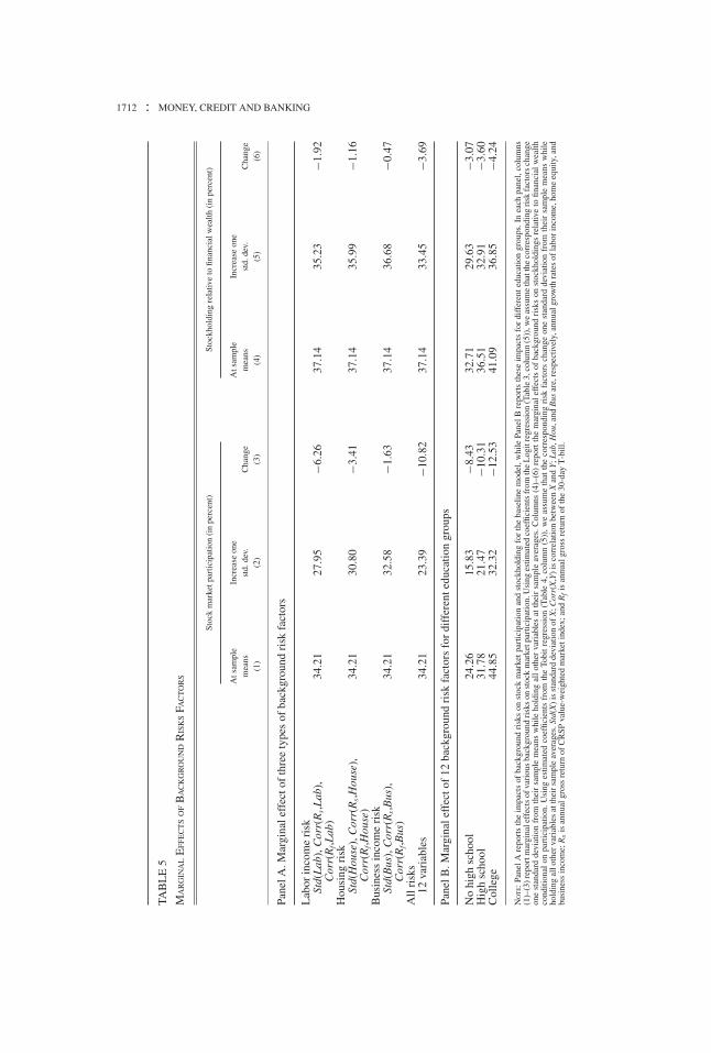
Given the statistical significance of the background risk factors, we study thequantitative impact of these risk factors. For each type of risk, we estimate thechange in a household’s probability of stock market participation and proportionof stock to financial wealth by assuming the corresponding risk variables changeone standard deviation in the unfavorable direction from their sample means whileholding all other variables at their sample means. Table 5 reports the results.
The left part of Panel A reports the change in the probability of stock marketparticipation. The calculation is based on the estimated coefficients in column (5) ofTable 3. For labor income risk, if Std(Lab), Corr(Rs,Lab), and Corr(Rf,Lab) all shiftone standard deviation from their respective sample means, the household will reduceits likelihood of participating in the stock market by 6.26%. Similarly, for housing riskand business risk, the respective changes in probabilities are 3.41% and 1.63%. If allbackground risk variables change together, the probability of participation declinesby 10.82%.21
The right part of Panel A in Table 5 provides the economic significance ofbackground risk variables on the proportion of stockholdings. Using the estimatedcoefficients reported in column (5) of Table 4, we calculate the change of the
21. The overall effect need not equal the sum of the separate effects due to the nonlinearity of the Logitmodel.

1710 : MONEY, CREDIT AND BANKING
TABLE 4
DETERMINANTS OF STOCKHOLDINGS
Baseline Labor risk Labor & house risk Labor & business risk All risks(1) (2) (3) (4) (5)
Likelihood ratio test (2)–(1) (3)–(2) (4)–(2) (5)–(1)Chi-square of likelihood ratio test 23.000 14.000 3.000 40.000p-value of likelihood ratio test (0.00) (0.00) (0.39) (0.00)Std(Lab) −0.251** −0.237** −0.246** −0.232**
(−3.40) (−3.19) (−3.33) (−3.12)Corr(Rs,Lab) −0.076** −0.076** −0.077** −0.077**
(−2.67) (−2.69) (−2.69) (−2.71)Corr(Rf,Lab) 0.069* 0.074* 0.069* 0.074*
(2.33) (2.50) (2.33) (2.49)Std(Hou) −0.089* −0.090*
(−2.10) (−2.11)Corr(Rs,Hou) −0.031 −0.031
(−1.00) (−0.99)Corr(Rf,Hou) 0.055 0.054
(1.81) (1.78)Std(Bus) −0.079 −0.075
(−1.75) (−1.67)Corr(Rs,Bus) 0.024 0.022
(0.40) (0.37)Corr(Rf,Bus) 0.049 0.053
(0.86) (0.92)Corr(Lab,Hou) −0.057* −0.056*
(−2.31) (−2.28)Corr(Lab,Bus) 0.013 0.017
(0.20) (0.25)Corr(Hou,Bus) 0.016
(0.35)Head has a job 0.027 0.076* 0.075* 0.084* 0.081*
(0.82) (2.14) (2.10) (2.35) (2.28)Owns a house 0.595** 0.593** 0.646** 0.601** 0.654**
(4.52) (4.50) (4.83) (4.56) (4.88)Has a business −0.065** −0.057** −0.055** −0.040* −0.039*
(−3.90) (−3.45) (−3.35) (−2.02) (−1.98)Head in unemployment −0.033 −0.027 −0.026 −0.027 −0.026
(−1.36) (−1.13) (−1.07) (−1.13) (−1.06)Head and wife in same industry −0.045 −0.043 −0.042 −0.042 −0.041
(−1.93) (−1.83) (−1.83) (−1.78) (−1.77)Log(Age) 0.805 0.719 0.779 0.743 0.806
(1.69) (1.50) (1.63) (1.55) (1.68)(Log(Age))2 −0.114 −0.102 −0.110 −0.105 −0.114
(−1.79) (−1.61) (−1.73) (−1.65) (−1.78)Log(Family size) −0.062** −0.062** −0.061** −0.063** −0.062**
(−4.36) (−4.35) (−4.26) (−4.40) (−4.32)Race—if white 0.213** 0.215** 0.216** 0.215** 0.215**
(7.45) (7.58) (7.66) (7.58) (7.65)High school 0.142** 0.140** 0.142** 0.140** 0.141**
(6.39) (6.33) (6.42) (6.29) (6.38)College 0.291** 0.287** 0.286** 0.286** 0.286**
(11.9) (11.7) (11.7) (11.7) (11.7)Log(Income) 0.085** 0.083** 0.083** 0.083** 0.084**
(8.44) (8.21) (8.26) (8.26) (8.31)Log(Wealth) 0.345** 0.345** 0.344** 0.346** 0.344**
(28.7) (28.7) (28.5) (28.7) (28.5)Log(House value) −0.074** −0.075** −0.077** −0.075** −0.077**
(−6.10) (−6.13) (−6.29) (−6.18) (−6.33)
(Continued)
DARIUS PALIA, YAXUAN QI, AND YANGRU WU : 1711
TABLE 4
CONTINUED
Baseline Labor risk Labor & house risk Labor & business risk All risks(1) (2) (3) (4) (5)
(1) (2) (3) (4) (5)Log(Unpaid Mortgage) 0.016** 0.015** 0.016** 0.016** 0.016**
(9.43) (9.33) (9.63) (9.37) (9.67)Log(Head Labor Income) −0.003 −0.002 −0.002 −0.003 −0.003
(−1.24) (−1.06) (−1.06) (−1.44) (−1.41)Constant Yes Yes Yes Yes YesIndustry fixed effect Yes Yes Yes Yes YesState fixed effect Yes Yes Yes Yes YesYear fixed effect Yes Yes Yes Yes YesObservations 21,938 21,938 21,938 21,938 21,938Pseudo R2 0.231 0.232 0.233 0.233 0.233
NOTE: This table reports maximum likelihood estimation of Tobit regressions. The dependent variable is PflStk_1, which is the proportion ofstock relative to total financial wealth. In each panel, coefficient estimates are reported with associated t-statistics in parentheses. Standarderrors are estimated with cluster of households. Log(X) is natural logarithm of variable X; Std(X) is standard deviation of X; Corr(X,Y) iscorrelation between X and Y; Lab, Hou, and Bus are, respectively, annual growth rates of labor income, home equity, and business income;Rs is annual gross return of CRSP value-weighted market index; and Rf is annual gross return of the 30-day T-bill. * and ** denote statisticalsignificance at the 5% and 1% levels, respectively.
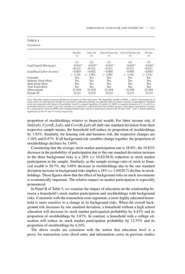
proportion of stockholdings relative to financial wealth. For labor income risk, ifStd(Lab), Corr(Rs,Lab), and Corr(Rf,Lab) all shift one standard deviation from theirrespective sample means, the household will reduce its proportion of stockholdingsby 1.92%. Similarly, for housing risk and business risk, the respective changes are1.16% and 0.47%. If all background risk variables change together, the proportion ofstockholdings declines by 3.69%.
Considering that the average stock market participation rate is 38.8%, the 10.82%decrease in the probability of participation due to the one standard deviation increasein the three background risks is a 28% (= 10.82/38.8) reduction in stock marketparticipation in the sample. Similarly, as the sample average ratio of stock to finan-cial wealth is 20.7%, the 3.69% decrease in stockholdings due to the one standarddeviation increase in background risks implies a 18% (= 3.69/20.7) decline in stock-holdings. These figures show that the effect of background risks on stock investmentsis economically important. The relative impact on market participation is especiallypronounced.
In Panel B of Table 5, we examine the impact of education on the relationship be-tween a household’s stock market participation and stockholdings with backgroundrisks. Consistent with the transaction costs argument, a more highly educated house-hold is more sensitive to a change in its background risks. When the overall back-ground risk increases by one standard deviation, a household without a high schooleducation will decrease its stock market participation probability by 8.43% and itsproportion of stockholdings by 3.07%. In contrast, a household with a college ed-ucation will reduce its stock market participation probability by 12.53% and itsproportion of stockholdings by 4.24%.
The above results are consistent with the notion that education level is aproxy for transaction costs (fixed entry and information costs) in previous studies
1712 : MONEY, CREDIT AND BANKING
TAB
LE
5
MA
RG
INA
LE
FFE
CT
SO
FB
AC
KG
RO
UN
DR
ISK
SFA
CT
OR
S
Stoc
km
arke
tpar
ticip
atio
n(i
npe
rcen
t)St
ockh
oldi
ngre
lativ
eto
finan
cial
wea
lth(i
npe
rcen
t)
Ats
ampl
eIn
crea
seon
eA
tsam
ple
Incr
ease
one
mea
nsst
d.de
v.C
hang
em
eans
std.
dev.
Cha
nge
(1)
(2)
(3)
(4)
(5)
(6)
Pane
lA.M
argi
nale
ffec
tof
thre
ety
pes
ofba
ckgr
ound
risk
fact
ors
Lab
orin
com
eri
skSt
d(L
ab),
Cor
r(R
s,Lab
),C
orr(
Rf,L
ab)
34.2
127
.95
−6.2
637
.14
35.2
3−1
.92
Hou
sing
risk
Std(
Hou
se),
Cor
r(R
s,Hou
se),
Cor
r(R
f,Hou
se)
34.2
130
.80
−3.4
137
.14
35.9
9−1
.16
Bus
ines
sin
com
eri
skSt
d(B
us),
Cor
r(R
s,Bus
),C
orr(
Rf,B
us)
34.2
132
.58
−1.6
337
.14
36.6
8−0
.47
All
risk
s12
vari
able
s34
.21
23.3
9−1
0.82
37.1
433
.45
−3.6
9
Pane
lB.M
argi
nale
ffec
tof
12ba
ckgr
ound
risk
fact
ors
for
diff
eren
tedu
catio
ngr
oups
No
high
scho
ol24
.26
15.8
3−8
.43
32.7
129
.63
−3.0
7H
igh
scho
ol31
.78
21.4
7−1
0.31
36.5
132
.91
−3.6
0C
olle
ge44
.85
32.3
2−1
2.53
41.0
936
.85
−4.2
4
NO
TE:P
anel
Are
port
sth
eim
pact
sof
back
grou
ndri
sks
onst
ock
mar
ketp
artic
ipat
ion
and
stoc
khol
ding
for
the
base
line
mod
el,w
hile
Pane
lBre
port
sth
ese
impa
cts
for
diff
eren
tedu
catio
ngr
oups
.In
each
pane
l,co
lum
ns(1
)–(3
)rep
ortm
argi
nale
ffec
tsof
vari
ous
back
grou
ndri
sks
onst
ock
mar
ketp
artic
ipat
ion.
Usi
nges
timat
edco
effic
ient
sfr
omth
eL
ogit
regr
essi
on(T
able
3,co
lum
n(5
)),w
eas
sum
eth
atth
eco
rres
pond
ing
risk
fact
ors
chan
geon
est
anda
rdde
viat
ion
from
thei
rsa
mpl
em
eans
whi
leho
ldin
gal
lot
her
vari
able
sat
thei
rsa
mpl
eav
erag
es.C
olum
ns(4
)–(6
)re
port
the
mar
gina
lef
fect
sof
back
grou
ndri
sks
onst
ockh
oldi
ngs
rela
tive
tofin
anci
alw
ealth
cond
ition
alon
part
icip
atio
n.U
sing
estim
ated
coef
ficie
nts
from
the
Tobi
tre
gres
sion
(Tab
le4,
colu
mn
(5))
,we
assu
me
that
the
corr
espo
ndin
gri
skfa
ctor
sch
ange
one
stan
dard
devi
atio
nfr
omth
eir
sam
ple
mea
nsw
hile
hold
ing
allo
ther
vari
able
sat
thei
rsa
mpl
eav
erag
es.S
td(X
)is
stan
dard
devi
atio
nof
X;C
orr(
X,Y
)is
corr
elat
ion
betw
een
Xan
dY
;Lab
,Hou
,and
Bus
are,
resp
ectiv
ely,
annu
algr
owth
rate
sof
labo
rin
com
e,ho
me
equi
ty,a
ndbu
sine
ssin
com
e;R
sis
annu
algr
oss
retu
rnof
CR
SPva
lue-
wei
ghte
dm
arke
tind
ex;a
ndR
fis
annu
algr
oss
retu
rnof
the
30-d
ayT
-bill
.
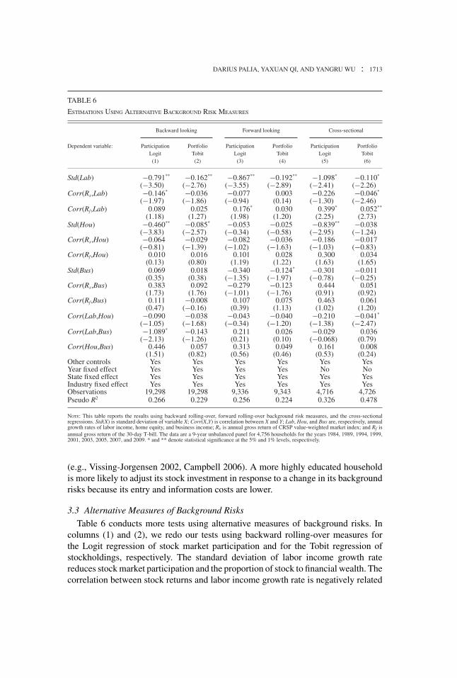
DARIUS PALIA, YAXUAN QI, AND YANGRU WU : 1713
TABLE 6
ESTIMATIONS USING ALTERNATIVE BACKGROUND RISK MEASURES
Backward looking Forward looking Cross-sectional
Dependent variable: Participation Portfolio Participation Portfolio Participation PortfolioLogit Tobit Logit Tobit Logit Tobit(1) (2) (3) (4) (5) (6)
Std(Lab) −0.791** −0.162** −0.867** −0.192** −1.098* −0.110*
(−3.50) (−2.76) (−3.55) (−2.89) (−2.41) (−2.26)Corr(Rs,Lab) −0.146* −0.036 −0.077 0.003 −0.226 −0.046*
(−1.97) (−1.86) (−0.94) (0.14) (−1.30) (−2.46)Corr(Rf,Lab) 0.089 0.025 0.176* 0.030 0.399* 0.052**
(1.18) (1.27) (1.98) (1.20) (2.25) (2.73)Std(Hou) −0.460** −0.085* −0.053 −0.025 −0.839** −0.038
(−3.83) (−2.57) (−0.34) (−0.58) (−2.95) (−1.24)Corr(Rs,Hou) −0.064 −0.029 −0.082 −0.036 −0.186 −0.017
(−0.81) (−1.39) (−1.02) (−1.63) (−1.03) (−0.83)Corr(Rf,Hou) 0.010 0.016 0.101 0.028 0.300 0.034
(0.13) (0.80) (1.19) (1.22) (1.63) (1.65)Std(Bus) 0.069 0.018 −0.340 −0.124* −0.301 −0.011
(0.35) (0.38) (−1.35) (−1.97) (−0.78) (−0.25)Corr(Rs,Bus) 0.383 0.092 −0.279 −0.123 0.444 0.051
(1.73) (1.76) (−1.01) (−1.76) (0.91) (0.92)Corr(Rf,Bus) 0.111 −0.008 0.107 0.075 0.463 0.061
(0.47) (−0.16) (0.39) (1.13) (1.02) (1.20)Corr(Lab,Hou) −0.090 −0.038 −0.043 −0.040 −0.210 −0.041*
(−1.05) (−1.68) (−0.34) (−1.20) (−1.38) (−2.47)Corr(Lab,Bus) −1.089* −0.143 0.211 0.026 −0.029 0.036
(−2.13) (−1.26) (0.21) (0.10) (−0.068) (0.79)Corr(Hou,Bus) 0.446 0.057 0.313 0.049 0.161 0.008
(1.51) (0.82) (0.56) (0.46) (0.53) (0.24)Other controls Yes Yes Yes Yes Yes YesYear fixed effect Yes Yes Yes Yes No NoState fixed effect Yes Yes Yes Yes Yes YesIndustry fixed effect Yes Yes Yes Yes Yes YesObservations 19,298 19,298 9,336 9,343 4,716 4,726Pseudo R2 0.266 0.229 0.256 0.224 0.326 0.478
NOTE: This table reports the results using backward rolling-over, forward rolling-over background risk measures, and the cross-sectionalregressions. Std(X) is standard deviation of variable X; Corr(X,Y) is correlation between X and Y; Lab, Hou, and Bus are, respectively, annualgrowth rates of labor income, home equity, and business income; Rs is annual gross return of CRSP value-weighted market index; and Rf isannual gross return of the 30-day T-bill. The data are a 9-year unbalanced panel for 4,756 households for the years 1984, 1989, 1994, 1999,2001, 2003, 2005, 2007, and 2009. * and ** denote statistical significance at the 5% and 1% levels, respectively.
(e.g., Vissing-Jorgensen 2002, Campbell 2006). A more highly educated householdis more likely to adjust its stock investment in response to a change in its backgroundrisks because its entry and information costs are lower.
3.3 Alternative Measures of Background Risks
Table 6 conducts more tests using alternative measures of background risks. Incolumns (1) and (2), we redo our tests using backward rolling-over measures forthe Logit regression of stock market participation and for the Tobit regression ofstockholdings, respectively. The standard deviation of labor income growth ratereduces stock market participation and the proportion of stock to financial wealth. Thecorrelation between stock returns and labor income growth rate is negatively related

1714 : MONEY, CREDIT AND BANKING
to stock market participation and stockholdings, whereas the correlation between therisk-free rate and labor income growth is not significant. Housing risk is also importantin that the standard deviation of home equity growth significantly decreases stockmarket participation and stockholdings.
In columns (3) and (4), we redo our regressions using forward rolling-over mea-sures. For the stock market participation regression, the only two significant variablesare the standard deviation of labor income growth and the correlation between therisk-free rate and labor income growth. As for the stockholdings regression, we findthat two variables are statistically significant: the standard deviation of labor incomegrowth and standard deviation of business income growth.
In columns (5) and (6), we consider cross-sectional regressions. For the Logitregression in column (5), we sum the stock market participation dummy variableover years and divide this variable by the number of years when the householdappears in the sample. We classify a household as a stock market participant if itholds stocks in more than half of the time in the sample period. As for the Tobitregression in column (6), we regress the time average of stockholdings relative towealth on the time-invariant background risk factors and the time-averages of othercontrol variables.
As shown in column (5), the standard deviation of labor income growth sig-nificantly negatively impacts stock market participation, while the correlation oflabor income and the risk-free rate significantly encourages stock market participa-tion. The standard deviation of home equity growth rate also significantly decreasesstock market participation. Column (6) confirms the importance of labor income riskvariables in affecting a household’s portfolio choice. Furthermore, the correlation oflabor income and housing significantly decreases stockholdings.
In general, these tests using alterative measures of background risks yield weakerresults than the baseline cases reported in Tables 3 and 4, primarily due to the lessprecise estimates of background risk measures with fewer observations. However,some observations can be made. Labor income risk is the most important one. Thestandard deviation of labor income growth is significant in all regressions. The corre-lation between stock returns and labor income growth carries the expected negativesign and is significant in two of six regressions. The correlation between labor incomegrowth and the risk-free rate also has the expected positive sign in all regressions andis significant in three of six regressions. We therefore conclude that the volatility oflabor income is an important factor that significantly affects household stock marketparticipation and stockholdings. Moreover, households with risky (risk-free) laborincome are less (more) likely to participation in stock market and to hold less (more)risky assets in their portfolios.
The standard deviation of home equity growth rate carries the expected negativesign and is significant in three of six regressions, suggesting that the volatility of homeequity growth discourages stock market participation and stockholdings. However,results based on the correlation between home equity growth and financial assetreturns are in general insignificant. Furthermore, we find that the business incomerisk factors that are estimated with the least observations yield the most mixed results.
DARIUS PALIA, YAXUAN QI, AND YANGRU WU : 1715
3.4 Alternative Estimation Methods of Portfolio Choice
In Table 7, we compare the estimation results using the Tobit model, the Heckmanselection model, and OLS regressions for the truncated sample consisting of onlystockholders. We use two additional measures of the stock to wealth ratio: the ratioof stock to total wealth without home equity, denoted as PflStk_2, and the ratio ofstock to total wealth including home equity, denoted as PflStk_3.
Column (1) in Table 7 is a repeat of the Tobit model in column (5) of Table 4where the stock-to-wealth ratio is defined as a ratio of stock to total financial wealth(Pflstk_1). Columns (2) and (3) in Table 7 are Tobit models using alternative measuresof the stock to wealth ratio (Pflstk_2 and Pflstick_3). The results are very similar toprevious findings in Table 4.
The next three columns in Table 7 present OLS regressions. In the OLS regressions,Std(Lab) is not significant. As for the correlation terms, Corr(Rs,Lab) is negativelyrelated to stockholdings, and Corr(Rf,Lab) is positively related to stockholdings, con-sistent with findings in the Tobit regressions. Among the three housing risk variables,only Corr(Rs,Hou) is significantly negatively related to PtfStk_1 and PtfStk_2. As forthe business income risk, Std(Bus) has the expected negative sign, but it is statisticallysignificant only in the PtfStk_3 regression. Overall, the OLS regression results arequalitatively consistent with those using the Tobit model, but are statistically lesssignificant.
As for Heckman selection model, we find that lagged stockholding has strongexplanatory power for current stockholding. We report the Lambda, which would be0 if stockholders were a random subgroup of the population. We reject the hypothesisthat stockholders are random subgroup in favor of the alternative that stockholdersare a selected group. Labor income risk appears less important in the Heckmanmodel. In contrast, housing risk is relatively more important after controlling forsample selection. Corr(Rs,Hou) is significantly negatively related to stockholdingsin the PtfStk_1 regression, and Corr(Rf,Hou) is significantly positively related tostockholdings in the PtfStk_1 and PtfStk_3 regressions. As for business risk, consistentwith previous findings, only Std(Bus) is important. In summary, the estimation of theHeckman model is in general consistent with the Tobit model, but is statistically lesssignificant.
Overall, while we find that the results using OLS and Heckman models are weakerthan those using the Tobit model, they still indicate the importance of backgroundrisks. Therefore, the significance of background risks in portfolio holdings is notprimarily driven by the difference between stockholders and nonstockholders. Wealso note that the impact of background risks is relatively more important for stockparticipation than for stockholdings.
3.5 Other Robustness Checks
We conduct additional robustness checks. We first consider alternative ways toconstruct background risk factors. Specifically, we examine separate effects based onwhether the correlation of a background risk factor with stock returns is positive or

1716 : MONEY, CREDIT AND BANKING
TAB
LE
7
ALT
ER
NA
TIV
EE
STIM
AT
ION
SO
FPO
RT
FOL
IOH
OL
DIN
GS
Tobi
tO
LS
Hec
kman
Dep
ende
ntva
riab
le:
PflS
tk_1
PflS
tk_2
PflS
tk_3
PflS
tk_1
PflS
tk_2
PflS
tk_3
PflS
tk_1
PflS
tk_2
PflS
tk_3
(1)
(2)
(3)
(4)
(5)
(6)
(7)
(8)
(9)
Std(
Lab
)−0
.232
**−0
.230
**−0
.158
**0.
024
−0.0
28−0
.022
0.03
−0.0
25−0
.043
(−3.
12)
(−3.
85)
(−3.
94)
(0.6
8)(−
0.87
)(−
0.96
)(0
.79)
(−0.
69)
(−1.
74)
Cor
r(R
s,Lab
)−0
.077
**−0
.064
**−0
.039
*−0
.026
*−0
.024
*−0
.014
−0.0
01−0
.01
0.00
3(−
2.71
)(−
2.81
)(−
2.52
)(−
1.97
)(−
2.07
)(−
1.69
)(−
0.04
5)(−
0.68
)(0
.32)
Cor
r(R
f,Lab
)0.
074*
0.07
2**0.
047**
0.02
20.
032*
0.02
2*−0
.004
0.02
30.
006
(2.4
9)(2
.96)
(2.8
4)(1
.55)
(2.4
8)(2
.37)
(−0.
28)
(1.5
4)(0
.54)
Std(
Hou
)−0
.090
*−0
.097
**−0
.037
0.00
4−0
.028
0.01
10.
026
−0.0
130.
027
(−2.
11)
(−2.
77)
(−1.
61)
(0.1
8)(−
1.30
)(0
.75)
(1.1
7)(−
0.63
)(1
.89)
Cor
r(R
s,Hou
)−0
.031
−0.0
27−0
.015
−0.0
33*
−0.0
28*
−0.0
15−0
.035
*−0
.029
−0.0
17(−
0.99
)(−
1.05
)(−
0.93
)(−
2.11
)(−
1.88
)(−
1.53
)(−
2.20
)(−
1.93
)(−
1.67
)C
orr(
Rf,H
ou)
0.05
40.
041
0.02
90.
025
0.02
0.01
60.
032*
0.02
10.
022*
(1.7
8)(1
.63)
(1.8
0)(1
.61)
(1.3
7)(1
.63)
(2.0
2)(1
.38)
(2.1
3)St
d(B
us)
−0.0
75−0
.076
*−0
.058
*−0
.024
−0.0
35−0
.032
*−0
.019
−0.0
45*
−0.0
32*
(−1.
67)
(−2.
06)
(−2.
33)
(−1.
01)
(−1.
54)
(−2.
04)
(−0.
78)
(−1.
96)
(−2.
07)
Cor
r(R
s,Bus
)0.
022
0.01
6−0
.004
0.02
20.
013
−0.0
060.
009
0.02
50.
001
(0.3
7)(0
.34)
(−0.
13)
(0.6
4)(0
.40)
(−0.
28)
(0.2
7)(0
.82)
(0.0
42)
Cor
r(R
f,Bus
)0.
053
0.02
30.
030.
039
0.01
70.
024
0.02
20.
007
0.01
7(0
.92)
(0.4
9)(0
.95)
(1.2
3)(0
.60)
(1.2
3)(0
.73)
(0.2
6)(0
.86)
Cor
r(L
ab,H
ou)
−0.0
56*
−0.0
45*
−0.0
25−0
.014
−0.0
12−0
.004
−0.0
14−0
.021
−0.0
04(−
2.28
)(−
2.23
)(−
1.91
)(−
1.10
)(−
1.10
)(−
0.48
)(−
1.08
)(−
1.73
)(−
0.52
)C
orr(
Lab
,Bus
)0.
017
−0.0
02−0
.009
−0.0
12−0
.022
−0.0
16−0
.015
−0.0
16−0
.024
(0.2
5)(−
0.02
8)(−
0.24
)(−
0.36
)(−
0.68
)(−
0.71
)(−
0.55
)(−
0.61
)(−
1.34
)C
orr(
Hou
,Bus
)0.
016
0.01
90.
016
0.00
60.
014
0.01
1−0
.008
0.00
0−0
.001
(0.3
5)(0
.48)
(0.6
2)(0
.24)
(0.6
1)(0
.69)
(−0.
35)
(−0.
0083
)(−
0.06
7)L
agge
dP
tfSt
k0.
321**
0.36
7**0.
363**
(26.
0)(2
9.7)
(31.
3)L
amda
0.17
0.08
0.06
(11.
49)
(6.5
9)(7
.38)
Oth
erco
ntro
lsY
esY
esY
esY
esY
esY
esY
esY
esY
esY
ear
fixed
effe
ctY
esY
esY
esY
esY
esY
esY
esY
esY
esSt
ate
fixed
effe
ctY
esY
esY
esY
esY
esY
esY
esY
esY
esIn
dust
ryfix
edef
fect
Yes
Yes
Yes
Yes
Yes
Yes
Yes
Yes
Yes
Obs
erva
tions
21,9
3821
,938
21,9
3813
,976
13,9
7613
,976
17,7
7117
,771
17,7
71R
20.
230.
280.
380.
250.
250.
26
NO
TE:O
LS
regr
essi
onis
appl
ied
toa
subs
ampl
eof
hous
ehol
dsth
atha
vepa
rtic
ipat
edin
stoc
km
arke
tin
curr
enta
nd/o
rpri
orye
ars.
Inth
eH
eckm
anse
lect
ion
mod
el,w
hich
ises
timat
edus
ing
atw
o-st
age
met
hod,
we
incl
ude
lagg
edpa
rtic
ipat
ion
and
stoc
khol
ding
inth
epa
rtic
ipat
ion
and
port
folio
hold
ing
equa
tions
,res
pect
ivel
y.O
nly
the
seco
nd-s
tage
resu
ltsar
ere
port
ed.P
flStk
_1(P
flStk
_2,
PflS
tk_3
)st
ands
for
the
ratio
ofst
ockh
oldi
ngs
tofin
anci
alw
ealth
(tot
alw
ealth
excl
udin
gho
me
equi
ty,t
otal
wea
lthin
clud
ing
hom
eeq
uity
).St
d(X
)is
stan
dard
devi
atio
nof
vari
able
X;C
orr(
X,Y
)is
corr
elat
ion
betw
een
Xan
dY
;Lab
,Hou
,and
Bus
are,
resp
ectiv
ely,
annu
algr
owth
rate
sof
labo
rin
com
e,ho
me
equi
ty,a
ndbu
sine
ssin
com
e;R
sis
annu
algr
oss
retu
rnof
CR
SPva
lue-
wei
ghte
dm
arke
tind
ex;a
ndR
fis
annu
algr
oss
retu
rnof
the
30-d
ayT
-bill
.The
data
are
a9-
year
unba
lanc
edpa
nel
for
4,75
6ho
useh
olds
for
the
year
s19
84,1
989,
1994
,199
9,20
01,2
003,
2005
,200
7,an
d20
09.*
and
**de
note
stat
istic
alsi
gnifi
canc
eat
the
5%an
d1%
leve
ls,r
espe
ctiv
ely.
DARIUS PALIA, YAXUAN QI, AND YANGRU WU : 1717
negative; that is, the explanatory variables are (standard deviation × positive correla-tion) and (standard deviation × negative correlation). This specification allows us tofurther examine the hedging motive hypothesis. We find that the standard deviationof labor income interacting with a positive correlation, (Std(Lab) × Corr(Rs,Lab)+),is significantly negatively related to stock participation while the impact of the stan-dard deviation of labor income interacting with a negative correlation, (Std(Lab) ×Corr(Rs,Lab)−), is not significant. We also consider the correlations of excess stockreturns with the background risk variables, that is, (Corr(Rs − Rf,X)), where X is laborincome, home equity, or business income growth. The results using this alternativemeasures are consistent with our baseline regressions.
It is known that estimation of Tobit models can be sensitive to the underlyingassumptions about the error terms, and indeed maximum likelihood estimation can beinconsistent under heteroskedasticity or nonnormality (Amemiya 1985, pp. 378–81).We adopt three alternative specifications, which assume the residual standard errorsto be an exponential function of total wealth, or total income, or both, respectively.These experiments produce similar results.
Since the PSID changes the definition of stockholdings in 1997. As a robustnesscheck, we redo our baseline model by excluding observations for the years 1997and 1999 and the qualitative results stay the same. Our baseline study uses Filter2to estimate background risk variables. As a robustness test, we apply Filter3 andFilter5 to filter our data and obtain similar results. We also redo our regressionsusing three subsamples of households that have labor income, housing, and businessincome, respectively. The results in these experiments confirm our previous findings.Following Angerer and Lam (2009), we decompose the background risks to expected(predictable) and unexpected (unpredictable) components. Specifically, we regress thegrowth rate of labor income (home equity, business income) on the lagged dependentvariable and other explanatory variables, including the age of the head of householdand its squared term, the age of wife and its squared term, and the two educationvariables. The regression residuals are regarded as the unexpected component andthe fitted values of the regression are considered as the expected component of thebackground risk. We find that the expected labor income risk is positively relatedto stock market participation and stockholdings while the unexpected labor incomerisk is negatively related to stock market participation and stockholdings, consistentwith Angerer and Lam (2009). We obtain a similar result for housing income risk.In contrast, the expected business income risk decreases stock investment while theunexpected business risk increases stock investment. Results obtained in this sectionare not reported to save space but are available upon request.
4. CONCLUSIONS
Using a sample of U.S. households with household-level background risk mea-sures, we examine the empirical importance of background risks for a household’s
1718 : MONEY, CREDIT AND BANKING
investment decision. We document significant heterogeneity of background risk ex-posures across households. The low stock market participation rates and the largevariation of stockholdings are significantly related to the heterogeneity in backgroundrisks across households. Specifically, a household is more (less) likely to enter thestock market and invests a larger (smaller) fraction of wealth in stocks if its nonfinan-cial income (e.g., labor income) is less (more) volatile, is less (more) highly correlatedwith stock returns, or is more (less) highly correlated with the risk-free rate. In termsof relative importance, we find that labor income risk is the most important, followedby housing risk, while the impact of business income risk is limited.
LITERATURE CITED
Amemiya, Takeshi. (1985) Advanced Econometrics. Cambridge, MA: Harvard UniversityPress.
Angerer, Xiaohong, and Pok-Sang Lam. (2009) “Income Risk and Portfolio Choice: AnEmpirical Study.” Journal of Finance, 64, 1037–55.
Ball, Steffan. (2008) “Stock Market Participation, Portfolio Choice and Pension over the LifeCycle.” Finance and Economics Discussion Series 2008-64, Board of Governors of theFederal Reserve System, Washington.
Benzoni, Luca, Pierre Collin-Dufresne, and Robert S. Goldstein. (2007) “Portfolio Choice overthe Life-Cycle When the Stock and Labor Markets Are Cointegrated.” Journal of Finance,62, 2123–67.
Bodie, Zvi, Robert Merton, and William F. Samuelson. (1992) “Labor Supply Flexibility andPortfolio Choice in a Life Cycle Model.” Journal of Economic Dynamics and Control, 16,427–49.
Campbell, John Y. (2006) “Household Finance.” Journal of Finance, 61, 1553–1604.
Chen, Xuanjuan, Tong Yao, and Tong Yu. (2007) “How Does Background Risks Affect Invest-ment Risk-Taking? Evidence from Insurers’ Corporate Bond Portfolios.” Mimeo, Universityof Iowa.
Cocco, Joao F. (2005) “Portfolio Choice in the Presence of Housing.” Review of FinancialStudies, 18, 535–67.
Cocco, Joao F., Francisco J. Gomes, and Pascal J. Maenhout. (2005) “Consumption andPortfolio Choice over the Life Cycle.” Review of Financial Studies, 18, 491–532.
Cochrane, John. (2006) Financial Markets and the Real Economy. International Library ofCritical Writings in Financial Economics, Vol. 18. London: Edward Elgar.
Cochrane, John. (2008) “A Mean-Variance Benchmark for Intertemporal Portfolio Choice.”Mimeo, University of Chicago.
Constantinides, George M., and Darrell Duffie. (1996) “Asset Pricing with HeterogeneousConsumers.” Journal of Political Economy, 104, 219–40.
Davis, Steven J., and Paul Willen. (2002) “Income Shock, Asset Returns and Portfolio Choice.”In Innovations in Financing Retirement, edited by Zvi Bodie, Olivia S. Mitchell, BrettHammond, and Stephen Zeldes, pp. 20–49. Philadelphia: University of Pennsylvania Press.
Dimmock, Stephen G. (2012) “Background Risk and University Endowment Funds.” Reviewof Economics and Statistics, 94, 789–99.
DARIUS PALIA, YAXUAN QI, AND YANGRU WU : 1719
Duffie, Darrell, Wendell Fleming, H. Mete Soner, and Thaleia Zariphopoulou. (1997) “Hedgingin Incomplete Markets with HARA Utility.” Journal of Economic Dynamics and Control,21, 753–82.
Eiling, Esther. (2013) “Industry Specific Human Capital, Idiosyncratic Risk and the Cross-Section of Expected Stock Returns.” Journal of Finance, 68, 43–84.
Flavin, Marjorie, and Takashi Yamashita. (2002) “Owner-Occupied Housing and Compositionof the Household Portfolio.” American Economic Review, 92, 345–62.
Goetzmann, William N., and Eduardas Valaitis. (2006) “Simulating Real Estate in the Invest-ment Portfolio: Model Uncertainty and Inflation Hedging.” Mimeo, Yale University.
Gomes, Fransico, and Allexander Michaelides. (2005) “Optimal Life-Cycle Asset Allocation:Understanding the Empirical Evidence.” Journal of Finance, 55, 869–904.
Guiso, Luigi, Tullio Jappell, and Daniele Terlizzese. (1996) “Income Risk, Borrowing Con-straints, and Portfolio Choice.” American Economic Review, 86, 158–72.
Guo, Hui. (2004) “Limited Stock Market Participation and Asset Prices in a Dynamic Econ-omy.” Journal of Financial and Quantitative Analysis, 39, 495–516.
Haliassos, Michael, and Carol C. Bertaut. (1995) “Why Do So Few Hold Stocks?” EconomicJournal, 105, 1110–29.
Haliassos, Michael, and Alexander Michaelides. (2003) “Portfolio Choice and Liquidity Con-straints.” International Economic Review, 44, 143–77.
Heaton, John, and Deborah Lucas. (1996) “Evaluating the Effects of Incomplete Markets onRisk Sharing and Asset Pricing.” Journal of Political Economy, 104, 443–87.
Heaton, John, and Deborah Lucas. (1997) “Market Frictions, Savings Behavior, and PortfolioChoice.” Macroeconomic Dynamics, 1, 76–101.
Heaton, John, and Deborah Lucas. (2000a) “Portfolio Choice in the Presence of BackgroundRisk.” Economic Journal, 110, 1–26.
Heaton, John, and Deborah Lucas. (2000b) “Portfolio Choice and Asset Prices: The Importanceof Entrepreneurial Risk.” Journal of Finance, 55, 1163–98.
Hochguertel, Stefan. (2002) “Precautionary Motives and Portfolio Decisions.” Journal ofApplied Econometrics, 18, 61–77.
Hong, Harrison, Jeffery D. Kubik, and Jeremy C. Stein. (2004) “Social Interaction and Stock-Market Participation.” Journal of Finance, 59, 137–63.
Jagannathan, Ravi, and Narayana Kocherlakota. (1996) “Why Should Older People Invest Lessin Stocks Than Younger People?” Federal Reserve Bank of Minneapolis Quarterly Review,20, 11–23.
Jagannathan, Ravi, and Zhenyu Wang. (1996) “The Conditional CAPM and the Cross-Sectionof Expected Returns.” Journal of Finance, 51, 3–53.
Krueger, Dirk, and Hanno Lustig. (2010) “When Is Market Incompleteness Irrelevant for thePrice of Aggregate Risk (and When Is It Not)?” Journal of Economic Theory, 145, 1–41.
Mankiw, N. Gregory, and Stephen P. Zeldes. (1991) “The Consumption of Stockholders andNon-Stockholders.” Journal of Financial Economics, 29, 97–112.
Massa, Massimo, and Andrei Simonov. (2006) “Hedging, Familiarity and Portfolio Choice.”Review of Financial Studies, 19, 633–85.
Orosel, Gerhard O. (1998) “Participation Costs, Trend Chasing, and Volatility of Stock Prices.”Review of Financial Studies, 11, 521–57.
1720 : MONEY, CREDIT AND BANKING
Petersen, Mitchell A. (2009) “Estimating Standard Errors in Finance Panel Data Sets: Com-paring Approaches.” Review of Financial Studies, 22, 435–80.
Roussanov, Nikolai. (2004) “Human Capital Investment and Portfolio Choice over the Life-Cycle.” Mimeo, University of Chicago.
Storesletten, Kjetil, Chris I. Telmer, and Amir Yaron. (2004) “Cyclical Dynamics in Idiosyn-cratic Labor-Market Risk.” Journal of Political Economy, 112, 695–717.
Viceira, Luis M. (2001) “Optimal Portfolio Choice for Long-Horizon Investors with Nontrad-able Labor Income.” Journal of Finance, 56, 433–70.
Vissing-Jorgensen, Annette. (2002) “Towards an Explanation of Household Portfolio ChoiceHeterogeneity: Nonfinancial Income and Participation Cost Structures.” NBER WorkingPaper No. 8884.
Yao, Rui, and Harold Zhang. (2005) “Optimal Consumption and Portfolio Choice with RiskyHousing and Borrowing Constraints.” Review of Financial Studies, 18, 197–239.