Water quality in four regions of the Maryland coastal bays: assessing nitrogen source in relation to...

Water quality in four regions of the Maryland Coastal Bays:

assessing nitrogen source in relation to rainfall and brown tide.

Data Report

Financial assistance provided by Maryland Coastal Bays Program

Ben Fertig1

Tim Carruthers1

Cathy Wazniak2

Brian Sturgis3

Matt Hall2

Adrian Jones

William Dennison1

1Integration and Application Network, University of Maryland Center for Environmental Science

2Maryland Department of Natural Resources 2Assateague National Seashore, National Parks Service

November 2006

2

Conclusions

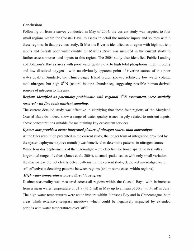
Following on from a survey conducted in May of 2004, the current study was targeted to four

small regions within the Coastal Bays, to assess in detail the nutrient inputs and sources within

these regions. In that previous study, St Martins River is identified as a region with high nutrient

inputs and overall poor water quality. St Martins River was included in the current study to

further assess sources and inputs to this region. The 2004 study also identified Public Landing

and Johnson’s Bay as areas with poor water quality due to high total phosphorus, high turbidity

and low dissolved oxygen – with no obviously apparent point of riverine source of this poor

water quality. Similarly, the Chincoteague Island region showed relatively low water column

total nitrogen, but high δ15N (natural isotope abundance), suggesting possible human-derived

sources of nitrogen to this area.

Regions identified as potentially problematic with regional δ15N assessment, were spatially

resolved with fine scale nutrient sampling.

The current detailed study was effective in clarifying that these four regions of the Maryland

Coastal Bays do indeed show a range of water quality issues largely related to nutrient inputs,

above concentrations suitable for maintaining key ecosystem services.

Oysters may provide a better integrated picture of nitrogen source than macroalgae

At the finer resolution presented in the current study, the longer term of integration provided by

the oyster deployment (three months) was beneficial to determine patterns in nitrogen source.

While four day deployments of the macroalgae were effective for broad spatial scales with a

larger total range of values (Jones et al., 2004), at small spatial scales with only small variation

the macroalgae did not clearly detect patterns. In the current study, deployed macroalgae were

still effective at detecting patterns between regions (and in some cases within regions).

High water temperatures pose a threat to seagrass

Distinct seasonality was measured across all regions within the Coastal Bays, with in increase

from a mean water temperature of 21.7 (±1.6, sd) in May up to a mean of 30.3 (±1.4, sd) in July.

The high water temperatures were acute inshore within Johnsons Bay and in Chincoteague, both

areas whith extensive seagrass meadows which could be negatively impacted by extended

periods with water temperatures over 30°C.

3

Johnsons Bay shows evidence of local freshwater and nutrient inputs inshore

After rain in July, a clear signal of lower salinity water was observed inshore in Johnsons Bay,

suggesting groundwater or overland flow to this area. This input of water was reflected in higher

water column total nitrogen as well as elevated δ15N in oyster tissue in the southern region of

Johnsons Bay.

Public Landing shows evidence of local inputs of nitrogen and phosphorus

Higher water column total nitrogen and elevated δ15N in Oyster tissue inshore and in the

northern region of Public Landing suggests that there is a local source of this nitrogen,

contributing to the poor water quality in this region of the Coastal Bays.

St Martins (a mini estuary) shows high total nutrient inputs and a flushing gradient.

The only possible local or point source of nutrients to St Martins River was near to Shell Gut

Point, but in general, the large diffuse load coming from upstream overwhelms any smaller scale

inputs.

Complex waterflows from the inlets around Chincoteague Island influence sources of

nitrogen identified with macroalgal and oyster bioindicators.

In the northern, central and southern regions of the Chincoteague Island sampling region

macroalgae and oyster bioindicators revealed a complex pattern of highly processed nitrogen,

consistent with local but low concentration wastewater inflows.

4

Figure 1: Water Quality Index before and after a rain event for four regions within the Maryland Coastal Bays.

5

Table of Contents

Conclusions ..................................................................................................................................................................2 Regions identified as potentially problematic with regional δ15N assessment, were spatially resolved with fine scale nutrient sampling............................................................................................................................................2 Oysters may provide a better integrated picture of nitrogen source than macroalgae ..........................................2 High water temperatures pose a threat to seagrass ................................................................................................2 Johnsons Bay shows evidence of local freshwater and nutrient inputs inshore....................................................3 Public Landing shows evidence of local inputs of nitrogen and phosphorus........................................................3 St Martins (a mini estuary) shows high total nutrient inputs and a flushing gradient. ........................................3 Complex waterflows from the inlets around Chincoteague Island influence sources of nitrogen identified with macroalgal and oyster bioindicators. ......................................................................................................................3

Table of Contents.........................................................................................................................................................5

Table of Figures ...........................................................................................................................................................7

Table of Tables.............................................................................................................................................................8

Introduction .................................................................................................................................................................9

Introduction .................................................................................................................................................................9

Methodology...............................................................................................................................................................15 Study Region ...........................................................................................................................................................15 Water quality sampling...........................................................................................................................................16 Continuous monitoring ...........................................................................................................................................16 Water column nutrients...........................................................................................................................................16 Chlorophyll a ..........................................................................................................................................................16 Microbial Source Tracking .....................................................................................................................................16 Stable isotope technique .........................................................................................................................................16 Oyster stable isotope analysis.................................................................................................................................17 Calculating Water Quality Index (WQI).................................................................................................................18 Spatial analysis .......................................................................................................................................................18

Findings ......................................................................................................................................................................19 Continuous monitoring ...........................................................................................................................................19 Rainfall ...................................................................................................................................................................19 Salinity ....................................................................................................................................................................19 Temperature............................................................................................................................................................19 Dissolved Oxygen (DO) ..........................................................................................................................................19 Secchi depth ............................................................................................................................................................20

6

Microbial Source Tracking .....................................................................................................................................20 Water column total nitrogen ...................................................................................................................................28 Water column total phosphorus ..............................................................................................................................28 Water column chlorophyll a....................................................................................................................................28 Bio-indicator Gracilaria %N..................................................................................................................................32 Bio-indicator Gracilaria δ15N.................................................................................................................................32 Water quality index.................................................................................................................................................32 Bio-indicator Oyster δ15N muscle ...........................................................................................................................36 Bio-indicator Oyster δ15N gill.................................................................................................................................36 Bio-indicator Oyster δ15N mantle ...........................................................................................................................36

Acknowledgments......................................................................................................................................................38

Appendix 1 – Survey data May 2006 .......................................................................................................................42

Appendix 2 – Survey data July 2006........................................................................................................................45

7

Table of Figures

Figure 1: Water Quality Index before and after a rain event for four regions within the Maryland Coastal Bays............................................................................................................................ 4

Figure 2: Conceptual diagram showing the key physical and biological processes within the Maryland Coastal Bays (after Wazniak et al., 2004).............................................................. 9

Figure 3: Integrated water quality index from an intensive survey during 2004 (after Jones et al., 2004) ..................................................................................................................................... 10

Figure 4: Summary of linear (a) and quadratic (b) trends in total nitrogen, total phosphorus and Chlorphyll a over more than a decade in the southern Coastal Bays (after Wazniak et al., 2006) ..................................................................................................................................... 11

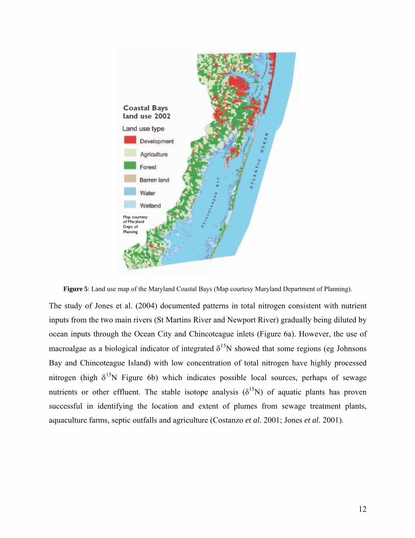
Figure 5: Land use map of the Maryland Coastal Bays (Map courtesy Maryland Department of Planning). .............................................................................................................................. 12

Figure 6: Comparison of total water column nitrogen (a) and δ15N (b) throughout the Maryland Coastal Bays in June 2004 (after Jones et al., 2004). ........................................................... 13

Figure 7: Map of the Maryland Coastal Bays showing the nitrogen isotope map from the 2004 survey which assisted in choosing the four regions sampled intensively in 2006: Public Landing (22 sites), Johnsons Bay (28 sites), St Martins River (21 sites) and Chincoteague Island (29 sites). The two continuous monitoring locations In Johnsons Bay and off Chincoteague Island are shown in white (Figure 7, Table 1). . ............................................ 15

Figure 8: Rainfall data for Assateague Island, Maryland ............................................................. 21 Figure 9: Data from Chincoteague Bay continuous monitoring site ............................................ 22 Figure 10: Data from Johnsons Bay continuous monitoring site.................................................. 23 Figure 11: Surface salinity ............................................................................................................ 24 Figure 12: Surface water temperature (°C)................................................................................... 25 Figure 13: Bottom dissolved oxygen (DO) (mgl-1)....................................................................... 26 Figure 14: Secchi depth (m).......................................................................................................... 27 Figure 15: Surface water total nitrogen (μM)............................................................................... 29 Figure 16: Surface water total phosphorus (μM).......................................................................... 30 Figure 17: Surface water Chlorophyll a (μg l-1) ........................................................................... 31 Figure 18: Deployed macroalgal tissue nitrogen, Gracilaria %N................................................ 33 Figure 19: Natural nitrogen isotope abundance, Gracilaria δ15N (ppt)........................................ 34 Figure 20: Integrated water quality index for all regions ............................................................. 35 Figure 21: Natural nitrogen isotope abundance, Crassostrea δ15N (ppt) ..................................... 37 Figure 22: Natural nitrogen isotope abundance, Crassostrea δ15N (ppt) ..................................... 38

8

Table of Tables

Table 1. Reporting region statistics detailing five regions with spatial predictions and three regions with linear predictions.............................................................................................. 15

Table 2. Table of management objectives for the Maryland Coastal Bays together with water quality indicators and reference values to determine the status of the objectives (Wazniak et al., in press)........................................................................................................................... 18

Table 3. Summary data from continuous monitoring sites. Data is medians (standard deviations) and is taken from 19th May – 1st June and 12th July – 20th July, 2006.................................. 21

Table 4. Surface salinity (mean±standard deviation) ................................................................... 24 Table 5. Surface water temperature (°C) (mean±standard deviation) .......................................... 25 Table 6: Dissolved Oxygen (mgl-1) (mean±standard deviation)................................................... 26 Table 7: Secchi depth (m) (mean±standard deviation) ................................................................. 27 Table 8: Surface water Phaeophytin pigments (μgl-1) (mean±standard deviation) ...................... 28 Table 9: Surface water total nitrogen (μM) (mean±standard deviation) ...................................... 29 Table 10: Surface water total phosphorus (μM) (mean±standard deviation) ............................... 30 Table 11: Surface water Chlorophyll a (μg l-1) (mean±standard deviation)................................. 31 Table 12: Deployed macroalgal tissue nitrogen, Gracilaria %N (mean±standard deviation) ..... 33 Table 13: Natural nitrogen isotope abundance, Gracilaria δ15N (mean±standard deviation)...... 34 Table 14: Integrated water quality index for all regions (mean±standard deviation)................... 35 Table 15: Natural nitrogen isotope abundance, Crassostrea δ15N (mean±standard deviation).... 37 Table 16: Natural nitrogen isotope abundance, Crassostrea δ15N (mean±standard deviation).... 38

9

Introduction

Maryland’s Coastal Bays are shallow water bodies (less than 3 m deep) that are uniform in depth

(Figure 2), occurring between a small coastal watershed (175 sq. miles) and sandy barrier

islands. Tidal exchange is limited, and restricted to the Ocean City and Chincoteague inlets.

River input is low and groundwater is an important source of freshwater inflow. The Coastal

Bays receive inputs from a range of nutrient sources, including wastewater treatment plants,

septic systems, agricultural inputs, stormwater and urban runoff. Comparatively, Maryland’s

Coastal Bays have fewer human impacts than Chesapeake Bay, but the limited water exchange

makes them more susceptible to nutrient increases.

Figure 2: Conceptual diagram showing the key physical and biological processes within the Maryland Coastal Bays (after Wazniak et al., 2004)

An intensive study of the water quality of the Maryland Coastal Bays, carried out during July

2004, concluded that while water quality within St Martins River and Newport River was poor,

there was also a large region of Chincoteague Bay with water quality below threshold values for

maintenance of ecosystem services such as seagrass and fisheries (Figure 3; Jones et al., 2004).

Low water quality resulted from high turbidity and water column total phosphorus as well as

regions of low dissolved oxygen (Jones et al., 2004).

10

Figure 3: Integrated water quality index from an intensive survey during 2004 (after Jones et al., 2004)

A recent summary of long term data within the southern Coastal Bays of Maryland came to a

similar conclusion, suggesting that even though water column nutrients and Chorophyll a are

lower than they have been in the past, these trends have not only flattened out but in many cases

are once again increasing (Figure 4). This raises the question of what is leading to these increases

in nutrients, as while the northern Coastal Bays are showing extensive development,

Chincoteague watershed is largely free from intensive urban development (Figure 5).

11

Figure 4: Summary of linear (a) and quadratic (b) trends in total nitrogen, total phosphorus and Chlorphyll a over more than a decade in the southern Coastal Bays (after Wazniak et al., 2006)

The slow flushing times (months) in the Coastal Bays result in a system where the water quality

is strongly impacted by land use. The northern sections of the Coastal Bays are more heavily

developed, particularly in the region of Ocean City, whereas the southern sections are

predominantly agriculture and forest (Figure 5).

Determining the impacts and extent of sewage and septic derived nitrogen in marine systems

with multiple inputs (both point and non-point source) is typically problematic, and it has been

shown that physical and chemical water quality monitoring techniques are unable to determine

the ecological impact of wastewater discharges. Biological indicators have long been used to

determine ecological impacts of point source discharges (Worf, 1980; Kramer, 1994). The key

feature of biological indicators is their ability to provide temporally and spatially integrated

insights into the biological impacts of changes in anthropogenic activity. Unlike traditional

chemical analyses of water column nutrients, these biological indicators measure the biologically

available nutrients therefore providing more ecologically meaningful information.

12

Figure 5: Land use map of the Maryland Coastal Bays (Map courtesy Maryland Department of Planning).

The study of Jones et al. (2004) documented patterns in total nitrogen consistent with nutrient

inputs from the two main rivers (St Martins River and Newport River) gradually being diluted by

ocean inputs through the Ocean City and Chincoteague inlets (Figure 6a). However, the use of

macroalgae as a biological indicator of integrated δ15N showed that some regions (eg Johnsons

Bay and Chincoteague Island) with low concentration of total nitrogen have highly processed

nitrogen (high δ15N Figure 6b) which indicates possible local sources, perhaps of sewage

nutrients or other effluent. The stable isotope analysis (δ15N) of aquatic plants has proven

successful in identifying the location and extent of plumes from sewage treatment plants,

aquaculture farms, septic outfalls and agriculture (Costanzo et al. 2001; Jones et al. 2001).

13

Figure 6: Comparison of total water column nitrogen (a) and δ15N (b) throughout the Maryland Coastal Bays in

June 2004 (after Jones et al., 2004).

All biological processing of nitrogen can result in changing the natural abundance ratio of

nitrogen, including repeated nitrogen recycling by bacteria (Fourqurean et al., 1997), so this

study aimed to identify whether regions in southern Chincoteague Bay and Johnsons Bay with

elevated δ15N have highly processed nitrogen inputs (eg from effluent) or whether there is little

flushing and therefore high rates of recycling of nitrogen within these regions.

The project also aimed to assess the usefulness of oysters as a potential integrator of δ15N, as

they have the potential to integrate over longer time periods (months) than deployed macroagae

(4 days). The eastern oyster, (Crassostrea virginica) is potentially a simple yet powerful spatial

and temporal indicator of nitrogen sources. When deployed in a spatial network along the coastal

bays, oysters can provide spatially explicit baseline datasets of biologically important nitrogen

sources to focus nutrient reduction strategies. Eastern oysters are euryhaline suspension filter

feeders that derive nitrogen from a variety of spatially variable sources including

microorganisms, phytoplankton, detritus and inorganic particles (Langdon and Newell 1996,

Newell and Langdon 1996). Sydney rock oysters (Saccostrea commercialis) turn over nitrogen at

different rates in different tissues and thus potentially provide a provide a long-, medium-, and

short- term integrated history of nitrogen sources (Moore 2003). Analyzing the muscle, gills, and

mantle, oysters provides this history for 1-2 weeks, 2-4 weeks, and > three months (Moore,

2003). This can be analyzed by δ15N natural abundance.

14

The overall aim of this project was to conduct a comprehensive, spatially intensive survey of

four regions of the Maryland Coastal Bays, St Martins River, Public Landing, Johnsons Bay and

Chincoteague, analyzing stable nitrogen isotope ratios of (δ15N), together with traditional water

quality parameters (dissolved oxygen, temperature, salinity, total nitrogen, total phosphorus and

chlorophyll a concentration) to assess the sources and distribution of nutrients within these

regions. These parameters were combined to produce a water quality index (WQI). Finally,

bacteria counts were carried out to assess overall concentrations within Public Landing and

Chincoteague, to assess whether bacterial source tracking might be used in the future to

determine the sources of fecal bacteria and establish whether fecal bacteria and associated

nutrients are being introduced into water bodies through human, wildlife, agricultural, or pet

wastes.

15

Methodology

Study Region

The Maryland Coastal Bays comprise a series of shallow lagoons behind Fenwick and

Assateague Islands. In May and July of 2006, an intensive field sampling program (248 sites)

was conducted to measure a suite of water quality parameters and to determine the δ15N isotopic

signature of deployed macroalgae (Gracilaria sp) and oysters (Crassostrea virginica). Site

locations were generated randomly using ArcView software, with the number of samples based

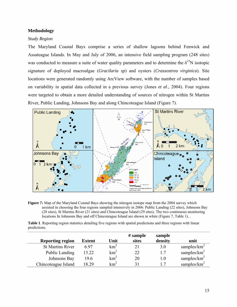
on variability in spatial data collected in a previous survey (Jones et al., 2004). Four regions

were targeted to obtain a more detailed understanding of sources of nitrogen within St Martins

River, Public Landing, Johnsons Bay and along Chincoteague Island (Figure 7).

Figure 7: Map of the Maryland Coastal Bays showing the nitrogen isotope map from the 2004 survey which assisted in choosing the four regions sampled intensively in 2006: Public Landing (22 sites), Johnsons Bay (28 sites), St Martins River (21 sites) and Chincoteague Island (29 sites). The two continuous monitoring locations In Johnsons Bay and off Chincoteague Island are shown in white (Figure 7, Table 1). .

Table 1. Reporting region statistics detailing five regions with spatial predictions and three regions with linear predictions.

Reporting region Extent Unit # sample

sites sample density unit

St Martins River 6.97 km2 21 3.0 samples/km2 Public Landing 13.22 km2 22 1.7 samples/km2

Johnsons Bay 19.6 km2 20 1.0 samples/km2 Chincoteague Island 18.29 km2 31 1.7 samples/km2

16

Water quality sampling

Salinity, pH, temperature and dissolved oxygen (DO) were measured with a WTW water quality

probe. Secchi depth was determined by lowering a 20 cm diameter Secchi disk through the water

column until it was no longer possible to distinguish between the black and white quadrants.

Continuous monitoring

Two continuous monitoring stations were established for comparison to the once off spatial

intensive sampling. Locations of continuous monitors were off Chincoteague Island (Lat

37.96331N, Long 75.35500W) and in Johnsons Bay (Lat 38.06611N, Long 75.34492W) (Figure

7).

Water column nutrients

Total nitrogen and total phosphorus were determined by collecting water samples in pre-rinsed

containers, placed on ice and returned to the laboratory where they were frozen for subsequent

analysis in accordance with the methods of Clesceri et al. (1989).

Chlorophyll a

Chlorophyll a concentrations were used as an indicator of phytoplankton biomass. At each site,

Chlorophyll a concentration was determined by filtering a known volume of water through a

Whatman GF/F filter which was immediately frozen. In the laboratory, the filter was ground in

acetone to extract chlorophyll a, spectral extinction coefficients were determined on a

fluorometer.

Microbial Source Tracking

At all sampling stations in Johnsons Bay and Chincoteague (May) and all stations in Public

Landing and Johnsons Bay (July), 60 ml of surface water was collected. These were plated onto

‘ColiPlate testkits’ produced by Bluewater Biosciences and incubated at 35 °C for 24 hours,

before reading.

Stable isotope technique

Gracilaria sp. (a red macroalgae) was collected from Greenbackville on the Maryland/Virginia

border. Sub-samples were analyzed for their initial δ15N isotopic signature. At each site, the

macroalgae were incubated for four days in transparent, perforated chambers at half Secchi depth

(Costanzo et al., 2001). Samples were oven dried to constant weight at 60 °C, ground and

oxidized in a CN Biological Sample Converter. The resultant N2 was analyzed by a continuous

flow isotope ratio mass spectrometer. Total %N was determined, and the ratio of 15N to 14N was

17

expressed as the relative difference between the sample and a standard (N2 in air) using the

following equation (Peterson & Fry, 1987):

δ15N = (15N/14N (sample) / 15N/14N (standard) – 1) x 1000 (‰).

Nitrogen (N) occurs in two naturally stable forms, 15N and 14N, with the predominant form being 14N (99.6%). The various sources of nitrogen often have distinguishable 15N to 14N ratios,

thereby making it possible to identify the source of the nutrients (Heaton, 1986). Stable isotope

ratios of nitrogen (δ15N) have been used widely in marine systems as tracers of discharged

nitrogen from point and diffuse sources, including sewage effluent (Rau et al., 1981; Heaton,

1986; Wada., 1980; Van Dover et al., 1992; Macko & Ostrom, 1994; Cifuentes et al., 1996;

McClelland & Valiela, 1998). Plant δ15N signatures have been used to identify nitrogen sources

available for plant uptake (Heaton, 1986). Elevated δ15N signatures in seagrass, mangroves and

macroalgae have been attributed to plant assimilation of N from treated sewage effluent (Wada,

1980; Grice et al., 1996; Udy & Dennison, 1997; Abal et al., 1998, Carruthers et al., 2005). The

elevated δ15N signature subsequent to treatment of the sewage effluent is a result of isotopic

fractionation during ammonia volatilization, nitrification and denitrification (McClelland &

Valiela, 1998).

Oyster stable isotope analysis

Oysters were sourced from two locations in the Maryland Coastal Bays, near Ocean Pines, on St

Martins River. These cultchless oysters, less than one year old, were initially grown as part of the

Maryland Coastal Bays Oyster Gardening Program. Three oysters from a randomly selected

source were placed in cages made from ¾” mesh, anchored by 3 bricks and suspended by surface

buoys. Oysters from each source were randomly selected to be deployed on 22nd May in St

Martins River and Johnson Bay and 23rd May in Public Landing and Chincoteague (see maps).

Oyster cages were collected from Johnson Bay and St Martins on 13th July and from lower

Chincoteage and Public Landing on 14th July. Samples were kept on ice until frozen at the

laboratory until dissection. Shell length was measured and then mantle, gills, and adductor

muscle were dissected out. Tissues were oven dried at 60°C for 48 hrs or until thoroughly dry

and then ground with mortar and pestle. 1 mg subsamples were packed in tin capsules and sent to

University California, Davis for stable isotope analysis.

18

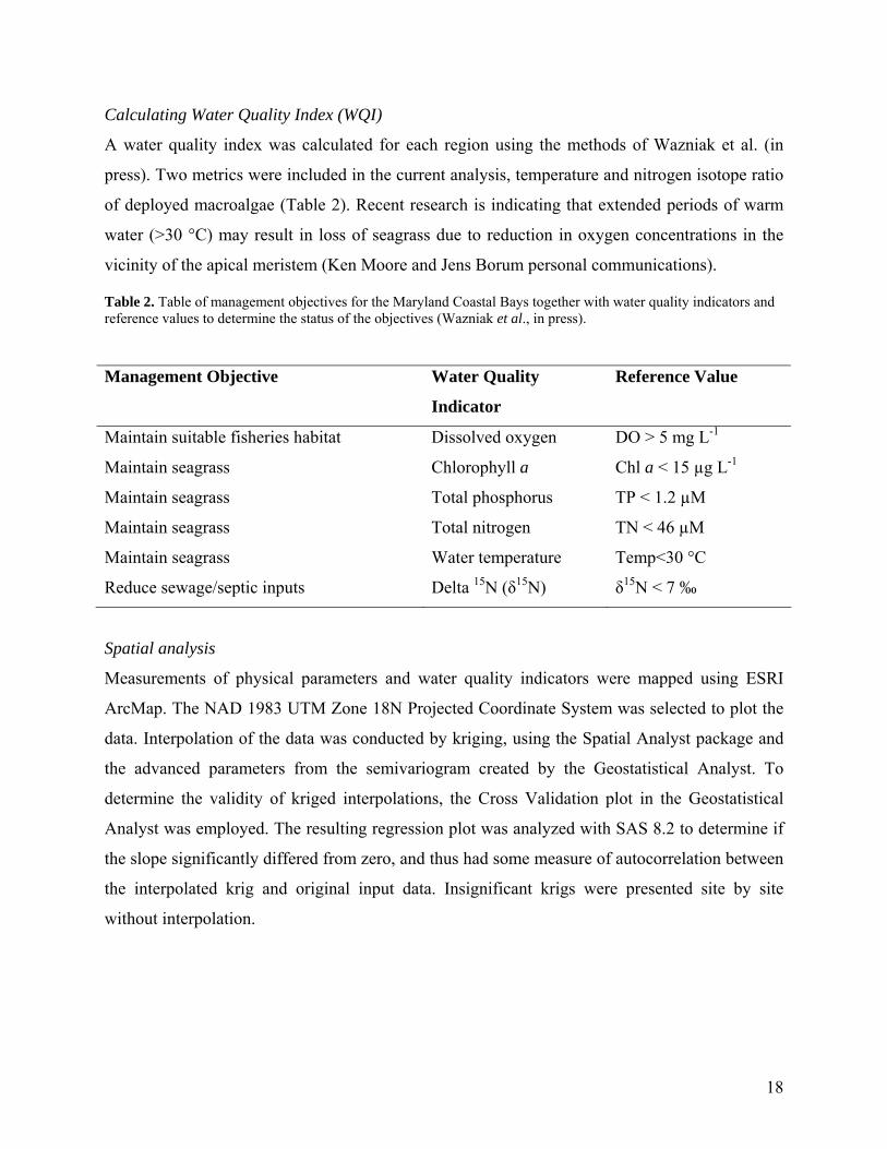
Calculating Water Quality Index (WQI)

A water quality index was calculated for each region using the methods of Wazniak et al. (in

press). Two metrics were included in the current analysis, temperature and nitrogen isotope ratio

of deployed macroalgae (Table 2). Recent research is indicating that extended periods of warm

water (>30 °C) may result in loss of seagrass due to reduction in oxygen concentrations in the

vicinity of the apical meristem (Ken Moore and Jens Borum personal communications).

Table 2. Table of management objectives for the Maryland Coastal Bays together with water quality indicators and reference values to determine the status of the objectives (Wazniak et al., in press).

Management Objective Water Quality

Indicator

Reference Value

Maintain suitable fisheries habitat Dissolved oxygen DO > 5 mg L-1

Maintain seagrass Chlorophyll a Chl a < 15 µg L-1

Maintain seagrass Total phosphorus TP < 1.2 µM

Maintain seagrass Total nitrogen TN < 46 µM

Maintain seagrass Water temperature Temp<30 °C

Reduce sewage/septic inputs Delta 15N (δ15N) δ15N < 7 ‰

Spatial analysis

Measurements of physical parameters and water quality indicators were mapped using ESRI

ArcMap. The NAD 1983 UTM Zone 18N Projected Coordinate System was selected to plot the

data. Interpolation of the data was conducted by kriging, using the Spatial Analyst package and

the advanced parameters from the semivariogram created by the Geostatistical Analyst. To

determine the validity of kriged interpolations, the Cross Validation plot in the Geostatistical

Analyst was employed. The resulting regression plot was analyzed with SAS 8.2 to determine if

the slope significantly differed from zero, and thus had some measure of autocorrelation between

the interpolated krig and original input data. Insignificant krigs were presented site by site

without interpolation.

19

Findings

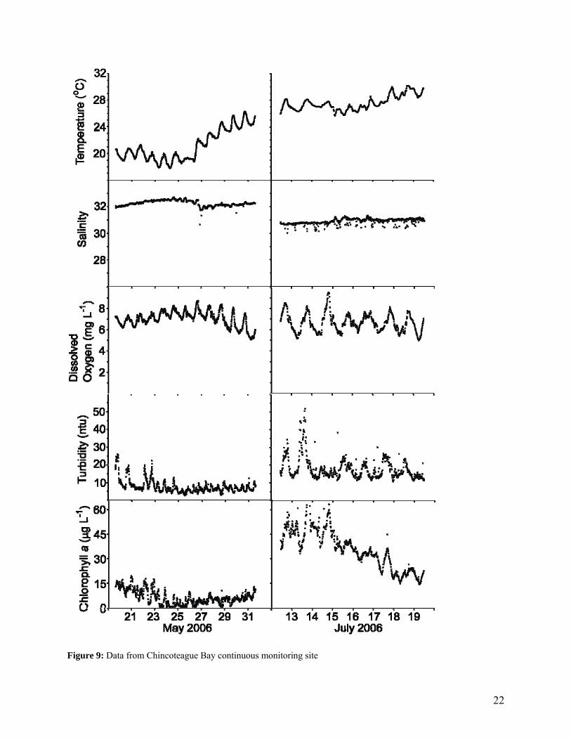
Continuous monitoring

The continuous monitoring data showed the extent of daily variations in temperature, dissolved

oxygen, turbidity and Chlorophyll a as well as providing an effective comparison for the survey

results (Figure 9, 10). Johnsons Bay had consistently higher turbidity and Chlorophyll a than

Chincoteague (Table 3).

Rainfall

Rainfall was low before the May sampling, with a cumulative total for 2006 of 162mm by 22nd

May. There was however several large rain events between late may and mid July such that

cumulative total 2006 rainfall by 13th July was 380mm (Figure 8).

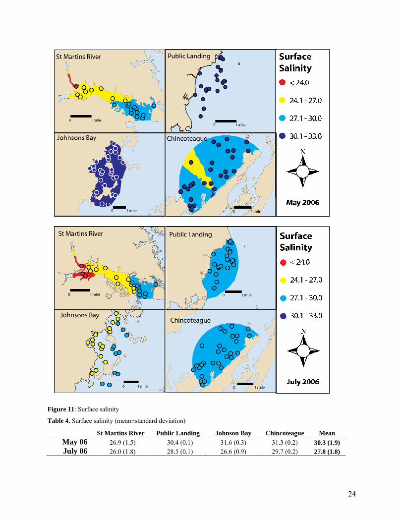
Salinity

Salinity in St Martins River had the largest range of all sites (24.9 – 28.9 in May and 24.3 – 28.2

in July), and this range was consistent between sampling events, however the lower salinity

water was measured further downstream in July after heavy rainfall (Figs 8 and 11; table 4).

Public Landing, Johnsons Bay and Chincoteague all had a reduction in salinity from

approximately 31 in May to approximately 28 in July (Figure 11; table 4). Johnsons Bay showed

a distinct onshore (ca 25) to offshore (ca 28) gradient in salinity in July, consistent with local

freshwater inputs from groundwater or surface flow sources (Figure 11).

Temperature

Variation in surface water temperature between sites was 5-6 °C in both May (range 19.0 –

25.0°C) and July (range 27.9 – 33.7°C) (Figure 12). However, there was a large increase in water

temperature across all sites during these months, from 21.7±1.6°C in May to 30.3±1.4°C (mean

± standard deviation) (Table 5). During July, 90% of the 21 sampling sites in St Martins River

and 83% of 31 sites in Chincoteague were above the 30°C threshold for seagrass survival and

while there is little seagrass in St Martins River, the sampling area near Chincoteague Island is

amongst some of the most extensive Zostera marina meadows in the MD Coastal Bays.

Dissolved Oxygen (DO)

Public Landing and Chincoteague sites showed a large reduction in DO between May (8.10±0.26

and 8.17±2.04 mgl-1 respectively) and July (4.47±0.36 and 5.28±0.38 mgl-1 respectively) (mean

20

± standard deviation; table 6). Samples were taken at the bottom of the water column, however

were once off samples taken during the day and the continuous monitoring data shows a daily

variation of up to 4 mgl-1, (Figures 9, 10), so these values are certainly a conservative estimate of

DO. The relatively high concentration of DO in St Martins River versus Public Landing during

July may be a result of the high phytoplankton populations in both which are shown by the high

Chl a and low Secchi depths in these regions (Figures 14, 17), and that Public Landing was

sampled in the morning (7:00-10:00am) while St Martins River was sampled in the afternoon

(1:20-4:00pm), so DO may have still been low following night-time respiration in Public

Landing, and elevated due to high photosynthesis in St Martins River.

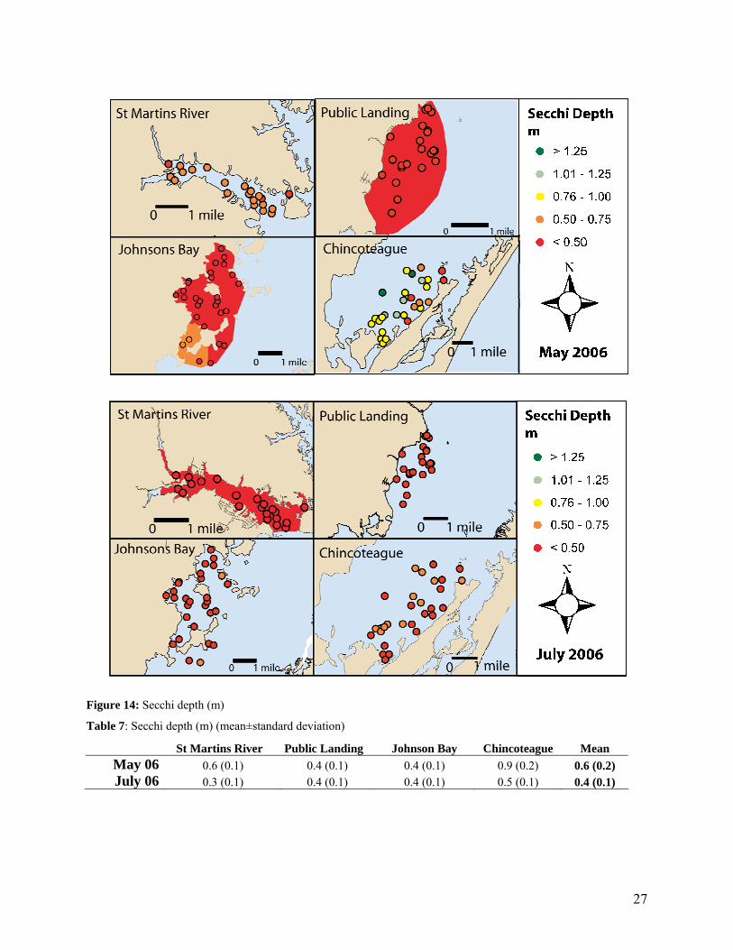
Secchi depth

Mean Secchi depth decreased from a mean across all sites of 0.6±0.2 m in May to 0.4±0.1 m in

July, the largest reduction being in the Chincoteague sampling region, reducing from 0.9±0.2 m

in May to 0.5±0.1 m (Figure 14, Table 7). These high turbidity (low Secchi) readings in St

Martins, Public Landing and Johnsons Bay, with lower turbidity in Chincoteague were consistent

with the 2004 survey (Jones et al.,) and the increased turbidity in July suggests that it is later in

the summer that the phytoplankton bloom reaches its maximum concentration (Figure 14).

Microbial Source Tracking

None of the samples (except positive controls) grew any bacteria colonies, suggesting that all

sites had coliform and E. coli counts less than 5 cfu’s (colony forming units) per 100ml.

21

Table 3. Summary data from continuous monitoring sites. Data is medians (standard deviations) and is taken from 19th May – 1st June and 12th July – 20th July, 2006.

Chincoteague Johnsons May July May July

Temperature (ºC) 20.33 (2.30) 28.47 (1.25) 20.90 (2.51) 27.27 (1.08) Salinity 32.22 (0.21) 28.00 (0.28) 32.85 (0.53) 30.92 (0.20)

DO (mg L-1) 7.11 (0.73) 6.91 (0.95) 7.39 (0.67) 6.55 (0.86) Turbidity (ntu) 6.70 (3.69) 13.60 (6.93) 12.40 (3.51) 15.80 (47.88)

Chlorophyll a (μg L-1) 5.30 (4.40) 28.30 (5.18) 18.40 (6.05) 35.80 (12.38)

Figure 8: Rainfall data for Assateague Island, Maryland

22

Figure 9: Data from Chincoteague Bay continuous monitoring site

23

Figure 10: Data from Johnsons Bay continuous monitoring site

24

Figure 11: Surface salinity

Table 4. Surface salinity (mean±standard deviation)

St Martins River Public Landing Johnson Bay Chincoteague Mean May 06 26.9 (1.5) 30.4 (0.1) 31.6 (0.3) 31.3 (0.2) 30.3 (1.9) July 06 26.0 (1.8) 28.5 (0.1) 26.6 (0.9) 29.7 (0.2) 27.8 (1.8)

25

Figure 12: Surface water temperature (°C)

Table 5. Surface water temperature (°C) (mean±standard deviation)


26

Figure 13: Bottom dissolved oxygen (DO) (mgl-1)

Table 6: Dissolved Oxygen (mgl-1) (mean±standard deviation)

St Martins River Public Landing Johnson Bay Chincoteague Mean May 06 8.10 (0.26) 8.17 (2.04) 8.14 (1.50) July 06 6.64 (1.55) 4.47 (0.36) 5.04 (0.80) 5.28 (0.38) 5.32 (1.14)

27

Figure 14: Secchi depth (m)

Table 7: Secchi depth (m) (mean±standard deviation)


28

Water column total nitrogen

During both May and July, Chincoteague was the only sampling region which was , on average, below

the water column total nitrogen threshold of 46 μM (22.8±8.4 and 33.9±3.3μM respectively,

mean±standard error) (Figure 15, table 9). Rainfall events resulting in only moderate reductions in salinity

(Figure 8), resulted in large increases in total nitrogen concentration in surface waters of St Martins River

(Figure 15). Johnsons Bay and Public Landing both show elevated total nitrogen concentrations in some

inshore regions, suggesting local sources of nitrogen input to these regions and as these were observed

also during May, it is likely that these are at least in part sourced from groundwater inflows (Figure 15).

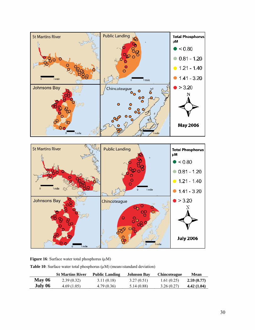
Water column total phosphorus

All sampling sites for both May and July samplings were above the threshold value for water column total

phosphorus of 1.2μM (Figure 16), however, there was still an increase from an overall mean of 2.59±0.77

μM in May to 4.42±1.04 μM in July (Table 10). Public Landing and Johnsons Bay had higher total

phosphorus concentrations inshore, which is consistent with the total nitrogen measurements in indicating

groundwater or overland nutrient inputs in these regions. During July, the slightly lower concentrations of

total phosphorus in southern Chincoteague most likely reflect increased flushing from the southern ocean

opening to Chincoteague Bay (Figure 16).

Water column chlorophyll a

Chlorophyll a concentration was low at all sites in May (<15 μgl-1) (Figure 17). However, this was not

consistent with high turbidity (low Secchi, Figure 14), high nutrients (Figure 15, 16) and high temperature

(Figure 12). Further investigation revealed that the Phaeopigments were high at all sites for the May

samples and, as Phaeopigments record degraded Chlorophyll a, this suggests that either there was a large

number of decaying phytoplankton or, more likely, the Chlorophyll degraded in the samples (Table x, x).

During July there was high to very high Chlorophyll a recorded in all sampling regions (15-50+ μgl-1),

suggesting phytoplankton blooms throughout the system (Figure 17). This is also consistent with the

continuous monitoring data which were similar in July, but in Johnsons Bay (particularly) continuous

monitoring data recorded Chl a concentrations from 10-30 μgl-1 while the survey values were all <15μgl-1

(Figure 10, 17).

Table 8: Surface water Phaeophytin pigments (μgl-1) (mean±standard deviation)


29

Figure 15: Surface water total nitrogen (μM)

Table 9: Surface water total nitrogen (μM) (mean±standard deviation)


30

Figure 16: Surface water total phosphorus (μM)

Table 10: Surface water total phosphorus (μM) (mean±standard deviation)


31

Figure 17: Surface water Chlorophyll a (μg l-1)

Table 11: Surface water Chlorophyll a (μg l-1) (mean±standard deviation)


32

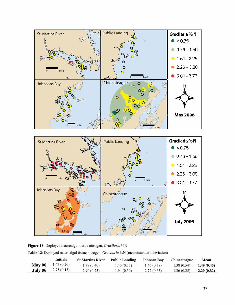
Bio-indicator Gracilaria %N

The tissue nitrogen measured in deployed Gracilaria for four days, closely reflected patterns in the

surface water total nitrogen, with Chincoteague being lower in both May and July (ca 1.37% N, table x)

than the other three sampling regions, which all showed an increase from May (global mean 1.49±0.46%)

to June (global mean 1.49±0.46%) (Table 12). Patterns within each of the regions were less distinct,

largely due to low variation at the scale of sampling (Figure 18). The initial values of %N in the

Gracilaria used for deployment showed the same trend of being higher in July (2.75±0.13%) than May

(1.47±0.20%), however, after the four day deployment, samples had both increased and decreased from

the initial (Table 12).

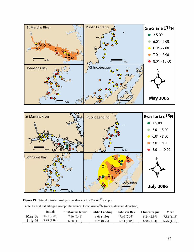
Bio-indicator Gracilaria δ15N

The mean δ15N over all sampling regions reduced from 7.33±1.15 ppt in May to 6.76±1.15 ppt in July

(mean ± standard deviation), and while St Martins River and Johnsons Bay were slightly higher than the

other regions in May, all regions were similar in the July sampling (Figure 19, Table 13). The only region

to show clear spatial patterning in δ15N was the July sampling in Chincoteague, where a northern, central

and southern area of higher δ15N (Figure 19). The lack of patterns may have resulted from the high initial

value of the deployed gracilaria, or alternately may be reflecting processes within the coastal bays were

mostly occurring at a larger scale when samples were taken, as evidenced by the uniformly high total

phosphorus and Chlorophyll a concentrations.

Water quality index

A large decline in water quality, relative to threshold values to maintain fisheries and seagrass, was

observed between May (overall mean water quality poor; 0.58±0.16) and July (mean water quality poor;

0.58±0.16), the largest declines in water quality between the two sampling periods being in Public

Landing and Chincoteague (Figure 20, Table 14). In May, water quality was uniform throughout the St

Martins River, Public Landing and Chincoteague regions however showed a distinct gradient in Johnsons

Bay with water quality poor inshore and good offshore (Figure 20). In July, water quality was uniformly

degraded to very degraded in St Martins River and Public Landing, while in Johnsons Bay the northern

section had poor water quality and the southern section degraded to very degraded water quality and in

Chincoteague water quality was generally poor with degraded areas in the north and centre of the

sampling region and some good water quality to the south where there is higher flushing rates (Figure

20).

33

Figure 18: Deployed macroalgal tissue nitrogen, Gracilaria %N

Table 12: Deployed macroalgal tissue nitrogen, Gracilaria %N (mean±standard deviation)

Initials St Martins River Public Landing Johnson Bay Chincoteague Mean May 06 1.47 (0.20) 1.79 (0.40) 1.40 (0.37) 1.46 (0.38) 1.38 (0.54) 1.49 (0.46) July 06 2.75 (0.13) 2.90 (0.75) 1.94 (0.30) 2.72 (0.63) 1.36 (0.25) 2.20 (0.82)

34

Figure 19: Natural nitrogen isotope abundance, Gracilaria δ15N (ppt)

Table 13: Natural nitrogen isotope abundance, Gracilaria δ15N (mean±standard deviation)

Initials St Martins River Public Landing Johnson Bay Chincoteague Mean May 06 5.21 (0.26) 7.40 (0.41) 6.66 (1.50) 7.60 (2.33) 6.24 (2.19) 7.33 (1.15) July 06 9.48 (1.09) 6.28 (1.30) 6.78 (0.93) 6.84 (0.85) 6.98 (1.34) 6.76 (1.15)

35

Figure 20: Integrated water quality index for all regions

Table 14: Integrated water quality index for all regions (mean±standard deviation)


36

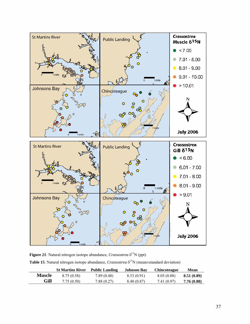
Bio-indicator Oyster δ15N muscle

Mean Crassostrea muscle tissue δ15N over all sampling regions was 8.51±0.89 ppt after the

deployment period, which was a mean increase of 0.34 ppt from the initial isotope values.

Similar to the Gracilaria in May, St Martins River and Johnsons Bay were slightly higher than

the other regions (Table 15). The southern portion of Johnson Bay showed higher isotope values

than the northern portion. (Figure 21) Oyster mortalities make patterns in Public Landing and St

Martins River difficult to determine.

Bio-indicator Oyster δ15N gill

Gill tissue δ15N were close to 1 ppt lower than those in the muscle, a pattern consistent with

previous observations, and likely due to oyster physiology. The overall mean of 7.76 ± 0.88 is

thus comparable to the muscle mean. A similar spatial pattern was found to that of the muscle,

with an increasing gradient north to south in Johnson Bay. However, Public Landing had a

higher mean of 7.88 ± 0.27 than St Martins River, with 7.75 ± 0.50. An increasing north to south

gradient was also found in Chincoteague, though overall, it had the lowest mean of 7.41 ± 0.97.

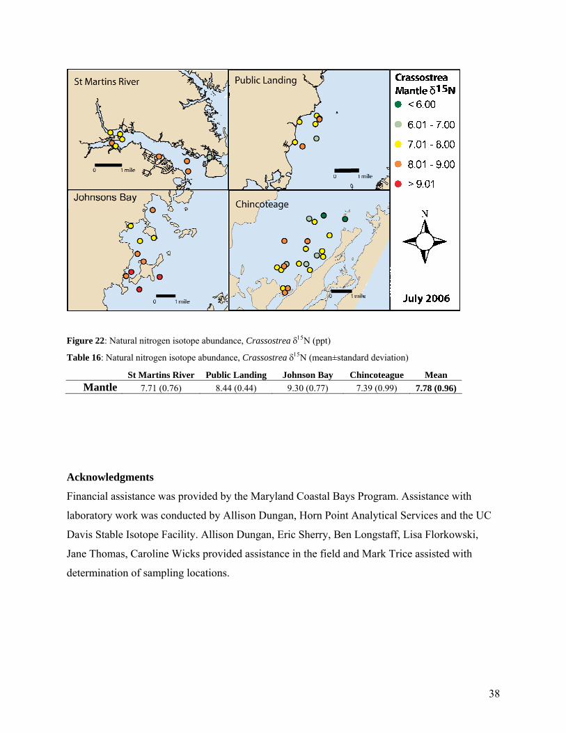
Bio-indicator Oyster δ15N mantle

Mantle, the shortest length integrator, had roughly the same mean isotope values as the gills, at

7.78 ± 0.96. Values in St Martin River and Chincoteague were very similar to those of the gill,

but were higher than the gill in Public Landing and Johnson Bay. The north to south gradient in

Johnsons Bay and Chincoteague can also be seen in the mantle (Figure 22).

37

Figure 21: Natural nitrogen isotope abundance, Crassostrea δ15N (ppt)

Table 15: Natural nitrogen isotope abundance, Crassostrea δ15N (mean±standard deviation)

St Martins River Public Landing Johnson Bay Chincoteague Mean Muscle 8.75 (0.58) 7.89 (0.48) 8.53 (0.91) 8.05 (0.88) 8.51 (0.89)

Gill 7.75 (0.50) 7.88 (0.27) 8.40 (0.87) 7.41 (0.97) 7.76 (0.88)

38

Figure 22: Natural nitrogen isotope abundance, Crassostrea δ15N (ppt)

Table 16: Natural nitrogen isotope abundance, Crassostrea δ15N (mean±standard deviation)

St Martins River Public Landing Johnson Bay Chincoteague Mean Mantle 7.71 (0.76) 8.44 (0.44) 9.30 (0.77) 7.39 (0.99) 7.78 (0.96)

Acknowledgments

Financial assistance was provided by the Maryland Coastal Bays Program. Assistance with

laboratory work was conducted by Allison Dungan, Horn Point Analytical Services and the UC

Davis Stable Isotope Facility. Allison Dungan, Eric Sherry, Ben Longstaff, Lisa Florkowski,

Jane Thomas, Caroline Wicks provided assistance in the field and Mark Trice assisted with

determination of sampling locations.

39

References

Abal, E.G., Holloway, K.M. & Dennison, W.C. (eds.) (1998) Interim Stage 2 Scientific Report.

Brisbane River and Moreton Bay Wastewater Management Study, Brisbane.

Carruthers, T.J.B., van Tussenbroek, B.I. and Dennison, W.C. (2005). Influence of submarine

springs and wastewater on nutrient dynamics of Caribbean seagrass meadows. Estuarine

Coastal Shelf Science 64: 191-199.

Cifuentes, L.A., Coffin, R.B., Solorzano, L., Cardenas, W., Espinoza, J. & Twilley, R.R. (1996)

Isotopic and elemental variations of carbon and nitrogen in a mangrove estuary.

Estuarine, Coastal and Shelf Science 43, 781-800.

Clesceri, L.S., Greenberg, A.E. & Trussel, R.R. (1989) Standard methods for the examination of

water and wastewater. American Public Health Association, New York. Chambers, R.M.

& Odum, W.E. (1990) Porewater oxidation, dissolved phosphate and the iron curtain:

Iron-phosphorus relations in tidal freshwater marshes. Biogeochemistry 10, 37-52.

Costanzo, S. D., M. J. O'Donohue, et al. (2001). A new approach for detecting and mapping

sewage impacts. Marine Pollution Bulletin 42(2): 149-156.

Grice, A.M., Loneragan, N.R. & Dennison, W.C. (1996) Light intensity and the interactions

between physiology, morphology and stable isotope ratios in five species of seagrass.

Journal of Experimental Marine Biology and Ecology 195, 91-110.

Fourqurean, J. W., Moore, T. O., Fry, B., Hollibaugh, J.T. (1997) Spatial and temporal variation in C:N:P ratios, δ15N and δ13C of eelgrass Zostera marina as indicators of ecosystem processes, Tomales Bay, California, USA. Marine Ecology Progress Series 157, 147-157.

Heaton, T.H.E. (1986) Isotope studies of nitrogen pollution in the hydrosphere and atmosphere:

A review. Chemical Geology 59, 87-102.

Jones, A. B., O’Donohue, M. J., Udy, J. and Dennison, W. C. (2001) Assessing ecological

impacts of shrimp and sewage effluent: biological indicators with standard water quality

analyses. Estuarine, Coastal and Shelf Science 52, 91–109.

Jones, A. B. (2004) A water quality assessment of the Maryland Coastal Bays including nitrogen

source identification using stable isotopes. Data report to the Maryland Coastal Bays

Program. http://ian.umces.edu/pdfs/md_coastal_bays_report.pdf

http://ian.umces.edu/pdfs/md_coastal_bays_report.pdf

40

Kramer, K. J. M. (ed) 1994. Biomonitoring of coastal waters and estuaries. CRC Press, Boca

Raton. 327 pp.

Langdon, C.J. and Newell, R.I.E. 1996. Digestion and nutrition in larvae and adults. In:

Kennedy, V.S., Newell, R.I.E. and Eble, A.F. (Eds) The Eastern Oyster Crassostrea

virginica. Maryland Sea Grant pp 231-260.

Macko, S.A. & Ostrom, N.E. (1994) Pollution studies using stable isotopes. In Stable isotopes in

ecology and environmental science Latja, K. & Michener, R.H. (eds). Blackwell

Scientific Publications, Oxford, pp. 45-62.

McClelland, J.W. & Valiela, I. (1998) Linking nitrogen in estuarine producers to land derived

sources. Limnology and Oceanography 43, 577-585.

Moore, K.B. 2003. Uptake dynamics and sensitivity of oysters to detect sewage-derived

nitrogen. Honours thesis, University of the Sunshine Coast, Australia.

Newell, R.I.E. and C.J. Langdon. 1996. Mechanism and Physiology of Larval and Adult

Feeding. In: Kennedy, V.S., Newell, R.I.E. and Eble, A.F. (Eds) The Eastern Oyster

Crassostrea virginica. Maryland Sea Grant pp 185-223.

Peterson, B.J. and Fry, B. 1987. Stable isotopes in ecosystem studies. Annual Review of Ecology

and Systematics 18: 293-320

Rau, G.H., Sweeney, R.E., Kaplan, I.R., Mearns, A.J. & Young, D.R. (1981) Differences in

animal 13C, 15N and D abundance between a polluted and unpolluted coastal site. Likely

indicators of sewage uptake by a marine food web. Estuarine, Coastal and Shelf Science

13, 711-720.

Udy, J.W. & Dennison, W.C. (1997) Growth and physiological responses of three seagrass

species to elevated sediment nutrients in Moreton Bay, Australia. Journal of experimental

Marine Biology and Ecology 217, 253-277.

Van Dover, C.L., Grassle, J.F., Fry, B., Garritt, R.H. & Starczak, V.R. (1992) Stable isotope

evidence for entry of sewage-derived organic material into deep-sea food web. Nature

360, 153-156.

Wada, E. (1980) Nitrogen isotope fractionation and its significance in biogeochemical processes

occurring in marine environments. In Isotope Marine Chemistry Goldberg, E.D. &

Horibe, Y. (eds). Uchida-Rokakuho, pp. 375-398.

41

Wazniak, C., Hall, M., Cain, C., Wilson, D., Jesien, R. Thomas, J., Carruthers, T. and Dennison,

W. 2004. State of the Maryland Coastal Bays. Maryland Department of Natural

Resources, Maryland Coastal Bays Program, and University of Maryland Center for

Environmental Science.

Wazniak, C.E., Hall, M.R., Carruthers, T.J.B., Sturgis, B. and Dennison, W.C. (2006). Assessing

eutrophication in a shallow lagoon: linking water quality status and trends to living

resources in the Maryland Coastal Bays. Ecological Applications in press

Worf, D. L. 1980. Biological monitoring for environmental effects. Lexington Books, Lexington.

227 pp.

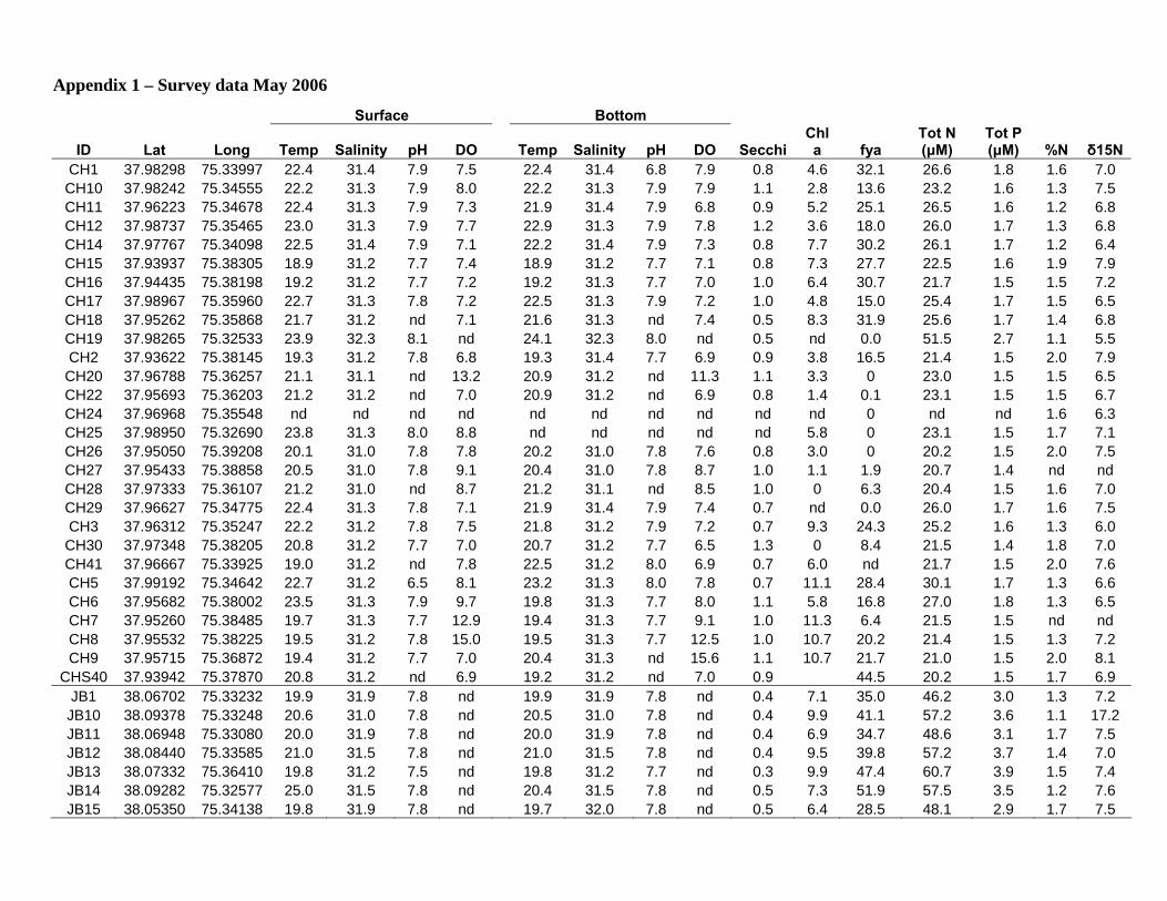
Appendix 1 – Survey data May 2006

Surface Bottom

ID Lat Long Temp Salinity pH DO

Temp Salinity pH DO SecchiChl a fya

Tot N (μM)

Tot P (μM) %N δ15N

CH1 37.98298 75.33997 22.4 31.4 7.9 7.5 22.4 31.4 6.8 7.9 0.8 4.6 32.1 26.6 1.8 1.6 7.0 CH10 37.98242 75.34555 22.2 31.3 7.9 8.0 22.2 31.3 7.9 7.9 1.1 2.8 13.6 23.2 1.6 1.3 7.5 CH11 37.96223 75.34678 22.4 31.3 7.9 7.3 21.9 31.4 7.9 6.8 0.9 5.2 25.1 26.5 1.6 1.2 6.8 CH12 37.98737 75.35465 23.0 31.3 7.9 7.7 22.9 31.3 7.9 7.8 1.2 3.6 18.0 26.0 1.7 1.3 6.8 CH14 37.97767 75.34098 22.5 31.4 7.9 7.1 22.2 31.4 7.9 7.3 0.8 7.7 30.2 26.1 1.7 1.2 6.4 CH15 37.93937 75.38305 18.9 31.2 7.7 7.4 18.9 31.2 7.7 7.1 0.8 7.3 27.7 22.5 1.6 1.9 7.9 CH16 37.94435 75.38198 19.2 31.2 7.7 7.2 19.2 31.3 7.7 7.0 1.0 6.4 30.7 21.7 1.5 1.5 7.2 CH17 37.98967 75.35960 22.7 31.3 7.8 7.2 22.5 31.3 7.9 7.2 1.0 4.8 15.0 25.4 1.7 1.5 6.5 CH18 37.95262 75.35868 21.7 31.2 nd 7.1 21.6 31.3 nd 7.4 0.5 8.3 31.9 25.6 1.7 1.4 6.8 CH19 37.98265 75.32533 23.9 32.3 8.1 nd 24.1 32.3 8.0 nd 0.5 nd 0.0 51.5 2.7 1.1 5.5 CH2 37.93622 75.38145 19.3 31.2 7.8 6.8 19.3 31.4 7.7 6.9 0.9 3.8 16.5 21.4 1.5 2.0 7.9 CH20 37.96788 75.36257 21.1 31.1 nd 13.2 20.9 31.2 nd 11.3 1.1 3.3 0 23.0 1.5 1.5 6.5 CH22 37.95693 75.36203 21.2 31.2 nd 7.0 20.9 31.2 nd 6.9 0.8 1.4 0.1 23.1 1.5 1.5 6.7 CH24 37.96968 75.35548 nd nd nd nd nd nd nd nd nd nd 0 nd nd 1.6 6.3 CH25 37.98950 75.32690 23.8 31.3 8.0 8.8 nd nd nd nd nd 5.8 0 23.1 1.5 1.7 7.1 CH26 37.95050 75.39208 20.1 31.0 7.8 7.8 20.2 31.0 7.8 7.6 0.8 3.0 0 20.2 1.5 2.0 7.5 CH27 37.95433 75.38858 20.5 31.0 7.8 9.1 20.4 31.0 7.8 8.7 1.0 1.1 1.9 20.7 1.4 nd nd CH28 37.97333 75.36107 21.2 31.0 nd 8.7 21.2 31.1 nd 8.5 1.0 0 6.3 20.4 1.5 1.6 7.0 CH29 37.96627 75.34775 22.4 31.3 7.8 7.1 21.9 31.4 7.9 7.4 0.7 nd 0.0 26.0 1.7 1.6 7.5 CH3 37.96312 75.35247 22.2 31.2 7.8 7.5 21.8 31.2 7.9 7.2 0.7 9.3 24.3 25.2 1.6 1.3 6.0 CH30 37.97348 75.38205 20.8 31.2 7.7 7.0 20.7 31.2 7.7 6.5 1.3 0 8.4 21.5 1.4 1.8 7.0 CH41 37.96667 75.33925 19.0 31.2 nd 7.8 22.5 31.2 8.0 6.9 0.7 6.0 nd 21.7 1.5 2.0 7.6 CH5 37.99192 75.34642 22.7 31.2 6.5 8.1 23.2 31.3 8.0 7.8 0.7 11.1 28.4 30.1 1.7 1.3 6.6 CH6 37.95682 75.38002 23.5 31.3 7.9 9.7 19.8 31.3 7.7 8.0 1.1 5.8 16.8 27.0 1.8 1.3 6.5 CH7 37.95260 75.38485 19.7 31.3 7.7 12.9 19.4 31.3 7.7 9.1 1.0 11.3 6.4 21.5 1.5 nd nd CH8 37.95532 75.38225 19.5 31.2 7.8 15.0 19.5 31.3 7.7 12.5 1.0 10.7 20.2 21.4 1.5 1.3 7.2 CH9 37.95715 75.36872 19.4 31.2 7.7 7.0 20.4 31.3 nd 15.6 1.1 10.7 21.7 21.0 1.5 2.0 8.1

CHS40 37.93942 75.37870 20.8 31.2 nd 6.9 19.2 31.2 nd 7.0 0.9 44.5 20.2 1.5 1.7 6.9 JB1 38.06702 75.33232 19.9 31.9 7.8 nd 19.9 31.9 7.8 nd 0.4 7.1 35.0 46.2 3.0 1.3 7.2 JB10 38.09378 75.33248 20.6 31.0 7.8 nd 20.5 31.0 7.8 nd 0.4 9.9 41.1 57.2 3.6 1.1 17.2 JB11 38.06948 75.33080 20.0 31.9 7.8 nd 20.0 31.9 7.8 nd 0.4 6.9 34.7 48.6 3.1 1.7 7.5 JB12 38.08440 75.33585 21.0 31.5 7.8 nd 21.0 31.5 7.8 nd 0.4 9.5 39.8 57.2 3.7 1.4 7.0 JB13 38.07332 75.36410 19.8 31.2 7.5 nd 19.8 31.2 7.7 nd 0.3 9.9 47.4 60.7 3.9 1.5 7.4 JB14 38.09282 75.32577 25.0 31.5 7.8 nd 20.4 31.5 7.8 nd 0.5 7.3 51.9 57.5 3.5 1.2 7.6 JB15 38.05350 75.34138 19.8 31.9 7.8 nd 19.7 32.0 7.8 nd 0.5 6.4 28.5 48.1 2.9 1.7 7.5

43

Surface Bottom



Tot N (μM)


JB16 38.06712 75.34653 19.8 31.7 7.7 nd 19.8 31.7 7.7 nd 0.4 6.2 37.6 56.6 3.5 1.4 7.3 JB17 38.04527 75.35350 19.5 32.0 7.6 nd 19.5 32.0 7.6 nd 0.6 2.8 12.0 38.8 2.1 2.2 8.1 JB18 38.03045 75.33627 19.6 31.7 7.8 nd 19.6 31.7 7.8 nd 0.5 3.9 17.9 44.4 3.2 1.5 7.9 JB2 38.04207 75.35852 19.6 32.0 7.6 nd 19.6 32.0 7.6 nd 0.6 2.6 12.0 37.7 2.3 1.9 7.8 JB20 38.10280 75.32807 20.6 30.9 7.8 nd 20.6 31.0 7.8 nd 0.3 11.7 39.2 60.6 3.8 1.5 7.2 JB21 38.03160 75.34532 19.5 31.9 7.7 nd 19.6 31.9 7.7 nd 0.5 3.0 12.7 39.6 2.6 1.6 8.2 JB22 38.09733 75.32565 20.4 31.3 7.8 nd 20.4 31.3 7.8 nd 0.2 8.7 36.6 55.5 3.6 1.7 7.8 JB23 38.04257 75.32952 19.9 32.1 7.7 nd 19.6 32.1 7.7 nd 0.5 3.6 27.9 38.6 2.4 2.1 8.2 JB24 38.06230 75.32818 19.9 31.9 7.8 nd 19.9 31.9 7.8 nd 0.3 4.6 36.4 46.3 2.9 1.7 6.9 JB25 38.08078 75.31430 19.9 31.8 7.8 nd 19.9 31.9 7.8 nd 0.5 4.6 44.2 45.3 3.2 1.4 7.9 JB26 38.07598 75.35812 21.4 31.6 7.8 nd 21.3 31.6 7.8 nd 0.5 0 95.9 57.5 3.8 1.4 6.9 JB27 38.06338 75.32387 19.9 32.0 7.7 nd 19.9 32.0 7.7 nd 0.4 12.1 34.9 47.2 2.9 1.5 7.8 JB28 38.08223 75.35387 21.2 31.6 7.8 nd 21.1 31.6 7.8 nd 0.4 13.1 43.7 58.4 4.0 1.6 7.7 JB3 38.04153 75.32540 19.6 31.7 7.9 nd 19.6 31.8 7.9 nd 0.4 3.6 17.2 44.4 3.0 1.1 6.4 JB4 38.07145 75.34815 19.8 31.3 7.7 nd 19.7 31.3 7.7 nd 0.4 3.4 19.9 57.2 3.6 1.6 7.4 JB5 38.08130 75.35423 21.3 31.6 7.8 nd 21.2 31.6 7.8 nd 0.4 8.1 45.4 57.6 3.8 1.3 8.8 JB6 38.05950 75.34743 19.8 31.8 7.6 nd 19.8 31.8 7.6 nd 0.5 6.0 42.1 56.1 3.3 1.6 8.0 JB7 38.08620 75.31900 20.1 31.4 7.8 nd 20.1 31.3 7.9 nd 0.5 6.4 39.0 52.2 3.2 1.2 7.0 JB8 38.08762 75.33642 20.7 31.1 7.8 nd 20.7 31.1 7.8 nd 0.4 8.7 47.1 56.9 3.6 1.6 7.8 JB9 38.06950 75.34493 19.7 31.9 7.7 nd 19.7 31.8 7.7 nd 0.5 6.7 31.0 52.5 3.1 1.1 6.6

JBS30 38.07183 75.35755 19.8 31.4 7.6 nd 19.8 31.4 7.6 nd 0.4 7.9 48.8 62.0 4.0 1.2 7.4 PL1 38.14750 75.26952 23.2 30.3 8.1 8.4 30.3 23.0 8.1 7.9 0.4 10.3 45.6 49.6 3.1 1.4 7.0

PL10 38.13995 75.28325 22.9 30.4 8.1 8.4 22.8 30.4 8.1 8.4 0.4 9.7 42.2 50.3 3.3 1.2 6.4 PL11 38.14425 75.26870 23.0 30.3 8.1 8.3 22.4 30.4 8.1 7.6 0.4 7.5 42.3 50.9 3.0 1.6 6.8 PL12 38.12412 75.28073 22.7 30.4 8.0 8.5 22.5 30.4 8.1 8.1 0.3 9.9 41.0 50.0 3.2 1.6 6.9 PL13 38.11877 75.28355 23.0 30.5 8.1 8.4 22.8 30.5 8.1 8.3 0.4 6.4 52.7 50.4 3.2 1.6 6.9 PL14 38.15995 75.26668 23.7 30.3 8.0 8.2 23.3 30.3 8.0 8.3 nd 4.8 64.5 52.9 3.1 1.2 6.8 PL15 38.15363 75.26825 23.6 30.4 8.1 8.1 23.3 30.3 8.0 7.7 0.4 nd 0.0 53.5 3.2 1.7 6.9 PL16 38.15907 75.26385 23.4 30.2 8.0 8.4 23.1 30.3 8.0 8.0 0.4 nd 0.0 50.0 3.0 1.5 7.7 PL17 38.13688 75.27862 22.6 30.3 8.0 8.1 22.1 30.3 8.1 8.1 0.4 6.2 54.2 51.9 3.2 1.4 6.9 PL18 38.14353 75.26205 23.1 30.3 8.1 8.4 22.6 30.3 8.1 8.4 0.3 4.0 51.6 49.8 3.0 1.3 6.8 PL19 38.16048 75.26555 nd 30.4 8.1 8.3 23.3 30.4 8.0 8.3 0.4 7.1 56.2 53.2 3.1 2.0 7.3 PL2 38.13770 75.27867 22.7 30.7 8.0 8.5 21.9 30.3 8.1 7.8 0.4 9.9 49.2 50.3 3.3 1.6 7.2

PL20 38.13085 75.28155 22.8 30.3 8.0 8.6 22.7 30.4 8.1 8.4 0.4 4.8 54.5 49.8 3.2 1.2 6.9 PL21 38.14247 75.26388 23.0 30.3 8.0 8.4 22.5 30.3 8.1 8.1 0.4 3.9 21.8 49.1 2.9 1.3 6.2 PL22 38.14905 75.28447 23.4 30.4 8.0 7.9 23.3 30.5 8.0 7.8 0.4 8.5 60.2 62.1 3.5 1.7 6.8 PL3 38.13388 75.28858 24.4 30.5 8.0 8.3 24.3 30.5 8.0 8.2 0.3 8.9 39.3 53.1 3.1 1.4 7.4

44

Surface Bottom



Tot N (μM)


PL4 38.15162 75.26570 23.3 30.3 8.1 8.2 23.1 30.3 8.1 7.8 0.4 nd 0.0 51.5 3.2 1.2 6.8 PL5 38.13820 75.27607 22.8 30.3 8.1 8.5 22.4 30.3 8.0 8.5 0.3 6.7 46.1 48.1 2.9 1.6 7.3 PL6 38.14357 75.26278 22.8 30.3 8.1 8.4 22.7 30.3 8.0 8.0 0.3 8.3 44.0 48.4 3.0 nd nd PL7 38.15098 75.26577 23.4 30.3 8.0 8.3 23.2 30.3 8.1 8.2 0.4 10.3 48.2 51.8 3.2 1.2 7.1 PL8 38.13678 75.26853 22.7 30.4 8.0 8.4 22.2 30.4 8.1 8.3 0.5 6.7 43.1 47.1 2.8 1.6 7.7 PL9 38.13945 75.26163 22.9 30.3 8.0 8.4 22.7 30.4 8.1 8.3 0.4 10.9 35.3 45.6 2.7 1.2 6.8 SM1 38.41235 75.17388 24.3 24.9 7.7 nd 24.3 24.9 7.7 nd 0.6 5.1 40.0 57.4 2.7 1.5 7.4

SM10 38.40733 75.17957 23.9 25.1 7.7 nd 23.8 25.1 7.7 nd 0.6 6.8 49.7 58.0 2.6 1.7 7.6 SM11 38.39963 75.11118 23.4 28.9 7.6 nd 23.4 28.9 7.6 nd 0.4 3.6 17.6 47.0 1.8 2.2 7.7 SM12 38.39078 75.12132 21.3 28.8 7.6 nd 21.2 28.8 7.7 nd 0.7 5.4 33.3 47.1 2.2 1.7 7.3 SM13 38.41053 75.16702 23.6 25.1 7.7 nd 23.0 25.5 7.7 nd 0.6 9.1 26.2 57.9 2.5 1.7 7.1 SM14 38.39188 75.12618 21.7 28.5 7.6 nd 21.3 28.4 7.6 nd 0.7 8.3 27.4 58.7 2.3 1.6 7.8 SM15 38.39957 75.13437 21.8 27.7 7.6 nd 21.8 27.7 7.6 nd 0.6 9.3 23.2 49.8 2.2 1.8 6.7 SM16 38.40307 75.13685 22.1 26.7 7.6 nd 22.1 26.1 7.6 nd 0.7 8.9 19.7 57.1 2.4 2.1 7.7 SM17 38.39477 75.12627 21.4 28.4 7.5 nd 21.3 28.4 7.6 nd 0.6 9.7 20.9 50.0 2.2 2.2 7.5 SM18 38.39282 75.12080 21.4 28.6 7.7 nd 21.2 28.6 7.7 nd 0.6 12.7 22.0 46.9 2.1 1.5 7.5 SM19 38.41163 75.15837 23.0 25.6 7.7 nd 23.0 25.6 7.7 nd 0.7 11.0 17.2 56.5 2.5 1.4 7.4 SM2 38.39447 75.13135 21.7 28.3 7.5 nd 21.6 28.3 7.6 nd 0.6 5.2 40.6 50.3 2.3 2.0 7.4

SM20 38.39752 75.12698 21.7 27.8 7.6 nd 21.7 27.8 7.7 nd 0.5 11.7 16.2 53.1 2.1 1.8 7.8 SM3 38.40573 75.17702 23.8 25.1 7.7 nd 23.5 20.6 7.7 nd 0.6 3.9 49.2 57.3 2.5 1.5 7.4

SM31 38.40943 75.17240 23.4 25.4 7.8 nd 23.2 25.5 7.7 nd 0.7 6.6 18.7 57.5 2.5 2.1 7.5 SM4 38.40467 75.14813 22.5 26.6 7.6 nd 22.4 26.6 7.6 nd 0.6 6.9 29.4 56.5 2.5 1.3 7.2 SM5 38.40000 75.14665 22.2 27.6 7.4 nd 20.5 27.8 7.4 nd 0.7 4.6 33.7 57.1 2.6 3.2 8.3 SM6 38.41312 75.18072 24.8 23.6 7.8 nd 24.4 24.0 7.8 nd 0.5 14.3 66.1 69.3 3.5 1.6 6.9 SM7 38.39862 75.12857 21.8 27.7 7.6 nd 21.8 27.8 7.6 nd 0.6 5.4 32.0 52.0 2.2 1.4 6.4 SM9 38.40085 75.13327 22.0 27.3 7.6 nd 21.9 27.4 7.6 nd 0.6 5.4 23.1 56.1 2.3 1.6 7.0

SMS28 38.39673 75.13168 21.6 28.0 7.5 nd 21.5 28.0 7.6 nd 0.7 19.7 33.2 51.1 2.2 1.7 7.6

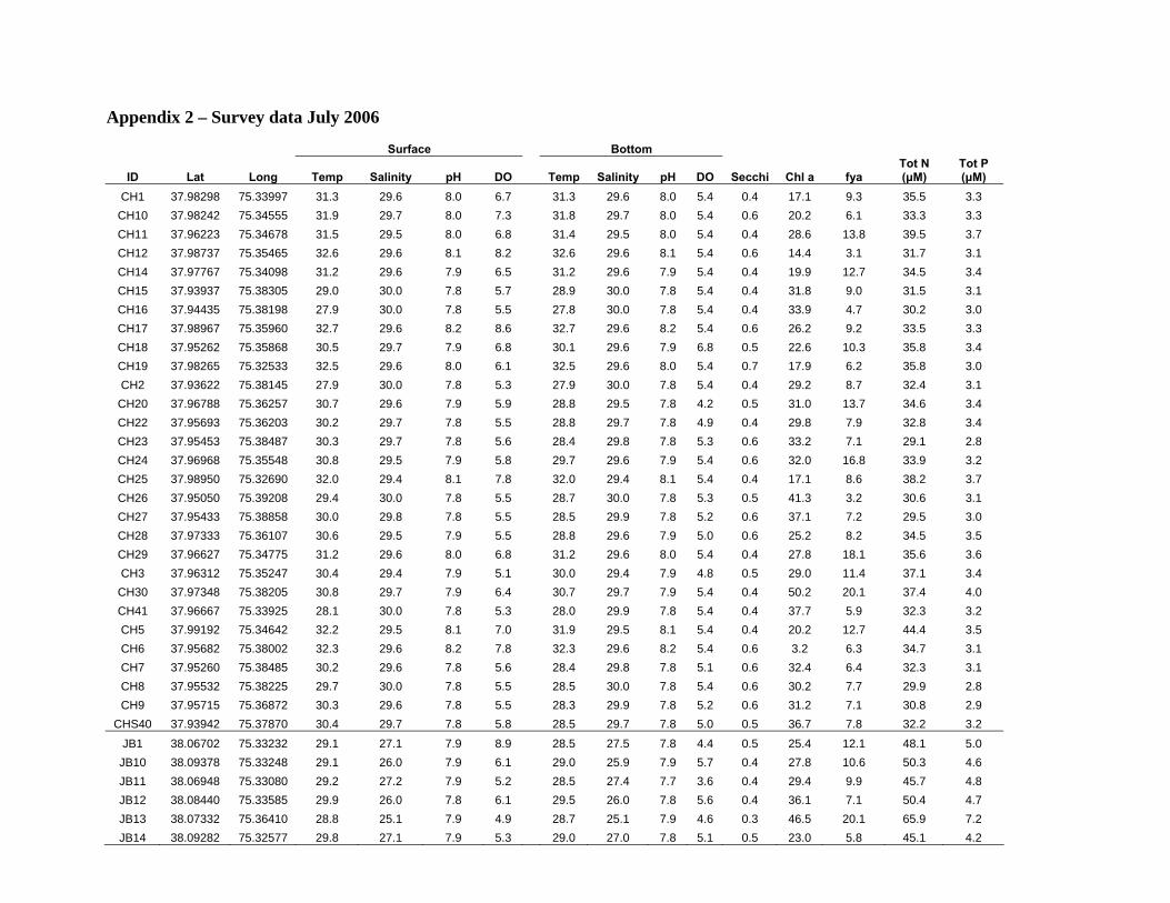
Appendix 2 – Survey data July 2006

Surface Bottom


Temp Salinity pH DO Secchi Chl a fya Tot N (μM)

Tot P (μM)

CH1 37.98298 75.33997 31.3 29.6 8.0 6.7 31.3 29.6 8.0 5.4 0.4 17.1 9.3 35.5 3.3 CH10 37.98242 75.34555 31.9 29.7 8.0 7.3 31.8 29.7 8.0 5.4 0.6 20.2 6.1 33.3 3.3 CH11 37.96223 75.34678 31.5 29.5 8.0 6.8 31.4 29.5 8.0 5.4 0.4 28.6 13.8 39.5 3.7 CH12 37.98737 75.35465 32.6 29.6 8.1 8.2 32.6 29.6 8.1 5.4 0.6 14.4 3.1 31.7 3.1 CH14 37.97767 75.34098 31.2 29.6 7.9 6.5 31.2 29.6 7.9 5.4 0.4 19.9 12.7 34.5 3.4 CH15 37.93937 75.38305 29.0 30.0 7.8 5.7 28.9 30.0 7.8 5.4 0.4 31.8 9.0 31.5 3.1 CH16 37.94435 75.38198 27.9 30.0 7.8 5.5 27.8 30.0 7.8 5.4 0.4 33.9 4.7 30.2 3.0 CH17 37.98967 75.35960 32.7 29.6 8.2 8.6 32.7 29.6 8.2 5.4 0.6 26.2 9.2 33.5 3.3 CH18 37.95262 75.35868 30.5 29.7 7.9 6.8 30.1 29.6 7.9 6.8 0.5 22.6 10.3 35.8 3.4 CH19 37.98265 75.32533 32.5 29.6 8.0 6.1 32.5 29.6 8.0 5.4 0.7 17.9 6.2 35.8 3.0 CH2 37.93622 75.38145 27.9 30.0 7.8 5.3 27.9 30.0 7.8 5.4 0.4 29.2 8.7 32.4 3.1

CH20 37.96788 75.36257 30.7 29.6 7.9 5.9 28.8 29.5 7.8 4.2 0.5 31.0 13.7 34.6 3.4 CH22 37.95693 75.36203 30.2 29.7 7.8 5.5 28.8 29.7 7.8 4.9 0.4 29.8 7.9 32.8 3.4 CH23 37.95453 75.38487 30.3 29.7 7.8 5.6 28.4 29.8 7.8 5.3 0.6 33.2 7.1 29.1 2.8 CH24 37.96968 75.35548 30.8 29.5 7.9 5.8 29.7 29.6 7.9 5.4 0.6 32.0 16.8 33.9 3.2 CH25 37.98950 75.32690 32.0 29.4 8.1 7.8 32.0 29.4 8.1 5.4 0.4 17.1 8.6 38.2 3.7 CH26 37.95050 75.39208 29.4 30.0 7.8 5.5 28.7 30.0 7.8 5.3 0.5 41.3 3.2 30.6 3.1 CH27 37.95433 75.38858 30.0 29.8 7.8 5.5 28.5 29.9 7.8 5.2 0.6 37.1 7.2 29.5 3.0 CH28 37.97333 75.36107 30.6 29.5 7.9 5.5 28.8 29.6 7.9 5.0 0.6 25.2 8.2 34.5 3.5 CH29 37.96627 75.34775 31.2 29.6 8.0 6.8 31.2 29.6 8.0 5.4 0.4 27.8 18.1 35.6 3.6 CH3 37.96312 75.35247 30.4 29.4 7.9 5.1 30.0 29.4 7.9 4.8 0.5 29.0 11.4 37.1 3.4

CH30 37.97348 75.38205 30.8 29.7 7.9 6.4 30.7 29.7 7.9 5.4 0.4 50.2 20.1 37.4 4.0 CH41 37.96667 75.33925 28.1 30.0 7.8 5.3 28.0 29.9 7.8 5.4 0.4 37.7 5.9 32.3 3.2 CH5 37.99192 75.34642 32.2 29.5 8.1 7.0 31.9 29.5 8.1 5.4 0.4 20.2 12.7 44.4 3.5 CH6 37.95682 75.38002 32.3 29.6 8.2 7.8 32.3 29.6 8.2 5.4 0.6 3.2 6.3 34.7 3.1 CH7 37.95260 75.38485 30.2 29.6 7.8 5.6 28.4 29.8 7.8 5.1 0.6 32.4 6.4 32.3 3.1 CH8 37.95532 75.38225 29.7 30.0 7.8 5.5 28.5 30.0 7.8 5.4 0.6 30.2 7.7 29.9 2.8 CH9 37.95715 75.36872 30.3 29.6 7.8 5.5 28.3 29.9 7.8 5.2 0.6 31.2 7.1 30.8 2.9

CHS40 37.93942 75.37870 30.4 29.7 7.8 5.8 28.5 29.7 7.8 5.0 0.5 36.7 7.8 32.2 3.2 JB1 38.06702 75.33232 29.1 27.1 7.9 8.9 28.5 27.5 7.8 4.4 0.5 25.4 12.1 48.1 5.0 JB10 38.09378 75.33248 29.1 26.0 7.9 6.1 29.0 25.9 7.9 5.7 0.4 27.8 10.6 50.3 4.6 JB11 38.06948 75.33080 29.2 27.2 7.9 5.2 28.5 27.4 7.7 3.6 0.4 29.4 9.9 45.7 4.8 JB12 38.08440 75.33585 29.9 26.0 7.8 6.1 29.5 26.0 7.8 5.6 0.4 36.1 7.1 50.4 4.7 JB13 38.07332 75.36410 28.8 25.1 7.9 4.9 28.7 25.1 7.9 4.6 0.3 46.5 20.1 65.9 7.2 JB14 38.09282 75.32577 29.8 27.1 7.9 5.3 29.0 27.0 7.8 5.1 0.5 23.0 5.8 45.1 4.2

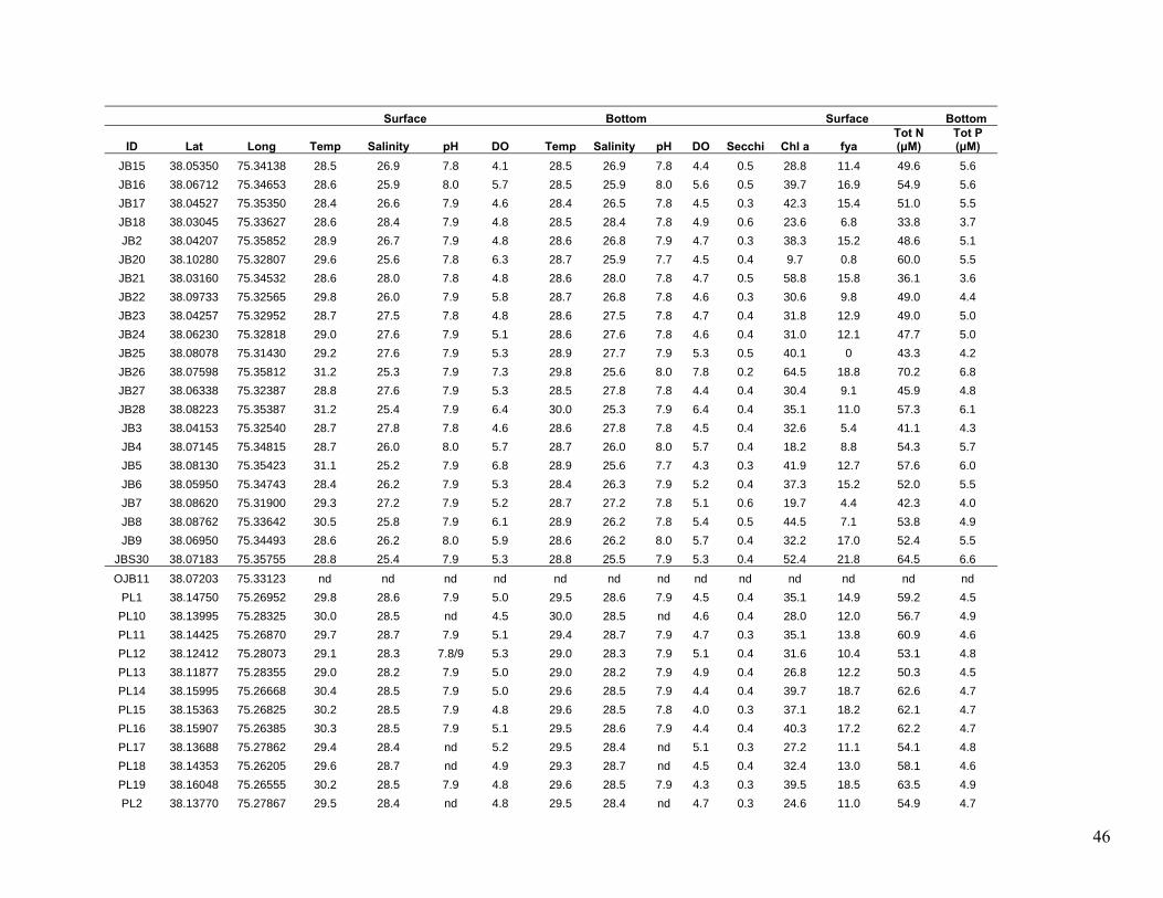
46

Surface Bottom Surface Bottom



Tot P (μM)

JB15 38.05350 75.34138 28.5 26.9 7.8 4.1 28.5 26.9 7.8 4.4 0.5 28.8 11.4 49.6 5.6 JB16 38.06712 75.34653 28.6 25.9 8.0 5.7 28.5 25.9 8.0 5.6 0.5 39.7 16.9 54.9 5.6 JB17 38.04527 75.35350 28.4 26.6 7.9 4.6 28.4 26.5 7.8 4.5 0.3 42.3 15.4 51.0 5.5 JB18 38.03045 75.33627 28.6 28.4 7.9 4.8 28.5 28.4 7.8 4.9 0.6 23.6 6.8 33.8 3.7 JB2 38.04207 75.35852 28.9 26.7 7.9 4.8 28.6 26.8 7.9 4.7 0.3 38.3 15.2 48.6 5.1

JB20 38.10280 75.32807 29.6 25.6 7.8 6.3 28.7 25.9 7.7 4.5 0.4 9.7 0.8 60.0 5.5 JB21 38.03160 75.34532 28.6 28.0 7.8 4.8 28.6 28.0 7.8 4.7 0.5 58.8 15.8 36.1 3.6 JB22 38.09733 75.32565 29.8 26.0 7.9 5.8 28.7 26.8 7.8 4.6 0.3 30.6 9.8 49.0 4.4 JB23 38.04257 75.32952 28.7 27.5 7.8 4.8 28.6 27.5 7.8 4.7 0.4 31.8 12.9 49.0 5.0 JB24 38.06230 75.32818 29.0 27.6 7.9 5.1 28.6 27.6 7.8 4.6 0.4 31.0 12.1 47.7 5.0 JB25 38.08078 75.31430 29.2 27.6 7.9 5.3 28.9 27.7 7.9 5.3 0.5 40.1 0 43.3 4.2 JB26 38.07598 75.35812 31.2 25.3 7.9 7.3 29.8 25.6 8.0 7.8 0.2 64.5 18.8 70.2 6.8 JB27 38.06338 75.32387 28.8 27.6 7.9 5.3 28.5 27.8 7.8 4.4 0.4 30.4 9.1 45.9 4.8 JB28 38.08223 75.35387 31.2 25.4 7.9 6.4 30.0 25.3 7.9 6.4 0.4 35.1 11.0 57.3 6.1 JB3 38.04153 75.32540 28.7 27.8 7.8 4.6 28.6 27.8 7.8 4.5 0.4 32.6 5.4 41.1 4.3 JB4 38.07145 75.34815 28.7 26.0 8.0 5.7 28.7 26.0 8.0 5.7 0.4 18.2 8.8 54.3 5.7 JB5 38.08130 75.35423 31.1 25.2 7.9 6.8 28.9 25.6 7.7 4.3 0.3 41.9 12.7 57.6 6.0 JB6 38.05950 75.34743 28.4 26.2 7.9 5.3 28.4 26.3 7.9 5.2 0.4 37.3 15.2 52.0 5.5 JB7 38.08620 75.31900 29.3 27.2 7.9 5.2 28.7 27.2 7.8 5.1 0.6 19.7 4.4 42.3 4.0 JB8 38.08762 75.33642 30.5 25.8 7.9 6.1 28.9 26.2 7.8 5.4 0.5 44.5 7.1 53.8 4.9 JB9 38.06950 75.34493 28.6 26.2 8.0 5.9 28.6 26.2 8.0 5.7 0.4 32.2 17.0 52.4 5.5

JBS30 38.07183 75.35755 28.8 25.4 7.9 5.3 28.8 25.5 7.9 5.3 0.4 52.4 21.8 64.5 6.6 OJB11 38.07203 75.33123 nd nd nd nd nd nd nd nd nd nd nd nd nd

PL1 38.14750 75.26952 29.8 28.6 7.9 5.0 29.5 28.6 7.9 4.5 0.4 35.1 14.9 59.2 4.5 PL10 38.13995 75.28325 30.0 28.5 nd 4.5 30.0 28.5 nd 4.6 0.4 28.0 12.0 56.7 4.9 PL11 38.14425 75.26870 29.7 28.7 7.9 5.1 29.4 28.7 7.9 4.7 0.3 35.1 13.8 60.9 4.6 PL12 38.12412 75.28073 29.1 28.3 7.8/9 5.3 29.0 28.3 7.9 5.1 0.4 31.6 10.4 53.1 4.8 PL13 38.11877 75.28355 29.0 28.2 7.9 5.0 29.0 28.2 7.9 4.9 0.4 26.8 12.2 50.3 4.5 PL14 38.15995 75.26668 30.4 28.5 7.9 5.0 29.6 28.5 7.9 4.4 0.4 39.7 18.7 62.6 4.7 PL15 38.15363 75.26825 30.2 28.5 7.9 4.8 29.6 28.5 7.8 4.0 0.3 37.1 18.2 62.1 4.7 PL16 38.15907 75.26385 30.3 28.5 7.9 5.1 29.5 28.6 7.9 4.4 0.4 40.3 17.2 62.2 4.7 PL17 38.13688 75.27862 29.4 28.4 nd 5.2 29.5 28.4 nd 5.1 0.3 27.2 11.1 54.1 4.8 PL18 38.14353 75.26205 29.6 28.7 nd 4.9 29.3 28.7 nd 4.5 0.4 32.4 13.0 58.1 4.6 PL19 38.16048 75.26555 30.2 28.5 7.9 4.8 29.6 28.5 7.9 4.3 0.3 39.5 18.5 63.5 4.9 PL2 38.13770 75.27867 29.5 28.4 nd 4.8 29.5 28.4 nd 4.7 0.3 24.6 11.0 54.9 4.7

47

Surface Bottom



Tot P (μM)

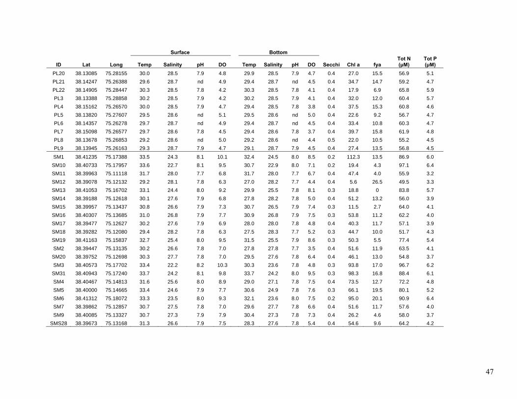
PL20 38.13085 75.28155 30.0 28.5 7.9 4.8 29.9 28.5 7.9 4.7 0.4 27.0 15.5 56.9 5.1 PL21 38.14247 75.26388 29.6 28.7 nd 4.9 29.4 28.7 nd 4.5 0.4 34.7 14.7 59.2 4.7 PL22 38.14905 75.28447 30.3 28.5 7.8 4.2 30.3 28.5 7.8 4.1 0.4 17.9 6.9 65.8 5.9 PL3 38.13388 75.28858 30.2 28.5 7.9 4.2 30.2 28.5 7.9 4.1 0.4 32.0 12.0 60.4 5.7 PL4 38.15162 75.26570 30.0 28.5 7.9 4.7 29.4 28.5 7.8 3.8 0.4 37.5 15.3 60.8 4.6 PL5 38.13820 75.27607 29.5 28.6 nd 5.1 29.5 28.6 nd 5.0 0.4 22.6 9.2 56.7 4.7 PL6 38.14357 75.26278 29.7 28.7 nd 4.9 29.4 28.7 nd 4.5 0.4 33.4 10.8 60.3 4.7 PL7 38.15098 75.26577 29.7 28.6 7.8 4.5 29.4 28.6 7.8 3.7 0.4 39.7 15.8 61.9 4.8 PL8 38.13678 75.26853 29.2 28.6 nd 5.0 29.2 28.6 nd 4.4 0.5 22.0 10.5 55.2 4.5 PL9 38.13945 75.26163 29.3 28.7 7.9 4.7 29.1 28.7 7.9 4.5 0.4 27.4 13.5 56.8 4.5

SM1 38.41235 75.17388 33.5 24.3 8.1 10.1 32.4 24.5 8.0 8.5 0.2 112.3 13.5 86.9 6.0 SM10 38.40733 75.17957 33.6 22.7 8.1 9.5 30.7 22.9 8.0 7.1 0.2 19.4 4.3 97.1 6.4 SM11 38.39963 75.11118 31.7 28.0 7.7 6.8 31.7 28.0 7.7 6.7 0.4 47.4 4.0 55.9 3.2 SM12 38.39078 75.12132 29.2 28.1 7.8 6.3 27.0 28.2 7.7 4.4 0.4 5.6 26.5 49.5 3.3 SM13 38.41053 75.16702 33.1 24.4 8.0 9.2 29.9 25.5 7.8 8.1 0.3 18.8 0 83.8 5.7 SM14 38.39188 75.12618 30.1 27.6 7.9 6.8 27.8 28.2 7.8 5.0 0.4 51.2 13.2 56.0 3.9 SM15 38.39957 75.13437 30.8 26.6 7.9 7.3 30.7 26.5 7.9 7.4 0.3 11.5 2.7 64.0 4.1 SM16 38.40307 75.13685 31.0 26.8 7.9 7.7 30.9 26.8 7.9 7.5 0.3 53.8 11.2 62.2 4.0 SM17 38.39477 75.12627 30.2 27.6 7.9 6.9 28.0 28.0 7.8 4.8 0.4 40.3 11.7 57.1 3.9 SM18 38.39282 75.12080 29.4 28.2 7.8 6.3 27.5 28.3 7.7 5.2 0.3 44.7 10.0 51.7 4.3 SM19 38.41163 75.15837 32.7 25.4 8.0 9.5 31.5 25.5 7.9 8.6 0.3 50.3 5.5 77.4 5.4 SM2 38.39447 75.13135 30.2 26.6 7.8 7.0 27.8 27.8 7.7 3.5 0.4 51.6 11.9 63.5 4.1

SM20 38.39752 75.12698 30.3 27.7 7.8 7.0 29.5 27.6 7.8 6.4 0.4 46.1 13.0 54.8 3.7 SM3 38.40573 75.17702 33.4 22.2 8.2 10.3 30.3 23.6 7.8 4.8 0.3 93.8 17.0 96.7 6.2

SM31 38.40943 75.17240 33.7 24.2 8.1 9.8 33.7 24.2 8.0 9.5 0.3 98.3 16.8 88.4 6.1 SM4 38.40467 75.14813 31.6 25.6 8.0 8.9 29.0 27.1 7.8 7.5 0.4 73.5 12.7 72.2 4.8 SM5 38.40000 75.14665 33.4 24.6 7.9 7.7 30.6 24.9 7.8 7.6 0.3 66.1 19.5 80.1 5.2 SM6 38.41312 75.18072 33.3 23.5 8.0 9.3 32.1 23.6 8.0 7.5 0.2 95.0 20.1 90.9 6.4 SM7 38.39862 75.12857 30.7 27.5 7.8 7.0 29.6 27.7 7.8 6.6 0.4 51.6 11.7 57.6 4.0 SM9 38.40085 75.13327 30.7 27.3 7.9 7.9 30.4 27.3 7.8 7.3 0.4 26.2 4.6 58.0 3.7

SMS28 38.39673 75.13168 31.3 26.6 7.9 7.5 28.3 27.6 7.8 5.4 0.4 54.6 9.6 64.2 4.2

Gracilaria Crassostrea

ID Lat Long %N δ15N Muscle

%N Muscle δ15N

Gill %N

Gill δ15N

Mantle %N

Mantle δ15N

CH1 37.98298 75.33997 1.1 4.0 0.0 0.0 0.0 0.0 0.0 0.0 CH10 37.98242 75.34555 1.0 8.4 nd nd nd nd nd nd CH11 37.96223 75.34678 1.6 8.0 11.6 8.9 7.6 6.9 8.0 7.4 CH12 37.98737 75.35465 1.3 7.4 12.4 9.2 7.9 7.7 8.5 7.8 CH14 37.97767 75.34098 1.5 4.9 11.0 8.3 6.9 7.4 7.5 7.8 CH15 37.93937 75.38305 1.5 6.6 13.0 8.8 8.8 8.9 9.5 7.9 CH16 37.94435 75.38198 1.2 7.3 nd nd nd nd nd nd CH17 37.98967 75.35960 1.3 6.2 12.7 8.5 8.4 7.1 7.6 6.9 CH18 37.95262 75.35868 1.5 7.6 12.0 7.4 8.3 6.5 8.9 7.1 CH19 37.98265 75.32533 1.3 8.7 nd nd nd nd nd nd CH2 37.93622 75.38145 1.2 5.1 12.2 8.6 8.2 8.0 8.3 8.7 CH20 37.96788 75.36257 1.3 7.0 12.6 8.1 7.9 7.6 8.1 7.1 CH22 37.95693 75.36203 1.3 7.3 12.0 7.9 7.8 7.8 8.5 7.0 CH23 37.95453 75.38487 1.5 6.8 nd nd nd nd nd nd CH24 37.96968 75.35548 1.4 8.1 nd nd nd nd nd nd CH25 37.98950 75.32690 1.2 9.1 11.2 6.5 7.8 5.5 6.9 5.1 CH26 37.95050 75.39208 1.2 8.0 nd nd nd nd nd nd CH27 37.95433 75.38858 1.1 8.4 11.2 7.8 8.2 7.1 7.2 7.3 CH28 37.97333 75.36107 1.5 7.3 11.1 7.2 8.0 8.1 8.2 8.0 CH29 37.96627 75.34775 2.0 8.7 10.5 7.2 7.1 6.4 8.1 7.8 CH3 37.96312 75.35247 1.9 7.6 12.6 7.2 8.2 7.0 7.0 6.5 CH30 37.97348 75.38205 1.1 6.9 12.2 8.1 8.6 7.7 9.7 8.4 CH41 37.96667 75.33925 1.4 5.6 nd nd nd nd nd nd CH5 37.99192 75.34642 1.9 5.3 11.1 6.5 7.8 5.3 7.1 5.2 CH6 37.95682 75.38002 1.2 6.4 11.6 7.1 7.3 6.6 7.1 6.5 CH7 37.95260 75.38485 1.4 5.4 10.4 8.3 7.5 8.5 6.2 7.8 CH8 37.95532 75.38225 1.2 4.5 10.7 8.6 7.1 8.4 7.2 8.6 CH9 37.95715 75.36872 1.3 7.7 10.6 8.9 5.7 8.2 6.4 7.6

CHS40 37.93942 75.37870 1.0 8.4 10.5 10.0 7.6 8.8 7.0 8.9 JB1 38.06702 75.33232 3.1 5.3 nd nd nd nd nd nd JB10 38.09378 75.33248 3.0 7.0 14.1 8.6 10.3 7.8 9.8 8.3 JB11 38.06948 75.33080 2.0 6.1 nd nd nd nd nd nd JB12 38.08440 75.33585 3.1 5.9 nd nd nd nd nd nd JB13 38.07332 75.36410 2.5 7.0 nd nd nd nd nd nd JB14 38.09282 75.32577 3.7 6.8 nd nd nd nd nd nd JB15 38.05350 75.34138 2.8 7.3 12.6 9.1 9.0 8.6 8.5 8.2 JB16 38.06712 75.34653 2.6 5.4 nd nd nd nd nd nd JB17 38.04527 75.35350 3.0 6.4 14.0 10.2 8.6 8.8 10.9 9.1 JB18 38.03045 75.33627 3.1 6.9 nd nd nd nd nd nd JB2 38.04207 75.35852 3.1 7.5 12.5 9.7 7.7 8.5 8.2 8.7 JB20 38.10280 75.32807 2.7 7.5 nd nd nd nd nd nd JB21 38.03160 75.34532 2.8 5.2 11.8 10.3 8.6 9.5 9.2 9.6 JB22 38.09733 75.32565 2.9 5.8 nd nd nd nd nd nd JB23 38.04257 75.32952 3.2 8.0 nd nd nd nd nd nd JB24 38.06230 75.32818 3.2 6.7 nd nd nd nd nd nd JB25 38.08078 75.31430 2.8 7.3 nd nd nd nd nd nd JB26 38.07598 75.35812 2.9 5.8 nd nd nd nd nd nd JB27 38.06338 75.32387 2.2 6.1 nd nd nd nd nd nd JB28 38.08223 75.35387 2.8 7.3 nd nd nd nd nd nd JB3 38.04153 75.32540 3.1 7.6 12.4 10.3 11.0 10.2 11.3 10.4 JB4 38.07145 75.34815 2.6 7.8 nd nd nd nd nd nd

49

Gracilaria Crassostrea

ID Lat Long %N δ15N Muscle

%N Muscle δ15N

Gill %N

Gill δ15N

Mantle %N

Mantle δ15N

JB5 38.08130 75.35423 2.8 8.0 12.8 9.1 8.4 7.3 9.9 8.0 JB6 38.05950 75.34743 2.9 7.9 12.0 9.1 7.6 7.6 10.5 8.2 JB7 38.08620 75.31900 3.0 6.9 nd nd nd nd nd nd JB8 38.08762 75.33642 3.0 6.4 nd nd nd nd nd nd JB9 38.06950 75.34493 2.1 7.8 11.6 7.8 8.1 7.6 8.2 7.2

JBS30 38.07183 75.35755 2.1 7.9 nd nd nd nd nd nd OJB11 38.07203 75.33123 nd nd 12.7 8.8 8.4 8.1 7.3 7.6

PL1 38.14750 75.26952 1.9 6.6 11.8 7.7 8.0 7.7 8.3 7.9 PL10 38.13995 75.28325 1.5 7.7 nd nd nd nd nd nd PL11 38.14425 75.26870 1.9 6.5 nd nd nd nd nd nd PL12 38.12412 75.28073 1.7 6.3 nd nd nd nd nd nd PL13 38.11877 75.28355 1.8 7.7 nd nd nd nd nd nd PL14 38.15995 75.26668 2.1 5.8 nd nd nd nd nd nd PL15 38.15363 75.26825 1.9 7.6 11.4 8.7 9.0 7.9 8.3 7.8 PL16 38.15907 75.26385 2.3 6.1 nd nd nd nd nd nd PL17 38.13688 75.27862 2.1 6.6 nd nd nd nd nd nd PL18 38.14353 75.26205 1.8 5.5 nd nd nd nd nd nd PL19 38.16048 75.26555 2.7 6.7 nd nd nd nd nd nd PL2 38.13770 75.27867 2.2 6.9 nd nd nd nd nd nd PL20 38.13085 75.28155 1.8 6.3 12.4 7.9 10.4 7.9 11.2 8.3 PL21 38.14247 75.26388 2.2 5.8 nd nd nd nd nd nd PL22 38.14905 75.28447 1.6 5.9 12.1 9.0 8.0 7.8 7.5 7.5 PL3 38.13388 75.28858 1.6 8.1 13.0 8.7 8.9 8.1 8.8 7.9 PL4 38.15162 75.26570 2.2 6.3 12.5 8.7 9.4 8.3 11.0 8.1 PL5 38.13820 75.27607 1.8 8.2 nd nd nd nd nd nd PL6 38.14357 75.26278 1.7 8.3 nd nd nd nd nd nd PL7 38.15098 75.26577 1.7 6.9 12.9 8.6 9.5 8.2 11.6 8.6 PL8 38.13678 75.26853 1.7 5.1 11.0 8.1 7.7 7.4 8.0 6.9 PL9 38.13945 75.26163 2.4 8.2 nd nd nd nd nd nd SM1 38.41235 75.17388 3.3 6.1 13.6 8.7 9.3 7.6 9.5 7.5

SM10 38.40733 75.17957 3.3 6.0 13.4 8.7 7.8 8.1 5.2 8.2 SM11 38.39963 75.11118 3.1 5.6 12.9 8.2 7.1 6.8 6.7 6.3 SM12 38.39078 75.12132 nd nd nd nd nd nd nd nd SM13 38.41053 75.16702 3.5 6.8 nd nd nd nd nd nd SM14 38.39188 75.12618 2.9 8.2 13.3 9.6 8.0 8.5 7.5 8.7 SM15 38.39957 75.13437 2.3 7.5 nd nd nd nd nd nd SM16 38.40307 75.13685 2.4 6.1 nd nd nd nd nd nd SM17 38.39477 75.12627 3.3 7.3 nd nd nd nd nd nd SM18 38.39282 75.12080 3.1 7.2 nd nd nd nd nd nd SM19 38.41163 75.15837 3.0 6.8 nd nd nd nd nd nd SM2 38.39447 75.13135 2.5 2.5 nd nd nd nd nd nd

SM20 38.39752 75.12698 3.0 7.2 12.7 8.7 8.2 7.8 9.4 8.4 SM3 38.40573 75.17702 3.6 6.0 13.1 9.1 7.3 7.9 7.0 7.9

SM31 38.40943 75.17240 3.8 6.8 12.7 7.5 8.0 7.3 8.2 7.1 SM4 38.40467 75.14813 2.7 5.3 nd nd nd nd nd nd SM5 38.40000 75.14665 2.8 8.4 12.8 9.1 8.2 8.4 9.4 8.4 SM6 38.41312 75.18072 3.1 6.4 12.1 9.1 7.7 7.6 7.0 7.0 SM7 38.39862 75.12857 3.3 5.5 nd nd nd nd nd nd SM9 38.40085 75.13327 2.7 5.1 nd nd nd nd nd nd

SMS28 38.39673 75.13168 3.0 4.7 nd nd nd nd nd nd

Water quality in four regions of the Maryland coastal bays: assessing nitrogen source in relation to...

Documents

Transcript of Water quality in four regions of the Maryland coastal bays: assessing nitrogen source in relation to...