Water Nationalization and Service Quality∗

Fernando Borraz†

Nicolas Gonzalez Pampillon‡

Marcelo Olarreaga§

October 2012

Abstract

The objective of this paper is to explore the impact of Uruguay’s privatization, andthen nationalization of water services on network access and water quality. Resultssuggest that while the early privatization of water services had little impact on accessto the sanitation network, the re-nationalization led to an increase in network accessat the bottom of the income distribution, as well as an improvement in water quality.

JEL: D60, H51, I10, I30, L33, O12Keywords: nationalization, access to sanitation, water quality.

∗We are grateful to the Editor, Elisabeth Sadoulet, Dale Whittington, Guido Porto, Juan Robalino,Roxana Barrantes, Guillermo Valles, Mina Mashayekh, Cristian Rodriguez, and three anonymous referees aswell as seminar participants at a LACEEP workshop in San Jose de Costa Rica, the BCDE 2011 in La Paz,the 2011 LACEA annual meeting in Santiago de Chile, and the Geneva Trade and Development Workshopfor their very constructive comments and suggestions. We are also grateful to Alvaro Capandeguy fromthe Uruguay’s Energy and Water Services regulator (URSEA) for providing us with access to data on thequality of water, and Abelardo Gianola also from URSEA for providing us with information regarding priceregulation before and after the nationalization. The views expressed here are those of the authors and donot reflect necessarily the views of the Banco Central del Uruguay. This work was carried out with the aid ofa grant from the Latin American and Caribbean Environmental Economics Program (LACEEP). All errorsare our responsibility.†Banco Central del Uruguay and Deparmento de Economıa FCS-UDELAR. Email: fborraz@bcu.gub.uy.‡Universidad de Montevideo. Email: ngonzalez@correo.um.edu.uy§University of Geneva and CEPR. Email: marcelo.olarreaga@unige.ch

1 Introduction

In the 1970s the role of the government as provider of basic services in sectors with a

natural monopoly component, such as water supply and sanitation, was hardly questioned.

Indeed, it was thought that private firms were likely to abuse their monopoly power in this

type of market, as they concentrate their supply on rich households, leaving poor households

without access to a basic service. On the other hand, public companies would have incentives

to ensure access to a maximum of potential voters (at least in democracies).

By the late 1980s the weak economic performance and low productivity of many public

companies around the world changed this view (World Bank, 2004). Bad management

practices, due to political agendas rather than profit-oriented motives, shed light on large

inefficiencies and poor quality of services being provided by these public companies. In

the 1990s, privatization of water services was seen by some as a potential solution to the

poor performance of publicly owned water monopolies that left more than 1 billion people

in developing countries without any access to clean and safe water, and 40 percent of the

world’s population without access to safe and clean sanitation services (Segerfledt, 2005).

UNDP in its Human Development Report of 2006 notes that “not having access to water and

sanitation is a polite euphemism for a form of deprivation that threatens life.”And Galiani

et al. (2005) provide empirical evidence that a move towards privatization of water services

in Argentina in the 1990s led to a faster decline in child mortality.

France was an early example of a country with privately provided water services. And

throughout the 1990s many countries engaged in privatization of water services, starting

with England in 1989, followed by Eastern European and Latin American countries. A few

Asian and African countries followed them in the mid and late 1990s (Hall et al. 2010).

Nevertheless, the share of public water companies is still very large.1 Moreover, it has

increased in the last ten years as backlashes to privatization occurred in many countries.

Uruguay is a recent example of this reversal. Until 1993 all water services in Uruguay

were publicly owned, a part from a few small community-based private companies that

1According to Hall et al. (2010) water services are owned and run by the public sector in 90% of thelargest 400 cities in the world. This figure should be compared to the share of formal employment in publiccompanies across all sectors, which is on average 5 percent according to Kikeri (1999).

2

operated in the Department of Canelones since the 1940s in areas that the public company

was not reaching.2 In 1993 a first wave of privatization took place in the Department of

Maldonado affecting around three thousand customers. It was followed by a larger second

wave of privatization in the same department that affected more than 20,000 customers,

including some in the capital of Maldonado. The privatization was reversed in 2004 when

an amendment to the Uruguayan constitution was passed declaring water as “part of the

public domain”. The private provision of water was made illegal.3

The apparent reasons for Uruguay’s re-nationalization of water companies were no

different from the ones observed in other Latin American countries in the last decade (Bolivia,

Argentina, Brazil, etc). Privatization of water services did not keep its promises.4 Private

companies became deeply unpopular due to perceptions, at least, of low or falling quality

of water, as well as the high prices private companies charged. A series of highly publicized

episodes of low quality water supplied by Uragua and Aguas de la Costa (subsidiaries of the

Spanish water companies Aguas de Barcelona and Aquas de Bilbao) led as early as 2003 (in

the middle of a financial crisis) to an also well publicized request by the then Minister of

Economics and Finance, Alejandro Atchugarry, for Uragua to leave the country.

Whether public or private provision of water leads to better access and quality is an

empirical question. The objective of this paper is to explore the impact that the privatization

and then re-nationalization of water services had on the quality of water (microbiological

and inorganic tests) and access to sanitation networks (percentage of households with

water-sealed toilets connected to sewer lines) in Uruguay.

The study of Uruguay’s water services is interesting because household access to

Uruguay’s piped sewerage network is particularly low compared to countries at similar levels

of development. With an access rate below 50 percent Uruguay compares badly with other

Latin American countries such as Chile, Colombia, Mexico and some comparable Brazilian

2For an assessment of the performance of community-driven water providers in developing countries seeWhittington et al (2009).

3In the Netherlands water privatization was also made illegal.4The reason for the failure of privatization is not necessarily inherent to privatization, but may also be

explained by poorly designed contracts (in terms of required investments) or non-adequate regulatory bodies.These are also often associated with problems of corruption (see Chong and Lopez-de-Silanes, 2005).

3

states in terms of income per capita. Also, like in many other Latin American countries,

issues regarding the quality of water provided by private companies were part of the reason

behind the nationalization.

The existing empirical evidence on the impact of privatization on water quality and access

is relatively small and tends to suggest a positive impact of privatization, or the absence of

an impact. Barrera-Osorio et al. (2009) using a difference-in-difference methodology assess

the impact of water privatization in Colombia on several outcomes like coverage (percentage

of households connected to water service) and water quality (frequency of the service and

aspect of water, such as its color). They find that, in urban areas, water access increases and

that water quality improves as a result of privatization, while negative effects on access were

detected in rural areas. This is consistent with the idea that as water services are privatized

the poorest consumers may be the ones left behind.

In a developed country context, Wallsten and Kosec (2005) analyze the effects of water

ownership on water quality, measured as the number of violations of the Safe Drinking Water

Act (SDWA) in the US between 1997 and 2003. Using panel data at the community level, and

controlling for community fixed effects, they find that ownership does not matter in terms

of compliance with the SDWA. This may be due to the fact that the study is undertaken

in a developed country with high levels of income and therefore a strong demand for high

quality water.5

There is also an important literature looking at the impact of the privatization of water

services on child mortality in developing countries. Child mortality is an indirect measure of

water quality, but it has been shown that increases in water access and quality are negatively

associated with child mortality (Lee et al., 1997, Shi, 2000 or Galdo and Bertha, 2005). Using

a panel data setup, Galiani, Gertler and Schargrodsky (2005) provide convincing evidence

that in Argentinean municipalities where water services were privatized, the incidence of child

mortality from water-related diseases declined significantly (whereas the incidence of child

mortality for other reasons remained stagnant). They therefore provide indirect evidence of

5In their review of the literature Nauges and D. Whittington (2009) suggest that income elasticities ofdemand oscillate between 0.1 and 0.4.

4

improvements in water quality and access.6

The empirical methodology we followed is similar to the one in Galiani, Gertler, and

Schargrodosky (2005). Using panel data around the nationalization episode, we identify

differences in sanitation rates and water quality indicators between regions that first

privatized their water suppliers and later nationalized them, and those that did not using

a difference-in-difference estimator. There are however three important differences with

Galiani, Gertler and Schargrodosky (2005). First, as explained above we focus on the

nationalization and not the privatization of water services. Second, for network access

our data spans from the pre-privatization period to the nationalization period. Thus, as

part of our identification strategy we can control for the determinants of privatization when

estimating the impact of nationalization. Third, our dependent variables are direct measures

of the quality of service by water companies (access and quality of water). Health outcomes

are important, in particular child mortality, but they tend to be determined by many other

external factors than water services. In a middle income country, such as Uruguay, child

mortality is more rare than in low income countries, and therefore the quality of water can

improve dramatically without observing any change in child mortality.7 Direct measures of

the quality of water services seem more appropriate in such a context.

Our results suggest that, while the earlier privatization period had little impact in terms

of access to the sanitation network, the nationalization of water services had a positive and

statistically significant impact on access, in particular among household in the bottom 25

percent of the income distribution.

The re-nationalization seems to have led to higher quality of water as well. Indeed,

the impact of nationalization on the detection of abnormal levels in microbiological and

inorganic water tests is always negative and has a relatively large coefficient, suggesting that

6Note that the same critiques towards private water suppliers that were present in Uruguay in the late1990s and early 2000s were present also in the Argentinean press at the time (high prices, water provided byprivate companies being unfit for human consumption, or the fact that these private companies only honorhalf of their investment commitments).

7Over the last decade, the average number of child deaths in Uruguay was 10 per jurisdiction. And of thoseless than 10 percent were water-related. See Borraz and Olarreaga (2011). The reason why in Argentina,which is also a middle income country, the effect of privatization on child mortality was estimated to berelatively large is probably that even though the two countries have similar levels of income per capita,Uruguay is much more homogenous than Argentina in terms of both income and race.

5

nationalization led to an improvement of water quality.

It is important to note that while it may be tempting to conclude from our results that

the public sector can do it as well or better than the private sector, this conclusion cannot be

reached using our empirical evidence. Indeed, the control group in our difference-in-difference

strategy includes cities that were always served by public companies, making it impossible

to answer such a question.8 What the results suggest is that the privatization of water

companies had little impact in terms of network access, confirming the public opinion

that privatization did not keep its promises. However, the re-nationalization of water

companies brought progress in terms of both network access and water quality relative to

those companies that were always publicly owned. This goes against most of the existing

evidence for developing countries that generally shows that water privatization leads to a

higher quality of service.

The reminder of the paper is organized as follows. Section 2 describes the functioning of

the water system in Uruguay. Section 3 discusses the empirical methodology, and Section 4

presents the data and some descriptive statistics. Section 5 presents the results, and Section

6 concludes.

2 The Water System in Uruguay

Until the early 1990s water and sewage services were exclusively provided by a publicly-owned

company, called OSE (Obras Sanitarias del Estado) in most of the country, except for a series

of small community-based providers that were created starting in the 1940s by residents with

the objective of fostering land sales in the area of El Pinar in the Department of Canelones.

The largest of these community-based providers was Aguas Corrientes El Pinar that served

less than 1,000 clients in the 1990s and had only twelve full time staff.

In 1993 the first privatization of water services previously provided by OSE occurred in

the Department of Maldonado. The new company, Aguas de la Costa, supplied water and

sewage in the wealthier areas of La Barra, Manantiales and Jose Ignacio, which are to the

8We are grateful to a referee for this clarification.

6

east of the international well-known resort of Punta del Este. It was a joint-venture between

a local company, S.T.A Ingenerios and Benecio S.A., which had around 10% ownership, and

the Spanish company Aguas de Barcelona, a subsidiary of Suez Lyonaisse des Eaux, which

owned the rest of the company. Aguas de la Costa signed the concession in 1993 for twenty

five years. The company had around 3,100 customers.

A second privatization of water services took place in 2000. Uragua started providing

water and sewage services in urban and sub-urban areas of Maldonado. Maldonado has

150,000 inhabitants from a total of 3,300,000 in Uruguay. Uragua served the west of the

Maldonado stream with the exception of the city of Aigua. More specifically, Uragua served

the capital of Maldonado (50,417 inhabitants), San Carlos (23,878), Pan de Azucar (6,969),

Piriapolis (7,579), Cerros Azules, Nueva Carrara, Pueblo Gerona, West of River Solıs, Silver

River, Highway 9 North, and Punta del Este (7,298 inhabitants).9 Uragua was owned by

Aguas de Bilbao, a Spanish water provider.

Thus, by 2000 only the city of Aigua in Maldonado was served by OSE, and all the other

jurisdictions of Maldonado were served by two private companies: Uragua and Aguas de la

Costa. OSE had an exclusive monopoly in the rest of the country except for the area of El

Pinar which was served by small community-based providers. OSE accounted for more than

90% of all connections.

In 2004 Uragua entered in litigation with OSE because of a breach of contract, following

some well publicized episodes of colored water in Maldonado. This led to a referendum that

declared water as being part of the public domain, and an amendment to the Uruguayan

constitution. Urugua reached a deal with the Uruguayan government and all Uragua assets

were transferred to OSE by the end of 2005. After an agreement with the government, the

company left the country in 2005. Aguas de la Costa assets were transferred to OSE in

2005. Aguas Corrientes el Pinar was nationalized in December 2006 and its assets were also

transferred to OSE.

Maldonado was particularly hit by the nationalization reversal. At the turn of the

century, the only city in Maldonado served by the publicly-owned OSE was Aigua with

9We take all year around population and not the tourist population, which can reach hundreds ofthousands during the summer.

7

2,676 inhabitants. By 2006, OSE was the only provider of water services in Maldonado.

Our empirical analysis will therefore focus on the change of ownership in the Department

of Maldonado, as we do not have data at the city level for the small community-based

providers in the Department of Canelones. As discussed in the data section, when looking

at the impact of the privatization and then re-nationalization of water services on network

access our treated group is restricted to three cities due to data availability. The treated

cities are Maldonado, Pan de Azucar and San Carlos, and we use as a control group 32

cities that include the 19 Department capitals (except Maldonado) and other large cities.

When exploring the impact on water quality we have six treated cities in the Department of

Maldonado: Maldonado, Pan de Azucar, Priapolis, Punta Ballena, Punta del Este and San

Carlos. The control group has twenty six cities that include all the Departments’ capitals,

except Maldonado.

Table 1 shows the evolution of some indicators of the public company OSE before and

after the nationalization. Note that the number of employees did not suffer a substantial

modification after nationalization. This is important because we do not want to attribute

any change in the performance of water companies to a change in the composition of the

workforce due to layoffs at the time of the nationalization. The absence of layoffs was

confirmed through interviews of managers of the water company which indicated that only

top managers of the nationalized companies were let go by OSE. As expected, the volume

of water produced grew after nationalization since the water service coverage increased.

Moreover, the population served with sewerage rose from 531,300 in 2004 to 729,100 in

2006. Total gross fixed assets (including work in progress) increased sharply (around 38%)

between 2004 and 2006. This partly includes acquisitions of the private companies, but also

new infrastructure investments through a sanitation project supported by the World Bank

after nationalization. Finally, OSE’s prices increased sharply in 2003 during the privatization

period and then remained stable after the nationalization. Note that these are the prices

of the public company, but during the privatization period there were no major differences

between prices of public or private companies which were under the control of the energy

and water services regulator: URSEA.

8

3 Methodology

The identification strategy we followed is similar to the one in Galiani et al. (2005) in where

they search for systematic differences in changes in child mortality rates between regions that

have privatized and those that have not changed the ownership structure of water companies

using a difference-in-difference approach.10 We followed their approach but have a double

treatment which includes first the privatization of water providers in some cities and then

their re-nationalization.

Selection bias due to cherry-picking at the moment of privatization is an issue in this

setup. Governments may have decided to privatize companies in cities that were more

profitable and had better prospects in order to maximize the short-run financial benefits from

the privatization. If profitability positively affects performance over time (i.e., performance is

serially correlated) we will observe that nationalization will lead to a better performing water

company, but this was just due to the trend in the performance of water companies in that

region. In this context, even if nationalization adversely affected performance, estimation

might not identify this effect because the treatment group includes a disproportionate number

of utilities that perform well.

We address this issue, as we discuss in the Data section below, using parallel trend

tests for the outcome variables (access to sewage network and water quality) before the

privatization. In the absence of any difference in trends before the privatization, there would

be little evidence of cherry-picking along these dimensions, and time fixed effects in our

difference-in-difference specification can therefore control for these common trends.

Our econometric model is given by:

(1) yit = φNit + γPit + x′itβ + αt + αi + uit

where yit is the outcome variable in city i in year t. We consider two different outcome

variables: sanitation rates, and water quality. The unit of observation i are cities. Nit is a

10Lee et al. (1997) show that this reduced form approach may downward bias the effects of treatment ashouseholds adjust their behavior to the new environment, and provide an alternative structural approach toestimate the impact of better quality on health outcomes.

9

dummy variable that captures the nationalization of the water provider. It is equal to zero

for all cities before the nationalization, and takes the value 1 after the nationalization, but

only in cities where a private water provider existed. Pit is a dummy variable indicating

that the water company in city i in period t is privately-owned; αi is a city specific fixed

effect; αt is a year effect, xit is a vector of control variables, β is the corresponding vector of

coefficients, and uit is a city time-varying error (distributed independently across department

and time).

The parameters of interest are φ and γ which measure the impact of the double treatment

of first the privatization and then nationalization of water services. When sanitation rate

is the outcome variable, a positive value for φ or γ will indicate that nationalization or

privatization of private companies led to larger sanitation rates relative to companies that

were always under public ownership. When considering water quality tests (abnormal levels

of microbiological and organoleptic elements) as the dependent variable, a positive coefficient

implies that nationalization or privatization led to a higher number of tests with abnormal

results relative to companies that were always under public ownership. As discussed in the

next section, because the water quality sample does not cover the pre-privatization period

we do not control for the privatization of water companies when examining water companies.

An important issue in panel data models is that observations tend to be correlated across

time within individual cities. One possible solution to address the serial correlation problem

is to use robust standard errors clustered at the city level. In this context, asymptotic

statistical inference depends on the number of clusters and time periods. A small number of

clusters could result in biased (clustered) standard errors, tending to underestimate inference

precision.

Bertrand, Duflo and Mullainthan (2004) analyzed the performance of different alternative

solutions to the serial correlation problem: 1) parametric methods, that is, specifying an

autocorrelation structure; 2) block bootstrap; 3) “ignoring time series information”, that is,

averaging the data before and after treatment; and 4) using an “empirical variance-covariance

matrix”. Bertrand, et al. find that the latter perform better than the others, but it does not

work properly with small samples. Moreover, Cameron, Gelbach and Miller (2008) states

10

that block bootstrap work properly with small numbers of groups.11

In our case, bootstrap clustered standard errors are similar to clustered standard errors

and in most cases the latter method reports greater standard errors, and in some cases

conventional standard error are larger than the latter. As a conservative criterion, we decided

to report the method with the largest standard errors in each case. Depending on the nature

of the outcome variable: continuous, count or fractional, we will use different estimators that

will be discussed in the results section.

4 Data sources and variable construction

We start describing data sources and variable construction for the analysis of the impact of

nationalization on access to water sanitation networks. We then turn to data sources and

variable construction for the study of the impact of nationalization on water quality.

4.1 Access to sanitation networks

The data regarding the percentage of households with water-sealed toilets connected to

sewer lines are obtained from the annual Uruguayan national household survey, Encuesta

Continua de Hogares (ECH) conducted by the National Statistical Office of Uruguay,

Instituto Nacional de Estadıstica (INE). The ECH is the main source of socio-economic

information about Uruguayan households and their members at the national level. The

surveys were carried out throughout the year with the objective of generating a proper

description of the socio-economic situation of the entire population.

The ECH also includes questions about household living conditions. In particular, the

survey asks whether water-sealed toilets are connected to sewer lines. Hence, we generate

a dummy variable that takes the value 1 if the household is connected to sewer lines and

0 otherwise. Then, we aggregate the data by city in order to obtain the percentage of

households with sanitation access in each city. We therefore work with panel data by

11An alternative solution is to use the method proposed by Bell and McCaffrey (2002) “bias correction ofclustered standard errors”, but unfortunately this approach cannot be applied in a difference-in-differenceset up.

11

city from 1986 to 2009. The time-span includes the pre-privatization period in the case of

Maldonado, as the two privatizations in Maldonado occurred in 1993 and 2000 as discussed

earlier.

The ECH survey is only representative at the Department level or at the city level for the

largest cities in terms of population. Therefore, and to have a representative sample, we keep

only capital cities of the different Departments and other big cities in our sample. We have a

total of 35 cities, three in the treatment group (Maldonado, Pan de Azucar and San Carlos)

and 32 in the control group: Artigas, Bella Union, Canelones, Carmelo, Colonia, Dolores,

Durazno, Florida, Fray Bentos, Lascano, Libertad, Melo, Mercedes, Minas, Montevideo, Paso

de los Toros, Paysandu, Periferia Canelones, Rivera, Rocha, Rosario, Rıo Branco, Salto, San

Jose de Mayo, San Ramon, Santa Lucıa, Sarandı del Yı, Sarandı Grande, Tacuarembo,

Tranqueras, Treinta y Tres, Trinidad and Young.12

Due to the fact that there are some selected cities which were not surveyed in some years

(mainly in the ECH older edition), we have an unbalanced panel which could possibly imply

panel attrition bias. For instance, in the treatment group, of the total 24 time periods,

Pan de Azucar appears 15 times and San Carlos 18 times. In the control group, we have

observations for Lascano in 10 of the 24 time periods, and for Bella Union, Libertad and

Rosario in 12 years, Santa Lucıa in 15 years, Carmelo, Dolores, Paso de los Toros, Rıo

Branco, San Ramon, Sarandı del Yı and Sarandı Grande in 17 years, and Young in 18 years.

So, we have a total of 735 observations13. Some cities started to appear in the ECH because

of their rapid growth in terms of population and therefore we checked the robustness of

results to a smaller sub-sample in terms of time-span: 1993-2009.

The are two observations that need to be made. First, control cities largely exceed

treatment cities and hence we will also estimate our model reducing the number of controls

to only capital cities. The sanitation data of each capital city are available in every year of

the whole period, so in this case panel attrition problems are potentially solved. Second,

since we lose observation as we drop cities, small sample bias could arise. Thus, this could

12Of these 35 cities, only 19 are capital cities.13There are 35 cities. We have 21 cities times 24 (1986-2009 period) which represent 504 observations. In

addition, we have 1 x 10 + 3 x 12 + 2 x 15 + 7 x 17 + 2 x 18 = 231 observations.

12

be seen as a trade-off between small sample bias and possible panel attrition bias, which

provides some robustness checks to our results.

The top panel of Table 2 provides some descriptive statistics by treatment and control

groups for the network access sample before and after the privatization and nationalization.

Overall, the treatment and control group present similar characteristics with relatively small

differences on average, even though they tend to be statistically significant. It will be

important therefore to control for these characteristics in our econometric analysis.14 More

importantly, the network access rates are not statistically different between treated and

control cities before the privatization and before the nationalization. However, treated cities

have a statistically larger network access rate after the nationalization. Whether this can

be attributed to a causal effect will be addressed using the difference-in-difference method

described in the previous section.

As discussed earlier, a concern one may have with our methodology is that even though,

on average, network access rates were not different in control and treated cities before the

privatization (and nationalization), they may have been trending differently which would

bias our estimates of the impact of privatization and nationalization. To address this

we performed a test of parallel trends for the period before the privatization. Thus, we

introduced in the setup of equation (1) a time trend for treated cities, and check for its

statistical significance. Results are reported in Table 3 for different specifications and

samples. In all columns except D, the coefficient on the time trend for treated cities is

statistically insignificant, suggesting that treated and control cities had common trends

before the before the privatization.15 In column D, where we only use department capitals as

treated and control cities, the coefficient is negative and statistically significant. This would

be a concern if we were to find that the nationalization or privatization of water services led

to a decline in network access, which could be explained by its trend before the change of

ownership. But as discussed in the results section, we found that network access increased

before the nationalization and therefore the differences in trends could only downward bias

14These differences reflect the fact that only a few cities were privatized and later nationalized.15We obtain qualitatively identical results when doing a parallel test trend for the period before the

nationalization that are available upon request.

13

the estimated positive impact of the nationalization.

4.2 Water quality

Data on water quality comes from URSEA. In 2004, URSEA jointly with the chemistry

department of University of La Republica created a water quality unit (UAA) which is

in charge of monitoring the water supply system in the whole country, according to the

guidelines of the World Health Organization. This unit carries out several water tests (in

the distribution network) to measure the water quality provided to consumers.

Our units of observation are cities from Uruguay’s 19 Departments. We have data for

the period 2004-2009 but some observations are missing for some of the cities. As treatment

cities we have Maldonado, Pan de Azucar, Piriapolis, Punta Ballena, Punta del Este and

San Carlos. And as control cities: Artigas, Canelones, Colonia, Dolores, Durazno, Florida,

Fray Bentos, La Paloma, La Paz, Las Piedras, Melo, Mercedes, Minas, Montevideo, Pando,

Paysandu, Progreso, Rivera, Rocha, Salto, San Jose, Atlantida, Tacuarembo, Toledo, Treinta

y Tres and Trinidad.16

We have data for two different microbiological tests and two organoleptic tests, which we

will use as outcome variables because of their importance in terms of direct and indirect

negative effects on health. The two microbiological tests are for fecal coliforms, and

pseudomonas aeruginosa. The two organoleptic tests are ph and cloudiness tests.

The first test indicates whether the fecal coliforms exceed the accepted limit value.

The second test indicates whether pseudomononas aeruginosa is present. In the case of

organolpetic tests, the UAA reports the observed value. In the case of ph tests, the upper

limit is 8 mg/Land, and higher levels are considered abnormal. The upper limit in the

cloudiness test is 5, so a result greater or equal to this value represents a high level of

cloudiness in the water, which could indirectly affect health via a higher likelihood of bacteria

formation and a reduction in the quantity of water consumed.

The outcome variable that captures abnormal levels of microbiological or organoleptic

16Note that we have six treated cities in the water sample, instead of only three in the network accesssample. This is still a relatively small number of treated cities which suggests results should be interpretedwith care.

14

substances is constructed as follows. For each test we generate a dummy variable that takes

the value 1 if the test is above the accepted limit and zero otherwise. We then sum these four

binary variables to create a count variable that measures the number of tests that showed

abnormal levels in each city.

One possible drawback of this data is that tests have become better and more precise

over time, allowing to detect more often abnormal levels of substances. This could bias our

estimates, as we would observe a deterioration of the water quality throughout the period

due to better testing techniques, rather than poorer water quality. This is addressed in our

econometric framework by the use of year fixed effects as control variables.

In the bottom panel of Table 2, we provide some descriptive statistics by treatment

and control group. It is important to note that before the nationalization there was no

statistical significant difference in the count of abnormal results between treated and control

cities, while after the nationalization the count of abnormal results was significantly lower

in treated cities.17 And this seems to be driven by a lower count of abnormal levels of

cloudiness and pseudomonoas aeruginosa. Note that we cannot perform a test of parallel

trends because we only have two periods (2004 and 2005) before the nationalization in the

water quality sample. The nationalization dummy takes therefore the value 1 in treated

cities between 2006 and 2009 and the value 0 otherwise. Note also that we do not have

data for the pre-privatization period and therefore we cannot control for the privatization

of treated cities, as the privatization and nationalization of water services would then be

perfectly collinear with the city fixed effects.

5 Results

We start discussing the results of the estimation of equations (1) when access to sanitation

rates is the outcome variable. We then turn to the estimates obtained when water quality

is the outcome variable.

17Note that some of the control variables present some relatively large differences between treated andcontrol cities which reflects again the fact that only a few cities had their water company privatized andlater nationalized.

15

5.1 Access to sanitation networks

We estimate equation (1) for different subsamples, with and without control variables.

Because the left-hand-side variable is a fractional variable (percent of households with

water-sealed toilets connected to sewer lines) we used a Papke and Wooldridge (2008)

estimator. Control variables include average completed years of education of the household

head and average real per capita household income at the city level, as well as accumulated

precipitations at the department level. We expect the three control variables to be positively

correlated with network evacuation rates.

Table 4 presents the results. In all subsamples and specifications there is a positive and

statistically significant impact of “nationalization” on sanitation rates. A positive effect

means that cities where water services were nationalized experienced an increase in access

to sanitation networks. The coefficient which captures the causal impact is on average 0.15,

which means that nationalization led to a 15% increase in access to sanitation networks. The

impact of “privatization” on the other hand is never statistically significant except in column

D where the coefficient is negative and statistically significant. This tends to suggest that

cities that were privatized did not experience an increase in access to sanitation rates relative

to the pre-privatization period.18 Note that these results need to be interpreted with care as

in columns A and B we only have 3 treated cities and in columns C and D only 1 treated city

due to data constraints discussed in section 4.1. However, the low number of treated cities

makes, if anything, more difficult the identification of a statistically significant coefficient as

discussed in McKenzie (2012), which is not the case for the impact of nationalization in the

results reported in Table 4.19

In order to check whether the increase in access to sanitation networks occurred where

we expect it, i.e., among poor households, we aggregate the data at the city level using

only the lower 25th household income percentile in one case and the higher 25th in the

18We also tested whether during periods of public provision of water services (i.e., the pre-privatizationperiod and post-nationalization period) network access was higher and we find a statistically significantcoefficient for most specifications (available upon request). However the coefficients are 50% smaller whenusing this alternative definition, which confirms that most of the positive impact is due to the nationalizationof water services, and not to the pre-privatization period.

19This however may explain the statistically insignificant results for privatization.

16

other.20 We then append these data and introduce a dummy variable that indicates that

the observation corresponds to the bottom 25 percent of the income distribution, as well

as interaction variables between this dummy and the nationalization and privatization

dummy. A positive coefficient between the bottom 25 percent income dummy and the

nationalization dummy would indicate that poor households experienced a larger increase in

their network access after nationalization. Table 5 presents the results for the four different

samples with and without using household head education, household per capita income,

and accumulated precipitations. Without these controls the interaction of the bottom 25

percent income dummy with nationalization is always positive and statistically significant,

but after introducing the control variables, the interaction is only significant for sample D.

The interaction of the bottom 25 percent dummy with the privatization dummy is negative

and statistically significant when using the control variables, but not in the specifications

without. If we combine these results, we have across all samples that the bottom 25

percent has a larger access to the network during the nationalization period than during

the privatization period relative to those firms that were always publicly owned.21

Because serial correlation may be an issue in this difference-in-difference setup, we

parametrically model the serial correlation of the error term as a first autoregressive process

AR(1). We use different estimation methods which imply different assumptions. Results are

reported in Table 6. In the first column, we report feasible generalized least squares estimates,

allowing the error term to be correlated over cities, i.e., we allow for error correlation across

panels or usually called “spatial correlation”. In the second column, error correlation across

individuals is assumed to be identically and independently distributed. In the third column,

we use a within estimator with city fixed effects, and in the last column we provide estimates

using Driscoll and Kraay (1998) method to obtain Newey West type standard errors, which

allow error autocorrelation of the general form. We use the sub-sample, which only includes

capital cities apart from Montevideo. Again, in all cases there is a positive impact of

20Unfortunately the ECH data does not follow households through time and therefore we cannot implementour difference-in-difference methodology at the household level.

21We also tried these regression for households above and below the poverty line. The results, which areavailable upon request, also tend to suggest that the nationalization has helped increase more rapidly theaccess to the network of poor households.

17

nationalization on access to network sanitation.

This increase in sanitation access is consistent with the fact that a USD 50 million

loan was obtained from the World Bank for an OSE project on sanitation and residual

treatment after nationalization of the private companies. However the external funding from

the World Bank to Uruguay’s water company was not unusual. Three loans were granted for

the improvement of water services in Uruguay since 1999 and covered the pre-privatization

period, the privatization period and the nationalization period.22 So there is not a systematic

bias towards the nationalization period. More importantly, we could not find any reference

in official documents that the last loan should be mainly used for improvements in treated

cities (those that were nationalized). Thus, one should not expect that this last loan should

be the reason for the improvement in water services in treated cities. We cannot obviously

exclude that the loan has helped improve access and quality of water in those nationalized

cities, but this seems to have been driving by something deeper than simply the availability

of funds. On its website, OSE has published that after nationalization work related to

sanitation improvements, which has been stopped since 2002, restarted again. Sanitation

projects in Ciudad de la Costa, Punta del Este and Maldonado, where private companies

were located apparently became priority in OSE’s agenda regardless of the availability of

funding from external sources.

5.2 Water quality

The outcome variable is the count of tests that reported an abnormal level of microbiological

or organolpectic substances. This type of right-hand-side variables requires an appropriate

estimator. We will use a Poisson and a Negative Binomial estimator to take into account

over-dispersion in water tests (a non-constant ratio of variance over conditional mean).

22The World Bank has financially supported Uruguay in the development of the water and sanitationservices with 3 investment loans in different time periods: 1) Water Supply Rehabilitation project (1988-1999)- USD 22.3 million; 2) OSE Modernization and Systems Rehabilitation project, APL-1 (2000-2007) – USD27 million; 3) OSE Modernization and Systems Rehabilitation project, APL-2 (ongoing since 2007) – USD 50million. Additionally, there were other loans which focus on technical support: Public Services ModernizationTechnical Assistance project (2001-2008) – USD 6 million. These objective of these loans were to helpUruguay carry out investments in the water sector infrastructure, improving efficiency and coverage of thewater supply and sanitation service. See World Bank (2010) for more details.

18

Because there is a large number of zeros in the data (see Table 2) we also perform a Vuong

test which indicated that the zero-inflated Poisson was the appropriate model.23

We used as control variables accumulated precipitations, minimum temperature and

average temperature at the department level. We expect precipitation to be positively

correlated with the number of abnormal quality tests, since a high level of precipitations

is likely to negatively affect the functioning of the water network, making water tests more

prone to detecting higher levels of undesired substances. Low temperatures could increase

the likelihood of failure of the network distribution system and a high average temperature

could contribute to the reproduction of bacterium like coliforms, so we expect a negative

coefficient on the former and a positive coefficient on the latter.

Table 7 reports the estimates with and without control variables. The first two columns

provide the zero-inflated Poisson estimates, and the last two columns the zero-inflated

Negative Binomial estimates. Control variables have the expected signs across both

specifications, but none of the variables is statistically significant. The nationalization of

water services is always negatively associated with abnormal levels of undesired substances

in water quality tests, and the impact is statistically significant at the 10 percent level.

It is also very large, with a reduction of 0.7 tests per city showing abnormal levels after

nationalization. Thus, results suggest that water quality improved with nationalization.

As discussed earlier, note that due to the small number of treated cities, results should be

interpreted with care even though we have a larger number of treated cities in the water

quality sample than in the network access sample. Also because the water quality sample does

not cover the pre-privatization period, we cannot control for the determinants of privatization

which leaves us with a weaker identification strategy than for the network access sample.24

23When testing the negative binomial estimator, the Vuong tests takes the value 5.79 in the specificationwithout controls and 6.45 in the specification with control. When testing the Poisson estimator, the Vuongtest takes the value 1.81 without controls and the value 1.87 with controls. They all reject at the 5 percentlevel that the ordinary poisson or negative binomial models should be preferred to the zero-inflated estimators,which is not surprising given the large number of zeroes.

24Note that when using instead of a nationalization dummy a public provider dummy that takes thevalue 1 when the cities is served by a water company that is publicly-owned we obtain very similar resultsqualitatively and quantitatively to the ones reported in Table 7.

19

6 Conclusions

The question of market versus government failures in the provision of water services is

complex, and unlikely to be answered without empirical evidence. In this paper we examine

the impact of nationalization of water services on the quality of services. Contrary to most

of the existing literature we identify the impact not only through the privatization of public

firms, but also through the nationalization of private firms. Another important aspect of the

study is the focus on direct measures of service quality (access to the network and quality

of water) rather than on indirect measures such as health outcomes.

Using difference-in-difference estimators, we found that Uruguay’s privatization of water

companies in 1993 and 2000 brought little progress in terms of access to sanitation networks.

However the nationalization of all private companies in 2006 led to an improvement in

access to the sewage network, as well as an improvement in water quality. The improvement

in access following the nationalization of water services tended to be pro-poor with larger

increases in access for poor households.

These results contrast with existing evidence for privatization of water services in other

Latin American countries, which tend to find that privatization led to a decline in child

mortality, and an increase in water access and quality.

Future research should try to disentangle the determinants of these two different outcomes

to help understand why privatization and nationalization had a different impact in Uruguay.

Private and public companies have different objectives: private firms tend to maximize

profits whereas the objectives of public companies are more varied and can go from political

consideration to corruption or social objectives. These differences in objectives are often

behind the calls for both privatization or nationalization (see Chong and Lopes-de-Silanes,

2005) and probably explain part of our empirical findings for Uruguay. However, other

potential explanations may also be important. For example, the type of regulations at

the time of privatization or nationalization (investment requested, universal services), the

functioning of regulatory bodies, or badly designed contracts and bidding processes, can help

reconciliate the results found here and in the rest of the literature. A detailed examination of

these differences will help understand what works and what does not work in terms of water

20

privatization. Also differences in the functioning of public companies (external funding,

composition of the board of directors, etc) could help explain differences at the time of

privatization or nationalization of water services.

Finally, the results in this paper suggest that the focus on private versus public ownership

of natural monopolies such as water providers may be misleading. The institutional

environment under which the natural monopoly operates may be much more important.

21

References

Barrera-Osorio, F., Olivera, M. and Ospino, C. (2009). “Does Society Win or Lose as a

Result of Privatization? The Case of Water Sector Privatization in Colombia” Economica

76(304), 649-674.

Borraz, F. and M. Olarreaga (2011).“Service ownership and access to safe water”. UNCTAD

mimeo.

Chong, A. and F. Lopez-de-Silanes (2005). “Privatization in Latin America: Myths and

realities”, Standford University Press.

Driscoll, J. and A. Kraay (1998). “Consistent Covariance Matrix Estimation With Spatially

Dependent Panel Data”, Review of Economics and Statistics 80(4), 549-560.

Galdo, G. and Bertha, B. (2005). “Evaluating the Impact on Child Mortality of a Water

Supply and Sewerage Expansion in Quito: Is Water Enough?” OVE Working Papers 0105,

Inter-American Development Bank, Office of Evaluation and Oversight (OVE).

Galiani, S., Gertler, P. and Schargrodsky, E. (2005) “Water for Life: The Impact of the

Privatization of Water Services on Child Mortality” Journal of Political Economy, University

of Chicago Press 113(1), 83-120.

Galiani, S., Gertler, P., Schargrodsky, E. and Sturzenegger, F. (2005): “The Benefits and

Costs of Privatization in Argentina: A Microeconomic Analysis”, in Chong, A. and F.

Lopez-de-Silanes (eds.), Privatization in Latin America: Myths and Realities, Standford

University Press.

Hall, D., Lobina, E. and Corral, V. (2010). “Replacing failed private water contracts”, PSIRU

(Public Services International Research Unit), University of Greenwich, London.

Kikeri, S. (1999). “Privatization and labor: what happens to workers when governments

divest?” World Bank, World Bank Technical Paper No. 396.

22

Lee, L., M. R. Rosenzweig, and M. M. Pitt (1997). “The Effects of Improved Nutrition,

Sanitation, and Water Quality on Child Health in High-Mortality Populations”, Journal of

Econometrics 77.

McKenzie, D. (2012), “Beyond Baseline and Follow-up: The Case for More T in

Experiments”, Journal of Development Economics, forthcoming.

Nauges, C. and D. Whittington (2009). “Estimation of water demand in developing countries:

an overview”, World Bank Research Observer 25(2), 263-294.

Papke, L. and Wooldridge, J. M., (2008). “Panel data methods for fractional response

variables with an application to test pass rates”, Journal of Econometrics 145(1-2), 121-133.

Segerfeldt, F. (2005). “Water for Sale: How Business and The Market Can Resolve the

World’s Water Crisis”, Cato Institute, June 2005.

Shi, A. (2000) “ How Access to Urban Potable Water and Sewerage Connection Affects Child

Mortality” The World Bank, Policy Research Working Paper 2274.

Wallsten, S. and Kosec, K. (2005). “Public or Private Drinking Water? The Effects of

Ownership and Benchmark Competition on U.S. Water System Regulatory Compliance and

Household Water Expenditures” AEI-Brookings Joint Center Working Paper No. 05-05.

Whittington, D., J. Davis, L. Prokopy, K. Komives, R. Thorsten, H. Lukacs, W. Wakeman,

and A. Bakalian (2009). “How Well is the Demand-Driven, Community Management Model

for Rural Water Supply Systems Doing? Evidence from Bolivia, Peru, and Ghana.” Water

Policy 11(6).

World Bank (2004). Reforming Infrastructure: privatization, regulation and competition.

World Bank and Oxford University Press, Washington, DC.

World Bank (2010), “Modernizing Public Water Services in Uruguay through a long-term

partnership”, mimeo, Washington, DC.

23

Tab

le1

Indic

ator

sof

the

public

wat

erco

mpan

y:

OSE

Unit

s2002

2003

2004

2005

2006

Serv

ice

Are

aT

otal

pop

ula

tion

-w

ater

supply

’000

inhab

itan

ts3,

158.

43,

178.

23,

100.

73,

245.

03,

253.

7T

otal

pop

ula

tion

-w

aste

wat

er’0

00in

hab

itan

ts1,

791.

61,

805.

91,

541.

21,

919.

01,

935.

7T

otal

num

ber

ofst

aff#

FT

E4.

816

4.50

84.

362

4.17

44.

280

Wate

rServ

ice

Pop

ula

tion

serv

ed-

wat

er’0

00in

hab

itan

ts3,

041.

63,

063.

82,

833.

52,

980.

93,

055.

3W

ater

connec

tion

sye

aren

d’0

00co

nnec

tion

s73

5.1

732.

973

7.7

799.

982

2.5

Vol

um

eof

wat

erpro

duce

dM

illion

m3/

year

282.

727

5.1

288.

130

9.4

320.

0T

otal

volu

me

ofw

ater

sold

Million

m3/

year

135.

313

1.0

132.

314

2.0

147.

1Sew

era

ge

Serv

ice

Pop

ula

tion

serv

ed-

sew

erag

e’0

00in

hab

itan

ts46

7.8

479.

753

1.3

633.

872

9.1

Sew

erag

eco

nnec

tion

sye

aren

d’0

00co

nnec

tion

s16

2.2

166.

116

9.5

195.

620

5.9

Len

gth

ofse

wer

sK

m1,

683.

01,

759.

61,

872.

52,

410.

82,

494.

5F

inanci

al

Info

rmati

on

Tot

alop

erat

ing

reve

nues

Million

UY

pes

osof

2010

3,95

1.3

6,01

5.2

6,03

6.5

6,27

7.3

6,84

8.2

Tot

albillings

tore

siden

tial

cust

omer

sM

illion

UY

pes

osof

2010

2,25

2.1

3,41

7.8

3,53

7.0

3,71

8.0

4,07

0.0

Tot

albillings

toin

dust

rial

cust

omer

sM

illion

UY

pes

osof

2010

840.

91,

219.

01,

269.

51,

340.

11,

499.

5T

otal

wat

eran

dw

aste

wat

erop

erat

ional

exp

ense

sM

illion

UY

pes

osof

2010

2,49

9.8

3,73

6.6

3,73

3.9

3,68

9.6

4,01

0.7

Lab

orco

sts

Million

UY

pes

osof

2010

1,34

2.1

1,85

1.9

1,84

2.9

1,68

8.4

1,84

8.8

Tot

algr

oss

fixed

asse

tsin

cludin

gw

ork

inpro

gres

sM

illion

UY

pes

osof

2010

17,9

07.5

24,0

51.4

23,7

56.2

24,3

30.8

24,6

04.8

Tari

ffIn

form

ati

on

Fix

edch

arge

per

mon

thfo

rw

ater

and

was

tew

ater

UY

pes

osof

2010

86.4

140.

714

4.5

145.

714

5.0

serv

ices

for

resi

den

tial

cust

omer

sp

erm

onth

Con

nec

tion

char

ges

-w

ater

UY

pes

osof

2010

1,41

4.1

1,81

4.4

1,80

3.5

1,89

1.0

1,95

7.6

Con

nec

tion

char

ges

-se

wer

sU

Yp

esos

of20

1056

7.3

726.

772

2.3

757.

178

4.3

Sou

rce:

OS

E

24

Tab

le2

Des

crip

tive

stat

isti

csfo

rtr

eatm

ent

and

contr

olgr

oups

Pre

-pri

vati

zati

onP

riva

tiza

tion

Nat

ion

aliz

atio

n(1

986-

2000

)(2

000-

2005

)(2

006-

2009

)T

reat

edC

ontr

olD

iffer

ence

Tre

ated

Con

trol

Diff

eren

ceT

reat

edC

ontr

olD

iffer

ence

Acc

ess

tose

wage

sam

ple

Net

wor

kE

vacu

atio

nR

ate

0.47

0.44

0.03

0.53

0.49

0.04

0.69

0.54

0.15

**(0

.10)

(0.1

9)(0

.07)

(0.2

1)(0

.10)

(0.2

2)E

du

cati

on(H

ead

ofH

ouse

hol

d)

6.78

6.58

0.20

*7.

227.

180.

047.

827.

770.

05(0

.42)

(0.7

7)(0

.55)

(0.7

3)(0

.38)

(0.7

5)(l

og)

Hou

seh

old

per

Cap

ita

Inco

me

7.90

7.58

0.32

***

7.52

7.43

0.09

*7.

837.

630.

20**

*(0

.10)

(0.2

5)(0

.14)

(0.2

2)(0

.18)

(0.2

1)(l

og)

Acc

um

ula

ted

Pre

cip

itat

ion

s6.

957.

11-0

.16*

**7.

097.

240.

15**

6.97

7.07

-0.1

0(0

.17)

(0.2

3)(0

.20)

(0.2

7)(0

.17)

(0.3

1)O

bse

rvat

ion

s31

385

1516

511

128

Wate

rqu

ali

tysa

mp

leF

ecal

coli

form

sN

AN

AN

A0.

000.

000.

000.

000.

65-0

.65

(0.0

0)(0

.00)

(0.0

0)(6

.19)

Pse

ud

omon

asae

rogi

nos

aN

AN

AN

A0.

000.

04-0

.04

0.00

0.14

-0.1

4**

(0.0

0)(0

.19)

(0.0

0)(0

.35)

ph

NA

NA

NA

7.11

7.35

-0.2

4*6.

947.

310.

37**

*(0

.48)

(0.4

7)(0

.39)

(0.4

8)C

lou

din

ess

NA

NA

NA

1.57

1.73

-0.1

60.

641.

37-0

.73*

*(1

.86)

(1.9

3)(0

.63)

(1.7

4)C

ount

ofn

on-c

omp

lian

cete

sts

NA

NA

NA

0.33

0.46

-0.1

30.

050.

45-0

.40*

**(0

.49)

(0.7

9)(0

.21)

(0.7

8)M

inim

um

tem

per

atu

re(c

)N

AN

AN

A9.

024.

708.

624.

863.

76**

*(0

.30)

(1.1

1)(0

.44)

(1.1

5)A

vera

gete

mp

erat

ure

(c)

NA

NA

NA

16.9

617

.50

0.54

**16

.74

17.5

50.

80**

*(0

.06)

(0.9

4)(0

.15)

(0.9

9)(l

og)

Acc

um

ula

ted

pre

cip

itat

ion

sN

AN

AN

A4.

184.

330.

15**

*4.

204.

290.

09*

(0.0

5)(0

.19)

(0.2

4)(0

.27)

Ob

serv

atio

ns

1254

2294

Sou

rces

:U

RS

EA

,E

CH

and

the

Nat

ion

alM

eteo

rolo

gy

Offi

ce.

Not

e1:

Fig

ure

sin

par

enth

esis

are

stan

dar

dd

evia

tion

s.

Not

e2:

*st

and

sfo

rst

atis

tica

lsi

gnifi

can

ceat

the

10p

erce

nt

leve

l;**

atth

e5

per

cent

leve

l,an

d**

*at

the

1p

erce

nt

level

.

25

Tab

le3

Tes

tof

par

alle

ltr

ends

bef

ore

pri

vati

zati

onin

the

net

wor

kac

cess

sam

ple

a

Var

iable

sA

bB

cC

dD

e

(1)

(2)

(1)

(2)

(1)

(2)

(1)

(2)

Tim

etr

end

0.00

2-0

.003

0.01

0**

0.00

8*0.

003

-0.0

020.

006*

*0.

001

(0.0

02)

(0.0

03)

(0.0

04)

(0.0

05)

(0.0

02)

(0.0

03)

(0.0

02)

(0.0

04)

Tim

etr

end×

treatm

ent

0.00

40.

004

0.00

40.

004

-0.0

00-0

.005

-0.0

07**

-0.0

10**

(0.0

04)

(0.0

06)

(0.0

04)

(0.0

06)

(0.0

03)

(0.0

05)

(0.0

03)

(0.0

05)

Educa

tion

0.03

00.

038

0.03

70.

041*

**(0

.027

)(0

.033

)(0

.027

)(0

.015

)(l

og)

Hou

sehol

dp

erC

apit

aIn

com

e0.

205*

0.23

4**

0.18

5*0.

098

(0.1

05)

(0.1

07)

(0.1

06)

(0.1

04)

(log

)A

ccum

ula

ted

Pre

cipit

atio

ns

0.05

2**

0.05

00.

046*

*0.

053*

**(0

.021

)(0

.043

)(0

.021

)(0

.020

)

Yea

rE

ffec

tsN

oY

esN

oY

esN

oY

esN

oY

esO

bse

rvat

ions

416

416

261

261

400

400

270

270

Log

-lik

elih

ood

-199

.18

-184

.35

-126

.12

-116

.78

-191

.76

-176

.84

-124

.75

-122

.75

Sam

ple

Per

iod

1986

-200

019

93-2

000

1986

-200

019

86-2

000

aE

stim

ates

are

obta

ined

usi

ng

Pap

ke

&W

oold

rid

ge

Fra

ctio

nal

Logit

Mod

el.

Marg

inal

effec

tsre

port

edan

dro

bu

stst

an

dard

erro

rscl

ust

ered

at

city

level

rep

orte

din

par

enth

eses

.A

llm

od

els

incl

ud

eci

tyfi

xed

effec

ts.

*st

an

ds

for

sign

ifica

nce

at

the

10%

level

;**

stan

ds

for

sign

ifica

nce

at

the

5%le

vel

;**

*st

and

sfo

rsi

gnifi

can

ceat

1%le

vel.

bT

reat

men

tU

nit

s(3

citi

es):

Mal

don

ado,

San

Carl

os

an

dP

an

de

Azu

car;

Contr

ol

Un

its

(32

citi

es):

Art

igas,

Bel

laU

nio

n,

Can

elon

es,

Carm

elo,

Col

onia

,D

olor

es,

Du

razn

o,F

lori

da,

Fra

yB

ento

s,L

asc

an

o,

Lib

erta

d,

Mel

o,

Mer

ced

es,

Min

as,

Monte

vid

eo,

Paso

de

los

Toro

s,P

aysa

nd

u,

Per

ifer

iaC

anel

ones

,R

iver

a,R

och

a,R

osar

io,

Rıo

Bra

nco

,S

alt

o,

San

Jose

de

May

o,

San

Ram

on

,S

anta

Lu

cıa,

Sara

nd

ıd

elY

ı,S

ara

nd

ıG

ran

de,

Tacu

are

mb

o,

Tra

nqu

eras

,T

rein

tay

Tre

s,T

rin

idad

and

You

ng.

cS

ame

asin

A.

dO

nly

Mal

don

ado

asT

reat

men

tU

nit

and

the

sam

eC

ontr

ol

Un

its

as

inA

an

dB

.eT

reat

men

tU

nit

s(1

city

):M

ald

onad

o;C

ontr

ol

Un

its

(17

citi

es):

Art

igas,

Can

elon

es,

Colo

nia

,D

ura

zno,

Flo

rid

a,

Fra

yB

ento

s,M

elo,

Mer

ced

es,

Min

as,

Pay

san

du

,R

iver

a,R

och

a,S

alto

,S

anJose

de

May

o,

Tacu

are

mb

o,

Tre

inta

yT

res

an

dT

rin

idad

.

26

Tab

le4

Impac

tof

nat

ional

izat

ion

and

pri

vati

zati

onon

acce

ssto

sew

age

net

wor

kin

Mal

don

adoa

Var

iab

les

Ab

Bc

Cd

De

(1)

(2)

(1)

(2)

(1)

(2)

(1)

(2)

Pri

vate

wat

erp

rovid

er0.

037

0.05

50.

037

0.05

3-0

.003

-0.0

35-0

.086

***

-0.0

81(0

.042

)(0

.066

)(0

.042

)(0

.067

)(0

.036

)(0

.054

)(0

.031

)(0

.049

)N

atio

nal

izat

ion

0.16

3***

0.14

3**

0.16

3***

0.14

0**

0.24

4***

0.17

3***

0.15

4***

0.13

9**

(0.0

53)

(0.0

58)

(0.0

53)

(0.0

61)

(0.0

36)

(0.0

56)

(0.0

37)

(0.0

55)

Ed

uca

tion

0.04

10.

049

0.04

50.

025*

*(0

.028

)(0

.031

)(0

.029

)(0

.012

)(l

og)

Hou

seh

old

per

Cap

ita

Inco

me

0.21

0***

0.22

1***

0.19

1***

0.16

9***

(0.0

63)

(0.0

85)

(0.0

62)

(0.0

60)

(log

)A

ccu

mu

late

dP

reci

pit

atio

ns

0.07

5**

0.07

2*0.

072*

*0.

063*

**(0

.030

)(0

.043

)(0

.030

)(0

.022

)

Ob

serv

atio

ns

735

735

580

580

702

702

432

432

Log

-lik

elih

ood

-355

.21

-331

.55

-282

.16

-263

.89

-340

.11

-316

.54

-198

.54

-195

.19

Sam

ple

Per

iod

1986

-200

919

93-2

009

1986

-200

919

86-2

009

aE

stim

ates

are

obta

ined

usi

ng

Pap

ke

&W

oold

rid

ge

Fra

ctio

nal

Logit

Mod

el.

Marg

inal

effec

tsre

port

edan

dro

bu

stst

an

dard

erro

rscl

ust

ered

at

city

leve

lre

por

ted

inp

aren

thes

es.

All

mod

els

incl

ud

eci

tyan

dye

ar

fixed

effec

ts.

*st

an

ds

for

sign

ifica

nce

at

the

10%

leve

l;**

stan

ds

for

sign

ifica

nce

atth

e5%

leve

l;**

*st

and

sfo

rsi

gnifi

cance

at

1%

leve

l.bT

reat

men

tU

nit

s(3

citi

es):

Mal

don

ado,

San

Carl

os

an

dP

an

de

Azu

car;

Contr

ol

Un

its

(32

citi

es):

Art

igas,

Bel

laU

nio

n,

Can

elon

es,

Carm

elo,

Col

onia

,D

olor

es,

Du

razn

o,F

lori

da,

Fra

yB

ento

s,L

asc

an

o,

Lib

erta

d,

Mel

o,

Mer

ced

es,

Min

as,

Monte

vid

eo,

Paso

de

los

Toro

s,P

aysa

nd

u,

Per

ifer

iaC

anel

ones

,R

iver

a,R

och

a,R

osar

io,

Rıo

Bra

nco

,S

alt

o,

San

Jose

de

May

o,

San

Ram

on

,S

anta

Lu

cıa,

Sara

nd

ıd

elY

ı,S

ara

nd

ıG

ran

de,

Tacu

are

mb

o,

Tra

nqu

eras

,T

rein

tay

Tre

s,T

rin

idad

and

You

ng.

cS

ame

asin

A.

dO

nly

Mal

don

ado

asT

reat

men

tU

nit

and

the

sam

eC

ontr

ol

Un

its

as

inA

an

dB

.eT

reat

men

tU

nit

s(1

city

):M

ald

onad

o;C

ontr

ol

Un

its

(17

citi

es):

Art

igas,

Can

elon

es,

Colo

nia

,D

ura

zno,

Flo

rid

a,

Fra

yB

ento

s,M

elo,

Mer

ced

es,

Min

as,

Pay

san

du

,R

iver

a,R

och

a,S

alto

,S

anJose

de

May

o,

Tacu

are

mb

o,

Tre

inta

yT

res

an

dT

rin

idad

.

27

Tab

le5

Impac

tof

nat

ional

izat

ion

onac

cess

tose

wag

enet

wor

kin

Mal

don

ado

inth

eb

otto

man

dto

p25

%of

the

inco

me

dis

trib

uti

ona

Var

iab

les

Ab

Bc

Cd

De

(1)

(2)

(1)

(2)

(1)

(2)

(1)

(2)

Pri

vate

wat

erp

rovid

er0.

013

0.08

30.

022

0.08

4-0

.030

-0.0

05-0

.152

***

-0.1

19**

(0.0

46)

(0.0

89)

(0.0

47)

(0.0

91)

(0.0

43)

(0.0

53)

(0.0

30)

(0.0

48)

Nat

ion

aliz

atio

n0.

093*

0.14

3**

0.10

5*0.

146*

*0.

158*

**0.

164*

**0.

016

0.04

4(0

.056

)(0

.063

)(0

.056

)(0

.066

)(0

.045

)(0

.053

)(0

.035

)(0

.052

)P

rivate

Wate

rP

rovid

er×

Bott

om

25

perc

ent

0.03

2-0

.134

*0.

013

-0.1

39*

0.02

5-0

.112

***

0.10

1***

0.01

3(0

.024

)(0

.070

)(0

.024

)(0

.072

)(0

.023

)(0

.033

)(0

.015

)(0

.043

)N

ati

on

ali

zati

on×

Bott

om

25

perc

ent

0.10

9***

-0.0

470.

091*

*-0

.049

0.10

8***

-0.0

280.

177*

**0.

094*

*(0

.036

)(0

.041

)(0

.037

)(0

.043

)(0

.022

)(0

.033

)(0

.013

)(0

.042

)B

otto

m25

per

cent

-0.3

62**

*0.

111

-0.3

48**

*0.

103

-0.3

64**

*0.

128

-0.4

15**

*-0

.185

*(0

.018

)(0

.086

)(0

.018

)(0

.093

)(0

.018

)(0

.089

)(0

.009

)(0

.110

)

Con

trol

sN

oY

esN

oY

esN

oY

esN

oY

esO

bse

rvat

ion

s14

7014

7011

6011

6014

0414

0486

486

4L

og-l

ikel

ihood

-653

.93

-597

.64

-524

.11

-482

.46

-625

.26

-568

.37

-341

.32

-338

.75

Sam

ple

Per

iod

1986

-200

919

93-2

009

1986

-200

919

86-2

009

aE

stim

ates

are

obta

ined

usi

ng

Pap

ke

&W

oold

rid

ge

Fra

ctio

nal

Logit

Mod

el.

Marg

inal

effec

tsre

port

edan

dro

bu

stst

an

dard

erro

rscl

ust

ered

at

city

leve

lre

por

ted

inp

aren

thes

es.

All

mod

els

incl

ud

eci

tyan

dye

ar

fixed

effec

ts.

*st

an

ds

for

sign

ifica

nce

at

the

10%

leve

l;**

stan

ds

for

sign

ifica

nce

atth

e5%

leve

l;**

*st

and

sfo

rsi

gnifi

cance

at

1%

leve

l.bT

reat

men

tU

nit

s(3

citi

es):

Mal

don

ado,

San

Carl

os

an

dP

an

de

Azu

car;

Contr

ol

Un

its

(32

citi

es):

Art

igas,

Bel

laU

nio

n,

Can

elon

es,

Carm

elo,

Col

onia

,D

olor

es,

Du

razn

o,F

lori

da,

Fra

yB

ento

s,L

asc

an

o,

Lib

erta

d,

Mel

o,

Mer

ced

es,

Min

as,

Monte

vid

eo,

Paso

de

los

Toro

s,P

aysa

nd

u,

Per

ifer

iaC

anel

ones

,R

iver

a,R

och

a,R

osar

io,

Rıo

Bra

nco

,S

alt

o,

San

Jose

de

May

o,

San

Ram

on

,S

anta

Lu

cıa,

Sara

nd

ıd

elY

ı,S

ara

nd

ıG

ran

de,

Tacu

are

mb

o,

Tra

nqu

eras

,T

rein

tay

Tre

s,T

rin

idad

and

You

ng.

cS

ame

asin

A.

dO

nly

Mal

don

ado

asT

reat

men

tU

nit

and

the

sam

eC

ontr

ol

Un

its

as

inA

an

dB

.eT

reat

men

tU

nit

s(1

city

):M

ald

onad

o;C

ontr

ol

Un

its

(17

citi

es):

Art

igas,

Can

elon

es,

Colo

nia

,D

ura

zno,

Flo

rid

a,

Fra

yB

ento

s,M

elo,

Mer

ced

es,

Min

as,

Pay

san

du

,R

iver

a,R

och

a,S

alto

,S

anJose

de

May

o,

Tacu

are

mb

o,

Tre

inta

yT

res

an

dT

rin

idad

.

28

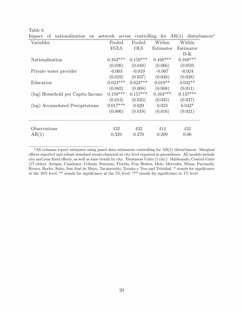
Table 6Impact of nationalization on network access controlling for AR(1) disturbancesa

Variables Pooled Pooled Within WithinFGLS OLS Estimator Estimator

D-KNationalization 0.163*** 0.159*** 0.168*** 0.168***

(0.026) (0.048) (0.066) (0.059)Private water provider -0.003 -0.019 -0.007 -0.024

(0.019) (0.037) (0.048) (0.038)Education 0.024*** 0.023*** 0.019** 0.032**

(0.003) (0.008) (0.008) (0.011)(log) Household per Capita Income 0.159*** 0.157*** 0.164*** 0.137***

(0.013) (0.035) (0.035) (0.037)(log) Accumulated Precipitations 0.017*** 0.029 0.023 0.042*

(0.006) (0.018) (0.016) (0.021)

Observations 432 432 414 432AR(1) 0.329 0.270 0.209 0.06

aAll columns report estimates using panel data estimators controlling for AR(1) disturbances. Marginaleffects reported and robust standard errors clustered at city level reported in parentheses. All models includecity and year fixed effects, as well as time trends by city. Treatment Units (1 city): Maldonado; Control Units(17 cities): Artigas, Canelones, Colonia, Durazno, Florida, Fray Bentos, Melo, Mercedes, Minas, Paysandu,Rivera, Rocha, Salto, San Jose de Mayo, Tacuarembo, Treinta y Tres and Trinidad. * stands for significanceat the 10% level; ** stands for significance at the 5% level; *** stands for significance at 1% level.

29

Table 7Impact of nationalization on water qualitya

(count of abnormal tests of levels of microbiological elements)

Poisson Negative BinomialVariables (1) (2) (3) (4)

Nationalization -0.651* -0.642* -0.650* -0.665*(0.357) (0.371) (0.355) (0.390)

Education 0.367 0.466(0.247) (0.306)

(log) Household per capita income -0.016 0.145(0.865) (0.848)

Precipitations 0.423 0.611(0.330) (0.385)

Minimum temperature -0.146 -0.235(0.118) (0.165)

Average temperature 0.014 0.002(0.146) (0.149)

City Effects Yes Yes Yes YesYear Effects Yes Yes Yes YesObservations 182 182 182 182Log Likelihood -101 -100 -101 -100

aAll columns report estimates using a zero inflated model. Marginal effects reported and robust standarderrors clustered at city level reported in parentheses. All models include city and year fixed effects. Vuongtests indicated that the zero inflated models are appropriate. * stands for significance at the 10% level; **stands for significance at the 5% level; *** stands for significance at 1% level. Treatment units (6 cities):Maldonado, Pan de Azucar, Piriapolies, Punta Ballena, Punta del Este and San Carlos. Control units(26 cities): Artigas, Canelones, Colonia, Dolores, Durazno, Florida, Fray Bentos, La Paloma, La Paz, LasPiedras, Melo, Mercedes, Minas, Montevideo, Pando, Paysandu, Progreso, Rivera, Rocha, Salto, San Jose,Atlantida, Tacuarembo, Toledo, Treinta y Tres and Trinidad.

30