Water Loss 2007 - Volum I

IWA International Specialised Conference 23 – 26 September 2007

Bucharest, Romania

Conference chair: Anton ANTON (Romania)

Scientific Committee

• Chair: Roland LIEMBERGER (Austria)

• Bambos CHARALAMBOUS (Cyprus)

• Francisco CUBILLO (Spain) • Mary Ann DICKINSON (USA) • Marco FANTOZZI (Italy) • Malcolm FARLEY (United

Kingdom) • Dewi ROGERS (Italy) • Tim WALDRON (Australia)

Organising Committee

• Chair: Prof. Marin SANDU • Costin BEREVOIANU • Ardeleanu BOGDAN • Dorin CIATARAS • Vasile CIOMOS • Toma IOAN • Mircea NICULESCU • Gabriel RACOVITEANU • Felix STROE • Ilie VLAICU

Descrierea CIP a Bibliotecii Nationale a Romaniei Water Loss 2007 : Conference Proceedings : Bucharest – Romania : 23-26 September 2007 / ed: Vasile Ciomos, Eugenia Demetrescu, Silviu Lacatusu, Razvan Horac Bubuianu – Bucuresti: Estfalia, 2007

3 vol. ISBN 978-973-7681-24-9 Vol.1. – Bibliogr. – ISBN 978-973-7681-25-6

I. Ciomos, Vasile (ed.) II. Demetrescu, Eugenia (ed.) III. Lacatusu, Silviu (ed.) IV. Horac Bubuianu, Razvan (ed.) 628.179.3(03) 628.147(063)

Conference Proceedings Volume I

Source: Water and Sanitation Program of the World Bank

Foreword

One of the major challenges facing many water utilities around the world is a high level of water losses ei-ther through real losses (leakage) or apparent losses (meter under-registration, theft of water). This differ-ence between the amount of water put into the distribution system and the amount of water billed to con-sumers is known as “Non-Revenue Water” (NRW). According to a recent World Bank discussion paper1 the total cost to water utilities caused by NRW worldwide can be conservatively estimated at $15 billion/year.

Not understanding the magnitude, sources, and cost of NRW is one of the main reasons for insufficient NRW reduction efforts around the world. Only by quantifying NRW and its components, calculating water loss performance indicators, and turning volumes of lost water into monetary values can the NRW situation be properly understood and the required action taken.

For the last ten years the Water Loss Task Force (WLTF) of the IWA's Specialist Group on "Efficient Operation and Management of Urban Water Systems" is developing and advocating new concepts and methodologies that can help water utilities to reduce water losses more efficiently.

A part of the WLTF's efforts is the organisation of specialised conferences and the biggest so far was "Leakage 2005", an event that took place in Halifax, Canada in September 2005. More than 50 high quality papers were presented during this three day event.

Two years have passed since and the global water industry is showing even more interest in the work of the WLTF – and especially in the WLTF's 2007 conference: “Water Loss 2007” in Bucharest, Romania where some 90 papers from around the world will be presented, the majority of them included in these pro-ceedings.

I like to take the opportunity to thank the members of the Scientific Committee (Francisco Cubillo, Prof. Anton Anton, Bambos Charalambous, Tim Waldron, Mary Ann Dickinson, Malcolm Farley, Marco Fantozzi and Dewi Rogers) for reviewing close to 120 abstracts and helping me to put the program for “Water Loss 2007” together.

However, it would not have been possible to organise “Water Loss 2007” and publish these proceed-ings without the enormous efforts of ARA, the Romanian Water Association. I would like to thank the Man-agement and the Staff of ARA for all the hard work, in particular Cristina Popescu, Eugenia Demetrescu, Silviu Lacatusu, Daniel Zaharia and Vasile Ciomos.

In June 2007 I had the opportunity to visit SABESP, the water utility of São Paulo, Brazil. One of their leak detection specialists showed me the Leakage 2005 proceedings – downloaded from the Internet and nicely printed and bound. He referred to it as the "best water loss management publication". I sincerely hope that the “Water Loss 2007” proceedings will be considered an equally useful reference document for water loss management professionals around the world.

Roland Liemberger Chair, Scientific Committee

1 The Challenge of Reducing Non-Revenue Water (NRW) in Developing Countries - How the Private Sector Can Help: A Look at Performance-Based Service Contracting, WSS Sector Board Discussion Paper #8, World Bank, 2006, by William D. Kingdom, Roland Liemberger, and Philippe Marin

I

VOLUME 1 Session A1 1. Action plan water loss reduction Liviu Litescu 2. Measures to increase the reliability of drinking water distribution networks Calin Neamtu 3. Water loss management in the distribution system of Brasov city Teodor POPA, Dan Ganea Session A2 4. Night Flow Analysis of Pilot DMAs in Ottawa Osama Hunaidi, Ken Brothers 5. When is a DMA not a DMA? S Hamilton 6. Optimum Size of District Metered Areas Osama Hunaidi, Ken Brothers 7. Sustainable District Metering J A E Morrison, S Tooms, G Hall Session A3 8. Alternative Approaches to Setting Leakage Targets Stuart Trow 9. Do you know how many of your colleagues will come to your funeral? D Pearson 10. An Action Planning Model to Control for Non-Revenue Water Michel Vermersch, Alex Rizzo Session A4 11. City of Vienna – Network Information System – How to record the condition of water distribution systems Michaela Hladej 12. Managing the “Repair or Replace” dilemma on Water Leakages S. Christodoulou, C. Charalambous, A. Adamou 13 . “Inliner-“ and “Close Fit” Technologies - Potentials and Advantages for Water Pipe Rehabilitation U. Rabmer-Koller Session B1

14. Acceptable Level of Water Losses in Geneva H. Guibentif, H.P. Rufenacht, P. Rapillard, M. Rüetschi Session B2 15 . Water Loss Performance Indicators R. Liemberger, K. Brothers, A. Lambert, R McKenzie, A Rizzo, T Waldron 16. Benchmarking of losses from potable water reticulation systems – results from IWA Task Team R S Mckenzie, C Seago, R Liemberger

1

13

22

32

47

57

68

75

86

94

108

115

126

138

148

161

II

17. Experiences with Water Loss PIs in the Austrian Benchmarking Project J. Kölbl, H. Theuretzbacher-Fritz, R. Neunteufel, R. Perfler, G. Gangl, H. Kainz , R. Haberl 18. Analysing London’s Leakage – Experiences of an Expert Witness J Parker Session B3 19. Case studies in applying the IWA WLTF approach in the West Balkan region: Pressure management Jurica Kovac 20. Pressure Management Works……and Doesn’t! P. V. Fanner 21. Design and Establishment of a Very Large Scale Low Pressure DMA Project V Anuvongnukroh, U Makmaitree, T Chuenchom, S Sethaputra, T Waldron Session B4 22. The Modulation of the Pressure in Casablanca - LYDEC Elhassane Benahmed, Diego LUCENTE, Gabriel Lorrain 23. Effective Pressure Management of District Metered Areas B Charalambous Session C1 24. Including the effects of pressure management in calculations of Short-Run Economic Leakage Levels Fantozzi, Dr M, Lambert, A. 25. Water Loss Control in North America: More Cost Effective Than Customer Side Conservation – Why Wouldn’t You Do It?! R. Sturm, J. Thornton 26. An Approach to Determining the True Value of Lost Water: California’s Avoided Cost Model M. A. Dickinson Session C2 27. Water Loss management strategies in Kayseri, Turkey Vedat Uyak, Oktay Ozkan, Ozgur Ozdemir , Fatih Mehmet Durmuscelebi 28. Managing UFW in Iran Sattar Mahmoodi 29. Water Loss Management in difficult operating situations Experience with NRW reduction in Latina Province (Italy) Hébel P. Session C3 30. A procedure based on Performance Indicators in Water Distribution Systems for the identification of Scenarios in terms of water losses reduction and structural improvements Cristiana Bragalli, Tonino Liserra, Marco Maglionico 31. Investigarea pierderilor de apa în retelele de distributie. Studiu de caz Anton ANTON, Lucian SANDU, Sorin PERJU 32 . Predicting leakage rates through background losses and unreported burst modelling O. Chesneau, B. Bremond, Y. Le Gat.

176

188

199

214

226

237

241

256

268

281

286

290

296

307

318

325

III

Session C4 33 . Active leakage control project; the particular DMA’s in the city of Skopje. Macedonia B. Ristovski, S. Spirovska 34 . Water Losses in Maputo Water Supply System An Overview of the Strategic Plan for Leakage Reduction J. V. Q. Langa; J. Quessouji VOLUME 2 Session A5 35 . Relationship between Water Losses and Financial Elements Study Case - Romanian Water Sector Augustin Boer 36 . Measures for reduction of water losses from the distribution networks of the localities from Constanta Country. Aurel PRESURA, Nicolae PITU 37 . Reaching optimum level of looses in the distribution network – a balance between the rehabilitation measures and the supportability of the consummers Gabriel Racoviţeanu, Sandu Marin Session A6 38 . GIS Acoustic Mapping in Ottawa Kenneth J. Brothers, P. 39 . Using an AMR System to Aid in the Evaluation of Water Losses: A Small DMA Case Study at East Bay Municipal Utility District, USA Andrew Chastain-Howley, David Wallenstein 40 . Managing London’s Leakage – How London’s other water company achieves its leakage targets J Parker 41 . Leak Location and Repair Guidance Notes and….. The Never Ending War against Leakage Richard Pilcher Session A7 42 . Water Loss Management for Utilities in Low Income Countries: Case studies from Four African Water Utilities S.M. Kayaga, I.K. Smout 43. A Case Study of Leakage Management in Medellin City, Colombia F Garzon-Contreras, C Palacio-Sierra 44 . Non-Revenue Water Reduction in Indonesia The Challenge and the Way Forward Chris Ingram, Ahmad Hayat Session B5 45. Audit of 29 Water Distribution Networks of Romania J Valverde , V Ciomos

338

351

363

370

380

389

394

404

412

423

434

444

454

IV

46. The Dimension and Significance of Water Losses in Turkey M. Çakmakcı, V. Uyak, İ. Öztürk, A. F. Aydın, E. Soyer, L. Akça 47. Influence of Measurement Inaccuracies at a Storage Tank on Water Losses G. Gangl, J. Kölbl, G. Haas, E. Hassler, D. Fuchs-Hanusch, P. Kauch Session B6 48. The reality of undertaking a large leakage control project Dewi Rogers, Corrado Rossi 49. Sustainable reduction of water loss in urban water distribution systems Erwin Kober 50. Combating Non-Revenue Water in a large multi-functional company; A case study of EPAL; Portugal’s largest water supplier A Donnelly Session B7 51. Pressure management extends infrastructure life and reduces unnecessary energy costs J. Thornton, A.O. Lambert 52. Research on pressure-leakage relationship in water networks of housing estates Wojciech KORAL 53. A closer look at measured night flows in sectorised networks R P Warren Session C5 54. Advanced Pressure Management via Flow Modulation; the Dartmouth Central PMA Carl D. Yates, Graham D. MacDonald 55 . Pressure-management in mature networks using batch-processed pressure-dependent hydraulic modelling S Tooms, N Tansley, A Green Session C6 56. Quatification of mater errors of domestic users: a case study Arregui F.J., Pardo M.A., Parra J.C., Soriano J. 57. Some experience in reduction of losses in Belgrade water supply system Stevo Savić 58 . When Customers Don’t Pay: The Problem of Unpaid Bills R H Jones Session C7 59 . Managing leakage economically D Rogers, M Gastaldi, A Figliolini 60 . Research for the establishment of an optimum water loss reduction level from the economic point of view Al. Manescu, B. Manescu 61 . Technical and economical evaluation of integrated approach to the water loss management in the Czech Republic Zdeněk Sviták, Eva Radkovská, Iva Čiháková

464

474

485

493

501

511

522

531

541

549

554

566

576

587

595

601

V

VOLUME 3 Session A8 62. Appropriate materials to use for potable water service connections Nigel Ellul 63. WaterPipe project: an innovative high resolution Ground Penetration Imaging Radar (GPIR) for detecting water pipes and for detecting leaks and a Decision-Support-System (DSS) for the rehabilitation management of the water pipelines G. Kiss, K. Koncz, C. Melinte 64. Comprehensive solution of water loss reduction Kolovrat Oldřich, ISviták Zdeněk Session A9 65. Hidden benefits of small Scale performance based public private partnerships R S Mckenzie, W Wegelin, P Mohajane, S Shabalala 66 . Performance based Non-Revenue Water Reduction Contracts R Liemberger, W D Kingdom, P Marin Session B8 67. Understanding the components of your Infrastructure Leakage Index (ILI) is necessary to develop a successful strategy to reduce the overall ILI value – especially in systems with a low ILI S. J. Preston, R. Sturm 68. Studies of reference values for the linear losses index in the case of rural water distribution systems RENAUD Eddy, BREMOND Bernard, POULTON Matthew Session B9 69. Calculation, Estimation and Uncertainty in the Apparent Losses Volume in the Water Supply System of Canal de Isabel II. E. H. Sánchez

70. Trials to Quantify and Reduce in-situ Meter Under-Registration Alex Rizzo, Michael Bonello, Stephen Galea St. John 71. UFR – an innovative solution for water matter under registration – case study in Jerusalem, Israel Amir Davidesko 72 . Meter Under-Registration caused by Ball Valves in Roof Tanks B Charalambous, S Charalambous, I Ioannou

Session C8 73. Snapshot ILI - a KPI-based tool to complement goal achievement S. Riolo 74. Practical experiences in applying advanced solutions for calculation of frequency of intervention with Active Leakage Control: results obtained Benvenuti, D 75 . Remote DMA Monitoring As a Useful Tool In Water Loss Control Wojciech KORAL, Slawomir KEDZIERSKI M.

612

621

631

642

654

664

674

684

695

704

710

720

727

736

VI

Session C9 76. Leakage Detection - Assessment of four different leakage control techniques E. Algaard, P. Campbel , J. Picarel 77. An Economic Active Leakage Control Policy without a Performance Indicator is not a Myth S. Hamilton 78. Innovations in step testing using sluice valve metering A Arscott 79. Development of an Enterprise System of Integrated Water Leakage Management Applications (i WLMA) for Bangkok’s Metropolitan Waterworks Authority B Chuenkul, P Singhaprink, T Chuenchom, J Pingclasai, R S Mckenzie POSTER 80.Reabilty and availability analysis for water distribution network C. GAVRILA 81. Cost efficient leakage management in water supply systems M. Hammerer 82. Integrated Decision Support for Water Loss Management in Water Distribution Networks in Developing Countries by the example of Peru Ana Cangahuala Janampa, Wilhelm Urban 83 . Monitoring System for the close meshed Water-pipe network to the City of CRAILSHEIM - Germany Christian SAX, Markus Schreitmüller 84 Trunk Mains Leakage – The missing part of the jigsaw A Bond, D Marshallsay. 86. Decision Support System (DSS) for Water Loss Reduction: Approach Based on Simulation Models T. Liserra, S. Artina, C. Bragalli, C. Lenzi 87. Reliability assessment & data classification using discriminant functions & factor analysis V. Kanakoudis, S. Tsitsifli

744

752

762

772

782

790

800

809

817

826

836

- 1 -

ACTION PLAN

WATER LOSS REDUCTION

SEPTEMBER 2007

- 2 -

ACTION PLAN WATER LOSS REDUCTION

Liviu Litescu,

Veolia Water, Apa Nova Bucharest, [email protected]

Linear loss index instead of output

Output

The network’s output is given by the following formula:

Output = (Billed Volume/ Produced Volume)*100

Hence, we may note from the beginning that this value depends on various factors which will be listed later on, particularly on volume variations. Let’s take for instance the following situation:

First year

Produced volume = 100, billed volume = 80 output = 80%, lost volume = 20

8 year The lost volume remains the same (20), but the billed volumes are lower. Produced

volume = 70, billed volume = 50 output = 50 / 70 = 71 %.

Volume losses remained constant and output decreased.

Therefore, on the technical level, the network output is not a relevant indicator in the monitoring of lost volumes. We’ll shortly define and use more technical instruments for loss reduction, such as linear loss indicators. On the other hand, the output can be an useful ratio as far as the sustainable development is concerned.

Linear loss index (LLI) Among the various values and indicators, the lost volume and the Linear Loss Index are assuredly the most adequate elements for monitoring the evolution of the networks over time.

Lost Volume = Produced Volume – Billed Volume

LLI = Lost Volume / (L transfer pipes + distribution)

Linear repair index

The linear repair index allows the monitoring of network status and the adjustment of appropriate rehabilitation programs.

LRI = total number of losses / total network length

- 3 -

This index is calculated for the duration of a year.

Bucharest Network

Structural characteristics

The Bucharest network can be defined according to the following chart:

Transport from the production plants to the pumping plants (PP) through aqueducts with gravitational flow.

Low pressure network : transport from the PP to the re-pumping plants (RP) and booster stations (HP) + low pressure distribution network.

High pressure network : high pressure distribution.

D e m a n d e g lo b a lee n d is tribu tio n

D e m a n d e g lo ba led u q u a rtie r

P ro d u ctio n

P u m p in g p la n t

R e p u m p in g p la n t o rh yd ro p ho re p la n t

L ow presure d is tr ib u tion

H ig h presure d is tr ib u tion

Length structure by categories:

180 km of aqueducts ;

490 km of transfer pipes (DN≥300mm);

1.600 km of distribution pipes ;

93.000 water connections counting about 700 km of length.

- 4 -

62.0%

11.4%4.0%

10.3%11.3%

1.0% 0.02%0%

10%

20%

30%

40%

50%

60%

70%

80%

90%

100%

GRA

Y CA

STIR

ON STEE

L

PREM

O

AZBO

PEH

D

DU

CTIL

ECA

ST IR

ON

OTH

ER

PERCENTAGE NETWORK DISTRIBUTION ACCORDING TO THE MATERIAL

Exploitation characteristics

The network in Bucharest has known significant losses over time. In 2001, when the Contract was signed, 19.000 losses were solved, compared with 14.300 in 2005.

The linear repair index for damages has decreased from 6,7 to 5,1 in 4 years.

Average LRI in France: about 0,5 – in Bucharest : 5

10 times as many losses

1. Global balance 2003-2006

Evolution of produced and billed volumes

When the Contract was signed, the average consumption per capita was of about l 424 litres/day/inhabitant. In 2006, it had decreased to 223 litres /day/ inhabitant.

This natural phenomenon can be mainly explained by the fact that the population has become aware of the need to save the resources and to reduce the housing costs (electricity, water etc.)

EVOLUTION OF THE DRINKING WATER VOLUMES PRODUCED AND BILLED

Year Produced Volumes (thousand m3) Billed Volumes (thousand m3)

2003 455 220,4 2004 387,4 195,2 2005 326,5 173,5

2006 (Estimated) 300 165

- 5 -

Evolution of gained volumes

ANB has recovered a cumulated volume of about 100 millions m3 from 2003 to 2006.

Evolution of the loss linear index (LLI) and output

LLI has decreased significantly from 2003 to 2006. The reduction amounted to 42%.

2. How to install meters and distribute properly

Installing meters

In order to reduce lost volumes, we need to have an accurate knowledge of the produced and billed volumes. Hence, from the beginning of the concession, ANB has lead simultaneously 2 priority actions:

Evolution of gained volumes

0 20

40 60

80 100 120 140

2003 2004 2005 200644%

46%

48%

50%

52%

54%

56%

Gained volume Output

Evolution of the Daily Loss Linear Index

0

50

100

150

200

250

2003 2004 2005 2006

LLI Bucharest LLI EU

- 6 -

Installing flow meters for production. ANB has installed over 50 electromagnetic flow meters in the repression area of the drinking water production plants and in the in repression areas of the pumping plants.

Achieving compliance for the meter stock: over 96% of the meter stock was replaced. The aim was to achieve stock compliance and to resize meters (60.000 resizing).

Division into sectors

In order to locate the areas with the most important losses in a 2800 km network (including the water connections), the network was divided into sectors, which involved a rigorous long-term process.

Cumulation meter replacement

0

20 000

40 000

60 000

80 000

100 000

2002 2003 2004 2005 2006

No of replacements Meter stock

- 7 -

This lead to the creation of:

5 low pressure sectors corresponding to the areas of influence of the pumping plants. In order to achieve this activity, we had to :

→ Set the hydraulic limitations for each sector, attributing a code to each one of them;

→ Set an optimum number of sections (network valves) to remain open and with flow meters, in order to ensure volume control and the safety of the operation of the network;

→ Avoid the creation of terminus points in the network that would influence the quality of the water;

→ Set maximum diameters, speed and flows for flow meters ;

→ Attribute sector codes to clients from the commercial database ;

→ To allot, in each area, the 90000 water connections for clients.

240 sub-sectors of low and high pressure :

→ Following the analysis of the hydraulic configuration of the network, each low pressure sector was divided, according to the GIS plans, in several sub-sectors of low and high pressure ;

→ On site checks of the status of valves and connections between the low pressure network and the high pressure network.

- 8 -

3. Measures implemented by ANB

The Centre for Water Movement (CMA)

Aside from loss reduction, CMA has to fulfil the following tasks: Achievement of the monthly balances for all the sectors and sub-

sectors in the network, containing loss linear indexes and output; Analysis of the balance results and loss monitoring; Monitoring the pressure policy related to the objectives of loss

reduction and service guarantee, according to CC requirements; Modelling the network, in view of the elimination of areas with

numerous hidden losses, the elimination of illicit users and the increase of speed in the networks.

Operating centres

The Operating Centres exploit the water and sewage networks. About 50 people are in charge, during a part-time job, of improving the output:

The studies and analyses teams: personnel drawing up balances for sub-sectors;

Teams in charge of detecting illicit users ;

Field teams: detecting losses, measuring flows and pressure, checking clients etc.

Technical Division

The TD has 3 acoustic correlators and it has created a ten-people team. Two others new corelators will be purchased in order to have an exact distribution of the emergency curative activity of the preventive organised operations.

4. Strategic actions

Pressure control

2 criteria are considered when dealing with the issue of pressure control: energy costs and lost volumes.

The logic adopted in Bucharest since 2002 has consisted in a progressive reduction of low pressure followed by that of high pressures. Pressure reduction was achieved differently at night time (0 – 05) as compared to daytime (05-24). The decrease coefficient was higher at night, considering that the size of distributed volumes is higher than the effective consumption.

It is difficult to set a quantum for gained volumes issued from this action. However, is we express the flow lost through damages as a pressure function:

Q = φε S √2gH where

φ : speed coefficient ;

ε : contraction coefficient;

- 9 -

S : surface;

H : pressure,

a : variable close to 1

The above formula is entirely respected when talking about a network without water losses. However, when speaking about a network having water losses, we can notice some variations of the coefficient “a” which can vary from 0.5 to 2 according to the losses type. Globally, we can consider that this ratio is close to 1 and we can thus conclude that the losses volume is proportional to the pressure.

Q1 / Q2 = (H1/H2) a

Evolution of average daily pressure and of average daily volume distributed every year

40.338.3 37.1 36.6

1120.4

987.8

881.8825.3

20

25

30

35

40

45

2003 2004 2005 2006 (octobre)

An

Aver

age

daily

pre

ssur

e (w

ater

co

l.)

500

600

700

800

900

1000

1100

1200

Ave

rage

dai

ly v

olum

e (t

hous

and

i m3)

Average pressure Average flow distributed

Network rehabilitation

Network rehabilitation is essential for rationalizing intervention costs and reducing lost volumes.

Lengths of network replaces from 2001 to 2006:

2003 332004 262005 29

2006 (end of September) 20

representing about 1% of the network/year.

Water connections rehabilitation

Starting with 2005 there were more efforts to replace the water connections in the sensitive areas of the networks. From a historical point of view, most water connections are made of lead and low quality steel. In 2006, about 1800 water connections were replaced.

- 10 -

Year No.2004 6352005 594

2006 (end of september) 1520

BRANCHING REHABILITATION

Locating losses

3 equipments – acoustic correlators and about 10 Hydrolux devices allow the ANB teams to locate losses within a prevention program in the areas with very low output and in the areas with materials similar to steel.

Thus, 1500 losses were located and solved in 3 years.

Status of locating hidden losses

Year Linear

network (km)

No. of detected losses

2004 215 311 2005 490 711 2006 569 673

5. Complementary technical actions

Clear waters inside the sewage network

Each week a minute is drawn up with the operators of the sewage network with a list clean abnormal water flows. In order to find the source in the distribution network, this information is transmitted to the teams equipped with correlators.

There are direct discharges from the drinking water network into the sewage network. Considering that these represent a significant hazard, they have been checked and some of them were eliminated.

Water analysis

Water analyses were made in all the lakes in Bucharest in order to check the presence of chlorine and possible losses.

Gallery visits

Visits to municipal galleries are planned each year to detect losses “invisible” from the surface. Many water losses were localised and stopped in this way, particularly in the areas of the dilatation compensators.

Hydraulic improvement

Some areas have an excessive network length. Thus, there are efforts made to eliminate redundant pipes and, if possible, to resize diameters.

- 11 -

Improving the quality of interventions

The concern for interventions on the network and, particularly, for the elimination of losses, can be intensified. In this respect, implementation instructions were elaborated, and internal auditors make regular checks to ensure the observance of technical instructions. Moreover, internal training courses are organised.

6. Complementary commercial acitons

Illicit users

The presence of illicit users is a particular situation in Romania. It is quite widespread. As a proof, about 3500 illicit users are regularized each year (starting with 2003).

EVOLUTION OF DISCOVERED ILLICITE USERS YEAR NO 2005 3464

2006 (Estimate) 3850

This phenomenon can be explained by heavy legal constrains which impose administrative measures taking about 6 months. Moreover, an illegal branching is much cheaper.

Lump contracts

An in-depth study of contracts based upon lump billings was lead. The following measures resulted:

Elimination of wells (permanent flow) following network extension;

Meter installation ;

Re-evaluation of billed volumes.

Adjacent communes

At the beginning of the contract, billing of adjacent communes was incoherent. This made ANB install meters at the entrance of several communes and achieve compliance for the meter stock in several of them.

7. One step ahead Modelling

In 2006, ANB has started modelling several neighbourhoods in order to elaborate a strategic model starting with 2007. Such an instrument will allow in the future a better control of the network’s functioning through:

A diagnostic for the definition of the functioning of the system in its present and future status, in order to pinpoint weaknesses and to plan the necessary consolidations on medium and short term ;

A study of critical situations related to the availability of a source: pumping plant or main pipe ;

- 12 -

A simulation of the capacity of the distribution network: supplying a sufficient flow to each neighbourhood;

A study of the critical situations related to threats to the quality of drinking water, due to a too low speed in the network ;

A study of the optimum management: finding optimum operation parameters in order to reach a proper control of distribution pressure, with the reduction of exploitation costs.

Online division into sectors

The purpose of this action is to follow in real time the hydraulic parameters (flow, pressure) of the distribution network sub-sectors, in order to take quick preventive actions for the reduction of losses and illicit users. Thus, ANB will send daily balances, day-night flow reports and pressure curves which will be compared with the pre-established values.

The attributed program (Lerne, created by the Veolia’s Technical Department) will be used starting with February 2007. This program uses a database containing the operating parameters from Production to Distribution. Data will be imported through the scada system.

8. Lost volume reduction, with the involvement of everyone

Considering the very high stake, it is quite important to involve all personnel. The reduction of lost volumes supposes the involvement of all employees, whether it is the sewage network operators who indicate an abnormal leak, or the GIS teams checking the network, or the commercial managers that check illicit users, or the drinking water operators that stop losses in less than 24 hours.

Once the strategic steps are implemented (network rehabilitation, meter installation, correlators, pressure), the stake will be to maintain motivation and personnel involvement in order to reduce lost volumes even further.

- 13 -

MEASURES TO INCREASE THE RELIABILITY OF DRINKING WATER DISTRIBUTION NETWORKS [email protected], Calin Neamtu

1. Background

At present, Somes Water Company, having the headquarters in Cluj Napoca city, is treating and producing drinking water from 4 sources of surface water and 7 sources of underground water, located in the Somes – Tisa hydrographic basin.

The area serviced by Somes Water Company comprises 8 cities and towns, and 25 rural localities within the Cluj and Salaj counties (Figure 1).

Somes Tisa hydrographic basin

Figure 1. CA Somes service area

For this purpose, CA Somes operates a drinking water transport and distribution system with a length of about 850 km, and also a waste water collection system (sewerage) of about 600 km in length.

The largest and oldest micro-regional system supplies with water the cities of Cluj Napoca and Gherla, and its construction actually began in 1892 (Figure 2).

- 14 -

Figure 2. Cluj micro-regional system

Due to the vertical structure of Cluj Napoca city, the supply of drinking water is performed on pressure areas. At present there are 6 pressure areas, each pressure area being served by a pumping station provided with centrifugal pumps and a service tank. One of these pressure areas is the intermediary pressure area (Micro II Gheorgheni district), where the pilot project for the reduction of water losses was implemented between 1998 – 1999.

2. Pilot Project Micro II Gheorgheni

The goal of preparing the pilot project in the operational field was to improve the quality of drinking water supply services, to optimise the system’s operation and to reduce the water losses, to obtain data about the water losses, to quantify the costs related to defects remediation, to develop a methodology to monitor and control water losses, to evaluate the water consumption and also the specific water consumption.

Causes of losing and wasting the water within the distribution network were identified as follows:

• high number of damages on network sections made of fibber cement and steel;

• high number of damages in the indoor installations;

• high average consumption of drinking water of the domestic consumers (425 l/person x day);

• Water being used for other purposes (watering gardens, car washing etc) is the main cause of wasting water during summer time.

The area of application of the pilot project is Gheorgheni district, Micro II section, located in the SE of Cluj Napoca city (Figure 3). In the area of application of the pilot project there are 62 water connections serving 7,725 residents accommodated in apartment blocks with 4 and 10 levels.

GGHHEERRLLAA QQ==113300

BBOONNTTIIDDAA QQ==1133 ll//ss

RRAASSCCRRUUCCII QQ==55 ll//ss

CCOOJJOOCCNNAA

AAPPAAHHIIDDAA QQ==1155 ll//ss

SSAANNIICCOOAARR

BBAACCII

FFLLOORREESSTTII

GGIILLAAUU

CCLLUUJJ--

QQ==1122 ll//ss

QQ==66 ll//ss

QQ==1188 ll//ss

QQ==1166ll//ss QQ==4400 ll//ss

WWAATTEERR MMAAIINN

DDnn 11..440000,, LL==1133,,55

FFLLOORREESSTTII CCAATTCCHHIINNGG

WW..TT..SS..

GGIILLAAUU

WWAATTEERR MMAAIINN

WWAATTEERR MMAAIINN

IICCLLOODD QQ== 99 ll//ss

LLIIVVAADDAA QQ== 33 ll//ss

JJUUCCUU QQ== 88 ll//ss

IICCLLOOZZEELL QQ== 22 ll//ss

FFUUNNDDAATTUURRAA QQ== 55 ll//ss

LLUUNNAA DDEE

SSAAVVAADDIISSLLAA

VVLLAAHHAA

QQ==66 ll//ss

QQ==33 ll//ss

QQ== 55 ll//ss

- 15 -

Figure 3. Project’s application area

These water connections are grouped in 57 connections to residents’ associations and 5 connections to companies. The total water consumption in 1998 – 1999 was of 1,156.00 m3/year.

The total length of network in this area is around 6 km that is 0.77 m /person. The pipe material is mostly fibber cement, less the service pipes made of cast iron, with diameters ranging between 50 and 250 mm. These pipes had a service life of 31 years, exceeding the designated 20 years of service life, which lead to the occurrence of a large number of repair actions: 70 during 7 months. The energy consumption was of 0.14 kWh / m3, calculated as being required for the distribution in the area, aside of the energy used for bringing the water to the area. There is a pumping station (CT 7) supplying this area, including 6 pumps with the following characteristics:

1. 2 units of Lotru 125 pumps, H = 2.5 – 3.2, P = 22 kW;

2. 4 units of Lotru 100 pumps, H = 4.5 – 5.5, P = 22 kW.

The water is actually supplied to the customers in the area in two systems:

a) a low pressure system, 2 – 2.5 bar (4 level blocks)

b) a high pressure system, 5 – 5.5 bar (10 level blocks, pressure booster).

The pumping station is supplied from the urban network. The low pressure system (2 pumps), for the 4 level blocks supplies the network and the Alverna tank (located at about 1.5 km) between 05.00 – 23.00 hrs, while the tank supplies water to the network between 23.00 – 05.00 hrs (at present the system’s operation is automated). The high pressure system (1, 2 pumps operating out of the existing 4 pumps), for the 10 level blocks is supplied from the network by a pressure boosting station.

- 16 -

The 5000 m3 tank has an overflowed operation (to maintain the maximum pressure in the low pressure area) and also stores the fire fighting water reserve (Figure 4).

NIVEL REZERVOR ALVERNA

0

0,5

1

1,5

2

2,5

3

3,5

0 5 9 13 15 18 21 24

NIVEL REZERVORCOTA INCENDIU

Figure 4. Water level in the tank

2.1. Work method

Three measuring campaigns were scheduled in order to monitor the system’s operation:

a) Stage I - checking the area, metering the system (input and output), checking the

existing water meters;

- measurements were performed in this stage during the normal operation of the water supply system;

- pressure within the network and the water level in Alverna tank were measured simultaneously;

- night-time measurements were performed between 02.00 – 04.00 hrs on the sewerage installations of the blocks, where possible.

b) Stage II - measurements in this stage were done after repairing the water network;

- recommendations were issued to the residents’ associations to repair the indoor installations;

- measurement period was of 60 minutes during 24 hours, due to the fact that the recorded consumption variation was almost identical with the consumption values recorded in the first stage;

c) Stage III - the indoor installations were checked together with representatives of the

residents’ associations;

- non-invasive inspection of water network was performed using the correlation device.

The most accurate determination of water losses amount within the distribution network was made using the method of water balance: accurate measurement of water

- 17 -

flows entering and exiting (at consumers’ level) from the system. The difference between these two Figure s represents the water losses.

2.2. Measurement results

Consequent to the measurements performed, the following have been identified:

• variation of daily-hourly flow rates;

• variation of pressure during the day;

• variation of water consumption per number of persons (l/person x day);

• variation of water losses in the indoor installations;

• comparative conclusions among the three work stages (Figure 5, 6).

1580

1541,9

1396,25

1270,71

1420,92

1279,41

309,39

120,98

116,840

200400600800

1000120014001600

DEBITINTRARE

mc/zi

DEBIT IESIREmc/zi

PIERDERI DEAPA mc/zi

BILANTUL APEI retea joasa presiune

ETAPA IETAPA IIETAPA III

Figure 5. Water balance in the low pressure (4 levels) network

1413,1

1416,91198,8

1395,21

1394,01

1188,4717,89 22,89

10,330

200400

600

8001000

1200

1400

1600

DEBITINTRARE

mc/zi

DEBIT IESIREmc/zi

PIERDERI DEAPA mc/zi

BILANTUL APEI retea inalta presiune

ETAPA IETAPA IIETAPA III

Figure 6. Water balance in the high pressure (10 levels) network

- 18 -

• the system efficiency in the 4 level blocks pressure area increased from 80.42%

to 91.70%, while in the 10 level blocks pressure area increased from 98.74% to 99.20%;

• a reduction of water losses within the indoor installations was achieved, from 2.10 m3/h down to 0.38 m3/h;

• specific consumption decreased from 452 l/person x day down to 133 l/person x day;

• the observed variation of water level in the tank was between 1.9 m and 3.25 m. The overflow level of the tank is of 6 m, while the fire fighting reserve level is of 1.6 m. The resulting conclusion is that the available volume of the tank is used at 30%;

• a reduction of energy consumption with about 50% would be achieved with the replacement of pumps.

The data collected from the measurements have been used in Epanet, a water supply system calculations software, an application that was used to optimise the operation of the supply system. The resulting output determined the resizing of the water supply network (already performed) and the optimisation of Alverna tank operation.

3.Optimisation of water supply network operation, mathematical modelling

3.1. EPANET application

EPANET is a software application enabling the time simulation of hydraulic and quality conditions of water in the pressure networks. A network includes: pipes, nodes (sections’ junctions), pumps, valves and supply tanks. During the simulation the EPANET application calculates the water flow rate per each section of the network, pressure in each node, water level in each tank and the concentration of substance (if the simulation also includes the water quality).

The following input data are required for calculations on a given network (Figure 7):

• network configure teen (nodes, sections, pumps, valves, tanks);

• data for each node: elevation, flow rate, time variation of flow in the node (when time simulation of network operation is performed);

• data for each tank: initial water level in the tank, maximum allowed level, tank’s diameter;

• data for each section: number of nodes at the ends, section’s diameter, section’s material, material roughness;

• various information about the other network elements: valves, hydrants, pumps.

- 19 -

Map of water network in Micro II Gheorgheni district

Figure 7. Intermediary pressure area

3.2. Network calculations in Micro II Gheorgheni district

After running the EPANET application, the following output data were obtained:

• pressure values in each node of the network along the simulated period;

• flow rates in each network section;

• flow rate and pumping head of each pump in the network;

• data about the network tanks (e.g. the time needed for a tank to get empty depending on the water consumption if during a certain period there is no water pumped into the tank).

The application also allows for a series of simulation options, such as the starting and stopping of pumps at certain moments of time, opening and closing of valves etc.

When completing the calculation, the application displays the map of the network, on which all nodes and the water flow direction in each section are marked. The calculation results may be saved in a file that may be printed later (Figure 8).

- 20 -

Figure 8. Screen captures with the map of water supply network

4.Applications of Project results

After performing the pilot project the following results were obtained:

1. The initial water losses in the 4 level blocks network were of 21% and were reduced to 11.3% after performing repairs. Water losses in the 10 level blocks network were found to be negligible (around 1%) which was actually a surprise;

2. Accurate modelling of the network was made, which enables any simulation of operation conditions of the present networks;

3. The alternative which eliminates the parallelism between the two networks by applying local re-pumping was identified, and the optimal diameters were identified taking into account the worst possible situation of fire occurrence requiring 70 l/s in node 92;

4. Energy consumption was calculated for pumping in two networks, compared to the situation of pumping in one network then strictly re-pumping the needed flow. Energy consumptions are in principle the same, however the material use and labour involved are substantially different;

5. The actual amount of physical and economical losses of water in the outdoor network was determined;

6. The reduction of water losses by remedying the damages was highlighted, together with the actual costs related to the network maintenance;

7. Data are available in order to size the new network;

8. The reduction of water supply depending on the reduction of specific consumption and water losses may be assessed and further used for calculations in the Company’s strategy;

9. Achieving the reduction of specific consumption without affecting the consumer’s way of life;

- 21 -

10. Achieving the reduction of amount of water being wasted with some 0.6 m3/day by remedying the indoor installations;

11. By reducing the water losses the consequent amount of water invoiced will decrease, however:

a. The drinking water treatment and pumping costs will decrease;

b. The amount of purchased raw water will decrease;

c. Volumes of water will be made available for distribution to other areas;

d. Waste water treatment costs will decrease.

As a conclusion, the identification of a water losses control strategy, the expansion of measurement actions and the remediation of defects at the Company’s level are necessary without doubt.

Bibliography: Manescu A., Sandu M., Ianculescu o. (1994) Alimentari cu apa, Editura Didactica si Pedagogica ,

Bucuresti Epanet – Users Manual Pislarasu i., Rotaru N., Teodorescu M. (1981) Alimentari cu apa, Editura Tehnica, Bucuresti Catuneanu M.V., Popentiu F., (1990) Optimizarea fiabilitatii sistemelor, Editura Academiei Bucuresti Cioc D., Anton A., Retele hidraulice:Calcul, optimizare, siguranta, Editura Orizonturi Universitare,

Timisoara

- 22 -

Water loss management in the distribution system of Brasov city Teodor POPA – Financial Manager – Compania Apa Brasov

Dan GANEA – Head of GIS Dpt. – Compania Apa Brasov

[email protected]

Compania Apa Brasov

13, Vlad Tepes street

500092 Brasov, Romania

Tel: +4 0744 64 84 14

Fax: +4 0268 408 645

[email protected]

Compania Apa Brasov

13, Vlad Tepes street

500092 Brasov, Romania

Tel: +4 0744 921 455

Fax: +4 0268 408 645

Keywords: water demand, tariff policy, leakage detection

Introduction

Compania Apa Brasov (CAB) it is a drinking water producer and distributor for the city of Brasov (300,000 inhabitants) and other localities near around. CAB is also responsible for waste water collection and waste water treatment.

The water distribution of Brasov city is one of the first systems put into operation in Romania (1893) and it had an important development after the Second World War at the same time with the industrialization process.

At the beginning of the 90’s it was obsolete and with large amount of losses. These, correlated with the increasing demand, stimulated by water wasting, determined the “water crisis” meaning insufficient pressure and even water supply interruptions, especially for the high buildings and the buildings located in the superior areas of the city.

Many investments were made after 1993, first in order to increase the water supply capacity and then for networks rehabilitation.

1. Unaccounted for water

The unaccounted (non-revenue) for water is being always a “taboo” subject for the water company and also a matter of concern.

Before to have water meters installed to inlet of the system and to the consumers it was a temptation to “cosmetic” the figures as long even the specialists were not prepare to accept figure more than 20-25%. The final prove was that it would be more “the city shall be flooded all the time”. For this reason, the date prior 2000 can only be estimated.

- 23 -

Due to the fact that the district metering is not complete yet and other consumption (authorised and non authorised) can only be estimated the unaccounted for water is calculated as a difference between bough water and sold water as invoiced to the consumers. The bought water is 100% according to water meters in place at the inlet of the system. The invoiced water is based on meters 85% of the total billed quantity and remaining 15% is the estimated consumption (were is no meter or the meter is not working).

Figure 1. Unaccounted for water 2001 – 2007 *)

0

10000

20000

30000

40000

50000

60000

70000

80000

000

cm

bought water (Bw) 67372 64925 60434 60540 53291 51120 49500

sold water (Sw) 36457 28033 27133 26335 24402 22600 22200

Bw - Sw [cm] 30915 36892 33301 34420 28889 28520 27300

Sw/ Bw [%] 54,11% 43,18% 44,89% 43,5% 45,79% 44,20% 44,85%

2001 2002 2003 2004 2005 2006 2007

Note : *)The information for 2007 were provided considering the extrapolations for the first 4 month of 2007

The huge unaccounted for water measured as percentage is influenced by decreasing of water consumption even there are signs that the absolute quantity slightly decrease.

To understand the situation following is the analyses of the water demand.

1.1 Water demand

Comparative with 1992 water demand decrease in 2007 with 62%. As shown in the figure 1.1.

- 24 -

Figure 1.1. Water demand 1992 -2007*)

20000250003000035000400004500050000550006000065000

1992

1993

1994

1995

1996

1997

1998

1999

2000

2001

2002

2003

2004

2005

2006

2007

'000

cm

8%

93

4%

94

7.4%

2006

3%

2004

7%

2005

1.8%

2007

-6%

95

3%23%16%8%7%1%4%3%Decrease yoy [%]

2003200220012000199919989796

The water production decrease 2007/1995 = 62%Note : *)the information for 2007 were provided considering the extrapolations of the first 4 months of 2007

There are three phases:

First shown decrease of water demand corresponding with economic decay, the slightly increase being related with first meters replacing rather than an real demand.

In the second period (1999-2002) the water demand is in a “free falling” as a consequence of economic causes and as a result of metering and tariff policy.

The period after 2002 is characterised by different rates of decreasing: only 3% / year in 2003 and 2004 but more than 7% for the next two years.

The situation is corresponding with the economic growth that stops the decline of water demand for companies and with reduction of water consumption of population.

1.1.1 Consumption distribution between consumers

In 1992 there was an equilibrium of water consumption distribution between domestic and non-domestic consumption. This was dramatically changed during next ten years and re-established in 2003 as shown in figure 1.2.1.

- 25 -

Figure 1.1.1 Water demand structure1992 – 2007 *)

0

10

20

30

40

50

60

70

80

[%]

domestic [%] 48 51 60 61 61 63 67 69 70 69 62 50 48 50 53 54non domestic [%] 52 49 40 39 39 37 33 31 30 31 38 50 52 50 47 46

1992 1993 1994 1995 1996 1997 1998 1999 2000 2001 2002 2003 2004 2005 2006 2007

Note : *) the information for 2007 were provided considering the extrapolations for the first 4 month of 2007

There are few causes for dramatic decrease of the water consumption weight of

population. One is increase of the water price but, more important, is apartment water meters installation in order to control their individual payment by splitting the block of flats invoice according to real consumption of the family.

1.1.2 Per capita consumption

As shown in the chart below, the water consumption dramatically dropped from 300 l/day-person in early ’90 under 100 l/day-person nowadays.

Figure 1.1.2 Water consumption per capita1995 – 2007 *)

0

50

100

150

200

250

300

350

l/cap

ita/d

ay

1995 1996 1997 1998 1999 2000 2001 2002 2003 2004 2005 2006 2007


- 26 -

1.2 Tariff policy

Before 1995 the water price and sewerage tariff were different. The population and institutions paid less than industrial consumers. Anyway the tariffs barely cover the minimum operational cost.

The situation was improved by eliminating the cross-subsidies and establishing the unique tariff. Beside this, the tariffs were increased in real terms in order to insure the financial resources for investments.

It can be seen in the figure 1.2 the strong increase of water price and a moderate one for sewerage. The trend is change since 2 years ago when the “polluters pay” principle has started to be applied.

Figure 1.2 Water and sewerage tariffs in Brasov city1995 – 2007

0

0.5

1

1.5

2

2.5

3

1995 1996 1997 1998 1999 2000 2001 2002 2003 2004 2005 2006 2007

lei

/ cm

water price domestic water price non domestic sewerage tariff domesticsewerage tariff non domestic water & sewerage domestic water $ sewerage nondomestic

Jul 2007 – 1 leu = 2,13 $ = 3,13€

The price evolution was influenced also by high inflation rates and exchange rate. The inflation evolution is shown in figure 1.2.1 below:

- 27 -

Figure 1.2.1 Inflation1995 – 2007 *)

0

50

100

150

200

250

300

350

400

450

500

1995 1996 1997 1998 1999 2000 2001 2002 2003 2004 2005 2006 2007

%

Note : *) The data for 2007is an estimate

In ten years the water becomes from “free” a valuable good determining consumer

to appreciate and to save it.

1.2.2 Tariff affordability

Combining those two evolutions, the one of tariffs and the one of consumption, result that in the last 7 years the average family monthly invoice remaining constant in local currency (lei). This is around 44 lei (12-15 euro) per month and family, meaning around 2% from the average income.

Figure 1.2.2 The average bill per household1995 – 2007 *)

1.7 2.6

11.5

16.4

24.1

31.7

43.1 41.7 40.3 41.644 44.4 44.6

0

5

10

15

20

25

30

35

40

45

50

1995 1996 1997 1998 1999 2000 2001 2002 2003 2004 2005 2006 2007

lei

/ fam


July 2007 exchange rates: 1 leu= 0.3 €

- 28 -

3. Technical measures for loss control

3.1 Network rehabilitation

3.1.1 Municipal Utilities Development Programme

First major programme for network rehabilitation started in 1995 at the same time with signing the Loan Agreement with European Bank for Reconstruction and Development (EBRD) for co-financing the Municipal Utilities Development Programme (MUDP). Started in 1997 and completed in 2001, the works consisted in rehabilitation of more than 10 km of main pipes, 90 km of water distribution (out of 450 km in total), over 2,000 network connections, 14 bulk meters for network and 4,500 water meters for connections.

Beside the investments itself, a plan was established for maintaining 85% of meters into function. In 1999 the first leakage/network detection equipment was purchased.

3.1.2 ISPA Project ISPA Measure includes rehabilitation of more than 100 km of water pipes (as shown in the chart) and installation of 4550 water meters.

Figure 3.1.2 The ISPA Project for water network2007 -2008

Rehabilitation 26.4Km

Developement 52,44Km

Main pipes 27.03 Km

3.2 Pressure control

This method was applied since the very beginning and continued with first network rehabilitations. In Brasov the network is split in four pressure zones. Also, in area with big difference of altitude and one distribution, the pressure reduction valves were installed.

In order to monitoring the network water pressure, a system was put into operation consisting in 28 points of pressure measurement connected by radio with 24/7 dispatcher.

3.3 District metering

There are two districts metered. Both are a part of ISPA project funded by European Union and co-financed by EBRD for network replacing and metering.

- 29 -

3.3.1 Racadau District

In this zone the works are not completed yet. This is visible from the chart where is shown that unaccounted for water as percentage remain approximately constant, even that by some repairing and meter replacing the difference decrease.

Figure 3.3.1 Racadau district mesurements

50000

70000

90000

110000

130000

150000

170000

190000

210000

230000

250000

Aug-0

3

Sep-0

3

Oct-03

Nov-0

3

Dec-0

3

Jan-0

4

Feb-

04

Mar-04

Apr-04

May-04

Jun-0

4

Jul-0

4

Aug-0

4

Sep-0

4

Oct-04

Nov-0

4

Dec-0

4

Jan-0

5

Feb-

05

Mar-05

Apr-05

May-05

Jun-0

5

Jul-0

5

Aug-0

5

Sep-0

5

Oct-05

Nov-0

5

Dec-0

5

Jan-0

6

Feb-

06

Mar-06

Apr-06

May-06

Jun-0

6

Jul-0

6

Aug-0

6

Sep-0

6

Oct-06

Nov-0

6

Dec-0

6

Jan-0

7

m3

0.00

10.00

20.00

30.00

40.00

50.00

60.00

70.00

80.00

90.00

100.00

%

Delivered Invoiced %

3.3.2 Triaj District

Started with august 2006, parts of the water network were putted in function together with water meters installing for all the consumers and also for the district distribution network inlet. The results shown a spectacular decrease of non-revenue as shown in figure 3.3.2.

Figura 3.3.2 Triaj district project

10000

15000

20000

25000

30000

35000

Jan-0

5

Mar-05

May-05

Jul-0

5

Sep-0

5

Nov-0

5

Jan-0

6

Mar-06

May-06

Jul-0

6

Sep-0

6

Nov-0

6

Jan-0

7

Mar-07

May-07

m3

0.0010.0020.0030.0040.0050.0060.0070.0080.0090.00100.00

%

Livrat Facturat %

3.4 Water meters installation

The company started in early ’90 with installing performing meters. Therefore, today more than 85% of the total clients are invoiced according to meters in function.

- 30 -

Figure 3.4 Metering process1996- 2007

-2500

2500

7500

12500

17500

22500

cone

ctio

ns

domestic non domestic

non domestic 546 1556 1067 1067 1886 2056 2521 2919 2975 2469 2657 2950

domestic 7886 8071 9473 10483 11814 12444 13473 15042 15718 16424 16896 17000

1996 1997 1998 1999 2000 2001 2002 2003 2004 2005 2006 2007

3.5 Leakage and network detection equipment

First equipment was bought in 1999 and it consisted in a correlator and a metal network route detector. Today we are using also a new correlator a leak detector and a date logger system.

Figure 3.5 Leakage detection equipment

- 31 -

4. Conclusion

Once the water consumption reducing the unaccounted for water has become a strong problem.

Network rehabilitation is a solution with spectacular results, but at the same time, an expensive one.

Low cost method should doubling the rehabilitation efforts in order to identify all the consumers and to meter their water.

Leak detection should be correlate in the strategies for maintenance and repairing the water network.

Pressure control and district metering are needed to be correlated in the same monitoring system.

Encouraging consumers for rational use of water in order to avoid exaggerate consumption or irrational savings should be among priority of public information campaign.

- 32 -

Night Flow Analysis of Pilot DMAs in Ottawa

Osama Hunaidi* and Ken Brothers**

* National Research Council, Institute for Research in Construction, Ottawa, ON, Canada, K1A 0R6 (email: [email protected])

** City of Ottawa, Utility Services Branch, 100 Constellation Crescent, Ottawa, ON, Canada, K2G 6J8 (e-mail: [email protected])

Keywords: DMA; residential demand; background leakage

Abstract Commonly used estimates for background leakage, residential night water demand, and pressure-leakage relationships may not be representative for North American water distribution systems. This paper reports the results of measurements at two pilot DMAs in Ottawa, Canada, that were undertaken to determine actual values. Residential night demand was found to be higher than expected; background leakage was as expected for ductile iron pipes but the leakage-pressure relationship deviated significantly from the expected one.

Introduction Several important estimates commonly used in flow analysis of district metered areas (or DMAs), namely, background leakage level, residential night water demand, and pressure-leakage relationships are based on data collected primarily from water systems in Europe, mainly the U.K. and Germany. These estimates may not be representative for North American water distribution pipe networks. Pipes in North America are larger in diameter than those in European systems and therefore may have different background losses, leak frequencies and flow rates. Also, patterns of night water demand in North America may be significantly different from those in Europe due to differences in population lifestyle and residential plumping. Representative information about residential night demand, background leakage, and pressure effect is important for determining the level of recoverable leakage in DMAs.

The following are further issues regarding international leakage management methods that need to be assessed when applied to North American systems: (i) IWA’s model for estimating Unavoidable Annual Real Losses (UARL) does not account for soil type, pipe burial depth and climate – these have significant effects for systems in Canada and Northern United States, (ii) the 500 litres per hour threshold for technically undetectable leaks is dated – significant advances in acoustic leak detection equipment were made in recent years which dramatically lowered the threshold, and (iii) the UARL model does not account for different leak survey procedures, e.g., acoustic noise mapping, correlation-based surveys, general listening surveys and detailed listening surveys. Inaccurate UARL may adversely impact the effectiveness of leakage management since it may lead to underestimates of recoverable leakage and unreliable infrastructure leakage indices.

The study reported in this paper was undertaken to measure and anlayse flow and pressure nightlines for residential district-metered areas in Ottawa, Canada. Fieldwork was performed under controlled conditions to: (i) determine average residential night water demand and background leakage levels, (ii) evaluate indirect statistical calculation of residential night demand, (iii) model background leakage, (iv) evaluate analytical procedure(s) for component identification of minimum night flow, (v) verify leakage-pressure relationships, and (vi) compare different leak detection strategies.

- 33 -

In this paper, findings based on fieldwork carried out in Ottawa in summer and fall 2006 are presented and discussed. Details of field tests; instrumentation and software; measurement and analysis procedures are also presented.

Description of Tests

Test Sites

Measurements of night flow and pressure were performed for two temporarily created DMAs in Ottawa over a period of three weeks in summer and fall 2006. The first DMA was in the Orleans area in the eastern part of the City. It has 21.74 km of distribution pipes constructed in the late 1960s, 70s and 80s, of which 84.8% is ductile iron (DI), 7% is polyvinyl chloride (PVC), and 8.2% is copper for service pipes. The number of service connections in this DMA is 1834, the majority of which is residential except for 2 schools and a large retirement home. This DMA includes a large residential complex comprising ~194 apartments. The number of boundary valves that were needed to be closed to completely isolate this DMA was 5. Flow and pressure were also measured in a sub-area (sub-DMA) of this DMA that consisted of ~2.33 km of distribution pipes (almost all is ductile iron) and 298 service connections, all of which are residential except for two schools. The number of boundary valves that was needed to be closed to completely isolate this sub-DMA was 6.

The second DMA was in the Meadowlands area in the west of the City. This is a high-pressure area that is known to have pipe breakage and leakage problems. Pipe pressure in the DMA is ~88 psi compared to 50 to 60 psi in surrounding areas. The DMA has 15.31 km of distribution pipes constructed in the 1960s, 70s and 80s, of which 66.6% is cast iron (CI), 15.6% is ductile iron, 10.2% is PVC, and 7.2% copper service pipes. The number of service connections is 909, most of it is residential except for 4 schools and 25 small commercial outlets. Also this DMA includes 2 large residential buildings comprised of 447 apartments. The number of boundary valves that was needed to be closed to completely isolate this DMA was 2, in addition to 20 permanently closed valves that are part of the pressure zone boundary. Flow and pressure were also measured in a sub-area of this DMA that consisted of ~2 km of cast iron pipes and 220 service connections, all of which residential. The number of boundary valves that was needed to be closed to completely isolate this sub-DMA was 17.

Setup of DMAs

District metered areas were isolated at night by temporarily closing all boundary valves between approximately 11:00 PM and 5:00 AM. Water was supplied to the isolated area via an above ground bypass by running a short 2-inch fire hose (~10 m long) connected to taps on either side of a boundary valve inside a manhole (see Figure 1). Above ground, fire hoses were connected to a portable rig that included a flow meter, pressure reducing valve (PRV) and a pressure gauge (see Figures 2 and 3). Pipe pressure was recorded at the DMA’s inlet as well as at a fire hydrant near a point where pressure was approximately equal to average pressure in the whole DMA.

The integrity of boundary valves, i.e., their water tightness, was checked nightly prior to flow measurements. For this, pressure inside DMAs was reduced below that in surrounding areas by at least 20 psi. A valve that’s not tightly seated creates a hissing sound under differential pressure, which is easy to detect with an acoustic listening device attached to a valve key (see Figure 4). Initially, few valves were found to be passing in each DMA.

- 34 -

Tight seating of most passing valves was restored by either closing and opening them several times or by scouring valve seats and discs by creating high velocity flows. In some instances, simply turning valves backward a couple of turns restored proper seating. If turning or scouring did not work, valves were dug out and repaired or the boundary of the DMA was adjusted to exclude them. Following the initial check, only valves that were reopened between night measurements were re-checked. During re-checks, simply turning valves backward a couple of turns restored proper seating of most passing valves.

Instrumentation and Software

All instrumentation and software used for measuring, recording and analyzing flow and pressure were off-the-shelf and commercially available. Water flow into DMAs was measured using one of the following flow meters:

• 3/4-inch Neptune T-10 positive displacement flow meter having a pulse factor of 17.07 pulses per litre; low flow rate of 1 litre per minute at 95% accuracy; and normal operating range between 2.8 and 114 litres per minute at 100% accuracy (±1.5%)

• 2-inch Neptune T-10 positive displacement flow meter having a pulse factor of 1.98 pulses per litre; low flow rate of 3.83 litres per minute at 95% accuracy; and normal operating range between 9.5 and 606 litres per minute at 100% accuracy (±1.5%)

• 3-inch Neptune high performance turbine flow meter having a pulse factor of 0.148 pulses per litre; normal operating range between 19 and 1703 litres per minute at 100% accuracy (±1.5%); and maximum intermittent flow rate of 2120 litres per second

Calibration of flow meters was checked at the City’s meter shop prior to field measurements. Magnetic drive signals of flow meters were digitized and recorded using Neptune FloSearch II transmitter inserted between the flow meter and its register and MeterMaster data logger model 100. For comparison, magnetic drive signals of flow meters were also digitized and recorded using MeterMaster Model 50 strap-on magnetic sensor and Radcom model LoLogLL data logger. The register of the flow meter was read manually at the beginning and end of the period over which flow information was recorded and totals based on recorded flows and manual readings were compared as an accuracy check; differences were always found to be negligible.

The MeterMaster logger operates in pulse-count mode only while the Radcom logger can operate in both pulse-count and pulse-interval-timing (PIT) mode. PIT overcomes accuracy problems suffered by simple pulse-counting for measuring low flow with flow meters that have insufficient pulse output. Data files were exported from loggers to spreadsheets for analysis and display.

A Singer model 106-PR 1 ½ inch pressure reducing valve with a low flow stabilizer model 26 was used to control pipe pressures in DMAs.

Test and Analysis Procedures

Residential night water demand and background leakage levels were established based on measurement of flow for sub-DMAs consisting of 200 to 400 residences. Initially, it was planned to perform flow measurements for the sub-DMAs while residential curb-stops were open and closed. However, closing curb stops was unfeasible. Flow measurements into the DI sub-DMA in Orleans were performed in summer and fall 2006 for several nights between approximately 11:00 PM and 5:00

- 35 -

AM. Initial measurements were undertaken in the CI sub-DMA in Meadowlands in fall 2006, but further measurements are planned in 2007. Prior to conducting these measurements, leak detection surveys were undertaken and all detected leaks were repaired.

Because of the small number of residences in the sub-DMAs, it’s very likely that there are several short intervals with no water being consumed by residences (except for plumping losses). Therefore, background leakage level could be assumed to correspond to the minimum value of the measured flow rate. Average residential night water demand was estimated as the average hourly flow rate (calculated over a 2-hour period) minus the minimum flow rate divided by the number of residences in the sub-DMA. Average residential night demand based on these measurements excludes losses from residential plumbing.

Water loss due to leakage in DMAs was evaluated based on minimum moving 60-minute average flow rate of water supplied to DMA minus average flow rate due residential demand based on sub-DMA flow measurement.

It may be possible to indirectly estimate residential night demand by statistically analysing 1-week long (or more) high-resolution measurements of night flow into DMAs. The concept behind this is that unless there are significant fluctuations in pressure, water demand due to leakage in DMAs remains almost constant at night. Therefore, fluctuations in night flow rate of a DMA will be wholly attributable to demand from residences in the district (assuming commercial and industrial use is insignificant or can be accounted for fully). In this statistical method (Creasey et al., 1996), residential demand is assumed to be dominated by a known short fixed-volume event, e.g., toilette flush, and that the average total demand is constant. There was insufficient flow data to apply this method in the current paper.

It may also be possible to analytically determine background and recoverable leakage levels and residential night demand based on DMA night flow measurements under significantly different pipe pressures. Background and recoverable leakage components respond differently to variation in pressure. Assuming that residential night demand is not dependent on pipe pressure (e.g., due to fixed volume toilette flushes), a model can be established to separate these components.

The relationship between leakage level and pipe pressure is based on DMA night flow measurements during at least 3 different pipe pressures before / after leak detection and repair.

Water flow and pipe pressure were recorded with high resolution at 5-second long intervals between approximately 11:00 PM and 5:00 AM. Recorded flow information was used to determine minimum, average and maximum flow rates for stationary 1-mintute long intervals. A 60-minute moving average was also determined. Recorded pressure information was averaged over stationary 1-minute long intervals.

Results and Observations

Background Leakage Level

As can be seen from the flow nightline obtained from a preliminary flow measurement in the ductile iron sub-DMA in Orleans on 7 June 2006 (Figure 5), there were short periods over which the flow rate remained almost constant. This could be taken as an indication that there was no residential demand during these periods and subsequently the background leakage level may be assumed to be equal to the minimum flow rate. It should be noted that this background level includes losses in residential plumping, e.g., leaking toilette tanks and dripping faucets. Background

- 36 -

leakage levels of ~6 litres per connection per hour were obtained at pipe pressures of ~49 and 55 psi (34 and 38 m), and ~8 litres per connection per hour at ~73 psi (50 m). These values are approximately four times background leakage levels estimated using the following commonly used equation for systems in good condition (Lambert, 1999):

⎟⎟⎠

⎞⎜⎜⎝

⎛×++= s

dL

c34.8Plevel leakage Background 016.06.06.9

, in litres per connection per hour

(1)

where P is pipe pressure in psi, cd is service connection density in services per km (taken equal to 127), and Ls is average length of service connection pipes in metres (assumed to be 20). For systems in average and poor conditions, commonly used background leakage levels are two and three times those determined using Eq. (1), respectively. The high level of measured background leakage could be due to the use of a lawn-watering sprinkler and/or high losses from residential plumping. A single sprinkler may consume ~30 litre per minute at 73 psi pressure, which could spuriously raise background leakage by ~6 litres per connection per hour. Based on this, actual background leakage may be equal to 2 litres per connection per hour, which is close to the expected value based on Eq. (1) for a system in good condition.

Significant flow oscillation was observed in the flow nightline obtained from the preliminary flow measurement in the DI sub-DMA in Orleans on 7 June 2006 (Figure 5). It was suspected that this was due to PRV hunting under low flows. To investigate this, flow in the DI sub-DMA in Orleans were re-measured on 26 June 2006 but with the PRV bypassed. During flow measurement, it was observed that the telltale indicator of the flow meter’s register sometimes rotated backwards (for up to 5 seconds), which indicates backflow from the sub-DMA. Most likely, this is as a result of sudden high demand in surrounding areas. Subsequently, minimum flow rates may not correspond to actual background leakage levels. As can be seen from Figure 6, there were several minima below 1 litre per connection per hour but they did not last for more than 5 seconds. For the purpose of estimating background leakage, minimum flow rate that did not last for a period of at least 30 seconds was not considered. Close inspection of Figure 6 indicates that there are three such periods at 1:57, 2:01 and 2:45 AM. There was slight fluctuation in minima over these periods but the average value was consistently equal to ~3.2 litres per connection per hour. This background leakage level at ~88.5 psi (60.7 m) is reasonably close to the value of 2.54 litres per connection per hour obtained using Eq. (1) that is currently used for estimating background leakage for distribution systems in good condition. The measured value is slightly higher because it includes leakage from residential plumping.

To prevent backflow from the DI sub-DMA in Orleans, flow was re-measured on 27 June 2006 while passing through a fully open PRV to introduce some head loss. As a result of this, the telltale of the flow meter’s register never turned backwards; however, on several occasions it almost came to a complete stop. The head loss in the PRV was just sufficient to prevent backflow but not high enough to keep the sub-DMA’s pressure sufficiently below that of surrounding areas when their demand exceeded that in the sub-DMA. Nonetheless, as can be seen from the flow nightline in Figure 7, there were two or more long enough periods over which minimum flow corresponding to background leakage almost remained constant at 2.9 litres per connection per hour. Average pressure in the sub-DMA during these measurements was ~88.5 psi.

Flow in the DI sub-DMA in Orleans was also re-measured on 28 June 2006 while passing through a check valve and bypassing the PRV. As can be seen from Figure 8, the flow came to a complete stop on several occasions for no more than 5 seconds.

- 37 -

However, it can also be seen that there were two or more long enough periods over which minimum flow corresponding to background leakage almost remained constant at ~2.9 litres per connection per hour. Average pressure in the sub-DMA during these measurements was ~88.5 psi (60.7 m). It’s interesting to observe that at 3:30 AM the flow increased suddenly by about 5 litres per connection per hour. This may correspond to flow from a lawn water sprinkler.

Flow measurements in the Orleans DI sub-DMA to establish the relationship between background leakage level and pressure were performed in late October 2006, outside the lawn-watering season. On 17 October, flow was measured under normal operating pressure of ~88 psi, bypassing the PRV. As for similar measurements in June 2006, it was observed that the telltale of the flow meter’s register sometimes almost stopped or rotated backwards, indicating backflow from the sub-DMA. However, as can be seen from the flow nightline (Figure 9), there were two or more long enough periods over which the minimum flow rate corresponding to background leakage almost remained constant at ~3.04 litres per connection per hour. This leakage level is close to the background leakage levels measured in June 2006 at similar pipe pressure.

Flow in the DI sub-DMA in Orleans was also measured on 18 and 19 October 2006 under reduced pressures of ~49 and 67.5 psi, respectively. As can be seen from the flow nightlines (Figures 10 and 11), there were several long enough periods over which minimum flow rate remained almost constant. These levels correspond to background leakage equal to 1.65 and 2.26 litres per connection per hour at 49 and 67.5 psi, respectively. It should be noted that at these reduced pressures, oscillation over the constant flow rate periods was significantly less than that under normal operating pressure. The small oscillation at reduced pressure is mainly due to quantization error related to the limited pulse output of the flow meter used. The higher the pulse output the lower the flow oscillation.

Night flow was measured on 14 November 2006 on preliminary basis in the cast iron sub-DMA in Meadowlands. A boundary valve check revealed 4 noisy valves. Two of these valves (V272 and V036) were fixed by turning them up and down several times; but the other two (V294 and V282) could not be fixed by simple turning. The latter valves were also noisy when fully open which was taken as an indication that there was a leak nearby. This was confirmed later in December; however it was realized that for V294 to be tightly closed it had to be turned down fully and then backwards a couple of turns which was not done at the time of flow measurement. Subsequently, the flow nightline (Figure 12) of the CI sub-DMA with V294 on its boundary may not be representative. As can be seen from the flow nightline, there were several long enough periods over which minimum flow corresponding to background leakage almost remained constant at ~0.5 litres per connection per hour under a pressure of 60 psi and ~6.25 litres per connection per hour under a pressure of 85 psi (note: pressures were measured at the DMA inlet only because of freezing problems). The leakage level at ~85 psi is close to the commonly used estimate for distribution systems in average condition. However, unlike results obtained for the ductile iron sub-DMA in Orleans, the above leakage levels deviate substantially from the expected leakage-pressure power relationship (discussed later) and they may be due to a passing boundary valve.

Subsequently the boundary of the sub-DMA was modified to exclude V294 and V282 and flow was re-measured on 15 November 2006. As can be seen from the corresponding flow nightline (Figure 13), there were several long enough periods over which minimum flow rate corresponding to background leakage almost remained constant at ~0.24, 0.96 and 5.31 litres per connection per hour under inlet pressures of ~49, 62 and 79 psi. These are relatively close to the values obtained on 14 November

- 38 -

and it appears that the expected leakage-pressure relationship is not due to passing boundary valves. More flow measurements will be undertaken to verify this.

Residential Night Demand

Average residential night demand based on flow measurements in the ductile iron sub-DMA in Orleans in June and October 2006 is presented in Table 1. Demand levels are shown for three 2-hour periods between 1:00 and 4:30 AM, as well as for the whole 1:00 to 4:30 AM period. Moving 60-minute average residential demand is also shown graphically in Figure 14. Residential demand was calculated by subtracting background leakage level from the flow rate at the inlet of the sub-DMA, averaged over the specified period. Residential demand determined as such does not include losses from residential plumbing—these are included in background leakage levels. The following observations can be made based on results in Table 1 and Figure 14:

• Except for the night of 19 Oct 2006 between 2:00 and 4:00 AM, residential demand was always higher than the commonly used estimate of 1.7 litres per connection per hour based on flow measurements in the 1990s in the U.K. (Report E, 1994). This was most pronounced for demand measured during the lawn-watering season in June with demand up to 3 times the commonly used estimate. For a typical DMA size of 2000 service connections, this could lead to a spurious recoverable leakage level of up to 113 litres per minute, which is equivalent to about 4 service pipe leaks or a break of a small-diameter distribution pipe.

• Residential night demand varied significantly from night to night in June, most likely as a result of lawn watering at night. For example, demand on the night of 28 June was higher than that on the nights 26 or 27 June by up to 2.14 litres per connection per hour (~87% higher). It rained heavily during the nights of 26 and 27 June and hence most likely fewer (if not none) lawn water sprinklers were turned on.

• In October, which falls outside the lawn-watering season, residential demand varied only slightly from night to night over the same 2-hour period. Generally, the demand was higher than the commonly used estimate of 1.7 litres per connection per hour. However, it fell within the 95% confidence range between 1.79 and 2.89 litres per connection per hour determined based on the assumption of a Binomial distribution of active population, a proportion of 6% active population per hour at night, 13 litres toilette tank, and 3 residents per home (Report E, 1994). The corresponding mean and standard deviation are 2.34 and 0.276 litres per connection per hour, respectively. For a typical DMA size of 2000 service connections, assuming no other sources of error, the 95% confidence range of recoverable leakage level will be an insignificant ±18.4 litre per minute about the level calculated based on a mean residential night demand of 2.34 litres per connection per hour.

• Demand measured on the rainy nights of 26 and 27 June for 1:30-3:30 and 2:00-4:00 AM were higher than corresponding demand in October but it also generally fell within the above 95% confidence limits. A higher proportion of people can be expected to be staying up at night during the summer vacation months (June to August). Hence, even if no sprinklers are used during rainy nights, residential night demand in summer months can be expected to be higher than in the rest of the year.

• Generally, demand decreased from period to period over the same night with the most decrease occurring from 1:00-3:00 to 1:30-3:30 AM. The most decrease

- 39 -

outside the lawn-watering season in October was 0.66 litres per connection per hour.

During preliminary flow measurements in the ductile iron sub-DMA in Orleans on 7 June (not listed in Table 1), average flow rate at the sub-DMA’s inlet was ~10.25 litres per connection per hour at ~74 psi pipe average pressure. Background leakage level at this pressure is equal to ~2.55 litres per connection per hour (see Figure 18). Subsequently, actual residential demand is equal to 7.7 litres per connection per hour. This is almost 5 times the commonly used estimate of 1.7 litres per connection per hour. If not accounted for, this would lead to a false recoverable leakage level of ~200 litres per minute for a typical DMA having 2000 service connections. On the level of the whole distribution system, an error in residential demand of +1 or –1 litres per connection per hour corresponds to a leakage level of –1.1 or +1.1%, respectively, for a system the size that of Ottawa’s (having ~2500 km of distribution pipes and ~179,000 service connections). Therefore, for reliable estimation of leakage levels under the condition of variable night demand, it may be necessary that residential demand be measured using AMR simultaneously with water flow into DMAs.

Recoverable Leakage Level

Total and recoverable leakage levels for the ductile iron pipe DMA in Orleans based on flow measurements over six nights in June and October 2006 are listed in Table 2. Total leakage levels were obtained by subtracting residential and non-residential demand from the minimum value of the moving 60-minute average supply flow rate. Residential demand was taken equal to 2.34 litres per connection per hour. A retirement home was the only major non-residential user in this DMA⎯its average night demand was found to be ~20 litres per minute. Background leakage level was estimated based on a reference value of 3.04 litres per connection per hour at 88 psi and adjusted for pressure using a power relationship with N1 = 1.08. Recoverable leakage level was determined as total leakage level minus the background leakage level.

As can be seen from Table 2, there is significant variation in the recoverable leakage level from night to night. This was most pronounced during June, which falls in the lawn-watering and vacation season. Leakage level did not vary with pressure as expected, i.e., it did not necessarily increase with pressure. The lowest recoverable leakage level in June occurred on the 19th under the highest pressure level of 85 psi. This unpredictable variation may be attributed to lawn watering at night, with different numbers of active sprinklers on different nights. It rained heavily on 19 June and subsequently fewer sprinklers might have been turned on during the night (new sprinkler systems are fitted with rain sensors). Prior to flow measurements, the DMA was surveyed for leaks but none were detected.

Recoverable leakage levels in the ductile iron pipe DMA in Orleans in late October were lower than those measured in June. Most likely, this is due to the fact that lawns are rarely watered at the time flow was measured in October. Prior to flow measurements in October the DMA was surveyed for leaks but none were detected. The non-zero levels of recoverable leakage obtained in October are most likely due to underestimation of residential demand, or the calculation method itself involving the mixed use of minimum supply flow rate and average demand, or variation of plumbing leakage in residences and major establishments such as schools of which there were 4 in this DMA. This could also explain the unexpected variation of recoverable leakage level with pressure, i.e., its increase with decreasing pressure.

Flow in the cast iron pipe DMA in Meadowlands was preliminarily measured on 16 November 2006 but the flow rate was unexpectedly high and beyond the high limit of

- 40 -

the 2-inch positive displacement meter that was used. Initially, as a result of routine boundary valve check, the high flow was suspected to be due to a boundary breach at one of the valves (V269 on Merivale Road) on the permanent boundary of the Meadowlands high-pressure zone. The suspected valve was repaired and flow was re-measured on 23 November 2006 using a 3-inch turbine flow meter. As can be seen from the flow nightline in Figure 15, the flow rate was ~750 litres per minute (~33.2 litres per connection per hour). This is much higher than the expected background leakage level for a system in average condition and average residential night demand equal to ~4 and ~2.34 litres per connection per hour, respectively. Such high flow rate is indicative of a major leakage in the DMA or a breach of its boundary or both.

Boundary valves in the CI DMA in Meadowlands were checked again but all were found to be quiet. Also, an extensive leak survey did not reveal any leaks, except for a minor one at a fire hydrant (H063) that was duly repaired. Subsequently, it was decided to step test the DMA in order to narrow down the area of the leak. For this, the DMA was divided into 5 small areas that could be isolated individually (see Figure 16). The flow step test was performed on the night of 19 December 2006 with the flow monitored between ½ to 1 hour for each step. Step 1 comprised area 1 and step 2 comprised areas 1 and 2, etc. In step 5, the flow increased suddenly (see Figure 17) and this was taken as indication of a major leak in area 5.

Area 5 was then thoroughly surveyed for leaks using the LeakfinderRT sate-of-the-art leak noise correlator (Hunaidi and Wang, 2006) on 27 and 28 December 2006. The correlator detected a leak in a 10-inch cast iron pipe (between fire hydrants H117 and H118 on Meadowlands Drive slightly to the east of Eagle Lane). The position of the leak was confirmed with ground geophones and a chlorine test on a water sample from a nearby storm water manhole. The leak location was excavated and a full circumferential pipe break was found. Subsequent to the repair of the pipe break, minimum night flow rate in the Meadowlands high-pressure zone, of which the CI DMA is part, dropped by ~600 litres per minute. Further measurements in the DMA to determine residential night demand and background and recoverable leakage levels are scheduled to take place in 2007.

It’s not clear why the above large leak was missed initially by listening surveys. Probably, this may be due to the attenuation of leak sound in the presence of a deep frost layer. The latter increases the effective mass of fire hydrants and in turn reduces their response to vibration.

Leakage-Pressure Relationship

It’s generally assumed that leakage level in water distribution networks varies with pressure to the power N1 (Lambert, 2001). The power coefficient typically ranges from 0.5 to 2.5, depending on the type of pipe material and type and size of leaks. According to Lambert (2001), small background leaks in both metal and plastic pipes are very sensitive to pressure with N1 being close to 1.5; large detectable leaks in plastic pipes also have N1 equal to 1.5 or higher; and large detectable leaks in metal pipes have N1 close to 0.5. For background leakage measured in the Orleans sub-DMA consisting of ductile iron pipes, N1 was found to be ~1.08 (see Figure 18). This power is significantly lower than the 1.5 value suggested by Lambert (2001). For cast iron pipes, based on preliminary measurements in the Meadowlands sub-DMA, N1 was found to be ~6.5 (see Figure 19). This power coefficient is very high and it will be verified with further flow measurements in 2007.

Leak detection surveys in the ductile iron pipe DMA in Orleans did not uncover any leaks and therefore it was not possible to determine a relationship between recoverable leakage level and pressure. The spurious recoverable leakage level detected on the

- 41 -

nights of 20 to 22 June 2006 in this DMA is most likely due to the use of lawn-watering sprinklers. The corresponding N1 is ~1.5 (Figure 20), which may not be unrealistic for water sprinklers not fitted with pressure regulators.

A relationship between recoverable leakage and pressure for cast iron pipes in the Meadowlands DMA will be determined based on flow measurements planned in 2007.

Analytical Identification of Flow Components

Analytical identification of the components of minimum moving 60-minute flow rates measured on the nights of 20 to 22 June 2006 was first attempted assuming N1 = 1.5 for background leakage and 0.5 for recoverable leakage. Residential demand was assumed to be constant. Minimum moving 60-minute flow rates were 7.4, 8.6 and 10.4 litres per connection per hour under average pipe pressures of 44, 56.4 and 68.8, respectively. This led to background leakage level, recoverable leakage level and residential demand equal to 14.2, -20 and 15.8 litres per connection per hour, respectively. These are significantly different from measured levels. A second attempt was made using measured N1 values of 1.08 and 1.5 for background and recoverable leakage levels, respectively. This led to background leakage level, recoverable leakage level and residential demand equal to -24.5, 25.3 and 9.5 litres per connection per hour, respectively. These are also significantly different from measured levels.

The failure to analytically identify night flow components is most likely due to the invalidity of the assumption of constant residential demand and / or use of minimum 60-minute flow rate. The latter was ruled out by using average flow rates between 2:00 and 4:00 AM, which also led to unrealistic flow components.

Conclusions

Based on fieldwork performed in Ottawa to measure night flow and pressure in ductile and cast iron pipe DMAs, the following preliminary conclusions can be made:

• Residential night demand was generally higher than the commonly used estimate of 1.7 litres per connection per hour. This was especially the case during the lawn-watering season, with demand being up to 5 times the commonly used estimate. Residential demand in this season varied significantly from night to night. Consequently, leakage levels based on analysis of minimum night flows may be in error by up to ~200 litres per minute for a typical DMA of 2000 service connections. This is equivalent to 8 service pipe leaks or a distribution pipe break. For improved accuracy, automatic meter reading (AMR) of all flow meters in the DMA may be necessary.

• Residential night demand outside the lawn-watering season varied only slightly from night to night. The mean demand was close to the value of 2.34 litres per connection per hour. The latter was estimated based on average volume of a toilet flush of 13 litres, average number of residents per connection of 3 and 6% percent of population active per hour.

• Residential demand generally decreased over night, with the most decrease occurring from the period 1:00-3:00 to 1:30-3:30 AM. The decrease was up to 0.66 litres per connection per hour, outside the lawn-watering season.

• Background leakage level was found to be ~3 litres per connection per hour at ~88 psi pipe pressure for ductile iron pipes, and it varied almost linearly with pressure. For cast iron pipes, it was ~6.25 litres per connection per hour at ~85 psi, which is close to commonly used estimates for distribution systems in

- 42 -

average condition. However, the leakage-pressure relationship deviated significantly from the expected one.

• There was significant night-to-night variation during summer in the level of recoverable leakage obtained from the analysis of minimum night flows. In one instance leakage increased with decreasing pipe pressure. This variation is believed to be due to different precipitation conditions on different nights, which affects the number of lawn water sprinklers in use and subsequently water demand.

• When no leaks can be revealed by leak detection surveys, the level of recoverable leakage may not be zero. This can be due to one or more of the following: ineffective leak surveys, underestimation of residential demand, the mixed use of minimum supply flow and average residential demand, variation of plumbing leakage in residences and major establishments such as schools.

• General leak listening surveys during winter may miss some leaks, including large ones. This is probably due to the attenuation of leak sound in the presence of a deep frost layer. The latter increases the effective mass of fire hydrants and in turn reduces their response to vibration.

• The N1 coefficient of the leakage-pressure power relationship for background leakage in ductile iron pipes was ~1.08, which is significantly lower than the value of 1.5 reported in the literature. For cast iron pipes, N1 was ~6.5, which is much higher than the expected value of 1.5 and hence it will be verified with further measurements. It was not possible to determine the power coefficient for recoverable leakage in the ductile iron pipes because the selected DMA had no detectable leaks. For cast iron pipes, measurements are scheduled in 2007.

• Poor accuracy was obtained for minimum night flow components calculated analytically using a system of linear algebraic equations based on commonly used or measured leakage-pressure power coefficients and assuming constant residential night demand. Most likely, this is due to the invalidity of the assumption of constant residential night demand.

References Creasey, J.D., Joy, J.S., and Oakes A. (1996), Direct Assessment of District Leakage Levels. Report No.

PT 1097, Water Research Centre, United Kingdom. Hunaidi, O., and Wang, A. (2006). “A new System for Locating Leaks in Urban Water Distribution

Systems”, International Journal of Management of Environmental Quality, V. 15, No. 4, pp. 450-466. Lambert, A. (2001), “What Do We Know About Pressure / Leakage Relationships in Distribution

Systems?”, Proc. IWA Specialised Conference: System Approach to Leakage Control and Water Distribution Systems Management, Brno, Czech Republic, May 16-18, 2001, pp. 89-96.

Lambert, A. (1999), “A Review of Performance Indicators for Real Losses from Water Supply Systems”, J. Water SRT-Aqua, Vol. 48, pp. 227-237, International Water Supply Association.

Report E (1994). Interpreting Measured Night Flows (Report E), Engineering and Operations Committee, WRc, UK.

Acknowledgements This study was carried out under collaborative research agreements between the Institute for Research in Construction of the National Research Council Canada (NRC); Communities of Tomorrow Inc. (CT) and the City of Ottawa. Funding for the study was provided by CT and NRC and in-kind contributions were provided by the City of Ottawa. The help of Mr. Alex Wang of the National Research Council; and Ms. Shelley McDonald and Messrs. Joseph Hannewyk and Martin Leclair of the City of Ottawa in planning and carrying out fieldwork is greatly appreciated.

- 43 -

Table 1: Average residential demand (in litres per connection per hour) based on supply flow measurements in Orleans ductile iron pipe sub-DMA

A B C

Minimum flow rate equal to background leakage level including residential

plumping losses1

Average supply to sub-DMA

Average residential demand excluding plumping losses (B minus A)

Period 1:00 AM to 4:30 AM 1:00 AM to 3:00 AM 1:30 AM to 3:30 AM 2:00 AM to 4:00 AM

26 June 2006

27 June 2006

28 June 2006

17 Oct

2006

18 Oct

2006

19 Oct

2006 3.2 2.9 2.9 3.04 1.65 2.26

26 June 2006

27 June 2006

28 June 2006

17 Oct

2006

18 Oct

2006

19 Oct

2006 6.38 5.76 8.10 5.15 4.04 4.43 6.65 6.10 8.05 5.59 4.45 4.91 6.32 5.55 7.32 4.98 3.79 4.35 6.09 5.36 7.5 4.84 3.88 3.68

26 June 2006

27 June 2006

28 June 2006

17 Oct

2006

18 Oct

2006

19 Oct

2006 3.18 2.86 5.2 2.11 2.39 2.17 3.45 3.2 5.15 2.55 2.8 2.65 3.12 2.65 4.42 1.94 2.14 2.09 2.89 2.46 4.6 1.8 2.23 1.42

1 Average pressure in the sub-DMA was ~88.5 psi on 26/27/28 June, 88 psi on 17 Oct, 49 psi on 18 Oct, and 67.5 on 19 Oct.

Table 2: Recoverable leakage levels in the ductile iron pipe DMA in Orleans

A B C D E F

Night

Pressure (psi)

Minimum total flow (litres per minute)1

Residential demand (litres per minute)2

Non-residential demand (litres per minute)

Total leakage (litres per minute)

(A minus B minus C) Background leakage (litres per minute)3

Recoverable leakage (litres per minute)

(D minus E)

19 June 2006 85 242 71.5 20 150.5 89.5 61.0

20 June 2006 44 225 71.5 20 133.5 49.4 84.1

21 June 2006 56 263 71.5 20 171.5 58.1 113.3

22 June 2006 69 317 71.5 20 225.5 71.5 154.0

24 October 2006 85 219 71.5 20 127.5 89.5 38.0

26 October 2006 52 204 71.5 20 112.5 52.6 59.8

1 Minimum value of moving 60-minute average flow 2 Based on average demand of 2.34 litres per service connection per hour 3 Based on measured value of 3.04 litres per service connection per hour at 88 psi

- 44 -

Figure 1: Bypass around a closed valve at DMA inlet

Figure 2: Above ground water supply bypass

Figure 3: Flow meter and PRV rig

Figure 4: Acoustic listening to check boundary valves

0

2

4

6

8

10

12

14

16

18

20

1:55:12 2:24:00 2:52:48 3:21:36 3:50:24 4:19:12 4:48:00

Time (night of 7 June 2006)

Litre

s pe

r con

nect

ion

per h

our

Figure 5: Flow nightline at 5-seconds interval for ductile

iron sub-DMA in Orleans on 7 June 2006

0

2

4

6

8

10

12

14

16

18

0:57:36 1:26:24 1:55:12 2:24:00 2:52:48 3:21:36 3:50:24


Litre

s pe

r con

nect

ion

per h

our



- 45 -

0

5

10

15

20

25

0:00:00 0:28:48 0:57:36 1:26:24 1:55:12 2:24:00 2:52:48 3:21:36 3:50:24 4:19:12


Litre

s pe

r con

nect

ion

per h

our



0

5

10

15

20

25

30

23:45:36 0:14:24 0:43:12 1:12:00 1:40:48 2:09:36 2:38:24 3:07:12 3:36:00 4:04:48


Litre

s pe

r con

nect

ion

per h

our



0

2

4

6

8

10

12

14

16

0:46:05 1:14:53 1:43:41 2:12:29 2:41:17 3:10:05 3:38:53 4:07:41 4:36:29

Time (night of 17 October 2006)

Litre

s pe

r con

nect

ion

per h

our


iron sub-DMA in Orleans on 17 October 2006

0

10

20

30

40

50

60

70

80

90

0:57:36 1:26:24 1:55:12 2:24:00 2:52:48 3:21:36 3:50:24 4:19:12 4:48:00


Litre

s pe

r con

nect

ion

per h

our



0.00

10.00

20.00

30.00

40.00

50.00

60.00

70.00

80.00

90.00

100.00

0:14:24 0:43:12 1:12:00 1:40:48 2:09:36 2:38:24 3:07:12 3:36:00 4:04:48 4:33:36


Litre

s pe

r con

nect

ion

per h

our



0.00

10.00

20.00

30.00

40.00

50.00

60.00

70.00

80.00

90.00

100.00

3:07:12 3:21:36 3:36:00 3:50:24 4:04:48 4:19:12 4:33:36

Time (night of 14 November 2006)

Litre

s pe

r con

nect

ion

per h

our

Figure 12: Flow nightline at 5-seconds interval for cast iron sub-DMA in Meadowlands on 14 November 2006

0.0

10.0

20.0

30.0

40.0

50.0

60.0

70.0

80.0

90.0

3:36:00 3:43:12 3:50:24 3:57:36 4:04:48 4:12:00 4:19:12 4:26:24 4:33:36

Time (night of 15 November 2006)

Litre

s pe

r con

nect

ion

per h

our

0.00

1.00

2.00

3.00

4.00

5.00

6.00

7.00

8.00

23:45:54 0:15:54 0:45:54 1:15:54 1:45:54 2:15:54 2:45:54 3:15:54 3:45:54

Time

Litr

e pe

r con

nect

ion

per h

our

Monday night, 26 June 2006 (88 psi)Tuesday night, 27 June 2006(88 psi)Wednesday night, 28 June 2006 (88 psi)Wednesday night, 18 October 2006 (49 psi)Thursday night, 19 October 2006 (67 psi)Tuesday night, 17 October 2006 (88 psi)

60 psi

85 psi

49 psi

79 psi

62 psi

- 46 -

Figure 13: Flow nightline at 5-seconds interval for cast iron sub-DMA in Meadowlands on 15 November 2006

Figure 14: Moving 60-minute average residential night demand in the ductile iron pipe sub-DMA in Orleans

500

550

600

650

700

750

800

850

900

950

1000

2:30 3:00 3:30 4:00 4:30 5:00

Thursday night (23 November 2006)

Litre

s pe

r con

nect

ion

per h

our

1-m inute average flow

Moving 60-minute average flow

Figure 15: Flow nightline in the cast iron pipe DMA in Meadowlands on 23 November 2006

Figure 16: Zones used for flow step testing in the

cast iron pipe DMA in Meadowlands

0

100

200

300

400

500

600

700

23:35:33 0:05:33 0:37:46 1:07:46 1:37:46 2:07:46 2:37:46 3:07:46 3:37:46 4:07:46 4:37:46

Time (night of 19 December 2006)

Litre

s pe

r min

ute Step 1 Step 2 Step 3 Step 4 Step 5

Figure 17: Flow nightline of step test in the cast iron pipe

DMA in Meadowlands on 19 December 2006

0

0.5

1

1.5

2

2.5

3

3.5

4

0 20 40 60 80 100 120

Pressure (psi)

Bac

kgro

und

leak

age

leve

l (li

tres

per c

onn

per h

our)

Measured

Power relationship with N1 = 1.08

Figure 18: Background leakage level versus pressure

for ductile iron pipe sub-DMA in Orleans

0

5

10

15

20

25

30

0 20 40 60 80 100 120

Pressure (psi)

Bac

kgro

und

leak

age

leve

l (li

tres

per c

onn

per h

our)

Measured


Figure 19: Background leakage level versus pressure for

cast iron pipe sub-DMA in Meadowlands

0.0

50.0

100.0

150.0

200.0

250.0

300.0

0 20 40 60 80 100 120

Pressure (psi)

Rec

over

able

leak

age

leve

l (li

tres

per m

inut

e)

Measured


Figure 20: Recoverable leakage level versus pressure

for ductile iron pipe DMA in Orleans

- 47 -

When is a DMA not a DMA? S Hamilton*

* Hydrosave International, The Barn, Thorpe Underwood, Northamptonshire, UK, NN6 9PA

Email [email protected]

Keywords: District Metered Area, Pressure Zero Test, Boundary Valve

Abstract

How many times do we think that we have considered all the dependencies necessary to demonstrate to various regulatory bodies that all our data is validated and proved to be correct only to find that a reported burst main does not appear to manifest on the Daily Measured Flow (DMF) or even worse, that the burst when repaired does not significantly reduce or impact on Minimum Night Flow (MNF).

This paper aims at making engineers think of “When is a DMA not a DMA” and the associated improvements that should be considered in an attempt to demonstrate that 100% of all DMFs into an area are captured effectively and more importantly if the MNF does not reduce after a burst has been repaired within a District Metered Area (DMA) then what maybe the cause.

Introduction

Modern leakage detection strategies are based around the need for the capture of accurately derived infrastructure data sets. To most water companies concise information on network performance is essential in the effective management of leakage detection activity and repair functions, which directly impacts upon the company’s annual Operational Performance Assessment (OPA) score and subsequent regulatory standing.

Several instances have already been gathered from various countries around the world where a DMA is reported as such and yet burst water mains have been repaired and not had any effect to the incoming flow data at the time of repair or the MNF.

Water companies should not continue to promote and report their losses without some form of verification process that recorded DMFs are correct.

Under current mechanisms, high night time flows are identified from metered flows by the register of the intervention or trigger level. Leakage detection is then mobilised in order to establish where the losses occur and subsequent repairs completed, often without any apparent significant improvement in MNF characteristics.

This paper explores a significant component part in the effective measurement of network performance from metered flow data captured within the field and how this may be interpreted in order to identify the robustness of leakage strategy.

Principles of a DMA

As mentioned the key principle behind DMA management is the use of flow to determine the level of leakage within a defined area of the water network. The establishment of DMAs will enable the current levels of leakage to be determined and to consequently

- 48 -

prioritise the leakage location activities. By monitoring flows in the DMAs it will be possible to identify the presence of new bursts so that leakage can be maintained at the optimum level. Leakage is dynamic and whilst initially significant reductions can be made, levels over a period of time will tend to rise unless on-going leakage control is carried out. DMA management should therefore be considered as a method to reduce and subsequently maintain a low leakage level in a water distribution network.

The key to DMA management is the correct analysis of the flow to determine whether there is excess leakage and identify the presence of new leaks.

The extent of leakage can be gauged by assessing the 24-hour flow pattern of a network. A limited variation between the minimum and peak flow, particularly in a network with little industrial night use, is indicative of a leaky network. However this approach does not allow the leakage level to be directly quantified.

Leakage is most accurately determined when the customer consumption is a minimum, which normally occurs at night. This is the principle of minimum night flow originally recommended in the UK document Report 26 (1980).

Figure 1.1 shows the typical variation of minimum night flow in a valid and proven DMA in which there is little seasonal variation in night consumption and all flows are measure accurately. In this instance the presence of reported and unreported bursts can be identified and results of the savings made can be measured after any leakage have been repaired

Interpritation of variation in Miminum Night Flow in a proven and valid DMA

0

10

0 20 40 60 80 100 120 140 160 180

Time in Days

Nig

ht F

low

cum

/hr

Figure 1.1 Variation in minimum night flow over time

DMA Verification

After the design of the DMA boundaries, trial closure of the valves should be undertaken to verify their efficiency and identify those valves which need to be replaced. The importance of tight boundaries should not be underestimated, as one inefficient valve can compromise the leakage estimate of two DMAs. In fact, an important reason for locating a boundary valve as close as possible to the natural hydraulic balance point is to limit the pressure drop, and hence any flow, across the valve. Once the efficiency of

- 49 -

the valves has been verified, they should be closed and the pressure inside each DMA monitored to ensure that the operational pressure is as designed.

Once the DMA has been created, a zero pressure test should be carried out.

Historically this can be completed in various ways, two of which are mentioned below. Method 1 A brief procedure for a pressure zero test is as follows:

1 Indicate boundary valves by marking valve covers (e.g. often by painting the valve cover).

2 Set up pressure loggers or gauges at key locations throughout the DMA.

3 Close the DMA inlet to isolate the DMA.

4 Monitor pressure

This method is initiated by isolating the in-coming flow into a given area with all identified BVs in the closed position whilst monitoring the reduction in pressure at the highest elevated point in order to establish if this pressure falls to zero, thus indicating that no other inflows into the area are apparent. However, in attempting to PZT the whole DMA and achieving a zero pressure this can also be misleading due to the following reasons:

• A previously unidentified significant loss may be occurring within the area that is sufficiently large enough to be consuming the incoming water at a lower elevation from an unknown connection hence an imitation ZPT occurs. Or

• The legitimate night time use from commercial and domestic properties is comparable to that of the unknown connection, which consumes the incoming water.

Method 2 This method is where the BVs are individually tested to achieve a local PZT where the mains into a diminutive area are independently isolated and to achieve a zero pressure reduction. The test is carried out on a shorter pipe length to substantiate that the BV is watertight and thus will not allow any water to pass through into the adjoining DMA. This method is often considered as the preferred option for DMAs which have a history of poor water quality or where iron deposits are prevalent and subject to impact directly by any changes in flow or pressure. So in assessing each identified BV it is considered sufficient to say that the DMA has been proven. The problem with this method is that only known BVs are tested, what happens to those connections that have not effectively been captured on record drawings or situated within private sites?

- 50 -

These continue to supply water into the area, which is not captured through the flow meter provisions and subsequently presenting false or misleading data to the end user inevitably wasting valuable survey resource time and unsuccessful loss abatement or that any leaks that are identified and repaired cannot be measured with the anticipated savings realised.

World Case Studies

Several countries have supplied data from DMAs that did not reduce in flow upon the completion of confirmed repairs.

The following data sets are representative of these areas.

DMA with confirmed 2 bursts repaired on the 26th January 2007

0

5

10

15

20

24/0

1/20

07

24/0

1/20

07

24/0

1/20

07

24/0

1/20

07

25/0

1/20

07

25/0

1/20

07

25/0

1/20

07

25/0

1/20

07

25/0

1/20

07

25/0

1/20

07

25/0

1/20

07

26/0

1/20

07

26/0

1/20

07

26/0

1/20

07

26/0

1/20

07

26/0

1/20

07

26/0

1/20

07

27/0

1/20

07

27/0

1/20

07

27/0

1/20

07

27/0

1/20

07

27/0

1/20

07

27/0

1/20

07

27/0

1/20

07

Graph 1.1 – 2 Bursts repaired 16/01/2007

It was confirmed that during the day of the 26th January 2007 two burst water mains were repaired. One of these was confirmed as a 6” PVC water main that had a split along the pipe wall and a section had to be removed to complete the repair.

The second was a confirmed circumferential fracture on a 4” cast iron main that also required the pipe section to be isolated whilst the repair clamp was fitted. Both isolations were completed during the working day. Upon examining the flow data it is evident that no reduction in flow is captured during the isolation periods and that the MNF on the morning of the 27th had in fact increased by some 2 litres per second whilst the daytime flow remains largely unchanged.

This DMA is considered as being “proven” and is being reported upon as legitimate by the water company in their annual “bottom up” water balance calculation.

- 51 -

DMA with confirmed burst repaired on the 2nd May 2006

0.00

2.00

4.00

6.00

8.00

10.00

12.00

01/0

5/06

01/0

5/06

01/0

5/06

01/0

5/06

02/0

5/06

02/0

5/06

02/0

5/06

02/0

5/06

03/0

5/06

03/0

5/06

03/0

5/06

03/0

5/06

04/0

5/06

04/0

5/06

04/0

5/06

04/0

5/06

05/0

5/06

05/0

5/06

05/0

5/06

05/0

5/06

06/0

5/06

06/0

5/06

06/0

5/06

06/0

5/06

Graph 1.2 – Burst repaired on 02/05/2006

DMA with confirmed burst repaired on the 25th May 2006

0.00

5.00

10.00

15.00

20.00

25.00

22/0

5/06

22/0

5/06

22/0

5/06

23/0

5/06

23/0

5/06

23/0

5/06

24/0

5/06

24/0

5/06

25/0

5/06

25/0

5/06

25/0

5/06

26/0

5/06

26/0

5/06

26/0

5/06

27/0

5/06

27/0

5/06

28/0

5/06

28/0

5/06

28/0

5/06

29/0

5/06

29/0

5/06

29/0

5/06

30/0

5/06

30/0

5/06

Graph 1.3 – Burst repaired 25/05/2006

DMA with burst confirmed repaired on the 11th May 2006

0.00

5.00

10.00

15.00

20.00

25.00

30.00

04/0

5/06

04/0

5/06

05/0

5/06

05/0

5/06

06/0

5/06

06/0

5/06

07/0

5/06

07/0

5/06

08/0

5/06

08/0

5/06

09/0

5/06

09/0

5/06

10/0

5/06

10/0

5/06

11/0

5/06

11/0

5/06

12/0

5/06

12/0

5/06

13/0

5/06

13/0

5/06

14/0

5/06

14/0

5/06

15/0

5/06

15/0

5/06

Graph 1.4 – Burst repaired 11/05/2006

- 52 -

Note the daytime peak flow actually increases during the weekdays Mon – Fri (no industrial usage in this DMA) On the above graphs flow changes remain relatively unaffected during the period of repair with any anticipated reduction in MNFs not reflected.

In a recent meeting with one water company it was stated that in over 40% of DMAs subject to recent mains repair recorded no apparent reduction in day or night time flows was achieved and yet these DMAs are routinely being reported.

Incidentally, the purpose for intervention was not excessive MNL but that the water company strategy incorporated the survey of all areas annually.

It is recognised that the reduction is however reflected within distribution input and captured within the “top down” water balance calculation.

Photo 1.1 – Typical example of an unknown connection Photo 1.1 shows an unknown boundary valve that was located after many months of investigation work after continuous problems with pressure management, the DMA was depicted as proven within GIS plans and all known boundary valves closed. The area was supposed to be supplied by two PRVs and the flow measured through a singular bulk meter.

Extract from email No 1 reference photo 1.1 “On the GIS it showed 2 closed valves on the boundary of the zone to make this a discreet DMA.

When the PRV entering the zone was logged it was found that the PRV downstream pressure at night is higher than in the day. This suggested that pressure is entering into the zone at night pushing back against the PRV.

Unfortunately the meter for the zone was not working at the time of logging the PRV and it was requested that the council should replace the meter. After two attempts from the council to replace the meter it was finally installed. The field guys told me that one

- 53 -

thing that was strange that the meter was turning forward when the PRV was totally closed during this exercise and when no water should have been entering the zone.

After further investigation and excavations the consultant and the council found 2 T-pieces between the PRV and meter that was not shown on the drawings and that was covered with soil. This was obviously the reason why the meter did not stop while it was being replaced and water was continuously running during the meter change.

The council now has to decide to either meter those two valves or to close them.

The council also discovered that the 2 boundary valves that was showed as closed on the GIS – was in fact not closed.

Attached is a photo (photo1.1) of the 2 valves found between the PRV and the bulk meter”.

As shown in the email, although the GIS plans show that the boundary valves are in the closed position they should be checked regardless. The flow into the area was being measured however the pressure was not being controlled by the PRV at night and the two unknown connections were allowing the area at minimum flow periods to receive an uncontrolled and unmanaged pressure.

Extract from email No 2

“It was found that after repairing unreported bursts, the night flow didn't reduce in some DMAs, but it did in others. Simple solution - in the DMAs with direct pumping at night, no-one thought to tell the guys at the pumping station to cut back on the rate of pumping after the bursts were repaired. So the system average pressure would simply have risen, to accommodate (by increased leakage and new bursts) the same amount of water being pumped in. This reinforces, to me at least, the importance of measuring not only inflows but also Average Zone Pressures when interpreting night flows in DMAs, and not only in pumped-systems”.

An alternative method of checking if boundary valves are passing (inside or outside of the DMA) was identified from a special version of the 'N1' test software, where inlet pressure is reduced in steps, and the corresponding pairs of points for leakage (= inflow minus estimated night consumption) and Average Zone Night Pressure (AZNP) is analysed.

By calculating the effective area of each of the leakage values (as if it was one hole) on the Y-axis against AZNP on the X-axis, and fitting a straight line to the data, it is possible to identify if water is entering the DMA (this gives a negative intercept on the Y-axis). If you have an all-plastic system, and you see a large positive intercept on the Y-axis, it is likely that water is flowing out through a boundary valve (this was proved for sure in an N1 test in Florida which gave a low N1 value for an all-plastic system).

ALC project UK 2003

Evidence of the comments mentioned in ‘’email no 2’’ are confirmed by the results taken from an ALC project completed within the UK during 2003. See figure 2.1 results from ALC project 2003. This ALC project was completed within an unusually large DMA (properties exceeded 20,000) known as a District Zone or Super DMA. Although the

- 54 -

MNF could not be significantly reduced after all identified leaks were repaired the AZNP within the area was increased by some 4 metres head.

Figure2.1 Results from ALC project UK 2003

Solutions

As presented within this paper a proven DMA is not always a functional DMA, an assessment of previous repairs and comparable flow data sets should be routinely completed and a % confidence factor given for each when reporting losses. For example a DMA with reported losses of ‘X’ is reported with a 90% confidence factor.

Some solutions of how to measure this are as follows:

As technology progresses engineering companies have developed a robust measurement process for capturing legitimate operational discharge from a standard standpipe facility by the incorporation of an electromagnetic flow meter situated within the design of the device.

By utilising this technology it can be proven that the DMA is in fact a DMA by the following principle:

A flow should be induced at a strategic point within the DMA similar to that of an average burst during the period of historic MNF in order to reduce the risk of potential water quality issues from increased velocities in excess of known day time flows.

The induced flow would be incrementally attained from the operation of a fire hydrant with the metered standpipe fitted and when achieved held for a minimum of 20 minutes before closure which for accountability reasons can also be logged.

- 55 -

This process should then be replicated at several points throughout a cross sectional area of the DMA and the data obtained checked to correspond with the incoming permanently installed meter flow. Any discrepancy or failure in the comparable data sets can then be assigned a weighted % confidence factor.

Example confidence factors:

Below 5% error = 100% confidence factor in DMA data

Between 5% - 10% error = 95% confidence factor In DMA data

Between 10% – 15% error = 90% confidence factor in DMA data




The principle behind this is that if an unknown connection is apparent then flows will be incoming from this adjoining system and will not be comparably captured upon the permanent flow meter.

A further test should always be carried out as a matter of routine and should be used as evidence that the DMA is recording all known flows.

Each and every time a burst is completed within a water company then the flow data from within the DMA that this repair was carried should be examined to for the following.

Time of day mains turn off was initialised

Time of day main was returned to full pressure

Confirmation of type of repair completed

Estimation of flow from leak

Check against materials booked out the repair to confirm what was carried out

On all DMAs that are considered to be operational then a flow reduction must be seen during these operational procedures. On any DMA that does not show any reduction in flow during a turn off procedure for the repair of a burst then this should be deemed as “NOT a DMA”

Hence the title of this paper “When is a DMA not a DMA” = when recorded flows do not replicate a reduction in flow when certified repairs are completed regardless of the zero pressure test of the boundary valves be completed be it as individual valves or as a complete area.

Conclusions

• Engineers should not fall into a false sense of security that because all the Boundary Valves have been checked that a DMA is validated by this method alone.

• A flow should be induced into the DMA at strategic points and that this induced flow can be measured and quantified on the incoming water meter.

- 56 -

• A DMA should not only be reported with the Performance Indicator of choice but to match this with a % confidence factor that is an indicator the DMA is recording all flows correctly

• After each and every repair the flow data should be analysed so to prove that the reduction in flow has been measured and that the DMA can be reported as working to a satisfactory level for reporting purposes.

• Investigate a rule of thumb rough guide that acts as an immediate indicator where the Maximum Day Flow is divided by the Minimum Night Flow thus giving a ratio. This ratio could be used after investigating the parameters as an indicator of is the DMA is performing to a satisfactory level and within operational parameters.

• Pressure management should be monitored and in situ within all DMA’s to prevent pressure increase from occurring thus feeding the bursts after mains leak repairs

• How this idea will work with cascading DMA’s needs to be investigated

• The method of how software reports on level of leakage within companies may need to be investigated of how this information is gathered – does this report on data that was applicable when a DMA was not a DMA hence reporting on a level of leakage that is below or above that, that is genuine.

References Lambert, A. (2007) – email attachment WRP South Africa (2007) - email attachment WLTF (2007) – IWA WLTF DMA manual Hamilton, S. (2006) – Flow Data Graphs Hydrosave Ltd (2003) – DMA reporting information UK Report 26 (1980) – DMA flow data Minimum Night Flow

- 57 -

Optimum Size of District Metered Areas

Osama Hunaidi* and Ken Brothers**

* National Research Council, Institute for Research in Construction, Ottawa, ON, Canada, K1A 0R6 (email: [email protected])

** City of Ottawa, Utility Services Branch, 100 Constellation Crescent, Ottawa, ON, Canada, K2G 6J8 (e-mail: [email protected])

Keywords: Economics; leakage; DMA

Abstract

The size of DMAs traditionally ranged from 500 to 3000 service connections, depending on the ease of establishing the boundary of the DMA and/or the criterion for smallest detectable leak. Economics has not been considered in the past in determining DMA size. An economically optimum DMA size is established in this paper based on theoretical models for the cost of DMA-based leakage management strategies with 3 different intervention criteria.

Introduction

District metered areas (DMAs) are not commonly used in Canada and the United States. However, an increasing number of utilities, encouraged by the widespread use and success of this leakage management method in the United Kingdom, are considering its use. An important aspect of the design of DMAs that needs to be addressed by new users is the DMA size. Traditionally, size ranged from 500 to 3000 service connections.

In most cases, actual DMA size is governed by ease of isolation of the area and/or the criterion for smallest detectable leak. The smaller the DMA size, the smaller the leak size that can be differentiated from background leakage and legitimate night demand. To be able to easily differentiate a single typical service connection leak (~27 L/minute), it’s usually necessary for the DMA size to be less than 1000 services. For DMAs that comprise more than 3000 service connections, it’s usually difficult to differentiate a break in a 150 mm diameter distribution pipe.

DMA size should also be governed by economics but this has not been considered in the past. In this paper, an economically optimum DMA size will be established based on theoretical models for the cost of DMA-based leakage management strategies with 3 different intervention criteria. Minimum annual costs of these strategies and their corresponding water loss, i.e., economic leakage levels, will also be established. Using a large water distribution system as an example, it will be shown that optimum DMA size depends on the marginal cost of water, leak frequency, cost of leak detection, and intervention criterion.

Optimum Timing of Acoustic Surveys for DMAs

To determine the optimum timing of acoustic surveys for district metered areas, it’s assumed that interventions to survey a DMA acoustically occur periodically, at the end of periods that are TI long. The amount of water lost during the period TI, assuming a constant leak frequency, is then given by:

- 58 -

[1]

2/

)(

20

IoDMA

T

IoDMAT

TFRL

dttTFRLWLI

I

=

−= ∫

where R is the average volume of water lost in m3 per year per leak, LDMA is the length of distribution pipes in the DMA in km, Fo is the frequency of unreported leaks per km of pipe per year, and t is time.

The total yearly cost, annualDMAC , i.e., combined cost of lost water and acoustic surveys,

is given by:

[2] [ ]

IDMAsurveyIoDMA

IDMAsurveyIoDMA

annualDMA

TCTFcRL

TCTFcRLC

/2/

/2/2

+=

+=

where c is the marginal cost of lost water ($/m3), and DMAsurveyC is the cost of acoustically

surveying the whole DMA. The survey is assumed to be performed in a very short time compared to the period TI, and hence the volume of water lost during the survey is assumed to be small and not taken into account.

The optimum intervention period, optimumIT , is the period that minimizes the total yearly

cost. It’s found by equating the derivative of the total yearly cost, annualDMAC , with respect to

TI, to zero, i.e.:

[3] 0/2/ 2 =− IDMAsurveyoDMA TCFcRL

Hence:

[4] oDMA

DMAsurveyoptimum

I FcRLC

T2

=

Eqs. [1] and [3] are the same as the equations that would have been obtained if acoustic surveys were performed uniformly over the period TI. This may be taken as an indication that the uniformity of the survey is not necessary for these equations to hold. The cost of surveying the DMA is given by: [5] DMA

surveyC = Length of DMA’s distribution pipes in km / survey rate (km / year /team) x No. of persons per team x annual salary per person x overhead factor

The minimum annual combined cost of lost water and acoustic surveys is obtained by substituting Eq. [4] in Eq. [2] as follows:

[6] DMAsurveyoDMA

annual CFcRLC 2min =

From Eq. [4], it is found that:

[7] DMAsurvey

optimumIoDMA CTFcRL =2/)( 2

The term on the left hand side of Eq. [7] is the volume of water lost during the period optimum

IT . In words, Eq. [7] means that the most economic time to undertake an acoustic

- 59 -

leak detection survey for DMAs is when the accumulated cost of lost water is equal to the cost of the survey. In the long term, the average length of the intervention period will be equal to optimum

IT given by Eq. [3]. However, as demonstrated further on, this intervention criterion alone does not lead to the minimum cost under most conditions.

Intervention Criteria for DMAs and Corresponding Minimum Cost

The following three intervention criteria to survey DMAs for leaks are considered. It’s assumed that the exit level, i.e., the leakage level of a DMA at which acoustic leak surveys are concluded, is equal to the background leakage level. It’s also assumed that night flows of DMAs are continuously monitored via telemetry.

Criterion 1 – Major Leakage Event

Intervention to survey the whole DMA is triggered by the detection of a major leak, e.g., distribution pipe break, in the DMA’s minimum night flow record. All leaks found by the survey are repaired. In the long-term, this intervention criterion is equivalent to surveying the DMA at time periods equal to:

[8] DMA

mainso

I LFT 1

=

where mainsoF is the frequency of leaks in distribution pipes and LDMA is the total length of

distribution pipes in the DMA. The minimum total yearly cost of leakage management, i.e., combined cost of lost water and leak detection surveys excluding the cost of initial DMA setup, maintenance and night flow monitoring, is equal to:

[9] annualCmin = cost of water lost due to mains leaks + cost of mains leak detection surveys + cost of water lost due to service pipe leaks

2/1

)(

⎟⎟⎠

⎞⎜⎜⎝

⎛+

+++=

DMAmains

o

servicesoDMAservicesDMA

DMAsurvey

mainsoDMADMArepairlocationawareness

mainsoDMAmainsDMA

LFFLcRN

CFLNTTTFLcRN

and the corresponding annual total water loss, excluding loss from background and reported leaks, is equal to:

[10] 2/1

)(

⎟⎟⎠

⎞⎜⎜⎝

⎛+

++=

DMAmains

o

servicesoDMAservicesDMA

repairlocationawarenessmains

oDMAmainsDMAannualtotal

LFFLRN

TTTFLRNWL

where NDMA is the total number of DMAs in the distribution system, c is the marginal cost of lost water ($/m3), Rmains is the average flow rate for a mains leak (m3/year), LDMA is the length of distribution pipes (mains) in the DMA, mains

oF is the leak frequency for distribution pipes (leaks / km / year), Tawareness is the time it takes to detect the leak in minimum night flow record, in years, Tlocation is the average time it takes to locate a leak, equal to one-half the time it takes to survey the whole DMA, Trepair is the wait time for the

- 60 -

leak to be repaired, DMAsurveyC is the cost of acoustically surveying the whole DMA, Rservices is

the average flow rate for a service pipe leak (m3/year), and servicesoF is the frequency of

service pipe leaks (leaks / km of distribution pipe / year).

This criterion may not lead to minimum cost if the optimum intervention time based on the frequency and size of service pipe leaks is less than the intervention interval given by Eq. [32], i.e.:

[11] DMA

mainso

serviceoDMAservice

DMAsurvey

LFFLcRC 12

≤

Possibly, this can be avoided if a secondary trigger occurs when the accumulated cost of lost water, excluding losses from background and reported leaks, monitored via continuous night flow measurement exceeds the cost of surveying the DMA. Frequently, however, especially in the case of large and frequent distribution pipe leaks, Criterion 1 is more economic than Criterion 3 and sometimes Criterion 2 below, which incorporate this secondary trigger. This is because for Criterions 1 and 2, the survey is synchronized with the time at which a large distribution pipe leak occurs. Subsequently, this reduces the duration of large leaks to at most few days, instead of half the optimum survey interval had their occurrence been assumed random (as when surveying without the aid of DMAs). Criterion 1 can be more economic than Criterion 2 when the inequality sign in Eq. [11] changes direction.

Criterion 2 – Major Leakage Event or Leakage Exceeding a Threshold

Intervention to survey DMAs is triggered by the detection of a major leak in the DMA’s minimum night flow record. The DMA is first step-tested to narrow down the area of the leak and then the suspected sub-area is surveyed acoustically to locate the leak. In the long-term, this is equivalent to step-testing / surveying the DMA at time intervals given by Eq. [8]. Also, an intervention to survey the whole DMA is triggered when the accumulated cost of lost water, excluding losses from background and reported leaks, is equal to the cost of surveying the DMA. In the long-term, considering only service pipe leaks, this is equivalent to surveying the DMA at time intervals equal to:

[12] serviceoDMAservice

DMAsurveyoptimum

service FLcRC

T2

=

The minimum total yearly cost of leakage management, i.e., combined cost of lost water and step-testing / leak detection surveys excluding the cost of the initial cost of DMA setup, and maintenance and night flow monitoring costs, is equal to:

[13] annualCmin = cost of water lost due to mains leaks + Cost of mains step-tests / surveys + cost of water lost and leak detection surveys for service pipes

DMAsurvey

serviceoDMAserviceDMA

DMAsurveyteststep

mainsoDMADMArepairlocationawareness

mainsoDMAmainsDMA

CFLcRN

CFLNTTTFLcRN

2

)( /

+

+++= −


- 61 -

[14]

cCFLR

N

TTTFLRNWLDMAsurvey

serviceoDMAservice

DMA

repairlocationawarenessmains

oDMAmainsDMAannualtotal

2

)(

+

++=

Assuming that each DMA can be subdivided into k sub-areas, and assuming that the cost of step testing is 1/l the cost of surveying the whole DMA, then the cost of step-testing and surveying the suspected area for a major leak detected in the DMA’s minimum night flow record is equal to:

[15] DMAsurvey

DMAsurvey

DMAsurvey

DMAteststep

DMAsurvey

DMAsurveyteststep C

lklkC

lC

kCC

kC +

=+=+= −−111

/

In Eq. [15], it’s assumed that the whole sub-area where the leak is suspected will be surveyed acoustically since it may not be possible to distinguish the major leak from smaller ones. All leaks found in the sub-area will be repaired. The cost of water saved by repairing service leaks found in the sub-area is assumed to be small and hence not taken into account in Eq. [13]. Like Criterion 1, especially in the case of frequent large leaks in distribution pipes, Criterion 2 is often more economical than Criterion 3 below.

Criterion 3 – Leakage Exceeding a Threshold

Intervention to survey the whole DMA is triggered only when the accumulated cost of lost water, including that due to unreported leaks in both distribution and service pipes but excluding losses from background and reported leaks, is equal to the cost of surveying the DMA. In the long-term, this is equivalent to surveying the DMA at the end of time intervals equal to:

[16] totaloDMAweighted

DMAsurvey

I FLcRC

T2

=

where

[17] serviceo

mainso

totalo FFF +=

and

[18] totalo

serviceoservice

mainsomains

weighted FFRFR

R+

=

The minimum total yearly cost of leakage management, i.e., combined cost of lost water and leak detection surveys but excluding the cost of the initial cost of DMA setup, and maintenance and night flow monitoring costs, is equal to:

[19] annualCmin = cost of water lost due to mains leaks + cost of water lost due to service leaks + cost of surveying the whole DMA

I

DMAsurveyDMA

Iservice

oDMAserviceDMAImains

oDMAmainsDMA

TCN

TFLcRNTFLcRN

/

2/2/

+

+=

- 62 -

IDMAsurveyDMA

Itotal

oDMAtotalo

serviceoservice

mainsomains

DMA

TCN

TFLF

FRFRcN

/

2/

+

⎟⎟⎠

⎞⎜⎜⎝

⎛ +=


[20] 2/Itotal

oDMAtotalo

serviceoservice

mainsomains

DMAannualtotal TFL

FFRFRNWL ⎟⎟

⎠

⎞⎜⎜⎝

⎛ +=

Initial Setup and Maintenance Cost of Equipment

The initial setup cost of DMAs and acoustic leak detection equipment is factored into the annual cost of leakage management strategies by spreading it over several years. If the initial cost of equipment, P, is spread over n years at the utility’s discount rate, r, the yearly cost, a, is given by:

[21] 1)1(

)1(−+

+= n

n

rrrPa

The yearly maintenance cost of equipment is assumed to be equal to fixed percentage of its yearly cost.

Example

The application of the above theoretical models to perform an economic comparison between periodic acoustic surveys and DMA-based leakage management strategies is demonstrated for a large distribution system. The system is comprised of 2,391 km of distribution pipes, of which 39% is cast iron, 34% is ductile iron, and 26% is PVC. The system has 168,704 service connections, with an average pipe length of 15 m, and it services 765,000 people. The average pressure in the system is 47.6 m (70 psi). The average volume of water pumped into the system is 368 ML/day, and the average volume delivered is 312.6 ML/day. The current leakage management strategy is passive. The infrastructure is assumed to be in an average condition. The system’s marginal cost of water is 4.6 ¢/m3.

It’s assumed that each DMA can be divided into 5 sub-areas for step-testing and the cost of step-testing is equal to 1/5th the cost of acoustic surveys (irrespective of DMA size) . Leak frequencies of distribution pipes are assumed to be 0.24, 0.064,and 0.006 leaks/km/year for cast iron, ductile iron, and PVC pipes, respectively. It’s assumed that 50% of distribution pipe leaks are unreported and the average leak size is 65.7 ML/year (150 L/minute, based on a night-to-day flow rate conversion factor equal to 20). It’s also assumed that the leak frequency of service connection pipes is 0.5 leaks/km/year (distribution pipe kms), 50% of leaks are unreported and the average leak size is 11.8 ML/year (27 L/minute). It’s assumed that it takes 3 and 14 days to pinpoint and repair unreported leaks in distribution and service pipes, respectively; reported leaks are assumed to take 1 and 7 days for distribution and service pipes, respectively. The cost of leak repair is assumed to be independent of the leakage management strategy and hence not considered in the analysis.

- 63 -

Equipment and maintenance cost for each DMA is $7,222/year based on the following assumptions: initial setup cost is $75,000 (irrespective of DMA size), service life is 20 years, maintenance cost is 20% of amortized initial cost, and discount rate is 5%. Cost for all DMAs is $606,648/year. Equipment and maintenance cost for a 2-person leak correlation team is $23,559/year based on the following assumptions: initial setup cost is $85,000 (2 vehicles at $30,0000 each and 1 correlator/locate equipment at $25,000), service life is 5 years, maintenance cost is 20% of amortized initial cost, and discount rate is 5%. Equipment and maintenance cost for a 1-person correlation team is $15,244/year based on the following assumptions: initial setup cost is $55,000 (1 vehicle at $30,0000 and 1 correlator at $25,000), service life is 5 years, maintenance cost is 20% of amortized initial cost, and discount rate is 5%. Equipment and maintenance cost for a 1-person leak sounding team is $9,700/year based on the following assumptions: initial setup cost is $35,000 (1 vehicle at $30,0000 and 1 listening device at $5,000), service life is 5 years, maintenance cost is 20% of amortized initial cost, and discount rate is 5%.

The cost of conducting correlation-based surveys is $107.5/km, or $128/km if equipment and maintenance cost is included, based on the following assumptions: time spent per correlation is 12 minutes, average distance between correlation points is 150 m, net time worked is 1488.5 hours/year (which leads to a survey rate of 1116 km/year/team), salary is $40,000/year/person, overhead cost is 50% of salaries, and each survey team consists of 2 persons. The labour cost of surveying the whole distribution system is $257,010 and the cost of surveying a DMA is $3,047, or $1,219 if a DMA step-test is performed first.

The cost of acoustic listening (sounding) surveys is $203/km, or $241/km if equipment and maintenance cost is included, based on the following assumptions: time spent listening per service is 5 minutes, net time worked is 1488.5 hours/year (leading to a survey rate of 253.2 km/year/team or 17862 services/year/team), salary is $40,000/year/person, overhead cost is 50% of salaries, and each survey team consists of 1 person. The labour cost of sounding the whole system is $485,154 and the cost of surveying a DMA is $5,752, or $1,725 if a DMA step-test is performed first.

The cost of pinpointing both unreported and reported leaks, excluding equipment cost, is $120,000/year based on the following assumptions: salary is $40,000/year/person, overhead cost is 50% of salaries, each survey team consists of 1 person and number of teams is 2.

For a marginal cost of water of ¢4.6/m3, considered to be the Reference Case (Figure 1), optimum DMA size for criterion 1 is 2250 and 1500 using correlation and listening surveys, respectively. For criterion 2, optimum size is 3500 and 2750 using correlation and listening surveys, respectively. Optimum total cost of criterion 2 is less than that of criterion 1. For criterion 3, total yearly cost decreases continuously with DMA size. Criteria 1 and 2 are more economic than criterion 3 only for DMA size less than ~2000 and ~2250 using correlation and listening surveys, respectively. Hence, the most economic DMA-based leakage management strategy would be to use super-sized DMAs consisting of 10,000 to 15,000 services with intervention criterion 3. This was found to be the case for a marginal cost of water up to ~¢20/m3.

Optimum DMA size for criteria 1 and 2 increases if leak frequencies for distribution pipes were lower than the values assumed above. This can be seen from Figure 2, which shows yearly total cost when a leak frequency of 0.1 leaks/km/year is used for cast iron pipes instead of the frequency of 0.24 assumed for the Reference Case in

- 64 -

Figure 1. Optimum cost of criterion 1 also becomes less or almost equal to that of criterion 2.

Optimum DMA size changes slightly if the frequency of service pipe leaks decreases relative to the frequency of distribution pipe leaks. This can be seen from Figure 3, which shows yearly total cost when a leak frequency of 0.25 leaks/km/year is used for service pipes instead of the frequency of 0.5 assumed for the Reference Case in Figure 1. However, total cost of criterion 2 becomes increasingly more optimum than that of criterion 1. Also, the DMA size for which criterion 1 or 2 are more economic than criterion 3 increases as the leak frequency for service pipes deceases. As can be seen from Figure 4, optimum DMA size for criterion 1 and 2 also changed slightly as the percentage of unreported leaks increased to 90%, in comparison to 50% used for the Reference Case in Figure 1.

As the salaries of leak detection staff decrease, optimum size of DMAs increases and total cost decreases for criteria 1 and 2. This can be seen from Figure 5 for a staff salary of $20,000/year, in comparison $40,000/year for the Reference Case in Figure 1. Also, the DMA size for which criterion 1 or 2 are more economic than criterion 3 increases as staff salaries decrease. Figure 6 shows the yearly total cost for longer times to perform the correlation and listening operations of 30 and 10 minutes, respectively, instead of the 12 and 5 minutes used for the Reference Case. It can be seen that as a result of the increased duration, optimum DMA size decreased significantly from 2250 and 1500 for criteria 1 and 2, respectively, to 1500 and 1250.

Figures 7 to10 show yearly total costs versus DMA size for marginal costs of water of ¢25, ¢50, $1 and $2/m3, respectively. It can be seen that for criterion 1, optimum DMA size increases significantly as the marginal cost of water increases; e.g., it increased from 3000 at ¢25/m3 to 5000 at $2/m3 for correlation-base surveys. However, for criterion 2, optimum DMA size decreases slightly as the marginal cost of water increases; e.g., it decreased from 3500 at ¢25/m3 to 3000 at $2/m3for correlation-based surveys. Optimum total cost of criterion 1 became less than that of criterion 2 for a marginal cost of water of ¢25/m3 and remained so up to a cost between $1 and $2/ m3. The DMA size below which criterion 1 or 2 is more economic than criterion 3 is about 5000 for a marginal cost of water of ¢25/m3. The DMA size below which this occurs increases with the marginal cost of water.

Finally, total yearly cost is unsymmetrical around the optimum DMA size. The variation of the cost with DMA size is much greater below the optimum size. As the marginal cost of water increases, the variation of total yearly cost with DMA size above the optimum size decreases. This is especially so for criterion 1.

Conclusions

An economically optimum DMA size was established based on theoretical models for the cost of DMA-based leakage management strategies with 3 different intervention criteria. Minimum annual costs of these strategies and their corresponding economic leakage levels were also established. Using a large water distribution system as an example, it was demonstrated that optimum DMA size depends on the marginal cost of water, leak frequency, cost of leak detection, and intervention criterion.

For intervention criteria 1 and 2, optimum DMA size increases if leak frequencies for distribution pipes decreases; changes slightly if the frequency of service pipe leaks decreases relative to the frequency of distribution pipe leaks; change slightly as the

- 65 -

percentage of unreported leaks increases; and increases as the cost of leak surveys increases. For criterion 3, total yearly cost decreases continuously with increasing DMA size.

At marginal cost of water up to ¢20/m3, and other characteristics similar to those of the distribution system used as example in this paper, the most economic DMA-based leakage management strategy would be to use super-sized DMAs consisting of 10,000 to 15,000 services with intervention criterion 3. For more expensive water, the most economic strategy would be to use optimum DMA size corresponding to intervention criterion 1.

For simplicity in determining optimum DMA size for the example used in this paper, it was assumed, although may be unrealistic in practice, that costs of step-testing and initial setup of DMAs are constant, irrespective of DMA size. For more optimum size, the impact of DMA size on these two costs should be taken into account.

900,000

1,300,000

1,700,000

2,100,000

2,500,000

0 2000 4000 6000 8000 10000DMA size (connections)

Tota

l cos

t ($/

year

)

Criterion 1

Criterion 2

Criterion 3

Correlation surveys

1,000,000

1,500,000

2,000,000

2,500,000

3,000,000

3,500,000

4,000,000

0 2000 4000 6000 8000 10000

DMA size (connections)

Tota

l cos

t ($/

year

)

Criterion 1

Criterion 2

Criterion 3

Listening surveys

Figure 1: Minimum yearly cost versus DMA size and intervention criterion (Reference Case).

800,000

1,100,000

1,400,000

1,700,000

2,000,000


Tota

l cos

t ($/

year

)

Criterion 1

Criterion 2

Criterion 3

Correlation surveys

1,000,000

1,300,000

1,600,000

1,900,000

2,200,000

2,500,000

0 2000 4000 6000 8000 10000


Tota

l cos

t ($/

year

)

Criterion 1

Criterion 2

Criterion 3

Listening surveys

Figure 2: Minimum yearly cost using leak frequency of 0.1 leaks/km/year for cast iron pipes.

800,000

1,200,000

1,600,000

2,000,000

2,400,000


Tota

l cos

t ($/

year

)

Criterion 1

Criterion 2

Criterion 3

Correlation surveys

1,000,000

2,000,000

3,000,000

4,000,000

5,000,000

0 2000 4000 6000 8000 10000


Tota

l cos

t ($/

year

)

Criterion 1

Criterion 2

Criterion 3

Listening surveys

Figure 3: Minimum yearly cost using leak frequency of 0.25 leaks/km/year for service pipes.

- 66 -

1,000,000

1,300,000

1,600,000

1,900,000

2,200,000

2,500,000


Tota

l cos

t ($/

year

)

Criterion 1

Criterion 2

Criterion 3

Correlation surveys

1,000,000

2,000,000

3,000,000

4,000,000

5,000,000

0 2000 4000 6000 8000 10000


Tota

l cos

t ($/

year

)

Criterion 1

Criterion 2

Criterion 3

Listening surveys

Figure 4: Minimum yearly cost assuming 90% of leaks in service pipes are unreported.

700,000

1,000,000

1,300,000

1,600,000


Tota

l cos

t ($/

year

)

Criterion 1

Criterion 2

Criterion 3

Correlation surveys

900,000

1,600,000

2,300,000

3,000,000

0 2000 4000 6000 8000 10000

DMA size (connections)To

tal c

ost (

$/ye

ar)

Criterion 1

Criterion 2

Criterion 3

Listening surveys

Figure 5: Minimum yearly cost using staff salary of $20,000/year.

1,200,000

1,800,000

2,400,000

3,000,000

3,600,000


Tota

l cos

t ($/

year

)

Criterion 1

Criterion 2

Criterion 3

Correlation surveys

1,500,000

2,200,000

2,900,000

3,600,000

4,300,000

5,000,000

0 2000 4000 6000 8000 10000


Tota

l cos

t ($/

year

)

Criterion 1

Criterion 2

Criterion 3

Listening surveys

Figure 6: Minimum yearly cost using 30 and 10 minutes for correlation and listening, respectively.

1,700,000

1,900,000

2,100,000

2,300,000

2,500,000

2,700,000


Tota

l cos

t ($/

year

)

Criterion 1

Criterion 2

Criterion 3

Correlation surveys

2,000,000

2,500,000

3,000,000

3,500,000

4,000,000

4,500,000

5,000,000

0 2000 4000 6000 8000 10000


Tota

l cos

t ($/

year

)

Criterion 1

Criterion 2

Criterion 3

Listening surveys

Figure 7: Minimum yearly cost using marginal cost of water of ¢25/m3.

- 67 -

2,000,000

2,500,000

3,000,000

3,500,000

4,000,000


Tota

l cos

t ($/

year

)

Criterion 1

Criterion 2

Criterion 3

Correlation surveys

3,000,000

3,500,000

4,000,000

4,500,000

5,000,000

0 2000 4000 6000 8000 10000


Tota

l cos

t ($/

year

)

Criterion 1

Criterion 2

Criterion 3

Listening surveys

Figure 8: Minimum yearly cost using marginal cost of water of ¢50/m3.

3,000,000

3,600,000

4,200,000

4,800,000

5,400,000

6,000,000


Tota

l cos

t ($/

year

)

Criterion 1

Criterion 2

Criterion 3

Correlation surveys

4,000,000

4,600,000

5,200,000

5,800,000

6,400,000

7,000,000

0 2000 4000 6000 8000 10000

DMA size (connections)To

tal c

ost (

$/ye

ar)

Criterion 1

Criterion 2

Criterion 3

Listening surveys

Figure 9: Minimum yearly cost using marginal cost of water of $1/m3.

4,000,000

4,800,000

5,600,000

6,400,000

7,200,000

8,000,000


Tota

l cos

t ($/

year

)

Criterion 1

Criterion 2

Criterion 3

Correlation surveys

6,000,000

6,600,000

7,200,000

7,800,000

8,400,000

9,000,000

0 2000 4000 6000 8000 10000


Tota

l cos

t ($/

year

)

Criterion 1

Criterion 2

Criterion 3

Listening surveys

Figure 10: Minimum yearly cost using marginal cost of water of $2/m3.

- 68 -

Sustainable District Metering J A E Morrison*, S Tooms**, G Hall***

*Hyder Consulting / Morrison Technical Support, Penrhos, Ffordd Maelog Rhosneigr, Anglesey, UK, LL64 5QE

e-mail: [email protected]

** Hyder Consulting, 50 Rocky Lane, Aston, Birmingham, UK, B6 5RQ U

e- mail: [email protected]

*** Dwr Cymru Welsh Water, Pentwyn Road, Nelson, Treharris, Mid Glamorgan, UK, CF46 6LY

e- mail: [email protected]

Keywords: Leakage, DMA, Sustainable

Introduction

District Metered Area (DMA) management is a well proven technique which when implemented correctly in conjunction with other measurers can effectively assist reduce or monitor leakage levels with the distribution network.

The technique as currently practised has been utilised for over 25 years. DMA management is basically the measurement of flows into discrete parts of the network and the subsequent analysis of the flow particularly at night to estimate the level of leakage (typically the night flow into an area minus the assessed customer night use) and determine the level leakage that can be reduced.

Figure 1: typical flow monitoring and DMA configuration

- 69 -

The use of DMAs has proved suitable for leakage control with many differing network

configurations, irrespective of whether the customers are unmetered or metered and on both continuous and intermittent supply systems. One American network, which has a Customer Automatic Meter Reading System that allows for customer meter readings during minimum night hours, is linking actual customer consumption at night to DMA night flow to enhance the leakage analysis. (Philadelphia Water Department)

In combination with other techniques (such as pressure management, free/subsidised quick repair of bursts on private supply pipes, etc.), DMA management has helped the water industry in England and Wales reduce leakage significantly and one company has reduced leakage by nearly 50 percent over 10 years (Figure 2).

A UK Company leakage 1000 m3/day

390413

357

329306

288

260245

233 231 226 225

180

230

280

330

380

430

1994-95 1995-96 1996-97 1997-98 1998-99 1999-00 2000-01 2001-02 2002-03 2003-04 2004-05 2005-06

Figure 2. An example of how a UK water utility has reduced leakage by DMA management

Examples of the successful implementation of DMAs, and the subsequent reduction

of leakage, are not confined to the UK, and the DMA Guidance Notes publishes examples from:

• El Dorado Irrigation District, California, USA • California, USA • Water Board of Lemesos, Cyprus • Johore, Malaysia • Halifax Regional Water Commission, Canada • Jakarta, Indonesia Over the last 20 years or so various key international documents have been

published which aim to improve water loss management. These are: 1980 Leakage Control Policy and Practice (Report 26), UK (1) 1985 District Metering: Part 1: System Design and Installation, UK(2) 1987 District Metering: Part 2: System Operation, UK(3) 1994 Managing Leakage Reports, UK(4) 1999 A Manual of DMA Practice, UK(5) 2001 Leakage Management and Control, WHO, Geneva(6) 2002 Losses in Water Distribution Networks, UK(7) 2004 Managing Leakage by District Metered Areas, UK(8) 2005 Managing and Reducing Losses from Water Distribution Systems, Australia(9) 2006 Water losses control in drinking water systems, Portugal(10)

- 70 -

2007 Leakage Management Technologies, AWWA(11)

The latest publication, from the IWA Water Loss Task Force (WLTF), is “DMA Guidance Notes”, available as a download from the WLTF web site www.iwaom.org/wltf. The Guidance Notes are intended as an introduction for leakage practitioners to the benefits, design and management of active leakage control activities based on the use of DMAs. It is part of a series of Guidance Notes prepared by the WLTF to cover all aspects of Water Loss Management.

Sustainable DMA Management

DMA management is only successful if it is introduced as part of a total sustainable package, as the technique is part of a permanent long-term strategy to monitor, reduce and control leakage. Often this long-term commitment is not well understood and planned for.

For the technique to be sustainable three key conditions have to be created:

• Commitment from key decision-makers within the utility • Adequate technical understanding • The organisational and information systems

Commitment

Many words have been written about how to persuade an organisation to accept new practices. However, the basic requirement is to develop a convincing argument in favour of change, and this should be soundly based on engineering principles and facts. In the utility there should be a long-term commitment at director level to the strategy, a clear understanding of what is required and the financial implications. This commitment should be cascaded down throughout the utility and the key requirements identified, to enable commitment and enthusiasm for the total package at all levels.

Unfortunately there are many instances where trial DMAs have been introduced into a utility, but in the long term these have not been successful because not all of the requirements to ensure sustainability have been put in place. DMA management is often considered as just the creation of areas that can be measured.

However, there are numerous examples of utilities where DMAs have been implemented successfully. These demonstrate that the technique can be sustained, and the IWA DMA Guidance Notes illustrate examples of these successes. There are also some simple but persuasive mathematical and economic models to illustrate the benefits of DMAs in practice.

Technical Understanding

The development of the ‘BABE’ (Background and Bursts Estimates) component analysis of leakage (Lambert, 1994) (12) has been a big contribution to the technical understanding and analysis of leakage. It enables the interaction of activities such as run time of bursts, and the pressure and size of DMAs to be understood. This technical understanding was further enhanced by the FAVAD (Fixed and Variable Area

- 71 -

Discharges) concept (May, 1994) (13), which allowed different BABE components of Real Losses to be assigned different pressure flow relationships, leading to the ability to separate 24-hour DMA inflow data into components. Figure 3 illustrates the diurnal flow pattern and the components of night flow.

Figure 3. Components of night flow

For successful implementation, this technical understanding needs to be spread to a

number of people within the organisation. To achieve this, a training programme will be required, tailored to the needs of the different departments and skill levels within the utility.

Good technical understanding of the issues also leads to good design. The initial design contributes to the sustainability of the DMA. The design should consider pressures, topography, size of DMA required and a good understanding of how the network is operated, with practical considerations. If these factors are considered there is no reason why the basic configuration of the DMA cannot be permanent - many of the DMAs set up some 20 years ago still function today as originally designed.

Systems

With this technical understanding it is possible to develop the systems required to make the DMAs sustainable. The criteria for this would typically be.

• Data flow capture • Data storage and analysis of flows • Work management • Mapping of network GIS • Customer records • DMA maintenance

- 72 -

With the correct systems in place it is possible to have effective analysis of flows to direct leakage technicians to the most effective areas to carry out location and repair of bursts.

As each of the systems and methods are developed and enhanced, training should be seen as an ongoing commitment as new staff are recruited, systems developed and enhanced and new equipment becomes available to undertake the various tasks. Figure 3 summarises all the requirements, and their interaction, for system sustainability.

DMA management as one of the tools to monitor and control leakage must not be seen as a ‘quick fix’. It is a long term commitment, which, if implemented correctly with a full understanding of the sustainable issues, can be one of the most effective measures to safeguard the planet’s most precious resource.

Integration

To insure that the DMA management is sustainable it is necessary to make sure that the systems and leakage methodologies are total integrated to develop the leakage strategy. In many instances DMAs have been designed and set up but have not been maintained or the additional requirements put in place, as a result the potential technique of DMA management has been considered a failure to deliver a system to manage leakage going forward or the full benefits of low leakage levels have not been achieved.

Figure 4. Requirements for system sustainability

Systems

Technical understanding Utility

commitment

Sustainable DMAs

Location & repair

Analysis

Training

Design

- 73 -

The Way Ahead

For utilities there is an ever-growing range of software, equipment and techniques that are promoted as the way ahead. In reality each piece of software, equipment or technique is one of many tools available in the leakage control toolbox, which need to be evaluated for a particular application and used in conjunction with other tools.

Clearly with so many techniques equipment and software available one of the issues for the Leakage Task Force is to develop guidance notes with the aim to identify when the various techniques and tools are best utilised and how these should be integrated into the overall methodology for the utility to manage leakage.

This could be developed as an initial methodology to determine for a particular utility

the broad way ahead to manage leakage. Based on a series of options and guidance as to when each technique should be utilised similar to the IWA the actions on leakage based on the International Leakage Index ILI that has been develop by the Task Force.

Table 1 IWA Leakage Task Force Summary of leakage options based on ILI Band ILI Developed

countries ILI Developing countries

Summary of potential actions

A 1 - 2

1 - 4 Options for further pressure management? Reduction in run time of burst? Determine economic level of leakage

B 2 – 4

4 - 8 As band A Identify options for improved leakage control

C 4 – 8

8 - 16 Pressure management review Improve speed and quality of repairs Introduce / improve leakage control Develop 5 year plan to achieve Band B

D >8

>16 Peer review Likely poor utility management Identify changes in utility structure Develop 5 year plan to achieve Band C

For each of the systems that are required to run behind the scene to make DMA management sustainable a basic statement of requirements could be developed to give initial guidance as to what is required from each system. Clearly in the delivery of a

- 74 -

proprietary system several systems can be merged into one. In particular a mapping GIS system could provide many of the requirements.

For the utility there are also the choose of how many of these resources are

provided and resourced i.e. increasingly specialist companies are offering services that range from

• Consultancy services to determine way ahead for leakage management • Consultancy services to develop systems • Consultancy services to design and implement leakage strategies • Data capture and validation of flow and pressure data • Burst leak location • Network repair

For each of these activities there are advantages and disadvantages to buy in

services and clearly part of this analysis will depend on skill levels within the utility.

References

Leakage Control Policy and Practice, Technical Working Group on Waste of Water (1985), UK Water Authorities Association, WRc, ISBN 094561 95 X

District Metering: Part 1: System Design and Installation by MR Farley (1985). WRc order code: 180E District Metering: Part 2: System Operation, by MR Farley and TE Merrifield, (1987). WRc order code: 210E WSA/WCA Engineering and Operations Committee (1994) Managing Leakage: UK Water Industry

Managing Leakage Reports A–J: Report J - Techniques, Technology and Training. London: WRc/WSA/WCA

UK Water Industry Research Ltd. (1999) A Manual of DMA Practice. London: UK Water Industry Research. Leakage Management and Control - A Best Practice Training Manual (2001): M Farley, World Health

Organisation, Geneva. IWA ‘Water 21’, February 2004. Farley, M. and Trow, S (2003) 'Losses in Water Distribution Networks - A Practitioner's Guide to Assessment,

Monitoring and Control”. London: IWA Publishing, ISBN 1900222116 Managing and Reducing Losses from Water Distribution Systems (2004), 10 manuals, Wide Bay Water

Corporation, ISBN 0724294953 ALEGRE, H.; COELHO, S.T.; ALMEIDA, M.C.; VIEIRA, P. (2005) - Controlo de perdas de água em

sistemas públicos de adução e distribuição series “Guias Técnicos do IRAR”, IRAR, INAG e LNEC, ISBN 972-99354-4-0 (306 pp.).

AWWARF report “Leakage Management Technologies” due for publication late 2007 Lambert, A.O(1994) Accounting for Losses – the Bursts and Background Estimates Concepts Journal of the

Institution of Water and Environmental Management, April, Volume 8 (2), pp 205-214 May, J (1994) Pressure Dependent Leakage. World Water and Environmental Engineering, October 1994

- 75 -

Alternative Approaches to Setting Leakage Targets Stuart Trow

Leakage Consultant and Director of CaL Solutions (Billingham) Ltd (UK)

[email protected] Introduction It is generally agreed that it is both impracticable and uneconomic to eliminate water loss completely. Conversely, excessive water loss resulting from inadequate controls is also inefficient, and could lead to water shortages as well as high operational costs. Between these two extremes there is an optimum level of water loss which can be tolerated.

However, the debate over how to set and achieve an optimum target level of water loss has continued for many years and there is ongoing discussion over how best to achieve a compromise between several often competing factors as shown in the diagram below:

Figure 1 – Leakage Targets in Context of the Water Supply / Demand Balance Setting targets for water losses is not just about calculating an Economic Level of Leakage (ELL). Whilst ELL is a key element of any approach to target setting, there are a number of other issues which have to be considered.

- 76 -

Reasons for Setting Targets There are many reasons why a water supply organisation would wish to set a target for water losses from its water distribution system. These may relate to external factors, internal operational factors, or economic reasons, and include the following:

• To ensure efficient operations • To safeguard future water supplies • For technical comparisons between water supply organisations, nationally and

internationally, and between supply zones • To demonstrate continual improvements to customers, in order to improve public

perception • To take account of political considerations • To meet regulatory requirements

Factors affecting Targets The ideal target should take account of a number of issues, and will effectively be a compromise between a number of competing factors. The ideal target should be:

• Based on economic principles

• Practical - in terms of data needs and implementation

• Sustainable in the long term and flexible in the short term

• Consistent with the water resources plan

• Understandable, transparent, simple and consistent

• Founded on a sound understanding of leakage and water loss mechanics

• Sensitive to political considerations

• Able to allow for comparisons between organisations

It is likely that one or two factors will predominate. This is the case where regulation of the water industry leads to mandatory targets set by Governmental organisations e.g. OFWAT in the UK. It is unlikely that any one target will meet all of the above requirements, and a number of measures will be needed.

Measuring Progress All targets require some unit of measure, and these will differ depending on the purpose of the target, the way in which it has been established and the processes to be adopted to monitor progress against the target. The alternative measures include:

• Ml/day

The most reliable target setting value is the absolute volume measured in Ml/day. This is best used for monitoring changes within an organisation over time. However it is of no use as a means of comparing performance between organisations.

• Scaled measures

- 77 -

Targets may be set in term of the volume of water loss per unit length of distribution system (m3/km/day) or per connected property (litres/ property /day). Such measures are useful as comparators but they do not take account of pressure or economics.

• Percentages (%)

Water losses are often expressed as a percentage of the water into supply, or the water into the distribution system (DI). It is generally accepted that %’s are not a good technical measure because they are affected by other factors such as customer demand, and so they can vary seasonally even though the absolute volume of water loss remains the same. However it seems inevitable that the general public and the media will continue to use percentages.

• Infrastructure Leakage Index (ILI)

ILI was introduced as a performance measure to allow reasonable comparisons between water suppliers and between zones within the same supply organisation. It has been considered for use as a target setting measure, and while this has some merit, the following issues should be taken into account:

• ILI is generally used to benchmark performance to indicate how current losses compare with what could be achieved with best practice active leakage control.

• ILI is the ratio of current losses (CARL) to unavoidable losses (UARL), and the assumptions used to calculate these parameters are not universally accepted

• UARL is based on best achievable background and burst losses at a standardised pressure, and will not change if pressure is managed upwards or downwards

• ILI only measures performance on ALC – find and fix activities, not the other leakage reduction options

• ILI does not take account of economics

As such, ILI can be part of a target setting approach but should not be used in isolation to set targets.

Economic Leakage Index (ELI)

A recent derivation of ILI has been to introduce economic principles into the equation to derive an ELI:

• ELI has been developed to take account of the costs of ALC and the value of the savings

• ELI requires an understanding of the costs of undertaking ALC and marginal value of water

• ELI calculates an economic intervention frequency, and an economic level of real losses (ELRL)

• ELI is the ratio of CARL to ELRL

• ELI does not take account of pressure management or infrastructure asset management

A Matrix of which measure should be used for which target would be of benefit.

- 78 -

The Principal Leakage Reduction Measures

Figure 2 – The four Principal Methods of Water Leakage Reduction

Figure 2 shows the four principle methods of leakage reduction. The IWS Water Loss Task Force promotes a methodology called “Squeezing the Box” which refers to the control of the shaded area of potentially recoverable real losses. In this method, each technique is employed to the optimum level, and the level of losses which results is deemed to be the optimum level of losses.

Diminishing Returns A fundamental fact about leakage control is that every possible leakage control measure follows a law of diminishing returns. As more money is spent, the return in terms of water saved due to lower losses, becomes progressively less. Some level of each activity will form part of an economic strategy.

In order to set an optimum target for water losses, it is necessary to decide the appropriate level of each activity. More details are given later in the paper.

Time Factor It is important when setting targets to recognise that there is a time factor which must be taken into account. Targets will vary depending on:

• The status of the water loss strategy:

UARL

Potentially Recoverable Annual

Volume of Real Losses

Speed and Quality of Repairs

Active Leakage Control

Pressure Management

Pipe Materials

selection, installation,

maintenance, renewal,

replacement

Management:

- 79 -

At the beginning of a water loss reduction initiative, targets will tend to be based on default values, general data and assumptions. As the programme progresses, data specific to the particular organisation will be collected which will allow targets to be reviewed.

• The availability of water:

The availability of raw water will vary due to climatic changes, and the capacity of reservoirs and abstraction processes. Treatment works capacity will also be a limiting factor.

The timescales required to implement water loss reduction initiatives, which fall into three general categories:

• Short term measures:

– Leak detection and repair

• Medium term measures:

– Pressure Management

– District metering

• Long term measures:

– Mains and service renewal

To establish an economic approach to setting and achieving targets, the following steps are recommended:

1. Clear the backlog of unreported bursts which has accumulated in the network from under investment in previous years by a period of intensive find and fix operations

2. Vary Active Leakage Control:

• Optimise against variable cost of Water (CV)

- This is short run ELL

3. Consider capital investment in leakage management options:

• Pressure control, rehabilitation, sectorisation etc.

• Hypothesise interventions – work out discounted cost, benefit and derive Average Incremental Cost (AIC)

• Rank and implement in order

• Reassess benefits of each scheme after implementation of other schemes

– This is long run ELL

From experience of implementing water loss reduction strategies it has been found that for any system, the Economic Level of Leakage comprises 3 Principal Components:

1. A level of “background” losses which results from an optimised entry and exit policy for DMA management, or exit policies for regular survey

2. A level of leakage from reported bursts with optimised repair time policy

- 80 -

3. A level of leakage from unreported (hidden) bursts resulting from an economic intervention policy for leak detection and repair

Achieving ELL For any system, achievement of the ELL comprises 4 inter-related activities:

1. An optimised overall Pressure Management policy:

- identify presence of surges and minimise their adverse effects

- basic simple reduction of excess pressures

- Select pressure management schemes in order of cost effectiveness

Figure 3 – Choosing Pressure Management Schemes by Rank Ordering them in terms of Cost / Benefit Figure 3 shows one method of ranking pressure management sschemes in order of their cost per property x metre factor.

2. An optimised Repair Time policy for all bursts:

0

500

1000

1500

2000

2500

3000

Scheme Reference

Num

ber o

f Pro

pert

ies

in S

chem

e

£0.00

£5.00

£10.00

£15.00

£20.00

£25.00

£30.00

£35.00

£40.00

Cos

t Per

PM

PRA propertycountCost perproperty metre

- 81 -

Figure 4 – Optimising Repair Times Figure 4 shows how the cost of repairs can rise significantly when the repair time is reduced. This is due to the need to have additional resources on standby to cover peaks in workload. 3. An economic Intervention Policy for awareness, location and repair of unreported

(hidden) bursts . This will be influenced by the level of investment in leakage management infrastructure i.e. Telemetry/SCADA, DMAs, and advanced pressure management. The policy minimum level of leakage or exit level (background and other leaks remaining after interventions) will also influence the policy.

Recent studies have shown that a short run economic intervention policy is governed by only three factors:

- the marginal value of water saved - the cost of undertaking the intervention exercise - the natural rate of rise of leakage (NRR)

4. An economic level of Investment in mains and services renewals which takes account of all other factors

0 10 20 30 40 50 60 70

Repair Time Days

Add

ition

al C

ost /

Rep

air

- 82 -

Scheme

Leng

th k

m /

Mld

sav

ed

Burst Rate Distribution

0

2

4

6

8

10

0% 20% 40% 60% 80% 100%

Cumulative % of network

Busr

t Rat

e no/k

m/yr

Figure 5 – Burst Rate Distribution

Figure 5 shows the uneven spread of bursts across a typical distribution system. By careful selection of mains for replacement it is possible to determine a cost effective programme of mains for renewal to reduce leakage. The benefit from other factors such as water quality and interruptions to supply should be factored into the analysis.

Figure 6 – Rank Ordering Mains Replacement Schemes according to the length per Ml/day saved Figure 6 outlines a method of selecting mains for replacement in terms if their cost effectiveness. shown as the length required to be replaced to save 1 Ml/day of leakage.

With all of the above methods, the break even point between the economic and the uneconomic range occurs when the slope of the diminishing returns curve is equal to the marginal value of water (sometimes referred to as the long run marginal

UK Review

A review is underway in the UK to review how leakage targets should be set. This builds on the Tripartite Review of March 2002 which developed a report entitled “Future

- 83 -

Approaches to Leakage Target Setting in the UK”. The three parties involved were a government department (DEFRA), the Office of Water Services (OFWAT) and the Environment Agency (EA). The report recommended a best practice approach to ELL, and several alternatives based on ELL.

Many water companies in the UK are now working close to ELL, and a new review has been establish involving other parties, the customer representative body, CCWater and the trade body, Water UK. This will consider alternatives to ELL and will compare current ELL methodologies.

An update on progress with the review will be given in the presentation.

Water Loss Task Force (WLTF) Target Setting Initiative The WLTF has recently (July 2007) established an initiative to consider the issues involved in setting targets which will include:

• Economic level of leakage (ELL) methodologies

• Water Loss as part of the Water Supply Demand Balance

• Cost comparisons of alternative water loss reduction measures

• The role of comparative performance measures such as ILI in target setting

• Alternative and novel approaches to target setting

• Political considerations

• Regulatory Issues

• Funding requirements

• Understanding the mechanics and components of water loss

• The impact of topography and pressure management on setting and achieving water loss targets

The initiative is co-chaired by Stuart Trow ([email protected]) and David Pearson ([email protected]).

As a first step, a consultation paper is to be issued to WLTF members to seek their views. The aim is then to hold a meeting to discuss the approach to be taken.

• The outputs from the initiative are expected to be as follows:

• The consultation paper

• A summary of the current approach to ELL

• A summary of possible alternative target setting options

• A Target Setting Methodology which is consistent weith other WLTF initiatives

• Case studies from WLTF members

The expected duration of the initiative is 18 months reporting by the end of 2008.

- 84 -

Pressure Management

X Current Position

Economic Range Active Leakage Control

1

UnavoidableLevel

1 ILI

Twin Track Approach Of the four principle components of leakage management, (Fig 2), the two which can be controlled to greatest effect are ALC (active leakage control) and pressure management. These factors are interlinked when attempting to set targets or to develop a strategy, and so a twin track approach has been recommended as shown in Figure 7. Possible Way Forward In order to generate more interest in the WLTF Initiative, the author would like to suggest a way of comparing performance on water loss management which will assist with the target setting initiative.

Figure 8 – Possible Twin Axis Chart for Monitoring Leakage Management Performance

If the level of investment in infrastructure renewal is established, and an optyimum burst repair policy has been implemented, then the two remaining drivers to “squeeze the box” are ALC and pressure management. The ILI is an indicator of performance on ALC. If a similar indicator can be developed for pressure management (PMI), then it would be possible to aim for a chart similar to that shown in Figure 8, in which overall performance on leakage management could be plotted against two axes. This would satisfy the following criteria:

- it would be technically based

- it would allow for economic principles

- It would allow for comparisons

- It would be relatively simple to understand

PMI could be calculated by considering a range of possible pressure management schemes, and ranking them in similar way to Figure 3. These will tend towards an asymptote, which would be regarded and the unavoidable minimum pressure. In a similar way to ILI, PMI would be the ratio of current pressure to unavoidable pressure. It would take account of pressure requirements for customer service in different environments.

- 85 -

The author would appreciate comments on the practicality of such an approach.

Figure 7 The twin track approach to benchmarking and management of real losses

References

Pearson, D. Fantozzi, M., Soares, D. and Waldron, T. (2005) Searching for N2: How does pressure reduction reduce burst frequency? IWA Leakage2005 Conference, Halifax, Canada

Pearson, D. and Trow S. (2005) Calculating Economic Levels of Leakage. IWA Leakage2005 Conference, Halifax, Canada

Lambert A., Brown T.G., Takizawa M. and Weimer D. (1999) A Review of Performance Indicators for Real Losses from Water Supply Systems. AQUA, Vol. 48 No 6. ISSN 0003-7214

Liemberger R (2002): Do you know how misleading the use of wrong performance indicators can be? Proceedings of IWA International Specialised Conference 'Leakage Management: A Practical Approach', November 2002, Lemesos, Cyprus. ISBN 9963-8759-0-4

Lambert A and McKenzie Dr R (2002): Practical Experience in using the Infrastructure Leakage Index . Proceedings of IWA International Specialised Conference 'Leakage Management: A Practical Approach', November 2002, Lemesos, Cyprus. ISBN 9963-8759-0-4 .

Malcolm Farley and Stuart Trow “Losses in Water Distribution Networks: A Practitioner’s Guide to Assessment, Monitoring and Control” IWA Publishing 2003. ISBN: 1 900222 11 6

Identify opportunities for achieving economic management of operating

pressures, to reduce frequencies of new bursts leaks, and flow rates of running leaks

Calculate Unavoidable Annual Real Losses (UARL) using average system pressure

Use the IWA water balance to calculate the Current Annual Real Losses

(CARL) with 95% confidence limits

Measure system pressures: check for the presence of surges,

identify excess pressure above minimum standard of service, and any pressure below the minimum standard of service

Calculate the Infrastructure Leakage Index ILI = CARL / UARL

Benchmark the operational performance in managing Real Losses by comparing

the ILI and ELI with international, national and sub-system data ILI data

UARL < CARL < EARL Identify opportunities for achieving

economic infrastructure management activities:

assets, mains and service connections

Calculate Economic Intervention times and Economic Annual Real Losses (EARL) using cost of water

Calculate the Economic Leakage Index

ELI = CARL / EARL

Operate to economic ALC intervention times

Identify economic speed and quality of repairs, extent and size of sectors

- 86 -

Do you know how many of your colleagues will come to your funeral? D Pearson*

59 Cliff Road, Acton Bridge, Northwich, Cheshire, CW83QY, UK: [email protected]

Keywords: Water loss management; Active leakage control; Natural rate of rise of leakage

Abstract

A number of leakage practitioners will relay experiences that increased leakage activity appears to increase the number of leaks on the system. This paper explores evidence for this phenomenon using case studies from two major UK companies. The paper explores whether this phenomena explains studies which have shown very poor returns from leakage control activity and quantifies the extent of the problem. It shows how the information can affect estimates of the natural rate of rise of leakage and the estimates of the average flow rate for leaks. The paper also makes recommendations on how allowances can be made for the phenomena in leakage control strategies and policies within a company. Introduction A number of leakage practitioners report that there is evidence that there is little reduction in night flows from a large number of leaks that are found and repaired. A figure of 35% was quoted at a UK conference in 2006 (Hall et al., 2006) as the number of leaks located and repaired that resulted in no apparent drop in leakage. A number of attempts have been made to establish average flow rates by looking at the reduction in nightline and this has shown evidence that in some cases night flows in fact increase when leaks have been located and repaired. Can this be correct?

In addition, a significant number of leakage practitioners believe that they have experienced increased burst frequencies when there has been an increase in active leakage detection. Work carried out in Canada has shown a strong relationship both spatially and temporally between bursts – but is this due to asset condition or other factors? The author is not aware of any work that has been carried out to look at the possible relationship between proactive leakage control activity and burst frequency.

Evaluating leak flow rates Knowledge of typical and average flow rates of leaks is of benefit in a number of areas of water loss management. For example, with the cost benefit analysis of leakage detection activity and the economic level of leakage. A number of studies (WRc, 1994), (Thornton, 2002) have been carried out with the intention of evaluating typical flow rates.

The most common methodology adopted for this type of analysis in areas covered by district metered areas (DMAs) is to look at the change in net night flow recorded on the DMA following the repair of a leak. In this approach the average nightline for a few nights before a leak is compared to the average after the repair. An average has to be taken in order to smooth out small variations due to changes in night use. The analysis can be

- 87 -

automated in the case of large volumes of data. The results can be split between type and category of repair, for example, mains repair, service pipe repair and fitting repair and whether the leak was reported by customers or found by proactive detection.

Figure 1 shows the result of the analysis of over 200 mains leak repairs carried out in a utility in the UK. The drop in nightline following the repair of the leak has been ranked in ascending order and plotted. As can be seen from the graph in some cases there was a significant increase in the nightline following the repair – as much as 15m3/hr in one case. In fact the graph shows that nightlines increased in about 40% of cases. This is surprising as one would expect the nightline to drop in all cases. It could be argued that the drop may be caused by short term stochastic variations in night use. If this was the case then these fluctuations would be negative in 50% of occasions and therefore enhance the drop in nightline in these cases. In order to compensate for this the full population should be taken in evaluating the average size of leak and not a biased sample by only taking those where the drop has been positive.

Figure 1 Changes in nightline following leak repair

If the full population plotted in Figure 1 is used to estimate flow rates then the average leak size is 0.8m3/hr and the median is 0.2m3/hr. It could be argued that the median is more representative of leak size in this case because the average is skewed by a very small number of large reductions. The flow rate of 0.2m3/hr is very small, particularly for a mains repair.

This flow rate could be corroborated by looking at the Natural Rate of Rise of leakage (NRR). The NRR is the rate at which leakage would rise if no proactive leakage detection was carried out (Lambert et al., 2005). In this case unreported leaks accumulate on the system and the rise in leakage is equal to the sum of the product of the number of leaks and their average flow rate. When this check was carried out on the system taking into account the average number of unreported mains, service pipe and fittings and their respective average flow rates derived by the method outlined above, the predicted rate of rise in leakage was significantly lower than that experienced when leakage detection was reduced. This implied that the average flow rates derived by the method above were underestimating the average flow rates for some reason.

Value of a Leak Mains Leak Repairs

-15

-10

-5

0

5

10

15

20

25

0% 10% 20% 30% 40% 50% 60% 70% 80% 90% 100%

Leak

age

(m3/

hr)

Work Code 180 Median = 0.2 m3/hr Average = 0.8 m3/hr

- 88 -

Alternative method of assessment An alternative method of estimating the average leak size was therefore sought with the intention of verifying or otherwise the results of the approach described above. It was noted that leakage detection activity had varied significantly over a four year period at the operating company whose data had been analysed in the study above. Due to these changes in resource levels devoted to leakage detection, the number of leaks repaired and leakage levels had fluctuated over the period. Figure 2 shows the number of full time equivalent (FTE) personnel devoted to proactive leakage detection, the number of leaks detected and the company leakage level. The company leakage level is the sum of leakage assessed on 2500 district meter areas (DMAs).

10000

12000

14000

16000

18000

20000

22000

Jan

Feb

Mar

Apr

May Jun

Jul

Aug

Sep

Oct

Nov

Dec Jan

Feb

Mar

Apr

May Jun

Jul

Aug

Sep

Oct

Nov

Dec Jan

Feb

Mar

Apr

May Jun

Jul

Aug

Sep

Oct

Nov

Dec Jan

Feb

Mar

Apr

May Jun

Jul

Aug

Sep

Oct

Nov

Dec

2001 2002 2003 2004

Leak

age

(m3/

hr)

0

50

100

150

200

250

300

Res

ourc

es (F

TEs)

/ Lea

ks (n

o/w

k)

LeakageDetection FTEsDet Leaks (no/week)

Figure 2 Historical pattern of leakage control activity and corresponding leakage levels

The graph clearly shows that in the early part of 2001, when over 170 FTEs were employed on leakage detection, leakage reduced significantly. At this time approximately 200 leaks per week were located and repaired from this activity. In the latter part of 2001 resources were reduced significantly and during 2002 approximately 50 FTEs were deployed on leakage detection. During this period the number of leaks located dropped to approximately 75 per week and leakage rose significantly. During 2003 and 2004 resources were restored to about 100 FTEs. Leakage continued to rise but at a much lower rate. It was clear that there was a relationship between detection resources, leaks located and leakage levels, and that investigation of this may yield information about the average leak flow arte.

It should be noted that this effect is in fact only a short term effect. With time, leakage would stabilise at a given level for a given resource – represented by a point on the Active Leakage Control (ALC) curve (Figure 3). At any point on the curve the number of leaks detected will be the same, otherwise leakage would not be stable. However as one moves from one point to another on the curve the number of leaks detected will change in the short term and will be reflected in either a drop or increase in leakage levels until a new stable level of leakage is attained.

- 89 -

Figure 3 Active leakage control curve

In order to carry out the analysis, the four year record was split into periods where the resources were approximately constant. Four periods were identified, namely January to October 2001, November 2001 to December 2002, January 2003 to April 2003 and May 2003 to December 2004. These are shown in Figure 4.

Figure 4 Selected periods of leakage detection activity

Table 1 Results of detection for four periods – 2001-2004

Jobs Jobs Change Change Jobs All DetectedNo No/week Start End m3/hr/wk Ml/d/yr no/year no/week no/week

18000Jan-01 Oct-01 43 21773 503 18000 13000 -116 -139.4 26156 503 186Nov-01 Dec-02 61 20289 334 13000 19500 107 129.2 17377 334 67Jan-03 Apr-03 17 8087 476 19500 17500 -118 -141.9 24737 476 131May-03 Dec-04 87 34343 394 17500 19000 17 20.8 20493 394 97

Leakage (m3/hr)Period Weeks

Active Leakage Control Curve

0

50

100

150

200

250

300

350

0 50 100 150 200

Leakage (Ml/d)

Det

ectio

n R

esou

rces

(FTE

s)

N ig h t L e a k a g e o v e r F o u r Y e a rs

1 0 0 0 0

1 2 0 0 0

1 4 0 0 0

1 6 0 0 0

1 8 0 0 0

2 0 0 0 0

2 2 0 0 0

01/1

0/20

00

01/1

2/20

00

01/0

2/20

01

01/0

4/20

01

01/0

6/20

01

01/0

8/20

01

01/1

0/20

01

01/1

2/20

01

01/0

2/20

02

01/0

4/20

02

01/0

6/20

02

01/0

8/20

02

01/1

0/20

02

01/1

2/20

02

01/0

2/20

03

01/0

4/20

03

01/0

6/20

03

01/0

8/20

03

01/1

0/20

03

01/1

2/20

03

01/0

2/20

04

01/0

4/20

04

01/0

6/20

04

01/0

8/20

04

01/1

0/20

04

01/1

2/20

04

01/0

2/20

05

Leak

age

m3/

hr

N ig h t L e a k a g e m 3 /h r

- 90 -

The leakage, the number of leaks detected and the total number of leaks repaired

was abstracted for these periods and are shown in Table 1. Table 1 also shows the calculated rate of change in leakage for these periods. Interpretation of Results The rate of change in leakage was plotted against the total number of leaks repaired. This is shown in Figure 5. The points showed a linear relationship. A straight line regression was therefore fitted through the points.

Figure 5 Rate of change in leakage compared to total number of leaks repaired

The intercept on the Y axis can be interpreted as the rate at which leakage would rise if no leaks at all (including customer reported leaks) were repaired. This is sometimes referred (UKWIR, 2005) to as the Gross NRR. It can be seen that this is 700Ml/d/yr.

The intercept on the X axis can be interpreted as the total number of leaks that have to be repaired in order to hold leakage stable. This is just over 400 leaks per week.

The slope of the line can be interpreted therefore as the average leak flow rate. This is of all types of leaks – i.e. both reported and unreported mains and service leaks. This was found to be 1.4m3/hr. Average system pressure is 40m so this flow rate is equivalent to 1.75m3/hr if adjusted to 50m pressure using n1=1 (Thornton et al., 2005). Unfortunately it is not possible to estimate flow rates by type or category using this method. However this flow rate is not unreasonable compared to flow rates previously quoted (WRc, 1994) taking into account the mix of mains and service pipe leaks and the generally accepted belief that average flow rates are now lower following intensive active leakage control carried out since 1994.

Change in Le akage v All le aks re paire d

y = -1.6926x + 689.47R2 = 0.9766

-300

-200

-100

0

100

200

300

400

500

600

700

0 100 200 300 400 500 600

All le a ks (no/w e e k)

Cha

nge

in le

akag

e (M

l/d/y

r)

Tota l

C us tom er R eported

L inear (To ta l)

- 91 -

Proactively Detected Leaks Further analysis of the data was carried to see if the data could be used to estimate the flow rate of unreported leaks only. In this case the change in leakage was plotted against the number of proactive leaks only. The result is shown in Figure 6.

Change in Leakage v No of Detected Leaks Found

y = -1.9169x + 203.43R2 = 0.7981

-200

-150

-100

-50

0

50

100

150

200

0 50 100 150 200

No of jobs/week (pro-active)

Chan

ge in

leak

age

(m3/

hr/w

eek)

Detected LeaksLinear (Detected Leaks)

Figure 6 Change in leakage compared to number of proactive leaks repaired

In this case the Y intercept could be interpreted as the net or unreported NRR, i.e.

200Ml/d/yr, and the X intercept as the number of leaks that have to be proactively detected to hold leakage stable, i.e. 110 leaks/week. The slope of the line would be the average flow rate of unreported leaks. This worked out as 1.9m3/hr. This was surprising as one would normally expect unreported leaks to have, if anything, a lower flow rate than reported leaks and therefore should have been less than the 1.4m3/hr identified earlier.

In order to investigate this result further, the number of proactive leaks was plotted against the total number of leaks. This is shown in Figure 7.

Detected v All Leaks

y = 0.6296x - 148.36R2 = 0.9054

0

50

100

150

200

250

0 100 200 300 400 500 600

All leaks (no/week)

Dete

cted

Lea

ks (n

o/w

eek)

Figure 7 Comparison of proactive detection leaks to total number of leaks repaired -Case Study 1

- 92 -

On the basis that the number of reported leaks should be independent of the level of active leakage control, it was expected that the relationship should be of the form of a straight line at a ratio of 1:1 after some intercept on the X axis. Furthermore it was expected that the intercept should be of the order of 290 leaks per week (the difference between 400 and 110 in the analyses above). A line was fitted to the data and this had a slope of 0.63 and an intercept of about 230 leaks per week. A line at a slope of 1:1 was drawn from this intercept. This is shown by the dashed line in the Figure 7.It can be seen that all the results fall below this line.

This relationship can be interpreted as the fact that reported leaks increased with the level of detection i.e. approximately one additional reported leak was created on 50% of the occasions when an unreported leak was repaired. When this is taken into account the average flow rate of unreported leaks would be less than 1.4m3/hr as expected. Second Case Study The work was repeated with data from another large company in the UK. The results are shown in Figure 8.

Detected v All Leaks

0

50

100

150

200

250

0 100 200 300 400 500 600 700

All leaks (no/week)

Det

ecte

d Le

aks

(no/

wee

k)

Figure 8 Comparison of proactive detection leaks to total number of leaks repaired -Case Study 2

Although the fit is not as strong as with the first case study the data supports the

conclusion that additional leaks are caused by the repair of a previous failure. Previous analyses Goulter analyzed data on the occurrence of pipe failures in the city of Winnipeg in Canada. In this work he found (Goulter et al., 1988), (Goulter et al., 1989)) that there was a strong correlation both spatially and temporally between mains failures. He found, based on analysis of the data, for example, that “24% of all breaks were found to occur within 1m of a previous break” and that “43% of all breaks occurring within 1m of a previous break also occurred within 1 day of a previous break in the immediate vicinity”. He went on (Goulter et al., 1993) to postulate functions to predict the likelihood of a burst

- 93 -

occurring as a function of it distance from and time following the repair of a previous failure. All this work showed a strong correlation of one repair following on from and being close to a previous failure.

Goulter did not draw any conclusion as to the reason behind this clustering save to quote a belief that it may be caused by ”disturbance to the surrounding ground and bedding caused both by the initial failure and its subsequent repair…..” . It is the author’s belief that another possible and perhaps stronger reason for the failures would be pressure fluctuations caused by the shut-off and subsequent recharging of the network in the vicinity of the leak in order to effect the repair.

Conclusion This work has shown that leakage control activity can cause an increase in burst frequency – or as one leakage practitioner once said “when we repair one leak another comes to its funeral” (Arscott, 1985). This paper has shown that although it is not as bad as one for one it is significant (approximately one for every two) and should be taken into account in developing and costing leakage control strategies.

It is the author’s view that these subsequent failures could well be being caused by pressure fluctuations and that there could be benefit in carrying out short interval pressure logging at the time of leak repairs in order to investigate the pressure surges induced by shut-offs. If this is found to be a predominant cause then it would suggest that there could be significant benefit in investigating methods or procedures for the repair of leaks that eliminate such pressure surges.

Although this work has shown a link between reported bursts and unreported burst repairs this is only because of the approach taken. There is no reason to believe that the repair of a reported leak would not have the same effect and that in fact some of these subsequent leaks could be unreported as well as reported. The conclusion therefore is that the underlying “natural” burst rate of any system is significantly lower than the actual repair rate due to the fact that the intervention on the network necessary to repair the leak causes other leaks to break out.

References Arscott, A. (1985) Private communication

Goulter, I., Davidson, J. and Jacobs, P (1993) Predicting water-main breakage rates, Journal of Water Resources Planning and Management. Vol 119, No 4, July/August 1993, 419-436, ISSN 0733-9496/93/0004-0419

Goulter, I.C. and Kazemi, A. (1988) Analysis of water distribution pipe failures types in Winnipeg, Canada, Journal of Transportation Engineering. Vol 115, No.2, March 1989, 95-111, ISSN 0733-947X/89/0002-0095

Goulter, I.C. and Kazemi, A. (1989) Analysis of water distribution pipe failures types in Winnipeg, Canada, Journal of Transportation Engineering. Vol 115, No.2, March 1989, 95-111, ISSN 0733-947X/89/0002-0095

Hall, G. and Arscott, A. (2006) Innovations in step testing using sluice valve metering. SBWWI Conference, Warwick UK

Lambert, A.O. and Fantozzi, M. (2005) Recent advances in calculating Economic Intervention Frequency for Active Leakage Control, and implications for calculation of Economic Leakage Levels. IWA Water Loss Conference Halifax, Canada

Thornton, J. and Lambert, A.O. (2005) Progress in practical prediction of pressure: leakage, pressure: burst frequency and pressure: consumption relationships. IWA Water Loss Conference Halifax, Canada

Thornton, J. (2002) Water Loss Control Manual. McGraw Hill, ISBN 0-07-137434-5 UKWIR (2005) Natural Rate of Rise in Lekage. 05/WM/08/33 ISBN 1 84057 7 393 7 WRc (1994) Managing Leakage. WRc, ISBN 1 898920 0 87

- 94 -

An Action Planning Model to Control for Non-Revenue Water Ing. Michel Vermersch [email protected]

Ing. Alex Rizzo [email protected]

Abstract

The authors have analysed a large sample of actions plans to control non-revenue water with the objective of evidencing the main causes for failure or success. Their conclusion is that any action plan needs to be considered under three dimensions for both design and implementation: the operational dimension, the project management dimension and the change management dimension. These three dimensions are the base of the proposed action planning model. Most utilities can deal with the operational dimension but it appears that the main causes for failure and lack of sustainability result in the underestimation or misunderstanding of both additional dimensions: project management and change management. The paper presents some basic recommendations in those areas.

The authors also outline a theory about the “dynamic management of loss” the non consideration of which causes many failures. They introduce some new concepts such as: the coefficient of return of anomalies (each time one regularizes some anomalies, new anomalies occur); the migratory attribute of losses (under certain conditions real losses may be transmuted into apparent losses, and vice versa); and the time factor and visibility threshold (every action has its own time factor). The understanding of these concepts is useful for the management of actions plans to control for non-revenue water.

Keywords: Non-revenue water, Action planning, Project management, Change management,

1. Introduction

During the last decade, a huge effort has been made by many organizations, including the IWA, in order to promote new concepts and methods to improving efficiency in the management of water utilities and, in particular, in the reduction of Non Revenue Water. However it clearly appears worldwide that the level of NRW is not under control in most utilities: very often it continues to increase in an apparently unavoidable way. As shown in their post-appraisal reports, many financing agencies have spent huge amounts of money to reduce NRW and the results are often rather poor. It shows that improving definitions and concepts is not sufficient to address the issue, causes of failure need to be investigated in depth at the stage of action planning and implementation and a more systematic approach needs to be developed.

The authors have designed and implemented action plans to reduce and control NRW in many developed and developing countries on all continents. The establishment of any action plan always starts from the review and assessment of the current situation, and – what is often more important – from the audit of the former actions that have been implemented in the previous years. Considering both former action plans and new action plans the authors have established a very complete and significant sample about action

- 95 -

planning in the field of NRW. The following conclusions are based on the review of more than 60 action plans, analyzing both causes for failure and success. From this survey it has been possible to outline an effective action planning model to control Non Revenue Water.

The authors believe that there is a gap between (i) the detailed concepts and specialized indicators that are now rather well known and (ii) the way to deal with them in the frame of an action plan. The objective of this paper is not to provide one more miracle formula, it aims at proposing a more systematic approach to both consultants and practitioners in order to avoid the usual traps and to build and realise winning action plans.

The reduction and sustainable control of non revenue water in a water supply system is more complex that many people believe. It is necessary to look into the topic from a holistic and multi-dimensional perspective. The prescriptive model-based approach that is presented hereafter is based on the usual concepts that are well known by the IWA members and other professionals but it also develops some rather new approaches such as “the Dynamic Management of Loss”, “Global NRW Project Management” and finally the” Change Management”. But it is firstly necessary to remind how action plans are designed and implemented and to identify why they succeed or fail.

Let us consider successively:

- The general theory of loss and what is missing

- The establishing of the water balance

- The design of the action plan

- The most frequent causes for success or failure

- The implementation of the action plan

- The change management scenario

2. The general theory of loss and what is missing

In any water supply system, like in any system, there is a natural entropic tendency to disorder. Whatever their nature, the losses have an unfortunate natural tendency to increase if one does nothing: there is more and more leakage from the pipes, there is more and more defective meters, and out of date information in the customer and network databases.

Therefore, the value of the network efficiency at any moment is the combined result of the natural deterioration of the installations, and the procedures that have been put into place since their creation by the technical and the customer services departments to fight against this deterioration.

As an introduction let us focus first on three basic statements that bring about a new perspective:

Statement 1: About the causes of the losses. The value of the losses from a system always results from two fundamental elements: - The technical condition of the installations : age of the network, of the equipment, of

the meters for instance

- 96 -

- How the installations have been managed in the past and how they are managed in the present.

To reduce the losses it is therefore necessary to do something about the installations (programme for rehabilitation and renewal) – what is currently admitted- but also about the management itself. This is the explanation of one of the more common error: many utility managers do believe that the only way to reduce their losses is to renew their installations and carry out substantial investments. But no sustainable results may be met without changing the management procedures themselves: implies full awareness from the managers and a management of change, the importance of which is often underestimated, if not completely denied.

Statement 2: About real and apparent losses. Water Losses are divided into Real Losses (such as leakage) and Apparent Losses (such as under metering and unauthorised consumption).

The Water Balance, the application of which is promoted by IWA since Year 2000, facilitates both definition and calculation of the various kinds of loss. But here also we find the source of many usual misunderstanding and misuse of the concepts.

The first point is that the methods that are proposed are not always applicable and in some cases the accuracy of the apportionment of loss is very questionable; it may cause errors in terms of action planning. A lot has been done to manage real losses but much is still to be done to deal with apparent losses. IWA has created a special task force to work on that point (this is not the topic of this paper).

The second point is that the water balance just gives a picture of the situation at one given moment. Action planning is about how the balance will change when an action plan is carried out. Common mistakes are made by many practitioners, such as the incorrect perception that each time a leak is repaired physical loss is reduced by the volume saved and each time an illegal connection is regularised, the apparent loss will decrease by the related consumption. These two approaches are obviously wrong but there is little concern about the way these points should be taken into account.

In fact some other extremely important factors are often neglected by consultants and practitioners. The authors have defined some important concepts that should be taken into account in the design and implementation of any action planning model.

- The Coefficient of Return of Anomalies (CRA): The name is self explanatory. When you replace "x" old meters, do not forget that those which have not been changed go on getting older, generating additional metering losses. When you repair "y" invisible leaks, how many new invisible leaks make their appearance after your intervention? And when you regularize "z" illegal connections, how many new illegal connections have been installed during the same period?

- The Migratory Attribute of Losses (MCL): Have you thought that when you repair leaks in a district next to a low income area or next to an unmetered area for example, you are going to improve the pressure conditions and, indirectly, you are going to increase the non-metered and non-billed consumption of this area, generating additional apparent losses. Your loss indicator is not going to improve: you simply have transformed some real losses into apparent ones. This general phenomenon does not apply only to this example. More generally speaking any

- 97 -

action may have side-effects and these side effects must be forecast and taken into account in the design of the action plan.

- Time Factor and Visibility Threshold (TF): When you repair one invisible leak or even 10 invisible leaks in a big system, the performance indicator, whatever it is, may not change. Starting from how many detected and repaired leaks will there be a visible impact on the performance indicator? Often the utility management loses patience and abandons the project even before the threshold is reached: this is a pity, for it is only after the detection threshold has been reached, that "the snowball effect", which will ensure the success of the project, occurs.

Statement 3: About a holistic approach. The total loss (Lt) from any water supply system is the sum of many components: real losses (Lr) and apparent losses (La) that can be divided themselves into many components as shown in figures 1 and 2.

Lt = ∑ Lri + ∑ Laj (Equation 1)

During the implementation of an action plan each component will change (∆L), negatively if there is some corrective actions and positively if nothing is done:

∆Lt = ∑ ∆Lri + ∑ ∆Laj (Equation 2)

This is an algebraic formula. When all the components are not taken into account to design the action plan, the result may be surprising to the practitioner. The natural degradation of some term of the formula that had not been taken into account may have a higher impact than the action plan itself. For instance, if the practitioner only focuses on leak detection and repair, the real loss will be reduced but the total loss may continue to increase if there is a simultaneous increase in apparent losses.

Other example: if the utility renews 5% of its water meter each year, the impact on NRW may be lower than the impact of the aging of the 95% remaining meters.

The taking into account of these different phenomena and others that we cannot enumerate here, constitute what we call the dynamics of losses, or the dynamic management of losses. Many actions plans have failed for not having taken this into account. Taking this concept into account is one of the keys to success.

3. Review, assessment and water balance

All methods propose, before anything else, the establishment of a hydraulic balance separating the different kinds of loss, real or apparent. They can be presented either as a table (IWA format) or as a circular diagram as shown in figures 1 and 2. The circular representation enables one to visualize rapidly the proportion of the various loss and consumption components.

- 98 -

Overflow or leakage of storage tanks

Transmission and distribution mains

Service connections to meter

Non Revenue Water or (unbilled volumes)

Unbilled metered consumption

Unbilled unmetered consumption

Metering inaccuracies

Unauthorized consumption

Billed metered consumption (including water exported) Revenue Water (or billed volumes)Billed unmetered consumption

System Input Volume

Autorized consumption

Billed authorized consumption

Unbilled authorized

consumption

Apparent losses

Water losses

Real losses

Table 1 : IWA Water Balance

Free authorised

usage

Physical losses

Water sales

Metering lossesCustomer

losses

Figure 1 : Simplified Circular Water Balance Diagram

- 99 -

Billing of metered consumption

Billing of unmetered consumption

Water for service

Authorised consumption free of

charge

Discounts

Background and unavoidable leakage

Unavoidable underregistration Water meters out of

operation

Other frauds

Obsolete water metersBilling errors

Prohibited use of network equipment

Poorly calibrated water meters

Illegal connectionsWater tank overflow

Detectable leaks

Reported leaks

Figure 2 : Detailed Circular Water Balance Diagram

The establishment of a water balance is generally based on a rough appreciation of the apparent losses and a direct evaluation of real losses through the measurement of the minimum night flows (top-down approach and bottom-up approach). It generally gives good results when data are available and when it is possible to measure the minimum night flows. Unfortunately this method is not always applicable and this application may be very expensive. When it is possible, the authors recommend evaluating both real and apparent losses with the same rigour. To do this, it is necessary to use statistical methods and field and laboratory operations as precise and rigorous as those used for the evaluation of the physical losses: consumption profile of users, study of ageing of meters, determination of the weighted mean error per type of meter, determination of general under-registration of all the meters, definition of segments of consumers at risk, targeted field surveys etc. Anyway, the NRW audit and the establishment of the water balance is a prerequisite for action planning. The detailed NRW audit and the establishment of the water balance generally consist of two levels: 1. The preliminary diagnosis that is conducted by the analysis

of data available in the water utility 2. The final diagnosis that requires complementary study (field

or laboratory) in order to refine the preliminary diagnosis. With regards to the final diagnosis it must be based on sample or pilot surveys with the following objectives: - testing a method to reduce the considered type of loss - testing human and material resources - calculating indicators - measuring impact, time factor and visibility threshold - assessing rate of returns of anomalies - making cost benefit analysis

Figure 3 : From the preliminary analysis to the action plan

Additional Analysisbased on Pilot and Sample surveys

Final DiagnosisFinal Outline of the Diagram of Water Losses

Elaboration of the Action Plan

Implementation of the Action Plan

Preliminary Analysisbased on existing dataPreliminary outline of

the Diagram of Water Losses

- 100 -

An action plan for the reduction of losses must never be constructed without having undertaken as detailed a diagnosis as possible beforehand. Each component of the loss needs to be tested. One could indeed quote many examples of action plans that have failed for the lack of global vision of the loss processes. As said before, the cause is simple: some actions, however logical, simply do not give the expected results because the gains that they are producing are hidden by increased losses in other domains. Whatever the case, the overall review, quantified through the Water Balance, is never a waste of time. This statement needs to be repeated because too many utilities start action plans without any global vision: It is a frequent cause of failure. 4. The design of the action plan The objective of the action plan is to counterbalance the entropic tendency of the losses to increase. The audit and action plan will necessarily include seven constituents: to neglect one of them, either for the audit or for the action plan, would have harmful results on the implementation of the plan. We will be even more categorical: it would be a nearly automatic cause of failure. To be convinced just have a look at equation 2.

The structure of the circular water balance defines the structuring of the audit and that of the action plan.:

Part 1 : Bulk Metering Part 2: Customer Management and Water Sales. Part 3: Service Water and other Free Distributions. Part 4: Real Losses. Part 5: Commercial (Apparent) Losses. Part 6: Metering (Apparent) Losses. Part 7 : Project Management and Change Management

Table 2 : The seven components of an action plan for reduction of loss

The first six components of the Audit and action plan correspond very precisely to the Circular Balance itself and the five sectors that make it up. The objective of the first three parts is to know, as precisely as possible, the global value of the loss. They also aim at improving the normal operational procedures of the utility. Whatever program is used for the reduction of the losses it will only produce permanent results if it is accompanied by a real effort to improve the operating conditions of the company (organization, procedures, human resources, etc.), such as:

1. A program for the control and optimisation of the macro metering of the volumes distributed.

2. A program for the optimisation of the customer meter reading and billing activity.

3. A program for the control and the reduction of the authorised unbilled consumptions.

The objective of the following three parts is to reduce each major component of the loss:

4. Program for the detection and the reduction of the physical losses: detection and repair of the visible and invisible leaks, renewal of the network, control of reservoir overflows.

5. Programs for the reduction of under metering (meter park management)

6. Programs for the detection and reduction of the commercial losses (customer services management)

- 101 -

Each program consists in a set of specific actions related to the various sectors of figure 2. Most practitioners know these actions; they are not described in this paper which mainly aims at describing the best way to carry them out in the frame of a holistic and successful approach. It is fundamental in the elaboration of these various programs to take into account the dynamic approach to the losses.

7. Project management and Change management

The seventh component is by far the most important component. Firstly at the level of the audit: in analysing the functioning and the organisation of the utility in all its aspects, one will understand the causes for the present level of losses and its evolution in the course of the past years. Secondly at the stage of the implementation it will be responsible for the success of the plan and the sustainability of its results. The sections ahead are dedicated to these topics.

5. The most frequent causes for failure and the keys to success

It is a well known saying: "you learn more from your setbacks than you do from your successes". The authors have applied it; the detailed analysis of many action plans for the reduction of losses has enabled them to detect the most frequent causes for failure. There is no room here to comment on these individually, but it must be remembered that just one of these causes is enough to stop a plan from succeeding. These causes for failure are the direct consequence of the non-application of the principles described above.

1. Partial implementation of the plan: working on one component only, for instance.

2. Initial diagnosis too perfunctory: Too many diagnoses are based on preconception instead of experimentation.

3. Action plan poorly elaborated: migratory attributes of losses have not been taken into account.

4. Non mobilisation of necessary human and financial resources. 5. Lack of coordination between the components of the plan 6. Under-estimation of the difficulties. 7. Under-estimation of the time factor.

Table 3 : The 7 most frequent source of failure

On the other hand, the keys to success are as follows: all of them were implemented in the successful plans that have been analysed.

1. Real management of the project: project manager, clear quantified objectives, time schedule, appropriate resources, proper follow-up and monitoring.

2. Management Committee ensuring the coordination within the Utility. 3. Appropriate human and financial resources. 4. Modern high performance techniques and tools. 5. Tools for monitoring progress indicators and performance indicators by

sector of activity. 6. Conscious management of change 7. Real desire of the top management for success of the project.

Table 4 : The 7 keys to success

- 102 -

6. Implementation of the action plan

Let us focus now on the way to avoid the causes for failure and use the keys for success. The analysis of the causes for success and failure shows that the seven components of the plan have different natures:

- Components 1 to 3 refer to the improvement of the current operation of the utility

- Components 4 to 6 refer to the action plan itself

- Component 7 refer to the project management and change management dimensions of the project.

The analysis of the causes for failure shows that Part 7 (Organisation) is the more important for both implementation and success of the programme. Part 7 is responsible for:

- the implementation of the programme

- the sustainability of the results

- the change management put into place

Most practitioners know a lot about the first six operational components of the action plan and many papers are presented on this topic in most conferences. Therefore the stress is put hereafter on the non-operational matters that are necessary to make action planning successful; project management and change management.

7. Project Management

Many utility managers believe that NRW will reduce if each department does its work properly. A current mistake is to say that each department is responsible for a part of the plan, i.e. the distribution network department is in charge of the leak detection programme and the customer department is in charge of replacing meters and detecting illegal consumption. But, due to the migratory nature of the losses it will not work if there is no integrated coordination.

To avoid this situation it is necessary to have a real project management structure. What is real project management? It is the same as for any project, but there is also some specificity in the case of action planning to control for non-revenue water.

A genuine Project Management - Objective: Too often the objective is only qualitative: reducing the loss. This is not enough: the objective must be quantified: for instance reducing the total loss from 30% to 25% of the water input. If the Utility believes it is impossible to fix so precise targets it simply shows that the audit has not been properly carried out. The plan will probably fail.

- Project manager: There is a need for a single project manager as the champion of the project. In failed action plans there were many people in charge and each one was convinced that the others were responsible for the global failure.

- Detailed time schedule: A detailed time schedule must be prepared for each action of each component of the action plan. The concept of critical path is particularly important in that sort of project.

- Human resources and material resources: Human and material resources must be planned at the design stage of the project. Very often the financial resources are not available (because they have not been properly forecasted) and the utility concentrates

- 103 -

Example of a large organisationExample of a large organisation

RR.HH Finance InvestmentProjects

CommercialSI

Technical Production

RegionalAgencies

Operation

GeneralManagement

QualificationTraining

Motivation

LoansResults

Reimbursements

Capex IncomeNon-Physical

Losses

OpexPhysicalLosses

OpexInvestmentDeferment

All actions!LeakageIllegals

Metering

Need for transversal actions & coordination !

MIS

KEY ISSUE!

NRW Unit

the resources on one or two sub- projects that are considered as priority. Generally it is a major mistake that proves that there is no understanding of what a comprehensive NRW action plan is.

- Monitoring progress: As for any project it is necessary to produce periodical reports showing the progress of the various components of the project. If it has been decided to replace 25km of pipes and 10.000 water meters and to make a customers’ survey covering 50% of the city for instance the progress will be evaluated through progress indicators monthly or quarterly calculated as a percentage of each target.

- Monitoring results: This is already something more specific for NRW action planning. It often happens that the Utility has finished the forecast investments and works as scheduled and that the initial NRW target has not been met. In the worst cases – unfortunately those are not so uncommon - there is no improvement at all in the NRW value. This is probably due to a poor analysis of the dynamics of losses: we can imagine for instance that the plan has focused on real losses only and that most real losses have been converted into apparent losses, with no profit at all for the utility. To avoid such a situation it is absolutely necessary to have a proper follow-up of the performance indicators and to analyse what the correlation between performance indicators and progress indicators is.

Specificity of the NRW project management An NRW project has a lot of specificity that are not usual for other kinds of project:

At first, NRW project is not an external project that can be fully outsourced. Following Figure 4 shows a typical organisation chart and what the involvement of each unit of the utility is. All departments are involved, and must be involved, in the implementation of the action plan.

Figure 4 : NRW in a large water utility This chart also shows that:

- Human resources, including qualification, training and motivation are a key issue

- There is a need for transversal actions and coordination.

- 104 -

- The NRW Unit needs to work at the level of the General Management of the Utility; it should work as a NRW Steering Committee.

- In addition there is a need for an appropriate Management Information System (MIS) that will give all useful data including progress and performance indicators. It is difficult to manage an action plan in a large water utility without such a MIS.

There are other specificities for that kind of project:

- The project is implemented by a multiple structure (the water utility) in which each department also has its own annual objectives: it may create some internal conflicts that need to be solved.

- The utility is at the same time the main actor of the action plan and its target in terms of change management. The results will not be sustainable if the utility does not change its own culture.

These two specificities are two more reasons to promote the creation of a NRW Steering Committee.

The NRW Steering Committee The NRW Steering Committee generally consists of the NRW Coordinator (or NRW Project Manager),

the Heads of the main Departments, invited corporate staff depending on the main items of the agenda and external auditor (sometimes). The use of an external auditor is recommended, firstly because this unit is independent and it is easier for the unit to propose solutions to internal conflicts, secondly because the unit is experienced in NRW action plan, which is sometimes not the case for the other members of the Committee.

In monthly or quarterly meetings the main tasks of the NRW Steering Committee are the following: (i) analysing the coordinator’s reports, (ii) verifying that the last committee’s decision have been fully implemented, (iii) taking current decisions, (iv) re-orienting some actions when necessary, (v) addressing the internal conflicts and (vi) being in charge of managing the Change scenario.

NRW Simulation Software Being able to reorienting an action plan when necessary is one of the main key for success. It is very useful, not to say indispensable, that the manager of the plan has at his disposal computer tools allowing him to evaluate at any moment the components of the loss (simulation of the water balance) and to compare the actual results to the expected results of the various actions (simulation of the Plan itself).

A NRW simulation model aggregates the forecast results of each action and compares the forecast NRW indicators to the real NRW indicator measured in the field. To calculate the impact of each action on NRW indicator it is necessary to take into account the direct positive impact of this action, the natural deterioration in the same field, and some parameters related to the dynamics of loss such as the rate of return of the anomalies.

- 105 -

Figure 5 : NRW simulation in a project including more than 10 components (Source: IWA 2004 – Marrakech – The Casablanca Case)

As in any simulation software, the NRW simulation software needs to be calibrated. The calibration is often based on the result of the initial audit but it can be improved during the first stage of the action plan.

Operational comment: In many cases special reports are established to follow up the action plan and it appears that the data are not consistent with the overall corporate information system. It is of paramount importance in the monitoring of an action plan to check the consistency between the NRW reporting and the other softwares used by the utility, such as Customers’database & Billing system (CIS).

8. Change Management

As far as losses are concerned the objective is passing from a level of loss A ("natural" taking into account the current mode of management) to another level of loss B (reached thanks to the Action Plan).

The passage from Level A to Level B will involve many aspects, technical, human, organisational or even institutional ones. It is the conscious management of this change which will guarantee the success of the plan, but also and above all the sustainability of the results obtained. There are many paths from A to B.

The authors have analyzed many plans that have failed. In all these plans the change component had never been taken into account seriously. In fact there was a diffuse awareness that many things had to be changed but it was considered as a somewhat philosophical concern: the management thought that the use of new tools and the definition of new procedures were sufficient to automatically change mental attitudes and corporate culture.

This is a very basic mistake: the change must be analysed as a component of the action plan itself. As for any change approach there is a need for understanding change, planning change, implementing change and consolidating change.

“Understanding Change” must be part of the NRW audit itself; each utility department needs (i) to understand why the change is necessary, (ii) to analyse what are the

NRW calculated on a quarterly basis

15 831 884

14 851 722

12 133 987

11 553 196

17 453 154

13 909 294

12 400 178

17 580 645

6 500 000 8 500 000

10 500 000 12 500 000 14 500 000 16 500 000 18 500 000

1TR98 3TR98 1TR99 3TR99 1TR00 3TR00 1TR01 3TR01 1TR02 3TR02 1TR033TR03 1TR04 3TR04

NRW in m3

NRW Evolution NRW TH Evolution NRW -5% Linear (NRW)

A

B

A

B

- 106 -

causes and the sources of change and (iii) to categorize the various needed type of change.

Change must be planned as the other operational components of the global NRW plan. It is necessary to focus on specific goals, to identify the demand for change, and to select the essential change necessary to meet the final NRW target. It is necessary to evaluate the complexity of change and in particular to anticipate side-effects and resistance to change.

The main components of change are an appropriate communication, an appropriate training policy, the assignment of responsibilities and the development of commitment at all levels. All these actions will obviously change the corporate culture, albeit gradually. Only though a management philosophy that is implemented by the Water Utility’s top management team can this corporate culture develop and proliferate. Finally the Change needs to be consolidated. Progress must be monitored, assumption must be continuously reviewed and change management skills must be continuously assessed. Many approaches and tools are used to define a change policy, such as: Enterprise Engineering Assessment (M.O.S.T. approach, management operation staff and technology); Creation of a Value Stream based Change Programme; and a Quality programme (ISO 9001-2000 and ISO 24500).

9. Action Planning Model

Current analysis shows that the seventh component of the 7-part action plan is of paramount importance for the success of the other components and for the sustainability of the plan and results.

Finally, the analyses of failed and successful plans show that that the three dimensions of interest in NRW action planning are as follows:

o The dimension relating to change management. This first dimension looks at the readiness or willingness of the water utility to tackle the NRW project. Issues such as institutional and stakeholder support, a clear mandate, an established project strategy and a well-chosen project management team all come into play.

o The dimension relating to project management. Once the utility has accepted, and is committed, to the implementation of a project to manage non-revenue water, the onus then falls on the management team entrusted with the project. Genuine project management requires a project champion, quantified objectives, time scheduling, resource availability, and the correct tools and techniques, for the project to be successful.

o The operational dimension. This third dimension looks at the creation of a present and target water balance for a water utility, and the technical and operational issues that are required to transgress from the present to the target water balance. The basis for this operational dimension is an innovative concept described by the authors as the ‘dynamic management of losses’. The project team (dimension 2) supported by the mandate provided by the entity (dimension 1) has to implement an action plan in the face of various opposing forces.

- 107 -

Figure 6 : Action Planning Model for NRW Reduction and Control The reader will understand that the approach that is proposed here is quite different of the usual one. In fact it is just the opposite: the main target is a global and sustainable change and operational measures are just a mean - necessary but not sufficient - to meet this target.

The authors hope that these few considerations will complete the methods used at present and will contribute to bring them nearer to the real needs of the water utilities. In their next paper, they plan to give a specific focus on the essential dimension relating to change management in water utilities.

Operational Dimension:• Bulk Metering• Customer Management and water sales.• Service Water and other free distributions.• Physical or Real Losses.• Commercial (apparent) Losses.• Metering (apparent) Losses.

Project Management Dimension:

• Quality, Cost and Time Objective Setting• Adequate Tools and Techniques• Adequate Human, Physical and Organizational Resources• Correct Project Management Policies and Procedures

Change Management Dimension:

• Organizational Context Aligned with Change Project• Stakeholders to Organization Bought Into Change Project• Change Manager and Change Management Team Assigned• Strategy for Change Project Defined

Operational Dimension:• Bulk Metering• Customer Management and water sales.• Service Water and other free distributions.• Physical or Real Losses.• Commercial (apparent) Losses.• Metering (apparent) Losses.

Project Management Dimension:

• Quality, Cost and Time Objective Setting• Adequate Tools and Techniques• Adequate Human, Physical and Organizational Resources• Correct Project Management Policies and Procedures

Change Management Dimension:

• Organizational Context Aligned with Change Project• Stakeholders to Organization Bought Into Change Project• Change Manager and Change Management Team Assigned• Strategy for Change Project Defined

- 108 -

City of Vienna – Network Information System – How to record the condition of water distribution systems Michaela Hladej, Austria, 1060 Wien, Grabnergasse 6, [email protected],

Introduction

The availability of clean drinking water has always been the basis for human life. Vienna’s City Administrations department 31 (waterworks) is responsible for Vienna’s water supplying system.

Aside from two spring water mains (2 water pipelines of approximately 200 km length each) and 30 reservoirs the Viennese water supplying system includes a water distribution network of about 3300 km length reaching more than 100.000 households within the city limits.

To ensure a 100% reliable water supply for the almost 1,6 million residents and to manage this widespread infrastructure in the most economic way, it is absolutely necessary to have all relevant information about the water network (maps, descriptive data) available. The information needed ranges from up to date as-built documentation to manifold process information (condition, maintenance, operational issues).

To fulfil these challenging requirements, the Viennese waterworks department started its GIS based technical documentation efforts already in the year 1991 with the goal to establish a GIS based documentation system or Network Information System (NIS). On the one hand this NIS is an as-built documentation and a process information system, on the other hand all data about the distribution system and processes are necessary for recording the condition of the distribution system. The first step of development and integration of the NIS is allready done, the development of the second step, namely the condition recording system of the distribution system, will start in autumn 2007.

History and Development of the Network Information System

Before the beginning of the digital period (1991) at the Viennese Waterworks Department all relevant information was kept in paper form, coming along with all problems like actuality, updating, sheet wise organisation of maps, fixed scales and also different scales and also actuality of base maps (like cadastral maps or surveying maps).

Descriptive information was kept in files which faced the problem of actuality and also searching/querying, which would not support any kind of reports without implying really vast manual work.

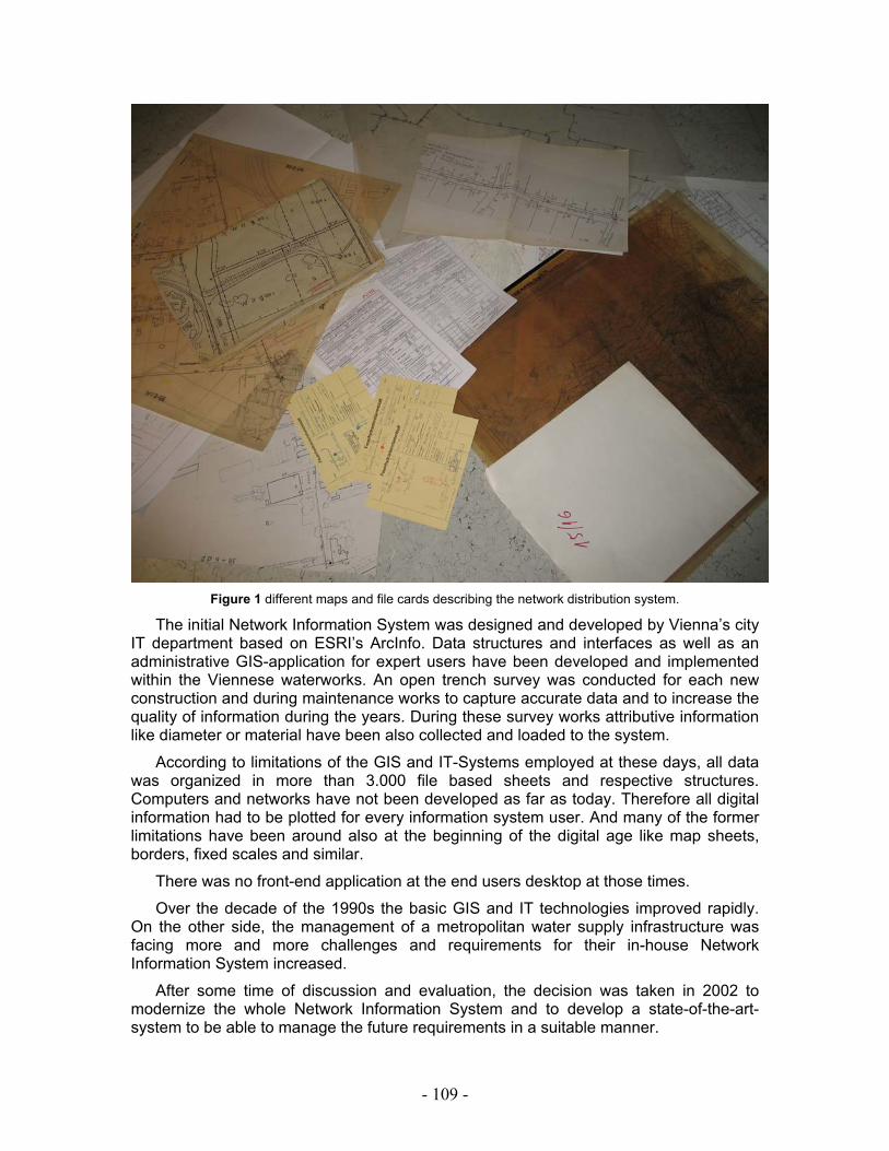
- 109 -

Figure 1 different maps and file cards describing the network distribution system.

The initial Network Information System was designed and developed by Vienna’s city IT department based on ESRI’s ArcInfo. Data structures and interfaces as well as an administrative GIS-application for expert users have been developed and implemented within the Viennese waterworks. An open trench survey was conducted for each new construction and during maintenance works to capture accurate data and to increase the quality of information during the years. During these survey works attributive information like diameter or material have been also collected and loaded to the system.

According to limitations of the GIS and IT-Systems employed at these days, all data was organized in more than 3.000 file based sheets and respective structures. Computers and networks have not been developed as far as today. Therefore all digital information had to be plotted for every information system user. And many of the former limitations have been around also at the beginning of the digital age like map sheets, borders, fixed scales and similar.

There was no front-end application at the end users desktop at those times.

Over the decade of the 1990s the basic GIS and IT technologies improved rapidly. On the other side, the management of a metropolitan water supply infrastructure was facing more and more challenges and requirements for their in-house Network Information System increased.

After some time of discussion and evaluation, the decision was taken in 2002 to modernize the whole Network Information System and to develop a state-of-the-art-system to be able to manage the future requirements in a suitable manner.

- 110 -

Goals and Requirements of the NIS

The main goal was to provide a direct access to all electronic data within headquarters and all branch offices with the guarantee of a 24x7 availability of information by the IT-System. The other issues were the guarantee of up-to-date information available at any time, multi user operation and performance (a fast data providing and display).

The main goal regarding the information and data quality was the continuous improvement by analyses and consolidation efforts of existing data as well the merging of all graphical data into a seamless dataset. The integration of data of various formats, scales and sheet organization was another crucial item.

All data (graphical/spatial and descriptive) should be stored in one single database and the use of the front end application should be very easy, especially for non IT experts. Existing workflows should be supported and the implementation of a mobile solution for emergency reasons should be possible.

All the above requirements have been included within a tender procedure to select the best suited partner for the implementation of the new system. Finally ms.GIS Informationssysteme GmbH, a privately held Austrian company, has been selected to team with the in-house experts to implement the new state-of–the-art-system.

“The NIS Implementation Project” Design of the Network Information System and the Data Migration

The implementation of the NIS project was done by the means of a close cooperation and partnership with ms.GIS. The following phases describe the challenges and the respective approaches taken.

Base technology decision

The first challenge was the evaluation of common software products for the future information system. In 2002 ms.GIS evaluated several products according to the needs of the Viennese Waterworks to cover at least the following listed tasks:

• Direct access to all electronic data within headquarters and all branches • Guarantee of a 24x7 availability of information by the IT-System • Guarantee of up-to-date information available all the time • Multi user access and a fast data providing • Improvement of data quality by analyses and consolidation (existing data) • Possibility to display different information and data formats (as background) • All data (graphical & attributive) to be stored in a database • Merging of all graphical data into a seamless dataset • Support of existing workflows • Easy to use front end application • Implementation of a mobile solution

- 111 -

After the evaluation process the decision was found to use the following listed set of technologies:

• ms.GIS CORE 3 Technology • Oracle 9i (Spatial) • ESRI ArcGIS / ArcObjects • Safe FME • Microsoft Terminal Server

Analysis of data and workflows/processes

During the next phase a detailed study regarding the workflows and business processes was initiated. This was made by interviewing staff of involved departments and compiling according specifications for realization. Also interaction between different departments within complex workflows was analysed and resulted as an important requirement for future needs.

At the same time the existing data stored in the former system became analysed. During these analyses we figured out that there where many inconsistent information captured and stored in the old data structures within the last 10 years. At the very first beginning of data capturing in electronic format some data fields where used in another meaning then some years later (before 2002). For data validation and improvement each data set had to be checked manually which caused high expenses and a lot of time to receive high quality data again.

Data modelling

After these complex analyses an appropriate data model became designed to match all needs as specified during the interviews. There where also some existing third party information like topographical data, cadastre, addresses, land usage, etc. this information also needed to be implemented into the future data model. Some of this information had to be merged (linked) with information coming from the Viennese waterworks.

Especially the data set describing the addresses needed to be merged with the feed lines as the feed lines are supplying each house. Some inconsistencies where found in the data here as well which needed to be verified and corrected manually again.

Business Processes & Application design

Of course a lot of business processes were implemented within the NIS for a better documentation as well as for quality control and quality assurance. Some of these business processes will be shortly described below.

Daily works like repair and maintenance are becoming recorded within the NIS as well as future works can be planned. In this manner the user has always the overview about all present, past and future works done within the whole city of Vienna. For future works it is necessary to retrieve an appropriate excavation approval from the Viennese road construction authority to start maintenance works. The applications and retrievals of excavation approvals are also managed by using the NIS.

- 112 -

There is also a Customer Relation Management (CRM) implemented within the NIS. The CRM deals with customer complaints calling the 24x7 call centre (e.g. bad smell or bad colour, etc.) including the follow up of laboratory results after taking samples from the customers water tap. Also the given answers to the customer are becoming recorded for avoiding miss-information when several clients calling from the same house. Another tool within the CRM is an automated customer notification in case of a planned supply suspension due to maintenance works.

Additional features for administrating the network asset and its components (e.g. line pipes, valves, reservoirs, hydrants, etc.) were implemented as well. As there are a lot of other documents like plans, photos, scanned file cards (for hydrants), etc. describing asset components more detailed these documents became hyperlinked to their corresponding part within the network. All this documents are accessible through the system now, so the user doesn’t have to search in dusty analogue archives anymore but has all the information on the hands by clicking in the system.

For keeping all information up-to-date and for improving existing information a memo function was designed. This means every user within the department is able to attach to every component within the network a memo holding updated or new information. All memos are forwarded automatically to the planning department, where draftsmen are incorporating these information’s by using their professional edit stations.

Figure 2 professional edit station of a specialist within the NIS group.

- 113 -

For providing all the data regarding the distribution network to the 24 hour call center of the Vienna waterworks we designed an offline version of the information system to install it to mobile computers for having the information always on the hands.

The new Network Information System was launched in 2005 and is fully integrated to the user’s daily work.

Our special staff for update the information of the distribution system consists of 5 to 7 persons in the head office and is responsible for keep all information up to date as well as for the planning of new lines or replacement of existing ones. All employees of the branch offices additionally collect information and point out mistakes of graphical or attributive data by using a special memo function.

Use of the network information system to investigate leakages and waterlosses

A very important task while operating such a distribution network is the knowledge about the networks condition in the manner of age, water losses and pipe bursts. The year of construction of the pipelines of Vienna is best known and documented in the NIS. Data about water losses und pipe bursts nowadays are recorded in file cards and access-databases without geografical reference except an address.

For investigating leakages the distribution network will be spitted into defined subnets. Within these subnets we are launching minimum night flow measurements periodically. If water losses in one of these defined subnets are measured, we split these areas into smaller net partitions and repeat the measurement for isolation of leaky pipelines. Currently the results of these measurements are documented in file cards in every branch office. The goal for 2007 is to convert these informations into the NIS. Therefor we have to design the defined subnets and develop special table elements. The discussion about the level of detail is currently an on going process.

Future strategies to use GIS for leakage control

In case of pipe burst data and relevant additional informations the development process is more difficult because in the european union a lot of guidelines are available. We have to be very careful in choosing the right and most relevant informations for feed into the database. I think that for an evaluation of the condition of the whole distribution network it would be more effective to have less attributes but therefor for the whole pipeline net of Vienna. To define several table elements our department for distribution system made exhaustive studies of the existing guidelines. The most important guidelines published by DVGW are GW 133 “DV-gestütztes Störfallmanagement und Schadenstatistik unter Einbindung von GIS”, “Schadenstatistik Wasser” and W 395 “Schadenstatistik für Wasserrohrnetze”. The evaluation process is not finished yet but the main table elements could be defined.

To connect geografical information with attributive data we basically have two options. It is possible to use the existing features (pipelines) for database connection or to construct new features. Using the first option has the disprofit of loosing the connection if pipelines become changed or rehabilitated. The second option implicates that new features (point of pipeline burst) must be constructed before informations can be feed to

- 114 -

the database. In every case it will be possible to evaluate database information in combination with geografical data by using our geografical information system ArcInfo which is one of the base products of NIS.

The goal is to provide a tool for statistics regarding leakages and pipe bursts, based on that it will give decision support and enables preventive maintenance works.

- 115 -

Managing the “Repair or Replace” dilemma on Water Leakages

S. CHRISTODOULOU *, C. CHARALAMBOUS**, A. ADAMOU***

* Dept. of Civil and Environmental Engineering, University of Cyprus, [email protected]

** Water Board of Lemesos, Cyprus, [email protected]

*** Water Board of Larnaca, Cyprus, [email protected]

Keywords: asset management; risk of failure; repair or replace

Abstract

In light of the increasing and pressing need to efficiently manage scarce water resources there has been renewed interest by water distribution network owners to develop and implement water management strategies and tools that would assist in the integrated and automated management of those networks. Such asset management strategies should assist the network owners evaluate the condition of the water distribution network, assess historical incident data (leakage or breakage) and risk of failure, visualize areas of high risk, propose “repair or replace” strategies and prioritize the work based on the inherent risk and cost of action. The methodology and support system outlined in this paper can form an integral part of a leakage management strategy and provide a useful decision making tool.

The work presented outlines an integrated methodology and a decision support system for arriving at such “repair-or-replace” decisions, as part of a long-term pipeline asset management program that could be undertaken by a water utility to improve on the reliability of the water distribution networks. The International Water Association’s Water Loss Task Force has been advocating and promoting four basic leakage management activities for leakage reduction, namely: pressure management, active leakage control, speed and quality of repairs and pipeline asset management, maintenance and renewal (Lambert, A. and Mckenzie, R., 2002).

The risk assessment and management (“repair or replace”) system is based on analytical and numerical modelling techniques and supplemented with geographical distribution systems (GIS). The goal is to enable water utilities to better manage condition assessment information, to process historical records with a number of analytical and numerical models, to identify underlying data patterns with artificial intelligence techniques and eventually to assess the corresponding risk of failure of each network element and to visually disseminate this information via geographical information systems.

Introduction

Increased demands on resource usage, reliability of systems and of provided services placed on urban utility owners as a direct result of the ongoing globalization and urbanization have put a high strain on aging urban infrastructure and water distribution agencies.

This is even more evident and time-pressing in countries with limited water resources. In such cases, the complexity and severity of the problem is compounded and amplified by the inability of the owners of the distribution network to easily and cost-

- 116 -

effectively replace utilized or lost resources (water and pipes) as they are faced with a lack of alternatives and a pressing need to provide these resources to the public in periods of extended drought. After all, in the case of water distribution networks the resource managed and provided to customers (water) is the essential element for life and no substitute can fulfil this resource’s role. Furthermore, in the case of most developing countries the managed distribution networks are based on ageing and neglected infrastructure that is highly unreliable and cost-inefficient. As a result, utilities in charge of managing such water distribution networks are nowadays faced with the increasingly more complex task to intelligently and efficiently manage such networks in ways that maximize a system’s reliability and minimize its operational and management costs. In these cases, life-cycle costing and maintenance strategies become of paramount importance to the utilities as they seek ways to increase system reliability and quality of service while minimizing costs of operation.

Central to this balancing act of operating costs and reliability is one of the most important dilemmas facing water distribution -organisations. Should an organisation repair or replace ageing and/or deteriorating water mains and what, in any case, should the sequence of any such repairs be as part of a long-term network rehabilitation strategy?

The work presented outlines an integrated methodology and a decision support system for arriving at such “rehabilitate-or-replace” decisions, as part of a long-term pipeline asset management program that could be undertaken by a water utility to improve on the reliability of the water distribution networks. The International Water Association’s Water Loss Task Force has been advocating and promoting four basic leakage management activities for leakage reduction, namely: pressure management, active leakage control, speed and quality of repairs and pipeline asset management, maintenance and renewal (Lambert and Mckenzie, 2002). The methodology and support system outlined in this paper can form an integral part of a leakage management strategy and provide a useful decision making tool.

Relevant Studies in Literature

To-date a number of studies has been undertaken on infrastructure assessment and deterioration modelling; with the intent to assist owners of such systems improve their understanding of a system’s behaviour over time, its deterioration rate and its reliability with respect to presumed risk factors. The intent has always been to assist owners and operators of water distribution networks in arriving at “repair-or-replace” decisions on a more scientific basis. The studies usually attempt to identify statistical relationships between water main break rates and influential risk factors such as a pipe’s age, diameter and material, the corrosiveness of the soil, the operating pressure and temperature, possible external loads (including highway traffic) and recorded history of pipe breaks.

Most studies in literature show a relationship between failure rates and time of failure (age of pipes), and some of them suggest a methodology to optimize the replacement time of pipes. Shamir and Howard (1979) reported an exponential relationship, and Clark (1982) developed a linear multivariate equation to characterize the time from pipe installation to the first break and a multivariate exponential equation to determine the breakage rate after the first break. A study by Andreou et al. (1987) suggested a probabilistic approach consisting of a proportional hazards model to predict failure at an early age, and a Poisson-type model for the later stages, and further asserted that

- 117 -

stratification of data (based on specific parameters) would increase the accuracy of the model. A non-homogeneous Poisson distribution model was later proposed by Goulter and Kazemi (1987) to predict the probability of subsequent breaks given that at least one break had already occurred. Finally, Kleiner et al. (1998, 1999) developed a framework to assess future rehabilitation needs using limited and incomplete data on pipe conditions.

More recently, a simulation model was applied to an inventory of water mains in New York City to analyze replacement strategies, and Vanrenterghem (2003) developed models for the structural degradation of urban water distribution systems based on data from New York City. Additional work on the same case study was reported by Aslani (2003) and Christodoulou et. al. (2003). The knowledge gained by the New York City case study was furthered and reported upon by Christodoulou et al. (2006) in a developed framework for integrated GIS-based management, risk assessment and prioritization of water leakage actions.

Integrated Water Leakage Management System – A Case Study

In managing water distribution assets (water, pipes, valves, connections, etc.) water utility agencies need to implement asset management strategies, alongside operations and maintenance methodologies that improve on a system’s reliability and cost-efficiency. To that effect, an integrated pipeline asset management system is of high importance. The system proposed in the following pages is an example of such system as developed and implemented in Cyprus for the monitoring, rehabilitation and life-cycle-costing of urban water distribution networks.

The described integrated system and the lessons learned from its implementation are in essence a knowledge-based system, complemented with analytical and numerical analysis tools and supplemented with a geographical information system (GIS) for the delivery to water distribution network owners and administrators of a complete decision support system (DSS) that can help them improve on the management of the water distribution networks.

The Proposed Integrated Pipeline Asset Management System

Starting with the premise that historical data on pipe breaks, reaction methodologies, social and financial impacts and life-cycle costing are important ingredients in the puzzle of “repair or replace” strategies and action prioritization, the proposed system envisions the integration of all these key elements in the delivery of one integrated management system which will help utilities manage their distribution networks more efficiently.

As such, the proposed system encompasses:

• Data on system characteristics (such as pipe diameter, length, material, installation date, zoning, etc.),

• Historical data on pipe break incidents (date of incident, response time and cost to repair/replace, number of previously observed breaks, reason for and classification of break incident, etc.),

• A statistical analysis tool for the analysis of pipe break incidents,

• An artificial neural network component for data pattern identification,

- 118 -

• A fuzzy logic processor, for the development of fuzzy logic rules describing the behaviour of the network,

• A risk assessment module (primarily a survival analysis module),

• A geographical information system (GIS) for visualization ,

• A life cycle costing module for the aggregation of costs by area and pipe,

• A prioritization-of-work module,

• A data query and reporting system for the retrieval of needed information.

System’s Process and Data Flow

The system proposed relies heavily on past knowledge acquired through operations and maintenance by the Water Boards, and historical records relating incidents on the network (primarily pipe failures) with internal and external parameters. Sample internal parameters include pipe materials, diameters, operating pressures, etc, and sample external parameters include external loading conditions, temperature, soil conditions, etc.

The premise is that lessons learned through past incidents can significantly improve future operations and maintenance practices and thus improve the piping network’s operational reliability and life-cycle costs. Furthermore, an integrated and automated methodology should help Water Boards more efficiently and intelligently address the “repair or replace” dilemma facing them, prioritize their actions and save on non-revenue water.

The proposed asset management, operations and maintenance system relies on a company access-wide relational database (client-server application) that feeds into a decision support system (DSS). This database comprises the time-related knowledge repository for the piping network, feeding related data to a neurofuzzy system which then processes the information to arrive at estimated risk-of-failure calculations. On the one hand, the underlying databases are relational and integrated to minimize entry points by the users, standardize input, minimize risk of errors in data handling, and maximize automation of data analysis and reporting. On the other hand, the DSS and its neurofuzzy elements allow for the numerical analysis of the data and the evaluation of key system parameters such as survival analysis curves and risk-of-failure metrics for each network element.

The latter (risk-of-failure metrics) is a key system characteristic of the piping network, for it provides the Water Boards with numerical appraisals on the condition of the city’s pipe network. A high “risk of failure” index, or consecutively a low survival index, highlights to the Water Board a necessity to replace a failing pipe to avoid further escalation of the induced problem of repeated failures and downtime, as well as escalating operations and maintenance costs.

Historical data is processed by means of a combination of decision support tools, such as survival analysis, statistical analysis, artificial neural networks and fuzzy logic. This analysis aims the identification of possible risk factors for pipe breaks and a ranking of them according to their severity and causal effect. Christodoulou et al. (2006) and Deliyanni (2006) reported on the severity of a number of presumed factors (such as pipe diameter, material, length, age, number of previously observed breaks, etc.) and proceeded in listing the factors by means of a neurofuzzy system. A subset of the derived fuzzy rules is tabulated in Table 1.

- 119 -

Table 1. Fuzzy logic rules describing expected behaviour of water pipes.

If … Then …

Diameter (D)

Number of Observed Previous Breaks (NOPB)

Length (L)

Material (Mat)

Traffic (Traf)

Break (1) or Not (0)

Small Small Small 2 1 0 Small Small Small 1 1 1 Large Large Small 4 2 1

Medium Small Small 4 2 0 Small Small Medium - 1 0 Small Small Large 1 0 0

Medium Medium Small 4 2 1 Large Large - 2 - 1

- Small - 1 - 0 S: 4 – 30” S: 0 – 2 S: 0.25 – 5.50

M: 20 – 48” M: 1 – 4 M: 4.50 – 14.0 L: 40 – 72” L: 3 – 9 L: 10.0 – 21.0

The Case-Study Water Distribution Network

The water distribution network currently under review (Water Board of Lemesos) is over 50 years of age and serves approximately 170,000 residents through approximately 64,000 consumer meters in an area of 70 km2. The annual volume of potable water distributed through the network of pipes, of approximate length 795km, is about 13.7x106 m3 and of value €7.0 million. The development of the system infrastructure took place in a much organised fashion with new areas of supply being incorporated into their respective pressure zones, which are strictly governed by contours. Each pressure zone is subdivided into District Metered Areas (DMAs), having a single metered source with physical discontinuity of pipe network between DMA boundaries. The DMAs vary in size from 50 properties to 7000 although the average size being approximately 3000 properties. Distribution main diameters within the DMAs vary between 100mm and 250mm and where possible, interconnecting ring systems within the DMAs have been formed to minimize head loss at peak demands. The network owner (the Water Board of Lemesos) has maintained records of its operational activities since 1963, which include production of water from sources, distribution through district meters and consumption from consumer meters. Meter readings at water sources (boreholes and treatment plant) are connected via a SCADA telemetry system to the control room. This enables continuous monitoring of the water source outputs and accurate recording of flows. Likewise storage reservoir outlet meters are monitored on SCADA providing the same ability to observe trends as well as to record daily, weekly, monthly and yearly totals (Charalambous, B., 2005). The continuous monitoring of the DMA meters combines information technology and telecommunication networks to transfer the data via the World Wide Web. The historical data gathered in the programmable controller of each DMA is sent by the controller to an email account. Operating software installed in the dedicated computer at the Water Board’s control room connects to this email account twice a week and downloads the data, which are first sorted according to the DMA and then are used to update existing reports.

The Water Board recognised at a very early stage the importance and significance of establishing a proper water audit system and has over the years developed its infrastructure in such a way so as to be able to account efficiently and accurately for all water produced (Figure 1) or “lost” (non-revenue water). Reduction and control of water

- 120 -

loss was achieved through the application of a holistic strategy based on the approach developed by the Water Loss Task Force of the International Water Association. Integral part of this approach is the establishment of a strategy for pipe break incidents (“pipe breaks policy”). The policy further envisions the prioritization of the repair/replacement actions on the basis of risk of failure, life-cycle costing, social and financial impacts.

In addition to the reported bursts, the Water Board of Lemesos through its strategy for active leakage control maintains records of unreported bursts located by means of acoustic leak localizers. Typical results are shown in Table 2 (Charalambous, B., 2002). Details of all such breaks are maintained and included in the analysis, together with the reported bursts.

Table 2. Unreported bursts – identified, located and repaired.

Number of bursts Percentage per type

Type of pipe

1999 2002 1999 2002 20mm MDPE 7 7 32mm MDPE 9 8

39% 44%

100mm AC mains 10 10 150mm AC mains 12 9 200mm AC mains 3 0

61%

56%

TOTAL 41 34 100% 100% Estimated water saved 140,000 m3 110,000 m3

Worth of water saved US$ 45,000 US$ 35,000

Figure 1. Non-revenue water.

Risk-Of-Failure Analysis

Following the DMA strategy for minimizing water losses through uniform pressure zones, the Water Boards recognized the need to develop mechanisms for evaluating historical incident data (when and how water pipes break) for identifying possible data patterns in the behavior of the network, and for using these patterns for forecasting new breaks. The analysis of historical data was based on a number of analytical and numerical tools (such as statistical analysis, artificial neural networks, and neurofuzzy systems) and investigated the possible contribution of a number of presumed risk factors to a “break or not?” outcome, ranking these factors according to their relative importance and contribution to the “Break or Not” forecasted output.

0.00%

5.00%

10.00%

15.00%

20.00%

25.00%

30.00%

1986 1988 1990 1992 1994 1996 1998 2000 2002 2004Y E A R

N R W a s

%

o f

SIV

Drought YearsIntermittent Supply

- 121 -

The analysis identified the most important risk factors to be the number of previously observed breaks (NOPB), the material type (MAT), the length (L) and the diameter (D) of each pipe. The presence of high traffic volume (TRAF), subway (SUB), block intersection (INTER BLOC) and highway (HWAY) seem to be of less risk-contributing importance than the former four factors (Christodoulou et. al., 2006).

The analysis on whether to repair or replace a burst, and thus the Board’s asset management, is to be based on a combination of the previously mentioned tools (statistical analysis, survival analysis, neurofuzzy systems), with the end-results tabulated in a database management system and then mapped on a spatial database (GIS) that enables users to query both the raw data and the computed risk-of-failure values.

Examples of the GIS-based decision support system are shown in Figures 2 and 3. At first historical data on previously observed breaks (NOPB) are lumped at a street level and then mapped to a GIS representation of the pipe network, colour-coded to indicate the variable degrees of their inherent risk of failure (Figure 2). The Boards can therefore easily and holistically review the status of their network in terms of where and how often pipes break, as well as the computed risk-of-failure for each segment of the pipe network. Even though the eventual goal is to calculate risk-of-failure metrics at the pipe level and not the street level (in other words an individual forecast for each pipe segment) it was deemed redundant and over-complicating at this early stage of the research and thus overlooked in favour of metrics for each street segment.

Figure 2. Color-coded GIS mapping of risk-of-failure.

The data is also categorized by the type of pipe for which burst incidents are reported, and graphed in histograms also at the street level (Figure 2). For example, for two case-study streets (Valtetsiou and Kosti Palama) the histograms indicate the majority of incidents are AC and LDPE pipes respectively. Should one break the data further down, the data can be categorized by pipe type (mains or house connections) or

- 122 -

incident type (connection failure, corrosion, tree roots, deterioration due to aging) as shown in Figure 3.

Figure 3. Histograms of incident categorization.

The histograms show that the majority of incidents are due to tree roots (Valtetsiou) and aging (Kosti Palama), with most incidents observed on mains (Valtetsiou) and house connections (Kosti Palama) respectively.

The above visual analysis and representation is coupled with numerical analysis of the hazard rate and survival plots, “stratified” by different logical groups. For example, survival analysis of the pipe incidents grouped by the type of incident (such as pipe deterioration, interference by others, tree roots, corrosion, etc.) reveals interesting patterns in terms of the causes for pipe failure. Should one examine the hazard rate over the time (measured in days of presumed pipe age) then one can see that the rate with which the hazard for failure increases for pipes experiencing deterioration is faster than the hazard rate for pipes under “interference by others” (Figure 4). Also evident in the same plot of survival analysis (Figure 4), the hazard rate for pipes in the vicinity of tree roots picks up pace (larger slope) over time indicating that pipes in proximity of tree roots should be replaced at shorter time intervals or otherwise risk failure (alternatively, tree roots become an issue for pipe failure as time progresses).

- 123 -

Figure 4. Hazard rate plot, by incident type.

Asset Management

This type of visually-represented analysis furnishes the managing agency with an insight into the frequency, the severity, the categorization and the reasons behind pipe breaks over time for all segments of the pipe network. In the case of the two street segments mentioned in this manuscript, the analysis can be summarized in linguistic terms of the form:

• Pipes located on Kosti Palama Street have higher risk of failure than pipes located on Valtetsiou Street (therefore higher priority for maintenance/replacement).

• Pipes on Kosti Palama Street break primarily due to aging (therefore need replacement). The majority of the pipe breaks are on house connections rather than water mains.

• Pipes on Valtetsiou Street break primarily due to tree roots in their vicinity (therefore the municipality needs to address the problem of trees close to pipes, either by cutting trees down, or by moving the pipes to a different location). The majority of the pipe breaks are on water mains rather than house connections.

The study further summarizes collective knowledge acquired through data pattern recognition and neurofuzzy systems and lumps it into linguistic fuzzy rules (Deligianni, 2006). Based on these rules,

• Priority is given to areas in proximity of buildings of high pubic value (e.g. hospitals, schools).

• Priority is then given to areas combining residential and industrial use.

- 124 -

• Priority is then given to areas where other planned construction work is taking place (such as roadway rehabilitation) so as to maximize parallel work and minimize successive disruption.

• Priority is then given to pipes with high number of observed previous breaks (NOPB), based on our study.

• Then, pipes with diameter greater than 40 inches (D>40) take precedence.

• These are followed by pipes made out of cast-iron, followed in priority by steel pipes.

• Finally, replacement of pipes subjected to heavy traffic loads takes precedence.

Conclusions

The paper reports on the development of an integrated GIS-based decision support system for asset management of urban water distribution networks. The work, which is still under development, is now piloted for implementation in two cities in Cyprus. The water utilities involved aspire, through this implementation, to reduce water losses in their water distribution networks and to improve on the reliability of their systems. The underlying knowledgebase and integrated decision support tools (statistics, ANN, fuzzy logic, GIS) aim to support these utilities in their endeavours and benefit their consumers the most.

Acknowledgements

This report is based partially upon work supported by the National Science Foundation (under Grant No. CMS-0118376) and upon work supported by the Cyprus Research Foundation (under Grant No. AKGEN/1204/01). Gratitude is also extended to the Democritus University of Thrace for their contributions to aspects of the research, as part of the EU-funded System Engineering and Management Program.

- 125 -

References Andreou S.A., Marks D.H. and Clark R.M. (1987) A new methodology for modeling break failure patterns in

deteriorating water distribution systems: theory. Advances in Water Resources, 10(3), 2-10. Aslani, P. (2003) Hazard rate modeling and risk analysis of water mains. M.Sc. thesis, Dept. of Civil Eng.,

Polytechnic University, New York, NY, 86 pp. Charalambous, B. (2002) Historical development of leakage reduction strategies at the Water Board of

Lemesos. Proceedings of the International Water Association’s specialised conference on Leakage Management – A Practical Approach, ISBN 9963-8759-0-4, 26-31.

Charalambous, B. (2005) Experiences in DMA redesign at the Water Board of Lemesos, Cyprus. Proceedings of the International Water Association’s specialised conference on Leakage, Halifax, Nova Scotia, Canada, 403-413.

Christodoulou S., Aslani P. and Vanrenterghem A. (2003) A risk analysis framework for evaluating structural degradation of water mains in urban settings, using neurofuzzy systems and statistical modeling techniques. Proceedings of the 2003 ASCE EWRI 2003 World Water & Environmental Resources Congress, Jun.23-26, Pennsylvania, USA.

Christodoulou S., Aslani P. and Deliyanni A. (2006) Integrated GIS-based management of water distribution networks. Proceedings of the 2006 ASCE International Conference on Computing and Decision Making in Civil and Building Engineering, June 14-16, Montreal, Canada.

Clark M.A., Stafford C.L. and Goodrich J.A. (1982) Water distribution systems: a spatial and cost evaluation. Journal of the American Water Works Association (AWWA), Planning and Management Division, 108, 243-256.

Deliyanni, A. (2006) Risk assessment of urban water distribution networks and strategic planning of rehabilitation/ replacement. M.Sc. thesis, Dept. of Civil Eng., Democritus University of Thrace, Xanthi, Greece.

Goulter I.C. and Kazemi A. (1988) Spatial and temporal groupings of water main pipe breakage in Winipeg. Canadian J. of Civil Eng., 15(1), 91 - 100.

Kleiner Y., Adams B.J. and Rogers, J.S. (1998) Long-term planning methodology for water distribution system rehabilitation. Water Resources Research, 34(8), 2039-2051.

Kleiner Y. and Rajani B. (1999) Using limited data to access future needs. Journal of the American Water Works Association (AWWA), 91(7), 47-62.

Lambert A. and Mckenzie R. (2002) Practical experience in using the infrastructure leakage index. Proceedings of the International Water Association’s specialised conference on Leakage Management – A Practical Approach, ISBN 9963-8759-0-4, 112-126.

Shamir U. and Howard D.D. (1979) An analytic approach to scheduling pipe replacement. Journal of the American Water Works Association (AWWA), 71(5), 248-258.

Vanrenterghem, A. (2003) Modeling of the structural degradation of an urban water distribution system. Ph.D. thesis, Department of Civil Eng., Polytechnic University, New York.

- 126 -

“Inliner-“ and “Close Fit” Technologies - Potentials and Advantages for Water Pipe Rehabilitation U., Rabmer-Koller

NODIG Pipe Rehabilitation, Inliner, Close Fit

Introduction

The access to drinking water is a very precious good on earth. Even in regions which are rich of water in natural deposits, there are problems with efficient water tapping and supply. In many cities more than 50 % of the water is lost on the way to its end customer, a fact which is often caused by leaking pipes. Based on the Global Water Supply and Sanitation Assessment 2000 Report the water losses are often 50 % higher then the water extraction. In Asia und Latin America the losses because of leaking pipes are in average 42 %, in Africa 39 % and in North America the loss is still 15 %.

The conventional replacement of pipelines by excavation is very expensive, time-consuming and noisy and it generally involves considerable disruptions of traffic in urban areas. This is the reason for the steadily increasing demand for No-Dig technologies worldwide and why trends are shifting to the development of innovative solutions for water pipe – systems based on NO DIG technologies during the last years.

Based on the experience of big projects in Budapest (Hungary), Vienna (Austria) or Bydgoshsz (Poland), the latest trends for “Inliner-“ and “Close Fit” systems used for the rehabilitation of pressure pipes will be explained in this paper. Information about the preliminary works as cleaning and CCTV (Closed Circuit Television) inspection, the selection process for the materials and systems utilised. The paper concludes with critical issues of rehabilitation and possible strategies for future enhancements.

Potentials

Once a supply main has been identified as failing to meet its service requirements, the method of replacement or renewal will need to be evaluated and verified. Though popular, open-cut methods can create considerable inconveniences to customers, businesses, residences, and traffic. In urban areas these inconveniences can also become very costly. As a result, trenchless technologies have attracted the attention of the water supply industry as an alternative to open-trench methods. Trenchless technologies can substantially reduce direct rehabilitation costs and do diminish the inevitable collateral damage on all residential and commercial parties within the instant environment of the job site as the open cut area is reduced to minor access points.

Rehabilitation / Structural Lining

The selection of the system in depending on the host pipe condition and operational demands is the key in ensuring a long lasting rehabilitation success. The primary interaction between a flexible liner and its relatively rigid host when subject to internal pressure is classified in “independent” vs “interactive” adopted in current European renovation product standards and illustrated in Figure 1.

- 127 -

Figure 1. Structural classification of pressure pipe liners according to EN 13689:2002

It is important to note that in EN 13689 these adjectives are not defined in isolation but incorporated in the following compound terms:

Independent pressure pipe Liner: Fully capable of bearing all internal and external loads

Interactive pressure pipe Liner: Reliance on the existing pipeline for some measure of radial support in order to resist without failure all applicable internal loads throughout its design life, no external load bearing capacity

Key elements in the selection of a rehabilitation method are:

a. Exact nature of the problem(s) to be solved, particularly the host pipe condition and its mode of failure.

b. Hydraulic and operating pressure requirements including forecasted parameter

c. Materials, dimensions, age and geometry of the water main.

d. Types and locations of valves, fittings, and service connections.

e. Maximum time period in which the main can be taken out of service.

f. Site-specific factors, instant environment, soil conditions

g. Location and type of adjacent underground infrastructure

The selection of renewal technologies depends on pipe and site characteristics as well as on the inherent parameter of the techniques available. The aim of the selection process is to consider all these factors to arrive at the most cost-effective, technically viable solution. Ideally, the cost estimate should include not only direct contracting and related costs, but also indirect costs associated with public disruption and long-term maintenance. The ubiquity of scarce budgets defines the aim of selecting the most cost-effective technology.

The evaluation of the pipe conditions and the mode of failure and/or the status of deterioration are vital when selecting renewal technologies:

Mode of

failure

Available solutions Applied solution will also address:

Loss of

structural

- Replacement with same size or lager

- Structural Liner

- Joint imperfections - Water quality improvement - Increases hydraulic capacity

- 128 -

integrity

Lack of

hydraulic

capacity

- Replacement with same size or larger

- Structural, sem-structural or non-structural Liner in case diameter of host pipe is adequate

- Joint imperfections - Water quality

Joint failure - Replacement with same size or larger

- Structural or semi-structural Liner

- Water quality improvement - Increases hydraulic capacity

Water quality - Replacement with same size or larger

- Structural, semi-structural or non-structural Liner

- Increased hydraulic capacity

“INLINER” AND “CLOSE FIT”-SYSTEM

Lining with CLOSE FIT LINERS

Introduction close fit liner

In this procedure a thermo-mechanically deformed polyethylene tube coming straight from the factory is pulled in through a pre-existent access shaft. The high-strength polyethylene tube is re-shaped into a U-form shortly after it has been extruded. Its cross-section is thereby reduced by 30% in comparison with its original state. Because of the enhanced flexibility and smaller cross-section of the Inliner, which result from its U-shape, it can be pulled into the existent reach of the underground pipeline with the help of a winch. After reaching the final entry position the original tube shape is restored under pressure and of the addition of hot steam. The tube thereby presses itself firmly against the existent cross-section and assumes a continuous, smooth tubular form without any annular gaps.

Figure 2. Technology Close Fit (Source: Rabmer)

- 129 -

Procedure close fit liner A – Preliminary works Cleaning, disconnection of the pipeline to be rehabilitated, mobile CCTV monitoring, pipe calibration and transport of the close fit liner to the site are the first steps. More details about these working steps see section 8.

The physical properties and the shape of the close fit liner enable it to be wound around drums in lengths of up to 1,600 m when it is produced. It is completely seamless. The twofold deformation involved in bending it into a U and winding it around the drum has no negative effect on the quality of the polyethylene tube.

Figure 3: Close fit liner wound on a drum (Source: Rabmer)

Division into rehabilitation sections and spatial requirements

The pipeline system is divided into sections that can be up to 950 m long in straight reaches, depending on the diameter, delivered length and strength of the close fit system. In determining the lengths of the allocated sections, the capacity of the equipment, the selected cleaning method and especially the structural properties of the pipe must be considered.

B - Installation of the close fit liner: Pulling-in process The close fit liner is pulled directly off the drum through the shaft into the pipe by a wire rope winch. Deflection rollers and pulling-in devices are utilised, assuring a smooth passage of the close fit liner through the shaft and pipe entrance. This method facilitates pulling processes of Liner being several hundred meters long. Apart from the access points, no excavation is necessary.

Figure 4: Close fit liner pulled into a water pipe (Source: Rabmer) Reforming the tube After the close fit liner has reached its final position, both ends are cut off. Specially developed terminal pieces are then fitted onto its ends to close them off, and finally the tube is reformed to its original round shape with the help of steam (up to 125°C) and pressure (about 1.8 bars). Since the external diameter of the close fit liner corresponds

- 130 -

to the internal diameter of the host pipe, it presses firmly against the wall of that pipe after reformation. No annular gap remains.

Figure 5-7: “Old pipe” / close fit liner before reforming / close fit liner after reforming (Source: Rabmer) C - Final steps Finishing processes The finishing process consists of the attachment of fastening rings to both ends of the section. It varies according to application. Connections These are done in open construction by means of flanging or welding. All existing standard pipe connecting methods can be applied on close fit liners. Processing the removed sections of the pipe in the shaft area The removed sections of the existing pipe are either replaced by new sections or they are processed and prepared at the same time as the main pipeline and then inserted in between the ends of the close fit Liner. Reconnection of the section All newly installed sections are re-connected with either flanges or electrofusion couplings. Final cleaning A final CCTV inspection and a high-pressure jetting conclude the process..

Materials for close fit liners Close fit liners for water pipes are made of polyethylene (PE-HD). Polyethylene is a chemically highly stabile, flexible, environmentally friendly thermo elastic plastic that is very resistant to abrasion and has a favourable roughness under operational conditions. The following table shows the lowest wall thicknesses of the different sizes. The SDR (standard dimension ratio) expresses the relationship between diameter and wall thickness.

Dimension Water Gas SDR Minimal wall thickness

[mm] PE 80 PE 100 PE 80 PE 100 [ - ] [mm]

100 6 bar 10 bar 1 bar 4 bar 17,6 6

125 6 bar 10 bar 1 bar 4 bar 17,6 7

150 6 bar 10 bar 1 bar 4 bar 17,6 8

- 131 -

200 6 bar 10 bar 1 bar 4 bar 17,6 11

300 6 bar 10 bar 1 bar 4 bar 17,6 17 Figure 8: Wall thickness of liners depending on dimension and pressure

Summary close fit liner The close fit liner procedure is an economical and reliable solution for the renewal of gravity and pressure pipelines. The advantages of the close fit procedure are:

Operational performance

• Very long sections without couplings and improved hydraulics due to smooth surface

• Slight loss of diameter is compensated by the smoothness of the inner surface keeping the hydraulic capacity

Quality of the transported medium • Suitable for potable water

• Prevention of inner and outer corrosion, no new accumulation of deposits/incrustations

Spatial requirements/ operating sequence • Little or no work above ground

• Little space required for the construction site and excavation of access pits

• If existing, installation can be executed through pre-existent access shafts

• Close fit method can be applied independent from existing host pipe material and dimension

Procedural advantages

• Structural integrity either restored or improved

Economic efficiency • Lower costs compared to conventional rehabilitation methods

• No indirect costs resulting from public disruptions (traffic jams, dust, dirty roads...)

• Short construction time (about 1 to 2 days per rehabilitated section)

• No isolation of laterals is necessary, since no annular gap is formed

• Minimal disruption of the affected households

- 132 -

Lining with cured-in-place pipes – The INLINER - System

Introduction Inliner system

A flexible, multi-layered textile tube, impregnated with epoxy resin is inverted through the entire length of the interior of the pipeline to be renovated. . The polyaddition (=hardening) of the resin takes place under a pressurised condition and the addition of hot steam, resulting in a continuous seamless cured pipe, entirely in contact with the host pipe.

Figure 9: Inliner System (Source: Rabmer)

Operating sequence – Inliner system A - Preliminary works Cleaning, disconnection of the pipeline to be rehabilitated, mobile CCTV monitoring, pipe calibration and transport of the close fit liner to the site are the first steps. More details about these working steps see section 8.

Division into rehabilitation sections and spatial requirements The pipeline system is subdivided into sections, which can be up to 350 m long for diameters over 500 mm and up to 650 m long for diameters under 300 mm. The length renovated strongly depends on other factors than the capacity of the inversion machine, e.g. bends.

Preparation of the epoxy resin and impregnation of the tube The tube is wound on a drum. In order to fill it, a few meters are wound off and laid down on a protection foil to prevent damage.

Pulling-in process As a result of the reversal process, the tube lining is turned inside out. The inner side impregnated with resin is pressed up against the wall of the host pipe. The rotation of the drum shaft thrusts the tube, constantly being pressurised during the inversion process.. The reversion speed of up to 2 to 5 m/ min. is controlled by a retaining belt attached to the tube end.

- 133 -

Figure 10: Schematically draft of an Inliner installation (Source: Rabmer)

Heat curing process After the liner has passed throughout the entire length of the host pipe and arrived at the target shaft, vent tips are attached to the end of the tube to enable the circulation of hot. Hot steam is introduced through the drum into the pressurised Liner. Steam circulates throughout the curing process by keeping the internal pressure constant. C - Final working steps

• Final processing • Re-connection • Re-establishing the connections between the sections • Final cleaning and CCTV inspection

Range of Applications

The Inliner system can be used for all types of pipes (sewage, gas, potable water, oil, industry, etc.) from DN 100- DN 1600 mm.

Limitations of bends:

• Bends with a radius of < 3D: maximal angle 60° • Bends with a radius of = 3D - 5D: maximal angle 90° • Bends with a radius of > 5D: Several 90° bends • The difference of inner to outer radius causes wrinkling at the inner side and

potentially a gap at the outer radius. This is an inherent part of the system and cannot be avoided and the customer must be aware of this limitation

Material of Inliner systems for water pipes

A – Tubes for pressure pipes Base material: The textile structure of the base material consists of high-strength, endless woven (seamless) polyester yarn, serving as the carrying layer for the polymer coating that firmly adheres to it.

Coating for drinking water: For potable water applications a PELD (= low density polyethylene) or LLDPE (= linear low density polyethylene) coating is used. It guarantees water tightness, provides perfectly smooth surfaces and an unusually high level of chemical resistance.

B - Two-component epoxy resin: Only high-quality, two-component epoxy resins are utilised with good properties for adhesion and curing in humid environments. The curing process of epoxy resins doesn’t require volatile components and therefore don’t show shrinkage. Unlike polyesters, the

- 134 -

volumes of epoxy resins remain constant when they harden, which is an important advantage. When they solidify, they maintain a relaxed polymer structure without residual tension. The reach high flexural E-modulus of up to 3,700 Mpa, high resistance to mechanical impact and abrasion and exceptional adhesive strength. When completed cured, all of the materials are insoluble in water and environmentally neutral.

Summary Inliner System

Figure 11 – 13: Pipe before rehabilitation / pipe with impregnated textile tube before heating / rehabilitated

pipe (Source: Rabmer)

The Inliner-procedure is a reliable and an economical solution for the renovation of open channel- and pressure pipes. The advantages of the Inliner system are:

Operational performance

• Long sections without couplings and improved hydraulics due to smooth surface

• Slight loss of diameter is compensated by the smoothness of the inner surface keeping the hydraulic capacity

• Guaranteed impermeability

Quality of the transported medium

• Coating applicable for the transportation of potable water

• Complete protection against inner corrosion

Spatial requirements / work process

• Minimised civil engineering work

• Construction site above ground reduced to access pit and one truck with installation unit

• If available, installation can be executed from pre-existent access shafts

• Flexible dimensioning to any shape and size required

Process-technological advantages

• Bends, deflections and deformations in the pipeline do not represent crucial process-technological difficulties.

• Lateral connections can be incorporated into the rehabilitation process.

• Applying a well designed Inliner with the required structural load-bearing capacity can restore the section implying conditions comparable to a newly installed pipeline.

• The elongation at break and the flexural and tensile properties of the Epoxy resins can be modified to specific customer requirements.

- 135 -

Economic efficiency

• Lower costs compared to conventional rehabilitation methods.

• No indirect costs resulting from public disruptions (traffic jams, dust, dirty roads...)

• Short construction time (about 1 to 2 days per rehabilitated section)

• Minimal disruption of the affected households No risk and/or disruption of the adjacent underground infrastructure as a result of excavation. Subsequently, damage to the road surface as a result of settling down soils is avoided.

Project Case Studies

Water supply system Budapest: Main lines with a length of 40 km were rehabilitated using different Lining systems interactive compound systems, interactive load bearing systems or full structural solutions. The used Liner systems were chosen for each line by the degree of deterioration, operational experience and quantitative risk assessment. A good example for a thorough investigation and evaluation process are cast iron mains with 70+ years of age being in excellent condition. These mains had only to be sealed water-tight by an interactive compound Liner system, as the former sealants were biodegradable and already absent.

Water supply system Vienna: A necessary pressure increase at a 2.3 km pipeline required a structural CIPP-Liner to minimise the water losses to an acceptable level and to achieve a sustainable status of its structural integrity. Gas supply system Vienna: Main lines were rehabilitated using different Liner systems either interactive compound systems or fully structural solutions. The applied Liner systems were chosen for each line, following specific criteria for the degree of deterioration, operational experience and quantitative risk assessment.

Preliminary Work

Cleaning The cleaning process and its parameter depend on the Liner system chosen, degree of incrustations, pipe material, pipe integrity and discharge method of the loosened deposits. As an example, a CIPP-Liner technology requires high pressure water jetting with up to 1200 bars.

Retention of Water supply For the duration of the rehabilitation the line has to be put out of service. Temporary bypass is provided to retain the water supply.

CCTV-Inspection TV-Inspections have to be made in different stages of the rehabilitation sequence:

- Prior rehabilitation or renewal of the lines: to inspect, allocate and document the existing conditions

- Immediately after the cleaning and before installation of the CIPP-System to control the efficacy of the cleaning and the required status for the rehabilitation process applied

- 136 -

- After rehabilitation of the pipe-section: for documentation of the finished product

Pipe calibration A calibration of the pipeline becomes necessary when the required free cross-section of the host cannot be guaranteed. Additionally, intruding welding seams, protruding tapping etc... can easily be removed by a robot cutter. Incrustations and deposits can be loosened by rotating jets, high pressure water cleaning or rotating chains.

Approvals/Authorisations The chosen materials and combinations thereof have to be authorized by public institutions and continuously approved for the use with the transported medium. This includes aptitude testing as well as the quality control of the final product.

Critical issues for rehabilitation - rehabilitation strategies The rate of deterioration of an underground supply system is not only a function of material ageing but rather the cumulative effect of numerous external forces acting on it. During a recent water main evaluation, a 70+-year-old unlined cast iron pipe was found to be in excellent condition with negligible internal or external corrosion. Based on the field observations, there is no reason to believe that these mains will not provide another 70+ years of satisfactory service. Conversely, in another system, cast iron mains less than 50 years old are experiencing excessive and rapidly increasing burst rates and severely progressing corrosion. Rehabilitation of these mains is needed in the near future.

These strategies to handle deviations of the actual pipe condition from the desired status can be divided into:

• Fire-brigade strategy: a corrective action takes place only when the deviation becomes obvious

• Preventive (interval-based) strategy: a corrective action takes place in fixed intervals

• Condition-oriented (demand based) strategy: corrective action takes place when output reaches an optimum

- 137 -

Fire-Brigade Preventive Demand-Based

repair

accident

maintenance

inspection

administration

Figure 14. Pipe rehabilitation strategies and costs If the costs between these strategies are compared, one can see that the overall costs of a fire-brigade-strategy are the highest. When deviations from a planned state occur during this strategy immediate action is necessary and planned actions with a call for tenders is often impossible and the missing planning phase will cause collateral damages. Therefore, broad based decision factors regarding infrastructure replacement, whether based on age, pipe size, pipe material, linings, etc. will not result in an effective use of limited capital resources. A more holistic approach prior to the decision making is needed to achieve the optimum exploitation of the asset owner’s limited resources. This question can only be answered through actual knowledge of the conditions and service characteristics of the existing main, comparing repair, replacement, and rehabilitation costs, and a clear understanding of the anticipated results of the various rehabilitation techniques available.

Conclusion The population worldwide is steadily growing, resulting in a steadily increasing demand for potable water. Although a lot of new water pipelines were built in recent decades, it is a fact that in many places clean and reliable water supply is not the status quo. Defective underground pipelines, being corrosive, structural unreliable, contaminated, are not only waste our scarce resources but also are responsible for spreading diseases. None revenue water levels of up to 50% is a reality in various regions of the world.

The conventional replacement of pipelines by excavation is very expensive, time-consuming and extremely disruptive to the public. The steadily increasing demand for excavation free technologies worldwide is a good sign that the potential of this innovative methodology will be more and more appreciated. Numerous No-Dig projects, especially the Close Fit – and the Inliner system, applied in major cities in Europe and all over the world have proven its applicability and efficiency. The relative short construction time and ”new pipe” quality, by limiting the disruption of the immediate environment to a minimum are indisputable advantages.

- 138 -

Acceptable Level of Water Losses in Geneva H. Guibentif*, H.P. Rufenacht**, P. Rapillard***, M. Rüetschi*

* 2, ch. Château Bloch, CH-1211 Geneva 2, Switzerland [email protected]

** 2, ch. Château Bloch, CH-1211 Geneva 2, Switzerland [email protected]

*** 2, ch. Château Bloch, CH-1211 Geneva 2, Switzerland [email protected]

Keywords: IWA water balance, performance indicators, water losses assessment

Introduction Geneva Water (SIG) is a public utility company which produces each year about 70 Mm³ of drinking water for approximately 450'000 customers. In order to optimise the production process, Geneva Water has standardised the methodology to estimate the quantities of Non Revenue Water (NRW) produced and supplied to the network each year. This first step has been achieved in March 2006 using the methodology proposed by IWA (International Water Association).

This process highlighted that the previous estimations were under-evaluated, and that improvement of the whole process of water production and distribution was necessary. The aim of this paper is to share the actions implemented and the first results obtained toward an acceptable level of Water Losses for Geneva.

Water Balance calculation Until 2004, there was no standard methodology to establish an accurate annual Water Balance at SIG. Estimation of water losses for year 2004 led to an increase of 1% and NRW exceeded the virtual level of 10%. This initiated the project for a standard and stable estimation of Non Revenue Water. During year 2005, and in-depth study of each component of IWA Water Balance model has been carried out, including a detailed calculation of the tolerances. This procedure is now followed every year and the results for year 2006 are presented in Figure 2.

- 139 -

Unbilled Metered Consumption 0.5 Mm³ ± 1.7%

Unbilled Unmetered Consumption 0.9 Mm³ ± 10%

Billed Metered Consumption 58.2 Mm³ ± 2.7%

Billed Unmetered Consumption 0.2 Mm³ ± 14%

Real Losses3.3 Mm³ ± 40%

REVENUEWATER

58.6 Mm3+ ± 2.7%

NONREVENUE

WATER 9.3 Mm³ ± 18.4%

Billed Authorised

Consumption58.4 Mm³ ±

2.7%

Unbilled Authorised

Consumption1.4 Mm³ ± 6%

Apparent Losses 2.2 Mm³ ± 50%

Annual System

Input Volume

67.5 Mm³ ± 1%

Authorised Consumption

59.8 Mm³ ± 2.6%

LOSSES 7.8 Mm³ ± 21%

Excess leakage 2 2Mm³

Background Leakage

Reservoir Leakage, Overflow

Reported Bursts

Unreported Bursts

Figure 2: IWA’s Water Balance results for SIG – year 2004

Table 5 highlights the evolution of the Non Revenue and the Real Losses for the last years.

Non Revenue WaterYear Previous

estimationsIWA’s

methodology2002 9.30%2003 9.60%2004 10.40% 13.30%2005 14.00%2006 13.70%

Table 5: evolution of the Non Revenue Water (% of water production)

Not only the 10% level was passed in year 2004, but also an additional 3% resulted from use of the new methodology…

The detailed analysis of the Non Revenue Water on quantity and financial point of views is presented in Figure 3 for year 2004.

- 140 -

NON REVENUE WATERby VOLUMES

Leakage and Overflow or reservoirs

2%

Apparent Losses26%

Unbilled Unmetered17%Unbilled Metered

6%

Excess Losses13%

Unreported Bursts16%

Background Leakage18%

Reported Bursts2%

8.57 Mm³

3.2 M$

Unbilled10%

Excess Losses 5%

Apparent Losses 69%

Real Losses 16%

NON REVENUE WATER by FINANCIAL LOSSES

Figure 3: Losses in 2004 with both volume and financial views

These significant results confirmed that improvement was achievable and led to the elaboration of a detailed action plan.

Action plan

Some actions were immediately undertaken and did not need any further analysis: for example, the spilling of water during winter in order to prevent freezing of certain exposed pipes was drastically reduced with a better management, and pipe flushing is now limited to strict necessity. However, other actions need some more analysis to fix the target value of the loss reduction at an acceptable limit.

From the result of the Water Balance calculation, two types of actions have been planned and are currently implemented:

• Improvement of the reliability of figures (decrease tolerances)

o Flow meters checking; o Customer meters sampling o Proposition of an improved method for integration of the consumption data

(annual index). • Identification and reduction of the losses

o Optimisation of the customer meter’s renewal program o Calculation of the ILI indicator (Infrastructure Leakage Index) to focus

pertinent actions o Identification and implementation of pilot sectors for reducing the average

pressure in the network The aim of the first type of actions is to improve the Water Balance by increasing the

accuracy of figures. Indeed, Water Losses being deducted from this calculation, the accuracy of the results is essential to focus on the correct actions for the reduction of losses. Concerning the second type of actions, the aim is to implement actions where

- 141 -

the potential of improvement has already been demonstrated, and in parallel to investigate complementary actions. In this way, SIG is able to directly enhance the efficiency of the water supply network toward an acceptable limit.

Improvement of the reliability of figures

Flow meters checking

The tolerance of the volume of water delivered into the network depends on the accuracy of the flow meters at the production units (treatment plants, pumping stations). It is essential to get the most accurate value for the total input volume of water as it affects the Non Revenue Water in the water balance. First estimations were based on figures from manufacturer (% of tolerance versus age of the flow meters for different models). This had to be confirmed on site and the verification of the accuracy of the flow meters at the production units has been initiated, as most of these flow meters, either ultrasonic or electromagnetic, are more than 10 years old and have never been checked.

Up to now, more than 15 flow meters have been checked (total of 28) measuring 70% of the total production volume. The results of the checks are very positive as none of these measurement instruments gave noticeably wrong data (deviation of more than 3% of the measured flow). Until now, it is not possible to deduct a tendency for the flow meters to over or under register the production volumes.

However, this process recently pointed out that the systematic errors in the transmissions of data from the site to the Control Centre, were figures are stored, was higher than previously estimated. Indeed, the 8-bits (256 steps) converters used in most of the equipments produce a systematic under registration of the volumes as illustrated on Figure 4 hereafter.

Systematic under-registration from data conversion

0

255

0 20

Intensity [mA]

bina

ry s

cale

BA

I1 I2

Figure 4: systematic error during binary conversion

For intensity I from the flow meter between I1 and I2, the binary conversion will always give the value A on the binary scale. To reach the binary value immediately above (B), the intensity has to reach I2. The flow rates are therefore always under estimated to the Last Significant Bit (LSB).

- 142 -

The resulting error was initially estimated to 0.2% (average error with 255 step) However, considering that many flow meters are sized for maximum flow but are usually operating at less than 50 % of their capacity, the difference can be quite important for some flow meters. Considering the real operation of flow meters for the whole production units, the average under estimation of the production is above 0.5%, representing 3% of the NRW…

Customer Meter sampling

The estimated tolerance of the apparent losses from customer meter under registration is high (50%, see Figure 2) as the figures are taken from literature and not specific to Geneva situation. A whole campaign of in-depth measurements of the accuracy of meters registration has therefore been started to assess the apparent losses for the meters’ park in Geneva. Two different tasks are now ongoing:

• Construction of the water consumption pattern to determine the actual volumes measured through the meters at different flow rates;

• Assess the metrological performances of the meters at these different flow rates.

More than 200 meters have been selected in a sample representing the whole meters park of Geneva in terms of annual volumes, diameters, manufacturer, age, type of customer etc. Up to now more than 100 meters have been investigated. The intermediate results indicate that the type of meters (velocity meters) used in Geneva tends to under estimate the low flows (especially the old meters) but are accurate at high flow (Table 6). For the customer meters with a diameter of 30 [mm], the mean error represents 6% of the registered volume and for the 40 [mm]; the mean error is above 10% (Table 7). This high result if confirmed by further investigations will increase the apparent losses in the Water Balance.

Flow rates [l/h] consumption pattern meter error registered

volume0 - 22 0.4% -100% 0%

22 - 120 9% -50% 4%120 - 300 14% -3.5% 13%300 - 480 16% 0.3% 17%480 - 3'240 60% -0.5% 60%

3'240 - 6'000 0.5% -0.9% 0.4%6'000 - 12'000 0% -0.4% 0%

total 94%weigthed error 6%

Table 6: Error of the 30 [mm] customer meters – results of a sample of 25 meters

Flow rates [l/h] consumption pattern meter error registered

volume0 - 45 0.4% -100% 0.0%

45 - 200 11% -76% 2.7%200 - 500 20% -5% 19%500 - 800 22% -1.7% 22%800 - 5'400 46% -1.2% 45%

5'400 - 10'000 0% -1.2% 0%10'000 - 20'000 0% 0.1% 0%

total 89%weigthed error 11%

Table 7: Error of the 40 [mm] customer meters – results of a sample of 20 meters

- 143 -

These first results are still to be confirmed with the ongoing checking process, but they already highlight that the customer meters renewal (presently done every 12 years for domestic customers) will need a strong review.

Improvement of integration of the Billed Metered Consumption

The Billed Metered Consumption represents more than 97% of the Authorised Consumption (Figure 2). Thus, 1% of deviation of this component of the Water Balance leads to a deviation of approximately 10% of Non Revenue Water…

In Geneva most of the indexes of the customer meters are read only once a year. It is therefore essential to correct the total volume invoiced during a year as the gap between two years with significant differences in the total annual production of water can be high (Figure 5).

Year NYear N - 1

Time

Cummulative consumption

Client Ci

Client CjInvoiced during year N

Real consumption during year N

Gap

Figure 5: gap between real consumption and billed consumption

The estimation of this gap is based on the calculation of the difference between the Annual Production and a « sliding » production average as shown of Figure 6 hereunder.

Annual correction (∆)

3.0

3.5

4.0

4.5

5.0

5.5

6.0

6.5

7.0

7.5

8.0

Mon

thly

Vol

ume

Mm

³

Over-invoicingUnder-invoicingProductionSliding 356 days production

∆ 2002330'000 m³

∆ 20032'992'000 m³

∆ 2004-2'757'000

∆ 2005629'000 m³

Figure 6: Billed Metered correction

- 144 -

The calculation is the following:

)365

( )(365

1

365

1 )(nn

i in PP

BGapBBMC −+=+= ∑ ∑=

= −

where: BMC = Annual Billed Metered Consumption B = Annual Billed Volume P = Net Daily Production (without estimated NRW part).

This formula will be slightly adapted to take into account that some of the customer's meters (mainly for industrial customers) are read every month (and are therefore not subject to annual deviation). This represents approximately 15% of the total consumption. A daily estimation of the volumes billed monthly will be deducted from the daily production in the above formula.

Considering a 1% tolerance on the monthly-billed volume (to take into account the time between readings and invoicing which affect the volume in beginning of January and end of December), the tolerance for Billed Metered Consumption can be reduced from 2.7% to 2%. Further investigations are still necessary, particularly on a possible shift of the annual period taken into account (April to March instead of January to December), to reduce the influence of the position of the peak consumption period.

A project is also under implementation for the installation, as a first step, of about 600 radio frequency remote read water meters in 2008. This will increase the percentage of monthly read volumes and increase the accuracy of the annual billed metered consumption.

Identification and reduction of the losses

To actions for reducing the losses were started without any additional investigation: improve the leak detection by enhancing the frequency of the detection operation, and reduction of the winter spilling and pipe flushing. Results of leak detection new program have not yet been analysed, but spilling of water has been reduced by 98% during the winter 06-07 (this winter was not very cold), and flushing of pipes was reduced by 75% during the first 6 months of 2007, owing to a better management of compulsory pipe cleanings.

The following actions are also planned:

Optimisation of the water meter’s renewal program

The renewal program for the water meters, aiming at reducing the virtual losses, depends on the final results of the sampling campaign for both metrological curves and consumption patterns. The questions to be answered concern the renewal frequency and also whether the current velocity meters are the best options in comparison with other technologies (for example the volumetric meters).

The renewal program will be analysed by the end of the year, and will probably propose a renewal frequency depending on the type and the diameter of the meters.

Calculation of the indicator ILI (Infrastructure Leakage Index)

The ILI for the whole Geneva Network is between 2.5 and 3 for years 2004 to 2006, calculated with CARL (Current Annual Real Losses) issued from the Water Balance.

- 145 -

There are however 6 main networks in Geneva and 10 smaller secondary and tertiary networks. An estimation of the ILI for the 6 main networks was completed, and the results are presented in Figure 7 below. It was not possible to calculate the Water Balance for each network, as the Billed Volumes are not geographically plotted, and thus ILI was estimated taking into account the minimal night flow analysis. The result for the whole network computed with this methodology by aggregating the weighted ILI for each network is 2.8, in the range of the ILI calculated from Water Balance. However, Figure 7 points out important discrepancies (mainly for primary networks of Bessinge and Ville), which will have to be elucidated with further investigations.

ILI 2007 for the main networks in Geneva

0

2

4

6

8

10

Bessinge Ville Bellevue Rhône Arve Nappe

ILI

Figure 7: ILI for the main networks in Geneva

These results probably highlight the limit of the ILI calculation for small networks

Pilot sectors for reducing the average pressure

The average pressure in the Geneva Network is quite high (above 75 m), and there is some room for pressure management. However, the first step is to check the target; indeed, pressure management will request some important investments (pressure reducing valves, modification of networks), and the real benefit has to be confirmed beforehand. Therefore, the on-going project features pilot areas for pressure management.

Two different targets are pursued by a reduction of the average pressure in the network: the background leakages can be reduced and the frequency of bursts can also be dramatically lowered.

A first test has been completed in small sub-network in Geneva (Figure 8), which highlighted the effects of a reduction of pressure applied during a few nights.

- 146 -

Capite Network : 13 and 16 march 07pressure reduction effect

Flow

Pressure

0

10

20

30

40

50

60

70

00:00 01:00 02:00 03:00 04:00 05:00 06:00 07:00

time [h:m]

flow

[l/s

]

0

10

20

30

40

50

60

70

Pres

sure

[mC

E]

Before pressure reductionAfter pressure reduction

Figure 8: Reduction of pressure and effects on background leakages

Two pilot areas are under definition: the total length of networks concerned is 31 and 37 km, and the possible pressure reduction will be between 3 and 3.5 bars (close to 50% reduction). As the equipment of the network with pressure reduction valves will be implemented during next winter only, results will be available at the time of the next congress…

Conclusions

An in-depth evaluation of the Water Balance for Geneva, carried out when the previous calculation reached a Non Revenue Water percentage exceeding 10%, highlighted that the situation was not acceptable and that many improvements where necessary and possible. This work allowed for a better knowledge of all the components of the water balance and wide spread information of the staff involved. Necessary improvements concern both the reliability of the Water Balance figures and the reduction of losses.

The first steps of implementation of the action plan allowed to reduce easily some of operation losses, and the next step will fix the necessary targets for the two main points: optimisation of the Consumer Meters renewal program (important financial losses) and pressure management (important reduction of bursts are expected).

The main lesson learned from this project is that the situation remains acceptable until we really look at it…

- 147 -

References Farley M and Trow S: (2003) Losses in Water Distribution Networks. IWA Publishing, London UK, (282

pages). Arregui F, Cabrera E, Cobacho R: (2006) Integrated Water Meter Management. IWA Publishing, London

UK, (272 pages). Arregui FJ, Cabrera E, Cobacho R, Garcia-Serra J: (2006) Reducing Apparent Losses By Meters

Inaccuracies. IWA Publishing 2006. Ferreol E: How to Mesure and Reduce the Water Park Inefficiency ?, p. 112-115, Leakage 2005 –

Conference proceedings, Specialized Conference in Halifax, Nova Scotia, Canada, Sept.r 2005. McKenzie R, Seago C: (2005) Assessment of real losses in potable water distribution systems: some recent

developments. IWA publishing 2005. Thornton J, Shaw M, Liemberger R: (2005) How Low Can You Go ? A Practical Approach to Pressure

Control in Low Pressure Systems. Leakage 2005 Conference Proceedings. Levine B, Lucas J, Cynar P, Hildebrand T, Morgan W: (2005) Pressure Management in the Pittsburgh Area:

A Working and Economical Solution. Leakage 2005 Conference Proceedings. Liemberger R, Farley M.: (2004) Developing a Non-Revenue Water Reduction Strategy Part 1: Investigating

and Assessing Water Losses, IWA WWC 2004 Conference

- 148 -

Water Loss Performance Indicators R. Liemberger *, K. Brothers**, A. Lambert ***, R McKenzie****, A Rizzo*****, T Waldron******

* R Liemberger, Liemberger & Partners, Austria, [email protected]

** K Brothers, Utility Services Branch, Ottawa, Canada, [email protected]

*** A Lambert, ILMSS Ltd, UK [email protected]

**** R McKenzie, WRP Pty Ltd, South Africa, www.wrp.co.za

***** A Rizzo, Rizzo Consultants Ltd., Malta, alex@rizzoconsultants

****** T Waldron, Wide Bay Water Corporation, Australia, [email protected]

Keywords: Performance Indicators; Apparent Losses; Real Losses

Introduction

The 2nd Edition of the IWA Manual of Best Practice, ‘Performance Indicators for Water Supply Systems’ (Alegre et al, 2006) updates the 1st Edition (Alegre et al, 2000). The changes include (but are not limited to) modification and extension of the overall number of PIs; changes to the reference numbers of some PIs; and removal of the Level 1 to 3 pre-classification of importance. The 2nd Edition also recommends that the choice of Performance Indicators for individual stakeholders should be based on an initial definition of demanding and realistic objectives.

The Vision Statement of the Water Loss Task Force (WLTF) is ‘to develop and promote international best practices and measurements in water loss management’. The use of appropriate ‘Best Practice’ Performance Indicators for performance comparisons and target setting are clearly fundamental to achieving this objective.

The 2nd Edition recommendations relating to Water Loss performance indicators were not subject to prior discussion with members of the WLTF, so do not mention (or take due account of) several important recent developments in practical water loss management; such as the World Bank Institute Banding system, the ever-increasing importance of pressure management, and the positive evaluation and adoption of 1st Edition Performance Indicators in Australia, Malta1 and South Africa, and by American Water Works Association.

The authors of this paper were invited by the current Chairman of the WLTF to review the new and revised material in the 2nd Edition of the PIs Report, and to present this paper at Water Loss 2007. This paper is the result of a long consultation process between the authors and in parts a compromise that was not easy to reach.

The conclusions differ in some respects from the material in the 2nd Edition of the IWA Manual and the authors hope that the WLTF will be involved in the preparation of a possible 3rd edition of the Best Practice manual. Until then, it might be a suitable option for the WLTF to publish an article in Water 21 based on the conclusions of this paper.

1 Malta – although it is small, it is one of the most significant European examples of how major achievements in improving NRW management on a drought-stressed island have been recognised by the use of the best practice PIs in the 1st Edition. Previously, water losses were calculated in % of system input volume and per km mains – nothing could hardly have been more inappropriate for Malta.

- 149 -

The 2nd Edition of ‘Performance Indicators for Water Supply Systems’

Widening the experience on which recommendations are based Of the 170 PIs listed in the 2nd Edition, Non-Revenue Water and its components account for 15 (9 Operational, 4 Water Resources, 2 Financial). The 2nd edition recommends that the choice of PIs for individual stakeholders should be based on ‘an initial definition of demanding and realistic objectives’. The objective of the Water Loss Task Force is to use ‘practical approaches’ to ‘develop and promote international best practices in water loss management’.

During the development of the 1st Edition (Alegre et al, 2000), there was comprehensive discussion and input from the Water Loss Task Force. However, during the development of the 2nd Edition, the Performance Indicators Task Force relied upon their own experiences in testing the 1st Edition methods (principally in Europe), and did not include (in relation to Water Loss PIs) the experiences of Water Loss Task Force members in introducing and applying the methods in many other industrialised countries as well as in low and middle income countries. Consequently, some aspects of the 2nd Edition are inconsistent with current practical approaches now endorsed by the Water Loss Task Force.

The differences in emphasis between this paper and the 2nd Edition can also be attributed to the fact that, for the Water Loss Task Force, use of Performance Indicators has moved on from being simply a calculation of appropriate meaningful PIs, to interpreting them and recommending appropriate actions - the World Bank Institute Banding System (of which, more later in the paper) is one of several such examples initiated by WLTF members. The emphasis of this paper can be summarised as follows:

• To continue to explain why expressing NRW and its components as % of system input volume can be very misleading (although the authors are aware that this is – unfortunately – still the most popular water loss PI)

• To reinforce the message from the 1st Edition that NRW expressed as a % of System Input Volume (Fi46 in the 2nd Edition) is a Financial PI which should definitely not be used as an Operational PI or for target setting

• To highlight the need of developing an effective Operational PI for Apparent Losses

• To show that the inclusion of pressure in Real Loss performance indicators and targets is essential

• To discuss the criticism of the Infrastructure Leakage Index (ILI) in the 2nd Edition.

• To provide guidelines for practical and effective PIs for Operational and Target Setting purposes

To assist interpretation of the contents of this paper, and emphasise the difference between ‘System Input Volume’ (which includes ‘Water Exported’) and ‘Water Supplied’ (which does not), a simplified IWA Standard Water Balance is shown in Figure 1 below.

- 150 -

Unauthorised ConsumptionCustomer metering errors

System Input

Volume

Non-Revenue Water NRW

Apparent Losses

Exported Water (part of Authorised Consumption)

Other Billed Authorised Consumption

Unbilled Authorised Conumption

Real Losses

Volume from own sources

Imported Water

Water Supplied

Figure 9: Simplified IWA Annual Water Balance

Why shouldn’t NRW% by volume be used as an Operational PI?

The initial objective2 of the Water Loss and Performance Indicators Task Forces, to develop a standard water balance which could be used for calculating both operational and financial PIs (and even some Water Resources PIs) was ambitious and has largely succeeded. However, experience shows that there are some traps for the unwary. The practice of expressing NRW, and components of NRW, as a % of either System Input Volume or a % of Water Supplied, is one such problem area.

The introductory section of the 2nd Edition of the PIs Manual (page 10) states that ‘Performance indicators are typically expressed as a ratio between variables …….. the use of denominators of variables which may vary substantially from one year to another ... should be avoided (e.g. Annual consumption, that may be affected by weather or other external reasons).’

Because consumption (including water exported) normally makes up a very substantial part of System Input Volume or Water Supplied for most systems and sub-systems, this severely compromises the use of %s by volume as a suitable PI for NRW and its components. However, because calculation of % by volume is traditional, and usually a simple ‘first step’, it can be found in the 1st and 2nd PIs Reports as a Financial PI for NRW, calculated as a % of System Input Volume.

This is not totally illogical for a crude Financial PI, as it represents the % of System Input Volume which is generating Revenue. However, it takes no account of the different valuations of components of NRW, nor the cost of operating the system. A better Financial PI for NRW is % by cost (Fi47 in the 2nd Edition), which calculates the cost of each of the three principal components of NRW (Unbilled Authorised Consumption, Apparent Losses and Real Losses) by attributing different monetary valuations (per m3)

2 During the preparation of the 1st Edition of the IWA Best Practice Manual on Performance Indicators (1996-2000)

- 151 -

to each of these NRW components, and dividing by the operating cost of running the system.

However, the numerous problems that occur if %s by volume are used as Operational PIs for NRW and its components have been well documented internationally since the 1980’s, and extensively by members of the Water Loss Task Force. The problem is that the level of NRW is substantially influenced by the following (non-exhaustive list):

• whether the calculation uses, as the denominator, System Input Volume (which includes water exported) or Water Supplied (which does not)

• differences in consumption levels, and changes in consumption (e.g. by tariff increases)

• whether the Utility’s customers have individual storage tanks, or are supplied by direct pressure (in the first case, customer meter under-registration will be much higher than the second case)

• the average supply time in systems with intermittent supply (which, unfortunately, is the rule rather than the exception in many systems in low income countries)

• the average pressure (wide variations between systems without pressure control in industrialised countries on the one hand and low(est) pressure systems in low and middle income countries on the other hand)

It is clearly evident from Figure 1 that, if water is exported from a system or sub-system, then for any given volume of NRW, the % NRW will be lower than in the case where no water is exported. The substantial influence of consumption on %NRW has been previously explained in other papers by the authors, but the influence of ‘water exported’ has not been previously highlighted. Two simple examples, based on actual case studies, and shown in Appendix 1.

Case Study 1 shows that, if NRW % by volume is to be used for any aspect of operational or target purposes, it must be expressed as % of Water Supplied, or in litres/connection/day, or as m3/km of mains/day. Case Study 2 demonstrates not only differences between NRW % of System Input Volume and NRW % of Water Supplied for a Utility with exports, but also how NRW % can increase when NRW volume decreases, in this case during a drought; expressing NRW in litres/service connection/day (or m3/km of mains/day for systems with connection density less than 20 per km of mains) avoids both problems in the Case Studies.

For almost 30 years, reputable working groups and National Organisations have been recommending against expressing NRW or its components as % of system input volume, for example:

• UK Report 26 (1979), Managing Leakage (1994), Economic Regulator (OFWAT) (1996)

• German DVGW W391 Guidelines (1986) and W392 Guidelines (May 2003)

• South African Bureau of Standards (1999)

• American Water Works Association (2003), for USA and Canada

• Malta Water Services Corporation and it’s regulator (2003)

- 152 -

• Water Services Association of Australia (2003), regulators for the States of Queensland and Victoria (2004), and new National reporting standards (2007)

• World Bank Institute in its NRW Management training modules (2005) (except for policy dialogue)

Given this gradual international movement away from %s by volume, it comes as a surprise that the 2nd Edition:

• makes no criticism whatsoever of the many known anomalies and problems associated with use of NRW % by volume:

• states that ‘Fi46 (NRW as % of System Input Volume) is perhaps the most popular and easy way to assess water losses’ - but without any accompanying ‘Health Warning’

• promotes the use of Fi46 as the key PI objective in the example PI measurement system in Fig.3, page 58 of the 2nd Edition

In complete contrast to the 2nd Edition, a recent American Water Works Association Research Foundation study (AwwaRF, 2007) concluded that %s by volume - including %s by volume for NRW- were unsuitable for target setting for any of the following purposes:

Regulation, Environmental Protection, Contract Supervision, Financial Optimization, Operational Management.

This conclusion is endorsed by all of the authors of this paper. But perhaps the Water Loss Task Force needs to recognise that one of the reasons why % by volume continues to be incorrectly used as an operational PI and for setting targets is that the IWA Water Loss and Performance Indicator Task Forces have no recommended operational PI for NRW. This deficiency is considered and addressed in the Summary and Conclusions.

Apparent Losses: the need for a better Performance Indicator

From 1996 to 1999 the Water Losses Task Force was tasked to identify the best traditional PIs for Non-Revenue Water and Real Losses, and to develop improved PIs for these parameters. But similar objectives for Apparent Losses were not included in their terms of reference. Accordingly, in the 1st Edition of the PIs Manual (2000), the parameters selected for use in the Apparent Losses PI (and for Water Losses, = Real + Apparent Losses) were the same as the units used for the Real Losses PI, i.e. ’per service connection’ or ‘per km of mains’, depending upon system connection density.

The 2nd Edition states that ‘the field test and the experience of the Water Losses Task Force demonstrated that this was not a good option, and the use of percentages is now recommended’. Actually, there is no consensus on the best international operational PI for Apparent Losses, not even within the Water Loss Task Force. Personal views tend to be influenced by personal experiences, depending upon the relative proportions of ‘unauthorised consumption’ and ‘customer metering errors’.

The WLTF is keenly aware of the need to develop an improved practical PI for Apparent Losses, and have actively been at work on this topic. The Apparent Loss Team members (12 members spanning 7 countries) have agreed that the % PI (both as a % of System Input Volume and as a % of Water Supplied) is a poor indicator, containing little

- 153 -

valuable information that can be acted upon. A main reason for this is the complexity of the Apparent Losses issue:

• four components act upon Apparent Losses (under-registration, theft, billing errors and meter reading errors)

• systems without roof tanks provide an entirely different scenario from systems with roof tanks; customer meter under-registration is much greater where customers have private storage tanks (Lambert et al, 2002)

• the Apparent Losses volume can actually be negative due to the effect of jetting causing over-recording of single-jet and multi-jet meters

At this point in time the Team is working on an index which hosts, as a denominator, the concept of the Maximum Acceptable Apparent Loss, based primarily upon metering and direct/indirect supply considerations. The concept is similar to the ILI fro Real Losses, an approach that the team endorses. Pending completion of the development of this PI, the ‘least worst’ simple PIs for apparent losses are considered to be litres/service connection/day, or litres/metered property/day, or % of water supplied, or % of authorized consumption with the choice depending upon local circumstances.

Whatever the interim simple PI used, Apparent Losses from systems with customer storage tanks, and Apparent Losses from direct pressure systems, should not be compared directly with each other, but rather as two separate data sets. An if apparent losses are expressed as % of water supplied then the comparison of systems with very different leakage levels is also obviously troublesome.

Operational Performance Indicators for Real Losses

The best traditional performance indicators

The 2nd Edition again confirms previous conclusions of the Water Loss Task Force, regarding selection of the most appropriate traditional operational PI for Real losses:

• use ‘per service connection’ if connection density is 20/km of mains or more

• use ‘per km of mains’ if connection densities is less than 20/km of mains

In the 2nd Edition, the definitions of Real Losses PIs Op27 (per service connection) and Op28 (per km of mains) clearly specify this. However, in the main text (e.g. Table 21, Page 30, and page 31) the situation is unnecessarily confused by terms such as ‘Urban’, and ‘low service connection densities’ which have no specific meaning. These terms were avoided in the 1st edition, as some urban systems have low service connection densities3.

Most distribution systems have service connection densities of 20 per km or more, and the 2nd edition reaffirms that Op27 (litres/service connection/day when the system is pressurised) is a much better operational performance indicator for Real Losses than any traditional percentage indicator. However, the limitations of Op27 (and Op28) are that:

3 This problem has also been recognised in Germany and the next revision of the W392 guidelines will most likely note use "urban" and "rural" anymore to differentiate between systems with different connection density

- 154 -

• the allowance for density of connections is ‘either/or’, rather than allowing for actual density of connections

• the distance between the property line (or curb stop in North America) to the customer meters (or first point of consumption) is not taken into account

• the average pressure is not taken into account (on average, leak flow rates for large systems vary linearly with pressure)

For any individual system, the first two of these limitations effectively disappear, and Op27 (or Op28, if connection density is less than 20/km) have proved to be both practical and versatile for target setting and assessment of progress in Real Loss management. (AwwaRF, 2007). This is because:

• Real Losses can be reduced by pressure management (as well as by speed and quality of repairs, active leakage control and infrastructure management)

• if the system size is increasing, the performance indicator allows for this

However, for State, National and International comparisons all three parameters need to be taken into account, which is why the Infrastructure Leakage Index (ILI) was developed, to be used (where appropriate) in addition to the simpler PI of litres/service connection/day or m3/km of mains/day.

The Infrastructure Leakage Index (ILI)

The ILI is the dimensionless ratio of the Current Annual Real Losses (CARL) to the Unavoidable Annual Real Losses (UARL). UARL is calculated using an empirical formula (based on an auditable component analysis of Real Losses) which allows for mains length, number of service connections, average distance from property line (or curb stop) to customer meter (or first point of consumption) and average operating pressure.

The advantage of a performance indicator that includes a reasonably reliable estimate of the ‘Unavoidable’ Real Losses are obvious – it identifies not only what the current losses are, but also permits an initial estimate of the maximum potential for reduction in real losses at the current pressure.

The parameters used in the UARL formula were researched over a 4 year period, and the equation subject to sensitivity testing before being published (Lambert et al, 1999). It has proved to be robust in application, with many hundreds of ILIs having been calculated in numerous countries. In a very few cases, where there are virtually no unreported leaks and bursts due to local circumstances (so far such cases were reported from some water utilities in Australia, Austria and the Netherlands) lower annual Real Losses have been achieved, but for the great majority of Utilities worldwide, the UARL (corresponding to an ILI of 1.0) has proved to be an effective ‘gold standard’ for operational management of Real Losses in developed countries with good infrastructure condition. However, for many developing countries, ILIs for some systems are usually found to be in excess of 10, or in some cases even in excess of 100, so very low ILIs can be considered almost an impossible target for such systems.

- 155 -

The World Bank Institute Banding System.

Water Loss Task Force members who started to use the ILI quickly realised what a powerful PI it was for categorising operational performance in managing Real Losses in a wide variety of diverse international situations. But in the absence of widespread training programs for a new approach in what is essentially a conservative industry, an intermediate approach was also needed, which takes operating pressure into account.

Following earlier development of banding systems considered appropriate for South Africa, Australia and New Zealand, the World Bank Institute adopted and are promoting internationally a broader based Banding system (Liemberger et al, 2005) applicable to both developed and developing countries. This uses a matrix approach to identify a Technical Performance Category (Bands A to D) for a Utility’s management of Real Losses, and guidance on the type of actions the Utility should be undertaking.

Figure 2 shows the WBI Target Matrix, which is expressed in terms of Litres/service connection/day, and average pressure. The values in the Matrix, in litres/connection/day, are based on the assumption that customer meters are located at the property line, with an average density of connections of 40 per km of mains. For meter locations and connection densities significantly different to these assumptions, users may wish to calculate the ILI and use it to identify the appropriate Band for the system under consideration.

Real Losses in Litres/Connection/Day

(when the system is pressurised); at an average pressure of:

Technical Performance

Category ILI

10 m 20 m 30 m 40 m 50 m

A 1 - 2 < 50 < 75 < 100 < 125

B 2 - 4 50 - 100 75 - 150 100 - 200 125 - 250

C 4 - 8 100 - 200 150 - 300 200 - 400 250 - 500

Dev

elop

ed

Cou

ntrie

s

D > 8 > 200 > 300 > 400 > 500

A 1 - 4 < 50 < 100 < 150 < 200 < 250

B 4 - 8 50 – 100 100 - 200 150 - 300 200 - 400 250 - 500

C 8 - 16 100 - 200 200 - 400 300 - 600 400 - 800 500 - 1000

Dev

elop

ing

Cou

ntrie

s

D > 16 > 200 > 400 > 600 > 800 > 1000

Figure 10: Physical Loss Target Matrix (from WBI NRW Training Module 6: Performance Indicators)

It is sometimes queried why it was considered necessary to show the band limits in both litres/service connection/day and average pressure, rather than to simply use

- 156 -

litres/service connection/day/metre of pressure. The reason is that the matrix approach demonstrates visually how reduction of excess pressures can reduce real losses.

The interpretation of Bands A to D is as follows:

A Further loss reduction may be uneconomic unless there are shortages

B Possibilities for further improvement

C Poor leakage management, tolerable only if resources are plentiful and cheap

D Very inefficient use of resources, indicative of poor maintenance and system condition in general

Pro-active National organisations (South African Water Resource Commission, Australian Water Services Association, New Zealand Water & Waste Association) had already introduced national banding systems prior to the publication of the WBI system, based on their own perceived country-specific requirements. The advantage of the WBI system is that it enables any Utility, in any country, to not only quickly assess and compare its performance using an international standard, but also to interpret the broad appropriate actions required to improve matters. This is an important step beyond the calculation of PIs and will, it is hoped, encourage Utilities to start to take action rather than fall into the trap of ‘paralysis by analysis’.

Comments on 2nd Edition criticisms of the ILI

The 2nd Edition of the PIs manual acknowledged that the ILI has great support, but also received ‘a lot of criticism’ in the field tests in which PI Task Force members were involved; most (if not all) of these seem to have been European projects. The 2nd Edition also states that ‘in general, it (the ILI) seems to be supported by Water Losses Consultants’; this is true, as the WLTF contains many consultants who now regularly use the ILI, but there are also many WLTF Utility members (including the past, present and next WLTF Chairmen) who endorse and promote it .

No mention was in the 2nd Edition (2006) that the ILI had already been adopted and/or recommended by, for example:

• the South African Water Resources Commission (2000)

• the American Water Works Association (2003), for the USA and Canada

• Malta Water Services Corporation and its regulator (2002)

• the Water Services Association of Australia (2003), and the Regulator for the State of Victoria (2005)

• in calculating the Band Limits for the WBI Banding System (2005)

The first of the two main criticisms in the 2nd Edition of the PIs Report is that ‘It is the only indicator in the whole IWA PI system that contains a judgement in itself and is based on an empirical expression (and for this reason does not fit all the PI requirements)’. However, there are several other PIs in the 2nd Edition that do not meet all the PI requirements – notably all the %s by volume, and the two new Water Resources PIs for Real Losses (WR2 and WR3 which, like the ILI, contain ‘a judgement’ in empirical calculations of ‘Annual Yield Capacity of Own Resources’). And the WLTF’s proposed Apparent Losses PI, Maximum Acceptable Apparent Losses, will use a similar approach.

- 157 -

The second criticism of the ILI in the PIs Report is that ‘Shortcomings relate to the meaning and confidence level when the variability of the operating pressure and/of the service connection length in the system is high (e.g. hilly regions, systems with significant daily pressure fluctuations, systems with apartment blocks and individual apartment meters.’

Experiences of WLTF members who have been using confidence levels in Water Balance and PI calculations since 2001 show this criticism is not justified. Because in practice the largest error impacting Water Balance and PI calculations has consistently been the reliability of System Input Volume measurements and the estimates of Apparent Losses for (i) systems with customer storage tanks (neither of which are mentioned in the 2nd Edition Report) and (ii) utilities with a substantial volume of illegal consumption.

Practical techniques for assessing average pressure are in fact widely available and widely used by the WLTF members – and of course by other well run utilities. But the authors of this paper find it almost incomprehensible that the vast majority of Water Utilities take no systematic measurements of system pressure, given that pressure management is the foundation for effective management of leak flow rates, break frequency, some components of Apparent Losses, and infrastructure in general. Given the importance of pressure, Utilities must surely become more pro-active regarding pressure monitoring and management, rather than looking for reasons not to do so.

Reported problems with estimating average service pipe length were exacerbated by use in the 1st Edition of total service pipe lengths (main to meter) and an alternative formula for UARL. The original UARL formula (Lambert et al, 1999) uses number of service connections (main to meter), and length of pipe (property line to meter); this makes the criticism irrelevant for systems with meters close to the property line. The original correct approach is now included in the 2nd Edition definition of the ILI (Op29). For systems with meters distant from the property line, the 2nd Edition exaggerates the problem; users who doubt this are invited to contact authors Lambert, Liemberger or McKenzie for free software to test the implications of the accuracy of their calculations.

It should also be noted that Accuracy Bands recommended in the 2nd Edition (0-5%, 5-20%, 20-50% and >50%) are far too broad for effective Water Balance and PI calculations. If the Accuracy Bands recommended in the 2nd Edition are used, the criticisms relating to reliability of pressure and service pipe length would be irrelevant as all accuracies for all parameters would be assumed to be at the mid-points of one of the Bands (2.5%, or 12.5%, or 35%, or greater than 50%)

Summary and Conclusions

• This paper seeks ‘to review the current Water Loss Task Force position on international best practice Performance Indicators for Water Utilities seeking to improve their management of Non-Revenue Water and its components’, following publication of the PIs Report, 2nd Edition in 2006

• The following conclusions, for Operational and Target Setting purposes, draw upon the authors’ WLTF experiences and international developments that were not considered as part of the development of the 2nd Edition.

• NRW and its components should always be presented in both volume and monetary terms, preferably with confidence limits, before performance indicators are calculated.

- 158 -

• % of System Input Volume is unsuitable for NRW or any of its components for a wide variety of reasons - notably the presence or absence of water exported, differences and changes in consumption, and presence or absence of customer storage tanks.

• More work will have to be done by the WLTF and its Apparent Losses Team before further recommendations on a PI or PIs for Apparent Losses can be made

• the best simple traditional Real Losses PIs are ‘per service connection’ or ‘per km of mains’ (depending upon connection density); they should be accompanied by an estimate of average pressure, and preferably with a calculation of ILI.

• the absence of an Operational and Target Setting PI for NRW needs to be remedied; while % of Water Supplied might be used initially for some minor components of NRW, it is not suitable for NRW as a whole, so the choice should logically be the PI that is selected for the largest component of NRW (normally Real Losses), and will therefore usually be either volume/service connection/day or volume/km of mains/day, depending upon density of connections.

- 159 -

References Alegre H., et al. (2000) Performance Indicators for Water Supply Services. IWA Manual of Best Practice, 1st

Edition. ISBN 900222272 Alegre H., et al. (2006) Performance Indicators for Water Supply Services. IWA Manual of Best Practice,

2nd Edition. ISBN 1843390515 American Water Works Association (AWWA) Water Loss Control Committee, 2003. Applying Worldwide

Best Management Practices in Water Loss Control. AWWA Journal August 2003. AWWA Research Foundation (2007): Evaluating Water Loss and Planning Loss Reduction Strategies.

Report 1P-4.5C-91163-03/07-NH Deutsche Vereinigung des Gas- und Wasserfaches (DVGW) (2003). W392 Guidelines: Network inspection

and water losses: activities, procedures and assessments. Lambert A. et al (1999). A Review of Performance Indicators for Real Losses from Water Supply Systems.

AQUA, Dec 1999. ISSN 0003-7214 Liemberger R and McKenzie R. ”Accuracy Limitations of the ILI: Is It an Appropriate Indicator for Developing

Countries?” Conference Proceedings, IWA Leakage 2005 Conference in Halifax, Nova Scotia, Canada. (download from http://waterloss2007.com/Leakage2005.com/index.php)

Liemberger R. (2002): Do You Know How Misleading the Use of Wrong Performance Indicators can be? IWA Specialised Conference, Leakage Management - A Practical Approach, Cyprus, November 2002, Conference Proceedings, ISBN 9963875904 (download from www.liemberger.cc)

Seago C, McKenzie R., Liemberger R. (2005) International Benchmarking of Leakage from Water Reticulation Systems, Paper to Leakage 2005 Conference, Halifax, September 2005

South African Bureau of Standards Code of Practice: SABS 0306:1999 The management of potable water in distribution systems

Wide Bay Water Corporation and Queensland Environmental Protection Agency, (2005) Managing and Reducing Losses from Water Distribution Systems, Manual 10 – Executive Summary (ISBN 0724294988)

World Bank Institute (2005): NRW Training Module 6: Performance Indicators WSAA Facts 2004. ISSN 1328-2751 Water Services Association of Australia Appendix 1: Case Studies demonstrating problems with using NRW% by volume Case Study 1: A Bulk Supply Utility serves 4 Distribution Utilities, via transmission mains which pass through each of the Distribution Utilities in sequence, with bulk export/import meters on the transmission mains at the boundary of each distribution Utility.

Each Distribution Utility has 25,000 service connections and 500 km of mains, and the Bulk Supply Utility has 500 km of transmission mains prior to the first export meter. The Water Balances and PIs are shown below.

>>>>>>>>

Met

er

>>>>>>>>

Met

er

>>>>>>>>

Met

er

>>>>>>>>

Met

er

>>>>>>>>

Water from own sources Ml/day 102 0 0 0 0Water Imported Ml/day 0 100 75 50 25

System Input Volume SIV Ml/day 102 100 75 50 25Water Exported Ml/day 100 75 50 25 0

Water Supplied WS Ml/day 2 25 25 25 25Other Billed Consumption Ml/day 0 20 20 20 20

Ml/day 2 5 5 5 5% of SIV 2.0% 5.0% 6.7% 10.0% 20.0%% of WS 100.0% 20.0% 20.0% 20.0% 20.0%

l/conn/day 200 200 200 200m3/km/day 4.0 10.0 10.0 10.0 10.0

Direction of flow in Transmission Main

Non Revenue Water

Distribution Utility DWater Balance Component Units Distribution

Utility ADistribution

Utility B

Bulk Supply Utility

Distribution Utility C

- 160 -

• NRW volume is the same for all four Distribution Utilities (5 Ml/day)

• But NRW as % of System Input Volume varies from 5% to 20% - due to exports

• NRW as % of Water Supplied is not influenced by differences in water exported

• But for operational or target purposes, preferable to use litres/connection/day (or m3/km of mains/day for systems with less than 20 service connections/km of mains), or Infrastructure Leakage Index.

Case Study 2: An Australian Utility, exporting water to an adjacent Utility, and experiencing reduced consumption during a severe multi-year drought.

Simplified Water Balance for two successive years are shown below.:

Year 1 Year 2 Year 1 Year 1 Year 2 Year 2

Volumetric units % of SIV % of WS % of SIV % of WS

System Input Volume 255 198 100% 155% 100% 147%

Water Exported 79 63 31% 45% 32% 47%

Water Supplied 176 135 95% 100% 68% 100%

Other Billed Consumption 152 115 45% 86 % 58% 85%

Non-Revenue Water 24 20 9% 14% 10% 15%

• Year 1: % NRW is either 9% or 14%, depending on whether calculation is based on System Input Volume SIV (as in the IWA Financial PI) or Water Supplied (WS).

• Year 2: with restrictions on customers as drought severity increased, NRW was reduced from 24 units to 20 units; but due to reduced consumption, the % NRW increased to 10% or 15% (depending on whether SIV or WS was used).

• Fortunately, Water Services Association of Australia had ceased (in the early 1990’s) to use %s by volume and moved to an IWA recommended operational PI (in this case the ILI, but litres/service connection/day would have equally well demonstrated the improved performance).

- 161 -

BENCHMARKING OF LOSSES FROM POTABLE WATER RETICULATION SYSTEMS – RESULTS FROM IWA TASK TEAM R S Mckenzie1, C Seago1 and R Liemberger2

1WRP Pty Ltd, PO Box 1522, Brooklyn Square, South Africa 0075, [email protected]

ABSTRACT For several years, the use of the Infrastructure Leakage Index (ILI) has been actively promoted by various members of the IWA Water Loss Task Force. Considerable debate and discussion has arisen over the use of the ILI as well as the misuse of percentages to define real losses. Although the debate continues to grow, the results from various assessments from around the world provide some interesting and useful information. The paper provides some of the latest results of ILI assessments from around the world and summarises them in terms of developing and developed countries. Some of the key problem issues that have been identified by the authors are explained and where possible solutions are suggested Issues that are discussed include, the problems experienced with low pressure systems, intermittent supply systems and the use of the ILI methodology in smaller systems where the number of connections is less than the recommended minimum number of 3 000. The paper also raises the issue of using percentages to express real losses and once again highlights why percentages should not be used. The paper will conclude by discussing the various software packages available to assist water utilities to undertake a basic water audit in a clear and accepted manner. It also highlights some of the key benefits that have been identified through the development of several hundred water audits worldwide.

Introduction

The use of the standard IWA water balance has gained considerable momentum since it was first introduced in the late 1990’s largely through the efforts of members of various IWA task teams. As part of the process of undertaking a standard water balance, various performance indicators have also been produced, the most recent of which is the Infrastructure Leakage Index or ILI. This performance indicator has been the subject of considerable debate since it was first introduced by Lambert in 1999 (Lambert et al, 1999). It was introduced is an alternative to the traditional indicator for real losses where percentages were used in virtually every water utility worldwide. Through the active promotion of the ILI and active efforts to discourage the use of percentages, significant progress has been made and many water utilities and regulation authorities around the world are now using either the ILI or an alternative performance indicator to the standard percentages which have been shown to be potentially misleading at best to completely irrelevant at worst.

As part of the continuous efforts of members of the IWA to promote good governance and “best practice”, one small initiative has been to gather information on water auditing and the associated performance indicators for various water supply systems worldwide. The initiative was started prior to 1999 where the originators of the ILI worked with 27 data sets from around the world. These data sets were used to develop the basic

- 162 -

parameters used to calculate the Unavoidable Annual Real Losses (UARL) which in turn is the foundation of the ILI calculation as shown in Equations 1 and 2

Equation 1

UARL = (18 * Lm + 0.80 * Nc + 25 * Lp) * P Where:

UARL = Unavoidable annual real losses (litres/day)

Lm = Length of mains (km)

Nc = Number of service connections (main to meter)

Lp = Length of unmetered underground pipe from street edge to customer meters (km)

P = Average operating pressure at average zone point (m)

Equation 2

ILI = CARL / UARL Where:

ILI = Infrastructure Leakage Index

CARL = Current annual real losses (litres/day)

UARL = Unavoidable annual real losses (litres/day)

Numerous specialists working in the water supply sector have been using the standard IWA water balance as well as the ILI for many years including the authors of this paper. Data sets have been gathered and processed by the team for many years and the results have been presented at previous IWA conferences in Cyprus and Halifax in 2002 and 2005 respectively details of which are provided in the papers by Mckenzie (2002) and Seago (2005). Over the past two years, significant progress has been made with the use of the ILI in many additional countries and it has now been tested in areas where it had never been used previously with varying degrees of success. The remainder of this paper will provide a summary of the results obtained from the collection and collation of almost 300 data sets from around the world. It should be noted that not all of the data sets have been used since some are of dubious quality and in other cases only a table of ILI values was provided which could not be validated or verified in any way. The data sets are provided to the authors on the basis of anonymity and for this reason the paper includes basic summary information and no utility details are presented.

Modified IWA Water Balance

Before presenting the results of the various water audits analysed as part of the IWA benchmarking initiative the authors would like to present a small but potentially controversial modification to the IWA water balance for specific use in South Africa where the IWA water balance has been used for many years. In a recent study undertaken for the South African Department of Water Affairs and Forestry, the authors persuaded the government to adopt the IWA best practice including the ILI and all

- 163 -

associated terminology etc. The IWA water balance was used to assess the potential for reducing wastage in the Gauteng area which is effectively the industrial powerhouse of Africa and supports an official population of approximately 14 million (plus or minus a few million illegal immigrants from neighbouring countries).

Many water audits have been undertaken throughout South Africa over the past 5 years, most of which were undertaken through projects supported by the South African Water Research Commission which was one of the first organisations in the world to support the IWA methodology on a national basis. The most recent work on this issue, however, was carried out through a joint initiative supported by both the Department of Water Affairs and Forestry and the Water Research Commission.

The government appointed the authors to undertake preliminary water audits for the key demand centres in Gauteng and the surrounding areas which effectively involved developing water audits for 49 separate systems. This was one of the most comprehensive water audit assessments undertaken to date in South Africa and the results proved very useful and informative and are provided in a government report (DWAF 2006). The purpose of the study was to estimate the potential savings that can be achieved through Water Demand Management interventions in the main urban areas of Gauteng based on a combination of the assessment of the overall water balance of an area together with practical knowledge of the area which in turn is supported by additional night-flow analyses and analyses of the system pressures.

The standard IWA water Balance was initially used as shown in Figure 11 which is well known to all IWA members by now and is repeated here since no paper on benchmarking can be complete without such a figure.

Figure 11 : Standard IWA Water Balance

During the assessment of the potential savings from WC/WDM for the Gauteng area, it was found that the standard IWA water balance lacked certain information required by the project team to estimate realistic savings. The problem is particularly significant in South Africa and is due in part to the “free basic water allowance” and in part to the high levels of non-payment for “Billed Authorised” water. In order to address this issue, the standard water balance shown in Figure 11 was modified to that shown in Figure 12

- 164 -

where it can be seen that the “Revenue Water” has been split into 3 components which have specific relevance in the South African situation.

Figure 12: Modified IWA Water Balance as used in SA for Gauteng Assessment

The modification was effectively achieved by splitting the “Revenue Water” component into three components namely:

• Free basic water – can be considered as billed and paid for at a zero tariff;

• Recovered revenue water which is billed and paid for by consumers

• Non recovered water which is reflected in the billing records as billed although there is no possibility of payment.

This last component is the key problem in many parts of South Africa and is very significant in some areas. For example, in a typical low income area with very high leakage where water is metered and bills are sent out in accordance with the metered consumption, the monthly consumption per property may be in the order of 50 kl. Of this 50kl, the consumer receives 6kl as the free basic allowance and a bill for the remaining 44 kl. Since it is a low income area, the residents are often unable to pay for the services and the accounts simply accumulate. Eventually, the water service provider decides to address the problem and installs either some form of restrictor or a pre-paid meter. If this intervention is implemented properly, the household leaks will usually be repaired as part of the process and the accumulated account will be written off as a “once-off” gesture of goodwill by the water provider on the basis that the consumer agrees to pay for all water used from that date forward. Following the implementation of the cost recovery measures, the average consumption rarely remains at the pre-implementation levels and in most documented case studies it drops significantly to approximately 12 kl/month. In effect, the interventions will result in a real reduction of 38 kl/month per property.

The modification to the water balance is fully described by Seago (2007) and has not been sanctioned by the IWA. It is introduced in this paper to highlight a situation where great benefit was derived by adopting the IWA methodology although it was modified slightly to accommodate a very specific problem. It should be noted that the savings were assessed individually for each of the 49 areas mentioned previously and the

- 165 -

savings were then added where appropriate to provide an indication of savings per Municipality.

The breakdown of potential savings per Municipality are shown in Table 8 (DWAF, 2006) from which it can be seen that the bulk of the savings are concentrated in the four main Johannesburg, Ekurhuleni, Tshwane and Emfuleni. It should be noted that Emfuleni is the area where the large Sebokeng pressure management project has already achieved savings of 10 million m3/a (Mckenzie, 2007) out of the possible 18 million m3/a which, if expressed as a percentage, would be quite impressive.

Table 8 : Distribution of potential savings throughout Gauteng

Area Annual Demand

(million m3/a)

Estimated NRW

(million m3/a)

Possible Savings

(million m3/a) Johannesburg 470 154 67

Ekurhuleni 291 91 23 Tshwane 255 66 14 Emfuleni 79 49 18

Rustenburg 26 8 3 Mogale 24 6 2

Govan Mbeki 18 5 1 Matjhabeng 16 9 2 Randfontein 7 2 <1

Total 1 186 390 131

Problems with the use of Percentages No paper on the subject of benchmarking of losses from water supply systems would be complete without the usual criticism of using percentages to express the real losses and this paper will be no exception. Percentages should not be used since they can be very misleading and do not allow proper comparison between different systems. The authors of this paper therefore do not recommend the use of percentages, however, the reality of the situation is that many water utilities and their advisors still use percentages when assessing real losses from potable water distribution systems.

The authors of this paper have undertaken many water audits throughout the world and have a wide range of experience in both developed and developing countries. From the assessment of the many water audits completed by various organisations, the good news is that the message of not using percentages for real losses is reaching all corners of the world. The bad news is that many of the organisations either chose to ignore the IWA recommendations or manage to replace the reference to percentages with an equally irrelevant indicator. For example the following statement which includes the use of percentages

Leakage was estimated to be 51% of the water supplied.

Can be replaced by the following which is technically the same.

- 166 -

Virtually half of all water supplied to the system was lost through leakage

The lengths to which some organisations will go in order to drop the use of percentages but in fact still manage to use them is quite comical and it is often interesting to see how water managers approach the subject of leakage knowing that they must try not to use percentages and at the same time make what they are trying to say clear to the general public. In many cases, the managers often start off properly and then fall into the old trap – e.g. “In the City of ??? (name withheld to avoid embarrassment) we have an ILI of 6.5 which represents leakage of about 30%”.

In such cases the message of not using percentages has clearly filtered through to the water manager but unfortunately there is usually a senior Council member somewhere who wants to know what is going on in terms of percentages and the politicians always triumph. This is exactly the situation in several of the large Water Service Providers in South Africa where percentages continue to be used despite the fact that this was possibly one of the first countries where the ILI was introduced at a national level in 1999 (Mckenzie and Lambert, 2000) .

When giving presentations on leakage throughout the country and carefully avoiding giving any indications of leakage in percentage, the first question that always comes up involves converting whatever was used to convey the leakage into a percentage. Even when told that percentages are unreliable or meaningless, the politicians in particular appear to have a limited grasp of technical indicators and will cling to percentages to the bitter end. This unfortunately is one of the many aspects of leakage management that is unlikely ever to be resolved and while the authors will no doubt be heavily criticised for even suggesting that percentages will remain in use, it is a fact of life. If Clients steadfastly refuse to give up the use of percentages despite every effort to dissuade them from doing so, then try to ensure that they also use one or more of the other performance indicators such as the ILI or litres/conn/day for example. In this manner, at least the Client is aware of the potential problems and how to overcome them.

Comparing ILI Values Between Different Countries

From the assessment of the various data sets gathered by the authors it has become clear that even the ILI is not always suitable for comparing systems in developed and developing countries. This first became evident in South Africa which tends to be rather unique in the respect that it often has highly developed water supply systems comparable with the best in the developing world and also has some very poor systems which have been neglected for several decades and are therefore comparable with some of those in the developing world. This issue was first addressed when using the IWA water balance for approximately 40 systems in 1999. One of the first water balance models based on the IWA methodology was developed (Mckenzie and Lambert 2000) in which limits for the ILI were defined to identify if the leakage from a system was acceptable or not. Two limits were proposed, an ILI of 2 was set as the target for a well managed system in a “developed” area while an ILI value of 5 was suggested as a target in the more “developing” areas.

This concept was improved and further developed by the Australian authorities (Waldron and Lambert, 2005) where a range of ILI values from less than 1.5 to more than 3.5 was used to provide an indication of which Water Demand Management interventions should

- 167 -

be considered in order to address the problem issues. Clearly such a range of ILI values would be inappropriate in most developing countries where ILI values as low as 3.5 are virtually unknown.

In 2005, Liemberger (2005) produced a compromise solution where he provided a table of ILI values with one set of limits (1 to >8) for developed countries and another set (1 to >16) for developing countries. Clearly even those using the ILI on a regular basis have realised that it is not ideally suited for comparing systems between developed and developing countries This highlights a potential limitation of the ILI if it is accepted that one of its key functions was originally to provide a performance indicator that could be used to compare a wide range of systems. In reality, however, the ILI is seldom used to compare systems between developed and developing countries and the results provided in this paper clearly highlight that the range in values between the developed and developing countries is highly significant.

Low Pressure Systems

When using the ILI, various guidelines are provided to ensure that the methodology is used within certain constraints since it is effectively an empirical approach where the key process parameters have been derived from the analysis of between 20 and 30 data sets from various water utilities around the world. The methodology was recently used in the Bangkok system in Thailand where potable water is supplied on a continuous basis (i.e. not intermittent supply) but at extremely low pressures (below 5m) and through very large diameter water mains – typically 3m in diameter. The ILI methodology was not designed for such conditions and the resulting ILI figures provided in Table 9 highlight the problem.

Table 9: Typical ILI values from Low Pressure System Reference System Input

(mil m3/a) Real Losses (mil m3/a)

Real Losses as %

ILI

1 142 38 153 2 145 45 195 3 119 29 93 4 123 36 158 5 96 29 218 6 139 50 543 7 110 28 99 8 83 24 83 9 73 19 74 10 126 30 83 11 86 28 113 12 209 73 191 13 109 31 91 14 64 16 46 Total System 1 628 475 127

- 168 -

Systems with Intermittent Supply

Although the calculation of the ILI takes intermittent supply into account, it is clear from the results obtained to date that comparing systems with full pressurised supply to those with intermittent supply is not useful. The ILI values obtained from systems operating on only a few hours of pressure per day (or even less in some cases) tend to be in the hundreds which clearly indicates a serious problem. Once the ILI value increases beyond a certain limit (some may use 20 while others may select 100) it is really not appropriate to display such performance indicators when the system is clearly not functioning as it was designed. This is a completely different problem to the low pressure problem mentioned previously where some very high ILI values were obtained despite the fact that the system is fully pressurised 24-hours a day. Areas where intermittent supply created huge ILI values include parts of Asia, Africa as well as several parts of the former Yugoslavia. Obviously there will be other areas in the world where similar conditions exist, however, the authors have only gathered data from approximately 50 countries worldwide and there are many countries that have yet to be investigated.

From the initial results it is recommended that all systems with intermittent supply are considered separately from those systems with 24-hour pressurised supply. When investigating systems with intermittent supply, the first priority must be to re-instate a full pressure profile irrespective of the various performance indicators. Only after the system is operating on a 24-hour pressurised supply are the other performance indicators including the ILI of any significance.

Software Developments Considerable progress has been made regarding the software available to undertake a standard IWA water audit. Many different models have now been developed to assist with such audits and most are freely available from the various developers. The available models range from excel spreadsheets to complete Windows based packages and most of them tend to be quick and efficient to use. Any differences between the models tend to be largely cosmetic and anyone wishing to undertake a standard water audit can usually obtain software freely from any one of the numerous individuals or organisations working in this field. The authors of this paper have developed many water audit models ranging from the original BENCHLEAK model (Mckenzie and Lambert, 2000) which was one of the first to be developed and is still available free of charge from the South African Water Research Commission. The 2007 version of Aqualite (Mckenzie, 2007) was recently developed to replace BENCHLEAK and is once again available free of charge from the South African Water Research Commission. Other available models are mentioned in various papers and users wishing to carry out a water audit can select the model of their choice.

Results from the Benchmarking Initiative

Water Audit data sets were requested and received from many individuals and organisations from around the world. In some cases, the data were supplied as a simple list of ILI values and in other cases the data were supplied as a full water audit for a

- 169 -

specific water utility. In most cases, the individuals supplying the data requested that the water utility should remain anonymous and that the data would not be distributed except as processed diagrams and tables etc as given in this paper. In cases where lists of ILI values were provided, they have been excluded from the analyses since it was not possible to ensure that the same data set had not already been included elsewhere and it was also not possible to compare with other performance indicators. It should be noted that the information provided in this paper excludes all information included in the previous paper presented in Halifax in 2005 (see Seago, 2005).

Each year the data set increases in size and covers more countries than in previous years. For this paper, approximately 269 data sets were obtained from 25 countries of which 196 data sets have been used in the comparison. Details of the individuals who assisted with the data sets referred to in this paper are provided in Table 10. It should be noted that some additional data sets were also provided by other individuals which were either too late to be included in this paper or did not include certain information allowing them to be added to the main data base. Such issues will be addressed in future and it is anticipated that the data set can be improved significantly for future assessments.

- 170 -

Table 10: Details of data sources used in the 2007 analysis

ILI Values

Country Data Supplier

Number of data

sets Min MaxJanet Ham 1 0.5 1.7Australia

Peter Brown 1 Austria Jorg Kolbl 27 0.3 6.6Burkina Faso Roland Liemberger 1 8 Canada Yann Delieuvin 17 1.1 9Croatia, Bosnia & Herzegovina Jurica Kovac 13 1.5 17Cyprus Bambos Charalambous 1 2.0 Ethiopia Ronnie Mckenzie 1 20 Finland Petri Juntunen 1 3.0 Kingdom of Bahrain Hana Al-Maskati 1 60 Kosovo Vera Muhaxhiri 7 3.3 23Malawi Roland Liemberger 2 12 26Namibia Ben van der Merwe 1 10

Peter Geudens 1 0.3 0.6Netherlands Ralph Beuken 3

Andrew Bingham 1 0.6 4.7James Craig 1 K. G. Dayananda / Graeme Mills 1 Richard Taylor 2 T See 2

New Zealand Zoran Pilipovic 1

Caryn Seago 54 0.4 16.9South Africa Ronnie Mckenzie South East Asia Roland Liemberger 15 19 598Spain Fernando Pérez 1 12 Tanzania Roland Liemberger 2 16 32Thailand Thatchai Chuenchom 14 46 543

Frank van der Kleij 2 1.7 1.8UK JAE Morrison

Russell Titus 3 2.8 4.6USA / Canada George Kunkel 20 1.0 6.7Total 197

From the data, various graphs were prepared to display the range of ILI values as well as one or two additional performance indicators. Due to space limitations, only the graphs of the ILI values are provided in this paper and are given in Figure 13 to Figure 18

- 171 -

Figure 13: ILI for complete data set

Figure 14: ILI's for Low Pressure Systems

- 172 -

Figure 15: ILI's for Systems with Intermittent Supply

Figure 16: ILI for utilities 1 to 52 in ascending order

- 173 -

Figure 17: ILI’s for utilities 53 to 104 in ascending order

Figure 18: ILI's for utilities 105 to 157 in ascending order

- 174 -

While it is not possible to provide a detailed assessment of the various data sets included in the assessment it is clear from Figure 13 that it is not practical to include the data from all systems in the same graph since the range in values is too high to allow a meaningful comparison. For this reason it was decided to separate the low pressure systems and the systems with intermittent supply from the remaining systems. The systems operating at extremely low pressures are shown in Figure 14 while the results from the systems with intermittent supply are shown in Figure 15. The final three figures, Figure 16, Figure 17 and Figure 18 provide the ILI values for the remaining systems and have been sorted into ascending order.

As can be seen from the figures, there is a relatively large range in the ILI values even after those with very low operating pressures or intermittent supply have been separated from the main data set. It should be noted that the variability at the low operating pressures is to be expected since the ILI calculation is being used outside the range of pressures suggested by the original developers of the performance indicator. The ILI’s for the low pressure systems have been included in this paper to highlight an interesting aspect of the use of the ILI which can hopefully receive further investigation in future.

The results from systems with intermittent supply appear to vary from typical developing country values (as obtained from the Kosovo data sets) to extremely high values as obtained in parts of India. Figure 15 provides the ILI values for most of the data sets with intermittent supply but excludes four examples from India where the ILI’s ranged from a minimum of 200 to a maximum of 500 since these will render the comparison meaningless. Once again, the results require further investigation to assess how best they can be used to assist the water utilities in addressing their leakage problems.


It is clear that the ILI has become a very useful performance indicator and in most cases is preferable to any of the traditional indicators. It is sometimes difficult to obtain the information necessary to calculate the ILI since it requires details of the length of mains, number of connections, length of underground connection pipe and average operating pressure etc. Although such information should be readily available from any well managed system, the key use of the ILI is to identify systems that are not well managed and in such cases, the required information is often not readily available. Despite the problems experienced in obtaining the data, the IWA water balance is being readily accepted around the world together with a clear willingness amongst most water utilities to abandon percentages as the key Performance Indicator for real losses and replace it with either the ILI or a combination of several other Performance Indicators.

It is also evident from the figures presented in this paper that the ILI is not always appropriate for comparing systems from different countries but tends to be very helpful for comparing systems within the same country or even systems within the same classification of service delivery – e.g. all systems in fully developed countries. It is the personal opinion of the authors that ILI’s for certain types of system should be separated from the “normal” systems with particular reference to systems that experience intermittent supply as well as systems being operated at extremely low pressures.

Further work on the ILI will no doubt continue as the movement away from the use of percentages appears to be gaining momentum and there is a clear need for more

- 175 -

appropriate performance indicators. As more data sets are added to the overall data base, it will be possible to provide many useful comparisons and to establish different groups of data that can be compared to each other in a meaningful manner. .

References

DWAF, 2006.. Potential Savings through WC/WDM in the Upper and Middle Vaal Water Management Areas. Department of Water Affairs and Forestry, South Africa, Report No. P RSA C000/00/4405/02, compiled by WRP Consulting Engineers (Pty) Ltd, DMM Development Consultants, and PD Naidoo on behalf of the Directorates: Water Use Efficiency and National Water Resource Planning.

Lambert A., Brown T.G. Takizawa M. Weimer D, (1999). A Review of Performance Indicators for Real Losses from Water Supply Systems. AQUA, Dec 1999, ISSN 0003-7214

Liemberger, R & Mckenzie R (2005) Accuracy Limitations of the ILI – Is it an Appropriate Indicator for Developing Countries. Proceedings from the International Water Association Specialist Conference: Leakage 2005, Halifax, Nova Scotia, Canada, pp 82 to 89. 12 - 14 September 2005.

Liemberger, R. (2005) Real Losses and Apparent Losses and the new W392 Guidelines from Germany. Paper presented at the International Water Association Specialist Workshop, Radisson Resort, Gold Coast, Queensland Australia. 24 February 2005.

Liemberger, R, and McKenzie, R. (2003) “Aqualibre: A New Innovative Water Balance Software. Paper presented at the IWA & AWWA Conference on Efficient Management of Urban Water Supply, Tenerife, April 2003.

McKenzie, R. (2007) “Aqualite: Water Balance Software – User Guide. Report to the South African Water Research Commission to be published in 2007.

McKenzie, R. and Lambert A (2000) Development of a simple and pragmatic approach to benchmark real losses in potable was distribution systems in South Africa: BENCHLEAK. Report TT159/01 published by the South African Water Research Commission, 2000. ISBN No. 1 86845 773 7

Mckenzie, R. Bhagwan, JN. & Lambert AO.(2002) Leakage Reduction Software developed through the Water Research Commission. Paper presented at the IWA Managing Leakage Conference, Cyprus, November 2002

Seago, CJ. & Mckenzie, RS., (2007) An Assessment of Non Revenue Water in South Africa. Report prepared for DWAF and the WRC by WRP Pty Ltd. Water Research Commission Report Number TT 300/07 , ISBN 978-1-77005-529-2

Seago, CJ, Mckenzie, RS & Liemberger, R. (2005) International Benchmarking of Leakage from Water Reticulation Systems. Proceedings from the International Water Association Specialist Conference: Leakage 2005, Halifax, Nova Scotia, Canada, pp 48-61. 12 - 14 September 2005.

Waldron T. (2005) Managing and reducing losses from water distribution systems. Manual 10, Executive Summary. ISBN 0 7242 9498 8

Acknowledgements

The authors wish to acknowledge the South African Water Research Commission and the South African Department of Water Affairs and Forestry for their continued support for the use of the ILI and associated water auditing software in South Africa.

In addition, the authors with to thank the numerous individuals from around the world who kindly supported the collection and collation of the various data sets as mentioned in Table 10 used in this paper as well as Allan Lambert who provided information on more than 70 systems.

- 176 -

Experiences with Water Loss PIs in the Austrian Benchmarking Project

J. Kölbl*, H. Theuretzbacher-Fritz*, R. Neunteufel**, R. Perfler**, G. Gangl*, H. Kainz* & R. Haberl**

* University of Technology Graz, Institute of Urban Water Management and Water Landscape Engineering, Stremayrgasse 10/I, 8010 Graz, Austria (Email: [email protected])

** University of Natural Resources and Applied Life Sciences Vienna, Institute of Sanitary Engineering and Water Pollution Control, Muthgasse 18, A-1190 Vienna, Austria (Email: [email protected])

Keywords: Austria; benchmarking; water loss

Abstract

In the years 2003 and 2004 OVGW (Austrian Association for Gas and Water) carried out a pilot project on benchmarking in the water supply sector (Neunteufel et al., 2004). The system of performance indicators is based on the IWA system of performance indicators for water supply services (Alegre et al., 2000 and Alegre et al., 2006).

More than 70 water supply companies, which represent about 50 % of the supplied water in Austria, participated in a second project run (stage B, data from 2004) which was completed in summer 2006 (Theuretzbacher-Fritz et al., 2006).

The analysis of water losses is one part of the holistic system. This paper should give an overview regarding the experiences with the calculated water loss PIs. The factors which most influence the volume of water losses, problems in data collection and results of stage B will be discussed.

Introduction

The Austrian water supply sector is small structured. Around 3,000 water supply companies supply 8 million inhabitants in rural, urban and metropolitan areas. Based upon the international and national debates on requirements concerning the improvement of efficiency and the assurance of quality of drinking water services, the Austrian Association for Gas and Water (OVGW) has developed a mid-term strategy for setting up and carrying out benchmarking activities (Figure 1). The OVGW benchmarking activities follow a strategic approach for the successive and sustainable implementation of benchmarking instruments within the Austrian water supply sector, based upon the principles of voluntary and anonymous participation (Theuretzbacher-Fritz et al., 2007).

The pilot study in 2002 was followed by the pilot project (stage A) which was completed in summer 2004. The following stage B (2004 project) with a larger number of participants was finished in June 2006. Future projects on metric benchmarking will be organised in time intervals of three years (Kölbl et al., 2006). In the time between two metric benchmarking projects, projects on process benchmarking are carried out.

OVGW benchmarking activities are conducted at a high-quality level. A strong focus is therefore laid on aspects of comparability (clear and extensive definition of data elements, homogeneous data collection, data verification including company visits, grouping of similar enterprises, project execution by university institutes etc.) and on data security and confidentiality. Continuity is the second methodical goal – to be

- 177 -

achieved by developing a system which can be reapplied for the future project stages and which also reflects on the international benchmarking development. Therefore, a close connection to the IWA PI system was aspired and a co-operation with the Bavarian EffWB project was strategically defined (Theuretzbacher-Fritz et al., 2007).

Figure 19 OVGW benchmarking strategy (Theuretzbacher-Fritz et al., 2005 amended)

Based on the five-columns-model (compare Hirner & Merkel, 2002) the OVGW metric benchmarking system is a holistic system which considers the five target categories supply safety, supply quality, customer service, sustainability and efficiency but also task fulfilment, outsourcing and organisation. The topic of water losses belongs to the category of “supply quality” (Figure 20).

tasks fulfillment, outsourcing and organisation

performance of water supply enterprises

SUPPLYSAFETY

SUPPLYQUALITY

CUSTOMERSERVICE

SUSTAIN-ABILITY EFFICIENCY

tasks fulfillment, outsourcing and organisation


SUPPLYSAFETY

SUPPLYQUALITY

CUSTOMERSERVICE



SUPPLYSAFETY

SUPPLYQUALITY

CUSTOMERSERVICE


Figure 20 Target categories of OVGW benchmarking system (Hirner & Merkel 2002, amended,

in Neunteufel et al. 2004)

Water Loss PIs of the OVGW system

The OVGW stage B system consists of 75 performance indicators calculated from 190 variables. In addition to these variables, 90 questions about task fulfilment and

- 178 -

outsourcing, 75 questions about organisation, 30 questions about customer service and 90 facts as background information for high comparability complete the system.

Five of these performance indicators deal with water losses and are discussed within this paper:

• Water loss ratio (%)

• Real losses per connection and day (l/(connection*d))

• Real losses per mains length (l/(km*h))

• Infrastructure Leakage Index (ILI)

• Non-revenue water (%)

The OVGW W 63 Austrian guideline (1993) states with consideration of an overview calculation the use of the water loss PI “water loss ratio”. Many water utilities are still operating only with water losses as a “percentage” of the system input. Hence, a lot of convincing is still necessary to persuade companies to use “new” PIs like “Real losses per connection and day” or ILI.

Influencing factors

For a correct interpretation of water loss PIs, responsible influencing or explanatory factors (frame conditions) have to be considered. It is necessary to classify the field of participants in comparable groups.

Structure of the distribution system

For the Austrian project it was found that the highest influence on many water loss PIs is the structure of the distribution system. An “urbanity” criterion was created to include the network delivery rate, the service connections density and the meter delivery rate, (categories: rural, urban or metropolitan).

Another structural parameter is the function of the water supply system. It is necessary to differentiate between direct supply and bulk supply. In general, water losses in bulk supply systems are much lower than in systems with direct supply. This is a result of the non-existence of service connections, a minor complex structure of the network and therefore an easy option to practice leakage monitoring and active leakage control.

Average age of networks

On the basis of experiences in the Austrian pilot project, which showed that the context information used for “average mains age” (number CI53 of IW-system) is too general and not appropriate to evaluate the existing mains failure rates and water losses, an new index was developed - the Average Network Age Index (NAX). This weighted index considers the average age and the length-share of different pipe materials used in the network. A differentiation of different pipe diameters was forgone to keep the data acquisition for this index affordable. In accordance with several water utilities, a reference age was defined for each material, while bearing in mind that many factors influence service lives (construction quality, soil and water conditions, static and dynamic forces etc.). However, NAX is used within the benchmarking project as an explanatory factor and therefore the inaccuracy is of relative matter and can more or less be

- 179 -

neglected. NAX (categories: young, medium or old) was identified as a factor exerting a big influence on water losses and mains failure rates (Theuretzbacher-Fritz et al., 2007).

Leakage Monitoring and Active Leakage Control (ALC)

The existing practices of leakage monitoring (including night flow monitoring and district meter areas – DMA), active leakage control as well as the speed of repair are also very important influencing factors on leakage performance. The amount of investment in ALC often depends on the costs of water production and the amount of water available.

The technologies used of participants are very different. Whereas some utilities, even small ones, have a permanent leakage monitoring for different district meter areas, others don’t even know their exact annual system input because there are no flow meters at springs.

Costs of water production and distribution

Costs of water production and distribution depend on available amount, quality (treatment necessary or not) and types of resources (natural springs with gravity pipes or wells) as well as on the average pumping height. In some cases where there are very low costs of water production and distribution, the speed of repair is noticeably higher than the repair times of companies with higher costs.

Data collection

For data collection, the IWA water balance was used, amongst others (Table 11). This water balance is used in many countries all over the world e.g. Australia, Germany, Canada, New Zealand, South Africa and by the American Water Works Association (Liemberger, 2006).

Table 11: IWA water balance (e.g. Farley & Trow, 2003)

System Input Volume

Revenue Water

Non-revenue Water

Water Losses

Authorised Consumption

Leakage on Service Connections up to Piont of Customer Metering

Billed Authorised

Consumption

Unbilled Authorised

Consumption

Apparent Losses

Real Losses

Unauthorised Consumption

Customer Metering Inaccuracies

Leakage on Transmission and/or Distribution Mains

Leakage and Overflows at Utility`s Storage Tanks

Billed Metered Consumption

Billed Unmetered Consumption

Unbilled Metered Consumption

Unbilled Unmetered Consumption

Many water utilities, especially smaller ones, were not accustomed to using this type

of water balance before participating in the OVGW benchmarking project. The reason for that is probably another type of water balance described in the OVGW directive W 63

- 180 -

(1993). This directive is the current standard for calculating water losses in Austria but it will be revised within the next few months.

To get information about reliability and accuracy of data for each single value the data quality was acquired (Table 12).

Table 12 Categories for data quality

Category Reliability Accuracy

A very reliable < 5 %

B reliable 5 – 25 %

C unreliable 25 – 100 %

D very unreliable > 100 %

In some cases the system input of natural springs is not metered and it is necessary to estimate these data. It was also a great challenge to estimate unbilled unmetered consumption. Only a few utilities have detailed information about unbilled unmetered consumption e.g. for fire fighting, washing streets, spilling sewers or watering public gardens. Another characteristic of many Austrian water utilities (particularly those with natural springs) are running wells in the distribution system. These running wells are almost always non-metered so their discharge needs to be estimated. If data of sporadic discharge measurements with buckets are available, it has to be born in mind that the network pressure in the night usually is higher because of lower demand, which causes a higher discharge at running wells.

Another problem is the estimation of the average network pressure. Depending on the structure of the distribution system (homogenous topography or hilly), the lack of pressure data is often in a range of plus or minus 1 bar. The average network pressure is one of the most influencing parameters for calculating ILI-values.

Estimating apparent losses is also quite difficult. Except single utilities theft of water e.g. at hydrants is no problem. In general, customer metering inaccuracies were only estimated due to the lack of any serious investigations into the problem.

The average length of service connections is needed for the calculation of the Infrastructure Leakage Index. Only utilities with GIS-systems are able to deliver exact data, but only estimated values are available from most participants. Because of these difficulties in data collection the data quality of such estimated values sometimes is only “C”.

Another element of uncertainty is the period-end accrual of system input and customer meter readings (e.g. Gangl et al., 2006). Whereas system input data usually can be quoted for a key date without any problem, customer meter readings extend over a longer period from some weeks in smaller water companies up to the whole year in very large utilities. These data need to be confined to the key period. Inaccuracies resulting from customer meter reading periods were not considered for the current project.

Results

Theuretzbacher-Fritz et al. (2006) and Neunteufel et al. (2006) describe the stage B results in relation to the five target categories: supply safety, supply quality, customer service, sustainability and efficiency. In this paper selected results for water losses are

- 181 -

presented. In the following figures reduced box plots are used. The grey boxes show 25 % and 75 % percentiles of the data. The numbers within the little white boxes show the number of utilities displayed in the figure and the black lines represent the median values.

Water Loss Ratio

Figure 21 Water Loss Ratio Figure 22 Water Loss Ratio This performance indicator should act as a first reference value for discussing water

losses. On closer examination, and together with other water loss PIs, it becomes clear that the water loss ratio alone is an insufficient indicator for interpreting the volume of water losses for a single utility.

The average network ages as well as the structure of the distribution systems have been identified as the factors exerting the biggest influence. The tendency of increasing water loss ratios due to network age is noticeable within all the different structures of distribution systems (rural, urban and metropolitan). It was also discovered that an increasing effort in active leakage control leads to a reduction in water losses (median decreases from 11 % to 7 %).

Real losses per connection and day

Usually a large amount of leakage occurs at service connections. Figure 23 shows the real losses per connection and day (l/connection/d) for rural, urban and metropolitan water suppliers. The increase in the median from rural to metropolitan networks probably goes back to complex influences in cities e.g. buildings, traffic and other infrastructure networks (Kölbl et al., 2006). With increasing average network age the median value (without grouping) is about 70 l/d in young systems and about 140 l/d in older systems (no figure).

- 182 -

classification: urbanityclassification: urbanity

Figure 23 Real losses per connection andday

Figure 24 Real losses per mains length

Real losses per mains length

Beside the average age of the network, the structure of the distribution system is the most important influencing factor for this performance indicator. With increasing service connection density as well as with increasing network delivery rate, the losses per kilometre mains length are increasing. The “urbanity” as an indicator for the population density takes these influencing factors into consideration (Figure 24).

With increasing urbanity external influences like traffic, construction sites of other underground infrastructure, ground settlements etc. are also increasing. Hence, urban and metropolitan networks usually show higher losses per mains length than rural networks. Considering the network age, the median value in rural networks has increased from 0.02 m³/(km*h) in young systems to 0.06 m³/(km*h) in old systems. In urban networks the median value has risen from 0.06 m³/(km*h) up to 0.20 m³/(km*h) and for metropolitan networks, an increase from 0.16 m³/(km*h) up to 0.30 m³/(km*h) was found (no figure).

The influence of active leakage control is also interesting. Whereas in rural networks a decrease of median values from 0.05 m³/(km*h) with less active leakage control to 0.04 m³/(km*h) at high ALC-Level was noticed, in urban networks a reduction of the median values from 0.20 m³/(km*h) to 0.08 m³/(km*h) was detected. In metropolitan networks the median value at low ALC-level is about 0.30 m³/(km*h) and at high ALC-level the losses are about 0.16 m³/(km*h), (no figure).

Compared with the relatively strict standard values of DVGW W392 (2003) in Table 13, about 50 % of participating rural networks show low water losses. The main part of urban networks is classified as networks with medium or high water losses and the metropolitan ones also tend to high water losses within this classification.

- 183 -

Table 13: Standard values for real water losses per mains length in water distribution networks in m³/(km×h) according to DVGW W 392 (2003)

structure of distribution network evaluation of water losses area 1 (metropolitan) area 2 (urban) area 3 (rural)

low water losses < 0.10 < 0.07 < 0.05 medium water losses 0.10 - 0.20 0.07 - 0.15 0.05 - 0.10 high water losses > 0.20 > 0.15 > 0.10

Infrastructure Leakage Index

Compared to other water loss PIs like “real losses per mains length” or “real losses per connection and day”, the Infrastructure Leakage Index (ILI) also considers essential influencing factors like average network pressure and service connection density (Theuretzbacher-Fritz et al., 2006).

ILI = CARL / UARL CARL = Current Annual Real Losses [litre/(connection * day)]

UARL = Unavoidable Annual Real Losses [litre/(connection * day)]

PNcLp

NcLmUARL **258,0*18 ⎟

⎠⎞

⎜⎝⎛ ++=

Lm = length of mains [km]

Nc = number of service connections

Lp = length of service connections (from property boundary to measurement point) [km]

P = metre of average service pressure [m]

Thus ILI represents a quite complex indicator which has not been common in the Austrian drinking water sector up to now. ILI has been integrated into the OVGW stage B benchmarking system for the purpose of testing and first experiences are positive, even if this highly aggregated indicator seems to be too complex for some participants in the first instance.

Figure 25 and Figure 26 show ILI values for different structures of distribution systems and for networks of different average ages. Rural systems show lower ILI values than urban and metropolitan ones and of course, older networks show higher ILI values which indicate higher water losses. ILI values close to 1.0 represent networks which are well maintained and in a very good state.

Compared with international ILI values these results are excellent. Many water utilities in international regions do not reach ILI values close to 1. According to Liemberger (2006), well managed utilities in Western Europe, North America and Japan will probably have ILI values under 10. In Eastern Europe, ILI values can lie between 20 and 40. Values up to 100 are not uncommon in Central Asia.

- 184 -

Figure 25 Infrastructure Leakage Index Figure 26 Infrastructure Leakage Index Eleven Austrian ILI values are lower than 1.0 which means that the current losses

are even lower than the unavoidable minimum losses. To investigate if these values represent very well managed networks or if there are other reasons, e.g. data quality of input parameters, additional analyses of all values lower than 1 were carried out. The free calculation software WB-EasyCalc was used for this purpose, courtesy of Liemberger & Partners. The individual accuracy was estimated for each input parameter (e.g. system input of each resource, system pressure, length of service connections etc.). The main influencing factors were the accuracy of the system input and pressure.

0,0

0,2

0,4

0,6

0,8

1,0

1,2

1,4

1,6

0 10 20 30 40

service connections density [con. / km]

ILI

ILI original data max. ILI with WB-EasyCalc

0,0

0,2

0,4

0,6

0,8

1,0

1,2

1,4

1,6

0 5 10 15 20 25 3

district meters per 100 km mains length

ILI

ILI original data max. ILI with WB-EasyCalc

Figure 27 Infrastructure Leakage Index in subject to service connections density

Figure 28 Infrastructure Leakage Index in subject to density of district meters

Maximal and minimal ILI values were calculated on the basis of these individual data qualities. Figure 27 and Figure 28 show original ILI values as well as maximum values calculated with WB-EasyCalc. The maximum values of six of these eleven utilities lie above 1.0, but five values are still under 1.0. It is significant that mainly utilities with a high service connection density show these low values. One reason for these results could be due to the structures of the distribution systems. Each of the companies within the dotted marking supplies different distribution zones, which have the function of DMA`s. Therefore bursts can be detected quickly and run-times are kept short.

- 185 -

Non-revenue water

The total amount of unbilled water is described with this indicator. It is calculated by subtracting the billed consumption from the system input. Because billed unmetered consumption is negligible for almost all participants, only “hard facts” (measured values) are responsible for the quality of this indicator.

As Figure 29 shows, non-revenue water increases with the availability. The lower the costs for water production and distribution (e.g. natural springs without treatment effort and without pumping), the smaller the incentive to reduce water losses or unbilled consumption. Localising and repairing small burst costs a lot of money. So at first glance it seems more attractive to save this money. But with an aging network this loss of substance becomes indirectly cost-effective.

The large difference between values of water loss ratio and non-revenue water results from unbilled consumption. The problem of running wells etc. was discussed in the Data collection chapter.

Conclusions

Experiences during the OVGW benchmarking project have shown that an adequate database is necessary for interpreting leakage values of single water companies as well as for comparing the water loss PIs of different water supply companies. This includes both water balance data of good quality and enough background information to characterise the structure of the distribution system.

When evaluating leakage values of single utilities, the consideration of different performance indicators is required. It can be shown that the “water loss ratio” alone, which is still the most common water loss PI in the Austrian water sector, is an insufficient indicator for interpreting leakage data. Therefore the additional consideration of “real losses per mains length” and “real losses per connection and day” is essential.

The Infrastructure Leakage Index considers essential influencing factors like average network pressure as well as density and average length of service connections. So this aggregated indicator gives a good overview of the leakage situation. The first test of ILI within the Austrian benchmarking project was successful; nevertheless, further convincing is necessary to implement this indicator into the daily operational management of water supply utilities.

Other methodical results are the need to estimating the data quality of each single input parameter of the water balance but also various improvements in data collection (100 % metering of system input, metering running wells, more pressure monitoring etc.).

Figure 29 Non-revenue water

- 186 -

When considering factual results, the structure of the distribution system and the average network age are the two most influencing factors. In general, rural networks have lower leakage values than urban and metropolitan ones. Water losses increase as a network gets older. It has been shown that the amount of non-revenue water increases with the availability of water.

The results also show the importance of leakage monitoring and active leakage control. Those companies that put in more effort in these tasks achieve much better water loss results than others. Compared with international water loss values the project results are very good in general, although a high potential for improvement was found in some companies.

Further investigations

Currently the focus of the Austrian OVGW benchmarking project is on process benchmarking. One topic deals with the process of “water loss management”. The aims of these analyses are comparisons of costs, qualities and benefits of different tasks of water loss management like leakage monitoring, leak detection etc. and the embedding of these tasks into the operational management.

In 2008 the next metric benchmarking project – stage C, databases 2007 - will follow. This will give the stage B participants the possibility to compare the results and find out if measures have been successful.

Further convincing is necessary to increase the data quality (e.g. by installation of meters at delivery points of unbilled consumption), to use “innovative” performance indicators like ILI, to implement leakage monitoring etc.. Another requirement is to investigate how to solve the problem of period-end accruals of customer meter readings. Beside statistical solutions, new technologies like telemetry are also conceivable.

- 187 -

References Alegre, H., Baptista, J.M., Cabrera, E., Cubillo, F., Duarte, P., Hirner, W., Merkel, W. and Parena, R. (2006)

Performance Indicators for Water Supply Services. - Second Edition, Manual of Best Practice, IWA Publishing, London, UK. ISBN 1843390515.

Alegre, H., Hirner, W., Baptista, J.M. and Parena, R. (2000) Performance Indicators for Water Supply Services. - Manual of Best Practice, IWA Publishing, London, UK.

DVGW - Arbeitsblatt W 392 (2003) Rohrnetzinspektion und Wasserverluste – Maßnahmen, Verfahren und Bewertungen. – DVGW, Bonn, Germany.

Farley, M. and Trow, S. (2003) Losses in Water Distribution Networks – A Practitioner’s Guide to Assessment, Monitoring and Control. – IWA Publishing, London. ISBN 1900222116.

Gangl, G., Kölbl, J., Kainz, H., Theuretzbacher-Fritz, H. and Tieber, M. (2006) Erfahrungen mit der Wasserverlustberechnung im ÖVGW Benchmarking-Projekt. - Proceedings Symposium Wasserver-sorgung 2006, OVGW, Vienna, Austria.

Hirner, W. and Merkel, W. (2002) Benchmarking als Mittel des organisierten Wettbewerbs, 26. Wasser-technisches Seminar, Berichte aus Wassergüte- und Abfallwirtschaft, 173 (2002), TU München, Germany, pp. 1-30.

Kölbl, J., Theuretzbacher-Fritz, H., Neunteufel, R., Perfler, R. and Krendelsberger, R. (2006) Benchmarking in the Austrian Water Supply Sector: Objectives, Development, Structure and First Results of the 2004 Project. - Water and Environmental Management Series 12, p. 197-204, London, UK. ISBN: 1843395134.

Liemberger, R. (2006) Das neue IWA-System zur Beurteilung von Wasserverlusten. - Proceedings Symposium Wasserversorgung 2006, OVGW, Vienna, Austria.

Neunteufel R.; Theuretzbacher-Fritz H., Kölbl J., Perfler R., Unterwainig M., Krendelsberger R. and Mayr, E. (2006) Benchmarking und Best Practices in der österreichischen Wasserversorgung, Stufe B.– 69 Individual Reports on Austrian project 2005/06, Vienna-Graz-Wiener Neustadt, Austria.

Neunteufel, R., Theuretzbacher-Fritz, H., Teix, P., Kölbl, J. and Perfler, R. (2004) Benchmarking und Best Practices in der österreichischen Wasserversorgung – Stufe A. - Final Report of OVGW pilot project 2003/04, OVGW, Vienna, Austria.

Theuretzbacher-Fritz H., Kölbl J., Neunteufel R. and Perfler R. (2007) New PIs and explanatory index factors in the Austrian Water Supply Benchmarking System. – IWA Conference EFFICIENT 2007, Jeju Island, Korea.

Theuretzbacher-Fritz, H., Neunteufel, R., Kölbl, J., Perfler, R., Unterwainig, M. and Krendelsberger, R. (2006) Benchmarking und Best Practices in der österreichischen Wasserversorgung – Stufe B. – Final Report of OVGW project 2005/06, Graz-Wien-Wiener Neustadt, Austria.

Theuretzbacher-Fritz, H., Schielein, J., Kiesl, H., Kölbl, J., Neunteufel, R. and Perfler, R. (2005) Trans-National Water Supply Benchmarking: The Cross-Border Co-operation of The Bavarian EffWB Project and The Austrian OVGW Project. - Water Science & Technology, Water Supply 6 (2005), p. 273-280, London, UK.

- 188 -

Analysing London’s Leakage – Experiences of an Expert Witness J Parker Watershed Associates, Little Cuppers, Rushmere, Leighton Buzzard, Bedfordshire, LU7 0DZ, UK. [email protected] Introduction

London, the capital of the England and the UK is situated in the South East of the

UK. This area is densely populated and has relatively low rainfall compared with areas to the north and west such that rainfall per head of population is very low and comparable with areas generally considered arid. Water supplies come from both surface water, and in particular the River Thames and ground water. A number of hot dry summers and dry winters have meant that water resources have sometimes been stretched such that some limited water use restrictions were implemented in 2006, although these have since been lifted.

Much of London is supplied by Thames Water, one of 8 private water companies supplying water and sewerage services in England. In 2005 Thames Water applied for planning permission to build a desalination plant in the lower part of the River Thames. This would extract water from the saline part of the river and remove the salt using the reverse osmosis process. However, the planning approval was refused by the Greater London Authority (GLA) headed by the Mayor of London, a very high profile politician Ken Livingstone. Permission was withheld on the basis that the site chosen was designated open land. Permission would only be justified if the plant was shown to be essential. The GLA did not believe that the plant was essential. In addition, the GLA had published its policy to become a sustainable city. The desalination plant would use more energy than other methods of solving the water shortage and would add to the carbon footprint.

Thames Water submitted an appeal against the refusal and it was decided to hold a public enquiry. This promised to be a high profile event with the mayor himself appearing as a witness, an unprecedented event. The drought combined with concerns for the 2012 Olympics and the aftermath of the bombings in London on July 7th 2005 meant that water was of interest to everyone in London, including the politicians.

The enquiry would follow strict procedural guidelines, with each side being represented by a senior member of the legal profession used to appearing in court, known as a barrister. The enquiry would be presided over by an inspector who on the basis of the evidence would write a report to allow the secretary of state to make a decision. Each side could call upon experts in the various areas in question. The GLA appointed three experts to comment in detail on the water supply demand balance. Chris Binnie would comment on Thames Water’s activities to control demand, Colin Fenn would comment on the availability of additional water resources in the area and on Thames Water’s choice of desalination above other options. The author was chosen to comment on Thames Water’s leakage activities and the management of their distribution assets.

- 189 -

The role of the expert witness

As experts we were bound by strict laws which dictate how an ‘expert witness’ should carry out their duties. First and foremost the duty of an expert witness is to the court or in this case the tribunal, not the employing organisation. In some cases the expert witness acts for both sides jointly but in this case, Thames Water would have their own expert witnesses, principally the manager in charge of determining their supply demand policy.

Each expert witness must produce a report, called their ‘Proof of Evidence’, known colloquially as ‘proofs’. This will be presented as evidence and therefore must be written in such a way as to make clear what is fact, what is assumption and what is opinion. As an example I could say that the level of leakage which Thames Water reported did not meet the leakage target set for them by OFWAT in 2005. That would be fact. I could say that I was assuming that OFWAT had considered the target carefully before setting it. I could then say that in my opinion it was fair target. A report should avoid using ‘hearsay’ evidence. Something must be provable as fact. If there is no proof for a statement then the statement will be soundly refuted and may jeopardise other parts of the evidence by discrediting the witness. The report must also demonstrate the expert’s expertise in the subject area to show they truly can be considered an ‘expert’. Anything said in that report can be questioned, with the legal process based on the adversarial approach used in the UK. In order to produce the report witnesses can request information from the other side but, unlike in criminal cases, there is no obligatory disclosure of evidence in a civil tribunal like a planning enquiry. There are also no deadlines to produce information.

Once the proofs are completed, usually by a date agreed by both sides, they are exchanged. The relevant witness on the other side then has a short time to produce a rebuttal report. This provides counter arguments to those in the Proof of Evidence. Both the proofs and the rebuttals are submitted to the court or tribunal. Each expert is then questioned on the reports. Firstly the expert’s own barrister will question them in such a way as to draw out the main points of the proof. After this the opposing side’s barrister will question the expert in a process called cross examination. This questioning may be on anything in either the proof or the rebuttal. The main purpose of the questioning is for the opposition to bring out the weaknesses in the expert’s arguments and the questioning may continue for several days. Finally the expert’s own barrister will sum up the case defined by the expert.

Leakage Regulation in the English water industry

The Water Services Regulation Authority, commonly known as OFWAT, is responsible for providing regulation on financial and customer service levels for the English and Welsh Water Companies. Scotland and Northern Ireland water and sewerage services have not been privatised and are regulated by different bodies.

Water companies are expected to meet targets for their leakage each year which are based on the Economic Level of Leakage (ELL). This is calculated via an agreed approach which is laid down in the Tripartite report published in 2002 , which was developed jointly by OFWAT, DEFRA and the Environment Agency (the environmental regulator for England) (OFWAT 2002). Provided companies are shown to have robust calculations for their ELL then they can set their own targets showing a gradual reduction to that level over a period of time. Many companies in South East England are

- 190 -

already at or even below their ELL (Environment Agency 2004).

Each year water companies submit information about their performance for the past year (running from April to the following March) in a return to be completed in June. Data from this return is audited by technical consultants appointed by OFWAT.

The challenge as expert witness

As expert witness for the GLA I had to comment on Thames Water’s performance. I was to do this completely dispassionately and based only on information which could be referenced. If they were not performing as well others I had to give my opinion as to the reasons. I had to identify if they were doing everything they could do to reduce leakage within a reasonable cost – and justify what was a reasonable cost. If I found that they could save more leakage than were actually saving, I had to estimate how much more could be saved. I could request information from Thames Water, or from any other organisation, but I had no guarantee that I would be given the information. Finally I was always aware that every statement I made had to stand up to cross examination.

I therefore had to make sure that I had read every document related to leakage that had been published sufficiently recently to be relevant. These included both UK and international publications to ensure that I was clear on international best practice and had the references available. I started by reading all the documents produced by Thames Water on leakage, water resources or asset management which had been made available to the GLA. The Thames Water documents which I used the most were the water resources plan, the price review business plan for 2004, the 2005 – 2010 monitoring plan, the environmental statement for the desalination plant and a report submitted to OFWAT entitled ‘London is Different’. In some cases these referenced other documents which had not been made available so I had to pass a request to the GLA solicitors to request the documents. I read all the annual reports produced by OFWAT on the leakage performance of the English Water Companies. I carried out web searches to find any other references to leakage activities in Thames Water which might be useful.

Initial Observations

Thames Water performance had without doubt been poor since the mid 1990s as witnessed by their failure to meet OFWAT targets since the turn of the millennium (Figure 1) A review of the leakage estimates around the turn of the century had lead to Thames water reporting a substantial increase from 2000 to 20003 and this trend had only just been reversed. Thames Water had questioned the validity of the OFWAT targets set at the end of the last millennium and eventually they had been revised upwards in 2004.

- 191 -

0100200300400500600700800900

1000

1997/8 1999/00 2002/3 2004/5

Leakage levels (ML/d)OFWAT target

In 2003 no targets were set pending review of the leakage figures and targets by OFWAT

Figure 1 Thames Water performance and OFWAT targets

Thames water is divided in to two discrete areas, Thames Valley and London (Figure 2) The Thames Valley area was similar in nature to much of the South East with a number of conurbations such as Oxford, Reading, Windsor, Swindon and Guildford, but no major cities.

Figure 2 Thames Water Area

- 192 -

Choice of comparator It was important to choose the comparators I used carefully as any review would

have to stand up to the scrutiny described earlier. The main comparators I considered were the Infrastructure Leakage Index (ILI), performance in total Ml/d against the OFWAT target, and the two unit measures, litres per property served per day (l/prop/d) and litres per kilometer main per hour (l/km/hr). Thames Water’s performance using each of these measures is shown in table 1.

The ILI is recognised internationally and I could assess the performance of Thames for central or Metropolitan London, outer London as well as London as a whole and the Thames Valley. Although at the low levels that most of the UK water companies have achieved, differentiating between the companies is difficult, Thames Water was a clear outlier.

However, OFWAT do not support the ILI as a comparator and have been critical of it in the past, based as it is on some empirical data. This could leave my report open to criticism under cross examination. The comparison of performance against OFWAT targets was marred by the fact that OFWAT had revised the targets upwards. There had not been a general acceptance of Thames Water’s ELL, although there was now agreement on the targets. In addition, both reported performance and target was specific to the water company with an overall amount of leakage which would make it difficult to compare Thames Water’s performance with other water companies.

This therefore left the two unit measures, both of which are used in OFWAT’s annual performance reports. This would mean that I would have access not only to Thames Water’s performance but also to other water companies through the OFWAT reports. The measure per kilometer of main is not considered as robust for urban locations as the measure per property so I opted to use the measure l/prop/day as my main measure.

TWUL Total

London Total

Metropolitan London

Outer London

Provinces Three Valleys

Overall Leakage (ML/d)

915 809* 464* 340* 115* 150

Connections (000s)

3,684 2,674 1,336 1,338 827 1,230

Km of main 31,279 17,191 7,434 9,757 14,088 13,609

Unit Leakage (l/prop/d)

261 301 347 254 139 120

Burst Frequency (per 100 km)

430 795 370 180 226

Density of Connections (cons/km of main

117 155 180 137 99 90

ILI 7.3 8.9 4.8 2.3 2.1

Table 1 Thames Water and Three Valleys performance in 2004/5 using different parameters

(OFWAT 2004/5)

- 193 -

I would need to compare the leakage targets with other water companies. With the whole of the world to choose from I needed to focus in on a limited number of comparator companies. I started by selecting only UK water companies. This was partly due to ease of obtaining comparator data, but also as the companies would be working in the same financial and regulatory environment, both of which can have an impact on what leakage levels are achieved. I then needed water companies with a high percentage of urban area. The availability of water resources would also affect the overall leakage level, based as it was on the ELL. I therefore selected other water companies around Thames Water and ones which had large conurbations in their area. Some comparisons are given in table 2

Water Company l/prop/day Ratio to TWUL levels

m3/km/d

TWUL 261 29

Three Valleys 120 2.2 10

Essex and Suffolk 87 3 8

Sutton and East Surrey

90 2.9 7

United Utilities 159 1.6 12

Severn Trent 151 1.7 11

South Staffs 134 1.9 13

Yorkshire Water 137 1.9 9

Table 2 Comparisons of leakage levels with other water companies (OFWAT 2004/5).

This work was complicated by the existence of a document ‘London Is Different’

which outlined why it considered that a higher level of leakage than other water companies was acceptable. This report argued that London’s leakage problems were unique because no other water company had such a proportion of clay soil, old mains, heavy traffic and round the clock activity. The clay soils were aggressive, attacking the large stock of ferrous mains, many of them over 100 years, and also very responsive to changes in soil moisture such that mains, already weakened due to the aggressive soil, suffered high stresses due to the ground movement. The heavy traffic and constant activity round the clock made it difficult to locate leaks due to the constant noise and water demands round the clock and the heavy traffic also made it difficult to repair the leaks once located. As a result the base level of leakage is higher, driving up the ELL high anyway, due to the high cost of leakage control.

I needed to answer the questions: ‘Are the arguments in the report valid, relevant and robust?’ Is Thames water’s high level of leakage in London justified due to problems which are unique to London? Even if they do have problems which are unique, are they doing everything they can? Is their performance comparable with best practice?

- 194 -

The arguments in ‘London is Different’ Thames Water certainly appeared to have a strong case. Sadly the report

referenced in it: ‘Leakage Operations in Thames Water – A review of current practice.’ was not made available. However, the report made some strong cases. 28% of mains in London were laid pre 1844 and over half were over 100 years old. Thames Water had 82 % of unlined mains compared with an average of 45% amongst other water companies. They produced models which showed that there was a strong correlation in the UK leakage between the length of unlined mains and leakage levels. Thames Water had commissioned a soils study by Cranfield University which showed that London had almost twice the amount of highly or very highly corrosive soils compared with the rest of England and Wales, with greater shrinkability as ell. Soil moisture deficits were higher in the South East and the reaction to ‘climatic shocks’ was greater.

London was shown to be ‘more urbanised’ with greater car ownership, road length and traffic flows. Traffic speeds in central London were half the average of urban traffic speeds. The urban area of Thames water dominated the company in a way not seen in other water companies. With 76% of Thames Water located in urban areas, as opposed to for example, Yorkshire only having 68% and Three Valleys only having 53%

The report stated that Thames had a high leak occurrence rate. They had commissioned the consultants WRc to comment on the likely affect that would have on the base level of leakage and based on their work in two other water companies, WRc had shown that the base level of leakage was strongly related to occurrence.

Reviewing Thames Water’s performance

Whilst all of these arguments had some justification, I did not feel the impact of

203 Ml/d on leakage performance suggested by Thames Water was argued robustly, for the principal reason that several of the affects were interactive and therefore there was some double counting. I felt I needed additional comparators to assess Thames Water’s performance, which would not just show Thames water’s leakage achievement but would also show whether their leakage management approach and activity was commensurate with a company following best practice. Whilst leakage management in London did pose some problems which might be greater than elsewhere, it still did not answer the question of whether they were finding all the leaks they should and if not, how much lower should the leakage be.

Obtaining comparators would require detailed information, not all of which was in the public domain such as the annual OFWAT leakage report. Thames Water’s assessment of their ELL included some detailed modeling, to which I did not have access as well as input from specialist consultants which was not made available to me.

However, Water UK, the trade organisation for the water industry, does carry out a comparability exercise and information on this is given every year at a leakage seminar. Although the results are kept anonymous, they would give me information on current best practice in the UK. I could ask Thames Water to supply information on their performance such as amounts of equipment, leakage detection and repair staff, time taken to repair leaks and the configuration of their network.

This produced a number of interesting comparators.

- 195 -

DMAs The average size of DMAs in Thames Water was 5000 and were only introduced

I the London area in 2002. The average size of DMAs in other urban water companies was much smaller – for instance in Severn Trent and Yorkshire Water their DMAs were around 1000 properties. In Three Valleys the average size was 1400 properties.

Locating and repairing leaks

OFWAT had repeatedly criticised the numbers of leaks Thames Water found

each year and had eventually set a target for this which required a substantial increase in leakage detection. Now that Thames Water was approaching this level, leakage management certainly seemed to be improving with a slight reduction the previous year after 5 years of increasing leakage. Thames Water did supply me with their repair times , which showed that these were the slowest in the country, (table 3) but Thames Water explained that repair times were hampered by traffic problems.

Type of leak Reported (visible) Detected (not visible)

Mains 5.9 21

Mains fittings 15.5 28.3

Communication pipes 11.4 25.5

Supply pipes 23.3 23.3

Stop taps/meter boxes 9.4 20.0

Industry average - mains Approx. 8

Table 3 Leakage repair times in days for Thames Water

Supply pipes

Supply pipes are owned by the property owner and are their responsibility.

However, supply pipe leakage is considered as part of a water company’s target and as such water companies have subsidized repair schemes for supply pipes. Thames Water were tenth out of 22 water companies in the rate of supply pipe repairs. The highest rate of repair was 60 per 1000 whilst Thames water achieved 30 per 1000.Thames Water commented in ‘London is Different’ that leakage from their own communication pipes was likely to be substantial, so it likely that leakage from supply pipes will be substantial as well.

Thames Water also had a low level of meter penetration which would not help identify and reduce supply pipe leakage. Supply pipes were also not being replaced when mains were being replaced, which would maintain the high age profile of the supply pipes and may be a missed opportunity to reduce leakage.

- 196 -

Thames Water’s Mains replacement programme Quite clearly a major issue for Thames Water was the age and condition of their

mains network, with an average failure rate for the year 2004/5 of 1 failure per ear for each 1.26 km of main. Thames water had recently initiated a major renewal programme, with plans to renew 1625 km over 5 years. This length was decided based on the cost of a new source, the desalination plant versus the cost of the water saved from the mains renewal. Thames Water also argued that they could not renew any more mains as it would be impossible to manage the traffic in London with a larger programme.

My concern here was whether the programme was sufficient for the size of the problem. I did not have access to the calculation to allow me to check the mains renewal savings. However, my fellow expert witness did check the cost of the desalination plant and felt that the cost was underestimated. In addition, there appeared to have been no account taken of the fact that leakage repairs were savings at the point of delivery. Any new resource had the additional delivery cost which would include the leakage losses en route. This would tip the economic argument in favour of replacing more mains which would in turn reduce leakage further.

As far as the traffic disruption was concerned, there was no doubt that it was substantial. However, I interviewed the traffic engineers for a number of London Boroughs and they all agreed that the disruption from a planned renewal programme was far less than that from an unscheduled leak, which could cause additional damage, slowing the repair still further. Whilst not welcoming any increased activity in mains renewal, they would infinitely prefer that to unplanned repairs and would tolerate increases in renewal if it reduced the unplanned repairs.

In fact Thames Water did announce at the hearing that they would be increasing the size of the mains renewal programme by 368 km.

A real comparator?

All the above arguments made me feel question whether Thames water’s

argument that their leakage was so high because of their unique problems could account for the entire amount of leakage. However, I still lacked a real comparator. Due my previous role managing the distribution network in Three Valleys, I was aware that a large part of Three Valleys was located in London with the problems of clay soil, old mains and dense traffic, similar to much of Thames Water’s London area. I did not have access to Three Valleys detailed leakage performance. However, ‘London is Different’ did give the percentage of the Three Valleys population located in urban areas, 53%.

I made the assumption that the average occupancy rate across Three Valleys would be consistent, so that 53% of properties were in the urban area. As I knew the total number of properties in Three Valleys I could work out that there were 650,000 properties in an urban area and 580,000 properties outside the urban area. I then took the lowest rate of leakage reported from any water company, 90 l/prop/day in order to work out the leakage in the non urban area. As this was the lowest likely it would give the highest possible comparator for the urban area. This I estimated as 150 l/prop/day in the urban area.

As I felt it was not a fair comparison to include the area of inner London, I took Thames Water’s unit figure of leakage in Outer London. This was 254 l/prop/day. Clearly

- 197 -

there was a large discrepancy between Thames Water’s leakage rates in outer London and Three Valleys’ estimated rates. Using Thames Water’s own population figures, I estimated that if they achieved the leakage rates in outer London I had estimated for Three Valleys this would lead to a reduction in leakage of 139 Ml/d

The planning outcome

At the time of preparing the presentation the outcome of the enquiry was not

know. However, the inspector’s report has now been published (Lyon 2007). Planning permission for the desalination plant was granted and the inspector disagreed with many of the arguments that Thames Water could reduce their leakage further than they had already committed to, although he did accept that Thames Water’s performance was currently poor. Some of his statement even questioned generally agreed leakage control principals, raising the question of whether my evidence had failed to explain the basic principals of leakage control, or external drivers had guided some of the inspector’s comments.

Conclusions

Whilst the response from the planning inspector is disappointing, it does

emphasize that a number of problems exist when discussing levels of leakage and leakage performance. Leakage, which seems to the public to be a simple problem, is in fact a highly technical issue and conveying these issues to non specialists will continue to challenge the industry.

Much of the problem relates to the fact that the calculation of leakage levels will always include some estimates, particularly in a country like the UK with limited customer metering. Nevertheless, all the comparators confirmed that Thames Water was performing poorly and the planning inspector recognised that. The key issues were whether the current poor performance was justified in view of local conditions and whether future targets were appropriate.

The assessment of appropriate future targets will require even more estimation than current levels of leakage. This makes it difficult to assess in some cases whether a high level of leakage is inevitable due to particular problems unique to that location or could be reduced at an affordable cost, in spite of the problems.

Although the approach to calculating the ELL in the UK is documented, the procedures still leave some ambiguities. The procedure does not currently specify whether delivery costs should be included and there is still much discussion as to how environmental costs should be included. Leakage cost models generally require an assessment of the base level of leakage and there is much scope for discussion as to what this should be, particularly if a company is not currently following best practice.

When considering specific comparators, there is no prefect system. The ILI is not accepted by the UK regulator as a comparator and as such does not hold weight within much of the UK Water Industry. The main concern is that the unavoidable annual real losses are based on empirical values. The measure of litres per property per hour is at least a unit which is easily measured. However, using this as a comparison fails to identify other differences and issues which may be picked up if a detailed comparison is carried out. The only way to improve in the use for comparators is to continue to collect

- 198 -

and analyse performance data.

The exercise of working to legal evidence standards was challenging, exacting and certainly focused the mind. It is unfortunate that the legal and political framework surrounding the enquiry prevented co-operation between the two parties as a completely independent review may have been helpful to Thames Water. Whilst it could be argued that this is provided by the regulatory audits carried out by OFWAT’s reporters, these rarely have the luxury of such an in depth analysis. However, it is to be hoped that wherever possible water utilities will continue to critically evaluate their performance and make use of organisations such as the IWA Water loss Task Force to obtain external views on their performance and the application of best practice

References Environment Agency Report ‘Maintaining Water Supply’ July 2004. OFWAT ‘Leakage target setting for water companies in England and Wales: an investigation by WRc with

Stone and Webster Consultants for the Tripartite Group of the Department for Environment, Food and Rural Affairs, the Environment Agency and Ofwat’ 2002.

OFWAT Leakage and the Efficient Use of Water 2004-5 RR Lyon Report APP/G5750/A/05/1184751 July 2007 Thames Water Utilities Limited ‘London is Different’ April 2001 Unpublished

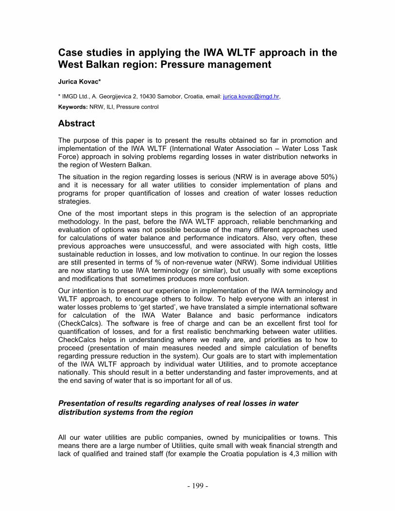
- 199 -

Case studies in applying the IWA WLTF approach in the West Balkan region: Pressure management

Jurica Kovac*

* IMGD Ltd., A. Georgijevica 2, 10430 Samobor, Croatia, email: [email protected],

Keywords: NRW, ILI, Pressure control

Abstract

The purpose of this paper is to present the results obtained so far in promotion and implementation of the IWA WLTF (International Water Association – Water Loss Task Force) approach in solving problems regarding losses in water distribution networks in the region of Western Balkan.

The situation in the region regarding losses is serious (NRW is in average above 50%) and it is necessary for all water utilities to consider implementation of plans and programs for proper quantification of losses and creation of water losses reduction strategies.

One of the most important steps in this program is the selection of an appropriate methodology. In the past, before the IWA WLTF approach, reliable benchmarking and evaluation of options was not possible because of the many different approaches used for calculations of water balance and performance indicators. Also, very often, these previous approaches were unsuccessful, and were associated with high costs, little sustainable reduction in losses, and low motivation to continue. In our region the losses are still presented in terms of % of non-revenue water (NRW). Some individual Utilities are now starting to use IWA terminology (or similar), but usually with some exceptions and modifications that sometimes produces more confusion.

Our intention is to present our experience in implementation of the IWA terminology and WLTF approach, to encourage others to follow. To help everyone with an interest in water losses problems to ‘get started’, we have translated a simple international software for calculation of the IWA Water Balance and basic performance indicators (CheckCalcs). The software is free of charge and can be an excellent first tool for quantification of losses, and for a first realistic benchmarking between water utilities. CheckCalcs helps in understanding where we really are, and priorities as to how to proceed (presentation of main measures needed and simple calculation of benefits regarding pressure reduction in the system). Our goals are to start with implementation of the IWA WLTF approach by individual water Utilities, and to promote acceptance nationally. This should result in a better understanding and faster improvements, and at the end saving of water that is so important for all of us.

Presentation of results regarding analyses of real losses in water distribution systems from the region

All our water utilities are public companies, owned by municipalities or towns. This means there are a large number of Utilities, quite small with weak financial strength and lack of qualified and trained staff (for example the Croatia population is 4,3 million with

- 200 -

116 public water Utilities). Also, the problem of losses in distribution system was for a long time considered less important than increasing the coverage of population with safe drinking water. Very often the same utility is responsible also for the sewers, and sometimes also for some other communal activities like waste collecting, maintenance of parks, cemeteries etc.

In the last couple of years many large water Utilities have invested in equipment for leakage detection and pipeline inspection (ground microphones, leak correlators, mobile flow and pressure meters). But very often they had not developed loss reduction programs based on pressure management, or active leakage control for awareness and location of unreported leaks. Some mid-size and small Utilities received some equipment through donations or by other kinds of international help (for example Bosnia and Herzegovina, Serbia, Monte Negro, Croatia); but in most cases equipment was purchased without proper selection and at the end often without proper (or without any) staff training.

Knowledge regarding district measuring areas (DMA) is getting more accepted in the region but is still not used enough. The reason is that old systems were developed with many interconnections for emergency supply and water quality objectives. However, the Utilities with lowest losses are using system zoning with installed control flow meters.

Installations for pressure control in the systems are rare, perhaps because we have lacked knowledge regarding the influence on pressure on leak flow rates and burst frequencies. We have cases where pressure reduction valves (PRVs) are installed because of very high pressures, but without proper maintenance they malfunction, resulting in higher losses and frequent bursts.

We have also, more recently, some positive examples where Utilities with lowest losses are implementing PRVs or other solutions in pressure control.

We must also underline a serious problem in our water Utilities : the lack of qualified, trained and motivated staff. Sometimes the problem is technicians who are responsible for the leakage detection and pipeline inspections (untrained or underpaid). More often, managers do not understand importance of managing losses, have lack of knowledge of practical effective methods, or are simply too occupied with other obligations; this sometimes results in the incorrect conclusion that losses can be effectively reduced only by replacing old pipelines.

From our experience it is most often the case that Utilities have the staff necessary for successful implementation of losses reduction program, but the staff are not adequately managed.

From the beginning of 2005. IMGD started to use the IWA terminology in calculations of all the components of the Water Balance, including Real Losses. Also, other concepts promoted by the IWA WLTF are now becoming part of our activities (BABE and FAVAD concepts, Active Leakage Control, Pressure Management etc.).

An important evolution was the introduction of the performance indicator ILI (Infrastructure Leakage Index), which is the ratio of CARL (current annual real losses) to UARL (unavoidable annual real losses. This was a major step forward for our water Utilities considering that for the first time we could assess unavoidable annual real losses on a system-specific basis, taking account of local characteristics (main length, number of service connections, meter location, pressure).

- 201 -

In Croatia, it has been traditional to consider NRW losses of less than 25% as being a good performance, without allowing for different system characteristics (current average NRW is 40% for 2005.).

Figure 1. Western Balkan Region

In the table below, % NRW and ILI are calculated for 12 Croatian systems and one from Bosnia and Herzegovina (Table 1). Note: some received data from some users are based on approximate data and some errors are possible (unbilled authorized consumption, unauthorized consumption, average pressure) but we assume that in all cases the confidence limit is acceptable for initial comparisons of this kind. In the future with more experience regarding the new methodology, the accuracy will be better.

- 202 -

Pipelines length

NRW CARL CARL UARL Average Pressure

Distribution system

Km

Number of service connections %

WS %

WS l/s.conn/day l/s.conn/day (m)

ILI

1 142 6310 33 31 111 73 55 1,5

2 1500 42000 27 25 168 99 60 1,7

3 259 4834 39 35 259 96 45 2,7

4 991 30375 42 39 277 82 50 3,4

5 1500 23000 54 50 451 122 60 3,7

6 338 9000 37 33 290 82 60 3,7

7 713 33073 24 19 302 73 65 3,7

8 550 21700 41 35 230 55 40 4,2

9 435 12000 38 34 464 80 50 5,8

10 265 13995 52 46 346 47 40 7,4

11 97 4535 53 49 486 73 45 7,5

12 117 9184 49 43 345 40 35 8,7

13 769 42308 70 65 1069 63 50 17 Table 1.

Figure 2.

When these data are compared with international data sets where we have mean ILI 4,38 (Mckenzie and Lambert, 2004, Water21) it is evident that situation in our water distribution systems regarding real losses is similar to the world scale.

It is also important to emphasize that % NRW is not adequate for assessing performance in managing real losses (Figure 3). For example, in systems 3 and 9, the %NRW is similar (39% and 38%), but the ILI provides more meaningful performance

- 203 -

information for real losses management. Because each system has different specific characteristics and different unavoidable annual real losses, we can see from the ILIs that real losses management in system 3 (ILI=2,7) is twice as good as in system 9 (ILI= 5,8).

Figure 4.

The following case studies are used to demonstrate how implementation of activities like zoning, pressure control etc. also supported by IWA WLTF approach, can be effective. We will present them briefly with the most important steps undertaken and the results obtained.

Case study 1: Pilot project Zagreb, Croatia Reduction of leakage through pressure control - development and result obtained The water distribution system in Zagreb city, the capital of Croatia, is one of the largest in our region (over 2.900 km of pipelines and more then 100.000 connections, serving a population of approximately 800.000). In October 2005 we have started a pilot project regarding pressure control for leakage (losses) reduction. The selected zone (see Figure 6. and Figure 8.) is a residential area with multi-storey buildings (averaging 10 floors), high pressures and a suspected high level of leakage. The zone has 13,5 km of cast iron mains, and 653 service connections (cast iron, galvanized iron and PEHD).

- 204 -

Figure 5.

The first step was initial measurement of flow and pressure within the zone (after all boundary valves had been closed and checked). IMGD selected the location, and specified all details regarding chambers, for installation of pressure reduction valves and all other equipment (PRV DN250, woltmann type flowmeter, valve controller and remote GSM monitoring – Figure 6.).

Figure 6.

Also we have established 3 selected locations for pressure monitoring (with GSM data transfer) inside of the zone (Figure 7.).

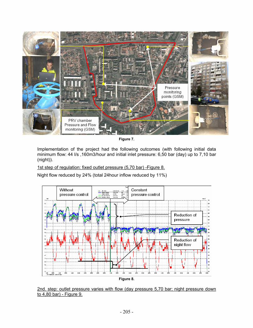
- 205 -

Figure 7. Implementation of the project had the following outcomes (with following initial data minimum flow: 44 l/s ,160m3/hour and initial inlet pressure: 6,50 bar (day) up to 7,10 bar (night)).

1st step of regulation: fixed outlet pressure (5,70 bar) -Figure 8.

Night flow reduced by 24% (total 24hour inflow reduced by 11%)

Figure 8.

2nd. step: outlet pressure varies with flow (day pressure 5,70 bar; night pressure down to 4,80 bar) - Figure 9.

- 206 -

Night flow reduced by 39% (total 24 hour inflow reduced by 14%)

Total 24h inflow reduced from 6300m3 to 5400m3 (900 m3/day savings)

Detailed estimation is underway – using FAVAD method and calculating ICF Infrastructure condition factor.

Figure 9.

This reduction in pressure had no influence on consumer’s standard of service for water supply.

Case study 2: Project Gračanica, Bosnia and Herzegovina Pressure : Burst frequencies relationship, development and results obtained The gravitational water distribution system in the town of Gračanica, north Bosnia and Herzegovina has 70 km of mains and 4500 service connections, mainly private houses with 2 floors, and a population of approximately 15000), and has for a long time experienced water shortage, especially in summer time. In the first half of 2005 we analyzed the system and concluded that pressure control is most favorable regarding short-time benefits. The key objective was to reduce current leakage, but we also wished to explore the relationship between pressure reduction and burst frequency.

- 207 -

Figure 10.

The first step was initial measurements of flow and pressure and separation of the system into 6 zones. The system was already separated into 3 areas based on ground elevation.

Separation of the system in 6 zones was made in order to implement flow and pressure control in more detail (introduction of DMA – district measuring areas), and especially to separate central area (Grad) into 3 smaller zones (Figure 11. and Figure 12.).

Zone 1 2 3 4 5 6 Name Grad north Grad

center Grad south

Čiriš north

Čiriš south

Mejdanić

Figure 11.

- 208 -

Figure 12.

Pressure control was implemented in the area Grad (in our new zoning this area covers zones 1,2,3 see Figure 12.) with pressure reduction by 20%. IMGD selected the location, and specified all details regarding chambers, for installation of pressure reduction valves and all other equipment (2 PRVs DN150, woltmann type flowmeter, valve controller and remote GSM monitoring – Figure 13.).

- 209 -

Pressure at zone inlet before and after implemented pressure control - 2nd step (flow modulated)

0

1

2

3

4

5

6

12:0

013

:00

14:0

0

15:0

016

:00

17:0

018

:00

19:0

0

20:0

0

21:0

022

:00

23:0

0

0:00

1:00

2:00

3:00

4:00

5:00

6:00

7:00

8:00

9:00

10:0

0

11:0

0

12:0

0

Time

Pres

sure

(bar

)

Before (without pressure control) After (with pressure control)

Pressure at zone inlet before and after implemented pressure control - 1st step (constant pressure)

0

1

2

3

4

5

6

12:0

0

13:0

0

14:0

015

:00

16:0

0

17:0

018

:00

19:0

020

:00

21:0

0

22:0

023

:00

0:00

1:00

2:00

3:00

4:00

5:00

6:00

7:00

8:00

9:00

10:0

0

11:0

012

:00

Time

Pres

sure

(bar

)

Before (without pressure control) After (with pressure control)

Figure 13.

Pressure before implementation of control and reduction was in the range between 4,80 and 5,30 bar. (average 5,00 bar). Reduction of pressure and control was tested in two steps; first step with constant pressure at PRV outlet of 4,00 bar, and second step with pressure modulated by PRV controller according to current flow registered by flowmeter inside of the chamber (see Figure 14.).

Figure 14.

Figure 15 clearly demonstrates the existence of a pressure : burst frequency relationship. With reduction and control of pressure, the number of bursts is dramatically reduced. Note: presented bursts in Figure 15. are for the whole distribution system but pressure control was implemented for zones 1,2,3. Determination of results only for zones 1,2,3 is currently under way.

- 210 -

Water utility Gračanica, Bosna and HerzegovinaPressure control : Burst frequency

0

5

10

15

20

25

30

35

40

45

50

55

60

Jan

2004

Feb

2004

Mar

200

4

Apr

200

4

May

200

4

Jun

2004

Jul 2

004

Aug

200

4

Sep

200

4

Oct

200

4

Nov

200

4

Dec

200

4

Jan

2005

Feb

2005

Mar

200

5

Apr

200

5

May

200

5

Jun

2005

Jul 2

005

Aug

200

5

Sep

200

5

Oct

200

5

Nov

200

5

Dec

200

5

Jan

2006

Feb

2006

Mar

200

6

Apr

200

6

May

200

6

Jun

2006

Months (2004 - 2006)

Service breaks Mains breaks Implementation of pressure control

Figure 15.

Accomplished results for a 20% reduction of inlet pressure in area Grad (Zones 1,2,3); for complete system: Mains bursts reduced by 59%; Service connection burst reduced by 72% (% reductions based on PressCalcs software calculation comparing bursts rate 638 days before pressure control and 272 days with pressure control).

Another important outcome of pressure control was reduction of losses (leakage). Daily inflow was reduced by 12% (average savings 450 m3/day) – for the complete system Figure 16 presents data received by remote monitoring via GSM, showing how pressure control (blue line) is modulated by current flow (red line). This mode of pressure control secures adequate pressure according to current demand (for example in case of fire fighting, the system recognizes the rise in flow and automatically increases the pressure). This mode of operation can be used to ensure that all consumers will always have enough pressure. It is also important to have remote monitoring of modulated systems, because new leaks and bursts will also produce a rise of flow and a rise in inlet pressure, and such events may not be noticed if they do not generate customer complaints of low pressure or no water.

- 211 -

2.4

2.6

2.8

3.0

3.2

3.4

3.6

3.8

4.0

4.2

40

50

60

70

80

90

100

110

120

130Bar cum/hr

21:00 00:00 03:00 06:00 09:00 12:00 15:00 18:00 21:00 00:00 03:00 06:00 09:00Sat 17 Dec 2005 21:00 (hour:min)

Reduktor tlaka grad

Line Site NameReduktor tlaka gradReduktor tlaka grad

MeasurandPressureProtok1

UnitsBarcum/hr

Max 4.00128.00

Min 2.6052.00

Total691.303138.00 cum

Figure 16.

Pressure management projects implementation in the region In the last year pressure management becomed more recognized as efficient solution regarding water leakage reduction and bursts frequency reduction. Couple of projects are under way led by IMGD. On the map (Figure 17) are presented locations were projects are in preparation or in implementation faze.

Figure 17.

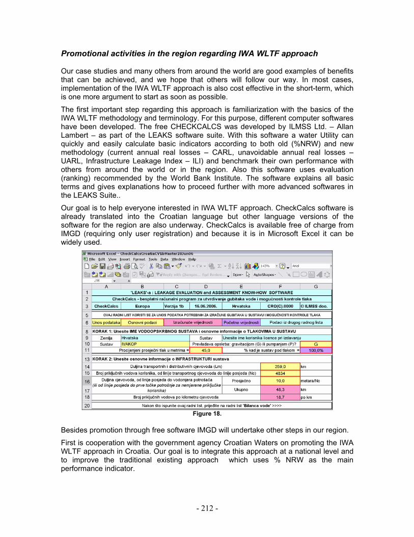
- 212 -

Promotional activities in the region regarding IWA WLTF approach Our case studies and many others from around the world are good examples of benefits that can be achieved, and we hope that others will follow our way. In most cases, implementation of the IWA WLTF approach is also cost effective in the short-term, which is one more argument to start as soon as possible.

The first important step regarding this approach is familiarization with the basics of the IWA WLTF methodology and terminology. For this purpose, different computer softwares have been developed. The free CHECKCALCS was developed by ILMSS Ltd. – Allan Lambert – as part of the LEAKS software suite. With this software a water Utility can quickly and easily calculate basic indicators according to both old (%NRW) and new methodology (current annual real losses – CARL, unavoidable annual real losses – UARL, Infrastructure Leakage Index – ILI) and benchmark their own performance with others from around the world or in the region. Also this software uses evaluation (ranking) recommended by the World Bank Institute. The software explains all basic terms and gives explanations how to proceed further with more advanced softwares in the LEAKS Suite..

Our goal is to help everyone interested in IWA WLTF approach. CheckCalcs software is already translated into the Croatian language but other language versions of the software for the region are also underway. CheckCalcs is available free of charge from IMGD (requiring only user registration) and because it is in Microsoft Excel it can be widely used.

Figure 18.

Besides promotion through free software IMGD will undertake other steps in our region.

First is cooperation with the government agency Croatian Waters on promoting the IWA WLTF approach in Croatia. Our goal is to integrate this approach at a national level and to improve the traditional existing approach which uses % NRW as the main performance indicator.

- 213 -

The second step is already undertaken and consists in the transfer of knowledge through our services for water utilities.

The third step involves promotion in other countries in the region through attendances at conferences and seminars also we have started close cooperation with UNDP [United Nations Development Program] office in Croatia regarding water loss management.

For the beginning this program will start with implementation in Croatia. UNDP representatives are hoping that after Croatia this approach will be recognised and used in wider region.

References Lambert, A and Meckenzie, R (2004) Best Practice performance indicators: practical approach, Water21,

43-45 Lambert, A (2006) CheckCalcs, Western Balkan version, software manual, Leaks Suite of Softwares Kovac, J (2006) Case studies in applying the IWA WLTF approach in the West Balkan region: Results

obtained, International conference Water loss management, telemetry and SCADA systems in water distribution systems, Skopje, Macedonia

- 214 -

Pressure Management Works……and Doesn’t! P. V. Fanner, 7 Brunswick Hill, Reading, Berkshire, RG1 7YT, United Kingdom, [email protected]

Keywords: Three keywords separated by; semi-colons

Introduction

Non-Revenue Water reduction has been a concern at the Bahamas Water and Sewerage Corporation (WSC) since the early 1990s. Unfortunately, it was never given the attention it deserved and progress, if any, was minimal. In 2001/2002, WSC created a Corporate Business Plan followed in 2003 with a Water Supply Strategy for New Providence. An integral component was a strategy to reduce Non Revenue Water (NRW), focused on the principles developed by the IWA Water Loss Task Force. The WSC NRW reduction strategy included a performance-based NRW reduction contract which would involve retaining a contractor who would reduce NRW by a guaranteed amount in a specified timeframe.

Consolidated Water Co. Ltd

Consolidated Water Co. Ltd. (CWCO) was incorporated in 1973 in the Cayman Islands to provide desalinated water and sewerage services to customers in Grand Cayman, the largest of the three Cayman Islands. CWCO's primary business is to provide water services in areas where naturally occurring supplies of drinking water are scarce. These water services include production of potable water from seawater, and the distribution of water through pipelines. They provide these services to residential, commercial and tourist properties, government agencies, and public utilities in four countries (Grand Cayman, Bahamas, BVI, and Barbados.).

Contract

In 2005 WSC contracted Consolidated Water (Bahamas) Ltd. (CWBL) to build and operate the 27.3 Mld (6 MIGD) Blue Hills Road Reverse Osmosis (RO) Plant. As a part of this contract, CWBL was required to reduce Non-Revenue Water (NRW) in the New Providence distribution system by 4.6 Mld (1 MIG) a day. The required reduction was achieved when it had been demonstrated that NRW losses had been reduced by 1,659 Mld (365 MIG) over a period of one year, as confirmed through the IWA annual water balance. CWBL contracted Paul Fanner and Julian Thornton to provide specialized advisory services in order to ensure that the NRW contract was completed as expeditiously as possible. NRW reduction performance was guaranteed by an agreement which stated that if NRW was not reduced by the agreed amount, CWBL will provide the said amount of water free of charge until the NRW reduction targets are met. There was no mention in the contract of how changes in average system pressures between the water balances should be handled.

CWBL wished to over-achieve the contractual target, in order to minimize the period over which it was necessary to provide 4.6 Mld of free water from the Blue Hills RO plant. An over-achievement target of 7.7 Mld was therefore used in developing the strategy.

- 215 -

Baseline Water Balance

A detailed validated water balance was undertaken to establish the baseline using the IWA water loss management methodologies. The key system input meters were flow tested using insertion magmeters to determine the accuracy of the WSC system input meters. A full extract of all relevant data was taken from the billing system for the start of January 2003 to the end of June 2004. This data was analyzed to check for systematic errors in the data handling, checking and estimating processes, from the meter reading through to customer billing. A random sample of small meters was removed for bench testing and a random sample of the large meter tests were tested in situ. Based on these tests, the average small meter under-registration, including an allowance for stopped meters was determined to be 3% and for the large meters, 8%. The volumes of all unmetered water consumption were estimated by building up estimates of use components for each event from first principals and estimating the number of events per year.

The results of the validated water balance for the baseline period of April 2003 to March 2004 are summarized as follows (volumes in MI):

System Input Volume 15,034

Billed Authorized 6,952

Non-Revenue Water 8,082

Unbilled Authorized 296

Water Losses 7,786

Apparent Losses 523

Real Losses 7,263

Recoverable Real Losses 6,846

l/Service connection/day 406

ILI 17

It may be seen from the above figures that real losses form by far the largest component of NRW.

- 216 -

New Providence Supply and Distribution System

Figure 30 - New Providence Key Supply Facilities

The New Providence system comprises of approximately 998 km of main pipe ranging from 600 mm to 25 mm in diameter. The largest percentage of main material is PVC which forms around 44% of the network. There are a variety of other materials such as cast iron, ductile iron and galvanized iron. The system is one hundred percent metered through approximately 38,000 active connections. More than ninety percent of the service connections are PVC. There are also approximately 11,000 inactive connections at this time.

Figure 30 details the location of the key supply facilities in New Providence and the main transmission mains. Most of the system input was supplied through two facilities; Windsor PS and Arawak Cay PS, until the Blue Hills RO plant was commissioned.

System Pressures and Control

Average distribution system pressures in New Providence are relatively low. The average zone pressure is only 20.4 m., however there is considerable variation in average pressures from zone to zone ranging from a maximum of 44.4 m. to a minimum of 5.7 m. The use of FAVAD pressure leakage modelling shows that at these low average system pressures, small changes in pressure result in substantial changes in real losses. For example, if the average system pressure were to increase by only 1.4 m, from 20.4 m to 21.8 m, background losses and losses from breaks in plastic pipes will increase by 15% and losses from breaks in metallic pipes will increase by 5%. Effective management of system pressures is therefore a key component of the NRW reduction strategy.

Reported Breaks

Reported service line breaks average 4756 per annum, or 97.3 breaks per 1000 service connections per year. This figure is an extremely high break rate when compared with typical break rates for service connections in reasonable condition of around 3 breaks per 1000 service connections. Reported main breaks over the same period are

- 217 -

averaging 430 per annum over this period, or 435 breaks per 1000 km of main. These figures indicate that the distribution infrastructure is in a fragile condition, particularly the service lines, however they also reflect the historically poor level of control over pressure fluctuations and transients often caused by supply issues and the need to throttle pressure to some locations in order to supply others. Until recently, pumps at all the key pumping stations have only operated as fixed speed pumps. It was therefore not possible to match the pumped supply to system demand, with the result that systems pressures fluctuated as demand changed and large pressure transients were created when switching between pumps.

NRW Reduction Strategy

It was apparent from the results of the validated water balance that the NRW reduction strategy needed to be primarily focused on the reduction of real losses, although the large meter testing does confirm that improving the performance of the large revenue meters was also justified. The NRW reduction strategy therefore comprised the following components:

• Pump Control and Surge Protection • Large Revenue Meter Improvement • Pressure Management (Macro and Micro) • District Metering (DMAs) • Leak Detection and Repair • Monitoring and Control

The following sections outline details of the reduction strategy components.

Pump Control and Surge Protection

WSC installed soft start / stop controls and variable speed controllers on the main duty pumps at Windsor pumping, Arawak Cay and Winton pumping stations intended to reduce the rate of new breaks.

Prospect PS was the only pumping station that WSC had not equipped with variable speed control and soft start / stop on selected pumps, because WSC planned to remove this station from service. CWBL equipped this pumping station with pump control valves to control pump delivery pressures and also to protect the distribution system from transient pressures by slow opening / closing of the control valve on pump start / stop.

CWBL installed a 12” PRV on the outlet mains from Windsor pumping station to control system pressures from this key station and protect the system against failure of the variable speed controllers. Additional pump control valves were also installed to protect the standby pumps at Windsor, Arawak Cay, and Winton pumping stations which were not covered by the variable speed controllers.

Pressure Management Areas

A total of 25 macro and micro pressure management schemes were installed in New Providence as shown in Figure 31. These schemes were primarily designed to reduce night pressures in excess of the minimum level of service, but some schemes also allowed day time pressure reduction. Each pressure reducing valve (PRV) was installed

- 218 -

with a strainer upstream, a Modulo electronic PRV controller, a magmeter which provides flow data for the controller and a Cello logger monitoring the flow into the pressure management area (PMA) and the PRV outlet pressure. Cello loggers were also installed on the average zone pressure tapping and the critical point pressure tapping to ensure that key PMA pressures are continually available.

Figure 31 – Location of Pressure Management Areas

Because there is a meter at the inlet of each of these PMA, they were also used as large DMA to monitor real loss volumes within these areas and help prioritize the deployment of leak detection resources.

District Metered Areas (DMA)

A total of 46 permanently monitored DMA were implemented, as shown in Figure 32. Cello loggers were permanently installed on the DMA meters, where they monitor flow and inlet pressure. Cello loggers were also installed to monitor critical point pressures and average zone pressures in those DMA which were targeted for active leak detection. All the Cello loggers send this data back to a central PC on a daily basis so that the nightlines can be analyzed and leak detection resources allocated to the DMA with the highest level of losses.

- 219 -

Figure 32 - Location of District Meter Areas

Leak Detection and Repair

The predominance of plastic materials in the distribution system on both mains and service lines, the low system pressures and the limited numbers of valves and hydrants on the mains, all make leak detection in New Providence challenging.

Two teams of leakage inspectors worked continually on the project to locate unreported breaks in the system, which were repaired by WSC repair crews. By the end of July 2007, a total of 2092 unreported service leaks, 278 main breaks and 73 valve and hydrant leaks had been located and repaired. The strategy anticipated saving 2.3 Mld from leak detection and repair work up to the end of 2006.

Large Revenue Meter Improvement

It was shown in the baseline water balance that total apparent losses only account for 523 Ml per annum of the total NRW volume. However, 305 Ml of this volume was due to the poor performance of the large revenue meter population. If the average under-registration of these meters could be reduced from the 9.8% of the baseline balance to 1%, 277 Ml per annum would be saved, which will result in NRW volume savings for CWBL and revenue enhancement for WSC.

Whilst this was a small volume in comparison to the target NRW reduction, improving the performance of the large meter stock was relatively simple to do because there are only a 113 of these meters and an estimated 46 of these meters could be downsized to a positive displacement meter. CWBL therefore worked with the WSC billing department to replace the larger meters with new correctly selected replacement meters, installed together with strainers and meter test ports.

Expected NRW Savings

The estimated volumes of NRW that were expected to be saved through each of the components of the strategy are summarized in Table 1.

- 220 -

Table 14 - Breakdown of Components of NRW Reduction Strategy

Strategy Component Estimated Saving (Mld)

Pump Control, Surge Protection and Pressure Management

6.4

Leak Detection and Repair 2.3 Large Revenue Meter Improvement 0.27 Rise of Leakage over 12 months - 0.9 Net Total Reduction 8.0

NRW Reduction Results

The DMA and the majority of the PMA were established by July 2006, when the new Blue Hills RO Plant was commissioned. The remaining PMA were commissioned during the second half of 2006. Prior to installation of the PMA schemes, WSC had made extensive use of valve throttling to limit flows into zones during off peak and night time periods in order to compensate for the fact that the previous volume of system input was insufficient to meet both the consumption and leakage demands of the system. After the PRVs were commissioned, WSC stopped the valve throttling, which the PRVs had effectively replaced.

The new Blue Hills plant added 27.3 Mld to the water available to supply the island. This enabled WSC to improve the level of service provided to their customers. Before this water was available, pressures at critical points in most zones were close to or a zero m head. With the additional water available, WSC sought to maintain pressures of 10.5 m head (15 psi) at critical points at all times, although WSC did allow CWBL to reduce pressures at critical points during minimum demand night hours to 7 m head (10 psi) in some zones.

The NRW reduction performance over time was closely monitored by undertaking regular annual water balances and comparing the NRW volumes with the baseline NRW volume. The key results of the various balances and the change in the annual average island pressure, weighted by service connection, are detailed in Figure 33. It may be seen that initially there was a substantial drop in the NRW volume as a result of WSC’s implementation of variable speed controls and soft stop/start on the pumping stations, together with the initial leak detection and repair work. However after this initial reduction in NRW volume, despite all the work undertaken in implementing the strategy, it may be seen that the volume of NRW gradually increased, primarily as a result of the significant increase in the annual average island weighted pressure. Although the contract did not specifically deal with how the increase in pressure should be taken into account, WSC agreed with CWBL that the NRW volumes of each balance should be pressure adjusted to account for the increase in average pressure, compared with the average pressure during the baseline period.

Unfortunately, there was very little pressure data available from the baseline period, which was well before the start of the project. In order to estimate pressures during this period, a detailed all mains hydraulic model was constructed and calibrated, then used to estimate the average annual weighted pressures during the baseline period. Average annual weighted pressures during each of the subsequent balance periods were determined using the logged AZP pressures from each PMA. N1 step tests were

- 221 -

undertaken on a representative sample of the PMAs to determine the average N1 value across the island. The real loss components of the NRW volumes of each subsequent balance were adjusted using this data and the FAVAD pressure leakage relationship.

Impact of Pressure on New Providence NRW

6000.0

7000.0

8000.0

9000.0

10000.0

11000.0

12000.0

13000.0

14000.0

15000.0

16000.0

Apr-04 Jan-06 Apr-06 Jul-06 Oct-06 Nov-06 Jan-07 Feb-07 Mar-07 Apr-07 May-07

Ml/Y

ear

0.0

5.0

10.0

15.0

20.0

25.0

30.0

Ave

rage

Ann

ual P

ress

ure

(m)

Water Into Supply Billed Authorized Consumption NRW Volume - No Pressure AdjustmentNRW Volume - Pressure Adjusted Target NRW Volume Annual Average Island Weighted Pressure (m)

Figure 33 – NRW Reduction Achieved and the Influence of Average Pressure

It may be seen from Figure 33 that the project succeeded in reducing the volume of NRW to the target volume, after pressure adjustment, however rather than achieving the target by the end of December 2006, which was the intention of the strategy, the target was only met in March 2007, with the result that CWBL had to supply the free 4.6 Mld of RO water for three months longer than planned. There are several reasons for this delay in achieving the target which are discussed in the following section.

Reasons For Delayed Target Achievement

Pressure Management Less Effective Than Planned

For internal control purposes, the monthly volume of inflow to each of the pressure zones was tracked on a monthly basis and monitored against the monthly inflow volume prior to implementing pressure control. This analysis therefore did not consider changes in customer consumption and is not considered to be a robust monitoring tool. Nevertheless it does provided a simple indication of the savings achieved in each of the zones as a result of pressure management (and leak detection interventions). Figure 34 summarizes the results of this analysis. It may be seen that significant monthly savings were achieved as a result of pressure management in 9 of the zones analyzed, although in some zones the saving was less than anticipated due to the need to maintain 10.5 m at the critical point. However these savings were partially offset by losses in 6 of the zones for some or all the period analyzed.

- 222 -

Monthly Savings by Zone

-60

-40

-20

0

20

40

60

80

100

Mar-06 Apr-06 May-06 Jun-06 Jul-06 Aug-06 Sep-06 Oct-06 Nov-06 Dec-06 Jan-07 Feb-07 Mar-07

Ml

Bay st & DowndeswellCable BeachCarmichael RoadChenilleDanottageEast EndElizabeth EstateFort FincastleGarden Hill Imperial ParkPalmdaleStapledonWulff RdColombusRobinson Rd

Monthly Savings by Zone

-60

-40

-20

0

20

40

60

80

100

Mar-06 Apr-06 May-06 Jun-06 Jul-06 Aug-06 Sep-06 Oct-06 Nov-06 Dec-06 Jan-07 Feb-07 Mar-07

Ml

Bay st & DowndeswellCable BeachCarmichael RoadChenilleDanottageEast EndElizabeth EstateFort FincastleGarden Hill Imperial ParkPalmdaleStapledonWulff RdColombusRobinson Rd

Figure 34 - Monthly Real Loss Savings By pressure Zone

The reasons for the losses in these 6 zones vary from zone to zone:

• A new large customer was connected near the end of the Carmichael Rd system in August 2006, drawing at least 2.3 Mld. This system has high friction losses therefore it was necessary to significantly increase the inlet pressure to the zone in order to satisfy levels of service at critical points. This problem was eventually resolved by WSC when they provided a new connection from the Windsor plant to supply this customer and others at the end of the Carmichael system.

• It proved to be impossible to control pressures in the Robinson Rd system and zones fed from Robinson Rd because of the pressure draw down caused by the operation of the Winton Booster pumps during peak demand periods.

• In Imperial Park, unresolved anomalies in the system meant that head losses across the zone were higher than they should have been, limiting the scope for pressure reduction.

• The losses in the other zones were due to the fact that although the PRVs were operating, the higher critical point pressures meant that pressures in these zones were actually higher than they were prior to implementing the scheme.

Main and Service Break Rates Were Not Reduced

Although no prediction had been made of the reduction in break rates due to pressure management, a reduction in break rates had been expected. It can be seen in Table 15 and Table 16 that in most zones where pressures were actually reduced, the frequency

- 223 -

of new main and service breaks was also reduced. However, these reductions in break frequency are more than offset in most of those pressure zones where pressure has actually increased, and mains and service break frequencies have also increased. Unfortunately, the net effect has been to actually slightly increase the overall frequency of mains breaks by 5.5% and service breaks by 11.2%.

Table 15 – Pressure Management Impact on Reported Mains Breaks

Pressure Zone

Avg. Breaks/ 1000 km/ year

Before PM

Avg. Breaks/ 1000 km/ year

After PMPressure

ReductionBreak Frequency

ReductionTotal

BreaksBay Street 633 603 6% 4.8% 7Cable Beach 277 208 24% 25.0% 5Carmichael Rd 355 168 6% 52.8% 35Chenille 263 314 -80% -19.0% 32East End 459 482 18% -5.0% 25Elizabeth Estates 0 983 -19% -infinity 4Fort Fincastle East 879 628 41% 28.6% 10Garden Hills 846 141 26% 83.3% 7Imperial Park 595 580 -30% 2.6% 52Old Fort 646 0 18% 100.0% 11Palmdale 464 662 8% -42.9% 24Skyline 684 0 -98% 100.0% 8Stapledon 308 514 -6% -66.7% 24Wulff Road 906 561 37% 38.1% 68Grand Total 482 508 -5.5% 312

Table 16 – Pressure Management Impact on Reported Service Breaks

Pressure Zone

Avg. Breaks/ 1000 conns./ year

Before PM

Avg. Breaks/ 1000 conns./ year After PM

Pressure Reduction

Break Frequency Reduction

Total Breaks

Bay Street 225 190 6% 2.2% 83Cable Beach 95 78 24% 4.2% 82Carmichael Rd 90 85 6% 5.0% 374Chenille 75 74 -80% 0.7% 361East End 77 84 18% -9.6% 162Elizabeth Estates 138 65 -19% 52.6% 94Fort Fincastle East 136 140 41% -3.0% 105Garden Hills 107 38 26% 64.5% 42Imperial Park 52 72 -30% -38.9% 212Old Fort 128 112 18% 12.0% 54Palmdale 117 79 8% 32.8% 196Skyline 132 161 -98% -22.2% 30Stapledon 104 108 -6% -3.9% 316Wulff Road 140 108 37% 22.7% 601Grand Total 90 100 -11.2% 2712

N1 Estimates Incorrect

Prior to implementing the PMA and undertaking the N1 step tests, the N1 values for each zone had been estimated using an N1 prediction component of the LEAKS Suite of software which estimates N1 exponent values based on the percentage of different pipe materials used for mains and services. The methodology used by the software was detailed by Thornton and Lambert, 2005. Using these predictions, the average N1 exponent value was estimated at 1.25. This estimated N1 value was used to estimate

- 224 -

the impact of pressure adjustment on the real loss components of NRW volumes from each balance.

However, when the N1 exponent values were subsequently measured using single step N1 step tests, the average N1 exponent value was found to be 0.86, thereby reducing the impact of pressure adjustment. Table 17 compares the estimated and measured N1 exponent values for the zones in which N1 step tests were undertaken.

Table 17 - Differences In Estimated and Measured N1 Values By Pressure Zone

Pressure Zone Estimated N1 Measured N1 DifferenceCable beach 1.2 0.9 -0.4Cable Beach East 1.1 0.8 -0.3Carmichael 1.3 0.8 -0.5Stapledon 1.2 0.8 -0.3Fort Fincastle E. 1.1 1.0 -0.1Fort Fincastle W. 1.0 0.9 -0.1Chenille 1.2 0.8 -0.4Elizabeth Estates 1.4 0.7 -0.7East End 1.3 1.0 -0.3Old Fort 1.2 1.0 -0.2Bain Town 1.1 1.0 -0.1

The differences observed are believed to be due to the fact that the estimates assume an average N1 of 1.5 for detectable leaks from flexible pipes and 80% of the service lines in the Bahamas were assumed to be flexible pipes. However a high proportion of the breaks on these pipes are believed to be joint failures (with an average N1 value of 0.5), rather than pipe splits.

Conclusions

The implementation of pressure management in this project was largely responsible for achieving the target 4.6 Mld NRW reduction. However, the target was not met until March 2007, three months later than planned, resulting in additional costs for CWBL because some of the pressure management schemes were less effective than anticipated for a range of reasons detailed in this paper.

The target was met after pressure adjustment of the real loss components of the NRW volumes achieved. It is clear that the target would never have been met without pressure adjustment, due to the significant increase in average system pressures. This therefore highlights the importance of linking water balances used for performance based contracts to average pressures over the balance period. The application of the pressure adjustment was complicated by the absence of pressure data during the baseline period. It is therefore recommended that, where possible, baseline pressure data is collected in parallel with determining the baseline water balance to facilitate pressure adjustment of the real loss volumes achieved.

Data from this project confirms that pressure reduction reduces mains and service break frequencies, but also highlights the fact that pressure increases also increase break frequencies, with the net result that on this project break frequencies actually slightly increased.

- 225 -

This project has also highlighted the need to take care to examine the nature of the breaks on flexible pipes when estimating N1 values in systems with a high proportion of flexible pipes.

References Thornton, J and Lambert A (2005): Progress in Practical Prediction of Pressure:Leakage, Pressure:Burst

Frequency and Pressure:Consumption Relationships. Proceedings of IWA Special Conferences 'Leakage 2005' , Halifax, Nova Scotia, Canada, September 12-14 2005

- 226 -

Design and Establishment of a Very Large Scale Low Pressure DMA Project V Anuvongnukroh*, U Makmaitree*, T Chuenchom**, S Sethaputra***, T Waldron****

* Metropolitan Waterworks Authority, Bangkok, Thailand, [email protected], [email protected]

** Technology Service and Consulting 1656 Co., Ltd., Bangkok, Thailand, [email protected]

*** Kornkan University, Kornkean, Thailand, [email protected]

**** Wide Bay Water, Queensland, Australia, [email protected]

Keywords: District Metered Area, (DMA); Pressure Management Area, (PMA); DMA design strategy

Abstract Bangkok’s Metropolitan Waterworks Authority (MWA)4 has over 25,000 km of water pipes and the supply area covers more than 1,800 square kilometers with a 24-hour pressurized supply to more than 1.77 million connections. MWA recently implemented a project to reduce water losses in the distribution system through the implementation of around 620 new District Metered Areas (DMA’s) and associated Pressure Management Areas (PMA’s). The current levels of non-revenue water are estimated to exceed 30% which the MWA is committed to reduce over the next 10 years.

Currently, MWA operates the entire distribution system at average pressures in the order of 5 m although in some areas the pressure can increase to a maximum of 15 m during off-peak demand periods. In some other areas, the water pressures drop to below 2 m during the day which causes problems when trying to establish DMA’s. It has been found that when establishing discrete DMA’s, the water pressure inside the district may drop as a result of the reduced supply points which in turn can result in a lower level of service. The MWA is trying to implement existing World’s best practice as presented at the various IWA Leakage Conferences, however, few, if any, of the case studies presented by the other IWA members involve systems operating at such low pressures as those experienced in the Bangkok system without degenerating towards an intermittent supply. The establishment of so many DMA’s in a low pressure environment presented many interesting challenges which are discussed in the paper. The key to the success of the project has been the intensive coordination between the MWA and project team, excellent collaboration with leak survey and repair teams and the establishment of a network of control centers. A thorough understanding of the nature of demand in each area as well as a solid grasp of the BABE methodology together with support from various internationally recognised specialists have all contributed to a successful project.

The paper presents details of the strategic processes adopted in the project to manage in excess of 50 engineers and more than 250 survey workers using GIS and state-of-the-art network analysis software. New design approaches using integrated GIS system and water network analysis software together with innovative mobile pressure sensing devices called MPS, were developed by the project team to assist in undertaking the zero pressure tests, to accelerate the design process and condense the testing time for

4 http://www.mwa.co.th

- 227 -

all 620 DMAs into an 8 month period. The information available from this project may assist other utilities facing similar problems to plan a cost effective solution for DMA design in low pressure systems.

Introduction

Bangkok’s Metropolitan Waterworks Authority (MWA)5 has over 25,000 km of water pipes covering service areas of 2,050 sqr km of Bangkok and its suburb, namely Samutprakarn and Nonthaburi. The MWA’s production facilities include 4 treatment plants and 14 pumping stations spreading throughout the Metropolitan Bangkok to produce and supply over 1,700 million m3 of potable water per year for its 1.77 million customers. With existing facilities, the MWA has the production capacity at over 2,000 million m3 per year.

In terms of revenue collection and customer services, the MWA is geographically divided in to 4 regions and 15 branches. The branch office is responsible for meter installation and maintenance, meter reading and revenue collection, distribution and service pipe relay and repair, and leak survey and repair for its assigned service area and customers. Each regional office on the other hand supervises the operations of 3-4 branch offices within its region and ensures that the policies set by the MWA’s headquarter are successfully implemented at the branch level. The MWA currently employs approximately 4,300 employees to support its operations and has revenue of 430 million USD per year.

Figure 1: MWA Production-Transmission and Distribution System

5 http://www.mwa.co.th

Production-Transmission and Distribution System

Operation Pressure: 6 mNo. of Customer: 1.77 millionRevenue: 15.80 Bil. Baht/yearUFW: 30%

No. of Treatment Plant: 4No. of Pumping Station: 14No. of Region: 4No. of Branch: 15No. of Employee: 4,300

Service Areas: 2,050 Sqr. kmProduction: 1,700 Mil.m3/yearMain Length: 22,000 km

Production-Transmission and Distribution System

Operation Pressure: 6 mNo. of Customer: 1.77 millionRevenue: 15.80 Bil. Baht/yearUFW: 30%

No. of Treatment Plant: 4No. of Pumping Station: 14No. of Region: 4No. of Branch: 15No. of Employee: 4,300

Service Areas: 2,050 Sqr. kmProduction: 1,700 Mil.m3/yearMain Length: 22,000 km

- 228 -

The unaccounted for water (UFW) for the entire MWA is currently at 30%. The

MWA’s goal is to sustain the UFW level at 30% throughout the next 10 years while MWA expects to improve their service level by increasing average pressure of the entire system from approximately 5 m to 6 m in the near future. Subsequently, the MWA has awarded two management contracts and four supply and installation contracts for design and set up of district metering areas (DMA) for all 15 branches (the management contracts: 4 branches; the supply and install contracts: 11 branches) for the past six years. For management contracts, which were completed in 2003, the contractors were responsible for designing and installing DMA, managing operations and performing leak survey and repair to have the UFW reduced to 30% and sustaining it at that level for the period of 6 months. This resulted in establishment of 270 DMAs for four branches. For the four supply and install contracts (one for each regional office) under the name of MWA Water Loss Management Improvement using Information Communication Technology, the objectives can be described as follows:

• To design and set up approximately additional 620 DMAs for 11 branches;

• To install SCADA system for trunk main pipes at 120 locations;

• To develop an enterprise-level integrated water leakage management application (iWLMA) based on International Water Association (IWA) framework;

• To establish network of control centers for all 15 branch offices;

• To perform system integration and upgrade network system for entire MWA;

• To perform initial field operations associated with water loss management such as step test, pressure step test, and meter reading to collect DMA-related data for setting up and initializing the WLMA;

• To provide training and technology transfer to the MWA.

These supply and install contracts have the overall budget of 70 million USD and the duration period of 630 days.

In addition to these contracts, the MWA in 2006 has conducted a workshop with international experts on water loss management to set up directives and overall policies for their water loss management program. As a result from this workshop, the MWA now has policies that will guide the overall operations of the water loss management program. Their policies can be stated as follows:

• Adapt the Total Demand Management (TDM) concept to water loss management to improve MWA’s profit;

• Improve water loss forecast method by applying non-revenue water (NRW) reduction practice and IWA standard water balance, loss strategies, and ILI;

• Knowledge and skilled personnel development in TDM and NRW for long term benefits to the MWA.

MWA System Conditions and Current Situations

The MWA supplies water to their customers using pumping systems. Out of 14 pumping stations, about half use manually on-off operation, whereas the rest install adjustable-

- 229 -

speed pumping systems. The MWA supplies the water continuously 24 hours a day, 7 days a week with the pressure kept at minimum during night. A typical pressure profile for continuous supply pumping operation is shown in Figure 2 a) which is in contrast with the profile of the gravity fed-system, shown in Figure 2 b), where the minimum pressure occurs during day where the water usage is at its maximum.

The overall system conditions of the MWA can be summarized as follows:

• Each pumping station supplies water at 15-40 m head but has long distance pumping (more than 40 – 60 km), resulting in low pressure towards the end of distribution main;

• There is no elevated water reservoirs available;

• The average pressure in the distribution main is 5 m, however, during peak hours, the pressure can drop to 2 – 3 m in some areas;

• The distribution main are made from AC and PVC pipes and has the pipe sizes of 150, 200, 300, and 400 mm (majority are 300 mm);

Figure 2 a) Figure 2 b)

Figure 2: Pressure Profiles for Continuous Supply Pumping System and Gravity-Fed System

• Some branches have 20 – 30% growth due to underground water usage

conversion.

For the described system, there are some critical areas that pressure can become very low at 2 – 3 m during peak hours because of their remote locations relative to the pumping stations as shown in Figure 3. This very low pressure during peak hours creates challenges in the design and operation of DMA. For these areas, the MWA had considered the following solutions.

• increase inlet pressure from trunk main, or

• increase size of main, or

• install new distribution main, or

• redesign DMA according to take-off location, etc.

• merge DMAs; however, the total number of properties should not exceed 8,000 - 10,000 unit

กราฟแสดงผลการวดแรงดนนำกอนและหลงการทำ Zero Pressure Test DMA 01-04-02

0

1

2

3

4

5

6

7

8

9

10

12:3

5:00

19:0

0:00

1:25

:00

7:50

:00

14:1

5:00

20:4

0:00

3:05

:00

9:30

:00

15:5

5:00

22:2

0:00

4:45

:00

11:1

0:00

17:3

5:00

0:00

:00

6:25

:00

12:5

0:00

19:1

5:00

1:40

:00

8:05

:00

14:3

0:00

20:5

5:00

3:20

:00

9:45

:00

16:1

0:00

22:3

5:00

5:00

:00

เวลา

แรงดนนำ m

/s

Fh155_s281

Fh153_s295

Fh154_s235

- 230 -

• increase number of inlets (number of meters may be more than 4 eventually)

Figure 3: MWA System Conditions with Very Low Pressure during Peak Hours

DMA Design for MWA System

Design Problem Statement and Criteria

Design Problem Statement

The DMA design problem statement can be described as follows: Design Objective: design DMA to fit budget and within 8 month Design Variables (Majors): number of meters Design Parameters (Majors): consumption, number of properties, number of service connections, number of field measurement points, etc. Design Constraints: - average and peak pressures - limited GIS and as-built data - total number of meters <= bill of quantity - time 240 days - pressure difference before and after DMA setup < 20-30% - number of service connections (1,000 < SC < 3,000) - number of meters per DMA <= 4 Design Criteria

The DMA is designed using information on physical boundary, hydraulic data, customer information from GIS/CIS databases and field survey with the design criteria as follows:

• The number of properties in each DMA should be between 1,000 – 3,000 units;

@ 16:00 hr.

@ 07:00 hr.

@ 20:00 hr.

MWA System Conditions:1) Long Distance Pumping with 15 – 40 m head2) Pressure is too low (2 - 3 m during peak hours

in some areas)3) No elevated Reservoir available 4) Distribution Mains are PVC and AC5) Some areas are mixed of residential and industrial 6) Sizes of Dist. Main are 150, 200, 300, 400 mm 7) Some branches have 20 – 30% growth due to

underground water usage conversion

@ 16:00 hr.

@ 07:00 hr.

@ 20:00 hr.

MWA System Conditions:1) Long Distance Pumping with 15 – 40 m head2) Pressure is too low (2 - 3 m during peak hours

in some areas)3) No elevated Reservoir available 4) Distribution Mains are PVC and AC5) Some areas are mixed of residential and industrial 6) Sizes of Dist. Main are 150, 200, 300, 400 mm 7) Some branches have 20 – 30% growth due to

underground water usage conversion

- 231 -

• The average zone pressure before and after DMA set up should not be much different (The target is set at maximum pressure drop between 20 – 30% and there are no major complaints from customers);

• The number of inlets should not exceed 4 inlets for each DMA

• For isolated areas such as bridges, industrial areas, air port, etc., consider installing new pipes across the bridges, or consider as a specific zone;

• In case of critical pressure areas and when the design cannot be established within 240 days (Phase-I), network simulation will be used with 6 m pressure condition at inlet pressure.

Design Strategy

Under the constraints of large-scale DMA design and set up in a short period timeframe (approximately 600 DMAs in 630 days) and the very low pressure during peak hours in critical areas, the following design strategies have been adopted:

• Adapt IWA best practices with GIS and network simulation

The boundary valves (BDV) for prospect DMA areas were closed to verify the operating pressure after valve closing. The advanced pressure logger called Mobile Pressure Sensor (MPS) with the GPRS and GPS capabilities were then deployed to log and transmit pressure data back to the operation center. The design team could monitor on-line the pressure profile and spotted low pressure immediately as it occurred. For meter sizing, the network simulation is employed to determine the size of inlet meters, with confirmation from branch office’s personnel. The actual in-line flow measurement was only used when discrepancies occurred.

• Divide areas of each branch after preliminary survey into three groups:

o Green DMA: pressure around 6-7 m or higher and pass the design criteria. Also, can use GIS/CIS information and experiences of design engineers to instantly design the DMA

o Yellow DMA: pressure is quite low (3 – 5 m) and pass the design criteria. Also, can use designer experience and network simulation to confirm the results

o Red DMA: pressure is very low (below 3 – 4 m) and considered as a critical area. Data logging and network simulation results with criterion of 6 m supply condition at DMA entry are applied.

• The processes are set with innovative devices and system support

The design process is fully supported by innovative devices such as MPS and ruggadized PDA and hand-held computer and ICT (i.e., GPRS network) to expedite the DMA design and validation process and reduce the number of deployed field workers. The low pressure can be spotted at any time during the period after BDV closing and the non-zero pressure of several-inlet DMA can be spotted on technician’s hand-held computer during zero test.

• DMA express teams are set for field operation and services in cases of emergency.

- 232 -

Design Process The design of DMA and pressure management area (PMA) was set up and carried out according to the IWA framework, as depicted Figure 4. In summary, the network model was primarily deployed during the DMA design to get flow and pressure data at the inlet of DMA. If the operating pressure from the model dropped more than 20 – 30%, the number of inlets were increased. The flow analysis data on the other hand was used for meter sizing. After confirmation and approval from branch office, the BDVs were closed to set up and verify the DMA designs. Figure 4 also demonstrates the design procedure used for critical areas with low pressure or with incomplete pipe network. Design Tools The water network analysis software used for DMA design is the AQUIS software (Seven Technologies A/S, 2006) that has the features of on-line calibrating the network model from SCADA data. For field operations, the Mobile Pressure Sensor (MPS) has been devised that can report pressure data with time-stamp and GPS location on-line via GPRS network as well as log pressure profile continuously for 2 weeks, as shown in Figure 5. Together with the developed mobile application on the PDA and handheld computer, field operators can view the pressure plot graphically in real-time to confirm/verify design and field test results right on spot.

Further, project web portal were set up to promote project visibility and communication among contractor teams and with the MWA. On this portal, there were links to various web-based project management tools, namely DMA Earth (based on Google Earth), Communication List, Knowledge Bases, E-Learning, Call Center, PMI Calendar, Issue Management, Milestone Management, Meter/RTU Installation Tracking, etc.

Figure 4: DMA/PMA Design and Setup Guidelines based on IWA Framework

Prepare Relevant Data for DMA Design such as

GIS and CIS data

Survey Pipe Network and Load Data into

Network Model Analysis Software (AQUIS)

Is Data Completed and Accurate?

No

Preliminary DMA Design

Field Survey of Piping

Equipment in the Preliminary

Designed DMA

Verify/Test Designed

DMA

Verification Result

Fail

Yes

Yes, but field measurement is

required

Build Pipe Network Model at

Branch Level

Measure Area Flow Rate and

Pressure

Adjust and Calibrate Network

Model

Analyze Network Model

Design DMA using Network Model

Filed Survey of Piping

Equipment in the DMA

Design PMA using Network Model

Prepare DMA Design

Summary Report Prepare Meter

Installation Shop Drawing

Verify/Test Pressure in the Area to Set Up

PMA

Verification Result

Prepare PMA Design Summary

Report

Prepare PCV Installation

Shop Drawing

Need to InstallPCV

PCV is not

Needed

Close BDV to Set Up DMA

Verify Data

PCV Sizing

Pass

Submit Design Report to Consult and MWA for Verification and Approval

Design DMA using Network Model with Inlet

Pressure at 6 Meter during Peak Demand

Period

Verify DMA Design by Consult, Project Engineer,

Branch Office, and Distribution Control Center

Submit Design Report to Consult and MWA for Verification and Approval

- 233 -

Figure 5: Mobile Pressure Sensor (MPS)

Design Issues and Constraints

There are several issues and constraints that have been encountered throughout the design and verification process, as shown below:

• GIS information and pipe information

The process of updating GIS from as-built drawing is ongoing and there is three months lead time for the GIS to be fully updated. As a result, field surveys are required to confirm GIS information and discrepancy reports were issued for mismatches.

• Low pressure areas

Closing additional BDVs for low pressure areas resulted in customer complaints. MPSs were deployed to monitor pressure on-line after BDV closing to spot very low pressure condition. In this case, BDVs were re-opened and additional inlets were added or the DMA was combined with adjacent DMA to increase average pressure.

• Valve conditions and locations

Not all BDVs were fully functional; thus, valve surveys were required to determine BDV status and BDV repair/replacement must be carried out when necessary. For subsequent step tests, step valve surveys and repair/replacements were also requisite.

• Project time constraints

There are 621 DMAs to be designed, validated, and set up within project time frame of 630 days. On average, one DMA need to be designed and set up every day. Various project management tools have been deployed to promote communication, collaboration among different teams, and accelerate the implementation.

- 234 -

• Other constraints

Rights of way was also a concern as it took minimum of 45 days to obtain permits. There was concerted effort between the contractor and the MWA to secure the permits for all 621 DMAs. In some cases, ground excavation was commenced prior to obtaining the permit. Other complicating factors were area of installation, traffic conditions, and limited time for installation. The work must be carried out at night starting at 9-10PM and by 4–5 AM work sites must be cleared for morning traffic. In heavy traffic areas, the allowable working time was only 3-4 hours.

Design Results and Validation

Network Analysis Results from Water Network Analysis Software

The analysis and design process is as follows:

• Building a network model in Model Manager by importing verified/corrected GIS;

• Calibrating the network model using flow and pressure measurements from branch meters, and pressure profile measurement using mobile pressure sensors (MPS) installed in each DMA;

• Input water demand profiles in the network model from billing data;

• Set up the DMA by closing BDVs on the DMA boundary in the network model;

• Simulate pressure and flow rate at the DMA inlets.

The analysis and design results from the AQUIS software were put into the DMA design report (Chuenchom, 2006) for each individual DMA. The design report is consisted of the following material:

• DMA layout plan

• Meter installation layout plan

• Boundary valve layout plan

• Pressure logging location layout plan

• Customer and demand information

• Network simulation results

• Pressure field measurement graphs

• Shop drawing

Field Test for DMA Validation The DMA designs were validated and verified in the fields as in these steps:

- 235 -

• Install MPS to verify average pressure inside DMA three days before and three days after BDV closing. The average pressure before and after DMA setup should not be different more than 20-30%;

• Perform the zero pressure test (ZPT) to verify that the pressure at the inlets and inside the DMA were in fact zero and the pressure outside DMA is not affected;

• Verify the drop test to simulate the peak demand.

These three steps were used to validate and confirm every DMA.

Figure 6: Field Test for DMA Validation Expert Comments The design process and results as well as methodology were reviewed by a panel of IWA experts during DMA design workshop held in Bangkok on May 11, 2006. All comments were incorporated to improve design process and methodology. DMA Setup and Installation DMA and Control Center Installation DMA setup includes installations of water meters (electronic Woltman meter and electromagnetic water meter, depending on contracts), pressure sensors, and RTU cabinets. The communication includes both PSTN and GPRS wireless network. The control centers at each branch office is equipped with 7 servers for applications, database, GIS, and WLMA, 5 workstations, and a high performance LCD projector. The video conference and VOIP systems were also installed to promote communications among branch officers and with Distribution Control Center (DCC).

Befor After

E

C

C

C

C

C

C

C

C

C

C

C

C

C

C

C

C

C

C

C

C

C

C

C

C

C

C

C

C

C

C

C

C

C

C

C

C

C

C

C

C

C

C

C

C

C

CC

C

C

C

C

C

C

C

C

C

CC

C

C

C

C

C

C

C

C

C

C

C

C

C

C

C

C

C

C

C

C

C

C

C

C

C

C

C

C

C

C

C

C

C

C

C C

C

C

C

C

C

C

C

C

C

C

C

C

C

CC

C

C

C

C

C

C

C

C

C

C

C

C

C

C

C

C

C

C

C

C C

C

C

C

C

C

C

C

C

C

C

C

C

C

C

C

C

CC

C

C

C

C

C

C

C

C

C

C

C C

C

C

C

C

C

C

C

C

C

C

C

C

C

C

C

C

C

C

C

C

C

C

C

C

C

C

C

C

C

C

C

C

C

C

C

C

C

C

C

C

C

C

C

C

C

C

C

C

C

C

C

C

C

C

C

C

C

C C

CC

C

C

C

C

C

C

C

C

C

C

C

C

C

C

C

C

C

C

C

C

C

C

C

C

C

C

C

C

C

C

C

C

C

C

C

C

C

C

C

C

C

C

C

C

C

C

C C

C

C

C

C

C

C

C

C

C

C

C

C

C

C

C

C

C

C C

C

C

C

C

C

C

C

C

C

C

C

C

C

C

C

C

C

C

C

C

C

C

C

C

C

C

C

C

C

C

C

C

CC

C

C

C

C

C

C

C

C

C

C

C

C

C

C

C

C

C

C

C

C

C

C

C

C

C

C

C

C

C

C

C

C

C

C

C

C

C

C

C

C

C

C

C

C

C

C

C

C

C

C

C

C

C

C

C

C

C

C

C

C

C

C C

C

C

C

C

C

C

C

C

C

D

D

D

D

D

D

D

D

D

D

D

D

D

D

D

D

D

D

D

D

DD

D

D

D

D

D

D

D

D

D

D

D

D

D

D

D

D

D

DD

D

D

D

D

D

D

D

D

D

D

D

D

D

D

D

D

H

F

F

F

F

F

F

F

F

F

F

F

F

F

F

FF

F

F

F

F

F

F

F

F

F

F

F F

F

F

F

F

F

F

F F

F

F

F

F

F

F

FF

F

FF

F

F

F

F

F

F

F

F

F

F

F

F

F

F

F

F

F

F

F

F

F

F

F

F

F

F

F

F

F

F

F

F

I

I

III II

I

II

II III

I

I II II II

I

II

II

I

IIII

I

I

GG

GG

GG

G

G

G

G

G

G

«ÍÂ¡Ôµµ

ÔªÑÂ

«ÍÂàµÔÁº

Ø-

¶¹¹ºÒ§¢Ø¹¹¹· ì

«ÍÂ 5

«ÍÂÀÒÇ

¹Ò

«ÍÂ 2

«ÍÂÈÔÃÔÇ

Ñ² ¹ì

«ÍÂ¢ØÁ·ÃÑ¾Âì 6

«ÍÂÇÑ²¹ÊØ¢¹ÔàÇÈ¹ì

«ÍÂà¡Ô

·ÃÑ¾Âì


«ÍÂÊ¶Ò¹

ÕÑºà¾ÅÔ§

«ÍÂÇÑÈÃ

ÕÊØÒÃÒÁ«ÍÂ

ÃØé§à¾ªÃ

«ÍÂ»ÅÑ

ãË-è


«ÍÂÈÃÕ¾

Òà¾ÅÔ¹

«ÍÂÇÑã

ËÁè (ÂÒÂ

á»é¹)

«ÍÂÈÈÔ¼ÅÔ¹

«ÍÂÍ§¤

ì¡ÒÃÊÇ¹Â

Ò§

«ÍÂÃÑ-Ê¹Ô·Ç§Èì 29 (ÊÇèÒ§)

ÊÐ¾Ò¹¤

Å Í§ªÑ¡¾

ÃÐ

«ÍÂ¡Ò-

¨¹ÐâËµ

Ô

«ÍÂÀÒÇ¹Ò

¶¹¹¨ÃÑ-

Ê¹Ô·Ç§Èì

N

DMA-01-02-01¤ÅÍ§ªÑ¡¾ÃÐ

BDV-01-151

CCD

I

II

DM-01-02-01-01

C

C

C

C

C

CC

C

BDV-01-132

C

C

C

C

D

IBDV-01-150

C

CD

DM-01-02-02-02

C

FH-01-182TP2

FH-01-183

TP1FH-01-181

Peak Test

·ÔÈàË¹×Í·ÔÈãµé·ÔÈµÐÇÑ¹ÍÍ¡·ÔÈµÐÇÑ¹µ¡

¤ÅÍ§ªÑ¡¾ÃÐ¶¹¹¨ÃÑ-Ê¹Ô·Ç§Èì¤ÅÍ§ºÒ§¡Í¡¹éÍÂ¤ÅÍ§¢Ø¹ÍÔ¹ ,¤ÅÍ§ªÑ¡¾ÃÐ

Update 2006-07-25

Zero Pressure Test & Drop Test 10.96

7.316.48

5.90 5.76

0.00

5.98 6.30

4.785.32 5.40 5.62 5.64

0.00

2.00

4.00

6.00

8.00

10.00

12.00

22:3

7:39

22:4

2:39

22:4

7:39

22:5

2:39

22:5

7:39

23:0

6:35

23:1

1:35

23:1

6:35

23:2

1:35

23:2

6:35

23:3

1:35

23:3

6:35

23:4

1:35

Time (Hr)

Pre

ssru

e (m

)

Zero Pressure Test & Drop Test (Flow)

82.62

65.09 61.20 64.0558.72

0.00

62.4355.94

108.56

51.14 49.69 47.47 47.62

0.00

20.00

40.00

60.00

80.00

100.00

120.00

22:3

7:3

9

22:4

2:3

9

22:4

7:3

9

22:5

2:3

9

22:5

7:3

9

23:0

6:3

5

23:1

1:3

5

23:1

6:3

5

23:2

1:3

5

23:2

6:3

5

23:3

1:3

5

23:3

6:3

5

23:4

1:3

5

Time (Hr)

Flow

(m3/

hr)

- 236 -

Integrated System Installaltion and Technology Transfer The system integration works include upgrades of network links to the computer center at the headquarter, installation of knowledge portal and data mart system for key performance index (KPI) reports for MWA’s top management.

Another critical component is the training and technology transfer to enable MWA to effectively operate installed equipment and system. The technology transfer program included 36 lecture (lasting 3-6 hours for each lectrure) and 17 on-the-job-training courses, covering instruments, DMA design and setup, field tests and operations, and ICT. The e-learning system was also setup to promote continuous learning among MWA officers.

Conclusions The MWA Water Loss Management Improvement using ICT Technology Project is a very large scale project including 621 DMAs and 120 zone and branch meter installations within a very short time frame. The project has already completed and during commissioning at the MWA. The project is proven to be successful in its time, quality, thanks to the collaborative model between the MWA as a project owner, the consultant, and the contractor, and to various ICT that were introduced to fast track the design and installation process. However, the budget for implementation are quite higher than expected due to the increasing cost of construction (the budget was based on the cost two years ago) and rework are around 30 – 50% at the beginning of the DMA survey and test in some areas. Whether the NRW can be decreased and sustained as planned depending on several other factors. MWA now has advanced systems to be aware of underground leakage situations. However, branch offices will need disciplines to change the way they operate and to use the installed systems and to maintain field equipments in the functioning conditions. Furthermore, the locate and repair components of the ALR need also be addressed. One of the critical problems is the applicability of leak survey and locating devices such as noise correlator and noise logger in the low pressure environment and AC and PVC pipe material. A new leak survey and repair program is now under way to improve the real loss for each branch using information available from the ICT system. References Chuenchom, T. (2006) Report No. DMA02: DMA Design Report for MWA Water Loss Management

Improvement using ICT Technology, the Metropolitan Waterworks Authority, Bangkok, Thailand. Seven Technologies A/S (2006) AQUIS Help Manual for AQUIS 1.45 for Windows NT/2000/XP, Seven

Technologies A/S, Birkeroed, Denmark.

- 237 -

The Modulation of the Pressure in Casablanca - LYDEC Authors:

Elhassane Benahmed *: NRW Project Manager – Technical Division LYDEC – Casablanca.

Diego LUCENTE **: NRW & Distribution Senior Engineer - Suez Environnement

Gabriel Lorrain ***: Deputy Director - Water & Waste Water Exploitation Division - LYDEC – Casablanca. * [email protected] *** [email protected] Lyonnaise des Eaux de Casablanca 48, Rue Mohamed Diouri BP. 10924 – 2000 Casablanca, Maroc Tel: +212 22 54 92 32 ** [email protected] SUEZ ENVIRONNEMENT – DORE 38 rue du Président Wilson 78230 Le Pecq – France Tel : +33 1 34 80 53 66

Keywords: pressure regulation, water distribution, NRW, leakage management

Introduction

The objective of this paper is to present :

The action plan for the Pressure Regulation of the Casablanca’s network

The results and achievements of this actions in terms of water savings, leakage and NRW impact.

Main text

Lydec, the Suez Environnement subsidiary in Casablanca, is a company of Moroccan right, which mission is the delegated management of water supply, wastewater, and electricity supply since August 1st, 1997. At present the capital shareholder is detained at the rate of :

- 51 % by Suez Environnement, - 20 % by Fipar Holding, - 15 % by by RMA Watanya, - 14 % floating in the Casablanca stock exchange.

The water supply is insured by 99 % from surface water, treated at in approximately 100 km far from Casablanca. In 1997, the water volume needed was 184 Mm3 in order to satisfy about 440 000 customers (that is more than 500 000 m3 / day)

The distribution system is very complex : 24 Reservoirs distributed on 11 pressure zones, 3800 km of pipes of different materials, and different diameters ranging from DN 60 mm to 1000 mm.

- 238 -

The return NRW is of the order of 28% by the end of the year 2005, and the volume is estimated at 48 Mm3 for the cost of 4.13 Dh/m3 (~0.4 Euros)

Since 1997, Lydec started several actions for NRW reduction. Pressure modulation is one of these projects. It was applied in certain zones of the network.

Indeed, the modulation started at the level of a pilot sector, said Old Medina, constituted mainly of old network that has a length of 21 km. This homogeneous pilot zone, as regards its environment, and flat, is situated at the sea level. The lowest level is 5m GML, near the port, and at 14 m NGM, in the other extremity.

The pressure modulation in this zone allowed :

1. To reduce the in night flow by 33 m3/hour,

2. To realize a daily water economy distribution of 720 m3/d,

3. To reduce leak numbers by 50%

Situation avant la modulation:

200 mm Almohades

250mm El Ansali200 mm El Alaoui

Guerouaoui

Chleuhs

Zaizouna

Lalla Tajja

Delimitation of the Old Medina network In front of the success of this pilot study, Lydec decided to realize the same

experiment in wider distribution zones. Indeed, the second zone where the modulation was realized is the distribution pressure zone called 110. The choice was dictated by the following considerations:

1. This zone is fed without reservoirs from the distribution pressure zone called 140,

2. It is subjected to high pressures during the nights,

3. The high flow during the night,

4. The length of network is of 180 Km

The pressure modulation in this zone allowed :

1. To reduce the night flow by 80 m3/hour

- 239 -

2. To realize a daily water economy distribution of 800 m3/d

3. To reduce leak numbers by 50%

600mm 300 mm

Dakla

Oulfa Extension

Ibn Sina

Oum Er Bia

Delimitation of the 110 pressure zone network

In front of the pressure modulation successes met for both cases, Lydec decided to study pressure zones of more complex distribution network. Indeed, the choice was put on the 85 pressure zone. Its characteristics are as follows :

- The network length : 1 100 Km

- The average daily volume distributed is between 160 000 and 180 000 m3

- The NRW is more than 20 Mm3/year that is of 54 000 m3/d representing 43 % of the global NRW,

- This pressure zone is fed from 2 reservoirs which capacity of:

o The western North called Bouskoura of a capacity of 70 000 m3

o The North is Called Médiouna of a capacity: 170 000 m3

- The distribution is from 6 trunk mains of diameter Ø 800 to Ø 1000 mm

- This pressure zone is subjected in certain sectors to high pressure mainly during night

- The zone is geographically diverse:

o 60 MGL in the North of the highway

o 05 MGL on the littoral band The first results of the modulation in this pressure zone are:

- The reduction of the night flow by 220 m3/hour,

- To realize a daily water economy distribution of 8000 m3/d.

- 240 -

1

2

3

5

4

6

Low modulated area

High area (not modulated)

Point de modulation

Delimitation of the 85 pressure zone network

- 241 -

Effective Pressure Management of District Metered Areas B Charalambous, Water Board of Lemesos, [email protected]

Keywords: pressure management; real losses; District Metered Areas.

Abstract

This paper reviews international experience in the application of pressure management and optimisation as a leakage management technique for reducing water losses from distribution networks and describes the methodology applied and experiences gained at the Water Board of Lemesos in striving to reduce leakage to economically acceptable levels and to maintain these levels through the adoption of advanced pressure control techniques, such as two point control and/or flow modulation. An account of the work carried out in pressure reduction is given together with the results obtained in further reducing real losses from the distribution system by applying in the first instance fixed outlet control followed later, once conditions in the DMA were stabilised, by other methods of control and optimisation, such as flow modulation.

Introduction

Management of pressure is a key factor in an effective leakage management policy. This has long been recognised by the Water Board of Lemesos and the ultimate goal is for all District Metered Areas (DMAs) to be equipped with Pressure Regulating Valves (PRVs) in order to reduce pressure in the network to the minimum acceptable levels and where reduction is not practicable to control and stabilise pressure.

Measurements of pressures within the DMAs were carried out to establish operating pressures at the low, medium and high points of each DMA as well as the Average Zone Night Pressure (AZNP) for each DMA. Furthermore, the pressure measurements were critically examined with the aim to reduce pressure as much as possible whilst maintaining the minimum level of service to the consumers set at 2 bar at the highest point at maximum demand.

Pressure measurements were repeated in each DMA after pressure reduction was effected to ensure that there were no potential problems and that the minimum level of service was maintained.

The pressure in DMAs where this was possible was further controlled using advanced techniques such as flow modulation or two point control in order to achieve further reduction thus driving leakage to even lower levels. These advanced techniques were tried in two DMAs with extremely successful results.

District Metered Areas

A District Metered Area (DMA) is defined as an area of the supply network having ideally about 2000 properties supplied preferably from a single entry point which is metered (water entering and leaving) and pressure controlled.

- 242 -

The main objective of establishing a DMA is to reduce real losses to an economically acceptable level and to maintain this level through the application of proactive strategies, such as Active Leakage Control.

There are a number of advantages in setting up DMAs, namely:

• The areas of the network are smaller, more manageable.

• The application of active leakage control is easier.

• Leaks are identified quicker based on MNF monitoring.

• Run time of leaks is much shorter.

• Better pressure optimisation.

• Lower water losses.

• Financial savings.

Minor problems may be encountered in the formation of DMAs which of course with proper planning and design can be resolved. These problems are:

• Possible water quality problems associated with “dead ends” in the network.

• Potential customer complaints due to optimisation of water pressures.

Pressure Management

Losses from water distribution systems must be of concern to any water utility, especially in areas of our planet where water is found in very limited quantities. It is therefore imperative that water utilities apply simple and effective methodologies in accounting for water losses from their transmission and distribution systems. The Water Loss Task Force (WLTF) of the International Water Association (IWA) has established a water audit (balance) method, which traces water from its source right through the system and derives at the end the revenue and non-revenue component, in other words is a methodology for water accountability and an integrated approach to water loss control (Yates, 2005).

It is beneficial that pressure management is an integral part of any water loss strategy. Pressure management does not only involve pressure reduction but also other methods of controlling and optimising pressure in order to achieve the maximum possible pressure reduction without compromising customer service and minimising leakage at the same time. A definition of pressure management in its widest sense has be given by Thornton et al, 2005 as “the practice of managing system pressures to the optimum levels of service ensuring sufficient and efficient supply to legitimate uses and consumers, while reducing unnecessary excess pressures, eliminating transients and faulty level controls all of which cause the distribution system to leak unnecessarily.”

According to Farley and Trow, 2003, “there are several benefits in applying pressure management, and if it is designed and maintained well, there are few, if any disadvantages”. Water utilities will therefore only benefit from the adoption of an effective pressure management policy which inevitably will have positive results in improving the operational performance of the network and in providing better customer service. International experience has shown that there are several benefits (Farley and Trow, 2003) in adopting an appropriate pressure management police, such as:

- 243 -

• Reduction of leakage – bursts and background

• Reduction of pressure-related consumption

• Reduction of frequency of bursts

• Provision of more constant supply to customers

The above benefits are being recognized worldwide and the number of utilities applying pressure management is continuously increasing. Thornton and Lambert, 2005, international experts in pressure management, stated that “an ever-increasing number of countries and utilities are now recognizing that good pressure management is the fundamental foundation of good leakage and infrastructure management”

It is common practice for water utilities to design their distribution networks to provide the minimum standard of service to the customers who are at the highest location of the system at maximum demand. This means that the minimum pressure occurs at this location at some time during the day when demand is at its maximum. Depending on how well designed the network is, significant variations in demand are reflected in varying pressures ranging from minimum at maximum demand to maximum at minimum demand at the critical point .

Understanding this concept is of the utmost importance since regulation of pressure can bring about significant reduction in leakage without compromising the level of service to the customers. Makenzie and Wegelin, 2005, based on the results of a project which they carried out in Sebokeng/Evaton, South Africa, reported that “by controlling pressures during the off-peak periods it was often possible to significantly reduce the losses without identifying or repairing a single leak. After the excessive pressures have been addressed, the other measures such as repairing pipes and /or retrofitting can be tackled”

The Water Loss Task Force promotes the adoption of the “four component” approach for managing real losses. Figure 1 shows that Pressure Management has an influence on the other components with favourable results (Manual 5, 2002), namely:

• Water conservation

• Reduced pipes failures

• Extended asset life

• Cost savings

- 244 -

Figure 1: The four component diagram with secondary influences of pressure

Understanding the impact that pressure management will have on the operation of a

distribution system is essential in the application of the correct type of approach and equipment. Pressure management is the optimisation of pressure in a distribution system to provide the minimum level of service to all customers, which ideally should be between 20m and 40m with absolute minimum of 15 m if conditions allow.

Pressure management is achieved through pressure control devices, such as pressure reducing or regulating valves. The types of pressure management that are most commonly used are:

• Fixed outlet • Two point control (Time or Flow) • Flow modulation

In the case of a fixed outlet pressure regulating valves (PRV) the pressure is continuously regulated immediately downstream of the PRV irrespective of the value of the pressure in the network. The pressure at the PRV is usually set so that the minimum level of service is achieved at the critical point at maximum demand. The draw back of this particular method is that the pressure in the network rises during periods of minimum demand without effectively being able to apply further control.

The other two methods provide better control of pressure. Two point control PRV is used to regulate the pressure in the network at two different pressures depending on the demand for flow or the time period. Again the setting of the pressure is on the downstream side of the PRV at a fixed value. Flow modulation is the most advanced method of pressure regulation and it’s increasingly gaining ground as the benefits from using such a method are becoming known and are backed up by tangible evidence form field applications worldwide. With this method pressure is continuously controlled based on the demand so that at the critical point in the network the pressure is always maintained at the minimum level of service thus achieving maximum pressure reduction at any time.

- 245 -

Implementing Pressure Management at the Water Board of Lemesos

The Water Board recognised at a very early stage the importance and significance of establishing a proper water audit system and has over the years developed its infrastructure in such a way in order to be able to account efficiently and accurately for all water produced. Reduction and control of water loss was achieved through the application of a holistic strategy based on the approach developed by the WLTF of the IWA. Integral part of this approach was the establishment and operation of DMAs in conjunction with pressure management.

At the Water Board of Lemesos the practice of leakage control by DMAs and Pressure Management has been applied based on the principle of Minimum Night Flow measurement to determine the level of leakage, to identify the presence of new bursts (reported or unreported) and to assess the impact of run time and pressure. The advantages of applying this approach are broadly described as follows:

• Smaller more manageable areas

• Easier application of active leakage control

• Quicker identification of leaks based on MNF monitoring

• Shorter Run Time of leaks

• Lower losses by controlling pressures

Since 1993 leakage management at the Water Board of Lemesos was effected through data logging, pressure reduction and leak location. Data logging for flow and pressure was carried out using 10 “Radcom” data logger devices. Logging was typically done for a period of 7 days and the loggers were then removed, the data downloaded, and deployed again to monitor other DMAs. In this way each DMA was monitored 3 to 4 times a year for a period of one week each time. It was also recognised that there was potential for pressure reduction and in 8 out of a total of 27 DMAs, Pressure Reducing Valves (PRVs) were installed. Initially leak location was done using step testing and sounding. Since 1999 the Water Board employs acoustic loggers, correlators and ground microphones for leak identification and location.

The above methodology, however, presented several shortcomings. The data available from the periodic logging were insufficient to enable proper monitoring and control. Awareness, Location and Repair (ALR) time of leaks was extremely long and it was very difficult to prioritise intervention activities. The deployment and removal of loggers was time consuming and labour intensive.

It was obvious that there was a need for an immediate review of the Water Board’s leakage management strategy. After careful consideration and examination of the available techniques, methodologies and technologies it was decided that in order to achieve further reduction of real losses from the distribution network it was imperative that a proactive approach in evaluating the efficiency of the network needed to be adopted based on continuous monitoring of flow and pressure in all DMAs.

Therefore, it was considered important to first carefully examine the size of the DMAs in an effort to further reduce the real losses from the network and provide better and more effective active leakage control. The key factors for good DMA design (Water Loss Task Force, 2004) formed the basis of the redesign. These were:

- 246 -

• minimum variation in ground level across the DMA, • easily identified boundaries that are robust, • area metres correctly sized and located, • single entry point into the DMA, • discrete DMA boundaries, • pressure optimised to maintain standard of service to customers, • degree of difficultly in working in urban area.

The variation in ground levels across the supply area was examined and particular attention was given to the influence of pressure within the DMAs. Main highways and physical features, such as streams were chosen to form discrete boundaries between DMAs. A single entry point into the district was chosen where a meter chamber was constructed to house the district meter, a pressure reducing valve and a pressure sensor. It must be stressed that the implementation of the redesign was not an easy task due to the difficulties and restrictions imposed in executing works in built up areas. These works involved inter alia, the construction of new district meter chambers, laying new lengths of pipeline and installation of new telemetry system for continuous monitoring of flow and pressure.

The redesign process (Figure 2) yielded DMAs of smaller, more manageable size with physical pipework discontinuity between DMAs. In order to verify that all interconnecting pipes between DMAs were located and isolated, a zero pressure test was carried out which involved closing the valve at the inlet to the DMA thus isolating the DMA and observing that the pressure within the DMA dropped immediately indicating that all interconnecting pipes were isolated. This test was usually carried out between 02:00 and 04:00 in the morning in order not to inconvenience consumers.

It is essential, for the effective operation of DMAs, to establish a reliable continuous monitoring system in order to apply best practice DMA management which involves the analysis of DMA night flow referred to as the Minimum Night Flow (MNF) in order to assess leakage. For this purpose each district meter is equipped with a programmable controller which is powered in most cases by solar energy panels providing a cheap and effective solution, approximately €1800 per station. Most importantly the operating cost of such a solution is extremely low, €14/month. The continuous monitoring of the district metres combines information technology and telecommunication networks to transfer the data via the World Wide Web.

- 247 -

Figure 2. Smaller more manageable DMAs

Pressure Reduction

General

Continuous flow monitoring began immediately upon completion of the redesign works in each DMA. This enabled the establishment of flow patterns for the DMAs providing essential information such as maximum and average daily flows as well as minimum night flows. Data required to establish legitimate customer night use and background leakage in each DMA were collected. Having available this information the Burst and Background Estimates (BABE) component approach to leakage was used to analyse the Minimum Night Flow (MNF).

Management of pressure is a key factor in an effective leakage management policy. This has long been recognised by the Water Board and the ultimate goal is for all DMAs to be equipped with PRVs to reduce pressure where possible and to control and stabilise pressure in DMAs where pressure reduction is not practicable.

Measurements of pressures within the DMAs were carried out to establish operating pressures at the low, medium and high points of the DMA as well as the Average Zone Night Pressure (AZNP) for each DMA. Furthermore, the pressure measurements were critically examined with the aim to reduce pressure as much as possible whilst maintaining the minimum standard of service to the consumers. As a rule a minimum standard of service of 2 bars at the highest point in the DMA at maximum demand was considered. This of course had to be reconsidered in some cases where there were high rise buildings which utilise the network’s pressure to push the water to their roof tanks. In these cases the Water Board will subsidise the installation of ground tanks and pumping systems in order that the water is pumped to the roof tanks of the high rise buildings thus enabling further pressure reduction to be effected.

- 248 -

According to common practice pressure should not be reduced in a single step otherwise there could be adverse effect on customer supplies. This of course is valid where the customers are directly fed from the mains. In systems where customer roof tanks are used, which is the case for the Water Board of Lemesos, the effect on customer supplies should be minimal since all water used in the household comes from the roof tank, except for a single tap in the kitchen which is fed directly from the network and is used for fresh potable water. Therefore, on the basis of the above it was decided to reduce the pressure in the DMAs in a single step (Figure 3) and as originally evaluated no complaints were received from consumers except in some cases where people were using the mains pressure to water their lawns. It was explained to them that they can no longer rely on the mains pressure to water their lawns and that they will be assisted by the Water Board to install small pumping systems for garden irrigation. Pressure measurements were repeated in each DMA after pressure reduction was effected to ensure that there were no potential problems and that the minimum standard of service was maintained.

Figure 3. Pressure reduction

Results

Background and Locatable Losses

Having implemented the DMA redesign works, data was collected and BABE calculations were carried out in order to determine background and locatable losses for each DMA. A similar calculation was carried out after applying pressure reduction in each DMA. The results of the calculations before and after are shown in Table1 below (Charalambous, 2005). It must be stressed that the values used for actual MNF were field values measured over a period of approximate one month before and one month after the application of the pressure reduction so that the values of the flows before and after are comparable and are not influenced by seasonal variations in customer usage.

It was decided that pressure reduction will be effected in all DMAs without attempting to locate and fix the locatable losses in these DMAs. The main reason for adopting this particular approach was to establish that by lowering the pressure the leakage reduction

- 249 -

may be such that there will be no need for further intervention. The redesign works started in 2002 and were completed in 2005 in Sector 2 of the network transforming the existing 9 DMAs to 15 smaller, easier to manage DMAs.

The application of pressure reduction in these 15 new DMAs resulted in a total reduction of 38,1% in the background losses and in a total reduction of 38,8% in locatable losses. It is evident from the results in Table1 that for twelve out of the fifteen DMAs there was no need to take further action in locating and repairing leaks. Priority for locating and repairing leaks should be given first to DMA 230 followed by DMAs 225 and 227 all of which have locatable losses greater than the threshold value of 1.5 m3/hr, figure used as the equivalent value of a single pipe burst.

Table 1. Components of real losses before and after pressure reduction in Sector 2

AZNP (m) Actual MNF

(m³/hr)

Background losses

(m³/hr)

Locatable losses

(m³/hr)

DMA

Sector 2

before after before after before after before after

220 64 32 3,92 2,16 0,63 0,24 1,88 0,51

221 63 36 5,69 3,85 3,39 1,65 0,16 0,07

222 54 28 3,07 2,24 1,53 0,71 0,05 0,03

223 53 29 3,58 2,56 1,70 0,82 0,35 0,20

224 53 29 5,50 2,52 1,68 0,82 2,23 0,11

225 64 34 12,96 9,78 5,42 2,41 4,16 3,99

226 64 34 10,04 6,84 5,62 2,55 0,37 0,24

227 59 38 15,52 10,44 5,91 3,38 5,11 2,56

228 43 39 7,60 7,20 3,42 3,03 0,51 0,50

229 41 36 4,06 3,73 1,13 0,96 2,01 1,85

230 47 40 21,80 18,00 5,57 4,60 9,37 6,54

231 52 42 11,01 7,92 4,63 3,54 2,17 0,18

232 39 32 5,17 4,32 1,32 1,05 2,21 1,63

233 42 33 4,45 3,96 1,48 1,10 1,48 1,37

234 48 38 3,55 2,44 0,32 0,23 2,26 1,24

Total before 117,92 43,75 34,32

Total after 87.96 27.09 21,02

It is worthwhile noting that pressure reduction in Sector 2 had extremely beneficial results. There was an immediate reduction of 25% in the volume of water required for the needs of Sector 2 which meant a saving of 220.000 m3 per annum valued at €170.000.

Pressure – Leakage Rate Relationship

The leakage – pressure relationship (L1/L0) = (P1/P0)N1 is valid for calculating the possible leakage reduction in a water distribution system for a given pressure reduction. The exponent “N1” is specific to the distribution network depending on the type of

- 250 -

material that the pipework is made of. In order to establish the “N1” values for the Water Board’s network the ratios P1/P0 and L1/L0 were calculated and the “N1” exponent derived for each DMA as shown in Table2. The leakage ratio included both background and locatable losses.

The values of N1 vary between 0,64 and 2,83 with an average value of 1,47. These figures are of the same order of magnitude as figures reported by others (Lambert, 2001), which reinforce the use of the leakage – pressure relationship (L1/L0) = (P1/P0)N1. The distribution mains in all of the DMA’s under consideration is a mixture of asbestos cement and uPVC with MDPE communication pipes.

Table 2. Calculation of “N1” for Sector 2

DMA L1/L0 P1/P0 N1

220 0,30 0,50 1,74

221 0,48 0,57 1,30

222 0,47 0,52 1,14

223 0,50 0,55 1,15

224 0,24 0,55 2,38

225 0,67 0,53 0,64

226 0,47 0,53 1,21

227 0,54 0,64 1,41

228 0,90 0,91 1,10

229 0,89 0,88 0,85

230 0,75 0,85 1,82

231 0,55 0,81 2,83

232 0,76 0,82 1,39

233 0,83 0,79 0,75

234 0,57 0,79 2,41

AVERAGE 1,47

New Burst Frequency

Records were kept of reported leaks before and after pressure reduction in Sector 2 and an analysis of these shows a reduction of leaks both for distribution mains and communication pipes. The results shown in Table 3 cover a period of seven months before pressure reduction and the corresponding seven months after pressure reduction.

- 251 -

Table 3. Reported leaks in Sector 2

No. of leaks reported Description

before after

Reduction of leaks

Distribution mains

49

27

45%

Communication pipes

296

178

40%

The weighted overall Average Zone Night Pressure for Sector 2 was 52,5m before the reduction and 35,8m after. This meant that there was an overall pressure reduction of 32%. Therefore, for a 32% overall pressure reduction there was an overall reduction in new leaks on mains, fittings and communication pipes of 41% which compares favourably with a similar case in Australia reported by Lambert, 2001, where a 40% reduction in one sector of a city reduced frequencies of all new leaks on mains, services and fittings in that sector by 55%. Of course there many other factors affecting burst frequency of mains such as: weather conditions, accidental damages, etc. (Farley and Trow, 2003).

It was estimated that based on the above percentage reduction in new bursts the Water Board saved in labour and material costs that would have incurred for locating and repairing these bursts approximately €100.000 per annum.

Advanced Pressure Management

General

The Water Board continuously strives for further improvement of the operational performance of its network. To this end it has gone ahead and is applying on a trial basis further pressure management in DMAs where it is possible to optimise pressure further using advanced techniques such as flow modulation or two point control in order to achieve further reduction thus driving leakage to even lower levels. These advanced techniques were tried in two DMAs, Flow Modulation in DMA 230 and Two Point PRV in DMA 123, with extremely successful results

Flow Modulation

All PRVs installed were with fixed outlet which meant that the pressure in the DMAs varies with customer demand depending on the head loss across the network. Flow modulation however, provides an advanced method of controlling pressures and the outlet pressure is continuously controlled and varied so that the pressure required at the critical point in the network is always maintained at acceptable levels. In this manner during periods of high demand the valve adjusts itself to increase the flow in order to maintain acceptable pressures in the system. When demand in the system is reduced the valve readjusts so that excess pressures are reduced thus reducing leakage further. In order to examine the benefits of this technique the Water Board installed a “hydraulic modulator” on an existing PRV in DMA 230. It should be noted that since the installation of the fixed outlet PRV in this DMA no proactive leakage repair activity was undertaken except for reported leaks. The reason behind this was to have a clear picture of the benefit that each pressure management method will have in reducing leakage. The

- 252 -

benefit can clearly be seen in Figure 4 below. It is evident that after installing a fixed outlet there was a reduction in the Minimum Night Flow (MNF) of 4,1 m3/hr. When flow modulation was effected there was a further reduction of 2,5 m3/hr, which proves that provided the conditions are such that favour the application of flow modulation further reduction in leakage is possible.

Figure 4. Application of fixed outlet and flow modulation PRV

In order to highlight further the benefits in applying flow modulation the daily water consumption of DMA 230 was plotted for exactly the same period in 2006 when pressure was controlled by fixed outlet PRV and in 2007 when pressure was flow modulated. It is evident from Figure 5 that the installation of flow modulation resulted in a reduction in the volume of water registered by the area meter over the 101 days period under examination of the order of 6.000 m3 which means that over a 12 month period the volume saved will be of the order of 21.500 m3 valued at approximately €17.000. Without a doubt flow modulation is an investment worth making considering that the cost of the hydraulic modulator together with its installation in the case of DMA 230 was less than €3.000. It must be stressed that flow modulation can not be applied effectively in all DMAs. Flow modulation calculations must be carried out beforehand to establish the potential of flow modulation applicability in each DMA. The main criterion for applying flow modulation is that the pressure difference at the critical point between high and low demands is large enough say in excess of 5m, in order to be able to apply modulation. For DMA 230 this difference is 7m and the pressure is modulated between 1.7 bar at the lowest demand, usually at around 3am, to 2.4 bar at maximum demand which is usually at about 9am.

- 253 -

Figure 5. Comparison of flows with fixed outlet and flow modulation PRV

Two Point PRV

This method of pressure management is a variation of a fixed outlet PRV. It has two fixed downstream pressures depending on demand. The fixed outlet PRV is set so that irrespective of demand the pressure immediately downstream of the PRV is fixed at a given value. The Two Point PRV has a second setting of pressure which is effected automatically depending on demand. The PRV can also be set to change over from one pressure setting to the other based on time. In this trial it was set on flow and it was installed in DMA 123 which supplies water solely to the port of Lemesos. The use of this type of pressure management was chosen for this area due to the irregular demand of water at the port. For flows up to 20 m3/hr, sufficient for all activities in the port area apart for providing water to any ships docked in the harbour, the pressure setting is at 1.7 bar. In case of supplying water to a ship the flow immediately increases beyond 20 m3/hr and the pressure changes to the second setting which is set at 4.7 bar in order to satisfy the demand. The system operates only a few hours a day at the high pressure in order to supply water to the ships. Once demand falls below 60 m3/hr the pressure setting changes back to 1.7 bar. This system was an improvement to the fixed outlet in that pressure surges were eliminated and the MNF was reduced from 12 m3/hr to 5 m3/hr.

DMA Redesign and Pressure Reduction in Other Sectors

The application of the DMA concept together with pressure management in Sector 2 of the network yielded favourable results and proved extremely successful not only in reducing losses but also in maintaining these at acceptable levels. Following completion in 2005 of the works in Sector 2, early in 2006 work commenced in redesigning other Sectors using the same approach and principles as for Sector 2. The work carried out so far ( by mid 2007) and the results achieved are summarised in Tables 4 and 5 below.

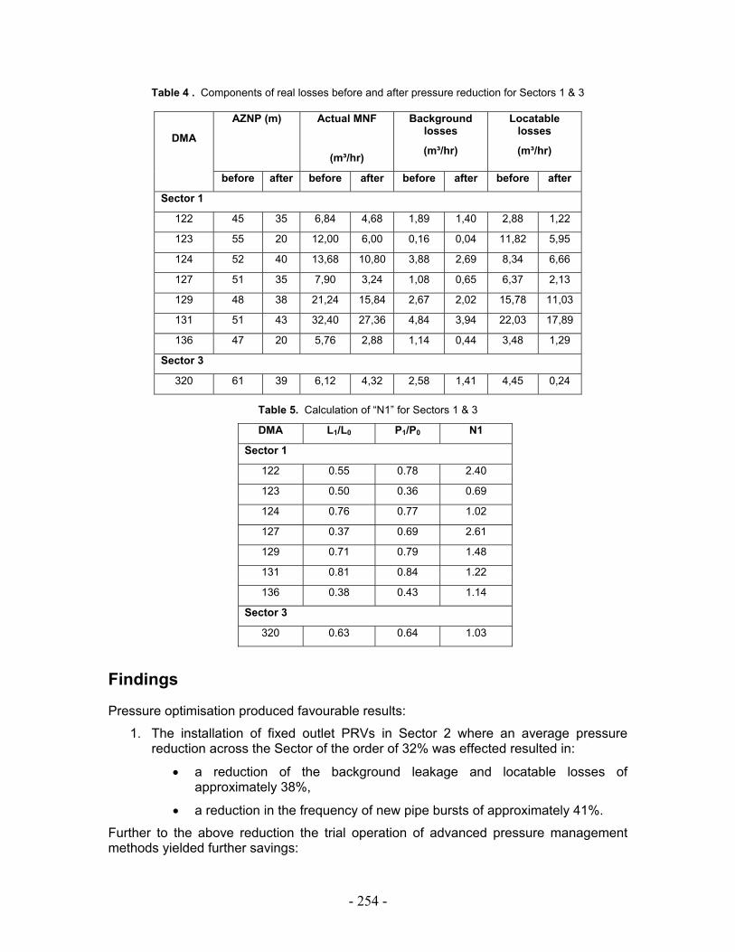
- 254 -

Table 4 . Components of real losses before and after pressure reduction for Sectors 1 & 3

Table 5. Calculation of “N1” for Sectors 1 & 3

DMA L1/L0 P1/P0 N1

Sector 1

122 0.55 0.78 2.40

123 0.50 0.36 0.69

124 0.76 0.77 1.02

127 0.37 0.69 2.61

129 0.71 0.79 1.48

131 0.81 0.84 1.22

136 0.38 0.43 1.14

Sector 3

320 0.63 0.64 1.03

Findings

Pressure optimisation produced favourable results:

1. The installation of fixed outlet PRVs in Sector 2 where an average pressure reduction across the Sector of the order of 32% was effected resulted in:

• a reduction of the background leakage and locatable losses of approximately 38%,

• a reduction in the frequency of new pipe bursts of approximately 41%.

Further to the above reduction the trial operation of advanced pressure management methods yielded further savings:

AZNP (m) Actual MNF

(m³/hr)

Background losses

(m³/hr)

Locatable losses

(m³/hr)

DMA

before after before after before after before after

Sector 1

122 45 35 6,84 4,68 1,89 1,40 2,88 1,22

123 55 20 12,00 6,00 0,16 0,04 11,82 5,95

124 52 40 13,68 10,80 3,88 2,69 8,34 6,66

127 51 35 7,90 3,24 1,08 0,65 6,37 2,13

129 48 38 21,24 15,84 2,67 2,02 15,78 11,03

131 51 43 32,40 27,36 4,84 3,94 22,03 17,89

136 47 20 5,76 2,88 1,14 0,44 3,48 1,29

Sector 3

320 61 39 6,12 4,32 2,58 1,41 4,45 0,24

- 255 -

2. Flow modulation • background leakage and locatable losses were further reduced by

approximately 50% of the fixed outlet reduction.

• payback period for the additional investment less than 3 months. 3. Two point PRV

• background leakage and locatable losses were further reduced by approximately 60% of the fixed outlet reduction.

• payback period for the additional investment less than 2 months.

References Charalambous, B. 2005, Experiences in DMA redesign at the Water Board of Lemesos, IWA Specialised

Conference “Leakage 2005”, Halifax, Nova Scotia, Canada, Conference Proceedings, pp411-412. Farley, M. and Trow, S. 2003. Losses in Water Distribution Networks, A Practitioner’s Guide to Assessment,

Monitoring and Control, London, IWA, ISBN1 900222 11 6, pp146-151 Lambert, A.O. 2001. What do we know about pressure: Leakage Relationships in Distribution Systems? IWA

Conference on system Approach to Leakage Control and Water Distribution systems Management, Brno ISBN 80-7204-197-S.

Manual 5, 2002: Advanced Pressure Management and PRV Selection, Managing and Reducing Losses from Water Distribution Systems, State of Queensland, Environmental Protection Agency, Wide Bay Water, ISBN 0 7242 9493 7, p25

Mckenzie, R.S. and Wegelin, W. 2005, Sebokeng/Evaton Pressure/Leakage Reduction: Public Private Partnership, IWA Specialised Conference “Leakage 2005”, Halifax, Nova Scotia, Canada, Conference Proceedings, p385.

Thornton, J. and Lambert , A. 2005, Progress in Practical Prediction of Leakage: leakage, pressure: burst frequency and pressure: consumption relationships, IWA Specialised Conference “Leakage 2005”, Halifax, Nova Scotia, Canada, Conference Proceedings, p347.

Thornton, J. Shaw, M. Aguiar, M. and Liemberger, R. 2005 How Low Can You Go? A Practical Approach to Pressure Control in Low Pressure Systems, IWA Specialised Conference “Leakage 2005”, Halifax, Nova Scotia, Canada, Conference Proceedings, p392.

Water Loss Task Force , DMA Guidance Notes, IWA WLTF, 2007. Yates, C. D. 2005, Water Accountability – The New Way. IWA Specialised Conference “Leakage 2005”,

Halifax, Nova Scotia, Canada, Conference Proceedings, pp 15-21.

- 256 -

Including the effects of pressure management in calculations of Short-Run Economic Leakage Levels

Fantozzi, Dr M, Via Forcella 29, 25064, Gussago (BS), Italy [email protected]

Lambert, A, 3 Hillview Close. Llanrhos, LL30 1SL, UK. [email protected]

Keywords: Leakage, Pressure management; Economic Leakage Levels

Abstract

During 2005 and 2006, research and publications by IWA Water Loss Task Force members have shown, beyond reasonable doubt, that management of surges and excess pressures can have a significant effect of the frequency of new leaks and bursts in water distribution systems. Reductions in new burst frequencies in the range 23% to 90% have recently been reported for 112 pressure management schemes in 10 Countries.

Existing UK methods of calculating Short Run Economic Leakage Levels (SRELLs) are usually based only on the principle of economic management of the run-time of current numbers of unreported numbers of leaks and breaks, assuming no change in pressure. Some of these approaches have also allowed for changes in pressure in relation to changes in the flow rates of leaks and bursts, but not to changes in the number of leaks and bursts, or for the effects of changes in annual repair costs. As changes in annual repair costs (following pressure management) may well be a dominant economic factor, the coming generation of SRELL calculations must surely include allowances for the influences of pressure management, if they are to be meaningful.

The paper proposes a practical way in which the effects of pressure management can be included in calculations of short-run economic leakage level, taking into account changes in leak flow rates, changes in numbers of leaks and repair costs, and changes in income from metered customers (for financial planning purposes).

Introduction

The paper consists of the following Sections and Sub-Sections:

• Achieving an Economic Level of Real Losses

o Definition of Short Run Economic Leakage Level SRELL

• Steps in development of a practical international SRELL calculation method

• How does pressure management influence components of SRELL?

o Predicting changes in leak flow rates

o Predicting reductions in frequencies of leaks and bursts

o Predicting changes in Economic Unreported Real Losses and associated parameters

o Predicting changes in consumption

- 257 -

• SRELL calculations using BABE component analysis and FAVAD Concepts

• Other Calculations using Pressure:burst relationship predictions

• Summary and Conclusions

Achieving an Economic Level of Real Losses

Figure 1 is now widely used internationally to demonstrate the essential principles for effective economic management of Real Losses. For all but a very few Utility systems, the Current Annual Real Losses (CARL, represented by the largest box) exceed the Unavoidable Annual Real Losses (UARL, the smallest box), and there is an Economic Level of Leakage (ELL) somewhere between the two.

An economic level of real losses (ELL) for a particular system cannot be achieved, or calculated, unless the Utility commits to effectively applying all four methods of real losses management shown in Figure 1. The ELL can be broadly defined (CIWEM, 2003) as:

‘the level of leakage at which any further reduction would incur costs in excess of the benefits derived from the savings’ In the absence of a simplified method for calculating economic leakage levels,

progressive Utilities such as Malta Water Services Corporation, and Halifax Regional Water Council (Canada) have previously adopted a ‘step by step’ approach. A series of ‘best practice’ initiatives within the 4 components that individually have high benefit: cost ratios, or short payback periods, are identified and implemented. When no further economically viable initiatives can be found, it can be reasonably assumed that an economic leakage level - based on the above definition of ELL - has probably been achieved, whilst recognising that the economic leakage level will change with time.

- 258 -

Current Annual Real Losses

Pressure Management

Pressure

Management

Active LeakageControl

Speed and Quality of Repairs

Speed and quality

of repairs


Pipe Materials Management:

selection,installation,

maintenance,renewal,

replacement

Pipeline and Assets

Management: Selection,

Installation, Maintenance,

Renewal, Replacement

UnavoidableAnnual Real

Losses

Potentially Recoverable Real Losses

Economic Annual Real Losses

Figure 1: The Four Components Approach to Management of Real Losses

The ratio of the CARL to the UARL is known as the Infrastructure Leakage Index (ILI). If the ILI for a system in a developed country is greater than 4 (i.e. in Bands C or D of the World Bank Institute Banding System) there is little point in attempting to calculate or predict an Economic Leakage Level, as there are likely to be one or more fundamental activities which are not being effectively carried out. On more than one occasion, this has been found to be failure to ensure prompt repairs (or any repairs!) of leaks on customers’ private pipes upstream of the customer meters used in the water balance calculation.

When a Utility commences to apply the ‘Four Component Approach’ to management of Real Losses in its system(s), activities of ‘Pipeline and Assets Management’ almost always (in the experience of the authors) have considerably longer payback periods than the other three activities ‘Speed and Quality of Repairs’ , ‘Pressure Management’ and ‘Active Leakage Control’. So, by concentrating on these three activities, for the first few years at least, Utilities with initial high leakage levels (expressed in volume/day) can usually achieve substantial reductions in Real Losses with short payback periods.

Definition of Short Run Economic Leakage Level SRELL

While there are varying degrees of sophistication of pressure control and active leakage control, the initial objective should be to ‘get started’ with each of the simple basic activities. In this paper, the term ‘Short Run Economic Leakage Level (SRELL)’ is defined as that which should be achievable by the ‘West’, ‘North’ and ‘South’ arrows on Figure 1, i.e. by

• ensuring all detected leaks and bursts are repaired promptly and to a high standard

• introducing basic pressure management, to reduce excess pressures and surges

- 259 -

• active leakage control by regular survey, at an economic intervention frequency

Steps in development of a practical international SRELL calculation method This paper can be considered as one of a series by Water Loss Task Force members which have sought to develop and refine practical international methods for predicting Short Run Economic Leakage Levels (SRELLs) for water distribution systems.

One of the more intractable problems – that of quickly assessing the SRELL component relating to unreported leaks – was substantially solved (for a policy of regular survey) by the development of basic equations (Fantozzi and Lambert, 2005), using three local parameters:

• CI: Cost of an Intervention – excluding repair costs (local currency)

• CV: Variable cost of water (in local currency/m3)

• Rate of Rise of Unreported Leakage – m3 per day, in a year

to calculate:

• EIF: Economic Intervention Frequency EIF (in months)

• EP%: Economic % of System to be surveyed each year

• ABI: Annual Budget for Intervention – excluding repair costs (local currency)

• EURL: Economic Unreported Real Losses (m3/year)

In a second paper ((Lambert & Lalonde, 2005) the presentation of the equations used for calculating EIF and associated parameters was improved, and an example given of how to calculate SRELL for an Australian system at the current average operating pressure. The paper then briefly highlighted the necessity to incorporate pressure management options into calculation of SRELLs, but without going into detail as to how this could be accomplished.

The third paper in the sequence (Thornton and Lambert, 2005) summarised methods for analysis and prediction of pressure:leak flow rate and pressure:consumption relationships using the FAVAD (Fixed and Variable Area Discharges) concept, using the exponent N1 for components of leakage, and N3 for components of consumption. That paper also attempted to analyse a limited number of early sets of pressure:burst data using a FAVAD type of relationship (exponent N2) but following discussions between WLTF members after Leakage 2005, it quickly became clear that the N2 exponent approach was definitely not appropriate for pressure:bursts relationships.

Following further collection of many more sets of pressure:burst data, an alternative concept for analysis and prediction of pressure:bursts relationships was circulated amongst WLTF members during 2006, with a brief summary appeared in Water 21 (Thornton and Lambert, 2006). Further research since then is being reported more fully in the fifth key paper (Thornton and Lambert, 2007), to the Water Loss 2007 Conference in Bucharest.

This research has now reached the stage where predictions of likely % reductions in the frequencies of leaks and bursts can be attempted separately for mains and services. Whilst further testing, refinement and improvement of the prediction method is

- 260 -

continuing, this remainder of this paper explains, with an example, how predictions of changes in leak flow rates and frequency of leaks and bursts, following pressure management, can be included in the calculation of SRELL.

How does pressure management influence components of SRELL? Component Analysis models based on BABE (Background and Bursts Estimates) concepts can be used to estimate, for each relevant part of the infrastructure (mains, service connections etc) the following components of annual real losses volume, using appropriate average flow rates and average run-times:

‘Reported’ leaks and bursts (typically with high flow rates, but short run times)

‘Background’ leakage (small non-visible, inaudible leaks, running continuously)

‘Unreported’ leaks (moderate flow rates, run times depend on Utility policies)

A visual example of the effect of pressure management on components of SRELL is shown in a simplified format in Figures 2 and 3. Figure 2 illustrates the three BABE components of SRELL as a simplified time series, at some specified average pressure, before pressure management is introduced to reduce excess pressures and surges.

0.5 1 1.5 2Time (years) -------->

Leve

l of l

eaka

ge --

------

-->

Background leakage

Unreported leakage

Unreported leakage

Reported leaks and bursts

Figure 2: Simplified BABE components of SRELL, varying with time, assuming regular survey

Background (undetectable) small leaks run continuously. Unreported leakage gradually accumulates, at an average rate of rise RR, and economic intervention occurs when the accumulated value of the ‘triangle’ of unreported leakage equals the cost of the intervention - once per year, in this example - and the process then repeats itself. Reported leaks and bursts (generally high flow rates but short duration) are superimposed on the other two components. The SRELL (shown as a dashed line) is the annual average of all three components.

Next, consider what happens after pressure management, if excess pressures and surges are reduced. The flow rates of existing and new leaks are reduced, and (in most cases) the number of new leaks and bursts is also reduced. As shown in Figure 3:

- 261 -

• the background leakage (which is very sensitive to pressure, N1 = 1.5) reduces

• the frequency and flow rates of reported leaks and bursts are reduced

• the rate of rise of unreported leakage also reduces

• the SRELL reduces to the lower dashed line

0.5 1 1.5 2 2.5 3 3.5 4 4.5 5Time (years) -------->

Leve

l of l

eaka

ge --

------

-->

<- BEFORE PRESSURE MANAGEMENT -><-------------- AFTER PRESSURE MANAGEMENT ----------------------->

Background leakageBackground leakage

Unreported leakage

Unreported leakage

Unreported leakage

Unreported leakage

Frequency and flow rates of reported leaks reduceRate of rise of unreported leakage reduces

Frequency and cost of economic intervention reducesBackground leakage reduces

Reported leaks and bursts

Figure 3: Influence of pressure management on simplifies BABE components of SRELL

The predicted reduction in annual expenditure ‘before’ and ‘after’ pressure

management will consist of 3 elements:

• the reduction in SRELL volume multiplied by the assumed variable cost of water

• the reduction in annual cost of economic interventions, as fewer will be needed

• the reduction in annual cost of repairs due to fewer leaks and bursts occurring

The estimated cost of implementing different methods of pressure management can then be compared against the predicted reductions in annual expenditure, and ‘payback periods’ calculated, to identify which pressure management option is likely to be most economic.

Predicting changes in leak flow rates

The most physically meaningful ‘Best Practice’ form of equation for pressure: leak flow rate relationships is the FAVAD (Fixed and Variable Area Discharges) equation:

L varies with PN1 and L1/L0 = (P1/P0)N1

If the average pressure is reduced from P0 to P1, flow rates through existing leaks change from L0 to L1, and the extent of the change depends on the ratio of average pressures and the exponent N1.

Tests on systems where all detectable leaks have been repaired or temporarily shut off, leaving only background (undetectable) leakage, tend to produce high N1 exponents close to 1.5. Detectable leaks and bursts on rigid pipes usually have an N1 value in the range 0.5 to 1.0, whilst splits on flexible pipes can have N1 values of 1.5 or even higher.

- 262 -

However, not all detectable leaks on flexible pipes necessarily have high N1 values; leaks associated with poor quality connections at the main can have N1 values as low as 0.5

A practical approach for pressure management SRELL predictions as follows:

• for background leakage, assume N1 = 1.5

• for detectable leaks and bursts (reported and unreported),

o assume N1 = 1.0 if pipe materials are not known

o assume 1.0 < N1 < 1.5 if splits in flexible pipes are predominant

o assume 0.5 < N1 < 1.0 if leaks from rigid pipes, or leaks from flexible pipes at the mains connection point, predominate

Predicting reductions in frequencies of leaks and bursts. Recent data from 112 systems in 10 countries (Thornton & Lambert 2007), has

clearly demonstrated that the frequency of new leaks and bursts can be significantly decreased by pressure management. A simple plot of the data relationship is shown in Figure 4; in these calculations it is more appropriate to use the % reduction in the maximum pressure at the average Zone Point.

Figure 4: Simple basis for predicting % reduction in breaks from % reduction in maximum pressure

The average relationship in Figure 4 suggests that a permanent reduction of X% in maximum pressure will reduce new break frequency by 1.4 x X%; the upper and lower limits are respectively 2.8 x X% (subject to a maximum reduction of 90%), and 0.7 x X%. However, it was noted that in some cases there were:

• significant reductions in mains burst frequency, but not in service pipe bursts

• significant reductions in service pipe burst frequency, but not in mains bursts

Using and testing a conceptual approach to explain why these differences may occur, Thornton & Lambert (2007) consider that an important parameter for practical predictions of reductions in burst frequency may be the initial (pre-pressure management) burst frequency. Initial burst frequency Fbo can be expressed as a multiple of the frequency (Fbu) used in the Unavoidable Annual Real Losses formula (Lambert et al, 1999) for well maintained pipes in good condition, which are:

- 263 -

• Mains and private length of service connection: 13 repairs per 100 km per year

• Services (main to property line): 3 repairs per 1000 service connections/year

Initial comparisons in Thornton & Lambert (2007) suggest that if the multiple Fbo/Fbu is high the % reduction in burst frequency will also tend to be high – near the upper line in Figure 4 – indicated by movement from the red circle towards the blue circle in Fig 5.. If Fbo/Fbu is closer to 1 (indicating pipes in good condition before pressure management, blue circle) the % reduction in burst frequency will tend to be smaller (lower range in Figure 4), or even absent. This practical approach is in fact assuming that burst frequencies on pipes that already have high burst frequencies will be more strongly influenced by pressure management than burst frequencies on pipes that already have low burst frequencies.

FAILURERATE

PRESSURE Figure 5: % reductions in burst frequency influenced by initial burst frequency.

Predicting changes in Economic Unreported Real Losses Calculation of the Economic Unreported Real Losses (EURL) and other economic

intervention parameters is easily done using a set of equations (Lambert and Lalonde, 2005) based on Cost of Intervention CI, Variable Cost of Water CV, and Rate of Rise of Unreported Leakage RR: • Economic Intervention Frequency EIF = √(0.789 x CI/(CV x RR)) • Economic % of system to be surveyed annually EP (%) = 100 x 12/EIF • Annual Budget for Intervention (excluding repair costs) ABI = EP% x CI • Economic Unreported Real Losses EURL (volume/year) = ABI/CV

Predicting changes in consumption

For a full financial analysis of pressure management options, Utilities may wish to take into account the effect of pressure management on income from metered consumption. The most physically meaningful and ‘Best Practice’ form of equation for representing relationships between average pressure and certain components of consumption is the FAVAD (Fixed and Variable Area Discharges) equation:

C varies with PN3 and C1/C = (P1/P0)N3

- 264 -

For external consumption (garden watering etc), an N3 of 0.5 is usually appropriate. For internal residential consumption, an N3 of around 0.1 can be used, unless this is supplied through a customer’s private storage tank, in which case N3 would be zero.

SRELL Calculations using BABE component analysis and FAVAD concepts

To demonstrate the effect of introducing pressure management options to SRELL calculations, the example in Lambert and Lalonde (of SRELL for an Australian System at an initial average pressure of 65 metres) has been taken as the starting point (Table 1). Table 1: Summary of SRELL components for an Australian System at initial pressure of 65 metres

System 65 metres1.01.5 1.1

Unavoidable AdditionalMl/year Ml/year Ml/year Ml/year Ml/year lit/conn/day

Mains (km) 603 92 157 16

Services, main to property line 16000 133 260 26

Services, prop. line to meter (km) 0 0 0 0

225 416 42

Background leakage Economic Unreported Real Losses

Real Losses from Reported

bursts

200 883

Anytown

Infrastructure Component Length or number

Short -Run Economic Leakage Level SRELL

Assumed Infrastructure Condition Factor ICF =

Current average pressure =

151

Totals

Assumed FAVAD N1 for Reported Bursts = Assumed FAVAD N1 for Background Leakage =

Other data for this system are as follows:

• 82 reported mains bursts/year, costing $3500 each to repair • 533 service pipe bursts per year (333 reported, 200 unreported) at $500 per repair • Rate of Rise RR = 0.020 m3/conn/day/year or 320 m3/day/year • Cost of an Intervention CI = $5.0/service conn. ($80,000) • Variable Cost of Water CV = $0.12/m3. Calculations of Economic Intervention parameters for regular survey are as follows: EIF (months) = √(0.789 x CI/ (CV x RR)) = √(0.789 x 80000/(0.12 x 320)) = 40 months Economic % of system to be surveyed annually EP (%) = 100 x 12/EIF = 30 % Annual Budget for Intervention (excluding repair costs) ABI ($) = EP% x CI = $24,000 Economic Unreported Real Losses EURL = ABI/CV = 200,000 m3/year = 200 Ml/year

Using the prediction methods now available, consider the effect of reducing the average pressure by around 20%, to 52 metres, through a combination of sectorisation and pressure reducing valves. The background leakage at the new average pressure (52 metres) can be calculated using the FAVAD equation with an exponent of 1.5

L1/L0 = (P1/P0)N1 or L1 = L0 x (P1/P0)1.5 = L0 x (52/65)1.5 = 0.715 x L0

and the figures of 157, 16, 260, 26, 416 and 42 in Table 1 become, respectively: 112, 11, 186, 19, 297 and 30; total, background leakage is predicted to decrease by 131 Ml/year.

As for Real Losses from Reported Bursts, assuming (for simplicity in this example) an N1 of 1.0, the leak flow rates will fall to (52/65)1.0 or 0.8 times their original value, and the numbers may also reduce. Initial mains burst frequency is 82 from 603 km, or 13.6/100 km/year; this is almost equal to the UARL mains burst frequency of 13 per 100 km/year, so no significant reduction in mains burst frequency can be expected. So real losses from reported mains bursts are predicted to reduce only in terms of flow rates, from 92 Ml/year to 92 x 0.8 = 74 Ml/year, a reduction of 18 Ml/year.

- 265 -

In contrast, service pipe burst frequency is 533 from 16,000 service connections, or 33 per 1000 service connections/year; this is 11 times the UARL service pipe burst frequency. If reduction in average pressure is 20%, % reduction in maximum pressure will be less – say 16% - and the ‘Upper’ line in Figure 4 indicates an expected 45% reduction in reported service connection bursts, from 333 per year to 183 per year, or 55% of their former number. So real losses from reported service connection bursts are predicted to reduce from 145 Ml/year to 145 x 0.8 (for flow rates) x 0.55 (for bursts) = 64 Ml/year, and annual repair costs for reported service pipe bursts by (333–183) x $500 = $75,000/year

As for Unreported Real Losses, these included repairs to 200 service pipes per year. Using the same approach as for Real Losses from reported bursts (a 20% reduction in flow rates and a 45% reduction in numbers of service pipe bursts), the Rate of Rise may be expected to fall from 320 m3/day/year to 320 x 0.8 x 0.55 = 141 m3/day/year, giving the following revised parameters for economic intervention:

EIF (months) = √(0.789 x CI/ (CV x RR)) = √(0.789 x 80000/(0.12 x 141)) = 60 months Economic % of system to be surveyed annually EP (%) = 100 x 12/EIF = 20 % Annual Budget for Intervention (excluding repair costs) ABI ($) = EP% x CI = $16,000 Economic Unreported Real Losses EURL = ABI/CV = 133,333 m3/year = 133 Ml/year

The estimated reduction is $8,000 and 67 Ml/year in Economic Intervention parameters, and a saving of 90 x $500 = $45,000/year in repair costs of unreported service pipe leaks.

Table 2 summarises the predicted effects on SRELL of reducing the average system pressure by 20%; a 36% reduction in SRELL from 881 Ml/year, 151 litres/service connection/day, to 599 Ml/year, 103 litres/connection/day. The predicted saving in production and distribution costs is (881-599) Ml/year x $0.12/m3 = $34 k per year. Annual cost of service connection repairs is predicted to fall by $120k, and annual cost of economic intervention by $8k per year. So the cost of implementing the sectorisation and pressure management program can be offset by predicted savings of $162k per year.

Table 2: Summary of predicted SRELL components, Australian System, at new pressure of 65 metres

System 52 metres1.0

1.5 1.1

Unavoidable AdditionalMl/year Ml/year Ml/year Ml/year Ml/year lit/conn/day

Mains (km) 603 74 112 11

Services, main to property line 16000 64 186 19

Services, prop. line to meter (km) 0 0 0 0

138 298 30

Anytown New average pressure =Assumed FAVAD N1 for Reported Bursts =

Assumed FAVAD N1 for Background Leakage = Assumed Infrastructure Condition Factor ICF =

Totals

Economic Unreported Real Losses

Short -Run Economic Leakage Level SRELL

133 599 103

Infrastructure Component Length or number

Real Losses from Reported

Bursts

Background leakage

Table 1 data in the above example are based on an actual ‘pre-pressure management’ situation as it was in 2001, and the predictions in Table 2 can be compared with actual achievements 5 years later, in 2006. The system has grown rapidly to almost 20,000 service connections, while the average pressure has been reduced from 65 to 53 metres (rather than 52 as assumed in Table 2). Real Losses calculated from annual water balances have been reduced to 105 litres/service connection/day, as compared to the 103 litres/service conn/day predicted in Table 2

- 266 -

above. The mains burst frequency has not changed to any obvious extent, but service pipe burst frequencies have reduced by 73% (substantially more than the 45% predicted); however there has been some replacement of older service connections, and also substantial increases in new service connections.

Other Calculations using Pressure: Burst Relationship Predictions

The ability to be able to make reasonably meaningful predictions of changes in frequencies of leaks and bursts on mains and service connections separately, following pressure management, is likely to have significant impact upon the payback periods for pressure management schemes in individual zones. Previously, payback period was usually based only upon the predicted saving in the value of the volume of water saved through reduction in leak flow rates. However, bringing reductions in annual repair costs into the calculations is likely to significantly reduce payback periods in many situations, and make it economic to proceed with schemes that are at present being deferred.

LEAKSSuite softwares Checkcalcs, PressCalcs, PreMoCalcs and ELLCalcs have been updated to include the latest prediction methods for pressure:leak flows and pressure:burst frequency; and also for pressure:consumption relationships (as some Utilities will wish to include predictions of changes in income from metered customers in their calculations).

As an example, Table 3 below, from the Pressure Management Options software PreMoCalcs, predicts the various components of volume and cost savings for options of Fixed Outlet, Time Modulation and Flow Modulation, based on a 24-hour Zone test in a Brazilian system in which inflows are measured at the Inlet point, and pressures are measured at the Inlet, Average Zone Point and Critical Point.

Table 3: Various payback periods for Pressure management options in a Zone in Brazil (PreMoCalcs)

Leakage Euro/yr 21572 45830 71397Repairs Euro/yr 2790 4680 6240Income Euro/yr -2331 -2419 -5866

Euro 20000 30000 40000

Months

Predicted Payback Periods, allowing

for:

Months

CALCULATION OF PAYBACK PERIODS

11.1 7.9 6.7

7.5 6.7

Leakage - Net Loss of Income

Implementation CostLeakage only

Leakage - Net Loss of Income + Repairs Months 10.9

Fixed Outlet

Time Modulation

Flow Modulation

Predicted Changes

8.3 7.3

Leakage + Repairs Months 9.9 7.1 6.2

12.5


• Most methods of assessing Short Run Economic Leakage Levels, developed in the

UK in the 1990’s, do not allow for any influences of changes in pressure • Those methods that do allow for changes in pressure take account of changes in

leak flow rates, but not changes in frequencies of leaks and breaks, changes in repair costs, changes in frequency and cost of economic intervention, or changes in income from metered customers

• The paper shows how concepts developed collaboratively by Water Loss Task Force Members - the latest being a method to predict changes in new break frequency following pressure management - can be used to incorporate these additional concepts for more comprehensive and meaningful SRELL calculations

- 267 -

• The example shown in the paper demonstrates that attempts to calculate SRELL without taking pressure management options into account cannot be considered as being meaningful – the many influences of pressure on all components of leakage, and on costs of repairs and economic active leakage control, are simply too substantial to be ignored.

• Research continues into testing and refining the prediction methods, and the longer term economic effects of pressure management on mains and services replacement policies and costs.

Acknowledgements

To the many Water Loss Task Force colleagues, too numerous to mention individually, who have contributed to this work.

References Fantozzi M and Lambert A (2005) Recent advances in calculating Economic Intervention Frequency for

Active Leakage Control, and implications for calculation of Economic Leakage Levels. Proceedings of IWA International Conference on Water Economics, Statistics and Finance, Crete, July 2005; and Wat. Sci. Tech. Water Supply Journal Vol. 5, No 6, 263-271

Lambert A and Lalonde A (2005). Using practical predictions of Economic Intervention Frequency to calculate Short-run Economic Leakage Level, with or without Pressure Management . Proceedings of IWA

Specialised Conference ‘Leakage 2005’, Halifax, Nova Scotia, Canada Thornton J and Lambert A (2005): Progress in Practical Prediction of Pressure:Leakage, Pressure:Burst

Frequency and Pressure:Consumption Relationships. Proceedings of IWA Special Conference 'Leakage 2005' , Halifax, Nova Scotia, Canada, September 12-14 2005

Thornton J and Lambert A (2006): Managing pressures to reduce new break frequencies, and improve nfrastructure management. Water 21, December 2006. Thornton J and Lambert A (2007). Pressure management extends infrastructure life and reduces unnecessary

energy costs . Proceedings of IWA Special Conference 'Water Loss 2007', Bucharest, Romania, 23-27 September 2007 (in press).

- 268 -

Water Loss Control in North America: More Cost Effective Than Customer Side Conservation – Why Wouldn’t You Do It?! R. Sturm*, J. Thornton**

* Water Systems Optimization (WSO), 255 King Street, Suite 437, San Francisco, CA 94107, USA; phone: 415 538 8641, 786 877 5752, e-mail: [email protected]

** Thornton International Ltd, Rua Arueira 370, Condominium Sausalito, Mairipora SP 076000-00 Brazil; e-mail [email protected]

Keywords: Water Loss Control; Water Conservation; Cost Effectiveness

Abstract

Times are changing rapidly in North America; the old reactive loss control measures are giving way to a more proactive control. Many states and regulators are starting to require their agencies to prepare standard AWWA (IWA) water balances and in many cases a more detailed component based analysis of losses. The authors have worked on several of these comprehensive projects throughout North America and will present key findings from small, medium and large sized utilities with a variety of resource constraints and loss components. One of the most important findings over the last few years is the relative low cost of distribution side water conservation (loss control) over demand side water conservation. Examples from Metro Nashville TN, LADWP CA and SFPUC CA show that the range of cost, including the initial high cost transitional intervention and repair costs, still leaves comprehensive real loss management as an option that compares very favourably with traditional demand side conservation methods.

Introduction:

Distribution side conservation programs, also known as water loss control programs, are ready for new innovation in North America while, on the other hand, creative demand side conservation programs are a common practise, especially in the western states of the United States.

Whilst it is difficult to generalize the reasons for not employing more thorough distribution side conservation, the most common reasons are mentioned by Dickinson as: political infeasibility of admitting system leakage; falsifying water accounting records; lack of recognition that recapturing non-revenue water with an upfront investment is a still great business case with fast payback; and inherent mistrust of anyone outside the utility examining their system (Dickinson, 2005).

Demand side conservation is already widely practised in the U.S. and is seen as a state of the art and cost effective conservation measure. This paper provides the reader with a general comparison of distribution and demand side conservation and their cost effectiveness, keeping a special focus on the U.S..

Background:

In North America, comprehensive water loss control programs are not pervasive, even though leakage (water loss) can be reduced with some simple starting points, resulting in multiple benefits to the drinking water utility and the environment.

- 269 -

Currently, the U.S. water industry has no uniform regulatory structure for water loss control in place. Existing U.S. regulations are simple and typically of poor precision. Validation of the water loss performance of drinking water utilities is rarely conducted and the most commonly used water loss performance indicator (percentage ratio of water losses in relation to the total system supply) is highly unreliable and, therefore, inappropriate. As a result the majority of U.S. water utilities only apply reactive leakage management practices. Similar to the absence of standard reporting and accounting methods and regulations, no national strategy exists to control and reduce these noteworthy losses (Fanner et al., 2007). Another likely reason for the lack of widespread distribution side conservation might be the fact that system losses and the monetary losses they are causing can be incorporated in the water rates paid by the customers.

Due to the current lack of standard reporting methods, it is difficult to quantify the amount of water lost in U.S. distribution systems. One of the few sources available estimating the current level of water losses in the U.S. is the U.S. Geological Survey (United States Geological Survey, 1998). This survey identifies 6 billion gallons per day as “public use and loss”, an amount of water sufficient to supply the ten largest cities in the U.S.

The past 20 years have seen major improvements on demand side conservation. Recent water utilities’ promotions of water conservation and efficiency resulted in major advances in research, public education and water use practices, particularly increased installation of water efficient fixtures, better irrigation practices, and more climate appropriate landscaping. However, water conservation in North America has largely focused on reducing customer demand conservation (Fanner et al., 2007). It appears that more precise regulatory structures in form of federal and state standards plus government incentives for demand side conservation have helped to make demand side water conservation a standard practice for water utilities.

Nevertheless, it is a main responsibility of the water utility to manage both the demand and supply of water responsibly and efficiently. Distribution side conservation through reduction and efficient management of system water losses provides real benefits to a water utility. These benefits include:

• Most effective and economic way of reducing level of losses from distribution system

• Improves public health protection • Increases the level of service provided to customers through increased reliability

of water supplies • Leakage recovery often stands as the best source for new water resources for

systems facing water supply shortage • Reduced pressure on water resources and therefore environmental improvement • Deferment of capital expenditure on water resources and supply schemes • Improved public perception of water companies • Applying best leakage management practice reduces liability to water supplier

- 270 -

Governments in North America are expressing interest in this area of water conservation, by mandating water audits and other initiatives to improve long-term water sustainability via better water supply efficiency. Some of the most important recent initiatives are:

• The Water Loss Control Committee (WLCC) of the American Water Works Association (AWWA) recommended both the IWA Water Balance and the IWA Performance Indicators in their Committee Report (Kunkel, 2003) as the current industry best practice for assessing water losses.

• In 2003, the Texas State Legislature passed house bill 3338, which includes in its language a requirement for drinking water utilities to submit a standardized IWA/AWWA water audit every five years.

• Other water oversight agencies also want to improve water supply efficiency and long term sustainability. The following organizations are reviewing state regulations, statutes, and water plans: Delaware River Basin Commission (DRBC), and the states California, Washington, Maryland, Massachusetts, Pennsylvania, Florida and New Mexico.

• The AWWA WLCC is rewriting the AWWA M36 Manual of Water Supply Practices, Water Audits and Leak Detection, to reflect the developments in the use of water audits, as well as leakage management and assessment.

• In early 2006, a free introductory software developed by the AWWA WLCC became available. The software includes a Water Balance and Performance Indicators, based on the AWWA approved standard water audit methodology and performance indicators. The software can be downloaded from the AWWA web page.

• California Urban Water Conservation Council (CUWCC) is currently revising its Best Management Practice 3 (BMP 3) to adopt the water loss management best practise recommended by the WLCC. Water losses will be assessed using standard water balance methodology and component analysis of real losses. Utilities will be required to achieve their economic optimum level of leakage within a set time frame.

• California Public Utilities Commission (CPUC) is in the process of ordering its member agencies to undertake distribution side water conservation measures. These measures will include regular standard water audits and component analysis and cost effective intervention against system losses.

Clearly, the awareness about the importance of distribution side conservation has increased over the past several years and with growing population and static water supplies it is paramount to accurately quantify system losses and to reduce system losses to an economic optimal point.

Water Conservation Goals:

According to the Pacific Institute (2003) “the largest, least expensive, and most environmentally sound source of water to meet California’s future need is the water currently being wasted in every sector of our economy”. Key benefits of global water conservation and efficiency are quoted as:

• No need for further water reservoir and dam construction • Saving water saves money! Both for Water providers and consumers as

well as for the State • Ecological and esthetic benefits to the environment

- 271 -

• Energy efficiency

Defining water “conservation” and “efficiency”

The concept of conservation and improved management of water use goes back many decades. In 1950, the Presidents Water Resources Policy Commission published “A water for the American people” which noted:

“We can no longer be wasteful and careless in our attitude towards our water resources. Not only in the West where the crucial value of water has long been recognized, but in every part of the country, we must manage and conserve water if we are to make the best use of it for future development”.

The Pacific Institute (2003), goes on to say that there are many different and sometimes contradictory definitions of conservation. Bauman et al. (1980) defined water conservation as using the benefit cost approach for the socially beneficial reduction of water use or water loss. In this context water conservation includes trade offs between benefits and costs of water management options. The advantage of this definition is that it focuses on comprehensive demand management strategies with a goal of increasing overall well being – not curtailing water use.

Another term “technical efficiency” is sometimes used to refer to the ratio of outputs to inputs such as dollars per gallon of water used. Improving technical efficiency can be achieved by either increasing output or reducing water inputs. This is not dissimilar to the concepts used in water loss management where either billed volumes can be increased by reduction of apparent losses or water input can be reduced by reduction of real losses.

The Principle of Cost Effectiveness:

Cost effectiveness analysis is the comparison of costs of a conservation device or activity, measured in dollars, with its benefits expressed in physical units for example $ per acre foot of savings or $ per MG of savings. Cost benefit analysis is the comparison of costs of a conservation device or activity measured in dollars with its benefits expressed in dollar terms for example $ net benefits = $ benefits - $ costs. The most meaningful measure for purposes of cost benefit analysis is net present value NPV. NPV compares costs and benefits that occur at different times by discounting to determine their present value (CUWCC, 2000).

BMP and the Importance of Cost Effectiveness

In California many stakeholder groups including water utilities, regulators, environmental groups and consultants and contractors recognize the need for conservation of the State water resources. To this effect a memorandum of understanding (MOU) regarding urban water conservation was adopted in 1991. The signatories of this MOU pledge to uphold 14 different Best Management Practices (BMPs) covering various customer side and distribution side conservation activities. However, a signatory water utility is deemed to be exempt from the implementation of a specific BMP if that supplier can substantiate that after a full cost benefit analysis has been undertaken the conservation measure in question was deemed was not cost effective.

The exemption clause therefore serves to bring a certain business view point to environmental custodianship.

- 272 -

Importance of Cost Effectiveness in Distribution Side Conservation

The core of efficiency analysis often takes the form of applied cost analysis comparing the costs and benefits of management alternatives. The first step is to identify the costs and benefits of the alternatives under consideration. The cost of the intervention tools is often relatively simple to identify however the benefit is often more difficult to define. It can be understood using avoided cost methods as identified in the AWWARF project “Water Efficiency Programs for Integrated Water Management”. Variable costs for water supply have grown over the years; specifically chemicals, treatment processes, energy for pumping as well as capital costs to develop new supplies. All of these costs should be applied to the benefit portion of the calculation for distribution side conservation (Chestnut T et al., 2007).

Components of a Comprehensive Water Loss Control Program:

Water loss control programs vary from utility to utility, since they are tailored to the needs and specific characteristics of the utility. However, in general there are three major components in each comprehensive water loss control program. First the water audit phase, which is complemented by a component analysis of real losses, the assessment of the economic optimum volume of real losses, and the design of an appropriate intervention strategy. The next step is the intervention phase, and finally the result evaluation phase. It is paramount for the success of any intervention program or any investment in leak detection equipment, no matter how expensive and sophisticated the equipment might be, that the utility has undertaken a detailed water audit in order to gain the necessary understanding of their water losses.

Water Audit and Component Analysis of Real Losses

The Water Audit itself is the process of identification and validation of the volumes which go into the Water Balance (see Figure 35).

Billed Water Exported

Billed Metered Authorized Consumption

Billed Authorized Consumption

Billed Un-metered Authorized Consumption

Revenue Water

Un-billed Metered Authorized Consumption

Authorized Consumption

Un-billed Authorized Consumption Un-billed Un-metered


Unauthorized Use (including theft of water) Apparent

Losses Consumption Meter Error

System Input

(Corrected)

Water Losses

Real Losses

Non-Revenue Water

Figure 35 AWWA Standard Water Balance

First the corrected System Input Volume (corrected for any system input meter inaccuracies) is identified and then all of the Authorized Consumption volume is subtracted. The remaining volume is classified as Water Losses. Water Losses are defined as the difference between the volume of water put into the distribution system and the volume taken out for billed and unbilled Authorized Consumption.

- 273 -

Next, Water Losses are broken down through a series of analyses into two components; Apparent Losses and Real Losses.

Revenue Water represents the total amount of Billed Authorized Consumption. Non-Revenue Water is composed of Unbilled Authorized Consumption and Water Losses.

The Water Balance calculates the total volume of Real Losses for the audit year. However, it does not provide the information on what portion of these Real Losses is due to Hidden Losses (losses from leaks that have not been capture by the utilities current leakage management policy). Hence, an additional methodology (component analysis of real losses) is used to assess the level of Hidden Losses so that specific cost-effective Real Loss management activities can be identified. By assessing the volume of Real Losses through component based analysis, it is possible to determine the volume of Real Losses that have been captured through the current leakage control policy. Therefore, by deducting the Real Losses assessed through the component based analysis from the Real Losses assessed through the top down Water Balance, it is possible to determine the volume of Hidden Losses. Appendix A (Figure 38) provides a general flow chart on the process that is involved in calculating the amount of Hidden Losses. Hidden Losses are made up of detectable leaks that are not being identified because of insufficient or incorrectly targeted leak detection activities. In effect, Hidden Losses are a backlog of leaks and breaks waiting to be detected and repaired. Individually, each hidden leak may not be causing a customer service problem and may not be visible at the ground surface. Collectively, however, Hidden Losses can account for a considerable volume of Real Loss each year. Based on the volume and nature of the Hidden Losses an appropriate and cost effective intervention program is designed.

Intervention Program

Based on the results of the water balance and component analysis the economically most feasible intervention program is designed for the water utility. There is a variety of intervention measures available and according to the needs of a utility they will be used as found appropriate to design the intervention program. The most common intervention measures to reduce hidden losses are:

Active Leak Detection Campaign

Active leak detection involves sounding parts of or the entire distribution network in set intervals for hidden leaks. The technologies used for detecting the sound generated by hidden leaks may vary from utility to utility. In most cases a combination of technologies is used in order to achieve the maximum results.

District Metered Area (DMA)

Hydraulically discrete zones (DMA) are created on temporary or permanent bases and supply into the DMA is metered and recorded. By deducting the legitimate consumption from the total inflow to the DMA the volume of real losses existent in the DMA can be calculated. DMAs allow prioritizing leak detection efforts to those areas with the highest volume of real losses and therefore guarantee the most efficient use of leak detection resources. DMAs also allow, when used on a permanent bases, to identify the rise of leakage volumes in DMAs in order to determine when it is cost effective to go back into the DMA and find and fix the newly occurred leaks. DMA measurements provide the utility with information necessary to reduce the runtime of hidden leaks to an economic

- 274 -

optimum. However, DMAs are also the most expensive form of intervention against real losses.

Pressure Management

Pressure management for leakage control, in its widest sense, can be defined as “The practice of managing system pressures to the optimum levels of service ensuring sufficient and efficient supply to legitimate uses and customers, while reducing unnecessary or excess pressures, eliminating transients and faulty level controls all of which cause the distribution system leak unnecessarily” (Thornton, 2005). Pressure management has the effect of reducing the frequency of new breaks and it reduces the flow rates of all breaks and background losses.

Based on the volume and nature of system losses and their monetary value the most feasible intervention program is designed using all, a combination or only one of the intervention measures outlined above.

Result Evaluation

If the intervention program was designed for the entire distribution system then a second water balance should be established after completion of the intervention program. If the intervention took place on a DMA level then it is best to repeat the DMA measurements after completion of the intervention.

Typical Demand Side Conservation Programs:

A great variety of demand side conservation programs exist and this section tries to outline the most common ones.

High Efficiency Washing Machines Rebate Programs

High efficiency washing machines are designed to save water and energy. Water utilities provide customers using high efficiency washing machines with rebates in various forms.

Metering Programs

Meters are installed at existing customer sites where currently no meter exists. These programs also require installation of water meters at all new construction sites. Such programs can also add meters to individual units in a multi-family building where there was previously only a master meter (BMP cost and Savings Study, 2003).

Residential Plumbing Retrofits Programs

Low flow shower heads and other water efficient plumbing devices are provided to the customer through various types of incentive programs.

Residential Surveys/Audits

Residential home surveys target both indoor and outdoor water use. In practice, home surveys usually imply a site visit by trained staff who solicit information on current water use practices and make recommendations for improvements in those practices. Sometimes indoor plumbing retrofit devices are directly installed when appropriate. The outdoor portion of the survey can vary widely, ranging from an intensive outdoor

- 275 -

efficiency study to provision of a brochure on outdoor watering practices (BMP cost and Savings Study, 2003).

Ultra Low Flush and High-Efficiency Toilet Programs

Ultra-low-flush (ULF) toilets are low water using toilets using no more than 1.6 gallons a flush, and High Efficiency Toilets (HETs) are high efficiency toilets using no more than 1.3 gallons per flush. HETs include dual-flush fixtures. Various incentive programs are used by water utilities to promote the installation of ULF toilets and HETs.

Commercial – Institutional and Industrial Surveys/Audits

Such surveys can range from short “walkthroughs” to sophisticated water efficiency studies. Customers are targeted with a marketing strategy and incentives. Recommendations are made to reduce the water consumption at the facility (BMP cost and Savings Study, 2003).

Cost and Savings of water loss control programs:

In order to evaluate the cost of distribution side conservation programs, eight systems and their water loss control programs were analysed. The cost for the programs includes the cost for detailed audits and assessment of economic optimum volume of losses, the cost for the leak detection program and the repair of the leaks.

San Francisco Public Utilities Commission (SFPUC)

SFPUC has a relatively low volume of real losses due to a very efficient leak repair policy and good infrastructure. However, analyses of the economic optimum for real losses have shown that it is economically feasible for SPFUC to reduce the volume of real losses though proactive leak detection and repair if real losses are valued at the retail cost of water. SFPUC is a very proactive utility already applying numerous conservation programs and a policy decision was taken to value real losses at the retail cost since the volume gained from real loss reduction will form part of SFPUC water conservation port folio. Since, the intervention part of the project has not started yet it was necessary to estimate the cost for the leak detection and repair program based on average industry cost data. The average cost for the entire program including the cost for the detailed water audits that formed the bases for the intervention program and the cost to detect and repair the leaks was calculated to be $439 per acre foot of water saved.

Nashville Water Works

Nashville Water Works is in the third year (of a five year program) of an intensive leak detection and repair program. The detailed water audits and related economic analysis have shown that it is economically feasible for Nashville Water Works to increase their water loss control efforts in actively detecting and repairing hidden leaks. Water Systems Optimization was contracted to carry out this five year leak detection program. DMAs are set up on a temporary basis to evaluate the volume of losses in each DMA. Following the DMA measurements leak detection teams from WSO are sent into the DMA to find all leaks and mark their location. Once all leaks are identified the information is handed over to Nashville Water Works for the repair of the leaks. After all leaks have been repaired a second DMA measurement is carried out to calculate the savings in real losses. The average cost for the entire program including the cost for

- 276 -

the detailed audits and the cost to detect and repair the leaks was calculated to be $318 per acre foot of water saved.

Los Angeles Department of Water & Power (LADWP)

LADWP has a relatively low level of real losses. However, economic analyses have shown that a more aggressive active leak detection and repair policy is economically feasible. Since this part of the project has not started yet it was necessary to estimate the cost for the leak detection and repair program based on average industry cost data. The average cost for the entire program including the cost for a detailed water audit that forms the bases for the intervention program and the cost to detect and repair the leaks was calculated to be $347 per acre foot of water saved.

California Department of Water Recourses- Water Audit and Leak Detection Program 1988

In 1988, the California Department of Water Resources carried out a Water Audit and Leak Detection Grant Program with 47 participating utilities from California. All utilities conducted a detailed water audit prior to the leak detection program to asses the cost effectiveness of such a program. Utilities showing a cost/benefit ratio grater than 1.0 continued into the leak detection and repair phase. The average cost for an entire water loss control program was $658/acre foot of water saved.

Las Vegas Valley Water District (LVVWD)

An article by Marcellus Jones Jr. from LVVWD published in the AWWA journal in February 2006, was used to estimate the cost for the water loss reduction program in LVVWD. The article did not include any cost for a detailed water audit. In order to be able to compare the program cost with the other cases presented an average audit cost based on the utilities size was assumed. The cost for the noise loggers purchased by LVVWD for this program was not included in the analysis since their investment cost has to be spread out over several years. The total cost for the water loss control program including audit cost, the cost to run an active leak detection program and the cost to repair the leaks was estimated to be $464/acre foot of water saved.

Large Utility – Western United States

A large utility in the western U.S. that wishes to remain anonymous conducted a detailed water audit. The findings showed that it was economically feasible to conduct an aggressive leak detection and repair program covering the entire network once a year. Since the intervention program has not started yet average industry cost data were used to assess the cost for the leak detection and repair program. The total cost for the water loss control program was estimated to be $318/acre foot of water saved.

Orange County Utilities (OCU) Florida

A detailed water audit has shown that reducing real losses through an active leak detection and repair program is economically feasible for OCU. The leak detection program is planned to commence in summer 2007. In order to be able to compare the program cost to the other utilities the cost for the leak detection and repair program was estimated based on average industry cost data. The total cost for the water loss control program was estimated to be $463/acre foot of water saved.

- 277 -

Cost of Distribution Side Conservation Programs in $/AF

$0

$100

$200

$300

$400

$500

$600

$700

SFPUC Nashville WaterWorks

LADWP Cal DWR LVVWD Large Utility -Western U.S.

Orange CountyUtilities - Florida

Utility

Cos

t [$/

AF]

Distribution side conservationprogram cost (cost/AF)

Average cost per AF fordistribution side conservationprogram

Figure 36 Cost for distribution side conservation programs

This analysis shows that the program cost might vary from utility to utility. A general guideline is that distribution side conservation programs are cheaper when the volume of real losses is high. The lower the volume of real losses the more effort is required to reduce them and therefore the overall cost for the distribution side conservation program increases. Since it is recommended by the CUWCC to calculate the cost effectiveness of demand side conservation programs against the avoided cost of water (basically the retail cost of water) the average avoided cost for an acre foot of water was calculated for the six utilities shown in Figure 36. The average avoided cost (retail cost) of an acre foot of water was $1,030/acre foot. This clearly shows the cost effectiveness of the distribution side conservation programs evaluated for this paper.

Typical costs per AF for demand side conservation:

Two documents form the basis for the demand side conservation program costs outlined in this paper. The first source was the CALFED Bay Delta Program – “Water Use Efficiency Program Plan July 2000”. The unit cost estimates in this report were constructed using methods outlined in the California Urban Water Conservation Councils (CUWCC) “Guidelines for Preparing Cost-Effectiveness Analyses of Urban Water Conservation Best Management Practices”. Water supplier BMP implementation reports provided most of the program cost data used for these estimates. The second source was the “Evaluation and Cost Benefit Analysis of Municipal Water Conservation Programs” prepared by the Water Conservation Alliance of Southern Arizona.

The typical costs per acre foot saved water were assessed for 13 demand side conservation programs and are depicted in Figure 37.

- 278 -

Cost of Demand Side Conservation Programs in $/AF

0

200

400

600

800

1,000

1,200

1,400

1,600

1,800

2,000

Deman

d Side

Con

serva

tion A

udits

Device

Give

away

s

Was

hing M

achin

e Reb

ate

Land

scap

e Con

versi

on R

ebate

Toilet

Rebate

s

Toilet

Distrib

ution

Reside

ntial

ULFT R

ebate

s

Reside

ntial

ULFT D

irect

Instal

l

CII ULF

T Rep

lacem

ent

H-Axis

Was

her R

ebate

s

Home S

urvey

- Targ

eted

Home S

urvey

- Unta

rgeted

Reside

ntial

Meterin

g

Types of Conservation Programs

Cos

t [$/

AF]

Cost for Demand Side Conservation Program ($/AF)

Avergae Cost for Distribution Side Conservation Program

Figure 37 Typical cost for demand side conservation programs compared to average cost for distribution

side conservation programs

The cost for demand side conservation programs varies considerably. The average cost for demand side conservation programs employed in California averages between $250 and $600/AF water saved based on discussions with the CUWCC. Reality is that utilities will start by employing the cheapest demand side conservation programs first, which can be very cost effective – less than $200/AF. However, with time the utility will have to move on to more expensive demand side conservation programs with some of them costing as much as $1,000/AF of water saved. . Figure 37 also shows for the purpose of comparison the average cost for distribution side conservation programs ($429/AF) as a blue line.

Conclusions:

Demand side conservation programs are now becoming an integral part of a water utilities operation. An important factor in promoting demand side conservation programs is that over the past 15 to 20 years meaningful and unambiguous federal and state water conservation standards and policies were introduced. So far distribution side conservation is not seen as a complementing component of a comprehensive water conservation port folio. However, when comparing demand side conservation program cost with distribution side conservation program cost it becomes clear that the cost effectiveness of distribution side conservation programs is equal or in many cases better than the cost effectiveness of demand side conservation programs. The water saved through reduction of real losses makes available new sources that can be used for additional supply which will help to avoid or reduce the need for demand restrictions during periods of droughts, and will ease the pressure on the environment and water resources. The authors therefore conclude that based on the cost effectiveness and benefits related to distribution side conservation programs water utilities should include distribution side conservation programs in their water conservation port folio.

- 279 -

References: Dickinson M. A. Redesigning Water Loss Standards in California Using the New IWA Methodology. In

Proc. of the Leakage 2005 Conference, Halifax, Canada. The World Bank Institute. Fanner, V. P., R. Sturm, J. Thornton, R. Liemberger, S. Davis and T. Hoogerwerf. To be published 2007.

Leakage Management Technologies. Denver, Colo.: AwwaRF and AWWA United States Geological Survey, 1998 Estimated Use of Water in the United States in 1995, Circular

1200 Kunkel, G. 2003. Applying Worldwide Best Management Practices in Water Loss Control, AWWA Water

Loss Control Committee Report. Jour. AWWA, volume 95 Thornton, J., and A. Lambert. 2005. Progress in practical prediction of pressure: leakage, pressure: burst

frequency and pressure: consumption relationships. In Proc. of the Leakage 2005 Conference, Halifax, Canada. The World Bank Institute

California Urban Water Conservation Council, 2003. BMP Cost & Savings Study. Sacramento, California: CUWCC

Jones, M. 2006. With today’s technology, what percentage of unaccounted-for water is OK?. Jour AWWA, February 2006

http://www.awwa.org/communications/journal/2006/February/JAW200602_m2m.pdf(accessed February 15, 2007)

California Bay Delta Program, 2000. Water Use Efficiency Program Plan, http://calwater.ca.gov/Programs/WaterUseEfficiency/ProgramPlan/WUE_ProgramPlan_5_UrbanWaterC

onservation_5-41_5-51.pdf (accessed February 15, 2007) Water Conservation Alliance of Southern Arizona, 2004. Evaluation and Cost Benefit Analysis of

Municipal Water Conservation Programs http://www.watercasa.org/research/ecoba/PDFs/WHOLEDOCUMENT.pdf (accessed February 15, 2007) Presidents Water Resources Policy Commission, 1950. A Water for the American People. Pacific Institute, 2003. Waste Not, Want Not: The potential for Urban Water Conservation in California.

ISBN 1-893790-09-6. 2003 November Chestnut T. et al., 2007. Water Efficiency Programs for Integrated Water Management. Denver, Colo.:

AwwaRF and AWWA

- 280 -

Appendix A

Figure 38 Flow Chart How to Determine Hidden Losses

Analyze and verify System input Volume (SIV)

Standardize Authorized Consumption Volumes by categorizing into

• Billed Authorized Consumption and its subcomponents

• Un-Billed Authorized Consumption and its subcomponents

SIV minus Authorized Consumption = Water Loss

Determine Apparent Loss Volume

Real Loss = Water Loss minus Apparent Loss

Determine Background Leakage based on system specifics (miles of mains, # of service connections etc.), condition of system infrastructure and average system pressure

Determine leakage based on number of leaks repaired, average system pressure and awareness-location and repair time for each leak.

Calculate the level of Real Losses by adding up all the Real Loss components detailed above. Real Losses = Losses from Background Leakage + Losses from reported and unreported leaks repaired.

Hidden Losses (Losses that can be reduced by active leakage control)

= Real Losses from Water Balance – Real Losses from component

based BABE and FAVAD analysis

Top Down Water Balance

Component based BABE and FAVAD Analysis

- 281 -

An Approach to Determining the True Value of Lost Water: California’s Avoided Cost Model M. A. Dickinson, Executive Director, Alliance for Water Efficiency, [email protected] Keywords: Economic recovery; ELL; business case

Introduction North America is beginning to revise its methods for assessing network water losses to correspond to the new International Water Association (IWA) Water Balance and Performance Indicator methodology. This activity is a response to the leadership of the American Water Works Association’s Water Loss Control Committee, which is in the process of revising its previously published training materials on non-revenue water management. A new manual has been written and will soon be published, entitled Water Audits and Loss Control Programs (M36), which provides detailed instruction on proper water audit methods using a complete water balance. It eliminates the term “unaccounted for water”, and provides information on the latest methods for curbing non-revenue water losses. Accompanying the new soon-to-be-published M36 Manual is an Excel spreadsheet, which has already been completed and is downloadable at www.waterwiser.org. The spreadsheet allows the user to compute the pieces of the water balance and to refine the data as the data are validated. This new manual and spreadsheet will help North American utilities to address both apparent losses due to metering errors and real losses of water in the network itself.

Because of this recent development, a few states are beginning to look at the IWA methods from a regulatory perspective. Some examples are:

• The State of Texas enacted legislation in 2003 (House Bill 3338) which now requires that all water utilities in Texas undertake a full system water audit every five years using the IWA methodology and to submit a report showing the audit results to the Texas Water Development Board. The first set of water audits were filed by Texas water utilities in December, 2006 and the results are now being analyzed by Water Board staff.

• The State of Washington has developed draft regulations requiring that water utilities address water loss recovery using the IWA methodology; the draft regulations have been issued for formal comment before adoption.

• The California Public Utilities Commission has developed draft regulations requiring that private investor-owned water utilities undertake water audits every three years when the utilities file for revenue rate adjustments before the Commission; the draft regulations have been issued for formal comment before adoption.

• The California Urban Water Conservation Council is currently revising its Best Management Practice #3, System Water Audits and Leak Detection. This Best Management Practice is being revised to follow the IWA water balance audit methodology and to require that cost-effective water loss recovery strategies be undertaken by the participating water utilities.

- 282 -

California’s Approach California has a set of fourteen Best Management Practices for water conservation and demand management, which are outlined in a Memorandum of Understanding signed by over 320 utilities and other organizations throughout the State. By signing the memorandum, the water utility pledges a “good faith effort” to implement all of the best management practices that are cost-effective. That is, if the cost of any best practice is below the expected marginal incremental cost of adding new water supplies, then the measure is considered cost-effective. In California, new supply costs vary widely across the state, depending upon the region, but because of the relative unavailability of new water supply options, particularly in the more arid regions, the investment costs for new water are such that all the Best Management Practices are cost-effective, even those requiring plumbing and appliance retrofits in customer homes. The Best Management Practices have quite specific language clarifying procedures for implementation, deadlines for completion, and benchmarks for interim compliance. The memorandum also requires water utilities to report their progress on implementing Best Management Practices to the Council every two years. The data of these reports are directly entered into a web-enabled database, and the results are rolled up into aggregate totals for reporting to the State Water Resources Control Board, the regulatory agency in California which manages water quality and water rights. If a water utility wishes to apply for state and federal revolving loan funding for water treatment or wastewater treatment expansions, the utility must certify that it is implementing the fourteen Best Management Practices that are cost-effective.

One of the Best Management Practices concerns water loss. It was drafted in 1991 based on a 10% “unaccounted-for water” standard of allowable water loss, and it references the AWWA M36 Manual as the guidance for completing full system water audits. However, since 1991 the practice has failed in its intended implementation. The language created a process of annual “pre-screening system audits” to determine if a full-scale water audit was warranted; this pre-screen created an opportunity for evasion. If a simple calculation of dividing the metered sales plus other verifiable uses by the total supply into the system yielded a calculation equal to or more than 0.9, then nothing further from the utility was required. Hence, water utilities quickly figured out that simple manipulation of data could yield the desired answer and thus avoid the expense of a full audit and other leakage activity, despite the potential paybacks of doing so.

Beginning in 2004, the Council began to examine how to revise this practice to reflect the new methodology developed by the IWA and to provide greater incentive for utilities to undertake water loss management programs. The term “unaccounted-for water” will be eliminated from the practice, as the referenced IWA water balance will require that all water be accounted for. Appropriate performance indicator benchmarks will eventually be developed, once some data is gathered from California water utilities to determine the current level of current apparent and real losses and what a reasonable set of performance benchmarks thus might be. But properly assessing the level of leakage and accurately validating it are not enough. A measuring method must be determined of how much non-revenue water and leakage should be economically recoverable. The cost-effectiveness standard existing in the other best management practices needs to be applied to this water loss control practice as well; the water utility should be required to undertake all actions for apparent and real water loss recovery that are cost-effective. What is at issue is: how to properly define “cost-effective.”

- 283 -

Defining Economic Level of Leakage Much discussion is presently occurring on this topic world wide. Farley and Trow (2003)6 define the economic level of leakage (ELL) as that “level of leakage below which it is not cost-effective to make further investment, or use additional resources, to drive leakage down further. In other words, the value of the water saved is less than the cost of making the further reduction.” They further define the calculation of the ELL to include the cost of water (variable operating costs as well as capital investment costs), the short-term costs of leakage reduction, burst repair costs, and the net present value of the investment which is planned for leakage reduction measures.7

Fanner, Thornton, Liemberger and Sturm (2007)8 also discuss the valuation of water for the economic level of leakage. “If a utility has limited water resource availability to supply new demands, and has plans to invest in the construction of new water resource/treatment capacity, which could be deferred by a real loss reduction program, the marginal cost of this capital deferment should also be included in the value of water lost. The value of the marginal cost of capital deferment is usually much larger than the marginal production and distribution components, due to the high capital cost of developing new capacity.”

Thus, a proper measure for valuing real loss recovery in a supply-short region should be the marginal incremental new supply cost. In a region where additional investment is necessary for treatment capacity additions, the proper measure for valuing real loss recovery should be the marginal cost of capital deferment. As an example, the city of Toronto, Ontario is valuing its real water losses at the retail cost of water to the customer, because of the sizable capital cost investment of $88 million dollars CAN for a new water treatment plant which might be avoided with a successful water loss recovery program.

Where a utility system is not experiencing shortages, or is not planning any new water supply additions or other capital investment in the future, the economic level of leakage is likely to be only the variable operating cost of the system. Thus, the city of Philadelphia, Pennsylvania values its real losses at its system’s variable operating cost, principally because it has surplus water, its demand is declining, and there are no foreseeable plans to invest in new supply capacity or treatment.

Using An Avoided Cost Model In California, the arid climate, current drought, and supply shortage conditions warrant a stronger approach than that of Philadelphia. The current draft of the revised water loss Best Management Practice recommends that apparent losses be valued at the retail price of water, and that real (physical) water losses be valued at the avoided cost, or marginal incremental cost, of supply – not at the variable production cost. This recommendation is being made to encourage water utilities to properly value water loss recovery in the development of their water resource supply planning portfolios.

But how to determine the avoided marginal cost? In 2006, the California Urban Water Conservation Council finished work on an Avoided Cost model, funded by the

6 Malcolm Farley and Stuart Trow, Losses in Water Distribution Networks, IWA Publishing, 2003, page 54. 7 Ibid, pages 57-58 8 Paul Fanner, Julian Thornton, Roland Liemberger, and Reinhard Sturm, Evaluating Water Loss and Planning Loss Reduction Strategies, American Water Works Association Research Foundation, 2007, page 106

- 284 -

U.S. Environmental Protection Agency and the U.S. Bureau of Reclamation. This model is also provided on a CD in an integrated water supply planning project report published by the American Water Works Association Research Foundation9. The model conducts an analysis of the utility supply options and costs, and determines the utility’s avoided cost of supply as well as the on-margin cost. These values, expressed in dollars per unit of volume, can be creatively used to benchmark appropriate water conservation programs, including water loss recovery intervention strategies. The standard being considered in California would require that all leakage intervention strategies priced below the value of avoided cost of supply be fully undertaken by the water utility, with a fixed time period required for that recovery.

How does the model work? The model is an Excel spreadsheet that estimates both short-run avoided costs and long-run avoided costs. Short-run avoided costs are the costs that are immediately avoided by the water utility due to the reduced water production that results from the conservation-induced demand reductions. Long-run avoided costs are those costs which reflect deferral and/or downsizing of planned supply or facility additions and expansions. The model estimates the economic value to the water utility of these conservation-induced investment modifications, and estimates each year’s avoided costs for user-defined peak and off-peak seasons.

The excel spreadsheet has a number of pages, some of which have user-supplied inputs, and some of which are calculated by the model itself. The sheets are as follows:

• Common Assumptions Sheet. The inputs here are the analysis start year, planning horizon, cost-reference year, peak season start and end dates, projected interest rate, inflation rate, units of measurement, and other info, as entered by the user;

• Demands Sheet. A seasonal demand forecast of demands at the customer meter, in either volumes or flows, as entered by the user;

• Variable Operating Costs and Revenues Sheet. Costs such as power, chemicals, purchases, variable labor costs, etc and revenues such as hydropower, as entered by the user;

• On-Margin Probabilities Sheet. Identification of what system components “on the margin” which would be cut back in response to demand reductions, as entered by the user;

• Short-run Avoided Costs Sheet. Model calculation of the variable operating costs (no user inputs);

• Planned System Additions Sheet. System additions planned which could be subject to downsizing or deferral, as entered by the user;

• Seasonal Multipliers Sheet. For systems with seasonal storage, the degree to which costs are seasonally avoided, as entered by the user;

• Potential Avoided Costs in On-Line Year. Model calculation of annualized cost of planned addition, annualized deferred cost, annualized downsized cost, and potential avoided cost (no user inputs);

• Avoided Capital and Fixed Operations and Maintenance Costs. Model calculation (no user inputs);

• Total Long-Run Avoided Costs. Model calculation (no user inputs); 9 Thomas Chesnutt, Gary Fiske, Janice Beecher, and David Pekelney, Water Efficiency Programs for Integrated Water Management, American Water Works Association Research Foundation, 2007.

- 285 -

• Total Direct Utility Avoided Costs Sheet. Model calculation (no user inputs); and

• Non-Water Utility Avoided Costs Sheet. Model calculation (no user inputs) The results from the Council’s avoided cost model can be productively used to analyze whether water loss recovery intervention strategies are cost-effective for the utility to undertake. If the cost of the water loss recovery program is lower than the utility’s short-run or long-run avoided costs of water, then the water loss recovery programs are cost-effective to run and should be undertaken.

Requiring that utilities run the model to determine their true short-run and long-run avoided costs offers several advantages:

1. It establishes a common understanding of terms;

2. It provides a uniform methodology for determining avoided cost across different utilities; and

3. It allows a level comparison of economic levels of leakage across utilities.

The Avoided Cost Model is downloadable from the Technical Resources page of the California Urban Water Conservation Council website: www.cuwcc.org

- 286 -

WATER LOSS MANAGEMENT STRATEGIES IN KAYSERI, TURKEY Vedat Uyak1, Oktay Ozkan2, Ozgur Ozdemir3and Fatih Mehmet Durmuscelebi3 1Department of Environmental Eng., Pamukkale University, 20020 Kinikli, Denizli, Turkey

email: [email protected] 2Department of Environmental Engineering, Erciyes University, Kayseri, Turkey

email: [email protected] 3Kayseri Water and Sewerage Administration (KASKI), Kayseri, Turkey

Abstract Water losses from distribution systems can be grouped as either real losses or apparent losses. The IWA water balance indicates how these fit into the larger water balance perspective. Currently 99% of the potable water consumption in Kayseri is based on ground water. This study is intended to provide guidance for water service provider and their consultants on the processes involved in establishing and implementing effective water loss management strategies and procedures and developing associated documentation in Kayseri. Kayseri Water and Sewerage Administration (KASKI) is getting well staffed and equipped for proper water demand management and active leakage control in Kayseri. Generally leakage control programmes are included among the various actions that government and local authorities are taking. These actions include putting pressure on their limited water resources or when the cost of water is high, thus providing a powerful financial incentive to reduce costs through lower losses. There are financial, environmental and social benefits to be gained by improving the management of water distribution systems, especially in the reduction of underground leaks and unaccounted for water. For these reasons, recently KASKI formulated an active leakage detection and prevention policy which has resulted in the reduction of unaccounted for water from the initial 54% to 35%. Further, the entire distribution network of Kayseri was subdivided into 7 subsections. In addition, old pipes were replaced with ductile pipes in distribution systems, and home connection of galvanized pipes was replaced with polyethylene pipes.

Key words: water supply, distribution system, water loss

Introduction

Drinking water demand of Kayseri City is supplied from ground water without any treatment. After chlorination step, water is directly distributed to city with water network systems. In current situation some of the old font and galvanize pipes needs to be replaced. With these old pipes, clean water which is given to city is exposed to some chemical changes. On the other hand, the amount of water loss is thought to be approximately 54 %. Several past studies reported that as drinking water distribution networks get older, their performance tends to decline. Further, bursts and leakage increase with the age of the pipelines, water quality problems arise from internal pipe corrosion, and additional pumping energy is required to overcome bottlenecks and to compensate for head losses due to incrustation situations (1). Therefore, measures of pipeline rehabilitation have to be performed in order to maintain the standards of network performance.

- 287 -

In this context, in order to use the drinking water efficiently and reduce the high level water losses, Kayseri Water and Sewerage Administration (KASKI) decided to replace the old pipes with ductil pipes and polyethylene pipes. In this study, Kayseri city was divided into 7 zones for effective management of drinking water supply and for reducing water loss significantly. Moreover, one of the most important duties of a local water authority is to supply drinking water to consumers.

Present situation

The water supply system of Kayseri serves about 600,000 people. Water consumption of households plus industry is about 75,000 m3 per day. About half of the water fed into the system is non-revenue water, amounting to water losses of 54%. Recently the water loss was reduced to 35%. Probably about two thirds of these water losses are due to bursts and leakage at cracks, corrosion holes, joints, valves and hydrants (2,3). Further, almost half of the leakage may occur on service pipes. The future need of network rehabilitation depends on the aging behavior of the existing stock. The water is distributed to city with SCADA system.

Factors Affecting System Leakage

Some of the major factors affecting the current level of leakage in a distribution system are (2,3,4):

• length, diameter, age, material and construction method of water pipes;

• service connections density;

• service connections length;

• density of joints, valves and fittings;

• operational pressure;

• water utilities policies and practices for the detection and repair of bursts and leaks;

• water utilities mains replacement strategy; and

• water utilities pressure management strategy.

While some of the above factors are related to the efficiency of management and operational arrangements of the system, others are associated with the difficulty of the operating environment. A system with high operating pressures and high density of connections will tend to leak more than those of connections even though management practices are similar in both (4,5). A fair comparison must take into account this difference in operating environment. It was reported that there is a level of water loss generally accepted as unavoidable and this is strongly dependent on the characteristics of the system. Simplistic indicators however, tend to make no differences between avoidable and unavoidable water loss and, hence, can present a distorted picture of the situation.

Water Balance

An accurate water balance is fundamental to establishing a reliable estimate of real water losses and hence leakage. The IWA has done some great work in establishing a standard approach to the water balance. Fundamental to a reliable water balance is accurate bulk and customer metering. This standard approach has provided a more rigorous definition for elements of the water balance including Non Revenue Water

- 288 -

(NRW) which comprises apparent losses (ie unauthorised consumption and customer metering inaccuracies) and real losses (ie background leakage and losses from water main bursts and reservoir overflows). The IWA Water Balance of Kayseri City is depicted in Table 1. Unless there is sufficient metering to measure night flows, real losses are normally estimated as a balancing component after all other components of total system input have been evaluated, including apparent losses such as customer metering inaccuracies and data handling errors, theft of water and illegal connections. These items can be inflated so as to reduce the inferred quantity of real losses. Although the IWA has set guidelines for default values in the absence of concrete data, the use of too many defaults can result in a final figure for real losses that bears little relation to reality.

Table 1. The 2005 Annual Water Balance for Kayseri

8,861,109 m3/year

18,861,109 m3/year 38.83%

28,861,109 m3/year

48,583,298

m3/year 18%

0 m3/year 0.00% 59.39%

99.08% 2,538,811 m3/year

411,720 m3/year 0.85%

48,593,298 m3/year 5%

10,000 m3/year 0.02%

19,732,189 m3/year

100% 8,091,689 m3/year

208,780 m3/year 0.43% 40.61%

10,000 m3/year 16.65%

0 m3/year 0.00%

0.02% 29,101,689

m3/year

59.88%

Conclusion

In this study, Kayseri city was divided into 7 zones for effective management of drinking water supply and for reducing water loss significantly. In Kayseri, recently the water loss was reduced to 35%. Probably about two thirds of these water losses are due to bursts and leakage at cracks, corrosion holes, joints, valves and hydrants. Further, almost half of the leakage may occur on service pipes. The future need of network rehabilitation depends on the aging behavior of the existing stock. Besides, the amount of water loss will be reduced more by using new constructed SCADA system.

- 289 -

References Jowitt, P. W. and Xu, C., 1990, ‘Optimal valve control in water distribution networks’, Journal of Water

Resources Planning and Management, ASCE, July/August. 455–472. Morgan W. 2006. Managing water loss Journal of American Water Works Association, 98(2), 33-35. Thornton J.2003. Managing leakage by managing pressure: a practical approach. Water21 October Issue,

43-44. Ulanicka, K., Bounds, P., Ulanicki, B., and Rance, J., 2001, Pressure Control of a Large Scale Water

Distribution Network with Interacting Water Sources: A Case Study. Water Software Systems: Theory and Applications, Volume 2, Research Studies Press Ltd., Baldock, Hertfordshire, England, pp. 41–53.

Vıtkovsky, J. P., Simpson, A. R., and Lambert, M. F., 2000, ‘Leak detection and calibration using transients and genetic algorithms’,Water Resources Planning and Management, ASCE, July/August, 258–262.

- 290 -

Managing UFW in Iran

Sattar Mahmoudi: Advisor to the Minister of Energy in water And waste water affairs

Ministry of Energy (Vezarat’e Nirou) Niyayesh Highway, Tehran, Iran

[email protected]

Abstract From Geographical point of view, Iran is located in Dried and semidried part of the globe. In these areas, Due to dried weather conditions and rapid evaporation, water has a special value attached to it.

Range of annual precipitation , in some areas like Kavir loot is about 50 mm , and other areas like Northern provinces i.e. Caspian sea sides is about 1800 mm.

Total area of Iran is 1.648 Millions square meters, and based on the latest statistics, population is close to 70 millions, of those 46.5 millions are living is 1000 different cities.

In 1996, average rate of UFW was close to 32%; today that rate has dropped to 30%. Reducing the rate of UFW, Because of two main factors, is very important. The first one is economic reasons; the second one is social welfare reason.

Because of above mentioned reasons, 39 provincial water and wastewater companies which have the responsibility to provide safe urban water, are forerunner in executing various programs in order to reduce existing rate of UFW.

By structural reorganization of these companies and central government focuses on providing safe drinking water base of WHO standards, we definitely can claim that a good level of investments for providing safe drinking water has been made.

In some periods of time, increases in water production have unfortunately resulted in increased in UFW rate. But, in recent years, in order to reduce UFW rate, some good steps have been taken, valuable experiences have been gained, tools related to leakage detection have been recognized and utilized, improvement in ways that water supply and distribution projects are executed, these all together have created an atmosphere of hope that we will be able to reach 19% rate of UFW by 2025 horizon.

In this article, we have paid attention to what have been done so far, Economic achievements and results of reducing UFW and future plans and programs.

Key words: Limitation of water resources, Managing UFW, Experiences and solutions

Introduction

Iran, from global point of view is located in dry and semi dry part of the world. Usually, in these areas due to dry weather conditions and high rate of evaporation, water has a special value attached to it. At the same time, supplying water in these areas is extremely expensive. There is a constant struggle among various water subscribers to receive a higher share of existing and available body of water.

Increase in population, increase in rate of services demanded, expansion of industrial and agricultural activities are all various reasons for increase in water demands.

- 291 -

Almost 1000 cities with 46.5 millions of population, as of know are consuming about 4.5 Billion of cubic meters of water on annual basis. Supplying this volume of water requires heavy investments and current expenses.

Unfortunately, despite what is being done, a large volume of supplied water is being lost as UFW in this consumption cycle. This is also causes extreme and very expensive economic losses.

UFW rates are different in various cities of the country, in eastern Azerbaijan province, 20.4% of UFW rate has been registered, on the other hand, in Hamadan Province, the average rate is about 36.6%.

In 2005, Average UFW rate in the whole country was close to 30.2%. This means 1.37 Billion of cubic meters of UFW in waterworks’ system in Iran. From various point of views, volume wise, economically, and sanitation wise, the effects of this huge UFW rate is felt. This is considered, as one of the most serious challenges related to Iran’s urban water issues.

Main Axis of activities for reducing UFW in Iran

In recent years, steps have been taken to recognize effective alternatives to reduce UFW rate, in many cases, we have reach desirable results. Some of axis that to improve the UFW conditions in Iran, are as follow:

• Improvement in designing of installation and exerting Effective supervision during construction phase of water Supply and distribution projects.

• Paying special attention to technical and engineering Principals and utilizing available and existing national Standards during installment of water branches.

• Dedicating a portion of government budget and also National water and wastewater companies’ budget for reducing UFW.

• Leakage detection and repairing of them in water Distribution network.

• Changing traditional metering system, and utilizing more accurate water meters in some cities.

• Working on a quicker response system to accidents Related to water distribution system.

• Utilizing various managerial alternatives with the aim of controlling water pressure in water networks and Utilizing more advance soft wares in some cities.

• Executing various practical – engineering pilots with the Aim of recognizing more effective alternatives in reducing UFW in such a way that these alternatives are not only Effective, but also help us to recognize vulnerable parts of water networks.

During last five years, sue to implementing above mentioned items, UFW rate has been reduced two percentage points. And now, this rate is 30%.

But due to climate conditions, ever increases in water demand and limitation on water resources, this rate still is a fundamental problem.

So far, due to experiences gained inside Iran and from participation in International conferences and gathering , we have reach this conclusion and believe that by

- 292 -

executing various mentioned alternatives, we will be able to reduce UFW rate effectively in future.

Water without income and related economic results;

During 2006, fluctuation in weather conditions, specially changes in temperature and last but not least changes in Demographic condition, 4.53 billion cubic meters of water was supplied and distributed in Iran. Meanwhile, of that volume, 3.93 billion cubic meters was sold and 1.37 billion cubic meters did not generate any income, from this volume 0.8 billion cubic meters is considered real lost.

Above mentioned statistics, are sensitive indicators, because they are so large, that they attract managers' attention, not only from public welfare point of view, but because of water economic reasons.

Water has a special value in Iran, due to these country geographical conditions. Some portions of water that is being used is extracted from Qantas (underground aquifer), and some other portion from ground resources like deep wells. Unfortunately, a favorable rate of replenishment of these resources is not taken place.

Some of the Qantas that are being used as part of water supply system, have a long historical background and they are the results of previous and huge efforts and activities of people who loved to serve public. Therefore, water supplied from these resources shall not be wasted under any conditions.

From economical point of view, water supply and distribution activities in Iran is a very expensive, for some of these projects, sometimes up to 700 Km of water transfer is taking place. Therefore, the overall price for each cubic meter of water is very high, on average; the cost of per cubic meter of water that is being distributed is close to 1130 Rials, if we add supply costs to it, the price will reach 2500 Rials per cubic meter (0.28USD).

Therefore, the value of annual UFW is close to 3400 billion Rials, of that 2000 billion Rials is considered real waste. It is important to mention this point that unlawful and illegal consumption of water without any income for water industry is about 150 billion cubic meters on annual basis (close to 3.03 percent). It monetary value is about 37 billion Rials.

Figure 39: Estimated value of UFW million USD

370

220

45

0 50

100150200250300350400

Million $

UFW Real loss Legal use

- 293 -

This amount of money is so large and important for water industry that related companies have been trying to come up with various solutions to improve this condition. So far, thru engineering and planning activities, they have been trying to reduce UFW rate, with an eye on financial results.

There are other indicators which makes UFW rate so important, in Iran there are 89.4 thousands of Km of water distribution network and also 8.9 millions of water subscribers, almost $45 per year is being imposed on each subscriber because of UFW, this number for per Km of water network is close to $4000 per year.

These numbers indicate that leakage detection and reconstruction and renovation of old parts of water networks from economical point of view is justifiable.

Figure 40: comparison between supply and urban UFW

Reasons and problems relate to UFW in Iran

There are various reasons for increase in UFW rate in many different cities of Iran. Although, many of these reasons are same as and similar to what is happening in other large cities in the world, but, we think, there are some reasons that are unique:

• Age of pipes, valves, and related equipments in some cities.

• Problems and lack of updating and upgrading in water distribution diagrams in some cities

• The way reconstruction ,repairs and maintenance of water distribution systems are being handled

• Lack of utilizing data that are being gathered from repeated accidents

• Diversity of designs of distribution networks

• Diversity of pipes being used in networks

• Diversity and age of water meters in various cities

One of the most important needs to effectively reduce UFW rate is technical inspections of water installations and equipments. So far, following activities are being followed;

800 1370

39304530

0

1000

2000

3000

4000

5000

M Cubic meter

Real loss UFW Sold water supplied water

- 294 -

Inspection and recognition of where water is being lost

In order to reduce water loss and recognize water leakage spots, constant inspection is considered one of the main items in managing UFW in Iran. Following activities and priorities are considered;

• paying attention to unusual reduction of water pressure in The network

• paying attention to sudden increase in accidents

• paying attention to sudden increase of water pressure in some part of the network

• paying special attention to increase in customers' complains about changes in water pressure and quality of water

• paying special attention to inspection of fire hydrants , valves in the network, air release valves and high pressure joints in the network

• paying special attention to inspection of water pressure valves and equipments related to registering water pressure

• Inspecting water meters conditions (especially in water supply sector) and customers' water meters.

Experiences gained so far in these inspections indicates in most of the cities in Iran like other cities in the world, the rate of water loss in the main water networks is not very high, and is close to two percent.

But in distribution networks due to large numbers of valves and joints, this rate is higher and is close to 8.9 percent. Inspections in any case shall always be translated into effective and practical plans.

Statistics and data gained in these inspections, in some cases which can be analyzed from a non practical point of view, is being done so and reconstruction plans is usually planned.

In most cases gained data and information not only are not enough but also they are not complete, unfortunately in many cases in this stage leakage detection usually starts. Information gained from leakage detection activities is normally more expensive, but these data are usually more accurate than previous way of collecting data. Presently, there are leakage detection activities plans are considered for some big cities, but these programs are not in priority for some of them. In big cities, specially centers of provinces like Tehran, Tabriz, Mashed, Esfahan, Shiraz,… due to high costs of water supply, treatment and supply, activities related to leakage detection are either completed are close to completion and results have been relatively favorable.

Leakage detection in water distribution network of Tehran Priorities: Based on analysis that have been conducted and also based on the results of 217 various pilot studies in all over the country during last decade, collected data indicate 8.9% of water volume in being lost in distribution network, 2% is being lost in transfer lines, 5.6% in connections, and less than .4% in water reservoirs .

Average rate of UFW in Iran is about 30%, of that 18% is real lost, 10% is apparent lost, 2% are consumption without any income. There are a lot of rooms for improvements in all of above categories. In order to effectively improve and decrease UFW rate, practical and plans have to be determine and prioritize.

- 295 -

Practical and managerial activities underway to reduce UFW rate in Iran

There are many activities underway in Iran; some of them are as follow:

• Observing design standards

• Technical supervision during implementation phase of water projects.

• Observing technical standards in relation to water meters’ installations and providing proper training of installers.

• Improving technical knowledge of operators

• Increasing water meters accuracy and selecting proper types of water meters.

• Selecting proper technology

• Repairing water meters on proper interval

There are serious determinations to reduce UFW rate, main limitation, as of right now is financial resource limitation, and low water tariffs is also an important factor. Managerial activities in relation to UFW rate have been very objective and effective. Reduction of 7.5% in UFW rate in last decade, is the result of above mentioned activities and they are continued

1. In each of provincial water and waste water companies an executive have been designated specifically for UFW activities and also an organizational position been defined for him.

2. Policies and programs for controlling and reducing UFW rate have been defined.

3. An annual budget and practical programs for each of provincial water and wastewater companies have been defined.

4. For each of cities, separate plans related to UFW have been selected.

5. In most of the cities, after engineering studies have been completed, a limited pilot has been executed in other to define its effectiveness and then it was extended to other cities.

6. In order to prevent the increase of UFW rate, special attention was paid to design and expansion of new water networks.

7. There is some competition among water and wastewater companies to reach their goals in relation to UFW objectives, those which have been more successful in reaching their objectives are being praised.

8. National Engineering water and wastewater company which supervises all water and wastewater companies in Iran, controls all activities related to UFW. It sets policies, analysis the results and back up those activities.

References:

Report of UFW National water and wastewater, Iran Jan 2007.

- 296 -

Water Loss Management in difficult operating situations Experience with NRW reduction in Latina Province (Italy)

Hébel P.

Keywords: NRW strategy, Pressure management model, Genetic Algorithm

General

Context

In Italy, from 2002, the company in charge of the concession contract of water and sewage of the ATO n°4 is Acqualatina in which Veolia is the main private partner. After one transitional period, Veolia required its international engineering subsidiary (Seureca) to study the solutions of the major problems:

o elevated presence of arsenic in several sources of water, o efficiency of the water distribution system lower than 35%, o water shortages in summer, o saturated or defective sewage system which generates discharges of

polluted water in the natural environment (river or beaches). The area covered by ATO n°4 coincides mainly with the Province of Latina which is

located between Roma and Naples. This zone extends on more than 100 km in length and 30 km in width. It is comprised of 36 communes, the largest being Anzio, Nettuno, Aprilia, Latina, Terracina and Formia. The resident population is approximately 600 000 inhabitants.

Figure 1.1 Location of the Aqualatina’s service area.

Anzio Nettuno

Aprilia

- 297 -

Existing situation of the water supply

Topographical complexity and uncontrolled extension

Due to the hilly landscape and the dispersion of the living areas, water supply systems have been equipped with many facilities including tanks and pumping stations but also break-pressure tanks or boosters which directly supply distribution networks. Due to the urban extensions, the water supply systems have sometimes been developed in an uncontrolled way:

o Some distribution areas have been connected directly to the water mains, leading to unclear distinction between water mains and distribution pipes,

o Some tanks are by-passed to allow a better pressure level,

o Some connections between different pressure zones have been opened to reinforce the supply to the most distant zones.

Most of these uncontrolled dispositions have been taken in a hurried way (temporary disposition). Unfortunately they have never been completed and/or reported on maps or sketches.

Figure 1.2 Uncontrolled extensions at the outlet of a booster.

Production of water in Latina Province

The Latina Province is a province with high resources of water: it is the province with the biggest irrigated surface in Italy. Most of the sources are located at the base of the mountains where a water of very good quality runs in large quantity. Due to this exceptional condition, the inhabitants of Latina Province kept the idea that water is free and abundant. The drinking water consumption remains very high in the Province, the

- 298 -

price of water is low (1 euro per m3 on average), wasting and illegal uses are numerous.

Figure 1.3 Mazzocolo source intake built by the Romans 21 centuries ago.

Operating situation

The operation of facilities are not automated; the operators follow their own experience to try to satisfy as much as possible the consumers but sometimes they loose control. This mode of management is delicate because the demand to satisfy can be very different according to the season. The lack of reserves combined with the saturation of some sources and adductions do not allow for any flexibility and each error (delay in the startup of a pump or the opening of a valve) can generate an overflow or the draining of a tank. In addition, due to their brittleness, some pipes have frequent leakages and are most of the time out of order.

In light of this situation, more specifically, during the first couple of years, Acqualatina has installed meters at the different facilities, implemented reporting procedures for the repaired leakages, built a structure to support a GIS and another one to detect and repair sub-surface leakages on the network and at connections, using acoustic leak locators and leak noise correlators. Nevertheless, in 2005, Acqualatina asked to Seureca to define its NRW strategy. Bases of this study are the consequences of the previous actions taken by Acqualatina:

o Maps of the network even if very inaccurate,

o Historical data even if only one year is available,

o A first estimate of the flows (production and transfer between municipalities),

o Water balance even if all data are not available.

- 299 -

Methodology used

Prioritization of different systems

Based on the existing data, the different systems have been classified according to different criteria such as estimated efficiency but also the complexity of the system, shortages, problems of operation and importance due to the relation between Acqualatina and the Municipalities concerned by the system.

Hydraulic diagnosis

Measurement campaign

For the selected systems, a hydraulic diagnosis has been performed. Based on a heavy measurement campaign, the operation of the main facilities (tanks, pumps and adductions) has been fully studied. A specific pressure measurement campaign has given the distribution of the pressures over the distribution network.

The results of the measurement are the only accurate data which can give a real idea of the situation. Most of the time, shortages of water and low pressures are due to local problems: saturation of small pipes supplying a new urban area, closed valves, operational human failures for scheduled pumping and electrical blackouts due to frequent storm in the mountainous areas.

Strategic model of the main facilities

A calibrate strategic model has been performed under Epanet. It provided explanation for each measurement and for each phenomenon. Following this way, it has been possible, for example, to detect the operation of a very old disaffected water tower tank which faced problems of overflowing during the nights. This phenomenon explained why the new tower tank built close to the old one at a higher elevation was empty most of the time. Inspection of this old tank has confirmed that it was still connected to the network. Measurements have allowed us to know the volume of water lost each night.

Estimate of the loss of water

The flow measurements could estimate the lost volumes of water by overflow of the tanks and the volumes distributed by the supply network. An estimate of the billing quantities of water and the under metering of the revenue meters have given an estimate of the volumes lost in the network.

Efficiency and return rate of the different solution

Overflow

The first recommended action is the control of overflow. Most of the time, they can be stopped with the implementation of a local control between pumps at the source or valves at the inlet and the level of water in the tank.

- 300 -

Rehabilitation/replacement of the brittle pipes

According to the different pumping stages to supply the different zones, the operating cost of water is more or less expensive especially for the numerous historical villages which are located at the top of hills. In this case, it could be economically interesting to replace brittle pipes due to the high quantity of water they loose and a high rate of repair per year. For example, it has been demonstrated that the economic linear repair ratio for ND100 pipes is as follow for the different distribution areas of SS Cosma e Damiano – Castelforte.

Economic linear repair ratio for ND100 pipes in SS Cosma e Damiano - Castelforte according to the different distribution areas

0

1

2

3

4

5

6

0.1 0.12 0.14 0.16 0.18 0.2 0.22 0.24

Marginal water rate (Euros/m3)

ILR

(Rep

airs

/km

/an)

Zone a valle Forma del Duca

Ventosa

Zone a valle serbatoio Monte di Civita per Castelforte

Media della zona

0.13

Zone a valle rilancio Ianara

Figure 2.1 Example of Economic Linear Repair Ratio by zone.

According to the address noted by the operators during the last year when they have had to perform a repair of leakage, it has been possible to locate the brittle pipes. It has been assumed that the diameter of the repaired pipe is the one of the replacement parts used for the repair. The pipes with an interesting economic linear repair ratio have been identified as pipes to be replaced as follow.

- 301 -

Figure 2.2 Identification of the pipes to be replaced in centre Terracina

Detection and repair of sub-surface leakages

An expert of the leak detection from Veolia has performed a test in Terracina with the local team; he has concluded it should be possible to detect half of the sub-surface leakages when an efficient job will be performed in the network:

o Census of the pipes and establishment of the maps of the network,

o Renewal of the broken and blocked valves especially the strategic ones,

o Rationalization of the small networks in order to make it understandable (to know, in each street, how consumers are supplied),

o Implementation of zoning management areas in grade to measure the flow distributed in a street or a zone.

Pressure management

The flow measurements have allowed knowing an estimate of the volumes lost in the network. The specific pressure measurement campaign has given the distribution of the pressures. According to these data, the flow distributed in each pressure zone has been divided in two: consumption and losses. It has been assumed that night consumption is around 20% of the average consumption and losses are linked to the average pressure of the zone by the following correlation:

Losses (t) = Losses (night) x {Pressure (t) / Pressure (night)} ^ N

It has been assumed N = 1.15. This value is the average value drawn from English, Japanese and Brazilian samples.

- 302 -

Rilancio Carlo III - Corso Italia - 02/08/2005

0.00

10.00

20.00

30.00

40.00

50.00

0.00 2.00 4.00 6.00 8.00 10.00 12.00 14.00 16.00 18.00 20.00 22.00

Hours

Flow

(l/s

)

0

1

2

3

4

50.00 2.00 4.00 6.00 8.00 10.00 12.00 14.00 16.00 18.00 20.00 22.00 24.00

Pres

sure

(bar

)

Losses Consomption Pressure of reference

Figure 2.3 Division of the distributed flow between consumption and losses

In this way, it has been possible to estimate the reduction of the losses due to a better management of the pressure.

Corso ItaliaPressure and Losses

0

10

20

30

40

50

0:00 3:00 6:00 9:00 12:00 15:00 18:00 21:00 0:00

Hours

Flow

(l/s

)

0

1

2

3

4

5

Pres

sure

(bar

)

Current losses Future losses w ith a managed pressure

Current average pressure Future managed pressure

Figure 2.5 Estimation of the losses according to a future managed pressure

- 303 -

Results

Strategic model of the different systems has been used to design the proposed facilities and to verify the operation of systems in the future.

The obtained results for the studied systems are given in the following table. Table 3.1 Estimated reduction of NRW for the different studied systems

Estimated reduction of NRW (106 m3/year)

System Current

losses (106 m3/year)

Efficiency 2005

Suppression of

overflows

Pressure managemen

t Replacement

of network Leakage detection TOTAL

Estimated future losses (106 m3/year)

Future efficiency

Terracina 6.5 24% 0.7 2.2 0.6 1.0 4.5 2.0 58% Gaeta 4.4 26% 0.0 1.7 0.7 0.7 3.2 1.2 60% Capodacqua (*) 7.0 23% 1.3 1.0 0.8 1.1 4.2 2.8 48% Latina 15.2 33% 0.4 1.7 1.5 4.3 7.9 7.3 58% Cisterna 1.5 45% 0.0 0.6 0.2 0.2 1.0 0.6 74% Sermoneta Basso 0.7 37% 0.0 0.5 0.0 0.0 0.5 0.2 72% TOTAL 35.3 30% 2.5 7.7 3.8 7.4 21.3 14.0 58%

*: Minturno, Castelforte, Santi Cosma e Damiano

The economic level of NRW in the future should be around 40% of the production. 36% of the gained losses should be due to a better Pressure Management. By comparison, the replacement of the brittle pipes should allow only half of this gain while its implementation should cost twice. Leakage detection should be efficient but it will take time to implement due to the preliminary works it requests.

Test: Validation of the proposed strategy by genetic algorithm

Strategic model has been used to design facilities including pressure reduction valves and boosters’ speed drivers but also new resources scheme due to the elevated presence of Arsenic in several sources of water etc.

By experience, engineers are able to define the optimum solution which will allow responding to the operators’ request but the Technical Director of Veolia Water Europe has proposed to test if it is possible to improve a proposed solution using genetic algorithm like NSGA2.

About genetic algorithm

When your solution depends on many parameters, it is not possible to test each combination, it is too long. An example: how to optimise the trip between 40 different cities. It exists 40! solutions = 8 * 10 47 solutions. Even if, you need only 8 ns for each calculation, it will take 10 39 seconds (10 31 years) to perform the whole calculations (age of the universe is only 12-16 * 10 9 years).

Because it will create at each step new solutions generated by the best tested solutions, a genetic algorithm will propose solutions which are better and better according several objectives (lower investment and lower electric consumption, for example).

- 304 -

Experimental link between NSGA2 and Epanet

Using Mathlab, a link has been created between Epanet, NSGA2 and Excel:

• Epanet calculates the results of a solution proposed by NSGA2.

• An analysis of the results by excel allows to know if the solution meets the minimum pressures at nodes, the cost of the proposed facilities, the electrical consumption of the pumps,

• The best solutions are considered by NSGA2 to generate new solutions.

100 solutions are generated at each step and the loop is implemented 100 times.

Test in Cisterna

Context of Cisterna

Cisterna is a city supplied by 3 sources which contain Arsenic. Both of them supply directly the network, the third one is close to the only tank of the city. In 2005, the pressure in the network is high and variable. In 2006, Acqualatina has installed:

• One pressure reduction valve at the outlet of the tower tank,

• Speed drivers at the both sources.

The produced flow has been decreased of 25% and pressures in the network are more stable.

Pressures in Cisterna - Evolution between Nov. 05 and Nov. 06

0

1

2

3

4

5

6

12:00 18:00 0:00 6:00 12:00

hours

Pres

sure

(bar

)

Pressure at the oulet of Dante Alighieri tank - Nov 05 Pressure at the oulet of Dante Alighieri tank - Nov 06

Pressure on distribution network (P6) - Nov 05 Pressure on distribution network (P6) - Nov 06

Figure 4.1 First step in the management pressure in Cisterna

Proposed solutions

It has been proposed to develop a new adduction from another source and to generalize the pressure management: several locations for pressure reduction valves (PRV) are possible in the network.

- 305 -

Figure 4.2 Schema of the proposed solutions

58 parameters have to be defined:

• Design of the proposed pumps (total head, nominal flow rate, schedule of operation),

• Design of the PRVs (location, settings),

• Choice of the routing and diameter of the proposed pipes.

Pareto front

NSGA2 has found 77 solutions on the Pareto front. The solution proposed by the engineer in charge of the study is one of the best according to the current cost of kWh and a 7% actualisation rate. But it is possible to improve the investment cost (with one PRV less) if we accept to increase a little bit the electric consumption.

Existing sources to be closed

New source to be equipped

Proposed solutions for the new adduction

Proposed solutions for the

new PRV

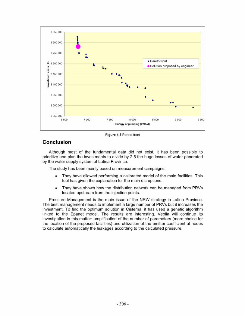
- 306 -

2 950 000

3 000 000

3 050 000

3 100 000

3 150 000

3 200 000

3 250 000

3 300 000

3 350 000

6 500 7 000 7 500 8 000 8 500 9 000 9 500Energy of pumping (kWh/d)

Inve

stm

ent c

osts

( € ) Pareto front

Solution proposed by engineer

Figure 4.3 Pareto front

Conclusion

Although most of the fundamental data did not exist, it has been possible to prioritize and plan the investments to divide by 2.5 the huge losses of water generated by the water supply system of Latina Province.

The study has been mainly based on measurement campaigns:

• They have allowed performing a calibrated model of the main facilities. This tool has given the explanation for the main disruptions.

• They have shown how the distribution network can be managed from PRVs located upstream from the injection points.

Pressure Management is the main issue of the NRW strategy in Latina Province. The best management needs to implement a large number of PRVs but it increases the investment. To find the optimum solution in Cisterna, it has used a genetic algorithm linked to the Epanet model. The results are interesting. Veolia will continue its investigation in this matter: amplification of the number of parameters (more choice for the location of the proposed facilities) and utilization of the emitter coefficient at nodes to calculate automatically the leakages according to the calculated pressure.

- 307 -

A procedure based on Performance Indicators in Water Distribution Systems for the identification of Scenarios in terms of water losses reduction and structural improvements

Cristiana Bragalli, Tonino Liserra, Marco Maglionico

DISTART, University of Bologna, viale Risorgimento 2 – 40136 BOLOGNA (Italy) tel. +39 051 2093363, fax. +39 051 331446 e-mail: [email protected], [email protected] , [email protected]

Keywords: Water loss, scenario, performance indicators

Introduction

Water loss reduction, in water distribution networks (WDNs), can be obtained by means of different methods and technologies. In many cases stakeholders have an insufficient interest to reduce water losses because the low production cost of drinkable water and because usually environmental costs are not considered, also for the difficulties in its evaluation.

An increment in actual or further water requested can lead to infrastructures insufficiency of parts of the supply system. Then water losses reduction should be evaluated together with WDN structural adjustments. In these cases the leakage detection should become more attractive as a consequence of higher marginal water production costs.

As stated by IWA (Alegre at al. 2006), activities, combination of the four primary components of real losses management can be done; for each one different effects, in terms of water retrieved, can be expected. Because of the numerous possibilities in actions and effects, it can be necessary to identify a certain number of scenarios (SCNs), successively subjected to technical and economical evaluation. The proposed procedure is based on a set of WDN Performance Indicators (PIs) for the generation of intervention scenarios in terms of water losses reduction and structural improvements. The objective is to give indications to combine in the most opportune way typology and intensity of each intervention.

The procedure can be summarised in the following steps (Figure 1):

1. Evaluation of the demand increase for a fixed time horizon;

2. Evaluation of WDN global functioning, and per components, affected by updated demand (at the time horizon considered);

3. Elaboration of a number of scenarios obtained with different intervention on WDN;

3.1 recoverable volume evaluation by reducing leakages;

3.2 evaluation of WDN performance, in terms of PIs, as a result of both structural improvement and leakage reduction activities;

3.3 Evaluation of all economical investment necessary to SCN realization. The result of the procedure is a number of intervention scenarios, composed by

water losses reduction and structural improvements, coupled with a water recovered estimation. The final goal is to provide indications on the most suitable combination of the various actions in order to obtain an efficient and economic water losses management.

- 308 -

Scenario building procedure

Methodology

The necessity to increase the water resources availability due to a growth of water demand or, more simply, the need to reduce the level of water losses, requires to undertake actions on WDN that, in either case, have an impact in terms of technical performance and economic management (Figure 1).

In a planning perspective, it should be convenient to analyse the situation considering classes of interventions related to leakage reduction activities and to structural interventions on WDN.

The construction of the SCNs is based on the identification of a set of Performance Indicators and, subsequently, on their quantification and analysis. Each PI value will be compared with the corresponding acceptable reference value, determining whether his state is critical.

LEAKAGE REDUCTION

POSSIBLE NEED OF WATER RESOURCES

STRUCTURAL INTERVENTION

IMPACT on WDN:

- technical performance

- economic management

< 0∆V = 0

> 0

Intervention database

Figure 1 Consequences of a change in needs of water resources

The procedure of the construction of SCNs highlights some possible problems, in particular the evaluation of the effectiveness of each intervention. Through the introduction of an uncertainty component, it is possible to take into account the lack of knowledge and possible errors.

A further aspect to be taken into account is the durability of the effects of each intervention on the WDN, because, in many cases, it is not determined a priori or can change in time. The procedure of scenario construction is described in Figure 2.

The starting point is the analysis of the WDN in the actual state (t=0, V0) through a set of PIs (t=0, V0) able to describe its condition, in particular in terms of:

- saturation degree of the WDN, that is the utilisation degree of water resources, plants (treatment plant, pumping station, storage) and networks;

- state of conservation of the WDN, in particular with reference to the failure rate of the network;

- water loss level;

- 309 -

- evaluation of the expected volume ∆VE, necessary to increment the actual availability of water resources V0 to satisfy the future requirement.

At the present, it is not distinguished the situation in which ∆VE have to be found to improve the actual state t=0 or in a future perspective at time t=n, because the attention is pointed on the relationship between intensity of intervention and outcome in terms of PI set and volume retrieved ∆VR.

With this remark, the first scenario is considered applying the whole increment of required volume at the WDN in the actual state (t=0, V0+ ∆VE) and recalculating the PIs (t=0, V0+ ∆VE) to evaluate the impact on WDN in the case in which no intervention is done.

The generator builds the scenarios (SCN1, …, SCN j,…, SCN n) combining the interventions and changing, in a discrete way, the intensity of each intervention within an opportune range; the intensity is described through variables characterising the intervention itself.

A model of expected outcomes evaluation is used to evaluate the consequence of each scenario on WDN (t=n, SCN j) in terms of recovered volume ∆VR, PIs (t=n, SCN j, V0+ ∆VR) and cost.

WDN (t=0,V0)PI set (t=0, V0)

Expected∆VE (t=n)

WDN (t=0,V0+∆VE)PI set (t=0,V0+∆VE)

Intervention Database(t = 0 → n)

Leakage Reduction Intervention (LRI)Structural Intervention (SI)

SCNs (LRI, SI) generator

SCN 1, …, SCN j, …, SCN N

MODEL of SCNs

classification

MODEL of ID SCN expected outcomes evaluation

WDN (t=n, SCN j)Recovered ∆VR (t=n, SCN j)PI set (t=n, SCN j, V0 +∆ VR)

Cost ((t=n, SCN j, ∆VR)

ID SCN 1 LRI1.. LRI i.. LRI L SI 1 …SI i … SI S PI 1.. PI i.. PI M.. Recovered ∆VR Cost

ID SCN j LRI1.. LRI i.. LRI L SI 1 …SI i … SI S PI 1.. PI i.. PI M.. Recovered ∆VR Cost

ID SCN N LRI1.. LRI i.. LRI L SI 1 …SI i … SI S PI 1.. PI i.. PI M.. Recovered ∆VR Cost

WDN (t=0,V0)PI set (t=0, V0)

Expected∆VE (t=n)

WDN (t=0,V0+∆VE)PI set (t=0,V0+∆VE)

Intervention Database(t = 0 → n)

Leakage Reduction Intervention (LRI)Structural Intervention (SI)

SCNs (LRI, SI) generator

SCN 1, …, SCN j, …, SCN N

MODEL of SCNs

classification

MODEL of ID SCN expected outcomes evaluation

WDN (t=n, SCN j)Recovered ∆VR (t=n, SCN j)PI set (t=n, SCN j, V0 +∆ VR)

Cost ((t=n, SCN j, ∆VR)

ID SCN 1 LRI1.. LRI i.. LRI L SI 1 …SI i … SI S PI 1.. PI i.. PI M.. Recovered ∆VR Cost

ID SCN j LRI1.. LRI i.. LRI L SI 1 …SI i … SI S PI 1.. PI i.. PI M.. Recovered ∆VR Cost

ID SCN N LRI1.. LRI i.. LRI L SI 1 …SI i … SI S PI 1.. PI i.. PI M.. Recovered ∆VR Cost

Figure 2 Generator of the scenarios on the base of the interventions intensity

Intervention scenarios based on Leakage reduction

- 310 -

Only a part of the described methodology (Figure 2) is presented. In particular the SCNs composed by water loss reduction interventions. The WDN PIs used are based on IWA Performance Indicators for Water Supply Services (Alegre et al., 2006) and three new PIs are proposed for aspects not explicitly considered in IWA PIs system.

The model of expected outcomes evaluation of scenarios is based on Burst and Background Estimate model (BABE) (Lambert, 1999) and on some concepts used in Econoleak (McKenzie & Lambert, 1999). An important aspect to observe is that BABE uses the idea of fixed-area and variable-area discharges (FAVAD) (May, 1994) to obtain a corrector factor that allows to align the leakage to the pressure variation.

The generation of scenarios for leakage reduction interventions has been referred to the four actions of the IWA approach: pressure management, active leakage control, speed and quality of repairs and infrastructure renewal.

In Figure 3, the highlighted area between the initial leakage level of real losses (CARL) and the reduced leakage level, represent the expected outcomes of a scenario (ID SCN) when interventions to reduce water loss are applied.

InfrastructureRenewal


UARL Speed and quality of repairs

Initial Leakage Level CARL

PressureManagement

Economic level of leakage ELL

Reduced Leakage Level

Expected outcomes of

ID SCN

* IWA approach Figure 3 Leakage reduction in IWA approach

Pressure management represents the main activity for leakage reduction because not only it reduces the actual lost volume, but because allows to reduce leaks and bursts.

The reduction of pressure is associated, as well as a decrease water that flows through the cracks of pipes, a change of the rates of failure, whose determination is very complex because this effect varies over time (Thornton & Lambert, 2005; Pearson et al., 2005). The relationship (1) has been proposed (Lambert, 2001; Farley & Trow, 2003) to describe as the burst frequency varies with pressure:

N2

0

1

0

1

PP

BB

⎟⎟⎠

⎞⎜⎜⎝

⎛= (1)

where B1, B0 are the burst frequency after and before pressure reduction respectively, and P1, P0 are the pressure after and before the reduction, respectively, and N2 is the exponent of (1). The N2 values have a large range of variation: between a minimum of 0.5 to a maximum of 6.5 (Thornton & Lambert, 2005), and between 0.2 – 8.5 for mains

- 311 -

breaks and 0.2 – 12.0 for service pipe breaks, with a medium value of 2.47 and 2.36, respectively (Pearson et al., 2005).

The Active Leakage Control (ALC) consists in a periodic inspection of the surface area over the network with technologies primarily based on acoustic properties. Its characterization foresees the definition of a time period at the end of which is expected that all the network has been inspected, even if the high cost of this intervention advances to apply methodologies of pre-localisation in order to concentrate the efforts on areas of higher criticality. The frequency of inspection is affected by the time of the non-reported burst activities. In general is accepted a uniform probability distribution, with time t/2 where t is the interval between two following explorations, which must be added the repair time. The purpose is that ALC in cyclical time allows to maintain the WDN to a level of losses almost constant and pre-assignable.

The rehabilitation or replacement of pipes is strongly influenced by economic aspects.

The model of expected outcomes evaluation calculates the recovered volume ∆VR with reference to component analysis proposed in the BABE model (Lambert, 2002). In fact Real losses are calculated like sum of three components:

- Background (undetectable) leakage, at pipe joint and fittings, with flow rates too low for sonic detection,

- Reported leaks and bursts, characterised from high flow rates and short duration,

- Unreported leaks and bursts, with moderate flow rates, average duration depending of the active leakage control method (Lambert, 2002).

Background Losses, Reported and Unreported Bursts can occur on different system components of the WDN, mainly transmission mains, distributions mains, connections and service pipes.

With this allocation of the water leakage, the component analysis assigns a rate of leakage as in the Econoleak model (McKenzie & Lambert, 1999) (Table 1). Because the nature of this approach, the procedure should be applied to sufficient homogeneous areas.

Table 1 MODEL of ID SCN expected outcomes evaluation: RATE@50m from Econoleak model

UnreportedRate@50

RepotedRate@50

BURTS LOSSESUNAVOIDABLE BACKGROUND LOSSESRate@50

COMPONENT ANALYSIS

0 l/conn/hr

1.25 l/conn/hr

20 l/km/hr

20 l/km/hr

1.6 m3/hr1.6 m3/hrConnections

1.6 m3/hr1.6 m3/hrService pipes

6 m3/hr12 m3/hrDistribution mains

12 m3/hr30 m3/hrTransmission mains

UnreportedRate@50

RepotedRate@50

BURTS LOSSESUNAVOIDABLE BACKGROUND LOSSESRate@50

COMPONENT ANALYSIS

0 l/conn/hr

1.25 l/conn/hr

20 l/km/hr

20 l/km/hr

1.6 m3/hr1.6 m3/hrConnections

1.6 m3/hr1.6 m3/hrService pipes

6 m3/hr12 m3/hrDistribution mains

12 m3/hr30 m3/hrTransmission mains

The evaluation of the burst losses and background losses, likewise to Econoleak model, has been done as in the following:

Burst Losses = PCF . Rate@50 . BCF . Frequency . Duration

Background Losses = ICF . PCF . Rate@50 . Dimension (km, conn) . Duration

- 312 -

where Pressure Corrector Factor is expressed by PCF = (P1/P2)N1, while Infrastructure Condition Factor ICF (Farley & Trow, 2003) is a factor to apply to the Unavoidable Background Losses to derive a realistic level of background losses. It has been introduced the influence on burst frequency of the pressure with BCF Burst Corrector Factor that is the ratio (P1/P0)N2 of the relationship (1). The most significant factor affecting the level of leakage in a water network is the general condition of the mains and service pipes, and the service reservoirs. The condition of the infrastructure is something inherited from previous regimes and generations; the condition of the infrastructure in terms of its affect on the level of background leakage is referred in fact in the Infrastructure Condition Factor ICF (Farley & Trow, 2003).

The model of outcome evaluation of the recovered volume ∆VR considered in which way each water leakage intervention operates on the expression of burst losses and background losses changing some of the factors, as it is explained in Table 2.

Table 2 MODEL of ID SCN expected outcomes evaluation of the recovered volume �VR

Speed of repairs



PressureManagement

Scenario ID SCN

Frequency

• Burst losses• Background losses

% component rahabilitation

Duration

• Unreported burst losses• Background losses

new intervention time

PCF, BCF


new P

Duration

• Unreported burst losses• Detectable background losses

new ALC temporal interval

CHANGE:

EFFECT ON:

VARIABLE:

Speed of repairs



PressureManagement

Scenario ID SCN

Frequency


% component rahabilitation

Duration

• Unreported burst losses• Background losses

new intervention time

PCF, BCF


new P

Duration

• Unreported burst losses• Detectable background losses

new ALC temporal interval

CHANGE:

EFFECT ON:

VARIABLE:

Case study

Performance Indicators set

The PIs set utilised for the case study is composed from a restricted subset of IWA PIs system (Alegre et al., 2006) and from three new PIs proposed.

The PI subset has been identified with regard to saturation degree, state of conservation and water loss level of the WDN, as it is shown in Table 3. The necessity to introduce new PI is connected to the absence of explicit performance indicators in IWA PI system for the saturation degree of the network and for the surplus of pressure for the actual operation of WDN. In both case, the aspects involved are not easily able to be translated in terms of PI; the proposed PI are described in Table 4.

Table 3 PI set utilised (*IWA PI)

- 313 -

Real losses per connectionOp27*

No/1000 connections/year

No/100 km/year

-%

%

%%

days%Units

Service connection failuresMains failures

Infrastructure leakage indexApparent losses

Inefficiency of use of water resources

Water resources availabilityPumping utilisation

Transmission and distribution storage capacity

Treatment plant utilisationDefinition

WATER RESOURCESAVAILABLE SATURATION

WR2*

Op32*MAINTENANCE STATEOp31*

Op29*Op25*

WATER LOSSWR1*

Ph4*

Ph3*PLANT SATURATIONPh1*Reading KeyCode

Real losses per connectionOp27*

No/1000 connections/year

No/100 km/year

-%

%

%%

days%Units

Service connection failuresMains failures

Infrastructure leakage indexApparent losses

Inefficiency of use of water resources

Water resources availabilityPumping utilisation

Transmission and distribution storage capacity

Treatment plant utilisationDefinition

WATER RESOURCESAVAILABLE SATURATION

WR2*

Op32*MAINTENANCE STATEOp31*

Op29*Op25*

WATER LOSSWR1*

Ph4*

Ph3*PLANT SATURATIONPh1*Reading KeyCode

Water loss analysis

The Ganaceto DMA (District Metered Area) belong to the WDN of Modena (Italy), it is located in a flat area, with an average level of 32.86 m and one entry point at 41 m, over the sea level. The distribution system covers a total pipe length of 35.4 km with 540 connections and pipes are mainly in asbestos cement and polyethylene. This district has been used as a hypothetical case study, supposed independent to the WDN of Modena and with a water resource that supply a system input volume of 447300 m3/year.

Table 4 PI proposed to evaluate network saturation and pressure surplus

%A3/(S1*H1)*100Utilisation degree of main network

MNS

%A3/(S2*H1)*100Utilisation degree of distribution network

DNS

UnitsFormulaDefinitionCode

%A3/(S1*H1)*100Utilisation degree of main network

MNS

%A3/(S2*H1)*100Utilisation degree of distribution network

DNS

UnitsFormulaDefinitionCode

%(D34-P1)/ P1*100Surplus of pressure at critical point

PSUnitsFormulaDefinitionCode

%(D34-P1)/ P1*100Surplus of pressure at critical point

PSUnitsFormulaDefinitionCode

m3/dayDesign system input volume of Distribution network S2kPaAverage operating pressureD34*kPaMinimum average operating pressure**P1

m3/dayDesign system input volume of Main network S1UnitsDefinitionCode

m3/dayDesign system input volume of Distribution network S2kPaAverage operating pressureD34*kPaMinimum average operating pressure**P1

m3/dayDesign system input volume of Main network S1UnitsDefinitionCode

* IWA PI variable ** Reported to the critical point

Real losses derived from IWA Water Balance are 188390 m3/year, which

corresponds an average water loss of 516 m3/day.

With reference to Pressure Correction Factor PCF=(AZP/50)N1, the average pressure AZP is equal to 33.5 m and a lowering of 5 m at critical point was estimated possible. The estimation of unreported bursts is based on the observed data regarding the discovered bursts during the last leakage detection campaign on the DMA in 2002.

The procedure of scenario construction SCNs connected to water loss reduction interventions was applied. It has been supposed an increment of required volume of 100 m3/day . In Table 5 the impact of the expected volume ∆VE, evaluated in terms of values of PIs set respect to the actual state, in absence of interventions, is shown.

- 314 -

Pressure Reduction

0

100

200

300

400

500

33.5 32.5 31.5 30.5 29.5 28.5P1 (m)

Retri

eved

Vol

ume

m3 /d

ay

0.0 0.2 0.5 1.0 2.04.0 8.0

Table 5 Impact of the increment ∆VE on the technical performance of WDN evaluated by means PIs set

••956956350500200Op27

•17.517.58105PS3640

53

56205050801

60

Reference Value

6751

76

67288080902

80

Superiorlimit50%

8.430

31

5014404075

0.8340

Inferiorlimit50%

58.032.0

11.9 5.0

72.238.982.885.582.6 1.4

86.2

Predicted value atupdate service level (t=0,V0+∆VE)

•

•

Change inV0 →V0+∆VE

•

••

•

•

PI in critical stateV0+∆VE

79.1MNS76.6DNS

57.9Op3231.8Op31

11.9Op294.7Op25

66.8WR242.1WR1

76.4Ph41.5Ph3

79.7Ph1

Value at Actual Service Level (t=0,V0)

Code

••956956350500200Op27

•17.517.58105PS3640

53

56205050801

60

Reference Value

6751

76

67288080902

80

Superiorlimit50%

8.430

31

5014404075

0.8340

Inferiorlimit50%

58.032.0

11.9 5.0

72.238.982.885.582.6 1.4

86.2

Predicted value atupdate service level (t=0,V0+∆VE)

•

•

Change inV0 →V0+∆VE

•

••

•

•

PI in critical stateV0+∆VE

79.1MNS76.6DNS

57.9Op3231.8Op31

11.9Op294.7Op25

66.8WR242.1WR1

76.4Ph41.5Ph3

79.7Ph1

Value at Actual Service Level (t=0,V0)

Code

The actual time of location and repair was assumed of 4 days for distribution mains,

50 days for connection and 60 days for service pipes. Burst frequency derives from the frequencies of repairs in the Ganaceto DMA, which is characterised by ALC interval of 4 years.

N1 has been assumed equal to 0.6 for Reported and Unreported burst and 1.5 for Background losses. Component analysis for Ganaceto DMA is shown in Table 6.

Table 6 Component analysis for Ganaceto DMA in the actual state

55.7

9.1

22.8

23.8

-

BACKGROUND LOSSES m3/day Unreported

m3/dayRepoted

m3/day

149.6

54.6

67.8

27.2

-

BURTS LOSSES

311.3

107.2

141.8

62.3

-

171.0Service pipes

516.6Total

TotalCOMPONENT ANALYSIS

232.3

113.3

-

Connections

Distribution mains

Transmission mains

55.7

9.1

22.8

23.8

-

BACKGROUND LOSSES m3/day Unreported

m3/dayRepoted

m3/day

149.6

54.6

67.8

27.2

-

BURTS LOSSES

311.3

107.2

141.8

62.3

-

171.0Service pipes

516.6Total

TotalCOMPONENT ANALYSIS

232.3

113.3

-

Connections

Distribution mains

Transmission mains

The base scenarios are those in which only one typology of water loss reduction

intervention is considered: pressure reduction, active leakage control, rehabilitation of the network and repair times reduction. A sensitivity analysis for the retrieved volume relevant to each intervention varying N2 has been done and the results are shown in Figure 4.

ALC Interval for 28.5 m of Pressure

0

100

200

300

400

500

4 2 1ALC Interval (years)

Ret

rieve

d V

olum

e m

3 /day

0.0 0.2 0.5 1.0 2.04.0 8.0

- 315 -

Rehabilitation for 28.5 m of Pressure

0

100

200

300

400

500

0 5 10 15 20 25Assets Rehabiltation (%)

Retri

eved

Vol

ume

m3 /d

ay

0.0 0.2 0.5 1.0 2.04.0 8.0

Repair Time for 28.5 m of Pressure

0

100

200

300

400

500

1 1.5 2Reparation Time ratio

Ret

riev

ed V

olum

e m

3 /day

0.0 0.2 0.5 1.0 2.04.0 8.0

Figure 4 Retrieved Volume for each water loss reduction intervention applying the procedure of scenario construction SCNs for different value of N2

The strong influence of N2 (Figure 4) and the relatively low level in operating pressure, a precautionary value of 0.2 has been assumed for N2 both for pipe mains and pipe services.

0

100

200

300

400

500

600

700

800

900

1000

SCN

1

SCN

240

SCN

479

SCN

718

SCN

957

SC

N 1

196

SC

N 1

435

SC

N 1

674

SC

N 1

913

SC

N 2

152

SC

N 2

391

SC

N 2

630

SC

N 2

869

SC

N 3

108

SC

N 3

347

SC

N 3

586

SC

N 3

825

SC

N 4

064

SC

N 4

303

SC

N 4

542

SC

N 4

781

SC

N 5

020

SC

N 5

259

SC

N 5

498

SC

N 5

737

SC

N 5

976

SC

N 6

215

SC

N 6

454

Scenarios

Y1

0

5

10

15

20

25

30

35

Y2

Total Losses(m3/day) Y1-axis

Retrieved Volume (m3/day) Y1-axis

Op27 (l/conn./day) Y1-axis

Pressure (m) Y2-axis

ALC Interval (Years) Y2-axis

Minimum Required Retrieved volume

Figure 5 Scenarios for water loss reduction: the effect on water loss and retrieved volume consequent to

different combinations of the interventions

- 316 -

0

10

20

30

40

50

60

70

80

90

100

SC

N 1

SCN

240

SCN

479

SCN

718

SCN

957

SCN

119

6

SCN

143

5

SCN

167

4

SCN

191

3

SCN

215

2

SCN

239

1

SCN

263

0

SCN

286

9

SCN

310

8

SCN

334

7

SCN

358

6

SCN

382

5

SCN

406

4

SCN

430

3

SCN

454

2

SCN

478

1

SCN

502

0

SCN

525

9

SCN

549

8

SCN

573

7

SCN

597

6

SCN

621

5

SCN

645

4

Scenarios

Y1

0

5

10

15

20

25

30

35

Y2

WR1 (%) Y1-axis

WR2 (%) Y1-axis

Op31(No./100km/year) Y2-axis

Pressure (m) Y2-axis

Op25 (%) Y2-axis

ALC Interval (years) Y2-axis

Figure 6 Scenarios for water loss reduction: the effect some PIs consequent to different combinations of

the interventions

Therefore, with these parameters, the procedure was used to build scenarios (SCNs), combining types and intensity of water loss reduction interventions, with the same ranges shown in Figure 4. The evaluation of the effectiveness of all possible scenarios is shown in Figure 5 regarding water loss reduction, recovered volume and Op27, and in Figure 6 in terms of impact of water losses reduction interventions on some PIs.

In Figure 5, the feasible scenarios are those with recovered volume above 100 m3/day (Y1 – axis). It is evident the wide range of recovered volume obtainable varying the intensity for each water loss reduction activity. At the same time, equivalent SCNs in terms of recovered volume are possible, but characterised from different combination of interventions and response of the technical performance given to the PIs (Figure 6). In particular, feasible SCNs respect to recovered volume can not satisfy the required limit for some PIs; for example, to change the critical state of WR1 it is necessary to reach 200 m3/day.

To support the decisions, therefore, the model have to include the economic evaluation on a temporal interval, because it is clear that equivalent SCNs in terms of Retrieved volume can be completely different in terms of costs.

Conclusion

The objective of the procedure described, based on a set of Performance Indicators, is to generate intervention scenarios in terms of water loss reduction and structural improvements in WDNs. This procedure could be useful for the preliminary analysis of WDNs.

- 317 -

At the moment the procedure proposed take into account only scenarios for water loss reduction interventions. The subsequent efforts will be done in order to include structural improvement interventions and economic evaluation on a temporal interval.

Further analysis will be necessary to better understand the possibility of PIs to describe the technical impact and the evaluation of recovered volume for more complex scenarios.

References Alegre H., Baptista J., Cabrera E., Cubillo F., Duarte P., Hirner W., Merkel W., Parena R. (2006),

Performance Indicators for Water supply Services, Second Edition IWA Manual of best Practice, IWA Publishing.

Farley M., Trow S. (2003), Losses in Water Distribution Networks, IWA Publishing London UK. Lambert A. O., Brown T. G., Takizawa M., Weimer D. (1999), A review of performance indicators for real

losses, IWA/AQUA, December 1999. Lambert A. O. (2001), What do we know about pressure :leakage relationships, System approach to

leakage control and water distribution systems management, IWA Conference, Brno, Czech Republic, May 2001.

Lambert A. O. (2002), International report: water losses management and techniques, Water Science and Technology: Water Supply, Vol 2, No 4.

May J. (1994), Leakage pressure control, BICS International Conference on Leakage Control Investigation in Underground Assets, London, March 1994.

McKenzie R., Lambert A. O. (1999), Econoleak Model User Guide, South African Water Research Commission.

Thornton J., Lambert A. (2005), Progress in practical prediction of pressure: leakage, pressure: burst frequency and pressure: consumption relationships, Leakage 2005 – Conference Proceedings, Halifax Canada 2005.

Pearson D., Fantozzi M., Soares D., Waldron T., Searching for N2: How does pressure reduction reduce burst frequency?, Leakage 2005 – Conference Proceedings, Halifax Canada 2005.

- 318 -

Investigarea pierderilor de apa în retelele de distributie. Studiu de caz Anton ANTON – prof.dr.ing. – Universitatea Tehnica de Constructii Bucuresti

Lucian SANDU – prof.dr.ing. – Universitatea Tehnica de Constructii Bucuresti

Sorin PERJU – dr.ing. - Apa Nova Veolia Water Bucuresti

Abstract

The reduce evaluation and identification possibilities of water leaks within the distribution networks, as well as those of quick determination of nature of this leaks represents the primes weakness for the water networks distribution operators.

In this material are presented both methods of determination and investigation water leaks în the distribution networks with a view to analyzing the networks and the increase safety degree în operating, and a study case for a network sector within the water distribution networks from town Bucharest.

1. Introducere Sectorul alimentărilor cu apă şi mai ales reţelele centralizate de distribuţie a

apei potabile constituie pentru centrele populate şi agenţii economici, o componentă valoroasă pentru activităţile umane, care condiţionează desfăşurarea vieţii igienice a localităţilor, contribuind ca un factor esenţial în toate procesele de producţie industrială, fără de care nu se poate concepe dezvoltarea economică şi socială.

Reţelele de distributie au fost şi sunt construite pentru a fi exploatate pe o perioada limitată de timp ce poate varia atât funcţie de calitatea materialelor folosite cât şi în funcţie de modul în care este exploatată reţeaua.

Consideraţiile economice şi ambientale reprezintă două dintre motivele majore ce determină necesitatea efectuării cercetărilor de identificare şi localizare a pierderilor de apă în reţelele de transport şi distribuţie a apei potabile. O cale efectivă de a conserva apa şi de a economisi bani o reprezintă localizarea şi remedierea defecţiunilor ivite în cadrul reţelelor de conducte.

Proiectate în diverse etape şi realizate având ca suport cunoştinţele, tehnologiile, echipamentele şi materialele cunoscute pentru etapele respective, reţelele de distribuţie a apei, aflate în exploatare au fost concepute într-o perioadă în care preţul energiei avea o pondere redusă în costurile de exploatare. Astăzi când practic preţul energiei tinde să se alinieze la preţul ţărilor occidentale, ponderea energiei în preţul apei este mult mai însemnată.

În acest context, o bună parte din eforturile producătorilor şi distribuitorilor de apă potabilă este concentrată asupra localizării avariilor din conducte în scopul reducerii pierderilor de apă. Pierderile de apă din instalaţiile de alimentare cu apă au multiple implicaţii asupra performanţelor economice, ambientale şi relaţionale cu beneficiarii şi pentru beneficiari, deoarece atât costurile lipsei de performanţă a instalaţiilor de alimentare cu apă cât şi neplăcerile lipsei de apă sau chiar a unei calităţii proaste a apei sunt suportate de către consumatori. În consecinţă, ambele părţi, producătorul de apă şi consumatorul, sunt obligate să ia măsurile adecvate pentru diminuarea acestor pierderi şi menţinerea lor în limite rezonabile.

- 319 -

2. Factori ce influenţează pierderile de apă

Prin pierderile care apar în conductele instalaţiilor de alimentare cu apă se înţelege, cantitatea totală de apă care datorită unor defecţiuni apărute în sistemul de distribuţie nu ajunge la consumatori.

Pierderile de apă dintr-o reţea de distributie pot fi subdivizate în pierderi reale şi pierderi aparente. Pierderile reale sunt reprezentate de volumul de apă pompată (furnizată) care nu ajunge la consumatori şi se pierde în exterior prin fisuri, spărturi, neetanşeităţi şi alte defecţiuni ale sistemului. Pierderile aparente sunt rezultatul unor estimări eronate a consumului, datorate în principal unor utilizări ce nu pot fi controlate din punct de vedere consumului. O parte din aceste consumuri sunt autorizate de companiile de apă, cum ar fi (spălarea canalizării, utilizarea hidranţilor, udarea grădinilor şi spatiilor verzi, spălarea străzilor, etc. Totusi există şi consumuri neaprobate care nu pot fi inregistrate, cum este cazul utilizatorilor branşaţi ilegal la reţeaua de distribuţie a apei. O componentă importantă a acestui tip de consum o au însă şi echipamentele vechi de măsură sau cele necalibrate care indică valori eronate.

Principalii factori ce influenţează mărimea pierderilor de apă din instalaţiile de alimentare cu apă sunt:

• Presiunea în reţea – aceasta variabilă influenţează pierderile de apă în mod direct prin creşterea debitelor pierdute prin fisuri sau neetanşeităţi. De asemenea presiunea are şi o influenţă indirectă prin faptul că o creştere a presiunii conduce la solicitări importante a infrastructurii şi deci creşte riscul de aparitie a unor noi defecţiuni. Cantitatea de apă pierdută este proporţională cu presiunea, factorul de proporţionalitate fiind funcţie de dimensiunile şi forma orificiilor prin care se pierde apa

∑ ⋅⋅⋅⋅µ= hg2SQp unde: Qp = debitul de apă pierdută, [m3/s] µ = coeficient mediu de debit, µ = 0,59 … 0,65 ∑S = suma suprafeţelor vii a orificiilor prin care se pierde apa g = acceleraţia gravitaţională, [m/s2] h = diferenţa de înălţime piezometrică măsurată între interiorul şi

exteriorul conductei, [ mCA] • Caracteristicele materialelor conductelor şi caracteristicile terenului în care este

pozată conducta – trebuie cunoscut comportamentul materialului conductei în terenul în care se produc solicitările externe. O conductă de oţel aflată într-un teren parţial argilos şi nisipos, accelerează procesul de coroziune; o conductă din material rigid (azbociment) pozată în terenuri alcătuite din sedimente diferite poate suferi fisuri, pentru care în condiţiile unui sol permeabil există pericolul infiltraţiilor.

• Numărul elementelor componente specifice reţelei (vane, hidranţi, aparate de măsură etc). Vanele şi hidraţii sunt elementele cele mai importante pentru o corectă subdivizare a reţelei în zone şi sectoare. Pe de altă parte fiecare element specific într-o reţea reprezintă o potenţială sursă de pierderi de apă.

• Variaţia presiunilor oscilante dată de funcţionarea intermitentă a pompelor. Debitul de apă pompat şi tranzitat în reţelele de distribuţie este variabil în decursul unei zile şi nu este acelaşi în fiecare zi, depinzând de factori aleatori (ocuparea forţei de muncă în ziua respectivă, tradiţia în zilele de sărbătoare, etc), sau fiind restricţionat de factori obiectivi (resurse insuficiente de apă, consumuri exagerate, restricţii tehnice în funcţionarea pompelor sau motoarelor).

- 320 -

• Variaţii mari ale temperaturii apei vehiculate funcţie de anotimp vara/iarna

3. Metode de estimare a pierderilor de apa

Estimarea pierderilor de apă şi a modului cum se produc aceste pierderi, este importantă deoarece în funcţie de o serie de factori ce influenţează, se poate stabili metoda de detectare şi control a pierderilor de apă. În literatura de specialitate există mai multe metode de estimare şi localizare a pierderilor de apă cum ar fi:

• Controlul pasiv (metoda curentă) – prin apariţia apei la suprafaţa solului, prin apariţia de denivelări, prabusiri pe traseul conductelor de apa, prin depistarea apei cu ocazia realizării unor săpături, prin controlul periodic al bilanţului apei ce se distribuie, prin urmărirea informaţiilor primite de la echipele de intervenii şi reparaţii, etc

• Monitorizarea presiunilor – prin urmărirea valorilor de presiuni în nodurile semnificative ale reţelei

• Contorizarea parţială – prin sectorizarea reţelelor şi instalarea unor contori de district pentru zonele care prezintă consumuri nejustificate de apă

• Contorizarea totală – prin introducerea echipării tuturor branşamentelor cu contori de apă

• Cercetarea prin ascultare – prin folosirea de echipamente dotate cu amplificatoare şi microfoane sensibile sensibile şi de precizie (Hidrolux, Aqualux, Correlux, etc)

• Controlul consumului minim de noapte – se consideră că o creştere semnificativă a debitului minim nocturn peste limita normală acceptată indică prezenţa unor pierderi de apă

• Monitorizarea şi informatizarea totală a sistemului – prin introducerea unui sistem de management tehnic integrat în care pe un model matematic al reţelei care cuprinde graful reţelei (configuraţia reţelei, lungimi de conducte, diametre, material, rugozităţi, cote topografice, etc) se poate simula funcţionarea sistemului în diverse scenarii de exploatare.

Practic o campanie de evaluare a pierderilor reprezintă o metodă de a determina cât de multă apă este pierdută şi ce pierderi are din acest motiv compania care asigura funcţionarea sistemului. Principalul scop al acestei acţiuni este de a ajuta compania de a reduce pierderile şi de a furniza o apa mai ieftina.

4. Studiu de caz: Investigarea pierderilor de apă în reţeaua de distribuţie deservită de SRp Lacul Tei - Bucureşti

Situată în zona cartierului Tei, SRp Lacul Tei este o staţie de repompare gândită să asigure necesarul de debit şi presiune în reţeaua de înaltă presiune ce deserveşte consumatori casnici şi economici din zonă. Staţia este echipată cu o unitate modulară de pompare compusă din 6 grupuri de pompare tip CR 64 de provenienţă Grundfos actionate cu turaţie variabilă. De asemenea parametrii de funcţionare ai staţiei sunt monitorizaţi prin achiziţionarea mărimilor hidraulice şi electrice din ¼ în ¼ de oră, prin intermediul unei plăci de achiziţie şi descărcarea acestor date cu ajutorul unui echipament SHARP SL-5500 (personal mobile tool).

- 321 -

Este unanim acceptată ideea că pentru gestionarea şi diagnosticarea unei reţele de distribuţie a apei potabile este necesar întocmirea unei etapizări logice a metodologiei de abordare, astfel încât trecerea de la o etapă la alta să fie condiţionată şi realizată după criterii bine definite. În acest sens etapele ce trebuiesc parcurse în tentativa de investigare a pierderilor de apă sunt:

Figura 1

Cercetarea pierderilor de apă pe baza metodologiei prezentate în figura 1, a fost aplicată folosind metoda de determinare a debitului minim nocturn (orele 000 - 500) pompat în reţeaua de distribuţie şi înregistrat din ¼ în ¼ de oră pentru o perioadă însemnată de timp (ianuarie – noiembrie 2006). Aşa cum se prezintă în figura 2, se observă că pentru perioada de timp menţionată creşterile debitului pompat nocturn care indicau apariţia unor consumuri nejustificate datorate avariilor din reţea, au fost urmate de localizarea şi remedierea acestor avarii. Pe baza acestei monitorizări continue a debitului minim nocturn s-a obţinut la sfârşitul perioadei o reducere debitului pompat cu 55%.

Etapa 1: AUDIT - PATRIMONIUL REŢELEI

Precizarea tuturor elementelor şi informaţiilor esenţiale de care dispune reţeaua (tip consumatori, poziţionarea vanelor, lungimea reţelei, consumuri contorizate, consumurinecontorizate, etc)

Etapa 2: SECTORIZAREA REŢELEI

Sectorizarea constă în izolarea reţelei şi decompunerea acesteia dacă este cazul în subreţele astfel incât să poată fi identificat volumul de apă distribuit. Validarea punctelor de măsură şi control temporar sau permanent.

Investigarea pierderilor

Prelucrarea datelor masurateInvestigarea in teren a zoneloravariate, localizarea pierderilorin vederea remedierii.

Modelare matematica

Modelarea numerica virtuala a retelei de distributie permite simularea functionarii retelei inscenarii de exploatare.

Etapa 1: AUDIT - PATRIMONIUL REŢELEI

Precizarea tuturor elementelor şi informaţiilor esenţiale de care dispune reţeaua (tip consumatori, poziţionarea vanelor, lungimea reţelei, consumuri contorizate, consumurinecontorizate, etc)

Etapa 2: SECTORIZAREA REŢELEI

Sectorizarea constă în izolarea reţelei şi decompunerea acesteia dacă este cazul în subreţele astfel incât să poată fi identificat volumul de apă distribuit. Validarea punctelor de măsură şi control temporar sau permanent.

Investigarea pierderilor

Prelucrarea datelor masurateInvestigarea in teren a zoneloravariate, localizarea pierderilorin vederea remedierii.

Modelare matematica

Modelarea numerica virtuala a retelei de distributie permite simularea functionarii retelei inscenarii de exploatare.

- 322 -

SRP Lacul Tei

0

50

100

150

200

250

300

350

400

450

500

1-Ja

n-06

11-J

an-0

6

21-J

an-0

6

31-J

an-0

6

10-F

eb-0

6

20-F

eb-0

6

2-M

ar-0

6

12-M

ar-0

6

22-M

ar-0

6

1-Ap

r-06

11-A

pr-0

6

21-A

pr-0

6

1-M

ay-0

6

11-M

ay-0

6

21-M

ay-0

6

31-M

ay-0

6

10-J

un-0

6

20-J

un-0

6

30-J

un-0

6

10-J

ul-0

6

20-J

ul-0

6

30-J

ul-0

6

9-Au

g-06

19-A

ug-0

6

29-A

ug-0

6

8-Se

p-06

18-S

ep-0

6

28-S

ep-0

6

8-O

ct-0

6

18-O

ct-0

6

28-O

ct-0

6

7-N

ov-0

6

17-N

ov-0

6

27-N

ov-0

6

Data

Volu

m p

ompa

t noc

turn

[mc]

Volume pompate intre orele 0...5

remediere avarie

remediere avarie

remediere avarie

remediere avarie

Figura 2

În continuare, având în vedere poziţionarea în plan (figura 3) şi conexiunile cu reţelele de distribuţie a apei din zona adiacentă reţelei deservite de SRp Lacul Tei, au fost întocmite modele numerice de calcul cu ajutorul cărora a fost simulată posibilitatea scoaterii din circuitul hidraulic al SRp Lacul Tei. În acest context folosind modulul RET al programului de calcul RET&LOB&DES au fost realizate modelele numerice aferente SRp Lacul Tei şi SRp Teiul Doamnei (figura 4).

Etapele parcurse în realizarea celor două modele numerice au fost următoarele:

• Definirea corectă a configuraţiei reţelelor, corespunzător celor două zone din punct de vedere al elementelor fizice (noduri, artere, diametre, cote geodezice, conexiuni, etc.).

• Alocarea debitelor în nodurile reţelei având la bază consumurile facturate în luna decembrie 2006.

• Realizarea modelelor numerice de calcul zonele de reţea de distribuţie, corespunzător SRp Teiul Doamnei şi SRp Lacul Tei .

• Calibrarea modelelor numerice pe baza valorilor presiunilor măsurate în staţiile de repompare şi unele puncte semnificative din cadrul reţelelor.

• Cuplarea celor două modele şi simularea funcţionării reţelelor de distribuţie ca fiind deservite doar de SRp Teiul Doamnei şi eliminarea funcţionarii SRp Lacul Tei.

Figura 3

- 323 -

Figura 4

Calculele hidraulice au constat în determinarea cotelor piezometrice în nodurile reţelei simulând ca secvenţă de exploatare funcţionarea SRp Teiul Doamnei având ca parametri de exploatare 5 bar în bara de refulare a staţiei. Ipotezele simulării funcţionarii reţelelor de distribuţie pentru această configuraţie de exploatare au fost realizate în două variante şi anume: prima variantă a fost aceea pentru care debitul injectat în retea a fost cel facturat, iar cea de a doua ipoteză a constat în determinarea capacităţii de pompare a SRP Teiul Doamnei simulând debitul pompat ca fiind dublu. Argumentele celei de a doua ipoteze au avut în vedere faptul că zona de influenţă a SRp Teiul Doamnei s-a extins prin preluarea zonei deservite de SRp Lacul Tei pe de o parte, iar pe de altă parte aceste reţele sunt vechi şi prezintă pierderi reale de apă de cca. 40 %. În ambele variante analizate rezultatele calculelor hidraulice au demonstrat că parametrii realizaţi prin funcţionarea SRp Teiul Doamnei pot asigura necesarul de debit şi presiune pentru consumatorii branşaţi reţelei deservite în prezent de SRp Lacul Tei şi SRp Teiul Doamnei (figura 5).

- 324 -

Variatia presiunilor in nodurile retelei

45

47

49

51

53

55

57

0 10 20 30 40 50 60 70 80 90 100 110 120 130 140 150 160 170 180 190 200 210 220

Noduri retea

Pre

siun

e [m

CA

]

Qcalcul=Qfacturat Qcalcul=2xQfacturat

Figura 5

Concluzii Analiza hidraulică efectuată a fost realizată exclusiv pentru reţelele de înaltă presiune deservite de către SRp Lacul Tei şi SRp Teiul Doamnei, reţele care se constituie parte integrantă a sistemului de distribuţie al apei din municipiul Bucureşti. Scopul studiului de caz a plecat de la ipoteza investigării pierderilor de apă din zonele respective (folosind metoda directă de determinare a debitului minim nocturn pompat de către SRp Lacul Tei), urmată de localizarea, remedierea şi eliminarea acestor pierderi, continuând cu modelarea matematică prin întocmirea modelelor numerice de calcul al reţelelor deservite de către SRp Lacul Tei şi SRp Teiul Doamnei şi incheind cu simularea numerică a funcţionării reţelelor şi eliminarea din circuitul hidraulic a unei staţii de repompare (SRp Lacul Tei).

Adoptarea unei astfel de metodologii de investigare a pierderilor de apă conduce la diminuarea consumurilor energetice şi totodată la reduceri importante a cheltuielilor de exploatare şi întreţinere a sistemului de distribuţie al apei din zonă.

- 325 -

Predicting leakage rates through background losses and unreported burst modelling Dr O. Chesneau*, Dr B. Brémond ** & Y. Le Gat ***

* Cemagref, 50 avenue de Verdun 33612 CESTAS France, [email protected] ** Cemagref, 50 avenue de Verdun 33612 CESTAS France , [email protected] *** Cemagref, 50 avenue de Verdun 33612 CESTAS France, [email protected]

Keywords Water distribution systems, leaks prediction; database management;

Keywords: Background leaks, Bursts, Leak-finding operations, Modelling, Renewal, Water networks

Abstract

Sustainable management of leaks in drinking water networks is a key issue for water distribution companies. Since it can reduce water losses and therefore groundwater abstraction operations, it is an important element in the assessment of facility and operator performance.

The various phases in the process leading to the appearance and development of water losses are modelled. First, a distinction is made between background leaks and leaks due to larger bursts which are either detectable during a leak-finding operation or located visually. Next, a dynamic model for leakage (DML) is proposed, in order to explain the evolution of the volumes lost.

The hypothesis of the DML model is that leaks evolve over time. They first appear as background leaks and then change into undetected bursts. Eventually they are located, either during a leak-finding operation or because they become visible. The model implements dynamic equilibriums between each stage in the form of differential equations.

The model parameters are set by area of distribution in which there is a night flow history of around two years.

The DML model can quantify the proportion of the leak flow which is retrievable by searching for and repairing leaks, and that which is due to background leaks and therefore retrievable by renewing pipes. It thus makes it possible to assess different asset management strategies.

1. Issues and state of the art

1.1. Framework for the study

Water networks suffer from leaks. The volumes lost commonly reach 20% of volumes introduced into the networks, and sometimes exceed this figure. There are many origins of losses but a large proportion is due to leaks in the mains or connections before they are repaired. Network efficiency, or non-revenue water as it is called by the IWA (2000), is an indicator which measures the performance of a service with regard to volumes of water transiting from production through to the consumer. It is widely used but also called into question. Indeed, there are no target values for this indicator according to the nature of the network, its age, the type of piping, etc. It is therefore impossible to set an output objective to be reached specific to each network.

- 326 -

While it has become crucial not to waste water, network operators must have an indicator which shows the quantities of water that are retrievable by undertaking leak-finding operations or by renewing part of the mains. It would also be very useful for operators to have a vision of the evolution of losses according to their strategy with the both types of action – leak-finding and renewal. In this paper, we propose to develop a dynamic model of the evolution of losses in a network using a chronicle of night flows which takes account of the variation in leaks over time. This model makes it possible to distinguish, in the network for which it is built, the proportion of background leaks that are difficult to detect and that of leaks that are detectable via a leak-finding operation. It explains the noted evolution of water losses in a network, taking into account the frequency of leak-finding operations.

After a review of past works, we present the way the model was built and its formulation. The results obtained in a panel of equipped areas are then set out and discussed. Lastly, there is a presentation of use of the model to test different strategies of leak-finding or mains renewal.

1.2. Past works

The works of Lambert (1994, 1999, 2000) establish a distinction between different types of leak in a network:

- background leaks which it is not technically possible or economically viable to try to eliminate. They are often located at the connections or the junctions between pipes. They depend on the condition of the network and on the service pressure.

- leaks due to bursts. By bursts we mean breakages which lead to repairs of the mains once they are detected. In an episode of this type, water is lost until the section has been isolated by the closure of the valves. There are two possibilities:

- undetected bursts: their leak flow is by definition higher than that of background leaks, but they do not manifest themselves clearly and a leak-finding operation is required to detect them. The corresponding losses depend on the efforts made by the operator to find the leaks.

- detected or manifest leaks: these can be located without any specific leak-finding operation. They require urgent repair after the sections concerned have been isolated. The corresponding losses depend on the reactivity of the operator.

Lambert qualifies background leaks and a proportion of leaks due to bursts as unavoidable.

To quantify all the unavoidable leaks, Lambert bases his work on several dozen networks with “infrastructures in good condition”. He makes the hypothesis that it is not possible to reduce losses in these networks, leading to his use of the term “unavoidable losses” (UL). He proposes an expression to calculate the amount of these losses in pipes and connections:

in L/day:

where Lm represents the length of the mains in km, not including connections, Nc is the number of connections, Lp is the length in km of the connecting pipes beyond the roads and as far as the meter, P is the mean service pressure in m. The various parameters, presented here in agglomerated form, have been set for

- 327 -

each category of leak or burst defined by Lambert. Where necessary, each of them has been attributed with a frequency of appearance, a mean lifespan, and a mean flow. Note that for manifest bursts, forecasting models can be used to determine their frequency of appearance. These models, like the one proposed by Eisenbeis and Le Gat (2000), are based on burst histories and differentiate the forecasts according to the nature of the pipe, its age, its diameter, and the environment likely to explain the incident: corrosive soil, road traffic, etc.

We can clearly see the appearance of a limit to the Lambert model. He proposes a formulation using a constant number of bursts or leaks for “infrastructures in good condition”, without making any reference to the age of the network. However, the models for forecasting existing bursts use the age of the mains in their calculations, since the frequency of occurrence increases with the age of the mains.

It is true that Lambert’s reasoning covers the network as a whole, while the forecasting models apply to the level of the sections. Nevertheless, the unavoidable quantity of leaks is necessarily dependent on the age of the network.

The various works by Lambert have served as a basis for the development of leak-management tools such as the BABE (Bursts And Background Estimates) software. It takes account both of the nature of the various types of leaks and of the associated flow rates, according to the categories and values proposed by Lambert.

They have also been used by the IWA to elaborate a performance indicator called the Infrastructure Leakage Index (ILI).

This index corresponds to the ratio of Current Annual Real Losses (CARL) to Unavoidable Annual Real Losses (UARL).

Since unavoidable leaks are part of water losses, the value of ILI is necessarily higher than 1. Following this definition, a network with few leaks will be characterised by an ILI close to 1. The reduction of the ILI in definable proportions can be an objective to achieve.

Farley and Trow (2003) emphasise the fact that ILI is a key indicator with regard to potential reductions in leaks.

The formulation proposed by Lambert has the merit of expressing the unavoidable quantity of leaks specific to each network and therefore of setting realistic limits to the performance objectives to be achieved. It is nonetheless necessary, as we have started to show, to elaborate a method which takes account of the state and nature of the network (age, notably) to provide a potential leak reduction value based more on the characteristics of the DMA under consideration.

2. Data

The study was conducted on data supplied by Veolia Water, collected from various English metered areas. In this article these zones are called DMA (District Metered Areas).

The data includes night flow and repair chronicles over a period of around 2.5 years. With regard to night flow rates, we have a minimum hourly value at a weekly time step. An estimate of consumption (domestic and industrial subscribers) at the same moment accompanies this value. The repairs history includes the number of repairs on the DMA under consideration, for each week, with a distinction made regarding the origin of the repair. This distinction relates to the element leading to the

- 328 -

repair, in other words a leak-finding operation carried out by the operator or a telephone call resulting from a visual detection.

These definitions imply that manifest bursts are repaired following telephone calls, while undetected leaks will obviously be repaired following leak-finding operations.

Added to this temporal data is asset-related data, relatively precise and complete enough for most DMA. This gives the information required about the different mean ages, materials and diameters of the mains, the length, the number of connections and a mean pressure level of the DMA.

3. Modelling

The modelling operation attempts to reconstitute the night flows observed by considering them as the sum of two distinct components:

- one part due to background leaks which are undetectable at a reasonable cost and with a mean unit flow rate that can be adjusted

- one part that can be retrieved, corresponding to undetected bursts and manifest bursts.

Note that the term “unavoidable losses” only applies to background leaks here. Water losses resulting from bursts, detectable or otherwise, do exist but their volume depends on the reactivity of the operators and their efforts to find leaks. This is why these leaks are qualified as retrievable and are removed from the category of unavoidable.

Two convergent phenomena explain the variations in the “unavoidable” percentage. As the network gets older, we suppose that the number of background leaks increases. However, at the same time, the flow rates of these leaks gradually increase until they move into the category of detectable leaks and therefore contribute to reducing the proportion of unavoidable leaks. The detection threshold which defines the limit between background leaks and detectable leaks is related to the technology used in leak-finding operations, and to financial constraints.

Similarly, the “retrievable” percentage simultaneously undergoes an increase owing to the transformation of background leaks into detectable leaks, and a drop when detectable leaks are found in a leak-finding operation or when they are transformed into manifest bursts.

In both cases, repairs are made and contribute to the reduction in the retrievable percentage of lost flows.

The model must therefore be built in such a way as to show and represent the dynamic equilibrium between all these phenomena via unknown parameters to be determined.

3.1. Hypotheses and representation of the DML model

A hypothesis is made that leaks develop according to three successive statuses, as described above:

• Status 0 – undetectable background leak

• Status 1 – leak detectable by a leak-finding operation

• Status 2 – manifest burst located visually or following a leak-finding operation and justifying immediate repair

- 329 -

To each of these statuses we attribute a number of leaks or bursts associated with a specific mean flow rate and a specific mean lifespan.

For status 0, the hypothesis is made that the number of background leaks

present at time t follows an exponential law of the type . Placed in the theoretical framework of the study of stochastic processes, this growth model corresponds to the increase over time of a population which initially only has one individual, and in which the individuals have a zero mortality rate and a reproduction rate µ>0. This process is called the Pure Birth Process or the Yule Process (Ross, 1983).

Part of these background leaks are transformed into detectable leaks and therefore switch from status 0 to status 1 with a transition rate . The mean

lifetime of background leaks in status 0 is . In turn, part of the detectable leaks are transformed into manifest leaks and

move from status 1 to status 2 with a transition rate .The mean lifespan of detectable leaks in status 1 is .

The lifespan of statuses 0 and 1 are random, exponentially distributed variables.

Parameters do and d1 are mean values; en emerging leak can move instantly to the following status.

The duration of status 2 is considered as negligible and without influence on the minimum weekly night flow, since a manifest leak is expected to be repaired within a week maximum.

The dynamic process of the appearance and transformation of leaks is shown on the diagram in figure 1:

Figure 1. Dynamics of leaks

3.2. Formulation

The balance of leaks or bursts in each status is examined between t and t+dt: Status 0: the number of background leaks which appear in status

0 between t and t+dt is:

if N0(t) is the number of background leaks present at t in status 0, the number of background leaks N0s(t) which switch from status 0 to status 1 between t and t + dt is:

the balance in the status is therefore written as:

- 330 -

Status 1: the number of detectable bursts which appear in status 1 between t and t+dt is:

If N1(t) is the number of detectable bursts present at t in status 1, the number of these bursts N1s(t) which switch from status 1 to status 2 between t and t + dt, is:

the balance in the status is therefore written as:

Status 2: the number of detected bursts which appear in status 1 between t and t+dt is:

these bursts are supposed to be repaired within time dt. They are therefore equal to the number of bursts detected during the observation time step of one week following telephone calls.

where is the number of repairs following telephone calls at time t.

It is therefore proposed to formalise the dynamics of the entire process via the following system of differential equations:

(1)

(2)

(3)

These equations represent the natural evolution of leaks. The effect of leak-finding operations will be taken into account in the formulation of the observed flow.

The differential system is thus resolved as follows:

And for a sufficiently large t:

(4)

- 331 -

(5)

Now we associate a mean flow rate q0 with background leaks N0(t) and a mean flow rate q1 with detectable bursts N1(t). This mean flow is also the one we attribute to leaks detected by leak-finding operations and repaired, which total r2(t) over the time step dt.

Over a period [t1,t2], the model proposed to explain the minimum night flow (minimum hourly value at the weekly time step) Q(t) is as follows:

(6) with: (7)

3.3. Resolution

The data is Q(t), et

The parameters to be sought are µ, λ0, λ1, q1. The value of the unit flow associated with background leaks q0 is set a priori. The value of is chosen in the interval [0.01;0.25], resulting from simplified, separately tested models.

Parameters and q1 are obtained from equation (6) by a regression model whose adjustment quality is characterised by the determination factor .

Knowledge of alone does not determine parameters λ0 and λ1. By combining

equations (3) and (5), we obtain:

Then, simply by integrating between t1 and t: (8) with (9)

Parameter is obtained simply by a regression procedure whose correlation factor is

- 332 -

Therefore, the two relations (7) and (9) give access to the parameters λ0 and λ1 that we are seeking:

(10) The estimate of λ0 and λ1 is therefore made in 3 phases:

- For a given , we calculate parameter from equation (6) which leads to

correlation factor , and parameter from equation (8) which leads to determination factor - We conserve the value of which, in the end, maximises product and leads to the respect of certain imposed physical constraints such as q0< q1.

- λ0 and λ1 are deduced from equation (10)

4. Results

Data processing and the estimate of parameters are carried out using the methods described above, with the statistics software SAS version 8.2. The estimate of parameters is done DMA by DMA.

For 6 of the 18 DMA studied, the calculations of λ0 and λ1 lead to results which do not respect the physical constraints imposed.

4.1. Values of parameters and graphic representation

The various calculations presented here were made for a background leak unit flow value q0 = 0.001m3.h-1.

Table 1 below presents the values of the parameters obtained in 12 DMA for which the calculations went smoothly.

Table 1. Values of parameters

Parameter µ varies from 0.09 to 0.23 according to the DMA. Annexe works show that the unit background leak flow, taken here as equal to 0.001m3.h-1, and µ both vary in reverse to respect the rate observed.

We also note that the mean lifespan of background leaks is generally greater than that of undetected leaks, which is a few years at most.

The mean flow of undetected leaks, higher than that associated with background leaks, is in the order of magnitude of 1m3.h-1. This value is close to those proposed by Lambert.

- 333 -

The data concerning the number of leaks in each category is not essential. The key indication is the product of this number multiplied by the unit flow, supplying the corresponding percentage of the total flow.

As an example, figure 2 represents for DMA 9 the observed and modelled flows as well as the unavoidable losses due to background leaks.

Figure2. Chronicles of measured and calculated flows, and of background leaks for DMA 9

We note a good fit between the rates observed and those modeled. The natural growth of leaks and the sharp flow drops caused by the effects of repairs after leak-finding operations are well represented.

The graphic representation of the unavoidable part is doubly interesting. It shows both the evolution over time of the flow caused by background leaks and the evolution of the deviation between the global leakage flow and the unavoidable part. This deviation depends directly on the efforts made to look for leaks. The modelling of the evolution of minimum flows coupled with that of background leaks quantifies the interest of undertaking searches for leaks or acting on background leaks via a renewal policy. This approach is presented in the following chapter.

4.2. Applications of the DML model

4.2.1. Influence of leak-finding operations

The formulation used allows us to forecast the probable flows that operators are confronted with if they do not conduct a leak-finding operation or a change of mains pipes. The two sets of curves below (figure 3 and 4) each represent, for two different DMAs: - over the period considered, the observed and modelled leak flows. - the increasing proportion of background leaks from the start of the around 3 years after the end of the observations. - the evolution in the minimum leak flow as part of a totally passive

- 334 -

Figure 4 Forecast of background leaks losses without leak-finding operations for DMA 9

The representation of the proportion due to unavoidable background leaks shows the deviation between the observed, modeled rate at a moment t and what it might be if all the undetected leaks were eliminated.

This deviation tends towards 0 for DMA 6 at the end of the period of observation. Leak-finding operations have turned out to be effective and the optimum has almost been reached. The size of the unavoidable part is quantified at around 0.5 m3.h-1.km-1. To go below this threshold, renewals should be carried out. For DMA 9, the proportion of back is smaller and the impact of renewal would be low. In this, it looks like efforts to find leaks should not be reduced and a large part of the flow remains to be retrieved.

For the two DMAs represented, the increase in the global leak flow is more marked than the rise in the unavoidable part. This leads us to believe that leak-finding operations would contain leaks better than renewal would. In both DMA, renewal therefore appears to be less effective than leak-finding operations.

Indeed, we observe that in barely three years, the network returns to its start-of-observation status if no leak-finding operations are conducted.

- 335 -

4.2.2. Study of the influence of renewal

Using present parameters, it is possible to study the influence of several renewal policies by comparing, for each scenario, the expected gains and the level of leaks reached at the end of a given period.

As well as the simple reduction of background leaks, the resulting drop in average age of the DMA has an effect on the calculation of all the variables and acts on all the components in the flow, notably undetected leaks.

We present here an example of a renewal scenario for 2 DMAs. For the chosen DMAs, we suppose a renewal of 3% of mains length in one year. The works are carried out in three phases, at 4-month intervals, with 1% achieved at each phase.

Renewal in a DMA is characterized by a reduction in its average age. To calculate this evolution, we must necessarily put forward a hypothesis about the age of the pipes replaced.

In DMA 6 and 9 we replace 60-year-old pipes. In the model, we simply subtract the variation in mean age due to renewal from t for background leaks or from the week corresponding to the number of undetected bursts really present at t for this precise category. Then we recalculate the number of background leaks and undetected bursts at the new date. The curves in figures 5 and 6 below present a simulation of the consequences of replacing 3% of 60-year-old pipes in DMAs 6 and 9.

Figure 5. Graphic representation of a renewal scenario for DMA 6

6 Figure 6. Graphic representation of a renewal scenario for DMA 9

- 336 -

This renewal leads to a reduction in the number of leaks or bursts present in the DMA; the unit flows associated with each type of leak being identical, the result is a reduction in the global flow compared with that of the end of the chronicle. The beneficial effect of renewal can be observed in figures 5 and 6 with a series of drops in flows following the three works phases, clearly visible on the global flow and much less so on the very low proportion of background leaks of DMA 9. In this period of works and beyond – within the limit of about a year – the reduction in leaks thanks to renewal is greater than the natural increase in the leak flow.

For DMA 6, the undetected bursts are almost all found at the end of the chronicle (60 repairs during the observed period for 7 undetected leaks theoretically present at the end). Therefore, the effects of the renewal are mostly concentrated on the background leaks as seen in figure 5. The decreases in the global modelled flows are almost the same as those on the undetectable part, because of the small number of unreported bursts in the system.

Now, we can notice that renewal has a much greater effect on the global flow than on background leaks for DMA 9 where the level of leakage at the end of the chronicle is far from the level of background leaks. Indeed, the recoverable leak flow, due to unreported bursts, is higher than that for DMA 6. The decrease of the mean age allows the elimination of some of the undetected bursts, whose mean flow is much higher than that of background leaks. Furthermore, the flow due to background leaks is so weak that the effects of renewal on it are quite limited.

5. Perspectives and conclusion

The DML model described here uses a distinction between background leaks and undetected leaks to quantify the respective proportions of flows retrievable by leak-finding operations and by renewing the mains. It thus makes it possible to evaluate different water facility management strategies.

This model is based on a succession of statuses, from background leaks through to the stage where they are detected. It applies to DMA or networks in which weekly night flow chronicles and repair histories are collected over a minimum period of two years.

The model parameters are set in each DMA. At present, it is not possible to establish relationships between the values of the parameters and those of structural variables such as mean age of the DMA, nature of the mains, or operational factors such as pressure. Analyses over a large number of DMA are required to highlight any such relationships. However, the minimum period of observation of around two years does not seem to be an obstacle to the search for a model specific to a given DMA.

Observation of the trends revealed by modelling can guide action. If the flow observed is high compared with the proportion of background leaks, then leak-finding operations can be envisaged. On the other hand, if this rate is close to this proportion, the renewal solution can reduce the volumes lost. A combination of the two types of intervention is of course possible.

In order to judge the pertinence of these different possible policies, it is natural to envisage a new indicator to inform operators of the proportion that is retrievable by leak-finding operations or by renewal. The elaboration of such an indicator implies the regular monitoring of the network for two years. It would complement the “night flow per km” and “output” indicators which judge performance more globally in regard to losses, by taking account of the volumes lost because of manifest bursts and incorrectly quantified uses of water.

- 337 -

Bibliography Farley, M., & Trow, S. Losses in Water Distribution Networks, 2003 (IWA Publishing: London). Alegre, H., Hirnir, W., Melo Baptista, J. & Parena R. Performance Indicators for Water Supply Service,

2000 (IWA Publishing: London). Lambert, A. Accounting for Losses – the Bursts and Background Estimates Concepts. Journal of the

Institution of Water and Environmental Management, 1994, 8, 205-214. Lambert, A., Brown, T.G., Takizawa, M. & Weimer, D. A Review of Performance Indicators for Real

Losses from Water Supply Systems. J Water SRT - AQUA, 1999, 48(6), 227-237. Lambert, A., Hirner, W. Water Losses from Water Supply Systems: Standard Terminology and

Recommended Performance Measures. IWA – The blue pages , 2000. Legat, Y., & Eisenbeis, P. . Using maintenance records for forecast failures in water networks. Urban

Water, 2000, 3, 173-181. Ross, S. Stochastic Process, 1983 (John Wiley and Sons: New York). Appendix

Symbol Unit Definition

m3/h Minimum weekly night flow

number Number of background leaks present at t

number Number of detectable leaks present at t

number Number of bursts appeared in [0,t]

number /week Number of repairs following searches at t

number /week Number of repairs following calls at t

m3/h Mean unit flow of a background leak

m3/h Mean unit flow of a detectable leak

t

year year

Time Mean age of the DMA at the beginning of the chronicle

year-1 Intensity of occurrence of background leaks

year-1 Transition rate from status 0 to status 1

year-1 Transition rate from status 1 to status 2

Notations used

- 338 -

ACTIVE LEAKAGE CONTROL PROJECT; THE PARTICULAR DMA’S IN THE CITY OF SKOPJE, MACEDONIA B. Ristovski*, S. Spirovska** *J.P. Vodovod I Kanalizacija-Skopje, Lazar Licenoski 27, 1000 Skopje, Macedonia, [email protected]

**J.P. Vodovod I Kanalizacija-Skopje, Lazar Licenoski 27, 1000 Skopje, Macedonia, [email protected]

Keywords: DMA Management; Network Modeling; Leak Detection

Introduction

Scarcity of water recourses, pollution, climate change and more construction of cities intensified the need for development of appropriate water management approaches which will aim in keeping a balance between water supply and demand. It is evident that water is becoming a limited recourse in most parts of the world, consequently in Macedonia, a situation that has highlighted, among other things, the need to reduce leakage from water distribution systems to levels that are considered economically acceptable.

Water loss is a phenomenon, present in the utilities which are dealing with production and distribution of potable water. The value of this parameter generally reveals the condition of the entire water supply system. With regards to the water supply companies in Republic of Macedonia, leakage has been identified as a serious problem with excessive leakage levels in many parts of the country exceeding the revenue water. The water losses in water supply companies in Macedonia are generally in the range between 45-65% of system inputs. This data itself indicates that it is inevitable to adopt a Strategy for water loss reduction.

Abstract This paper is focused on promotion of the idea for establishment of District

Metered Area (DMA), as an appropriate method for water loss control as well as the tendency for gradual transfer from passive to active method for controlling these losses, introduction of standard terminology for annual water balance components and IWA suggested indicators for evaluation of real water losses. Within this water loss project, the programe of coordinated approach was applied in terms of identification and elimination of the components of water losses (WL), in an organized manner enabling early failure detection and systematic water loss reduction. On the bases of the analyses made and the results obtained, a general picture of the condition of the network in the monitored areas was obtained, the volume of total losses presented in percentage of real losses, as well as the percentage of influence in each of the subDMA’s in relation to the total consumption within the DMA’s. Analyzing the consumption, subDMA’s by sub-DMA’s, predominantly in the night hours when the legal consumption is relatively low, the subDMA’s with unacceptably high flow rates were identified and appropriate actions for location and elimination of the causes for increased consumption were taken.

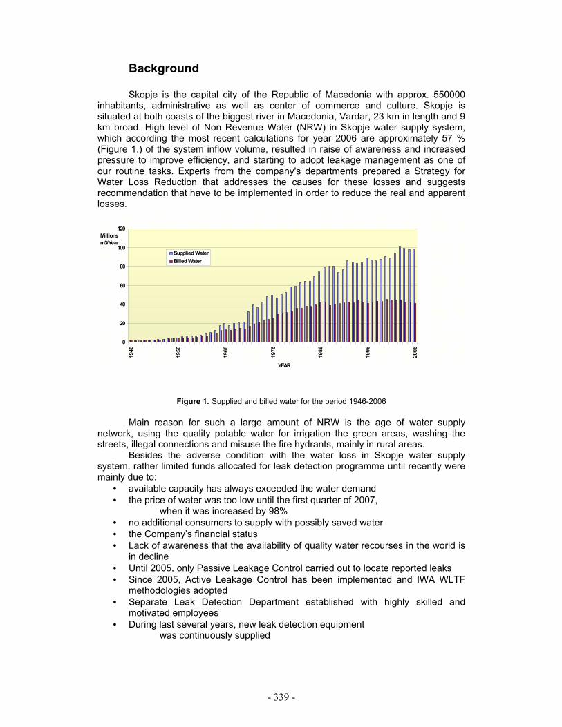
- 339 -

Background Skopje is the capital city of the Republic of Macedonia with approx. 550000

inhabitants, administrative as well as center of commerce and culture. Skopje is situated at both coasts of the biggest river in Macedonia, Vardar, 23 km in length and 9 km broad. High level of Non Revenue Water (NRW) in Skopje water supply system, which according the most recent calculations for year 2006 are approximately 57 % (Figure 1.) of the system inflow volume, resulted in raise of awareness and increased pressure to improve efficiency, and starting to adopt leakage management as one of our routine tasks. Experts from the company's departments prepared a Strategy for Water Loss Reduction that addresses the causes for these losses and suggests recommendation that have to be implemented in order to reduce the real and apparent losses.

Figure 1. Supplied and billed water for the period 1946-2006 Main reason for such a large amount of NRW is the age of water supply

network, using the quality potable water for irrigation the green areas, washing the streets, illegal connections and misuse the fire hydrants, mainly in rural areas.

Besides the adverse condition with the water loss in Skopje water supply system, rather limited funds allocated for leak detection programme until recently were mainly due to:

• available capacity has always exceeded the water demand • the price of water was too low until the first quarter of 2007,

when it was increased by 98% • no additional consumers to supply with possibly saved water • the Company’s financial status • Lack of awareness that the availability of quality water recourses in the world is

in decline • Until 2005, only Passive Leakage Control carried out to locate reported leaks • Since 2005, Active Leakage Control has been implemented and IWA WLTF

methodologies adopted • Separate Leak Detection Department established with highly skilled and

motivated employees • During last several years, new leak detection equipment

was continuously supplied

0

20

40

60

80

100

120

1946

1956

1966

1976

1986

1996

2006

Supplied WaterBilled Water

YEAR

Millions m3/Year

- 340 -

1. Water supply system Butel-Radisani-Suto Orizari The city of Skopje is mainly supplied by gravity from the Rasce spring, with

average input in the system of 4700 l/s and from the well areas Nerezi-Lepenec, with total capacity of 1420 l/s.

For certain higher areas of the city of Skopje, where water supply by gravity is impossible, high pressure zones were established. The current project analyzed the water losses in two of the above pressure zones: System of first high zone North (Consumption zone Butel-Suto Orizari - DMA 200 and DMA 300) and System of second high zone North (Consumption zone Radisani - DMA 100), represented on Figure 2.

Figure 2. Water supply system Butel – Radisani – Suto Orizari in relation to Skopje water supply system The system of the first high zone North (Pumping Station Butel) supplies the

settlements Suto Orizari, Butel 1, Butel 2 and Radisani.The pump station Butel pumps the water into the reservoirs Suto Orizari and Radisani 2, which are used to ensure balance of the daily water consumption in the settlements Butel I, Suto Orizari, part of Butel II. The above mentioned area, in addition to water supply from Pumping station Butel, is also supplied from the Pumping station Akvadukt. The system of the second high zone North (Pumping station Radisani) provides water to the settlement Radisani and the village Radisani. The Pumping station Radisani pumps the water into the reservoir Radisani 1, which is used to balance the daily water consumption for Radisani settlement.

2. DMA design in the particular network The project, which is subject of this paper, addresses one of the four Leakage

Management strategies - Active water loss control and is based on: Monitoring and on-site measurements of flow and pressure, Calculation of the annual water balance components, Water Loss Assessment Methodologies and Network Modeling.

- 341 -

Considering the fact that well established network of DMA’s and bulk water meters is the base for successful system for water loss reduction, the monitored DMA 100, DMA 200, and DMA 300 were subdivided as follows: DMA 100 was divided into six sub-DMA’s, DMA 200 into seven sub-DMA’s and DMA 300 into three sub DMA’s. The territories of each DMA’s, which are well distinguished with correctly defined boundaries, are shown on Figure 3.

Figure 3. Division the particular area into DMA’s and sub-DMA’s

Taking into account the fact that some of these sub DMA’s are supplied with water

from common pipelines and have several inlets and outlets, thus requiring well defined boundaries for the purposes of successful control of consumption within the sub-DMA’s, they were isolated by temporary closing of seven boundary valves.

For simulation of hydraulic parameters within the water supply network of the analyzed sub-zones, a Network Model was developed by using the program package EPANET.The model includes 795 pipelines and 652 connection, among which: four reservoirs: Rezervoir Radisani 1, Rezervoir Radisani 2, Rezervoir Akvadukt and Rezervoir Suto Orizari; three Pump stations: Pump station Butel, Pump station Radisani and Pump station Akvadukt; and two collectors: collector Butel and collector Akvadukt.

After the completion of the simulation of water supply network performance within the system Butel-Radisani-Suto Orizari and prior to taking any action that might change the hydraulic regime (closing the boundary valves), the previous conclusions that the regular and qualitative water supply is not interrupted have been confirmed. The fact that the results obtained through the mathematical model were practically confirmed during the site pressure measurements in the determined areas is encouraging and pleasant.

- 342 -

3. Used equipment for performing flow and pressure measurements within sub DMA’s

The monitoring of flow rate within DMA 100, DMA 200 and DMA 300 was realized

through the installed electromagnetic flow meters in Pump stations Radisani and Butel which were equipped with a GSM Data Loggers with built-in pressure sensors, enabling parallel measurement and monitoring of both, flow and pressure. Using the GSM connection, the flow and pressure values registered on 10 minutes intervals within 24 hours, were transferred to the central PC, where the dates were analyzed.

Within the project, the flow in each sub-DMA’s was monitored and registered in 10 min intervals by Ultrasonic mobile flow meters (Figure 4), which have been installed on the inlets and outlets for the appropriate area. During the project, we carried out around 30 flow measurements, and the sub DMA’s with unacceptably high flow rates were identified.

Taking into consideration the fact that the permanent monitoring of the water flow within the determined consumption zones results in early failure detection and is a base for successful water loss control, a WLM probe, which measured three parameters at the same time (flow, pressure and noise), was installed on the inlet into the pipeline Ф 300 mm in the sub-DMA’s 205. The values have been transferred via GSM connection to the control center (Figure 5).

Regarding the field pressure measurements, they have been performed by pressure sensors with in-built data logger in total of around 40 measurements.

To determinate the balance of water consumption in DMA 100 and DMA 300, as well as water losses calculation, monitoring the levels in all three reservoirs in the examined areas has been extremely important.

4. Water Loss methodology used in this project The approach used in this project in order to address and reduce water loss within the selected water distribution systems was to implement District Metered Areas (DMA). To enable efficient control of recoverable leakage, the distribution systems that make up Butel, Radisani, Suto Orizari Region were divided into 3 DMAs and 16 temporary sub DMA’s. These DMAs are being used both to identify and reduce recoverable

Figure 4. Flow measuring with Ultrasonic mobile flow meter

Figure 5. Permanent flow monitoring with WLM probe

- 343 -

leakage in the short term and then to monitor and control leakage in an ongoing manner. You can find below (Figure 6) the used methodology in this project for water loss analyze and reduction.

4.1 Minimum night flow analyze Best practice analysis of DMA flows required the estimation of leakage when the flow into the DMA and sub-DMA’s were at its minimum - this typically occurred at night between 01-04 h when customer demand was also at its minimum and therefore the leakage component was at its largest percentage of the flow. The analysis of leakage was based on the minimum night flow, which has been recorded and analyzed continuously night after night with the use of data loggers and appropriate software. Once a repeatable MNF has been established, any legitimate usage during the MNF period has been determined and subtracted from the MNF. Legitimate night-time usage was determined using proven allowances for residential accounts, or through actual meter readings for several domestic and industrial accounts. Hence, any remaining MNF can be classified as potential system leakage. This methodology helps to prioritize areas of high leakage, and, in addition, quantifies the rate of leakage in each zone to be used in payback calculations, or to justify further investigation. Techniques and software (Sanflow, PressCalcs) based on component analysis have been used in this project to analyze the minimum night flow and estimate the level of leakage and the relative volumes of background and burst volumes (see Table 5. and Table 6.)

ANALYZE THE DATA

AZNP AND MNF

ON SITE MEASUREMENT OF

PRESSURE AND FLOW

DMA DESIGN

VISUAL INSPECTION OF

WATER, SEWERAGE SYSTEM, ON SITE SURVEY

FOR ILLEGAL CONNECTIONS

ACOUSTIC SOUNDING

SURVEY

LEAK

LOCATION

REPAIR, ANALYZE

DETECTION ACTIVITIES

EFFECTIVENESS

Figure 6. Water Loss Methodology

- 344 -

Ref. Date AZP (bar)

AZNP (bar)

avg. MNF

(m3/h)

Customer Side

Leakage (m3/h)

Background Losses (m3/h)

Normal Night Use

(m3/h)

Expected MNF

(m3/h)

Excess NF

(m3/h)

DMA 100

27.03. 2007

4,73 4,95 74,79 10,3 7,64 4,8 12,24 52,05

DMA 200

30.03. 2007

5,38 5,82 95,19 5 14,63 6,34 20,97 68,9

DMA 300

30.03. 2007

4,20 4,48 636,93 102 28,29 11,27 40,16 494

Ref. Date Inflow (m3/d)

avg. MNF

(m3/h)

Night Leakage (m3/h)= Night Flows – Night

Demands

NDF Daily Leakage (m3/d)= Night

Leakage * NDF

DMA 100 27.03.2007 2289 74,79 59,69 23,44 1399,13 DMA 200 30.03.2007 3437 95,19 83,85 23,04 1931,90 DMA 300 30.03.2007 17977 636,93 523,66 23,22 12159,39

When analyzing the consumption, sub-DMA’s by sub-DMA’s, predominantly

during the night hours when the legal consumption is relatively low, the zones with unacceptably high consumption were identified and appropriate actions were taken for identification of the causes for this increased consumption.

4.2 Visual inspection of water supply and sewerage network

Taking into consideration that the high night consumption indicates high

percentage of real water losses, visual inspection and systematic examination of the entire water supply network in the critical sub-zones were made. The huge losses, especially in certain sub-DMA’s, necessitated visual inspection of the water supply network. The visual inspection was made by Water Supply Sector-Branch Radisani.

The Sewerage Sector (Branch Radisani) was also involved in this inspection, which, after inspecting the entire sewerage network, indicated several sewerage manholes where constant drinking water flow was noticed. This is a reliable indicator of a failure of the water supply network in the surrounding area. The indicated manholes were in the near vicinity of the failure locations indicated by Leak Detection Department.

4.3 Apparent Losses The Water losses consist of Real and Apparent losses. This paragraph refers to the efforts have been done by Account and Collection Department to find out the quantity of Apparent losses in the examined areas. The results proved that the main parameters influencing the apparent losses in the Butel-Radisani-Suto Orizari Region are unauthorized consumption (illegal connections, theft of water and fraud), data collection and transfer errors, meter inaccuracies and customer data base errors.

Table 1; Table 2. Quantifying leakage using Sanflow and PressCalcs software packages

- 345 -

Reference Illegal connection

Unregistered

water meter

Connected without permission

(after they have been disconnected)

Leaks on water meter

connections

Faulty

water meter

DMA 100 16 59 59 14 14

DMA 200 3 54 38 25 44

4.4 Acoustic sounding survey In certain sub-DMA’s, where higher night consumption was registered, acoustic contact microphones were used for initial identification of the place of breaks. This included routine listening of the directly accessible metal parts of the water supply network, like valves, hydrants and connection pipes in water meter box. The contact microphones, used in this project, are highly sensitive electronic acoustic devices that enable flexibility and comfort in operation as the noise from the place of occurrence is transferred via wireless to the earphones, thus avoiding the traditional cable connection (Figure 7)

More comfortable and faster way for leak localization was carried out with noise loggers.

This system allowed testing without disruption to the water supply, and provided accurate results in 24 hours, with minimal operation time and cost. Noise loggers were deployed throughout the distribution system to provide continuous surveying of leakage. These loggers were used to focus the leakage surveys in specific areas of the network. (Figure 8)

Table 3. Results obtained from on-site survey for illegal connections

Table 7. Acoustic Contact microphone Table 8. Acoustic noisse loger

- 346 -

4.5 Leak Location and Repair

Once a leak has been identified, it was then pinpointed using proven sonic and correlation techniques. Leak noise correlators and Ground microphones were become the method of choice for pinpointing leakage. The final step of the process was to mark the leak location and repaired the leak. During the systematic inspection of the water supply network, realized by Leak Detection Department, 30 leaks in DMA 200 and 22 leaks in DMA 100 have been located and repaired that effected that higher level of night consumption. Once the areas have been cleaned of previously located leaks, additional flow measuring has been performed to analyze detection activities effectiveness and to identify leakages which hasn’t been located yet. Once leakage is identified again in justifiable amounts, the whole process starts again.

5. Results obtained Pilot projects for Water Loss analyzes and adopt DMA methodologies was started in 2005. DMA 100 (Radisani) was observed as a Pilot Area. According to the monthly flow records of the installed electromagnetic water meter in the Pumping station Radisani and population demand, unacceptable increasing of daily inflow was determined. To explain the reason, only visual inspection of the water and sewerage system and partially Leak Detection were carried out. This actions achieved decreasing of 1580 m3/day; 47.460 m3/month that means 38,98% of monthly inflow was found to be mainly due to:

• open flushing outflow of 100 mm connected to the main pressure pipe

• 7 pipe bursts which were pinpointed and repaired Realizing the need of additional water loss decreasing in the selected area, the second phase, which is subject of this project, continued in 2007. After all located leaks have been repaired, additional flow and pressure measurement have been carried out. The achieved results for DMA 100, including the both graphs, the first and the control measurement are shown as follows:

DMA 100

avg. MNF

(m3/h)

Savings

(m3/d)

Savings

(m3/month)

Savings

(%)

22.05.2007

control measurement

49,09

602,41

18.072,3

34,36

* Previous avg. MNF on 27.03.2007: 74,79 m3/h

Table 4. Achieved results in DMA 100

- 347 -

Daily flow pattern in DMA 100 (27.03.2007)

0,005,00

10,0015,0020,0025,0030,0035,0040,00

11:1

0:00

12:3

0:00

13:5

0:00

15:1

0:00

16:3

0:00

17:5

0:00

19:1

0:00

20:3

0:00

21:5

0:00

23:1

0:00

00:3

0:00

01:5

0:00

03:1

0:00

04:3

0:00

05:5

0:00

07:1

0:00

08:3

0:00

09:5

0:00

Time

Flow

(l/s

Dailly flow pattern in DMA 100 (22.05.2007)

0,00

5,00

10,00

15,00

20,00

25,00

30,00

35,00

10:3

0:00

13:5

0:00

17:1

0:00

20:3

0:00

23:5

0:00

03:1

0:00

06:3

0:00

09:5

0:00

Vreme (h)

Flow

(l/s

The results obtained for DMA 200 are shown in Table 5.

DMA 200

avg. MNF

(m3/h)

Savings

(m3/d)

Savings

(m3/month)

Savings

(%)

15.06.2007

Control measurement

61,43

778

23.335

35,5

According to the night flow measurement on each sub-DMA’s in DMA 200, the sub DMA’s 205 was found to have the biggest leakage rate, and its influence was the highest. On the following two graphs, which shows the first and control measurement, the average minimum night flow decreased from 56,32 m3/h to 39,17 m3/h, that means 17,15 m3/h savings or 30,49% of daily inflow within the sub DMA’s.

* Previous avg. MNF on 30.03.2007: 95,19 m3/h

Table 5. Achieved results in DMA 200

- 348 -

6. Water Loss Performance Indicators

During the project, the water consumption balance components for the examined area (all three DMA’s were included) have been calculated using the following two methods:

• Water consumption balance using the traditional performance indicators • By using appropriate software

6.1 Calculation of the components of water consumption balance with Traditional PI This method represents the total water consumption registered by all water meters within the zone; the difference between the total volume of water supplied into the zone and the sum of the individual consumptions represents the water lost or water

Daily flow pattern in sub DMA's 205 (15.06.2007)

05

101520253035

2:20:16PM

4:50:16PM

7:20:16PM

9:50:16PM

12:20:16AM

2:50:16AM

5:20:16AM

7:50:16AM

10:20:16AM

12:50:16PM

Time

Flow

l/s

Flow

l/s

Daily flow pattern in sub DMA's 205 (14.05.2007)

05

10152025303540

1:09:56PM

3:39:56PM

6:09:56PM

8:39:56PM

11:09:56PM

1:39:56AM

4:09:56AM

6:39:56AM

9:09:56AM

11:39:56AM

Time

Flow

l/s

- 349 -

which cannot be tracked where it was consumed. The water supplied to the zones is determined on the bases of the flow through the main supply pipeline, while the consumption is determined from the water accounts i.e. by adding up the invoiced quantities for the individual and commercial consumers in certain area.

Ref.

Year

Water Input

Billed Water

Water Losses

Water

Losses WL/WI

Water

Losses per

connection

Electricity Consumption

Specific Electricity Consumpt.

of Water Input

m3 x103

m3 x103

m3

%

m3 /conn.

kWh x103/year

kWh/m3

DMA 100 DMA 200 DMA 300

2006

9290

4067

5223

56,22

533,61

4096,8

0,44

4.2 Calculation of the components of water balance and IWA recommended PI, by using appropriate software

Different software packages have been developed throughout the world, used

for calculation of the standard annual water consumption balance as recommended by IWA and for determination of the various performance indicators for water losses in the water supply systems. Within this project, one of the newest and most comprehensive software CheckCalcs was used. This software was designed for evaluation of real water losses in the water supply system, based on the traditional “IWA top down water balance” approach. This “top down” approach enables initial assessment of the level of real losses and calculation of the ILI parameter, which is used for evaluation and comparison of the operational management with the real water losses. You can find below the input data and calculated components of water balance for the whole examined area, using the mentioned software CheckCalcs.

Variable Description Units DMA 100, DMA 200, DMA 300 Lm Length of mains km 87,6 Ns Number of Service Connections no. 9788 D Density of service connection conn/km 111,7 P Average operating pressure m 47,7 T % time the system is pressurized % 100 Population served by the system 37357

TSIV Total system input volume m3x103 9290 TBC Total billed consumption m3x103 4067 WL Water Losses m3x103 5084

CARL Current annual real losses m3x103 4553 UARL Unavoidable annual real losses m3x103 190 NRW Non Revenue Water m3x103 5223 NRW Non Revenue Water % 56,2 AL Apparent losses % 5,7 AL Apparent losses m3x103 531 RL Best traditional simple PI litres/conn/day 1271 ILI Infrastructure Leakage Index 24

Table 6. Annual Water Consumption Balance using traditional performance indicators

Table 7. Input data, annual water balance components and calculated PI for 2006 using CheckCalcs

- 350 -

Conclusion

For the first time in Macedonia, a Water Loss project was designed and carried out without any consultancy from abroad

Promotion of the idea for establishment of DMA as appropriate method for water loss control

Introduction and calculation of IWA standard Water balance terminology and the IWA suggested performance indicators

The sub-zones with increased real water losses were identified and appropriate activities for its reduction were taken upon detection of a large number of failures

Decreased water loss in DMA 100 and DMA 200 for approximately 38 % of DMA’s each input volume

Pressure management methodology is recommended Adopt IWA WLTF “best practice” approach to leakage management The Water Loss activities are ongoing...

References Malcolm, F. Stuart, T. () Losses in Water Distribution Networks Conference Proceedings,(2001) Brno, Czech Republic, IWA Specialized conference ”System

Approach to Leakage Control and Water Distribution Systems Management”- David B. () Leakage Detection and Management Conference Proceedings (2002), Lemesos, Cyprus, IWA Specialized conference “Leakage

Management-A practical Approach Dr. Dusan, O.()Organization of the system of measurements in the modern water supply systems-

- 351 -

Water Losses in Maputo Water Supply System An Overview of the Strategic Plan for Leakage Reduction

J. V. Q. Langa1; J. Quessouji2 1Master in Environmental Engineering, University of Porto, Portugal.

Civil Engineer, Eduardo Mondlane University, Mozambique.

e-mail: ([email protected]); Cell: +258 30 42 589 2Civil Engineer, Eduardo Mondlane University, Mozambique.

e-mail: ( [email protected]); Cell: + 258 82 32 70 130

Key words: Water losses, Flow meters, Transmission System, Pilot Zone.

Summary

This paper presents a preliminary overview of the strategic plan for leakage reduction in the Water Supply System, in Maputo, Mozambique, a city with about 1.200.000 people and 40 % network estimated coverage. Diagnosis of the water losses according to the actual database and prognostic of mitigation measures to reduce the leakage are discussed. Some intervention measures were already considered, taking into account the local conditions and other aspects.

In average, the total losses estimated currently in the system, in the main system from the Intake Station at the Water Treatment Plant that supplies the study area are ciphered in 60 %. The final task of the shares in course is to define measures that allow reaching, in short and medium term, levels of losses that point out in average values in the order of 20 to 30 %.

Given the diagnosis characteristics responsible for the origin of the losses, the global losses of water in the system must be faced as a multi-sector and multidimensional problem.

The analysis will enclose the whole system, from the Water Treatment Plant to the branch of connection of each customer, including the alignment for each individual and collective flow meter. It will be able to enter, for comparative effect and for the decurrently ones, the values of water consumption registered by totalises counting, that will be placed in the entrance of each apartment house installation.

With this data and by using the Performance Indicators given by the IWA model, the water losses existing in the system will be determined and as well optimised the interventions measures necessary to reduce the impact of losses on the management of the system.

In the calculations, special attention goes to particular means of Performance Indicators, taking in to account the singular characteristics of the study area. The study seeks to answer the following questions:

How is possible to have a real evaluation of the water losses with values based in uncertain and estimated data’s?

How is possible to define efficient measures to reduce the leakage in an unknown network?

How is possible to guarantee goals and objectives in a not well-known network implanted mostly in per urban areas?

- 352 -

How the IWA Performance Indicators can really give a reasonable interpretation in a system where mostly of the data’s are unknown, uncertain and estimated?

Introduction

Mozambique is located in the Southeastern Zone of the African Continent, in front of the Madagascar Island, from which is separated by the Indian Ocean. It is characterized by a wet to dry tropical climate, with annual average temperature between 22 and 24º C and average precipitation of 1200 mm each year.

The water supply services, with more than 128 companies of small, medium and big dimension that up to 1999 were integrally managed by the State, comes to be, gradual and partially concession to private companies, through temporary contracts, in form of delegated management and/or technique assistance. The finally task is to endow the companies with abilities that allows to guaranty their sustainability, which, is strongly conditioned by the improvement of better levels on the performance services of the system, in the case, with particular attention to the reduction of the leakage and the actual water losses in the most part of the systems.

“Grande Maputo” is the owner of the biggest water supply system in Mozambique. In this system, important part of the intake water is lost in the Water Treatment Plant (WTP) and along the Main Pipes Transmission System (MPTS), including the pipes installed to transport the water to the final consumers, assuming an significant portion, neither in the investment costs, neither in the burden on the system exploration, reducing significantly the economic yield and the viability of its exploration.

Context

The study is fit to the leak detection and water losses reduction project taking out in the “Grande Maputo” Water Supply System, in the scope of the leasing contract between Águas de Moçambique (AdeM), in the quality of operator, and, Fundo de Investimentos e Patrimóneo de Abastecimento de Água (FIPAG), in the quality of assignor.

Characterization of the Departure Situation

Goals The main objective of the departure characterization is to quantify the water losses in the supplying system, through a water balance, where, it is compared the volumes of water allegedly supplied for the system and the volumes of water supposedly consumed by the customers. In the subsequent phases, the quality of data register will be improved as well as the identification of the origins and causes of the total water losses.

The attainment of the used information demanded an exhaustive and accurate analysis of the actual working conditions of the supplying system and its way of exploration.

Database

General

In order to make a sector analysis of the existing losses, the system was divided in two areas of analysis: MPTS and Distribution Network. For initial analyses in the network, a pilot zone was defined, to survey the strategy and methodology of

- 353 -

intervention measures that will be applied in the whole distribution network system (DNS).

Main Pipes Transmission System

The data of MPTS are related to the volumes of water produced in the WTP and distributed by each Distribution Centre (DC) (Picture 1), the general characteristics of the MPTS (Picture 2) and the values of the average pressures in the considered MPTS alignments.

Volumes of Produced and Distributed Water

The data refers to the registered values of the produced water in the WTP and distributed by each DC during the year of 2006. From these data and with the installation of the flow and pressure meters in each one of the measurement points, it is expected to initiate a set of interventional measures that lead to the reduction of the existing physical losses.

Quadric 1: Water Production and Distribution [AdeM Reports]

Umbeluzi WTP Abstracted Water 67.739.508Treated/Produted Water 63.861.300

Higth Zone - NW 7.799.200Low Zone - NW 2.549.720

Machava - DC NW 4.805.000Chamanculo - DC NW 7.470.000

Higth Zone - NW 10.515.000Low Zone - NW 2.479.800Higth Zone - NW 1.689.300Low Zone - NW 876.220

Higth Zone Distribution Tanks 92.375Connectios to the Main Pipes T S NW 5.269.391

Maxaquene - DC

Alto-Maé - DC

WATER PRODUTION AND DISTRIBUTION - 2006

Producted Water - (m3)

Distributed Water - (m3)

Matola - DC

General Characteristics of the Main Pipe Transmission System

Quadric 2: Resume of the Main Pipes Transmission System Data’s [AdeM Reports]

Reinforced Concrete/Steel

Cast Iron

Asbestocement

PVCCast Iron

Reinforced ConcreteReinforced

Concrete/SteelSteel

Steel

Cast Iron

1000

CD Chamanculo - CD Maxaquene I

0.5

0,25

6,2 (3,5 + 2,7)

Connection to Maxaquene II DC 400

800

400Connection to Alto-Maé DCCD Chamanculo - CD Laulane 800 7,5

4,5

Connection to Boane DC

Connection to Matola DC

Connection to Machava DC

150200

800

3,54,0

0,1

MAIN PIPE TRANSMISSION SYSTEM

ID Pipe Material

ETA - CD Chamanculo800 27,0

1000 27,0

Diameter (mm) Length (Km)

- 354 -

Average value of pressure in the Main Pipes Transmission System The average value of pressure in the MPTS is about 8 Bars. Pilot Zone

The data of the PZ are related to the volumes of water supplied from the Alto-Maé DC (Table 1), to the volumes of water billed and/or consumed by the customers in legal contractual situation (Table 2), to the existing pressures in different points defined in a first phase of study (Figure 1), to the number of interventional rupture recorded in the area supplied by the Alto-Maé DC (Figure 2) and to the general characteristics of the identified pipes (Table 3).

The area is supplied from the Alto-Maé DC, by a circular reservoir, embedded, with useful capacity of 4.600 m3. The esteemed total volume of water supplied from the transmission system of the Alto-Maé DC is 8.400 m3/day, with a 24-hour of continuous supplying.

From the total volume of supplied consumption to 474 customers, it’s esteemed that about 44 % is for domestic consumption, 32 % for commercial and industrial consumption, 23 % for commerce and services consumption and the remains 1 % for general public consumption.

In physiographic terms, this area can be characterized as of medium population density, when compared to the other singular areas of the Maputo city,

Volumes of Water Supplied to the Pilot Zone from the Alto-Maé DC

The presented volumes were gotten from the registers of the Alto-Maé DC, during 2006, and recorded in the reports produced by AdeM. From these values, it is expected to have reference on the total volume supplied for consumption in the PZ, through which, it will be possible, even so in not yet conclusive way, to know the amount of water allegedly consumed in the PZ. The final accuracies of these values will be made after the installations of the flow meter in the pipe that supplies the PZ, from the Alto-Maé DC.

- 355 -

Table 1: Volumes of Water Distributed to the Pilot Zone (2006) [AdeM Reports]

Jan Feb Mar Apr May Jun Jul Aug Sep Oct Nov Dec1 2.640 2.640 2.640 2.640 2.640 2.640 2.640 2.640 2.640 2.640 2.640 2.6402 2.640 2.640 2.640 2.640 2.640 2.640 2.640 2.640 2.640 2.640 2.6403 2.640 2.640 2.640 2.640 2.640 1.870 2.640 2.640 2.640 2.640 2.6404 2.640 2.640 2.640 2.640 2.640 2.640 2.640 2.640 2.640 2.640 2.6405 2.640 2.640 2.640 2.640 2.640 2.640 2.640 2.640 2.640 2.640 2.6406 2.640 2.640 2.640 2.640 2.640 2.640 2.640 2.640 2.640 2.640 1.3207 2.640 2.640 2.640 2.640 2.640 2.640 2.640 2.640 2.640 2.640 2.0908 2.640 2.640 2.640 2.640 2.640 2.640 2.640 1.870 2.640 2.640 2.6009 2.640 2.640 2.640 2.640 2.640 2.640 2.640 0 2.640 2.640 2.64010 2.640 2.640 2.640 2.640 2.640 2.640 2.640 2.530 2.640 2.640 2.64011 2.640 2.640 2.640 2.640 2.640 2.640 2.640 2.640 2.640 2.640 2.64012 2.640 2.640 2.640 2.640 2.640 2.640 2.640 2.640 2.640 2.640 2.64013 2.640 2.640 2.640 2.640 2.640 2.640 2.640 2.640 2.640 2.640 2.64014 2.640 2.640 2.640 2.640 2.640 2.640 2.640 2.640 2.640 2.640 2.64015 2.640 2.640 2.640 2.640 2.640 2.640 2.640 2.640 2.640 1.760 2.64016 2.640 2.640 2.640 2.640 2.640 2.640 2.640 2.640 2.640 2.640 2.64017 2.640 2.640 2.640 2.640 2.640 2.640 2.640 2.640 2.640 2.640 2.64018 2.640 2.640 2.640 2.640 2.640 2.640 2.640 2.640 2.640 2.640 2.64019 2.640 2.640 2.640 2.640 2.640 2.640 2.640 2.640 2.640 2.640 2.64020 2.640 2.640 2.640 2.640 2.640 2.640 2.640 2.640 2.640 2.640 2.64021 2.640 2.640 2.640 2.640 2.640 2.640 2.640 2.640 2.640 2.640 2.64022 2.640 2.640 2.640 2.640 2.640 2.640 2.640 2.640 2.640 2.640 2.64023 2.640 2.640 2.640 2.640 2.640 2.640 2.640 2.640 2.640 2.640 2.64024 2.640 2.640 2.640 2.640 2.640 2.640 2.640 2.640 2.640 2.640 2.64025 2.640 2.640 2.640 2.640 2.640 2.640 2.640 2.640 2.640 2.640 2.64026 2.640 2.640 2.640 2.640 2.640 2.640 2.640 2.640 2.640 2.640 2.64027 2.640 2.640 1.760 2.640 2.640 2.640 2.640 2.640 2.640 2.640 2.64028 2.640 2.640 2.640 2.640 2.640 2.640 2.640 2.640 2.420 2.640 2.64029 2.640 2.640 2.640 2.640 2.640 2.640 2.640 2.640 2.640 2.64030 2.640 2.640 2.640 2.640 2.640 2.640 2.640 2.640 2.640 2.64031 2.640 2.640 2.640 2.640 2.640 2.640

Total 2.640 73.920 81.840 78.320 81.840 79.200 81.070 81.840 75.680 81.620 78.320 79.930

Volume (m3) Day

Billed and/or consumed Values of Water in the Pilot Zone The presented volumes were gotten by the AdeM Commercial Board registers during 2006, for the set of customers register in the PZ database. Although a clear plurality regarding the existing bill conditions does not exist, it is expected through these values, to have a minimum reference on the real volumes of water consumption, for the customers entered in the PZ during the considered period. With these values it will be possible, in comparison with the DC supplied volumes, to determine, the existing water losses in the PZ. In this phase, the error is relatively coarse.

- 356 -

Pressure Measured Under the PZ

0,000,501,001,502,002,503,003,504,00

P1 P2 P5 P4 P3 P6 P7Measured Points

Pres

sure

[ba]

Mourning (9:30H)Afternoon(12:30H)

Table 2: Volumes of Billed and Consumed Water in the Pilot Zone (2006) [AdeM Reports]

Jan Feb Mar Apr May Jun Jul Aug Sep Oct Nov DecTotal 450 450 450 450 450 450 450 450 450 450 450 450 450

Domest. 343 343 343 343 343 343 343 343 343 343 343 343Com/Serv. 73 73 73 73 73 73 73 73 73 73 73 73Indu/Com. 31 31 31 31 31 31 31 31 31 31 31 31

General/Pub 3 3 3 3 3 3 3 3 3 3 3 3Total 24 24 24 24 24 24 24 24 24 24 24 24 24

Domest. 14 14 14 14 14 14 14 14 14 14 14 14 14Com/Serv. 10 10 10 10 10 10 10 10 10 10 10 10 10Indu/Com. 0 0 0 0 0 0 0 0 0 0 0 0 0

General/Pub 0 0 0 0 0 0 0 0 0 0 0 0 0Total 9.034 9.531 10.194 14.281 13.774 12.090 10.046 13.066 11.252 12.516 13.955 10.982 140.721

Domest. 4.230 4.574 4.244 4.853 4.954 5.754 4.284 5.039 4.949 5.419 5.480 4.592Com/Serv. 1.735 1.620 3.371 1.879 3.159 3.235 2.610 3.060 2.451 1.979 2.332 2.410Indu/Com. 2.968 3.260 2.469 7.185 5.661 3.101 3.152 4.920 3.852 5.118 6.143 3.980

General/Pub 101 77 110 364 0 0 0 47 0 0 0 0Total 4.891 4.514 4.837 4.049 4.275 4.384 3.471 4.224 4.244 4.045 3.877 4.296 51.107

Domest. 2.565 2.540 2.476 2.241 2.230 2.531 2.086 2.112 1.983 1.933 2.122 2.059Com/Serv. 1511 1.053 1.507 952 1.181 1.173 900 1.479 1.462 1.259 1.195 1.271Indu/Com. 815 921 854 763 768 577 485 633 760 814 517 743

General/Pub 0 0 0 93 96 103 0 0 39 39 43 223Total 0 0 0 0 0 0 0 0 0 0 0 0 0

Domest.Com/Serv.Indu/Com.

General/PubTotal 0 0 0 0 0 0 0 0 0 0 0 0 0

Domest.Com/Serv.Indu/Com.

General/Pub

2.640 73.920 81.840 78.320 81.840 79.200 81.070 81.840 75.680 81.620 78.320 79.930 876.22013.925 14.045 15.031 18.330 18.049 16.474 13.517 17.290 15.496 16.561 17.832 15.278 191.828

390 390 390 390 390 390 390 390 390 390 390 390 4.680

Total

Billed Metered Consumption (m3)

Billed Unmetered Consumption (m3)

Unbilled Metered Consumption (m3)

Billed and Consumed Water - PZ - 2006

Total Distributed WaterTotal Billed Consumption

Tot. Minimum Illegal Estimated Consumption

ItemsLegal Consumers (nr.)

Illegal Consumers (nr.)

Unbilled Unmetered Consumption (m3)

MonthConsumption

Values of Pressure Register in the Pilot Zone

In the first phase, in order to have a minimum reference on the existing pressures in different points chosen in the PZ DNS, pressure values were recorded. These values will be used for evaluation of the hydraulic working conditions on the PZ network.

A total of 7 distinct points were recorded, with registers for two reference periods, namely in the morning and the afternoon periods respectively. The period for recordings was defined to supposedly make registers in the hours of bigger consumption and therefore of bigger request of the network, which is equivalent to the deficit or less favorable period in terms of pressures.

From these values, it is expected to diagnosis in the first analysis, the network working conditions, from which, it can be able to define ways of intervention for the regularization of the system, including the possible mapping errors of the pipes and the valves positioning. This proceedings, will be use to define measurements and corrective interventions, that will allow and improve the quality of the services regarding the water distribution system in the PZ area. The final task is to reduce the existing water losses.

Figure 1: Values of Register Pressure in the Pilot Zone

- 357 -

Number of Crack Interventional Corrections in the Pilot Zone Network

The quantification of the rupture interventions in the PZ DNS was made on the basis of the recorded data carried through registers of the Technical Board of AdeM. Through these registers, it is expected to have a preliminary diagnosis on the relative vulnerability of specific alignments on the DNS. With these values and the other referring data regarding the characteristics of the installed pipes, namely the diameter’s, the materials and eventually, when possible, the referencing of the age of the pipes, will be evaluate the necessary interventional measures for rehabilitation of these alignments. These interventional measures will create conditions that propitiate the reduction of the existing physical losses in the ZP.

The presented data doesn’t give the real location of the rupture points during the registry, as a consequence of the type of register used by the AdeM. The register does not mention the section where the rupture occurred. In this context, the registers are presented only in function of Street or Avenue where it had been verified and not in function of the coordinates of the respective sections of rupture requested for intervention, as it would be recommendable. Having in consideration the necessary mapping of these data, in the future, the register of the points of rupture will have to be recorded in GIS maps.

Crack Recordings During 2006

Alto-Maé / PZ

2

5

30

4

4

4

18

6

10

3

1

0

1

1

0

0

0

1

0

0

0

0

0 5 10 15 20 25 30 35

Av. 25 de Setembro

Av. Ahmed S. Barre

Av. Albert Luthuli

Av. Fernão Mangalhães

Av. Guerra Popular

Av. Rio Tembe

Av. Romão F. Farinha

Av. Zedequias Manganhela

Rua Comandante Baete Neves

Rua Comandante Maura Braz

Rua P. Santos Gil

Roa

ds /

Ave

nues

Nr. Interventions / Year Branch Network

Figure 2: Annual register of Rupture Interventions in the Alto-Maé DNS in 2006.

General Characteristics of the Pipes in the Pilot Zone

The network of the ZP is composed by a set of equipment, to detach the system of pipes with diameters of dimensions between 50 and 450 mm, a set of valves with different utilities. Some of the valves are operational and others are damage.

In the distribution network, it’s esteemed that it has an approached total length of 12.630 m, considering the total length of the primary, secondary and tertiary net.

- 358 -

Table 4: Characteristics of the pipes in the Pilot Zone [AdeM Reports] PipeID Material

Diameter (mm)

Length (m) C_Y C_X

D00676_D00681 Steel 100 141,60 7128193,646 456486,220D04170_D04181 Steel 100 0,06 7128374,745 456189,995

100 Total 141,66D06639_D06643 Steel 150 353,66 0,000 0,000D06639_D06642 Steel 150 427,42 0,000 0,000

150 Total 781,07D04181_D04201 Steel 400 10,47 7128379,460 456192,280D04171_D04201 Steel 400 268,53 7128504,630 456253,875

400 Total 279,01D00681_D00682 Asbestos Cement 100 79,02 7128267,145 456448,747D04182_D04184 Asbestos Cement 100 84,49 7128435,375 456206,120D00711_D00715 Asbestos Cement 100 32,76 7127772,913 456768,765D00712_D00715 Asbestos Cement 100 35,39 7127790,845 456739,792D00672_D04201 Asbestos Cement 100 564,50 7128224,204 456427,142D04210_D04211 Asbestos Cement 100 25,04 7127611,570 456505,355D04212_D04213 Asbestos Cement 100 33,88 7127590,925 456547,990D00742_D04213 Asbestos Cement 100 35,76 7127595,836 456571,400D04214_D04215 Asbestos Cement 100 71,99 7127597,045 456574,675D00722_D04215 Asbestos Cement 100 16,90 7127622,845 456600,383D00647_D04230 Asbestos Cement 100 140,73 7128146,252 456699,314D04161_D04230 Asbestos Cement 100 10,99 7128079,755 456664,600D00666_D05200 Asbestos Cement 100 1,32 7127963,674 456827,736

100 Total 1132,76

Preliminary Water Balance Methodology


In the present phase, the evaluation of the water losses in the MPTS was made through the comparison between the volumes of water register as supplied water from the WTP and the volumes supplied by each one of the DC, to the network. With the comparison of these values, the volume of water loss in the MPTS was determined. In the next future, will be defined interventional measurements and goals to reduce the water lost in the MPTS.

Pilot Zone

The analysis of the data of water losses in the PZ was made on the basis of the comparison between the volumes allegedly supplied by the Alto-Maé DC and the billed and/or consumed volumes of the whole customers that belong to the PZ DNS area. Preliminary Results

The presented values are the results of the entered data for the water balance in the MPTS and in the PZ Network Distribution System.

- 359 -

Main Pipes Transmission System Quadric 3: Water Balance

Annual System Input Volume

Unbilled Authorized Consumption

m3/year00,0%Error Margin [+/-]:

Error Margin [+/-]:

43.546.006 m3/year

0,0%

0,0%Error Margin [+/-]:0,0%

Error Margin [+/-]:Error Margin [+/-]: 0,0%

0,0%Error Margin [+/-]:

Water Losses

20.315.294 m3/year

Revenue Water

20.315.294 m3/year

43.546.006 m3/year

Non-Revenue Water

Error Margin [+/-]: 0,0%

Physical Losses

m3/year20.315.294


m3/year0

Commercial Losses


63.861.300 m3/year


Unauthorized Consumption

Customer Meter Inaccuracies and Data Handling Errors0 m3/year

0 m3/year

Unbilled Unmetered Consumption0 m3/year

Unbilled Metered Consumption0 m3/year


Billed Unmetered Consumption0 m3/year

43.546.006 m3/year

HomeBilled Metered Consumption

m3/year43.546.006Billed Authorized Consumption

Pilot Zone Quadric 4: Water Balance

HomeBilled Metered Consumption

m3/year140.721Billed Authorized Consumption


Billed Unmetered Consumption51.107 m3/year

191.828 m3/year

Unbilled Metered Consumption0 m3/year

4.680 m3/year

Unbilled Unmetered Consumption0 m3/year

Customer Meter Inaccuracies and Data Handling Errors0 m3/year

Commercial Losses


876.220 m3/year


Unauthorized Consumption


m3/year0


Physical Losses

m3/year679.712

Revenue Water

684.392 m3/year

191.828 m3/year

Non-Revenue Water


Water Losses

684.392 m3/year0,0%

Error Margin [+/-]:0,0%Error Margin [+/-]:


Annual System Input Volume

Unbilled Authorized Consumption

m3/year4.6800,0%Error Margin [+/-]:

Error Margin [+/-]:

191.828 m3/year

0,0%

Preliminary Diagnosis


Water Balance The total volume produced and supplied from the WTP of Umbeluzi in 2006 was 63.861.300 m3, which corresponds to the Annual System Input Volume.

The total volume distributed by the DC in the same period of analysis, including the volume supplied to the Auto-Tanks and the connections along the MPTS, totalizes

- 360 -

43.546.006 m3, which corresponds to the Total Authorized Consumption. For this case, it also corresponds to the Billed Water Volume.

In this way, the volume of water lost in the MPTS (WTP and DC) in this period, that corresponds to the Physical Losses was 20.315.294 m3.

Performance Indicators For this preliminary phase of analysis, the significant Performance Indicators are:

o Level of Service The water supply in the MPTS was made 24 hours per day with an average pressure of 8 bars.

o Physical Losses Performance Indicators For the case of the MPTS, the evaluation of the losses was made regarding the length of the pipes. In this way, the volume of water losses for each miter of the MPTS is 23.19 m3/hour.

o Financial Performance Indicators The Total Volume of Water Losses corresponds to 32 % of the Volume of Water Entered in the System. Pilot Zone

Water Balance The total volume of water distributed by the Alto-Maé DC to the PZ in 2006 was of 876.220 m3, which corresponds to the Annual System Input Volume. In the same period, the Total Volume of Authorized Consumption in the PZ was 191.828 m3.

About 4.680 m3 of water was esteem as volume used by clandestine consumption (illegal connections). This value, in the Water Balance, corresponds to the Commercial Losses.

The total water loss entered for the same period was 684.392 m3, of which 4,680 m3 correspond to the Commercial Losses and 679,712 m3 correspond to the Physical Losses.

Performance Indicators For this preliminary phase on the analysis, the significant Performance Indicators are:

o Level of service The water supply to the PZ was made 24 hours per day, with an average pressure of 21.4 m. In relation to the pressure, the average value in the morning was 32.1 m and in the afternoon was 10.7 m.

o Physical Losses Performance Indicators The losses entered on average of branch connections, admitting that they are equal to the number of customers, correspond to 3,929 l/day.

The analysis of the loss in relation to the linear length does not have to be considered therefore, the density of connections by the length of pipes gotten was 38 Connections/km, greater than 20 Connections/km, the recommendable value of minimum Connections/km to consideration of this variable in the calculation of the referred Indicator.

o Commercial Losses Performance Indicators The commercial loss corresponds to the illegal consumption through clandestine connections. This value corresponds to 2 % of Authorized Billed Consumption, which means, of the Volume of Billed Water.

o Financial Performance The Total Volume of Water Losses corresponds to 78 % of the Volume of Water Entered in the System.

- 361 -

Preliminary Conclusions and Recommendations

General

Given the uncertainty of the used values in the calculation model, resultant from the current inexistence of conditions that allow the real measurement of the volumes of produced, transported and consumed water in the MPTS and the PZ, the value of losses presented can’t be considered as real, once is not yet possible, in relatively conclusive way, to make a honest balance of the physical losses that really occur in this system.

Associated to the previous point, the comparison between the value of losses gotten with the model and the average value of losses assumed as existing in the system, fixed in about 60 %, induct to doubts in relation to the accurately of the used database for the model calculation. This point is supported given that, the physical-structure characteristics of the PZ with influence in the occurrence of physical and commercial losses, namely, the possibility of existence of clandestine connections among others factors, when compared to other singular zones of the system, would have to propitiate an less value of losses than the assumed average value as existing in all the system.

The implementation of a plan for reduction of water losses is urgent, taking in to account the implications of the losses in the performance levels and profitability of the Company.

To sure that the defined strategy and methodology of execution adopted by the AdeM request the desired effect, it is necessary that the shares to carry through have an enough reliable level. This faith ness will have to be guaranteed by the availability of qualified human resources, by the persistence of the technician in the performance of the set requested services, and, in absolute, by the administration investment politics that create functional objective conditions that become the leakage detection and losses reduction, an immediate priority of the AdeM.

7, 2 Main Pipes Transmission System

Conclusions Given the uncertainty of the used values for the database in the determination of

the level of existing losses in the MPTS, including the deficit knowledge on the installation conditions of the main pipes and the existence of illegal connections along the transmission alignments, it’s not yet possible, in a conclusive way, to make a honest balance of the physical losses that really occur in this system.

Recommendations: The installation of flow and pressure meters is urgent in all the points defined for

such, in order to make possible the beginning of the survey of values wove will support the strategy to use for the reduction of existing losses.

7.3 Pilot Zone

Conclusions: Given the inefficient used database for the determination of the level of existing

losses in the distribution net that supplies the PZ, including the deficit knowledge on the installation conditions of the main pipes and the existing number of illegal connections in the installed net, it’s not yet possible, in a conclusive way, to make a honest balance of the physical losses that really occur in this system.

- 362 -

Recommendations: It urges the implementation of shares that make possible the survey of a accurate

database, that allows to the determination of the necessary variables to calculate the values of commercial and physical losses that occur in the PZ net, among which, the survey of the values of pressure in different points of the net and the exhausting survey of the number of customers beneficiaries of the net, including the working conditions of the installed accountants.

The Romanian Water Association (RWA) is the national network of water

professionals, spanning the continuum between research and practice and

covering all facets of the water cycle.

Through RWA, members collaborate to lead the development of effective

and sustainable approaches to water resources management, drinking water,

wastewater and storm water management in areas through the country,

creating value and driving the advancement of both the science and best

practice of water management.

The ultimate strength and potential of RWA lies in the professional and

geographic diversity of its membership - a “mosaic” of members communities

including academic researchers and research centers, utilities, consultants,

industrial water users and water equipment manufacturers. RWA members from

each of these communities represent the leading edge in their fields of

specialty, and together are building new frontiers in national water management

through interdisciplinary exchange and collaboration.

In the environment, RWA and its members are committed to furthering

sustainable and holistic resource management and service provision, built on

the concept of the water cycle.

Contac us: Address:

202A, Splaiul Independentei., 9th floor 6th district , Bucharest, Romania.

Phone / Fax: 004 021 316 27 87 / 004 021 316 27 88

004 0747 029 988

E-mail: [email protected]

Website: www.ara.ro

Water Loss 2007 - Volum I

Documents

Transcript of Water Loss 2007 - Volum I