vol37-1.pdf - EMIS
136
Memoirs on Differential Equations and Mathematical Physics Volume 37, 2006, 1–136 S. Kharibegashvili SOME MULTIDIMENSIONAL PROBLEMS FOR HYPERBOLIC PARTIAL DIFFERENTIAL EQUATIONS AND SYSTEMS
-
Upload
khangminh22 -
Category
Documents
-
view
3 -
download
0
Transcript of vol37-1.pdf - EMIS

Memoirs on Differential Equations and Mathematical Physics
Volume 37, 2006, 1–136
S. Kharibegashvili
SOME MULTIDIMENSIONAL PROBLEMS
FOR HYPERBOLIC PARTIAL DIFFERENTIAL
EQUATIONS AND SYSTEMS

Abstract. For a class of first and second order hyperbolic systems withsymmetric principal part, to which belong systems of Maxwell and Diracequations, crystal optics equations, equations of the mathematical theory ofelasticity and so on which are well known from the mathematical physics,we have developed a method allowing one to give correct formulations ofboundary value problems in dihedral angles and conical domains in Sobolevspaces. For second order hyperbolic equations of various types of degen-eration, we study the multidimensional versions of the Goursat and Dar-boux problems in dihedral angles and conical domains in the correspondingSobolev spaces with weight. For the wave equation with one or two spatialvariables, the correctness of some nonlocal problems is shown. The existenceor nonexistence of global solutions of the characteristic Cauchy problem ina conic domain is studied for multidimensional wave equations with powernonlinearity.
2000 Mathematics Subject Classification: 35L05, 35L20, 35L50,35L70, 35L80, 35Q60.
Key words and phrases: Hyperbolic equations and systems, hyper-bolic systems with symmetric principal part, multidimensional versions ofthe Darboux and Goursat problems, degenerating hyperbolic equations ofthe second order, nonlocal problems, existence or nonexistence of globalsolutions for nonlinear wave equations.
! " #!$ % & '( () * + ,- $ ' # ) " . # $ / &0' 1 $ )2,#) 3 +' $ +4$ % $ +# $ ( $ ( # 5 ) +26 /6 7 +% ,8 * 5 ) $ 5 6 9$ ) / : 6 ; ( 1'<# : ,# ) ($ 3 % : 6 7 9 ,4 6 => 5 5 5 7 3 ) . ! ) # & * 5 ) &$ "5 6 &.$ ) / - 6 .6 *' / & / ,# ) ) 1 ) ) =4 %<# ) % ? ,4 #?,4 % ?6 #5 6 2 $ ?1/ #. "$ / ,# ) ?$ 3 ' $ #5 =#5 5 ) 2 */ 0' 6 ,4 ! ) 1 ) . %<# ) .6 * " .$ 6 5 # & ,# ) & ! ) 5 ) & 2 $ 5 ?$ ) / @ 6 =

Introduction
In this work we investigate some multidimensional problems for hyper-bolic partial differential equations and systems. It should be said that whenpassing from two to more than two independent variables difficulties mayarise that are not only technical. They may arise even when formulatingmultidimensional versions of classical two-dimensional problems, for exam-ple, of the Goursat and Darboux problems.
As is known, the strict hyperbolicity of a system plays an importantrole in establishing the correctness of the posed initial, initial-boundaryand other problems. At the same time, the investigation of some problemsmakes it possible to consider a class of systems wider than that of strictlyhyperbolic ones. In the case of one equation this is the ultrahyperbolicequation. In the first section of Chapter I we consider second order systemswith several independent variables hyperbolic with respect to some two-dimensional planes. For such systems, in dihedral domains of a certainorientation we consider boundary value problems in special weight functionspaces with boundary conditions of Poincare type imposed on the facesof the dihedral angle. The correctness of these problems is proved whenthe order of the weight function determining the function space is greaterthan a definite value [69]. A separate consideration is given to the case ofultrahyperbolic equation [70].
In the second section of Chapter I we develop methods of formulatingcorrect boundary value problems for a class of second order hyperbolic sys-tems with several independent variables with symmetric principal part inconic domains, taking into account the spatial orientation of the latter.
In the third section of the same chapter we investigate boundary valueproblems for a class of first order hyperbolic systems with symmetric princi-pal part. To this class belong, in particular, the Maxwell and Dirac systemsof differential equations and the equation of crystal optics which are wellknown from mathematical physics. We begin the subsection by consider-ing boundary value problems in a conic domain whose boundary is one ofthe connected components of the characteristic conoid of the system [71],[72]. Certain difficulties arise even if the cone of normals of the systemconsists of infinitely smooth sheets and the connected components of thecharacteristic conoid of the system corresponding to these sheets may have
3

4 S. Kharibegashvili
strong singularities [24, p. 586]. Thus difficulties already arise when formu-lating a characteristic problem, when the carrier of boundary data must beindicated [72].
In the second part of Section 3 we consider boundary value problemsin dihedral domains [73], [74]. To show that the formulation of a problemin terms of its correctness demands much care we give the following simpleexample of symmetric system [105]
E0Ut +AUx +BUy = F,
where E0 =
(1 00 1
), A =
(1 00 −1
), B =
(0 −1−1 0
), F = (F1, F2) is a
given and U = (u1, u2) is an unknown two-dimensional real vector. Thecharacteristic polynomial of the system is p(ξ0, ξ1, ξ2) = det(ξ0E0 + ξ1A +ξ2B) = ξ20−ξ21−ξ22 . We denote byD : −t < x < t, 0 < t < +∞ the dihedralangle bounded by the characteristic surfaces S1 : t − x = 0, 0 ≤ t < +∞and S2 : t + x = 0, 0 ≤ t < +∞, of the system. As is shown in [71],the problem of finding a solution of the system under consideration in thedomain D by the boundary conditions
u2
∣∣S1
= f1, u1
∣∣S2
= f2
is posed correctly, whereas in the case of the boundary conditions
u1
∣∣S1
= f1, u2
∣∣S2
= f2
for the problem to be solvable we need the fulfulment of a continual set ofsolvability conditions imposed on the right-hand sides F , f1 and f2 of theproblem.
Note that in the second and third sections the approaches to statingcorrect boundary value problems make an essential use of the structure ofquadratic forms which correspond to characteristic matrices of the systemsand which, in particular, depend on the spatial orientation of the problemdata carriers. We conclude the sections by presenting the correct statementsof boundary value problems for Maxwell and Dirac systems of differentialequations and those of crystal optics.
Problems in a certain sense close to the ones we consider in this chap-ter, were investigated by A. V. Bitsadze [8]–[10], K. O. Friedrichs [30], [31],K. O. Friedrichs and P. D. Lax [32], [33], A. A. Dezin [25]–[27], M. S. Agra-novich [1]–[3], V. S. Vladimirov [122], [123], V. N. Vragov [125], [126],K. Kubota and T. Ohkubo [80], [81], T. Ohkubo [106], S. Kharibegashvili[61], [64], [65], O. Jokhadze [55], [56], P. Secchi [113], Y. Tanaka [117] andother authors.
In Chapter II we study some multidimensional versions of the Goursatand Darboux problems for degenerating hyperbolic equations of second or-der. Note that when passing from nondegenerating hyperbolic equations todegenerating ones there may arise essential differences in the correct state-ment of multidimensional versions of the Goursat and Darboux problems.

Some Multidimensional Problems 5
For example, if the characteristic conoid for a second order nondegeneratinghyperbolic equation which is simultaneously the data carrier of the charac-teristic Cauchy problem (of the multidimensional version of the Goursatproblem), consisting of bicharacteristic curves emanating from one point(conoid vertex), is homeomorphic to the conic surface of a circular cone,then in the case of degeneration this conoid may have a smaller dimension.For example, for the equation
utt − ux1x1 − ux2x2 − x3ux3x3 = F
the characteristic conoid KO with the vertex at the origin O degeneratesinto the two-dimensional conic manifold (x1, x2, x3, t) ∈ R4 : t2−x2
1−x22 =
0, x3 = 0, while for the equation
xm3 utt − ux1x1 − ux2x2 − ux3x3 = F
the characteristic conoid KO consists only of one bicharacteristic curve(x1, x2, x3, t) ∈ R4 : x1 = x2 = 0, t2 = 4
9 x33, x3 > 0 in the case m = 1
and it degenerates into one point O(0, 0, 0, 0) in the case m = 2. It clearlyfollows that in such cases the statement of the characteristic Cauchy prob-lem is out of question. Another peculiarity connected with degeneration ofan equation is that the parts of the boundary where the equation under-goes characteristic degeneration must be completely free from any kind ofboundary conditions.
In the first section of Chapter II, for the degenerating equation
utt − ux1x1 − x3ux2x2 − ux3x3 = F
we construct the characteristic conoids KO and KA, where O = (0, 0, 0, 0),A = (0, 0, 0, t0), and study a multidimensional version of the first Darbouxproblem in a finite domain bounded by the hyperplane x3 = 0 and by someparts of the conoids KO and KA lying in the half-space x3 ≥ 0 [76].
In the second section of that chapter we investigate the characteristicCauchy problem for the equation
utt−tm(ux1x1 +ux2x2)+a1ux1 +a2ux2 +a3ut+a4u=F, m=const>0,
with noncharacteristic degeneration, and for the equation
(tmut)t−ux1x1−ux2x2 +a1ux1 +a2ux2 +a3uxt +a1u=F, 1≤m=const<2,
with characteristic degeneration on the plane t = 0 [68].Finally, in the last section of Chapter II we consider some multidimen-
sional versions of the first Darboux problem in dihedral domains for thedegenerating equations
utt−|x2|mux1x1−ux2x2 +a1ux1 +a2ux2 +a3ut+a4u=F, m=const≥0,
and
utt−ux1x1−(|x2|mux2)x2+a1ux1+a2ux2 +a3ut+a4u=F, 1≤m=const<2,
respectively with noncharacteristic and characteristic degeneration on theplane x2 = 0 [66], [67].

6 S. Kharibegashvili
All the results of this chapter are obtained by the method of a prioriestimates in negative Lax norms in special Sobolev weight spaces connectedwith the principal parts of degenerating equations.
The questions raised in this chapter were investigated by many authors(see A. V. Bitsadze [7], [10], A. M. Nakhushev [103], [104], A. V. Bitsadzeand A. M. Nakhushev [11]–[13], R. W. Carrol and R. E. Showalter [22],M. M. Smirnov [116], D. Gvazava and S. Kharibegashvili [40], J. M. Rassias[109], N. I. Popivanov and M. F. Schneider [107] and other works).
Chapter III, consisting of two sections, deals with some nonlocal prob-lems for wave equations. In the first section, we show for the wave equationwith one spatial variable that the lowest term affects the correctness of thenonlocal problem: in some cases the problem has a unique solution, whilein other cases the corresponding homogeneous problem has an infinite setof linearly independent solutions [75]. We give the correct formulation of anonlocal problem with an integral condition. The multidimensional versionof this problem is studied in the next section. In the second section weestablish one property of solutions of the wave equation with two spatialvariables. This property is of integral nature and defines solutions com-pletely. Furthermore, we give the properties of wave potentials, by meansof which the nonlocal problem is reduced to a Volterra type integral equationwith a weakly singular kernel. The investigation of this integral equationmade it possible to prove the correctness of the nonlocal problem both in theclass of generalized solutions and in the class of regular classical solutionsof arbitrary smoothness [75].
The active interest shown recently in nonlocal problems for partial dif-ferential equations is, to a certain extent, connected with the fact thatnonlocal problems arise in the mathematical modelling of some physical,biological and other processes. For equations of parabolic and elliptic type,these problems were studied by J. R. Cannon [21], L. I. Kamynin [58],N. I. Ionkin [51], N. I. Yurchuk [129], A. Bouziani [18], S. Mesloub andA. Bouziani [94], A. M. Nakhushev [104], A. V. Bitsadze and A. A. Samarskii[14], A. V. Bitsadze [15], [16], V. A. Il’in and E. I. Moiseyev [49], E. Moi-seyev [102], D. G. Gordeziani [36], A. L. Skubachevskii [115], A. K. Gushchinand V. P. Mikhailov [39], F. J. Correa and S. D. Menezes [23] and otherauthors. For equations of hyperbolic type, mention should be made ofthe works by Z. O. Mel’nik [90], Z. O. Mel’nik and V. M. Kirilich [91],T. I. Kiguradze [77], [78], V. A. Il’in and E. I. Moiseyev [50], S. Meslouband A. Bouziani [93], A. Bouziani [19], S. Mesloub and N. Lekrine [95],G. Avalishvili and D. Gordeziani [4], D. G. Gordeziani and G. A. Aval-ishvili [37], [38], G. A. Avalishvili [5], L. S. Pul’kina [108], J. Gvazava [41],[42], B. Midodashvili [97], [98], G. G. Bogveradze and S. S. Kharibegashvili[17], M. Dohghan [28].
As is known, the characteristic Cauchy problem for linear hyperbolicequations of second order with the data carrier on a characteristic conoid (in

Some Multidimensional Problems 7
particular, for the linear wave equation with the data carrier on the bound-ary of a light cone of the future) is globally solvable in the correspondingfunction spaces [20], [24], [43], [88]. This circumstance may significantlychange if the equation involves nonlinear terms. In the last Chapter IV,consisting of two sections, we study the question of the existence and nonex-istence of global solutions of the characteristic Cauchy problem in a lightcone of the future for nonlinear wave Gordon equations
utt −n∑
i=1
uxixi = f(u) + F (x, t), n > 1,
with power nonlinearity of the type f(u) = λ|u|α, or f(u) = −λ|u|pu in theright-hand side, where λ, α and p are real constants, and λ 6= 0, α > 0,p > 0. In the first section, in the case f(u) = λ|u|α, 1 < α < n+1
n−1 ,where n is the spatial dimension of the equation, the local solvability ofthat problem is proved; for λ > 0, the conditions on the right-hand sides ofthe problem are found when a global solution does not exist. The estimateof the time interval of solution’s life is given. In the second section, incase f(u) = −λ|u|pu, for λ > 0 the existence of the global solution of thecharacteristic Cauchy problem and for λ < 0 the nonexistence of such asolution is proved, when some additional conditions are imposed on theright-hand sides of the problem.
Note that the problems of existence or nonexistence of global solutionsfor nonlinear equations with the initial conditions u|u=0 = u0,
∂u∂t
∣∣t=0
= u1
have been considered and studied by K. Jorgens [57], H. A. Levin [85],F. John [52], [53], F. John and S. Klainerman [54], T. Kato [59], V. Georgiev,H. Lindblad and C. Sogge [35], L. Hormander [47], E. Mitidieri and S. I. Po-hozaev [101], M. Keel, H. F. Smith, and C. D. Sogge [60], C. Miao, B. Zhang,and D. Fang [96], Z. Yin [128], K. Hidano [45], G. Todorava and E. Vitil-laro [119], F. Merle and H. Zaag [92], Y. Zhou [130], Z. Gan and J. Zhang[34], etc.

CHAPTER 1
Boundary Value Problems for Some Classes
of Hyperbolic Systems in Conic and Dihedral
Domains
1. Boundary Value Problems for a Class of Systems of PartialDifferential Equations of Second Order, Hyperbolic with
Respect to Some Two-Dimensional Planes
1.1. Statement of the problem and formulation of results. Con-sider in the real n-dimensional space Rn, n > 2, a system of linear partialdifferential equations of second order
n∑
i,j=1
Aijuxixj +
n∑
i=1
Biuxi + Cu = F, (1.1)
where Aij , Bi, C are given constant (m×m)-matrices, F is a given and uis an unknown n-dimensional real vector.
Under strict hyperbolicity of the system (1.1) is meant the existence ofthe vector ζ ∈ Rn, passing through the point O(0, . . . , 0), such that any two-dimensional plane π, passing through ζ, intersects the cone of normals of
the system (1.1) K : p(ξ) ≡ det( n∑i,j=1
Aijξiξj)
= 0, ξ = (ξ1, . . . , ξn) ∈ Rn,
along 2m different real lines [24, p. 584].Below, we will consider a wider class of systems of equations, when there
exists a two-dimensional plane π0 passing through the point O(0, . . . , 0) andintersecting the cone of normals K : p(ξ) = 0 of the system (1.1) along2m different real lines. For the sake of simplicity, without restriction ofgenerality, we can assume that π0 : ξ3 = · · · = ξn = 0. For m = 1, anexample of such equation is the ultrahyperbolic equation
ux1x1 − ux2x2 + ux3x3 − Ux4x4 = 0 (1.2)
for which π0 : ξ3 = ξ4 = 0.By D : k2x2 < x1 < k1x2, 0 < x2 < +∞, ki = const, i = 1, 2,
k2 < k1, we denote the dihedral angle bounded by the plane surfaces Si :x1 − kix2 = 0, 0 ≤ x2 < +∞, i = 1, 2. It will be assumed that thehyperplane S : x1 − k0x2 = 0 with k2 ≤ k0 ≤ k1 is not characteristic forthe system (1.1).
8

Some Multidimensional Problems 9
Consider the boundary value problem formulated as follows: in thedomain D, find a solution u(x1, . . . , xn) of the system (1.1) satisfying theboundary conditions
( n∑
i=1
Mjiuxi + Cju)∣∣∣∣Sj
= fj , j = 1, 2, (1.3)
where Mji, Cj are given real (sj ×m)-matrices, fj are given sj-dimensionalreal vectors with sj ≥ 1, j = 1, 2, and s1 + s2 = 2m.
By our assumption, in the plane of variables x1, x2 the system of equa-tions
2∑
i,j=1
Aij uxixj = 0 (1.4)
is strictly hyperbolic. Without restriction of generality, we can assume thatp(0, 1, 0, . . . , 0) = detA22 6= 0. In this case under strict hyperbolicity ofthe system (1.4) is meant that the polynomial p0(λ) = det(A11 + (A12 +A21)λ+ A22λ
2) has only simple real roots λ1, . . . , λ2m. The characteristicsof the system (1.4) are the families of straight lines x1 + λix2 = const,i = 1, . . . , 2m.
Denote byD0 the section of the domain D by the two-dimensional planeπ0 : x3 = · · · = xn = 0, i.e. D0 is the angle in the half-plane (x1, x2) ∈R2 : x2 > 0 bounded by the rays γi : x1 − kix2 = 0, 0 ≤ x2 < +∞,i = 1, 2, coming out of the origin (0, 0). By the requirements on the domainD, the rays γ1, γ2 are not characteristics of the system (1.4). On γ1 wefix arbitrarily a point P1 different from the origin (0, 0), and enumeratethe roots of the polynomial p0(λ) in such a way that the characteristic rays`1(P1), . . . , `2m(P1) corresponding to the roots λ1, . . . , λm and coming out ofthe point P1 to the inside of the angle D0 were numbered counter-clockwise,starting from `1(P1).
Let P = P (x1, x2) ∈ D0. Denote by D0P ⊂ D0 the convex quadranglewith vertex at the origin (0, 0) bounded by the rays γ1, γ2 and the character-istics Ls1(P ), Ls1+1(P ) of the system (1.4) passing through the point P . Ob-viously, as P → P0 ∈ ∂D0 \ (0, 0) the quadrangle D0P degenerates into thecorresponding triangle D0P . If now Q = Q(x1, x2, . . . , xn) ∈ D \ (S1 ∩ S2),then by DQ ⊂ D we denote the domain DQ =
(x0
1, x02, . . . , x
0n) ∈ D :
(x01, x
02) ∈ D0P , P = P (x1, x2)
.
Since all the roots λ1, . . . , λ2m of the polynomial p0(λ) are simple, theretake place the equalities dim Ker(A11 + (A12 + A21)λi + A22λ
2i ) = 1, i =
1, . . . , 2m. Denote by νi the vectors νi ∈ Ker(A11 +(A12 +A21)λi+A22λ2i ),
‖νi‖ 6= 0, i = 1, . . . , 2m, and form the matrices
V1 =
(ν1 . . . νs1λ1ν1 . . . λs1νs1
), V2 =
(νs1+1 . . . ν2m
λs1+1νs1+1 . . . λ2mν2m
),
Γi = (Mi1,Mi2), i = 1, 2,
of dimensions 2m× s1, 2m× s2, si × 2m, i = 1, 2, respectively.

10 S. Kharibegashvili
Denote byΦkα(D), k ≥ 2, α ≥ 0, the space of the functions u(x1, . . . , xn)
of the class Ck(D) for which ∂i1,i2u(0, 0, x3, . . . , xn) = 0, −∞ < xi <
+∞, i = 3, . . . , n, 0 ≤ i1 + i2 ≤ k, ∂i1,i2 = ∂i1+i2/∂xi1i ∂xi22 , and whose
partial Fourier transforms u(x1, x2, ξ3, . . . , ξn) with respect to the variablesx3 . . . , xn are functions continuous in G1 =
(x1, x2, ξ3, . . . , ξn) ∈ Rn :
(x1, x2) ∈ D0, ξ0 = (ξ3, . . . , ξn) ∈ Rn−2
together with partial derivatives
with respect to the variables x1 and x2 up to the k-th order, inclusively,and satisfy the following estimates: for any natural N there exist positive
numbers CN = CN (x1, x2) and KN = KN(x1, x2), independent of ξ0 =
(ξ3, . . . , ξn), such that for (x1, x2) ∈ D0 and |ξ0| = |ξ3| + · · · + |ξn| > KN
the inequalities
∥∥∂i1,i2 u(x1, x2, ξ0)
∥∥ ≤ CNxk+α−i1−i22 exp(−N |ξ0|), 0 ≤ i1 + i2 ≤ k, (1.5)
hold, where C0N (x1, x2) = sup
(x01,x
02)∈D0P \(0,0)
CN (x01, x
02) < +∞, K0
N (x1, x2) =
sup(x0
1,x02)∈D0P \(0,0)
KN(x01, x
02) < +∞, P = P (x1, x2).
Analogously we introduce the spacesΦkα(Si), i = 1, 2. Note that the
trace u|S of the function u from the spaceΦkα(D) belongs to the space
Φkα(Si). It can be easily verified that the function u(x1, x2, . . . , xn) =
xk+α2 ϕ(x1, x2) exp(−
n∑i=3
ψi(x1, x2)x2i
)belongs to the space
Φkα(D) for any
ϕ, ψi ∈ Ck(D0) if ψi(x1, x2) ≥ const > 0, i = 3, . . . , n.
Remark 1.1. When considering the problem (1.1), (1.3) in the classΦkα(D), it is required of the functions F , fj and the coefficients Mji, Cj ,
i = 1, . . . , n, j = 1, 2, that in the boundary conditions (1.3) F ∈Φk−1α (D),
fj ∈Φk−1α (Sj), j = 1, 2, Mji, Cj ∈ Ck−1(Sj), j = 1, 2, i = 1, . . . , n. Below
it will be assumed that the coefficients Mji and Cj , j = 1, 2, i = 1, . . . , n,depend only on the variables x1, x2.
In Subsection 30 we prove the following statements.
Theorem 1.1. Let the conditions
det(Γi × Vi)∣∣Si6= 0, i = 1, 2, (1.6)
be fulfilled. Then if at least one of the equalities (Γ1 × V2)(O) = 0 or
(Γ2 × V1)(O) = 0 holds, where O = O(0, . . . , 0), then for any F ∈Φk−1α (D)
and fj ∈Φk−1α (Sj), j = 1, 2, the problem (1.1), (1.3) is uniquely solvable in
the classΦkα(D) for k ≥ 2, α ≥ 0, and the domain of dependence of the
solution u of that problem for the point Q ∈ D is contained in DQ.
Some Multidimensional Problems 11
Theorem 1.2. Let the conditions (1.6) and (Γ1×V2)(0) 6= 0 be fulfilled.
Then there exists a positive number ρ0, depending only of the coefficients Aij
and Mij , 1 ≤ i, j ≤ 2, such that for any F ∈Φk−1α (D) and fj ∈
Φk−1α (Sj),
j = 1, 2, the problem (1.1), (1.3) is uniquely solvable in the classΦkα(D) for
k+α > ρ0, and the domain of dependence of the solution u of that problem
for the point Q ∈ D is contained in DQ.
In the case where the equation (1.2) is ultrahyperbolic, in the boundaryconditions (1.3) we should assume that s1 = s2 = 1, i.e. the coefficientsMji, Cj are scalar functions and |ki| < 1, i = 1, 2, k2 < 0 and k1 > 0.Suppose τ0 = (1 + k2)(1− k1)/((1 + k1)(1− k2)), σ =
[(M11 −M12)(M21 +
M22)/((M11 + M12)(M21 − M22))](0). Owing to our assumptions, it is
obvious that 0 < τ0 < 1.
Corollary 1.1. Let the conditions (M11+M12)∣∣S16= 0, (M21−M22)
∣∣S2
6= 0 be fulfilled. Then if at least one of the equalities (M11−M12)(O) = 0 or
(M21 +M22)(O) = 0 holds, then for any F ∈Φk−1α (D) and fj ∈
Φk−1α (Sj),
j = 1, 2, the problem (1.2), (1.3) is uniquely solvable in the classΦkα(D)
for k ≥ 2, α ≥ 0, and the domain of dependence of the solution u of that
problem for the point Q ∈ D is contained in DQ.
Corollary 1.2. Let the conditions of Corollary 1.1 and (M11−M12)∣∣S1
6= 0, (M21 + M22)∣∣S2
6= 0 be fulfilled. Then for any F ∈Φk−1α (D) and
fj ∈Φk−1α (Sj), j = 1, 2, the problem (1.2), (1.3) is uniquely solvable in the
classΦkα(D) for k+α > − log |σ|/ log τ0 +1, and the domain of dependence
of the solution u of that problem for the point Q ∈ D is contained in DQ.
1.2. Reduction of the problem (1.1), (1.3) to a system of integ-ro-functional equations with a parameter. Below, without restrictionof generality it will be assumed that
k1 > 0, k2 < 0, λs1 > 0, λs1+1 < 0, (1.7)
since otherwise, due to the above enumeration of the roots λ1, . . . , λ2m ofthe polynomial p0(λ), one can achieve the fulfillment of the equalities (1.7)by a proper linear transformation of the variables x1 and x2. As far asdetA22 6= 0, in the system (1.1) we assume A22 = E, where E is the unit(m ×m)-matrix, since otherwise one can achieve this by multiplying bothparts of the system (1.1) by the inverse matrix A−1
22 .In the notation vi = uxi , i = 1, . . . , n, the system (1.1) is reduced to
the following system of the first order:
ux2 = v2, (1.8)
v1x2 − v2x1 = 0, (1.9)

12 S. Kharibegashvili
v2x2 +A11v1x1 + (A12 + A21)v2x1 +
2∑
i=1
n∑
j=3
Aijvixj +
+
n∑
i=3
2∑
j=1
Aijvjxi +
n∑
i,j=3
Aijvixj +
n∑
i=1
Bivi + Cu = F, (1.10)
vix2 − v2xi = 0, i = 3, . . . , n, (1.11)
and the boundary conditions (1.3) can now be written as
( n∑
i=1
Mjivi + Cju)∣∣∣∣Sj
= fj , j = 1, 2. (1.12)
Along with the conditions (1.12), let us consider the boundary condi-tions
(uxi − vi)∣∣S1∪S2
= 0, i = 1, 3 . . . , n. (1.13i)
It is evident that if u is a regular solution of the problem (1.1), (1.3) of the
classΦkα(D), then the system of functions u, vi, i = 1, . . . , n, will be a regular
solution of the boundary value problem (1.8)–(1.13), where vi ∈Φk−1α (D),
i = 1, . . . , n. Conversely, let the system of functions u, vi, i = 1, . . . , n, of
the classΦk−1α (D) be a solution of the problem (1.8)–(1.13). Let us prove
that in this case vi = uxi , i = 1, . . . , n, and hence the function u is a solution
of the problem (1.1), (1.3) in the classΦkα(D). Indeed, using the equality
(1.9), we have (ux1 − v1)x2 = (ux2)x1 − v2x1 = v2x1 − v2x1 = 0, whence bythe boundary condition (1.131) we find that v1 ≡ vx1 in D.
Further, applying the equality (1.11) we obtain (uxi −vi)x2 = (ux2)xi −v2xi = v2xi − v2xi = 0, whence by the boundary condition (1.13i), i 6= 1, weobtain vi ≡ uxi in D, i = 3, . . . , n.
Thus the problem (1.1), (1.3) in the classΦkα(D) is equivalent to the
problem of finding a system of functions u, vi, i = 1, . . . , n, in the classΦk−1α (D) satisfying the boundary value problem (1.8)–(1.13).
Introduce the following (2m× 2m)-matrices:
A0 =
(0 −EA11 (A12 +A21)
),
quadK = (V1, V2) =
(ν1 ν2 . . . ν2mλ1ν1 λ2ν2 . . . λ2mν2m
),
where E is the unit (m×m)-matrix.Due to strict hyperbolicity of the system (1.4) it can be easily shown
that
K−1A0K = D1; (1.14)
here D1 = diag(−λ1, . . . ,−λ2m).

Some Multidimensional Problems 13
Suppose v = (v1, v2). As a result of the substitution v = Kw, by virtueof (1.14) instead of the system (1.9), (1.10) we have
wx2 +D1wx1 +
n∑
j=3
Ajwxj +
n∑
p,j=3
A1pjvpxj +
n∑
j=3
B1j vj+B
0w+C1u=F 1, (1.15)
where Aj and B0 are (2m× 2m)-matrices, A1pj , B
1j and C1 are (2m× 2m)-
matrices which are expressed in terms of the coefficients of the system (1.1),F 1 = K−1F 0, F 0 = (0, F ).
Representing the matrix K in the form K = colon(K1,K2), where K1,K2 are matrices of order m × 2m, from the equality v = Kw we find thatvj = Kjw, j = 1, 2.
If u, vj , j = 1, . . . , n, is a solution of the problem (1.8)–(1.13), then afterthe Fourier transform with respect to the variables x3 . . . , xn the system ofequations (1.8), (1.15), (1.11) and the boundary conditions (1.12), (1.13)take the form
ux2 = K2w, (1.16)
wx2 +D1wx1 + i( n∑
j=3
Ajξj
)w + i
n∑
p=3
( n∑
j=3
A1pjξj
)vp+
+
n∑
j=3
B1j vj +B0w + C1u = F 1, (1.17)
vjx2 − iξjK2w = 0, j = 3, . . . , n, (1.18)
[(Mk1K1 +Mk2K2)w +
n∑
j=3
Mkj vj + Cku] ∣∣∣∣γk
= fk, k = 1, 2, (1.19)
(ux1 −K1w)∣∣γ1∪γ2 = 0, (1.20)
(vj − iξj u)∣∣γ1∪γ2 = 0, j = 3, . . . , n, (1.21)
where u, w, vj , j = 3, . . . , n; F 1, f1, f2 are the Fourier transforms respec-tively of the functions u, vj , j = 3, . . . , n, F 1, f1, f2 with respect to thevariables x3 . . . , xn, and γj : x1− kjx2 = 0, 0 ≤ x2 < +∞, j = 1, 2, are theabove-introduced rays bounding the angular domain D0 in the plane of thevariables x1, x2. Here in these equalities i = −
√1.
Remark 1.2. Thus after the Fourier transform with respect to the vari-ables x1, . . . , xn the spatial problem (1.8)–(1.13) is reduced to the planeproblem (1.16)–(1.21) with the parameters ξ3, . . . , ξn in the domain D0 :k2x2 < x1 < k1x2, 0 < x2 < +∞ of the plane of the variables x1, x2.
It is easy to see that in the classΦkα(D) of the functions defined by the
inequalities (1.5), this reduction is equivalent.
Written parametrically, let Lj(x01, x
02) : x1 = zj(x
01, x
02, t) = x0
1 +λjx02−
λjt, x2 = t be the characteristic of the j-th family of the system (1.4)
14 S. Kharibegashvili
passing through the point (x01, x
02) ∈ D0, 1 ≤ j ≤ 2m. Denote by ωj(x1, x2)
the ordinate of the point of intersection of the characteristic Lj(x1, x2) with
the curve γ1 for 1 ≤ j ≤ s1 and with γ2 for s1 < j ≤ 2m, (x1, x2) ∈ D0.Here as the ordinate of the point (x1, x2) in the plane of the variables x1
and x2 we take x2. Obviously, ωj(x1, x2)∈C∞(D0), 1≤j≤ 2m.
By the inequalities (1.7), the domain D0P , P (x01, x
02) ∈ D0 \ (0, 0) con-
structed above lies entirely in the half-plane x2 ≤ x02. Therefore from the
construction of the function ωj(x1, x2) it follows that
0 ≤ ωj(x1, x2) ≤ x2, (x1, x2) ∈ D0, j = 1, . . . , 2m, (1.22)
since the segment of the characteristic Lj(p) coming out of the point P ∈D0 \ (0, 0) up to the intersection with γ1 for 1 ≤ j ≤ s1 and with γ2 fors1 < j ≤ 2m lies entirely in D0P .
It can be easily verified that
ωj∣∣γl
=
τ l−1j x2, j = 1, . . . , s1,
τ2−lj x2, j = s1 + 1, . . . , 2m,
l = 1, 2,
τj =
(k2 + λj)(k1 + λj)
−1, j = 1, . . . , s1,
(k1 + λj)(k2 + λj)−1, j = s1 + 1, . . . , 2m,
(1.23)
and by virtue of (1.7) and the fact that γ1 and γ2 are not characteristic raysof the system (1.4), we have
0 < τj < 1, j = 1, . . . , 2m. (1.24)
Remark 1.3. The functions u, w, vj , j = 3, . . . , n, F 1, f1, f2, besides theindependent variables x1 and x2, depend also on the parameters ξ3 . . . , ξn.For the sake of simplicity of writing, these parameters will be omitted below.For example, instead of u(x1, x2, ξ3, . . . , ξn) we will write u(x1, x2).
By (1.16), (1.20) and the fact that u(0, 0) = 0, if u ∈Φkα(D) we have
u(x1, x2) =
x2∫
0
(kj ux1 + ux2)(kj t, t) dt =
=
x2∫
0
(kjK1 +K2)w(kj t, t) dt, (x1, x2) ∈ γj . (1.25)
Denote by σ(x01, x
02) the ordinate of the point of intersection of the
straight line x1 = x01 passing through the point P (x0
1, x02) ∈ D0 with γ1 for
x01 > 0 and with γ2 for x0
1 ≤ 0. Obviously, σ(x1, x2) =
k−11 x1 for x1 > 0,
k−12 x2 for x1 ≤ 0,
and by (1.7) we have 0 ≤ σ(x1, x2) ≤ x2, (x1, x2) ∈ D0.

Some Multidimensional Problems 15
Suppose β =
k1 for x1 > 0,
k2 for x1 ≤ 0,. Integrating the equations (1.16) and
(1.18) with respect to the variable x2 and taking into account the boundaryconditions (1.21) and (1.25), we obtain for (x1, x2) ∈ D0
u(x1, x2) =
σ(x1,x2)∫
0
(βK1 +K2)w(βt, t) dt+
x2∫
σ(x1,x2)
K2w(x1, t) dt, (1.26)
vj(x1, x2) = iξj
σ(x1,x2)∫
0
(βK1 +K2)w(βt, t) dt+iξj
x2∫
σ(x1,x2)
K2w(x1, t) dt, (1.27)
j = 3, . . . , n.
Suppose
ϕj(x2) =
wj
∣∣γ1
= wj(k1x2, x2), j = 1, . . . , s1,
wj∣∣γ2
= wj(k2x2, x2), j = s1 + 1, . . . , 2m.
Integrating now the j-th equation of the system (1.17) along the j-th charac-teristic Lj(x1, x2) from the point P (x1, x2) ∈ D0 to the point of intersectionLj(x1, x2) with γ1 for j ≤ s1 and with γ2 for j > s1, we obtain
wj(x1, x2) = ϕj(ωj(x1, x2)
)+
x2∫
ωj(x1,x2)
[ 2m∑
p=1
E1jpwp +
n∑
p=3
m∑
q=1
E2jpq vpq+
+
m∑
q=1
E3jquq
](zj(x1, x2; t), t
)dt+ F2j(x1, x2), j = 1, . . . , 2m, (1.28)
whereE1jp, E2jpq , E3jq are quite definite linear scalar functions with respectto the parameters ξ3, . . . , ξn, vp = (vp1, . . . , vpm),
F2j(x1, x2) =
x2∫
ωj(x1,x2)
F 1j
(zj(x1, x2; t), t
)dt, j = 1, . . . , 2m.
Rewrite the system of equations (1.28) in the form of one equation
w(x1, x2) = ϕ(x1, x2)+
+
2m∑
j=1
x2∫
ωj(x1,x2)
[E4jw +
n∑
q=3
E5jq vq+E6ju](zj(x1, x2; t), t
)dt+F (x1, x2), (1.29)
where E4j , E5jp and E6j are matrices of orders 2m × 2m, 2m × m and2m×m, respectively, whose elements are linear functions with respect to theparameters ξ3, . . . , ξn; ϕ(x1, x2) = (ϕ1(w1(x1, x2)), . . . , ϕ2m(w2m(x1, x2))).

16 S. Kharibegashvili
Substituting the expressions for the values u, w, vj , j = 3, . . . , n, from(1.26), (1.27), (1.29) into the boundary conditions (1.19) and using theequalities (1.23), we obtain for 0 ≤ x2 < +∞
G10(x2)ϕ(x2) +
2m∑
j=s1+1
G1j (x2)ψ(τjx2)+
+[T1(u, w, v3, . . . , vn)
](x2) = f3(x2), (1.30)
G20(x2)ψ(x2) +
s1∑
j=1
G2j (x2)ϕ(τjx2)+
+[T2(u, w, v3, . . . , vn)
](x2) = f4(x2), (1.31)
where ϕ(x2) = (ϕ1(x2), . . . , ϕs1(x2)), ψ(x2) = (ϕs1+1(x2), . . . , ϕ2m(x2)),G1j , G
2j are quite definite matrices of the class Ck−1([0,+∞)), and T1 and
T2 are linear integral operators.It is obvious that Gj0, j = 1, 2, from (1.30) and (1.31) are matrices of
order sj × sj representable in the form of a product Gj0 = Γj × Vj , j = 1, 2.Therefore if the conditions (1.6) are fulfilled, the matrices G1
0 and G20 are
invertible, and resolving the equations (1.30) and (1.31) with respect to ϕand ψ, we obtain
ϕ(x2)−s1∑
j=1
2m∑
p=s1+1
G1jpϕ(τjτpx2) =
=[T3(u, w, v3, . . . , vn)
](x2) + f5(x2), 0 ≤ x2 < +∞, (1.32)
ψ(x2)−s1∑
j=1
2m∑
p=s1+1
G2jpψ(τjτpx2) =
=[T4(u, w, v3, . . . , vn)
](x2) + f6(x2), 0 ≤ x2 < +∞, (1.33)
where G1jp and G2jp are matrices of the class Ck−1([0,+∞)) which aredefined through the matricesG1
j , G2j , and T3, T4 are linear integral operators
with kernels linearly depending on the parameters ξ3, . . . , ξn.Let P ∈ D0. Denote by P1 and P2 the vertices of the above-constructed
quadrangle D0P which lie, respectively, on γ1 and γ2 and are different fromthe origin (0, 0).
Remark 1.4. As is seen from our reasoning above, if the conditions (1.6)
are fulfilled, the problem (1.1), (1.3) in the classΦkα(D) is equivalent to the
problem of finding a system of functions u, w, vj , j = 3, . . . , n, ϕ and ψfrom the system of integro-functional equations (1.26), (1.27), (1.29), (1.32),
(1.33), where u, w, vj ∈Φk−1α (D0), ϕ, ψ ∈
Φk−1α ([0,+∞)), F ∈
Φk−1α (D0),
f5, f6 ∈Φk−1α ([0,+∞)). Note also that in considering the problem (1.16)–
(1.21) in the domain D0P , it is sufficient to investigate the equations (1.32)and (1.33) respectively on the segments [0, d1] and [0, d2], where d1 and d2

Some Multidimensional Problems 17
are the ordinates of the points P1 and P2 which are the points of intersectionof the characteristics Ls1(P ) and Ls1+1(P ) respectively with the curves γ1
and γ2.
1.3. Investigation of the system of integro-functional equati-ons (1.26), (1.27), (1.29), (1.32), (1.33) and proof of the theorems.Introduce into consideration the functions
hq(ρ) =
s1∑
j=1
2m∑
p=s1+1
(τjτp)ρ−1‖Gqjp(0)‖, q = 1, 2,
where Gqjp, τjτp are defined in (1.32), (1.33), and ‖ · ‖ is the norm ofthe matrix operator in the space Rsq . If all the values ‖Gqjp(O)‖ = 0 forj = 1, . . . , s1, p = s1 + 1, . . . , 2m, then we put ρq = −∞. Let now forsome values of the indices q, j, p the number ‖Gqjp(O)‖ be different fromzero. In this case, by virtue of (1.24), the function hq(ρ) is continuous andstrictly monotonically decreases on (−∞,+∞) with lim
ρ→−∞hq(ρ) = +∞ and
limρ→+∞
hq(ρ) = 0. Therefore there exists a unique real number ρq such that
hq(ρq) = 1. Assume that ρ0 = max(ρ1, ρ2). It can be easily verified thatif at least one of the equalities (Γ1 × V2)(O) = 0 or (Γ2 × V1)(O) = 0given in the conditions of Theorem 1.1 holds, then ρ0 = −∞. Note alsothat in the case of the problem (1.2), (1.3) if at least one of the equalities(M11 −M12)(O) = 0 or (M21 +M22)(O) = 0 holds, then ρ0 = −∞, whileotherwise ρ0 = −(log |σ|)/ log τ0 + 1, where σ and τ0 are introduced inSubsection 1.1.
Consider the functional equations
(Λ1i(ϕ))(x2) = ϕ(x2)−s1∑
j=1
2m∑
p=s1+1
(τjτp)iG1jpϕ(τjτpx2) =
= χ1(x2), 0 ≤ x2 ≤ d1, i = 0, 1, . . . , k − 1, (1.34)
(Λ2i(ψ))(x2) = ψ(x2)−s1∑
j=1
2m∑
p=s1+1
(τjτp)iG2jpψ(τjτpx2) =
= χ2(x2), 0 ≤ x2 ≤ d2, i = 0, 1, . . . , k − 1. (1.35)
Note that if one differentiates i times the expression (Λ10(ϕ))(x2) in theleft-hand side of the equation (1.32) with respect to x2, then in the obtainedexpression the sum of the summands in which the function ϕ(x2) appears inthe form of the derivative ϕ(i)(x2) yields (Λ1i(ϕ
(i)))(x2). A similar remarkis valid for the operators Λ2i.
Let in the equations (1.34), (1.35) the left-hand sides χq be inΦk−1+α−i([0, dq ]), q = 1, 2. Here we agree to write
Φkα([0, dq ]) =
Φα([0, dq ])
for k = 0. Then by the definition of the spaceΦk−1+α−i([0, dq]) for any nat-
uralN there exist positive numbers Cq = Cq(x2, N, χq), Kq = Kq(x2, N, χq
)

18 S. Kharibegashvili
independent of ξ0 = (ξ3, . . . , ξn) and such that for 0 ≤ x2 ≤ dq and
|ξ0| > Kq the inequality ‖χq(x2)‖ ≤ Cqx
k−1+α−i2 exp(−N |ξ0|) holds, where
C0q = sup
0≤x02≤x2
Cq(x02) < +∞, K0
q = sup0≤x0
2≤x2
Kq(x02) < +∞.
Lemma 1.1. For k+ α > ρ0, the equations (1.34), (1.35) are uniquely
solvable in the spacesΦk−1+α−i([0, d1]) and
Φk−1+α−i([0, d2]), and for |ξ0| >
K1 and |ξ0| > K2 respectively the estimates
∥∥(Λ−11i (χ
1))(x2)
∥∥ = ‖ϕ(x2)‖ ≤ δ1C1xk−1+α−i2 exp(−N |ξ0|), (1.36)
∥∥(Λ−12i (χ2))(x2)
∥∥ = ‖ϕ(x2)‖ ≤ δ2C2xk−1+α−i2 exp(−N |ξ0|) (1.37)
are valid, where the positive constants δ1 and δ2 do not depend on N , ξ0
and on the functions χ1 , χ2 .
The proof of Lemma 1.1 word for word repeats the reasoning of [62], [63].We solve the system of equations (1.26), (1.27), (1.29), (1.32), (1.33)
with respect to the unknowns u, w, vj ∈Φk−1α (D0P ), j = 3, . . . , n, ϕ ∈
Φk−1α ([0, d1]) and ψ ∈
Φk−1α ([0, d2]) by the method of successive approxima-
tions.Assume u0(x1, x2) ≡ 0, w0(x1, x2) ≡ 0, vj,0(x1, x2) ≡ 0, j = 3, . . . , n,
ϕ(x2) ≡ 0, ψ0(x2) ≡ 0,
up(x1, x2) =
σ(x1,x2)∫
0
(βK1 +K2)wp−1(βt, t) dt+
x2∫
σ(x1,x2)
K2wp−1(x1, t) dt, (1.38)
vq,p(x1, x2) = iξq
σ(x1,x2)∫
0
(βK1 +K2)wp−1(βt, t) dt+
+ iξq
x2∫
σ(x1,x2)
K2wp−1(x1, t) dt, q = 3, . . . , n, (1.39)
wp(x1, x2) = ϕp(x1, x2)+
+
2m∑
j=1
x2∫
ωj(x1,x2)
[E4j wp−1 +
n∑
q=3
E5jq vq,p−1 +E6j up−1
](zj(x1, x2; t), t
)dt+
+F (x1, x2), (1.40)
and define the functions ϕp(x2) and ψp(x2) from the equations
(Λ10(ϕp))(x2) =[T3
(up−1, wp−1, v3,p−1, . . . , vn,p−1
)](x2) + f5(x2),
(Λ20(ψp))(x2) =[T4
(up−1, wp−1, v3,p−1, . . . , vn,p−1
)](x2) + f6(x2).
(1.41)

Some Multidimensional Problems 19
By (1.22), (1.24) and the inequality 0 ≤ σ(x1, x2) ≤ x2, the integral ope-rators in the equalities (1.26), (1.27), (1.29), (1.32), (1.33) are of Volterrastructure. Therefore in the domain D0P , P (x0
1, x02) ∈ D0, using the es-
timates (1.36) and (1.37), for |ξ0| > K3 by the method of mathematicalinduction we obtain
∥∥[∂i1,j1(up+1 − up
](x1, x2)
∥∥ ≤≤M∗(Mp
∗ /p!)(1 + |ξ0|)pxp+k+α−i1−j1−12 exp(−N |ξ0|), (1.42)
∥∥[∂i1,j1(wp+1 − wp
](x1, x2)
∥∥ ≤≤M∗(Mp
∗ /p!)(1 + |ξ0|)pxp+k+α−i1−j1−12 exp(−N |ξ0|), (1.43)
∥∥[∂i1,j1(vq,p+1 − vq,p
](x1, x2)
∥∥ ≤≤M∗(Mp
∗ /p!)(1+|ξ0|)pxp+k+α−i1−j1−12 exp(−N |ξ0|), q = 3, . . . , n, (1.44)
∥∥∥[di1+j1(ϕp+1 − ϕp)/dx
i1+j12
](x2)
∥∥∥ ≤
≤M∗(Mp∗ /p!)(1 + |ξ0|)pxp+k+α−i1−j1−1
2 exp(−N |ξ0|), (1.45)∥∥∥[di1+j1(ψp+1 − ψp)/dx
i1+j12
](x2)
∥∥∥ ≤
≤M∗(Mp∗ /p!)(1 + |ξ0|)pxp+k+α−i1−j1−1
2 exp(−N |ξ0|), (1.46)
where ∂i1,j1 = ∂i1+j1
∂xi11 ∂x
j12
, 0 ≤ i1 + j1 ≤ k − 1, K3 = K3(x01, x
02, N, f1, f2, F ),
M∗ = M∗(x01, x
02, N, f1, f2, F, δ1, δ2) andM∗ = M∗(x0
1, x02, N, f1, f2, F, δ1, δ2)
do not depend on ξ0, and δ1 and δ2 are the constants from (1.36), (1.37).
Remark 1.5. By the definition of σ(x1, x2) and β, the inequalities (1.38)and (1.39) define the functions up, vq,p, q = 3, . . . , n, using different formulasfor x1 > 0 and x1 ≤ 0. But this does not imply the existence of discontinu-ities along the axis Ox2 : x1 = 0 of the functions up, vq,p, q = 3, . . . , n, andtheir derivatives with respect to x1 and x2 up to the order (k−1) inclusively
since the functions F , f5, f6 from (1.40), (1.41) and their derivatives up tothe order (k − 1) inclusively are equal to zero at the point (0, 0), by thecondition.
It follows from (1.42) that for 0 ≤ i1 + j1 ≤ k − 1 the series
ui1,j1(x1, x2) = limp→∞
[∂i1,j1 up
](x1, x2) =
∞∑
p=1
[∂i1,j1(up − up−1)
](x1, x2)
converges uniformly in D0P , and for its sum the estimate∥∥ui1,j1(x1, x2)
∥∥≤M∗xk+α−i1−j1−12 exp
[M∗(1+|ξ0|)x2
]exp(−N |ξ0|) (1.47)
is valid, from which it follows that ui1,j1 ∈Φk−1+α−i1−j1(D0P ) since, as
it can be easily verified, the operator of multiplication by the function
exp[M∗(1 + |ξ0|)x2] maps the spaceΦk−1+α−i1−j1(D0P ) into itself. In its

20 S. Kharibegashvili
turn, this implies that the function u1 ≡ u0,0(x1, x2) belongs toΦk−1α (D0P ),
where ui1,j1(x1, x2) ≡ ∂i1,j1 u1(x1, x2).Analogously, from (1.43)–(1.46) we obtain that the series
w1(x1, x2) = limp→∞
wp(x1, x2) =
∞∑
p=1
(wp(x1, x2)− wp−1(x1, x2)
),
v1q (x1, x2) = lim
p→∞vq,p(x1, x2) =
∞∑
p=1
(vq,p(x1, x2)− vq,p−1(x1, x2)
),
q = 3, . . . , n,
converge in the spaceΦk−1α (D0P ), and the series
ϕ1(x2) = limp→∞
ϕp(x2) =
∞∑
p=1
(ϕp(x2)− ϕp−1(x2)
),
ψ1(x2) = limp→∞
ψp(x2) =∞∑
p=1
(ψp(x2)− ψp−1(x2)
)
converge respectively in the spacesΦk−1α ([0, d1]) and
Φk−1α ([0, d2]). By
virtue of (1.38)–(1.41) it follows that the limiting functions u1, w1, v1q ∈
Φk−1α (D0P ), q = 3, . . . , n, ϕ1 ∈
Φk−1α ([0, d1]) and ψ1 ∈
Φk−1α ([0, d2]) satisfy
the system of equations (1.26), (1.27), (1.29), (1.32), (1.33).Thus to prove Theorems 1.1 and 1.2, it remains to show that this sys-
tem of equations has no other solutions in the classes under consideration.Indeed, assume that the functions u∗, w∗, v∗q , q = 3, . . . , n, ϕ∗ and ψ∗ fromthe above-mentioned classes satisfy the homogeneous system of equations
corresponding to (1.26), (1.27), (1.29), (1.32), (1.33), i.e. for F = 0, f5 = 0,f6 = 0. To this system we apply the method of successive approximations,taking the functions u∗, w∗, v∗q , q = 3, . . . , n, ϕ∗ and ψ∗ themselves aszero approximations. Since these functions satisfy the homogeneous systemof equations, then every next approximation will coincide with them, i.e.u∗p(x1, x2) ≡ u∗(x1, x2), w
∗p(x1, x2) ≡ w∗(x1, x2), v
∗q,p(x1, x2) ≡ v∗(x1, x2),
q = 3, . . . , n, ϕ∗p(x2) ≡ ϕ∗(x2), ψ∗p(x2) ≡ ψ∗(x2). The same reasoning as in
deducing the estimates (1.42)–(1.46) allows one to obtain
‖u∗(x1, x2)‖=‖u∗p(x1, x2)‖≤M∗(Mp∗ /p!)(1+|ξ0|)pxp+k+α−1
2 exp(−N |ξ0|),‖w∗(x1, x2)‖=‖w∗p(x1, x2)‖≤M∗(Mp
∗ /p!)(1+|ξ0|)pxp+k+α−12 exp(−N |ξ0|),
‖v∗q (x1, x2)‖ = ‖v∗q,p(x1, x2)‖ ≤≤ M∗(Mp
∗ /p!)(1+|ξ0|)pxp+k+α−12 exp(−N |ξ0|), q=3, . . . , n,
‖ϕ∗(x2)‖ = ‖ϕ∗p(x2)‖ ≤ M∗(Mp∗ /p!)(1 + |ξ0|)pxp+k+α−1
2 exp(−N |ξ0|),‖ψ∗(x2)‖ = ‖ψ∗p(x2)‖ ≤ M∗(Mp
∗ /p!)(1 + |ξ0|)pxp+k+α−12 exp(−N |ξ0|),

Some Multidimensional Problems 21
whence in the limit as p → ∞ we find that u∗ ≡ 0, w∗ ≡ 0, v∗q ≡ 0,q = 3, . . . , n, ϕ∗ ≡ 0, ψ∗ ≡ 0.
2. Boundary Value Problems for a Class of Hyperbolic Systemsof Second Order with Symmetric Principal Part
2.1. Statement of the problem. In the Euclidean space Rn+1 of thevariables x = (x1, . . . , xn) and t let us consider a system of linear differentialequations of the type
Lu ≡ utt −n∑
i,j=1
Aijuxixj +
n∑
i=1
Biuxi + Cu = F, (2.1)
where Aij (Aij = Aji), Bi and C are given real (m ×m)-matrices, F is agiven and u is an unknown m-dimensional real vector, n ≥ 2, m > 1.
The matrices Aij below will be assumed to be symmetric and constant,and for any m-dimensional real vectors ηi, i = 1, . . . , n, the inequality
n∑
i,j=1
Aijηiηj ≥ c0
n∑
i=1
|ηi|2, c0 = const > 0, (2.2)
is assumed to be valid.It can be easily verified that by the condition (2.2) the system (2.1) is
hyperbolic.Let D be the conic domain
(x, t) ∈ Rn+1 : |x|g(x/|x|) < t < +∞
ly-
ing in the half-space t > 0 and bounded by the conic manifold S =(x, t) ∈
Rn+1 : t = |x|g(x/|x|), where g is a positive continuous piecewise-smooth
function given on the unit sphere of the space Rn. For τ > 0 we denote byDτ :=
(x, t) ∈ Rn+1 : |x|g(x/|x|) < t < τ
the domain in the half-space
t > 0 bounded by the cone S and the hyperplane t = τ .Let S0 = ∂Dτ0 ∩ S be the conic portion of the boundary of Dτ0 for an
arbitrary τ0 > 0. Assume that S1, . . . , Sk1 , Sk1+1, . . . , Sk1+k2 are noninter-secting smooth conic open hypersurfaces, where S1, . . . , Sk1 are characteris-
tic manifolds of the system (2.1), and S0 =k1+k2⋃i=1
Si, where Si is the closure
of Si.Consider the boundary value problem which is stated as follows: find
in the domain Dτ0 a solution u(x, t) of the system (2.1) satisfying the con-ditions
u∣∣S0
= f0, (2.3)
Γiut∣∣Si
= fi, i = 1, . . . , k1 + k2, (2.4)
where fi, i = 0, 1, . . . , k1 + k2, are given real κi-dimensional vectors, Γi,i = 1, . . . , k1 + k2, are given real constant (κi × m)-matrices, and κ0 =m, 0 ≤ κi ≤ m, i = 1, . . . , k1 + k2. Here the number κi, 1 ≤ i ≤ m,shows to what extent the part Si of the boundary ∂Dτ0 is occupied; inparticular, κ0 = 0 shows that the corresponding part Si (2.4) is completely

22 S. Kharibegashvili
free of boundary conditions. Below we will see that in order to ensure thecorrectness of the problem (2.1), (2.3), (2.4) the number κi must be chosen ina quite definite way, depending on geometric properties of the hypersurfaceSi.
Below the elements of the matrices Bi, C in the system (2.1) will beassumed to be bounded measurable functions in the domain Dτ0 , and theright-hand side of that system F to belong to L2(Dτ0).
2.2. The method of the choice of the numbers κi and matri-ces Γi in the boundary conditions (2.4) depending on geomet-ric properties of Si. By the condition (2.2), the symmetrical matrix
Q(ξ′) =n∑
i,j=1
Aijξiξj , ξ′ = (ξ, . . . , ξn) ∈ Rn\(0, . . . , 0), is positive definite.
Therefore there exists an orthogonal matrix T = T (ξ ′) such that the matrixT−1(ξ′)Q(ξ′)T (ξ′) is diagonal, and its elements µ1, . . . , µm on the diagonal
are positive, i.e. µi = λ2i (ξ
′) > 0, λi > 0, i = 1, . . . ,m. In addition, without
restriction of generality, we can assume that λm(ξ′) ≥ · · · ≥ λ1(ξ′) > 0,
∀ ξ′ ∈ Rn \ (0, . . . , 0). Below it will be assumed that the multiplicities ofthe values `1, . . . , `s do not depend on ξ′, and we assume that
λ(ξ′) = λ1(ξ′) = · · · = λ`1(ξ
′) < λ2(ξ′) = λ`1+1(ξ
′) = · · · λ`1+`2(ξ′) << λs(ξ
′) = λm−`s+1(ξ′) = · · · = λm(ξ′), ξ′ ∈ Rn \ (0, . . . , 0). (2.5)
Note that by virtue of (2.5) and the continuous dependence of the rootsof the characteristic polynomial of a symmetric matrix on its elements,λ1(ξ
′), . . . , λ2(ξ′) are continuous first degree homogeneous functions [46,
p. 634].It can be easily seen that the roots of the characteristic polynomial
det(Eξ2n+1 − Q(ξ′)) of the system (2.1) with respect to ξn+1 are the num-bers ξn+1 = ±λi(ξ1, . . . , ξn), i = 1, . . . , s, with multiplicities `1, . . . , `s, re-spectively, where E is the unit (m×m)-matrix. Therefore the cone of thenormals K =
ξ = (ξ1, . . . , ξn, ξn+1) ∈ Rn+1 : det(Eξ2n+1 −Q(ξ′)) = 0
of
the system (2.1) consists of its separate connected components K±i =
ξ =
(ξ′, ξn+1) ∈ Rn+1 : ξn+1 ∓ λi(ξ′) = 0
, i = 1, . . . , s.
Denote by D−i =
ξ = (ξ′, ξn+1) ∈ Rn+1 : ξn+1 + λi(ξ
′) < 0
the
conic domain whose boundary is the hypersurface K−i , i = 1, . . . , s. By
(2.5), we have D−1 ⊃ D−
2 ⊃ · · · ⊃ D−s . Let Gi = D−
i−1 \D−i for 1 < i ≤ s,
G1 = Rn+1− \D−
1 with Rn+1− = ξ ∈ Rn+1 : ξn+1 < 0, and Gs+1 = D−
s .Since for the unit vector of the outer normal α = (α1, . . . , αn, αn+1) at
the points of the cone S different from its vertex O(0, . . . , 0) we have
αi =
∂g0∂xi√
1 + |∇xg0|2, i = 1, . . . , n, αn+1 =
−1√1 + |∇xg0|2
,

Some Multidimensional Problems 23
where ∇x =(∂∂x1
, . . . , ∂∂xn
)and g0(x) = |x|g(x/|x|), therefore
αn+1
∣∣S\O < 0. (2.6)
According to our assumption, the smooth conic hypersurface Si for1 ≤ i ≤ k1 is a characteristic one. Therefore by virtue of the fact that Si ⊂S0 ⊂ S and the condition (2.6) is fulfilled, for some index mi, 1 ≤ mi ≤ s,we have
α∣∣Si∈ K−
mi, i = 1, . . . , k1. (2.7)
Since Si for k1 + 1 ≤ i ≤ k1 + k2 at none of its point is characteristic,by virtue of Si ⊂ S0 ⊂ S and (2.6), and by the definition of the domainsGj there is an index ni, 1 ≤ ni ≤ s+ 1, such that
α∣∣Si∈ Gni , i = k1 + 1, . . . , k1 + k2. (2.8)
Below, without restriction of generality, it will be assumed that m1 ≤· · · ≤ mk1 and nk1+1 ≤ · · · ≤ mk1+k2 .
By Q0(ξ) = Eξ2n+1 − Q(ξ′) we denote the characteristic matrix of thesystem (2.1) and consider the question on reduction of the quadratic form(Q0(ξ)η, η) to the canonic form when ξ = α is the unit vector of the normalto the hypersurface Si, 1 ≤ i ≤ k1 + k2, exterior with respect to the domainDτ0 . Here η ∈ Rm and (· , ·) is the scalar product in the Euclidean spaceRm.
Since
T−1(α′)Q(α)T (α′) =
=diag(λ2
1(α′), . . . , λ2
1(α′)︸ ︷︷ ︸
`1
, . . . , λ2s(α
′), . . . , λ2s(α
′)︸ ︷︷ ︸`s
), α′=(α1, . . . , αn), (2.9)
for η = Tζ we have
(Q0(α)η, η) =((T−1Q0T )(α)ζ, ζ
)=
((Eα2
n+1 − (T−1QT )(α′))ζ, ζ
)=
= (α2n+1 − λ2
1(α′))ζ2
1 + · · ·+ (α2n+1 − λ2
1(α′))ζ2
`1+
+(α2n+1 − λ2
2(α′))ζ2
`1+1 + · · ·+ (α2n+1 − λ2
2(α′))ζ2
`1+`2 + · · ·++(α2
n+1 − λ2s(α
′))ζ2m−`s+1 + · · ·+ (α2
n+1 − λ2s(α
′))ζ2m. (2.10)
For 1 ≤ i ≤ k1, i.e. in the case (2.7), since α2n+1 − λ2
mi(α′) = 0, by
virtue of (2.5) we have
[α2n+1−λ2
j (α′)]
∣∣K−
mi
>0, j=1, . . . ,mi−1; [α2n+1−λ2
mi(α′)]
∣∣K−
mi
=0,
[α2n+1 − λ2
j (α′)]
∣∣K−
mi
< 0, j = mi + 1, . . . , s.(2.11)

24 S. Kharibegashvili
If k1 + 1 ≤ i ≤ k1 + k2, i.e. in the case (2.8), by the definition of thedomain Gni from (2.5) it follows that for ni ≤ s
[α2n+1 − λ2
j (α′)]
∣∣Gni
> 0, j = 1, . . . , ni − 1,
[α2n+1 − λ2
j (α′)]
∣∣Gni
< 0, j = ni, . . . , s,
and for ni = s+ 1
[α2n+1 − λ2
j (α′)]
∣∣Gni
> 0, j = 1, . . . , s.
(2.12)
Denote by κ+i and κ
−i the positive and the negative indices of inertia
of the quadratic form (Q0(α)η, η) for α ∈ K−mi
when 1 ≤ i ≤ k1 and forα ∈ Gni when k1 + 1 ≤ i ≤ k1 + k2. For 1 ≤ i ≤ k1, by (2.10) and (2.11)we have
κ+i = `1 + · · ·+ `mi−1, κ
−i = `mi+1 + · · ·+ `s, (def)mi = `mi , (2.13)
where (def)mi is the defect of that form, and in addition κ+i = 0 formi = 1.
In the case k1 + 1 ≤ i ≤ k1 + k2, by (2.10) and (2.12) we have
κ+i = `1 + · · ·+ `ni−1, κ
−i = `ni + · · ·+ `s, (2.14)
where κ+i = 0 for ni = 1.
If now ζ = Ciη is an arbitrary nondegenerate linear transformationreducing the quadratic form (Q0(α)η, η) in the case (2.13) or (2.14) to thecanonic form, then by the invariance of indices of inertia of the quadraticform with respect to nondegenerate linear transformations we have
(Q0(α)η, η) =
κ+i∑
j=1
[Λ+ij(α, η)]
2 −κ−i∑
j=1
[Λ−ij(α, η)]2, 1 ≤ i ≤ k1 + k2. (2.15)
Here
Λ+ij(α, η) =
m∑
p=1
cijp(α)ηp, Λ−ij(α, η) =
m∑
p=1
ciκi+j,p(α)ηp,
Ci = Ci(α) = (cijp(α))mj,p=1, 1 ≤ i ≤ k1 + k2.
(2.16)
In accordance with (2.16), in the boundary conditions (2.4) as the mat-rix Γi we take the matrix of order (κi × m) whose elements κi = κ
+i ,
1 ≤ i ≤ k1 + k2, are given by the equalities
Γijp = cijp(α), j = 1, . . . ,κ+i ; p = 1, . . . ,m, (2.17)
where α ∈ K−mi
for 1 ≤ i ≤ k1 and α ∈ Gni for k1 + 1 ≤ i ≤ k1 + k2.Below it will be assumed that in the boundary conditions (2.4) the
elements Γijp of the matrices Γi on Si are bounded measurable functions. Itwill also be assumed that the domain Dτ0 is a Lipschitz domain [89, p. 68].

Some Multidimensional Problems 25
2.3. Deduction of an a priori estimate for the solution of theproblem (2.1), (2.3), (2.4). Below, if it will not cause ambiguity, insteadof u = (u1, . . . , um) ∈ [W k
2 (Dτ0 ]m we will write u ∈ W k
2 (Dτ0). The condi-tion F = (F1, . . . , Fm) ∈ L2(Dτ0) should be understood analogously. Letu ∈ W 2
2 (Dτ0) be a solution of the problem (2.1), (2.3), (2.4). Multiplyingboth parts of the system of equations (2.1) scalarly by the vector 2ut andintegrating the obtained expression over Dτ , 0 < τ ≤ τ0, we obtain
2
∫
Dτ
(F−
n∑
i=1
Biuxi − Cu)ut dx dt=
∫
Dτ
[∂(ut, ut)
∂t+2
n∑
i,j=1
Aijuxiutxj
]dx dt−
−2
∫
S0∩t≤τ
n∑
i,j=1
Aijutuxjαids =
∫
∂Dτ\S0
(utut +
n∑
i,j=1
Aijuxiuxj
)dx+
+
∫
S0∩t≤τ
[(utut +
n∑
i,j=1
Aijuxiuxj
)αn+1 − 2
n∑
i,j=1
Aijutuxjαi
]ds =
=
∫
∂Dτ\S0
(utut +
n∑
i,j=1
Aijuxiuxj
)dx+
+
∫
S0∩t≤τ
α−1n+1
[ n∑
i,j=1
Aij(αn+1uxi − αiut)(αn+1uxj − αjut)+
+(Eα2
n+1 −n∑
i,j=1
Aijαiαj
)utut
]ds =
∫
∂Dτ\S0
(utut +
n∑
i,j=1
Aijuxiuxj
)dx+
+
∫
S0∩t≤τ
α−1n+1
[ n∑
i,j=1
Aij(αn+1uxi − αiut)(αn+1uxj − αjut)]ds+
+
∫
S0∩t≤τ
α−1n+1(Q0(α)ut, ut) ds. (2.18)
Since(αn+1
∂∂xi
− αi∂∂t
)is inner differential operator on the conic hy-
persurface S0, by virtue of (2.3) and the boundedness of |α−1n+1| on S0 we
have
∣∣∣∣∫
S0∩t≤τ
α−1n+1
[ n∑
i,j=1
Aij(αn+1uxi − αiut)(αn+1uxj − αjut)]ds
∣∣∣∣ ≤
≤ c1‖f0‖W1
2 (S0∩t≤τ), c1 = const > 0. (2.19)
26 S. Kharibegashvili
On the other hand, by (2.15), (2.16), (2.17) and (2.4), (2.6) we have
∫
S0∩t≤τ
α−1n+1(Q0(α)ut, ut) ds=−
k1+k2∑
i=1
∫
Si∩t≤τ
|α−1n+1|
κ+i∑
j=1
[Λ+ij(α, ut)
]2ds+
+
k1+k2∑
i=1
∫
Si∩t≤τ
|α−1n+1|
κ−i∑
j=1
[Λ−ij(α, ut)
]2ds ≥
≥ −k1+k2∑
i=1
∫
Si∩t≤τ
|α−1n+1|
κ+i∑
j=1
[Λ+ij(α, ut)
]2ds ≥
≥ −c2k1+k2∑
i=1
∫
Si∩t≤τ
κ+i∑
j=1
[Λ+ij(α, ut)
]2ds=−c2
k1+k2∑
i=1
‖fi‖2L2(Si∩t≤τ)
, (2.20)
where 0 < c2 = supS0
|α−1n+1| < +∞.
Assume
w(τ) =
∫
∂Dτ\S0
(utut +
n∑
i,j=1
Aijuxiuxj
)dx, ui = αn+1uxi − αiut.
Then since the elements of the matrices Bi and C in the system (2.1) arebounded and measurable, as well as by (2.18), (2.19) and (2.20), we have
w(τ) ≤ c3
τ∫
0
w(t) dt + c4
∫
Dτ
uu dx dt+ c5‖f0‖W1
2(S0∩t≤τ)
+
+ c6
k1+k2∑
i=1
‖fi‖2L2(S0∩t≤τ) + c7‖F‖L2(Dτ )
. (2.21)
Here and in what follows, all the values ci, i ≥ 1, are positive constantsindependent of u.
Let (x, τx) be the point of intersection of the conic hypersurface S withthe straight line parallel to the axis t and passing through the point (x, 0).We have
u(x, t) = u(x, τx) +
τ∫
τx
ut(x, t) dt, τ ≥ τx,
whence with regard for (2.3) we find that∫
∂Dτ\S0
u(x, τ)u(x, τ) dx ≤

Some Multidimensional Problems 27
≤ 2
∫
∂Dτ\S0
u(x, τx)u(x, τx) dx+ 2|τ − τx|∫
∂Dτ\S0
dx
τ∫
τx
ut(x, t)ut(x, t) dt ≤
≤ c8
∫
S0∩t≤τ
uu ds+ c9
τ∫
0
w(t) dt = c8‖f0‖2L2(S0∩t≤τ) + c9
τ∫
0
w(t) dt. (2.22)
Introduce the notation
w0(τ) =
∫
∂Dτ\S0
(uu+ utut +
n∑
i,j=1
Aijuxiuxj
)dx.
Summing up the inequalities (2.21) and (2.22), we obtain
w0(τ) ≤
≤ c10
[ τ∫
0
w0(t) dt+ ‖f0‖2
W12 (S0∩t≤τ)
+
k1+k2∑
i=1
‖fi‖2L2(Si∩t≤τ)
+ ‖F‖2L2(Dτ )
],
whence by the Gronwall lemma we find that
w0(τ) ≤ c11
(‖f0‖
W12(S0∩t≤τ)
+
k1+k2∑
i=1
‖fi‖2L2(Si∩t≤τ) + ‖F‖2
L2(Dτ )
). (2.23)
Integrating both parts of the inequality (2.23) with respect to τ , wearrive at the following a priori estimate for the solution u ∈ W 2
2 (Dτ0) of theproblem (2.1), (2.3), (2.4):
‖u‖W1
2(Dτ0 )
≤ c(‖f0‖
W12(S0)
+
k1+k2∑
i=1
‖fi‖2L2(Si)
+ ‖F‖2L2(Dτ0 )
)(2.24)
with a positive constant c independent of u.Introduce the notion of the strong generalized solution of the problem
(2.1), (2.3), (2.4) of the class W 12 .
Definition 2.1. Let f0 ∈ W 12 (S0), fi ∈ L2(Si), i = 1, . . . , k1 + k2,
and F ∈ L2(Dτ0). A vector function u = (u1, . . . , um) is said to be astrong generalized solution of the problem (2.1), (2.3), (2.4) of the class W 1
2
if u ∈ W 12 (Dτ0) and there exists a sequence of vector functions uk∞k=1
from the space W 22 (Dτ0) such that
limk→∞
‖uk − u‖W1
2(Dτ0 )
= 0, limk→∞
∥∥uk∣∣S0− f0
∥∥W 1
2 (S0)= 0,
limk→∞
∥∥∥Γi∂uk∂t
∣∣∣Si
− fi
∥∥∥L2(Si)
= 0, i = 1, . . . , k1 + k2,
limk→∞
‖Luk − F |L2(Dτ0 )
= 0.
Below we will prove the existence of a strong generalized solution ofthe problem (2.1), (2.3), (2.4) of the class W 1
2 for the case when the conic

28 S. Kharibegashvili
hypersurface S0 is of temporal type, i.e. when the characteristic matrix ofthe system (2.1) is negative definite on S0 \O. The latter can be written asfollows:
([Eα2
n+1 −n∑
i,j=1
Aijαiαj
]η, η
)< 0 ∀ η ∈ Rn \ 0, . . . , 0), (2.25)
where the vector α = (α1, . . . , αn, αn+1) is the outer unit normal to thecone S0 at the points different from its vertex O.
In the case (2.25), by (2.13)–(2.17) and according to our choice of Γi,i = 1, . . . , k1 + k2, in (2.4) we have κi = 0, i = 1, . . . , k1 + k2, i.e. theproblem (2.1), (2.3), (2.4) is free from the boundary conditions (2.4), andthe a priori estimate (2.24) for the solution u ∈ W 2
2 (Dτ0) of the problem(2.1), (2.3) takes the form
‖u‖W1
2(Dτ0 )
≤ c(‖f0‖
W12(S0)
+ ‖F‖L2(Dτ0 )
). (2.26)
Note that the geometric meaning of the condition (2.25) has been elu-cidated in [61], and also therein for the solution u ∈ W 2
2 (Dτ0) of the prob-lem (2.1), (2.3) the a priori estimate (2.26) is obtained, although there isnot proved the existence of a strong generalized solution of the problem(2.1), (2.3) of the class W 1
2 whose uniqueness directly follows from the esti-mate (2.26).
2.4. Proof of the existence of a strong generalized solution ofthe problem (2.1), (2.3) of the class W 1
2 . Consider the question on thesolvability of the above-mentioned problem, when the conic hypersurface isof temporal type. For the sake of simplicity of our discussion, we restrictourselves to the case where the boundary condition (2.3) is homogeneous, i.e.
u∣∣S0
= 0. (2.27)
The system (2.1) after the change of variables
y =x
t, z = t or x = zy, t = z (2.28)
with respect to the unknown vector function v(y, z) = u(zy, y) takes theform
L1v = vzz−1
z2
n∑
i,j=1
Aijvyiyj −2
z
n∑
i=1
yivzyi +1
z
n∑
i=1
Bivyi + Cv = F . (2.29)
HereAij = Eyiyj +Aij ,
Bi = Bi(zy, z), C = C(zy, z), ; F = F (zy, z).(2.30)
Denote by G the n-dimensional domain being the intersection of theconic domain D : t > |x|g(x/|x|) and the hyperplane t = 1 in which thevariable x is replaced by y. Obviously ∂G = y ∈ Rn : 1 = |y|g(y/|y|).Upon the transformation (x, t) → (y, z), by the equalities (2.28) the domainDτ transforms into the cylindrical domain Ωτ = G × (0, τ) = (y, z) ∈

Some Multidimensional Problems 29
Rn+1 : y ∈ G, z ∈ (0, τ) lying in the space of the variables y, z. Denoteby Γτ = ∂G × [0, τ ] the lateral surface of the cylinder Ωτ . The boundarycondition (2.27) with respect to the vector function v takes the form
v∣∣Γτ0
= 0. (2.31)
The proof of existence of a strong generalized solution of the problem(2.1), (2.3) of the class W 1
2 will be presented in several steps.
10. First of all we deduce an a priori estimate for the solution v =(v1, . . . , vm) of the problem (2.29), (2.31) from the space W 2
2 (Ωτ0), equal tozero in the domain Ωδ , 0 < δ < τ0.
Let v be a solution of the problem (2.29), (2.31) from the spaceW 22 (Ωτ0)
such that for some positive δ
v∣∣Ωδ
= 0, 0 < δ < τ0. (2.32)
Under the assumption that (0, . . . , 0) ∈ G and diamG is sufficientlysmall, by (2.2) and (2.30) for any m-dimensional vectors ηi, i = 1, . . . , n,the inequality
n∑
i,j=1
Aij(y)ηiηj ≥ c0
n∑
i=1
|ηi|2, c0 = const > 0, ∀ y ∈ G, (2.33)
is valid.If ν = (ν1, . . . , νn, νn+1) is the unit vector of the outer normal to the
boundary ∂Ω0 of the cylinder Ωτ0 at the points (y, z) where it exists, thenwith regard for (2.32) we can easily see that
νn+1
∣∣Γτ0
= 0, νi∣∣∂Ωτ0∩z=τ0
= 0, i = 1, . . . , n, vz∣∣Γτ0
= 0. (2.34)
Assume Gτ = Ωτ0 ∩ z = τ.Multiplying both parts of the system (2.29) by the vector 2vz and in-
tegrating the obtained expression over Ωτ , δ < τ ≤ τ0, and also taking intoaccount (2.30), (2.31), (2.32) and (2.34), we obtain
2
∫
Ωτ
(F − 1
z
n∑
i=1
Bivyi − Cv)vz dy dz =
=
∫
Ωτ
[2vzzvz −
2
z2
n∑
i,j=1
Aij(y)vyiyjvz −4
z
n∑
i=1
yivzyivz
]dy dz =
=
∫
Ωτ
[∂(vz, vz)
∂z+
2
z2
n∑
i,j=1
Aij(y)vyivzyj +2
z2
n∑
i,j=1
∂Aij(y)
∂yivyivz−
−2
z
n∑
i=1
yi∂(vzvz)
∂yi
]dy dz =
∫
Ωτ
[∂(vzvz)
∂z+
1
z2
∂
∂z
( n∑
i,j=1
Aij(y)vyivyj
)+
30 S. Kharibegashvili
+2
z2
n∑
i,j=1
Eyivyivz +2
z
n∑
i=1
∂yi∂yi
vzvz
]dy dz =
=
∫
Gτ
[vzvz +
1
z2
n∑
i,j=1
Aij(y)vyivyj
]dy+
+
∫
Ωτ\Ωδ
[ 2
z3
n∑
i,j=1
Aijvyivyj +2
z2
n∑
i,j=1
Eyivyivz +2n
zvzvz
]dy dz. (2.35)
Since the ranges of the variables yi in G are bounded, i.e. supG|yi| ≤ d,
i = 1, . . . , n, by (2.30) and (2.33) for some c1 = const > 0 the inequality
n∑
i,j=1
Aij(y)ηiηj ≤ c1
n∑
i=1
|ηi|2 ∀ ηi ∈ Rn, ∀ y ∈ G, (2.36)
holds.Under the notation
w(τ) =
∫
Gτ
[vzvz +
n∑
i=1
vyivyi
]dy, w0(τ) =
∫
Gτ
[v v + vzvz +
n∑
i=1
vyivyi
]dy,
by (2.33), (2.35) and (2.36) we have
min(1,c0τ2
)w(τ) ≤
≤∫
Ωτ\Ωδ
[2c1z3
n∑
i,j=1
vyivyi +dn
z2
n∑
i=1
(vyivyi + vzvz) +2n
zvzvz
]dy dz+
+
∫
Ωτ\Ωδ
[F F + vzvz +
1
z
n∑
i=1
‖Bi‖L∞ (vyivyi + vzvz)+
+‖C‖L∞ (v v + vzvz)
]dy dz ≤
≤(2c1δ3
+dn
z2+
1
δmax
1≤i≤n‖Bi‖L∞
) ∫
Ωτ\Ωδ
( n∑
i=1
vyivyi
)dy dz+
+(dn2
δ2+
2n
δ+ 1 + ‖C‖
L∞
) ∫
Ωτ\Ωδ
vzvz dy dz+
+‖C‖L∞
∫
Ωτ\Ωδ
v v dy dz +
∫
Ωτ\Ωδ
F F dy dz ≤
≤ c2(δ)
∫
Ωτ
[v v + vzvz +
n∑
i=1
vyivyi
]dy dz +
∫
Ωτ
F F dy dz =

Some Multidimensional Problems 31
= c2(δ)
τ∫
0
w0(σ) dσ +
∫
Ωτ
F F dy dz, (2.37)
where c2(δ) = const > 0, δ < τ ≤ τ0, and ‖Bi‖L∞ and ‖C‖L∞ are the upper
bounds of the norms of the matrices Bi and C in Ωτ0 .By (2.32) we have
v(y, z) =
τ∫
0
vz(y, σ) dσ,
whence
∫
Gτ
v(y, τ)v(y, τ) dy ≤∫
G
[ τ∫
0
|vz(y, σ)| dσ]2
dy ≤
≤∫
G
[( τ∫
0
12 dσ)1/2( τ∫
0
|vz(y, σ)|2 dσ)1/2
]2
dy ≤
≤ τ
∫
G
τ∫
0
v2z(y, σ) dσ dy = τ
∫
Ωτ
v2z dy dz. (2.38)
Taking into account (2.38), from (2.37) we have
w0(τ) ≤ c3(δ)
τ∫
0
w0(σ) + c4(δ)
∫
Ωτ
F F dy dz,
where ci(δ) = const > 0, i = 3, 4. From the above reasoning, on the basisof the Gronwall lemma we can conclude that
w0(z) ≤ c(δ)
∫
Ω
F F dy dz, 0 < τ ≤ τ0, (2.39)
with c(δ) = const > 0.In turn, from (2.39) it follows that
‖v‖W1
2 (Ωτ0 )≤ c(δ)‖F‖
L2(Ωτ0 ), c(δ) = const > 0. (2.40)
Remark 2.1. To construct for
F∣∣Ωδ
= 0, 0 < δ < τ0, (2.41)
a solution v of the problem (2.29), (2.31) from the space W 22 (Ωτ0) satisfying
the condition (2.32), we apply Galerkin’s method [84, pp. 213–220]. Notethat unlike equations and systems of hyperbolic type considered in [84], thesystem (2.29) contains terms with mixed derivatives vzyi .

32 S. Kharibegashvili
20. Here we prove the existence of a weak solution of the problem(2.29), (2.31), (2.32) of the class W 1
2 . Let ϕk(y)∞k=1 be an orthogonal basis
in a separable Hilbert space [W 1
2(G)]m. As elements of the basis ϕk(y)∞k=1
in the space [W 1
2(G)]m we take proper vector functions of the Laplace oper-ator: ∆ϕk = λkϕk, ϕk|∂G = 0 [84, pp. 110, 248]. In addition, in the space
[W 1
2(G)]m as an equivalent norm we can take
‖v‖2
W12(G)
=
∫
G
( n∑
i=1
vyivyi
)dy,
v = (v1, . . . , vm), vi ∈W 1
2(G), i = 1, . . . ,m.
An approximate solution vN (y, z) of the problem (2.29), (2.31) will besought in the form of the sum
vN (y, z) =
N∑
k=1
CNk (z)ϕk(y), (2.42)
whose coefficients CNk (z) are defined from the relations
(∂2vN
∂z2, ϕl
)L2(G)
+1
z2
∫
G
n∑
i,j=1
[Aij(y)v
Nyiϕlyj +
∂Aij∂yi
vNyiϕl
]dy+
+2
z
∫
G
n∑
i=1
[yiv
Nz ϕlyi + vNz ϕl
]dy +
∫
G
[1
z
n∑
i=1
BivNyiϕl + CvNϕl
]dy =
= (F , ϕl)L2(G), δ ≤ z ≤ τ0, l = 1, . . . , N, (2.43)
d
dzCNk (z)
∣∣∣z=δ
= 0, CNk (z)∣∣z=δ
= 0, k = 1, . . . , N, (2.44)
CNk (z) = 0, 0 ≤ z < δ, k = 1, . . . , N. (2.45)
The equalities (2.43) represent a system of linear ordinary differentialequations of second order in z with respect to unknown functions CNk , k =1, . . . , N , with the constant matrix containing the elements which are in
fact the coefficients of the second order derivativesd2CN
k (z)dz2 , and with the
determinant different from zero, since it is the Gramm determinant withrespect to the scalar product in L2(G) of a linearly independent system ofvector functions ϕ1(y), . . . , ϕN (y). The coefficients of each of the equationsof that system are measurable bounded functions, and the right-hand sides
gl(z) = (F , ϕl)L2(G)belong to L1((0, τ0)).
As is known [84, p. 214], the system (2.43) has a unique solution sat-isfying both the initial conditions (2.44) and the condition (2.45) by virtue
of (2.41), whered2CN
k
dz2 ∈ L1((0, τ0)).
Let us now show that for v = vN the estimates (2.39) and (2.40) arevalid. Indeed, multiplying each of the equalities (2.43) by d
dz CNl (z) and
Some Multidimensional Problems 33
summing up with respect to l from 1 to N , we obtain the equality
(∂2vN
∂z2,∂vN
∂z
)L2(G)
+1
z2
∫
G
n∑
i,j=1
[Aij(y)v
NyivNzyj
+∂Aij∂yj
vNyivNz
]dy+
+1
z
∫
G
n∑
i=1
[yiv
Nz v
Nzyi
+ vNz vNz
]dy +
∫
G
[ 1
z2
n∑
i=1
BivNyivNz + CvNvNz
]dy =
= (F , vNz )L2(G), (2.46)
from which after integration with respect to z from 0 to τ0, with regardfor (2.45) and subsequent transformations we have actually deduced theinequalities (2.39) and (2.40). In addition, by (2.45) it is obvious that
vN∣∣Ωδ
= 0, N = 1, 2, . . . . (2.47)
Thus the estimates∫
Gτ0
[vNvN+vNz v
Nz
n∑
i=1
vNyivNyi
]dy≤c5(δ)‖F‖2
L2(Ωτ ), 0<τ≤τ0, N≥1,
‖vN‖W1
2(Ωτ0 )
≤ c6(δ)‖F‖L2(Ωτ0 ), N ≥ 1,
(2.48)
are valid, where the positive constants c5(δ) and c6(δ) do not depend on N .Owing to (2.48) and weak compactness of the closed ball in the Hilbert
spaceW 12 (Ωτ0), from the sequence vN we can choose a subsequence, with-
out changing the notation, converging weakly in W 12 (Ωτ0) to some element
v ∈W 12 (Ωτ0) for which the equality (2.32) is valid by virtue of (2.47). Note
also that since vN |Γτ0= 0, N ≥ 1, by the compactness of the operation
of taking the trace v → v|Γτ0from the space W 1
2 (Ωτ0) into L2(Γτ0), the
element v satisfies the homogeneous boundary condition (2.31) [84, p. 71].Let us now show that v is a weak generalized solution of the system
(2.29), i.e. the identity∫
Ωτ0
[− vzwz +
1
z2
n∑
i,j=1
vyi(Aijw)yj +2
z
n∑
i=1
vz(yiw)yi+
+1
z
n∑
i=1
Bivyiw + Cvw
]dy dz =
∫
Ωτ0
Fw dy dz (2.49)
holds for any w ∈ V satisfying the following homogeneous boundary condi-tions:
w∣∣Γτ0
= 0, w∣∣z=τ0
= 0, (2.50)
where V is the closure of the space W 12 (Ωτ0) of the vector functions ω =
(ω1, . . . , ωm) of the class C2(Ωτ0).Towards this end, we multiply each of the equalities (2.43) by its func-
tion dl(z) ∈ C2([0, τ0]), dl(τ0) = 0, and then we sum the obtained equalities

34 S. Kharibegashvili
with respect to all l from 1 to N and integrate with respect to z from 0 toτ0. Further, integration by parts in the first term results in the identity
∫
Ωτ0
[− vNz wz +
1
z2
n∑
i,j=1
vNyi(Aijw)yj +
2
z
n∑
i=1
vNz (yiw)yi+
+1
z
n∑
i=1
BivNyiw + CvNw
]dy dz =
∫
Ωτ0
Fw dy dz, (2.51)
which is valid for every w of the typeN∑l=1
dl(z)ϕl(y). We denote the family of
such v by VN . If we pass in (2.51) to the limit by means of the above chosensubsequence for a fixed w from some VN , then we will arrive at the identity
(2.49) for the limiting function v ∈ W 12 (Ωτ0), valid for every w ∈
∞⋃N=1
VN .
Now we show that∞⋃N=1
VN is dense in V .
Indeed, let w ∈ C2(Ωτ0), and let the equalities (2.50) be fulfilled. Thenthere exists an extension w0 of the vector function w to a larger cylinderΩ∗ =
(y, z) ∈ Rn+1 : y ∈ G, z ∈ (−τ0, τ0)
of the class C2(Ω∗) such
that w0|∂Ω∗ = 0, w0|Ωτ0= w [29, p. 591]. Consequently, w0 ∈
W 1
2(Ω∗), andsince the system of functions
ϕl(y) sin
πk(z + τ02τ0
∞k,l=1
(2.52)
is fundamental in the spaceW 1
2(Ω∗) [100, pp. 112, 165], for every ε > 0 there
exists a linear combinationn∑i=1
αiwi of vector functions from the system
(2.52) such that∥∥∥w0 −
k∑
i=1
αiwi
∥∥∥W 1
2 (Ω∗)< ε, (2.53)
because ‖w‖ W1
2(Ω∗)
= ‖w‖W1
2 (Ω∗). By (2.50) and the fact that w0|Ωτ0
= w,
we have∥∥∥w−
k∑
i=1
αiwi
∥∥∥V
=∥∥∥w−
k∑
i=1
αiwi
∥∥∥W 1
2 (Ωτ0 )≤
∥∥∥w0−k∑
i=1
αiwi
∥∥∥W 1
2 (Ω∗)<ε. (2.54)
Butn∑i=1
αiwi ∈∞⋃N=1
VN . Therefore from (2.54) and the fact that the setw ∈ C2(Ωτ0) : w|Γτ0
= 0, w|z=τ0 = 0
is dense in the space V , we find
that∞⋃N=1
VN is dense in V . Since v ∈W 12 (Ωτ0), this in its turn implies that
the identity (2.49), valid for every w ∈∞⋃N=1
VN , is likewise valid for every

Some Multidimensional Problems 35
w ∈ V . Thus the limiting vector function v = v(y, z) is a weak generalizedsolution of the equation (2.29) satisfying the equalities (2.31) and (2.32).
30. Let us show that if the supplementary conditions
∂G ∈ C2; Bixj Bit, Cxj , Ct ∈ L∞(Dτ0), i, j = 1, . . . , n, (2.55)
F ∈W 12 (Dτ0), F
∣∣Dδ
= 0 (2.56)
are fulfilled, then the above-obtained vector function v is a solution of theproblem (2.29), (2.31), (2.39) from the space W 1
2 (Ωτ0), where L∞(Dτ0) isthe space of measurable functions bounded in Dτ0 .
First we multiply the expression obtained after differentiation of the
equality (2.43) with respect to z by d2
dz2 CNl (z) and then sum with respect
to l from 1 to N . Reasoning as in deducing the inequality (2.39) and usingthe already proven estimate (2.39), we obtain
w0(τ) ≤ c10(δ)
∫
Ωτ
(F F + FzFz) dy dz, c10(δ) = const > 0,
where w0(τ) =∫Gτ
[vNzzv
Nzz +
n∑i=1
vNzyivNzyi
]dy, whence in its turn we have
‖vNzz‖L2(Ωτ0 )+
n∑
i=1
‖vNzyi‖
L2(Ωτ0 )≤ c11(δ)
[‖F‖
L2(Ωτ0 )+ ‖Fz‖L2(Ωτ0 )
], (2.57)
where c11(δ) = const > 0.By the estimates (2.48) and (2.57), some subsequence vNk converges
weakly in L2 together with the first order derivatives vNz , vNyi, i = 1, . . . , n,
and the derivatives vNkzz , vNk
zyi, i = 1, . . . , n, to the above-constructed solution
v and respectively to vz , vyi , vzz , vzyi , i = 1, . . . , n. In addition, for v theinequality
‖vzz‖L2(Ωτ0 )+
n∑
i=1
‖vzyi‖L2(Ωτ0 )≤ c12(δ)
[‖F‖
L2(Ωτ0 )+ ‖Fz‖L2(Ωτ0 )
](2.58)
is valid, where c12(δ) = const > 0.By (2.40) and (2.58), the vector function v will belong to the space
W 22 (Ωτ0) if we show that v has generalized derivatives vyiyj from L2(Ωτ0),
i, j = 1, . . . , n.
By V we denote the space of all vector functions w = (w1, . . . , wm) ∈L2(Ωτ0) which have generalized derivatives wyiyj , i, j = 1, . . . , n, fromL2(Ωτ0) and satisfy the homogeneous boundary condition (2.31), i.e.w|Γτ0
= 0.
Analogously to our reasoning when we obtained (2.49) from (2.43), itfollows from (2.43) that the vector function v satisfies the following integral

36 S. Kharibegashvili
identity
∫
Ωτ0
[vzzw+
1
z2
n∑
i,j=1
vyi(Aijw)yj−2
z
n∑
i=1
vzyiyiw+1
z
n∑
i=1
Bivyiw+Cvw
]dy dz=
=
∫
Ωτ0
Fw dy dz ∀w ∈ V . (2.59)
If in (2.59) we take as w ∈ V the vector function w(y, z) = ψ(z)Ψ(y),where the scalar function ψ(t) and the vector function Ψ(y) are arbitrary
elements respectively from L2((0, τ0)) andW 1
2(G), then by Fubini’s theoremthe equality (2.59) can be rewritten in the form
τ0∫
0
ψ(z)
∫
Gz
[vzzΨ +
1
z2
n∑
i,j=1
vyi(AijΨ)yj −2
z
n∑
i=1
vzyiyiΨ+
+1
z
n∑
i=1
BivyiΨ + CvΨ
]dy
dz =
∫
Ωτ0
ψ(z)[ ∫
Gz
FΨ dy]dz, (2.60)
whence because of the arbitrary choice of ψ(z) ∈ L2((0, τ0)), for all z ∈(0, τ0) we get
∫
Gz
[ n∑
i,j=1
vyi(AijΨ)yj + z
n∑
i=1
BivyiΨ + z2CvΨ
]dy =
=
∫
Gz
(− z2vzz + 2z
n∑
i=1
vzyiyi + z2F)Ψ dy ∀Ψ ∈
W 1
2(G). (2.61)
Since for such z ∈ (0, τ0) the vector function
F =[− z2vzz + 2z
n∑
i=1
vzyiyi + z2F]
belongs to L2(G), the identity (2.61) means that the vector function v =
(v1, . . . , vm) is a generalized solution from the spaceW 1
2(G) for the followingelliptic system of equations:
−n∑
i,j=1
Aijvyiyj + z
n∑
i=1
Bivyi + z2Cv = F . (2.62)
By the inequality (2.33), the system (2.62) is strongly elliptic. Thereforeunder the assumption that ∂G ∈ C2, i.e. the appearing in the definition ofthe conic domain D function g belongs to C2, we have that in the system
(2.1) Bi, C ∈ C1(Dτ0) and hence in the system (2.62) Bi, C ∈ C1(Ωτ0), the

Some Multidimensional Problems 37
generalized solution v of the system (2.62) from the spaceW 1
2(G) belongslikewise to the space W 2
2 (G) for these z ∈ (0, τ0) [89, p. 109], and
‖v‖W2
2 (G)≤ c12‖F‖L2(Gz)
≤ c14
[‖vzz‖L2(Gz)
+
+n∑
i=1
‖vzyi‖L2(G)+ ‖F‖
L2(Gz)
], c13, c14 = const > 0. (2.63)
Thus for such z ∈ (0, τ0) the vector function v has the generalizedderivatives vyiyj , i, j = 1, . . . , n, and by virtue of (2.58) and (2.63) we havegij(z) = ‖vyiyj‖L2(Gz)
∈ L2((0, τ0)). Therefore it remains only to note that
the function g(y, z) ∈ L2(Ωτ0) has the generalized derivative gyi(y, z) ∈L2(Ωτ0), 1 ≤ i ≤ n, if and only if for almost all z ∈ (0, τ0) the functiong has the generalized derivative gyi ∈ L2(Gz), and ϕi(z) = ‖gyi‖L2(G2)
∈L2((0, τ0)).
Getting back from y, z to the initial variables x, t, the vector functionu(x, t) = v(xt , t) due to the equalities (2.28) will be a solution of the sys-
tem (2.1) from the space W 22 (Dτ0) satisfying the homogeneous boundary
condition (2.27).Thus we have proved the following
Lemma 2.1. Let g ∈ C2, Bi, C ∈ C1(Dτ0), i = 1, . . . , n, F ∈W 1
2 (Dτ0), F |Dδ= 0, 0 < δ < τ0, and let the condition (2.33) be ful-
filled. Then the problem (2.1), (2.27) has a unique solution u from the space
W 22 (Dτ0), where u|Dδ
= 0.
In the case where F ∈ L2(Dτ0), since the space of infinitely differen-tiable finite functions C∞0 (D) is dense in L2(Dτ0), there exists a sequenceof vector functions Fk ∈ C∞0 (Dτ0) such that Fk → F in L2(Dτ0). SinceFk ∈ C∞0 (Dτ0), we have Fk ∈ W 1
2 (Dτ0), and for a sufficiently small positiveδk, δk < τ0, we have Fk|Dδk
= 0. Therefore, according to Lemma 2.1, there
exists a unique solution uk ∈ W 22 (Dτ0) of the problem (2.1), (2.27). By
(2.27), from the inequality (2.26) we have
‖uk − up‖W1
2 (Dτ0 )≤ c‖Fk − Fp‖L2(Dτ0 )
,
whence it follows that the sequence uk∞k=1 is fundamental in W 12 (Dτ0),
because Fk → F in L2(Dτ0).Since the space W 1
2 (Dτ0) is complete, there exists a vector functionu ∈ W 1
2 (Dτ0) such that uk → u in W 12 (Dτ0) and Luk = Fk → F in L2(Dτ0).
Consequently, u is a strong generalized solution of the problem (2.1), (2.27)of the class W 1
2 , for which the estimate
‖u‖W1
2(Dτ0 )
≤ c‖F‖L2(Dτ0 )
(2.64)
holds by virtue of (2.26).Thus the following theorem is valid.

38 S. Kharibegashvili
Theorem 2.1. Let g ∈ C2; Bi, C ∈ C1(Dτ0), i = 1, . . . , n, and let
the condition (2.33) be fulfilled. Then for every F ∈ L2(Dτ0) there exists
a unique strong generalized solution of the problem (2.1), (2.27) of the class
W 12 for which the estimate (2.64) is valid.
3. Boundary Value Problems for a Class of First OrderHyperbolic Systems with Symmetric Principal Part
3.1. Statement of the problem in conic domains. In the spaceof variables x1, . . . , xn and t we consider a system of differential equationsof the first order of the type
Lu ≡ Eut +
n∑
i=1
Aiuxi +Bu = F, (3.1)
where Ai and B are given real (m ×m)-matrices, E is the unit (m ×m)-matrix, F is a given and u is an unknown m-dimensional real vector, n > 1,m > 1.
Below the matrices Ai will be assumed to be symmetric and constant.In this case the system (3.1) is hyperbolic [24, p. 587].
Since the matrix Q(ξ′) = −n∑i=1
Aiξi, ξ′ = (ξ1, . . . , ξn) ∈ RN is sym-
metric, its characteristic roots are real. We enumerate them in decreasing
order: λ1(ξ′) ≥ λ2(ξ
′) ≥ · · · ≥ λm(ξ′). The multiplicities k1, . . . , ks of theseroots are assumed to be constant, i.e. do not depend on ξ ′, and we put
λ1(ξ′) = λ1(ξ
′) = · · · = λk1(ξ′) > λ2(ξ
′) = λk1+1(ξ′) = · · · = λk1+k2(ξ
′) >
> λs(ξ′) = λm−ks+1(ξ
′) = · · · = λm(ξ′), ξ′ ∈ Rn \ (0, . . . , 0). (3.2)
Note that due to (3.2) and continuous dependence of the roots of apolynomial on its coefficients, λ1(ξ
′), . . . , λs(ξ′) are continuous homogeneousfunctions of degree 1 [46].
As far as the matrix Q(ξ′) is symmetric, there exists an orthogonalmatrix T = T (ξ′) such that
(T−1QT )(ξ′) = diag(λ1(ξ
′), . . . , λ1(ξ′)︸ ︷︷ ︸
k1
, . . . , λs(ξ′), . . . , λs(ξ
′)︸ ︷︷ ︸ks
). (3.3)
By (3.2) and (3.3), the cone of the normals K =ξ = (ξ1, . . . , ξn, ξ0) ∈
Rn+1 : det(Eξ0−Q(ξ′)) = 0
of the system (3.1) consists of separate sheets
Ki =ξ = (ξ′, ξ0) ∈ Rn+1 : ξ0 − λi(ξ
′) = 0, i = 1, . . . , s.
Since
λj(ξ′) = −λs+1−j(−ξ′), 0 ≤ j ≤
[s+ 1
2
], (3.4)
the cones Kj and Ks+1−j are centrally symmetric with respect to the point(0, . . . , 0), where [a] denotes the integer part of the number a.

Some Multidimensional Problems 39
Remark 3.1. In the case where s is an odd number, we have j = s+1−jfor j =
[s+12
]. Therefore the cone Kj for j =
[s+12
]is centrally symmetric
with respect to the point (0, . . . , 0). In this case, for the sake of simplicityof our presentation, for s = 2s0 + 1 we assume that
λs0+1(ξ′) ≡ 0,
[s+ 1
2
]= s0 + 1, (3.5)
where Ks0+1 is the hyperplane π0 : ξ0 = 0.
Remark 3.2. Below it will be assumed that π0 ∩Ks0 = (0, . . . , 0) foreven s = 2s0. By (3.2) and (3.4) this implies that the cones K1, . . . ,Ks0 lieon one side from π0 : ξ0 = 0, while Ks0+1, . . . ,K2s0 on the other side, i.e.
λ1(ξ′) > · · · > λs0(ξ
′) > 0 > λs0+1(ξ′) > · · · > λ2s0(ξ
′), (3.6)
ξ′ ∈ Rn \ (0, . . . , 0).
If s = 2s0 + 1 is odd, by virtue of (3.2), (3.4) and (3.5) we have π0 ∩Ks0 =(0, . . . , 0), and hence
λ1(ξ′) > · · · > λs0 (ξ
′) > λs0+1(ξ′) ≡ 0 >
> λs0+2(ξ′) > · · · > λ2s0+1(ξ
′), ξ′ ∈ Rn \ (0, . . . , 0). (3.7)
In this case K1, . . . ,Ks0 lie on one side from π0 = Ks0+1, whileKs0+2, . . . ,K2s0+1 on the other side. From (3.4)–(3.7) it follows that forthe multiplicities kj of the roots λj the equalities
kj = ks+1−j , j = 1, . . . ,[s+ 1
2
](3.8)
are valid.
Let K∗i =
⋂η∈Ki
ζ ∈ Rn+1 : ζ · η < 0
, where ζ · η is the scalar product
of the vectors ζ and η. By (3.4) or (3.5) we have π0 ∩ Ki = (0, . . . , 0),1 ≤ i ≤ s, and if s is odd we assume that i 6=
[s+12
]. Therefore K∗
i is aconic domain, and if s = 2s0 is even we have K∗
s0 ⊂ K∗s0−1 ⊂ · · · ⊂ K∗
1 ,K∗s0+1 ⊂ K∗
s0+2 ⊂ · · · ⊂ K∗2s0 , while for s = 2s0 + 1 there takes place
K∗s0 ⊂ K∗
s0−1 ⊂ · · · ⊂ K∗1 , K∗
s0+2 ⊂ K∗s0+3 ⊂ · · · ⊂ K∗
2s0+1.
Remark 3.3. Note that ∂(K∗i ) is a convex cone, where i 6=
[s+12
]for odd
s, and at those points P of the cone ∂(K∗i ) which contain the unit vector
αP
of the outer normal to ∂(K∗i ) we have [61]
αP∈ Ki, P ∈ ∂(K∗
i ). (3.9)
It follows from (3.9) that at the points at which there exists the tangentplane, the conic surface ∂(K∗
i ) is a characteristic one. Below, as exam-ples, we will consider some symmetric first order hyperbolic systems of themathematical physics for which ∂(K∗
i ) is a smooth or piecewise smoothcharacteristic cone.

40 S. Kharibegashvili
By Q0(ξ) ≡ Eξ0 +n∑i=1
Aiξi = Eξ0 −Q(ξ′) we denote the characteristic
matrix of the system (3.1) and consider the question on the reduction ofthe quadratic form (Q0(ξ)η, η) to the canonical form when ξ ∈ K ′
i = Ki \(0, . . . , 0), where η ∈ Rm and (· , ·) denotes the scalar product in theEuclidean space Rm.
By (3.3), for η = Tζ we have
(Q0(ξ)η, η) =((T−1Q0T )(ξ)ζ, ζ
)=
([Eξ0 − (T−1QT )(ξ′)
]ζ, ζ
)=
= (ξ0 − λ1(ξ′))ζ2
1 + · · ·+ (ξ0 − λ1(ξ′))ζ2
k1+
+(ξ0 − λ2(ξ′))ζ2
k1+1 + · · ·+ (ξ0 − λ2(ξ′))ζ2
k1+k2 + · · ·++(ξ0 − λs(ξ
′))ζ2m−ks+1 + · · ·+ (ξ0 − λs(ξ
′))ζ2m. (3.10)
Since for ξ = (ξ′, ξ0) ∈ K ′i there takes place the equality ξ0 = λi(ξ
′),with regard for (3.2) we have
[ξ0 − λj(ξ′)]
∣∣K′
i
< 0, j = 1, . . . , i− 1; [ξ0 − λi(ξ′)]
∣∣K′
i
= 0,
[ξ0 − λj(ξ′)]
∣∣K′
i
> 0, j = i+ 1, . . . , s.(3.11)
Denoting by κ+i and κ
−i the positive and the negative index of inertia
of the quadratic form (Q0(ξ)η, η)∣∣ξ∈K′
i
, by virtue of (3.10) and (3.11) we
find that
κ−i = k1 + · · ·+ ki−1, κ
+i = ki+1 + · · ·+ ks, (def)i = ki, (3.12)
where (def)i is the defect of that form, and κ−i = 0 for i = 1.
If now ζ = Ciη is some nondegenerate linear transformation reducingthe quadratic form (Q0(ξ)η, η)
∣∣ξ∈K′
i
to the canonical form, then due to (3.12)
and the invariance of indices of inertia of the quadratic form with respectto nondegenerate linear transformations we have
(Q0(ξ)η, η)∣∣ξ∈K′
i
=
κ+i∑
j=1
[Λ+j (ξ, η)
]2 −κ−i∑
j=1
[Λ−j (ξ, η)
]2. (3.13)
Here
Λ−j (ξ, η) =
m∑
p=1
cijp(ξ)ηp, Λ+j (ξ, η) =
m∑
p=1
ciκ−i +j,p
(ξ)ηp,
Ci = Ci(ξ) = (cijp(ξ)), ξ ∈ K ′i.
(3.14)
Remark 3.4. Below it will be assumed that the elements cijp(ξ) of the
matrix Ci = Ci(ξ) are bounded piecewise continuous functions with respectto ξ on every compact subset of the conic surface Ki, and according to Re-mark 3.3 we assume that Si = ∂(K∗
i ), where i 6=[s+12
]if s is odd, is
a smooth or piecewise smooth characteristic cone, i.e. the surface Si \(0, . . . , 0) is smooth or piecewise smooth. Note also that by (3.4) the

Some Multidimensional Problems 41
conic surfaces Si and Ss+1−i are centrally symmetric with respect to thepoint (0, . . . , 0), where i 6=
[s+12
]if s is odd.
Let P0(x0, t0) ∈ K∗
i , where i >[s+12
]. Denote by S1(P0) the cone
with vertex at the point P0 obtained by parallel transfer of the cone S1, i.e.S1(P0) =
(x, t) ∈ Rn+1 : (x − x0, t − t0) ∈ S1 = ∂(K∗
1 ). Note that by
virtue of the inequalities (3.6) or (3.7), the cone Si for i >[s+12
]is directed
towards the increasing values of t, while S1(P0) towards the decreasing ones.Denote by Di ⊂ K∗
i the finite domain bounded by the cones Si and S1(P0),and let S0
i = ∂Di ∩ Si, S01 = ∂Di ∩ S1(P0).
In accordance with (3.14), by Γ−ij we denote the boundary operatoracting by the formula
Γ−ij(u)∣∣S0
i
≡ Λ−ij(α, u)∣∣S0
i
≡[ m∑
p=1
cijp(α)up
]∣∣∣∣S0
i
,
where α is the unit vector of the outer normal to S0i , u = (u1, . . . , um).
Let us consider the characteristic problem which is formulated as fol-lows: in the domainDi, find a solution u of the system (3.1) by the boundaryconditions
Γ−ij(u)∣∣S0
i
= fj , j = 1, . . . , k−i , (3.15)
where fj are given real scalar functions, and the number κ−i is defined
in (3.12).Below we assume that the elements of the matrix B in the system (3.1)
are bounded measurable functions in Di.
3.2. A priori estimate.
Lemma 3.1. For any solution u ∈ W 12 (Di) of the problem (3.1), (3.15)
the following a priori estimate
‖u‖L2(Di)
≤ C( κ
−i∑
j=1
‖fj‖L2(S0
i)+ ‖F‖
L2(Di)
)(3.16)
is valid, where W 12 (Di) is the Sobolev space, and the positive constant C
does not depend on u, fj and F .
Proof. For any u ∈ W 12 (Di) and λ = const > 0, integrating by parts we
obtain
2
∫
Di
(Lu, u exp(−λt)
)dDi =
=
∫
∂Di
(Q0(α)u, u) exp(−λt) ds+
∫
Di
((λE + 2B)u, u exp(−λt)
)dDi, (3.17)

42 S. Kharibegashvili
where Q0(α) = Eα0 +n∑j=1
Ajαj , α = (α1, . . . , αn, α0) is the unit vector of
the outer normal to ∂Di, i >[s+12
].
From (3.9) it follows that
α∣∣S0
i
∈ K ′i, α
∣∣S0
1∈ K ′
1. (3.18)
Taking now into account that ∂Di = S0i ∪S0
1 , by virtue of (3.12), (3.13),(3.15) and (3.18) we have
(Q0(α)u, u)∣∣S0
1=
( κ+1∑
j=1
[Λ+
1j(α, u)]2
)∣∣∣∣S0
1
, (3.19)
(Q0(α)u, u)∣∣S0
i
=( κ
+i∑
j=1
[Λ+ij(α, u)
]2)∣∣∣∣S0
i
−( κ
−i∑
j=1
[Λ−ij(α, u)
]2)∣∣∣∣S0
i
=
=( κ
+i∑
j=1
[Λ+ij(α, u)
]2)∣∣∣∣S0
i
−( κ
−i∑
j=1
[Γ−ij(u)
]2)∣∣∣∣S0
i
≥ −κ−i∑
j=1
f2j . (3.20)
From (3.17)–(3.20) we find that
2
∫
Di
(F, u exp(−λt)
)dDi = 2
∫
Di
(Lu, u exp(−λt)
)dDi =
=
∫
S01
(Q0(α)u, u) exp(−λt) ds+
∫
S0i
(Q0(α)u, u) exp(−λt) ds+
+
∫
Di
((λE + 2B)u, u exp(−λt)
)dDi ≥
≥ −κ−i∑
j=1
∫
S0i
f2j exp(−λt) ds+
∫
Di
((λE + 2B)u, u exp(−λt)
)dDi. (3.21)
Taking now into account that Di is a bounded domain and the ele-ments of the matrix B are bounded measurable functions, from (3.21) forsufficiently large λ it follows (3.16). Thus the proof of the lemma is com-plete.
3.3. The existence and uniqueness theorems. Here we introduceinto consideration a new unknown vector function v(x, t) = u(x, t) exp(−λt),λ = const > 0. Then for v(x, t) we obtain the following system of equations:
Lλv ≡ Evt +n∑
i=1
Aivxi +Bλv = Fλ, (3.22)
where Bλ = B + λE, Fλ = F exp(−λt).

Some Multidimensional Problems 43
Denote by G = K∗s the unbounded conic domain whose boundary is the
characteristic cone Ss. If v ∈ W 22 (G) ∩
W 1
2(G), then on the boundary ∂Gwe have v = 0, and hence
∂G : vt = α0vα, vxi = αivα, i = 1, . . . , n, (3.23)
where vα = α0vt +n∑i=1
αivxi , α = (α1, . . . , αn, α0) is the unit vector of the
outer normal to ∂G.Further, for the sake of simplicity we introduce the notation t = xn+1,
α0 = αn+1, An+1 = E. Then the principal part of the system (3.22) can be
written as L0λv ≡
n+1∑i=1
Aivxi . For v ∈ W 22 (G) ∩
W 1
2(G), simple integration
by parts yields∫
G
(Aivxi , vxjxj ) dG =1
2
∫
∂G
(Ajαjvxj , vxj ) ds, i = j,
∫
G
(Aivxi , vxjxj ) dG =
∫
∂G
(Aiαjvxi , vxj ) ds−1
2
∫
∂G
(Aiαivxj , vxj ) ds, i 6= j,
whence it directly follows that
∫
G
(L0λv, vxjxj ) dG =
∫
∂G
( n+1∑
i=1i6=j
Aiαjvxi , vxj
)ds−
−1
2
∫
∂G
( n+1∑
i=1i6=j
Aiαivxj , vxj
)ds+
1
2
∫
∂G
(Ajαjvxj , vxj ) ds. (3.24)
By (3.23), (3.24) and also by the equality α2 =n+1∑i=1
α2i = 1, we have
∫
G
(L0λv,∆v) dG =
∫
G
(L0λv,
n+1∑
j=1
vxjxj
)dG =
=
n+1∑
j=1
∫
∂G
( n+1∑
i=1
Aiαjvxi , vxj
)ds+
1
2
n+1∑
j=1
∫
∂G
([Ajαj−
n+1∑
i=1i6=j
Aiαi
]α2jvα, vα
)ds=
=1
2
n+1∑
j=1
∫
∂G
([Ajαj +
n+1∑
i=1i6=j
Aiαi
]α2jvα, vα
)ds =
=1
2
n+1∑
j=1
∫
∂G
(( n+1∑
i=1
Aiαi
)α2jvα, vα
)ds =
44 S. Kharibegashvili
=
[1
2
∫
∂G
( n+1∑
i=1
Aiαivα, vα
)ds
]( n+1∑
j=1
α2j
)=
1
2
∫
∂G
(Q0(α)vα, vα
)ds, (3.25)
where Q0(α) =n+1∑i=1
Aiαi = Eα0 +n∑i=1
Aiαi is the characteristic matrix of
the system (3.22).Below it will be assumed that the elements of the matrix B are bounded
in the closed domain G together with their partial first order derivatives.Reasoning analogously, owing to (3.22) and (3.25) we obtain
−∫
G
(Lλv,∆v − v) dG = −∫
G
(Lλv,
n+1∑
j=1
vxjxj − v)dG =
=n+1∑
j=1
∫
G
(Bλvxj , vxj ) dG+n+1∑
j=1
∫
G
(Bλxjv, vxj ) dG+
+
∫
G
(Bλv, v) dG +1
2
∫
∂G
(Q0(α)v, v) ds − 1
2
∫
∂G
(Q0(α)vα, vα
)ds. (3.26)
Since ∂G = ∂K∗s , by (3.9), (3.10) and (3.11) the matrix Q0(α), where
α is the unit vector of the outer normal to ∂K∗s , is nonpositive. Therefore
−1
2
∫
∂G
(Q0(α)vα, vα
)ds ≥ 0. (3.27)
As far as v ∈W 22 (G) ∩
W 1
2(G), we have v|∂G = 0 and
1
2
∫
∂G
(Q0(α)v, v) ds = 0. (3.28)
Under the assumption, the matrices B and Bxi , i = 1, . . . , n + 1, arebounded in G, i.e. there exists M = const > 0 such that
‖B‖+n+1∑
i=1
‖Bxi‖ ≤M. (3.29)
From (3.29) for λ ≥ 12 M(n + 3) + 1, using the Cauchy inequality we
can easily get
n+1∑
j=1
∫
G
(Bλvxj , vxj ) dG+
n+1∑
j=1
∫
G
(Bλxj , vxj ) dG+
∫
G
(Bλv, v) dG ≥
≥ (λ −M)
∫
G
( n+1∑
j=1
v2xj
)dG−

Some Multidimensional Problems 45
−M2
∫
G
[ n+1∑
j=1
(v2 + v2xj
)]dG+ (λ−M)
∫
G
v2 dG =
=(λ− 3
2M
)∫
G
( n+1∑
j=1
v2xj
)dG+
(λ− M
2(n+ 3)
) ∫
G
v2 dG ≥
≥∫
G
(v2 +
n+1∑
j=1
v2xj
)dG = ‖v‖2
W12(G). (3.30)
Next, by (3.27)–(3.30) from (3.26) it follows that for λ ≥ 12 M(n+3)+1
and v ∈ W 22 (G) ∩
W 1
2(G), the inequality∣∣∣∫
G
(Lλv,∆v − v
)dG
∣∣∣ ≥ ‖v‖2
W12 (G)
(3.31)
holds.From (3.31) in the well-known manner we obtain the inequality [126,
p. 51]‖L∗λw‖−1 ≥ c‖w‖−1 ∀w ∈W 1
2 (G), (3.32)
where L∗λw ≡ −Ewt −n+1∑i=1
Aiwxi + BTλw, the positive constant c does not
depend on w and
‖w‖−1 = sup
v∈W 1
2(G)
(w, v)L2(G)
‖v‖ W1
2(G)
is a norm in the negative Lax spaceW−1
2 (G), ( · )T is the operation oftransposition.
Consider now the corresponding to (3.1), (3.15) characteristic problemfor i = s with homogeneous boundary conditions, which after the changev(x, t) = u(x, t) exp(−λt) can be written as follows:
Lλv = Fλ, (3.33)
Γ−sj(v)∣∣S0
s= 0, j = 1, . . . ,κ−s . (3.34)
Definition 3.1. The vector function v ∈ L2(G) is said to be a weakgeneralized solution of the problem (3.33), (3.34), where Fλ ∈ L2(G), if forany w ∈ W 1
2 (G) the identity
(v, L∗λw)L2(G)
= (Fλ, w)L2(G)
(3.35)
is valid.
Let us show that for any vector function Fλ ∈W 1
2(G) there existsa unique weak generalized solution of the problem (3.33), (3.34) from the
spaceW 1
2(G). Obviously, this solution v ∈W 1
2(G) will satisfy the system(3.33) a.e., and the boundary conditions (3.34) in the sense of the trace

46 S. Kharibegashvili
theory [84]. Indeed, considering the linear functional (v, L∗λw)L2(G)
over the
spaceW−1
2 (G), by virtue of (3.32) for any w ∈W 12 (G) we have
∣∣(Fλ, w)L2(G)
∣∣ ≤ ‖Fλ‖1‖w‖−1 ≤ c−1‖L∗λw‖−1‖Fλ‖1, (3.36)
where ‖Fλ‖1 = ‖F‖ W1
2(G)
. On the basis of (3.36), we can extend the above
functional to the whole spaceW−1
2 (G). Further, using the Riesz theorem
on the representation of the functional over the spaceW−1
2 (G), we find
that there exists a vector function v ∈W 1
2(G) satisfying the identity (3.35).To prove the uniqueness of solution, it should be noted that for a weak
generalized solution v of the problem (3.33), (3.34) from the spaceW 1
2(G)we have v|∂G = 0. Therefore integrating the identity (3.35) by parts, weobtain Lλv = Fλ, (x, t) ∈ G. It remains only to note that analogously to
the above proven a priori estimate (3.16), for any v ∈W 1
2(G) the inequality
‖v‖L2(G)
≤ C1‖Lλv‖L2(G), C1 = const > 0,
holds.Now we get back to the problem (3.1), (3.15) when i = s, i.e. in the
domain Ds under the homogeneous boundary conditions
Γ−sj(u)∣∣S0
s= 0, j = 1, . . . ,κ−s . (3.37)
Let F ∈ W 12 (Ds) and F |S0
s= 0. We extend F from the domain Ds to G in
such a way that F ∈W 1
2(G), and hence Fλ = F exp(−λt) ∈W 1
2(G), whereλ ≥ 1
2 M(n + 3) + 1. As is shown above, the problem (3.33), (3.34) has a
solution v from the spaceW 1
2(G). But in this case in the domain Ds thevector function u = v exp(λt) is a solution of the problem (3.1), (3.15) fromthe space W 1
2 (Ds). The uniqueness of that solution in the space W 12 (Ds)
follows from the a priori estimate (3.16). Thus the following theorem isvalid.
Theorem 3.1. For any F ∈ W 12 (Ds) such that F |S0
s= 0, there exists
a unique solution of the problem (3.1), (3.17) from the space W 12 (Ds).
Definition 3.2. Let F ∈ L2(Ds). We call the function u ∈ L2(Ds) astrong generalized solution of the problem (3.1), (3.37) of the class L2 if thereexists a sequence of functions uk ∈ W 1
2 (Ds) satisfying the homogeneousboundary conditions (1.37) such that
limk→∞
‖u− uk‖L2(Ds)= 0, lim
k→∞‖F − Luk‖L2(Ds)
= 0.
If F ∈ L2(Ds), then since the space C10 (Ds) = v ∈ C1(Ds) : supp v ⊂
Ds is dense in L2(Ds), there exists a sequence Fk ∈ C10 (Ds) such that
Fk → F in L2(Ds). Since Fk ∈ C10 (Ds), we have Fk ∈ W 1
2 (Ds) and

Some Multidimensional Problems 47
Fk|S0s
= 0. Thus by Theorem 3.1 for F = Fk there exists a unique solution
uk ∈ W 12 (Ds) of the problem (3.1), (3.37). From the inequality (3.16) we
have
‖uk − ul‖L2(Ds)≤ C‖Fk − Fl‖L2(Ds)
,
whence it follows that the sequence uk is fundamental in L2(Ds), becauseFk → F in L2(Ds). Since the space L2(Ds) is complete, there exists afunction u ∈ L2(Ds) such that uk → u and Luk = Fk → F in L2(Ds).Consequently, u is a strong generalized solution of the problem (3.1), (3.37)of the class L2. The uniqueness of the strong generalized solution of theproblem (3.1), (3.37) of the class L2 follows from the inequality (3.16).
Thus the following theorem is proved.
Theorem 3.2. For any F ∈ L2(Ds), there exists a unique strong
generalized solution u of the problem (3.1), (3.37) of the class L2 for which
the estimate
‖u‖L2(Ds)
≤ C‖F‖L2(Ds)
is valid with a positive constant C independent of F .
3.4. Some examples of systems of differential equations of ma-thematical physics.
10. In the space of the variables x, y, z and t we consider the nonhomo-geneous system of Maxwell differential equations for electromagnetic fieldin vacuum [24, p. 640]
Et − rotH = F1, H1 + rot E = F2, (3.38)
where E = (E1, E2, E3) is the electromagnetic field vector and H =(H1, H2, H3) is the magnetic field vector. Light velocity is assumed to beequal to unity.
Assuming U = (E,H), F = (F1, F2), we can rewrite the system (3.38)in the form
L1U ≡ Ut +A1Ux +A2Uy +A3Uz = F, (3.39)
where A1, A2, A3 are quite definite real symmetric (6 × 6)-matrices. Thecharacteristic determinant of the system (3.39) is equal to ξ =(ξ0, ξ1, ξ2, ξ3) ∈ R4, Q0(ξ) = ξ0E + ξ1A1 + ξ2A2 + ξ3A3 is the characteristicmatrix of that system. Here E is the unit (6× 6)-matrix.
In accordance with (3.2), (3.5) and (3.7), for the system (3.39) we have
s0 = 1, s = 2s0 + 1, k1 = k2 = k3 = 2, λ1(ξ′) = (ξ21 + ξ22 + ξ23)1/2,
λ2(ξ′) ≡ 0, λ2(ξ
′) = −(ξ21 + ξ22 + ξ23)1/2,
Ki : ξ0 − λi(ξ′) = 0, i = 1, 2, 3,
S1 : t = −(x2 + y2 + z2)1/2, S3 : t = (x2 + y2 + z2)1/2.

48 S. Kharibegashvili
For the unit vector of the outer normal α = (α1, α2, α3, α0) = (α, α0)on S3 we have [24, p. 642]
(Q0(α), U, U) =1
α0
[(Eα0 + [H × α]
)2+ (H, α)2
]. (3.40)
Since α0 < 0 on S3, according to (3.13) and (3.40) κ−3 = 4 and the boundary
conditions (3.15) for the system (3.38) take the form(Eα0 + [H × α]
)∣∣∣S0
3
= f1, (3.41)
(H, α)∣∣S0
3= f2. (3.42)
Owing to (3.16), for every solution U = (E,H) ∈ W 12 (D3) of the prob-
lem (3.38), (3.41), (3.42) the a priori estimate
‖U‖L2(D3)
≤ C(‖f1‖
L2(S03)+ ‖f2‖
L2(S03)+ ‖F‖
L2(D3)
)
is valid with a positive constant C, independent of U . Next, by the aboveproven theorems, for every F ∈ L2(D3) there exists a unique strong gener-alized solution of the problem (3.38), (3.41), (3.42) of the class L2 with thehomogeneous boundary conditions f1 = f2 = 0. Moreover, if F ∈ W 1
2 (D3)and F |S0
3= 0, then this solution belongs to the class W 1
2 (D3).
20. Consider the nonhomogeneous system of Dirac differential equa-tions in the complex form [24, p. 183]
4∑
k=1
µk
( ∂
∂xk− ak
)u− βbu = F, (3.43)
where the vector (a1, a2, a3) is proportional to the magnetic potential, a4
to the electric potential, and b to the rest-mass; F = (F1, F2, F3, F4) is agiven and u = (u1, u2, u3, u4) is an unknown 4-dimensional complex vectorfunction of the variables x1, x2, x3, x4 = t. The coefficients in the system(3.43) are the following matrices:
µ1 =
0 0 0 10 0 1 00 1 0 01 0 0 0
, µ2 =
0 0 0 −i0 0 i 00 −i 0 0i 0 0 0
, µ3 =
0 0 1 00 0 0 −11 0 0 00 −1 0 0
,
µ4 =
−1 0 0 00 −1 0 00 0 −1 00 0 0 −1
, β =
1 0 0 00 1 0 00 0 −1 00 0 0 −1
.
If u = w + iv, then the system (3.43) with respect to the unknown8-dimensional real vector U = (w, v) can be written as
L2U ≡4∑
k=1
σ4Uxk+ σU = F1, (3.44)

Some Multidimensional Problems 49
where F1 = (ReF, ImF ), σ is some real (8× 8)-matrix, and
σ1 =
(µ1 00 µ2
), σ2 =
(0 iµ2
−iµ2 0
), σ3 =
(µ3 00 µ3
), σ4 =
(µ4 00 µ4
).
The system (3.44) is the first order symmetric hyperbolic system whosecharacteristic polynomial is equal to
p(ξ) = detQ0(ξ) = (ξ21 + ξ22 + ξ23 − ξ20)4,
where ξ = (ξ0, ξ1, ξ2, ξ3) ∈ R4, Q0(ξ) = ξ0σ4 + ξ1σ1 + ξ2σ2 + ξ3σ3 is thecharacteristic matrix of the system.
Taking into account (3.2) and (3.6), for the system (3.44) we have
s0 = 1, s = 2s0 = 2, k1 = k2 = 4, λ1(ξ′) = (ξ21 + ξ22 + ξ23)1/2,
λ2(ξ′) = −(ξ21 + ξ22 + ξ23)1/2, Kj : ξ0 − λj(ξ
′) = 0, j = 1, 2,
S1 : t = −(x21 + x2
2 + x23)
1/2, S2 : t = (x21 + x2
2 + x23)
1/2.
We rewrite the system (3.44) in the form of scalar equations and mul-tiply the equations under numbers 1, 2, 5 and 8 by −1. Then we transpose
these equations according to the permutation
(1 2 3 4 5 6 7 82 1 8 3 4 5 6 7
).
Then under the new notation Λ=(W,V, ω1, ω2), whereW=(v1, w1,−v2),V = (w3,−v3,−w4), ω1 = v4, ω2 = −w2, we obtain the system of equationswhich in the matrix form is written as follows:
L3Λ ≡ EΛt +
3∑
j=1
AjΛxj + BΛ = F2, (3.45)
where
A1 =
0 0 0 0 0 0 −1 00 0 0 0 0 1 0 00 0 0 0 −1 0 0 00 0 0 0 0 0 0 10 0 −1 0 0 0 0 00 1 0 0 0 0 0 0−1 0 0 0 0 0 0 00 0 0 1 0 0 0 0
,
A2 =
0 0 0 0 0 −1 0 00 0 0 0 0 0 −1 00 0 0 1 0 0 0 00 0 1 0 0 0 0 00 0 0 0 0 0 0 1−1 0 0 0 0 0 0 00 −1 0 0 0 0 0 00 0 0 0 1 0 0 0
,
50 S. Kharibegashvili
A3 =
0 0 0 0 1 0 0 00 0 0 −1 0 0 0 00 0 0 0 0 0 −1 00 −1 0 0 0 0 0 01 0 0 0 0 0 0 00 0 0 0 0 0 0 10 0 −1 0 0 0 0 00 0 0 0 0 1 0 0
,
F2 is the known vector function, and B is a quite definite real (8×8)-matrix.Obviously, the systems (3.44) and (3.45) are equivalent.
It can be easily verified that if L03 ≡ E ∂
∂t +3∑j=1
Aj∂∂xj
is the principal
part of the operator from (3.45), then
2(L03Λ)Λ = 2
∂W
∂tV − 2W rotV − 2W gradω1 + 2V
∂V
∂t+ 2V rotW+
+ 2V gradω2 + 2ω1∂ω1
∂t− 2ω1 divW + 2ω2
∂ω2
∂t+ 2ω2 div V,
whence
2(L0Λ)Λ = (W 2 + V 2)t + 2 div[W × V ]+
+ (ω21 + ω2
2)t + 2 div[ω2V − ω1W ], (3.46)
where [W × V ] is the vector product of the vectors W and V .On the other hand, for every Λ ∈ W 1
2 (D2) analogously to (3.17) wehave
2
∫
D2
(L03Λ)Λ dx dt =
∫
∂D2
(Q0(α)Λ,Λ) ds,
where Q0(α) = Eα0 +3∑j=1
Ajαj , α = (α, α0) = (α1, α2, α3, α0) is the unit
vector of the outer normal to ∂D2. Therefore taking into account that
α0
∣∣S0
2
< 0,[(α0)
2 − |α|2]∣∣∣S0
2
= 0
and using the well-known vector relations [24, p. 642]
W 2α2 = [W × α]2 + [W · α]2, V 2α2 = [V × α]2 + [V · α]2,
from (3.46) we have
(Q0(α)Λ,Λ) =
=1
α0
[(W 2+V 2)α2
0+2[W×V ]αα0+(ω21+ω2
2)α20+2[ω2V −ω1W ]αα0
]=
=1
α0
[(ω1α0 −Wα)2 + (ω2α0 + V α)2 + (W 2 + V 2)α2
0+
+2[W × V ]αα0 − (Wα)2 − (V α)2]
=
Some Multidimensional Problems 51
=1
α0
[(ω1α0 −Wα)2 + (ω2α0 + V α)2 + [W × α]2+
+2[W × V ]αα0 + [V × α]2]. (3.47)
AssumeI = [W × α]2 + 2[W × V ]αα0 + [V × α]2. (3.48)
Let firstα = α0 = (0, 0, |α0|) = |α0|(0, 0, 1). (3.49)
Then it can be easily verified that
[W × α]2 = |α0|2(W 21 +W 2
2 ),
2[W × V ]αα0 = 2α0|α0|(W1V2 −W2V1),
[V × α]2 = |α0|2(V 21 + V 2
2 ).
(3.50)
Therefore in the case (3.49) due to the fact that |α0| = |α|, α0 < 0,
α20 + |α|
2= 1 and hence |α0|2 = 1
2 , from (3.48) and (3.50) we have
I =1
2(W1 − V2)
2 +1
2(W2 + V1)
2. (3.51)
Let T be the matrix of the orthogonal transformation which transformsthe vector α into α0 = (0, 0, |α0|) not changing the space orientation. As isknown, the action of that transformation on the vector x = (x1, x2, x3) forα 6= −α0 is given by the following equality [99, p. 68]:
Tx = x− (α+ α0) · xα2
0 + α · α0(α+ α0) +
2
α20
(α · x)α0, α 6= −α0.
Using the properties of the vector and mixed product of vectors, we cansee that
I = [W × α]2 + 2[W × V ]αα0 + [V × α]2 =
= [TW × T α]2 + 2[TW × TV ]T αα0 + [TV × T α]2 =
= [TW × α0]2 + 2[TW × TV ]α0α0 + [TV × α0]. (3.52)
Let ν1, ν2 and ν3 be the rows of the matrix T , i.e.
T =
ν11 ν12 ν13ν21 ν22 ν23ν31 ν32 ν33
=
ν1ν2ν3
.
By (3.49)–(3.51), from (3.52) we obtain
I =1
2(ν1W − ν2V )2 +
1
2(ν2W + ν2V )2. (3.53)
Now from (3.47),(3.48) and (3.53) it follows that
(Q0(α)Λ,Λ) =1
α0
[(ω1α0 −Wα)2 + (ω2α0 + V α)2+
+1
2(ν1W − ν2V )2 +
1
2(ν2W + ν1V )2
]. (3.54)

52 S. Kharibegashvili
According to (3.13)–(3.15), from (3.54) for κ−2 = 4 we obtain the fol-
lowing boundary conditions for the system (3.45),
(ω1α0 −Wα)∣∣S0
2
= f1, (ω2α0 + V α)∣∣S0
2
= f2,
(ν1W − ν2V )∣∣S0
2
= f3, (ν2W + ν1V )∣∣S0
2
= f4.(3.55)
By (3.16), for every solution u ∈ W 12 (D2) of the problem (3.43), (3.55) the
a priori estimate
‖u‖L2(D2)
≤ C( 4∑
j=1
‖fj‖L2(S0
2)+ ‖F‖
L2(D2)
), C = const > 0,
is valid.Further, just as when considering the problem (3.38), (3.41), (3.42) we
find that for every F ∈ L2(D2) there exists a unique strong generalizedsolution of the problem (3.43), (3.55) of the class L2 with the homogeneousboundary conditions fi = 0, i = 1, . . . , 4. Moreover, if F ∈ W 1
2 (D2) andF |S0
2= 0, then this solution belongs to the class W 1
2 (D2).
30. The system of equations of the crystal optics has the form
1
cEεEt − rotH = F1,
1
cµHt + rot E = F2, (3.56)
where E and H are the same as for the Maxwell equations (3.38), c is thelight velocity, µ is the constant of magnetic permeability, E3 is the diagonal(3× 3)-matrix with elements ε1, ε2 and ε3 on the diagonal, and εi are thedielectric constants is valid in the direction of three coordinate axes.
In the notation U = (E,H), F = (F1, F2) the system (3.56) takes theform
EεUt +A1Ux +A2Uy +A3Uz = F, (3.57)
where Ai, i = 1, 2, 3, are the same matrices as in (3.39), and
Eε =1
cdiag(ε1, ε2, ε3, µ, µ, µ).
Since all the coefficients in (3.57) are real symmetric matrices and Eεis positive definite, the system (3.57) is hyperbolic [24, p. 587].
Assume σi = (µ/c2)εi, i = 1, 2, 3, and σ1 > σ2 > σ3. If K and S arerespectively the cone of normals and that of rays for the system (3.56), thenas is known, they are algebraic surfaces of sixth order given by the equations[24, p. 599]
K :
3∏
i=1
(ρ2 − σiξ0)[1−
3∑
i=1
ξ2iρ2 − σiξ20
]= 0,
S : 1−3∑
i=1
x2i
r2 − σ−1i t2
= 0,
(3.58)

Some Multidimensional Problems 53
where ρ2 = ξ21 + ξ22 + ξ23 , r2 = x21 + x2
2 + x33, and instead of x, y and z are
written x1, x2 and x3, respectively.In accordance with (3.2), (3.5) and (3.7), in this case we have
s0 = 2, s = 2s0 + 1 = 5, k1 = k2 = k4 = k5 = 1,
k3 = 2, κ−5 = 5, λ3(ξ
′) ≡ 0,
the remaining λi(ξ′) are the roots of the first of the equations (3.58) with
respect to ξ0 which determine the sheets Ki : ξ0 − λi(ξ′) = 0 of the cone of
normals K. If S+ = S ∩ t ≥ 0, then S5 = ∂(K∗5 ) is the convex shell of
S+, and S5 is a piecewise smooth conic manifold [24, p. 602].
Remark 3.5. Note that in the given case the constancy of multiplicitieski of the roots λi(ξ
′), ξ′ ∈ Rn \ (0, . . . , 0), or what is the same, thefulfilment of the inequalities (3.2) is violated only on the set of measure zeroin Rn, but this fact, as it can be easily noticed, does not affect the validityof the a priori estimate (3.16) and the theorems proven above. Analogousremark is true for the coefficients cijp(α) in the boundary conditions (3.15)which can be assumed to be bounded and measurable.
As for the unknown vector function V = (Eε)1/2U , the system (3.57)
can be rewritten equivalently as
Vt +
3∑
i=1
AiVxi = F , (3.59)
where Ai = (Eε)−1/2Ai(Eε)
−1/2, i = 1, 2, 3, are likewise real symmetric
matrices, F = (Eε)−1/2F . Let Q0(ξ) be the characteristic matrix of the
system (3.59), and let T be the orthogonal matrix from the correspondingequality (3.3). Then by (3.10) and (3.11) applied to the system (3.59) wehave
(Q0(α)η, η) = −κ−5∑
j=1
[(λj(α) − λ5(α)
)1/2ζj
]2
=
= −5∑
j=1
[(λj(α) − λ5(α)
)1/2(T ′η)j
]2
=
= −5∑
j=1
[(λj(α) − λ5(α)
)1/26∑
i=1
Tijηi
]2
=
= −5∑
j=1
[ 6∑
i=1
cji(α)ηi
]2
, α ∈ K ′5, (3.60)
where according to (3.2) we obtain λi = λ1, λ2 = λ2, λ3 = λ4 = λ3,
λ5 = λ4, η ∈ R6, (T ′η)j is the j-th component of the vector T ′η, cji(α) =
(λj(α) − λ5(α))1/2Tij are bounded measurable functions.

54 S. Kharibegashvili
By virtue of (3.13) and (3.60), the boundary conditions (3.37) for thesystem (3.59) take the form
( 6∑
i=1
cji(α)Vi
)∣∣∣∣S0
5
= 0, j = 1, . . . , 5,
which with respect to the unknown U = (Eε)−1/2V of the initial system
(3.57) can be written in the form
( 6∑
i=1
cji(α) diUi
)∣∣∣∣S0
5
= 0, j = 1, . . . , 5, (3.61)
where di, i = 1, . . . , 6, are the diagonal elements of the matrix (Eε)1/2, and
α is the unit vector of the outer normal to S05 . Therefore by the above-
proven Theorem 3.1, for every F ∈W 12 (D5) such that F |S0
5= 0 there exists
a unique solution of the problem (3.57), (3.61) from the space W 12 (D5). If,
however, F ∈ L2(D5), then there exists a strong generalized solution of thesame problem of the class L2.
3.5. Boundary value problems in dihedral domains. In this sub-section we will give a brief scheme of investigation of boundary value prob-lems for the system (3.1) with the symmetric principal part in the dihedral
domain D =(x1, . . . , xn, t) ∈ Rn+1 : αi0t +
n∑j=1
αijxj < 0, i = 1, 2
bounded by the hypersurfaces Π1 : α10t +
n∑j=1
α1jxj = 0 and Π2 : α2
0t +
n∑j=1
α2jxj = 0, where αj = (αj1, . . . , α
jn, α
j0) is the unit vector of the outer
normal to ∂D at the point of the face Πj = Πj ∩∂D, j 6= 1, 2, α1 6= α2. For
the sake of simplicity it will be assumed that αj0 < 0, j = 1, 2.Consider the boundary value problem which is formulated as follows:
find in the domain D a solution u of the system (3.1) by the boundaryconditions
Γju∣∣Πj
= f j , j = 1, 2, (3.62)
where Γj are given real constant (κj ×m)-matrices, and f j = (f j1 , . . . , fjκj
)are given κj-dimensional real vectors, j = 1, 2.
Below, the elements of the matrix B in the system (3.1) will be assumedto be bounded measurable functions in D, i.e. B ∈ C∞(D). Introduce intoconsideration the following weight spaces:
W 12,λ(D) =
u ∈ L2,loc(D) : u exp(−λt) ∈ W 1
2 (D),
‖u‖W1
2,λ(D)
=∥∥u exp(−λt)
∥∥W 1
2 (D),
L2,λ(D) =F ∈ L2,loc(D) : F exp(−λt) ∈ L2(D)
,
‖F‖L2,λ(D)
=∥∥F exp(−λt)
∥∥L2(D)
,

Some Multidimensional Problems 55
L2,λ(Πj) =f ∈ L2,loc(Πj) : f exp(−λt) ∈ L2(Πj)
, j = 1, 2,
‖f‖L2,λ(Πj )
=∥∥f exp(−λt)
∥∥L2(Πj)
,
where λ is a real parameter, and L2,loc(D), W 12 (D), L2,loc(Πj), j = 1, 2, are
well-known function spaces [121, p. 384].Let λmax(P ) be the largest characteristic number of the nonpositively
defined symmetric matrix BTB at the point P ∈ D, where ( · )T denotestransposition. Then due to the fact that B ∈ L∞(D), we have
λ20 = sup
P∈Dλmax(P ) < +∞. (3.63)
Let the faces Π1 and Π2 of the dihedral angle D be characteristic ones,namely αj ∈ Ksj , where sj >
[s+12
], j = 1, 2, and Ki is the i-th connected
component of the cone of normals K of the system (3.1) considered in theSubsection 3.1. In accordance with (3.13) and (3.14), in the boundaryconditions (3.62) we put κj = κ
−sj
, and as Γj we take the matrix of order
(κ−sj×m) which is composed of the first κ
−sj
rows of the matrix Csj (αj),
j = 1, 2, and the number κ−sj
is defined in (3.12). Under these assumptionsthe following proposition is valid.
Lemma 3.2. For every solution u ∈W 12,λ(D) of the problem (3.1),(3.62)
for λ > λ0 the a priori estimate
‖u‖L2,λ(D)
≤ 1√λ− λ0
2∑
j=1
κj∑
i=1
‖f ji ‖L2,λ(Πj )+
1
λ− λ0‖F‖
L2,λ(D)(3.64)
is valid, where κj = κ−sj
, j = 1, 2, and the number λ0 ≥ 0 is defined from
(3.63).
Proof of Lemma 3.2 is similar to that of Lemma 3.1 [73].Let f j = 0, j = 1, 2, and F ∈ L2,λ(D). Analogously to Definition 3.2
from Subsection 3.3 we call a function u ∈ L2,λ(D) strong generalized solu-tion of the problem (3.1), (3.62) of the class L2,λ if there exists a sequence offunctions uk ∈W 1
2 (D) satisfying the homogeneous condition correspondingto (3.62) such that
limk→∞
‖u− uk‖L2,λ(D)= lim
k→∞‖F − Luk‖L2,λ(D)
= 0.
Below the elements of the matrix B will be assumed to be bounded inthe closed domain D together with their partial first order derivatives, andthe faces Π1 and Π2 of the dihedral angle D be tangent to the outer coneof rays of the characteristic conoid of the system (3.1), i.e.
s1 = s2 = s, αj ∈ Ks, j = 1, 2. (3.65)
Let λimax(P ) be the largest characteristic number of the nonnegativelydefined symmetric matrix BTxi
Bxi at the point P ∈ D, i = 1, . . . , n + 1,where we have introduced the notation xn+1 = t. Then taking into account
56 S. Kharibegashvili
that by our assumption the elements of the matrices Bxi , i = 1, . . . , n+ 1,are bounded in D, we have λ2
∗ = max1≤i≤n+1
supP∈D
λimax(P ) < +∞.
Consider the condition
λ > λ0 +1
2(n+ 1)λ∗. (3.66)
Analogously to Theorems 3.1 and 3.2 from Subsection 3.3 we prove thefollowing
Theorem 3.3. Let f j = 0, j = 1, 2, and let the conditions (3.65) and
(3.66) be fulfilled. Then for every F ∈ L2,λ(D) there exists a unique strong
generalized solution u of the problem (3.1), (3.62) of the class L2,λ. For
F ∈W 1
2,λ =u ∈ W 1
2,λ(D) : u|∂D = 0, this solution belongs to the space
W 12,λ(D).
Here we give examples of systems of differential equations from math-ematical physics and boundary value problems corresponding to these sys-tems for which Theorem 3.3 is valid [73].
As D ⊂ R4 we take the dihedral angle D : t > |x3|, n = 3, whose facesare the characteristic surfaces Π1 : t− x3 = 0, t ≥ 0, and Π2 : t+ x3 = 0,t ≥ 0.
10. For the system of Maxwell differential equations (3.38) such kindof boundary conditions are
(H2 + (−1)jE1)∣∣Πj
= f j1 , (H1 + (−1)j+1E2)∣∣Πj
= f j2 ,
E3
∣∣Πj
= f j3 , H3
∣∣Πj
= f j4 , j = 1, 2.
20. For the Dirac differential equations, as the boundary conditions(when Theorem 3.3 holds) we can take
(v4 + (−1)jv2)∣∣Πj
= f j1 , (w4 + (−1)jw2)∣∣Πj
= f j2 ,
(v1 + (−1)j+1v3)∣∣Πj
= f j3 , (w1 + (−1)j+1w3)∣∣Πj
= f j4 , j = 1, 2.
Remark 3.6. The method of proving the existence of solutions of theproblems presented in Theorems 3.1–3.3 in fact uses the requirement thatthe data carriers of the problem be tangent to the outer cone of rays ofthe characteristic conoid of the system (3.1). For the dihedral domain thisrequirement is reflected in the condition (3.65). When the condition (3.65) isviolated, the proof of the existence of a solution of the problem (3.1), (3.62)is carried out according to a different scheme in several steps [74]:
(i) using the Fourier transform with respect to the variables varyingin the subspace Π1 ∩ Π2, similarly to Section 1 of Chapter I we prove theexistence of a solution of the problem (3.1), (3.62) in the weight functional
spaceΦkα(D);

Some Multidimensional Problems 57
(ii) it is proved that the spaceΦkα(D) (
Φkα(Πj)) is densely embedded
into the space L2(D) (L2(Πj));(iii) on the basis of the facts cited in (i) and (ii), we prove the existence
of a strong generalized solution of the problem (3.1), (3.62) by using the apriori estimate (3.64).
The same approach can be used for the investigation of the above prob-lem when one or both faces Π1 and Π2 are noncharacteristic [74].

CHAPTER 2
Multidimensional Versions of the Goursat and
Darboux Problems for Degenerating Second
Order Hyperbolic Equations
1. A Multidimensional Version of the First Darboux Problemfor a Model Degenerating Second Order Hyperbolic Equation
in a Cone-Shaped Domain
1.1. Statement of the problem. In the space of the variables x1,x2, x3, t we consider a degenerating second order hyperbolic equation ofthe type
Lu ≡ utt − ux1x1 − xm3 ux2x2 − ux3x3 = F, (1.1)
where F is a given, and u is an unknown real function, m is a natural num-ber. The equation (1.1) degenerates parabolically for x3 = 0 and is strictlyhyperbolic for x3 > 0. For x3 < 0, the equation (1.1) is ultrahyperbolicwhen m is odd and strictly hyperbolic when m is even.
Below for the equation (1.1) in the case m = 1 we will construct char-acteristic conoids KO and KA with vertices at the point O(0, 0, 0, 0) andA(0, 0, 0, t0), t0 > 0, respectively, and consider the boundary value problemwhose data carriers are a part of the hypersurface x3 = 0 and some partsof the conoids KO and KA contained in the half-layer
(x1, x2, x3, t) ∈ R4 :
0 ≤ t ≤ t0, x3 ≥ 0. Note that already for m = 2 the characteristic conoid
KO of the equation (1.1) has sufficiently complicated geometric structurewhich makes it difficult to formulate the boundary value problem. Of inter-est is the fact that for the equation
utt − ux1x1 − ux2x2 − x3ux3x3 = F
the characteristic conoid KO degenerates into the two-dimensional conicmanifold
(x1, x2, x3, t) ∈ R4 : t2−x2
1−x22 = 0, x3 = 0
. For the equation
xm3 utt − ux1x1 − ux2x2 − ux3x3 = F
the characteristic conoid KO for m = 1 consists of only one bicharacteristiccurve
(x1, x2, x3, t) ∈ R4 : x1 = x2 = 0, t2 = 4
9 x33, x3 > 0
, and for
m = 2 the conoid KO degenerates into one point O(0, 0, 0, 0).By K+
O and K+A we denote the parts of the characteristic conoids KO
and KA with vertices at the points O(0, 0, 0, 0) and A(0, 0, 0, t0) which arecontained respectively in the dihedral angles
(x1, x2, x3, t) ∈ R4 : x3 ≥
58
Some Multidimensional Problems 59
0, t ≥ 0
and(x1, x2, x3, t) ∈ R4 : x3 ≥ 0, t ≤ t0
. Let the domain D,
lying in the half-layer(x1, x2, x3, t) ∈ R4 : ≤ t ≤ t0, x3 ≥ 0
, be bounded
by the hyperplane x3 = 0 and by the characteristic hypersurfaces K+O and
K+A of the equation (1.1). Assume S0 = ∂D ∩ x3 = 0, S1 = ∂D ∩ K+
0 ,
S2 = ∂D ∩K−A .
For the equation (1.1) we consider a multidimensional version of theDarboux problem formulated as follows: in the domain D, find a solutionu of the equation (1.1) satisfying the boundary condition
u∣∣S0∪S1
= 0. (1.2)
Note that the operator L appearing in (1.1) is formally self-conjugate,i.e. L∗ = L.
The problem for the equation (1.1) in the domain D is formulated anal-ogously by means of the boundary condition
u∣∣S0∪S2
= 0. (1.3)
By E and E∗ we denote the classes of functions from the space C2(D)satisfying respectively the boundary condition (1.2) or (1.3). Let W+ (W ∗
+)be the Hilbert space with weight which is obtained by closing the space E(E∗) by the norm
‖u‖21 =
∫
D
[u2 + u2
x1+ x3u
2x2
+ u2x3
+ u2t
]dD.
Let W− (W ∗−) be the space with the negative norm constructed on the
basis of L2(D) and W+ (W ∗+) [6, p. 46].
Definition. If F ∈ L2(D)(W ∗−), then the function u is said to be a
strong generalized solution of the problem (1.1), (1.2) of the class W+(L2) ifu ∈ W+(L2(D)) and there exists a sequence of functions un ∈ E such thatun → u in the space W+(L2(D)) and Lun → F in the space W ∗
− (W ∗−).
1.2. Construction of the characteristic conoids KO and KA ofthe equation (1.1). The system of ordinary differential equations of abicharacteristic strip [24, p. 577]:
xi = pξi , ξi = −pxi , i = 1, . . . , n,
for the equation (1.1), i.e. for p = ξ24 − ξ21 − x3ξ22 − ξ23 , x4 = t, n = 4, has
the form
x1 = −2ξ1, x2 = −2x3ξ2, x3 = −2ξ3, x4 = 2ξ4, (1.4)
ξ1 = 0, ξ2 = 0, ξ3 = ξ22 , ξ4 = 0, (1.5)
where xi (ξi) is the ordinary derivative of the function x = xi(τ) (ξi = ξi(τ))with respect to the parameter τ . To construct the characteristic conoid KO,

60 S. Kharibegashvili
the initial conditions for xi = xi(τ) and ξi = ξi(τ), 1 ≤ i ≤ 4, when τ = 0must be the following:
xi(0)=0, 1≤ i≤4; ξ1(0)=α, ξ2(0)=β, ξ3(0)=γ, ξ4(0)=δ. (1.6)
In addition, since we are interested in zero bicharacteristic strips, i.e. instrips along which the first integral p = p(x, ξ) of the system (1.4), (1.5)vanishes, the real parameters α, β, γ and δ from (1.6) with regard forx3(0) = 0 should obey the equality
δ2 − α2 − γ2 = 0
or
δ = ±√α2 + γ2. (1.7)
Integrating the differential equations (1.4), (1.5) and taking into accountthe initial conditions (1.6), we obtain
ξ1 = α, ξ2 = β, ξ3 = γ + β2τ, ξ4 = δ, τ ≥ 0, (1.8)
x1 = −2ατ, x2 = 2γβτ2 +2
3β3τ3,
x3 = −2γτ − β2τ2, x4 = 2δτ, τ ≥ 0.(1.9)
The equalities (1.8) and (1.9) provide us with a parametric representa-tion of the bicharacteristic strip of the equation (1.1) satisfying the initialconditions (1.6).
By (1.7) and (1.9), we have
4(γτ)2 = x24 − x2
1, (βτ)2 = −x3 − 2γτ. (1.10)
For γ ≥ 0, since τ ≥ 0, from (1.10) we find that
2γτ = (x24 − x2
1)1/2, βτ =
(− x3 − (x2
4 − x21)
1/2)1/2
sgnβ. (1.11)
It follows from (1.10) and (1.11) that for γ ≥ 0 the condition
x3 +√x2
4 − x21 ≤ 0 (1.12)
must be fulfilled along the bicharacteristic strip.By (1.9) and (1.11), we have
x2 = βτ[2γτ +
2
3(βτ)2
]=
(− x2
3 − (x24 − x2
1)1/2
)1/2×
×[(x2
4 − x21)
1/2 +2
3
(− x3 − (x2
4 − x21)
1/2)1/2
sgnβ =
=1
3
(− x2
3 − (x24 − x2
1)1/2
)1/2[(x2
4 − x21)
1/2 − 2x3
]sgnβ. (1.13)
Squaring both parts of the equality (1.13), we obtain
x22 =
1
9
[− x3 −
√x2
4 − x21
] [√x2
4 − x21 − 2x3
]2. (1.14)

Some Multidimensional Problems 61
Thus all bicharacteristics of the equation (1.1) coming out of the ori-gin O(0, 0, 0, 0) for γ ≥ 0 lie on the characteristic hypersurface which isdescribed by the equations (1.14).
For γ ≤ 0 we analogously obtain
2γτ = −(x24 − x2
1)1/2, βτ =
(− x3 + (x2
4 − x21)
1/2)1/2
sgnβ, (1.15)
and hence
x2 = βτ[2γτ +
2
3(βτ)2
]=
(− x2
3 + (x24 − x2
1)1/2
)1/2×
×[− (x2
4 − x21)
1/2 +2
3
(− x3 + (x2
4 − x21)
1/2)]
sgnβ =
= −1
3
(− x2
3 + (x24 − x2
1)1/2
)1/2[(x2
4 − x21)
1/2 + 2x3
]sgnβ. (1.16)
It follows from (1.15) that all bicharacteristics of the equation (1.1)coming out of the point O for γ ≤ 0 lie on the characteristic hypersurfacewhich is described by the equation
x22 =
1
9
[√x2
4 − x21 − x3
] [√x2
4 − x21 + 2x3
]2. (1.17)
Obviously the equalities (1.16) and (1.17) make sense under the condi-tion x2
4 ≥ x22 + x2
3.
Remark 1.1. In accordance with the above-considered cases, the char-acteristic conoid KO with the vertex at the point O consists of two partsK1O and K2
O. K1O is given by the equality (1.14) and lies, by (1.12), en-
tirely in the half-space x3 ≤ 0, i.e. in the closed domain where the equation(1.1) is ultrahyperbolic, while K2
O is given by the equation (1.17) and liesin the closed domain
(x1, x2, x3, t) ∈ R4 : x2
4 ≥ x21 + x2
3
. Analogously
we can show that the characteristic conoid KA with the vertex at the pointA(0, 0, 0, t0) consists of two parts K1
A and K2O which are described, respec-
tively, by the equations
K1A : x2
2 =1
9
[− x3−
√(x4−t0)2−x2
1
] [√(x4−t0)2−x2
1−2x3
]2,
K2A : x2
2 =1
9
[√(x4−t0)2−x2
1−x3
] [√(x4−t0)2−x2
1+2x3
]2,
(1.18)
where, just as above, x4 = t.
Let us now show that K+O = KO∩
(x1, x2, x3, t) ∈ R4 : x3 ≥ 0, t ≥ 0
can be represented in the form
K+O : t = g+(x1, x2, x3) ∈ C∞(Ω) ∩ C(Ω), (1.19)
where Ω =(x1, x2, x3) ∈ R3 : x3 > 0
.
Indeed, it is obvious that K+O ⊂ K2
O, and since this case corresponds toγ ≤ 0, in the notation z = βτ from (1.9) and (1.15) we have
x2 = −√x2
4 − x21 z +
2
3z2, x3 =
√x2
4 − x21 − z2,
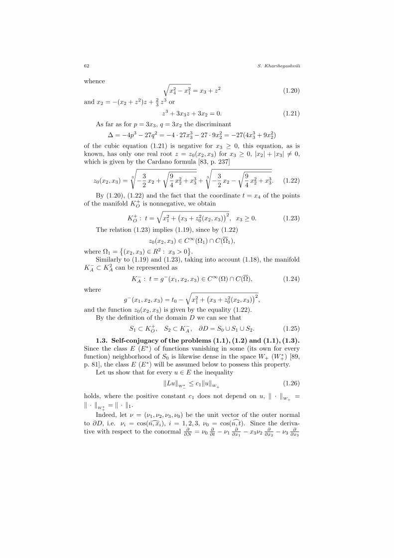
62 S. Kharibegashvili
whence √x2
4 − x21 = x3 + z2 (1.20)
and x2 = −(x2 + z2)z + 23 z
3 or
z3 + 3x3z + 3x2 = 0. (1.21)
As far as for p = 3x3, q = 3x2 the discriminant
∆ = −4p3 − 27q2 = −4 · 27x33 − 27 · 9x2
2 = −27(4x33 + 9x2
2)
of the cubic equation (1.21) is negative for x3 ≥ 0, this equation, as isknown, has only one real root z = z0(x2, x3) for x3 ≥ 0, |x2| + |x3| 6= 0,which is given by the Cardano formula [83, p. 237]
z0(x2, x3) =3
√
−3
2x2 +
√9
4x2
2 + x33 +
3
√
−3
2x2 −
√9
4x2
2 + x33. (1.22)
By (1.20), (1.22) and the fact that the coordinate t = x4 of the pointsof the manifold K+
O is nonnegative, we obtain
K+O : t =
√x2
1 +(x3 + z2
0(x2, x3))2, x3 ≥ 0. (1.23)
The relation (1.23) implies (1.19), since by (1.22)
z0(x2, x3) ∈ C∞(Ω1) ∩ C(Ω1),
where Ω1 =(x2, x3) ∈ R2 : x3 > 0
.
Similarly to (1.19) and (1.23), taking into account (1.18), the manifoldK−A ⊂ K2
A can be represented as
K−A : t = g−(x1, x2, x3) ∈ C∞(Ω) ∩ C(Ω), (1.24)
where
g−(x1, x2, x3) = t0 −√x2
1 +(x3 + z2
0(x2, x3))2,
and the function z0(x2, x3) is given by the equality (1.22).By the definition of the domain D we can see that
S1 ⊂ K+O , S2 ⊂ K−
A , ∂D = S0 ∪ S1 ∪ S2. (1.25)
1.3. Self-conjugacy of the problems (1.1), (1.2) and (1.1), (1.3).Since the class E (E∗) of functions vanishing in some (its own for everyfunction) neighborhood of S0 is likewise dense in the space W+ (W ∗
+) [89,p. 81], the class E (E∗) will be assumed below to possess this property.
Let us show that for every u ∈ E the inequality
‖Lu‖W∗−≤ c1‖u‖W+
(1.26)
holds, where the positive constant c1 does not depend on u, ‖ · ‖W+
=
‖ · ‖W∗
+= ‖ · ‖1.
Indeed, let ν = (ν1, ν2, ν3, ν0) be the unit vector of the outer normal
to ∂D, i.e. νi = cos(n, xi), i = 1, 2, 3, ν0 = cos(n, t). Since the deriva-tive with respect to the conormal ∂
∂N = ν0∂∂t − ν1
∂∂x1
− x3ν2∂∂x2
− ν3∂∂x3

Some Multidimensional Problems 63
corresponding to the operator L is an interior differential operator on thecharacteristic hypersurfaces of the equation (1.1), by (1.12) for the functionu ∈ E we have
∂u
∂N
∣∣∣S1
= 0. (1.27)
By definition of the negative norm, the equalities (1.2), (1.27) for u ∈ Eand the equality (1.3) for v ∈ E∗ ⊂W ∗
+, we have
‖Lu‖W∗ = sup
v∈W∗+
‖v‖−1W∗
+
(Lu, v)L2(D)
= supv∈E∗
‖v‖−1W∗
+
(Lu, v)L2(D)
=
= supv∈E∗
‖v‖−1W∗
+
∫
S0∪S1∪S2
∂u
∂Nv ds+
+ supv∈E∗
‖v‖−1W∗
+
∫
D
[− utvt + ux1vx1 + x3ux2vx2 + ux3vx3
]dD =
= supv∈E∗
‖v‖−1W∗
+
∫
D
[− utvt + ux1vx1 + x3ux2vx2 + ux3vx3
]dD. (1.28)
Using the Cauchy and Schwartz inequalities, from (1.28) we have
‖Lu‖W∗ ≤
≤ supv∈E∗
‖v‖−1W∗
+
∫
D
[(u2t+u
2x1
+x3u2x2
+u2x3
)1/2(v2t +v
2x1
+x3v2x2
+v2x3
)1/2]dD≤
≤ supv∈E∗
‖v‖−1W∗
+
[ ∫
D
(u2t + u2
x1+ x3u
2x2
+ u2x3
)dD
]1/2
×
×[∫
D
(v2t + v2
x1+x3v
2x2
+ v2x3
)dD
]1/2
≤ supv∈E∗
‖v‖−1W∗
+
‖u‖W+‖v‖
W∗+
=‖u‖W+,
which proves the inequality (1.26).Analogously it can be proved that for every v ∈ E∗ the inequality
‖L∗v‖W−
≤ c2‖v‖W∗−
(1.29)
is valid with a positive constant c2 independent of v.
Remark 1.2. By (1.26) ((1.29)), the operator L : W+ → W ∗− (L∗ = L :
W ∗+ →W−) with the dense domain of definition E (E∗) admits the closure
which in fact is a continuous operator from the space W+ (W ∗+) to the space
W ∗− (W−). Leaving for that closure the same notation L (L∗ = L), we can
say that it is defined on the whole Hilbert space W+ (W ∗+).
Let us now show that the problems (1.1), (1.2) and (1.1), (1.3) are self-conjugate, i.e. the inequality
(Lu, v) = (u, Lv) ∀u ∈ W+, ∀ v ∈ W ∗+ (1.30)
holds.

64 S. Kharibegashvili
Indeed, by Remark 1.2 it suffices to prove the equality (1.30) whenu ∈ E and v ∈ E∗. We have
(Lu, v) = (Lu, v)L2(D)
=
∫
∂D
[v∂u
∂N− u
∂v
∂N
]ds+ (u, Lv)
L2(D). (1.31)
Since the equality (1.3) is valid for v ∈ E∗, analogously to (1.27) wehave
∂v
∂N
∣∣∣S2
= 0. (1.32)
From (1.31), owing to (1.2), (1.37) as well as (1.3), (1.32) for v, imme-diately follows (1.30).
1.4. A priori estimates. The existence and uniqueness theo-rem. We have the following
Lemma 1.1. For any function u ∈W+ the estimate
c‖u‖L2(D)
≤ ‖Lu‖W∗−
(1.33)
is valid with a positive constant c independent of u.
Proof. By Remark 1.2, it suffices to prove the estimate (1.33) for u ∈ E. Inthis case, since the function u vanishes in some neighborhood S0 ⊂ ∂D, asit can be easily verified the function
v(x, t) =
g−(x)∫
t
e−λτu(x, τ) dτ, λ = const > 0, x = (x1, x2, x3),
where t = g−(x) represents by virtue of (1.24), (1.25) the equation of thecharacteristic hypersurface S2, belongs to the space E∗, and the equalities
vt(x, t) = −e−λtu(x, t), ut(x, t) = −eλtvt(x, t) (1.34)
are valid.By (1.2), (1.3), (1.27), (1.32) and (1.34) we have
(Lu, v)L2(D)
=
=
∫
∂D
v∂u
∂Nds+
∫
D
[− utvt + ux1vx1 + x3ux2vx2 + ux3vx3
]dD =
=
∫
D
[− utvt + ux1vx1 + x3ux2vx2 + ux3vx3
]dD =
=
∫
D
e−λtutu dD +
∫
D
e−λt[− ux1tvx1 − x3vx2tvx2 − vx3tvx3
]dD, (1.35)
∫
D
e−λtutu dD =1
2
∫
∂D
e−λtu2ν0 ds+1
2
∫
D
e−λtλu2 dD =

Some Multidimensional Problems 65
=1
2
∫
S2
e−λtu2ν0 ds+1
2
∫
D
eλtλv2t dD=
1
2
∫
S2
eλtv2t ν0 ds+
1
2
∫
D
eλtλv2t dD, (1.36)
∫
D
eλt[− vx1tvx1 − x3vx2tvx2 − vx3tvx3
]dD =
=−1
2
∫
∂D
eλt[v2x1
+x3v2x2
+v2x3
]ν0 ds+
1
2
∫
D
eλtλ[v2x1
+x3v2x2
+v2x3
]dD. (1.37)
As far as v|S2 = 0, the gradient ∇v = (vx1 , vx2 , vx3 , vt) is proportionalto the vector of the outer normal ν on S2, i.e. for some α we have vx1 = αν1,vx2 = αν2, vx3 = αν3, vt = αν0 on S2. Thus taking into account that S2 isa characteristic surface, we get
(v2t − v2
x1− x3v
2x2− v2
x3
)∣∣∣S2
= α2(ν20 − ν2
1 − x3ν22 − ν2
3
)∣∣∣S2
= 0. (1.38)
It is easy to see that
ν0∣∣S0
= 0, ν0∣∣S1\0 < 0, ν0
∣∣S2\0 > 0. (1.39)
By virtue of (1.3),(1.38), (1.39) we arrive at
1
2
∫
S2
eλtv2t ν0 ds−
1
2
∫
D
eλt[v2x1
+ x3v2x2
+ v2x3
]ν0 ds =
=1
2
∫
S2
eλtv2t ν0 ds−
1
2
∫
S1
eλt[v2x1
+ x3v2x2
+ v2x3
]ν0 ds−
−1
2
∫
S2
eλt[v2x1
+ x3v2x2
+ v2x3
]ν0 ds ≥
≥ 1
2
∫
S2
eλtv2t ν0 ds−
1
2
∫
S2
eλt[v2x1
+ x3v2x2
+ v2x3
]ν0 ds =
=1
2
∫
S2
eλt[v2t − v2
x1− x3v
2x2− v2
x3
]ν0 ds = 0. (1.40)
Taking now into account (1.34), (1.36), (1.37) and (1.40), from (1.35)for the fixed λ > 0 we obtain
(Lu, v)L2(D)
=1
2
∫
S2
eλtv2t ν0 ds+
1
2
∫
D
eλtλv2t dD−
−1
2
∫
∂D
eλt[v2x1
+ x3v2x2
+ v2x3
]ν0 ds+
1
2
∫
D
eλtλ[v2x1
+ x3v2x2
+ v2x3
]dD ≥
≥ λ
2
∫
D
eλt[v2t + v2
x1+ x3v
2x2
+ v2x3
]dD ≥

66 S. Kharibegashvili
≥ λ
2
[ ∫
D
eλtv2t dD
]1/2[ ∫
D
eλt(v2t + v2
x1+ x3v
2x2
+ v2x3
)dD
]1/2
=
=λ
2
[ ∫
D
e−λtu2 dD]1/2
[ ∫
D
eλt(v2t + v2
x1+ x3v
2x2
+ v2x3
)dD
]1/2
≥
=λ
2e−
12 λt0
[ ∫
D
u2 dD]1/2
[∫
D
(v2t + v2
x1+ x3v
2x2
+ v2x3
)dD
]1/2
(1.41)
because t|D ≥ 0 and e−12 λt0 =
(infDe−λt
)1/2> 0.
Since v|S2 = 0 (u|S1 = 0), standard reasoning allows one to prove thatthe inequalities
∫
D
v2 dD ≤ c0
∫
D
v2t dD
( ∫
D
u2 dD ≤ c0
∫
D
u2t dD
)
are valid for some c0 = const > 0 independent of v ∈ E∗ (u ∈ E). Thisimplies that in the space W+ (W ∗
+) the norm
‖v‖2W+ (W∗
+)=
∫
D
(v2 + v2
x1+ x3v
2x2
+ v2x3
+ v2t
)dD
is equivalent to the norm
‖v‖2 =
∫
D
(v2t + v2
x1+ x3v
2x2
+ v2x3
)dD. (1.42)
Therefore leaving for the norm (1.42) the same notation ‖v‖W+ (W∗
+),
from (1.41) we obtain
(Lu, v)L2(D)
≥ µ‖u‖L2(D)
‖v‖W∗
+, (1.43)
where µ = λ2 e
− 12 λt0 > 0. Thus we can easily verify that sup
λ>0µ(λ) = µ
(2t0
)=
(e t0)−1.
Applying the generalized Schwartz inequality
(Lu, v) ≤ ‖Lu‖W∗−‖v‖
W∗+
to the left-hand side of (1.43), after reduction by ‖v‖W∗
+we obtain the ine-
quality (1.33) with c = µ > 0. Thus the lemma is proved.
Lemma 1.2. For every function v ∈W ∗+ the estimate
c‖v‖L2(D)
≤ ‖Lv‖W−
(1.44)
is valid with a positive constant c independent of v.

Some Multidimensional Problems 67
Proof. Just as in the case of Lemma 1.1, by Remark 1.2 it is sufficientto prove that the inequality (1.44) is valid for v ∈ E∗. Let v ∈ E∗. Weintroduce into consideration the function
u(x, t) =
t∫
g+(x)
eλτv(x, τ) dτ, λ = const > 0,
where t = g+(x) is by virtue of (1.19), (1.25) the equation of the character-istic hypersurface S1. The function u(x, t) belongs to the space E, and theequality
ut(x, t) = eλtv(x, t), v(x, t) = e−λtut(x, t) (1.45)
holds.By virtue of (1.2), (1.3), (1.27), (1.32) and (1.45), analogously to (1.35)–
(1.40) we have
(Lv, u)L2(D)
= −∫
D
eλtvtv dD+
+
∫
D
e−λt[ux1tux1 + x3ux2tux2 + ux3tux3
]dD, (1.46)
−∫
D
eλtvtv dD = −1
2
∫
D
eλtv2ν0 ds+1
2
∫
D
eλtλv2 dD =
= −1
2
∫
S1
eλtv2ν0 ds+1
2
∫
D
e−λtλu2t dD =
= −1
2
∫
S1
e−λtu2tν0 ds+
1
2
∫
D
e−λtλu2t dD, (1.47)
∫
D
e−λt[ux1tux1 + x3ux2tux2 + ux3tux3
]dD =
=1
2
∫
∂D
e−λt[u2x1
+x3u2x2
+u2x3
]ν0 ds+
1
2
∫
D
e−λtλ[u2x1
+x3u2x2
+u2x3
]dD, (1.48)
(u2t − u2
x1− x3u
2x2− u2
x3
)∣∣∣S1
= 0, (1.49)
−1
2
∫
S1
e−λtu2tν0 ds+
1
2
∫
∂D
e−λt[u2x1
+ x3u2x2
+ u2x3
]ν0 ds =
= −1
2
∫
S1
e−λtu2tν0 ds+
1
2
∫
S1
e−λt[u2x1
+ x3u2x2
+ u2x3
]ν0 ds+
+1
2
∫
S2
e−λt[u2x1
+ x3u2x2
+ u2x3
]ν0 ds ≥

68 S. Kharibegashvili
≥ −1
2
∫
S1
e−λt[u2t − u2
x1− x3u
2x2− u2
x3
]ν0 ds = 0. (1.50)
By (1.45) and (1.47)–(1.50), from (1.46) it follows that
(Lv, u)L2(D)
≥ λ
2
∫
D
e−λt[u2t + u2
x1+ x3u
2x2t + u2
x3
]dD ≥
≥ λ
2
[ ∫
D
e−λtu2t dD
]1/2[ ∫
D
e−λt(u2t + u2
x1+ x3u
2x2
+ u2x3
)dD
]1/2
=
=λ
2
[ ∫
D
eλtv2 dD]1/2
[ ∫
D
e−λt(u2t + u2
x1+ x3u
2x2
+ u2x3
)dD
]1/2
≥
≥ λ
2e−
12 λt0
[ ∫
D
v2 dD]1/2
[∫
D
(u2t + u2
x1+ x3u
2x2
+ u2x3
)dD
]1/2
,
whence just in the same way as in obtaining the inequality (1.33) from(1.44) in Lemma 1.1, we arrive at the inequality (1.44). Thus the lemma isproved.
Due to the results of [86, pp. 184–186], the consequence of the inequa-lities (1.26) and (1.29), the equality (1.30) and Lemmas 1.1 and 1.2 is thefollowing
Theorem 1.1. For every F ∈ L2(D) (W ∗−) there exists a unique strong
generalized solution u of the problem (1.1), (1.2) of the class W+ (L2) for
which the estimate
‖u‖L2(D)
≤ c0‖F‖W∗−
is valid with a positive constant c0 independent of F .
2. The Characteristic Cauchy problem for Some DegeneratingSecond Order Hyperbolic Equations in Cone-Shaped Domains
2.1. The case of equation with noncharacteristic degeneration.In the space of variables x1, x2, t we consider a degenerating second orderhyperbolic equation of the type
Lu ≡ utt − tm(ux1x1 + ux2x2) + a1ux1 + a2ux2 + a3ut + a4u = F, (2.1)
where ai, i = 1, . . . , 4, F are given and u is an unknown real function,m = const > 0.
By
D : 0 < t <[1− 2 +m
2r] 2
2+m
, r = (x21 + x2
2)1/2 <
2
2 +m

Some Multidimensional Problems 69
we denote the bounded domain lying in a half-space t > 0, bounded aboveby the characteristic conoid
S : t =[1− 2 +m
2r] 2
2+m
, r ≤ 2
2 +m
of the equation (2.1) with vertex at the point (0, 0, 1) and below by the basis
S0 : t = 0, r ≤ 2
2 +m
of the conoid on which the equation (2.1) has a noncharacteristic degenera-tion. Below in the domain D the coefficients ai, i = 1, . . . , 4, of the equation(2.1) will be assumed to be functions of the class C2(D).
For the equation (2.1) we consider the characteristic problem which isformulated as follows: in the domain D, find a solution u(x1, x2, t) of theequation (2.1) satisfying the boundary condition
u∣∣S
= 0. (2.2)
As it will be shown, the Cauchy problem on finding a solution of theequation
L∗v ≡ vtt− tm(vx1x1 + vx2x2)− (a1v)x1 − (a2v)x2 − (a3v)t +a4v = F (2.3)
in the domain D by the boundary conditions
v∣∣S0
= 0, vt∣∣S0
= 0 (2.4)
is the problem conjugate to the problem (2.1), (2.2), where L∗ is the operatorformally conjugate to L.
Here by E and E∗ we denote the classes of functions from the Sobolevspace W 2
2 (D) which satisfy respectively the boundary condition (2.2) or(2.4) and vanish in some (its own for every function) three-dimensionalneighborhood of the circumference Γ = S ∩ S0 : r = 2
2+m , t = 0 and of thesegment I : x1 = x2 = 0, 0 ≤ t ≤ 1.
Let W+ (W ∗+) be the Hilbert space with weight obtained by closing the
space E (E∗) by the norm
‖u‖21 =
∫
D
[u2t + tm(u2
x1+ u2
x2) + u2
]dD.
Denote by W− (W ∗−) the space with the negative norm constructed with
respect to L2(D) and W+ (W ∗+) [6].
Let ν = (ν1, ν2, ν3) be the unit vector of the outer normal to ∂D, i.e.
ν1 = cos(ν, x1), ν2 = cos(ν, x2), ν0 = cos(ν, t). By definition, the derivativewith respect to the conormal on the boundary ∂D of D for the operator Lis calculated by the formula
∂
∂N= ν0
∂
∂t− tmν1
∂
∂x1− tmν2
∂
∂x2.

70 S. Kharibegashvili
Remark 2.1. Since the derivative with respect to the conormal ∂∂N for
the operator L is an inner differential operator on the characteristic surfacesof the equation (2.1), by virtue of (2.2) and (2.4) for the functions u ∈ Eand v ∈ E∗ we have
∂u
∂N
∣∣∣S
= 0,∂v
∂N
∣∣∣S0
= 0. (2.5)
In the equation (2.1) we impose on the coefficients a1 and a2 the fol-lowing restrictions:
Mi = supD
∣∣t−m2 ai(x1, x2, t)
∣∣ < +∞, i = 1, 2. (2.6)
Lemma 2.1. For all functions u ∈ E, v ∈ E∗ the inequalities
‖Lu‖W∗−≤ c1‖u‖W+
, (2.7)
‖L∗v‖W−
≤ c2‖v‖W∗+
(2.8)
hold, where the positive constants c1 and c2 do not depend respectively on uand v, ‖ · ‖
W+= ‖ · ‖
W∗+
= ‖ · ‖1.
Proof. By definition of negative norm, for u ∈ E, by virtue of the equalities(2.2), (2.4) and (2.5), using the integration by parts we obtain
‖Lu‖W∗−
= supv∈W∗
+
‖v‖−1W∗
+
(Lu, v)L2(D)
= supv∈E∗
‖v‖−1W∗
+
(Lu, v)L2(D)
=
= supv∈E∗
‖v‖−1W∗
+
∫
D
[− utvt + tm(ux1vx1 + ux2vx2)+
+ a1ux1v + a2ux2v + a3utv + a4uv]dD. (2.9)
From (2.6) and the Cauchy and Schwartz inequalities it follows that∣∣∣∣∫
D
[− utvt + tm(ux1vx1 + ux2vx2)
]dD
∣∣∣∣ ≤ ‖u‖W+‖v‖
W∗+, (2.10)
∣∣∣∣∫
D
[a1ux1v + a2ux2v + a3utv + a4uv
]dD
∣∣∣∣ ≤ c‖u‖W+‖v‖
W∗+, (2.11)
where c =2∑
=1
(Mi + sup
D
|a2+i|), and from (2.9)–(2.11) it follows
‖Lu‖W∗−≤ (1 + c) sup
v∈E∗‖v‖−1
W∗+
‖u‖W+‖v‖
W∗+
= (1 + c)‖u‖W+,
i.e. we have obtained the inequality (2.7) for c1 = 1 + c. Since the proof ofthe inequality (2.8) repeats word for word that of the inequality (2.7), wecan conclude that Lemma 2.1 is proved completely.
Remark 2.2. By the inequality (2.7) ((2.8)), the operator L : W+ →W ∗−
(L∗ : W ∗+ → W−) with the dense domain of definition E (E∗) admits a

Some Multidimensional Problems 71
closure which itself is a continuous operator from the space W+ (W ∗+) to
the space W ∗− (W−). Leaving for that closure the same notation L (L∗), we
can say that it is defined on the entire Hilbert space W+ (W ∗+).
Lemma 2.2. The problems (2.1), (2.2) and (2.3), (2.4) are self-conju-
gate, i.e. for every u ∈W+ and v ∈W ∗+ the equality
(Lu, v) = (u, L∗v) (2.12)
holds.
Proof. By Remark 2.2 it is sufficient to prove the equality (2.12) in thecase where u ∈ E and v ∈ E∗. In this case it is evident that (Lu, v) =(Lu, v)
L2(D). Therefore the integration by parts yields
(Lu, v) =
=
∫
∂D
[(v∂u
∂N−u ∂v
∂N
)+(a1ν1+a2ν2+a3ν0)uv
]ds+(u, L∗v)
L2(D). (2.13)
From the equalities (2.2), (2.4), (2.5) and (2.13) immediately follows(2.12).
Consider the following conditions:
Ω∣∣S≤ 0,
[tΩt − (λt+m)Ω
]∣∣∣D≥ 0, (2.14)
where the second inequality holds if λ is sufficiently large, and Ω = a1x1 +a2x2 + a3t − a4.
Remark 2.3. It is easy to see that the inequalities (2.14) are a conse-quence of the condition
Ω|D ≤ const < 0.
Lemma 2.3. Let the conditions (2.6) and (2.14) be fulfilled. Then for
every u ∈W+ the inequality
c∥∥t 1
2 (m−1)u∥∥L2(D)
≤ ‖Lu‖W∗−
(2.15)
is valid with a positive constant c independent of u.
Proof. By Remark 2.2, it suffices to prove the inequality (2.15) for u ∈ E.If u ∈ E, then for α = const > 0 and λ = const > 0 the function
v(x1, x2, t) =
t∫
0
eλτ ταu(x1, x2, τ) dτ (2.16)
belongs to the space E∗. We can easily verify that for α ≥ 1 the function vbelongs to E∗, and for 0 < α < 1 this statement follows from the well-known

72 S. Kharibegashvili
Hardy’s inequality [118, p. 405]
1∫
0
t−2g2(t) dt ≤ 4
1∫
0
f2(t) dt,
where f ∈ L2(0, 1) and g(t) =t∫0
f(τ) dτ .
By virtue of (2.16), the equalities
vt(x1, x2, t) = eλttαu(x1, x2, t), u(x1, x2, t) = e−λtt−αvt(x1, x2, t) (2.17)
are valid.Taking into account (2.2), (2.4), (2.5) and (2.17), we have
(Lu, v)L2(D)
=
∫
∂D
[v∂u
∂N+ (a1ν1 + a2ν2 + a3ν0)uv
]ds+
+
∫
D
[−utvt+tmux1vx1+t
mux2vx2−u(a1v)x1−u(a2v)x2−u(a3v)t+a4uv]dD=
= −∫
D
eλttαuut dD +
∫
D
e−λtt−α[tm(vx1tvx1 + vx2tvx2)−
−(a1vx1 + a2vx2)vt − (a1x1t + a2x2 + a3t − a4)vtv − a3v2t
]dD, (2.18)
and by (2.2) we find that
−∫
D
eλttαuut dD = −1
2
∫
D
eλttα(u2)t dD = −1
2
∫
∂D
eλttαu2ν0 ds+
+1
2
∫
D
eλt(αtα−1 + λtα)u2 dD =1
2
∫
D
eλt(αtα−1 + λtα)u2 dD =
=α
2
∫
D
eλttα−1u2 dD +1
2
∫
D
λe−λtt−αv2t dD, (2.19)
∫
D
e−λttm−α(vx1tvx1 +vx2tvx2) dD=1
2
∫
∂D
e−λttm−α(v2x1
+ v2x2
)ν0 ds+
+1
2
∫
D
e−λt[λtm−α + (α−m)tm−α−1
](v2x1
+ v2x2
) dD ≥
≥ 1
2
∫
D
e−λt[λtm−α + (α −m)tm−α−1
](v2x1
+ v2x2
) dD. (2.20)
In deducing the inequality (2.20) we took into account that
ν0∣∣S≥ 0, (v2
x1+ v2
x2)∣∣S0
= 0.

Some Multidimensional Problems 73
From (2.19) we have
−∫
D
eλttαuut dD ≥ α
2
∥∥t 12 (α−1)u
∥∥2
L2(D)+
1
2
∫
D
λe−λtt−αv2t dD. (2.21)
Below it will be assumed that α = m.By (2.6) we have
∣∣∣∣∫
D
e−λtt−m(a1vx1 + a2vx2)vt dD
∣∣∣∣ ≤
≤M
∫
D
e−λtt−m[v2t +
1
2tm(v2
x1+ v2
x2)]dD ≤
≤M
∫
D
e−λtt−mv2t dD +
M
2
∫
D
e−λt(v2x1
+ v2x2
) dD, (2.22)
where M = max(M1,M2).Since ν0|S ≥ 0, taking into account the conditions (2.4) and (2.14) and
integrating by parts, we obtain
−∫
D
e−λtt−m(a1x1 + a2x2 + a3t − a4)vtv dD =
= −1
2
∫
D
e−λtt−mΩ(v2)t dD = −1
2
∫
∂D
e−λtt−mΩv2ν0 ds+
+1
2
∫
D
e−λtt−m−1[tΩt − (λt+m)Ω
]v2 dD ≥ 0. (2.23)
In deducing the inequality (2.23) we used the fact that the function t−mv2
has the zero trace on S0, i.e. t−mv2|S0 = 0.From (2.18) and (2.20)–(2.23) we have
(Lu, v)L2(D)
≥ m
2‖t 1
2 (m−1)u‖2L2(D)
+1
2
∫
D
λe−λtt−mv2t dD+
+1
2
∫
D
λe−λt(v2x1
+ v2x2
) dD −M
∫
D
e−λtt−mv2t dD−
−M2
∫
D
e−λt(v2x1
+ v2x2
) dD − supD
|a3|∫
D
e−λtt−mv2t dD =
=m
2‖t 1
2 (m−1)u‖2L2(D)
+(λ
2−M − sup
D
|a3|)∫
D
e−λtt−mv2t dD+
+1
2(λ−M)
∫
D
e−λt(v2x1
+ v2x2
) dD ≥

74 S. Kharibegashvili
≥ m
2‖t 1
2 (m−1)u‖2L2(D)
+ σ
∫
D
e−λt(v2t + v2
x1+ v2
x2) dD ≥
≥√
2mσ infDe−λt ‖t 1
2 (m−1)u‖L2(D)
( ∫
D
[v2t +t
m(v2x1
+v2x2
)]dD
)1/2
, (2.24)
where σ =[λ2 −M − sup
D
|a3|]> 0 for sufficiently large λ, and inf
De−λt =
e−λ > 0. In deducing the inequality (2.24) we took into account thatt−m|D ≥ 1.
If u ∈ W+ (W ∗+), then due to the fact that u|S = 0 (u|S0 = 0) it is not
difficult to prove the inequality∫
D
u2 dD ≤ c0
∫
D
u2t dD
for some c0 = const > 0 independent of u. This implies that in the spaceW+ (W ∗
+) the norm
‖u‖2W+ (W∗
+)=
∫
D
[u2t + tm(u2
x1+ u2
x2) + u2
]dD
is equivalent to the norm
‖u‖2 =
∫
D
[u2t + tm(u2
x1+ u2
x2)]dD. (2.25)
Therefore leaving for the latter the same notation ‖u‖W+ (W∗
+), from (2.24)
we obtain
(Lu, v)L2(D)
≥√
2mσe−λ ‖t 12 (m−1)u‖
L2(D)‖v‖
W∗+. (2.26)
Applying now the generalized Schwartz inequality
(Lu, v) ≤ ‖Lu‖W∗−‖v‖
W∗+
to the left-hand side of (2.26), after reduction by ‖v‖W∗
+we obtain the
inequality (2.15) with c =√
2mσe−λ. Thus the proof of Lemma 2.3 iscomplete.
Consider the conditions
a4
∣∣S0≥ 0, (λa4 + a4t)
∣∣D≥ 0, (2.27)
where the second inequality holds for sufficiently large λ.
Lemma 2.4. Let the conditions (2.6) and (2.27) be fulfilled. Then for
every v ∈ W ∗+ the inequality
c‖v‖L2(D)
≤ ‖L∗v‖W−
(2.28)
is valid for some c = const > 0 independent of v ∈ W ∗+.

Some Multidimensional Problems 75
Proof. Just as in the case of Lemma 2.3, by Remark 2.2 it is sufficientto prove that the inequality (2.28) is valid for v ∈ E∗. Let v ∈ E∗, andintroduce into consideration the function
u(x1, x2, t) =
ϕ(x1,x2)∫
t
e−λτv(x1, x2, τ) dτ, λ = const > 0, (2.29)
where t = ϕ(x1, x2) is the equation of the characteristic conoid S. Althoughthe function
ϕ(x1, x2) =[1− 2 +m
2r] 2
2+m
has singularities on the circumference r= 22+m and at the origin x1 =x2 = 0,
since by the definition of the space E∗ the function v vanishes in someneighborhood of the circumference Γ = S ∩ S0 and the segment I : x1 =x2 = 0, 0 ≤ t ≤ 1, the function u defined by the equality (2.29) belongs tothe space E. In addition, it is obvious that the equalities
ut(x1, x2, t) = −e−λtv(x1, x2, t), v(x1, x2, t) = −e−λtut(x1, x2, t) (2.30)
hold.By (2.6), (2.27), (2.29) and (2.30), the same reasoning as in proving the
estimate (2.28) allows us to prove the estimate (2.15) in Lemma 2.3.
Denote by L2,α(D) the space of functions u such that tαu ∈ L2(D).Assume
‖u‖L2,α(D)
= ‖tαu‖L2(D)
, αm =1
2(m− 1).
Definition 2.1. If F ∈ L2(D) (W ∗−), then the function u is said to
be a strong generalized solution of the problem (2.1), (2.2) of the class W+
(L2,αm) if u ∈ W+ (L2,αm(D)) and there exists a sequence of functionsun ∈ E such that un → u in the space W+ (L2,αm(D)) and Lun → F inthe space W ∗
− (W ∗−).
By the results of [86, p. 184–186], a consequence of Lemmas 2.1–2.4 isthe following
Theorem 2.1. Let the conditions (2.6), (2.14) and (2.27) be fulfilled.
Then for every F ∈ L2(D) (W ∗−) there exists a unique strong generalized
solution u of the problem (2.1), (2.2) of the class W+ (L2,αm) for which the
estimate
‖u‖L2,αm(D)
≤ c‖F‖W∗−
is valid with a positive constant c independent of F .
2.2. The case of equation with characteristic degeneration.Consider a hyperbolic second order equation with characteristic degener-ation of the type
L1u ≡ (tmut)t − ux1x1 − ux2x2 + a1ux1 + a2ux2 + a3ut + a4u = F, (2.31)
where 1 ≤ m = const < 2.

76 S. Kharibegashvili
Denote by
D1 : 0 < t <[1− 2−m
2r] 2
2−m
, r = (x21 + x2
2)1/2 <
2
2−m
a finite domain lying in the half-space t > 0 which is bounded above by thecharacteristic conoid
S2 : t =[1− 2−m
2r] 2
2−m
, r ≤ 2
2−m
of the equation (2.31) with the vertex at the point (0, 0, 1) and below bythe basis
S1 : t = 0, r ≤ 2
2−m
of that conoid on which the equation (2.31) has a characteristic degenera-tion. Just as in the case of the equation (2.1), we assume that in the domainD1 the coefficients ai, i = 1, . . . , 4, of the equation (2.31) are functions ofthe class C2(D).
For the equation (2.31) we consider a characteristic problem which isformulated as follows: in the domain D1, find a solution u(x1, x2, t) of theequation (2.31) satisfying the boundary condition
u∣∣S1
= 0 (2.32)
on the plane characteristic surface S1.Analogously we formulate a characteristic problem for the equation
L∗1v ≡ (tmvt)t−vx1x1−vx2x2− (a1v)x1− (a2v)x2− (a3v)t+a4v = F (2.33)
in the domain D1 by means of the boundary condition
v∣∣S2
= 0, (2.34)
where L∗1 is the operator formally conjugate to the operator L1.By E1 and E∗1 we denote the classes of functions from the Sobolev
space W 22 (D1) which satisfy respectively the boundary condition (2.32) or
(2.34) and vanish in some (its own for every function) three-dimensionalneighborhood of the segment I : x1 = 0, x2 = 0, 0 ≤ t ≤ 1. Let W1+
(W ∗1+) be the Hilbert space obtained by closing the space E1 (E∗1 ) by the
norm
‖u‖2 =
∫
D1
[u2t + u2
x1+ u2
x2+ u2
]dD1.
Denote by W1− (W ∗1−) the space with the negative norm which is con-
structed with respect to L2(D1) and W1+ (W ∗1+).
Analogously to Lemmas 2.1 and 2.2 we prove
Lemma 2.5. For all functions u ∈ E1, v ∈ E∗1 the inequalities
‖L1‖W∗1−≤ c1‖u‖W1+
, ‖L∗1v‖W1−≤ c2‖u‖W∗
1+

Some Multidimensional Problems 77
hold, and the problems (2.31), (2.32), and (2.33), (2.34) are self-conjugate,
i.e. for every u ∈ W1+ and v ∈ W ∗1+ the equality
(L1u, v) = (u, L∗1v)
holds.
Consider the conditions
infD1
(a4 − a1x1 − a2x2 − a3t) > 0, (2.35)
infS1
a3 >1
2for m = 1, inf
S1
a3 > 0 for m > 1. (2.36)
Lemma 2.6. Let the conditions (2.35) and (2.36) be fulfilled. Then for
every u ∈W1+ the inequality
c‖u‖L2(D1)
≤ ‖L1u‖W∗1−
is valid with a positive constant c independent of u.
Consider now the conditions
infD1
a4 > 0, (2.37)
infS1
a3 > −1
2for m = 1, inf
S1
a3 > 0 for m > 1. (2.38)
Note the the condition (2.38) follows from (2.36).
Lemma 2.7. Let the conditions (2.37) and (2.38) be fulfilled. Then for
every v ∈ W ∗1+ the inequality
c‖u‖L2(D1)
≤ ‖L∗1v‖W1−
is valid with a positive constant c independent of v.
From Lemmas 2.5–2.7, the proof of which to a certain extent repeatsthat of Lemmas 2.1–2.4, we have the following [68]
Theorem 2.2. Let the conditions (2.35), (2.36), (2.37) be fulfilled.
Then for every F ∈ L2(D1) (W ∗1−) there exists a unique strong generalized
solution u of the problem (2.31), (2.32) of the class W1+ (L2) for which the
estimate
‖u‖L2(D1)
≤ c‖F‖W∗
1−
is valid with a positive constant c independent of F .
Theorem 2.3. Let the conditions (2.35), (2.36), (2.37) be fulfilled.
Then for every F ∈ L2(D1) (W1−) there exists a unique strong generalized
solution v of the problem (2.33), (2.34) of the class W ∗1+ (L2) for which the
estimate
‖v‖L2(D1)
≤ c‖F‖W1−
is valid with a positive constant c independent of F .

78 S. Kharibegashvili
Here, just as in Definition 2.1, for F ∈ L2(D1) (W ∗1−) the function u is
said to be a strong generalized solution of the problem (2.31), (2.32) of theclassW1+ (L2) if u ∈W1+ (L2(D1)) and there exists a sequence of functionsun ∈ E1 such that un → u in the space W1+ (L2(D1)) and L1un → F inthe space W ∗
1− (W ∗1−). For F ∈ L2(D) (W1−), the function v is called a
strong generalized solution of the problem (2.33), (2.34) of the class W ∗1+
(L2) if v ∈W ∗1+ (L2(D1)) and there exists a sequence of functions vn ∈ E∗1
such that vn → v in the space W ∗1+ (L2(D1)) and L∗1vn → F in the space
W1− (W1−).
3. Multi-Dimensional Versions of the First Darboux Problem forSome Degenerating Second Order Hyperbolic Equations in
Dihedral Domains
3.1. The case of equation with noncharacteristic degeneration.Consider a degenerating second order hyperbolic equation of the type
L1u ≡ utt − |x2|mux1x1 − ux2x2 + a1ux1 + a2ux2 + a3ut + a4u = F, (3.1)
where m = const > 0.By D : x2 < t < 1 − x2, 0 < x2 < 1/2 we denote the unbounded
domain lying in the half-plane x2 > 0 and bounded by the characteristicsurfaces S1 : t− x2 = 0, 0 ≤ x2 ≤ 1/2, S2 : t+ x2 − 1 = 0, 0 ≤ x2 ≤ 1/2of the equation (3.1) and by the plane surface S0 : x2 = 0, 0 ≤ t ≤ 1 oftemporal type on which the above equation degenerates. We assume thatin the domain D the coefficients ai, i = 1, . . . , 4, of the equation (3.1) arebounded functions of the class C1(D).
For the equation (3.1), we consider a multidimensional version of thefirst Darboux problem which is formulated as follows: in the domain D, finda solution u(x1, x2, t) of the equation (3.1) satisfying the boundary condition
u∣∣S0∩S1
= 0. (3.2)
Analogously we formulate the problem for the equation
L∗v ≡ vtt−|x2|mvx1x1−vx2x2− (a1v)x1 − (a2v)x2 − (a3v)t+a4v = F (3.3)
in the domain D by the boundary condition
v∣∣S0∩S2
= 0, (3.4)
where L∗ is the operator formally conjugate to the operator L.Denote by E and E∗ the classes of functions from the Sobolev space
W 22 (D) which satisfy respectively the boundary condition (3.2) or (3.4). Let
W+ (W ∗+) be the Hilbert space obtained by closing the space E (E∗) by the
norm
‖u‖2 =
∫
D
(u2t + xm2 u
2x1
+ u2x2
+ u2) dD.
By W− (W ∗−) we denote the space with negative norm which is con-
structed with respect to L2(D) and W+ (W ∗+).
Some Multidimensional Problems 79
Below we impose on the coefficient a1 in the equation (3.1) the followingrestriction:
supD
∣∣x−m2
2 a1(x1, x2, t)∣∣ < +∞. (3.5)
For F ∈ L2(D) (W ∗−), the function u is said to be a strong generalized
solution of the problem (3.1), (3.2) of the class W+ (L2) if u ∈W+ (L2(D))and there exists a sequence un ∈ E, such that un → u in the space W+
(L2(D)) and Lun → F in the space W ∗− (W ∗
−).Similarly to the results obtained in the above subsections of this chapter
we prove that the estimates
c‖u‖L2(D)
≤ ‖Lu‖W∗−≤ c−1‖u‖W+
, c‖v‖L2(D)
≤ ‖L∗v‖W−≤ c‖v‖
W∗+
∀u (v) ∈ E (E∗) are valid and the problems (3.1), (3.2) and (3.3), (3.4) areself-conjugate. In its turn, this results in the following [66]
Theorem 3.1. Let the condition (3.5) be fulfilled. Then for every
F ∈ L2(D) (W ∗−) there exists a unique strong generalized solution u of the
problem (3.1), (3.2) of the class W+ (L2) for which the estimate
c‖u‖L2(D)
≤ ‖F‖W∗−
is valid with a positive constant c independent of F .
3.2. The case of equation with characteristic degeneration.Consider the second order equation of the type
L1u ≡ utt − ux1x1 − (|x2|mux2)x2 + a1ux1 + a2ux2 + a3ut + a4u = F, (3.6)
where 1 ≤ m = const < 2. We denote by
D1 :2
2−mx
2−m2
2 < t < 1− 2
2−mx
2−m2
2 , 0 < x2 <(2−m
4
) 22−m
the unbounded domain lying in the half-space x2 > 0 and bounded by thecharacteristic surfaces
S1 : t− 2
2−mx
2−m2
2 = 0, 0 ≤ x2 ≤(2−m
4
) 22−m
,
S2 : t+2
2−mx
2−m2
2 = 1, 0 ≤ x2 ≤(2−m
4
) 22−m
of the equation (3.6) and by the plane surface S0 : x2 = 0, 0 ≤ t ≤ 1, onwhich this equation has a characteristic degeneration. It is assumed thatin the domain D1 the coefficients ai, i = 1, . . . , 4, of the equation (3.6) arebounded functions of the class C2(D1).
For the equation (3.6) we consider a multidimensional version of theDarboux problem which is formulated as follows: in the domain D, find asolution u(x1, x2, t) of the equation (3.6) satisfying the boundary condition
u∣∣S1
= 0. (3.7)

80 S. Kharibegashvili
Analogously is formulated the problem for the equation
L∗1u ≡ vtt−vx1x1−(|x2|mvx2)x2−(a1v)x1−(a2v)x2−(a3v)t+a4v = F (3.8)
in the domain D by means of the boundary condition
v∣∣S2
= 0, (3.9)
where L∗1 is the operator formally conjugate to the operator L1.Here E1 and E∗1 are the classes of functions from the Sobolev space
W 22 (D1) which satisfy respectively the boundary condition (3.7) or (3.9).
Let W1+ (W ∗1+) be the Hilbert Sobolev space with weight obtained by clos-
ing the space E1 (E∗1 ) by the norm
‖u‖2 =
∫
D1
(u2t + u2
x1+ xm2 u
2x2
+ u2)dD.
Denote by W1− (W ∗1−) the space with negative norm constructed with
respect to L2(D1) and W1+ (W ∗1+). We impose on the coefficient of the
equation (3.6) the following conditions:
supD
∣∣x−m2
2 a2(x1, x2, t)∣∣ < +∞, (3.10)
Ω∣∣S1≤ 0, (λΩ + Ωt)
∣∣D≤ 0, a4
∣∣S2≥ 0, (λa4 − a4t)
∣∣D≥ 0, (3.11)
where Ω = a1x1 + a2x2 + a3t − a4, and λ is a sufficient large number.For F ∈ L2(D) (W ∗
1−), just as in the previous section, we introducethe notion of a strong generalized solution of the problem (3.6), (3.7) ofthe class W1+ (L2), prove the two-sided estimates for the values ‖L1u‖W∗
1−and ‖L∗1v‖W1−
, and show that the problems (3.6), (3.7) and (3.8), (3.9) are
self-conjugate. As a consequence we have the following [67]
Theorem 3.2. Let the conditions (3.10), (3.11) be fulfilled. Then for
every F ∈ L2(D) (W ∗1−) the problem (3.6), (3.7) has a unique strong gener-
alized solution u of the class W1+ (L2) for which the estimate
c‖u‖L2(D1) ≤ ‖F‖W∗
1−
is valid with a positive constant c independent of F .
CHAPTER 3
Some Nonlocal Problems for Wave Equations
1. A Nonlocal Problem for the Wave Equation with One SpatialVariable
1.1. Statement of the problem. Consider the wave equation withone spatial variable
1u := utt − uxx = 0. (1.1)
By D we denote the characteristic quadrangle of the equation (1.1)with vertices at the points O(0, 0), A(1, 1), B(−1, 1) and C(0, 2). Let J :OA → OC be the mapping transforming the point P ∈ OA into the pointJ(P ) ∈ OC lying on the characteristic of the family x + t = const passingthrough the point P , i.e. if P = (x, x) ∈ OA, then J(P ) = (0, 2x) ∈ OC.
For the equation (1.1), in the domain D we consider a nonlocal problemwhich is formulated as follows: find a regular in the domain D solutionu(x, t) of the equation (1.1), continuous in D and satisfying the conditions
u(P ) = ϕ(P ), P ∈ OB, (1.2)
u(J(P )) = u(P ), P ∈ OA, (1.3)
where ϕ is a given function continuous on the segment OB of the charac-teristic x+ t = 0.
It is easy to verify that the problem (1.1)–(1.3) is not correctly posedbecause the corresponding homogeneous problem has an infinite set of lin-early independent solutions of the type u(x, t) = ψ(x+ t), where ψ(x) is anarbitrary function of the class C([0, 2]) ∩ C2([0, 2]) satisfying ψ(0) = 0.
Consider now the same problem for the equation
(1 + λ)u : utt − uxx + λu = 0, λ = const 6= 0. (1.4)
In new variables ξ = 2−1(t+x), η = 2−1(t−x), the problem (1.4), (1.2),(1.3) in the domain Ω : 0 < ξ < 1, 0 < η < 1 of the plane of the variablesξ, η can be rewritten as
vξη + λv = 0, (1.5)
v(0, η) = ϕ(η), 0 ≤ η ≤ 1, (1.6)
v(ξ, ξ) = v(ξ, 0), 0 ≤ ξ ≤ 1, (1.7)
where v(ξ, η) := u(ξ − η, ξ + η).
81

82 S. Kharibegashvili
1.2. The existence and uniqueness theorem. As is known [10,p. 66], every solution v(ξ, η) of the equation (1.5) of the class C(Ω)∩C2(Ω)is representable in the form
v(ξ, η) = R(ξ, 0; ξ, η)v(ξ, 0) +R(0, η; ξ, η)v(0, η)−R(0, 0; ξ, η)v(0, 0)−
−ξ∫
0
∂R(σ, 0; ξ, η)
∂σv(σ, 0) dσ −
η∫
0
∂R(0, τ ; ξ, η)
∂τv(0, τ) dτ, (1.8)
where R(ξ1, η1; ξ, η) is the Riemann function of the equation (1.5).This function for the equation (1.5) can be represented in terms of the
Bessel function of zero order in the form [24, p. 455]
R(ξ1, η1; ξ, η) = J0
(2√λ(ξ − ξ1)(η − η1)
)=
=
∞∑
k=0
(−1)kλk
(k!)2(ξ − ξ1)
k(η − η1)k. (1.9)
Substituting (1.8) in (1.6) and (1.7) and taking into account (1.9), withrespect to the unknown function ψ(ξ) = v(ξ, 0) we obtain the first orderVolterra equation
ξ∫
0
K(ξ, σ;λ)ψ(σ) dσ = f(ξ), 0 ≤ ξ ≤ 1; (1.10)
here
K(ξ, σ;λ) : = λ+∞∑
k=2
(−1)k+1 kλk
(k!)2(ξ − σ)k−1ξk−1, (1.11)
f(ξ) : = −ξ∫
0
K(ξ, τ ;λ)ϕ(τ) dτ +1
ξ
(ϕ(ξ) −R(0, 0; ξ, ξ)ϕ(0)
). (1.12)
If the equation (1.10) is solvable in the class of continuous functionsC([0, 1]), then f(ξ) ∈ C1([0, 1]) and, differentiating both parts of the equa-tion (1.10), by means of (1.11) we obtain
λψ(ξ) +
ξ∫
0
∂K(ξ, σ;λ)
∂ξψ(σ) dσ = f ′(ξ), 0 ≤ ξ ≤ 1. (1.13)
With regard for (1.11) and (1.12), we have
f ′(ξ) = −λϕ(ξ)−ξ∫
0
∂K(ξ, τ ;λ)
∂ξϕ(τ) dτ +
(ϕ(ξ)− ϕ(0)
ξ
)′−
− ϕ(0)
∞∑
k=1
(−1)k(2k − 1)λk
(k!)2ξ2(k−1). (1.14)

Some Multidimensional Problems 83
From (1.13) and (1.14) we immediately obtain
Theorem 1.1. The problem (1.4), (1.2), (1.3) in the class C(D)∩C2(D)cannot have more than one solution. For every function ϕ such that (ϕ(ξ)−ϕ(0))/ξ ∈ C3([0, 1]), the problem (1.4), (1.2), (1.3) has a unique solution
u(x, t) of the class C2(D).
Remark 1.1. Since (ϕ(ξ)−ϕ(0))/ξ =1∫0
ϕ′(ξτ) dτ , it is enough to require
in the Theorem 1.1 that ϕ ∈ C4([0, 1]).
Remark 1.2. Note that the theorem on the uniqueness for the problem(1.4), (1.2), (1.3) is likewise valid in the class of generalized solutions u(x, t)of the class C(D), i.e. when u(x, t) ∈ C(D) and (u,1ω + λω)
L2(D)= 0 for
any ω ∈ C∞0 (D). In addition, the representation (1.8) holds for generalizedsolutions of the equation (1.4) of the class C(D) as well. For a generalizedsolution u(x, t) of the problem (1.4), (1.2), (1.3) of the class C(D) to exist,it is sufficient that ϕ ∈ C1([0, 1]) and ϕ ∈ C2([0, ε]) for arbitrarily smallε > 0. Here (· , ·)
L2(D)is the scalar product in the space L2(D).
Remark 1.3. As it can be easily verified, for the equation (1.1) thenonlocal problem in which instead of (1.3) the condition
∫
OJ(P )
u ds :=
2x∫
0
u(0, t) dt = u(P ), P (x, t) ∈ OA, (1.15)
is prescribed and the condition (1.2) remains as before, i.e. the problem(1.1), (1.2), (1.15), is well-posed, where OJ(P ) is the rectilinear segmentconnecting the points O and J(P ).
2. A Nonlocal Problem with the Integral Condition for theWave Equation with Two Spatial Variables
2.1. Statement of the problem. One integral property of solu-tions of the wave equation. Consider the wave equation
2u := utt − ux1x1 − ux2x2 = 0 (2.1)
in the dihedral angle D : −t < x2 < t, 0 < t < +∞ whose faces are thecharacteristic surfaces S1 : t−x2 = 0, 0 ≤ t < +∞ and S2 : t+x2 = 0, 0 ≤t < +∞ of the equation (2.1). Let J±(P ) be the point of intersection withthe plane x2 = 0 of the bicharacteristic ray `±(P ) : x1 = x0
1, x2 = x02 − τ ,
t = t0 ± τ , 0 ≤ τ < +∞ of the equation (2.1) passing through the pointP (x0
1, x02, t
0) ∈ S1, i.e. t0 = x02 ≥ 0. Obviously, J±(P ) = (x0
1, 0, x02 ± x0
2).Denote by t+(P ) the coordinate of the point J+(P ) with respect to the axist, i.e. t+(P ) = 2x0
2.

84 S. Kharibegashvili
Consider a nonlocal problem which is formulated as follows: find inthe domain D a solution u(x1, x2, t) of the equation (2.1) satisfying theconditions
u(P ) = ϕ(P ), P ∈ S2, (2.2)
∫
J−(P )J+(P )
u ds :=
t+(P )∫
0
u(x1, 0, t) dt = u(P ) + µ(P ), P (x01, x
02, t
0) ∈ S1, (2.3)
where µ and ϕ are given functions on S1 and S2 satisfying on S1 ∩ S2 theconsistency condition (µ+ϕ)|S1∩S2 = 0, and J−(P )J+(P ) is the rectilinearsegment connecting the points J−(P ) and J+(P ).
Definition 2.1. The function u(x1, x2, t) is said to be a weak general-ized solution of the equation (2.1) of the class C(D) if u ∈ C(D) and thisfunction satisfies the equation (2.1) in terms of generalized functions [48,p. 8], i.e. (u,2ω)
L2(D):=
∫D
u2ω dD = 0 ∀ω ∈ C∞0 (D).
Definition 2.2. The function u(x1, x2, t) is said to be a strong gener-alized solution of the equation (2.1) of the class C(D) if u ∈ C(D) and forevery subdomain D1 compactly imbedded in D (i.e. D1 is a compact andD1 ⊂ D) there exists a sequence un of regular solutions of the equation (2.1)of the class C2(D1) tending to u in the space C(D1): ‖un − u‖
C(D1)→ 0
for n→∞.
Denote by E(r, t, τ) the Volterra function [10, p. 83]
E(r, t, τ) =1
2πlog
t− τ −√
(t− τ)2 − r2
r, r2 =
2∑
i=1
(xi − yi)2, (2.4)
which is a solution of the equation (2.1) inside the cone
Kx,t : t− τ − r = 0, x = (x1, x2), (2.5)
characteristic for the equation (2.1). This solution vanishes on the cone(2.5), but has singularities along its axis r = 0. Let Six,t, (x, t) ∈ D, be a part
of the surface Si lying inside the cone Kx,t, i = 1, 2, and Sx,t = S1x,t ∪ S2
x,t.As is known [64, p. 96], for every regular solution u(x, t) of the equation(2.1) of the class C2(D) the integral equality
t∫
x2
u(x1, x2, τ) dτ =
∫
Sx,t
[u∂E(r, t, τ)
∂N−E(r, t, τ)
∂u
∂N
]ds, ∀ (x, t)∈D, (2.6)
holds, whereN is the unit vector of the conormal to Sx,t at the point (y, τ) ∈Sx,t, i.e. N = (cos nx1, cos nx2,− cos nt), n = (cos nx1, cos nx2, cos nt) isthe unit vector of the outer normal to Sx,t at the point (y, τ) ∈ Sx,t, andy = (y1, y2) and τ are the variables of integration in the right-hand side

Some Multidimensional Problems 85
of the equality (2.6). It is evident that N |S1x,t
= (0, 1/√
2, 1/√
2), N |S2x,t
=
(0,−1/√
2, 1/√
2).Taking into account that E|Kx,t = 0 and on the characteristic surface
Sx,t the differentiation with respect to the conormal ∂/∂N is an inner dif-ferential operator and integrating by parts the equality (2.6), we obtain
t∫
x2
u(x1, x2, τ) dτ =
=1
π
x1+√t2−x2
2∫
x1−√t2−x2
2
u(y1, 0, 0) log(x1 − y1)
2 + x22√
(x1−y1)2+x22(t+
√t2−(x1−y1)2−x2
2)dy1+
+2
∫
Sx,t
u∂E(r, t, τ)
∂Nds. (2.7)
2.2. Some properties of wave potentials. First of all we make thefollowing
Remark 2.1. In the characteristic half-plane S1 : t−x2 = 0, 0 ≤ t < +∞introduce a Cartesian coordinate system of the points y1, y
′2: one of its
axes Oy1 coincides with Ox1 and the other axis Oy′2 is directed along the
bicharacteristic ray with the directional vector (0, 1/√
2, 1/√
2). Below, fora function g defined on the surface S1 or on S1
x,t ⊂ S1, we will assumethat it is a function of the variables y1, y
′2, i.e. g = g(y1, y
′2). Obviously,
∂g/∂N |S1 = ∂g(y1, y′2)/∂y
′2, and on S1 ds = dy1dy
′2.
Lemma 2.1. The operator T1 acting by the formula
(T1g)(x, t) :=
∫
S1x,t
g∂E(r, t, τ)
∂Nds, (x, t) ∈ D, (2.8)
is a linear continuous operator from the space C(S1) into the space C(D),and
(T1g)(x, t) = 0, (x, t) ∈ S1 ∪ S2. (2.9)
The operator T0 acting by the formula (T0g)(x, t) :=∫S1
x,t
g ∂E(r,t,τ)∂t ds,
(x, t) ∈ D, is likewise a linear continuous operator from the space C(S1)into the space C(D), and
(T0g)(x, t) =1
2
√2 t∫
0
g(x1, y′2) dy
′2, (x, t) ∈ S1;
(T0g)(x, t) = 0, (x, t) ∈ S2,
(2.10)
86 S. Kharibegashvili
Proof. Taking into account the fact that on the space S1 the variables y1,y2, τ , where y2 = τ , are connected with the variables y1, y
′2 by the equality
τ = y′2/√
2, we have
2√
2π∂E(r, t, τ)
∂N
∣∣∣S1
=((t− τ)2 − (x1 − y1)
2 − (x2 − y2)2)− 1
2−
−(t− τ)(x2 − y2)[(x1 − y1)
2 + (x2 − y2)2]−1×
×((t− τ)2 − (x1 − y1)
2 − (x2 − y2)2)− 1
2 =
=((t− y′2√
2
)2
− (x1 − y1)2 −
(x2 −
y′2√2
)2)− 12−
−(t− y′2√
2
)(x2 −
y′2√2
)[(x1 − y1)
2 +(x2 −
y′2√2
)]−1
×
×((t− y′2√
2
)2
− (x1 − y1)2 −
(x2 −
y′2√2
)2)− 12
. (2.11)
As is easily seen, when the point (x, t) belongs to D, the boundary∂S1
x,t of the plane domain S1x,t consists of the upper part of the parabola
γ1x,t : y′2 = −(
√2 (t − x2))
−1(y1 − x1)2 + (t + x2)/
√2, y′2 ≥ 0 and the
segment δ1x,t : x1−√t22 − x2
2 ≤ y1 ≤ x1 +√t2 − x2
2, y′2 = 0, in the plane of
the variables y1, y′2.
Under the new variables z1, z2
y′2 −√
2x2 = (t− x2)z2, y1 − x1 = (t− x2)z1 (2.12)
we have(t− y′2√
2
)2
−(x1−y1)2−(x2−
y′2√2
)2
= (t−x2)2[1−
√2 z2−z2
1
],
(x1 − y1)2 +
(x2 −
y′2√2
)2
= (t− x2)2[z21 +
z22
2
],
(t− y′2√
2
)2(x2 −
y′2√2
)2
= 2−1(t− x2)[z2 −√
2 ]z2.
(2.13)
After the transformation of (2.25), the domain S1x,t transforms into the
plane domain
Ωx2,t : −( √
2
t− x2
)x2 ≤ z2 ≤
( 1√2
)(1− z2
1),
−( t+ x2
t− x2
)1/2
≤ z1 ≤( t+ x2
t− x2
)1/2
,
which is bounded by the parabola z2 = (1/√
2)(1− z21) and the straight line
z2 = −(√
2/(t− x2))x2 in the plane of the variables z1, z2.By virtue of (2.11) -(2.13), we rewrite the equality (2.8) in the form
(T1g)(x, t) =

Some Multidimensional Problems 87
= (t−x2)
∫
Ωx2,t
G1(z1, z2)g(x1+(t−x2)z1,
√2x2+(t−x2)z2
)dz1 dz2, (2.14)
where
G1(z1, z2) : = (2√
2π)−1(1−√
2 z2 − z21)− 1
2−
− (4√
2π)−1z2(z2 −√
2)[z21 +
z22
2
]−1
(1−√
2 z2 − z21)− 1
2 .
For (x, t) ∈ D, i.e. for t > |x2|, it can be easily shown that∫Ωx2,t
|G1(z1, z2)| dz1 dz2 < +∞, whence by the representation (2.14) it
directly follows that the function T1g is continuous at the point (x, t) ifg ∈ C(S1).
Let now (x0, t0) ∈ S1, t0 > 0. Denote by Πx,t, (x, t) ∈ D, the rectangle
|y − x1| ≤√t2 − x2
2, 0 ≤ y′2 ≤ ((t + x2)/√
2) in the plane of the variablesy1, y
′2. Obviously, S1
x,t ⊂ Πx,t. Therefore as D 3 (x, t) → (x0, t0), the
plane domain S1x,t shrinks into the segment I =
(x1, x2, t) ∈ S1 : x1 =
x01, x2 = τ, t = τ, 0 ≤ τ ≤ t0
which in the plane of the variables y1, y
′2
(see Remark 2.1) represents the segment I : y1 = x01, 0 ≤ y′2 ≤
√2 t0. Since
g ∈ C(S), for every ε > 0 there exists a number δ = δ(ε) > 0, δ < ε, suchthat for |x− x0| < δ, |t− t0| < δ we have
∣∣g(y1, y′2)− g(x01, y
′2)
∣∣ < ε, (y1, y′2) ∈ S1
x,t. (2.15)
Assuming a2 = (t−y′2/√
2)2− (x2−y′2/√
2)2 = (t−x2)(t+x2−√
2 y′2),a > 0, we can see that
∫
S1x,t
1
2√
2π
g(x01, y
′2)[
(t− y′2/√
2)2 − (x1 − y1)2 − (x2 − y′2/√
2)2]1/2 dy1 dy
′2 =
=1
2√
2π
(t+x2)/√
2∫
0
dy′2
x1+a∫
x1−a
g(x01, y
′2)
[a2 − (y1 − x1)2]1/2dy1 =
=1
2√
2π
(t+x2)/√
2∫
0
g(x01, y
′2) arcsin
y1 − x1
a
∣∣∣y1=x1+a
y1=x1−ady′2 =
=1
2√
2
(t+x2)/√
2∫
0
g(x01, y
′2) dy
′2. (2.16)
Obviously, the latter equality can be rewritten as follows:
1√2
(T0g)(x, t) =

88 S. Kharibegashvili
= − 1√2
∫
S1x,t
g(x01, y
′2)∂E(r, t, τ)
∂tds =
1
2√
2
(t+x2)/√
2∫
0
g(x01, y
′2) dy
′2, (2.17)
where g(y1, y′2) := g(x0
1, y′2), T0 is the operator from (2.10), and
−∂E(r, t, τ)/∂t = ∂E(r, t, τ)/∂τ = (2π)−1((t − τ)2 − r2)−12 , r2 = (x1 −
y1)2 + (x2 − y2)
2.From (2.17) it follows that
2√
2 (T01)(x, t) = t+ x2. (2.18)
Assuming that M = max0≤y′2≤
√2 (t0+ε)
|g(x01, y
′2)| and taking into account
that t0 = x02 on S1, for |x − x0| < δ, |t− t0| < δ, by virtue of (2.15)–(2.18)
we have
∣∣∣∣(T0g)(x, t)−1
2
√2 t0∫
0
g(x01, y
′2) dy
′2
∣∣∣∣ =
∣∣∣∣(T0
[g(y1, y
′2)− g(x0
1, y′2)
])(x, t)+
+1
2
(t+x2)/√
2∫
0
g(x01, y
′2) dy
′2 −
1
2
√2 t0∫
0
g(x01, y
′2) dy
′2
∣∣∣∣ ≤ ε∣∣(T01)(x, t)
∣∣+
+1
2
∣∣∣(t+x2)/
√2∫
√2 t
g(x01, y
′2) dy
′2
∣∣∣ ≤ ε1
2√
2|t+ x2|+
1
2M
∣∣∣ 1√2
(t+ x2)−√
2 t0∣∣∣ =
=
[ε|t+ x2|+M
∣∣(t− t0) + (x2 − x02)
∣∣]
2√
2≤
≤ ε(|t− t0|+ |x2 − x0
2|+ |t+ x02|
)+M
(|t− t0|+ |x2 − x0
2|)
2√
2≤
≤ ε(2δ + 2t0) + 2δM
2√
2≤ (ε+ t0 +M)ε√
2. (2.19)
From (2.19) immediately follows the continuity of the function T0g atthe point (x0, t0) ∈ S1, as well as the first of the equalities (2.10). Thecontinuity of T0g at an arbitrary point (x0, t0) ∈ S2 and the second of theequalities (2.10) are proved analogously.
We introduce now the operator
(L0g)(x, t) :=
∫
S1x,t
G0(x, t; y1, y′2)g(y1, y
′2) dy1 dy2,
where
G0(x, t; y1, y′2) :=
1
2√
2π×

Some Multidimensional Problems 89
× (t− y′2/√
2)(x2 − y′2/√
2)[(x1−y1)2+(x2−y′2/
√2)2
]((t−y′2/
√2)2−(x1−y1)2−(x2−y′2/
√2)2
)1/2.
Note that on the segment 0 ≤ y′2 ≤ (t + x2)/√
2, where (x, t) ∈ D,
i.e. t > |x2|, the function (x2 − y′2/√
2) is positive for 0 < y′2 <√
2x2 and
negative for√
2x2 < y′2 < (t+ x2)/√
2. Taking this fact and the equality∫
b
(b2 + x2)√a2 − x2
dx =
=1√
a2 + b2arctg
x√a2 + b2
b√a2 − x2
+ const, b 6= 0, a 6= 0,
into account, by analogy with (2.16) we have
(L0g)(x, t) =
∫
S1x,t
G0(x, t; y1, y′2)g(x
01, y
′2) dy1 dy
′2 =
=1
2√
2π
(√
2x2∫
0
+
(t+x2)/√
2∫
√2x2
)dy′2
(t− y′2√
2
)×
×g(x01, y
′2)
x1+a∫
x1−a
(x2 − y′2/√
2)[(x2 − y′2/
√2)2 + (y1 − x1)2
]√a2 − (y1 − x1)2
dy1 =
=1
2√
2π
(√
2x2∫
0
+
(t+x2)/√
2∫
√2x2
)×
×g(x01, y
′2) arctg
(y1 − x1)(t− y′2/√
2)
(x2 − y′2/√
2)√a2 − (y1 − x1)2
∣∣∣∣y1−x1=a
y1−x1=−ady′2 =
=1
2√
2
√2 x2∫
0
g(x01, y
′2) dy
′2 −
1
2√
2
(t+x2)/√
2∫
√2x2
g(x01, y
′2) dy
′2, (2.20)
where g(y1, y′2) := g(x0
1, y′2).
It should be noted that the second summand in (2.20) tends to zero as
D 3 (x, t) → (x0, t0) ∈ S1 since√
2x2 →√
2 t0 and (t + x2)/√
2 →√
2 t0.From (2.20), just as in proving the continuity of the function T0g at thepoint (x0, t0) ∈ S1, it follows that the function L0g is continuous at thepoint (x0, t0) ∈ S1, where
(Log)(x0, t0) =
1
2√
2
√2t0∫
0
g(x01, y
′2) dy
′2, (x0, t0) ∈ S1. (2.21)

90 S. Kharibegashvili
Since now T1 = T0
√2 − L0, we find that the function T1g is continu-
ous at the point (x0, t0) ∈ S1, and by virtue of (2.10) and (2.21) we have(T1g)(x
0, t0) = 0, (x0, t0) ∈ S1. The continuity of the function T1g at thepoints of the set S2 and (T1g)(x
0, t0) = 0, (x0, t0) ∈ S2, and hence theequality (2.9) are proved analogously.
The same reasoning allows us to show that the operator T1 acting fromthe space C(S1) into C(D) is continuous. Let X be an arbitrary compactsubset from S1, DX be the set of points (x, t) from D for which S1
x,t ⊂ X ,and let DX 6= ∅. Then there exists a positive constant c = c(X) such thatfor every g ∈ C(S1) the inequality ‖T1g‖C(DX )
≤ c(X)‖g‖C(X)
is valid. In
the same sense the operator T0 acting from the space C(S1) into C(D), iscontinuous. Thus the lemma is proved.
Remark 2.2. Note that Lemma 2.1 remains valid if instead of the surfaceS1x,t we consider S2
x,t for the corresponding operators T0 and T1.
2.3. Some properties of generalized solutions of the wave equa-tion. We have the following
Lemma 2.2. The following conditions are equivalent:
(i) the function u is a weak generalized solution of the equation (2.1) of
the class C(D);(ii) the function u is a strong generalized solution of the equation (2.1)
of the class C(D);(iii) the function u belongs to the class C(D) and for every (x, t) ∈ D
the equality (2.7) is valid.
Proof. The condition (ii) follows from (i). Indeed, let u be a weak gener-alized solution of the equation (2.1) of the class C(D). Denote by ωε(x, t) =ε−3ω0(x/ε, t/ε), ε > 0, an averaging function, where ω0 ∈ C∞0 (R3),∫ω0(x, t) dx dt = 1, ω0 ≥ 0, suppω0 = (x, t) ∈ R3 : |x|2 + t2 ≤ 1
[48, p. 9]. Let D1 ⊂ D be a subdomain compactly embedded in D, and letε be less than the distance δ > 0 between the sets D1 and ∂D. Then byproperties of convolution [48, pp. 9, 23], the function uε = u ∗ ωε belongsto the class C∞(D1), is a classical solution of the equation (2.1) in D1, andconverges as ε→ 0 to u in the norm of the space C(D1), i.e. the condition(ii) holds.
If the condition (ii) is fulfilled, then, as is easily seen, the functionuε = u ∗ ωε ∈ C∞(Dε) is a classical solution of the equation (2.1) in the
closed domain Dε, where Dε : −t +√
2 ε < x2 < t −√
2 ε,√
2 ε < t <+∞. Let Sx,t,ε, (x, t) ∈ Dε be a part of the boundary ∂Dε lying insidethe characteristic cone Kx,t from (2.5). Then for the solution uε of theequation (2.1) the integral equality (2.7) is valid, in which instead of Dand Sx,t,ε we take Dε and Sx,t,ε and denote it by (2.7ε). By Lemma 2.1,since the linear operators represented by the left- and right-hand sides ofthe equality (2.7ε) are continuous in the corresponding spaces of functions

Some Multidimensional Problems 91
u ∈ C(D) and for every subdomain D1 ⊂ D compactly embedded in D wehave lim
ε→0‖uε − u‖
C(D1), passing in the integral equality (2.7ε) to the limit
as ε→ 0 we obtain (2.7). Consequently, (iii) follows from (ii).Thus it remains only to show that (i) follows from (iii). Indeed, let
u ∈ C(D) and for every (x, t) ∈ D the integral equality (2.7) be valid.We take an arbitrary function ω ∈ C∞0 (D) and introduce the set Siω =⋃(x,t)∈suppω
Six,t, i = 1, 2. It is obvious that Siω ⊂ Si, i = 1, 2. By the
Weierstrass theorem, there exists a sequence of functions f in ∈ C∞(Si),diam supp f in < +∞, i = 1, 2, such that ‖f in−u|Si‖C(Si
ω)→ 0 as n→∞. In
[64, p. 98] it is proved that there exists a unique solution un ∈ C∞(D) ofthe equation (2.1) satisfying the boundary conditions un|Si = f in, i = 1, 2,for which the integral equality (2.7) is valid. Since ‖f in − u|Si‖C(Si
ω)→ 0
as n → ∞, by Lemma 2.1 there exists a limit in the right-hand side of theequality (2.7), and in this case a limit exists in the left-hand side of the
same equality, i.e. the sequence vn(x1, x2, t) =t∫x2
un(x1, x2, τ) dτ tends to
some continuous function v(x1, x2, t) in the topology of the space C(D).But ∂vn(x,x2, t)/∂t = un(x1, x2, t) is a solution of the equation (2.1). Next,by the condition (iii) and Lemma 2.1, we have the equality v(x1, x2, t) =t∫x2
u(x1, x2, τ) dτ . Therefore the function u = ∂v/∂t is a weak generalized
solution of the equation (2.1) because
(u,2ω)L2(D)
=(∂v∂t,2ω
)L2(D)
= −(v,
( ∂∂t
)2ω
)L2(D)
=
= − limn→∞
(vn,
( ∂
∂t
)2ω
)L2(D)
= limn→∞
(∂vn∂t
,2ω)L2(D)
=
= limn→∞
(un,2ω)L2(D)
= limn→∞
0 = 0,
which was to be demonstrated.
Remark 2.3. Without restriction of generality, we assume that in theproblem (2.1)–(2.3)
u∣∣S1∩S2
= ϕ∣∣S1∩S2
= µ∣∣S1∩S2
= 0 (2.22)
since otherwise, if ϕ|S1∩S2 = λ(x1) 6≡ 0, the function λ(t+ x1) is likewise asolution of the equation (2.1), and the new unknown function u1(x1, x2, t) =
u(x1, x2, t)− λ(t+ x1) satisfies the equation (2.1) and the boundary condi-tions
u1(P ) = ϕ1(P ), P ∈ S2;
∫
J−(P )J+(P )
u1 ds = u1(P ) + µ1(P ), P ∈ S1,
in which by the consistency condition (µ+ϕ)|S1∩S2 = 0 we have u1|S1∩S2 =ϕ1|S1∩S2 = µ1|S1∩S2 = 0.

92 S. Kharibegashvili
2.4. Reduction of the problem (2.1), (2.2), (2.3) to an integralVolterra type equation with a singular kernel, and its investiga-tion. A solution of the problem (2.1)–(2.3) will be sought in the class ofgeneralized solutions of the equation (2.1) of the class C(D). Then ac-cording to Remark 2.1, by Lemma 2.2 the boundary condition (2.3) for
P = (x1, t/√
2, t/√
2) ∈ S1, i.e. J(P ) = (x1, 0,√
2 t), with regard for (2.2),(2.22) and the integral equality (2.7) can be written in the form of theequation
ψ(x1, t)−∫
S1J+(P )
B(x1, t; y1, y′2)ψ(y1, y
′2) dy1 dy
′2 = f(x1, t) (2.23)
with respect to the unknown function ψ(x1, t) :=u|S1J+(P )
=u(x1, t/√
2, t/√
2).
Here, by (2.11) and (2.22),
f(x1, t) := 2
∫
S2J+(P )
ϕ∂E(r,
√2 t, τ)
∂Nds− µ(x1, t), f
∣∣S1∩S2
= 0, (2.24)
2√
2πB(x1, t; y1, y′2) := −4
√2π
∂E(r,√
2 t, τ)
∂N
∣∣∣S1
J+(P )
=
= −2((√
2 t− τ)2 − (x1 − y1)2 − τ2
)− 12
∣∣∣τ=y′2/
√2− 2τ(
√2 t− τ)×
×[(x1 − y1)
2 + τ2]−1(
(√
2 t− τ)2 − (x1 − y1)2 − τ2
)− 12
∣∣∣τ=y′2/
√2
=
= 2(2t
[t− y′2 − (2t)−1(x1 − y1)
2])− 1
2−
−y′2(2t−y′2)[(x1−y1)2+
y′22
2
]−1(2t
[t−y′2−(2t)−1(x1−y1)2
])− 12 . (2.25)
To estimate the integral term in the left-hand side of the equation (2.23),we will use the following reasoning. Under the transformation y1 = x1 +tz1,y′2 = tz2 the domain S1
J+(P ) transforms into the domain Ω3 : −
√2 ≤ z1 ≤√
2, 0 ≤ z2 ≤ (−1/2)z21 + 1 of the plane of the variables z1, z2. In its
turn, the domain Ω3 under the transformation z1 = σ, z2 = −(2τ)−1σ2 + τ
transforms into the triangle Ω3 : 0 ≤ τ ≤ 1, −√
2 τ ≤ σ ≤√
2 τ of theplane of the variables σ, τ (the parabola z2 = −(2τ0)
−1z21 + τ0 for a fixed
τ0 ∈ (0, 1] transforms into the segment τ = τ0, −√
2 τ0 ≤ σ ≤√
2 τ0). Inaddition, it is easy to see that
∂(y1, y2)
∂(z1, z2)= t2, (z1, z2) ∈ Ω3, (2.26)
1 ≤ ∂(z1, z2)
∂(σ, τ)= 1 +
σ2
(2τ)2≤ 2,
σ2
(2τ)2≤ 1, (σ, τ) ∈ Ω3. (2.27)
In the plane of the variables z1, z2 we introduce the domains Ω4 :−√
2/4 ≤ z1 ≤√
2/4, 0 ≤ z2 ≤ −2z21+1/4 and Ω5 : z2
1+z22 ≤ 1/4, z2 ≥ 0. It

Some Multidimensional Problems 93
is not difficult to verify that Ω4 ⊂ Ω5 ⊂ Ω3 and hence Ω3\Ω5 ⊂ Ω3\Ω4 since√1/4− z2
1 ≤ 1/2 < 7/8 = −(1/2)(1/2)2 + 1 ≤ −(1/2)z21 + 1 for |z1| ≤ 1/2
and −2z21 + 1/4 ≤ 1/4 < 1/(2
√2) =
√1/4− 2(1/4)2 ≤
√1/4− z2
1 for
|z1| ≤√
2/4. Moreover, taking into account (2.27), we see that there takeplace the following inequalities:
(1 +
σ2
2τ
)− 12 ∂(z1, z2)
∂(σ, τ)≤ 2, (σ, τ) ∈ Ω3,
1− z2 −(1
2
)z21 ≥ 1− 1
2− 1
2· 1
4=
3
8, (z1, z2) ∈ Ω5,
z2(2−z2)z21+z2
2/2≤ 2z2z21+z2
2
(2−z2)≤22−z2
(z21 +z2
2)1/2
≤ 4
(z21+z2
2)1/2
, (z1, z2)∈Ω5,
z2(2− z2)
[z21 + z2
2/2](2(1− z2 − z21/2))1/2
≤
≤ 4
(2(3/8))1/2(z21 + z2
2)1/2=
8
31/2(z21 + z2
2)1/2, (z1, z2) ∈ Ω5,
z2(2− z2)
z21 + z2
2/2≤ 2
z2(2− z2)
z21 + z2
2
≤ 2(1/2) · 2
1/4= 8, (z1, z2) ∈ Ω3 \ Ω5.
Therefore by (2.25)–(2.27) we have
∫
S1J+(P )
∣∣B(x1, t; y1, y′2)
∣∣ dy1 dy′2 =
∫
Ω3
∣∣B(x1, t;x1 + tz1, tz2)∣∣t2 dz1 dz2 =
=t√2π
∫
Ω3
1
(2(1− z22 − z2
1/2))1/2dz1 dz2+
+t
2√
2π
∫
Ω3
z2(2− z2)
[z21 + z2
2/2](2(1− z2 − z21/2))1/2
dz1 dz2 =
=t√2π
1∫
0
dτ
√2 τ∫
−√
2 τ
1
(2(1− τ)(1 + σ2/(2τ)))1/2∂(z1, z2)
∂(σ, τ)dσ+
+t
2√
2π
∫
Ω5
z2(2− z2)
[z21 + z2
2/2](2(1− z2 − z21/2))1/2
dz1 dz2+
+t
2√
2π
∫
Ω3\Ω5
z2(2− z2)
[z21 + z2
2/2](2(1− z2 − z21/2))1/2
dz1 dz2 ≤
≤ t√2π
1∫
0
dτ
√2 τ∫
−√
2 τ
2
(2(1− τ))1/2dσ +
t
2√
2π
8√3
∫
Ω5
dz1 dz2(z2
1 + z22)1/2
+

94 S. Kharibegashvili
+t
2√
2π
∫
Ω3\Ω5
8
(2(1− z2 − z21/2))1/2
dz1 dz2 ≤2√
2
πt
1∫
0
τ(1− τ)−12 dτ+
+4t√6π
t
1/2∫
0
dr
π∫
0
r
rdθ +
t
2√
2π
∫
Ω3\Ω4
8(2(1− z2 −
z21
2
))− 12
dz1 dz2 ≤
≤ 2√
2
πt
1∫
0
τ(1− τ)−12 dτ +
4t√6π
· π2
+
+2t
π
1∫
1/4
dτ
√2 τ∫
−√
2 τ
((1− τ)
(1 +
σ2
2τ
))− 12 ∂(z1, z2∂(σ, τ)
dσ ≤
≤ 2√
2
πt
1∫
0
τ(1− τ)−12 dτ +
2t√6
+2t
π
1∫
1/4
4√
2 τ(1− τ)−12 dτ ≤
≤ 10√
2
πt
1∫
0
τ(1− τ)−12 dτ +
2√6t ≤
(20√
2
π+
2√6
)t. (2.28)
Remark 2.4. Since the function B(x1, t; y1, y′2) has weak singularities,
the operator K acting by the formula
(Kψ)(x1, t) :=
∫
S1J+
(P )
B(x1, t; y1, y′2)ψ(y1, y
′2)ψ(y1, y
′2) dy1 dy
′2 (2.29)
is a linear continuous operator acting from the Banach space C(Σδ) of con-tinuous bounded functions defined in the closed strip Σδ =
(y1, y
′2) ∈ R2 :
−∞ < y1 < ∞, 0 ≤ y′2 ≤ δ
into itself, and owing to (2.29) for its normthe estimate
‖K‖C(Σδ)→C(Σδ)
≤ cδ, c =20√
2
π+
2√6
(2.30)
holds.
For 0 < τ < t, 0 < τ < δ, P = (x1, t/√
2, t/√
2) ∈ S1 we introduce thesets ΩP,τ = (y1, y′2) ∈ S1
J+(P ) : y′2 ≥ τ, Σδ,τ = (y1, y′2) ∈ Σδ : y′2 ≥ τ.Remark 2.5. Analogously we can show that the operator Kτ acting by
the formula
(Kτψ)(x1, t) :=
∫
ΩP,τ
B(x1, t; y1, y′2)ψ(y1, y
′2) dy1 dy
′2 (2.31)
is a linear continuous operator acting from the space C(Σδ,τ ) of continuousbounded functions with the domain of definition Σδ,τ into itself, and for its
Some Multidimensional Problems 95
norm the estimate
‖Kτ‖C(Σδ,τ )→C(Σδ,τ )≤ c1(δ − τ) (2.32)
is valid with a positive constant c1 (c1 ≥ c) independent of δ and τ .
Lemma 2.3. In the class C(Σδ) the equation (2.23) cannot have more
than one solution.
Proof. Indeed, let ψ(x1, t) ∈ C(Σδ) be a solution of the homogeneous equa-tion corresponding to (2.23), i.e. with regard for (2.29),
ψ(x1, t)− (Kψ)(x1, t) = 0, (x1, t) ∈ Σδ. (2.33)
It immediately follows from the above equality and (2.30) that for δ<c−1
the solution ψ(x1, t) of the equation (2.33) is identically equal to zero in Σδ.Let now δ ≥ c−1. Then there exists a natural number k such that
δ/k < c−11 . By the above-said, the solution ψ(x1, t) of the equation (2.33)
is equal to zero identically in the strip Σδ/k. Therefore this equation in the
strip Σ2δ/k,δ/k with regard for the structure of the set S1J+(P ) and (2.31) can
be rewritten in the form ψ(x1, t) − (Kδ/kψ)(x1, t) = 0, (x1, t) ∈ Σ2δ/k,δ/k ,whence by virtue of (2.32) we obtain ψ(x1, t) = 0, (x1, t) ∈ Σ2δ/k,δ/k.
Continuing this process, step by step we obtain that the solution ψ(x1, t)of the equation (2.33) is equal to zero in each of the stripsΣδ/k,Σ2δ/k,δ/k , . . . ,Σiδ/k,((i−1)/k)δ , . . . ,Σδ,((k−1)/k)δ , i.e. ψ(x1, t) is equal tozero in the entire strip Σδ. Thus Lemma 2.3 is proved.
Lemma 2.4. For every f ∈ C(Σδ) the equation (2.23) is uniquely
solvable in the class C(Σδ). In addition, if f(y1, 0) = 0, −∞ < y1 < +∞,
then ψ(y1, 0) = 0, −∞ < y1 < +∞.
Proof. Indeed, by the estimate (2.30) and the principle of contracted mapsthe equation (2.23) is uniquely solvable in the space C(Σδ/k), where a nat-
ural number k is chosen in such a way that δ/k < c−11 ≤ c−1, and the
solution ψ of the equation (2.23) in the strip Σδ/k is representable in the
form ψ =∞∑i=0
Kif .
Having denoted this solution in the strip Σδ/k by ψ0 ∈ C(Σδ/k), forfinding a solution of the equation (2.23) in the strip Σ2δ/k,δ/k we obtain theequality
ψ(x1, t)− (Kδ/k)(x1, t) =
= f(x1, t) +
∫
S1J+(P )
\ΩP,δ/k
B(x1, t; y1, y′2)ψ0(y1, y
′2) dy1 dy
′2,
which by virtue of the estimate (2.32) is likewise uniquely solvable in thespace C(Σ2δ/k,δ/k). In addition, the given solution is a continuous extensionof the solution ψ0 from the strip Σδ/k to the strip Σ2δ/k,δ/k . Continuing

96 S. Kharibegashvili
this process in the strips Σ3δ/k,2δ/k , . . . ,Σδ,((k−1)/k)δ , we can construct inthe space C(Σδ) a solution ψ of the equation (2.23) whose uniqueness followsfrom Lemma 2.3. It can be easily seen that if f(y1, 0) = 0, −∞ < y1 < +∞,then ψ(y1, 0) = 0, −∞ < y1 < +∞, as well. Thus according to Remark 2.3Lemma 2.4 is proved.
Below under Ck(Σδ) it is meant the Banach space of k times continu-ously differentiable functions in the closed strip Σδ with the finite norm
‖ψ‖Ck(Σδ)
:=∑
α1+α2≤ksup
(y1,y′2)∈Σδ
∣∣∣∂α1+α2ψ(y1, y
′2)
∂yα11 ∂y′α2
2
∣∣∣ < +∞, k ≥ 0.
Lemma 2.5. Under the conditions of Lemma 2.4, if Ck(Σδ), then a
continuous bounded solution ψ of the equation (2.23) belongs to the space
Ck(Σδ).
Proof. For the sake of simplicity, we restrict ourselves to the considerationof the case k = 1. By (2.25), (2.26) and (2.29), we have
(Kψ)(x1, t) =
∫
S1J+(P )
B(x1, t; y1, y′2)ψ(y1, y
′2) dy1 dy
′2 =
=
∫
Ω3
B(x1, t;x3 + tz1, tz2)ψ(x1 + tz1, tz2)t2 dz1 dz2 =
= t
∫
Ω3
G(z1, z2)ψ(x1 + tz1, tz2) dz1 dz2, (2.34)
where Ω3 : −√
2 ≤ z1 ≤√
2, 0 ≤ z2 ≤ −(1/2)z21 + 1, 4πG(z1, z2) :=
−2(1 − z2 − z21/2)−
12 − z2(2 − z2)[z
21 + z2
2/2]−1(1 − z2 − z21/2)−
12 . From
(2.34), for ψ ∈ C1(Σδ) we obtain
∂(Kψ)(x1, t)
∂t=
∫
Ω3
G(z1, z2)ψ(x1 + tz1, tz2) dz1 dz2+
+t
∫
Ω3
G(z1, z2)z1ψ(x1 + tz1, tz2)
∂y1dz1 dz2+
+t
∫
Ω3
G(z1, z2)z2ψ(x1 + tz1, tz2)
∂y′2dz1 dz2 = J1 + tJ2 + tJ3, (2.35)
∂(Kψ)(x1, t)
∂x1= tJ2. (2.36)
Comparing with (2.28) and taking into account that |z1| ≤√
2, 0 ≤z2 ≤ 1 when (z1, z2) ∈ Ω3, we can see that
J1, J2 ≤ c, J3 ≤√
2 c, c =20√
2
π+
2√6. (2.37)

Some Multidimensional Problems 97
By (2.22), (2.24) and Lemma 2.4 we have
f(y1, 0) = ψ(y1, 0) = 0, −∞ < y1 <∞, (2.38)
and hence for ψ ∈ C1(Σδ) we obtain
ψ(y1, y′2) =
y′2∫
0
∂ψ(y1, ξ)
∂y′2dξ,
|ψ(y1, y′2)| ≤ y′2
∥∥∥ ∂ψ∂y′2
∥∥∥C(Σy′2
),
∣∣ψ(x1 + tz1, tz2)∣∣ ≤ t
∥∥∥ ∂ψ∂y′2
∥∥∥C(Σt)
.
(2.39)
From (2.35)–(2.39) we find that
∣∣(Kψ)(x1, t)∣∣+
∣∣∣∂(Kψ)(x1, t)
∂t
∣∣∣+∣∣∣∂(Kψ)(x1, t)
∂x1
∣∣∣≤ t‖ψ‖C(Σt)+t
∥∥∥ ∂ψ∂y′2
∥∥∥C(Σt)
+
+√
2 t∥∥∥ ∂ψ∂y1
∥∥∥C(Σt)
+ t∥∥∥ ∂ψ∂y′2
∥∥∥C(Σt)
+ t∥∥∥ ∂ψ∂y1
∥∥∥C(Σt)
∫
Ω3
|G(z1, z2)| dz1 dz2 ≤
≤ 3ct[‖ψ‖
C(Σt)+
∥∥∥ ∂ψ∂y1
∥∥∥C(Σt)
+∥∥∥ ∂ψ∂y′2
∥∥∥C(Σt)
]=
= 3ct‖ψ‖C1(Σt)
, (x1, t) ∈ Σδ. (2.40)
Due to (2.40), for the norm of the operator K : C1(Σδ) → C1(Σδ) theestimate
‖K‖C1(Σδ)→C1(Σδ)
≤ 3cδ
holds, from which it follows that Lemma 2.5 is valid for δ < 1/(3c). Ifδ ≥ 1/(3c), then our reasoning is the same as in proving Lemmas 2.3 and2.4. The case k > 1 is considered analogously. Thus the proof of Lemma 2.5is complete.
Let Dτ := (x1, x2, t) ∈ D; t < τ, τ = const > 0. Under Ck(D)we mean the space of k times continuously differentiable in D functions forwhich the norm
‖u‖Ck(Dτ )
:=∑
|α|≤ksup
(x,t)∈Dτ
∣∣∣ ∂|α|u(x, t)
∂xα11 ∂xα2
2 ∂tα3
∣∣∣ <∞
is finite for every τ > 0; here x = (x1, x2), α = (α1, α2, α3), |α| = α1 +α2 +α3. For k = 0, instead of C0(D) we write C(D).
In accordance with Remarks 2.1, if y1 and y′2 are rectangular coordinateson S1, then we assume that S1τ := (y1, y′2) ∈ S1 : y′2 ≤ τ, τ = const > 0.Denote by Ck(S1) the space of k times continuously differentiable in S1
functions for which the norm
‖ψ‖Ck(S1τ )
:=∑
|α|≤ksup
(y1,y′2)∈S1τ
∣∣∣∂α1+α2ψ(y1, y
′2)
∂yα11 ∂y′2
α2
∣∣∣ <∞
is finite for τ > 0. For k = 0, instead of C0(S1) we write C(S1). Analogouslywe introduce the space Ck(S1).

98 S. Kharibegashvili
From Lemmas 2.2 and 2.3 immediately follows
Lemma 2.6. The problem (2.1)–(2.3) cannot have more than one gen-
eralized solution of the class C(D).
To construct a generalized solution of the class C(D) of the problem(2.1)–(2.3), of the functions ϕ and µ in the boundary conditions (2.2) and(2.3) it is required that ϕ ∈ C1(S2), µ ∈ C1(S1), and as is mentioned above,without restriction of generality we assume that these functions satisfy theequalities (2.22). In this case f ∈ C1(S1), and by Lemma 2.5 the solution ψof the equation (2.23) belongs to the space C1(S1) and satisfies the equality(2.38).
Let us show that the function
U1(x, t) := 2
∫
S1x,t
ψ∂E(r, t, τ)
∂Nds (2.41)
and its derivative ∂U1/∂t, belong to the space C(D), where the surfacesSix,t, i = 1, 2, Sx,t and the function E(r, t, τ) are defined above (see the
equalities (2.4)–(2.7)). Indeed, the fact that U1 ∈ C(D) follows from Lem-ma 2.1. Taking into account (2.38) and integrating the right-hand side of(2.41) by parts, we obtain
U1(x, t) = −2
∫
S1x,t
∂ψ
∂NE(r, t, τ) ds =
= −2
x1+√t2−x2
2∫
x1−√t2−x2
2
dy1
σ(x,y1,t)∫
0
∂ψ
∂NE(r, t, τ) dy′2, (2.42)
where σ(x, y1, t) := [−(y1 − x1)2/(t − x2) + t + x2]/
√2. Denote by γ1
x,t
the part of the parabola y′2 − σ(x, y1, t) = 0 lying on S1x,t. Since σ(x, y1, t)
for y1 = x1 ±√t2 − x2
2 and E(r, t, τ)|γ1x,t
= 0, from (2.42) it follows that
∂U1/∂t = −2∫S1
x,t
(∂ψ/∂N)(∂E(r, t, τ)/∂t) ds = 2(T0∂ψ/∂N)(x, t), where T0
is the operator from Lemma 2.1. Therefore by Lemma 2.1 the function∂U1/∂t belongs to C(D), and by the equalities (2.10) and (2.38) we have
∂U1(x, t)
∂t=
√2 t∫
0
∂ψ(x1, y′2)
∂Ndy′2 =
=
√2 t∫
0
∂ψ(x1, y′2)
∂y′2dy′2 = ψ(x1,
√2 t), (x, t) ∈ S1,
∂U1(x, t)
∂t= 0, (x, t) ∈ S2.
(2.43)

Some Multidimensional Problems 99
Similarly, by Remark 2.2, the function
U2(x, t) := 2
∫
S2x,t
ϕ∂E(r, t, τ)
∂Nds (2.44)
and its derivative ∂U2/∂t belong to the space C(D), where
∂U2(x, t)
∂t= ϕ(x1,
√2 t), (x, t) ∈ S2;
∂U2(x, t)
∂t= 0, (x, t) ∈ S1. (2.45)
Consider now the function
u(x, t) :=( ∂
∂t
)(U1(x, t) + U2(x, t)
)(2.46)
which by virtue of the above-said belongs to the space C(D). By (2.43)–(2.46) and Remark 2.1, we have
u∣∣S1
= ψ, u∣∣S2
= ϕ, (2.47)
t∫
x2
u(x1, x2, τ) dτ = 2
∫
S1x,t
ψ∂E(r, t, τ)
∂Nds+ 2
∫
S2x,t
ϕ∂E(r, t, τ)
∂Nds =
= 2
∫
Sx,t
u∂E(r, t, τ)
∂Nds. (2.48)
It follows from (2.22), (2.48) and Lemma 2.2 that the function u(x, t)defined by the formula (2.46) is a generalized solution of the equation (2.1) ofthe class C(D), and from the equalities (2.23) and (2.47) it follows that thisfunction satisfies the conditions (2.2) and (2.3). Consequently, the functionu(x, t) constructed by the formula (2.46) is a generalized solution of theproblem (2.1)–(2.3) of the class C(D). Thus with regard for Lemma 2.6and Remark 2.3 we have the following
Theorem 2.1. For every µ ∈ C1(S1) and ϕ ∈ C1(S2) the problem
(2.1)–(2.3) has a unique generalized solution of the class C(D).
Remark 2.6. On the basis of Lemma 2.5 we can show that if ϕ ∈Ck+1(S2) and µ ∈ Ck+1(S1), k ≥ 1, then the solution of the problem(2.1)–(2.3) whose existence is stated in Theorem 2.1 will belong to the classCk(D), and hence for k ≥ 2 it will be a classical one.

CHAPTER 4
The Characteristic Cauchy Problem for
Multi-Dimensional Wave Equations with
Power Nonlinearity
1. Nonexistence of Global Solutions of the CharacteristicCauchy Problem for the Wave Equation with Power
Nonlinearity of Type λ|u|α
1.1. Statement of the problem. For a nonlinear wave equation ofthe type
u := utt −∆u = λ|u|α + F, (1.1)
where λ and α are given positive constants, F is a given and u is an unknownreal function, we consider the characteristic Cauchy problem on finding inthe light cone of the future D : t > |x|, x = (x1, . . . , xn), n > 1, a solutionu(x, t) of the equation (1.1) by the boundary condition
u∣∣∂D
= f. (1.2)
Here f is a given real function on the characteristic conic surface ∂D : t =|x|, ∆ is the Laplace operator with respect to the variables x1, . . . , xn.
Below it will be shown that under certain conditions imposed on thenonlinearity exponent α and on the functions F and f , the problem (1.1),(1.2) has no global solution, although, as it will be proved, this problem islocally solvable.
To introduce the definition of weak generalized solution of the problem(1.1), (1.2), it should be noted that if u ∈ C2(D) is a classical solutionof that problem, then multiplying both parts of the equation (1.1) by anarbitrary function ϕ ∈ C1(D) with a bounded support with respect to thevariable r = (t2 + |x|2)1/2, i.e. equal to zero for sufficiently large r, afterintegration by parts we obtain
∫
∂D
∂u
∂Nϕds−
∫
D
utϕt dx dt+
∫
D
∇u∇ϕ dx dt =
= λ
∫
D
|u|αϕ dx dt+
∫
D
Fϕ dx dt, (1.3)
100

Some Multidimensional Problems 101
where ∂∂N = νn+1
∂∂t −
n∑i=1
νi∂∂xi
is the derivative with respect to the conor-
mal, ν = (ν1, . . . , νn, νn+1) is the unit vector of the outer normal to ∂D,∇ =
(∂∂x1
, . . . , ∂∂xn
).
Taking into account that on the conic surface ∂D : t = |x| the derivative
with respect to the conormal ∂∂N = νn+1
∂∂t−
n∑i=1
νi∂∂xi
is an inner differential
operator, the equality (1.3) by virtue of (1.2) can be written as
−∫
D
utϕt dx dt+
∫
D
∇u∇ϕ dx dt =
= λ
∫
D
|u|αϕ dx dt +
∫
D
Fϕ dx dt−∫
∂D
∂f
∂Nϕds. (1.4)
The equality (1.4) is basic in the definition of generalized solution ofthe problem (1.1), (1.2).
Definition 1.1. For F ∈ L2,loc(D) and f ∈ W 12,loc(∂D), the function
u ∈ Lα,loc(D) ∩ W 12,loc(D) is said to be a weak generalized solution of the
problem (1.1), (1.2) if for every function ϕ ∈ C1(D) with a bounded supportwith respect to the variable r = (t2 + |x|2)1/2 the integral equality (1.4) isfulfilled. Such a solution will be also called a global solution of the problem(1.1), (1.2).
Here the space L2,loc(D) (W 12,loc(∂D)) consists of the functions F (f)
whose restriction to the set D ∩ t < τ (∂D ∩ t < τ) for every τ > 0belongs to the space L2(D ∩ t < τ) (W 1
2 (∂D ∩ t < τ)). The spaces
Lα,loc(D) and W 12,loc(D) are determined analogously. The space W 1
2 (Ω) is
the well-known Sobolev space [84, p. 56].For the equation (1.1), the characteristic problem in the conic domain
Dτ = D ∩ t < τ, τ = const > 0, i.e. Dτ : |x| < t < τ , is formulatedanalogously. Assume Sτ = ∂D ∩ ∂Dτ , i.e. Sτ :; t = |x|, t ≤ τ .
Definition 1.2. Let F ∈ L2(Dτ ) and f ∈ W 12 (Sτ ). Then the function
u ∈ Lα(Dτ ) ∩ W 12 (Dτ ) is said to be a weak generalized solution of the
equation (1.1) in the domain Dτ satisfying instead of (1.2) the boundarycondition u|Sτ = f , if for every function ϕ ∈ C1(Dτ ) such that ϕ|∂Dτ\Sτ
= 0the integral equality
−∫
∂Dτ
utϕt dx dt +
∫
Dτ
∇u∇ϕ dx dt =
= λ
∫
Dτ
|u|αϕ dx dt+
∫
Dτ
Fϕ dx dt−∫
Sτ
∂f
∂Nϕds (1.5)
is fulfilled.

102 S. Kharibegashvili
1.2. The nonexistence of a global solution of the problem (1.1),(1.2).
Theorem 1.1. Let
f ∈ L2,loc(D), F∣∣D≥ 0 (1.6)
and
f ∈ W 12,loc(∂D), f
∣∣∂D
≥ 0,∂f
∂r
∣∣∣∂D
≥ 0. (1.7)
Then if the nonlinearity exponent α in the equation (1.1) satisfies the in-
equalities
1 < α ≤ n+ 1
n− 1, (1.8)
then the problem (1.1), (1.2) cannot have a global (if F = 0 and f = 0
nontrivial) weak generalized solution u ∈ Lα,loc(D) ∩ W 12,loc(D).
Proof. It should be noted that the inequality ∂f∂r
∣∣∂D
≥ 0 in the condi-tion (1.7) is understood in a generalized sense, i.e. by the assumption
f ∈ W 12,loc(∂D) there exists the nonnegative generalized derivative ∂f
∂r ∈L2,loc(D), and hence for every function ψ ∈ C(∂D), ψ ≥ 0, with a boundedsupport with respect to the variable r the inequality
∫
∂D
∂f
∂rψ ds ≥ 0 (1.9)
holds.Here we apply the method of test functions [101, pp. 10–12]. As-
sume that under the conditions of Theorem 1.1 there exists a nontrivialglobal weak generalized solution u ∈ Lα,loc(D) ∩ W 1
2,loc(D) of the problem
(1.1), (1.2).Assuming that in the integral equality (1.4) ϕ ∈ C2(D) and
diam suppϕ < +∞, and integrating the left-hand side of that equality byparts, with regard for the boundary condition (1.2) we obtain
−∫
D
utϕt dx dt+
∫
D
∇u∇ϕ dx dt =
=
∫
D
uϕ dx dt−∫
∂D
u∂ϕ
∂Nds =
∫
D
uϕ dx dt−∫
∂D
f∂ϕ
∂Nds. (1.10)
Taking now into account that the derivative with respect to the conor-mal ∂/∂N coincides on ∂D with that with respect to the spherical variabler = (t2 + |x|2)1/2 with the minus sign and taking as the test function in(1.4) the function ϕ(x, t) = ϕ0[R
−2(t2 + |x|2)], where ϕ0 ∈ C2((−∞,+∞)),ϕ0 ≥ 0, ϕ′0 ≤ 0, ϕ0(σ) = 1 for 0 ≤ σ ≤ 1 and ϕ0(σ) = 0 for σ ≥ 2,

Some Multidimensional Problems 103
R = const ≥ 0 [101, p. 22], by virtue of (1.6), (1.7) and (1.9) we have∫
D
Fϕ dx dt ≥ 0,
∫
∂D
f∂ϕ
∂Nds ≥ 0,
∫
∂D
∂f
∂Nϕds ≤ 0. (1.11)
By (1.10) and (1.11), from (1.4) it follows that∫
D
uϕ dx dt ≥ λ
∫
D
|u|αϕ dx dt. (1.12)
Using the Holder inequality∫
D
g1g2 dx dt ≤( ∫
D
|g1|α dx dt)1/α(∫
D
|g2|α dx dt)1/α′
,1
α+
1
α′= 1,
we find that ∫
D
uϕ dx dt ≤∫
D
(|u|ϕ 1
α
)(ϕ−
1α |ϕ|
)dx dt ≤
≤( ∫
D
|u|αϕ dx dt)1/α(∫
D
ϕ−α′α |ϕ|α′ dx dt
)1/α′
=
=(∫
D
|u|αϕ dx dt)1/α( ∫
D
|ϕ|α′
ϕα′−1dx dt
)1/α′
. (1.13)
It follows from (1.12) and (1.13) that
λ
∫
D
|u|αϕ dx dt ≤(∫
D
|u|αϕ dx dt)1/α( ∫
D
|ϕ|α′
ϕα′−1dx dt
)1/α′
,
whence ∫
D
|u|αϕ dx dt ≤ λ−α′∫
D
|ϕ|α′
ϕα′−1dx dt. (1.14)
After the change of variables t = Rξ0, x = Rξ, we obtain ϕ(x, t) =ϕ0(ξ
20 + |ξ|2) and
∫
D
|ϕ|α′
ϕα′−1dx dt =
∫
D
∣∣2(1− n)ϕ′0 + 4R−2(t2 − |x|2)ϕ′′0∣∣α′
R2α′ϕα′−1dx dt =
= Rn+1−2α′∫
1≤|ξ0|2+|ξ|2≤2,ξ0<|ξ|
∣∣2(1− n)ϕ′0 + 4(ξ20 − |ξ|2)ϕ′′0∣∣α′
ϕα′−1
0
dξ dξ0. (1.15)
As is known [101, p. 22], the test function ϕ(x, t) = ϕ0[R−2(t2 + |x|2)]
with the above-mentioned properties exists, and its integrals in the right-hand side of (1.14) and (1.15) are finite.

104 S. Kharibegashvili
From (1.14) and (1.15) it follows that∫
D
|u|αϕ dx dt ≤ CRn+1−2α′ (1.16)
with a positive constant C independent of R. Passing in (1.16) to limit asR→∞, when n+1−2α′ < 0 which for n > 1 is equivalent to the conditionα < n+1
n−1 we obtain ∫
D
|u|α dx dt = 0,
but this contradicts our assumption. The limiting case in the condition(1.8) when n + 1− 2α′ = 0, i.e. for α = n+1
n−1 , is similar to that considered
in [101, p. 23]. Thus Theorem 1.1 is proved completely.
Remark 1.1. Despite the fact that under the conditions of Theorem 1.1the problem (1.1), (1.2) cannot have a global solution, there may exist alocal solution of the characteristic problem in the domain Dτ in the senseof Definition 1.2, i.e. of the problem
u(x, t) = λ|u(x, t)|α + F (x, t), (x, t) ∈ Dτ , (1.17)
u(x, t) = f(x, t), (x, t) ∈ Sτ . (1.18)
Therefore there naturally arises the question on the estimation of the valueτ = T such that for τ < T a solution of the problem (1.17), (1.18) exists inthe domain Dτ , while for τ ≥ T no solution of that problem exists in thespace Lα(Dτ ) ∩W 1
2 (Dτ ).
Assume that u ∈ Lα(Dτ )∩W 12 (Dτ ) is a solution of the problem (1.17),
(1.18) in the domain Dτ in the sense of the integral equality (1.5). As atest function in the equality (1.5) we take the function ϕ(x, t) = ϕ0
[2τ2 (t2 +
|x|2)], where the function ϕ0 ∈ C2((−∞,+∞)) is introduced in proving
Theorem 1.1. Obviously this function satisfies all the conditions quoted inDefinition 1.2. Integrating the left-hand side (1.5) by parts, just as in (1.10)we obtain ∫
Dτ
uϕ dx dt =
= λ
∫
Dτ
|u|αϕ dx dt+
∫
Dτ
Fϕ dx dt+
∫
Sτ
f∂ϕ
∂Nds−
∫
Sτ
∂f
∂Nϕds. (1.19)
By (1.6) and (1.7), similarly to (1.11) the inequalities∫
Dτ
Fϕ dx dt ≥ 0,
∫
Sτ
f∂ϕ
∂Nds ≥ 0,
∫
Sτ
∂f
∂Nϕds ≤ 0 (1.20)
are valid.

Some Multidimensional Problems 105
Assuming that the functions F , f and ϕ are fixed, we introduce afunction of one variable τ ,
γ(τ) =
∫
Dτ
Fϕ dx dt+
∫
Sτ
f∂ϕ
∂Nds−
∫
Sτ
∂f
∂Nϕds, τ > 0. (1.21)
Due to the absolute continuity of the integral and the inequalities (1.20),the function γ(τ) from (1.21) is nonnegative, continuous and nondecreasing,and
limτ→0
γ(τ) = 0. (1.22)
Taking into account (1.21), we rewrite the equality (1.19) in the form
λ
∫
Dτ
|u|αϕ dx dt =
∫
Dτ
uϕ dx dt − γ(τ). (1.23)
If in the Young inequality with the parameter ε > 0
ab ≤ ε
αaα +
1
α′εα′−1bα
′, ab ≥ 0, α′ =
α
α− 1
we take a = |u|ϕ1/α, b = |ϕ|ϕ1/α , then with regard for α′
α = α− 1 we obtain
|uϕ| = |u|ϕ1/α · |ϕ|ϕ1/α
≤ ε
α|u|αϕ+
1
α′εα′−1
|ϕ|α′
ϕα′−1. (1.24)
By (1.24), from (1.23) we have
(λ− ε
α
) ∫
Dτ
|u|αϕ dx dt ≤ 1
α′εα′−1
∫
Dτ
|ϕ|α′
ϕα′−1dx dt− γ(τ),
whence for ε < λα it follows∫
Dτ
|u|αϕ dx dt ≤ α
(λα − ε)α′εα′−1
∫
Dτ
|ϕ|α′
ϕα′−1dx dt− α
λα− εγ(τ). (1.25)
Since α′ = αα−1 , α = α′
α′−1 and min0<ε<λα
α(λα−ε)α′εα′−1 = 1
λα′ is achieved
for ε = λ, from (1.25) it follows that∫
Dτ
|u|αϕ dx dt ≤ 1
λα′
∫
Dτ
|ϕ|α′
ϕα′−1dx dt− α′
λγ(τ). (1.26)
According to the properties of the function ϕ0, the test function ϕ(x, t)=ϕ0
[2τ2 (t2 + |x|2)
]equals to 0 for r = (t2 + |x|2)1/2 ≥ τ . Therefore after the
change of variables t =√
2 τξ0, x =√
2 τξ, just as when obtaining (1.15)we can easily verify that∫
Dτ
|ϕ|α′
ϕα′−1dx dt =
∫
r=(t2+|x|2)1/2≤τ
|ϕ|α′
ϕα′−1dx dt = (
√2 τ)n+1−2α′
κ0, (1.27)

106 S. Kharibegashvili
where
κ0 =
∫
1≤|ξ0|2+ξ|2≤2
∣∣2(1− n)ϕ′0 + 4(ξ20 − |ξ|2)ϕ′′0∣∣α′
ϕα′−1dξ dξ0 < +∞.
By virtue of (1.27), from the inequality (1.26) and the fact that ϕ0(σ)=1for 0 ≤ σ ≤ 1 we obtain
∫
r≤ τ√2
|u|α dx dt ≤∫
Dτ
|u|αϕ dx dt ≤ (√
2 τ)n+1−2α′
λα′κ0 −
α′
λγ(τ). (1.28)
In the case α < n+1n−1 , i.e. for n+ 1− 2α′ < 0, the equation
g(τ) =(√
2 τ)n+1−2α′
λα′κ0 −
α′
λγ(τ) = 0 (1.29)
has a unique positive root τ = τ0 > 0 since the function g1(τ) =(√
2 τ)n+1−2α′
λα′ κ0 is positive, continuous and strictly decreasing on the inter-
val (0,+∞) with limτ→0
g1(τ) = +∞ and limτ→+∞
g1(τ) = 0, while the function
γ(τ) is, as is mentioned above, nonnegative, continuous and nondecreasing.In addition, since we assume that at least one of the functions F and f isnontrivial, we have lim
τ→+∞γ(τ) > 0. Moreover, g(τ) < 0 for τ > τ0 and
g(τ) > 0 for 0 < τ < τ0. Consequently, for τ > τ0 the right-hand sideof (1.28) is negative, but this is impossible. Therefore if a solution of theproblem (1.17), (1.18) exists in the domain Dτ , then τ ≤ τ0 without fail,and hence for the value τ = T from Remark 1.1 the estimate
T ≤ τ0, (1.30)
is valid, where τ0 is the unique positive root of the equation (1.29).In the limiting case α = n+1
n−1 , i.e. for n+ 1− 2α′ = 0, if
limτ→+∞
γ(τ) >κ0
α′λα′−1, (1.31)
then arguing word for word as in the case α < n+1n−1 , we again arrive at the
estimate (1.30) in which τ0 is the least positive root of the equation (1.29)which by (1.31) does exist.
Remark 1.2. Under the conditions (1.6) and (1.7) of Theorem 1.1 theright-hand sides in the equation (1.1) and in the boundary conditions (1.2),
as well as the derivative ∂f∂r are nonnegative. Therefore for n = 2 and
n = 3, by the well-known properties of solutions of the linear characteristicproblem [24, p. 745], [10, p. 84] a solution u(x, t) of the nonlinear problem(1.1), (1.2) will likewise be nonnegative. But in this case, for α = 1 thissolution will satisfy the following linear problem:
u = λu+ F,
u∣∣∂D
= f,
Some Multidimensional Problems 107
which is globally solvable in the corresponding function spaces.
Remark 1.3. In case 0 < α < 1 the problem (1.1), (1.2) may havemore than one global solution. For example, for F = 0 and f = 0 theconditions (1.6) and (1.7) are fulfilled, but the problem (1.1), (1.2) has,besides the trivial solution, an infinite set of global linearly independentsolutions uσ(x, t) depending on a parameter σ ≥ 0 and given by the formula
uσ(x, t) =
β[(t− σ)2 − |x|2
] 11−α , t > σ + |x|,
0, |x| ≤ t ≤ σ + |x|,
where β = λ1
1−α[
4α(1−α)2 + 2(n+1)
1−α]− 1
1−α . It can be easily seen that uσ(x, t) ∈L2,loc(D)∩W 1
2,loc(D) and, moreover, uσ(x, t) ∈ C1(D), but for 1/2 < α < 1
the function uσ(x, t) belongs to C2(D).
Remark 1.4. The conclusion of Theorem 1.1 ceases to be valid if insteadof (1.8) the inequality α > n+1
n−1 is fulfilled and simultaneously only the
first of the conditions (1.7) violates, i.e. f |∂D ≥ 0. Indeed, the function
u(x, t) = −ε(1+ t2−|x|2) 11−α , ε = const > 0, is a global classical and hence
a generalized solution of the problem (1.1), (1.2) for f = −ε(∂f∂r
∣∣∂D
= 0)
and F =[2ε n+1
α−1 − 4ε α(α−1)2
t2−|x|21+t2−|x|2 −λεα
](1 + t2− |x|2) 1
1−α , where, as it
can be easily verified, F |D ≥ 0 if α > n+1n−1 and 0 < ε ≤
2λ
[n+1− 2αα−1
α−1
] 1α−1 .
Note that the inequality n+ 1− 2αα−1 > 0 is equivalent to α > n+1
n−1 .
Remark 1.5. The conclusion of Theorem 1.1 ceases likewise to be valid ifviolates only the second of the conditions (1.7), i.e. the condition ∂f
∂r
∣∣∂D
≥ 0.
Indeed, the function u(x, t) = β[(t+1)2−|x|2] 11−α , where β = λ
11−α
[4α
(1−α)2 +
2(n+1)1−α
]− 11−α , is a global classical solution of the problem (1.1), (1.2) for
F = 0 and f = u|∂D: t=|x| = β[(t + 1)2 − t2]1
1−α > 0.
1.3. Local solvability of the characteristic Cauchy problem.Below we will restrict ourselves to the consideration of the problem (1.17),(1.18) in the domain Dτ under the homogeneous boundary condition (1.18),i.e.
u∣∣Sτ
= 0. (1.32)
First of all, we consider the linear case, when in the equation (1.17) theparameter λ = 0, i.e. we consider the linear boundary value problem
Lu(x, t) = F (x, t), (x, t) ∈ Dτ , (1.33)
u(x, t) = 0, (x, t) ∈ Sτ , (1.34)
where for convenience we introduce the notation L = (
= ∂2
∂t2 −∆).

108 S. Kharibegashvili
Definition 1.3. Let F ∈ L2(Dτ ). The function u ∈W 1
2(Dτ , Sτ ) =u ∈ W 1
2 (Dτ ) : u|Sτ = 0
is said to be a strong generalized solutionof the problem (1.33), (1.34) if there exists a sequence of functions um ∈W 2
2 (Dτ ) ∩W 1
2(Dτ , Sτ ) such that
limm→∞
‖um − u‖W1
2 (Dτ )= 0, lim
m→∞‖Lum − F‖
L2(Dτ )= 0.
To obtain the required a priori estimate for the solution u ∈ W 22 (Dτ )
of the problem (1.33), (1.34), we will use the considerations from [61]. Mul-tiplying both parts of the equation (1.33) by 2ut and integrating over thedomain Dδ, 0 < δ ≤ τ , after simple transformations together with integra-tion by parts and conditions (1.34), we obtain the equality
∫
Ωδ
[u2t +
n∑
i=1
u2xi
]dx = 2
∫
Dδ
Fut dx dt, (1.35)
where Ωδ = Dτ ∩ t = δ. Under the notation w(δ) =∫Ωδ
[u2t +
n∑i=1
u2xi
]dx,
with regard for the inequality 2Fut ≤ εu2t + 1
ε F2 for every ε = const > 0,
from (1.35) we have
w(δ) ≤ ε
δ∫
0
w(σ) dσ +1
ε‖F‖2
L2(Dδ ), 0 < δ ≤ τ. (1.36)
From (1.36), taking into account that ‖F‖2L2(Dδ )
as a function of δ is
nondecreasing, by Gronwall’s lemma [44, p. 13], we have
w(δ) ≤ 1
ε‖F‖2
L2(Dδ)exp δε,
whence with regard for the fact that infε>0
exp δεε = eδ is achieved for ε = 1
δ
we find that
w(δ) ≤ eδ‖F‖2L2(Dδ)
.
In its turn, it follows that
∫
Dτ
[u2t +
n∑
i=1
u2xi
]dx dt =
τ∫
0
w(σ) dσ ≤ eτ2‖F‖2L2(Dδ)
and hence
‖u‖ W1
2(Dτ ,Sτ )
≤√e τ‖F‖
L2(Dτ ). (1.37)
Here we have used the fact that in the spaceW 1
2(Dτ , Sτ ) the norm
‖u‖W1
2(Dτ )
≤ ∫
Dτ
[u2 + u2
t +
n∑
i=1
u2xi
]dx dt
1/2

Some Multidimensional Problems 109
is equivalent to the norm
‖u‖ =
∫
Dτ
[u2t +
n∑
i=1
u2xi
]dx dt
1/2
.
Since the space C∞0 (Dτ ) is dense in L2(Dτ ), for the given F ∈ L2(Dτ )there exists a sequence of functions Fm ∈ C∞0 (Dτ ) such that lim
m→∞‖Fm −
F‖L2(Dτ )
= 0. For fixed m, extending the function Fm by zero outside the
domain Dτ and leaving for it the same notation, we have Fm ∈ C∞(Rn+1+ ),
for which suppFm ⊂ D, where Rn+1+ = Rn+1 ∩ t ≥ 0. Denote by um
a solution of the Cauchy problem Lum = Fm, um|t=0 = 0, ∂um
∂t
∣∣t=0
= 0.As is known, the solution of that problem exists, is unique and belongs tothe space C∞(Rn+1
+ ), and since suppFm ⊂ D, um|t=0 = 0, ∂um
∂t
∣∣t=0
= 0,according to the geometry of the domain of dependence of a solution of thewave equation we have suppum ⊂ D : t > |x| [48, p. 191]. Leaving for therestriction of the function um on the domain Dτ the same notation, we can
see that um ∈ W 22 (Dτ ) ∩
W 1
2(Dτ , Sτ ), and by (1.37) we find that
‖um − um1‖ W1
2(Dτ ,Sτ )
≤√e τ‖Fm − Fm1‖L2(Dτ )
. (1.38)
Since the sequence Fm is fundamental in L2(Dτ ), by virtue of (1.38)
the sequence um is likewise fundamental in the complete spaceW 1
2(Dτ , Sτ ).
Therefore there exists a function u ∈W 1
2(Dτ , Sτ ) such that limm→∞
‖um −u‖
W12(Dτ ,Sτ )
= 0, and as far as Lum = Fm → F in the space L2(Dτ ),
this function is, according to Definition 1.3, a strong generalized solutionof the problem (1.33), (1.34). The uniqueness of a strong generalized solu-
tion of the problem (1.33), (1.34) from the spaceW 1
2(Dτ , Sτ ) follows fromthe a priori estimate (1.37). Consequently, for a solution u of the problem
(1.33), (1.34) we can write u = L−1F , where L−1 : L2(Dτ ) →W 1
2(Dτ , Sτ )is a linear continuous operator whose norm by virtue of (1.37) admits theestimate
‖L−1‖L2(Dτ )→
W1
2(Dτ ,Sτ )
≤√e τ. (1.39)
Remark 1.6. The embedding operator I :W 1
2(Dτ , Sτ ) → Lq(Dτ ) is a
linear continuous compact operator for 1 < q < 2(n+1)n−1 when n > 1 [84,
p. 81]. At the same time, the Nemytski operator T : Lq(Dτ ) → L2(Dτ ),acting by the formula Tu = λ|u|α is continuous and bounded if q ≥ 2α [79,
p. 349], [82, pp. 66, 67]. Thus if α < n+1n−1 , i.e. 2α < 2(n+1)
n−1 , there exists a
number q such that 1 < 2α ≤ q < 2(n+1)n−1 and hence the operator
T0 = TI :W 1
2(Dτ , Sτ ) → Lq(Dτ ) (1.40)

110 S. Kharibegashvili
is continuous and compact. In addition, from u ∈W 1
2(Dτ , Sτ ) it followsu ∈ Lα(Dτ ). Everywhere above we assumed that α > 1.
Definition 1.4. Let F ∈ L2(Dτ ) and 1 < α < n+1n−1 . The function
u ∈W 1
2(Dτ , Sτ ) is said to be a strong generalized solution of the non-linear problem (1.17), (1.32) if there exists a sequence of functions um ∈W 2
2 (Dτ ) ∩W 1
2(Dτ , Sτ ) such that um → u in the spaceW 1
2(Dτ , Sτ ) and[Lum − λ|um|α] → F in the space L2(Dτ ). Moreover, the convergence ofthe sequence λ|um|α to the function λ|u|α in the space L2(Dτ ) as um → u
in the spaceW 1
2(Dτ , Sτ ) follows from Remark 1.6, and since |u|α ∈ L2(Dτ ),by the boundedness of the domain Dτ the function u belongs to Lα(Dτ ) allthe more.
Remark 1.7. It can be easily verified that by Remark 1.6, for 1 < α <n+1n−1 , if u is a strong generalized solution of the problem (1.17), (1.32) in thesense of Definition 1.4, then this solution is a weak generalized solution ofthat problem for f = 0 in the sense of Definition 1.2, i.e. in the sense of theintegral identity (1.5).
Remark 1.8. Note that for F ∈ L2(Dτ ), 1 < α < n+1n−1 , the function
u ∈W 1
2(Dτ , Sτ ) is a strong generalized solution of the problem (1.17), (1.32)if and only if u is a solution of the following functional equation
u = L−1(λ|u|α + F
)(1.41)
in the spaceW 1
2(Dτ , Sτ ).
We rewrite the equation (1.41) as follows:
u = Au+ u0, (1.42)
where A = L−1T0 :W 1
2(Dτ , Sτ ) →W 1
2(Dτ , Sτ ) by virtue of (1.39), (1.40)and Remark 1.6 is a continuous and compact operator acting in the spaceW 1
2(Dτ , Sτ ), and u0 = L−1F ∈W 1
2(Dτ , Sτ ).
Remark 1.9. Let B(0, z2) :=u ∈
W 1
2(Dτ , Sτ ) : ‖u‖ W1
2(Dτ ,Sτ )
≤ z2
be a closed (convex) ball in the Hilbert spaceW 1
2(Dτ , Sτ ) of radius z2 > 0,
with center in the zero. Since the operator A :W 1
2(Dτ , Sτ ) →W 1
2(Dτ , Sτ )for 1 < α < n+1
n−1 is continuous and compact, by the Schauder principle for
the equation (1.42) to be solvable it is sufficient to prove that the operatorA1, acting by the formula A1u = A0u+u0, transforms the ball B(0, z2) intoitself for some z2 > 0 [120, p. 370]. Towards this end, below we will indicatethe needed estimate for ‖Au‖
W12(Dτ ,Sτ )
.

Some Multidimensional Problems 111
If u ∈W 1
2(Dτ , Sτ ), then we denote by u the function which is the evencontinuation of the function u through the plane t = τ into the domainD∗τ : τ < t < 2τ − |x|, i.e.
u(x, t) =
u(x, t), (x, t) ∈ Dτ ,
u(x, 2τ − t), (x, t) ∈ D∗τ
and u(x, t) = u(x, t) for t = τ , |x| < τ in the sense of the trace theory.
Obviously u ∈W 1
2(Dτ ), where Dτ : |x| < t < 2τ − |x|. It is clear that
Dτ = Dτ ∪ (x, t) : t = τ, |x| < τ ∪D∗τ .
Using the inequality [127, p. 258]∫
Ω
|v| dΩ ≤ (mes Ω)1−1p ‖v‖
p,Ω, p ≥ 1,
and taking into account the equalities
‖u‖pLp(Dτ )
= 2‖u‖pLp(Dτ )
, ‖u‖2
W12(Dτ )
= 2‖u‖2W1
2(Dτ ,Sτ )
,
from the well-known multiplicative inequality [84, p. 78]
‖v‖p,Ω
≤ β‖vx‖αm,Ω‖v‖1−α
r,Ω∀ v ∈
W 1
2(Ω), Ω ⊂ Rn+1,
α =(1
r− 1
p
)(1
r− 1
m
)−1
, m =(n+ 1)m
n+ 1−m,
for Ω = Dτ ⊂ Rn+1, v = u, r = 1, m = 2 and 1 < p ≤ 2(n+1)n−1 , where
β = const > 0 does not depend on v and τ , we obtain the inequality
‖u‖Lp(Dτ )
≤ c0(mesDτ )1p+ 1
n+1− 12 ‖u‖
W12(Dτ ,Sτ )
∀u ∈W 1
2(Dτ , Sτ ), (1.43)
where c0 = const > 0 is independent of u.Taking into account that mesDτ = ωn
n+1 τn+1, where ωn is the volume
of the unit ball in Rn, from (1.43) for p = 2α we obtain
‖u‖L2α(Dτ )
≤
≤ c0 ˜α,nτ (n+1)(
12α + 1
n+1− 12
)‖u‖
W12(Dτ ,Sτ )
∀u∈W 1
2(Dτ , Sτ ), (1.44)
where ˜α,n =
(ωn
n+1
)( 12α + 1
n+1− 12
).
For ‖T0u‖L2(Dτ ), where u ∈
W 1
2(Dτ , Sτ ) and the operator T0 acts by
the formula (1.40), by virtue of (1.44) we have the estimate
‖T0u‖L2(Dτ )≤ λ
[ ∫
Dτ
|u|2α dx dt]1/2
= λ‖u‖αL2α(Dτ )
≤
≤ λ`α,nτα(n+1)
(12α + 1
n+1− 12
)‖u‖α
W12(Dτ ,Sτ )
, (1.45)

112 S. Kharibegashvili
where `α,n = [c0 ˜α,n]
α.Now from (1.39) and (1.45) for ‖Au‖
W12(Dτ ,Sτ )
, where Au = L−1T0u,
the estimate
‖Au| W1
2(Dτ ,Sτ )
≤ ‖L−1‖L2(Dτ )→
W1
2(Dτ ,Sτ )
‖T0u‖L2(Dτ )≤
≤√eλ`α,nτ
1+α(n+1)(
12α + 1
n+1− 12
)‖u‖α
W12(Dτ ,Sτ )
∀u ∈W 1
2(Dτ , Sτ ) (1.46)
is valid. Note that 12α + 1
n+1 − 12 > 0 for α < n+1
n−1 .Consider the equation
azα + b = z (1.47)
with respect to the unknown z, where
a =√eλ`α,nτ
1+α(n+1)(
12α + 1
n+1− 12
), b =
√e τ‖F‖
L2(Dτ ). (1.48)
For τ > 0 it is obvious that a > 0 and b ≥ 0. A simple analysis, similar tothat carried out for α = 3 in [120, pp. 373, 374], shows that:
(1) for b = 0, along with the zero root z1 = 0 the equation (1.47) has
only one positive root z2 = a−1
α−1 ;(2) if b > 0, then for 0 < b < b0, where
b0 =[α−
1α−1 − α−
αα−1
]a−
1α−1 , (1.49)
the equation (1.47) has two positive roots z1 and z2, 0 < z1 < z2. For b = b0these roots get equal, and we have one positive root
z1 = z2 = z0 = (αa)−1
α−1 ;
(3) for b > b0, the equation (1.47) has no nonnegative roots.Note that for 0 < b < b0 the inequalities
z1 < z0 = (αa)−1
α−1 < z2
hold.Owing to (1.48) and (1.49), the condition b ≤ b0 is equivalent to the
condition√e τ‖F‖
L2(Dτ )≤
[√eλ`α,nτ
1+α(n+1)(
12α + 1
n+1− 12
)]− 1α−1
[α−
1α−1 − α−
αα−1
],
that is,
‖F‖L2(Dτ )
≤ γn,λ,ατ−αn , αn > 0, (1.50)
where
γn,λ,α =[α−
1α−1 − α−
αα−1
](λ`α,n)−
1α−1 exp
[− 1
2
(1 +
1
α− 1
)],
αn = 1 +1
α− 1
[1 + α(n+ 1)
( 1
2α+
1
n+ 1− 1
2
)].
Because of the absolute continuity of the Lebesgue integral, we havelimτ→0
‖F‖L2(Dτ )
= 0. At the same time limτ→0
τ−αn = +∞. Therefore there

Some Multidimensional Problems 113
exists a number τ1 = τ1(F ), 0 < τ1 < +∞, such that the inequality (1.50)holds for
0 < τ ≤ τ1(F ). (1.51)
Let us now show that if the condition (1.51) is fulfilled, the operator
A1u = Au + u0 :W 1
2(Dτ , Sτ ) →W 1
2(Dτ , Sτ ) transforms the ball B(0, z2)mentioned in Remark 1.9 into itself, where z2 is the maximal positive rootof the equation (1.47). Indeed, if u ∈ B(0, z2), then by (1.46)–(1.48) wehave
‖A1u‖ W1
2(Dτ ,Sτ )
≤ a‖u‖αW1
2(Dτ ,Sτ )
+ b ≤ azα2 + b = z2.
Thus by Remarks 1.7–1.9, the following theorem is valid.
Theorem 1.2. Let F ∈ L2,loc(D), 1 < α < n+1n−1 , and for the value
τ the condition (1.51) be fulfilled. Then the problem (1.17), (1.32) in the
domain Dτ has at least one strong generalized solution u ∈W 1
2(Dτ , Sτ ) in
the sense of Definition 1.4, which is at the same time a weak generalized
solution of that problem in the sense of Definition 1.2.
Remark 1.10. Note that for 1 < α < n+1n−1 the uniqueness of a solution
of the problem (1.17), (1.32) in the domain Dτ can be proved in a more
narrow thanW 1
2(Dτ , Sτ ) space of functions
E1
2 =
u ∈
W 1
2(Dτ , Sτ ) : ess supp0<σ≤τ
∫
Ωσ=D∩t=σ
[u2t +
n∑
i=1
u2xi
]dx < +∞
.
Remark 1.11. It is easily seen that the value t = T considered in Remark1.1 is contained in the interval [τ1, τ0], by virtue of the estimates (1.30) and(1.51).
2. The Existence or Nonexistence of Global Solutions of theCharacteristic Cauchy Problem for the Wave Equation with
Power Nonlinearity of Type −λ|u|pu2.1. Statement of the problem. Consider a nonlinear wave equa-
tion of the type
u :=∂2u
∂t2−∆u = f(u) + F, (2.1)
where f and F are given real functions, f is a nonlinear function, and u is
an unknown real function, ∆ =n∑i=1
∂2
∂x2i.
For the equation (2.1) we consider the characteristic Cauchy problemon finding in the truncated light cone of the future DT : |x| < t < T ,x = (x1, . . . , xn), n > 1, T = const > 0, a solution u(x, t) of that equationby the boundary condition
u∣∣ST
= g, (2.2)

114 S. Kharibegashvili
where g is a given real function on the characteristic surface ST : t = |x|,t ≤ T . Considering the case T = +∞, we assume that D∞ : t > |x| andS∞ = ∂D : t = |x|.
Below we will distinguish particular cases for the nonlinear functionf = f(u), when in some cases the problem (2.1), (2.2) is globally solvable,while in other cases such solvability does not take place.
2.2. The global solvability of the problem. Consider the casef(u) = −λ|u|pu, where λ 6= 0 and p > 0 are given real numbers. In thiscase the equation (2.1) takes the form
Lu :=∂2u
∂t2−∆u = −λ|u|pu+ F, (2.3)
where for convenience we introduce the notation L = . As is known, theequation (2.3) arises in the relativistic quantum mechanics [87], [110], [112],[114].
For the sake of simplicity, we assume that the boundary condition (2.2)is homogeneous, i.e.
u∣∣ST
= 0. (2.4)
AssumeW 1
2(Dτ , Sτ ) = u ∈ W 12 (DT ) : u|ST = 0, where W 1
2 (DT ) isthe known Sobolev space.
Remark 2.1. The embedding operator I :W 1
2(Dτ , Sτ ) → Lq(DT ) is
linear continuous compact for 1 < q < 2(n+1)n−1 , when n > 1 [84, p. 81].
At same time, the Nemytski operator K : Lq(DT ) → L2(DT ), acting bythe formula Ku = −λ|u|pu is continuous and bounded if q ≥ 2(p + 1) [79,
p. 349], [82, p. 66, 67]. Thus if p < 2n−1 , i.e. 2(p+ 1) < 2(n+1)
n−1 , then there
exists a number q such that 1 < 2(p + 1) ≤ q < 2(n+1)n−1 , and hence the
operator
K0 = KI :W 1
2(Dτ , Sτ ) → L2(DT ) (2.5)
is continuous and compact. In addition, from u ∈W 1
2(Dτ , Sτ ) it all themore follows that u ∈ Lp+1(D). As is mentioned above, here and in whatfollows we assume p > 0.
Definition 2.1. Let F ∈ L2(DT ) and 0 < p < 2n−1 . The function
u ∈W 1
2(Dτ , Sτ ) is said to be a strong generalized solution of the nonlinearproblem (2.3), (2.4) in the domain DT , if there exists a sequence of functions
um ∈C2(Dτ , Sτ ) = u ∈ C2(DT ) : u|ST = 0 such that um → u in
the spaceW 1
2(Dτ , Sτ ) and [Lum + λ|um|pum] → F in the space L2(DT ).In addition, the convergence of the sequence λ|um|pum to the function
λ|u|pu in the space L2(DT ), as um → u in the spaceW 1
2(Dτ , Sτ ), follows

Some Multidimensional Problems 115
from Remark 2.1, and since |u|p+1 ∈ L2(DT ), due to the boundedness ofthe domain DT , the function u belongs to Lp+1(DT ) all the more.
Definition 2.2. Let 0 < p < 2n−1 , F ∈ L2,loc(D∞) and F ∈ L2(DT )
for every T > 0. We say that the problem (2.3), (2.4) is globally solvable,if for every T > 0 this problem has a strong generalized solution from the
spaceW 1
2(Dτ , Sτ ) in the domain DT .
Lemma 2.1. Let λ > 0, 0 < p < 2n−1 and F ∈ L2(DT ). Then for
every strong generalized solution u ∈W 1
2(Dτ , Sτ ) of the problem (2.3), (2.4)in the domain DT the estimate
‖u‖ W1
2(Dτ ,Sτ )
≤√eT‖F‖
L2(DT )(2.6)
is valid.
Proof. Let u ∈W 1
2(Dτ , Sτ ) be a strong generalized solution of the problem(2.3), (2.4). By Definition 2.1 and Remark 2.1, there exists a sequence of
functions um ∈C2(Dτ , ST ) such that
limn→∞
‖um−u‖ W1
2(Dτ ,Sτ )
= 0, limm→∞
‖Lum+λ|um|pum−F‖L2(DT )= 0. (2.7)
We can consider the function um ∈C2(Dτ , Sτ ) as a solution of the
problem
Lum + λ|um|pum = Fm, (2.8)
um∣∣ST
= 0. (2.9)
Here
Fm = Lum + λ|um|pum. (2.10)
Multiplying both parts of the equation (2.8) by ∂um
∂t and integratingover the domain Dτ , 0 < τ ≤ T , we obtain
1
2
∫
Dτ
∂
∂t
(∂um∂t
)2
dx dt−∫
Dτ
∆um∂um∂t
dx dt+λ
p+ 2
∫
Dτ
∂
∂t|um|p+2 dx dt =
=
∫
Dτ
Fm∂um∂t
dx dt. (2.11)
Assume Ωτ := DT ∩t = τ and denote by ν = (ν1, . . . , νn, ν0) the unitvector of the outer normal to ST \ (0, . . . , 0, 0). Taking into account theequalities (2.9) and ν|Ωτ = (0, . . . , 0, 1) and integrating by parts, we get
∫
Dτ
∂
∂t
(∂um∂t
)2
dx dt =
∫
∂Dτ
(∂um∂t
)2
ν0 ds =

116 S. Kharibegashvili
=
∫
Ωτ
(∂um∂t
)2
dx+
∫
Sτ
(∂um∂t
)2
ν0 ds,
∫
Dτ
∂
∂t|um|p+2 dx dt =
∫
∂Dτ
|um|p+2ν0 ds =
∫
Ωτ
|um|p+2 dx,
∫
Dτ
∂2um∂x2
i
∂um∂t
dx dt =
∫
∂Dτ
∂um∂xi
∂um∂t
νi ds−1
2
∫
Dτ
∂
∂t
(∂um∂xi
)2
dx dt =
=
∫
∂Dτ
∂um∂xi
∂um∂t
νi ds−1
2
∫
∂Dτ
(∂um∂xi
)2
ν0 ds =
=
∫
∂Dτ
∂um∂xi
∂um∂t
νi ds−1
2
∫
Sτ
(∂um∂xi
)2
ν0 ds−1
2
∫
Ωτ
(∂um∂xi
)2
dx,
whence by virtue of (2.11) we obtain∫
Dτ
Fm∂um∂t
dx dt =
=
∫
Sτ
1
2ν0
[ n∑
i=1
(∂um∂xi
ν0 −∂um∂t
νi
)2
+(∂um∂t
)2(ν20 −
n∑
j=1
ν2j
)]ds+
+1
2
∫
Ωτ
[(∂um∂t
)2
+n∑
i=1
(∂um∂xi
)2]dx+
λ
p+ 2
∫
Ωτ
|um|p+2 dx. (2.12)
Since Sτ is a characteristic surface, we have
(ν20 −
n∑
j=1
ν2j
)∣∣∣∣Sτ
= 0. (2.13)
Taking into account that(ν0
∂∂xi
− νi∂∂t
), i = 1, . . . , n, is an inner
differential operator on Sτ , owing to (2.9) we have(∂um∂xi
ν0 −∂um∂t
νi
)∣∣∣∣Sτ
= 0, i = 1, . . . , n. (2.14)
By (2.13) and (2.14), from (2.12) we obtain∫
Ωτ
[(∂um∂t
)2
+
n∑
i=1
(∂um∂xi
)2]dx+
2λ
p+ 2
∫
Ωτ
|um|p+2 dx =
= 2
∫
Dτ
Fm∂um∂t
dx dt. (2.15)
Under the notation w(δ) =∫Ωδ
[(∂um
∂t
)2+
n∑i=1
(∂νm
∂xi
)2]dx, taking into
account that λp+2 > 0 and the inequality 2Fm
∂um
∂t ≤ ε(∂um
∂t
)2+ 1
ε F2m,

Some Multidimensional Problems 117
which is valid for every ε = const > 0, we have
w(δ) ≤ ε
δ∫
0
w(σ) dσ +1
ε‖Fm‖2
L2(Dδ), 0 < δ ≤ T. (2.16)
From (2.16), bearing in mind that ‖Fm‖2L2(Dδ)
as a function of δ is
nondecreasing, by the Gronwall lemma [44, p. 13] we find that
w(δ) ≤ 1
ε‖Fm‖2
L2(Dδ)exp δε,
whence with regard for the fact that infε>0
exp δεε = eδ which is achieved for
ε = 1δ , we obtain
w(δ) ≤ eδ‖Fm‖2L2(Dδ)
, 0 < δ ≤ T. (2.17)
From (2.17) in its turn it follows that
‖um‖2
W12(DT ,ST )
=
∫
DT
[(∂um∂t
)2
+
n∑
i=1
(∂um∂xi
)2]dx dt =
=
T∫
0
w(δ) dδ ≤ eT 2‖Fm‖2L2(DT )
,
and thus
‖um‖ W1
2(DT ,ST )
≤√eT‖Fm‖L2(DT )
. (2.18)
Here we have used the fact that in the spaceW 1
2(DT , ST ) the norm
‖u‖W1
2 (DT )=
∫
DT
[u2 +
(∂u∂t
)2
+
n∑
i=1
( ∂u∂xi
)2]dx dt
1/2
is equivalent to the norm
‖u‖ =
∫
DT
[(∂u∂t
)2
+
n∑
i=1
( ∂u∂xi
)2]dx dt
1/2
since from the equalities u|ST = 0 and u(x, t) =t∫|x|
∂u(x,t)∂t dτ , (x, t) ∈ DT ,
valid for every function u ∈C2(Dτ , Sτ ), we obtain the inequality [84, p. 63]
∫
DT
u2(x, t) dx dt ≤ T 2
∫
DT
(∂u∂t
)2
dx dt.
In view of (2.7) and (2.10), passing in the inequality (2.18) to limit asm→∞, we obtain (2.6), which proves the lemma.

118 S. Kharibegashvili
Remark 2.2. Before we proceed to considering the question on the solv-ability of the nonlinear problem (2.3),(2.4), we have to consider the samequestion for the linear case, when in the equation (2.3) the parameter λ = 0,i.e. for the problem
Lu(x, t) = F (x, t), (x, t) ∈ DT ,
u(x, t) = 0, (x, t) ∈ ST .(2.19)
In this case, for F ∈ L2(DT ) we analogously introduce the notion of a strong
generalized solution u ∈W 1
2(DT , ST ) of the problem (2.19) for which there
exists a sequence of functions um ∈C2(Dτ , Sτ ) such that lim
m→∞‖um −
u‖ W1
2(DT ,ST )
= 0, limm→∞
‖Lum−F‖L2(DT )= 0. Moreover, it should be noted
that as is seen from the proof of Lemma 2.1, the a priori estimate (2.6) islikewise valid for a strong generalized solution of the problem (2.19).
Since the space C∞0 (DT ) of infinitely differentiable in DT functions withbounded support is dense in L2(DT ), for the given F ∈ L2(DT ) there existsa sequence of functions Fm ∈ C∞0 (DT ) such that lim
m→∞‖Fm−F‖L2(DT )
= 0.
For m fixed, extending the function Fm by zero outside the domain DT
and preserving for it the same notation, we will have Fm ∈ C∞(Rn+1+ ) and
suppFm ⊂ D∞, where Rn+1+ = Rn+1 ∩ t ≥ 0. Denote by um the solution
of the Cauchy problem Lum = Fm, um|t=0 = 0, ∂um
∂t
∣∣t=0
= 0, which, as is
known, exists, is unique and belongs to the space C∞(Rn+1+ ) [48, p. 192].
In addition, since suppFm ⊂ D∞, um|t=0 = 0, ∂um
∂t
∣∣t=0
= 0, in view ofthe geometry of the domain of dependence of a solution of the linear waveequation we have suppum ⊂ D∞ [48, p. 191]. Preserving for the restrictionof the function um to the domain DT the same notation, we easily see that
um ∈C2(Dτ , Sτ ), and by (2.6) and Remark 2.2 we have
‖um − uk‖ W1
2(DT ,ST )
≤√eT‖Fm − Fk‖L2(DT )
. (2.20)
Since the sequence Fm is fundamental in L2(DT ), by virtue of (2.20) the
sequence um is likewise fundamental in the complete spaceW 1
2(DT , ST ).
Therefore there exists a function u ∈W 1
2(DT , ST ) such that limm→∞
‖um −u‖
W12(DT ,ST )
= 0, and as far as Lum = Fm → F in the space L2(DT ), this
function will, by Remark 2.2, be a strong generalized solution of the problem
(2.19). The uniqueness of that solution in the spaceW 1
2(DT , ST ) followsfrom the a priori estimate (2.6). Consequently, for the solution u = L−1Fof the problem (2.19) we can write u = L−1F , where L−1 : L2(DT ) →W 1
2(DT , ST ) is a linear continuous operator whose norm, by virtue of (2.6),admits the estimate
‖L−1‖L2(DT )→
W1
2(DT ,ST )
≤√eT. (2.21)

Some Multidimensional Problems 119
Remark 2.3. In view of (2.21) for F ∈ L2(DT ), 0 < p < 2n−1 and
Remark 2.1 we can see that the function u ∈W 1
2(DT , ST ) is a strong gen-eralized solution of the problem (2.3), (2.4) if and only if u is a solution ofthe following functional equation
u = L−1(−λ|u|pu+ F ) (2.22)
in the spaceW 1
2(DT , ST ).
We rewrite the equation (2.22) in the form
u = Au := L−1(K0u+ F ), (2.23)
where the operator K0 :W 1
2(DT , ST ) → L2(DT ) from (2.5) is, by Re-mark 2.1, continuous and compact. Consequently, by (2.21) the operator
A :W 1
2(DT , ST ) →W 1
2(DT , ST ) is likewise continuous and compact. At thesame time, by Lemma 2.1, for an arbitrary parameter τ ∈ [0, 1] and for everysolution of the equation with the parameter u = τAu the a priori estimate‖u‖
W12(DT ,ST )
≤ c‖F‖L2(DT )
is valid with a positive constant c independent
of u, τ and F . Therefore by the Leray–Schauder theorem [120, p. 375] theequation (2.23) and hence the problem (2.3), (2.4) has at least one solution
u ∈W 1
2(DT , ST ).Thus the following theorem is valid.
Theorem 2.1. Let λ > 0, 0 < p < 2n−1 , F ∈ L2,loc(D∞) and F ∈
L2(DT ) for every T > 0. Then the problem (2.3), (2.4) is globally solvable,
i.e. for every T > 0 this problem has a strong generalized solution u ∈W 1
2(DT , ST ) in the domain DT .
2.3. Absence of the global solvability. Below we will restrict our-selves to the consideration of the case where in the equation (2.3) the pa-rameter λ < 0 and the spatial dimension n = 2.
Definition 2.3. Let F ∈ C(DT ). A function u is said to be a strong
generalized continuous solution of the problem (1.19) if u ∈C2(Dτ , Sτ ) =
u ∈ C2(D) : u|ST = 0 and there exists a sequence of functions um ∈C2(Dτ , Sτ ) such that lim
m→∞‖um−u‖C(DT )
=0 and limm→∞
‖Lum−F‖C(DT )= 0.
Introduce into consideration the domain Dx0,t0 = (x, t) ∈ R3 : |x| <t < t0−|x−x0| which for (x0, t0) ∈ DT is bounded below by the light coneof the future S∞ with the vertex at the origin and above by the light coneof the past S−x0,t0 : t = t0 − |x− x0| with the vertex at the point (x0, t0).
Lemma 2.2. Let n = 2, F ∈C(Dτ , Sτ ). Then there exists a unique
strong generalized continuous solution of the problem (2.19) for which the

120 S. Kharibegashvili
integral representation
u(x, t) =1
2π
∫
Dx,t
F (ξ, τ)√(t− τ)2 − |x− ξ|2
dξ dτ, (x, t) ∈ DT , (2.24)
and the estimate
‖u‖C(DT )
≤ c‖F‖C(DT )
(2.25)
are valid with a positive constant c independent of F .
Proof. Without restriction of generality, we can assume that the function
F ∈C(Dτ , Sτ ) is extended into the domain D∞ so that F ∈
C(D∞, S∞).
Indeed, if (x, t) ∈ D∞ \ DT , we can take F (x, t) = F (Tt x, T ). Assume
DT,δ : |x| + δ < t < T , where 0 < δ = const < 12 T . Obviously, DT,δ ⊂ DT .
Since F ∈ C(DT ) and F |ST = 0 for some vanishing, strictly monotonicallydecreasing sequence of positive numbers δk, there exists a sequence offunctions Fk such that
Fk ∈ C∞(DT ), suppFk ⊂ DT,δk, k = 1, 2, . . . ,
limk→∞
‖Fk − F‖C(DT )
= 0.(2.26)
Indeed, let ϕδ ∈ C([0,+∞)) be a nondecreasing continuous function ofone variable such that ϕδ(τ) = 0 for 0 ≤ τ ≤ 2δ and ϕδ(τ) = 1 for t ≥ 3δ.
Assume Fδ(x, t) = ϕδ(t − |x|)F (x, t), (x, t) ∈ DT . Since F ∈ C(DT ) andF |ST = 0, as it can be easily verified,
Fδ ∈ C(DT ), supp Fδ ⊂ DT,2δ , limδ→∞
‖Fδ − F‖C(DT )
= 0. (2.27)
Now we apply the averaging operation and assume
Gδ(x, t) = ε−n∫
R3
Fδ(ξ, τ)ρ(x− ξ
ε,τ
ε
)dξ dτ, ε = (
√2− 1)δ,
where
ρ∈C∞0 (R3),
∫
R3
ρ dx dt=1, ρ≥0, supp ρ=(x, t)∈R3 : x2+t2≤1
.
From (2.27) and averaging properties [48, p. 9] it follows that the se-quence Fk = Gδk
, k = 1, 2, . . ., satisfies (2.26). Extending the function Fkby zero into the layer ΛT : 0 < t < T and preserving for it the same notation,we have Fk ∈ C∞(ΛT ), where suppFk ⊂ DT,δk
⊂ DT , k = 1, 2, . . .. There-fore analogously as in proving Lemma 2.1, for the solution of the Cauchyproblem Luk = Fk, uk|t=0 = 0, ∂uk
∂t
∣∣t=0
= 0 in the layer ΛT which exists,
is unique and belongs to the space C∞(ΛT ) we have suppuk ⊂ DT , and all
the more uk ∈C2(Dτ , Sτ ), k = 1, 2, . . . .

Some Multidimensional Problems 121
On the other hand, since suppFk ⊂ DT and Fk ∈ C∞(ΛT ), for thesolution uk of the Cauchy problem by the Poisson formula the integralrepresentation [124, p. 227]
uk(x, t) =1
2π
∫
Dx,t
Fk(ξ, τ)√(t− τ)2 − |x− ξ|2
dξ dτ, (x, t) ∈ DT , (2.28)
is valid and the estimate [124, p. 215]
‖uk‖C(DT )≤ T 2
2‖Fk‖C(DT )
(2.29)
holds.
In view of (2.27) and (2.29), the sequence uk ⊂C2(Dτ , Sτ ) is fun-
damental in the spaceC(Dτ , Sτ ). Therefore it tends to some function
u ∈C(Dτ , Sτ ) in that space. For the function u by (2.28) the represen-
tation (2.24) is valid and the estimate (2.25) holds. Thus we have proved
the solvability of the problem (2.19) in the spaceC(Dτ , Sτ ).
As for the uniqueness of a strong generalized continuous solution ofthe problem (2.19), it follows from the following considerations. Let u ∈C(Dτ , Sτ ), F = 0, and there exist a sequence of functions uk ∈
C2(Dτ , Sτ )
such that limk→∞
‖uk − u‖C(DT )
= 0, limk→∞
‖Luk‖C(DT )= 0. This implies
that limk→∞
‖uk − u‖L2(DT )
= 0 and limk→∞
‖Luk‖L2(DT )= 0. Since we can
consider the function uk ∈C2(DT , ST ) as a strong generalized solution of
the problem (2.19) for Fk = Luk from the spaceW 1
2(DT , ST ), accordingto Remark 2.2 the estimate ‖uk‖
W12(DT ,ST )
≤ √e T‖Luk‖L2(DT )
is valid.
Therefore limk→∞
‖Luk‖L2(DT )= 0 implies lim
k→∞‖uk‖
W12(DT ,ST )
= 0, and hence
limk→∞
‖uk‖L2(DT )= 0. Taking into account that lim
k→∞‖uk− u‖L2(DT )
= 0, we
obtain u = 0. Thus Lemma 2.2 is proved completely.
Lemma 2.3. Let n = 2, λ < 0, F ∈C(DT , ST ) and F ≥ 0. Then if
u ∈ C2(DT ) is a classical solution of the problem (2.3), (2.4), then u ≥ 0 in
the domain D.
Proof. If u ∈ C2(DT ) is a classical solution of the problem (2.3), (2.4),
then u ∈C2(DT , ST ), and since F ∈
C(DT , ST ), the right-hand side G =
−λ|u|pu+F of the equation (2.3) belongs to the spaceC(DT , ST ). Consider
the function u ∈C2(DT , ST ) as a classical solution of the problem (2.19)
for F = G, i.e.
Lu = G, u∣∣ST
= 0. (2.30)

122 S. Kharibegashvili
This function will, all the more, be a strong generalized continuous solution
of the problem (2.30). Therefore taking into account that G ∈C(DT , ST ),
according to Lemma 2.2 for the function u the integral representation
u(x, t) = − 1
2π
∫
Dx,t
|u|pu√(t− τ)2 − |x− ξ|2
dξ dτ + F0(x, t) (2.31)
holds. Here
F0(x, t) =1
2π
∫
Dx,t
F (ξ, η)√(t− τ)2 − |x− ξ|2
dξ dτ. (2.32)
Consider now the integral equation
v(x, t) =
∫
Dx,t
g0v√(t− τ)2 − |x− ξ|2
dξ dτ + F0(x, t), (x, t) ∈ DT , (2.33)
with respect to the unknown function v, where g0 = − λ2π |u|p. As far
as g0, F ∈C(DT , ST ) and the operator in the right-hand side of (2.33)
is a Volterra type integral operator with weak singularity, the equation(2.33) is uniquely solvable in the space C(DT ). In addition, a solution vof the equation (2.33) can be obtained by the Picard method of successiveapproximations:
v0 = 0, vk+1(x, t) =
∫
Dx,t
g0vk√(t− τ)2 − |x− ξ|2
dξ dτ + F0(x, t), (2.34)
k = 1, 2, . . . .
Indeed, let Ωτ = DT ∩ t = τ, wm|DT= vm+1 − vm (w0|DT
=
F0), wm|0≤t≤T\DT= 0, λm(t) = max
x∈Ωt
wm(x, t)|, m = 0, 1, . . . , b =
∫|η<1
dη1 dη2√1−|η|2
‖g0‖C(DT )=2π‖g0‖C(DT )
. Then if Bβϕ(t)=bt∫0
(t−τ)β−1ϕ(τ)dτ ,
β > 0, then taking into account the equality Bmβ ϕ(t) = 1Γ(mβ)
t∫0
(bΓ(β))m(t−
τ)mβ−1ϕ(τ) dτ [44, p. 206], by virtue of (2.34) we have
|wm(x, t)| =∣∣∣∣
∫
Dx,t
g0wm−1√(t− τ)2 − |x− ξ|2
dξ dη
∣∣∣∣ ≤
≤t∫
0
dτ
∫
|x−ξ|<t−τ
|g0| |wm−1|√(t− τ)2 − |x− ξ|2
dξ ≤
≤ ‖g0‖C(DT )
t∫
0
dτ
∫
|x−ξ|<t−τ
λm−1(τ)√(t− τ)2 − |x− ξ|2
dξ =

Some Multidimensional Problems 123
= ‖g0‖C(DT )
t∫
0
(t− τ)λm−1(τ) dτ
∫
|η|<1
dη1 dη2√1− |η|2
=
= B2λm−1(t), (x, t) ∈ DT ,
whence
λm(t) ≤ B2λm−1(t) ≤ · · · ≤ Bm2 λ0(t) =
=1
Γ(2m)
t∫
0
(bΓ2))m(t− τ)2m−1λ0(τ) dτ ≤
≤ bm
Γ(2m)
t∫
0
(t− τ)2m−1‖w0‖C(DT )dτ =
(bT 2)m
Γ(2m)2m‖F0‖C(DT )
=
=(bT 2)m
(2m)!‖F0‖C(DT )
,
and hence
‖wm‖C(DT= ‖λm‖C([0,T ])
≤ (bT 2)m
(2m)!‖F0‖C(DT )
.
Therefore the series v = limm→∞
vm = v0 +∞∑m=0
wm converges in the class
C(DT ), and its sum is a solution of the equation (2.33). The uniqueness ofthe solution of the equation (2.33) in the space C(DT ) is proved analogously.
Since λ < 0, we have g0 = − λ2π |u|p ≥ 0, and by (2.32) the function
F0 ≥ 0 because by the condition we have F ≥ 0. Therefore the successiveapproximations vk from (2.34) are nonnegative, and as far as lim
k→∞‖vk −
v‖C(DT )
= 0, the solution v ≥ 0 in the domain DT . Now it remains only
to note that the function u by virtue of (2.31) is a solution of the equation(2.33), and due to the unique solvability of that equation, u = v ≥ 0 in thedomain DT . Thus Lemma 2.3 is proved.
Remark 2.4. As is seen from the proof, Lemma 2.3 is likewise valid ifinstead of the condition F ≥ 0 we require fulfilment of the weaker conditionF0 ≥ 0, where the function F0 is given by the formula (2.32).
Lemma 2.4. Let n = 2, F ∈C(DT , ST ) and u ∈ C2(DT ) be a classical
solution of the problem (2.3), (2.4). Then if for some point (x0, t0) ∈ DT
the function F |Dx0,t0= 0, then also u|Dx0,t0
= 0, where Dx0,t0 =(x, t) ∈
R3 : |x| < t < t0 − |x− x0|.
Proof. Since F |Dx0,t0= 0, by the representation (2.24) and Lemma 2.2
a solution u of the problem (2.3), (2.4) in the domain Dx0,t0 satisfies the

124 S. Kharibegashvili
integral equation
u(x, t) =1
2π
∫
Dx,t
g0(ξ, τ)u(ξ, τ)√(t− τ)2 − |x− ξ|2
dξ dτ, (x, t) ∈ Dx0,t0 , (2.35)
where g0 = −λ|u|p. Taking into account that
1
2π
∫
Dx,t
τm√(t− τ)2 − |x− ξ|2
dξ dτ ≤
≤ 1
2π
t∫
0
dτ
∫
|x−ξ|<t−τ
τm√(t− τ)2 − |x− ξ|2
dξ =
=1
2π
t∫
0
τm(t− τ) dτ
∫
|η|<1
dη√1− |η|2
=tm+2
(m+ 1)(m+ 2),
from (2.34) using the method of mathematical induction we easily get
|u(x, t)| ≤MMk1
t2k
(2k)!, (x, t) ∈ Dx0,t0 , k = 1, 2, . . . ,
where M = maxDT
|u(x, t)| = ‖u‖C(DT )
, M1 = maxDT
|g0(x, t)|. Therefore, as
k →∞ this implies that u|Dx0,t0= 0. Thus Lemma 2.4 is proved.
Let cR and ϕR(x) be respectively the first eigenvalue and eigenfunctionof the Dirichlet problem in the circle ΩR : x2
1 + x22 < R2. Consequently,
(∆ϕR + cRϕR)∣∣ΩR
= 0, ϕR∣∣∂ΩR
= 0. (2.36)
In addition, as is known, cR > 0, and changing the sign and making thecorresponding normalization we can assume that [111, p. 25]
ϕR∣∣ΩR
> 0,
∫
ΩR
ϕR dx = 1. (2.37)
Theorem 2.2. Let n = 2, λ < 0, p > 0, F ∈ C(D∞), suppF ∩S∞ = ∅
and F ≥ 0. Then if the condition
limT→∞
Tp+2
p
T∫
0
dt
∫
Ω1
F (2Tξ, t)ϕ1(ξ) dξ = +∞ (2.38)
is fulfilled, then there exists a number T0 = T0(F ) > 0 such that for T ≥ T0
the problem (2.3), (2.4) cannot have a classical solution u ∈ C2(DT ) in the
domain DT .
Proof. Assume that the problem (2.3), (2.4) has a classical solution u ∈C(DT ) in the domain DT . Since suppF ∩ S∞ = ∅, there exists a positive
Some Multidimensional Problems 125
number δ < T/2 such that F |Uδ(ST ) = 0, where Uδ(ST ) : |x| ≤ t ≤ |x|+ δ,t ≤ T , whence, according to Lemma 2.4 we get
u|Uδ(ST ) = 0. (2.39)
Next, as far as by the condition we have F ≥ 0, by Lemma 2.3 we find
u|DT≥ 0. (2.40)
Therefore extending the functions F and u by zero outside the domain DT
into the layer ΛT : 0 < t < T and preserving for them the same notation,we find that u ∈ C2(ΛT ) is a classical solution of the equation (2.3) in thelayer ΛT , which by virtue of λ < 0 and (2.40) can be written as
utt −∆u = |λ|up+1 + F (x, t), (x, t) ∈ ΛT . (2.41)
By (2.39),
suppu ⊂ DT,δ , DT,δ =(x, t) ∈ R3 : |x|+ δ < t < T
. (2.42)
Below without restriction of generality we assume that λ = −1 and,consequently, |λ| = 1, since the case λ < 0, λ 6= −1, owing to p > 0is reduced to the case λ = −1 by introducing a new unknown functionv = |λ|1/pu. In addition, the function v will satisfy the condition
vtt −∆v = vp+1 + |λ|1/pF (x, t), (x, t) ∈ ΛT . (2.43)
In accordance with (2.43), below instead of (2.3) we will consider theequation
utt −∆u = up+1 + F (x, t), (x, t) ∈ ΛT . (2.44)
We take R ≥ T and introduce into consideration the functions
E(t)=
∫
ΩR
u(x, t)ϕR(x) dx, fR(t)=
∫
ΩR
F (x, t)ϕR(x) dx, 0≤ t≤T. (2.45)
It is clear that E ∈ C2([0, T ]), fR ∈ C([0, T ]), and the function E ≥ 0,by (2.40).
In view of (2.36), (2.42) and (2.45), integration by parts yields∫
ΩR
∆uϕR dx =
∫
ΩR
u∆ϕR dx = −cR∫
ΩR
uϕR dx = −cRE. (2.46)
By virtue of (2.37), (2.40) and p > 0, using Jensen’s inequality [111,p. 26] we obtain
∫
ΩR
up+1ϕR dx ≥( ∫
ΩR
uϕR dx)p+1
= Ep+1. (2.47)
It easily follows from (2.42) and (2.44)–(2.47) that
E′′ + cRE ≥ Ep+1 + fR, 0 ≤ t ≤ T, (2.48)
E(0) = 0, E′(0) = 0. (2.49)

126 S. Kharibegashvili
To investigate the problem (2.48), (2.49) we use the method of testfunctions [101, pp. 10–12]. Towards this end, we take T1, 0 < T1 < T , andconsider a nonnegative test function ψ ∈ C2([0, T ]) such that
0 ≤ ψ ≤ 1, ψ(t) = 1, 0 ≤ t ≤ T1, ψ(k)(T ) = 0, k = 0, 1, 2. (2.50)
It follows from (2.48)–(2.50) that
T∫
0
Ep+1(t)ψ(t) dt ≤T∫
0
E(t)[ψ′′(t) + cRψ(t)
]dt−
T∫
0
fR(t)ψ(t) dt. (2.51)
If in the Young inequality with the parameter ε > 0, ab ≤ εa a
α +1
α′εα′−1 bα′ , a, b ≥ 0, α′ = α
α−1 , we take α = p + 1, α′ = p+1p , a = Eψ
1p+1 ,
b = |ψ′′+cRψ|ψ
1p+1
, and take into account that α′
α = 1α−1 = α′ − 1, then we get
E|ψ′′ + cRψ| =
= Eψ1/α |ψ′′ + cRψ|ψ1/α
≤ ε
αEαψ +
1
α′εα′−1
|ψ′′ + cRψ|α′
ψα′−1. (2.52)
By (2.52), from (2.51) we have
(1− ε
α
) T∫
0
Eαψ dt ≤ 1
α′εα′−1
T∫
0
|ψ′′ + cRψ|α′
ψα′−1dt−
T∫
0
fR(t)ψ(t) dt. (2.53)
Bearing in mind that min0<ε<α
[α−1α−ε
1εα′−1
]= 1, which is achieved for ε = 1,
from (2.53) and (2.50) we find that
T1∫
0
Eα dt ≤T∫
0
|ψ′′ + cRψ|α′
ψα′−1dt− α′
T∫
0
fR(t)ψ(t) dt. (2.54)
Now as the test function ψ we take the function of the type
ψ(t) = ψ0(τ), τ =t
T1, 0 ≤ τ ≤ τ1 =
T
T1, (2.55)
where
ψ0 ∈ C2([0, τ1]), 0 ≤ ψ0 ≤ 1, ψ0(τ) = 1, 0 ≤ τ ≤ 1,
ψ(k)0 (τ1) = 0, k = 0, 1, 2.
(2.56)
It can be easily seen that
cR =c1R2
≤ c1T 2
≤ c1T 2
1
, ϕR(x) =1
R2ϕ1
( xR
). (2.57)
Owing to (2.55), (2.56), (2.57) and taking into account that ψ′′(t) = 0for 0 ≤ t ≤ T1 and fR ≥ 0 since F ≥ 0, as well as the well-known inequality

Some Multidimensional Problems 127
|a+ b|α′ ≤ 2α′−1(|a|α′ + |b|α′), from (2.54) we obtain
T1∫
0
Eα dt ≤T1∫
0
cα′
R ψα′
ψα′−1dt+
T∫
T1
|ψ′′ + cRψ|α′
ψα′−1dt− α′
T∫
0
fR(t)ψ(t) dt ≤
≤ cα′
R
T1∫
0
ψ dt+ T1
τ1∫
1
∣∣ 1T 21ψ′′0 (τ) + cRψ0(τ)
∣∣α′
(ψ0(τ))α′−1
dτ − α′T1∫
0
fR(t) dt ≤
≤ cα′
R T1 +2α
′−1
T 2α′−11
τ1∫
1
|ψ′′0 (τ)|α′
(ψ0(τ))α′−1
dτ + T12α′−1cα
′
R
τ1∫
1
ψ0(τ) dτ−
−α′T1∫
0
fR(t) dt ≤ cα′
1
T 2α′−11
+2α
′−1
T 2α′−11
τ1∫
1
|ψ′′0 (τ)|α′
(ψ0(τ))α′−1
dτ+
+2α
′−1cα′
1
T 2α′−11
(τ1 − 1)− α′T1∫
0
fR(t) dt. (2.58)
Now we put R = T , τ1 = 2, i.e. T1 = 12 T . Then the inequality (2.58)
takes the form12 T∫
0
Eα dt ≤(1
2T
)1−2α′[cα
′
1 (1 + 2α′−1) + 2α
′−1
2∫
1
|ψ′′0 (τ)|α′
(ψ0(τ))α′−1
dτ−
−α′(1
2T
)2α′−1
12 T∫
0
fT (t) dt, 2α′ − 1 =p+ 2
p. (2.59)
As is known, the function ψ0 with the properties (2.56) for which theintegral
κ(ψ0) =
2∫
1
|ψ′′0 (τ)|α′
(ψ0(τ))α′−1
dτ < +∞ (2.60)
is finite does exist.With regard for (2.45) and (2.57), we have
β(T ) =
12 T∫
0
fT (t) dt =
12 T∫
0
dt
∫
ΩT
F (x, t)ϕT (x) dx =
=
12 T∫
0
dt
∫
ΩT
F (x, t)1
T2ϕ1
( xT
)dx =
12 T∫
0
dt
∫
Ω1
F (Tξ, t)ϕ1(ξ) dξ. (2.61)
If the condition (2.38) is fulfilled, then due to (2.59), (2.60) and (2.61)there exists a number T = T0 > 0 such that the right-hand side of the

128 S. Kharibegashvili
inequality (2.59) is negative, but this is impossible because the left-handside of the inequality (2.59) is nonnegative. Thus for T = T0, and hence forT ≥ T0, the problem (2.3), (2.4) cannot have a classical solution u ∈ C2(DT )in the domain DT . Thus Theorem 2.2 is proved completely.
Corollary 2.1. Let n=2, λ<0, F ∈C(D∞), suppF ∩ S∞=∅, F 6≡ 0and F ≥ 0. Then if 0 < p < 2, then there exists a number T0 = T0(F ) > 0such that for T ≥ T0 the problem (2.3), (2.4) cannot have a classical solution
u ∈ C2(DT ) in the domain DT .
Indeed, since F 6≡ 0 and F ≥ 0, there exists a point P0(x0, t0) ∈ D∞
such that F (x0, t0) > 0. Without restriction of generality, we can assumethat the point P0 lies on the t-axis, i.e. x0 = 0; otherwise, this can beachieved by the Lorentz transformation under which the equation (2.3) isinvariant and the characteristic cone S∞ : t = |x| remains unchanged [24,p. 744]. Since F (0, t0) > 0 and F ∈ C(D∞), there exist numbers t0 > 0,ε0 > 0 and σ > 0 such that F (x, t) ≥ σ for |x| < ε0, |t − t0| < ε0. We takeT > 2(t0 + ε0). Then for |x| < ε0 it is obvious that |x/T | < 1/2. If weintroduce the notation m0 = inf
|η|<1/2ϕ1(η), then since ϕ1(x) > 0 in the unit
circle Ω1 : |x| < 1, we have m0 > 0, and by (2.61) we get
β(T ) =1
T 2
12 T∫
0
dt
∫
ΩT
F (x, t)ϕ1
( xT
)dx≥ 1
T 2
t0+ε∫
t0−ε
dt
∫
|x|<ε0
F (x, t)ϕ1
( xT
)dx≥
≥ 1
T 2
t0+ε∫
t0−ε
dt
∫
|x|<ε0
σm0 dx=2πε30σm0
T 2.
Consequently,
Tp+2
p
T∫
0
dt
∫
Ω1
F (2Tξ, t)(ξ) dξ = Tp+22 β(2T ) ≥ 1
2πε30σm0T
2−pp .
The above expression for 0 < p < 2 immediately results in (2.38), andby Theorem 2.2 the problem (2.3), (2.4) cannot have a classical solutionu ∈ C2(DT ) in the domain DT for T ≥ T0.
Corollary 2.2. Let n = 2, λ < 0, F ∈ C(D∞), suppF ∩ S∞ = ∅
and F ≥ 0. Assume that F (x, t) ≥ γ(t) ≥ 0 for |x| < ε(t) < t, t > δ, and
supt>δ
ε(t)t = ε0 < 1, where γ(t) and ε(t) are given continuous functions with
γ(t) ≥ 0 and ε(t) > 0. Then if the condition
limT→+∞
T2−p
p
T∫
δ
ε2(t)γ(t) dt = +∞ (2.62)

Some Multidimensional Problems 129
is fulfilled, then there exists a number T0 = T0(F ) > 0 such that for T ≥ T0
the problem (2.3), (2.4) cannot have a classical solution u ∈ C2(DT ) in the
domain DT .
Indeed, for |x| < ε(t), t ≤ 12 T we have
∣∣ xT
∣∣ < ε(t)T = ε(t)
ttT ≤ 1
2 ε0.Since inf
|η|< 12ε0ϕ1(η) = m0 > 0, by virtue of (2.61) we have
β(T )=1
T 2
12 T∫
0
dt
∫
ΩT
F (x, t)ϕ1
( xT
)dx≥ 1
T 2
12 T∫
δ
dt
∫
|x|<ε(t)
γ(t)ϕ1
( xT
)dx≥
≥m0
T 2
12 T∫
δ
dt
∫
|x|<ε(t)
γ(t) dx=πm0
T 2
12 T∫
δ
ε2(t)γ(t) dt.
Therefore
Tp+2
p
T∫
0
dt
∫
Ω1
F (2Tξ, t)ϕ1(ξ) dξ = Tp+2
p β(2T )≥ πm0
4T
2−pp
T∫
δ
ε2(t)γ(t) dt,
whence by (2.62) it follows (2.38), and the conclusion of Theorem 2.2 isvalid.
Remark 2.5. The inequality (2.59) allows one to estimate the timeinterval after which a solution ceases to exist. Indeed, assume that
χ(T )= sup0<t<T
α′(1
2t)2α′−1
12 t∫
0
ft(τ) dτ, χ0 =cα′
1 (1+2α′−1)+2α
′−1κ(ψ0),
where α′ = p+1p , and the finite positive number κ(ψ0) is given by the
equality (2.60). Since F ∈ C(D∞), the function χ(T ) on the interval 0 <T < +∞ is continuous and nondecreasing, and owing to (2.38) and (2.61),we have lim
T→+∞χ(T ) = +∞. Therefore since lim
T→0χ(T ) = 0, the equation
χ(T ) = χ0 is solvable. Denote by T = T1 that root of the above equationfor which χ(T ) > χ(T1) for T1 < T < T1 + ε, where ε is a sufficiently smallpositive number. It becomes now clear that the problem (2.3), (2.4) cannothave a classical solution in the domain DT for T > T1, since in that casethe right-hand side of the inequality (2.59) would be negative.
Acknowledgement
This work was supported in part by INTAS (Grant No. 03–51–5007).

Bibliography
1. M. S. Agranovich, Positive mixed problems for certain hyperbolic systems. (Rus-sian) Dokl. Akad. Nauk SSSR 167(1966), 1215–1218; English transl.: Sov. Math.,Dokl. 7(1966), 539–542.
2. M. S. Agranovich, On the theory of boundary value problems for symmetrizablefirst-order systems. (Russian) Mat. Sb. (N.S.) 73(115)(1967), 161–197.
3. M. S. Agranovich, Boundary value problems for systems of first order pseudodif-ferential operators. (Russian) Uspekhi Mat. Nauk 24(1969), No. 1(145), 61–125.
4. G. Avalishvili and D. Gordeziani, On one class of spatial nonlocal problems forsome hyperbolic equations. Georgian Math. J. 7(2000), No. 3, 417–425.
5. G. A. Avalishvili, Nonlocal in time problems for evolution equations of second order.J. Appl. Anal. 8(2002), No. 2, 245–259.
6. Yu. M. Berezans’kiı, Expansions in eigenfunctions of selfadjoint operators. (Rus-sian) Naukova Dumka, Kiev, 1965.
7. A. V. Bitsadze, Equations of mixed type in three-dimensional regions. (Russian)Dokl. Akad. Nauk SSSR 143(1962), 1017–1019.
8. A. V. Bitsadze, On the question of formulating the characteristic problem for secondorder hyperbolic systems. (Russian) Dokl. Akad. Nauk SSSR 223(1975), No. 6, 1289–1292.
9. A. V. Bitsadze, Influence of the lower terms on the correctness of the formulation ofcharacteristic problems for second order hyperbolic systems. (Russian) Dokl. Akad.Nauk SSSR 225(1975), No. 1, 31–34.
10. A. V. Bitsadze, Some classes of partial differential equations. (Russian) Nauka,Moscow, 1981.
11. A. V. Bitsadze and A. M. Nakhushev, On the theory of degenerate hyper-bolic equations in multidimensional domains. (Russian) Dokl. Akad. Nauk SSSR
204(1972), 1289–1291; English transl.: Sov. Math., Dokl. 13(1972), 807–810.12. A. V. Bitsadze and A. M. Nakhushev, Correctly posed problems for equations
of mixed type in multidimensional domains. (Russian) Dokl. Akad. Nauk SSSR205(1972), 9–12; English transl.: Sov. Math., Dokl. 13(1972), 857–860.
13. A. V. Bitsadze and A. M. Nakhushev, On the theory of equations of mixed type inmultidimensional domains. (Russian) Differentsial’nye Uravneniya 10(1974), 2184–2191.
14. A. V. Bitsadze and A. A. Samarskiı, Some elementary generalizations of linearelliptic boundary value problems. (Russian) Dokl. Akad. Nauk SSSR 185(1969), 739–740; English transl.: Sov. Math., Dokl. 10(1969), 398–400.
15. A. V. Bitsadze, On the theory of nonlocal boundary value problems. (Russian) Dokl.Akad. Nauk SSSR 277(1984), No. 1, 17–19.
16. A. V. Bitsadze, A class of conditionally solvable nonlocal boundary value problemsfor harmonic functions. (Russian) Dokl. Akad. Nauk SSSR 280(1985), No. 3, 521–524.
130

Some Multidimensional Problems 131
17. G. Bogveradze and S. Kharibegashvili, On some nonlocal problems for a hyper-bolic equation of second order on a plane. Proc. A. Razmadze Math. Inst. 136(2004),1–36.
18. A. Bouziani, On a class of parabolic equations with a nonlocal boundary condition.Acad. Roy. Belg. Bull. Cl. Sci. (6) 10(1999), No. 1–6, 61–77.
19. A. Bouziani, On a class of nonclassical hyperbolic equations with nonlocal conditions.J. Appl. Math. Stochastic Anal. 15(2002), No. 2, 135–153.
20. F. Cagnac, Probleme de Cauchy sur un conoıde caracteristique. Ann. Mat. PuraAppl. (4) 104(1975), 355–393.
21. J. R. Cannon, The solution of the heat equation subject to the specification ofenergy. Quart. Appl. Math. 21(1963), 155–160.
22. R. W. Carrol and R. E. Showalter, Singular and degenerate Cauchy problems.Mathematics in Science and Engineering, Vol. 127, Academic Press, New York–London, 1976.
23. F. J. S. A. Correa and S. D. B. Menezes, Existence of solutions to nonlocal andsingular elliptic problems via Galerkin method. Electron. J. Differential Equations,2004, No. 19, 10 pp. (electronic).
24. R. Courant, Partial differential equations. (Russian) Mir, Moscow, 1964.25. A. A. Dezin, Mixed problems for certain symmetric hyperbolic systems. (Russian)
Dokl. Akad. Nauk SSSR (N.S.) 107(1956), 13–16.26. A. A. Dezin, Boundary value problems for some symmetric linear systems of the
first order. (Russian) Mat. Sb. 49(1959), No. 4, 459–484.27. A. A. Dezin, Invariant hyperbolic systems and the Goursat problem. (Russian)
Dokl. Akad. Nauk SSSR 135(1961), 1042–1045; English transl.: Soviet Math. Dokl.1(1961), 1340–1343.
28. M. Dehghan, On the solution of an initial-boundary value problem that combinesNeumann and integral condition for the wave equation. Numer. Methods PartialDifferential Equations 21(2005), No. 1, 24–40.
29. C. M. Fichtengolz, Course of differential and integral calculus. I. (Russian) Nauka,Moscow, 1969.
30. K. O. Friedrichs, Symmetric hyperbolic linear differential equations. Comm. PureAppl. Math. 7(1954), 345–392.
31. K. O. Friedrichs, Symmetric positive linear differential equations. Comm. PureAppl. Math. 11(1958), 333–418.
32. K. O. Friedrichs and P. D. Lax, Boundary value problems for first order operators.Comm. Pure Appl. Math. 18(1965), 355–388.
33. K. O. Friedrichs and P. D. Lax, On symmetrizable differential operators. 1967 Sin-gular Integrals (Proc. Sympos. Pure Math., Chicago, Ill., 1966, pp. 128–137, Amer.Math. Soc., Providence, R.I.
34. Z. Gan and J. Zhang, Instability of standing waves for Klein-Gordon-Zakharovequations with different propagation speeds in three space dimensions. J. Math. Anal.Appl. 307(2005), No. 1, 219–231.
35. V. Georgiev, H. Lindblad, and C. D. Sogge, Weighted Strichartz estimates andglobal existence for semilinear wave equations. Amer. J. Math. 119(1997), No. 6,1291–1319.
36. D. G. Gordeziani, Methods for solving a class of nonlocal boundary value problems.(Russian) Tbilis. Gos. Univ., Inst. Prikl. Mat., Tbilisi, 1981.
37. D. G. Gordeziani and G. A. Avalishvili, Solution of nonlocal problems for one-dimensional oscillations of a medium. (Russian) Mat. Model. 12(2000), No. 1, 94–103.
38. D. Gordeziani and G. Avalishvili, Investigation of the nonlocal initial boundaryvalue problems for some hyperbolic equations. Hiroshima Math. J. 31(2001), No. 3,345–366.

132 S. Kharibegashvili
39. A. K. Gushchin and V. P. Mikhaılov, Continuity of solutions of a class of nonlocalproblems for an elliptic equation. (Russian) Mat. Sb. 186(1995), No. 2, 37–58; Englishtransl.: Sb. Math. 186(1995), No. 2, 197–219.
40. J. Gvazava and S. Kharibegashvili, To the theory of boundary value problems forhyperbolic type equations and systems. Mem. Differential Equations Math. Phys.12(1997), 68–75.
41. J. Gvazava, The mean value property for nonstrictly hyperbolic second orderquasilinear equations and the nonlocal problems. Proc. A. Razmadze Math. Inst.135(2004), 79–96.
42. J. Gvazava, Nonlocal and initial problems for quasilinear, nonstrictly hyperbolicequations with general solutions represented by superposition of arbitrary functions.Georgian Math. J. 10(2003), No. 4, 687–707.
43. J. Hadamard, Lectures on Cauchy’s Problem on Partial Differential Equations. NewHaven, Yale University Press, 1933.
44. D. Henry, Geometric theory of semilinear parabolic equations. (Russian) Mir,Moscow, 1985.
45. K. Hidano, The global existence theorem for quasi-linear wave equations with mul-tiple speeds. Hokkaido Math. J. 33(2004), No. 3, 607–636.
46. R. Horn and Ch. Johnson, Matrix analysis. (Russian) Mir, Moscow, 1989.
47. L. Hormander, Lectures on nonlinear hyperbolic differential equations. Mathematics& Applications, 26, Springer–Verlag, Berlin, 1997.
48. L. Hormander, Linear partial differential operators. (Russian) Mir, Moscow, 1965.49. V. A. Il’in and E. I. Moiseev, A two-dimensional nonlocal boundary value problem
for the Poisson operator in the differential and the difference interpretation. (Russian)Mat. Model. 2(1990), No. 8, 139–156.
50. V. A. Il’in and E. I. Moiseev, On the uniqueness of the solution of a mixed problemfor the wave equation with nonlocal boundary conditions. (Russian) Differentsial’nyeUravneniya 36(2000), No. 5, 656–661, 719; English transl.: Differ. Equ. 36(2000),No. 5, 728–733.
51. N. I. Ionkin, The solution of a certain boundary value problem of the theory ofheat conduction with a nonclassical boundary condition. (Russian) Differentsial’nyeUravneniya 13(1977), No. 2, 294–304.
52. F. John, Blow-up of solutions of nonlinear wave equations in three space dimensions.Manuscripta Math. 28(1979), No. 1–3, 235–268.
53. F. John, Blow-up for quasilinear wave equations in three space dimensions. Comm.Pure Appl. Math. 34(1981), No. 1, 29–51.
54. F. John and S. Klainerman, Almost global existence to nonlinear wave equationsin three space dimensions. Comm. Pure Appl. Math. 37(1984), No. 4, 443–455.
55. O. Jokhadze, On the boundary value problems for normally hyperbolic systems offirst order equations in the space. Rend. Mat. Appl. (7) 18(1998), No. 3, 497–528.
56. O. Jokhadze, On the boundary value problem in a dihedral angle for normallyhyperbolic systems of first order. Georgian Math. J. 5(1998), No. 2, 121–138.
57. K. Jorgens, Konrad. Das Anfangswertproblem im Grossen fur eine Klasse nichtlin-earer Wellengleichungen. Math. Z. 77(1961), 295–308.
58. L. I. Kamynin, A boundary-value problem in the theory of heat conduction withnon-classical boundary conditions. (Russian) Zh. Vychisl. Mat. i Mat. Fiz. 4(1964),1006–1024; English transl.: U.S.S.R. Comput. Math. Math. Phys. 4(1964), No. 6,33–59.
59. T. Kato, Blow-up of solutions of some nonlinear hyperbolic equations. Comm. PureAppl. Math. 33(1980), No. 4, 501–505.
60. M. Keel, H. F. Smith, and C. D. Sogge, Almost global existence for quasilinearwave equations in three space dimensions. J. Amer. Math. Soc. 17(2004), No. 1,109–153 (electronic).

Some Multidimensional Problems 133
61. S. S. Kharibegashvili, A problem of Goursat type for a class of hyperbolic systems.(Russian) Differentsial’nye Uravneniya 17(1981), No. 1, 157–164, 199.
62. S. S. Kharibegashvili, A boundary value problem for second-order normally hy-perbolic systems with variable coefficients. (Russian) Differentsial’nye Uravneniya21(1985), No. 1, 149–155; English transl.: Differ. Equations 21(1985), 121–126.
63. S. S. Kharibegashvili, Solvability of a boundary value problem for second-orderhyperbolic equations. (Russian) Tbiliss. Gos. Univ. Inst. Prikl. Mat. Trudy 19(1987),122–173, 208–209.
64. S. Kharibegashvili, Goursat and Darboux type problems for linear hyperbolic par-tial differential equations and systems. Mem. Differential Equations Math. Phys.4(1995), 1–127.
65. S. Kharibegashvili, On a Darboux type multidimensional problem for second-orderhyperbolic systems. Georgian Math. J. 3(1996), No. 4, 363–378.
66. S. Kharibegashvili, On the solvability of the multidimensional version of the firstDarboux problem for a model second-order degenerating hyperbolic equation. Geor-gian Math. J. 4(1997), No. 4, 341–354.
67. S. Kharibegashvili, On the solvability of a multidimensional version of the Goursatproblem for a second order hyperbolic equation with characteristic degeneration. Ded-icated to Revaz Gamkrelidze. Mem. Differential Equations Math. Phys. 11(1997),
89–103.68. S. Kharibegashvili, On some multidimensional versions of a characteristic prob-
lem for second-order degenerating hyperbolic equations. Georgian Math. J. 5(1998),No. 2, 139–156.
69. S. S. Kharibegashvili, Boundary value problems for a class of systems of second-order partial differential equations. (Russian) Differentsial’nye Uravneniya 34(1998),No. 1, 114–122; English transl.: Differential Equations 34(1998), No. 1, 117–125.
70. S. Kharibegashvili, On some boundary value problems for an ultrahyperbolic equa-tion. Georgian Math. J. 5(1998), No. 4, 341–360.
71. S. S. Kharibegashvili, On the solvability of some multidimensional versions ofthe Goursat problem for a first-order hyperbolic system. (Russian) Differentsial’nyeUravneniya 35(1999), No. 8, 1112–1121; English transl.: Differential Equations35(1999), No. 8, 1125–1135.
72. S. S. Kharibegashvili, On the formulation of characteristic problems for first-ordersymmetric hyperbolic systems. (Russian) Differentsial’nye Uravneniya 36(2000),No. 8, 1113–1122; English transl.: Differential Equations 36(2000), No. 8, 1233–1243.
73. S. Kharibegashvili, On the solvability of some boundary value problems for sym-metric first order hyperbolic systems in a dihedral angle. Mem. Differential EquationsMath. Phys. 27(2002), 115–144.
74. S. Kharibegashvili, On the correct formulation of some boundary value problemsfor symmetric hyperbolic systems of first order in a dihedral angle. Mem. DifferentialEquations Math. Phys. 29(2003), 1–30.
75. S. S. Kharibegashvili, On the well-posedness of some nonlocal problems for thewave equation. (Russian) Differentsial’nye Uravneniya 39(2003), No. 4, 539–553;English transl.: Differential Equations 39(2003), No. 4, 577–592.
76. S. S. Kharibegashvili, A multidimensional version of the Darboux problem fora model second-order degenerate hyperbolic equation. (Russian) Differentsial’nyeUravneniya 40(2004), No. 4, 565–573; English transl.: Differential Equations40(2004), No. 4, 610–619.
77. T. Kiguradze, Some boundary value problems for systems of linear partial differen-tial equations of hyperbolic type. Mem. Differential Equations Math. Phys. 1(1994),1-144.

134 S. Kharibegashvili
78. T. I. Kiguradze, Some nonlocal problems for linear hyperbolic systems. (Russian)Dokl. Akad. Nauk 345(1995), No. 3, 300–302; English transl.: Dokl. Math. 52(1995),No. 3, 376–378.
79. M. A. Krasnosel’skiı, P. P. Zabreıko, E. I. Pustyl’nik, and P. E. Sobolevskiı,Integral operators in spaces of summable functions. (Russian) Nauka, Moscow, 1966.
80. K. Kubota and T. Ohkubo, On well posedness of mixed problems for Maxwell’sequations. Hokkaido Math. J. 7(1978), No. 1, 142–168.
81. K. Kubota and T. Ohkubo, On well-posedness of mixed problems for Maxwell’sequations. II. Hokkaido Math. J. 7(1978), No. 2, 308–327.
82. A. Kufner and S. Fuchic, Nonlinear differential equations. (Russian) Nauka,Moscow, 1988.
83. A. G. Kurosh, Course of Higher Algebra. (Russian) Nauka, Moscow, 1968.84. O. A. Ladyzhenskaya, Boundary value problems of mathematical physics. (Russian)
Nauka, Moscow, 1973.85. H. A. Levin, Instability and nonexistence of global solutions to nonlinear wave equa-
tions of the form Putt = −Au + F(u). Trans. Amer. Math. Soc. 192(1974), 1–24.86. I. I. Ljashko, V. P. Didenko, and P. E. Tsitritskiı, Filtering of noise. (Russian)
Naukova Dumka, Kiev, 1979.87. J. L. Lions, Quelcues methods de resolution des problemes aux limites non lineaires.
Dunod, Gauthier–Villars, Paris, 1969.88. L. Lundberg, The Klein–Gordon equation with light-cone data. Comm. Math. Phys.
62(1978), No. 2, 107–118.89. W. McLean, Strongly elliptic systems and boundary integral equations. Cambridge
University Press, Cambridge, 2000.90. Z. O. Mel’nik, A problem with integral constraints for general two-dimensional hy-
perbolic equations and systems. (Russian) Differentsial’nye Uravneniya 21(1985),No. 2, 246–253.
91. Z. O. Mel’nik and V.M. Kirilich, Problems without initial conditions with integralconstraints for hyperbolic equations and systems on the line. (Russian) Ukrain. Mat.Zh. 35(1983), No. 6, 722–727.
92. F. Merle and H. Zaag, Determination of the blow-up rate for a critical semilinearwave equation. Math. Ann. 331(2005), No. 2, 395–416.
93. S. Mesloub and A Bouziani, On a class of singular hyperbolic equation with aweighted integral condition. Int. J. Math. Math. Sci. 22(1999), No. 3, 511–519.
94. S. Mesloub and A. Bouziani, Mixed problem with a weighted integral conditionfor a parabolic equation with the Bessel operator. J. Appl. Math. Stochastic Anal.15(2002), No. 3, 291–300.
95. S. Mesloub and N. Lekrine, On a nonlocal hyperbolic mixed problem. Acta Sci.Math. (Szeged) 70(2004), No. 1–2, 65–75.
96. C. Miao, B. Zhang, and D. Fang, Global well-posedness for the Klein–Gordonequation below the energy norm. J. Partial Differential Equations 17(2004), No. 2,97–121.
97. B. Midodashvili, A nonlocal problem for fourth order hyperbolic equations withmultiple characteristics. Electron. J. Differential Equations, 2002, No. 85, 7 pp. (elec-tronic).
98. B. Midodashvili, Generalized Goursat problem for a spatial fourth order hyperbolicequation with dominated low terms. Proc. A. Razmadze Math. Inst. 138(2005), 43–54.
99. J. W. Milnor and J. Stasheff, Characteristic classes. (Russian) Mir, Moscow,1979.
100. S. G. Mikhlin, A course in mathematical physics. (Russian) Nauka, Moscow, 1968.
101. E. Mitidieri and S. I. Pohozaev, A priori estimates and the absence of solu-tions of nonlinear partial differential equations and inequalities. (Russian) Tr. Mat.

Some Multidimensional Problems 135
Inst. Steklova 234(2001), 1–384; English transl.: Proc. Steklov Inst. Math., 2001,No. 3(234), 1–362.
102. E. Moiseev, Spectral characteristics of some nonlocal boundary-value problems.Computational tools of complex systems, II. Comput. Math. Appl. 34(1997), No. 5–6, 649–655.
103. A. M. Nakhushev, A multidimensional analogue of the problem of Darboux forhyperbolic equations. (Russian) Dokl. Akad. Nauk SSSR 194(1970), 31–34.
104. A. M. Nakhushev, Equations of mathematical biology. (Russian) Vysshaya Shkola,Moscow, 1995.
105. E. I. Obolashvili, Some boundary value problems for a metaparabolic equation.(Russian) Reports of the extended sessions of a seminar of the I. N. Vekua Instituteof Applied Mathematics, Vol. I, No. 1 (Russian) (Tbilisi, 1985), 161–164, Tbilis.Gos. Univ., Tbilisi, 1985.
106. T. Ohkubo, Regularity of solutions to hyperbolic mixed problems with uniformlycharacteristic boundary. Hokkaido Math. J. 10(1981), No. 1, 93–123.
107. N. I. Popivanov and M. F. Schneider, The Darboux problems in R3 for a class ofdegenerating hyperbolic equations. J. Math. Anal. Appl. 175(1993), No. 2, 537–578.
108. L. S. Pul’kina, A mixed problem with an integral condition for a hyperbolic equa-tion. (Russian) Mat. Zametki 74(2003), No. 3, 435–445; English transl.: Math. Notes
74(2003), No. 3-4, 411–421.109. J. M. Rassias, On a Goursat type problem. C. R. Math. Rep. Acad. Sci. Canada
2(1980/81), No. 1, 49–51.110. M. Reed and B. Simon, Methods of modern mathematical physics. II. Fourier
analysis, self-adjointness. Academic Press, New York-London, 1975.111. A. A. Samarskı, V. A. Galaktionov, S. P. Kurdjumov, and A. P. Mikhaılov,
Peaking modes in problems for quasilinear parabolic equations. (Russian) Nauka,Moscow, 1987.
112. L. I. Schiff, Nonlinear meson theory of nuclear forces. I. Neutral scalar mesonswith point-contact repulsion. Phys. Rev., II. Ser. 84(1951), 1–9.
113. P. Secchi, Full regularity of solutions to a nonuniformly characteristic boundaryvalue problem for symmetric positive systems. Adv. Math. Sci. Appl. 10(2000), No. 1,39–55.
114. I. E. Segal, The global Cauchy problem for a relativistic scalar field with powerinteraction. Bull. Soc. Math. France 91(1963), 129–135.
115. A. L. Skubachevskiı, Nonlocal elliptic problems and multidimensional diffusionprocesses. Russian J. Math. Phys. 3(1995), No. 3, 327–360.
116. M. M. Smirnov, Degenerating elliptic and hyperbolic equations. (Russian) Nauka,Moscow, 1966.
117. Y. Tanaka, The existence of solutions to the mixed problem for symmetric hyper-bolic systems. Japan. J. Math. (N.S.) 30(2004), No. 2, 349–386.
118. E. Titchmarsh, The theory of functions. (Russian) Nauka, Moscow, 1980.119. G. Todorova and E. Vitillaro, Blow-up for nonlinear dissipative wave equations
in Rn. J. Math. Anal. Appl. 303(2005), No. 1, 242–257.
120. V. A. Trenogin, Functional analysis. (Russian) Nauka, Moscow, 1993.121. H. Triebel, Interpolation theory, function spaces, differential operators. (Russian)
Mir, Moscow, 1980.122. V. S. Vladimirov, Linear passive systems. (Russian) Teoret. Mat. Fiz. 1(1969),
No. 1, 67–94. (loose errata).123. V. S. Vladimirov, Generalized functions in mathematical physics. (Russian)
Nauka, Moscow, 1979.124. V. S. Vladimirov, Equations of mathematical physics. (Russian) Nauka, Moscow,
1971.125. V. N. Vragov, The Goursat and Darboux problems for a certain class of hyperbolic
equations. (Russian) Differentsial’nye Uravneniya 8(1972), 7–16.

136 S. Kharibegashvili
126. V. N. Vragov, Boundary value problems for nonclassical equations of mathematicalphysics. (Russian) Novosibirsk: NSU, 1983.
127. B. Z. Vulikh, Concise course of the theory of functions of a real variable. (Russian)Nauka, Moscow, 1973.
128. Z. Yin, Well-posedness, global solutions and blowup phenomena for a nonlinearlydispersive wave equation. J. Evol. Equ. 4(2004), No. 3, 391–419.
129. N. I. Yurchuk, Mixed problem with an integral condition for certain parabolicequations. (Russian) Differentsial’nye Uravneniya 22(1986), No. 12, 2117-2126.
130. Y. Zhou, A blow-up result for a nonlinear wave equation with damping and van-ishing initial energy in R
N . Appl. Math. Lett. 18(2005), No. 3, 281–286.
(Received 15.09.2005)
Author’s address:
A. Razmadze Mathematical InstituteGeorgian Academy of Sciences1, M. Aleksidze St., Tbilisi 0193GeorgiaE-mail: [email protected]