Visualization Schemas and a Web-based Architecture for Custom Multiple-View Visualization of Multiple-Table Databases

Chris North Nathan Conklin Kiran Indukuri Varun Saini Center for Human-Computer Interaction Department of Computer Science Virginia Polytechnic Institute and State University Blacksburg, Virginia, USA Correspondence: Chris North, Computer Science, Virginia Tech, Blacksburg, VA 24061 USA Tel: 540-231-2458; Fax: 540-231-6075 E-mail: north@cs.vt.edu http://infovis.cs.vt.edu/

Abstract Relational databases provide significant flexibility to organize, store, and manipulate an

infinite variety of complex data collections. This flexibility is enabled by the concept of relational data schemas, which allow data owners to easily design custom databases according to their unique needs. However, user interfaces and information visualizations for accessing and utilizing databases have not kept pace with this level of flexibility. Visualizations need to integrate multiple tables and diverse visualization tools into custom solutions. This paper describes advances to Snap-Together Visualization, introduces Visualization Schemas, and presents an extensible system architecture. The Snap model for custom multiple-view visualization establishes an analogy to the relational data model, enabling coordinated data design and visualization design. Visualization Schemas are a natural extension to data schemas, and provide a user interface that enables data owners to rapidly construct and disseminate custom visualizations without programming. The web-based software architecture supports run-time extensibility, enabling end-user integration and dissemination of diverse data and visualization tools from the field.

Introduction Advances in database technology have enabled the widespread collection and

proliferation of data. A major contributor to this success is the advent of relational databases, perhaps the most popular storage platform, and its concept of relational data schemas. Data schemas enable data owners to design and define custom database instances that satisfy their unique needs. They do not need to program a new database system, but can simply use data schema tools to organize and manipulate a custom structure for their particular data set. This high level of flexibility supports the definition of an infinite variety of databases, and clearly has had great positive impact on the storage of vast quantities of information.

However, there has not been a similar level of flexibility for constructing effective user interfaces and information visualizations for multi-table databases. The design of an appropriate visualization for a given database depends greatly on the data schema and user tasks. Because each data schema is unique, each database requires a unique visualization. General-purpose visualization tools (such as Spotfire [AW95]) can be applied, but often are only a partial solution. For non-trivial data schemas and tasks, appropriate visualizations must be custom programmed. This is an expensive and time consuming effort, even when general-purpose visualizations are utilized within the solution. As a result, many databases do not have adequate visualizations, and data is underutilized.

In addition, the flexibility of data schemas enables frequent database modifications. In rapidly evolving data-intensive environments (e.g. bioinformatics), data schemas and domain tasks are in constant flux. As a result, visualizations developed for a specific database are often obsolete by the time they are implemented. Developers are forced to redesign and re-implement, but often cannot keep pace with the rate of change. The problem is exacerbated by the fact that different users and tasks often require different visualizations for the same database.

Furthermore, while each database may be unique, they are not independent. Typically, data analysis tasks must integrate information from several different data sources. For example, experimental scientists must compare experiment results with local data such as prior

experiments, and remote data such as results from other labs, collaborators, or public collections. This is recognized as a key requirement in many domains such as bioinformatics [HR02][KGM02], digital government and NSF initiatives [NSF97].

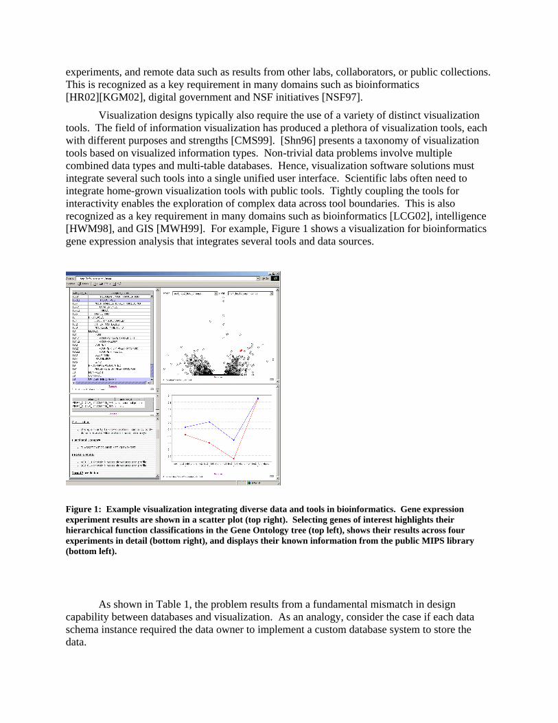
Visualization designs typically also require the use of a variety of distinct visualization tools. The field of information visualization has produced a plethora of visualization tools, each with different purposes and strengths [CMS99]. [Shn96] presents a taxonomy of visualization tools based on visualized information types. Non-trivial data problems involve multiple combined data types and multi-table databases. Hence, visualization software solutions must integrate several such tools into a single unified user interface. Scientific labs often need to integrate home-grown visualization tools with public tools. Tightly coupling the tools for interactivity enables the exploration of complex data across tool boundaries. This is also recognized as a key requirement in many domains such as bioinformatics [LCG02], intelligence [HWM98], and GIS [MWH99]. For example, Figure 1 shows a visualization for bioinformatics gene expression analysis that integrates several tools and data sources.

Figure 1: Example visualization integrating diverse data and tools in bioinformatics. Gene expression experiment results are shown in a scatter plot (top right). Selecting genes of interest highlights their hierarchical function classifications in the Gene Ontology tree (top left), shows their results across four experiments in detail (bottom right), and displays their known information from the public MIPS library (bottom left).

As shown in Table 1, the problem results from a fundamental mismatch in design capability between databases and visualization. As an analogy, consider the case if each data schema instance required the data owner to implement a custom database system to store the data.

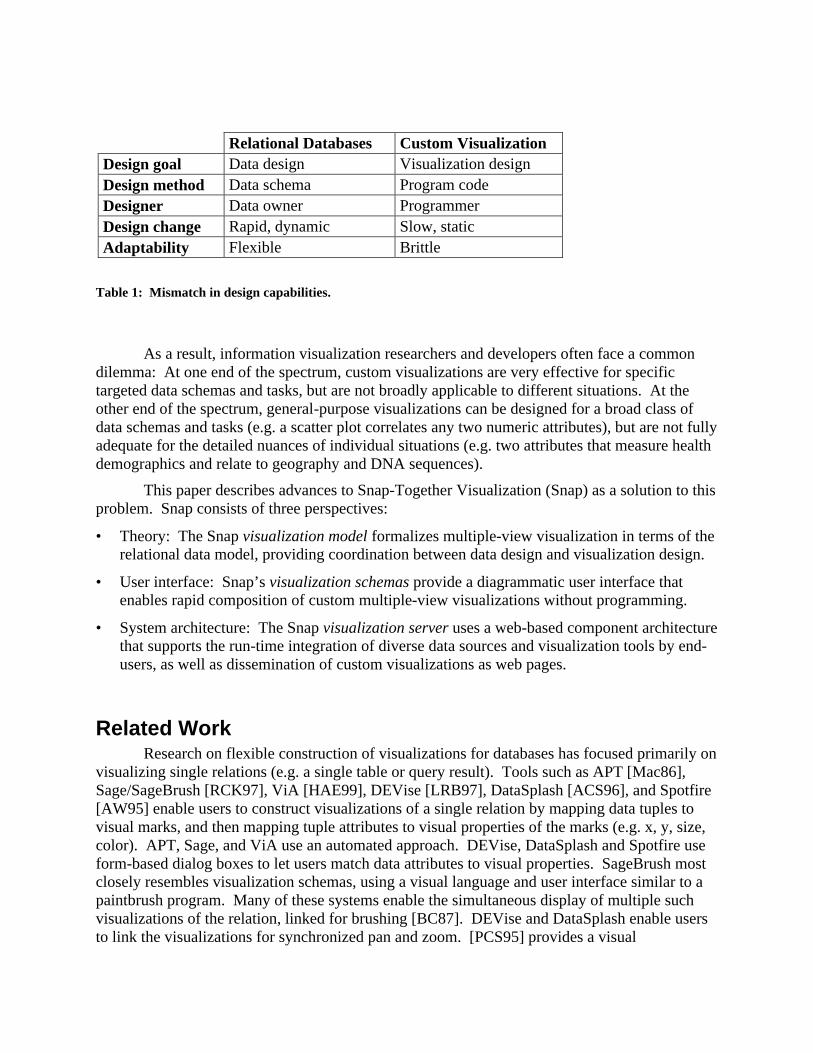
Relational Databases Custom Visualization Design goal Data design Visualization design Design method Data schema Program code Designer Data owner Programmer Design change Rapid, dynamic Slow, static Adaptability Flexible Brittle

Table 1: Mismatch in design capabilities.

As a result, information visualization researchers and developers often face a common dilemma: At one end of the spectrum, custom visualizations are very effective for specific targeted data schemas and tasks, but are not broadly applicable to different situations. At the other end of the spectrum, general-purpose visualizations can be designed for a broad class of data schemas and tasks (e.g. a scatter plot correlates any two numeric attributes), but are not fully adequate for the detailed nuances of individual situations (e.g. two attributes that measure health demographics and relate to geography and DNA sequences).

This paper describes advances to Snap-Together Visualization (Snap) as a solution to this problem. Snap consists of three perspectives:

• Theory: The Snap visualization model formalizes multiple-view visualization in terms of the relational data model, providing coordination between data design and visualization design.

• User interface: Snap’s visualization schemas provide a diagrammatic user interface that enables rapid composition of custom multiple-view visualizations without programming.

• System architecture: The Snap visualization server uses a web-based component architecture that supports the run-time integration of diverse data sources and visualization tools by end-users, as well as dissemination of custom visualizations as web pages.

Related Work Research on flexible construction of visualizations for databases has focused primarily on

visualizing single relations (e.g. a single table or query result). Tools such as APT [Mac86], Sage/SageBrush [RCK97], ViA [HAE99], DEVise [LRB97], DataSplash [ACS96], and Spotfire [AW95] enable users to construct visualizations of a single relation by mapping data tuples to visual marks, and then mapping tuple attributes to visual properties of the marks (e.g. x, y, size, color). APT, Sage, and ViA use an automated approach. DEVise, DataSplash and Spotfire use form-based dialog boxes to let users match data attributes to visual properties. SageBrush most closely resembles visualization schemas, using a visual language and user interface similar to a paintbrush program. Many of these systems enable the simultaneous display of multiple such visualizations of the relation, linked for brushing [BC87]. DEVise and DataSplash enable users to link the visualizations for synchronized pan and zoom. [PCS95] provides a visual

specification for such links. In LinkWinds [JBO94], users can link views into a pipeline for filtering data.

For databases containing multiple relations, Visage/VQE [DRK97] extends attribute mapping, brushing, and dynamic queries to multiple relations. Users can perform the operations on tuples and attributes in different relations that share joined entities. DataSplash lets users construct ‘wormholes’ in a semantic zooming space that allows them drill down across relations by zooming in. RMM [ISB95] uses a hypertext schema approach, similar to visualization schemas, based on entity-relationship diagrams to construct data-driven websites. Tuples map to web pages, relations map to index pages, and associations map to hyperlinks.

Dataflow systems such as AVS [UFK89] and GeoVista [TG02] enable flexible specification of data processing pipelines. Because of the focus on computationally intensive scientific-visualization applications, dataflow diagrams have evolved more as a representation for data processing rather than a specification for interactive visualizations or user interfaces (perhaps away from Haeberli’s original vision with ConMan [Hae88]). Due to the complexity of such data processing environments, dataflow systems are generally geared towards programmers as users. Similar to dataflow, ISYS [SFT01] provides an extensible architecture for linking data sources to service providers to data viewers.

There are many flexible visualization toolkits and frameworks, such as Rivet [BST00] and Sieve [IBW97], that can produce similar multiple-view visualizations as Snap, but require programming.

Database Background Relational databases consist of three major perspectives: The relational data model

provides compositional principles to organize information in a structured form that is usable and manipulable. Relational data schemas enable users to define a custom structure for a particular dataset. Relational database management systems (DBMS) implement the model and schema. Together, these perspectives enable users to organize, store, manipulate, and share data in a flexible and customized fashion.

From the users’ perspective, the design flexibility is accomplished through the use of data schemas. Relational data schemas provide several primitives that users compose to create a database: attributes (fields), tuples (records), and relations (tables). Many modern database systems also explicitly represent join associations between relations (primary keys and foreign keys that associate tuples between relations).

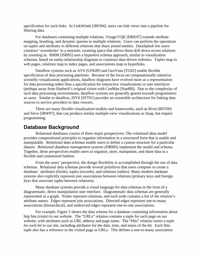
Many database systems provide a visual language for data schemas in the form of a diagrammatic, direct manipulation user interface. Diagrammatic data schemas are generally represented as a graph. Nodes represent relations, and each node contains a list of the relation’s attribute names. Edges represent join associations. Directed edges represent one-to-many associations (hierarchical), and undirected edges represent one-to-one associations.

For example, Figure 2 shows the data schema for a database containing information about http hits (visits) to our website. The “URLs” relation contains a tuple for each page on our website, with attributes such as URL address and page name. The “Hits” relation stores a tuple for each hit to our site, including attributes for the date, time, and status of the hit. Each Hits tuple also has a reference to the visited page in URLs. This defines a one-to-many association

between URLs and Hits, because each page can have many hits, but each hit is to one page. The “Referrers” relation contains tuples for external websites that link to our website. Each Hits tuple also references the Referrer site that linked the visitor to our site. The combination of these join associations defines a many-to-many association between URLs and Referrers through the intervening Hits relation. That is, each page has many referrers and each referrer can send hits to many pages. Similarly, the “Links” relation contains information about all known links between external sites and our site, regardless of hits generated.

Data schema users have a wide range of expertise. Very complex or high performance databases may require expert data modelers, but many simpler databases are maintained by relative novices. In previous work with data analysts at the Census Bureau [NS00], we found that the analysts were very familiar with concepts of the tabular data format. While many had not previously used relational databases, they were quick to learn with data schema diagrams.

Data schemas, especially diagrammatic data schemas, have many important benefits for

data storage:

• Enables data owners to define and modify a custom structure of a database using a simple language.

• Provides guidance for data design, and enforces rules of the data model (e.g. validity).

• Provides an overview of database structure to help other users understand database contents.

• Provides usability for data storage tasks.

• Enables systems to store and interpret database contents interchangeably.

Visualization schemas can have similar benefits for visualization.

Figure 2: An example data schema for a database of http hits to our website. “URLs” stores information about pages on our website. “Referrers” stores information about external websites that have links to our website. “Hits” stores information about each hit, including a reference to the page requested in “URLs” and the external referring site in “Referrers”.

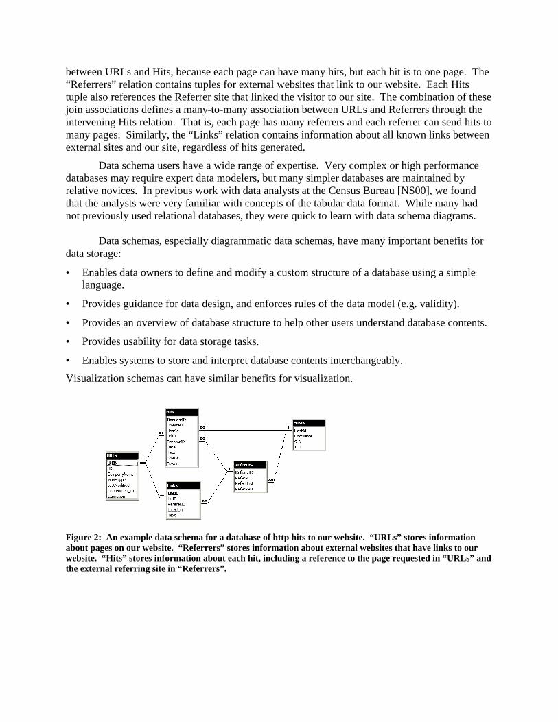
Figure 3: An example multiple-view visualization constructed with Snap for the database shown in Figure 2. The website map generated from the URLs is shown in the TreeView (top left). Selecting a page in the map displays the page in the web browser (top right), and displays the distribution of hits to that page in the scatter plot (top center). Selecting pages also highlights referring sites listed in the table view (bottom left). Likewise, selecting referring sites highlights pages linked to, and shows their hits in the plot. Clicking a referrer shows its page in the other web browser (bottom right).

Note to editor: figures 2&3 should be near each other.

Snap-Together Visualization The primary goal of Snap is to enable a level of flexibility in visualization design that

rivals that of data design. To accomplish this, the primary guiding principle of Snap is to establish a tight analogy between relational data concepts and visualization concepts (summarized in Table 2).

Database concepts have been very successful in the database realm, resulting in massive data storage. Similar concepts may have similar success in the visualization realm, leading to increased data visualization and utilization. This analogical approach has several major motivations:

• Flexibility: Database concepts have successfully enabled flexible data design. Mimicking these concepts in visualization can enable flexible visualization design.

• Learnability: Leveraging data users existing knowledge of data concepts reduces overall learning time. Diagrammatic database schemas have extended basic data storage capabilities to non-experts, and visualization schemas can have similar benefits for data utilization.

• User performance: Visualization as a natural extension to database concepts improves user performance in design, and reduces turn-around time.

• Design Coordination: Close coordination between data design and visualization design closes the gap between data storage and visualization. This is important because data and visualization design affect each other. This also enables the same users to do both data and visualization design tasks.

The analogy begins at the three high-level perspectives of databases: theory, user interface, and system architecture. For each of these perspectives, Snap contains an analogous perspective that extends the relational database counterpart to the visualization realm. In the theory perspective, the Snap visualization model formalizes visualization in terms of the

principles of the relational data model. In the user interface perspective, Snap visualization schemas are analogous to relational data schemas, enabling users to define custom visualizations for custom databases. In the system architecture perspective, the Snap visualization server operates on top of a relational DBMS.

An initial model for Snap is previously reported in [NS00]. This paper reports on significant advancements to the Snap model that establish a clean analogy to the relational data model, the novel concept of visualization schemas as a user interface for visualization design, and a new architecture that coordinates visualization schemas with data schemas and supports new goals in access, extensibility, and collaboration. These three high-level perspectives are discussed in turn in the following sections.

Theory: Snap Visualization Model

Multiple Views The Snap visualization model is based on composition of multiple-views. In the

multiple-view visualization approach, data is displayed in several different views (called visualization components). Different components may display the same or different portions of the data. These components can then be tightly coupled (or coordinated) in a variety of ways [Nor01] such that interacting with one component causes meaningful effects in others. This produces an integrated composite or multiple-view visualization [BWK00]. Figure 3 shows an example of a multiple-view visualization for the website hits database.

Snap’s use of the multiple-views approach has several major motivations:

• Composition of multiple views enables flexibility. • Mimics the way visualization designers often build custom visualization solutions

[BWK00][Nor01]. • Enables the use of diverse visualization tools, and supports diverse and complex data. • Enables reuse of the plethora of visualization tools implemented in the field, as well as

automated techniques for constructing individual views such as APT [Mac86].

Snap’s basic assumption is that the fundamental unit of creative design in information visualization is an individual visualization component. A secondary goal of Snap is to leverage component implementations from the field. Our hope is that this will create a pipeline that transfers tools from research to practical application, and thus facilitates information visualization in “crossing the chasm” [Shn01]. Visualization components are donated by their inventors; coordinations are constructed by users.

Schema Primitives The Snap model rigorously defines multiple-view visualization in terms of the relational

data model. Like the relational data model, it represents a balance between theory and practice. That is, it is intended to capture not only theoretical design of multiple-view visualization, but also common design practices of typical multiple-view visualizations. This approach enables additional goals of extensibility and applicability to existing components as described later in the architecture section.

Relational Databases

Snap Visualization

Design goal Data design Visualization design Design method Data schema Visualization schema Designer Data owner Data owner Design change Rapid, dynamic Rapid, dynamic Adaptability Flexible Flexible Perspectives: Theory Rel. data model Snap vis. model User interface Rel. data schema Snap vis. schema Architecture Rel. DBMS Snap vis. server Schema Primitives:

Relation Vis. component Tuple Visual item Attribute Visual property Selection User interaction

Theory

Join Coordination User interface

Join

Coord- ination

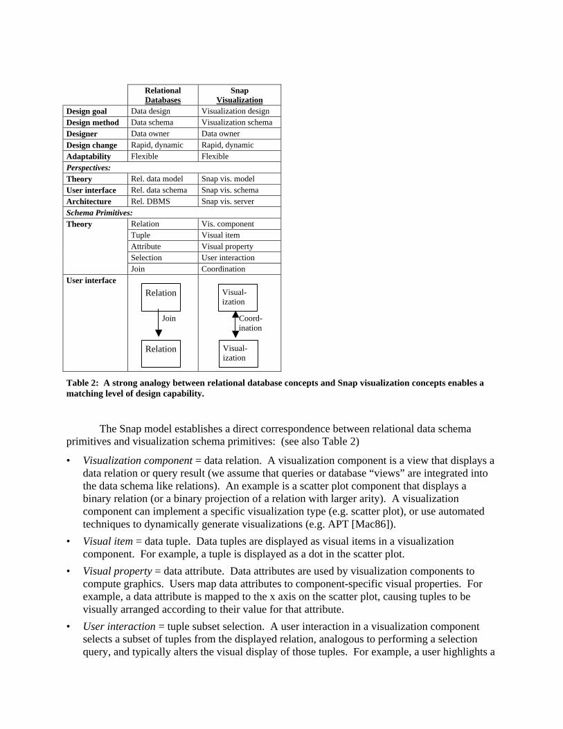
Table 2: A strong analogy between relational database concepts and Snap visualization concepts enables a matching level of design capability.

The Snap model establishes a direct correspondence between relational data schema primitives and visualization schema primitives: (see also Table 2)

• Visualization component = data relation. A visualization component is a view that displays a data relation or query result (we assume that queries or database “views” are integrated into the data schema like relations). An example is a scatter plot component that displays a binary relation (or a binary projection of a relation with larger arity). A visualization component can implement a specific visualization type (e.g. scatter plot), or use automated techniques to dynamically generate visualizations (e.g. APT [Mac86]).

• Visual item = data tuple. Data tuples are displayed as visual items in a visualization component. For example, a tuple is displayed as a dot in the scatter plot.

• Visual property = data attribute. Data attributes are used by visualization components to compute graphics. Users map data attributes to component-specific visual properties. For example, a data attribute is mapped to the x axis on the scatter plot, causing tuples to be visually arranged according to their value for that attribute.

• User interaction = tuple subset selection. A user interaction in a visualization component selects a subset of tuples from the displayed relation, analogous to performing a selection query, and typically alters the visual display of those tuples. For example, a user highlights a

Relation

Relation

Visual-ization

Visual-ization

set of outlier tuples in the scatter plot by directly selecting them, or zooms onto a single tuple to reveal more details. Interactions are defined by each component and identified only by name (e.g. “select”, or “zoom”). Each interaction defined by a component has a corresponding tuple subset that it controls. A subset consists of zero or more tuples from the relation (an empty subset indicates no tuples were selected). Tuples in a subset can be identified by their unique primary-key values. Every component also has an inherent “load” action, which contains the entire relation currently loaded and displayed in the component.

• Visualization coordination = data join. A coordination links an interaction in one component to an interaction in another component, by equating the corresponding subset selections according to a join between the components’ relations. User actions on tuples in one component cause visual actions on join associated tuples in the other component. The tuple subset of the user action in the former component is inner-joined to the latter component’s relation, resulting in the new tuple subset to use for the action in the latter component. For example, brushing-and-linking between two scatter plots of the same relation is a coordination of the “select” actions across the implicit one-to-one join association. Then, when users highlight items in one plot, the associated items are automatically highlighted in the other plot. A coordination can link any pair of actions between components. Coordinations, like joins, are bidirectional.

Coordinations and Joins An important advancement in this model is the generalization of coordinations and

interactions. A coordination is generalized to any single or compound join association, including one-to-one, one-to-many, and many-to-many associations. Join associations for coordinations are automatically derived and executed from data schemas, eliminating the need for user-defined parameterized queries for joins. Furthermore, interactions are generalized to tuple subset selections, enabling them to act on single or multiple tuples. Chained coordinations cascade across arbitrary associations, beyond the previously limited one-to-one cascading.

Four cases demonstrate how generalized coordinations correspond to various joins in the data schema. These are demonstrated using the example data schema and multiple-view visualization for website hits shown in Figure 2 and Figure 3.

• Self join: A coordination can be established between two visualization components that display the same relation. In this case, the coordination corresponds to the implicit one-to-one join association that exists between the relation and itself. For example, the TreeView visualization component displays the URLs relation, using the URL page pathname attribute to display the tuples as a website tree structure. A web browser component also displays the URLs relation, using the URL attribute to display actual pages represented by the tuples. The “select” action of the TreeView is coordinated to the “navigate” action of the web browser across the self join. When users select a tuple in the TreeView, there is no need to actually perform a join since it is a self join, so the same tuple is used to navigate the web browser to the selected page. TreeView ← URLs → web browser

• Single join: A coordination can be established between two components whose relations have a direct join association in the data schema. The relational model provides two primitive types of direct join associations: one-to-one and one-to-many. For example, in addition to the TreeView of the URLs relation, the scatter plot displays the Hits relation, showing all hits to the website by date and time. The “select” action of the TreeView is coordinated to the “load” action of the plot, using the direct join association between the URLs and Hits relations. The data schema indicates this is a one-to-many association. Selecting tuples in the TreeView joins those tuples to the Hits relation to find all the hits to the selected pages. The resulting Hits subset is then loaded and displayed in the plot, essentially filtering out hits to any other pages. This enables users to drill down from pages to hits. TreeView ← URLs ↔ Hits → Scatter plot

• Compound join: A coordination can be established between two components whose relations have an indirect association via one or more intermediate relations in the data schema. This requires a compound join, concatenating each of the direct joins along the indirect association path. Compound joins enable more complex associations such as many-to-many. For example, in addition to the TreeView of the URLs relation, the TableView displays the Referrers relation, showing an alphabetical list of all the websites that link (refer) readers to the URLs website (alternatively, it might be interesting to show referrers geographically). The “select” action of the TreeView is coordinated to the “select” action of the TableView, using the compound join from URLs to Hits to Referrers. The concatenation of the one-to-many and many-to-one joins creates a many-to-many join. Selecting tuples in the TreeView joins those tuples to the Hits relation and then to the Referrers relation to identify the websites that actually sent readers to the selected pages, and then selects them in the TableView. Since coordinations are bidirectional, the reverse interaction also occurs. This example illustrates brushing-and-linking across a many-to-many association. TreeView ← URLs ↔ Hits ↔ Referrers → TableView

• Multiple alternative joins: A coordination between two components whose relations have multiple alternative join associations connecting them requires the selection of one of the join associations for use in the coordination. In the compound join example above, an alternative is the compound join through the Links relation. This alternative would have a different effect. Selecting pages in the TreeView would indicate all the websites in the TableView that have links to those pages, rather than the websites that actually referred readers and generated hits. TreeView ← URLs ↔ Hits ↔ Referrers → TableView TreeView ← URLs ↔ Links ↔ Referrers → TableView

Data-centric Coordination The Snap multiple-view coordination model employs a data-centric approach by focusing

on tuple-based coordinations. The motivation for this approach is that tuple-based coordination is most necessary for multi-table multi-view visualization, is representation independent (and

therefore can be applied between any two visualization components), is under explored, and coincides well with extensibility goals described later in the Architecture section. While the model focuses on data visualization and not data editing operations, data edits are tuple-based and can easily be added to the coordination model using standard data change events. Major data modifications that alter entire relations are better implemented directly in the data schema. Snap’s coordination model would combine well with other data-centric visualization concepts such as Visage [RCK97].

The Snap model captures the common types of coordinations used for data navigation. See [Nor01] for a detailed taxonomy of coordinations achievable with this model. These common coordinations support scalability of visualization in each aspect of relational data:

• Scalability in number of tuples: Overview+detail strategies support very large numbers of tuples, especially when chained across several views [PCS95].

• Scalability in number of attributes: Many attributes can be partitioned into multiple simpler views, while brushing-and-linking strategies [BC87] enable correlation between them. Systems such as Visage [RCK97] and Spotfire [AW95] demonstrate the value of brushing.

• Scalability in number of relations and associations: Coordinated drill-down strategies enable drill down across one-to-many associations between relations in different views [FNP99].

• Scalability in number of different data types: Data containing multiple distinct types of data requires different types of views and coordinations to navigate between them. Examples include geographic information systems that combine maps and statistics [MWH99], or bioinformatics [KGM02], which can involve numerical data, images, tree structures, and networks.

Other types of multiple-view coordinations are representation-centric and are not explicitly modeled here. They coordinate specifics of the representations of two visualization components, such as sharing a common color-mapping scheme or displaying the same arbitrary region of a visual space. In the example of displaying the same region (e.g. synchronized pan and zoom of the axes of two plots), if the region is strictly determined by a set of tuples then the tuple-based technique will work. Otherwise, components must share parameters of the visual representation. DEVise [LRB97] has demonstrated an approach for handling a subset of representation-centric coordinations based on sharing attribute ranges of 1- and 2-dimensional spaces (its “visual” and “cursor” links). These can be easily integrated with the Snap model (DEVise “record” links are tuple-based and can already be represented in the Snap model). However, in the general case, as in the example of sharing a common color scheme, a more detailed level of integration is needed. Improvise [WL02] employs an MVC approach that treats such properties of the visual representation as sharable data. Components must share many complex data structures that complicate inter-component communication and must be specified by users. Hence, representation-centric coordinations currently trade off with ease of extensibility and usability.

User Interface: Visualization Schemas Visualization schema diagrams are visually represented similar to data schema diagrams.

Visualization schemas are represented as a graph, and support direct manipulation. Nodes in the

graph represent instantiated visualization components. Edges represent coordinations between components.

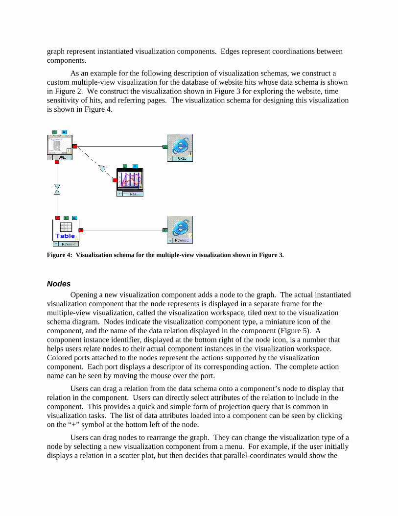
As an example for the following description of visualization schemas, we construct a custom multiple-view visualization for the database of website hits whose data schema is shown in Figure 2. We construct the visualization shown in Figure 3 for exploring the website, time sensitivity of hits, and referring pages. The visualization schema for designing this visualization is shown in Figure 4.

Figure 4: Visualization schema for the multiple-view visualization shown in Figure 3.

Nodes Opening a new visualization component adds a node to the graph. The actual instantiated

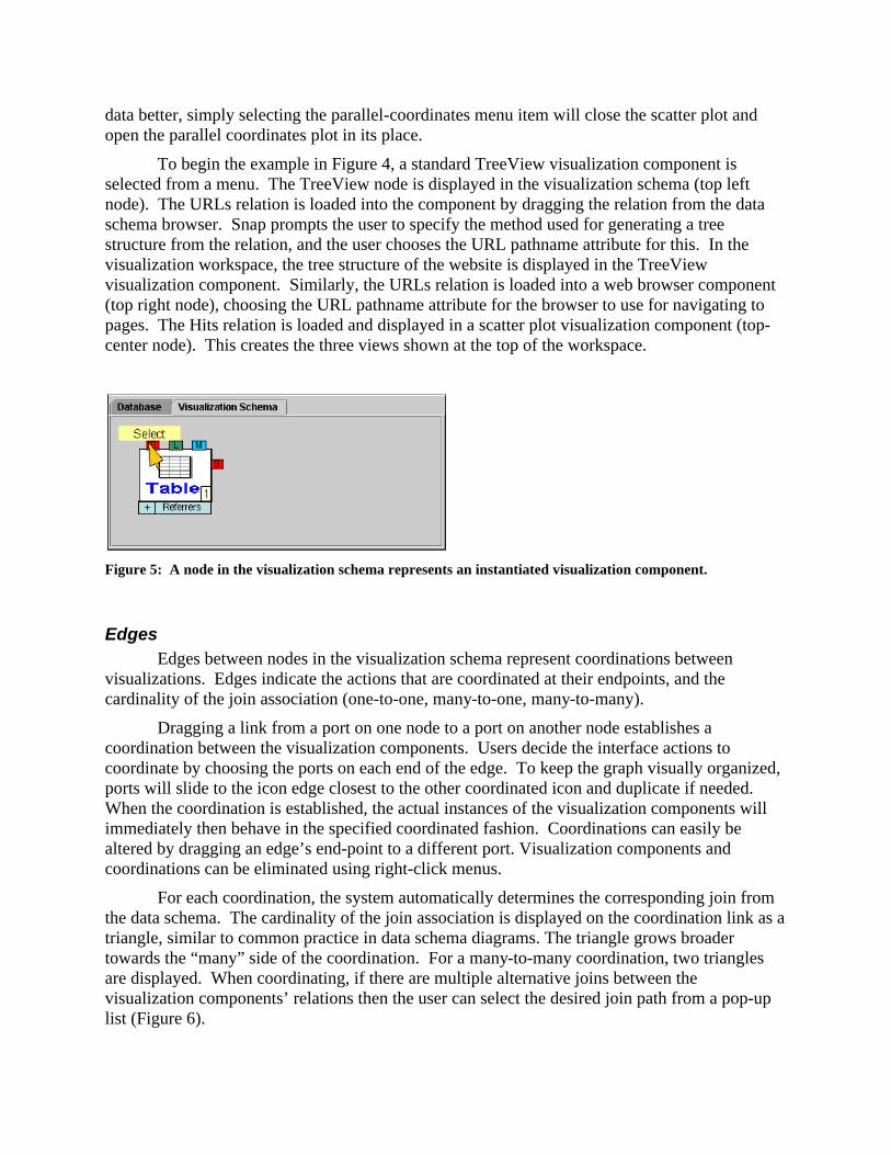
visualization component that the node represents is displayed in a separate frame for the multiple-view visualization, called the visualization workspace, tiled next to the visualization schema diagram. Nodes indicate the visualization component type, a miniature icon of the component, and the name of the data relation displayed in the component (Figure 5). A component instance identifier, displayed at the bottom right of the node icon, is a number that helps users relate nodes to their actual component instances in the visualization workspace. Colored ports attached to the nodes represent the actions supported by the visualization component. Each port displays a descriptor of its corresponding action. The complete action name can be seen by moving the mouse over the port.

Users can drag a relation from the data schema onto a component’s node to display that relation in the component. Users can directly select attributes of the relation to include in the component. This provides a quick and simple form of projection query that is common in visualization tasks. The list of data attributes loaded into a component can be seen by clicking on the “+” symbol at the bottom left of the node.

Users can drag nodes to rearrange the graph. They can change the visualization type of a node by selecting a new visualization component from a menu. For example, if the user initially displays a relation in a scatter plot, but then decides that parallel-coordinates would show the

data better, simply selecting the parallel-coordinates menu item will close the scatter plot and open the parallel coordinates plot in its place.

To begin the example in Figure 4, a standard TreeView visualization component is selected from a menu. The TreeView node is displayed in the visualization schema (top left node). The URLs relation is loaded into the component by dragging the relation from the data schema browser. Snap prompts the user to specify the method used for generating a tree structure from the relation, and the user chooses the URL pathname attribute for this. In the visualization workspace, the tree structure of the website is displayed in the TreeView visualization component. Similarly, the URLs relation is loaded into a web browser component (top right node), choosing the URL pathname attribute for the browser to use for navigating to pages. The Hits relation is loaded and displayed in a scatter plot visualization component (top-center node). This creates the three views shown at the top of the workspace.

Figure 5: A node in the visualization schema represents an instantiated visualization component.

Edges Edges between nodes in the visualization schema represent coordinations between

visualizations. Edges indicate the actions that are coordinated at their endpoints, and the cardinality of the join association (one-to-one, many-to-one, many-to-many).

Dragging a link from a port on one node to a port on another node establishes a coordination between the visualization components. Users decide the interface actions to coordinate by choosing the ports on each end of the edge. To keep the graph visually organized, ports will slide to the icon edge closest to the other coordinated icon and duplicate if needed. When the coordination is established, the actual instances of the visualization components will immediately then behave in the specified coordinated fashion. Coordinations can easily be altered by dragging an edge’s end-point to a different port. Visualization components and coordinations can be eliminated using right-click menus.

For each coordination, the system automatically determines the corresponding join from the data schema. The cardinality of the join association is displayed on the coordination link as a triangle, similar to common practice in data schema diagrams. The triangle grows broader towards the “many” side of the coordination. For a many-to-many coordination, two triangles are displayed. When coordinating, if there are multiple alternative joins between the visualization components’ relations then the user can select the desired join path from a pop-up list (Figure 6).

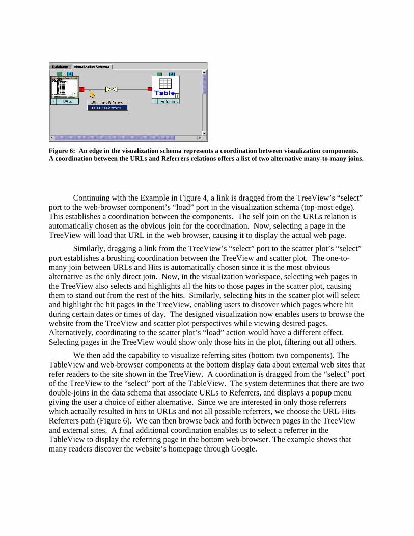
Figure 6: An edge in the visualization schema represents a coordination between visualization components. A coordination between the URLs and Referrers relations offers a list of two alternative many-to-many joins.

Continuing with the Example in Figure 4, a link is dragged from the TreeView’s “select” port to the web-browser component’s “load” port in the visualization schema (top-most edge). This establishes a coordination between the components. The self join on the URLs relation is automatically chosen as the obvious join for the coordination. Now, selecting a page in the TreeView will load that URL in the web browser, causing it to display the actual web page.

Similarly, dragging a link from the TreeView’s “select” port to the scatter plot’s “select” port establishes a brushing coordination between the TreeView and scatter plot. The one-to-many join between URLs and Hits is automatically chosen since it is the most obvious alternative as the only direct join. Now, in the visualization workspace, selecting web pages in the TreeView also selects and highlights all the hits to those pages in the scatter plot, causing them to stand out from the rest of the hits. Similarly, selecting hits in the scatter plot will select and highlight the hit pages in the TreeView, enabling users to discover which pages where hit during certain dates or times of day. The designed visualization now enables users to browse the website from the TreeView and scatter plot perspectives while viewing desired pages. Alternatively, coordinating to the scatter plot’s “load” action would have a different effect. Selecting pages in the TreeView would show only those hits in the plot, filtering out all others.

We then add the capability to visualize referring sites (bottom two components). The TableView and web-browser components at the bottom display data about external web sites that refer readers to the site shown in the TreeView. A coordination is dragged from the “select” port of the TreeView to the “select” port of the TableView. The system determines that there are two double-joins in the data schema that associate URLs to Referrers, and displays a popup menu giving the user a choice of either alternative. Since we are interested in only those referrers which actually resulted in hits to URLs and not all possible referrers, we choose the URL-Hits-Referrers path (Figure 6). We can then browse back and forth between pages in the TreeView and external sites. A final additional coordination enables us to select a referrer in the TableView to display the referring page in the bottom web-browser. The example shows that many readers discover the website’s homepage through Google.

Advantages Visualization schemas have many advantages. Its direct manipulation approach enables

users to construct and modify multiple-view visualizations very rapidly. Because it closely resembles relational data schemas, its learning time is greatly reduced from the previous form-based approach [NS00] and it helps users learn the Snap model concepts. Also, visualization schemas are used to specify user interactions, which is a level that users are familiar with, in contrast to dataflow specifications which are at a much more detailed data processing level.

Furthermore, it provides a visual overview of the coordination structure of the visualization, which helps users quickly learn how to operate the visualizations and understand its response. This helps to solve a long-standing usability problem with multiple-view visualizations in general. Hence, visualization schemas improve usability at both the construction phase as well as the operation phase. Visualization schemas also can provide a compact representation of visualizations for the purpose of browsing and recognizing many alternate designs. It also provides a context in which to show other information related to visualizations and their use, such as animations of propagation of actions through the coordination graph or saved sequences of actions such as macros.

Finally, it enables a new level of flexibility in visualization that matches that of databases. It does not require programming, which enables visualizations to be rapidly updated along with dynamic database schemas.

Scenario In bioinformatics, visualization can help biologists analyze large quantities of

experimental data and discover relationships. Flexibility is critical in bioinformatics since there is much variety and unpredictability in the problems, and custom visualizations are routinely needed. This scenario is based on actual investigations underway by collaborators in the life sciences on the genomics of pine tree response to drought stress conditions [HRS02]. Proteins provide the structural components of cells and tissues as well as enzymes for essential biochemical reactions. A gene is a specific sequence of nucleotide bases, whose sequences carry the information required for constructing proteins. Hence, genes influence the basic functions of an organism. These low-level functions are categorized in a functional hierarchy, and genes are experimentally linked to these categories over time.

Data A biologist is investigating the results of several micro-array experiments, in which the

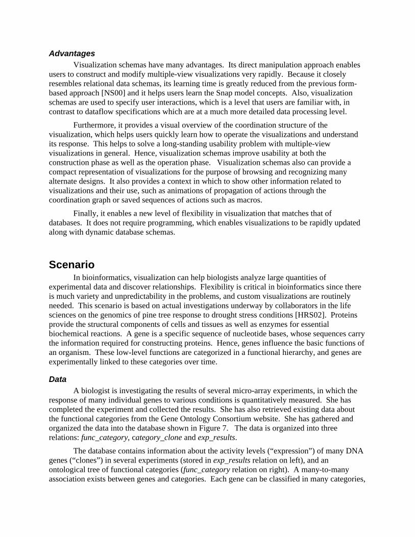
response of many individual genes to various conditions is quantitatively measured. She has completed the experiment and collected the results. She has also retrieved existing data about the functional categories from the Gene Ontology Consortium website. She has gathered and organized the data into the database shown in Figure 7. The data is organized into three relations: func_category, category_clone and exp_results.

The database contains information about the activity levels (“expression”) of many DNA genes (“clones”) in several experiments (stored in exp_results relation on left), and an ontological tree of functional categories (func_category relation on right). A many-to-many association exists between genes and categories. Each gene can be classified in many categories,

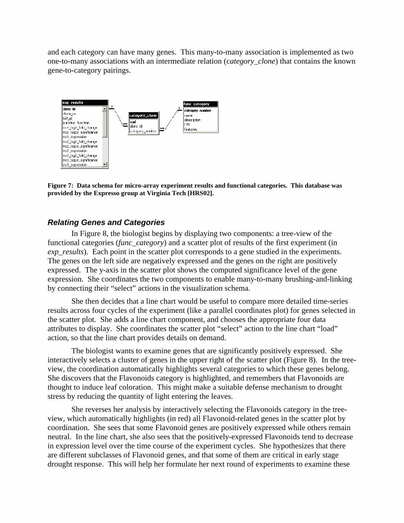
and each category can have many genes. This many-to-many association is implemented as two one-to-many associations with an intermediate relation (category_clone) that contains the known gene-to-category pairings.

Figure 7: Data schema for micro-array experiment results and functional categories. This database was provided by the Expresso group at Virginia Tech [HRS02].

Relating Genes and Categories In Figure 8, the biologist begins by displaying two components: a tree-view of the

functional categories (func_category) and a scatter plot of results of the first experiment (in exp_results). Each point in the scatter plot corresponds to a gene studied in the experiments. The genes on the left side are negatively expressed and the genes on the right are positively expressed. The y-axis in the scatter plot shows the computed significance level of the gene expression. She coordinates the two components to enable many-to-many brushing-and-linking by connecting their “select” actions in the visualization schema.

She then decides that a line chart would be useful to compare more detailed time-series results across four cycles of the experiment (like a parallel coordinates plot) for genes selected in the scatter plot. She adds a line chart component, and chooses the appropriate four data attributes to display. She coordinates the scatter plot “select” action to the line chart “load” action, so that the line chart provides details on demand.

The biologist wants to examine genes that are significantly positively expressed. She interactively selects a cluster of genes in the upper right of the scatter plot (Figure 8). In the tree-view, the coordination automatically highlights several categories to which these genes belong. She discovers that the Flavonoids category is highlighted, and remembers that Flavonoids are thought to induce leaf coloration. This might make a suitable defense mechanism to drought stress by reducing the quantity of light entering the leaves.

She reverses her analysis by interactively selecting the Flavonoids category in the tree-view, which automatically highlights (in red) all Flavonoid-related genes in the scatter plot by coordination. She sees that some Flavonoid genes are positively expressed while others remain neutral. In the line chart, she also sees that the positively-expressed Flavonoids tend to decrease in expression level over the time course of the experiment cycles. She hypothesizes that there are different subclasses of Flavonoid genes, and that some of them are critical in early stage drought response. This will help her formulate her next round of experiments to examine these

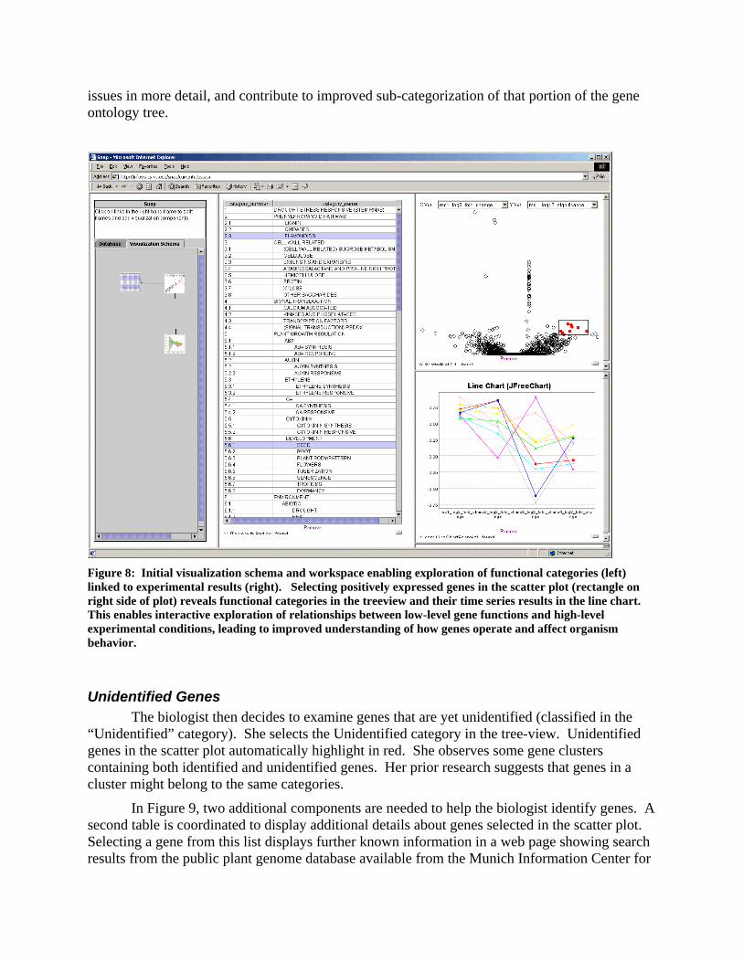
issues in more detail, and contribute to improved sub-categorization of that portion of the gene ontology tree.

Figure 8: Initial visualization schema and workspace enabling exploration of functional categories (left) linked to experimental results (right). Selecting positively expressed genes in the scatter plot (rectangle on right side of plot) reveals functional categories in the treeview and their time series results in the line chart. This enables interactive exploration of relationships between low-level gene functions and high-level experimental conditions, leading to improved understanding of how genes operate and affect organism behavior.

Unidentified Genes The biologist then decides to examine genes that are yet unidentified (classified in the

“Unidentified” category). She selects the Unidentified category in the tree-view. Unidentified genes in the scatter plot automatically highlight in red. She observes some gene clusters containing both identified and unidentified genes. Her prior research suggests that genes in a cluster might belong to the same categories.

In Figure 9, two additional components are needed to help the biologist identify genes. A second table is coordinated to display additional details about genes selected in the scatter plot. Selecting a gene from this list displays further known information in a web page showing search results from the public plant genome database available from the Munich Information Center for

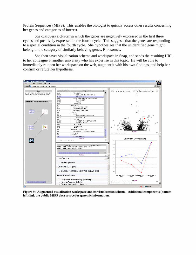
Protein Sequences (MIPS). This enables the biologist to quickly access other results concerning her genes and categories of interest.

She discovers a cluster in which the genes are negatively expressed in the first three cycles and positively expressed in the fourth cycle. This suggests that the genes are responding to a special condition in the fourth cycle. She hypothesizes that the unidentified gene might belong to the category of similarly behaving genes, Ribosomes.

She then saves visualization schema and workspace in Snap, and sends the resulting URL to her colleague at another university who has expertise in this topic. He will be able to immediately re-open her workspace on the web, augment it with his own findings, and help her confirm or refute her hypothesis.

Figure 9: Augmented visualization workspace and its visualization schema. Additional components (bottom left) link the public MIPS data source for genomic information.

Architecture: Snap Visualization Server The Snap visualization server is the software system that enables users to design

multiple-view visualizations by creating visualization schemas. The Snap client runs in a web browser and uses frames to organize multiple visualization components in a tiled space-filling fashion (Figure 9). The Snap control panel is the Java applet tiled on the left side. This panel lets users establish database connections and design a visualization schema. The visualization workspace enables users to add components by splitting frames horizontally or vertically.

Snap has an event-based, implicit invocation software architecture [SG96]. The visualization schema is used to coordinate events between the individual visualization components. When a view is added, Snap registers itself as a listener for the component’s events. When users interact with a component, the component fires an event. Snap receives the event and propagates it to other coordinated visualizations. Snap acts as a mediator between each component [GHJ95]. Visualization components implement a “Snapable” programming interface exposing the component’s capabilities to Snap. Additionally, each visualization component can act as a fully functional individual visualization outside of the Snap system. An interesting side effect of this approach is that Snap can track and control the state of each component, enabling additional centralized features such as interactive history keeping, and saving and restoring state.

The Snap architecture consists of three major layers for coordinating components (Figure 10). The data source maintains the data to be visualized. The first layer of the architecture includes the Database Manager and Database Schema. They provide connectivity to data sources and describe join associations between the separate data relations. The second layer contains the Visualization Schema and Coordination Graph. This layer supports the assignment of data relations to visualization components, and the coordination of events between components. The Visualization Schema allows two components to be coordinated only when their encapsulated relations can be associated by joins in the data schema. The third layer includes the Coordination Manager. It handles all communication with the visualization components, and is responsible for the receiving and firing of events. The Coordination Manager utilizes the bottom two layers to propagate events to coordinated components and translate events as needed.

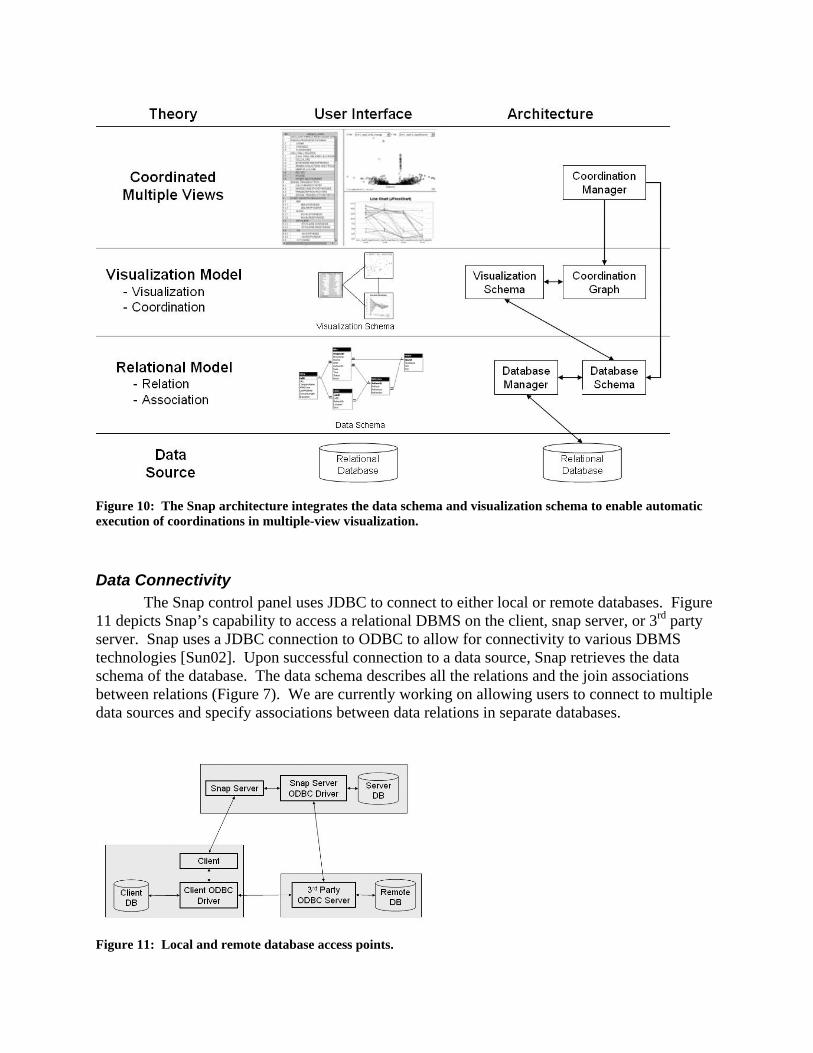
Figure 10: The Snap architecture integrates the data schema and visualization schema to enable automatic execution of coordinations in multiple-view visualization.

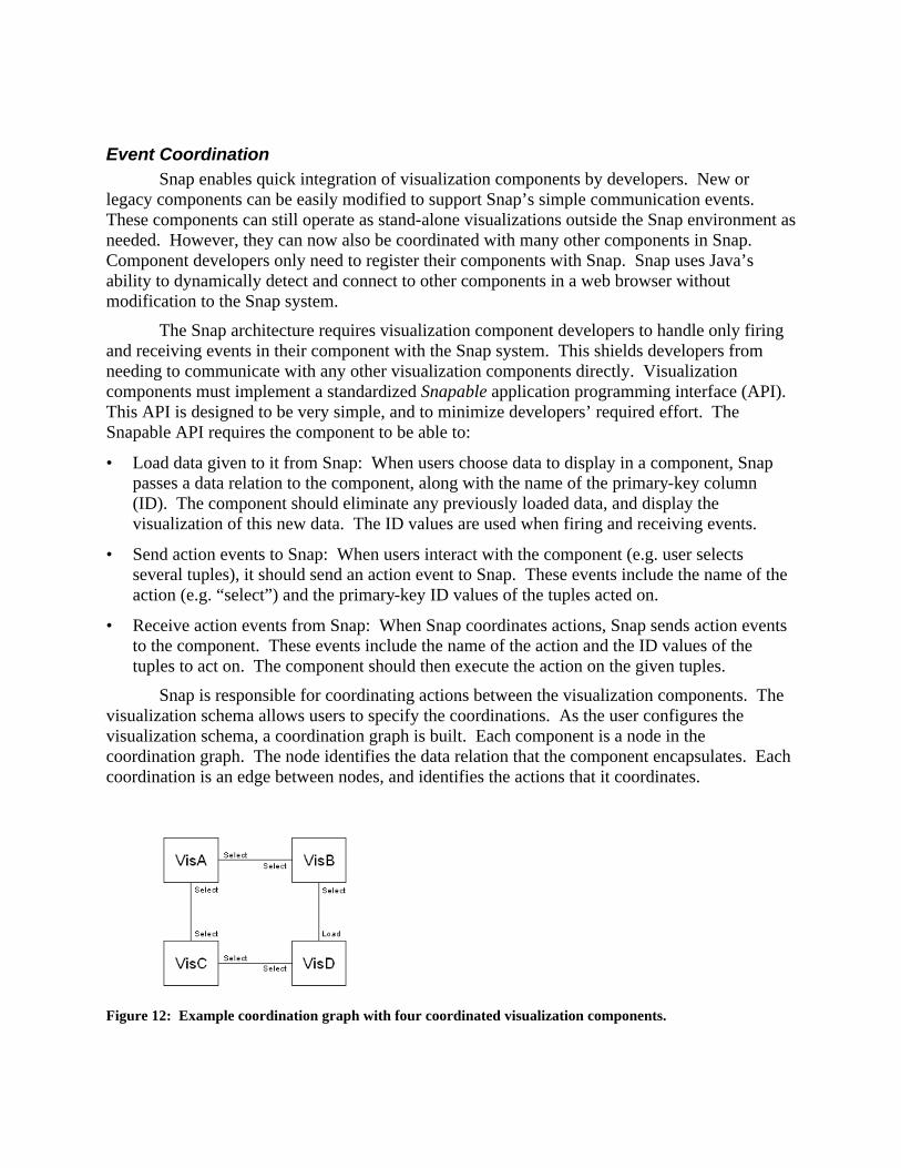
Data Connectivity The Snap control panel uses JDBC to connect to either local or remote databases. Figure

11 depicts Snap’s capability to access a relational DBMS on the client, snap server, or 3rd party server. Snap uses a JDBC connection to ODBC to allow for connectivity to various DBMS technologies [Sun02]. Upon successful connection to a data source, Snap retrieves the data schema of the database. The data schema describes all the relations and the join associations between relations (Figure 7). We are currently working on allowing users to connect to multiple data sources and specify associations between data relations in separate databases.

Figure 11: Local and remote database access points.

Event Coordination Snap enables quick integration of visualization components by developers. New or

legacy components can be easily modified to support Snap’s simple communication events. These components can still operate as stand-alone visualizations outside the Snap environment as needed. However, they can now also be coordinated with many other components in Snap. Component developers only need to register their components with Snap. Snap uses Java’s ability to dynamically detect and connect to other components in a web browser without modification to the Snap system.

The Snap architecture requires visualization component developers to handle only firing and receiving events in their component with the Snap system. This shields developers from needing to communicate with any other visualization components directly. Visualization components must implement a standardized Snapable application programming interface (API). This API is designed to be very simple, and to minimize developers’ required effort. The Snapable API requires the component to be able to:

• Load data given to it from Snap: When users choose data to display in a component, Snap passes a data relation to the component, along with the name of the primary-key column (ID). The component should eliminate any previously loaded data, and display the visualization of this new data. The ID values are used when firing and receiving events.

• Send action events to Snap: When users interact with the component (e.g. user selects several tuples), it should send an action event to Snap. These events include the name of the action (e.g. “select”) and the primary-key ID values of the tuples acted on.

• Receive action events from Snap: When Snap coordinates actions, Snap sends action events to the component. These events include the name of the action and the ID values of the tuples to act on. The component should then execute the action on the given tuples.

Snap is responsible for coordinating actions between the visualization components. The visualization schema allows users to specify the coordinations. As the user configures the visualization schema, a coordination graph is built. Each component is a node in the coordination graph. The node identifies the data relation that the component encapsulates. Each coordination is an edge between nodes, and identifies the actions that it coordinates.

Figure 12: Example coordination graph with four coordinated visualization components.

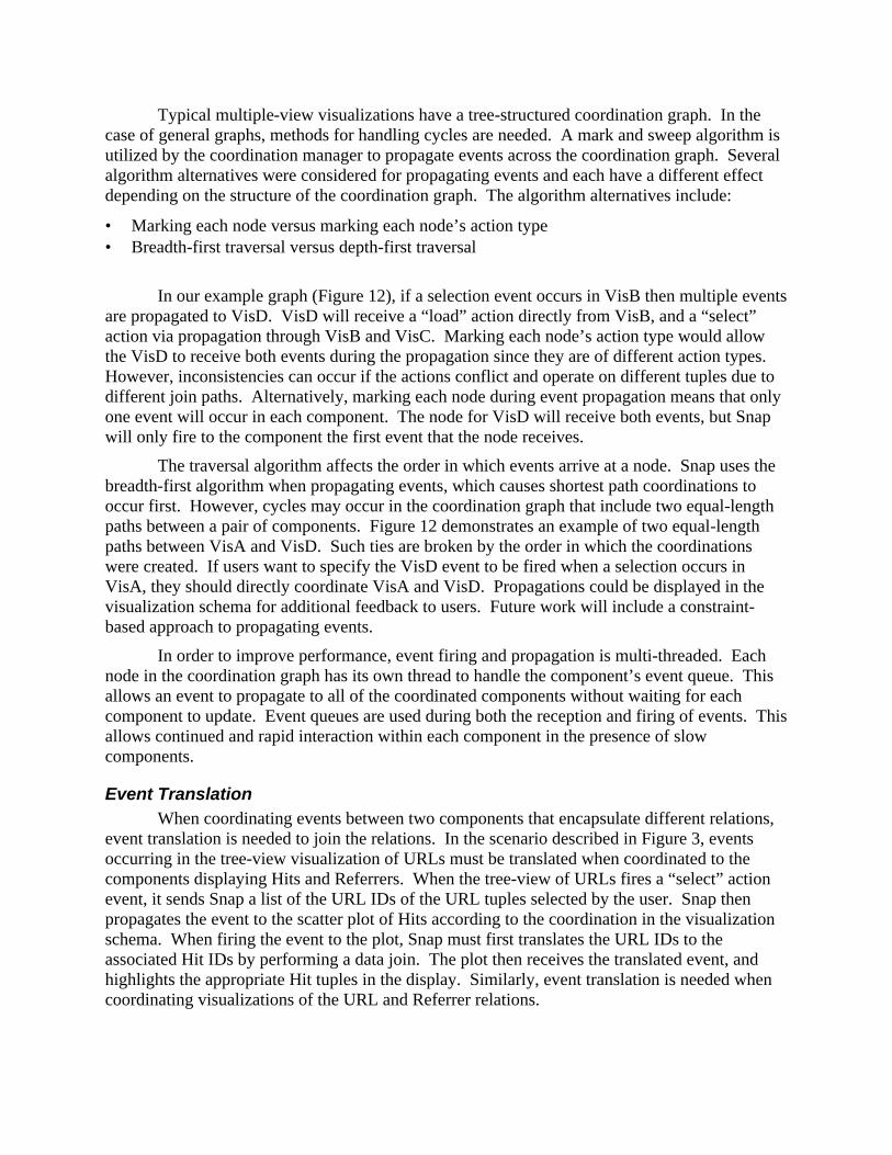
Typical multiple-view visualizations have a tree-structured coordination graph. In the case of general graphs, methods for handling cycles are needed. A mark and sweep algorithm is utilized by the coordination manager to propagate events across the coordination graph. Several algorithm alternatives were considered for propagating events and each have a different effect depending on the structure of the coordination graph. The algorithm alternatives include:

• Marking each node versus marking each node’s action type • Breadth-first traversal versus depth-first traversal

In our example graph (Figure 12), if a selection event occurs in VisB then multiple events are propagated to VisD. VisD will receive a “load” action directly from VisB, and a “select” action via propagation through VisB and VisC. Marking each node’s action type would allow the VisD to receive both events during the propagation since they are of different action types. However, inconsistencies can occur if the actions conflict and operate on different tuples due to different join paths. Alternatively, marking each node during event propagation means that only one event will occur in each component. The node for VisD will receive both events, but Snap will only fire to the component the first event that the node receives.

The traversal algorithm affects the order in which events arrive at a node. Snap uses the breadth-first algorithm when propagating events, which causes shortest path coordinations to occur first. However, cycles may occur in the coordination graph that include two equal-length paths between a pair of components. Figure 12 demonstrates an example of two equal-length paths between VisA and VisD. Such ties are broken by the order in which the coordinations were created. If users want to specify the VisD event to be fired when a selection occurs in VisA, they should directly coordinate VisA and VisD. Propagations could be displayed in the visualization schema for additional feedback to users. Future work will include a constraint-based approach to propagating events.

In order to improve performance, event firing and propagation is multi-threaded. Each node in the coordination graph has its own thread to handle the component’s event queue. This allows an event to propagate to all of the coordinated components without waiting for each component to update. Event queues are used during both the reception and firing of events. This allows continued and rapid interaction within each component in the presence of slow components.

Event Translation When coordinating events between two components that encapsulate different relations,

event translation is needed to join the relations. In the scenario described in Figure 3, events occurring in the tree-view visualization of URLs must be translated when coordinated to the components displaying Hits and Referrers. When the tree-view of URLs fires a “select” action event, it sends Snap a list of the URL IDs of the URL tuples selected by the user. Snap then propagates the event to the scatter plot of Hits according to the coordination in the visualization schema. When firing the event to the plot, Snap must first translates the URL IDs to the associated Hit IDs by performing a data join. The plot then receives the translated event, and highlights the appropriate Hit tuples in the display. Similarly, event translation is needed when coordinating visualizations of the URL and Referrer relations.

The Coordination Manager utilizes the visualization schema to propagate events and determine the relations encapsulated by each component. It then utilizes the data schema to translate events appropriately based on the underlying data join associations. The data schema manager translates events across single and compound joins. The events are translated by constructing a join query between the two relations. In the example of Figure 3, selecting multiple URLs in the tree-view requires Snap to translate the event for coordinated components. If three URL tuples whose URL IDs are 4, 5, and 6 are selected, then the data schema manager constructs the following query to translate the URLs into Hits for the scatter plot:

SELECT Hits.RequestID FROM Hits INNER JOIN URLs ON Hits.UrlID = URLs.UrlID WHERE URLs.UrlID IN (4,5,6);

For coordinating across intermediate relations, event translation requires a compound join query. For the table-view of Referrers, the following query retrieves the Referrer tuples associated with the selected URL tuples:

SELECT Referers.RefererID FROM Referers INNER JOIN (Hits INNER JOIN URLs ON Hits.UrlID = URLs.UrlID) ON Referers.RefererID = Hits.RefererID WHERE URLs.UrlID IN (4,5,6);

For firing “load” actions, the query would be modified to retrieve all the attributes to be displayed in the destination component, instead of only the primary key attribute. Database queries have a performance impact on the feedback of the multiple-view visualization. This is especially true when Snap is connected to remote data sources. Result caching and preloading of IDs provide performance improvements. Future work will continue to explore the integration of these and other data management techniques.

Component Extensions Snap leverages third party visualization components. Developers of visualization

components can submit their components to the Snap server, enabling other users to utilize the components in their visualization schemas. The Snap server acts as a repository for visualization components, which facilitates the transfer of new components to practical application. The Snap server is runtime extensible, meaning that new components can be added without the need to re-compile or restart the server. Adapters are included within the architecture to support Snap’s extensibility.

Snap’s adapter layer enables visualization components implemented in many different technologies to be coordinated in visualization schemas (Figure 13). Hence, visualization components may be JavaBeans, Java applets, ActiveX components, and JavaScript pages. The

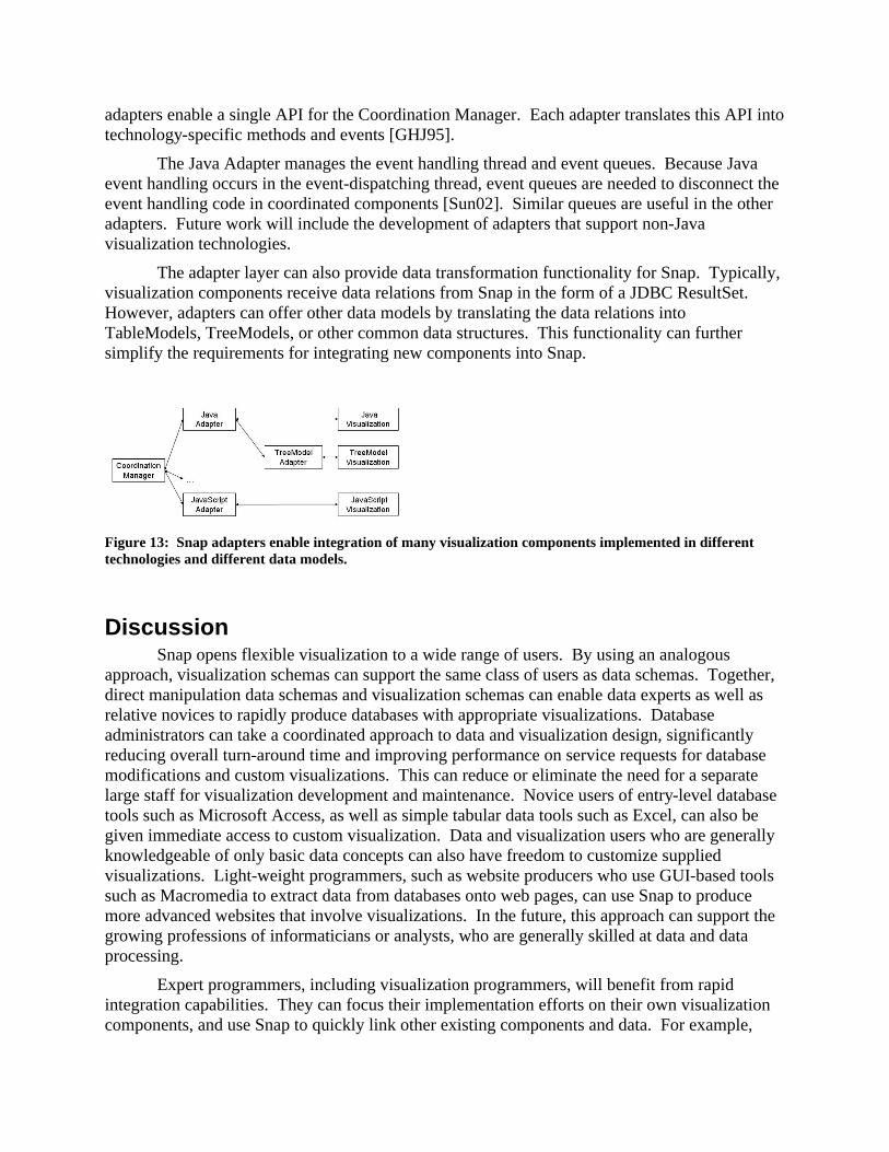
adapters enable a single API for the Coordination Manager. Each adapter translates this API into technology-specific methods and events [GHJ95].

The Java Adapter manages the event handling thread and event queues. Because Java event handling occurs in the event-dispatching thread, event queues are needed to disconnect the event handling code in coordinated components [Sun02]. Similar queues are useful in the other adapters. Future work will include the development of adapters that support non-Java visualization technologies.

The adapter layer can also provide data transformation functionality for Snap. Typically, visualization components receive data relations from Snap in the form of a JDBC ResultSet. However, adapters can offer other data models by translating the data relations into TableModels, TreeModels, or other common data structures. This functionality can further simplify the requirements for integrating new components into Snap.

Figure 13: Snap adapters enable integration of many visualization components implemented in different technologies and different data models.

Discussion Snap opens flexible visualization to a wide range of users. By using an analogous

approach, visualization schemas can support the same class of users as data schemas. Together, direct manipulation data schemas and visualization schemas can enable data experts as well as relative novices to rapidly produce databases with appropriate visualizations. Database administrators can take a coordinated approach to data and visualization design, significantly reducing overall turn-around time and improving performance on service requests for database modifications and custom visualizations. This can reduce or eliminate the need for a separate large staff for visualization development and maintenance. Novice users of entry-level database tools such as Microsoft Access, as well as simple tabular data tools such as Excel, can also be given immediate access to custom visualization. Data and visualization users who are generally knowledgeable of only basic data concepts can also have freedom to customize supplied visualizations. Light-weight programmers, such as website producers who use GUI-based tools such as Macromedia to extract data from databases onto web pages, can use Snap to produce more advanced websites that involve visualizations. In the future, this approach can support the growing professions of informaticians or analysts, who are generally skilled at data and data processing.

Expert programmers, including visualization programmers, will benefit from rapid integration capabilities. They can focus their implementation efforts on their own visualization components, and use Snap to quickly link other existing components and data. For example,

scientific labs often need to link specialized in-house components with externally developed components. This can support increased collaboration, sharing, and resuse of tools between labs.

Future Work Our future vision, called “Fusion”, is of further flexibility for dynamically integrating

diverse data sources, data processing, visualization tools, and data mining algorithms. Currently, the Snap model generalizes visualization coordinations to represent any compound join of primary- and foreign-key associations between relations in the data schema. However, coordinations can now be further generalized to more complex associations between relations that result from dynamic computation such as data mining algorithms. Data mining algorithms can be used to compute new associations based on selections, or to filter static association based on probability or confidence calculations. For example, in the bioinformatics scenario, the brushing-and-linking coordination between gene experiment results and functional categories might be augmented with a simple statistical probability calculation. Then, selecting a cluster of genes in the plot could highlight only well-represented corresponding functional categories, or display confidence levels of categories directly using color encoding. Augmenting the coordination with a more advanced data mining component based on inductive logic programming might watch users’ selections, narrow the search space for association rules, and then display other interesting selections to the user. This can result in a potent interplay between visualization and data mining.

Dataflow concepts can be integrated at the data schema level to support advanced data transformation and massaging. Dataflow paths may also provide a basis for visualization coordination. Interesting issues will arise in supporting bidirectional coordinations on unidirectional dataflows.

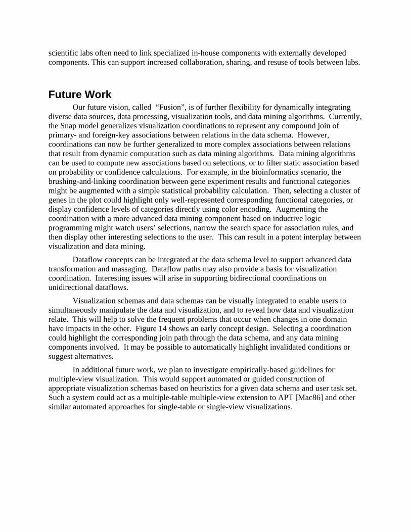
Visualization schemas and data schemas can be visually integrated to enable users to simultaneously manipulate the data and visualization, and to reveal how data and visualization relate. This will help to solve the frequent problems that occur when changes in one domain have impacts in the other. Figure 14 shows an early concept design. Selecting a coordination could highlight the corresponding join path through the data schema, and any data mining components involved. It may be possible to automatically highlight invalidated conditions or suggest alternatives.

In additional future work, we plan to investigate empirically-based guidelines for multiple-view visualization. This would support automated or guided construction of appropriate visualization schemas based on heuristics for a given data schema and user task set. Such a system could act as a multiple-table multiple-view extension to APT [Mac86] and other similar automated approaches for single-table or single-view visualizations.

Figure 14: Concept design for future integrated data schemas and visualization schemas.

Conclusions Snap-Together Visualization supports visualization design in a manner analogous to

relational databases’ support for data design. This enables a significant level of flexibility in composing custom multiple-view visualizations of multiple-table databases. The primary contributions of this work are:

• Theory: The Snap visualization model formalizes multiple-view visualization in terms of the relational data model. An analogy between the primitives and compositional operators of each domain affords a coordinated approach to data design and visualization design.

• User interface: Visualization schemas, a diagrammatic direct-manipulation visual language, are a natural extension to relational data schemas. A wide range of data designers and users can rapidly specify and understand custom visualizations without the need for programming.

• System architecture: The Snap visualization server operates on top of relational database systems. Custom coordinations in multiple-view visualization automatically query the database to support navigation. A component-based mediator dynamically integrates diverse data and external visualization tools from the field. A web-based approach enables simple access and dissemination of custom visualizations.

Due to its basis on common relational database concepts and general multiple-view visualization concepts, this approach is widely applicable in many domains and easily extended with new capabilities such as data mining. A significant level of flexibility is achieved while maintaining usability. This provides data owners with a new ability to rapidly create custom visualizations for data exploration. Construction of typical multiple-view visualizations that

traditionally required significant development effort can now be accomplished dynamically in a few minutes.

Acknowledgements This work was partially supported by funding from the U.S. Bureau of the Census and

Agilent Labs. Thanks to Matt Clement, Umer Farooq, Aniket Prabhune, and Xiaofeng Bao for implementation efforts.

References [AW95] Ahlberg, C., Wistrand, E., “IVEE: An Information Visualization and Exploration Environment”, Proc. IEEE Information Visualization ’95, pp. 66-73, (1995). [ACS96] Aiken, A., Chen, J., Stonebraker, M., Woodruff, A., “Tioga-2: A Direct Manipulation Database Visualization Environment”, Proc, 12th Intl. Conference on Data Engineering, pg. 208-217, (February 1996). [BWK00] Baldonado, M., Woodruff, A., Kuchinsky, A., “Guidelines for Using Multiple Views in Information Visualization”, Proc. Advanced Visual Interfaces, (2000). [BC87] Becker, R., Cleveland, W., “Brushing Scatterplots”, Technometrics, 29(2), pp. 127-142, (1987). [BST00] Robert Bosch, Chris Stolte, Diane Tang, John Gerth, Mendel Rosenblum, and Pat Hanrahan. “Rivet: A Flexible Environment for Computer Systems Visualization”, Computer Graphics 34(1), (February 2000). [CMS99] Card, S., Mackinlay, J., Shneiderman, B. (editors), Readings in Information Visualization: Using Vision to Think, Morgan Kaufmann, (1999). [DRK97] Derthick, M., Roth, S.F., Kolojejchick, J., “Coordinating declarative queries with a direct manipulation data exploration environment”, IEEE Information Visualization Symposium, pp. 65 -72, (1997). [FNP99] Fredrikson, A., North, C., Plaisant, C., Shneiderman, B., "Temporal, Geographical and Categorical Aggregations Viewed through Coordinated Displays: a Case Study with Highway Incident Data", Proc. ACM CIKM '99 Workshop on New Paradigms in Information Visualization and Manipulation, (1999). [GHJ95] Gamma, E., Helm, R., Johnson, R., Vlissides, J., Design Patterns: Elements of Resuable Object-Oriented Software. Addison-Wesley, 1995. [Hae88] Haeberli, P., “ConMan: A Visual Programming Language for Interactive Graphics”, Proc. ACM SigGraph ’88, pp. 103-111, (1988). [HAE99] Healey, C. G., St. Amant, R., and Elhaddad, M. "ViA: A Perceptual Visualization Assistant", Proc. 28th Applied Imagery Pattern Recognition Workshop, pp. 1-11, (1999). [HR02] L.S. Heath and N. Ramakrishnan, “The Emerging Landscape of Bioinformatics Software Systems”, IEEE Computer, Vol. 35, No. 7, pages 41-45, July 2002. [HRS02] Lenwood S. Heath, Naren Ramakrishnan, Ronald R. Sederoff, Ross W. Whetten, Boris I. Chevone, Craig A. Struble, Vincent Y. Jouenne, Dawei Chen, Leonel Merwe van Zyl, and Ruth Grene, "Studying the Functional Genomics of Stress Responses in Loblolly Pine using

the Expresso Microarray Management System," Comparative and Functional Genomics 3, 2002, pp. 226--243. [HWM98] Beth Hetzler, Paul Whitney, Lou Martucci, Jim Thomas. “Multi-faceted Insight Through Interoperable Visual Information Analysis Paradigms”. In Proceedings of IEEE Symposium on Information Visualization, InfoVis '98, October 19-20, 1998. pp.137-144. [ISB95] Isakowitz, T., Stohr, E., Balasubramanian, P., “RMM: a methodology for structured hypermedia design”, Communications of the ACM, 38(8), pp. 34-44, (1995). [IBW97] Philip Isenhour, James "Bo" Begole, Winfield S. Heagy, and Clifford A. Shaffer, "Sieve: A Java-Based Collaborative Visualization Environment," In IEEE Visualization '97, (October 1997). [JBO94] Jacobson, A., Berkin, A., Orton, M., “LinkWinds: interactive scientific data analysis and visualization”, Communications of the ACM, 37(4), pp. 43-52, (April 1994). [KGM02] Allan Kuchinsky, Kathy Graham, David Moh, Michael L. Creech, “Biological Storytelling: A Software Tool for Biological Information Organization Based upon Narrative Structure”, Proc ACM Advanced Visual Interfaces Conference, May 2002. [LCG02] Lee, J.P., Carr, D., Grinstein, G., Kinney, J., Saffer, J., “Visualization for bio- and chem-informatics: the next frontier”, IEEE Computer Graphics and Applications, Sept 2002. [LRB97] Livny, M., Ramakrishnan, R., Beyer, K., Chen, G., Donjerkovic, D., Lawande, S., Myllymaki, J., Wenger, K., “DEVise: integrated querying and visual exploration of large datasets”, Proc. ACM SIGMOD’97, pp. 301-312, (1997). [MWH99] MacEachren, A., M. Wachowicz, D. Haug, R. Edsall, and R. Masters. “Constructing Knowledge from Multivariate Spatiotemporal Data: Integrating Geographic Visualization with Knowledge Discovery in Database Methods”. Inter. J. of Geographic Information Science, 13(4): 311-334. 1999. [Mac86] Mackinlay, J., “Automating the design of graphical presentations of relational information”. ACM Trans. on Graphics 5(2), 111-141, (1986). [NSF97] National Science Foundation, “More than Screen Deep: Toward an Every-Citizen Interface to the Nation's Information Infrastructure”, National Academy Press, Washington, D.C., 1997. [NS00] North, C., Shneiderman, B., “Snap-Together Visualization: Can Users Construct and Operate Coordinated Views?”, Intl. Journal of Human Computer Studies, Academic Press, 53(5), pg. 715-739, (November 2000). [Nor01] North, C., “Multiple Views and Tight Coupling in Visualization: A Language, Taxonomy, and System”, Proc. CSREA CISST 2001 Workshop on Fundamental Issues in Visualization, pp. 626-632, (2001). [PCS95] Plaisant, C., Carr, D., Shneiderman, B., “Image browsers: taxonomy, guidelines, and informal specifications”, IEEE Software, 12(2), pp. 21-32, (March 1995). [RCK97] Roth, S., Chuah, M., Kerpedjiev, S., Kolojejchick, J., Lucas, P., “Towards an Information Visualization Workspace: Combining Multiple Means of Expression”, Human-Computer Interaction Journal, 12(1&2), pp. 131-185, (1997). [SFT01] Siepel, A., Farmer, A., Tolopko, A., Zhuang, M., Nedes, P., Beavis, W., Sobral, B., “ISYS: a decentralized, component-based approach to the integration of heterogeneous bioinformatics resources”, Bioinformatics, 17(1), pp. 83-94, (2001). [SG96] Shaw, M. and Garlan, D., Software Architecture: Perspectives on an Emerging Discipline. Prentice Hall, Inc. (1996).

[Shn96] Shneiderman, B., “The Eyes Have It: A Task by Data Type Taxonomy of Information Visualizations”, Proc. IEEE Visual Languages '96, pp.336-343, (1996). [Shn01] Shneiderman, B., “Supporting Creativity with Advanced Information-Abundant User Interfaces”, in Human-Centered Computing, Online Communities, and Virtual Environments, Springer-Verlag, pp. 469-480, (2001). [Sun02] Sun Microsystems, Inc. Java 2 Platform, Standard Edition, v 1.4.0 API Specification [WWW document] http://java.sun.com/j2se/1.4/docs/api/ (accessed 30 August 2002). [TG02] Takatsuka, M. and Gahegan, M "GeoVISTA Studio: A Codeless Visual Programming Environment For Geoscientific Data Analysis and Visualization", The Journal of Computers & Geosciences, (2002). [UFK89] Upson, C, Faulhaber, T, Kamins, D, Laidlaw D, Schlegel D, Vroom J, Gurwitz, R, van Dam, A, “The Application Visualization System: A Computational Environment for Scientific Visualization”, IEEE Computer Graphics and Applications, pp. 30-42, (July 1989). [WL02] Weaver, C., Livney, M., “Metavisualization of Dynamic Queries”, Posters Compendium, IEEE InfoVis 2002 Symposium, pg. 54-55, (2002).