Vision-based techniques for following paths with mobile robots.
124
Sapienza Universit ` a di Roma Dipartimento di Informatica e Sistemistica Doctoral Thesis in Systems Engineering ING-INF/04 XX Ciclo Vision-based techniques for following paths with mobile robots Andrea Cherubini Advisor Coordinator Prof. Giuseppe Oriolo Prof. Carlo Bruni December 2007
Transcript of Vision-based techniques for following paths with mobile robots.

Sapienza Universita di Roma
Dipartimento di Informatica e Sistemistica
Doctoral Thesis in
Systems Engineering
ING-INF/04
XX Ciclo
Vision-based techniques for following
paths with mobile robots
Andrea Cherubini
Advisor Coordinator
Prof. Giuseppe Oriolo Prof. Carlo Bruni
December 2007

Sapienza Universita di Roma
Dipartimento di Informatica e Sistemistica
Doctoral Thesis in
Systems Engineering
ING-INF/04
XX Ciclo
Vision-based techniques for following
paths with mobile robots
Andrea Cherubini
Advisor Coordinator
Prof. Giuseppe Oriolo Prof. Carlo Bruni
December 2007

to my family

Abstract
In this thesis, we focus on the use of robot vision sensors to solve the path following
problem, which in recent years, has been a popular target for engaged researchers
around the world. Initially, we shall present the working assumptions that we used,
along with the relevant kinematic and sensor models of interest, and with the main
characteristics of visual servoing. Then, we shall attempt to survey the research
carried out in the field of vision-based path following. Following this, we shall present
two schemes that we designed for reaching and following paths. These respectively
involve nonholonomic robots and legged robots. Both schemes require only some visible
path features, along with a coarse camera model, and, under certain conditions, may
guarantee convergence even when the initial error is large. The first control scheme is
designed to enable nonholonomic mobile robots with a fixed pinhole camera to reach and
follow a continuous path on the ground. Two visual servoing controllers (position-based
and image-based) have been designed. For both controllers, a Lyapunov-based stability
analysis has been carried out. The performance of the two controllers is validated and
compared by simulations and experiments on a car-like robot. The second control
scheme is more application-oriented than the first and has been used in ASPICE,
an assistive robotics project, to enable the autonomous navigation of a legged robot
equipped with an actuated pinhole camera. The robot uses a position-based visual
servoing controller to follow artificial paths on the ground, and travel to some required
destinations. Apart from being a useful testing-ground for this path following scheme,
the ASPICE project has also permitted the development of many other aspects in the
field of assistive robotics. These shall be outlined at the end of the thesis.
i

Acknowledgments
In these few lines, I want to thank all the people that have been with me in these
wonderful three years of research. Firstly, I am grateful to my advisor Giuseppe Oriolo
for his help and support throughout the PhD course. I also want to thank all the guys
at LabRob: Antonio, Ciccio, Leonardo, Luigi, Massimo, and Paolo for coffee et al.
breaks, as well as for fundamental work-related hints and tips. I am also grateful to
Professors Nardi and Iocchi, and all the SPQR team (particularly Vittorio and Luca)
for the nice moments spent attempting to make quadruped roman robots play football
better than biped flesh-and-blood brazilian. Thanks also to Dr. Francois Chaumette,
for his fundamental support during my 8 month stay in Rennes, and to all the rest
of the Lagadic gang for making Breizh feel like home/Rome. I also thank the team
at Laboratorio di Neurofisiopatologia at Fondazione Santa Lucia, for the development
of ASPICE, and Michael Greech and Romeo Tatsambon, for being excellent revisors
of this thesis. Finally, given my mediterranean nature, I wish to thank my awesome
family, to whom I dedicate this work.
ii

Contents
Introduction 1
Notations 4
1 Working assumptions 6
1.1 The path following problem . . . . . . . . . . . . . . . . . . . . . . . . . 6
1.2 Kinematic model and motion control . . . . . . . . . . . . . . . . . . . . 8
1.2.1 Wheeled robots . . . . . . . . . . . . . . . . . . . . . . . . . . . . 9
1.2.2 Legged robots . . . . . . . . . . . . . . . . . . . . . . . . . . . . . 15
1.3 Central catadioptric vision sensor model . . . . . . . . . . . . . . . . . . 23
1.3.1 Definitions . . . . . . . . . . . . . . . . . . . . . . . . . . . . . . 23
1.3.2 Extrinsic parameters . . . . . . . . . . . . . . . . . . . . . . . . . 25
1.3.3 Intrinsic parameters . . . . . . . . . . . . . . . . . . . . . . . . . 26
1.4 Visual servoing . . . . . . . . . . . . . . . . . . . . . . . . . . . . . . . . 27
1.4.1 Outline . . . . . . . . . . . . . . . . . . . . . . . . . . . . . . . . 28
1.4.2 Image-based visual servoing . . . . . . . . . . . . . . . . . . . . . 30
1.4.3 Position-based visual servoing . . . . . . . . . . . . . . . . . . . . 30
2 Related work 31
2.1 Sensor-less path following . . . . . . . . . . . . . . . . . . . . . . . . . . 31
2.2 Vision-based path following . . . . . . . . . . . . . . . . . . . . . . . . . 33
3 Vision-based path following for a nonholonomic mobile robot with
fixed pinhole camera 36
3.1 Definitions . . . . . . . . . . . . . . . . . . . . . . . . . . . . . . . . . . . 37
iii

3.2 Control design . . . . . . . . . . . . . . . . . . . . . . . . . . . . . . . . 39
3.2.1 Deriving the path 3D features . . . . . . . . . . . . . . . . . . . . 40
3.2.2 Position-based path follower . . . . . . . . . . . . . . . . . . . . . 41
3.2.3 Image-based path follower . . . . . . . . . . . . . . . . . . . . . . 43
3.3 Stability analysis . . . . . . . . . . . . . . . . . . . . . . . . . . . . . . . 46
3.4 Experimental setup . . . . . . . . . . . . . . . . . . . . . . . . . . . . . . 47
3.5 Simulations . . . . . . . . . . . . . . . . . . . . . . . . . . . . . . . . . . 48
3.6 Experiments . . . . . . . . . . . . . . . . . . . . . . . . . . . . . . . . . . 51
3.6.1 Position-based experiments . . . . . . . . . . . . . . . . . . . . . 55
3.6.2 Image-based experiments . . . . . . . . . . . . . . . . . . . . . . 60
3.7 Conclusions and future work . . . . . . . . . . . . . . . . . . . . . . . . 65
4 Vision-based path following for a legged robot with actuated pinhole
camera and its application in the ASPICE project 67
4.1 The ASPICE project . . . . . . . . . . . . . . . . . . . . . . . . . . . . . 68
4.1.1 Overview . . . . . . . . . . . . . . . . . . . . . . . . . . . . . . . 68
4.1.2 The robot driver . . . . . . . . . . . . . . . . . . . . . . . . . . . 70
4.2 The robot platform: AIBO . . . . . . . . . . . . . . . . . . . . . . . . . 72
4.3 Primitives . . . . . . . . . . . . . . . . . . . . . . . . . . . . . . . . . . . 74
4.3.1 Perception primitives . . . . . . . . . . . . . . . . . . . . . . . . . 74
4.3.2 Motion primitives . . . . . . . . . . . . . . . . . . . . . . . . . . 80
4.4 Visual path following scheme . . . . . . . . . . . . . . . . . . . . . . . . 84
4.5 Experiments . . . . . . . . . . . . . . . . . . . . . . . . . . . . . . . . . . 86
4.6 Conclusions . . . . . . . . . . . . . . . . . . . . . . . . . . . . . . . . . . 92
5 Other aspects of the ASPICE project 93
5.1 Occupancy grid generator . . . . . . . . . . . . . . . . . . . . . . . . . . 94
5.2 Single step navigation mode . . . . . . . . . . . . . . . . . . . . . . . . . 96
5.3 Semi-autonomous navigation mode . . . . . . . . . . . . . . . . . . . . . 97
5.4 Brain-Computer Interface . . . . . . . . . . . . . . . . . . . . . . . . . . 98
5.5 Other robot driver features . . . . . . . . . . . . . . . . . . . . . . . . . 100
5.5.1 Video feedback . . . . . . . . . . . . . . . . . . . . . . . . . . . . 101
5.5.2 Vocal request interface . . . . . . . . . . . . . . . . . . . . . . . . 101
5.5.3 Head control interface . . . . . . . . . . . . . . . . . . . . . . . . 102
iv

5.5.4 Walking gait . . . . . . . . . . . . . . . . . . . . . . . . . . . . . 102
5.6 Simulations and experiments . . . . . . . . . . . . . . . . . . . . . . . . 103
5.7 Clinical validation . . . . . . . . . . . . . . . . . . . . . . . . . . . . . . 105
Bibliography 107
v

Introduction
Mobile land robots require a high degree of autonomy in their operations; a requirement
which calls for accurate and efficient position determination and verification in order
to guarantee safe navigation in different environments. In many recent works, this
has been done by processing information from the robot vision sensors [74]. In this
thesis, we shall present the case for utilizing the robot vision sensors for solving the
path following (PF) problem, which in recent years, has engaged numerous researchers
around the world. In the PF task, the controller must stabilize to zero some path error
function, indicating the position of the robot with respect to the path [16, 18]. The
path to be followed is defined as a continuous curve on the ground. In some works,
assumptions on the shape, curvature, and differential properties of the path have been
introduced, for focusing on specific applications and control designs.
Much work dealing with the design of visual controllers for the tracking of reference
paths has been carried out in the field of autonomous vehicle guidance [4]. In fact, some
of the earliest Automated Guided Vehicles (AGVs) were line following mobile robots.
They could follow a painted or embedded visual straight line on a floor or ceiling. Later,
visual servoing techniques [8] (which were originally developed for manipulator arms
with vision sensors mounted at their end-effector [23]) provided excellent results in the
field of mobile robot visual navigation. Visual servoing systems are classified in two
major categories: position-based control and image-based control. Position-based visual
servoing techniques can be used whenever the visual navigation system relies on the
geometry of the environment and on other metrical information. The feedback law is
computed by reducing errors in estimated pose space. For instance, in the field of PF,
many works address the problem by zeroing the lateral displacement and orientation
error of the vehicle at a lookahead distance [49]. Alternative visual navigation systems
use no explicit representation of the environment in which navigation takes place. In
1

2
this case, image-based visual servoing techniques can be used to control the robot: an
error signal measured directly in the image is mapped to actuator commands. The
image-based approach reduces computational delay, eliminates the necessity for image
interpretation, and errors due to camera modeling and calibration [7, 13].
In this thesis, we present two vision-based approaches for path following with
mobile robots. The two approaches have respectively been designed and assessed on
nonholonomic and on legged robots. In both cases, a pinhole camera is used. However,
in the first approach, the camera is fixed, whereas in the second it is actuated. Both
approaches require only some visible path features, along with a coarse camera model,
and, under certain conditions, guarantee convergence even when the initial error is
large.
The first approach is designed to enable nonholonomic mobile robots with a fixed
pinhole camera to reach and follow a continuous path on the ground. In this regard, two
controllers (position-based and image-based) have been designed. For both controllers,
a Lyapunov-based stability analysis is carried out. The performance of the two
controllers is validated and compared by simulations and experiments on a car-like
robot equipped with a pinhole camera. To our knowledge, this is the first time that
an extensive comparison between position-based and image-based visual servoing for
nonholonomic mobile robot navigation is carried out.
The second approach is position-based and more application-oriented than the first
approach. It has been used in ASPICE, an assistive robotics project, to enable the
autonomous navigation of a legged robot in an indoor environment [10]. The robot
uses a position-based visual servoing control scheme to follow artificial paths on the
ground, and to travel to required targets in the environment. The paths are formed by
straight white lines connected by black and white coded square crossings. The approach
has been designed in relation to the ASPICE system requirements.
This thesis is organized as follows. In the first chapter we will present the working
assumptions that we used for tackling the path following problem. The PF problem is
defined, along with the relevant kinematic and sensor models. The main characteristics
of visual servoing are also outlined. In the second chapter, we attempt to survey the
research carried out in the field of vision-based path following. In Chapter 3, we present
two path following (PF) control schemes which enable nonholonomic mobile robots with
a fixed pinhole camera to reach and follow a continuous path on the ground. The design,

3
stability analysis and experimental validation of the two controllers are described. In
the fourth chapter, we present the position-based visual path following controller that
has been used in the ASPICE project. The image processing aspects and the motion
controllers and experimental results of this work, are also presented. The ASPICE
project has both provided a useful testbed for this path following scheme and also
allowed the development of many other aspects in the field of assistive robotics. These
numerous aspects are described in Chapter 5.

Notations
The following notations will be used throughout this thesis.
W the robot workspace. It is modeled with the Euclidean space IR2.
FW the world reference frame, with origin W and axes x′, y′, z′.
R the robot. It is the compact subset of W occupied by the robot.
r the robot reference point. It is the point on the robot, with FWcoordinates [x′ y′]T , that should track the path.
θ the robot orientation in FW .
FR the robot reference frame, with origin r and axes x, y, z.
p the path. It is represented by a continuous curve in the workspace W.
n the number of robot generalized coordinates; in this work, n = 3.
m the number of control inputs applied to the robot; m ≤ n.
q the robot configuration: q = [x′ y′ θ]T .
u the control applied to the robot.
d the path desired reference point. It is the point with FW coordinates
[x′d y′d]
T that should be tracked by r.
θd the orientation of the path tangent at d in FW .
cd the path curvature at d.
qd the robot desired reference configuration: qd = [x′d y′d θd]
T .
FP the path reference frame, with origin d and axes xd, yd, zd.
et the tangential path error.
en the normal path error.
eθ the orientation path error.
C the principal projection center of the visual sensor.
4

5
FC the camera reference frame, with origin C and axes xc, yc, zc.
I the image center, or principal point.
FI the image reference frame, with origin I and axes X and Y .
D the projection of d on the image plane, with FI coordinates [X Y ]T .
P the projection of the path p on the image plane.
f the focal length in the perspective camera model.
(XI YI) the principal point error in the perspective camera model.
(lX lY ) the metric size of the pixel in the perspective camera model.

Chapter 1
Working assumptions
The object of this chapter is to present the assumptions used in this thesis. Firstly,
we will formally introduce the path following problem for mobile ground robots.
Afterwards, the kinematic models of the two classes of robots (i.e., wheeled and legged)
that have been used in the experimental part of the thesis are presented. Regarding
wheeled robots, the main issues of nonholonomic motion control are discussed, and the
two most common models (unicycle and car-like) are outlined. As to legged robots, the
gait control algorithm (kinematic parameterized trot) which has been utilized in the
thesis is explained in the second section. In the third section, we present the general
visual sensor model (the central catadioptric model) which applies to all the systems
that will be cited in the survey of Chapter 2, as well as to the systems used in our work.
Finally, we recall the main concepts of visual servo control i.e., robot motion control
using computer vision data in the servo loop.
1.1 The path following problem
Let us consider a ground mobile robot R. We assume that the workspace where the
robot moves is planar (i.e, W = IR2) and we define FW (W,x′, y′, z′) the world frame
(shown in Fig. 1.1). The path p to be followed is represented by a continuous curve
in the workspace W. In some cases, a following direction can be associated to the
path. We assume that the robot has a symmetric plane (the sagittal plane) orthogonal
to W, and is forward oriented. We name r the robot reference point, i.e., the point
on the robot sagittal plane that should track the path, and FR (r, x, y, z) the robot
6

1.1. The path following problem 7
pθd(ε)
x’
y’
z’
W
d (x’d(ε), y’d(ε))
y
z
x
yd
xd
zd
et
θ(ε)r (x’(ε), y’(ε))
eθ(ε)en
Figure 1.1: Path following relevant variables.
frame. The y axis is the intersection line between the sagittal plane and W, oriented
in the robot forward orientation, and the x axis pertains to W and is oriented to the
right of the robot. The robot state coordinates (i.e., the robot generalized coordinates)
are q (ε) = [x′ (ε) y′ (ε) θ (ε)]T , where ε ∈ IR is a parameter with infinite domain,
[x′ (ε) y′ (ε)]T represent the Cartesian position of r in FW , and θ (ε) ∈ ]−π,+π] is the
orientation of the robot frame y axis with respect to the world frame x′ axis (positive
counterclockwise). Thus, the dimension of the robot configuration space is n = 3.
Recalling [18], the objective of PF is to drive the error e (ε) = q (ε) − qd (ε) =[ex′ (ε) ey′ (ε) eθ (ε)
]T to a desired error e (ε). Usually, e (ε) is set to zero. The vector
qd (ε) = [x′d (ε) y′d (ε) θd (ε)]T defines a desired reference configuration, such that the
point d (ε) ∈ W of coordinates [x′d (ε) y′d (ε)]T belongs to p, and θd (ε) is the desired
robot orientation. If the tangent of p at d (ε) exists, and the path has a following
direction (as in Fig. 1.1), θd (ε) is the orientation of the tangent in FW considering the
direction. Otherwise, θd (ε) is defined by the PF specifications. If it exists, the path
curvature at d is noted cd. If there exist some constraints in the robot model (e.g.,
nonholonomic constraints), the path must be feasible with respect to such constraints,
i.e. qd (ε) must attend to these constraints. Moreover, we note u ∈ IRm the applied
control, which usually corresponds to the robot velocities; m ≤ n is the number of
control inputs. The reference path cannot contain points where the tracking control

1.2. Kinematic model and motion control 8
ud ≡ 0.
The PF task is often formalized by projecting the FW errors[ex′ (ε) ey′ (ε) eθ (ε)
]T
to the path frame FP (d, xd, yd, zd), shown in Fig. 3.1(a). Frame FP is linked to the
path at d, with zd parallel to z, yd coincident with the path tangent at d in the following
direction, and xd completing the right-handed frame. The path error in FP consists
of the tangent error et (i.e., the error projection on yd), the normal error en (i.e., the
error projection on xd), and the orientation error eθ, i.e.:et = ex′ cos θd + ey′ sin θd
en = ex′ sin θd − ey′ cos θd
eθ = θ − θd
(1.1)
With this formalism, the PF task consists of driving error [et (ε) en (ε) eθ (ε)]T to a
desired error [et en eθ]T . In the remainder of the thesis the desired error [et en eθ]
T is
set to [0 0 0]T , unless it is otherwise specified.
In opposition to the trajectory tracking problem, where the desired trajectory
evolution is determined by a rigid law like ε = ε (t) (i.e., parameter ε is associated
to the time t), in PF we can choose the relationship that defines the desired reference
configuration qd (ε) that the robot should track. We call such relationship path following
constraint. The path following constraint eliminates one of the three error coordinates.
Details regarding the choice of the projecting function used to define qd (ε) in this work
will be given later. In most works, the path following constraint is chosen by defining
d as the normal projection of r on p, i.e., by choosing d such that et =const = 0.
Finally, in PF, the robot should move at all times independently from qd (ε) (clearly,
a control law must concurrently ensure convergence to the path). Thus, a motion must
be imposed to the robot to guarantee that it moves or progresses. This is the motion
exigency condition defined in [18].
1.2 Kinematic model and motion control
In this section, we will focus on the kinematic model and motion control of the two
classes of robots that have been used in the experimental part of this thesis: wheeled
and legged robots.

1.2. Kinematic model and motion control 9
1.2.1 Wheeled robots
Motivations
Wheels are ubiquitous in human designed systems. As might be expected, the
vast majority of robots move on wheels. Wheeled mobile robots (WMRs) are
increasingly present in industrial and service robotics, particularly when flexible motion
capabilities are required on reasonably smooth grounds and surfaces. Several mobility
configurations (wheel number, type, location and actuation, single-body or multi-body
vehicle structure) can be found in the applications. The most common configurations
for single-body robots are differential drive and synchro drive (both kinematically
equivalent to a unicycle), tricycle or car-like drive, and omnidirectional steering [53].
Numerous wheeled robots were developed at the NASA Jet Propulsion Laboratory
(JPL) [3] in the 1970s, including various rovers for planetary exploration. These
developments culminated in the landing of the Sojourner robot on Mars in 2001. Today
the most common research robots are wheeled.
Beyond their relevance in applications, the problem of autonomous motion planning
and control of WMRs has attracted the interest of researchers in view of its theoretical
challenges. In particular, these systems are a typical example of nonholonomic
mechanisms due to the perfect rolling constraints on the wheel motion (no longitudinal
or lateral slipping).
The nonholonomic constraint
The notion of nonholonomy (borrowed from Mechanics) appears in literature on robot
motion planning because of the problem of car parking which the pioneering mobile
robot navigation systems had not managed to solve [51]. Nonholonomic systems are
characterized by constraint equations involving the time derivatives of the system
configuration variables. These equations are non integrable; they typically arise when
the system has less controls than configuration variables (m < n). For instance, a
car-like robot has m = 2 controls (linear and angular velocities) while it moves in a
configuration space of dimension n = 3. As a consequence, a path in the configuration
space does not necessarily correspond to a feasible path for the system. This explains
why the purely geometrical techniques developed in motion planning for holonomic
systems do not apply directly to nonholonomic systems.

1.2. Kinematic model and motion control 10
While the constraints due to the obstacles are expressed directly in the manifold of
configurations, nonholonomic constraints deal with the tangent space of such manifold.
In the presence of a link between the robot parameters and their derivatives, the first
question to be addressed is: does such a link reduce the accessible configuration space?
This question may be answered by studying the structure of the distribution spanned
by the Lie algebra of system controls. Thus, even in the absence of obstacles, planning
nonholonomic motions is not an easy task. Today there is no general algorithm which
enables one to plan motions for nonholonomic systems, in a way that guarantees that
the system reaches exactly a destination. The only existing results are for approximate
methods (which guarantee only that the system reaches a neighborhood of the goal)
or exact methods for special classes of systems. Fortunately, these classes cover almost
all the existing mobile robots.
In the absence of workspace obstacles, the basic motion tasks assigned to a WMR
may be reduced to moving between two robot postures and to the following of a given
trajectory. From a control viewpoint, the peculiar nature of nonholonomic kinematics
makes the second problem easier than the first. Indeed, it is a well known fact that
feedback stabilization at a given posture cannot be achieved via smooth time-invariant
control [5]. This indicates that the problem is truly nonlinear; linear control is
ineffective, even locally, and innovative design techniques are required.
Here, we will briefly outline the theory of Pfaffian nonholonomic systems. Further
details can be found in [51] and [53]. Recalling (Sect. 1.1) that q denotes the n-vector of
robot generalized coordinates, Pfaffian nonholonomic systems are characterized by the
presence of n −m non-integrable differential constraints on the generalized velocities
of the form:
A (q) q = 0 (1.2)
with A (q) matrix of size (n−m) × n. For a WMR, these Pfaffian constraints arise
from the rolling without slipping condition for the wheels. All feasible instantaneous
motions can then be generated as:
q = G (q)u (1.3)
for some control input: u(t) ∈ IRm. The columns gi, i = 1, . . . ,m of the n × m
matrix G (q) are chosen so as to span the null-space of matrix A (q). Different choices
are possible for G, according to the physical interpretation that may be given to the
1.2. Kinematic model and motion control 11
x’
y’
z’
W
y
u1
xθ
u2z
r
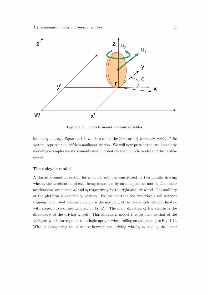
Figure 1.2: Unicycle model relevant variables.
inputs u1, . . . , um. Equation 1.3, which is called the (first-order) kinematic model of the
system, represents a driftless nonlinear system. We will now present the two kinematic
modeling examples most commonly used in robotics: the unicycle model and the car-like
model.
The unicycle model
A classic locomotion system for a mobile robot is constituted by two parallel driving
wheels, the acceleration of each being controlled by an independent motor. The linear
accelerations are noted: ar and al respectively for the right and left wheel. The stability
of the platform is ensured by castors. We assume that the two wheels roll without
slipping. The robot reference point r is the midpoint of the two wheels; its coordinates,
with respect to FW are denoted by (x′, y′). The main direction of the vehicle is the
direction θ of the driving wheels. This kinematic model is equivalent to that of the
unicycle, which corresponds to a single upright wheel rolling on the plane (see Fig. 1.2).
With w designating the distance between the driving wheels, vr and vl the linear
1.2. Kinematic model and motion control 12
velocities respectively of the right and left wheel, the kinematic model is:
x′
y′
θ
vr
vl
=
vr+vl2 cos θ
vr+vl2 sin θvr−vl
w
0
0
+
0
0
0
1
0
ar +
0
0
0
0
1
al (1.4)
Clearly, ar, al, vr and vl are bounded; these bounds appear at this level as ’obstacles’
to avoid in the 5-dimensional manifold. By setting: u1 = vr+vl2 and u2 = vr−vl
l
(respectively, the linear velocity of the wheel and its angular velocity around the vertical
axis), we get the kinematic model, which is expressed as the following 3-dimensional
system: x′
y′
θ
= g1 (q)u1 + g2 (q)u2 =
cos θ
sin θ
0
u1 +
0
0
1
u2 (1.5)
where the generalized coordinates are q = [x′ y′ θ]T ∈ IR2 × SO1 (n = 3), and u1 and
u2 are the control inputs (m = 2). The bounds on vl and vr induce bounds u1,max and
u2,max on the new controls u1 and u2. System (1.5) is symmetric without drift, and
displays a number of structural control properties, most of which actually hold for the
general nonholonomic kinematic model (1.3).
The constraint that the wheel cannot slip in the lateral direction is given in the
form (1.2) as:
A (q) q = [sin θ − cos θ 0] q = x′ sin θ − y′ cos θ = 0
As expected, g1 and g2 span the null-space of matrix A (q).
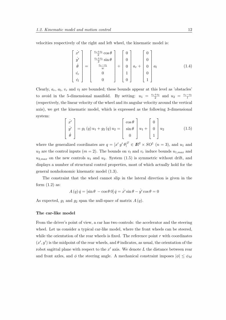
The car-like model
From the driver’s point of view, a car has two controls: the accelerator and the steering
wheel. Let us consider a typical car-like model, where the front wheels can be steered,
while the orientation of the rear wheels is fixed. The reference point r with coordinates
(x′, y′) is the midpoint of the rear wheels, and θ indicates, as usual, the orientation of the
robot sagittal plane with respect to the x′ axis. We denote L the distance between rear
and front axles, and φ the steering angle. A mechanical constraint imposes |φ| ≤ φM

1.2. Kinematic model and motion control 13
x’
y’
W
y
x
θr
z’
z
ϕ
x’f
y’fL
Figure 1.3: Car-like model relevant variables.
and, consequently, a minimum turning radius. For simplicity, we assume that the
two wheels on each axis (front and rear) collapse into a single wheel located at the
midpoint of the axis (bicycle model). The generalized coordinates are q = [x′ y′ θ φ]T ∈IR2 × SO1 × [−φM , φM ] (n = 4). These variables are shown in Fig. 1.3.
The system is subject to two nonholonomic constraints, one for each wheel:
x′ sin θ − y′ cos θ = 0
x′f sin (θ + φ)− y′f cos (θ + φ) = 0(x′f , y
′f
)being the position of the front-axle midpoint. By using the rigid-body
constraint:x′f = x′ + L cos θ
y′f = y′ + L sin θ
the second kinematic constraint becomes:
x′ sin (θ + φ)− y′ cos (θ + φ)− θL cosφ = 0
1.2. Kinematic model and motion control 14
Hence, the constraint matrix is:
A (q) =
sin θ − cos θ 0 0
sin (θ + φ) − cos (θ + φ) −L cosφ 0
and has constant rank 2. Its null-space is two-dimensional, and all the admissible
generalized velocities are obtained as:x′
y′
θ
φ
=
cos θ cosφ
sin θ cosφsin φ
L
0
u1 +
0
0
0
1
u2 (1.6)
Since the front wheel can be steered, we set u2 = φ, (φ is the steering velocity input).
The expression of u1 depends on the location of the driving input. If the car has
front-wheel driving, i.e., front wheel velocity as control input u1, the control system
becomes: x′
y′
θ
φ
=
cos θ cosφ
sin θ cosφsin φ
L
0
u1 +
0
0
0
1
u2 (1.7)
The control inputs u1 and u2 are respectively the front wheel velocity and the steering
velocity.
If the car has rear-wheel driving, i.e., rear wheel velocity as control input u1 , we
have: x′
y′
θ
φ
=
cos θ
sin θtan φ
L
0
u1 +
0
0
0
1
u2 (1.8)
The control inputs u1 and u2 are respectively the rear wheel velocity and the steering
velocity. Note that in (1.8), there is a control singularity at φ = ±π2 , where the first
vector field blows out. This corresponds to the rear-wheel drive car becoming jammed
when the front wheel is normal to the longitudinal axis of the car body. Instead,
this singularity does not occur for the front-wheel drive car (1.7), which in the same
situation may still pivot about its rear-axle midpoint.
1.2. Kinematic model and motion control 15
By setting u2 = u1 tan φL in (1.8), we get a 3-dimensional control system:
x′
y′
θ
=
cos θ
sin θ
0
u1 +
0
0
1
u2 (1.9)
The control inputs u1 and u2 are respectively the rear wheel velocity and the robot
angular velocity with respect to r. This representation of the car-like model is consistent
with the definitions of Sect. 1.1, since the robot generalized coordinates become: q =
[x′ y′ θ]T ∈ IR2×SO1 (n = 4). Equation (1.9) can also represent the front-wheel driving
by using u1 cosφ as first control input, and u1 sin φL as second control input. System (1.9)
is identical to the unicycle kinematic model (1.5). By construction the values of u1
and u2 are bounded. The main difference lies on the admissible control domains,
since in (1.9) the constraints on u1 and u2 are no longer independent. Moreover, the
instantaneous applicable curvature of the car must be smaller than:
cM =tanφM
L(1.10)
In practice, the control inputs in (1.9) must verify:∣∣∣∣u2
u1
∣∣∣∣ < cM (1.11)
There is no such bound for the unicycle instantaneous applicable curvature.
1.2.2 Legged robots
Motivations
Walking on legs is particularly significant as a mode of locomotion in robotics.
Beginning with the automatons built in the nineteenth century, people have been
fascinated by legged machines, especially when they display some autonomy. Aside
from the sheer thrill of creating robots that actually run, there are two serious reasons
for exploring the use of legs for locomotion.
One reason is mobility: there is a need for vehicles that can travel in difficult terrains
where wheeled vehicles would not be able to get. Wheels excel on prepared surfaces
such as rails and roads, but perform poorly wherever the terrain is soft or uneven.
Because of these limitations, only about half of the earth’s landmass is accessible to

1.2. Kinematic model and motion control 16
existing wheeled and tracked vehicles, whereas a much greater area can be reached
by animals on foot [65]. Legs provide better mobility in rough terrain since they can
use isolated footholds that optimize support and traction, whereas a wheel requires
a continuous path of support. As a consequence, a legged robot can choose among
the best footholds in the reachable terrain; a wheeled vehicle must plunge into the
worst terrain. Another advantage of legs is that they provide an active suspension that
decouples the body trajectory from the path trajectory. The payload is free to travel
smoothly despite pronounced variations in the terrain. A legged system can also step
over obstacles. In principle, the performance of legged vehicles can, to a great extent,
be independent of the detailed roughness of the ground.
Another reason for exploring legged machines is to gain a better understanding of
human and animal locomotion. Despite the skill we apply in using our own legs for
locomotion, we are still at a primitive stage in understanding the control principles
that underlie walking and running. The concrete theories and algorithms developed
to design legged robots can guide biological research by suggesting specific models for
experimental testing and verification. This sort of interdisciplinary approach is already
becoming popular in other areas where biology and robotics have a common ground,
such as vision, speech, and manipulation.
In this work, we shall focus uniquely on robots with Nl ≥ 4 legs. In the remainder
of this section, we summarize some basic principles of legged locomotion, review some
works in the area of legged locomotion, and present the locomotion control algorithm
(kinematic parameterized trot) which has been utilized in the thesis.
Motion control
From a kinematic viewpoint, legged robots can be considered omnidirectional, i.e.,
m = 3 control inputs can be independently specified. Usually, these control inputs are
the absolute velocities applied in the robot reference point r: forward u1 in the y axis
direction, lateral u2 in the x axis direction, and angular u3 around the z axis.
Stable walking requires the generation of systematic periodic sequences of leg
movements at various speeds of progression [3]. At slow velocities, stable walking
is characterized by static stability: the center of mass of the body remains within the
polygon of support formed by the legs in contact with the ground. During motion,
the support forces of the legs, momentum and inertial forces are summed to produce

1.2. Kinematic model and motion control 17
dynamic stability. In both humans and animals, each leg alternates between stance
(the time its end point is in contact with the ground), and swing (the time it spends in
forward motion). To change speed, animals exhibit a variety of gaits. It now appears
that the switch from one gait pattern to another occurs, at least in part, by means of
mechanisms that attempt to keep the muscular forces and joint loads in the leg within
particular limits.
In practice, the major task in enabling a legged robot to walk is foot trajectory
generation. This can be based either on the dynamic or on the kinematic model of
the robot. A short overview of some approaches used to generate stable legged gaits
is presented in the next paragraph. Afterwards, we focus on the approach used in this
thesis.
Related work
Various approaches for generating stable walking have been explored in literature.
In [61], a graph search method is proposed to generate the gait for a quadruped
robot. To determine if a node in the graph is promising or not, each node is endowed
with an evaluating function that incorporates the robot configuration, the distance
the robot traveled, and the stability margin of a particular configuration. The search
method exhibits promising features under adverse terrain conditions. The generated
gait is: periodic when the terrain is flat, without obstacles, and free in the presence of
obstacles.
Goodwine and Burdick [32] present a general trajectory generation scheme for legged
robots. The scheme is based on an extension of a nonlinear trajectory generation
algorithm for smooth systems (e.g., wheeled robots) to the legged case, where the
relevant mechanics are not smooth. The extension utilizes a stratification model of the
legged robot configuration spaces. Experiments indicate that the approach is simple to
apply, independently from the number of legs.
Other researchers have successfully applied machine learning techniques for
generating stable legged gaits. Krasny and Orin have used an evolutionary algorithm to
generate an energy-efficient, natural, and unconstrained gallop for a quadrupedal robot
with articulated legs, asymmetric mass distribution, and compliant legs [50]. In [75],
a distributed neural architecture for the general control of robots has been applied for
walking gait generation on a Sony AIBO robot. Genetic algorithms have been used to

1.2. Kinematic model and motion control 18
evolve from scratch the walking gaits of eight-legged [31] and hexapod robots [62].
An important testbed for developing and improving motion control schemes for
legged robots has been the annual RoboCup Four-Legged league1. RoboCup is “an
attempt to promote AI and robotics research by providing a common task for evaluation
of various theories, algorithms, and agent architectures”; the ultimate goal is, “to
build a team of robot soccer players, which can beat a human World Cup champion
team” [47]. The Robocup Four-Legged League prescribes the use of a standard robot
platform: Sony AIBO. No hardware changes are permitted. In particular, since speed is
a major key to winning robot soccer games, in the past years, the Robocup Four-Legged
League has strongly fostered research in the field of legged motion control.
The kinematic parameterized trot walk approach
Here, we will illustrate the walking gait control scheme implemented in this thesis for
following paths with a legged robot. The scheme is inspired by the parameterized walk
approach developed by Hengst and others [37], which is widely used in the legged robot
community. In particular, we will hereby describe the version implemented on Sony
AIBO four-legged robots in [24], which inspired our control scheme. The algorithm can
be easily extended for gait generation on other platforms, including robots with more
than four legs (Nl > 4). The approach presented is based on the robot kinematic model,
i.e. dynamic effects are not taken into account. This choice is appropriate whenever
a complete dynamic model for the robot is unavailable, or whenever the on-board
resources are not sufficient for the computation of a dynamic controller (e.g. if the
resources are shared with other processes, such as image processing). Since the robot is
kinematically omnidirectional on the plane, the robot leg joint angles must be generated
in order to let the robot walk with absolute speed applied in r: u = [u1 u2 u3]T . The
kinematic parameterized trot walk algorithm consists of two phases. In a first phase,
for a given u, the time trajectories of the robot feet in FR are derived. In practice, we
shall show that u imposes some constraints on these trajectories, without univocally
defining them. In a second phase, the robot leg joint angles enabling each foot to track
the time trajectories (derived in the first phase) are derived and used to control the
robot motors.1www.tzi.de/4legged

1.2. Kinematic model and motion control 19
Ωzs
ys
Sxs
u1
u2 u3r
Figure 1.4: Foot loci during kinematic parameterized trot walk: the feet are indicated
in blue and the loci in red during stance, and in orange during swing.
Consider a robot with Nl legs noted l1 . . . lN,l linked to the robot body. The leg end
points (feet) are noted fi, with i = 1 . . . Nl, and shown in blue in Fig. 1.4. A trot gait
is used. Each gait step is formed by two phases of the same duration τ . During each
phase, one half of the legs is in stance on the ground, and the other half is swinging
in the air. The legs that were swinging in the previous phase are in stance in the
current phase, and viceversa. In practice, during a step, each foot fi tracks a 3-D
time trajectory in the robot frame FR, named foot locus. Each foot locus has a stance
portion (stance locus, red in Fig. 1.4) and a swing portion (swing locus, orange in the
figure). A wide set of parameters, noted with vector Υ, can be tuned independently
from u to determine the shape (rectangular in Fig. 1.4) and other characteristics of the
foot loci. These parameters allow implementation of completely different walks. Some
versions of the kinematic parameterized trot algorithm can interpolate between several
provided sets to generate an optimal parameter set Υ for each u (see [20]). In other
versions of the algorithm, since hand tuning the set Υ is not feasible, machine learning
approaches have been used to optimize Υ for each u (see [68] and [9]). However, there
are also some characteristics of the foot loci which are univocally defined by the desired
control input u, and the step duration τ .
In fact, the absolute robot speed u is generated by the stance legs, which ’push’ the
robot with respect to the ground. We design as stance loci, straight segments, and fix
constant stance feet velocities relative to the robot body, which we note: uf,i for each
foot fi. Then, the length and direction of the stance loci can be univocally derived from
1.2. Kinematic model and motion control 20
u and τ by applying the rigid body kinematic theory. Firstly, note that every desired
motion u results in turning around an Instantaneous Center of Rotation (degenerate for
pure translations), noted Ω in Fig. 1.4, left. Let us consider the case of pure translations
(i.e, u3 ≡ 0): uf,i for each stance foot must be −u, and the direction of all stance loci
must be identical to that of u. On the other hand, for u3 6= 0, the direction of each
stance locus is orthogonal to segment fiΩ. Moreover, for u3 6= 0, uf,i for each stance
foot must be proportional to the length of segment fiΩ, and the application of all
stance velocities uf,i in R must be −u. By imposing these two conditions, all stance
foot velocities uf,i can be calculated. In both cases (u3 ≡ 0 and u3 6= 0), since the
stance feet velocities are constant, the length of each stance locus is ‖ uf,i ‖ τ .In summary, during the first phase of the algorithm, the 3-D time trajectories of
each foot in the robot frame FR are derived from u, τ , and Υ. Once the desired foot
loci are calculated, it is necessary to calculate the required leg joint angles to reach
the desired foot position on the locus at each time step. This is done in the second
phase of the algorithm. The joint angles necessary to track the desired foot position
are calculated by solving the inverse kinematics problem at each time step.
In general, the inverse kinematics problem is a set of non-linear equations, which
can only be solved numerically. Instead, we shall show that for the Sony AIBO
kinematics, it is possible to derive an analytical closed form solution. Firstly, a solution
to the forward kinematics problem is given. This will be used for solving the inverse
kinematics problem. The forward kinematics problem consists of calculating the foot
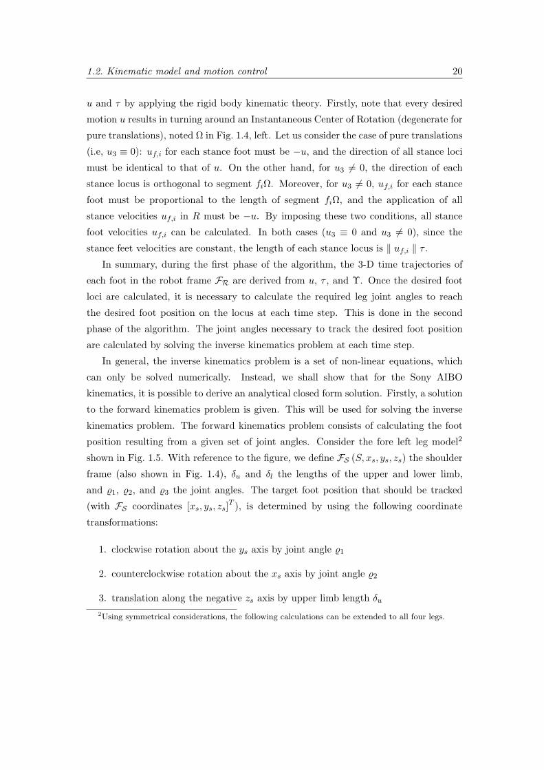
position resulting from a given set of joint angles. Consider the fore left leg model2
shown in Fig. 1.5. With reference to the figure, we define FS (S, xs, ys, zs) the shoulder
frame (also shown in Fig. 1.4), δu and δl the lengths of the upper and lower limb,
and %1, %2, and %3 the joint angles. The target foot position that should be tracked
(with FS coordinates [xs, ys, zs]T ), is determined by using the following coordinate
transformations:
1. clockwise rotation about the ys axis by joint angle %1
2. counterclockwise rotation about the xs axis by joint angle %2
3. translation along the negative zs axis by upper limb length δu2Using symmetrical considerations, the following calculations can be extended to all four legs.

1.2. Kinematic model and motion control 21
Figure 1.5: Fore left leg design: side view (left), and front view (right).
4. clockwise rotation about the ys axis by joint angle %3
5. translation along the negative zs axis by lower limb length δl
In homogeneous coordinates, by using the Denavit and Hartenberg method [35], this
transformation can be described as a concatenation of transformation matrices:xs
ys
zs
1
= Ry(−%1)Rx(%2)T−δuRy(−%3)T−δl
0
0
0
1
(1.12)
where Ry(%i) is the rotation matrix of angle %i around the ys axis, and Tδ the translation
matrix associated to vector [0 0 δ]T . The solution of the forward kinematics problem
can be derived from (1.12):xs = δl cos %1 sin %3 + δl sin %1 cos %2 cos %3 + δu sin %1 cos %2
ys = δu sin %2 + δl sin %2 cos %3
zs = δl sin %1 sin %3 − δl cos %1 cos %2 cos %3 − δu cos %1 cos %2
(1.13)
To solve the inverse kinematics problem, the knee joint angle %3 is initially calculated.
Since the knee joint position determines how far the leg is stretched, %3 can be calculated

1.2. Kinematic model and motion control 22
from the distance of the target position (xs, ys, zs) to the shoulder joint. According to
the law of cosine (see Fig. 1.4):
|%3| = arccosx2
s + y2s + z2
s − δ2u − δ2l2δuδl
There exist two solutions, since there are two possible knee positions to reach the target
position (xs, ys, zs). Here, the positive value of %3 is chosen due to the larger freedom
of movement for positive %3.
Plugging the result for %3 into the forward kinematics solution (1.13) allows
determining %2 easily. According to equation (1.13):
ys = δu sin %2 + δl sin %2 cos %3
Consequently:
%2 = arcsin(
ys
δl cos %3 + δu
)Since |%2| < 90, the determination of %2 via arc sine is satisfactory.
Finally the joint angle %1 can be calculated. According to equation (1.13):
xs = δl cos %1 sin %3 + δl sin %1 cos %2 cos %3 + δu sin %1 cos %2
which can be transformed to:
xs = δ∗ cos (%1 + %∗)
with:%∗ = arctan δl sin %3
− cos %2(δl cos %3+δu)
δ∗ = − cos %2(δl cos %3+δu)sin %∗
Hence:
|%1 + %∗| = arccos(xs
δ∗
)The sign of %1 + %∗ can be obtained by checking the zs component in (1.13):
zs = δl (sin %1 sin %3 − cos %1 cos %2 cos %3)− δu cos %1 cos %2 = δ∗ sin (%1 + %∗)
Since δ∗ > 0, %1 + %∗ has the same sign as zs. Hence the last joint value %1 can be
computed.

1.3. Central catadioptric vision sensor model 23
1.3 Central catadioptric vision sensor model
1.3.1 Definitions
Here, we present the fundamental mathematical models of optical cameras and their
parameters. Part of this section is taken from [76]. We concentrate on illuminance
images, i.e. images measuring the amount of light impinging on a photosensitive device.
It is important to stress that any digital image, irrespective of its type, is a 2-D array
(matrix) of numbers. Hence, any information contained in the images (e.g. shape,
measurements, or object identity) must ultimately be extracted from 2-D numerical
arrays, in which it is encoded. A simple look at any ordinary photograph suggests the
variety of physical parameters playing a role in image formation. Here is an incomplete
list:
• optical parameters of the lens (lens type, focal length, field of view, angular
apertures);
• photometric parameters appearing in the model of the light power reaching the
sensor after being reflected from the objects in the scene (type, intensity, direction
of illumination, reflectance properties of the viewed surfaces);
• geometric parameters determining the image position on which a 3-D point is
projected (type of projections, position and orientation of the camera in space,
perspective distortions introduced by the imaging process).
The most common vision sensor designs used in robotics are based on the
conventional perspective camera model, and on the catadioptric camera model. The
latter is obtained by combining mirrors with a conventional imaging system, in order
to increase the field of view of the camera, which is restricted in the perspective
model. Originally introduced mainly for monitoring activities, catadioptric visual
sensors are now widely used in applications like: surveillance, immersive telepresence,
videoconferencing, mosaicing, robotics, and map building [30]. The larger field of view
eliminates the need for more cameras or for a mechanically turnable camera.
In literature, several methods have been proposed for increasing the field of view of
camera systems. Here, we focus uniquely on central catadioptric designs, i.e. designs
based on models that utilize a single projection center for world to image mapping.

1.3. Central catadioptric vision sensor model 24
In central catadioptric vision sensors, all rays joining a world point and its projection
in the image plane pass through a single point called principal projection center. The
conventional perspective camera model, also known as pinhole camera model is a typical
example of central catadioptric vision sensor, based on the assumption that the mapping
of world points into image plane points is linear in homogeneous coordinates. There are
central catadioptric systems whose geometry cannot be modeled using the conventional
pinhole model. Baker and Nayar in [2] show that all central catadioptric systems with
a wide field of view may be built by combining an hyperbolic, elliptical or planar
mirror with a perspective camera and a parabolic mirror with an orthographic camera.
However, the mapping between world points and points in the image plane is no longer
linear. In [30], the unifying model for all central catadioptric imaging systems has been
introduced. In this model, which uses a virtual unitary sphere (shown in Fig. 1.6) as a
calculus artefact, the conventional perspective camera appears as a particular case. In
the remainder of this chapter, this unified central catadioptric model will be utilized to
derive the mapping between world points and corresponding image points.
With reference to Fig. 1.6, let us define the reference frames: camera frame
FC(C, xc, yc, zc) (C is the principal projection center of the central catadioptric system)
and image frame FI(I,X, Y ). The world frame FW(W,x′, y′, z′) has been defined in
Sect. 1.1. Point coordinates are expressed in meters in FW and FC , and in pixels in FI .The virtual unitary sphere is centered in C, and the optical center of the conventional
camera (with coordinates [0 0 − ξ]T in FC) is denoted C ′. I is the image center, also
known as principal point. IC is the intersection between the zC axis and the image
plane. Its coordinates in FI , XI and YI , determine the signed offsets in pixels from
I to the zC axis, also known as principal point error. The image plane has equation
zc = ψ − 2ξ in FC . Parameters ξ and ψ describe the type of sensor and the shape of
the mirror, and are function of mirror shape parameters.
For any world point d (see Fig. 1.6), we want to derive the image coordinates of the
corresponding projected point D. The world point is denoted d, because in visual PF
it is often chosen coincident with the path desired reference point defined in Sect. 1.1.
This relationship can be written:
D =I TCCTW
[dT 1
]T(1.14)
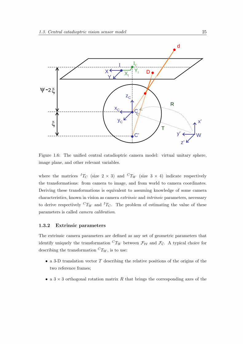
1.3. Central catadioptric vision sensor model 25
W
x’
y’
z’
C
zC
xC
yC
C’
-2
DI
XY
YI
IC
XI
T
R
d
Figure 1.6: The unified central catadioptric camera model: virtual unitary sphere,
image plane, and other relevant variables.
where the matrices ITC (size 2 × 3) and CTW (size 3 × 4) indicate respectively
the transformations: from camera to image, and from world to camera coordinates.
Deriving these transformations is equivalent to assuming knowledge of some camera
characteristics, known in vision as camera extrinsic and intrinsic parameters, necessary
to derive respectively CTW and ITC . The problem of estimating the value of these
parameters is called camera calibration.
1.3.2 Extrinsic parameters
The extrinsic camera parameters are defined as any set of geometric parameters that
identify uniquely the transformation CTW between FW and FC . A typical choice for
describing the transformation CTW , is to use:
• a 3-D translation vector T describing the relative positions of the origins of the
two reference frames;
• a 3 × 3 orthogonal rotation matrix R that brings the corresponding axes of the

1.3. Central catadioptric vision sensor model 26
two frames onto each other (N.B: the orthogonality relations reduce the number
of degrees of freedom of R to three).
Thus, the relation between the world and camera coordinates (noted dc) of a point d,
is:
dc = R(d− T ) (1.15)
Hence, the 3× 4 matrix CTW is:
CTW = [R −RT ]
1.3.3 Intrinsic parameters
The intrinsic parameters are the set of parameters that characterize the optical,
geometric and digital characteristics of the viewing camera. They are necessary to
link the pixel coordinates of an image point with the corresponding coordinates in the
camera reference frame, i.e., to identify the transformation ITC .
For the conventional perspective camera model, for instance, we need three sets of
intrinsic parameters, respectively specifying:
• the perspective projection, for which the only parameter is the focal length f ;
• the transformation between FC and FI coordinates, for which the parameters
are: the metric size of the pixel lX and lY in the axis directions, and the principal
point error (XI , YI);
• the geometric distortion induced by the optics; usually, distortion is evident at the
periphery of the image (radial distortion3), or even elsewhere when using optics
with large fields of view; radial distortion is ignored whenever high accuracy is
not required in all regions of the image, or when the peripheral pixels can be
discarded.3Radial distortions can be modeled rather accurately according to the relations:
X = X(1 + α1D
2 + α2D4)
Y = Y(1 + α1D
2 + α2D4)
with X and Y the coordinates of the distorted points, and D2 = X2 + Y 2. This distortion is a radial
displacement of the image points. A simplified model with α2 set to zero is often still accurate.

1.4. Visual servoing 27
Neglecting radial distortion, the relation between the camera and image coordinates
of a point d is:
[D 1]T = Mint
[xc
zc + ξ ‖ dc ‖yc
zc + ξ ‖ dc ‖1]T
The matrix Mint can be written as Mint = McMm where the upper triangular matrix
Mc contains the conventional camera intrinsic parameters, and the diagonal matrix Mm
contains the mirror intrinsic parameters:
Mc =
1lY
0 XI
0 1lX
YI
0 0 1
Mm =
ψ − ξ 0 0
0 ψ − ξ 0
0 0 1
Note that, setting ξ = 0 and ψ = f , the general projection model becomes the well
known perspective projection model. In this case, the 2×3 matrix ITC relating camera
and image coordinates becomes:
ITC =1zc
flX
0 XI
0 flY
YI
(1.16)
The relationship:
D =I TCdc (1.17)
is nonlinear because of factor 1/zc, and does not preserve neither distances between
points (not even up to a common scaling factor) nor angles between lines. However, it
does map lines into lines. A classic approximation that makes this relationship linear
is the weak perspective camera model. This model requires that the relative distance
along the optical axis between any two scene points is much smaller than the average
distance zc, of the points from the viewing camera. In this case, (1.16) can be rewritten
by replacing zc with zc. Another simplification, the normalized perspective camera
model, is obtained by assuming: XI = YI = 0 and lX = lY = 1.
1.4 Visual servoing
In this Section, which is taken in part from [8], we describe the basic techniques that
are by now well established in the field of visual servoing. We first give an overview
of the general formulation of the visual servo control problem. We then describe the

1.4. Visual servoing 28
two basic visual servo control schemes: image-based and position-based visual servo
control. In position-based approaches, visual feedback is computed by reducing errors
in estimated pose space. In image-based servoing, control values are computed on the
basis of image features directly.
1.4.1 Outline
Visual servo control refers to the use of computer vision data to control the motion of
a robot. The vision data may be acquired from a camera that is mounted directly on
a robot manipulator or on a mobile robot (in this case, motion of the robot induces
camera motion). Otherwise, the camera can be fixed in the workspace (the camera
can observe the robot motion from a stationary configuration). Other configurations
can also be considered. However, the mathematical development of all these cases is
similar, and here we shall specifically focus on the former case (referred to as eye-in-hand
in the literature), since in this thesis we consider mobile robots with an on-board
camera. Visual servo control relies on techniques from image processing, computer
vision, and control theory. Since it is not possible to cover all of these in depth, we
will focus here primarily on issues related to control, and to those specific geometric
aspects of computer vision that are uniquely relevant to the study of visual servo
control. For instance, we will not specifically address issues related to feature tracking
or three-dimensional pose estimation.
The aim of all vision-based control schemes is to minimize a k-dimensional error
e(t), which is typically defined by:
e(t) = s (M(t),P)− s∗ (1.18)
In (1.18), The vector M(t) is a set of image measurements (e.g., the image coordinates
of interest points or the image coordinates of the centroid of an object). These image
measurements are used to compute a vector of k visual features, s (M(t),P), in which Pis a set of parameters that represent potential additional knowledge about the system
(e.g., coarse camera intrinsic parameters or 3-D models of objects). The vector s∗
contains the desired values of the features. Let us consider for simplicity the case of a
fixed goal pose and a motionless target, (i.e., s∗ = const, and changes in s depend only
on camera motion). Moreover, we consider the general case of controlling the motion of
a camera with six degrees of freedom: let the spatial velocity of the camera be denoted
1.4. Visual servoing 29
by uc. We consider uc as the input to the robot controller. Visual servoing schemes
mainly differ in the way that s is designed. Here, we shall consider two very different
approaches. First, we describe image-based visual servo control, in which s consists of
a set of features that are immediately available in the image data. Then, we describe
position-based visual servo control, in which s consists of a set of 3-D parameters,
which must be estimated from image measurements. Once s is selected, the design of
the control scheme can be quite simple. Perhaps the most straightforward approach is
to design a velocity controller. To do this, we require the relationship between the time
variation of s and the camera velocity. The relationship between s and uc is given by:
s = Lsuc (1.19)
where the k × 6 matrix Ls is named the interaction matrix related to s. The term
feature Jacobian is also used somewhat interchangeably in the visual servo literature.
Using (1.18) and (1.19), we immediately obtain the relationship between the camera
velocity and the time variation of the error:
e = Lsuc (1.20)
If we wish to ensure an exponential decoupled decrease of the error (i.e., e = −λe), we
obtain using (1.20):
uc = −λL+s e, (1.21)
where the 6 × k matrix L+s is chosen as the Moore-Penrose pseudoinverse of Ls, that
is: L+s = (LT
s Ls)−1LTs when Ls is of full rank 6. This choice allows ‖ e−λLsL
+s e ‖ and
‖ uc ‖ to be minimal. When k = 6, if detLs 6= 0, it is possible to invert Ls, giving the
control uc = −λL−1s e. In real visual servo systems, it is impossible to know perfectly
in practice either Ls or L+s . So an approximation or an estimation of one of these
two matrices must be realized. In the sequel, we denote both the pseudoinverse of the
approximation of the interaction matrix and the approximation of the pseudoinverse
of the interaction matrix by the symbol L+s . Using this notation, the control law is in
fact:
uc = −λL+s e (1.22)
This is the basic design implemented by most visual servo controllers. All that remains
is to fill in the details: How should s be chosen? What then is the form of Ls? How

1.4. Visual servoing 30
should we estimate L+s ? What are the performance characteristics of the resulting
closed-loop system? These questions are addressed in the remainder of this Section.
1.4.2 Image-based visual servoing
Traditional image-based control schemes use the image-plane coordinates of a set of
points (other choices are possible, but we shall not discuss these here) to define the set
s. Consider the case of a conventional perspective camera. We assume (recalling the
notation from Sect. 1.3) that XI = YI = 0 and lX = lY = l. Then, for a 3-D point d
with image coordinates D = [X,Y ]T , the interaction matrix Ls is (s ≡ D):
Ls =
− fzcl 0 X
zc
lXYf −f2+l2X2
fl Y
0 − fzcl
Yzc
f2+Y 2
fl − lXYf −X
(1.23)
In the matrix Ls, the value zc is the depth of the point d relative to the camera frame
FC . Therefore, any control scheme that uses this form of the interaction matrix must
estimate or approximate the value of zc. Similarly, the camera intrinsic parameters are
involved in the computation of Ls. Thus, Ls cannot be directly used in (1.21), and an
estimation or an approximation Ls must be used. To control the 6 degrees of freedom,
at least three points are necessary (i.e., we require k ≥ 6).
1.4.3 Position-based visual servoing
Position-based control schemes use the pose of the camera with respect to some
reference coordinate frame to define s. Computing that pose from a set of measurements
in one image necessitates the camera intrinsic and extrinsic parameters to be known.
It is then typical to define s in terms of the parameterization used to represent the
camera pose. The image measurements M are usually the pixel coordinates of the set
of image points (but this is not the only possible choice), and the parameters P in the
definition of s = s(M,P) in (1.18) are the camera intrinsic and extrinsic parameters.
Many solutions for position-based visual servoing have been proposed in the literature.

Chapter 2
Related work
This chapter reviews some recent research works in the field of path following. First
we shall focus on general works on path following that do not specify the sensor used
to detect the path, but assume geometric knowledge of the path characteristics. These
works will be referred to as ’sensor-less’ approaches, since they focus on the control
aspects of PF rather than on the sensor processing required to detect and model the
path. In the second section, we shall instead focus on works that use a visual approach
to solve path following, and include considerations and practical implementation of the
sensing techniques, along with the control aspects. Throughout the chapter, we adopt
the notation defined in Chapter 1. Unless otherwise specified, in all works the PF task
consists of driving the path error e (ε) to e (ε) ≡ 0.
2.1 Sensor-less path following
In [16], Canudas de Wit and others tackle the problem of following a path with a
unicycle robot. The path following constraint is chosen by defining d as the normal
projection of r on p, i.e., by choosing d such that et =const = 0. The authors assume
that the path curvature is differentiable, and the motion exigency is guaranteed by
imposing constant linear velocity: u1 = const > 0. Two alternative controllers on the
angular velocity u2 are designed. The first is a locally stabilizing linear feedback control
obtained by tangent linearization of the kinematic model:
u2 =(λ1en − λ2eθ +
cd cos eθ1 + cden
)u1 (2.1)
31

2.1. Sensor-less path following 32
The second controller is nonlinear:
u2 =(λ1en
sin eθeθ
+cd cos eθ1 + cden
)u1 − λ2 (u1) eθ (2.2)
and is used to asymptotically stabilize the system under some conditions on the initial
robot configuration. A Lyapunov-based proof is carried out for the second controller.
In both controllers, λ1 and λ2 are positive gains. Note that in the nonlinear controller,
λ2 is a function of u1.
In [15], straight line following with a car-like robot is considered. Although the
implementation presented uses an on-board omnidirectional camera, the algorithm
relies only on the 3-D features of the line, which can be detected independently from
the sensor. For this reason, we consider this controller among the sensor-less path
following approaches. The authors use the car-like model (1.9). The path following
constraint is et =const = 0, and the linear velocity u1 is piecewise constant non-null
(hence, the motion exigency is guaranteed). Feedback linearization is used to design
a proportional-derivative path following controller on the robot angular velocity with
respect to the midpoint of the rear wheels:
u2 = λ1en
u1 cos eθ− λ2 tan eθ
λ1 and λ2 are positive controller gains. Critically damping behavior can be obtained
if λ2 = 2√λ1. Note that this controller presents a singularity for eθ = ±π
2 .
Frezza and others [29] enable a unicycle robot to follow paths assumed to be
representable in FR as: x = x (y, t) (the path changes over time under the action of
robot motion). They define moments νi as a chain of derivatives of the path function,
computed in y = 0: νi = ∂i−1x∂i−1y
|y=0. The proposed controller should regulate to zero ν1
and ν2. Note that this formulation of PF is equivalent to imposing path following
constraint: et =const = 0. Since conventional control via feedback linearization
demands exact knowledge of the contour and is not robust to disturbances, they
define xb = xb (y, t) as a feasible cubic B-spline instantaneously approximating the
path. Under these assumptions, they show that the system can be locally stabilized by
controller:
u2 = u1∂2xb
∂2y(0, t)

2.2. Vision-based path following 33
For u1 non-null, the motion exigency is guaranteed.
In [69], a smooth time-varying feedback stabilization method is proposed for a
nonholonomic mobile robot with m = 2 control inputs, and n ≤ 4 generalized
coordinates. The method is based on the chained form model, which is a
canonical model for which the nonholonomic motion planning problem can be solved
efficiently [58]. The author assumes that the robot kinematic model can be converted
into a chained form via input transformation and change of coordinates. An
appropriate chained form representation of the model is used: [χ1 χ2 . . . χn−1 χn]T =
[u′1 χ3u′1 . . . χnu
′1 u
′2]
T , where u′1 and u′2 are the new control inputs. Following a path
is equivalent to zeroing Ξ = [χ2 . . . χn]T . The author shows that a time-varying control
u′2 = u′2(u′1, t,Ξ) globally asymptotically stabilizes Ξ = 0 for any piecewise-continuous,
bounded and strictly positive u′1(t).
2.2 Vision-based path following
In [72], Skaff and others study vision-based following of straight lines for a six-legged
robot equipped with a fixed conventional perspective camera. The camera leans forward
with a constant tilt angle with respect to the ground. The legged robot is modeled as
a unicycle. The authors propose two steering policies u2, that in the article are called
’position-based controller’ and ’field of view respecting controller’ in the article. In
both controllers, the motion exigency is guaranteed by imposing: u1 = const > 0. In
the first case, the path following constraint is et = const = 0, and the controller is
identical to (2.1), in the particular case of straight path (cd ≡ 0):
u2 = (λ1en − λ2eθ)u1
For the ’field of view respecting controller’, the path following constraint is defined
in the image. It consists of centering the perspective projection of the line in the
image plane. This corresponds to zeroing Xtop and Xbot, which are defined (assuming
that they always exist) as the abscissas in FI of the intersection points of the image
projection of the line with the top and bottom sides of the field of view. Note that if
the camera optical axis is in the robot sagittal plane (as it is assumed in the article),
this is equivalent to imposing PF constraint et = const = 0. The states [Xtop Xbot]T

2.2. Vision-based path following 34
are mapped to a new state space [ϕ1 ϕ2]T defined by the projection of the image plane
on the ground. In the new state space, a closed loop policy (detailed in the paper):
u2 = u2 (ϕ1, ϕ2)
regulates the system to the desired set point. The controller is mapped back to
[XtopXbot]T coordinates, and a Lyapunov-like function is used to prove the asymptotic
stability of the system under given conditions on the camera parameters.
More recently, Coulaud and others [14] have proposed a vision-based feedback
controller and discussed the existence and stability of an equilibrium trajectory for
arbitrary paths. They focus on following paths with a unicycle robot equipped with a
fixed conventional perspective camera. The camera leans forward, with a tilt angle of
45. The motion exigency is verified by imposing constant linear velocity u1 = const
> 0. Having defined the horizon as the straight line parallel to the wheel axle and
at constant distance yh ahead of it, and d the intersection point between horizon and
path1, the proposed controller is:
u2 = λX
with λ positive gain and X abscissa in FI of the projection D of d in the image
plane. For a circular path, local asymptotic stability of an equilibrium state [θ X]Teqthat is function of cd, u1, and λ (i.e., [θ X]Teq = [θ (cd) X (c, u1, λ)]T ) is proved. The
authors show that tracking error is bounded for a path with continuously differentiable
curvature. Arbitrary paths can be tracked by dynamically adapting u1, λ and yh.
Design constraints, stability margin and convergence rate are represented in the phase
plane (θ, X).
Another interesting work is presented in [54], where vision-based PF for unicycle
and car-like robots equipped with a conventional perspective camera is achieved by
controlling the curve shape in the image plane. Similarly to [14] and [72], the camera
leans forward with non-null tilt angle. The approach is similar to [29]. The authors
assume that the curve orthographic projection on the zc = 1 plane in FC can be
represented as: xc = xc(yc, t) (N.B: time dependance is due to robot motion) and1In case of multiple intersection points, D will be the closest to the robot sagittal plane.

2.2. Vision-based path following 35
define νci = ∂i−1xc
∂i−1yc, with i = 1, 2, . . .. Then, for linear curvature curves (clothoids), the
dynamics of the orthographic projection image curve (i.e. νci ) are proved equivalent
to those of the perspective projection image curve. Both can then be expressed
as a function of νc1, ν
c2 and νc
3 alone. Noting [xrc y
rc z
rc ]
T the FC coordinates of the
contact point between wheel and ground (i.e., the robot reference point r), following
the path is equivalent to zeroing νc1|yc=yr
cand νc
2|yc=yrc. Again, this is equivalent to
imposing PF constraint et = const = 0. By transforming the system [νc1 ν
c2 ν
c3]
T
in canonical form, “clothoid following” is shown to be globally achievable with
piecewise smooth sinusoidal inputs. Such piecewise smooth controllers are given for an
arbitrary path, and asymptotic stability of the closed-loop system is proved. In this
formulation of PF, the motion exigency specification is not explicitly guaranteed. The
practical implementation is rather sophisticated, implying an extended Kalman filter
to dynamically estimate the path curve derivatives up to order three.
In [33], Hadj-Abdelkader and others present an image-based visual servoing scheme
which enable a mobile robot equipped with a para-catadioptric camera to follow straight
lines. The line following control law is designed for generic mobile robots, and is
implemented on a unicycle robot in the paper. The PF constraint is et = const
= 0, and the motion exigency is guaranteed by u1 = const > 0. Para-catadioptric
cameras are formed by a parabolic mirror combined with an orthographic camera. The
central catadioptric model described in Sect. 1.3 can be used for this kind of sensors by
appropriately setting ξ and ψ. The equation of the conic curve in FI , corresponding
to the straight path is derived. Then, a minimal and generic analytical form of the
central catadioptric interaction matrix Ls for the image of 3D straight lines is derived.
Finally, the authors rely on a number of experiments to show that the image-based
control law (1.22) on the angular velocity enables the unicycle robot to follow the line.

Chapter 3
Vision-based path following for a
nonholonomic mobile robot with
fixed pinhole camera
Applying visual servoing control techniques for navigation with wheeled mobile robots,
involves well known control problems related to the nonholonomic constraint. Firstly,
the linearization of these systems is uncontrollable, and, secondly, there do not
exist smooth state feedback laws for stabilizing these systems to an equilibrium.
Notwithstanding, visual servoing techniques have been successfully used to control
nonholonomic mobile robots in [36], [56], [77], and more recently in [55]. Here, we
present two path following (PF) control schemes (position-based and image based),
enabling nonholonomic mobile robots with a fixed pinhole camera to reach and follow a
continuous path on the ground by processing a small set of features in the image plane.
This chapter is organized as follows. In Sect. 3.1, all the relevant variables utilized
in our method are defined. In Sect. 3.2, we propose and illustrate the two controllers.
In Sect. 3.3 a Lyapunov-based stability analysis, which takes into account the robot
kinematic constraint on maximum curvature, is carried out. The experimental setup
and simulated and experimental results are respectively presented in Sect. 3.4, Sect. 3.5
and 3.6. In the conclusion, we summarize the results, and compare the two controllers.
36

3.1. Definitions 37
ρ
ty
tz
z
yr x(a)
(b)
(c)
r
eθz
x
y
yd
p
d
en
et
y_
β
y0eθ_
(d)
x_
X
Y
ΘI
Γ P
D
TESI
r eθz
x
y
yd
p
enu1
u2 θd
ud2
ud1θ
d
et
x’
y’
z’
W
xd
zdC
zc
xc
yc
xd
x’
y’
z’
W
zd
Figure 3.1: Relevant variables utilized in this work. The task for the robot (represented
in orange), equipped with a fixed pinhole camera (blue) is to follow the red path, noted
p. The figure represents: top view (a,d), image plane (b), and side view (c). The
camera field of view and its projection on the ground are represented in cyan. The
control inputs are represented in green.
3.1 Definitions
In this work, we focus on the path following task for nonholonomic mobile robots
equipped with a fixed pinhole camera. All relevant variables (most of which have been
defined in Chapter 1) are shown in Fig. 3.1. The camera optical axis has a constant
tilt offset 0 < ρ < π2 with respect to the y axis and the optical center C is positioned
in the robot sagittal plane at [x y z]T = [0 ty tz]T (see Fig. 3.1(c)). We assume that in
FW , the path curve p, can be expressed by a twice differentiable function. A following
direction is associated to the path. Point r is chosen as the projection on the ground
of the wheels center in the case of a unicycle robot, and of the rear axis center in
the case of a car-like robot. We refer to the general nonholonomic model (1.9), which
is valid both for unicycle and car-like robots. In (1.9), control input u1 represents
the linear velocity, while control input u2 represents the angular velocity around the
z axis (positive counterclockwise). Recall (see Sect. 1.2.1) that for a car-like robot,
the steering angle constraint |φ| ≤ φM imposes the bound (1.11) on the instantaneous
applicable curvature; in the case of a unicycle robot, there is no such bound.
For the nonholonomic model (1.9), the dynamics of the FP path errors et, en and
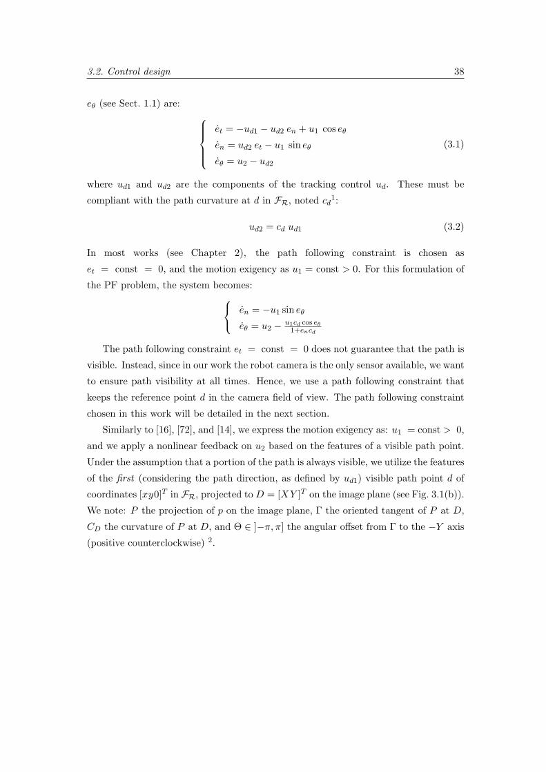
3.2. Control design 38
eθ (see Sect. 1.1) are: et = −ud1 − ud2 en + u1 cos eθen = ud2 et − u1 sin eθeθ = u2 − ud2
(3.1)
where ud1 and ud2 are the components of the tracking control ud. These must be
compliant with the path curvature at d in FR, noted cd1:
ud2 = cd ud1 (3.2)
In most works (see Chapter 2), the path following constraint is chosen as
et = const = 0, and the motion exigency as u1 = const > 0. For this formulation of
the PF problem, the system becomes: en = −u1 sin eθeθ = u2 − u1cd cos eθ
1+encd
The path following constraint et = const = 0 does not guarantee that the path is
visible. Instead, since in our work the robot camera is the only sensor available, we want
to ensure path visibility at all times. Hence, we use a path following constraint that
keeps the reference point d in the camera field of view. The path following constraint
chosen in this work will be detailed in the next section.
Similarly to [16], [72], and [14], we express the motion exigency as: u1 = const > 0,
and we apply a nonlinear feedback on u2 based on the features of a visible path point.
Under the assumption that a portion of the path is always visible, we utilize the features
of the first (considering the path direction, as defined by ud1) visible path point d of
coordinates [xy0]T in FR, projected to D = [XY ]T on the image plane (see Fig. 3.1(b)).
We note: P the projection of p on the image plane, Γ the oriented tangent of P at D,
CD the curvature of P at D, and Θ ∈ ]−π, π] the angular offset from Γ to the −Y axis
(positive counterclockwise) 2.
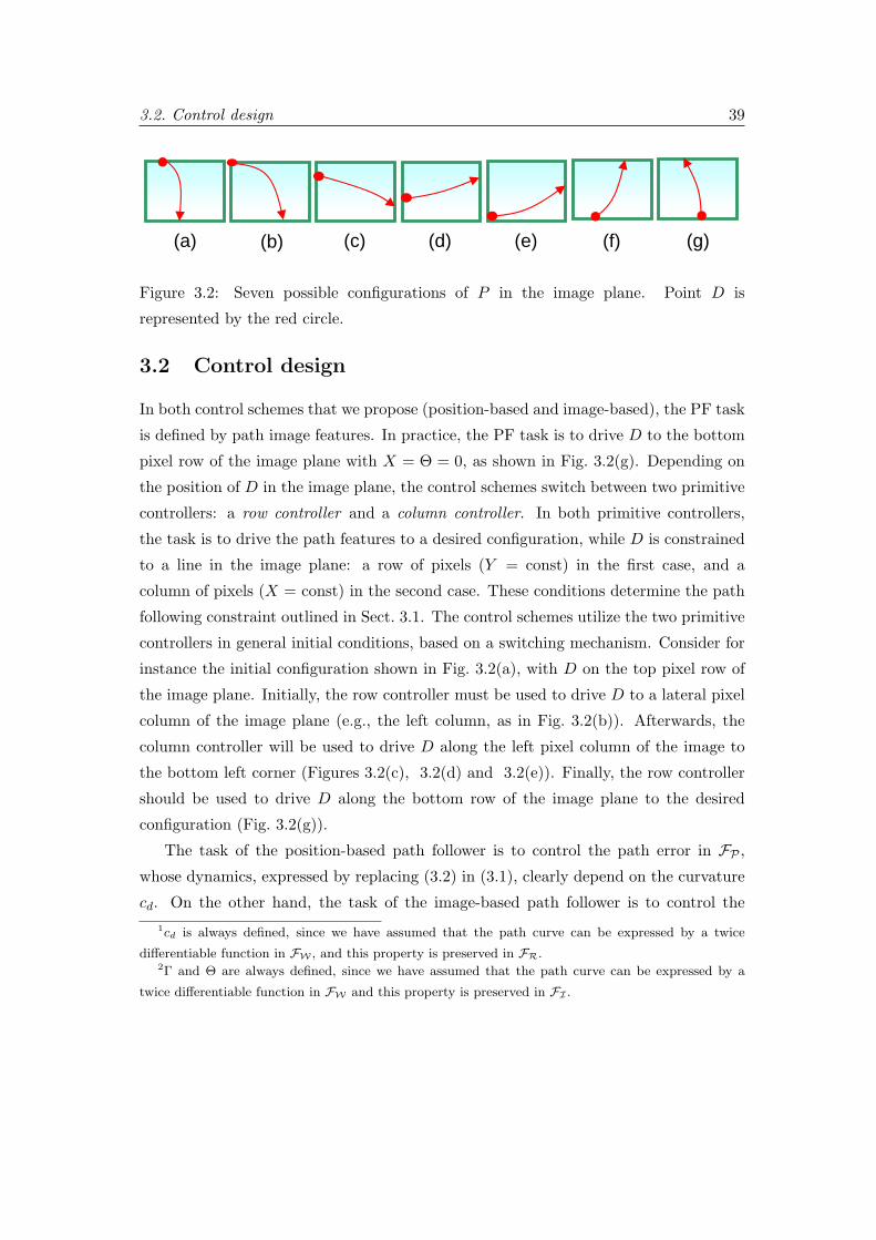
3.2. Control design 39
(a) (b) (c) (d) (e) (f) (g)
Figure 3.2: Seven possible configurations of P in the image plane. Point D is
represented by the red circle.
3.2 Control design
In both control schemes that we propose (position-based and image-based), the PF task
is defined by path image features. In practice, the PF task is to drive D to the bottom
pixel row of the image plane with X = Θ = 0, as shown in Fig. 3.2(g). Depending on
the position of D in the image plane, the control schemes switch between two primitive
controllers: a row controller and a column controller. In both primitive controllers,
the task is to drive the path features to a desired configuration, while D is constrained
to a line in the image plane: a row of pixels (Y = const) in the first case, and a
column of pixels (X = const) in the second case. These conditions determine the path
following constraint outlined in Sect. 3.1. The control schemes utilize the two primitive
controllers in general initial conditions, based on a switching mechanism. Consider for
instance the initial configuration shown in Fig. 3.2(a), with D on the top pixel row of
the image plane. Initially, the row controller must be used to drive D to a lateral pixel
column of the image plane (e.g., the left column, as in Fig. 3.2(b)). Afterwards, the
column controller will be used to drive D along the left pixel column of the image to
the bottom left corner (Figures 3.2(c), 3.2(d) and 3.2(e)). Finally, the row controller
should be used to drive D along the bottom row of the image plane to the desired
configuration (Fig. 3.2(g)).
The task of the position-based path follower is to control the path error in FP ,
whose dynamics, expressed by replacing (3.2) in (3.1), clearly depend on the curvature
cd. On the other hand, the task of the image-based path follower is to control the1cd is always defined, since we have assumed that the path curve can be expressed by a twice
differentiable function in FW , and this property is preserved in FR.2Γ and Θ are always defined, since we have assumed that the path curve can be expressed by a
twice differentiable function in FW and this property is preserved in FI .

3.2. Control design 40
error related to the image features X, Y , and Θ, without taking into account the
path curvature. Therefore, a major difference between the two proposed controllers is
that the position-based controller depends on cd, whereas the image-based controller
does not. In the remainder of this section, we shall describe how the 3D path
features are derived from the corresponding image path features. We shall also
illustrate the implementation of the two primitive controllers for both position-based
and image-based visual servoing.
3.2.1 Deriving the path 3D features
For the position-based approach, the path 3D features in FR must be derived from the
image features by considering a pinhole camera model; radial distortion and principal
point error are neglected. Hence, the five camera parameters used for projecting are:
P = [fX fY ρ ty tz]T
where the focal lengths in horizontal and vertical pixel size fX and fY are the camera
intrinsic parameters, and ρ, ty and tz are the extrinsic parameters shown in Fig. 3.1(c).
For simplicity, let us consider a camera model with fX = fY = 1, known in the
literature as normalized perspective camera model. The mapping between the FI and
FC coordinates of a ground point gives3:
xc =Xtz
sin ρ+ Y cos ρ(3.3)
yc =Y tz
sin ρ+ Y cos ρ(3.4)
zc =tz
sin ρ+ Y cos ρ(3.5)
The robot frame coordinates of the ground point can then be easily derived by using
the homogenous transformation from FR to FC (i.e, the camera extrinsic parameters).
For the orientation of the tangent at d, we obtain:
eθ = ATAN2 (− sinΘ (sinρ+ Y cosρ)−X cosΘ cosρ, cosΘ)
To derive cd (i.e., the path curvature at d in FR), the image path points are initially
projected to FR. Afterwards, the equation of the path osculating circle in d (thus, the
value of cd) is derived using least square interpolation.3Equations (3.3) - (3.5) do not present singularities, since by construction the image projection of
any ground point has Y > − tan ρ.

3.2. Control design 41
3.2.2 Position-based path follower
Row controller
The task of the position-based row controller is to drive (x, y, eθ) to a desired set point
(x, y, eθ) under constraint Y = const = Y ∗ (i.e., D is constrained to a pixel row in the
image plane).
This is equivalent to constraining d to the projection of the pixel row on the ground
(see Fig. 3.1(a)), i.e. to the line of equation:
y = const = y∗
The above equation, which defines the path following constraint, can be rewritten by
introducing the position errors in FP :
y =d
dt(en sin eθ − et cos eθ) = 0
Using (3.1) simple calculations lead to:
ud1 =u1 + u2x
cos eθ
under the constraint that |eθ| 6= ±π2 , which is plausible, assuming that Γ is never
parallel to the the X axis of frame FI4. Replacing ud1 and using (3.1) in:
x =d
dt(−en cos eθ − et sin eθ)
gives:
x = (tan eθ)u1 + (y∗ + x tan eθ)u2
Hence, the system state equations are: x
eθ
= Au1 +Bu2 (3.6)
where:
A =
tan eθ− cd
cos eθ
B =
y∗ + x tan eθ1− cdx
cos eθ
4This singularity can be avoided by temporarily switching to the position-based column controller.

3.2. Control design 42
When B 6= 0 (i.e. r is not at the center of the osculating circle of p at d), the system
is controllable and we select as control law:
u2 = −B+
λxex
λθeθ
+Au1
(3.7)
where ex = x−x and eθ = eθ−eθ are the state errors, and λx, λθ are given positive gains.
Column controller
The task of the position-based column controller is to drive (x, y, eθ) to a desired set
point (x, y, eθ) under constraint X = const = X∗ (i.e., D is constrained to a pixel
column in the image plane). This is equivalent to constraining d to the projection of
the pixel column on the ground (see Fig. 3.1(d)), i.e. to the line of equation:
y = y0 + x tanβ
where y0 and β ∈]−π
2 ,π2
](shown in Fig. 3.1(d)) are: y0 = ty − tz tan ρ
β = ATAN 1X cos ρ
with β = π2 at the singularity X = 05.
Let us redefine the system variables in a new frame FR(r, x, y, z), obtained by
rotating FR by β around z and shown in Fig. 3.1(d).
In this new frame, noting eθ = eθ + β, we have: x
y
=
− cos eθ − sin eθsin eθ − cos eθ
en
et
The path following constraint becomes:
y = const = y∗ (3.8)
with y∗ = y0 cosβ. Hence, as before, but in FR:
˙y =d
dt(en sin eθ − et cos eθ) = 0
5In that case, the projection of the pixel column on the ground is the line of equation: x = 0.

3.2. Control design 43
Using (3.1) simple calculations yield:
ud1 =u1 cosβ + u2x
cos eθ
under the constraint that |eθ| 6= ±π2 , which is plausible, assuming that Γ is never
parallel to the Y axis of frame FI6. Replacing ud1 and using (3.1) in:
˙x =d
dt(−en cos eθ − et sin eθ)
gives:˙x = (tan eθ cosβ − sinβ)u1 + (y∗ + x tan eθ)u2
Hence, the system state equations are: ˙x˙eθ
= Au1 + Bu2 (3.9)
where:
A =
tan eθ cosβ − sinβ
− cd cos βcos eθ
B =
y∗ + x tan eθ1− cdx
cos eθ
When B 6= 0 (i.e. r is not at the center of the osculating circle of p at d), the system
is controllable, and we select as control law:
u2 = −B+
λxex
λθeθ
+ Au1
(3.10)
where ex = x − ˆx and eθ = eθ − ˆeθ are the state errors, and λx, λθ are given positive
gains. Note that in this case, the desired states ˆx and ˆeθ are expressed in FR.
3.2.3 Image-based path follower
Recalling Sect. 1.4, the interaction matrix Ls (X,Y,Θ), relating the path image features
with the spatial velocity of the robot camera uc, must be derived in order to design the
image-based path following controller. In this work:[X Y Θ
]T= Ls (X,Y,Θ)uc
6This singularity can be avoided by temporarily switching to the position-based row controller.
3.2. Control design 44
Ls (X, Y, Θ) =
− 1
zc0 X
zcXY −1−X2 Y
0 − 1zc
Yzc
1 + Y 2 −XY −X
cos ρ
tz
(1+tan2 Θ
) 0−Xcosρ+tanΘ[sinρ+(Y−1) cos ρ]
tz
(1+tan2 Θ
) −X+(1−Y)tanΘ1+tan2 Θ
− tanΘ(2X+tanΘ)1+tan2 Θ
− 11+tan2 Θ
(3.11)
The expression of Ls (X,Y,Θ) for the normalized perspective camera model (introduced
in Sect. 3.2.1) is shown at the top of this page. In (3.11), zc is derived from (3.5). In the
following, we shall note LX , LY and LΘ the rows of Ls (respectively, top to bottom).
Note that the singularity at Θ = ±π2 does not jeopardize the controller behavior, if, for
Θ tending to ±π2 , LΘ is approximated with its limit LΘ:
LΘ = [0 0 0 0 − 1 0]
The robot velocity in FC can be expressed in function of u by using the homogenous
transformation from FR to FC :uc =C TRu
with:
CTR =
0 −ty− sin ρ 0
cos ρ 0
0 0
0 − cos ρ
0 − sin ρ
In the following, we shall note T1, T2 respectively the first and second columns of CTR.
Similarly to the position-based path follower, the image-based path follower also
utilizes a row a column primitive controllers. However, in this case, the controllers are
based on the reference path point image features instead of its 3D features.
Row controller
The task of the image-based row controller is to drive (X, Θ) to a desired set point
(X, Θ) under constraint Y = const = Y ∗ (i.e., D is constrained to a pixel row in the

3.3. Stability analysis 45
image plane). Since Y = 0, the system state equations are: X
Θ
= Acu1 +Bcu2 (3.12)
where:
Ac =
LX
LΘ
T1 Bc =
LX
LΘ
T2
When Bc 6= 0, the system is controllable, and we select as control law:
u2 = −B+c
λXeX
λΘeΘ
+Acu1
(3.13)
where eX = X − X and eΘ = Θ − Θ are the state errors defined in the image plane,
and λX , λΘ are given positive gains.
Column controller
The task of the image-based column controller is to drive (Y , Θ) to a desired set point
(Y , Θ) under constraint X = const = X∗ (i.e., D is constrained to a pixel column in
the image plane). Since X = 0, the system state equations are: Y
Θ
= Acu1 + Bcu2 (3.14)
where:
Ac =
LY
LΘ
T1 Bc =
LY
LΘ
T2
When Bc 6= 0 the system is controllable, and we select as control law:
u2 = −B+c
λY eY
λΘeΘ
+ Acu1
(3.15)
where eY = Y − Y and eΘ = Θ − Θ are the state errors defined in the image plane,
and λY , λΘ are given positive gains.

3.3. Stability analysis 46
control scheme position-based image-based
primitive controller row column row column
X1 x x X Y
X2 eθ eθ Θ Θ
A1 tan eθ tan eθ cosβ − sinβ LXT1 LY T1
A2 − cdcos eθ
− cd cos βcos eθ
LΘT1 LΘT1
B1 y∗ + x tan eθ y∗ + x tan eθ LXT2 LY T2
B2 1− cdxcos eθ
1− cdxcos eθ
LΘT2 LΘT2
G1 λx λx λX λY
G2 λθ λθ λΘ λΘ
E1 x− x x− ˆx X − X Y − Y
E2 eθ − eθ eθ − ˆeθ Θ− Θ Θ− Θ
Table 3.1: Components of: X , A, B, G, and E for the four controllers
3.3 Stability analysis
The stability analysis has been carried out for both control schemes (position-based and
image-based) by using a Lyapunov-based approach. Note that the four state equations
(3.6), (3.9), (3.12) and (3.14) can be generally written:
X = Au1 + Bu2 (3.16)
and, similarly, when B 6= 07, the four control laws (3.7), (3.10), (3.13), and (3.15) can
be generally expressed as:
u2 = −B+ (GE +Au1) (3.17)
with X = [X1 X2]T , A = [A1 A2]
T , B = [B1 B2]T , and E = [E1 E2]
T two-dimensional
column vectors, and:
G =
G1 0
0 G2
The components of X , A, B, G and E for the four controllers are recalled in Table 3.1.
Note that, as mentioned in Sect. 3.2, for the two primitive image-based controllers, as
opposed to the position-based controllers, these variables are independent from cd.7We don’t manage singularity B = 0, since it is extremely unlikely to occur in practice.

3.4. Experimental setup 47
Hence, the following stability analysis is valid for all four controllers. Let us consider
the quadratic Lyapunov function candidate:
V =|E|2
2
Taking the time derivative of this function along a solution of the closed-loop system
gives:
V = ET X
Using (3.16) and (3.17) leads to:
V = ET (Au1 − BB+ (GE +Au1)
)If we set G1 = G2 = G∗ > 0, since u1 > 0, V is negative semidefinite if and only if:
ET (A− BB+A)ETBB+E
<G∗
u1(3.18)
To verify the Lyapunov sufficient condition (3.18), the robot kinematic constraint on
the maximum applicable curvature cM must be analyzed, since it imposes a constraint
on the maximum applicable gain G∗. In fact, replacing (3.17) in (1.11), gives:
−cM + B+A < −G∗
u1BTE < cM + B+A
This equation can be used to derive a sufficient condition for (3.18):
∣∣∣∣∣ET (A− BB+A)ETB
+ B+A∣∣∣∣∣ < cM (3.19)
In (3.19) we have expressed a sufficient condition for asymptotic stability as a
condition on the maximum applicable curvature cM , hence on the robot kinematic
model. This condition is also determined by the path characteristics, which must be
compliant with the robot nonholonomic constraint. Condition (3.19) will be verified
numerically, depending on the controller used, on the robot parameters and on the
desired states, as will be shown in the next section.
3.4 Experimental setup
In the following section, we report the simulated and real experimental results obtained
by applying the two proposed PF control schemes. All experiments have been carried

3.5. Simulations 48
out with a CyCab. CyCabs are 4 wheel drive, 4 wheel steered intelligent vehicles
designed to carry two passengers. In our CyCab, all computations except the low-level
control have been executed on a laptop with a 2 GHz Centrino processor. A 70 field
of view, forward looking, B&W Marlin F-131B camera is mounted on the robot. The
robot is used in car-like mode (i.e., only the front wheels are used for steering), and
the camera is used in auto shutter mode, with image resolution 320× 240 pixels. The
maximum curvature constraint (1.10) must be considered. In particular, for CyCab,
φM = 0.40 rad and L = 1.21 m; thus, cM = 0.30 m−1.
The system has been coarsely calibrated, and we obtained: fX = fY = 240 pixels,
ρ = 0.545 rad, ty = 550 mm and tz = 1625 mm.
The applicable steering angle φ used to control CyCab is derived from the angular
speed u2 (calculated using either (3.7), (3.10), (3.13), or (3.15)):
φ = ATANLu2
u1(3.20)
In all the simulations and experiments, we set u1 = 0.2 ms−1. Short
video clips of the simulations and experiments can be viewed on the web site:
http://www.dis.uniroma1.it/∼labrob/research/VBPF.html).
3.5 Simulations
The possibility of testing the proposed path following scheme in a simulated
environment has been crucial from the very early stages of this work. To this
end, we have adopted Webots, a mobile robot simulation environment developed by
Cyberbotics, which is used by many universities worldwide for modeling and controlling
mobile robots. In Webots, a complete mobile robotics setup can be defined, by creating
complex environments and equipping robots with sensors and actuators. One can define
all physical properties for each object, and the simulated robot can be programmed with
the same development environment as the real one. By using Webots, it is possible to
debug the algorithms effectively and to test them without endangering the real robot.
Besides, the problem of tuning all the gains can be easily solved in the simulation before
porting on the CyCab.
In Webots, we have designed a simulated robot with the same kinematic and
sensorial characteristics of CyCab. A circular path of radius 12.5 m (i.e., cd = const

3.5. Simulations 49
Figure 3.3: Position-based simulation. The robot positions and corresponding
processed images at consecutive time frames are shown during PF.
= 0.08 m−1) has been drawn in the simulation environment. The two control schemes
(position-based and image-based) have been simulated in Webots starting from various
initial configurations.
Consider the initial configuration with the path intersecting the right pixel column
(see Fig. 3.3, top left). A switching strategy combining the column and row controllers
is used. Initially, the column controller (respectively (3.10) for the position-based
simulations, and (3.15) for the image-based simulations) is used to drive D along the
right pixel column of the image to the bottom right corner. For the position-based
controller, we use λx = λθ = 7.0. For the image-based controller, we use λY = λΘ = 0.5.
Afterwards, the row controller (respectively (3.7) for the position-based simulations,

3.5. Simulations 50
Figure 3.4: Evolution of relevant variables during simulated PF with path initially
intersecting the right pixel column. Top: applied steering angle φ in rad (purple:
position-based, green: image-based). Center: state errors E1 (red, in m) and E2 (blue, in
rad) for the position-based column controller (left) and row controller (right). Bottom:
state errors E∗1 (red, non-dimensional) and E2 (blue, in rad) for the image-based column
controller (left) and row controller (right).
and (3.13) for the image-based simulations) is used to drive D along the bottom row of
the image plane to: X = Θ = 0. An adaptive gain is used. This design choice provides
fast convergence for large error values, while avoiding overshoot for small errors. For the
position-based simulations, we use: λx = λθ = 5 exp−10||E|| +5 with ||E|| =√e2x + e2θ
the error norm. For the image-based simulations, we use: λX = λΘ = 3 exp−10||E||
with ||E|| =√e2X + e2Θ the error norm. With both control schemes, the simulated
robot is able to successfully follow the path. For the position-based simulation, the
robot positions and processed images at consecutive time frames while Cycab follows
the path are shown in Fig. 3.3. The evolution of relevant variables (steering angle and

3.6. Experiments 51
Figure 3.5: Initial conditions used in the path following experiments. The point D and
tangent Γ derived by image processing are indicated respectively by a red circle and a
red line.
state errors) for the two control schemes, is plotted in Fig. 3.4. For the image-based
controller, instead of state errors E1 = eX and E1 = eY , we have respectively plotted
the scaled values E∗1 = eX2XM
for the row controller, and E∗1 = eY2YM
for the column
controller (2XM and 2YM respectively denote the image width and height). Note
that the steering angle φ, as well as the state errors E∗1 and E2, oscillate more in the
image-based simulations, than in the position-based simulations. This occurs because
the position-based controller utilizes the path curvature for feedback control, which
is not utilized in the image-based scheme: hence, the oscillations in the image-based
steering angle are necessary to compensate the state variations introduced by the path
curvature. Note that at the end of the first phase (after the column controllers have
been applied) the errors on the tangent orientation E2 have not reached 0. This is due
to the switching condition, which is imposed only by the error on the point position E1.
Nevertheless, for both control schemes, when the row controller is applied, the tracking
errors converge, and the mean value of the steering angle at steady state is as expected
from (3.20): ATAN Lcd = 0.096 rad.
3.6 Experiments
After the Webots simulations, the two control schemes have been tested on the real
CyCab in a series of outdoor experiments. The path used in the experiments is
composed of two straight lines of length 6 m joined by a 60 arc of circle of radius
10 m (i.e., cd = ±0.1 m−1, with the sign of cd depending on the path direction to be

3.6. Experiments 52
Figure 3.6: Position-based stability loci of the state variables (x, x in m, etθ, eθ, eθ in
rad) that verify the Lyapunov sufficient asymptotic stability condition (cyan) for cd = 0
(above) and cd = ±0.1 m−1 (below), and for: top row controller (left), right column
controller (center), and bottom row controller (right). The desired states are indicated
with the blue cross.
followed by the robot). The path features are derived by tracking straight lines and arcs
of parabola with the ViSP visual servoing software [21]. The tracker must be initialized
by clicking on five path points oriented in the desired path direction.
For each of the two control schemes, experiments with three different initial
conditions have been carried out. The three experiments are enumerated below, and
the corresponding initial conditions are shown in Fig. 3.5 (left to right).
1. Cycab is initially positioned on the path with the correct orientation and small
initial error. Hence, D is on the bottom pixel row of the image plane (see Fig. 3.5,
left). The row controller is used to drive D to X = Θ = 0.
2. CyCab is initially near the path, with D on the right pixel column of the image
plane (see Fig. 3.5, center). A switching strategy combining both row and column
controllers is used. Initially (phase 2.1), the column controller is used to drive D
along the right pixel column of the image to the bottom right corner. Afterwards

3.6. Experiments 53
Figure 3.7: Image-based stability loci of the state variables (X, Y in pixels, Θ, Θt
in rad) that verify the Lyapunov sufficient asymptotic stability condition (pink) for:
top row controller (left), right column controller (center), and bottom row controller
(right). The desired states are indicated with the black cross.
(phase 2.2), the row controller is used to drive D along the bottom row of the
image plane to X = Θ = 0.
3. CyCab is initially far from the path, with D on the top pixel row of the image
plane (see Fig. 3.5, right). Initially (phase 3.1), the row controller is used to drive
point D to a lateral pixel column of the image plane. Afterwards (phase 3.2), the
column controller is used to drive D along the right pixel column of the image to
the bottom right corner. Finally (phase 3.3), the row controller is used to drive
D along the bottom row of the image plane to X = Θ = 0.
In order to verify the robustness of the two controllers, the three experiments have
been repeated by considering a random calibration error of either +10% or −10% on
each of the five camera parameters in P.
For the calibrated camera experiments, we have numerically verified the system
sufficient asymptotic stability condition (3.19) as the system state variables evolve. The
state loci that verify condition (3.19) are represented in Fig. 3.6 for the position-based
controllers and in Fig. 3.7 for the image-based controllers. In the position-based case,
as mentioned in Sect. 3.3, the system state and the controller depend on the curvature
cd. In our experimental setup, the value of cd can be 0 (for the straight path portions)
or ±0.1 m−1 (for the arc of circle). Hence, in Fig. 3.6, the state loci are represented
for cd = 0 (above) and cd = ±0.1 m−1 (below). Besides, in the proposed experiments,
three instances of the primitive controllers are used:

3.6. Experiments 54
Figure 3.8: First position-based experiment: Cycab is initially positioned on the path
with small initial error. The robot positions and corresponding processed images at
consecutive time frames are shown during PF.
• bottom row controller (throughout the first experiment and during phases 2.2
and 3.3 of the two other experiments),
• right column controller (during phases 2.1 and 3.2),
• top row controller (during phase 3.1).
Hence, in Fig. 3.6 and 3.7, the state loci are represented for each of these three
controllers: top row (left in the two figures), right column (center), and bottom row
(right).
For the top row controllers, the range of X2 (i.e., the range of eθ for the

3.6. Experiments 55
path 1cal 06-09 x gamma curv steer deg steer rad exact_curv path 1err 06-09 x gamma curv stesteer rad path 1 22-08 x gamma curv steer
V=0.2 B=1.5 b=0 e=0 -0,03695 -0,007711 0 1,927581 0,033642 0 V=0.2 B=0.4 b=1.4 e=3 -0,013108 -0,051239 0 3 0,05504 0,148238 0,055265 0 -9,78791-0,036987 -0,00752 0 1,919734 0,033505 0 -0,01303 -0,051335 0 3 0,055058 0,148238 0,055265 0 -9,78791-0,037454 -0,00648 0 1,888206 0,032954 0 -0,0137 -0,049437 0 3 0,053995 0,148442 0,054825 0 -9,775116
-0,03746 -0,006573 0 1,893008 0,033038 0 -0,013676 -0,049515 0 3 0,054042 0,148463 0,054744 0 -9,772119-0,037404 -0,006679 0 1,895883 0,033088 0 -0,0137 -0,049437 0 3 0,053995 0,14846 0,05475 0 -9,772243
-0,03743 -0,006632 0 1,894701 0,033068 0 -0,013662 -0,049387 0 3 0,053921 0,148463 0,054744 0 -9,772119-0,037492 -0,006477 0 1,889651 0,03298 0 -0,0137 -0,049437 0 3 0,053995 0,148481 0,054663 0 -9,76897-0,037642 -0,00677 0 1,910327 0,033341 0 -0,015015 -0,054635 0 3 0,05951 0,147363 0,052789 0 -9,634026-0,037621 -0,006737 0 1,907805 0,033296 0 -0,015143 -0,054281 0 3 0,059316 0,147363 0,052789 0 -9,634026-0,037621 -0,006737 0 1,907805 0,033296 0 -0,01511 -0,054472 0 3 0,05945 0,147363 0,052789 0 -9,634026
-0,03763 -0,00678 0 1,910318 0,03334 0 -0,015048 -0,054444 0 3 0,059375 0,147363 0,052789 0 -9,634026-0,037612 -0,006898 0 1,915352 0,033428 0 -0,015158 -0,054517 0 3 0,059528 0,147363 0,052789 0 -9,634026-0,037547 -0,006858 0 1,910686 0,033347 0 -0,015054 -0,054506 0 3 0,059433 0,147411 0,052667 0 -9,630116-0,037524 -0,00648 0 1,891128 0,033005 0 -0,015012 -0,054739 0 3 0,059597 0,14742 0,05265 0 -9,629666-0,037522 -0,006608 0 1,897317 0,033113 0 -0,015002 -0,0546 0 3 0,05947 0,14742 0,05265 0 -9,629666-0,037545 -0,006381 0 1,887185 0,032937 0 -0,014939 -0,054788 0 3 0,059578 0,14742 0,05265 0 -9,629666-0,037604 -0,006254 0 1,883403 0,032871 0 -0,014846 -0,054701 0 3 0,059427 0,147393 0,052656 0 -9,628855-0,037609 -0,006174 0 1,879664 0,032805 0 -0,014949 -0,054367 0 3 0,059229 0,147371 0,05276 0 -9,632967-0,037785 -0,006734 0 1,914535 0,033414 0 -0,014972 -0,053892 0 3 0,058843 0,147371 0,05276 0 -9,632967
-0,03761 -0,007169 0 1,928592 0,033659 0 -0,014883 -0,053991 0 3 0,058854 0,147361 0,052725 0 -9,630858-0,037678 -0,006519 0 1,899523 0,033152 0 -0,015047 -0,054317 0 3 0,059267 0,1474 0,052708 0 -9,631609
-0,03743 -0,007019 0 1,91371 0,0334 0 -0,015552 -0,054443 0 3 0,059792 0,147423 0,052615 0 -9,628132-0,037257 -0,006938 0 1,902488 0,033204 0 -0,015404 -0,054501 0 3 0,059719 0,14747 0,052407 0 -9,620038-0,037268 -0,006696 0 1,891044 0,033004 0 -0,015298 -0,05436 0 3 0,059512 0,14747 0,052407 0 -9,620038-0,037476 -0,006697 0 1,899806 0,033157 0 -0,015336 -0,054429 0 3 0,059601 0,14747 0,052407 0 -9,620038
-0,03727 -0,006697 0 1,891174 0,033006 0 -0,015057 -0,054583 0 3 0,059502 0,14747 0,052407 0 -9,620038-0,037956 -0,009344 0 2,049855 0,035776 0 -0,014648 -0,053715 0 3 0,058425 0,14747 0,052407 0 -9,620038-0,037978 -0,010786 0 2,121562 0,037027 0 -0,015267 -0,053885 0 3 0,059081 0,147596 0,052222 0 -9,616213-0,037732 -0,011116 0 2,127496 0,037131 0 -0,015126 -0,053571 0 3 0,058698 0,147626 0,05243 0 -9,627462
-0,03802 -0,010804 0 2,124245 0,037074 0 -0,014835 -0,053692 0 3 0,05856 0,147677 0,052384 0 -9,627301-0,037762 -0,011145 0 2,130164 0,037177 0 -0,01508 -0,053583 0 3 0,05867 0,147596 0,052222 0 -9,616213-0,037991 -0,010919 0 2,12863 0,037151 0 -0,014963 -0,053662 0 3 0,05864 0,147545 0,052297 0 -9,617797-0,037856 -0,010951 0 2,124548 0,037079 0 -0,015073 -0,053609 0 3 0,058686 0,147548 0,052453 0 -9,625386-0,037844 -0,011121 0 2,132397 0,037216 0 -0,015016 -0,053588 0 3 0,058621 0,14756 0,05239 0 -9,622849-0,037823 -0,011234 0 2,137066 0,037298 0 -0,015029 -0,053695 0 3 0,058723 0,147576 0,052511 0 -9,629316-0,037778 -0,011097 0 2,128504 0,037148 0 -0,01516 -0,053435 0 3 0,05861 0,147548 0,052453 0 -9,625386-0,037912 -0,011063 0 2,132372 0,037216 0 -0,014993 -0,053558 0 3 0,058576 0,147548 0,052453 0 -9,625386-0,037964 -0,010794 0 2,121389 0,037024 0 -0,014991 -0,053844 0 3 0,058818 0,147493 0,052187 0 -9,610375-0,037928 -0,0108 0 2,12019 0,037003 0 -0,014834 -0,05398 0 3 0,058804 0,147482 0,052343 0 -9,617468-0,037964 -0,010794 0 2,121389 0,037024 0 -0,014885 -0,053903 0 3 0,058781 0,147495 0,052274 0 -9,614656-0,037947 -0,010884 0 2,125093 0,037089 0 -0,014922 -0,053772 0 3 0,0587 0,147519 0,052181 0 -9,611169-0,037969 -0,010671 0 2,115542 0,036922 0 -0,01493 -0,0538 0 3 0,058731 0,147506 0,052262 0 -9,614535-0,037961 -0,010819 0 2,122498 0,037043 0 -0,014877 -0,053837 0 3 0,058718 0,147485 0,052505 0 -9,625362-0,037911 -0,011019 0 2,130215 0,037178 0 -0,014963 -0,053681 0 3 0,058656 0,147485 0,052505 0 -9,625362-0,037932 -0,010935 0 2,126969 0,037122 0 -0,014915 -0,053707 0 3 0,058639 0,14722 0,051991 0 -9,589869-0,037911 -0,011019 0 2,130215 0,037178 0 -0,014842 -0,053701 0 3 0,058573 0,146816 0,05055 0 -9,504188-0,037905 -0,011096 0 2,133727 0,037239 0 -0,014907 -0,053769 0 3 0,058685 0,146816 0,05055 0 -9,504188-0,038005 -0,010926 0 2,129575 0,037167 0 -0,014779 -0,054015 0 3 0,058788 0,146593 0,050787 0 -9,506524-0,037998 -0,011003 0 2,133087 0,037228 0 -0,014955 -0,053978 0 3 0,058902 0,146564 0,050752 0 -9,503703-0,037975 -0,011028 0 2,133334 0,037233 0 -0,014811 -0,054166 0 3 0,058943 0,146593 0,050787 0 -9,506524-0,038005 -0,010926 0 2,129575 0,037167 0 -0,014756 -0,054183 0 3 0,058912 0,146632 0,05077 0 -9,507288-0,037998 -0,011003 0 2,133087 0,037228 0 -0,014907 -0,053986 0 3 0,058869 0,146617 0,050706 0 -9,503614-0,037851 -0,011103 0 2,131837 0,037206 0 -0,014836 -0,054018 0 3 0,058837 0,146674 0,050642 0 -9,502871-0,037822 -0,011219 0 2,136319 0,037285 0 -0,014923 -0,05379 0 3 0,058716 0,146714 0,050631 0 -9,503913-0,037868 -0,011028 0 2,128842 0,037154 0 -0,014837 -0,054093 0 3 0,058903 0,146699 0,050556 0 -9,499683-0,037851 -0,011103 0 2,131837 0,037206 0 -0,014921 -0,053751 0 3 0,058681 0,146674 0,050642 0 -9,502871-0,037822 -0,011219 0 2,136319 0,037285 0 -0,01488 -0,053896 0 3 0,058771 0,146699 0,050556 0 -9,499683-0,037885 -0,011023 0 2,129345 0,037163 0 -0,01489 -0,05371 0 3 0,058621 0,146791 0,050619 0 -9,506515-0,037885 -0,011023 0 2,129345 0,037163 0 -0,014863 -0,053819 0 3 0,058691 0,146791 0,050619 0 -9,506515-0,037905 -0,010939 0 2,126067 0,037106 0 -0,014868 -0,053899 0 3 0,058763 0,146791 0,050619 0 -9,506515-0,037885 -0,011023 0 2,129345 0,037163 0 -0,014861 -0,05378 0 3 0,058656 0,146767 0,050694 0 -9,509152-0,037905 -0,010939 0 2,126067 0,037106 0 -0,014964 -0,053719 0 3 0,058689 0,146791 0,050619 0 -9,506515-0,038003 -0,010578 0 2,112416 0,036868 0 -0,014937 -0,053683 0 3 0,058637 0,146871 0,05066 0 -9,5117-0,037952 -0,010733 0 2,117923 0,036964 0 -0,014857 -0,05392 0 3 0,058771 0,146871 0,05066 0 -9,5117-0,037995 -0,010826 0 2,12427 0,037074 0 -0,014937 -0,053683 0 3 0,058637 0,146766 0,050764 0 -9,512456-0,037982 -0,010677 0 2,116405 0,036937 0 -0,014883 -0,053719 0 3 0,058623 0,146766 0,050764 0 -9,512456
-0,03796 -0,010847 0 2,123809 0,037066 0 -0,014873 -0,053761 0 3 0,05865 0,146766 0,050764 0 -9,512456-0,037894 -0,011195 0 2,138101 0,037316 0 -0,015013 -0,053638 0 3 0,058661 0,146651 0,050799 0 -9,509442
-0,03791 -0,011103 0 2,134301 0,037249 0 -0,014962 -0,053716 0 3 0,058686 0,146692 0,05077 0 -9,509718-0,03791 -0,011103 0 2,134301 0,037249 0 -0,014975 -0,05377 0 3 0,058742 0,146599 0,050851 0 -9,509825-0,03791 -0,011103 0 2,134301 0,037249 0 -0,015 -0,053584 0 3 0,058605 0,146651 0,050799 0 -9,509442-0,03791 -0,011103 0 2,134301 0,037249 0 -0,014958 -0,053674 0 3 0,058646 0,146599 0,050851 0 -9,509825-0,03796 -0,011063 0 2,134415 0,037251 0 -0,014845 -0,054139 0 3 0,058948 0,146799 0,050411 0 -9,496807
-0,038018 -0,011003 0 2,133911 0,037243 0 -0,01481 -0,054129 0 3 0,058911 0,146799 0,050411 0 -9,496807-0,03796 -0,011063 0 2,134415 0,037251 0 -0,014939 -0,053974 0 3 0,058886 0,146747 0,050463 0 -9,497192
-0,038018 -0,011003 0 2,133911 0,037243 0 -0,014881 -0,053807 0 3 0,058696 0,146875 0,050411 0 -9,499898-0,037976 -0,010984 0 2,131229 0,037196 0 -0,014961 -0,053787 0 3 0,058745 0,14683 0,05044 0 -9,499463-0,038025 -0,010899 0 2,129088 0,037158 0 -0,01501 -0,053634 0 3 0,058655 0,146866 0,050596 0 -9,508432-0,038099 -0,010748 0 2,124785 0,037083 0 -0,014926 -0,053849 0 3 0,058769 0,146845 0,050532 0 -9,504522-0,038083 -0,010839 0 2,128584 0,03715 0 -0,014908 -0,05377 0 3 0,058686 0,146845 0,050532 0 -9,504522-0,038055 -0,010941 0 2,132386 0,037216 0 -0,014892 -0,053984 0 3 0,058855 0,146866 0,050596 0 -9,508432-0,038059 -0,010817 0 2,126493 0,037113 0 -0,015002 -0,053588 0 3 0,05861 0,146821 0,050631 0 -9,508283-0,037991 -0,011035 0 2,134344 0,03725 0 -0,014947 -0,053478 0 3 0,058471 0,146875 0,05048 0 -9,503222-0,038015 -0,011055 0 2,136342 0,037285 0 -0,015111 -0,053461 0 3 0,058591 0,14692 0,05044 0 -9,503093-0,037991 -0,011035 0 2,134344 0,03725 0 -0,014847 -0,053599 0 3 0,058491 0,14692 0,05044 0 -9,503093-0,038019 -0,010947 0 2,131177 0,037195 0 -0,014925 -0,053666 0 3 0,058612 0,146875 0,05048 0 -9,503222-0,038015 -0,011055 0 2,136342 0,037285 0 -0,015016 -0,053497 0 3 0,058544 0,146875 0,05048 0 -9,503222-0,037979 -0,011061 0 2,135118 0,037264 0 -0,015007 -0,053847 0 3 0,058834 0,146776 0,050446 0 -9,497517-0,038025 -0,010768 0 2,122691 0,037047 0 -0,015075 -0,053667 0 3 0,058737 0,146882 0,050405 0 -9,499897-0,038034 -0,010854 0 2,127239 0,037126 0 -0,015147 -0,053671 0 3 0,0588 0,146882 0,050405 0 -9,499897-0,038014 -0,011054 0 2,136226 0,037283 0 -0,015007 -0,053847 0 3 0,058834 0,146838 0,050434 0 -9,499476-0,038058 -0,010889 0 2,129949 0,037174 0 -0,015035 -0,053667 0 3 0,058704 0,146823 0,050417 0 -9,498048-0,037843 -0,011164 0 2,134508 0,037253 0 -0,014934 -0,053624 0 3 0,058584 0,146943 0,050278 0 -9,496257-0,037807 -0,01117 0 2,133284 0,037232 0 -0,015044 -0,053553 0 3 0,058614 0,146899 0,050295 0 -9,49528-0,037802 -0,011074 0 2,128348 0,037146 0 -0,015029 -0,053515 0 3 0,058569 0,146943 0,050278 0 -9,496257-0,037815 -0,011267 0 2,138366 0,03732 0 -0,014988 -0,053605 0 3 0,058612 0,146899 0,050295 0 -9,49528-0,037826 -0,01108 0 2,129636 0,037168 0 -0,01508 -0,053437 0 3 0,058546 0,146851 0,050359 0 -9,49642-0,038036 -0,010871 0 2,12819 0,037143 0 -0,014952 -0,053756 0 3 0,058711 0,146814 0,050637 0 -9,508272-0,037947 -0,011028 0 2,132158 0,037212 0 -0,015004 -0,0537 0 3 0,058706 0,146716 0,050718 0 -9,508179-0,038054 -0,010883 0 2,129507 0,037166 0 -0,014927 -0,053688 0 3 0,058633 0,146814 0,050637 0 -9,508272-0,038042 -0,010965 0 2,133058 0,037228 0 -0,014999 -0,053764 0 3 0,058757 0,14667 0,050625 0 -9,501857-0,037931 -0,011119 0 2,135957 0,037278 0 -0,014964 -0,053827 0 3 0,058781 0,146814 0,050637 0 -9,508272-0,037923 -0,010935 0 2,126571 0,037115 0 -0,014903 -0,0538 0 3 0,058708 0,146837 0,050538 0 -9,50447-0,037924 -0,011009 0 2,130244 0,037179 0 -0,014903 -0,0538 0 3 0,058708 0,146884 0,050498 0 -9,504436-0,037924 -0,011009 0 2,130244 0,037179 0 -0,014908 -0,053843 0 3 0,058749 0,146881 0,050544 0 -9,50653-0,037947 -0,010941 0 2,127859 0,037137 0 -0,014856 -0,053919 0 3 0,05877 0,146881 0,050544 0 -9,50653-0,037924 -0,011009 0 2,130244 0,037179 0 -0,014941 -0,053724 0 3 0,058675 0,146881 0,050544 0 -9,50653-0,037998 -0,010974 0 2,131648 0,037203 0 -0,01488 -0,05386 0 3 0,05874 0,146788 0,050613 0 -9,506086-0,038054 -0,010912 0 2,130946 0,037191 0 -0,01488 -0,05386 0 3 0,05874 0,146733 0,050619 0 -9,504149-0,037998 -0,010974 0 2,131648 0,037203 0 -0,014877 -0,053873 0 3 0,058748 0,14655 0,05033 0 -9,482758-0,038054 -0,010912 0 2,130946 0,037191 0 -0,014886 -0,053977 0 3 0,058845 0,14655 0,05033 0 -9,482758-0,038031 -0,010891 0 2,128966 0,037156 0 -0,014934 -0,053823 0 3 0,058753 0,146526 0,050272 0 -9,479011-0,038041 -0,010748 0 2,122324 0,03704 0 -0,014968 -0,053651 0 3 0,058635 0,146544 0,050168 0 -9,474709-0,038056 -0,01067 0 2,119141 0,036985 0 -0,015085 -0,053662 0 3 0,058742 0,146506 0,050197 0 -9,474545-0,038061 -0,010678 0 2,119781 0,036996 0 -0,014992 -0,053828 0 3 0,058805 0,146506 0,050197 0 -9,474545-0,038097 -0,010687 0 2,121693 0,037029 0 -0,014967 -0,053686 0 3 0,058664 0,146573 0,050168 0 -9,47591-0,038017 -0,010728 0 2,120344 0,037006 0 -0,014984 -0,053745 0 3 0,058729 0,146544 0,050168 0 -9,474709
-0,03798 -0,011019 0 2,133101 0,037229 0 -0,01503 -0,053516 0 3 0,058572 0,146583 0,050278 0 -9,481606-0,038023 -0,010839 0 2,126092 0,037106 0 -0,014898 -0,053775 0 3 0,058682 0,147135 0,050399 0 -9,509879
-0,03798 -0,011019 0 2,133101 0,037229 0 -0,014898 -0,053775 0 3 0,058682 0,147504 0,050353 0 -9,522624-0,037996 -0,010942 0 2,129992 0,037174 0 -0,014903 -0,0538 0 3 0,058708 0,147445 0,05044 0 -9,524441
-0,038 -0,010817 0 2,124036 0,03707 0 -0,014883 -0,053719 0 3 0,058622 0,14674 0,050208 0 -9,484652-0,037974 -0,010923 0 2,128138 0,037142 0 -0,015005 -0,053663 0 3 0,058676 0,144133 0,048848 0 -9,312513-0,038001 -0,01082 0 2,124238 0,037074 0 -0,014948 -0,053696 0 3 0,058657 0,139555 0,045931 0 -8,981782-0,038001 -0,01082 0 2,124238 0,037074 0 -0,015051 -0,053634 0 3 0,058689 0,137054 0,044026 0 -8,784274-0,037974 -0,010923 0 2,128138 0,037142 0 -0,014907 -0,05377 0 3 0,058686 0,131041 0,040592 0 -8,361062-0,038073 -0,010681 0 2,120415 0,037007 0 -0,014907 -0,05377 0 3 0,058686 0,124348 0,03597 0 -7,843288-0,037971 -0,01089 0 2,126379 0,037111 0 -0,015067 -0,053728 0 3 0,058783 0,117066 0,031215 0 -7,285147-0,037947 -0,010884 0 2,125091 0,037089 0 -0,015069 -0,053713 0 3 0,058772 0,109809 0,025848 0 -6,688725
-0,03803 -0,010833 0 2,126082 0,037106 0 -0,015075 -0,053486 0 3 0,058583 0,10242 0,020455 0 -6,076711-0,038042 -0,01082 0 2,125925 0,037103 0 -0,015145 -0,053507 0 3 0,058659 0,095139 0,015108 0 -5,464237-0,037901 -0,010961 0 2,126945 0,037121 0 -0,015041 -0,053694 0 3 0,058732 0,089236 0,011057 0 -4,977311-0,037937 -0,011129 0 2,136733 0,037292 0 -0,014996 -0,053852 0 3 0,058829 0,08629 0,009804 0 -4,772975-0,037971 -0,011135 0 2,138426 0,037321 0 -0,014938 -0,053828 0 3 0,058761 0,082586 0,007179 0 -4,459888-0,038001 -0,010963 0 2,131192 0,037195 0 -0,014895 -0,053899 0 3 0,058786 0,079332 0,005099 0 -4,195532-0,037971 -0,011135 0 2,138426 0,037321 0 -0,014895 -0,053899 0 3 0,058786 0,075973 0,002666 0 -3,906432-0,037955 -0,010997 0 2,130985 0,037192 0 -0,014936 -0,053826 0 3 0,058757 0,071992 -0,000281 0 -3,559005-0,037927 -0,011099 0 2,134811 0,037258 0 -0,014964 -0,053701 0 3 0,058674 0,067358 -0,003391 0 -3,16978
-0,03791 -0,011031 0 2,130724 0,037187 0 -0,014998 -0,053636 0 3 0,058647 0,064882 -0,004589 0 -2,985694-0,037943 -0,011022 0 2,131707 0,037204 0 -0,014876 -0,053854 0 3 0,058732 0,060007 -0,007691 0 -2,582591-0,037966 -0,011028 0 2,132963 0,037226 0 -0,014912 -0,05374 0 3 0,058664 0,055418 -0,010765 0 -2,19342-0,037927 -0,011099 0 2,134811 0,037258 0 -0,014937 -0,053593 0 3 0,05856 0,051374 -0,0138 0 -1,832125-0,037822 -0,011132 0 2,132045 0,03721 0 -0,014971 -0,053547 0 3 0,058549 0,049344 -0,014662 0 -1,68575-0,037846 -0,010938 0 2,123501 0,037061 0 -0,014837 -0,053784 0 3 0,058639 0,045881 -0,017235 0 -1,376623-0,037878 -0,01107 0 2,131309 0,037197 0 -0,014837 -0,053784 0 3 0,058639 0,042489 -0,019316 0 -1,096912-0,037846 -0,010938 0 2,123501 0,037061 0 -0,014979 -0,053594 0 3 0,058595 0,039214 -0,020848 0 -0,851961-0,037838 -0,011055 0 2,128936 0,037156 0 -0,014971 -0,053601 0 3 0,058594 0,03658 -0,023242 0 -0,592627-0,037908 -0,010857 0 2,122123 0,037037 0 -0,01494 -0,053523 0 3 0,058503 0,035098 -0,023457 0 -0,507112-0,037892 -0,010948 0 2,125943 0,037104 0 -0,014995 -0,053507 0 3 0,058535 0,032813 -0,025353 0 -0,291589-0,037915 -0,010968 0 2,12791 0,037138 0 -0,0148 -0,053862 0 3 0,058675 0,030449 -0,026356 0 -0,119776
-0,5
0
0,5
0 200 400 600 800 1000
-0,2-0,15-0,1
-0,050
0,050,1
0,150,2
0,250,3
0,35
0 200 400 600 800 1000 1200
curv_calcurv_err
-0,4-0,35-0,3
-0,25-0,2
-0,15-0,1
-0,050
0,050,1
-0,1 -0,05 0 0,05 0,1 0,15 0,2 0,25 0,3
Serie1
-0,05
0
0,05
0,1
0,15
0,2
0 200 400 600 800 1000
-0,2
0
0,2
0,4
0,6
0 100 200 300 400 500 600 700 800 900
-4
-2
0
0 10 20-4
0
4
8
0 40 80 120
-1,5-1
-0,50
0,51
0 200 400 600
Figure 3.9: Evolution of relevant variables during the first position-based experiment.
Top: errors E1 in m, and E2, in rad (red and blue: correct camera calibration, pink and
cyan: coarse calibration). Bottom: cd in m−1 (purple) and φ in rad (green: correct
camera calibration, black: coarse calibration).
position-based, and of Θ for the image-based cases) is discontinuous:]−π,−π
2
[∪
]π2 , π
].
Thus, the top row loci are represented by using the orientation of yd with respect to
−y (noted etθ) in the position-based case and the orientation of Γ with respect to Y
(noted Θt) in the image-based case.
The desired state values are also indicated in the two figures for each controller.
Note that in all cases, the desired state values belong to the loci where the asymptotic
stability condition is verified. Moreover, the figures show that, for the right column and
the bottom row controllers, the loci area is much smaller in the image-based, than in
the position-based case. In our opinion, this is due to the fact that the position-based
controller takes into account the path curvature cd, which is not considered in the
image-based case. In Sections 3.6.1 and 3.6.2, the loci of Fig. 3.6 and 3.7 will be used
to verify the asymptotic stability condition on the system state during the experiments.
3.6.1 Position-based experiments
In the first position-based experiment (shown in Fig. 3.8), D is on the bottom pixel
row of the image plane. The row controller (3.7) is used with G∗ = 0.3. The evolution

3.6. Experiments 56
Figure 3.10: Second position-based experiment: D is initially on the right pixel column
of the image plane.
of the relevant variables during the experiment is shown in Fig. 3.9. The robot is able
to successfully follow the path, and the tracking errors ex and eθ (respectively red and
blue curves) are low throughout the experiment. At the end of the experiment, both
errors are below 0.10. Both errors increase when the robot reaches the discontinuity in
the path curvature (frame 335). Correspondingly, φ increases in order to compensate
for the error and enables CyCab to follow the curve. Using Fig. 3.6, we verify that
throughout the experiment, the state variables verify the stability condition.
In the second experiment (shown in Fig. 3.10), CyCab is initially near the path,
with D on the right pixel column of the image plane. During phase 2.1, the column
controller (3.10) is used, with adaptive gain: G∗ = 0.26 exp−15||E|| +0.24. Then (phase

3.6. Experiments 57
Figure 3.11: Evolution of relevant variables during the second position-based
experiment. Top: errors E1 (red, in m) and E2 (blue, in rad) with correct camera
calibration for phases 2.1 (left) and 2.2 (right). Center: same errors (E1 in pink, and
E2 in cyan) with coarse camera calibration. Bottom: cd in m−1 (purple) and φ in rad
(green: correct camera calibration, black: coarse calibration).
2.2), the row controller (3.7) is used with: G∗ = 0.34 exp−30||E|| +0.02. The state errors
are plotted in the top of Fig. 3.11, for phases 2.1 (left) and 2.2 (right). The path
curvature cd (purple) and steering angle φ (green) are plotted in the bottom graph of
Fig. 3.11. The robot is able to successfully follow the path, and the tracking errors
converge during both phases. Similarly to the first experiment, while the robot is on
the path curve (i.e., from frame 305), the error convergence rate is low. Nevertheless,
the steering angle increases to enable the robot to follow the curve and at the end of
the experiment both state errors are zeroed. Using Fig. 3.6, we verify that throughout
the experiment, the state variables verify the stability condition.
In the third experiment (shown in Fig. 3.12), CyCab is initially far from the path,
with D on the top pixel row of the image plane. During phase 3.1, the row controller

3.6. Experiments 58
Figure 3.12: Third position-based experiment: the initial error is large (D is on the top
pixel row of the image plane).
(3.7) is used to drive point D to a lateral pixel column of the image plane. Since
initially −π2 < eθ < −π, the controller selects the right side column. We use G∗ = 24.
Afterwards (phase 3.2), the column controller (3.10) is used, with G∗ = 0.4. Finally
(phase 3.3), the row controller (3.7) is used with: G∗ = 0.34 exp−30||E|| +0.02. The state
errors are plotted in the top of Fig. 3.13, for phases 3.1 to 3.3 (left to right graphs).
The path curvature cd (purple) and steering angle φ (green) are plotted in the bottom
graph of Fig. 3.13. Once again, the robot is able to successfully follow the path and
the tracking errors converge. The controller initially saturates the steering angle φ to
its maximum value φM = 0.40 rad in order to enable the robot to reach the path.

3.6. Experiments 59
Figure 3.13: Evolution of relevant variables during the third position-based experiment.
Top: errors during phases 3.1 to 3.3 (left to right). E1 (in m) and E2 (rad) are plotted
(red and blue: correct camera calibration, pink and cyan: coarse calibration). The
iteration steps with state variables not verifying the stability condition are highlighted
in yellow. Bottom: cd in m−1 (purple) and φ in rad (green: correct camera calibration,
black: coarse calibration).
At the end of phase 3.3, both errors are below 0.10. The iteration steps with state
variables not meeting the asymptotic stability condition (i.e., values of X outside the
loci of Fig. 3.6) are highlighted in yellow in Fig. 3.13. The plots show that during most
of phase 3.2 and during the beginning of phase 3.3, condition (3.19) is not verified.
Nevertheless, the system is able to converge, as outlined above.
The three position-based experiments have been repeated by considering a
calibration error on the camera parameters. The evolution of the relevant variables
in the coarse calibration experiments is also shown in Fig. 3.9, 3.11, and 3.13 (pink and
cyan for the errors, black for φ), for comparison with the calibrated camera experiments.
The robot is able to successfully follow the path in all three cases. However, the
convergence rate is lower than in the calibrated camera experiments. In particular,
in the second experiment, the controller performance is considerably worsened (see
Fig. 3.11, center and bottom). Firstly, the column controller convergence is much
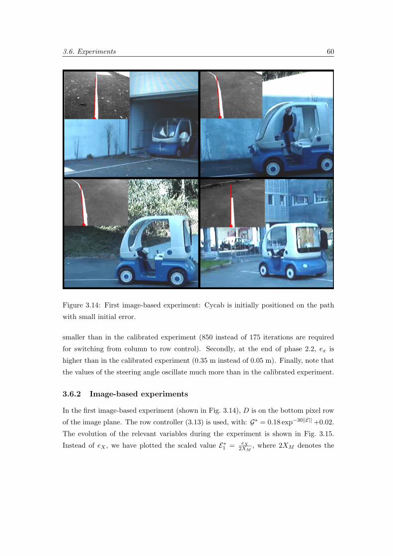
3.6. Experiments 60
Figure 3.14: First image-based experiment: Cycab is initially positioned on the path
with small initial error.
smaller than in the calibrated experiment (850 instead of 175 iterations are required
for switching from column to row control). Secondly, at the end of phase 2.2, ex is
higher than in the calibrated experiment (0.35 m instead of 0.05 m). Finally, note that
the values of the steering angle oscillate much more than in the calibrated experiment.
3.6.2 Image-based experiments
In the first image-based experiment (shown in Fig. 3.14), D is on the bottom pixel row
of the image plane. The row controller (3.13) is used, with: G∗ = 0.18 exp−30||E|| +0.02.
The evolution of the relevant variables during the experiment is shown in Fig. 3.15.
Instead of eX , we have plotted the scaled value E∗1 = eX2XM
, where 2XM denotes the

3.6. Experiments 61
Figure 3.15: Evolution of relevant variables during the first image-based experiment.
Top: errors E∗1 (non-dimensional), and E2 (in rad) are plotted (red and blue: correct
camera calibration, pink and cyan: coarse calibration). Bottom: cd in m−1 (purple)
and φ in rad (green: correct camera calibration, black: coarse calibration).
image width in pixels. The robot is able to successfully follow the path and the tracking
errors are low throughout the experiment. At the end of the experiment, both errors are
below 0.03. As in the position-based experiment, both errors increase when the robot
reaches the discontinuity in the path curvature (frame 335), and correspondingly, φ
increases in order to compensate for the error. Using Fig. 3.7, we verify that throughout
the experiment, the state variables verify the stability condition.
In the second experiment (shown in Fig. 3.16), CyCab is initially near the path,
with D on the right pixel column of the image plane. During phase 2.1, the column
controller (3.15) is used, with: G∗ = 0.98 exp−3.6||E|| +0.05. Then (phase 2.2), the row
controller (3.13) is used with: G∗ = 0.18 exp−30||E|| +0.02 (as in the first experiment).
The state errors are plotted in the top of Fig. 3.17, for phases 2.1 (left) and 2.2 (right).
Instead of eX and eY , we have respectively plotted the scaled values E∗1 = eX2XM
for phase
2.1, and E∗1 = eY2YM
for phase 2.2 (2XM and 2YM respectively denote the image width
and height). The path curvature cd (purple) and steering angle φ (green) are plotted
in the bottom graph of Fig. 3.17. The robot is able to successfully follow the path, and
the tracking errors converge during both phases. At the end of the experiment both
state errors are zeroed. Note the completely different initial trend of φ, as compared

3.6. Experiments 62
Figure 3.16: Second image-based experiment: D is initially on the right pixel column
of the image plane.
to the position-based experiment (shown in Fig. 3.11, bottom). The iteration steps
with state variables not verifying the asymptotic stability condition (i.e., values of Xoutside the loci of Fig. 3.7) are highlighted in yellow in Fig. 3.17. The plots show that,
throughout phase 2.1 and during the beginning of phase 2.2, condition (3.19) is not
verified. Nevertheless, the system is able to converge.
In the third experiment (shown in Fig. 3.18), CyCab is initially far from the path,
with D on the top pixel row of the image plane. The evolution of the relevant variables
during the experiment is shown in Fig. 3.19. Once again, in the graphs, the values of
E have been scaled by the image size. During phase 3.1, the row controller (3.13) is
applied, to drive point D to a lateral pixel column of the image plane. Since initially

3.6. Experiments 63
Figure 3.17: Evolution of relevant variables during the second image-based experiment.
Top: errors during phases 2.1 (left) and 2.2 (right). E∗1 (non-dimensional) and
E2 (in rad) are plotted (red and blue: correct camera calibration, pink and cyan:
coarse calibration). The iteration steps with state variables not verifying the stability
condition are highlighted in yellow. Bottom: cd in m−1 (purple) and φ in rad (green:
correct camera calibration, black: coarse calibration).
−π2 < Θ < −π, the controller selects the right side column. We use: G∗ = 10.
Afterwards (phase 3.2), the column controller (3.15) is applied, with G∗ = 4.0. Finally
(phase 3.3), the row controller (3.15) is used with: G∗ = 0.18 exp−30||E|| +0.02. The
experiment fails during phase 3.3: the error eX diverges and the path exits the field of
view. Tests with other values of G∗ are also unsuccessful. The reason is the failure of
asymptotic stability condition (3.19) during the experiment. The iteration steps with
state variables not verifying (3.19) are highlighted in yellow in Fig. 3.19. The plots
show that, during most of phase 3.2 and throughout phase 3.3, the asymptotic stability
condition is not verified. Although during phase 3.2 the errors converge in spite of this,
during phase 3.3 the experiment fails. As we mentioned throughout this article, a flaw
of the image-based control law is that it does not take into account the curvature cd.
This is particularly relevant in this experiment, and causes, in our opinion, the failure.
In fact (see the bottom left snapshot of Fig. 3.18), the robot switches to phase 3.3
with a large error on E2, in a critically curve portion of the path. In contrast with the
position-based scheme, in this case, the error dynamics cannot be controlled since the

3.6. Experiments 64
Figure 3.18: Third image-based experiment: the initial error is large (D is on the top
pixel row of the image plane). The experiment fails.
curvature is not used to compute the feedback law. However, the initial state for phase
3.3 (which causes the failure) cannot be changed. In fact, the gains G∗ during phases
3.1 and 3.2, must be chosen so that the controller saturates the steering angle φ to its
maximum value φM = 0.40 rad, and thus determine the initial state of phase 3.3.
The two successful image-based experiments (i.e., first and second experiments)
have been repeated by considering a calibration error on the camera parameters.
The evolution of the relevant variables in the coarse calibration experiments is
also shown in Fig. 3.15 and 3.17 (pink and cyan for the errors, black for φ), for
comparison with the calibrated camera experiments. The robot is able to successfully
follow the path in both cases. The convergence rate is slightly lower than in the

3.7. Conclusions and future work 65
Figure 3.19: Evolution of relevant variables during the third image-based experiment
with correct camera calibration. Left to right: cd (purple, in m−1) with φ (green, in
rad), and errors E∗1 (red, non-dimensional) and E2 (blue, in rad) during phases 3.1 to
3.3. The iterations steps with state variables not verifying the stability condition are
highlighted in yellow.
calibrated camera experiments. However, in particular for the second experiment, the
image-based approach outperforms the position-based approach when the camera is
coarsely calibrated.
3.7 Conclusions and future work
In this chapter, we presented two visual servoing control schemes (position-based and
image-based) enabling nonholonomic mobile robots with a fixed pinhole camera to
follow a continuous path on the ground. The controllers utilize only a small set of
path features extracted from the image plane, without using the complete geometric
representation of the path. The features are: the position of a path point, and the path
tangent orientation at that point. For the position-based controller, the path curvature
at that point is also utilized. A major contribution of this work is that both approaches
can be used in general initial conditions, thanks to a switching strategy between
two primitive controllers. A Lyapunov-based stability analysis has been carried out.
The performance of both controllers has been experimentally validated on a car-like
robot equipped with a pinhole camera starting from three different initial conditions.
The scheme robustness was also verified, by adding camera model errors in all the
experiments.
The experiments point out the main characteristics of the two approaches for the
specific task of path following. The image-based primitive controllers have smaller
3.7. Conclusions and future work 66
stability zones than the corresponding position-based primitive controllers. As a
consequence, one of the three experiments fails when using the image-based approach
and succeeds with the position-based approach. On the other hand, for the two other
experiments, the image-based approach is more effective (a smoother control input φ
is needed to achieve the task), and robust to camera calibration errors.
These results confirm the properties of the two control schemes. The image-based
controller is less effective when the initial error is large, since it does not rely on the
curvature measure, which, acting as a second derivative, fosters the prediction of the
error dynamics. On the other hand, by using the path curvature measure, which is
typically more biased than path position and path tangent orientation measures, the
position-based control law is less smooth and less robust to calibration errors.
Chapter 4
Vision-based path following for a
legged robot with actuated
pinhole camera and its
application in the ASPICE
project
In this chapter, we present the design and implementation of a vision-based path
following scheme which has been integrated in the ASPICE (Assistive System for
Patient’s Increase of Communication, ambient control and mobility in absence of
muscular Effort) project [11].
One central feature of the ASPICE system is the possibility for the user to remotely
control the motion of a mobile robot (a Sony AIBO) by means of various input devices,
including a Brain-Computer Interface (BCI). While moving, the robot should assist
the user by monitoring the environment and by communicating specific requests to the
caregiver. Depending on the residual abilities of the user, as well as on the desired
task, it is possible to choose between three different navigating modes for controlling
the robot motion: Single step, Semi-autonomous and Autonomous navigation modes.
In this chapter, we focus on the development of the autonomous navigation mode,
which is based on a vision-based path following scheme. The other navigation modes
67

4.1. The ASPICE project 68
are simply outlined in this chapter for the purpose of comparison with the autonomous
mode. They will be described in detail in the Chapter 5, along with other aspects of
ASPICE.
The chapter is organized as follows. In Sect. 4.1, the architecture of the ASPICE
system is briefly illustrated. In Sect. 4.2, the main features of the AIBO robot are
described. Sect. 4.3 presents the primitives developed for the robot PF framework,
at perception and motion levels. The robot visual path following scheme that we
implemented on the basis of the ASPICE requirements is outlined in Sect. 4.4. The
experiments are reported in Sect. 4.5. In the conclusion, we summarize the results.
4.1 The ASPICE project
4.1.1 Overview
The ASPICE project received in 2004 a two-year funding grant from TELETHON,
an italian medical research charity foundation. The project involves three partners,
including the Clinical Neurophysiopathology Laboratory of the Fondazione Santa Lucia
IRCCS and the Robotics Lab of the University of Rome “La Sapienza”.
The project is aimed at the development of a technological aid which allows
neuromotor-disabled users to improve or recover their mobility and communication
within the surrounding environment. The project is particularly addressed towards
those patients whose residual muscular strength is low and who is bed-ridden because
of practical obstacles or security concerns (see [11] for more details). Hence, the
major requirements are: adaptability to different levels of disability, low cost, and
robustness to the setting. Depending on the user requirements, the assistive device will
be a program running on a common low-power PC, on a palmtop, or on a powerful
workstation.
The ASPICE architecture, with input and output devices, is summarized in Fig. 4.1.
Some key elements of the system are:
• a variety of input devices for easy access to the Control Unit: these include
standard input devices (mouse, joystick, eye tracker, voice recognition) as well as
a Brain-Computer Interface;
• the Control Unit, which receives signals from the input devices through a Graphic

4.1. The ASPICE project 69
Feedback
USER
ENVIRONMENT
MobileRobot
DomoticAppliances
Brain-ComputerInterface
CONTROLUNIT
Standard Input Devices
Figure 4.1: The ASPICE architecture.
User Interface (GUI) and converts them into commands that drive the output
devices (either the domotic appliances or a mobile robot);
• the mobile robot;
• a number of domotic appliances, which must comply with the patient’s need for
ambient control (e.g., TV, lights, video camera, telephone, personal computer);
• visual feedback (either through the fixed video camera or through the robot
vision system) to provide the user with an increased sense of presence in the
environment.
The Control Unit contains drivers for all output devices; in some cases, previously
existing drivers are utilized, whereas in other cases (e.g., the mobile robot) the driver
has been designed “ad hoc” for the specific system. Note that all the signals between
the input devices and the Control Unit, and between the latter and the output devices

4.1. The ASPICE project 70
(including visual feedback) are transmitted over a wireless connection. In the remainder
of this section, the BCI which is used as input device and the Robot Driver that we
implemented are briefly described.
4.1.2 The robot driver
In any assistive robotics project, a major requirement is the user friendliness of
the robotic platform. In fact, although in recent years users are becoming, on the
average, more acquainted with technology, characteristics such as low cost, safety, and
low request for maintenance are still fundamental needs of any biomedical robotic
application. Moreover, clinicians have often emphasized the importance of working
with a familiar, friendly-looking robot, in order to limit its psychological impact on
patients [42]. In our case, these considerations led to the choice of the dog-like robot
Sony AIBO ERS-7 (described in Sect. 4.2) for inclusion in the system. Besides, studies
using AIBO to improve the quality of life, among elderly, have given good results [44].
AIBO should be driven around the user home with a small set of commands,
depending on the residual abilities of the patient. It should also assist the impaired
patient in visually monitoring the environment and in communicating with the
caregiver. Partial autonomy should be implemented in order to avoid collisions with
unexpected obstacles present in the environment. The robot range sensors are used
to avoid obstacles, as we shall show in Chapter 5. Another requirement is that AIBO
should be able to charge its battery when needed without any user intervention. As
already stated, one of the objectives of the ASPICE project is compatibility with a
variety of users and their level of disability. In light of this, three navigation modes
have been developed: single step, semi-autonomous and autonomous mode. The user
is expected to choose single step navigation when he/she wants to retain complete
control of the robot motion; e.g., for fine motion in cluttered areas. In semi-autonomous
navigation, the user specifies the main direction of motion, leaving to the robot the task
of avoiding obstacles. Finally, in the autonomous navigation mode, only a target point
in the environment is assigned by the user. The robot then travels to the target; this
is useful for quickly reaching some important locations (a window, the front door, the
kitchen). This mode of operation is expected to be particularly useful for severely
impaired patients who are unable to send frequent commands. To implement the
autonomous mode, we have designed a physical roadmap (shown in Fig. 4.2) to reach
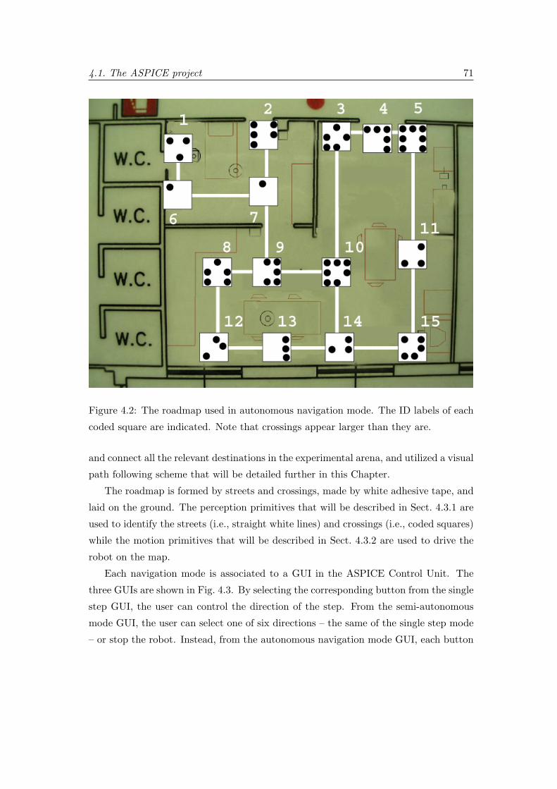
4.1. The ASPICE project 71
Figure 4.2: The roadmap used in autonomous navigation mode. The ID labels of each
coded square are indicated. Note that crossings appear larger than they are.
and connect all the relevant destinations in the experimental arena, and utilized a visual
path following scheme that will be detailed further in this Chapter.
The roadmap is formed by streets and crossings, made by white adhesive tape, and
laid on the ground. The perception primitives that will be described in Sect. 4.3.1 are
used to identify the streets (i.e., straight white lines) and crossings (i.e., coded squares)
while the motion primitives that will be described in Sect. 4.3.2 are used to drive the
robot on the map.
Each navigation mode is associated to a GUI in the ASPICE Control Unit. The
three GUIs are shown in Fig. 4.3. By selecting the corresponding button from the single
step GUI, the user can control the direction of the step. From the semi-autonomous
mode GUI, the user can select one of six directions – the same of the single step mode
– or stop the robot. Instead, from the autonomous navigation mode GUI, each button

4.2. The robot platform: AIBO 72
Figure 4.3: The ASPICE navigation GUIs: single step (above), semi-autonomous
(center) and autonomous (below) modes. In each GUI, the home button brings back
to the ASPICE main GUI.
that the user can select corresponds to a destination in the user apartment (here, the
bedroom, the living room, the bathroom, and the kitchen).
4.2 The robot platform: AIBO
The platform used in this work is a quadruped robot, Sony AIBO ERS-7, pictured
in Fig. 4.4. AIBO is a very interesting low-cost robot, widely used for research
and entertainment purposes. AIBO has been chosen in ASPICE for its familiar and
friendly-looking aspect, since it has been shown that in assistive robotic applications,
an important role is played by the robot’s design, which should facilitate everyday
interaction with the patients [42, 44]. Practical advantages in using legged robots
have been outlined in Sect. 1.2.2. The robot is equipped with 20 actuated joints, a
CMOS camera, two distance sensors (on the head and on the chest), an accelerometer,
a stereo microphone, a MIDI speaker, a set of leds and pression sensors. A wireless
LAN card enables remote control and debugging. The actuated joints are: 3 for each
leg, 3 for the head (head tilt, head pan, and neck tilt), 2 for the tail, 1 for each ear
and 1 for the mouth. AIBO’s real-time operating system APERIOS runs a specialized
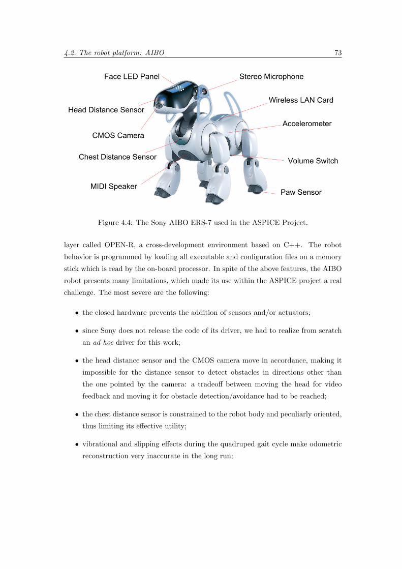
4.2. The robot platform: AIBO 73
CMOS Camera
MIDI Speaker
Wireless LAN Card
Face LED Panel Stereo Microphone
Head Distance Sensor
Chest Distance Sensor
Paw Sensor
Volume Switch
Accelerometer
Figure 4.4: The Sony AIBO ERS-7 used in the ASPICE Project.
layer called OPEN-R, a cross-development environment based on C++. The robot
behavior is programmed by loading all executable and configuration files on a memory
stick which is read by the on-board processor. In spite of the above features, the AIBO
robot presents many limitations, which made its use within the ASPICE project a real
challenge. The most severe are the following:
• the closed hardware prevents the addition of sensors and/or actuators;
• since Sony does not release the code of its driver, we had to realize from scratch
an ad hoc driver for this work;
• the head distance sensor and the CMOS camera move in accordance, making it
impossible for the distance sensor to detect obstacles in directions other than
the one pointed by the camera: a tradeoff between moving the head for video
feedback and moving it for obstacle detection/avoidance had to be reached;
• the chest distance sensor is constrained to the robot body and peculiarly oriented,
thus limiting its effective utility;
• vibrational and slipping effects during the quadruped gait cycle make odometric
reconstruction very inaccurate in the long run;

4.3. Primitives 74
• the variable attitude of AIBO during its gait precludes the use of an external
sensory system (e.g., based on infrared triangulation with a detector placed on
the robot) for solving the localization problem.
4.3 Primitives
In order to utilize AIBO, specific primitives have been developed and integrated in the
driver framework. The perception primitives have been designed to identify the visual
landmarks on the roadmap, while the motion primitives are used to drive the robot on
the map.
The three reference frames which will be used in this work are: the robot frame FR(Fig. 4.7 and 4.6), the image frame FI (Fig. 4.5), and the camera frame FC (Fig. 4.6).
For the definition of these frames, refer to Chapter 1. We also note the robot neck tilt,
head pan, and head tilt joint angular positions respectively with: %h = [%nt %hp %ht]T .
4.3.1 Perception primitives
The features that the robot should perceive with the on-board camera are the landmarks
that it needs for localization and path planning purposes. The visual landmarks that
we use are straight white lines and coded squares placed on the floor. Thus, a straight
white line extractor and a coded square extractor have been developed. Moreover, the
visual landmarks should be located in sequential scenes. This task is accomplished by
a visual landmark tracker.
Straight white line extractor
A requirement of the robot driver is straight white line extraction. In order to be
independent from color classification, the straight white lines are detected by search on
the luminance signal I (X, Y ). Thus, line edges are searched at pixels with a strong
variation of luminance with respect to that of adjacent pixels. For each pixel located
in D = [X Y ]T the gradient of luminance ∇I (D) is computed, using the Roberts

4.3. Primitives 75
D
Y
XI(D)
∠ (D)
Y
XIO
XO
YO
Figure 4.5: Extracting edges (in yellow) for straight white line (left) and coded square
(right) detection. The detected coded square center is marked in red and the dot centers
are marked in cyan.
operator [66] as in [24]:
Ixy (D) = I (X + 1, Y + 1)− I (X, Y )
I−xy (D) = I (X + 1, Y )− I (X, Y + 1)
|∇I (D)| =√I2
xy (D) + I2−xy (D)
6 ∇I (D) = ATAN2 (Ixy (D) , I−xy (D))
(4.1)
where |∇I (D)| is the magnitude and 6 ∇I (D) ∈ (−π, π] is the direction of the pixel
luminance gradient (with respect to line Y = −X and positive clockwise, see Fig. 4.5.
Edges are then detected by applying a threshold test to |∇I (D)|. We use a threshold I∗
dependent on the mean value (noted µ|I|) of |I (D)| on the given image: I∗ = I∗(µ|I|
).
This adaptive thresholding makes the edge detection algorithm more robust to varying
light conditions, as compared to similar works implemented in environments where light
conditions had to be controlled. The threshold test may be written:
D ∈ De if |I (D)| ≥ I∗(µ|I|
)D /∈ De else
(4.2)
where De is the set of image edge pixels (marked in yellow in Fig. 4.5).
Afterwards, by applying threshold tests to relative distances and to luminance
gradient directions of the edge pixels belonging to De, subsets of line pixels are derived.
Indicating with NSWL the total number of straight white lines extracted on the image,

4.3. Primitives 76
the line pixel subsets are noted: DSWL,i (i = 1 . . . NSWL). Each DSWL,i defines a line
detected on the image frame, must contain at least nSWL,min pixels. We note nSWL,i
the number of pixels contained in each line pixel subset DSWL,i (nSWL,i ≥ nSWL,min
for each i = 1 . . . NSWL).
We tested several other edge detection algorithms (Sobel [67], Susan [73]), but the
Roberts operator showed better results, although the aforementioned methods are more
efficient for color space based extraction [78]. Besides, due to its low computation time,
this line extraction method was preferred to the Hough Transform technique, which we
also tested, and which is widely used for line detection in noisy images, with extensions
also accounting for line connectivity and thickness, as in [82].
In conclusion, the straight white line extractor algorithm returns the coordinates of
the pixels belonging to the NSWL lines extracted on the image frame (Fig. 4.5):
[Xj Yj ]TSWL,i ∈ DSWL,i
j = 1, . . . , nSWL,i
i = 1, . . . , NSWL
(4.3)
Coded square extractor
Along with the straight white lines, we have chosen to use as visual landmarks a set of
white coded squares laid on the ground. The identity and orientation of each square
is uniquely identified through a dotted black code, similar to the one used in[6]. The
choice of binary coding, i.e., black and white, is aimed at using luminance variation
instead of color classification, for extracting the square characteristics. We arranged
from 1 to 7 black dots on the border of the squares, in order to generate configurations
which uniquely define the landmark identity (defined by its label: ID) and orientation.
The 15 landmarks that we used can be seen in Fig. 4.2. Note that all the used landmarks
are unambiguous with respect to multiple 90 orientation errors. Hence, the landmark
identity and orientation can be uniquely identified in spite of the square rotational
symmetry.
In practice, edges of squares are searched within the set of edge pixels De derived as
in the straight white line extractor. The robot frame coordinates of all edge pixels are
derived from their image frame coordinates, with the projection that will be presented
below. Then, the projected edges are compared with a reference square with the same
dimensions of the coded square, so that the square perimeter pixels are identified.

4.3. Primitives 77
These define a subset of De for each square (see Fig. 4.5). Indicating with NCS the
total number of coded squares extracted on the image, the subsets of edge pixels of
each square i are noted: DCS,j (j = 1 . . . NCS). Each DCS,j defines a coded square
detected on the image frame and must contain at least nCS,min pixels. Following this,
pixels on the segments (scanlines) leading from the center to the perimeter edges are
classified by using a binary segmentation which uses the mean value of I on the image
as threshold. Corke [13] showed how binary segmentation is affected by noise, threshold
selection and edge gradient. However, in this application, the choice of binary coding
and the use of binary segmentation in only a small image window, and with adaptive
thresholding, reduces these problems. Finally, black dots are extracted by associating
a sufficient number of near black pixels found on the scanlines.
In conclusion, for each of the NCS detected coded squares, the coded square
extractor returns: the image coordinates of the square center O and of the centers
of the ndots black dots (respectively marked in red, and in cyan in Fig. 4.5):
[XO YO]TCS,j j = 1, . . . , NCS
[Xi Yi]TCS,j i = 1, . . . , ndots ndots = 1, . . . , 7
(4.4)
Visual landmark tracker
The straight white line extractor and coded square extractor only take into account
information from the current image. They provide no long-term knowledge. Thus,
consistent landmarks must be obtained by comparing the extracted landmarks over
consecutive images. This is done by projecting the characteristic points of each
extracted visual landmark V L = SWL1, . . . , SWLNSWL, CS1, . . . , CSNCS
from the
image frame FI (coordinates [X Y ]TV L) to the robot frame FR (coordinates [x y z]TV L).
Such mapping is not one-to-one, and can only determine the projecting ray of the point.
However, regarding our application, since all the visual landmarks are on the ground
plane, the problem can be solved in closed form.
In fact, recalling Sect. 1.3, the point coordinates in the camera and image frames
are related by:
D =I TCdc (4.5)
4.3. Primitives 78
with matrix ITC given by (1.16). This equation can be rewritten:
− flX
0 X −XI
0 − flY
Y − YI
xc
yc
zc
=
0
0
(4.6)
with the camera intrinsic parameters f , lX , lY , XI and YI defined in Sect. 1.3.
Moreover, given the homogeneous transformation matrix RTC representing the camera
frame pose with respect to the robot frame, the coordinates of a point in the two
reference frames are related by:
x
y
z
1
=R TC
xc
yc
zc
1
(4.7)
We neglect the distance between the robot head tilt and head pan axes, assuming
they intersect in a point which stays in a constant position ς = [0 yς zς ]T in the
robot frame (see Fig. 4.6). We also assume that during its motion, the robot body
maintains constant orientation around the x axis, and null orientation around the two
other axes. Under these assumptions, RTC can be easily computed at every frame
through the three head joint positions %h = [%nt %hp %ht]T and ς, by using the Denavit
and Hartenberg method [35] as in [24]. Since landmarks are on the ground plane
(i.e. zV L = 0) the third equation from (4.7) can be expanded and used, along with (4.5):
t31 t32 t33
− flX
0 XV L −XI
0 − flY
YV L − YI
xc
yc
zc
V L
=
−t34
0
0
(4.8)
where t31 . . . t34 indicate the elements of the third row of RTC . Inverting this equation
away from singularities, allows for computation of the landmark position [xc yc zc]TV L in
the camera frame, given the landmark position [X Y ]TV L in the image frame returned
by the straight white line extractor and coded square extractor. Finally, substituting
[xc yc zc]TV L in (4.7) gives the landmark position [x y 0]TV L in the robot frame.
The robot frame coordinates of all straight white line points [xj yj 0]TSWL,i are
then processed with a least square error algorithm in order to identify the path errors

4.3. Primitives 79
Figure 4.6: The camera frame and head joint positions.
[en eθ]TSWL,i of each of the NSWL lines (see Sect. 1.1). In this case, since the path
direction is not specified, the path following algorithm chooses the direction with
smaller orientation error. Hence, the path errors are defined as shown in Fig. 4.7a. The
orientation error eθ is always in the interval(−π
2 ,π2
]. The normal path error en is chosen
accordingly. A similar approach is used to process all the coded squares characteristic
points [xo yo 0]TCS,j , and [xi yi 0]TCS,j , and obtain the identity IDj = 1 . . . 15 and
orientation γj , of each of the NCS coded squares (see Fig. 4.7b). Visual landmarks,
extracted and projected at previous frames, are displaced according to the robot
measured motion and compared with the current projected landmarks for checking
consistency and filtering out false positives. The algorithm returns the characteristics

4.3. Primitives 80
x
yo
xo
γ > 0 y(b)yeθ > 0
x
d
(a)
en >0
Figure 4.7: Relevant variables utilized in: (a) straight white line tracking, and (b)
coded square tracking.
of the visual landmarks, validated in a sufficient number of consecutive frames:
[en eθ]TSWL,i i = 1, . . . , NSWL
IDj γj [xo yo 0]TCS,j j = 1, . . . , NCS
(4.9)
4.3.2 Motion primitives
From a kinematic point of view, AIBO can be considered as an omnidirectional robot,
i.e., three velocities (forward u1, lateral u2, and angular u3 around the robot center,
positive for counterclockwise rotation) can be independently specified. In all cases
where the robot velocities are specified in FR coordinates as V = [Vx Vy]T (e.g., when
they are imposed by a user command), they must be mapped to the control input u.
To perform this conversion, we have used two strategies. The first (omnidirectional
translational motion), consists of simply setting:
u1 = Vy
u2 = Vx
(4.10)
with u1 forward velocity, and u2 lateral velocity. The robot orientation is not
controlled in this first kind of conversion. Instead, the second kind of conversion

4.3. Primitives 81
(nonholonomic-like motion), consists in setting:
u1 = Vy
u2 = ATAN2(Vx, Vy)(4.11)
with u1 and u2 respectively forward and angular velocity. The advantages of each
strategy will be illustrated later.
Basic motion primitives for controlling the robot legs in order to obtain the desired
motion u are based on the kinematic parameterized trot walk algorithm described in
Sect. 1.2.2. Velocity commands computed by the motion primitives are suitably scaled
if any of them exceeds the physical limits of the actuators.
We also developed three primitives: Landmark fixer, Landmark approacher (LA),
and Straight line follower, which use visual information returned by the perception
primitives to guide the robot. In practice, the robot actuators are driven by a visual
servoing scheme. Since the visual landmark tracker returns the position of the visual
landmarks relative to the robot, position-based visual servo control turns out to offer
a better solution than image-based servoing. The three vision-based motion primitives
are explained below.
Landmark fixer
Referring to [13], “fixation” is defined as motion aimed at keeping one point in the
scene (the “target”, noted TG) at the same location in the image plane. In this work,
it is of great interest to apply this control technique to a visual landmark, by keeping it
centered in the image plane. Advantages include: reducing chances of losing sight of the
landmark during motion, reducing motion blur, and reducing the effect of geometric
distortion in the lens (since the optical axis will be pointed at the landmark). In
many visual servoing works, the knowledge of camera motion during fixation is used to
determine the 3D position of the target: [x y z]TTG. Instead, in this application, since
the 3D position of the target is returned by the visual landmark tracker algorithm
outlined above both for straight white lines and for coded squares, it can be used as is
for fixation.
For fixation of a straight white line with parameters [en eθ]T , we choose the 3D
position of the target to be the normal projection of the robot center on the line
(which is also the point that should be tracked by the robot during PF): [x y z]TTG =

4.3. Primitives 82
[−en cos eθ en sin eθ 0]T . Instead, for fixation of a coded square with center [xo yo 0]T , we
choose: [x y z]TTG = [xo yo 0]T . In both cases, the position [x y z]TTG is used for solving
the inverse kinematics problem of finding the head joint coordinates for fixation. In
practice, given the target coordinates in the robot frame, the fixation task consists
in finding the robot head joint positions %h = [%nt %hp %ht]T such that the target
coordinates in the camera frame are [xc =0 yc =0 zc]TTG (corresponding to centering
the target in the image plane). This is equivalent to solving equation:0
0
zc
1
TG
=C TR
x
y
z
1
TG
(4.12)
for %h. CTR is the homogeneous transformation matrix representing the robot frame
pose with respect to the camera frame coordinates. It is derived by inverting RTC away
from singularities.
Apart from singular configurations, where no solution can be determined due either
to joint limits (e.g. target “behind” the robot head: in this case a different target point
must be chosen) or to singularities of RTC , for most configurations the solution of (4.12)
is non-unique. In fact, although the head pan joint position %hp can be derived from
the first equation in (4.12):
%hp = −ATAN2 (xTG, yTG − yς) (4.13)
replacing it in the two other equations does not guarantee a unique solution for the
head tilt and neck tilt joint positions. In our implementation, we choose, whenever
possible (i.e. when yTG is “sufficiently” large) to fix %nt to its lower bound (in order to
maximize scene depth zc), and derive %ht from (4.12). If it is not possible to adopt this
strategy, due to the %ht joint limits, we fix %ht to its limit and derive %nt.
Landmark approacher
When the robot finds a landmark (with the extractors described in Sect. 4.3.1), it should
approach it, in order to get a better perception which can be useful for localization
purposes. In practice, it is a posture stabilization task with reference configuration
defined by the absolute position and orientation of the landmark. As we suggested
4.3. Primitives 83
previously, some tasks can be accomplished more effectively if nonholonomic-like motion
is enforced. However, no smooth state-feedback control law can solve the non-square
posture stabilization problem for a nonholonomic mobile robot [16]. Alternative control
approaches (e.g. smooth time-varying [70] and discontinuous feedbacks) have shown
limitations such as slow convergence and oscillatory transient. These considerations,
along with the requirement of minimizing the path to the target, led us to the choice
of omnidirectional motion, instead of nonholonomic motion, in the implementation of
the landmark approacher.
The omnidirectional walk that drives the robot to the landmark implements a
proportional closed-loop control strategy for reducing the robot’s relative distance and
orientation with respect to the nearest landmark perceived. In the case of straight
white line approaching, this is done by setting robot velocities (respectively: forward,
lateral and angular): u1 = λT en sin eθu2 = −λT en cos eθu3 = −λReθ
(4.14)
A similar controller is used for coded square approaching; in this case the robot
velocities are set to: u1 = λT yo
u2 = λTxo
u3 = −λRγ
(4.15)
In both cases, λT and λR are positive given gains.
Straight line follower
This primitive should solve the path following problem for a straight white line. For
this problem, we decided to adopt a nonholonomic model for the robot, in order to
obtain more effective obstacle avoidance (as will be shown in Chapter 5), and a more
“natural-looking” walk. Moreover, the path following problem differs from the posture
stabilization problem in that both linear and non-linear smooth state-feedback control
solutions exist for nonholonomic mobile robots [16]. On the other hand, since the task
is less stringent than posture stabilization, it can be achieved by using only one control
variable. In this work, we utilize only the angular velocity u2. The PF constraint, as
defined in 1.1, is et =const = 0, since the robot center must track its normal projection

4.4. Visual path following scheme 84
on the line. AIBO is modeled as a unicycle robot, with velocities [u1 u2]T and it is
rather simple to verify that the following kinematic equations hold:
en = −u1 sin eθeθ = u2
(4.16)
Linear feedback control can be realized by tangent linearization of the two equations
above, in the neighborhood of (en = 0, eθ = 0). This gives the second order linear
system:en = −u1eθ
eθ = u2
(4.17)
which is clearly controllable, and thus asymptotically stabilizable by linear state
feedback on u2, when u1 is constant and strictly positive. Thus, the motion exigency
(see Sect. 1.1) for this application is: u1 = const > 0. It is rather simple to verify that
a stabilizing linear feedback is of the form:
u2 = (λ1en − λ2eθ)u1 (4.18)
with λ2 = 2ε√λ1. Gain λ1 > 0 must be chosen so as to specify the transient ’rise
distance’ and ε ∈ (0, 1) is the damping coefficient. The validity of this approach at
walking and jogging speeds has been proved by similar works (e.g., [72] and [16]), as
shown in Chapter 2.
4.4 Visual path following scheme
The visual path following scheme that will be described in this section has been used to
control the motion of AIBO in the ASPICE Autonomous navigation mode. With this
navigation mode, the ASPICE user selects a target destination on the roadmap (shown
in Fig. 4.2), and the robot utilizes the map features in order to reach the destination.
The map is formed by streets and crossings, all delineated through white adhesive tape
and laid on the ground. The streets are straight segments, which the robot follows
using the straight line following primitive. The crossings enable the self-localization of
the robot. In order to find the shortest path to the destination, the robot utilizes a
Dijkstra-based graph search [19]. Hence, given the initial robot configuration and the
desired destination in the workspace, the path to be followed is formed by a continuous,

4.4. Visual path following scheme 85
piecewise differentiable curve (i.e., a series of segments), which is compatible with the
definition of path given in Sect. 1.1
The perception primitives described in Sect. 4.3.1 are used to identify the streets
(i.e. straight white lines) and crossings (i.e. coded squares) while the motion primitives
described in Sect. 4.3.2 are used to drive the robot on the map. When approaching
a landmark or following a street, the robot concurrently implements landmark fixing,
in order to keep the landmark centered in the image plane. The robot autonomous
behavior is represented by a Petri Nets [57] based framework which has been successfully
deployed on the AIBO Platform in the Robocup field [83]. The Petri Net Plan formalism
allows for high level description of complex action interactions that are necessary in
programming a cognitive robot: non-instantaneous actions, sensing and conditional
actions, action failures, concurrent actions, interrupts, action synchronization.
The autonomous navigation plan uses the following actions (note that at all times
during the actions, the perception primitives are also executed for searching and
updating perceived data):
• Seek streets The robot seeks streets by exploring the environment, while avoiding
collisions. Motion directions are predefined: AIBO alternates forward and
rotation steps.
• Approach the nearest street When it perceives some streets with the straight white
line extractor, and tracks them with the visual landmark tracker, the robot uses
the landmark approacher to walk towards the nearest street.
• Follow the street When the robot is sufficiently close to the street, it implements
the linear straight line follower for walking on the street, until at least one crossing
is detected.
• Plan the path to destination When a crossing is detected with the coded square
extractor and is tracked with the visual landmark tracker, the robot will have
univocally identified its ID and orientation. This information, along with the
coded square positions in the robot frame, and with the map, identifies the robot
pose (position and orientation). The robot then utilizes a Dijkstra-based graph
search [19] to find the shortest path to the destination. Depending on the result
of the graph search, the robot will approach and follow another street (repeat

4.5. Experiments 86
Figure 4.8: The maximum distance at which the robot can detect the roadmap is
measured by positioning the robot in various configurations around a straight white
line.
the corresponding actions in the plan), or stop if the crossing corresponds to the
desired destination.
The autonomous navigation plan repeats the above actions until the destination is
reached. Transitions that start or terminate the actions represent events (e.g. Street
seen, or Crossing near) which are triggered by conditions on sensed information (e.g.
distance from a line). The plan must also deal with action failures. For instance,
whenever the robot loses visual contact with a street it was approaching, the system
aborts the current action and moves to the state where the street is not seen, and so
on, until the robot reaches the street again.
4.5 Experiments
In this section, we show the results of various experiments that were
performed with the visual path following scheme developed for the ASPICE
project. Short video clips of the experiments can be viewed on the web site:
http://www.dis.uniroma1.it/∼labrob/research/ASPICE.html.
In a first experiment, the performance of the straight white line extractor is
evaluated by estimating the maximum distance from the roadmap at which the robot is
4.5. Experiments 87
able to detect the straight lines. In our opinion, is also a good metric for evaluating the
performance of the ASPICE autonomous navigation mode. In fact, as soon as at least
one line is detected, the robot is able to reach the roadmap and find coded squares
’showing’ the way to the requested destination. Hence, line detection is the major
bottleneck in the visual path following scheme. For the experiment, the robot is placed
at a distance of 3 m from a straight white line, in various positions and orientations
(some configurations are shown in Fig. 4.8). The distance at which the robot detects
the line is measured and averaged along the experiments. After 20 experiments, the
average value is 2.14 m, with standard deviation 0.15 m. Clearly, these values are
strongly related to the environment light conditions and possible visual occlusions.In
the roadmap used for the ASPICE experiments (see Fig. 4.2), the robot is capable
of reaching the roadmap from every position in the environment, since the maximum
distance between lines is compatible with such results. Moreover, even when the initial
position is far from the roadmap, the seek streets action (see Sect. 4.4) will lead the
robot to a position where it is able to detect at least one line.
In a second series of experiments, the performance of the autonomous navigation
mode (and correspondingly, the visual path following scheme) is compared with the
other modes developed in ASPICE: single step and semi-autonomous modes. With
single step navigation, the user retains complete control of the robot motion: with a
fixed step size, the robot can be driven in six possible directions. Before the step, a
collision check is executed. Instead, in semi-autonomous navigation, the user specifies
the main direction of motion, leaving to the robot the task of avoiding obstacles: the
robot walks continuously in a specified direction until in receives a new command and
concurrently avoids obstacles that are on the way. Details on the implementation
of the ASPICE single step and semi-autonomous modes will be given in Chapter 5.
Here, we report the results of the experiment comparing the three navigation modes.
The comparison is carried out by driving the robot from a start point to a goal point
(noted respectively “S” and “G” in Figures 4.9 and 4.10). The task is repeated 5
times for each of the three navigation modes by using first a mouse (Fig. 4.9), and
afterwards a BCI (Fig. 4.10) as input devices. In the BCI experiments, a sequence
of icons corresponding to possible ASPICE commands is shown on a screen and aids
the user in choosing the command to be sent to the ASPICE Control Unit. The EEG
potentials are captured by means of an electrode cap. Details on the BCI will be given

4.5. Experiments 88
Figure 4.9: Comparison between the three ASPICE navigation modes: with the mouse
as input device, the user drives the robot from point S to point G using the single step
(above), semi-autonomous (center) and autonomous (below) modes.
in Chapter 5. The comparison between the three modes and between the two input
devices is based on execution time and user intervention (i.e. number of times the
user had to intervene by updating the commands) averaged over the experiments. As
expected, the results (plotted in Fig. 4.11) confirm the qualitative properties expected
for each mode. Note that the best choice depends not only on the user preference and
ability but also on the specific task (e.g., position of the start and goal points in the
environment, presence and position of obstacles). As expected, the user intervention
diminishes as the robot autonomy increases (both using BCI and mouse). On the other
hand, note that in the specific configuration used in the experiment, the execution

4.5. Experiments 89
Figure 4.10: BCI-driven single step navigation experiment. A feedback stimulus is
provided on the screen. The commands used to drive the robot from point S to point
G are displayed on the bottom.
time does not always decrease as autonomy increases. For example, when the robot is
mouse-driven, the task is executed in 1:23 minutes using the semi-autonomous mode
and in 1:30 using the autonomous mode. The differences may depend, among other
factors, on the distances of the start and goal points from the roadmap. The use of the
BCI introduces a time delay on each user intervention. This delay is due to the time
required for selection of each command. In fact, to reduce the effect of the EEG signal
noise, the command selection is validated after the user has ’confirmed’ it various
times (in our experiment, 6 times). Moreover, BCI control introduces errors during
the navigation, due to EEG noise and large user inaccuracy, as compared to mouse

4.5. Experiments 90
Figure 4.11: Comparison between the 3 navigation modes using 2 input devices: mouse
(blue) and BCI (red). Execution time (in minutes): dashed, user intervention (number
of commands): solid.
control. Hence, the user intervention is greater with the BCI, since the user must apply
extra commands to correct the errors. Consider, for example, the semi-autonomous
experiment: with the mouse, four clicks were sufficient, whereas with the BCI, the
user had to intervene 11 times. This specific result is related to the characteristics
of the semi-autonomous mode, which requires precise timing when switching between
walking directions. This requirement is hardly compatible with the BCI. For both the
aforementioned reasons (time delay on each command and errors), the total execution
time is particularly worsened when a high intervention is required. For instance, in
single step mode, the experiment requires 2:22 more with the BCI than with the mouse,
whereas in autonomous mode the difference is only 17 seconds. Thus, when using the
BCI, the autonomous navigation mode is the most appropriate.
The usefulness of the proposed scheme to increase patient independence in everyday
life is shown in an experiment where a domestic task is achieved by taking advantage
of the visual path follower. The task is shown in Fig. 4.12: the robot is used to verify
whether the bottle of water is on the green table in a domestic environment. The
visual feedback from the robot camera supports the user throughout navigation. The
robot is initially located far from the roadmap with an obstacle on the way. The user
perceives this information via the robot camera, and decides to control AIBO with the
semi-autonomous mode to approach the roadmap (Fig. 4.12a). When the user perceives
that the robot is sufficiently near the roadmap, the autonomous mode is used to drive
the robot to the target nearest to the green table (Fig. 4.12b, c and d). Then, in order
to obtain precise motion of the robot camera and check if the bottle is on the table,

4.5. Experiments 91
Figure 4.12: Executing a domestic task (check if the bottle is on the green table) by
taking advantage of all the characteristics of the ASPICE robot driver.
the user controls the robot with the single step mode, and finally displaces the robot
camera with the head control menu (Fig. 4.12e). Clearly, the task would have been
much harder to achieve in the absence of the path following controller.
Finally, in another experiment, autonomous robot battery charging, is implemented.
This behavior is also present in the commercial Sony Driver, but since Sony does not
release the code of its driver, we had to realize it ad hoc for this project. This experiment
not only fulfills an important ASPICE requirement, but also provides an additional
testbed for the visual path following scheme. In fact, the AIBO Charging Station is
placed near a marked crossing on the roadmap shown in Fig. 4.2, and as soon as the
battery level is low, the robot autonomously moves to the station. The experiment is
illustrated in Fig. 4.13. The robot position at consecutive time frames is shown while it
approaches the roadmap, follows the street up to the battery charger crossing, detects
it and makes a turn in order to reach its destination (the charging station) on the basis
of the plan.
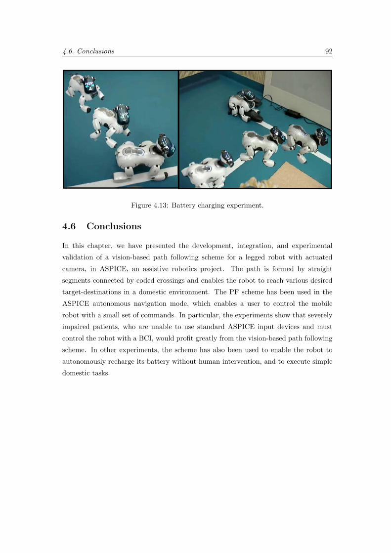
4.6. Conclusions 92
Figure 4.13: Battery charging experiment.
4.6 Conclusions
In this chapter, we have presented the development, integration, and experimental
validation of a vision-based path following scheme for a legged robot with actuated
camera, in ASPICE, an assistive robotics project. The path is formed by straight
segments connected by coded crossings and enables the robot to reach various desired
target-destinations in a domestic environment. The PF scheme has been used in the
ASPICE autonomous navigation mode, which enables a user to control the mobile
robot with a small set of commands. In particular, the experiments show that severely
impaired patients, who are unable to use standard ASPICE input devices and must
control the robot with a BCI, would profit greatly from the vision-based path following
scheme. In other experiments, the scheme has also been used to enable the robot to
autonomously recharge its battery without human intervention, and to execute simple
domestic tasks.

Chapter 5
Other aspects of the ASPICE
project
Although the ASPICE project has provided a useful testbed for the path following
scheme which has been described in Chapter 4, it has also permitted the development
of many other aspects in the field of assistive robotics. These numerous aspects are
described in this chapter.
An important objective in assistive technology is to design versatile systems, which
adapt to the user level of disability by offering various human-robot interfaces and
various levels of interaction. Semi-autonomous navigation systems for wheelchairs
which adapt to the patient autonomy level [27, 46] are an example of this approach.
Similarly, in ASPICE, as mentioned in Chapter 4, three navigation modes have
been developed. The autonomous navigation mode has been thoroughly described
in Chapter 4. In this chapter, we will describe the single step and semi-autonomous
navigation modes. Automatic obstacle detection and avoidance is integrated in all
navigation modes to guarantee safe, collision-free motion in cluttered environments.
This is done by generating an occupancy grid, which will also be described in this
chapter, along with the experimental validation of the obstacle avoidance algorithm.
Another objective of the ASPICE project is to enable robot control based on signals
from different sources, depending on the user residual abilities. In particular, in this
chapter, we will describe the Brain-Computer Interface which has been utilized to
control AIBO with the user electro-encephalographic brain signals. Other features
93

5.1. Occupancy grid generator 94
of the system, such as the video feedback from the robotic platform to the user and
the use of AIBO as communication aid, are also briefly described. A third objective
of ASPICE is to aid or support a human user in everyday tasks. Hence, the system
must be assessed by considering its effects on the quality of the user’s life. Human-robot
interaction during the ASPICE experimentation has been assessed by patient feedback.
The ASPICE clinical assessment on potential users has also been briefly reported at
the end of the chapter.
The chapter is organized as follows. In Sect. 5.1, the occupancy grid generator
needed to avoid obstacles during navigation is illustrated. The ASPICE single step
and semi-autonomous navigation modes are described respectively in Sect. 5.2 and
in Sect. 5.3. In Sect. 5.4, we present the Brain-Computer interface used by severely
impaired patients to control AIBO and the other ASPICE appliances. Other aspects
of the ASPICE robot driver are described in Sect. 5.5. Simulations and experiments
are presented in Sect. 5.6. The ASPICE clinical validation is reported in Sect. 5.7.
5.1 Occupancy grid generator
The main features that the robot should perceive are the obstacles that it should
avoid. We chose to use the robot range sensors to detect obstacles. We use a
local two-dimensional occupancy grid to represent the detected obstacles, built by the
occupancy grid generator.
The robot should be able to recover robust and useful spatial descriptions of its
surrounding obstacles, using sensory information. These descriptions should be used for
short-term planning in the environment. To do this, we use a tesselated two-dimensional
representation of spatial information called the occupancy grid. In the past years,
the occupancy grid framework proved to be extremely efficient for performing path
planning and obstacle avoidance in unknown and unstructured environments, and
researchers have proposed different functions for updating the grid cells (e.g. Fuzzy [60],
Bayesian [40], Gaussian [22]). The occupancy grids have also been used for obstacle
detection on Sony AIBO. Fasola and others [26] make use of the robot camera to
generate a local occupancy grid, used for taking navigation decisions. A similar
approach is used in [39], where recent information is integrated along with current
information, based on odometric data. However, both works were used in the Robocup

5.1. Occupancy grid generator 95
xx
y(u1 u2 )
y
u3
Figure 5.1: Relevant variables utilized in occupancy grid generation.
application, where free space can be easily identified by the green color (the color of the
soccer field). Instead, in unknown environments, using visual information for obstacle
detection is very challenging. The AIBO range sensors are a better tool, although only
two are available. In [41], a scanning motion of the AIBO head distance sensor is used
to map the obstacles locally and the position of the barycenter of the sensor readings
after every scan is used for robot navigation.
In our approach, the two range finders (head and chest) are used to detect obstacles,
although the chest sensor can only detect near obstacles, due to its limited range and
particular orientation (see Sect. 4.2), and hence is not used to compute the occupancy
grid. Thus, only the head sensor is utilized to build the local occupancy grid by moving
the head pan joint along a sinusoidal profile spanning an angular width of 90. While
the origin of the occupancy grid is always on the head pan axis and its longitudinal

5.2. Single step navigation mode 96
extent is limited by the range of the head distance sensor (1 m), its orientation (i.e., the
direction of its bisectrix) is the same as the direction of motion introduced in Sect. 4.3.2
V = [Vx Vy]T (see Fig. 5.1). As is shown in the figure, 30 grid cells are used. The cells
are annulus sectors of width 15 and height 0.2 m. Obviously, due to the joint limit, it is
impossible to build occupancy grids for backward motions. The grid may be built with
the robot when this is in stationary position or in motion. In the second case, the head
pan movement is synchronized with the gait cycle and odometric data (reconstructed
through the leg joint encoders) are used to build a consistent map: in practice, at every
time frame, the previous range readings are displaced on the map according to the robot
measured motion. When the pan cycle is complete, a cell in the grid is considered to
be occupied if there is a sensor reading indicating an obstacle inside that cell.
5.2 Single step navigation mode
With single step motion, the robot can be driven, with a fixed step size, in any of
six directions (forward, backward, lateral left/right, clockwise and counterclockwise
rotations). The user selects the desired direction from the corresponding GUI, shown
in Fig. 4.3, above. Before performing the motion command, the robot generates the
appropriate occupancy grid (oriented along the intention of motion) from its stationary
position and verifies whether the step can be performed without colliding with obstacles.
The collision is checked by applying a threshold test to the sum of the inverse distances
of all the occupied grid cells. We note ‖ζ‖ the distance of the occupied cell center from
the robot center. If the collision check is positive:
∑ζ
1‖ζ‖
> TSS
the robot will not step in the desired direction. Otherwise, the step will be performed.
Clearly, the contribution of near occupied cells to the above sum is greater than that
of far-occupied cells. Note that, since no occupancy grid can be built for backward or
rotational motions, the corresponding step commands should be used with care.

5.3. Semi-autonomous navigation mode 97
5.3 Semi-autonomous navigation mode
With semi-autonomous motion, the user specifies the general directions of motion,
which the robot should track as closely as possible. The user selects the desired direction
from the corresponding GUI, shown in Fig. 4.3, center. This mode may be useful for
“gross” movements, leaving the user the possibility of returning to the single step
navigator for finer motion control. In contrast with single step navigation, in the
semi-autonomous mode, occupancy grid generation and motion control are executed
simultaneously. Instead of executing a single step, the robot walks continuously in
the specified direction until it receives a new command (either a new direction or a
stop). If the specified direction is forward or lateral1 (i.e., the user desired direction
of motion in the workspace is Vdes = [Vdes,x 0]T or Vdes = [0 Vdes,y]T ), autonomous
obstacle avoidance is obtained by the use of potential fields. The algorithm used in this
case is explained below.
In fact, the use of potential fields has proved to be a powerful technique for
controlling robot motion [45]. Some researchers have used potential fields to address the
problem of real time action selection both for navigation and manipulation purposes
on the AIBO [43]. Others [64] calculate the potential fields needed for autonomous
exploration of an environment, from an occupancy grid. We decided to use the latter
approach by generating the occupancy grid as the robot moves and then use it to
compute the robot velocities. Our algorithm uses a composition of vortex and repulsive
fields to build the velocity field. In particular, for each occupied cell on the occupancy
grid, centered at ζ = [xζ yζ ]T , with xζ and yζ cell coordinates in the robot frame (see
Fig. 5.1), define the repulsive potential as:
Ur (‖ζ‖ , η) =
λr
(1‖ζ‖
− 1η
)2
if ‖ζ‖ ≤ η
0 else(5.1)
where ‖ζ‖ is the distance of the occupied cell from the robot center, η the radius of
influence of the potential, and λr a given gain. The repulsive field induced by each cell1As for the single step mode, no obstacle avoidance can be performed when executing backward or
rotational motions.
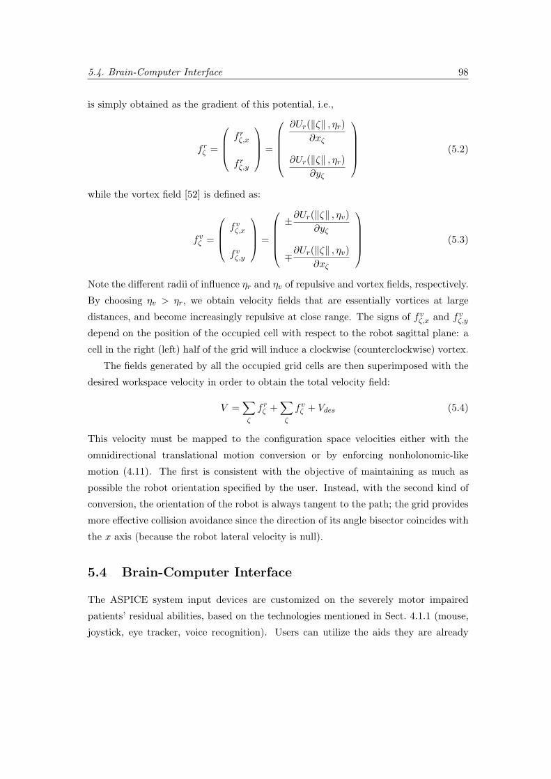
5.4. Brain-Computer Interface 98
is simply obtained as the gradient of this potential, i.e.,
f rζ =
f rζ,x
f rζ,y
=
∂Ur(‖ζ‖ , ηr)
∂xζ
∂Ur(‖ζ‖ , ηr)∂yζ
(5.2)
while the vortex field [52] is defined as:
fvζ =
fvζ,x
fvζ,y
=
±∂Ur(‖ζ‖ , ηv)
∂yζ
∓∂Ur(‖ζ‖ , ηv)∂xζ
(5.3)
Note the different radii of influence ηr and ηv of repulsive and vortex fields, respectively.
By choosing ηv > ηr, we obtain velocity fields that are essentially vortices at large
distances, and become increasingly repulsive at close range. The signs of fvζ,x and fv
ζ,y
depend on the position of the occupied cell with respect to the robot sagittal plane: a
cell in the right (left) half of the grid will induce a clockwise (counterclockwise) vortex.
The fields generated by all the occupied grid cells are then superimposed with the
desired workspace velocity in order to obtain the total velocity field:
V =∑ζ
f rζ +
∑ζ
fvζ + Vdes (5.4)
This velocity must be mapped to the configuration space velocities either with the
omnidirectional translational motion conversion or by enforcing nonholonomic-like
motion (4.11). The first is consistent with the objective of maintaining as much as
possible the robot orientation specified by the user. Instead, with the second kind of
conversion, the orientation of the robot is always tangent to the path; the grid provides
more effective collision avoidance since the direction of its angle bisector coincides with
the x axis (because the robot lateral velocity is null).
5.4 Brain-Computer Interface
The ASPICE system input devices are customized on the severely motor impaired
patients’ residual abilities, based on the technologies mentioned in Sect. 4.1.1 (mouse,
joystick, eye tracker, voice recognition). Users can utilize the aids they are already

5.4. Brain-Computer Interface 99
familiar with. On the other hand, the variety of input devices provides robustness to
the worsening of the patient abilities, which is a typical consequence of degenerative
diseases. When the patient is not able to use any of the standard input devices or
when a degenerative disease likely implies that in the future he/she will no more be
able to use them, a BCI should be utilized to access the Control Unit. The BCI gives
the user communication and control channels that do not depend on the brain normal
output channels of peripheral nerves and muscles [79]. In other terms, a BCI can
detect the activation patterns of the brain, and whenever the user induces a voluntary
modification of these patterns, it is able to detect it and to translate it into an action
that is associated to the user will. BCI technology has substantially improved in the
last decade and it is reasonable to expect that, in the near future, a wider class of users
will profit from it. Though the number of completely paralyzed patients is rather small
(some one hundred thousand worldwide), BCIs have the relevance that derives from
being the ’only’ option for such users, who would otherwise be locked in their bodies.
As it emerges from a concise review of related work, real time control tasks based
on human electro-encephalography (EEG) have been addressed to simple applications,
such as moving a computer cursor on a screen [81], opening a hand orthosis [63] or
driving a wheeled robot [17]. Recently, an experimental BCI which was implanted into
the brain motor cortex, enabled a tetraplegic to move a computer cursor [38]. However,
to our knowledge, the application of non-invasive BCI technology to interaction with a
wider set of devices has not been explored yet, and it represents one of the goals of the
ASPICE system.
The BCI used in ASPICE can be alternatively based on time domain (i.e., P300
evoked potentials [25]) or on frequency domain features (i.e., sensorimotor rhythms [80])
of the EEG signal. The performance of these two BCI versions varies on an individual
basis and the most reliable features are chosen depending on the user predisposition. In
both versions, a visual interface (on a screen) aids the user in choosing the command to
be sent to the ASPICE Control Unit. The EEG potentials are captured by means
of an electrode cap, amplified, digitized and transmitted to a personal computer.
Processing is handled by the BCI2000 software package [71]. After a preliminary signal
conditioning phase, which includes a linear mixture of channels implementing a high
pass spatial filter, the features (either in the time or frequency domain) are extracted
and used to identify the user desired command.

5.5. Other robot driver features 100
When time domain features are employed, a sequence of icons corresponding to
possible ASPICE commands is shown on the screen to the user. The icons are
highlighted successively one by one (ca. 3 icons are highlighted per second). After
each sequence, classification is implemented and the command corresponding to the
identified target icon is forwarded to the ASPICE Control Unit. Time domain features
are the result of an averaging procedure: the mean of time samples at equal latency
from the stimulus (i.e., the icon display) is computed for each channel and for each
stimulus. Averaged potentials at specific latencies and channels are fed into a linear
classifier. The latency/channel choice and the weights for classification are determined
in advance by training the classifier. A threshold is used to assess reliability of the
classification. The BCI which has been used in the experiments presented in Sect. 4.5
is based on time domain features.
When frequency domain features are employed, two targets positioned at the top
and bottom edge of the screen are shown to the user. Two actions (scroll along all
possible ASPICE commands and select the desired command) are associated with the
targets. The subject controls the vertical velocity of a cursor on the visual interface
by modulating the amplitude of his EEG sensorimotor rhythms above or below a
dynamically adapted threshold value. When the cursor reaches either the top or the
bottom target, the corresponding action (scroll or select) is performed in order to choose
the command to be forwarded to the ASPICE Control Unit. Frequency domain features
are computed using a parametric estimation, which takes into account the latest 300
ms of signal and is updated every 100 ms. The power spectral density values at specific
channels and frequency bins (which are identified in advance during the training phase)
are linearly combined. The output is detrended using a moving average value, which
avoids drift of the control signal if the EEG amplitude is increased or decreased (e.g.,
due to non-voluntary arousal effects).
5.5 Other robot driver features
In this Section, we will describe the implementation of four features of the ASPICE
robot driver.
5.5. Other robot driver features 101
5.5.1 Video feedback
Firstly, a fundamental requirement for effective remote controlled navigation is the
feedback of the robot camera to the Control Unit (i.e., to the user). This is not
only an essential aid for the user to drive the robot in the environment, but also
helpful for exploration and extension of virtual mobility. By driving the robot in a
desired spot of the apartment, the disabled person can monitor, with AIBO’s on board
camera, that area. Thus, an algorithm for feeding back to the ASPICE GUI the
image captured by the robot has been developed. Each new image captured by the
robot camera is compressed on board using the Independent JPEG Group libraries2,
before being streamed over a wireless connection to the ASPICE Control Unit. To
improve video quality in varying light conditions, the image luminosity is adaptively
icremented/reduced before compression, depending on the image average luminosity.
This simple approach reduces the variations in the average image luminosity during
video stream.
5.5.2 Vocal request interface
Another feature of the system is a GUI for vocal requests that has been included to
improve the communication of the patient with the caregiver. This feature covers an
important issue in ASPICE, enabling the robot to be socially interactive. Socially
interactive robots have been defined by Fong [28] to describe robots whose main task
is some form of interaction. Fong categorizes these robots by the aspects of social
interaction (speech, gestures, etc.) they use.
When the robot receives a vocal request (e.g., ‘I am thirsty’) from the control unit,
it plays the corresponding prerecorded audio file with its speakers in order to attract
the caregiver’s attention. The vocal request GUI is shown in Fig. 5.2 (bottom). In
the GUI, each button that the user can select corresponds to vocal request (here, ‘turn
on/off the light’, ‘Please come’, ‘I am thirsty’ ‘Close the window’ and ‘I am hungry’).
Each vocal request is associated to a robot gesture generated by a sequence of fixed
joint positions. Joint data containing angles for all joints, as well as timing information
that state for how long the values will be sent, is specified in a special description
language developed for AIBO and described in [24]. For each vocal request, there is a2www.ijg.org

5.5. Other robot driver features 102
Figure 5.2: The ASPICE GUIs for head control (top), and for vocal requests (bottom).
file in this description language which contains all the joint data.
5.5.3 Head control interface
To improve ambient exploration with the camera, a GUI for head control has also been
developed. This GUI allows the user to directly move the robot head and point the
camera in a desired direction. With this GUI, the user can control the head pan and
head tilt angles (%hp and %ht) with fixed steps, in order to point the camera in a desired
direction. The head control GUI is shown in Fig. 5.2 (top).
5.5.4 Walking gait
Finally, another issue that deserved attention is AIBO’s walking gait, which has been
modified on the basis of the ASPICE requirements (e.g., reducing the noise caused by
foot contact with the ground). The basic principles of the walking algorithm have been
described in Sect. 1.2.2. The goal of the algorithm is to move the robot feet alternatively
(in trot style) on rectangular trajectories. The directions and sizes of such rectangles
are determined by the motion command u. The joint angles required to drive the
feet on the rectangular trajectories are calculated by solving the inverse kinematics
problem for each leg. Nevertheless, many walking styles can be implemented, and a set
of parameters (e.g., the position of the rectangles with respect to AIBO’s body, or their
height) defines each possible walking style. Hence, a set of such parameters (noted Υ
in Sect. 1.2.2) was hand tuned and tested to fulfill ASPICE requirements. Clearly, the
limitations in the robot hardware forbid usage in environments with steps (e.g. stairs)
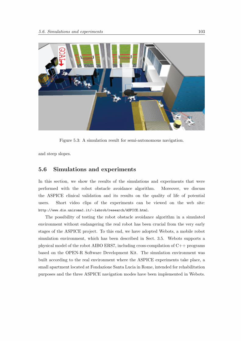
5.6. Simulations and experiments 103
GOAL
Figure 5.3: A simulation result for semi-autonomous navigation.
and steep slopes.
5.6 Simulations and experiments
In this section, we show the results of the simulations and experiments that were
performed with the robot obstacle avoidance algorithm. Moreover, we discuss
the ASPICE clinical validation and its results on the quality of life of potential
users. Short video clips of the experiments can be viewed on the web site:
http://www.dis.uniroma1.it/∼labrob/research/ASPICE.html.
The possibility of testing the robot obstacle avoidance algorithm in a simulated
environment without endangering the real robot has been crucial from the very early
stages of the ASPICE project. To this end, we have adopted Webots, a mobile robot
simulation environment, which has been described in Sect. 3.5. Webots supports a
physical model of the robot AIBO ERS7, including cross-compilation of C++ programs
based on the OPEN-R Software Development Kit. The simulation environment was
built according to the real environment where the ASPICE experiments take place, a
small apartment located at Fondazione Santa Lucia in Rome, intended for rehabilitation
purposes and the three ASPICE navigation modes have been implemented in Webots.

5.6. Simulations and experiments 104
Figure 5.4: Three experiments showing the performance of semi-autonomous
navigation. The user drives the robot using a single command: ’go forward’(top left
and bottom) and ’go right’ (top right).
A typical simulation of the ASPICE semi-autonomous mode is shown in Fig. 5.3. Here,
the user tried to drive AIBO to a given destination in the apartment (indicated by
a red arrow in the figure), through a single direction command (forward) along the
line joining the initial and final configuration. The obstacle avoidance algorithm was
able to successfully accomplish the task in spite of the many obstacles along the way.
Here, the nonholonomic conversion entailed by eq. (4.11) was used to map the reference
velocities to robot velocities. By using Webots, it was possible to debug the algorithms
effectively and to test them without endangering the real robot. It was also possible
to progressively develop the obstacle avoidance algorithms (initially based solely on

5.7. Clinical validation 105
repulsive potential fields) by reducing the local minima cases and developing adaptive
vortex fields. Besides, the problem of tuning all the parameters (gains, characteristics
of the grid-based map, etc.) could be easily solved in the simulation before porting on
the real AIBO.
After the Webots simulations, the obstacle avoidance algorithm has been tested
on AIBO in a series of experiments. In the experiments (shown in Fig. 5.4),
the performance of the obstacle avoidance algorithms is tested by using the
semi-autonomous navigation mode. Omnidirectional translational motion (4.10) is used
for mapping desired user velocities to the corresponding control inputs. In the first
(top left in the figure) and third (bottom) experiments, a single ’go forward’ command
is used. The robot is able to successfully avoid the obstacles while maintaining the
orientation desired by the user. In the second experiment (top right in the figure),
a single ’go right’ command is used. Again, the robot avoids the obstacle while
maintaining the desired orientation. The robustness of the obstacle avoidance algorithm
is evident in the third experiment, where the obstacle scenario is more complex than
in the two other experiments. In general, due to the vibrations in the quadruped gait
cycle and to the low-quality of AIBO’s distance sensors, small and mobile obstacles
might not be detected by the robot. However, using the robot camera video feedback
presented in Sect. 5.5.1, the user can detect such obstacles and intervene to prevent
collisions.
5.7 Clinical validation
At this stage of the ASPICE project, the system has been implemented and is available
at the Fondazione Santa Lucia in Rome for validation with patients [12]. All domotic
appliances used in ASPICE have been installed in the experimental apartment of
the Santa Lucia hospital. A portable computer runs the Control Unit program and
several input devices are available to cope with as many categories of users as possible.
The subjects have been admitted for a neuro-rehabilitation program and the whole
procedure underwent the approval of the local ethical committee. The patients have
been informed on the device and have given their voluntary informed written consent.
Furthermore, they have been interviewed and physically examined by the clinicians, in
order to evaluate some variables of interest: the degree of motor impairment and of

5.7. Clinical validation 106
reliance on the caregivers for everyday activities as assessed by current standardized
scale (Barthel Index BI), the familiarity with the system input devices, the ability to
speak or communicate, and the level of informatics alphabetization measured by the
number of hours per week spent in front of a computer. Then, for a period ranging from
3 to 4 weeks, the patient and (when required) her/his caregivers have been practising
weekly with the ASPICE system. During the whole period, patients had the assistance
of an engineer and a therapist in their interaction with the system. The experiments
have been carried out with eight subjects suffering from Spinal Muscular Atrophy type
II (SMA II) and six subjects suffering from Duchenne Muscular Dystrophy (DMD).
Depending on their level of disability, users controlled AIBO through keyboard, mouse,
touchpad, head tracker, microphone or BCI.
According to the score of the BI, all patients were on almost complete dependence
of caregivers, especially the six subjects suffering from DMD (BI < 35), who required
artificial ventilation, had minimal residual mobility of the upper limbs and very slow
speech. Because of the high level of muscular impairment, the DMD patients all had
access to the system via joypads. As for the eight SMA II subjects, their level of
dependency was slightly lower with respect the DMD patients, but they also required
continuous assistance for daily life activity (BI < 50). These patients have accessed
the system via joystick, touchpad, keyboard and microphone, since the residual motor
abilities were still functionally effective both in terms of muscular strength and range
of movements preserved. Four of them interacted with the system via BCI. All of the
patients were able to master the system and control AIBO within 5 sessions. Data
on user satisfaction, increase of independence, and reduction of caregiver workload,
have been collected and structured in questionnaires during the experimentation. For
instance, the users were asked to indicate with a number ranging from 0 (not satisfied)
to 5 (very satisfied) their degree of acceptance relative to each of the output devices.
The average grade given by the patients to their ’personal satisfaction in utilizing the
robot’ was 3.04 on a 5-point scale. This is a very promising result, considering that the
users were originally more accustomed to using and controlling the ’traditional’ ASPICE
appliances rather than the mobile robot. According to the results of the questionnaire,
all patients reported that they were independent in the use of the system at the end
of the training and they experienced (as they reported) “the possibility to interact
with the environment by myself”. From the clinical viewpoint, the robot navigation

5.7. Clinical validation 107
system was useful in blending the “desiderata” of the patients (e.g., being in the living
room with the relatives, reaching someone far from the patient’s location) with their
level of disability (which prevented them from acting as first-person in realizing such
“desiderata”). For example, patients with a partial preservation of distal arm muscular
ability (i.e., most SMA II patients) could have a complete control of the robot via
single step navigation. On the other hand, severely impaired patients (i.e. DMD
patients), who were unable to send frequent commands, could operate the robot in
semi-autonomous and autonomous navigation modes. In summary, the robot driver
has been designed in order to be effectively operated by low-speed input devices, such
as the ones developed in ASPICE (e.g., the BCI). Hence, in this work we did not
attempt to provide a new control interface for robot navigation, but rather focused on
the design and implementation of an appropriate robot navigation system, that can be
matched to various forms of detection of the user’s will. The clinical validation showed
feasibility of the proposed approach.
Further studies are necessary to confront a larger population of patients with
ASPICE, in order to assess the robot navigation system impact on the quality of life
by taking into account a range of outcomes (e.g. mood, motivation, caregiver burden,
employability, satisfaction, [48], [1], [59]). However, the results obtained from this pilot
study are encouraging for the establishment of a solid link between the field of human
machine interaction and neurorehabilitation strategy [34]. The ASPICE system cannot
substitute the assistance provided by humans. Nevertheless, it can contribute to relieve
the caregiver from the continuous presence in the room of the patient, since the latter
can perform some simple activities on his/her own. The perception of the patients
is that they no longer have to rely on the caregiver for each and every action. This
provides the patient with both a sense of independence, and a sense of privacy. For
both reasons, her/his quality of life is sensibly improved.

Bibliography
[1] J. R. Bach, J. Vega, J. Majors, and A. Friedman, Spinal muscular atrophy type
I quality of life, American Journal of Physical Medicine and Rehabilitation 82
(2003), no. 2, 137–142.
[2] S. Baker and S. K. Nayar, A theory of single-viewpoint catadioptric image
formation, International Journal of Computer Vision 35 (1999), no. 2, 1–22.
[3] G. A. Bekey, Autonomous robots: from biological inspiration to implementation
and control, MIT Press, 2005.
[4] M. Bertozzi, A. Broggi, and A. Fascioli, Vision-based intelligent vehicles: State of
the art and perspectives, Robotics and Automation Systems 32 (2000), 1–16.
[5] G. Campion, B. D’Andrea-Novel, and G. Bastin, Modeling and state feedback
control of nonholonomic mechanical systems, 30th IEEE Conference on Decision
and Control, 1991.
[6] M. Carreras, P. Ridao, R. Garcia, and T. Nicosevici, Vision-based localization of
an underwater robot in a structured environment, IEEE International Conference
on Robotics and Automation, 2003.
[7] F. Chaumette, Potential problems of stability and convergence in image-based and
position-based visual servoing, Lecture Notes in Control and Information Sciences,
ch. The Confluence of Vision and Control, Springer Berlin / Heidelberg, 1998.
[8] F. Chaumette and S. Hutchinson, Visual servo control tutorial, part I and II, IEEE
Robotics and Automation Magazine 13,14 (2007).
108

BIBLIOGRAPHY 109
[9] A. Cherubini, F. Giannone, L. Iocchi, and P. F. Palamara, An extended policy
gradient algorithm for robot task learning, IEEE/RSJ International Conference on
Intelligent Robots and System, 2007.
[10] A. Cherubini, G. Oriolo, F. Macrı, F. Aloise, F. Cincotti, and D. Mattia,
Development of a multimode navigation system for an assistive robotics project,
IEEE International Conference on Robotics and Automation, 2007.
[11] F. Cincotti, F. Aloise, F. Babiloni, M. G. Marciani, D. Morelli, S. Paolucci,
G. Oriolo, A. Cherubini, F. Sciarra, F. Mangiola, A. Melpignano, F. Davide,
and D. Mattia, Brain-operated assistive devices: the ASPICE project,
1st IEEE/RAS-EMBS International Conference on Biomedical Robotics and
Biomechatronics, 2006.
[12] F. Cincotti, D. Mattia, F. Aloise, S. Bufalari, G. Schalk, G. Oriolo, A. Cherubini,
M. G. Marciani, and F. Babiloni, Non-invasive brain-computer interface system:
towards its application as assistive technology, to appear in Brain Research Bulletin
(2008).
[13] P. I. Corke, Visual control of robots: high performance visual servoing, Research
Studies Press LTD, 1996.
[14] J.-B. Coulaud, G. Bastin, and M. De Wan, Stability analysis of a vision-based
control design, IEEE Transactions on Robotics (2006).
[15] A. K. Das, R. Fierro, V. Kumar, B. Southall, B. Spletzer, and J. Taylor,
Real-time vision-based control of a nonholonomic mobile robot, IEEE International
Conference on Robotics and Automation, 2001.
[16] C. Canudas de Wit, B. Siciliano, and G. Bastin Eds., Theory of robot control, 1996.
[17] J. del R. Millan, F. Renkens, J. Mourino, and W. Gerstner, Non-invasive
brain-actuated control of a mobile robot by human EEG, IEEE Transactions on
Biomedical Engineering 51 (2004), 1026–1033.
[18] F. Diaz del Rio, G. Jimenez, J. L. Sevillano, S. Vicente, and A. Civit Balcells, A
generalization of path following for mobile robots, IEEE International Conference
on Robotics and Automation, 1999.

BIBLIOGRAPHY 110
[19] E. W. Dijkstra, A note on two problems in connection with graphs, Numerische
Mathematik 1 (1959), no. 269–271.
[20] U. Duffert and J. Hoffmann, Reliable and precise gait modeling for a quadruped
robot, 9th International Robocup Symposium, 2005.
[21] F. Spindler E. Marchand and F. Chaumette, Visp for visual servoing: a generic
software platform with a wide class of robot control skills, IEEE Robotics and
Automation Magazine 12 (2005), no. 4, 40–52.
[22] A. Elfes, Using occupancy grids for mobile robot perception and navigation,
Computer 22 (1989), no. 6, 46–57.
[23] B. Espiau, F. Chaumette, and P. Rives, A new approach to visual servoing in
robotics, IEEE Transactions on Robotics and Automation 8 (1992), no. 3, 313–326.
[24] T. Rofer et al., Robocup 2005 german team technical report, Tech. report, Center
for Computing Technology - Universitat Bremen.
[25] L. A. Farwell and E. Donchin, Talking off the top of your head: Towards a
mental prosthesis utilizing event-related brain potentials, Electroencephalography
and Clinical Neurophysiology 70 (1988), no. 6, 510–523.
[26] J. Fasola, P. Rybski, and M. Veloso, Fast goal navigation with obstacle avoidance
using a dynamic local visual model, SBAI’05, The VII Brazilian Symposium of
Artificial Intelligence, Sao Luiz, Brazil, 2005.
[27] S. Fioretti, T. Leo, and S. Longhi, A navigation system for increasing the
authonomy and the security of powered wheelhairs, IEEE Transactions on
Rehabilitation Engineering 8 (2000), no. 4, 490–498.
[28] T. Fong, I. Nourbakhsh, and K. Dautenhahn, A survey of socially interactive
robots, Robotics and Autonomous Systems (2003).
[29] R. Frezza, G. Picci, and S. Soatto, A lagrangian formulation of nonholonomic path
following, Lecture Notes in Control and Information Sciences, vol. 237, ch. The
Confluence of Vision and Control, pp. 118–133, Springer Berlin / Heidelberg, 1998.

BIBLIOGRAPHY 111
[30] C. Geyer and K. Daniilidis, A unifying theory for central panoramic systems and
practical applications, ECCV, 2000.
[31] T. Gomi and K. Ide, Evolution of gaits of a legged robot, Fuzzy Systems
Proceedings. IEEE World Congress on Computational Intelligence, vol. 1, 1998,
pp. 159–164.
[32] B. Goodwine and J. Burdick, Trajectory generation for kinematic legged robots,
IEEE International Conference on Robotics and Automation, 1997, pp. 2689–2696.
[33] H. Hadj-Abdelkader, Y. Mezouar, N. Andreff, and P. Martinet, Omnidirectional
visual servoing from polar lines, IEEE International Conference on Robotics and
Automation, 2006, pp. 2385 – 2390.
[34] J. Hammel, Technology and the environment: supportive resource or barrier for
people with developmental disabilities?, Nursing Clinics of North America 38
(2003), no. 2, 331–349.
[35] R. S. Hartenberg and J. Denavit, A kinematic notation for lower pair mechanisms
based on matrices, Journal of applied Mechanics 77 (1955), no. 2, 215–221.
[36] K. Hashimoto and T. Noritsugu, Visual servoing of nonholonomic cart, IEEE
International Conference on Robotics and Automation, 1997.
[37] B. Hengts, D. Ibbotson, S. B. Pham, and C. Sammut, Omnidirectional motion for
quadruped robots, Robocup International Symposium, Lecture Notes in Computer
Science, Lecture Notes in Artificial Intelligence LNAI 2377, 2001.
[38] L. R. Hochberg, M. D. Serruya, G. M. Friehs, J. A. Mukand, M. Saleh, A. H.
Caplan, A. Branner, D. Chen, R. D. Penn, and J. P. Donoghue, Neuronal ensemble
control of prosthetic devices by a human with tetraplegia, Nature 442 (2006),
164–171.
[39] J. Hoffmann, M. Jungel, and M. Lotzsch, A vision based system for goal-directed
obstacle avoidance, 8th International Robocup Symposium, 2004.
[40] A. Howard and L. Kitchen, Generating sonar maps in highly specular
environments, 4th International Conference on Control, Automation, Robotics
and Vision.

BIBLIOGRAPHY 112
[41] V. Hugel, T. Costis, O. Strasse, P. Bonnin, and P. Blazevic, Robocup 2003 les
trois mousquetaires technical report, Tech. report, Laboratoire de Robotique de
Versailles, Velizy, France.
[42] R. Irie and T. Shibata, Artificial emotional creature for human-robot interaction -
a new direction for intelligent systems, IEEE/ASME International Conference on
Advanced Intelligent Mechatronics, 1997.
[43] S. J. Johansson and A. Saffiotti, Using the electric field approach in the robocup
domain, 5th International Robocup Symposium, 2001.
[44] M. Kanamori, M. Suzuki, H. Oshiro, and HAAT Members, Pilot study
on improvement of quality of life among elderly using a pet-type robot,
IEEE International Symposium on Computational Intelligence in Robotics and
Automation, 2003.
[45] O. Khatib, Real-time obstacle avoidance for manipulators and mobile robots, The
International Journal of Robotics Research 5 (1986), no. 1, 90–98.
[46] L. Kitagawa, T. Kobayashi, T. Beppu, and K. Terashima, Semi-autonomous
obstacle avoidance of omnidirectional wheelchair by joystick impedance control,
IEEE/RSJ International Conference on Intelligent Robots and Systems, vol. 4,
2001, pp. 2148–2153.
[47] H. Kitano (ed.), Robocup-1997: Robot soccer world cup I, LNCS, vol. 1395,
Springer, 1998.
[48] M. Kohler, C. F. Clarenbach, L. Boni, T. Brack, E. W. Russi, and K. E.
Bloch, Quality of life, physical disability, and respiratory impairment in Duchenne
Muscular Dystrophy, American Journal of Respiratory and Critical Care Medicine
172 (2005), no. 8, 1032–1036.
[49] J. Kosecka, R. Blasi, C. J. Taylor, and J. Malik, A comparative study of vision-based
lateral control strategies for autonomous highway driving, IEEE International
Conference on Robotics and Automation, 1998.

BIBLIOGRAPHY 113
[50] D. P. Krasny and D. E. Orin, Generating high-speed dynamic running gaits in a
quadruped robot using an evolutionary search, IEEE Transactions on Systems, Man
and Cybernetics, Part B: Cybernetics 34 (2004), no. 4.
[51] J.-P. Laumond, S. Sekhavat, and F. Lamiraux, Robot motion planning and control,
LNCIS, vol. 229, ch. Guidelines in Nonholonomic Motion Planning for Mobile
Robots, pp. 1–54, Springer, 1998.
[52] A. De Luca and G. Oriolo, Local incremental planning for nonholonomic mobile
robots, IEEE International Conference on Robotics and Automation, 1994,
pp. 104–110.
[53] A. De Luca, G. Oriolo, and M. Vendittelli, Ramsete - articulated and mobile
robotics for services and technologies, LNCIS, vol. 207, ch. Control of wheeled
mobile robots: An experimental overview, pp. 181–226, Springer, 2001.
[54] Y. Ma, J. Kosecka, and S. Sastry, Vision-guided navigation for a nonholonomic
mobile robot, IEEE Transactions on Robotics and Automation 15 (1999), no. 3,
521–536.
[55] G. L. Mariottini, G. Oriolo, and D. Prattichizzo, Image-based visual servoing
for nonholonomic mobile robots using epipolar geometry, IEEE Transactions on
Robotics 23 (2007), no. 1, 87–100.
[56] Y. Masutani, M. Mikawa, N. Maru, and F. Miyazaki, Visual servoing
for non-holonomic mobile robots, IEEE/RSJ/GI International Conference on
Intelligent Robots and Systems, 1994.
[57] T. Murata, Petri nets: Properties, analysis and applications, Proceedings of the
IEEE, vol. 77, 1989, pp. 541–580.
[58] R. M. Murray and S. S. Sastry, Nonholonomic motion planning: steering using
sinusoids, IEEE Transactions on Automatic Control 38 (1993), no. 5, 700–716.
[59] B. Natterlund, L. G. Gunnarsson, and G. Ahlstro, Disability, coping and quality
of life in individuals with muscular dystrophy: a prospective study over five years,
Disability and Rehabilitation 22 (2000), no. 17, 776–785.

BIBLIOGRAPHY 114
[60] G. Oriolo, G. Ulivi, and M. Vendittelli, Fuzzy maps: a new tool for mobile robot
perception and planning, Journal of Robotic Systems 14 (1997), no. 3, 179–197.
[61] D. J. Pack and H. Kang, Free gait control for a quadruped walking robot, LRA 11
(1998).
[62] G.B. Parker, D.W. Braun, and I. Cyliax, Learning gaits for the stiquito, 8th
International Conference on Advanced Robotics, ICAR, july 1997.
[63] G. Pfurtscheller and C. Neuper, Motor imagery and direct brain-computer
communication, Proceedings of the IEEE, vol. 89, 2001, pp. 1123–1134.
[64] E. Prestes, M. A. P. Idiart, P. M. Engel, and M. Trevisan, Exploration technique
using potential fields calculated from relaxation methods, IEEE/RSJ International
Conference on Intelligent Robots and System, 2001.
[65] M. Raibert, Legged robots, Communications of the ACM 29 (1986), no. 6, 499–514.
[66] L. G. Roberts, Machine perception of three-dimensional solids, Optical and
Electro-optical Information Processing, M.I.T. Press, Cambridge, MA (1965).
[67] J. C. Russ, The image processing handbook, CRC Press, 1999.
[68] C. Murch S. Chalup and M. Quinlan, Machine learning with AIBO robots in
the four-legged league of robocup, IEEE Transactions on Systems, Man and
Cybernetics, Part C (2006).
[69] C. Samson, Control of chained systems. application to path following and
time-varying point-stabilization of mobile robots, IEEE Transactions on Automatic
Control (1995).
[70] C. Samson and K. Ait-Abderrahim, Feedback stabilization of a non-holonomic
wheeled mobie robot, IEEE/RSJ International Workshop on Intelligent Robots and
Systems, 1991, pp. 1242–1247.
[71] G. Schalk, D. McFarland, T. Hinterberger, N. Birbaumer, and J. Wolpaw,
BCI2000: A general-purpose brain-computer interface (BCI) system, IEEE
Transactions on Biomedical Engineering 51 (2004), 1034–1043.

BIBLIOGRAPHY 115
[72] S. Skaff, G. Kantor, D. Maiwand, and A. Rizzi, Inertial navigation and visual line
following for a dynamical hexapod robot, IEEE/RSJ International Conference on
Intelligent Robots and System, vol. 2, 2003, pp. 1808–1813.
[73] S. M. Smith and J. M. Brady, Susan: A new approach to low-level image-processing,
International Journal of Computer Vision 23 (1997), no. 1, 45–78.
[74] G. N. De Souza and A. C. Kak, Vision for mobile robot navigation: a survey, IEEE
Transactions on Pattern Analysis and Machine Intelligence 24 (2002), no. 2.
[75] R. A. Tellez, C. Angulo, and D. A. Pardo, Evolving the walking behaviour of a 12
DOF quaduped using a distributed neural architecture, Lecture Notes in Computer
Science, vol. 3853, ch. The Confluence of Vision and Control, pp. 5–19, Springer
Berlin / Heidelberg, 2006.
[76] E. Trucco and A. Verri, Introductory techniques for 3D computer vision,
Prentice-Hall, 1998.
[77] D. P. Tsakiris, P. Rives, and C. Samson, Applying visual servoing techniques
to control nonholonomic mobile robots, IEEE/RSJ International Conference on
Intelligent Robots and Systems, 1997.
[78] S. Wesolkowski, M. E. Jernigan, and R. D. Dony, Comparison of color image edge
detectors in multiple color spaces, International Conference on Image Processing,
vol. 2, 2000, pp. 796–799.
[79] J. R. Wolpaw, N. Birbaumer, D. J. McFarland, G. Pfurtscheller, and T. M.
Vaughan, Brain-computer interfaces for communication and control, Clinical
Neurophysiology 113 (2002), 767–791.
[80] J. R. Wolpaw and D. J. McFarland, Multichannel EEG-based brain-computer
communication, Electroencephalography and Clinical Neurophysiology 90 (1994),
no. 6, 444–449.
[81] J. R. Wolpaw, D. J. McFarland, G. W. Neat, and C. A. Forneris, An EEG-based
brain-computer interface for cursor control, Electroencephalography and Clinical
Neurophysiology 78 (1991), 252–259.

BIBLIOGRAPHY 116
[82] M. C. K. Yang, L. Jong-Sen, L. Cheng-Chang, and H. Chung-Lin, Hough transform
modified by line connectivity and line thickness, IEEE Transactions on Pattern
Analysis and Machine Intelligence 19 (1997), no. 8, 905–910.
[83] V. A. Ziparo and L. Iocchi, Petri net plans, Fourth International Workshop on
Modelling of Objects, Components, and Agents (MOCA’06), Turku, Finland, 2006.